STATISTICS - Byjus
280
GOVERNMENT OF TAMIL NADU STATISTICS A publication under Free Textbook Programme of Government of Tamil Nadu D e p ar t m e n t Of Schol Educat ion HIGHER SECONDARY SECOND YEAR Untouchability is Inhuman and a Crime 12th_Statistics_EM_FM.indd 1 3/4/2019 11:50:13 AM
-
Upload
khangminh22 -
Category
Documents
-
view
0 -
download
0
Transcript of STATISTICS - Byjus

GOVERNMENT OF TAMIL NADU
STATISTICS
A publication under Free Textbook Programme of Government of Tamil Nadu
D e p ar t m e n t Of S c h ool Ed u c at i on
HIGHER SECONDARY SECOND YEAR
Untouchability is Inhuman and a Crime
12th_Statistics_EM_FM.indd 1 3/4/2019 11:50:13 AM

I I
T a m i l N a d u T e x t b o o k a n d E d u c a t i o n a lS e r v i c e s C o r p o r a t i o nw w w .t e xt b o o kso n l i n e .t n .n i c. i n
S t a t e C o u n c i l o f E d u c a t i o n a lR e s e a r c h a n d T r a i n i n g© S C E R T 2019
Printing & Publishing
Content Creation
T h e w i s ep o s s e s s a l l
NOT FOR SALE
Government of Tamil NaduF i r s t E d i t i o n - 2019( P u b l i s h e d u n d e r N e w S y l l a b u s )
12th_Statistics_EM_FM.indd 2 3/4/2019 11:50:13 AM

I I I
CONTENTS
E- b o o k D IGI l i n k s
Chapter 1 Tests of Significance – Basic Concepts and Large Sample Tests 1
Chapter 2 Tests Based on Sampling Distributions- I 37
Chapter 3 Tests Based on Sampling Distributions - II 77
Chapter 4 Correlation Analysis 106
Chapter 5 Regression Analysis 129
Chapter 6 Index Numbers 153
Chapter 7 Time Series and Forecasting 182
Chapter 8 Vital Statistics and Official Statistics 208
Chapter 9 Project Work 247
STATISTICS
Lets use the QR code in the text books ! How ?• Download the QR code scanner from the Google PlayStore/ Apple App Store into your smartphone• Open the QR code scanner application• Once the scanner button in the application is clicked, camera opens and then bring it closer to the QR code in the text book. • Once the camera detects the QR code, a url appears in the screen.Click the url and goto the content page.
As s e s s m e n t
12th_Statistics_EM_FM.indd 3 3/4/2019 11:50:13 AM

I VI V
Explanation of scienti� c termsGlossary
Assess students to pause, think and check their understandingEvaluation
Directions are provided to students to conduct activities in order to explore, enrich the conceptActivity
Visual representation of the lesson to enrich learning Infographics
To motivate the students to further explore the content digitally and take them to virtual world
Amazing facts, Rhetorical questions to lead students to Statistical inquiry
Additional inputs to content is provided Note
KEY FEATURESOF THE BOOK
To enhance digital skills among studentsICT
Success Stories given as a source of inspirationSuccess Story
Learning Objectives Goals to transform the classroom processes a learner centric
Pro� le of a Statistician Presents a brief history and contribution of a statistician
Summary of each lesson is given at the endPoints to Remember
12th_Statistics_EM_FM.indd 4 3/4/2019 11:50:13 AM

V
Specialized �elds in Statistics : Colleges/universities, Indian Statistical Institute(ISI) of fer a number of specialisations in statistics at undergraduate, postgraduate and research level. A candidate with bachelor’s degree in statistics can also apply for Indian Statistical Services (ISS).
B.A.(Economics)B.ComB.B.AB.C.AB.Sc.(Maths)B.PharmB.EdB.StatB.EDiploma Courses
After completion of Higher Secondary Course, the subject Statistics is an essential part of the curriculum of many undergraduate, postgraduate, professional courses and research level studies.At least one or more papers are included in the Syllabus of the following courses:
• Strong Foundation in Mathematical Statistics• Logical Thinking & Ability to Comprehend Key Facts• Ability to Interact with people from various fields to understand the problems• Strong Background in Statistical Computing• Ability to stay updated on recent literature & statistical software• Versatility in solving problems
Career in Statistics
�����������������������
����������������������
M.A.(Economics)M.ComM.B.AM.C.AM.ScM.PharmM.EdM.StatM.EC.AI.C.W.AActuarial science
������������ �����������
UPSCTNPSC Staf f Selection CommissionExaminationsI.A.SI.F.Sand many more
��������
• Statisticians• Business Analyst• Mathematician• Professor• Risk Analyst• Data Analyst• Content Analyst• Statistics Trainer• Data Scientist• Consultant• Biostatistician• Econometrician
• Census• Ecology• Medicine• Election• Crime• Economics• Education• Film• Sports• Tourism
���������
��������������������������������
12th_Statistics_EM_FM.indd 5 3/4/2019 11:50:14 AM

12th_Statistics_EM_FM.indd 6 3/4/2019 11:50:14 AM

sts Si ni canc asic nc ts and a Sa l sts1
� e students will be able to� understand the purpose of hypothesis testing;� de� ne parameter and statistic;� understand sampling distribution of statistic;� de� ne standard error;� understand di� erent types of hypotheses;� determine type I and type II errors in hypotheses testing problems;� understand level of signi� cance, critical region and critical values;� categorize one-sided and two-sided tests;� understand the procedure for tests of hypotheses based on large samples; and� solve the problems of testing hypotheses concerning mean(s) and proportion(s) based on
large samples.
LEARNING OBJECTIVES
Neyman and Pearson worked together about a decade from 1928 to 1938 and developed the theory of testing statistical hypotheses. Neyman-Pearson Fundamental Lemma is a milestone work, which forms the basis for the present theory of testing statistical hypotheses. In spite of severe criticisms for their theory, in those days, by the leading authorities especially Prof.R.A.Fisher, their theory survived and is currently in use.
“Statistics is the servant to all sciences” – Jerzy Neyman
Jerzy Neyman (1894-1981) was born into a Polish family in Russia. He is one of the Principal architects of Modern Statistics. He developed the idea of con� dence interval estimation during 1937. He had also contributed to other branches
of Statistics, which include Design of Experiments, � eory of Sampling and Contagious Distributions.He established the Department of Statistics inUniversity of California at Berkeley, which is oneof the preeminent centres for statistical researchworldwide.
Egon Sharpe Pearson (1885-1980) was the son of Prof. Karl Pearson. He was the Editor of Biometrika, which is still one of the premier journals in Statistics. He was instrumental in publishing the two volumes of Biometrika Tables for Statisticians, which has been a significant contribution to the world of Statistical Data Analysis till the invention of modern computing facilities.
Jerzy Neyman (1894-1981)born into a Polish family in Russia. He is one of the Principal architects of Modern Statistics. He developed the idea of con� dence interval estimation during 1937. He had also contributed to other branches Jerzy Neyman
Egon Sharpe Pearson
CHAPTER
1TESTS OF SIGNIFICANCE – BASIC CONCEPTS AND LARGE SAMPLE TESTS
12th_Statistics_EM_Unit_1.indd 1 2/27/2019 1:35:21 PM

12t h S t d S t a t i s t i c s 2
One of the main objectives of any scientific investigation or any survey is to find out the unknown facts or characteristics of the population under consideration. It is practically not feasible to examine the entire population, since it will increase the time and cost involved. But one may examine a part of it, called sample. On the basis of this limited information, one can make decisions or draw inferences on the unknown facts or characteristics of the population.
Thus, inferential statistics refers to a collection of statistical methods in which random samples are used to draw valid inferences or to make decisions in terms of probabilistic statements about the population under study.
Before going to study in detail about Inferential Statistics, we need to understand some of the important terms and definitions related to this topic.
1.1 PARAMETER AND STATISTIC
A population, as described in Section 2.4 in XI Standard text book, is a collection of units/objects/numbers under study, whose elements can be considered as the values of a random variable, say, X. As mentioned in Section 9.3 in XI Standard text book, there will be a probability distribution associated with X.
Parameter: Generally, parameter is a quantitative characteristic, which indexes/identifies the respective distribution. In many cases, statistical quantitative characteristics calculated based on all the units in the population are the respective parameters. For example, population mean, population standard deviation, population proportion are parameters for some distributions.
Recall: The unknown constants which appear in the probability density function or probability mass function of the random variable X, are also called parameters of the corresponding distribution/population.
The parameters are commonly denoted by Greek letters. In Statistical Inference, some or all the parameters of a population are assumed to be unknown.
POPULATION
POPULATION AND SAMPLE
SAMPLEUse Sta�s�cs toSummarize features
Use parameters toSummarize features
Inference on the popula�on from the sample
12th_Statistics_EM_Unit_1.indd 2 2/27/2019 1:35:22 PM
IntroductionIn XI Standard classes, we concentrated on collection, presentation and analysis of data
along with calculation of various measures of central tendency and measures of dispersion. These kinds of describing the data are popularly known as descriptive statistics. Now, we need to understand another dimension of statistical data analysis, which is called inferential statistics. Various concepts and methods related to this dimension will be discussed in the first four Chapters of this volume. Inferential Statistics may be described as follows from the statistical point of view:

sts Si ni canc asic nc ts and a Sa l sts3
Let (x1, x2, …, xn) be an observed value of (X1, X2, ..., Xn). The collection of (x1, x2, …, xn) is known as sample space, which will be denoted by ‘S’.
Note 1:A set of n sample observations can be made on X,
say, x1, x2, …, xn for making inferences on the unknown parameters. It is to be noted that these n values may vary from sample to sample. Thus, these values can be considered as the realizations of the random variables X1, X2, ..., Xn
,
which are assumed to be independent and have the same distribution as that of X. These are also called independently and identically distributed (iid) random variables.
Note 2:In Statistical Inference, the sample standard deviation is defined as S
nX Xi
i
n
��
���1
12
1
( ) ,
where Xn
Xii
n
���1
1. It may be noted that the divisor is n – 1 instead of n.
Note 3:
The statistic itself is a random variable, until the numerical values of X1, X2, ..., Xn are observed, and hence it has a probability distribution.
Notations to denote various population parameters and their corresponding sample statistics are listed in Table 1.1. The notations will be used in the first four chapters of this book with the same meaning for the sake of uniformity.
Table 1.1 Notations for Parameters and Statistics
Statistical measure Parameter StatisticValue of the Statistic for a
given sample
Mean μ xStandard deviation σ S s
Proportion P p p0
1.2 SAMPLING DISTRIBUTION
The probability distribution of a statistic is called sampling distribution of the statistic. In other words, it is the probability distribution of possible values of the statistic, whose values are computed from possible random samples of same size.
The following example will help to understand this concept.
�e statistic itself is a randomvariable and has a probability distribution.
NOTE
X
12th_Statistics_EM_Unit_1.indd 3 2/27/2019 1:35:22 PM
Random sample: Any set of reliazations (X1, X2 , ..., Xn) made on X under independent and identical conditions is called a random sample.
Statistic: Any statistical quantity calculated on the basis of the random sample is called a statistic. The sample mean, sample standard deviation, sample proportion etc., are called statistics (plural form of statistic).They will be denoted by Roman letters.

12t h S t d S t a t i s t i c s 4
Ex ample 1.1Suppose that a population consists of 4 elements such as 4, 8, 12 and 16. These may be
considered as the values of a random variable, say, X. Let a random sample of size 2 be drawn from this population under sampling with replacement scheme. Then, the possible number of samples is 42.
It is to be noted that, if we take samples of size n each from a finite population of size N, then the number of samples will be Nn under with replacement scheme and NCn samples under without replacement scheme.
In each of the 42 samples, the sample elements x1 and x2 can be considered as the values of the two iid random variables X1 and X2. The possible samples, which could be drawn from the above population and their respective means are presented in Table 1.2.
Table 1.2 Possible Samples and their Means
Sample Number Sample elements (x1, x2) Sample Mean x
1 4,4 4
2 4,8 6
3 4,12 8
4 4,16 10
5 8,4 6
6 8,8 8
7 8,12 10
8 8,16 12
9 12,4 8
10 12,8 10
11 12,12 12
12 12,16 14
13 16,4 10
14 16,8 12
15 16,12 14
16 16,16 16
�e set of pairs (x1, x2) listed in column 2 constitute the sample space of samples of size 2 each.
Hence, the sample space is:
S = {(4,4), (4,8), (4,12), (4,16), (8,4), (8,8), (8,12), (8,16), (12,4), (12,8), (12,12), (12,16),(16,4), (16,8), (16,12), (16,16)}
�e sampling distribution of X, the sample mean, is determined and is presented in Table 1.3.
12th_Statistics_EM_Unit_1.indd 4 2/27/2019 1:35:22 PM

sts Si ni canc asic nc ts and a Sa l sts5
Table 1.3 Sampling Distribution of Sample Mean
Sample mean: x 4 6 8 10 12 14 16 Total
Probability: P(X– = x–)116
216
316
416
316
216
116 1
Note 4: The sample obtained under sampling with replacement from a finite population satisfies the conditions for a random sample as described earlier.
Note 5: If the sample values are selected under without replacement scheme, independence property of X1, X2, ... Xn will be violated. Hence it will not be a random sample.
Note 6: When the sample size is greater than or equal to 30, in most of the text books, the sample is termed as a large sample. Also, the sample of size less than 30 is termed as small sample. However, in practice, there is no rigidity in this number i.e., 30, and that depends on the nature of the population and the sample.
Note 7: � e learners may recall from XI Standard Textbook that some of the probability distributions possess the additive property. For example, if X1, X2, ..., Xn are iid N(μ, σ2) random variables, then the probability distributions of X1 + X2 + ... + Xn and X are respectively the N(nμ, nσ2) and N(μ, σ2/n). � ese two distributions, in statistical inference point of view, can be considered respectively as the sampling distributions of the sample total and sample mean of a random sample drawn from the N(μ, σ2) distribution. � e notation N(μ, σ2) refers to the normal distribution having mean μ and variance σ2.
1.3 STANDARD ERROR
The standard deviation of the sampling distribution of a statistic is defined as the standard error of the statistic, which is abbreviated as SE.
For example, the standard deviation of the sampling distribution of the sample mean, x–, isknown as the standard error of the sample mean, or SE (X).
If the random variables X1, X2, ..., Xn are independent and have the same distribution with mean μ and variance σ2, then variance of X– becomes as
V X Vn
Xn
V Xn
nni
i
n
ii
n
i
n
( )=
= ( )= = =
= = =∑ ∑ ∑1 1 1
12
12
2
1
2
2ss ss2
n
Thus, SE X
n( )= s
.
Also, note that mean of ( ) ( )1 1 1
1 1 1n n n
i ii i i
nX E X E X E Xn n n n
µµ µ= = =
= = = = = = ∑ ∑ ∑
Ex ample 1.2Calculate the standard error of X for the sampling distribution obtained in Example 1.
Solution:
Here, the population is {4, 8, 12, 16}.
12th_Statistics_EM_Unit_1.indd 5 2/27/2019 1:35:24 PM

12t h Std Statistics 6
Population size (N) = 4, Sample size (n) = 2
Population mean (µ) = (4 + 8 + 12+ 16)/4 = 40/4 = 10
The population variance is calculated as
� 2 2
1
1� �
��N
Xii
N
( )�
� �� � � �� � � �� � � �� ���
�� � � � ��� �� �
14
4 10 8 10 12 10 16 10 14
36 4 4 36 22 2 2 2 00.
Hence, SE Xn
( )= = =s2 202
10
This can also be verified from the sampling distribution of X (see Table 1.3)
V( )X x P X x� � ��( ) ( )� 2
where the summation is taken over all values of x
Thus, V( )X x P X x� � ��( ) ( )� 2 ( ) ( ) ( ) ( )4 101
166 10
2
168 10
3
1610 10
4
16
2 2 2 2
( ) ( ) ( )12 103
1614 10
2
1616 10
1
16
2 2 2
1
1636 32 12 0 12 32 36 10( )
Hence, the standard deviation of the sampling distribution of X is = 10 .
Standard Errors of some of the frequently referred statistics are listed in Table 1.4.
Table 1.4 Statistics and their Standard Errors
Statistic Standard error
Sample proportion: p PQn , where P is the population proportion and Q = 1 – P.
Di� erence between the means X and Y of two independent samples: X Y�� �
� �X Y
m n
2 2
� where m and n are the sizes of samples drawn from the populations whose variances are 2 2 and X Y respectively.
�1 1m n� , where σ2 is the common variance of the populations.
Di� erence between the proportions pX and pY of two independent samples: (pX – pY)
P Qm
P Qn
X X Y Y , where m and n are sizes of the samples drawn from
the populations whose proportions are respectively PX and PY; QX = 1 – PX, QY = 1 – PY.
pqm n1 1��
��
��� , where p mp np
m nq pX Y�
��
� �, 1 , m and n are sample sizes,
when PX and PY are unknown.
12th_Statistics_EM_Unit_1.indd 6 2/27/2019 1:35:30 PM
sts Si ni canc asic nc ts and a Sa l sts7
1.4 NULL HY POTHESIS AND ALTERNATIVE HY POTHESIS
In many practical studies, as mentioned earlier, it is necessary to make decisions about a population or its unknown characteristics on the basis of sample observations. For example, in bio-medical studies, we may be investigating a particular theory that the recently developed medicine is much better than the conventional medicine in curing a disease. For this purpose, we propose a statement on the population or the theory. Such statements are called hypotheses.
�us, a hypothesis can be de�ned as a statement on the population or the values of theunknown parameters associated with the respective probability distribution. All the hypotheses should be tested for their validity using statistical concepts and a representative sample drawn from the study population. ‘Hypotheses’ is the plural form of ‘hypothesis’.
A statistical test is a procedure governed by certain determined/derived rules, which lead to take a decision about the null hypothesis for its rejection or otherwise on the basis of sample values. �is process is called statistical hypotheses testing.
�e statistical hypotheses testing plays an important role, among others, in various �eldsincluding industry, biological sciences, behavioral sciences and Economics. In each hypotheses testing problem, we will o�en �nd as there are two hypotheses to choose between viz., null hypothesis and alternative hypothesis.
Null Hypothesis:
A hypothesis which is to be actually tested for possible rejection based on a random sample is termed as null hypothesis, which will be denoted by H0.
Alternative Hypothesis:
A statement about the population, which contradicts the null hypothesis, depending upon the situation, is called alternative hypothesis, which will be denoted by H1.
For example, if we test whether the population mean has a specified value μ0, then the null hypothesis would be expressed as:
H0: μ = μ0
The alternative hypothesis may be formulated suitably as anyone of the following:
(i) H1: μ ≠ μ0
(ii) H1: μ > μ0
(iii) H1: μ < μ0
Y OU WILL KNOW
(i) Generally, it is a hypothesis of no difference in the case of comparison.
(ii) Assigning a value to the unknown parameter in the case of single sample problems
(iii) Suggesting a suitable model to the given environment in the case of model construction.
(iv) The given two attributes are independent in the case of Chi-square test for independenceof attributes.
12th_Statistics_EM_Unit_1.indd 7 2/27/2019 1:35:30 PM

12t h S t d S t a t i s t i c s 8
1.5 ERRORS IN STATISTICAL HY POTHESES TESTING
A statistical decision in a hypotheses testing problem is either of rejecting or not rejecting H0 based on a given random sample. Statistical decisions are governed by certain rules, developed applying a statistical theory, which are known as decision rules. The decision rule leading to rejection of H0 is called as rejection rule.
The null hypothesis may be either true or false, in reality. Under this circumstance, there will arise four possible situations in each hypotheses testing or decision making problem as displayed in Table 1.5.
It must be recognized that the final decision of rejecting H0 or not rejecting H0 may be incorrect. The error committed by rejecting H0, when H0 is really true, is called type I error. The error committed by not rejecting H0, when H0 is false, is called type II error.
Ex ample 1.3A so� drink manufacturing company makes a new kind of so� drink. Daily sales of the new so� drink, in a city, is assumed to be distributed with mean sales of ₹40,000 and standard deviation of ₹2,500 per day. �e Advertising Manager of the company considers placing advertisements in local TV Channels. He does this on 10 random days and tests to see whether or not sales has increased. Formulate suitable null and alternative hypotheses. What would be type I and type II errors?
Solution:
The Advertising Manager is testing whether or not sales increased more than ₹40,000. Let μ be the average amount of sales, if the advertisement does appear.
The null and alternative hypotheses can be framed based on the given information as follows:
Null hypothesis: Ho: μ = 40000
i.e., The mean sales due to the advertisement is not significantly different from ₹40,000.
Alternative hypothesis: H1: μ > 40000
i.e., Increase in the mean sales due to the advertisement is significant.
(i) If type I error occurs, then it will be concluded as the advertisement has improvedsales. But, really it is not.
(ii) If type II error occurs, then it will be concluded that the advertisement has notimproved the sales. But, really, the advertisement has improved the sales.
Table 1.5 Decision Table
H0 is true H0 is false
Reject H0 Type I error Correct decision
Do not Reject Ho Correct decision Type II error
12th_Statistics_EM_Unit_1.indd 8 2/27/2019 1:35:30 PM
The alternative hypothesis in (i) is known as two-sided alternative and the alternative hypothesis in (ii) is known as one-sided (right) alternative and (iii) is known as one-sided (left) alternative.

sts Si ni canc asic nc ts and a Sa l sts9
1.6 LEVEL OF SIGNIFICANCE, CRITICAL REGION AND CRITICAL VALUE( S)
In a given hypotheses testing problem, the maximum probability with which we would be willing to tolerate the occurrence of type I error is called level of significance of the test. This probability is usually denoted by ‘α’. Level of significance is specified before samples are drawn to test the hypothesis.
The level of significance normally chosen in every hypotheses testing problem is 0.05 (5%) or 0.01 (1%). If, for example, the level of significance is chosen as 5%, then it means that among the 100 decisions of rejecting the null hypothesis based on 100 random samples, maximum of 5 of among them would be wrong. It is emphasized that the 100 random samples are drawn under identical and independent conditions. That is, the null hypothesis H0 is rejected wrongly based on 5% samples when H0 is actually true. We are about 95% confident that we made the right decision of rejecting H0.
Critical region in a hypotheses testing problem is a subset of the sample space whose elements lead to rejection of H0. Hence, its elements have the dimension as that of the sample size, say, n(n > 1). That is,
Critical Region =
x x x x Hn={ }( , , ..., )|1 2 0is rejected .
A subset of the sample space whose elements does not lead to rejection of H0 may be termed as acceptance region, which is the complement of the critical region. Thus,
S = {Critical Region} U {Acceptance Region}.
Test statistic, a function of statistic(s) and the known value(s) of the underlying parameter(s), is used to make decision on H0. Consider a hypotheses testing problem, which uses a test statistic t X( ) and a constant c for deciding on H0. Suppose that H0 is rejected, when t x c( ) . It is to be noted here that t X( ) is a scalar and is of dimension one. Its sampling distribution is a univariate probability distribution. The values of t X( ) satisfying the condition t x c( ) will identify the samples in the sample space, which lead to rejection of H0. It does not mean that t t x c | ( ) � � isthe corresponding critical region. The value ‘c’, distinguishing the elements of the critical region and the acceptance region, is referred to as critical value. There may be one or many critical values for a hypotheses testing problem. The critical values are determined from the sampling distribution of the respective test statistic under H0.
12th_Statistics_EM_Unit_1.indd 9 2/27/2019 1:35:31 PM
The following may be the penalties due to the occurrence of these errors:
If type I error occurs, then the company may spend towards advertisement. It may increase the expenditure of the company. On the other hand, if type II error occurs, then the company will not spend towards advertisement. It may not improve the sales of the company.

12t h S t d S t a t i s t i c s 10
Ex ample 1.4Suppose an electrical equipment manufacturing industry receives screws in lots, as raw
materials. The production engineer decides to reject a lot when the number of defective screws is one or more in a randomly selected sample of size 2.
Define Xi xiii �
10,,
if screw is defectiveif screw is not defect
th
th iive i = 1, 2
�
��,, i = 1, 2
Then, X1 and X2 are iid random variables and they have the Bernoulli (P) distribution.
Let H P013
: and H P123
:
The sample space is S = {(0,0),(0,1),(1,0),(1,1)}
If T(X1, X2) represents the number of defective screws, in each random sample, then the statistic T(X1, X2) = X1 + X2 is a random variable distributed according to the Binomial (2, P) distribution. The possible values of T(X1, X2) are 0, 1 and 2. The values of T(X1, X2) which lead to rejection of H0 constitute the set {1,2}.
But, the critical region is defined by the elements of S corresponding to T(X1,X2) = 1 or 2. Thus, the critical region is {(0,1), (1,0), (1,1)} whose dimension is 2.
Note 8: When the sampling distribution is continuous, the set of values of t X( ) corresponding to the rejection rule will be an interval or union of intervals depending on the alternative hypothesis.It is empahazized that these intervals identify the elements of critical region, but they do not constitute the critical region.
When the sampling distribution of the test statistic Z is a normal distribution, the critical values for testing H0 against the possible alternative hypothesis at two different levels of significance, say 5% and 1% are displayed in Table 1.6.
Table 1.6 Critical values of the Z statistic
Alternative hypothesisLevel of Signi�cance (α)
0.05 or 5% 0.01 or 1%
One- sided ( right ) zα = z0.05 = 1.645 zα = z0.01 = 2.33
One- sided (le� ) –zα = –z0.05 = –1.645 –zα = –z0.01 = –2.33
Two-sided zα/2 = z0.025 =1.96 zα/2 = z0.005 = 2.58
12th_Statistics_EM_Unit_1.indd 10 2/27/2019 1:35:32 PM
sts Si ni canc asic nc ts and a Sa l sts11
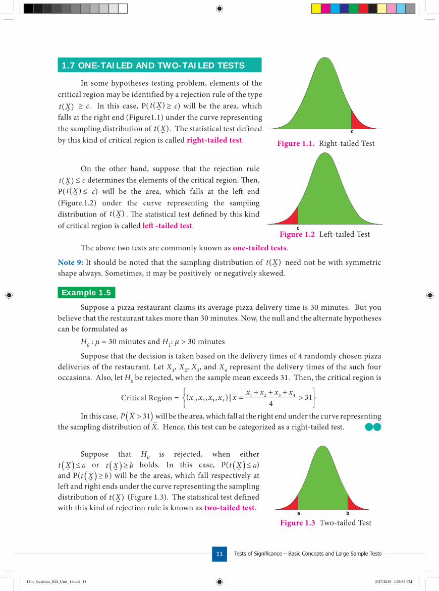
1.7 ONE- TAILED AND TWO- TAILED TESTS
In some hypotheses testing problem, elements of the critical region may be identified by a rejection rule of the type t X( ) ≥ c. In this case, P( t X( ) ≥ c) will be the area, which falls at the right end (Figure1.1) under the curve representing the sampling distribution of t X( ). The statistical test defined by this kind of critical region is called right-tailed test.
On the other hand, suppose that the rejection rulet X( ) ≤ c determines the elements of the critical region. �en, P( t X( ) ≤ c) will be the area, which falls at the le� end (Figure.1.2) under the curve representing the sampling distribution of t X( ) . �e statistical test de�ned by this kind of critical region is called le� -tailed test.
The above two tests are commonly known as one-tailed tests.
Note 9: It should be noted that the sampling distribution of t X( ) need not be with symmetric shape always. Sometimes, it may be positively or negatively skewed.
Ex ample 1.5Suppose a pizza restaurant claims its average pizza delivery time is 30 minutes. But you
believe that the restaurant takes more than 30 minutes. Now, the null and the alternate hypotheses can be formulated as
H0 : μ = 30 minutes and H1: μ > 30 minutes
Suppose that the decision is taken based on the delivery times of 4 randomly chosen pizza deliveries of the restaurant. Let X1, X2, X3, and X4 represent the delivery times of the such four occasions. Also, let H0 be rejected, when the sample mean exceeds 31. Then, the critical region is
Critical Region = ( , , , ) |x x x x xx x x x
1 2 3 41 2 3 4
431�
� � �
�
���
In this case, P X � �31 will be the area, which fall at the right end under the curve representing the sampling distribution of X
–. Hence, this test can be categorized as a right-tailed test.
Suppose that H0 is rejected, when either t X a� � � or t X b� � �
holds. In this case, P(t X a� � � ) and P(t X b� � � ) will be the areas, which fall respectively atleft and right ends under the curve representing the sampling distribution of t X( ) (Figure 1.3). The statistical test defined with this kind of rejection rule is known as two-tailed test.
a b
Figure 1.3 Two-tailed Test
c
Figure 1.1. Right-tailed Test
cFigure 1.2 Left-tailed Test
12th_Statistics_EM_Unit_1.indd 11 2/27/2019 1:35:33 PM

12t h Std Statistics 12
Ex ample 1.6A manufacturer of ball-bearings, which are used in some machines, inspects to see whether
the diameter of each ball-bearing is 5 mm. If the average diameter of ball-bearings is less than 4.75 mm or greater than 5.10 mm, then such ball-bearings will cause damages to the machine.
Here the null and the alternate hypotheses are
H0 : μ = 5 and H1: μ ≠ 5.
Suppose that the decision on H0 is made based on the diameter of 10 randomly selected ball-bearings. Let Xi, i = 1, 2, …, 10 represent the diameter of the randomly chosen ball bearings. Then, the critical region is
Critical Region = ( , ,..., ) |...
. .x x x xx x x
or1 2 101 2 10
104 75 5 10�
� � ��
�
���
In this case, P X �� �4 75. is the area, which will fall at the left end and P X � �5 10. is thearea, which will fall at the right end under the curve representing the sampling distribution of X. This kind of test can be categorized as a two-tailed test (see Figure 1.3).
1.8 GENERAL PROCEDURE FOR TEST OF HY POTHESES
The following steps constitute a general procedure, which can be followed for solving hypotheses testing problems based on both large and small samples.
Step 1 : Describe the population and its parameter(s). Frame the null hypothesis (H0) and alternative hypothesis (H1).
Step 2 : Describe the sample i.e., data.
Step 3 : Specify the desired level of significance, α.
Step 4 : Specify the test statistic and its sampling distribution under H0.
Step 5 : Calculate the value of the test statistic under H0 for given sample.
Step 6 : Find the critical value(s) (table value(s)) from the statistical table generated from the sampling distribution of the test statistic under H0 corresponding to α.
Step 7 : Decide on rejecting or not rejecting the null hypothesis based on the rejection rule which compares the calculated value(s) of the test statistic with the table value(s).
Now, let us see some of the large sample tests, which apply the above general procedure. As mentioned in Note-6, for large samples, the size of the sample is greater than or equal to 30. In the case of two samples considered for a hypotheses testing problem, the test is a large sample test, when the sizes of both the samples are greater than or equal to 30.
Step 1 : Describe the population and its parameter(s). Frame the null hypothesis (H0H0H ) and alternative hypothesis (H1).
Step 2 : Describe the sample i.e., data.
Step 3 : Specify the desired level of significance, α.
Step 4 : Specify the test statistic and its sampling distribution under H0H0H .
Step 5 : Calculate the value of the test statistic under H0H0H for given sample.
Step 6 : Find the critical value(s) (table value(s)) from the statistical table generated from the sampling distribution of the test statistic under H0H0H corresponding to α.
Step 7 : Decide on rejecting or not rejecting the null hypothesis based on the rejection rulewhich compares the calculated value(s) of the test statistic with the table value(s).
12th_Statistics_EM_Unit_1.indd 12 2/27/2019 1:35:34 PM

sts Si ni canc asic nc ts and a Sa l sts13
1.9 TEST OF HY POTHESES FOR POPULATION MEAN( Population v ariance is k now n)
Procedure:
Step 1 : Let µ and σ2 be respectively the mean and the variance of the population under study, where σ2 is known. If µ0 is an admissible value of µ, then frame the null hypothesis as H0: µ = µ0 and choose the suitable alternative hypothesis from
(i) H1: µ ≠ µ0 (ii) H1: µ > µ0 (iii) H1: µ < µ0
Step 2 : Let (X1, X2, …, Xn) be a random sample of n observations drawn from the population, where n is large (n ≥ 30).
Step 3 : Let the level of significance be α.
Step 4 : Consider the test statistic ZX
n= −µσ
0
/under H0. Here, X represents the sample
mean, which is defined in Note 2. The approximate sampling distribution of the test statistic under H0 is the N(0,1) distribution.
Step 5 : Calculate the value of Z for the given sample (x1, x2, ..., xn) as
zx
n00�
� �� /
Step 6 : Find the critical value, ze, corresponding to α and H1 from the following table
Alternative Hypothesis (H1) µ ≠ µ0 µ > µ0 µ < µ0
Critical Value (ze) zα/2 zα –zα
Step 7 : Decide on H0 choosing the suitable rejection rule from the following table corresponding to H1.
Alternative Hypothesis (H1) µ ≠ µ0 µ > µ0 µ < µ0
Rejection Rule |z0| ≥ zα/2 z0 > zα z0 < –zα
Ex ample 1.7A company producing LED bulbs finds that mean life span of the population of its bulbs
is 2000 hours with a standard derivation of 150 hours. A sample of 100 bulbs randomly chosen is found to have the mean life span of 1950 hours. Test, at 5% level of significance, whether the mean life span of the bulbs is significantly different from 2000 hours.
Step 4 : Consider the test statistic ZX
n= −µσ
0
/under H0. Here, X represents the sample
mean, which is defined in Note 2. The approximate sampling distribution of thetest statistic under H0 is the N(0,1) distribution.
12th_Statistics_EM_Unit_1.indd 13 2/27/2019 1:35:34 PM

12t h S t d S t a t i s t i c s 14
Solution:
Step 1 : Let μ and σ represent respectively the mean and standard deviation of the probability distribution of the life span of the bulbs. It is given that σ = 150 hours. The null and alternative hypotheses are
Null hypothesis: H0: μ = 2000
i.e., the mean life span of the bulbs is not significantly different from 2000 hours.
Alternative hypothesis: H1 : μ ≠ 2000
i.e., the mean life span of the bulbs is significantly different from 2000 hours.
It is a two-sided alternative hypothesis.
Step 2 : Data
The given sample information are
Sample size (n) = 100, Sample mean (x) = 1950 hours
Step 3 : Level of significance
α = 5%
Step 4 : Test statistic
The test statistic is ZX
n�
� ��
0
/, under H0
Under the null hypothesis H0, Z follows the N(0,1) distribution.
Step 5 : Calculation of Test Statistic
The value of Z under H0 is calculated from
zx
n00�
� �� /
as
z0 ��1950 2000
150 100 = –3.33Thus; | |z0 = 3.33
Step 6 : Critical value
Since H1 is a two-sided alternative, the critical value at α = 0.05 is ze = z0.025 = 1.96. (see Table 1.6).
Step 7 : Decision
Since H1 is a two-sided alternative, elements of the critical region are determined by the rejection rule |z0| ≥ ze. Thus, it is a two-tailed test. For the given sample information, the rejection rule holds i.e., |z0| = 3.33 > ze = 1.96. Hence, H0 is rejected in favour of H1: μ ≠ 2000. Thus, the mean life span of the LED bulbs is significantly different from 2000 hours.
12th_Statistics_EM_Unit_1.indd 14 2/27/2019 1:35:35 PM

sts Si ni canc asic nc ts and a Sa l sts15
Ex ample 1.8The mean breaking strength of cables supplied by a manufacturer is 1900 n/m2 with a
standard deviation of 120 n/m2. The manufacturer introduced a new technique in the manufacturing process and claimed that the breaking strength of the cables has increased. In order to test the claim, a sample of 60 cables is tested. It is found that the mean breaking strength of the sampled cables is 1960 n/m2. Can we support the claim at 1% level of significance?
Solution:
Step 1 : Let μ and σ represent respectively the mean and standard deviation of the probability distribution of the breaking strength of the cables. It is given that σ = 120 n/m2. The null and alternative hypotheses are
Null hypothesis H0: μ = 1900
i.e., the mean breaking strength of the cables is not signi�cantly di�erent from1900n/m2.
Alternative hypothesis: H1: μ > 1900
i.e., the mean breaking strength of the cables is significantly more than 1900n/m2.
It may be noted that it is a one-sided (right) alternative hypothesis.
Step 2 : Data
The given sample information are
Sample size (n) = 60. Hence, it is a large sample.
Sample mean (x)= 1960
Step 3 : Level of significance
α = 1%
Step 4 : Test statistic
The test statistic is ZX
n= −µσ
0
/, under H0
Since n is large, under the null hypothesis, the sampling distribution of Z is the N(0,1) distribution.
Step 5 : Calculation of test statistic
The value of Z under H0 is calculated from zx
n00�
� �� /
z01960 1900120 60
��/
Thus, z0 = 3.87
Step 6 : Critical value
Since H1 is a one-sided (right) alternative hypothesis, the critical value at α = 0.01 level of significance is ze = z0.01= 2.33 (see Table 1.6)
12th_Statistics_EM_Unit_1.indd 15 2/27/2019 1:35:36 PM

12t h S t d S t a t i s t i c s 16
Step 7 : Decision
Since H1 is a one-sided (right) alternative, elements of the critical region are determined by the rejection rule z0 > ze. �us, it is a right-tailed test. For the given sample information, the observed value z0 = 3.87 is greater than the critical value ze = 2.33. Hence, the null hypothesis H0 is rejected. �erefore, the mean breaking strength of the cables is signi�cantly more than 1900 n/m2. Thus, the manufacturer’s claim that the breaking strength of cables has increased by the new technique is found valid.
1.10 TEST OF HY POTHESES FOR POPULATION MEAN ( POPULATION VARIANCE IS UNKNOWN)
Procedure:
Step1 : Let µ and σ2 be respectively the mean and the variance of the population under study, where σ2 is unknown. If µ0 is an admissible value of µ, then frame the null hypothesis as H0: µ = µ0 and choose the suitable alternative hypothesis from
(i) H1: µ ≠ µ0 (ii) H1: µ > µ0 (iii) H1: µ < µ0
Step 2 : Let (X1, X2, …, Xn) be a random sample of n observations drawn from the population, where n is large (n ≥ 30).
Step 3 : Specify the level of significance, α.
Step 4 : Consider the test statistic ZXS n
�� �0
/ under H0, where X and S are the sample
mean and sample standard deviation respectively. It may be noted that the above
test statistic is obtained from Z considered in the test described in Section 1.9 by substituting S for σ.
The approximate sampling distribution of the test statistic under H0 is the N(0,1) distribution.
Step 5 : Calculate the value of Z for the given sample (x1, x2, ..., xn) as zxs n0
0�� �/
. Here, x
and s are respectively the values of X and S calculated for the given sample.
Step 6 : Find the critical value, ze, corresponding to α and H1 from the following table
Alternative Hypothesis (H1) µ ≠ µ0 µ > µ0 µ < µ0
Critical Value (ze) zα/2 zα -zα
Y OU WILL KNOW
It is important to note that the exact sampling distribution of Z is the Student’s ‘t’ distribution with (n – 1) degrees of freedom, when n is small (n < 30). This hypotheses testing problem, when n is small, is discussed, in detail, in Chapter 2. When n is large, the Student’s ‘t’ distribution converges to the N(0,1) distribution.
12th_Statistics_EM_Unit_1.indd 16 2/27/2019 1:35:37 PM

sts Si ni canc asic nc ts and a Sa l sts17
Step 7 : Decide on H0 choosing the suitable rejection rule from the following table corresponding to H1.
Alternative Hypothesis (H1) µ ≠ µ0 µ > µ0 µ < µ0
Rejection Rule |z0| ≥ zα/2 z0 > zα z0 < -zα
Ex ample 1.9A motor vehicle manufacturing company desires to introduce a new model motor vehicle.
The company claims that the mean fuel consumption of its new model vehicle is lower than that of the existing model of the motor vehicle, which is 27 kms/litre. A sample of 100 vehicles of the new model vehicle is selected randomly and their fuel consumptions are observed. It is found that the mean fuel consumption of the 100 new model motor vehicles is 30 kms/litre with a standard deviation of 3 kms/litre. Test the claim of the company at 5% level of significance.
Solution:
Step 1 : Let the fuel consumption of the new model motor vehicle be assumed to be distributed according to a distribution with mean and standard deviation respectively μ and σ. The null and alternative hypotheses are
Null hypothesis H0: μ = 27
i.e., the average fuel consumption of the company’s new model motor vehicle is notsignificantly different from that of the existing model.
Alternative hypothesis H1: μ > 27
i.e., the average fuel consumption of the company’s new model motor vehicle issignificantly lower than that of the existing model. In other words, the number ofkms by the new model motor vehicle is significantly more than that of the existingmodel motor vehicle.
Step 2 : Data:
The given sample information are
Size of the sample (n) = 100. Hence, it is a large sample.
Sample mean ( x )= 30
Sample standard deviation(s) = 3
Step 3 : Level of significance
α = 5%
Step 4 : Test statistic
The test statistic under H0 is
ZXS n
�� �0 .
Since n is large, the sampling distribution of Z under H0 is the N(0,1) distribution.
12th_Statistics_EM_Unit_1.indd 17 2/27/2019 1:35:37 PM

12t h S t d S t a t i s t i c s 18
Step 5 : Calculation of Test Statistic
The value of Z for the given sample information is calculated from
zxs n0
0�� �/
as
z030 273 100
��
Thus, z0 = 10.
Step 6 : Critical Value
Since H1 is a one-sided (right) alternative hypothesis, the critical value at α = 0.05 is ze = z0.05 = 1.645.
Step 7 : Decision
Since H1 is a one-sided (right) alternative, elements of the critical region are de�ned by the rejection rule z0 > ze = z0.05. �us, it is a right-tailed test. Since, for the given sample information, z0 = 10 > ze = 1.645, H0 is rejected.
1.11 TEST OF HY POTHESES FOR EQUALITY OF MEANS OF TWO POPULATIONS ( Population v ariances are k now n)
Procedure:
Step-1 : Let µX and sX2
be respectively the mean and the variance of Population -1. Also, let µY and sY
2 be respectively the mean and the variance of Population -2 under study. Here sX
2 and sY2 are known admissible values.
Frame the null hypothesis as H0: µX = µY and choose the suitable alternative hypothesis from
(i) H1: µX ≠ µY (ii) H1: µX> µY (iii) H1: µX< µY
Step 2 : Let (X1, X2, …, Xm) be a random sample of m observations drawn from Population-1 and (Y1, Y2, …, Yn) be a random sample of n observations drawn from Population-2, where m and n are large(i.e., m ≥ 30 and n ≥ 30). Further, these two samples are assumed to be independent.
Step 3 : Specify the level of significance, α.
Step 4 : Consider the test statistic Z X Y
m n
X Y
X Y
�� � �
�
( ) ( )� �
� �2 2 under H0, where X and Y are
respectively the means of the two samples described in Step-2.
12th_Statistics_EM_Unit_1.indd 18 2/27/2019 1:35:38 PM

sts Si ni canc asic nc ts and a Sa l sts19
The approximate sampling distribution of the test statistic Z X Y
m nX Y
= −
+
( )
s s2 2 under H0
(i.e., µX = µY) is the N(0,1) distribution.
It may be noted that the test statistic, when sX2 = sY
2 = σ2, is Z X Y
m n
= −
+
( )
s1 1
.
Step 5 : Calculate the value of Z for the given samples (x1, x2, ..., xm) and (y1, y2, …, yn) as z x y
m n
o
X Y
= −
+
( )
s s2 2.
Here, x and y are respectively the values of and X Y for the given samples.
Step 6 : Find the critical value, ze, corresponding to α and H1 from the following table
Alternative Hypothesis (H1) µX ≠ µY µX > µY µX < µY
Critical Value (ze) zα/2 zα –zα
Step 7 : Make decision on H0 choosing the suitable rejection rule from the following table corresponding to H1.
Alternative Hypothesis (H1) µX ≠ µY µX > µY µX < µY
Rejection Rule |z0| ≥ zα/2 z0 > zα z0 < –zα
Ex ample 1.10Performance of students of X Standard in a national level talent search examination was studied.
�e scores secured by randomly selected students from two districts, viz., D1 and D2 of a State wereanalyzed. �e number of students randomly selected from D1 and D2 are respectively 500 and 800.Average scores secured by the students selected from D1 and D2 are respectively 58 and 57. Can thesamples be regarded as drawn from the identical populations having common standard deviation 2?Test at 5% level of signi�cance.
Solution:
Step 1 : Let μX and μY be respectively the mean scores secured in the national level talent search examination by all the students from the districts D1 and D2 considered for the study. It is given that the populations of the scores of the students of these districts have the common standard deviation σ = 2. The null and alternative hypotheses are
Null hypothesis: H0: µX = µY
i.e., average scores secured by the students from the study districts are not significantlydifferent.
Alternative hypothesis: H1: µX ≠ µY
i.e., average scores secured by the students from the study districts are significantlydifferent. It is a two-sided alternative.
12th_Statistics_EM_Unit_1.indd 19 2/27/2019 1:35:39 PM

12t h S t d S t a t i s t i c s 20
Step 2 : Data
The given sample information are
Size of the Sample-1 (m) = 500
Size of the Sample-2 (n) = 800. Hence, both the samples are large.
Mean of Sample-1 ( x ) = 58
Mean of Sample-2 ( y ) = 57
Step 3 : Level of significance
α = 5%
Step 4 : Test statistic
The test statistic under the null hypothesis H0 is
ZX Y
m n
��
�� 1 1.
Since both m and n are large, the sampling distribution of Z under H0 is the N(0, 1) distribution.
Step 5 : Calculation of Test Statistic
The value of Z is calculated for the given sample information from
z0 zx y
m n
��
�� 1 1as
z058 57
2 1500
1800
��
�
z0 = 8.77
Step-6 : Critical value
Since H1 is a two-sided alternative hypothesis, the critical value at α = 0.05 is ze = z0.025 = 1.96.
Step-7 : Decision
Since H1 is a two-sided alternative, elements of the critical region are defined by the rejection rule |z0| ≥ ze = z0.025. For the given sample information, |z0| = 8.77 > ze = 1.96. It indicates that the given sample contains sufficient evidence to reject H0. Thus, it may be decided that H0 is rejected. Therefore, the average performance of the students in the districts D1 and D2 in the national level talent search examination are significantly different. Thus the given samples are not drawn from identical populations.
12th_Statistics_EM_Unit_1.indd 20 2/27/2019 1:35:39 PM

sts Si ni canc asic nc ts and a Sa l sts21
1.12 TEST OF HY POTHESES FOR EQUALITY OF MEANS OF TWO POPULATIONS ( POPULATION VARIANCES ARE UNKNOWN)
Procedure:
Step-1 : Let µX and sX2
be respectively the mean and the variance of Population -1. Also, let µY and sY
2 be respectively the mean and the variance of Population -2 under study. Here sX
2 and sY2 are assumed to be unknown.
Frame the null hypothesis as H0: µX = µY and choose the suitable alternative hypothesis from
(i) H1: µX ≠ µY (ii) H1: µX> µY (iii) H1: µX< µY
Step 2 : Let (X1, X2, …, Xm) be a random sample of m observations drawn from Population-1 and (Y1, Y2, …, Yn) be a random sample of n observations drawn from Population-2, where m and n are large (m ≥30 and n ≥30). Here, these two samples are assumed to be independent.
Step 3 : Specify the level of significance, α.
Step 4 : Consider the test statistic
nS
mS
YXZ
YX
YX
22
)()( under H0 (i.e., µX = µY).
i.e., the above test statistic is obtained from Z considered in the test described inSection 1.11 by substituting SX
2 and SY2 respectively for sX
2 and sY
2
The approximate sampling distribution of the test statistic Z X Y
Sm
Sn
X Y
��
�2 2 under H0
is the N(0,1) distribution.
Step 5 : Calculate the value of Z for the given samples (x1, x2, ...,xm) and (y1, y2, …, yn) as
z x y
sm
sn
X Y
0 2 2�
�
� .
Here x and y are respectively the values of and X Y for the given samples. Also, s2
X and s2Y are respectively the values of SX
2 and SY2 for the given samples.
Step 6 : Find the critical value, ze, corresponding to α and H1 from the following table
Alternative Hypothesis (H1) µX ≠ µY µX > µY µX < µY
Critical Value (ze) zα/2 zα –zα
12th_Statistics_EM_Unit_1.indd 21 2/27/2019 1:35:40 PM

12t h S t d S t a t i s t i c s 22
Step 7 : Make decision on H0 choosing the suitable rejection rule from the following table corresponding to H1.
Alternative Hypothesis (H1) µX ≠ µY µX > µY µX < µY
Rejection Rule |z0| ≥ zα/2 z0 > zα z0 < -zα
Ex ample 1.11A Model Examination was conducted to XII Standard students in the subject of Statistics.
A District Educational Officer wanted to analyze the Gender-wise performance of the students using the marks secured by randomly selected boys and girls. Sample measures were calculated and the details are presented below:
Gender Sample Size Sample Mean Sample Standard deviationBoys 100 50 4
Girls 150 51 5
Test, at 5% level of significance, whether performance of the students differ significantly with respect to their gender.
Solution:
Step 1 : Let μX and μY denote respectively the average marks secured by boys and girls in the Model Examination conducted to the XII Standard students in the subject of Statistics. Then, the null and the alternative hypotheses are
Null hypothesis: H0:1 : X YH = 1 : X YH
i.e., there is no significant difference in the performance of the students with respect totheir gender.
Alternative hypothesis: 1 : X YH
i.e., performance of the students differ significantly with the respect to the gender. It isa two-sided alternative hypothesis.
Step 2 : Data
The given sample information are
Gender of the Students
Sample Size Sample Mean Sample Standard Deviation
Boys m = 100 x = 50 sX = 4
Girls n = 150 y = 51 sY = 5
Since m ≥ 30 and n ≥ 30, both the samples are large.
Step 3 : Level of significance α = 5%
12th_Statistics_EM_Unit_1.indd 22 2/27/2019 1:35:40 PM

sts Si ni canc asic nc ts and a Sa l sts23
Step 4 : Test statistic
The test statistic under H0 is
ZX Y
Sm
Sn
X Y
��
�2 2
.
The sampling distribution of Z under H0 is the N(0,1) distribution.
Step 5 : Calculation of the Test Statistic
The value of Z is calculated for the given sample informations from
zx y
sm
sn
X Y
0 2 2�
�
�
as
z0 2 2
50 51
4100
5150
��
�
Thus, z0 = −1.75
Step 6 : Critical value
Since H1 is a two-sided alternative, the critical value at 5% level of significance is ze = z0.025 = 1.96.
Step 7 : Decision
Since H1 is a two-sided alternative, elements of the critical region are determined by the rejection rule 0z ≥ 0z . Thus it is a two-tailed test. But, 0z = 1.75 is less than the critical value ze = 1.96. Hence, it may inferred as the given sample information does not provide sufficient evidence to reject H0. Therefore, it may be decided that there is no sufficient evidence in the given sample to conclude that performance of boys and girls in the Model Examination conducted in the subject of Statistics differ significantly.
1.13 TEST OF HY POTHESES FOR POPULATION PROPORTION
Procedure:
Step 1 : Let P denote the proportion of the population possessing the qualitative characteristic (attribute) under study. If p0 is an admissible value of P, then frame the null hypothesis as H0:P = p0 and choose the suitable alternative hypothesis from
(i) H1: P ≠ p0 (ii) H1: P > p0 (iii) H1: P < p0
Step 2 : Let p be proportion of the sample observations possessing the attribute, where n is large, np > 5 and n(1 – p) > 5.
12th_Statistics_EM_Unit_1.indd 23 2/27/2019 1:35:41 PM
12t h S t d S t a t i s t i c s 24
Step 3 : Specify the level of significance, α.
Step 4 : Consider the test statistic Zp P
PQn
��
under H0. Here, Q = 1 – P.
The approximate sampling distribution of the test statistic under H0 is the N(0,1) distribution.
Step 5 : Calculate the value of Z under H0 for the given data as zp p
p qn
00
0 0
�� , q0 = 1 – p0.
Step 6 : Choose the critical value, ze, corresponding to α and H1 from the following table
Alternative Hypothesis (H1) P ≠ p0 P > p0 P < p0
Critical Value (ze) zα/2 zα -zα
Step 7 : Make decision on H0 choosing the suitable rejection rule from the following table corresponding to H1.
Alternative Hypothesis (H1) P ≠ p0 P > p0 P < p0
Rejection Rule |z0| ≥ zα/2 z0 > zα z0 < -zα
Ex ample 1.12A survey was conducted among the citizens of a city to study their preference towards
consumption of tea and co�ee. Among 1000 randomly selected persons, it is found that 560 are tea-drinkers and the remaining are co�ee-drinkers. Can we conclude at 1% level of signi�cance from this information that both tea and co�ee are equally preferred among the citizens in the city?
Solution:
Step 1 : Let P denote the proportion of people in the city who preferred to consume tea. Then, the null and the alternative hypotheses are
Null hypothesis: 0 : 0.5H P
i.e., it is significant that both tea and coffee are preferred equally in the city.
Alternative hypothesis: 1 : 0.5H P
i.e., preference of tea and coffee are not significantly equal. It is a two-sided alternativehypothesis.
Step 2 : Data
The given sample information are
Sample size (n) = 1000. Hence, it is a large sample.
No. of tea-drinkers = 560
Sample proportion (p) = 5601000
= 0.56
Step 3 : Level of significance
α = 1%
12th_Statistics_EM_Unit_1.indd 24 2/27/2019 1:35:42 PM

sts Si ni canc asic nc ts and a Sa l sts25
Step 4 : Test statistic
Since n is large, np = 560 > 5 and n(1 – p) = 440 > 5, the test statistic under the null
hypothesis, is Zp P
PQn
��
.
Its sampling distribution under H0 is the N(0,1) distribution.
Step 5 : Calculation of Test Statistic
The value of Z can be calculated for the sample information from
zp p
p qn
00
0 0
�� as
z00 56 0 50
0 5 0 51000
���
. .. .
Thus, 0 3.79z
Step 6 : Critical value
Since H1 is a two-sided alternative hypothesis, the critical value at 1% level of significance is zα/2 = z0.005 = 2.58.
Step 7 : Decision
Since H1 is a two-sided alternative, elements of the critical region are determined by the rejection rule |z0| ≥ ze. Thus it is a two-tailed test. Since |z0| = 3.79 > ze = 2.58, reject H0 at 1% level of significance. Therefore, there is significant evidence to conclude that the preference of tea and coffee are different.
1.14 TEST OF HY POTHESES FOR EQUALITY OF PROPORTIONS OF TWO POPULATIONS
Procedure:
Step 1 : Let PX and PY denote respectively the proportions of Population-1 and Population-2 possessing the qualitative characteristic (attribute) under study. Frame the null hypothesis as H0: PX=PY and choose the suitable alternative hypothesis from
(i) H1: PX≠ PY (ii) H1: PX>PY (iii) H1: PX<PY
Step 2 : Let and X Yp p denote respectively the proportions of the samples of sizes m and n drawn from Population-1 and Population-2 possessing the attribute, where m and n are large (i.e., m ≥ 30 and n ≥ 30). Also, mp m p np n pX X Y Y �� � �� � 5 1 5 5 1 5, , and . Here, these two samples are assumed to be independent.
Step 3 : Specify the level of significance, α.
12th_Statistics_EM_Unit_1.indd 25 2/27/2019 1:35:42 PM

12t h S t d S t a t i s t i c s 26
Step 4 : Consider the test statistic Zp p P P
pqm n
X Y X Y�� � �
����
���
( ) ( )1 1
under H0. Here,
p p mp npm n
X Y���
, q = 1 − p. The approximate sampling distribution of the test statistic
under H0 is the N(0,1) distribution.
Step 5 : Calculate the value of Z for the given data as zp p
pqm n
X Y0
1 1�
�
����
��� .
Step 6 : Choose the critical value, ze, corresponding to α and H1 from the following table
Alternative Hypothesis (H1) PX ≠ PY PX > PY PX < PY
Critical Value (ze) zα/2 zα –zα
Step 7 : Decide on H0 choosing the suitable rejection rule from the following table corresponding to H1.
Alternative Hypothesis (H1) PX ≠ PY PX > PY PX < PY
Rejection Rule |z0| ≥ zα/2 z0 > zα z0 < –zα
Ex ample 1.13A study was conducted to investigate the interest of people living in cities towards self-
employment. Among randomly selected 500 persons from City-1, 400 persons were found to be self-employed. From City-2, 800 persons were selected randomly and among them 600 persons are self-employed. Do the data indicate that the two cities are significantly different with respect to prevalence of self-employment among the persons? Choose the level of significance as α = 0.05.
Solution:
Step1 : Let PX and PY be respectively the proportions of self-employed people in City-1 and City-2. Then, the null and alternative hypotheses are
Null hypothesis: H P PX Y0 : i.e., there is no significant difference between the proportions of self-employed
people in City-1 and City-2. Alternative hypothesis: H P PX Y1 : i.e., difference between the proportions of self-employed people in City-1 and City-2
is significant. It is a two-sided alternative hypothesis.
12th_Statistics_EM_Unit_1.indd 26 2/27/2019 1:35:43 PM

sts Si ni canc asic nc ts and a Sa l sts27
Step 2 : Data
The given sample information are
City Sample Size Sample Proportion
City-1 m = 500 pX400500
= 0.80
City-2 n = 800 pY600800
= 0.75
Here, m 30, n 30, mpX = 400 > 5, m(1− pX) = 100 > 5, npY = 600 > 5 and n(1− pY) = 200 > 5.
Step 3 : Level of significance
α = 5%
Step 4 : Test statistic
The test statistic under the null hypothesis is
Z p p
pqm n
p mp npm n
q pX Y X Y��
����
���
���
� �1 1
1where and
The sampling distribution of Z under H0 is the N(0,1) distribution.
Step 5 : Calculation of Test Statistic
The value of Z for given sample information is calculated from
z p p
pqm n
X Y0
1 1�
�
����
���
.
Now, p � ��
� �400 600500 800
10001300
0 77. and q 0 23.
Thus, z00 80 0 75
0 77 0 23 1500
1800
��
� �� � ����
���
. .
. .
z0 = 2.0764
Step 6 : Critical value Since H1 is a two-sided alternative hypothesis, the critical value at 5% level of
significance is ze = 1.96.
Step 7 : Decision Since H0 is a two-sided alternative, elements of the critical region are determined by the
rejection rule |z0| > ze. �us, it is a two-tailed test. For the given sample information, ez= 2.0764 > ez = 1.96. Hence, H0 is rejected. We can conclude that the di�erence between the proportions of self-employed people in City-1 and City-2 is signi�cant.
12th_Statistics_EM_Unit_1.indd 27 2/27/2019 1:35:45 PM

12t h S t d S t a t i s t i c s 28
EXERCISE 1
I. Choose the best answer.
1. Standard error of the sample mean is(a)
2(b)
n
(c) n
(d) n
2. When n is large and σ2 is unknown, σ2 is replaced in the test statistic by(a) Sample mean (b) Sample variance(c) Sample standard deviation (d) Sample proportion
POINTS TO REMEMBER
� Statistic is a random variable and its probability distribution is called sampling distribution.
� Generally, the random sample used in Statistical Inference is drawn under sampling withreplacement from a �nite population.
� Standard error is the standard deviation of the sampling distribution.
� Hypothesis is a statement on the population or the values of the parameters.
� Null hypothesis is a hypothesis which is tested for possible rejection.
� Statistical test leads to take decision on the null hypothesis.
� In each statistical hypotheses testing problem, there is one null hypothesis and one alternativehypothesis.
� Type I error is rejecting the true null hypothesis.
� Type II error is not rejecting a false null hypothesis.
� Upper limit of the P (Type I error) is called level of signi�cance, denoted by α.
� Critical region is a subset of the sample space de�ned by the rejection rule.
� Critical value identi�es the elements of critical region.
� If the number of sample observations is greater than or equal to 30, it is called large sample.
� For hypotheses testing based on two samples, if the sizes of both the samples are greater thanor equal to 30, they are called large samples.
� For testing population proportion, the sampling distribution of the test statistic is N(0, 1), onlywhen n > 30, np > 5 and n (1 - p) > 5.
� For testing equality of two population proportions, the sampling distribution of the test statistic is N (0, 1) only when m > 30, n > 30, mpX > 5, m(1− pX) > 5, npY > 5 and n(1− pY) > 5.
12th_Statistics_EM_Unit_1.indd 28 2/27/2019 1:35:45 PM

sts Si ni canc asic nc ts and a Sa l sts29
3. Critical region of a test is(a) rejection region (b) acceptance region(c) sample space (d) subset of the sample space
4. The critical value (table value) of the test statistic at the level of significance α for a two-tailedlarge sample test is(a) 2z (b) z(c) - z (d) / 2z
5. In general, large sample theory is applicable when(a) n > 100 (b) n > 50(c) n > 40 (d) n > 30
6. When H1 is a one-sided (right) alternative hypothesis, the critical region is determined by
(a) both right and left tails (b) neither right nor left tail(c) right tail (d) left tail
7. Critical value at 5% level of significance for two-tailed large sample test is
(a) 1.645 (b) 2.33(c) 2.58 (d) 1.96
8. For testing H0: μ = μ0 against H1 : μ < μ0, what is the critical value at α = 0.01?
(a) 1.645 (b) –1.645(c) –2.33 (d) 2.33
9. The hypotheses testing problem H0: μ0 = 45 against H1: μ0 < 45 be categorized as
(a) left-tailed (b) right-tailed(c) two-tailed (d) one-tailed
10. When the alternative hypothesis is 1 0:H , the critical region will be determined by(a) both right and left tails (b) neither right nor left tail(c) right tail (d) left tail
11. Rejecting H0, when it is true is called
(a) type I error (b) type II error(c) sampling error (d) standard error
12. What is the standard error of the sample proportion under H0?
(a) PQn
( ) pqn
(c) PQn
(d) pqn
12th_Statistics_EM_Unit_1.indd 29 2/27/2019 1:35:46 PM

12t h S t d S t a t i s t i c s 30
13. The test statistic for testing the equality of two population means, when the populationvariances are known is
(a) X Y
m nX Y
�
�� �2 2
(b) X Ysm
sn
X Y
−
+2 2
(c) X Y
m nX Y
�
�� �2 2
(d) X Y
sm
sn
X Y
−
+2 2
14. When the population variances are known and equal, the statistic Z X Y
m n
��
�� 1 1 is used to
test the null hypothesis
(a) 0 : X YH P P µ = µ0 (b) H0 : µX = µY
(c) 0 : X YH P P (d) H0 : P = p0
15. What is the standard error of the difference between two sample proportions, (PX – PY)?
(a) 1 1pqm n
(b) 1 1pqm n
(c) pqm n1 1��
��
��� (d) 1 1ˆ ˆpq
m n
16. What is level of significance?
(a) P(Type I Error) (b) P(Type II Error)(c) upper limit of P(Type I Error) (d) upper limit of P(Type II Error)
17. Large sample test for testing population proportion is valid, when
(a) n is large, n ≥ 30, np > 5, n(1 – p) > 5 (b) n is large, n ≥ 30, np > 5, n(1 – p) < 5(c) n is large, n ≥ 30, np > 5, np (1 – p) > 5 (d) n is large, n ≥ 30, np > 5, np(1 – p) < 5
18. Large sample test can be applied for two-sample problems, for testing the equality of twopopulation means, when
(a) m + n ≥ 30 (b) m ≥ 30, n ≥ 30(c) m ≥ 30, m + n ≥ 30 (d) mn ≥ 30
19. Large sample test is applicable, when the parent population is
(a) normal distribution only (b) binomial distribution(c) Poisson distribution (d) any probability distribution
20. What is the rejection rule, based on large sample, for testing H0 against one-sided (left)alternative hypothesis?
(a) 0 / 2z z (b) 0z z(c) z0 ≤ –zα/2 (d) 0z z
12th_Statistics_EM_Unit_1.indd 30 2/27/2019 1:35:47 PM

sts Si ni canc asic nc ts and a Sa l sts31
II. Give very short answer to the following questions.
21. What is Inferential Statistics?22. Define sample space.23. What do you understand by random sample?24. What are the different types of errors in hypotheses testing problem?25. Prescribe the rejection rules for testing H0: µ =µ0 against all possible alternative hypotheses.26. List the possible alternative hypotheses and the corresponding rejection rules followed in
testing equality of two population means.27. Specify the alternative hypotheses and the rejection rules prescribed for testing equality of
two population proportions.28. Define parameter.29. What is statistic?30. Define standard error of a statistic.31. What do you understand by sampling distribution of a statistic?32. What is null hypothesis?33. Distinguish between null and alternative hypotheses.34. For testing a null hypothesis against a two-sided alternative hypothesis, if |z0| >zα/2 is found
to hold, what will be your decision?35. In a recent survey, conducted among 2000 randomly selected graduates in a district, 367 of
them are IAS aspirants. Calculate the proportion of IAS aspirants among the graduates in thedistrict.
36. Which type of test should be used for testing 0 : 27H against 1 : 27H ?37. Formulate the null and alternative hypotheses for testing whether the average time required
to XI standard students to complete a Chemistry laboratory exercise is less than 30 minutes.38. If μ denotes the population mean, then find the critical value to be used for testing H0: μ = 100
against H1 : μ < 100 based on 250 observations at 5% level of significance.39. The mean height of students studying X Standard in a school is 150 cms and the average
height of 15 randomly selected students is 155 cms. Identify the parameter, statistic and theirvalues from these information.
40. Calculate standard error of the sample mean, when sample mean is 100, sample size is 64 andpopulation standard deviation is 24.
41. Find standard error of the sample proportion p = 0.45 when the population proportion is 0.5and the sample size is 100.
III. Give short answer to the following questions.42. Describe Decision Table.
43. What are type I and type II errors?
44. What do you mean by level of significance?
45. Explain one-tailed and two-tailed tests.
46. Explain critical value.
12th_Statistics_EM_Unit_1.indd 31 2/27/2019 1:35:47 PM

12t h S t d S t a t i s t i c s 32
47. A set of 100 students is selected randomly from an Institution. The mean height of thesestudents is 163 cms and the standard deviation is 10 cms. Calculate the value of the teststatistic under 0 : 167.H
48. In a random sample of 50 students from School A, 35 of them preferred junk food. Inanother sample of 80 from School B, 40 of them preferred junk food. Find the standard errorof the difference between two sample proportions.
49. If m = 35, n = 40, x = 10.8, y =11.9, sX = 3 and sY = 4, then calculate standard error of X – Y.
50. In test for population proportion, if n=500 and np=383, then calculate the value of the teststatistic under 0 : 0.68H P .
51. In test for two population proportions, if m = 100, n = 150, mpX = 78 and npY =100, thencalculate the value of the test statistic under H0: PX = PY.
IV. Give detailed answer to the following questions.
52. Explain the general procedure to be followed for testing of hypotheses.
53. Explain the procedure for testing hypotheses for population mean, when the populationvariance is unknown.
54. How will you formulate the hypotheses for testing equality of means of two populations,when the population variances are known? Describe the method.
55. Describe the procedure for testing hypotheses concerning equality of means of twopopulations, assuming that the population variances are unknown.
56. Give a detailed account on testing hypotheses for population proportion.
57. Explain the procedure of testing hypotheses for equality of proportion of two populations.
58. A special training programme was organized by a District Educational Officer to the VIIIStandard students for improving their skill in Letter Writing. Time taken by the students in aLetter Writing competition was recorded. The average time taken by 100 randomly selectedstudents was 15 minutes. Can the Officer decide that at 1% level of significance the meantime in this kind of exercise required to VIII Students of the district is 13 minutes, assumingthe population standard deviation as 8 minutes?
59. Carry out hypotheses testing exercise for testing H0 : µX = µY against 1 : X YH with usual notations, when x = 7 and y =8 , X = 3 and Y = 2 and m = 40 and n = 40. Use α = 0.01.
60. Chief Educational Officer wanted to study the performance of XII Standard students inMathematics subject. The following are the information obtained from randomly selectedstudents from two Educational Districts.
Educational District
No. of students selected
Mean Standard Deviation
A 45 62 15
B 53 60 17
Examine at 5% level of significance whether students in District A perform better compared to students in District B.
12th_Statistics_EM_Unit_1.indd 32 2/27/2019 1:35:47 PM

sts Si ni canc asic nc ts and a Sa l sts33
61. �e mean yield of rice observed from randomly selected 100 plots in District A was 210 kg peracre with standard deviation of 10 kg per acre. �e mean yield of rice observed from randomlyselected 150 plots in District B was 220 kg per acre with standard deviation of 12 kg per acre.Assuming that the standard deviation of yield in the entire state was 11kg, test at 1% level ofsigni�cance whether di�erence between the mean yields of rice in the two districts is signi�cant.
62. The standard deviation of the scores secured by XI standard students in a test conducted forexamining their numerical ability is known to be 15. A school implemented a new method ofteaching which is supposed to increase general quantitative ability. A group of 99 students arerandomly assigned to one of two classes. Fifty students in Class-I are given the new methodof teaching, whereas the remaining 49 students in Class-II are taught in the standard way. Atthe end of the particular term, students are given the same test of ability. The average scoressecured by the students studied in Class-I and Class-II are respectively 116.0 and 113.1. Doesthis information provide significant evidence at 5% level, to conclude that the new methodimproved the numerical ability of students?
63. A machine assesses the life of a ball point pen, by measuring the length of a continuous linedrawn using the pen. A random sample of 80 pens of Brand A have a total writing lengthof 96.84 km. Random sample of 75 pens of Brand B have a total writing length of 93.75 km.Assuming that the standard deviation of the writing length of a single pen is 0.15 km for bothbrands, can the consumer decide to choose Brand B pens assuming that their average writinglength is more than that of Brand A pens? Set level of significance as 1%.
64. A study was conducted to compare the performance of athletes of two States in Inter-StateAthlete Meets. Details of the number of successes achieved by the athletes of the two Statesare given hereunder:
State No. of Athletes Mean Standard DeviationState-1 300 75 10State-2 400 73 11
Does the above information ensure at 1% level of signi�cance that the di�erence between the performances of the athletes of the two States is signi�cant?
65. A District Administration conducted awareness campaign on a contagious disease utilizing theservices of school students. Among 64 randomly selected households, 50 of them appreciatedthe involvement of students. Can the District Administration decide whether more than 90%success could be achieved in these kinds of programmes by involving the students? Fix thelevel of signi�cance as 1%.
66. A coin is tossed 10, 000 times and head turned up 5,195 times. Test the hypothesis, at 5%level of significance, that the coin is unbiased.
67. A study was conducted among randomly selected families who are living in two locations ofa district, and parents were asked “Whether watching TV programmes by parents affects thestudies of their children?” Details are presented hereunder:
LocalityNo. of Families
Contacted AgreedA 200 48B 600 96
12th_Statistics_EM_Unit_1.indd 33 2/27/2019 1:35:47 PM

12t h S t d S t a t i s t i c s 34
Test, at 5% level of significance, whether the difference between the proportions of families in the two localities agreed the statement.
68. One thousand apples kept under one type of storage were found to show rotting to the extentof 4% and 1500 apples kept under another kind of storage showed 3% rotting. Can it bereasonably concluded at 5% level of significance that the second type of storage is superiorto the first?
69. Preference of school students, who participate in Sports events, to do physical exercisesin Modern Gymnasium rather than doing aerobic exercises was analyzed. The number ofstudents randomly selected from two States and their preference for Modern Gymnasium aregiven below.
StateNo. of Students
Sampled Preferred Modern Gymnasium
A 50 38
B 60 52
Test whether the difference between proportions of school students who prefer Modern Gymnasium to do their exercises in the two States is significant at 5% level of significance.
70. Interest of XII Students on Residential Schooling was investigated among randomly selectedstudents from two regions. Among 300 students selected from Region A, 34 studentsexpressed their interest. Among 200 students selected from Region B, 28 students expressedtheir interest. Does this information provide sufficient evidence to conclude at 5% level ofsignificance that students in Region A are more interested in Residential Schooling than thestudents in Region B?
ACTIVITIES
1. In your institution, collect data from your Physical Education department about height/weightof the students in a particular class (Standard 9). Take a random sample of 50 students fromyour school and �nd the mean and standard deviation for their height/weight. Verify throughthe statistical tests of inferential statistics, Find the signi�cant di�erence between sample meanand population mean. Give your comments.
2. Consider two group of students of same class (Standard 10) taking an examination in aparticular subject in Tamil medium and in English medium in your school. Get samples fromtwo medium and �nd their mean and standard deviation. Is there any signi�cant di�erencebetween the performance between the students taking their examination in Tamil medium andEnglish medium? Discuss with your friends.
Note: The teacher and students discuss and they may create their own problems similar to the above problems and expand this exercises.
12th_Statistics_EM_Unit_1.indd 34 2/27/2019 1:35:47 PM

sts Si ni canc asic nc ts and a Sa l sts35
ANSWERS
I. 1. (c) 2. (b) 3. (a) 4. (a) 5. (d)
6. (c) 7. (d) 8. (c) 9. (a) 10. (a)
11. (a) 12.(a) 13. (c) 14. (b) 15. (a)
16. (c) 17. (a) 18. (b) 19. (d) 20. (b)
II. 34. reject H0 35. 0.1835 36. one-tailed test (right)
37. H0: μ = 30, H1: μ < 30 38. −1.645 39. −1.645
39. Parameter = Mean height of X standard students in the school = 150 cms
Statistic = Average height of sampled students in the school = 155 cms
40. SE(X–
) = 3
41. SE(p) = 0.05
III. 47. z0 = −448. 0.08949. 0.810650. 4.12251. 1.937
IV. 58. z0 = 2.5; do not reject H0
59. z0 = −1.75; do not reject H0
60. z0 = 0.619; do not reject H0
61. z0 = −7.04; reject H0
62. z0 = 1.302; do not reject H0
63. z0 = −1.638; do not reject H0
64. z0 = 2.508; do not reject H0
65. z0 = −3.167; do not reject H0
66. z0 = 3.90; reject H0
67. z0 = 2.55; reject H0
68. z0 = 1.352; do not reject H0
69. z0 = −1.444; do not reject H0
70. z0 = −0.886; do not reject H0
12th_Statistics_EM_Unit_1.indd 35 2/27/2019 1:35:47 PM

12t h Std Statistics 36
Steps:• Open the browser and type the URL given (or) scan the QR code.GeoGebra work book called “Tests of
Signi� cance – Basic Concepts and Large Sample Tests”will appear.• In that Tick the square boxes for “Show Rejection Region-Show Type I Error probability-Show Alternative
Distribution”• Now If press and drag the Orange and Blue colour buttons you will get the diff erent results.
ICT CORNER
Pictures are indicatives only*
Step-1 Step-2
Step-3
� is activity helps to understand about Signi� cance
in Hypothesis Testing
TESTS OF SIGNIFICANCE – BASIC CONCEPTS AND LARGE SAMPLE TESTS
Step-4
12th_Statistics_EM_Unit_1.indd 36 2/27/2019 1:35:48 PM

T e s t s B a s e d o n S a m p l i n g D i s t r i b u t i o n s I37
W Gosset (1876-1937), born in England studied Chemistry and Mathematics at New College , Oxford. Upon graduating in 1899, he joined a brewery in Ireland. Gosset applied his statistical knowledge both in the brewery and on the farm to the selection of the best varieties of Barley. Gosset acquired that knowledge by study, by trial and error, and by spending two terms in 1906–1907 in the biometrical laboratory of Karl Pearson. Gosset and Pearson had a good relationship. Pearson helped Gosset with the mathematics of his research papers. The brewery where he was employed allowed publishing his work under a pseudonym (“Student”). Thus, his most noteworthy achievement is now called Student's t, rather than Gosset's, t-distribution.
IntroductionIn the earlier chapter, we have discussed various problems related to tests of signi� cance based
on large samples by applying the standard normal distribution. However, if the sample size is small (n < 30) the sampling distributions of test statistics are far from normal and the procedures discussed in Chapter-1 cannot be applied, except the general procedure (Section 1.8). But in this case, there exists a probability distribution called t-distribution which may be used instead of standard normal distribution to study the problems based on small samples.
� e student will be able to
� understand the purpose for using t-test and chi-square test .� understand procedures for tests of hypotheses based on small samples.
� solve problems to test the hypotheses concerning mean(s) using t-distribution.
� solve problems to test the hypothesis whether the population has a particular variance usingchi-square test.
� solve problems to test the hypotheses relating to independence of attributes and goodnessof � t using chi-square test.
LEARNING OBJECTIVES
W.S. Gossett
CHAPTER
2TESTS BASED ON SAMPLING DISTRIBUTIONS I
12th_Statistics_EM_Unit_2.indd 37 3/4/2019 1:29:30 PM

12t h S t d S t a t i s t i c s 38
2.1 STUDENT’ S t DISTRIBUTION AND ITS APPLICATIONS
2.1.1 Student’ s t- distrib utionIf X~N(0,1) and Y~χn
2 are independent random variables, then
T XYn
is said to have t-distribution with n degrees of freedom. �is can be denoted by tn.
Note 1: �e degrees of freedom of t is the same as the degrees of freedom of the corresponding chi-square random variable.
Note 2: �e t-distribution is used as the sampling distribution(s) of the statistics(s) de�ned based on random sample(s) drawn from normal population(s).
i) If X1, X2 , …, Xn is a random sample drawn from N (μ, σ2) population then
XX
n
N�� � ��
� 0 1, and Y
X Xi
n��� ��
�
2
2 12
�� are independent.
Hence,
T XY
n
X
n
n
X X
XS
n
t SX X
i
n
ii
1
2
1
2
1
11
�
�
��
��� ��� �
��
��
�
��
��
�
� where
( )nn
n
��( )1
.
ii) If (X1 , X2 , …, Xm) and (Y1 , Y2 , …, Yn) are independent random samples drawn from N (μX , σ2)
and N (μY , σ2) populations respectively, then
X Y
m n
NX Y�� �� �� �
�� �
� �
� 1 10 1 , and X X Y Yi
i
m
jj
n
m n
�� � � �� �� �
� �
� �2
1
2
12 2
2
��
are independent.
�en,
TX Y
Sm n
tX Y
p
m n2 21 1�
�� �� �� �
�� �
� �
χ2-distribution and some of its applications are discussed in Section 2.2
12th_Statistics_EM_Unit_2.indd 38 3/4/2019 1:29:33 PM

T e s t s B a s e d o n S a m p l i n g D i s t r i b u t i o n s I39
where SX X Y Y
m np
ii
m
jj
n
2
2
1
2
1
2�
�� � � �� �� �
� �� �
3. If (X1 , Y1), (X2 , Y2), …, (Xn , Yn) is a random sample of n paired observations drawn from a bivariate normal population, then Di = Xi – Yi , i = 1, 2, …, n is a random sample drawn from N (μD , σD
2). Here μD = μX – μY.
Hence,
TDS
n
tD
Dn3 1�
��
�
2.1.2 Properties of th e Student’ s t- distrib ution1. t–distribution is symmetrical distribution with mean zero.
2. �e graph of t-distribution is similar to normaldistribution except for the following two reasons:
i. �e normal distribution curve is higher inthe middle than t-distribution curve.
ii. t–distribution has a greater spreadsideways than the normal distributioncurve. It means that there is more area inthe tails of t-distribution.
3. �e t-distribution curve is asymptotic to X-axis,that is, it extends to in�nity on either side.
4. �e shape of t-distribution curve varies with thedegrees of freedom. �e larger is the numberof degrees of freedom, closeness of its shape tostandard normal distribution (�g. 2.1).
5. Sampling distribution of t does not depend onpopulation parameter. It depends on degrees offreedom (n–1).
2.1.3 Applications of t- distrib ution�e t-distribution has the following important applications in testing the hypotheses for small
samples.1. To test signi�cance of a single population mean, when population variance is unknown, using T1.
-4 -2 0
0.0
0.1
0.2
0.3
0.4
2
X
f(x)
4
df=1df=5df=12df=30normal
Figure 2.1. Student’s t-distribution
12th_Statistics_EM_Unit_2.indd 39 3/4/2019 1:29:33 PM

12t h S t d S t a t i s t i c s 40
2. To test the equality of two population means when population variances are equal and unknown,using T2.
3. To test the equality of two means – paired t-test, based on dependent samples, T3.
Y OU WILL KNOW
The t-distribution has few more applications but they are not considered in this Chapter. You will study these applications in higher classes.
2.1.4 Test of Hypoth eses for Normal Population Mean ( Population Variance is Unk now n)
Procedure:
Step 1 : Let µ and σ2 be respectively the mean and variance of the population under study, where σ2 is unknown. If µ0 is an admissible value of µ, then frame the null hypothesis as
H0: µ = µ0 and choose the suitable alternative hypothesis from
(i) H1: µ ≠ µ0 (ii) H1: µ > µ0 (iii) H1: µ < µ0
Step 2 : Describe the sample/data and its descriptive measures. Let (X1, X2, …, Xn) be a random sample of n observations drawn from the population, where n is small (n < 30).
Step 3 : Specify the level of signi�cance, α.
Step 4 : Consider the test statistic TXS n
�� �0
/ under H0, where X and S are the sample mean and
sample standard deviation respectively. �e approximate sampling distribution of the
test statistic under H0 is the t-distribution with (n–1) degrees of freedom.
Step 5 : Calculate the value of t for the given sample 1 2( , ,... )nx x x as Txs n
�� �
.
here x is the sample mean and sn
x xii
n�
��
��1
1
2
1( ) is the sample standard deviation.
Step 6 : Choose the critical value, te, corresponding to α and H1 from the following table
Alternative Hypothesis (H1) µ ≠ µ0 µ > µ0 µ < µ0
Critical Value (te) tn–1 ,α/2 tn–1,α –tn–1,α
Step 7 : Decide on H0 choosing the suitable rejection rule from the following table corresponding to H1.
Alternative Hypothesis (H1) µ ≠ µ0 µ > µ0 µ < µ0
Rejection Rule |t0| ≥ tn–1,α/2 t0 > tn–1,α t0 < –tn–1,α
12th_Statistics_EM_Unit_2.indd 40 3/4/2019 1:29:35 PM

T e s t s B a s e d o n S a m p l i n g D i s t r i b u t i o n s I41
Ex ample 2. 1�e average monthly sales, based on past experience of a particular brand of tooth paste in
departmental stores is R 200. An advertisement campaign was made by the company and then a sample of 26 departmental stores was taken at random and found that the average sales of the particular brand of tooth paste is R 216 with a standard deviation of R 8. Does the campaign have helped in promoting the sales of a particular brand of tooth paste?
Solution:
Step 1 : Hypotheses Null Hypothesis H0: µ = 200
i.e., the average monthly sales of a particular brand of tooth paste is not signi�cantly di�erent from R 200.
Alternative Hypothesis H1: µ > 200i.e., the average monthly sales of a particular brand of tooth paste are signi�cantlydi�erent from R 200. It is one-sided (right) alternative hypothesis.
Step 2 : Data�e given sample information are:Size of the sample (n) = 26. Hence, it is a small sample.Sample mean ( )x = 216, Standard deviation of the sample = 8.
Step 3 : Level of signi�cance α = 5%
Step 4 : Test statistic�e test statistic under H0 is T 0Xt
S n Since n is small, the sampling distribution of T is the t-distribution with (n–1) degrees
of freedom.
Step 5 : Calculation of test statistic�e value of T for the given sample information is calculated from
txs n0
0�� � as
t0216 200
8 26�
�= 10.20
Step 6 : Critical value Since H1 is one-sided (right) alternative hypothesis, the critical value at α =0.05 is
te = tn-1, α =t25,0.05 = 1.708
Step 7 : Decision Since it is right-tailed test, elements of critical region are de�ned by the rejection rule
t0 >te = tn-1, α =t25,0.05 = 1.708. For the given sample information 0 10.20t > et =1.708. It indicates that given sample contains su�cient evidence to reject H0. Hence, the campaign has helped in promoting the increase in sales of a particular brand of tooth paste.
12th_Statistics_EM_Unit_2.indd 41 3/4/2019 1:29:35 PM

12t h S t d S t a t i s t i c s 42
Ex ample 2.2A sample of 10 students from a school was selected. �eir scores in a particular subject are 72, 82,
96, 85, 84, 75, 76, 93, 94 and 93. Can we support the claim that the class average scores is 90?
Solution:
Step 1 : Hypotheses Null Hypothesis H0: µ = 90
i.e., the class average scores is not signi�cantly di�erent from 90.Alternative Hypothesis H1 : µ ≠ 90i.e., the class means scores is signi�cantly di�erent from 90.It is a two-sided alternative hypothesis.
Step 2 : Data�e given sample information areSize of the sample (n) = 10. Hence, it is a small sample.
Step 3 : Level of signi�cance α = 5%
Step 4 : Test statistic�e test statistic under H0 is T
XS n
�� �0
Since n is small, the sampling distribution of T is the t - distribution with (n–1) degrees of freedom.
Step 5 : Calculation of test statistic�e value of T for the given sample information is calculated from t
xs n0
0�� �
as under:
xi ui = xi –A; (A = 85) ui2
72 –13 16982 –3 996 11 12185 0 084 –1 175 –10 10076 –9 8193 8 6494 9 8193 8 64
10
10i
iu ui
i
2
1
10
690�� �
12th_Statistics_EM_Unit_2.indd 42 3/4/2019 1:29:36 PM

T e s t s B a s e d o n S a m p l i n g D i s t r i b u t i o n s I43
Sample mean10
1i
iu
x A where Ais theassumed meann
where A is assumed mean
= 85 + 0 = 85
Sample standard deviation
102
1
11 i
i
s un =
=- å
1 690976.67
= ´
=
= 8.756
Hence,
txs n0
0�� �
085 90 5
8.756 2.7710
t
= –1.806 and |t0| = 1.806
Step 6 : Critical value Since H1 is two-sided alternative hypothesis, the critical value at α = 0.05 is
te = tn-1, 2 =t9,0.025 = 2.262
Step 7 : Decision
Since it is two-tailed test, elements of critical region are de�ned by the rejection rule |t0| > te = tn-1, 2
= t9,0.025 = 2.262. For the given sample information |t0| = 1.806 < et = 2.262. It indicates that given sample does not provide su�cient evidence to reject H0. Hence, we conclude that the class average scores is 90.
2.1.5 Test of Hypoth eses for Eq uality of Means of Tw o Normal Populations ( Independent Random Samples)
Procedure:
Step 1 : Let μX and μY be respectively the means of population-1 and population-2 under study. �e variances of the population-1 and population-2 are assumed to be equal and unknown given by σ2.Frame the null hypothesis as 0 : X YH and choose the suitable alternative hypothesis from (i) H1 : μX ≠ μY (ii) H1 : μX > μY (iii) H1 : μX < μY
12th_Statistics_EM_Unit_2.indd 43 3/4/2019 1:29:36 PM
12t h S t d S t a t i s t i c s 44
Step 2 : Describe the sample/data. Let (X1 , X2 , …, Xm) be a random sample of m observations drawn from Population-1 and (Y1 , Y2 , …, Yn) be a random sample of n observations drawn from Population-2, where m and n are small (i.e., m < 30 and n < 30). Here, these two samples are assumed to be independent.
Step 3 : Set up level of signi�cance (α)
Step 4 : Consider the test statistic
TX Y
Sm n
X Y
p
�� � �
�
( ) ( )� �
1 1under H0 (i.e., X Y )
where Sp is the “pooled” standard deviation (combined standard deviation) given by
Sp
2 21 12
X Ym s n sS
m n;
and
2 2
1
1 ( )1
m
X ii
s X Xm
2 2
1
1 ( )1
n
Y ii
s Y Yn
�e approximate sampling distribution of the test statistic
T X Y
Sm np
��
�
( )1 1
under H0
is the t-distribution with m+n–2 degrees of freedom i.e., t ~ tm+n–2.
Step 5 : Calculate the value of T for the given sample 1 2( , ,... )mx x x and 1 2( , ,... )ny y y as
t x y
sm n
0 1 1�
�
�
( ) .
Here x and y are the values of X and Y for the samples. Also sm
x xx ii
m2 2
1
11
��
���( ) ,
sn
y yy ii
n2 2
1
11
��
���( ) are the sample variances and sp
2 21 12
x ym s n ss
m n .
Step 6 : Choose the critical value, te, corresponding to α and H1 from the following table
Alternative Hypothesis (H1) µX ≠ µY µX > µY µX < µY
Critical Value (te) tn–1, 2tn–1, 2
–t(n–1), α
12th_Statistics_EM_Unit_2.indd 44 3/4/2019 1:29:38 PM

T e s t s B a s e d o n S a m p l i n g D i s t r i b u t i o n s I45
Step 7 : Decide on H0 choosing the suitable rejection rule from the following table corresponding to H1.
Alternative Hypothesis (H1) µX ≠ µY µX > µY µX < µY
Rejection Rule |t0| ≥ tn–1,2
t0 > tn–1,α t0 < –tn–1,α
Ex ample 2.3�e following table gives the scores (out of 15) of two batches of students in an examination.
Batch I 6 7 9 2 13 3 4 8 7 11
Batch II 5 6 5 7 1 7 2 7
Test at 1% level of signi�cance the average performance of the students in Batch I and Batch II are equal.
Solution:
Step 1 : Hypotheses: Let X and Y denote respectively the average performance of students in Batch I and Batch II. �en the null and alternative hypotheses are :
Null Hypothesis 0 : X YH
i.e., the average performance of the students in Batch I and Batch II are equal.
Alternative Hypothesis 1 : X YH
i.e., the average performance of the students in Batch I and Batch II are not equal.
Step 2 : Data
�e given sample information are:
Sample size for Batch I : m =10
Sample size for Batch II : n = 8
Step 3 : Level of signi�cance α = 1%
Step 4 : Test statistic�e test statistic under H0 is
T X Y
Sm np
��
�1 1
�e sampling distribution of T under H0 is the t-distribution with m+n–2 degrees offreedom i.e., t ~ tm+n–2
12th_Statistics_EM_Unit_2.indd 45 3/4/2019 1:29:38 PM

12t h S t d S t a t i s t i c s 46
Step 5 : Calculation of test statistic To �nd sample mean and sample standard deviation:
ixi iu x x
( 7)x
2iu
iy i iv y y
( 5)y2
iv
6 -1 1 5 0 0 7 0 0 6 1 1 9 2 4 5 0 0 2 -5 25 7 2 413 6 36 1 -4 16 3 -4 16 7 2 4 4 -3 9 2 -3 9 8 1 1 7 2 4 7 0 011 4 16
10
170i
ix
10
10i
iu
102
1108i
iu
8
140i
iy
8
10i
iv
82
138i
iv
To �nd sample means:Let (x1 , x2 ,..., x10) and (y1, y2 ,..., y8) denote the scores of students in Batch I and Batch II respectively.
xxi
i� ��
1
10
10x 70
107
yyi
i� ��
1
8
8y 40
85
To �nd combined sample standard deviation:
s x x uX ii
ii
2 2
1
102
1
1019
19
1089
12� � � � �� �� �( )
s y y vY ii
ii
2 2
1
82
1
817
17
387
5 4� � � � �� �� �( ) .
Pooled standard deviation is:
Sp
2 2( 1) ( 1) 108 38 9.125 3.0212 10 8 2
x ym s n ss
m n
�e value of T is calculated for the given information as
t x y
sm np
01 1
7 5
3 0211
10
1
8
1 3957��
��
�
��
.
.
12th_Statistics_EM_Unit_2.indd 46 3/4/2019 1:29:40 PM

T e s t s B a s e d o n S a m p l i n g D i s t r i b u t i o n s I47
Step 6 : Critical value
Since H1 is two-sided alternative hypothesis, the critical value at α = 0.01 is te = tm+n-2, 2
=t16,0.005 = 2.921
Step 7 : Decision
Since it is two-tailed test, elements of critical region are de�ned by the rejection rule |t0| < te = tm+n-2, 2
= t16,0.005 = 2.921. For the given sample information |t0| = 1.3957 < et = 2.921. It indicates that given sample contains insu�cient evidence to reject H0. Hence, the mean performance of the students in these batches are equal.
Ex ample 2.4Two types of batteries are tested for their length of life (in hours). �e following data is the
summary descriptive statistics.
Type Number of batteries Average life (in hours) Sample standard deviation
A 14 94 16
B 13 86 20
Is there any signi�cant di�erence between the average life of the two batteries at 5% level of signi�cance?
Solution:
Step 1 : Hypotheses
Null Hypothesis H0 : μX = μY
i.e., there is no signi�cant di�erence in average life of two types of batteries A and B.
Alternative Hypothesis H0 : μX μY
i.e., there is signi�cant di�erence in average life of two types of batteries A and B. It is atwo-sided alternative hypothesis
Step 2 : Data
�e given sample information are :
m = number of batteries under type A = 14
n = number of batteries under type B = 13
x = Average life (in hours) of type A battery = 94
y = Average life (in hours) of type B battery = 86
sX = standard deviation of type A battery =16
sY = standard deviation of type B battery = 20
12th_Statistics_EM_Unit_2.indd 47 3/4/2019 1:29:41 PM

12t h S t d S t a t i s t i c s 48
Step 3 : Level of signi�canceα = 5%
Step 4 : Test statistic�e test statistic under H0 is
T X Y
Sm np
��
�1 1
.
�e sampling distribution of T under H0 is the t-distribution with m+n–2 degrees offreedom i.e., t ~ tm+n–2
Step 5 : Calculation of test statistic
Under null hypotheses H0:
tx y
sm np
0 1 1�
�
�
where s is the pooled standard deviation given by,
sm s n s
m npX Y�
�� � � �� �� �
1 12
2 2
2 2 2 21 1 14 1 (16) 13 1 (20)325.12 18.03
2 14 13 2x ym s n s
sm n
�e value of T is calculated for the given information as
tx y
sm np
0 1 194 86
18 03 114
113
86 944
1 15��
��
�
�� �
..
.
Step 6 : Critical valueSince H1 is two-sided alternative hypothesis, the critical value at α = 0.05 is te = tm+n-2, 2
= t25, 0.025 = 2.060.
Step 7 : DecisionSince it is a two-tailed test, elements of critical region are de�ned by the rejection rule |t0| < te = tm+n-2, 2
= t25, 0.025 = 2.060. For the given sample information |t0| = 1.15 < te = 2.060. It indicates that given sample contains insu�cient evidence to reject H0. Hence, there is no signi�cant di�erence between the average life of the two types of batteries.
12th_Statistics_EM_Unit_2.indd 48 3/4/2019 1:29:42 PM

T e s t s B a s e d o n S a m p l i n g D i s t r i b u t i o n s I49
2.1.6 To test th e eq uality of tw o means – paired t- test
Procedure:
Step 1 : Let X and Y be two correlated random variables having the distributions respectively N(μX , σ
2X) (Population-1) and N(μY , σ
2Y) (Population-2). Let D = X–Y, then it has normal
distribution N(μD = μX – μY, σ2D).
Frame null hypothesis as
H0 : μD= 0
And choose alternative hypothesis from
(i) H1 : μD≠ 0 (ii) H1 : μD> 0 (iii) H1 : μD< 0
Step 2 : Describe the sample/data. Let (X1, X2, …, Xm) be a random sample of m observations drawn from Population-1 and (Y1, Y2, …, Yn) be a random sample of n observations drawn from Population-2. Here, these two samples are correlated in pairs.
Step 3 : Set up level of signi�cance (α)
Step 4 : Consider the test statistic
T DSn
Hunder 0 .
where 1
n
ii
DD
n; Di = Xi – Yi and S
D D
n
ii
n
��
���( )
1
2
1.
�e approximate sampling distribution of the test statistic T under H0 is t - distribution
with (n–1) degrees of freedom.
Step 5 : Calculate the value of T for the given data as
0dt sn
where 1
1
n
i ni
ii
dsamplemean d X
n; i i id x y (sample mean) and
2
1( )
1
n
ii
d ds
n (sample standard deviation)
Step 6 : Choose the critical value, te, corresponding to α and H1 from the following table
Alternative Hypothesis (H1) μD ≠ 0 μD > 0 μD < 0
Critical Value (te) tn–1, 2tn–1, α –tn–1, α
12th_Statistics_EM_Unit_2.indd 49 3/4/2019 1:29:43 PM

12t h S t d S t a t i s t i c s 50
Step 7 : Decide on H0 choosing the suitable rejection rule from the following table corresponding to H1.
Alternative Hypothesis (H1) μD ≠ 0 μD > 0 μD < 0
Rejection Rule |t0| ≥ tn-1, 2t0 > tn-1, α t0 < –tn-1, α
Ex ample 2.5A company gave an intensive training to its salesmen to increase the sales. A random sample of
10 salesmen was selected and the value (in lakhs of Rupees) of their sales per month, made before and a�er the training is recorded in the following table. Test whether there is any increase in mean sales at 5% level of signi�cance.
Salesman 1 2 3 4 5 6 7 8 9 10
Before 15 22 6 17 12 20 18 14 10 16
A�er 17 23 16 20 14 21 18 20 10 11
Solution:
Step 1 : Hypotheses
Null Hypothesis H0 : μD= 0
i.e., there is no signi�cant increase in the mean sales a�er the training.
Alternative Hypothesis H1 : μD> 0
i.e., there is signi�cant increase in the mean sales a�er the training. It is a one-sidedalternative hypothesis.
Step 2 : DataSample size n = 10
Step 3 : Level of signi�cance α = 5%
Step 4 : Test statistic
Test statistic under the null hypothesis is
T Dt Sn
�e sampling distribution of T under H0 is t - distribution with (10–1) = 9 degrees offreedom.
12th_Statistics_EM_Unit_2.indd 50 3/4/2019 1:29:43 PM

T e s t s B a s e d o n S a m p l i n g D i s t r i b u t i o n s I51
Step 5 : Calculation of test statistic
To �nd d and s:
Let x denote sales before training and y denote sales a�er training
Salesmen xi yi di = yi – xi d di d di �� �2
1 15 17 2 0 02 22 23 1 -1 13 6 16 10 8 644 17 20 3 1 15 12 14 2 0 06 20 21 1 -1 17 18 18 0 -2 48 14 20 6 4 169 10 10 0 -2 4
10 16 11 -5 -7 49
Total1
20n
ii
d1
( ) 0n
ii
d d 2
1( ) 140
n
ii
d d
Here instead of di = xi – yi it is assumed di = yi – xi for calculations to be simpler.
dd
n
ii
n
� � ���
1 20
102
2
1
1 140( ) 15.56 3.94( 1) 9
n
ii
s d dn
�e calculated value of the statistic is
02 1.60523.9410
dt sn
Step 6 : Critical value
Since H0 is a one-sided alternative hypothesis, the critical value at 5% level of signi�cance is te = tn-1, α =t9,0.05 = 1.833
Step 7 : Decision
It is a one-tailed test. Since |t0| = 1.6052 < te = tn-1, α = t9,0.05 = 1.833, H0 is not rejected. Hence, there is no evidence that the mean sales has increased a�er the training.
12th_Statistics_EM_Unit_2.indd 51 3/4/2019 1:29:45 PM

12t h S t d S t a t i s t i c s 52
2.2 CHI- SQUARE DISTRIBUTION AND ITS APPLICATIONS
Karl Pearson (1857-1936) was a English Mathematician and Biostatistician. He founded the world’s � rst university statistics department at University College, London in 1911. He was the � rst to examine whether the observed data support a given speci� cation, in a paper published in 1900. He called it ‘Chi-square goodness of � t’ test which motivated research in statistical inference and led to the development of statistics as separate discipline.
Karl Pearson chi-square test the dawn of Statistical Inference - C R Rao. Karl Pearson’s famous chi square paper appeared in the spring of 1900, an auspicious beginning to a wonderful century for the field of statistics - B. Efron
2.2.1 Ch i- Sq uare distrib utionThe square of standard normal variable is known as a chi-square variable with 1 degree of
freedom (d.f.). Thus
If X ~ N (µ, σ2), then it is known that Z X N�� � ���
0 1, . Further Z2 is said to follow
χ2 – distribution with 1 degree of freedom (χ2 – pronounced as chi-square)
Note: i) If Xi ~ N (µ, σ2) , i = 1, 2, …, n are n iid random variables, then
Z Xii
n
ii
n2
1
2
1� �� �� �� �� � follows χ2 with n d.f (additive property of χ2)
ii) If μ is replaced by Xn
Xii
n
���1
1
then X Xi
i
n
�� ���
2
12�
follows χn-12
2.2.2 Properties of c2 distrib ution• It is a continuous distribution.• � e distribution has only one parameter i.e. n d.f.• � e shape of the distribution depends upon the d.f, n.• � e mean of the chi-square distribution is n and variance 2n• If U and V are independent random variables having χ2 distributions with degree of freedom n1
and n2 respectively, then their sum U + V has the same χ2 distribution with d.f n1 + n2.
2.2.3 Applications of ch i- sq uare distrib ution• To test the variance of the normal population, using the statistic in note (ii) (sec. 2.2.1)• To test the independence of attributes. (sec. 2.2.5)• To test the goodness of � t of a distribution. (sec. 2.2.6)• � e sampling distributions of the test statistics used in the last two applications are approximately
chi-square distributions.
Karl Pearson
12th_Statistics_EM_Unit_2.indd 52 3/4/2019 1:29:46 PM

T e s t s B a s e d o n S a m p l i n g D i s t r i b u t i o n s I53
2.2.4 Test of Hypoth eses for population v ariance of th e normal population ( Population mean is assumed to b e unk now n)
Procedure
Step 1 : Let µ and σ2 be respectively the mean and the variance of the normal population under study, where σ2 is known and µ unknown. If σ0
2 is an admissible value of σ2, then frame the
Null hypothesis as H0: σ 2 = σ 0
2
and choose the suitable alternative hypothesis from
(i) H1: σ 2 ≠ σ0
2 (ii) H1: σ 2 > σ0
2 (iii) H1: σ 2 < σ0
2
Step 2 : Describe the sample/data and its descriptive measures. Let (X1, X2, …, Xn) be a random sample of n observations drawn from the population, where n is small (n < 30).
Step 3 : Fix the desired level of signi�cance α.
Step 4 : Consider the test statistic ��
22
0
2
1�
�( )n S under H0. �e approximate sampling distribution of
the test statistic under H0 is the chi-square distribution with (n–1) degrees of freedom.
Step 5 : Calculate the value of the of χ2 for the given sample as ��0
22
0
2
1�
�( )n s
Step 6 : Choose the critical value of χe2 corresponding to α and H1 from the following table.
Alternative Hypothesis (H1) σ2 ≠ σ02 σ2 > σ0
2 σ2 < σ02
Critical value ( )ce2
�
� �
�
�
21
02 2
1 1
2
2
n
n
�
� ��,
,
and� �n�1
2
,� �n� �1 1
2,
Step 7 : Decide on H0 choosing the suitable rejection rule from the following table corresponding to H1.
Alternative Hypothesis (H1) σ2 ≠ σ02 σ2 > σ0
2 σ2 < σ02
Rejection Rule �
� �
�
�
21
02 2
1 1
2
2
n
n
�
� ��,
,
and � � �02 2
1 �n ,� � �0
2 21 1� � �n ,
If the population mean µ is known then for testing H0 : σ2 = σ02 against any of the alternatives, we
use ��
�0
2
2
1
0
2�
��� ( )xii
n
with n d.f.
NOTE
12th_Statistics_EM_Unit_2.indd 53 3/4/2019 1:29:50 PM

12t h S t d S t a t i s t i c s 54
Ex ample 2.6The weights (in kg.) of 8 students of class VII are 38, 42, 43, 50, 48, 45, 52 and 50. Test the
hypothesis that the variance of the population is 48 kg, assuming the population is normal and µ is unknown.
Solution:
Step 1 : Null Hypothesis H0: σ2 = 48 kg.
i.e. Population variance can be regarded as 48 kg.
Alternative hypothesis H1: σ2 ≠ 48 kg.
i.e. Population variance cannot be regarded as 48 kg.
Step 2 : �e given sample information is Sample size (n)= 8
Step 3 : Level of signi�cance α = 5%
Step 4 : Test statisticUnder null hypothesis H0
χσ
22
02
1�
�( )n S
follows chi-square distribution with (n–1) d.f.
Step 5 : Calculation of test statistic
�e value of chi-square under H0 is calculated as under:
To �nd x and sample variance s2, we form the following table.
ix ( 46)ix 2( 46)ix
38 -8 64
42 -4 16
43 -3 9
50 4 16
48 2 4
45 -1 1
52 6 36
50 4 16
xii�� �
1
8
368 0 ( )x xii
� ��� 2
1
8
162
12th_Statistics_EM_Unit_2.indd 54 3/4/2019 1:29:52 PM

T e s t s B a s e d o n S a m p l i n g D i s t r i b u t i o n s I55
xx
n
ii� � ���
1
8
3688
46
sx x
n
xii
ii2
2
1
82
1
8
1
46
8 1
162
723 143�
�
��
�
�� �� �
� �( )
( )
( )
( ).
.
�e calculated value of chi-square is ��0
22
2
1�
�( )n s�
�� ��
� ( )
.
x xii
2
1
8
0
2
162
483 375
s
Step 6 : Critical values
Since H1 is a two sided alternative, the critical values at α =0.05 are χ27, 0.025 = 16.01 and
χ27,0.975 = 1.69.
Step 7 : Decision
Since it is a two-tailed test, the elements of the critical region are determined by the rejection rule � � �0
2 21 2
� �n , or � � �02 2
1 1 2� � �n , .
For the given sample information, the rejection rule does not hold, since
1.69 = χ27, 0.975 < χ0
2 (=3.375) < χ27,0.025 = 16.01.
Hence, H0 is not rejected in favour of H1. �us, Population variance can be regarded as 48 kg.
Ex ample 2.7A normal population has mean µ (unknown) and variance 9. A sample of size 9 observations
has been taken and its variance is found to be 5.4. Test the null hypothesis H0: σ2 = 9 against H1: σ2 > 9 at 5% level of significance.
Solution:
Step 1 : Null Hypothesis H0: σ2 = 9.
i.e., Population variance regarded as 9.
Alternative hypothesis H1: σ2 > 9.
i.e. Population variance is regarded as greater than 9.
Step 2 : DataSample size (n) = 9
Sample variance (s2) = 5.4
Step 3 : Level of signi�cance α = 5%
12th_Statistics_EM_Unit_2.indd 55 3/4/2019 1:29:54 PM
12t h S t d S t a t i s t i c s 56
Step 4 : Test statistic Under null hypothesis H0
χσ
22
02
1�
�( )n S
follows chi-square distribution with (n-1) degrees of freedom.
Step 5 : Calculation of test statistic �e value of chi-square under H0 is calculated as
��0
22
02
1 8 5 49
4 8��
��
�( ) . .n s
Step 6 : Critical valueSince H1 is a one-sided alternative, the critical values at α =0.05 is χe
2 = χ28, 0.05 = 15.507.
Step 7 : DecisionSince it is a one-tailed test, the elements of the critical region are determined by the rejection rule χ0
2 > χe2.
For the given sample information, the rejection rule does not hold , sinceχ0
2 = 4.8 < χ28, 0.05 = 15.507. Hence, H0 is not rejected in favour of H1. �us, the population
variance can be regarded as 9.
Ex ample 2.8A normal population has mean µ (unknown) and variance 0.018. A random sample of
size 20 observations has been taken and its variance is found to be 0.024. Test the null hypothesis H0: σ2 = 0.018 against H1: σ2 < 0.018 at 5% level of significance.
Solution:
Step 1 : Null Hypothesis H0: σ2 = 0.018.
i.e. Population variance regarded as 0.018.Alternative hypothesis H1: σ
2 < 0.018.i.e. Population variance is regarded as lessthan 0.018.
Step 2 : DataSample size (n) = 20 Sample variance (s2) = 0.024
Step 3 : Level of signi�cance
α = 5%
Step 4 : Test statistic Under null hypothesis H0
χσ
22
02
1�
�( )n S
follows chi-square distribution with (n–1) degrees of freedom.
12th_Statistics_EM_Unit_2.indd 56 3/4/2019 1:29:55 PM

T e s t s B a s e d o n S a m p l i n g D i s t r i b u t i o n s I57
Step 5 : Calculation of test statistic �e value of chi-square under H0 is calculated as
��0
22
02
1 19 0 0240 018
25 3��
��
�( ) .
..n s
Step 6 : Critical valueSince H1 is a one-sided alternative, the critical values at α =0.05 is χe
2 = χ219, 0.95 = 10.117.
Step 7 : DecisionSince it is a one-tailed test, the elements of the critical region are determined by the rejection rule χ0
2 < χe2
For the given sample information, the rejection rule does not hold, since
χ02 = 25.3 > χe
2 = χ219, 0.95 = 10.117.
Hence, H0 is not rejected in favour of H1 . �us, the population variance can be regarded as 0.018.
2.2.5 Test of Hypoth eses for independence of Attrib utesAnother important application of χ2 test is the testing of independence of attributes.
Attributes: Attributes are qualitative characteristic such as levels of literacy, employment status, etc., which are quantified in terms of levels/scores.
Contigency table: Independence of two attributes is an important statistical application in which the data pertaining to the attributes are cross classified in the form of a two – dimensional table. The levels of one attribute are arranged in rows and of the other in columns. Such an arrangement in the form of a table is called as a contingency table.
Computational steps for testing the independence of attributes:
Step 1 : Framing the hypotheses
Null hypothesis H0: �e two attributes are independent
Alternative hypothesis H1: �e two attributes are not independent.
Step 2 : Data�e data set is given in the form of a contigency as under. Compute expected frequenciesEij corresponding to each cell of the contingency table, using the formula
1,2,... ; 1, 2,..i jij
R CE i m j n
N× ; 1,2,... ; 1, 2,..i j
ij
R CE i m j n
N×
where,N = Total sample size
iR = Row sum corresponding to ith row
jC = Column sum corresponding to jth column
12th_Statistics_EM_Unit_2.indd 57 3/4/2019 1:29:55 PM

12t h S t d S t a t i s t i c s 58
NOTE
�e contingency table consisting of m rows and n columns.�e observed data is presented in the form of a contingency table :
Attribute B TotalB1 B2 … Bj … Bn
Attr
ibut
e A
A1 O11 O12 … O1j … O1n R1
A2 O21 O22 … O2j … O2n R2
: : : : : : : :. . . . . . . .
Ai Oi1 Oi2 … Oij … Oin Ri
: : : : : : : :. . . . . . . .
Am Om1 Om2 … Omj … Omn Rm
Total C1 C2 … Cj … Cn N = m×n
Step 3 : Level of signi�cance
Fix the desired level of signi�cance α
Step 4 : Calculation Calculate the value of the test statistic as
�0
2
2
11
��
����
( )O EE
ij ij
ijj
n
i
m
Step 5 : Critical value�e critical value is obtained from the table of χ2 with (m–1)(n–1) degrees of freedomat given level of signi�cance, α as χ2
(m–1)(n–1), α.
Step 6 : DecisionDecide on rejecting or not rejecting the null hypothesis by comparing the calculated value of the test statistic with the table value. If χ0
2 ≥ χ2(m–1)(n–1), α reject H0.
Note: • N, the total frequency should be reasonably large, say greater than 50.• No theoretical cell-frequency should be less than 5. If cell frequencies are less than 5,
then it should be grouped such that the total frequency is made greater than 5 withthe preceding or succeeding cell.
Ex ample 2.9�e following table gives the performance of 500 students classi�ed according to age in a
computer test. Test whether the attributes age and performance are independent at 5% of signi�cance.
12th_Statistics_EM_Unit_2.indd 58 3/4/2019 1:29:56 PM

T e s t s B a s e d o n S a m p l i n g D i s t r i b u t i o n s I59
Performance Below 20 21-30 Above 30 Total
Average 138 83 64 285
Good 64 67 84 215
Total 202 150 148 500
Solution:
Step 1 : Null hypothesis H0: �e attributes age and performance are independent.Alternative hypothesis H1: �e attributes age and performance are not independent.
Step 2 : DataCompute expected frequencies Eij corresponding to each cell of the contingency table, using the formula
ER CN
i jiji j��
� �1 2 1 2 3, ; , ,
where,
N = Total sample size Ri = Row sum corresponding to ith rowCj = Column sum corresponding to jth column
Performance Below average Average Above average Total
Average285 202
500115 14
�� .
285
50085 5
150�� .
285 148
50084 36
�� . 285
Good215 202
50086 86
�� .
215
50064 5
150�� .
215
50063 64
148�� . 215
Total 202 150 148 500
Step 3 : Level of signi�cance α = 5%
Step 4 : CalculationCalculate the value of the test statistic as
�0
2
2
1
3
1
2
��
����
( )O EE
ij ij
ijji
�is chi-square test statistic is calculated as follows:
�0
2 83 64138 115 14
115 14
85 50
88 50
84 36
84 36
2 2 2
� � � �� � �( ) ( ) ( ).
.
.
.
.
.
(( ) ( ) ( ).
.
.
.
.
.
64 67 8486 86
86 86
64 50
64 50
63 64
63 64
2 2 2� � �� �
= 22.152 with degrees of freedom (3–1)(2–1) = 2
Step 5 : Critical value From the chi-square table the critical value at 5% level of signi�cance is
� �2
2 1 3 1 0 05
2
2 0 05 5 991( )( ), . , . .� � � � .
12th_Statistics_EM_Unit_2.indd 59 3/4/2019 1:30:01 PM

12t h S t d S t a t i s t i c s 60
Step 6 : DecisionAs the calculated value �0
2 � 22.152 is greater than the critical value � 2
2 0 05 5 991, . .�, the null hypothesis H0 is rejected. Hence, the performance and age of students are not independent.
NOTE
If the contigency table is 2 x 2 then the value of χ2 can be calculated as given below:
A not A TotalB a b a+bnot B c d c+dTotal a+c b+d N=a+b+c+d
� ��02
22 1�
�� � � �
N ad bca b c d a c b d
d f( )
( )( )( )( )( . )
�e following example will illustrate the procedure
Ex ample 2.10A survey was conducted with 500 female students of which 60% were intelligent, 40% had
uneducated fathers, while 30 % of the not intelligent female students had educated fathers. Test the hypothesis that the education of fathers and intelligence of female students are independent.
Solution:
Step 1 : Null hypothesis H0: �e attributes are independent i.e. No association between education fathers and intelligence of female students
Alternative hypothesis H1: �e attributes are not independent i.e there is association between education of fathers and intelligence of female students
Step 2 : Data�e observed frequencies (O) has been computed from the given information as under.
Intelligent females Not intelligent females Row total
Educated fathers 300 120 180 30 200 60100
× 240
Uneducated fathers40 300 120
100× 200 60 140 260
Total60 500 300
100× 500 300 200 N= 500
Step 3 : Level of signi�cance α = 5%
12th_Statistics_EM_Unit_2.indd 60 3/4/2019 1:30:02 PM

T e s t s B a s e d o n S a m p l i n g D i s t r i b u t i o n s I61
Step 4 : Calculation
Calculate the value of the test statistic as
�02
2
��
� � � �N ad bc
a b c d a c b d( )
( )( )( )( )
where, a= 620, b = 380, c = 550, d = 450 and N = 2000
�02
22000 620 450 380 550620 380 550 450 620 550 380
�� � �
� � � �( )
( )( )( )( 445010 092
).�
Step 5 : Critical valueFrom chi-square table the critical value at 5% level of signi�cance is � 2
1 0 05 3 841, . .�
Step 6 : Decision�e calculated value �0
2 10 092� . is greater than the critical value �2
1 0 05 3 841, . .� , thenull hypothesis H0 is rejected. Hence, education of fathers and intelligence of female students are not independent.
2.2.6 Tests for Goodness of Fit Another important application of chi-square distribution is testing goodness of a pattern
or distribution fitted to given data. This application was regarded as one of the most important inventions in mathematical sciences during 20th century. Goodness of fit indicates the closeness of observed frequency with that of the expected frequency. If the curves of these two distributions do not coincide or appear to diverge much, it is noted that the fit is poor. If two curves do not diverge much, the fit is fair.
Computational steps for testing the signi�cance of goodness of �t:
Step 1 : Framing of hypothesisNull hypothesis H0 : �e goodness of �t is appropriate for the given data setAlternative hypothesis H1 : �e goodness of �t is not appropriate for the given data set
Step 2 : DataCalculate the expected frequencies (Ei) using appropriate theoretical distribution such as Binomial or Poisson.
Step 3 : Select the desired level of signi�cance α
Step 4 : Test statistic�e test statistic is
c22
1
��� �
��
O EE
i i
ii
k
where k = number of classes
12th_Statistics_EM_Unit_2.indd 61 3/4/2019 1:30:03 PM
12t h S t d S t a t i s t i c s 62
Oi and Ei are respectively the observed and expected frequency of ith class such that
O Eii
k
ii
k
� �� ��
1 1
.
If any of Ei is found less than 5, the corresponding class frequency may be pooled with preceding or succeeding classes such that Ei's of all classes are greater than or equal to 5. It may be noted that the value of k may be determined a�er pooling the classes.
�e approximate sampling distribution of the test statistic under H0 is the chi-square distribution with k-1-s d.f , s being the number of parametres to be estimated.
Step 5 : CalculationCalculate the value of chi-square as
c02
2
1
��� �
��
O EE
i i
ii
k
The above steps in calculating the chi-square can be summarized in the form of the table as follows:
Step 6 : Critical value
�e critical value is obtained from the table of χ2 for a given level of signi�cance α.
Step 7 : Decision
Decide on rejecting or not rejecting the null hypothesis by comparing the calculated value of the test statistic with the table value, at the desired level of signi�cance.
Ex ample 2.11Five coins are tossed 640 times and the following results were obtained.
Number of heads 0 1 2 3 4 5
Frequency 19 99 197 198 105 22
Fit binomial distribution to the above data.
Solution:
Step 1 : Null hypothesis H0: Fitting of binomial distribution is appropriate for the given data.
Alternative hypothesis H1: Fitting of binomial distribution is not appropriate to the given data.
Step 2 : Data
Compute the expected frequencies:
n = number of coins tossed at a time = 5
Let X denote the number of heads (success) in n tosses
N = number of times experiment is repeated = 640
12th_Statistics_EM_Unit_2.indd 62 3/4/2019 1:30:04 PM

T e s t s B a s e d o n S a m p l i n g D i s t r i b u t i o n s I63
To �nd mean of the distribution
x f fx0 19 01 99 992 197 3943 198 5944 105 4205 22 110
Total 640 1617
Mean : xfxf
� � ���
1617640
2 526.
�e probability mass function of binomial distribution is :
p(x) = nCx px qn–x, x = 0,1,..., n (2.1)
Mean of the binomial distribution is x np .
Hence, p xn
^ . .� � �2 526
50 5
q p^ ^ .� � �1 0 5
For x = 0, the equation (2.1) becomes
P(X = 0) = P(0) = 5c0 (0.5)5 = 0.03125
�e expected frequency at x = N P(x)
�e expected frequency at x =0 : N × P(0)
= 640 × 0.03125 = 20
We use recurrence formula to �nd the other expected frequencies.
�e expected frequency at x+1 is
11
n x pE x E xx q
× Expected frequency at x
x1
n xx
pq 1
n x px q
Expected frequency at x = N P(x)
0 5 1 5 201 2 1 2 1002 1 1 1 2003 0.5 1 0.5 2004 0.2 1 0.2 1005 0 1 0 20
12th_Statistics_EM_Unit_2.indd 63 3/4/2019 1:30:05 PM
12t h S t d S t a t i s t i c s 64
Table of expected frequencies:
Number of heads 0 1 2 3 4 5 TotalExpected frequencies
20 100 200 200 100 20 640
Step 3 : Level of signi�cance α = 5%
Step 4 : Test statistic
c22
1
��� �
��
O EE
i i
ii
k
Step 5 : Calculation�e test statistic is computed as under:
Observed frequency (Oi)
Expected frequency (Ei)
Oi – Ei (Oi – Ei)2
( )O EE
i i
i
2
19 20 –1 1 0.050
99 100 –1 1 0.010
197 200 –3 9 0.045
198 200 –2 4 0.020
105 100 5 25 0.250
22 20 2 4 0.200
Total 0.575
�0
2
2
1
0 575
��� �
���
O EE
i i
ii
k
.
Step 6 : Critical value
Degrees of freedom = k – 1 – s = 6 – 1 – 1 = 4
Critical value for d.f 4 at 5% level of signi�cance is 9.488 i.e., c4 0 05
2 9 488, . .
Step 7 : Decision
As the calculated c02(=0.575) is less than the critical value c4 0 05
2 9 488, . . , we do not reject the null hypothesis. Hence, the �tting of binomial distribution is appropriate.
12th_Statistics_EM_Unit_2.indd 64 3/4/2019 1:30:08 PM

T e s t s B a s e d o n S a m p l i n g D i s t r i b u t i o n s I65
Ex ample 2.12A packet consists of 100 ball pens. The distribution of the number of defective ball pens
in each packet is given below:
x 0 1 2 3 4 5f 61 14 10 7 5 3
Examine whether Poisson distribution is appropriate for the above data at 5% level of significance.
Solution:
Step 1 : Null hypothesis H0: Fitting of Poisson distribution is appropriate for the given data.
Alternative hypothesis H1: Fitting of Poisson distribution is not appropriate for the given data.
Step 2 : Data
�e expected frequencies are computed as under:
To �nd the mean of the distribution.
x f f x
0 61 0
1 14 14
2 10 20
3 7 21
4 5 20
5 3 15
Total 100 90
xfxf
� ��
90100
0 9.
Probability mass function of Poisson distribution is:
p x e mx
xm x
( )!
; , ,...� ��
0 1 (2.2)
In the case of Poisson distribution mean (m) = x = 0.9.
At x = 0, equation (2.2) becomes
p e m e em
m00
0 40660
0 9� � � � � ��
!.. .
�e expected frequency at x is N P(x)
12th_Statistics_EM_Unit_2.indd 65 3/4/2019 1:30:10 PM

12t h S t d S t a t i s t i c s 66
�erefore, �e expected frequency at 0 is
N P� � �� ��
0
100 0 4066
40 66
.
.
We use recurrence formula to �nd the other expected frequencies.
�e expected frequency at x+1 is
11
mE x E xx
× × Expected frequency at x
x1
mx
Expected frequencyat x = N P(x)
00.9
40.66
10.92
36.594
20.93
16.4673
30.94
4.94019
40.95
1.1115
50.96
0.20007
Table of expected frequency distribution (on rounding to the nearest integer)
x 0 1 2 3 4 5Expected frequency 41 37 16 5 1 0
Step 3 : Level of signi�cance α = 5%
Step 4 : Test statistic
c22
1
��� �
��
O EE
i i
ii
k
12th_Statistics_EM_Unit_2.indd 66 3/4/2019 1:30:11 PM

T e s t s B a s e d o n S a m p l i n g D i s t r i b u t i o n s I67
Step 5 : CalculationTest statistic is computed as under:
Observed frequency (Oi)
Expected frequency (Ei)
Oi – Ei (Oi – Ei)2
( )O EE
i i
i
2
61 41 20 400 9.75614 37 -23 529 14.29710 16 -6 36 2.2507 55 1 9 81 13.53 0
Total 51.253
Note: In the above table, we find the cell frequencies 0,1 in the expected frequency column (E) is less than 5, Hence, we combine (pool) with either succeeding or preceding one such that the total is made greater than 5. Here we have pooled with preceding frequency 5 such that the total frequency is made greater than 5. Correspondingly, cell frequencies in observed frequencies are pooled.
c02
2
1
51 253
��� �
���
O EE
i i
ii
k
.
Step 6 : Critical valueDegrees of freedom = (k – 1 – s) = 4 – 1 – 1 = 2Critical value for 2 d.f at 5% level of signi�cance is 5.991 i.e., c2 0 05
2 5 991, . .
Step 7 : Decision
�e calculated c02(=51.253) is greater than the critical value (5.991) at 5% level of
signi�cance. Hence, we reject H0. i.e., �tting of Poisson distribution is not appropriatefor the given data.
Ex ample 2.13A sample 800 students appeared for a competitive examination. It was found that 320 students
have failed, 270 have secured a third grade, 190 have secured a second grade and the remaining students quali�ed in �rst grade. �e general opinion that the above grades are in the ratio 4:3:2:1 respectively. Test the hypothesis the general opinion about the grades is appropriate at 5% level of signi�cance.
Step 1 : Null hypothesis H0: �e result in four grades follows the ratio 4:3:2:1
Alternative hypothesis H1: �e result in four grades does not follows the ratio 4:3:2:1
615
12th_Statistics_EM_Unit_2.indd 67 3/4/2019 1:30:12 PM

12t h S t d S t a t i s t i c s 68
Step 2 : Data
Compute expected frequencies:
Under the assumption on H0, the expected frequencies of the four grades are:
4 3 2 1800 320 ; 800 240 ; 800 160 ; 800 8010 10 10 10
× × × ×
Step 3 : Test statistic
�e test statistic is computed using the following table.
Observed frequency (Oi)
Expected frequency (Ei)
Oi – Ei (Oi – Ei)2
( )O EE
i i
i
2
320 320 0 0 0270 240 30 900 3.75
190 160 30 900 5.625
20 80 -60 3600 45
Total 54.375
�e test statistic is calculated as
�0
2
2
1
54 375
��� �
���
O EE
i i
ii
k
.
Step 4 : Critical value�e critical value of χ2 for 3 d.f. at 5% level of signi�cance is 7.81 i.e., c3 0 05
2 7 81, . .
Step 5 : DecisionAs the calculated value of c0
2(=54.375) is greater than the critical value c3 0 05
2 7 81, . . , reject H0. Hence, the results of the four grades do not follow the ratio 4:3:2:1.
Ex ample 2.14The following table shows the distribution of digits in numbers chosen at random from a
telephone directory.
Digit 0 1 2 3 4 5 6 7 8 9Frequency 1026 1107 997 966 1075 933 1107 972 964 853
Test whether the occurence of the digits in the directory are equal at 5% level of significance.
Step 1 : Null hypothesis H0: �e occurrence of the digits are equal in the directory.
Alternative hypothesis H1: �e occurrence of the digits are not equal in the directory.
12th_Statistics_EM_Unit_2.indd 68 3/4/2019 1:30:13 PM

T e s t s B a s e d o n S a m p l i n g D i s t r i b u t i o n s I69
Step 2 : Data�e expected frequency for each digit = 10000
10 = 1000
Step 3 : Level of signi�cance α = 5%
Step 3 : Test statistic�e test statistic is computed using the following table.
Observed frequency (Oi)
Expected frequency (Ei)
Oi – Ei (Oi – Ei)2
( )O EE
i i
i
2
1026 1000 26 676 0.6761107 1000 107 11449 11.449
997 1000 3 9 0.009966 1000 34 1156 1.156
1075 1000 75 5625 5.625933 1000 67 4489 4.489
1107 1000 107 11449 11.449972 1000 28 784 0.784964 1000 36 1296 1.296853 1000 147 21609 21.609
Total 58.542
�e test statistic is calculated as
�0
2
2
1
58 542
��� �
���
O EE
i i
ii
k
.
Step 4 : Critical valueCritical value for 9 df at 5% level of signi�cance is 16.919 i.e., �9 0 05
2 16 919, . .�
Step 5 : DecisionSince the calculated χ0
2 (58.542) is greater than the critical value �9 0 05
2 16 919, . .� , reject H0. Hence, the digits are not uniformly distributed in the directory.
POINTS TO REMEMBER
� If the number of elements in the sample is less than 30, it is called a small sample.
� For conducting t-tests the parent population(s) should be normal and the samples(s)should be small.
� In case of two sample problems based on t-distribution the sizes of both samples mustbe less than 30.
� �e t-distribution is symmetrical about its mean(zero)
� When the degrees of freedom is large the t-distribution converges to N(0,1) distribution.
12th_Statistics_EM_Unit_2.indd 69 3/4/2019 1:30:14 PM

12t h S t d S t a t i s t i c s 70
� �e degree of freedom represents the number of independent observation in the sample.
� �e sampling distribution of the test statistic for testing hypothesis about normalpopulation mean is tn–1, when n is small and σ is unknown.
� �e sampling distribution of the test statistic for testing equality of two normal population mean is tm+n–2 when m, n < 30 and the common population variance σ2 is unknown.
� If Z N 0 1,� � then Z 2 2 with 1 d.f.
� �e uses of χ2 – distribution are (i) testing the speci�ed variance of a normalpopulation (ii) testing goodness of �t and (iii) testing independence of attributes.
� When expected frequency for a cell is less than 5, it is should be clubbed with theadjacent cells such that the expected frequency in the resultant cell is greater than 5.
� �e degrees of freedom for the χ2 – statistic used for the independence of attributes is(m–1) × (n–1), where m and n are respectively the number of rows and columns in acontegency table.
� �e expected cell frequency testing independence of attributes is calculated asRow total Column total
S ample S iz e×
� �e expected cell frequency in testing goodness of �t is calculated assample size × {probability for the corresponding cell}
EXERCISE 2
I. Choose the best answer.1. Student’s ‘t’ distribution was found by
a) Karl Pearson b) Laplacec) R.A. Fisher d) William S.Gosset
2. Support of student’s t random variable isa) –∞ < t ≤ 0 b) 0 ≤ t < ∞c) –∞ < t < ∞ d) 0 ≤ t ≤ 1
3. Paired t-test is applicable when the observations in both the samples area) Paired b) Correlatedc) Equal in number d) all the above
4. The number of degrees of freedom for the test statistic ( )xt sn
is
a) n – 1 b) n c) n – 2 d) n + 15. Standard error of difference between two sample means in the case of small samples is
a) 2 1 1m n
b) 2 21 2
m nc) s
m np1 1 d) 1 2
m n
12th_Statistics_EM_Unit_2.indd 70 3/4/2019 1:30:16 PM

T e s t s B a s e d o n S a m p l i n g D i s t r i b u t i o n s I71
6. If the size of sample is larger than 30, the t-distribution tends toa) normal distribution b) F-distributionc) chi-square distribution d) Poisson distribution
7. If a random sample of 10 observations has variance 324 then standard error isa) 18/ 10 b)18/10c) 10/18 d) 2/ 5
8. A sample of 16 units was taken for testing an hypothesis concerning the mean of a normalpopulation. Then the degrees of freedom of the appropriate test statictic isa) 14 b) 15c) 16 d) 8
9. If s12 and s2
2 are respectively the variance of two independent random samples of sizes ‘m’ and‘n’. Then standard deviation of the combined sample is
a) 2 21 2ms nsm n
b) 2 21 21 1m s n sm n
c)2 21 1
2ms nsm n
d) 2 21 21 1
2m s n s
m n
10. A company gave an intensive training to its salesman to increase the sales. A random sampleof 6 salesmen was selected and the value of their sales made before and a�er the training isrecorded. Which test will be more appropriate to test whether there is an increase in mean salesa) normal test b) paired t-test c) χ2-test d) F-test
11. If the order of the contigency table is (5 × 4). Then the degree of freedom of the correspondingchi-square test statistic isa) 18 b) 17 c) 12 d) 25
12. For testing the hypothesis concerning variance of a normal population _______ is used.a) t-test b) F-test c) Z-test d) χ2-test
13. If σ2 is the variance of normal population, then the degrees of freedom of the samplingdistribution of the test statistic for testing H0 : σ2 = σ0
2 is:a) n–1 b) n+1 c) n d) n–2
14. If n is the degree of freedom of chi-square distribution then its variance isa) n b) n–1 c) 2n d) n+1
15. If chi-square is performed for testing goodness of fit to a data with k classes on estimating ‘s’parameters then degrees of fredom of test statistic is.a) k–s b) (k–1)(s–1)c) k–1–s d) k–1
16. The statistic χ2, with usual notations, in case of contingency table of order (m × n) is given by
a) �0
2
2
11
��
����
( )O EE
ij ij
ijj
n
i
mb) �0
2
1
2
��� ��
��
�
��
��
O EE
i i
ii
k
c) �02
1
��� �
��
O EE
i i
ii
k
d) �ci
ii
k OE
2
1
���
12th_Statistics_EM_Unit_2.indd 71 3/4/2019 1:30:18 PM

12t h S t d S t a t i s t i c s 72
II. Give very short answer to the following questions.
17. Define student’s t-statistic.18. Define: degrees of freedom.19. Define the paired t-statistic.20. When paired t-test can be applied?21. Write the test statistic to test the difference between normal population means.22. Write the standard error of the difference between sample means.23. Define chi-square statistic.24. Write the applications of chi-square distribution.25. What are the minimum requirements of chi-square test?26. Define an attribute.27. Give the recurrence formula for binomial distribution.
III. Give short answer to the following questions.28. List out the properties of t-distribution.29. Write down the applications of t-distribution.30. Explain the testing procedure to test the normal population mean, when population variance
is unknown.31. Write down the procedure to test signi�cance for equality of means of two normal populations
based on small samples.32. A random sample of ten students is taken and their marks in a particular subject are recorded. �e
average mark is 60 with standard deviation 6.5. Test the hypothesis that the average mark of studentsis 55.
33. State the properties of χ2 distribution.34. What is a contigency table?35. Write the procedure to test the population variance.36. Write the test procedure for testing the independence of attributes.37. Write down the computational steps for testing the significance of goodness of fit.38. Give the test statistic for 2 × 2 contingency tables.
IV. Give detailed answer to the following questions.39. A random sample of 10 packets containing cashew nuts weigh (in grams) 70,120,110,101,
88,83,95,98,107,100 each. Test whether the population mean weight of 100 grams?40. The average run of cricket player from the past records is 80. The recent scores of the player
in 6 test matches are 84, 82, 83, 79, 83 and 85. Test whether the average run is more than 80?41. The heights (in feet) of 6 rain trees in a town A are 30, 28, 29, 32, 31, 36 and that of 8 rain
trees in another town B are 35, 36, 37, 30, 32, 29, 35, 30. Is there any significant differencein mean heights of rain trees?
12th_Statistics_EM_Unit_2.indd 72 3/4/2019 1:30:18 PM

T e s t s B a s e d o n S a m p l i n g D i s t r i b u t i o n s I73
42. Samples of two types of electric bulbs were tested for life (in hours) and the following datawere obtained.
TYPE-I TYPE-II
Number of units 8 7
Mean of the samples (in hrs.) 1134 1024
Standard deviation of the samples (in hrs) 35 40
Test the hypothesis that the population means are equal at 5% level of significance.43. The number of pages typed by 5 DTP – operators for 1 hour in the morning sessions are 10,
12, 13, 8, 9 and the number of pages typed by them in the afternoon are 11, 15, 12, 10, 8. Isthere any significant difference in the mean number of pages typed?
44. An IQ test was conducted to 5 persons before and after they were trained. The results aregiven below:
Candidates I II III IV V
IQ before training 110 120 123 132 125IQ after training 120 118 125 136 121
Test whether any change in IQ at 1% level of significance.45. The marks secured by 9 students in Statistics and that of 12 students in Business Mathematics
are given below:
Marks in Statistics 65 74 64 58 60 67 71 69 75
Marks in Business Mathematics
52 45 59 47 53 64 58 62 54 61 57 48
Test whether the mean marks obtained by the students in Statistics and Business mathematics differ significantly at 1% level of significance.
46. A test was conducted with 6 students before and after the training programme. Their markswere recorded and tabulated as shown below. Test whether the training was helpful inimproving their scores.
Before training 100 160 113 122 120 105A�er training 120 155 120 128 115 100
47. An experiment was conducted 144 times with tossing of four coins and the number of headsappeared at each throw are recorded.
No. of heads 0 1 2 3 4
frequency 10 34 56 36 8
Fit binomial distribution to the above data.
12th_Statistics_EM_Unit_2.indd 73 3/4/2019 1:30:18 PM

12t h S t d S t a t i s t i c s 74
48. The distribution of the number of defective blades produced in a single shift in a factory over100 shifts is given below.
Number of defective blades 0 1 2 3 4
Number of shi�s 12 14 23 18 33
Test whether the number of defective blades follows a Poisson distribution with mean = 0.44. Use α = 0.05.
49. The quality grade of electric components produced in two factories is given in the table givenbelow.
FactoryQuality of grade Total
Poor Medium Good ExcellentA 136 165 151 148 600B 31 58 55 36 180Total 167 223 206 184 780
Test whether there is any association between factories and quality of grades.50. The eyesight was tested among 2000 randomly selected patients from a city and the following
details are obtained.
GenderEye-sight
TotalPoor Good
Male 620 380 1000Female 550 450 1000Total 1170 830 2000
Can we conclude that there is an association between gender and quality of eye-sight at 5% level of significance?
51. The weights (in kg) of 10 students from a school are 38,40,45,53,47,43,55,48,52,49. Can wesay that variance of the distribution of weights of all students from the above school is equalto 20 kg?
52. In a sample of 200 households in a colony, two brands of hair oils A and B are applied by 90females. Further, 60 females and 70 males are using brand A. To test whether there is anyassociation between the gender and brand of hair oil used, by constructing a contigency table.
12th_Statistics_EM_Unit_2.indd 74 3/4/2019 1:30:18 PM
T e s t s B a s e d o n S a m p l i n g D i s t r i b u t i o n s I75
ANSWERS
I. 1. d 2. c 3. d 4. a 5. c6. a 7. a 8. c 9. d 10. b11. c 12.d 13. a 14.c 15. c16 a
III. 32. t = 2.43, reject H0
IV. 39. t = 10.15, reject H0
40. t = 3.16, reject H0
41. |t| = –1.23443, we do not reject H0
42. t = 5.683, reject H0
43. |t| = 1, we do not reject H0
44. t = 0.8164, we do not reject H0
45. t = 4.4898,reject H0
46. |t| = 0.7304, we do not reject H0
47. χ02 = 0.407407, we do not reject H0 at 5% level with 4 d.f.
48. χ02 = 35.10855, reject H0 at 5% level with 4 d.f.
49. χ02 = 370.4034, reject H0 at 5% level with 3 d.f.
50. χ02 = 10.09165, reject H0 at 5% level with 2 d.f.
51. χ02 =14, we do not reject H0 at 5% level with 9 d.f.
52.
Gender Hair Oil Brands TOTALA B
Male 70 40 110Female 60 30 90Total 130 70 200
χ02 = 0.1998, we do not reject H0 at 5% level with 1 d.f.
12th_Statistics_EM_Unit_2.indd 75 3/4/2019 1:30:18 PM

12t h S t d S t a t i s t i c s 76
Steps:• Th is is an android app activity. Open the browser and type the URL given (or) scan the QR code. (Or)
search for Probability Statistical Distributions Calculator in google play store.• (i) Install the app and open the app, (ii) click “Menu”, (iii) In the menu page click “Students Distribution”
menu.• Input freedom degree and t-store, cumulative probability to get the output.
ICT CORNER
Pictures are indicatives only*
Step-1 Step-2 Step-3
STATS IN YOUR PALM� is activity is to calculate
Chi distribution, Binomial Distribution, Students Distribution
TESTS BASED ON SAMPLING DISTRIBUTIONS I
12th_Statistics_EM_Unit_2.indd 76 3/4/2019 1:30:18 PM

T e s t s B a s e d O n S a m p l i n g D i s t r i b u t i o n s – I I77
Sir Ronald Aylmer Fisher (1890–1962) was a British statistician and geneticist. His work in statistics, made him popularly known as “a genius who almost single-handedly created the foundations for modern statistical science” and “the single most important � gure in 20th century Statistics”. In genetics, his work used Mathematics to combine Mendelian Genetics and natural selection and this contributed to the revival of Darwinism in the early 20th century revision of the � eory of Evolution.
“Natural selection is a mechanism for generating an exceedingly high degree of improbability”“� e Best time to plan an experiment is a� er you have done it”
“� e analysis of variance is not a mathematical theorem, but rather a convenient method of arranging the arithmetic”
R. A. Fisher
IntroductionIn the previous chapters, we have discussed various concepts used in testing of hypotheses
and problems relating to means of the populations. Although many practical problems involve inferences about population means or proportions, the inference about population variances is important and needs to be studied. In this chapter we will study (i) testing equality of two population variances (ii) one-way ANOVA and (iii) two-way ANOVA, using F-distribution.
R. A. Fisher
The students will be able to� compare variances of two populations� understand the testing of hypothesis for comparing three or more population means.� di� erentiate Treatments and Blocks.� di� erentiate one-way and two-way Analysis of Variance.� calculate F-ratio for Treatments and Blocks.� infer by comparing the estimated and critical values.
LEARNING OBJECTIVES
TESTS BASED ON SAMPLING DISTRIBUTIONS – II
CHAPTER
3
12th_Statistics_EM_Unit_3.indd 77 3/4/2019 9:20:24 AM

12t h S t d S t a t i s t i c s 78
3.1 F - DISTRIBUTION AND ITS APPLICATIONS
F-statistic is the ratio of two sums of the squares of deviations of observations fromrespective means. The sampling distribution of the statistic is F-distribution.
De�nition: F -Distribution
Let X and Y be two independent χ2 random variates with m and n degrees of freedom respectively.
Then FX
m
Yn
is said to follow F-distribution with (m, n) degrees of freedom. This F-distribution
is named after the famous statistician R.A. Fisher (1890 to 1962).
De�nition: F-Statistic
Let (X1, X2, …, Xm) and (Y1, Y2, …, Yn) be two independent random samples drawn from N(μX, σX
2) and N(μY, σY2) populations respectively.
�en,
12
2
12
1��
Xi m
i
m
X X�� � ��� and
12
2
11
2
��
Yj
j
n
nY Y�� ��
��
are independent
(1) Hence, F-Statistic is defined as
Fm S n S
FX
X
Y
Ym n�
�� � �� �� �
1 12
2
2
2 1 1� � ,
where
Sm
X XX ii
m2
2
1
11
��
�� ��� and S
nY YY j
j
n2
2
1
11
��
�� ���
(2) F-Statistic is also defined as the ratio of two mean square errors.
Applications of F-distribution
The following are some of the important applications where the sampling distribution of the respective statistic under H0 is F–distribution.
(i) Testing the equality of variances of two normal populations. [Using (1)]
(ii) Testing the equality of means of k (>2) normal populations. [Using (2)]
(iii) Carrying out analysis of variance for two-way classified data. [Using (2)]
CARE
If the populations are not normal, F – test may not be used.Assumptions for testing the ratio of two normal population variancesi) �e population from which the
samples were obtained must be normally distributed.
ii) �e two samples must beindependent of each other.
12th_Statistics_EM_Unit_3.indd 78 3/4/2019 9:20:26 AM

12t h S t d S t a t i s t i c s 78 T e s t s B a s e d O n S a m p l i n g D i s t r i b u t i o n s – I I79
3.2 TEST OF SIGNIFICANCE FOR TWO NORMAL POPULATION VARIANCES
Test procedure:
This test compares the variances of two independent normal populations, viz., N(μX, σX2)
and N(μY, σY2).
Step 1 : Null Hypothesis H0 : σX2 = σY
2
�at is, there is no signi�cant di�erence between the variances of the two normalpopulations.�e alternative hypothesis can be chosen suitably from any one of the following
(i) H1 : σX2 < σY
2 (ii) H1 : σX2 > σY
2 (iii) H1 : σX2 ≠ σY
2
Step 2 : DataLet X1, X2,. . ., Xm and Y1, Y2,. . ., Yn be two independent samples drawn from two normal populations respectively.
Step 3 : Level of signi�cance α
Step 4 : �e test Statistic
FSS
SS
� �12
12
22
22
12
22
//��
under H0 and its sampling distribution under H0 is F(m-1, n-1).
Step 5 : Calculation of the Test Statistic
�e test statistic F ss
X
Y0
2
2
Step 6 : Critical values
H1 σX2 < σY
2 σX2 > σY
2 σX2 ≠ σY
2
Critical value(s) fe f(m–1, n –1),1–α f(m–1, n–1), α f(m–1, n–1),1–α/2
andf(m–1, n–1), α/2
Step 7 : Decision
H1 σX2 < σY
2 σX2 > σY
2 σX2 ≠ σY
2
Rejection Rule
F0 ≤ f(m–1, n–1), 1–α F0 ≥ f(m–1, n–1), α F0 ≤ f(m–1, n–1), 1–α/2 orF0 ≥ f(m–1, n–1), α/2
Note 1: Since f(m–1, n–1), 1–α is not avilable in the given F-table, it is computed as the reciprocal of f(n–1, m–1),α.
i.e., ffm n
n m� � �
� �� �
� ��1 1
1 1
1, ,
, , 1
�
�
Note 2: A F-test is based on the ratio of variances, it is also known as Variance Ratio Test.
12th_Statistics_EM_Unit_3.indd 79 3/4/2019 9:20:27 AM

12t h S t d S t a t i s t i c s 80
Note 3: When μX and μY are known, for testing the equality of variances of two normal populations, the test statistic is
F mx
ny
i Xi
m
i Yi
n��
�
�
�
�
�
1
1
2
1
2
1
( )
( )
�
�and follows Fm, n-distribution under H0
Ex ample 3.1Two samples of sizes 9 and 8 give the sum of squares of deviations from their respective means as
160 inches square and 91 inches square respectively. Test the hypothesis that the variances of the two populations from which the samples are drawn are equal at 10% level of signi�cance.
Solution:
Step 1 : Null Hypothesis: H0 : σX2 = σY
2
�at is there is no signi�cant di�erence between the two population variances.
Alternative Hypothesis: H1 : σX2 ≠ σY
2
�at is there is signi�cant di�erence between the two population variances.
Step 2 : Data
m = 9, n = 8
x x y yii
jj
�� � � �� � �� �� �2
1
92
1
8
160 91
Step 3 : Level of signi�cance α = 10%
Step 4 : Test Statistic FSS
SS
� �12
12
22
22
12
22
//��
, under H0.
Step 5 : Calculation
sm
x xX ii
m2 2
1
1
1�
��� �
�� and s n
y yY jj
n2
2
1
1
1�
��� �
��
s s
F ss
X Y
X
Y
2 2
0
2
2
1608
20 917
13
2013
1 54.
Step 6 : Critical valuesSince H1 is a two-sided alternative hypothesis the corresponding critical values are:
f (8, 7),0.05 = 3.73 and f (8, 7),0.95 1 1
3 50 286
7 8 0 05f( , ), . ..
Step 7 : DecisionSince f (8, 7),0.95 = 0.286 < F0 = 1.54 < f (8, 7),0.05 = 3.73, the null hypothesis is not rejected and we conclude that there is no signi�cant di�erence between the two population variances.
12th_Statistics_EM_Unit_3.indd 80 3/4/2019 9:20:30 AM

12t h S t d S t a t i s t i c s 80 T e s t s B a s e d O n S a m p l i n g D i s t r i b u t i o n s – I I81
Note 4: �e critical values of F corresponding to α = 0.05 requires table values at 0.025 and 0.975 which are not provided. Hence α is taken as 0.1 in this example.
Ex ample 3.2A medical researcher claims that the variance of the heart rates (in beats per minute) of
smokers is greater than the variance of heart rates of people who do not smoke. Samples from two groups are selected and the data is given below. Using = 0.05, test whether there is enough evidence to support the claim.
Smokers Non Smokersm = 25 n = 18
s12 = 36 s2
2 = 10
Solution:
Step 1 : Null Hypothesis: H0 : σ12 = σ2
2
�at is there is no signi�cant di�erence between the two population variances.
H1 : σ12 > σ2
2
That is, the variance of heart rates of smokers is greater than that of non-smokers.
Step 2 : Data
Smokers Non Smokersm = 25 n = 18s1
2 = 36 s22 = 10
Step 3 : Level of signi�cance α = 5%
Step 4 : Test statistic
FSS
SS
� �12
12
22
22
12
22
//��
Step 5 : Calculation
F ss0
12
22
21
0 22
036 3.610
sFs
F
Step 6 : Critical value
f (m-1,n-1),0.05 = f (24,17),0.05 = 2.19
Step 7 : Decision
Since F0 = 3.6 > f (24,17),0.05 = 2.19, the null hypothesis is rejected and we conclude that the variance of heart beats for smokers seems to be considerably higher compared to that of the non-smokers.
12th_Statistics_EM_Unit_3.indd 81 3/4/2019 9:20:30 AM

12t h S t d S t a t i s t i c s 82
Ex ample 3.3The following table gives the random sample of marks scored by students in two schools,
A and B.
School A 63 72 80 60 85 83 70 72 81School B 86 93 64 82 81 75 86 63 63
Is the variance of the marks of students in school A is less than that of those in school B? Test at 5% level of significance.
Solution:
Let X1, X2, …, Xm represent sample values for school A and let Y1, Y2, …, Yn represent sample values for school B.
Step 1 : Null Hypothesis: H1 : σX2 = σY
2
That is, there is no significant difference between the two population variances.
Alternative Hypothesis: H1 : σX2 < σY
2
That is, the variance of marks in school A is significantly less than that of school B.
Step 2 : Data
X1, X2,…, Xm are sample from school A
Y1, Y2, ..., Yn are sample from school B
Step 3 : Test statistic
F ss
sm
x x
sn
y y
X
Y
Xi
m
Yi
n
�
��
�� �
��
�� ��
�
�
�
2
2
2
1
2
2
1
2
11
11
sm
x xX ii
m2 2
1
1
1�
��� �
��
sn
y yY jj
n2
2
1
1
1�
��� �
��
Step 4 : Calculations
xi xi – x (xi – x)2 yi yi – y (yi – y)2
63 -11 121 86 9 8172 -2 4 93 16 25680 6 36 64 -13 16960 -14 196 82 5 2585 11 121 81 4 1683 9 81 75 -2 470 -4 16 86 9 8172 -2 4 63 -14 19681 7 49 63 -14 196
666 628 693 1024
12th_Statistics_EM_Unit_3.indd 82 3/4/2019 9:20:31 AM
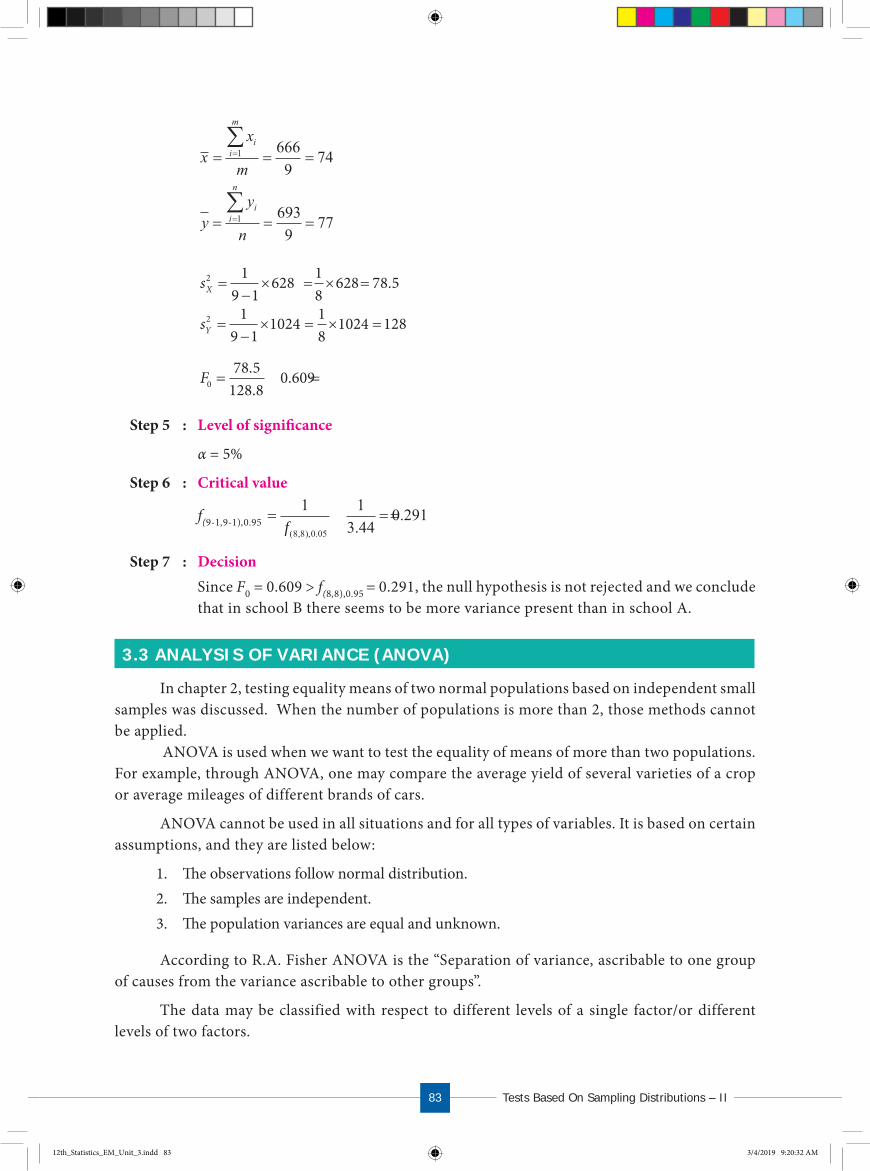
12t h S t d S t a t i s t i c s 82 T e s t s B a s e d O n S a m p l i n g D i s t r i b u t i o n s – I I83
xx
m
yy
n
ii
m
ii
n
� � �
� � �
�
�
�
�
1
1
666
974
693
977
s
s
X
Y
2
2
19 1
628 18
628 78 5
19 1
1024 18
1024 128
��
� � � �
��
� � � �
.
F078 5
128 80 609.
..
Step 5 : Level of signi�cance
α = 5%
Step 6 : Critical value
f(9-1,9-1),0.95 1 1
3 440 291
8 8 0 05f( , ), . ..
Step 7 : DecisionSince F0 = 0.609 > f(8,8),0.95 = 0.291, the null hypothesis is not rejected and we conclude that in school B there seems to be more variance present than in school A.
3.3 ANALY SIS OF VARIANCE ( ANOVA)
In chapter 2, testing equality means of two normal populations based on independent small samples was discussed. When the number of populations is more than 2, those methods cannot be applied.
ANOVA is used when we want to test the equality of means of more than two populations. For example, through ANOVA, one may compare the average yield of several varieties of a crop or average mileages of different brands of cars.
ANOVA cannot be used in all situations and for all types of variables. It is based on certain assumptions, and they are listed below:
1. �e observations follow normal distribution.2. �e samples are independent.3. �e population variances are equal and unknown.
According to R.A. Fisher ANOVA is the “Separation of variance, ascribable to one group of causes from the variance ascribable to other groups”.
The data may be classified with respect to different levels of a single factor/or different levels of two factors.
12th_Statistics_EM_Unit_3.indd 83 3/4/2019 9:20:32 AM

12t h S t d S t a t i s t i c s 84
Treatments Total
Treatment 1 x11 x12 … x1n1x1.
Treatment 2 x21 x22 … x2n2x2.
…
Treatment k xk1 xk2 … xknkxk.
xij - the j th sample value from the ith treatment, j = 1, 2, …,ni, i =1, 2,…,k k - number of treatments compared. xi. - the sample total of i th treatment.ni - the number of observations in the ith treatment.
1
k
ii
n n
�e total variation in the observations xij can be split into the following two components
i) variation between the levels or the variation due to different bases of classification,commonly known as treatments.
ii) The variation within the treatments i.e. inherent variation among the observationswithin levels.
Causes involved in the first type of variation are known as assignable causes. The causes leading to the second type of variation are known as chance or random causes.
�e �rst type of variation that is due to assignable causes, can be detected and controlled byhuman endeavor and the second type of variation that is due to chance causes, is beyond the human control.
3.3.2 Test ProcedureLet the observations xij, j = 1, 2, …, ni for treatment i, be assumed to come from N(μi, σ
2) population, i = 1, 2, …, k where σ2 is unknown.
12th_Statistics_EM_Unit_3.indd 84 3/4/2019 9:20:32 AM
The former is called one-way classified data and the latter is called two-way classified data. Applications of ANOVA technique to these kinds of data are discussed in the following sections.
3.3.1 One- w ay ANOVAANOVA is a statistical technique used to determine whether differences exist among three
or more population means.In one-way ANOVA the effect of one factor on the mean is tested. It is based on independent
random samples drawn from k – different levels of a factor, also called treatments.The following notations are used in one-way ANOVA. The data can be represented in the
following tabular structure.
Data representation for one-way ANOVA

12t h S t d S t a t i s t i c s 84 T e s t s B a s e d O n S a m p l i n g D i s t r i b u t i o n s – I I85
Step 1 : Framing Hypotheses
Null Hypothesis H0 : μ1 = μ2 = ... = μk
�at is, there is no signi�cant di�erence among the population means of k treatments.
Alternative Hypothesis
H1: μi≠μj for atleast one pair (i,j); i, j =1,2,...,k; i ≠ j
�at is, at least one pair of means di�er signi�cantly.
Step 2 : Data
Data is presented in the tabular form as described in the previous section
Step 3 : Level of signi�cance : α
Step 4 : Test Statistic F SST k
SSE n k�
��
/ ( )/ ( )
10
MSTFMSE
which follows F(k-1, n-k), under H0
To evaluate the test statistic we compute the following:
(i) Correction factor: C.F =n
G 2 where G = xij
j
n
i
k i
����
11
(ii) Total Sum of Squares: TSS = x C Fijj
n
i
k i2
11 ���� � .
(iii) Sum of Squares between Treatments: SST =xn
C F x x i ki
ii
k
i ijj
ni.
.. , , , , ,2
1 1
1 2� �� �� � � where
xn
C F x x i ki
ii
k
i ijj
ni.
.. , , , , ,2
1 1
1 2� �� �� � � where
(iv) Sum of Squares due to Error: SSE = TSS – SST
Degrees of Freedom (d.f)
Degrees of freedom (d.f.) d.f.Total Sum of Squares Total no. of observations –1 n–1Treatment Sum of Squares Total no. of observations –1 k–1Error of Sum Squares Total no. of observations –1 n–k
Mean Sum of Squares
Mean Sum of Squares due to treatment: MST SSTk
= 1
Mean Sum of Squares due to Error:
MSE SSEn k
=
12th_Statistics_EM_Unit_3.indd 85 3/4/2019 9:20:35 AM

12t h S t d S t a t i s t i c s 86
Step 5 : Calculation of Test statistic
ANOVA Table (one-way)
Source of variation Sum of squaresDegrees of
freedomMean sum of
squaresF-ratio
Treatments SST k-1 MST SSTk
= 1 0
MSTFMSE
Error SSE n-k MSE SSEn k
=
Total TSS n-1
Step 6 : Critical valuefe = f(k-1, n-k),α.
Step 7 : Decision
If F0 < f(k-1, n-k),α then reject H0.
3.3.3 Merits and Demerits of One- Way ANOVA
Merits• Layout is very simple and easy to understand.
• Gives maximum degrees of freedom for error.
Demerits• Population variances of experimental units for different treatments need to be equal.
• Verification of normality assumption may be difficult.
Ex ample 3.4Three different techniques namely medication, exercises and special diet are randomly
assigned to (individuals diagnosed with high blood pressure) lower the blood pressure. After four weeks the reduction in each person’s blood pressure is recorded. Test at 5% level, whether there is significant difference in mean reduction of blood pressure among the three techniques.
Medication 10 12 9 15 13Exercise 6 8 3 0 2Diet 5 9 12 8 4
Solution:
Step 1 : HypothesesNull Hypothesis: H0: 321
�at is, there is no signi�cant di�erence among the three groups on the average reductionin blood pressure.
12th_Statistics_EM_Unit_3.indd 86 3/4/2019 9:20:35 AM

12t h S t d S t a t i s t i c s 86 T e s t s B a s e d O n S a m p l i n g D i s t r i b u t i o n s – I I87
Alternative Hypothesis: H1: μi ≠ μj for atleast one pair (i, j); i, j = 1, 2, 3; i ≠ j.
�at is, there is signi�cant di�erence in the average reduction in blood pressure in atleastone pair of treatments.
Step 2 : Data
Medication 10 12 9 15 13
Exercise 6 8 3 0 2
Diet 5 9 12 8 4
Step 3 : Level of signi�cance α = 0.05Step 4 : Test statistic
0MSTFMSE
Step 5 : Calculation of Test statistic
Total SquareMedication 10 12 9 15 13 59 3481
Exercise 6 8 3 0 2 19 361Diet 5 9 12 8 4 38 1444
G = 116 5286
Individual squares
Medication 100 144 81 225 169
Exercise 36 64 9 0 4
Diet 25 81 144 64 16
xij2 1162���
1. Correction Factor: CF = 22 116 13456 897.06
15 15Gn
2. Total Sum of Squares: TSS = � ��� x C Fij2 .
= 1162 – 897.06 = 264.94
3. Sum of Squares between Treatments: SST = FCn
x
i
i .2
� �
� ��
52865
897 06
1057 2 897 06160 14
.
. ..
4. Sum of Squares due to Error: SSE = TSS – SST= 264.94 – 160.14 = 104.8
12th_Statistics_EM_Unit_3.indd 87 3/4/2019 9:20:36 AM
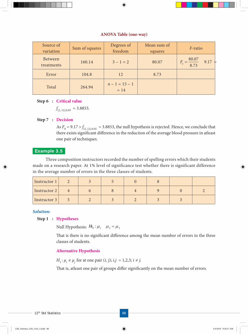
12t h S t d S t a t i s t i c s 88
ANOVA Table (one-way)
Source of variation
Sum of squaresDegrees of
freedomMean sum of
squaresF-ratio
Between treatments
160.14 3 – 1 = 2 80.07 Fo80 078 73
9 17..
.
Error 104.8 12 8.73
Total 264.94n – 1 = 15 – 1
= 14
Step 6 : Critical valuef(2, 12),0.05 = 3.8853.
Step 7 : DecisionAs F0 = 9.17 f(2, 12),0.05 = 3.8853, the null hypothesis is rejected. Hence, we conclude that there exists signi�cant di�erence in the reduction of the average blood pressure in atleast one pair of techniques.
Ex ample 3.5Three composition instructors recorded the number of spelling errors which their students
made on a research paper. At 1% level of significance test whether there is significant difference in the average number of errors in the three classes of students.
Instructor 1 2 3 5 0 8
Instructor 2 4 6 8 4 9 0 2
Instructor 3 5 2 3 2 3 3
Solution:Step 1 : Hypotheses
Null Hypothesis: 3210 :H
�at is there is no signi�cant di�erence among the mean number of errors in the threeclasses of students.
Alternative Hypothesis
H1 : μi ≠ μj for at one pair (i, j); i,j = 1,2,3; i ≠ j.
�at is, atleast one pair of groups di�er signi�cantly on the mean number of errors.
12th_Statistics_EM_Unit_3.indd 88 3/4/2019 9:20:37 AM

12t h S t d S t a t i s t i c s 88 T e s t s B a s e d O n S a m p l i n g D i s t r i b u t i o n s – I I89
Step 2 : Data
Instructor 1 2 3 5 0 8
Instructor 2 4 6 8 4 9 0 2
Instructor 3 5 2 3 2 3 3
Step 3 : Level of signi�cance α = 5%
Step 4 : Test Statistic
0MSTFMSE
Step 5 : Calculation of Test statistic
Total SquareInstructor 1 2 3 5 0 8 18 324Instructor 2 4 6 8 4 9 0 2 33 1089Instructor 3 5 2 3 2 3 3 18 324
69
Individual squares
Instructor 1 4 9 25 0 64
Instructor 2 16 36 64 16 81 0 4
Instructor 3 25 4 9 4 9 9
xij2 1162��� 379
Correction Factor: CF = Gn
2 26918
476118
264 5�� �
� � .
Total Sum of Squares: TSS � �
� � ��� x C Fij
2
379 264 5 114 5.
. .
Sum of Squares between Treatments: SST = FCn
x
i
i .2
� � ����
��� �
� � �� � �� � �
3245
10897
3246
264 5
64 8 155 6 54 264 5274 4
.
. . .. ��
�264 5
9 9.
.Sum of Squares due to Error: SSE = TSS – SST
= 114.5 – 9.9 = 104.6
12th_Statistics_EM_Unit_3.indd 89 3/4/2019 9:20:37 AM

12t h S t d S t a t i s t i c s 90
ANOVA Table
Source of variationSum of squares
Degrees of freedom
Mean sum of squares
F-ratio
Between treatments 9.9 3 – 1 = 29 92
4 95. . F04 956 97
0 710..
.
Error 104.6 15104 6
156 97. .
Totaln – 1 = 18 – 1
= 17
Step 6 : Critical value�e critical value = f(15, 2),0.05 = 3.6823.
Step 7 : DecisionAs F0 = 0.710 f(15, 2),0.05 = 3.6823, null hypothesis is not rejected. �ere is no enough evidence to reject the null hypothesis and hence we conclude that the mean number of errors made by these three classes of students are not equal.
3.4 TWO- WAY ANOVA
In two-way ANOVA a study variable is compared over three or more groups, controlling for another variable. The grouping is taken as one factor and the control is taken as another factor. The grouping factor is usually known as Treatment. The control factor is usually called Block. The accuracy of the test in two-way ANOVA is considerably higher than that of the one-way ANOVA, as the additional factor, block is used to reduce the error variance.
In two-way ANOVA, the data can be represented in the following tabular form.
Blocks
Gro
ups o
r Tre
atm
ents
1 2 3 … m xi.
1 x11 x12 x13.… x1m x1.
2 x21 x22 x2.… x2m x2.
3 x31 x32 x3.… x3m x3.
k xk1 xk2 xk3 … xkm xk.
x.j x.1 x.2 x.3 … x.m G
We use the following notations.
xij - ith treatment value from the j th block, i = 1,2, ..., k; j = 1,2, ..., m.
�e ith treatment total - x x i ki ijj
m
. , , , ...,� ��� 1 2
1
12th_Statistics_EM_Unit_3.indd 90 3/4/2019 9:20:38 AM

12t h S t d S t a t i s t i c s 90 T e s t s B a s e d O n S a m p l i n g D i s t r i b u t i o n s – I I91
�e j th block total - x x j mj iji
k
. , , , ...,� ��� 1 2
1
Note that, k × m = n, where m = number of blocks, and k = number of treatments (groups) and n is the total number of observations in the study.
The total variation present in the observations xij can be split into the following three components:
i) The variation between treatments (groups)ii) The variation between blocks.iii) The variation inherent within a particular setting or combination of treatment and
block.
3.4.1 Test ProcedureSteps involved in two-way ANOVA are:
Step 1 : In two-way ANOVA we have two pairs of hypotheses, one for treatments and one for the blocks.
Framing Hypotheses
Null Hypotheses
H01: �ere is no signi�cant di�erence among the population means of di�erent groups (Treatments)
H02: �ere is no signi�cant di�erence among the population means of di�erent Blocks
Alternative Hypotheses
H11: Atleast one pair of treatment means di�ers signi�cantly
H12: Atleast one pair of block means di�ers signi�cantly
Step 2 : Data is presented in a rectangular table form as described in the previous section.
Step 3 : Level of signi�cance α.
Step 4 : Test Statistic
F MSTMSEt0 ( )treatments
F MSBMSEb0 ( )block
To �nd the test statistic we have to �nd the following intermediate values.
i) Correction Factor: C.F 2G
n where
1 1
m k
ijj i
G x
ii) Total Sum of Squares: 2
1 1.
k m
iji j
TSS x C F
iii) Sum of Squares between Treatments:2.
1.
ki
i
xSST C Fm
12th_Statistics_EM_Unit_3.indd 91 3/4/2019 9:20:39 AM

12t h S t d S t a t i s t i c s 92
iv) Sum of squares between blocks:2.
1.
mj
j
xSSB C F
k
v) Sum of Squares due to Error: SSE = TSS-SST-SSB
vi) Degrees of freedom
Degrees of freedom (d.f.) d.f.Total Sum of Squares n–1
Treatment Sum of Squares k–1Block Sum of Squares m–1Error of Sum Squares (m – 1) (k – 1)
vii) Mean Sum of Squares
Mean sum of Squares due to Treatments:1
SSTMSTk
Mean sum of Squares due to Blocks: 1
SSBMSBm
Mean sum of Squares due to Error: 1 1SSEMSE
k m
Step 5 : Calculation of the Test Statistic
ANOVA Table (two-way)
Source of variation Sum of squaresDegrees of
freedomMean sum of
squaresF-ratio
Treatments SST k-1 MST 0tMSTFMSE
Blocks SSB m-1 MSB 0bMSBFMSE
Error SSE (k-1)( m-1) MSE
Total TSS n-1
Step 6 : Critical valuesCritical value for treatments = f(k-1,(m-1)(k-1)),α
Critical value for blocks = f(m-1, (m-1)(k-1)),α
Step 7 : Decision
For Treatments: If the calculated F0t value is greater than the corresponding critical value, then we reject the null hypothesis and conclude that there is significant difference among the treatment means, in atleast one pair.
12th_Statistics_EM_Unit_3.indd 92 3/4/2019 9:20:39 AM

12t h S t d S t a t i s t i c s 92 T e s t s B a s e d O n S a m p l i n g D i s t r i b u t i o n s – I I93
For Blocks: If the calculated F0b value is greater than the corresponding critical value, then we reject the null hypothesis and conclude that there is signi�cant di�erence among the block means, in at least one pair.
3.4.2 Merits and Demerits of tw o- w ay ANOVA
Merits• Any number of blocks and treatments can be used.
• Number of units in each block should be equal.
• It is the most used design in view of the smaller total sample size since we are studying twovariable at a time.
Demerits• If the number of treatments is large enough, then it becomes difficult to maintain the
homogeneity of the blocks.• If there is a missing value, it cannot be ignored. It has to be replaced with some function of
the existing values and certain adjustments have to be made in the analysis. This makes the analysis slightly complex.
Comparison between one-way ANOVA and two-way ANOVA
Basis of comparisonANOVA
One-way Two-way
Independent variable One Two
ComparesThree or more levels of one factor
Three or more levels of two factors, simultaneously
Number of observationsNeed not be same in each treatment group
Need to be equal in each treatment group
Ex ample 3.6A reputed marketing agency in India has three different training programs for its salesmen.
The three programs are Method – A, B, C. To assess the success of the programs, 4 salesmen from each of the programs were sent to the field. Their performances in terms of sales are given in the following table.
SalesmenMethods
A B C1 4 6 22 6 10 63 5 7 44 7 5 4
Test whether there is signi�cant di�erence among methods and among salesmen.
12th_Statistics_EM_Unit_3.indd 93 3/4/2019 9:20:39 AM

12t h S t d S t a t i s t i c s 94
Solution:
Step 1 : HypothesesNull Hypotheses: H01 : μM1
= μM2 = μM3 (for treatments)
�at is, there is no signi�cant di�erence among the three programs in their mean sales.
H02 : μS1 = μS2
= μS3 = μS4 (for blocks)
Alternative Hypotheses: H11 : At least one average is di�erent from the other, among the three programs.H12 : At least one average is di�erent from the other, among the four salesmen.
Step 2 : Data
Salesmen MethodsA B C
1 4 6 22 6 10 63 5 7 44 7 5 4
Step 3 : Level of signi�cance α = 5%
Step 4 : Test Statistic
F MSTMSEt0 ( )treatment
F MSBMSEb0 ( )block
Step-5 : Calculation of the Test Statistic
Methods Total xi. xi.2
A B C1 4 6 2 12 1442 6 10 6 22 4843 5 7 4 16 2564 7 5 4 16 256xi 22 28 16 66 1140
xi.2 484 784 256 1524
Squares
16 36 436 100 3625 49 1649 25 16
2 408ijx
12th_Statistics_EM_Unit_3.indd 94 3/4/2019 9:20:40 AM

12t h S t d S t a t i s t i c s 94 T e s t s B a s e d O n S a m p l i n g D i s t r i b u t i o n s – I I95
Correction Factor: CF = Gn
2 26612
435612
363�� �
� �
Total Sum of Squares: TSS � �
� � ��� x C Fij
2
408 363 45.
Sum of Squares due to Treatments: SST = x
kC F
ji
k
.
.
2
1��
�
� �
� � �
11403
363
380 363 17
Sum of Squares due to Blocks: SSB = x
kC F
ji
k
.
.
2
1��
�
� �
� ��
15244
363
381 36318
Sum of Squares due to Error: SSE = TSS – SST - SSB= 45 – 17 - 18 = 10
Mean sum of squares: MST SSTk
MSB SSBm
MSE SSEk m
��
� �
��
� �
�� �
� �
1
17
35 67
1
18
29
1 1
10
61
.
( )( )..67
ANOVA Table (two-way)
Sources of variation Sum of squaresDegrees of
freedomMean sum of
squaresF-ratio
Between treatments (Programs)
17 3 5.67 Fot5 67
1 673 40
.
..
Between blocks (Salesmen)
18 2 9 Fob9
1 675 39
..
Error 10 6 1.67
Total 11
Step 6 : Critical values(i) f(3, 6),0.05 = 4.7571 (for treatments)(ii) f(2, 6),0.05 = 5.1456 (for blocks)
12th_Statistics_EM_Unit_3.indd 95 3/4/2019 9:20:43 AM

12t h S t d S t a t i s t i c s 96
Step 7 : Decisioni) Calculated F0t = 3.40 < f(3, 6),0.05 = 4.7571, the null hypothesis is not rejected and
we conclude that there is signi�cant di�erence in the mean sales among the threeprograms.
ii) Calculate F0b = 5.39 > f(2, 6),0.05 = 5.1456, the null hypothesis is rejected and concludethat there does not exist signi�cant di�erence in the mean sales among the foursalesmen.
Ex ample 3.7�e illness caused by a virus in a city concerning some restaurant inspectors is not consistent
with their evaluations of cleanliness of restaurants. In order to investigate this possibility, the director has �ve restaurant inspectors to grade the cleanliness of three restaurants. �e results are shown below.
InspectorsRestaurants
I II III
1 71 55 84
2 65 57 86
3 70 65 77
4 72 69 70
5 76 64 85
Carry out two-way ANOVA at 5% level of signi�cance.
Solution:
Step 1 :Null hypotheses
0 1 2 3 4 5:IH (For inspectors - Treatments)
�at is, there is no signi�cant di�erence among the �ve inspectors over their meancleanliness scores
H0R : μI = μII = μIII (For restaurants - Blocks)
�at is, there is no signi�cant di�erence among the three restaurants over their meancleanliness scores
Alternative Hypotheses
H1I: At least one mean is di�erent from the other among the Inspectors
H1R: At least one mean is di�erent from the other among the Restaurants.
12th_Statistics_EM_Unit_3.indd 96 3/4/2019 9:20:43 AM

12t h S t d S t a t i s t i c s 96 T e s t s B a s e d O n S a m p l i n g D i s t r i b u t i o n s – I I97
Step 2 : Data
InspectorsRestaurants
I II III
1 71 55 84
2 65 57 86
3 70 65 77
4 72 69 70
5 76 64 85
Step 3 : Level of signi�cance α = 5%
Step 4 : Test Statistic
For inspectors: F0a (treatments) = 0 ( )tMSTF treatmentMSE
For restaurants: F0b (blocks) 0 ( )b
MSBF blockMSE
Step-5 : Calculation of the Test Statistic
InspectorsRestaurants
Total xi.2.ixI II III
1 71 55 84 210 441002 65 57 86 208 432643 70 65 77 212 449444 72 69 70 211 445215 76 64 85 225 50625
jx. 354 310 402 1066
2. jx 125316 96100 161604
Squares
5041 3025 7056
4225 3249 7396
4900 4225 5929
5184 4761 4900
5776 4096 72252 76988ijx
Correction Factor: CF = 22 1066 1136356 75757.07
15 15Gn
12th_Statistics_EM_Unit_3.indd 97 3/4/2019 9:20:43 AM

12t h S t d S t a t i s t i c s 98
Total Sum of Squares: TSS 2 .76988 75757.07 1230.93
ijx C F
Sum of Squares due to Treatments: SST = 2.
1 .
l
ij
xC F
l227454 75757.07
375818 75757.0760.93
Sum of Squares due to Blocks: SSB = FC
k
xk
ij
.1
2.
383020 75757.075
76604 75757.07846.93
Sum of squares due to error: SSE = TSS – SST - SSB = 1230.93 – 60.93 – 846.93 = 323.07
ANOVA Table (two-way)
Sources of variation Sum of squaresDegrees of
freedomMean sum of
squaresF-ratio
Between inspectors 60.93 4 15.23 015.23 0.37740.38IF
Between restaurants 846.93 2 423.47
Error 323.07 8 40.38
Total 1230.93 14
Step 6 : Critical values
(i) f(4, 8),0.05 = 3.838 (for inspectors)
(ii) f(2, 8),0.05 = 4.459 (for restaurants)
Step 7 : Decision
i) As F0I = 0.377 < f(4, 8),0.05 = 3.838, the null hypothesis is not rejected and we concludethat there is no signi�cant di�erence among the mean cleanliness scores of inspectors.
ii) As F0R = 10.49 > f(2, 8),0.05 = 4.459, the null hypothesis is rejected and we conclude thatthere exists signi�cant di�erence in atleast one pair of restaurants over their meancleanliness scores.
0423.47 10.4940.38RF
12th_Statistics_EM_Unit_3.indd 98 3/4/2019 9:20:43 AM

12t h S t d S t a t i s t i c s 98 T e s t s B a s e d O n S a m p l i n g D i s t r i b u t i o n s – I I99
EXERCISE 3
I. Choose the best Answer.
1. ANOVA was developed by
(a) S.D. Poisson (b) Karl Pearson
(c) R.A. Fisher (d) W.S. Gosset
2. ANOVA technique originated in the field of
(a) Industry (b) Agriculture
(c) Medicine (d) Genetics
3. One of the assumptions of ANOVA is that the population from which the samples are drawn is
(a) Binomial (b) Poisson (c) Chi-square (d) Normal
4. In one-way classification the total variation can be split into
(a) Two components (b) Three components
(c) Four components (d) Only one components
POINTS TO REMEMBER
� F-statistic is the ratio of two independent sample variances
� If X and Y are two independent 2 variates with m and n degrees of freedom respectively,
then FX
m
Yn
is said to follow F distribution with (m, n) degrees of freedom.
� Two independent random samples of size m and n are taken from Normal populations.
�en the statistic Fss
X
Y
2
2 is a random variable following the F-distribution with m–1 and
n–1 degrees of freedom.
� According to R.A. Fisher, ANOVA is the “Separation of variance, ascribable to one groupof causes from the variance ascribable to other groups”.
� One-way ANOVA is used to compare means in more than two groups.
� Two-way ANOVA is used to compare means in more than two groups, controlling anothervariable.
� Assumptions required for ANOVA are:• �e observations follow normal distribution.• Experimental units assigned to treatments are random.• �e sample observations are independent.• �e population variances of the groups are unknown but are assumed to be equal.
12th_Statistics_EM_Unit_3.indd 99 3/4/2019 9:20:43 AM

12t h S t d S t a t i s t i c s 100
5. The null hypothesis in the ANOVA is that all the population means are
(a) Equal (b) Variable
(c) Unequal (d) none of the above
6. In one-way classi�cation with 30 observation and 5 treatments the degrees of freedom for error is
(a) 29 (b) 4 (c) 25 (d) 150
7. In two-way classification the total variation TSS is
(a) SST+SSB+SSE (b) SST-SSB+SSE
(c) SST+SSB-SSE (d) SST+SSB
8. In two-way classification if TSS = 210, SST = 32, SSB = 42 then SSE =
(a) 126 (b) 74 (c) 136 (d) 178
9. In two-way classification with 5 treatments and 4 blocks the degrees of freedom due to erroris
(a) 12 (b) 19 (c) 16 (d) 15
10. The formula for comparing three or more means in one-way analysis of variance is
(a) MSTFMSE
(b) TSSFSST
(c) MSBFMST
(d) MSTFMSB
11. ______ test is used to compare three or more means.
(a) t (b) χ2 (c) F (d) Z
12. When there is no significant difference among three or more means the value of F will beclose to
(a) 0 (b) -1 (c) 1 (d) ∞
13. F-test is also called as
(a) mean ratio test (b) variance ratio test
(c) variance test (d) standard deviation ratio test
14. The Analysis of Variance procedure is appropriate for testing the equivalence of three ormore population
(a) variances (b) proportions
(c) means (d) observations
12th_Statistics_EM_Unit_3.indd 100 3/4/2019 9:20:43 AM

12t h S t d S t a t i s t i c s 100 T e s t s B a s e d O n S a m p l i n g D i s t r i b u t i o n s – I I101
15. In two-way classi�cation with 'm' treatments and 'n' blocks the degrees of freedom due to error is
(a) mn-1 (b) m-1 (c) n-1 (d) (m-1)(n-1)
16. If the calculated value of F is greater than the critical value at the given level of significancethen the H0 is
(a) Rejected (b) Not rejected
(c) Always true (d) Sometimes true
17. ______ and ______ causes are present in Analysis of Variance techniques
(a) Chance, error (b) Fixed, block
(c) Assignable, chance (d) Assignable, fixed
18. In ANOVA, the sample observations are
(a) dependent (b) independent
(c) equal (d) unequal
19. The correction factor is ______ in ANOVA (with the usual notations).
(a) T
n
ij2
(b) n
Ti2.
(c) n
G 2(d)
n
Ti.
20. Mean Sum of Squares is the ratio of Sum of Squarea to its
(a) number of blocks (b) number of treatments
(c) degrees of freedom (d) total sum of squares
II. Give very short answers to the following questions.
21. What is Analysis of Variance?
22. Write the applications of F-statistic.
23. What are the assumptions of ANOVA?
24. Define: Between group variance and within group variance.
25. State the hypotheses used in one-way ANOVA.
26. What are the components in a two-way ANOVA?
27. Name the causes of variation?
12th_Statistics_EM_Unit_3.indd 101 3/4/2019 9:20:44 AM
12t h S t d S t a t i s t i c s 102
III. Give short answer to the following questions.
28. What are the merits and demerits of one-way classification?
29. Write the model ANOVA table for one-way classification.
30. What are the values to be found for finding the test statistic in one-way classification?
31. What are the merits and demerits of two-way classification?
32. Write the model ANOVA table for two-way classification.
33. What are the components in two-way ANOVA?
34. What are the values to be found for finding the test statistic in two way classification?
35. Compare one-way and two-way ANOVA.
IV. Give detailed answer to the following questions.
36. In a sample of 8 observations, the sum of the squares of deviations of the sample values fromits sample mean was 84.4. In another sample of 10 observations it was 102.6. Test whether thetwo population variances are equal at 5% level.
37. Two random samples gave the following results
Sample Size Sample mean Sum of squares of deviations from the mean
I 10 15 90
II 12 14 108
Test whether the populations have same variances at 5% level of significance.
38. The following data refer to the yield of wheat in quintals on plots of equal area in twoagricultural blocks A and B.
Number of plots Mean yield Sample variance
Block A 8 60 50
Block B 6 51 40
Is the variance of yield for block A is greater than that of block B at 5% level of signi�cance.
39. The calories contained in 1/2 cup servings of ice-creams selected randomly from two nationalbrands are listed here. At 5% level of significance, is there sufficient evidence to conclude thatthe variance of calories is less for brand A than brand B?
Brand A 330 310 300 310 300 350 380 300 300
Brand B 300 300 270 290 310 370 300 310 250
40. �e carbohydrates contained in servings of some randomly selected chocolate and non-chocolatecandies are listed below. Is there su�cient evidence to conclude that the variance in carbohydratesvaries between chocolate and non-chocolate candies? Use = 2%.
12th_Statistics_EM_Unit_3.indd 102 3/4/2019 9:20:44 AM

12t h S t d S t a t i s t i c s 102 T e s t s B a s e d O n S a m p l i n g D i s t r i b u t i o n s – I I103
Chocolate 29 25 18 40 41 25 32 30 38 34 25 28
Non-chocolate 39 39 37 29 30 38 39 10 29 55 29
41. A home gardener wishes to determine the effects of four fertilizers on the average number oftomatoes produced. Test at 5% level of significance the hypothesis that the fertilizers A, B, Cand D have equal average yields.
A 14 10 12 16 17B 9 11 12 8 10C 16 15 14 10 18D 10 11 11 13 8
42. Three processes X, Y and Z are tested to see whether their outputs are equivalent. Thefollowing observations on outputs were made.
X 10 13 12 11 10 14 15 13
Y 9 11 10 12 13
Z 11 10 15 14 12 13
Carry out the one-way analysis of variance and state your conclusion.
43. A test was given to five students taken at random from XII class of three schools of a town.The individual scores are
School I 9 7 6 5 8
School II 7 4 5 4 5
School III 6 5 6 7 6
Carry out the one-way ANOVA.
44. A farmer applies three types of fertilizers on four separate plots. The figures on yield per acreare tabulated below.
FertilizerPlots
A B C D
Nitrogen 6 4 8 6
Potash 7 6 6 9
Phosphate 8 5 10 9
Test whether there is any signi�cant di�erence among mean yields of di�erent plots and among di�erent fertilizers.
12th_Statistics_EM_Unit_3.indd 103 3/4/2019 9:20:44 AM

12t h S t d S t a t i s t i c s 104
45. Operators are tested for their efficiency in terms of number of units produced per day byfive different types of machines. Test at 5% level of significance whether the operators andmachines differ in terms of their efficiency?
OperatorsMachine types
A B C D E
I 8 10 7 12 6
II 12 13 8 9 12
III 7 8 6 8 8
IV 5 5 3 5 14
ANSWERS
I. 1. (c) 2. (b) 3. (d) 4. (a) 5. (a)
6. (c) 7. (a) 8. (c) 9. (a) 10. (a)
11. (c) 12. (c) 13. (b) 14. (c) 15. (d)
16. (a) 17. (c) 18. (b) 19. (c) 20. (c)
III. 36. F0 = 1.06, H0 is not rejected
37. F0 = 1.02, H0 is not rejected
38. F0 = 1.25, H0 is not rejected
39. F0 = 1.34, H0 is not rejected
40. F0 = 2.52, H0 is not rejected
41. F0 = 4.59, H0 is rejected
42. F0 = 1.097, H0 is not rejected
43. F0 = 3.33, H0 is not rejected
44. F0 =2.39, H0 is not rejected F0 = 3.59, H0 is not rejected
45. F0 = 2.53, H0 is not rejected F0 = 1.24, H0 is not rejected
12th_Statistics_EM_Unit_3.indd 104 3/4/2019 9:20:44 AM

12t h S t d S t a t i s t i c s 104 T e s t s B a s e d O n S a m p l i n g D i s t r i b u t i o n s – I I105
Steps:• Open the browser and type the URL given (or) scan the QR code. GeoGebra work book called“F-Distribution” will appear.• In this several work sheets for statisticsare given, open the worksheet named “F-Distribution”• Drag and move the Red colour and Blue colour button or type the values in the left side box for result
ICT CORNER
Pictures are indicatives only*
S t e p - 1 S t e p - 2
S t e p - 3
� is activity helps to understand about
F-DISTRIBUTION
TESTS BASED ON SAMPLING DISTRIBUTIONS – II
S t e p - 4
12th_Statistics_EM_Unit_3.indd 105 3/4/2019 9:20:44 AM

10612t h S t d S t a t i s t i c s
Karl Pearson (1857-1936) was a English Mathematician and Biostatistician. He founded the world’s � rst university statistics department at University College, London in 1911. � e linear correlation
coe� cient is also called Pearson product moment correlation coe� cent. It was developed by Karl Pearson with a related idea by Francis Galton (see Regression analysis - for Galton’s contribution). It is the � rst of the correlation measures developed and commonly used.
Charles Edward Spearman (1863-1945) was an English psychologist and ,after serving 15 years in Army he joined to study PhD in Experimental Psychology and obtained his degree in 1906. Spearman was strongly influenced by the work of Galton and developed rank correlation in 1904.He also pioneered factor analysis in statistics.
Karl Pearson (1857-1936)a English Mathematician and Biostatistician. He founded the world’s � rst university statistics department at University College, London
Karl Pearson Charles Spearman
The student will be able to
� learn the meaning, de� nition and the uses of correlation.� identify the types of correlation.� understand correlation coe� cient for di� erent types of measurement scales.� di� erentiate di� erent types of correlation using scatter diagram.� calculate Karl Pearson’s coe� cient of correlation, Spearman’s rank correlation coe� cient
and Yule’s coe� cient of association.� interpret the given data with the help of coe� cient of correlation.
LEARNING OBJECTIVES
“When the relationship is of a quantitative nature, the appropriate statistical tool for discovering the existence of relation and measuring the intensity of relationship is known as correlation”
—CROXTON AND COWDEN
CORRELATIONANALY SIS
CHAPTER
4
12th_Statistics_EM_Unit_4.indd 106 3/4/2019 1:36:35 PM

C o r r e l a t i o n A n a l y s i s107
Introduction
“Figure as far as you can, then add judgment”
The statistical techniques discussed so far are for only one variable. In many research situations one has to consider two variables simultaneously to know whether these two variables are related linearly. If so, what type of relationship that exists between them. This leads to bivariate (two variables) data analysis namely correlation analysis. If two quantities vary in such a way that movements ( upward or downward) in one are accompanied by the movements( upward or downward) in the other, these quantities are said to be co-related or correlated.
The correlation concept will help to answer the following types of questions.
• Whether study time in hours is related with marks scored in the examination?• Is it worth spending on advertisement for the promotion of sales?• Whether a woman’s age and her systolic blood pressure are related? • Is age of husband and age of wife related?• Whether price of a commodity and demand related?• Is there any relationship between rainfall and production of rice?
4.1 DEFINITION OF CORRELATION
Correlation is a statistical measure which helps in analyzing the interdependence of two or more variables. In this chapter the dependence between only two variables are considered.
1. A.M. Tuttle de�nes correlation as:“An analysis of the co-variation of two or more variables is usually called correlation”
2. Ya-kun-chou de�nes correlation as:“The attempts to determine the degree of relationship between variables”.
Correlation analysis is the process of studying the strength of the relationship between two related variables. High correlation means that variables have a strong linear relationship with each other while a low correlation means that the variables are hardly related. The type and intensity of correlation is measured through the correlation analysis. The measure of correlation is the correlation coefficient or correlation index. It is an absolute measure.
Uses of correlation
• Investigates the type and strength of the relationship that exists between the two variables.• Progressive development in the methods of science and philosophy has been characterized by
the rich knowledge of relationship.
4.2 TY PES OF CORRELATION
1. Simple (Linear) correlation (2 variables only) : �e correlation between the given two variables.It is denoted by rxy
2. Partial correlation (more than 2 variables): �e correlation between any two variables whileremoving the e�ect of other variables. It is denoted by rxy.z …
12th_Statistics_EM_Unit_4.indd 107 3/4/2019 1:36:35 PM

10812t h S t d S t a t i s t i c s
3. Multiple correlation (more than 2 variables) : �e correlation between a group of variables anda variable which is not included in that group. It is denoted by Ry.(xz…)
In this chapter, we study simple correlation only, multiple correlation and partial correlation involving three or more variables will be studied in higher classes .
4.2.1 Simple correlation or Linear correlationHere, we are dealing with data involving two related variables and generally we assign a
symbol ‘x ’ to scores of one variable and symbol ‘y ’ to scores of the other variable. There are five types in simple correlation. They are
1. Positive correlation (Direct correlation)
2. Negative correlation (Inverse correlation)
3. Uncorrelated
4. Perfect positive correlation
5. Perfect negative correlation
1) Positive correlation: (Direct correlation)
The variables are said to be positively correlated if larger values of x are associated with larger values of y and smaller values of x are associated with smaller values of y. In other words, if both the variables are varying in thesame direction then the correlation is said to be positive.In other words, if one variable increases, the other variable (on an average) also increases or if one variable decreases, the other (on an average)variable also decreases.
For example,
i) Income and savings
ii) Marks in Mathematics and Marks in Statistics. (i.e.,Direct relationship pattern exists).
Y -Height posi�on of this li�
Height of the Li� increases / decreases accordingto the Height of goods increases / decreases.
The star�ng posi�on of wri�ng depends on the height ofthe writer.
X -Height of goods
Posi�ve or Direct Correla�on
Things move in the same direc�on
X Y YX
12th_Statistics_EM_Unit_4.indd 108 3/4/2019 1:36:36 PM

108 C o r r e l a t i o n A n a l y s i s109
2) Negative correlation: (Inverse correlation)
�e variables are said to be negatively correlated ifsmaller values of x are associated with larger values of y or larger values x are associated with smaller values of y. �at is the variables varying in the opposite directions is said to be negatively correlated. In other words, if one variable increases the other variable decreases and vice versa.
For example,
i) Price and demand
ii) Unemployment and purchasing power
3) Uncorrelated:
The variables are said to be uncorrelated if smaller values of x are associated with smaller or larger values of y and larger values of x are associated with larger or smaller values of y. If the two variables do not associate linearly, they are said to be uncorrelated. Here r = 0.
Important note: Uncorrelated does not imply independence. This means “do not interpret as the two variables are independent instead interpret as there is no specific linear pattern exists but there may be non linear relationship”.
4) Perfect Positive Correlation
If the values of x and y increase or decrease proportionately then they are said to have perfect positive correlation.
5) Perfect Negative Correlation
If x increases and y decreases proportionately or if x decreases and y increases proportionately, then they are said to have perfect negative correlation.
Correlation Analysis
The purpose of correlation analysis is to find the existence of linear relationship between the variables. However, the method of calculating correlation coefficient depends on the types of measurement scale, namely, ratio scale or ordinal scale or nominal scale.
Nega�ve or Inverse rela�onship
Things move in opposite direc�on
DownDown UpUp
X Y X Y
12th_Statistics_EM_Unit_4.indd 109 3/4/2019 1:36:36 PM

11012t h S t d S t a t i s t i c s
Statistical tool selection
Methods to find correlation
1. Scatter diagram2. Karl Pearson’s product moment correlation
coe�cient : ‘r’3. Spearman’s Rank correlation coe�cient: ‘ ’4. Yule’s coe�cient of Association: ‘Q’
4.3 SCATTER DIAGRAM
A scatter diagram is the simplest way of the diagrammatic representation of bivariate data. One variable is represented along the X-axis and the other variable is represented along the Y-axis. �e pair of points are plotted on the two dimensional graph. �e diagram of points so obtained is known as scatter diagram. �e direction of �ow of points shows the type of correlation that exists between the two given variables.
1) Positive correlationIf the plotted points in the plane form a band and they show the
rising trend from the lower left hand corner to the upper right hand corner, the two variables are positively correlated.
2) Negative correlationIf the plotted points in the plane form a band and they show the falling
trend from the upper left hand corner to the lower right hand corner, the two variables are negatively correlated.
3) UncorrelatedIf the plotted points spread over in the plane then the two variables
are uncorrelated.
4) Perfect positive correlationIf all the plotted points lie on a straight line from lower left hand
corner to the upper right hand corner then the two variables have perfect positive correlation.
NOTEFor higher order dimension of nominal or categorical variables in a contingency table, use chi-square test for independence of attributes. (Refer Chapter 2)
X
Y
In this case 0 < r < 1
X
Y
In this case -1 < r < 0
X
Y
In this case r = 0
X
Y
In this case r = +1
12th_Statistics_EM_Unit_4.indd 110 3/4/2019 1:36:37 PM

110 C o r r e l a t i o n A n a l y s i s111
5) Perfect Negative correlationIf all the plotted points lie on a straight line falling from upper le�
hand corner to lower right hand corner, the two variables have perfect negative correlation.
4.3.1 Merits and Demerits of scatter diag ramMerits• It is a simple and non-mathematical method of studying correlation between the variables.• It is not in�uenced by the extreme items• It is the �rst step in investigating the relationship between two variables.• It gives a rough idea at a glance whether there is a positive correlation, negative correlation or
uncorrelated.
Demerits• We get an idea about the direction of correlation but we cannot establish the exact strength of
correlation between the variables.• No mathematical formula is involved.
4.4 KARL PEARSON’ S CORRELATION COEFFICIENT
When there exists some relationship between two measurable variables, we compute the degree of relationship using the correlation coefficient.
Co-variance
Let (X,Y) be a bivariable normal random variable where V(X) and V(Y) exists. Then, covariance between X and Y is defined as
cov(X,Y) = E[(X-E(X))(Y-E(Y))] = E(XY) – E(X)E(Y)
If (xi,yi), i=1,2, ..., n is a set of n realisations of (X,Y), then the sample covariance between X and Y can be calculated from
cov , ( )( )X Yn
x x y yn
x y x yi ii
n
i ii
n
� �� � � � �� �� �1 1
1 1
. . a l Pea son s coefficient o co elationWhen X and Y are linearly related and (X,Y) has a bivariate normal distribution, the
co-efficient of correlation between X and Y is defined as
r X Y X YV X V Y
, cov( , )( ) ( )
� ��
�is is also called as product moment correlation co-e�cient which was de�ned by Karl Pearson.Based on a given set of n paired observations (xi,yi), i=1,2, ... n the sample correlation
co-efficient between X and Y can be calculated from
r X Y nx y x y
nx x
ny y
i ii
n
ii
n
ii
n,� ��
�
� �
�
� �
�
� �
1
1 11
2 2
1
2 2
1
X
Y
In this case r = -1
12th_Statistics_EM_Unit_4.indd 111 3/4/2019 1:36:38 PM

11212t h S t d S t a t i s t i c s
or, equivalently
r X Yn x y x y
n x x n y
i ii
n
i ii
n
i
n
i ii
n
i
n,� ��
�
��
��
�
��
� ��
��
� ��
��
1 11
2
1
2
1ii i
i
n
i
n
y2
1
2
1
��
��
�
��
����
4.4.2 Properties1. �e correlation coe�cient between X and Y is same as the correlation coe�cient between Y and
X (i.e, rxy = ryx ).
2. �e correlation coe�cient is free from the units of measurements of X and Y
3. �e correlation coe�cient is una�ected by change of scale and origin.
�us, if ux A
cv
y Bdi
ii
i��
��
and with c ≠ 0 and d ≠ 0 i=1,2, ..., n
rn u v u v
n u u n v
i i ii
n
ii
n
i
n
ii
n
ii
n
ii
��
��
��
�
��
� ��
� � �
� ��
� �
1 11
2
1 1
22
1
nn
ii
n
v� ���
��
�
��
�1
2
where A and B are arbitrary values.
Remark 1: If the widths between the values of the variabls are not equal then take c = 1 and d = 1.
Interpretation
The correlation coefficient lies between -1 and +1. i.e. -1 ≤ r ≤ 1
• A positive value of ‘r’ indicates positive correlation.
• A negative value of ‘r’ indicates negative correlation
• If r = +1, then the correlation is perfect positive
• If r = –1, then the correlation is perfect negative.
• If r = 0, then the variables are uncorrelated.
• If 0.7r then the correlation will be of higher degree. In interpretation we use the adjective ‘highly’
• If X and Y are independent, then rxy = 0. However the converse need not be true.
Ex ample 4.1The following data gives the heights(in inches) of father and his eldest son. Compute the
correlation coefficient between the heights of fathers and sons using Karl Pearson’s method.
Height of father 65 66 67 67 68 69 70 72
Height of son 67 68 65 68 72 72 69 71
12th_Statistics_EM_Unit_4.indd 112 3/4/2019 1:36:39 PM

112 C o r r e l a t i o n A n a l y s i s113
rn x y x y
n x x n y
i i ii
n
ii
n
i
n
ii
n
ii
n
ii
��
��
��
�
��
� ��
� � �
� ��
� �
1 11
2
1 1
22
1
nn
ii
n
y� ���
��
�
��
�1
2
Calculationxi yi xi
2 yi2 xiyi
65 67 4225 4489 435566 68 4356 4624 448867 65 4489 4225 435567 68 4489 4624 455668 72 4624 5184 489669 72 4761 5184 496870 69 4900 4761 483072 71 5184 5041 5112
544 552 37028 38132 37560
r = 2 2
8 37560 544 552
8 37028 544 8 38132 552
× ×
× × = 0.603
Heights of father and son are positively correlated. It means that on the average , if fathers are tall then sons will probably tall and if fathers are short, probably sons may be short.
Short-cut methodLet A = 68 , B = 69, c = 1 and d = 1
xi yi ui = (xi – A)/c= xi – 68
vi = (yi – B)/d= yi – 69
ui2 vi
2 uivi
65 67 -3 -2 9 4 666 68 -2 -1 4 1 267 65 -1 -4 1 16 467 68 -1 -1 1 1 168 72 0 3 0 9 069 72 1 3 1 9 370 69 2 0 4 0 072 71 4 2 16 4 8
Total 0 0 36 44 24
rn u v u v
n u u n v
i i ii
n
ii
n
i
n
ii
n
ii
n
ii
��
��
��
�
��
� ��
� � �
� ��
� �
1 11
2
1 1
22
1
nn
ii
n
v� ���
��
�
��
�1
2
12th_Statistics_EM_Unit_4.indd 113 3/4/2019 1:36:39 PM
Solution:
Let x denote height of father and y denote height of son. The data is on the ratio scale. We use Karl Pearson’s method.

11412t h S t d S t a t i s t i c s
2 2
8 24 0 0
8 36 0 8 44 0r × ×
× ×
8 248 36 8 44
0.603
r ×× ×
Note: �e correlation coe�cient computed by using direct method and short-cut method is the same.
Ex ample 4.2The following are the marks scored by 7 students in two tests in a subject. Calculate
coefficient of correlation from the following data and interpret.
Marks in test-1 12 9 8 10 11 13 7
Marks in test-2 14 8 6 9 11 12 3
Solution:Let x denote marks in test-1 and y denote marks in test-2.
xi yi xi2 yi
2 xiyi
12 14 144 196 1689 8 81 64 728 6 64 36 48
10 9 100 81 9011 11 121 121 1211 12 169 144 1567 3 49 9 21
Total 70 63 728 651 676
rn x y x y
n x x n y
i i ii
n
ii
n
i
n
ii
n
ii
n
ii
��
��
��
�
��
� ��
� � �
� ��
� �
1 11
2
1 1
2
2
1
nn
ii
n
ii
n
ii
n
i ii
n
ii
y
x x x y
y
� �
� � �
��
��
�
��
� � �
�
� � �
�
1
2
1
2
1 1
1
70 728 676
nn
ii
n
y n� �� � ��
63 651 72
1
r � � � �
� ��� �� � � ��� ��
��
�
7 676 70 63
7 728 70 7 651 63
4732 4410
5096 490
2 2
00 7 651 3969
322
196 588
322
14 24 25
322
339 50 95
� � � � �
��
��
� �. .
.
12th_Statistics_EM_Unit_4.indd 114 3/4/2019 1:36:41 PM

114 C o r r e l a t i o n A n a l y s i s115
1. Outliers (extreme observations)strongly influence the correlationcoefficient. If we see outliers in ourdata, we should be careful about theconclusions we draw from the valueof r. The outliers may be dropped before the calculation for meaningful conclusion.
2. Correlation does not imply causal relationship. That a change in one variable causes achange in another.
NOTE1. Uncorrelated : Uncorrelated (r = 0) implies no ‘linear relationship’. But there may exist non-
linear relationship (curvilinear relationship).
Example: Age and health care are related. Children and elderly people need much more healthcare than middle aged persons as seen from the following graph.
Age
Heal
th ca
re
Child
Adult
Old
0
However, if we compute the linear correlation r for such data, it may be zero implying age and health care are uncorrelated, but non-linear correlation is present.
2. Spurious Correlation : �e word ‘spurious’ from Latin means ‘false’ or ‘illegitimate’. Spuriouscorrelation means an association extracted from correlation coe�cient that may not exist in reality.
12th_Statistics_EM_Unit_4.indd 115 3/4/2019 1:36:41 PM
There is a high positive correlation between test-1 and test-2. That is those who perform well in test-1 will also perform well in test-2 and those who perform poor in test-1 will perform poor in test- 2.
The students can also verify the results by using shortcut method.
4.4.3 Limitations of CorrelationAlthough correlation is a powerful tool, there are some limitations in using it:

11612t h S t d S t a t i s t i c s
4.5 SPEARMAN’ S RANK CORRELATION COEFFICIENT
If the data are in ordinal scale then Spearman’s rank correlation coefficient is used. It is denoted by the Greek letter ρ (rho).
Spearman’s correlation can be calculated for the subjectivity data also, like competition scores. The data can be ranked from low to high or high to low by assigning ranks.
Spearman’s rank correlation coefficient is given by the formula
� � ��� �
��
1
6
1
2
1
2
D
n n
ii
n
where Di = R1i – R2i
R1i = rank of i in the first set of data
R2i = rank of i in the second set of data and
n = number of pairs of observations
Interpretation
Spearman’s rank correlation coefficient is a statistical measure of the strength of a monotonic (increasing/decreasing) relationship between paired data. Its interpretation is similar to that of Pearson’s. That is, the closer to the ±1 means the stronger the monotonic relationship.
Positive Range Negative Range
0.01 to 0.19: “Very Weak Agreement” (-0.01) to (-0.19): “Very Weak Disagreement”
0.20 to 0.39:“Weak Agreement” (-0.20) to (-0.39): “Weak Disagreement”
0.40 to 0.59: “Moderate Agreement” (-0.40) to (-0.59): “Moderate Disagreement”
0.60 to 0.79: “Strong Agreement” (-0.60) to (-0.79): “Strong Disagreement”
0.80 to 1.0: “Very Strong Agreement” (-0.80) to (-1.0): “Very Strong Disagreement”
Ex ample 4.3Two referees in a flower beauty competition rank the 10 types of flowers as follows:
Referee A 1 6 5 10 3 2 4 9 7 8
Referee B 6 4 9 8 1 2 3 10 5 7
Use the rank correlation coefficient and find out what degree of agreement is between the referees.
12th_Statistics_EM_Unit_4.indd 116 3/4/2019 1:36:42 PM

116 C o r r e l a t i o n A n a l y s i s117
Solution:
Rank by 1st refereeR1i
Rank by 2nd refereeR2i
Di= R1i – R2i Di2
1 6 -5 25
6 4 2 4
5 9 -4 16
10 8 2 4
3 1 2 4
2 2 0 0
4 3 1 1
9 10 -1 1
7 5 2 4
8 7 1 1
Dii
n2
1
60�� �
Here n = 10 and Dii
n2
1
60�� �
� � ��� �
� ��
�� �� �
� �� � �
��
1
6
1
16 60
10 10 11
360
10 991
360
990
2
1
2
2
D
n n
ii
n
00 636.
Interpretation: Degree of agreement between the referees ‘A’ and ‘B’ is 0.636 and they have “strong agreement” in evaluating the competitors.
Ex ample 4.4Calculate the Spearman’s rank correlation coefficient for the following data.
Candidates 1 2 3 4 5
Marks in Tamil 75 40 52 65 60
Marks in English 25 42 35 29 33
12th_Statistics_EM_Unit_4.indd 117 3/4/2019 1:36:43 PM

11812t h S t d S t a t i s t i c s
Solution:
Tamil English Di = R1i – R2i Di2
Marks Rank (R1i) Marks Rank (R2i)75 1 25 5 -4 1640 5 42 1 4 1652 4 35 2 2 465 2 20 4 -2 460 3 33 3 0 0
40
Dii
n2
1
40�� � and n = 5
� � ��� �
� ���� �
� �� �
� �
��
1
6
1
16 40
5 5 11
240
5 241
2
1
2
2
D
n n
ii
n
Interpretation: This perfect negative rank correlation (-1) indicates that scorings in the subjects, totally disagree. Student who is best in Tamil is weakest in English subject and vice-versa.
Ex ample 4.5Quotations of index numbers of equity share prices of a certain joint stock company and
the prices of preference shares are given below.
Years 2013 2014 2015 2016 2017 2008 2009Equity shares 97.5 99.4 98.6 96.2 95.1 98.4 97.1Reference shares 75.1 75.9 77.1 78.2 79 74.6 76.2
Using the method of rank correlation determine the relationship between equity shares and preference shares prices.
Solution:
Equity shares Preference share R1i R2i Di = R1i – R2i Di2
97.5 75.1 4 6 -2 499.4 75.9 1 5 -4 1698.6 77.1 2 3 -1 196.2 78.2 6 2 4 1695.1 79.0 7 1 6 3698.4 74.6 3 7 -4 1697.1 76.2 5 4 1 1
Dii
n2
1
90�� �
12th_Statistics_EM_Unit_4.indd 118 3/4/2019 1:36:45 PM

118 C o r r e l a t i o n A n a l y s i s119
Dii
n2
1
90�� � and n = 7.
Rank correlation coefficient is
� � ��� �
� ���� �
� ��
� � � �
��
1
6
1
16 90
7 7 11
540
7 481
540
3361 1
2
1
2
2
D
n n
ii
n
.66071 0 6071� � .
Interpretation: There is a negative correlation between equity shares and preference share prices. There is a strong disagreement between equity shares and preference share prices.
4.5 .1 Repeated rank sWhen two or more items have equal values (i.e., a tie) it is difficult to give ranks to them.
In such cases the items are given the average of the ranks they would have received. For example,
if two individuals are placed in the 8th place, they are given the rank 8 9 8.5
2 each, which is
common rank to be assigned and the next will be 10; and if three ranked equal at the 8th place,
they are given the rank 8 9 10 9
3 which is the common rank to be assigned to each; and the
next rank will be 11.
In this case, a different formula is used when there is more than one item having the same value.
� � �� �� � � �� � �
�� �
�
�
���
�
�
���
�1 6
112
112
1
213
1 23
2
2
D m m m m
n n
i ...
where mi is the number of repetitions of ith rank
Ex ample 4.6Compute the rank correlation coefficient for the following data of the marks obtained by
8 students in the Commerce and Mathematics.
Marks in Commerce 15 20 28 12 40 60 20 80
Marks in Mathematics 40 30 50 30 20 10 30 60
12th_Statistics_EM_Unit_4.indd 119 3/4/2019 1:36:46 PM

12012t h S t d S t a t i s t i c s
Solution:
Marks in Commerce (X) Rank (R1i)
Marks in Mathematics (Y) Rank (R2i) Di = R1i – R2i Di
2
15 2 40 6 -4 1620 3.5 30 4 -0.5 0.2528 5 50 7 -2 412 1 30 4 -3 940 6 20 2 4 1660 7 10 1 6 3620 3.5 30 4 -0.5 0.2580 8 60 8 0 0
Total 2 81.5D
� � �� �� � � �� � �
�� �
�
�
���
�
�
���
�1 6
112
112
1
213
1 23
2
2
D m m m m
n n
i ...
Repetitions of ranksIn Commerce (X), 20 is repeated two times corresponding to ranks 3 and 4. Therefore, 3.5
is assigned for rank 2 and 3 with m1=2.In Mathematics (Y), 30 is repeated three times corresponding to ranks 3, 4 and 5. Therefore,
4 is assigned for ranks 3,4 and 5 with m2=3. Therefore,
3 3
2
1 181.5 2 2 3 312 121 6
8 8 1
81.5 0.5 21 6
5045041504
0
= 0
Interpretation: Marks in Commerce and Mathematics are uncorrelated
4.6 Y ULE’ S COEFFICIENT OF ASSOCIATION
This measure is used to know the existence of relationship between the two attributes A and B (binary complementary variables). Examples of attributes are drinking, smoking, blindness, honesty, etc.
Udny Yule (1871 – 1951), was a British statistician. He was educated at Winchester College and at University College London. After a year dong research in experimental physics, he returned to University College in 1893 to work as a demonstrator for Karl Pearson. Pearson was beginning to work in statistics and Yule followed him into this new field. Yule was a prolific writer, and was active in Royal Statistical Society and received its Guy Medal in Gold in 1911, and served as its President in 1924–26.The concept of Association is due to him.
Udny yule
12th_Statistics_EM_Unit_4.indd 120 3/4/2019 1:36:46 PM
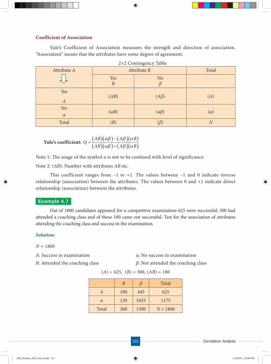
120 C o r r e l a t i o n A n a l y s i s121
2×2 Contingency Table Attribute A Attribute B Total
Yes B
No β
Yes
A(AB) (Aβ) (A)
No α (αB) (αβ) (α)
Total (B) (β) N
Yule’s coefficient: QB A B
AB A B�� �� � � � �� �� �� � � � �� �A �� � �
�� � �
Note 1: The usage of the symbol α is not to be confused with level of significance.
Note 2: (AB): Number with attributes AB etc.
This coefficient ranges from –1 to +1. The values between –1 and 0 indicate inverse relationship (association) between the attributes. The values between 0 and +1 indicate direct relationship (association) between the attributes.
Ex ample 4.7Out of 1800 candidates appeared for a competitive examination 625 were successful; 300 had
attended a coaching class and of these 180 came out successful. Test for the association of attributes attending the coaching class and success in the examination.
Solution:
N = 1800
A: Success in examination α: No success in examinationB: Attended the coaching class β: Not attended the coaching class
(A) = 625, (B) = 300, (AB) = 180
B β Total
A 180 445 625
α 120 1055 1175
Total 300 1500 N = 1800
12th_Statistics_EM_Unit_4.indd 121 3/4/2019 1:36:46 PM
Coefficient of Association
Yule’s Coefficient of Association measures the strength and direction of association. “Association” means that the attributes have some degree of agreement.

12212t h S t d S t a t i s t i c s
Yule’s coefficient: AB A B
QAB A B
180 1055 445 120180 1055 445 120189900 53400189900 534001365002433000.561 0
× ×× ×
Interpretation: There is a positive association between success in examination and attending coaching classes. Coaching class is useful for success in examination.
Remark: Consistency in the data using contingency table may be found as under.
Construct a 2 × 2 contingency table for the given information. If at least one of the cell frequencies is negative then there is inconsistency in the given data.
Ex ample 4.8Verify whether the given data: N = 100, (A) = 75, (B) = 60 and (AB) = 15 is consistent.
Solution:
The given information is presented in the following contingency table.
B β TotalA 15 60 75
α 45 -20 25
Total 60 40 N = 100
Notice that (αβ) = −20
Interpretation: Since one of the cell frequencies is negative, the given data is “Inconsistent”.
POINTS TO REMEMBER
� Correlation study is about finding the linear relationship between two variables.Correlation is not causation. Sometimes the correlation may be spurious.
� Correlation coefficient lies between –1 and +1.
� Pearson’s correlation coefficient provides the type of relationship and intensity ofrelationship, for the data in ratio scale measure.
� Spearman’s correlation measures the relationship between the two ordinal variables.
� Yule’s coefficient of Association measures the association between two dichotomousattributes.
12th_Statistics_EM_Unit_4.indd 122 3/4/2019 1:36:46 PM

122 C o r r e l a t i o n A n a l y s i s123
EXERCISE 4
I. Choose the best answer.
1. The statistical device which helps in analyzing the co-variation of two ormore variables is
(a) variance (b) probability
(c) correlation coefficient (d) coefficient of skewness
2. “The attempts to determine the degree of relationship between variables is correlation” is thedefinition given by
(a) A.M. Tuttle (b) Ya-Kun-Chou
(c) A.L. Bowley (d) Croxton and Cowden
3. If the two variables do not have linear relationship between them then they are said to have
(a) positive correlation (b) negative correlation
(c) uncorrelated (d) spurious correlation
4. If all the plotted points lie on a straight line falling from upper left hand corner to lower righthand corner then it is called
(a) perfect positive correlation (b) perfect negative correlation
(c) positive correlation (d) negative correlation
5. If r = +1, then the correlation is called
(a) perfect positive correlation (b) perfect negative correlation
(c) positive correlation (d) negative correlation
6. The correlation coefficient lies in the interval
(a) -1 ≤ r ≤ 0 (b) –1 < r < 1 (c) 0 ≤ r ≤ 1 (d) –1 ≤ r ≤ 1
7. Rank correlation coefficient is given by
(a) 1
6 2
1
3�
���D
n n
ii
n
(b) 1
6 2
1
3�
���D
n n
ii
n
(c) 1
6 2
1
3�
���D
n n
ii
n
(d) 1
6
1
3
1
2�
�� ���D
n n
ii
n
8. If ,02D rank correlation is
(a) 0 (b) 1 (c) 0.5 (d) –1
9. Rank correlation was developed by
(a) Pearson (b) Spearman (c) Yule (d) Fisher
10. Product moment coefficient of correlation is
(a) cov ,
x yrx y
(b) x yr (c) cov ,
x y
x yr (d) cov ,
xy
x yr
12th_Statistics_EM_Unit_4.indd 123 3/4/2019 1:36:49 PM

12412t h S t d S t a t i s t i c s
11. The purpose of the study of _________ is to identify the factors of influence and try to controlthem for better performance.
(a) mean (b) correlation (c) standard deviation (d) skewness
12. The height and weight of a group of persons will have _______ correlation.
(a) positive (b) negative
(c) zero (d) both positive and negative
13. ______ correlation studies the association of two variables with ordinal scale.
(a) A.M. Tuttle rank (b) Croxton and Cowdon rank
(c) Karl Pearson’s rank (d) Spearman’s rank.
14. ______ presents a graphic description of quantitative relation between two series of facts.
(a) scatter diagram (b) bar diagram (c) pareto diagram (d) pie diagram
15. ______ measures the degree of relationship between two variables.
(a) standard deviation (b) correlation coefficient
(c) moment (d) median
16. The correlation coefficient of x and y is symmetric. Hence
(a) rxy = ryx (b) rxy > ryx (c) rxy < ryx (d) rxy ≠ ryx
17. If cov (x, y) = 0 then its interpretation is
(a) x and y are positively correlated (b) x and y are negatively correlated
(c) x and y are uncorrelated (d) x and y are independent
18. Rank correlation is useful to study data in ______ scale.
(a) ratio (b) ordinal (c) nominal (d) ratio and nominal
19. If r = 0 then cov(x, y) is
(a) 0 (b) +1 (c) -1 (d) α
20. If cov(x, y) = σx, σy then
(a) r = 0 (b) r = –1 (c) r = +1 (d) r = α
II. Give very short answer to the following questions.
21. What is correlation?
22. Write the definition of correlation by A.M. Tuttle.
23. What are the different types of correlation?
24. What are the types of simple correlation?
25. What do you mean by uncorrelated?
26. What you understand by spurious correlation?
12th_Statistics_EM_Unit_4.indd 124 3/4/2019 1:36:49 PM

124 C o r r e l a t i o n A n a l y s i s125
27. What is scatter diagram?
28. Define co-variance.
29. Define rank correlation.
30. If 02D what is your conclusion regarding Spearman’s rank correlation coefficient?
31. Give an example for (i) positive correlation
(ii) negative correlation (iii) no correlation
32. What is the value of ‘r’ when two variables are uncorrelated?
33. When the correlation coefficient is +1, state your interpretation.
III. Give short answer to the following questions.
34. Write any three uses of correlation.
35. Define Karl Pearson’s coefficient of correlation.
36. How do you interpret the coefficient of correlation which lies between 0 and +1?
37. Write down any 3 properties of correlation?
38. If rank correlation coefficient r = 0.8, 332D 3 then find n?
39. Write any three merits of scatter diagram.
40. Given that cov(x, y) = 18.6, variance of x = 20.2, variance of y = 23.7. Find r.
41. Test the consistency of the following data with the symbols having their usual meaning.N = 1000, (A) = 600, (B) = 500, (AB) = 50.
IV. Give detailed answer to the following questions.
42. Explain different types of correlation.
43. Explain scatter diagram.
44. Calculate the Karl Pearson’s coefficient of correlation for the following data and interpret.
x 9 8 7 6 5 4 3 2 1y 15 16 14 13 11 12 10 8 9
45. Find the Karl Pearson’s coefficient of correlation for the following data.
Wages 100 101 102 102 100 99 97 98 96 95Cost of living 98 99 99 97 95 92 95 94 90 91
How are the wages and cost of living correlated?
46. Calculate the Karl Pearson’s correlation coefficient between the marks (out of 10) in statisticsand mathematics of 6 students.
Student 1 2 3 4 5 6Statistics 7 4 6 9 3 8
Mathematics 8 5 4 8 3 6
12th_Statistics_EM_Unit_4.indd 125 3/4/2019 1:36:49 PM

12612t h S t d S t a t i s t i c s
47. In a marketing survey the prices of tea and prices of coffee in a town based on quality wasfound as shown below. Find the rank correlation between prices of tea and prices of coffee.
Price of tea 88 90 95 70 60 75 50
Price of co�ee 120 134 150 115 110 140 100
48. Calculate the Spearman’s rank correlation coefficient between price and supply from thefollowing data.
Price 4 6 8 10 12 14 16 18Supply 10 15 20 25 30 35 40 45
49. A random sample of 5 college students is selected and their marks in Tamil and English arefound to be:
Tamil 85 60 73 40 90English 93 75 65 50 80
Calculate Spearman’s rank correlation coefficient.
50. Calculate Spearman’s coefficient of rank correlation for the following data.
x 53 98 95 81 75 71 59 55y 47 25 32 37 30 40 39 45
51. Calculate the coefficient of correlation for the following data using ranks.
Mark in Tamil 29 24 25 27 30 31
Mark in English 29 19 30 33 37 36
52. From the following data calculate the rank correlation coefficient.
x 49 34 41 10 17 17 66 25 17 58y 14 14 25 7 16 5 21 10 7 20
Yule’s coe�cient
53. Can vaccination be regarded as a preventive measure of Hepatitis B from the data given below.Of 1500 person in a locality, 400 were attacked by Hepatitis B. 750 has been vaccinated. Amongthem only 75 were attacked.
12th_Statistics_EM_Unit_4.indd 126 3/4/2019 1:36:49 PM

126 C o r r e l a t i o n A n a l y s i s127
ANSWERS
I 1. (c) 2. (b) 3. (c) 4. (b) 5. (a)
6. (d) 7. (b) 8. (b) 9. (b) 10. (b)
11. (b) 12. (a) 13. (d) 14. (a) 15. (b)
16. (a) 17. (c) 18. (b) 19. (a) 20. (c)
II 30. r = 1
III 38. n = 10
40. r = 0.85
41. 50 , �e given data is inconsistent
IV 44. r = 0.95 it is highly positively correlated
45. r = 0.847 wages and cost of living are highly positively correlated.
46. r = 0.8081. Statistics and mathematics marks are highly positively correlated.
47. = 0.8929 price of tea and coffee are highly positively correlated.
48. = 1 (perfect positive correlation)
49. = 0.8
50. = -0.905 x and y are highly negatively
51. = -0.78 marks in Tamil and English are negatively correlated.
52. = +0.733
53. There is a negative association between attacked and vaccinated.
54. There is a positive association between not attacked and not vaccinated.
55. Hence vaccination can be regarded as a preventive measure of Hepatitis B.
12th_Statistics_EM_Unit_4.indd 127 3/4/2019 1:36:50 PM

12812t h S t d S t a t i s t i c s
Steps:• Th is is an android app activity. Open the browser and type the URL given (or) scan the QR code. (Or)
search for “Correlation Coe� cient” in google play store.• (i) Install the app and open the app, (ii) To calculate Correlation Co-effi cient in put the the values of
X and Y in the given box (iii) � en click “CALCULATE” we will get the result.
ICT CORNER
Pictures are indicatives only*
S t e p - 1 S t e p - 2
S t e p - 3
STATS IN YOUR PALM� is activity is to calculate
Correlation Coe� cient
CORRELATION ANALYSIS
Re s u l t
12th_Statistics_EM_Unit_4.indd 128 3/4/2019 1:36:50 PM

R e g r e s s i o n A n a l y s i s129
IntroductionThe correlation coefficient is an useful statistical tool for describing the type ( positive or
negative or uncorrelated ) and intensity of linear relationship (such as moderately or highly) between two variables. But it fails to give a mathematical functional relationship for prediction purposes. Regression analysis is a vital statistical method for obtaining functional relationship between a dependent variable and one or more independent variables. More specifically, regression analysis helps one to understand how the typical value of the dependent variable (or ‘response variable’) changes when any one of the independent variables (regressor(s) or predictor(s)) is varied, while the other independent variables are held fixed. It helps to determine the impact of changes in the value(s) of the the independent variable(s) upon changes in the value of the dependent variable. Regression analysis is widely used for prediction.
The student will be able to � know the concept of regression, its types and their uses.� � t best line of regression by applying the method of least squares.� calculate the regression coe� cient and interpret the same.� know the uses of regression coe� cients.� distinguish between correlation analysis and regression analysis.
LEARNING OBJECTIVES
Francis Galton (1822-1911) was born in a wealthy family. The youngest of nine children, he appeared as an intelligent child. Galton’s progress in education was not smooth. He dabbled in medicine and then studied Mathematics at Cambridge. In fact he subsequently freely acknowledged his weakness in formal Mathematics, but this weakness was compensated by an exceptional ability to understand the meaning of data. Many statistical terms, which are in current usage were coined by Galton. For example, correlation is due to him, as is regression, and he was the originator of terms and concepts such as quartile, decile and percentile, and of the use of median as the midpoint of a distribution.
The concept of regression comes from genetics and was popularized by Sir Francis Galton during the late 19th century with the publication of regression towards mediocrity in hereditary stature. Galton observed that extreme characteristics (e.g., height) in parents are not passed on completely to their offspring. An examination of publications of Sir Francis Galton and Karl Pearson revealed that Galton's work on inherited characteristics of sweet peas led to the initial conceptualization of linear regression. Subsequent efforts by Galton and Pearson brought many techniques of multiple regression and the product-moment correlation coefficient.
REGRESSIONANALY SIS
CHAPTER
5
Francis GaltonFrancis Galton
12th_Statistics_EM_Unit_5.indd 129 2/27/2019 1:42:56 PM

13012t h S t d S t a t i s t i c s
5 .1 DEFINITION
Regression analysis is a statistical method of determining the mathematical functional relationship connecting independent variable(s) and a dependent variable.
Types of ‘Regression’
Based on the kind of relationship between the dependent variable and the set of independent variable(s), there arises two broad categories of regression viz., linear regression and non-linear regression.
If the relationship is linear and there is only one independent variable, then the regression is called as simple linear regression. On the other hand, if the relationship is linear and the number of independent variables is two or more, then the regression is called as multiple linear regression. If the relationship between the dependent variable and the independent variable(s) is not linear, then the regression is called as non-linear regression.
5 .1.1 Simple Linear Reg ressionIt is one of the most widely known modeling techniques. In this technique, the dependent
variable is continuous, independent variable(s) can be continuous or discrete and nature of relationship is linear. This relationship can be expressed using a straight line equation (linear regression) that best approximates all the individual data points.
Simple linear regression establishes a relationship between a dependent variable (Y) and one independent variable (X) using a best fitted straight line (also known as regression line).
The general form of the simple linear regression equation is Y = a + bX + e, where ‘X’ is independent variable, ‘Y’ is dependent variable, a’ is intercept, ‘b’ is slope of the line and ‘ e’ is error term. This equation can be used to estimate the value of response variable (Y) based on the given values of the predictor variable (X) within its domain.
5 .1.2 Multiple Linear Reg ressionIn the case of several independent variables, regression analysis also allows us to compare
the effects of independent variables measured on different scales, such as the effect of price changes and the number of promotional activities.
Multiple linear regression uses two or more independent variables to estimate the value(s) of the response variable (Y).
Error
Dependentvariable Y
Regression line,Y=a+bX+e
Inependentvariable X
There are many reasons for the presence of the error term in the linear regression model. It is also known as measurement error. In some situations, it indicates the presence of several variables other than the present set of regressors.
NOTE
X�
X�
X�
Y
12th_Statistics_EM_Unit_5.indd 130 2/27/2019 1:42:56 PM

130 R e g r e s s i o n A n a l y s i s131
The general form of the multiple linear regression equation is Y = a + b1X1
+ b2X2 + b3X3 + ... + btXt + e
Here, Y represents the dependent (response) variable, Xi represents the ith independent variable (regressor), a and bi are the regression coefficients and e is the error term.
Suppose that price of a product (Y) depends mainly upon three promotional activities such as discount (X1), instalment scheme (X2) and free installation (X3). If the price of the product has linear relationship with each promotional activity, then the relationship among Y and X1, X2 and X3 may be expressed using the above general form as
1 1 2 2 3 3Y a b X b X b X e .
These benefits help market researchers / data analysts / data scientists to eliminate and evaluate the best set of variables to be used for building regression models for predictive purposes.
5 .1.3 Non- Linear Reg ressionIf the regression is not linear and is in some other form, then the regression is said to be
non-linear regression. Some of the non-linear relationships are displayed below.
5 .2 USES OF REGRESSION
Benefits of using regression analysis are as follows:
1. It indicates the significant mathematicalrelationship between independent variable (X) anddependent variable( Y ). (i.e) Model construction
2. It indicates the strength of impact (b) ofindependent variable on a dependent variable.
3. It is used to estimate (interpolate) the value ofthe response variable for different values of the independent variable from its range in the given data. It means that extrapolation of the dependent variable is not generally permissible.
Multiple linear regression and Curvilinear relationships (non-linear regression) are out of the syllabus. Basic information about them are given here, for enhancing the knowledge.
NOTE
5 .1 DEFINITION
Regression analysis is a statistical method of determining the mathematical functionalrelationship connecting independent variable(s) and a dependent variable.
Types of ‘Regression’
Based on the kind of relationship between the dependent variable and the set of independentvariable(s), there arises two broad categories of regression viz., linear regression and non-linear regression.
If the relationship is linear and there is only one independent variable, then the regressionis called as simple linear regression. On the other hand, if the relationship is linear and thenumber of independent variables is two or more, then the regression is called as multiple linearregression. If the relationship between the dependent variable and the independent variable(s) isnot linear, then the regression is called as non-linear regression.
5 .1.1 Simple Linear Reg ressionIt is one of the most widely known modeling techniques. In this technique, the dependent
variable is continuous, independent variable(s) can be continuous or discrete and nature ofrelationship is linear. This relationship can be expressed using a straight line equation (linearregression) that best approximates all the individual data points.
Simple linear regression establishes a relationship between a dependent variable (Y) and one independent variable (X) using a best fitted straight line (also known as regression line).
The general form of the simple linear regression equation is Y = a + bX + e, where ‘X’ is independent variable, ‘Y’ is dependent variable, a’ is intercept, ‘b’ is slope of the line and ‘ e’ is error term. This equation can be used to estimate the value of response variable (Y) based on thegiven values of the predictor variable (X) within its domain.
5 .1.2 Multiple Linear Reg ressionIn the case of several independent variables, regression analysis also allows us to compare
the effects of independent variables measured on different scales, such as the effect of pricechanges and the number of promotional activities.
Multiple linear regression uses two or more independent variables to estimate the value(s)of the response variable (Y).
Error
Dependentvariable Y
Regression line,Y=a+bX+e
Inependentvariable X
There are many reasons for thepresence of the error term in thelinear regression model. It is alsoknown as measurement error. Insome situations, it indicates thepresence of several variables otherthan the present set of regressors.
NOTE
X�
X�
X�
Y
12th_Statistics_EM_Unit_5.indd 131 2/27/2019 1:42:56 PM
13212t h S t d S t a t i s t i c s
4. In the case of several independent variables, regression analysis is a way of mathematicallysorting out which of those variables indeed have an impact (It answers the questions: Whichindependent variable matters most? Which can we ignore? How do those independentvariables interact with each other?
5 .3 WHY ARE THERE TWO REGRESSION LINES?
There may exist two regression lines in certain circumstances. When the variables X and Y are interchangeable with related to causal effects, one can consider X as independent variable and Y as dependent variable (or) Y as independent variable and X as dependent variable. As the result, we have (1) the regression line of Y on X and (2) the regression line of X on Y.
Both are valid regression lines. But we must judicially select the one regression equation which is suitable to the given environment.
Note: If, X only causes Y, then there is only one regression line, of Y on X.
5 .3.1 Simple Linear Reg ressionIn the general form of the simple linear regression equation of Y on X
Y= a + bX + e
the constants ‘a’ and ‘b’ are generally called as the regression coefficients.
The coefficient ‘b’ represents the rate of change in the value of the mean of Y due to every unit change in the value of X. When the range of X includes ‘0’, then the intercept ‘a’ is E(Y|X = 0). If the range of X does not include ‘0’, then ‘a’ does not have practical interpretation.
If (xi,yi), i = 1, 2, ..., n is a set of n-pairs of observations made on (X, Y), then fitting of the above regression equation means finding the estimates ‘a’ and ‘b
^’ for ‘a’ and ‘b’ respectively.
These estimates are determined based on the following general assumptions:
i) the relationship between Y and X is linear (approximately).ii) the error term ‘e’ is a random variable with mean zero.
iii) the error term ‘e’ has constant variance.
There are other assumptions on ‘e’, which are not required at this level of study.
Before going for further study, the following points are to be kept in mind.
• Both the independent and dependent variables must be measured at the interval scale.• There must be linear relationship between independent and dependent variables.• Linear Regression is very sensitive to Outliers (extreme observations). It can affect the
regression line extremely and eventually the estimated values of Y too.
Meaning of line of “best �t”
Based on the assumption (ii), the response variable Y is also a random variable with mean
E(Y|X=x) = a + bx
12th_Statistics_EM_Unit_5.indd 132 2/27/2019 1:42:56 PM

132 R e g r e s s i o n A n a l y s i s133
5 .4 METHOD OF LEAST SQUARES
In most of the cases, the data points do not fall on a straight line (not highly correlated), thus leading to a possibility of depicting the relationship between the two variables using several different lines. Selection of each line may lead to a situation where the line will be closer to some points and farther from other points. We cannot decide which line can provide best fit to the data.
Method of least squares can be used to determine the line of best fit in such cases. It determines the line of best fit for given observed data by minimizing the sum of the squares of the vertical deviations from each data point to the line.
5 .4.1 Meth od of Least Sq uaresTo obtain the estimates of the coefficients ‘a’ and ‘b’, the least squares method minimizes
the sum of squares of residuals. The residual for the ith data point ei is defined as the difference between the observed value of the response variable, yi, and the estimate of the response variable, ŷi, and is identified as the error associated with the data. i.e., ei = yi–ŷi , i =1 ,2, ..., n.
The method of least squares helps us to find the values of unknowns ‘a’ and ‘b’ in such a way that the following two conditions are satisfied:
• Sum of the residuals is zero. That is 1
ˆ 0n
i ii
y y .
• Sum of the squares of the residuals 2
1
ˆ( , )n
i ii
E a b y y is the least.
5 .4.2 Fitting of Simple Linear Reg ression Eq uationThe method of least squares can be applied to determine the estimates of ‘a’ and ‘b’ in the
simple linear regression equation using the given data (x1,y1), (x2,y2), ..., (xn,yn) by minimizing
2
1
ˆ( , )n
i ii
E a b y y
i.e.,2
1( , )
n
i ii
E a b y a bx .
Here, ˆ iy = a + bxi is the expected (estimated) value of the response variable for given xi.
}tyi =a+b xi
yi =a+b xi+Error
ErrorRegression line
Observed Value
Simple Linear Regression Model
X
Y
12th_Statistics_EM_Unit_5.indd 133 2/27/2019 1:42:57 PM
In regression analysis, the main objective is finding the line of best fit, which provides the fitted equation of Y on X.
The line of ‘best fit‘ is the line (straight line equation) which minimizes the error in the estimation of the dependent variable Y, for any specified value of the independent variable X from its range.
The regression equation E(Y|X=x) = a +bx represents a family of straight lines for different values of the coefficients ‘a’ and ‘b’. The problem is to determine the estimates of ‘a’ and ‘b’ by minimizing the error in the estimation of Y so that the line is a best fit. This necessitates to find the suitable values of the estimates of ‘a’ and ‘b’.

13412t h S t d S t a t i s t i c s
1
( , ) 2 ( )n
i ii
E a b y a bxa
= 0
1
( , ) 2 ( )n
i i ii
E a b x y a bxb
= 0
These give
1 1
n n
i ii i
na b x y
2
1 1 1
n n n
i i i ii i i
a x b x x y
These equations are popularly known as normal equations. Solving these equations for ‘a’ and ‘b’ yield the estimates a and b .
ˆa y bx
and
1
2 2
1
1 ˆ
1
n
i ii
n
ii
x y x ynb
x xn
It may be seen that in the estimate of ‘b’, the numerator and denominator are respectively the sample covariance between X and Y, and the sample variance of X. Hence, the estimate of ‘b’ may be expressed as
( , )ˆ( )
Cov X YbV X
Further, it may be noted that for notational convenience the denominator of b above is mentioned as variance of X. But, the definition of sample variance remains valid as defined in
Chapter I, that is, 1
12
1nx xi
i
n
��� �
�� .
From Chapter 4, the above estimate can be expressed using, X Yr , Pearson’s coefficient of the simple correlation between X and Y, as
( )ˆ( )X Y
SD Yb rSD X
.
12th_Statistics_EM_Unit_5.indd 134 2/27/2019 1:42:57 PM
It is obvious that if the expected value (yi) is close to the observed value (yi), the residual will be small. Since the magnitude of the residual is determined by the values of ‘a’ and ‘b’, estimates of these coefficients are obtained by minimizing the sum of the squared residuals, E(a,b).
Differentiation of E(a,b) with respect to ‘a’ and ‘b’ and equating them to zero constitute a set of two equations as described below:

134 R e g r e s s i o n A n a l y s i s135
Important Considerations in the Use of Regression Equation:
1. Regression equation exhibits only the relationship between the respective two variables.Cause and effect study shall not be carried out using regression analysis.
2. The regression equation is fitted to the given values of the independent variable. Hence, thefitted equation can be used for prediction purpose corresponding to the values of the regressorwithin its range. Interpolation of values of the response variable may be done correspondingto the values of the regressor from its range only. The results obtained from extrapolationwork could not be interpreted.
Ex ample 5 .1Construct the simple linear regression equation of Y on X if n = 7, xi
i
n
��� 113
1, xi
i
n2
1
1983��� ,
yii
n
��� 182
1 and x yi i
i
n
��� 3186
1
.
Solution:
The simple linear regression equation of Y on X to be fitted for given data is of the form
Y^ = a + bx (1)
The values of ‘a’ and ‘b’ have to be estimated from the sample data solving the following normal equations.
na b x yii
n
ii
n
� �� �� �
1 1
(2)
a x b x x yii
n
ii
n
i ii
n
� � �� � �� �
1
2
1 1(3)
Substituting the given sample information in (2) and (3), the above equations can be expressed as
7 a + 113 b = 182 (4)113 a + 1983 b = 3186 (5)(4) �113 791 a + 12769 b = 20566(5) �7 791 a + 13881 b = 22302
(−) (−) (−)
−1112 b = −1736
�b = 17361112
1 56.
b = 1.56
Substituting this in (4) it follows that,
7 a + 113 × 1.56 = 182 7 a + 176.28 = 182
7 a = 182 – 176.28 = 5.72
Hence, a = 0.82
12th_Statistics_EM_Unit_5.indd 135 2/27/2019 1:42:59 PM

13612t h S t d S t a t i s t i c s
Ex ample 5 .2Number of man-hours and the corresponding productivity (in units) are furnished below.
Fit a simple linear regression equation ˆY a bx applying the method of least squares.
Man-hours 3.6 4.8 7.2 6.9 10.7 6.1 7.9 9.5 5.4Productivity (in units) 9.3 10.2 11.5 12 18.6 13.2 10.8 22.7 12.7
Solution:
The simple linear regression equation to be fitted for the given data is ˆY a bx
Here, the estimates of a and b can be calculated using their least squares estimatesˆa y bx
i.e., 1 1
1 1ˆˆn n
i ii i
a y b xn n
1
2 2
1
1 ( )ˆ
1
n
i ii
n
ii
x y x ynb
x xn
×
or equivalently 1 1 12
2
1 1
ˆ
n n n
i i i ii i i
n n
i ii i
n x y x yb
n x x
×
From the given data, the following calculations are made with n=9
Man-hours xi Productivity yi xi2 xiyi
3.6 9.3 12.96 33.484.8 10.2 23.04 48.967.2 11.5 51.84 82.86.9 12 47.61 82.8
10.7 18.6 114.49 199.026.1 13.2 37.21 80.527.9 10.8 62.41 85.329.5 22.7 90.25 215.655.4 12.7 29.16 66.42
9
1i
ix = 62.1
9
1i
iy = 121
92
1i
ix = 468.97
9
1i i
ix y = 894.97
12th_Statistics_EM_Unit_5.indd 136 2/27/2019 1:42:59 PM

136 R e g r e s s i o n A n a l y s i s137
Substituting the column totals in the respective places in the of the estimates a and b , their values can be calculated as follows:
2
(9 894.97) (62.1 121)ˆ(9 468.97) (62.1)
b × ××
= 8054.73 75144220.73 3856.41
= 540.73364.32
Thus, ˆ 1.48b .
Now a can be calculated using b as
121 62.1ˆ 1.489 9
a ×
= 13.40 – 10.21
Hence, a = 3.19
Therefore, the required simple linear regression equation fitted to the given data isˆ 3.19 1.48Y x
It should be noted that the value of Y can be estimated using the above fitted equation for the values of x in its range i.e., 3.6 to 10.7.
In the estimated simple linear regression equation of Y on X
ˆˆ ˆY a bx
we can substitute the estimate ˆa y bx . Then, the regression equation will become as
ˆ ˆˆY y bx bxˆˆ ( )Y y b x x
It shows that the simple linear regression equation of Y on X has the slope b and the corresponding straight line passes through the point of averages ( , )x y . The above representation of straight line is popularly known in the field of Coordinate Geometry as ‘Slope-Point form’. The above form can be applied in fitting the regression equation for given regression coefficient b and the averages and x y .
As mentioned in Section 5.3, there may be two simple linear regression equations for each X and Y. Since the regression coefficients of these regression equations are different, it is essential to distinguish the coefficients with different symbols. The regression coefficient of the simple linear regression equation of Y on X may be denoted as bYX and the regression coefficient of the simple linear regression equation of X on Y may be denoted as bXY.
12th_Statistics_EM_Unit_5.indd 137 2/27/2019 1:42:59 PM
13812t h S t d S t a t i s t i c s
Using the same argument for �tting the regression equation of Y on X, we have the simple linear regression equation of X on Y with best �t as
ˆ ˆ X YX c b y
where ˆ Y Xc x b yˆ ˆ X YX c b yˆ Y Xc x b y
1
2 2
1
1
1
n
i ii
X Y n
ii
x y xynb
y yn
The slope-point form of this equation is
ˆ ( )X YX x b y y .
Also, the relationship between the Karl Pearson’s coefficient of correlation and the regression coefficient are
bXX = r SD XSD YXY
( )( )
and bYX = ( )ˆ( )X Y
SD Yb rSD X .
5 .5 PROPERTIES OF REGRESSION COEFFICIENTS
1. Correlation coefficient is the geometric mean between the regression coefficients.
r b bXY XY YX� �
2. It is clear from the property 1, both regression coefficients must have the same sign.i.e., either they will positive or negative.
3. If one of the regression coefficients is greater than unity, the other must be less than unity.4. The correlation coefficient will have the same sign as that of the regression coefficients.5. Arithmetic mean of the regression coefficients is greater than the correlation coefficient.
b b rXY YXXY
��
26. Regression coefficients are independent of the change of origin but not of scale.
Properties of regression equation
1. If r = 0, the variables are uncorrelated, the lines of regression become perpendicular to eachother.
2. If r = 1, the two lines of regression either coincide or parallel to each other.
3. Angle between the two regression lines is � � ��
�
��
�
��
�tan 1 1 2
1 21
m mm m
where m1 and m2 are the
slopes of regression lines X on Y and Y on X respectively.
4. �e angle between the regression lines indicates the degree of dependence between the variable.
5. Regression equations intersect at (X, Y)
x y
12th_Statistics_EM_Unit_5.indd 138 2/27/2019 1:43:06 PM

138 R e g r e s s i o n A n a l y s i s139
Ex ample 5 .3Calculate the two regression equations of X on Y and Y on X from the data given below,
taking deviations from actual means of X and Y.
x 12 14 15 14 18 17
y 42 40 45 47 39 45
Estimate the likely demand when the X = 25.
Solution:
xi ui = xi – 15 ui2 yi vi = yi – 43 vi
2 uivi
12 -3 9 42 -1 1 3
14 -1 1 40 -3 9 3
15 -0 0 45 2 4 0
14 -1 1 47 4 16 -4
18 3 9 39 -4 16 -12
17 2 4 45 2 4 4
Total 90 0 24 258 0 50 -6
6
1
906 156i
ix x
6
1
906 156i
ix x
6
1
258/ 5 436i
iy y
The regression line of U on V is computed as under
b^
UV1 1 1
22
1 1
6 60.12
6 50
n n n
i i i ii i i
uvn n
i ii i
n u v u vb
n v v×
0uva u b vb^
UV 0uva u b v
Hence, the regression line of U on V is U = b^
UV v 0.12uvu b v a v
Thus, the regression line of X on Y is (Y–43) = –0.25(x–15)
When x = 25, y – 43 = –0.25 (25–15)
y = 40.5
/
12th_Statistics_EM_Unit_5.indd 139 2/27/2019 1:43:06 PM

14012t h S t d S t a t i s t i c s
Important Note: If X, Y are not integers then the above method is tedious and time consuming to calculate bYX and bXY. The following modified formulae are easy for calculation.
bn x y x y
n x xYX
i ii
n
ii
n
ii
n
ii
n
ii
n�
�
��
��
�
��
� � �
� �
� � �
� �1 1 1
2
1 1
2
bn x y x y
n y yXY
i ii
n
ii
n
ii
n
ii
n
ii
n�
�
��
��
�
��
� � �
� �
� � �
� �1 1 1
2
1 1
2
Ex ample 5 .4The following data gives the experience of machine operators and their performance
ratings as given by the number of good parts turned out per 50 pieces.
Operators 1 2 3 4 5 6 7 8
Experience (X) 8 11 7 10 12 5 4 6
Ratings (Y) 11 30 25 44 38 25 20 27
Obtain the regression equations and estimate the ratings corresponding to the experience x=15.
Solution:
xi yi xiyi xi2 yi
2
8 11 88 64 12111 30 330 121 9007 25 175 49 625
10 44 440 100 193612 38 456 144 14445 25 125 25 6254 20 80 16 4006 27 162 36 729
Total 63 220 1856 555 6780
Regression equation of Y on X,
Y y b x xYX^ � � �� �
xx
n
ii
n
� � ���
1 63
87 875.
yy
n
ii
n
� � ���
1 220
827 5.
12th_Statistics_EM_Unit_5.indd 140 2/27/2019 1:43:13 PM

140 R e g r e s s i o n A n a l y s i s141
�e above two means are in decimal places so for the simplicity we use this formula to compute bYX .
bn x y x y
n x xYX
i ii
n
ii
n
ii
n
ii
n
ii
n�
�
��
��
�
��
� � �
� �
� � �
� �1 1 1
2
1 1
2
�� � �� � �
8 1856 63 220
8 555 63 63
���
14848 13860
4440 3969
988
471
bYX 2 098.
The regression equation of Y on X,
Y y b x xYX^ � � �� �
Y^
– 27.5 = 2.098 (x – 7.875)
Y^
– 27.5 = 2.098 x – 16.52
Y^ = 2.098x + 10.98
When x = 15,
Y^ = 2.098 × 15 +10.98
Y^ = 31.47 + 10.98
= 42.45
Regression equation of X on Y,
X x b y yXY^ � � �� �
bn x y x y
n y yXY
i ii
n
ii
n
ii
n
ii
n
ii
n�
�
��
��
�
��
� � �
� �
� � �
� �1 1 1
2
1 1
2
�� � �� � �
8 1856 63 220
8 6780 220 220
���
14848 13860
54240 48400
988
5840
bXY 0 169.
12th_Statistics_EM_Unit_5.indd 141 2/27/2019 1:43:24 PM
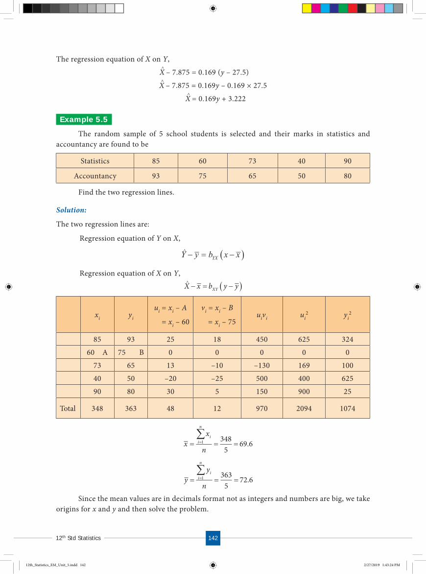
14212t h S t d S t a t i s t i c s
The regression equation of X on Y,
X^ – 7.875 = 0.169 (y – 27.5)
X^ – 7.875 = 0.169y – 0.169 × 27.5
X^ = 0.169y + 3.222
Ex ample 5 .5The random sample of 5 school students is selected and their marks in statistics and
accountancy are found to be
Statistics 85 60 73 40 90
Accountancy 93 75 65 50 80
Find the two regression lines.
Solution:
The two regression lines are:
Regression equation of Y on X,
Y y b x xYX^ � � �� �
Regression equation of X on Y,
X x b y yXY^ � � �� �
xi yi
ui = xi – A
= xi – 60
vi = xi – B
= xi – 75uivi ui
2 yi2
85 93 25 18 450 625 324
60 A 75 B 0 0 0 0 0
73 65 13 –10 –130 169 100
40 50 –20 –25 500 400 625
90 80 30 5 150 900 25
Total 348 363 48 12 970 2094 1074
xx
n
ii
n
� � ���
1 3485
69 6.
yy
n
ii
n
� � ���
1 3635
72 6.
Since the mean values are in decimals format not as integers and numbers are big, we take origins for x and y and then solve the problem.
12th_Statistics_EM_Unit_5.indd 142 2/27/2019 1:43:24 PM

142 R e g r e s s i o n A n a l y s i s143
Regression equation of Y on X,
Y y b x xYX^ � � �� �
Calculation of bYX
b bn u v u v
n u uYX VU
i ii
n
ii
n
ii
n
ii
n
ii
n�
�
��
��
�
��
� � �
� �
� � �
� �1 1 1
2
1 1
2
�� � � �� �
5 970 48 9 12
5 2094 48 2
( )
( )
= 4850 + 57610470 – 2304
= 54268126
= 0.664
b bYX VU 0 664.
Y^
– 72.6 = 0.664 (x – 69.6)
Y^
– 72.6 = 0.64x – 46.214
Y^ = 0.664x + 26.386
Regression equation of X on Y,
X x b y yXY^ � � �� �
Calculation of bXY
b bn u v u v
n v vXY UV
i ii
n
ii
n
ii
n
ii
n
ii
n�
�
��
��
�
��
� � �
� �
� � �
� �1 1 1
2
1 1
2
�� � � �� � �
5 970 48 12
5 1074 12 2
( )
( )
���
�4850 576
5370 144
5426
5226
bUV = 1.038
X^ – 69.6 = 1.038 (y – 72.6)
X^ – 69.6 = 1.038y – 75.359
X^ = 1.038y – 5.759
12th_Statistics_EM_Unit_5.indd 143 2/27/2019 1:43:32 PM

14412t h S t d S t a t i s t i c s
Ex ample 5 .6Is there any mistake in the data provided about the two regression lines
Y = −1.5 X + 7, and X = 0.6 Y + 9? Give reasons.
Solution:
The regression coefficient of Y on X is bYX = –1.5The regression coefficient of X on Y is bXY = 0.6
Both the regression coefficients are of different sign, which is a contrary. So the given equations cannot be regression lines.
Ex ample: 5 .7
mean S.D
Yield of wheat (kg. unit area) 10 8
Annual Rainfall (inches) 8 2
Correlation coefficient: 0.5
Estimate the yield when rainfall is 9 inches
Solution:
Let us denote the dependent variable yield by Y and the independent variable rainfall by X.
Regression equation of Y on X is given by
Y – y = ( )ˆ( )X Y
SD Yb rSD X
(x – x)
x = 8, SD(X) = 2, y = 10, SD(Y) = 8, rXY = 0.5
Y X� � � �� �10 0 58
28. (x – 8)
= 2 (x – 8)When x = 9,
Y – 10 = 2 (9 – 8)Y = 2 + 10
= 12 kg (per unit area)
Corresponding to the annual rain fall 9 inches the expected yield is 12 kg ( per unit area).
Ex ample 5 .8For 50 students of a class the regression equation of marks in Statistics (X) on marks in
Accountancy (Y) is 3Y – 5X + 180 = 0. The mean marks in of Accountancy is 50 and variance of marks in statistics is 16
25 of the variance of marks in Accountancy.
12th_Statistics_EM_Unit_5.indd 144 2/27/2019 1:43:34 PM

144 R e g r e s s i o n A n a l y s i s145
n = 50, Regression equation of X on Y as 3Y – 5X + 180 = 0
y 50 , V X V Y( ) ( )1625
, and V(Y) = 25.
We have to find (i) x and (ii) rXY
(i) Calculation for x
Since (x, y) is the point of intersection of the two regression lines, they lie on the regression line 3Y – 5X + 180 = 0Hence, 3 5 180 0
3 50 5 180 0y x
x� � �� � �( )
� � � �� �
5 180 150
330
x
x
x
���
�
�
330
566
66
(ii) Cal culation for coefficient of correlation.
3 5 180 0
5 180 3
36 0 6
0 6
Y XX Y
X YbXY
� � �� � � �� ��
.
.
Also bXY = r SD XSD YXY
( )( )
0.6 = r SD XSD YXY
( )( )
rXY = 0 6. ( )( )
×SD YSD X
r2XY = 0.36 ×
V YV X
( )( )
(1)
Given that:V(Y) = 25
V X V Y( ) ( )1625
= 16
2525×
V(X) = 16
12th_Statistics_EM_Unit_5.indd 145 2/27/2019 1:43:43 PM
Find the mean marks in statistics and the coefficient of correlation between marks in the two subjects when the variance of Y is 25.
Solution:
We are given that:

14612t h S t d S t a t i s t i c s
Substituting in (1) we have
rXY ��0 36 25
16.
= 0.75
Ex ample 5 .9If two regression coefficients are bYX
5
6and bXY
9
20, what would be the value of rXY?
Solution:
The correlation coefficient r b bXY YX XY� � � � � �
� � �56
920
= 0.375
Since both the signs in bYX and bXY are positive, correlation coefficient between X and Y is positive.
Ex ample 5 .10
Given that bYX � �18
7 and bXY � �5
6. Find r?
Solution:
r b bXY YX XY� � � � � �
� � ��18
7
5
6
15
7 = –0.553.
Since both the signs in bYX and bXY are negative, correlation coefficient between X and Y is negative.
rXY2 0 36 25
16�
�.
The sign of the corelation coefficient will be the signs of the regression coefficients.
NOTE
12th_Statistics_EM_Unit_5.indd 146 2/27/2019 1:43:55 PM

146 R e g r e s s i o n A n a l y s i s147
5 .6 DIFFERENCE BETWEEN CORRELATION AND REGRESSION
Correlation Regression
1. It indicates only the nature and extent oflinear relationship
It is the study about the impact of the independent variable on the dependent variable. It is used for predictions.
2. If the linear correlation is coe�cient ispositive / negative , then the two variablesare positively / or negatively correlated
The regression coefficient is positive, then for every unit increase in x, the corresponding average increase in y is bYX. Similarly, if the regression coefficient is negative , then for every unit increase in x, the corresponding average decrease in y is bYX.
3. One of the variables can be taken as x andthe other one can be taken as the variable y.
Care must be taken for the choice of independent variable and dependent variable. We can not assign arbitrarily x as independent variable and y as dependent variable.
4. It is symmetric in x and y,ie., rXY=rYX
It is not symmetric in x and y, that is, bXY and bYX have di�erent meaning and interpretations.
POINTS TO REMEMBER
� There are several types of regression - Simple linear correlation , multiple linearcorrelation and non-linear correlation.
� In simple linear regression there are two linear regression lines Y on X and X on Y.
� In the linear regression line Y = a + bX + e , where ‘X’ is independent variable, ‘Y’ isdependent variable, a’ is intercept, ‘b’ is slope of the line and ‘ e’ is error term.
� The point ( , )X Y passes through the regression lines.
� The “ Method of least squares” gives the line of best fit.
� Both the regression lines have the same sign either positive of negative.
� The sign of the regression coefficient and the sign of the correlation coefficient issame.
12th_Statistics_EM_Unit_5.indd 147 2/27/2019 1:43:57 PM

14812t h S t d S t a t i s t i c s
EXERCISE 5
I. Choose the best answer.
1. ______ is widely used for prediction
a) regression analysis b) correlation analysis
c) analysis of variance d) analysis of covariance
2. The linear regression analysis can be classified in to
a) 4 types b) 3 types c) 2 types d) none of the above
3. The linear equation Y = a + bx is called as regression equation of
a) X on Y b) Y on X c) between X and Y d) ‘a’ on ‘b’
4. In regression equation X = a + by + e is
a) correlation coefficient of Y on X b) correlation coefficient of X on Y
c) regression coefficient of Y on X d) regression coefficient of X on Y
5. bYX =
a) r SD XSD YXY
( )( )
b) r SD YSD XXY
( )( )
c) SD XSD Y
( )( )
d) SD YSD X
( )( )
6. If bXY > 1 then bYX is
a) 1 b) 0 c) > 1 d) < 1
7. In the Regression equation Y y r SD YSD X
x xXY^ ( )
( )� � �� � , r SD Y
SD XXY( )( )
is
a) bYX b) bXY c) rXY d) cov(X,Y)
8. Using the regression coefficients we can calculate
a) cov(X, Y) b) SD(X)
c) correlation coefficient d) coefficient of variance
9. Arithmetic mean of the regression coefficients bXY and bYX is
a) > rXY b) ≥ rXY c) ≤ rXY d) < rXY
10. Regression analysis helps in establishing a functional relationship between ______ variables.
a) 2 or more variables b) 2 variables
c) 3 variables d) none of these
11. _____ is the Father of mental tests
a) R.A. Fisher b) Croxton and Cowden
c) Francis Galton d) A.L. Bowley
12th_Statistics_EM_Unit_5.indd 148 2/27/2019 1:43:58 PM
148 R e g r e s s i o n A n a l y s i s149
12. Correlation coefficient is the _______ between the regression coefficients
a) arithmetic mean b) geometric mean
c) harmonic mean d) none of the above
13. If the two lines of regression are perpendicular to each other then rXY =
a) 0 b) 1 c) –1 d) 0.5
14. If the two regression lines are parallel then
a) rXY = 0 b) rXY = +1 c) rXY = –1 d) rXY = ± 1
15. Angle between the two regression lines is
a) tan� ��
�
��
�
��
1 1 2
1 21
m mm m
b) tan�
�
�
���
�
���
1 1 2
1 21m m
m m
c) tan� ��
�
��
�
��
1 1 2
1 21
m mm m
d) none of the above
16. bXY =
a) r SD YSD XXY
( )( )
b) r SD XSD YXY
( )( )
c) rXY SD(X) SD(Y) d)
1bYX
17. Regression equation of X on Y is
a) Y = a + bYXx + e b) Y = bXYx + a + e
c) X = a + bXYy + e d) X = bYXy + a + e
18. For the regression equation 2Y^ = 0.605x + 351.58. �e regression coe�cient of Y on X is
a) bXY = 0.3025 b) bXY = 0.605
c) bYX = 175.79 d) bYX = 351.58
19. If bXY = 0.7 and ‘a’ = 8 then the regression equation of X on Y is
a) Y = 8 + 0.7 X b) X = 8 + 0.7 Y
c) Y = 0.7 + 8 X d) X = 0.7 + 8 Y
20. The regression lines intersect at
a) (X, Y) b) (X, Y) c) (0, 0) d) (1, 1)
12th_Statistics_EM_Unit_5.indd 149 2/27/2019 1:44:02 PM

15012t h S t d S t a t i s t i c s
II. Give very short answer to the following questions.
21. Define regression.
22. What are the types of regression?
23. Write the two simple linear regression equations.
24. Write the two simple linear regression coefficients.
25. If the regression coefficient of X on Y is 16 and the regression coefficient of Y on X is 4, thenfind the correlation coefficient.
26. Find the standard deviation of Y given that V(X) is 36, bXY = 0.8, rXY = 0.5.
III. Give short answer to the following questions.
27. Define simple linear and multiple linear regressions
28. Distinguish between linear and non-linear regression.
29. Write the regression equation of X on Y and its normal equations.
30. Write the regression equation of Y on X and its normal equations.
31. Write any three properties of regression.
32. Write any three uses of regression.
33. Write any three differences between correlation and regression.
34. If the regression equations are X^ = 64 – 0.95y, Y^ = 7.25 – 0.95x then find the correlation
coefficient.
35. Given the following lines of regression.
8X – 10Y + 66 = 0 and 40X – 18Y = 214. Find the mean values of X and Y.
36. Given x = 90, y = 70, bXY = 1.36, bYX = 0.61 when y = 50, Find the most probable value of X.
37. Compute the two regression equations from the following data.
x 1 2 3 4 5y 3 4 5 6 7
If x = 3.5 what will be the value of Y^?
IV Give detailed answer to the following questions.
38. Write in detail the properties of regression.
39. Explain in detail the uses of regression analysis.
40. Distinguish between correlation and regression.
41. Interpret the result for the given information. A simple regression line is fitted for a data setand its intercept and slope respectively are 2 and 3. Construct the linear regression of theform Y = a + bx and offer your interpretation for ‘a’ and ‘b’. If X is increased from 1 to 2, whatis the increase in Y value. Further if X is increased from 2 to 5 what would be the increasein Y. Demonstrate your answer mathematically.
12th_Statistics_EM_Unit_5.indd 150 2/27/2019 1:44:02 PM

150 R e g r e s s i o n A n a l y s i s151
42. Using the method of least square, calculate the regression equation of X on Y and Y on X fromthe following data and estimate X where Y is 16.
x 10 12 13 17 18y 5 6 7 9 13
Also determine the value of correlation coefficient.
43. The following table shows the age (X) and systolic blood pressure (Y) of 8 persons.
Age (X) 56 42 60 50 54 49 39 45
Blood pressure (Y) 160 130 125 135 145 115 140 120
Fit a simple linear regression model, Y on X and estimate the blood pressure of a person of 60 years.
44. Find the regression equation of X on Y given that n = 5, ∑x = 30, ∑y = 40, ∑xy = 214, ∑x2 = 220,∑y2 = 340.
45. Given the following data, estimate the marks in statistics obtained by a student who hasscored 60 marks in English.
Mean of marks in Statistics = 80, Mean of marks in English = 50, S.D of marks in Statistics =15, S.D of marks in English = 10 and Coefficient of correlation = 0.4.
46. Find the linear regression equation of percentage worms (Y) on size of the crop (X) based onthe following seven observations.
Size of the crop (X) 16 15 11 27 39 22 20
Percentage worms (Y) 24 25 34 40 35 20 23
47. In a correlation analysis, between production (X) and price of a commodity (Y) we get thefollowing details.Variance of X = 36.The regression equations are:12X – 15Y + 99 = 0 and 60 X – 27 Y =321Calculate (a) The average value of X and Y.
(b) Coefficient of correlation between X and Y.
12th_Statistics_EM_Unit_5.indd 151 2/27/2019 1:44:02 PM
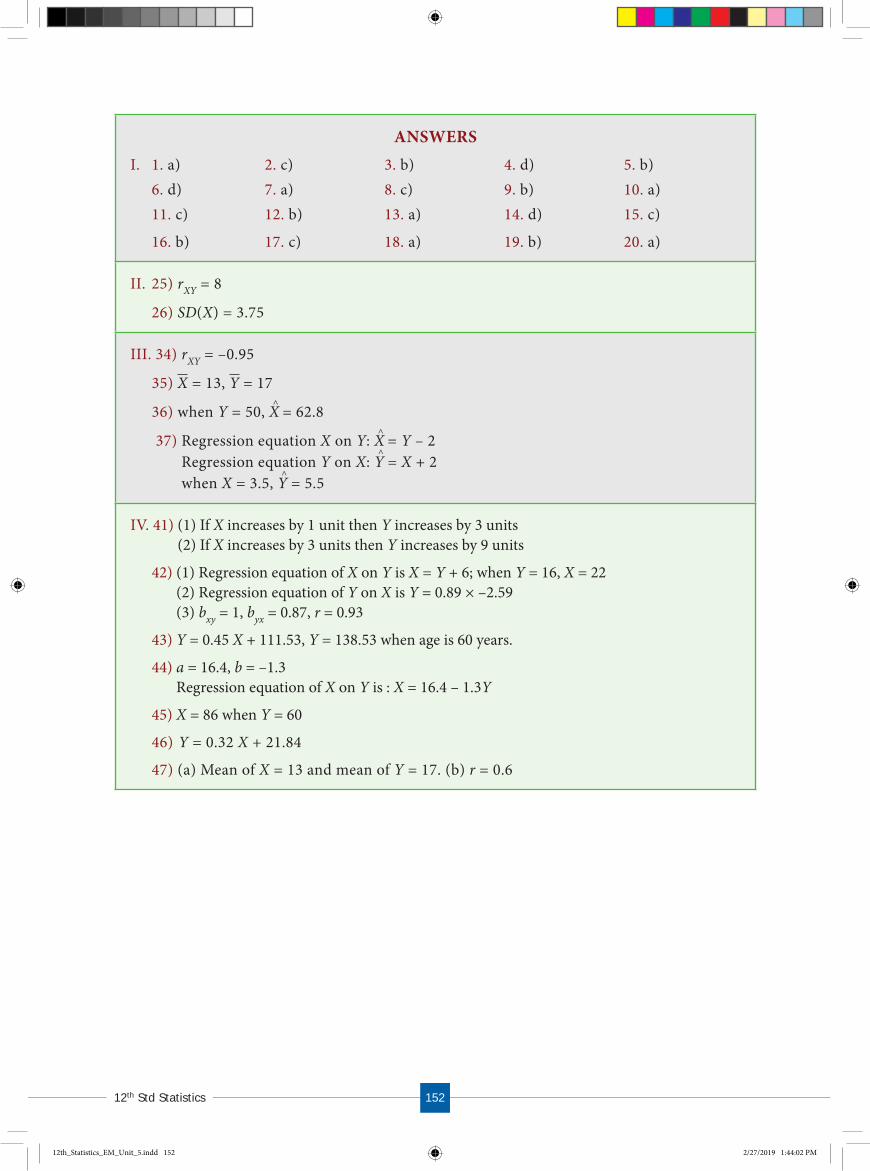
15212t h S t d S t a t i s t i c s
ANSWERSI. 1. a) 2. c) 3. b) 4. d) 5. b)
6. d) 7. a) 8. c) 9. b) 10. a)11. c) 12. b) 13. a) 14. d) 15. c)
16. b) 17. c) 18. a) 19. b) 20. a)
II. 25) rXY = 8
26) SD(X) = 3.75
III. 34) rXY = –0.95
35) X = 13, Y = 17
36) when Y = 50, X^ = 62.8
37) Regression equation X on Y: X^ = Y – 2Regression equation Y on X: Y
^ = X + 2
when X = 3.5, Y^ = 5.5
IV. 41) (1) If X increases by 1 unit then Y increases by 3 units(2) If X increases by 3 units then Y increases by 9 units
42) (1) Regression equation of X on Y is X = Y + 6; when Y = 16, X = 22(2) Regression equation of Y on X is Y = 0.89 × –2.59(3) bxy = 1, byx = 0.87, r = 0.93
43) Y = 0.45 X + 111.53, Y = 138.53 when age is 60 years.
44) a = 16.4, b = –1.3Regression equation of X on Y is : X = 16.4 – 1.3Y
45) X = 86 when Y = 60
46) Y = 0.32 X + 21.84
47) (a) Mean of X = 13 and mean of Y = 17. (b) r = 0.6
12th_Statistics_EM_Unit_5.indd 152 2/27/2019 1:44:02 PM

I n d e x N u m b e r153
� e students will able to� understand the concept and purpose of Index Numbers.� calculate the indices to measure price and quantity changes over period of
time.� understand di� erent tests an ideal Index Number satis� es.� understand consumer price Index Numbers.� understand the limitations of the construction of Index Numbers.
LEARNING OBJECTIVES
Introduction Index number is a technique of measuring changes in a variable or a group of variables
with respect to time, location or other characteristics. It is one of the most widely used statistical methods. Index number is a specialized average designed to measure the change in a group of related variables over a period of time. For example, the price of cotton in 2010 is studied with reference to its price in 2000. It is used to feel the pulse of the economy and it reveals the inflationary or deflationary tendencies. In reality, it is viewed as barometers of economic activity because if one wants to have an idea as to what is happening in an economy, he should check the important indicators like the index number of agricultural production, index number of industrial production, and the index number business activity etc., There are several types of index numbers and the students will learn them in this chapter.
Irving Fisher (1867–1947) was an American Statistician born in New York and his father was a teacher. As a child, he had remarkable mathematical ability and a flair for invention. In 1891, Fisher received the first Ph.D in economics from Yale University. Fisher had shown particular talent and inclination for mathematics, but he found that economics offered greater scope for his ambition and social concerns. He made important contributions to economics including index numbers. He edited the Yale Review from 1896 to 1910 and was active in many learned societies, institutes, and welfare organizations. He was a president of the American Economic Association. He died in New York City in 1947, at the age of 80.
Irving Fisher (1867–1947)and his father was a teacher. As a child, he had remarkable mathematical ability and a flair for invention. In 1891, Fisher received the first Ph.D in economics from Yale University. Fisher had shown particular talent and inclination for mathematics, but he found that economics offered greater scope for his ambition and social concerns. He made important contributions to economics including index numbers. He edited the Irving Fisher
INDEX NUMBERSCHAPTER
6
12th_Statistics_EM_Unit_6.indd 153 2/27/2019 1:44:48 PM

15412t h S t d S t a t i s t i c s
6
12th_Statistics_EM_Unit_6.indd 154 2/27/2019 1:44:48 PM
.1 DEFINITION AND USES OF INDEX NUMBERS
. . e nitionAn Index Number is defined as a relative measure to compare and describe the average
change in price, quantity value of an item or a group of related items with respect to time, geographic location or other characteristics accordingly.
In the words of Maslow “An index number is a numerical value characterizing the change in complex economic phenomenon over a period of time or space”
Spiegal defines, “An index number is a statistical measure designed to show changes in a variable on a group of related variables with respect to time, geographical location or other characteristics”.
According to Croxton and Cowden “Index numbers are devices for measuring differences in the magnitude of a group of related variables”.
Bowley describes “Index Numbers as a series which reflects in its trend and fluctuations the movements of some quantity”.
6 .1.2 UsesThe various uses of index numbers are:
Economic Parameters
The Index Numbers are one of the most useful devices to know the pulse of the economy. It is used as an indicator of inflanationary or deflanationary tendencies.
Measures Trends
Index numbers are widely used for measuring relative changes over successive periods of time. This enable us to determine the general tendency. For example, changes in levels of prices, population, production etc. over a period of time are analysed.
Useful for comparsion
The index numbers are given in percentages. So it is useful for comparison and easy to understand the changes between two points of time.
Help in framing suitable policies
Index numbers are more useful to frame economic and business policies. For example, consumer price index numbers are useful in fixing dearness allowance to the employees.
Useful in de�ating
Price index numbers are used for connecting the original data for changes in prices. The price index are used to determine the purchasing power of monetary unit.

I n d e x N u m b e r155
6 .2 TY PES OF INDEX NUMBERS
(i) Price Index NumbersPrice index is a ‘Special type’ of average which studies net relative change in the prices ofcommodities, expressed in di�erent units. Here comparison is made in respect of prices.Price index numbers are wholesale price index numbers and retail price index numbers.
(i) Quantity Index NumbersThis number measures changes in volume of goods produced, purchased or consumed.Here, the comparison is made in respect of quantity or volume. For example, thevolume of agricultural goods produced, consumed, import, export etc.
(ii) Value IndexValue index numbers study the changes in the total value of a certain period with thetotal value of the base period. For example, the indices of stock-in-made, purchase,sales profit etc., are analysed here.
NOTE
The points and precautions that should be taken in the constructing index numbers are:
• determination of the purpose• selection of the base period• selection of commodities• selection of price quotations• selection of appropriate weight• selection of an appropriate average• selection of an appropriate formula
12th_Statistics_EM_Unit_6.indd 155 2/27/2019 1:44:48 PM
Compares standard of living
Cost of living index of different periods and of different places will help us to compare the standard of living of the people. Th s enables the government to take suitable welfare measures.
Special type of average
All the basic ideas of averages are employed for the construction of index numbers. In averages, the data are homogeneous (in the same units) but in index number, we average the variables which have different units of measurements. Hence, it is a special type of average.

15612t h S t d S t a t i s t i c s
6 .3 METHODS OF CONSTRUCTING INDEX NUMBERS
Different types of index number (price/quantity/value) can be classified as follows.
6 .3.1 Unw eig h ted Index Numb ersAn unweighted price Index Number measures the percentage change in price of a single
item or a group of items between two periods of time. In unweighted index numbers, all the values taken for study are of equal importance. There are two methods in this category.
(i) Simple aggregative method:
Under this method the prices of di�erent items of current year are added and the total isdivided by the sum of prices of the base year items and multiplied by 100.
Ppp01
1
0
100� ���
p1 = Current year prices for various commodities p0 = Base year prices for various commoditiesP01 = Price Index number
Limitations of the simple aggregative method
(i) Relative importance of the commoditiesis not taken into account.
(ii) Highly priced items influence the index number
Ex ample 6 .1Construct the Price Index Number for the year 1997, from the following information
taking 1996 as base year.
Commodities Price in 1996 (`) Price in 1997 (`)Rice 130 115
Wheat 80 65Sugar 75 70Ragi 95 90Oil 105 105Dal 35 20
Methods of constructing Index Numbers
Simple Aggregative
Simple average of price relatives
Weighted Aggregative
Weighted Average of price relatives
Unweighted Weighted
The base period is the period against which comparison is made. Generally a year is taken as base period. The base period should be free from economic and natural disturbances.
NOTE
12th_Statistics_EM_Unit_6.indd 156 2/27/2019 1:44:51 PM

I n d e x N u m b e r157
Solution:
Construction of Price Index:
Commodities Price in 1996 (`) (p0) Price in 1997 (`) (p1)
Rice 130 115Wheat 80 65Sugar 75 70Ragi 95 90Oil 105 105Dal 35 20
p0 = 520 p1 = 465
Ppp01
1
0
100� ���
� � �465
520100 89 42.
Price Index in 1997, when compared to 1996 has fallen by 10.58%
Ex ample 6 .2Calculate Price Index Number for 2016 from the following data by simple aggregate
method, taking 2016 as base year.
CommoditiesPrice per kg
2015 2016Apple 100 140Orange 30 40Pomegranate 120 130Guava 40 50
Solution:
Commodities 2015 (p0) 2016 (p1)
Apple 100 140Orange 30 40Pomegranate 120 130Guava 40 50Total 290 360
Price index: P01 = 1
0100
pp
×
360 100290
×
12th_Statistics_EM_Unit_6.indd 157 2/27/2019 1:44:51 PM

15812t h S t d S t a t i s t i c s
360029
P01 = 124.13%
Price index for the year 2016 when compared to 2015 has been increased by 24.13%.
2. Simple average of price relative method
Under this method, first of all price relatives are obtained for the various items and then average of these relatives is obtained by using either arithmetic mean or geometric mean. Price relative is the price of the current year expressed as the percentage of the price of the base year. The formula for computing Index Number under this method on using Arithmetic mean and Geometric mean are given below.
If N is the member of items, p1 is the price of the commodity with current year and p0 is the price of the commodity in the base year then, the average Price Index Number is
(i) P
ppN01
1
0
100�
�� (using Arithmetic mean)
(ii) P01 = antilog log pp
N
1
0
100��
��
�
��� (using Geometric mean)
Advantages of Average Price Index1. It is not influenced by the extreme prices of items as equal importance is given to all items.
2. Price relatives are pure numbers; therefore the value of the average price relative index isnot affected by the units of measurement of commodities included in the calculation ofindex numbers.
Limitations 1. Equal weights are assigned to every commodity included in the index. Each price relatives
is given equal importance, but in actual practice, it is not true.2. Arithmetic mean is very often used to calculate the average price relatives, but it has a few
disadvantages. The use of geometric mean is difficult to calculate.
Ex ample 6 .3Compute price index number by simple average of price relatives method using arithmetic
mean and geometric mean.
Item Price in 2001 (`) Price in 2002 (`)
A 6 10B 2 2C 4 6D 10 12E 8 12
12th_Statistics_EM_Unit_6.indd 158 2/27/2019 1:44:52 PM

I n d e x N u m b e r159
Solution:
Calculation of price index number by simple average of price relatives:
ItemPrice in 2001
(`) p0
Price in 2002(`) p1
log p
A 6 10 166.7 2.2201B 2 2 100.0 2.0000C 4 6 150.0 2.1761D 10 12 120.0 2.0792E 8 12 150.0 2.1761
p = 686.7 logp = 10.6515
(i) Price relative index number based on arithmetic mean:
P
ppN01
1
0
100�
��=
pN
= 686 75
137 34. .
(ii) Price relative index number based on geometric mean:
P01 = antilog log pN
�����
�
���
= antilog 10 6515
5
.���
���
= antilog (2.13303)= 134.9
Hence, the price index number based on arithmetic mean and geometric mean for the year 2002 are 137.34 and 134.9 respectively.
Ex ample 6 .4Construct simple average price relative index number using arithmetic mean for the year 2012
for the following data showing the pro�t from various categories sold out in departmental stores.
Pro�t (per week) 2010 2012Groceries 150600 170800Cosmetics 70000 82000Stationery items 12000 10800Utensils 20000 18600
Solution: Index number uning Arithmertic Mean of price relatives
Pro�t in 2010 (p0) Pro�t in 2012 (p1) p1/p0 x 100
Groceries 150600 170800 170800 100 11341150600
×
Cosmetics 70000 82000 82000 100 117.1470000
×
Stationery items 12000 10800 10800 100 90.0012000
×
Utensils 20000 18600 18600 100 93.0020000
×
Total 413.55
p = pp
1
0
100×
12th_Statistics_EM_Unit_6.indd 159 2/27/2019 1:44:54 PM
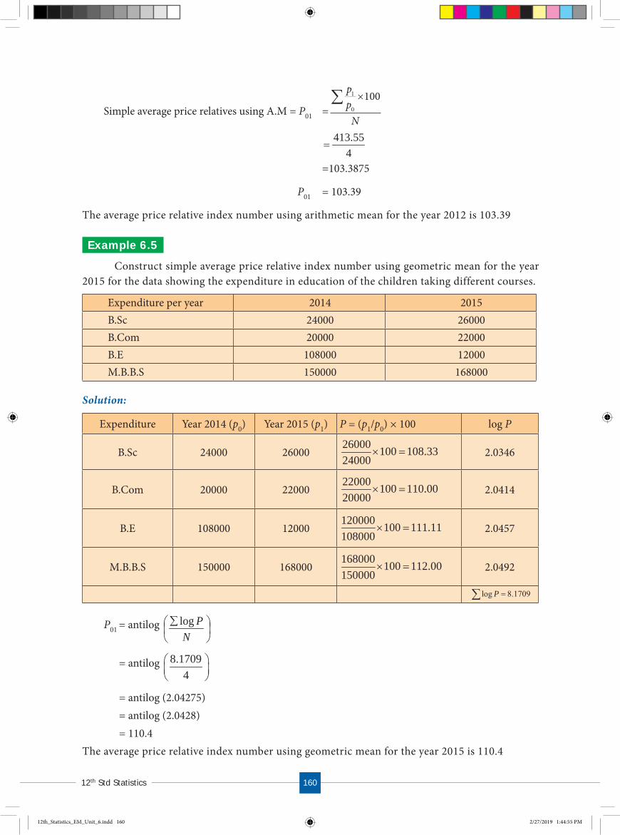
16012t h S t d S t a t i s t i c s
Simple average price relatives using A.M = P01 =
pp
N
1
0
100��
413.554
=103.3875
P01 = 103.39
The average price relative index number using arithmetic mean for the year 2012 is 103.39
Ex ample 6 .5Construct simple average price relative index number using geometric mean for the year
2015 for the data showing the expenditure in education of the children taking different courses.
Expenditure per year 2014 2015B.Sc 24000 26000B.Com 20000 22000B.E 108000 12000M.B.B.S 150000 168000
Solution:
Expenditure Year 2014 (p0) Year 2015 (p1) P = (p1/p0) × 100 log P
B.Sc 24000 2600026000 100 108.3324000
× 2.0346
B.Com 20000 2200022000 100 110.0020000
× 2.0414
B.E 108000 12000120000 100 111.11108000
× 2.0457
M.B.B.S 150000 168000168000 100 112.00150000
× 2.0492
P01 = antilog N
Plog
= antilog 8.17094
= antilog (2.04275) = antilog (2.0428)
= 110.4The average price relative index number using geometric mean for the year 2015 is 110.4
log .P �� 8 1709
12th_Statistics_EM_Unit_6.indd 160 2/27/2019 1:44:55 PM

I n d e x N u m b e r161
6 .4 WEIGHTED INDEX NUMBERS
In computing weighted Index Numbers, the weights are assigned to the items to bring out their economic importance. Generally quanties consumed or value are used as weights.
Weighted index numbers are also of two types
(i) Weighted aggregative
(ii) Weighted average of price relatives
6 .4.1 Weig h ted ag g reg ate Index Numb ersIn this method price of each commodity is weighted by the quantity sale either in the base
year or in the current year. There are various methods of assigning weights and thus there are many methods of constructing index numbers. Some of the important formulae used under this methods are
a) Laspeyre’s Index (P01L)
b) Paasche’s Index (P01P)
c) Dorbish and Bowley’s Index (P01DB)
d) Fisher’s Ideal Index (P01F)
e) Marshall-Edgeworth Index (P01Em)
f) Kelly’s Index (P01K)
a. Laspeyre’s method
The base period quantities are taken as weights. The Index is
Pp qp q
L01
1 0
0 0
100� ���
b. Paasche’s method
The current year quantities are taken as a weight. In this method, we use continuously revised weights and thus this method is not frequently used when the number of commodities is large. The Index is
Pp qp q
P01
1 1
0 1
100� ���
c. Dorbish and Bowley’s method
In order in take into account the impact of both the base and current year, we make use of simple arithmetic mean of Laspeyre’s and Paasche’s formula
The Index is
PP PDB
L P
0101 01
2�
�
12th_Statistics_EM_Unit_6.indd 161 2/27/2019 1:44:56 PM

16212t h S t d S t a t i s t i c s
1002
10
11
00
01
01 ×qpqp
qpqp
P
d. Fisher’s Ideal Index
It is the geometric mean of Laspeyre’s Index and Paasche’s Index, given by:
P P P
p qp q
p qp q
F L L01 01 01
1 0
0 0
1 1
0 1
100
� �
� � ���
��
e. Marshall-Edgeworth method
In this method also both the current year as well as base year prices and quantities are considered.
The Index is
Pp q qp q qp q p qp q p q
ME01
1 0 1
0 0 1
1 0 1 1
0 0 0 1
100
100
��� ��� �
�
���
�
��� �� �
f. Kelly’s method
The Kelly’s Index is
Pp qp q
qq qK
011
0
0 11002
� � ���
�,
where q refers to quantity of some period, not necessarily of the mean of the base year and current year. It is also possible to use average quantity of two or more years as weights. This method is known as fixed weight aggregative index.
Ex ample 6 .6Construct weighted aggregate index numbers of price from the following data by applying
1. Laspeyre’s method
2. Paasche’s method
3. Dorbish and Bowley’s method
4. Fisher’s ideal method
5. Marshall-Edgeworth method
P
12th_Statistics_EM_Unit_6.indd 162 2/27/2019 1:44:57 PM

I n d e x N u m b e r163
Commodity2016 2017
Price Quantity Price QuantityA 2 8 4 6B 5 10 6 5C 4 14 5 10D 2 19 2 13
Solution:
Calculation of various indices
Commodity
2016 2017
p1q0 p0q0 p1q1 p0q1Pricep0
Quantityq0
Pricep1
Quantityq1
A 2 8 4 6 32 16 24 12
B 5 10 6 5 60 50 30 25
C 4 14 5 10 70 56 50 40
D 2 19 2 13 38 38 26 26
(1) Laspeyre’s Index:
Pp qp q
L01
1 0
0 0
100� ���
125100160200
×
(2) Paasche’s Index
Pp qp q
P01
1 1
0 1
100� ���
21.126100103130
× 126.21
(3) Dorbish and Bowley’s Index
PP PDB
L P
0101 01
2125 126 21
2�
��
� .
= 125.6
20001qp 16000qp 13011qp 10310qp
12th_Statistics_EM_Unit_6.indd 163 2/27/2019 1:44:58 PM

16412t h S t d S t a t i s t i c s
(4) Fisher’s Ideal Index
Pp qp q
p qp q
F01
1 0
0 0
1 1
0 1
100� � ���
��
100103130
160200
××
1002561.1100578.1 ××
= 125.61
(5) Marshall-Edgeworth method
Pp q p qp q p q
ME01
1 0 1 1
0 0 0 1
100���
�� �� �
100263330100
103160130200
××
= 125.48
Ex ample 6 .7Calculate the price indices from the following data by applying (1) Laspeyre’s method
(2) Paasche’s method and (3) Fisher ideal number by taking 2010 as the base year.
Commodity2010 2011
Prices Quantities Prices Quantities
A 20 10 25 13
B 50 8 60 7
C 35 7 40 6
D 25 5 35 4
Solution: Calculations
p0 q0 p1 q1 p0 q0 p0 q1 p1 q0 p1 q1
20 10 25 13 200 260 250 325
50 8 60 7 400 350 480 420
35 7 40 6 245 210 280 240
25 5 35 4 125 100 175 140
970 920 1185 1125
12th_Statistics_EM_Unit_6.indd 164 2/27/2019 1:44:58 PM

I n d e x N u m b e r165
(1) Laspeyre’s Index
= 122.16
(2) ) Paasche’s Index
= 122.28
(3) Fisher’s Ideal Index
Pp qp q
p qp q
F01
1 0
0 0
1 1
0 1
100� � ���
��
= 1185
970
1125
920100× ×
� � �1 2216 1 2228 100. .
= 1 49377 100. ×
= 1.2055 100×
= 120.55
Ex ample 6 .8Calculate the Dorbish and Bowley’s price index number for the following data taking 2014
as base year.
Items2014 2015
Prices (per kg)Quantities
(purchased)Prices (per kg)
Quantities (purchased)
Oil 80 3 100 4Pulses 35 2 45 3Sugar 25 2 30 3Rice 50 30 54 35
Cereals 35 2 40 3
Pp qp q
L01
1 0
0 0
100� ���
� �1185
970100
Pp qp q
p01
1 1
0 1
100� ���
� �11254
920100
12th_Statistics_EM_Unit_6.indd 165 2/27/2019 1:45:09 PM

16612t h S t d S t a t i s t i c s
Solution: Price Index by Dorbish and Bowley’s Method
p0 q0 p1 q1 p0 q0 p0 q1 p1 q0 p1 q1
80 3 100 4 240 320 300 40035 2 45 3 70 105 90 13525 2 30 3 50 75 60 9050 30 54 35 1500 1750 1620 189035 2 40 3 70 105 80 120
1930 2355 2150 2635
P
p qp q
p qp qDB
01
1 0
0 0
1 1
0 1
2100�
��
��
��
� ����
����
1
2
2150
1930
2635
2355100
� � ��1
21 1139 1 1188 100. .
� ��1
22 2327 100.
= 1.1164 x 100 = 111.64
Ex ample 6 .9Compute Marshall – Edgeworth price index number for the following data by taking 2016
as base year.
Items sold out in a men’s wear
2016 2017Prices Quantity Prices Quantity
Shirts 700 150 900 175Pants 1000 100 1200 150
Sandals 500 70 600 100Shoes’ 1500 50 1800 60Belts 400 100 600 150
Watches 1200 300 1500 250
Solution: Price Index by Marshall-Edgeworth Method
p0 q0 p1 q1 p0 q0 p0 q1 p1 q0 p1 q1
700 150 900 175 105000 122500 135000 1565001000 100 1200 150 100000 150000 120000 180000500 70 600 100 35000 50000 42000 60000
1500 50 1800 60 75000 90000 120000 108000400 100 600 150 40000 60000 60000 90000
1200 300 1500 250 36000 300000 450000 375000391000 772500 927000 969500
12th_Statistics_EM_Unit_6.indd 166 2/27/2019 1:45:13 PM

I n d e x N u m b e r167
Marshall – Edgeworth Index:
Pp q p qp q p q
ME01
1 0 1 1
0 0 0 1
100���
�� �� �
���
�969500 927000
772500 391000100
� �1896500
1163500100
=162.99
Ex ample 6 .10Calculate a suitable price index form the following data.
Commodity Quantity Price 2007 2010
X 25 3 4Y 12 5 7Z 10 6 5
Solution:
In this problem, the quantities for both current year and base year are same. Hence, we can conlude Kelly’s Index price number.
Commodity q p0 p1 p0q p1qX 25 3 4 75 100Y 12 5 7 60 84Z 10 6 5 60 50
195 234
Kelly’s price Index number:
Pp qp q
K01
1
0
100� ���
01234 100195
kP ×
= 120
6 .4.2 Weig h ted av erag e of price relativ esThe weighted average of price relatives can be computed by introducing weights into the
unweighted price relatives. Here also, we may use either arithmetic mean or the geometric mean for the purpose of averaging weighted price relatives.
The weighted average price relatives using arithmetic mean:
If ppp
� �0
0
10010 0
001
0 0
100p p qp
Pp q
× × is the price relative index and w = p0q0 is attached to the commodity, then
the weighed price relative index is
12th_Statistics_EM_Unit_6.indd 167 2/27/2019 1:45:16 PM

16812t h S t d S t a t i s t i c s
10 0
001
0 0
100p p qp
Pp q
× ×
= Pwpw01 �
��
The weighted average price relatives using geometric mean:
Pw p
w01 ��
���
�
���
��
antiloglog
Ex ample 6 .11Compute price index for the following data by applying weighted average of price relatives
method using (i) Arithmetic mean and (ii) Geometric mean.
Item p0 q0 p1
Wheat 3.0 20 kg 4.0Flour 1.5 40 kg 1.6Milk 1.0 10 kg 1.5
Solution:
(i) Computation for the weighted average of price relatives using arithmatic mean.
Item p0 q0 p1 w p log p wp w log p
Wheat 3.0 20 4.0 60 133.3 2.1249 8000 127.494
Flour 1.5 40 1.6 60 106.7 2.0282 6400 121.692
Milk 1.0 10 1.5 10 150.0 2.1761 1500 21.761
w� �130 wp �� 15900 w plog = 270.947
Pwpw01 �
��
15,900 122.31130
This means that there has been a 22.31 % increase in prices over the base year.
(ii) Index number using geometric mean of price relatives is:
Pw p
w01 ���
Antiloglog
Antilog 270 947130
.
= Antilog (2.084) = 121.3
This means that there has been a 21.3 % increase in prices over the base year.
12th_Statistics_EM_Unit_6.indd 168 2/27/2019 1:45:18 PM

I n d e x N u m b e r169
6 .4.3 Quantity Index Numb er The quantity index number measures the changes in the level of quantities of items
consumed, or produced, or distributed during a year under study with reference to another year known as the base year.
Laspeyre’s quantity index:
1 001
0 0
100L q pQ
q p×
Paasche’s quantity index 1 1
010 1
100P q pQ
q p×
Fisher’s quantity index
Q Q QF L P01 01 01� �
� � ���
��
q pq p
q pq p
1 0
0 0
1 1
0 1
100
These formulae represent the quantity index in which quantities of the different commodities are weighted by their prices.
Ex ample 6 .12Compute the following quantity indices from the data given below:
(i) Laspeyre’s quantity index (ii) Paasche’s quantity index and (iii) Fisher’s quantity index
Commodity1970 1980
Price Total value Price Total valueA 10 80 11 110B 15 90 9 108C 8 96 17 340
Solution:
Since we are given the value and the prices, the quantity figures can be obtained by dividing the value by the price for each of the commodities.
Commodity p0 q0 p1 q1 p0q0 p1q0 p0q1 p1q1
A 10 8 11 10 80 88 100 110
B 15 6 9 12 90 54 180 108
C 8 12 17 20 96 204 160 340
Total 266 342 440 558
12th_Statistics_EM_Unit_6.indd 169 2/27/2019 1:45:21 PM
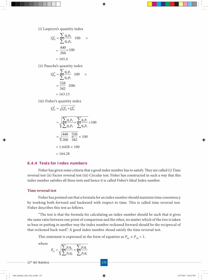
17012t h S t d S t a t i s t i c s
(i) Laspeyre’s quantity index
1 001
0 0
100L q pQ
q p×
= 440 100266
×
= 165.4
(ii) Paasche’s quantity index
1 101
0 1
100P q pQ
q p×
558 100342
×
= 163.15
(iii) Fisher’s quantity index
Q Q QF L P01 01 01� �
� � ���
��
q pq p
q pq p
1 0
0 0
1 1
0 1
100
440 558 100266 342
× × × 100
= 1.6428 × 100
= 164.28
6 .4.4 Tests for Index numb ersFisher has given some criteria that a good index number has to satisfy. �ey are called (i) Time
reversal test (ii) Factor reversal test (iii) Circular test. Fisher has constructed in such a way that this index number satis�es all these tests and hence it is called Fisher’s Ideal Index number.
Time reversal test
Fisher has pointed out that a formula for an index number should maintain time consistency by working both forward and backward with respect to time. This is called time reversal test. Fisher describes this test as follows.
“The test is that the formula for calculating an index number should be such that it gives the same ratio between one point of comparison and the other, no matter which of the two is taken as base or putting in another way the index number reckoned forward should be the reciprocal of that reckoned back ward”. A good index number shoud satisfy the time reversal test.
This statement is expressed in the form of equation as P01 × P10 = 1.
where
Pp qp q
p qp q01
1 0
0 0
1 1
0 1
� ���
��
12th_Statistics_EM_Unit_6.indd 170 2/27/2019 1:45:21 PM

I n d e x N u m b e r171
P10 ×01
00
11
1010 qp
qpqpqp
P
P01 × P10 ××××01
00
11
10
10
11
00
011001 qp
qpqpqp
qpqp
qpqp
PP
Hence, P01 × P10 1 = 1
Factor reversal test
This test is also suggested by Fisher According to the factor reversal test, the product of price index and quantity index should be equal to the corresponding value index.
In Fisher’s words “Just as each formula should permit the interchange of two times without giving inconsistent results so it ought to permit interchanging the prices and quantities without giving inconsistent results. i.e, the two results multiplied together should give the true ratio”.
This statement is expressed as follows:
1 101 01
0 0
p qP Q
p q×
Now, P01 ×10
11
00
0101 qp
qpqpqp
P
Q01 ×01
11
00
1001 qp
qpqpqp
Q
Hence, P01 × Q01 ××××01
11
00
10
10
11
00
010101 qp
qpqpqp
qpqp
qpqp
QP
××00
11
00
110101 qp
qpqpqp
QP
1 101 01
0 0
p qP Q
p q×
Circular Test
It is an extension of time reversal test. The time reversal test takes into account only two years. The current and base years. The circular test would require this property to holdgood for any two years. An index number is said to satisfy the circular test when there are three indices, P01, P12 and P20, such that P01 × P12 × P20 = 1.
Laspeyres, Paasche’s and Fisher’s ideal index numbers do not satisfy this test.
12th_Statistics_EM_Unit_6.indd 171 2/27/2019 1:45:21 PM

17212t h S t d S t a t i s t i c s
Ex ample 6 .13The table below gives the prices of base year and current year of 5 commodities with their
quantities. Use it to verify whether Fisher’s ideal index satisfies time reversal test.
Commodity Base year Current year
Unit price (`) Quantity Unit price (`) Quantity A 4 40 5 60B 5 50 10 70C 8 65 12 80D 6 20 6 90E 7 30 10 75
Solution:
Index number by Fisher’s ideal index method
Commodity p0 q0 p1 q1 p0q0 p0q1 p1q0 p1q1
A 4 40 5 60 160 240 200 300B 5 50 10 70 250 350 500 700C 8 65 12 80 520 640 780 960D 6 20 6 90 120 540 120 540E 7 30 10 75 210 525 300 750
1260 2295 1900 3250
1 0 1 101
0 0 0 1
q p q pP
q p q p×
1900 32501260 2295
×
0 1 0 010
1 1 1 0
q p q pP
q p q p×
2295 12603250 1900
×
Hence, 01 101900 3250 2295 12601260 2295 3250 1900
P P× × × ×
1 1
Fisher’s Index number satisties time reveral test.
12th_Statistics_EM_Unit_6.indd 172 2/27/2019 1:45:21 PM
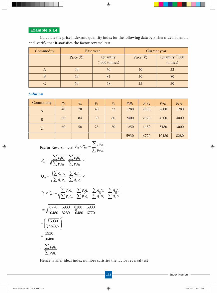
I n d e x N u m b e r173
Ex ample 6 .14Calculate the price index and quantity index for the following data by Fisher’s ideal formula
and verify that it statisfies the factor reversal test.
Commodity Base year Current yearPrice (`) Quantity
(`000 tonnes)Price (`) Quantity (`000
tonnes)
A 40 70 40 32
B 50 84 30 80
C 60 58 25 50
Solution
Commodity p0 q0 p1 q1 p1q1 p1q0 p0q0 p0 q1
A 40 70 40 32 1280 2800 2800 1280
B 50 84 30 80 2400 2520 4200 4000
C 60 58 25 50 1250 1450 3480 3000
5930 6770 10480 8280
Factor Reversal test: 1 1
01 010 0
p qP Q
p q×
1 0 1 1
010 0 0 1
p q p qP
p q p q×
1 0 1 101
0 0 0 1
q p q pQ
q p q p×
1 0 1 1 1 0 1 101 01
0 0 0 1 0 0 0 1
p q p q q p q pP Q
p q p q q p q p× × × ×
6770 5930 8280 593010480 8280 10480 6770
× × ×
25930
10480
593010480
1 1
0 0
p qp q
Hence, Fisher ideal index number satisfies the factor reversal test
12th_Statistics_EM_Unit_6.indd 173 2/27/2019 1:45:21 PM

17412t h S t d S t a t i s t i c s
6 .5 CONSUMER PRICE INDEX NUMBERS
Consumer Price Index Numbers are computed with a view of study the effect of changes in prices on the people as consumers. These indices give the average increase in the expenses if it is designed to maintain the standard of living of base year. General index numbers fail to give an indea about the effect of the change in the general price level on the cost of living of different classes of people since a given change in the price level affects different classes of people differently.
The consumer price indices are of great significance and is given below
1. This is very useful in wage negotiations, wage contracts and dearness allowanceadjustments in many countries.
2. At Government level the index numbers are used for wage policy, price policy, rentcontrol, taxation and general economic policies.
3. Change in the purchasing power of money and real income can be measured.
4. Index numbers are also used for analyzing market price for particular kind of goodsand services.
Note: Consumer price index numbers are also called as cost of living index numbers.
Methods of constructing consumer price Index
There are two methods of constructing consumer price index. They are:
1. Aggregate Expenditure method (or) Aggregate method
2. Family Budget method or method of weighted relative method.
1. Aggregate Expenditure method
This method is based upon the Laspeyre’s method. It is widely used. The quantities of commodities consumed by a particular group in the base year are the weight.
Thus, consumer price index number 1 0
0 0
100p qp q
×
2. Family budget method (or) Method of weight relatives method
This method estimates an aggregate expenditure of an average family on various items and it is weighted. It is given by
consumer price index � ��
wpw
where
p pp
� �1
0
100 for each item and w = p0q0
The family budget method is the same as “weighted average price relative method” which we have studied earlier.
12th_Statistics_EM_Unit_6.indd 174 2/27/2019 1:45:22 PM

I n d e x N u m b e r175
Ex ample 6 .15Calculate the consumer price index number for 2015 on the basis of 2000 from the
following data by using (i) the Aggregate expenditure method (ii) the family budget (or) weighted relatives method.
Commodity Quantity Price
2000 2015Wheat 20 15 20
Rice 8 20 24
Ghee 2 160 200
Sugar 4 40 40
Solution
(i) Calculation of cost of living index number on the basis of Aggregate expendituremethod.
Commodity q0 p0 p1 p0q0 p1q0
Wheat 20 15 20 300 400
Rice 8 20 24 160 192
Ghee 2 160 200 320 400
Sugar 4 40 40 160 160
Total 940 1152
Consumer price index number for 2015
P011 0
0 0
100p qp q
×
1152 100940
×
≈ 112.6
(iii) Calculation of consumer price index number according to family budget method orweighted relative method
Commodity q0 p0 p1p p
p� �1
0
100 w = p0q0 wp
Wheat 20 15 20 400/3 300 40000Rice 8 20 24 120 160 19200
Sugar 2 160 200 125 320 40000Ghee 4 40 40 100 160 16000
940 115200
Consumer price index number for 2015
12th_Statistics_EM_Unit_6.indd 175 2/27/2019 1:45:24 PM

17612t h S t d S t a t i s t i c s
P01 � ���wpw
115200
940
≈ 122.6
POINTS TO REMEMBER
� Index numbers are barometers of an Economy.
� It is a specilized average designed to measure the changes in a group of variables overtime.
� The different types of Index Numbers are Price Index Number, Quantity Index Numberand Value Index Number.
� Index numbers are classi�ed as simple aggregative and weighted aggregative.
� �e base period must be free from natural calamities.
� Laspeyeres, Paasches, Dorbish and Bowley, Fisher’s ideal and Kelly’s are weighed indexnumbers.
� Index numbers generally satis�ed three tests – Time reversal, factor reversal and circular.
� Fisher’s ideal index number satis�es both time and factor reversal tests.
� Many index numbers do not satisfy circular test.
� Cost of living index numbers is useful to the Government for policy making etc.
EXERCISE 6
I. Choose the best answer.
1) In simple aggregate method, the aggregate price of all items in the givenyear is expressed as percentage of the same in the(a) current year (b) base year(c) Quarterly (d) half yearly
2) If the index for 1990 to the base 1980 is 250, the index number for 1980 to the base 1990 is(a) 4 (b) 400 (c) 40 (d) 4000
3) If Laspeyre’s price index is 324 and Paasche’s price index is 144, then Fisher’s ideal index is(a) 234 (b) 243 (c) 261 (d) 216
4) The index that satisfies factor reversal test is(a) Paasche’s Index (b) Laspeyre’s Index(c) Fisher’s Ideal Index (d) Walsh price index
12th_Statistics_EM_Unit_6.indd 176 2/27/2019 1:45:26 PM

I n d e x N u m b e r177
5) The Dorbish-Bowley’s price index is the(a) geometric mean of Laspeyre’s and Paasche’s Price indices(b) arithmetic mean of Laspeyre’s and Paasche’s Price indices(c) weighted mean of Laspeyre’s and Paasche’s Price indices(d) weighted mean of Laspeyre’s and Paasche’s quantity indices
6) The condition for the time reversal test to hold good with usal notation is(a) 01 10 1P P× (b) 01 10 1P P (c) 01 10 1P P (d) 01 10 1P P
7) The geometric mean of Laspeyre’s and Paasche’s price indices is also known as(a) Dorbish – Bowley’s price index (b) Kelly’s price index(c) Fisher’s price index (d) Walsh price index
8) The index number for 1985 to the base 1980 is 125 and for 1980 to the base1985 is 80. Thegiven indices satisfy(a) circular test (b) factor reversal test(c) time reversal test (d) Marshall-Edgeworth test
9) The consumer price index numbers for 1981 and 1982 to the base 1974 are 320 and 400respectively. The consumer price index for 1981 to the base 1982 is(a)80 (b)128 (c)125 (d) 85
10) The consumer price index in 2000 increases by 80% as compared to the base 1990. A personI 1990 getting Rs. 60,000 per annum should now get:(a)Rs. 1,08,000 p.a. (b)Rs. 1,02,000 p.a.(c)Rs. 1,18,000 p.a. (d) Rs. 1,80,000 p.a.
II. Give very short answer to the following questions.
11. Define index number?
12. Write the uses of Index numbers.
13. Define base period.
14. State the types of Index numbers.
15. Point out the difference between weighted and unweighted index numbers.
16. Define weighted index number.
17. What is circular test?
18. State the methods of constructing consumer price index.
III. Give short answer to the following questions.
19. Give the diagrammatic representation of different types of index number.
20. Write the advantages of average price index.
21. State the methods of weighted aggregate index numbers.
22. What is the difference between the price index and quantity index numbers?
23. Write short notes on consumer price index.
12th_Statistics_EM_Unit_6.indd 177 2/27/2019 1:45:26 PM

17812t h S t d S t a t i s t i c s
24. Calculate index number from the following data by simple aggregate method taking prices of2015 as base.
Commodity UnitsPrice per kg
2015 2016Wheat Quintal 200 250Rice Quintal 300 400
Pulses Quintal 400 500Milk Litre 2 3
Clothing Meter 3 5
25. Compute (i) Laspeyre’s (ii) Paasche’s index numbers for the 2000 form the following
CommodityPrice Quantity
2002 2010 2002 2010A 4 6 8 7B 3 5 10 8C 2 4 14 12D 5 7 19 11
26. Calculate Fisher’s ideal index method for the following data.
Commodity2000 2001
Price Quantity Price QuantityA 2 7 3 5B 5 11 6 10C 3 14 5 11D 4 16 4 18
IV. Give detail answer to the following questions.
27. Calculate the simple aggregate price index for the year 2013, and 2014 taking 2012 as the base year.
Categories of employeesSalary per month
2012 2013 2014A 6000 6500 7200B 12000 14000 16000C 50000 64000 80000D 70000 78000 84000
28 Construct the price indices from the following data by applying (1) Laspeyre’s method (2) Paasche’s method and (3) Fisher ideal number by taking 2010 as the base year.
Commodity2010 2011
Price (`) Quantity Price (`) QuantityA 15 15 22 12B 20 5 27 4C 4 10 7 5
12th_Statistics_EM_Unit_6.indd 178 2/27/2019 1:45:26 PM

I n d e x N u m b e r179
29. Construct (1) Laspeyre’s index, (2) Paasche’s index, (3) Marshall-Edgeworth index, and (4)Fisher ideal index for the following data taking 2014 as base year
Items year 2014 year 2015
Price Quantity Price QuantityA 6 50 10 56B 2 100 2 120C 4 60 6 60D 10 30 12 24E 8 40 12 36
30. Construct Marshall–Edgeworth price index number for the following data taking 2016 asbase year
Commodityyear 2016 year 2017
Price Quantity Price QuantityA 4 58500 6 62000B 3.5 15630 5.5 13050C 3 26230 5 25000D 2.5 11360 4 10000E 2 30000 3 31500
31. A popular consumer co-operative store located in a labour colory reported the averagemonthly data on prices and quantities sold of a group of selected items of mass consumptionas follows.
ItemsJan 2015 Jan 2018
Prices ` Per kg Quantity sold kg Prices Per kg Quantity sold kgVeg oil 26 40 31 45Sugar 28 90 32 100Rice 16 120 19 20
Wheat 15 110 18 130
Compute the following indices.(a) Laspeyre’s price index for 2018 using 2015 us base year.(b) Paache’s price index for 2018 using 2015 as base year.
32. From the data given, in problem. obtain the following(a) Laspeyre’s quantity index for 2018 using 2015 as the base year.(b) Paasche’s quantity index for 2018 using 2015 as the base(c) Compute Index number using Fisher’s formula and show it satisfies time reversal test and
factor reversal test
CommodityBase year Current year
Price Quantity Price QuantityA 10 12 12 15B 7 15 5 20C 5 24 9 20D 16 5 14 5
12th_Statistics_EM_Unit_6.indd 179 2/27/2019 1:45:26 PM

18012t h S t d S t a t i s t i c s
33. Construct the consumer price index number of 2015 on the from the following data using (i)the average expenditure method and (ii) the family budget method.
Commodity Quantity consumed in 2014 Price in 2014 Price in 2015A 6 Quintal 5 6B 6 Quintal 6 7C 1 Quintal 5 6D 6 Quintal 6 7E 4 kg 7 8F 6 kg 8 9
34. An enquiry into the budgets of the middle class families in a city in India gave the followinginformation.
Expenses onFood Rent Clothing Fuel Mise 35% 15% 20% 10% 20%
Price in 2014 450 90 225 75 120Price in 2015 435 90 195 69 135
What change in the cost of living figures of 2015 has taken place as compared to 2014?
35. Construct the cost of living index of 2014 using family budget method.
Expenses % base year (2000) year 2004Food 40 150 174Rent 15 50 60
Clothing 15 100 125Fuel 10 20 25Misc 20 60 90
36. Construct the index of 2014 from the following data for the year 2012 taking 2011 as baseyear as base using i) arithmetic mean and ii) geometric mean.
Item Price (`) in 2014 Price (`) in 2015A 6 10B 2 2C 4 6D 10 12E 8 12
37. Compute price index for the following data by applying weighted average of price relativemethod using i) arithmetic mean and ii) geometric mean.
Item Price (`) in 2006 Price (`) in 2007 Quantity in 1996A 2 2.5 40B 3 3.25 20C 1.5 1.75 10
12th_Statistics_EM_Unit_6.indd 180 2/27/2019 1:45:26 PM
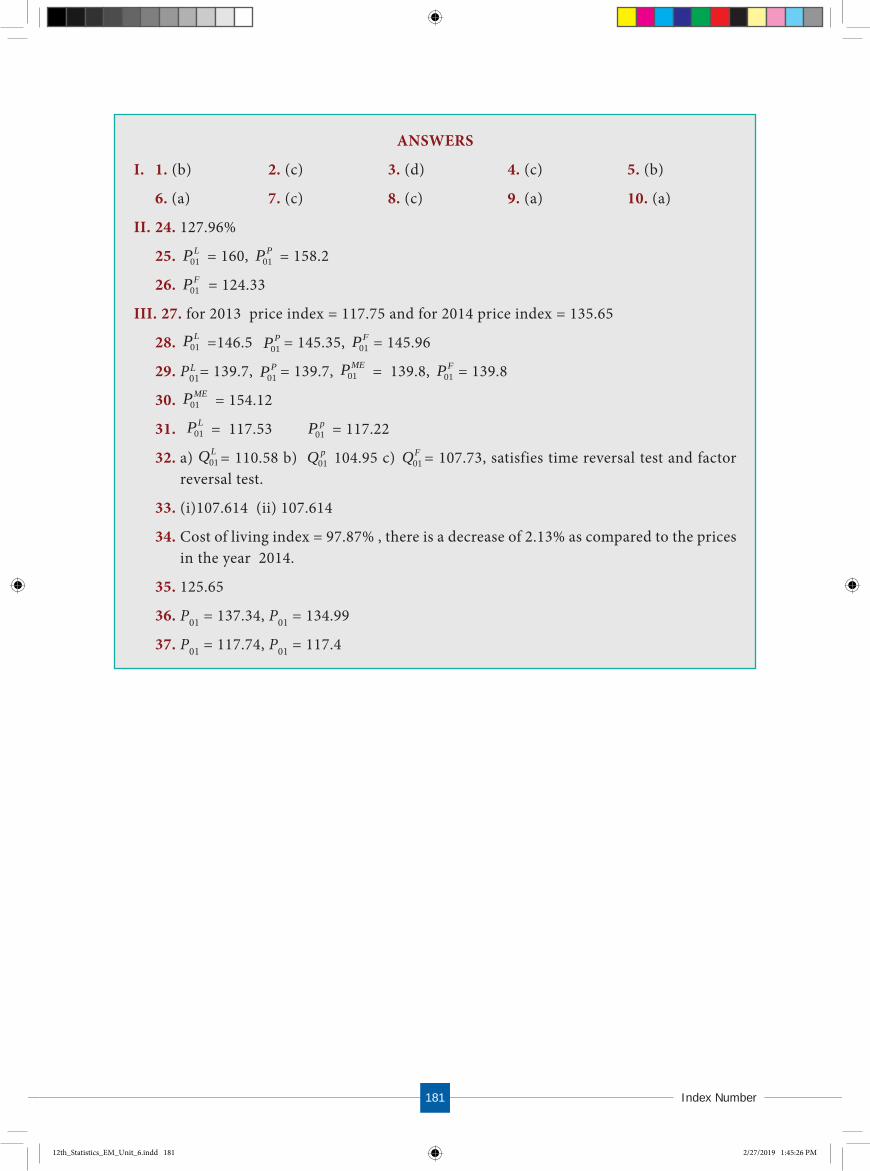
I n d e x N u m b e r181
ANSWERS
I. 1. (b) 2. (c) 3. (d) 4. (c) 5. (b)
6. (a) 7. (c) 8. (c) 9. (a) 10. (a)
II. 24. 127.96%
25. 01LP = 160, 01
PP = 158.2
26. 01FP = 124.33
III. 27. for 2013 price index = 117.75 and for 2014 price index = 135.65
28. 01LP =146.5 01
PP = 145.35, 01FP = 145.96
29. P01L = 139.7, 01
PP = 139.7, 01MEP = 139.8, 01
FP = 139.8
30. 01MEP = 154.12
31. 01LP = 117.53 01
pP = 117.22
32. a) 01LQ = 110.58 b) 01
pQ 104.95 c) 01FQ = 107.73, satisfies time reversal test and factor
reversal test.
33. (i)107.614 (ii) 107.614
34. Cost of living index = 97.87% , there is a decrease of 2.13% as compared to the pricesin the year 2014.
35. 125.65
36. P01 = 137.34, P01 = 134.99
37. P01 = 117.74, P01 = 117.4
12th_Statistics_EM_Unit_6.indd 181 2/27/2019 1:45:26 PM

18212t h S t d S t a t i s t i c s
� e students will be able to understand the concept of time series know the upward and downward trends calculate the trend values using semi - average and moving average methods estimate the trend values using method of least squares compute seasonal indices understand cyclical and irregular variations understand the forecasting concept
LEARNING OBJECTIVES
Both Box and Jenkins contributed to Auto regressive moving average models popularly known as Box-Jenkins Models.
IntroductionIn modern times we see data all around. The urge to evaluate the past and to peep into
the future has made the need for forecasting. There are many factors which change with the passage of time. Sometimes sets of observations which vary with the passage of time and whose measurements made at equidistant points may be regarded as time series data. Statistical data which are collected, observed or recorded at successive intervals of time constitute time series data. In the study of time series, comparison of the past and the present data is made. It also compares two or more series at a time. The purpose of time series is to measure chronological variations in the observed data.
G. E. P. Box (1919-2013) was a Britsh Statistician was “one of the great statistical minds” of the 20th century, who received his Ph.D., from the University of London, under the supervision of E. S. Pearson. He served as President of Americal Statistical Association in
1978 and of the Institute of Mathematics in 1979. His name is associated with Box-Cox transformation in addition to Box-Jenkins models in time series.
G. M. Jenkins (1932-1982)was a British Statistician,earned his Ph.D. degreefrom University College,London under the supervision of F. N. David and N. L. Johnson. He served on the Research Section Committee and Council of Royal Statistical Society in 1960’s. He was elected to the Institute of Mathematical Statitics
G. E. P. Box (1919-2013)Britsh Statistician was “one of the great statistical minds” of the 20th century, who received his Ph.D., from the University of London, under the supervision of E. S. Pearson. He served as President of Americal Statistical Association in
G. E. P. Box
G. M. Jenkins
TIME SERIES AND FORECASTING
CHAPTER
7
12th_Statistics_EM_Unit_7.indd 182 3/4/2019 9:39:20 AM

T i m e S e r i e s a n d F o r e c a s t i n g183
7.1 DEFINITION
Time series refers to any group of statistical information collected at regular intervals of time. Time series analysis is used to detect the changes in patterns in these collected data.
7.1.1 Definition by AuthorsAccording to Mooris Hamburg “A time series is a set of statistical observations arranged in chronological order”.
Ya-Lun-Chou : “A time series may be defined as a collection of readings belonging to different time periods of some economic variable or composite of variables”.
W.Z. Hirsch says “The main objective in analyzing time series is to understand, interpret and evaluate change in economic phenomena in the hope of more correctly anticipating the course of future events”.
7.1.2 Uses of Time Series• Time series is used to predict future values based on previously observed values.
• Time series analysis is used to identify the fluctuation in economics and business.
• It helps in the evaluation of current achievements.
• Time series is used in pattern recognition, signal processing, weather forecasting andearthquake prediction.
It can be said that time series analysis is a big tool in the hands of business executives to plan their sales, prices, policies and production.
7.2 COMPONENTS OF TIME SERIES
The factors that are responsible for bringing about changes in a time series are called the components of time series.
Components of Time Series
1. Secular trend2. Seasonal variation3. Cyclical variation4. Irregular (random) variation
12th_Statistics_EM_Unit_7.indd 183 3/4/2019 9:39:20 AM
In an ever changing business and economic environment, it is necessary to have an idea about the probable future course of events. Analysis of relevant time series helps to achieve this, especially by facilitating future business forecasts. Such forecasts may serve as crucial inputs in deciding competitive strategies and planning growth initiatives.

18412t h S t d S t a t i s t i c s
Approaches to time series
There are two approaches to the decomposition of time series data
(i) Additive approach
(ii) Multiplicative approach
The above two approaches are used in decomposition, depending on the nature ofrelationship among the four components.
�e additive approach
The additive approach is used when the four components of a time series are visualized as independent of one another. Independence implies that the magnitude and pattern of movement of the components do not affect one another. Under this assumption the magnitudes of the time series are regarded as the sum of separate influences of its four components.
Y = T + C + S + R
where Y = magnitude of a time series
T = Trend, C =Cyclical component, S =Seasonal component, and R = Random component
In additive approach, the unit of measurements remains the same for all the four components.
�e Multiplicative approach
The multiplicative approach is used where the forces giving rise to the four types of variations are visualized as interdependent. Under this assumption, the magnitude of the time series is the product of its four components.
i.e. Y = T × C × S × R
Di�erence between the two approaches
Multiplicative Additive
(i) Four components of time series areinterdependent
Four components of time series are independent
(ii) Logarithm of components are additive Components are additive
7.3 MEASEUREMENTS OF COMPONENTS
(i) Secular trend
It refers to the long term tendency of the data to move in an upward or downward direction. For example, changes in productivity, increase in the rate of capital formation, growth of population, etc., follow secular trend which has upward direction, while deaths due to improved medical facilities and sanitations show downward trend. All these forces occur in slow process and influence the time series variable in a gradual manner.
12th_Statistics_EM_Unit_7.indd 184 3/4/2019 9:39:20 AM

T i m e S e r i e s a n d F o r e c a s t i n g185
Methods of Measuring Trend
Trend is measured using by the following methods:
1. Graphical method
2. Semi averages method
3. Moving averages method
4. Method of least squares
7.3.1 Graphical MethodUnder this method the values of a time series are plotted on a graph paper by taking time
variable on the X-axis and the values variable on the Y-axis. After this, a smooth curve is drawn with free hand through the plotted points. The trend line drawn above can be extended to forecast the values. The following points must be kept in mind in drawing the freehand smooth curve.
(i) The curve should be smooth
(ii) The number of points above the line or curve should be approximately equal to the pointsbelow it
(iii) The sum of the squares of the vertical deviation of the points above the smoothed line isequal to the sum of the squares of the vertical deviation of the points below the line.
Merits
• It is simple method of estimating trend.
• It requires no mathematical calculations.
• This method can be used even if trend is not linear.
Demerits
• It is a subjective method
• The values of trend obtained by different statisticians would be different and hence not reliable.
Example 7.1Annual power consumption per household in a certain locality was reported below.
Years 1991 1992 1993 1994 1995 1996 1997 1998 1999 2000
Power used (units)
15 20 21 25 28 26 30 32 40 38
Draw a free hand curve for the above data.
12th_Statistics_EM_Unit_7.indd 185 3/4/2019 9:39:20 AM

18612t h S t d S t a t i s t i c s
Solution:
7.3.2 Semi-Average MethodIn this method, the series is divided into two equal parts and the average of each part is
plotted at the mid-point of their time duration.
(i) In case the series consists of an even number of years, the series is divisible into two halves.Find the average of the two parts of the series and place these values in the mid-year of eachof the respective durations.
(ii) In case the series consists of odd number of years, it is not possible to divide the series intotwo equal halves. The middle year will be omitted. After dividing the data into two parts,find the arithmetic mean of each part. Thus we get semi-averages.
(iii) The trend values for other years can be computed by successive addition or subtraction foreach year ahead or behind any year.
Merits
• This method is very simple and easy to understand
• It does not require many calculations.
Demerits
• This method is used only when the trend is linear.
• It is used for calculation of averages and they are affected by extreme values.
Example 7.2Calculate the trend values using semi-averages methods for the income from the forest
department. Find the yearly increase.
Year 2008 2009 2010 2011 2012 2013
Income (in crores) 46.17 51.65 63.81 70.99 84.91 91.64
Source: The Principal Chief conservator of forests, Chennai-15. (pg. 231)
Years
Pow
er u
sed
(uni
ts)
In semi-average method if the difference between the semi-averages is negative then the trend values will be in decreasing order.
NOTE
12th_Statistics_EM_Unit_7.indd 186 3/4/2019 9:39:20 AM

T i m e S e r i e s a n d F o r e c a s t i n g187
Solution:
Year Income 3-Year semi-total Semi-average
2008 46.17
161.63 53.8772009 51.65
2010 63.81
2011 70.99
247.54 82.5132012 84.91
2013 91.64
Difference between the central years = 2012 – 2009 = 3
Difference between the semi-averages = 82.513 – 53.877 = 28.636
Increase in trend value for one year =
Trend values for the previous and successive years of the central years can be calculated by subtracting and adding respectively, the increase in annual trend value.
Example 7.3Population of India for 7 successive census years are given below. Find the trend values
using semi-averages method.
Census Year 1951 1961 1971 1981 1991 2001 2011
Population (in lakhs) 301.2 336.9 412.0 484.1 558.6 624.1 721.4
Solution:
Trend values using semi average method
Census YearPopulation (in lakhs)
3-year semi-total 3-year semi-average Trend values
1951 301.2
1050.1 350.03
278.86
1961 336.9 350.03
1971 412.0 421.2
1981 484.1 492.37
1991 558.6
1904.1 634.7
563.54
2001 624.1 634.71
2011 721.4 705.88
Difference between the years = 2001 – 1961 = 40
Difference between the semi-averages = 634.7 – 350.03 = 284.67
Increase in trend value for 10 year =
28 636
39 545
..
284 67
471 17
..
12th_Statistics_EM_Unit_7.indd 187 3/4/2019 9:39:21 AM

18812t h S t d S t a t i s t i c s
For example the trend value for the year 1951 = 350.03 – 71.17 = 278.86
The value for the year 2011 = 634.7 + 71.17 = 705.87
The trend values have been calculated by successively subtracting and adding the increase in trend for previous and following years respectively.
Example 7.4Find the trend values by semi-average method for the following data.
Year 1965 1966 1967 1968 1969 1970 1971 1972
Production of bleaching powder (in tonnes)
7.4 10.8 9.2 10.5 15.5 13.7 16.7 15
Solution:
Trend values using semi averages method
YearProduction of
bleaching powder4 year semi-total 4 year semi-average Trend
1965 7.4
37.9 9.475
7.315
1966 10.8 8.755
1967 9.2 10.195
1968 10.5 11.635
1969 15.5
60.9 15.225
13.075
1970 13.7 14.515
1971 16.7 15.955
1972 15 17.395
Difference between the years = 1970.5 – 1966.5 = 4
Difference between the semi-averages = 15.225 – 9.475 = 5.75
Increase in trend =
Half yearly increase in trend =
The trend value for 1967 = 9.475 + 0.72 = 10.195
The trend value for 1968 = 9.475 + 3 * 0.72 = 11.635
Similarly the trend values for the other years can be calculated.
7.3.3 Moving Averages MethodMoving averages is a series of arithmetic means of variate values of a sequence. This is
another way of drawing a smooth curve for a time series data.
5 75
41 44
..
1 44
20 72
..
12th_Statistics_EM_Unit_7.indd 188 3/4/2019 9:39:22 AM

T i m e S e r i e s a n d F o r e c a s t i n g189
• It can be easily applied
• It is useful in case of series with periodic fluctuations.
• It does not show different results when used by different persons
• It can be used to find the figures on either extremes; that is, for the past and future years.
Demerits
• In non-periodic data this method is less effective.
• Selection of proper ‘period’ or ‘time interval’ for computing moving average is difficult.
• Values for the first few years and as well as for the last few years cannot be found.
Moving averages odd number of years (3 years)
To find the trend values by the method of three yearly moving averages, the following steps have to be considered.
1. Add up the values of the first 3 years and place the yearly sum against the median year.[This sum is called moving total]
2. Leave the first year value, add up the values of the next three years and place it against itsmedian year.
3. This process must be continued till all the values of the data are taken for calculation.
4. Each 3-yearly moving total must be divided by 3 to get the 3-year moving averages, which isour required trend values.
Example 7.5Calculate the 3-year moving averages for the loans issued by co-operative banks for non-
farm sector/small scale industries based on the values given below.
Year 2004-05 2005-06 2006-07 2007-08 2008-09 2009-10 2010-11 2011-12 2012-13 2013-14 2014-15
Loan by District Central
Cooperative banks (Rupees in crores)
41.82 40.05 39.12 24.72 26.69 59.66 23.65 28.36 33.31 31.60 36.48
12th_Statistics_EM_Unit_7.indd 189 3/4/2019 9:39:22 AM
Moving averages is more frequently used for eliminating the seasonal variations. Even when applied for estimating trend values, the moving average method helps to establish a trend line by eliminating the cyclical, seasonal and random variations present in the time series. The period of the moving average depends upon the length of the time series data.
The choice of the length of a moving average is an important decision in using this method. For a moving average, appropriate length plays a significant role in smoothening the variations. In general, if the number of years for the moving average is more then the curve becomes smooth.
Merits
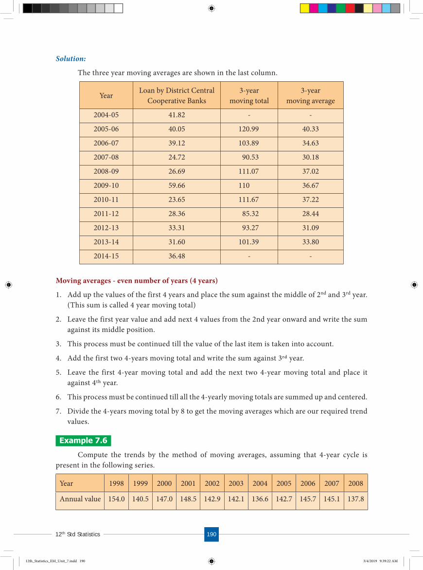
19012t h S t d S t a t i s t i c s
Solution:
The three year moving averages are shown in the last column.
YearLoan by District Central
Cooperative Banks3-year
moving total3-year
moving average
2004-05 41.82 - -
2005-06 40.05 120.99 40.33
2006-07 39.12 103.89 34.63
2007-08 24.72 90.53 30.18
2008-09 26.69 111.07 37.02
2009-10 59.66 110 36.67
2010-11 23.65 111.67 37.22
2011-12 28.36 85.32 28.44
2012-13 33.31 93.27 31.09
2013-14 31.60 101.39 33.80
2014-15 36.48 - -
Moving averages - even number of years (4 years)
1. Add up the values of the first 4 years and place the sum against the middle of 2nd and 3rd year.(This sum is called 4 year moving total)
2. Leave the first year value and add next 4 values from the 2nd year onward and write the sumagainst its middle position.
3. This process must be continued till the value of the last item is taken into account.
4. Add the first two 4-years moving total and write the sum against 3rd year.
5. Leave the first 4-year moving total and add the next two 4-year moving total and place itagainst 4th year.
6. This process must be continued till all the 4-yearly moving totals are summed up and centered.
7. Divide the 4-years moving total by 8 to get the moving averages which are our required trendvalues.
Example 7.6Compute the trends by the method of moving averages, assuming that 4-year cycle is
present in the following series.
Year 1998 1999 2000 2001 2002 2003 2004 2005 2006 2007 2008
Annual value 154.0 140.5 147.0 148.5 142.9 142.1 136.6 142.7 145.7 145.1 137.8
12th_Statistics_EM_Unit_7.indd 190 3/4/2019 9:39:22 AM
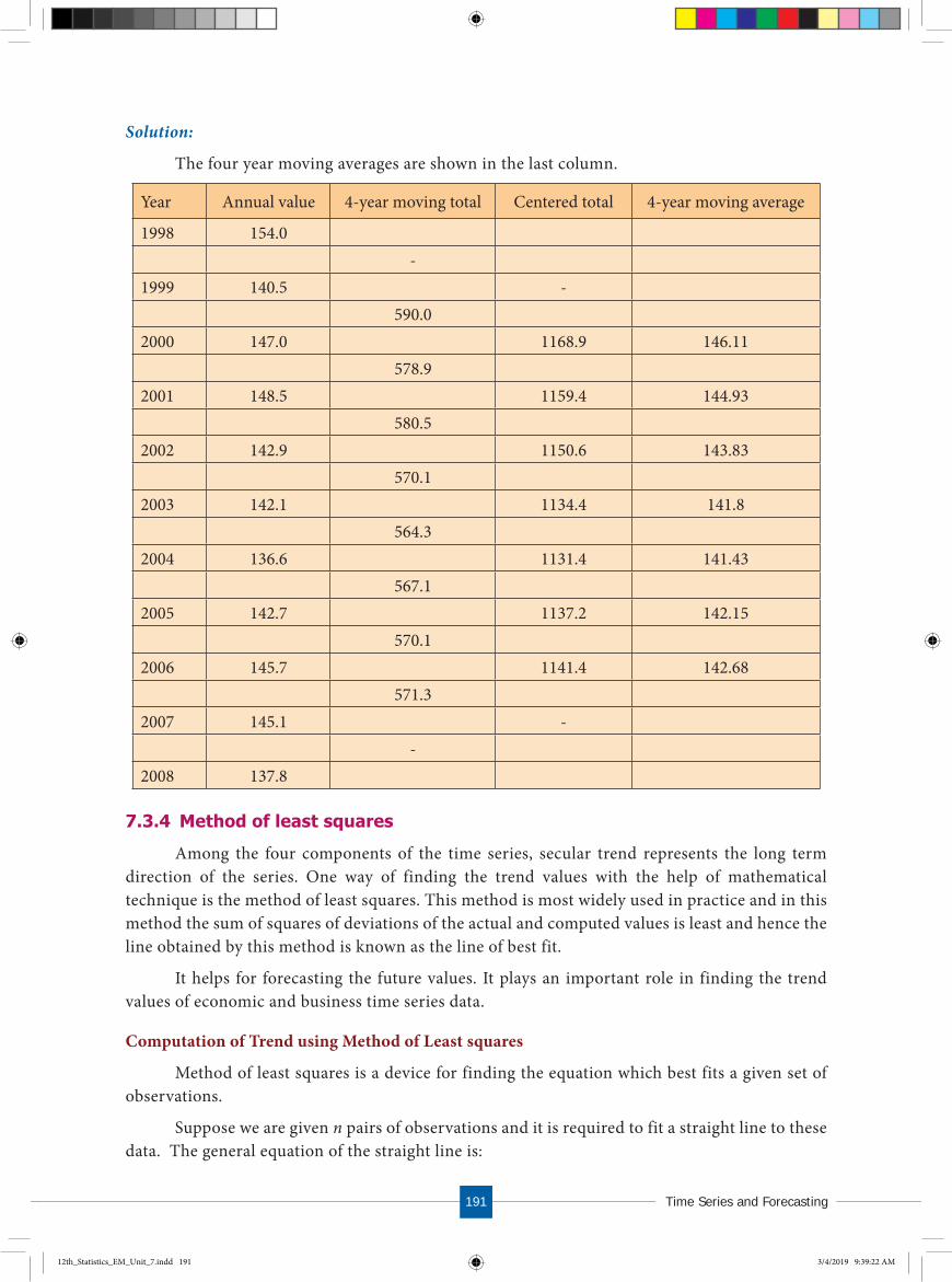
T i m e S e r i e s a n d F o r e c a s t i n g191
Solution:
The four year moving averages are shown in the last column.
Year Annual value 4-year moving total Centered total 4-year moving average
1998 154.0-
1999 140.5 -590.0
2000 147.0 1168.9 146.11578.9
2001 148.5 1159.4 144.93580.5
2002 142.9 1150.6 143.83570.1
2003 142.1 1134.4 141.8564.3
2004 136.6 1131.4 141.43567.1
2005 142.7 1137.2 142.15570.1
2006 145.7 1141.4 142.68571.3
2007 145.1 --
2008 137.8
7.3.4 Method of least squaresAmong the four components of the time series, secular trend represents the long term
direction of the series. One way of finding the trend values with the help of mathematical technique is the method of least squares. This method is most widely used in practice and in this method the sum of squares of deviations of the actual and computed values is least and hence the line obtained by this method is known as the line of best fit.
It helps for forecasting the future values. It plays an important role in finding the trend values of economic and business time series data.
Computation of Trend using Method of Least squares
Method of least squares is a device for finding the equation which best fits a given set of observations.
Suppose we are given n pairs of observations and it is required to fit a straight line to these data. The general equation of the straight line is:
12th_Statistics_EM_Unit_7.indd 191 3/4/2019 9:39:22 AM

19212t h S t d S t a t i s t i c s
obtained by minimizing the sum of squares of differences y yi ii
n
����
���
�� ^
1
2
�at is, y y y a bxi i i ii
n
����
��� � � �� �� �
�
^2
1
2
is minimum. �is leads us to two normal equations.
y na b xii
n
ii
n
� �� �� �
1 1 (7.1)
x y a x b xi ii
n
i
n
ii
n
� � �� � �� �
1 1
2
1 (7.2)
Solving these two equations we get the vales for a and b and the fit of the trend equation (line of best):
y = a + bx (7.3)
Substituting the observed values xi in (7.3) we get the trend values yi, i = 1, 2, …, n.
Note: The time unit is usually of uniform duration and occurs in consecutive numbers. Thus, when the middle period is taken as the point of origin, it reduces the sum of the time variable x
to zero xii
n
��
��
�
��
�� 0
1
and hence we get
1
n
ii
ya
n and 1
2
1
n
i ii
n
ii
x yb
x by simplifying (7.1) and (7.2)
The number of time units may be even or odd, depending upon this, we follow the method of calculating trend values using least square method.
Merits
• The method of least squares completely eliminates personal bias.
• Trend values for all the given time periods can be obtained
• This method enables us to forecast future values.
Demerits
• The calculations for this method are difficult compared to the other methods.
• Addition of new observations requires recalculations.
• It ignores cyclical, seasonal and irregular fluctuations.
• The trend can be estimated only for immediate future and not for distant future.
12th_Statistics_EM_Unit_7.indd 192 3/4/2019 9:39:24 AM
y = a + bx
where a and b are constants. Any value of a and b would give a straight line, and once these values are obtained an estimate of y can be obtained by substituting the observed values of y. In order that the equation y = a + b x gives a good representation of the linear relationship between x and y, it is desirable that the estimated values of yi, say y^i on the whole close enough to the observed values y i, i = 1, 2, …, n. According to the principle of least squares, the best fitting equation is

T i m e S e r i e s a n d F o r e c a s t i n g193
Steps for calculating trend values when n is odd:
i) Subtract the first year from all the years (x)
ii) Take the middle value (A)
iii) Find ui = xi – A
iv) Find ui2 and uiyi
Then use the normal equations:
y na b u
u y a u b u
ii
n
ii
n
i ii
n
ii
n
ii
n� �
� � �
� �
� � �
� �
� �
1 1
1 1
2
1
Find 1
n
ii
ya
n and 1
2
1
n
i ii
n
ii
u yb
u
Then the estimated equation of straight line is:
y = a + b u = a + b (x – A)
Example 7.7Fit a straight line trend by the method of least squares for the following consumer price
index numbers of the industrial workers.
Year 2010 2011 2012 2013 2014
Index number 166 177 198 221 225
Solution:
YearIndex
NumberX = xi – 2010
ui = X – A = X – 2
ui2 uiyi Trend
2010 166 0 –2 4 –332 165
2011 177 1 –1 1 –177 181.2
2012 198 2 0 0 0 197.4
2013 221 3 1 1 221 213.6
2014 225 4 2 4 450 229.8
The equation of the straight line is y = a + bx
= a + bu where u = X – 2
yii
��� 987
1
5
uii
��� 0
1
5
uii
2
1
5
10��� u yi i
i�
�� 162
1
5
12th_Statistics_EM_Unit_7.indd 193 3/4/2019 9:39:28 AM

19412t h S t d S t a t i s t i c s
The normal equations give:1
n
ii
ya
na
yn
� � �� 987
5197 4.
1
2
1
n
i ii
n
ii
u yb
ub
uyu
� � ��� 2
162
1016 2.
y = 197.4 + 16.2 (X – 2)
= 197.4 + 16.2 X – 32.4
= 16.2 X + 165
That is, y = 165 + 16.2X
To get the required trend values, put X = 0, 1, 2, 3, 4 in the estimated equation.
X = 0, y = 165 + 0 = 165
X = 1, y = 165 + 16.2 = 181.2
X = 2, y = 165 + 32.4 = 197.4
X = 3, y = 165 + 48.6 = 213.6
X = 4, y = 165 + 64.8 = 229.8
Hence, the trend values for 2010, 2011, 2012, 2013 and 2014 are 165, 181.2, 197.4, 213.6 and 229.8 respectively.
Steps for calculating trend values when n is even:
i). Subtract the first year from all the years (x)
ii). Find ui = 2X – (n – 1)
iii). Find ui2 and uiyi
Then follow the same procedure used in previous method for odd years
Example 7.8Tourist arrivals (Foreigners) in Tamil Nadu for 6 consecutive years are given in the following table. Calculate the trend values by using the method of least squares.
Year 2005 2006 2007 2008 2009 2010
No. of arrivals (in lakhs) 12 13 18 20 24 28
12th_Statistics_EM_Unit_7.indd 194 3/4/2019 9:39:29 AM
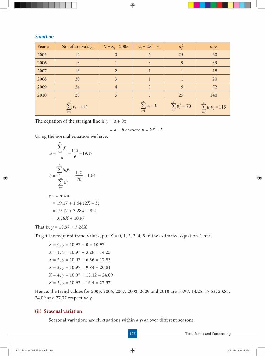
T i m e S e r i e s a n d F o r e c a s t i n g195
Solution:
Year x No. of arrivals yi X = xi – 2005 ui = 2X – 5 ui2 ui yi
2005 12 0 –5 25 –60
2006 13 1 –3 9 –39
2007 18 2 –1 1 –18
2008 20 3 1 1 20
2009 24 4 3 9 72
2010 28 5 5 25 140
The equation of the straight line is y = a + bx
= a + bu where u = 2X – 5Using the normal equation we have,
ay
n
ii
n
� ��
1ayn
� � �� 115
619 17.
1
2
1
n
i ii
n
ii
u yb
ub
uyu
� � ��� 2
115
701 64.
y = a + bu= 19.17 + 1.64 (2X – 5)= 19.17 + 3.28X – 8.2= 3.28X + 10.97
That is, y = 10.97 + 3.28X
To get the required trend values, put X = 0, 1, 2, 3, 4, 5 in the estimated equation. Thus,
X = 0, y = 10.97 + 0 = 10.97X = 1, y = 10.97 + 3.28 = 14.25X = 2, y = 10.97 + 6.56 = 17.53X = 3, y = 10.97 + 9.84 = 20.81X = 4, y = 10.97 + 13.12 = 24.09X = 5, y = 10.97 + 16.4 = 27.37
Hence, the trend values for 2005, 2006, 2007, 2008, 2009 and 2010 are 10.97, 14.25, 17.53, 20.81, 24.09 and 27.37 respectively.
(ii) Seasonal variation
Seasonal variations are fluctuations within a year over different seasons.
yii
��� 115
1
6
uii
��� 0
1
6
uii
2
1
6
70��� u yi i
i�
�� 115
1
6
12th_Statistics_EM_Unit_7.indd 195 3/4/2019 9:39:34 AM

19612t h S t d S t a t i s t i c s
There are four methods of constructing seasonal indices.
1. Simple averages method2. Ratio to trend method3. Percentage moving average method4. Link relatives method
Among these, we shall discuss the construction of seasonal index by the first method only.
7.3.5 Simple Averages MethodUnder this method, the time series data for each of the 4 seasons (for quarterly data) of a
particular year are expressed as percentages to the seasonal average for that year.The percentages for different seasons are averaged over the years by using simple average.
The resulting percentages for each of the 4 seasons then constitute the required seasonal indices.
Method of calculating seasonal indices
i) The data is arranged season-wise
ii) The data for all the 4 seasons are added first for all the years and the seasonal averages foreach year is computed.
iii) The average of seasonal averages is calculated(i.e., Grand average = Total of seasonal averages /number of years).
iv) The seasonal average for each year is divided by the corresponding grand average and theresults are expressed in percentages and these are called seasonal indices.
Example 7.9Calculate the seasonal indices for the rain fall (in mm) data in Tamil Nadu given below by
simple average method
YearSeason
I II III IV
2001 118.4 260.0 379.4 70
2002 85.8 185.4 407.1 8.7
2003 129.8 336.5 403.1 12.0
2004 283.4 360.7 472.1 14.3
2005 231.7 308.5 828.8 15.9
12th_Statistics_EM_Unit_7.indd 196 3/4/2019 9:39:34 AM
Estimation of seasonal variations requires that the time series data are recorded at even intervals such as quarterly, monthly, weekly or daily, depending on the nature of the time series. Changes due to seasons, weather conditions and social customs are the primary causes of seasonal variations. The main objective of the measurement of seasonal variation is to study their effect and isolate them from the trend.
Methods of constructing seasonal indices

T i m e S e r i e s a n d F o r e c a s t i n g197
Solution:
YearSeason
I II III IV
2001 118.4 260.0 379.4 70
2002 85.8 185.4 407.1 8.7
2003 129.8 336.5 403.1 12.0
2004 283.4 360.7 472.1 14.3
2005 231.7 308.5 828.8 15.9
Seasonal total 849.1 1451.1 2490.5 120.9
Seasonal average 169.82 290.22 498.1 24.18
Seasonal index 69 118 203 10
Grand Average = Total of seasonal averages
4
= 169.82 + 290.22 + 498.1 + 24.18
4
= 982.32
= 245.584
Seasonal Index = Seasonal average
× 100Grand average
Seasonal Index for Season I = 169.82
× 100 = 69.15 ≈ 69245.58
Seasonal Index for Season II = 290.22
× 100 = 118.18 ≈ 118245.58
Seasonal Index for Season III = 498.1
× 100 = 202.83 ≈ 203245.58
Seasonal Index for Season IV = 24.18
× 100 = 9.85 ≈ 10245.58
Example 7.10Obtain the seasonal indices for the rain fall (in mm) data in India given in the following table.
2009 2010 2011 2012
I 38.2 38.5 55 50.5
II 166.8 250.9 277.7 197
III 612.6 773.1 717.8 706.1
IV 72.2 153.1 65.8 101.1
YearQuarter
12th_Statistics_EM_Unit_7.indd 197 3/4/2019 9:39:34 AM

19812t h S t d S t a t i s t i c s
Solution:
YearQuarter
I II III IV
2009 38.2 166.8 612.6 72.2
2010 38.5 250.9 773.1 153.1
2011 55 277.7 717.8 65.8
2012 50.5 197 706.1 101.1
Seasonal total 182.2 892.4 2809.6 392.2
Seasonal average 45.55 223.1 702.4 98.05
Seasonal index 17 83 263 37
Grand Average = Total of seasonal averages
4
= 45.55 + 223.1 + 702.4 + 98.05
4
= 1069.10
= 267.284
Seasonal Index = Seasonal average
× 100Grand average
Seasonal Index for Quarter I = 45.55
× 100 = 17.04 ≈ 17267.28
Seasonal Index for Quarter II = 223.1
× 100 = 83.47 ≈ 83267.28
Seasonal Index for Quarter III = 702.4
× 100 = 262.80 ≈ 263267.28
Seasonal Index for Quarter IV = 98.05
× 100 = 36.69 ≈ 37267.28
12th_Statistics_EM_Unit_7.indd 198 3/4/2019 9:39:34 AM

T i m e S e r i e s a n d F o r e c a s t i n g199
(iii) Cyclical variation
Cyclical variations refer to periodic movements in the time series about the trend line,described by upswings and downswings. They occur in a cyclical fashion over an extended period of time (more than a year). For example, the business cycle may be described as follows.
�e cyclical pattern of any time series tells about the prosperity and recession, ups and downs,booms and depression of a business. In most of the businesses there are upward trend for some time followed by a downfall, touching its lowest level. Again a rise starts which touches its peak. �is process of prosperity and recession continues and may be considered as a natural phenomenon.
YOU WILL KNOW
Cyclic movements are mainly due to Trade cycle.
(iv) Irregular variation
In practice, the changes in a time series that cannotbe attributed to the influence of cyclic fluctuations or seasonal variations or those of the secular trend are classified as irregular variations.
In the words of Patterson, “Irregular variation in a time series is composed of non-recurring sporadic (rare) form which is not attributed to trend, cyclical or seasonal factors”.
Nothing can be predicted about the occurrence of irregular influences and the magnitude of such effects. Hence, no standard method has been evolved to estimate the same. It is taken as the residual left in the time series, after accounting for the trend, seasonal and cyclic variations.
7.4 FORECASTING
The importance of statistics lies in the extent to which it serves as the basis for making reliable forecasts, against arbitrary forecast with no statistical background.
Prosperity Decline
Depression
Recovery
There is no statistical technique for measuring or isolating irregular fluctuations
NOTE
YOU WILL KNOW
Irregular variation is also called erratic fluctuations.
12th_Statistics_EM_Unit_7.indd 199 3/4/2019 9:39:34 AM

20012t h S t d S t a t i s t i c s
Forecasting is a scientific process which aims at reducing the uncertainty of the future state of business and trade, not dependent merely on guess work, but with a sound scientific footing for the decision on the future course of action.
7.4.1 Definition“Forecasting refers to the analysis of past and
present conditions with a view of arriving at rough estimates about the future conditions.
According to T.S. Lewis and R.A. Fox “Forecasting is using the knowledge we have at one time to estimate what will happen at some future moment of time”.
Forecasting is an important tool that serves many fields including business and industry, government, economics, environmental sciences, medicine, social science, politics and finance. Forecasting problems are often classified as short-term, medium-term, and long-term.
Short-term forecasting problems involve predicting events for a few time periods (days, weeks, months) into the future.
Medium-term forecast extends from one to two years into the future.
Long-term forecasting problems can extend beyond that by many years.
Short and medium-term forecasts are required for activities that range from operations management to budgeting and selecting new research and development projects. Long term forecasts impact issues relating to strategic planning.
POINTS TO REMEMBER
Time series is a time oriented sequence of observations.
Components of time series are secular trend, seasonal variations, cyclical variations and irregular (erratic) variations
Methods of calculating trend values are graphical method, semi - averages method, moving averages method, and method of least squares.
�e line y = a + b x found out using the method of least squares is called ‘line of best �t’.
Normal equations involved in the method of least squares are
y na b xii
n
ii
n
� �� �� �
1 1
x y a x b xi ii
n
i
n
ii
n
� � �� � �� �
1 1
2
1
Seasonal indices may be found out by using simple average method. Forecasting is the analysis of using past and present conditions to get rough estimates of the
future conditions Forecasting methods can be short-term, medium-term and long-term.
1. Long term forecasting can befound using Trend.
2. Short term forecasting canbe found using seasonalvariations.
NOTE
12th_Statistics_EM_Unit_7.indd 200 3/4/2019 9:39:34 AM
T i m e S e r i e s a n d F o r e c a s t i n g201
EXERCISE 7
I. Choose the best answer.
1. An overall tendency of rise or fall in a time series is called
(a) seasonal variation (b) secular trend(c) cyclical variation (d) irregular variation
2. The component having primary use for short-term forecasting is
(a) cyclical variation (b) irregular variation(c) seasonal variation (d) trend
3. Cyclical movements are due to
(a) ratio to trend (b) seasonal(c) trend (d) trade cycle
4. Data on annual turnover of a company over a period of ten years can be represented by a
(a) a time series (b) an index number(c) a parameter (d) a statistic
5. The component having primary use for long term forecasting is
(a) cyclical variation (b) irregular variation(c) seasonal variation (d) trend
6. A time series is a set of data recorded
(a) periodically (b) at equal time intervals(c) at successive points of time (d) all the above
7. A time series consists of
(a) two components (b) three components(c) four components (d) five components
8. Irregular variation in a time series can be due to
(a) trend variations (b) seasonal variations(c) cyclical variations (d) unpredictable causes
9. The terms prosperity, recession, depression and recovery are in particular attached to
(a) secular trend (b) seasonal fluctuation(c) cyclical movements (d) irregular variation
10. An additive model of time series with components, T, S, C and I is
(a) Y = × S × C × I (b) Y = T + S + C + I(c) Y = T × S + C × I (d) Y = T × S × C + I
12th_Statistics_EM_Unit_7.indd 201 3/4/2019 9:39:34 AM

20212t h S t d S t a t i s t i c s
11. A decline in the sale of ice cream during November to March is associated with
(a) seasonal variation (b) cyclical variation(c) irregular variation (d) secular trend
12. Business forecasts are made on the basis of
(a) future data (b) past data(c) tax regulations (d) Government policies
13. The four components of time series in a multiplicative model are
(a) independent (b) interdependent(c) constant (d) additive
14. In the least square theory the sum of squares of residuals is
(a) zero (b) minimum(c) constant (d) maximum
15. No statistical techniques for measuring or isolating _______is available.
(a) cyclical variation (b) seasonal variation(c) erratic fluctuations (d) secular trend
II. Give very short answers to the following questions
16. What is a time series?
17. What are the components of a time series?
18. Name different methods of estimating the trend?
19. Write short notes on irregular variation.
20. Mention the methods used to find seasonal indices?
21. What are the demerits of moving averages?
22. What are the merits of method of least squares?
23. Write the normal equations used in method of least squares?
24. Define forecasting.
25. What are the three types of forecasting?
26. What is a short-term forecast?
12th_Statistics_EM_Unit_7.indd 202 3/4/2019 9:39:34 AM

T i m e S e r i e s a n d F o r e c a s t i n g203
III. Give short answers to the following questions
27. Write the uses of time series.
28. Explain semi-averages method
29. Write the merits of moving averages.
30. What is cyclical variation?
31. What is seasonal variation?
32. What are medium-term and long-term forecasts?
33. Describe the method of finding seasonal indices.
34. With what characteristic component of a time series should each of the following be associated.(i) An upturn in business activity
(ii) Fire loss in a factory(iii) General increase in the sale of Television sets.
35. The number of units of a product exported during 1990-97 is given below. Draw the trendline using graphical method.
Year 1990 1991 1992 1993 1994 1995 1996 1997
No. of units exported (in ‘000)
12 13 13 16 19 23 21 23
36. Draw a time series graph relating to the following data and show the trend by free handmethod
Year 1996 1997 1998 1999 2000 2001 2002 2003
Production in Million tonnes 40 44 42 48 51 54 50 56
37. Draw a trend line by the method semi averages
Year 1992 1993 1994 1995 1996 1997
Production of steel in Million tonnes
21 23 25 23 26 25
38. Yield of ground nut in Kharif season in India for the years 2003-04 to 2009-10 are givenbelow. Calculate 3-year moving averages.
Year 2003-04 2004-05 2005-06 2006-07 2007-08 2008-09 2009-10
Yield (kg/hectare)
1320 909 1097 689 1386 1063 835
39. What do you understand by seasonal variations?
12th_Statistics_EM_Unit_7.indd 203 3/4/2019 9:39:35 AM

20412t h S t d S t a t i s t i c s
IV. Give detailed answers to the following questions
40. Explain the method of least squares
41. The following data states the number of ATM centers during 1995 to2001.
Year 1995 1996 1997 1998 1999 2000 2001
Number of ATM centres 50 63 75 100 109 120 135
Obtain the trend values using semi averages method
42. From the following data estimate the trend values using semi averages method
Year 2003 2004 2005 2006 2007 2008 2009 2010
Consumption of cotton (�ousands of bales)
677 696 747 755 766 777 785 836
43. Following data gives the yield of food grains in India for the years 2000-01 to 2009-10. Findthe trend values using 4 year moving averages.
Year 2000-01 2001-02 2002-03 2003-04 2004-05 2005-06 2006-07 2007-08 2008-09 2009-10
Yield (kg/hectare)
1626 1734 1535 1727 1652 1715 1756 1860 1909 1798
44. Estimate the value of production for the year 1995 by using the method of least squares fromthe following data.
Year 1990 1991 1992 1993 1994
Production (1000s tons) 70 72 88 90 92
45. Find the following for the calculation of number of telephones for the year 2000.(1) Fit a straight line trend by the method of least squares.
(2) Calculate the trend values.
Year 1990 1991 1992 1993 1994 1995
No. of telephones (in 100s) 20 21 23 25 27 29
46. The following data describes the export quantity of a company.
Year 1995 1996 1997 1998 1999 2000 2001
Export (in millions) 12 13 13 16 16 19 23
Fit a straight line trend and estimate the export for the year 2005.
12th_Statistics_EM_Unit_7.indd 204 3/4/2019 9:39:35 AM

T i m e S e r i e s a n d F o r e c a s t i n g205
47. Calculate seasonal indices for the rainfall data of Tamil Nadu by using simple average method.
I II III IV
2000-01 314.5 335.6 16.8 118.4
2001-02 260.0 379.4 70.0 85.8
2002-03 185.4 407.1 8.7 129.8
2003-04 336.5 403.1 12.0 283.4
2004-05 360.7 472.1 14.3 231.7
48. Find seasonal Indices for the rainfall data in Tamil Nadu (in mm)
2009 2010 2011 2012
I 38.2 38.5 55 50.5
II 166.8 250.9 277.7 197
III 612.6 773.1 717.8 706.1
IV 72.2 153.1 65.8 101.1
49. The following table gives quarterly expenditure over a number of years. Obtain seasonalcorrection for the data
2000 2001 2002 2003
I 78 84 92 100
II 62 64 70 81
III 56 61 63 72
IV 71 82 83 96
50. Find the trend values using semi averages method. The following table shows the area coveredfor cultivation of Ragi in Tamil Nadu (in ‘000 hectares)
Year 2003 2004 2005 2006 2007 2008 2009 2010
Area(in ‘000 hectares)
118 109 100 95 94 90 82 76
(Hint: Decreasing trend)
Year Quarter
SeasonYear
Year Quarter
12th_Statistics_EM_Unit_7.indd 205 3/4/2019 9:39:35 AM
20612t h S t d S t a t i s t i c s
ANSWERS
I 1. (b) 2. (c) 3. (d) 4. (a) 5. (d)
6. (d) 7. (c) 8. (d) 9. (c) 10. (b)
11. (a) 12. (b) 13. (b) 14. (b) 15. (c)
III 34. i). Cyclic variation ii). Irregular variation iii). Secular trend
37. 22.44, 23, 23.56, 24.11, 24.67, 25.22
38. –, 108.67, 898.33, 1057.33, 1046, 1094.67, –
IV 41. 48.00, 62.67, 77.33, 92, 106.67, 121.33, 136
42. 691.66, 709.72, 727.78, 745.84, 763.91, 781.97, 800.03, 818.09
43. –, –, 1658.75, 1659.625, 1684.875, 1729.125, 1777.875, 1820.375, –, –
44. 70, 76.2, 82.4, 88.6, 94.8, 101
45. 19.52, 21.38, 23.24, 25.1, 26.95, 28.81
Number of telephones in the year 2000 is 3810
46. 10.86, 12.57, 14.29, 16, 17.71, 19.42, 21.14
Export for the year 2005 is 28 millions
47. 132, 181, 11, 77
48. 17, 83, 263, 37
49. 117, 91, 83, 109
50. 113, 108, 103, 98, 93, 88, 83, 78
12th_Statistics_EM_Unit_7.indd 206 3/4/2019 9:39:35 AM

T i m e S e r i e s a n d F o r e c a s t i n g207
Steps:• Open the browser and type the URL given (or) scan the QR code.• GeoGebra work book called “Time Series Plot” will open.• Move the “seed” slider to select a new sample.• Put the Tick Mark in the Check box to see an answer to the problem.
ICT CORNER
Pictures are indicatives only*
� is activity helps to Understand about
Times Series and Forecasting
Step-1 Step-2
Step-3
TIME SERIES AND FORECASTING
12th_Statistics_EM_Unit_7.indd 207 3/4/2019 9:39:35 AM

20812t h S t d S t a t i s t i c s
The students will be able to understand� the importance of Vital Statistics
� various mortality rates
� di� erent fertility rates
� di� erent components of Life Table
� construction of Life Table for a given community
� evolvement of Statistical System in India
� the role of O� cial Statistics
� the establishment and roles of di� erent divisions of CSO and NSSO.
� the present Statistical System in India
LEARNING OBJECTIVES
William Farr (1807–1883) was a British Epidemiologist, regarded as one of the founders of Medical Statistics. Farr, systematically collected and analyzed Britain’s Vital
Statistics, is known as “the father of Modern Vital Statistics and surveillance.” Farr’s name features on the wall painting of the London School of Hygiene and Tropical Medicine (LSHTM) in recognition of his work. Twenty three names of public health and tropical medicine pioneers were chosen to appear on the School building in Keppel Street when it was constructed in 1926.
P.C. Mahalanobis (1893-1972)took initiatives for establishment of the Official Statistical Systemin India. He was the firstHonorary Statistical Advisor tothe Government of India. He was instrumental for establishing the present Central Statistical Office and National Sample Survey Office. He is the founder of the internationally renowned Indian Statistical Institute (ISI) at Kolkata, which has centres located at various parts of the country. ISI also concentrates on other disciplines of study which include Geology, Sociology, Computer Science and Theoretical Physics.
William Farr (1807–1883)Epidemiologist, regarded as one of the founders of Medical Statistics. Farr, systematically collected and analyzed Britain’s Vital William Farr P.C. Mahalanobis
VITAL STATISTICS AND OFFICIAL STATISTICS
CHAPTER
8
12th_Statistics_EM_Unit_8.indd 208 2/27/2019 1:54:37 PM

Vital Statistics and Official Statistics209
8
The following are some of the important definitions of Vital Statistics:
“The whole study of mankind by heredity or environment in so far as the results of their study can be arithmetically stated”
–Arthur Newsholme
“Vital Statistics are conventional numerical records of marriages, births, sickness and deaths by which the health and growth of a community may be studied”.
–Benjamin
Vital Statistics is the science of numbers applied to the life history of communities or regions.
8 .1.1 Importance of Vital Statistics Vital Statistics are quantitative measurements on live births, deaths, foetal deaths, infant
deaths, fertility and so on.
• Vital Statistics are essential for conducting demographic studies on human community duringspecific time period.
• Vital Statistics play an important role in the development of a country especially in heath care.
• They are of great use in planning and evaluation of socio-economic and public healthdevelopment of a country.
• They help to identify factors relating to fluctuations in mortality and fertility rates.
• Maternal and infant mortality are important indications of nation’s health, thereby influencing the government to develop policies, funding of programs to maintain quality of health care.Timely documentation of births and deaths is essential to maintain high quality indices.
• They are also of great use for comparison of health indicators at national and internationallevels.
• They are useful in medical and demographical, actuarial studies and research.
• They are of great use to the government to assess the impact of various family welfareprogrammes implemented in a country.
12th_Statistics_EM_Unit_8.indd 209 2/27/2019 1:54:37 PM
.1 VITAL STATISTICS
IntroductionDemography is a term, generally, concerned with human population and it is also
concerned with the social implications of periodical variations taking place in the population with reference to geographical location(s).
Vital Statistics is a branch of Demography, which is the science applied to the analysis and interpretation of numerical facts regarding vital events occurring in human population such as births, deaths, marriages, divorces, migration etc.

21012t h S t d S t a t i s t i c s
• Vital Statistics reflect the changing pattern of the population of any region, community orcountry in terms of vital events.
• Vital Statistics help to compare two different regions or communities or countries with respectto public health based on vital events.
8 .1.2 Collection of Vital StatisticsThe following are the five methods normally adopted for collecting data related to various
vital events:
(i) Civil Registration System(ii) Census or Complete Enumeration method
(iii) Survey method(iv) Sample Registration System(v) Analytical method
(i) Civil Registration System
Civil Registration System is the most common method of collecting information on vital events. It is an administrative procedure followed by governments, to record various vital events occurring in their population.
In this method, occurrence of the vital events such as births, deaths, marriages, migration etc., are registered. Many countries adopt this system. Registration is done with the Authorities appointed by the respective government. In India, registration of births and deaths are made compulsory by legislation, through an act viz., "The Registration of Births and Deaths Act, 1969”. It came into force throughout the country through a gazette notification published in 1970.
(ii) Census or Complete Enumeration Method
Census presents a comprehensive profile of the country’s population. Census is conducted in most countries at intervals of ten years. The complete enumeration method normally covers data regarding age, sex, marital status, educational level, occupation, religion and other factors needed for computing Vital Statistics. However, all these information are available for the census year only.
(iii) Survey method
Ad hoc surveys are conducted in areas where the recording of births and deaths has not been done properly and periodically, particularly in those areas where registration offices have not been established. However, survey records help to provide Vital Statistics for that region only.
(iv) Sample Registration System
Vital rates are required to monitor population growth, especially for the purpose of evaluation of family planning programmes in terms of their ultimate objective of controlling fertility.
12th_Statistics_EM_Unit_8.indd 210 2/27/2019 1:54:37 PM

Vital Statistics and Official Statistics211
(a) Infant mortality(b) Age speci�c mortality rates in rural areas(c) Sampling variability of vital rates
State Level
(a) Di�erences in birth rates with respect to education, religion, parity(b) Sex ratio(a) Seasonality in birth and death rates
(v) Analytical Method
It is generally not possible to conduct ad hoc surveys to assess the population at any specific period between two consecutive census years. Population estimates of any vital event at a given time can be obtained without ad hoc surveys applying analytical methods which use mathematical formulae.
Calculation of Vital Rates
Generally, rate of a vital event is calculated using the formula
Rate of a vital event = s c 1000 exp
Number of occurrences of the event during the pe ified periodSize of the population osed to the risk of the event
×
Rates of vital events are usually expressed ‘per thousand’.
8 .1.3 Mortality and Its MeasurementsMortality refers to the deaths, which occur in the population/community/region due to
sickness, accidents, etc.
Several rates are used for measuring mortality. We will discuss the following primary mortality rates.
(i) Crude Death Rate
(ii) Specific Death Rate
(iii) Infant Mortality Rate
(i) Crude Death Rate
Crude Death Rate (CDR) is the simplest type of death rate, which relates the number of deaths in a specific community or region to the population size of the community in a given
12th_Statistics_EM_Unit_8.indd 211 2/27/2019 1:54:38 PM
Sample Registration System is adopted at both national and state levels in India to collect the following information:
National Level
21212t h S t d S t a t i s t i c s
D: Number of deaths in the population or community during the given period, andP: Number of persons in the population or community during the given period.
Ex ample 8 .1There were 15,000 persons living in a village during a period and the number of persons
dead during the same period was 98.
Then, the CDR of the village can be calculated from
1000DCDRP×
as98 1000
15000CDR × = 6.53 per thousand.
In some cases, information about the population may be provided in such a manner that people in the population are grouped according to their age into mutually exclusive and exhaustive age groups. The CDR can also be calculated based on such kind of information.
Ex ample 8 .2People living in a town are grouped according to their age into five groups. The number of
persons lived during a calendar year and the number of deaths recorded during the same period are as follows:
Age Group (in years) 0-10 10-30 30-50 50-70 70 and above
No. of Persons 5,000 10,000 15,000 10,000 2,000
No. of Deaths 125 30 30 200 1,000
Calculate crude death rate of the town.
Solution:
The total number of deaths occurred in the town, irrespective of the age, is 1385 and the population size is 42,000. Therefore, the CDR of the town can be calculated as
1385 100042000
CDR × = 32.98
Thus, the Crude Death Rate of the town is 32.98 per thousand.
12th_Statistics_EM_Unit_8.indd 212 2/27/2019 1:54:38 PM
period, preferably on yearly basis. The formula used to calculate this mortality rate for a given period is
CDR = D ×1000P
where

Vital Statistics and Official Statistics213
SDR = 1000S
S
DP
× ,
where
DS refers to the number of deaths in a specific section of population during the given period, and PS refers to the total number of persons in the specific section of population during the given period.
SDRs can be calculated for any age group, gender, religion, caste or community. If the death rates are calculated for different age groups, say, 0-5 years, 5-15 years, 50-60 years, they are called age specific death rates (ASDRs). In the age group (x,x+n), all the persons in the population or in its section, who have attained the age of x years and the persons with age less than x+n years, are included in the age group.
If D(x,n) denotes the number of deaths in the age group (x,x+n) recorded in a given region during a given period, and P(x,n) denotes the number of persons in the age group (x,x+n) in the region during the same period, then
ASDR for the age group (x,x+n) for the given region during the period is given by( , )( , ) 1000( , )
D x nASDR x nP x n
× .
The death rates, calculated for persons belonging to different gender, is called as gender specific death rate. The SDR can also be used to compare the death rates due to different kinds of seasonal diseases such as dengue, chikungunya, swine flu.
The SDR helps to measure the death rates for different sections/segments of the population unlike CDR. ASDR and SDR for gender can be used to compare the death rates of the respective sections of the given population in different regions.
12th_Statistics_EM_Unit_8.indd 213 2/27/2019 1:54:38 PM
CDR is the widely used mortality measure. It is popular, because it is very easy to compute. However, it is only a crude measure of mortality, which does not take into account of the age and sex, on the whole, of the population/community/region. The probability of death may not be same at all ages. Hence, if the age distribution of two different communities are not similar, then comparing the communities based on their CDR can mislead. Also, use of CDR may again be misleading, since the probability of death may vary over gender, though they are at the same age.
(ii) Speci�c Death Rate
Mortality pattern may differ in different sections/segments of the population such as age, gender, occupation etc.
Specific Death Rate (SDR) can be calculated exclusively for a section of the population. The SDR can be calculated for a group of persons, who are distinguished by age or gender or occupational class or marital status. The formula to calculate SDR is

21412t h S t d S t a t i s t i c s
Ex ample 8 .3Number of deaths recorded in various age groups in two areas, viz., Area I and Area II and
the population size in each age group are given in the following table.
Age Group (in years)
Area I Area II
Population No. of Deaths Population No. of Deaths0-10 3000 55 7500 300
10-25 4500 30 6000 5025-45 6000 40 8000 40
45 and over 1000 15 2000 64
Find the crude death rates and age specific death rates of Area I and Area II.
Solution:
Age Specific Death Rate can be calculated for each age group using the formula
( , )( , ) 1000( , )
D x nASDR x nP x n
×
Calculation of the ASDR for both the areas in each age group is presented in the following table:
Age Group (x)
Area I Area II
P(x,n) D(x,n)ASDR(x,n)
(per thousand)P(x,n) D(x,n)
ASDR(x,n) (per thousand)
0-10 3000 55 55 10003000
× = 18.33 7500 300 300 10007500
× = 40.00
10-25 4500 30 30 10004500
× = 6.67 6000 50 50 10006000
× = 8.33
25-45 6000 40 40 10006000
× = 6.67 8000 40 40 10008000
× = 5.00
45 and over 1000 15 15 10001000
× = 15.00 2000 64 64 10002000
× = 32.00
Total 14500 140 23500 454
CDR of Area I = 140 100014500
× = 9.66 per thousand
CDR of Area II = 454 100023500
× = 19.32 per thousand
12th_Statistics_EM_Unit_8.indd 214 2/27/2019 1:54:38 PM
Vital Statistics and Official Statistics215
Ex ample 8 .4The following are the information about the number of persons who are affected by
Diabetes and Lung Cancer and the number of persons died due to each cause of death during a calendar year in two different districts:
Cause of DeathDistrict A District B
No. of Persons No. of PersonsA�ected Died A�ected Died
Diabetes 20,000 325 22,000 400Lung Cancer 19500 300 21,225 380
Find the Illness specific death rates for the two districts. Also, compare health conditions of both the districts with reference to these two causes of death. Assume that a person affected by Diabetes is not affected by Lung Cancer and vice-versa.
Solution:
The SDR due to the two causes of death are calculated as follows:
SDR of District A
SDRDiabetes 1000DiabetesDiabetes
Diabetes
DSDRP
×
= 325 100020000
×
SDRDiabetes = 16.25 per thousand
SDRLung Cancer
1000Lung CancerLung Cancer
Lung Cancer
DSDR
P×
=
300 100019500
×
SDRLung Cancer = 15.38 per thousand
SDR of District B400 1000
22000DiabetesSDR ×
SDRDiabetes = 18.18 per thousand
380 1000
21225Lung CancerSDR ×
SDRLung Cnacer = 17.90 per thousand
In both the districts, death rates are more due to Diabetes in comparison with Lung Cancer. Among the two districts, District B has relatively more death rate due to both Diabetes and Lung Cancer.
12th_Statistics_EM_Unit_8.indd 215 2/27/2019 1:54:38 PM

21612t h S t d S t a t i s t i c s
The SDR can be calculated with respect to gender also. For example, SDR for males in a given region during a given period can be calculated as
SDRMale = 1000Male
Male
DP
× .
Here, DMale is the number of male deaths in the region during the specified period, and
PMale is the male population size in the region during the specified period.
(iii) Infant Mortality Rate
‘Infant’ means a baby of age less than a year. Infant Mortality Rate (IMR) is de�ned as the number of infant deaths per thousand live births in a period or children die before they attain age of one year. �e following formula is used to calculate infant mortality rate
IMR = 1000Infant
Infant
DP
×
where
DInfant denotes the number of deaths of infants in a population during a period, and
PInfant denotes the number of live births in the population during the period.
Child Mortality Rate: Child mortality is the death of a child before the child’s fifth birth day, measured as the under 5 child mortality rate (U5MR).
Ex ample 8 .5The number of live births recorded and the number of infants died in a town during a
given period are respectively 400 and 25. Calculate, from these information, the infant mortality rate of the town for the period.
Solution:
The IMR of the town is given by
25 1000400
IMR ×
IMR = 62.50 per thousand.
8 .1.4 Life Tab le and Its Applications A Life Table is a presentation of summary of the mortality experiences of a community
during a given period in the form of a table. The Life Table exhibits the number of persons living and dying at each age, on the basis of the experience of a cohort. It also gives the probability of dying and living separately. The Life Table tells the life history of a cohort.
Cohort is a group of individuals who born at the same time and experienced the same mortality conditions.
12th_Statistics_EM_Unit_8.indd 216 2/27/2019 1:54:38 PM

Vital Statistics and Official Statistics217
Uses of Life Table• Actuaries compute rate of premiums for persons of different age groups using Life Table.
• It helps to assess the accuracy of census figures, death and birth registrations.
• It helps to evaluate the impact of family planning on population growth.
• It enables to assess the increase in the life span due to new scientific inventions, sophisticatedmedical treatments and improved living conditions.
• Estimates of migration can be made from Life Table.
Construction of Life TableConstruction of Life Table begins with a cohort population. The following are the standard
set of components of a Life Table:
(i) Age (x)(ii) Survivorship function
(iii) Number of deaths in the age interval (x, x+1)(iv) Probability for a person surviving at the age x to die before x+1 years(v) Probability for a person aged x years to survive upto x+1 years
(vi) Number of persons lived in aggregate in the age interval (x,x+1)(vii) Number of years lived by the cohort at and above the age x years(viii) Expectation of life.
These components are described below with their respective notations and formularequired to compute each of them.
(i) x : Age, in years
(ii) l(x): Number of survivors at the exact age of x years. For instance, l(25) denotes the number of persons who survive to the moment of attainingage 25 years. Hence, l(x) is a decreasing function of x.
l(0) is called radix of the Life Table or cohort, which is conventionally taken as 1,00,000.
(iii) d(x): Number of persons among l(x) persons who die before reaching the age x years.
i.e., d(x) = l(x) – l(x+1)
(iv) q(x): Probability for a person surviving at the age x will die before x+1 years.
i.e., )()()(
xlxdxq
It is the proportion of persons dying between the ages of x and x +1 to the number of persons surviving at the age of x years, i.e., at the beginning of the corresponding age interval.
(v) p(x): Probability for a person aged x years to survive up to x+1 years
i.e., )(1)( xqxp , or equivalently, ( 1)( )
( )l xp x
l x It is the proportion of persons surviving up to (x + 1) years to the number of persons at the
age of x years.
12th_Statistics_EM_Unit_8.indd 217 2/27/2019 1:54:38 PM

21812t h S t d S t a t i s t i c s
(vi) L(x): Number of persons lived in aggregate in the age interval (x,x+1)
i.e., 2
)1()()( xlxlxL
or equivalently1( ) ( ) ( )2
L x l x d x
(vii) T(x): Number of years lived by the cohort at and above the age x
i.e., T(x) = L(x)+L(x+1)+L(x+2)+ ...
or equivalently
T(x+1) = T(x) – L(x).
Total number of years lived by the cohort after x years of age.
(viii) e0(x): Expectation of life
0 ( )( )( )
T xe xl x
It gives the average number of years a person of age x years is expected to survive under the existing mortality conditions.
Assumptions of Life TableThe following assumptions are made while constructing a Life Table.
(i) There is no effect of immigration and emigration on the cohort. It means that the reductionin the number of the initial cohorts is merely due to deaths.
(ii) The size of cohort begins with a convenient figure, it is conventionally 1,00,000.(iii) Deaths are uniformly distributed over each age interval.
Ex ample 8 .6A Life Table was constructed for a cohort. The following is a section of the table, wherein
some of the entries are not available. Find the estimates of missing values and complete the Life Table.
Age (in years) l(x) d(x) p(x) q(x) L(x) T(x) e0(x)
40 10, 645 - - - - 1, 93, 820 -
41 10, 543 169 - - - - -
Solution:
�e Life Table can be completed using the relationship among missing terms and other terms.
The number of persons who die before reaching age 40 years is calculated as
d(40) = l(40) – l(41)
= 10645 – 10543
Therefore, d(40) = 102.
12th_Statistics_EM_Unit_8.indd 218 2/27/2019 1:54:38 PM
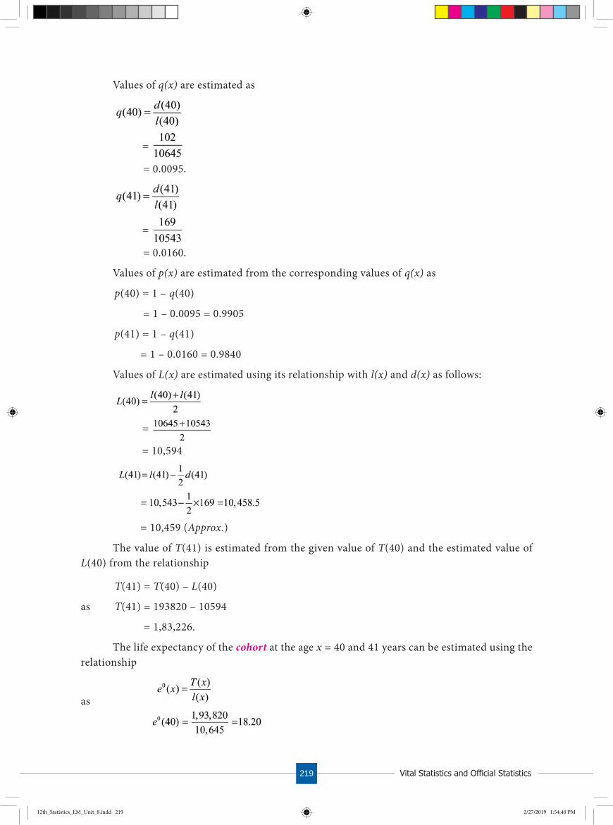
Vital Statistics and Official Statistics219
Values of q(x) are estimated as
=
= 0.0095.
=
= 0.0160.
Values of p(x) are estimated from the corresponding values of q(x) as
p(40) = 1 – q(40)
= 1 – 0.0095 = 0.9905
p(41) = 1 – q(41)
= 1 – 0.0160 = 0.9840
Values of L(x) are estimated using its relationship with l(x) and d(x) as follows:
=
= 10,594
= 10,459 (Approx.)
The value of T(41) is estimated from the given value of T(40) and the estimated value of L(40) from the relationship
T(41) = T(40) – L(40)
as T(41) = 193820 – 10594
= 1,83,226.
The life expectancy of the cohort at the age x = 40 and 41 years can be estimated using the relationship
as
12th_Statistics_EM_Unit_8.indd 219 2/27/2019 1:54:40 PM

22012t h S t d S t a t i s t i c s
Now, the completed Life Table becomes as
x l(x) d(x) p(x) q(x) L(x) T(x) e0(x)
40 10, 645 102 0.9905 0.0095 10,594 1, 93, 820 18.20
41 10, 543 169 0.9840 0.0160 10,459 1,83,226 17.37
Ex ample 8 .7
The following is a part of the Life Table constructed for a population, where the contents are incomplete. Evaluate the missing values using the given data and complete the Life Table.
x l(x) d(x) p(x) q(x) L(x) T(x) e0(x)83 3560 - - 0.16 - -84 - 508 - 0.17 - 11975
Solution:
Values of the missing entries can be estimated from the given data applying the respective formulae as follows:
The number of persons who die before reaching age of 83 years is calculated as
d(83) = l(83) × q(83)
= 3560 × 0.16
= 569.6 = 570
The value of the survivorship function l(x) at x = 84 years is estimated as
l(84) = l(83) – d(83)
= 3560 – 570
= 2990
Values of p(x) are estimated from the corresponding values of q(x) as
p(83) = 1 – q(83)
= 1 – 0.16 = 0.84
p(84) = 1 – q(84)
= 1 – 0.17 = 0.83
12th_Statistics_EM_Unit_8.indd 220 2/27/2019 1:54:40 PM

Vital Statistics and Official Statistics221
Values of L(x) are estimated using its relationship with l(x) and d(x) as follows:
=
= 3,275
L(84) = 2736.
The value of T(83) can be estimated from the given value of T(84) and the estimated value of L(83) from the relationship
T(84) = T(83) – L(83)
T(83) = L(83) + T(84)
as
T(83) = 3,275 + 11975 = 15,250
The life expectancy of the cohort at the age x = 83 and 84 years is estimated using the relationship
as
Now, the completed Life Table is as follows:
x l(x) d(x) p(x) q(x) L(x) T(x) e0(x)
83 3560 570 0.84 0.16 3275 15250 4.28
84 2990 508 0.83 0.17 2736 11975 4.01
Ex ample 8 .8A part of the Life Table of a population is given hereunder with incomplete information.
Find those information from the given data and complete the Life Table.
12th_Statistics_EM_Unit_8.indd 221 2/27/2019 1:54:41 PM

22212t h S t d S t a t i s t i c s
Age (in years)
l(x) d(x) p(x) q(x) L(x) T(x) e0(x)
72 4412 - - - - - -
73 3724 - - - - - -
74 3201 642 - - - 26567 -
Solution:
Values of the missing entries can be calculated from the given data applying the respective formulae as follows:
�e number of persons who die before reaching age x = 72 and 73 years can be calculated as
d(72) = l(72) – l(73)
= 4412 – 3724
= 688
d(73) = l(73) – l(74)
= 3724 – 3201
d(73) = 523.
Values of q(x) are estimated as
=
= 0.1559
=
q(73) = 0.1404
=
= 0.2006.
Values of p(x) are estimated from the corresponding values of q(x) as
p(72) = 1 – q(72)
= 1 – 0.1559 = 0.8441
12th_Statistics_EM_Unit_8.indd 222 2/27/2019 1:54:41 PM

Vital Statistics and Official Statistics223
p(73) = 1 – q(73)
= 1 – 0.1404 = 0.8596
p(74) = 1 – q(74)
= 1 – 0.2006 = 0.7994.
Values of L(x) are estimated using its relationship with l(x) and d(x) as follows:
=
= 4,068
=
= 3,463
=
= 2880.
The value of T(x) is estimated for x = 72 and 73 from the given value of T(74) and the estimated values of L(72) and L(73) as
= 3463 + 26567 = 30,030.
= 4068 + 30030 = 34,098.
The life expectancy of the cohort at the age x = 72, 73 and 74 years is estimated using the relationship
as
12th_Statistics_EM_Unit_8.indd 223 2/27/2019 1:54:42 PM
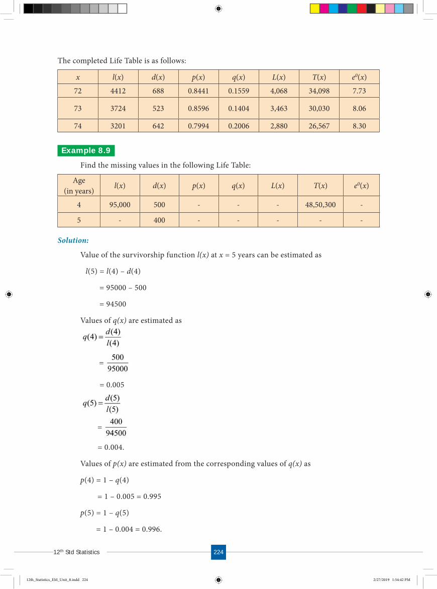
22412t h S t d S t a t i s t i c s
The completed Life Table is as follows:
x l(x) d(x) p(x) q(x) L(x) T(x) e0(x)
72 4412 688 0.8441 0.1559 4,068 34,098 7.73
73 3724 523 0.8596 0.1404 3,463 30,030 8.06
74 3201 642 0.7994 0.2006 2,880 26,567 8.30
Ex ample 8 .9Find the missing values in the following Life Table:
Age (in years)
l(x) d(x) p(x) q(x) L(x) T(x) e0(x)
4 95,000 500 - - - 48,50,300 -
5 - 400 - - - - -
Solution:
Value of the survivorship function l(x) at x = 5 years can be estimated as
l(5) = l(4) – d(4)
= 95000 – 500
= 94500
Values of q(x) are estimated as
=
= 0.005
=
= 0.004.
Values of p(x) are estimated from the corresponding values of q(x) as
p(4) = 1 – q(4)
= 1 – 0.005 = 0.995
p(5) = 1 – q(5)
= 1 – 0.004 = 0.996.
12th_Statistics_EM_Unit_8.indd 224 2/27/2019 1:54:42 PM

Vital Statistics and Official Statistics225
Values of L(x) are estimated using its relationship with l(x) and d(x) as follows:
=
= 94,750
=
= 94,300.
�e value of T(5) is estimated from the given value of T(4) and the estimate of L(4) as
T(5) = T(4) – L(4)T(5) = 4850300 – 94750 = 47,55,550.
�e life expectancy of the cohort at the age x = 4 and 5 years is estimated using the relationship
as
�e completed Life Table is
x l(x) d(x) p(x) q(x) L(x) T(x) e0(x)
4 95,000 500 0.995 0.005 94,750 48,50,300 51.06
5 94,500 400 0.996 0.004 94,300 47,55,550 50.32
8 .1.5 Fertility and its Measurements Fertility refers to births occurring to the women who are at child bearing age. A woman at
child bearing age is defined as the age of the female who can give birth to a child. In other words, it is the reproductive age of woman.
Fertility rates are the quantitative characteristics, which are used to measure the rate of growth of the population due to births during a specified period, usually a year. The fertility rates are expressed per thousand women who are at child bearing age.
As like mortality rates, there are several fertility rates. Among them, the following are the basic fertility rates discussed here
(i) Crude Birth Rate(ii) Specific Fertility Rate
(iii) General Fertility Rate
12th_Statistics_EM_Unit_8.indd 225 2/27/2019 1:54:43 PM
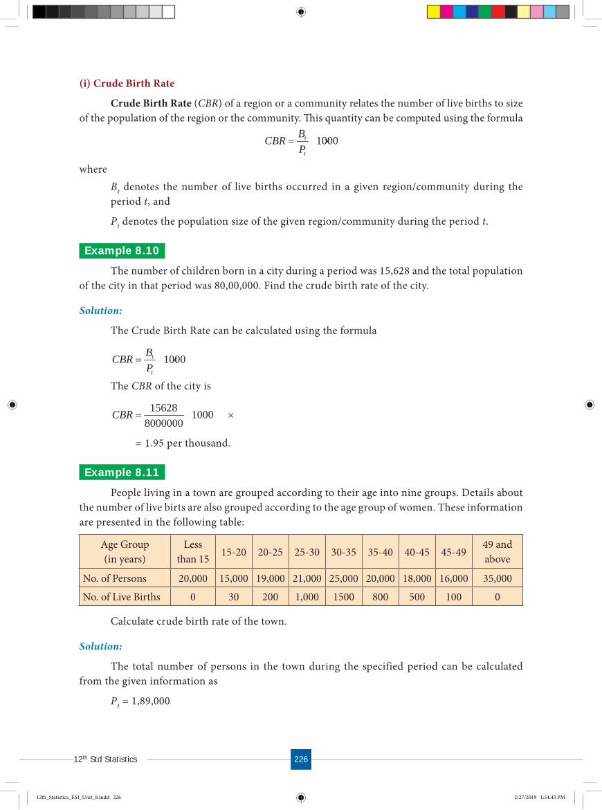
22612t h S t d S t a t i s t i c s
1000t
t
BCBRP×
where Bt denotes the number of live births occurred in a given region/community during the period t, and
Pt denotes the population size of the given region/community during the period t.
Ex ample 8 .10The number of children born in a city during a period was 15,628 and the total population
of the city in that period was 80,00,000. Find the crude birth rate of the city.
Solution:
The Crude Birth Rate can be calculated using the formula
1000t
t
BCBRP×
The CBR of the city is
15628 10008000000
CBR ×
= 1.95 per thousand.
Ex ample 8 .11People living in a town are grouped according to their age into nine groups. Details about
the number of live birts are also grouped according to the age group of women. These information are presented in the following table:
Age Group (in years)
Less than 15 15-20 20-25 25-30 30-35 35-40 40-45 45-49
49 and above
No. of Persons 20,000 15,000 19,000 21,000 25,000 20,000 18,000 16,000 35,000
No. of Live Births 0 30 200 1,000 1500 800 500 100 0
Calculate crude birth rate of the town.
Solution:
The total number of persons in the town during the specified period can be calculated from the given information as
Pt = 1,89,000
12th_Statistics_EM_Unit_8.indd 226 2/27/2019 1:54:43 PM
(i) Crude Birth Rate
Crude Birth Rate (CBR) of a region or a community relates the number of live births to size of the population of the region or the community. �is quantity can be computed using the formula

Vital Statistics and Official Statistics227
and the total number of live births as
Bt = 4,130.
Hence, the Crude Birth Rate of the town is4130 1000
189000CBR ×
= 21.85 per thousand.
is the simplest fertility rate, which provides a comprehensive idea about the population growth of any region/community. It is easy to compute for any given region.
However, CBR does not take into account of the age and gender distribution of the population or specifically the number of women at the child bearing age. This is a crude measure, since it includes the sections of the population who are not in the reproductive age group. It means that Pt includes the sections of the population who are not exposed to the risk of producing children, in particular, male and also the female beyond the reproductive age. CBR also assumes that all the women at child bearing age have the same reproductive capacity irrespective of their age, which is totally unrealistic.
(ii) General Fertility Rate
General Fertility Rate (GFR) of a region or a community relates the number of live births to the number of women in the reproductive age.
i.e., ×1000Number of live birthsGFRNumber of women at child bearing age
This quantity can be computed using the formula
2
1
1000ta
it
i a
BGFRP
×
where
itP denotes the number of women in the reproductive age i years in the given region/
community during the period t, i = a1 to a2.
In India, generally, a1 = 15 years and a2 = 49 years.
GFR overcomes the disadvantage of CBR considering only the women population at the child bearing age group, since the denominator in the above formula represents the entire women population at the reproductive age group. GFR expresses the increase in the women population at the child bearing age through live births.
However, GFR does not express the age composition of women population at the reproductive age group. Hence, two different regions/communities cannot be compared with respect to age of women using GFR.
12th_Statistics_EM_Unit_8.indd 227 2/27/2019 1:54:43 PM
22812t h S t d S t a t i s t i c s
Ex ample 8 .12Women, at child bearing age, of a district are grouped into seven age groups. The number
of women lived during a calendar year in the district and the number of live births recorded during the same period are as follows:
Age Group (in years) 15-20 20-25 25-30 30-35 35-40 40-45 45-49No. of Persons 20,000 22,000 28,000 32,000 29,000 24,000 8,000No. of Live Births 50 1500 1700 2,000 1800 500 80
Calculate the general fertility rate of the district.
Solution:
The total number of women, at child bearing age in the district during the study period can be calculated from the given information as
49
15
it
iP = 1,63,000
and the total number of live births as
Bt = 7,630.
Hence, the general fertility rate of the district is
7630 1000163000
GFR ×
= 46.81 per thousand.
(iii) Speci�c Fertility Rate (SFR)
It is a well known fact that fertility is affected by several factors such as age, marriage, migration, region etc. But, both CBR and GFR do not take into account of this fact. In this respect, Specific Fertility Rate (SFR) is defined as
SFR � Number of live births to the women population in the reeproductive age groups of specific section in a given periiod
Total number of women in the reproductive age groups off the specific section in the given period �1000
SFR can be calculated separately for various age groups of females who are at child bearing age such as 15-20, 20-25, and so on. The SFR computed with respect to different reproductive age of women is known as the Age Specific Fertility Rate (ASFR), which can be calculated using the formula
( , )( , ) 1000( , )
t
t
B x x nASFR x x nP x x n
×
where
( , )tB x x n denotes the number of live births to the women in the reproductive age group (x,x+n) during the period t in the given region, and
( , )tP x x n denotes the number of women in the reproductive age group (x,x+n) during the period t in the given region.
12th_Statistics_EM_Unit_8.indd 228 2/27/2019 1:54:48 PM

Vital Statistics and Official Statistics229
Ex ample 8 .13The female population, at reproductive age, of a country is grouped into six age groups.
The number of women in each group and the number of live births given by them are given the following table.
Age Group (in years) No. of Women No. of Live Births
15-20 1,16,610 10,668
20-25 1,13,810 17,183
25-30 1,03,130 12,722
30-35 93,500 7,283
35-40 74,120 3,656
40-45 62,900 1,340
Calculate the general fertility rate and the age specific fertility rates of the country.
Solution:
Total number of women in the country at reproductive age during the period of ‘t’ is44
15
it
iP = 5,64,070
and the total number of live births of the country during the same period is
Bt = 52,852
Therefore, the general fertility rate of the country is
52852= ×1000564070
GFR
= 93.69 per thousand.
The age specific fertility rates of the country can be calculated for each age group using the formula
( , )( , ) 1000( , )
t
t
B x x nASFR x x nP x x n
×
where
( , )tB x x n denotes the number of live births to the women in the reproductive age group (x,x+n) during the period t in the given region, and
( , )tP x x n denotes the number of women in the reproductive age group (x,x+n) during the period t in the given region.
12th_Statistics_EM_Unit_8.indd 229 2/27/2019 1:54:48 PM
Grouping of women with respect to their age is essential, since capacity of women to give birth to child varies over the age of women. Thus, ASFR enables to compare the fertility rates of two or more different regions with respect to specific age groups. Moreover, ASFR can be considered as a probability value.

23012t h S t d S t a t i s t i c s
�e ASFRs are calculated from the given information and are presented in the following table:
Age Group ASFR
15-2010668 ×1000 = 91.48
116610
20-2517183 ×1000 = 150.98
113810
25-3012722 ×1000 = 123.36
103130
30-357283 ×1000 = 77.89
93500
35-403656 ×1000 = 49.3374120
40-451340 ×1000 = 21.3062900
It is can be observed, with respect to ASFRs, that the women in the country falling in the age group of 20-25 years have given relatively more live births. The women at the age of 40-45 years have reproduced less number of live births.
Ex ample 8 .14The following is the data regarding the size of female population in a country at reproductive
age and the live births during a period.
Age Group (yrs) Female Population No. of Live Births
15–20 2,16,410 20,468
20–25 2,13,610 26,983
25–30 2,02,930 22,522
30–35 1,93,300 17,083
35–40 1,73,920 13,456
40–45 1,62,870 11,140
Calculate the general fertility rate and the age specific fertility rates of the country.
Solution:
Size of the women population of the country at reproductive age during the period ‘t’, is 44
15
it
iP = 11,63,040
and the total number of live births occurred during the same period in the country is
Bt = 1,11,652.
12th_Statistics_EM_Unit_8.indd 230 2/27/2019 1:54:48 PM

Vital Statistics and Official Statistics231
Hence, the general fertility rate of the country during the period is
GFR 111652GFR = × 10001163040
= 96.00
The age specific fertility rate of the country during the same period is calculated for each reproductive age group and the rates are presented in the following table:
Age Group (in years) ASFR
15 – 2020468 1000 94.58
216410×
20 – 2526983 1000 126.32
213610×
25 – 3022522 1000 110.98
202930×
30 – 3517083 1000 88.38
193300×
35 – 4013456 1000 77.37173920
×
40 – 4511140 1000 68.40162870
×
It can be observed, with respect to ASFR, that the women population of the country falling in the age group of 20-25 years have given relatively more live births. The women at the age of 40-45 years have reproduced less number of live births.
8 .1.6 Measurement of Population Grow thEvery human population, normally, may have a change in its size over a period of time.
Each change in the population size may be an increase or decrease in magnitude. Sometimes, the population size may remain without any change. Such a population is known as stable population. The tendency to increase in the population size may be called as population growth. Every government requires information about the rate of growth of its population.
If many new born babies in a population are female, the corresponding population size may increase. If gender of the infant deaths is female, change in the population size may be downward. Hence, fertility and mortality rates, individually, do not provide knowledge on population growth.
Quantitative ideas about the growth of a population can be obtained from several measurements. Among them,
(i) Crude Rate of Natural Increase, and
(ii) Pearl’s Vital Index
may be considered as the basic indicators of population growth. These two measures can be calculated using the following formulae
Crude Rate of Natural Increase = CBR – CDR
12th_Statistics_EM_Unit_8.indd 231 2/27/2019 1:54:49 PM

23212t h S t d S t a t i s t i c s
Pearl's Vital Index' 100CBRPearle s Vital IndexCDR
×
Positive values of Crude Rate of Natural Increase indicate the net increase in the population. Similarly, negative values of Crude Rate of Natural Increase indicate the net decrease in the population.
If Pearl’s Vital Index is greater than 100, then it can be regarded as the population is growing. On the other hand, if this index is less than 100, it can be regarded as the population is not growing. The above formula shows that the Vital Index can also provide knowledge on birth-death ratio of the population.
These two measures are simple and easy to calculate. They indicate whether the number of births exceeds the number of deaths. However, these two measures suffer from the limitations of CBR and CDR. They cannot be used for comparing two different populations. Also, information regarding whether the population has a tendency to increase or decrease cannot be obtained from these two measures.
8 .2 OFFICIAL STATISTICS
Official statistics are the statistical information published by government agencies or other public bodies, which are collected and compiled on various aspects for administrative purposes. Official Statistics are collected in a systematic manner through a well-established Statistical System. These information include quantitative and qualitative information on all major areas of citizens’ lives, such as economic and social development, living conditions, health, education and environment. Official statistics should be objective and easily accessible, produced on a continual basis so that measurement of change is possible. The following may be considered as the main functions of the Statistical System:
(i) collection, validation, compilation of data
(ii) publication/dissemination of the statistical information
(iii) maintenance of statistical standards such as definitions, classification, statisticalmethodology, comparability etc.
(iv) coordination of statistical activities
(v) training statistical personnel
(vi) independence and integrity of its functioning
(vii) international coordination
8 .2.1 Early History of Statistical System in IndiaStatistical data collection and compilation began in India during 321-298 BC and are
documented in Kautilya’s Arthasastra. Later, during the Moghul’s period, the details of Official Statistics can be found in Ain-i-Akbari written by Abul Fazal in Emperor Akbar’s rule during 1590 AD. It contains Official Statistics of various characteristics including land classification, crop yields, measurement system, revenue etc.
12th_Statistics_EM_Unit_8.indd 232 2/27/2019 1:54:49 PM

Vital Statistics and Official Statistics233
12th_Statistics_EM_Unit_8.indd 233 2/27/2019 1:54:49 PM
In British India, a statistical survey was conducted, in the year 1807 by Dr.Francis Buchanan, Governor-in-Council of East India Company. Information were collected regarding topographical account of each district, conditions of the inhabitants, their religion and customs, details of fisheries, mines and forests, farm sizes, vegetables grown, commerce, list of useful plants and seeds. An Official Statistical System was established in India by Col. Sykes during 1847 with a Department of Statistics in India House. The first Census Report of India was published in 1848. The second Census Report was published in 1881 and since then Census was conducted every 10 years.
8.2.2 Post-Independence Indian Official Statistical SystemAfter Independence, the need for a statistical system for monitoring socio-economic
development of the country was felt by the Government of India. In 1949, Shri.P.C.Mahalanobis was appointed by the Government of India as the Honorary Statistical Advisor to the government. In the same year, he established the Central Statistical Unit. This Unit was renamed, in 1951, as Central Statistical Organization, which coordinated various statistical activities in the country. It also defined and maintained statistical standards in the country.
During the same period, National Income Committee was established in 1949 to estimate the National Income of the country. The Committee recommended the use of sampling methods for collecting information in order to fill the large gaps in the statistical information required for estimation of the National Income. Sample surveys were conducted at national level for this purpose. The first round of National Sample Survey was conducted in October 1950. Later, a separate organization under the government set-up for conducting sample surveys was formed in the name of National Sample Survey Organization.
The Central Statistical Organization and National Sample Survey Organization are now called respectively as Central Statistics Office (CSO) and National Sample Survey Office (NSSO).
The Ministry of Statistics and Programme Implementation (MoS&PI), a ministry with independent charge in the Government of India, was formed on October 15, 1999 with two wings, viz., National Statistical Office (NSO) and Programme Implementation.
The Government of India set up a Commission in the year 2000 under the headship of Shri.C.Rangarajan to address the growing statistical needs of the country. Based on the recommendations of the Commission, a permanent and statutory apex body, called National Statistical Commission (NSC), was set up in NSO on July 12, 2006. The NSC was formed to evolve policies, priorities and to maintain quality standards in statistical matters.
The NSC is constituted with an eminent statistician or a social-scientist as its Chairperson and four members - one each from the areas of Economic Statistics; Social and Environmental Statistics; Census Operations, Surveys and Statistical Information System; and National Accounts. The Chief Statistician of India is the Secretary of the Commission and the Chief Executive Officer of NITI Aayog of Planning Commission of India is an ex-officio member of NSC. The Chief Statistician of India is the Head of National Statistical Office and Secretary of the MoS&PI. NSC, in addition to the above responsibilities, also performs the functions of Governing Council of the NSSO since August 30, 2006.
Presently, the main sections of NSO are NSC, CSO, NSSO and a Computer Center.

23412t h S t d S t a t i s t i c s
This division is responsible for
• preparation of national accounts including Gross Domestic Product
• preparation of quarterly estimates of Gross Domestic Product
• estimation of Capital Stock and Consumption of fixed capital
• estimation of State-wise Gross Value Added and Gross Fixed Capital Formation
• preparation of Input-Output Transaction Tables, and
• preparation of comparable estimates of State Domestic Product.
(ii) Social Statistics Division
This division is responsible for
• statistical monitoring of the Millennium Development goals
• preparation and maintaining environmental economic accounting
• grant-in-aid for research, workshop/seminars/conferences in Official/Applied Statistics
• national/international awards for statisticians
• preparation of National Data Bank on socio-religious categories
• basic statistics for Local Level Development Pilot scheme
• conduct of time-use surveys and release of regular and ad hoc publications.
National Statistics Day and World Statistics Day�e Government of India declared 29th June, the birthday of Prof. P.C. Mahalanobis, as the National Statistics Day to honour his contribution to the establishment of O�cial Statistical System in India.As a part of the celebration of this day, essay writing competitions are conducted nationwide among postgraduate students of Statistics. �e winners are honoured with awards during the celebrationat New Delhi. �e �rst National Statistics Day was celebrated on June 29, 2007.
United Nations Statistical Commission declared October 20 as the World Statistics Day. It is celebrated every �ve years in almost all the countries focussing on speci�c theme. �e �rst World Statistics Day was celebrated all over the world on October 20, 2010. �e second World Statistics Day was celebrated on October 20, 2015 on the theme Better Data, Better Lives to emphasize the important role of high quality o�cial statistical information in decision-making.
All the government departments, educational departments and others dealing with Statistics take part in celebration of National Statistics Day as well as World Statistics Day.
�e year 2013 was observed as the International Year of Statistics.
12th_Statistics_EM_Unit_8.indd 234 2/27/2019 1:54:49 PM
8.2.2.1 Central Statistics O�ce
The Central Statistics Office is responsible for coordination of statistical activities in the country, and evolving and maintaining statistical standards. CSO is headed by a Director General, who is assisted by five Additional Director Generals. The CSO has five main divisions. The divisions and their responsibilities are presented below:
(i) National Accounts Division

Vital Statistics and Official Statistics235
(iii) Economic Statistics Division
This division is responsible for
• conducting Economic Census and Annual Survey of Industries• compiling All India Index of Industrial Production• collecting and compiling Energy Statistics and Infrastructure Statistics• developing classifications like, National Industrial Classification and National Product
Classification.
(iv) Training Division
This division is responsible for
• training manpower in theoretical and applied statistics to deal with the challenges of datacollection, compilation, analysis and dissemination of information for policy making,planning, monitoring and evaluation
• looking after the National Statistical Systems Training Academy, which is a premier institutefor developing human resource to deal with Official Statistics in India as well as at internationallevel.
(v) Coordination and Publications Division
This division is responsible for
• coordinating the works related to statistical matters within CSO and the Ministries of CentralGovernment and State/UT Governments
• organizing Conferences of Central and State Statistical Organizations• celebration of National Statistics Day every year
The State and Central Governments recruit professionals, who are trained in applications of statistical methods, for appointment as Statistical Investigators, Assistant Directors. Most of the statisticians in CSO, NSSO and in ministries now qualify Indian Statistical Service (ISS) examination conducted by Union Public Service Commission. They are trained by the National Statistical Systems Training Academy.
The first Economic Census was conducted in 1977.
The Second Five Year Plan of India followed the model developed by Prof. P.C. Mahalanobis, which focused on public sector development and rapid industrialization. The Government of India honoured him with one of the highest civilian awards Padma Vibhushan. The Government of India released a stamp on June 29, 1993 in commemoration of his 100th birthday. Recently, the Government of India released a commemorative coin on June 29, 2018 during the celebration of his 125th birthday.
12th_Statistics_EM_Unit_8.indd 235 2/27/2019 1:54:49 PM

23612t h S t d S t a t i s t i c s
• preparation of Results Framework Document, Citizens’ Charter, Annual Action Plan andOutcome Budget of the MoS&PI
• implementation of Capacity Development Scheme and Support for Statistical Strengtheningwith an aim of improving the Capacity and Infrastructure of the State Statistical System forcollection, compilation and dissemination of reliable Official Statistics for policy making
• coordinating implementation of recommendations of NSC• administrative works related to Indian Statistical Institute.
8.2.2.2 National Sample Survey O�ce
National Sample Survey Office (NSSO), headed by a Director General, is responsible for conduct of national level large scale sample surveys in diverse fields. Primarily, data are collected through nation-wide household surveys on various socio-economic subjects. Besides these surveys, NSSO collects data on rural and urban prices and plays a significant role in the improvement of crop statistics through monitoring the area enumeration and crop estimation surveys of the State agencies. It also maintains a sampling frame of urban area units for conducting sample surveys in urban areas.
NSSO has four divisions. The divisions and their responsibilities are listed below:
(i) Survey Design and Research Division
This division, located at Kolkata, is responsible for
• technical planning of surveys• formulation of concepts and definitions• preparation of sampling design• designing of inquiry schedules• drawing up of tabulation plan• analysing and presenting survey results.
(ii) Field Operations Division
The headquarters of this division is at Delhi. This division has a network of 6 Zonal Offices, 49 Regional Offices and 118 Sub-Regional Offices spread throughout the country. This division is responsible for collection of primary data for the surveys undertaken by NSSO.
(iii) Data Processing Division
The Division, with its headquarters at Kolkata and 6 Data Processing Centers at various places, is responsible for
• selection of sample subjects• developing relevant software• processing, validation and tabulation of the data collected through surveys.
12th_Statistics_EM_Unit_8.indd 236 2/27/2019 1:54:49 PM

Vital Statistics and Official Statistics237
(iv) Coordination and Publications Division
This Division, located at New Delhi, is responsible for
• coordinating all the activities of different Divisions of NSSO• publishing the bi-annual journal of NSSO, titled “Sarvekshana”• organizing National Seminars on the results of various socio-economic surveys undertaken
by NSSO.
8 .2.3 Present Statistical System in IndiaIn addition to the role played by CSO and NSSO, most of the Central Ministries collect
statistical information on the subjects related to the respective ministries. �e statistical information are collected as by-products of administration of the ministries or for monitoring the progress of speci�c programmes implemented by the respective ministries. Some Ministries in Government of India, like Agriculture, Water Resources, Health, Finance, Commerce, Labour, and Industrial Development have separate statistical divisions, while most others have nucleus cells.
The Statistical System in the States is similar to the system at the Central Government. A Directorate of Economics and Statistics, functioning in each State under a decentralized system, is a nodal agency, which is responsible for the coordination of statistical activities in the State. The Directorates have statistical offices at the headquarters in each district. The district level offices collect statistical information related to all sections of economy of the respective district. The Directorates compile and publish such information as Statistical Hand Books every year. The Hand Books contain several information including estimates of area, production and yield of principal crops. In Tamil Nadu, the Directorate is functioning with the nomenclature “Department of Economics and Statistics”. This department, with headquarters at Chennai, is headed by a Commissioner, who is assisted by a Director, 3 Additional Directors and 2 Joint Directors, in addition to Assistant Directors and supportive officials.
Generally, flow of statistical information in Indian Statistical System is upwards from village → block → district → State Government Departments → corresponding Ministries at the Centre.
In addition to CSO, NSSO and the Ministries, there are other public and private organizations in India, which also deal with collection of Official Statistics on various characteristics. Reserve Bank of India is one such organization, which collects, compiles and publishes, every year, the statistical information related to economy of the country as the “Hand Book of Indian Economy”.
12th_Statistics_EM_Unit_8.indd 237 2/27/2019 1:54:49 PM

23812t h S t d S t a t i s t i c s
POINTS TO REMEMBER
�� Vital Statistics are quantitative measurements on live births, deaths, foetal deaths, infantdeaths, fertility and so on.
�� Data on vital events are collected adopting the �ve methods - Civil Registration System,Census or Complete Enumeration method, Survey method, Sample Registration System and Analytical method.
�� Census method normally covers data regarding age, sex, marital status, educational level,occupation, religion and other factors needed for computing vital statistics. Census is conducted in most countries at intervals of ten years.
�� Rates of vital events are usually expressed ‘per thousand’.
�� Crude Death Rate =
No. of deaths in the population or community during the given period 1000Total number of persons in the population or community during the given period
×
�� Speci�c Death Rate =
No. of deaths in a specific section of the population during the given period 1000Total number of persons in the specific section of the population during the given period
×
�� Infant Mortality Rate =
No. of infant deaths in a population during the given period 1000Number of live births in the population during the given period
×
�� Cohort is a group of individuals who born at the same time and experienced the samemortality conditions.
�� A Life Table exhibits the number of persons living and dying at each age, on the basis of theexperience of a cohort, which also gives the life expectancy of the population.
�� Radix of a Life Table refers to the number of survivors at the beginning of the table.
�� Crude Birth Rate =
No. of live births in the population during the given period 1000Total number of persons in the population during the given period
×
�� General Fertility Rate = No. of live births occurred in the population during the given period 1000
Total number of women at the reproductive age in the population during the given period×
12th_Statistics_EM_Unit_8.indd 238 2/27/2019 1:54:49 PM

Vital Statistics and Official Statistics239
EXERCISE 8
I. Choose the best answer.
1. One of the branches of Demography is(a) Economic Statistics (b) Vital Statistics(c) Official Statistics (d) Agricultural Statistics
2. When there is no proper system of recording births and deaths, Vital Statistics are collectedthrough(a) Registration Method (b) Census Method(c) Survey Method (d) Analytical Method
3. Compulsory registration of births and deaths was implemented in India, during the year(a) 1947 (b) 1951 (c) 1969 (d) 1970
4. Rates of vital events are usually measured as(a) per ten lakh (b) per ten thousand(c) per thousand (d) per hundred
5. Death of a child before the child’s fifth birth day is measured by(a) crude death rate (b) specific death rate(c) infant mortality rate (d) child mortality rate
�� Speci�c Fertility Rate =Number of live births to the women population in the reprodductive age groups of specific section in a given period
Tootal number of women in the reproductive age groups of thee specific section in the given period ×1000
�� Crude Rate of Natural Increase = Crude Birth Rate – Crude Death Rate
�� Pearl's Crude Birth RatePearle's Vital Index= ×100Crude Death Rate
�� O�cial statistics are the statistical information collected and compiled on various aspectsincluding all major areas of citizens’ lives, such as economic and social development, living conditions, health, education and environment.
�� An O�cial Statistical System was established in India by Col. Sykes during 1847 with aDepartment of Statistics in India House. �e �rst Census Report of India was published in 1848.
�� �e Central Statistics O�ce is responsible for coordination of statistical activities in thecountry, and evolving and maintaining statistical standards, which has �ve main divisions.
�� National Sample Survey O�ce (NSSO), headed by a Director General, is responsiblefor conduct of national level large scale sample surveys in diverse �elds, which has four divisions.
12th_Statistics_EM_Unit_8.indd 239 2/27/2019 1:54:50 PM

24012t h S t d S t a t i s t i c s
6. Death rates due to different kinds of diseases can be calculated using(a) crude death rate (b) infant mortality rate(c) specific death rate (d) vital index
7. History of a cohort can be understood from(a) mortality rates (b) life table(c) fertility rates (d) population growth
8. Total number of women at child bearing age group is used to calculate(a) crude birth rate (b) general fertility rate(c) age specific fertility rate (d) population growth
9. Population growth can be measured using(a) crude birth rate, specific death rate(b) general fertility rate, infant mortality rate(c) specific fertility rate, specific death rate(d) crude birth rate, crude death rate
10. Vital Index measures(a) birth-death ratio (b) rate of vital event(c) infant mortality rate (d) general fertility rate
11. The first census Report of India was published in(a) 1858 (b) 1848 (c) 1948 (d) 1958
12. Department of Statistics in India House was established in India by Col. Sykes during(a) 1847 (b) 1947 (c) 1857 (d) 1887
13. The first Honorary Statistical Advisor to Government of India is(a) P.C. Mahalanobias (b) Col. Sykes(c) C. Rangarajan (d) Dr. Francis Buchanan
14. Ministry of Statistics and Programme Implementation was formed on(a) October 2, 1959 (b) October 15, 1999(c) November 13, 1969 (d) November 15, 1999
15. Secretary to MoS&PI and Head of NSO is(a) Chairman, Planning Commission (b) Director, NSSTA(c) Chief Statistician of India (d) CEO, NITI Aayog
16. National Statistical Commission was formed on(a) January 12, 2006 (b) April 12, 2006(c) June 12, 2006 (d) July 12, 2006
17. Celebration of National Statistics Day is one of the responsibilities of ______ Division ofCSO.(a) Coordination and Publications (b) Training(c) Social Statistics (d) Economic Statistics
12th_Statistics_EM_Unit_8.indd 240 2/27/2019 1:54:50 PM

Vital Statistics and Official Statistics241
18. Collection of primary data for the surveys undertaken by NSSO is one of the responsibilitiesof _______ Division.(a) Survey Design and Research (b) Field Operations(c) Data Processing (d) Coordination and Publications
19. NSSO publishes the bi-annual journal(a) Sarvekshana (b) Sankhya (c) Pramana (d) Yojana
20. “Hand Book of Indian Economy” is published periodically by(a) State Bank of India (b) Reserve Bank of India(c) NSO (d) Ministry of Economics
II. Give very short answer to the following questions.21. What is Registration method?22. Define rate of vital event.23. Mention the purpose of Analytical method in collecting Vital Statistics.24. What is meant by mortality?25. What is known as fertility?26. What is cohort?27. What is called radix of Life Table?28. How will you calculate expectation of life?29. Write down the formula to compute crude death rate.30. What is the formula used to compute infant mortality rate?31. Define crude birth rate.32. What is specific fertility rate?33. Write down the formula to compute general fertility rate.34. Define vital index.35. Specify the difference between crude birth rate and general fertility rate.36. What are known as Official Statistics?37. What were the Official Statistics collected by East India Company?38. What were the earlier attempts made in India before British rule for collection of O�cial Statistics?39. What are the wings of MoS & PI?40. What are the divisions of CSO?41. List the divisions of NSSO:42. Which Ministries of Government of India have separate statistical divisions?
III. Give short answer to the following questions.
43. Write down the definitions of Vital Statistics.44. Write a brief note on Census Method of collecting Vital Statistics.
12th_Statistics_EM_Unit_8.indd 241 2/27/2019 1:54:50 PM
24212t h S t d S t a t i s t i c s
45. What are various information collected under Sample Registration System?46. If the number of deaths occurred is 980 in a town consisting of 1,50,000 persons during a
period, quantify the death rate of the town using suitable formula.47. Population size of a Hamlet in a hill station during a calendar year was 55,000 and the number
of deaths recorded in the Hamlet during the same year was 185. What is the crude death rateof the village?
48. The number of women at reproductive age in a district is 70,000. Also, the number of livebirths and infant deaths registered in the district are respectively 10,000 and 70. Whichmortality rate you will calculate? What is its value?
49. A Primary Health Centre located in a village has a record of 135 live births during a year. Thenumber of deaths recorded in the village was 300. Among them, 5 are new born babies of ageless than a year. Measure the infant mortality rate of the village.
50. What is specific death rate? What are its uses?51. List various uses of Life Table.52. What are the assumptions made in the construction of Life Table?53. Population size of a District during a calendar year was 1,25,526. Also, the number of live
births registered in the district during the same period was 987. Compute appropriate vitalrate using this information.
54. The number of women at child bearing age in a tribal village during a year was 2275 and thenumber of new born babies of age less than a year in the same village was 23. How will youquantify the birth rate of the village? Find its value.
55. Write a brief note on specific fertility rate.
IV. Give detailed answer to the following questions.
56. What are the importance of Vital Statistics?
57. Calculate crude death rate of a population living in a town from the following data:
Age Group (in years) 0-10 10-20 20-40 40-60 60 and aboveNo. of Persons 6500 12,000 24,000 20,000 8,000No. of Deaths 25 37 30 90 100
58. The number of deaths registered in a district with respect to age during a year and thepopulation size in each age group are given below. Calculate the crude death rate of thedistrict for the period.
Age Group (in years) Below 15 15-25 25-40 40-65 65 and aboveNo. of Persons 40,000 88,000 90,000 60,800 23,000No. of Deaths 40 62 100 78 20
12th_Statistics_EM_Unit_8.indd 242 2/27/2019 1:54:50 PM

Vital Statistics and Official Statistics243
59. The population of a District during a Census year was grouped into 8 age groups. The dataregarding the number of deaths and the population size for each age group are given hereunder.
Age Group (in years)
0-5 5-15 15-25 25-40 40-50 50-60 60-6565 and above
No. of Persons (in '000)
42,345 19046 93,578 30,724 28,874 62,087 28,473 37,693
No. of Deaths 900 798 512 186 174 213 475 883
Calculate the age specific death rates of the District.
60. Calculate the specific death rates for each age group of a population, whose size and thenumber of deaths are given in the following table:
Age Group (in years) Below 10 10-20 20-40 40-60 60 and aboveNo. of Persons 36,000 28,000 62,000 52,000 18,000No. of Deaths 682 204 576 878 725
61. What are the different components and their formulae of Life Table?
62. Find the missing entries in the following Life Table.
Age (in years) l(x) d(x) p(x) q(x) L(x) T(x) e0(x)
25 75818
26 75445 2722331
27 75039 0.009
63. There are missing entries in some of the columns in the following Life Table. Find the valuesof the missing entries.
Age (in years) l(x) d(x) p(x) q(x) L(x) T(x) e0(x)
42 64711 1513333
43 63787
44 62821 62310
64. The following is a section of a Life Table with some missing entries. Complete the Life Table.
Age (in years) l(x) d(x) p(x) q(x) L(x) T(x) e0(x)
36 69818
37 69032
38 68212 850 1779254
12th_Statistics_EM_Unit_8.indd 243 2/27/2019 1:54:50 PM

24412t h S t d S t a t i s t i c s
65. Calculate crude birth rate from the following data:
Age Group (in years) 15-20 20-25 25-30 30-40 40-49No. of Perosns 16,000 18,000 14,000 15,000 28,000No. of Live Births 25 30 38 28 14
66. The women population at reproductive age in a State are grouped and the population size ineach group are given hereunder. The number of live births given by the women in each groupare also presented. Find the general fertility rate of the State. Also, calculate the age specificfertility rate for each group.
Age Group (in years)
15-20 20-25 25-30 30-35 35-40 40-45 45-49
No. of Women 2,12,724 1,89,237 2,45,367 1,32,109 1,29,645 90,708 34,975No. of Live Births 20,209 23,655 37,787 12,815 9,723 4,898 874
67. The number of live births occurred in a District during a calendar year are classified accordingto the age of mother. The female population size at child bearing age are also given.
Age Group (in years)
15-20 20-25 25-30 30-35 35-40 40-45 45-49
No. of Women 4,729 6,236 8,034 9,408 5,907 4,657 2,975No. of Live Births 356 845 970 1,878 856 608 452
Calculate the general fertility rate of the District. Also, calculate the specific fertility rates for each of the reproductive age group.
68. The following are the information registered about the number of live births and the femalepopulation size in a town during a calendar year.
Age Group (in years)
15-20 20-25 25-30 30-35 35-40 40-45 45-49
No. of Women 1,276 3,253 5,628 7,345 6,901 4,253 3,957No. of Live Births 218 361 693 1,305 1,031 634 390
Calculate from these information the general fertility rate of the town and the age specific fertility rates for the year.
12th_Statistics_EM_Unit_8.indd 244 2/27/2019 1:54:50 PM

Vital Statistics and Official Statistics245
ANSWERS
I. 1. (b) 2. (c) 3. (d) 4. (c) 5. (d)
6. (c) 7. (b) 8. (b) 9. (d) 10. (a)
11. (b) 12. (a) 13. (a) 14. (b) 15. (c)
16. (d) 17. (a) 18. (b) 19. (a) 20. (b)
III. 46. CDR = 6.53 47. CDR = 3.36 48. IMR = 7.00 49. IMR = 37.04
53. CBR = 7.86 54. GFR = 10.11
IV. 57. CDR = 4.00 58. CDR = 0.99
59.
Age Group (in years)
0-5 5-15 15-25 25-40 40-50 50-60 60-6565 and above
ASDR 21.25 41.90 5.47 6.05 6.03 3.43 16.68 23.43
60.
Age Group (in years)
Below 10 10-20 20-40 40-60 60 and above
ASDR 18.94 7.29 9.29 16.88 40.28
62.
x l(x) d(x) p(x) q(x) L(x) T(x) e0(x)
25 75818 373 0.9951 0.0049 75632 27,97,968 36.90
26 75445 406 0.9946 0.0054 75242 27,22,331 36.08
27 75039 675 0.9910 0.0090 74702 26,47,629 35.28
63.
x l(x) d(x) p(x) q(x) L(x) T(x) e0(x)
42 64711 924 0.9857 0.0143 64249 1513333 23.39
43 63787 966 0.9849 0.0151 63304 1449084 22.72
44 62821 1022 0.9837 0.0163 62310 1385780 22.06
64.
x l(x) d(x) p(x) q(x) L(x) T(x) e0(x)
36 69818 786 0.9887 0.0113 69425 1917301 27.46
37 69032 820 0.9881 0.0119 68622 1847876 26.77
38 68212 853 0.9875 0.0125 67787 1779254 26.08
12th_Statistics_EM_Unit_8.indd 245 2/27/2019 1:54:50 PM

24612t h S t d S t a t i s t i c s
References
Mukhopadhyay, P.(2016). Applied Statistics. Books and Allied (P) Ltd., Kolkata.
Goon, A.M., Gupta M. K. and Das Gupta B. (2016). Fundamentals of Statistics, Vol. 2. The World Press pvt Ltd, Kolkatta.
Rao, T.J. (2010). Official Statistics in India: The Past and the Present. Journal of Official Statistics, Vo. 26(2), 215-231.
Rao, T.J. (2013). National Statistical Commission and Indian Official Statistics. Resonance, December, 1062-1072.
65. CBR = 1.48
66. GFR = 106.27
Age Group (in years)
15-20 20-25 25-30 30-35 35-40 40-45 45-49
ASFR 95.00 125.00 154.00 97.00 75.00 54.00 24.99
67. GFR = 142.21
Age Group (in years)
15-20 20-25 25-30 30-35 35-40 40-45 45-49
ASFR 75.28 135.50 120.74 199.62 145.06 130.56 151.93
68. GFR = 142.03
Age Group (in years)
15-20 20-25 25-30 30-35 35-40 40-45 45-49
ASFR 170.85 110.97 123.13 177.67 149.40 149.07 98.56
12th_Statistics_EM_Unit_8.indd 246 2/27/2019 1:54:51 PM

P r o j e c t W o r k247
IntroductionA mechanical engineer has to spend time in an Industry as an apprentice, a medical doctor
with a hospital as a house surgeon, an auditor with an accountant, a budding lawyer with an established senior as a junior to get to know intricacies of the profession in his day to day affairs. Where is the counterpart of this for a student studying Statistics? It is in this background, the inclusion of project work in the curriculum gains importance. This would help to some extent to bridge the gap between the theory learned in the class room and application.
Project Work is a student-centered pedagogy in which students learn about a subject through the experience of solving an open-ended problem. � is necessitates to synthesize knowledge from various areas of learning, and critically and creatively apply it to real life situations.
� e student will be able to
� Design a questionnaire for a given project� Collect data using questionnaire.� Compile and tabulate the collected data.� Statistically analyze the data�Write a brief report
LEARNING OBJECTIVES
PROJECT WORKCHAPTER
9
12th_Statistics_EM_Unit_9.indd 247 3/1/2019 12:44:53 PM

248 P r o j e c t W o r k24912t h S t d S t a t i s t i c s
Characteristics
�e Project work is an assignment to be carried out by students during the course, eitherindividually or in a group under supervision of the teacher. A brief written report of this work is an integral part of the assignment. �us the project work is a complete assignment. . It contains the levels of planning, execution, analysis and reporting the work done.
Advantages
1. Formulating a real world problem with statistical perspective, student acquires applicationknowledge through the completion of the project.
2. Project works provides the knowledge about systematic collection of data, organization of ideasand an ability to analyze them with in a stipulated time. �e following intangible bene�ts will bederived on completion of the project work.
� Development of the capacity to identify and correctly specify statistical problem.� Being aware of the assumptions and the steps to validate them.� Ability to interpret results.� Development of report writing skill.
3. It pave the way for interaction with the respondents, the ability to �t into a team, provides co-operation and provides interaction among the students and between the teachers.
4. It gives them a sense of involvement and commitment.
9.1 DESIGNING A PROJECT
There are Six stages while doing a project work.
� Stage 1 - Identify the topic of the project work� Stage 2 - De�ne Your Goals. Formulate Objectives / Hypothesis� Stage 3 - Develop Your project work Plan.� Stage 4 - Collection of Data and creating a data �le.� Stage 5 - Analyze Data� Stage 6 - Report writing
Stage 1 . Fixing the project work topic
�e �rst and foremost stages of any project work is identifying the topic of the project work. �esources for selecting the topic include (i) individual experiences, (2) personal conversation, (4) day-to-day practical experience, (5) Social problems (6) Politics like opinion poll.
The criteria for fixing the topic depends about data availability, time period to complete a research, availability of expertise.
12th_Statistics_EM_Unit_9.indd 248 3/1/2019 12:44:53 PM

248 P r o j e c t W o r k249
Stage 2. Clearly state the objectives / Formulate Hypotheses
Objectives:
�e aspects, the project worker want to probe in the project be spelt out in clear terms as objectives. Research should not proceed until objectives are clearly spelt out.
Hypothesis
Hypothesis is the perception of the researcher. It is stated as a testable proposition subject to empirical veri�cation. Some times it is called as research hypothesis.
Stage 3: Project work planning
It involves selecting the most appropriate methods of (i) selecting respondents, (ii) method of collecting the data, (iii) selecting the data gathering instrument and test for its reliability and validity reliability and (iv) techniques to solve the problem under investigation. Designing a research project can be compared to that of an architect designing a building. It is a plan or blue print for collection, analysis and interpretation of data.
Stage 4: Data collection and data file preparation
Once the project plan is ready, the student will know from whom/ where to collect the data and the data gathering instrument. Now he moves to collect the required data.
Data file preparation involves entering in a spread sheet and checking for errors if any.
Stage 5: Statistical Data Analysis
�is activity is most important. Here, we select the appropriate statistical tool for data analysis.�is necessitates a good conceptual clarity and application understanding of the subject. The selectionof statistical tool primarily depends on Research Objective. And subsequently on the variables involved,its measurement scale (nominal, ordinal and scale ) and number of variables considered at a time.
Stage 6: Report writing
�e important step in any project study is that of preparing the project report. �e report recordsthe purpose, the importance, the procedure, the �ndings, the limitations and the conclusion of the project study. �is should be prepared in such a way that it is easily understood and is helpful to other research or project workers in a similar �eld.
9.2 PROJECT WORK PLAN
A project work plan find the answers to the following host of questions:
12th_Statistics_EM_Unit_9.indd 249 3/1/2019 12:44:53 PM

250 P r o j e c t W o r k25112t h S t d S t a t i s t i c s
1. What is study about?
2. Why is the study being made? (Motivation of the study)
3. Where will the study be carried out? (Scope of coverage)
4. What type of data is required? (Survey data / Experimental data)
5. What are instruments needed? (Questionnaire / Instruments)
6. From whom can be required data be found? (Where to collect? Target group?)
7. What periods of time will study include? (How many times to collect?)
8. What techniques of data collection will be used? (Which method to follow?)
9. How the data will be analyzed?
9.3 QUESTIONNAIRE DEVELOPMENT PROCESS
Questionnaire Format
It consists of two parts namely (1) Questions and (2) Responses.
Questions RESPONSES
1. Name2. Age (in completed years)3. Sex
----------------------------------------_______ Years 1. Male 2. Female
Once the researcher has decided on the speci�c type of questions and the response formats, the next task is the actual writing of the questions. �e wording in speci�c questions always poses signi�cant time investment for the researcher. �e general guidelines are useful to bear in mind during the wording and sequencing of each question.
Characteristics of a questionnaire
��e wording must be clear� Select words so as to avoid biasing the respondent� Consider the ability of the respondent to answer the question� Create the willingness of the respondent to answer the questions.
Excellent:SURVEY
Good:Fair:
Poor:
12th_Statistics_EM_Unit_9.indd 250 3/1/2019 12:44:54 PM
250 P r o j e c t W o r k251
• Is the question necessary?• Is the survey too long?• Will the question provide the answers to the survey objectives?
Pre-Test
A�er the questionnaire is prepared, pre-test is to be done. �e process collecting information from the related respondent in small number with the framed questionnaire is called Pre-Test. Sometimes, the questionnaire is circulated among some competent investigators and they are asked to make suggestions for its improvement. Once this has been done and suggestion incorporated in the �nal form of the questionnaire is ready for the collection of data.
9.4 FEATURES OF A PROJECT REPORT
Features of a project report.
�e general structure of a project report consists of three main divisions.
A. The Preliminary Section:
�is includes the title page, the preface, the acknowledgement, the table of contents and the listof tables and �gures.
B. The Main Body Or The Text Of The Project :
�is contains the introduction to the problem, the review of previous research in a similar �eld,the details of the procedure, the �ndings, the analysis of that, and conclusions.
C. The Reference section :
�is includes Foot Notes, Bibliography Appendix , Index, etc.
LANGUAGE OF THE REPORT:
Report should be written in a simple language. It should be clear, precise and simple in style, and brief. It should be written in third person or passive voice. Spelling mistakes, colloquial form of presentation should be avoided. Spelling of non-English words, if used, should be kept uniform throughout.
12th_Statistics_EM_Unit_9.indd 251 3/1/2019 12:44:54 PM
Evaluate the Questionnaire
Once a rough draft of the Questionnaire has been designed the researcher is obligated to take a step back and critically evaluate it. �is phase may seem redundant, given all the careful thoughts that went into each question. But recall the crucial role played by the questionnaire. At this point in the questionnaire development of the following item should be considered.

252 P r o j e c t W o r k25312t h S t d S t a t i s t i c s
EXERCISE 9
I. Choose the best answer.
1. Which one is the correct sequence of activities in project work?a) formulating objectives, report writing, data analysis, project work planb) report writing, data analysis, project work plan , formulating objectivesc) formulating objectives, data analysis report writing, , project work pland) formulating objectives, , project work plan, data analysis, report writing.
2. Qualitative data implies:a) Measurable b) Non measurable c) Partly measurable d) All the above
3. The measurement scale of ‘taste of a coffee’ is :a) Nominal b) Ordinal c) Interval d) Ratio
4. When the researcher uses the data of an agency, then the data is called:a) Quantitative data b) Qualitative datac) Secondary data d) Primary data
5. Opinion poll in a study is conducted:a) Before the process start b) After the process startc) Middle of the process d) At any point of time of the process
6. a) Independent variable b) Dependent variablec) Intervening variable d) Extraneous variable
7. Which one is false in the questionnaire method?a) Vast coverage in less time b) This method can be adopted to any respondentc) Response rate may be low d) It offers greater anonymity.
8. Null hypothesis in a research is:a) A positive directional hypothesis b) A negative directional hypothesisc) Hypothesis of no difference d) None of the above.
9. When we study the effect of any new intervention is,a) F test b) ANOVA c) Chi Square test d) Paired t test
10. Thanking the people who helped as to complete the project work will come under:a) Reference b) Conclusionc) Acknowledgement d) Need not appear in the report.
II. Give very short answer to the following questions.11. Why is a project work needed in the curriculum?12. Define population or target group under study.
12th_Statistics_EM_Unit_9.indd 252 3/1/2019 12:44:54 PM

252 P r o j e c t W o r k253
13. List the points to be noted before fixing the project topic.14. State the situations where hypothesis testing is inevitable in a project work15. List the components that decide the tool selection.
III. Give short answer to the following questions.
16. State the characteristics of a project17. List the intangible benefits derived by doing a project work18. State the stages involved in doing a project work19. What are things to be included in the primary section of a project report?20. What is a pretest in the questionnaire method?
IV. Give detailed answer to the following questions.21. State the advantages of doing a project work?22. Briefly explain the characteristics of various stages in a project work.23. State the points kept in mind while writing the questionnaire24. In project work planning, state the aspects to be focused?25. Discuss the features of a project report.
Answers: Since the answers are part and parcel of the course and none of the questions have any problem, writing answers does not arise.
ANNEXURES
(These Annextures use for understanding purpose only and questions should not be asked in this portion)
Stage 1. Fixing the project work topic
A study on the prevalence of obesity among the students
Stage 2. Clearly state the objectives / Formulate Hypotheses
1. How the respondents are distributed in sex and community wise.
2. How obesity is prevalent among the college students?
3. Whether sex has any influence on obesity?
4. Whether diet intake and obesity are related?
5. Establish a simple linear equation (linear model) for prediction purpose between height andweight?
6. Do the male and female differs with respect to average height?
7. Whether the average weights of different diet takers can be taken as equal?
SAMPLE PROJECT - TEMPLATE
12th_Statistics_EM_Unit_9.indd 253 3/1/2019 12:44:54 PM

254 P r o j e c t W o r k25512t h S t d S t a t i s t i c s
Objectives:
1. To describe the demographic features of the respondents
2. To find the prevalence of obesity among the population.
3. To know whether sex and diet in take is associated with obesity.
4. To test whether the suggested linear model between height and weight is good �t to the given data.
5. To test whether the sex and diet intake has influence on average weight
Hypothess:
1. Obesity doesn't depend on sex
2. Diet intake is not associated with obesity.
3. The linear model is good fit for the data between height and weight
4. The average weight of male and the average height female do not differ due to sex.
5. Different diet intake do not affect the average height.
Stage 3: Project work planning
Planning for Data Collection
(i). Source : a). Survey b). Experiment c). Observational study
(ii) Type of data: a). Primary data b). Secondary data
(iii) Population or target group: ___________
(iv) Coverage : ___________a). Census survey b). Sample survey
If you go for a sample survey, answer the following:
(v) Sampling frame : a). available b). Not available
(vi) Sample size determination: ____________
(vii ) Number of contacts: a). Only one time ( Cross section study ).
b). Two times ( before and after the intervention/ treatment)
c). Several times ( Longitudinal study )
(viii) Sampling to be used? __________________
(ix) Is it appropriate or whether will it give representative population ?
1. Yes 2. No
(x) The measuring instruments you intend to use? _________
(xi) In case of, questionnaire, Whether “ Pre test “ is conducted
1. Yes 2. No
(xii ) Are they reliable and valid? 1. Yes 2. No
✓
✓
✓
✓
✓
✓
✓
✓
12th_Statistics_EM_Unit_9.indd 254 3/1/2019 12:44:54 PM

254 P r o j e c t W o r k255
QUESTIONNAIRE
For this purpose the researcher has prepared a suitable questionnaire.
1. Name :
2. Sex 1.Male 2.Female
3. Residence type: 1. Urban 2. Rural.
4. Height in cms
5. Weight in kgs.
Stage 4: Data collection and data file preparation
Data Entry
S.No Diet in take Sex Height Weight
1 2 1 137.8 30
2 3 1 131.5 30.5
3 1 2 132.8 31.5
4 3 1 139.8 30.5
--- --- --- --- ---
39 2 1 126 24
40 3 2 128.5 23.5
Stage 5. Statistical Data Analysis
�e appropriate statistical tools are selected based on the four following aspects.
1. Purpose.
2. Variables involved.
3. Types of measurement scales.
4. Number of variables considered at a time.
Interpretation: While interpreting data, the researcher should give both �ndings/inference and conclusion. It should be remembered that �nding is what you have obtained from the data and conclusion is with related to answering the research question.
12th_Statistics_EM_Unit_9.indd 255 3/1/2019 12:44:54 PM
256 P r o j e c t W o r k25712t h S t d S t a t i s t i c s
Template for Statistical Tool Selection and Analysis for formula typeResearch Objective:
Template for selecting suitable test for testing of hypothesis and Analysis
Research Hypothesis:
Identify the variables involved:
Type of measurement scales:
Number of Variables:
==============================================================
Selection of Appropriate Statistical Tool:
==============================================================
Statistical calculation:
Findings:
Conclusion:
1. Study design (Tick appropriate)
One sample Two independent sample
More than two independent sample Related sample ( before – after )
Repeated measure more tha 2 times ( Longitudinal)
2. Identify the appropriate parameter to be used:
Mean Proportion Variance Median
3. Number of samples considered simultaneously:
One Two More than two
4. Sample size: Greater than 30 (n ≥ 30 ) Less than 30 ( n ≤ 29)
5. Data set follows: Normal Distribution Non Normal
==============================================================
Suitable statistical test: Parametric Non Parametric
Name of the test: _____________________
12th_Statistics_EM_Unit_9.indd 256 3/1/2019 12:44:55 PM

256 P r o j e c t W o r k257
Statistical Tool Selection based on purpose or aim
S.No. Purpose / Aim Stat. Tool
1 Describing or highlighting the variables Descriptive Statistics
2 Relationship between variables. In terms of movements
Correlation Analysis
Pearson’s Correlation,Correlation with Spearman’s Correlation
3 Relationship between Attributes. Chi-square test for independence of attributes
4 Finding mathematical relationship for future prediction Or impact of independent variables on the dependent variable
Regression Analysis
Simple Regression analysis
5 Hypothesis Testing
1. Assigning a value to the parameter
2. Comparing the efficiency of onegroup over other groups.
Large sample: Z tests
Parametric Tests:Small Sample: , Single sample t test, Independent Sample t test, Paired Sample t test. ANOVA
6 To study the relative changes with respect to a base period in production, salary, prices etc
Index Numbers
7 In time series data to know the trend and to analyze the seasonal effect
Time series analysisMethod of moving averages- method of least squares
8 To calculate the demographic details like birth rates, death rates, expected life time etc
Vital statistics-Mortality table
Test Procedure:Null Hypothesis H0 :
Alternative Hypothesis H1:
Level of Significance α:
Test Statistic:
Calculation of calculated value using sample data:
Critical value from the table:
Inference:
TEST PROCEDURE
12th_Statistics_EM_Unit_9.indd 257 3/1/2019 12:44:55 PM

25812t h S t d S t a t i s t i c s
Report writing
Preliminaries,
Chapter I INTRODUCTION
Introduction about the research area : Broad Area
Problem Selection : Selection of the topic
Objectives of the study
Hypothesis of the study
Methodology of the study:
� Sample Design
� Source of Data - Instrument used for extracting information from the sample units
� Pre test- Reliability and validity of the data collection instrument and Pilot study
� Description of variables
� Frame work of analysis
� Signi�cance of the study
� Period of study
� Scope of Study
� Limitations of the study
� Scheme or layout or organization of the report.
Chapter II METHODOLOGY / DATA COLLECTION
Chapter III ANALYSIS AND INTERPRETATION
Chapter IV SUMMARY AND CONCLUSION
Reference
RESEARCH REPORT FORMAT
12th_Statistics_EM_Unit_9.indd 258 3/1/2019 12:44:55 PM

S t a t i s t i c s P r a c t i c a l259
The syllabus for 12th standard practical are the following problems should be taken from the textbook examples or Exercises or relevant problems in real life situation. The question paper consists of two sections. Each section contains five questions. The students should answer four questions choosing two from each section.
Section A1. Tests of Significance of a Proportion and Equality of Proportions based on Z-Statistic.
2. Tests of Significance of a Mean and Equality of Means based on Z-Statistic
3. Tests of Significance of a Mean based on t-Statistic.
4. Tests of Significance for equality of Means of two Independent Populations. (Independentsamples ‘t’ test)
5. Paired t-Test for dependent samples.
6. Test of Significance for Equality of Population Variances based on F-Statistic.
7. ANOVA for One Way Classification.
8. ANOVA for Two Way Classification.
9. Chi-square Test for Independence of attributes.
10. Chi-square Test for Goodness of fit.
Section B1. Computation of Pearson’s Correlation Coefficient.
2. Computation of Spearman’s Rank Correlation.
3. Computation of Yule’s coefficient of association.
4. Construction of Regression Equations.
5. Construction of Index Numbers.
6. Trend by the Method of “Moving Averages” of a Time series data.
7. Trend by the Method of “Least Squares” of a Time series data.
8. Seasonal Indices by the Method of “Simple Averages” of a Time series data.
9. Computation of CBR, ASBR, CDR,ASDR.
10. Construction of Life Table for Vital Statistics.
12th standard – Statistics Practical
12th_Statistics_EM_Practical.indd 259 2/27/2019 2:05:14 PM

26012t h S t d S t a t i s t i c s
The Outline of the each of the problems is as follows.
1. Aim or purpose:
2. Selection of the suitable statistical tool
3. The following procedure is to be followed for the SECTION A and SECTION B.
SECTION B: Problem solving type SECTION A: Hypothesis testing
¾ Formula
¾ Substitution of datain the formula
¾ Calculation
¾ Result
Test procedure¾ Null Hypothesis H0
¾ Alternative Hypothesis H1
¾ Level of Significance α
¾ Test Statistic
¾ Calculation of test statistic value usingsample data
¾ Critical value from the table
¾ Decision
Include graphs / diagrams wherever needed
12th_Statistics_EM_Practical.indd 260 2/27/2019 2:05:15 PM

G l o s s a r y261
GLOSSARY Acceptance region H0 ஐ ஏறகும பகுதி
Action-Reaction Theory செயல-எதிரசெயல க�ோடபோடு
Alternative Hypothesis மோறறு �ருதுக�ோள
ANOVA மோறுபோடடு பகுபபோயவு
Association of attributes பணபு�ளின இணை சதோடரபு
Assumption அனுமோனங�ள
Attributes பணபு�ள
Best fit straight line சிறநத சபோருததமோன கேரக�ோடு
Blocks சதோகுதி�ள
Cell frequency �டட நி�ழசவெண
Central Statistics Office (CSO) கதசிய புளளியியல அலுவெல�ம
Cohort ஆயவுககு எடுததுகச�ோளளும சபருஙகுழு
Contingency table இணைபபுப படடியல
Correction factor திருததக�ோரணி
Correlation ஒடடுறவு
Critical region தரமோனிககும பகுதி அலலது H0 ஐ மறுககும பகுதி
Critical value தரமோனிககும எலணல மதிபபு அலலது தரமோனிககும
மதிபபு
Crude Death Rate (CDR) செபபனிடோ இறபபு விகிதம
Cyclical Variation சுழல மோறுபோடு�ள
Decision Rules முடிசவெடுககும விதி�ள
Decision முடிவு
Degrees of freedom �டடினணம கூறு�ள
Demography மக�ள சதோண�யியல
Depression வழசசி
Descriptive Statistics விளக�ப புளளியியல
Economic Rhythm theory சபோருளோதோர ஏறற இறக� க�ோடபோடு
Erratic Fluctuation ஒழுங�றற கவெறுபோடு�ள
Error பிணழ
Expected frequency எதிரபோரக�பபடும நி�ழசவெண
Forecast முன�ணிபபு
General Fertility Rate (GFR) சபோது �ருவுறுதல விகிதம
goodness of fit செமணம சபோருததம
grade தரம
Hypothesis Testing �ருதுக�ோள கெோதணன
Hypothesis �ருதுக�ோள
Independent ெோரபறற
Infant Mortality Rate குழவி இறபபு விகிதம
Inferential Statistics அனுமோனப புளளியியல
12th_Statistics_EM_Glossary.indd 261 2/27/2019 2:04:31 PM

12t h S t d S t a t i s t i c s 262
Irregular Variation ஒழுங�றற மோறுபோடு�ள
Large Sample சபருஙகூறு (n ≥ 30)
Least Squares மசசிறு வெரக�ம
Level of significance மிண��ோண நிணல அலலது மிண��ோண மடடம
Life Table வெோழநிணல அடடவெணை
Linear Regression கேரக�ோடடு உடனசதோடரபு
Mean sum of squares வெரக�ங�ளின கூடுதல ெரோெரி
Mean ெரோெரி
Method of Least Square மசசிறு வெரக� முணற
Mortality இறபபு நிணல
Multiple Correlation பலெோர ஒடடுறவு
Multiple Linear Regression பலெோர உடனசதோடரபு
National Sample Survey Office (NSSO) கதசிய மோதிரிக �ைகச�டுபபு அலுவெல�ம
Negative Correlation (Inverse Correlation) குணற ஒடடுறவு (எதிர ஒடடுறவு)
Non-Linear Regression வெணளக�ோடடு உடனசதோடரபு
Normal Equations இயலநிணலச ெமனபோடு�ள
Normal population இயல நிணல முழுணமத சதோகுதி
Null Hypothesis இனணம �ருதுக�ோள
Observed frequency �ணடறிநத நி�ழசவெண
Official Statistics நிரவெோ�ப புளளியியல
One tailed (left) test ஒரு முணன (இடது) கெோதணன
One tailed (right) test ஒரு முணன (வெலது) கெோதணன
Opinion polling �ருததுக �ணிபபு
Paired t-test இணை t-கெோதணன
Parameter சதோகுதிபபணபளணவெ
Partial Correlation பகுதி ஒடடுறவு
Perfect Negative Correlation முழுணமயோன எதிர ஒடடுறவு
Perfect Positive Correlation முழுணமயோன கேர ஒடடுறவு
Pooled estimate கூடடபபடட மதிபபடு
Population முழுணமதசதோகுதி
Positive Correlation (Direct Correlation) மிண� ஒடடுறவு (கேர ஒடடுறவு)
Prediction முனனகர யூகிததல
Projection விரிவெோக�ம செயதல
Proportion விகிதெமம
Prosperity வெளம, செழிபபு
Radix சபருஙகுழுவில உளகளோர எணணிகண�
Rank Correlation தர ஒடடுறவு
Ratio விகிதம
Recession பினனணடவு
12th_Statistics_EM_Glossary.indd 262 2/27/2019 2:04:31 PM

G l o s s a r y263
Recovery மடசி
Regression Coefficient உடனசதோடரபு ச�ழு
Regression உடன சதோடரபு
Rejection Rule H0 ஐ மறுககும விதி
Sample size மோதிரி அளவு, கூறு அளவு
Sample Space கூறுசவெளி
Sample மோதிரி அலலது கூறு
Sampling distribution மோதிரி பரவெல, கூறுபரவெல
Sampling கூறசடுததல
Scatter Diagram சிதறல விளக�பபடம
Seasonal Variation பருவெ �ோல மோறுபோடு
Secular Trend நணட �ோல கபோககு
Simple Correlation எளிய ஒடடுறவு
Simple Linear Regression எளிய கேரக�ோடடு உடனசதோடரபு
skewed ெமசசரறற
Small Sample சிறுகூறு (n < 30)
Specific Death Rate (SDR) குறிதத இறபபு விகிதம
Specific Fertility Rate (SFR) குறிதத �ருவுறுதல விகிதம
Standard Deviation திடடவிலக�ம
Standard Error திடடபபிணழ
Statistic மோதிரிபபணபளணவெ, கூறுபணபளணவெ
Statistics புளளியியல
Strength of impact தோக�ததின வெலிணம
Sum of squares வெரக�ங�ளின கூடுதல
Symmetrical distribution ெமசசர பரவெல
Symmetry ெமசசர
Test of Hypothesis �ருதுக�ோள கெோதணன
Test statistic மோதிரிபபணபளணவெ கெோதணன, கூறுபணபளணவெ
கெோதணன
Time Series �ோலத சதோடர வெரிணெ
Trade cycle வெணி�ச சுழல
Treatment ேடததுமுணற�ள
Two tailed test இருமுணன கெோதணன
Type I error முதல வெண�ப பிணழ
Type II error இரணடோம வெண�ப பிணழ
Uncorrelated ஒடடுறவினணம
Variance மோறுபோடடு அளணவெ
Vital Statistics வெோழநிணல புளளியியல
Yule’s Correlation யூலின சதோடரபுக ச�ழு
12th_Statistics_EM_Glossary.indd 263 2/27/2019 2:04:31 PM

264
Mean Difference
0 1 2 3 4 5 6 7 8 9 1 2 3 4 5 6 7 8 91.0 0.0000 0.0043 0.0086 0.0128 0.0170 0.0212 0.0253 0.0294 0.0334 0.0374 4 8 12 17 21 25 29 33 37
1.1 0.0414 0.0453 0.0492 0.0531 0.0569 0.0607 0.0645 0.0682 0.0719 0.0755 4 8 11 15 19 23 26 30 341.2 0.0792 0.0828 0.0864 0.0899 0.0934 0.0969 0.1004 0.1038 0.1072 0.1106 3 7 10 14 17 21 24 28 311.3 0.1139 0.1173 0.1206 0.1239 0.1271 0.1303 0.1335 0.1367 0.1399 0.1430 3 6 10 13 16 19 23 26 291.4 0.1461 0.1492 0.1523 0.1553 0.1584 0.1614 0.1644 0.1673 0.1703 0.1732 3 6 9 12 15 18 21 24 271.5 0.1761 0.1790 0.1818 0.1847 0.1875 0.1903 0.1931 0.1959 0.1987 0.2014 3 6 8 11 14 17 20 22 25
1.6 0.2041 0.2068 0.2095 0.2122 0.2148 0.2175 0.2201 0.2227 0.2253 0.2279 3 5 8 11 13 16 18 21 241.7 0.2304 0.2330 0.2355 0.2380 0.2405 0.2430 0.2455 0.2480 0.2504 0.2529 2 5 7 10 12 15 17 20 221.8 0.2553 0.2577 0.2601 0.2625 0.2648 0.2672 0.2695 0.2718 0.2742 0.2765 2 5 7 9 12 14 16 19 211.9 0.2788 0.2810 0.2833 0.2856 0.2878 0.2900 0.2923 0.2945 0.2967 0.2989 2 4 7 9 11 13 16 18 202.0 0.3010 0.3032 0.3054 0.3075 0.3096 0.3118 0.3139 0.3160 0.3181 0.3201 2 4 6 8 11 13 15 17 19
2.1 0.3222 0.3243 0.3263 0.3284 0.3304 0.3324 0.3345 0.3365 0.3385 0.3404 2 4 6 8 10 12 14 16 182.2 0.3424 0.3444 0.3464 0.3483 0.3502 0.3522 0.3541 0.3560 0.3579 0.3598 2 4 6 8 10 12 14 15 172.3 0.3617 0.3636 0.3655 0.3674 0.3692 0.3711 0.3729 0.3747 0.3766 0.3784 2 4 6 7 9 11 13 15 172.4 0.3802 0.3820 0.3838 0.3856 0.3874 0.3892 0.3909 0.3927 0.3945 0.3962 2 4 5 7 9 11 12 14 162.5 0.3979 0.3997 0.4014 0.4031 0.4048 0.4065 0.4082 0.4099 0.4116 0.4133 2 3 5 7 9 10 12 14 15
2.6 0.4150 0.4166 0.4183 0.4200 0.4216 0.4232 0.4249 0.4265 0.4281 0.4298 2 3 5 7 8 10 11 13 152.7 0.4314 0.4330 0.4346 0.4362 0.4378 0.4393 0.4409 0.4425 0.4440 0.4456 2 3 5 6 8 9 11 13 142.8 0.4472 0.4487 0.4502 0.4518 0.4533 0.4548 0.4564 0.4579 0.4594 0.4609 2 3 5 6 8 9 11 12 142.9 0.4624 0.4639 0.4654 0.4669 0.4683 0.4698 0.4713 0.4728 0.4742 0.4757 1 3 4 6 7 9 10 12 133.0 0.4771 0.4786 0.4800 0.4814 0.4829 0.4843 0.4857 0.4871 0.4886 0.4900 1 3 4 6 7 9 10 11 13
3.1 0.4914 0.4928 0.4942 0.4955 0.4969 0.4983 0.4997 0.5011 0.5024 0.5038 1 3 4 6 7 8 10 11 123.2 0.5051 0.5065 0.5079 0.5092 0.5105 0.5119 0.5132 0.5145 0.5159 0.5172 1 3 4 5 7 8 9 11 123.3 0.5185 0.5198 0.5211 0.5224 0.5237 0.5250 0.5263 0.5276 0.5289 0.5302 1 3 4 5 6 8 9 10 123.4 0.5315 0.5328 0.5340 0.5353 0.5366 0.5378 0.5391 0.5403 0.5416 0.5428 1 3 4 5 6 8 9 10 113.5 0.5441 0.5453 0.5465 0.5478 0.5490 0.5502 0.5514 0.5527 0.5539 0.5551 1 2 4 5 6 7 9 10 11
3.6 0.5563 0.5575 0.5587 0.5599 0.5611 0.5623 0.5635 0.5647 0.5658 0.5670 1 2 4 5 6 7 8 10 113.7 0.5682 0.5694 0.5705 0.5717 0.5729 0.5740 0.5752 0.5763 0.5775 0.5786 1 2 3 5 6 7 8 9 103.8 0.5798 0.5809 0.5821 0.5832 0.5843 0.5855 0.5866 0.5877 0.5888 0.5899 1 2 3 5 6 7 8 9 103.9 0.5911 0.5922 0.5933 0.5944 0.5955 0.5966 0.5977 0.5988 0.5999 0.6010 1 2 3 4 5 7 8 9 104.0 0.6021 0.6031 0.6042 0.6053 0.6064 0.6075 0.6085 0.6096 0.6107 0.6117 1 2 3 4 5 6 8 9 10
4.1 0.6128 0.6138 0.6149 0.6160 0.6170 0.6180 0.6191 0.6201 0.6212 0.6222 1 2 3 4 5 6 7 8 94.2 0.6232 0.6243 0.6253 0.6263 0.6274 0.6284 0.6294 0.6304 0.6314 0.6325 1 2 3 4 5 6 7 8 94.3 0.6335 0.6345 0.6355 0.6365 0.6375 0.6385 0.6395 0.6405 0.6415 0.6425 1 2 3 4 5 6 7 8 94.4 0.6435 0.6444 0.6454 0.6464 0.6474 0.6484 0.6493 0.6503 0.6513 0.6522 1 2 3 4 5 6 7 8 94.5 0.6532 0.6542 0.6551 0.6561 0.6571 0.6580 0.6590 0.6599 0.6609 0.6618 1 2 3 4 5 6 7 8 9
4.6 0.6628 0.6637 0.6646 0.6656 0.6665 0.6675 0.6684 0.6693 0.6702 0.6712 1 2 3 4 5 6 7 7 84.7 0.6721 0.6730 0.6739 0.6749 0.6758 0.6767 0.6776 0.6785 0.6794 0.6803 1 2 3 4 5 5 6 7 84.8 0.6812 0.6821 0.6830 0.6839 0.6848 0.6857 0.6866 0.6875 0.6884 0.6893 1 2 3 4 4 5 6 7 84.9 0.6902 0.6911 0.6920 0.6928 0.6937 0.6946 0.6955 0.6964 0.6972 0.6981 1 2 3 4 4 5 6 7 85.0 0.6990 0.6998 0.7007 0.7016 0.7024 0.7033 0.7042 0.7050 0.7059 0.7067 1 2 3 3 4 5 6 7 8
5.1 0.7076 0.7084 0.7093 0.7101 0.7110 0.7118 0.7126 0.7135 0.7143 0.7152 1 2 3 3 4 5 6 7 85.2 0.7160 0.7168 0.7177 0.7185 0.7193 0.7202 0.7210 0.7218 0.7226 0.7235 1 2 2 3 4 5 6 7 75.3 0.7243 0.7251 0.7259 0.7267 0.7275 0.7284 0.7292 0.7300 0.7308 0.7316 1 2 2 3 4 5 6 6 75.4 0.7324 0.7332 0.7340 0.7348 0.7356 0.7364 0.7372 0.7380 0.7388 0.7396 1 2 2 3 4 5 6 6 7
LOGARITHM TABLE
12th_Statistics_EM_Logtable.indd 264 2/27/2019 2:07:11 PM

265
LOGARITHM TABLE
Mean Difference
0 1 2 3 4 5 6 7 8 9 1 2 3 4 5 6 7 8 9
5.5 0.7404 0.7412 0.7419 0.7427 0.7435 0.7443 0.7451 0.7459 0.7466 0.7474 1 2 2 3 4 5 5 6 7
5.6 0.7482 0.7490 0.7497 0.7505 0.7513 0.7520 0.7528 0.7536 0.7543 0.7551 1 2 2 3 4 5 5 6 75.7 0.7559 0.7566 0.7574 0.7582 0.7589 0.7597 0.7604 0.7612 0.7619 0.7627 1 2 2 3 4 5 5 6 75.8 0.7634 0.7642 0.7649 0.7657 0.7664 0.7672 0.7679 0.7686 0.7694 0.7701 1 1 2 3 4 4 5 6 75.9 0.7709 0.7716 0.7723 0.7731 0.7738 0.7745 0.7752 0.7760 0.7767 0.7774 1 1 2 3 4 4 5 6 76.0 0.7782 0.7789 0.7796 0.7803 0.7810 0.7818 0.7825 0.7832 0.7839 0.7846 1 1 2 3 4 4 5 6 6
6.1 0.7853 0.7860 0.7868 0.7875 0.7882 0.7889 0.7896 0.7903 0.7910 0.7917 1 1 2 3 4 4 5 6 66.2 0.7924 0.7931 0.7938 0.7945 0.7952 0.7959 0.7966 0.7973 0.7980 0.7987 1 1 2 3 3 4 5 6 66.3 0.7993 0.8000 0.8007 0.8014 0.8021 0.8028 0.8035 0.8041 0.8048 0.8055 1 1 2 3 3 4 5 5 66.4 0.8062 0.8069 0.8075 0.8082 0.8089 0.8096 0.8102 0.8109 0.8116 0.8122 1 1 2 3 3 4 5 5 66.5 0.8129 0.8136 0.8142 0.8149 0.8156 0.8162 0.8169 0.8176 0.8182 0.8189 1 1 2 3 3 4 5 5 6
6.6 0.8195 0.8202 0.8209 0.8215 0.8222 0.8228 0.8235 0.8241 0.8248 0.8254 1 1 2 3 3 4 5 5 66.7 0.8261 0.8267 0.8274 0.8280 0.8287 0.8293 0.8299 0.8306 0.8312 0.8319 1 1 2 3 3 4 5 5 66.8 0.8325 0.8331 0.8338 0.8344 0.8351 0.8357 0.8363 0.8370 0.8376 0.8382 1 1 2 3 3 4 4 5 66.9 0.8388 0.8395 0.8401 0.8407 0.8414 0.8420 0.8426 0.8432 0.8439 0.8445 1 1 2 2 3 4 4 5 67.0 0.8451 0.8457 0.8463 0.8470 0.8476 0.8482 0.8488 0.8494 0.8500 0.8506 1 1 2 2 3 4 4 5 6
7.1 0.8513 0.8519 0.8525 0.8531 0.8537 0.8543 0.8549 0.8555 0.8561 0.8567 1 1 2 2 3 4 4 5 57.2 0.8573 0.8579 0.8585 0.8591 0.8597 0.8603 0.8609 0.8615 0.8621 0.8627 1 1 2 2 3 4 4 5 57.3 0.8633 0.8639 0.8645 0.8651 0.8657 0.8663 0.8669 0.8675 0.8681 0.8686 1 1 2 2 3 4 4 5 57.4 0.8692 0.8698 0.8704 0.8710 0.8716 0.8722 0.8727 0.8733 0.8739 0.8745 1 1 2 2 3 4 4 5 57.5 0.8751 0.8756 0.8762 0.8768 0.8774 0.8779 0.8785 0.8791 0.8797 0.8802 1 1 2 2 3 3 4 5 5
7.6 0.8808 0.8814 0.8820 0.8825 0.8831 0.8837 0.8842 0.8848 0.8854 0.8859 1 1 2 2 3 3 4 5 57.7 0.8865 0.8871 0.8876 0.8882 0.8887 0.8893 0.8899 0.8904 0.8910 0.8915 1 1 2 2 3 3 4 4 57.8 0.8921 0.8927 0.8932 0.8938 0.8943 0.8949 0.8954 0.8960 0.8965 0.8971 1 1 2 2 3 3 4 4 57.9 0.8976 0.8982 0.8987 0.8993 0.8998 0.9004 0.9009 0.9015 0.9020 0.9025 1 1 2 2 3 3 4 4 58.0 0.9031 0.9036 0.9042 0.9047 0.9053 0.9058 0.9063 0.9069 0.9074 0.9079 1 1 2 2 3 3 4 4 5
8.1 0.9085 0.9090 0.9096 0.9101 0.9106 0.9112 0.9117 0.9122 0.9128 0.9133 1 1 2 2 3 3 4 4 58.2 0.9138 0.9143 0.9149 0.9154 0.9159 0.9165 0.9170 0.9175 0.9180 0.9186 1 1 2 2 3 3 4 4 58.3 0.9191 0.9196 0.9201 0.9206 0.9212 0.9217 0.9222 0.9227 0.9232 0.9238 1 1 2 2 3 3 4 4 58.4 0.9243 0.9248 0.9253 0.9258 0.9263 0.9269 0.9274 0.9279 0.9284 0.9289 1 1 2 2 3 3 4 4 58.5 0.9294 0.9299 0.9304 0.9309 0.9315 0.9320 0.9325 0.9330 0.9335 0.9340 1 1 2 2 3 3 4 4 5
8.6 0.9345 0.9350 0.9355 0.9360 0.9365 0.9370 0.9375 0.9380 0.9385 0.9390 1 1 2 2 3 3 4 4 58.7 0.9395 0.9400 0.9405 0.9410 0.9415 0.9420 0.9425 0.9430 0.9435 0.9440 0 1 1 2 2 3 3 4 48.8 0.9445 0.9450 0.9455 0.9460 0.9465 0.9469 0.9474 0.9479 0.9484 0.9489 0 1 1 2 2 3 3 4 48.9 0.9494 0.9499 0.9504 0.9509 0.9513 0.9518 0.9523 0.9528 0.9533 0.9538 0 1 1 2 2 3 3 4 49.0 0.9542 0.9547 0.9552 0.9557 0.9562 0.9566 0.9571 0.9576 0.9581 0.9586 0 1 1 2 2 3 3 4 4
9.1 0.9590 0.9595 0.9600 0.9605 0.9609 0.9614 0.9619 0.9624 0.9628 0.9633 0 1 1 2 2 3 3 4 49.2 0.9638 0.9643 0.9647 0.9652 0.9657 0.9661 0.9666 0.9671 0.9675 0.9680 0 1 1 2 2 3 3 4 49.3 0.9685 0.9689 0.9694 0.9699 0.9703 0.9708 0.9713 0.9717 0.9722 0.9727 0 1 1 2 2 3 3 4 49.4 0.9731 0.9736 0.9741 0.9745 0.9750 0.9754 0.9759 0.9763 0.9768 0.9773 0 1 1 2 2 3 3 4 49.5 0.9777 0.9782 0.9786 0.9791 0.9795 0.9800 0.9805 0.9809 0.9814 0.9818 0 1 1 2 2 3 3 4 4
9.6 0.9823 0.9827 0.9832 0.9836 0.9841 0.9845 0.9850 0.9854 0.9859 0.9863 0 1 1 2 2 3 3 4 49.7 0.9868 0.9872 0.9877 0.9881 0.9886 0.9890 0.9894 0.9899 0.9903 0.9908 0 1 1 2 2 3 3 4 49.8 0.9912 0.9917 0.9921 0.9926 0.9930 0.9934 0.9939 0.9943 0.9948 0.9952 0 1 1 2 2 3 3 4 49.9 0.9956 0.9961 0.9965 0.9969 0.9974 0.9978 0.9983 0.9987 0.9991 0.9996 0 1 1 2 2 3 3 3 4
12th_Statistics_EM_Logtable.indd 265 2/27/2019 2:07:11 PM

266
ANTI LOGARITHM TABLE
Mean Difference0 1 2 3 4 5 6 7 8 9 1 2 3 4 5 6 7 8 9
0.00 1.000 1.002 1.005 1.007 1.009 1.012 1.014 1.016 1.019 1.021 0 0 1 1 1 1 2 2 2
0.01 1.023 1.026 1.028 1.030 1.033 1.035 1.038 1.040 1.042 1.045 0 0 1 1 1 1 2 2 20.02 1.047 1.050 1.052 1.054 1.057 1.059 1.062 1.064 1.067 1.069 0 0 1 1 1 1 2 2 20.03 1.072 1.074 1.076 1.079 1.081 1.084 1.086 1.089 1.091 1.094 0 0 1 1 1 1 2 2 20.04 1.096 1.099 1.102 1.104 1.107 1.109 1.112 1.114 1.117 1.119 0 1 1 1 1 2 2 2 20.05 1.122 1.125 1.127 1.130 1.132 1.135 1.138 1.140 1.143 1.146 0 1 1 1 1 2 2 2 2
0.06 1.148 1.151 1.153 1.156 1.159 1.161 1.164 1.167 1.169 1.172 0 1 1 1 1 2 2 2 20.07 1.175 1.178 1.180 1.183 1.186 1.189 1.191 1.194 1.197 1.199 0 1 1 1 1 2 2 2 20.08 1.202 1.205 1.208 1.211 1.213 1.216 1.219 1.222 1.225 1.227 0 1 1 1 1 2 2 2 30.09 1.230 1.233 1.236 1.239 1.242 1.245 1.247 1.250 1.253 1.256 0 1 1 1 1 2 2 2 30.10 1.259 1.262 1.265 1.268 1.271 1.274 1.276 1.279 1.282 1.285 0 1 1 1 1 2 2 2 3
0.11 1.288 1.291 1.294 1.297 1.300 1.303 1.306 1.309 1.312 1.315 0 1 1 1 2 2 2 2 30.12 1.318 1.321 1.324 1.327 1.330 1.334 1.337 1.340 1.343 1.346 0 1 1 1 2 2 2 2 30.13 1.349 1.352 1.355 1.358 1.361 1.365 1.368 1.371 1.374 1.377 0 1 1 1 2 2 2 3 30.14 1.380 1.384 1.387 1.390 1.393 1.396 1.400 1.403 1.406 1.409 0 1 1 1 2 2 2 3 30.15 1.413 1.416 1.419 1.422 1.426 1.429 1.432 1.435 1.439 1.442 0 1 1 1 2 2 2 3 3
0.16 1.445 1.449 1.452 1.455 1.459 1.462 1.466 1.469 1.472 1.476 0 1 1 1 2 2 2 3 30.17 1.479 1.483 1.486 1.489 1.493 1.496 1.500 1.503 1.507 1.510 0 1 1 1 2 2 2 3 30.18 1.514 1.517 1.521 1.524 1.528 1.531 1.535 1.538 1.542 1.545 0 1 1 1 2 2 2 3 30.19 1.549 1.552 1.556 1.560 1.563 1.567 1.570 1.574 1.578 1.581 0 1 1 1 2 2 3 3 30.20 1.585 1.589 1.592 1.596 1.600 1.603 1.607 1.611 1.614 1.618 0 1 1 1 2 2 3 3 3
0.21 1.622 1.626 1.629 1.633 1.637 1.641 1.644 1.648 1.652 1.656 0 1 1 2 2 2 3 3 30.22 1.660 1.663 1.667 1.671 1.675 1.679 1.683 1.687 1.690 1.694 0 1 1 2 2 2 3 3 30.23 1.698 1.702 1.706 1.710 1.714 1.718 1.722 1.726 1.730 1.734 0 1 1 2 2 2 3 3 40.24 1.738 1.742 1.746 1.750 1.754 1.758 1.762 1.766 1.770 1.774 0 1 1 2 2 2 3 3 40.25 1.778 1.782 1.786 1.791 1.795 1.799 1.803 1.807 1.811 1.816 0 1 1 2 2 2 3 3 4
0.26 1.820 1.824 1.828 1.832 1.837 1.841 1.845 1.849 1.854 1.858 0 1 1 2 2 3 3 3 40.27 1.862 1.866 1.871 1.875 1.879 1.884 1.888 1.892 1.897 1.901 0 1 1 2 2 3 3 3 40.28 1.905 1.910 1.914 1.919 1.923 1.928 1.932 1.936 1.941 1.945 0 1 1 2 2 3 3 4 40.29 1.950 1.954 1.959 1.963 1.968 1.972 1.977 1.982 1.986 1.991 0 1 1 2 2 3 3 4 40.30 1.995 2.000 2.004 2.009 2.014 2.018 2.023 2.028 2.032 2.037 0 1 1 2 2 3 3 4 4
0.31 2.042 2.046 2.051 2.056 2.061 2.065 2.070 2.075 2.080 2.084 0 1 1 2 2 3 3 4 40.32 2.089 2.094 2.099 2.104 2.109 2.113 2.118 2.123 2.128 2.133 0 1 1 2 2 3 3 4 40.33 2.138 2.143 2.148 2.153 2.158 2.163 2.168 2.173 2.178 2.183 0 1 1 2 2 3 3 4 40.34 2.188 2.193 2.198 2.203 2.208 2.213 2.218 2.223 2.228 2.234 1 1 2 2 3 3 4 4 50.35 2.239 2.244 2.249 2.254 2.259 2.265 2.270 2.275 2.280 2.286 1 1 2 2 3 3 4 4 5
0.36 2.291 2.296 2.301 2.307 2.312 2.317 2.323 2.328 2.333 2.339 1 1 2 2 3 3 4 4 50.37 2.344 2.350 2.355 2.360 2.366 2.371 2.377 2.382 2.388 2.393 1 1 2 2 3 3 4 4 50.38 2.399 2.404 2.410 2.415 2.421 2.427 2.432 2.438 2.443 2.449 1 1 2 2 3 3 4 4 50.39 2.455 2.460 2.466 2.472 2.477 2.483 2.489 2.495 2.500 2.506 1 1 2 2 3 3 4 5 50.40 2.512 2.518 2.523 2.529 2.535 2.541 2.547 2.553 2.559 2.564 1 1 2 2 3 4 4 5 5
0.41 2.570 2.576 2.582 2.588 2.594 2.600 2.606 2.612 2.618 2.624 1 1 2 2 3 4 4 5 50.42 2.630 2.636 2.642 2.649 2.655 2.661 2.667 2.673 2.679 2.685 1 1 2 2 3 4 4 5 60.43 2.692 2.698 2.704 2.710 2.716 2.723 2.729 2.735 2.742 2.748 1 1 2 3 3 4 4 5 60.44 2.754 2.761 2.767 2.773 2.780 2.786 2.793 2.799 2.805 2.812 1 1 2 3 3 4 4 5 60.45 2.818 2.825 2.831 2.838 2.844 2.851 2.858 2.864 2.871 2.877 1 1 2 3 3 4 5 5 6
0.46 2.884 2.891 2.897 2.904 2.911 2.917 2.924 2.931 2.938 2.944 1 1 2 3 3 4 5 5 60.47 2.951 2.958 2.965 2.972 2.979 2.985 2.992 2.999 3.006 3.013 1 1 2 3 3 4 5 5 60.48 3.020 3.027 3.034 3.041 3.048 3.055 3.062 3.069 3.076 3.083 1 1 2 3 4 4 5 6 60.49 3.090 3.097 3.105 3.112 3.119 3.126 3.133 3.141 3.148 3.155 1 1 2 3 4 4 5 6 6
12th_Statistics_EM_Logtable.indd 266 2/27/2019 2:07:12 PM
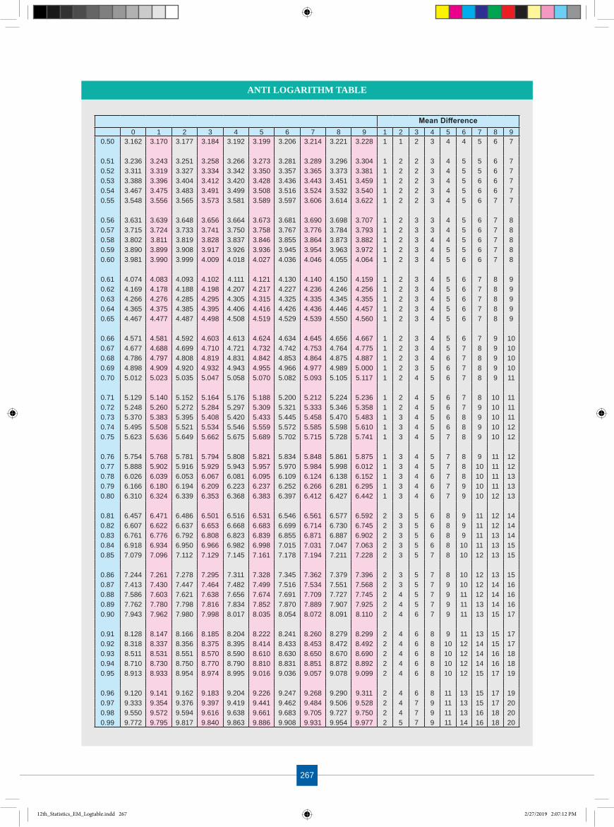
267
ANTI LOGARITHM TABLE
Mean Difference0 1 2 3 4 5 6 7 8 9 1 2 3 4 5 6 7 8 9
0.50 3.162 3.170 3.177 3.184 3.192 3.199 3.206 3.214 3.221 3.228 1 1 2 3 4 4 5 6 7
0.51 3.236 3.243 3.251 3.258 3.266 3.273 3.281 3.289 3.296 3.304 1 2 2 3 4 5 5 6 70.52 3.311 3.319 3.327 3.334 3.342 3.350 3.357 3.365 3.373 3.381 1 2 2 3 4 5 5 6 70.53 3.388 3.396 3.404 3.412 3.420 3.428 3.436 3.443 3.451 3.459 1 2 2 3 4 5 6 6 70.54 3.467 3.475 3.483 3.491 3.499 3.508 3.516 3.524 3.532 3.540 1 2 2 3 4 5 6 6 70.55 3.548 3.556 3.565 3.573 3.581 3.589 3.597 3.606 3.614 3.622 1 2 2 3 4 5 6 7 7
0.56 3.631 3.639 3.648 3.656 3.664 3.673 3.681 3.690 3.698 3.707 1 2 3 3 4 5 6 7 80.57 3.715 3.724 3.733 3.741 3.750 3.758 3.767 3.776 3.784 3.793 1 2 3 3 4 5 6 7 80.58 3.802 3.811 3.819 3.828 3.837 3.846 3.855 3.864 3.873 3.882 1 2 3 4 4 5 6 7 80.59 3.890 3.899 3.908 3.917 3.926 3.936 3.945 3.954 3.963 3.972 1 2 3 4 5 5 6 7 80.60 3.981 3.990 3.999 4.009 4.018 4.027 4.036 4.046 4.055 4.064 1 2 3 4 5 6 6 7 8
0.61 4.074 4.083 4.093 4.102 4.111 4.121 4.130 4.140 4.150 4.159 1 2 3 4 5 6 7 8 90.62 4.169 4.178 4.188 4.198 4.207 4.217 4.227 4.236 4.246 4.256 1 2 3 4 5 6 7 8 90.63 4.266 4.276 4.285 4.295 4.305 4.315 4.325 4.335 4.345 4.355 1 2 3 4 5 6 7 8 90.64 4.365 4.375 4.385 4.395 4.406 4.416 4.426 4.436 4.446 4.457 1 2 3 4 5 6 7 8 90.65 4.467 4.477 4.487 4.498 4.508 4.519 4.529 4.539 4.550 4.560 1 2 3 4 5 6 7 8 9
0.66 4.571 4.581 4.592 4.603 4.613 4.624 4.634 4.645 4.656 4.667 1 2 3 4 5 6 7 9 100.67 4.677 4.688 4.699 4.710 4.721 4.732 4.742 4.753 4.764 4.775 1 2 3 4 5 7 8 9 100.68 4.786 4.797 4.808 4.819 4.831 4.842 4.853 4.864 4.875 4.887 1 2 3 4 6 7 8 9 100.69 4.898 4.909 4.920 4.932 4.943 4.955 4.966 4.977 4.989 5.000 1 2 3 5 6 7 8 9 100.70 5.012 5.023 5.035 5.047 5.058 5.070 5.082 5.093 5.105 5.117 1 2 4 5 6 7 8 9 11
0.71 5.129 5.140 5.152 5.164 5.176 5.188 5.200 5.212 5.224 5.236 1 2 4 5 6 7 8 10 110.72 5.248 5.260 5.272 5.284 5.297 5.309 5.321 5.333 5.346 5.358 1 2 4 5 6 7 9 10 110.73 5.370 5.383 5.395 5.408 5.420 5.433 5.445 5.458 5.470 5.483 1 3 4 5 6 8 9 10 110.74 5.495 5.508 5.521 5.534 5.546 5.559 5.572 5.585 5.598 5.610 1 3 4 5 6 8 9 10 120.75 5.623 5.636 5.649 5.662 5.675 5.689 5.702 5.715 5.728 5.741 1 3 4 5 7 8 9 10 12
0.76 5.754 5.768 5.781 5.794 5.808 5.821 5.834 5.848 5.861 5.875 1 3 4 5 7 8 9 11 120.77 5.888 5.902 5.916 5.929 5.943 5.957 5.970 5.984 5.998 6.012 1 3 4 5 7 8 10 11 120.78 6.026 6.039 6.053 6.067 6.081 6.095 6.109 6.124 6.138 6.152 1 3 4 6 7 8 10 11 130.79 6.166 6.180 6.194 6.209 6.223 6.237 6.252 6.266 6.281 6.295 1 3 4 6 7 9 10 11 130.80 6.310 6.324 6.339 6.353 6.368 6.383 6.397 6.412 6.427 6.442 1 3 4 6 7 9 10 12 13
0.81 6.457 6.471 6.486 6.501 6.516 6.531 6.546 6.561 6.577 6.592 2 3 5 6 8 9 11 12 140.82 6.607 6.622 6.637 6.653 6.668 6.683 6.699 6.714 6.730 6.745 2 3 5 6 8 9 11 12 140.83 6.761 6.776 6.792 6.808 6.823 6.839 6.855 6.871 6.887 6.902 2 3 5 6 8 9 11 13 140.84 6.918 6.934 6.950 6.966 6.982 6.998 7.015 7.031 7.047 7.063 2 3 5 6 8 10 11 13 150.85 7.079 7.096 7.112 7.129 7.145 7.161 7.178 7.194 7.211 7.228 2 3 5 7 8 10 12 13 15
0.86 7.244 7.261 7.278 7.295 7.311 7.328 7.345 7.362 7.379 7.396 2 3 5 7 8 10 12 13 150.87 7.413 7.430 7.447 7.464 7.482 7.499 7.516 7.534 7.551 7.568 2 3 5 7 9 10 12 14 160.88 7.586 7.603 7.621 7.638 7.656 7.674 7.691 7.709 7.727 7.745 2 4 5 7 9 11 12 14 160.89 7.762 7.780 7.798 7.816 7.834 7.852 7.870 7.889 7.907 7.925 2 4 5 7 9 11 13 14 160.90 7.943 7.962 7.980 7.998 8.017 8.035 8.054 8.072 8.091 8.110 2 4 6 7 9 11 13 15 17
0.91 8.128 8.147 8.166 8.185 8.204 8.222 8.241 8.260 8.279 8.299 2 4 6 8 9 11 13 15 170.92 8.318 8.337 8.356 8.375 8.395 8.414 8.433 8.453 8.472 8.492 2 4 6 8 10 12 14 15 170.93 8.511 8.531 8.551 8.570 8.590 8.610 8.630 8.650 8.670 8.690 2 4 6 8 10 12 14 16 180.94 8.710 8.730 8.750 8.770 8.790 8.810 8.831 8.851 8.872 8.892 2 4 6 8 10 12 14 16 180.95 8.913 8.933 8.954 8.974 8.995 9.016 9.036 9.057 9.078 9.099 2 4 6 8 10 12 15 17 19
0.96 9.120 9.141 9.162 9.183 9.204 9.226 9.247 9.268 9.290 9.311 2 4 6 8 11 13 15 17 190.97 9.333 9.354 9.376 9.397 9.419 9.441 9.462 9.484 9.506 9.528 2 4 7 9 11 13 15 17 200.98 9.550 9.572 9.594 9.616 9.638 9.661 9.683 9.705 9.727 9.750 2 4 7 9 11 13 16 18 200.99 9.772 9.795 9.817 9.840 9.863 9.886 9.908 9.931 9.954 9.977 2 5 7 9 11 14 16 18 20
12th_Statistics_EM_Logtable.indd 267 2/27/2019 2:07:12 PM

268
Standard Normal Distribution Values - Critical Values
0 zα
α
P(z > zα) = α
z 0.00 0.01 0.02 0.03 0.04 0.05 0.06 0.07 0.08 0.09 z0.0 0.5000 0.4960 0.4920 0.4880 0.4841 0.4801 0.4761 0.4721 0.4681 0.4641 0.00.1 0.4602 0.4562 0.4522 0.4483 0.4443 0.4404 0.4364 0.4325 0.4286 0.4247 0.10.2 0.4207 0.4168 0.4129 0.4091 0.4052 0.4013 0.3974 0.3936 0.3897 0.3859 0.20.3 0.3821 0.3783 0.3745 0.3707 0.3669 0.3632 0.3594 0.3557 0.3520 0.3483 0.30.4 0.3446 0.3409 0.3372 0.3336 0.3300 0.3264 0.3228 0.3192 0.3156 0.3121 0.40.5 0.3085 0.3050 0.3015 0.2981 0.2946 0.2912 0.2877 0.2843 0.2810 0.2776 0.50.6 0.2743 0.2709 0.2676 0.2644 0.2611 0.2579 0.2546 0.2514 0.2483 0.2451 0.60.7 0.2420 0.2389 0.2358 0.2327 0.2297 0.2266 0.2236 0.2207 0.2177 0.2148 0.70.8 0.2119 0.2090 0.2061 0.2033 0.2005 0.1977 0.1949 0.1922 0.1894 0.1867 0.80.9 0.1841 0.1814 0.1788 0.1762 0.1736 0.1711 0.1685 0.1660 0.1635 0.1611 0.91.0 0.1587 0.1563 0.1539 0.1515 0.1492 0.1469 0.1446 0.1423 0.1401 0.1379 1.01.1 0.1357 0.1335 0.1314 0.1292 0.1271 0.1251 0.1230 0.1210 0.1190 0.1170 1.11.2 0.1151 0.1131 0.1112 0.1094 0.1075 0.1057 0.1038 0.1020 0.1003 0.0985 1.21.3 0.0968 0.0951 0.0934 0.0918 0.0901 0.0885 0.0869 0.0853 0.0838 0.0823 1.31.4 0.0808 0.0793 0.0778 0.0764 0.0749 0.0735 0.0722 0.0708 0.0694 0.0681 1.41.5 0.0668 0.0655 0.0643 0.0630 0.0618 0.0606 0.0594 0.0582 0.0571 0.0559 1.51.6 0.0548 0.0537 0.0526 0.0516 0.0505 0.0495 0.0485 0.0475 0.0465 0.0455 1.61.7 0.0446 0.0436 0.0427 0.0418 0.0409 0.0401 0.0392 0.0384 0.0375 0.0367 1.71.8 0.0359 0.0352 0.0344 0.0336 0.0329 0.0322 0.0314 0.0307 0.0301 0.0294 1.81.9 0.0287 0.0281 0.0274 0.0268 0.0262 0.0256 0.0250 0.0244 0.0239 0.0233 1.92.0 0.0228 0.0222 0.0217 0.0212 0.0207 0.0202 0.0197 0.0192 0.0188 0.0183 2.02.1 0.0179 0.0174 0.0170 0.0166 0.0162 0.0158 0.0154 0.0150 0.0146 0.0143 2.12.2 0.0139 0.0136 0.0132 0.0129 0.0126 0.0122 0.0119 0.0116 0.0113 0.0110 2.22.3 0.0107 0.0104 0.0102 0.0099 0.0096 0.0094 0.0091 0.0089 0.0087 0.0084 2.32.4 0.0082 0.0080 0.0078 0.0076 0.0073 0.0071 0.0070 0.0068 0.0066 0.0064 2.42.5 0.0062 0.0060 0.0059 0.0057 0.0055 0.0054 0.0052 0.0051 0.0049 0.0048 2.52.6 0.0047 0.0045 0.0044 0.0043 0.0042 0.0040 0.0039 0.0038 0.0037 0.0036 2.62.7 0.0035 0.0034 0.0033 0.0032 0.0031 0.0030 0.0029 0.0028 0.0027 0.0026 2.72.8 0.0026 0.0025 0.0024 0.0023 0.0023 0.0022 0.0021 0.0021 0.0020 0.0019 2.82.9 0.0019 0.0018 0.0018 0.0017 0.0016 0.0016 0.0015 0.0015 0.0014 0.0014 2.93.0 0.0014 0.0013 0.0013 0.0012 0.0012 0.0011 0.0011 0.0011 0.0010 0.0010 3.03.1 0.0010 0.0009 0.0009 0.0009 0.0009 0.0008 0.0008 0.0008 0.0007 0.0007 3.13.2 0.0007 0.0007 0.0006 0.0006 0.0006 0.0006 0.0006 0.0005 0.0005 0.0005 3.23.3 0.0005 0.0005 0.0005 0.0004 0.0004 0.0004 0.0004 0.0004 0.0004 0.0004 3.33.4 0.0003 0.0003 0.0003 0.0003 0.0003 0.0003 0.0003 0.0003 0.0003 0.0002 3.43.5 0.0002 0.0002 0.0002 0.0002 0.0002 0.0002 0.0002 0.0002 0.0002 0.0002 3.5
12th_Statistics_EM_Logtable.indd 268 2/27/2019 2:07:13 PM

269
0 tn,α
α
P(T > tn,α) = α
df
Area in One Tails0.005 0.01 0.025 0.05 0.10
Area in Two Tails0.01 0.02 0.05 0.10 0.20
1 63.657 31.821 12.706 6.314 3.0782 9.925 6.965 4.303 2.920 1.8863 5.841 4.541 3.182 2.353 1.6384 4.604 3.747 2.776 2.132 1.5335 4.032 3.365 2.571 2.015 1.4766 3.707 3.143 2.447 1.943 1.4407 3.499 2.998 2.365 1.895 1.4158 3.355 2.896 2.306 1.860 1.3979 3.250 2.821 2.262 1.833 1.38310 3.169 2.764 2.228 1.812 1.37211 3.106 2.718 2.201 1.796 1.36312 3.055 2.681 2.179 1.782 1.35613 3.012 2.650 2.160 1.771 1.35014 2.977 2.624 2.145 1.761 1.34515 2.947 2.602 2.131 1.753 1.34116 2.921 2.583 2.120 1.746 1.33717 2.898 2.567 2.110 1.740 1.33318 2.878 2.552 2.101 1.734 1.33019 2.861 2.539 2.093 1.729 1.32820 2.845 2.528 2.086 1.725 1.32521 2.831 2.518 2.080 1.721 1.32322 2.819 2.508 2.074 1.717 1.32123 2.807 2.500 2.069 1.714 1.31924 2.797 2.492 2.064 1.711 1.31825 2.787 2.485 2.060 1.708 1.31626 2.779 2.479 2.056 1.706 1.31527 2.771 2.473 2.052 1.703 1.31428 2.763 2.467 2.048 1.701 1.31329 2.756 2.462 2.045 1.699 1.31130 2.750 2.457 2.042 1.697 1.31040 2.704 2.423 2.021 1.684 1.30350 2.678 2.403 2.009 1.676 1.29960 2.660 2.390 2.000 1.671 1.296100 2.626 2.364 1.984 1.660 1.290120 2.617 2.358 1.980 1.658 1.289Infinity 2.576 2.326 1.960 1.645 1.282
t Distribution : Critical t Values: tn,α
12th_Statistics_EM_Logtable.indd 269 2/27/2019 2:07:13 PM

270
Critical Values of χ2 Statistic
0
α
n,α
P(χ2n > χ2
n,α) = α
αdf 0.995 0.990 0.975 0.950 0.900 0.100 0.050 0.025 0.010 0.005 df1 0.000 0.000 0.001 0.004 0.016 2.706 3.841 5.024 6.635 7.879 12 0.010 0.020 0.051 0.103 0.211 4.605 5.991 7.378 9.210 10.597 23 0.072 0.115 0.216 0.352 0.584 6.251 7.815 9.348 11.345 12.838 34 0.207 0.297 0.484 0.711 1.064 7.779 9.488 11.143 13.277 14.860 45 0.412 0.554 0.831 1.145 1.610 9.236 11.070 12.833 15.086 16.750 56 0.676 0.872 1.237 1.635 2.204 10.645 12.592 14.449 16.812 18.548 67 0.989 1.239 1.690 2.167 2.833 12.017 14.067 16.013 18.475 20.278 78 1.344 1.646 2.180 2.733 3.490 13.362 15.507 17.535 20.090 21.955 89 1.735 2.088 2.700 3.325 4.168 14.684 16.919 19.023 21.666 23.589 9
10 2.156 2.558 3.247 3.940 4.865 15.987 18.307 20.483 23.209 25.188 1011 2.603 3.053 3.816 4.575 5.578 17.275 19.675 21.920 24.725 26.757 1112 3.074 3.571 4.404 5.226 6.304 18.549 21.026 23.337 26.217 28.300 1213 3.565 4.107 5.009 5.892 7.042 19.812 22.362 24.736 27.688 29.819 1314 4.075 4.660 5.629 6.571 7.790 21.064 23.685 26.119 29.141 31.319 1415 4.601 5.229 6.262 7.261 8.547 22.307 24.996 27.488 30.578 32.801 1516 5.142 5.812 6.908 7.962 9.312 23.542 26.296 28.845 32.000 34.267 1617 5.697 6.408 7.564 8.672 10.085 24.769 27.587 30.191 33.409 35.718 1718 6.265 7.015 8.231 9.390 10.865 25.989 28.869 31.526 34.805 37.156 1819 6.844 7.633 8.907 10.117 11.651 27.204 30.144 32.852 36.191 38.582 1920 7.434 8.260 9.591 10.851 12.443 28.412 31.410 34.170 37.566 39.997 2021 8.034 8.897 10.283 11.591 13.240 29.615 32.671 35.479 38.932 41.401 2122 8.643 9.542 10.982 12.338 14.041 30.813 33.924 36.781 40.289 42.796 2223 9.260 10.196 11.689 13.091 14.848 32.007 35.172 38.076 41.638 44.181 2324 9.886 10.856 12.401 13.848 15.659 33.196 36.415 39.364 42.980 45.559 2425 10.520 11.524 13.120 14.611 16.473 34.382 37.652 40.646 44.314 46.928 2526 11.160 12.198 13.844 15.379 17.292 35.563 38.885 41.923 45.642 48.290 2627 11.808 12.879 14.573 16.151 18.114 36.741 40.113 43.195 46.963 49.645 2728 12.461 13.565 15.308 16.928 18.939 37.916 41.337 44.461 48.278 50.993 2829 13.121 14.256 16.047 17.708 19.768 39.087 42.557 45.722 49.588 52.336 2930 13.787 14.953 16.791 18.493 20.599 40.256 43.773 46.979 50.892 53.672 3040 20.707 22.164 24.433 26.509 29.051 51.805 55.758 59.342 63.691 66.766 4050 27.991 29.707 32.357 34.764 37.689 63.167 67.505 71.420 76.154 79.490 5060 35.534 37.485 40.482 43.188 46.459 74.397 79.082 83.298 88.379 91.952 6070 43.275 45.442 48.758 51.739 55.329 85.527 90.531 95.023 100.425 104.215 7080 51.172 53.540 57.153 60.391 64.278 96.578 101.879 106.629 112.329 116.321 8090 59.196 61.754 65.647 69.126 73.291 107.565 113.145 118.136 124.116 128.299 90
100 67.328 70.065 74.222 77.929 82.358 118.498 124.342 129.561 135.807 140.169 100
12th_Statistics_EM_Logtable.indd 270 2/27/2019 2:07:13 PM

271
F-D
istr
ibut
ion
- Cri
tical
Val
ues α
= 0
.01
nm
12
34
56
78
910
1215
2024
3040
6012
01
4052
.181
4999
.500
5403
.352
5624
.583
5763
.650
5858
.986
5928
.356
5981
.070
6022
.473
6055
.847
6106
.321
6157
.285
6208
.730
6234
.631
6260
.649
6286
.782
6313
.030
6339
.391
298
.503
99.0
0099
.166
99.2
4999
.299
99.3
3399
.356
99.3
7499
.388
99.3
9999
.416
99.4
3399
.449
99.4
5899
.466
99.4
7499
.482
99.4
913
34.1
1630
.817
29.4
5728
.710
28.2
3727
.911
27.6
7227
.489
27.3
4527
.229
27.0
5226
.872
26.6
9026
.598
26.5
0526
.411
26.3
1626
.221
421
.198
18.0
0016
.694
15.9
7715
.522
15.2
0714
.976
14.7
9914
.659
14.5
4614
.374
14.1
9814
.020
13.9
2913
.838
13.7
4513
.652
13.5
585
16.2
5813
.274
12.0
6011
.392
10.9
6710
.672
10.4
5610
.289
10.1
5810
.051
9.88
89.
722
9.55
39.
466
9.37
99.
291
9.20
29.
112
613
.745
10.9
259.
780
9.14
88.
746
8.46
68.
260
8.10
27.
976
7.87
47.
718
7.55
97.
396
7.31
37.
229
7.14
37.
057
6.96
97
12.2
469.
547
8.45
17.
847
7.46
07.
191
6.99
36.
840
6.71
96.
620
6.46
96.
314
6.15
56.
074
5.99
25.
908
5.82
45.
737
811
.259
8.64
97.
591
7.00
66.
632
6.37
16.
178
6.02
95.
911
5.81
45.
667
5.51
55.
359
5.27
95.
198
5.11
65.
032
4.94
69
10.5
618.
022
6.99
26.
422
6.05
75.
802
5.61
35.
467
5.35
15.
257
5.11
14.
962
4.80
84.
729
4.64
94.
567
4.48
34.
398
1010
.044
7.55
96.
552
5.99
45.
636
5.38
65.
200
5.05
74.
942
4.84
94.
706
4.55
84.
405
4.32
74.
247
4.16
54.
082
3.99
611
9.64
67.
206
6.21
75.
668
5.31
65.
069
4.88
64.
744
4.63
24.
539
4.39
74.
251
4.09
94.
021
3.94
13.
860
3.77
63.
690
129.
330
6.92
75.
953
5.41
25.
064
4.82
14.
640
4.49
94.
388
4.29
64.
155
4.01
03.
858
3.78
03.
701
3.61
93.
535
3.44
913
9.07
46.
701
5.73
95.
205
4.86
24.
620
4.44
14.
302
4.19
14.
100
3.96
03.
815
3.66
53.
587
3.50
73.
425
3.34
13.
255
148.
862
6.51
55.
564
5.03
54.
695
4.45
64.
278
4.14
04.
030
3.93
93.
800
3.65
63.
505
3.42
73.
348
3.26
63.
181
3.09
415
8.68
36.
359
5.41
74.
893
4.55
64.
318
4.14
24.
004
3.89
53.
805
3.66
63.
522
3.37
23.
294
3.21
43.
132
3.04
72.
959
168.
531
6.22
65.
292
4.77
34.
437
4.20
24.
026
3.89
03.
780
3.69
13.
553
3.40
93.
259
3.18
13.
101
3.01
82.
933
2.84
517
8.40
06.
112
5.18
54.
669
4.33
64.
102
3.92
73.
791
3.68
23.
593
3.45
53.
312
3.16
23.
084
3.00
32.
920
2.83
52.
746
188.
285
6.01
35.
092
4.57
94.
248
4.01
53.
841
3.70
53.
597
3.50
83.
371
3.22
73.
077
2.99
92.
919
2.83
52.
749
2.66
019
8.18
55.
926
5.01
04.
500
4.17
13.
939
3.76
53.
631
3.52
33.
434
3.29
73.
153
3.00
32.
925
2.84
42.
761
2.67
42.
584
208.
096
5.84
94.
938
4.43
14.
103
3.87
13.
699
3.56
43.
457
3.36
83.
231
3.08
82.
938
2.85
92.
778
2.69
52.
608
2.51
721
8.01
75.
780
4.87
44.
369
4.04
23.
812
3.64
03.
506
3.39
83.
310
3.17
33.
030
2.88
02.
801
2.72
02.
636
2.54
82.
457
227.
945
5.71
94.
817
4.31
33.
988
3.75
83.
587
3.45
33.
346
3.25
83.
121
2.97
82.
827
2.74
92.
667
2.58
32.
495
2.40
323
7.88
15.
664
4.76
54.
264
3.93
93.
710
3.53
93.
406
3.29
93.
211
3.07
42.
931
2.78
12.
702
2.62
02.
535
2.44
72.
354
247.
823
5.61
44.
718
4.21
83.
895
3.66
73.
496
3.36
33.
256
3.16
83.
032
2.88
92.
738
2.65
92.
577
2.49
22.
403
2.31
025
7.77
05.
568
4.67
54.
177
3.85
53.
627
3.45
73.
324
3.21
73.
129
2.99
32.
850
2.69
92.
620
2.53
82.
453
2.36
42.
270
267.
721
5.52
64.
637
4.14
03.
818
3.59
13.
421
3.28
83.
182
3.09
42.
958
2.81
52.
664
2.58
52.
503
2.41
72.
327
2.23
327
7.67
75.
488
4.60
14.
106
3.78
53.
558
3.38
83.
256
3.14
93.
062
2.92
62.
783
2.63
22.
552
2.47
02.
384
2.29
42.
198
287.
636
5.45
34.
568
4.07
43.
754
3.52
83.
358
3.22
63.
120
3.03
22.
896
2.75
32.
602
2.52
22.
440
2.35
42.
263
2.16
729
7.59
85.
420
4.53
84.
045
3.72
53.
499
3.33
03.
198
3.09
23.
005
2.86
82.
726
2.57
42.
495
2.41
22.
325
2.23
42.
138
307.
562
5.39
04.
510
4.01
83.
699
3.47
33.
304
3.17
33.
067
2.97
92.
843
2.70
02.
549
2.46
92.
386
2.29
92.
208
2.11
140
7.31
45.
179
4.31
33.
828
3.51
43.
291
3.12
42.
993
2.88
82.
801
2.66
52.
522
2.36
92.
288
2.20
32.
114
2.01
91.
917
607.
077
4.97
74.
126
3.64
93.
339
3.11
92.
953
2.82
32.
718
2.63
22.
496
2.35
22.
198
2.11
52.
028
1.93
61.
836
1.72
612
06.
851
4.78
73.
949
3.48
3.17
42.
956
2.79
22.
663
2.55
92.
472
2.33
62.
192
2.03
51.
951.
861.
763
1.65
61.
533
0
α
F (m,n),α
12th_Statistics_EM_Logtable.indd 271 2/27/2019 2:07:14 PM

272
nm
12
34
56
78
910
1215
2024
3040
6012
01
161.
448
199.
500
215.
707
224.
583
230.
162
233.
986
236.
768
238.
883
240.
543
241.
882
243.
906
245.
950
248.
013
249.
052
250.
095
251.
143
252.
196
253.
253
218
.513
19.0
0019
.164
19.2
4719
.296
19.3
3019
.353
19.3
7119
.385
19.3
9619
.413
19.4
2919
.446
19.4
5419
.462
19.4
7119
.479
19.4
873
10.1
289.
552
9.27
79.
117
9.01
38.
941
8.88
78.
845
8.81
28.
786
8.74
58.
703
8.66
08.
639
8.61
78.
594
8.57
28.
549
47.
709
6.94
46.
591
6.38
86.
256
6.16
36.
094
6.04
15.
999
5.96
45.
912
5.85
85.
803
5.77
45.
746
5.71
75.
688
5.65
85
6.60
85.
786
5.40
95.
192
5.05
04.
950
4.87
64.
818
4.77
24.
735
4.67
84.
619
4.55
84.
527
4.49
64.
464
4.43
14.
398
65.
987
5.14
34.
757
4.53
44.
387
4.28
44.
207
4.14
74.
099
4.06
04.
000
3.93
83.
874
3.84
13.
808
3.77
43.
740
3.70
57
5.59
14.
737
4.34
74.
120
3.97
23.
866
3.78
73.
726
3.67
73.
637
3.57
53.
511
3.44
53.
410
3.37
63.
340
3.30
43.
267
85.
318
4.45
94.
066
3.83
83.
687
3.58
13.
500
3.43
83.
388
3.34
73.
284
3.21
83.
150
3.11
53.
079
3.04
33.
005
2.96
79
5.11
74.
256
3.86
33.
633
3.48
23.
374
3.29
33.
230
3.17
93.
137
3.07
33.
006
2.93
62.
900
2.86
42.
826
2.78
72.
748
104.
965
4.10
33.
708
3.47
83.
326
3.21
73.
135
3.07
23.
020
2.97
82.
913
2.84
52.
774
2.73
72.
700
2.66
12.
621
2.58
011
4.84
43.
982
3.58
73.
357
3.20
43.
095
3.01
22.
948
2.89
62.
854
2.78
82.
719
2.64
62.
609
2.57
02.
531
2.49
02.
448
124.
747
3.88
53.
490
3.25
93.
106
2.99
62.
913
2.84
92.
796
2.75
32.
687
2.61
72.
544
2.50
52.
466
2.42
62.
384
2.34
113
4.66
73.
806
3.41
13.
179
3.02
52.
915
2.83
22.
767
2.71
42.
671
2.60
42.
533
2.45
92.
420
2.38
02.
339
2.29
72.
252
144.
600
3.73
93.
344
3.11
22.
958
2.84
82.
764
2.69
92.
646
2.60
22.
534
2.46
32.
388
2.34
92.
308
2.26
62.
223
2.17
815
4.54
33.
682
3.28
73.
056
2.90
12.
790
2.70
72.
641
2.58
82.
544
2.47
52.
403
2.32
82.
288
2.24
72.
204
2.16
02.
114
164.
494
3.63
43.
239
3.00
72.
852
2.74
12.
657
2.59
12.
538
2.49
42.
425
2.35
22.
276
2.23
52.
194
2.15
12.
106
2.05
917
4.45
13.
592
3.19
72.
965
2.81
02.
699
2.61
42.
548
2.49
42.
450
2.38
12.
308
2.23
02.
190
2.14
82.
104
2.05
82.
011
184.
414
3.55
53.
160
2.92
82.
773
2.66
12.
577
2.51
02.
456
2.41
22.
342
2.26
92.
191
2.15
02.
107
2.06
32.
017
1.96
819
4.38
13.
522
3.12
72.
895
2.74
02.
628
2.54
42.
477
2.42
32.
378
2.30
82.
234
2.15
52.
114
2.07
12.
026
1.98
01.
930
204.
351
3.49
33.
098
2.86
62.
711
2.59
92.
514
2.44
72.
393
2.34
82.
278
2.20
32.
124
2.08
22.
039
1.99
41.
946
1.89
621
4.32
53.
467
3.07
22.
840
2.68
52.
573
2.48
82.
420
2.36
62.
321
2.25
02.
176
2.09
62.
054
2.01
01.
965
1.91
61.
866
224.
301
3.44
33.
049
2.81
72.
661
2.54
92.
464
2.39
72.
342
2.29
72.
226
2.15
12.
071
2.02
81.
984
1.93
81.
889
1.83
823
4.27
93.
422
3.02
82.
796
2.64
02.
528
2.44
22.
375
2.32
02.
275
2.20
42.
128
2.04
82.
005
1.96
11.
914
1.86
51.
813
244.
260
3.40
33.
009
2.77
62.
621
2.50
82.
423
2.35
52.
300
2.25
52.
183
2.10
82.
027
1.98
41.
939
1.89
21.
842
1.79
025
4.24
23.
385
2.99
12.
759
2.60
32.
490
2.40
52.
337
2.28
22.
236
2.16
52.
089
2.00
71.
964
1.91
91.
872
1.82
21.
768
264.
225
3.36
92.
975
2.74
32.
587
2.47
42.
388
2.32
12.
265
2.22
02.
148
2.07
21.
990
1.94
61.
901
1.85
31.
803
1.74
927
4.21
03.
354
2.96
02.
728
2.57
22.
459
2.37
32.
305
2.25
02.
204
2.13
22.
056
1.97
41.
930
1.88
41.
836
1.78
51.
731
284.
196
3.34
02.
947
2.71
42.
558
2.44
52.
359
2.29
12.
236
2.19
02.
118
2.04
11.
959
1.91
51.
869
1.82
01.
769
1.71
429
4.18
33.
328
2.93
42.
701
2.54
52.
432
2.34
62.
278
2.22
32.
177
2.10
42.
027
1.94
51.
901
1.85
41.
806
1.75
41.
698
304.
171
3.31
62.
922
2.69
02.
534
2.42
12.
334
2.26
62.
211
2.16
52.
092
2.01
51.
932
1.88
71.
841
1.79
21.
740
1.68
340
4.08
53.
232
2.83
92.
606
2.44
92.
336
2.24
92.
180
2.12
42.
077
2.00
31.
924
1.83
91.
793
1.74
41.
693
1.63
71.
577
604.
001
3.15
02.
758
2.52
52.
368
2.25
42.
167
2.09
72.
040
1.99
31.
917
1.83
61.
748
1.70
01.
649
1.59
41.
534
1.46
712
03.
920
3.07
22.
680
2.44
72.
290
2.17
52.
087
2.01
61.
959
1.91
01.
834
1.75
01.
659
1.60
81.
554
1.49
51.
429
1.35
2
12th_Statistics_EM_Logtable.indd 272 2/27/2019 2:07:14 PM

273
m0.
000.
010.
020.
030.
040.
050.
060.
070.
080.
09
0.0
1.00
000.
9900
0.98
020.
9704
0.96
080.
9512
0.94
180.
9324
0.92
310.
9139
0.1
0.90
480.
8958
0.88
690.
8781
0.86
940.
8607
0.85
210.
8437
0.83
530.
8270
0.2
0.81
870.
8106
0.80
250.
7945
0.78
660.
7788
0.77
110.
7634
0.75
580.
7483
0.3
0.74
080.
7334
0.72
610.
7189
0.71
180.
7047
0.69
770.
6907
0.68
390.
6771
0.4
0.67
030.
6637
0.65
700.
6505
0.64
400.
6376
0.63
130.
6250
0.61
880.
6126
0.5
0.60
650.
6005
0.59
450.
5886
0.58
270.
5769
0.57
120.
5655
0.55
990.
5543
0.6
0.54
880.
5434
0.53
790.
5326
0.52
730.
5220
0.51
690.
5117
0.50
660.
5016
0.7
0.49
660.
4916
0.48
680.
4819
0.47
710.
4724
0.46
770.
4630
0.45
840.
4538
0.8
0.44
930.
4449
0.44
040.
4360
0.43
170.
4274
0.42
320.
4190
0.41
480.
4107
0.9
0.40
660.
4025
0.39
850.
3946
0.39
060.
3867
0.38
290.
3791
0.37
530.
3716
Expo
nent
ial F
unct
ion
Tabl
e (V
alue
s of e
–m)
12th_Statistics_EM_Logtable.indd 273 2/27/2019 2:07:14 PM

Domain ExpertsDr. G. GopalProfessor & Head (Retd.), Dept. of Statistics University of Madras, Chennai
Dr. G. Stephen VincentAssociate Professor & Head (Retd.), Dept. of Statistics St.Joseph's College, Trichy
Dr. R. RavananPrincipal, Presidency College, Chennai.
Dr. K. Senthamarai KannanProfessor, Dept. of Statistics, Manonmaniam Sundaranar University, Tirunelveli.
Dr. A. Loganathan Professor, Dept. of Statistics, Manonmaniam Sundaranar University, Tirunelveli.
Dr. R. Kannan Professor, Dept. of Statistics, Annamalai University, Chidambaram.
Dr. N. Viswanathan Associate Professor, Dept. of Statistics, Presidency College, Chennai.
Dr. R.K. RadhaAssistant Professor, Dept. of Statistics, Presidency College, Chennai.
LayoutYogesh B, Yesurathinam
Illustrations & Image EditingMuthukumar R.
Art and Design Team
In-House QC - Rajesh Thangapppan
Kamatchi Balan Arumugam Arun Kamaraj Jerald
Wrapper- Kathir Arumugam
Co-ordinationRamesh Munisamy
TypistG. Beula Lancy
ReviewersDr. M.R. SrinivasanProfessor & Head, Dept. of Statistics, University of Madras, Chennai.
Dr. P. DhanavanthanProfessor and Dean, Dept. of Statistics, Pondicherry University, Pondicherry.
�is book has been printed on 80 G.S.M. Elegant Maplitho paper.Printed by o�set at:
Content WritersG. GnanasundaramHM (Retd.), SSV HSS, Parktown, Chennai.
P. RengarajanPG Asst., (Retd.), Thiyagarajar HSS, Madurai.
S. John KennadiPG Asst., St. Xavier's HSS, Purathakudi, Trichy.
AL.NagammaiPG Asst., Sevasangam GHSS, Trichy.
M. Rama LakshmiPG Asst., Suguni Bai Sanathana Dharma GHSS, Chennai.
Maala BhaskaranPG Asst., GGHSS, Nandhivaram, Kanchipuram.
M. BoobalanPG Asst., Zamindar HSS, Thuraiyur, Trichy.
R. AvoodaiappanPG Asst., GGHSS, Ashok Pillar, Chennai.
K. ChitraPG Asst., Tarapore and Loganathan GHSS, Chennai.
Academic CoordinatorN. GnanasekaranB.T. Asst., Govt. Girls Hr. Sec. School, Thiruporur, Kanchipuram Dt.
ICT CoordinatorD. VasurajBT Asst., PUMS, Kosapur, Puzhal Block, Thiruvallur Dt.
QR CoordinatorsR. Jaganathan , SGT,PUMS - Ganesapuram, Polur , Thiruvannamalai.
V. Padmavathi, B.T,GHS, Vetriyur, Ariyalur.
M. Murugesan, B.T,PUMS. Pethavelankottagam, Muttupettai, Thiruvarur.
12th_Statistics_EM_Ack.indd 274 05-03-2019 10:14:32
Statistics – Class XIIList of Authors and Reviewers