
Probability and Statistics for Computer Scientists - Prakash ...
469
-
Upload
khangminh22 -
Category
Documents
-
view
2 -
download
0
Transcript of Probability and Statistics for Computer Scientists - Prakash ...


PROBABILITY AND STATISTICS FOR COMPUTER SCIENTISTS
SECOND EDITION
K13525_FM.indd 1 7/2/13 3:37 PM

K13525_FM.indd 2 7/2/13 3:37 PM

PROBABILITY AND STATISTICS FOR COMPUTER SCIENTISTS
SECOND EDITION
Michael BaronUniversity of Texas at Dallas
Richardson, USA
K13525_FM.indd 3 7/2/13 3:37 PM

CRC PressTaylor & Francis Group6000 Broken Sound Parkway NW, Suite 300Boca Raton, FL 33487-2742
© 2014 by Taylor & Francis Group, LLCCRC Press is an imprint of Taylor & Francis Group, an Informa business
No claim to original U.S. Government worksVersion Date: 20130625
International Standard Book Number-13: 978-1-4822-1410-9 (eBook - ePub)
This book contains information obtained from authentic and highly regarded sources. Reasonable efforts have been made to publish reliable data and information, but the author and publisher cannot assume responsibility for the valid-ity of all materials or the consequences of their use. The authors and publishers have attempted to trace the copyright holders of all material reproduced in this publication and apologize to copyright holders if permission to publish in this form has not been obtained. If any copyright material has not been acknowledged please write and let us know so we may rectify in any future reprint.
Except as permitted under U.S. Copyright Law, no part of this book may be reprinted, reproduced, transmitted, or uti-lized in any form by any electronic, mechanical, or other means, now known or hereafter invented, including photocopy-ing, microfilming, and recording, or in any information storage or retrieval system, without written permission from the publishers.
For permission to photocopy or use material electronically from this work, please access www.copyright.com (http://www.copyright.com/) or contact the Copyright Clearance Center, Inc. (CCC), 222 Rosewood Drive, Danvers, MA 01923, 978-750-8400. CCC is a not-for-profit organization that provides licenses and registration for a variety of users. For organizations that have been granted a photocopy license by the CCC, a separate system of payment has been arranged.
Trademark Notice: Product or corporate names may be trademarks or registered trademarks, and are used only for identification and explanation without intent to infringe.
Visit the Taylor & Francis Web site athttp://www.taylorandfrancis.com
and the CRC Press Web site athttp://www.crcpress.com

To my parents – Genrietta and Izrael-Vulf Baron

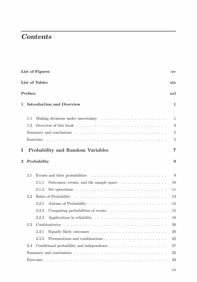
Contents
List of Figures xv
List of Tables xix
Preface xxi
1 Introduction and Overview 1
1.1 Making decisions under uncertainty . . . . . . . . . . . . . . . . . . . . . . 1
1.2 Overview of this book . . . . . . . . . . . . . . . . . . . . . . . . . . . . . . 3
Summary and conclusions . . . . . . . . . . . . . . . . . . . . . . . . . . . . . . . 5
Exercises . . . . . . . . . . . . . . . . . . . . . . . . . . . . . . . . . . . . . . . . 5
I Probability and Random Variables 7
2 Probability 9
2.1 Events and their probabilities . . . . . . . . . . . . . . . . . . . . . . . . . 9
2.1.1 Outcomes, events, and the sample space . . . . . . . . . . . . . . . . 10
2.1.2 Set operations . . . . . . . . . . . . . . . . . . . . . . . . . . . . . . 11
2.2 Rules of Probability . . . . . . . . . . . . . . . . . . . . . . . . . . . . . . . 13
2.2.1 Axioms of Probability . . . . . . . . . . . . . . . . . . . . . . . . . . 14
2.2.2 Computing probabilities of events . . . . . . . . . . . . . . . . . . . 15
2.2.3 Applications in reliability . . . . . . . . . . . . . . . . . . . . . . . . 18
2.3 Combinatorics . . . . . . . . . . . . . . . . . . . . . . . . . . . . . . . . . . 20
2.3.1 Equally likely outcomes . . . . . . . . . . . . . . . . . . . . . . . . . 20
2.3.2 Permutations and combinations . . . . . . . . . . . . . . . . . . . . . 22
2.4 Conditional probability and independence . . . . . . . . . . . . . . . . . . . 27
Summary and conclusions . . . . . . . . . . . . . . . . . . . . . . . . . . . . . . . 32
Exercises . . . . . . . . . . . . . . . . . . . . . . . . . . . . . . . . . . . . . . . . 33
vii
viii
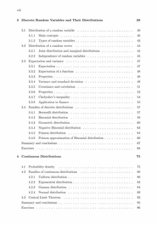
3 Discrete Random Variables and Their Distributions 39
3.1 Distribution of a random variable . . . . . . . . . . . . . . . . . . . . . . . 40
3.1.1 Main concepts . . . . . . . . . . . . . . . . . . . . . . . . . . . . . . 40
3.1.2 Types of random variables . . . . . . . . . . . . . . . . . . . . . . . . 43
3.2 Distribution of a random vector . . . . . . . . . . . . . . . . . . . . . . . . 44
3.2.1 Joint distribution and marginal distributions . . . . . . . . . . . . . 44
3.2.2 Independence of random variables . . . . . . . . . . . . . . . . . . . 45
3.3 Expectation and variance . . . . . . . . . . . . . . . . . . . . . . . . . . . . 47
3.3.1 Expectation . . . . . . . . . . . . . . . . . . . . . . . . . . . . . . . . 47
3.3.2 Expectation of a function . . . . . . . . . . . . . . . . . . . . . . . . 48
3.3.3 Properties . . . . . . . . . . . . . . . . . . . . . . . . . . . . . . . . . 48
3.3.4 Variance and standard deviation . . . . . . . . . . . . . . . . . . . . 49
3.3.5 Covariance and correlation . . . . . . . . . . . . . . . . . . . . . . . 51
3.3.6 Properties . . . . . . . . . . . . . . . . . . . . . . . . . . . . . . . . . 52
3.3.7 Chebyshev’s inequality . . . . . . . . . . . . . . . . . . . . . . . . . . 54
3.3.8 Application to finance . . . . . . . . . . . . . . . . . . . . . . . . . . 55
3.4 Families of discrete distributions . . . . . . . . . . . . . . . . . . . . . . . . 57
3.4.1 Bernoulli distribution . . . . . . . . . . . . . . . . . . . . . . . . . . 57
3.4.2 Binomial distribution . . . . . . . . . . . . . . . . . . . . . . . . . . 58
3.4.3 Geometric distribution . . . . . . . . . . . . . . . . . . . . . . . . . . 60
3.4.4 Negative Binomial distribution . . . . . . . . . . . . . . . . . . . . . 63
3.4.5 Poisson distribution . . . . . . . . . . . . . . . . . . . . . . . . . . . 64
3.4.6 Poisson approximation of Binomial distribution . . . . . . . . . . . . 66
Summary and conclusions . . . . . . . . . . . . . . . . . . . . . . . . . . . . . . . 67
Exercises . . . . . . . . . . . . . . . . . . . . . . . . . . . . . . . . . . . . . . . . 68
4 Continuous Distributions 75
4.1 Probability density . . . . . . . . . . . . . . . . . . . . . . . . . . . . . . . 75
4.2 Families of continuous distributions . . . . . . . . . . . . . . . . . . . . . . 80
4.2.1 Uniform distribution . . . . . . . . . . . . . . . . . . . . . . . . . . . 80
4.2.2 Exponential distribution . . . . . . . . . . . . . . . . . . . . . . . . . 82
4.2.3 Gamma distribution . . . . . . . . . . . . . . . . . . . . . . . . . . . 84
4.2.4 Normal distribution . . . . . . . . . . . . . . . . . . . . . . . . . . . 89
4.3 Central Limit Theorem . . . . . . . . . . . . . . . . . . . . . . . . . . . . . 92
Summary and conclusions . . . . . . . . . . . . . . . . . . . . . . . . . . . . . . . 95
Exercises . . . . . . . . . . . . . . . . . . . . . . . . . . . . . . . . . . . . . . . . 96
ix
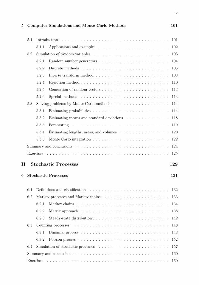
5 Computer Simulations and Monte Carlo Methods 101
5.1 Introduction . . . . . . . . . . . . . . . . . . . . . . . . . . . . . . . . . . . 101
5.1.1 Applications and examples . . . . . . . . . . . . . . . . . . . . . . . 102
5.2 Simulation of random variables . . . . . . . . . . . . . . . . . . . . . . . . . 103
5.2.1 Random number generators . . . . . . . . . . . . . . . . . . . . . . . 104
5.2.2 Discrete methods . . . . . . . . . . . . . . . . . . . . . . . . . . . . . 105
5.2.3 Inverse transform method . . . . . . . . . . . . . . . . . . . . . . . . 108
5.2.4 Rejection method . . . . . . . . . . . . . . . . . . . . . . . . . . . . . 110
5.2.5 Generation of random vectors . . . . . . . . . . . . . . . . . . . . . . 113
5.2.6 Special methods . . . . . . . . . . . . . . . . . . . . . . . . . . . . . 113
5.3 Solving problems by Monte Carlo methods . . . . . . . . . . . . . . . . . . 114
5.3.1 Estimating probabilities . . . . . . . . . . . . . . . . . . . . . . . . . 114
5.3.2 Estimating means and standard deviations . . . . . . . . . . . . . . 118
5.3.3 Forecasting . . . . . . . . . . . . . . . . . . . . . . . . . . . . . . . . 119
5.3.4 Estimating lengths, areas, and volumes . . . . . . . . . . . . . . . . 120
5.3.5 Monte Carlo integration . . . . . . . . . . . . . . . . . . . . . . . . . 122
Summary and conclusions . . . . . . . . . . . . . . . . . . . . . . . . . . . . . . . 124
Exercises . . . . . . . . . . . . . . . . . . . . . . . . . . . . . . . . . . . . . . . . 125
II Stochastic Processes 129
6 Stochastic Processes 131
6.1 Definitions and classifications . . . . . . . . . . . . . . . . . . . . . . . . . . 132
6.2 Markov processes and Markov chains . . . . . . . . . . . . . . . . . . . . . 133
6.2.1 Markov chains . . . . . . . . . . . . . . . . . . . . . . . . . . . . . . 134
6.2.2 Matrix approach . . . . . . . . . . . . . . . . . . . . . . . . . . . . . 138
6.2.3 Steady-state distribution . . . . . . . . . . . . . . . . . . . . . . . . . 142
6.3 Counting processes . . . . . . . . . . . . . . . . . . . . . . . . . . . . . . . 148
6.3.1 Binomial process . . . . . . . . . . . . . . . . . . . . . . . . . . . . . 148
6.3.2 Poisson process . . . . . . . . . . . . . . . . . . . . . . . . . . . . . . 152
6.4 Simulation of stochastic processes . . . . . . . . . . . . . . . . . . . . . . . 157
Summary and conclusions . . . . . . . . . . . . . . . . . . . . . . . . . . . . . . . 160
Exercises . . . . . . . . . . . . . . . . . . . . . . . . . . . . . . . . . . . . . . . . 160

x
7 Queuing Systems 167
7.1 Main components of a queuing system . . . . . . . . . . . . . . . . . . . . . 168
7.2 The Little’s Law . . . . . . . . . . . . . . . . . . . . . . . . . . . . . . . . . 170
7.3 Bernoulli single-server queuing process . . . . . . . . . . . . . . . . . . . . 173
7.3.1 Systems with limited capacity . . . . . . . . . . . . . . . . . . . . . . 176
7.4 M/M/1 system . . . . . . . . . . . . . . . . . . . . . . . . . . . . . . . . . . 178
7.4.1 Evaluating the system’s performance . . . . . . . . . . . . . . . . . . 181
7.5 Multiserver queuing systems . . . . . . . . . . . . . . . . . . . . . . . . . . 185
7.5.1 Bernoulli k-server queuing process . . . . . . . . . . . . . . . . . . . 186
7.5.2 M/M/k systems . . . . . . . . . . . . . . . . . . . . . . . . . . . . . 189
7.5.3 Unlimited number of servers and M/M/∞ . . . . . . . . . . . . . . . 192
7.6 Simulation of queuing systems . . . . . . . . . . . . . . . . . . . . . . . . . 193
Summary and conclusions . . . . . . . . . . . . . . . . . . . . . . . . . . . . . . . 197
Exercises . . . . . . . . . . . . . . . . . . . . . . . . . . . . . . . . . . . . . . . . 198
III Statistics 205
8 Introduction to Statistics 207
8.1 Population and sample, parameters and statistics . . . . . . . . . . . . . . 208
8.2 Simple descriptive statistics . . . . . . . . . . . . . . . . . . . . . . . . . . . 211
8.2.1 Mean . . . . . . . . . . . . . . . . . . . . . . . . . . . . . . . . . . . 211
8.2.2 Median . . . . . . . . . . . . . . . . . . . . . . . . . . . . . . . . . . 213
8.2.3 Quantiles, percentiles, and quartiles . . . . . . . . . . . . . . . . . . 217
8.2.4 Variance and standard deviation . . . . . . . . . . . . . . . . . . . . 219
8.2.5 Standard errors of estimates . . . . . . . . . . . . . . . . . . . . . . . 221
8.2.6 Interquartile range . . . . . . . . . . . . . . . . . . . . . . . . . . . . 222
8.3 Graphical statistics . . . . . . . . . . . . . . . . . . . . . . . . . . . . . . . 223
8.3.1 Histogram . . . . . . . . . . . . . . . . . . . . . . . . . . . . . . . . . 224
8.3.2 Stem-and-leaf plot . . . . . . . . . . . . . . . . . . . . . . . . . . . . 227
8.3.3 Boxplot . . . . . . . . . . . . . . . . . . . . . . . . . . . . . . . . . . 229
8.3.4 Scatter plots and time plots . . . . . . . . . . . . . . . . . . . . . . . 231
Summary and conclusions . . . . . . . . . . . . . . . . . . . . . . . . . . . . . . . 233
Exercises . . . . . . . . . . . . . . . . . . . . . . . . . . . . . . . . . . . . . . . . 233
xi
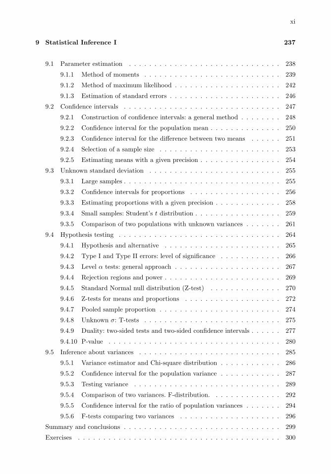
9 Statistical Inference I 237
9.1 Parameter estimation . . . . . . . . . . . . . . . . . . . . . . . . . . . . . . 238
9.1.1 Method of moments . . . . . . . . . . . . . . . . . . . . . . . . . . . 239
9.1.2 Method of maximum likelihood . . . . . . . . . . . . . . . . . . . . . 242
9.1.3 Estimation of standard errors . . . . . . . . . . . . . . . . . . . . . . 246
9.2 Confidence intervals . . . . . . . . . . . . . . . . . . . . . . . . . . . . . . . 247
9.2.1 Construction of confidence intervals: a general method . . . . . . . . 248
9.2.2 Confidence interval for the population mean . . . . . . . . . . . . . . 250
9.2.3 Confidence interval for the difference between two means . . . . . . 251
9.2.4 Selection of a sample size . . . . . . . . . . . . . . . . . . . . . . . . 253
9.2.5 Estimating means with a given precision . . . . . . . . . . . . . . . . 254
9.3 Unknown standard deviation . . . . . . . . . . . . . . . . . . . . . . . . . . 255
9.3.1 Large samples . . . . . . . . . . . . . . . . . . . . . . . . . . . . . . . 255
9.3.2 Confidence intervals for proportions . . . . . . . . . . . . . . . . . . 256
9.3.3 Estimating proportions with a given precision . . . . . . . . . . . . . 258
9.3.4 Small samples: Student’s t distribution . . . . . . . . . . . . . . . . . 259
9.3.5 Comparison of two populations with unknown variances . . . . . . . 261
9.4 Hypothesis testing . . . . . . . . . . . . . . . . . . . . . . . . . . . . . . . . 264
9.4.1 Hypothesis and alternative . . . . . . . . . . . . . . . . . . . . . . . 265
9.4.2 Type I and Type II errors: level of significance . . . . . . . . . . . . 266
9.4.3 Level α tests: general approach . . . . . . . . . . . . . . . . . . . . . 267
9.4.4 Rejection regions and power . . . . . . . . . . . . . . . . . . . . . . . 269
9.4.5 Standard Normal null distribution (Z-test) . . . . . . . . . . . . . . 270
9.4.6 Z-tests for means and proportions . . . . . . . . . . . . . . . . . . . 272
9.4.7 Pooled sample proportion . . . . . . . . . . . . . . . . . . . . . . . . 274
9.4.8 Unknown σ: T-tests . . . . . . . . . . . . . . . . . . . . . . . . . . . 275
9.4.9 Duality: two-sided tests and two-sided confidence intervals . . . . . . 277
9.4.10 P-value . . . . . . . . . . . . . . . . . . . . . . . . . . . . . . . . . . 280
9.5 Inference about variances . . . . . . . . . . . . . . . . . . . . . . . . . . . . 285
9.5.1 Variance estimator and Chi-square distribution . . . . . . . . . . . . 286
9.5.2 Confidence interval for the population variance . . . . . . . . . . . . 287
9.5.3 Testing variance . . . . . . . . . . . . . . . . . . . . . . . . . . . . . 289
9.5.4 Comparison of two variances. F-distribution. . . . . . . . . . . . . . 292
9.5.5 Confidence interval for the ratio of population variances . . . . . . . 294
9.5.6 F-tests comparing two variances . . . . . . . . . . . . . . . . . . . . 296
Summary and conclusions . . . . . . . . . . . . . . . . . . . . . . . . . . . . . . . 299
Exercises . . . . . . . . . . . . . . . . . . . . . . . . . . . . . . . . . . . . . . . . 300

xii
10 Statistical Inference II 305
10.1 Chi-square tests . . . . . . . . . . . . . . . . . . . . . . . . . . . . . . . . . 305
10.1.1 Testing a distribution . . . . . . . . . . . . . . . . . . . . . . . . . . 306
10.1.2 Testing a family of distributions . . . . . . . . . . . . . . . . . . . . 308
10.1.3 Testing independence . . . . . . . . . . . . . . . . . . . . . . . . . . 310
10.2 Nonparametric statistics . . . . . . . . . . . . . . . . . . . . . . . . . . . . 314
10.2.1 Sign test . . . . . . . . . . . . . . . . . . . . . . . . . . . . . . . . . . 315
10.2.2 Wilcoxon signed rank test . . . . . . . . . . . . . . . . . . . . . . . . 317
10.2.3 Mann-Whitney-Wilcoxon rank sum test . . . . . . . . . . . . . . . . 322
10.3 Bootstrap . . . . . . . . . . . . . . . . . . . . . . . . . . . . . . . . . . . . . 328
10.3.1 Bootstrap distribution and all bootstrap samples . . . . . . . . . . . 328
10.3.2 Computer generated bootstrap samples . . . . . . . . . . . . . . . . 333
10.3.3 Bootstrap confidence intervals . . . . . . . . . . . . . . . . . . . . . . 335
10.4 Bayesian inference . . . . . . . . . . . . . . . . . . . . . . . . . . . . . . . . 339
10.4.1 Prior and posterior . . . . . . . . . . . . . . . . . . . . . . . . . . . . 340
10.4.2 Bayesian estimation . . . . . . . . . . . . . . . . . . . . . . . . . . . 345
10.4.3 Bayesian credible sets . . . . . . . . . . . . . . . . . . . . . . . . . . 347
10.4.4 Bayesian hypothesis testing . . . . . . . . . . . . . . . . . . . . . . . 351
Summary and conclusions . . . . . . . . . . . . . . . . . . . . . . . . . . . . . . . 352
Exercises . . . . . . . . . . . . . . . . . . . . . . . . . . . . . . . . . . . . . . . . 353
11 Regression 361
11.1 Least squares estimation . . . . . . . . . . . . . . . . . . . . . . . . . . . . 362
11.1.1 Examples . . . . . . . . . . . . . . . . . . . . . . . . . . . . . . . . . 362
11.1.2 Method of least squares . . . . . . . . . . . . . . . . . . . . . . . . . 364
11.1.3 Linear regression . . . . . . . . . . . . . . . . . . . . . . . . . . . . . 365
11.1.4 Regression and correlation . . . . . . . . . . . . . . . . . . . . . . . . 367
11.1.5 Overfitting a model . . . . . . . . . . . . . . . . . . . . . . . . . . . 368
11.2 Analysis of variance, prediction, and further inference . . . . . . . . . . . . 369
11.2.1 ANOVA and R-square . . . . . . . . . . . . . . . . . . . . . . . . . . 369
11.2.2 Tests and confidence intervals . . . . . . . . . . . . . . . . . . . . . . 371
11.2.3 Prediction . . . . . . . . . . . . . . . . . . . . . . . . . . . . . . . . . 377
11.3 Multivariate regression . . . . . . . . . . . . . . . . . . . . . . . . . . . . . 381

xiii
11.3.1 Introduction and examples . . . . . . . . . . . . . . . . . . . . . . . 381
11.3.2 Matrix approach and least squares estimation . . . . . . . . . . . . . 382
11.3.3 Analysis of variance, tests, and prediction . . . . . . . . . . . . . . . 384
11.4 Model building . . . . . . . . . . . . . . . . . . . . . . . . . . . . . . . . . . 390
11.4.1 Adjusted R-square . . . . . . . . . . . . . . . . . . . . . . . . . . . . 390
11.4.2 Extra sum of squares, partial F-tests, and variable selection . . . . . 391
11.4.3 Categorical predictors and dummy variables . . . . . . . . . . . . . . 394
Summary and conclusions . . . . . . . . . . . . . . . . . . . . . . . . . . . . . . . 397
Exercises . . . . . . . . . . . . . . . . . . . . . . . . . . . . . . . . . . . . . . . . 397
IV Appendix 403
12 Appendix 405
12.1 Inventory of distributions . . . . . . . . . . . . . . . . . . . . . . . . . . . . 405
12.1.1 Discrete families . . . . . . . . . . . . . . . . . . . . . . . . . . . . . 405
12.1.2 Continuous families . . . . . . . . . . . . . . . . . . . . . . . . . . . 407
12.2 Distribution tables . . . . . . . . . . . . . . . . . . . . . . . . . . . . . . . . 411
12.3 Calculus review . . . . . . . . . . . . . . . . . . . . . . . . . . . . . . . . . 428
12.3.1 Inverse function . . . . . . . . . . . . . . . . . . . . . . . . . . . . . . 428
12.3.2 Limits and continuity . . . . . . . . . . . . . . . . . . . . . . . . . . 428
12.3.3 Sequences and series . . . . . . . . . . . . . . . . . . . . . . . . . . . 429
12.3.4 Derivatives, minimum, and maximum . . . . . . . . . . . . . . . . . 429
12.3.5 Integrals . . . . . . . . . . . . . . . . . . . . . . . . . . . . . . . . . . 431
12.4 Matrices and linear systems . . . . . . . . . . . . . . . . . . . . . . . . . . . 434
12.5 Answers to selected exercises . . . . . . . . . . . . . . . . . . . . . . . . . . 439
Index 445

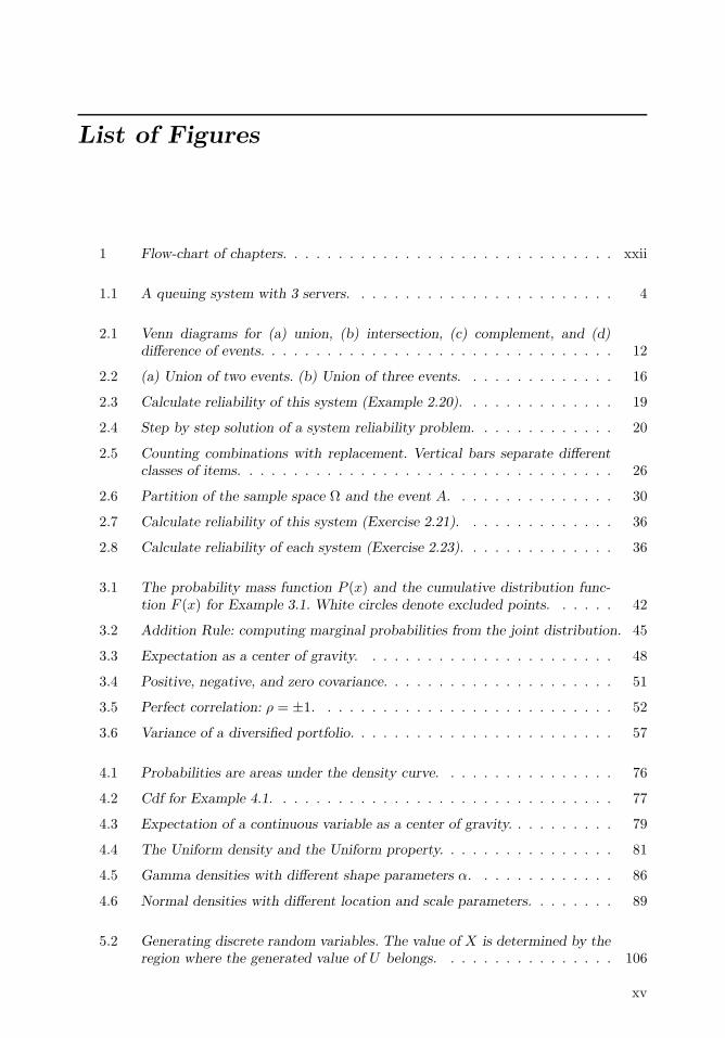
List of Figures
1 Flow-chart of chapters. . . . . . . . . . . . . . . . . . . . . . . . . . . . . . xxii
1.1 A queuing system with 3 servers. . . . . . . . . . . . . . . . . . . . . . . . 4
2.1 Venn diagrams for (a) union, (b) intersection, (c) complement, and (d)difference of events. . . . . . . . . . . . . . . . . . . . . . . . . . . . . . . . 12
2.2 (a) Union of two events. (b) Union of three events. . . . . . . . . . . . . . 16
2.3 Calculate reliability of this system (Example 2.20). . . . . . . . . . . . . . 19
2.4 Step by step solution of a system reliability problem. . . . . . . . . . . . . 20
2.5 Counting combinations with replacement. Vertical bars separate differentclasses of items. . . . . . . . . . . . . . . . . . . . . . . . . . . . . . . . . . 26
2.6 Partition of the sample space Ω and the event A. . . . . . . . . . . . . . . 30
2.7 Calculate reliability of this system (Exercise 2.21). . . . . . . . . . . . . . 36
2.8 Calculate reliability of each system (Exercise 2.23). . . . . . . . . . . . . . 36
3.1 The probability mass function P (x) and the cumulative distribution func-tion F (x) for Example 3.1. White circles denote excluded points. . . . . . 42
3.2 Addition Rule: computing marginal probabilities from the joint distribution. 45
3.3 Expectation as a center of gravity. . . . . . . . . . . . . . . . . . . . . . . 48
3.4 Positive, negative, and zero covariance. . . . . . . . . . . . . . . . . . . . . 51
3.5 Perfect correlation: ρ = ±1. . . . . . . . . . . . . . . . . . . . . . . . . . . 52
3.6 Variance of a diversified portfolio. . . . . . . . . . . . . . . . . . . . . . . . 57
4.1 Probabilities are areas under the density curve. . . . . . . . . . . . . . . . 76
4.2 Cdf for Example 4.1. . . . . . . . . . . . . . . . . . . . . . . . . . . . . . . 77
4.3 Expectation of a continuous variable as a center of gravity. . . . . . . . . . 79
4.4 The Uniform density and the Uniform property. . . . . . . . . . . . . . . . 81
4.5 Gamma densities with different shape parameters α. . . . . . . . . . . . . 86
4.6 Normal densities with different location and scale parameters. . . . . . . . 89
5.2 Generating discrete random variables. The value of X is determined by theregion where the generated value of U belongs. . . . . . . . . . . . . . . . 106
xv
xvi Probability and Statistics for Computer Scientists
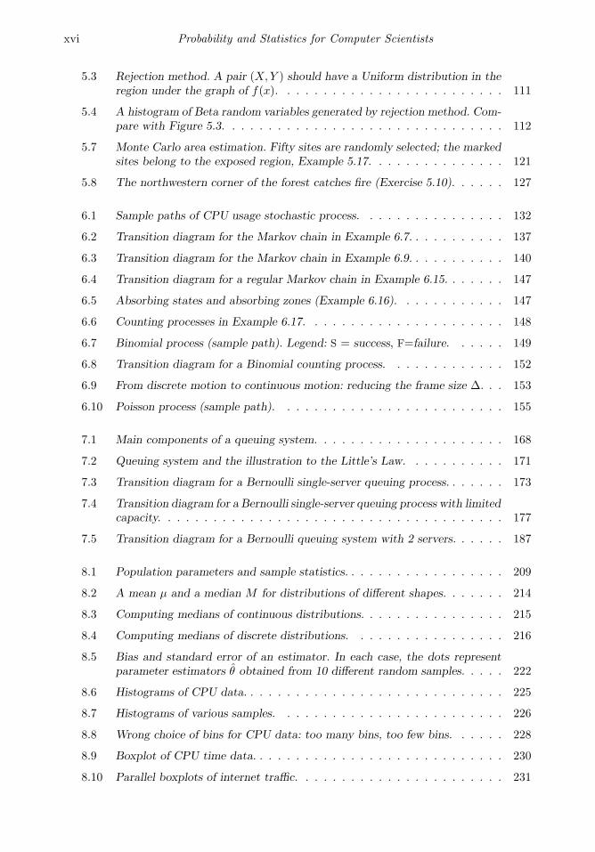
5.3 Rejection method. A pair (X,Y ) should have a Uniform distribution in theregion under the graph of f(x). . . . . . . . . . . . . . . . . . . . . . . . . 111
5.4 A histogram of Beta random variables generated by rejection method. Com-pare with Figure 5.3. . . . . . . . . . . . . . . . . . . . . . . . . . . . . . . 112
5.7 Monte Carlo area estimation. Fifty sites are randomly selected; the markedsites belong to the exposed region, Example 5.17. . . . . . . . . . . . . . . 121
5.8 The northwestern corner of the forest catches fire (Exercise 5.10). . . . . . 127
6.1 Sample paths of CPU usage stochastic process. . . . . . . . . . . . . . . . 132
6.2 Transition diagram for the Markov chain in Example 6.7. . . . . . . . . . . 137
6.3 Transition diagram for the Markov chain in Example 6.9. . . . . . . . . . . 140
6.4 Transition diagram for a regular Markov chain in Example 6.15. . . . . . . 147
6.5 Absorbing states and absorbing zones (Example 6.16). . . . . . . . . . . . 147
6.6 Counting processes in Example 6.17. . . . . . . . . . . . . . . . . . . . . . 148
6.7 Binomial process (sample path). Legend: S = success, F=failure. . . . . . 149
6.8 Transition diagram for a Binomial counting process. . . . . . . . . . . . . 152
6.9 From discrete motion to continuous motion: reducing the frame size ∆. . . 153
6.10 Poisson process (sample path). . . . . . . . . . . . . . . . . . . . . . . . . 155
7.1 Main components of a queuing system. . . . . . . . . . . . . . . . . . . . . 168
7.2 Queuing system and the illustration to the Little’s Law. . . . . . . . . . . 171
7.3 Transition diagram for a Bernoulli single-server queuing process. . . . . . . 173
7.4 Transition diagram for a Bernoulli single-server queuing process with limitedcapacity. . . . . . . . . . . . . . . . . . . . . . . . . . . . . . . . . . . . . . 177
7.5 Transition diagram for a Bernoulli queuing system with 2 servers. . . . . . 187
8.1 Population parameters and sample statistics. . . . . . . . . . . . . . . . . . 209
8.2 A mean µ and a median M for distributions of different shapes. . . . . . . 214
8.3 Computing medians of continuous distributions. . . . . . . . . . . . . . . . 215
8.4 Computing medians of discrete distributions. . . . . . . . . . . . . . . . . 216
8.5 Bias and standard error of an estimator. In each case, the dots representparameter estimators θ obtained from 10 different random samples. . . . . 222
8.6 Histograms of CPU data. . . . . . . . . . . . . . . . . . . . . . . . . . . . . 225
8.7 Histograms of various samples. . . . . . . . . . . . . . . . . . . . . . . . . 226
8.8 Wrong choice of bins for CPU data: too many bins, too few bins. . . . . . 228
8.9 Boxplot of CPU time data. . . . . . . . . . . . . . . . . . . . . . . . . . . . 230
8.10 Parallel boxplots of internet traffic. . . . . . . . . . . . . . . . . . . . . . . 231
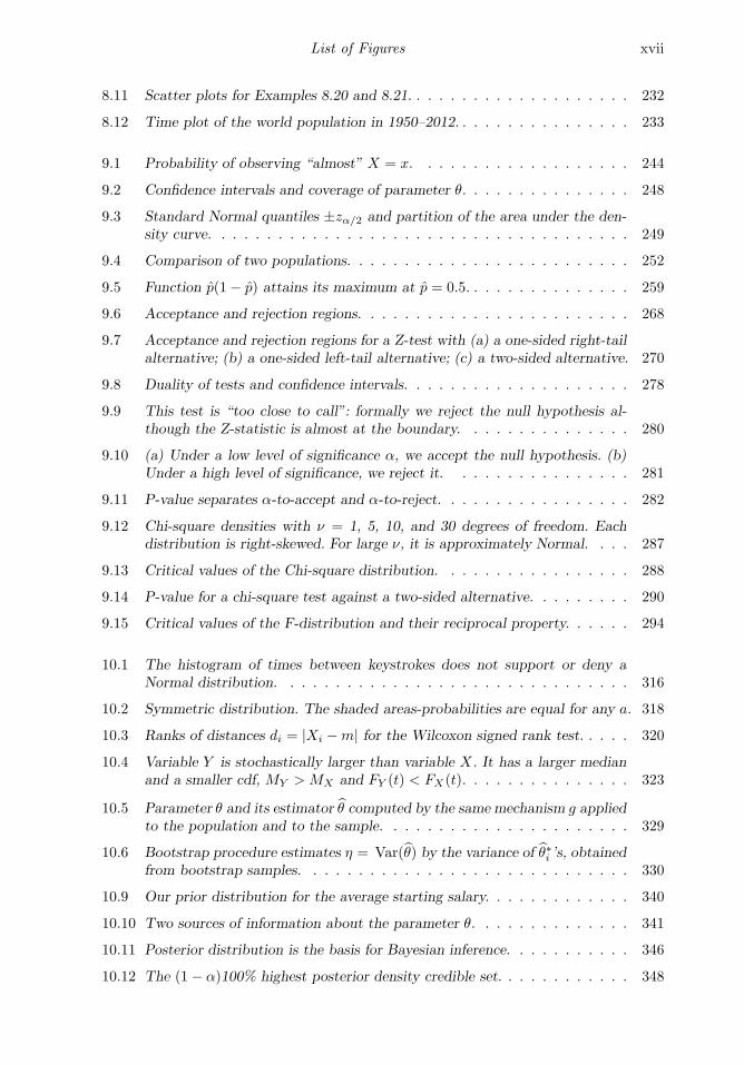
List of Figures xvii
8.11 Scatter plots for Examples 8.20 and 8.21. . . . . . . . . . . . . . . . . . . . 232
8.12 Time plot of the world population in 1950–2012. . . . . . . . . . . . . . . . 233
9.1 Probability of observing “almost” X = x. . . . . . . . . . . . . . . . . . . 244
9.2 Confidence intervals and coverage of parameter θ. . . . . . . . . . . . . . . 248
9.3 Standard Normal quantiles ±zα/2 and partition of the area under the den-sity curve. . . . . . . . . . . . . . . . . . . . . . . . . . . . . . . . . . . . . 249
9.4 Comparison of two populations. . . . . . . . . . . . . . . . . . . . . . . . . 252
9.5 Function p(1− p) attains its maximum at p = 0.5. . . . . . . . . . . . . . . 259
9.6 Acceptance and rejection regions. . . . . . . . . . . . . . . . . . . . . . . . 268
9.7 Acceptance and rejection regions for a Z-test with (a) a one-sided right-tailalternative; (b) a one-sided left-tail alternative; (c) a two-sided alternative. 270
9.8 Duality of tests and confidence intervals. . . . . . . . . . . . . . . . . . . . 278
9.9 This test is “too close to call”: formally we reject the null hypothesis al-though the Z-statistic is almost at the boundary. . . . . . . . . . . . . . . 280
9.10 (a) Under a low level of significance α, we accept the null hypothesis. (b)Under a high level of significance, we reject it. . . . . . . . . . . . . . . . 281
9.11 P-value separates α-to-accept and α-to-reject. . . . . . . . . . . . . . . . . 282
9.12 Chi-square densities with ν = 1, 5, 10, and 30 degrees of freedom. Eachdistribution is right-skewed. For large ν, it is approximately Normal. . . . 287
9.13 Critical values of the Chi-square distribution. . . . . . . . . . . . . . . . . 288
9.14 P-value for a chi-square test against a two-sided alternative. . . . . . . . . 290
9.15 Critical values of the F-distribution and their reciprocal property. . . . . . 294
10.1 The histogram of times between keystrokes does not support or deny aNormal distribution. . . . . . . . . . . . . . . . . . . . . . . . . . . . . . . 316
10.2 Symmetric distribution. The shaded areas-probabilities are equal for any a. 318
10.3 Ranks of distances di = |Xi −m| for the Wilcoxon signed rank test. . . . . 320
10.4 Variable Y is stochastically larger than variable X . It has a larger medianand a smaller cdf, MY > MX and FY (t) < FX(t). . . . . . . . . . . . . . . 323
10.5 Parameter θ and its estimator θ computed by the same mechanism g appliedto the population and to the sample. . . . . . . . . . . . . . . . . . . . . . 329
10.6 Bootstrap procedure estimates η = Var(θ) by the variance of θ∗i ’s, obtainedfrom bootstrap samples. . . . . . . . . . . . . . . . . . . . . . . . . . . . . 330
10.9 Our prior distribution for the average starting salary. . . . . . . . . . . . . 340
10.10 Two sources of information about the parameter θ. . . . . . . . . . . . . . 341
10.11 Posterior distribution is the basis for Bayesian inference. . . . . . . . . . . 346
10.12 The (1− α)100% highest posterior density credible set. . . . . . . . . . . . 348

xviii Probability and Statistics for Computer Scientists
10.13 Normal prior distribution and the 95% HPD credible set for the mean start-ing salary of Computer Science graduates (Example 10.29). . . . . . . . . 348
10.14 Normal prior and posterior distributions for the mean starting salary (Ex-ample 10.29). . . . . . . . . . . . . . . . . . . . . . . . . . . . . . . . . . . 349
11.1 World population in 1950–2010 and its regression forecast for 2015 and 2020. 363
11.2 House sale prices and their footage. . . . . . . . . . . . . . . . . . . . . . . 364
11.3 Least squares estimation of the regression line. . . . . . . . . . . . . . . . . 365
11.4 Regression-based prediction. . . . . . . . . . . . . . . . . . . . . . . . . . . 369
11.5 Regression prediction of program efficiency. . . . . . . . . . . . . . . . . . 380
11.6 U.S. population in 1790–2010 (million people). . . . . . . . . . . . . . . . . 382
12.1 Derivative is the slope of a tangent line. . . . . . . . . . . . . . . . . . . . 431
12.2 Integrals are areas under the graph of f(x). . . . . . . . . . . . . . . . . . 434

List of Tables
0.1 New material in the 2nd edition . . . . . . . . . . . . . . . . . . . . . . . . xxiii
4.1 Pmf P (x) versus pdf f(x). . . . . . . . . . . . . . . . . . . . . . . . . . . . 77
4.2 Joint and marginal distributions in discrete and continuous cases. . . . . . 78
4.3 Moments for discrete and continuous distributions. . . . . . . . . . . . . . 79
9.1 Summary of Z-tests. . . . . . . . . . . . . . . . . . . . . . . . . . . . . . . 273
9.2 Summary of T-tests. . . . . . . . . . . . . . . . . . . . . . . . . . . . . . . 276
9.3 P-values for Z-tests. . . . . . . . . . . . . . . . . . . . . . . . . . . . . . . . 283
9.4 P-values for T-tests (Fν is the cdf of T-distribution with the suitable numberν of degrees of freedom). . . . . . . . . . . . . . . . . . . . . . . . . . . . . 284
9.5 χ2-tests for the population variance . . . . . . . . . . . . . . . . . . . . . . 291
9.6 Summary of F-tests for the ratio of population variances . . . . . . . . . . 297
10.1 All bootstrap samples Bi drawn from S and the corresponding sample me-dians for Example 10.18. . . . . . . . . . . . . . . . . . . . . . . . . . . . . 331
10.2 Three classical conjugate families. . . . . . . . . . . . . . . . . . . . . . . . 345
11.1 Population of the world, 1950–2020. . . . . . . . . . . . . . . . . . . . . . . 362
xix


Preface
Starting with the fundamentals of probability, this text leads readers to computer simula-tions and Monte Carlo methods, stochastic processes and Markov chains, queuing systems,statistical inference, and regression. These areas are heavily used in modern computer sci-ence, computer engineering, software engineering, and related fields.
For whom this book is written
The book is primarily intended for junior undergraduate to beginning graduate level stu-dents majoring in computer-related fields – computer science, software engineering, infor-mation systems, information technology, telecommunications, etc. At the same time, it canbe used by electrical engineering, mathematics, statistics, natural science, and other majorsfor a standard calculus-based introductory statistics course. Standard topics in probabilityand statistics are covered in Chapters 1–4 and 8–9.
Graduate students can use this book to prepare for probability-based courses such as queu-ing theory, artificial neural networks, computer performance, etc.
The book can also be used as a standard reference on probability and statistical methods,simulation, and modeling tools.
Recommended courses
The text is mainly recommended for a one-semester course with several open-end optionsavailable. At the same time, with the new Chapter 10, the second edition of this book canserve as a text for a full two-semester course in Probability and Statistics.
After introducing probability and distributions in Chapters 1–4, instructors may choose thefollowing continuations, see Figure 1.
Probability-oriented course. Proceed to Chapters 6–7 for Stochastic Processes, MarkovChains, and Queuing Theory. Computer science majors will find it attractive to supple-ment such a course with computer simulations and Monte Carlo methods. Students canlearn and practice general simulation techniques in Chapter 5, then advance to the simu-lation of stochastic processes and rather complex queuing systems in Sections 6.4 and 7.6.Chapter 5 is highly recommended but not required for the rest of the material.
Statistics-emphasized course. Proceed to Chapters 8–9 directly after the probability core,followed by additional topics in Statistics selected from Chapters 10 and 11. Such a cur-riculum is more standard, and it is suitable for a wide range of majors. Chapter 5 remainsoptional but recommended; it discusses statistical methods based on computer simulations.Modern bootstrap techniques in Section 10.3 will attractively continue this discussion.
A course satisfying ABET requirements. Topics covered in this book satisfy ABET (Accred-itation Board for Engineering and Technology) requirements for probability and statistics.
xxi

xxii Probability and Statistics for Computer Scientists
Chap. 1–4Probability
Core
Chap. 5Monte CarloMethods
Sec. 6.4Simulation ofStochasticProcesses
Sec. 7.6Simulationof QueuingSystems
Chap. 6StochasticProcesses
Chap. 8–9StatisticsCore
Chap. 7QueuingTheory
Chap. 10AdvancedStatistics
Chap. 11Regression
⑦
⑦
FIGURE 1: Flow-chart of chapters.
To meet the requirements, instructors should choose topics from Chapters 1–11. All or someof Chapters 5–7 and 10–11 may be considered optional, depending on the program’s ABETobjectives.
A two-semester course will cover all Chapters 1–11, possibly skipping some sections. Thematerial presented in this book splits evenly between Probability topics for the first semester(Chapters 1–7) and Statistics topics for the second semester (Chapters 8–11).
Prerequisites, and use of the appendix
Working differentiation and integration skills are required starting from Chapter 4. Theyare usually covered in one semester of university calculus.
As a refresher, the appendix has a very brief summary of the minimum calculus techniquesrequired for reading this book (Section 12.3). Certainly, this section cannot be used to learncalculus “from scratch”. It only serves as a reference and student aid.
Next, Chapters 6–7 and Sections 11.3–11.4 rely on very basic matrix computations. Es-sentially, readers should be able to multiply matrices, solve linear systems (Chapters 6–7),and compute inverse matrices (Section 11.3). A basic refresher of these skills with someexamples is in the appendix, Section 12.4.
Style and motivation
The book is written in a lively style and reasonably simple language that students find easy
Preface xxiii
to read and understand. Reading this book, students should feel as if an experienced andenthusiastic lecturer is addressing them in person.
Besides computer science applications and multiple motivating examples, the book containsrelated interesting facts, paradoxical statements, wide applications to other fields, etc. Iexpect prepared students to enjoy the course, benefit from it, and find it attractive anduseful for their careers.
Every chapter contains multiple examples with explicit solutions, many of them motivatedby computer science applications. Every chapter is concluded with a short summary andmore exercises for homework assignments and self-training. Over 270 problems can be as-signed from this book.
Computers, demos, illustrations, and MATLABr
Frequent self-explaining figures help readers understand and visualize concepts, formulas,and even some proofs. Moreover, instructors and students are invited to use included shortprograms for computer demonstrations. Randomness, uncertainty, behavior of random vari-ables and stochastic processes, convergence results such as the Central Limit Theorem, andespecially Monte Carlo simulations can be nicely visualized by animated graphics.
These short computer codes contain very basic and simple MATLAB commands, withdetailed commentary. Preliminary knowledge of MATLAB is not necessary. Readers canchoose another language and use the given commands as a block-chart. The recent versionof the Statistics Toolbox of MATLAB contains most of the discussed statistical methods. Inaddition to these tools, I intentionally included simple codes that can be directly reproducedin other languages. Some of them can be used for the projects and mini-projects proposedin this book.
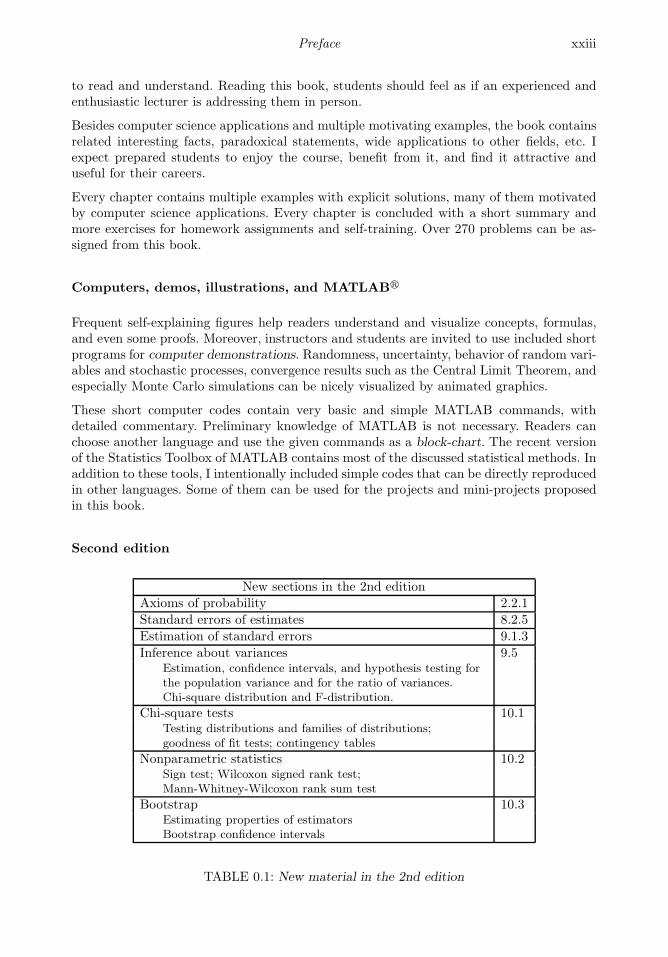
Second edition
New sections in the 2nd editionAxioms of probability 2.2.1
Standard errors of estimates 8.2.5
Estimation of standard errors 9.1.3
Inference about variances 9.5Estimation, confidence intervals, and hypothesis testing forthe population variance and for the ratio of variances.Chi-square distribution and F-distribution.
Chi-square tests 10.1Testing distributions and families of distributions;goodness of fit tests; contingency tables
Nonparametric statistics 10.2Sign test; Wilcoxon signed rank test;Mann-Whitney-Wilcoxon rank sum test
Bootstrap 10.3Estimating properties of estimatorsBootstrap confidence intervals
TABLE 0.1: New material in the 2nd edition

xxiv Probability and Statistics for Computer Scientists
Broad feedback coming from professors who use this book for their courses in differentcountries motivated me to work on the second edition. As a result, the Statistical Inferencechapter expanded and split into Chapters 9 and 10. The added material is organized in thenew sections, according to Table 0.1.
Also, the new edition has about 60 additional exercises. Get training, students, you willonly benefit from it!
Thanks and acknowledgments
The author is grateful to Taylor & Francis for their constant professional help, respon-siveness, support, and encouragement. Special thanks are due David Grubbs, Bob Stern,Marcus Fontaine, Jill Jurgensen, Barbara Johnson, Rachael Panthier, and Shashi Kumar.Many thanks go to my colleagues at UT-Dallas and other universities for their inspiringsupport and invaluable feedback, especially Professors Ali Hooshyar and Pankaj Choudharyat UT-Dallas, Joan Staniswalis and Amy Wagler at UT-El Paso, Lillian Cassel at Villanova,Alan Sprague at the University of Alabama, Katherine Merrill at the University of Vermont,Alessandro Di Bucchianico at Eindhoven University of Technology, and Marc Aerts at Has-selt University. I am grateful to Elena Baron for creative illustrations; Kate Pechekhonovafor interesting examples; and last but not least, to Eric, Anthony, and Masha Baron fortheir amazing patience and understanding.

Chapter 1
Introduction and Overview
1.1 Making decisions under uncertainty . . . . . . . . . . . . . . . . . . . . . . . . . . . . . 11.2 Overview of this book . . . . . . . . . . . . . . . . . . . . . . . . . . . . . . . . . . . . . . . . . . . . 3
Summary and conclusions . . . . . . . . . . . . . . . . . . . . . . . . . . . . . . . . . . . . . . . . . . 5Exercises . . . . . . . . . . . . . . . . . . . . . . . . . . . . . . . . . . . . . . . . . . . . . . . . . . . . . . . . . . . . 5
1.1 Making decisions under uncertainty
This course is about uncertainty, measuring and quantifying uncertainty, and making de-cisions under uncertainty. Loosely speaking, by uncertainty we mean the condition whenresults, outcomes, the nearest and remote future are not completely determined; their de-velopment depends on a number of factors and just on a pure chance.
Simple examples of uncertainty appear when you buy a lottery ticket, turn a wheel offortune, or toss a coin to make a choice.
Uncertainly appears in virtually all areas of Computer Science and Software Engineering.Installation of software requires uncertain time and often uncertain disk space. A newlyreleased software contains an uncertain number of defects. When a computer program isexecuted, the amount of required memory may be uncertain. When a job is sent to a printer,it takes uncertain time to print, and there is always a different number of jobs in a queueahead of it. Electronic components fail at uncertain times, and the order of their failurescannot be predicted exactly. Viruses attack a system at unpredictable times and affect anunpredictable number of files and directories.
Uncertainty surrounds us in everyday life, at home, at work, in business, and in leisure. Totake a snapshot, let us listen to the evening news.
Example 1.1. We may find out that the stock market had several ups and downs todaywhich were caused by new contracts being made, financial reports being released, and otherevents of this sort. Many turns of stock prices remained unexplained. Clearly, nobody wouldhave ever lost a cent in stock trading had the market contained no uncertainty.
We may find out that a launch of a space shuttle was postponed because of weather con-ditions. Why did not they know it in advance, when the event was scheduled? Forecastingweather precisely, with no error, is not a solvable problem, again, due to uncertainty.
To support these words, a meteorologist predicts, say, a 60% chance of rain. Why cannotshe let us know exactly whether it will rain or not, so we’ll know whether or not to takeour umbrellas? Yes, because of uncertainty. Because she cannot always know the situationwith future precipitation for sure.
We may find out that eruption of an active volcano has suddenly started, and it is not clear
1

2 Probability and Statistics for Computer Scientists
which regions will have to evacuate.
We may find out that a heavily favored home team unexpectedly lost to an outsider, anda young tennis player won against expectations. Existence and popularity of totalizators,where participants place bets on sports results, show that uncertainty enters sports, resultsof each game, and even the final standing.
We may also hear reports of traffic accidents, crimes, and convictions. Of course, if thatdriver knew about the coming accident ahead of time, he would have stayed home. ♦
Certainly, this list can be continued (at least one thing is certain!). Even when you driveto your college tomorrow, you will see an unpredictable number of green lights when youapproach them, you will find an uncertain number of vacant parking slots, you will reachthe classroom at an uncertain time, and you cannot be certain now about the number ofclassmates you will find in the classroom when you enter it.
Realizing that many important phenomena around us bear uncertainty, we have to un-derstand it and deal with it. Most of the time, we are forced to make decisions underuncertainty. For example, we have to deal with internet and e-mail knowing that we maynot be protected against all kinds of viruses. New software has to be released even if itstesting probably did not reveal all the defects. Some memory or disk quota has to be allo-cated for each customer by servers, internet service providers, etc., without knowing exactlywhat portion of users will be satisfied with these limitations. And so on.
This book is about measuring and dealing with uncertainty and randomness. Through basictheory and numerous examples, it teaches
– how to evaluate probabilities, or chances of different results (when the exact result isuncertain),
– how to select a suitable model for a phenomenon containing uncertainty and use it insubsequent decision making,
– how to evaluate performance characteristics and other important parameters for newdevices and servers,
– how to make optimal decisions under uncertainty.
Summary and conclusion
Uncertainty is a condition when the situation cannot be predetermined or predicted forsure with no error. Uncertainty exists in computer science, software engineering, in manyaspects of science, business, and our everyday life. It is an objective reality, and one has tobe able to deal with it. We are forced to make decisions under uncertainty.
Introduction and Overview 3
1.2 Overview of this book
The next chapter introduces a language that we’ll use to describe and quantify uncertainty.It is a language of Probability. When outcomes are uncertain, one can identify more likelyand less likely ones and assign, respectively, high and low probabilities to them. Probabilitiesare numbers between 0 and 1, with 0 being assigned to an impossible event and 1 being theprobability of an event that occurs for sure.
Next, using the introduced language, we shall discuss random variables as quantities thatdepend on chance. They assume different values with different probabilities. Due to un-certainty, an exact value of a random variable cannot be computed before this variable isactually observed or measured. Then, the best way to describe its behavior is to list all itspossible values along with the corresponding probabilities.
Such a collection of probabilities is called a distribution. Amazingly, many different phe-nomena of seemingly unrelated nature can be described by the same distribution or by thesame family of distributions. This allows a rather general approach to the entire class ofsituations involving uncertainty. As an application, it will be possible to compute probabil-ities of interest, once a suitable family of distributions is found. Chapters 3 and 4 introducefamilies of distributions that are most commonly used in computer science and other fields.
In modern practice, however, one often deals with rather complicated random phenom-ena where computation of probabilities and other quantities of interest is far from beingstraightforward. In such situations, we will make use of Monte Carlo methods (Chapter 5).Instead of direct computation, we shall learn methods of simulation or generation of randomvariables. If we are able to write a computer code for simulation of a certain phenomenon,we can immediately put it in a loop and simulate such a phenomenon thousands or millionsof times and simply count how many times our event of interest occurred. This is how weshall distinguish more likely and less likely events. We can then estimate probability of anevent by computing a proportion of simulations that led to the occurrence of this event.
As a step up to the next level, we shall realize that many random variables depend not onlyon a chance but also on time. That is, they evolve and develop in time while being randomat each particular moment. Examples include the number of concurrent users, the numberof jobs in a queue, the system’s available capacity, intensity of internet traffic, stock prices,air temperature, etc. A random variable that depends on time is called a stochastic process.In Chapter 6, we study some commonly used types of stochastic processes and use thesemodels to compute probabilities of events and other quantities of interest.
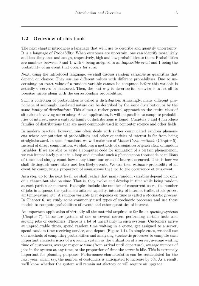
An important application of virtually all the material acquired so far lies in queuing systems(Chapter 7). These are systems of one or several servers performing certain tasks andserving jobs or customers. There is a lot of uncertainty in such systems. Customers arriveat unpredictable times, spend random time waiting in a queue, get assigned to a server,spend random time receiving service, and depart (Figure 1.1). In simple cases, we shall useour methods of computing probabilities and analyzing stochastic processes to compute suchimportant characteristics of a queuing system as the utilization of a server, average waitingtime of customers, average response time (from arrival until departure), average number ofjobs in the system at any time, or the proportion of time the server is idle. This is extremelyimportant for planning purposes. Performance characteristics can be recalculated for thenext year, when, say, the number of customers is anticipated to increase by 5%. As a result,we’ll know whether the system will remain satisfactory or will require an upgrade.

4 Probability and Statistics for Computer Scientists
Arrivals
Server I
Server II
Server III
Departures
FIGURE 1.1: A queuing system with 3 servers.
When direct computation is too complicated, resource consuming, too approximate, or sim-ply not feasible, we shall use Monte Carlo methods. The book contains standard examplesof computer codes simulating rather complex queuing systems and evaluating their vitalcharacteristics. The codes are written in MATLAB, with detailed explanations of steps,and most of them can be directly translated to other computer languages.
Next, we turn to Statistical Inference. While in Probability, we usually deal with more orless clearly described situations (models), in Statistics, all the analysis is based on collectedand observed data. Given the data, a suitable model (say, a family of distributions) is fitted,its parameters are estimated, and conclusions are drawn concerning the entire totality ofobserved and unobserved subjects of interest that should follow the same model.
A typical Probability problem sounds like this.
Example 1.2. A folder contains 50 executable files. When a computer virus attacks asystem, each file is affected with probability 0.2. Compute the probability that during avirus attack, more than 15 files get affected. ♦
Notice that the situation is rather clearly described, in terms of the total number of filesand the chance of affecting each file. The only uncertain quantity is the number of affectedfiles, which cannot be predicted for sure.
A typical Statistics problem sounds like this.
Example 1.3. A folder contains 50 executable files. When a computer virus attacks asystem, each file is affected with the same probability p. It has been observed that during avirus attack, 15 files got affected. Estimate p. Is there a strong indication that p is greaterthan 0.2? ♦
This is a practical situation. A user only knows the objectively observed data: the numberof files in the folder and the number of files that got affected. Based on that, he needs toestimate p, the proportion of all the files, including the ones in his system and any similarsystems. One may provide a point estimator of p, a real number, or may opt to construct aconfidence interval of “most probable” values of p. Similarly, a meteorologist may predict,say, a temperature of 70oF, which, realistically, does not exclude a possibility of 69 or 72degrees, or she may give us an interval by promising, say, between 68 and 72 degrees.
Most forecasts are being made from a carefully and suitably chosen model that fits the data.
Exercises 5
A widely used method is regression that utilizes the observed data to find a mathematicalform of relationship between two variables (Chapter 11). One variable is called predictor,the other is response. When the relationship between them is established, one can use thepredictor to infer about the response. For example, one can more or less accurately estimatethe average installation time of a software given the size of its executable files. An even moreaccurate inference about the response can be made based on several predictors such as thesize of executable files, amount of random access memory (RAM), and type of processorand operating system. This will call for multivariate regression.
Each method will be illustrated by numerous practical examples and exercises. As the ulti-mate target, by the end of this course, students should be able to read a word problem or acorporate report, realize the uncertainty involved in the described situation, select a suitableprobability model, estimate and test its parameters based on real data, compute probabil-ities of interesting events and other vital characteristics, and make meaningful conclusionsand forecasts.
Summary and conclusions
In this course, uncertainty is measured and described on a language of Probability. Usingthis language, we shall study random variables and stochastic processes and learn the mostcommonly used types of distributions. In particular, we shall be able to find a suitablestochastic model for the described situation and use it to compute probabilities and otherquantities of interest. When direct computation is not feasible, Monte Carlo methods willbe used based on a random number generator. We shall then learn how to make decisionsunder uncertainty based on the observed data, how to estimate parameters of interest, testhypotheses, fit regression models, and make forecasts.
Exercises
1.1. List 20 situations involving uncertainty that happened with you yesterday.
1.2. Name 10 random variables that you observed or dealt with yesterday.
1.3. Name 5 stochastic processes that played a role in your actions yesterday.
1.4. In a famous joke, a rather lazy student tosses a coin and decides what to do next. If it turnsup heads, play a computer game. If tails, watch a video. If it stands on its edge, do thehomework. If it hangs in the air, prepare for an exam.
(a) Which events should be assigned probability 0, probability 1, and some probabilitystrictly between 0 and 1?

6 Probability and Statistics for Computer Scientists
(b) What probability between 0 and 1 would you assign to the event “watch a video,”and how does it help you to define “a fair coin”?
1.5. A new software package is being tested by specialists. Every day, a number of defects isfound and corrected. It is planned to release this software in 30 days. Is it possible to predicthow many defects per day specialists will be finding at the time of the release? What datashould be collected for this purpose, what is the predictor, and what is the response?
1.6. Mr. Cheap plans to open a computer store to trade hardware. He would like to stock anoptimal number of different hardware products in order to optimize his monthly profit. Dataare available on similar computer stores opened in the area. What kind of data should Mr.Cheap collect in order to predict his monthly profit? What should he use as a predictor andas a response in his analysis?

Part I
Probability and RandomVariables
7


Chapter 2
Probability
2.1 Events and their probabilities . . . . . . . . . . . . . . . . . . . . . . . . . . . . . . . . . . . . 92.1.1 Outcomes, events, and the sample space . . . . . . . . . . . . . . . . 102.1.2 Set operations . . . . . . . . . . . . . . . . . . . . . . . . . . . . . . . . . . . . . . . . . . . 11
2.2 Rules of Probability . . . . . . . . . . . . . . . . . . . . . . . . . . . . . . . . . . . . . . . . . . . . . . 132.2.1 Axioms of Probability . . . . . . . . . . . . . . . . . . . . . . . . . . . . . . . . . . . 142.2.2 Computing probabilities of events . . . . . . . . . . . . . . . . . . . . . . . 152.2.3 Applications in reliability . . . . . . . . . . . . . . . . . . . . . . . . . . . . . . . . 18
2.3 Combinatorics . . . . . . . . . . . . . . . . . . . . . . . . . . . . . . . . . . . . . . . . . . . . . . . . . . . . 202.3.1 Equally likely outcomes . . . . . . . . . . . . . . . . . . . . . . . . . . . . . . . . . 202.3.2 Permutations and combinations . . . . . . . . . . . . . . . . . . . . . . . . . 22
2.4 Conditional probability and independence . . . . . . . . . . . . . . . . . . . . . . 27Summary and conclusions . . . . . . . . . . . . . . . . . . . . . . . . . . . . . . . . . . . . . . . . . . 32Exercises . . . . . . . . . . . . . . . . . . . . . . . . . . . . . . . . . . . . . . . . . . . . . . . . . . . . . . . . . . . . 33
This chapter introduces the key concept of probability, its fundamental rules and properties,and discusses most basic methods of computing probabilities of various events.
2.1 Events and their probabilities
The concept of probability perfectly agrees with our intuition. In everyday life, probabilityof an event is understood as a chance that this event will happen.
Example 2.1. If a fair coin is tossed, we say that it has a 50-50 (equal) chance of turningup heads or tails. Hence, the probability of each side equals 1/2. It does not mean that acoin tossed 10 times will always produce exactly 5 heads and 5 tails. If you don’t believe,try it! However, if you toss a coin 1 million times, the proportion of heads is anticipated tobe very close to 1/2.
♦
This example suggests that in a long run, probability of an event can be viewed as aproportion of times this event happens, or its relative frequency. In forecasting, it is commonto speak about the probability as a likelihood (say, the company’s profit is likely to riseduring the next quarter). In gambling and lottery, probability is equivalent to odds. Havingthe winning odds of 1 to 99 (1:99) means that the probability to win is 0.01, and theprobability to lose is 0.99. It also means, on a relative-frequency language, that if you playlong enough, you will win about 1% of the time.
9
10 Probability and Statistics for Computer Scientists
Example 2.2. If there are 5 communication channels in service, and a channel is selectedat random when a telephone call is placed, then each channel has a probability 1/5 = 0.2of being selected. ♦
Example 2.3. Two competing software companies are after an important contract. Com-pany A is twice as likely to win this competition as company B. Hence, the probability towin the contract equals 2/3 for A and 1/3 for B.
♦
A mathematical definition of probability will be given in Section 2.2.1, after we get ac-quainted with a few fundamental concepts.
2.1.1 Outcomes, events, and the sample space
Probabilities arise when one considers and weighs possible results of some experiment. Someresults are more likely than others. An experiment may be as simple as a coin toss, or ascomplex as starting a new business.
DEFINITION 2.1
A collection of all elementary results, or outcomes of an experiment, is calleda sample space.
DEFINITION 2.2
Any set of outcomes is an event. Thus, events are subsets of the sample space.
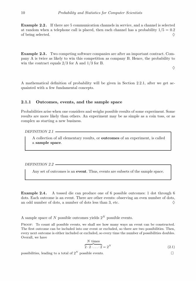
Example 2.4. A tossed die can produce one of 6 possible outcomes: 1 dot through 6dots. Each outcome is an event. There are other events: observing an even number of dots,an odd number of dots, a number of dots less than 3, etc. ♦
A sample space of N possible outcomes yields 2N possible events.
Proof: To count all possible events, we shall see how many ways an event can be constructed.The first outcome can be included into our event or excluded, so there are two possibilities. Then,every next outcome is either included or excluded, so every time the number of possibilities doubles.Overall, we have
N times︷ ︸︸ ︷2 · 2 · . . . · 2 = 2N (2.1)
possibilities, leading to a total of 2N possible events.

Probability 11
Example 2.5. Consider a football game between the Dallas Cowboys and the New YorkGiants. The sample space consists of 3 outcomes,
Ω = Cowboys win, Giants win, they tie Combining these outcomes in all possible ways, we obtain the following 23 = 8 events:Cowboys win, lose, tie, get at least a tie, get at most a tie, no tie, get some result, and getno result. The event “some result” is the entire sample space Ω, and by common sense, itshould have probability 1. The event “no result” is empty, it does not contain any outcomes,so its probability is 0. ♦
Notation Ω = sample space∅ = empty event
P E = probability of event E
2.1.2 Set operations
Events are sets of outcomes. Therefore, to learn how to compute probabilities of events, weshall discuss some set operations. Namely, we shall define unions, intersections, differences,and complements.
DEFINITION 2.3
A union of events A,B,C, . . . is an event consisting of all the outcomes in allthese events. It occurs if any of A,B,C, . . . occurs, and therefore, correspondsto the word “or”: A or B or C or ... (Figure 2.1a).
Diagrams like Figure 2.1, where events are represented by circles, are called Venn diagrams.
DEFINITION 2.4
An intersection of events A,B,C, . . . is an event consisting of outcomes thatare common in all these events. It occurs if each A,B,C, . . . occurs, and there-fore, corresponds to the word “and”: A and B and C and ... (Figure 2.1b).
DEFINITION 2.5
A complement of an event A is an event that occurs every time when A doesnot occur. It consists of outcomes excluded from A, and therefore, correspondsto the word “not”: not A (Figure 2.1c).
DEFINITION 2.6
A difference of events A and B consists of all outcomes included in A butexcluded from B. It occurs when A occurs and B does not, and corresponds to“but not”: A but not B (Figure 2.1d).
12 Probability and Statistics for Computer Scientists
(a)
A B
A ∪B
(b)
A B
A ∩B
(c)
A
A
(d)
A B
A\B
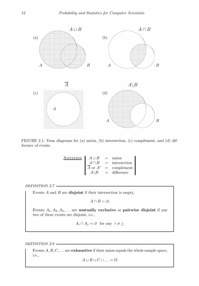
FIGURE 2.1: Venn diagrams for (a) union, (b) intersection, (c) complement, and (d) dif-ference of events.
Notation A ∪B = unionA ∩B = intersection
A or Ac = complementA\B = difference
DEFINITION 2.7
Events A and B are disjoint if their intersection is empty,
A ∩B = ∅.
Events A1, A2, A3, . . . are mutually exclusive or pairwise disjoint if anytwo of these events are disjoint, i.e.,
Ai ∩Aj = ∅ for any i 6= j .
DEFINITION 2.8
EventsA,B,C, . . . are exhaustive if their union equals the whole sample space,i.e.,
A ∪B ∪ C ∪ . . . = Ω.

Probability 13
Mutually exclusive events will never occur at the same time. Occurrence of any one of themeliminates the possibility for all the others to occur.
Exhaustive events cover the entire Ω, so that “there is nothing left.” In other words, amongany collection of exhaustive events, at least one occurs for sure.
Example 2.6. When a card is pooled from a deck at random, the four suits are at thesame time disjoint and exhaustive. ♦
Example 2.7. Any event A and its complement A represent a classical example of disjointand exhaustive events. ♦
Example 2.8. Receiving a grade of A, B, or C for some course are mutually exclusiveevents, but unfortunately, they are not exhaustive. ♦
As we see in the next sections, it is often easier to compute probability of an intersectionthan probability of a union. Taking complements converts unions into intersections, see(2.2).
E1 ∪ . . . ∪ En = E1 ∩ . . . ∩ En, E1 ∩ . . . ∩ En = E1 ∪ . . . ∪ En (2.2)
Proof of (2.2): Since the union E1 ∪ . . . ∪ En represents the event “at least one event occurs,”its complement has the form
E1 ∪ . . . ∪En = none of them occurs = E1 does not occur ∩ . . . ∩En does not occur
= E1 ∩ . . . ∩En.
The other equality in (2.2) is left as Exercise 2.34.
Example 2.9. Graduating with a GPA of 4.0 is an intersection of getting an A in eachcourse. Its complement, graduating with a GPA below 4.0, is a union of receiving a gradebelow A at least in one course. ♦
Rephrasing (2.2), a complement to “nothing” is “something,” and “not everything” means“at least one is missing”.
2.2 Rules of Probability
Now we are ready for the rigorous definition of probability. All the rules and principles ofcomputing probabilities of events follow from this definition.
Mathematically, probability is introduced through several axioms.
14 Probability and Statistics for Computer Scientists
2.2.1 Axioms of Probability
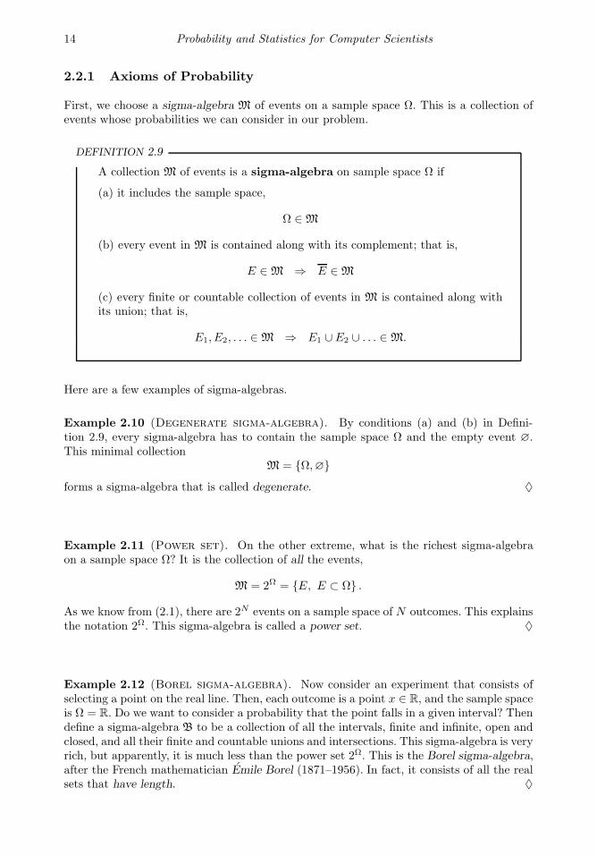
First, we choose a sigma-algebra M of events on a sample space Ω. This is a collection ofevents whose probabilities we can consider in our problem.
DEFINITION 2.9
A collection M of events is a sigma-algebra on sample space Ω if
(a) it includes the sample space,
Ω ∈ M
(b) every event in M is contained along with its complement; that is,
E ∈ M ⇒ E ∈ M
(c) every finite or countable collection of events in M is contained along withits union; that is,
E1, E2, . . . ∈ M ⇒ E1 ∪E2 ∪ . . . ∈ M.
Here are a few examples of sigma-algebras.
Example 2.10 (Degenerate sigma-algebra). By conditions (a) and (b) in Defini-tion 2.9, every sigma-algebra has to contain the sample space Ω and the empty event ∅.This minimal collection
M = Ω,∅forms a sigma-algebra that is called degenerate. ♦
Example 2.11 (Power set). On the other extreme, what is the richest sigma-algebraon a sample space Ω? It is the collection of all the events,
M = 2Ω = E, E ⊂ Ω .
As we know from (2.1), there are 2N events on a sample space of N outcomes. This explainsthe notation 2Ω. This sigma-algebra is called a power set. ♦
Example 2.12 (Borel sigma-algebra). Now consider an experiment that consists ofselecting a point on the real line. Then, each outcome is a point x ∈ R, and the sample spaceis Ω = R. Do we want to consider a probability that the point falls in a given interval? Thendefine a sigma-algebra B to be a collection of all the intervals, finite and infinite, open andclosed, and all their finite and countable unions and intersections. This sigma-algebra is veryrich, but apparently, it is much less than the power set 2Ω. This is the Borel sigma-algebra,after the French mathematician Emile Borel (1871–1956). In fact, it consists of all the realsets that have length. ♦
Probability 15
Axioms of Probability are in the following definition.
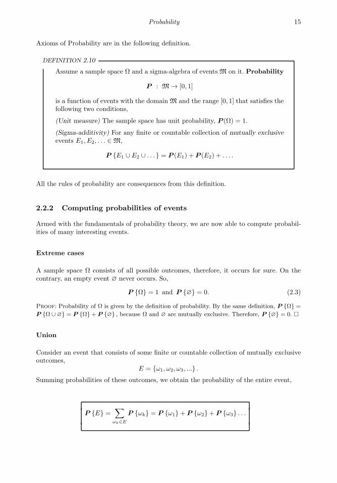
DEFINITION 2.10
Assume a sample space Ω and a sigma-algebra of events M on it. Probability
P : M → [0, 1]
is a function of events with the domain M and the range [0, 1] that satisfies thefollowing two conditions,
(Unit measure) The sample space has unit probability, P (Ω) = 1.
(Sigma-additivity) For any finite or countable collection of mutually exclusiveevents E1, E2, . . . ∈ M,
P E1 ∪ E2 ∪ . . . = P (E1) + P (E2) + . . . .
All the rules of probability are consequences from this definition.
2.2.2 Computing probabilities of events
Armed with the fundamentals of probability theory, we are now able to compute probabil-ities of many interesting events.
Extreme cases
A sample space Ω consists of all possible outcomes, therefore, it occurs for sure. On thecontrary, an empty event ∅ never occurs. So,
P Ω = 1 and P ∅ = 0. (2.3)
Proof: Probability of Ω is given by the definition of probability. By the same definition, P Ω =
P Ω ∪ ∅ = P Ω+ P ∅ , because Ω and ∅ are mutually exclusive. Therefore, P ∅ = 0.
Union
Consider an event that consists of some finite or countable collection of mutually exclusiveoutcomes,
E = ω1, ω2, ω3, ... .Summing probabilities of these outcomes, we obtain the probability of the entire event,
P E =∑
ωk∈E
P ωk = P ω1+ P ω2+ P ω3 . . .
16 Probability and Statistics for Computer Scientists
(a)
A B
A ∪B
A ∩B
(b)
A B
C
A ∪B ∪ C
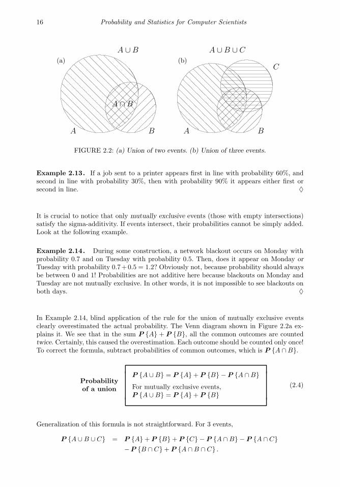
FIGURE 2.2: (a) Union of two events. (b) Union of three events.
Example 2.13. If a job sent to a printer appears first in line with probability 60%, andsecond in line with probability 30%, then with probability 90% it appears either first orsecond in line. ♦
It is crucial to notice that only mutually exclusive events (those with empty intersections)satisfy the sigma-additivity. If events intersect, their probabilities cannot be simply added.Look at the following example.
Example 2.14. During some construction, a network blackout occurs on Monday withprobability 0.7 and on Tuesday with probability 0.5. Then, does it appear on Monday orTuesday with probability 0.7+0.5 = 1.2? Obviously not, because probability should alwaysbe between 0 and 1! Probabilities are not additive here because blackouts on Monday andTuesday are not mutually exclusive. In other words, it is not impossible to see blackouts onboth days. ♦
In Example 2.14, blind application of the rule for the union of mutually exclusive eventsclearly overestimated the actual probability. The Venn diagram shown in Figure 2.2a ex-plains it. We see that in the sum P A + P B, all the common outcomes are countedtwice. Certainly, this caused the overestimation. Each outcome should be counted only once!To correct the formula, subtract probabilities of common outcomes, which is P A ∩B.
Probabilityof a union
P A ∪B = P A+ P B − P A ∩BFor mutually exclusive events,P A ∪B = P A+ P B
(2.4)
Generalization of this formula is not straightforward. For 3 events,
P A ∪B ∪ C = P A+ P B+ P C − P A ∩B − P A ∩C−P B ∩ C+ P A ∩B ∩ C .
Probability 17
As seen in Figure 2.2b, when we add probabilities of A, B, and C, each pairwise intersectionis counted twice. Therefore, we subtract the probabilities of P A ∩B, etc. Finally, considerthe triple intersection A∩B ∩C. Its probability is counted 3 times within each main event,then subtracted 3 times with each pairwise intersection. Thus, it is not counted at all sofar! Therefore, we add its probability P A ∩B ∩ C in the end.
For an arbitrary collection of events, see Exercise 2.33.
Example 2.15. In Example 2.14, suppose there is a probability 0.35 of experiencingnetwork blackouts on both Monday and Tuesday. Then the probability of having a blackouton Monday or Tuesday equals
0.7 + 0.5− 0.35 = 0.85.
♦
Complement
Recall that events A and A are exhaustive, hence A∪A = Ω. Also, they are disjoint, hence
P A+ PA= P
A ∪ A
= P Ω = 1.
Solving this for PA, we obtain a rule that perfectly agrees with the common sense,
Complement rule PA= 1− P A
Example 2.16. If a system appears protected against a new computer virus with prob-ability 0.7, then it is exposed to it with probability 1− 0.7 = 0.3. ♦
Example 2.17. Suppose a computer code has no errors with probability 0.45. Then, ithas at least one error with probability 0.55. ♦
Intersection of independent events
DEFINITION 2.11
Events E1, . . . , En are independent if they occur independently of each other,i.e., occurrence of one event does not affect the probabilities of others.
The following basic formula can serve as the criterion of independence.
Independentevents
P E1 ∩ . . . ∩ En = P E1 · . . . ·P En
18 Probability and Statistics for Computer Scientists
We shall defer explanation of this formula until Section 2.4 which will also give a rule forintersections of dependent events.
2.2.3 Applications in reliability
Formulas of the previous Section are widely used in reliability, when one computes theprobability for a system of several components to be functional.
Example 2.18 (Reliability of backups). There is a 1% probability for a hard driveto crash. Therefore, it has two backups, each having a 2% probability to crash, and all threecomponents are independent of each other. The stored information is lost only in an unfor-tunate situation when all three devices crash. What is the probability that the informationis saved?
Solution. Organize the data. Denote the events, say,
H = hard drive crashes ,
B1 = first backup crashes , B2 = second backup crashes .It is given that H , B1, and B2 are independent,
P H = 0.01, and P B1 = P B2 = 0.02.
Applying rules for the complement and for the intersection of independent events,
P saved = 1− P lost = 1− P H ∩B1 ∩B2= 1− P HP B1P B2= 1− (0.01)(0.02)(0.02) = 0.999996.
(This is precisely the reason of having backups, isn’t it? Without backups, the probabilityfor information to be saved is only 0.99.) ♦
When the system’s components are connected in parallel, it is sufficient for at least onecomponent to work in order for the whole system to function. Reliability of such a systemis computed as in Example 2.18. Backups can always be considered as devices connected inparallel.
At the other end, consider a system whose components are connected in sequel. Failure of onecomponent inevitably causes the whole system to fail. Such a system is more “vulnerable.”In order to function with a high probability, it needs each component to be reliable, as inthe next example.
Example 2.19. Suppose that a shuttle’s launch depends on three key devices that op-erate independently of each other and malfunction with probabilities 0.01, 0.02, and 0.02,respectively. If any of the key devices malfunctions, the launch will be postponed. Compute

Probability 19
the probability for the shuttle to be launched on time, according to its schedule.
Solution. In this case,
P on time = P all devices function = P
H ∩B1 ∩B2
= PHPB1
PB2
(independence)
= (1− 0.01)(1− 0.02)(1− 0.02) (complement rule)
= 0.9508.
Notice how with the same probabilities of individual components as in Example 2.18, thesystem’s reliability decreased because the components were connected sequentially. ♦
Many modern systems consist of a great number of devices connected in sequel and inparallel.
FIGURE 2.3: Calculate reliability of this system (Example 2.20).
Example 2.20 (Techniques for solving reliability problems). Calculate reliabilityof the system in Figure 2.3 if each component is operable with probability 0.92 independentlyof the other components.
Solution. This problem can be simplified and solved “step by step.”
1. The upper link A-B works if both A and B work, which has probability
P A ∩B = (0.92)2 = 0.8464.
We can represent this link as one component F that operates with probability 0.8464.
2. By the same token, components D and E, connected in parallel, can be replaced bycomponent G, operable with probability
P D ∪ E = 1− (1− 0.92)2 = 0.9936,
as shown in Figure 2.4a.

20 Probability and Statistics for Computer Scientists
(a) (b)
FIGURE 2.4: Step by step solution of a system reliability problem.
3. Components C and G, connected sequentially, can be replaced by component H, op-erable with probability P C ∩G = 0.92 · 0.9936 = 0.9141, as shown in Figure 2.4b.
4. Last step. The system operates with probability
P F ∪H = 1− (1− 0.8464)(1− 0.9141) = 0.9868,
which is the final answer.
In fact, the event “the system is operable” can be represented as (A∩B)∪C ∩ (D ∪ E) ,whose probability we found step by step. ♦
2.3 Combinatorics
2.3.1 Equally likely outcomes
A simple situation for computing probabilities is the case of equally likely outcomes. Thatis, when the sample space Ω consists of n possible outcomes, ω1, . . . , ωn, each having thesame probability. Since
n∑
1
P ωk = P Ω = 1,
we have in this case P ωk = 1/n for all k. Further, a probability of any event E consistingof t outcomes, equals
P E =∑
ωk∈E
(1
n
)= t
(1
n
)=
number of outcomes in E
number of outcomes in Ω.
The outcomes forming event E are often called “favorable.” Thus we have a formula
Equallylikely
outcomesP E =
number of favorable outcomes
total number of outcomes=
NF
NT(2.5)
where index “F” means “favorable” and “T ” means “total.”
Probability 21
Example 2.21. Tossing a die results in 6 equally likely possible outcomes, identified bythe number of dots from 1 to 6. Applying (2.5), we obtain,
P 1 = 1/6, P odd number of dots = 3/6, P less than 5 = 4/6.
♦
The solution and even the answer to such problems may depend on our choice of outcomesand a sample space. Outcomes should be defined in such a way that they appear equallylikely, otherwise formula (2.5) does not apply.
Example 2.22. A card is drawn from a bridge 52-card deck at random. Compute theprobability that the selected card is a spade.
First solution. The sample space consists of 52 equally likely outcomes—cards. Among them,there are 13 favorable outcomes—spades. Hence, P spade = 13/52 = 1/4.
Second solution. The sample space consists of 4 equally likely outcomes—suits: clubs,diamonds, hearts, and spades. Among them, one outcome is favorable—spades. Hence,P spade = 1/4. ♦
These two solutions relied on different sample spaces. However, in both cases, the definedoutcomes were equally likely, therefore (2.5) was applicable, and we obtained the sameresult.
However, the situation may be different.
Example 2.23. A young family plans to have two children. What is the probability oftwo girls?
Solution 1 (wrong). There are 3 possible families with 2 children: two girls, two boys, andone of each gender. Therefore, the probability of two girls is 1/3.
Solution 2 (right). Each child is (supposedly) equally likely to be a boy or a girl. Gendersof the two children are (supposedly) independent. Therefore,
P two girls =
(1
2
)(1
2
)= 1/4.
♦
The second solution implies that the sample space consists of four, not three, equally likelyoutcomes: two boys, two girls, a boy and a girl, a girl and a boy. Each outcome in thissample has probability 1/4. Notice that the last two outcomes are counted separately, withthe meaning, say, “the first child is a boy, the second one is a girl” and “the first child is agirl, the second one is a boy.”
It is all right to define a sample space as in Solution 1. However, one must know in this casethat the defined outcomes are not equally likely. Indeed, from Solution 2, we see that havingone child of each gender is the most likely outcome, with probability of 1/4+ 1/4 = 1/2. Itwas a mistake to apply (2.5) for such a sample space in Solution 1.
22 Probability and Statistics for Computer Scientists
Example 2.24 (Paradox). There is a simple but controversial “situation” about a fam-ily with two children. Even some graduate students often fail to resolve it.
A family has two children. You met one of them, Leo, and he is a boy. What is the proba-bility that the other child is also a boy?
On one hand, why would the other child’s gender be affected by Leo? Leo should have abrother or a sister with probabilities 1/2 and 1/2.
On the other hand, see Example 2.23. The sample space consists of 4 equally likely outcomes,GG,BB,BG,GB. You have already met one boy, thus the first outcome is automaticallyeliminated: BB,BG,GB. Among the remaining three outcomes, Jimmy has a brother inone case and a sister in two cases. Thus, isn’t the probability of a boy equal 1/3?
Where is the catch? Apparently, the sample space Ω has not been clearly defined in thisexample. The experiment is more complex than in Example 2.23 because we are now con-cerned not only about the gender of children but also about meeting one of them. What isthe mechanism, what are the probabilities for you to meet one or the other child? And onceyou met Leo, do the outcomes BB,BG,GB remain equally likely?
A complete solution to this paradox is broken into steps in Exercise 2.30. ♦
In reality, business-related, sports-related, and political events are typically not equallylikely. One outcome is usually more likely that another. For example, one team is alwaysstronger than the other. Equally likely outcomes are usually associated with conditions of“a fair game” and “selected at random.” In fair gambling, all cards, all dots on a die, allnumbers in a roulette are equally likely. Also, when a survey is conducted, or a sample isselected “at random,” the outcomes are “as close as possible” to being equally likely. Thismeans all the subjects have the same chance to be selected into a sample (otherwise, it isnot a fair sample, and it can produce “biased” results).
2.3.2 Permutations and combinations
Formula (2.5) is simple, as long as its numerator and denominator can be easily evaluated.This is rarely the case; often the sample space consists of a multitude of outcomes. Combi-natorics provides special techniques for the computation of NT and NF , the total numberand the number of favorable outcomes.
We shall consider a generic situation when objects are selected at random from a set of n.This general model has a number of useful applications.
The objects may be selected with replacement or without replacement. They may also bedistinguishable or indistinguishable.
DEFINITION 2.12
Sampling with replacement means that every sampled item is replaced intothe initial set, so that any of the objects can be selected with probability 1/nat any time. In particular, the same object may be sampled more than once.

Probability 23
DEFINITION 2.13
Sampling without replacement means that every sampled item is removedfrom further sampling, so the set of possibilities reduces by 1 after each selec-tion.
DEFINITION 2.14
Objects are distinguishable if sampling of exactly the same objects in a dif-ferent order yields a different outcome, that is, a different element of the samplespace. For indistinguishable objects, the order is not important, it only mat-ters which objects are sampled and which ones aren’t. Indistinguishable objectsarranged in a different order do not generate a new outcome.
Example 2.25 (Computer-generated passwords). When random passwords are gen-erated, the order of characters is important because a different order yields a different pass-word. Characters are distinguishable in this case. Further, if a password has to consist ofdifferent characters, they are sampled from the alphabet without replacement. ♦
Example 2.26 (Polls). When a sample of people is selected to conduct a poll, the sameparticipants produce the same responses regardless of their order. They can be consideredindistinguishable. ♦
Permutations with replacement
Possible selections of k distinguishable objects from a set of n are called permutations.When we sample with replacement, each time there are n possible selections, and the totalnumber of permutations is
Permutationswith
replacementPr(n, k) =
k terms︷ ︸︸ ︷n · n · . . . · n = nk
Example 2.27 (Breaking passwords). From an alphabet consisting of 10 digits, 26lower-case and 26 capital letters, one can create Pr(62, 8) = 218,340,105,584,896 (over 218trillion) different 8-character passwords. At a speed of 1 million passwords per second, itwill take a spy program almost 7 years to try all of them. Thus, on the average, it will guessyour password in about 3.5 years.
24 Probability and Statistics for Computer Scientists
At this speed, the spy program can test 604,800,000,000 passwords within 1 week. Theprobability that it guesses your password in 1 week is
NF
NT=
number of favorable outcomes
total number of outcomes=
604,800,000,000
218,340,105,584,896= 0.00277.
However, if capital letters are not used, the number of possible passwords is reduced toPr(36, 8) = 2,821,109,907,456. On the average, it takes the spy only 16 days to guess sucha password! The probability that it will happen in 1 week is 0.214. A wise recommendationto include all three types of characters in our passwords and to change them once a year isperfectly clear to us now... ♦
Permutations without replacement
During sampling without replacement, the number of possible selections reduces by 1 eachtime an object is sampled. Therefore, the number of permutations is
Permutationswithout
replacementP (n, k) =
k terms︷ ︸︸ ︷n(n− 1)(n− 2) · . . . · (n− k + 1) =
n!
(n− k)!
where n! = 1 · 2 · . . . n (n-factorial) denotes the product of all integers from 1 to n.
The number of permutations without replacement also equals the number of possible allo-cations of k distinguishable objects among n available slots.
Example 2.28. In how many ways can 10 students be seated in a classroom with 15chairs?
Solution. Students are distinguishable, and each student has a separate seat. Thus, the num-ber of possible allocations is the number of permutations without replacement, P (15, 10) =15 · 14 · . . . · 6 = 1.09 · 1010. Notice that if students enter the classroom one by one, the firststudent has 15 choices of seats, then one seat is occupied, and the second student has only14 choices, etc., and the last student takes one of 6 chairs available at that time. ♦
Combinations without replacement
Possible selections of k indistinguishable objects from a set of n are called combinations.The number of combinations without replacement is also called “n choose k” and is denoted
by C(n, k) or( n
k
).
The only difference from P (n, k) is disregarding the order. Now the same objects sampled

Probability 25
in a different order produce the same outcome. Thus, P (k, k) = k! different permutations(rearrangements) of the same objects yield only 1 combination. The total number of com-binations is then
Combinationswithout
replacementC(n, k) =
( nk
)=
P (n, k)
P (k, k)=
n!
k!(n− k)!(2.6)
Example 2.29. An antivirus software reports that 3 folders out of 10 are infected. Howmany possibilities are there?
Solution. Folders A, B, C and folders C, B, A represent the same outcome, thus, the orderis not important. A software clearly detected 3 different folders, thus it is sampling withoutreplacement. The number of possibilities is
(103
)=
10!
3! 7!=
10 · 9 · . . . · 1(3 · 2 · 1)(7 · . . . · 1) =
10 · 9 · 83 · 2 · 1 = 120.
♦
Computational shortcuts
Instead of computing C(n, k) directly by the formula, we can simplify the fraction. At least,the numerator and denominator can both be divided by either k! or (n − k)! (choose thelarger of these for greater reduction). As a result,
C(n, k) =(nk
)=
n · (n− 1) · . . . · (n− k + 1)
k · (k − 1) · . . . · 1 ,
the top and the bottom of this fraction being products of k terms. It is also handy to noticethat
C(n, k) = C(n, n− k) for any k and n
C(n, 0) = 1
C(n, 1) = n
Example 2.30. There are 20 computers in a store. Among them, 15 are brand new and5 are refurbished. Six computers are purchased for a student lab. From the first look, theyare indistinguishable, so the six computers are selected at random. Compute the probabilitythat among the chosen computers, two are refurbished.
Solution. Compute the total number and the number of favorable outcomes. The totalnumber of ways in which 6 computers are selected from 20 is
NT =( 20
6
)=
20 · 19 · 18 · 17 · 16 · 156 · 5 · 4 · 3 · 2 · 1 .
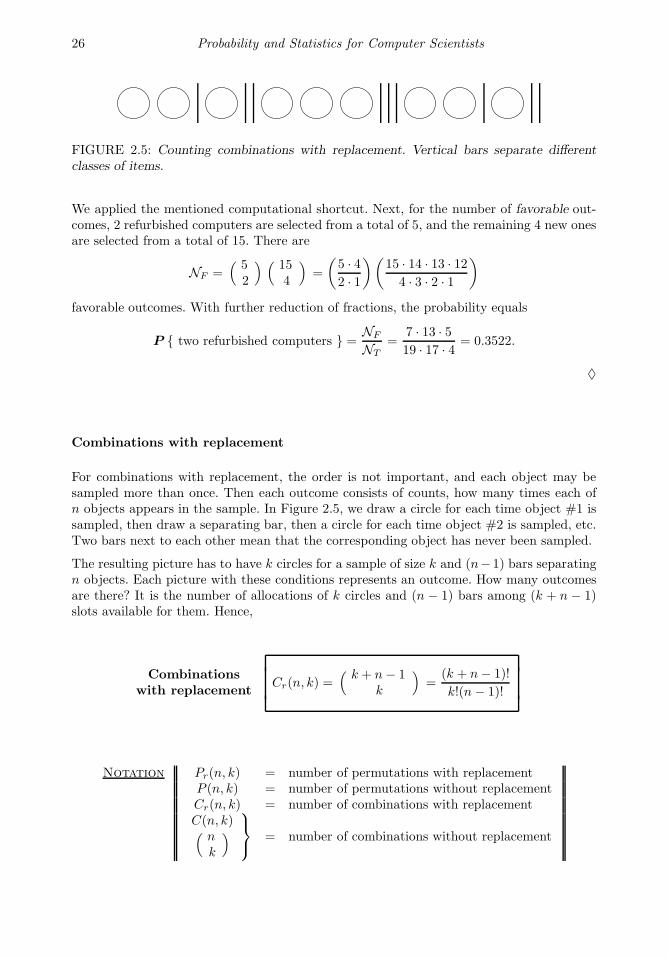
26 Probability and Statistics for Computer Scientists
FIGURE 2.5: Counting combinations with replacement. Vertical bars separate differentclasses of items.
We applied the mentioned computational shortcut. Next, for the number of favorable out-comes, 2 refurbished computers are selected from a total of 5, and the remaining 4 new onesare selected from a total of 15. There are
NF =( 5
2
) ( 154
)=
(5 · 42 · 1
)(15 · 14 · 13 · 124 · 3 · 2 · 1
)
favorable outcomes. With further reduction of fractions, the probability equals
P two refurbished computers =NF
NT=
7 · 13 · 519 · 17 · 4 = 0.3522.
♦
Combinations with replacement
For combinations with replacement, the order is not important, and each object may besampled more than once. Then each outcome consists of counts, how many times each ofn objects appears in the sample. In Figure 2.5, we draw a circle for each time object #1 issampled, then draw a separating bar, then a circle for each time object #2 is sampled, etc.Two bars next to each other mean that the corresponding object has never been sampled.
The resulting picture has to have k circles for a sample of size k and (n− 1) bars separatingn objects. Each picture with these conditions represents an outcome. How many outcomesare there? It is the number of allocations of k circles and (n − 1) bars among (k + n − 1)slots available for them. Hence,
Combinationswith replacement
Cr(n, k) =( k + n− 1
k
)=
(k + n− 1)!
k!(n− 1)!
Notation Pr(n, k) = number of permutations with replacementP (n, k) = number of permutations without replacementCr(n, k) = number of combinations with replacementC(n, k)( n
k
) = number of combinations without replacement
Probability 27
2.4 Conditional probability and independence
Conditional probability
Suppose you are meeting someone at an airport. The flight is likely to arrive on time; theprobability of that is 0.8. Suddenly it is announced that the flight departed one hour behindthe schedule. Now it has the probability of only 0.05 to arrive on time. New informationaffected the probability of meeting this flight on time. The new probability is called condi-tional probability, where the new information, that the flight departed late, is a condition.
DEFINITION 2.15
Conditional probability of event A given event B is the probability that Aoccurs when B is known to occur.
Notation P A | B = conditional probability of A given B
How does one compute the conditional probability? First, consider the case of equally likelyoutcomes. In view of the new information, occurrence of the condition B, only the outcomescontained in B still have a non-zero chance to occur. Counting only such outcomes, theunconditional probability of A,
P A =number of outcomes in A
number of outcomes in Ω,
is now replaced by the conditional probability of A given B,
P A | B =number of outcomes in A ∩B
number of outcomes in B=
P A ∩BP B .
This appears to be the general formula.
Conditionalprobability
P A | B =P A ∩BP B (2.7)
Rewriting (2.7) in a different way, we obtain the general formula for the probability ofintersection.
Intersection,general case
P A ∩B = P BP A | B (2.8)
28 Probability and Statistics for Computer Scientists
Independence
Now we can give an intuitively very clear definition of independence.
DEFINITION 2.16
Events A and B are independent if occurrence of B does not affect the prob-ability of A, i.e.,
P A | B = P A .
According to this definition, conditional probability equals unconditional probability in caseof independent events. Substituting this into (2.8) yields
P A ∩B = P AP B .
This is our old formula for independent events.
Example 2.31. Ninety percent of flights depart on time. Eighty percent of flights arriveon time. Seventy-five percent of flights depart on time and arrive on time.
(a) You are meeting a flight that departed on time. What is the probability that it willarrive on time?
(b) You have met a flight, and it arrived on time. What is the probability that it departedon time?
(c) Are the events, departing on time and arriving on time, independent?
Solution. Denote the events,
A = arriving on time ,D = departing on time .
We have:P A = 0.8, P D = 0.9, P A ∩D = 0.75.
(a) P A | D =P A ∩DP D =
0.75
0.9= 0.8333.
(b) P D | A =P A ∩DP A =
0.75
0.8= 0.9375.
(c) Events are not independent because
P A | D 6= P A , P D | A 6= P D , P A ∩D 6= P AP D .
Actually, any one of these inequalities is sufficient to prove that A and D are dependent.Further, we see that P A | D > P A and P D | A > P D. In other words, de-parting on time increases the probability of arriving on time, and vice versa. This perfectlyagrees with our intuition. ♦
Probability 29
Bayes Rule
The last example shows that two conditional probabilities, P A | B and P B | A, arenot the same, in general. Consider another example.
Example 2.32 (Reliability of a test). There exists a test for a certain viral infection(including a virus attack on a computer network). It is 95% reliable for infected patientsand 99% reliable for the healthy ones. That is, if a patient has the virus (event V ), the testshows that (event S) with probability P S | V = 0.95, and if the patient does not havethe virus, the test shows that with probability P
S | V
= 0.99.
Consider a patient whose test result is positive (i.e., the test shows that the patient has thevirus). Knowing that sometimes the test is wrong, naturally, the patient is eager to knowthe probability that he or she indeed has the virus. However, this conditional probability,P V | S, is not stated among the given characteristics of this test. ♦
This example is applicable to any testing procedure including software and hardware tests,pregnancy tests, paternity tests, alcohol tests, academic exams, etc. The problem is toconnect the given P S | V and the quantity in question, P V | S. This was done in theeighteenth century by English minister Thomas Bayes (1702–1761) in the following way.
Notice that A∩B = B ∩A. Therefore, using (2.8), P BP A | B = P AP B | A .Solve for P B | A to obtain
BayesRule
P B | A =P A | BP B
P A (2.9)
Example 2.33 (Situation on a midterm exam). On a midterm exam, students X , Y ,and Z forgot to sign their papers. Professor knows that they can write a good exam withprobabilities 0.8, 0.7, and 0.5, respectively. After the grading, he notices that two unsignedexams are good and one is bad. Given this information, and assuming that students workedindependently of each other, what is the probability that the bad exam belongs to studentZ?
Solution. Denote good and bad exams by G and B. Also, let GGB denote two good andone bad exams, XG denote the event “student X wrote a good exam,” etc. We need to findP ZB | GGB given that P G | X = 0.8, P G | Y = 0.7, and P G | Z = 0.5.
By the Bayes Rule,
P ZB | GGB =P GGB | ZBP ZB
P GGB .
Given ZB, event GGB occurs only when both X and Y write good exams. Thus,P GGB | ZB = (0.8)(0.7).
Event GGB consists of three outcomes depending on the student who wrote the bad exam.
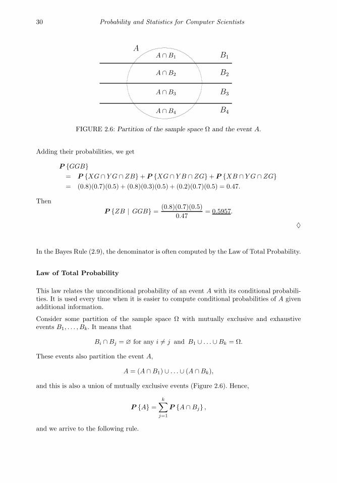
30 Probability and Statistics for Computer Scientists
A ∩B1 B1
A ∩B2 B2
A ∩B3 B3
A ∩B4 B4
A
FIGURE 2.6: Partition of the sample space Ω and the event A.
Adding their probabilities, we get
P GGB= P XG ∩ Y G ∩ ZB+ P XG ∩ Y B ∩ ZG+ P XB ∩ Y G ∩ ZG= (0.8)(0.7)(0.5) + (0.8)(0.3)(0.5) + (0.2)(0.7)(0.5) = 0.47.
Then
P ZB | GGB =(0.8)(0.7)(0.5)
0.47= 0.5957.
♦
In the Bayes Rule (2.9), the denominator is often computed by the Law of Total Probability.
Law of Total Probability
This law relates the unconditional probability of an event A with its conditional probabili-ties. It is used every time when it is easier to compute conditional probabilities of A givenadditional information.
Consider some partition of the sample space Ω with mutually exclusive and exhaustiveevents B1, . . . , Bk. It means that
Bi ∩Bj = ∅ for any i 6= j and B1 ∪ . . . ∪Bk = Ω.
These events also partition the event A,
A = (A ∩B1) ∪ . . . ∪ (A ∩Bk),
and this is also a union of mutually exclusive events (Figure 2.6). Hence,
P A =
k∑
j=1
P A ∩Bj ,
and we arrive to the following rule.
Probability 31
Law of TotalProbability
P A =
k∑
j=1
P A | BjP Bj
In case of two events (k = 2),
P A = P A | BP B+ PA | B
PB
(2.10)
Together with the Bayes Rule, it makes the following popular formula
Bayes Rulefor two events
P B | A =P A | BP B
P A | BP B+ PA | B
PB
Example 2.34 (Reliability of a test, continued). Continue Example 2.32. Sup-pose that 4% of all the patients are infected with the virus, P V = 0.04. Recall thatP S | V = 0.95 and P
S | V
= 0.99. If the test shows positive results, the (condi-
tional) probability that a patient has the virus equals
P V | S =P S | V P V
P S | V P V + PS | V
PV
=(0.95)(0.04)
(0.95)(0.04) + (1 − 0.99)(1− 0.04)= 0.7983.
♦
Example 2.35 (Diagnostics of computer codes). A new computer program consistsof two modules. The first module contains an error with probability 0.2. The second moduleis more complex; it has a probability of 0.4 to contain an error, independently of the firstmodule. An error in the first module alone causes the program to crash with probability0.5. For the second module, this probability is 0.8. If there are errors in both modules, theprogram crashes with probability 0.9. Suppose the program crashed. What is the probabilityof errors in both modules?
Solution. Denote the events,
A = errors in module I , B = errors in module II , C = crash .
Further,
errors in module I alone = A\B = A\(A ∩B)
errors in module II alone = B\A = B\(A ∩B).
It is given that P A = 0.2,P B = 0.4, P A ∩B = (0.2)(0.4) = 0.08, by independence,
32 Probability and Statistics for Computer Scientists
P C | A\B = 0.5, P C | B\A = 0.8, and P C | A ∩B = 0.9.
We need to compute P A ∩B | C. Since A is a union of disjoint events A\B and A ∩B,we compute
P A\B = P A − P A ∩B = 0.2− 0.08 = 0.12.
Similarly,P B\A = 0.4− 0.08 = 0.32.
Events (A\B), (B\A), A∩B, and (A ∪B) form a partition of Ω, because they are mutuallyexclusive and exhaustive. The last of them is the event of no errors in the entire program.Given this event, the probability of a crash is 0. Notice that A, B, and (A ∩B) are neithermutually exclusive nor exhaustive, so they cannot be used for the Bayes Rule. Now organizethe data.
Location of errors Probability of a crash
P A\B = 0.12 P C | A\B = 0.5P B\A = 0.32 P C | B\A = 0.8P A ∩B = 0.08 P C | A ∩B = 0.9PA ∪B
= 0.48 P
C | A ∪B
= 0
Combining the Bayes Rule and the Law of Total Probability,
P A ∩B | C =P C | A ∩BP A ∩B
P C ,
where
P C = P C | A\BP A\B+ P C | B\AP B\A+P C | A ∩BP A ∩B + P
C | A ∪B
PA ∪B
.
Then
P A ∩B | C =(0.9)(0.08)
(0.5)(0.12) + (0.8)(0.32) + (0.9)(0.08) + 0= 0.1856.
♦
Summary and conclusions
Probability of any event is a number between 0 and 1. The empty event has probability0, and the sample space has probability 1. There are rules for computing probabilities ofunions, intersections, and complements. For a union of disjoint events, probabilities areadded. For an intersection of independent events, probabilities are multiplied. Combiningthese rules, one evaluates reliability of a system given reliabilities of its components.
In the case of equally likely outcomes, probability is a ratio of the number of favorableoutcomes to the total number of outcomes. Combinatorics provides tools for computing
Exercises 33
these numbers in frequent situations involving permutations and combinations, with orwithout replacement.
Given occurrence of event B, one can compute conditional probability of event A. Uncon-ditional probability of A can be computed from its conditional probabilities by the Law ofTotal Probability. The Bayes Rule, often used in testing and diagnostics, relates conditionalprobabilities of A given B and of B given A.
Exercises
2.1. Out of six computer chips, two are defective. If two chips are randomly chosen for testing(without replacement), compute the probability that both of them are defective. List allthe outcomes in the sample space.
2.2. Suppose that after 10 years of service, 40% of computers have problems with motherboards(MB), 30% have problems with hard drives (HD), and 15% have problems with both MBand HD. What is the probability that a 10-year old computer still has fully functioning MBand HD?
2.3. A new computer virus can enter the system through e-mail or through the internet. Thereis a 30% chance of receiving this virus through e-mail. There is a 40% chance of receiving itthrough the internet. Also, the virus enters the system simultaneously through e-mail andthe internet with probability 0.15. What is the probability that the virus does not enter thesystem at all?
2.4. Among employees of a certain firm, 70% know C/C++, 60% know Fortran, and 50% knowboth languages. What portion of programmers
(a) does not know Fortran?
(b) does not know Fortran and does not know C/C++?
(c) knows C/C++ but not Fortran?
(d) knows Fortran but not C/C++?
(e) If someone knows Fortran, what is the probability that he/she knows C/C++ too?
(f) If someone knows C/C++, what is the probability that he/she knows Fortran too?
2.5. A computer program is tested by 3 independent tests. When there is an error, these testswill discover it with probabilities 0.2, 0.3, and 0.5, respectively. Suppose that the programcontains an error. What is the probability that it will be found by at least one test?
2.6. Under good weather conditions, 80% of flights arrive on time. During bad weather, only30% of flights arrive on time. Tomorrow, the chance of good weather is 60%. What is theprobability that your flight will arrive on time?
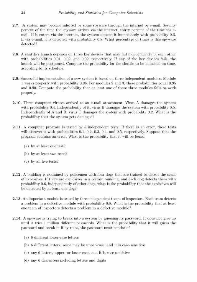
34 Probability and Statistics for Computer Scientists
2.7. A system may become infected by some spyware through the internet or e-mail. Seventypercent of the time the spyware arrives via the internet, thirty percent of the time via e-mail. If it enters via the internet, the system detects it immediately with probability 0.6.If via e-mail, it is detected with probability 0.8. What percentage of times is this spywaredetected?
2.8. A shuttle’s launch depends on three key devices that may fail independently of each otherwith probabilities 0.01, 0.02, and 0.02, respectively. If any of the key devices fails, thelaunch will be postponed. Compute the probability for the shuttle to be launched on time,according to its schedule.
2.9. Successful implementation of a new system is based on three independent modules. Module1 works properly with probability 0.96. For modules 2 and 3, these probabilities equal 0.95and 0.90. Compute the probability that at least one of these three modules fails to workproperly.
2.10. Three computer viruses arrived as an e-mail attachment. Virus A damages the systemwith probability 0.4. Independently of it, virus B damages the system with probability 0.5.Independently of A and B, virus C damages the system with probability 0.2. What is theprobability that the system gets damaged?
2.11. A computer program is tested by 5 independent tests. If there is an error, these testswill discover it with probabilities 0.1, 0.2, 0.3, 0.4, and 0.5, respectively. Suppose that theprogram contains an error. What is the probability that it will be found
(a) by at least one test?
(b) by at least two tests?
(c) by all five tests?
2.12. A building is examined by policemen with four dogs that are trained to detect the scentof explosives. If there are explosives in a certain building, and each dog detects them withprobability 0.6, independently of other dogs, what is the probability that the explosives willbe detected by at least one dog?
2.13.An important module is tested by three independent teams of inspectors. Each team detectsa problem in a defective module with probability 0.8. What is the probability that at leastone team of inspectors detects a problem in a defective module?
2.14. A spyware is trying to break into a system by guessing its password. It does not give upuntil it tries 1 million different passwords. What is the probability that it will guess thepassword and break in if by rules, the password must consist of
(a) 6 different lower-case letters
(b) 6 different letters, some may be upper-case, and it is case-sensitive
(c) any 6 letters, upper- or lower-case, and it is case-sensitive
(d) any 6 characters including letters and digits
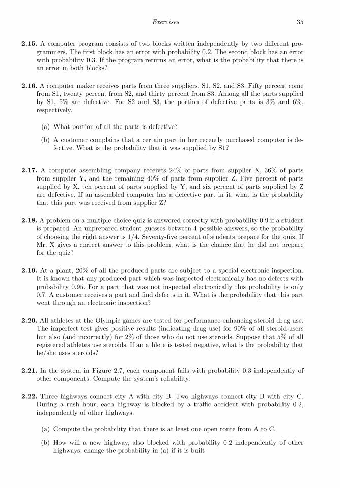
Exercises 35
2.15. A computer program consists of two blocks written independently by two different pro-grammers. The first block has an error with probability 0.2. The second block has an errorwith probability 0.3. If the program returns an error, what is the probability that there isan error in both blocks?
2.16. A computer maker receives parts from three suppliers, S1, S2, and S3. Fifty percent comefrom S1, twenty percent from S2, and thirty percent from S3. Among all the parts suppliedby S1, 5% are defective. For S2 and S3, the portion of defective parts is 3% and 6%,respectively.
(a) What portion of all the parts is defective?
(b) A customer complains that a certain part in her recently purchased computer is de-fective. What is the probability that it was supplied by S1?
2.17. A computer assembling company receives 24% of parts from supplier X, 36% of partsfrom supplier Y, and the remaining 40% of parts from supplier Z. Five percent of partssupplied by X, ten percent of parts supplied by Y, and six percent of parts supplied by Zare defective. If an assembled computer has a defective part in it, what is the probabilitythat this part was received from supplier Z?
2.18. A problem on a multiple-choice quiz is answered correctly with probability 0.9 if a studentis prepared. An unprepared student guesses between 4 possible answers, so the probabilityof choosing the right answer is 1/4. Seventy-five percent of students prepare for the quiz. IfMr. X gives a correct answer to this problem, what is the chance that he did not preparefor the quiz?
2.19. At a plant, 20% of all the produced parts are subject to a special electronic inspection.It is known that any produced part which was inspected electronically has no defects withprobability 0.95. For a part that was not inspected electronically this probability is only0.7. A customer receives a part and find defects in it. What is the probability that this partwent through an electronic inspection?
2.20. All athletes at the Olympic games are tested for performance-enhancing steroid drug use.The imperfect test gives positive results (indicating drug use) for 90% of all steroid-usersbut also (and incorrectly) for 2% of those who do not use steroids. Suppose that 5% of allregistered athletes use steroids. If an athlete is tested negative, what is the probability thathe/she uses steroids?
2.21. In the system in Figure 2.7, each component fails with probability 0.3 independently ofother components. Compute the system’s reliability.
2.22. Three highways connect city A with city B. Two highways connect city B with city C.During a rush hour, each highway is blocked by a traffic accident with probability 0.2,independently of other highways.
(a) Compute the probability that there is at least one open route from A to C.
(b) How will a new highway, also blocked with probability 0.2 independently of otherhighways, change the probability in (a) if it is built
36 Probability and Statistics for Computer Scientists
A B
FIGURE 2.7: Calculate reliability of this system (Exercise 2.21).
(a)
(b)
(c)
(d)(e)
FIGURE 2.8: Calculate reliability of each system (Exercise 2.23).
(α) between A and B?
(β) between B and C?
(γ) between A and C?
2.23. Calculate the reliability of each system shown in Figure 2.8, if components A, B, C, D,and E function properly with probabilities 0.9, 0.8, 0.7, 0.6, and 0.5, respectively.
2.24. Among 10 laptop computers, five are good and five have defects. Unaware of this, acustomer buys 6 laptops.
(a) What is the probability of exactly 2 defective laptops among them?
(b) Given that at least 2 purchased laptops are defective, what is the probability thatexactly 2 are defective?
2.25. This is known as the Birthday Problem.
Exercises 37
(a) Consider a class with 30 students. Compute the probability that at least two of themhave their birthdays on the same day. (For simplicity, ignore the leap year).
(b) How many students should be in class in order to have this probability above 0.5?
2.26. Two out of six computers in a lab have problems with hard drives. If three computers areselected at random for inspection, what is the probability that none of them has hard driveproblems?
2.27. Among eighteen computers in some store, six have defects. Five randomly selected com-puters are bought for the university lab. Compute the probability that all five computershave no defects.
2.28. A quiz consists of 6 multiple-choice questions. Each question has 4 possible answers. Astudent is unprepared, and he has no choice but guessing answers completely at random.He passes the quiz if he gets at least 3 questions correctly. What is the probability that hewill pass?
2.29. An internet search engine looks for a keyword in 9 databases, searching them in a randomorder. Only 5 of these databases contain the given keyword. Find the probability that itwill be found in at least 2 of the first 4 searched databases.
2.30. Consider the situation described in Example 2.24 on p. 22, but this time let us define thesample space clearly. Suppose that one child is older, and the other is younger, their genderis independent of their age, and the child you meet is one or the other with probabilities1/2 and 1/2.
(a) List all the outcomes in this sample space. Each outcome should tell the children’sgender, which child is older, and which child you have met.
(b) Show that unconditional probabilities of outcomes BB, BG, and GB are equal.
(c) Show that conditional probabilities of BB, BG, and GB, after you met Leo, are notequal.
(d) Show that the conditional probability that Leo has a brother is 1/2.
2.31. Show that events A,B,C, . . . are disjoint if and only if A,B,C, . . . are exhaustive.
2.32. Events A and B are independent. Show, intuitively and mathematically, that:
(a) Their complements are also independent.
(b) If they are disjoint, then P A = 0 or P B = 0.
(c) If they are exhaustive, then P A = 1 or P B = 1.
2.33. Derive a computational formula for the probability of a union of N arbitrary events.Assume that probabilities of all individual events and their intersections are given.

38 Probability and Statistics for Computer Scientists
2.34. Prove thatE1 ∩ . . . ∩ En = E1 ∪ . . . ∪ En
for arbitrary events E1, . . . , En.
2.35. From the “addition” rule of probability, derive the “subtraction” rule:
if B ⊂ A, then P A\B = P (A)− P (B).
2.36. Prove “subadditivity”: P E1 ∪E2 ∪ . . . ≤∑P Ei for any events E1, E2, . . . ∈ M.
Chapter 3
Discrete Random Variables and Their
Distributions
3.1 Distribution of a random variable . . . . . . . . . . . . . . . . . . . . . . . . . . . . . . . 403.1.1 Main concepts . . . . . . . . . . . . . . . . . . . . . . . . . . . . . . . . . . . . . . . . . . . 403.1.2 Types of random variables . . . . . . . . . . . . . . . . . . . . . . . . . . . . . . 43
3.2 Distribution of a random vector . . . . . . . . . . . . . . . . . . . . . . . . . . . . . . . . . 443.2.1 Joint distribution and marginal distributions . . . . . . . . . . . 443.2.2 Independence of random variables . . . . . . . . . . . . . . . . . . . . . . 45
3.3 Expectation and variance . . . . . . . . . . . . . . . . . . . . . . . . . . . . . . . . . . . . . . . . 473.3.1 Expectation . . . . . . . . . . . . . . . . . . . . . . . . . . . . . . . . . . . . . . . . . . . . . . 473.3.2 Expectation of a function . . . . . . . . . . . . . . . . . . . . . . . . . . . . . . . 483.3.3 Properties . . . . . . . . . . . . . . . . . . . . . . . . . . . . . . . . . . . . . . . . . . . . . . . . 483.3.4 Variance and standard deviation . . . . . . . . . . . . . . . . . . . . . . . . 493.3.5 Covariance and correlation . . . . . . . . . . . . . . . . . . . . . . . . . . . . . . 513.3.6 Properties . . . . . . . . . . . . . . . . . . . . . . . . . . . . . . . . . . . . . . . . . . . . . . . . 523.3.7 Chebyshev’s inequality . . . . . . . . . . . . . . . . . . . . . . . . . . . . . . . . . . 543.3.8 Application to finance . . . . . . . . . . . . . . . . . . . . . . . . . . . . . . . . . . . 55
3.4 Families of discrete distributions . . . . . . . . . . . . . . . . . . . . . . . . . . . . . . . . . 573.4.1 Bernoulli distribution . . . . . . . . . . . . . . . . . . . . . . . . . . . . . . . . . . . . 573.4.2 Binomial distribution . . . . . . . . . . . . . . . . . . . . . . . . . . . . . . . . . . . . 583.4.3 Geometric distribution . . . . . . . . . . . . . . . . . . . . . . . . . . . . . . . . . . 603.4.4 Negative Binomial distribution . . . . . . . . . . . . . . . . . . . . . . . . . . 633.4.5 Poisson distribution . . . . . . . . . . . . . . . . . . . . . . . . . . . . . . . . . . . . . 643.4.6 Poisson approximation of Binomial distribution . . . . . . . . 66
Summary and conclusions . . . . . . . . . . . . . . . . . . . . . . . . . . . . . . . . . . . . . . . . . . 67Exercises . . . . . . . . . . . . . . . . . . . . . . . . . . . . . . . . . . . . . . . . . . . . . . . . . . . . . . . . . . . . 68
This chapter introduces the concept of a random variable and studies discrete distributionsin detail. Continuous distributions are discussed in Chapter 4.
39

40 Probability and Statistics for Computer Scientists
3.1 Distribution of a random variable
3.1.1 Main concepts
DEFINITION 3.1
A random variable is a function of an outcome,
X = f(ω).
In other words, it is a quantity that depends on chance.
The domain of a random variable is the sample space Ω. Its range can be the set of all realnumbers R, or only the positive numbers (0,+∞), or the integers Z, or the interval (0, 1),etc., depending on what possible values the random variable can potentially take.
Once an experiment is completed, and the outcome ω is known, the value of random variableX(ω) becomes determined.
Example 3.1. Consider an experiment of tossing 3 fair coins and counting the numberof heads. Certainly, the same model suits the number of girls in a family with 3 children,the number of 1’s in a random binary code consisting of 3 characters, etc.
Let X be the number of heads (girls, 1’s). Prior to an experiment, its value is not known.All we can say is that X has to be an integer between 0 and 3. Since assuming each valueis an event, we can compute probabilities,
P X = 0 = P three tails = P TTT =(1
2
)(1
2
)(1
2
)=
1
8
P X = 1 = P HTT + P THT + P TTH = 3
8
P X = 2 = P HHT + P HTH+ P THH =3
8
P X = 3 = P HHH =1
8
Summarizing,x P X = x0 1/81 3/82 3/83 1/8
Total 1
♦
This table contains everything that is known about random variable X prior to the exper-iment. Before we know the outcome ω, we cannot tell what X equals to. However, we canlist all the possible values of X and determine the corresponding probabilities.
Discrete Random Variables and Their Distributions 41
DEFINITION 3.2
Collection of all the probabilities related to X is the distribution of X . Thefunction
P (x) = P X = xis the probability mass function, or pmf. The cumulative distributionfunction, or cdf is defined as
F (x) = P X ≤ x =∑
y≤x
P (y). (3.1)
The set of possible values of X is called the support of the distribution F .
For every outcome ω, the variable X takes one and only one value x. This makes eventsX = x disjoint and exhaustive, and therefore,
∑
x
P (x) =∑
x
P X = x = 1.
Looking at (3.1), we can conclude that the cdf F (x) is a non-decreasing function of x, alwaysbetween 0 and 1, with
limx↓−∞
F (x) = 0 and limx↑+∞
F (x) = 1.
Between any two subsequent values ofX , F (x) is constant. It jumps by P (x) at each possiblevalue x of X (see Fig. 3.1, right).
Recall that one way to compute the probability of an event is to add probabilities of all theoutcomes in it. Hence, for any set A,
P X ∈ A =∑
x∈A
P (x).
When A is an interval, its probability can be computed directly from the cdf F (x),
P a < X ≤ b = F (b)− F (a).
Example 3.2. The pmf and cdf of X in Example 3.1 are shown in Fig. 3.1.♦
Matlab Demo. The following MATLAB code simulates 3 coin tosses and computes a valueof X 10,000 times.
N = 10000; % Number of simulations
U = rand(3,N); % a 3-by-N matrix of random numbers from [0,1]
Y = (U < 0.5); % Y=1 (heads) if U < 0.5, otherwise Y=0 (tails)
X = sum(Y); % Sums across columns. X = number of heads
hist(X); % Histogram of X
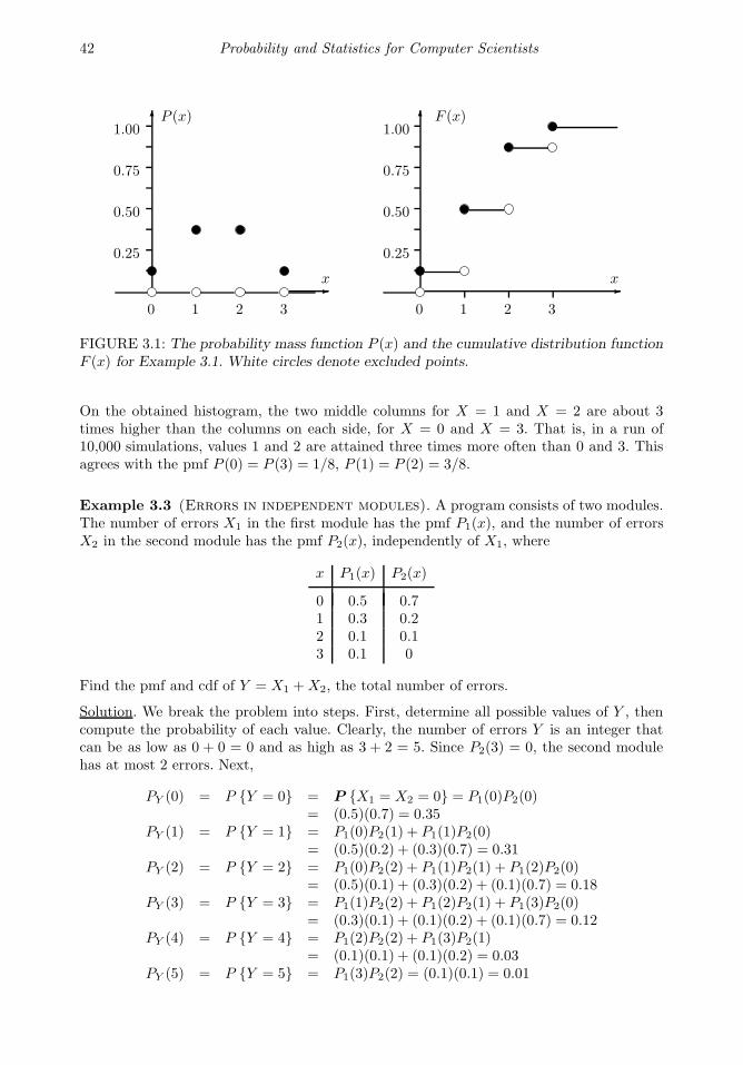
42 Probability and Statistics for Computer Scientists
0 1 2 3
x
0.25
0.50
0.75
1.00P (x)
0.25
0.50
0.75
1.00F (x)
0 1 2 3
x
FIGURE 3.1: The probability mass function P (x) and the cumulative distribution functionF (x) for Example 3.1. White circles denote excluded points.
On the obtained histogram, the two middle columns for X = 1 and X = 2 are about 3times higher than the columns on each side, for X = 0 and X = 3. That is, in a run of10,000 simulations, values 1 and 2 are attained three times more often than 0 and 3. Thisagrees with the pmf P (0) = P (3) = 1/8, P (1) = P (2) = 3/8.
Example 3.3 (Errors in independent modules). A program consists of two modules.The number of errors X1 in the first module has the pmf P1(x), and the number of errorsX2 in the second module has the pmf P2(x), independently of X1, where
x P1(x) P2(x)
0 0.5 0.71 0.3 0.22 0.1 0.13 0.1 0
Find the pmf and cdf of Y = X1 +X2, the total number of errors.
Solution. We break the problem into steps. First, determine all possible values of Y , thencompute the probability of each value. Clearly, the number of errors Y is an integer thatcan be as low as 0 + 0 = 0 and as high as 3 + 2 = 5. Since P2(3) = 0, the second modulehas at most 2 errors. Next,
PY (0) = P Y = 0 = P X1 = X2 = 0 = P1(0)P2(0)= (0.5)(0.7) = 0.35
PY (1) = P Y = 1 = P1(0)P2(1) + P1(1)P2(0)= (0.5)(0.2) + (0.3)(0.7) = 0.31
PY (2) = P Y = 2 = P1(0)P2(2) + P1(1)P2(1) + P1(2)P2(0)= (0.5)(0.1) + (0.3)(0.2) + (0.1)(0.7) = 0.18
PY (3) = P Y = 3 = P1(1)P2(2) + P1(2)P2(1) + P1(3)P2(0)= (0.3)(0.1) + (0.1)(0.2) + (0.1)(0.7) = 0.12
PY (4) = P Y = 4 = P1(2)P2(2) + P1(3)P2(1)= (0.1)(0.1) + (0.1)(0.2) = 0.03
PY (5) = P Y = 5 = P1(3)P2(2) = (0.1)(0.1) = 0.01
Discrete Random Variables and Their Distributions 43
Now check:5∑
y=0
PY (y) = 0.35 + 0.31 + 0.18 + 0.12 + 0.03 + 0.01 = 1,
thus we probably counted all the possibilities and did not miss any (we just wanted toemphasize that simply getting
∑P (x) = 1 does not guarantee that we made no mistake in
our solution. However, if this equality is not satisfied, we have a mistake for sure).
The cumulative function can be computed as
FY (0) = PY (0) = 0.35
FY (1) = FY (0) + PY (1) = 0.35 + 0.31 = 0.66
FY (2) = FY (1) + PY (2) = 0.66 + 0.18 = 0.84
FY (3) = FY (2) + PY (3) = 0.84 + 0.12 = 0.96
FY (4) = FY (3) + PY (4) = 0.96 + 0.03 = 0.99
FY (5) = FY (4) + PY (5) = 0.99 + 0.01 = 1.00
Between the values of Y , F (x) is constant. ♦
3.1.2 Types of random variables
So far, we are dealing with discrete random variables. These are variables whose range isfinite or countable. In particular, it means that their values can be listed, or arranged in asequence. Examples include the number of jobs submitted to a printer, the number of errors,the number of error-free modules, the number of failed components, and so on. Discretevariables don’t have to be integers. For example, the proportion of defective components ina lot of 100 can be 0, 1/100, 2/100, ..., 99/100, or 1. This variable assumes 101 differentvalues, so it is discrete, although not an integer.
On the contrary, continuous random variables assume a whole interval of values. Thiscould be a bounded interval (a, b), or an unbounded interval such as (a,+∞), (−∞, b), or(−∞,+∞). Sometimes, it may be a union of several such intervals. Intervals are uncount-able, therefore, all values of a random variable cannot be listed in this case. Examples ofcontinuous variables include various times (software installation time, code execution time,connection time, waiting time, lifetime), also physical variables like weight, height, voltage,temperature, distance, the number of miles per gallon, etc. We shall discuss continuousrandom variables in detail in Chapter 4.
Example 3.4. For comparison, observe that a long jump is formally a continuous randomvariable because an athlete can jump any distance within some range. Results of a highjump, however, are discrete because the bar can only be placed on a finite number ofheights. ♦
Notice that rounding a continuous random variable, say, to the nearest integer makes itdiscrete.
Sometimes we can see mixed random variables that are discrete on some range of valuesand continuous elsewhere. For example, see a remark about waiting times on page 182.

44 Probability and Statistics for Computer Scientists
Example 3.5. A job is sent to a printer. Let X be the waiting time before the jobstarts printing. With some probability, this job appears first in line and starts printingimmediately, X = 0. It is also possible that the job is first in line but it takes 20 seconds forthe printer to warm up, in which case X = 20. So far, the variable has a discrete behaviorwith a positive pmf P (x) at x = 0 and x = 20. However, if there are other jobs in aqueue, then X depends on the time it takes to print them, which is a continuous randomvariable. Using a popular jargon, besides “point masses” at x = 0 and x = 20, the variableis continuous, taking values in (0,+∞). Thus, X is neither discrete nor continuous. It ismixed. ♦
3.2 Distribution of a random vector
Often we deal with several random variables simultaneously. We may look at the size of aRAM and the speed of a CPU, the price of a computer and its capacity, temperature andhumidity, technical and artistic performance, etc.
3.2.1 Joint distribution and marginal distributions
DEFINITION 3.3
If X and Y are random variables, then the pair (X,Y ) is a random vec-tor. Its distribution is called the joint distribution of X and Y . Individualdistributions of X and Y are then called the marginal distributions.
Although we talk about two random variables in this section, all the concepts extend to avector (X1, X2, . . . , Xn) of n components and its joint distribution.
Similarly to a single variable, the joint distribution of a vector is a collection of probabilitiesfor a vector (X,Y ) to take a value (x, y). Recall that two vectors are equal,
(X,Y ) = (x, y),
if X = x and Y = y. This “and” means the intersection, therefore, the joint probabilitymass function of X and Y is
P (x, y) = P (X,Y ) = (x, y) = P X = x ∩ Y = y .
Again, (X,Y ) = (x, y) are exhaustive and mutually exclusive events for different pairs(x, y), therefore, ∑
x
∑
y
P (x, y) = 1.
The joint distribution of (X,Y ) carries the complete information about the behavior of thisrandom vector. In particular, the marginal probability mass functions of X and Y can beobtained from the joint pmf by the Addition Rule.
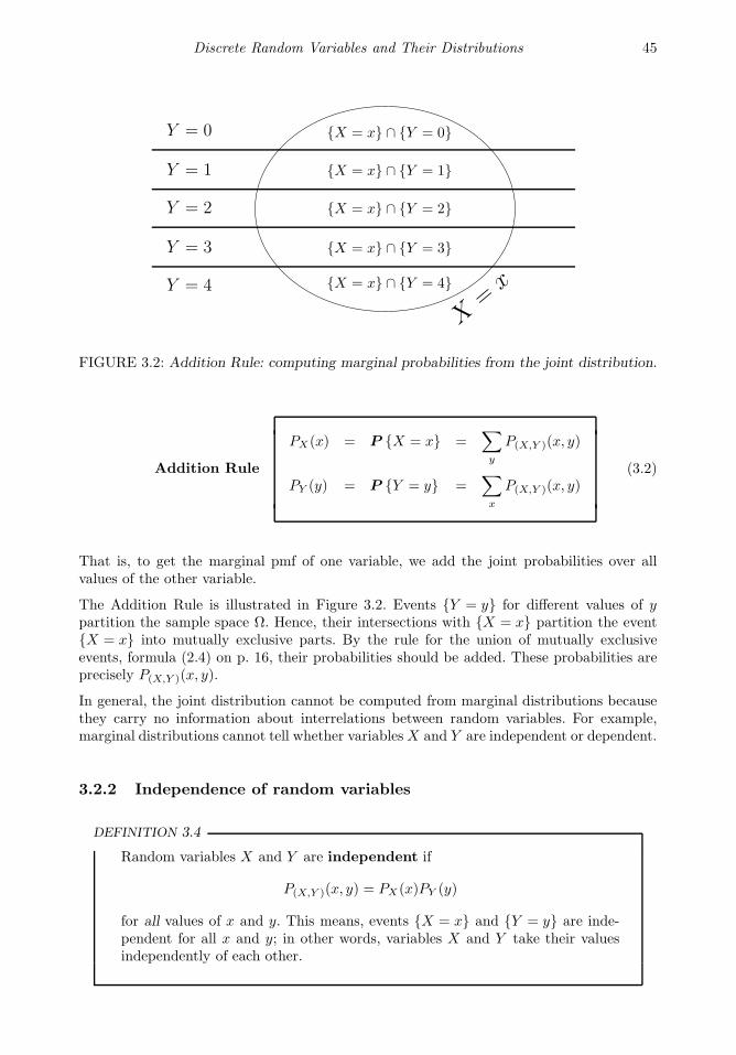
Discrete Random Variables and Their Distributions 45
Y = 0
Y = 1
Y = 2
Y = 3
Y = 4
X = x ∩ Y = 0
X = x ∩ Y = 1
X = x ∩ Y = 2
X = x ∩ Y = 3
X = x ∩ Y = 4
X=
x
FIGURE 3.2: Addition Rule: computing marginal probabilities from the joint distribution.
Addition Rule
PX(x) = P X = x =∑
y
P(X,Y )(x, y)
PY (y) = P Y = y =∑
x
P(X,Y )(x, y)(3.2)
That is, to get the marginal pmf of one variable, we add the joint probabilities over allvalues of the other variable.
The Addition Rule is illustrated in Figure 3.2. Events Y = y for different values of ypartition the sample space Ω. Hence, their intersections with X = x partition the eventX = x into mutually exclusive parts. By the rule for the union of mutually exclusiveevents, formula (2.4) on p. 16, their probabilities should be added. These probabilities areprecisely P(X,Y )(x, y).
In general, the joint distribution cannot be computed from marginal distributions becausethey carry no information about interrelations between random variables. For example,marginal distributions cannot tell whether variablesX and Y are independent or dependent.
3.2.2 Independence of random variables
DEFINITION 3.4
Random variables X and Y are independent if
P(X,Y )(x, y) = PX(x)PY (y)
for all values of x and y. This means, events X = x and Y = y are inde-pendent for all x and y; in other words, variables X and Y take their valuesindependently of each other.
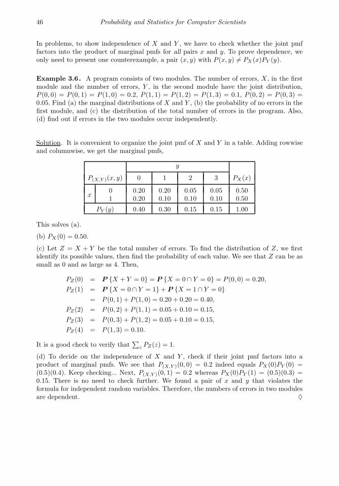
46 Probability and Statistics for Computer Scientists
In problems, to show independence of X and Y , we have to check whether the joint pmffactors into the product of marginal pmfs for all pairs x and y. To prove dependence, weonly need to present one counterexample, a pair (x, y) with P (x, y) 6= PX(x)PY (y).
Example 3.6. A program consists of two modules. The number of errors, X , in the firstmodule and the number of errors, Y , in the second module have the joint distribution,P (0, 0) = P (0, 1) = P (1, 0) = 0.2, P (1, 1) = P (1, 2) = P (1, 3) = 0.1, P (0, 2) = P (0, 3) =0.05. Find (a) the marginal distributions of X and Y , (b) the probability of no errors in thefirst module, and (c) the distribution of the total number of errors in the program. Also,(d) find out if errors in the two modules occur independently.
Solution. It is convenient to organize the joint pmf of X and Y in a table. Adding rowwiseand columnwise, we get the marginal pmfs,
y
P(X,Y )(x, y) 0 1 2 3 PX(x)
x01
0.200.20
0.200.10
0.050.10
0.050.10
0.500.50
PY (y) 0.40 0.30 0.15 0.15 1.00
This solves (a).
(b) PX(0) = 0.50.
(c) Let Z = X + Y be the total number of errors. To find the distribution of Z, we firstidentify its possible values, then find the probability of each value. We see that Z can be assmall as 0 and as large as 4. Then,
PZ(0) = P X + Y = 0 = P X = 0 ∩ Y = 0 = P (0, 0) = 0.20,
PZ(1) = P X = 0 ∩ Y = 1+ P X = 1 ∩ Y = 0= P (0, 1) + P (1, 0) = 0.20 + 0.20 = 0.40,
PZ(2) = P (0, 2) + P (1, 1) = 0.05 + 0.10 = 0.15,
PZ(3) = P (0, 3) + P (1, 2) = 0.05 + 0.10 = 0.15,
PZ(4) = P (1, 3) = 0.10.
It is a good check to verify that∑
z PZ(z) = 1.
(d) To decide on the independence of X and Y , check if their joint pmf factors into aproduct of marginal pmfs. We see that P(X,Y )(0, 0) = 0.2 indeed equals PX(0)PY (0) =(0.5)(0.4). Keep checking... Next, P(X,Y )(0, 1) = 0.2 whereas PX(0)PY (1) = (0.5)(0.3) =0.15. There is no need to check further. We found a pair of x and y that violates theformula for independent random variables. Therefore, the numbers of errors in two modulesare dependent. ♦
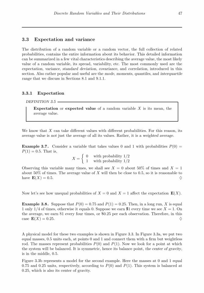
Discrete Random Variables and Their Distributions 47
3.3 Expectation and variance
The distribution of a random variable or a random vector, the full collection of relatedprobabilities, contains the entire information about its behavior. This detailed informationcan be summarized in a few vital characteristics describing the average value, the most likelyvalue of a random variable, its spread, variability, etc. The most commonly used are theexpectation, variance, standard deviation, covariance, and correlation, introduced in thissection. Also rather popular and useful are the mode, moments, quantiles, and interquartilerange that we discuss in Sections 8.1 and 9.1.1.
3.3.1 Expectation
DEFINITION 3.5
Expectation or expected value of a random variable X is its mean, theaverage value.
We know that X can take different values with different probabilities. For this reason, itsaverage value is not just the average of all its values. Rather, it is a weighted average.
Example 3.7. Consider a variable that takes values 0 and 1 with probabilities P (0) =P (1) = 0.5. That is,
X =
0 with probability 1/21 with probability 1/2
Observing this variable many times, we shall see X = 0 about 50% of times and X = 1about 50% of times. The average value of X will then be close to 0.5, so it is reasonable tohave E(X) = 0.5. ♦
Now let’s see how unequal probabilities of X = 0 and X = 1 affect the expectation E(X).
Example 3.8. Suppose that P (0) = 0.75 and P (1) = 0.25. Then, in a long run, X is equal1 only 1/4 of times, otherwise it equals 0. Suppose we earn $1 every time we see X = 1. Onthe average, we earn $1 every four times, or $0.25 per each observation. Therefore, in thiscase E(X) = 0.25. ♦
A physical model for these two examples is shown in Figure 3.3. In Figure 3.3a, we put twoequal masses, 0.5 units each, at points 0 and 1 and connect them with a firm but weightlessrod. The masses represent probabilities P (0) and P (1). Now we look for a point at whichthe system will be balanced. It is symmetric, hence its balance point, the center of gravity,is in the middle, 0.5.
Figure 3.3b represents a model for the second example. Here the masses at 0 and 1 equal0.75 and 0.25 units, respectively, according to P (0) and P (1). This system is balanced at0.25, which is also its center of gravity.
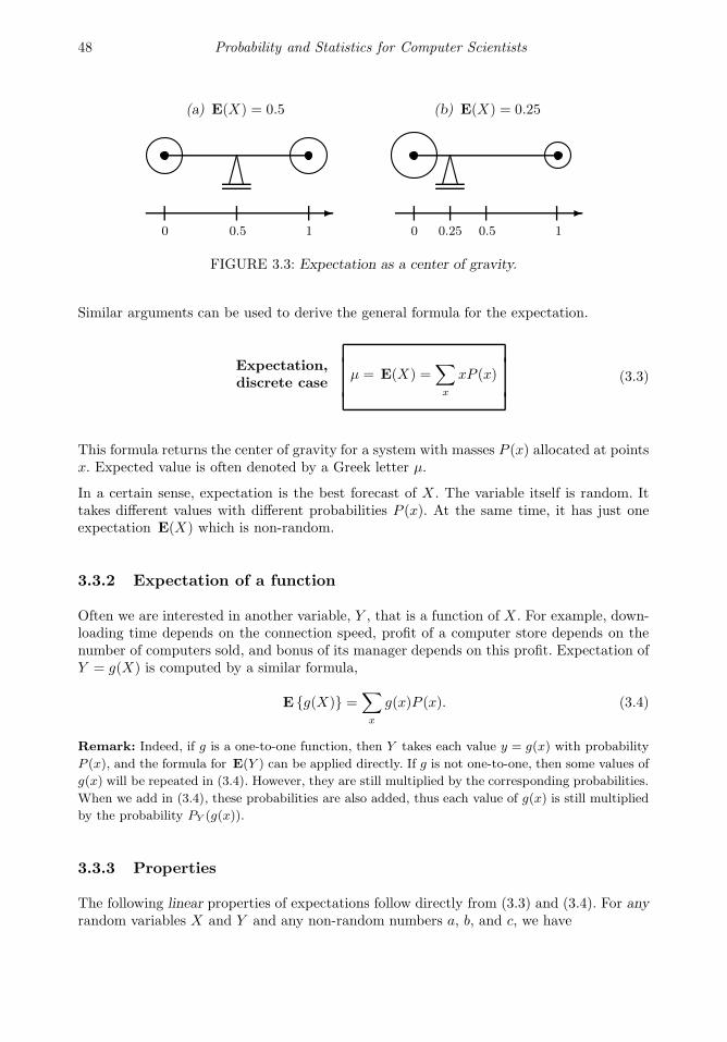
48 Probability and Statistics for Computer Scientists
(a) E(X) = 0.5
0 0.5 1
(b) E(X) = 0.25
0 0.25 0.5 1
FIGURE 3.3: Expectation as a center of gravity.
Similar arguments can be used to derive the general formula for the expectation.
Expectation,discrete case
µ = E(X) =∑
x
xP (x) (3.3)
This formula returns the center of gravity for a system with masses P (x) allocated at pointsx. Expected value is often denoted by a Greek letter µ.
In a certain sense, expectation is the best forecast of X . The variable itself is random. Ittakes different values with different probabilities P (x). At the same time, it has just oneexpectation E(X) which is non-random.
3.3.2 Expectation of a function
Often we are interested in another variable, Y , that is a function of X . For example, down-loading time depends on the connection speed, profit of a computer store depends on thenumber of computers sold, and bonus of its manager depends on this profit. Expectation ofY = g(X) is computed by a similar formula,
E g(X) =∑
x
g(x)P (x). (3.4)
Remark: Indeed, if g is a one-to-one function, then Y takes each value y = g(x) with probability
P (x), and the formula for E(Y ) can be applied directly. If g is not one-to-one, then some values of
g(x) will be repeated in (3.4). However, they are still multiplied by the corresponding probabilities.
When we add in (3.4), these probabilities are also added, thus each value of g(x) is still multiplied
by the probability PY (g(x)).
3.3.3 Properties
The following linear properties of expectations follow directly from (3.3) and (3.4). For anyrandom variables X and Y and any non-random numbers a, b, and c, we have
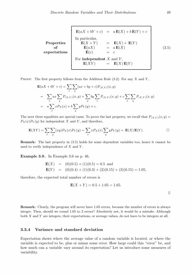
Discrete Random Variables and Their Distributions 49
Propertiesof
expectations
E(aX + bY + c) = aE(X) + bE(Y ) + c
In particular,E(X + Y ) = E(X) + E(Y )E(aX) = aE(X)E(c) = c
For independent X and Y ,E(XY ) = E(X)E(Y )
(3.5)
Proof: The first property follows from the Addition Rule (3.2). For any X and Y ,
E(aX + bY + c) =∑
x
∑
y
(ax+ by + c)P(X,Y )(x, y)
=∑
x
ax∑
y
P(X,Y )(x, y) +∑
y
by∑
x
P(X,Y )(x, y) + c∑
x
∑
y
P(X,Y )(x, y)
= a∑
x
xPX(x) + b∑
y
yPY (y) + c.
The next three equalities are special cases. To prove the last property, we recall that P(X,Y )(x, y) =
PX(x)PY (y) for independent X and Y , and therefore,
E(XY ) =∑
x
∑
y
(xy)PX(x)PY (y) =∑
x
xPX(x)∑
y
yPY (y) = E(X)E(Y ).
Remark: The last property in (3.5) holds for some dependent variables too, hence it cannot be
used to verify independence of X and Y .
Example 3.9. In Example 3.6 on p. 46,
E(X) = (0)(0.5) + (1)(0.5) = 0.5 and
E(Y ) = (0)(0.4) + (1)(0.3) + (2)(0.15) + (3)(0.15) = 1.05,
therefore, the expected total number of errors is
E(X + Y ) = 0.5 + 1.05 = 1.65.
♦
Remark: Clearly, the program will never have 1.65 errors, because the number of errors is always
integer. Then, should we round 1.65 to 2 errors? Absolutely not, it would be a mistake. Although
both X and Y are integers, their expectations, or average values, do not have to be integers at all.
3.3.4 Variance and standard deviation
Expectation shows where the average value of a random variable is located, or where thevariable is expected to be, plus or minus some error. How large could this “error” be, andhow much can a variable vary around its expectation? Let us introduce some measures ofvariability.
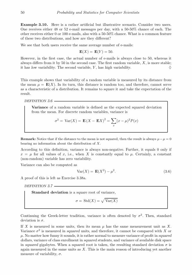
50 Probability and Statistics for Computer Scientists
Example 3.10. Here is a rather artificial but illustrative scenario. Consider two users.One receives either 48 or 52 e-mail messages per day, with a 50-50% chance of each. Theother receives either 0 or 100 e-mails, also with a 50-50% chance. What is a common featureof these two distributions, and how are they different?
We see that both users receive the same average number of e-mails:
E(X) = E(Y ) = 50.
However, in the first case, the actual number of e-mails is always close to 50, whereas italways differs from it by 50 in the second case. The first random variable, X , is more stable;it has low variability. The second variable, Y , has high variability. ♦
This example shows that variability of a random variable is measured by its distance fromthe mean µ = E(X). In its turn, this distance is random too, and therefore, cannot serveas a characteristic of a distribution. It remains to square it and take the expectation of theresult.
DEFINITION 3.6
Variance of a random variable is defined as the expected squared deviationfrom the mean. For discrete random variables, variance is
σ2 = Var(X) = E (X − EX)2=∑
x
(x− µ)2P (x)
Remark: Notice that if the distance to the mean is not squared, then the result is always µ−µ = 0
bearing no information about the distribution of X.
According to this definition, variance is always non-negative. Further, it equals 0 only ifx = µ for all values of x, i.e., when X is constantly equal to µ. Certainly, a constant(non-random) variable has zero variability.
Variance can also be computed as
Var(X) = E(X2)− µ2. (3.6)
A proof of this is left as Exercise 3.38a.
DEFINITION 3.7
Standard deviation is a square root of variance,
σ = Std(X) =√
Var(X)
Continuing the Greek-letter tradition, variance is often denoted by σ2. Then, standarddeviation is σ.
If X is measured in some units, then its mean µ has the same measurement unit as X .Variance σ2 is measured in squared units, and therefore, it cannot be compared with X orµ. No matter how funny it sounds, it is rather normal to measure variance of profit in squareddollars, variance of class enrollment in squared students, and variance of available disk spacein squared gigabytes. When a squared root is taken, the resulting standard deviation σ isagain measured in the same units as X . This is the main reason of introducing yet anothermeasure of variability, σ.

Discrete Random Variables and Their Distributions 51
3.3.5 Covariance and correlation
Expectation, variance, and standard deviation characterize the distribution of a single ran-dom variable. Now we introduce measures of association of two random variables.
Y
X
Y
X
Y
X
(a) Cov(X,Y ) > 0 (b) Cov(X,Y ) < 0 (c) Cov(X,Y ) = 0
FIGURE 3.4: Positive, negative, and zero covariance.
DEFINITION 3.8
Covariance σXY = Cov(X,Y ) is defined as
Cov(X,Y ) = E (X − EX)(Y − EY )= E(XY )− E(X)E(Y )
It summarizes interrelation of two random variables.
Covariance is the expected product of deviations of X and Y from their respective expecta-tions. If Cov(X,Y ) > 0, then positive deviations (X− EX) are more likely to be multipliedby positive (Y − EY ), and negative (X− EX) are more likely to be multiplied by negative(Y − EY ). In short, large X imply large Y , and small X imply small Y . These variablesare positively correlated, Figure 3.4a.
Conversely, Cov(X,Y ) < 0 means that large X generally correspond to small Y and smallX correspond to large Y . These variables are negatively correlated, Figure 3.4b.
If Cov(X,Y ) = 0, we say that X and Y are uncorrelated, Figure 3.4c.
DEFINITION 3.9
Correlation coefficient between variables X and Y is defined as
ρ =Cov(X,Y )
( StdX)( StdY )
Correlation coefficient is a rescaled, normalized covariance. Notice that covarianceCov(X,Y ) has a measurement unit. It is measured in units of X multiplied by units ofY . As a result, it is not clear from its value whether X and Y are strongly or weakly corre-lated. Really, one has to compare Cov(X,Y ) with the magnitude of X and Y . Correlationcoefficient performs such a comparison, and as a result, it is dimensionless.
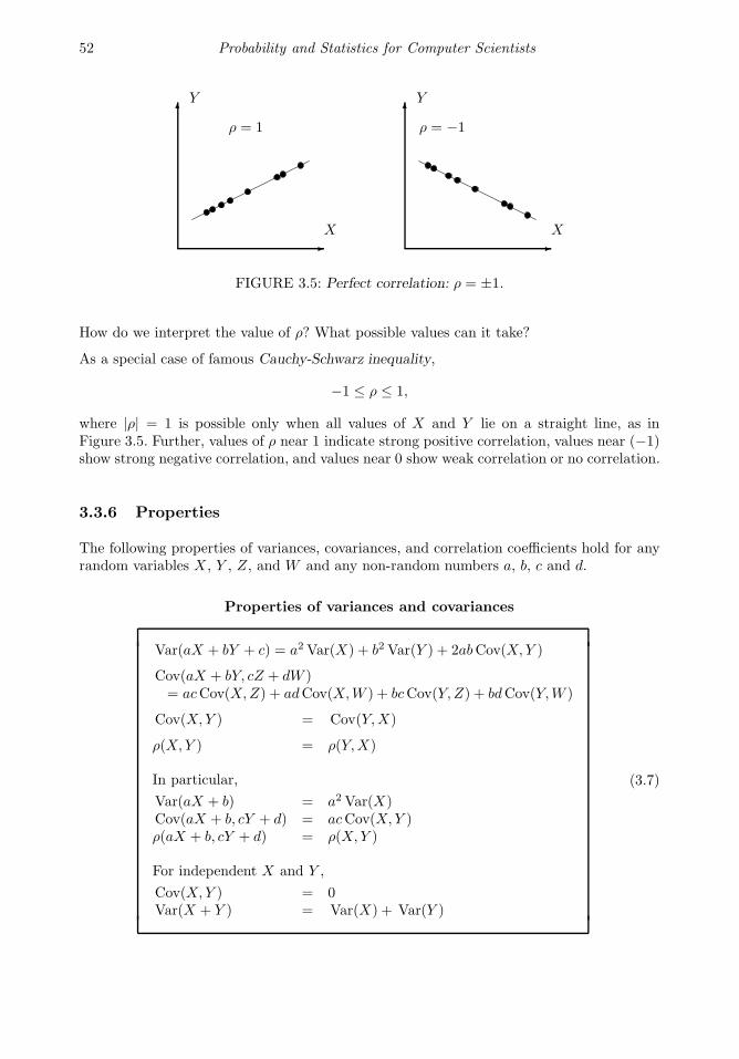
52 Probability and Statistics for Computer Scientists
X
Y
X
Y
ρ = 1 ρ = −1
FIGURE 3.5: Perfect correlation: ρ = ±1.
How do we interpret the value of ρ? What possible values can it take?
As a special case of famous Cauchy-Schwarz inequality,
−1 ≤ ρ ≤ 1,
where |ρ| = 1 is possible only when all values of X and Y lie on a straight line, as inFigure 3.5. Further, values of ρ near 1 indicate strong positive correlation, values near (−1)show strong negative correlation, and values near 0 show weak correlation or no correlation.
3.3.6 Properties
The following properties of variances, covariances, and correlation coefficients hold for anyrandom variables X , Y , Z, and W and any non-random numbers a, b, c and d.
Properties of variances and covariances
Var(aX + bY + c) = a2 Var(X) + b2 Var(Y ) + 2abCov(X,Y )
Cov(aX + bY, cZ + dW )= acCov(X,Z) + adCov(X,W ) + bcCov(Y, Z) + bdCov(Y,W )
Cov(X,Y ) = Cov(Y,X)
ρ(X,Y ) = ρ(Y,X)
In particular,
Var(aX + b) = a2 Var(X)Cov(aX + b, cY + d) = acCov(X,Y )ρ(aX + b, cY + d) = ρ(X,Y )
For independent X and Y ,
Cov(X,Y ) = 0Var(X + Y ) = Var(X) + Var(Y )
(3.7)
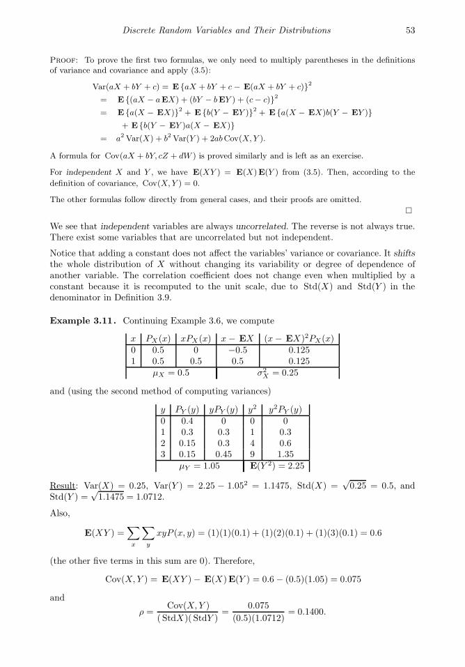
Discrete Random Variables and Their Distributions 53
Proof: To prove the first two formulas, we only need to multiply parentheses in the definitionsof variance and covariance and apply (3.5):
Var(aX + bY + c) = E aX + bY + c− E(aX + bY + c)2
= E (aX − aEX) + (bY − bEY ) + (c− c)2
= E a(X − EX)2 + E b(Y − EY )2 + E a(X − EX)b(Y − EY )
+ E b(Y − EY )a(X − EX)
= a2 Var(X) + b2 Var(Y ) + 2abCov(X,Y ).
A formula for Cov(aX + bY, cZ + dW ) is proved similarly and is left as an exercise.
For independent X and Y , we have E(XY ) = E(X)E(Y ) from (3.5). Then, according to the
definition of covariance, Cov(X,Y ) = 0.
The other formulas follow directly from general cases, and their proofs are omitted.
We see that independent variables are always uncorrelated. The reverse is not always true.There exist some variables that are uncorrelated but not independent.
Notice that adding a constant does not affect the variables’ variance or covariance. It shiftsthe whole distribution of X without changing its variability or degree of dependence ofanother variable. The correlation coefficient does not change even when multiplied by aconstant because it is recomputed to the unit scale, due to Std(X) and Std(Y ) in thedenominator in Definition 3.9.
Example 3.11. Continuing Example 3.6, we compute
x PX(x) xPX(x) x− EX (x− EX)2PX(x)0 0.5 0 −0.5 0.1251 0.5 0.5 0.5 0.125
µX = 0.5 σ2X = 0.25
and (using the second method of computing variances)
y PY (y) yPY (y) y2 y2PY (y)
0 0.4 0 0 01 0.3 0.3 1 0.32 0.15 0.3 4 0.63 0.15 0.45 9 1.35
µY = 1.05 E(Y 2) = 2.25
Result: Var(X) = 0.25, Var(Y ) = 2.25 − 1.052 = 1.1475, Std(X) =√0.25 = 0.5, and
Std(Y ) =√1.1475 = 1.0712.
Also,
E(XY ) =∑
x
∑
y
xyP (x, y) = (1)(1)(0.1) + (1)(2)(0.1) + (1)(3)(0.1) = 0.6
(the other five terms in this sum are 0). Therefore,
Cov(X,Y ) = E(XY )− E(X)E(Y ) = 0.6− (0.5)(1.05) = 0.075
and
ρ =Cov(X,Y )
( StdX)( StdY )=
0.075
(0.5)(1.0712)= 0.1400.
54 Probability and Statistics for Computer Scientists
Thus, the numbers of errors in two modules are positively and not very strongly correlated.♦
Notation µ or E(X) = expectationσ2X or Var(X) = variance
σX or Std(X) = standard deviationσXY or Cov(X,Y ) = covariance
ρXY = correlation coefficient
3.3.7 Chebyshev’s inequality
Knowing just the expectation and variance, one can find the range of values most likely takenby this variable. Russian mathematician Pafnuty Chebyshev (1821–1894) showed that anyrandom variable X with expectation µ = E(X) and variance σ2 = Var(X) belongs to theinterval µ± ε = [µ− ε, µ+ ε] with probability of at least 1− (σ/ε)2. That is,
Chebyshev’sinequality
P |X − µ| > ε ≤(σε
)2
for any distribution with expectation µand variance σ2 and for any positive ε.
(3.8)
Proof: Here we consider discrete random variables. For other types, the proof is similar. Accordingto Definition 3.6,
σ2 =∑
all x
(x− µ)2P (x) ≥∑
only x:|x−µ|>ε
(x− µ)2P (x)
≥∑
x:|x−µ|>ε
ε2P (x) = ε2∑
x:|x−µ|>ε
P (x) = ε2P |x− µ| > ε .
Hence, P |x− µ| > ε ≤ ε2/σ2.
Chebyshev’s inequality shows that only a large variance may allow a variable X to differsignificantly from its expectation µ. In this case, the risk of seeing an extremely low orextremely high value of X increases. For this reason, risk is often measured in terms of avariance or standard deviation.
Example 3.12. Suppose the number of errors in a new software has expectation µ = 20and a standard deviation of 2. According to (3.8), there are more than 30 errors withprobability
P X > 30 ≤ P |X − 20| > 10 ≤(
2
10
)2
= 0.04.
However, if the standard deviation is 5 instead of 2, then the probability of more than 30
errors can only be bounded by(
510
)2= 0.25. ♦
Chebyshev’s inequality is universal because it works for any distribution. Often it gives arather loose bound for the probability of |X − µ| > ε. With more information about thedistribution, this bound may be improved.
Discrete Random Variables and Their Distributions 55
3.3.8 Application to finance
Chebyshev’s inequality shows that in general, higher variance implies higher probabilitiesof large deviations, and this increases the risk for a random variable to take values far fromits expectation.
This finds a number of immediate applications. Here we focus on evaluating risks of financialdeals, allocating funds, and constructing optimal portfolios. This application is intuitivelysimple. The same methods can be used for the optimal allocation of computer memory,CPU time, customer support, or other resources.
Example 3.13 (Construction of an optimal portfolio). We would like to invest$10,000 into shares of companies XX and YY. Shares of XX cost $20 per share. The marketanalysis shows that their expected return is $1 per share with a standard deviation of $0.5.Shares of YY cost $50 per share, with an expected return of $2.50 and a standard deviationof $1 per share, and returns from the two companies are independent. In order to maximizethe expected return and minimize the risk (standard deviation or variance), is it better toinvest (A) all $10,000 into XX, (B) all $10,000 into YY, or (C) $5,000 in each company?
Solution. Let X be the actual (random) return from each share of XX, and Y be the actualreturn from each share of YY. Compute the expectation and variance of the return for eachof the proposed portfolios (A, B, and C).
(a) At $20 a piece, we can use $10,000 to buy 500 shares of XX collecting a profit ofA = 500X . Using (3.5) and (3.7),
E(A) = 500E(X) = (500)(1) = 500;
Var(A) = 5002Var(X) = 5002(0.5)2 = 62, 500.
(b) Investing all $10,000 into YY, we buy 10,000/50=200 shares of it and collect a profit ofB = 200Y ,
E(B) = 200E(Y ) = (200)(2.50) = 500;
Var(A) = 2002Var(Y ) = 2002(1)2 = 40, 000.
(c) Investing $5,000 into each company makes a portfolio consisting of 250 shares of XXand 100 shares of YY; the profit in this case will be C = 250X + 100Y . Following (3.7) forindependent X and Y ,
E(C) = 250E(X) + 100E(Y ) = 250 + 250 = 500;
Var(C) = 2502Var(X) + 1002Var(Y ) = 2502(0.5)2 + 1002(1)2 = 25, 625.
Result: The expected return is the same for each of the proposed three portfolios becauseeach share of each company is expected to return 1/20 or 2.50/50, which is 5%. In termsof the expected return, all three portfolios are equivalent. Portfolio C, where investment issplit between two companies, has the lowest variance; therefore, it is the least risky. Thissupports one of the basic principles in finance: to minimize the risk, diversify the portfolio.♦
56 Probability and Statistics for Computer Scientists
Example 3.14 (Optimal portfolio, correlated returns). Suppose now that theindividual stock returns X and Y are no longer independent. If the correlation coefficient isρ = 0.4, how will it change the results of the previous example? What if they are negativelycorrelated with ρ = −0.2?
Solution. Only the volatility of the diversified portfolio C changes due to the correlationcoefficient. Now Cov(X,Y ) = ρ Std(X) Std(Y ) = (0.4)(0.5)(1) = 0.2, thus the variance ofC increases by 2(250)(100)(0.2) = 10, 000,
Var(C) = Var(250X + 100Y )
= 2502Var(X) + 1002Var(Y ) + 2(250)(100)Cov(X,Y )
= 25, 625 + 10, 000 = 35, 625.
Nevertheless, the diversified portfolio C is still optimal.
Why did the risk of portfolio C increase due to positive correlation of the two stocks? WhenX and Y are positively correlated, low values of X are likely to accompany low values ofY ; therefore, the probability of the overall low return is higher, increasing the risk of theportfolio.
Conversely, negative correlation means that low values of X are likely to be compensatedby high values of Y , and vice versa. Thus, the risk is reduced. Say, with the given ρ = −0.2,we compute Cov(X,Y ) = ρ Std(X) Std(Y ) = (−0.2)(0.5)(1) = −0.1, and
Var(C) = 25, 625 + 2(250)(100)Cov(X,Y ) = 25, 625− 5, 000 = 20, 625.
Diversified portfolios consisting of negatively correlated components are the least risky. ♦
Example 3.15 (Optimizing even further). So, after all, with $10,000 to invest, whatis the most optimal portfolio consisting of shares of XX and YY, given their correlationcoefficient of ρ = −0.2?
This is an optimization problem. Suppose t dollars are invested into XX and (10, 000− t)dollars into YY, with the resulting profit is Ct. This amounts for t/20 shares of X and(10, 000− t)/50 = 200− t/50 shares of YY. Plans A and B correspond to t = 10, 000 andt = 0.
The expected return remains constant at $500. If Cov(X,Y ) = −0.1, as in Example 3.14above, then
Var(Ct) = Var tX + (200− t/50)Y = (t/20)2 Var(X) + (200− t/50)2Var(Y ) + 2(t/20)(200− t/50)Cov(X,Y )
= (t/20)2(0.5)2 + (200− t/50)2(1)2 + 2(t/20)(200− t/50)(−0.1)
=49t2
40, 000− 10t+ 40, 000.
See the graph of this function in Figure 3.6. Minimum of this variance is found at t∗ =
10/( 49t2
40,000 ) = 4081.63. Thus, for the most optimal portfolio, we should invest $4081.63into XX and the remaining $5919.37 into YY. Then we achieve the smallest possible risk(variance) of ($2)19, 592, measured, as we know, in squared dollars. ♦

Discrete Random Variables and Their Distributions 57
t, amount invested into XX ($)Riskoftheportfolio,Var(C
t)($
2)
15,000
30,000
45,000
60,000
0 2,000 4,000 6,000 8,000 10,000
Portfolio B
Portfolio A
Optimal portfolio
FIGURE 3.6: Variance of a diversified portfolio.
3.4 Families of discrete distributions
Next, we introduce the most commonly used families of discrete distributions. Amazingly,absolutely different phenomena can be adequately described by the same mathematicalmodel, or a family of distributions. For example, as we shall see below, the number ofvirus attacks, received e-mails, error messages, network blackouts, telephone calls, trafficaccidents, earthquakes, and so on can all be modeled by the same Poisson family of distri-butions.
3.4.1 Bernoulli distribution
The simplest random variable (excluding non-random ones!) takes just two possible values.Call them 0 and 1.
DEFINITION 3.10
A random variable with two possible values, 0 and 1, is called a Bernoullivariable, its distribution isBernoulli distribution, and any experiment witha binary outcome is called a Bernoulli trial.
This distribution is named after a Swiss mathematician Jacob Bernoulli (1654-1705) whodiscovered not only Bernoulli but also Binomial distribution.
Good or defective components, parts that pass or fail tests, transmitted or lost signals,working or malfunctioning hardware, benign or malicious attachments, sites that containor do not contain a keyword, girls and boys, heads and tails, and so on, are examples ofBernoulli trials. All these experiments fit the same Bernoulli model, where we shall usegeneric names for the two outcomes: “successes” and “failures.” These are nothing but

58 Probability and Statistics for Computer Scientists
commonly used generic names; in fact, successes do not have to be good, and failures donot have to be bad.
If P (1) = p is the probability of a success, then P (0) = q = 1 − p is the probability of afailure. We can then compute the expectation and variance as
E(X) =∑
x
P (x) = (0)(1− p) + (1)(p) = p,
Var(X) =∑
x
(x− p)2P (x) = (0− p)2(1 − p) + (1− p)2p
= p(1− p)(p+ 1− p) = p(1− p).
Bernoullidistribution
p = probability of success
P (x) =
q = 1− p if x = 0
p if x = 1E(X) = pVar(X) = pq
In fact, we see that there is a whole family of Bernoulli distributions, indexed by a parameterp. Every p between 0 and 1 defines another Bernoulli distribution. The distribution withp = 0.5 carries the highest level of uncertainty because Var(X) = pq is maximized byp = q = 0.5. Distributions with lower or higher p have lower variances. Extreme parametersp = 0 and p = 1 define non-random variables 0 and 1, respectively; their variance is 0.
3.4.2 Binomial distribution
Now consider a sequence of independent Bernoulli trials and count the number of successesin it. This may be the number of defective computers in a shipment, the number of updatedfiles in a folder, the number of girls in a family, the number of e-mails with attachments,etc.
DEFINITION 3.11
A variable described as the number of successes in a sequence of independentBernoulli trials has Binomial distribution. Its parameters are n, the numberof trials, and p, the probability of success.
Remark: “Binomial” can be translated as “two numbers,” bi meaning “two” and nom meaning
“a number,” thus reflecting the concept of binary outcomes.
Binomial probability mass function is
P (x) = P X = x =( n
x
)pxqn−x, x = 0, 1, . . . , n, (3.9)
which is the probability of exactly x successes in n trials. In this formula, px is the probabilityof x successes, probabilities being multiplied due to independence of trials. Also, qn−x is
Discrete Random Variables and Their Distributions 59
the probability of the remaining (n − x) trials being failures. Finally,( n
x
)= n!
x!(n−x)! is
the number of elements of the sample space Ω that form the event X = x. This is thenumber of possible orderings of x successes and (n − x) failures among n trials, and it iscomputed as C(n, x) in (2.6).
Due to a somewhat complicated form of (3.9), practitioners use a table of Binomial distri-bution, Table A2. Its entries are values of the Binomial cdf F (x). If we need a pmf insteadof a cdf, we can always compute it from the table as
P (x) = F (x)− F (x− 1).
Example 3.16. As part of a business strategy, randomly selected 20% of new internetservice subscribers receive a special promotion from the provider. A group of 10 neighborssigns for the service. What is the probability that at least 4 of them get a special promotion?
Solution. We need to find the probability P X ≥ 4, where X is the number of people,out of 10, who receive a special promotion. This is the number of successes in 10 Bernoullitrials, therefore, X has Binomial distribution with parameters n = 10 and p = 0.2. FromTable A2,
P X ≥ 4 = 1− F (3) = 1− 0.8791 = 0.1209.
♦
The table does not go beyond n = 20. For large n, we shall learn to use some good approx-imations.
Let’s turn to the Binomial expectation and variance. Computing the expected value directlyby (3.3) results in a complicated formula,
E(X) =
n∑
x=0
x( n
x
)pxqn−x = . . . ?
A shortcut can be obtained from the following important property.
Each Bernoulli trial is associated with a Bernoulli variable that equals 1 if the trial resultsin a success and 0 in case of a failure. Then, a sum of these variables is the overall numberof successes. Thus, any Binomial variable X can be represented as a sum of independentBernoulli variables,
X = X1 + . . .+Xn.
We can use this to compute (referring to (3.5) and (3.7))
E(X) = E(X1 + . . .+Xn) = E(X1) + . . .+ E(Xn) = p+ . . .+ p = np
and
Var(X) = Var(X1 + . . .+Xn) = Var(X1) + . . .+ Var(Xn) = npq.
Binomialdistribution
n = number of trialsp = probability of success
P (x) =( n
x
)pxqn−x
E(X) = npVar(X) = npq

60 Probability and Statistics for Computer Scientists
Example 3.17. An exciting computer game is released. Sixty percent of players completeall the levels. Thirty percent of them will then buy an advanced version of the game. Among15 users, what is the expected number of people who will buy the advanced version? Whatis the probability that at least two people will buy it?
Solution. Let X be the number of people (successes), among the mentioned 15 users (trials),who will buy the advanced version of the game. It has Binomial distribution with n = 15trials and the probability of success
p = P buy advanced= P buy advanced | complete all levelsP complete all levels= (0.30)(0.60) = 0.18.
Then we haveE(X) = np = (15)(0.18) = 2.7
andP X ≥ 2 = 1− P (0)− P (1) = 1− (1 − p)n − np(1− p)n−1 = 0.7813.
The last probability was computed directly by formula (3.9) because the probability ofsuccess, 0.18, is not in Table A2. ♦
MATLAB notes
All the distributions discussed in this book are coded in MATLAB Statistics Toolbox. Bi-nomial cdf can be calculated using the MATLAB function binocdf(x,n,p), where n andp are the parameters. Also, binopdf(x,n,p) computes the probability mass function, andbinornd(n,p) generates a Binomial random variable with the given parameters. Alterna-tively, we can write cdf(’binomial’,x,n,p) for the cdf and pdf(’binomial’,x,n,p) forthe pdf.
MATLAB commands for other distributions are similar; see our inventory in Section 12.1.
3.4.3 Geometric distribution
Again, consider a sequence of independent Bernoulli trials. Each trial results in a “success”or a “failure.”
DEFINITION 3.12
The number of Bernoulli trials needed to get the first success has Geometricdistribution.
Example 3.18. A search engine goes through a list of sites looking for a given key phrase.Suppose the search terminates as soon as the key phrase is found. The number of sitesvisited is Geometric. ♦
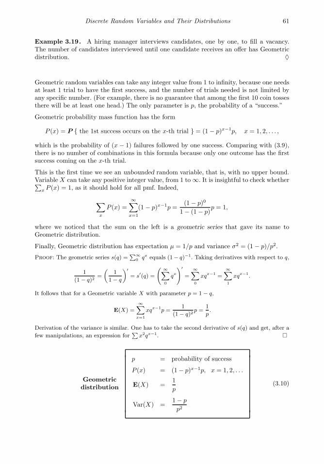
Discrete Random Variables and Their Distributions 61
Example 3.19. A hiring manager interviews candidates, one by one, to fill a vacancy.The number of candidates interviewed until one candidate receives an offer has Geometricdistribution. ♦
Geometric random variables can take any integer value from 1 to infinity, because one needsat least 1 trial to have the first success, and the number of trials needed is not limited byany specific number. (For example, there is no guarantee that among the first 10 coin tossesthere will be at least one head.) The only parameter is p, the probability of a “success.”
Geometric probability mass function has the form
P (x) = P the 1st success occurs on the x-th trial = (1− p)x−1p, x = 1, 2, . . . ,
which is the probability of (x − 1) failures followed by one success. Comparing with (3.9),there is no number of combinations in this formula because only one outcome has the firstsuccess coming on the x-th trial.
This is the first time we see an unbounded random variable, that is, with no upper bound.VariableX can take any positive integer value, from 1 to ∞. It is insightful to check whether∑
x P (x) = 1, as it should hold for all pmf. Indeed,
∑
x
P (x) =∞∑
x=1
(1 − p)x−1p =(1− p)0
1− (1− p)p = 1,
where we noticed that the sum on the left is a geometric series that gave its name toGeometric distribution.
Finally, Geometric distribution has expectation µ = 1/p and variance σ2 = (1 − p)/p2.
Proof: The geometric series s(q) =∑∞
0 qx equals (1− q)−1. Taking derivatives with respect to q,
1
(1− q)2=
(1
1− q
)′
= s′(q) =
(∞∑
0
qx)′
=∞∑
0
xqx−1 =∞∑
1
xqx−1.
It follows that for a Geometric variable X with parameter p = 1− q,
E(X) =∞∑
x=1
xqx−1p =1
(1− q)2p =
1
p.
Derivation of the variance is similar. One has to take the second derivative of s(q) and get, after a
few manipulations, an expression for∑
x2qx−1.
Geometricdistribution
p = probability of success
P (x) = (1− p)x−1p, x = 1, 2, . . .
E(X) =1
p
Var(X) =1− p
p2
(3.10)
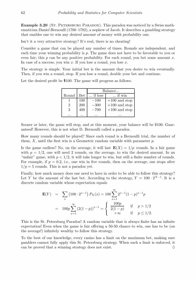
62 Probability and Statistics for Computer Scientists
Example 3.20 (St. Petersburg Paradox). This paradox was noticed by a Swiss math-ematician Daniel Bernoulli (1700–1782), a nephew of Jacob. It describes a gambling strategythat enables one to win any desired amount of money with probability one.
Isn’t it a very attractive strategy? It’s real, there is no cheating!
Consider a game that can be played any number of times. Rounds are independent, andeach time your winning probability is p. The game does not have to be favorable to you oreven fair; this p can be any positive probability. For each round, you bet some amount x.In case of a success, you win x. If you lose a round, you lose x.
The strategy is simple. Your initial bet is the amount that you desire to win eventually.Then, if you win a round, stop. If you lose a round, double your bet and continue.
Let the desired profit be $100. The game will progress as follows.
Balance...Round Bet ... if lose ... if win
1 100 −100 +100 and stop2 200 −300 +100 and stop3 400 −700 +100 and stop... ... ... ...
Sooner or later, the game will stop, and at this moment, your balance will be $100. Guar-anteed! However, this is not what D. Bernoulli called a paradox.
How many rounds should be played? Since each round is a Bernoulli trial, the number ofthem, X , until the first win is a Geometric random variable with parameter p.
Is the game endless? No, on the average, it will last E(X) = 1/p rounds. In a fair gamewith p = 1/2, one will need 2 rounds, on the average, to win the desired amount. In an“unfair” game, with p < 1/2, it will take longer to win, but still a finite number of rounds.For example, if p = 0.2, i.e., one win in five rounds, then on the average, one stops after1/p = 5 rounds. This is not a paradox yet.
Finally, how much money does one need to have in order to be able to follow this strategy?Let Y be the amount of the last bet. According to the strategy, Y = 100 · 2X−1. It is adiscrete random variable whose expectation equals
E(Y ) =∑
x
(100 · 2x−1
)PX(x) = 100
∞∑
x=1
2x−1(1− p)x−1p
= 100p
∞∑
x=1
(2(1− p))x−1
=
100p
2(1− p)if p > 1/2
+∞ if p ≤ 1/2.
This is the St. Petersburg Paradox! A random variable that is always finite has an infiniteexpectation! Even when the game is fair offering a 50-50 chance to win, one has to be (onthe average!) infinitely wealthy to follow this strategy.
To the best of our knowledge, every casino has a limit on the maximum bet, making suregamblers cannot fully apply this St. Petersburg strategy. When such a limit is enforced, itcan be proved that a winning strategy does not exist. ♦
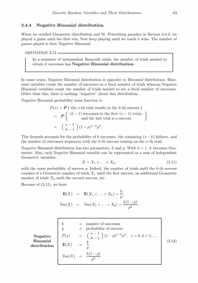
Discrete Random Variables and Their Distributions 63
3.4.4 Negative Binomial distribution
When we studied Geometric distribution and St. Petersburg paradox in Section 3.4.3, weplayed a game until the first win. Now keep playing until we reach k wins. The number ofgames played is then Negative Binomial.
DEFINITION 3.13
In a sequence of independent Bernoulli trials, the number of trials needed toobtain k successes has Negative Binomial distribution.
In some sense, Negative Binomial distribution is opposite to Binomial distribution. Bino-mial variables count the number of successes in a fixed number of trials whereas NegativeBinomial variables count the number of trials needed to see a fixed number of successes.Other than this, there is nothing “negative” about this distribution.
Negative Binomial probability mass function is
P (x) = P the x-th trial results in the k-th success
= P
(k − 1) successes in the first (x− 1) trials,
and the last trial is a success
=( x− 1
k − 1
)(1− p)x−kpk.
This formula accounts for the probability of k successes, the remaining (x− k) failures, andthe number of outcomes–sequences with the k-th success coming on the x-th trial.
Negative Binomial distribution has two parameters, k and p. With k = 1, it becomes Geo-metric. Also, each Negative Binomial variable can be represented as a sum of independentGeometric variables,
X = X1 + . . .+Xk, (3.11)
with the same probability of success p. Indeed, the number of trials until the k-th successconsists of a Geometric number of trials X1 until the first success, an additional Geometricnumber of trials X2 until the second success, etc.
Because of (3.11), we have
E(X) = E(X1 + . . .+Xk) =k
p;
Var(X) = Var(X1 + . . .+Xk) =k(1− p)
p2.
NegativeBinomial
distribution
k = number of successesp = probability of success
P (x) =( x− 1
k − 1
)(1− p)x−kpk, x = k, k + 1, . . .
E(X) =k
p
Var(X) =k(1− p)
p2
(3.12)

64 Probability and Statistics for Computer Scientists
Example 3.21 (Sequential testing). In a recent production, 5% of certain electroniccomponents are defective. We need to find 12 non-defective components for our 12 newcomputers. Components are tested until 12 non-defective ones are found. What is the prob-ability that more than 15 components will have to be tested?
Solution. Let X be the number of components tested until 12 non-defective ones are found.It is a number of trials needed to see 12 successes, hence X has Negative Binomial distri-bution with k = 12 and p = 0.05.
We need P X > 15 =∑∞
16 P (x) or 1 − F (15); however, there is no table of NegativeBinomial distribution in the Appendix, and applying the formula for P (x) directly is rathercumbersome. What would be a quick solution?
Virtually any Negative Binomial problem can be solved by a Binomial distribution. Al-though X is not Binomial at all, the probability P X > 15 can be related to some Bino-mial variable. In our example,
P X > 15 = P more than 15 trials needed to get 12 successes = P 15 trials are not sufficient = P there are fewer than 12 successes in 15 trials = P Y < 12 ,
where Y is the number of successes (non-defective components) in 15 trials, which is aBinomial variable with parameters n = 15 and p = 0.95. From Table A2 on p. 412,
P X > 15 = P Y < 12 = P Y ≤ 11 = F (11) = 0.0055.
This technique, expressing a probability about one random variable in terms of another ran-dom variable, is rather useful. Soon it will help us relate Gamma and Poisson distributionsand simplify computations significantly. ♦
3.4.5 Poisson distribution
The next distribution is related to a concept of rare events, or Poissonian events. Essentiallyit means that two such events are extremely unlikely to occur simultaneously or within avery short period of time. Arrivals of jobs, telephone calls, e-mail messages, traffic accidents,network blackouts, virus attacks, errors in software, floods, and earthquakes are examplesof rare events. The rigorous definition of rare events is given in Section 6.3.2.
DEFINITION 3.14
The number of rare events occurring within a fixed period of time has Poissondistribution.
This distribution bears the name of a famous French mathematician Simeon-Denis Poisson(1781–1840).
Discrete Random Variables and Their Distributions 65
Poissondistribution
λ = frequency, average number of events
P (x) = e−λλx
x!, x = 0, 1, 2, . . .
E(X) = λVar(X) = λ
Proof: This probability mass function satisfies∑∞
0 P (x) = 1 because the Taylor series for f(λ) =eλ at λ = 0 is
eλ =∞∑
x=0
λx
x!, (3.13)
and this series converges for all λ.
The expectation E(X) can be derived from (3.13) as
E(X) =
∞∑
x=0
xe−λλx
x!= 0 + e−λ
∞∑
x=1
λx−1 · λ
(x− 1)!= e−λ · eλ · λ = λ.
Similarly,
E(X2)− E(X) =
∞∑
x=0
(x2 − x)P (x) =
∞∑
x=2
x(x− 1)e−λλx
x!= e−λ
∞∑
x=2
λx−2 · λ2
(x− 2)!= λ2,
and therefore,
Var(X) = E(X2)− E2(X) = (λ2 + E(X))− E
2(X) = λ2 + λ− λ2 = λ.
A Poisson variable can take any nonnegative integer value because there may be no rareevents within the chosen period, on one end, and the possible number of events is notlimited, on the other end. Poisson distribution has one parameter, λ > 0, which is theaverage number of the considered rare events. Values of its cdf are given in Table A3 onp. 415.
Example 3.22 (New accounts). Customers of an internet service provider initiate newaccounts at the average rate of 10 accounts per day.
(a) What is the probability that more than 8 new accounts will be initiated today?(b) What is the probability that more than 16 accounts will be initiated within 2 days?
Solution. (a) New account initiations qualify as rare events because no two customersopen accounts simultaneously. Then the number X of today’s new accounts has Poissondistribution with parameter λ = 10. From Table A3,
P X > 8 = 1− FX(8) = 1− 0.333 = 0.667.
(b) The number of accounts, Y , opened within 2 days does not equal 2X . Rather, Y isanother Poisson random variable whose parameter equals 20. Indeed, the parameter is theaverage number of rare events, which, over the period of two days, doubles the one-dayaverage. Using Table A3 with λ = 20,
P Y > 16 = 1− FY (16) = 1− 0.221 = 0.779.
♦
66 Probability and Statistics for Computer Scientists
3.4.6 Poisson approximation of Binomial distribution
Poisson distribution can be effectively used to approximate Binomial probabilities when thenumber of trials n is large, and the probability of success p is small. Such an approximationis adequate, say, for n ≥ 30 and p ≤ 0.05, and it becomes more accurate for larger n.
Example 3.23 (New accounts, continued). Indeed, the situation in Example 3.22 canbe viewed as a sequence of Bernoulli trials. Suppose there are n = 400, 000 potential internetusers in the area, and on any specific day, each of them opens a new account with probabilityp = 0.000025. We see that the number of new accounts is the number of successes, hence aBinomial model with expectation E(X) = np = 10 is possible. However, a distribution withsuch extreme n and p is unlikely to be found in any table, and computing its pmf by handis tedious. Instead, one can use Poisson distribution with the same expectation λ = 10. ♦
Poissonapproximationto Binomial
Binomial(n, p) ≈ Poisson(λ)
where n ≥ 30, p ≤ 0.05, np = λ(3.14)
Remark: Mathematically, it means closeness of Binomial and Poisson pmf,
limn → ∞p → 0np → λ
( nx
)px(1− p)n−x = e−λλ
x
x!
and this is what S. D. Poisson has shown.
When p is large (p ≥ 0.95), the Poisson approximation is applicable too. The probability ofa failure q = 1 − p is small in this case. Then, we can approximate the number of failures,which is also Binomial, by a Poisson distribution.
Example 3.24. Ninety-seven percent of electronic messages are transmitted with no error.What is the probability that out of 200 messages, at least 195 will be transmitted correctly?
Solution. Let X be the number of correctly transmitted messages. It is the number ofsuccesses in 200 Bernoulli trials, thus X is Binomial with n = 200 and p = 0.97. Poissonapproximation cannot be applied to X because p is too large. However, the number offailures Y is also Binomial, with parameters n = 200 and q = 0.03, and it is approximatelyPoisson with λ = nq = 6. From Table A3,
P X ≥ 195 = P Y ≤ 5 = FY (5) ≈ 0.446.
♦
There is a great variety of applications involving a large number of trials with a smallprobability of success. If the trials are not independent, the number of successes is notBinomial, in general. However, if dependence is weak, the use of Poisson approximation insuch problems can still produce remarkably accurate results.
Discrete Random Variables and Their Distributions 67
Example 3.25 (Birthday problem). This continues Exercise 2.25 on p. 36. Consider aclass with N ≥ 10 students. Compute the probability that at least two of them have theirbirthdays on the same day. How many students should be in class in order to have thisprobability above 0.5?
Solution. Poisson approximation will be used for the number of shared birthdays among all
n =(N2
)=
N(N − 1)
2
pairs of students in this class. In each pair, both students are born on the same day withprobability p = 1/365. Each pair is a Bernoulli trial because the two birthdays either matchor don’t match. Besides, matches in two different pairs are “nearly” independent. Therefore,X , the number of pairs sharing birthdays, is “almost” Binomial. For N ≥ 10, n ≥ 45 islarge, and p is small, thus, we shall use Poisson approximation with λ = np = N(N−1)/730,
P there are two students sharing birthday = 1− P no matches
= 1− P X = 0 ≈ 1− e−λ ≈ 1− e−N2/730.
Solving the inequality 1 − e−N2/730 > 0.5, we obtain N >√730 ln2 ≈ 22.5. That is, in a
class of at least N = 23 students, there is a more than 50% chance that at least two studentswere born on the same day of the year! ♦
The introduced method can only be applied to very small and very large values of p. Formoderate p (0.05 ≤ p ≤ 0.95), the Poisson approximation may not be accurate. These casesare covered by the Central Limit Theorem on p. 93.
Summary and conclusions
Discrete random variables can take a finite or countable number of isolated values withdifferent probabilities. Collection of all such probabilities is a distribution, which describesthe behavior of a random variable. Random vectors are sets of random variables; theirbehavior is described by the joint distribution. Marginal probabilities can be computedfrom the joint distribution by the Addition Rule.
The average value of a random variable is its expectation. Variability around the expectationis measured by the variance and the standard deviation. Covariance and correlation measureassociation of two random variables. For any distribution, probabilities of large deviationscan be bounded by Chebyshev’s inequality, using only the expectation and variance.
Different phenomena can often be described by the same probabilistic model, or a family ofdistributions. The most commonly used discrete families are Binomial, including Bernoulli,Negative Binomial, including Geometric, and Poisson. Each family of distributions is usedfor a certain general type of situations; it has its parameters and a clear formula and/or atable for computing probabilities. These families are summarized in Section 12.1.1.

68 Probability and Statistics for Computer Scientists
Exercises
3.1.A computer virus is trying to corrupt two files. The first file will be corrupted with probability0.4. Independently of it, the second file will be corrupted with probability 0.3.
(a) Compute the probability mass function (pmf) of X , the number of corrupted files.
(b) Draw a graph of its cumulative distribution function (cdf).
3.2. Every day, the number of network blackouts has a distribution (probability mass function)
x 0 1 2
P (x) 0.7 0.2 0.1
A small internet trading company estimates that each network blackout results in a $500loss. Compute expectation and variance of this company’s daily loss due to blackouts.
3.3. There is one error in one of five blocks of a program. To find the error, we test three randomlyselected blocks. Let X be the number of errors in these three blocks. Compute E(X) andVar(X).
3.4. Tossing a fair die is an experiment that can result in any integer number from 1 to 6 withequal probabilities. Let X be the number of dots on the top face of a die. Compute E(X)and Var(X).
3.5. A software package consists of 12 programs, five of which must be upgraded. If 4 programsare randomly chosen for testing,
(a) What is the probability that at least two of them must be upgraded?
(b) What is the expected number of programs, out of the chosen four, that must beupgraded?
3.6. A computer program contains one error. In order to find the error, we split the programinto 6 blocks and test two of them, selected at random. Let X be the number of errors inthese blocks. Compute E(X).
3.7. The number of home runs scored by a certain team in one baseball game is a random variablewith the distribution
x 0 1 2P (x) 0.4 0.4 0.2
The team plays 2 games. The number of home runs scored in one game is independent ofthe number of home runs in the other game. Let Y be the total number of home runs. FindE(Y ) and Var(Y ).
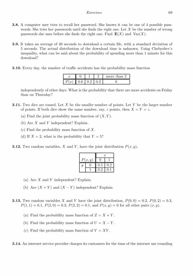
Exercises 69
3.8. A computer user tries to recall her password. She knows it can be one of 4 possible pass-words. She tries her passwords until she finds the right one. Let X be the number of wrongpasswords she uses before she finds the right one. Find E(X) and Var(X).
3.9. It takes an average of 40 seconds to download a certain file, with a standard deviation of5 seconds. The actual distribution of the download time is unknown. Using Chebyshev’sinequality, what can be said about the probability of spending more than 1 minute for thisdownload?
3.10. Every day, the number of traffic accidents has the probability mass function
x 0 1 2 more than 2
P (x) 0.6 0.2 0.2 0
independently of other days. What is the probability that there are more accidents on Fridaythan on Thursday?
3.11. Two dice are tossed. Let X be the smaller number of points. Let Y be the larger numberof points. If both dice show the same number, say, z points, then X = Y = z.
(a) Find the joint probability mass function of (X,Y ).
(b) Are X and Y independent? Explain.
(c) Find the probability mass function of X .
(d) If X = 2, what is the probability that Y = 5?
3.12. Two random variables, X and Y , have the joint distribution P (x, y),
xP (x, y) 0 1
y 0 0.5 0.21 0.2 0.1
(a) Are X and Y independent? Explain.
(b) Are (X + Y ) and (X − Y ) independent? Explain.
3.13. Two random variables X and Y have the joint distribution, P (0, 0) = 0.2, P (0, 2) = 0.3,P (1, 1) = 0.1, P (2, 0) = 0.3, P (2, 2) = 0.1, and P (x, y) = 0 for all other pairs (x, y).
(a) Find the probability mass function of Z = X + Y .
(b) Find the probability mass function of U = X − Y .
(c) Find the probability mass function of V = XY .
3.14. An internet service provider charges its customers for the time of the internet use rounding
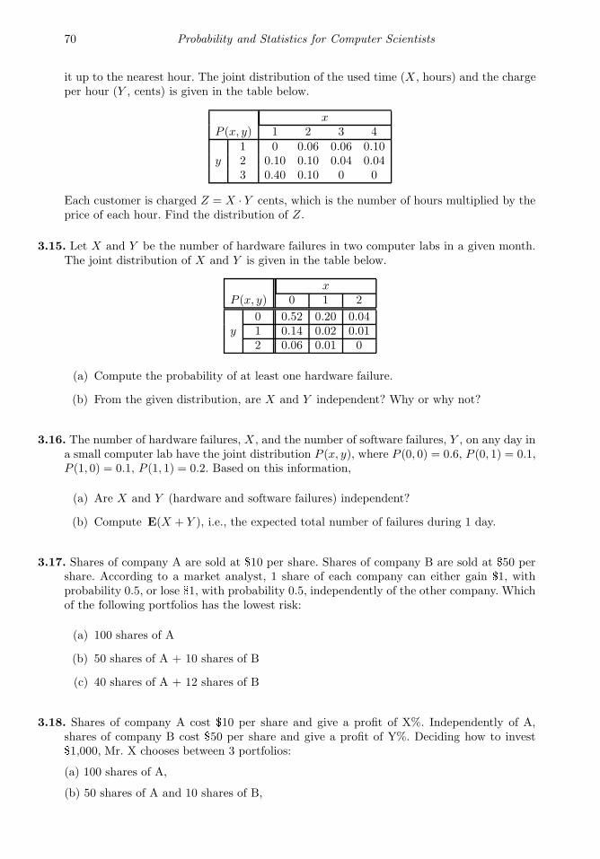
70 Probability and Statistics for Computer Scientists
it up to the nearest hour. The joint distribution of the used time (X , hours) and the chargeper hour (Y , cents) is given in the table below.
xP (x, y) 1 2 3 4
1 0 0.06 0.06 0.10y 2 0.10 0.10 0.04 0.04
3 0.40 0.10 0 0
Each customer is charged Z = X · Y cents, which is the number of hours multiplied by theprice of each hour. Find the distribution of Z.
3.15. Let X and Y be the number of hardware failures in two computer labs in a given month.The joint distribution of X and Y is given in the table below.
xP (x, y) 0 1 2
0 0.52 0.20 0.04y 1 0.14 0.02 0.01
2 0.06 0.01 0
(a) Compute the probability of at least one hardware failure.
(b) From the given distribution, are X and Y independent? Why or why not?
3.16. The number of hardware failures, X , and the number of software failures, Y , on any day ina small computer lab have the joint distribution P (x, y), where P (0, 0) = 0.6, P (0, 1) = 0.1,P (1, 0) = 0.1, P (1, 1) = 0.2. Based on this information,
(a) Are X and Y (hardware and software failures) independent?
(b) Compute E(X + Y ), i.e., the expected total number of failures during 1 day.
3.17. Shares of company A are sold at $10 per share. Shares of company B are sold at $50 pershare. According to a market analyst, 1 share of each company can either gain $1, withprobability 0.5, or lose $1, with probability 0.5, independently of the other company. Whichof the following portfolios has the lowest risk:
(a) 100 shares of A
(b) 50 shares of A + 10 shares of B
(c) 40 shares of A + 12 shares of B
3.18. Shares of company A cost $10 per share and give a profit of X%. Independently of A,shares of company B cost $50 per share and give a profit of Y%. Deciding how to invest$1,000, Mr. X chooses between 3 portfolios:
(a) 100 shares of A,
(b) 50 shares of A and 10 shares of B,
Exercises 71
(c) 20 shares of B.
The distribution of X is given by probabilities:
PX = −3 = 0.3, PX = 0 = 0.2, PX = 3 = 0.5.
The distribution of Y is given by probabilities:
PY = −3 = 0.4, PY = 3 = 0.6.
Compute expectations and variances of the total dollar profit generated by portfolios (a),(b), and (c). What is the least risky portfolio? What is the most risky portfolio?
3.19. A and B are two competing companies. An investor decides whether to buy
(a) 100 shares of A, or
(b) 100 shares of B, or
(c) 50 shares of A and 50 shares of B.
A profit made on 1 share of A is a random variable X with the distribution P (X = 2) =P (X = −2) = 0.5.
A profit made on 1 share of B is a random variable Y with the distribution P (Y = 4) =0.2, P (Y = −1) = 0.8.
If X and Y are independent, compute the expected value and variance of the total profitfor strategies (a), (b), and (c).
3.20. A quality control engineer tests the quality of produced computers. Suppose that 5% ofcomputers have defects, and defects occur independently of each other.
(a) Find the probability of exactly 3 defective computers in a shipment of twenty.
(b) Find the probability that the engineer has to test at least 5 computers in order to find2 defective ones.
3.21. A lab network consisting of 20 computers was attacked by a computer virus. This virusenters each computer with probability 0.4, independently of other computers. Find theprobability that it entered at least 10 computers.
3.22. Five percent of computer parts produced by a certain supplier are defective. What is theprobability that a sample of 16 parts contains more than 3 defective ones?
3.23. Every day, a lecture may be canceled due to inclement weather with probability 0.05. Classcancelations on different days are independent.
(a) There are 15 classes left this semester. Compute the probability that at least 4 ofthem get canceled.
(b) Compute the probability that the tenth class this semester is the third class that getscanceled.
72 Probability and Statistics for Computer Scientists
3.24. An internet search engine looks for a certain keyword in a sequence of independent websites. It is believed that 20% of the sites contain this keyword.
(a) Compute the probability that at least 5 of the first 10 sites contain the given keyword.
(b) Compute the probability that the search engine had to visit at least 5 sites in orderto find the first occurrence of a keyword.
3.25. About ten percent of users do not close Windows properly. Suppose that Windows isinstalled in a public library that is used by random people in a random order.
(a) On the average, how many users of this computer do not close Windows properlybefore someone does close it properly?
(b) What is the probability that exactly 8 of the next 10 users will close Windows prop-erly?
3.26. After a computer virus entered the system, a computer manager checks the condition ofall important files. She knows that each file has probability 0.2 to be damaged by the virus,independently of other files.
(a) Compute the probability that at least 5 of the first 20 files are damaged.
(b) Compute the probability that the manager has to check at least 6 files in order to find3 undamaged files.
3.27. Messages arrive at an electronic message center at random times, with an average of 9messages per hour.
(a) What is the probability of receiving at least five messages during the next hour?
(b) What is the probability of receiving exactly five messages during the next hour?
3.28. The number of received electronic messages has Poisson distribution with some parameterλ. Using Chebyshev inequality, show that the probability of receiving more than 4λmessagesdoes not exceed 1/(9λ).
3.29. An insurance company divides its customers into 2 groups. Twenty percent of customersare in the high-risk group, and eighty percent are in the low-risk group. The high-riskcustomers make an average of 1 accident per year while the low-risk customers make anaverage of 0.1 accidents per year. Eric had no accidents last year. What is the probabilitythat he is a high-risk driver?
3.30. Eric from Exercise 3.29 continues driving. After three years, he still has no traffic accidents.Now, what is the conditional probability that he is a high-risk driver?
3.31. Before the computer is assembled, its vital component (motherboard) goes through aspecial inspection. Only 80% of components pass this inspection.

Exercises 73
(a) What is the probability that at least 18 of the next 20 components pass inspection?
(b) On the average, how many components should be inspected until a component thatpasses inspection is found?
3.32.On the average, 1 computer in 800 crashes during a severe thunderstorm. A certain companyhad 4,000 working computers when the area was hit by a severe thunderstorm.
(a) Compute the probability that less than 10 computers crashed.
(b) Compute the probability that exactly 10 computers crashed.
You may want to use a suitable approximation.
3.33.The number of computer shutdowns during any month has a Poisson distribution, averaging0.25 shutdowns per month.
(a) What is the probability of at least 3 computer shutdowns during the next year?
(b) During the next year, what is the probability of at least 3 months (out of 12) withexactly 1 computer shutdown in each?
3.34. A dangerous computer virus attacks a folder consisting of 250 files. Files are affected by thevirus independently of one another. Each file is affected with the probability 0.032. Whatis the probability that more than 7 files are affected by this virus?
3.35. In some city, the probability of a thunderstorm on any day is 0.6. During a thunderstorm,the number of traffic accidents has Poisson distribution with parameter 10. Otherwise,the number of traffic accidents has Poisson distribution with parameter 4. If there were 7accidents yesterday, what is the probability that there was a thunderstorm?
3.36. An interactive system consists of ten terminals that are connected to the central com-puter. At any time, each terminal is ready to transmit a message with probability 0.7,independently of other terminals. Find the probability that exactly 6 terminals are readyto transmit at 8 o’clock.
3.37. Network breakdowns are unexpected rare events that occur every 3 weeks, on the average.Compute the probability of more than 4 breakdowns during a 21-week period.
3.38. Simplifying expressions, derive from the definitions of variance and covariance that
(a) Var(X) = E(X2)− E2(X);
(b) Cov(X,Y ) = E(XY )− E(X)E(Y ).
3.39. Show that
Cov(aX + bY + c, dZ + eW + f)
= adCov(X,Z) + aeCov(X,W ) + bdCov(Y, Z) + beCov(Y,W )
for any random variables X , Y , Z, W , and any non-random numbers a, b, c, d, e, f .

Chapter 4
Continuous Distributions
4.1 Probability density . . . . . . . . . . . . . . . . . . . . . . . . . . . . . . . . . . . . . . . . . . . . . . . 754.2 Families of continuous distributions . . . . . . . . . . . . . . . . . . . . . . . . . . . . . 80
4.2.1 Uniform distribution . . . . . . . . . . . . . . . . . . . . . . . . . . . . . . . . . . . . . 804.2.2 Exponential distribution . . . . . . . . . . . . . . . . . . . . . . . . . . . . . . . . . 824.2.3 Gamma distribution . . . . . . . . . . . . . . . . . . . . . . . . . . . . . . . . . . . . . 844.2.4 Normal distribution . . . . . . . . . . . . . . . . . . . . . . . . . . . . . . . . . . . . . 89
4.3 Central Limit Theorem . . . . . . . . . . . . . . . . . . . . . . . . . . . . . . . . . . . . . . . . . . 92Summary and conclusions . . . . . . . . . . . . . . . . . . . . . . . . . . . . . . . . . . . . . . . . . . 95Exercises . . . . . . . . . . . . . . . . . . . . . . . . . . . . . . . . . . . . . . . . . . . . . . . . . . . . . . . . . . . . 96
Recall that any discrete distribution is concentrated on a finite or countable number ofisolated values. Conversely, continuous variables can take any value of an interval, (a, b),(a,+∞), (−∞,+∞), etc. Various times like service time, installation time, download time,failure time, and also physical measurements like weight, height, distance, velocity, temper-ature, and connection speed are examples of continuous random variables.
4.1 Probability density
For all continuous variables, the probability mass function (pmf) is always equal to zero,1
P (x) = 0 for all x.
As a result, the pmf does not carry any information about a random variable. Rather, wecan use the cumulative distribution function (cdf) F (x). In the continuous case, it equals
F (x) = P X ≤ x = P X < x .
These two expressions for F (x) differ by P X = x = P (x) = 0.
In both continuous and discrete cases, the cdf F (x) is a non-decreasing function that rangesfrom 0 to 1. Recall from Chapter 3 that in the discrete case, the graph of F (x) has jumpsof magnitude P (x). For continuous distributions, P (x) = 0, which means no jumps. Thecdf in this case is a continuous function (see, for example, Fig. 4.2 on p. 77).
1Remark: In fact, any probability mass function P (x) can give positive probabilities to a finiteor countable set only. They key is that we must have
∑x P (x) = 1. So, there can be at most 2
values of x with P (x) ≥ 1/2, at most 4 values with P (x) ≥ 1/4, etc. Continuing this way, we canlist all x where P (x) > 0. And since all such values with positive probabilities can be listed, theirset is at most countable. It cannot be an interval because any interval is uncountable. This agreeswith P (x) = 0 for continuous random variables that take entire intervals of values.
75
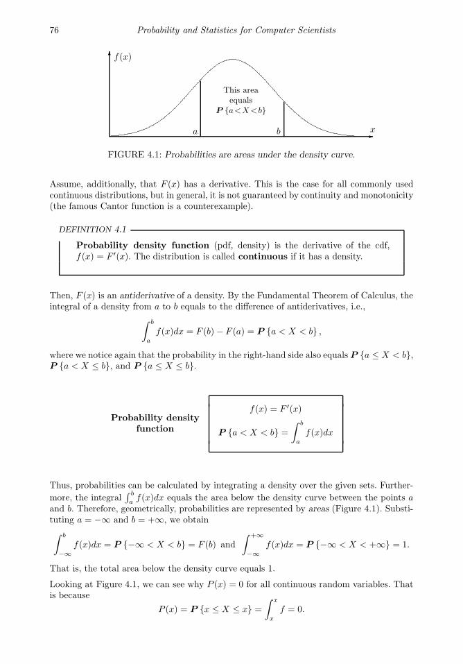
76 Probability and Statistics for Computer Scientists
x
f(x)
This areaequals
P a<X<b
a b
FIGURE 4.1: Probabilities are areas under the density curve.
Assume, additionally, that F (x) has a derivative. This is the case for all commonly usedcontinuous distributions, but in general, it is not guaranteed by continuity and monotonicity(the famous Cantor function is a counterexample).
DEFINITION 4.1
Probability density function (pdf, density) is the derivative of the cdf,f(x) = F ′(x). The distribution is called continuous if it has a density.
Then, F (x) is an antiderivative of a density. By the Fundamental Theorem of Calculus, theintegral of a density from a to b equals to the difference of antiderivatives, i.e.,
∫ b
a
f(x)dx = F (b)− F (a) = P a < X < b ,
where we notice again that the probability in the right-hand side also equals P a ≤ X < b,P a < X ≤ b, and P a ≤ X ≤ b.
Probability densityfunction
f(x) = F ′(x)
P a < X < b =
∫ b
a
f(x)dx
Thus, probabilities can be calculated by integrating a density over the given sets. Further-
more, the integral∫ b
af(x)dx equals the area below the density curve between the points a
and b. Therefore, geometrically, probabilities are represented by areas (Figure 4.1). Substi-tuting a = −∞ and b = +∞, we obtain
∫ b
−∞
f(x)dx = P −∞ < X < b = F (b) and
∫ +∞
−∞
f(x)dx = P −∞ < X < +∞ = 1.
That is, the total area below the density curve equals 1.
Looking at Figure 4.1, we can see why P (x) = 0 for all continuous random variables. Thatis because
P (x) = P x ≤ X ≤ x =
∫ x
x
f = 0.
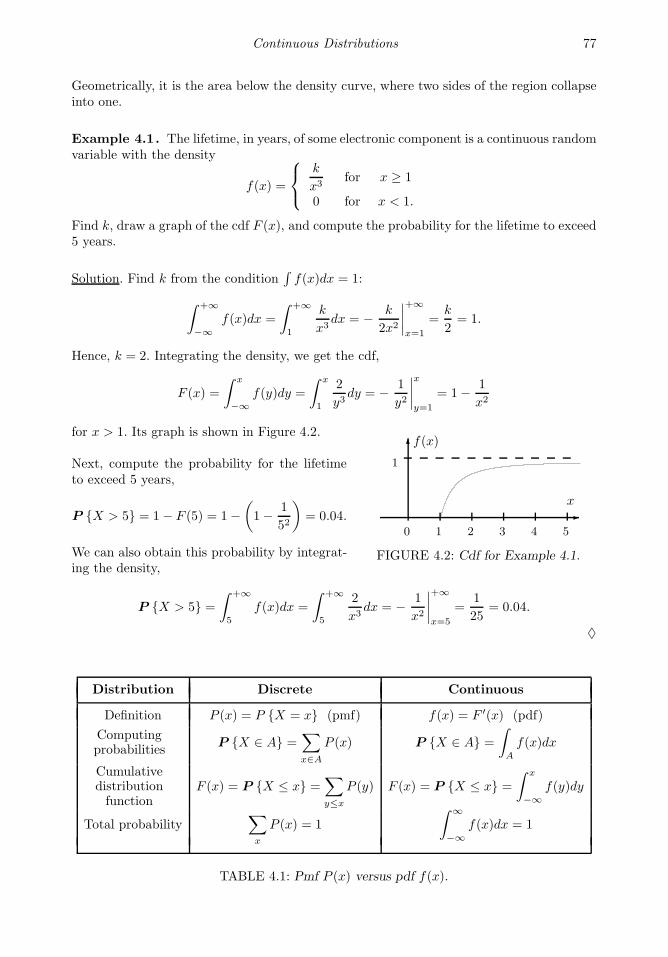
Continuous Distributions 77
Geometrically, it is the area below the density curve, where two sides of the region collapseinto one.
Example 4.1. The lifetime, in years, of some electronic component is a continuous randomvariable with the density
f(x) =
k
x3for x ≥ 1
0 for x < 1.
Find k, draw a graph of the cdf F (x), and compute the probability for the lifetime to exceed5 years.
Solution. Find k from the condition∫f(x)dx = 1:
∫ +∞
−∞
f(x)dx =
∫ +∞
1
k
x3dx = − k
2x2
∣∣∣∣+∞
x=1
=k
2= 1.
Hence, k = 2. Integrating the density, we get the cdf,
F (x) =
∫ x
−∞
f(y)dy =
∫ x
1
2
y3dy = − 1
y2
∣∣∣∣x
y=1
= 1− 1
x2
for x > 1. Its graph is shown in Figure 4.2.
0 1 2 3 4 5
x
f(x)
1
FIGURE 4.2: Cdf for Example 4.1.
Next, compute the probability for the lifetimeto exceed 5 years,
P X > 5 = 1− F (5) = 1−(1− 1
52
)= 0.04.
We can also obtain this probability by integrat-ing the density,
P X > 5 =
∫ +∞
5
f(x)dx =
∫ +∞
5
2
x3dx = − 1
x2
∣∣∣∣+∞
x=5
=1
25= 0.04.
♦
Distribution Discrete Continuous
Definition P (x) = P X = x (pmf) f(x) = F ′(x) (pdf)
Computingprobabilities
P X ∈ A =∑
x∈A
P (x) P X ∈ A =
∫
A
f(x)dx
Cumulativedistributionfunction
F (x) = P X ≤ x =∑
y≤x
P (y) F (x) = P X ≤ x =
∫ x
−∞
f(y)dy
Total probability∑
x
P (x) = 1
∫ ∞
−∞
f(x)dx = 1
TABLE 4.1: Pmf P (x) versus pdf f(x).

78 Probability and Statistics for Computer Scientists
Analogy: pmf versus pdf
The role of a density for continuous distributions is very similar to the role of the probabilitymass function for discrete distributions. Most vital concepts can be translated from thediscrete case to the continuous case by replacing pmf P (x) with pdf f(x) and integratinginstead of summing, as in Table 4.1.
Joint and marginal densities
DEFINITION 4.2
For a vector of random variables, the joint cumulative distribution func-tion is defined as
F(X,Y )(x, y) = P X ≤ x ∩ Y ≤ y .
The joint density is the mixed derivative of the joint cdf,
f(X,Y )(x, y) =∂2
∂x∂yF(X,Y )(x, y).
Similarly to the discrete case, a marginal density of X or Y can be obtained by integratingout the other variable. Variables X and Y are independent if their joint density factorsinto the product of marginal densities. Probabilities about X and Y can be computed byintegrating the joint density over the corresponding set of vector values (x, y) ∈ R2. This isalso analogous to the discrete case; see Table 4.2.
These concepts are directly extended to three or more variables.
Expectation and variance
Continuing our analogy with the discrete case, expectation of a continuous variable is also
Distribution Discrete Continuous
Marginaldistributions
P (x) =∑
y P (x, y)
P (y) =∑
x P (x, y)
f(x) =∫f(x, y)dy
f(y) =∫f(x, y)dx
Independence P (x, y) = P (x)P (y) f(x, y) = f(x)f(y)
Computingprobabilities
P (X,Y ) ∈ A
=∑∑
(x,y)∈A
P (x, y)
P (X,Y ) ∈ A
=
∫∫
(x,y)∈A
f(x, y) dx dy
TABLE 4.2: Joint and marginal distributions in discrete and continuous cases.
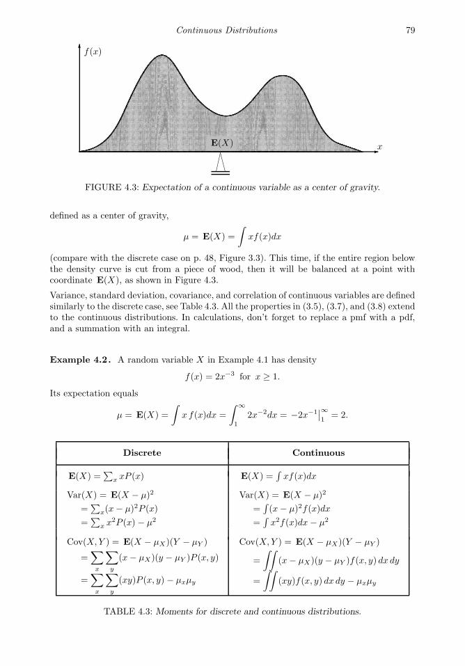
Continuous Distributions 79
f(x)
xE(X)
FIGURE 4.3: Expectation of a continuous variable as a center of gravity.
defined as a center of gravity,
µ = E(X) =
∫xf(x)dx
(compare with the discrete case on p. 48, Figure 3.3). This time, if the entire region belowthe density curve is cut from a piece of wood, then it will be balanced at a point withcoordinate E(X), as shown in Figure 4.3.
Variance, standard deviation, covariance, and correlation of continuous variables are definedsimilarly to the discrete case, see Table 4.3. All the properties in (3.5), (3.7), and (3.8) extendto the continuous distributions. In calculations, don’t forget to replace a pmf with a pdf,and a summation with an integral.
Example 4.2. A random variable X in Example 4.1 has density
f(x) = 2x−3 for x ≥ 1.
Its expectation equals
µ = E(X) =
∫x f(x)dx =
∫ ∞
1
2x−2dx = −2x−1∣∣∞1
= 2.
Discrete Continuous
E(X) =∑
x xP (x) E(X) =∫xf(x)dx
Var(X) = E(X − µ)2
=∑
x(x− µ)2P (x)
=∑
x x2P (x) − µ2
Var(X) = E(X − µ)2
=∫(x− µ)2f(x)dx
=∫x2f(x)dx − µ2
Cov(X,Y ) = E(X − µX)(Y − µY )
=∑
x
∑
y
(x− µX)(y − µY )P (x, y)
=∑
x
∑
y
(xy)P (x, y) − µxµy
Cov(X,Y ) = E(X − µX)(Y − µY )
=
∫∫(x− µX)(y − µY )f(x, y) dx dy
=
∫∫(xy)f(x, y) dx dy − µxµy
TABLE 4.3: Moments for discrete and continuous distributions.

80 Probability and Statistics for Computer Scientists
Computing its variance, we run into a “surprise,”
σ2 = Var(X) =
∫x2f(x)dx − µ2 =
∫ ∞
1
2x−1dx− 4 = 2 lnx|∞1 − 4 = +∞.
This variable does not have a finite variance! (Also, see the St. Petersburg paradox discussionon p. 62.) ♦
4.2 Families of continuous distributions
As in the discrete case, varieties of phenomena can be described by relatively few families ofcontinuous distributions. Here, we shall discuss Uniform, Exponential, Gamma, and Normalfamilies, adding Student’s t, Pearson’s χ2, and Fisher’s F distributions in later chapters.
4.2.1 Uniform distribution
Uniform distribution plays a unique role in stochastic modeling. As we shall see in Chapter 5,a random variable with any thinkable distribution can be generated from a Uniform ran-dom variable. Many computer languages and software are equipped with a random numbergenerator that produces Uniform random variables. Users can convert them into variableswith desired distributions and use for computer simulation of various events and processes.
Also, Uniform distribution is used in any situation when a value is picked “at random”from a given interval; that is, without any preference to lower, higher, or medium values.For example, locations of errors in a program, birthdays throughout a year, and manycontinuous random variables modulo 1, modulo 0.1, 0.01, etc., are uniformly distributedover their corresponding intervals.
To give equal preference to all values, the Uniform distribution has a constant density(Figure 4.4). On the interval (a, b), its density equals
f(x) =1
b− a, a < x < b,
because the rectangular area below the density graph must equal 1.
For the same reason, |b − a| has to be a finite number. There does not exist a Uniformdistribution on the entire real line. In other words, if you are asked to choose a randomnumber from (−∞,+∞), you cannot do it uniformly.
The Uniform property
For any h > 0 and t ∈ [a, b− h], the probability
P t < X < t+ h =
∫ t+h
t
1
b− adx =
h
b− a
is independent of t. This is the Uniform property: the probability is only determined by thelength of the interval, but not by its location.

Continuous Distributions 81
a b
x
1
b − a
f(x)
s s+ h t t+ h
A B
FIGURE 4.4: The Uniform density and the Uniform property.
Example 4.3. In Figure 4.4, rectangles A and B have the same area, showing thatP s < X < s+ h = P t < X < t+ h. ♦
Example 4.4. If a flight scheduled to arrive at 5 pm actually arrives at a Uniformlydistributed time between 4:50 and 5:10, then it is equally likely to arrive before 5 pm andafter 5 pm, equally likely before 4:55 and after 5:05, etc. ♦
Standard Uniform distribution
The Uniform distribution with a = 0 and b = 1 is called Standard Uniform distribution.The Standard Uniform density is f(x) = 1 for 0 < x < 1. Most random number generatorsreturn a Standard Uniform random variable.
All the Uniform distributions are related in the following way. IfX is a Uniform(a, b) randomvariable, then
Y =X − a
b− a
is Standard Uniform. Likewise, if Y is Standard Uniform, then
X = a+ (b − a)Y
is Uniform(a, b). Check that X ∈ (a, b) if and only if Y ∈ (0, 1).
A number of other families of distributions have a “standard” member. Typically, a simpletransformation converts a standard random variable into a non-standard one, and vice versa.
Expectation and variance
For a Standard Uniform variable Y ,
E(Y ) =
∫yf(y)dy =
∫ 1
0
ydy =1
2
and
Var(Y ) = E(Y 2)− E2(Y ) =
∫ 1
0
y2dy −(1
2
)2
=1
3− 1
4=
1
12.

82 Probability and Statistics for Computer Scientists
Now, consider the general case. Let X = a+(b−a)Y which has a Uniform(a, b) distribution.By the properties of expectations and variances in (3.5) and (3.7),
E(X) = E a+ (b − a)Y = a+ (b− a)E(Y ) = a+b− a
2=
a+ b
2
and
Var(X) = Var a+ (b− a)Y = (b− a)2 Var(Y ) =(b− a)2
12.
The expectation is precisely the middle of the interval [a, b]. Giving no preference to left orright sides, this agrees with the Uniform property and with the physical meaning of E(X)as a center of gravity.
Uniformdistribution
(a, b) = range of values
f(x) =1
b− a, a < x < b
E(X) =a+ b
2
Var(X) =(b− a)2
12
4.2.2 Exponential distribution
Exponential distribution is often used to model time: waiting time, interarrival time, hard-ware lifetime, failure time, time between telephone calls, etc. As we shall see below, in asequence of rare events, when the number of events is Poisson, the time between events isExponential.
Exponential distribution has density
f(x) = λe−λx for x > 0. (4.1)
With this density, we compute the Exponential cdf, mean, and variance as
F (x) =
∫ x
0
f(t)dt =
∫ x
0
λe−λtdt = 1− e−λx (x > 0), (4.2)
E(X) =
∫tf(t)dt =
∫ ∞
0
tλe−λtdt =1
λ
(integratingby parts
), (4.3)
Var(X) =
∫t2f(t)dt− E2(X)
=
∫ ∞
0
t2λe−λtdt−(1
λ
)2
(by parts twice)
=2
λ2− 1
λ2=
1
λ2. (4.4)
The quantity λ is a parameter of Exponential distribution, and its meaning is clear from

Continuous Distributions 83
E(X) = 1/λ. If X is time, measured in minutes, then λ is a frequency, measured in min−1.For example, if arrivals occur every half a minute, on the average, then E(X) = 0.5 andλ = 2, saying that they occur with a frequency (arrival rate) of 2 arrivals per minute. Thisλ has the same meaning as the parameter of Poisson distribution in Section 3.4.5.
Times between rare events are Exponential
What makes Exponential distribution a good model for interarrival times? Apparently, thisis not only experimental, but also a mathematical fact.
As in Section 3.4.5, consider the sequence of rare events, where the number of occurrencesduring time t has Poisson distribution with a parameter proportional to t. This process isrigorously defined in Section 6.3.2 where we call it Poisson process.
Event “the time T until the next event is greater than t” can be rephrased as “zero eventsoccur by the time t,” and further, as “X = 0,” where X is the number of events duringthe time interval [0, t]. This X has Poisson distribution with parameter λt. It equals 0 withprobability
PX(0) = e−λt (λt)0
0!= e−λt.
Then we can compute the cdf of T as
FT (t) = 1− P T > t = 1− P X = 0 = 1− e−λt, (4.5)
and here we recognize the Exponential cdf. Therefore, the time until the next arrival hasExponential distribution.
Example 4.5. Jobs are sent to a printer at an average rate of 3 jobs per hour.(a) What is the expected time between jobs?(b) What is the probability that the next job is sent within 5 minutes?
Solution. Job arrivals represent rare events, thus the time T between them is Exponentialwith the given parameter λ = 3 hrs−1 (jobs per hour).(a) E(T ) = 1/λ = 1/3 hours or 20 minutes between jobs;(b) Convert to the same measurement unit: 5 min = (1/12) hrs. Then,
P T < 1/12 hrs = F (1/12) = 1− e−λ(1/12) = 1− e−1/4 = 0.2212.
♦
Memoryless property
It is said that “Exponential variables lose memory.” What does it mean?
Suppose that an Exponential variable T represents waiting time. Memoryless propertymeans that the fact of having waited for t minutes gets “forgotten,” and it does not affectthe future waiting time. Regardless of the event T > t, when the total waiting time exceeds
84 Probability and Statistics for Computer Scientists
t, the remaining waiting time still has Exponential distribution with the same parameter.Mathematically,
P T > t+ x | T > t = P T > x for t, x > 0. (4.6)
In this formula, t is the already elapsed portion of waiting time, and x is the additional,remaining time.
Proof: From (4.2), P T > x = e−λx. Also, by the formula (2.7) for conditional probability,
P T > t+ x | T > t =P T > t+ x ∩ T > t
P T > t=
P T > t+ x
P T > t=
e−λ(t+ x)
e−λt= e−λx.
This property is unique for Exponential distribution. No other continuous variable X ∈(0,∞) is memoryless. Among discrete variables, such a property belongs to Geometricdistribution (Exercise 4.34).
In a sense, Geometric distribution is a discrete analogue of Exponential. Connection betweenthese two families of distributions will become clear in Section 5.2.3.
Exponentialdistribution
λ = frequency parameter, the number of eventsper time unit
f(x) = λe−λx, x > 0
E(X) =1
λ
Var(X) =1
λ2
4.2.3 Gamma distribution
When a certain procedure consists of α independent steps, and each step takesExponential(λ) amount of time, then the total time has Gamma distribution with parame-ters α and λ.
Thus, Gamma distribution can be widely used for the total time of a multistage scheme, forexample, related to downloading or installing a number of files. In a process of rare events,with Exponential times between any two consecutive events, the time of the α-th event hasGamma distribution because it consists of α independent Exponential times.
Example 4.6 (Internet promotions). Users visit a certain internet site at the averagerate of 12 hits per minute. Every sixth visitor receives some promotion that comes in aform of a flashing banner. Then the time between consecutive promotions has Gammadistribution with parameters α = 6 and λ = 12. ♦
Having two parameters, Gamma distribution family offers a variety of models for positive
Continuous Distributions 85
random variables. Besides the case when a Gamma variable represents a sum of independentExponential variables, Gamma distribution is often used for the amount of money beingpaid, amount of a commodity being used (gas, electricity, etc.), a loss incurred by someaccident, etc.
Gamma distribution has a density
f(x) =λα
Γ(α)xα−1e−λx, x > 0. (4.7)
The denominator contains a Gamma function, Section 12.3.5. With certain techniques, thisdensity can be mathematically derived for integer α by representing a Gamma variable Xas a sum of Exponential variables each having a density (4.1).
In fact, α can take any positive value, not necessarily integer. With different α, the Gammadensity takes different shapes (Figure 4.5). For this reason, α is called a shape parameter.
Notice two important special cases of a Gamma distribution. When α = 1, the Gammadistribution becomes Exponential. This can be seen comparing (4.7) and (4.1) for α = 1.Another special case with λ = 1/2 and any α > 0 results in a so-called Chi-square dis-tribution with (2α) degrees of freedom, which we discuss in Section 9.5.1 and use a lot inChapter 10.
Gamma(1, λ) = Exponential(λ)
Gamma(α, 1/2) = Chi-square(2α)
Expectation, variance, and some useful integration remarks
Gamma cdf has the form
F (t) =
∫ t
0
f(x)dx =λα
Γ(α)
∫ t
0
xα−1e−λxdx. (4.8)
This expression, related to a so-called incomplete Gamma function, does not simplify, andthus, computing probabilities is not always trivial. Let us offer several computational short-cuts.
First, let us notice that∫∞
0f(x)dx = 1 for Gamma and all the other densities. Then,
integrating (4.7) from 0 to ∞, we obtain that
∫ ∞
0
xα−1e−λxdx =Γ(α)
λαfor any α > 0 and λ > 0 (4.9)
Substituting α+ 1 and α+ 2 in place of α, we get for a Gamma variable X ,
E(X) =
∫xf(x)dx =
λα
Γ(α)
∫ ∞
0
xαe−λxdx =λα
Γ(α)· Γ(α+ 1)
λα+1=
α
λ(4.10)
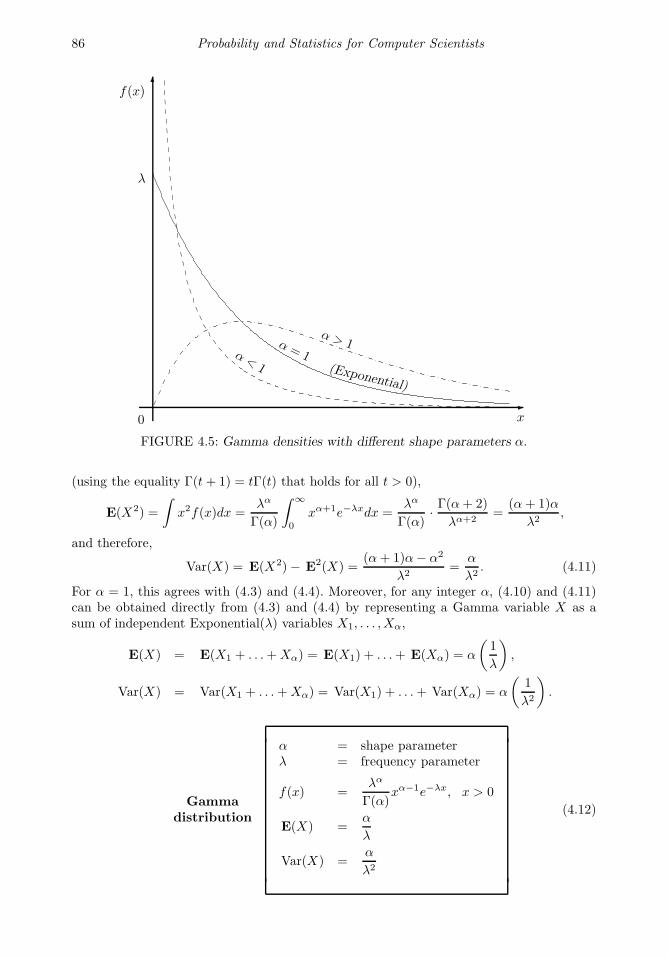
86 Probability and Statistics for Computer Scientists
0
λ
f(x)
x
α = 1(Exponential)
α > 1α <
1
FIGURE 4.5: Gamma densities with different shape parameters α.
(using the equality Γ(t+ 1) = tΓ(t) that holds for all t > 0),
E(X2) =
∫x2f(x)dx =
λα
Γ(α)
∫ ∞
0
xα+1e−λxdx =λα
Γ(α)· Γ(α+ 2)
λα+2=
(α+ 1)α
λ2,
and therefore,
Var(X) = E(X2)− E2(X) =(α+ 1)α− α2
λ2=
α
λ2. (4.11)
For α = 1, this agrees with (4.3) and (4.4). Moreover, for any integer α, (4.10) and (4.11)can be obtained directly from (4.3) and (4.4) by representing a Gamma variable X as asum of independent Exponential(λ) variables X1, . . . , Xα,
E(X) = E(X1 + . . .+Xα) = E(X1) + . . .+ E(Xα) = α
(1
λ
),
Var(X) = Var(X1 + . . .+Xα) = Var(X1) + . . .+ Var(Xα) = α
(1
λ2
).
Gammadistribution
α = shape parameterλ = frequency parameter
f(x) =λα
Γ(α)xα−1e−λx, x > 0
E(X) =α
λ
Var(X) =α
λ2
(4.12)

Continuous Distributions 87
Example 4.7 (Total compilation time). Compilation of a computer program consistsof 3 blocks that are processed sequentially, one after another. Each block takes Exponentialtime with the mean of 5 minutes, independently of other blocks.
(a) Compute the expectation and variance of the total compilation time.
(b) Compute the probability for the entire program to be compiled in less than 12 minutes.
Solution. The total time T is a sum of three independent Exponential times, therefore,it has Gamma distribution with α = 3. The frequency parameter λ equals (1/5) min−1
because the Exponential compilation time of each block has expectation 1/λ = 5 min.
(a) For a Gamma random variable T with α = 3 and λ = 1/5,
E(T ) =3
1/5= 15 (min) and Var(T ) =
3
(1/5)2= 75 (min 2).
(b) A direct solution involves two rounds of integration by parts,
P T < 12 =
∫ 12
0
f(t)dt =(1/5)3
Γ(3)
∫ 12
0
t2e−t/5dt
=(1/5)3
2!
(−5t2e−t/5
∣∣∣t=12
t=0+
∫ 12
0
10te−t/5dt
)
=1/125
2
(−5t2e−t/5 − 50te−t/5
∣∣∣t=12
t=0+
∫ 12
0
50e−t/5dt
)
=1
250
(−5t2e−t/5 − 50te−t/5 − 250e−t/5
)∣∣∣t=12
t=0
= 1− e−2.4 − 2.4e−2.4 − 2.88e−2.4 = 0.4303. (4.13)
A much shorter way is to apply the Gamma-Poisson formula below (Example 4.8). ♦
Gamma-Poisson formula
Computation of Gamma probabilities can be significantly simplified by thinking of a Gammavariable as the time between some rare events. In particular, one can avoid lengthy integra-tion by parts, as in Example 4.7, and use Poisson distribution instead.
Indeed, let T be a Gamma variable with an integer parameter α and some positive λ. Thisis a distribution of the time of the α-th rare event. Then, the event T > t means that theα-th rare event occurs after the moment t, and therefore, fewer than α rare events occurbefore the time t. We see that
T > t = X < α ,where X is the number of events that occur before the time t. This number of rare eventsX has Poisson distribution with parameter (λt); therefore, the probability
P T > t = P X < α
and the probability of a complement
P T ≤ t = P X ≥ α
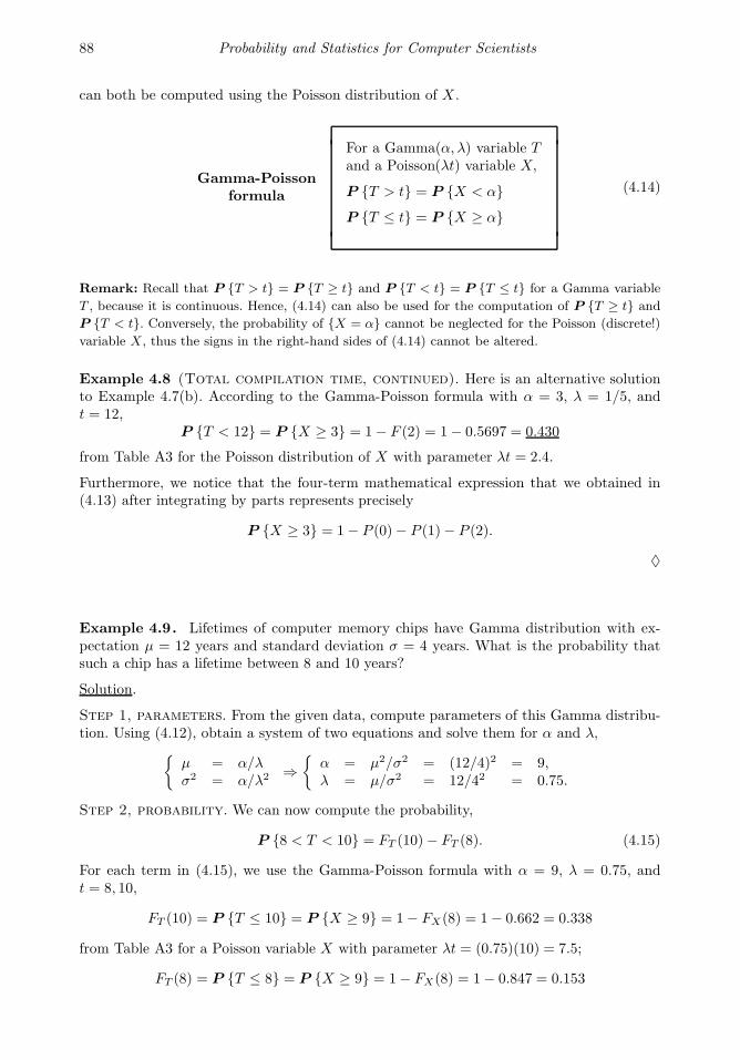
88 Probability and Statistics for Computer Scientists
can both be computed using the Poisson distribution of X .
Gamma-Poissonformula
For a Gamma(α, λ) variable Tand a Poisson(λt) variable X,
P T > t = P X < αP T ≤ t = P X ≥ α
(4.14)
Remark: Recall that P T > t = P T ≥ t and P T < t = P T ≤ t for a Gamma variable
T , because it is continuous. Hence, (4.14) can also be used for the computation of P T ≥ t and
P T < t. Conversely, the probability of X = α cannot be neglected for the Poisson (discrete!)
variable X, thus the signs in the right-hand sides of (4.14) cannot be altered.
Example 4.8 (Total compilation time, continued). Here is an alternative solutionto Example 4.7(b). According to the Gamma-Poisson formula with α = 3, λ = 1/5, andt = 12,
P T < 12 = P X ≥ 3 = 1− F (2) = 1− 0.5697 = 0.430
from Table A3 for the Poisson distribution of X with parameter λt = 2.4.
Furthermore, we notice that the four-term mathematical expression that we obtained in(4.13) after integrating by parts represents precisely
P X ≥ 3 = 1− P (0)− P (1)− P (2).
♦
Example 4.9. Lifetimes of computer memory chips have Gamma distribution with ex-pectation µ = 12 years and standard deviation σ = 4 years. What is the probability thatsuch a chip has a lifetime between 8 and 10 years?
Solution.
Step 1, parameters. From the given data, compute parameters of this Gamma distribu-tion. Using (4.12), obtain a system of two equations and solve them for α and λ,
µ = α/λσ2 = α/λ2 ⇒
α = µ2/σ2 = (12/4)2 = 9,λ = µ/σ2 = 12/42 = 0.75.
Step 2, probability. We can now compute the probability,
P 8 < T < 10 = FT (10)− FT (8). (4.15)
For each term in (4.15), we use the Gamma-Poisson formula with α = 9, λ = 0.75, andt = 8, 10,
FT (10) = P T ≤ 10 = P X ≥ 9 = 1− FX(8) = 1− 0.662 = 0.338
from Table A3 for a Poisson variable X with parameter λt = (0.75)(10) = 7.5;
FT (8) = P T ≤ 8 = P X ≥ 9 = 1− FX(8) = 1− 0.847 = 0.153
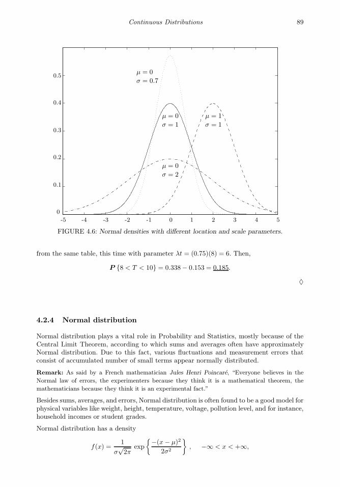
Continuous Distributions 89
µ = 0
σ = 1
µ = 1
σ = 1
µ = 0
σ = 0.7
µ = 0
σ = 2
0
0.1
0.2
0.3
0.4
0.5
-5 -4 -3 -2 -1 0 1 2 3 4 5
FIGURE 4.6: Normal densities with different location and scale parameters.
from the same table, this time with parameter λt = (0.75)(8) = 6. Then,
P 8 < T < 10 = 0.338− 0.153 = 0.185.
♦
4.2.4 Normal distribution
Normal distribution plays a vital role in Probability and Statistics, mostly because of theCentral Limit Theorem, according to which sums and averages often have approximatelyNormal distribution. Due to this fact, various fluctuations and measurement errors thatconsist of accumulated number of small terms appear normally distributed.
Remark: As said by a French mathematician Jules Henri Poincare, “Everyone believes in the
Normal law of errors, the experimenters because they think it is a mathematical theorem, the
mathematicians because they think it is an experimental fact.”
Besides sums, averages, and errors, Normal distribution is often found to be a good model forphysical variables like weight, height, temperature, voltage, pollution level, and for instance,household incomes or student grades.
Normal distribution has a density
f(x) =1
σ√2π
exp
−(x− µ)2
2σ2
, −∞ < x < +∞,
90 Probability and Statistics for Computer Scientists
where parameters µ and σ have a simple meaning of the expectation E(X) and the standarddeviation Std(X). This density is known as the bell-shaped curve, symmetric and centeredat µ, its spread being controlled by σ. As seen in Figure 4.6, changing µ shifts the curveto the left or to the right without affecting its shape, while changing σ makes it moreconcentrated or more flat. Often µ and σ are called location and scale parameters.
Normaldistribution
µ = expectation, location parameterσ = standard deviation, scale parameter
f(x) =1
σ√2π
exp
−(x− µ)2
2σ2
, −∞ < x < ∞
E(X) = µVar(X) = σ2
Standard Normal distribution
DEFINITION 4.3
Normal distribution with “standard parameters” µ = 0 and σ = 1 is calledStandard Normal distribution.
Notation Z = Standard Normal random variable
φ(x) =1√2π
e−x2/2, Standard Normal pdf
Φ(x) =
∫ x
−∞
1√2π
e−z2/2dz, Standard Normal cdf
A Standard Normal variable, usually denoted by Z, can be obtained from a non-standardNormal(µ, σ) random variable X by standardizing, that is, subtracting the mean and di-viding by the standard deviation,
Z =X − µ
σ. (4.16)
Unstandardizing Z, we can reconstruct the initial variable X ,
X = µ+ σ Z. (4.17)
Using these transformations, any Normal random variable can be obtained from a StandardNormal variable Z; therefore, we need a table of Standard Normal Distribution only (TableA4).
To find Φ(z) from Table A4, we locate a row with the first two digits of z and a column

Continuous Distributions 91
with the third digit of z and read the probability Φ(z) at their intersection. Notice thatΦ(z) ≈ 0 (is “practically” zero) for all z < −3.9, and Φ(z) ≈ 1 (is “practically” one) for allz > 3.9.
Example 4.10 (Computing Standard Normal probabilities). For a Standard Nor-mal random variable Z,
P Z < 1.35 = Φ(1.35) = 0.9115P Z > 1.35 = 1− Φ(1.35) = 0.0885
P −0.77 < Z < 1.35 = Φ(1.35)− Φ(−0.77) = 0.9115− 0.2206 = 0.6909.
according to Table A4. Notice that P Z < −1.35 = 0.0885 = P Z > 1.35, which isexplained by the symmetry of the Standard Normal density in Figure 4.6. Due to thissymmetry, “the left tail,” or the area to the left of (−1.35) equals “the right tail,” or thearea to the right of 1.35. ♦
In fact, the symmetry of the Normal density, mentioned in this example, allows to obtainthe first part of Table A4 on p. 417 directly from the second part,
Φ(−z) = 1− Φ(z) for −∞ < z < +∞.
To compute probabilities about an arbitrary Normal random variable X , we have to stan-dardize it first, as in (4.16), then use Table A4.
Example 4.11 (Computing non-standard Normal probabilities). Suppose thatthe average household income in some country is 900 coins, and the standard deviation is200 coins. Assuming the Normal distribution of incomes, compute the proportion of “themiddle class,” whose income is between 600 and 1200 coins.
Solution. Standardize and use Table A4. For a Normal(µ = 900, σ = 200) variable X ,
P 600 < X < 1200 = P
600− µ
σ<
X − µ
σ<
1200− µ
σ
= P
600− 900
200< Z <
1200− 900
200
= P −1.5 < Z < 1.5
= Φ(1.5)− Φ(−1.5) = 0.9332− 0.0668 = 0.8664.
♦
So far, we were computing probabilities of clearly defined events. These are direct problems.A number of applications require solution of an inverse problem, that is, finding a value ofx given the corresponding probability.
Example 4.12 (Inverse problem). The government of the country in Example 4.11decides to issue food stamps to the poorest 3% of households. Below what income willfamilies receive food stamps?
Solution. We need to find such income x that P X < x = 3% = 0.03. This is an equationthat can be solved in terms of x. Again, we standardize first, then use the table:
P X < x = P
Z <
x− µ
σ
= Φ
(x− µ
σ
)= 0.03,
92 Probability and Statistics for Computer Scientists
from wherex = µ+ σΦ−1(0.03).
In Table A4, we have to find the probability, the table entry of 0.03. We see that Φ(−1.88) ≈0.03. Therefore, Φ−1(0.03) = −1.88, and
x = µ+ σ(−1.88) = 900 + (200)(−1.88) = 524 (coins)
is the answer. In the literature, the value Φ−1(α) is often denoted by z1−α. ♦
As seen in this example, in order to solve an inverse problem, we use the table first, thenunstandardize, as in (4.17), and find the required value of x.
4.3 Central Limit Theorem
We now turn our attention to sums of random variables,
Sn = X1 + . . .+Xn,
that appear in many applications. Let µ = E(Xi) and σ = Std(Xi) for all i = 1, . . . , n.How does Sn behave for large n?
Matlab Demo. The following MATLAB code is a good illustration to the behavior ofpartial sums Sn.
S(1)=0;
for n=2:1000; S(n)=S(n-1)+randn; end; % nth partial sum
n=1:1000; comet(n,S); pause(3); % Behavior of S(n)comet(n,S./n); pause(3); % Behavior of S(n)/ncomet(n,S./sqrt(n)); pause(3); % Behavior of S(n)/
√n
Apparently (MATLAB users can see it from the obtained graphs), The pure sum Sn diverges. In fact, this should be anticipated because
Var(Sn) = nσ2 → ∞,
so that variability of Sn grows unboundedly as n goes to infinity. The average Sn/n converges. Indeed, in this case, we have
Var(Sn/n) = Var(Sn)/n2 = nσ2/n2 = σ2/n → 0,
so that variability of (Sn/n) vanishes as n → ∞. An interesting normalization factor is 1/√n. For µ = 0, we can see from MATLAB
simulations that Sn/√n neither diverges nor converges! It does not tend to leave 0,
but it does not converge to 0 either. Rather, it behaves like some random variable. Thefollowing theorem states that this variable has approximately Normal distribution forlarge n.
Continuous Distributions 93
Theorem 1 (Central Limit Theorem) Let X1, X2, . . . be independent random variableswith the same expectation µ = E(Xi) and the same standard deviation σ = Std(Xi), andlet
Sn =
n∑
i=1
Xi = X1 + . . .+Xn.
As n → ∞, the standardized sum
Zn =Sn − E(Sn)
Std(Sn)=
Sn − nµ
σ√n
converges in distribution to a Standard Normal random variable, that is,
FZn(z) = P
Sn − nµ
σ√n
≤ z
→ Φ(z) (4.18)
for all z.
This theorem is very powerful because it can be applied to random variables X1, X2, . . .having virtually any thinkable distribution with finite expectation and variance. As longas n is large (the rule of thumb is n > 30), one can use Normal distribution to computeprobabilities about Sn.
Theorem 1 is only one basic version of the Central Limit Theorem. Over the last twocenturies, it has been extended to large classes of dependent variables and vectors, stochasticprocesses, and so on.
Example 4.13 (Allocation of disk space). A disk has free space of 330 megabytes.Is it likely to be sufficient for 300 independent images, if each image has expected size of 1megabyte with a standard deviation of 0.5 megabytes?
Solution. We have n = 300, µ = 1, σ = 0.5. The number of images n is large, so the CentralLimit Theorem applies to their total size Sn. Then,
P sufficient space = P Sn ≤ 330 = P
Sn − nµ
σ√n
≤ 330− (300)(1)
0.5√300
≈ Φ(3.46) = 0.9997.
This probability is very high, hence, the available disk space is very likely to be sufficient.♦
In the special case of Normal variables X1, X2, . . ., the distribution of Sn is always Normal,and (4.18) becomes exact equality for arbitrary, even small n.
Example 4.14 (Elevator). You wait for an elevator, whose capacity is 2000 pounds.The elevator comes with ten adult passengers. Suppose your own weight is 150 lbs, andyou heard that human weights are normally distributed with the mean of 165 lbs and thestandard deviation of 20 lbs. Would you board this elevator or wait for the next one?
Solution. In other words, is overload likely? The probability of an overload equals
P S10 + 150 > 2000 = P
S10 − (10)(165)
20√10
>2000− 150− (10)(165)
20√10
= 1− Φ(3.16) = 0.0008.

94 Probability and Statistics for Computer Scientists
So, with probability 0.9992 it is safe to take this elevator. It is now for you to decide.♦
Among the random variables discussed in Chapters 3 and 4, at least three have a form ofSn:
Binomial variable = sum of independent Bernoulli variablesNegative Binomial variable = sum of independent Geometric variablesGamma variable = sum of independent Exponential variables
Hence, the Central Limit Theorem applies to all these distributions with sufficiently largen in the case of Binomial, k for Negative Binomial, and α for Gamma variables.
In fact, Abraham de Moivre (1667–1754) obtained the first version of the Central LimitTheorem as the approximation of Binomial distribution.
Normal approximation to Binomial distribution
Binomial variables represent a special case of Sn = X1+. . .+Xn, where allXi have Bernoullidistribution with some parameter p. We know from Section 3.4.5 that small p allows toapproximate Binomial distribution with Poisson, and large p allows such an approximationfor the number of failures. For the moderate values of p (say, 0.05 ≤ p ≤ 0.95) and for largen, we can use Theorem 1:
Binomial(n, p) ≈ Normal(µ = np, σ =
√np(1− p)
)(4.19)
Matlab Demo. To visualize how Binomial distribution gradually takes the shape of Normaldistribution when n → ∞, you may execute the following MATLAB code that graphsBinomial(n, p) pmf for increasing values of n.
for n=1:2:100; x=0:n;
p=gamma(n+1)./gamma(x+1)./gamma(n-x+1).*(0.3).x.*(0.7).(n-x);plot(x,p);
title(’Binomial probabilities for increasing values of n’);
pause(1); end;
Continuity correction
This correction is needed when we approximate a discrete distribution (Binomial in thiscase) by a continuous distribution (Normal). Recall that the probability P X = x maybe positive if X is discrete, whereas it is always 0 for continuous X . Thus, a direct use of(4.19) will always approximate this probability by 0. It is obviously a poor approximation.
This is resolved by introducing a continuity correction. Expand the interval by 0.5 units ineach direction, then use the Normal approximation. Notice that
PX(x) = P X = x = P x− 0.5 < X < x+ 0.5
Continuous Distributions 95
is true for a Binomial variable X ; therefore, the continuity correction does not change theevent and preserves its probability. It makes a difference for the Normal distribution, so everytime when we approximate some discrete distribution with some continuous distribution,we should be using a continuity correction. Now it is the probability of an interval insteadof one number, and it is not zero.
Example 4.15. A new computer virus attacks a folder consisting of 200 files. Each filegets damaged with probability 0.2 independently of other files. What is the probability thatfewer than 50 files get damaged?
Solution. The number X of damaged files has Binomial distribution with n = 200, p = 0.2,µ = np = 40, and σ =
√np(1− p) = 5.657. Applying the Central Limit Theorem with the
continuity correction,
P X < 50 = P X < 49.5 = P
X − 40
5.657<
49.5− 40
5.657
= Φ(1.68) = 0.9535.
Notice that the properly applied continuity correction replaces 50 with 49.5, not 50.5. In-deed, we are interested in the event that X is strictly less than 50. This includes all valuesup to 49 and corresponds to the interval [0, 49] that we expand to [0, 49.5]. In other words,events X < 50 and X < 49.5 are the same; they include the same possible values of X .Events X < 50 and X < 50.5 are different because the former includes X = 50, and thelatter does not. Replacing X < 50 with X < 50.5 would have changed its probabilityand would have given a wrong answer. ♦
When a continuous distribution (say, Gamma) is approximated by another continuous dis-tribution (Normal), the continuity correction is not needed. In fact, it would be an error touse it in this case because it would no longer preserve the probability.
Summary and conclusions
Continuous distributions are used to model various times, sizes, measurements, and all otherrandom variables that assume an entire interval of possible values.
Continuous distributions are described by their densities that play a role analogous toprobability mass functions of discrete variables. Computing probabilities essentially reducesto integrating a density over the given set. Expectations and variances are defined similarlyto the discrete case, replacing a probability mass function by a density and summation byintegration.
In different situations, one uses Uniform, Exponential, Gamma, or Normal distributions. Afew other families are studied in later chapters.
The Central Limit Theorem states that a standardized sum of a large number of indepen-dent random variables is approximately Normal, thus Table A4 can be used to computerelated probabilities. A continuity correction should be used when a discrete distribution isapproximated by a continuous distribution.
Characteristics of continuous families are summarized in Section 12.1.2.
96 Probability and Statistics for Computer Scientists
Exercises
4.1. The lifetime, in years, of some electronic component is a continuous random variable withthe density
f(x) =
k
x4for x ≥ 1
0 for x < 1.
Find k, the cumulative distribution function, and the probability for the lifetime to exceed2 years.
4.2. The time, in minutes, it takes to reboot a certain system is a continuous variable with thedensity
f(x) =
C(10− x)2, if 0 < x < 10
0, otherwise
(a) Compute C.
(b) Compute the probability that it takes between 1 and 2 minutes to reboot.
4.3. The installation time, in hours, for a certain software module has a probability densityfunction f(x) = k(1 − x3) for 0 < x < 1. Find k and compute the probability that it takesless than 1/2 hour to install this module.
4.4. Lifetime of a certain hardware is a continuous random variable with density
f(x) =
K− x/50 for 0 < x < 10 years
0 for all other x
(a) Find K.
(b) What is the probability of a failure within the first 5 years?
(c) What is the expectation of the lifetime?
4.5. Two continuous random variables X and Y have the joint density
f(x, y) = C(x2 + y), −1 ≤ x ≤ 1, 0 ≤ y ≤ 1.
(a) Compute the constant C.
(b) Find the marginal densities of X and Y . Are these two variables independent?
(c) Compute probabilities PY < 0.6 and PY < 0.6 | X < 0.5.
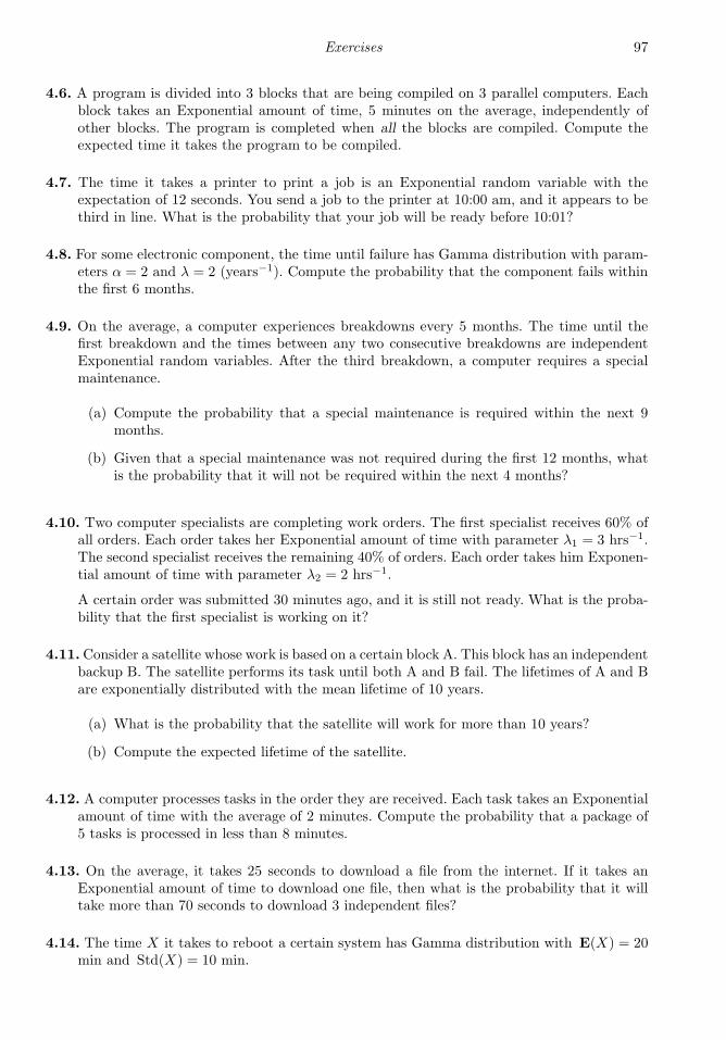
Exercises 97
4.6. A program is divided into 3 blocks that are being compiled on 3 parallel computers. Eachblock takes an Exponential amount of time, 5 minutes on the average, independently ofother blocks. The program is completed when all the blocks are compiled. Compute theexpected time it takes the program to be compiled.
4.7. The time it takes a printer to print a job is an Exponential random variable with theexpectation of 12 seconds. You send a job to the printer at 10:00 am, and it appears to bethird in line. What is the probability that your job will be ready before 10:01?
4.8. For some electronic component, the time until failure has Gamma distribution with param-eters α = 2 and λ = 2 (years−1). Compute the probability that the component fails withinthe first 6 months.
4.9. On the average, a computer experiences breakdowns every 5 months. The time until thefirst breakdown and the times between any two consecutive breakdowns are independentExponential random variables. After the third breakdown, a computer requires a specialmaintenance.
(a) Compute the probability that a special maintenance is required within the next 9months.
(b) Given that a special maintenance was not required during the first 12 months, whatis the probability that it will not be required within the next 4 months?
4.10. Two computer specialists are completing work orders. The first specialist receives 60% ofall orders. Each order takes her Exponential amount of time with parameter λ1 = 3 hrs−1.The second specialist receives the remaining 40% of orders. Each order takes him Exponen-tial amount of time with parameter λ2 = 2 hrs−1.
A certain order was submitted 30 minutes ago, and it is still not ready. What is the proba-bility that the first specialist is working on it?
4.11.Consider a satellite whose work is based on a certain block A. This block has an independentbackup B. The satellite performs its task until both A and B fail. The lifetimes of A and Bare exponentially distributed with the mean lifetime of 10 years.
(a) What is the probability that the satellite will work for more than 10 years?
(b) Compute the expected lifetime of the satellite.
4.12. A computer processes tasks in the order they are received. Each task takes an Exponentialamount of time with the average of 2 minutes. Compute the probability that a package of5 tasks is processed in less than 8 minutes.
4.13. On the average, it takes 25 seconds to download a file from the internet. If it takes anExponential amount of time to download one file, then what is the probability that it willtake more than 70 seconds to download 3 independent files?
4.14. The time X it takes to reboot a certain system has Gamma distribution with E(X) = 20min and Std(X) = 10 min.
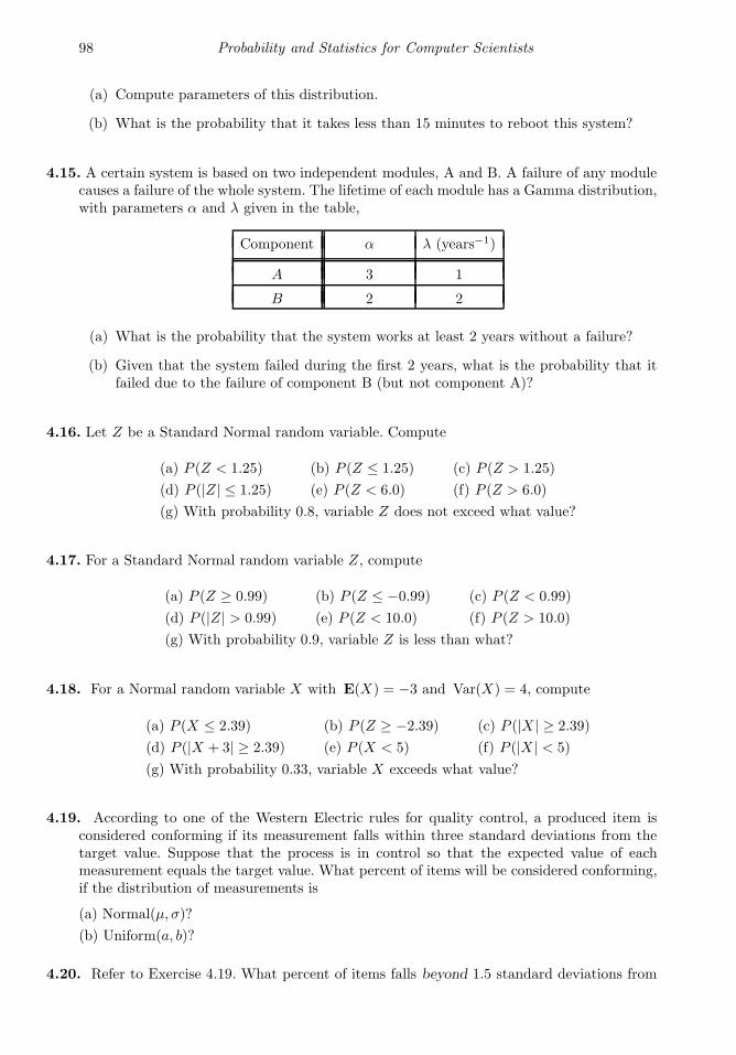
98 Probability and Statistics for Computer Scientists
(a) Compute parameters of this distribution.
(b) What is the probability that it takes less than 15 minutes to reboot this system?
4.15. A certain system is based on two independent modules, A and B. A failure of any modulecauses a failure of the whole system. The lifetime of each module has a Gamma distribution,with parameters α and λ given in the table,
Component α λ (years−1)
A 3 1
B 2 2
(a) What is the probability that the system works at least 2 years without a failure?
(b) Given that the system failed during the first 2 years, what is the probability that itfailed due to the failure of component B (but not component A)?
4.16. Let Z be a Standard Normal random variable. Compute
(a) P (Z < 1.25) (b) P (Z ≤ 1.25) (c) P (Z > 1.25)
(d) P (|Z| ≤ 1.25) (e) P (Z < 6.0) (f) P (Z > 6.0)
(g) With probability 0.8, variable Z does not exceed what value?
4.17. For a Standard Normal random variable Z, compute
(a) P (Z ≥ 0.99) (b) P (Z ≤ −0.99) (c) P (Z < 0.99)
(d) P (|Z| > 0.99) (e) P (Z < 10.0) (f) P (Z > 10.0)
(g) With probability 0.9, variable Z is less than what?
4.18. For a Normal random variable X with E(X) = −3 and Var(X) = 4, compute
(a) P (X ≤ 2.39) (b) P (Z ≥ −2.39) (c) P (|X | ≥ 2.39)
(d) P (|X + 3| ≥ 2.39) (e) P (X < 5) (f) P (|X | < 5)
(g) With probability 0.33, variable X exceeds what value?
4.19. According to one of the Western Electric rules for quality control, a produced item isconsidered conforming if its measurement falls within three standard deviations from thetarget value. Suppose that the process is in control so that the expected value of eachmeasurement equals the target value. What percent of items will be considered conforming,if the distribution of measurements is
(a) Normal(µ, σ)?
(b) Uniform(a, b)?
4.20. Refer to Exercise 4.19. What percent of items falls beyond 1.5 standard deviations from
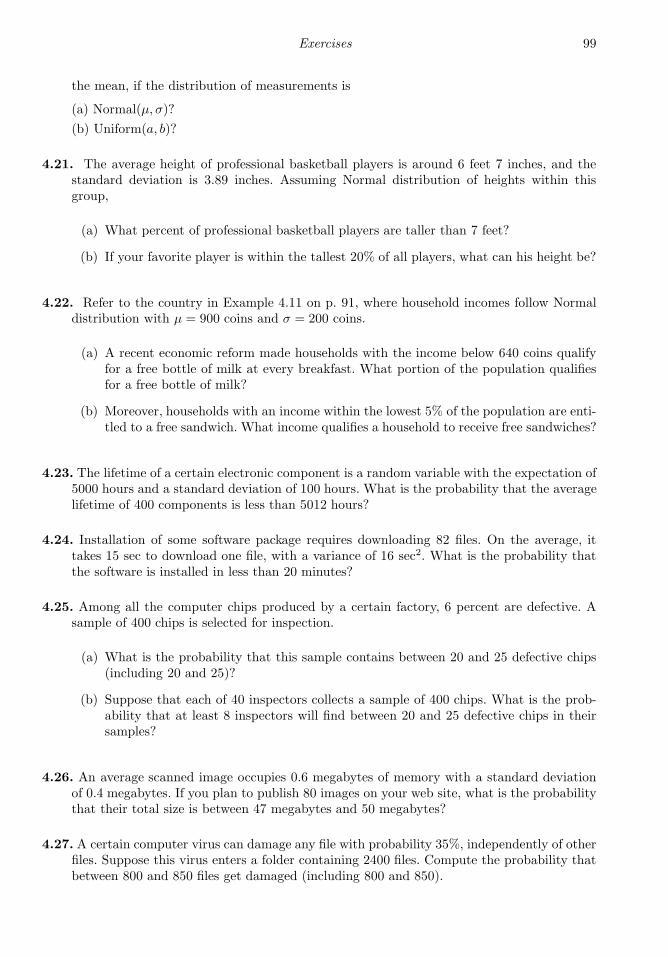
Exercises 99
the mean, if the distribution of measurements is
(a) Normal(µ, σ)?
(b) Uniform(a, b)?
4.21. The average height of professional basketball players is around 6 feet 7 inches, and thestandard deviation is 3.89 inches. Assuming Normal distribution of heights within thisgroup,
(a) What percent of professional basketball players are taller than 7 feet?
(b) If your favorite player is within the tallest 20% of all players, what can his height be?
4.22. Refer to the country in Example 4.11 on p. 91, where household incomes follow Normaldistribution with µ = 900 coins and σ = 200 coins.
(a) A recent economic reform made households with the income below 640 coins qualifyfor a free bottle of milk at every breakfast. What portion of the population qualifiesfor a free bottle of milk?
(b) Moreover, households with an income within the lowest 5% of the population are enti-tled to a free sandwich. What income qualifies a household to receive free sandwiches?
4.23. The lifetime of a certain electronic component is a random variable with the expectation of5000 hours and a standard deviation of 100 hours. What is the probability that the averagelifetime of 400 components is less than 5012 hours?
4.24. Installation of some software package requires downloading 82 files. On the average, ittakes 15 sec to download one file, with a variance of 16 sec2. What is the probability thatthe software is installed in less than 20 minutes?
4.25. Among all the computer chips produced by a certain factory, 6 percent are defective. Asample of 400 chips is selected for inspection.
(a) What is the probability that this sample contains between 20 and 25 defective chips(including 20 and 25)?
(b) Suppose that each of 40 inspectors collects a sample of 400 chips. What is the prob-ability that at least 8 inspectors will find between 20 and 25 defective chips in theirsamples?
4.26. An average scanned image occupies 0.6 megabytes of memory with a standard deviationof 0.4 megabytes. If you plan to publish 80 images on your web site, what is the probabilitythat their total size is between 47 megabytes and 50 megabytes?
4.27. A certain computer virus can damage any file with probability 35%, independently of otherfiles. Suppose this virus enters a folder containing 2400 files. Compute the probability thatbetween 800 and 850 files get damaged (including 800 and 850).

100 Probability and Statistics for Computer Scientists
4.28. Seventy independent messages are sent from an electronic transmission center. Messages areprocessed sequentially, one after another. Transmission time of each message is Exponentialwith parameter λ = 5 min−1. Find the probability that all 70 messages are transmitted inless than 12 minutes. Use the Central Limit Theorem.
4.29. A computer lab has two printers. Printer I handles 40% of all the jobs. Its printing time isExponential with the mean of 2 minutes. Printer II handles the remaining 60% of jobs. Itsprinting time is Uniform between 0 minutes and 5 minutes. A job was printed in less than1 minute. What is the probability that it was printed by Printer I?
4.30. An internet service provider has two connection lines for its customers. Eighty percent ofcustomers are connected through Line I, and twenty percent are connected through Line II.Line I has a Gamma connection time with parameters α = 3 and λ = 2 min−1. Line II hasa Uniform(a, b) connection time with parameters a = 20 sec and b = 50 sec. Compute theprobability that it takes a randomly selected customer more than 30 seconds to connect tothe internet.
4.31. Upgrading a certain software package requires installation of 68 new files. Files are installedconsecutively. The installation time is random, but on the average, it takes 15 sec to installone file, with a variance of 11 sec2.
(a) What is the probability that the whole package is upgraded in less than 12 minutes?
(b) A new version of the package is released. It requires only N new files to be installed,and it is promised that 95% of the time upgrading takes less than 10 minutes. Giventhis information, compute N .
4.32. Two independent customers are scheduled to arrive in the afternoon. Their arrival timesare uniformly distributed between 2 pm and 8 pm. Compute
(a) the expected time of the first (earlier) arrival;
(b) the expected time of the last (later) arrival.
4.33. Let X and Y be independent Standard Uniform random variables.
(a) Find the probability of an event 0.5 < (X + Y ) < 1.5.
(b) Find the conditional probability P 0.3 < X < 0.7 | Y > 0.5.
This problem can be solved analytically as well as geometrically.
4.34. Prove the memoryless property of Geometric distribution. That is, if X has Geometricdistribution with parameter p, show that
P X > x+ y | X > y = P X > x
for any integer x, y ≥ 0.
Chapter 5
Computer Simulations and Monte Carlo
Methods
5.1 Introduction . . . . . . . . . . . . . . . . . . . . . . . . . . . . . . . . . . . . . . . . . . . . . . . . . . . . . . 1015.1.1 Applications and examples . . . . . . . . . . . . . . . . . . . . . . . . . . . . . . 102
5.2 Simulation of random variables . . . . . . . . . . . . . . . . . . . . . . . . . . . . . . . . . . 1035.2.1 Random number generators . . . . . . . . . . . . . . . . . . . . . . . . . . . . . 1045.2.2 Discrete methods . . . . . . . . . . . . . . . . . . . . . . . . . . . . . . . . . . . . . . . . 1055.2.3 Inverse transform method . . . . . . . . . . . . . . . . . . . . . . . . . . . . . . . 1085.2.4 Rejection method . . . . . . . . . . . . . . . . . . . . . . . . . . . . . . . . . . . . . . . . 1105.2.5 Generation of random vectors . . . . . . . . . . . . . . . . . . . . . . . . . . . 1135.2.6 Special methods . . . . . . . . . . . . . . . . . . . . . . . . . . . . . . . . . . . . . . . . . 113
5.3 Solving problems by Monte Carlo methods . . . . . . . . . . . . . . . . . . . . . . 1145.3.1 Estimating probabilities . . . . . . . . . . . . . . . . . . . . . . . . . . . . . . . . . 1145.3.2 Estimating means and standard deviations . . . . . . . . . . . . . 1185.3.3 Forecasting . . . . . . . . . . . . . . . . . . . . . . . . . . . . . . . . . . . . . . . . . . . . . . . 1195.3.4 Estimating lengths, areas, and volumes . . . . . . . . . . . . . . . . . 1205.3.5 Monte Carlo integration . . . . . . . . . . . . . . . . . . . . . . . . . . . . . . . . . 122
Summary and conclusions . . . . . . . . . . . . . . . . . . . . . . . . . . . . . . . . . . . . . . . . . . 124Exercises . . . . . . . . . . . . . . . . . . . . . . . . . . . . . . . . . . . . . . . . . . . . . . . . . . . . . . . . . . . . 125
5.1 Introduction
Computer simulations refer to a regeneration of a process by writing a suitable computerprogram and observing its results. Monte Carlo methods are those based on computersimulations involving random numbers.
The main purpose of simulations is estimating such quantities whose direct computation iscomplicated, risky, consuming, expensive, or impossible. For example, suppose a complexdevice or machine is to be built and launched. Before it happens, its performance is sim-ulated, and this allows experts to evaluate its adequacy and associated risks carefully andsafely. For example, one surely prefers to evaluate reliability and safety of a new module ofa space station by means of computer simulations rather than during the actual mission.
Monte Carlo methods are mostly used for the computation of probabilities, expected values,and other distribution characteristics. Recall that probability can be defined as a long-runproportion. With the help of random number generators, computers can actually simulatea long run. Then, probability can be estimated by a mere computation of the associatedobserved frequency. The longer run is simulated, the more accurate result is obtained.Similarly, one can estimate expectations, variances, and other distribution characteristicsfrom a long run of simulated random variables.
101
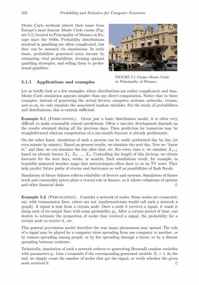
102 Probability and Statistics for Computer Scientists
Monte Carlo methods inherit their name fromEurope’s most famous Monte Carlo casino (Fig-ure 5.1) located in Principality of Monaco in Eu-rope since the 1850s. Probability distributionsinvolved in gambling are often complicated, butthey can be assessed via simulations. In earlytimes, probabilists generated extra income byestimating vital probabilities, devising optimalgambling strategies, and selling them to profes-sional gamblers.
FIGURE 5.1 Casino Monte Carloin Principality of Monaco.5.1.1 Applications and examples
Let us briefly look at a few examples, where distributions are rather complicated, and thus,Monte Carlo simulation appears simpler than any direct computation. Notice that in theseexamples, instead of generating the actual devices, computer systems, networks, viruses,and so on, we only simulate the associated random variables. For the study of probabilitiesand distributions, this is entirely sufficient.
Example 5.1 (Forecasting). Given just a basic distribution model, it is often verydifficult to make reasonably remote predictions. Often a one-day development depends onthe results obtained during all the previous days. Then prediction for tomorrow may bestraightforward whereas computation of a one-month forecast is already problematic.
On the other hand, simulation of such a process can be easily performed day by day (oreven minute by minute). Based on present results, we simulate the next day. Now we “knowit,” and thus, we can simulate the day after that, etc. For every time n, we simulate Xn+1
based on already known X1, X2, ..., Xn. Controlling the length of this do-loop, we obtainforecasts for the next days, weeks, or months. Such simulations result, for example, inbeautiful animated weather maps that meteorologists often show to us on TV news. Theyhelp predict future paths of storms and hurricanes as well as possibilities of flash floods.
Simulation of future failures reflects reliability of devices and systems. Simulation of futurestock and commodity prices plays a crucial role in finance, as it allows valuations of optionsand other financial deals. ♦
Example 5.2 (Percolation). Consider a network of nodes. Some nodes are connected,say, with transmission lines, others are not (mathematicians would call such a network agraph). A signal is sent from a certain node. Once a node k receives a signal, it sends italong each of its output lines with some probability pk. After a certain period of time, onedesires to estimate the proportion of nodes that received a signal, the probability for acertain node to receive it, etc.
This general percolation model describes the way many phenomena may spread. The roleof a signal may be played by a computer virus spreading from one computer to another, orby rumors spreading among people, or by fire spreading through a forest, or by a diseasespreading between residents.
Technically, simulation of such a network reduces to generating Bernoulli random variableswith parameters pi. Line i transmits if the corresponding generated variable Xi = 1. In theend, we simply count the number of nodes that got the signal, or verify whether the givennode received it. ♦

Computer Simulations and Monte Carlo Methods 103
Example 5.3 (Queuing). A queuing system is described by a number of random vari-ables. It involves spontaneous arrivals of jobs, their random waiting time, assignment toservers, and finally, their random service time and departure. In addition, some jobs mayexit prematurely, others may not enter the system if it appears full, and also, intensity ofthe incoming traffic and the number of servers on duty may change during the day.
When designing a queuing system or a server facility, it is important to evaluate its vitalperformance characteristics. This will include the job’s average waiting time, the averagelength of a queue, the proportion of customers who had to wait, the proportion of “unsat-isfied customers” (that exit prematurely or cannot enter), the proportion of jobs spending,say, more than one hour in the system, the expected usage of each server, the average num-ber of available (idle) servers at the time when a job arrives, and so on. Queuing systemsare discussed in detail in Chapter 7; methods of their simulation are in Section 7.6. ♦
Example 5.4 (Markov chain Monte Carlo). There is a modern technique of gen-erating random variables from rather complex, often intractable distributions, as long asconditional distributions have a reasonably simple form. In semiconductor industry, for ex-ample, the joint distribution of good and defective chips on a produced wafer has a rathercomplicated correlation structure. As a result, it can only be written explicitly for rathersimplified artificial models. On the other hand, the quality of each chip is predictable basedon the quality of the surrounding, neighboring chips. Given its neighborhood, conditionalprobability for a chip to fail can be written, and thus, its quality can be simulated by gen-erating a corresponding Bernoulli random variable with Xi = 1 indicating a failure.
According to the Markov chain Monte Carlo (MCMC) methodology, a long sequence of ran-dom variables is generated from conditional distributions. A wisely designed MCMC willthen produce random variables that have the desired unconditional distribution, no matterhow complex it is. ♦
In all the examples, we saw how different types of phenomena can be computer-simulated.However, one simulation is not enough for estimating probabilities and expectations. Afterwe understand how to program the given phenomenon once, we can embed it in a do-loopand repeat similar simulations a large number of times, generating a long run. Since thesimulated variables are random, we will generally obtain a number of different realizations,from which we calculate probabilities and expectations as long-run frequencies and averages.
5.2 Simulation of random variables
As we see, implementation of Monte Carlo methods reduces to generation of random vari-ables from given distributions. Hence, it remains to design algorithms for generating randomvariables and vectors that will have the desired distributions.
Statistics software packages like SAS, R, Splus, SPSS, Minitab, and others have built-inprocedures for the generation of random variables from the most common discrete and
104 Probability and Statistics for Computer Scientists
continuous distributions. Similar tools are found in recent versions of MATLAB, MicrosoftExcel, and some libraries.
Majority of computer languages have a random number generator that returns only Uni-formly distributed independent random variables. This section discusses general methods oftransforming Uniform random variables, obtained by a standard random number generator,into variables with desired distributions.
5.2.1 Random number generators
Obtaining a good random variable is not a simple task. How do we know that it is “trulyrandom” and does not have any undesired patterns? For example, quality random numbergeneration is so important in coding and password creation that people design special teststo verify the “randomness” of generated numbers.
In the fields sensitive to good random numbers, their generation is typically related to anaccurate measurement of some physical variable, for example, the computer time or noise.Certain transformations of this variable will generally give the desired result.
More often than not, a pseudo-random number generator is utilized. This is nothing but avery long list of numbers. A user specifies a random number seed that points to the locationfrom which this list will be read. It should be noted that if the same computer code isexecuted with the same seed, then the same random numbers get generated, leading toidentical results. Often each seed is generated within the system, which of course improvesthe quality of random numbers.
Instead of a computer, a table of random numbers is often used for small-size studies.For example, we can use Table A1 in Appendix.
Can a table adequately replace a computer random number generator? There are at leasttwo issues that one should be aware of.
1. Generating a random number seed. A rule of thumb suggests to close your eyes andput your finger “somewhere” on the table. Start reading random numbers from thispoint, either horizontally, or vertically, or even diagonally, etc. Either way, this methodis not pattern-free, and it does not guarantee “perfect” randomness.
2. Using the same table more than once. Most likely, we cannot find a new table ofrandom numbers for each Monte Carlo study. As soon as we use the same tableagain, we may no longer consider our results independent of each other. Should we beconcerned about it? It depends on the situation. For totally unrelated projects, thisshould not be a problem.
One way or another, a random number generator or a table of random numbers delivers tous Uniform random variables U1, U2, . . . ∈ (0, 1). The next three subsections show how totransform them into a random variable (vector) X with the given desired distribution F (x).
Notation U ; U1, U2, . . . =generated Uniform(0,1)
random variables
Computer Simulations and Monte Carlo Methods 105
5.2.2 Discrete methods
At this point, we have obtained one or several independent Uniform(0,1) random variablesby means of a random number generator or a table of random numbers. Variables fromcertain simple distributions can be immediately generated from this.
Example 5.5 (Bernoulli). First, simulate a Bernoulli trial with probability of successp. For a Standard Uniform variable U , define
X =
1 if U < p0 if U ≥ p
We call it “a success” if X = 1 and “a failure” if X = 0. Using the Uniform distribution ofU , we find that
P success = P U < p = p.
Thus, we have generated a Bernoulli trial, and X has Bernoulli distribution with the desiredprobability p, see Figure 5.2a.
A MATLAB code for this scheme is
U = rand;
X = (U < p)
The value of p should be specified prior to this program. ♦
Example 5.6 (Binomial). Once we know how to generate Bernoulli variables, we canobtain a Binomial variable as a sum of n independent Bernoulli. For this purpose, we startwith n Uniform random numbers, for example:
n = 20; p = 0.68;
U = rand(n,1);
X = sum(U < p)♦
Example 5.7 (Geometric). A while-loop of Bernoulli trials will generate a Geometricrandom variable, literally according to its definition on p. 60. We run the loop of trials untilthe first success occurs. Variable X counts the number of failures:
X = 1; % Need at least one trial
while rand > p; % Continue while there are failures
X = X+1;
end; % Stop at the first success
X
The percentage sign (%) is used to separate MATLAB statements from comments. ♦
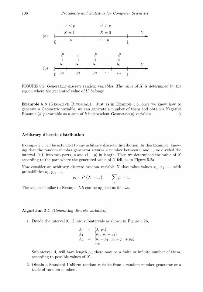
106 Probability and Statistics for Computer Scientists
(a)
(b)
U
U
p
U < p
X = 1
1− p
U > p
X = 0
0 1
p0
X=
x0
p1
X=
x1
p2
X=
x2
· · ·· · ·
pn
X=
xn
0 1
FIGURE 5.2: Generating discrete random variables. The value of X is determined by theregion where the generated value of U belongs.
Example 5.8 (Negative Binomial). Just as in Example 5.6, once we know how togenerate a Geometric variable, we can generate a number of them and obtain a NegativeBinomial(k, p) variable as a sum of k independent Geometric(p) variables. ♦
Arbitrary discrete distribution
Example 5.5 can be extended to any arbitrary discrete distribution. In this Example, know-ing that the random number generator returns a number between 0 and 1, we divided theinterval [0, 1] into two parts, p and (1 − p) in length. Then we determined the value of Xaccording to the part where the generated value of U fell, as in Figure 5.2a.
Now consider an arbitrary discrete random variable X that takes values x0, x1, . . . withprobabilities p0, p1, . . .,
pi = P X = xi ,∑
i
pi = 1.
The scheme similar to Example 5.5 can be applied as follows.
Algorithm 5.1 (Generating discrete variables)
1. Divide the interval [0, 1] into subintervals as shown in Figure 5.2b,
A0 = [0, p0)A1 = [p0, p0 + p1)A2 = [p0 + p1, p0 + p1 + p2)
etc.
Subinterval Ai will have length pi; there may be a finite or infinite number of them,according to possible values of X .
2. Obtain a Standard Uniform random variable from a random number generator or atable of random numbers.

Computer Simulations and Monte Carlo Methods 107
3. If U belongs to Ai, let X = xi.
From the Uniform distribution, it follows again that
P X = xi = P U ∈ Ai = pi.
Hence, the generated variable X has the desired distribution.
Notice that contrary to Examples 5.6 and 5.8, this algorithm is economic as it requires onlyone Uniform random number for each generated variable.
Values xi can be written in any order, but they have to correspond to their probabilities pi.
Example 5.9 (Poisson). Let us use Algorithm 5.1 to generate a Poisson variable withparameter λ = 5.
Recall from Section 3.4.5 that a Poisson variable takes values x0 = 0, x1 = 1, x2 = 2, ...with probabilities
pi = P X = xi = e−λλi
i!for i = 0, 1, 2, . . .
Following the algorithm, we generate a Uniform random number U and find the set Ai
containing U , so that
p0 + . . .+ pi−1 ≤ U < p0 + . . .+ pi−1 + pi,
or, in terms of the cumulative distribution function,
F (i− 1) ≤ U < F (i).
This can be done in MATLAB by means of a while-loop:
lambda = 5; % Parameter
U = rand; % Generated Uniform variable
i = 0; % Initial value
F = exp(-lambda); % Initial value, F(0)
while (U >= F); % The loop ends when U < F(i)
F = F + exp(-lambda) ∗ lambdaˆi/gamma(i+1);
i = i + 1;
end;
X=i♦
Remark: Statistical toolbox of MATLAB has built-in tools for generating random variables from
certain given distributions. Generating Binomial, Geometric, Poisson, and some other variables
can be done in one line random(name,parameters), where “name” indicates the desired family
of distributions, or by commands binornd, poissrnd, etc., listed in our distribution inventory in
Section 12.1. This chapter discusses general methods of generating random variables from arbitrary
distributions. The codes given here are general too – they can be used as flow-charts and be directly
translated into other languages.
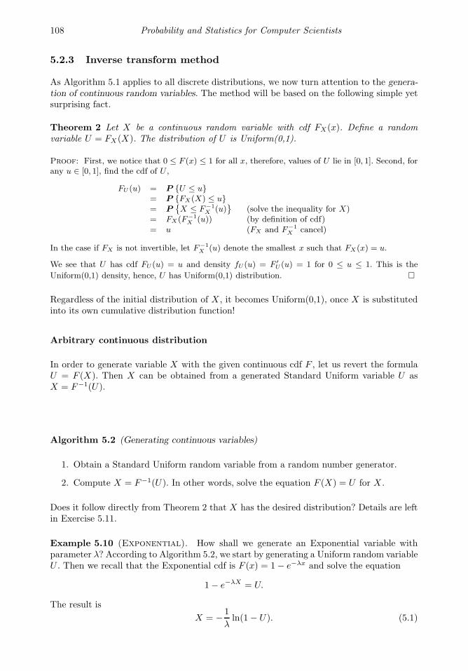
108 Probability and Statistics for Computer Scientists
5.2.3 Inverse transform method
As Algorithm 5.1 applies to all discrete distributions, we now turn attention to the genera-tion of continuous random variables. The method will be based on the following simple yetsurprising fact.
Theorem 2 Let X be a continuous random variable with cdf FX(x). Define a randomvariable U = FX(X). The distribution of U is Uniform(0,1).
Proof: First, we notice that 0 ≤ F (x) ≤ 1 for all x, therefore, values of U lie in [0, 1]. Second, forany u ∈ [0, 1], find the cdf of U ,
FU (u) = P U ≤ u= P FX(X) ≤ u= P
X ≤ F−1
X (u)
(solve the inequality for X)= FX(F−1
X (u)) (by definition of cdf)= u (FX and F−1
X cancel)
In the case if FX is not invertible, let F−1X (u) denote the smallest x such that FX(x) = u.
We see that U has cdf FU (u) = u and density fU (u) = F ′U (u) = 1 for 0 ≤ u ≤ 1. This is the
Uniform(0,1) density, hence, U has Uniform(0,1) distribution.
Regardless of the initial distribution of X , it becomes Uniform(0,1), once X is substitutedinto its own cumulative distribution function!
Arbitrary continuous distribution
In order to generate variable X with the given continuous cdf F , let us revert the formulaU = F (X). Then X can be obtained from a generated Standard Uniform variable U asX = F−1(U).
Algorithm 5.2 (Generating continuous variables)
1. Obtain a Standard Uniform random variable from a random number generator.
2. Compute X = F−1(U). In other words, solve the equation F (X) = U for X .
Does it follow directly from Theorem 2 that X has the desired distribution? Details are leftin Exercise 5.11.
Example 5.10 (Exponential). How shall we generate an Exponential variable withparameter λ? According to Algorithm 5.2, we start by generating a Uniform random variableU . Then we recall that the Exponential cdf is F (x) = 1− e−λx and solve the equation
1− e−λX = U.
The result is
X = − 1
λln(1− U). (5.1)

Computer Simulations and Monte Carlo Methods 109
Can this formula be simplified? By any rule of algebra, the answer is “no.” On the otherhand, (1−U) has the same distribution as U , Standard Uniform. Therefore, we can replaceU by (1− U), and variable
X1 = − 1
λln(U), (5.2)
although different from X , will also have the desired Exponential(λ) distribution.
Let us check if our generated variables, X and X1, have a suitable range of values. We knowthat 0 < U < 1 with probability 1, hence ln(U) and ln(1−U) are negative numbers, so thatboth X and X1 are positive, as Exponential variables should be. Just a check. ♦
Example 5.11 (Gamma). Gamma cdf has a complicated integral form (4.8), not men-tioning F−1, needed for Algorithm 5.2. There are numerical methods of solving the equationF (X) = U , but alternatively, much simpler, for any integer α, a Gamma variable can begenerated as a sum of α independent Exponential variables:
X = sum( -1/lambda * log(rand(alpha,1)) )
♦
Discrete distributions revisited
Algorithm 5.2 is not directly applicable to discrete distributions because the inverse functionF−1 does not exist in the discrete case. In other words, the key equation F (X) = U mayhave either infinitely many roots or no roots at all (see Figure 3.1 on p. 42).
Moreover, a discrete variableX has a finite or countable range of possible values, and so doesF (X). The probability that U coincidentally equals one of these values is 0. We concludethat the equation F (X) = U has no roots with probability 1.
Let us modify the scheme in order to accommodate discrete variables. Instead of solvingF (x) = U exactly, which is impossible, we solve it approximately by finding x, the smallestpossible value of X such that F (x) > U .
The resulting algorithm is described below.
Algorithm 5.3 (Generating discrete variables, revisited)
1. Obtain a Standard Uniform random variable from a random number generator or atable of random numbers.
2. Compute X = min x ∈ S such that F (x) > U, where S is a set of possible values ofX .
Algorithms 5.1 and 5.3 are equivalent if values xi are arranged in their increasing order inAlgorithm 5.1. Details are left in Exercise 5.12.

110 Probability and Statistics for Computer Scientists
Example 5.12 (Geometric revisited). Applying Algorithm 5.3 to Geometric cdf
F (x) = 1− (1− p)x,
we need to find the smallest integer x satisfying the inequality (solve it for x)
1− (1− p)x > U, (1− p)x < 1− U, x ln(1− p) < ln(1 − U),
x >ln(1 − U)
ln(1− p)(changing the sign because ln(1− p) < 0)
The smallest such integer is the ceiling1 of ln(1 − U)/ ln(1 − p), so that
X =
⌈ln(1 − U)
ln(1 − p)
⌉. (5.3)
♦
Exponential-Geometric relation
The formula (5.3) appears very similar to (5.1). With λ = − ln(1 − p), our generatedGeometric variable is just the ceiling of an Exponential variable! In other words, the ceilingof an Exponential variable has Geometric distribution.
This is not a coincidence. In a sense, Exponential distribution is a continuous analogue ofa Geometric distribution. Recall that an Exponential variable describes the time until thenext “rare event” whereas a Geometric variable is the time (the number of Bernoulli trials)until the next success. Also, both distributions have a memoryless property distinguishingthem from other distributions (see (4.6) and Exercise 4.34).
5.2.4 Rejection method
Besides a good computer, one thing is needed to generate continuous variables using theinverse transform method of Section 5.2.3. It is a reasonably simple form of the cdf F (x)that allows direct computation of X = F−1(U).
When F (x) has a complicated form but a density f(x) is available, random variables withthis density can be generated by rejection method.
Consider a point (X,Y ) chosen at random from under the graph of density f(x), as shownin Figure 5.3. What is the distribution of X , its first coordinate?
Theorem 3 Let a pair (X,Y ) have Uniform distribution over the region
A = (x, y) | 0 ≤ y ≤ f(x)
for some density function f . Then f is the density of X.
1Remark: Ceiling function ⌈x⌉ is defined as the smallest integer that is no less than x.
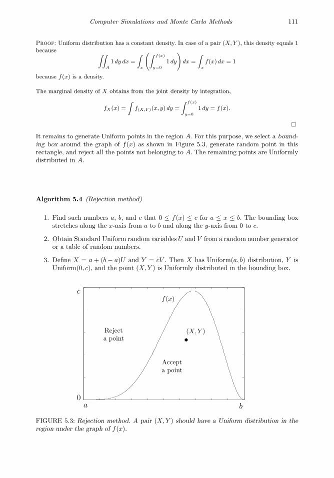
Computer Simulations and Monte Carlo Methods 111
Proof: Uniform distribution has a constant density. In case of a pair (X,Y ), this density equals 1because ∫∫
A
1 dy dx =
∫
x
(∫ f(x)
y=0
1 dy
)
dx =
∫
x
f(x) dx = 1
because f(x) is a density.
The marginal density of X obtains from the joint density by integration,
fX(x) =
∫f(X,Y )(x, y) dy =
∫ f(x)
y=0
1 dy = f(x).
It remains to generate Uniform points in the region A. For this purpose, we select a bound-ing box around the graph of f(x) as shown in Figure 5.3, generate random point in thisrectangle, and reject all the points not belonging to A. The remaining points are Uniformlydistributed in A.
Algorithm 5.4 (Rejection method)
1. Find such numbers a, b, and c that 0 ≤ f(x) ≤ c for a ≤ x ≤ b. The bounding boxstretches along the x-axis from a to b and along the y-axis from 0 to c.
2. Obtain Standard Uniform random variables U and V from a random number generatoror a table of random numbers.
3. Define X = a + (b − a)U and Y = cV . Then X has Uniform(a, b) distribution, Y isUniform(0, c), and the point (X,Y ) is Uniformly distributed in the bounding box.
f(x)
Rejecta point
Accepta point
(X,Y )
a b0
c
FIGURE 5.3: Rejection method. A pair (X,Y ) should have a Uniform distribution in theregion under the graph of f(x).

112 Probability and Statistics for Computer Scientists
0 10
200
400
600
800
FIGURE 5.4: A histogram of Beta random variables generated by rejection method. Com-pare with Figure 5.3.
4. If Y > f(X), reject the point and return to step 2. If Y ≤ f(X), then X is the desiredrandom variable having the density f(x).
Example 5.13 (Rejection method for Beta distribution). Beta distribution hasdensity
f(x) =Γ(α+ β)
Γ(α)Γ(β)xα−1(1− x)β−1 for 0 ≤ x ≤ 1.
For α = 5.5 and β = 3.1, this density is graphed in Figure 5.3. It never exceeds 2.5,therefore we choose the bounding box with a = 0, b = 1, and c = 2.5. MATLAB commandsfor generating a Beta(α, β) random variable by the rejection method are:
alpha=5.5; beta=3.1; a=0; b=1; c=2.5;
X=0; Y=c; % Initial values
while Y > gamma(alpha+beta)/gamma(alpha)/gamma(beta)...
* X.ˆ(alpha-1) .* (1-X).ˆ(beta-1);U=rand; V=rand; X=a+(b-a)*U; Y=c*V;
end; X
In this code, dot operations (preceded by a dot “.”) are applied separately to each elementof a matrix (as opposed to operations with whole matrices).
A histogram of 10,000 random variables generated (in a loop) by this algorithm is shownin Figure 5.4. Compare its shape with the graph of the density f(x) in Figure 5.3. It is notas smooth as f(x) because of randomness and a finite sample size, but if the simulationalgorithm is designed properly, the shapes should be similar. ♦
Computer Simulations and Monte Carlo Methods 113
5.2.5 Generation of random vectors
Along the same lines, we can use rejection method to generate random vectors havingdesired joint densities. A bounding box now becomes a multidimensional cube, where wegenerate a Uniformly distributed random point (X1, X2, . . . , Xn, Y ), accepted only if Y ≤f(X1, . . . , Xn). Then, the generated vector (X1, . . . , Xn) has the desired joint density
fX1,...,Xn(x1, . . . , xn) =
∫fX1,...,Xn,Y (x1, . . . , xn, y)dy
=
∫ f(x1,...,xn)
0
1 dy = f(x1, . . . , xn).
The inverse transform method can also be used to generate random vectors. Let us generateX1 with the marginal cdf FX1
. Observe its value, x1, and generate X2 from the conditionalcdf
FX2|X1(x2|x1) =
∑
x≤x2
PX1,X2(x1, x)
PX1(x1)
in the discrete case∫ x2
−∞
fX1,X2(x1, x)dx
fX1(x1)
in the continuous case
Then generate X3 from the cdf FX3|X1,X2(x3|x1, x2), etc.
The inverse transform method requires tractable expressions for the cdf F and conditionalcdf’s. Rejection method requires only the joint density; however, it needs more randomnumber generations due to rejections. This is not a significant disadvantage for relativelysmall Monte Carlo studies or relatively tight bounding boxes.
5.2.6 Special methods
Because of a complex form of their cdf F (x), some random variables are generated bymethods other than inverse transforms.
Poisson distribution
An alternative way of generating a Poisson variable is to count the number of “rare events”occurring during one unit of time.
Recall from Sections 3.4.5 and 4.2.2 that the number of “rare events” has Poisson distri-bution whereas the time between any two events is Exponential. So, let’s keep generatingExponential times between events according to (5.2) while their sum does not exceed 1. Thenumber of generated times equals the number of events, and this is our generated Poissonvariable. In short,
1. Obtain Uniform variables U1, U2, . . . from a random number generator.
2. Compute Exponential variables Ti = − 1λ ln(Ui).
3. Let X = max k : T1 + . . .+ Tk ≤ 1.

114 Probability and Statistics for Computer Scientists
This algorithm can be simplified if we notice that
T1 + . . .+ Tk = − 1
λ(ln(U1) + . . .+ ln(Uk)) = − 1
λln(U1 · . . . · Uk)
and therefore, X can be computed as
X = max
k : − 1
λln(U1 · . . . · Uk) ≤ 1
= maxk : U1 · . . . · Uk ≥ e−λ
. (5.4)
This formula for generating Poisson variables is rather popular.
Normal distribution
Box-Muller transformation
Z1 =√−2 ln(U1) cos(2πU2)
Z2 =√−2 ln(U2) sin(2πU2)
converts a pair of generated Standard Uniform variables (U1, U2) into a pair of independentStandard Normal variables (Z1, Z2). This is a rather economic algorithm. To see why itworks, solve Exercise 5.13.
5.3 Solving problems by Monte Carlo methods
We have learned how to generate random variables from any given distribution. Once weknow how to generate one variable, we can put the algorithm in a loop and generate manyvariables, a “long run.” Then, we shall estimate probabilities by the long-run proportions,expectations by the long-run averages, etc.
5.3.1 Estimating probabilities
This section discusses the most basic and most typical application of Monte Carlo methods.Keeping in mind that probabilities are long-run proportions, we generate a long run ofexperiments and compute the proportion of times when our event occurred.
For a random variable X , the probability p = P X ∈ A is estimated by
p = P X ∈ A =number of X1, . . . , XN ∈ A
N,
where N is the size of a Monte Carlo experiment, X1, . . . , XN are generated random vari-ables with the same distribution as X , and a “hat” means the estimator. The latter is avery common and standard notation:
Notation θ = estimator of an unknown quantity θ
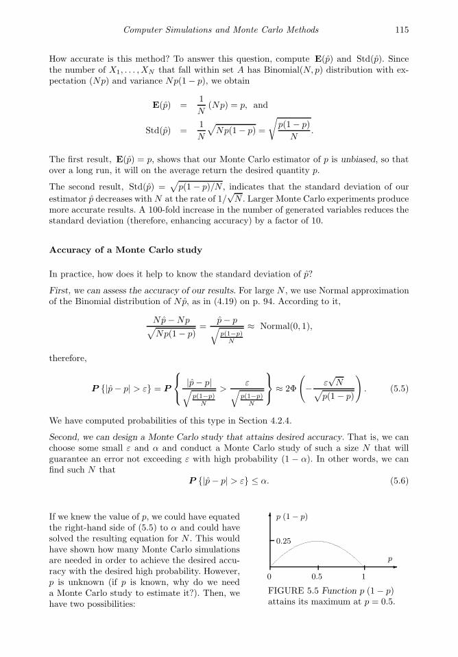
Computer Simulations and Monte Carlo Methods 115
How accurate is this method? To answer this question, compute E(p) and Std(p). Sincethe number of X1, . . . , XN that fall within set A has Binomial(N, p) distribution with ex-pectation (Np) and variance Np(1− p), we obtain
E(p) =1
N(Np) = p, and
Std(p) =1
N
√Np(1− p) =
√p(1− p)
N.
The first result, E(p) = p, shows that our Monte Carlo estimator of p is unbiased, so thatover a long run, it will on the average return the desired quantity p.
The second result, Std(p) =√p(1− p)/N , indicates that the standard deviation of our
estimator p decreases with N at the rate of 1/√N . Larger Monte Carlo experiments produce
more accurate results. A 100-fold increase in the number of generated variables reduces thestandard deviation (therefore, enhancing accuracy) by a factor of 10.
Accuracy of a Monte Carlo study
In practice, how does it help to know the standard deviation of p?
First, we can assess the accuracy of our results. For large N , we use Normal approximationof the Binomial distribution of Np, as in (4.19) on p. 94. According to it,
Np−Np√Np(1− p)
=p− p√p(1−p)
N
≈ Normal(0, 1),
therefore,
P |p− p| > ε = P
|p− p|√p(1−p)
N
>ε√
p(1−p)N
≈ 2Φ
(− ε
√N√
p(1− p)
). (5.5)
We have computed probabilities of this type in Section 4.2.4.
Second, we can design a Monte Carlo study that attains desired accuracy. That is, we canchoose some small ε and α and conduct a Monte Carlo study of such a size N that willguarantee an error not exceeding ε with high probability (1 − α). In other words, we canfind such N that
P |p− p| > ε ≤ α. (5.6)
If we knew the value of p, we could have equatedthe right-hand side of (5.5) to α and could havesolved the resulting equation for N . This wouldhave shown how many Monte Carlo simulationsare needed in order to achieve the desired accu-racy with the desired high probability. However,p is unknown (if p is known, why do we needa Monte Carlo study to estimate it?). Then, wehave two possibilities:
0 0.5 1
p
0.25
p (1− p)
FIGURE 5.5 Function p (1 − p)attains its maximum at p = 0.5.

116 Probability and Statistics for Computer Scientists
1. Use an “intelligent guess” (preliminary estimate) of p, if it is available.
2. Bound p (1− p) by its largest possible value (see Figure 5.5),
p (1− p) ≤ 0.25 for 0 ≤ p ≤ 1.
In the first case, if p∗ is an “intelligent guess” of p, then we solve the inequality
2Φ
(− ε
√N√
p∗(1 − p∗)
)≤ α
in terms of N . In the second case, we solve
2Φ(−2ε
√N)≤ α
to find the conservatively sufficient size of the Monte Carlo study.
Solutions of these inequalities give us the following rule.
Size of a MonteCarlo study
In order to guarantee that P |p− p| > ε ≤ α,one needs to simulate
N ≥ p∗(1− p∗)(zα/2
ε
)2
random variables, where p∗ is a preliminaryestimator of p, or
N ≥ 0.25(zα/2
ε
)2
random variables, if no such estimator is available.
Recall (from Example 4.12) that zα = Φ−1(1−α)is such a value of a Standard Normal variableZ that can be exceeded with probability α. Itcan be obtained from Table A4. The area underthe Normal curve to the right of zα equals α(Figure 5.6).If this formula returns N that is too small for theNormal approximation, we can use Chebyshev’sinequality (3.8) on p. 54. We then obtain that
x
φ(x)
0 zα
Area= α
FIGURE 5.6 Critical value zα.
N ≥ p∗(1− p∗)
αε2, (5.7)
if an “intelligent guess” p∗ is available for p, and
N ≥ 1
4αε2, (5.8)
otherwise, satisfy the desired condition (5.6) (Exercise 5.14).
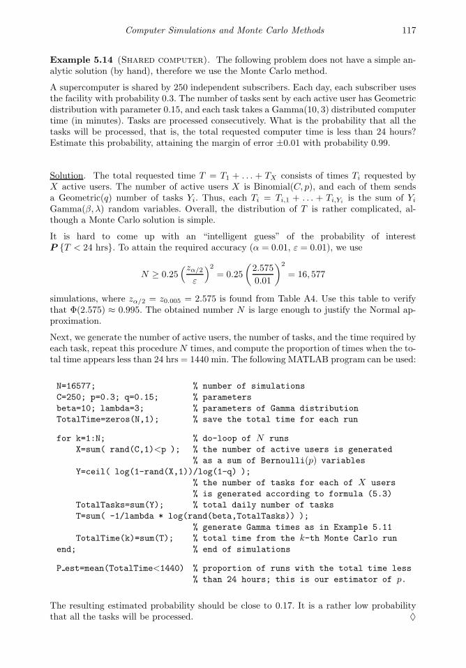
Computer Simulations and Monte Carlo Methods 117
Example 5.14 (Shared computer). The following problem does not have a simple an-alytic solution (by hand), therefore we use the Monte Carlo method.
A supercomputer is shared by 250 independent subscribers. Each day, each subscriber usesthe facility with probability 0.3. The number of tasks sent by each active user has Geometricdistribution with parameter 0.15, and each task takes a Gamma(10, 3) distributed computertime (in minutes). Tasks are processed consecutively. What is the probability that all thetasks will be processed, that is, the total requested computer time is less than 24 hours?Estimate this probability, attaining the margin of error ±0.01 with probability 0.99.
Solution. The total requested time T = T1 + . . . + TX consists of times Ti requested byX active users. The number of active users X is Binomial(C, p), and each of them sendsa Geometric(q) number of tasks Yi. Thus, each Ti = Ti,1 + . . . + Ti,Yi
is the sum of Yi
Gamma(β, λ) random variables. Overall, the distribution of T is rather complicated, al-though a Monte Carlo solution is simple.
It is hard to come up with an “intelligent guess” of the probability of interestP T < 24 hrs. To attain the required accuracy (α = 0.01, ε = 0.01), we use
N ≥ 0.25(zα/2
ε
)2= 0.25
(2.575
0.01
)2
= 16, 577
simulations, where zα/2 = z0.005 = 2.575 is found from Table A4. Use this table to verifythat Φ(2.575) ≈ 0.995. The obtained number N is large enough to justify the Normal ap-proximation.
Next, we generate the number of active users, the number of tasks, and the time required byeach task, repeat this procedure N times, and compute the proportion of times when the to-tal time appears less than 24 hrs = 1440 min. The following MATLAB program can be used:
N=16577; % number of simulations
C=250; p=0.3; q=0.15; % parameters
beta=10; lambda=3; % parameters of Gamma distribution
TotalTime=zeros(N,1); % save the total time for each run
for k=1:N; % do-loop of N runs
X=sum( rand(C,1)<p ); % the number of active users is generated
% as a sum of Bernoulli(p) variables
Y=ceil( log(1-rand(X,1))/log(1-q) );
% the number of tasks for each of X users
% is generated according to formula (5.3)
TotalTasks=sum(Y); % total daily number of tasks
T=sum( -1/lambda * log(rand(beta,TotalTasks)) );
% generate Gamma times as in Example 5.11
TotalTime(k)=sum(T); % total time from the k-th Monte Carlo run
end; % end of simulations
P est=mean(TotalTime<1440) % proportion of runs with the total time less
% than 24 hours; this is our estimator of p.
The resulting estimated probability should be close to 0.17. It is a rather low probabilitythat all the tasks will be processed. ♦
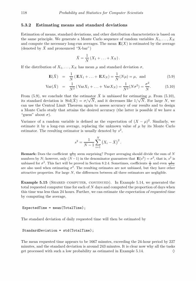
118 Probability and Statistics for Computer Scientists
5.3.2 Estimating means and standard deviations
Estimation of means, standard deviations, and other distribution characteristics is based onthe same principle. We generate a Monte Carlo sequence of random variables X1, . . . , XN
and compute the necessary long-run averages. The mean E(X) is estimated by the average(denoted by X and pronounced “X-bar”)
X =1
N(X1 + . . .+XN ) .
If the distribution of X1, . . . , XN has mean µ and standard deviation σ,
E(X) =1
N(EX1 + . . .+ EXN ) =
1
N(Nµ) = µ, and (5.9)
Var(X) =1
N2(VarX1 + . . .+ VarXN ) =
1
N2(Nσ2) =
σ2
N. (5.10)
From (5.9), we conclude that the estimator X is unbiased for estimating µ. From (5.10),its standard deviation is Std(X) = σ/
√N , and it decreases like 1/
√N . For large N , we
can use the Central Limit Theorem again to assess accuracy of our results and to designa Monte Carlo study that attains the desired accuracy (the latter is possible if we have a“guess” about σ).
Variance of a random variable is defined as the expectation of (X − µ)2. Similarly, weestimate it by a long-run average, replacing the unknown value of µ by its Monte Carloestimator. The resulting estimator is usually denoted by s2,
s2 =1
N − 1
N∑
i=1
(Xi − X
)2.
Remark: Does the coefficient 1N−1
seem surprising? Proper averaging should divide the sum of N
numbers by N ; however, only (N−1) in the denominator guarantees that E(s2) = σ2, that is, s2 is
unbiased for σ2. This fact will be proved in Section 8.2.4. Sometimes, coefficients 1N
and even 1N+1
are also used when estimating σ2. The resulting estimates are not unbiased, but they have other
attractive properties. For large N , the differences between all three estimators are negligible.
Example 5.15 (Shared computer, continued). In Example 5.14, we generated thetotal requested computer time for each ofN days and computed the proportion of days whenthis time was less than 24 hours. Further, we can estimate the expectation of requested timeby computing the average,
ExpectedTime = mean(TotalTime);
The standard deviation of daily requested time will then be estimated by
StandardDeviation = std(TotalTime);
The mean requested time appears to be 1667 minutes, exceeding the 24-hour period by 227minutes, and the standard deviation is around 243 minutes. It is clear now why all the tasksget processed with such a low probability as estimated in Example 5.14. ♦
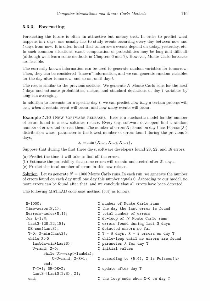
Computer Simulations and Monte Carlo Methods 119
5.3.3 Forecasting
Forecasting the future is often an attractive but uneasy task. In order to predict whathappens in t days, one usually has to study events occurring every day between now andt days from now. It is often found that tomorrow’s events depend on today, yesterday, etc.In such common situations, exact computation of probabilities may be long and difficult(although we’ll learn some methods in Chapters 6 and 7). However, Monte Carlo forecastsare feasible.
The currently known information can be used to generate random variables for tomorrow.Then, they can be considered “known” information, and we can generate random variablesfor the day after tomorrow, and so on, until day t.
The rest is similar to the previous sections. We generate N Monte Carlo runs for the nextt days and estimate probabilities, means, and standard deviations of day t variables bylong-run averaging.
In addition to forecasts for a specific day t, we can predict how long a certain process willlast, when a certain event will occur, and how many events will occur.
Example 5.16 (New software release). Here is a stochastic model for the numberof errors found in a new software release. Every day, software developers find a randomnumber of errors and correct them. The number of errors Xt found on day t has Poisson(λt)distribution whose parameter is the lowest number of errors found during the previous 3days,
λt = min Xt−1, Xt−2, Xt−3 .Suppose that during the first three days, software developers found 28, 22, and 18 errors.
(a) Predict the time it will take to find all the errors.(b) Estimate the probability that some errors will remain undetected after 21 days.(c) Predict the total number of errors in this new release.
Solution. Let us generate N = 1000 Monte Carlo runs. In each run, we generate the numberof errors found on each day until one day this number equals 0. According to our model, nomore errors can be found after that, and we conclude that all errors have been detected.
The following MATLAB code uses method (5.4) as follows,
N=1000; % number of Monte Carlo runs
Time=zeros(N,1); % the day the last error is found
Nerrors=zeros(N,1); % total number of errors
for k=1:N; % do-loop of N Monte Carlo runs
Last3=[28,22,18]; % errors found during last 3 days
DE=sum(Last3); % detected errors so far
T=0; X=min(Last3); % T = # days, X = # errors on day T
while X>0; % while-loop until no errors are found
lambda=min(Last3); % parameter λ for day T
U=rand; X=0; % initial values
while U>=exp(-lambda);
U=U*rand; X=X+1; % according to (5.4), X is Poisson(λ)end;
T=T+1; DE=DE+X; % update after day T
Last3=[Last3(2:3), X];
end; % the loop ends when X=0 on day T

120 Probability and Statistics for Computer Scientists
Time(k)=T-1;
Nerrors(k)=DE;
end;
Now we estimate the expected time it takes to detect all the errors by mean(Time), theprobability of errors remaining after 21 days by mean(Time>21), and the expected totalnumber of errors by mean(Nerrors). This Monte Carlo study should predict the expectedtime of about 16.75 days to detect all the errors, the probability 0.22 that errors remainafter 21 days, and about 222 errors overall. ♦
5.3.4 Estimating lengths, areas, and volumes
Lengths
A Standard Uniform variable U has density fU (u) = 1 for 0 ≤ u ≤ 1. Hence, U belongs toa set A ⊂ [0, 1] with probability
P U ∈ A =
∫
A
1 du = length of A. (5.11)
Monte Carlo methods can be used to estimate the probability in the left-hand side. At thesame time, we estimate the right-hand side of (5.11), the length of A. Generate a long runof Standard Uniform random variables U1, U2, . . . , Un and estimate the length of A by theproportion of Ui that fall into A.
What if set A does not lie within a unit interval? Well, we can always choose a suitablesystem of coordinates, with a suitable origin and scale, to make the interval [0, 1] coverthe given bounded set as long as the latter is bounded. Alternatively, we can cover A withsome interval [a, b] and generate non-standard Uniform variables on [a, b], in which case theestimated probability P U ∈ A should be multiplied by (b− a).
Areas and volumes
Computing lengths rarely represents a serious problem; therefore, one would rarely useMonte Carlo methods for this purpose. However, the situation is different with estimatingareas and volumes.
The method described for estimating lengths is directly translated into higher dimensions.Two independent Standard Uniform variables U and V have the joint density fU,V (u, v) = 1for 0 ≤ u, v ≤ 1, hence,
P (U, V ) ∈ B =
∫∫
B
1 du dv = area of B
for any two-dimensional set B that lies within a unit square [0, 1]× [0, 1]. Thus, the area ofB can be estimated as a long-run frequency of vectors (Ui, Vi) that belong to set B.
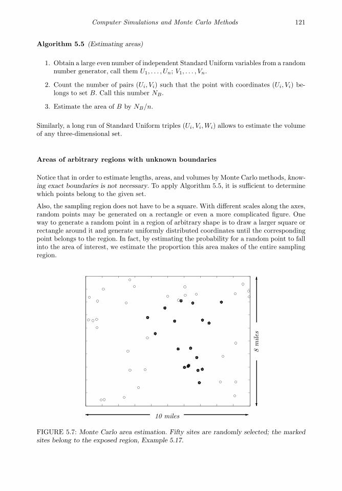
Computer Simulations and Monte Carlo Methods 121
Algorithm 5.5 (Estimating areas)
1. Obtain a large even number of independent Standard Uniform variables from a randomnumber generator, call them U1, . . . , Un; V1, . . . , Vn.
2. Count the number of pairs (Ui, Vi) such that the point with coordinates (Ui, Vi) be-longs to set B. Call this number NB.
3. Estimate the area of B by NB/n.
Similarly, a long run of Standard Uniform triples (Ui, Vi,Wi) allows to estimate the volumeof any three-dimensional set.
Areas of arbitrary regions with unknown boundaries
Notice that in order to estimate lengths, areas, and volumes by Monte Carlo methods, know-ing exact boundaries is not necessary. To apply Algorithm 5.5, it is sufficient to determinewhich points belong to the given set.
Also, the sampling region does not have to be a square. With different scales along the axes,random points may be generated on a rectangle or even a more complicated figure. Oneway to generate a random point in a region of arbitrary shape is to draw a larger square orrectangle around it and generate uniformly distributed coordinates until the correspondingpoint belongs to the region. In fact, by estimating the probability for a random point to fallinto the area of interest, we estimate the proportion this area makes of the entire samplingregion.
10 miles
8miles
FIGURE 5.7: Monte Carlo area estimation. Fifty sites are randomly selected; the markedsites belong to the exposed region, Example 5.17.
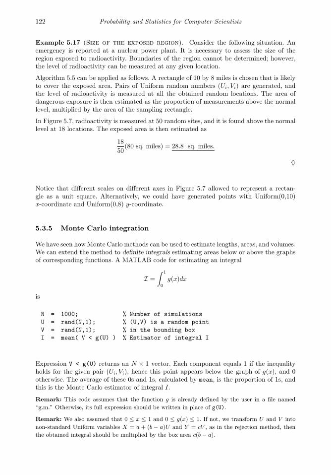
122 Probability and Statistics for Computer Scientists
Example 5.17 (Size of the exposed region). Consider the following situation. Anemergency is reported at a nuclear power plant. It is necessary to assess the size of theregion exposed to radioactivity. Boundaries of the region cannot be determined; however,the level of radioactivity can be measured at any given location.
Algorithm 5.5 can be applied as follows. A rectangle of 10 by 8 miles is chosen that is likelyto cover the exposed area. Pairs of Uniform random numbers (Ui, Vi) are generated, andthe level of radioactivity is measured at all the obtained random locations. The area ofdangerous exposure is then estimated as the proportion of measurements above the normallevel, multiplied by the area of the sampling rectangle.
In Figure 5.7, radioactivity is measured at 50 random sites, and it is found above the normallevel at 18 locations. The exposed area is then estimated as
18
50(80 sq. miles) = 28.8 sq. miles.
♦
Notice that different scales on different axes in Figure 5.7 allowed to represent a rectan-gle as a unit square. Alternatively, we could have generated points with Uniform(0,10)x-coordinate and Uniform(0,8) y-coordinate.
5.3.5 Monte Carlo integration
We have seen howMonte Carlo methods can be used to estimate lengths, areas, and volumes.We can extend the method to definite integrals estimating areas below or above the graphsof corresponding functions. A MATLAB code for estimating an integral
I =
∫ 1
0
g(x)dx
is
N = 1000; % Number of simulations
U = rand(N,1); % (U,V) is a random point
V = rand(N,1); % in the bounding box
I = mean( V < g(U) ) % Estimator of integral I
Expression V < g(U) returns an N × 1 vector. Each component equals 1 if the inequalityholds for the given pair (Ui, Vi), hence this point appears below the graph of g(x), and 0otherwise. The average of these 0s and 1s, calculated by mean, is the proportion of 1s, andthis is the Monte Carlo estimator of integral I.
Remark: This code assumes that the function g is already defined by the user in a file named
“g.m.” Otherwise, its full expression should be written in place of g(U).
Remark: We also assumed that 0 ≤ x ≤ 1 and 0 ≤ g(x) ≤ 1. If not, we transform U and V into
non-standard Uniform variables X = a + (b − a)U and Y = cV , as in the rejection method, then
the obtained integral should be multiplied by the box area c(b− a).
Computer Simulations and Monte Carlo Methods 123
Accuracy of results
So far, we estimated lengths, areas, volumes, and integrals by long-run proportions, themethod described in Section 5.3.1. As we noted there, our estimates are unbiased, and theirstandard deviation is
Std(I)=
√I(1 − I)
N, (5.12)
where I is the actual quantity of interest.
Turns out, there are Monte Carlo integration methods that can beat this rate. Next, wederive an unbiased area estimator with a lower standard deviation. Also, it will not berestricted to an interval [0, 1] or even [a, b].
Improved Monte Carlo integration method
First, we notice that a definite integral
I =
∫ b
a
g(x)dx =1
b− a
∫ b
a
(b− a)g(x)dx = E (b − a)g(X)
equals the expectation of (b − a)g(X) for a Uniform(a, b) variable X . Hence, instead ofusing proportions, we can estimate I by averaging (b − a)g(Xi) for some large number ofUniform(a, b) variables X1, . . . , XN .
Furthermore, with a proper adjustment, we can use any continuous distribution in place ofUniform(a, b). To do this, we choose some density f(x) and write I as
I =
∫ b
a
g(x)dx =
∫ b
a
g(x)
f(x)f(x) dx = E
(g(X)
f(X)
),
where X has density f(x). It remains to generate a long run of variables X1, . . . , XN withthis density and compute the average of g(Xi)/f(Xi).
In particular, we are no longer limited to a finite interval [a, b]. For example, by choosing f(x)to be a Standard Normal density, we can perform Monte Carlo integration from a = −∞to b = +∞:
N = 1000; % Number of simulations
Z = randn(N,1); % Standard Normal variables
f = 1/sqrt(2*Pi) * exp(-Z.ˆ2/2); % Standard Normal density
Iest = mean( g(Z)./f(Z) ) % Estimator of∫∞
−∞g(x) dx
Remark: recall that “dot” operations . and ./ stand for pointwise power and division. Without a
dot, MATLAB performs standard matrix operations instead.
Accuracy of the improved method
As we already know from (5.9), using long-run averaging returns an unbiased estimator I,hence E(I) = I. We also know from (5.10) that
Std(I) = σ√N
,

124 Probability and Statistics for Computer Scientists
where σ is the standard deviation of a random variable R = g(X)/f(X). Hence, the esti-mator I is more reliable if σ is small and N is large. Small σ can be obtained by choosinga density f(x) that is approximately proportional to g(x) making R nearly a constantwith Std(R) ≈ 0. However, generating variables from such a density will usually be just asdifficult as computing the integral I.In fact, using a simple Standard Uniform distribution of X , we already obtain a lowerstandard deviation than in (5.12). Indeed, suppose that 0 ≤ g(x) ≤ 1 for 0 ≤ x ≤ 1. For aUniform(0, 1) variable X , we have f(X) = 1 so that
σ2 = VarR = Var g(X) = Eg2(X)− E2g(X) =
∫ 1
0
g2(x)dx − I 2 ≤ I − I 2,
because g2 ≤ g for 0 ≤ g ≤ 1. We conclude that for this method,
Std(I) ≤
√I − I 2
N=
√I(1− I)
N.
Comparing with (5.12), we see that with the same number of simulations N , the lattermethod gives more accurate results. We can also say that to attain the same desired accu-racy, the second method requires fewer simulations.
This can be extended to an arbitrary interval [a, b] and any function g ∈ [0, c] (Exercise 5.16).
Summary and conclusions
Monte Carlo methods are effectively used for estimating probabilities, expectations, andother distribution characteristics in complex situations when computing these quantities byhand is difficult. According to Monte Carlo methodology, we generate a long sequence ofrandom variables X1, . . . , XN from the distribution of interest and estimate probabilitiesby long-run proportions, expectations by long-run averages, etc. We extend these methodsto the estimation of lengths, areas, volumes, and integrals. Similar techniques are used forforecasting.
All the discussed methods produce unbiased results. Standard deviations of the proposedestimators decrease at the rate of 1/
√N . Knowing the standard deviation enables us to
assess the accuracy of obtained estimates, and also, to design a Monte Carlo study thatattains the desired accuracy with the desired high probability.
In this chapter, we learned the inverse transform method of generating random variables,rejection method, discrete method, and some special methods. Monte Carlo simulation ofmore advanced models will be considered in Chapters 6 and 7, where we simulate stochasticprocesses, Markov chains, and queuing systems.
Exercises 125
Exercises
5.1. Derive a formula and explain how to generate a random variable with the density
f(x) = (1.5)√x for 0 < x < 1
if your random number generator produces a Standard Uniform random variable U . Usethe inverse transform method. Compute this variable if U = 0.001.
5.2. Let U be a Standard Uniform random variable. Show all the steps required to generate
(a) an Exponential random variable with the parameter λ = 2.5;
(b) a Bernoulli random variable with the probability of success 0.77;
(c) a Binomial random variable with parameters n = 15 and p = 0.4;
(d) a discrete random variable with the distribution P (x), where P (0) = 0.2, P (2) = 0.4,P (7) = 0.3, P (11) = 0.1;
(e) a continuous random variable with the density f(x) = 3x2, 0 < x < 1;
(f) a continuous random variable with the density f(x) = 1.5x2, −1 < x < 1;
(g) a continuous random variable with the density f(x) = 112
3√x, 0 ≤ x ≤ 8.
If a computer generates U and the result is U = 0.3972, compute the variables generatedin (a)–(g).
5.3. Explain how one can generate a random variable X that has a pdf
f(x) =
12 (1 + x) if − 1 ≤ x ≤ 1
0 otherwise,
given a computer-generated Standard Uniform variable U . Generate X using Table A1.
5.4. To evaluate the system parameters, one uses Monte Carlo methodology and simulates oneof its vital characteristics X , a continuous random variable with the density
f(x) =
29 (1 + x) if − 1 ≤ x ≤ 2
0 otherwise
Explain how one can generate X , given a computer-generated Standard Uniform variableU . If U = 0.2396, compute X .
5.5. Give an expression that transforms a Standard Uniform variable U into a variable X withthe following density,
f(x) =1
3x2, −1 < x < 2.
Compute X if a computer returns a value of U = 0.8.
126 Probability and Statistics for Computer Scientists
5.6. Two mechanics are changing oil filters for the arrived customers. The service time hasan Exponential distribution with the parameter λ = 5 hrs−1 for the first mechanic, andλ = 20 hrs−1 for the second mechanic. Since the second mechanic works faster, he is serving4 times more customers than his partner. Therefore, when you arrive to have your oil filterchanged, your probability of being served by the faster mechanic is 4/5. Let X be yourservice time. Explain how to generate the random variable X .
5.7. Explain how to estimate the following probabilities.
(a) P X > Y , where X and Y are independent Poisson random variables with param-eters 3 and 5, respectively.
(b) The probability of a royal-flush (a ten, a jack, a queen, a king, and an ace of the samesuit) in poker, if 5 cards are selected at random from a deck of 52 cards.
(c) The probability that it will take more than 35 minutes to have your oil filter changedin Exercise 5.6.
(d) With probability 0.95, we need to estimate each of the probabilities listed in (a-c)with a margin of error not exceeding 0.005. What should be the size of our MonteCarlo study in each case?
(e) (Computer mini-project) Conduct a Monte Carlo study and estimate probabilities(a-c) with an error not exceeding 0.005 with probability 0.95.
5.8. (Computer mini-project) Area of a unit circle equals π. Cover a circle with a 2 by 2square and follow Algorithm 5.5 to estimate number π based on 100, 1,000, and 10,000random numbers. Compare results with the exact value π = 3.14159265358... and commenton precision.
5.9. (Computer project) Twenty computers are connected in a network. One computer be-comes infected with a virus. Every day, this virus spreads from any infected computer toany uninfected computer with probability 0.1. Also, every day, a computer technician takes5 infected computers at random (or all infected computers, if their number is less than 5)and removes the virus from them. Estimate:
(a) the expected time it takes to remove the virus from the whole network;
(b) the probability that each computer gets infected at least once;
(c) the expected number of computers that get infected.
5.10. (Computer project) A forest consists of 1,000 trees forming a perfect 50× 20 rectangle,Figure 5.8. The northwestern (top-left) corner tree catches fire. Wind blows from the west,therefore, the probability that any tree catches fire from its burning left neighbor is 0.8.The probabilities to catch fire from trees immediately to the right, above, or below are allequal 0.3.
(a) Conduct a Monte Carlo study to estimate the probability that more than 30% of theforest will eventually be burning. With probability 0.95, your answer should differfrom the true value by no more than 0.005.
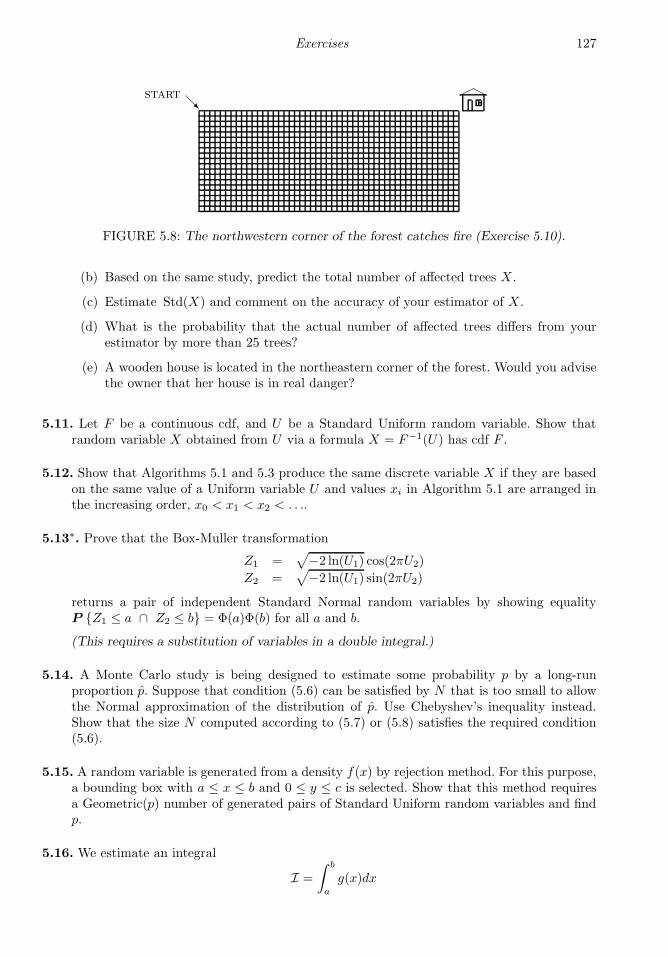
Exercises 127
start
FIGURE 5.8: The northwestern corner of the forest catches fire (Exercise 5.10).
(b) Based on the same study, predict the total number of affected trees X .
(c) Estimate Std(X) and comment on the accuracy of your estimator of X .
(d) What is the probability that the actual number of affected trees differs from yourestimator by more than 25 trees?
(e) A wooden house is located in the northeastern corner of the forest. Would you advisethe owner that her house is in real danger?
5.11. Let F be a continuous cdf, and U be a Standard Uniform random variable. Show thatrandom variable X obtained from U via a formula X = F−1(U) has cdf F .
5.12. Show that Algorithms 5.1 and 5.3 produce the same discrete variable X if they are basedon the same value of a Uniform variable U and values xi in Algorithm 5.1 are arranged inthe increasing order, x0 < x1 < x2 < . . ..
5.13∗. Prove that the Box-Muller transformation
Z1 =√−2 ln(U1) cos(2πU2)
Z2 =√−2 ln(U1) sin(2πU2)
returns a pair of independent Standard Normal random variables by showing equalityP Z1 ≤ a ∩ Z2 ≤ b = Φ(a)Φ(b) for all a and b.
(This requires a substitution of variables in a double integral.)
5.14. A Monte Carlo study is being designed to estimate some probability p by a long-runproportion p. Suppose that condition (5.6) can be satisfied by N that is too small to allowthe Normal approximation of the distribution of p. Use Chebyshev’s inequality instead.Show that the size N computed according to (5.7) or (5.8) satisfies the required condition(5.6).
5.15. A random variable is generated from a density f(x) by rejection method. For this purpose,a bounding box with a ≤ x ≤ b and 0 ≤ y ≤ c is selected. Show that this method requiresa Geometric(p) number of generated pairs of Standard Uniform random variables and findp.
5.16. We estimate an integral
I =
∫ b
a
g(x)dx

128 Probability and Statistics for Computer Scientists
for arbitrary a and b and a function 0 ≤ g(x) ≤ c using both Monte Carlo integrationmethods introduced in this chapter. First, we generate N pairs of Uniform variables (Ui, Vi),a ≤ Ui ≤ b, 0 ≤ Vi ≤ c, and estimate I by the properly rescaled proportion of pairs withVi ≤ g(Ui). Second, we generate only Ui and estimate I by the average value of (b−a)g(Ui).Show that the second method produces more accurate results.

Part II
Stochastic Processes
129

Chapter 6
Stochastic Processes
6.1 Definitions and classifications . . . . . . . . . . . . . . . . . . . . . . . . . . . . . . . . . . . . 1326.2 Markov processes and Markov chains . . . . . . . . . . . . . . . . . . . . . . . . . . . . 133
6.2.1 Markov chains . . . . . . . . . . . . . . . . . . . . . . . . . . . . . . . . . . . . . . . . . . . 1346.2.2 Matrix approach . . . . . . . . . . . . . . . . . . . . . . . . . . . . . . . . . . . . . . . . . 1386.2.3 Steady-state distribution . . . . . . . . . . . . . . . . . . . . . . . . . . . . . . . . 142
6.3 Counting processes . . . . . . . . . . . . . . . . . . . . . . . . . . . . . . . . . . . . . . . . . . . . . . . 1486.3.1 Binomial process . . . . . . . . . . . . . . . . . . . . . . . . . . . . . . . . . . . . . . . . . 1486.3.2 Poisson process . . . . . . . . . . . . . . . . . . . . . . . . . . . . . . . . . . . . . . . . . . 152
6.4 Simulation of stochastic processes . . . . . . . . . . . . . . . . . . . . . . . . . . . . . . . 157Summary and conclusions . . . . . . . . . . . . . . . . . . . . . . . . . . . . . . . . . . . . . . . . . . 160Exercises . . . . . . . . . . . . . . . . . . . . . . . . . . . . . . . . . . . . . . . . . . . . . . . . . . . . . . . . . . . . 160
Let us summarize what we have already accomplished. Our ultimate goal was to learn tomake decisions under uncertainty. We introduced a language of probability in Chapter 2and learned how to measure uncertainty. Then, through Chapters 3–5, we studied randomvariables, random vectors, and their distributions. Have we learned enough to describe asituation involving uncertainty and be able to make good decisions?
Let us look around. If you say “Freeze!” and everything freezes for a moment, the situationwill be completely described by random variables surrounding us at a particular moment oftime. However, the real world is dynamic. Many variables develop and change in real time:air temperatures, stock prices, interest rates, football scores, popularity of politicians, andalso, the CPU usage, the speed of internet connection, the number of concurrent users, thenumber of running processes, available memory, and so on.
We now start the discussion of stochastic processes, which are random variables that evolveand change in time.
131

132 Probability and Statistics for Computer Scientists
6.1 Definitions and classifications
DEFINITION 6.1
A stochastic process is a random variable that also depends on time. It istherefore a function of two arguments, X(t, ω), where:
• t ∈ T is time, with T being a set of possible times, usually [0,∞), (−∞,∞),0, 1, 2, . . ., or . . . ,−2,−1, 0, 1, 2, . . .;• ω ∈ Ω, as before, is an outcome of an experiment, with Ω being the wholesample space.
Values of X(t, ω) are called states.
At any fixed time t, we see a random variable Xt(ω), a function of a random outcome. Onthe other hand, if we fix ω, we obtain a function of time Xω(t). This function is called arealization, a sample path, or a trajectory of a process X(t, ω).
Example 6.1 (CPU usage). Looking at the past usage of the central processing unit(CPU), we see a realization of this process until the current time (Figure 6.1a). However,the future behavior of the process is unclear. Depending on which outcome ω will actuallytake place, the process can develop differently. For example, see two different trajectoriesfor ω = ω1 and ω = ω2, two elements of the sample space Ω, on Figure 6.1b.
Remark: You can observe a similar stochastic process on your personal computer. In the latest ver-
sions of Windows, Ctrl-Alt-Del, pressed simultaneously and followed by “Windows Task Manager,”
will show the real-time sample path of CPU usage under the tab “Performance.” ♦
Depending on possible values of T and X , stochastic processes are classified as follows.
X(t) X(t)
t t
(a) Observed sample path (b) Possible development, determined
by the outcome ω ∈ Ω
ω = ω1
ω = ω2
FIGURE 6.1: Sample paths of CPU usage stochastic process.
Stochastic Processes 133
DEFINITION 6.2
Stochastic process X(t, ω) is discrete-state if variable Xt(ω) is discrete foreach time t, and it is a continuous-state if Xt(ω) is continuous.
DEFINITION 6.3
Stochastic process X(t, ω) is a discrete-time process if the set of times T isdiscrete, that is, it consists of separate, isolated points. It is a continuous-timeprocess if T is a connected, possibly unbounded interval.
Example 6.2. The CPU usage process, in percents, is continuous-state and continuous-time, as we can see in Figure 6.1a. ♦
Example 6.3. The actual air temperature X(t, ω) at time t is a continuous-time,continuous-state stochastic process. Indeed, it changes smoothly and never jumps from onevalue to another. However, the temperature Y (t, ω) reported on a radio every 10 minutesis a discrete-time process. Moreover, since the reported temperature is usually rounded tothe nearest degree, it is also a discrete-state process. ♦
Example 6.4. In a printer shop, let X(n, ω) be the amount of time required to print then-th job. This is a discrete-time, continuous-state stochastic process, because n = 1, 2, 3, . . .,and X ∈ (0,∞).
Let Y (n, ω) be the number of pages of the n-th printing job. Now, Y = 1, 2, 3, . . . is discrete;therefore, this process is discrete-time and discrete-state.
♦
From now on, we shall not write ω as an argument of X(t, ω). Just keep in mind thatbehavior of a stochastic process depends on chance, just as we did with random variablesand random vectors.
Another important class of stochastic processes is defined in the next section.
6.2 Markov processes and Markov chains
DEFINITION 6.4
Stochastic process X(t) is Markov if for any t1 < ... < tn < t and any setsA;A1, . . . , An
P X(t) ∈ A | X(t1) ∈ A1, . . . , X(tn) ∈ An= P X(t) ∈ A | X(tn) ∈ An . (6.1)
134 Probability and Statistics for Computer Scientists
Let us look at the equation (6.1). It means that the conditional distribution of X(t) is thesame under two different conditions,
(1) given observations of the process X at several moments in the past;
(2) given only the latest observation of X .
If a process is Markov, then its future behavior is the same under conditions (1) and (2).In other words, knowing the present, we get no information from the past that can be usedto predict the future,
P future | past, present = P future | present
Then, for the future development of a Markov process, only its present state is important,and it does not matter how the process arrived to this state.
Some processes satisfy the Markov property, and some don’t.
Example 6.5 (Internet connections). Let X(t) be the total number of internet con-nections registered by some internet service provider by the time t. Typically, people con-nect to the internet at random times, regardless of how many connections have already beenmade. Therefore, the number of connections in a minute will only depend on the currentnumber. For example, if 999 connections have been registered by 10 o’clock, then their totalnumber will exceed 1000 during the next minute regardless of when and how these 999connections were made in the past. This process is Markov. ♦
Example 6.6 (Stock prices). Let Y (t) be the value of some stock or some market indexat time t. If we know Y (t), do we also want to know Y (t− 1) in order to predict Y (t+ 1)?One may argue that if Y (t−1) < Y (t), then the market is rising, therefore, Y (t+1) is likely(but not certain) to exceed Y (t). On the other hand, if Y (t− 1) > Y (t), we may concludethat the market is falling and may expect Y (t+1) < Y (t). It looks like knowing the past inaddition to the present did help us to predict the future. Then, this process is not Markov.♦
Due to a well-developed theory and a number of simple techniques available for Markovprocesses, it is important to know whether the process is Markov or not. The idea of Markovdependence was proposed and developed by Andrei Markov (1856–1922) who was a studentof P. Chebyshev (p. 54) at St. Petersburg University in Russia.
6.2.1 Markov chains
DEFINITION 6.5
A Markov chain is a discrete-time, discrete-state Markov stochastic process.
Introduce a few convenient simplifications. The time is discrete, so let us define the timeset as T = 0, 1, 2, . . .. We can then look at a Markov chain as a random sequence
X(0), X(1), X(2), . . . .

Stochastic Processes 135
The state set is also discrete, so let us enumerate the states as 1, 2, . . . , n. Sometimes we’llstart enumeration from state 0, and sometimes we’ll deal with a Markov chain with infinitelymany (discrete) states, then we’ll have n = ∞.
The Markov property means that only the value of X(t) matters for predicting X(t + 1),so the conditional probability
pij(t) = P X(t+ 1) = j | X(t) = i (6.2)
= P X(t+ 1) = j | X(t) = i, X(t− 1) = h, X(t− 2) = g, . . .
depends on i, j, and t only and equals the probability for the Markov chain X to make atransition from state i to state j at time t.
DEFINITION 6.6
Probability pij(t) in (6.2) is called a transition probability. Probability
p(h)ij (t) = P X(t+ h) = j | X(t) = i
of moving from state i to state j by means of h transitions is an h-steptransition probability.
DEFINITION 6.7
A Markov chain is homogeneous if all its transition probabilities are indepen-dent of t. Being homogeneous means that transition from i to j has the same
probability at any time. Then pij(t) = pij and p(h)ij (t) = p
(h)ij .
Characteristics of a Markov chain
What do we need to know to describe a Markov chain?
By the Markov property, each next state should be predicted from the previous state only.Therefore, it is sufficient to know the distribution of its initial stateX(0) and the mechanismof transitions from one state to another.
The distribution of a Markov chain is completely determined by the initial distribution P0
and one-step transition probabilities pij . Here P0 is the probability mass function of X0,
P0(x) = P X(0) = x for x ∈ 1, 2, . . . , n
Based on this data, we would like to compute:
• h-step transition probabilities p(h)ij ;
• Ph, the distribution of states at time h, which is our forecast for X(h);
• the limit of p(h)ij and Ph as h → ∞, which is our long-term forecast.
Indeed, when making forecasts for many transitions ahead, computations will become ratherlengthy, and thus, it will be more efficient to take the limit.

136 Probability and Statistics for Computer Scientists
Notation pij = P X(t+ 1) = j | X(t) = i,transition probability
p(h)ij = P X(t+ h) = j | X(t) = i,
h-step transition probability
Pt(x) = P X(t) = x, distribution of X(t),distribution of states at time t
P0(x) = P X(0) = x, initial distribution
Example 6.7 (Weather forecasts). In some town, each day is either sunny or rainy.A sunny day is followed by another sunny day with probability 0.7, whereas a rainy day isfollowed by a sunny day with probability 0.4.
It rains on Monday. Make forecasts for Tuesday, Wednesday, and Thursday.
Solution. Weather conditions in this problem represent a homogeneous Markov chain with2 states: state 1 = “sunny” and state 2 = “rainy.” Transition probabilities are:
p11 = 0.7, p12 = 0.3, p21 = 0.4, p22 = 0.6,
where p12 and p22 were computed by the complement rule.
If it rains on Monday, then Tuesday is sunny with probability p21 = 0.4 (making a transitionfrom a rainy to a sunny day), and Tuesday is rainy with probability p22 = 0.6. We can predicta 60% chance of rain.
Wednesday forecast requires 2-step transition probabilities, making one transition fromMonday to Tuesday, X(0) to X(1), and another one from Tuesday to Wednesday, X(1) toX(2). We’ll have to condition on the weather situation on Tuesday and use the Law of TotalProbability from p. 31,
p(2)21 = P Wednesday is sunny | Monday is rainy
=
2∑
i=1
P X(1) = i | X(0) = 2P X(2) = 1 | X(1) = i
= P X(1) = 1 | X(0) = 2P X(2) = 1 | X(1) = 1+P X(1) = 2 | X(0) = 2P X(2) = 1 | X(1) = 2
= p21p11 + p22p21 = (0.4)(0.7) + (0.6)(0.4) = 0.52.
By the Complement Rule, p(2)22 = 0.48, and thus, we predict a 52% chance of sun and a 48%
chance of rain on Wednesday.
For the Thursday forecast, we need to compute 3-step transition probabilities p(3)ij because
it takes 3 transitions to move from Monday to Thursday. We have to use the Law ofTotal Probability conditioning on both Tuesday and Wednesday. For example, going fromrainy Monday to sunny Thursday means going from rainy Monday to either rainy or sunnyTuesday, then to either rainy or sunny Wednesday, and finally, to sunny Thursday,
p(3)21 =
2∑
i=1
2∑
j=1
p2ipijpj1.
This corresponds to a sequence of states 2 → i → j → 1. However, we have already
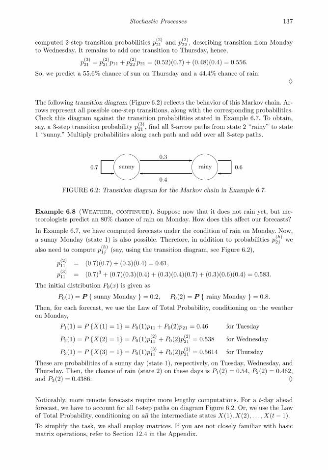
Stochastic Processes 137
computed 2-step transition probabilities p(2)21 and p
(2)22 , describing transition from Monday
to Wednesday. It remains to add one transition to Thursday, hence,
p(3)21 = p
(2)21 p11 + p
(2)22 p21 = (0.52)(0.7) + (0.48)(0.4) = 0.556.
So, we predict a 55.6% chance of sun on Thursday and a 44.4% chance of rain.♦
The following transition diagram (Figure 6.2) reflects the behavior of this Markov chain. Ar-rows represent all possible one-step transitions, along with the corresponding probabilities.Check this diagram against the transition probabilities stated in Example 6.7. To obtain,
say, a 3-step transition probability p(3)21 , find all 3-arrow paths from state 2 “rainy” to state
1 “sunny.” Multiply probabilities along each path and add over all 3-step paths.
sunny rainy
0.7 0.6
0.3
0.4
FIGURE 6.2: Transition diagram for the Markov chain in Example 6.7.
Example 6.8 (Weather, continued). Suppose now that it does not rain yet, but me-teorologists predict an 80% chance of rain on Monday. How does this affect our forecasts?
In Example 6.7, we have computed forecasts under the condition of rain on Monday. Now,
a sunny Monday (state 1) is also possible. Therefore, in addition to probabilities p(h)2j we
also need to compute p(h)1j (say, using the transition diagram, see Figure 6.2),
p(2)11 = (0.7)(0.7) + (0.3)(0.4) = 0.61,
p(3)11 = (0.7)3 + (0.7)(0.3)(0.4) + (0.3)(0.4)(0.7) + (0.3)(0.6)(0.4) = 0.583.
The initial distribution P0(x) is given as
P0(1) = P sunny Monday = 0.2, P0(2) = P rainy Monday = 0.8.
Then, for each forecast, we use the Law of Total Probability, conditioning on the weatheron Monday,
P1(1) = P X(1) = 1 = P0(1)p11 + P0(2)p21 = 0.46 for Tuesday
P2(1) = P X(2) = 1 = P0(1)p(2)11 + P0(2)p
(2)21 = 0.538 for Wednesday
P3(1) = P X(3) = 1 = P0(1)p(3)11 + P0(2)p
(3)21 = 0.5614 for Thursday
These are probabilities of a sunny day (state 1), respectively, on Tuesday, Wednesday, andThursday. Then, the chance of rain (state 2) on these days is P1(2) = 0.54, P2(2) = 0.462,and P3(2) = 0.4386. ♦
Noticeably, more remote forecasts require more lengthy computations. For a t-day aheadforecast, we have to account for all t-step paths on diagram Figure 6.2. Or, we use the Lawof Total Probability, conditioning on all the intermediate states X(1), X(2), . . . , X(t− 1).
To simplify the task, we shall employ matrices. If you are not closely familiar with basicmatrix operations, refer to Section 12.4 in the Appendix.
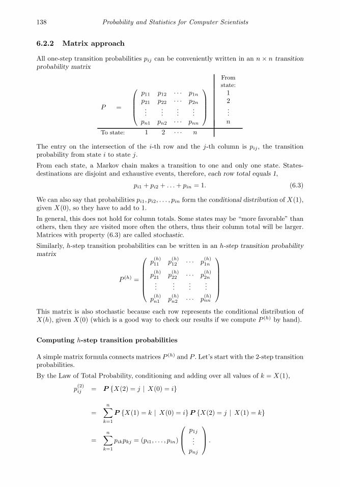
138 Probability and Statistics for Computer Scientists
6.2.2 Matrix approach
All one-step transition probabilities pij can be conveniently written in an n× n transitionprobability matrix
Fromstate:
P =
p11 p12 · · · p1np21 p22 · · · p2n...
......
...pn1 pn2 · · · pnn
12...n
To state: 1 2 · · · n
The entry on the intersection of the i-th row and the j-th column is pij , the transitionprobability from state i to state j.
From each state, a Markov chain makes a transition to one and only one state. States-destinations are disjoint and exhaustive events, therefore, each row total equals 1,
pi1 + pi2 + . . .+ pin = 1. (6.3)
We can also say that probabilities pi1, pi2, . . . , pin form the conditional distribution of X(1),given X(0), so they have to add to 1.
In general, this does not hold for column totals. Some states may be “more favorable” thanothers, then they are visited more often the others, thus their column total will be larger.Matrices with property (6.3) are called stochastic.
Similarly, h-step transition probabilities can be written in an h-step transition probabilitymatrix
P (h) =
p(h)11 p
(h)12 · · · p
(h)1n
p(h)21 p
(h)22 · · · p
(h)2n
......
......
p(h)n1 p
(h)n2 · · · p
(h)nn
This matrix is also stochastic because each row represents the conditional distribution ofX(h), given X(0) (which is a good way to check our results if we compute P (h) by hand).
Computing h-step transition probabilities
A simple matrix formula connects matrices P (h) and P . Let’s start with the 2-step transitionprobabilities.
By the Law of Total Probability, conditioning and adding over all values of k = X(1),
p(2)ij = P X(2) = j | X(0) = i
=
n∑
k=1
P X(1) = k | X(0) = iP X(2) = j | X(1) = k
=n∑
k=1
pikpkj = (pi1, . . . , pin)
p1j...
pnj
.

Stochastic Processes 139
Each probability p(2)ij is computed as a sum of P i → k → j, over all 2-step paths leading
from state i to state j (also, see Example 6.7). As a result, each p(2)ij is a product of the
i-th row and the j-th column of matrix P . Hence, the entire 2-step transition probabilitymatrix is
2-step transitionprobability matrix
P (2) = P · P = P 2
Further, h-step transition probabilities can be obtained from (h− 1)-step transition proba-bilities by conditioning on X(h− 1) = k,
p(h)ij = P X(h) = j | X(0) = i
=
n∑
k=1
P X(h− 1) = k | X(0) = iP X(h) = j | X(h− 1) = k
=
n∑
k=1
p(h−1)ik pkj =
(p(h−1)i1 , . . . , p
(h−1)in
)
p1j...
pnj
.
This time, we consider all h-step paths from i to j. They consist of all (h − 1)-step pathsfrom i to some state k, followed by one step from k to j. Now, the result is the i-th row ofmatrix P (h−1) multiplied by the j-th column of P . Hence, P (h) = P (h−1) · P , and we havea general formula
h-step transitionprobability matrix
P (h) = P · P · . . . · P︸ ︷︷ ︸h times
= P h
Example 6.9 (Shared device). A computer is shared by 2 users who send tasks toa computer remotely and work independently. At any minute, any connected user maydisconnect with probability 0.5, and any disconnected user may connect with a new taskwith probability 0.2. Let X(t) be the number of concurrent users at time t (minutes). Thisis a Markov chain with 3 states: 0, 1, and 2.
Compute transition probabilities. Suppose X(0) = 0, i.e., there are no users at time t = 0.Then X(1) is the number of new connections within the next minute. It has Binomial(2,0.2)distribution, therefore,
p00 = (.8)2 = .64, p01 = 2(.2)(.8) = .32, p02 = (.2)2 = .04.
Next, suppose X(0) = 1, i.e., one user is connected, and the other is not. The number of
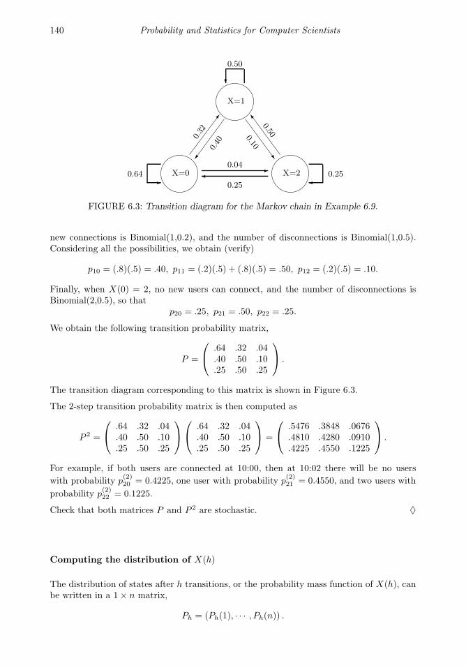
140 Probability and Statistics for Computer Scientists
X=0
X=1
X=2
♦
0.64 0.250.04
0.25
0.50
0.32
0.40
0.500.10FIGURE 6.3: Transition diagram for the Markov chain in Example 6.9.
new connections is Binomial(1,0.2), and the number of disconnections is Binomial(1,0.5).Considering all the possibilities, we obtain (verify)
p10 = (.8)(.5) = .40, p11 = (.2)(.5) + (.8)(.5) = .50, p12 = (.2)(.5) = .10.
Finally, when X(0) = 2, no new users can connect, and the number of disconnections isBinomial(2,0.5), so that
p20 = .25, p21 = .50, p22 = .25.
We obtain the following transition probability matrix,
P =
.64 .32 .04
.40 .50 .10
.25 .50 .25
.
The transition diagram corresponding to this matrix is shown in Figure 6.3.
The 2-step transition probability matrix is then computed as
P 2 =
.64 .32 .04
.40 .50 .10
.25 .50 .25
.64 .32 .04
.40 .50 .10
.25 .50 .25
=
.5476 .3848 .0676
.4810 .4280 .0910
.4225 .4550 .1225
.
For example, if both users are connected at 10:00, then at 10:02 there will be no users
with probability p(2)20 = 0.4225, one user with probability p
(2)21 = 0.4550, and two users with
probability p(2)22 = 0.1225.
Check that both matrices P and P 2 are stochastic. ♦
Computing the distribution of X(h)
The distribution of states after h transitions, or the probability mass function of X(h), canbe written in a 1× n matrix,
Ph = (Ph(1), · · · , Ph(n)) .

Stochastic Processes 141
By the Law of Total Probability, this time conditioning on X(0) = k, we compute
Ph(j) = P X(h) = j =∑
k
P X(0) = kP X(h) = j | X(0) = k
=∑
k
P0(k)p(h)kj =
(P0(1) · · · P0(n)
)
p(h)1j...
p(h)1n
.
Each probability Ph(j) is obtained when the entire row P0 (initial distribution of X) ismultiplied by the entire j-th column of matrix P . Hence,
Distributionof X(h)
Ph = P0Ph (6.4)
Example 6.10 (Shared device, continued). If we know that there are 2 users con-nected at 10:00, we can write the initial distribution as
P0 = (0, 0, 1) .
Then the distribution of the number of users at 10:02, after h = 2 transitions, is computedas
P2 = P0P2 = (0, 0, 1)
.5476 .3848 .0676
.4810 .4280 .0910
.4225 .4550 .1225
= (.4225, .4550, .1225) ,
just as we concluded in the end of Example 6.9.
Suppose that all states are equally likely at 10:00. How can we compute the probability of1 connected user at 10:02? Here, the initial distribution is
P0 = (1/3, 1/3, 1/3) .
The distribution of X(2) is
P2 = P0P2 = (1/3, 1/3, 1/3)
.5476 .3848 .0676
.4810 .4280 .0910
.4225 .4550 .1225
= (. . . , .4226, . . .) .
Thus, P X(2) = 1 = 0.4226. We only computed P2(1). The question did not requirecomputation of the entire distribution P2. ♦
In practice, knowing the distribution of the number of users at 10:00, one would rarely beinterested in the distribution at 10:02. How should one figure the distribution at 11:00, thenext day, or the next month?
In other words, how does one compute the distribution of X(h) for large h? A direct so-lution is Ph = P0 · P h, which can be computed for moderate n and h. For example, thedistribution of the number of users at 11:00, h = 60 transitions after 10:00, can be computedin MATLAB as
142 Probability and Statistics for Computer Scientists
P = [ .64 .32 .04
.40 .50 .10
.25 .50 .25 ];
P0 = [ 1/3 1/3 1/3 ];
h = 60;
P0*Pˆh
For large h, one would really like to take a limit of Ph as h → ∞ instead of a tediouscomputation of P0 · P h. We learn how to do it in the next section.
6.2.3 Steady-state distribution
This section discusses the distribution of states of a Markov chain after a large number oftransitions.
DEFINITION 6.8
A collection of limiting probabilities
πx = limh→∞
Ph(x)
is called a steady-state distribution of a Markov chain X(t).
When this limit exists, it can be used as a forecast of the distribution of X after many tran-sitions. A fast system (say, a central processing unit with a clock rate of several gigahertz),will go through a very large number of transitions very quickly. Then, its distribution ofstates at virtually any time is the steady-state distribution.
Computing the steady-state distribution
When a steady-state distribution π exists, it can be computed as follows. We notice that πis a limit of not only Ph but also Ph+1. The latter two are related by the formula
PhP = P0PhP = P0P
h+1 = Ph+1.
Taking the limit of Ph and Ph+1, as h → ∞, we obtain
πP = π. (6.5)
Then, solving (6.5) for π, we get the steady-state distribution of a Markov chain with atransition probability matrix P .
The system of steady-state equations (6.5) consists of n equations with n unknowns whichare probabilities of n states. However, this system is singular; it has infinitely many solutions.That is because both sides of the system (6.5) can be multiplied by any constant C, andthus, any multiple of π is also a solution of (6.5).
There is yet one more condition that we have not used. Being a distribution, all the proba-bilities πx must add to 1,
π1 + . . .+ πn = 1.
Only one solution of (6.5) can satisfy this condition, and this is the steady-state distribution.
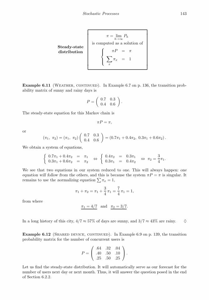
Stochastic Processes 143
Steady-statedistribution
π = limh→∞
Ph
is computed as a solution of
πP = π∑
x
πx = 1
Example 6.11 (Weather, continued). In Example 6.7 on p. 136, the transition prob-ability matrix of sunny and rainy days is
P =
(0.7 0.30.4 0.6
).
The steady-state equation for this Markov chain is
πP = π,
or
(π1, π2) = (π1, π2)
(0.7 0.30.4 0.6
)= (0.7π1 + 0.4π2, 0.3π1 + 0.6π2) .
We obtain a system of equations,
0.7π1 + 0.4π2 = π1
0.3π1 + 0.6π2 = π2⇔
0.4π2 = 0.3π1
0.3π1 = 0.4π2⇔ π2 =
3
4π1.
We see that two equations in our system reduced to one. This will always happen: oneequation will follow from the others, and this is because the system πP = π is singular. Itremains to use the normalizing equation
∑πx = 1,
π1 + π2 = π1 +3
4π1 =
7
4π1 = 1,
from whereπ1 = 4/7 and π2 = 3/7.
In a long history of this city, 4/7 ≈ 57% of days are sunny, and 3/7 ≈ 43% are rainy. ♦
Example 6.12 (Shared device, continued). In Example 6.9 on p. 139, the transitionprobability matrix for the number of concurrent users is
P =
.64 .32 .04
.40 .50 .10
.25 .50 .25
.
Let us find the steady-state distribution. It will automatically serve as our forecast for thenumber of users next day or next month. Thus, it will answer the question posed in the endof Section 6.2.2.

144 Probability and Statistics for Computer Scientists
The steady-state equations are:
.64π0 + .40π1 + .25π2 = π0
.32π0 + .50π1 + .50π2 = π1
.04π0 + .10π1 + .25π2 = π2
;
−.36π0 + .40π1 + .25π2 = 0.32π0 − .50π1 + .50π2 = 0.04π0 + .10π1 − .75π2 = 0
Solving this system by method of elimination, we express π2 from the first equation andsubstitute into the other equations,
π2 = 1.44π0 − 1.6π1
.32π0 − .50π1 + .50(1.44π0 − 1.6π1) = 0
.04π0 + .10π1 − .75(1.44π0 − 1.6π1) = 0;
π2 = 1.44π0 − 1.6π1
1.04π0 − 1.3π1 = 0−1.04π0 + 1.3π1 = 0
The last two equations are equivalent. This was anticipated; one equation should alwaysfollow from the others, so we are “probably” on a right track.
Express π1 from the second equation and substitute into the first one,
π2 = 1.44π0 − 1.6(.8π0)π1 = .8π0
;
π2 = .16π0
π1 = .8π0
Finally, use the normalizing equation,
π0 + π1 + π2 = π0 + .8π0 + .16π0 = 1.96π0 = 1,
from where we compute the answer,
π0 = 1/1.96 = .5102π1 = .8(.5102) = .4082π2 = .16(.5102) = .0816
This is a direct but a little longer way of finding the steady-state distribution π. For thisparticular problem, a shorter solution is offered in Exercise 6.25.
♦
The limit of P h
Then, what will the h-step transition probabilities be for large h? It turns out that matrixP (h) also has a limit, as h → ∞, and the limiting matrix has the form
Π = limh→∞
P (h) =
π1 π2 · · · πn
π1 π2 · · · πn
...... · · ·
...π1 π2 · · · πn
.
All the rows of the limiting matrix Π are equal, and they consist of the steady-state prob-abilities πx!
How can this phenomenon be explained? First, the forecast for some very remote futureshould not depend on the current state X(0). Say, our weather forecast for the next centuryshould not depend on the weather we have today. Therefore, pik = pjk for all i, j, k, andthis is why all rows of Π coincide.
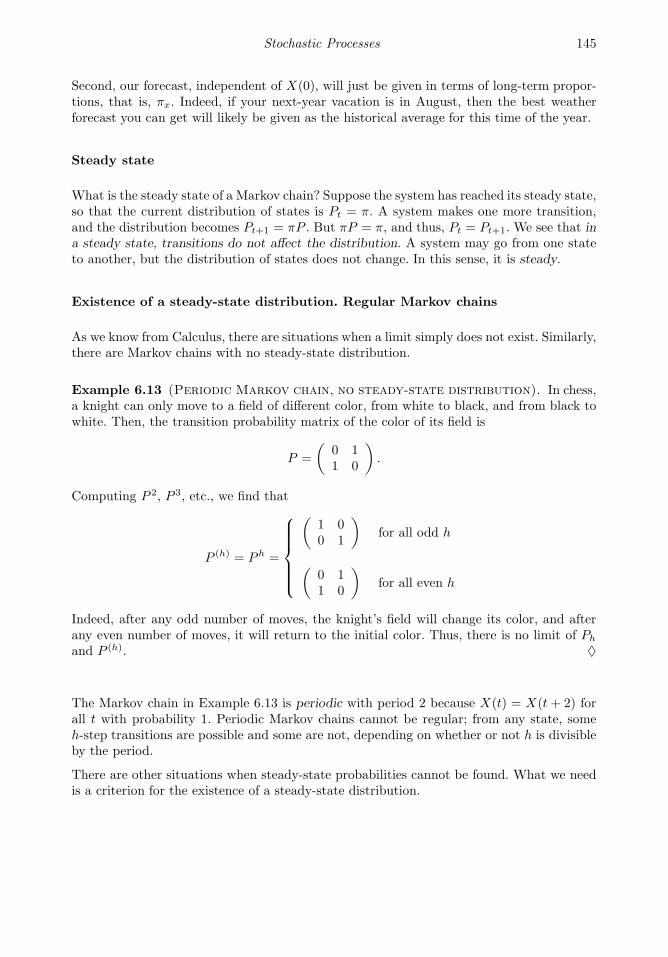
Stochastic Processes 145
Second, our forecast, independent of X(0), will just be given in terms of long-term propor-tions, that is, πx. Indeed, if your next-year vacation is in August, then the best weatherforecast you can get will likely be given as the historical average for this time of the year.
Steady state
What is the steady state of a Markov chain? Suppose the system has reached its steady state,so that the current distribution of states is Pt = π. A system makes one more transition,and the distribution becomes Pt+1 = πP . But πP = π, and thus, Pt = Pt+1. We see that ina steady state, transitions do not affect the distribution. A system may go from one stateto another, but the distribution of states does not change. In this sense, it is steady.
Existence of a steady-state distribution. Regular Markov chains
As we know from Calculus, there are situations when a limit simply does not exist. Similarly,there are Markov chains with no steady-state distribution.
Example 6.13 (Periodic Markov chain, no steady-state distribution). In chess,a knight can only move to a field of different color, from white to black, and from black towhite. Then, the transition probability matrix of the color of its field is
P =
(0 11 0
).
Computing P 2, P 3, etc., we find that
P (h) = P h =
(1 00 1
)for all odd h
(0 11 0
)for all even h
Indeed, after any odd number of moves, the knight’s field will change its color, and afterany even number of moves, it will return to the initial color. Thus, there is no limit of Ph
and P (h). ♦
The Markov chain in Example 6.13 is periodic with period 2 because X(t) = X(t+ 2) forall t with probability 1. Periodic Markov chains cannot be regular; from any state, someh-step transitions are possible and some are not, depending on whether or not h is divisibleby the period.
There are other situations when steady-state probabilities cannot be found. What we needis a criterion for the existence of a steady-state distribution.

146 Probability and Statistics for Computer Scientists
DEFINITION 6.9
A Markov chain is regular if
p(h)ij > 0
for some h and all i, j. That is, for some h, matrix P (h) has only non-zeroentries, and h-step transitions from any state to any state are possible.
Any regular Markov chain has a steady-state distribution.
Example 6.14. Markov chains in Examples 6.7 and 6.9 are regular because all transitionsare possible for h = 1 already, and matrix P does not contain any zeros. ♦
Example 6.15. A Markov chain with transition probability matrix
P =
0 1 0 00 0 1 00 0 0 10.9 0 0 0.1
.
is also regular. Matrix P contains zeros, and so do P 2, P 3, P 4, and P 5. The 6-step transitionprobability matrix
P (6) =
.009 .090 .900 .001
.001 .009 .090 .900
.810 .001 .009 .180
.162 .810 .001 .027
contains no zeros and proves regularity of this Markov chain.
In fact, computation of all P h up to h = 6 is not required in this problem. Regularity canalso be seen from the transition diagram in Figure 6.4. Based on this diagram, any state jcan be reached in 6 steps from any state i. Indeed, moving counterclockwise through thisFigure, we can reach state 4 from any state i in ≤ 3 steps. Then, we can reach state j fromstate 4 in ≤ 3 additional steps, for the total of ≤ 6 steps. If we can reach state i from state jin fewer than 6 steps, we just use the remaining steps circling around state 4. For example,state 2 is reached from state 1 in 6 steps as follows:
1 → 2 → 3 → 4 → 4 → 1 → 2.
Notice that we don’t have to compute p(h)ij . We only need to verify that they are all positive
for some h. ♦
Example 6.16 (Irregular Markov chain, absorbing states). When there is a statei with pii = 1, a Markov chain cannot be regular. There is no exit from state i; therefore,
p(h)ij = 0 for all h and all j 6= i. Such a state is called absorbing. For example, state 4 in
Figure 6.5a is absorbing, therefore, the Markov chain is irregular.
There may be several absorbing states or an entire absorbing zone, from which the remainingstates can never be reached. For example, states 3, 4, and 5 in Figure 6.5b form an absorbingzone, some kind of a Bermuda triangle. When this process finds itself in the set 3, 4, 5,there is no route from there to the set 1, 2. As a result, probabilities p
(h)31 , p
(h)52 and some

Stochastic Processes 147
1
2 3
4
1
1
1
0.9
0.1
FIGURE 6.4: Transition diagram for a regular Markov chain in Example 6.15.
(a) (b)
1
2 3
4
⑦
⑥
1
2
3
4
5
❨
FIGURE 6.5: Absorbing states and absorbing zones (Example 6.16).
others equal 0 for all h. Although all pij may be less than 1, such Markov chains are stillirregular.
Notice that both Markov chains do have steady-state distributions. The first process willeventually reach state 4 and will stay there for good. Therefore, the limiting distribution ofX(h) is π = limPh = (0, 0, 0, 1). The second Markov chain will eventually leave states 1 and2 for good, thus its limiting (steady-state) distribution has the form π = (0, 0, π3, π4, π5). ♦
Conclusion
This section gives us an important method of analyzing rather complicated stochastic sys-tems. Once the Markov property of a process is established, it only remains to find itsone-step transition probabilities. Then, the steady-state distribution can be computed, andthus, we obtain the distribution of the process at any time, after a sufficient number oftransitions.
This methodology will be our main working tool in Chapter 7, when we study queuingsystems and evaluate their performance.
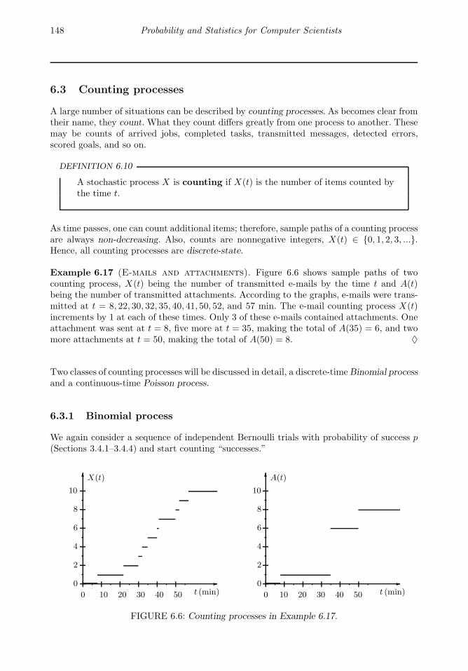
148 Probability and Statistics for Computer Scientists
6.3 Counting processes
A large number of situations can be described by counting processes. As becomes clear fromtheir name, they count. What they count differs greatly from one process to another. Thesemay be counts of arrived jobs, completed tasks, transmitted messages, detected errors,scored goals, and so on.
DEFINITION 6.10
A stochastic process X is counting if X(t) is the number of items counted bythe time t.
As time passes, one can count additional items; therefore, sample paths of a counting processare always non-decreasing. Also, counts are nonnegative integers, X(t) ∈ 0, 1, 2, 3, ....Hence, all counting processes are discrete-state.
Example 6.17 (E-mails and attachments). Figure 6.6 shows sample paths of twocounting process, X(t) being the number of transmitted e-mails by the time t and A(t)being the number of transmitted attachments. According to the graphs, e-mails were trans-mitted at t = 8, 22, 30, 32, 35, 40, 41, 50, 52, and 57 min. The e-mail counting process X(t)increments by 1 at each of these times. Only 3 of these e-mails contained attachments. Oneattachment was sent at t = 8, five more at t = 35, making the total of A(35) = 6, and twomore attachments at t = 50, making the total of A(50) = 8. ♦
Two classes of counting processes will be discussed in detail, a discrete-time Binomial processand a continuous-time Poisson process.
6.3.1 Binomial process
We again consider a sequence of independent Bernoulli trials with probability of success p(Sections 3.4.1–3.4.4) and start counting “successes.”
0
2
4
6
8
10
0 10 20 30 40 50 t (min)
X(t)
0
2
4
6
8
10
0 10 20 30 40 50 t (min)
A(t)
FIGURE 6.6: Counting processes in Example 6.17.
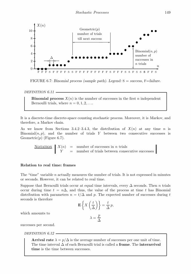
Stochastic Processes 149
X(n)
n0
2
4
6
8
10
F F F S F F F F S S F F F F F F F F F S F F F S S F S S SS F F S
∆
Binomial(n, p)number ofsuccesses inn trials
Geometric(p)
number of trials
till next success
FIGURE 6.7: Binomial process (sample path). Legend: S = success, F=failure.
DEFINITION 6.11
Binomial process X(n) is the number of successes in the first n independentBernoulli trials, where n = 0, 1, 2, . . ..
It is a discrete-time discrete-space counting stochastic process. Moreover, it is Markov, andtherefore, a Markov chain.
As we know from Sections 3.4.2–3.4.3, the distribution of X(n) at any time n isBinomial(n, p), and the number of trials Y between two consecutive successes isGeometric(p) (Figure 6.7).
Notation X(n) = number of successes in n trialsY = number of trials between consecutive successes
Relation to real time: frames
The “time” variable n actually measures the number of trials. It is not expressed in minutesor seconds. However, it can be related to real time.
Suppose that Bernoulli trials occur at equal time intervals, every ∆ seconds. Then n trialsoccur during time t = n∆, and thus, the value of the process at time t has Binomialdistribution with parameters n = t/∆ and p. The expected number of successes during tseconds is therefore
E
X
(t
∆
)=
t
∆p,
which amounts toλ =
p
∆successes per second.
DEFINITION 6.12
Arrival rate λ = p/∆ is the average number of successes per one unit of time.The time interval ∆ of each Bernoulli trial is called a frame. The interarrivaltime is the time between successes.
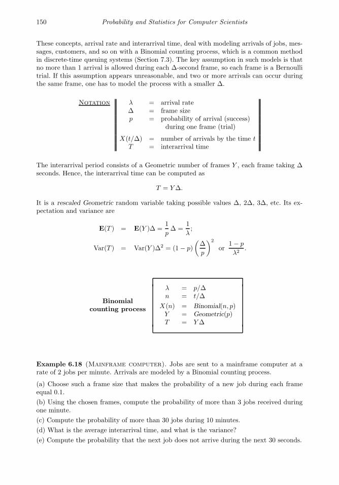
150 Probability and Statistics for Computer Scientists
These concepts, arrival rate and interarrival time, deal with modeling arrivals of jobs, mes-sages, customers, and so on with a Binomial counting process, which is a common methodin discrete-time queuing systems (Section 7.3). The key assumption in such models is thatno more than 1 arrival is allowed during each ∆-second frame, so each frame is a Bernoullitrial. If this assumption appears unreasonable, and two or more arrivals can occur duringthe same frame, one has to model the process with a smaller ∆.
Notation λ = arrival rate∆ = frame sizep = probability of arrival (success)
during one frame (trial)
X(t/∆) = number of arrivals by the time tT = interarrival time
The interarrival period consists of a Geometric number of frames Y , each frame taking ∆seconds. Hence, the interarrival time can be computed as
T = Y∆.
It is a rescaled Geometric random variable taking possible values ∆, 2∆, 3∆, etc. Its ex-pectation and variance are
E(T ) = E(Y )∆ =1
p∆ =
1
λ;
Var(T ) = Var(Y )∆2 = (1− p)
(∆
p
)2
or1− p
λ2.
Binomialcounting process
λ = p/∆n = t/∆
X(n) = Binomial(n, p)Y = Geometric(p)T = Y∆
Example 6.18 (Mainframe computer). Jobs are sent to a mainframe computer at arate of 2 jobs per minute. Arrivals are modeled by a Binomial counting process.
(a) Choose such a frame size that makes the probability of a new job during each frameequal 0.1.
(b) Using the chosen frames, compute the probability of more than 3 jobs received duringone minute.
(c) Compute the probability of more than 30 jobs during 10 minutes.
(d) What is the average interarrival time, and what is the variance?
(e) Compute the probability that the next job does not arrive during the next 30 seconds.
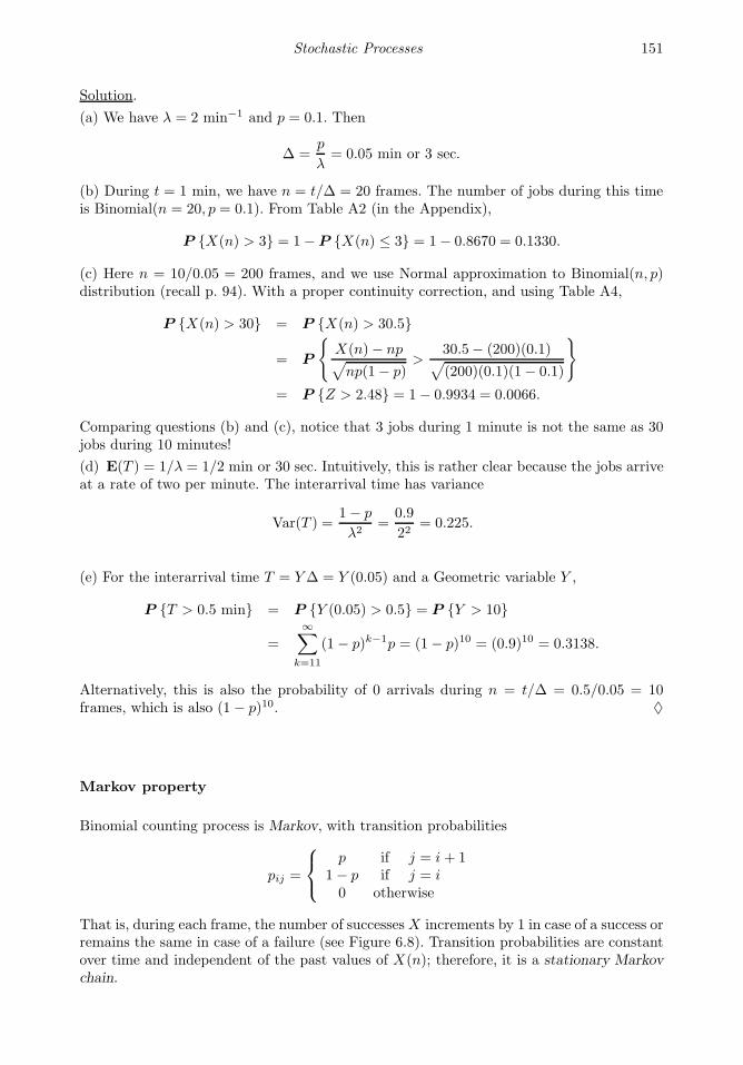
Stochastic Processes 151
Solution.
(a) We have λ = 2 min−1 and p = 0.1. Then
∆ =p
λ= 0.05 min or 3 sec.
(b) During t = 1 min, we have n = t/∆ = 20 frames. The number of jobs during this timeis Binomial(n = 20, p = 0.1). From Table A2 (in the Appendix),
P X(n) > 3 = 1− P X(n) ≤ 3 = 1− 0.8670 = 0.1330.
(c) Here n = 10/0.05 = 200 frames, and we use Normal approximation to Binomial(n, p)distribution (recall p. 94). With a proper continuity correction, and using Table A4,
P X(n) > 30 = P X(n) > 30.5
= P
X(n)− np√np(1− p)
>30.5− (200)(0.1)√(200)(0.1)(1− 0.1)
= P Z > 2.48 = 1− 0.9934 = 0.0066.
Comparing questions (b) and (c), notice that 3 jobs during 1 minute is not the same as 30jobs during 10 minutes!
(d) E(T ) = 1/λ = 1/2 min or 30 sec. Intuitively, this is rather clear because the jobs arriveat a rate of two per minute. The interarrival time has variance
Var(T ) =1− p
λ2=
0.9
22= 0.225.
(e) For the interarrival time T = Y∆ = Y (0.05) and a Geometric variable Y ,
P T > 0.5 min = P Y (0.05) > 0.5 = P Y > 10
=
∞∑
k=11
(1− p)k−1p = (1− p)10 = (0.9)10 = 0.3138.
Alternatively, this is also the probability of 0 arrivals during n = t/∆ = 0.5/0.05 = 10frames, which is also (1 − p)10. ♦
Markov property
Binomial counting process is Markov, with transition probabilities
pij =
p if j = i + 11− p if j = i0 otherwise
That is, during each frame, the number of successesX increments by 1 in case of a success orremains the same in case of a failure (see Figure 6.8). Transition probabilities are constantover time and independent of the past values of X(n); therefore, it is a stationary Markovchain.

152 Probability and Statistics for Computer Scientists
0 1 2 3
p p p p
1− p 1− p 1− p 1− p
FIGURE 6.8: Transition diagram for a Binomial counting process.
This Markov chain is irregular because X(n) is non-decreasing, thus p(h)10 = 0 for all h. Once
we see one success, the number of successes will never return to zero. Thus, this process hasno steady-state distribution.
The h-step transition probabilities simply form a Binomial distribution. Indeed, p(h)ij is the
probability of going from i to j successes in h transitions, i.e.,
p(h)ij = P (j − i) successes in h trials
=
(h
j − i
)pj−i(1− p)h−j+i if 0 ≤ j − i ≤ h
0 otherwise
Notice that the transition probability matrix has ∞ rows and ∞ columns because X(n)can reach any large value for sufficiently large n:
P =
1− p p 0 0 · · ·0 1− p p 0 · · ·0 0 1− p p · · ·0 0 0 1− p · · ·· · · · · · · · · · · · · · ·
6.3.2 Poisson process
Continuous time
We now turn attention to continuous-time stochastic processes. The time variable t willrun continuously through the whole interval, and thus, even during one minute there willbe infinitely many moments when the process X(t) may change. Then, how can one studysuch models?
Often a continuous-time process can be viewed as a limit of some discrete-time processwhose frame size gradually decreases to zero, therefore allowing more frames during anyfixed period of time,
∆ ↓ 0 and n ↑ ∞.
Example 6.19. For illustration, let us recall how movies are made. Although all motionson the screen seem continuous, we realize that an infinite amount of information could notbe stored in a video cassette. Instead, we see a discrete sequence of exposures that run sofast that each motion seems continuous and smooth.

Stochastic Processes 153
∆ = 0.16 sec ∆ = 0.04 sec
FIGURE 6.9: From discrete motion to continuous motion: reducing the frame size ∆.
Early-age video cameras shot exposures rather slowly; the interval ∆ between successiveshots was pretty long (∼ 0.2–0.5 sec). As a result, the quality of recorded video was ratherlow. Movies were “too discrete.”
Modern camcorders can shoot up to 200 exposures per second attaining ∆ = 0.005. Withsuch a small ∆, the resulting movie seems perfectly continuous. A shorter frame ∆ resultsin a “more continuous” process (Figure 6.9). ♦
Poisson process as the limiting case
Going from discrete time to continuous time, Poisson process is the limiting case of aBinomial counting process as ∆ ↓ 0.
DEFINITION 6.13
Poisson process is a continuous-time counting stochastic process obtainedfrom a Binomial counting process when its frame size ∆ decreases to 0 whilethe arrival rate λ remains constant.
We can now study a Poisson process by taking a Binomial counting process and letting itsframe size decrease to zero.
Consider a Binomial counting process that counts arrivals or other events occurring at arate λ. Let X(t) denote the number of arrivals occurring until time t. What will happenwith this process if we let its frame size ∆ converge to 0?
The arrival rate λ remains constant. Arrivals occur at the same rate (say, messages arriveat a server) regardless of your choice of frame ∆.
The number of frames during time t increases to infinity,
n =t
∆↑ ∞ as ∆ ↓ 0.
The probability of an arrival during each frame is proportional to ∆, so it also decreases to0,
p = λ∆ ↓ 0 as ∆ ↓ 0.

154 Probability and Statistics for Computer Scientists
Then, the number of arrivals during time t is a Binomial(n, p) variable with expectation
EX(t) = np =tp
∆= λt.
In the limiting case, as ∆ ↓ 0, n ↑ ∞, and p ↓ 0, it becomes a Poisson variable withparameter np = λt,
X(t) = Binomial(n, p) → Poisson(λ)
(if in doubt, see p. 66).
The interarrival time T becomes a random variable with the c.d.f.
FT (t) = P T ≤ t = P Y ≤ n because T = Y∆ and t = n∆
= 1− (1− p)n Geometric distribution of Y
= 1−(1− λt
n
)n
because p = λ∆ = λt/n
→ 1− eλt.This is the “Euler limit”:(1 + x/n)n → ex as n → ∞
What we got is the c.d.f. of Exponential distribution! Hence, the interarrival time is Expo-nential with parameter λ.
Further, the time Tk of the k-th arrival is the sum of k Exponential interrarival times that hasGamma(k, λ) distribution. From this, we immediately obtain our familiar Gamma-Poissonformula (4.14),
P Tk ≤ t = P k-th arrival before time t = P X(t) ≥ k
where Tk is Gamma(k, λ) and X(t) is Poisson(λt).
Poisson process
X(t) = Poisson(λt)T = Exponential(λ)Tk = Gamma(k, λ)
P Tk ≤ t = P X(t) ≥ kP Tk > t = P X(t) < k
A sample path of some Poisson process is shown in Figure 6.10.
Example 6.20 (Web site hits). The number of hits to a certain web site follows aPoisson process with the intensity parameter λ = 7 hits per minute.
On the average, how much time is needed to get 10,000 hits? What is the probability thatthis will happen within 24 hours?
Solution. The time of the 10, 000-th hit Tk has Gamma distribution with parameters k =10, 000 and λ = 7 min−1. Then, the expected time of the k-th hit is
µ = E(Tk) =k
λ= 1,428.6 min or 23.81 hrs.
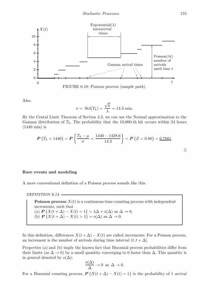
Stochastic Processes 155
X(t)
t0
2
4
6
8
10
0
Gamma arrival times
❯ ❫
Poisson(λt)number ofarrivalsuntil time t
Exponential(λ)interarrival
times
FIGURE 6.10: Poisson process (sample path).
Also,
σ = Std(Tk) =
√k
λ= 14.3 min.
By the Cental Limit Theorem of Section 4.3, we can use the Normal approximation to theGamma distribution of Tk. The probability that the 10,000-th hit occurs within 24 hours(1440 min) is
P Tk < 1440 = P
Tk − µ
σ<
1440− 1428.6
14.3
= P Z < 0.80 = 0.7881.
♦
Rare events and modeling
A more conventional definition of a Poisson process sounds like this.
DEFINITION 6.14
Poisson process X(t) is a continuous-time counting process with independentincrements, such that(a) P X(t+∆)−X(t) = 1 = λ∆+ o(∆) as ∆ → 0;(b) P X(t+∆)−X(t) > 1 = o(∆) as ∆ → 0.
In this definition, differences X(t+∆)−X(t) are called increments. For a Poisson process,an increment is the number of arrivals during time interval (t, t+∆].
Properties (a) and (b) imply the known fact that Binomial process probabilities differ fromtheir limits (as ∆ → 0) by a small quantity converging to 0 faster than ∆. This quantity isin general denoted by o(∆);
o(∆)
∆→ 0 as ∆ → 0.
For a Binomial counting process, P X(t+∆)−X(t) = 1 is the probability of 1 arrival
156 Probability and Statistics for Computer Scientists
during 1 frame, and it equals p = λ∆, whereas the probability of more than 1 arrival iszero. For the Poisson process, these probabilities may be different, but only by a little.
The last definition describes formally what we called rare events. These events occur atrandom times; probability of a new event during a short interval of time is proportionalto the length of this interval. Probability of more than 1 event during that time is muchsmaller comparing with the length of such interval. For such sequences of events a Poissonprocess is a suitable stochastic model. Examples of rare events include telephone calls,message arrivals, virus attacks, errors in codes, traffic accidents, natural disasters, networkblackouts, and so on.
Example 6.21 (Mainframe computer, revisited). Let us now model the job arrivalsin Example 6.18 on p. 150 with a Poisson process. Keeping the same arrival rate λ = 2min−1, this will remove a perhaps unnecessary assumption that no more than 1 job canarrive during any given frame.
Revisiting questions (b)–(e) in Example 6.18, we now obtain,
(b) The probability of more than 3 jobs during 1 minute is
P X(1) > 3 = 1− P X(1) ≤ 3 = 1− 0.8571 = 0.1429,
from Table A3 with parameter λt = (2)(1) = 2.
(c) The probability of more than 30 jobs during 10 minutes is
P X(10) > 30 = 1− P X(10) ≤ 30 = 1− 0.9865 = 0.0135,
from Table A3 with parameter λt = (2)(10) = 20.
(d) For the Exponential(λ = 2) distribution of interarrival times, we get again that
E(T ) =1
λ= 0.5 min or 30 sec.
This is because the jobs arrive to the computer at the same rate regardless of whether wemodel their arrivals with a Binomial or Poisson process. Also,
Var(T ) =1
λ2= 0.25.
(e) The probability that the next job does not arrive during the next 30 seconds is
P T > 0.5 min = e−λ(0.5) = e−1 = 0.3679.
Alternatively, this is also the probability of 0 arrivals during 0.5 min, i.e.,
P X(0.5) = 0 = 0.3679,
from Table A3 with parameter λt = (2)(0.5) = 1.
We see that most of the results are somewhat different from Example 6.18, where the sameevents were modeled by a Binomial counting process. Noticeably, the variance of interarrivaltimes increased. Binomial process introduces a restriction on the number of arrivals duringeach frame, therefore reducing variability. ♦
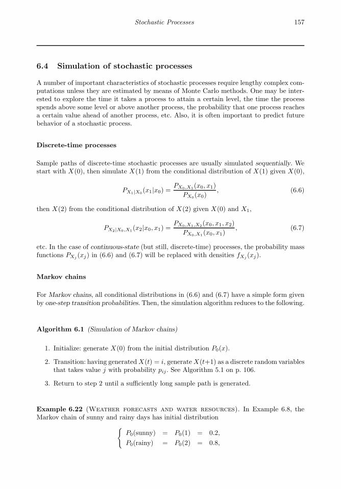
Stochastic Processes 157
6.4 Simulation of stochastic processes
A number of important characteristics of stochastic processes require lengthy complex com-putations unless they are estimated by means of Monte Carlo methods. One may be inter-ested to explore the time it takes a process to attain a certain level, the time the processspends above some level or above another process, the probability that one process reachesa certain value ahead of another process, etc. Also, it is often important to predict futurebehavior of a stochastic process.
Discrete-time processes
Sample paths of discrete-time stochastic processes are usually simulated sequentially. Westart with X(0), then simulate X(1) from the conditional distribution of X(1) given X(0),
PX1|X0(x1|x0) =
PX0,X1(x0, x1)
PX0(x0)
, (6.6)
then X(2) from the conditional distribution of X(2) given X(0) and X1,
PX2|X0,X1(x2|x0, x1) =
PX0,X1,X2(x0, x1, x2)
PX0,X1(x0, x1)
, (6.7)
etc. In the case of continuous-state (but still, discrete-time) processes, the probability massfunctions PXj
(xj) in (6.6) and (6.7) will be replaced with densities fXj(xj).
Markov chains
For Markov chains, all conditional distributions in (6.6) and (6.7) have a simple form givenby one-step transition probabilities. Then, the simulation algorithm reduces to the following.
Algorithm 6.1 (Simulation of Markov chains)
1. Initialize: generate X(0) from the initial distribution P0(x).
2. Transition: having generatedX(t) = i, generateX(t+1) as a discrete random variablesthat takes value j with probability pij . See Algorithm 5.1 on p. 106.
3. Return to step 2 until a sufficiently long sample path is generated.
Example 6.22 (Weather forecasts and water resources). In Example 6.8, theMarkov chain of sunny and rainy days has initial distribution
P0(sunny) = P0(1) = 0.2,
P0(rainy) = P0(2) = 0.8,

158 Probability and Statistics for Computer Scientists
and transition probability matrix
P =
(0.7 0.30.4 0.6
).
For simplicity, sunny days are denoted by X = 1, and rainy days by X = 2. The followingMATLAB code will generate the forecast for the next 100 days.
N = 100; % length of sample path
X = zeros(N,1);
p = [0.2 0.8]; % initial distribution
P = [0.7 0.3; 0.4 0.6]; % transition probability matrix
U = rand(N,1); % N Uniform variables to start with
for t=1:N; % simulate X(1),...,X(N) sequentially
X(t) = 1*( U(t) <= p(1) ) + 2*( U(t) > p(1) );
% X(t)=1 with probability p(1) and
% X(t)=2 with probability 1-p(1)=p(2)
p = P(X(t),:); % prepare the distribution of X(t+1);
% its pmf is X(t)th row of matrix P
end; X
This program returns a sequence of states that looks like this:
2211122212221121111111122222222112111222211111111112221211221...
Notice fairly long segments of sunny days (X = 1) and rainy days (X = 2), showingdependence among the generated variables. This is because a sunny day is more likely tobe followed by another sunny day, and a rainy day is more likely to be followed by a rainyday.
Generating a large number of such sequences, we can estimate, say, the probability of 20consecutive days without rain at least once during the next year, the average time betweensuch droughts, the expected number of times this may happen during the same year, etc.As an immediate application, based on this, water resources can be allocated accordingly.♦
Binomial process
Simulation of a Binomial process is rather straightforward, as it is based on a sequence ofindependent Bernoulli trials. After simulating such a sequence, compute partial sums asfollows.
N = 100; p = 0.4;
X = zeros(N,1); % initialization
Y = (rand(N,1) < p); % sequence of Bernoulli(p) variables
X(1) = Y(1);
for t=2:N; % X(t) is the number of successes
X(t)=X(t-1)+Y(t); % in the first t trials
end; X
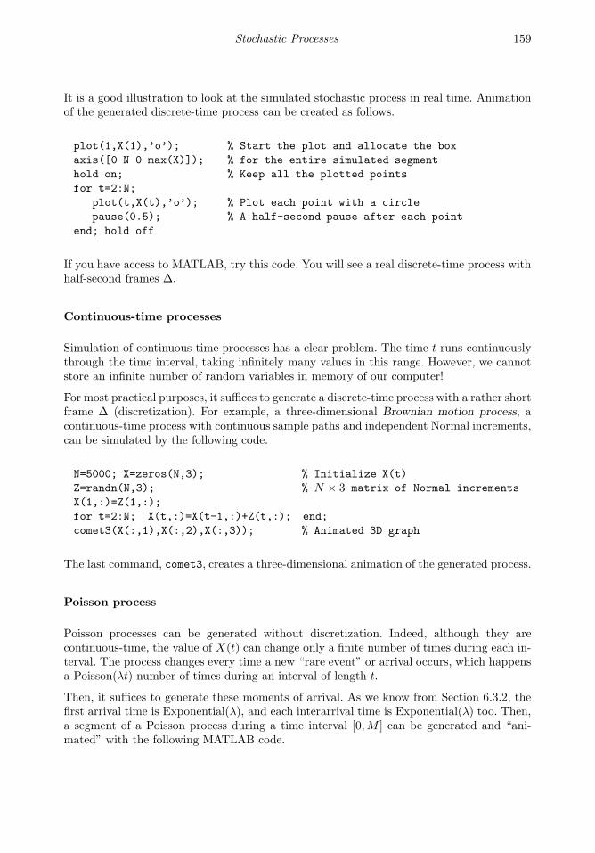
Stochastic Processes 159
It is a good illustration to look at the simulated stochastic process in real time. Animationof the generated discrete-time process can be created as follows.
plot(1,X(1),’o’); % Start the plot and allocate the box
axis([0 N 0 max(X)]); % for the entire simulated segment
hold on; % Keep all the plotted points
for t=2:N;
plot(t,X(t),’o’); % Plot each point with a circle
pause(0.5); % A half-second pause after each point
end; hold off
If you have access to MATLAB, try this code. You will see a real discrete-time process withhalf-second frames ∆.
Continuous-time processes
Simulation of continuous-time processes has a clear problem. The time t runs continuouslythrough the time interval, taking infinitely many values in this range. However, we cannotstore an infinite number of random variables in memory of our computer!
For most practical purposes, it suffices to generate a discrete-time process with a rather shortframe ∆ (discretization). For example, a three-dimensional Brownian motion process, acontinuous-time process with continuous sample paths and independent Normal increments,can be simulated by the following code.
N=5000; X=zeros(N,3); % Initialize X(t)
Z=randn(N,3); % N × 3 matrix of Normal increments
X(1,:)=Z(1,:);
for t=2:N; X(t,:)=X(t-1,:)+Z(t,:); end;
comet3(X(:,1),X(:,2),X(:,3)); % Animated 3D graph
The last command, comet3, creates a three-dimensional animation of the generated process.
Poisson process
Poisson processes can be generated without discretization. Indeed, although they arecontinuous-time, the value of X(t) can change only a finite number of times during each in-terval. The process changes every time a new “rare event” or arrival occurs, which happensa Poisson(λt) number of times during an interval of length t.
Then, it suffices to generate these moments of arrival. As we know from Section 6.3.2, thefirst arrival time is Exponential(λ), and each interarrival time is Exponential(λ) too. Then,a segment of a Poisson process during a time interval [0,M ] can be generated and “ani-mated” with the following MATLAB code.

160 Probability and Statistics for Computer Scientists
M=1000; lambda=0.04;
S=0; T=0; % T is a growing vector of arrival times
while S<=M; % Loop ends when arrival time S exceeds M
Y=-1/lambda * log(rand); % Exponential interarrival time
S=S+Y; % new arrival time
T=[T S]; % vector of arrival times extends
end; % by one element
N=length(T); % generated number of arrivals
X=zeros(M,1); % initialize the Poisson process
for t=1:M;
X(t)=sum(T<=t); % X(t) is the number of arrivals
end; % by the time t
comet(X); % Animation of the generated process!
Summary and conclusions
Stochastic processes are random variables that change, evolve, and develop in time. Thereare discrete- and continuous-time, discrete- and continuous-state processes, depending ontheir possible times and possible values.
Markov processes form an important class, where only the most recent value of the processis needed to predict its future probabilities. Then, a Markov chain is fully described by itsinitial distribution and transition probabilities. Its limiting behavior, after a large numberof transitions, is determined by a steady-state distribution which we compute by solving asystem of steady-state equations. Binomial and Poisson counting processes are both Markov,with discrete and continuous time, respectively.
Thus we developed an important tool for studying rather complex stochastic (involvinguncertainty) systems. As long as the process is Markov, we compute its forecast, steady-statedistribution, and other probabilities, expectations, and quantities of interest. Continuous-time processes can be viewed as limits of some discrete-time processes, when the frame sizereduces to zero.
In the next chapter, we use this approach to evaluate performance of queuing systems.
Exercises
6.1. A small computer lab has 2 terminals. The number of students working in this lab is recordedat the end of every hour. A computer assistant notices the following pattern: If there are 0 or 1 students in a lab, then the number of students in 1 hour has a
50-50% chance to increase by 1 or remain unchanged.
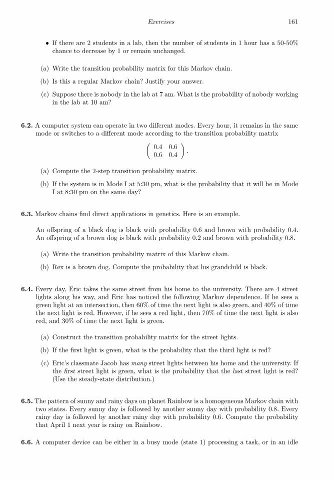
Exercises 161 If there are 2 students in a lab, then the number of students in 1 hour has a 50-50%chance to decrease by 1 or remain unchanged.
(a) Write the transition probability matrix for this Markov chain.
(b) Is this a regular Markov chain? Justify your answer.
(c) Suppose there is nobody in the lab at 7 am. What is the probability of nobody workingin the lab at 10 am?
6.2. A computer system can operate in two different modes. Every hour, it remains in the samemode or switches to a different mode according to the transition probability matrix
(0.4 0.60.6 0.4
).
(a) Compute the 2-step transition probability matrix.
(b) If the system is in Mode I at 5:30 pm, what is the probability that it will be in ModeI at 8:30 pm on the same day?
6.3. Markov chains find direct applications in genetics. Here is an example.
An offspring of a black dog is black with probability 0.6 and brown with probability 0.4.An offspring of a brown dog is black with probability 0.2 and brown with probability 0.8.
(a) Write the transition probability matrix of this Markov chain.
(b) Rex is a brown dog. Compute the probability that his grandchild is black.
6.4. Every day, Eric takes the same street from his home to the university. There are 4 streetlights along his way, and Eric has noticed the following Markov dependence. If he sees agreen light at an intersection, then 60% of time the next light is also green, and 40% of timethe next light is red. However, if he sees a red light, then 70% of time the next light is alsored, and 30% of time the next light is green.
(a) Construct the transition probability matrix for the street lights.
(b) If the first light is green, what is the probability that the third light is red?
(c) Eric’s classmate Jacob has many street lights between his home and the university. Ifthe first street light is green, what is the probability that the last street light is red?(Use the steady-state distribution.)
6.5. The pattern of sunny and rainy days on planet Rainbow is a homogeneous Markov chain withtwo states. Every sunny day is followed by another sunny day with probability 0.8. Everyrainy day is followed by another rainy day with probability 0.6. Compute the probabilitythat April 1 next year is rainy on Rainbow.
6.6. A computer device can be either in a busy mode (state 1) processing a task, or in an idle
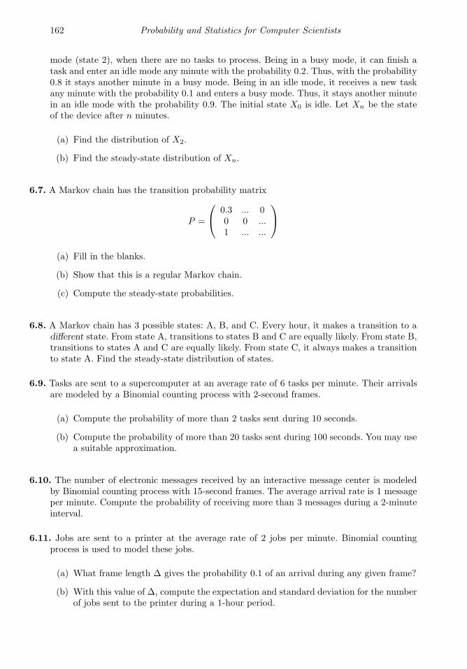
162 Probability and Statistics for Computer Scientists
mode (state 2), when there are no tasks to process. Being in a busy mode, it can finish atask and enter an idle mode any minute with the probability 0.2. Thus, with the probability0.8 it stays another minute in a busy mode. Being in an idle mode, it receives a new taskany minute with the probability 0.1 and enters a busy mode. Thus, it stays another minutein an idle mode with the probability 0.9. The initial state X0 is idle. Let Xn be the stateof the device after n minutes.
(a) Find the distribution of X2.
(b) Find the steady-state distribution of Xn.
6.7. A Markov chain has the transition probability matrix
P =
0.3 ... 00 0 ...1 ... ...
(a) Fill in the blanks.
(b) Show that this is a regular Markov chain.
(c) Compute the steady-state probabilities.
6.8. A Markov chain has 3 possible states: A, B, and C. Every hour, it makes a transition to adifferent state. From state A, transitions to states B and C are equally likely. From state B,transitions to states A and C are equally likely. From state C, it always makes a transitionto state A. Find the steady-state distribution of states.
6.9. Tasks are sent to a supercomputer at an average rate of 6 tasks per minute. Their arrivalsare modeled by a Binomial counting process with 2-second frames.
(a) Compute the probability of more than 2 tasks sent during 10 seconds.
(b) Compute the probability of more than 20 tasks sent during 100 seconds. You may usea suitable approximation.
6.10. The number of electronic messages received by an interactive message center is modeledby Binomial counting process with 15-second frames. The average arrival rate is 1 messageper minute. Compute the probability of receiving more than 3 messages during a 2-minuteinterval.
6.11. Jobs are sent to a printer at the average rate of 2 jobs per minute. Binomial countingprocess is used to model these jobs.
(a) What frame length ∆ gives the probability 0.1 of an arrival during any given frame?
(b) With this value of ∆, compute the expectation and standard deviation for the numberof jobs sent to the printer during a 1-hour period.
Exercises 163
6.12. On the average, 2 airplanes per minute land at a certain international airport. We wouldlike to model the number of landings by a Binomial counting process.
(a) What frame length should one use to guarantee that the probability of a landingduring any frame does not exceed 0.1?
(b) Using the chosen frames, compute the probability of no landings during the next 5minutes.
(c) Using the chosen frames, compute the probability of more than 100 landed airplanesduring the next hour.
6.13. On the average, every 12 seconds a customer makes a call using a certain phone card. Callsare modeled by a Binomial counting process with 2-second frames. Find the mean and thevariance for the time, in seconds, between two consecutive calls.
6.14. Customers of a certain internet service provider connect to the internet at the averagerate of 3 customers per minute. Assuming Binomial counting process with 5-second frames,compute the probability of more than 10 new connections during the next 3 minutes. Com-pute the mean and the standard deviation of the number of seconds between connections.
6.15. Customers of an internet service provider connect to the internet at the average rate of 12new connections per minute. Connections are modeled by a Binomial counting process.
(a) What frame length ∆ gives the probability 0.15 of an arrival during any given frame?
(b) With this value of ∆, compute the expectation and standard deviation for the numberof seconds between two consecutive connections.
6.16. Messages arrive at a transmission center according to a Binomial counting process with 30frames per minute. The average arrival rate is 40 messages per hour. Compute the meanand standard deviation of the number of messages arrived between 10 am and 10:30 am.
6.17. Messages arrive at an electronic message center at random times, with an average of 9messages per hour.
(a) What is the probability of receiving at least five messages during the next hour?
(b) What is the probability of receiving exactly five messages during the next hour?
6.18. Messages arrive at an interactive message center according to a Binomial counting processwith the average interarrival time of 15 seconds. Choosing a frame size of 5 seconds, computethe probability that during 200 minutes of operation, no more than 750 messages arrive.
6.19. Messages arrive at an electronic mail server at the average rate of 4 messages every 5minutes. Their number is modeled by a Binomial counting process.
(a) What frame length makes the probability of a new message arrival during a givenframe equal 0.05?
164 Probability and Statistics for Computer Scientists
(b) Suppose that 50 messages arrived during some 1-hour period. Does this indicate thatthe arrival rate is on the increase? Use frames computed in (a).
6.20. Power outages are unexpected rare events occurring according to a Poisson process withthe average rate of 3 outages per month. Compute the probability of more than 5 poweroutages during three summer months.
6.21. Telephone calls to a customer service center occur according to a Poisson process withthe rate of 1 call every 3 minutes. Compute the probability of receiving more than 5 callsduring the next 12 minutes.
6.22. Network blackouts occur at an average rate of 5 blackouts per month.
(a) Compute the probability of more than 3 blackouts during a given month.
(b) Each blackout costs $1500 for computer assistance and repair. Find the expectationand standard deviation of the monthly total cost due to blackouts.
6.23. An internet service provider offers special discounts to every third connecting customer.Its customers connect to the internet according to a Poisson process with the rate of 5customers per minute. Compute:
(a) the probability that no offer is made during the first 2 minutes
(b) expectation and variance of the time of the first offer
6.24. On the average, Mr. Z drinks and drives once in 4 years. He knows that Every time when he drinks and drives, he is caught by police. According to the laws of his state, the third time when he is caught drinking anddriving results in the loss of his driver’s license. Poisson process is the correct model for such “rare events” as drinking and driving.
What is the probability that Mr. Z will keep his driver’s license for at least 10 years?
6.25. Refer to Example 6.9. Find the steady-state distribution for the number of users by writingX(t) as a sum of two independent Markov chains,
X(t) = Y1(t) + Y2(t),
where Yi(t) = 1 if user i is connected at time t and Yi(t) = 0 if user i is not connected, fori = 1, 2. Find the steady-state distribution for each Yi, then use it to find the steady-statedistribution for X . Compare your result with Example 6.12.
6.26. (Computer mini-project) Generate 10,000 transitions of the Markov chain in Exam-ple 6.9 on p. 139. How many times do you find your generated Markov chain in each of itsthree states? Does it match the distribution found in Example 6.12?

Exercises 165
6.27. (Computer mini-project) In this project, we explore the effect of Markov dependence.
Start with a sunny day and generate weather forecasts for the next 100 days according tothe Markov chain in Example 6.7 on p. 136. Observe periods of sunny days and periods ofrainy days.
Then consider another city where each day, sunny or rainy, is followed by a sunny day withprobability (4/7) and by a rainy day with probability (3/7). As we know from Example 6.11on p. 143, this is the steady-state distribution of sunny and rainy days, so the overallproportion of sunny days should be the same in both cities. Generate weather forecasts for100 days and compare with the first city. What happened with periods of consecutive sunnyand rainy days?
Each day in the first city, the weather depends on the previous day. In the second city,weather forecasts for different days are independent.
6.28. (Computer mini-project) Generate a 24-hour segment of a Poisson process of arrivalswith the arrival rate λ = 2 hours−1. Graph its trajectory. Do you observe several arrivalsin a short period of time followed by relatively long periods with no arrivals at all? Whyare the arrivals so unevenly distributed over the 24-hour period?

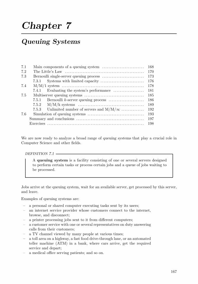
Chapter 7
Queuing Systems
7.1 Main components of a queuing system . . . . . . . . . . . . . . . . . . . . . . . . . . 1687.2 The Little’s Law . . . . . . . . . . . . . . . . . . . . . . . . . . . . . . . . . . . . . . . . . . . . . . . . . 1707.3 Bernoulli single-server queuing process . . . . . . . . . . . . . . . . . . . . . . . . . . 173
7.3.1 Systems with limited capacity . . . . . . . . . . . . . . . . . . . . . . . . . . . 1767.4 M/M/1 system . . . . . . . . . . . . . . . . . . . . . . . . . . . . . . . . . . . . . . . . . . . . . . . . . . . 178
7.4.1 Evaluating the system’s performance . . . . . . . . . . . . . . . . . . . 1817.5 Multiserver queuing systems . . . . . . . . . . . . . . . . . . . . . . . . . . . . . . . . . . . . . 185
7.5.1 Bernoulli k-server queuing process . . . . . . . . . . . . . . . . . . . . . . 1867.5.2 M/M/k systems . . . . . . . . . . . . . . . . . . . . . . . . . . . . . . . . . . . . . . . . . 1897.5.3 Unlimited number of servers and M/M/∞ . . . . . . . . . . . . . . 192
7.6 Simulation of queuing systems . . . . . . . . . . . . . . . . . . . . . . . . . . . . . . . . . . . 193Summary and conclusions . . . . . . . . . . . . . . . . . . . . . . . . . . . . . . . . . . . . . . . . . . 197Exercises . . . . . . . . . . . . . . . . . . . . . . . . . . . . . . . . . . . . . . . . . . . . . . . . . . . . . . . . . . . . 198
We are now ready to analyze a broad range of queuing systems that play a crucial role inComputer Science and other fields.
DEFINITION 7.1
A queuing system is a facility consisting of one or several servers designedto perform certain tasks or process certain jobs and a queue of jobs waiting tobe processed.
Jobs arrive at the queuing system, wait for an available server, get processed by this server,and leave.
Examples of queuing systems are:
– a personal or shared computer executing tasks sent by its users;– an internet service provider whose customers connect to the internet,
browse, and disconnect;– a printer processing jobs sent to it from different computers;– a customer service with one or several representatives on duty answering
calls from their customers;– a TV channel viewed by many people at various times;– a toll area on a highway, a fast food drive-through lane, or an automated
teller machine (ATM) in a bank, where cars arrive, get the requiredservice and depart;
– a medical office serving patients; and so on.
167

168 Probability and Statistics for Computer Scientists
Source population
Arrival
of jobs
Waiting line(queue)
Server I
Server II
Server III
Server IV
Service
Departure
FIGURE 7.1: Main components of a queuing system.
7.1 Main components of a queuing system
How does a queuing system work? What happens with a job when it goes through a queuingsystem? The main stages are depicted in Figure 7.1.
Arrival
Typically, jobs arrive to a queuing system at random times. A counting process A(t) tellsthe number of arrivals that occurred by the time t. In stationary queuing systems (whosedistribution characteristics do not change over time), arrivals occur at arrival rate
λA =EA(t)
t
for any t > 0, which is the expected number of arrivals per 1 unit of time. Then, the expectedtime between arrivals is
µA =1
λA.
Queuing and routing to servers
Arrived jobs are typically processed according to the order of their arrivals, on a “firstcome–first serve” basis.
When a new job arrives, it may find the system in different states. If one server is available

Queuing Systems 169
at that time, it will certainly take the new job. If several servers are available, the job maybe randomized to one of them, or the server may be chosen according to some rules. Forexample, the fastest server or the least loaded server may be assigned to process the newjob. Finally, if all servers are busy working on other jobs, the new job will join the queue,wait until all the previously arrived jobs are completed, and get routed to the next availableserver.
Various additional constraints may take place. For example, a queue may have a buffer thatlimits the number of waiting jobs. Such a queuing system will have limited capacity; thetotal number of jobs in it at any time is bounded by some constant C. If the capacity isfull (for example, in a parking garage), a new job cannot enter the system until another jobdeparts.
Also, jobs may leave the queue prematurely, say, after an excessively long waiting time.Servers may also open and close during the day as people need rest and servers need main-tenance. Complex queuing systems with many extra conditions may be difficult to studyanalytically; however, we shall learn Monte Carlo methods for queuing systems in Sec-tion 7.6.
Service
Once a server becomes available, it immediately starts processing the next assigned job. Inpractice, service times are random because they depend on the amount of work required byeach task. The average service time is µS . It may vary from one server to another as somecomputers or customer service representatives work faster than others. The service rate isdefined as the average number of jobs processed by a continuously working server duringone unit of time. It equals
λS =1
µS.
Departure
When the service is completed, the job leaves the system.
The following parameters and random variables describe performance of a queuing system.
Notation Parameters of a queuing system
λA = arrival rateλS = service rate
µA = 1/λA = mean interarrival timeµS = 1/λS = mean service time
r = λA/λS = µS/µA = utilization, or arrival-to-service ratio
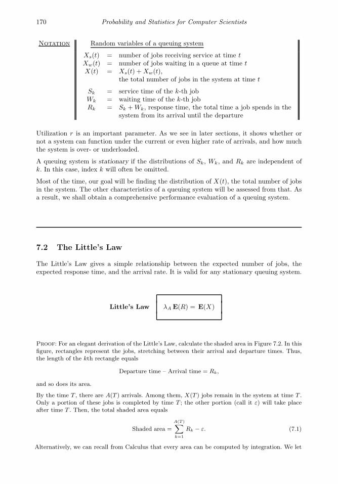
170 Probability and Statistics for Computer Scientists
Notation Random variables of a queuing system
Xs(t) = number of jobs receiving service at time tXw(t) = number of jobs waiting in a queue at time tX(t) = Xs(t) +Xw(t),
the total number of jobs in the system at time t
Sk = service time of the k-th jobWk = waiting time of the k-th jobRk = Sk +Wk, response time, the total time a job spends in the
system from its arrival until the departure
Utilization r is an important parameter. As we see in later sections, it shows whether ornot a system can function under the current or even higher rate of arrivals, and how muchthe system is over- or underloaded.
A queuing system is stationary if the distributions of Sk, Wk, and Rk are independent ofk. In this case, index k will often be omitted.
Most of the time, our goal will be finding the distribution of X(t), the total number of jobsin the system. The other characteristics of a queuing system will be assessed from that. Asa result, we shall obtain a comprehensive performance evaluation of a queuing system.
7.2 The Little’s Law
The Little’s Law gives a simple relationship between the expected number of jobs, theexpected response time, and the arrival rate. It is valid for any stationary queuing system.
Little’s Law λA E(R) = E(X)
Proof: For an elegant derivation of the Little’s Law, calculate the shaded area in Figure 7.2. In thisfigure, rectangles represent the jobs, stretching between their arrival and departure times. Thus,the length of the kth rectangle equals
Departure time – Arrival time = Rk,
and so does its area.
By the time T , there are A(T ) arrivals. Among them, X(T ) jobs remain in the system at time T .Only a portion of these jobs is completed by time T ; the other portion (call it ε) will take placeafter time T . Then, the total shaded area equals
Shaded area =
A(T )∑
k=1
Rk − ε. (7.1)
Alternatively, we can recall from Calculus that every area can be computed by integration. We let
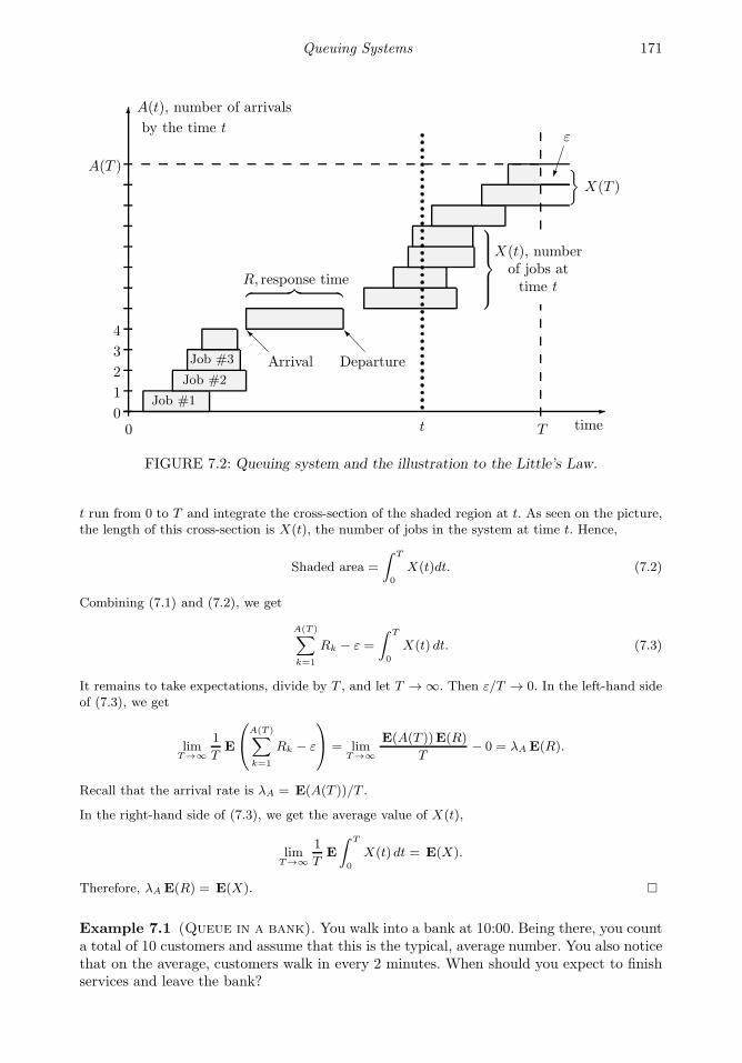
Queuing Systems 171
time
A(t), number of arrivals
by the time t
00
Arrival Departure
ε
X(t), numberof jobs attime t
X(T )
︷ ︸︸ ︷R, response time
Job #1
Job #2
Job #3
1
2
3
4
A(T )
Tt
FIGURE 7.2: Queuing system and the illustration to the Little’s Law.
t run from 0 to T and integrate the cross-section of the shaded region at t. As seen on the picture,the length of this cross-section is X(t), the number of jobs in the system at time t. Hence,
Shaded area =
∫ T
0
X(t)dt. (7.2)
Combining (7.1) and (7.2), we get
A(T )∑
k=1
Rk − ε =
∫ T
0
X(t) dt. (7.3)
It remains to take expectations, divide by T , and let T → ∞. Then ε/T → 0. In the left-hand sideof (7.3), we get
limT→∞
1
TE
A(T )∑
k=1
Rk − ε
= limT→∞
E(A(T ))E(R)
T− 0 = λA E(R).
Recall that the arrival rate is λA = E(A(T ))/T .
In the right-hand side of (7.3), we get the average value of X(t),
limT→∞
1
TE
∫ T
0
X(t) dt = E(X).
Therefore, λA E(R) = E(X).
Example 7.1 (Queue in a bank). You walk into a bank at 10:00. Being there, you counta total of 10 customers and assume that this is the typical, average number. You also noticethat on the average, customers walk in every 2 minutes. When should you expect to finishservices and leave the bank?
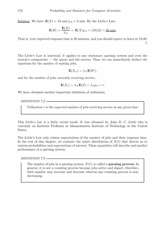
172 Probability and Statistics for Computer Scientists
Solution. We have E(X) = 10 and µA = 2 min. By the Little’s Law,
E(R) =E(X)
λA= E(X)µA = (10)(2) = 20 min.
That is, your expected response time is 20 minutes, and you should expect to leave at 10:20.♦
The Little’s Law is universal, it applies to any stationary queuing system and even thesystem’s components — the queue and the servers. Thus, we can immediately deduce theequations for the number of waiting jobs,
E(Xw) = λA E(W ),
and for the number of jobs currently receiving service,
E(Xs) = λA E(S) = λAµS = r.
We have obtained another important definition of utilization.
DEFINITION 7.2
Utilization r is the expected number of jobs receiving service at any given time.
This Little’s law is a fairly recent result. It was obtained by John D. C. Little who iscurrently an Institute Professor at Massachusetts Institute of Technology in the UnitedStates.
The Little’s Law only relates expectations of the number of jobs and their response time.In the rest of this chapter, we evaluate the entire distribution of X(t) that directs us tovarious probabilities and expectations of interest. These quantities will describe and predictperformance of a queuing system.
DEFINITION 7.3
The number of jobs in a queuing system, X(t), is called a queuing process. Ingeneral, it is not a counting process because jobs arrive and depart, therefore,their number may increase and decrease whereas any counting process is non-decreasing.
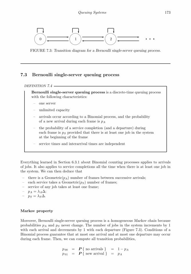
Queuing Systems 173
0 1 2
FIGURE 7.3: Transition diagram for a Bernoulli single-server queuing process.
7.3 Bernoulli single-server queuing process
DEFINITION 7.4
Bernoulli single-server queuing process is a discrete-time queuing processwith the following characteristics:
– one server
– unlimited capacity
– arrivals occur according to a Binomial process, and the probabilityof a new arrival during each frame is pA
– the probability of a service completion (and a departure) duringeach frame is pS provided that there is at least one job in the systemat the beginning of the frame
– service times and interarrival times are independent
Everything learned in Section 6.3.1 about Binomial counting processes applies to arrivalsof jobs. It also applies to service completions all the time when there is at least one job inthe system. We can then deduce that
– there is a Geometric(pA) number of frames between successive arrivals;– each service takes a Geometric(pS) number of frames;– service of any job takes at least one frame;– pA = λA∆;– pS = λS∆.
Markov property
Moreover, Bernoulli single-server queuing process is a homogeneous Markov chain becauseprobabilities pA and pS never change. The number of jobs in the system increments by 1with each arrival and decrements by 1 with each departure (Figure 7.3). Conditions of aBinomial process guarantee that at most one arrival and at most one departure may occurduring each frame. Then, we can compute all transition probabilities,
p 00 = P no arrivals = 1− pAp 01 = P new arrival = pA
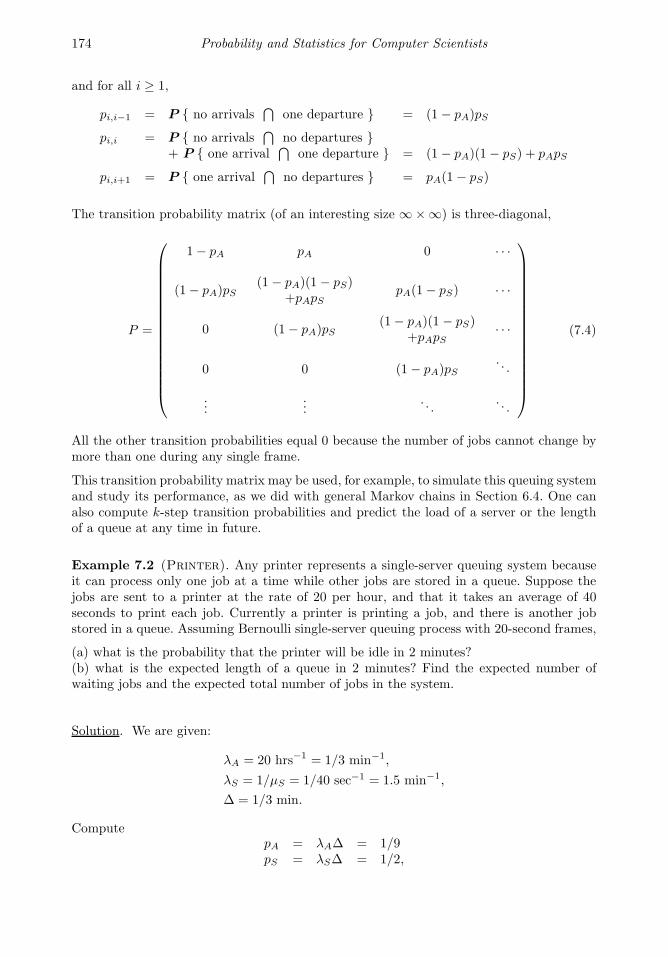
174 Probability and Statistics for Computer Scientists
and for all i ≥ 1,
pi,i−1 = P no arrivals⋂
one departure = (1 − pA)pS
pi,i = P no arrivals⋂
no departures + P one arrival
⋂one departure = (1 − pA)(1− pS) + pApS
pi,i+1 = P one arrival⋂
no departures = pA(1 − pS)
The transition probability matrix (of an interesting size ∞×∞) is three-diagonal,
P =
1− pA pA 0 · · ·
(1− pA)pS(1 − pA)(1 − pS)
+pApSpA(1− pS) · · ·
0 (1− pA)pS(1− pA)(1 − pS)
+pApS· · ·
0 0 (1− pA)pS. . .
......
. . .. . .
(7.4)
All the other transition probabilities equal 0 because the number of jobs cannot change bymore than one during any single frame.
This transition probability matrix may be used, for example, to simulate this queuing systemand study its performance, as we did with general Markov chains in Section 6.4. One canalso compute k-step transition probabilities and predict the load of a server or the lengthof a queue at any time in future.
Example 7.2 (Printer). Any printer represents a single-server queuing system becauseit can process only one job at a time while other jobs are stored in a queue. Suppose thejobs are sent to a printer at the rate of 20 per hour, and that it takes an average of 40seconds to print each job. Currently a printer is printing a job, and there is another jobstored in a queue. Assuming Bernoulli single-server queuing process with 20-second frames,
(a) what is the probability that the printer will be idle in 2 minutes?(b) what is the expected length of a queue in 2 minutes? Find the expected number ofwaiting jobs and the expected total number of jobs in the system.
Solution. We are given:
λA = 20 hrs−1 = 1/3 min−1,
λS = 1/µS = 1/40 sec−1 = 1.5 min−1,
∆ = 1/3 min.
ComputepA = λA∆ = 1/9pS = λS∆ = 1/2,

Queuing Systems 175
and all the transition probabilities for the number of jobs X ,
p 00 = 1− pA = 8/9 = 0.889p 01 = pA = 1/9 = 0.111
and for i ≥ 1,pi,i−1 = (1− pA)pS = 4/9 = 0.444pi,i+1 = pA(1− pS) = 1/18 = 0.056pi,i = 1− 0.444− 0.056 = 0.5
(7.5)
Notice the “shortcut” used in computing pi,i. Indeed, the row sum in a transition probabilitymatrix is always 1; therefore, pi,i = 1− pi,i−1 − pi,i+1.
We got the following transition probability matrix,
P =
.889 .111 0 0 · · ·
.444 .5 .056 0 · · ·0 .444 .5 .056 · · ·0 0 .444 .5
. . ....
......
. . .. . .
Since there are 2 min/∆ = 6 frames in 2 minutes, we need a distribution of X after 6 frames,which is
P6 = P0P6,
as we know from Section 6.2, formula (6.4). Here there is an interesting problem. How dowe deal with matrix P that has infinitely many rows and columns?
Fortunately, we only need a small portion of this matrix. There are 2 jobs currently in thesystem, so the initial distribution is
P0 = (0 0 1 0 0 0 0 0).
In a course of 6 frames, their number can change by 6 at most (look at Figure 7.3), andthus, it is sufficient to consider the the first 9 rows and 9 columns of P only, correspondingto states 0, 1, ..., 8. Then, we compute the distribution after 6 frames,
P6 = P0P6 = (0 0 1 0 0 0 0 0)
.889 .111 0 · · · 0 0
.444 .5 .056 · · · 0 00 .444 .5 · · · 0 0...
......
......
...0 0 0 · · · .5 .0560 0 0 · · · .444 .5
6
= (.644 .250 .080 .022 .004 .000 .000 .000 .000).
Based on this distribution,
(a) The probability that the printer is idle after 2 minutes is the probability of no jobs inthe system at that time,
P6(0) = 0.644.
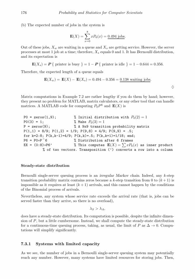
176 Probability and Statistics for Computer Scientists
(b) The expected number of jobs in the system is
E(X) =
8∑
x=0
xP6(x) = 0.494 jobs.
Out of these jobs, Xw are waiting in a queue and Xs are getting service. However, the serverprocesses at most 1 job at a time; therefore, Xs equals 0 and 1. It has Bernoulli distribution,and its expectation is
E(Xs) = P printer is busy = 1− P printer is idle = 1− 0.644 = 0.356.
Therefore, the expected length of a queue equals
E(Xw) = E(X)− E(Xs) = 0.494− 0.356 = 0.138 waiting jobs.
♦
Matrix computations in Example 7.2 are rather lengthy if you do them by hand; however,they present no problem for MATLAB, matrix calculators, or any other tool that can handlematrices. A MATLAB code for computing P0P
6 and E(X) is
P0 = zeros(1,9); % Initial distribution with P0(2) = 1P0(3) = 1; % Make P0(3) = 1P = zeros(9); % A 9x9 transition probability matrix
P(1,1) = 8/9; P(1,2) = 1/9; P(9,8) = 4/9; P(9,9) = .5;
for k=2:8; P(k,k-1)=4/9; P(k,k)=.5; P(k,k+1)=1/18; end;
P6 = P0∗P6 % Distribution after 6 frames
EX = (0:8)∗P6’ % This computes E(X) =∑
xP6(x) as inner product
% of two vectors. Transposition (’) converts a row into a column
Steady-state distribution
Bernoulli single-server queuing process is an irregular Markov chain. Indeed, any k-steptransition probability matrix contains zeros because a k-step transition from 0 to (k+1) isimpossible as it requires at least (k+ 1) arrivals, and this cannot happen by the conditionsof the Binomial process of arrivals.
Nevertheless, any system whose service rate exceeds the arrival rate (that is, jobs can beserved faster than they arrive, so there is no overload),
λS > λA,
does have a steady-state distribution. Its computation is possible, despite the infinite dimen-sion of P , but a little cumbersome. Instead, we shall compute the steady-state distributionfor a continuous-time queuing process, taking, as usual, the limit of P as ∆ → 0. Compu-tations will simplify significantly.
7.3.1 Systems with limited capacity
As we see, the number of jobs in a Bernoulli single-server queuing system may potentiallyreach any number. However, many systems have limited resources for storing jobs. Then,
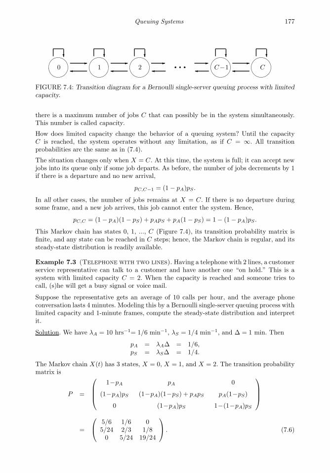
Queuing Systems 177
0 1 2 C−1 C
FIGURE 7.4: Transition diagram for a Bernoulli single-server queuing process with limitedcapacity.
there is a maximum number of jobs C that can possibly be in the system simultaneously.This number is called capacity.
How does limited capacity change the behavior of a queuing system? Until the capacityC is reached, the system operates without any limitation, as if C = ∞. All transitionprobabilities are the same as in (7.4).
The situation changes only when X = C. At this time, the system is full; it can accept newjobs into its queue only if some job departs. As before, the number of jobs decrements by 1if there is a departure and no new arrival,
pC,C−1 = (1− pA)pS .
In all other cases, the number of jobs remains at X = C. If there is no departure duringsome frame, and a new job arrives, this job cannot enter the system. Hence,
pC,C = (1− pA)(1− pS) + pApS + pA(1− pS) = 1− (1− pA)pS .
This Markov chain has states 0, 1, ..., C (Figure 7.4), its transition probability matrix isfinite, and any state can be reached in C steps; hence, the Markov chain is regular, and itssteady-state distribution is readily available.
Example 7.3 (Telephone with two lines). Having a telephone with 2 lines, a customerservice representative can talk to a customer and have another one “on hold.” This is asystem with limited capacity C = 2. When the capacity is reached and someone tries tocall, (s)he will get a busy signal or voice mail.
Suppose the representative gets an average of 10 calls per hour, and the average phoneconversation lasts 4 minutes. Modeling this by a Bernoulli single-server queuing process withlimited capacity and 1-minute frames, compute the steady-state distribution and interpretit.
Solution. We have λA = 10 hrs−1= 1/6 min−1, λS = 1/4 min−1, and ∆ = 1 min. Then
pA = λA∆ = 1/6,pS = λS∆ = 1/4.
The Markov chain X(t) has 3 states, X = 0, X = 1, and X = 2. The transition probabilitymatrix is
P =
1−pA pA 0
(1−pA)pS (1−pA)(1−pS) + pApS pA(1−pS)
0 (1−pA)pS 1−(1−pA)pS
=
5/6 1/6 05/24 2/3 1/80 5/24 19/24
. (7.6)
178 Probability and Statistics for Computer Scientists
Next, we solve the steady-state equations
πP = π ⇒
5
6π0 +
5
24π1 = π0
1
6π0 +
2
3π1 +
5
24π2 = π1
1
8π1 +
19
24π2 = π2
⇒
5
24π1 =
1
6π0
1
6π0 +
2
3π1 +
5
24π2 = π1
1
8π1 =
5
24π2
As we expect, the second equation follows from the others. After substitution, it becomesan identity
5
24π1 +
2
3π1 +
1
8π1 = π1.
We use this as a double-check and turn to the normalizing equation
π0 + π1 + π2 =5
4π1 + π1 +
3
5π1 =
57
20π1 = 1,
from where
π0 = 25/57 = 0.439, π1 = 20/57 = 0.351, π2 = 12/57 = 0.210.
Interpreting this result, 43.9% of time the representative is not talking on the phone, 35.1%of time (s)he talks but has the second line open, and 21.0% of time both lines are busy andnew calls don’t get through. ♦
7.4 M/M/1 system
We now turn our attention to continuous-time queuing processes. Our usual approach is tomove from discrete time to continuous time gradually by reducing the frame size ∆ to zero.
First, let us explain what the notation “M/M/1” actually means.
Notation A queuing system can be denoted as A/S/n/C, where
A denotes the distribution of interarrival timesS denotes the distribution of service timesn is the number of serversC is the capacity
Default capacity is C = ∞ (unlimited capacity)
Letter M denotes Exponential distribution because it is memoryless, and the resulting pro-cess is Markov.
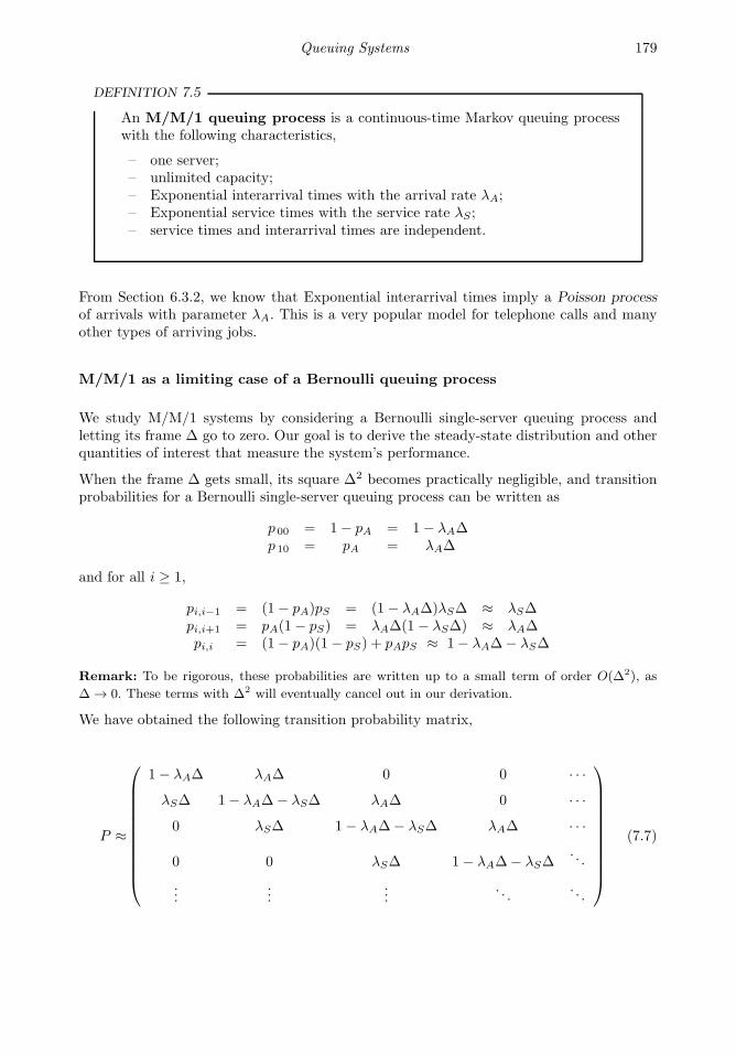
Queuing Systems 179
DEFINITION 7.5
An M/M/1 queuing process is a continuous-time Markov queuing processwith the following characteristics,
– one server;– unlimited capacity;– Exponential interarrival times with the arrival rate λA;– Exponential service times with the service rate λS ;– service times and interarrival times are independent.
From Section 6.3.2, we know that Exponential interarrival times imply a Poisson processof arrivals with parameter λA. This is a very popular model for telephone calls and manyother types of arriving jobs.
M/M/1 as a limiting case of a Bernoulli queuing process
We study M/M/1 systems by considering a Bernoulli single-server queuing process andletting its frame ∆ go to zero. Our goal is to derive the steady-state distribution and otherquantities of interest that measure the system’s performance.
When the frame ∆ gets small, its square ∆2 becomes practically negligible, and transitionprobabilities for a Bernoulli single-server queuing process can be written as
p 00 = 1− pA = 1− λA∆p 10 = pA = λA∆
and for all i ≥ 1,
pi,i−1 = (1− pA)pS = (1− λA∆)λS∆ ≈ λS∆pi,i+1 = pA(1− pS) = λA∆(1 − λS∆) ≈ λA∆pi,i = (1− pA)(1 − pS) + pApS ≈ 1− λA∆− λS∆
Remark: To be rigorous, these probabilities are written up to a small term of order O(∆2), as
∆ → 0. These terms with ∆2 will eventually cancel out in our derivation.
We have obtained the following transition probability matrix,
P ≈
1− λA∆ λA∆ 0 0 · · ·λS∆ 1− λA∆− λS∆ λA∆ 0 · · ·0 λS∆ 1− λA∆− λS∆ λA∆ · · ·
0 0 λS∆ 1− λA∆− λS∆.. .
......
.... . .
. . .
(7.7)
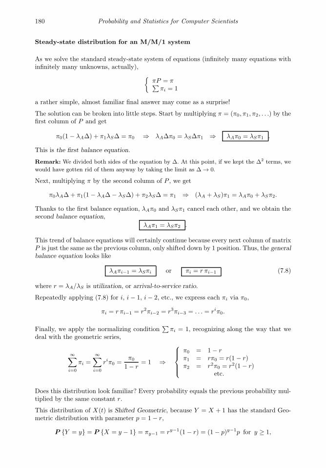
180 Probability and Statistics for Computer Scientists
Steady-state distribution for an M/M/1 system
As we solve the standard steady-state system of equations (infinitely many equations withinfinitely many unknowns, actually),
πP = π∑
πi = 1
a rather simple, almost familiar final answer may come as a surprise!
The solution can be broken into little steps. Start by multiplying π = (π0, π1, π2, . . .) by thefirst column of P and get
π0(1− λA∆) + π1λS∆ = π0 ⇒ λA∆π0 = λS∆π1 ⇒ λAπ0 = λSπ1 .
This is the first balance equation.
Remark: We divided both sides of the equation by ∆. At this point, if we kept the ∆2 terms, we
would have gotten rid of them anyway by taking the limit as ∆ → 0.
Next, multiplying π by the second column of P , we get
π0λA∆+ π1(1− λA∆− λS∆) + π2λS∆ = π1 ⇒ (λA + λS)π1 = λAπ0 + λSπ2.
Thanks to the first balance equation, λAπ0 and λSπ1 cancel each other, and we obtain thesecond balance equation,
λAπ1 = λSπ2 .
This trend of balance equations will certainly continue because every next column of matrixP is just the same as the previous column, only shifted down by 1 position. Thus, the generalbalance equation looks like
λAπi−1 = λSπi or πi = r πi−1 (7.8)
where r = λA/λS is utilization, or arrival-to-service ratio.
Repeatedly applying (7.8) for i, i − 1, i− 2, etc., we express each πi via π0,
πi = r πi−1 = r2πi−2 = r3πi−3 = . . . = riπ0.
Finally, we apply the normalizing condition∑
πi = 1, recognizing along the way that wedeal with the geometric series,
∞∑
i=0
πi =
∞∑
i=0
riπ0 =π0
1− r= 1 ⇒
π0 = 1− rπ1 = rπ0 = r(1 − r)π2 = r2π0 = r2(1 − r)
etc.
Does this distribution look familiar? Every probability equals the previous probability mul-tiplied by the same constant r.
This distribution of X(t) is Shifted Geometric, because Y = X + 1 has the standard Geo-metric distribution with parameter p = 1− r,
P Y = y = P X = y − 1 = πy−1 = ry−1(1− r) = (1− p)y−1p for y ≥ 1,
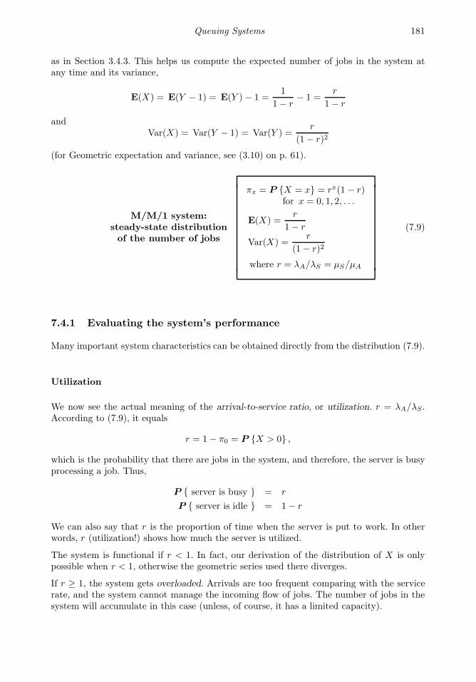
Queuing Systems 181
as in Section 3.4.3. This helps us compute the expected number of jobs in the system atany time and its variance,
E(X) = E(Y − 1) = E(Y )− 1 =1
1− r− 1 =
r
1− r
andVar(X) = Var(Y − 1) = Var(Y ) =
r
(1− r)2
(for Geometric expectation and variance, see (3.10) on p. 61).
M/M/1 system:steady-state distributionof the number of jobs
πx = P X = x = rx(1 − r)for x = 0, 1, 2, . . .
E(X) =r
1− r
Var(X) =r
(1− r)2
where r = λA/λS = µS/µA
(7.9)
7.4.1 Evaluating the system’s performance
Many important system characteristics can be obtained directly from the distribution (7.9).
Utilization
We now see the actual meaning of the arrival-to-service ratio, or utilization. r = λA/λS .According to (7.9), it equals
r = 1− π0 = P X > 0 ,
which is the probability that there are jobs in the system, and therefore, the server is busyprocessing a job. Thus,
P server is busy = r
P server is idle = 1− r
We can also say that r is the proportion of time when the server is put to work. In otherwords, r (utilization!) shows how much the server is utilized.
The system is functional if r < 1. In fact, our derivation of the distribution of X is onlypossible when r < 1, otherwise the geometric series used there diverges.
If r ≥ 1, the system gets overloaded. Arrivals are too frequent comparing with the servicerate, and the system cannot manage the incoming flow of jobs. The number of jobs in thesystem will accumulate in this case (unless, of course, it has a limited capacity).

182 Probability and Statistics for Computer Scientists
Waiting time
When a new job arrives, it finds the system with X jobs in it. While these X jobs are beingserved, the new job awaits its turn in a queue. Thus, its waiting time consists of servicetimes of X earlier jobs,
W = S1 + S2 + S3 + . . .+ SX .
Perhaps, the first job in this queue has already started its service. Magically, this possibilitydoes not affect the distribution of W . Recall that service times in M/M/1 systems are Ex-ponential, and this distribution has a memoryless property. At any moment, the remainingservice time of the first job still has Exponential(λS) distribution regardless of how long itis already being served!
We can then conclude that the new job has expected waiting time
E(W ) = E(S1 + . . .+ SX) = E(S)E(X) =µS r
1− ror
r
λS(1− r).
(By writing the product of expectations, we actually used the fact that service times areindependent of the number of jobs in the system at that time).
Remark: Notice that W is a rare example of a variable whose distribution is neither discrete nor
continuous. On one hand, it has a probability mass function at 0 because P W = 0 = 1 − r is
the probability that the server is idle and available and there is no waiting time for a new job. On
the other hand, W has a density f(x) for all x > 0. Given any positive number of jobs X = n, the
waiting time is the sum of n Exponential times which is Gamma(n, λS). Such a distribution of W
is mixed.
Response time
Response time is the time a job spends in the system, from its arrival until its departure.It consists of waiting time (if any) and service time. The expected response time can thenbe computed as
E(R) = E(W ) + E(S) =µS r
1− r+ µS =
µS
1− ror
1
λS(1− r).
Queue
The length of a queue is the number of waiting jobs,
Xw = X −Xs.
The number of jobs Xs getting service at any time is 0 or 1. It is therefore a Bernoullivariable with parameter
P server is busy = r.
Hence, the expected queue length is
E(Xw) = E(X)− E(Xs) =r
1− r− r =
r2
1− r.
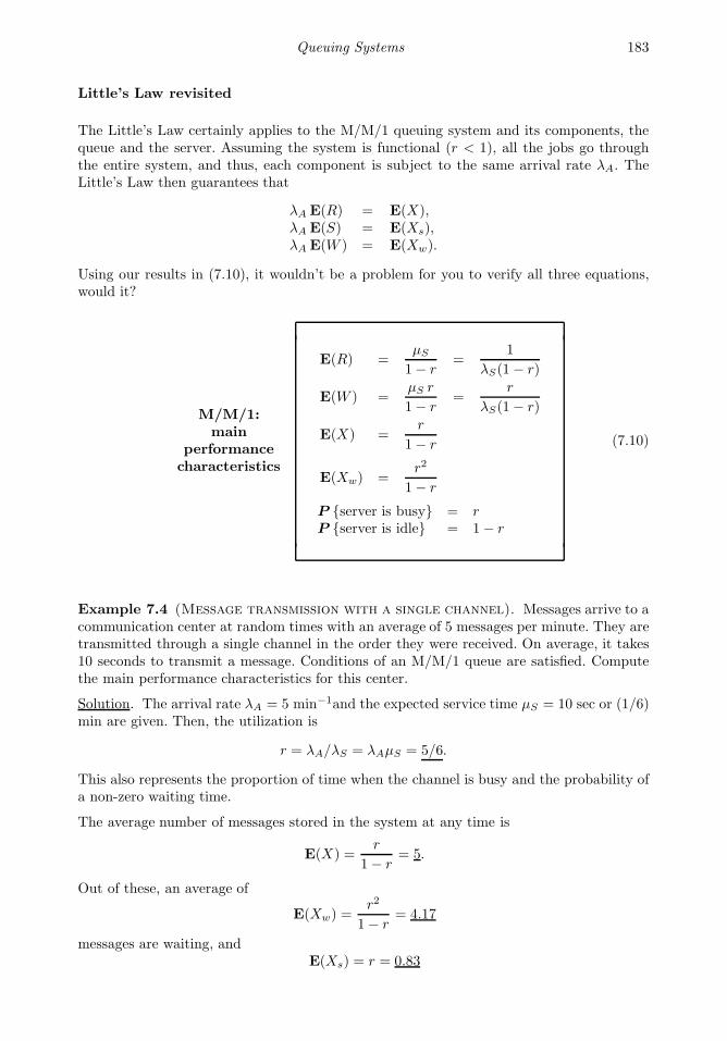
Queuing Systems 183
Little’s Law revisited
The Little’s Law certainly applies to the M/M/1 queuing system and its components, thequeue and the server. Assuming the system is functional (r < 1), all the jobs go throughthe entire system, and thus, each component is subject to the same arrival rate λA. TheLittle’s Law then guarantees that
λA E(R) = E(X),λA E(S) = E(Xs),λA E(W ) = E(Xw).
Using our results in (7.10), it wouldn’t be a problem for you to verify all three equations,would it?
M/M/1:main
performancecharacteristics
E(R) =µS
1− r=
1
λS(1− r)
E(W ) =µS r
1− r=
r
λS(1− r)
E(X) =r
1− r
E(Xw) =r2
1− r
P server is busy = rP server is idle = 1− r
(7.10)
Example 7.4 (Message transmission with a single channel). Messages arrive to acommunication center at random times with an average of 5 messages per minute. They aretransmitted through a single channel in the order they were received. On average, it takes10 seconds to transmit a message. Conditions of an M/M/1 queue are satisfied. Computethe main performance characteristics for this center.
Solution. The arrival rate λA = 5 min−1and the expected service time µS = 10 sec or (1/6)min are given. Then, the utilization is
r = λA/λS = λAµS = 5/6.
This also represents the proportion of time when the channel is busy and the probability ofa non-zero waiting time.
The average number of messages stored in the system at any time is
E(X) =r
1− r= 5.
Out of these, an average of
E(Xw) =r2
1− r= 4.17
messages are waiting, andE(Xs) = r = 0.83

184 Probability and Statistics for Computer Scientists
are being transmitted.
When a message arrives to the center, its waiting time until its transmission begins averages
E(W ) =µSr
1− r= 50 seconds,
whereas the total amount of time since its arrival until the end of its transmission has anaverage of
E(R) =µS
1− r= 1 minute.
♦
Example 7.5 (Forecast). Let’s continue Example 7.4. Suppose that next year the cus-tomer base of our transmission center is projected to increase by 10%, and thus, the intensityof incoming traffic λA increases by 10% too. How will this affect the center’s performance?
Solution. Recompute the main performance characteristics under the new arrival rate
λNEWA = (1.1)λOLD
A = 5.5 min−1.
Now the utilization equals r = 11/12, getting dangerously close to 1 where the system getsoverloaded. For high values of r, various parameters of the system increase rapidly. A 10%increase in the arrival rate will result in rather significant changes in other variables. Using(7.10), we now get
E(X) = 11 jobs,E(Xw) = 10.08 jobs,E(W ) = 110 seconds, andE(R) = 2 minutes.
We see that the response time, the waiting time, the average number of stored messages,and therefore, the average required amount of memory more than doubled when the numberof customers increased by a mere 10%. ♦
When a system gets nearly overloaded
As we observed in Example 7.5, the system slowed down significantly as a result of a 10%increase in the intensity of incoming traffic, projected for the next year. One may try toforecast the two-year future of the system, assuming a 10% increase of a customer base eachyear. It will appear that during the second year the utilization will exceed 1, and the systemwill be unable to function.
What is a practical solution to this problem? Another channel or two may be added to thecenter to help the existing channel handle all the arriving messages! The new system willthen have more than one channel-server, and it will be able to process more arriving jobs.
Such systems are analyzed in the next section.

Queuing Systems 185
7.5 Multiserver queuing systems
We now turn our attention to queuing systems with several servers. We assume that eachserver can perform the same range of services; however, in general, some servers may befaster than others. Thus, the service times for different servers may potentially have differentdistributions.
When a job arrives, it either finds all servers busy serving jobs, or it finds one or severalavailable servers. In the first case, the job will wait in a queue for its turn whereas in thesecond case, it will be routed to one of the idle servers. A mechanism assigning jobs toavailable servers may be random, or it may be based on some rule. For example, somecompanies follow the equity principle and make sure that each call to their customer serviceis handled by the least loaded customer service representative.
The number of servers may be finite or infinite. A system with infinitely many servers canafford an unlimited number of concurrent users. For example, any number of people canwatch a TV channel simultaneously. A job served by a system with k = ∞ servers will neverwait; it will always find available idle servers.
As in previous sections, here is our plan for analyzing multiserver systems:
– first, verify if the number of jobs in the system at time t is a Markov process andwrite its transition probability matrix P . For continuous-time processes, we select a“very short” frame ∆ and eventually let ∆ converge to zero;
– next, compute the steady-state distribution π, and
– finally, use π to evaluate the system’s long-term performance characteristics.
We treat a few common and analytically simple cases in detail. Advanced theory goesfurther; in this book we shall analyze more complex and non-Markov queuing systems byMonte Carlo methods in Section 7.6.
Notice that utilization r no longer has to be less than 1. A system with k servers can handlek times the traffic of a single-server system; therefore, it will function with any r < k.
As always, we start with a discrete-time process that can be described on a language ofBernoulli trials.
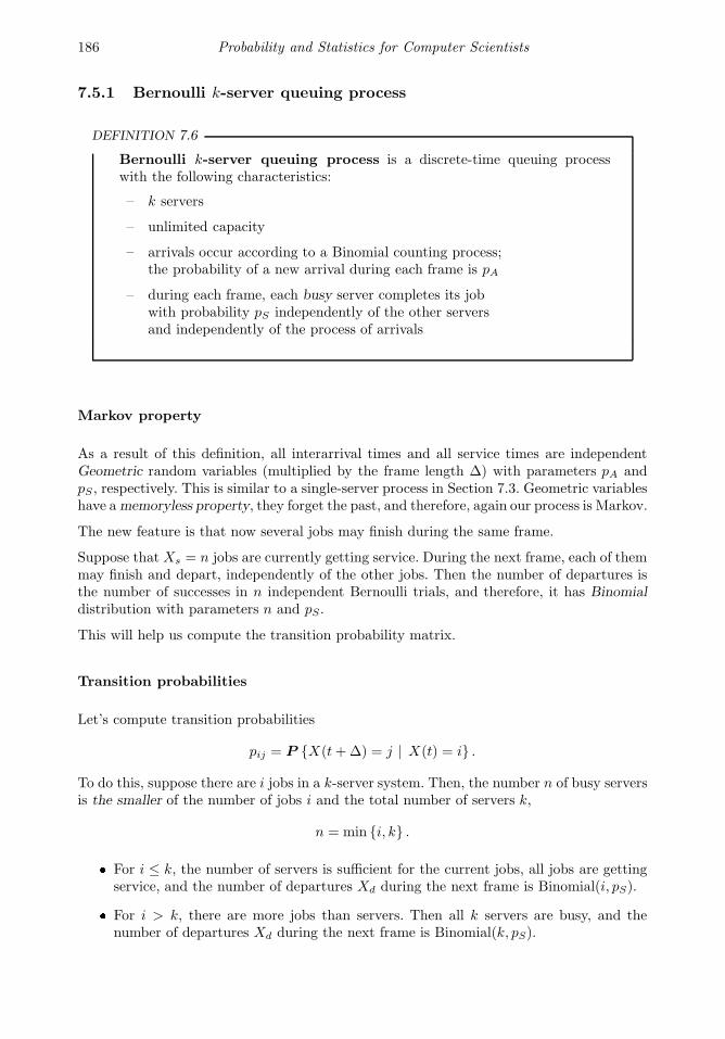
186 Probability and Statistics for Computer Scientists
7.5.1 Bernoulli k-server queuing process
DEFINITION 7.6
Bernoulli k-server queuing process is a discrete-time queuing processwith the following characteristics:
– k servers
– unlimited capacity
– arrivals occur according to a Binomial counting process;the probability of a new arrival during each frame is pA
– during each frame, each busy server completes its jobwith probability pS independently of the other serversand independently of the process of arrivals
Markov property
As a result of this definition, all interarrival times and all service times are independentGeometric random variables (multiplied by the frame length ∆) with parameters pA andpS , respectively. This is similar to a single-server process in Section 7.3. Geometric variableshave amemoryless property, they forget the past, and therefore, again our process is Markov.
The new feature is that now several jobs may finish during the same frame.
Suppose that Xs = n jobs are currently getting service. During the next frame, each of themmay finish and depart, independently of the other jobs. Then the number of departures isthe number of successes in n independent Bernoulli trials, and therefore, it has Binomialdistribution with parameters n and pS.
This will help us compute the transition probability matrix.
Transition probabilities
Let’s compute transition probabilities
pij = P X(t+∆) = j | X(t) = i .
To do this, suppose there are i jobs in a k-server system. Then, the number n of busy serversis the smaller of the number of jobs i and the total number of servers k,
n = min i, k . For i ≤ k, the number of servers is sufficient for the current jobs, all jobs are gettingservice, and the number of departures Xd during the next frame is Binomial(i, pS). For i > k, there are more jobs than servers. Then all k servers are busy, and thenumber of departures Xd during the next frame is Binomial(k, pS).
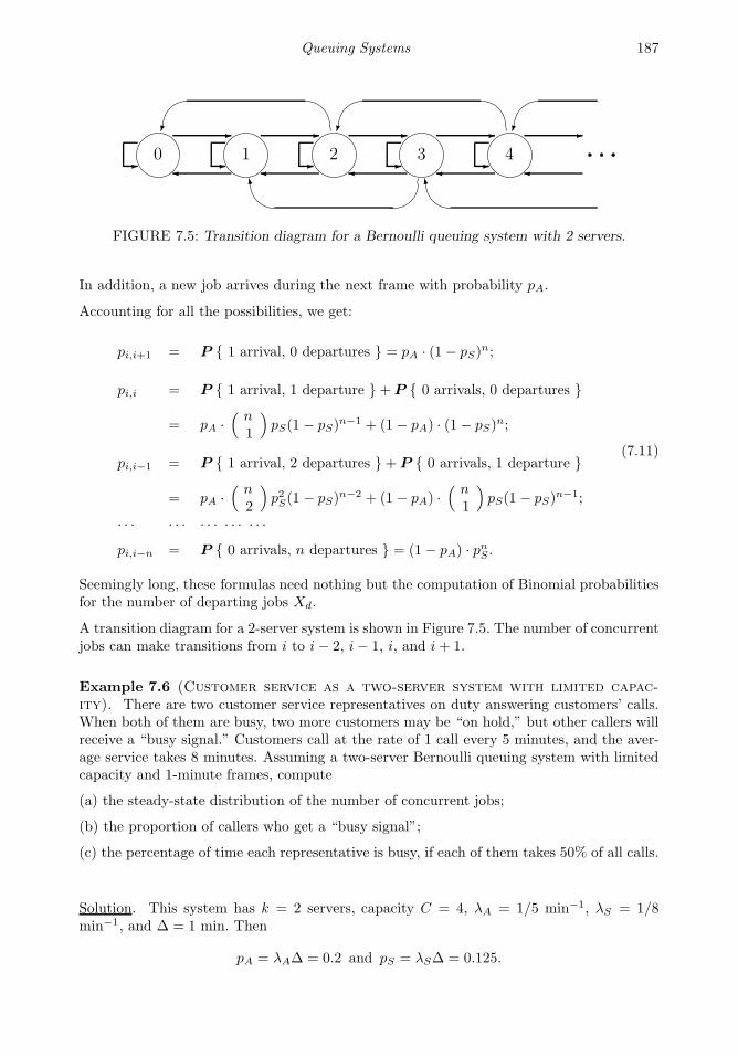
Queuing Systems 187
0 1 2 3 4
FIGURE 7.5: Transition diagram for a Bernoulli queuing system with 2 servers.
In addition, a new job arrives during the next frame with probability pA.
Accounting for all the possibilities, we get:
pi,i+1 = P 1 arrival, 0 departures = pA · (1− pS)n;
pi,i = P 1 arrival, 1 departure + P 0 arrivals, 0 departures
= pA ·( n
1
)pS(1 − pS)
n−1 + (1 − pA) · (1− pS)n;
pi,i−1 = P 1 arrival, 2 departures + P 0 arrivals, 1 departure
= pA ·( n
2
)p2S(1 − pS)
n−2 + (1 − pA) ·( n
1
)pS(1 − pS)
n−1;
· · · · · · · · · · · · · · ·pi,i−n = P 0 arrivals, n departures = (1 − pA) · pnS .
(7.11)
Seemingly long, these formulas need nothing but the computation of Binomial probabilitiesfor the number of departing jobs Xd.
A transition diagram for a 2-server system is shown in Figure 7.5. The number of concurrentjobs can make transitions from i to i− 2, i− 1, i, and i + 1.
Example 7.6 (Customer service as a two-server system with limited capac-ity). There are two customer service representatives on duty answering customers’ calls.When both of them are busy, two more customers may be “on hold,” but other callers willreceive a “busy signal.” Customers call at the rate of 1 call every 5 minutes, and the aver-age service takes 8 minutes. Assuming a two-server Bernoulli queuing system with limitedcapacity and 1-minute frames, compute
(a) the steady-state distribution of the number of concurrent jobs;
(b) the proportion of callers who get a “busy signal”;
(c) the percentage of time each representative is busy, if each of them takes 50% of all calls.
Solution. This system has k = 2 servers, capacity C = 4, λA = 1/5 min−1, λS = 1/8min−1, and ∆ = 1 min. Then
pA = λA∆ = 0.2 and pS = λS∆ = 0.125.
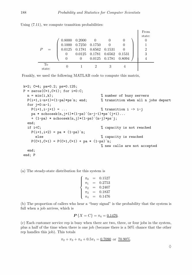
188 Probability and Statistics for Computer Scientists
Using (7.11), we compute transition probabilities:
Fromstate:
P =
0.8000 0.2000 0 0 00.1000 0.7250 0.1750 0 00.0125 0.1781 0.6562 0.1531 0
0 0.0125 0.1781 0.6562 0.15310 0 0.0125 0.1781 0.8094
01234
Tostate:
0 1 2 3 4
Frankly, we used the following MATLAB code to compute this matrix,
k=2; C=4; pa=0.2; ps=0.125;
P = zeros(C+1,C+1); for i=0:C;
n = min(i,k); % number of busy servers
P(i+1,i-n+1)=(1-pa)*psˆn; end; % transition when all n jobs depart
for j=0:n-1;
P(i+1,i-j+1) = ... % transition i -> i-j
pa * nchoosek(n,j+1)*(1-ps)ˆ(n-j-1)*psˆ(j+1)...+ (1-pa) * nchoosek(n,j)*(1-ps)ˆ(n-j)*psˆj;
end;
if i<C; % capacity is not reached
P(i+1,i+2) = pa * (1-ps)ˆn;else % capacity is reached
P(C+1,C+1) = P(C+1,C+1) + pa * (1-ps)ˆn;% new calls are not accepted
end;
end; P
(a) The steady-state distribution for this system is
π0 = 0.1527π1 = 0.2753π2 = 0.2407π3 = 0.1837π4 = 0.1476
(b) The proportion of callers who hear a “busy signal” is the probability that the system isfull when a job arrives, which is
P X = C = π4 = 0.1476.
(c) Each customer service rep is busy when there are two, three, or four jobs in the system,plus a half of the time when there is one job (because there is a 50% chance that the otherrep handles this job). This totals
π2 + π3 + π4 + 0.5π1 = 0.7090 or 70.90%.
♦

Queuing Systems 189
7.5.2 M/M/k systems
An M/M/k system is a multiserver extention of M/M/1. According to the general“A/S/n/C” notation in Section 7.4, it means the following.
DEFINITION 7.7
An M/M/k queuing process is a continuous-time Markov queuing processwith
– k servers– unlimited capacity– Exponential interarrival times with the arrival rate λA
– Exponential service time for each server with the service rate λS ,independent of all the arrival times and the other servers
Once again, we move from the discrete-time Bernoulli multiserver process to the continuous-time M/M/k by letting the frame ∆ go to 0. For very small ∆, transition probabilities (7.11)simplify,
pi,i+1 = λA∆ · (1− λS∆)n ≈ λA∆ = pA
pi,i = λA∆ · nλS∆(1− λS∆)n−1 + (1− λA∆) · (1 − λS∆)n
≈ 1− λA∆− nλS∆ = 1− pA − npS
pi,i−1 ≈ nλS∆ = npS
pi,j = 0 for all other j.
(7.12)
Again, n = min i, k is the number of jobs receiving service among the total of i jobs inthe system.
For example, for k = 3 servers, the transition probability matrix is
P ≈
1− pA pA 0 0 0. . .
pS 1−pA−pS pA 0 0. . .
0 2pS 1−pA−2pS pA 0. . .
0 0 3pS 1−pA−3pS pA. . .
0 0 0 3pS 1−pA−3pS. . .
0 0 0 0 3pS. . .
. . .. . .
. . .. . .
. . .. . .
(7.13)
Let’s try to understand these probabilities intuitively. Recall that ∆ is very small, so weignored terms proportional to ∆2, ∆3, etc. Then, no more than one event, arrival or de-parture, may occur during each frame. Probability of more than one event is of the order
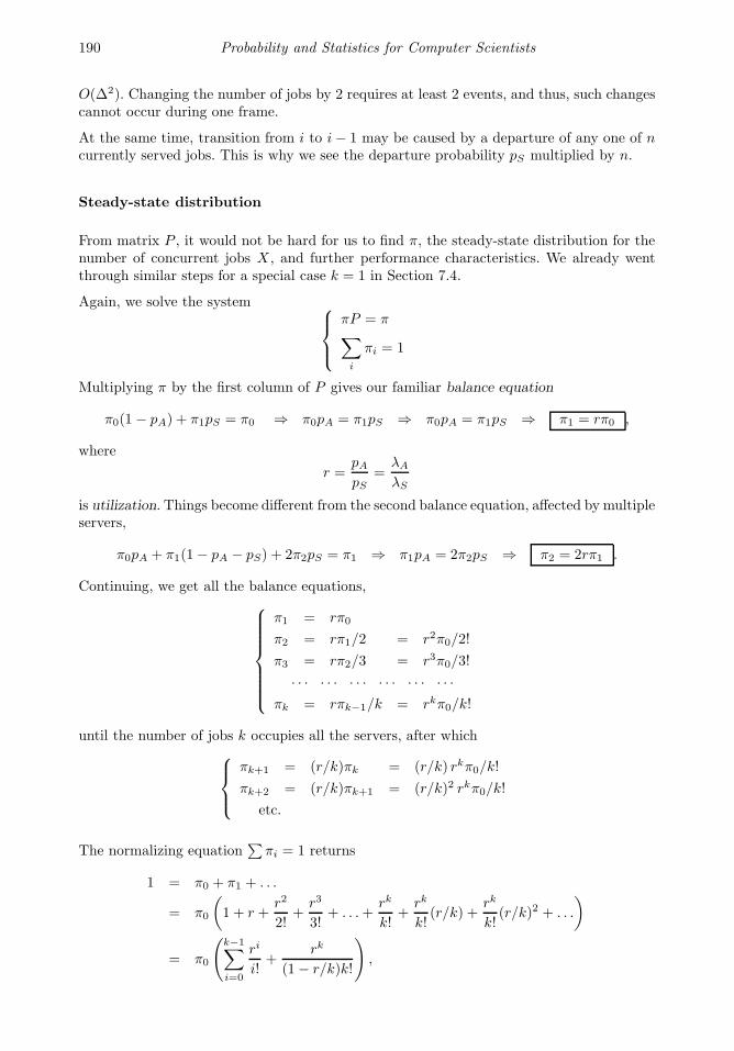
190 Probability and Statistics for Computer Scientists
O(∆2). Changing the number of jobs by 2 requires at least 2 events, and thus, such changescannot occur during one frame.
At the same time, transition from i to i− 1 may be caused by a departure of any one of ncurrently served jobs. This is why we see the departure probability pS multiplied by n.
Steady-state distribution
From matrix P , it would not be hard for us to find π, the steady-state distribution for thenumber of concurrent jobs X , and further performance characteristics. We already wentthrough similar steps for a special case k = 1 in Section 7.4.
Again, we solve the system
πP = π∑
i
πi = 1
Multiplying π by the first column of P gives our familiar balance equation
π0(1 − pA) + π1pS = π0 ⇒ π0pA = π1pS ⇒ π0pA = π1pS ⇒ π1 = rπ0 ,
where
r =pApS
=λA
λS
is utilization. Things become different from the second balance equation, affected by multipleservers,
π0pA + π1(1− pA − pS) + 2π2pS = π1 ⇒ π1pA = 2π2pS ⇒ π2 = 2rπ1 .
Continuing, we get all the balance equations,
π1 = rπ0
π2 = rπ1/2 = r2π0/2!
π3 = rπ2/3 = r3π0/3!
· · · · · · · · · · · · · · · · · ·πk = rπk−1/k = rkπ0/k!
until the number of jobs k occupies all the servers, after which
πk+1 = (r/k)πk = (r/k) rkπ0/k!
πk+2 = (r/k)πk+1 = (r/k)2 rkπ0/k!
etc.
The normalizing equation∑
πi = 1 returns
1 = π0 + π1 + . . .
= π0
(1 + r +
r2
2!+
r3
3!+ . . .+
rk
k!+
rk
k!(r/k) +
rk
k!(r/k)2 + . . .
)
= π0
(k−1∑
i=0
ri
i!+
rk
(1− r/k)k!
),
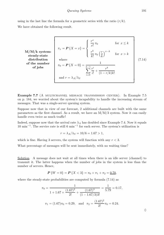
Queuing Systems 191
using in the last line the formula for a geometric series with the ratio (r/k).
We have obtained the following result.
M/M/k system:steady-statedistribution
of the numberof jobs
πx = P X = x =
rx
x!π0 for x ≤ k
rk
k!π0
( rk
)x−k
for x > k
where
π0 = P X = 0 =1
k−1∑
i=0
ri
i!+
rk
(1− r/k)k!
and r = λA/λS
(7.14)
Example 7.7 (A multichannel message transmission center). In Example 7.5on p. 184, we worried about the system’s incapability to handle the increasing stream ofmessages. That was a single-server queuing system.
Suppose now that in view of our forecast, 2 additional channels are built with the sameparameters as the first channel. As a result, we have an M/M/3 system. Now it can easilyhandle even twice as much traffic!
Indeed, suppose now that the arrival rate λA has doubled since Example 7.4. Now it equals10 min−1. The service rate is still 6 min−1 for each server. The system’s utilization is
r = λA/λS = 10/6 = 1.67 > 1,
which is fine. Having 3 servers, the system will function with any r < 3.
What percentage of messages will be sent immediately, with no waiting time?
Solution. A message does not wait at all times when there is an idle server (channel) totransmit it. The latter happens when the number of jobs in the system is less than thenumber of servers. Hence,
P W = 0 = P X < 3 = π0 + π1 + π2 = 0.70,
where the steady-state probabilities are computed by formula (7.14) as
π0 =1
1 + 1.67 +(1.67)2
2!+
(1.67)3
(1− 1.67/3)3!
=1
5.79= 0.17,
π1 = (1.67)π0 = 0.29, and π2 =(1.67)2
2!π0 = 0.24.
♦

192 Probability and Statistics for Computer Scientists
7.5.3 Unlimited number of servers and M/M/∞
An unlimited number of servers completely eliminates the waiting time. Whenever a jobarrives, there will always be servers available to handle it, and thus, the response time Rconsists of the service time only. In other words,
X = Xs, R = S, Xw = 0, and W = 0.
Have we seen such queuing systems?
Clearly, nobody can physically build an infinite number of devices. Having an unlimitednumber of servers simply means that any number of concurrent users can be served simul-taneously. For example, most internet service providers and most long-distance telephonecompanies allow virtually any number of concurrent connections; an unlimited number ofpeople can watch a TV channel, listen to a radio station, or take a sun bath.
Sometimes a model with infinitely many servers is a reasonable approximation for a systemwhere jobs typically don’t wait and get their service immediately. This may be appropriatefor a computer server, a grocery store, or a street with practically no traffic jams.
M/M/∞ queueing system
The definition and all the theory of M/M/k systems applies to M/M/∞ when we substitutek = ∞ or take a limit as the number of servers k goes to infinity. The number of jobs willalways be less than the number of servers (i < k), and therefore, we always have n = i.That is, with i jobs in the system, exactly i servers are busy.
The number of jobs X in an M/M/∞ system has a transition probability matrix
P =
1− pA pA 0 0. . .
pS 1−pA−pS pA 0. . .
0 2pS 1−pA−2pS pA. . .
0 0 3pS 1−pA−3pS. . .
0 0 0 4pS. . .
. . .. . .
. . .. . .
. . .
(7.15)
and its steady-state distribution is ... doesn’t it look familiar?
Taking a limit of (7.14) as k → ∞, we get
π0 =1
∞∑
i=0
ri
i!+ lim
k→∞
rk
(1 − r/k)k!
=1
er + 0= e−r,
and for all x ≥ 0,
πx =rx
x!π0 = e−r rx
x!.
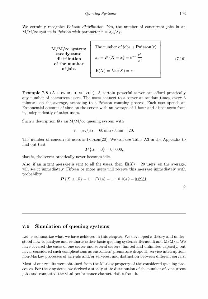
Queuing Systems 193
We certainly recognize Poisson distribution! Yes, the number of concurrent jobs in anM/M/∞ system is Poisson with parameter r = λA/λS .
M/M/∞ system:steady-statedistribution
of the numberof jobs
The number of jobs is Poisson(r)
πx = P X = x = e−r rx
x!
E(X) = Var(X) = r
(7.16)
Example 7.8 (A powerful server). A certain powerful server can afford practicallyany number of concurrent users. The users connect to a server at random times, every 3minutes, on the average, according to a Poisson counting process. Each user spends anExponential amount of time on the server with an average of 1 hour and disconnects fromit, independently of other users.
Such a description fits an M/M/∞ queuing system with
r = µS/µA = 60min /3min = 20.
The number of concurrent users is Poisson(20). We can use Table A3 in the Appendix tofind out that
P X = 0 = 0.0000,
that is, the server practically never becomes idle.
Also, if an urgent message is sent to all the users, then E(X) = 20 users, on the average,will see it immediately. Fifteen or more users will receive this message immediately withprobability
P X ≥ 15 = 1− F (14) = 1− 0.1049 = 0.8951.
♦
7.6 Simulation of queuing systems
Let us summarize what we have achieved in this chapter. We developed a theory and under-stood how to analyze and evaluate rather basic queuing systems: Bernoulli and M/M/k. Wehave covered the cases of one server and several servers, limited and unlimited capacity, butnever considered such complications as customers’ premature dropout, service interruption,non-Markov processes of arrivals and/or services, and distinction between different servers.
Most of our results were obtained from the Markov property of the considered queuing pro-cesses. For these systems, we derived a steady-state distribution of the number of concurrentjobs and computed the vital performance characteristics from it.

194 Probability and Statistics for Computer Scientists
The only general result is the Little’s Law of Section 7.2, which can be applied to anyqueuing system.
In practice, however, many queuing systems have a rather complex structure. Jobs mayarrive according to a non-Poisson process; often the rate of arrivals changes during the day(there is a rush hour on highways and on the internet). Service times may have differentdistributions, and they are not always memoryless, thus the Markov property may not besatisfied. The number of servers may also change during the day (additional servers mayturn on during rush hours). Some customers may get dissatisfied with a long waiting timeand quit in the middle of their queue. And so on.
Queuing theory does not cover all the possible situations. On the other hand, we can simulatethe behavior of almost any queuing system and study its properties byMonte Carlo methods.
Markov case
A queuing system is Markov only when its interarrival and service times are memoryless.Then the future can be predicted from the present without relying on the past (Section 6.2).
If this is the case, we compute the transition probability matrix as we did in (7.4), (7.6),(7.7), (7.11), (7.12), (7.13), or (7.15), and simulate the Markov chain according to Algo-rithm 6.1 on p. 157. To study long-term characteristics of a queuing system, the initialdistribution of X0 typically does not matter, so we may start this algorithm with 0 jobs inthe system and immediately “switch on” the servers.
Even when the system is Markov, some interesting characteristics do not follow from itssteady-state distribution directly. They can now be estimated from a Monte Carlo study bysimulated long-run proportions and averages. For example, we may be interested in estimat-ing the percentage of dissatisfied customers, the expected number of users during a periodof time from 3 pm till 5 pm, etc. We may also compute various forecasts (Section 5.3.3).
General case
Monte Carlo methods of Chapter 5 let us simulate and evaluate rather complex queuingsystems far beyond Bernoulli and M/M/k. As long as we know the distributions of inter-arrival and service times, we can generate the processes of arrivals and services. To assignjobs to servers, we keep track of servers that are available each time when a new job arrives.When all the servers are busy, the new job will enter a queue.
As we simulate the work of a queuing system, we keep records of events and variables thatare of interest to us. After a large number of Monte Carlo runs, we average our recordsin order to estimate probabilities by long-run proportions and expected values by long-runaverages.
Example: simulation of a multiserver queuing system
Let us simulate one day, from 8 am till 10 pm, of a queuing system that has
– four servers;
– Gamma distributed service times with parameters given in the table,

Queuing Systems 195
Server α λ
I 6 0.3 min−1
II 10 0.2 min−1
III 7 0.7 min−1
IV 5 1.0 min−1
– a Poisson process of arrivals with the rate of 1 arrival every 4 min, independent ofservice times;
– random assignment of servers, when more than 1 server is available.
In addition, suppose that after 15 minutes of waiting, jobs withdraw from a queue if theirservice has not started.
For an ordinary day of work of this system, we are interested to estimate the expectedvalues of:
– the total time each server is busy with jobs;
– the total number of jobs served by each server;
– the average waiting time;
– the longest waiting time;
– the number of withdrawn jobs;
– the number of times a server was available immediately (this is also the number ofjobs with no waiting time);
– the number of jobs remaining in the system at 10 pm.
We start by entering parameters of the system.
k = 4; % number of servers
mu = 4; % mean interarrival time
alpha = [6 10 7 5]; % parameters of service times
lambda = [0.3 0.2 0.7 1.0];
Then we initialize variables and start keeping track of arriving jobs. These are empty arraysso far. They get filled with each arriving job.
arrival = [ ]; % arrival time
start = [ ]; % service starts
finish = [ ]; % service finishes; departure time
server = [ ]; % assigned server
j = 0; % job number
T = 0; % arrival time of a new job
A = zeros(1,k); % array of times when each server
% becomes available for the next job
The queuing system is ready to work! We start a “while”-loop over the number of arriving
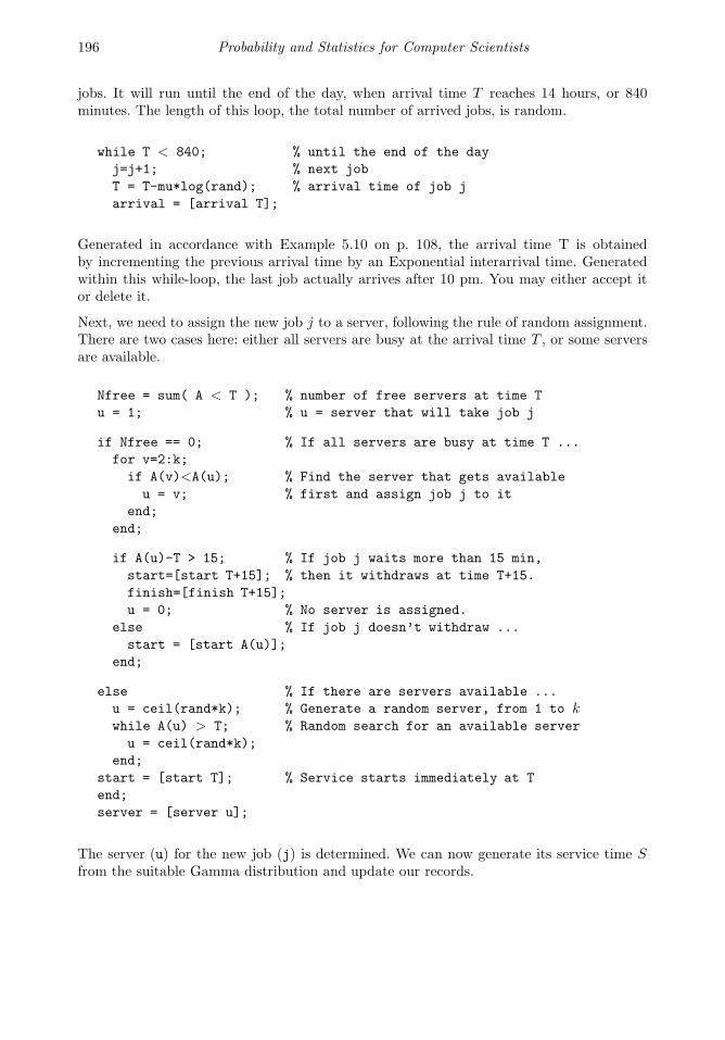
196 Probability and Statistics for Computer Scientists
jobs. It will run until the end of the day, when arrival time T reaches 14 hours, or 840minutes. The length of this loop, the total number of arrived jobs, is random.
while T < 840; % until the end of the day
j=j+1; % next job
T = T-mu*log(rand); % arrival time of job j
arrival = [arrival T];
Generated in accordance with Example 5.10 on p. 108, the arrival time T is obtainedby incrementing the previous arrival time by an Exponential interarrival time. Generatedwithin this while-loop, the last job actually arrives after 10 pm. You may either accept itor delete it.
Next, we need to assign the new job j to a server, following the rule of random assignment.There are two cases here: either all servers are busy at the arrival time T , or some serversare available.
Nfree = sum( A < T ); % number of free servers at time T
u = 1; % u = server that will take job j
if Nfree == 0; % If all servers are busy at time T ...
for v=2:k;
if A(v)<A(u); % Find the server that gets available
u = v; % first and assign job j to it
end;
end;
if A(u)-T > 15; % If job j waits more than 15 min,
start=[start T+15]; % then it withdraws at time T+15.
finish=[finish T+15];
u = 0; % No server is assigned.
else % If job j doesn’t withdraw ...
start = [start A(u)];
end;
else % If there are servers available ...
u = ceil(rand*k); % Generate a random server, from 1 to kwhile A(u) > T; % Random search for an available server
u = ceil(rand*k);
end;
start = [start T]; % Service starts immediately at T
end;
server = [server u];
The server (u) for the new job (j) is determined. We can now generate its service time Sfrom the suitable Gamma distribution and update our records.

Queuing Systems 197
if u>0; % if job j doesn’t withdraw ...
S = sum( -1/lambda(u) * log(rand(alpha(u),1) ) );
finish = [finish start(j)+S];
A(u) = start(j) + S; % This is the time when server u
end; % will now become available
end; % End of the while-loop
disp([(1:j)’ arrival’ start’ finish’ server’])
The day (our “while”-loop) has ended. The last command displayed the following records,
Job Arrival time Service starts Service ends Server
... ..... ..... ..... .....
From this table, all variables of our interest can be computed.
for u=1:k; % Twork(u) is the total working
Twork(u) = sum((server==u).*(finish-start)); % time for server u
Njobs(u) = sum(server==u); % number of jobs served by u
end;
Wmean = mean(start-arrival); % average waiting time
Wmax = max(start-arrival); % the longest waiting time
Nwithdr = sum(server==0); % number of withdrawn jobs
Nav = sum(start-arrival < 0.00001); % number of jobs that did not wait
Nat10 = sum(finish > 840); % number of jobs at 10 pm
We have computed all the required quantities for one day. Put this code into a “do”-loopand simulate a large number of days. The required expected values are then estimated byaveraging variables Wmean, Nwithdr, etc., over all days.
Summary and conclusions
Queuing systems are service facilities designed to serve randomly arriving jobs.
Several classes of queuing systems were studied in this chapter. We discussed discrete-timeand continuous-time, Markov and non-Markov, one-server and multiserver queuing processeswith limited and unlimited capacity.
Detailed theory was developed for Markov systems, where we derived the distribution ofthe number of concurrent jobs and obtained analytic expressions for a number of vitalcharacteristics. These results are used to evaluate performance of a queuing system, forecastits future efficiency when parameters change, and see if it is still functional under the newconditions.
Performance of more complicated and advanced queuing systems can be evaluated by MonteCarlo methods. One needs to simulate arrivals of jobs, assignment of servers, and servicetimes and to keep track of all variables of interest. A sample computer code for such asimulation is given.

198 Probability and Statistics for Computer Scientists
Exercises
7.1. Customers arrive at the ATM at the rate of 10 customers per hour and spend 2 minutes,on average, on all the transactions. This system is modeled by the Bernoulli single-serverqueuing process with 10-second frames. Write the transition probability matrix for thenumber of customers at the ATM at the end of each frame.
7.2. Consider Bernoulli single-server queuing process with an arrival rate of 2 jobs per minute,a service rate of 4 jobs per minute, frames of 0.2 minutes, and a capacity limited by 2 jobs.Compute the steady-state distribution of the number of jobs in the system.
7.3. Performance of a car wash center is modeled by the Bernoulli single-server queuing processwith 2-minute frames. The cars arrive every 10 minutes, on the average. The average servicetime is 6 minutes. Capacity is unlimited. If there are no cars at the center at 10 am, computethe probability that one car will be washed and another car will be waiting at 10:04 am.
7.4. Masha has a telephone with two lines that allows her to talk with a friend and have at mostone other friend on hold. On the average, she gets 10 calls every hour, and an average conver-sation takes 2 minutes. Assuming a single-server limited-capacity Bernoulli queuing processwith 1-minute frames, compute the fraction of time Masha spends using her telephone.
7.5. A customer service representative can work with one person at a time and have at most oneother customer waiting. Compute the steady-state distribution of the number of customersin this queuing system at any time, assuming that customers arrive according to a Binomialcounting process with 3-minute frames and the average interarrival time of 10 minutes, andthe average service takes 15 minutes.
7.6. Performance of a telephone with 2 lines is modeled by the Bernoulli single-server queuingprocess with limited capacity (C = 2). If both lines of a telephone are busy, the new callersreceive a busy signal and cannot enter the queue. On the average, there are 5 calls perhour, and the average call takes 20 minutes. Compute the steady-state probabilities usingfour-minute frames.
7.7. Jobs arrive at the server at the rate of 8 jobs per hour. The service takes 3 minutes, onthe average. This system is modeled by the Bernoulli single-server queuing process with5-second frames and capacity limited by 3 jobs. Write the transition probability matrix forthe number of jobs in the system at the end of each frame.
7.8. For an M/M/1 queuing process with the arrival rate of 5 min−1 and the average servicetime of 4 seconds, compute
(a) the proportion of time when there are exactly 2 customers in the system;
(b) the expected response time (the expected time from the arrival till the departure).
7.9. Jobs are sent to a printer at random times, according to a Poisson process of arrivals, with arate of 12 jobs per hour. The time it takes to print a job is an Exponential random variable,independent of the arrival time, with the average of 2 minutes per job.
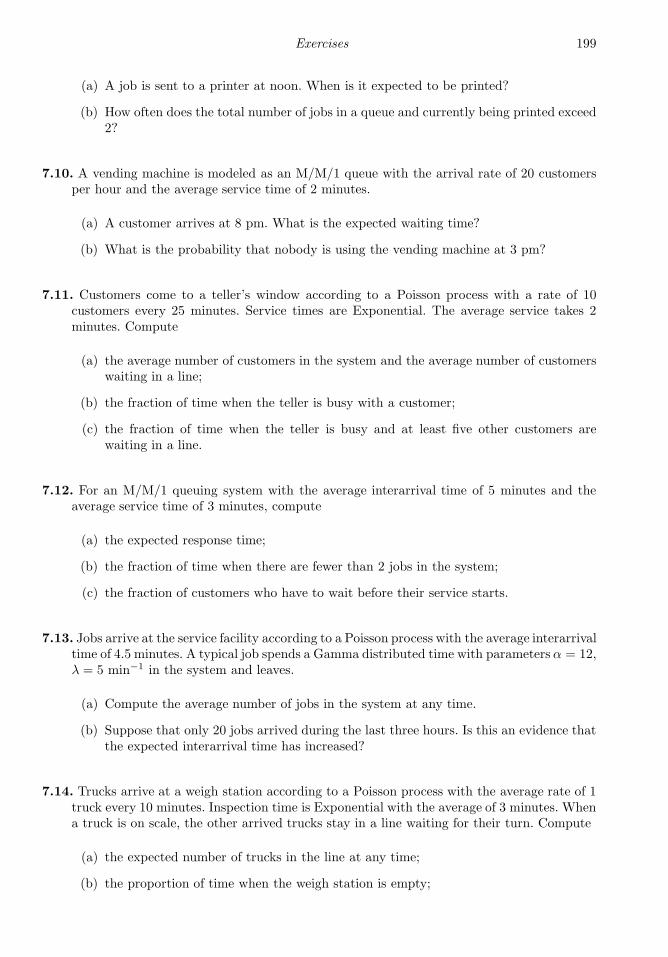
Exercises 199
(a) A job is sent to a printer at noon. When is it expected to be printed?
(b) How often does the total number of jobs in a queue and currently being printed exceed2?
7.10. A vending machine is modeled as an M/M/1 queue with the arrival rate of 20 customersper hour and the average service time of 2 minutes.
(a) A customer arrives at 8 pm. What is the expected waiting time?
(b) What is the probability that nobody is using the vending machine at 3 pm?
7.11. Customers come to a teller’s window according to a Poisson process with a rate of 10customers every 25 minutes. Service times are Exponential. The average service takes 2minutes. Compute
(a) the average number of customers in the system and the average number of customerswaiting in a line;
(b) the fraction of time when the teller is busy with a customer;
(c) the fraction of time when the teller is busy and at least five other customers arewaiting in a line.
7.12. For an M/M/1 queuing system with the average interarrival time of 5 minutes and theaverage service time of 3 minutes, compute
(a) the expected response time;
(b) the fraction of time when there are fewer than 2 jobs in the system;
(c) the fraction of customers who have to wait before their service starts.
7.13. Jobs arrive at the service facility according to a Poisson process with the average interarrivaltime of 4.5 minutes. A typical job spends a Gamma distributed time with parameters α = 12,λ = 5 min−1 in the system and leaves.
(a) Compute the average number of jobs in the system at any time.
(b) Suppose that only 20 jobs arrived during the last three hours. Is this an evidence thatthe expected interarrival time has increased?
7.14. Trucks arrive at a weigh station according to a Poisson process with the average rate of 1truck every 10 minutes. Inspection time is Exponential with the average of 3 minutes. Whena truck is on scale, the other arrived trucks stay in a line waiting for their turn. Compute
(a) the expected number of trucks in the line at any time;
(b) the proportion of time when the weigh station is empty;

200 Probability and Statistics for Computer Scientists
(c) the expected time each truck spends at the station, from arrival till departure.
7.15. Consider a hot-line telephone that has no second line. When the telephone is busy, the newcallers get a busy signal. People call at the average rate of 2 calls per minute. The averageduration of a telephone conversation is 1 minute. The system behaves like a Bernoulli single-server queuing process with a frame size of 1 second.
(a) Compute the steady-state distribution for the number of concurrent jobs.
(b) What is the probability that more than 150 people attempted to call this numberbetween 2 pm and 3 pm?
7.16. On the average, every 6 minutes a customer arrives at an M/M/k queuing system, spendsan average of 20 minutes there, and departs. What is the mean number of customers in thesystem at any given time?
7.17. Verify the Little’s Law for the M/M/1 queuing system and for its components – waitingand service.
7.18. A metered parking lot with two parking spaces represents a Bernoulli two-server queuingsystem with capacity limited by two cars and 30-second frames. Cars arrive at the rate ofone car every 4 minutes. Each car is parked for 5 minutes, on the average.
(a) Compute the transition probability matrix for the number of parked cars.
(b) Find the steady-state distribution for the number of parked cars.
(c) What fraction of the time are both parking spaces vacant?
(d) What fraction of arriving cars will not be able to park?
(e) Every 2 minutes of parking costs 25 cents. Assuming that the drivers use all theparking time they pay for, what revenue is the owner of this parking lot expected toget every 24 hours?
7.19. (This exercise may require a computer or at least a calculator.) A walk-in hairdressingsaloon has two hairdressers and two extra chairs for waiting customers. We model thissystem as a Bernoulli queuing process with two servers, 1-minute frames, capacity limitedby 4 customers, arrival rate of 3 customers per hour, and the average service time of 45minutes, not including the waiting time.
(a) Compute the transition probability matrix for the number of customers in the saloonat any time and find the steady-state distribution.
(b) Use this steady-state distribution to compute the expected number of customers inthe saloon at any time, the expected number of customers waiting for a hairdresser,and the fraction of customers who found all the available seats already occupied.
(c) Each hairdresser comes for an eight-hour working day. How does it split between theirworking time and their resting time?
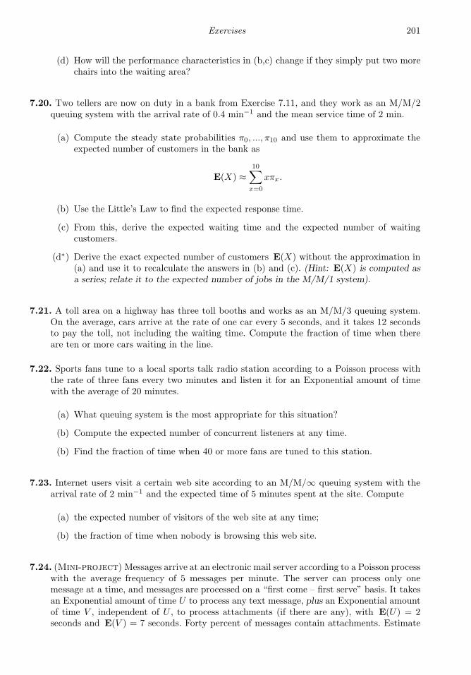
Exercises 201
(d) How will the performance characteristics in (b,c) change if they simply put two morechairs into the waiting area?
7.20. Two tellers are now on duty in a bank from Exercise 7.11, and they work as an M/M/2queuing system with the arrival rate of 0.4 min−1 and the mean service time of 2 min.
(a) Compute the steady state probabilities π0, ..., π10 and use them to approximate theexpected number of customers in the bank as
E(X) ≈10∑
x=0
xπx.
(b) Use the Little’s Law to find the expected response time.
(c) From this, derive the expected waiting time and the expected number of waitingcustomers.
(d∗) Derive the exact expected number of customers E(X) without the approximation in(a) and use it to recalculate the answers in (b) and (c). (Hint: E(X) is computed asa series; relate it to the expected number of jobs in the M/M/1 system).
7.21. A toll area on a highway has three toll booths and works as an M/M/3 queuing system.On the average, cars arrive at the rate of one car every 5 seconds, and it takes 12 secondsto pay the toll, not including the waiting time. Compute the fraction of time when thereare ten or more cars waiting in the line.
7.22. Sports fans tune to a local sports talk radio station according to a Poisson process withthe rate of three fans every two minutes and listen it for an Exponential amount of timewith the average of 20 minutes.
(a) What queuing system is the most appropriate for this situation?
(b) Compute the expected number of concurrent listeners at any time.
(b) Find the fraction of time when 40 or more fans are tuned to this station.
7.23. Internet users visit a certain web site according to an M/M/∞ queuing system with thearrival rate of 2 min−1 and the expected time of 5 minutes spent at the site. Compute
(a) the expected number of visitors of the web site at any time;
(b) the fraction of time when nobody is browsing this web site.
7.24. (Mini-project) Messages arrive at an electronic mail server according to a Poisson processwith the average frequency of 5 messages per minute. The server can process only onemessage at a time, and messages are processed on a “first come – first serve” basis. It takesan Exponential amount of time U to process any text message, plus an Exponential amountof time V , independent of U , to process attachments (if there are any), with E(U) = 2seconds and E(V ) = 7 seconds. Forty percent of messages contain attachments. Estimate

202 Probability and Statistics for Computer Scientists
the expected response time of this server by the Monte Carlo method.
(Notice that because of the attachments, the overall service time is not Exponential, so thesystem is not M/M/1.).
7.25. (Mini-project) A doctor scheduled her patients to arrive at equal 15-minute intervals.Patients are then served in the order of their arrivals, and each of them needs a Gammatime with the doctor that has parameters α = 4 and λ = 0.3 min−1. Use Monte Carlosimulations to estimate
(a) the expected response time;
(b) the expected waiting time;
(c) the probability that a patient has to wait before seeing the doctor.
(This system is not M/M/1 either because the interarrival times are not random.).
7.26. (Computer project) A multiserver system (computer lab, customer service, telephonecompany) consists of n = 4 servers (computers, customer service representatives, telephonecables). Every server is able to process any job, but some of them work faster than theothers. The service times are distributed according to the table.
Server Distribution Parameters
I Gamma α = 7, λ = 3 min−1
II Gamma α = 5, λ = 2 min−1
III Exponential λ = 0.3 min−1
IV Uniform a = 4 min, b = 9 min
The jobs (customers, telephone calls) arrive to the system at random times, independentlyof each other, according to a Poisson process. The average interarrival time is 2 minutes.If a job arrives, and there are free servers available, then the job is equally likely to beprocessed by any of the available servers. If no servers are available at the time of arrival,the job enters a queue. After waiting for 6 minutes, if the service has not started, the jobleaves the system. The system works 10 hours a day, from 8 am till 6 pm.
Run at least 1000 Monte Carlo simulations and estimate the following quantities:
(a) the expected waiting time for a randomly selected job;
(b) the expected response time;
(c) the expected length of a queue (excluding the jobs receiving service), when a new jobarrives;
(d) the expected maximum waiting time during a 10-hour day;
(e) the expected maximum length of a queue during a 10-hour day;
(f) the probability that at least one server is available, when a job arrives;
(g) the probability that at least two servers are available, when a job arrives;
(h) the expected number of jobs processed by each server;

Exercises 203
(i) the expected time each server is idle during the day;
(j) the expected number of jobs still remaining in the system at 6:03 pm;
(k) the expected percentage of jobs that left the queue prematurely.
7.27. (Computer project) An IT support help desk represents a queuing system with fiveassistants taking calls from customers. The calls occur according to a Poisson process withthe average rate of one call every 45 seconds. The service times for the 1st, 2nd, 3rd, 4th, and5th assistants are all Exponential random variables with parameters λ1 = 0.1, λ2 = 0.2,λ3 = 0.3, λ4 = 0.4, and λ5 = 0.5 min−1, respectively (the jth help desk assistant hasλk = k/10 min−1). Besides the customers who are being assisted, up to ten other customerscan be placed on hold. At times when this capacity is reached, the new callers receive abusy signal.
Use the Monte Carlo methods to estimate the following performance characteristics,
(a) the fraction of customers who receive a busy signal;
(b) the expected response time;
(c) the average waiting time;
(d) the portion of customers served by each help desk assistant;
(e) all of the above if the 6th help desk assistant has been hired to help the first five, andλ6 = 0.6. How has this assistant, the fastest on the team, improved performance ofthe queuing system?
Questions (b-d) refer to those customers who got into the system and did not receive a busysignal.


Part III
Statistics
205

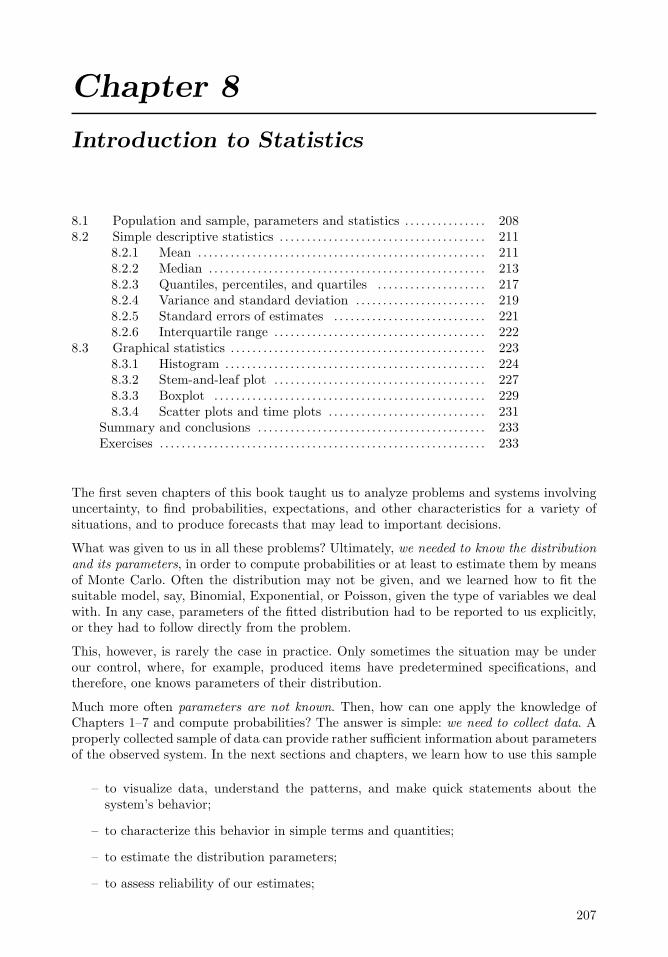
Chapter 8
Introduction to Statistics
8.1 Population and sample, parameters and statistics . . . . . . . . . . . . . . . 2088.2 Simple descriptive statistics . . . . . . . . . . . . . . . . . . . . . . . . . . . . . . . . . . . . . . 211
8.2.1 Mean . . . . . . . . . . . . . . . . . . . . . . . . . . . . . . . . . . . . . . . . . . . . . . . . . . . . . 2118.2.2 Median . . . . . . . . . . . . . . . . . . . . . . . . . . . . . . . . . . . . . . . . . . . . . . . . . . . 2138.2.3 Quantiles, percentiles, and quartiles . . . . . . . . . . . . . . . . . . . . 2178.2.4 Variance and standard deviation . . . . . . . . . . . . . . . . . . . . . . . . 2198.2.5 Standard errors of estimates . . . . . . . . . . . . . . . . . . . . . . . . . . . . 2218.2.6 Interquartile range . . . . . . . . . . . . . . . . . . . . . . . . . . . . . . . . . . . . . . . 222
8.3 Graphical statistics . . . . . . . . . . . . . . . . . . . . . . . . . . . . . . . . . . . . . . . . . . . . . . . 2238.3.1 Histogram . . . . . . . . . . . . . . . . . . . . . . . . . . . . . . . . . . . . . . . . . . . . . . . . 2248.3.2 Stem-and-leaf plot . . . . . . . . . . . . . . . . . . . . . . . . . . . . . . . . . . . . . . . 2278.3.3 Boxplot . . . . . . . . . . . . . . . . . . . . . . . . . . . . . . . . . . . . . . . . . . . . . . . . . . 2298.3.4 Scatter plots and time plots . . . . . . . . . . . . . . . . . . . . . . . . . . . . . 231
Summary and conclusions . . . . . . . . . . . . . . . . . . . . . . . . . . . . . . . . . . . . . . . . . . 233Exercises . . . . . . . . . . . . . . . . . . . . . . . . . . . . . . . . . . . . . . . . . . . . . . . . . . . . . . . . . . . . 233
The first seven chapters of this book taught us to analyze problems and systems involvinguncertainty, to find probabilities, expectations, and other characteristics for a variety ofsituations, and to produce forecasts that may lead to important decisions.
What was given to us in all these problems? Ultimately, we needed to know the distributionand its parameters, in order to compute probabilities or at least to estimate them by meansof Monte Carlo. Often the distribution may not be given, and we learned how to fit thesuitable model, say, Binomial, Exponential, or Poisson, given the type of variables we dealwith. In any case, parameters of the fitted distribution had to be reported to us explicitly,or they had to follow directly from the problem.
This, however, is rarely the case in practice. Only sometimes the situation may be underour control, where, for example, produced items have predetermined specifications, andtherefore, one knows parameters of their distribution.
Much more often parameters are not known. Then, how can one apply the knowledge ofChapters 1–7 and compute probabilities? The answer is simple: we need to collect data. Aproperly collected sample of data can provide rather sufficient information about parametersof the observed system. In the next sections and chapters, we learn how to use this sample
– to visualize data, understand the patterns, and make quick statements about thesystem’s behavior;
– to characterize this behavior in simple terms and quantities;
– to estimate the distribution parameters;
– to assess reliability of our estimates;
207

208 Probability and Statistics for Computer Scientists
– to test statements about parameters and the entire system;
– to understand relations among variables;
– to fit suitable models and use them to make forecasts.
8.1 Population and sample, parameters and statistics
Data collection is a crucially important step in Statistics. We use the collected and observedsample to make statements about a much larger set — the population.
DEFINITION 8.1
A population consists of all units of interest. Any numerical characteristic ofa population is a parameter. A sample consists of observed units collectedfrom the population. It is used to make statements about the population. Anyfunction of a sample is called statistic.
In real problems, we would like to make statements about the population. To computeprobabilities, expectations, and make optimal decisions under uncertainty, we need to knowthe population parameters. However, the only way to know these parameters is to measurethe entire population, i.e., to conduct a census.
Instead of a census, we may collect data in a form of a random sample from a population(Figure 8.1). This is our data. We can measure them, perform calculations, and estimatethe unknown parameters of the population up to a certain measurable degree of accuracy.
Notation θ = population parameter
θ = its estimator, obtained from a sample
Example 8.1 (Customer satisfaction). For example, even if 80% of users are satisfiedwith their internet connection, it does not mean that exactly 8 out of 10 customers inyour observed sample are satisfied. As we can see from Table A2 in the Appendix, withprobability 0.0328, only a half of ten sampled customers are satisfied. In other words, thereis a 3% chance for a random sample to suggest that contrary to the population parameter,no more than 50% of users are satisfied. ♦
This example shows that a sample may sometimes give a rather misleading informationabout the population although this happens with a low probability. Sampling errors cannotbe excluded.
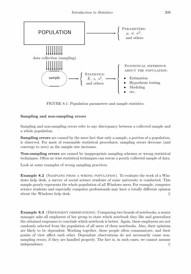
Introduction to Statistics 209
POPULATION
sample
data collection (sampling)
Parameters:µ, σ, σ2,and others
Statistics:X, s, s2,and others
Statistical inferenceabout the population:
• Estimation• Hypothesis testing• Modeling• etc.
FIGURE 8.1: Population parameters and sample statistics.
Sampling and non-sampling errors
Sampling and non-sampling errors refer to any discrepancy between a collected sample anda whole population.
Sampling errors are caused by the mere fact that only a sample, a portion of a population,is observed. For most of reasonable statistical procedures, sampling errors decrease (andconverge to zero) as the sample size increases.
Non-sampling errors are caused by inappropriate sampling schemes or wrong statisticaltechniques. Often no wise statistical techniques can rescue a poorly collected sample of data.
Look at some examples of wrong sampling practices.
Example 8.2 (Sampling from a wrong population). To evaluate the work of a Win-dows help desk, a survey of social science students of some university is conducted. Thissample poorly represents the whole population of all Windows users. For example, computerscience students and especially computer professionals may have a totally different opinionabout the Windows help desk. ♦
Example 8.3 (Dependent observations). Comparing two brands of notebooks, a seniormanager asks all employees of her group to state which notebook they like and generalizesthe obtained responses to conclude which notebook is better. Again, these employees are notrandomly selected from the population of all users of these notebooks. Also, their opinionsare likely to be dependent. Working together, these people often communicate, and theirpoints of view affect each other. Dependent observations do not necessarily cause non-sampling errors, if they are handled properly. The fact is, in such cases, we cannot assumeindependence. ♦
210 Probability and Statistics for Computer Scientists
Example 8.4 (Not equally likely). A survey among passengers of some airline is con-ducted in the following way. A sample of random flights is selected from a list, and tenpassengers on each of these flights are also randomly chosen. Each sampled passenger isasked to fill a questionnaire. Is this a representative sample?
Suppose Mr. X flies only once a year whereas Ms. Y has business trips twice a month. Ob-viously, Ms. Y has a much higher chance to be sampled than Mr. X. Unequal probabilitieshave to be taken into account, otherwise a non-sampling error will inevitably occur. ♦
Example 8.5 (Presidential Election of 1936). A popular weekly magazine The Lit-erary Digest correctly predicted the winners of 1920, 1924, 1928, and 1932 U.S. PresidentialElections. However, it failed to do so in 1936! Based on a survey of ten million people, itpredicted an overwhelming victory of Governor Alfred Landon. Instead, Franklin DelanoRoosevelt received 98.49% of the electoral vote, won 46 out of 48 states, and was re-elected.
So, what went wrong in that survey? At least two main issues with their sampling practicecaused this prediction error. First, the sample was based on the population of subscribers ofThe Literary Digest that was dominated by Republicans. Second, responses were voluntary,and 77% of mailed questionnaires were not returned, introducing further bias. These areclassical examples of non-sampling errors. ♦
In this book, we focus on simple random sampling, which is one way to avoid non-samplingerrors.
DEFINITION 8.2
Simple random sampling is a sampling design where units are collectedfrom the entire population independently of each other, all being equally likelyto be sampled.
Observations collected by means of a simple random sampling design are iid (independent,identically distributed) random variables.
Example 8.6. To evaluate its customers’ satisfaction, a bank makes a list of all theaccounts. A Monte Carlo method is used to choose a random number between 1 and N ,where N is the total number of bank accounts. Say, we generate a Uniform(0,N) variable Xand sample an account number ⌈X⌉ from the list. Similarly, we choose the second account,uniformly distributed among the remaining N − 1 accounts, etc., until we get a sample ofthe desired size n. This is a simple random sample. ♦
Obtaining a good, representative random sample is rather important in Statistics. Althoughwe have only a portion of the population in our hands, a rigorous sampling design followedby a suitable statistical inference allows to estimate parameters and make statements witha certain measurable degree of confidence.

Introduction to Statistics 211
8.2 Simple descriptive statistics
Suppose a good random sample
S = (X1, X2, . . . , Xn)
has been collected. For example, to evaluate effectiveness of a processor for a certain typeof tasks, we recorded the CPU time for n = 30 randomly chosen jobs (in seconds),
70 36 43 69 82 48 34 62 35 1559 139 46 37 42 30 55 56 36 8238 89 54 25 35 24 22 9 56 19
(8.1)
What information do we get from this collection of numbers?
We know that X , the CPU time of a random job, is a random variable, and its value doesnot have to be among the observed thirty. We’ll use the collected data to describe thedistribution of X .
Simple descriptive statistics measuring the location, spread, variability, and other char-acteristics can be computed immediately. In this section, we discuss the following statistics, mean, measuring the average value of a sample; median, measuring the central value; quantiles and quartiles, showing where certain portions of a sample are located; variance, standard deviation, and interquartile range, measuring variability and
spread of data.
Each statistic is a random variable because it is computed from random data. It has aso-called sampling distribution.
Each statistic estimates the corresponding population parameter and adds certain informa-tion about the distribution of X , the variable of interest.
We used similar methods in Section 5.3.2, where we estimated parameters from MonteCarlo samples obtained by computer simulations. Here we estimate parameters and makeconclusions based on real, not simulated, data.
8.2.1 Mean
Sample mean X estimates the population mean µ = E(X).
DEFINITION 8.3
Sample mean X is the arithmetic average,
X =X1 + . . .+Xn
n
212 Probability and Statistics for Computer Scientists
Naturally, being the average of sampled observations, X estimates the average value of thewhole distribution of X . Computed from random data, X does not necessarily equal µ;however, we would expect it to converge to µ when a large sample is collected.
Sample means possess a number of good properties. They are unbiased, consistent, andasymptotically Normal.
Remark: This is true if the population has finite mean and variance, which is the case for almost
all the distributions in this book (see, however, Example 3.20 on p. 62).
Unbiasedness
DEFINITION 8.4
An estimator θ is unbiased for a parameter θ if its expectation equals theparameter,
E(θ) = θ
for all possible values of θ.
Bias of θ is defined as Bias(θ) = E(θ − θ).
Unbiasedness means that in a long run, collecting a large number of samples and computingθ from each of them, on the average we hit the unknown parameter θ exactly. In other words,in a long run, unbiased estimators neither underestimate nor overestimate the parameter.
Sample mean estimates µ unbiasedly because its expectation is
E(X) = E
(X1 + . . .+Xn
n
)=
EX1 + . . .+ EXn
n=
nµ
n= µ.
Consistency
DEFINITION 8.5
An estimator θ is consistent for a parameter θ if the probability of its samplingerror of any magnitude converges to 0 as the sample size increases to infinity.Stating it rigorously,
P|θ − θ| > ε
→ 0 as n → ∞
for any ε > 0. That is, when we estimate θ from a large sample, the estimationerror |θ − θ| is unlikely to exceed ε, and it does it with smaller and smallerprobabilities as we increase the sample size.
Consistency of X follows directly from Chebyshev’s inequality on p. 54.

Introduction to Statistics 213
To use this inequality, we find the variance of X,
Var(X) = Var
(X1 + . . .+Xn
n
)=
VarX1 + . . .+ VarXn
n2=
nσ2
n2=
σ2
n. (8.2)
Then, using Chebyshev’s inequality for the random variable X, we get
P|X − µ| > ε
≤ Var(X)
ε2=
σ2/n
ε2→ 0,
as n → ∞.
Thus, a sample mean is consistent. Its sampling error will be small with a higher and higherprobability, as we collect larger and larger samples.
Asymptotic Normality
By the Central Limit Theorem, the sum of observations, and therefore, the sample meanhave approximately Normal distribution if they are computed from a large sample. That is,the distribution of
Z =X − EX
StdX=
X − µ
σ√n
converges to Standard Normal as n → ∞. This property is called Asymptotic Normality.
Example 8.7 (CPU times). Looking at the CPU data on p. 211, we estimate the average(expected) CPU time µ by
X =70 + 36 + . . .+ 56 + 19
30=
1447
30= 48.2333.
We may conclude that the mean CPU time of all the jobs is “near” 48.2333 seconds.♦
Notation µ = population meanX = sample mean, estimator of µ
σ = population standard deviations = sample standard deviation, estimator of σ
σ2 = population variances2 = sample variance, estimator of σ
8.2.2 Median
One disadvantage of a sample mean is its sensitivity to extreme observations. For example,if the first job in our sample is unusually heavy, and it takes 30 minutes to get processedinstead of 70 seconds, this one extremely large observation shifts the sample mean from48.2333 sec to 105.9 sec. Can we call such an estimator “reliable”?
Another simple measure of location is a sample median, which estimates the populationmedian. It is much less sensitive than the sample mean.
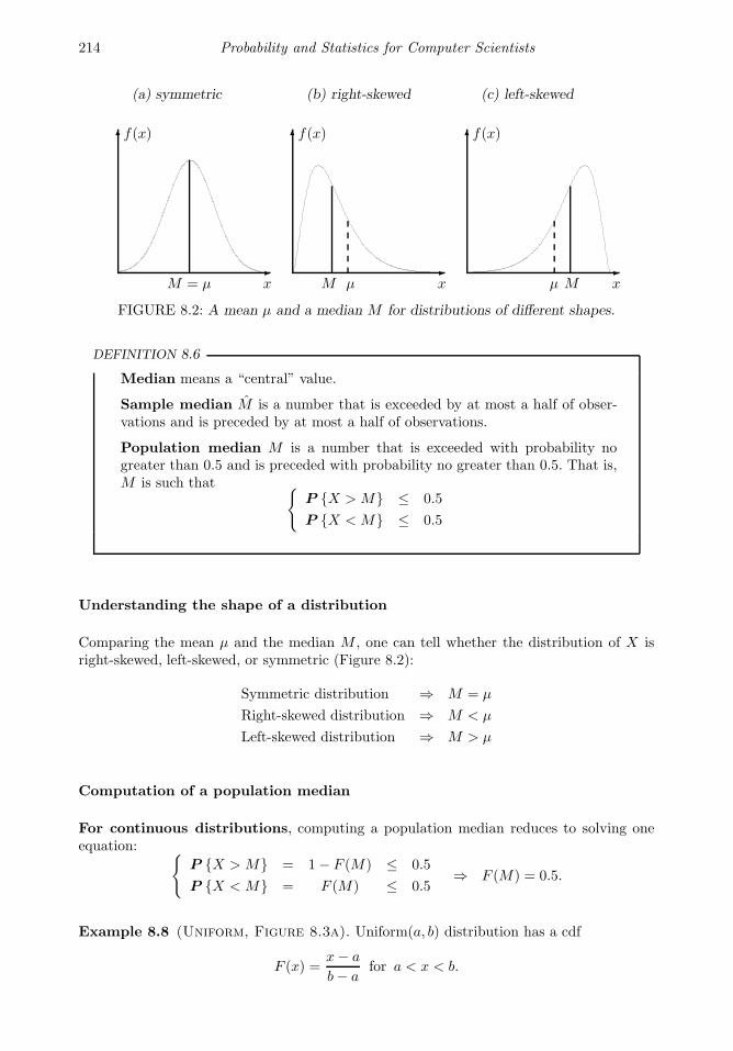
214 Probability and Statistics for Computer Scientists
x x x
f(x) f(x) f(x)
M = µ M µ µ M
(a) symmetric (b) right-skewed (c) left-skewed
FIGURE 8.2: A mean µ and a median M for distributions of different shapes.
DEFINITION 8.6
Median means a “central” value.
Sample median M is a number that is exceeded by at most a half of obser-vations and is preceded by at most a half of observations.
Population median M is a number that is exceeded with probability nogreater than 0.5 and is preceded with probability no greater than 0.5. That is,M is such that
P X > M ≤ 0.5
P X < M ≤ 0.5
Understanding the shape of a distribution
Comparing the mean µ and the median M , one can tell whether the distribution of X isright-skewed, left-skewed, or symmetric (Figure 8.2):
Symmetric distribution ⇒ M = µ
Right-skewed distribution ⇒ M < µ
Left-skewed distribution ⇒ M > µ
Computation of a population median
For continuous distributions, computing a population median reduces to solving oneequation:
P X > M = 1− F (M) ≤ 0.5
P X < M = F (M) ≤ 0.5⇒ F (M) = 0.5.
Example 8.8 (Uniform, Figure 8.3a). Uniform(a, b) distribution has a cdf
F (x) =x− a
b− afor a < x < b.

Introduction to Statistics 215
(a) Uniform (b) Exponential
0 0
1 1
0.5 0.5
a bM M
x x
F (x) F (x)
FIGURE 8.3: Computing medians of continuous distributions.
Solving the equation F (M) = (M − a)/(b− a) = 0.5, we get
M =a+ b
2.
It coincides with the mean because the Uniform distribution is symmetric. ♦
Example 8.9 (Exponential, Figure 8.3b). Exponential(λ) distribution has a cdf
F (x) = 1− e−λx for x > 0.
Solving the equation F (M) = 1− e−λx = 0.5, we get
M =ln 2
λ=
0.6931
λ.
We know that µ = 1/λ for Exponential distribution. Here the median is smaller than themean because Exponential distribution is right-skewed. ♦
For discrete distributions, equation F (x) = 0.5 has either a whole interval of roots orno roots at all (see Figure 8.4).
In the first case, any number in this interval, excluding the ends, is a median. Notice thatthe median in this case is not unique (Figure 8.4a). Often the middle of this interval isreported as the median.
In the second case, the smallest x with F (x) ≥ 0.5 is the median. It is the value of x wherethe cdf jumps over 0.5 (Figure 8.4b).
Example 8.10 (Symmetric Binomial, Figure 8.4a). Consider Binomial distributionwith n = 5 and p = 0.5. From Table A2, we see that for all 2 < x < 3,
P X < x = F (2) = 0.5
P X > x = 1− F (2) = 0.5
By Definition 8.6, any number of the interval (2,3) is a median.
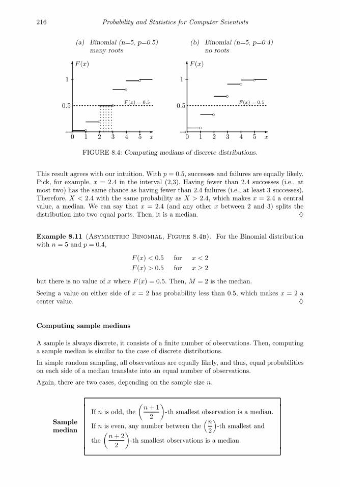
216 Probability and Statistics for Computer Scientists
x x
F (x) F (x)
(a) Binomial (n=5, p=0.5)many roots
(b) Binomial (n=5, p=0.4)no roots
0 01 12 23 34 45 5
1 1
0.5 0.5F (x) = 0.5 F (x) = 0.5
FIGURE 8.4: Computing medians of discrete distributions.
This result agrees with our intuition. With p = 0.5, successes and failures are equally likely.Pick, for example, x = 2.4 in the interval (2,3). Having fewer than 2.4 successes (i.e., atmost two) has the same chance as having fewer than 2.4 failures (i.e., at least 3 successes).Therefore, X < 2.4 with the same probability as X > 2.4, which makes x = 2.4 a centralvalue, a median. We can say that x = 2.4 (and any other x between 2 and 3) splits thedistribution into two equal parts. Then, it is a median. ♦
Example 8.11 (Asymmetric Binomial, Figure 8.4b). For the Binomial distributionwith n = 5 and p = 0.4,
F (x) < 0.5 for x < 2
F (x) > 0.5 for x ≥ 2
but there is no value of x where F (x) = 0.5. Then, M = 2 is the median.
Seeing a value on either side of x = 2 has probability less than 0.5, which makes x = 2 acenter value. ♦
Computing sample medians
A sample is always discrete, it consists of a finite number of observations. Then, computinga sample median is similar to the case of discrete distributions.
In simple random sampling, all observations are equally likely, and thus, equal probabilitieson each side of a median translate into an equal number of observations.
Again, there are two cases, depending on the sample size n.
Samplemedian
If n is odd, the
(n+ 1
2
)-th smallest observation is a median.
If n is even, any number between the(n2
)-th smallest and
the
(n+ 2
2
)-th smallest observations is a median.

Introduction to Statistics 217
Example 8.12 (Median CPU time). Let’s compute the median of n = 30 CPU timesfrom the data on p. 211.
First, order the data,
9 15 19 22 24 25 30 34 35 3536 36 37 38 42 43 46 48 54 5556 56 59 62 69 70 82 82 89 139
(8.3)
Next, since n = 30 is even, find n/2 = 15-th smallest and (n + 2)/2 = 16-th smallestobservations. These are 42 and 43. Any number between them is a sample median (typicallyreported as 42.5). ♦
We see why medians are not sensitive to extreme observations. If in the previous example,the first CPU time happens to be 30 minutes instead of 70 seconds, it does not affect thesample median at all!
Sample medians are easy to compute. In fact, no computations are needed, only the ordering.If you are driving (and only if you find it safe!), here is a simple experiment that you canconduct yourself.
Example 8.13 (Median speed on a highway). How can you measure the median speedof cars on a multilane road without a radar? It’s very simple. Adjust your speed so that ahalf of cars overtake you, and you overtake the other half. Then you are driving with themedian speed. ♦
8.2.3 Quantiles, percentiles, and quartiles
Generalizing the notion of a median, we replace 0.5 in its definition on p. 213 by some0 < p < 1.
DEFINITION 8.7
A p-quantile of a population is such a number x that solves equations
P X < x ≤ p
P X > x ≤ 1− p
A sample p-quantile is any number that exceeds at most 100p% of the sample,and is exceeded by at most 100(1− p)% of the sample.
A γ-percentile is (0.01γ)-quantile.
First, second, and third quartiles are the 25th, 50th, and 75th percentiles.They split a population or a sample into four equal parts.
Amedian is at the same time a 0.5-quantile, 50th percentile, and 2nd quartile.

218 Probability and Statistics for Computer Scientists
Notation qp = population p-quantileqp = sample p-quantile, estimator of qp
πγ = population γ-percentileπγ = sample γ-percentile, estimator of πγ
Q1, Q2, Q3 = population quartiles
Q1, Q2, Q3 = sample quartiles, estimators of Q1, Q2, and Q3
M = population median
M = sample median, estimator of M
Quantiles, quartiles, and percentiles are related as follows.
Quantiles,quartiles,percentiles
qp = π100p
Q1 = π25 = q1/4 Q3 = π75 = q3/4
M = Q2 = π50 = q1/2
Sample statistics are of course in a similar relation.
Computing quantiles is very similar to computing medians.
Example 8.14 (Sample quartiles). Let us compute the 1st and 3rd quartiles of CPUtimes. Again, we look at the ordered sample
9 15 19 22 24 25 30 34 35 3536 36 37 38 42 43 46 48 54 5556 56 59 62 69 70 82 82 89 139
First quartile Q1. For p = 0.25, we find that 25% of the sample equals np = 7.5, and 75%of the sample is n(1 − p) = 22.5 observations. From the ordered sample, we see that onlythe 8th element, 34, has no more than 7.5 observations to the left and no more than 22.5observations to the right of it. Hence, Q1 = 34.
Third quartile Q3. Similarly, the third sample quartile is the 23rd smallest element, Q3 = 59.♦
Example 8.15 (Calculating factory warranties from population percentiles).A computer maker sells extended warranty on the produced computers. It agrees to issuea warranty for x years if it knows that only 10% of computers will fail before the warrantyexpires. It is known from past experience that lifetimes of these computers have Gammadistribution with α = 60 and λ = 5 years−1. Compute x and advise the company on theimportant decision under uncertainty about possible warranties.
Solution. We just need to find the tenth percentile of the specified Gamma distribution andlet
x = π10.
Introduction to Statistics 219
As we know from Section 4.3, being a sum of Exponential variables, a Gamma variable isapproximately Normal for large α = 60. Using (4.12), compute
µ = α/λ = 12,
σ =√α/λ2 = 1.55.
From Table A4, the 10th percentile of a standardized variable
Z =X − µ
σ
equals (−1.28) (find the probability closest to 0.10 in the table and read the correspondingvalue of z). Unstandardizing it, we get
x = µ+ (−1.28)σ = 12− (1.28)(1.55) = 10.02.
Thus, the company can issue a 10-year warranty rather safely.
Remark: Of course, one does not have to use Normal approximation in the last example. A
number of computer packages have built-in commands for the exact evaluation of probabilities and
quantiles. For example, in recent versions of MATLAB, the 10th percentile of Gamma(α = 60, λ =
5) distribution can be obtained by the command gaminv(0.10, 60, 1/5) ♦
8.2.4 Variance and standard deviation
Statistics introduced in the previous sections showed where the average value and certainpercentages of a population are located. Now we are going to measure variability of ourvariable, how unstable the variable can be, and how much the actual value can differ fromits expectation. As a result, we’ll be able to assess reliability of our estimates and accuracyof our forecasts.
DEFINITION 8.8
For a sample (X1, X2, . . . , Xn), a sample variance is defined as
s2 =1
n− 1
n∑
i=1
(Xi − X
)2. (8.4)
It measures variability among observations and estimates the population vari-ance σ2 = Var(X).
Sample standard deviation is a square root of a sample variance,
s =√s2.
It measures variability in the same units as X and estimates the populationstandard deviation σ = Std(X).
Both population and sample variances are measured in squared units (in2, sec2, $2, etc.).Therefore, it is convenient to have standard deviations that are comparable with our variableof interest, X .
220 Probability and Statistics for Computer Scientists
The formula for s2 follows the same idea as that for σ2. It is also the average squared devi-ation from the mean, this time computed for a sample. Like σ2, sample variance measureshow far the actual values of X are from their average.
Computation
Often it is easier to compute the sample variance using another formula,
Sample variances2 =
n∑
i=1
X2i − nX2
n− 1.
(8.5)
Remark: Expressions (8.4) and (8.5) are equivalent because
∑(Xi − X
)2=∑
X2i − 2X
∑Xi +
∑X2 =
∑X2
i − 2X(nX)+ nX2 =
∑X2
i − nX2.
When X1, . . . , Xn are integers, but (X1 − X), . . . , (Xn − X) are fractions, it may be easier to use
(8.5). However, (Xn − X) are generally smaller in magnitude, and thus, we’d rather use (8.4) if
X1, . . . , Xn are rather large numbers.
Example 8.16 (CPU time, continued). For the data in (8.1) on p. 211, we have com-puted X = 48.2333. Following Definition 8.8, we can compute the sample variance as
s2 =(70− 48.2333)2 + . . .+ (19− 48.2333)2
30− 1=
20, 391
29= 703.1506 (sec2).
Alternatively, using (8.5),
s2 =702 + . . .+ 192 − (30)(48.2333)2
30− 1=
90, 185− 69, 794
29= 703.1506 (sec2).
The sample standard deviation is
s =√703.1506 = 26.1506 (sec2).
We can use these results, for example, as follows. Since X and s estimate the populationmean and standard deviation, we can make a claim that at least 8/9 of all tasks require lessthan
X + 3s = 127.78 seconds (8.6)
of CPU time. We used Chebyshev’s inequality (3.8) to derive this (also see Exercise 8.3). ♦
A seemingly strange coefficient(
1n−1
)ensures that s2 is an unbiased estimator of σ2.
Proof: Let us prove the unbiasedness of s2.
Case 1. Suppose for a moment that the population mean µ = E(X) = 0. Then
EX2i = VarXi = σ2,
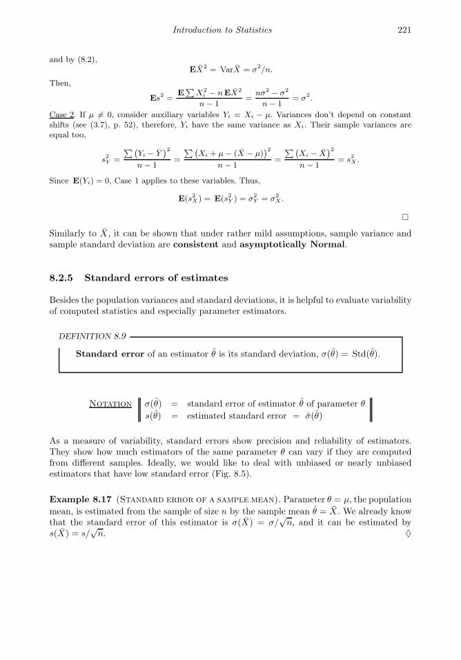
Introduction to Statistics 221
and by (8.2),EX2 = VarX = σ2/n.
Then,
Es2 =E∑
X2i − nEX2
n− 1=
nσ2 − σ2
n− 1= σ2.
Case 2. If µ 6= 0, consider auxiliary variables Yi = Xi − µ. Variances don’t depend on constantshifts (see (3.7), p. 52), therefore, Yi have the same variance as Xi. Their sample variances areequal too,
s2Y =
∑(Yi − Y
)2
n− 1=
∑(Xi + µ− (X − µ)
)2
n− 1=
∑(Xi − X
)2
n− 1= s2X .
Since E(Yi) = 0, Case 1 applies to these variables. Thus,
E(s2X) = E(s2Y ) = σ2Y = σ2
X .
Similarly to X, it can be shown that under rather mild assumptions, sample variance andsample standard deviation are consistent and asymptotically Normal.
8.2.5 Standard errors of estimates
Besides the population variances and standard deviations, it is helpful to evaluate variabilityof computed statistics and especially parameter estimators.
DEFINITION 8.9
Standard error of an estimator θ is its standard deviation, σ(θ) = Std(θ).
Notation σ(θ) = standard error of estimator θ of parameter θ
s(θ) = estimated standard error = σ(θ)
As a measure of variability, standard errors show precision and reliability of estimators.They show how much estimators of the same parameter θ can vary if they are computedfrom different samples. Ideally, we would like to deal with unbiased or nearly unbiasedestimators that have low standard error (Fig. 8.5).
Example 8.17 (Standard error of a sample mean). Parameter θ = µ, the population
mean, is estimated from the sample of size n by the sample mean θ = X. We already knowthat the standard error of this estimator is σ(X) = σ/
√n, and it can be estimated by
s(X) = s/√n. ♦
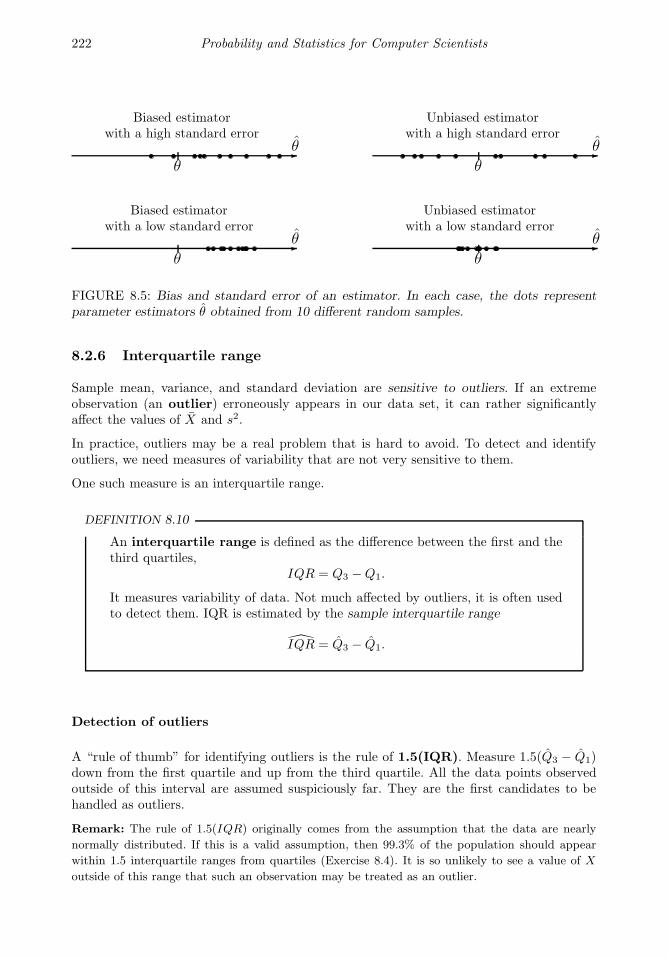
222 Probability and Statistics for Computer Scientists
Biased estimatorwith a high standard error
θ
θ
Biased estimatorwith a low standard error
θ
θ
Unbiased estimatorwith a high standard error
θ
θ
Unbiased estimatorwith a low standard error
θ
θ
FIGURE 8.5: Bias and standard error of an estimator. In each case, the dots representparameter estimators θ obtained from 10 different random samples.
8.2.6 Interquartile range
Sample mean, variance, and standard deviation are sensitive to outliers. If an extremeobservation (an outlier) erroneously appears in our data set, it can rather significantlyaffect the values of X and s2.
In practice, outliers may be a real problem that is hard to avoid. To detect and identifyoutliers, we need measures of variability that are not very sensitive to them.
One such measure is an interquartile range.
DEFINITION 8.10
An interquartile range is defined as the difference between the first and thethird quartiles,
IQR = Q3 −Q1.
It measures variability of data. Not much affected by outliers, it is often usedto detect them. IQR is estimated by the sample interquartile range
IQR = Q3 − Q1.
Detection of outliers
A “rule of thumb” for identifying outliers is the rule of 1.5(IQR). Measure 1.5(Q3 − Q1)down from the first quartile and up from the third quartile. All the data points observedoutside of this interval are assumed suspiciously far. They are the first candidates to behandled as outliers.
Remark: The rule of 1.5(IQR) originally comes from the assumption that the data are nearly
normally distributed. If this is a valid assumption, then 99.3% of the population should appear
within 1.5 interquartile ranges from quartiles (Exercise 8.4). It is so unlikely to see a value of X
outside of this range that such an observation may be treated as an outlier.

Introduction to Statistics 223
Example 8.18 (Any outlying CPU times?). Can we suspect that sample (8.1) hasoutliers? Compute
IQR = Q3 − Q1 = 59− 34 = 25
and measure 1.5 interquartile ranges from each quartile:
Q1 − 1.5(IQR) = 34− 37.5 = −3.5;
Q3 + 1.5(IQR) = 59 + 37.5 = 96.5.
In our data, one task took 139 seconds, which is well outside of the interval [−3.5, 96.5].This may be an outlier. ♦
Handling of outliers
What should we do if the 1.5(IQR) rule suggests possible outliers in the sample?
Many people simply delete suspicious observations, keeping in mind that one outlier cansignificantly affect sample mean and standard deviation and therefore spoil our statisticalanalysis. However, deleting them immediately may not be the best idea.
It is rather important to track the history of outliers and understand the reason theyappeared in the data set. There may be a pattern that a practitioner would want to beaware of. It may be a new trend that was not known before. Or, it may be an observationfrom a very special part of the population. Sometimes important phenomena are discoveredby looking at outliers.
If it is confirmed that a suspected observation entered the data set by a mere mistake, itcan be deleted.
8.3 Graphical statistics
Despite highly developed theory and methodology of Statistics, when it comes to analysisof real data, experienced statisticians will often follow a very simple advice:
Before you do anything with a data set,
look at it!
A quick look at a sample may clearly suggest
– a probability model, i.e., a family of distributions to be used;
– statistical methods suitable for the given data;

224 Probability and Statistics for Computer Scientists
– presence or absence of outliers;
– presence or absence of heterogeneity;
– existence of time trends and other patterns;
– relation between two or several variables.
There is a number of simple and advanced ways to visualize data. This section introduces histograms, stem-and-leaf plots, boxplots, time plots, and scatter plots.
Each graphical method serves a certain purpose and discovers certain information aboutdata.
8.3.1 Histogram
A histogram shows the shape of a pmf or a pdf of data, checks for homogeneity, andsuggests possible outliers. To construct a histogram, we split the range of data into equalintervals, “bins,” and count how many observations fall into each bin.
A frequency histogram consists of columns, one for each bin, whose height is determinedby the number of observations in the bin.
A relative frequency histogram has the same shape but a different vertical scale. Itscolumn heights represent the proportion of all data that appeared in each bin.
The sample of CPU times on p. 211 stretches from 9 to 139 seconds. Choosing intervals[0,14], [14,28], [28,42], . . . as bins, we count
1 observation between 0 and 145 observations ” 14 ” 289 ” ” 28 ” 427 ” ” 42 ” 564 ” ” 56 ” 70
. . . . . . . . . . . .
Using this for column heights, a (frequency) histogram of CPU times is then constructed(Figure 8.6a). A relative frequency histogram (Figure 8.6b) is only different in the verticalscale. Each count is now divided by the sample size n = 30.
What information can we draw from these histograms?
Histograms have a shape similar to the pmf or pdf of data,
especially in large samples.
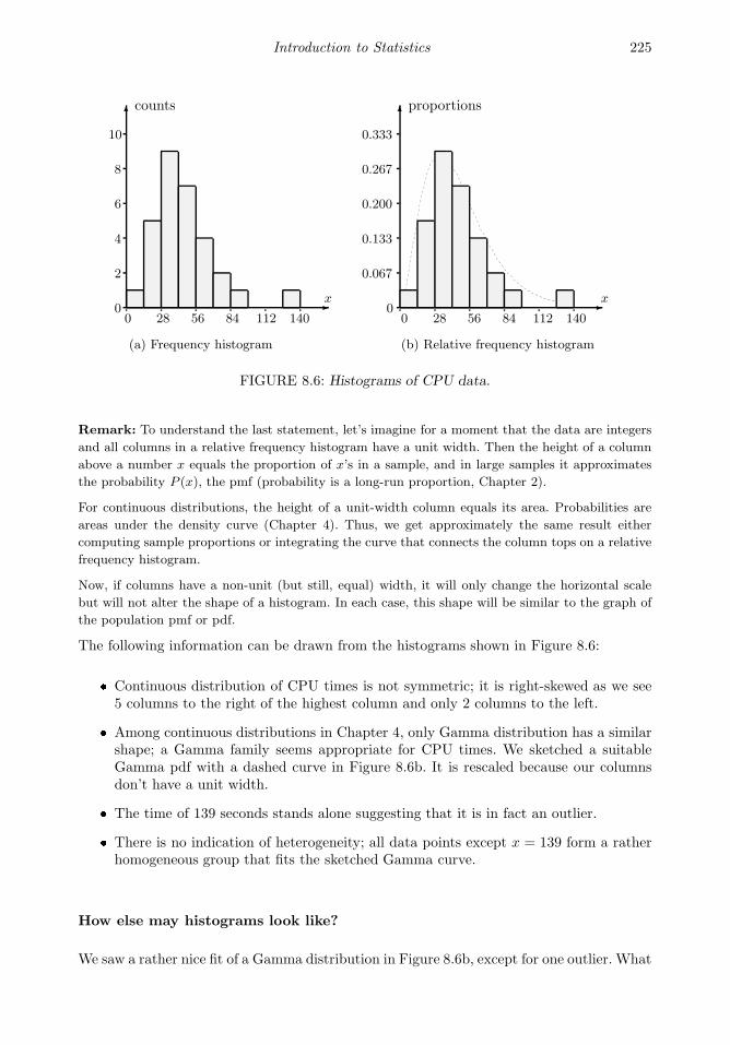
Introduction to Statistics 225
0 028 2856 5684 84112 112140 140
x x0
2
4
6
8
10
0
0.067
0.133
0.200
0.267
0.333
counts proportions
(a) Frequency histogram (b) Relative frequency histogram
FIGURE 8.6: Histograms of CPU data.
Remark: To understand the last statement, let’s imagine for a moment that the data are integers
and all columns in a relative frequency histogram have a unit width. Then the height of a column
above a number x equals the proportion of x’s in a sample, and in large samples it approximates
the probability P (x), the pmf (probability is a long-run proportion, Chapter 2).
For continuous distributions, the height of a unit-width column equals its area. Probabilities are
areas under the density curve (Chapter 4). Thus, we get approximately the same result either
computing sample proportions or integrating the curve that connects the column tops on a relative
frequency histogram.
Now, if columns have a non-unit (but still, equal) width, it will only change the horizontal scale
but will not alter the shape of a histogram. In each case, this shape will be similar to the graph of
the population pmf or pdf.
The following information can be drawn from the histograms shown in Figure 8.6: Continuous distribution of CPU times is not symmetric; it is right-skewed as we see5 columns to the right of the highest column and only 2 columns to the left. Among continuous distributions in Chapter 4, only Gamma distribution has a similarshape; a Gamma family seems appropriate for CPU times. We sketched a suitableGamma pdf with a dashed curve in Figure 8.6b. It is rescaled because our columnsdon’t have a unit width. The time of 139 seconds stands alone suggesting that it is in fact an outlier. There is no indication of heterogeneity; all data points except x = 139 form a ratherhomogeneous group that fits the sketched Gamma curve.
How else may histograms look like?
We saw a rather nice fit of a Gamma distribution in Figure 8.6b, except for one outlier. What
226 Probability and Statistics for Computer Scientists
a b 0
µ µ1 µ2
x x
x x
(a) Uniform (b) Exponential
(c) Normal (d) Mixture
FIGURE 8.7: Histograms of various samples.
other shapes of histograms can we see, and what other conclusions about the populationcan we make?
Certainly, histograms come in all shapes and sizes. Four examples are shown in Figure 8.7.
In Figure 8.7a, the distribution is almost symmetric, and columns have almost the sameheight. Slight differences can be attributed to the randomness of our sample, i.e., the sam-pling error. The histogram suggest a Uniform or Discrete Uniform distribution between aand b.
In Figure 8.7b, the distribution is heavily right-skewed, column heights decrease exponen-tially fast. This sample should come from an Exponential distribution, if variables arecontinuous, or from Geometric, if they are discrete.
In Figure 8.7c, the distribution is symmetric, with very quickly vanishing “tails.” Its bellshape reminds a Normal density that, as we know from Section 4.2.4, decays at a rate of∼ e−cx2
. We can locate the center µ of a histogram and conclude that this sample is likelyto come from a Normal distribution with a mean close to µ.
Figure 8.7d presents a rather interesting case that deserves special attention.

Introduction to Statistics 227
Mixtures
Let us look at Figure 8.7d . We have not seen a distribution with two “humps” in the previouschapters. Most likely, here we deal with a mixture of distributions. Each observationcomes from distribution F1 with some probability p1 and comes from distribution F2 withprobability p2 = 1− p1.
Mixtures typically appear in heterogeneous populations that consist of several groups: fe-males and males, graduate and undergraduate students, daytime and nighttime internettraffic, Windows, Unix, or Macintosh users, etc. In such cases, we can either study eachgroup separately, or use the Law of Total Probability on p. 31, write the (unconditional)cdf as
F (x) = p1F1(x) + p2F2(x) + . . . ,
and study the whole population at once.
Bell shapes of both humps in Figure 8.7d suggest that the sample came from a mixtureof two Normal distributions (with means around µ1 and µ2), with a higher probability ofhaving mean µ1, since the left hump is bigger.
The choice of bins
Experimenting with histograms, you can notice that their shape may depend on the choiceof bins. One can hear various rules of thumb about a good choice of bins, but in general,
– there should not be too few or too many bins;
– their number may increase with a sample size;
– they should be chosen to make the histogram informative, so that we can see shapes,outliers, etc.
In Figure 8.6, we simply divided the range of CPU data into 10 equal intervals, 14 sec each,and apparently this was sufficient for drawing important conclusions.
As two extremes, consider histograms in Figure 8.8 constructed from the same CPU data.
The first histogram has too many columns; therefore, each column is short. Most bins haveonly 1 observation. This tells little about the actual shape of the distribution; however, wecan still notice an outlier, X = 139.
The second histogram has only 3 columns. It is hard to guess the family of distributionshere, although a flat Uniform distribution is already ruled out. The outlier is not seen; itmerged with the rightmost bin.
Both histograms in Figure 8.8 can be made more informative by a better choice of bins.
8.3.2 Stem-and-leaf plot
Stem-and-leaf plots are similar to histograms although they carry more information. Namely,they also show how the data are distributed within columns.
To construct a stem-and-leaf plot, we need to draw a stem and a leaf. The first one or
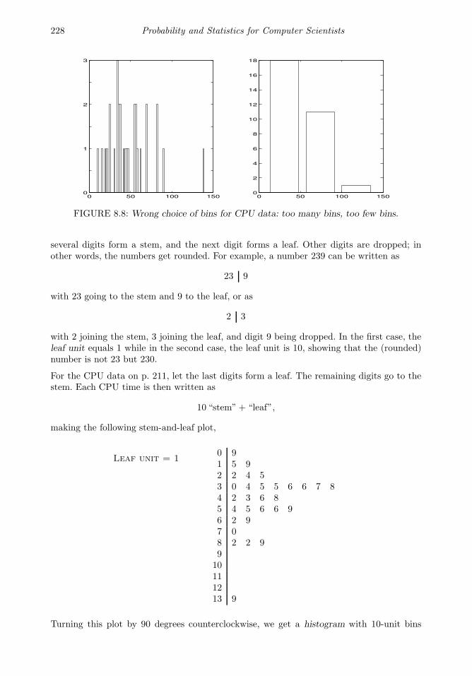
228 Probability and Statistics for Computer Scientists
0 50 100 1500
1
2
3
0 50 100 1500
2
4
6
8
10
12
14
16
18
FIGURE 8.8: Wrong choice of bins for CPU data: too many bins, too few bins.
several digits form a stem, and the next digit forms a leaf. Other digits are dropped; inother words, the numbers get rounded. For example, a number 239 can be written as
23 9
with 23 going to the stem and 9 to the leaf, or as
2 3
with 2 joining the stem, 3 joining the leaf, and digit 9 being dropped. In the first case, theleaf unit equals 1 while in the second case, the leaf unit is 10, showing that the (rounded)number is not 23 but 230.
For the CPU data on p. 211, let the last digits form a leaf. The remaining digits go to thestem. Each CPU time is then written as
10 “stem”+ “leaf”,
making the following stem-and-leaf plot,
Leaf unit = 10 91 5 92 2 4 53 0 4 5 5 6 6 7 84 2 3 6 85 4 5 6 6 96 2 97 08 2 2 9910111213 9
Turning this plot by 90 degrees counterclockwise, we get a histogram with 10-unit bins
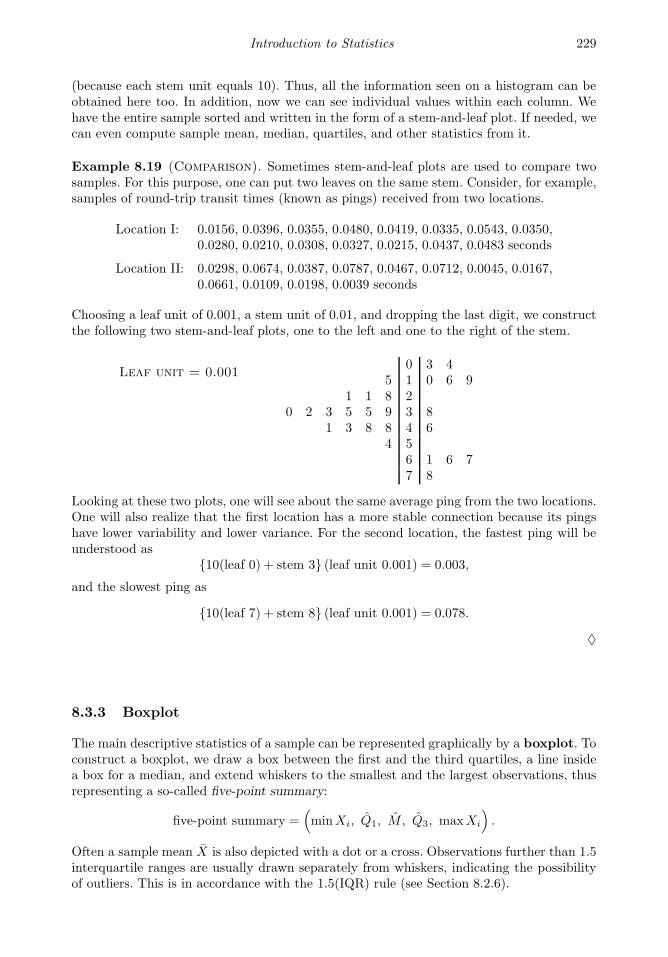
Introduction to Statistics 229
(because each stem unit equals 10). Thus, all the information seen on a histogram can beobtained here too. In addition, now we can see individual values within each column. Wehave the entire sample sorted and written in the form of a stem-and-leaf plot. If needed, wecan even compute sample mean, median, quartiles, and other statistics from it.
Example 8.19 (Comparison). Sometimes stem-and-leaf plots are used to compare twosamples. For this purpose, one can put two leaves on the same stem. Consider, for example,samples of round-trip transit times (known as pings) received from two locations.
Location I: 0.0156, 0.0396, 0.0355, 0.0480, 0.0419, 0.0335, 0.0543, 0.0350,0.0280, 0.0210, 0.0308, 0.0327, 0.0215, 0.0437, 0.0483 seconds
Location II: 0.0298, 0.0674, 0.0387, 0.0787, 0.0467, 0.0712, 0.0045, 0.0167,0.0661, 0.0109, 0.0198, 0.0039 seconds
Choosing a leaf unit of 0.001, a stem unit of 0.01, and dropping the last digit, we constructthe following two stem-and-leaf plots, one to the left and one to the right of the stem.
Leaf unit = 0.0010 3 4
5 1 0 6 91 1 8 2
0 2 3 5 5 9 3 81 3 8 8 4 6
4 56 1 6 77 8
Looking at these two plots, one will see about the same average ping from the two locations.One will also realize that the first location has a more stable connection because its pingshave lower variability and lower variance. For the second location, the fastest ping will beunderstood as
10(leaf 0) + stem 3 (leaf unit 0.001) = 0.003,
and the slowest ping as
10(leaf 7) + stem 8 (leaf unit 0.001) = 0.078.
♦
8.3.3 Boxplot
The main descriptive statistics of a sample can be represented graphically by a boxplot. Toconstruct a boxplot, we draw a box between the first and the third quartiles, a line insidea box for a median, and extend whiskers to the smallest and the largest observations, thusrepresenting a so-called five-point summary:
five-point summary =(minXi, Q1, M , Q3, maxXi
).
Often a sample mean X is also depicted with a dot or a cross. Observations further than 1.5interquartile ranges are usually drawn separately from whiskers, indicating the possibilityof outliers. This is in accordance with the 1.5(IQR) rule (see Section 8.2.6).

230 Probability and Statistics for Computer Scientists
The mean and five-point summary of CPU times were found in Examples 8.7, 8.12, and8.14,
X = 48.2333; minXi = 9, Q1 = 34, M = 42.5, Q3 = 59, maxXi = 139.
We also know that X = 139 is more than 1.5(IQR) away from the third quartile, and wesuspect that it may be an outlier.
0 20 40 60 80 100 120 140
+
x
FIGURE 8.9: Boxplot of CPU time data.
A boxplot is drawn in Figure 8.9. The mean is depicted with a “+,” and the right whiskerextends till the second largest observation X = 89 because X = 139 is a suspected outlier(depicted with a little circle).
From this boxplot, one can conclude:
– The distribution of CPU times is right skewed because (1) the mean exceeds themedian, and (2) the right half of the box is larger than the left half.
– Each half of a box and each whisker represents approximately 25% of the population.For example, we expect about 25% of all CPU times to fall between 42.5 and 59seconds.
Parallel boxplots
Boxplots are often used to compare different populations or parts of the same population.For such a comparison, samples of data are collected from each part, and their boxplots aredrawn on the same scale next to each other.
For example, seven parallel boxplots in Figure 8.10 represent the amount of internet traffichandled by a certain center during a week. We can see the following general patterns:
– The heaviest internet traffic occurs on Fridays.
– Fridays also have the highest variability.
– The lightest traffic is seen on weekends, with an increasing trend from Saturday toMonday.
– Each day, the distribution is right-skewed, with a few outliers on each day exceptSaturday. Outliers indicate occurrences of unusually heavy internet traffic.
Trends can also be seen on scatter plots and time plots.

Introduction to Statistics 231
Mon Tue Wed Thu Fri Sat Sun
+
++
+
+
+
+
FIGURE 8.10: Parallel boxplots of internet traffic.
8.3.4 Scatter plots and time plots
Scatter plots are used to see and understand a relationship between two variables. Thesecan be temperature and humidity, experience and salary, age of a network and its speed,number of servers and the expected response time, and so on.
To study the relationship, both variables are measured on each sampled item. For example,temperature and humidity during each of n days, age and speed of n networks, or experienceand salary of n randomly chosen computer scientists are recorded. Then, a scatter plotconsists of n points on an (x, y)-plane, with x- and y-coordinates representing the tworecorded variables.
Example 8.20 (Antivirus maintenance). Protection of a personal computer largelydepends on the frequency of running antivirus software on it. One can set to run it everyday, once a week, once a month, etc.
During a scheduled maintenance of computer facilities, a computer manager records thenumber of times the antivirus software was launched on each computer during 1 month(variable X) and the number of detected worms (variable Y ). The data for 30 computersare in the table.
X 30 30 30 30 30 30 30 30 30 30 30 15 15 15 10
Y 0 0 1 0 0 0 1 1 0 0 0 0 1 1 0
X 10 10 6 6 5 5 5 4 4 4 4 4 1 1 1Y 0 2 0 4 1 2 0 2 1 0 1 0 6 3 1
Is there a connection between the frequency of running antivirus software and the numberof worms in the system? A scatter plot of these data is given in Figure 8.11a. It clearlyshows that the number of worms reduces, in general, when the antivirus is employed morefrequently. This relationship, however, is not certain because no worm was detected on some“lucky” computers although the antivirus software was launched only once a week on them.
♦
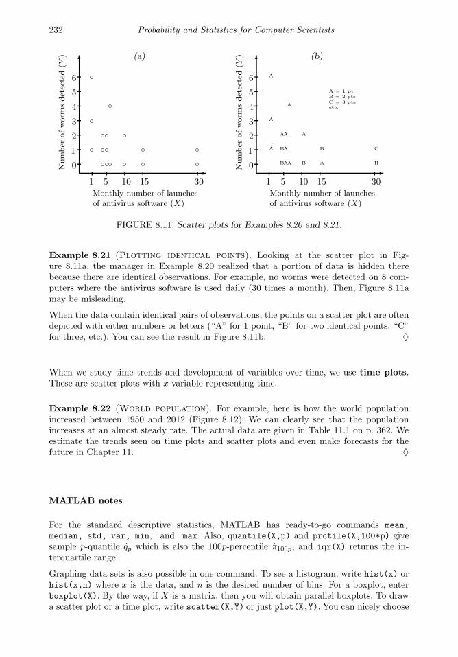
232 Probability and Statistics for Computer Scientists
0 0
1 1
2 2
3 3
4 4
5 5
6 6
1 15 510 1015 1530 30Monthly number of launchesof antivirus software (X)
Monthly number of launchesof antivirus software (X)
Number
ofworm
sdetected(Y
)
Number
ofworm
sdetected(Y
)
H
C
A
B
B
A
A
A
A
A
A
B
B
A
A
A
A
(a) (b)
A = 1 pt
B = 2 pts
C = 3 pts
etc.
FIGURE 8.11: Scatter plots for Examples 8.20 and 8.21.
Example 8.21 (Plotting identical points). Looking at the scatter plot in Fig-ure 8.11a, the manager in Example 8.20 realized that a portion of data is hidden therebecause there are identical observations. For example, no worms were detected on 8 com-puters where the antivirus software is used daily (30 times a month). Then, Figure 8.11amay be misleading.
When the data contain identical pairs of observations, the points on a scatter plot are oftendepicted with either numbers or letters (“A” for 1 point, “B” for two identical points, “C”for three, etc.). You can see the result in Figure 8.11b. ♦
When we study time trends and development of variables over time, we use time plots.These are scatter plots with x-variable representing time.
Example 8.22 (World population). For example, here is how the world populationincreased between 1950 and 2012 (Figure 8.12). We can clearly see that the populationincreases at an almost steady rate. The actual data are given in Table 11.1 on p. 362. Weestimate the trends seen on time plots and scatter plots and even make forecasts for thefuture in Chapter 11. ♦
MATLAB notes
For the standard descriptive statistics, MATLAB has ready-to-go commands mean,
median, std, var, min, and max. Also, quantile(X,p) and prctile(X,100*p) givesample p-quantile qp which is also the 100p-percentile π100p, and iqr(X) returns the in-terquartile range.
Graphing data sets is also possible in one command. To see a histogram, write hist(x) orhist(x,n) where x is the data, and n is the desired number of bins. For a boxplot, enterboxplot(X). By the way, if X is a matrix, then you will obtain parallel boxplots. To drawa scatter plot or a time plot, write scatter(X,Y) or just plot(X,Y). You can nicely choose

Exercises 233
1950 1960 1970 1980 1990 2000 20100
1000
2000
3000
4000
5000
6000
7000
Year
Wor
ld p
opul
atio
n, m
ln.
FIGURE 8.12: Time plot of the world population in 1950–2012.
the color and symbol in this command. For example, plot(X,Y,’r*’,X,Z,’bd’) will plotvariables Y and Z against variable X , with Y -points marked by red stars and Z-pointsmarked by blue diamonds.
Summary and conclusions
Methods discussed in this chapter provide a quick description of a data set, general conclu-sions about the population, and help to formulate conjectures about its features.
Sample mean, median, variance, moments, and quantiles estimate and give us an idea aboutthe corresponding population parameters. The interquartile range is used to detect outliers.
Before we start working with a data set, we look at it! There is a number of methods todisplay data: histograms, stem-and-leaf plots, boxplots, scatter plots, time plots. Good datadisplays show the shape of the distribution, the type of skewness or symmetry, interrelations,general trends, and possible outliers.
More advanced and accurate statistical methods are introduced in the next chapter.
Exercises
8.1. The numbers of blocked intrusion attempts on each day during the first two weeks of themonth were
56, 47, 49, 37, 38, 60, 50, 43, 43, 59, 50, 56, 54, 58

234 Probability and Statistics for Computer Scientists
After the change of firewall settings, the numbers of blocked intrusions during the next 20days were
53, 21, 32, 49, 45, 38, 44, 33, 32, 43, 53, 46, 36, 48, 39, 35, 37, 36, 39, 45.
Comparing the number of blocked intrusions before and after the change,
(a) construct side-by-side stem-and-leaf plots;
(b) compute the five-point summaries and construct parallel boxplots;
(c) comment on your findings.
8.2. A network provider investigates the load of its network. The number of concurrent users isrecorded at fifty locations (thousands of people),
17.2 22.1 18.5 17.2 18.6 14.8 21.7 15.8 16.3 22.824.1 13.3 16.2 17.5 19.0 23.9 14.8 22.2 21.7 20.713.5 15.8 13.1 16.1 21.9 23.9 19.3 12.0 19.9 19.415.4 16.7 19.5 16.2 16.9 17.1 20.2 13.4 19.8 17.719.7 18.7 17.6 15.9 15.2 17.1 15.0 18.8 21.6 11.9
(a) Compute the sample mean, variance, and standard deviation of the number of con-current users.
(b) Estimate the standard error of the sample mean.
(c) Compute the five-point summary and construct a boxplot.
(d) Compute the interquartile range. Are there any outliers?
(e) It is reported that the number of concurrent users follows approximately Normaldistribution. Does the histogram support this claim?
8.3. Verify the use of Chebyshev’s inequality in (8.6) of Example 8.16. Show that if the populationmean is indeed 48.2333 and the population standard deviation is indeed 26.5170, then atleast 8/9 of all tasks require less than 127.78 seconds of CPU time.
8.4. Use Table A4 to compute the probability for any Normal random variable to take a valuewithin 1.5 interquartile ranges from population quartiles.
8.5. The following data set shows population of the United States (in million) since 1790,
Year 1790 1800 1810 1820 1830 1840 1850 1860 1870 1880 1890 1900
Population 3.9 5.3 7.2 9.6 12.9 17.1 23.2 31.4 38.6 50.2 63.0 76.2
Year 1910 1920 1930 1940 1950 1960 1970 1980 1990 2000 2010
Population 92.2 106.0 123.2 132.2 151.3 179.3 203.3 226.5 248.7 281.4 308.7
Construct a time plot for the U.S. population. What kind of trend do you see? What infor-mation can be extracted from this plot?
8.6. Refer to Exercise 8.5. Compute 10-year increments of the population growth x1 = 5.3−3.9,x2 = 7.2− 5.3, etc.

Exercises 235
(a) Compute sample mean, median, and variance of 10-year increments. Discuss how theU.S. population changes during a decade.
(b) Construct a time plot of 10-year increments and discuss the observed pattern.
8.7. Refer to Exercise 8.5. Compute 10-year relative population change y1 = (5.3 − 3.9)/3.9,y2 = (7.2− 5.3)/5.3, etc.
(a) Compute sample mean, median, and variance of the relative population change.
(b) Construct a time plot of the relative population change. What trend do you see now?
(c) Comparing the time plots in Exercises 8.6 and 8.7, what kind of correlation betweenxi and yi would you expect? Verify by computing the sample correlation coefficient
r =
∑(xi − x)(yi − y)/(n− 1)
sxsy.
What can you conclude? How would you explain this phenomenon?
8.8. Consider three data sets.
(1) 19, 24, 12, 19, 18, 24, 8, 5, 9, 20, 13, 11, 1, 12, 11, 10, 22, 21, 7, 16, 15, 15, 26, 16, 1,13, 21, 21, 20, 19
(2) 17, 24, 21, 22, 26, 22, 19, 21, 23, 11, 19, 14, 23, 25, 26, 15, 17, 26, 21, 18, 19, 21, 24,18, 16, 20, 21, 20, 23, 33
(3) 56, 52, 13, 34, 33, 18, 44, 41, 48, 75, 24, 19, 35, 27, 46, 62, 71, 24, 66, 94, 40, 18, 15,39, 53, 23, 41, 78, 15, 35
(a) For each data set, draw a histogram and determine whether the distribution is right-skewed, left-skewed, or symmetric.
(b) Compute sample means and sample medians. Do they support your findings aboutskewness and symmetry? How?
8.9. The following data set represents the number of new computer accounts registered duringten consecutive days.
43, 37, 50, 51, 58, 105, 52, 45, 45, 10.
(a) Compute the mean, median, quartiles, and standard deviation.
(b) Check for outliers using the 1.5(IQR) rule.
(c) Delete the detected outliers and compute the mean, median, quartiles, and standarddeviation again.
(d) Make a conclusion about the effect of outliers on basic descriptive statistics.


Chapter 9
Statistical Inference I
9.1 Parameter estimation . . . . . . . . . . . . . . . . . . . . . . . . . . . . . . . . . . . . . . . . . . . . 2389.1.1 Method of moments . . . . . . . . . . . . . . . . . . . . . . . . . . . . . . . . . . . . . 2399.1.2 Method of maximum likelihood . . . . . . . . . . . . . . . . . . . . . . . . . 2429.1.3 Estimation of standard errors . . . . . . . . . . . . . . . . . . . . . . . . . . . 246
9.2 Confidence intervals . . . . . . . . . . . . . . . . . . . . . . . . . . . . . . . . . . . . . . . . . . . . . . 2479.2.1 Construction of confidence intervals: a general method . 2489.2.2 Confidence interval for the population mean . . . . . . . . . . . . 2509.2.3 Confidence interval for the difference between two
means . . . . . . . . . . . . . . . . . . . . . . . . . . . . . . . . . . . . . . . . . . . . . . . . . . . . 2519.2.4 Selection of a sample size . . . . . . . . . . . . . . . . . . . . . . . . . . . . . . . . 2539.2.5 Estimating means with a given precision . . . . . . . . . . . . . . . 254
9.3 Unknown standard deviation . . . . . . . . . . . . . . . . . . . . . . . . . . . . . . . . . . . . 2559.3.1 Large samples . . . . . . . . . . . . . . . . . . . . . . . . . . . . . . . . . . . . . . . . . . . . 2559.3.2 Confidence intervals for proportions . . . . . . . . . . . . . . . . . . . . 2569.3.3 Estimating proportions with a given precision . . . . . . . . . . 2589.3.4 Small samples: Student’s t distribution . . . . . . . . . . . . . . . . . 2599.3.5 Comparison of two populations with unknown variances 261
9.4 Hypothesis testing . . . . . . . . . . . . . . . . . . . . . . . . . . . . . . . . . . . . . . . . . . . . . . . 2649.4.1 Hypothesis and alternative . . . . . . . . . . . . . . . . . . . . . . . . . . . . . . 2659.4.2 Type I and Type II errors: level of significance . . . . . . . . . 2669.4.3 Level α tests: general approach . . . . . . . . . . . . . . . . . . . . . . . . . 2679.4.4 Rejection regions and power . . . . . . . . . . . . . . . . . . . . . . . . . . . . . 2699.4.5 Standard Normal null distribution (Z-test) . . . . . . . . . . . . . 2709.4.6 Z-tests for means and proportions . . . . . . . . . . . . . . . . . . . . . . 2729.4.7 Pooled sample proportion . . . . . . . . . . . . . . . . . . . . . . . . . . . . . . . 2749.4.8 Unknown σ: T-tests . . . . . . . . . . . . . . . . . . . . . . . . . . . . . . . . . . . . . 2759.4.9 Duality: two-sided tests and two-sided confidence
intervals . . . . . . . . . . . . . . . . . . . . . . . . . . . . . . . . . . . . . . . . . . . . . . . . . . 2779.4.10 P-value . . . . . . . . . . . . . . . . . . . . . . . . . . . . . . . . . . . . . . . . . . . . . . . . . . . 280
9.5 Inference about variances . . . . . . . . . . . . . . . . . . . . . . . . . . . . . . . . . . . . . . . . 2859.5.1 Variance estimator and Chi-square distribution . . . . . . . . 2869.5.2 Confidence interval for the population variance . . . . . . . . . 2879.5.3 Testing variance . . . . . . . . . . . . . . . . . . . . . . . . . . . . . . . . . . . . . . . . . 2899.5.4 Comparison of two variances. F-distribution. . . . . . . . . . . . 2929.5.5 Confidence interval for the ratio of population variances 2949.5.6 F-tests comparing two variances . . . . . . . . . . . . . . . . . . . . . . . . 296
Summary and conclusions . . . . . . . . . . . . . . . . . . . . . . . . . . . . . . . . . . . . . . . . . . 299Exercises . . . . . . . . . . . . . . . . . . . . . . . . . . . . . . . . . . . . . . . . . . . . . . . . . . . . . . . . . . . . 300
After taking a general look at the data, we are ready for more advanced and more informativestatistical analysis.
237

238 Probability and Statistics for Computer Scientists
In this chapter, we learn how
– to estimate parameters of the distribution. Methods of Chapter 8 mostly concernmeasure of location (mean, median, quantiles) and variability (variance, standard de-viation, interquartile range). As we know, this does not cover all possible parameters,and thus, we still lack a general methodology of estimation.
– to construct confidence intervals. Any estimator, computed from a collected randomsample instead of the whole population, is understood as only an approximation ofthe corresponding parameter. Instead of one estimator that is subject to a samplingerror, it is often more reasonable to produce an interval that will contain the truepopulation parameter with a certain known high probability.
– to test hypotheses. That is, we shall use the collected sample to verify statements andclaims about the population. As a result of each test, a statement is either rejected onbasis of the observed data or accepted (not rejected). Sampling error in this analysisresults in a possibility of wrongfully accepting or rejecting the hypothesis; however,we can design tests to control the probability of such errors.
Results of such statistical analysis are used for making decisions under uncertainty, devel-oping optimal strategies, forecasting, evaluating and controlling performance, and so on.
9.1 Parameter estimation
By now, we have learned a few elementary ways to determine the family of distributions. Wetake into account the nature of our data, basic description, and range; propose a suitablefamily of distributions; and support our conjecture by looking at a histogram.
In this section, we learn how to estimate parameters of distributions. As a result, a largefamily will be reduced to just one distribution that we can use for performance evaluation,forecasting, etc.
Example 9.1 (Poisson). For example, consider a sample of computer chips with a certaintype of rare defects. The number of defects on each chip is recorded. This is the number ofrare events, and thus, it should follow a Poisson distribution with some parameter λ.
We know that λ = E(X) is the expectation of a Poisson variable (Section 3.4.5). Then,should we estimate it with a sample mean X? Or, should we use a sample variance s2
because λ also equals Var(X)? ♦
Example 9.2 (Gamma). Suppose now that we deal with a Gamma(α, λ) family of distri-butions. Its parameters α and λ do not represent the mean, variance, standard deviation, orany other measures discussed in Chapter 8. What would the estimation algorithm be thistime? ♦
Statistical Inference I 239
Questions raised in these examples do not have unique answers. Statisticians developed anumber of estimation techniques, each having certain optimal properties.
Two rather popular methods are discussed in this section:
– method of moments, and
– method of maximum likelihood.
Several other methods are introduced later: bootstrap in Section 10.3, Bayesian parameterestimation in Section 10.4, and least squares estimation in Chapter 11.
9.1.1 Method of moments
Moments
First, let us define the moments.
DEFINITION 9.1
The k-th population moment is defined as
µk = E(Xk).
The k-th sample moment
mk =1
n
n∑
i=1
Xki
estimates µk from a sample (X1, . . . , Xn).
The first sample moment is the sample mean X.
Central moments are computed similarly, after centralizing the data, that is, subtractingthe mean.
DEFINITION 9.2
For k ≥ 2, the k-th population central moment is defined as
µ′k = E(X − µ1)
k.
The k-th sample central moment
m′k =
1
n
n∑
i=1
(Xi − X
)k
estimates µk from a sample (X1, . . . , Xn).

240 Probability and Statistics for Computer Scientists
Remark: The second population central moment is variance Var(X). The second sample centralmoment is sample variance, although (n−1) in its denominator is now replaced by n. We mentionedthat estimation methods are not unique. For unbiased estimation of σ2 = Var(X), we use
s2 =1
n− 1
n∑
i=1
(Xi − X)2;
however, method of moments and method of maximum likelihood produce a different version,
S2 = m′2 =
1
n
n∑
i=1
(Xi − X)2.
And this is not all! We’ll see other estimates of σ2 as well.
Estimation
Method of moments is based on a simple idea. Since our sample comes from a family ofdistributions F (θ), we choose such a member of this family whose properties are close toproperties of our data. Namely, we shall match the moments.
To estimate k parameters, equate the first k population and sample moments,
µ1 = m1
. . . . . . . . .µk = mk
The left-hand sides of these equations depend on the distribution parameters. The right-hand sides can be computed from data. The method of moments estimator is thesolution of this system of equations.
Example 9.3 (Poisson). To estimate parameter λ of Poisson(λ) distribution, we recallthat
µ1 = E(X) = λ.
There is only one unknown parameter, hence we write one equation,
µ1 = λ = m1 = X.
“Solving” it for λ, we obtainλ = X,
the method of moments estimator of λ. ♦
This does not look difficult, does it? Simplicity is the main attractive feature of the methodof moments.
If it is easier, one may opt to equate central moments.
Example 9.4 (Gamma distribution of CPU times). The histogram in Figure 8.6suggested that CPU times have Gamma distribution with some parameters α and λ. Toestimate them, we need two equations. From data on p. 211, we compute
m1 = X = 48.2333 and m′2 = S2 = 679.7122.
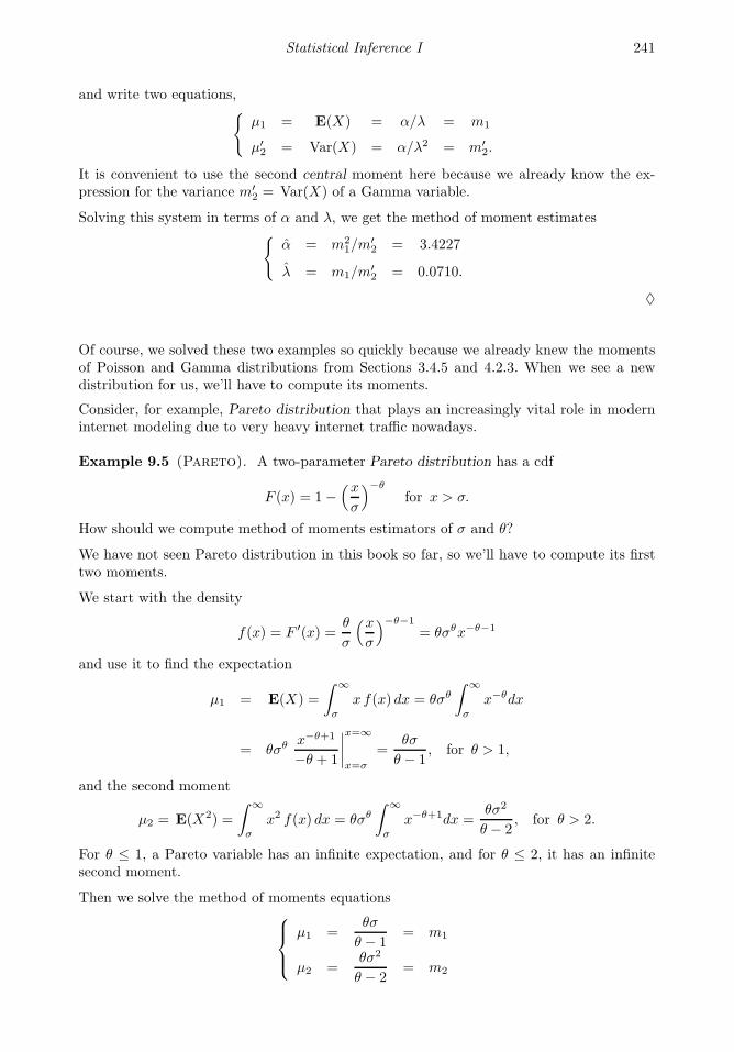
Statistical Inference I 241
and write two equations,
µ1 = E(X) = α/λ = m1
µ′2 = Var(X) = α/λ2 = m′
2.
It is convenient to use the second central moment here because we already know the ex-pression for the variance m′
2 = Var(X) of a Gamma variable.
Solving this system in terms of α and λ, we get the method of moment estimates
α = m21/m
′2 = 3.4227
λ = m1/m′2 = 0.0710.
♦
Of course, we solved these two examples so quickly because we already knew the momentsof Poisson and Gamma distributions from Sections 3.4.5 and 4.2.3. When we see a newdistribution for us, we’ll have to compute its moments.
Consider, for example, Pareto distribution that plays an increasingly vital role in moderninternet modeling due to very heavy internet traffic nowadays.
Example 9.5 (Pareto). A two-parameter Pareto distribution has a cdf
F (x) = 1−(xσ
)−θ
for x > σ.
How should we compute method of moments estimators of σ and θ?
We have not seen Pareto distribution in this book so far, so we’ll have to compute its firsttwo moments.
We start with the density
f(x) = F ′(x) =θ
σ
(xσ
)−θ−1
= θσθx−θ−1
and use it to find the expectation
µ1 = E(X) =
∫ ∞
σ
x f(x) dx = θσθ
∫ ∞
σ
x−θdx
= θσθ x−θ+1
−θ + 1
∣∣∣∣x=∞
x=σ
=θσ
θ − 1, for θ > 1,
and the second moment
µ2 = E(X2) =
∫ ∞
σ
x2 f(x) dx = θσθ
∫ ∞
σ
x−θ+1dx =θσ2
θ − 2, for θ > 2.
For θ ≤ 1, a Pareto variable has an infinite expectation, and for θ ≤ 2, it has an infinitesecond moment.
Then we solve the method of moments equations
µ1 =θσ
θ − 1= m1
µ2 =θσ2
θ − 2= m2

242 Probability and Statistics for Computer Scientists
and find that
θ =
√m2
m2 −m21
+ 1 and σ =m1(θ − 1)
θ. (9.1)
When we collect a sample from Pareto distribution, we can compute sample moments m1
and m2 and estimate parameters by (9.1). ♦
On rare occasions, when k equations are not enough to estimate k parameters, we’ll considerhigher moments.
Example 9.6 (Normal). Suppose we already know the mean µ of a Normal distributionand would like to estimate the variance σ2. Only one parameter σ2 is unknown; however,the first method of moments equation
µ1 = m1
does not contain σ2 and therefore does not produce its estimate. We then consider thesecond equation, say,
µ′2 = σ2 = m′
2 = S2,
which gives us the method of moments estimate immediately, σ2 = S2. ♦
Method of moments estimates are typically easy to compute. They can serve as a quick toolfor estimating parameters of interest.
9.1.2 Method of maximum likelihood
Another interesting idea is behind the method of maximum likelihood estimation.
Since the sample X = (X1, . . . , Xn) has already been observed, we find such parametersthat maximize the probability (likelihood) for this to happen. In other words, we make theevent that has already happened to be as likely as possible. This is yet another way to makethe chosen distribution consistent with the observed data.
DEFINITION 9.3
Maximum likelihood estimator is the parameter value that maximizes thelikelihood of the observed sample. For a discrete distribution, we maximize thejoint pmf of data P (X1, . . . , Xn). For a continuous distribution, we maximizethe joint density f(X1, . . . , Xn).
Both cases, discrete and continuous, are explained below.
Discrete case
For a discrete distribution, the probability of a given sample is the joint pmf of data,
P X = (X1, . . . , Xn) = P (X) = P (X1, . . . , Xn) =n∏
i=1
P (Xi),
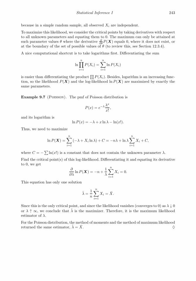
Statistical Inference I 243
because in a simple random sample, all observed Xi are independent.
To maximize this likelihood, we consider the critical points by taking derivatives with respectto all unknown parameters and equating them to 0. The maximum can only be attained atsuch parameter values θ where the derivative ∂
∂θP (X) equals 0, where it does not exist, orat the boundary of the set of possible values of θ (to review this, see Section 12.3.4).
A nice computational shortcut is to take logarithms first. Differentiating the sum
ln
n∏
i=1
P (Xi) =
n∑
i=1
lnP (Xi)
is easier than differentiating the product∏
P (Xi). Besides, logarithm is an increasing func-tion, so the likelihood P (X) and the log-likelihood lnP (X) are maximized by exactly thesame parameters.
Example 9.7 (Poisson). The pmf of Poisson distribution is
P (x) = e−λλx
x!,
and its logarithm islnP (x) = −λ+ x lnλ− ln(x!).
Thus, we need to maximize
lnP (X) =
n∑
i=1
(−λ+Xi lnλ) + C = −nλ+ lnλ
n∑
i=1
Xi + C,
where C = −∑ ln(x!) is a constant that does not contain the unknown parameter λ.
Find the critical point(s) of this log-likelihood. Differentiating it and equating its derivativeto 0, we get
∂
∂λlnP (X) = −n+
1
λ
n∑
i=1
Xi = 0.
This equation has only one solution
λ =1
n
n∑
i=1
Xi = X.
Since this is the only critical point, and since the likelihood vanishes (converges to 0) as λ ↓ 0
or λ ↑ ∞, we conclude that λ is the maximizer. Therefore, it is the maximum likelihoodestimator of λ.
For the Poisson distribution, the method of moments and the method of maximum likelihoodreturned the same estimator, λ = X. ♦
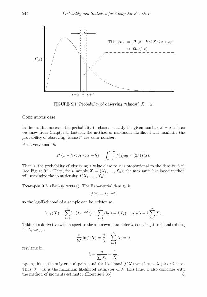
244 Probability and Statistics for Computer Scientists
x
2h
This area = P x− h ≤ X ≤ x+ h
≈ (2h)f(x)
f(x)
x − h x + h
FIGURE 9.1: Probability of observing “almost” X = x.
Continuous case
In the continuous case, the probability to observe exactly the given number X = x is 0, aswe know from Chapter 4. Instead, the method of maximum likelihood will maximize theprobability of observing “almost” the same number.
For a very small h,
P x− h < X < x+ h =
∫ x+h
x−h
f(y)dy ≈ (2h)f(x).
That is, the probability of observing a value close to x is proportional to the density f(x)(see Figure 9.1). Then, for a sample X = (X1, . . . , Xn), the maximum likelihood methodwill maximize the joint density f(X1, . . . , Xn).
Example 9.8 (Exponential). The Exponential density is
f(x) = λe−λx,
so the log-likelihood of a sample can be written as
ln f(X) =
n∑
i=1
ln(λe−λXi
)=
n∑
i=1
(lnλ− λXi) = n lnλ− λ
n∑
i=1
Xi.
Taking its derivative with respect to the unknown parameter λ, equating it to 0, and solvingfor λ, we get
∂
∂λln f(X) =
n
λ−
n∑
i=1
Xi = 0,
resulting in
λ =n∑Xi
=1
X.
Again, this is the only critical point, and the likelihood f(X) vanishes as λ ↓ 0 or λ ↑ ∞.
Thus, λ = X is the maximum likelihood estimator of λ. This time, it also coincides withthe method of moments estimator (Exercise 9.3b). ♦
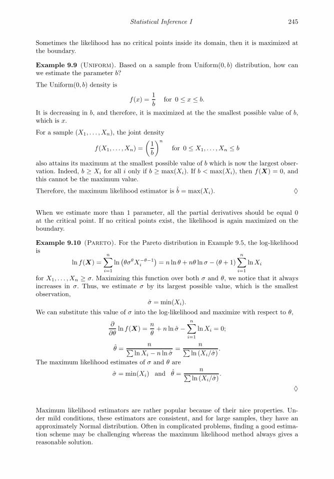
Statistical Inference I 245
Sometimes the likelihood has no critical points inside its domain, then it is maximized atthe boundary.
Example 9.9 (Uniform). Based on a sample from Uniform(0, b) distribution, how canwe estimate the parameter b?
The Uniform(0, b) density is
f(x) =1
bfor 0 ≤ x ≤ b.
It is decreasing in b, and therefore, it is maximized at the the smallest possible value of b,which is x.
For a sample (X1, . . . , Xn), the joint density
f(X1, . . . , Xn) =
(1
b
)n
for 0 ≤ X1, . . . , Xn ≤ b
also attains its maximum at the smallest possible value of b which is now the largest obser-vation. Indeed, b ≥ Xi for all i only if b ≥ max(Xi). If b < max(Xi), then f(X) = 0, andthis cannot be the maximum value.
Therefore, the maximum likelihood estimator is b = max(Xi). ♦
When we estimate more than 1 parameter, all the partial derivatives should be equal 0at the critical point. If no critical points exist, the likelihood is again maximized on theboundary.
Example 9.10 (Pareto). For the Pareto distribution in Example 9.5, the log-likelihoodis
ln f(X) =
n∑
i=1
ln(θσθX−θ−1
i
)= n ln θ + nθ lnσ − (θ + 1)
n∑
i=1
lnXi
for X1, . . . , Xn ≥ σ. Maximizing this function over both σ and θ, we notice that it alwaysincreases in σ. Thus, we estimate σ by its largest possible value, which is the smallestobservation,
σ = min(Xi).
We can substitute this value of σ into the log-likelihood and maximize with respect to θ,
∂
∂θln f(X) =
n
θ+ n ln σ −
n∑
i=1
lnXi = 0;
θ =n∑
lnXi − n ln σ=
n∑ln (Xi/σ)
.
The maximum likelihood estimates of σ and θ are
σ = min(Xi) and θ =n∑
ln (Xi/σ).
♦
Maximum likelihood estimators are rather popular because of their nice properties. Un-der mild conditions, these estimators are consistent, and for large samples, they have anapproximately Normal distribution. Often in complicated problems, finding a good estima-tion scheme may be challenging whereas the maximum likelihood method always gives areasonable solution.

246 Probability and Statistics for Computer Scientists
9.1.3 Estimation of standard errors
How good are the estimators that we learned in Sections 9.1.1 and 9.1.2? Standard errorscan serve as measures of their accuracy. To estimate them, we derive an expression for thestandard error and estimate all the unknown parameters in it.
Example 9.11 (Estimation of the Poisson parameter). In Examples 9.3 and 9.7, wefound the method of moments and maximum likelihood estimators of the Poisson parameterλ. Both estimators appear to be equal the sample mean λ = X. Let us now estimate thestandard error of λ.
Solution. There are at least two ways to do it.
On one hand, σ =√λ for the Poisson(λ) distribution, so σ(λ) = σ(X) = σ/
√n =
√λ/n,
as we know from (8.2) on p. 213. Estimating λ by X , we obtain
s1(λ) =
√X
n=
√∑Xi
n.
On the other hand, we can use the sample standard deviation and estimate the standarderror of the sample mean as in Example 8.17,
s2(λ) =s√n=
√∑(Xi − X)2
n(n− 1).
Apparently, we can estimate the standard error of λ by two good estimators, s1 and s2. ♦
Example 9.12 (Estimation of the Exponential parameter). Derive the standarderror of the maximum likelihood estimator in Example 9.8 and estimate it, assuming asample size n ≥ 3.
Solution. This requires some integration work. Fortunately, we can take a shortcut becausewe know that the integral of any Gamma density is one, i.e.,
∫ ∞
0
λα
Γ(α)xα−1e−λxdx = 1 for any α > 0, λ > 0.
Now, notice that λ = 1/X = n/∑
Xi, where∑
Xi has Gamma (n, λ) distribution becauseeach Xi is Exponential(λ).
Therefore, the k-th moment of λ equals
E(λk) = E
(n∑Xi
)k
=
∫ ∞
0
(nx
)k λn
Γ(n)xn−1e−λxdx =
nkλn
Γ(n)
∫ ∞
0
xn−k−1e−λxdx
=nkλn
Γ(n)
Γ(n− k)
λn−k
∫ ∞
0
λn−k
Γ(n− k)xn−k−1e−λxdx
=nkλn
Γ(n)
Γ(n− k)
λn−k· 1 =
nkλk(n− k − 1)!
(n− 1)!.
Substituting k = 1, we get the first moment,
E(λ) =nλ
n− 1.
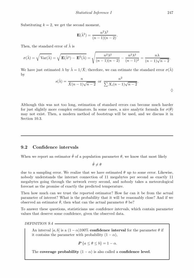
Statistical Inference I 247
Substituting k = 2, we get the second moment,
E(λ2) =n2λ2
(n− 1)(n− 2).
Then, the standard error of λ is
σ(λ) =
√Var(λ) =
√E(λ2)− E2(λ) =
√n2λ2
(n− 1)(n− 2)− n2λ2
(n− 1)2=
nλ
(n− 1)√n− 2
.
We have just estimated λ by λ = 1/X; therefore, we can estimate the standard error σ(λ)by
s(λ) =n
X(n− 1)√n− 2
orn2
∑Xi(n− 1)
√n− 2
.
♦
Although this was not too long, estimation of standard errors can become much harderfor just slightly more complex estimators. In some cases, a nice analytic formula for σ(θ)may not exist. Then, a modern method of bootstrap will be used, and we discuss it inSection 10.3.
9.2 Confidence intervals
When we report an estimator θ of a population parameter θ, we know that most likely
θ 6= θ
due to a sampling error. We realize that we have estimated θ up to some error. Likewise,nobody understands the internet connection of 11 megabytes per second as exactly 11megabytes going through the network every second, and nobody takes a meteorologicalforecast as the promise of exactly the predicted temperature.
Then how much can we trust the reported estimator? How far can it be from the actualparameter of interest? What is the probability that it will be reasonably close? And if weobserved an estimator θ, then what can the actual parameter θ be?
To answer these questions, statisticians use confidence intervals, which contain parametervalues that deserve some confidence, given the observed data.
DEFINITION 9.4
An interval [a, b] is a (1−α)100% confidence interval for the parameter θ ifit contains the parameter with probability (1− α),
P a ≤ θ ≤ b = 1− α.
The coverage probability (1− α) is also called a confidence level.
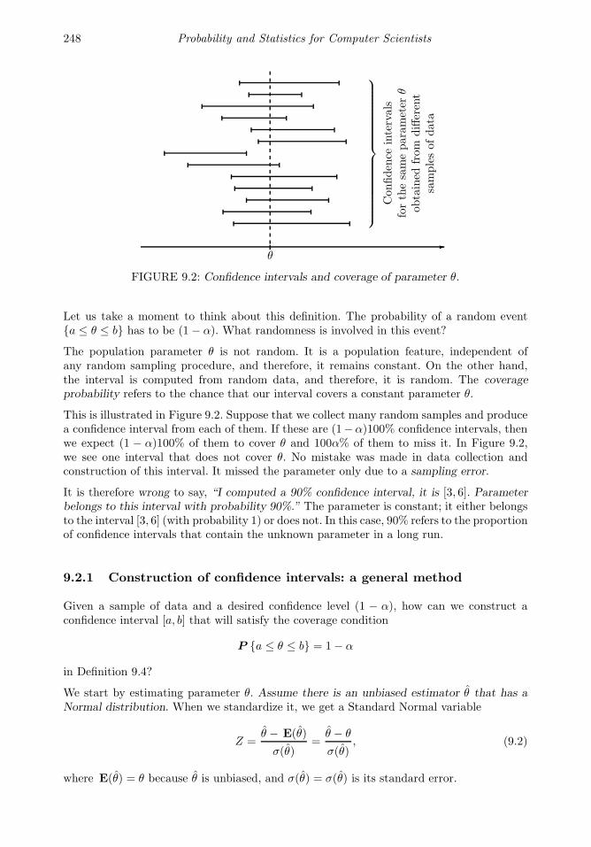
248 Probability and Statistics for Computer Scientists
θ
Confidence
intervals
forthesameparameter
θobtained
from
different
samplesofdata
FIGURE 9.2: Confidence intervals and coverage of parameter θ.
Let us take a moment to think about this definition. The probability of a random eventa ≤ θ ≤ b has to be (1 − α). What randomness is involved in this event?
The population parameter θ is not random. It is a population feature, independent ofany random sampling procedure, and therefore, it remains constant. On the other hand,the interval is computed from random data, and therefore, it is random. The coverageprobability refers to the chance that our interval covers a constant parameter θ.
This is illustrated in Figure 9.2. Suppose that we collect many random samples and producea confidence interval from each of them. If these are (1−α)100% confidence intervals, thenwe expect (1 − α)100% of them to cover θ and 100α% of them to miss it. In Figure 9.2,we see one interval that does not cover θ. No mistake was made in data collection andconstruction of this interval. It missed the parameter only due to a sampling error.
It is therefore wrong to say, “I computed a 90% confidence interval, it is [3, 6]. Parameterbelongs to this interval with probability 90%.” The parameter is constant; it either belongsto the interval [3, 6] (with probability 1) or does not. In this case, 90% refers to the proportionof confidence intervals that contain the unknown parameter in a long run.
9.2.1 Construction of confidence intervals: a general method
Given a sample of data and a desired confidence level (1 − α), how can we construct aconfidence interval [a, b] that will satisfy the coverage condition
P a ≤ θ ≤ b = 1− α
in Definition 9.4?
We start by estimating parameter θ. Assume there is an unbiased estimator θ that has aNormal distribution. When we standardize it, we get a Standard Normal variable
Z =θ − E(θ)
σ(θ)=
θ − θ
σ(θ), (9.2)
where E(θ) = θ because θ is unbiased, and σ(θ) = σ(θ) is its standard error.
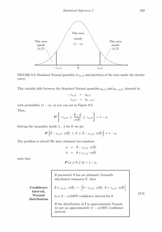
Statistical Inference I 249
0−zα/2 zα/2
This area
equals
(1− α)This areaequals(α/2)
This areaequals(α/2)
FIGURE 9.3: Standard Normal quantiles ±zα/2 and partition of the area under the densitycurve.
This variable falls between the Standard Normal quantiles qα/2 and q1−α/2, denoted by
−zα/2 = qα/2
zα/2 = q1−α/2
with probability (1− α), as you can see in Figure 9.3.
Then,
P
−zα/2 ≤ θ − θ
σ(θ)≤ zα/2
= 1− α.
Solving the inequality inside . . . for θ, we get
Pθ − zα/2 · σ(θ) ≤ θ ≤ θ − zα/2 · σ(θ)
= 1− α.
The problem is solved! We have obtained two numbers
a = θ − zα/2 · σ(θ)b = θ + zα/2 · σ(θ)
such thatP a ≤ θ ≤ b = 1− α.
Confidenceinterval,Normal
distribution
If parameter θ has an unbiased, Normally
distributed estimator θ, then
θ ± zα/2 · σ(θ) =[θ − zα/2 · σ(θ), θ + zα/2 · σ(θ)
]
is a (1− α)100% confidence interval for θ.
If the distribution of θ is approximately Normal,we get an approximately (1− α)100% confidenceinterval.
(9.3)
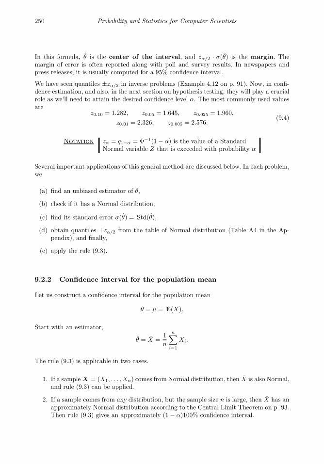
250 Probability and Statistics for Computer Scientists
In this formula, θ is the center of the interval, and zα/2 · σ(θ) is the margin. Themargin of error is often reported along with poll and survey results. In newspapers andpress releases, it is usually computed for a 95% confidence interval.
We have seen quantiles ±zα/2 in inverse problems (Example 4.12 on p. 91). Now, in confi-dence estimation, and also, in the next section on hypothesis testing, they will play a crucialrole as we’ll need to attain the desired confidence level α. The most commonly used valuesare
z0.10 = 1.282, z0.05 = 1.645, z0.025 = 1.960,
z0.01 = 2.326, z0.005 = 2.576.(9.4)
Notation zα = q1−α = Φ−1(1− α) is the value of a StandardNormal variable Z that is exceeded with probability α
Several important applications of this general method are discussed below. In each problem,we
(a) find an unbiased estimator of θ,
(b) check if it has a Normal distribution,
(c) find its standard error σ(θ) = Std(θ),
(d) obtain quantiles ±zα/2 from the table of Normal distribution (Table A4 in the Ap-pendix), and finally,
(e) apply the rule (9.3).
9.2.2 Confidence interval for the population mean
Let us construct a confidence interval for the population mean
θ = µ = E(X).
Start with an estimator,
θ = X =1
n
n∑
i=1
Xi.
The rule (9.3) is applicable in two cases.
1. If a sampleX = (X1, . . . , Xn) comes from Normal distribution, then X is also Normal,and rule (9.3) can be applied.
2. If a sample comes from any distribution, but the sample size n is large, then X has anapproximately Normal distribution according to the Central Limit Theorem on p. 93.Then rule (9.3) gives an approximately (1 − α)100% confidence interval.
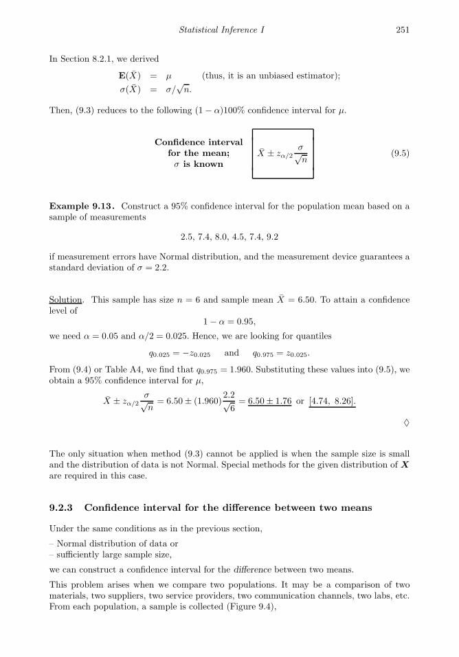
Statistical Inference I 251
In Section 8.2.1, we derived
E(X) = µ (thus, it is an unbiased estimator);
σ(X) = σ/√n.
Then, (9.3) reduces to the following (1− α)100% confidence interval for µ.
Confidence intervalfor the mean;σ is known
X ± zα/2σ√n
(9.5)
Example 9.13. Construct a 95% confidence interval for the population mean based on asample of measurements
2.5, 7.4, 8.0, 4.5, 7.4, 9.2
if measurement errors have Normal distribution, and the measurement device guarantees astandard deviation of σ = 2.2.
Solution. This sample has size n = 6 and sample mean X = 6.50. To attain a confidencelevel of
1− α = 0.95,
we need α = 0.05 and α/2 = 0.025. Hence, we are looking for quantiles
q0.025 = −z0.025 and q0.975 = z0.025.
From (9.4) or Table A4, we find that q0.975 = 1.960. Substituting these values into (9.5), weobtain a 95% confidence interval for µ,
X ± zα/2σ√n= 6.50± (1.960)
2.2√6= 6.50± 1.76 or [4.74, 8.26].
♦
The only situation when method (9.3) cannot be applied is when the sample size is smalland the distribution of data is not Normal. Special methods for the given distribution of Xare required in this case.
9.2.3 Confidence interval for the difference between two means
Under the same conditions as in the previous section,
– Normal distribution of data or– sufficiently large sample size,
we can construct a confidence interval for the difference between two means.
This problem arises when we compare two populations. It may be a comparison of twomaterials, two suppliers, two service providers, two communication channels, two labs, etc.From each population, a sample is collected (Figure 9.4),

252 Probability and Statistics for Computer Scientists
Population I
Parameters: µX , σ2X
Population II
Parameters: µY , σ2Y
Sample (X1, . . . , Xn)Statistics: X, s2X
Sample (Y1, . . . , Ym)Statistics: Y , s2Y
Collect independent samples
Confidence intervalfor θ = µX − µY
FIGURE 9.4: Comparison of two populations.
X = (X1, . . . , Xn) from one population,Y = (Y1, . . . , Ym) from the other population.
Suppose that the two samples are collected independently of each other.
To construct a confidence interval for the difference between population means
θ = µX − µY ,
we complete the usual steps (a)–(e) below.
(a) Propose an estimator of θ,
θ = X − Y .
It is natural to come up with this estimator because X estimates µX and Y estimatesµY .
(b) Check that θ is unbiased. Indeed,
E(θ) = E(X − Y
)= E
(X)− E
(Y)= µX − µY = θ.
(c) Check that θ has a Normal or approximately Normal distribution. This is true if theobservations are Normal or both sample sizes m and n are large.
(d) Find the standard error of θ (using independence of X and Y ),
σ(θ) =√
Var(X − Y
)=√
Var(X)+ Var
(Y)=
√σ2X
n+
σ2Y
m.
(e) Find quantiles ±zα/2 and compute the confidence interval according to (9.3). Thisresults in the following formula.
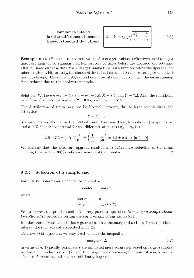
Statistical Inference I 253
Confidence intervalfor the difference of means;known standard deviations
X − Y ± zα/2
√σ2X
n+
σ2Y
m(9.6)
Example 9.14 (Effect of an upgrade). A manager evaluates effectiveness of a majorhardware upgrade by running a certain process 50 times before the upgrade and 50 timesafter it. Based on these data, the average running time is 8.5 minutes before the upgrade, 7.2minutes after it. Historically, the standard deviation has been 1.8 minutes, and presumably ithas not changed. Construct a 90% confidence interval showing how much the mean runningtime reduced due to the hardware upgrade.
Solution. We have n = m = 50, σX = σY = 1.8, X = 8.5, and Y = 7.2. Also, the confidencelevel (1− α) equals 0.9, hence α/2 = 0.05, and zα/2 = 1.645.
The distribution of times may not be Normal; however, due to large sample sizes, theestimator
θ = X − Y
is approximately Normal by the Central Limit Theorem. Thus, formula (9.6) is applicable,and a 90% confidence interval for the difference of means (µX − µY ) is
8.5− 7.2± (1.645)
√1.82
(1
50+
1
50
)= 1.3± 0.6 or [0.7, 1.9].
We can say that the hardware upgrade resulted in a 1.3-minute reduction of the meanrunning time, with a 90% confidence margin of 0.6 minutes. ♦
9.2.4 Selection of a sample size
Formula (9.3) describes a confidence interval as
center ± margin
wherecenter = θ,
margin = zα/2 · σ(θ).
We can revert the problem and ask a very practical question: How large a sample shouldbe collected to provide a certain desired precision of our estimator?
In other words, what sample size n guarantees that the margin of a (1−α)100% confidenceinterval does not exceed a specified limit ∆?
To answer this question, we only need to solve the inequality
margin ≤ ∆ (9.7)
in terms of n. Typically, parameters are estimated more accurately based on larger samples,so that the standard error σ(θ) and the margin are decreasing functions of sample size n.Then, (9.7) must be satisfied for sufficiently large n.
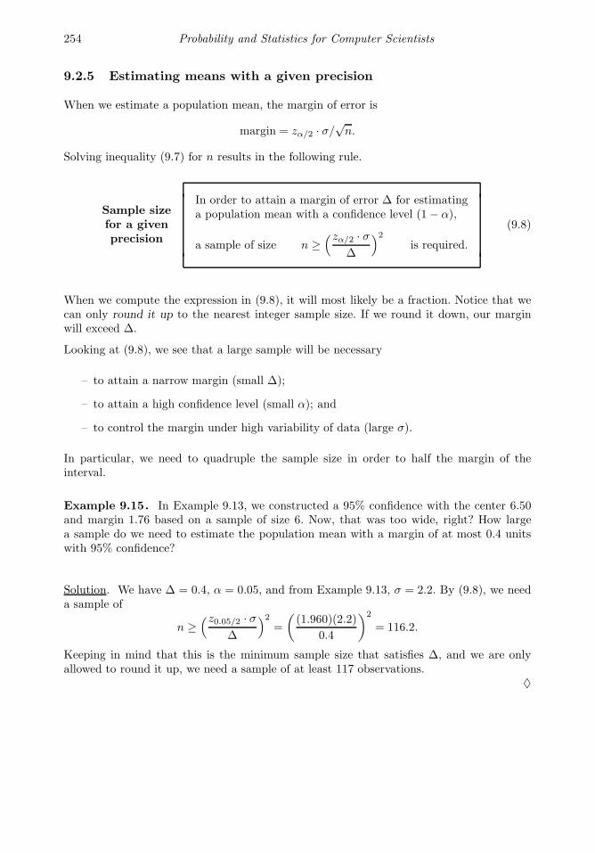
254 Probability and Statistics for Computer Scientists
9.2.5 Estimating means with a given precision
When we estimate a population mean, the margin of error is
margin = zα/2 · σ/√n.
Solving inequality (9.7) for n results in the following rule.
Sample sizefor a givenprecision
In order to attain a margin of error ∆ for estimatinga population mean with a confidence level (1− α),
a sample of size n ≥(zα/2 · σ
∆
)2is required.
(9.8)
When we compute the expression in (9.8), it will most likely be a fraction. Notice that wecan only round it up to the nearest integer sample size. If we round it down, our marginwill exceed ∆.
Looking at (9.8), we see that a large sample will be necessary
– to attain a narrow margin (small ∆);
– to attain a high confidence level (small α); and
– to control the margin under high variability of data (large σ).
In particular, we need to quadruple the sample size in order to half the margin of theinterval.
Example 9.15. In Example 9.13, we constructed a 95% confidence with the center 6.50and margin 1.76 based on a sample of size 6. Now, that was too wide, right? How largea sample do we need to estimate the population mean with a margin of at most 0.4 unitswith 95% confidence?
Solution. We have ∆ = 0.4, α = 0.05, and from Example 9.13, σ = 2.2. By (9.8), we needa sample of
n ≥(z0.05/2 · σ
∆
)2=
((1.960)(2.2)
0.4
)2
= 116.2.
Keeping in mind that this is the minimum sample size that satisfies ∆, and we are onlyallowed to round it up, we need a sample of at least 117 observations.
♦

Statistical Inference I 255
9.3 Unknown standard deviation
A rather heavy condition was assumed when we constructed all the confidence intervals.We assumed a known standard deviation σ and used it in all the derived formulas.
Sometimes this assumption is perfectly valid. We may know the variance from a large archiveof historical data, or it may be given as precision of a measuring device.
Much more often, however, the population variance is unknown. We’ll then estimate it fromdata and see if we can still apply methods of the previous section.
Two broad situations will be considered:
– large samples from any distribution,
– samples of any size from a Normal distribution.
In the only remaining case, a small non-Normal sample, a confidence interval will be con-structed by special methods. A popular modern approach called bootstrap is discussed inSection 10.3.3.
9.3.1 Large samples
A large sample should produce a rather accurate estimator of a variance. We can thenreplace the true standard error σ(θ) in (9.3) by its estimator s(θ), and obtain an approximateconfidence interval
θ ± zα/2 · s(θ).
Example 9.16 (Delays at nodes). Internet connections are often slowed by delays atnodes. Let us determine if the delay time increases during heavy-volume times.
Five hundred packets are sent through the same network between 5 pm and 6 pm (sampleX), and three hundred packets are sent between 10 pm and 11 pm (sample Y ). The earlysample has a mean delay time of 0.8 sec with a standard deviation of 0.1 sec whereas thesecond sample has a mean delay time of 0.5 sec with a standard deviation of 0.08 sec.Construct a 99.5% confidence interval for the difference between the mean delay times.
Solution. We have n = 500, X = 0.8, sX = 0.1; m = 300, Y = 0.5, sY = 0.08. Large samplesizes allow us to replace unknown population standard deviations by their estimates anduse an approximately Normal distribution of sample means.
For a confidence level of 1− α = 0.995, we need
zα/2 = z0.0025 = q0.9975.
Look for the probability 0.9975 in the body of Table A4 and find the corresponding valueof z,
z0.0025 = 2.81.
Then, a 99.5% confidence interval for the difference of mean execution times is
X − Y ± z0.0025
√s2Xn
+s2Ym
= (0.8− 0.5)± (2.81)
√(0.1)2
500+
(0.08)2
300= 0.3± 0.018 or [0.282, 0.318].
♦

256 Probability and Statistics for Computer Scientists
9.3.2 Confidence intervals for proportions
In particular, we surely don’t know the variance when we estimate a population proportion.
DEFINITION 9.5
We assume a subpopulation A of items that have a certain attribute. By thepopulation proportion we mean the probability
p = P i ∈ A
for a randomly selected item i to have this attribute.
A sample proportion
p =number of sampled items from A
n
is used to estimate p.
Let us use the indicator variables
Xi =
1 if i ∈ A0 if i 6∈ A
Each Xi has Bernoulli distribution with parameter p. In particular,
E (Xi) = p and Var (Xi) = p(1− p).
Also,
p =1
n
n∑
i=1
Xi
is nothing but a sample mean of Xi.
Therefore,
E (p) = p and Var (p) =p(1− p)
n,
as we know from properties of sample means on p. 213.
We conclude that
1. a sample proportion p is unbiased for the population proportion p;
2. it has approximately Normal distribution for large samples, because it has a form ofa sample mean;
3. when we construct a confidence interval for p, we do not know the standard deviationStd (p).
Indeed, knowing the standard deviation is equivalent to knowing p, and if we know p, whywould we need a confidence interval for it?

Statistical Inference I 257
Thus, we estimate the unknown standard error
σ(p) =
√p(1− p)
n
by
s(p) =
√p(1− p)
n
and use it in the general formulap± zα/2 · s(p)
to construct an approximate (1− α)100% confidence interval.
Confidence intervalfor a population proportion
p± zα/2
√p(1− p)
n
Similarly, we can construct a confidence interval for the difference between two proportions.In two populations, we have proportions p1 and p2 of items with an attribute. Independentsamples of size n1 and n2 are collected, and both parameters are estimated by sampleproportions p1 and p2.
Summarizing, we have
Parameter of interest: θ = p1 − p2
Estimated by: θ = p1 − p2
Its standard error: σ(θ) =
√p1(1− p1)
n1+
p2(1− p2)
n2
Estimated by: s(θ) =
√p1(1− p1)
n1+
p2(1− p2)
n2
Confidence intervalfor the differenceof proportions
p1 − p2 ± zα/2
√p1(1 − p1)
n1+
p2(1 − p2)
n2
Example 9.17 (Pre-election poll). A candidate prepares for the local elections. Dur-ing his campaign, 42 out of 70 randomly selected people in town A and 59 out of 100randomly selected people in town B showed they would vote for this candidate. Estimatethe difference in support that this candidate is getting in towns A and B with 95% confi-dence. Can we state affirmatively that the candidate gets a stronger support in town A?

258 Probability and Statistics for Computer Scientists
Solution. We have n1 = 70, n2 = 100, p1 = 42/70 = 0.6, and p2 = 59/100 = 0.59. For theconfidence interval, we have
center = p1 − p2 = 0.01,
and
margin = z0.05/2
√p1(1 − p1)
n1+
p2(1 − p2)
n2
= (1.960)
√(0.6)(0.4)
70+
(0.59)(0.41)
100= 0.15.
Then0.01± 0.15 = [-0.14, 0.16]
is a 95% confidence interval for the difference in support (p1 − p2) in the two towns.
So, is the support stronger in town A? On one hand, the estimator p1 − p2 = 0.01 suggeststhat the support is 1% higher in town A than in town B. On the other hand, the differencecould appear positive just because of a sampling error. As we see, the 95% confidenceinterval includes a large range of negative values too. Therefore, the obtained data does notindicate affirmatively that the support in town A is stronger.
In fact, we will test in Example 9.33 if there is any difference between the two towns andwill conclude that there is no evidence for it or against it. A formal procedure for testingstatements like that will be introduced in Section 9.4. ♦
9.3.3 Estimating proportions with a given precision
Our confidence interval for a population proportion has a margin
margin = zα/2
√p(1− p)
n.
A standard way of finding the sample size that provides the desired margin ∆ is to solvethe inequality
margin ≤ ∆ or n ≥ p(1− p)(zα/2
∆
)2.
However, this inequality includes p. To know p, we first need to collect a sample, but toknow the sample size, we first need to know p !
A way out of this circle is shown in Figure 9.5. As we see, the function p(1− p) never exceeds0.25. Therefore, we can replace the unknown value of p(1− p) by 0.25 and find a sample sizen, perhaps larger than we actually need, that will ensure that we estimate p with a marginnot exceeding ∆. That is, choose a sample size
n ≥ 0.25(zα/2
∆
)2.
It will automatically be at least as large as the required p(1 − p)(zα/2/∆)2, regardless ofthe unknown value of p.

Statistical Inference I 259
0 0.5 1
p
0.25
p(1− p)
FIGURE 9.5: Function p(1− p) attains its maximum at p = 0.5.
Example 9.18. A sample of size
n ≥ 0.25
(1.960
0.1
)2
= 96.04
(that is, at least 97 observations) always guarantees that a population proportion is esti-mated with an error of at most 0.1 with a 95% confidence. ♦
9.3.4 Small samples: Student’s t distribution
Having a small sample, we can no longer pretend that a sample standard deviation s is anaccurate estimator of the population standard deviation σ. Then, how should we adjust theconfidence interval when we replace σ by s, or more generally, when we replace the standarderror σ(θ) by its estimator s(θ)?
A famous solution was proposed by William Gosset (1876–1937), known by his pseudonymStudent. Working for the Irish brewery Guinness, he derived the T-distribution for thequality control problems in brewing.
Student followed the steps similar to our derivation of a confidence interval on p. 248. Thenhe replaced the true but unknown standard error of θ by its estimator s(θ) and concludedthat the T-ratio
t =θ − θ
s(θ),
the ratio of two random variables, no longer has a Normal distribution!
Student figured the distribution of a T-ratio. For the problem of estimating the mean basedon n Normal observations X1, . . . , Xn, this was T-distribution with (n − 1) degrees offreedom. Table A5 gives critical values tα of the T-distribution that we’ll use for confidenceintervals.
So, using T-distribution instead of Standard Normal and estimated standard error insteadof the unknown true one, we obtain the confidence interval for the population mean.
Confidenceinterval
for the mean;σ is unknown
X ± tα/2s√n
where tα/2 is a critical value from T-distributionwith n− 1 degrees of freedom
(9.9)

260 Probability and Statistics for Computer Scientists
Example 9.19 (Unauthorized use of a computer account). If an unauthorizedperson accesses a computer account with the correct username and password (stolen orcracked), can this intrusion be detected? Recently, a number of methods have been proposedto detect such unauthorized use. The time between keystrokes, the time a key is depressed,the frequency of various keywords are measured and compared with those of the accountowner. If there are significant differences, an intruder is detected.
The following times between keystrokes were recorded when a user typed the username andpassword:
.24, .22, .26, .34, .35, .32, .33, .29, .19, .36, .30, .15, .17, .28, .38, .40, .37, .27 seconds
As the first step in detecting an intrusion, let’s construct a 99% confidence interval for themean time between keystrokes assuming Normal distribution of these times.
Solution. The sample size is n = 18, the sample mean time is X = 0.29 sec, and the samplestandard deviation is s = 0.074. The critical value of t distribution with n− 1 = 17 degreesof freedom is tα/2 = t0.005 = 2.898. Then, the 99% confidence interval for the mean time is
0.29± (2.898)0.074√
18= 0.29± 0.05 = [0.24; 0.34]
Example 9.28 on p. 275 will show whether this result signals an intrusion. ♦
The density of Student’s T-distribution is a bell-shaped symmetric curve that can be easilyconfused with Normal. Comparing with the Normal density, its peak is lower and its tailsare thicker. Therefore, a larger number tα is generally needed to cut area α from the righttail. That is,
tα > zα
for small α. As a consequence, the confidence interval (9.9) is wider than the interval (9.5)for the case of known σ. This wider margin is the price paid for not knowing the standarddeviation σ. When we lack a certain piece of information, we cannot get a more accurateestimator.
However, we see in Table A5 thattα → zα,
as the number of degrees of freedom ν tends to infinity. Indeed, having a large sample(hence, large ν = n − 1), we can count on a very accurate estimator of σ, and thus, theconfidence interval is almost as narrow as if we knew σ in this case.
Degrees of freedom ν is the parameter of T-distribution controlling the shape of theT-density curve. Its meaning is the dimension of a vector used to estimate the variance.Here we estimate σ2 by a sample variance
s2 =1
n− 1
n∑
i=1
(Xi − X)2,
and thus, we use a vectorX ′ =
(X1 − X, . . . , Xn − X
).

Statistical Inference I 261
The initial vectorX = (X1, . . . , Xn) has dimension n; therefore, it has n degrees of freedom.However, when the sample mean X is subtracted from each observation, there appears alinear relation among the elements,
n∑
i=1
(Xi − X) = 0.
We lose 1 degree of freedom due to this constraint; the vector X ′ belongs to an (n − 1)-dimensional hyperplane, and this is why we have only ν = n− 1 degrees of freedom.
In many similar problems, degrees of freedom can be computed as
number ofdegrees of freedom
= sample size − number of estimatedlocation parameters
(9.10)
9.3.5 Comparison of two populations with unknown variances
We now construct a confidence interval for the difference of two means µX −µY , comparingthe population of X ’s with the population of Y ’s.
Again, independent random samples are collected,
X = (X1, . . . , Xn) and Y = (Y1, . . . , Ym),
one from each population, as in Figure 9.4 on p. 252. This time, however, population vari-ances σ2
X and σ2Y are unknown to us, and we use their estimates.
Two important cases need to be considered here. In one case, there exists an exact and simplesolution based on T-distribution. The other case suddenly appears to be a famous Behrens-Fisher problem, where no exact solution exists, and only approximations are available.
Case 1. Equal variances
Suppose there are reasons to assume that the two populations have equal variances,
σ2X = σ2
Y = σ2.
For example, two sets of data are collected with the same measurement device, thus, mea-surements have different means but the same precision.
In this case, there is only one variance σ2 to estimate instead of two. We should use bothsamples X and Y to estimate their common variance. This estimator of σ2 is called apooled sample variance, and it is computed as
s2p =
n∑
i=1
(Xi − X)2 +
m∑
i=1
(Yi − Y )2
n+m− 2=
(n− 1)s2X + (m− 1)s2Yn+m− 2
. (9.11)
Substituting this variance estimator in (9.6) for σ2X and σ2
Y , we get the following confidenceinterval.

262 Probability and Statistics for Computer Scientists
Confidenceinterval for
the differenceof means;
equal, unknownstandard deviations
X − Y ± tα/2 sp
√1
n+
1
m
where sp is the pooled standard deviation,a root of the pooled variance in (9.11)
and tα/2 is a critical value from T-distributionwith (n+m− 2) degrees of freedom
Example 9.20 (CD writer and battery life). CD writing is energy consuming; there-fore, it affects the battery lifetime on laptops. To estimate the effect of CD writing, 30 usersare asked to work on their laptops until the “low battery” sign comes on.
Eighteen users without a CD writer worked an average of 5.3 hours with a standard devi-ation of 1.4 hours. The other twelve, who used their CD writer, worked an average of 4.8hours with a standard deviation of 1.6 hours. Assuming Normal distributions with equalpopulation variances (σ2
X = σ2Y ), construct a 95% confidence interval for the battery life
reduction caused by CD writing.
Solution. Effect of the CD writer is measured by the reduction of the mean battery life. Wehave n = 12, X = 4.8, sX = 1.6 for users with a CD writer and m = 18, Y = 5.3, sY = 1.4for users without it. The pooled standard deviation is
sp =
√(n− 1)s2X + (m− 1)s2Y
n+m− 2=
√(11)(1.6)2 + (17)(1.4)2
28= 1.4818
(check: it has to be between sX and sY ). The critical value is t0.025 = 2.048 (use 28 d.f.).The 95% confidence interval for the difference between the mean battery lives is
(4.8− 5.3)± (2.048)(1.4818)
√1
18+
1
12= −0.5± 1.13 = [-1.63; 0.63].
♦
Remark: Let’s discuss formula (9.11). First, notice that different sample means X and Y are usedfor X-terms and Y -terms. Indeed, our two populations may have different means. As we know,variance of any variable measures its deviation from its mean. Thus, from each observation wesubtract its own mean-estimate.
Second, we lose 2 degrees of freedom due to the estimation of two means. Two constraints,
n∑
i=1
(Xi − X) = 0 andm∑
i=1
(Yi − Y ) = 0,
show that the number of degrees of freedom is only (n+m− 2) instead of (n+m). We see this
coefficient in the denominator, and it makes s2p an unbiased estimator of σ2 (see Exercise 9.19).

Statistical Inference I 263
Case 2. Unequal variances
The most difficult case is when both variances are unknown and unequal. Confidence esti-mation of µX − µY in this case is known as the Behrens-Fisher problem. Certainly, we canreplace unknown variances σ2
X , σ2Y by their estimates s2X , s2Y and form a T-ratio
t =
(X − Y
)− (µX − µY )√
s2X
n +s2Y
m
.
However, it won’t have a T-distribution.
An approximate solution was proposed in the 1940s by Franklin E. Satterthwaite, whoworked for General Electric Company at that time. Satterthwaite used the method of mo-ments to estimate degrees of freedom ν of a T-distribution that is “closest” to this T-ratio.This number depends on unknown variances. Estimating them by sample variances, heobtained the formula that is now known as Satterthwaite approximation,
ν =
(s2Xn
+s2Ym
)2
s4Xn2(n− 1)
+s4Y
m2(m− 1)
. (9.12)
This number of degrees of freedom often appears non-integer. There are T-distributionswith non-integer ν, see Section 12.1.1. To use Table A5, just take the closest ν that is givenin that table.
Formula (9.12) is widely used for t-intervals and t-tests.
Confidenceinterval
for the differenceof means;
unequal, unknownstandard deviations
X − Y ± tα/2
√s2Xn
+s2Ym
where tα/2 is a critical value fromT-distribution with ν degrees of freedomgiven by formula (9.12)
Example 9.21 (Comparison of two servers). An account on server A is more expen-sive than an account on server B. However, server A is faster. To see if it’s optimal to gowith the faster but more expensive server, a manager needs to know how much faster it is.A certain computer algorithm is executed 30 times on server A and 20 times on server Bwith the following results,
Server A Server B
Sample mean 6.7 min 7.5 minSample standard deviation 0.6 min 1.2 min
Construct a 95% confidence interval for the difference µ1 − µ2 between the mean execution
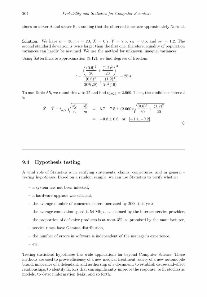
264 Probability and Statistics for Computer Scientists
times on server A and server B, assuming that the observed times are approximately Normal.
Solution. We have n = 30, m = 20, X = 6.7, Y = 7.5, sX = 0.6, and sY = 1.2. Thesecond standard deviation is twice larger than the first one; therefore, equality of populationvariances can hardly be assumed. We use the method for unknown, unequal variances.
Using Satterthwaite approximation (9.12), we find degrees of freedom:
ν =
((0.6)2
30+
(1.2)2
20
)2
(0.6)4
302(29)+
(1.2)4
202(19)
= 25.4.
To use Table A5, we round this ν to 25 and find t0.025 = 2.060. Then, the confidence intervalis
X − Y ± tα/2
√s2Xn
+s2Ym
= 6.7− 7.5± (2.060)
√(0.6)2
30+
(1.2)2
20
= −0.8± 0.6 or [−1.4,−0.2].♦
9.4 Hypothesis testing
A vital role of Statistics is in verifying statements, claims, conjectures, and in general -testing hypotheses. Based on a random sample, we can use Statistics to verify whether
– a system has not been infected,
– a hardware upgrade was efficient,
– the average number of concurrent users increased by 2000 this year,
– the average connection speed is 54 Mbps, as claimed by the internet service provider,
– the proportion of defective products is at most 3%, as promised by the manufacturer,
– service times have Gamma distribution,
– the number of errors in software is independent of the manager’s experience,
– etc.
Testing statistical hypotheses has wide applications far beyond Computer Science. Thesemethods are used to prove efficiency of a new medical treatment, safety of a new automobilebrand, innocence of a defendant, and authorship of a document; to establish cause-and-effectrelationships; to identify factors that can significantly improve the response; to fit stochasticmodels; to detect information leaks; and so forth.

Statistical Inference I 265
9.4.1 Hypothesis and alternative
To begin, we need to state exactly what we are testing. These are hypothesis and alternative.
Notation H0 = hypothesis (the null hypothesis)HA = alternative (the alternative hypothesis)
H0 and HA are simply two mutually exclusive statements. Each test results either in ac-ceptance of H0 or its rejection in favor of HA.
A null hypothesis is always an equality, absence of an effect or relation, some “normal,”usual statement that people have believed in for years. In order to overturn the commonbelief and to reject the hypothesis, we need significant evidence. Such evidence can onlybe provided by data. Only when such evidence is found, and when it strongly supports thealternative HA, can the hypothesis H0 be rejected in favor of HA.
Based on a random sample, a statistician cannot tell whether the hypothesis is true or thealternative. We need to see the entire population to tell that. The purpose of each test isto determine whether the data provides sufficient evidence against H0 in favor of HA.
This is similar to a criminal trial. Typically, the jury cannot tell whether the defendantcommitted a crime or not. It is not their task. They are only required to determine if thepresented evidence against the defendant is sufficient and convincing. By default, calledpresumption of innocence, insufficient evidence leads to acquittal.
Example 9.22. To verify that the the average connection speed is 54 Mbps, we test thehypothesis H0 : µ = 54 against the two-sided alternative HA : µ 6= 54, where µ is theaverage speed of all connections.
However, if we worry about a low connection speed only, we can conduct a one-sided testof
H0 : µ = 54 vs HA : µ < 54.
In this case, we only measure the amount of evidence supporting the one-sided alternativeHA : µ < 54. In the absence of such evidence, we gladly accept the null hypothesis. ♦
DEFINITION 9.6
Alternative of the type HA : µ 6= µ0 covering regions on both sides of thehypothesis (H0 : µ = µ0) is a two-sided alternative.
Alternative HA : µ < µ0 covering the region to the left of H0 is one-sided,left-tail.
Alternative HA : µ > µ0 covering the region to the right of H0 is one-sided,right-tail.
Example 9.23. To verify whether the average number of concurrent users increased by2000, we test
H0 : µ2 − µ1 = 2000 vs HA : µ2 − µ1 6= 2000,
266 Probability and Statistics for Computer Scientists
where µ1 is the average number of concurrent users last year, and µ2 is the average numberof concurrent users this year. Depending on the situation, we may replace the two-sided
alternative HA : µ2 − µ1 6= 2000 with a one-sided alternative H(1)A : µ2 − µ1 < 2000 or
H(2)A : µ2 − µ1 > 2000. The test of H0 against H
(1)A evaluates the amount of evidence that
the mean number of concurrent users changed by fewer than 2000. Testing against H(2)A , we
see if there is sufficient evidence to claim that this number increased by more than 2000. ♦
Example 9.24. To verify if the proportion of defective products is at most 3%, we test
H0 : p = 0.03 vs HA : p > 0.03,
where p is the proportion of defects in the whole shipment.
Why do we choose the right-tail alternative HA : p > 0.03? That is because we reject theshipment only if significant evidence supporting this alternative is collected. If the datasuggest that p < 0.03, the shipment will still be accepted. ♦
9.4.2 Type I and Type II errors: level of significance
When testing hypotheses, we realize that all we see is a random sample. Therefore, withall the best statistics skills, our decision to accept or to reject H0 may still be wrong. Thatwould be a sampling error (Section 8.1).
Four situations are possible,
Result of the test
Reject H0 Accept H0
H0 is true Type I error correct
H0 is false correct Type II error
In two of the four cases, the test results in a correct decision. Either we accepted a truehypothesis, or we rejected a false hypothesis. The other two situations are sampling errors.
DEFINITION 9.7
A type I error occurs when we reject the true null hypothesis.
A type II error occurs when we accept the false null hypothesis.
Each error occurs with a certain probability that we hope to keep small. A good test resultsin an erroneous decision only if the observed data are somewhat extreme.
Statistical Inference I 267
A type I error is often considered more dangerous and undesired than a type II error. Makinga type I error can be compared with convicting an innocent defendant or sending a patientto a surgery when (s)he does not need one.
For this reason, we shall design tests that bound the probability of type I error by a pre-assigned small number α. Under this condition, we may want to minimize the probabilityof type II error.
DEFINITION 9.8
Probability of a type I error is the significance level of a test,
α = P reject H0 | H0 is true .
Probability of rejecting a false hypothesis is the power of the test,
p(θ) = P reject H0 | θ; HA is true .
It is usually a function of the parameter θ because the alternative hypothesisincludes a set of parameter values. Also, the power is the probability to avoida Type II error.
Typically, hypotheses are tested at significance levels as small as 0.01, 0.05, or 0.10, althoughthere are exceptions. Testing at a low level of significance means that only a large amount ofevidence can force rejection of H0. Rejecting a hypothesis at a very low level of significanceis done with a lot of confidence that this decision is right.
9.4.3 Level α tests: general approach
A standard algorithm for a level α test of a hypothesis H0 against an alternativeHA consistsof 3 steps.
Step 1. Test statistic
Testing hypothesis is based on a test statistic T , a quantity computed from the data thathas some known, tabulated distribution F0 if the hypothesis H0 is true.
Test statistics are used to discriminate between the hypothesis and the alternative. Whenwe verify a hypothesis about some parameter θ, the test statistic is usually obtained by asuitable transformation of its estimator θ.
Step 2. Acceptance region and rejection region
Next, we consider the null distribution F0. This is the distribution of test statistic Twhen the hypothesis H0 is true. If it has a density f0, then the whole area under the densitycurve is 1, and we can always find a portion of it whose area is α, as shown in Figure 9.6.It is called rejection region (R).
The remaining part, the complement of the rejection region, is called acceptance region(A = R). By the complement rule, its area is (1− α).
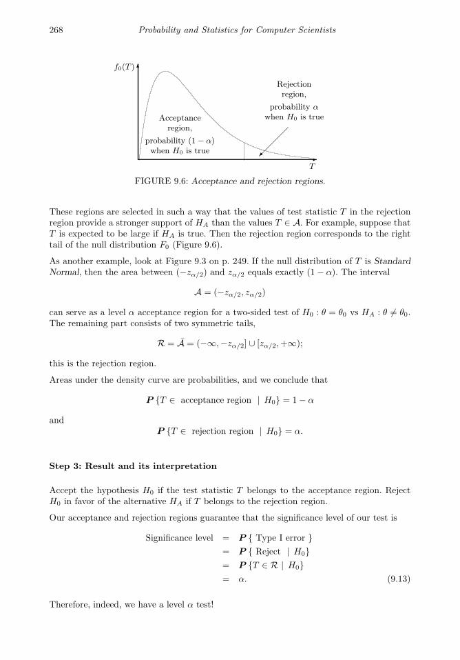
268 Probability and Statistics for Computer Scientists
f0(T )
T
Acceptanceregion,
probability (1− α)when H0 is true
Rejectionregion,
probability αwhen H0 is true
FIGURE 9.6: Acceptance and rejection regions.
These regions are selected in such a way that the values of test statistic T in the rejectionregion provide a stronger support of HA than the values T ∈ A. For example, suppose thatT is expected to be large if HA is true. Then the rejection region corresponds to the righttail of the null distribution F0 (Figure 9.6).
As another example, look at Figure 9.3 on p. 249. If the null distribution of T is StandardNormal, then the area between (−zα/2) and zα/2 equals exactly (1 − α). The interval
A = (−zα/2, zα/2)
can serve as a level α acceptance region for a two-sided test of H0 : θ = θ0 vs HA : θ 6= θ0.The remaining part consists of two symmetric tails,
R = A = (−∞,−zα/2] ∪ [zα/2,+∞);
this is the rejection region.
Areas under the density curve are probabilities, and we conclude that
P T ∈ acceptance region | H0 = 1− α
andP T ∈ rejection region | H0 = α.
Step 3: Result and its interpretation
Accept the hypothesis H0 if the test statistic T belongs to the acceptance region. RejectH0 in favor of the alternative HA if T belongs to the rejection region.
Our acceptance and rejection regions guarantee that the significance level of our test is
Significance level = P Type I error = P Reject | H0= P T ∈ R | H0= α. (9.13)
Therefore, indeed, we have a level α test!

Statistical Inference I 269
The interesting part is to interpret our result correctly. Notice that conclusions like “Mylevel α test accepted the hypothesis. Therefore, the hypothesis is true with probability(1−α)” are wrong! Statements H0 and HA are about a non-random population, and thus,the hypothesis can either be true with probability 1 or false with probability 1.
If the test rejects the hypothesis, all we can state is that the data provides sufficient evidenceagainst H0 and in favor of HA. It may either happen because H0 is not true, or becauseour sample is too extreme. The latter, however, can only happen with probability α.
If the test accepts the hypothesis, it only means that the evidence obtained from the datais not sufficient to reject it. In the absence of sufficient evidence, by default, we accept thenull hypothesis.
Notation α = level of significance, probability of type I error
p(θ) = power
T = test statistic
F0, f0 = null distribution of T and its density
A = acceptance region
R = rejection region
9.4.4 Rejection regions and power
Our construction of the rejection region guaranteed the desired significance level α, as weproved in (9.13). However, one can choose many regions that will also have probability α(see Figure 9.7). Among them, which one is the best choice?
To avoid type II errors, we choose such a rejection region that will likely cover the teststatistic T in case if the alternative HA is true. This maximizes the power of our testbecause we’ll rarely accept H0 in this case.
Then, we look at our test statistic T under the alternative. Often
(a) a right-tail alternative forces T to be large,
(b) a left-tail alternative forces T to be small,
(c) a two-sided alternative forces T to be either large or small
(although it certainly depends on how we choose T ). If this is the case, it tells us exactlywhen we should reject the null hypothesis:
(a) For a right-tail alternative, the rejection region R should consist of large values ofT . Choose R on the right, A on the left (Figure 9.7a).
(b) For a left-tail alternative, the rejection region R should consist of small values ofT . Choose R on the left, A on the right (Figure 9.7b).
(c) For a two-sided alternative, the rejection region R should consist of very smalland very large values of T . Let R consist of two extreme regions, while A covers themiddle (Figure 9.7c).
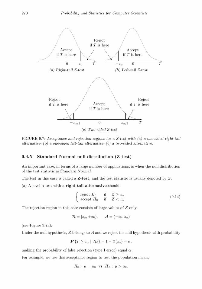
270 Probability and Statistics for Computer Scientists
0 0T Tzα −zα
Acceptif T is here
Acceptif T is here
Rejectif T is here
❫
0 T−zα/2 zα/2
Acceptif T is here
Rejectif T is here
Rejectif T is here
❯
(a) Right-tail Z-test (b) Left-tail Z-test
(c) Two-sided Z-test
FIGURE 9.7: Acceptance and rejection regions for a Z-test with (a) a one-sided right-tailalternative; (b) a one-sided left-tail alternative; (c) a two-sided alternative.
9.4.5 Standard Normal null distribution (Z-test)
An important case, in terms of a large number of applications, is when the null distributionof the test statistic is Standard Normal.
The test in this case is called a Z-test, and the test statistic is usually denoted by Z.
(a) A level α test with a right-tail alternative should
reject H0 if Z ≥ zαaccept H0 if Z < zα
(9.14)
The rejection region in this case consists of large values of Z only,
R = [zα,+∞), A = (−∞, zα)
(see Figure 9.7a).
Under the null hypothesis, Z belongs to A and we reject the null hypothesis with probability
P T ≥ zα | H0 = 1− Φ(zα) = α,
making the probability of false rejection (type I error) equal α .
For example, we use this acceptance region to test the population mean,
H0 : µ = µ0 vs HA : µ > µ0.

Statistical Inference I 271
(b) With a left-tail alternative, we should
reject H0 if Z ≤ −zαaccept H0 if Z > −zα
(9.15)
The rejection region consists of small values of Z only,
R = (−∞,−zα], A = (−zα,+∞).
Similarly, P Z ∈ R = α under H0; thus, the probability of type I error equals α.
For example, this is how we should test
H0 : µ = µ0 vs HA : µ < µ0.
(c) With a two-sided alternative, we
reject H0 if |Z| ≥ zα/2accept H0 if |Z| < zα/2
(9.16)
The rejection region consists of very small and very large values of Z,
R = (−∞, zα/2] ∪ [zα/2,+∞), A = (−zα/2, zα/2).
Again, the probability of type I error equals α in this case.
For example, we use this test for
H0 : µ = µ0 vs HA : µ 6= µ0.
This is easy to remember:
– for a two-sided test, divide α by two and use zα/2;
– for a one-sided test, use zα keeping in mind that the rejection region consists of justone piece.
Now consider testing a hypothesis about a population parameter θ. Suppose that its esti-mator θ has Normal distribution, at least approximately, and we know E(θ) and Var(θ) ifthe hypothesis is true.
Then the test statistic
Z =θ − E(θ)√
Var(θ)(9.17)
has Standard Normal distribution, and we can use (9.14), (9.15), and (9.16) to constructacceptance and rejection regions for a level α test. We call Z a Z-statistic.
Examples of Z-tests are in the next section.
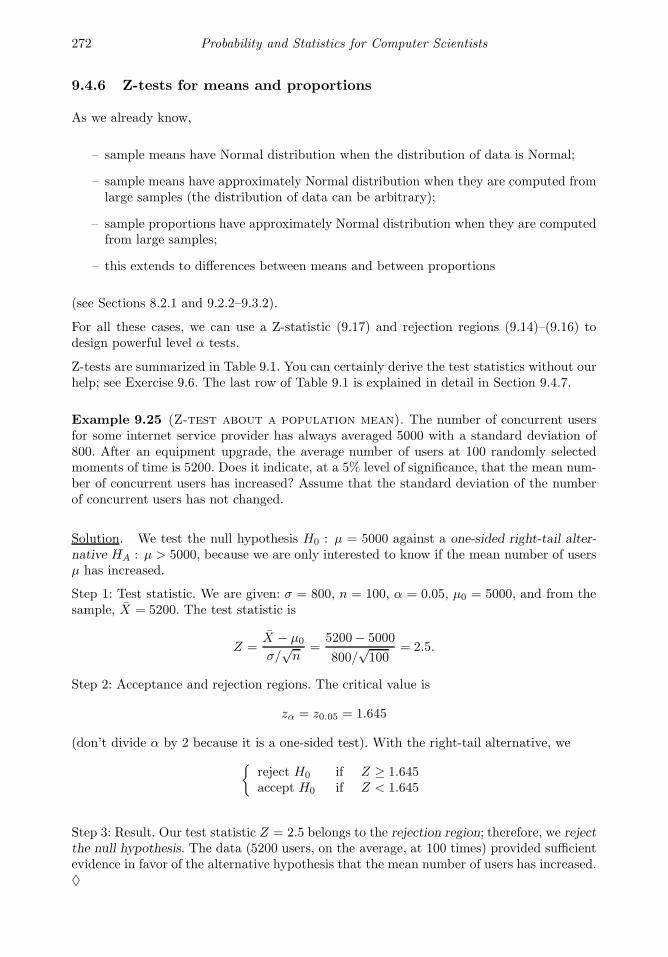
272 Probability and Statistics for Computer Scientists
9.4.6 Z-tests for means and proportions
As we already know,
– sample means have Normal distribution when the distribution of data is Normal;
– sample means have approximately Normal distribution when they are computed fromlarge samples (the distribution of data can be arbitrary);
– sample proportions have approximately Normal distribution when they are computedfrom large samples;
– this extends to differences between means and between proportions
(see Sections 8.2.1 and 9.2.2–9.3.2).
For all these cases, we can use a Z-statistic (9.17) and rejection regions (9.14)–(9.16) todesign powerful level α tests.
Z-tests are summarized in Table 9.1. You can certainly derive the test statistics without ourhelp; see Exercise 9.6. The last row of Table 9.1 is explained in detail in Section 9.4.7.
Example 9.25 (Z-test about a population mean). The number of concurrent usersfor some internet service provider has always averaged 5000 with a standard deviation of800. After an equipment upgrade, the average number of users at 100 randomly selectedmoments of time is 5200. Does it indicate, at a 5% level of significance, that the mean num-ber of concurrent users has increased? Assume that the standard deviation of the numberof concurrent users has not changed.
Solution. We test the null hypothesis H0 : µ = 5000 against a one-sided right-tail alter-native HA : µ > 5000, because we are only interested to know if the mean number of usersµ has increased.
Step 1: Test statistic. We are given: σ = 800, n = 100, α = 0.05, µ0 = 5000, and from thesample, X = 5200. The test statistic is
Z =X − µ0
σ/√n
=5200− 5000
800/√100
= 2.5.
Step 2: Acceptance and rejection regions. The critical value is
zα = z0.05 = 1.645
(don’t divide α by 2 because it is a one-sided test). With the right-tail alternative, we
reject H0 if Z ≥ 1.645accept H0 if Z < 1.645
Step 3: Result. Our test statistic Z = 2.5 belongs to the rejection region; therefore, we rejectthe null hypothesis. The data (5200 users, on the average, at 100 times) provided sufficientevidence in favor of the alternative hypothesis that the mean number of users has increased.♦
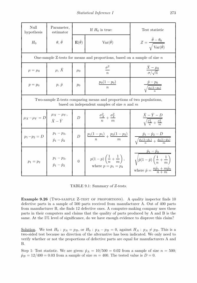
Statistical Inference I 273
Nullhypothesis
Parameter,estimator
If H0 is true: Test statistic
H0 θ, θ E(θ) Var(θ) Z =θ − θ0√Var(θ)
One-sample Z-tests for means and proportions, based on a sample of size n
µ = µ0 µ, X µ0σ2
n
X − µ0
σ/√n
p = p0 p, p p0p0(1− p0)
n
p− p0√p0(1−p0)
n
Two-sample Z-tests comparing means and proportions of two populations,based on independent samples of size n and m
µX−µY = DµX − µY ,
X − YD
σ2X
n+
σ2Y
m
X − Y −D√σ2X
n +σ2Y
m
p1−p2 = Dp1 − p2,
p1 − p2D
p1(1 − p1)
n+
p2(1 − p2)
m
p1 − p2 −D√p1(1−p1)
n + p2(1−p2)m
p1 = p2p1 − p2,
p1 − p20
p(1− p)
(1
n+
1
m
),
where p = p1 = p2
p1 − p2√p(1− p)
(1
n+
1
m
)
where p =np1 +mp2n+m
TABLE 9.1: Summary of Z-tests.
Example 9.26 (Two-sample Z-test of proportions). A quality inspector finds 10defective parts in a sample of 500 parts received from manufacturer A. Out of 400 partsfrom manufacturer B, she finds 12 defective ones. A computer-making company uses theseparts in their computers and claims that the quality of parts produced by A and B is thesame. At the 5% level of significance, do we have enough evidence to disprove this claim?
Solution. We test H0 : pA = pB, or H0 : pA − pB = 0, against HA : pA 6= pB. This is atwo-sided test because no direction of the alternative has been indicated. We only need toverify whether or not the proportions of defective parts are equal for manufacturers A andB.
Step 1: Test statistic. We are given: pA = 10/500 = 0.02 from a sample of size n = 500;pB = 12/400 = 0.03 from a sample of size m = 400. The tested value is D = 0.
274 Probability and Statistics for Computer Scientists
As we know, for these Bernoulli data, the variance depends on the unknown parameters pAand pB which are estimated by the sample proportions pA and pB.
The test statistic then equals
Z =pA − pB −D√
pA(1 − pA)
n+
pB(1− pB)
m
=0.02− 0.03√
(0.02)(0.98)
500+
(0.03)(0.97)
400
= −0.945.
Step 2: Acceptance and rejection regions. This is a two-sided test; thus we divide α by 2,find z0.05/2 = z0.025 = 1.96, and
reject H0 if |Z| ≥ 1.96;accept H0 if |Z| < 1.96.
Step 3: Result. The evidence against H0 is insufficient because |Z| < 1.96. Although sampleproportions of defective parts are unequal, the difference between them appears too smallto claim that population proportions are different. ♦
9.4.7 Pooled sample proportion
The test in Example 9.26 can be conducted differently and perhaps, more efficiently.
Indeed, we standardize the estimator θ = pA − pB using its expectation E(θ) and variance
Var(θ) under the null distribution, i.e., when H0 is true. However, under the null hypothesispA = pB. Then, when we standardize (pA − pB), instead of estimating two proportions inthe denominator, we only need to estimate one.
First, we estimate the common population proportion by the overall proportion of defectiveparts,
p(pooled) =number of defective parts
total number of parts=
npA +mpBn+m
.
Then we estimate the common variance as
Var(pA − pB) =p(1− p)
n+
p(1− p)
m= p(1 − p)
(1
n+
1
m
)
and use it for the Z-statistic,
Z =pA − pB√
p(1− p)(1n + 1
m
) .
Example 9.27 (Example 9.26, continued). Here the pooled proportion equals
p =10 + 12
500 + 400= 0.0244,
so that
Z =0.02− 0.03√
(0.0244)(0.9756)(
1500 + 1
400
) = −0.966.
Statistical Inference I 275
This does not affect our result. We obtained a different value of Z-statistic, but it alsobelongs to the acceptance region. We still don’t have a significant evidence against theequality of two population proportions. ♦
9.4.8 Unknown σ: T-tests
As we decided in Section 9.3, when we don’t know the population standard deviation, weestimate it. The resulting T-statistic has the form
t =θ − E(θ)
s(θ)=
θ − E(θ)√Var(θ)
.
In the case when the distribution of θ is Normal, the test is based on Student’s T-distributionwith acceptance and rejection regions according to the direction of HA:
(a) For a right-tail alternative,
reject H0 if t ≥ tαaccept H0 if t < tα
(9.18)
(b) For a left-tail alternative,
reject H0 if t ≤ −tαaccept H0 if t > −tα
(9.19)
(c) For a two-sided alternative,
reject H0 if |t| ≥ tα/2accept H0 if |t| < tα/2
(9.20)
Quantiles tα and tα/2 are given in Table A5. As in Section 9.3.4, the number of degrees offreedom depends on the problem and the sample size, see Table 9.2 and formula (9.10).
As in Section 9.3.4, the pooled sample variance
s2p =
n∑
i=1
(Xi − X)2 +
m∑
i=1
(Yi − Y )2
n+m− 2=
(n− 1)s2X + (m− 1)s2Yn+m− 2
is computed for the case of equal unknown variances. When variances are not equal, degreesof freedom are computed by Satterthwaite approximation (9.12).
Example 9.28 (Unauthorized use of a computer account, continued). A long-time authorized user of the account makes 0.2 seconds between keystrokes. One day, thedata in Example 9.19 on p. 260 are recorded as someone typed the correct username andpassword. At a 5% level of significance, is this an evidence of an unauthorized attempt?
Let us testH0 : µ = 0.2 vs HA : µ 6= 0.2
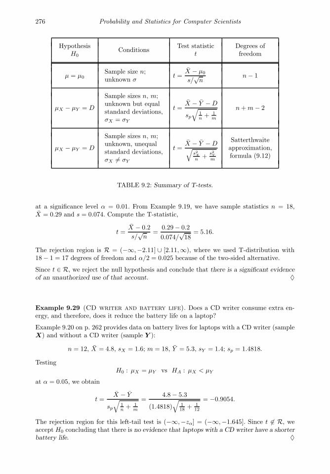
276 Probability and Statistics for Computer Scientists
HypothesisH0
ConditionsTest statistic
tDegrees offreedom
µ = µ0Sample size n;unknown σ
t =X − µ0
s/√n
n− 1
µX − µY = D
Sample sizes n, m;unknown but equalstandard deviations,σX = σY
t =X − Y −D
sp
√1n + 1
m
n+m− 2
µX − µY = D
Sample sizes n, m;unknown, unequalstandard deviations,σX 6= σY
t =X − Y −D√
s2X
n +s2Y
m
Satterthwaiteapproximation,formula (9.12)
TABLE 9.2: Summary of T-tests.
at a significance level α = 0.01. From Example 9.19, we have sample statistics n = 18,X = 0.29 and s = 0.074. Compute the T-statistic,
t =X − 0.2
s/√n
=0.29− 0.2
0.074/√18
= 5.16.
The rejection region is R = (−∞,−2.11] ∪ [2.11,∞), where we used T-distribution with18− 1 = 17 degrees of freedom and α/2 = 0.025 because of the two-sided alternative.
Since t ∈ R, we reject the null hypothesis and conclude that there is a significant evidenceof an unauthorized use of that account. ♦
Example 9.29 (CD writer and battery life). Does a CD writer consume extra en-ergy, and therefore, does it reduce the battery life on a laptop?
Example 9.20 on p. 262 provides data on battery lives for laptops with a CD writer (sampleX) and without a CD writer (sample Y ):
n = 12, X = 4.8, sX = 1.6; m = 18, Y = 5.3, sY = 1.4; sp = 1.4818.
TestingH0 : µX = µY vs HA : µX < µY
at α = 0.05, we obtain
t =X − Y
sp
√1n + 1
m
=4.8− 5.3
(1.4818)√
118 + 1
12
= −0.9054.
The rejection region for this left-tail test is (−∞,−zα] = (−∞,−1.645]. Since t 6∈ R, weaccept H0 concluding that there is no evidence that laptops with a CD writer have a shorterbattery life. ♦
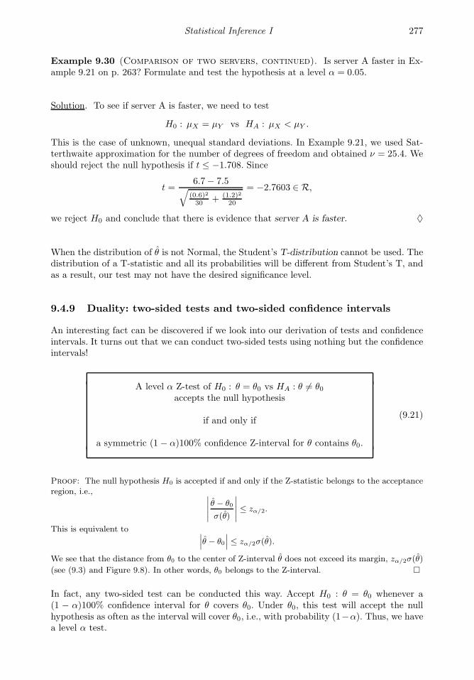
Statistical Inference I 277
Example 9.30 (Comparison of two servers, continued). Is server A faster in Ex-ample 9.21 on p. 263? Formulate and test the hypothesis at a level α = 0.05.
Solution. To see if server A is faster, we need to test
H0 : µX = µY vs HA : µX < µY .
This is the case of unknown, unequal standard deviations. In Example 9.21, we used Sat-terthwaite approximation for the number of degrees of freedom and obtained ν = 25.4. Weshould reject the null hypothesis if t ≤ −1.708. Since
t =6.7− 7.5√
(0.6)2
30 + (1.2)2
20
= −2.7603 ∈ R,
we reject H0 and conclude that there is evidence that server A is faster. ♦
When the distribution of θ is not Normal, the Student’s T-distribution cannot be used. Thedistribution of a T-statistic and all its probabilities will be different from Student’s T, andas a result, our test may not have the desired significance level.
9.4.9 Duality: two-sided tests and two-sided confidence intervals
An interesting fact can be discovered if we look into our derivation of tests and confidenceintervals. It turns out that we can conduct two-sided tests using nothing but the confidenceintervals!
A level α Z-test of H0 : θ = θ0 vs HA : θ 6= θ0accepts the null hypothesis
if and only if
a symmetric (1 − α)100% confidence Z-interval for θ contains θ0.
(9.21)
Proof: The null hypothesis H0 is accepted if and only if the Z-statistic belongs to the acceptanceregion, i.e., ∣∣∣∣∣
θ − θ0
σ(θ)
∣∣∣∣∣ ≤ zα/2.
This is equivalent to ∣∣∣θ − θ0
∣∣∣ ≤ zα/2σ(θ).
We see that the distance from θ0 to the center of Z-interval θ does not exceed its margin, zα/2σ(θ)
(see (9.3) and Figure 9.8). In other words, θ0 belongs to the Z-interval.
In fact, any two-sided test can be conducted this way. Accept H0 : θ = θ0 whenever a(1 − α)100% confidence interval for θ covers θ0. Under θ0, this test will accept the nullhypothesis as often as the interval will cover θ0, i.e., with probability (1−α). Thus, we havea level α test.
278 Probability and Statistics for Computer Scientists
0−zα zα
Z = θ−θ0σ(θ)
AcceptH0
if andonly if
θ
❯
θ0
Confidenceinterval
θ ± zα/2σ(θ)
FIGURE 9.8: Duality of tests and confidence intervals.
Rule (9.21) applies only when
– we are testing against a two-sided alternative (notice that our confidence intervals aretwo-sided too);
– significance level α of the test matches confidence level (1−α) of the confidence inter-val. For example, a two-sided 3% level test can be conducted using a 97% confidenceinterval.
Example 9.31. A sample of 6 measurements
2.5, 7.4, 8.0, 4.5, 7.4, 9.2
is collected from a Normal distribution with mean µ and standard deviation σ = 2.2. Testwhether µ = 6 against a two-sided alternative HA : µ 6= 6 at the 5% level of significance.
Solution. Solving Example 9.13 on p. 251, we have already constructed a 95% confidenceinterval for µ,
[4.74, 8.26].
The value of µ0 = 6 belongs to it; therefore, at the 5% level, the null hypothesis is accepted.♦
Example 9.32. Use data in Example 9.31 to test whether µ = 7.
Solution. The interval [4.74, 8.26] contains µ0 = 7 too; therefore, the hypothesis H0 : µ = 7is accepted as well. ♦
In the last two examples, how could we possibly accept both hypotheses, µ = 6 and µ = 7?Obviously, µ cannot be equal 6 and 7 at the same time! This is true. By accepting bothnull hypotheses, we only acknowledge that sufficient evidence against either of them is notfound in the given data.
Statistical Inference I 279
Example 9.33 (Pre-election poll). In Example 9.17 on p. 257, we computed a 95%confidence interval for the difference of proportions supporting a candidate in towns A andB: [−0.14, 0.16]. This interval contains 0, therefore, the test of
H0 : p1 = p2 vs HA : p1 6= p2
accepts the null hypothesis at the 5% level. Apparently, there is no evidence of unequalsupport of this candidate in the two towns. ♦
Example 9.34 (Hardware upgrade). In Example 9.14, we studied effectiveness of thehardware upgrade. We constructed a 90% confidence interval for the difference (µX − µY )in mean running times of a certain process: [0.7, 1.9].
So, can we conclude that the upgrade was successful? Ineffective upgrade corresponds toa null hypothesis H0 : µX = µY , or µX − µY = 0. Since the interval [0.7, 1.9] does notcontain 0, the no-effect hypothesis should be rejected at the 10% level of significance. ♦
Example 9.35 (Was the upgrade successful? One-sided test). Let’s look at Ex-ample 9.34 again. On second thought, we can only use Rule (9.21) to test the two-sidedalternative HA : µX 6= µY , right? At the same time, the hardware upgrade is successfulonly when the running time reduces, i.e., µX > µY . Then, we should judge effectiveness ofthe upgrade by a one-sided, right-tail test of
H0 : µX = µY vs HA : µX > µY . (9.22)
Let us try to use the interval [0.7, 1.9] for this test too. The null hypothesis in Example 9.34is rejected at the 10% level in favor of a two-sided alternative, thus
|Z| > zα/2 = z0.05.
Then, either Z < −z0.05 or Z > z0.05. The first case is ruled out because the interval [0.7, 1.9]consists of positive numbers, hence it cannot possibly support a left-tail alternative.
We conclude that Z > z0.05, hence the test (9.22) results in rejection of H0 at the 5% levelof significance.
Conclusion. Our 90% confidence interval for (µX − µY ) shows significant evidence, at the5% level of significance, that the hardware upgrade was successful. ♦
Similarly, for the case of unknown variance(s).
A level α T-test of H0 : θ = θ0 vs HA : θ 6= θ0accepts the null hypothesis
if and only if
a symmetric (1 − α)100% confidence T-interval for θ contains θ0.
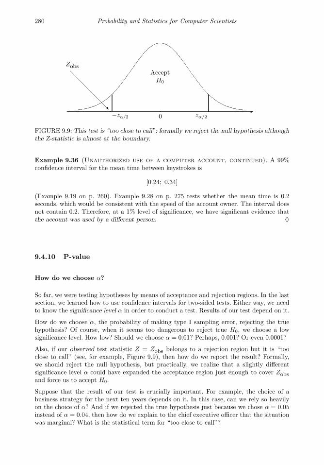
280 Probability and Statistics for Computer Scientists
−zα/2 zα/20
ZobsAcceptH0
FIGURE 9.9: This test is “too close to call”: formally we reject the null hypothesis althoughthe Z-statistic is almost at the boundary.
Example 9.36 (Unauthorized use of a computer account, continued). A 99%confidence interval for the mean time between keystrokes is
[0.24; 0.34]
(Example 9.19 on p. 260). Example 9.28 on p. 275 tests whether the mean time is 0.2seconds, which would be consistent with the speed of the account owner. The interval doesnot contain 0.2. Therefore, at a 1% level of significance, we have significant evidence thatthe account was used by a different person. ♦
9.4.10 P-value
How do we choose α?
So far, we were testing hypotheses by means of acceptance and rejection regions. In the lastsection, we learned how to use confidence intervals for two-sided tests. Either way, we needto know the significance level α in order to conduct a test. Results of our test depend on it.
How do we choose α, the probability of making type I sampling error, rejecting the truehypothesis? Of course, when it seems too dangerous to reject true H0, we choose a lowsignificance level. How low? Should we choose α = 0.01? Perhaps, 0.001? Or even 0.0001?
Also, if our observed test statistic Z = Zobs belongs to a rejection region but it is “tooclose to call” (see, for example, Figure 9.9), then how do we report the result? Formally,we should reject the null hypothesis, but practically, we realize that a slightly differentsignificance level α could have expanded the acceptance region just enough to cover Zobsand force us to accept H0.
Suppose that the result of our test is crucially important. For example, the choice of abusiness strategy for the next ten years depends on it. In this case, can we rely so heavilyon the choice of α? And if we rejected the true hypothesis just because we chose α = 0.05instead of α = 0.04, then how do we explain to the chief executive officer that the situationwas marginal? What is the statistical term for “too close to call”?

Statistical Inference I 281
Zobs
Zobs
zα
zα
0
0
AcceptH0
AcceptH0
(a) Small αAccept H0
(b) Large α,same Zobs
Reject H0
FIGURE 9.10: (a) Under a low level of significance α, we accept the null hypothesis. (b)Under a high level of significance, we reject it.
P-value
Using a P-value approach, we try not to rely on the level of significance. In fact, let us tryto test a hypothesis using all levels of significance!
Considering all levels of significance (between 0 and 1 because α is a probability of Type Ierror), we notice:
Case 1. If a level of significance is very low, we accept the null hypothesis (see Figure 9.10a).A low value of
α = P reject the null hypothesis when it is true makes it very unlikely to reject the hypothesis because it yields a very small rejection region.The right-tail area above the rejection region equals α.
Case 2. On the other extreme end, a high significance level α makes it likely to reject the nullhypothesis and corresponds to a large rejection region. A sufficiently large α will producesuch a large rejection region that will cover our test statistic, forcing us to reject H0 (seeFigure 9.10b).
Conclusion: there exists a boundary value between α-to-accept (case 1) and α-to-reject (case2). This number is a P-value (Figure 9.11).

282 Probability and Statistics for Computer Scientists
0 1P
P-value
α
Accept H0
with these αReject H0
with these α
FIGURE 9.11: P-value separates α-to-accept and α-to-reject.
DEFINITION 9.9
P-value is the lowest significance level α that forces rejection of the null hy-pothesis.
P-value is also the highest significance level α that forces acceptance of thenull hypothesis.
Testing hypotheses with a P-value
Once we know a P-value, we can indeed test hypotheses at all significance levels. Figure9.11 clearly shows that for all α < P we accept the null hypothesis, and for all α > P , wereject it.
Usual significance levels α lie in the interval [0.01, 0.1] (although there are exceptions). Then,a P-value greater than 0.1 exceeds all natural significance levels, and the null hypothesisshould be accepted. Conversely, if a P-value is less than 0.01, then it is smaller than allnatural significance levels, and the null hypothesis should be rejected. Notice that we didnot even have to specify the level α for these tests!
Only if the P-value happens to fall between 0.01 and 0.1, we really have to think aboutthe level of significance. This is the “marginal case,” “too close to call.” When we reportthe conclusion, accepting or rejecting the hypothesis, we should always remember that witha slightly different α, the decision could have been reverted. When the matter is cruciallyimportant, a good decision is to collect more data until a more definitive answer can beobtained.
Testing H0
with a P-value
For α < P, accept H0
For α > P, reject H0
Practically,
If P < 0.01, reject H0
If P > 0.1, accept H0

Statistical Inference I 283
Computing P-values
Here is how a P-value can be computed from data.
Let us look at Figure 9.10 again. Start from Figure 9.10a, gradually increase α, and keepyour eye at the vertical bar separating the acceptance and rejection region. It will move tothe left until it hits the observed test statistic Zobs. At this point, our decision changes,and we switch from case 1 (Figure 9.10a) to case 2 (Figure 9.10b). Increasing α further, wepass the Z-statistic and start accepting the null hypothesis.
What happens at the border of α-to-accept and α-to-reject? Definition 9.9 says that thisborderline α is the P-value,
P = α.
Also, at this border our observed Z-statistic coincides with the critical value zα,
Zobs = zα,
and thus,P = α = P Z ≥ zα = P Z ≥ Zobs .
In this formula, Z is any Standard Normal random variable, and Zobs is our observed teststatistic, which is a concrete number, computed from data. First, we compute Zobs, thenuse Table A4 to calculate
P Z ≥ Zobs = 1− Φ(Zobs).
P-values for the left-tail and for the two-sided alternatives are computed similarly, as givenin Table 9.3.
This table applies to all the Z-tests in this chapter. It can be directly extended to the caseof unknown standard deviations and T-tests (Table 9.4).
Understanding P-values
Looking at Tables 9.3 and 9.4, we see that P-value is the probability of observing a teststatistic at least as extreme as Zobs or tobs. Being “extreme” is determined by the alterna-tive. For a right-tail alternative, large numbers are extreme; for a left-tail alternative, small
HypothesisH0
AlternativeHA
P-value Computation
right-tailθ > θ0
P Z ≥ Zobs 1− Φ(Zobs)
θ = θ0left-tailθ < θ0
P Z ≤ Zobs Φ(Zobs)
two-sidedθ 6= θ0
P |Z| ≥ |Zobs| 2(1− Φ(|Zobs|))
TABLE 9.3: P-values for Z-tests.
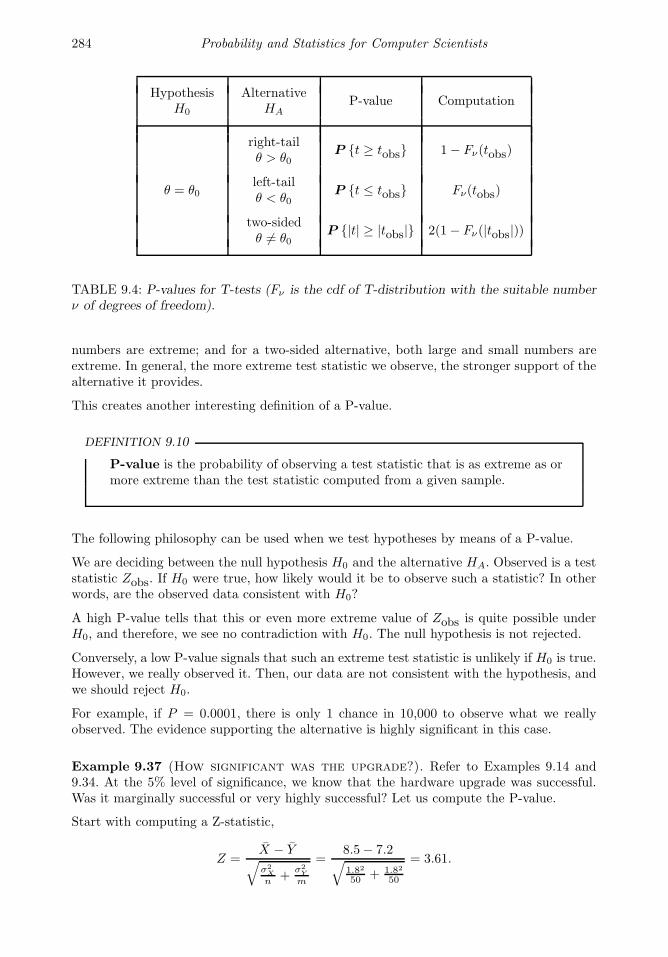
284 Probability and Statistics for Computer Scientists
HypothesisH0
AlternativeHA
P-value Computation
right-tailθ > θ0
P t ≥ tobs 1− Fν(tobs)
θ = θ0left-tailθ < θ0
P t ≤ tobs Fν(tobs)
two-sidedθ 6= θ0
P |t| ≥ |tobs| 2(1− Fν(|tobs|))
TABLE 9.4: P-values for T-tests (Fν is the cdf of T-distribution with the suitable numberν of degrees of freedom).
numbers are extreme; and for a two-sided alternative, both large and small numbers areextreme. In general, the more extreme test statistic we observe, the stronger support of thealternative it provides.
This creates another interesting definition of a P-value.
DEFINITION 9.10
P-value is the probability of observing a test statistic that is as extreme as ormore extreme than the test statistic computed from a given sample.
The following philosophy can be used when we test hypotheses by means of a P-value.
We are deciding between the null hypothesis H0 and the alternative HA. Observed is a teststatistic Zobs. If H0 were true, how likely would it be to observe such a statistic? In otherwords, are the observed data consistent with H0?
A high P-value tells that this or even more extreme value of Zobs is quite possible underH0, and therefore, we see no contradiction with H0. The null hypothesis is not rejected.
Conversely, a low P-value signals that such an extreme test statistic is unlikely if H0 is true.However, we really observed it. Then, our data are not consistent with the hypothesis, andwe should reject H0.
For example, if P = 0.0001, there is only 1 chance in 10,000 to observe what we reallyobserved. The evidence supporting the alternative is highly significant in this case.
Example 9.37 (How significant was the upgrade?). Refer to Examples 9.14 and9.34. At the 5% level of significance, we know that the hardware upgrade was successful.Was it marginally successful or very highly successful? Let us compute the P-value.
Start with computing a Z-statistic,
Z =X − Y√σ2X
n +σ2Y
m
=8.5− 7.2√1.82
50 + 1.82
50
= 3.61.
Statistical Inference I 285
From Table A4, we find that the P-value for the right-tail alternative is
P = P Z ≥ Zobs = P Z ≥ 3.61 = 1− Φ(3.61) = 0.0002.
The P-value is very low; therefore, we can reject the null hypothesis not only at the 5%, butalso at the 1% and even 0.05% level of significance! We see now that the hardware upgradewas extremely successful. ♦
Example 9.38 (Quality inspection). In Example 9.26, we compared the quality ofparts produced by two manufacturers by a two-sided test. We obtained a test statistic
Zobs = −0.94.
The P-value for this test equals
P = P |Z| ≥ | − 0.94| = 2(1− Φ(0.94)) = 2(1− 0.8264) = 0.3472.
This is a rather high P-value (greater than 0.1), and the null hypothesis is not rejected.Given H0, there is a 34% chance of observing what we really observed. No contradictionwith H0, and therefore, no evidence that the quality of parts is not the same. ♦
Table A5 is not as detailed as Table A4. Often we can only use it to bound the P-valuefrom below and from above. Typically, it suffices for hypothesis testing.
Example 9.39 (Unauthorized use of a computer account, continued). Howsignificant is the evidence in Examples 9.28 and 9.36 on pp. 275, 280 that the account wasused by an unauthorized person?
Under the null hypothesis, our T-statistic has T-distribution with 17 degrees of freedom.In the previous examples, we rejected H0 first at the 5% level, then at the 1% level. Now,comparing t = 5.16 from Example 9.28 with the entire row 17 of Table A5, we find thatit exceeds all the critical values given in the table until t0.0001. Therefore, a two-sided testrejects the null hypothesis at a very low level α = 0.0002, and the P-value is P < 0.0002.The evidence of an unauthorized use is very strong!
♦
9.5 Inference about variances
In this section, we’ll derive confidence intervals and tests for the population variance σ2 =Var(X) and for the comparison of two variances σ2
X = Var(X) and σ2Y = Var(Y ). This will
be a new type of inference for us because(a) variance is a scale and not a location parameter,(b) the distribution of its estimator, the sample variance, is not symmetric.

286 Probability and Statistics for Computer Scientists
Variance often needs to be estimated or tested for quality control, in order to assess stabilityand accuracy, evaluate various risks, and also, for tests and confidence intervals for thepopulation means when variance is unknown.
Recall that comparing two means in Section 9.3.5, we had to distinguish between the casesof equal and unequal variances. We no longer have to guess! In this section, we’ll see howto test the null hypothesis H0 : σ2
X = σ2Y against the alternative HA : σ2
X 6= σ2Y and decide
whether we should use the pooled variance (9.11) or the Satterthwaite approximation (9.12).
9.5.1 Variance estimator and Chi-square distribution
We start by estimating the population variance σ2 = Var(X) from an observed sample X =(X1, . . . , Xn). Recall from Section 8.2.4 that σ2 is estimated unbiasedly and consistently bythe sample variance
s2 =1
n− 1
n∑
i=1
(Xi − X
)2.
The summands(Xi − X
)2are not quite independent, as the Central Limit Theorem on p. 93
requires, because they all depend on X. Nevertheless, the distribution of s2 is approximatelyNormal, under mild conditions, when the sample is large.
For small to moderate samples, the distribution of s2 is not Normal at all. It is not evensymmetric. Indeed, why should it be symmetric if s2 is always non-negative!
Distribution ofthe sample variance
When observations X1, . . . , Xn are independentand Normal with Var(Xi) = σ2, the distribution of
(n− 1)s2
σ2=
n∑
i=1
(Xi − X
σ
)2
is Chi-square with (n− 1) degrees of freedom
Chi-square distribution, or χ2, is a continuous distribution with density
f(x) =1
2ν/2Γ(ν/2)xν/2−1e−x/2, x > 0,
where ν > 0 is a parameter that is called degrees of freedom and has the same meaning asfor the Student’s T-distribution (Figure 9.12).
Comparing this density with (4.7) on p. 85, we see that chi-square distribution is a specialcase of Gamma,
Chi-square(ν) = Gamma(ν/2, 1/2),
and in particular, the chi-square distribution with ν = 2 degrees of freedom is Exponen-tial(1/2).
We already know that Gamma(α, λ) distribution has expectation E(X) = α/λ andVar(X) = α/λ2. Substituting α = ν/2 and λ = 1/2, we get the chi-square moments,
E(X) = ν and Var(X) = 2ν.

Statistical Inference I 287
x
f(x)
010 20 30 40
0.1
0.2
ν = 1
ν = 5
ν = 10
ν = 30
FIGURE 9.12: Chi-square densities with ν = 1, 5, 10, and 30 degrees of freedom. Eachdistribution is right-skewed. For large ν, it is approximately Normal.
Chi-squaredistribution (χ2)
ν = degrees of freedom
f(x) =1
2ν/2Γ(ν/2)xν/2−1e−x/2, x > 0
E(X) = νVar(X) = 2ν
(9.23)
Chi-square distribution was introduced around 1900 by a famous English mathematicianKarl Pearson (1857-1936) who is regarded as a founder of the entire field of MathematicalStatistics. By the way, Pearson was a teacher and collaborator of William Gosset, which iswhy Student was Gosset’s pseudonym.
Table A6 in the Appendix contains critical values of the chi-square distribution.
9.5.2 Confidence interval for the population variance
Let us construct a (1 − α)100% confidence interval for the population variance σ2, basedon a sample of size n.
As always, we start with the estimator, the sample variance s2. However, since the distri-bution of s2 is not symmetric, our confidence interval won’t have the form “estimator ±margin” as before.
Instead, we use Table A6 to find the critical values χ21−α/2 and χ2
α/2 of the Chi-square
distribution with ν = n−1 degrees of freedom. These critical values chop the areas of (α/2)on the right and on the left sides of the region under the Chi-square density curve, as onFigure 9.13. This is similar to ±zα/2 and ±tα/2 in the previous sections, although these Chi-square quantiles are no longer symmetric. Recall that χ2
α/2 denotes the (1− α/2)-quantile,q1−α/2.
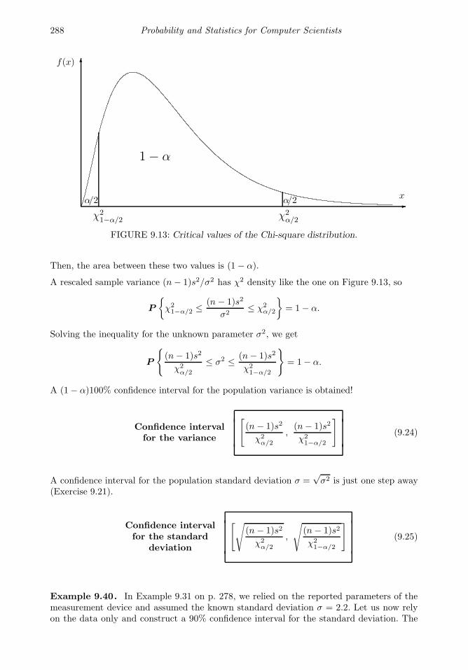
288 Probability and Statistics for Computer Scientists
x
f(x)
α/2 α/2
1− α
χ21−α/2 χ2
α/2
FIGURE 9.13: Critical values of the Chi-square distribution.
Then, the area between these two values is (1− α).
A rescaled sample variance (n− 1)s2/σ2 has χ2 density like the one on Figure 9.13, so
P
χ21−α/2 ≤ (n− 1)s2
σ2≤ χ2
α/2
= 1− α.
Solving the inequality for the unknown parameter σ2, we get
P
(n− 1)s2
χ2α/2
≤ σ2 ≤ (n− 1)s2
χ21−α/2
= 1− α.
A (1− α)100% confidence interval for the population variance is obtained!
Confidence intervalfor the variance
[(n− 1)s2
χ2α/2
,(n− 1)s2
χ21−α/2
](9.24)
A confidence interval for the population standard deviation σ =√σ2 is just one step away
(Exercise 9.21).
Confidence intervalfor the standard
deviation
[√(n− 1)s2
χ2α/2
,
√(n− 1)s2
χ21−α/2
](9.25)
Example 9.40. In Example 9.31 on p. 278, we relied on the reported parameters of themeasurement device and assumed the known standard deviation σ = 2.2. Let us now relyon the data only and construct a 90% confidence interval for the standard deviation. The

Statistical Inference I 289
sample contained n = 6 measurements, 2.5, 7.4, 8.0, 4.5, 7.4, and 9.2.
Solution. Compute the sample mean and then the sample variance,
X =1
6(2.5 + . . .+ 9.2) = 6.5;
s2 =1
6− 1
(2.5− 6.5)2 + . . .+ (9.2− 6.5)2
=
31.16
5= 6.232.
(actually, we only need (n− 1)s2 = 31.16).
From Table A6 of Chi-square distribution with ν = n − 1 = 5 degrees of freedom, we findthe critical values χ2
1−α/2 = χ20.95 = 1.15 and χ2
α/2 = χ20.05 = 11.1. Then,
[√(n− 1)s2
χ2α/2
,
√(n− 1)s2
χ21−α/2
]=
[√31.16
11.1,
√31.16
1.15
]= [1.68, 5.21].
is a 90% confidence interval for the population standard deviation (and by the way,[1.682, 5.212] = [2.82, 27.14] is a 90% confidence interval for the variance). ♦
9.5.3 Testing variance
Suppose now that we need to test the population variance, for example, to make sure thatthe actual variability, uncertainty, volatility, or risk does not exceed the promised value.We’ll derive a level α test based on the Chi-square distribution of the rescaled samplevariance.
Level α test
Let X1, . . . , Xn be a sample from the Normal distribution with the unknown populationvariance σ2. For testing the null hypothesis
H0 : σ2 = σ20 ,
compute the χ2-statistic
χ2obs =
(n− 1)s2
σ20
.
As we know, it follows the χ2 distribution with (n− 1) degrees of freedom if H0 is true andσ20 is indeed the correct population variance. Thus, it only remains to compare χ2
obs with
the critical values from Table A6 of χ2 distribution, using ν = n− 1.
Testing against the right-tail alternative HA : σ2 > σ20 , reject H0 if χ2
obs ≥ χ2α.
Testing against the left-tail alternative HA : σ2 < σ20 , reject H0 if χ2
obs ≤ χ21−α.
Testing against the two-sided alternative HA : σ2 6= σ20 , reject H0 if either χ2
obs ≥ χ2α/2 or
χ2obs ≤ χ2
1−α/2.
As an exercise, please verify that in each case, the probability of type I error is exactly α.
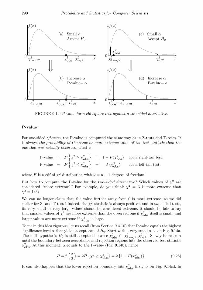
290 Probability and Statistics for Computer Scientists
0
0
0
0
x
x
x
x
f(x)
f(x)
f(x)
f(x)
χ21−α/2 χ2
α/2χ2obs χ2
1−α/2 χ2α/2
χ2obs
χ21−α/2 χ2
obs=χ2α/2 χ2
obs=χ21−α/2 χ2
α/2
(a) Small αAccept H0
(b) Increase αP-value= α
(c) Small αAccept H0
(d) Increase αP-value= α
FIGURE 9.14: P-value for a chi-square test against a two-sided alternative.
P-value
For one-sided χ2-tests, the P-value is computed the same way as in Z-tests and T-tests. Itis always the probability of the same or more extreme value of the test statistic than theone that was actually observed. That is,
P-value = Pχ2 ≥ χ2
obs
= 1− F (χ2
obs) for a right-tail test,
P-value = Pχ2 ≤ χ2
obs
= F (χ2
obs) for a left-tail test,
where F is a cdf of χ2 distribution with ν = n− 1 degrees of freedom.
But how to compute the P-value for the two-sided alternative? Which values of χ2 areconsidered “more extreme”? For example, do you think χ2 = 3 is more extreme thanχ2 = 1/3?
We can no longer claim that the value further away from 0 is more extreme, as we didearlier for Z- and T-tests! Indeed, the χ2-statistic is always positive, and in two-sided tests,its very small or very large values should be considered extreme. It should be fair to saythat smaller values of χ2 are more extreme than the observed one if χ2
obs itself is small, and
larger values are more extreme if χ2obs is large.
To make this idea rigorous, let us recall (from Section 9.4.10) that P-value equals the highestsignificance level α that yields acceptance of H0. Start with a very small α as on Fig. 9.14a.The null hypothesis H0 is still accepted because χ2
obs ∈ [χ21−α/2, χ
2α/2]. Slowly increase α
until the boundary between acceptance and rejection regions hits the observed test statisticχ2obs. At this moment, α equals to the P-value (Fig. 9.14b), hence
P = 2(α2
)= 2P
χ2 ≥ χ2
obs
= 2
1− F (χ2
obs). (9.26)
It can also happen that the lower rejection boundary hits χ2obs first, as on Fig. 9.14cd. In
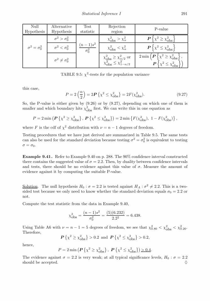
Statistical Inference I 291
NullHypothesis
AlternativeHypothesis
Teststatistic
Rejectionregion
P-value
σ2 > σ20 χ2
obs > χ2α P
χ2 ≥ χ2
obs
σ2 = σ20 σ2 < σ2
0
(n− 1)s2
σ20
χ2obs < χ2
α Pχ2 ≤ χ2
obs
σ2 6= σ20
χ2obs ≥ χ2
α/2 or
χ2obs ≤ χ2
1−α/2
2min(Pχ2 ≥ χ2
obs
,
Pχ2 ≤ χ2
obs
)
TABLE 9.5: χ2-tests for the population variance
this case,
P = 2(α2
)= 2P
χ2 ≤ χ2
obs
= 2F (χ2
obs). (9.27)
So, the P-value is either given by (9.26) or by (9.27), depending on which one of them issmaller and which boundary hits χ2
obs first. We can write this in one equation as
P = 2min(Pχ2 ≥ χ2
obs
, P
χ2 ≤ χ2
obs
)= 2min
F (χ2
obs), 1− F (χ2obs)
,
where F is the cdf of χ2 distribution with ν = n− 1 degrees of freedom.
Testing procedures that we have just derived are summarized in Table 9.5. The same testscan also be used for the standard deviation because testing σ2 = σ2
0 is equivalent to testingσ = σ0.
Example 9.41. Refer to Example 9.40 on p. 288. The 90% confidence interval constructedthere contains the suggested value of σ = 2.2. Then, by duality between confidence intervalsand tests, there should be no evidence against this value of σ. Measure the amount ofevidence against it by computing the suitable P-value.
Solution. The null hypothesis H0 : σ = 2.2 is tested against HA : σ2 6= 2.2. This is a two-sided test because we only need to know whether the standard deviation equals σ0 = 2.2 ornot.
Compute the test statistic from the data in Example 9.40,
χ2obs =
(n− 1)s2
σ20
=(5)(6.232)
2.22= 6.438.
Using Table A6 with ν = n − 1 = 5 degrees of freedom, we see that χ20.80 < χ2
obs < χ20.20.
Therefore,Pχ2 ≥ χ2
obs
> 0.2 and P
χ2 ≤ χ2
obs
> 0.2,
hence,P = 2min
(Pχ2 ≥ χ2
obs
, P
χ2 ≤ χ2
obs
)> 0.4.
The evidence against σ = 2.2 is very weak; at all typical significance levels, H0 : σ = 2.2should be accepted. ♦
292 Probability and Statistics for Computer Scientists
Example 9.42 (Remaining battery life). Creators of a new software claim that itmeasures the remaining notebook battery life with a standard deviation as low as 5 min-utes. To test this claim, a fully charged notebook was disconnected from the power supplyand continued on its battery. The experiment was repeated 50 times, and every time thepredicted battery life was recorded. The sample standard deviation of these 50 normallydistributed measurements was equal 5.6 minutes. At the 1% level of significance, do thesedata provide evidence that the actual standard deviation is greater than 5 min?
Solution. TestH0 : σ = 5 against a right-tailHA : σ > 5. From Table A6 with ν = n−1 = 49degrees of freedom, χ2
0.01 = 74.9. The null hypothesis will be rejected if χ2obs > 74.9.
Compute the test statistic,
χ2obs =
(n− 1)s2
σ20
=(49)(5.6)2
52= 61.5.
Accept H0 : σ = 5. The evidence against it is not significant at the 1% level of significance.♦
9.5.4 Comparison of two variances. F-distribution.
In this section, we deal with two populations whose variances need to be compared. Suchinference is used for the comparison of accuracy, stability, uncertainty, or risks arising intwo populations.
Example 9.43 (Efficient upgrade). A data channel has the average speed of 180Megabytes per second. A hardware upgrade is supposed to improve stability of the datatransfer while maintaining the same average speed. Stable data transfer rate implies lowstandard deviation. How can we estimate the relative change in the standard deviation ofthe transfer rate with 90% confidence? ♦
Example 9.44 (Conservative investment). Two mutual funds promise the same ex-pected return; however, one of them recorded a 10% higher volatility over the last 15 days.Is this a significant evidence for a conservative investor to prefer the other mutual fund?(Volatility is essentially the standard deviation of returns.) ♦
Example 9.45 (Which method to use?). For marketing purposes, a survey of usersof two operating systems is conducted. Twenty users of operating system ABC record theaverage level of satisfaction of 77 on a 100-point scale, with a sample variance of 220. Thirtyusers of operating system DEF have the average satisfaction level 70 with a sample varianceof 155. We already know from Section 9.4.8 how to compare the mean satisfaction levels. Butwhat method should we choose? Should we assume equality of population variances, σ2
X =σ2Y and use the pooled variance? Or we should allow for σ2
X 6= σ2Y and use Satterthwaite
approximation? ♦
Statistical Inference I 293
To compare variances or standard deviations, two independent samples X = (X1, . . . , Xn)and Y = (Y1, . . . , Ym) are collected, one from each population, as on Figure 9.4 on p. 252.Unlike population means or proportions, variances are scale factors, and they are comparedthrough their ratio
θ =σ2X
σ2Y
.
A natural estimator for the ratio of population variances θ = σ2X/σ2
Y is the ratio of samplevariances
θ =s2Xs2Y
=
∑(Xi − X)/(n− 1)∑(Yi − Y )/(m− 1)
. (9.28)
The distribution of this statistic was obtained in 1918 by a famous English statisticianand biologist Sir Ronald Fisher (1890-1962) and developed and formalized in 1934 by anAmerican mathematician George Snedecor (1881-1974). Its standard form, after we divideeach sample variance in formula (9.28) by the corresponding population variance, is thereforecalled the Fisher-Snedecor distribution or simply F-distribution with (n − 1) and (m − 1)degrees of freedom.
Distributionof the ratioof samplevariances
For independent samples X1, . . . , Xn from Normal (µX , σX)and Y1, . . . , Ym from Normal (µY , σY ), the standardizedratio of variances
F =s2X/σ2
X
s2Y /σ2Y
=
∑(Xi − X)2/σ2
X/(n− 1)∑(Yi − Y )2/σ2
Y /(m− 1)
has F-distribution with (n− 1) and (m− 1) degrees of freedom.
(9.29)
We know from Section 9.5.1 that for the Normal data, both s2X/σ2X and s2Y /σ
2Y follow χ2-
distributions. We can now conclude that the ratio of two independent χ2 variables, eachdivided by its degrees of freedom, has F-distribution. A ratio of two non-negative continuousrandom variables, any F-distributed variable is also non-negative and continuous.
F-distribution has two parameters, the numerator degrees of freedom and the denominatordegrees of freedom. These are degrees of freedom of the sample variances in the numeratorand denominator of the F-ratio (9.29).
Critical values of F-distribution are in Table A7, and we’ll use them to construct confidenceintervals and test hypotheses comparing two variances.
One question though... Comparing two variances, σ2X and σ2
Y , should we divide s2X by s2Y ors2Y by s2X? Of course, both ratios are ok to use, but we have to keep in mind that in the firstcase we deal with F(n− 1,m− 1) distribution, and in the second case with F(m− 1, n− 1).This leads us to an important general conclusion –
If F has F(ν1, ν2) distribution, then the distribution of1
Fis F(ν2, ν1). (9.30)
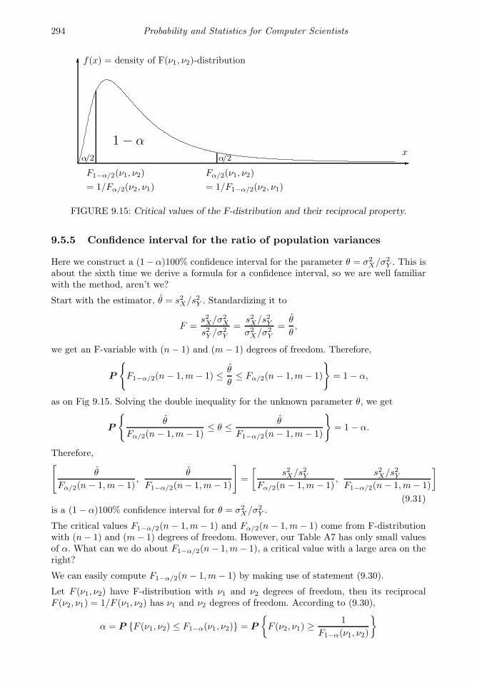
294 Probability and Statistics for Computer Scientists
x
f(x) = density of F(ν1, ν2)-distribution
α/2 α/2
1− α
F1−α/2(ν1, ν2)
= 1/Fα/2(ν2, ν1)
Fα/2(ν1, ν2)
= 1/F1−α/2(ν2, ν1)
FIGURE 9.15: Critical values of the F-distribution and their reciprocal property.
9.5.5 Confidence interval for the ratio of population variances
Here we construct a (1− α)100% confidence interval for the parameter θ = σ2X/σ2
Y . This isabout the sixth time we derive a formula for a confidence interval, so we are well familiarwith the method, aren’t we?
Start with the estimator, θ = s2X/s2Y . Standardizing it to
F =s2X/σ2
X
s2Y /σ2Y
=s2X/s2Yσ2X/σ2
Y
=θ
θ,
we get an F-variable with (n− 1) and (m− 1) degrees of freedom. Therefore,
P
F1−α/2(n− 1,m− 1) ≤ θ
θ≤ Fα/2(n− 1,m− 1)
= 1− α,
as on Fig 9.15. Solving the double inequality for the unknown parameter θ, we get
P
θ
Fα/2(n− 1,m− 1)≤ θ ≤ θ
F1−α/2(n− 1,m− 1)
= 1− α.
Therefore,[
θ
Fα/2(n− 1,m− 1),
θ
F1−α/2(n− 1,m− 1)
]=
[s2X/s2Y
Fα/2(n− 1,m− 1),
s2X/s2YF1−α/2(n− 1,m− 1)
]
(9.31)is a (1− α)100% confidence interval for θ = σ2
X/σ2Y .
The critical values F1−α/2(n − 1,m− 1) and Fα/2(n − 1,m− 1) come from F-distributionwith (n− 1) and (m− 1) degrees of freedom. However, our Table A7 has only small valuesof α. What can we do about F1−α/2(n− 1,m− 1), a critical value with a large area on theright?
We can easily compute F1−α/2(n− 1,m− 1) by making use of statement (9.30).
Let F (ν1, ν2) have F-distribution with ν1 and ν2 degrees of freedom, then its reciprocalF (ν2, ν1) = 1/F (ν1, ν2) has ν1 and ν2 degrees of freedom. According to (9.30),
α = P F (ν1, ν2) ≤ F1−α(ν1, ν2) = P
F (ν2, ν1) ≥
1
F1−α(ν1, ν2)
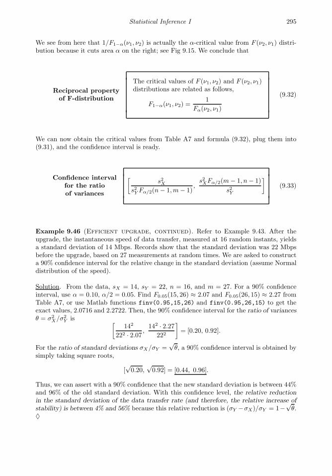
Statistical Inference I 295
We see from here that 1/F1−α(ν1, ν2) is actually the α-critical value from F (ν2, ν1) distri-bution because it cuts area α on the right; see Fig 9.15. We conclude that
Reciprocal propertyof F-distribution
The critical values of F (ν1, ν2) and F (ν2, ν1)distributions are related as follows,
F1−α(ν1, ν2) =1
Fα(ν2, ν1)
(9.32)
We can now obtain the critical values from Table A7 and formula (9.32), plug them into(9.31), and the confidence interval is ready.
Confidence intervalfor the ratioof variances
[s2X
s2Y Fα/2(n− 1,m− 1),s2XFα/2(m− 1, n− 1)
s2Y
](9.33)
Example 9.46 (Efficient upgrade, continued). Refer to Example 9.43. After theupgrade, the instantaneous speed of data transfer, measured at 16 random instants, yieldsa standard deviation of 14 Mbps. Records show that the standard deviation was 22 Mbpsbefore the upgrade, based on 27 measurements at random times. We are asked to constructa 90% confidence interval for the relative change in the standard deviation (assume Normaldistribution of the speed).
Solution. From the data, sX = 14, sY = 22, n = 16, and m = 27. For a 90% confidenceinterval, use α = 0.10, α/2 = 0.05. Find F0.05(15, 26) ≈ 2.07 and F0.05(26, 15) ≈ 2.27 fromTable A7, or use Matlab functions finv(0.95,15,26) and finv(0.95,26,15) to get theexact values, 2.0716 and 2.2722. Then, the 90% confidence interval for the ratio of variancesθ = σ2
X/σ2Y is [
142
222 · 2.07 ,142 · 2.27
222
]= [0.20, 0.92].
For the ratio of standard deviations σX/σY =√θ, a 90% confidence interval is obtained by
simply taking square roots,
[√0.20,
√0.92] = [0.44, 0.96].
Thus, we can assert with a 90% confidence that the new standard deviation is between 44%and 96% of the old standard deviation. With this confidence level, the relative reductionin the standard deviation of the data transfer rate (and therefore, the relative increase ofstability) is between 4% and 56% because this relative reduction is (σY −σX)/σY = 1−
√θ.
♦

296 Probability and Statistics for Computer Scientists
Example 9.47 (Efficient upgrade, continued again). Refer again to Examples 9.43and 9.46. Can we infer that the channel became twice as stable as it was, if increase ofstability is measured by the proportional reduction of standard deviation?
Solution. The 90% confidence interval obtained in Example 9.46 contains 0.5. Therefore,at the 10% level of significance, there is no evidence against H0 : σX/σY = 0.5, which isa two-fold reduction of standard deviation (recall Section 9.4.9 about the duality betweenconfidence intervals and tests). This is all we can state - there is no evidence against theclaim of a two-fold increase of stability. There is no “proof” that it actually happened. ♦
Testing hypotheses about the ratio of variances or standard deviations is in the next section.
9.5.6 F-tests comparing two variances
In this section, we test the null hypothesis about a ratio of variances
H0 :σ2X
σ2Y
= θ0 (9.34)
against a one-sided or a two-sided alternative. Often we only need to know if two variancesare equal, then we choose θ0 = 1. F-distribution is used to compare variances, so this testis called the F-test.
The test statistic for (9.34) is
F =s2Xs2Y
/θ0,
which under the null hypothesis equals
F =s2X/σ2
X
s2Y /σ2Y
.
If X and Y are samples from Normal distributions, this F-statistic has F-distribution with(n− 1) and (m− 1) degrees of freedom.
Just like χ2, F-statistic is also non-negative, with a non-symmetric right-skewed distribution.Level α tests and P-values are then developed similarly to χ2, see Table 9.6.
Example 9.48 (Which method to use? Continued). In Example 9.45 on p. 292,n = 20, X = 77, s2X = 220; m = 30, Y = 70, and s2Y = 155. To compare the populationmeans by a suitable method, we have to test whether the two population variances are equalor not.
Solution. Test H0 : σ2X = σ2
Y vs HA : σ2X 6= σ2
Y with the test statistic
Fobs =s2Xs2Y
= 1.42.
For testing equality of variances, we let the tested ratio θ0 = 1. This is a two-sided test, sothe P-value is
P = 2min (P F ≥ 1.42 , P F ≤ 1.42) = . . . ?
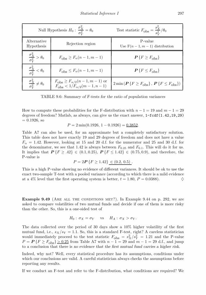
Statistical Inference I 297
Null Hypothesis H0 :σ2X
σ2Y
= θ0 Test statistic Fobs =s2Xs2Y
/θ0
AlternativeHypothesis
Rejection regionP-value
Use F(n− 1, m− 1) distribution
σ2X
σ2Y
> θ0 Fobs ≥ Fα(n− 1,m− 1) P F ≥ Fobs
σ2X
σ2Y
< θ0 Fobs ≤ Fα(n− 1,m− 1) P F ≤ Fobs
σ2X
σ2Y
6= θ0Fobs ≥ Fα/2(n− 1,m− 1) orFobs < 1/Fα/2(m− 1, n− 1)
2min (P F ≥ Fobs , P F ≤ Fobs)
TABLE 9.6: Summary of F-tests for the ratio of population variances
How to compute these probabilities for the F-distribution with n− 1 = 19 and m− 1 = 29degrees of freedom? Matlab, as always, can give us the exact answer, 1-fcdf(1.42,19,29)= 0.1926, so
P = 2min(0.1926, 1− 0.1926) = 0.3852.
Table A7 can also be used, for an approximate but a completely satisfactory solution.This table does not have exactly 19 and 29 degrees of freedom and does not have a valueFα = 1.42. However, looking at 15 and 20 d.f. for the numerator and 25 and 30 d.f. forthe denominator, we see that 1.42 is always between F0.25 and F0.1. This will do it for us.It implies that P F ≥ .42 ∈ (0.1, 0.25), P F ≤ 1.42 ∈ (0.75, 0.9), and therefore, theP-value is
P = 2P F ≥ 1.42 ∈ (0.2, 0.5) .
This is a high P-value showing no evidence of different variances. It should be ok to use theexact two-sample T-test with a pooled variance (according to which there is a mild evidenceat a 4% level that the first operating system is better, t = 1.80, P = 0.0388). ♦
Example 9.49 (Are all the conditions met?). In Example 9.44 on p. 292, we areasked to compare volatilities of two mutual funds and decide if one of them is more riskythan the other. So, this is a one-sided test of
H0 : σX = σY vs HA : σX > σY .
The data collected over the period of 30 days show a 10% higher volatility of the firstmutual fund, i.e., sX/sY = 1.1. So, this is a standard F-test, right? A careless statisticianwould immediately proceed to the test statistic Fobs = s2X/s2Y = 1.21 and the P-valueP = P F ≥ Fobs> 0.25 from Table A7 with n − 1 = 29 and m − 1 = 29 d.f., and jumpto a conclusion that there is no evidence that the first mutual fund carries a higher risk.
Indeed, why not? Well, every statistical procedure has its assumptions, conditions underwhich our conclusions are valid. A careful statistician always checks the assumptions beforereporting any results.
If we conduct an F-test and refer to the F-distribution, what conditions are required? We

298 Probability and Statistics for Computer Scientists
find the answer in (9.29) on p. 293. Apparently, for the F-statistic to have F-distributionunder H0, each of our two samples has to consist of independent and identically distributedNormal random variables, and the two samples have to be independent of each other.
Are these assumptions plausible, at the very least?
1. Normal distribution - may be. Returns on investments are typically not Normal butlog-returns are.
2. Independent and identically distributed data within each sample - unlikely. Typically,there are economic trends, ups and downs, and returns on two days in a row shouldbe dependent.
3. Independence between the two samples - it depends. If our mutual funds containstocks from the same industry, their returns are surely dependent.
Actually, conditions 1-3 can be tested statistically, and for this we need to have the entiresamples of data instead of the summary statistics.
The F-test is quite robust. It means that a mild departure from the assumptions 1-3 willnot affect our conclusions severely, and we can treat our result as approximate. However, ifthe assumptions are not met even approximately, for example, the distribution of our datais asymmetric and far from Normal, then the P-value computed above is simply wrong. ♦
Discussion in Example 9.49 leads us to a very important practical conclusion.
Every statistical procedure is valid under certain assumptions.When they are not satisfied, the obtained results may be wrong and misleading.Therefore, unless there are reasons to believe that all the conditions are met,
they have to be tested statistically.
MATLAB notes
Some hypothesis tests are built in MATLAB. For a Z-test of H0 : µ = µ0 vs HA : µ 6= µ0,write ztest(X,mu0,sigma,alpha), with the given tested value of µ0, given known standarddeviation σ, and significance level α. For a one-sided test, add ’left’ or ’right’ after α.The test will return 0 if the null hypothesis is not rejected and 1 if it has to be rejected atlevel α. To see a P-value for this test, write [h,p] = ztest(X,mu0,sigma).
T-tests can be done similarly, with a command [h,p] = ttest(X,mu0). Of course, thestandard deviation is not entered here; it is unknown.
Similar procedures are available for the two-sample T-test, for testing variances and ratiosof variances, ttest2(X,Y,alpha), vartest(X,alpha), and vartest2(X,Y,alpha).
Confidence intervals for the mean, the difference of means, the variance, and the ratio ofvariances can be obtained simply by adding CI in [h,p,CI]. For example, [h,p,CI] =
vartest2(X,Y,0.01) returns a 99% confidence interval for the ratio of variances σ2X/σ2
Y ,just as we derived it in Section 9.5.5.
Statistical Inference I 299
Summary and conclusions
After taking a general look at the data by methods of Chapter 8, we proceeded with themore advanced and informative statistical inference described in this chapter.
There is a number of methods for estimating the unknown population parameters. Eachmethod provides estimates with certain good and desired properties. We learned two generalmethods of parameter estimation.
Method of moments is based on matching the population and sample moments. It is rela-tively simple to implement, and it makes the estimated distribution “close” to the actualdistribution of data in terms of their moments.
Maximum likelihood estimators maximize the probability of observing the sample that wasreally observed, thus making the actually occurring situation as likely as possible under theestimated distribution.
In addition to parameter estimates, confidence intervals show the margin of error andattach a confidence level to the result. A (1 − α)100% confidence interval contains theunknown parameter with probability (1 − α). It means that (1 − α)100% of all confidenceintervals constructed from a large number of samples should contain the parameter, andonly 100α% may miss it.
We can use data to verify statements and test hypotheses. Essentially, we measure theevidence provided by the data against the null hypothesis H0. Then we decide whether itis sufficient for rejecting H0.
Given significance level α, we can construct acceptance and rejection regions, computea suitable test statistic, and make a decision depending on which region it belongs to.Alternatively, we may compute a P-value of the test. It shows how significant the evidenceagainstH0 is. Low P-values suggest rejection of the null hypothesis. P-value is the boundarybetween levels α-to reject and α-to-accept. It also represents the probability of observingthe same or more extreme sample than the one that was actually observed.
Depending on what we are testing against, the alternative hypothesis may be two-sided orone-sided. We account for the direction of the alternative when we construct acceptanceand rejection regions and when we compute a P-value.
We developed confidence intervals and tests of hypotheses for a number of parameters– population means, proportions, and variances, as well as the difference of means, thedifference of proportions, and the ratio of variances. This covers the majority of practicalproblems.
Each developed statistical procedure is valid under certain assumptions. Verifying them isan important step in statistical inference.
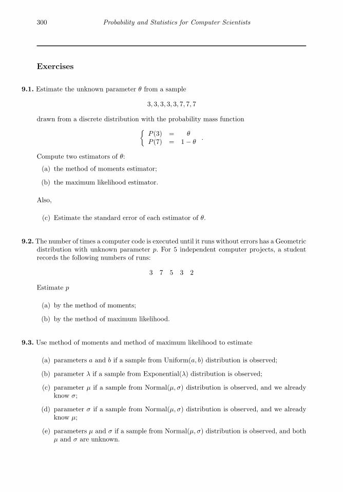
300 Probability and Statistics for Computer Scientists
Exercises
9.1. Estimate the unknown parameter θ from a sample
3, 3, 3, 3, 3, 7, 7, 7
drawn from a discrete distribution with the probability mass function
P (3) = θP (7) = 1− θ
.
Compute two estimators of θ:
(a) the method of moments estimator;
(b) the maximum likelihood estimator.
Also,
(c) Estimate the standard error of each estimator of θ.
9.2.The number of times a computer code is executed until it runs without errors has a Geometricdistribution with unknown parameter p. For 5 independent computer projects, a studentrecords the following numbers of runs:
3 7 5 3 2
Estimate p
(a) by the method of moments;
(b) by the method of maximum likelihood.
9.3. Use method of moments and method of maximum likelihood to estimate
(a) parameters a and b if a sample from Uniform(a, b) distribution is observed;
(b) parameter λ if a sample from Exponential(λ) distribution is observed;
(c) parameter µ if a sample from Normal(µ, σ) distribution is observed, and we alreadyknow σ;
(d) parameter σ if a sample from Normal(µ, σ) distribution is observed, and we alreadyknow µ;
(e) parameters µ and σ if a sample from Normal(µ, σ) distribution is observed, and bothµ and σ are unknown.

Exercises 301
9.4. A sample of 3 observations (X1 = 0.4, X2 = 0.7, X3 = 0.9) is collected from a continuousdistribution with density
f(x) =
θxθ−1 if 0 < x < 1
0 otherwise
Estimate θ by your favorite method.
9.5. A sample (X1, ..., X10) is drawn from a distribution with a probability density function
1
2
(1
θe−x/θ +
1
10e−x/10
), 0 < x < ∞
The sum of all 10 observations equals 150.
(a) Estimate θ by the method of moments.
(b) Estimate the standard error of your estimator in (a).
9.6. Verify columns 3-5 in Table 9.1 on p. 273. Section 9.4.7 will help you with the last row ofthe table.
9.7. In order to ensure efficient usage of a server, it is necessary to estimate the mean numberof concurrent users. According to records, the average number of concurrent users at 100randomly selected times is 37.7, with a standard deviation σ = 9.2.
(a) Construct a 90% confidence interval for the expectation of the number of concurrentusers.
(b) At the 1% significance level, do these data provide significant evidence that the meannumber of concurrent users is greater than 35?
9.8. Installation of a certain hardware takes random time with a standard deviation of 5 minutes.
(a) A computer technician installs this hardware on 64 different computers, with theaverage installation time of 42 minutes. Compute a 95% confidence interval for thepopulation mean installation time.
(b) Suppose that the population mean installation time is 40 minutes. A technician installsthe hardware on your PC. What is the probability that the installation time will bewithin the interval computed in (a)?
9.9. Salaries of entry-level computer engineers have Normal distribution with unknown meanand variance. Three randomly selected computer engineers have salaries (in $ 1000s):
30, 50, 70
(a) Construct a 90% confidence interval for the average salary of an entry-level computerengineer.
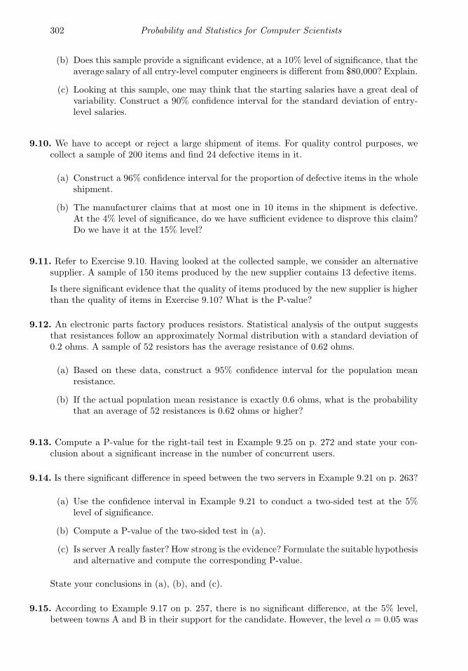
302 Probability and Statistics for Computer Scientists
(b) Does this sample provide a significant evidence, at a 10% level of significance, that theaverage salary of all entry-level computer engineers is different from $80,000? Explain.
(c) Looking at this sample, one may think that the starting salaries have a great deal ofvariability. Construct a 90% confidence interval for the standard deviation of entry-level salaries.
9.10. We have to accept or reject a large shipment of items. For quality control purposes, wecollect a sample of 200 items and find 24 defective items in it.
(a) Construct a 96% confidence interval for the proportion of defective items in the wholeshipment.
(b) The manufacturer claims that at most one in 10 items in the shipment is defective.At the 4% level of significance, do we have sufficient evidence to disprove this claim?Do we have it at the 15% level?
9.11. Refer to Exercise 9.10. Having looked at the collected sample, we consider an alternativesupplier. A sample of 150 items produced by the new supplier contains 13 defective items.
Is there significant evidence that the quality of items produced by the new supplier is higherthan the quality of items in Exercise 9.10? What is the P-value?
9.12. An electronic parts factory produces resistors. Statistical analysis of the output suggeststhat resistances follow an approximately Normal distribution with a standard deviation of0.2 ohms. A sample of 52 resistors has the average resistance of 0.62 ohms.
(a) Based on these data, construct a 95% confidence interval for the population meanresistance.
(b) If the actual population mean resistance is exactly 0.6 ohms, what is the probabilitythat an average of 52 resistances is 0.62 ohms or higher?
9.13. Compute a P-value for the right-tail test in Example 9.25 on p. 272 and state your con-clusion about a significant increase in the number of concurrent users.
9.14. Is there significant difference in speed between the two servers in Example 9.21 on p. 263?
(a) Use the confidence interval in Example 9.21 to conduct a two-sided test at the 5%level of significance.
(b) Compute a P-value of the two-sided test in (a).
(c) Is server A really faster? How strong is the evidence? Formulate the suitable hypothesisand alternative and compute the corresponding P-value.
State your conclusions in (a), (b), and (c).
9.15. According to Example 9.17 on p. 257, there is no significant difference, at the 5% level,between towns A and B in their support for the candidate. However, the level α = 0.05 was
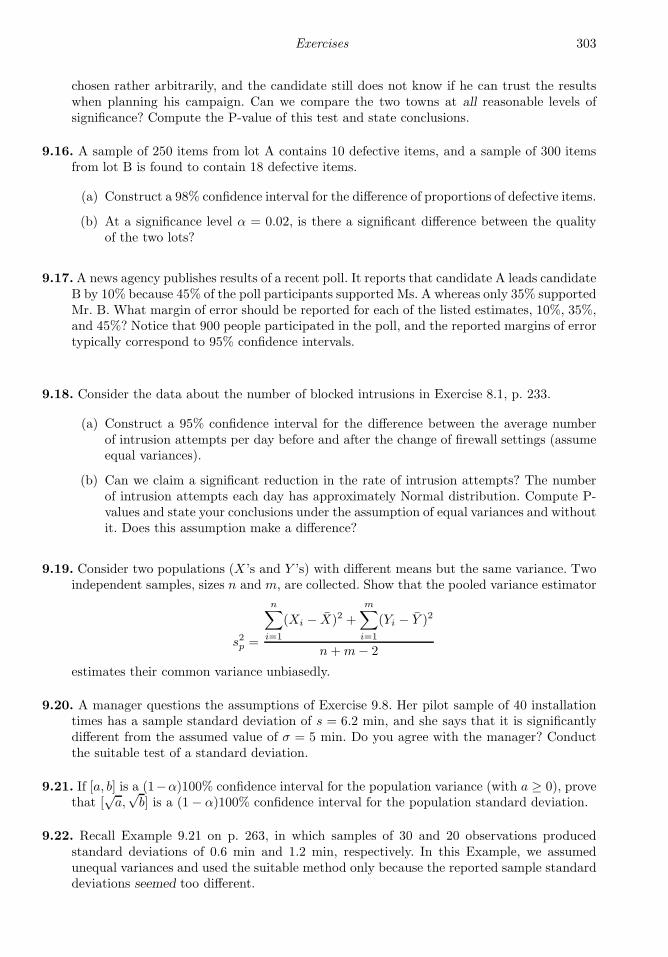
Exercises 303
chosen rather arbitrarily, and the candidate still does not know if he can trust the resultswhen planning his campaign. Can we compare the two towns at all reasonable levels ofsignificance? Compute the P-value of this test and state conclusions.
9.16. A sample of 250 items from lot A contains 10 defective items, and a sample of 300 itemsfrom lot B is found to contain 18 defective items.
(a) Construct a 98% confidence interval for the difference of proportions of defective items.
(b) At a significance level α = 0.02, is there a significant difference between the qualityof the two lots?
9.17.A news agency publishes results of a recent poll. It reports that candidate A leads candidateB by 10% because 45% of the poll participants supported Ms. A whereas only 35% supportedMr. B. What margin of error should be reported for each of the listed estimates, 10%, 35%,and 45%? Notice that 900 people participated in the poll, and the reported margins of errortypically correspond to 95% confidence intervals.
9.18. Consider the data about the number of blocked intrusions in Exercise 8.1, p. 233.
(a) Construct a 95% confidence interval for the difference between the average numberof intrusion attempts per day before and after the change of firewall settings (assumeequal variances).
(b) Can we claim a significant reduction in the rate of intrusion attempts? The numberof intrusion attempts each day has approximately Normal distribution. Compute P-values and state your conclusions under the assumption of equal variances and withoutit. Does this assumption make a difference?
9.19. Consider two populations (X ’s and Y ’s) with different means but the same variance. Twoindependent samples, sizes n and m, are collected. Show that the pooled variance estimator
s2p =
n∑
i=1
(Xi − X)2 +
m∑
i=1
(Yi − Y )2
n+m− 2
estimates their common variance unbiasedly.
9.20. A manager questions the assumptions of Exercise 9.8. Her pilot sample of 40 installationtimes has a sample standard deviation of s = 6.2 min, and she says that it is significantlydifferent from the assumed value of σ = 5 min. Do you agree with the manager? Conductthe suitable test of a standard deviation.
9.21. If [a, b] is a (1−α)100% confidence interval for the population variance (with a ≥ 0), provethat [
√a,√b] is a (1− α)100% confidence interval for the population standard deviation.
9.22. Recall Example 9.21 on p. 263, in which samples of 30 and 20 observations producedstandard deviations of 0.6 min and 1.2 min, respectively. In this Example, we assumedunequal variances and used the suitable method only because the reported sample standarddeviations seemed too different.

304 Probability and Statistics for Computer Scientists
(a) Argue for or against the chosen method by testing equality of the population variances.
(b) Also, construct a 95% confidence interval for the ratio of the two population variances.
9.23. Anthony says to Eric that he is a stronger student because his average grade for the firstsix quizzes is higher. However, Eric replies that he is more stable because the variance of hisgrades is lower. The actual scores of the two friends (presumably, independent and normallydistributed) are in the table.
Quiz 1 Quiz 2 Quiz 3 Quiz 4 Quiz 5 Quiz 6
Anthony 85 92 97 65 75 96
Eric 81 79 76 84 83 77
(a) Is there significant evidence to support Anthony’s claim? State H0 and HA. Testequality of variances and choose a suitable two-sample t-test. Then conduct the testand state conclusions.
(b) Is there significant evidence to support Eric’s claim? State H0 and HA and conductthe test.
For each test, use the 5% level of significance.
9.24. Recall Exercise 9.23. Results essentially show that a sample of six quizzes was too smallfor Anthony to claim that he is a stronger student. We realize that each student has his ownpopulation of grades, with his own mean µi and variance σ2
i . The observed quiz grades aresampled from this population, and they are different due to all the uncertainty and randomfactors involved when taking a quiz. Let us estimate the population parameters with someconfidence.
(a) Construct a 90% confidence interval for the population mean score for each student.
(b) Construct a 90% confidence interval for the difference of population means. If you havenot completed Exercise 9.23(a), start by testing equality of variances and choosing theappropriate method.
(c) Construct a 90% confidence interval for the population variance of scores for eachstudent.
(d) Construct a 90% confidence interval for the ratio of population variances.
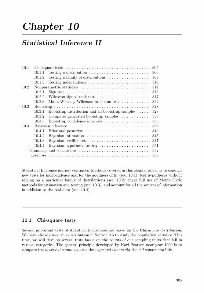
Chapter 10
Statistical Inference II
10.1 Chi-square tests . . . . . . . . . . . . . . . . . . . . . . . . . . . . . . . . . . . . . . . . . . . . . . . . . . 30510.1.1 Testing a distribution . . . . . . . . . . . . . . . . . . . . . . . . . . . . . . . . . . . . 30610.1.2 Testing a family of distributions . . . . . . . . . . . . . . . . . . . . . . . . 30810.1.3 Testing independence . . . . . . . . . . . . . . . . . . . . . . . . . . . . . . . . . . . . 310
10.2 Nonparametric statistics . . . . . . . . . . . . . . . . . . . . . . . . . . . . . . . . . . . . . . . . . 31410.2.1 Sign test . . . . . . . . . . . . . . . . . . . . . . . . . . . . . . . . . . . . . . . . . . . . . . . . . 31510.2.2 Wilcoxon signed rank test . . . . . . . . . . . . . . . . . . . . . . . . . . . . . . . 31710.2.3 Mann-Whitney-Wilcoxon rank sum test . . . . . . . . . . . . . . . . 322
10.3 Bootstrap . . . . . . . . . . . . . . . . . . . . . . . . . . . . . . . . . . . . . . . . . . . . . . . . . . . . . . . . . 32810.3.1 Bootstrap distribution and all bootstrap samples . . . . . . 32810.3.2 Computer generated bootstrap samples . . . . . . . . . . . . . . . . . 33310.3.3 Bootstrap confidence intervals . . . . . . . . . . . . . . . . . . . . . . . . . . . 335
10.4 Bayesian inference . . . . . . . . . . . . . . . . . . . . . . . . . . . . . . . . . . . . . . . . . . . . . . . . 33910.4.1 Prior and posterior . . . . . . . . . . . . . . . . . . . . . . . . . . . . . . . . . . . . . . 34010.4.2 Bayesian estimation . . . . . . . . . . . . . . . . . . . . . . . . . . . . . . . . . . . . . 34510.4.3 Bayesian credible sets . . . . . . . . . . . . . . . . . . . . . . . . . . . . . . . . . . . 34710.4.4 Bayesian hypothesis testing . . . . . . . . . . . . . . . . . . . . . . . . . . . . . 351
Summary and conclusions . . . . . . . . . . . . . . . . . . . . . . . . . . . . . . . . . . . . . . . . . . 352Exercises . . . . . . . . . . . . . . . . . . . . . . . . . . . . . . . . . . . . . . . . . . . . . . . . . . . . . . . . . . . . 353
Statistical Inference journey continues. Methods covered in this chapter allow us to conductnew tests for independence and for the goodness of fit (sec. 10.1), test hypotheses withoutrelying on a particular family of distributions (sec. 10.2), make full use of Monte Carlomethods for estimation and testing (sec. 10.3), and account for all the sources of informationin addition to the real data (sec. 10.4).
10.1 Chi-square tests
Several important tests of statistical hypotheses are based on the Chi-square distribution.We have already used this distribution in Section 9.5 to study the population variance. Thistime, we will develop several tests based on the counts of our sampling units that fall invarious categories. The general principle developed by Karl Pearson near year 1900 is tocompare the observed counts against the expected counts via the chi-square statistic
305

306 Probability and Statistics for Computer Scientists
Chi-squarestatistic
χ2 =N∑
k=1
Obs(k)− Exp(k)2Exp(k)
. (10.1)
Here the sum goes over N categories or groups of data defined depending on our testingproblem; Obs(k) is the actually observed number of sampling units in category k, andExp(k) = E Obs(k) | H0 is the expected number of sampling units in category k if thenull hypothesis H0 is true.
This is always a one-sided, right-tail test. That is because only the low values of χ2 showthat the observed counts are close to what we expect them to be under the null hypotheses,and therefore, the data support H0. On the contrary, large χ2 occurs when Obs are far fromExp, which shows inconsistency of the data and the null hypothesis and does not supportH0.
Therefore, a level α rejection region for this chi-square test is
R = [χ2α,+∞),
and the P-value is always calculated as
P = Pχ2 ≥ χ2
obs
.
Pearson showed that the null distribution of χ2 converges to the Chi-square distributionwith (N − 1) degrees of freedom, as the sample size increases to infinity. This follows froma suitable version of the Central Limit Theorem. To apply it, we need to make sure thesample size is large enough. The rule of thumb requires an expected count of at least 5 ineach category,
Exp(k) ≥ 5 for all k = 1, . . . , N.
If that is the case, then we can use the Chi-square distribution to construct rejection regionsand compute P-values. If a count in some category is less than 5, then we should mergethis category with another one, recalculate the χ2 statistic, and then use the Chi-squaredistribution.
Here are several main applications of the chi-square test.
10.1.1 Testing a distribution
The first type of applications focuses on testing whether the data belong to a particulardistribution. For example, we may want to test whether a sample comes from the Normaldistribution, whether interarrival times are Exponential and counts are Poisson, whether arandom number generator returns high quality Standard Uniform values, or whether a dieis unbiased.
In general, we observe a sample (X1, . . . , Xn) of size n from distribution F and test
H0 : F = F0 vs HA : F 6= F0 (10.2)
for some given distribution F0.

Statistical Inference II 307
To conduct the test, we take all possible values of X under F0, the support of F0, and splitthem into N bins B1, . . . , BN . A rule of thumb requires anywhere from 5 to 8 bins, whichis quite enough to identify the distribution F0 and at the same time have sufficiently highexpected count in each bin, as it is required by the chi-square test (Exp ≥ 5).
The observed count for the k-th bin is the number of Xi that fall into Bk,
Obs(k) = # i = 1, . . . , n : Xi ∈ Bk .
IfH0 is true and allXi have the distribution F0, then Obs(k), the number of “successes” in ntrials, has Binomial distribution with parameters n and pk = F0(Bk) = P Xi ∈ Bk | H0.Then, the corresponding expected count is the expected value of this Binomial distribution,
Exp(k) = npk = nF0(Bk).
After checking that all Exp(k) ≥ 5, we compute the χ2 statistic (10.1) and conduct the test.
Example 10.1 (Is the die unbiased?). Suppose that after losing a large amount ofmoney, an unlucky gambler questions whether the game was fair and the die was reallyunbiased. The last 90 tosses of this die gave the following results,
Number of dots on the die 1 2 3 4 5 6
Number of times it occurred 20 15 12 17 9 17
Let us test H0 : F = F0 vs HA : F 6= F0, where F is the distribution of the number of dotson the die, and F0 is the Discrete Uniform distribution, under which
P (X = x) =1
6for x = 1, 2, 3, 4, 5, 6.
Observed counts are Obs = 20, 15, 12, 17, 9, and 17. The corresponding expected counts are
Exp(k) = npk = (90)(1/6) = 15 (all more than 5).
Compute the chi-square statistic
χ2obs =
N∑
k=1
Obs(k)− Exp(k)2Exp(k)
=(20− 15)2
15+
(15− 15)2
15+
(12− 15)2
15+
(17− 15)2
15+
(9 − 15)2
15+
(17− 15)2
15= 5.2.
From Table A6 with N − 1 = 5 d.f., the P-value is
P = Pχ2 ≥ 5.2
= between 0.2 and 0.8 .
It means that there is no significant evidence to reject H0, and therefore, no evidence thatthe die was biased. ♦
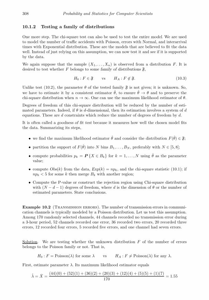
308 Probability and Statistics for Computer Scientists
10.1.2 Testing a family of distributions
One more step. The chi-square test can also be used to test the entire model. We are usedto model the number of traffic accidents with Poisson, errors with Normal, and interarrivaltimes with Exponential distribution. These are the models that are believed to fit the datawell. Instead of just relying on this assumption, we can now test it and see if it is supportedby the data.
We again suppose that the sample (X1, . . . , Xn) is observed from a distribution F . It isdesired to test whether F belongs to some family of distributions F,
H0 : F ∈ F vs HA : F 6∈ F. (10.3)
Unlike test (10.2), the parameter θ of the tested family F is not given; it is unknown. So,
we have to estimate it by a consistent estimator θ, to ensure θ → θ and to preserve thechi-square distribution when n → ∞. One can use the maximum likelihood estimator of θ.
Degrees of freedom of this chi-square distribution will be reduced by the number of esti-mated parameters. Indeed, if θ is d-dimensional, then its estimation involves a system of dequations. These are d constraints which reduce the number of degrees of freedom by d.
It is often called a goodness of fit test because it measures how well the chosen model fitsthe data. Summarizing its steps, we find the maximum likelihood estimator θ and consider the distribution F (θ) ∈ F; partition the support of F (θ) into N bins B1, . . . , BN , preferably with N ∈ [5, 8]; compute probabilities pk = P X ∈ Bk for k = 1, . . . , N using θ as the parameter
value; compute Obs(k) from the data, Exp(k) = npk, and the chi-square statistic (10.1); ifnpk < 5 for some k then merge Bk with another region; Compute the P-value or construct the rejection region using Chi-square distributionwith (N − d− 1) degrees of freedom, where d is the dimension of θ or the number ofestimated parameters. State conclusions.
Example 10.2 (Transmission errors). The number of transmission errors in communi-cation channels is typically modeled by a Poisson distribution. Let us test this assumption.Among 170 randomly selected channels, 44 channels recorded no transmission error duringa 3-hour period, 52 channels recorded one error, 36 recorded two errors, 20 recorded threeerrors, 12 recorded four errors, 5 recorded five errors, and one channel had seven errors.
Solution. We are testing whether the unknown distribution F of the number of errorsbelongs to the Poisson family or not. That is,
H0 : F = Poisson(λ) for some λ vs HA : F 6= Poisson(λ) for any λ.
First, estimate parameter λ. Its maximum likelihood estimator equals
λ = X =(44)(0) + (52)(1) + (36)(2) + (20)(3) + (12)(4) + (5)(5) + (1)(7)
170= 1.55

Statistical Inference II 309
(see Example 9.7 on p. 243).
Next, the support of Poisson distribution is the set of all non-negative integers. Partition itinto bins, let’s say,
B0 = 0 , B1 = 1 , B2 = 2 , B3 = 3 , B4 = 4 , B5 = [5,∞).
The observed counts for these bins are given: 44, 52, 36, 20, 12, and 5+1 = 6. The expectedcounts are calculated from the Poisson pmf as
Exp(k) = npk = ne−λ λk
k!for k = 0, . . . , 4, n = 170, and λ = 1.55.
The last expected count Exp(5) = 170 − Exp(0) − . . . − Exp(4) because∑
pk = 1, andtherefore,
∑npk = n. Thus, we have
k 0 1 2 3 4 5
pk 0.21 0.33 0.26 0.13 0.05 0.02npk 36.0 55.9 43.4 22.5 8.7 3.6
We notice that the last group has a count below five. So, let’s combine it with the previousgroup, B4 = [4,∞). For the new groups, we have
k 0 1 2 3 4
Exp(k) 36.0 55.9 43.4 22.5 12.3Obs(k) 44.0 52.0 36.0 20.0 18.0
Then compute the chi-square statistic
χ2obs =
∑
k
Obs(k)− Exp(k)2Exp(k)
= 6.2
and compare it against the Chi-square distribution with 5 − 1 − 1 = 3 d.f. in Table A6.With a P-value
P = Pχ2 ≥ 6.2
= between 0.1 and 0.2,
we conclude that there is no evidence against a Poisson distribution of the number oftransmission errors. ♦
Testing families of continuous distributions is rather similar.
Example 10.3 (Network load). The data in Exercise 8.2 on p. 234 shows the numberof concurrent users of a network in n = 50 locations. For further modeling and hypothesistesting, can we assume an approximately Normal distribution for the number of concurrentusers?
Solution. For the distribution F of the number of concurrent users, let us test
H0 : F = Normal(µ, σ) for some µ and σ vs HA : F 6= Normal(µ,σ) for any µ and σ.
Maximum likelihood estimates of µ and σ are (see Exercise 9.3 on p. 300)
µ = X = 17.95 and σ =
√(n− 1)s2
n=
√1
n
∑
i=1
(Xi − X)2 = 3.13.

310 Probability and Statistics for Computer Scientists
Split the support (−∞,+∞) (actually, only [0,∞) for the number of concurrent users) intobins, for example,
B1 = (−∞, 14), B2 = [14, 16), B3 = [16, 18), B4 = [18, 20), B5 = [20, 22), B6 = [22,∞)
(in thousands of users). While selecting these bins, we made sure that the expected countsin each of them will not be too low. Use Table A4 of Normal distribution to find theprobabilities pk,
p1 = P (X ∈ B1) = P (X ≤ 14) = P
(Z ≤ 14− 17.95
3.13
)= Φ(−1.26) = 0.1038,
and similarly for p1, . . . , p6. Then calculate Exp(k) = npk and count Obs(k) (check!),
k 1 2 3 4 5 6
Bk (−∞, 14) [14, 16) [16, 18) [18, 20) [20, 22) [22,∞)pk 0.10 0.16 0.24 0.24 0.16 0.10
Exp(k) 5 8 12 12 8 5
Obs(k) 6 8 13 11 6 6
From this table, the test statistic is
χ2obs =
N∑
k=1
Obs(k)− Exp(k)2Exp(k)
= 1.07,
which has a high P-valueP = P
χ2 ≥ 1.07
> 0.2.
Chi-square distribution was used with 6 − 1 − 2 = 3 d.f., where we lost 2 d.f. due to 2estimated parameters. Hence, there is no evidence against a Normal distribution of thenumber of concurrent users. ♦
10.1.3 Testing independence
Many practical applications require testing independence of two factors. If there is a signif-icant association between two features, it helps to understand the cause-and-effect relation-ships. For example, is it true that smoking causes lung cancer? Do the data confirm thatdrinking and driving increases the chance of a traffic accident? Does customer satisfactionwith their PC depend on the operating system? And does the graphical user interface (GUI)affect popularity of a software?
Apparently, chi-square statistics can help us test
H0 : Factors A and B are independent vs HA : Factors A and B are dependent.
It is understood that each factor partitions the whole population P into two or more cat-egories, A1, . . . , Ak and B1, . . . , Bm, where Ai ∩ Aj = ∅, Bi ∩ Bj = ∅, for any i 6= j, and∪Ai = ∪Bi = P .
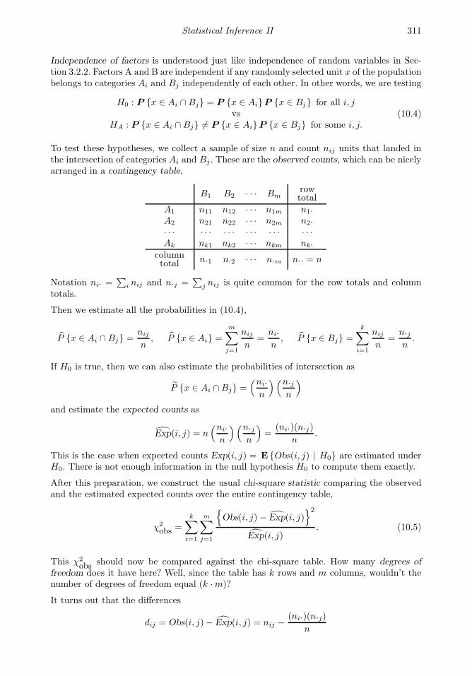
Statistical Inference II 311
Independence of factors is understood just like independence of random variables in Sec-tion 3.2.2. Factors A and B are independent if any randomly selected unit x of the populationbelongs to categories Ai and Bj independently of each other. In other words, we are testing
H0 : P x ∈ Ai ∩Bj = P x ∈ AiP x ∈ Bj for all i, jvs
HA : P x ∈ Ai ∩Bj 6= P x ∈ AiP x ∈ Bj for some i, j.(10.4)
To test these hypotheses, we collect a sample of size n and count nij units that landed inthe intersection of categories Ai and Bj . These are the observed counts, which can be nicelyarranged in a contingency table,
B1 B2 · · · Bmrowtotal
A1 n11 n12 · · · n1m n1·A2 n21 n22 · · · n2m n2·· · · · · · · · · · · · · · · · · ·Ak nk1 nk2 · · · nkm nk·
columntotal n·1 n·2 · · · n·m n·· = n
Notation ni· =∑
i nij and n·j =∑
j nij is quite common for the row totals and columntotals.
Then we estimate all the probabilities in (10.4),
P x ∈ Ai ∩Bj =nij
n, P x ∈ Ai =
m∑
j=1
nij
n=
ni·n
, P x ∈ Bj =
k∑
i=1
nij
n=
n·jn
.
If H0 is true, then we can also estimate the probabilities of intersection as
P x ∈ Ai ∩Bj =(ni·
n
)(n·jn
)
and estimate the expected counts as
Exp(i, j) = n(ni·
n
)(n·jn
)=
(ni·)(n·j)n
.
This is the case when expected counts Exp(i, j) = E Obs(i, j) | H0 are estimated underH0. There is not enough information in the null hypothesis H0 to compute them exactly.
After this preparation, we construct the usual chi-square statistic comparing the observedand the estimated expected counts over the entire contingency table,
χ2obs =
k∑
i=1
m∑
j=1
Obs(i, j)− Exp(i, j)
2
Exp(i, j). (10.5)
This χ2obs should now be compared against the chi-square table. How many degrees of
freedom does it have here? Well, since the table has k rows and m columns, wouldn’t thenumber of degrees of freedom equal (k ·m)?
It turns out that the differences
dij = Obs(i, j)− Exp(i, j) = nij −(ni·)(n·j)
n

312 Probability and Statistics for Computer Scientists
in (10.5) have many constraints. For any i = 1, . . . , k, the sum di· =∑
j dij = ni· −(ni·)(n··)
n = 0, and similarly, for any j = 1, . . . ,m, we have d·j =∑
i dij = n·j− (n··)(n·j)n = 0.
So, do we lose (k+m) degrees of freedom due to these (k+m) constraints? Yes, but there isalso one constraint among these constraints! Whatever dij are, the equality
∑i di· =
∑j d·j
always holds. So, if all the di· and d·j equal zero except the last one, d·m, then d·m = 0automatically because
∑i di· = 0 =
∑j d·j .
As a result, we have only (k + m − 1) linearly independent constraints, and the overallnumber of degrees of freedom in χ2
obs is
d.f. = km− (k +m− 1) = (k − 1)(m− 1).
Chi-squaretest for
independence
Test statistic
χ2obs =
k∑
i=1
m∑
j=1
Obs(i, j)− Exp(i, j)
2
Exp(i, j),
where
Obs(i, j) = nij are observed counts,
Exp(i, j) =(ni·)(n·j)
nare estimated expected counts,
and χ2obs has (k − 1)(m− 1) d.f.
As always in this section, this test is one-sided and right-tail.
Example 10.4 (Spam and attachments). Modern email servers and anti-spam filtersattempt to identify spam emails and direct them to a junk folder. There are various waysto detect spam, and research still continues. In this regard, an information security officertries to confirm that the chance for an email to be spam depends on whether it containsimages or not. The following data were collected on n = 1000 random email messages,
Obs(i, j) = nij With images No images ni·Spam 160 240 400
No spam 140 460 600n·j 300 700 1000
Testing H0: “being spam and containing images are independent factors” vs HA: “thesefactors are dependent”, calculate the estimated expected counts,
Exp(1, 1) =(300)(400)
1000= 120, Exp(1, 2) =
(700)(400)
1000= 280,
Exp(2, 1) =(300)(600)
1000= 180, Exp(2, 2) =
(700)(600)
1000= 420.
Exp(i, j) =(ni·)(n·j)
n With images No images ni·Spam 120 280 400
No spam 180 420 600
n·j 300 700 1000

Statistical Inference II 313
You can always check that all the row totals, the column totals, and the whole table totalare the same for the observed and the expected counts (so, if there is a mistake, catch ithere).
χ2obs =
(160− 120)2
120+
(240− 280)2
280+
(140− 180)2
180+
(460− 420)2
420= 31.75.
From Table A6 with (2− 1)(2− 1) = 1 d.f., we find that the P-value P < 0.001. We have asignificant evidence that an email having an attachment is somehow related to being spam.Therefore, this piece of information can be used in anti-spam filters. ♦
Example 10.5 (Internet shopping on different days of the week). A web de-signer suspects that the chance for an internet shopper to make a purchase through her website varies depending on the day of the week. To test this claim, she collects data duringone week, when the web site recorded 3758 hits.
Observed Mon Tue Wed Thu Fri Sat Sun Total
No purchase 399 261 284 263 393 531 502 2633Single purchase 119 72 97 51 143 145 150 777Multiple purchases 39 50 20 15 41 97 86 348
Total 557 383 401 329 577 773 738 3758
Testing independence (i.e., probability of making a purchase or multiple purchases is thesame on any day of the week), we compute the estimated expected counts,
Exp(i, j) =(ni·)(n·j)
nfor i = 1, . . . , 7, j = 1, 2, 3.
Expected Mon Tue Wed Thu Fri Sat Sun Total
No purchase 390.26 268.34 280.96 230.51 404.27 541.59 517.07 2633Single purchase 115.16 79.19 82.91 68.02 119.30 159.82 152.59 777Multiple purchases 51.58 35.47 37.13 30.47 53.43 71.58 68.34 348
Total 557 383 401 329 577 773 738 3758
Then, the test statistic is
χ2obs =
(399− 390.26)2
390.26+ . . .+
(86− 68.34)2
68.34= 60.79,
and it has (7− 1)(3− 1) = 12 degrees of freedom. From Table A6, we find that the P-valueis P < 0.001, so indeed, there is significant evidence that the probability of making a singlepurchase or multiple purchases varies during the week. ♦
Matlab Demo. The χ2 test for independence takes only a few lines of code in MATLAB.For example, here is the solution to Example 10.4.
X = [160 240; 140 460]; % Matrix of observed counts
Row = sum(X’)’; Col = sum(X); Tot = sum(Row); % Row and column totals
k = length(Col); m = length(Row); % Dimensions of the table
e = zeros(size(X)); % Expected counts
for i=1:k; for j=1:m; e(i,j) = Row(i)*Col(j)/Tot; end; end;
chisq = (X-e).2./e; % Chi-square terms
chistat = sum(sum(chisq)); % Chi-square statistic
Pvalue = 1-chi2cdf(chistat,(k-1)*(m-1)) % P-value
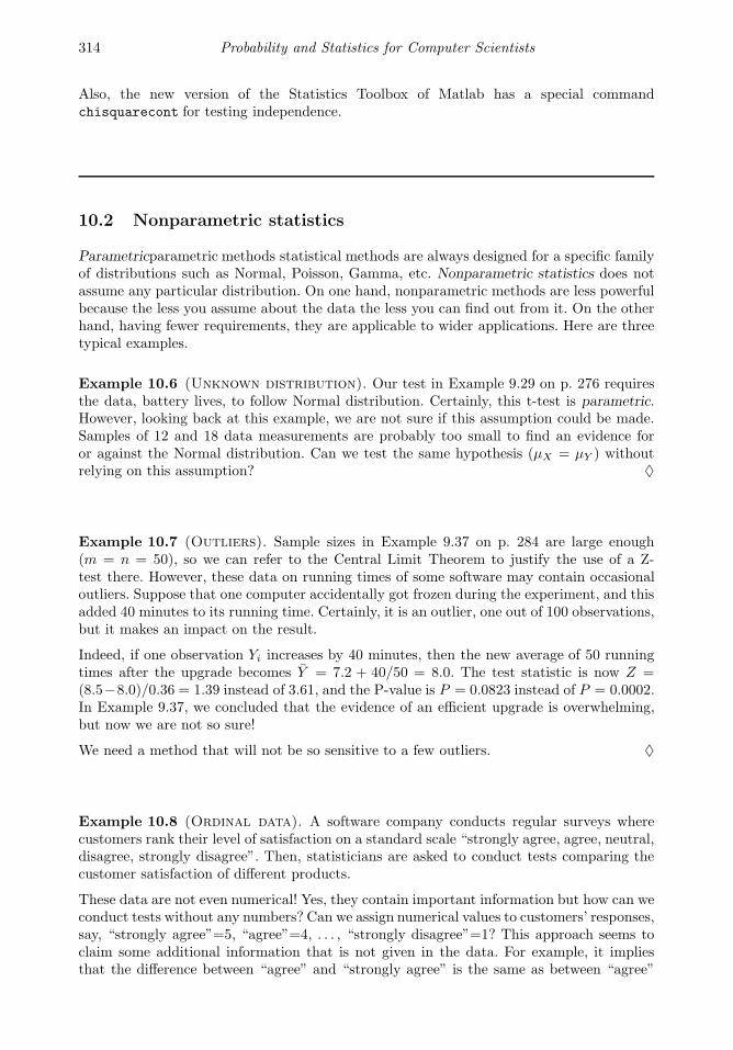
314 Probability and Statistics for Computer Scientists
Also, the new version of the Statistics Toolbox of Matlab has a special commandchisquarecont for testing independence.
10.2 Nonparametric statistics
Parametricparametric methods statistical methods are always designed for a specific familyof distributions such as Normal, Poisson, Gamma, etc. Nonparametric statistics does notassume any particular distribution. On one hand, nonparametric methods are less powerfulbecause the less you assume about the data the less you can find out from it. On the otherhand, having fewer requirements, they are applicable to wider applications. Here are threetypical examples.
Example 10.6 (Unknown distribution). Our test in Example 9.29 on p. 276 requiresthe data, battery lives, to follow Normal distribution. Certainly, this t-test is parametric.However, looking back at this example, we are not sure if this assumption could be made.Samples of 12 and 18 data measurements are probably too small to find an evidence foror against the Normal distribution. Can we test the same hypothesis (µX = µY ) withoutrelying on this assumption? ♦
Example 10.7 (Outliers). Sample sizes in Example 9.37 on p. 284 are large enough(m = n = 50), so we can refer to the Central Limit Theorem to justify the use of a Z-test there. However, these data on running times of some software may contain occasionaloutliers. Suppose that one computer accidentally got frozen during the experiment, and thisadded 40 minutes to its running time. Certainly, it is an outlier, one out of 100 observations,but it makes an impact on the result.
Indeed, if one observation Yi increases by 40 minutes, then the new average of 50 runningtimes after the upgrade becomes Y = 7.2 + 40/50 = 8.0. The test statistic is now Z =(8.5−8.0)/0.36 = 1.39 instead of 3.61, and the P-value is P = 0.0823 instead of P = 0.0002.In Example 9.37, we concluded that the evidence of an efficient upgrade is overwhelming,but now we are not so sure!
We need a method that will not be so sensitive to a few outliers. ♦
Example 10.8 (Ordinal data). A software company conducts regular surveys wherecustomers rank their level of satisfaction on a standard scale “strongly agree, agree, neutral,disagree, strongly disagree”. Then, statisticians are asked to conduct tests comparing thecustomer satisfaction of different products.
These data are not even numerical! Yes, they contain important information but how can weconduct tests without any numbers? Can we assign numerical values to customers’ responses,say, “strongly agree”=5, “agree”=4, . . . , “strongly disagree”=1? This approach seems toclaim some additional information that is not given in the data. For example, it impliesthat the difference between “agree” and “strongly agree” is the same as between “agree”

Statistical Inference II 315
and “neutral”. And further, the difference between “strongly agree” and “neutral” is thesame as between “agree” and “disagree”. We do have informative data, but this particularinformation is not given, so we cannot use it.
Are there methods in Statistics that allow us to work with the data that are not numbersbut ranks, so they can be ordered from the lowest (like “strongly disagree”) to the highest(like “strongly agree”)? ♦
The situation in Example 10.8 is rather typical. Besides satisfaction surveys, one may wantto analyze and compare the levels of education, high school to Ph.D.; military officer ranks,from a Second Lieutenant to a General; or chess skills, from Class J to Grandmaster. Also,many surveys ask for an interval instead of precise quantities, for example, income brackets- “is your annual income less than $20,000?” “between $20,000 and $30,000?” etc.
DEFINITION 10.1
Data that can be ordered from the lowest to the highest without any numericvalues are called ordinal data.
Most nonparametric methods can deal with situations described in Examples 10.6–10.8.Here we discuss three very common nonparametric tests for one sample and two samples:the sign test, the signed rank test, and the rank sum test.
10.2.1 Sign test
Here is a simple test for one population. It refers to a population median M and tests
H0 : M = m
against a one-sided or a two-sided alternative,HA : M < m,HA : M > m, orHA : M 6= m.So, we are testing whether exactly a half of the population is below m and a half is abovem.
To conduct the sign test, simply count how many observations are above m,
Sobs = S(X1, . . . , Xn) = number of i : Xi > m .
Typically, it is assumed that the underlying distribution is continuous, so P Xi = m = 0.In this case, if H0 is true and m is the median, then each Xi is equally likely to be above mor below m, and S has Binomial distribution with parameters n and p = 1/2. Using TableA2 of Binomial distribution for small n or Table A4 of Normal distribution for large n (witha proper standardization and continuity correction, of course), we compute the P-value andarrive at a conclusion.
The right-tail alternative will be supported by large values of Sobs, so the P-value shouldbe P = P S ≥ Sobs. Similarly, for the left-tail alternative, P = P S ≤ Sobs, and forthe two-sided test, P = 2min (P S ≤ Sobs , P S ≥ Sobs).

316 Probability and Statistics for Computer Scientists
The sign test
Test of the median, H0 : M = m
Test statistic S = number of Xi > m
Null distribution S ∼Binomial(n, 1/2)For large n, S ≈ Normal(n/2,
√n/2)
(if the distribution of Xi is continuous)
Example 10.9 (Unauthorized use of a computer account, continued). Exam-ple 9.39 on p. 285 shows very significant evidence that a computer account was used by anunauthorized person. This conclusion was based on the following times between keystrokes,
.24, .22, .26, .34, .35, .32, .33, .29, .19, .36, .30, .15, .17, .28, .38, .40, .37, .27 seconds,
whereas the account owner usually makes 0.2 sec between keystrokes. Our solution wasbased on a T-test and we had to assume the Normal distribution of data. However, thehistogram on Fig. 10.1 does not confirm this assumption. Also, the sample size is too smallto conduct a chi-square goodness-of-fit test (Exercise 10.5).
0.15 0.2 0.25 0.3 0.35 0.40
0.5
1
1.5
2
2.5
3
FIGURE 10.1: The histogram of timesbetween keystrokes does not support ordeny a Normal distribution.
Let’s apply the sign test because it does not re-quire the Normal distribution. The test statisticfor H0 : M = 0.2 vs HA : M 6= 0.2 is Sobs = 15because 15 of 18 recorded times exceed 0.2.
Then, from Table A2 with n = 18 and p = 0.5,we find the P-value,
P = 2min (P S ≤ Sobs , P S ≥ Sobs)= 2min (0.0038, 0.9993) = 0.0076.
(A hint for using the table here: P S ≥ 15 =P S ≤ 3, because the Binomial(0.5) distribu-tion is symmetric.) So, the sign test rejects H0
at any α > 0.0076), which is an evidence thatthe account was used by an unauthorized per-son.
Here is a large-sample version of the sign test.
Example 10.10 (Are the cars speeding?). When Eric learned to drive, he suspectedthat the median speed of cars on his way to school exceeds the speed limit, which is 30mph. As an experiment, he drives to school with his friend Evanne, precisely at the speed of30 mph, and Evanne counts the cars. At the end, Evanne reports that 56 cars were drivingfaster than Eric, and 44 cars were driving slower. Does this confirm Eric’s suspicion?
Solution. This is a one-sided right-tail test of
H0 : M = 30 vs HA : M > 30,

Statistical Inference II 317
because rejection of H0 should imply that more than 50% of cars are speeding. The signtest statistic is S = 56, and the sample size is n = 56 + 44 = 100. The null distribution ofS is approximately Normal with µ = n/2 = 50 and σ =
√n/2 = 5. Calculate the P-value
(don’t forget the continuity correction),
P = P S ≥ 56 = P
Z ≥ 55.5− 50
5
= 1− Φ(1.1) = 1− .8643 = 0.1357,
from Table A4. We can conclude that Eric and Evanne did not find a significant evidencethat the median speed of cars is above the speed limit.
Notice that we used ordinal data. Knowing the exact speed of each car was not necessaryfor the sign test. ♦
Applying the sign test, statisticians used to mark the data above the tested value (Xi > m)with pluses and those below m with minuses... which fully explains the test’s name.
10.2.2 Wilcoxon signed rank test
You certainly noticed how little information the sign test uses. All we had to know was howmany observed values are above m and below m. But perhaps the unused information canbe handy, and it should not be wasted. The next test takes magnitudes into account, inaddition to signs.
To test the population median M , we again split the sample into two parts - below m andabove m. But now we compare how far below m is the first group, collectively, and how farabove m is the second group. This comparison is done in terms of statistics called ranks.
DEFINITION 10.2
Rank of any unit of a sample is its position when the sample is arranged inthe increasing order. In a sample of size n, the smallest observation has rank 1,the second smallest has rank 2, and so on, and the largest observation has rankn. If two or more observations are equal, their ranks are typically replaced bytheir average rank.
Notation Ri = rank of the i-th observation
Having Ri = r means that Xi is the r-th smallest observation in the sample.
Example 10.11. Consider a sample
3, 7, 5, 6, 5, 4.
The smallest observation, X1 = 3, has rank 1. The second smallest is X6 = 4; it has rank2. The 3rd and 4th smallest are X3 = X5 = 5; their ranks 3 and 4 are averaged, and eachgets rank 3.5. Then, X4 = 6 and X2 = 7 get ranks 5 and 6. So, we have the following ranks,
R1 = 1, R2 = 6, R3 = 3.5, R4 = 5, R5 = 3.5, R6 = 2.♦

318 Probability and Statistics for Computer Scientists
Wilcoxon signed rank test of H0 : M = m is conducted as follows.
1. Consider the distances between observations and the tested value, di = |Xi −m|.
2. Order these distances and compute their ranks Ri. Notice! These are ranks of di, notXi.
3. Take only the ranks corresponding to observations Xi greater than m. Their sum isthe test statistic W . Namely,
W =∑
i:Xi>m
Ri
(see Figure 10.3 on p. 320 to visualize distances di and their ranks Ri).
4. Large values of W suggest rejection of H0 in favor of HA : M > m; small valuessupport HA : M < m; and both support a two-sided alternative HA : M 6= m.
This test was proposed by an Ireland-born American statistician Frank Wilcoxon (1892-1965), and it is often called Wilcoxon test.
For convenience, Wilcoxon proposed to use signed ranks, giving a “+” sign to a rank Ri ifXi > m and a “−” sign if Xi < m. His statistic W then equals the sum of positive signedranks. (Some people take the sum of negative ranks instead, or its simple transformation.These statistics are one-to-one functions of each other, so each of them can be used for theWilcoxon test.)
f(x), pdf
M − a M M + a x
FIGURE 10.2: Symmetric distribution.The shaded areas-probabilities are equalfor any a.
We assume that the distribution of X is symmet-ric about its median M , which means
P X ≤ M − a = P X ≥ M + a .
for any a (Figure 10.2). If the mean µ = E(X)exists, it will also equal M .
Let’s also assume that the distribution is contin-uous. So, there are no equal observations and noranks need to be averaged.
Under these assumptions, the null distribution ofWilcoxon test statistic W is derived later in thissection on p. 321. For n ≤ 30, the critical valuesare given in Table A8. For n ≥ 15, one can usea Normal approximation, with a continuity correction because the distribution of W isdiscrete.
Remark about acceptance and rejection regions: When we construct acceptance andrejection regions for some test statistic T , we always look for a critical value Tα such thatP T ≤ Tα = α or P T ≥ Tα = α.
But in the case of Wilcoxon test, statistic W takes only a finite number of possible values for anyn. As a result, there may be no such value w that makes probability P W ≤ w or P W ≥ wexactly equal α. One can achieve only inequalities P W ≤ w ≤ α and P W ≥ w ≤ α.
Critical values in Table A8 make these inequalities as tight as possible (that is, as close as possibleto equalities), still making sure that
P Type I error ≤ α.
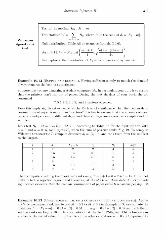
Statistical Inference II 319
Wilcoxonsigned rank
test
Test of the median, H0 : M = m.
Test statistic W =∑
i:Xi>m
Ri, where Ri is the rank of di = |Xi −m|.
Null distribution: Table A8 or recursive formula (10.6).
For n ≥ 15, W ≈ Normal
(n(n+ 1)
4,
√n(n+ 1)(2n+ 1)
24
)
Assumptions: the distribution of Xi is continuous and symmetric
Example 10.12 (Supply and demand). Having sufficient supply to match the demandalways requires the help of statisticians.
Suppose that you are managing a student computer lab. In particular, your duty is to ensurethat the printers don’t run out of paper. During the first six days of your work, the labconsumed
7, 5.5, 9.5, 6, 3.5, and 9 cartons of paper.
Does this imply significant evidence, at the 5% level of significance, that the median dailyconsumption of paper is more than 5 cartons? It is fair to assume that the amounts of usedpaper are independent on different days, and these six days are as good as a simple randomsample.
Let’s test H0 : M = 5 vs HA : M > 5. According to Table A8 for the right-tail test withn = 6 and α = 0.05, we’ll reject H0 when the sum of positive ranks T ≥ 19. To computeWilcoxon test statistic T , compute distances di = |Xi− 5| and rank them from the smallestto the largest.
i Xi Xi − 5 di Ri sign1 7 2 2 4 +2 5.5 0.5 0.5 1 +3 9.5 4.5 4.5 6 +4 6 1 1 2 +5 3.5 −1.5 1.5 3 −6 9 4 4 5 +
Then, compute T adding the “positive” ranks only, T = 4 + 1 + 6 + 2 + 5 = 18. It did notmake it to the rejection region, and therefore, at the 5% level, these data do not providesignificance evidence that the median consumption of paper exceeds 5 cartons per day. ♦
Example 10.13 (Unauthorized use of a computer account, continued). Apply-ing Wilcoxon signed rank test to test M = 0.2 vs M 6= 0.2 in Example 10.9, we compute thedistances d1 = |X1 −m| = |0.24− 0.2| = 0.04, . . . , d18 = |0.27− 0.2| = 0.07 and rank them;see the ranks on Figure 10.3. Here we notice that the 9-th, 12-th, and 13-th observationsare below the tested value m = 0.2 while all the others are above m = 0.2. Computing the
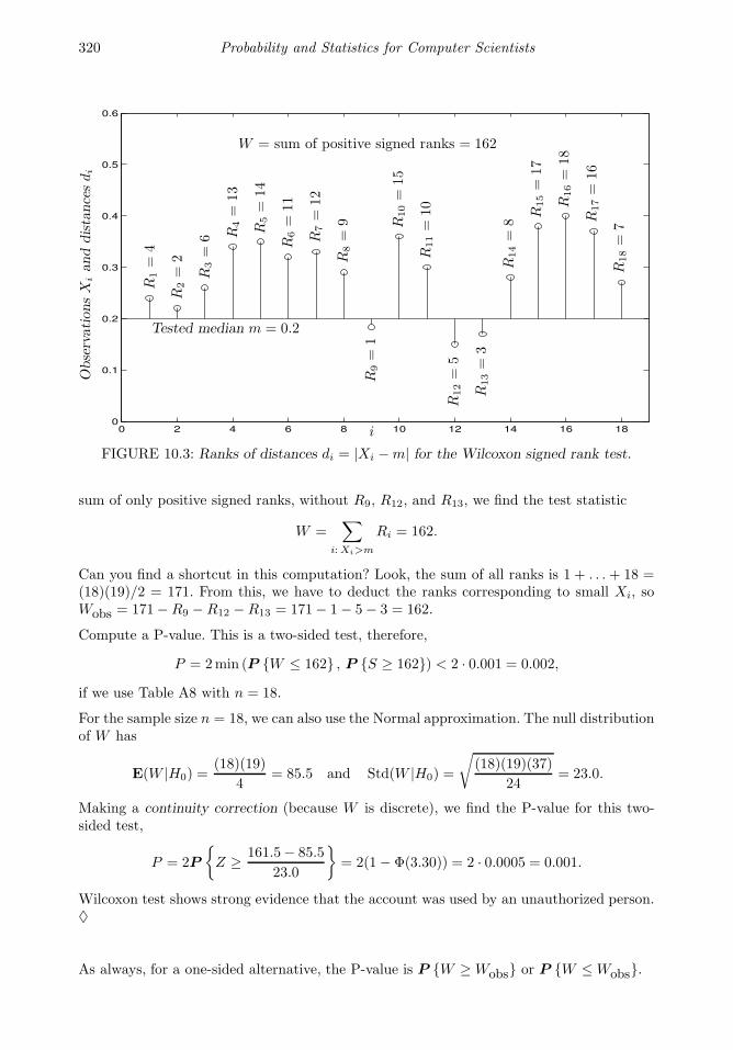
320 Probability and Statistics for Computer Scientists
0 2 4 6 8 10 12 14 16 180
0.1
0.2
0.3
0.4
0.5
0.6
ObservationsX
ianddistancesdi
i
Tested median m = 0.2
R1=
4
R2=
2
R3=
6 R4=
13
R5=
14
R6=
11
R7=
12
R8=
9
R9=
1
R10=
15
R11=
10
R12=
5
R13=
3
R14=
8
R15=
17
R16=
18
R17=
16
R18=
7
W = sum of positive signed ranks = 162
FIGURE 10.3: Ranks of distances di = |Xi −m| for the Wilcoxon signed rank test.
sum of only positive signed ranks, without R9, R12, and R13, we find the test statistic
W =∑
i:Xi>m
Ri = 162.
Can you find a shortcut in this computation? Look, the sum of all ranks is 1 + . . .+ 18 =(18)(19)/2 = 171. From this, we have to deduct the ranks corresponding to small Xi, soWobs = 171−R9 −R12 −R13 = 171− 1− 5− 3 = 162.
Compute a P-value. This is a two-sided test, therefore,
P = 2min (P W ≤ 162 , P S ≥ 162) < 2 · 0.001 = 0.002,
if we use Table A8 with n = 18.
For the sample size n = 18, we can also use the Normal approximation. The null distributionof W has
E(W |H0) =(18)(19)
4= 85.5 and Std(W |H0) =
√(18)(19)(37)
24= 23.0.
Making a continuity correction (because W is discrete), we find the P-value for this two-sided test,
P = 2P
Z ≥ 161.5− 85.5
23.0
= 2(1− Φ(3.30)) = 2 · 0.0005 = 0.001.
Wilcoxon test shows strong evidence that the account was used by an unauthorized person.♦
As always, for a one-sided alternative, the P-value is P W ≥ Wobs or P W ≤ Wobs.
Statistical Inference II 321
Comparing Examples 10.9 and 10.13, we can see that the evidence obtained by the Wilcoxontest is stronger. This should generally be the case. Wilcoxon signed rank test utilizes moreinformation contained in the data, and therefore, it is more powerful, i.e., more sensitive toa violation of H0. In other words, if H0 is not true, the Wilcoxon test is more likely to showthat.
Matlab Demo. The following code may be used to calculate the Wilcoxon signed ranktest statistic, given the data in vector X and the tested median m.
x = []; y=[]; % Split the data into Xi > m and Xi < mfor k = 1:length(X);
if X(k)>m; x=[x X(k)];
else y=[y X(k)]; end; end;
dx = abs(x-m); d = abs(X-m); % Distances to the tested median
W=0; for k=1:length(x); % Each rank is the number of distances dW=W+sum(d<dx(k))+1; end; % not exceeding the given distance dx(k)
W % W is the sum of positive ranks
Also, the Statistics Toolbox of MATLAB has a special command signrank for the Wilcoxonsigned rank test. It is designed to test H0 : M = 0 only, so subtract the tested value mfrom the data X before running this command: signrank(X-m). This command returns aP-value for the two-sided test.
Null distribution of Wilcoxon test statistic
Under the assumption of a symmetric and continuous distribution of X1, . . . , Xn, here we derivethe null distribution of W . Elegant ideas are used in this derivation.
Exact distribution
The exact null distribution of test statistic W can be found recursively. That is, we start with thetrivial case of a sample of size n = 1, then compute the distribution of W for n = 2 from it, usethat for n = 3, and so on, similarly to the mathematical induction.
In a sample of size n, all ranks are different integers between 1 and n. Because of the symmetry ofthe distribution, each of them can be a “positive rank” or a “negative rank” with probabilities 0.5and 0.5, if H0 is true.
Let pn(w) denote the probability mass function of W for a sample of size n. Then, for n = 1, thedistribution of W is
p1(0) = P W = 0 | n = 1 = 0.5 and p1(1) = P W = 1 | n = 1 = 0.5.
Now, make a transition from size (n − 1) to size n, under H0. By symmetry, the most distantobservation from M that produces the highest rank n can be above M or belowM with probabilities0.5 and 0.5. So, the sum of positive ranks W equals w in two cases:
(1) the sum of positive ranks without rank n equals w, and rank n is “negative”; or
(2) the sum of positive ranks without rank n equals (w − n), and rank n is “positive”, in whichcase it adds n to the sum making the sum equal w.
This gives us a recursive formula for calculating the pmf of Wilcoxon statistic W ,
pn(w) = 0.5pn−1(w) + 0.5pn−1(w − n). (10.6)
322 Probability and Statistics for Computer Scientists
Normal approximation
For large samples (n ≥ 15 is a rule of thumb), the distribution of W is approximately Normal. Letus find its parameters E(W ) and Var(W ).
Introduce Bernoulli(0.5) variables Y1, . . . , Yn, where Yi = 1 if the i-th signed rank is positive. Thetest statistic can then be written as
W =n∑
i=1
iYi.
In this sum, negative signed ranks will be multiplied by 0, so only the positive ones will be counted.Recall that for Bernoulli(0.5), E(Yi) = 0.5 and Var(Yi) = 0.25. Using independence of Yi, compute
E(W |H0) =
n∑
i=1
iE(Yi) =
(n∑
i=1
i
)
(0.5) =
(n(n+ 1)
2
)(0.5) =
n(n+ 1)
4,
Var(W |H0) =
n∑
i=1
i2 Var(Yi) =
(n(n+ 1)(2n+ 1)
6
)(1
4
)=
n(n+ 1)(2n+ 1)
24.
Applying this Normal approximation, do not forget to make a continuity correction because thedistribution of W is discrete.
The following MATLAB code can be used to calculate the probability mass function of W underH0 for n = 1, . . . , 15.
N=15; S=N*(N+1)/2; % max value of W
p=zeros(N,S+1); % pmf; columns 1..S+1 for w=0..S
p(1,1)=0.5; p(1,2)=0.5; % pmf for n=1
for n=2:N; % Sample sizes until N
for w=0:n-1; % Possible values of W
p(n,w+1) = 0.5*p(n-1,w+1); end;
for w=n:S; % Possible values of W
p(n,w+1) = 0.5*p(n-1,w+1) + 0.5*p(n-1,w-n+1); end;
end;
Taking partial sums F(n,w)=sum(p(n,1:w)), we can find the cdf. Table A8 is based on these
calculations.
10.2.3 Mann-Whitney-Wilcoxon rank sum test
What about two-sample procedures? Suppose we have samples from two populations, andwe need to compare their medians or just some location parameters to see how differentthey are.
Wilcoxon signed rank test can be extended to a two-sample problem as follows.
We are comparing two populations, the population of X and the population of Y . In termsof their cumulative distribution functions, we test
H0 : FX(t) = FY (t) for all t.
Assume that under the alternativeHA, either Y is stochastically larger thanX , and FX(t) >FY (t), or it is stochastically smaller than X , and FX(t) < FY (t). For example, it is the casewhen one distribution is obtained from the other by a simple shift, as on Figure 10.4.

Statistical Inference II 323
fX(t), fY (t)
MX MY
t
Density
ofX
Density
ofY
FX(t), FY (t)
MX MY
t
CDFofX
CDFofY
0
1/2
1
shift
FX(t) > FY (t)
FIGURE 10.4: Variable Y is stochastically larger than variable X . It has a larger medianand a smaller cdf, MY > MX and FY (t) < FX(t).
Observed are two independent samples X1, . . . , Xn and Y1, . . . , Ym.
In the previous section, we compared observations with the fixed tested value m. Instead,now we’ll compare one sample against the other! Here is how we conduct this test.
1. Combine all Xi and Yj into one sample.
2. Rank observations in this combined sample. Ranks Ri are from 1 to (n +m). Someof these ranks correspond to X-variables, others to Y -variables.
3. The test statistic U is the sum of all X-ranks.
When U is small, it means that X-variables have low ranks in the combined sample, so theyare generally smaller than Y -variables. This implies that Y is stochastically larger than X ,supporting the alternative HA : FY (t) < FX(t) (Figure 10.4).
This test was proposed by Frank Wilcoxon for equal sample sizes n = m and later general-ized to any n and m by other statisticians, Henry Mann and Donald Whitney.
The null distribution of the Mann-Whitney-Wilcoxon test statistic U is in Table A9. Forlarge sample sizes n and m (the rule of thumb is to have both n > 10 and m > 10), U isapproximately Normal.
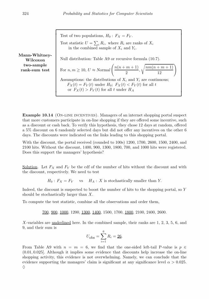
324 Probability and Statistics for Computer Scientists
Mann-Whitney-Wilcoxontwo-sample
rank-sum test
Test of two populations, H0 : FX = FY .
Test statistic U =∑
iRi, where Ri are ranks of Xi
in the combined sample of Xi and Yi.
Null distribution: Table A9 or recursive formula (10.7).
For n,m ≥ 10, U ≈ Normal
(n(n+m+ 1)
2,
√nm(n+m+ 1)
12
)
Assumptions: the distributions of Xi and Yi are continuous;FX(t) = FY (t) under H0; FX(t) < FY (t) for all tor FX(t) > FY (t) for all t under HA
Example 10.14 (On-line incentives). Managers of an internet shopping portal suspectthat more customers participate in on-line shopping if they are offered some incentive, suchas a discount or cash back. To verify this hypothesis, they chose 12 days at random, offereda 5% discount on 6 randomly selected days but did not offer any incentives on the other 6days. The discounts were indicated on the links leading to this shopping portal.
With the discount, the portal received (rounded to 100s) 1200, 1700, 2600, 1500, 2400, and2100 hits. Without the discount, 1400, 900, 1300, 1800, 700, and 1000 hits were registered.Does this support the managers’ hypothesis?
Solution. Let FX and FY be the cdf of the number of hits without the discount and withthe discount, respectively. We need to test
H0 : FX = FY vs HA : X is stochastically smaller than Y.
Indeed, the discount is suspected to boost the number of hits to the shopping portal, so Yshould be stochastically larger than X .
To compute the test statistic, combine all the observations and order them,
700, 900, 1000, 1200, 1300, 1400, 1500, 1700, 1800, 2100, 2400, 2600.
X-variables are underlined here. In the combined sample, their ranks are 1, 2, 3, 5, 6, and9, and their sum is
Uobs =6∑
i=1
Ri = 26.
From Table A9 with n = m = 6, we find that the one-sided left-tail P-value is p ∈(0.01, 0.025]. Although it implies some evidence that discounts help increase the on-lineshopping activity, this evidence is not overwhelming. Namely, we can conclude that theevidence supporting the managers’ claim is significant at any significance level α > 0.025.♦
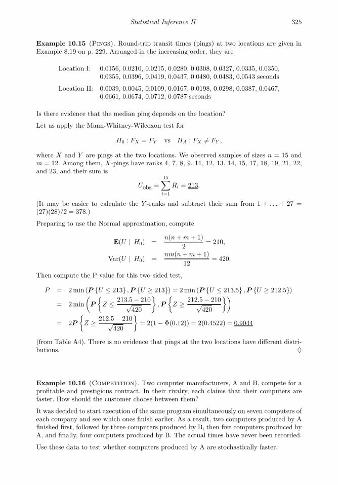
Statistical Inference II 325
Example 10.15 (Pings). Round-trip transit times (pings) at two locations are given inExample 8.19 on p. 229. Arranged in the increasing order, they are
Location I: 0.0156, 0.0210, 0.0215, 0.0280, 0.0308, 0.0327, 0.0335, 0.0350,0.0355, 0.0396, 0.0419, 0.0437, 0.0480, 0.0483, 0.0543 seconds
Location II: 0.0039, 0.0045, 0.0109, 0.0167, 0.0198, 0.0298, 0.0387, 0.0467,0.0661, 0.0674, 0.0712, 0.0787 seconds
Is there evidence that the median ping depends on the location?
Let us apply the Mann-Whitney-Wilcoxon test for
H0 : FX = FY vs HA : FX 6= FY ,
where X and Y are pings at the two locations. We observed samples of sizes n = 15 andm = 12. Among them, X-pings have ranks 4, 7, 8, 9, 11, 12, 13, 14, 15, 17, 18, 19, 21, 22,and 23, and their sum is
Uobs =
15∑
i=1
Ri = 213.
(It may be easier to calculate the Y -ranks and subtract their sum from 1 + . . . + 27 =(27)(28)/2 = 378.)
Preparing to use the Normal approximation, compute
E(U | H0) =n(n+m+ 1)
2= 210,
Var(U | H0) =nm(n+m+ 1)
12= 420.
Then compute the P-value for this two-sided test,
P = 2min (P U ≤ 213 ,P U ≥ 213) = 2min (P U ≤ 213.5 ,P U ≥ 212.5)
= 2min
(P
Z ≤ 213.5− 210√
420
,P
Z ≥ 212.5− 210√
420
)
= 2P
Z ≥ 212.5− 210√
420
= 2(1− Φ(0.12)) = 2(0.4522) = 0.9044
(from Table A4). There is no evidence that pings at the two locations have different distri-butions. ♦
Example 10.16 (Competition). Two computer manufacturers, A and B, compete for aprofitable and prestigious contract. In their rivalry, each claims that their computers arefaster. How should the customer choose between them?
It was decided to start execution of the same program simultaneously on seven computers ofeach company and see which ones finish earlier. As a result, two computers produced by Afinished first, followed by three computers produced by B, then five computers produced byA, and finally, four computers produced by B. The actual times have never been recorded.
Use these data to test whether computers produced by A are stochastically faster.

326 Probability and Statistics for Computer Scientists
Solution. In the absence of numerical data, we should use nonparametric tests. Apply theMann-Whitney Wilcoxon test for testing
H0 : FA = FB vs HA : XA is stochastically smaller than XB,
where XA and XB are the program execution times spent by computers produced by A andby B, and FA and FB are there respective cdf.
From results of this competition,
A,A,B,B,B,A,A,A,A,A,B,B,B,B,
we see that A-computers have ranks 1, 2, 6, 7, 8, 9, and 10. Their sum is
Uobs =
7∑
i=1
Ri = 43.
From Table A9, for the left-tail test with n1 = n2 = 7, we find that the P-value is between0.1 and 0.2. There is no significant evidence that computers produced by company A are(stochastically) faster. ♦
Mann-Whitney-Wilcoxon test in MATLAB
The Mann-Whitney-Wilcoxon test can be done in one line using the MATLAB Statisticstoolbox. The general command ranksum(x,y) returns a P-value for the two-sided test. Tosee the test statistic, write [P,H,stat] = ranksum(x,y). Then stats will contain the teststatistic U (MATLAB calculates the smaller of the sum of X-ranks and the sum of Y -ranksin the combined sample), and its standardized value Z = (U − E(U))/ Std(U); P will be atwo-sided P-value, and H will just equal 1 if H0 is rejected at the 5% level and 0 otherwise.
The following code can be used for Example 10.15.
x = [ 0.0156, 0.0210, 0.0215, 0.0280, 0.0308, 0.0327, 0.0335, 0.0350, ...
0.0355, 0.0396, 0.0419, 0.0437, 0.0480, 0.0483, 0.0543 ];
y = [0.0039, 0.0045, 0.0109, 0.0167, 0.0198, 0.0298, 0.0387, 0.0467, ...
0.0661, 0.0674, 0.0712, 0.0787 ];
[p,h,stats] = ranksum(x,y);
Variable stats contains the sum of Y -ranks, 165, because it is smaller than the sum ofX-ranks, and Z = 0.1220. Also, P is 0.9029, slightly different from our P = 0.9044 becausewe rounded the value of Z to 0.12.
Without the Statistics Toolbox, the Mann-Whitney-Wilcoxon test statistic can be computedby simple commands
U = 0; XY = [X Y]; % Joint sample
for k = 1:length(X); U = U + sum( XY < X(k) ) + 1; end;
U % Statistic U is the sum of X-ranks
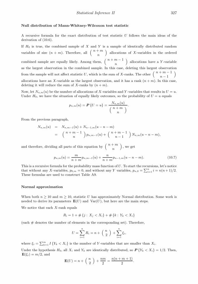
Statistical Inference II 327
Null distribution of Mann-Whitney-Wilcoxon test statistic
A recursive formula for the exact distribution of test statistic U follows the main ideas of thederivation of (10.6).
If H0 is true, the combined sample of X and Y is a sample of identically distributed random
variables of size (n + m). Therefore, all( n+m
n
)allocations of X-variables in the ordered
combined sample are equally likely. Among them,( n+m− 1
n
)allocations have a Y -variable
as the largest observation in the combined sample. In this case, deleting this largest observation
from the sample will not affect statistic U , which is the sum of X-ranks. The other( n+m− 1
n− 1
)
allocations have an X-variable as the largest observation, and it has a rank (n+m). In this case,deleting it will reduce the sum of X-ranks by (n+m).
Now, let Nn,m(u) be the number of allocations of X-variables and Y -variables that results in U = u.Under H0, we have the situation of equally likely outcomes, so the probability of U = u equals
pn,m(u) = P U = u =Nn,m(u)( n+m
n
) .
From the previous paragraph,
Nn,m(u) = Nn,m−1(u) +Nn−1,m(u− n−m)
=( n+m− 1
n
)pn,m−1(u) +
( n+m− 1n− 1
)Nn,m(u− n−m),
and therefore, dividing all parts of this equation by( n+m
n
), we get
pn,m(u) =m
n+mpn,m−1(u) +
n
n+mpn−1,m(u− n−m). (10.7)
This is a recursive formula for the probability mass function of U . To start the recursions, let’s noticethat without any X-variables, p0,m = 0, and without any Y variables, pn,0 =
∑ni=1 i = n(n+1)/2.
These formulas are used to construct Table A9.
Normal approximation
When both n ≥ 10 and m ≥ 10, statistic U has approximately Normal distribution. Some work isneeded to derive its parameters E(U) and Var(U), but here are the main steps.
We notice that each X-rank equals
Ri = 1 +# j : Xj < Xi+# k : Yk < Xi
(each # denotes the number of elements in the corresponding set). Therefore,
U =
n∑
i=1
Ri = n+( n
2
)+
n∑
i=1
ξi,
where ξi =∑m
k=1 I Yk < Xi is the number of Y -variables that are smaller than Xi.
Under the hypothesis H0, all Xi and Yk are identically distributed, so P Yk < Xi = 1/2. Then,E(ξi) = m/2, and
E(U) = n+( n
2
)+
nm
2=
n(n+m+ 1)
2.

328 Probability and Statistics for Computer Scientists
For Var(U) = Var∑
i ξi =∑
i
∑j Cov(ξi, ξj), we have to derive Var(ξi) = (m2 + 2m)/12 and
Cov(ξi, ξj) = m/12. This is not trivial, but you can fill in all the steps, as a nice non-requiredexercise! If you decide to do that, notice that all Xi and Yk have the same distribution, andtherefore, for any i 6= j and k 6= l,
P Yk < Xi ∩ Yl < Xi = P Xi is the smallest of Xi, Yk, Yl =1
3,
P Yk < Xi ∩ Yl < Xj =6 favorable allocations of Xi, Xj , Yk, Yl
4! allocations of Xi, Xj , Yk, Yl=
1
4.
Substituting into Var(U) and simplifying, we obtain
Var(U) =nm(n+m+ 1)
12.
10.3 Bootstrap
Bootstrap is used to estimate population parameters by Monte Carlo simulations when itis too difficult to do it analytically. When computers became powerful enough to handlelarge-scale simulations, the bootstrap methods got very popular for their ability to evaluateproperties of various estimates.
Consider, for example, the standard errors. From the previous chapters, we know the stan-dard errors of a sample mean and a sample proportion,
s(X) =σ√n
and s(p) =
√p(1− p)
n,
and they are quite simple. Well, try to derive standard errors of other statistics - samplemedian, sample variance, sample interquartile range, and so on. Each of these will requirea substantial amount of work.
Many complicated estimates are being used nowadays in modern Statistics. How can oneevaluate their performance, estimate their standard error, bias, etc.?
The difficulty is that we observe an estimator θ only once. That is, we have one sampleS = (X1, . . . , Xn) from the population P , and from this sample we compute θ. We would
very much like to observe many θ’s and then compute their sample variance, for example,but we don’t have this luxury. From one sample, we observe only one θ, and this is just notenough to compute its sample variance!
10.3.1 Bootstrap distribution and all bootstrap samples
In 1970s, an American mathematician, Bradley Efron, Professor at Stanford University,proposed a rather simple approach. He called it bootstrap referring to the idiom “to pulloneself up by one’s bootstraps”, which means to find a solution relying on your own sourcesand without any help from outside (a classical example is Baron Munchausen from the18th century collection of tales by R. E. Raspe, who avoided drowning in a lake by pulling

Statistical Inference II 329
Parameter θ = g(P) Estimator θ = g(S)
Population P
Sample S
a
bc d
e
f
gh
i
j
kl
m
no
p
q
rs
t
u
v
w
x
yz
AB
C
D
EF G
H
IJ
K
L
M N
OP
Q
RST
U
VWX
Y
Z
s,m,a,r,t
FIGURE 10.5: Parameter θ and its estimator θ computed by the same mechanism g appliedto the population and to the sample.
himself from the water by his own hair!). In our situation, even though we really need several
samples to explore the properties of an estimator θ, we’ll manage to do it with what wehave, which is just one sample.
To start, let’s notice that many commonly used statistics are constructed in the same way asthe corresponding population parameters. We are used to estimating a population mean µby a sample mean X , a population variance σ2 by a sample variance s2, population quantilesqp by sample quantiles qp, and so on. To estimate a certain parameter θ, we collect a random
sample S from P and essentially compute the estimator θ from this sample by the samemechanism as θ was computed from the whole population!
In other words, there is a function g that one can use to compute a parameter θ from thepopulation P (Figure 10.5). Then
θ = g(P) and θ = g(S).
Example 10.17 (Population mean and sample mean). Imagine a strange calculatorthat can only do one operation g – averaging. Give it 4 and 6, and it returns their averageg(4, 6) = 5. Give it 3, 7, and 8, and it returns g(3, 7, 8) = 6.
Give it the whole population P , and it returns the parameter θ = g(P) = µ. Give it a
sample S = (X1, . . . , Xn), and it returns the estimator θ = g(X1, . . . , Xn) = X. ♦
You can imagine similar calculators for the variances, medians, and other parameters andtheir estimates. Essentially, each estimator θ is a mechanism that copies the way a parameterθ is obtained from the population and then applies it to the sample.
Bradley Efron proposed one further step. Suppose some estimator is difficult to figure out.For example, we are interested in the variance of a sample median, η = Var(M) = h(P).This mechanism h consists of taking all possible samples from the population, taking theirsample medians M , and then calculating their variance,
η = h(P) = E(M − EM)2.
Of course, we typically cannot observe all possible samples; that’s why we cannot computeh(P), and parameter η is unknown. How can we estimate it based on just one sample S?

330 Probability and Statistics for Computer Scientists
Parametersθ = g(P)
η = Var(θ) = h(P)
Estimator
θ = g(S)
Population P
Sample S
a
bc d
e
f
gh
i
j
kl
m
no
p
q
rs
t
u
v
w
x
yz
AB
C
D
EF G
H
IJ
K
L
M N
OP
Q
RST
U
VWX
Y
Z
s,m,a,r,t
s,t,a,r,t
s,t,a,t,s
s,t,a,r,s
m,a,s,t,r
a,s,t,r,a
. . . . . . . . .
. . . . . . . . .. . . . . . . . .
Bootstrap samples B1,B2, . . .
θ∗5
θ∗4
θ∗3
θ∗2
θ∗1
Bootstrap estimator
η∗ = Var(θ∗)
FIGURE 10.6: Bootstrap procedure estimates η = Var(θ) by the variance of θ∗i ’s, obtainedfrom bootstrap samples.
Efron’s bootstrap approach is to apply the same mechanism to the sample S. That is,take all possible samples from S, compute their medians, and then compute the samplevariance of those, as on Figure 10.6. It may sound strange, but yes, we are proposing tocreate more samples from one sample S given to us. After all, exactly the same algorithmwas used to compute η = h(P). The advantage is that we know the observed sample S, andtherefore, we can perform all the bootstrap steps and estimate η.
Sampling from the observed sample S is a statistical technique called resampling. Bootstrapis one of the resampling methods. The obtained samples from S are called bootstrap samples.Each bootstrap sample Bj = (X∗
1j , . . . , X∗nj) consists of values X∗
ij sampled from S =(X1, . . . , Xn) independently and with equal probabilities. That is,
X∗ij =
X1 with probability 1/nX2 with probability 1/n· · · · · · · · · · · · · · ·Xn with probability 1/n
This is sampling with replacement, which means that the same observation Xi can besampled more than once. An asterisk (∗) is used to denote the contents of bootstrap samples.
DEFINITION 10.3
A bootstrap sample is a random sample drawn with replacement from theobserved sample S of the same size as S.The distribution of a statistic across bootstrap samples is called a bootstrapdistribution.
An estimator that is computed on basis of bootstrap samples is a bootstrapestimator.
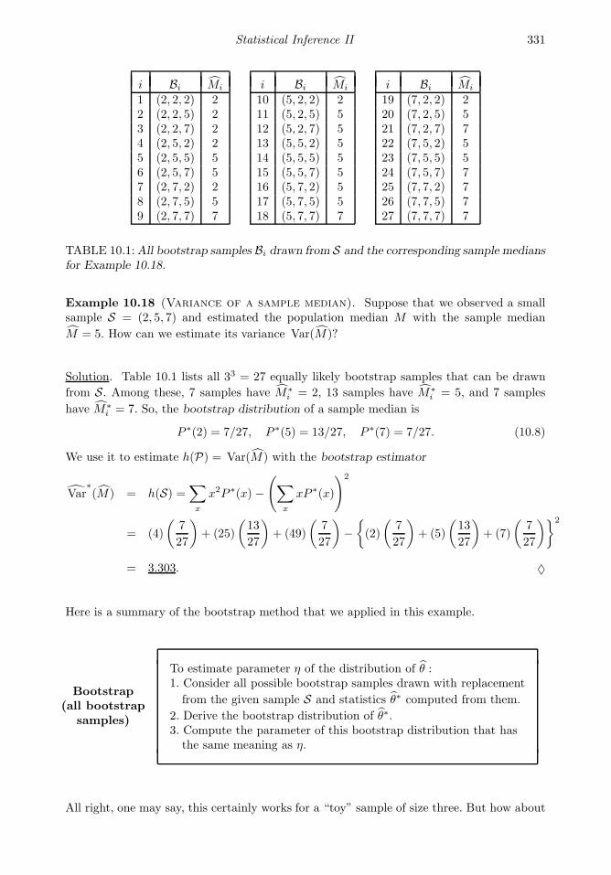
Statistical Inference II 331
i Bi Mi
1 (2, 2, 2) 22 (2, 2, 5) 23 (2, 2, 7) 24 (2, 5, 2) 25 (2, 5, 5) 56 (2, 5, 7) 57 (2, 7, 2) 28 (2, 7, 5) 59 (2, 7, 7) 7
i Bi Mi
10 (5, 2, 2) 211 (5, 2, 5) 512 (5, 2, 7) 513 (5, 5, 2) 514 (5, 5, 5) 515 (5, 5, 7) 516 (5, 7, 2) 517 (5, 7, 5) 518 (5, 7, 7) 7
i Bi Mi
19 (7, 2, 2) 220 (7, 2, 5) 521 (7, 2, 7) 722 (7, 5, 2) 523 (7, 5, 5) 524 (7, 5, 7) 725 (7, 7, 2) 726 (7, 7, 5) 727 (7, 7, 7) 7
TABLE 10.1:All bootstrap samples Bi drawn from S and the corresponding sample mediansfor Example 10.18.
Example 10.18 (Variance of a sample median). Suppose that we observed a smallsample S = (2, 5, 7) and estimated the population median M with the sample median
M = 5. How can we estimate its variance Var(M)?
Solution. Table 10.1 lists all 33 = 27 equally likely bootstrap samples that can be drawn
from S. Among these, 7 samples have M∗i = 2, 13 samples have M∗
i = 5, and 7 samples
have M∗i = 7. So, the bootstrap distribution of a sample median is
P ∗(2) = 7/27, P ∗(5) = 13/27, P ∗(7) = 7/27. (10.8)
We use it to estimate h(P) = Var(M) with the bootstrap estimator
Var∗(M) = h(S) =
∑
x
x2P ∗(x) −(∑
x
xP ∗(x)
)2
= (4)
(7
27
)+ (25)
(13
27
)+ (49)
(7
27
)−(2)
(7
27
)+ (5)
(13
27
)+ (7)
(7
27
)2
= 3.303. ♦
Here is a summary of the bootstrap method that we applied in this example.
Bootstrap(all bootstrap
samples)
To estimate parameter η of the distribution of θ :1. Consider all possible bootstrap samples drawn with replacement
from the given sample S and statistics θ∗ computed from them.
2. Derive the bootstrap distribution of θ∗.3. Compute the parameter of this bootstrap distribution that hasthe same meaning as η.
All right, one may say, this certainly works for a “toy” sample of size three. But how about
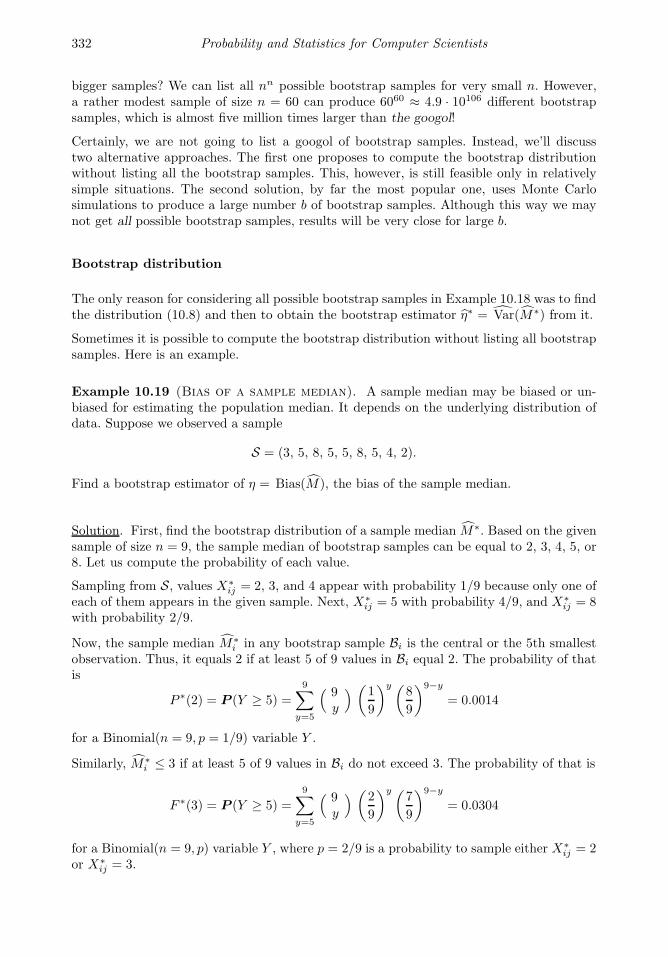
332 Probability and Statistics for Computer Scientists
bigger samples? We can list all nn possible bootstrap samples for very small n. However,a rather modest sample of size n = 60 can produce 6060 ≈ 4.9 · 10106 different bootstrapsamples, which is almost five million times larger than the googol!
Certainly, we are not going to list a googol of bootstrap samples. Instead, we’ll discusstwo alternative approaches. The first one proposes to compute the bootstrap distributionwithout listing all the bootstrap samples. This, however, is still feasible only in relativelysimple situations. The second solution, by far the most popular one, uses Monte Carlosimulations to produce a large number b of bootstrap samples. Although this way we maynot get all possible bootstrap samples, results will be very close for large b.
Bootstrap distribution
The only reason for considering all possible bootstrap samples in Example 10.18 was to findthe distribution (10.8) and then to obtain the bootstrap estimator η∗ = Var(M∗) from it.
Sometimes it is possible to compute the bootstrap distribution without listing all bootstrapsamples. Here is an example.
Example 10.19 (Bias of a sample median). A sample median may be biased or un-biased for estimating the population median. It depends on the underlying distribution ofdata. Suppose we observed a sample
S = (3, 5, 8, 5, 5, 8, 5, 4, 2).
Find a bootstrap estimator of η = Bias(M), the bias of the sample median.
Solution. First, find the bootstrap distribution of a sample median M∗. Based on the givensample of size n = 9, the sample median of bootstrap samples can be equal to 2, 3, 4, 5, or8. Let us compute the probability of each value.
Sampling from S, values X∗ij = 2, 3, and 4 appear with probability 1/9 because only one of
each of them appears in the given sample. Next, X∗ij = 5 with probability 4/9, and X∗
ij = 8with probability 2/9.
Now, the sample median M∗i in any bootstrap sample Bi is the central or the 5th smallest
observation. Thus, it equals 2 if at least 5 of 9 values in Bi equal 2. The probability of thatis
P ∗(2) = P (Y ≥ 5) =
9∑
y=5
( 9y
) (1
9
)y (8
9
)9−y
= 0.0014
for a Binomial(n = 9, p = 1/9) variable Y .
Similarly, M∗i ≤ 3 if at least 5 of 9 values in Bi do not exceed 3. The probability of that is
F ∗(3) = P (Y ≥ 5) =
9∑
y=5
( 9y
) (2
9
)y (7
9
)9−y
= 0.0304
for a Binomial(n = 9, p) variable Y , where p = 2/9 is a probability to sample either X∗ij = 2
or X∗ij = 3.
Statistical Inference II 333
Proceeding in a similar fashion, we get
F ∗(4) =9∑
y=5
(9y
) (3
9
)y (6
9
)9−y
= 0.1448,
F ∗(5) =
9∑
y=5
( 9y
) (7
9
)y (2
9
)9−y
= 0.9696, and
F ∗(8) = 1.
From this cdf, we can find the bootstrap probability mass function of M∗i ,
P ∗(2) = 0.0014, P ∗(3) = 0.0304− 0.0014 = 0.0290, P ∗(4) = 0.1448− 0.0304 = 0.1144,
P ∗(5) = 0.9696− 0.1448 = 0.8248, P ∗(8) = 1− 0.9696 = 0.0304.
From this, the bootstrap estimator of E(M) is the expected value of the bootstrap distri-bution,
E∗(M∗i ) = (2)(0.0014) + (3)(0.0290) + (4)(0.1144) + (5)(0.8248) + (8)(0.0304) = 4.9146.
Last step! The bias of M is defined as h(P) = Bias(M) = E(M)−M . We have estimated
the first term, E(M). Following the bootstrap ideas, what should we use as an estimatorof M , the second term of the bias? The answer is simple. We have agreed to estimate g(P)with g(S), so we just estimate the population median g(P) = M with the sample median
g(S) = M = 5 obtained from our original sample S.The bootstrap estimator of Bias(M) = E(M)−M (based on all possible bootstrap samples)is
η(S) = Bias(M) = E∗(M)− M = 4.9146− 5 = −0.0852 .
♦
Although the sample in Example 10.19 is still rather small, the method presented can beextended to a sample of any size. Manual computations may be rather tedious here, butone can write a suitable computer code.
10.3.2 Computer generated bootstrap samples
Modern Statistics makes use of many complicated estimates. As the earliest examples, Efronused bootstrap to explore properties of the sample correlation coefficient, the trimmedmean1, and the excess error2, but certainly, there are more complex situations. Typically,samples will be too large to list all the bootstrap samples, as in Table 10.1, and the statisticswill be too complicated to figure out their bootstrap distributions, as in Example 10.19.
This is where Monte Carlo simulations kick in. Instead of listing all possible bootstrapsamples, we use a computer to generate a large number b of them. The rest follows ourgeneral scheme on Figure 10.6, p. 330.
1Trimmed mean is a version of a sample mean, where a certain portion of the smallest and the largest
observations is dropped before computing the arithmetic average. Trimmed means are not sensitive to a few
extreme observations, and they are used if extreme outliers may be suspected in the sample.2This measures how well one can estimate the error of prediction in regression analysis. We study
regression in the next chapter.

334 Probability and Statistics for Computer Scientists
Bootstrap(generatedbootstrapsamples)
To estimate parameter η of the distribution of θ :1. Generate a large number b of bootstrap samples drawn withreplacement from the given sample S.
2. From each bootstrap sample Bi, compute statistic θ∗i the
same way as θ is computed from the original sample S.3. Estimate parameter η from the obtained values of θ∗1 , . . . , θ
∗b .
This is a classical bootstrap method of evaluating properties of parameter estimates. Doyou think it is less accurate than the one based on all the bootstrap samples? Notice thatb, the number of generated bootstrap samples, can be very large. Increasing b gives morework to your computer, but it does not require a more advanced computer code or a largeroriginal sample. And of course, as b → ∞, our estimator of η becomes just as good as ifwe had a complete list of bootstrap samples. Typically, thousands or tens of thousands ofbootstrap samples are being generated.
Matlab Demo. The following MATLAB code generates b bootstrap samples from thegiven sample X = (X1, . . . , Xn).
n = length(X); % Sample size
U = ceil(n*rand(b,n)); % A b× n matrix of random integers from 1 to nB = X(U); % A matrix of bootstrap samples.
% The i-th bootstrap sample is in the i-th row.
For example, based on a sample X = (10, 20, 30, 40, 50), we can generate the followingmatrix U of random indices which will determine the following matrix B of bootstrapsamples,
U =
1 4 5 5 13 2 3 1 53 4 5 2 31 4 1 2 32 4 3 5 11 3 1 3 54 1 5 5 42 2 1 1 23 5 4 2 31 1 5 1 3
, B =
B1
B2
B3
B4
B5
B6
B7
B8
B9
B10
=
10 40 50 50 1030 20 30 10 5030 40 50 20 3010 40 10 20 3020 40 30 50 1010 30 10 30 5040 10 50 50 4020 20 10 10 2030 50 40 20 3010 10 50 10 30
If b and n are so large that storing the entire matrices U and B requires too many computerresources, we can generate bootstrap samples in a do-loop, one at a time, and keep thestatistics θi only.
In fact, MATLAB has a special command bootstrp for generating bootstrap samples andcomputing estimates from them. For example, the code
M = bootstrp(50000,@median,S);
Statistical Inference II 335
takes the given sample S, generates b = 50, 000 bootstrap samples from it, computes mediansfrom each of them, and stores these median in a vector M . After that, we can computevarious sample statistics of M , the mean, standard deviation, etc., and use them to evaluatethe properties of a sample median.
Example 10.20 (Bias of a sample median (continued)). Based on the sample
S = (3, 5, 8, 5, 5, 8, 5, 4, 2)
from Example 10.19, we estimated the population median θ with the sample median θ = 5.Next, we investigate the properties of θ. The MATLAB code
S = [3 5 8 5 5 8 5 4 2];
b = 100000;
M = bootstrp(b,@median,S);
biasM = mean(M) - median(S);
sterrM = std(M);
prob4 = mean(M > 4);
is used to estimate the bias of θ, its standard error, and the probability of θ > 4. Vector Mcontains the bootstrap statistics θ∗1 , . . . , θ
∗b . Based on b = 100, 000 bootstrap samples, we
obtainedBias∗(θ) = M − θ = −0.0858,
s∗(θ) = s(M) = 0.7062, and
P∗(θ > 4) =
#i : θ∗i > 4
b= 0.8558.
♦
10.3.3 Bootstrap confidence intervals
In the previous chapters, we learned how to construct confidence intervals for the populationmean, proportion, variance, and also, difference of means, difference of proportions, and ratioof variances. Normal, T , χ2, and F distributions were used in these cases. These methodsrequired either a Normal distribution of the observed data or sufficiently large samples.
There are many situations, however, where these conditions will not hold, or the distributionof the test statistic is too difficult to obtain. Then the problem becomes nonparametric, andwe can use bootstrap to construct approximately (1 − α)100% confidence intervals for thepopulation parameters.
Two methods of bootstrap confidence intervals are rather popular.
Parametric method, based on the bootstrap estimation of the standard error
This method is used when we need a confidence interval for a parameter θ, and its estimatorθ has approximately Normal distribution.
In this case, we compute s∗(θ), the bootstrap estimator of the standard error σ(θ), and useit to compute the approximately (1− α)100% confidence interval for θ,
336 Probability and Statistics for Computer Scientists
Parametric bootstrapconfidence interval
θ ± zα/2s∗(θ) (10.9)
It is similar to our usual formula for the confidence interval in the case of Normal distribution(9.3), and zα/2 = q1−α/2 in it, as always, denotes the (1−α/2)-quantile from the StandardNormal distribution.
Example 10.21 (Confidence interval for a correlation coefficient). Exam-ple 8.20 on p. 231 contains the data on the number of times X the antivirus software waslaunched on 30 computers during 1 month and the number Y of detected worms,
X 30 30 30 30 30 30 30 30 30 30 30 15 15 15 10
Y 0 0 1 0 0 0 1 1 0 0 0 0 1 1 0
X 10 10 6 6 5 5 5 4 4 4 4 4 1 1 1
Y 0 2 0 4 1 2 0 2 1 0 1 0 6 3 1
Scatter plots on Figure 8.11 showed existence of a negative correlation between X and Y ,which means that in general, the number of worms reduces if the antivirus software is usedmore often.
Next, the computer manager asks for a 90% confidence interval for the correlation coefficientρ between X and Y .
The following MATLAB code can be used to solve this problem.
alpha = 0.10;
X = [30 30 30 30 30 30 30 30 30 30 30 15 15 15 10 10 10 6 6 5 5 5 4 4 4 4 4 1 1 1];
Y = [0 0 1 0 0 0 1 1 0 0 0 0 1 1 0 0 2 0 4 1 2 0 2 1 0 1 0 6 3 1];
r = corrcoef(X,Y); % correlation coefficient from the given sample
r = r(2,1); % because corrcoef returns a matrix of correlation coefficients
b = 10000; n = length(X);
U = ceil(n*rand(b,n));
BootX = X(U); BootY = Y(U); % Values X and Y of generated bootstrap samples
BootR = zeros(b,1); % Initiate the vector of bootstrap corr. coefficients
for i=1:b;
BR = corrcoef(BootX(i,:),BootY (i,:));
BootR(i) = BR(2,1);
end;
s = std(BootR); % Bootstrap estimator of the standard error of r
CI = [ r + s*norminv(alpha/2,0,1), r + s*norminv(1-alpha/2,0,1) ];
disp(CI) % Bootstrap confidence interval
As a result of this code, we get the sample correlation coefficient r = −0.4533, and also,b = 10, 000 bootstrap correlation coefficients r∗1 , . . . , r
∗b obtained from b generated bootstrap
samples.
Statistical Inference II 337
−1 −0.8 −0.6 −0.4 −0.2 0 0.2 0.40
100
200
300
400
500
600
700
800
900
1000
FIGURE 10.7 The histogram ofbootstrap correlation coefficients.
Next, we notice that for the sample of sizen = 30, r has approximately Normal distri-bution. For example, this can be confirmed bythe histogram of bootstrap correlation coeffi-cients on Figure 10.7.Applying the parametric method, we com-pute s∗(r) = 0.1028, the standard error ofr∗1 , . . . , r
∗b , and use it to construct the 90% con-
fidence interval
r ± zα/2s∗(r) = −0.4533± (1.645)(0.1028)
= [-0.2841, -0.6224]
♦
Nonparametric method, based on the bootstrap quantiles
Equation 10.9 simply estimates two quantiles qα/2 and q1−α/2 of the distribution of statistic
θ, so that
Pqα/2 ≤ θ ≤ q1−α/2
= 1− α. (10.10)
Since θ estimates parameter θ, this becomes an approximately (1 − α)100% confidenceinterval for θ.
25 30 35 40 45 50 55 60 65 700
1000
2000
3000
4000
5000
6000
7000
8000
FIGURE 10.8 The histogram ofbootstrap medians.
This method fails if the distribution of θis not Normal. The coverage probability in(10.10) may be rather different from (1−α)in this case. However, the idea to constructa confidence interval based on the quantilesof θ is still valid.
The quantiles qα/2 and q1−α/2 of the distri-
bution of θ will then be estimated from thebootstrap samples. To do this, we generateb bootstrap samples, compute statistic θ∗
for each of them, and determine the sam-ple quantiles q∗α/2 and q∗1−α/2 from them.These quantiles become the end points ofthe (1− α)100% confidence interval for θ.
Nonparametric bootstrapconfidence intervalfor parameter θ
[q∗α/2, q∗1−α/2
],
where q∗α/2 and q∗1−α/2 are quantiles
of the distribution of θ estimated frombootstrap samples
(10.11)
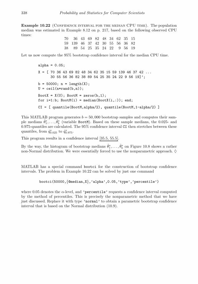
338 Probability and Statistics for Computer Scientists
Example 10.22 (Confidence interval for the median CPU time). The populationmedian was estimated in Example 8.12 on p. 217, based on the following observed CPUtimes:
70 36 43 69 82 48 34 62 35 1559 139 46 37 42 30 55 56 36 8238 89 54 25 35 24 22 9 56 19
Let us now compute the 95% bootstrap confidence interval for the median CPU time.
alpha = 0.05;
X = [ 70 36 43 69 82 48 34 62 35 15 59 139 46 37 42 ...
30 55 56 36 82 38 89 54 25 35 24 22 9 56 19]’;
b = 50000; n = length(X);
U = ceil(n*rand(b,n));
BootX = X(U); BootM = zeros(b,1);
for i=1:b; BootM(i) = median(BootX(i,:)); end;
CI = [ quantile(BootM,alpha/2), quantile(BootM,1-alpha/2) ]
This MATLAB program generates b = 50, 000 bootstrap samples and computes their sam-ple medians θ∗1 , . . . , θ
∗b (variable BootM). Based on these sample medians, the 0.025- and
0.975-quantiles are calculated. The 95% confidence interval CI then stretches between thesequantiles, from q∗0.025 to q∗0.975.
This program results in a confidence interval [35.5, 55.5].
By the way, the histogram of bootstrap medians θ∗1 , . . . , θ∗b on Figure 10.8 shows a rather
non-Normal distribution. We were essentially forced to use the nonparametric approach. ♦
MATLAB has a special command bootci for the construction of bootstrap confidenceintervals. The problem in Example 10.22 can be solved by just one command
bootci(50000,@median,X,’alpha’,0.05,’type’,’percentile’)
where 0.05 denotes the α-level, and ’percentile’ requests a confidence interval computedby the method of percentiles. This is precisely the nonparametric method that we havejust discussed. Replace it with type ’normal’ to obtain a parametric bootstrap confidenceinterval that is based on the Normal distribution (10.9).
Statistical Inference II 339
10.4 Bayesian inference
Interesting results and many new statistical methods can be obtained when we take a ratherdifferent look at statistical problems.
The difference is in our treatment of uncertainty.
So far, random samples were the only source of uncertainty in all the discussed statisticalproblems. The only distributions, expectations, and variances considered so far were dis-tributions, expectations, and variances of data and various statistics computed from data.Population parameters were considered fixed. Statistical procedures were based on the dis-tribution of data given these parameters,
f(x | θ) = f(X1, . . . , Xn | θ).
This is the frequentist approach. According to it, all probabilities refer to random sam-ples of data and possible long-run frequencies, and so do such concepts as unbiasedness,consistency, confidence level, and significance level:
– an estimator θ is unbiased if in a long run of random samples, it averages to theparameter θ;
– a test has significance level α if in a long run of random samples, (100α)% of timesthe true hypothesis is rejected;
– an interval has confidence level (1−α) if in a long run of random samples, (1−α)100%of obtained confidence intervals contain the parameter, as shown in Figure 9.2, p. 248;
– and so on.
However, there is another approach: the Bayesian approach. According to it, uncertaintyis also attributed to the unknown parameter θ. Some values of θ are more likely than others.Then, as long as we talk about the likelihood, we can define a whole distribution of valuesof θ. Let us call it a prior distribution. It reflects our ideas, beliefs, and past experiencesabout the parameter before we collect and use the data.
Example 10.23 (Salaries). What do you think is the average starting annual salary ofa Computer Science graduate? Is it $20,000 per year? Unlikely, that’s too low. Perhaps,$200,000 per year? No, that’s too high for a fresh graduate. Between $40,000 and $70,000sounds like a reasonable range. We can certainly collect data on 100 recent graduates,compute their average salary, and use it as an estimate, but before that, we already haveour beliefs on what the mean salary may be. We can express it as some distribution withthe most likely range between $40,000 and $70,000 (Figure 10.9). ♦
Collected data may force us to change our initial idea about the unknown parameter.Probabilities of different values of θ may change. Then we’ll have a posterior distributionof θ.
One benefit of this approach is that we no longer have to explain our results in terms of a“long run.” Often we collect just one sample for our analysis and don’t experience any longruns of samples. Instead, with the Bayesian approach, we can state the result in terms ofthe posterior distribution of θ. For example, we can clearly state the posterior probabilityfor a parameter to belong to the obtained confidence interval, or the posterior probabilitythat the hypothesis is true.
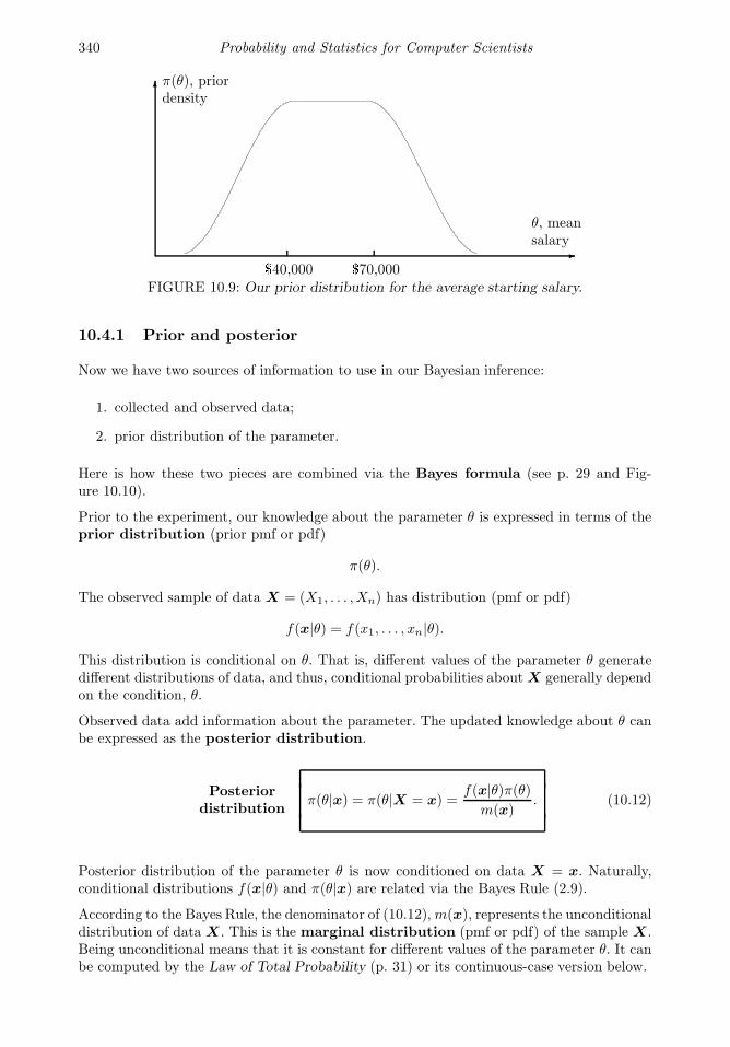
340 Probability and Statistics for Computer Scientists
π(θ), priordensity
θ, meansalary$40,000 $70,000
FIGURE 10.9: Our prior distribution for the average starting salary.
10.4.1 Prior and posterior
Now we have two sources of information to use in our Bayesian inference:
1. collected and observed data;
2. prior distribution of the parameter.
Here is how these two pieces are combined via the Bayes formula (see p. 29 and Fig-ure 10.10).
Prior to the experiment, our knowledge about the parameter θ is expressed in terms of theprior distribution (prior pmf or pdf)
π(θ).
The observed sample of data X = (X1, . . . , Xn) has distribution (pmf or pdf)
f(x|θ) = f(x1, . . . , xn|θ).
This distribution is conditional on θ. That is, different values of the parameter θ generatedifferent distributions of data, and thus, conditional probabilities about X generally dependon the condition, θ.
Observed data add information about the parameter. The updated knowledge about θ canbe expressed as the posterior distribution.
Posteriordistribution
π(θ|x) = π(θ|X = x) =f(x|θ)π(θ)
m(x). (10.12)
Posterior distribution of the parameter θ is now conditioned on data X = x. Naturally,conditional distributions f(x|θ) and π(θ|x) are related via the Bayes Rule (2.9).
According to the Bayes Rule, the denominator of (10.12),m(x), represents the unconditionaldistribution of data X. This is the marginal distribution (pmf or pdf) of the sample X.Being unconditional means that it is constant for different values of the parameter θ. It canbe computed by the Law of Total Probability (p. 31) or its continuous-case version below.
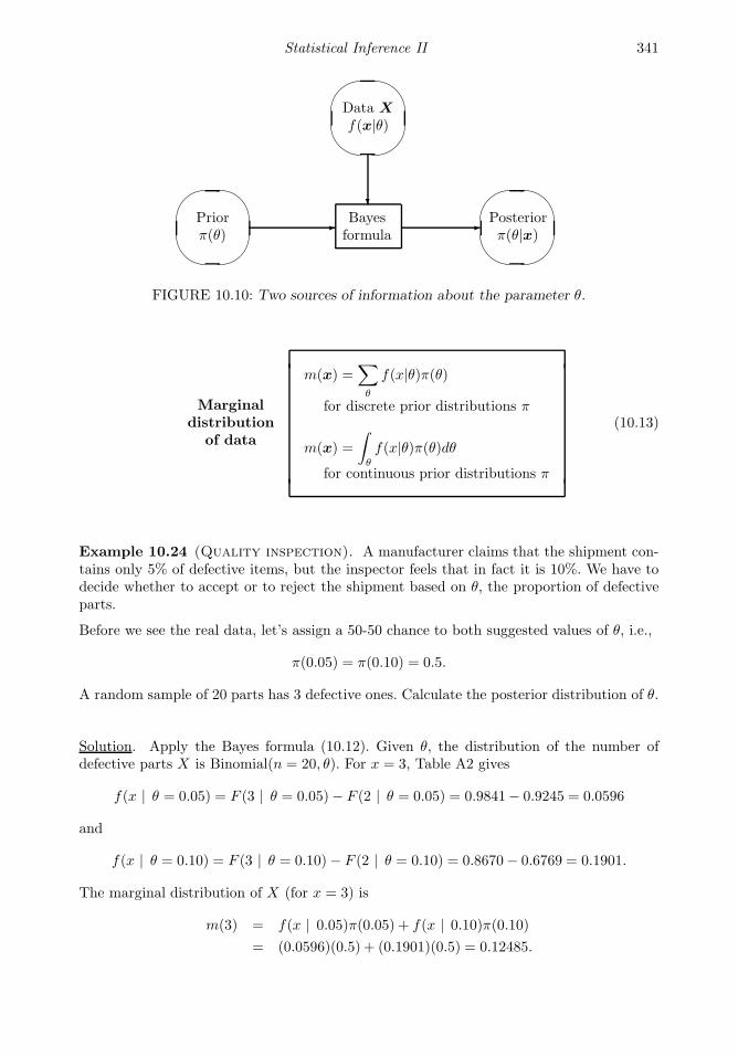
Statistical Inference II 341
Priorπ(θ)
Bayesformula
Data X
f(x|θ)
Posteriorπ(θ|x)
FIGURE 10.10: Two sources of information about the parameter θ.
Marginaldistribution
of data
m(x) =∑
θ
f(x|θ)π(θ)
for discrete prior distributions π
m(x) =
∫
θ
f(x|θ)π(θ)dθfor continuous prior distributions π
(10.13)
Example 10.24 (Quality inspection). A manufacturer claims that the shipment con-tains only 5% of defective items, but the inspector feels that in fact it is 10%. We have todecide whether to accept or to reject the shipment based on θ, the proportion of defectiveparts.
Before we see the real data, let’s assign a 50-50 chance to both suggested values of θ, i.e.,
π(0.05) = π(0.10) = 0.5.
A random sample of 20 parts has 3 defective ones. Calculate the posterior distribution of θ.
Solution. Apply the Bayes formula (10.12). Given θ, the distribution of the number ofdefective parts X is Binomial(n = 20, θ). For x = 3, Table A2 gives
f(x | θ = 0.05) = F (3 | θ = 0.05)− F (2 | θ = 0.05) = 0.9841− 0.9245 = 0.0596
and
f(x | θ = 0.10) = F (3 | θ = 0.10)− F (2 | θ = 0.10) = 0.8670− 0.6769 = 0.1901.
The marginal distribution of X (for x = 3) is
m(3) = f(x | 0.05)π(0.05) + f(x | 0.10)π(0.10)= (0.0596)(0.5) + (0.1901)(0.5) = 0.12485.
342 Probability and Statistics for Computer Scientists
Posterior probabilities of θ = 0.05 and θ = 0.10 are now computed as
π(0.05 | X = 3) =f(x | 0.05)π(0.05)
m(3)=
(0.0596)(0.5)
0.1248= 0.2387;
π(0.10 | X = 3) =f(x | 0.10)π(0.10)
m(3)=
(0.1901)(0.5)
0.1248= 0.7613.
Conclusion. In the beginning, we had no preference between the two suggested values of θ.Then we observed a rather high proportion of defective parts, 3/20=15%. Taking this intoaccount, θ = 0.10 is now about three times as likely than θ = 0.05. ♦
Notation π(θ) = prior distribution
π(θ | x) = posterior distribution
f(x|θ) = distribution of data (model)
m(x) = marginal distribution of data
X = (X1, . . . , Xn), sample of data
x = (x1, . . . , xn), observed values of X1, . . . , Xn.
Conjugate distribution families
A suitably chosen prior distribution of θ may lead to a very tractable form of the posterior.
DEFINITION 10.4
A family of prior distributions π is conjugate to the model f(x|θ) if theposterior distribution belongs to the same family.
Three classical examples of conjugate families are given below.
Gamma family is conjugate to the Poisson model
Let (X1, . . . , Xn) be a sample from Poisson(θ) distribution with a Gamma(α, λ) prior dis-tribution of θ.
Then
f(x|θ) =n∏
i=1
f(xi|θ) =n∏
i=1
e−θθxi
xi!∼ e−nθθ
∑xi . (10.14)
Remark about dropping constant coefficients. In the end of (10.14), we dropped (xi!) andwrote that the result is “proportional” (∼) to e−nθθ
∑xi . Dropping terms that don’t contain
θ often simplifies the computation. The form of the posterior distribution can be obtainedwithout the constant term, and if needed, we can eventually evaluate the normalizing con-stant in the end, making π(θ|x) a fine distribution with the total probability 1, for example,as we did in Example 4.1 on p. 77. In particular, the marginal distribution m(x) can be
Statistical Inference II 343
dropped because it is θ-free. But keep in mind that in this case we obtain the posteriordistribution “up to a constant coefficient.”
The Gamma prior distribution of θ has density
π(θ) ∼ θα−1e−λθ.
As a function of θ, this prior density has the same form as the model f(x|θ) – a power of θmultiplied by an exponential function. This is the general idea behind conjugate families.
Then, the posterior distribution of θ given X = x is
π(θ|x) ∼ f(x|θ)π(θ)∼
(e−nθθ
∑xi
) (θα−1e−λθ
)
∼ θα+∑
xi−1e−(λ+n)θ.
Comparing with the general form of a Gamma density (say, (4.7) on p. 85), we see thatπ(θ|x) is the Gamma distribution with new parameters,
αx = α+
n∑
i=1
xi and λx = λ+ n.
We can conclude that:
1. Gamma family of prior distributions is conjugate to Poisson models.
2. Having observed a Poisson sample X = x, we update the Gamma(α, λ) prior distri-bution of θ to the Gamma(α+
∑xi, λ+ n) posterior.
Gamma distribution family is rather rich; it has two parameters. There is often a goodchance to find a member of this large family that suitably reflects our knowledge about θ.
Example 10.25 (Network blackouts). The number of network blackouts each weekhas Poisson(θ) distribution. The weekly rate of blackouts θ is not known exactly, but accord-ing to the past experience with similar networks, it averages 4 blackouts with a standarddeviation of 2.
There exists a Gamma distribution with the given mean µ = α/λ = 4 and standard devia-tion σ =
√α/λ = 2. Its parameters α and λ can be obtained by solving the system,
α/λ = 4√α/λ = 2
⇒
α = (4/2)2 = 4λ = 22/4 = 1
Hence, we can assume the Gamma(α = 4, λ = 1) prior distribution θ. It is convenient tohave a conjugate prior because the posterior will then belong to the Gamma family too.
Suppose there were X1 = 2 blackouts this week. Given that, the posterior distribution of θis Gamma with parameters
αx = α+ 2 = 6, λx = λ+ 1 = 2.
If no blackouts occur during the next week, the updated posterior parameters become
αx = α+ 2 + 0 = 6, λx = λ+ 2 = 3.
This posterior distribution has the average weekly rate of 6/3 = 2 blackouts per week. Twoweeks with very few blackouts reduced our estimate of the average rate from 4 to 2. ♦
344 Probability and Statistics for Computer Scientists
Beta family is conjugate to the Binomial model
A sample from Binomial(k, θ) distribution (assume k is known) has the probability massfunction
f(x | θ) =n∏
i=1
( kxi
)θxi(1− θ)k−xi ∼ θ
∑xi(1− θ)nk−
∑xi .
Density of Beta(α, β) prior distribution has the same form, as a function of θ,
π(θ) ∼ θα−1(1− θ)β−1 for 0 < θ < 1
(see Section 12.1.2 in the Appendix). Then, the posterior density of θ is
π(θ | x) ∼ f(x | θ)π(θ) ∼ θα+∑
ni=1
xi−1(1− θ)β+nk−∑
ni=1
xi−1,
and we recognize the Beta density with new parameters
αx = α+
n∑
i=1
xi and βx = β + nk −n∑
i=1
xi.
Hence,
1. Beta family of prior distributions is conjugate to the Binomial model.
2. Posterior parameters are αx = α+∑
xi and βx = β + nk −∑xi.
Normal family is conjugate to the Normal model
Consider now a sample from Normal distribution with an unknown mean θ and a knownvariance σ2:
f(x | θ) =
n∏
i=1
1√2π
exp
− (xi − θ)2
2σ2
∼ exp
−
n∑
i=1
(xi − θ)2
2σ2
∼ exp
θ
∑xi
σ2− θ2
n
2σ2
= exp
(θX − θ2
2
)n
σ2
.
If the prior distribution of θ is also Normal, with prior mean µ and prior variance τ2, then
π(θ) ∼ exp
− (θ − µ)2
2τ2
∼ exp
(θµ− θ2
2
)1
τ2
,
and again, it has a similar form as f(x|θ).The posterior density of θ equals
π(θ | x) ∼ f(x | θ)π(θ) ∼ exp
θ
(nX
σ2+
µ
τ2
)− θ2
2
(n
σ2+
1
τ2
)
∼ exp
− (θ − µx)
2
2τ2x
,
where
µx =nX/σ2 + µ/τ2
n/σ2 + 1/τ2and τ2x =
1
n/σ2 + 1/τ2. (10.15)
This posterior distribution is certainly Normal with parameters µx and τx.
We can conclude that:
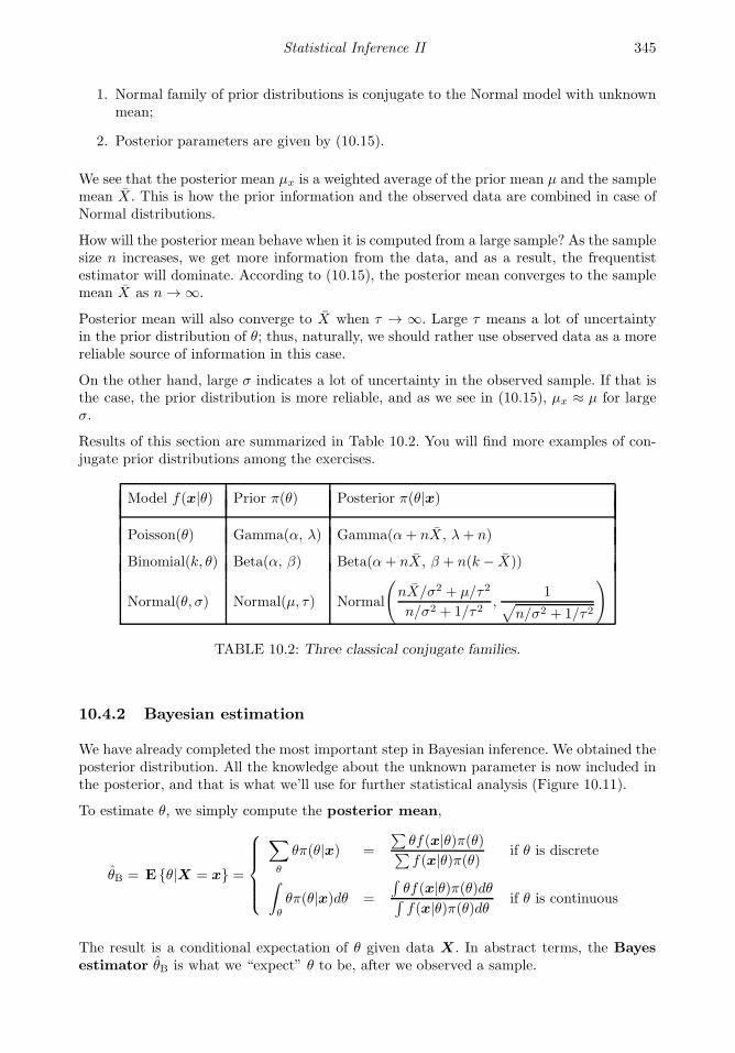
Statistical Inference II 345
1. Normal family of prior distributions is conjugate to the Normal model with unknownmean;
2. Posterior parameters are given by (10.15).
We see that the posterior mean µx is a weighted average of the prior mean µ and the samplemean X. This is how the prior information and the observed data are combined in case ofNormal distributions.
How will the posterior mean behave when it is computed from a large sample? As the samplesize n increases, we get more information from the data, and as a result, the frequentistestimator will dominate. According to (10.15), the posterior mean converges to the samplemean X as n → ∞.
Posterior mean will also converge to X when τ → ∞. Large τ means a lot of uncertaintyin the prior distribution of θ; thus, naturally, we should rather use observed data as a morereliable source of information in this case.
On the other hand, large σ indicates a lot of uncertainty in the observed sample. If that isthe case, the prior distribution is more reliable, and as we see in (10.15), µx ≈ µ for largeσ.
Results of this section are summarized in Table 10.2. You will find more examples of con-jugate prior distributions among the exercises.
Model f(x|θ) Prior π(θ) Posterior π(θ|x)
Poisson(θ) Gamma(α, λ) Gamma(α+ nX, λ+ n)
Binomial(k, θ) Beta(α, β) Beta(α+ nX, β + n(k − X))
Normal(θ, σ) Normal(µ, τ) Normal
(nX/σ2 + µ/τ2
n/σ2 + 1/τ2,
1√n/σ2 + 1/τ2
)
TABLE 10.2: Three classical conjugate families.
10.4.2 Bayesian estimation
We have already completed the most important step in Bayesian inference. We obtained theposterior distribution. All the knowledge about the unknown parameter is now included inthe posterior, and that is what we’ll use for further statistical analysis (Figure 10.11).
To estimate θ, we simply compute the posterior mean,
θB = E θ|X = x =
∑
θ
θπ(θ|x) =
∑θf(x|θ)π(θ)∑f(x|θ)π(θ) if θ is discrete
∫
θ
θπ(θ|x)dθ =
∫θf(x|θ)π(θ)dθ∫f(x|θ)π(θ)dθ if θ is continuous
The result is a conditional expectation of θ given data X. In abstract terms, the Bayesestimator θB is what we “expect” θ to be, after we observed a sample.

346 Probability and Statistics for Computer Scientists
Priorπ(θ)
Bayesformula
Data X
f(x|θ)
Posteriorπ(θ|x)
Bayesianinference:
EstimationTesting
Other decisions
FIGURE 10.11: Posterior distribution is the basis for Bayesian inference.
How accurate is this estimator? Among all estimators, θB = E θ|x has the lowest squared-error posterior risk
ρ(θ) = E(θ − θ)2 | X = x
.
For the Bayes estimator θB = E θ | x, posterior risk equals posterior variance,
ρ(θ) = E(E θ|x − θ)2 | x
= E
(θ − E θ|x)2 | x
= Var θ|x ,
which measures variability of θ around θB, according to the posterior distribution of θ.
Example 10.26 (Normal case). The Bayes estimator of the mean θ of Normal(θ, σ)distribution with a Normal(µ, τ) prior is
θB = µx =nX/σ2 + µ/τ2
n/σ2 + 1/τ2,
and its posterior risk is
ρ(θB) = τ2x =1
n/σ2 + 1/τ2
(Table 10.2). As we expect, this risk decreases to 0 as the sample size grows to infinity. ♦
Example 10.27 (Network blackouts, continued). After two weeks of data, theweekly rate of network blackouts, according to Example 10.25 on p. 343, has Gamma pos-terior distribution with parameters αx = 6 and λx = 3.
The Bayes estimator of the weekly rate θ is
θB = E θ|x =αx
λx= 2 (blackouts per week)
with a posterior risk
ρ(θB) = Var θ|x =αx
λ2x
=2
3.
♦

Statistical Inference II 347
Although conjugate priors simplify our statistics, Bayesian inference can certainly be donefor other priors too.
Example 10.28 (Quality inspection, continued). In Example 10.24 on p. 341, wecomputed posterior distribution of the proportion of defective parts θ. This was a discretedistribution,
π(0.05 | x) = 0.2387; π(0.10 | x) = 0.7613.
Now, the Bayes estimator of θ is
θB =∑
θ
θπ(θ | x) = (0.05)(0.2387) + (0.10)(0.7613) = 0.0881.
It does not agree with the manufacturer (who claims θ = 0.05) or with the quality inspector(who feels that θ = 0.10) but its value is much closer to the inspector’s estimate.
The posterior risk of θB is
Var θ|x = Eθ2|x
− E2 θ|x
= (0.05)2(0.2387) + (0.10)2(0.7613)− (0.0881)2 = 0.0004,
which means a rather low posterior standard deviation of 0.02. ♦
10.4.3 Bayesian credible sets
Confidence intervals have a totally different meaning in Bayesian analysis. Having a posteriordistribution of θ, we no longer have to explain the confidence level (1 − α) in terms of along run of samples. Instead, we can give an interval [a, b] or a set C that has a posteriorprobability (1−α) and state that the parameter θ belongs to this set with probability (1−α).Such a statement was impossible before we considered prior and posterior distributions. Thisset is called a (1− α)100% credible set.
DEFINITION 10.5
Set C is a (1 − α)100% credible set for the parameter θ if the posteriorprobability for θ to belong to C equals (1− α). That is,
P θ ∈ C | X = x =
∫
C
π(θ|x)dθ = 1− α.
Such a set is not unique. Recall that for two-sided, left-tail, and right-tail hypothesis testing,we took different portions of the area under the Normal curve, all equal (1− α).
Minimizing the length of set C among all (1−α)100% credible sets, we just have to includeall the points θ with a high posterior density π(θ|x),
C = θ : π(θ|x) ≥ c
(see Figure 10.12). Such a set is called the highest posterior density credible set, orjust the HPD set.

348 Probability and Statistics for Computer Scientists
θ
c
π(θ|x)
︸ ︷︷ ︸C
FIGURE 10.12: The (1− α)100% highest posterior density credible set.
θ meansalary
π(θ)prior density
$40,000 µ
1.96τ 1.96τ $70,000FIGURE 10.13: Normal prior distribution and the 95% HPD credible set for the meanstarting salary of Computer Science graduates (Example 10.29).
For the Normal(µx, τx) posterior distribution of θ, the (1 − α)100% HPD set is
µx ± zα/2τx = [µx − zα/2τx, µx + zα/2τx].
Example 10.29 (Salaries, continued). In Example 10.23 on p. 339, we “decided” thatthe most likely range for the mean starting salary θ of Computer Science graduates isbetween $40,000 and $70,000. Expressing this in a form of a prior distribution, we letthe prior mean be µ = (40, 000 + 70, 000)/2 = 55, 000. Further, if we feel that the range[40, 000; 70, 000] is 95% likely, and we accept a Normal prior distribution for θ, then thisrange should be equal
[40, 000; 70, 000] = µ± z0.025/2τ = µ± 1.96τ,
where τ is the prior standard deviation (Figure 10.13). We can now evaluate the priorstandard deviation parameter τ from this information,
τ =70, 000− 40, 000
2(1.96)= 7, 653.
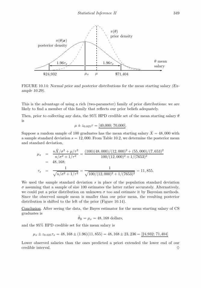
Statistical Inference II 349
θ meansalary
π(θ)prior density
π(θ|x)posterior density
$24,932 1.96τx 1.96τx
µx $71,404µ
FIGURE 10.14: Normal prior and posterior distributions for the mean starting salary (Ex-ample 10.29).
This is the advantage of using a rich (two-parameter) family of prior distributions: we arelikely to find a member of this family that reflects our prior beliefs adequately.
Then, prior to collecting any data, the 95% HPD credible set of the mean starting salary θis
µ± z0.025τ = [40,000; 70,000].
Suppose a random sample of 100 graduates has the mean starting salary X = 48, 000 witha sample standard deviation s = 12, 000. From Table 10.2, we determine the posterior meanand standard deviation,
µx =nX/σ2 + µ/τ2
n/σ2 + 1/τ2=
(100)(48, 000)/(12, 000)2 + (55, 000)/(7, 653)2
100/(12, 000)2 + 1/(7653)2
= 48, 168;
τx =1√
n/σ2 + 1/τ2=
1√100/(12, 000)2 + 1/(7653)2
= 11, 855.
We used the sample standard deviation s in place of the population standard deviationσ assuming that a sample of size 100 estimates the latter rather accurately. Alternatively,we could put a prior distribution on unknown σ too and estimate it by Bayesian methods.Since the observed sample mean is smaller than our prior mean, the resulting posteriordistribution is shifted to the left of the prior (Figure 10.14).
Conclusion. After seeing the data, the Bayes estimator for the mean starting salary of CSgraduates is
θB = µx = 48, 168 dollars,
and the 95% HPD credible set for this mean salary is
µx ± z0.025τx = 48, 168± (1.96)(11, 855) = 48, 168± 23, 236 = [24,932; 71,404]
Lower observed salaries than the ones predicted a priori extended the lower end of ourcredible interval. ♦
350 Probability and Statistics for Computer Scientists
Example 10.30 (Telephone company). A new telephone company predicts to handlean average of 1000 calls per hour. During 10 randomly selected hours of operation, it handled7265 calls.
How should it update the initial estimate of the frequency of telephone calls? Constructa 95% HPD credible set. Telephone calls are placed according to a Poisson process. Thehourly rate of calls has an Exponential prior distribution.
Solution. We need a Bayesian estimator of the frequency θ of telephone calls. The numberof calls during 1 hour has Poisson(θ) distribution, where θ is unknown, with
Exponential(λ) = Gamma(1, λ)
prior distribution that has an expectation of
E(θ) =1
λ= 1000 calls.
Hence, λ = 0.001. We observe a sample of size n = 10, totaling
n∑
i=1
Xi = nX = 7265 calls.
As we know (see Table 10.2 on p. 345), the posterior distribution in this case isGamma(αx, λx) with
αx = α+ nX = 7266,λx = λ+ n = 10.001.
This distribution has meanµx = αx/λx = 726.53
and standard deviationτx = αx/λ
2x = 72.65.
The Bayes estimator of θ is
E(θ|X) = µx = 726.53 calls per hour.
It almost coincides with the sample mean X showing the sample was informative enoughto dominate over the prior information.
For the credible set, we notice that αx is sufficiently large to make the Gamma posteriordistribution approximately equal the Normal distribution with parameters µx and τx. The95% HPD credible set is then
µx ± z0.05/2τx = 726.53± (1.96)(72.65) = 726.53± 142.39 = [584.14, 868.92]
♦

Statistical Inference II 351
10.4.4 Bayesian hypothesis testing
Bayesian hypothesis testing is very easy to interpret. We can compute prior and posteriorprobabilities for the hypothesis H0 and alternative HA to be true and decide from therewhich one to accept or to reject.
Computing such probabilities was not possible without prior and posterior distributions ofthe parameter θ. In non-Bayesian statistics, θ was not random, thus H0 and HA were eithertrue (with probability 1) or false (with probability 1).
For Bayesian tests, in order for H0 to have a meaningful, non-zero probability, it oftenrepresents a set of parameter values instead of just one θ0, and we are testing
H0 : θ ∈ Θ0 vs HA : θ ∈ Θ1.
This actually makes sense because exact equality θ = θ0 is unlikely to hold anyway, and inpractice it is understood as θ ≈ θ0.
Comparing posterior probabilities of H0 and HA,
P Θ0 | X = x and P Θ1 | X = x ,
we decide whether P Θ1 | X = x is large enough to present significant evidence and toreject the null hypothesis. One can again compare it with (1−α) such as 0.90, 0.95, 0.99, orstate the result in terms of likelihood, “the null hypothesis is this much likely to be true.”
Example 10.31 (Telephone company, continued). Let us test whether the telephonecompany in Example 10.30 can actually face a call rate of 1000 calls or more per hour. Weare testing
H0 : θ ≥ 1000 vs HA : θ < 1000,
where θ is the hourly rate of telephone calls.
According to the Gamma(αx, λx) posterior distribution of θ and its Normal (µx =726.53, τx = 72.65) approximation,
P H0 | X = x = P
θ − µx
τx≥ 1000− µx
τx
= 1− Φ(3.76) = 0.0001.
By the complement rule, P HA | X = x = 0.9999, and this presents sufficient evidenceagainst H0.
We conclude that it’s extremely unlikely for this company to face a frequency of 1000+ callsper hour. ♦
Loss and risk
Often one can anticipate the consequences of Type I and Type II errors in hypothesis testingand assign a loss L(θ, a) associated with each possible error. Here θ is the parameter, anda is our action, the decision on whether we accept or reject the null hypothesis.
Each decision then has its posterior risk ρ(a), defined as the expected loss computed underthe posterior distribution. The action with the lower posterior risk is our Bayes action.
352 Probability and Statistics for Computer Scientists
Suppose that the Type I error causes the loss
w0 = Loss(Type I error) = L(Θ0, reject H0),
and the Type II error causes the loss
w1 = Loss(Type II error) = L(Θ1, accept H0).
Posterior risks of each possible action are then computed as
ρ(reject H0) = w0π(Θ0 | x),ρ(accept H0) = w1π(Θ1 | x).
Now we can determine the Bayes action. If w0π(Θ0 | x) ≤ w1π(Θ1 | x), the Bayes actionis to accept H0. If w0π(Θ0 | x) ≥ w1π(Θ1 | x), the Bayes action is to reject H0.
Example 10.32 (Quality inspection, continued). In Example 10.24 on p. 341, weare testing
H0 : θ = 0.05 vs HA : θ = 0.10
for the proportion θ of defective parts. Suppose that the Type I error is three times as costlyhere as the Type II error. What is the Bayes action in this case?
Example 10.28 gives posterior probabilities
π(Θ0 | X = x) = 0.2387 and π(Θ1 | X = x) = 0.7613.
Since w0 = 3w1, the posterior risks are
ρ(reject H0) = w0π(Θ0 | x) = 3w1(0.2387) = 0.7161w1,
ρ(accept H0) = w1π(Θ1 | x) = 0.7613w1.
Thus, rejecting H0 has a lower posterior risk, and therefore, it is the Bayes action. RejectH0. ♦
Summary and conclusions
A number of popular methods of Statistical Inference are presented in this chapter.
Chi-square tests represent a general technique based on counts. Comparing the observedcounts with the counts expected under the null hypothesis through the chi-square statistic,one can test for the goodness of fit and for the independence of two factors. Contingencytables are widely used for the detection of significant relations between categorical variables.
Nonparametric statistical methods are not based on any particular distribution ofdata. So, they are often used when the distribution is unknown or complicated. They arealso very handy when the sample may contain some outliers, and even when the data arenot numerical.

Exercises 353
A sign test and Wilcoxon signed rank test for one sample and a two-sample Mann-Whitney-Wilcoxon rank sum test are introduced in this chapter for testing and comparing distribu-tions and their medians. Combinatorics helps to find the exact null distribution of eachconsidered test statistic. For large samples, this distribution is approximately Normal.
Bootstrap is a popular modern resampling technique that is widely used nowadays forstudying properties and evaluating performance of various statistics. A simple idea be-hind the bootstrap allows us to analyze complicated statistics using only the power of ourcomputer. This chapter showed the most basic applications of bootstrap to the estimationof standard errors and biases of parameter estimates and construction of parametric andnonparametric confidence intervals.
Bayesian inference combines the information contained in the data and in the priordistribution of the unknown parameter. It is based on the posterior distribution, which isthe conditional distribution of the unknown parameter, given the data.
The most commonly used Bayesian parameter estimator is the posterior mean. It minimizesthe squared-error posterior risk among all the estimates.
Bayesian (1−α)100% credible sets also contain the parameter θ with probability (1−α), butthis time the probability refers to the distribution of θ. Explaining a (1 − α)100% credibleset, we can say that given the observed data, θ belongs to the obtained set with probability(1− α).
For Bayesian hypothesis testing, we compute posterior probabilities of H0 and HA anddecide if the former is sufficiently smaller than the latter to suggest rejection of H0. We canalso take a Bayesian action that minimizes the posterior risk.
Exercises
10.1. Does the number of unsolicited (spam) emails follow a Poisson distribution? Here is therecord of the number of spam emails received during 60 consecutive days.
12 6 4 0 13 5 1 3 10 1 29 12 4 4 222 2 27 7 27 9 34 10 10 2 28 7 0 9 4
32 4 5 9 1 13 10 20 5 5 0 6 9 20 2822 10 8 11 15 1 14 0 9 9 1 9 0 7 13
Choose suitable bins and conduct a goodness-of-fit test at the 1% level of significance.
10.2. Applying the theory of M/M/1 queuing systems, we assume that the service times followExponential distribution. The following service times, in minutes, have been observed dur-ing 24 hours of operation:
10.5 1.2 6.3 3.7 0.9 7.1 3.3 4.0 1.7 11.6 5.1 2.8 4.8 2.0 8.0 4.63.1 10.2 5.9 12.6 4.5 8.8 7.2 7.5 4.3 8.0 0.2 4.4 3.5 9.6 5.5 0.32.7 4.9 6.8 8.6 0.8 2.2 2.1 0.5 2.3 2.9 11.7 0.6 6.9 11.4 3.8 3.22.6 1.9 1.0 4.1 2.4 13.6 15.2 6.4 5.3 5.4 1.4 5.0 3.9 1.8 4.7 0.7
Is the assumption of Exponentiality supported by these data?

354 Probability and Statistics for Computer Scientists
10.3. The following sample is collected to verify the accuracy of a new random number generator(it is already ordered for your convenience).
-2.434 -2.336 -2.192 -2.010 -1.967 -1.707 -1.678 -1.563 -1.476 -1.388-1.331 -1.269 -1.229 -1.227 -1.174 -1.136 -1.127 -1.124 -1.120 -1.073-1.052 -1.051 -1.032 -0.938 -0.884 -0.847 -0.846 -0.716 -0.644 -0.625-0.588 -0.584 -0.496 -0.489 -0.473 -0.453 -0.427 -0.395 -0.386 -0.386-0.373 -0.344 -0.280 -0.246 -0.239 -0.211 -0.188 -0.155 -0.149 -0.112-0.103 -0.101 -0.033 -0.011 0.033 0.110 0.139 0.143 0.218 0.2180.251 0.261 0.308 0.343 0.357 0.463 0.477 0.482 0.489 0.5450.590 0.638 0.652 0.656 0.673 0.772 0.775 0.776 0.787 0.9690.978 1.005 1.013 1.039 1.072 1.168 1.185 1.263 1.269 1.2971.360 1.370 1.681 1.721 1.735 1.779 1.792 1.881 1.903 2.009
(a) Apply the χ2 goodness-of-fit test to check if this sample comes from the StandardNormal distribution.
(b) Test if this sample comes from the Uniform(-3,3) distribution.
(c) Is it theoretically possible to accept both null hypotheses in (a) and (b) although theyare contradicting to each other? Why does it make sense?
10.4. In Example 10.3 on p. 309, we tested whether the number of concurrent users is approx-imately Normal. How does the result of the chi-square test depend on our choice of bins?For the same data, test the assumption of a Normal distribution using a different set of binsB1, . . . , BN .
10.5. Show that the sample size is too small in Example 10.9 on p. 316 to conduct a χ2 goodness-of-fit test of Normal distribution that involves estimation of its both parameters.
10.6. Two computer makers, A and B, compete for a certain market. Their users rank thequality of computers on a 4-point scale as “Not satisfied”, “Satisfied”, “Good quality”, and“Excellent quality, will recommend to others”. The following counts were observed,
Computermaker
“Notsatisfied”
“Satisfied”“Goodquality”
“Excellentquality”
A 20 40 70 20B 10 30 40 20
Is there a significant difference in customer satisfaction of the computers produced by Aand by B?
10.7. An AP test has been given in two schools. In the first school, 162 girls and 567 boys passedit whereas 69 girls and 378 boys failed. In the second school, 462 girls and 57 boys passedthe test whereas 693 girls and 132 boys failed it.
(a) In the first school, are the results significantly different for girls and boys?
(b) In the second school, are the results significantly different for girls and boys?
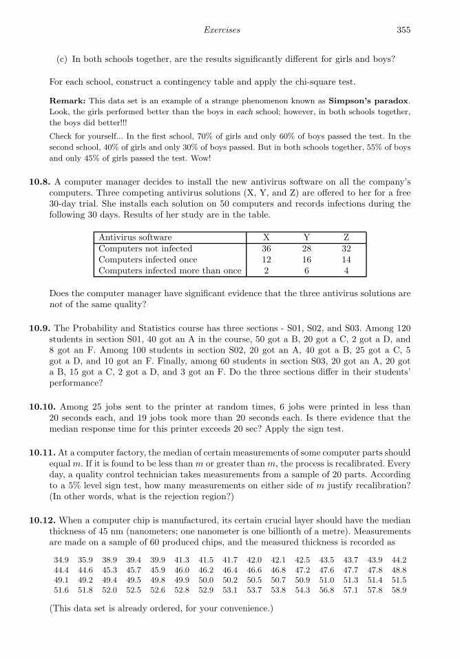
Exercises 355
(c) In both schools together, are the results significantly different for girls and boys?
For each school, construct a contingency table and apply the chi-square test.
Remark: This data set is an example of a strange phenomenon known as Simpson’s paradox.
Look, the girls performed better than the boys in each school; however, in both schools together,
the boys did better!!!
Check for yourself... In the first school, 70% of girls and only 60% of boys passed the test. In the
second school, 40% of girls and only 30% of boys passed. But in both schools together, 55% of boys
and only 45% of girls passed the test. Wow!
10.8. A computer manager decides to install the new antivirus software on all the company’scomputers. Three competing antivirus solutions (X, Y, and Z) are offered to her for a free30-day trial. She installs each solution on 50 computers and records infections during thefollowing 30 days. Results of her study are in the table.
Antivirus software X Y ZComputers not infected 36 28 32Computers infected once 12 16 14Computers infected more than once 2 6 4
Does the computer manager have significant evidence that the three antivirus solutions arenot of the same quality?
10.9. The Probability and Statistics course has three sections - S01, S02, and S03. Among 120students in section S01, 40 got an A in the course, 50 got a B, 20 got a C, 2 got a D, and8 got an F. Among 100 students in section S02, 20 got an A, 40 got a B, 25 got a C, 5got a D, and 10 got an F. Finally, among 60 students in section S03, 20 got an A, 20 gota B, 15 got a C, 2 got a D, and 3 got an F. Do the three sections differ in their students’performance?
10.10. Among 25 jobs sent to the printer at random times, 6 jobs were printed in less than20 seconds each, and 19 jobs took more than 20 seconds each. Is there evidence that themedian response time for this printer exceeds 20 sec? Apply the sign test.
10.11.At a computer factory, the median of certain measurements of some computer parts shouldequal m. If it is found to be less than m or greater than m, the process is recalibrated. Everyday, a quality control technician takes measurements from a sample of 20 parts. Accordingto a 5% level sign test, how many measurements on either side of m justify recalibration?(In other words, what is the rejection region?)
10.12. When a computer chip is manufactured, its certain crucial layer should have the medianthickness of 45 nm (nanometers; one nanometer is one billionth of a metre). Measurementsare made on a sample of 60 produced chips, and the measured thickness is recorded as
34.9 35.9 38.9 39.4 39.9 41.3 41.5 41.7 42.0 42.1 42.5 43.5 43.7 43.9 44.244.4 44.6 45.3 45.7 45.9 46.0 46.2 46.4 46.6 46.8 47.2 47.6 47.7 47.8 48.849.1 49.2 49.4 49.5 49.8 49.9 50.0 50.2 50.5 50.7 50.9 51.0 51.3 51.4 51.551.6 51.8 52.0 52.5 52.6 52.8 52.9 53.1 53.7 53.8 54.3 56.8 57.1 57.8 58.9
(This data set is already ordered, for your convenience.)
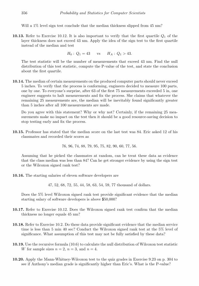
356 Probability and Statistics for Computer Scientists
Will a 1% level sign test conclude that the median thickness slipped from 45 nm?
10.13. Refer to Exercise 10.12. It is also important to verify that the first quartile Q1 of thelayer thickness does not exceed 43 nm. Apply the idea of the sign test to the first quartileinstead of the median and test
H0 : Q1 = 43 vs HA : Q1 > 43.
The test statistic will be the number of measurements that exceed 43 nm. Find the nulldistribution of this test statistic, compute the P-value of the test, and state the conclusionabout the first quartile.
10.14. The median of certain measurements on the produced computer parts should never exceed5 inches. To verify that the process is conforming, engineers decided to measure 100 parts,one by one. To everyone’s surprise, after 63 of the first 75 measurements exceeded 5 in, oneengineer suggests to halt measurements and fix the process. She claims that whatever theremaining 25 measurements are, the median will be inevitably found significantly greaterthan 5 inches after all 100 measurements are made.
Do you agree with this statement? Why or why not? Certainly, if the remaining 25 mea-surements make no impact on the test then it should be a good resource-saving decision tostop testing early and fix the process.
10.15. Professor has stated that the median score on the last test was 84. Eric asked 12 of hisclassmates and recorded their scores as
76, 96, 74, 88, 79, 95, 75, 82, 90, 60, 77, 56.
Assuming that he picked the classmates at random, can he treat these data as evidencethat the class median was less than 84? Can he get stronger evidence by using the sign testor the Wilcoxon signed rank test?
10.16. The starting salaries of eleven software developers are
47, 52, 68, 72, 55, 44, 58, 63, 54, 59, 77 thousand of dollars.
Does the 5% level Wilcoxon signed rank test provide significant evidence that the medianstarting salary of software developers is above $50,000?
10.17. Refer to Exercise 10.12. Does the Wilcoxon signed rank test confirm that the medianthickness no longer equals 45 nm?
10.18. Refer to Exercise 10.2. Do these data provide significant evidence that the median servicetime is less than 5 min 40 sec? Conduct the Wilcoxon signed rank test at the 5% level ofsignificance. What assumption of this test may not be fully satisfied by these data?
10.19.Use the recursive formula (10.6) to calculate the null distribution of Wilcoxon test statisticW for sample sizes n = 2, n = 3, and n = 4.
10.20. Apply the Mann-Whitney-Wilcoxon test to the quiz grades in Exercise 9.23 on p. 304 tosee if Anthony’s median grade is significantly higher than Eric’s. What is the P-value?

Exercises 357
10.21. Two internet service providers claim that they offer the fastest internet in the area. Alocal company requires the download speed of at least 20 Megabytes per second (Mbps),for its normal operation. It decides to conduct a fair contest by sending 10 packets of equalsize through each network and recording their download speed.
For the 1st internet service provider, the download speed is recorded as 26.7, 19.0, 26.5,29.1, 26.2, 27.6, 26.8, 24.2, 25.7, 23.0 Mbps. For the 2nd provider, the download speed isrecorded as 19.3, 22.1, 23.4, 24.8, 25.9, 22.2, 18.3, 20.1, 19.2, 27.9 Mbps.
(a) According to the sign test, is there significant evidence that the median downloadspeed for the 1st provider is at least 20 Mbps? What about the 2nd provider? Calculateeach P-value.
(b) Repeat (a) using the Wilcoxon signed rank test. Do the P-values show that this testis more sensitive than the sign test?
(c) At the 1% level, is there significant evidence that the median download speed forthe 1st provider exceeds the median download speed for the 2nd provider? Use thesuitable test.
10.22. Fifteen email attachments were classified as benign and malicious. Seven benign attach-ments were 0.4, 2.1, 3.6, 0.6, 0.8, 2.4, and 4.0 Mbytes in size. Eight malicious attachmentshad sizes 1.2, 0.2, 0.3, 3.3, 2.0, 0.9, 1.1, and 1.5 Mbytes. Does the Mann-Whitney-Wilcoxontest detect a significant difference in the distribution of sizes of benign and malicious at-tachments? (If so, the size could help classify email attachments and warn about possiblemalicious codes.)
10.23. During freshman year, Eric’s textbooks cost $89, $99, $119, $139, $189, $199, and $229.During his senior year, he had to pay $109, $159, $179, $209, $219, $259, $279, $299, and$309 for his textbooks. Is this significant evidence that the median cost of textbooks isrising, according to the Mann-Whitney-Wilcoxon test?
10.24. Two teams, six students each, competed at a programming contest. The judges gave theoverall 1st, 3rd, 6th, 7th, 9th, and 10th places to members of Team A. Now the captain ofTeam A claims the overall victory over Team B, according to a one-sided Mann-Whitney-Wilcoxon test? Do you concur with his conclusion? What hypothesis are you testing?
10.25. Refer to Exercise 10.2. After the first 32 service times were recorded (the first two rowsof data), the server was substantially modified. Conduct the Mann-Whitney-Wilcoxon testat the 10% level to see if this modification led to a reduction of the median service time.
10.26. On five days of the week, Anthony spends 2, 2, 3, 3, and 5 hours doing his homework.
(a) List all possible bootstrap samples and find the probability of each of them.
(b) Use your list to find the bootstrap distribution of the sample median.
(c) Use this bootstrap distribution to estimate the standard error and the bias of a samplemedian.

358 Probability and Statistics for Computer Scientists
10.27. In Exercise 10.16, we tested the median starting salary of software developers. We canactually estimate this starting salary by the sample median, which for these data equalsM = $58, 000.
(a) How many different bootstrap samples can be generated? Find the number of allpossible ordered and unordered samples.
(b) Find the bootstrap distribution of the sample median. Do not list all the bootstrapsamples!
(c) Use this distribution to estimate the standard error of M .
(d) Construct an 88% bootstrap confidence interval for the population median salary M .
(e) Use the bootstrap distribution to estimate the probability that 11 randomly selectedsoftware developers have their median starting salary above $50,000.
Exercises 10.28–10.30 require the use of a computer.
10.28. Refer to Exercise 10.15. Eric estimates the class median score by the sample median,which is any number between 77 and 79 for these data (Eric takes the middle value 78).Generate 10,000 bootstrap samples and use them for the following inference.
(a) Estimate the standard error of the sample median used by Eric.
(b) Is this sample median a biased estimator for the population median? Estimate itsbias.
(c) Construct a 95% bootstrap confidence interval for the population median. Can it beused to test whether the class median score is 84?
10.29. Refer to Exercise 10.13 where the first quartile of layer thickness is being tested. Thisquartile is estimated by the first sample quartile Q1 (in case of a whole interval of samplequartiles, its middle is taken). Use the bootstrap method to estimate the standard errorand the bias of this estimator.
10.30. Is there a correlation between the Eric’s and Anthony’s grades in Exercise 9.23 on p. 304?Construct an 80% nonparametric bootstrap confidence interval for the correlation coefficientbetween their quiz grades (a small sample size does not allow to assume the Normal distri-bution of the sample correlation coefficient).
10.31. A new section of a highway is opened, and X = 4 accidents occurred there during onemonth. The number of accidents has Poisson(θ) distribution, where θ is the expected numberof accidents during one month. Experience from the other sections of this highway suggeststhat the prior distribution of θ is Gamma(5,1). Find the Bayes estimator of θ under thesquared-error loss and find its posterior risk.
10.32. The data set consists of a sample X = (2, 3, 5, 8, 2) from the Geometric distribution withunknown parameter θ.
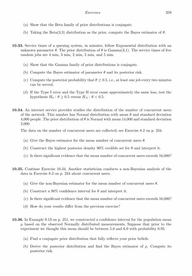
Exercises 359
(a) Show that the Beta family of prior distributions is conjugate.
(b) Taking the Beta(3,3) distribution as the prior, compute the Bayes estimator of θ.
10.33. Service times of a queuing system, in minutes, follow Exponential distribution with anunknown parameter θ. The prior distribution of θ is Gamma(3,1). The service times of fiverandom jobs are 4 min, 3 min, 2 min, 5 min, and 5 min.
(a) Show that the Gamma family of prior distributions is conjugate.
(b) Compute the Bayes estimator of parameter θ and its posterior risk.
(c) Compute the posterior probability that θ ≥ 0.5, i.e., at least one job every two minutescan be served.
(d) If the Type I error and the Type II error cause approximately the same loss, test thehypothesis H0 : θ ≥ 0.5 versus HA : θ < 0.5.
10.34. An internet service provider studies the distribution of the number of concurrent usersof the network. This number has Normal distribution with mean θ and standard deviation4,000 people. The prior distribution of θ is Normal with mean 14,000 and standard deviation2,000.
The data on the number of concurrent users are collected; see Exercise 8.2 on p. 234.
(a) Give the Bayes estimator for the mean number of concurrent users θ.
(b) Construct the highest posterior density 90% credible set for θ and interpret it.
(c) Is there significant evidence that the mean number of concurrent users exceeds 16,000?
10.35. Continue Exercise 10.34. Another statistician conducts a non-Bayesian analysis of thedata in Exercise 8.2 on p. 234 about concurrent users.
(a) Give the non-Bayesian estimator for the mean number of concurrent users θ.
(b) Construct a 90% confidence interval for θ and interpret it.
(c) Is there significant evidence that the mean number of concurrent users exceeds 16,000?
(d) How do your results differ from the previous exercise?
10.36. In Example 9.13 on p. 251, we constructed a confidence interval for the population meanµ based on the observed Normally distributed measurements. Suppose that prior to theexperiment we thought this mean should be between 5.0 and 6.0 with probability 0.95.
(a) Find a conjugate prior distribution that fully reflects your prior beliefs.
(b) Derive the posterior distribution and find the Bayes estimator of µ. Compute itsposterior risk.
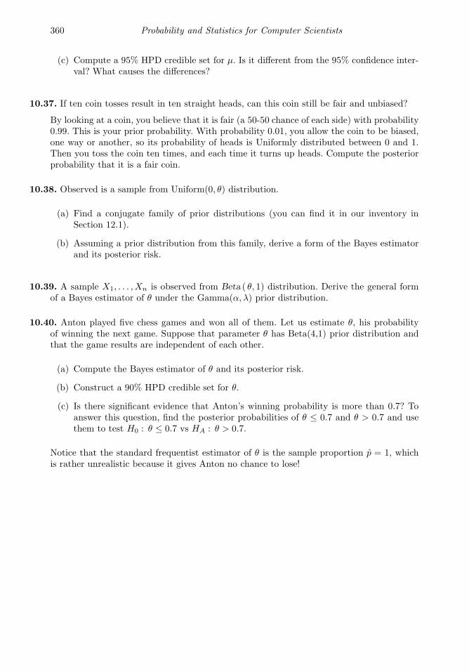
360 Probability and Statistics for Computer Scientists
(c) Compute a 95% HPD credible set for µ. Is it different from the 95% confidence inter-val? What causes the differences?
10.37. If ten coin tosses result in ten straight heads, can this coin still be fair and unbiased?
By looking at a coin, you believe that it is fair (a 50-50 chance of each side) with probability0.99. This is your prior probability. With probability 0.01, you allow the coin to be biased,one way or another, so its probability of heads is Uniformly distributed between 0 and 1.Then you toss the coin ten times, and each time it turns up heads. Compute the posteriorprobability that it is a fair coin.
10.38. Observed is a sample from Uniform(0, θ) distribution.
(a) Find a conjugate family of prior distributions (you can find it in our inventory inSection 12.1).
(b) Assuming a prior distribution from this family, derive a form of the Bayes estimatorand its posterior risk.
10.39. A sample X1, . . . , Xn is observed from Beta ( θ, 1) distribution. Derive the general formof a Bayes estimator of θ under the Gamma(α, λ) prior distribution.
10.40. Anton played five chess games and won all of them. Let us estimate θ, his probabilityof winning the next game. Suppose that parameter θ has Beta(4,1) prior distribution andthat the game results are independent of each other.
(a) Compute the Bayes estimator of θ and its posterior risk.
(b) Construct a 90% HPD credible set for θ.
(c) Is there significant evidence that Anton’s winning probability is more than 0.7? Toanswer this question, find the posterior probabilities of θ ≤ 0.7 and θ > 0.7 and usethem to test H0 : θ ≤ 0.7 vs HA : θ > 0.7.
Notice that the standard frequentist estimator of θ is the sample proportion p = 1, whichis rather unrealistic because it gives Anton no chance to lose!
Chapter 11
Regression
11.1 Least squares estimation . . . . . . . . . . . . . . . . . . . . . . . . . . . . . . . . . . . . . . . . . 36211.1.1 Examples . . . . . . . . . . . . . . . . . . . . . . . . . . . . . . . . . . . . . . . . . . . . . . . . 36211.1.2 Method of least squares . . . . . . . . . . . . . . . . . . . . . . . . . . . . . . . . . 36411.1.3 Linear regression . . . . . . . . . . . . . . . . . . . . . . . . . . . . . . . . . . . . . . . . . 36511.1.4 Regression and correlation . . . . . . . . . . . . . . . . . . . . . . . . . . . . . . 36711.1.5 Overfitting a model . . . . . . . . . . . . . . . . . . . . . . . . . . . . . . . . . . . . . . 368
11.2 Analysis of variance, prediction, and further inference . . . . . . . . . . 36911.2.1 ANOVA and R-square . . . . . . . . . . . . . . . . . . . . . . . . . . . . . . . . . . . 36911.2.2 Tests and confidence intervals . . . . . . . . . . . . . . . . . . . . . . . . . . . 37111.2.3 Prediction . . . . . . . . . . . . . . . . . . . . . . . . . . . . . . . . . . . . . . . . . . . . . . . . 377
11.3 Multivariate regression . . . . . . . . . . . . . . . . . . . . . . . . . . . . . . . . . . . . . . . . . . . 38111.3.1 Introduction and examples . . . . . . . . . . . . . . . . . . . . . . . . . . . . . . 38111.3.2 Matrix approach and least squares estimation . . . . . . . . . . 38211.3.3 Analysis of variance, tests, and prediction . . . . . . . . . . . . . . 384
11.4 Model building . . . . . . . . . . . . . . . . . . . . . . . . . . . . . . . . . . . . . . . . . . . . . . . . . . . 39011.4.1 Adjusted R-square . . . . . . . . . . . . . . . . . . . . . . . . . . . . . . . . . . . . . . . 39011.4.2 Extra sum of squares, partial F-tests, and variable
selection . . . . . . . . . . . . . . . . . . . . . . . . . . . . . . . . . . . . . . . . . . . . . . . . . . 39111.4.3 Categorical predictors and dummy variables . . . . . . . . . . . . 394
Summary and conclusions . . . . . . . . . . . . . . . . . . . . . . . . . . . . . . . . . . . . . . . . . . 397Exercises . . . . . . . . . . . . . . . . . . . . . . . . . . . . . . . . . . . . . . . . . . . . . . . . . . . . . . . . . . . . 397
In Chapters 8, 9, and 10, we were concerned about the distribution of one random variable,its parameters, expectation, variance, median, symmetry, skewness, etc. In this chapter, westudy relations among variables.
Many variables observed in real life are related. The type of their relation can often beexpressed in a mathematical form called regression. Establishing and testing such a relationenables us:
– to understand interactions, causes, and effects among variables;
– to predict unobserved variables based on the observed ones;
– to determine which variables significantly affect the variable of interest.
361
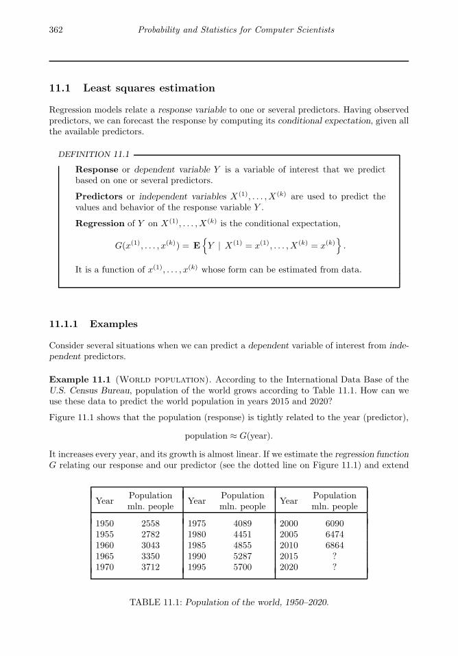
362 Probability and Statistics for Computer Scientists
11.1 Least squares estimation
Regression models relate a response variable to one or several predictors. Having observedpredictors, we can forecast the response by computing its conditional expectation, given allthe available predictors.
DEFINITION 11.1
Response or dependent variable Y is a variable of interest that we predictbased on one or several predictors.
Predictors or independent variables X(1), . . . , X(k) are used to predict thevalues and behavior of the response variable Y .
Regression of Y on X(1), . . . , X(k) is the conditional expectation,
G(x(1), . . . , x(k)) = EY | X(1) = x(1), . . . , X(k) = x(k)
.
It is a function of x(1), . . . , x(k) whose form can be estimated from data.
11.1.1 Examples
Consider several situations when we can predict a dependent variable of interest from inde-pendent predictors.
Example 11.1 (World population). According to the International Data Base of theU.S. Census Bureau, population of the world grows according to Table 11.1. How can weuse these data to predict the world population in years 2015 and 2020?
Figure 11.1 shows that the population (response) is tightly related to the year (predictor),
population ≈ G(year).
It increases every year, and its growth is almost linear. If we estimate the regression functionG relating our response and our predictor (see the dotted line on Figure 11.1) and extend
YearPopulationmln. people
YearPopulationmln. people
YearPopulationmln. people
1950 2558 1975 4089 2000 60901955 2782 1980 4451 2005 64741960 3043 1985 4855 2010 68641965 3350 1990 5287 2015 ?1970 3712 1995 5700 2020 ?
TABLE 11.1: Population of the world, 1950–2020.

Regression 363
1950 1960 1970 1980 1990 2000 2010 20200
1000
2000
3000
4000
5000
6000
7000
8000
Year
Wor
ld p
opul
atio
n, m
ln.
Observed population
Regression line
Computed forecast
FIGURE 11.1: World population in 1950–2010 and its regression forecast for 2015 and 2020.
its graph to the year 2020, the forecast is ready. We can simply compute G(2015) and andG(2020).
A straight line that fits the observed data for years 1950–2010 predicts the population of7.15 billion in 2015 and 7.52 billion in 2020. It also shows that between 2010 and 2015,around the year 2012, the world population reaches the historical mark of 7 billion. ♦
How accurate is the forecast obtained in this example? The observed population during1950–2010 appears rather close to the estimated regression line in Figure 11.1. It is reason-able to hope that it will continue to do so through 2020.
The situation is different in the next example.
Example 11.2 (House prices). Seventy house sale prices in a certain county are depictedin Figure 11.2 along with the house area.
First, we see a clear relation between these two variables, and in general, bigger houses aremore expensive. However, the trend no longer seems linear.
Second, there is a large amount of variability around this trend. Indeed, area is not theonly factor determining the house price. Houses with the same area may still be priceddifferently.
Then, how can we estimate the price of a 3200-square-foot house? We can estimate thegeneral trend (the dotted line in Figure 11.2) and plug 3200 into the resulting formula, butdue to obviously high variability, our estimation will not be as accurate as in Example 11.1.
♦
To improve our estimation in the last example, we may take other factors into account:the number of bedrooms and bathrooms, the backyard area, the average income of theneighborhood, etc. If all the added variables are relevant for pricing a house, our modelwill have a closer fit and will provide more accurate predictions. Regression models withmultiple predictors are studied in Section 11.3.

364 Probability and Statistics for Computer Scientists
2000 2200 2400 2600 2800 3000 3200 3400 3600 3800 4000
200
250
300
350
400Sale
price,
$1000s
House area, sq. feet
FIGURE 11.2: House sale prices and their footage.
11.1.2 Method of least squares
Our immediate goal is to estimate the regression function G that connects responsevariable Y with predictors X(1), . . . , X(k). First we focus on univariate regression predictingresponse Y based on one predictor X . The method will be extended to k predictors inSection 11.3.
In univariate regression, we observe pairs (x1, y1), . . . , (xn, yn), shown in Figure 11.3a.
For accurate forecasting, we are looking for the function G(x) that passes as close as possibleto the observed data points. This is achieved by minimizing distances between observed datapoints
y1, . . . , yn
and the corresponding points on the fitted regression line,
y1 = G(x1), . . . , yn = G(xn)
(see Figure 11.3b). Method of least squares minimizes the sum of squared distances.
DEFINITION 11.2
Residualsei = yi − yi
are differences between observed responses yi and their fitted values yi =G(xi).
Method of least squares finds a regression function G(x) that minimizes thesum of squared residuals
n∑
i=1
e2i =
n∑
i=1
(yi − yi)2. (11.1)

Regression 365
Predictor X Predictor X
Response
Y
Response
Y
(a) Observed pairs (b) Estimated regression line
(x1, y1)
(x2, y2)
(x3, y3)
(x4, y4)
(x5, y5)
y1
y1
y2
y2
y3
y3
y4
y4y5
y5
FIGURE 11.3: Least squares estimation of the regression line.
Function G is usually sought in a suitable form: linear, quadratic, logarithmic, etc. Thesimplest form is linear.
11.1.3 Linear regression
Linear regression model assumes that the conditional expectation
G(x) = E Y | X = x = β0 + β1 x
is a linear function of x. As any linear function, it has an intercept β0 and a slope β1.
The interceptβ0 = G(0)
equals the value of the regression function for x = 0. Sometimes it has no physical meaning.For example, nobody will try to predict the value of a computer with 0 random accessmemory (RAM), and nobody will consider the Federal reserve rate in year 0. In othercases, intercept is quite important. For example, according to the Ohm’s Law (V = RI)the voltage across an ideal conductor is proportional to the current. A non-zero intercept(V = V0 + R I) would show that the circuit is not ideal, and there is an external loss ofvoltage.
The slopeβ1 = G(x+ 1)−G(x)
is the predicted change in the response variable when predictor changes by 1. This is a veryimportant parameter that shows how fast we can change the expected response by varyingthe predictor. For example, customer satisfaction will increase by β1(∆x) when the qualityof produced computers increases by (∆x).
A zero slope means absence of a linear relationship between X and Y . In this case, Y isexpected to stay constant when X changes.
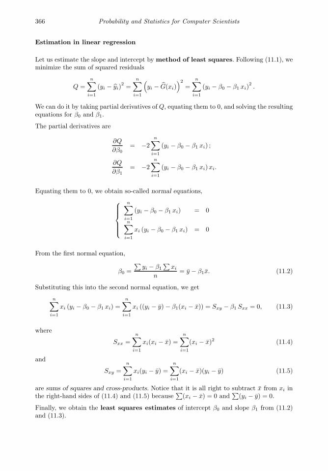
366 Probability and Statistics for Computer Scientists
Estimation in linear regression
Let us estimate the slope and intercept by method of least squares. Following (11.1), weminimize the sum of squared residuals
Q =
n∑
i=1
(yi − yi)2=
n∑
i=1
(yi − G(xi)
)2=
n∑
i=1
(yi − β0 − β1 xi)2.
We can do it by taking partial derivatives of Q, equating them to 0, and solving the resultingequations for β0 and β1.
The partial derivatives are
∂Q
∂β0= −2
n∑
i=1
(yi − β0 − β1 xi) ;
∂Q
∂β1= −2
n∑
i=1
(yi − β0 − β1 xi)xi.
Equating them to 0, we obtain so-called normal equations,
n∑
i=1
(yi − β0 − β1 xi) = 0
n∑
i=1
xi (yi − β0 − β1 xi) = 0
From the first normal equation,
β0 =
∑yi − β1
∑xi
n= y − β1x. (11.2)
Substituting this into the second normal equation, we get
n∑
i=1
xi (yi − β0 − β1 xi) =
n∑
i=1
xi ((yi − y)− β1(xi − x)) = Sxy − β1 Sxx = 0, (11.3)
where
Sxx =
n∑
i=1
xi(xi − x) =
n∑
i=1
(xi − x)2 (11.4)
and
Sxy =
n∑
i=1
xi(yi − y) =
n∑
i=1
(xi − x)(yi − y) (11.5)
are sums of squares and cross-products. Notice that it is all right to subtract x from xi inthe right-hand sides of (11.4) and (11.5) because
∑(xi − x) = 0 and
∑(yi − y) = 0.
Finally, we obtain the least squares estimates of intercept β0 and slope β1 from (11.2)and (11.3).

Regression 367
Regressionestimates
b0 = β0 = y − b1 x
b1 = β1 = Sxy/Sxx
where
Sxx =
n∑
i=1
(xi − x)2
Sxy =
n∑
i=1
(xi − x)(yi − y)
(11.6)
Example 11.3 (World population). In Example 11.1, xi is the year, and yi is the worldpopulation during that year. To estimate the regression line in Figure 11.1, we compute
x = 1980; y = 4558.1;
Sxx = (1950− x)2 + . . .+ (2010− x)2 = 4550;
Sxy = (1950− x)(2558− y) + . . .+ (2010− x)(6864− y) = 337250.
Then
b1 = Sxy/Sxx = 74.1
b0 = y − b1x = −142201.
The estimated regression line is
G(x) = b0 + b1 x = -142201 + 74.1x.
We conclude that the world population grows at the average rate of 74.1 million every year.
We can use the obtained equation to predict the future growth of the world population.Regression predictions for years 2015 and 2020 are
G(2015) = b0 + 2015 b1 = 7152 million people
G(2020) = b0 + 2020 b1 = 7523 million people
♦
11.1.4 Regression and correlation
Recall from Section 3.3.5 that covariance
Cov(X,Y ) = E(X − E(X))(Y − E(Y ))
and correlation coefficient
ρ =Cov(X,Y )
( StdX)( StdY )
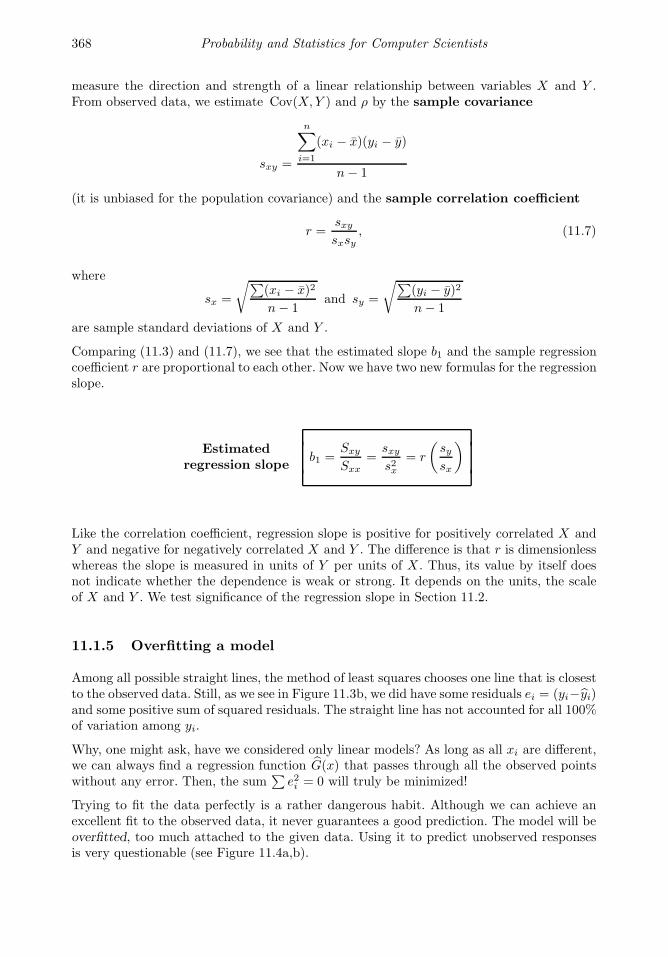
368 Probability and Statistics for Computer Scientists
measure the direction and strength of a linear relationship between variables X and Y .From observed data, we estimate Cov(X,Y ) and ρ by the sample covariance
sxy =
n∑
i=1
(xi − x)(yi − y)
n− 1
(it is unbiased for the population covariance) and the sample correlation coefficient
r =sxysxsy
, (11.7)
where
sx =
√∑(xi − x)2
n− 1and sy =
√∑(yi − y)2
n− 1
are sample standard deviations of X and Y .
Comparing (11.3) and (11.7), we see that the estimated slope b1 and the sample regressioncoefficient r are proportional to each other. Now we have two new formulas for the regressionslope.
Estimatedregression slope
b1 =Sxy
Sxx=
sxys2x
= r
(sysx
)
Like the correlation coefficient, regression slope is positive for positively correlated X andY and negative for negatively correlated X and Y . The difference is that r is dimensionlesswhereas the slope is measured in units of Y per units of X . Thus, its value by itself doesnot indicate whether the dependence is weak or strong. It depends on the units, the scaleof X and Y . We test significance of the regression slope in Section 11.2.
11.1.5 Overfitting a model
Among all possible straight lines, the method of least squares chooses one line that is closestto the observed data. Still, as we see in Figure 11.3b, we did have some residuals ei = (yi−yi)and some positive sum of squared residuals. The straight line has not accounted for all 100%of variation among yi.
Why, one might ask, have we considered only linear models? As long as all xi are different,we can always find a regression function G(x) that passes through all the observed pointswithout any error. Then, the sum
∑e2i = 0 will truly be minimized!
Trying to fit the data perfectly is a rather dangerous habit. Although we can achieve anexcellent fit to the observed data, it never guarantees a good prediction. The model will beoverfitted, too much attached to the given data. Using it to predict unobserved responsesis very questionable (see Figure 11.4a,b).

Regression 369
Predictor X Predictor X
Response
Y
Response
Y
(a) Overfitted regression lineshave low prediction power
(b) Linear predictionfor the same data
??
?
(x, y )
FIGURE 11.4: Regression-based prediction.
11.2 Analysis of variance, prediction, and further inference
In this section, we
– evaluate the goodness of fit of the chosen regression model to the observed data,
– estimate the response variance,
– test significance of regression parameters,
– construct confidence and prediction intervals.
11.2.1 ANOVA and R-square
Analysis of variance (ANOVA) explores variation among the observed responses. Aportion of this variation can be explained by predictors. The rest is attributed to “error.”
For example, there exists some variation among the house sale prices on Figure 11.2. Whyare the houses priced differently? Well, the price depends on the house area, and biggerhouses tend to be more expensive. So, to some extent, variation among prices is explainedby variation among house areas. However, two houses with the same area may still havedifferent prices. These differences cannot be explained by the area.
The total variation among observed responses is measured by the total sum of squares
SSTOT =
n∑
i=1
(yi − y)2 = (n− 1)s2y.
This is the variation of yi about their sample mean regardless of our regression model.
A portion of this total variation is attributed to predictor X and the regression model

370 Probability and Statistics for Computer Scientists
connecting predictor and response. This portion is measured by the regression sum ofsquares
SSREG =n∑
i=1
(yi − y)2.
This is the portion of total variation explained by the model. It is often computed as
SSREG =
n∑
i=1
(b0 + b1xi − y)2
=
n∑
i=1
(y − b1x+ b1xi − y)2
=n∑
i=1
b21(xi − x)2
= b21Sxx or (n− 1)b21s2x.
The rest of total variation is attributed to “error.” It is measured by the error sum ofsquares
SSERR =
n∑
i=1
(yi − yi)2 =
n∑
i=1
e2i .
This is the portion of total variation not explained by the model. It equals the sum ofsquared residuals that the method of least squares minimizes. Thus, applying this method,we minimize the error sum of squares.
Regression and error sums of squares partition SSTOT into two parts (Exercise 11.6),
SSTOT = SSREG + SSERR.
The goodness of fit, appropriateness of the predictor and the chosen regression model canbe judged by the proportion of SSTOT that the model can explain.
DEFINITION 11.3
R-square, or coefficient of determination is the proportion of the totalvariation explained by the model,
R2 =SSREG
SSTOT.
It is always between 0 and 1, with high values generally suggesting a good fit.
In univariate regression, R-square also equals the squared sample correlation coefficient(Exercise 11.7),
R2 = r2.
Example 11.4 (World population, continued). Continuing Example 11.3, we find
SSTOT = (n− 1)s2y = (12)(2.093 · 106) = 2.512 · 107,SSREG = b21Sxx = (74.1)2(4550) = 2.500 · 107,SSERR = SSTOT − SSREG = 1.2 · 105.
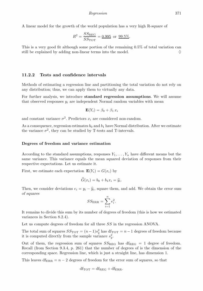
Regression 371
A linear model for the growth of the world population has a very high R-square of
R2 =SSREG
SSTOT= 0.995 or 99.5%.
This is a very good fit although some portion of the remaining 0.5% of total variation canstill be explained by adding non-linear terms into the model. ♦
11.2.2 Tests and confidence intervals
Methods of estimating a regression line and partitioning the total variation do not rely onany distribution; thus, we can apply them to virtually any data.
For further analysis, we introduce standard regression assumptions. We will assumethat observed responses yi are independent Normal random variables with mean
E(Yi) = β0 + β1 xi
and constant variance σ2. Predictors xi are considered non-random.
As a consequence, regression estimates b0 and b1 have Normal distribution. After we estimatethe variance σ2, they can be studied by T-tests and T-intervals.
Degrees of freedom and variance estimation
According to the standard assumptions, responses Y1, . . . , Yn have different means but thesame variance. This variance equals the mean squared deviation of responses from theirrespective expectations. Let us estimate it.
First, we estimate each expectation E(Yi) = G(xi) by
G(xi) = b0 + b1xi = yi.
Then, we consider deviations ei = yi − yi, square them, and add. We obtain the error sumof squares
SSERR =
n∑
i=1
e2i .
It remains to divide this sum by its number of degrees of freedom (this is how we estimatedvariances in Section 8.2.4).
Let us compute degrees of freedom for all three SS in the regression ANOVA.
The total sum of squares SSTOT = (n− 1)s2y has dfTOT = n− 1 degrees of freedom becauseit is computed directly from the sample variance s2y.
Out of them, the regression sum of squares SSREG has dfREG = 1 degree of freedom.Recall (from Section 9.3.4, p. 261) that the number of degrees of is the dimension of thecorresponding space. Regression line, which is just a straight line, has dimension 1.
This leaves dfERR = n− 2 degrees of freedom for the error sum of squares, so that
dfTOT = dfREG + dfERR.
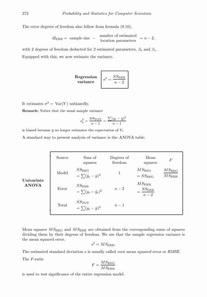
372 Probability and Statistics for Computer Scientists
The error degrees of freedom also follow from formula (9.10),
dfERR = sample size − number of estimatedlocation parameters
= n− 2,
with 2 degrees of freedom deducted for 2 estimated parameters, β0 and β1.
Equipped with this, we now estimate the variance.
Regressionvariance
s2 =SSERR
n− 2
It estimates σ2 = Var(Y ) unbiasedly.
Remark: Notice that the usual sample variance
s2y =SSTOT
n− 1=
∑(yi − y)2
n− 1
is biased because y no longer estimates the expectation of Yi.
A standard way to present analysis of variance is the ANOVA table.
UnivariateANOVA
Source Sum ofsquares
Degrees offreedom
Meansquares
F
ModelSSREG
=∑
(yi − y)21
MSREG
= SSREG
MSREG
MSERR
ErrorSSERR
=∑
(yi − yi)2
n− 2MSERR
=SSERR
n− 2
TotalSSTOT
=∑
(yi − y)2n− 1
Mean squares MSREG and MSERR are obtained from the corresponding sums of squaresdividing them by their degrees of freedom. We see that the sample regression variance isthe mean squared error,
s2 = MSERR.
The estimated standard deviation s is usually called root mean squared error or RMSE.
The F-ratio
F =MSREG
MSERR
is used to test significance of the entire regression model.
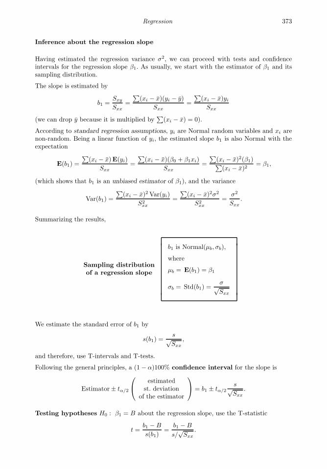
Regression 373
Inference about the regression slope
Having estimated the regression variance σ2, we can proceed with tests and confidenceintervals for the regression slope β1. As usually, we start with the estimator of β1 and itssampling distribution.
The slope is estimated by
b1 =Sxy
Sxx=
∑(xi − x)(yi − y)
Sxx=
∑(xi − x)yiSxx
(we can drop y because it is multiplied by∑
(xi − x) = 0).
According to standard regression assumptions, yi are Normal random variables and xi arenon-random. Being a linear function of yi, the estimated slope b1 is also Normal with theexpectation
E(b1) =
∑(xi − x)E(yi)
Sxx=
∑(xi − x)(β0 + β1xi)
Sxx=
∑(xi − x)2(β1)∑(xi − x)2
= β1,
(which shows that b1 is an unbiased estimator of β1), and the variance
Var(b1) =
∑(xi − x)2 Var(yi)
S2xx
=
∑(xi − x)2σ2
S2xx
=σ2
Sxx.
Summarizing the results,
Sampling distributionof a regression slope
b1 is Normal(µb, σb),
where
µb = E(b1) = β1
σb = Std(b1) =σ√Sxx
We estimate the standard error of b1 by
s(b1) =s√Sxx
,
and therefore, use T-intervals and T-tests.
Following the general principles, a (1− α)100% confidence interval for the slope is
Estimator± tα/2
estimatedst. deviation
of the estimator
= b1 ± tα/2
s√Sxx
.
Testing hypotheses H0 : β1 = B about the regression slope, use the T-statistic
t =b1 −B
s(b1)=
b1 −B
s/√Sxx
.

374 Probability and Statistics for Computer Scientists
P-values, acceptance and rejection regions are computed from Table A5 in the Appendix,T-distribution with (n − 2) degrees of freedom. These are degrees of freedom used in theestimation of σ2.
As always, the form of the alternative hypothesis determines whether it is a two-sided,right-tail, or left-tail test.
A non-zero slope indicates significance of the model, relevance of predictorX in the inferenceabout response Y , and existence of a linear relation among them. It means that a changein X causes changes in Y . In the absence of such relation, E(Y ) = β0 remains constant.
To see if X is significant for the prediction of Y , test the null hypothesis
H0 : β1 = 0 vs Ha : β1 6= 0.
ANOVA F-test
A more universal, and therefore, more popular method of testing significance of a model isthe ANOVA F-test. It compares the portion of variation explained by regression with theportion that remains unexplained. Significant models explain a relatively large portion.
Each portion of the total variation is measured by the corresponding sum of squares, SSREG
for the explained portion and SSERR for the unexplained portion (error). Dividing each SSby the number of degrees of freedom, we obtain mean squares,
MSREG =SSREG
dfREG=
SSREG
1= SSREG
and
MSERR =SSERR
dfERR=
SSERR
n− 2= s2.
Under the null hypothesisH0 : β1 = 0,
both mean squares, MSREG and MSERR are independent, and their ratio
F =MSR
MSE=
SSR
s2
has F-distribution with dfREG = 1 and dfERR = n− 2 degrees of freedom (d.f.).
As we discovered in Section 9.5.4, this F-distribution has two parameters, numerator d.f.and denominator d.f., and it is very popular for testing ratios of variances and significanceof models. Its critical values for the most popular significance levels between α = 0.001 andα = 0.25 are tabulated in Table A7.
ANOVA F-test is always one-sided and right-tail because only large values of the F-statisticshow a large portion of explained variation and the overall significance of the model.
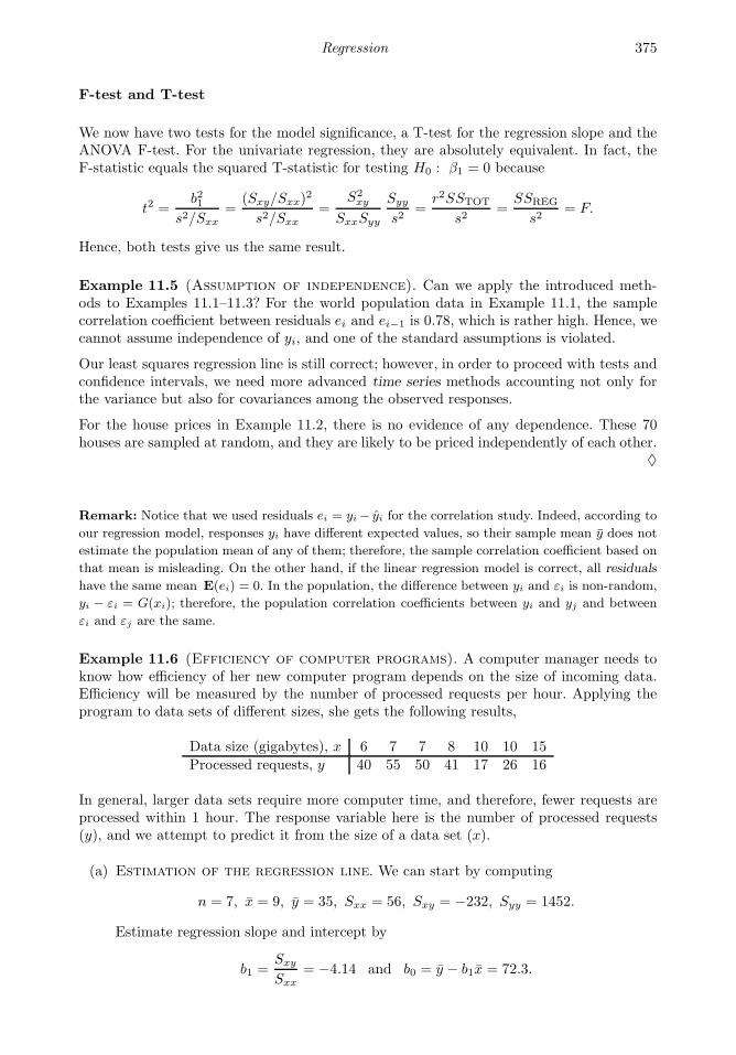
Regression 375
F-test and T-test
We now have two tests for the model significance, a T-test for the regression slope and theANOVA F-test. For the univariate regression, they are absolutely equivalent. In fact, theF-statistic equals the squared T-statistic for testing H0 : β1 = 0 because
t2 =b21
s2/Sxx=
(Sxy/Sxx)2
s2/Sxx=
S2xy
SxxSyy
Syy
s2=
r2SSTOT
s2=
SSREG
s2= F.
Hence, both tests give us the same result.
Example 11.5 (Assumption of independence). Can we apply the introduced meth-ods to Examples 11.1–11.3? For the world population data in Example 11.1, the samplecorrelation coefficient between residuals ei and ei−1 is 0.78, which is rather high. Hence, wecannot assume independence of yi, and one of the standard assumptions is violated.
Our least squares regression line is still correct; however, in order to proceed with tests andconfidence intervals, we need more advanced time series methods accounting not only forthe variance but also for covariances among the observed responses.
For the house prices in Example 11.2, there is no evidence of any dependence. These 70houses are sampled at random, and they are likely to be priced independently of each other.
♦
Remark: Notice that we used residuals ei = yi − yi for the correlation study. Indeed, according to
our regression model, responses yi have different expected values, so their sample mean y does not
estimate the population mean of any of them; therefore, the sample correlation coefficient based on
that mean is misleading. On the other hand, if the linear regression model is correct, all residuals
have the same mean E(ei) = 0. In the population, the difference between yi and εi is non-random,
yi − εi = G(xi); therefore, the population correlation coefficients between yi and yj and between
εi and εj are the same.
Example 11.6 (Efficiency of computer programs). A computer manager needs toknow how efficiency of her new computer program depends on the size of incoming data.Efficiency will be measured by the number of processed requests per hour. Applying theprogram to data sets of different sizes, she gets the following results,
Data size (gigabytes), x 6 7 7 8 10 10 15
Processed requests, y 40 55 50 41 17 26 16
In general, larger data sets require more computer time, and therefore, fewer requests areprocessed within 1 hour. The response variable here is the number of processed requests(y), and we attempt to predict it from the size of a data set (x).
(a) Estimation of the regression line. We can start by computing
n = 7, x = 9, y = 35, Sxx = 56, Sxy = −232, Syy = 1452.
Estimate regression slope and intercept by
b1 =Sxy
Sxx= −4.14 and b0 = y − b1x = 72.3.

376 Probability and Statistics for Computer Scientists
Then, the estimated regression line has an equation
y = 72.3− 4.14x.
Notice the negative slope. It means that increasing incoming data sets by 1 gigabyte,we expect to process 4.14 fewer requests per hour.
(b) ANOVA table and variance estimation. Let us compute all components of theANOVA. We have
SSTOT = Syy = 1452
partitioned into
SSREG = b21Sxx = 961 and SSERR = SSTOT − SSREG = 491.
Simultaneously, n−1 = 6 degrees of freedom of SSTOT are partitioned into dfREG = 1and dfERR = 5 degrees of freedom.
Fill the rest of the ANOVA table,
SourceSum ofsquares
Degrees offreedom
Meansquares F
Model 961 1 961 9.79Error 491 5 98.2Total 1452 6
Regression variance σ2 is estimated by
s2 = MSERR = 98.2.
R-square is
R2 =SSREG
SSTOT=
961
1452= 0.662.
That is, 66.2% of the total variation of the number of processed requests is explainedby sizes of data sets only.
(c) Inference about the slope. Is the slope statistically significant? Does the numberof processed requests really depend on the size of data sets? To test the null hypothesisH0 : β1 = 0, compute the T-statistic
t =b1√
s2/Sxx
=−4.14√98.2/56
= −3.13.
Checking the T-distribution table (Table A5) with 5 d.f., we find that the P-value forthe two-sided test is between 0.02 and 0.04. We conclude that the slope is moderatelysignificant. Precisely, it is significant at any level α ≥ 0.04 and not significant at anyα ≤ 0.02.
(d) ANOVA F-test. A similar result is suggested by the F-test. From Table A7, theF-statistic of 9.79 is not significant at the 0.025 level, but significant at the 0.05 level.
♦
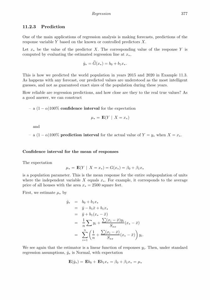
Regression 377
11.2.3 Prediction
One of the main applications of regression analysis is making forecasts, predictions of theresponse variable Y based on the known or controlled predictors X .
Let x∗ be the value of the predictor X . The corresponding value of the response Y iscomputed by evaluating the estimated regression line at x∗,
y∗ = G(x∗) = b0 + b1x∗.
This is how we predicted the world population in years 2015 and 2020 in Example 11.3.As happens with any forecast, our predicted values are understood as the most intelligentguesses, and not as guaranteed exact sizes of the population during these years.
How reliable are regression predictions, and how close are they to the real true values? Asa good answer, we can construct
– a (1− α)100% confidence interval for the expectation
µ∗ = E(Y | X = x∗)
and
– a (1− α)100% prediction interval for the actual value of Y = y∗ when X = x∗.
Confidence interval for the mean of responses
The expectationµ∗ = E(Y | X = x∗) = G(x∗) = β0 + β1x∗
is a population parameter. This is the mean response for the entire subpopulation of unitswhere the independent variable X equals x∗. For example, it corresponds to the averageprice of all houses with the area x∗ = 2500 square feet.
First, we estimate µ∗ by
y∗ = b0 + b1x∗
= y − b1x+ b1x∗
= y + b1(x∗ − x)
=1
n
∑yi +
∑(xi − x)yiSxx
(x∗ − x)
=
n∑
i=1
(1
n+
∑(xi − x)
Sxx(x∗ − x)
)yi.
We see again that the estimator is a linear function of responses yi. Then, under standardregression assumptions, y∗ is Normal, with expectation
E(y∗) = Eb0 + Eb1x∗ = β0 + β1x∗ = µ∗

378 Probability and Statistics for Computer Scientists
(it is unbiased), and variance
Var(y∗) =∑(
1
n+
∑(xi − x)
Sxx(x∗ − x)
)2
Var(yi)
= σ2
(n∑
i=1
1
n2+ 2
n∑
i=1
(xi − x)x∗ − x
Sxx+
Sxx(x∗ − x)2
S2xx
)
= σ2
(1
n+
(x∗ − x)2
Sxx
)(11.8)
(because∑
(xi − x) = 0).
Then, we estimate the regression variance σ2 by s2 and obtain the following confidenceinterval.
(1− α)100% confidenceinterval for the meanµ∗ = E(Y | X = x∗)
of all responses with X = x∗
b0 + b1x∗ ± tα/2 s
√1
n+
(x∗ − x)2
Sxx
Prediction interval for the individual response
Often we are more interested in predicting the actual response rather than the mean of allpossible responses. For example, we may be interested in the price of one particular housethat we are planning to buy, not in the average price of all similar houses.
Instead of estimating a population parameter, we are now predicting the actual value of arandom variable.
DEFINITION 11.4
An interval [a, b] is a (1 − α)100% prediction interval for the individualresponse Y corresponding to predictor X = x∗ if it contains the value of Ywith probability (1− α),
P a ≤ Y ≤ b | X = x∗ = 1− α.
This time, all three quantities, Y , a, and b, are random variables. Predicting Y by y∗,estimating the standard deviation
Std(Y − y∗) =√
Var(Y ) + Var(y∗) = σ
√1 +
1
n+
(x∗ − x)2
Sxx(11.9)
by
Std(Y − y∗) = s
√1 +
1
n+
(x∗ − x)2
Sxx,

Regression 379
and standardizing all three parts of the inequality
a ≤ Y ≤ b,
we realize that the (1− α)100% prediction interval for Y has to satisfy the equation
P
a− y∗
Std(Y − y∗)≤ Y − y∗
Std(Y − y∗)≤ b− y∗
Std(Y − y∗)
= 1− α.
At the same time, the properly standardized (Y − y∗) has T -distribution, and
P
−tα/2 ≤ Y − y∗
Std(Y − y∗)≤ tα/2
= 1− α.
A prediction interval is now computed by solving equations
a− y∗
Std(Y − y∗)= −tα/2 and
b− y∗
Std(Y − y∗)= tα/2
in terms of a and b.
(1 − α)100% prediction intervalfor the individual response Y
when X = x∗
b0 + b1x∗ ± tα/2 s
√1 +
1
n+
(x∗ − x)2
Sxx(11.10)
Several conclusions are apparent from this.
First, compare the standard deviations in (11.8) and (11.9). Response Y that we are pre-dicting made its contribution into the variance. This is the difference between a confidenceinterval for the mean of all responses and a prediction interval for the individual response.Predicting the individual value is a more difficult task; therefore, the prediction intervalis always wider than the confidence interval for the mean response. More uncertainty isinvolved, and as a result, the margin of a prediction interval is larger than the margin of aconfidence interval.
Second, we get more accurate estimates and more accurate predictions from large samples.When the sample size n (and therefore, typically, Sxx), tends to ∞, the margin of theconfidence interval converges to 0.
On the other hand, the margin of a prediction interval converges to (tα/2σ). As we collectmore and more observations, our estimates of b0 and b1 become more accurate; however,uncertainty about the individual response Y will never vanish.
Third, we see that regression estimation and prediction are most accurate when x∗ is closeto x so that
(x∗ − x)2 ≈ 0.
The margin increases as the independent variable x∗ drifts away from x. We conclude thatit is easiest to make forecasts under normal and “standard” conditions, and it is hardest topredict anomalies. And this agrees with our common sense.
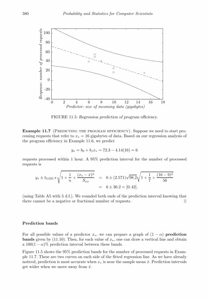
380 Probability and Statistics for Computer Scientists
Predictor: size of incoming data (gigabytes)
Response:numberofprocessed
requests
0 2 4 6 8 10 12 14 16 18-40
-20
0
20
40
60
80
100
FIGURE 11.5: Regression prediction of program efficiency.
Example 11.7 (Predicting the program efficiency). Suppose we need to start pro-cessing requests that refer to x∗ = 16 gigabytes of data. Based on our regression analysis ofthe program efficiency in Example 11.6, we predict
y∗ = b0 + b1x∗ = 72.3− 4.14(16) = 6
requests processed within 1 hour. A 95% prediction interval for the number of processedrequests is
y∗ ± t0.025 s
√1 +
1
n+
(x∗ − x)2
Sxx= 6± (2.571)
√98.2
√1 +
1
7+
(16− 9)2
56
= 6± 36.2 = [0; 42].
(using Table A5 with 5 d.f.). We rounded both ends of the prediction interval knowing thatthere cannot be a negative or fractional number of requests. ♦
Prediction bands
For all possible values of a predictor x∗, we can prepare a graph of (1 − α) predictionbands given by (11.10). Then, for each value of x∗, one can draw a vertical line and obtaina 100(1− α)% prediction interval between these bands.
Figure 11.5 shows the 95% prediction bands for the number of processed requests in Exam-ple 11.7. These are two curves on each side of the fitted regression line. As we have alreadynoticed, prediction is most accurate when x∗ is near the sample mean x. Prediction intervalsget wider when we move away from x.

Regression 381
11.3 Multivariate regression
In the previous two sections, we learned how to predict a response variable Y from apredictor variable X . We hoped in several examples that including more information andusing multiple predictors instead of one will enhance our prediction.
Now we introduce multiple linear regression that will connect a response Y with severalpredictors X(1), X(2), . . ., X(k).
11.3.1 Introduction and examples
Example 11.8 (Additional information). In Example 11.2, we discussed predictingprice of a house based on its area. We decided that perhaps this prediction is not veryaccurate due to a high variability among house prices.
What is the source of this variability? Why are houses of the same size priced differently?
Certainly, area is not the only important parameter of a house. Prices are different due todifferent design, location, number of rooms and bathrooms, presence of a basement, a garage,a swimming pool, different size of a backyard, etc. When we take all this information intoaccount, we’ll have a rather accurate description of a house and hopefully, a rather accurateprediction of its price. ♦
Example 11.9 (U.S. population and nonlinear terms). One can often reduce vari-ability around the trend and do more accurate analysis by adding nonlinear terms into theregression model. In Example 11.3, we predicted the world population for years 2015–2020based on the linear model
E(population) = β0 + β1(year).
We showed in Example 11.4 that this model has a pretty good fit.
However, a linear model does a poor prediction of the U.S. population between 1790 and2010 (see Figure 11.6a). The population growth over a longer period of time is clearlynonlinear.
On the other hand, a quadratic model in Figure 11.6b gives an amazingly excellent fit! Itseems to account for everything except a temporary decrease in the rate of growth duringthe World War II (1939–1945).
For this model, we assume
E(population) = β0 + β1(year) + β2(year)2,
or in a more convenient but equivalent form,
E(population) = β0 + β1(year-1800)+ β2(year-1800)2.
♦

382 Probability and Statistics for Computer Scientists
1800 1820 1840 1860 1880 1900 1920 1940 1960 1980 20000
50
100
150
200
250
300
350
Year
U.S
. P
op
ula
tio
n,
mln
.
1800 1820 1840 1860 1880 1900 1920 1940 1960 1980 20000
50
100
150
200
250
300
350
Year
U.S
. P
op
ula
tio
n,
mln
.
(a) Linear model (b) Quadratic model
FIGURE 11.6: U.S. population in 1790–2010 (million people).
A multivariate linear regression model assumes that the conditional expectation of aresponse
EY | X(1) = x(1), . . . , X(k) = x(k)
= β0 + β1x
(1) + . . .+ βkx(k) (11.11)
is a linear function of predictors x(1), . . . , x(k).
This regression model has one intercept and a total of k slopes, and therefore, it defines ak-dimensional regression plane in a (k + 1)-dimensional space of (X(1), . . . , X(k), Y ).
The intercept β0 is the expected response when all predictors equal zero.
Each regression slope βj is the expected change of the response Y when the correspondingpredictor X(j) changes by 1 while all the other predictors remain constant.
In order to estimate all the parameters of model (11.11), we collect a sample of nmultivariateobservations
X1 =(X
(1)1 , X
(2)1 , . . . , X
(k)1
)
X2 =(X
(1)2 , X
(2)2 , . . . , X
(k)2
)
......
...
Xn =(X
(1)n , X
(2)n , . . . , X
(k)n
).
Essentially, we collect a sample of n units (say, houses) and measure all k predictors oneach unit (area, number of rooms, etc.). Also, we measure responses, Y1, . . . , Yn. We thenestimate β0, β1, . . . , βk by the method of least squares, generalizing it from the univariatecase of Section 11.1 to multivariate regression.
11.3.2 Matrix approach and least squares estimation
According to the method of least squares, we find such slopes β1, . . . , βk and such an inter-cept β0 that will minimize the sum of squared “errors”
Q =n∑
i=1
(yi − yi)2 =
n∑
i=1
(yi − β0 − β1 x
(1)i − . . .− βk x
(k)i
)2.

Regression 383
Minimizing Q, we can again take partial derivatives of Q with respect to all the unknownparameters and solve the resulting system of equations. It can be conveniently written in amatrix form (which requires basic knowledge of linear algebra; if needed, refer to Appendix,Section 12.4).
Matrix approach to multivariate linear regression
We start with the data. Observed are an n×1 response vector Y and an n×(k+1) predictormatrix X,
Y =
Y1
...Yn
and X =
1 X1
......
1 Xn
=
1 X(1)1 · · · X
(k)1
......
......
1 X(1)n · · · X
(k)n
.
It is convenient to augment the predictor matrix with a column of 1’s because now themultivariate regression model (11.11) can be written as
E
Y1
...Yn
=
1 X(1)1 · · · X
(k)1
......
......
1 X(1)n · · · X
(k)n
β0
β1
...βk
,
or simplyE(Y ) = Xβ.
Now the multidimensional parameter
β =
β0
β1
...βk
∈ Rk+1
includes the intercept and all the slopes. In fact, the intercept β0 can also be treated as oneof the slopes that corresponds to the added column of 1’s.
Our goal is to estimate β with a vector of sample regression slopes
b =
b0b1...bk
.
Fitted values will then be computed as
y =
y1...yn
= Xb.
Thus, the least squares problem reduces to minimizing
Q(b) =
n∑
i=1
(yi − yi)2 = (y − y)T (y − y)
= (y −Xb)T (y −Xb). (11.12)

384 Probability and Statistics for Computer Scientists
with T denoting a transposed vector.
Least squares estimates
In the matrix form, the minimum of the sum of squares
Q(b) = (y −Xb)T (y −Xb) = bT (XTX)b− 2yTXb+ yTy
is attained by
Estimated slopesin multivariate regression
b = (XTX)−1XTy
As we can see from this formula, all the estimated slopes are
– linear functions of observed responses (y1, . . . , yn),
– unbiased for the regression slopes because
E(b) = (XTX)−1XT E(y) = (XTX)−1XTXβ = β,
– Normal if the response variable Y is Normal.
This is a multivariate analogue of b = Sxy/Sxx that we derived for the univariate case.
11.3.3 Analysis of variance, tests, and prediction
We can again partition the total sum of squares measuring the total variation of responsesinto the regression sum of squares and the error sum of squares.
The total sum of squares is still
SSTOT =
n∑
i=1
(yi − y)2 = (y − y)T (y − y),
with dfTOT = (n− 1) degrees of freedom, where
y =
y...y
= y
1...1
.
Again, SSTOT = SSREG + SSERR, where
SSREG =
n∑
i=1
(yi − y)2 = (y − y)T (y − y)
is the regression sum of squares, and
SSERR =n∑
i=1
(yi − yi)2 = (y − y)T (y − y) = eTe
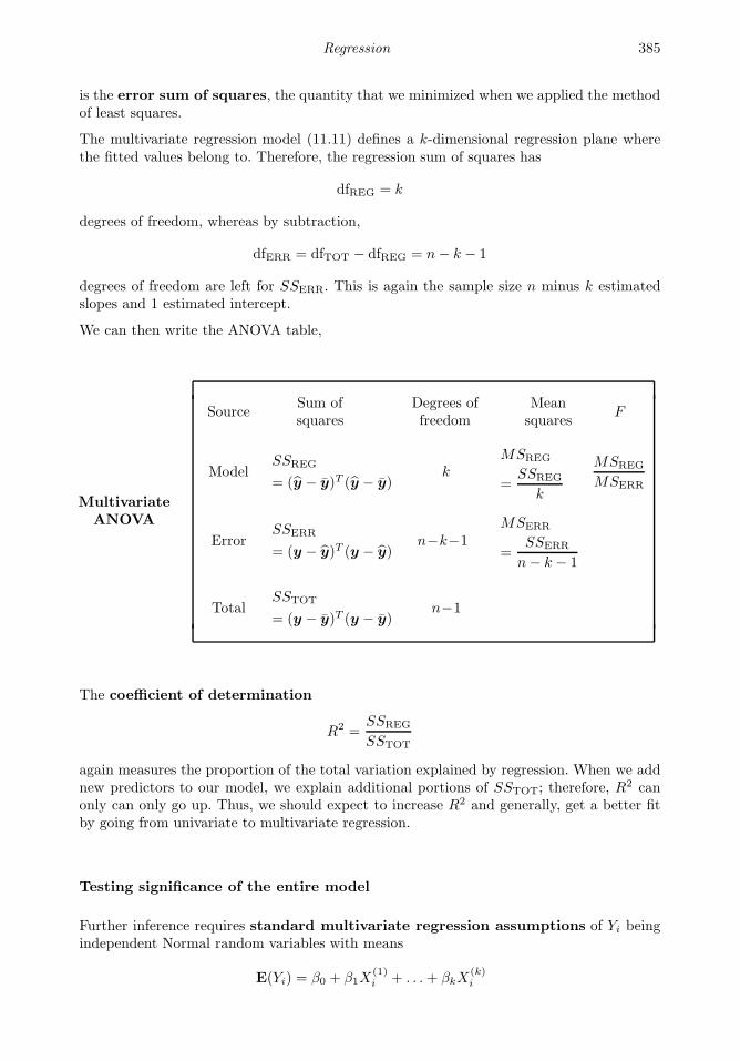
Regression 385
is the error sum of squares, the quantity that we minimized when we applied the methodof least squares.
The multivariate regression model (11.11) defines a k-dimensional regression plane wherethe fitted values belong to. Therefore, the regression sum of squares has
dfREG = k
degrees of freedom, whereas by subtraction,
dfERR = dfTOT − dfREG = n− k − 1
degrees of freedom are left for SSERR. This is again the sample size n minus k estimatedslopes and 1 estimated intercept.
We can then write the ANOVA table,
MultivariateANOVA
SourceSum ofsquares
Degrees offreedom
Meansquares
F
ModelSSREG
= (y − y)T (y − y)k
MSREG
=SSREG
k
MSREG
MSERR
ErrorSSERR
= (y − y)T (y − y)n−k−1
MSERR
=SSERR
n− k − 1
TotalSSTOT
= (y − y)T (y − y)n−1
The coefficient of determination
R2 =SSREG
SSTOT
again measures the proportion of the total variation explained by regression. When we addnew predictors to our model, we explain additional portions of SSTOT; therefore, R
2 canonly can only go up. Thus, we should expect to increase R2 and generally, get a better fitby going from univariate to multivariate regression.
Testing significance of the entire model
Further inference requires standard multivariate regression assumptions of Yi beingindependent Normal random variables with means
E(Yi) = β0 + β1X(1)i + . . .+ βkX
(k)i
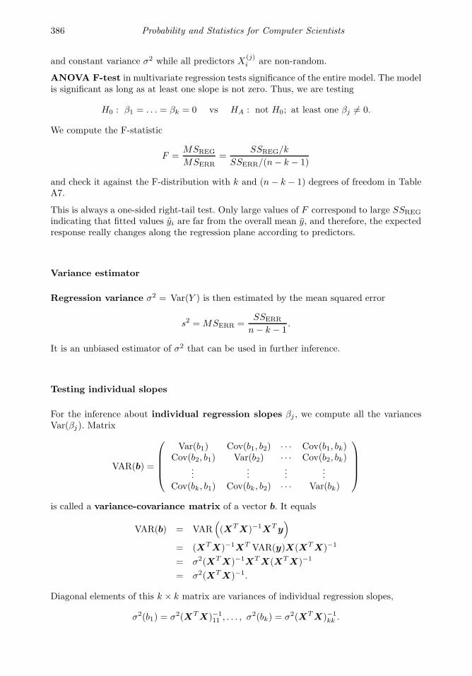
386 Probability and Statistics for Computer Scientists
and constant variance σ2 while all predictors X(j)i are non-random.
ANOVA F-test in multivariate regression tests significance of the entire model. The modelis significant as long as at least one slope is not zero. Thus, we are testing
H0 : β1 = . . . = βk = 0 vs HA : not H0; at least one βj 6= 0.
We compute the F-statistic
F =MSREG
MSERR=
SSREG/k
SSERR/(n− k − 1)
and check it against the F-distribution with k and (n− k − 1) degrees of freedom in TableA7.
This is always a one-sided right-tail test. Only large values of F correspond to large SSREG
indicating that fitted values yi are far from the overall mean y, and therefore, the expectedresponse really changes along the regression plane according to predictors.
Variance estimator
Regression variance σ2 = Var(Y ) is then estimated by the mean squared error
s2 = MSERR =SSERR
n− k − 1.
It is an unbiased estimator of σ2 that can be used in further inference.
Testing individual slopes
For the inference about individual regression slopes βj , we compute all the variancesVar(βj). Matrix
VAR(b) =
Var(b1) Cov(b1, b2) · · · Cov(b1, bk)Cov(b2, b1) Var(b2) · · · Cov(b2, bk)
......
......
Cov(bk, b1) Cov(bk, b2) · · · Var(bk)
is called a variance-covariance matrix of a vector b. It equals
VAR(b) = VAR((XTX)−1XTy
)
= (XTX)−1XT VAR(y)X(XTX)−1
= σ2(XTX)−1XTX(XTX)−1
= σ2(XTX)−1.
Diagonal elements of this k × k matrix are variances of individual regression slopes,
σ2(b1) = σ2(XTX)−111 , . . . , σ2(bk) = σ2(XTX)−1
kk .
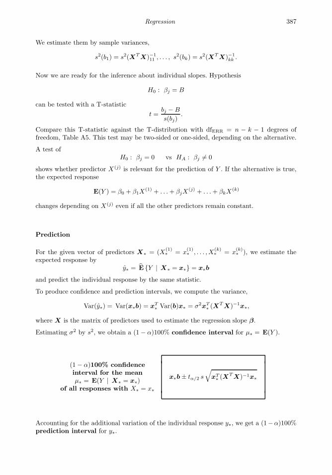
Regression 387
We estimate them by sample variances,
s2(b1) = s2(XTX)−111 , . . . , s2(bk) = s2(XTX)−1
kk .
Now we are ready for the inference about individual slopes. Hypothesis
H0 : βj = B
can be tested with a T-statistic
t =bj −B
s(bj).
Compare this T-statistic against the T-distribution with dfERR = n − k − 1 degrees offreedom, Table A5. This test may be two-sided or one-sided, depending on the alternative.
A test ofH0 : βj = 0 vs HA : βj 6= 0
shows whether predictor X(j) is relevant for the prediction of Y . If the alternative is true,the expected response
E(Y ) = β0 + β1X(1) + . . .+ βjX
(j) + . . .+ βkX(k)
changes depending on X(j) even if all the other predictors remain constant.
Prediction
For the given vector of predictors X∗ = (X(1)∗ = x
(1)∗ , . . . , X
(k)∗ = x
(k)∗ ), we estimate the
expected response byy∗ = E Y | X∗ = x∗ = x∗b
and predict the individual response by the same statistic.
To produce confidence and prediction intervals, we compute the variance,
Var(y∗) = Var(x∗b) = xT∗ Var(b)x∗ = σ2xT
∗ (XTX)−1x∗,
where X is the matrix of predictors used to estimate the regression slope β.
Estimating σ2 by s2, we obtain a (1− α)100% confidence interval for µ∗ = E(Y ).
(1 − α)100% confidenceinterval for the meanµ∗ = E(Y | X∗ = x∗)
of all responses with X∗ = x∗
x∗b± tα/2 s
√xT∗ (X
TX)−1x∗
Accounting for the additional variation of the individual response y∗, we get a (1−α)100%prediction interval for y∗.
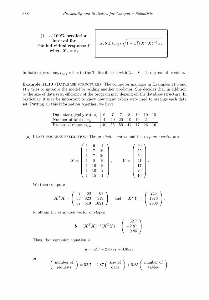
388 Probability and Statistics for Computer Scientists
(1− α)100% predictioninterval for
the individual response Ywhen X∗ = x∗
x∗b± tα/2 s
√1 + xT
∗ (XTX)−1x∗
In both expressions, tα/2 refers to the T-distribution with (n− k − 1) degrees of freedom.
Example 11.10 (Database structure). The computer manager in Examples 11.6 and11.7 tries to improve the model by adding another predictor. She decides that in additionto the size of data sets, efficiency of the program may depend on the database structure. Inparticular, it may be important to know how many tables were used to arrange each dataset. Putting all this information together, we have
Data size (gigabytes), x1 6 7 7 8 10 10 15Number of tables, x2 4 20 20 10 10 2 1
Processed requests, y 40 55 50 41 17 26 16
(a) Least squares estimation. The predictor matrix and the response vector are
X =
1 6 41 7 201 7 201 8 101 10 101 10 21 15 1
, Y =
40555041172616
.
We then compute
XTX =
7 63 6763 623 51967 519 1021
and XTY =
24519732908
,
to obtain the estimated vector of slopes
b = (XTX)−1(XTY ) =
52.7−2.870.85
.
Thus, the regression equation is
y = 52.7− 2.87x1 + 0.85x2,
or (number ofrequests
)= 52.7− 2.87
(size ofdata
)+ 0.85
(number oftables
).
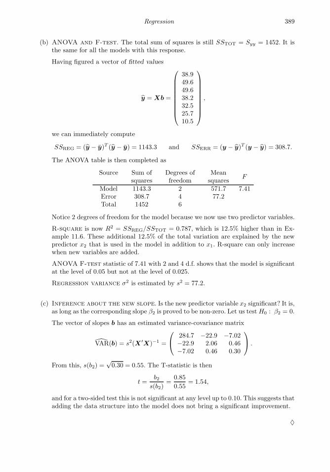
Regression 389
(b) ANOVA and F-test. The total sum of squares is still SSTOT = Syy = 1452. It isthe same for all the models with this response.
Having figured a vector of fitted values
y = Xb =
38.949.649.638.232.525.710.5
,
we can immediately compute
SSREG = (y − y)T (y − y) = 1143.3 and SSERR = (y − y)T (y − y) = 308.7.
The ANOVA table is then completed as
Source Sum ofsquares
Degrees offreedom
Meansquares
F
Model 1143.3 2 571.7 7.41Error 308.7 4 77.2Total 1452 6
Notice 2 degrees of freedom for the model because we now use two predictor variables.
R-square is now R2 = SSREG/SSTOT = 0.787, which is 12.5% higher than in Ex-ample 11.6. These additional 12.5% of the total variation are explained by the newpredictor x2 that is used in the model in addition to x1. R-square can only increasewhen new variables are added.
ANOVA F-test statistic of 7.41 with 2 and 4 d.f. shows that the model is significantat the level of 0.05 but not at the level of 0.025.
Regression variance σ2 is estimated by s2 = 77.2.
(c) Inference about the new slope. Is the new predictor variable x2 significant? It is,as long as the corresponding slope β2 is proved to be non-zero. Let us test H0 : β2 = 0.
The vector of slopes b has an estimated variance-covariance matrix
VAR(b) = s2(X ′X)−1 =
284.7 −22.9 −7.02−22.9 2.06 0.46−7.02 0.46 0.30
.
From this, s(b2) =√0.30 = 0.55. The T-statistic is then
t =b2
s(b2)=
0.85
0.55= 1.54,
and for a two-sided test this is not significant at any level up to 0.10. This suggests thatadding the data structure into the model does not bring a significant improvement.
♦
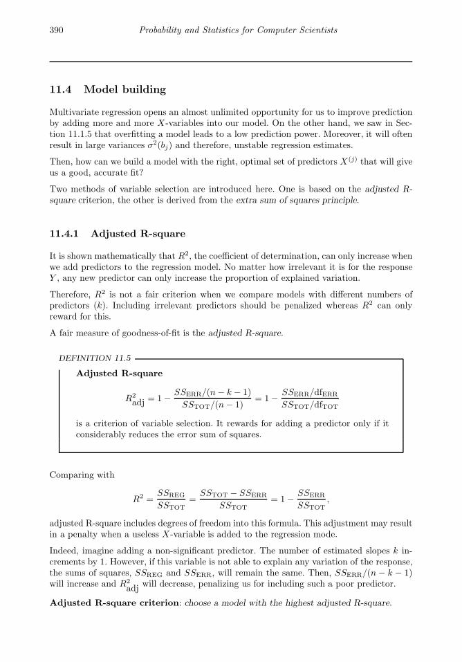
390 Probability and Statistics for Computer Scientists
11.4 Model building
Multivariate regression opens an almost unlimited opportunity for us to improve predictionby adding more and more X-variables into our model. On the other hand, we saw in Sec-tion 11.1.5 that overfitting a model leads to a low prediction power. Moreover, it will oftenresult in large variances σ2(bj) and therefore, unstable regression estimates.
Then, how can we build a model with the right, optimal set of predictors X(j) that will giveus a good, accurate fit?
Two methods of variable selection are introduced here. One is based on the adjusted R-square criterion, the other is derived from the extra sum of squares principle.
11.4.1 Adjusted R-square
It is shown mathematically that R2, the coefficient of determination, can only increase whenwe add predictors to the regression model. No matter how irrelevant it is for the responseY , any new predictor can only increase the proportion of explained variation.
Therefore, R2 is not a fair criterion when we compare models with different numbers ofpredictors (k). Including irrelevant predictors should be penalized whereas R2 can onlyreward for this.
A fair measure of goodness-of-fit is the adjusted R-square.
DEFINITION 11.5
Adjusted R-square
R2adj = 1− SSERR/(n− k − 1)
SSTOT/(n− 1)= 1− SSERR/dfERR
SSTOT/dfTOT
is a criterion of variable selection. It rewards for adding a predictor only if itconsiderably reduces the error sum of squares.
Comparing with
R2 =SSREG
SSTOT=
SSTOT − SSERR
SSTOT= 1− SSERR
SSTOT,
adjusted R-square includes degrees of freedom into this formula. This adjustment may resultin a penalty when a useless X-variable is added to the regression mode.
Indeed, imagine adding a non-significant predictor. The number of estimated slopes k in-crements by 1. However, if this variable is not able to explain any variation of the response,the sums of squares, SSREG and SSERR, will remain the same. Then, SSERR/(n− k − 1)will increase and R2
adj will decrease, penalizing us for including such a poor predictor.
Adjusted R-square criterion: choose a model with the highest adjusted R-square.

Regression 391
11.4.2 Extra sum of squares, partial F-tests, and variable selection
Suppose we have K predictors available for predicting a response. Technically, to select asubset that maximizes adjusted R-square, we need to fit all 2K models and choose the onewith the highest R2
adj. This is possible for rather moderate K, and such schemes are built
in some statistical software.
Fitting all models is not feasible when the total number of predictors is large. Instead, weconsider a sequential scheme that will follow a reasonable path through possible regressionmodels and consider only a few of them. At every step, it will compare some set of predictors
X(Full) =(X(1), . . . , X(k), X(k+1), . . . , X(m)
)
and the corresponding full model
E(Y | X = x) = β0 + β1x(1) + . . .+ βkx
(k) + βk+1x(k+1) + . . .+ βmx(m)
with a subsetX(Reduced) =
(X(1), . . . , X(k)
)
and the corresponding reduced model
E(Y | X = x) = β0 + β1x(1) + . . .+ βkx
(k).
If the full model is significantly better, expanding the set of predictors is justified. If it isjust as good as the reduced model, we should keep the smaller number of predictors in orderto attain lower variances of the estimated regression slopes, more accurate predictions, anda lower adjusted R-square.
DEFINITION 11.6
A model with a larger set of predictors is called a full model.
Including only a subset of predictors, we obtain a reduced model.
The difference in the variation explained by the two models is the extra sumof squares,
SSEX = SSREG(Full)− SSREG(Reduced)
= SSERR(Reduced)− SSERR(Full).
Extra sum of squares measures the additional amount of variation explained by additionalpredictors X(k+1), . . . , X(m). By subtraction, it has
dfEX = dfREG(Full)− dfREG(Reduced) = m− k
degrees of freedom.
Significance of the additional explained variation (measured by SSEX) is tested by a partialF-test statistic
F =SSEX/dfEX
MSERR(Full)=
SSERR(Reduced)− SSERR(Full)
SSERR(Full)
(n−m− 1
m− k
).
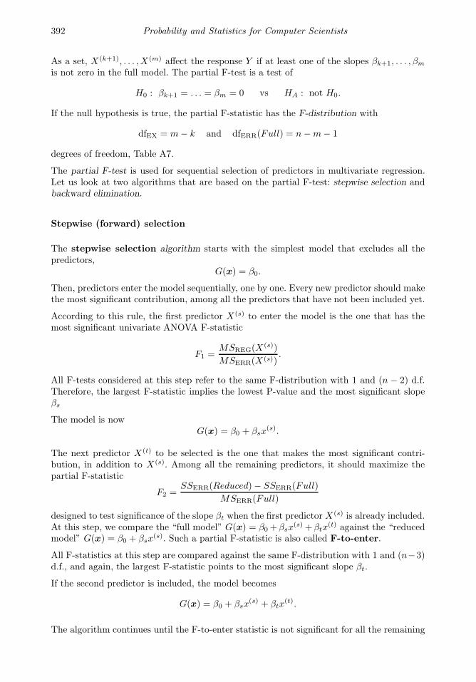
392 Probability and Statistics for Computer Scientists
As a set, X(k+1), . . . , X(m) affect the response Y if at least one of the slopes βk+1, . . . , βm
is not zero in the full model. The partial F-test is a test of
H0 : βk+1 = . . . = βm = 0 vs HA : not H0.
If the null hypothesis is true, the partial F-statistic has the F-distribution with
dfEX = m− k and dfERR(Full) = n−m− 1
degrees of freedom, Table A7.
The partial F-test is used for sequential selection of predictors in multivariate regression.Let us look at two algorithms that are based on the partial F-test: stepwise selection andbackward elimination.
Stepwise (forward) selection
The stepwise selection algorithm starts with the simplest model that excludes all thepredictors,
G(x) = β0.
Then, predictors enter the model sequentially, one by one. Every new predictor should makethe most significant contribution, among all the predictors that have not been included yet.
According to this rule, the first predictor X(s) to enter the model is the one that has themost significant univariate ANOVA F-statistic
F1 =MSREG(X
(s))
MSERR(X(s)).
All F-tests considered at this step refer to the same F-distribution with 1 and (n − 2) d.f.Therefore, the largest F-statistic implies the lowest P-value and the most significant slopeβs
The model is nowG(x) = β0 + βsx
(s).
The next predictor X(t) to be selected is the one that makes the most significant contri-bution, in addition to X(s). Among all the remaining predictors, it should maximize thepartial F-statistic
F2 =SSERR(Reduced)− SSERR(Full)
MSERR(Full)
designed to test significance of the slope βt when the first predictor X(s) is already included.At this step, we compare the “full model” G(x) = β0 +βsx
(s) +βtx(t) against the “reduced
model” G(x) = β0 + βsx(s). Such a partial F-statistic is also called F-to-enter.
All F-statistics at this step are compared against the same F-distribution with 1 and (n−3)d.f., and again, the largest F-statistic points to the most significant slope βt.
If the second predictor is included, the model becomes
G(x) = β0 + βsx(s) + βtx
(t).
The algorithm continues until the F-to-enter statistic is not significant for all the remaining
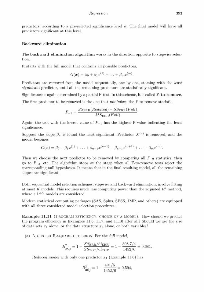
Regression 393
predictors, according to a pre-selected significance level α. The final model will have allpredictors significant at this level.
Backward elimination
The backward elimination algorithm works in the direction opposite to stepwise selec-tion.
It starts with the full model that contains all possible predictors,
G(x) = β0 + β1x(1) + . . .+ βmx(m).
Predictors are removed from the model sequentially, one by one, starting with the leastsignificant predictor, until all the remaining predictors are statistically significant.
Significance is again determined by a partial F-test. In this scheme, it is calledF-to-remove.
The first predictor to be removed is the one that minimizes the F-to-remove statistic
F−1 =SSERR(Reduced)− SSERR(Full)
MSERR(Full).
Again, the test with the lowest value of F−1 has the highest P-value indicating the leastsignificance.
Suppose the slope βu is found the least significant. Predictor X(u) is removed, and themodel becomes
G(x) = β0 + β1x(1) + . . .+ βu−1x
(u−1) + βu+1x(u+1) + . . .+ βmx(m).
Then we choose the next predictor to be removed by comparing all F−2 statistics, thengo to F−3, etc. The algorithm stops at the stage when all F-to-remove tests reject thecorresponding null hypotheses. It means that in the final resulting model, all the remainingslopes are significant.
Both sequential model selection schemes, stepwise and backward elimination, involve fittingat most K models. This requires much less computing power than the adjusted R2 method,where all 2K models are considered.
Modern statistical computing packages (SAS, Splus, SPSS, JMP, and others) are equippedwith all three considered model selection procedures.
Example 11.11 (Program efficiency: choice of a model). How should we predictthe program efficiency in Examples 11.6, 11.7, and 11.10 after all? Should we use the sizeof data sets x1 alone, or the data structure x2 alone, or both variables?
(a) Adjusted R-square criterion. For the full model,
R2adj = 1− SSERR/dfERR
SSTOT/dfTOT= 1− 308.7/4
1452/6= 0.681.
Reduced model with only one predictor x1 (Example 11.6) has
R2adj = 1− 491/5
1452/6= 0.594,
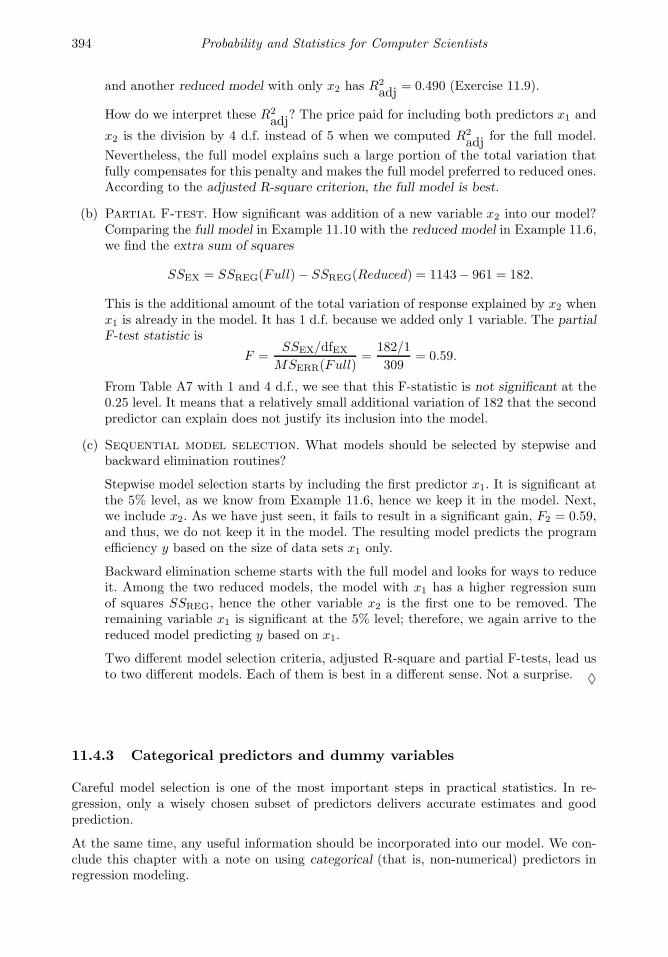
394 Probability and Statistics for Computer Scientists
and another reduced model with only x2 has R2adj = 0.490 (Exercise 11.9).
How do we interpret these R2adj? The price paid for including both predictors x1 and
x2 is the division by 4 d.f. instead of 5 when we computed R2adj for the full model.
Nevertheless, the full model explains such a large portion of the total variation thatfully compensates for this penalty and makes the full model preferred to reduced ones.According to the adjusted R-square criterion, the full model is best.
(b) Partial F-test. How significant was addition of a new variable x2 into our model?Comparing the full model in Example 11.10 with the reduced model in Example 11.6,we find the extra sum of squares
SSEX = SSREG(Full)− SSREG(Reduced) = 1143− 961 = 182.
This is the additional amount of the total variation of response explained by x2 whenx1 is already in the model. It has 1 d.f. because we added only 1 variable. The partialF-test statistic is
F =SSEX/dfEX
MSERR(Full)=
182/1
309= 0.59.
From Table A7 with 1 and 4 d.f., we see that this F-statistic is not significant at the0.25 level. It means that a relatively small additional variation of 182 that the secondpredictor can explain does not justify its inclusion into the model.
(c) Sequential model selection. What models should be selected by stepwise andbackward elimination routines?
Stepwise model selection starts by including the first predictor x1. It is significant atthe 5% level, as we know from Example 11.6, hence we keep it in the model. Next,we include x2. As we have just seen, it fails to result in a significant gain, F2 = 0.59,and thus, we do not keep it in the model. The resulting model predicts the programefficiency y based on the size of data sets x1 only.
Backward elimination scheme starts with the full model and looks for ways to reduceit. Among the two reduced models, the model with x1 has a higher regression sumof squares SSREG, hence the other variable x2 is the first one to be removed. Theremaining variable x1 is significant at the 5% level; therefore, we again arrive to thereduced model predicting y based on x1.
Two different model selection criteria, adjusted R-square and partial F-tests, lead usto two different models. Each of them is best in a different sense. Not a surprise. ♦
11.4.3 Categorical predictors and dummy variables
Careful model selection is one of the most important steps in practical statistics. In re-gression, only a wisely chosen subset of predictors delivers accurate estimates and goodprediction.
At the same time, any useful information should be incorporated into our model. We con-clude this chapter with a note on using categorical (that is, non-numerical) predictors inregression modeling.
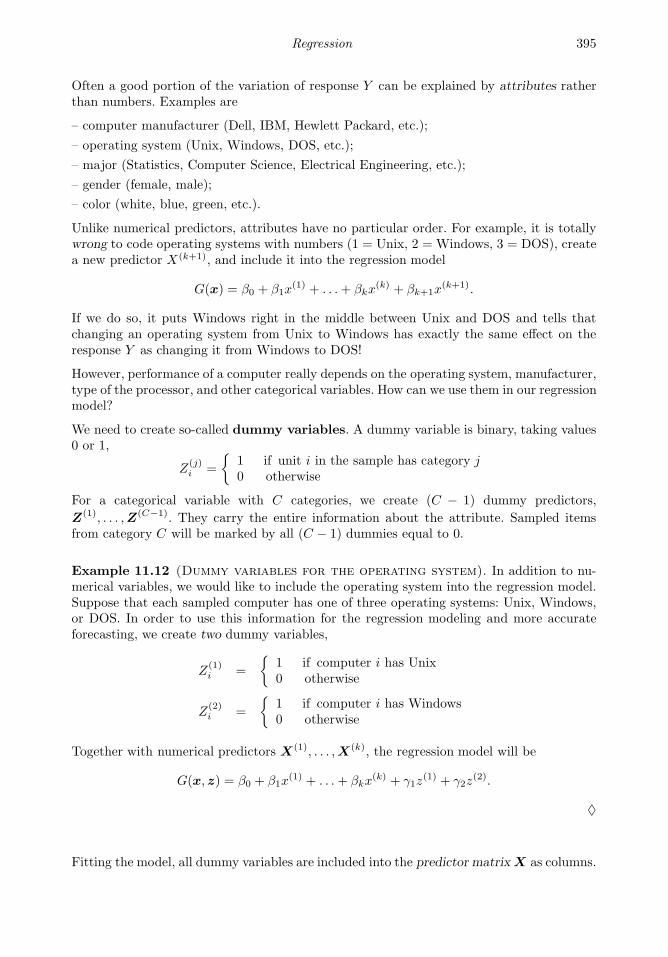
Regression 395
Often a good portion of the variation of response Y can be explained by attributes ratherthan numbers. Examples are
– computer manufacturer (Dell, IBM, Hewlett Packard, etc.);
– operating system (Unix, Windows, DOS, etc.);
– major (Statistics, Computer Science, Electrical Engineering, etc.);
– gender (female, male);
– color (white, blue, green, etc.).
Unlike numerical predictors, attributes have no particular order. For example, it is totallywrong to code operating systems with numbers (1 = Unix, 2 = Windows, 3 = DOS), createa new predictor X(k+1), and include it into the regression model
G(x) = β0 + β1x(1) + . . .+ βkx
(k) + βk+1x(k+1).
If we do so, it puts Windows right in the middle between Unix and DOS and tells thatchanging an operating system from Unix to Windows has exactly the same effect on theresponse Y as changing it from Windows to DOS!
However, performance of a computer really depends on the operating system, manufacturer,type of the processor, and other categorical variables. How can we use them in our regressionmodel?
We need to create so-called dummy variables. A dummy variable is binary, taking values0 or 1,
Z(j)i =
1 if unit i in the sample has category j0 otherwise
For a categorical variable with C categories, we create (C − 1) dummy predictors,
Z(1), . . . ,Z(C−1). They carry the entire information about the attribute. Sampled itemsfrom category C will be marked by all (C − 1) dummies equal to 0.
Example 11.12 (Dummy variables for the operating system). In addition to nu-merical variables, we would like to include the operating system into the regression model.Suppose that each sampled computer has one of three operating systems: Unix, Windows,or DOS. In order to use this information for the regression modeling and more accurateforecasting, we create two dummy variables,
Z(1)i =
1 if computer i has Unix0 otherwise
Z(2)i =
1 if computer i has Windows0 otherwise
Together with numerical predictors X(1), . . . ,X(k), the regression model will be
G(x, z) = β0 + β1x(1) + . . .+ βkx
(k) + γ1z(1) + γ2z
(2).
♦
Fitting the model, all dummy variables are included into the predictor matrixX as columns.

396 Probability and Statistics for Computer Scientists
Avoid singularity by creating only (C − 1) dummies
Notice that if we make a mistake and create C dummies for an attribute with C categories,one dummy per category, this would cause a linear relation
Z(1) + . . .+Z(C) = 1.
A column of 1’s is already included into the predictor matrix X, and therefore, such a linearrelation will cause singularity of (XTX) when we compute the least squares estimatesb = (XTX)−1XTy. Thus, it is necessary and sufficient to have only (C − 1) dummyvariables.
Interpretation of slopes for dummy variables
Each slope γj for a dummy predictor Z(j) is the expected change in the response causedby incrementing Z(j) by 1 while keeping all other predictors constant. Such an incrementoccurs when we compare the last category C with category j.
Thus, the slope γj is the difference in the expected response comparing category C withcategory j. The difference of two slopes (γj − γC) compares category j with category C.
To test significance of a categorical variable, we test all the corresponding slopes γj simul-taneously. This is done by a partial F-test.
Matlab notes
MATLAB (MATrix LABoratory) is great for matrix computations, so all the regressionanalysis can be done by writing the matrix formulas, b=inv(X’*X)*(X*Y) for the regressionslope, Yhat=X*b for the fitted values, e=Y-Yhat for residuals, etc., given a vector of responsesY and a matrix of predictors X . For more instructions on that, see the last paragraph ofSection 12.4.
Also, MATLAB’s Statistics Toolbox has special tools for regression. The gen-eral command regress(Y,X) returns a sample regression slope with a responseY and predictor X . Notice that if you’d like to fit regression with an inter-cept, then the vector of ones has to be included into matrix X . For example,
−30 −20 −10 0 10 20 30
X1
X2
X3
Coefficients with Error Bars Coeff. t−stat p−val
0 0.0000 1.0000
−4.14286 −3.1290 0.0260
0.84741 1.5366 0.1992
1 25
10
15
20Model History
RM
SE
FIGURE 11.7: Stepwise variable selectionto model program efficiency, Example 11.11.
X0 = ones(size(Y));
regress(Y,[X0,X1,X2]);
will create a vector of ones of the same sizeas the vector of responses and use it to fit aregression model Y = β0+β1X1+β2X2+ε.To get (1−α)100% confidence intervals forall the regression slopes, write [b bint] =
regress(Y,[X0,X1,X2],alpha).
Many components of the regression anal-ysis are available by the commandregstats(Y,X). A list of options appears

Exercises 397
where you can mark which statistics you’d like to obtain – mean squared error s2, ANOVAF-statistic, R2, R2
adj, etc.
You can also use stepwise(X,Y) to select variables for the multivariate regression. A windowopens such as on Figure 11.7, and the stepwise variable selection algorithm runs, reportingthe vital regression statistics at each step.
Summary and conclusions
This chapter provides methods of estimating mathematical relations between one or severalpredictor variables and a response variable. Results are used to explain behavior of theresponse and to predict its value for any new set of predictors.
Method of least squares is used to estimate regression parameters. Coefficient of determi-nation R2 shows the portion of the total variation that the included predictors can explain.The unexplained portion is considered as “error.”
Analysis of variance (ANOVA) partitions the total variation into explained and unexplainedparts and estimates regression variance by the mean squared error. This allows furtherstatistical inference, testing slopes, constructing confidence intervals for mean responsesand prediction intervals for individual responses. ANOVA F-test is used to test significanceof the entire model.
For accurate estimation and efficient prediction, it is important to select the right subsetof predictors. Sequential model selection algorithms are based on partial F-tests comparingfull and reduced models at each step.
Categorical predictors are included into regression modeling by creating dummy variables.
Exercises
Suppose that the standard regression assumptions, univariate or multivariate, hold in Ex-ercises 11.2, 11.3, 11.4, 11.5, 11.9, 11.14, and 11.15.
11.1. The time it takes to transmit a file always depends on the file size. Suppose you transmitted30 files, with the average size of 126 Kbytes and the standard deviation of 35 Kbytes. Theaverage transmittance time was 0.04 seconds with the standard deviation of 0.01 seconds.The correlation coefficient between the time and the size was 0.86.
Based on this data, fit a linear regression model and predict the time it will take to transmita 400 Kbyte file.
11.2. The following statistics were obtained from a sample of size n = 75:– the predictor variable X has mean 32.2, variance 6.4;
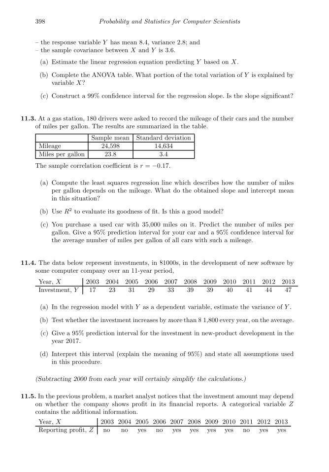
398 Probability and Statistics for Computer Scientists
– the response variable Y has mean 8.4, variance 2.8; and– the sample covariance between X and Y is 3.6.
(a) Estimate the linear regression equation predicting Y based on X .
(b) Complete the ANOVA table. What portion of the total variation of Y is explained byvariable X?
(c) Construct a 99% confidence interval for the regression slope. Is the slope significant?
11.3. At a gas station, 180 drivers were asked to record the mileage of their cars and the numberof miles per gallon. The results are summarized in the table.
Sample mean Standard deviation
Mileage 24,598 14,634
Miles per gallon 23.8 3.4
The sample correlation coefficient is r = −0.17.
(a) Compute the least squares regression line which describes how the number of milesper gallon depends on the mileage. What do the obtained slope and intercept meanin this situation?
(b) Use R2 to evaluate its goodness of fit. Is this a good model?
(c) You purchase a used car with 35,000 miles on it. Predict the number of miles pergallon. Give a 95% prediction interval for your car and a 95% confidence interval forthe average number of miles per gallon of all cars with such a mileage.
11.4. The data below represent investments, in $1000s, in the development of new software bysome computer company over an 11-year period,
Year, X 2003 2004 2005 2006 2007 2008 2009 2010 2011 2012 2013
Investment, Y 17 23 31 29 33 39 39 40 41 44 47
(a) In the regression model with Y as a dependent variable, estimate the variance of Y .
(b) Test whether the investment increases bymore than $ 1,800 every year, on the average.
(c) Give a 95% prediction interval for the investment in new-product development in theyear 2017.
(d) Interpret this interval (explain the meaning of 95%) and state all assumptions usedin this procedure.
(Subtracting 2000 from each year will certainly simplify the calculations.)
11.5. In the previous problem, a market analyst notices that the investment amount may dependon whether the company shows profit in its financial reports. A categorical variable Zcontains the additional information.
Year, X 2003 2004 2005 2006 2007 2008 2009 2010 2011 2012 2013Reporting profit, Z no no yes no yes yes yes yes no yes yes

Exercises 399
(a) Add a dummy variable to the model considered in Exercise 11.4 and estimate theintercept and slopes of the new multivariate regression model.
(b) If the company will report a profit during year 2015, predict the investment amount.
(c) How would your prediction change if the company reports a loss during year 2015?
(d) Complete a multivariate ANOVA table and test significance of the entire model.
(e) Does the new variable Z explain a significant portion of the total variation, in additionto the time trend?
11.6. For a univariate linear regression, show that
SSTOT = SSREG + SSERR.
Hint: Write SSTOT =∑n
i=1(yi − y)2 =∑n
i=1((yi − yi) + (yi − y))2.
11.7. For a univariate linear regression, show that R-square is the squared sample correlationcoefficient,
R2 = r2.
Hint: Write the regression sum of squares as
SSREG =
n∑
i=1
(b0 + b1 xi − y)2
and substitute our derived expressions for the regression intercept b0 and slope b1.
11.8. Anton wants to know if there is a relation between the number of hours he spends preparingfor his weekly quiz and the grade he receives on it. He keeps records for 10 weeks.
It turns out that on the average, he spends 3.6 hours a week preparing for the quiz, withthe standard deviation of 0.5 hours. His average grade is 82 (out of 100), with the standarddeviation of 14. The correlation between the two variables is r = 0.62.
(a) Find the equation of the regression line predicting the quiz grade based on the timespent on preparation.
(b) This week, Anton studied for 4 hours. Predict his grade.
(c) Does this linear model explain most of the variation? Is it a good fit? Why?
11.9. For the data in Example 11.10, fit a linear regression model predicting the program effi-ciency (number of processed requests) based on the database structure x2 only. Completethe ANOVA table, compute R-square and adjusted R-square. Is this reduced model signif-icant?
11.10. Refer to Exercise 8.5 on p. 234.
(a) Fit a linear regression model estimating the time trend of the U.S. population. Forsimplicity, subtract 1800 from each year and let x = year− 1800 serve as a predictor.
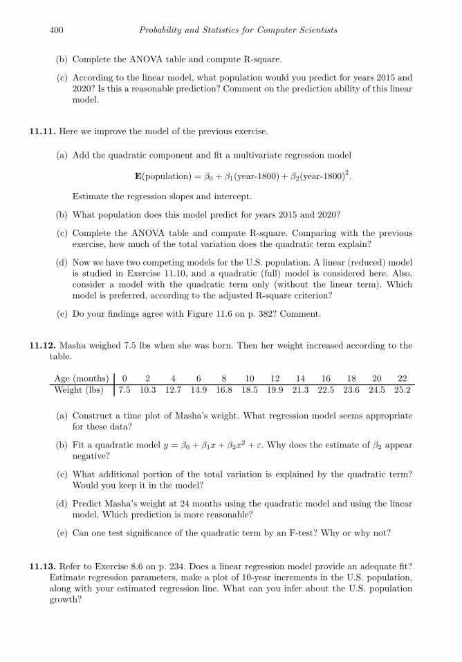
400 Probability and Statistics for Computer Scientists
(b) Complete the ANOVA table and compute R-square.
(c) According to the linear model, what population would you predict for years 2015 and2020? Is this a reasonable prediction? Comment on the prediction ability of this linearmodel.
11.11. Here we improve the model of the previous exercise.
(a) Add the quadratic component and fit a multivariate regression model
E(population) = β0 + β1(year-1800)+ β2(year-1800)2.
Estimate the regression slopes and intercept.
(b) What population does this model predict for years 2015 and 2020?
(c) Complete the ANOVA table and compute R-square. Comparing with the previousexercise, how much of the total variation does the quadratic term explain?
(d) Now we have two competing models for the U.S. population. A linear (reduced) modelis studied in Exercise 11.10, and a quadratic (full) model is considered here. Also,consider a model with the quadratic term only (without the linear term). Whichmodel is preferred, according to the adjusted R-square criterion?
(e) Do your findings agree with Figure 11.6 on p. 382? Comment.
11.12. Masha weighed 7.5 lbs when she was born. Then her weight increased according to thetable.
Age (months) 0 2 4 6 8 10 12 14 16 18 20 22Weight (lbs) 7.5 10.3 12.7 14.9 16.8 18.5 19.9 21.3 22.5 23.6 24.5 25.2
(a) Construct a time plot of Masha’s weight. What regression model seems appropriatefor these data?
(b) Fit a quadratic model y = β0 + β1x+ β2x2 + ε. Why does the estimate of β2 appear
negative?
(c) What additional portion of the total variation is explained by the quadratic term?Would you keep it in the model?
(d) Predict Masha’s weight at 24 months using the quadratic model and using the linearmodel. Which prediction is more reasonable?
(e) Can one test significance of the quadratic term by an F-test? Why or why not?
11.13. Refer to Exercise 8.6 on p. 234. Does a linear regression model provide an adequate fit?Estimate regression parameters, make a plot of 10-year increments in the U.S. population,along with your estimated regression line. What can you infer about the U.S. populationgrowth?
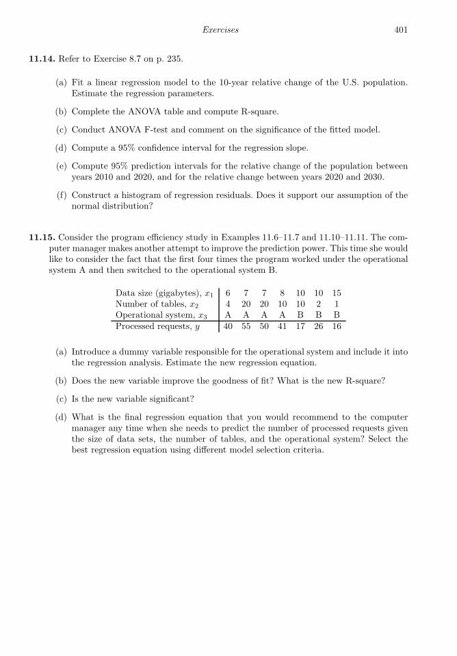
Exercises 401
11.14. Refer to Exercise 8.7 on p. 235.
(a) Fit a linear regression model to the 10-year relative change of the U.S. population.Estimate the regression parameters.
(b) Complete the ANOVA table and compute R-square.
(c) Conduct ANOVA F-test and comment on the significance of the fitted model.
(d) Compute a 95% confidence interval for the regression slope.
(e) Compute 95% prediction intervals for the relative change of the population betweenyears 2010 and 2020, and for the relative change between years 2020 and 2030.
(f) Construct a histogram of regression residuals. Does it support our assumption of thenormal distribution?
11.15. Consider the program efficiency study in Examples 11.6–11.7 and 11.10–11.11. The com-puter manager makes another attempt to improve the prediction power. This time she wouldlike to consider the fact that the first four times the program worked under the operationalsystem A and then switched to the operational system B.
Data size (gigabytes), x1 6 7 7 8 10 10 15Number of tables, x2 4 20 20 10 10 2 1Operational system, x3 A A A A B B BProcessed requests, y 40 55 50 41 17 26 16
(a) Introduce a dummy variable responsible for the operational system and include it intothe regression analysis. Estimate the new regression equation.
(b) Does the new variable improve the goodness of fit? What is the new R-square?
(c) Is the new variable significant?
(d) What is the final regression equation that you would recommend to the computermanager any time when she needs to predict the number of processed requests giventhe size of data sets, the number of tables, and the operational system? Select thebest regression equation using different model selection criteria.


Part IV
Appendix
403

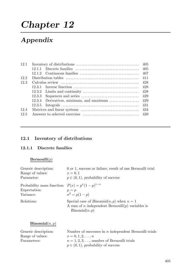
Chapter 12
Appendix
12.1 Inventory of distributions . . . . . . . . . . . . . . . . . . . . . . . . . . . . . . . . . . . . . . . . 40512.1.1 Discrete families . . . . . . . . . . . . . . . . . . . . . . . . . . . . . . . . . . . . . . . . . 40512.1.2 Continuous families . . . . . . . . . . . . . . . . . . . . . . . . . . . . . . . . . . . . . . 407
12.2 Distribution tables . . . . . . . . . . . . . . . . . . . . . . . . . . . . . . . . . . . . . . . . . . . . . . . 41112.3 Calculus review . . . . . . . . . . . . . . . . . . . . . . . . . . . . . . . . . . . . . . . . . . . . . . . . . . 428
12.3.1 Inverse function . . . . . . . . . . . . . . . . . . . . . . . . . . . . . . . . . . . . . . . . . . 42812.3.2 Limits and continuity . . . . . . . . . . . . . . . . . . . . . . . . . . . . . . . . . . . . 42812.3.3 Sequences and series . . . . . . . . . . . . . . . . . . . . . . . . . . . . . . . . . . . . . 42912.3.4 Derivatives, minimum, and maximum . . . . . . . . . . . . . . . . . . . 42912.3.5 Integrals . . . . . . . . . . . . . . . . . . . . . . . . . . . . . . . . . . . . . . . . . . . . . . . . . 431
12.4 Matrices and linear systems . . . . . . . . . . . . . . . . . . . . . . . . . . . . . . . . . . . . . 43412.5 Answers to selected exercises . . . . . . . . . . . . . . . . . . . . . . . . . . . . . . . . . . . . 439
12.1 Inventory of distributions
12.1.1 Discrete families
Bernoulli(p)
Generic description: 0 or 1, success or failure, result of one Bernoulli trialRange of values: x = 0, 1Parameter: p ∈ (0, 1), probability of success
Probability mass function: P (x) = px(1− p)1−x
Expectation: µ = pVariance: σ2 = p(1− p)
Relations: Special case of Binomial(n, p) when n = 1A sum of n independent Bernoulli(p) variables isBinomial(n, p)
Binomial(n, p)
Generic description: Number of successes in n independent Bernoulli trialsRange of values: x = 0, 1, 2, . . . , nParameters: n = 1, 2, 3, . . ., number of Bernoulli trials
p ∈ (0, 1), probability of success
405

406 Probability and Statistics for Computer Scientists
Probability mass function: P (x) =( n
x
)px(1 − p)n−x
Cdf: Table A2Expectation: µ = npVariance: σ2 = np(1− p)
Relations: Binomial(n, p) is a sum of n independent Bernoulli(p)variables
Binomial(1, p) = Bernoulli(p)Table: Appendix, Table A2MATLAB: binocdf, binopdf, binornd
Geometric(p)
Generic description: Number of Bernoulli trials until the first successRange of values: x = 1, 2, 3, . . .Parameter: p ∈ (0, 1), probability of success
Probability mass function: P (x) = p(1− p)x−1
Cdf: 1− (1 − p)x
Expectation: µ =1
p
Variance: σ2 =1− p
p2
Relations: Special case of Negative Binomial(k, p) when k = 1A sum of n independent Geometric(p) variables isNegative Binomial(n, p)
MATLAB: geocdf, geopdf, geornd
Negative Binomial(k, p)
Generic description: Number of Bernoulli trials until the kth successRange of values: x = k, k + 1, k + 2, . . .Parameters: k = 1, 2, 3, . . ., number of successes
p ∈ (0, 1), probability of success
Probability mass function: P (x) =(x− 1k − 1
)(1− p)x−kpk
Expectation: µ =k
p
Variance: σ2 =k(1− p)
p2
Relations: Negative Binomial(k, p) is a sum of n independentGeometric(p) variables
Negative Binomial(1, p) = Geometric(p)MATLAB: nbincdf, nbinpdf, nbinrnd
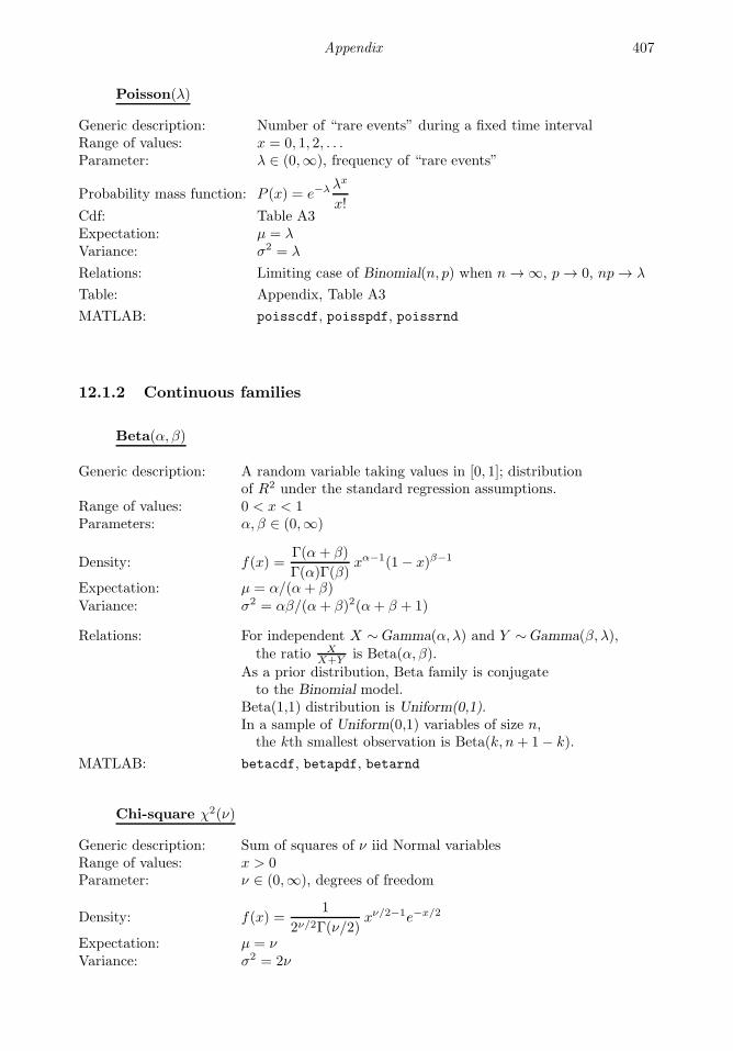
Appendix 407
Poisson(λ)
Generic description: Number of “rare events” during a fixed time intervalRange of values: x = 0, 1, 2, . . .Parameter: λ ∈ (0,∞), frequency of “rare events”
Probability mass function: P (x) = e−λλx
x!Cdf: Table A3Expectation: µ = λVariance: σ2 = λ
Relations: Limiting case of Binomial(n, p) when n → ∞, p → 0, np → λ
Table: Appendix, Table A3
MATLAB: poisscdf, poisspdf, poissrnd
12.1.2 Continuous families
Beta(α, β)
Generic description: A random variable taking values in [0, 1]; distributionof R2 under the standard regression assumptions.
Range of values: 0 < x < 1Parameters: α, β ∈ (0,∞)
Density: f(x) =Γ(α+ β)
Γ(α)Γ(β)xα−1(1− x)β−1
Expectation: µ = α/(α+ β)Variance: σ2 = αβ/(α+ β)2(α+ β + 1)
Relations: For independent X ∼Gamma(α, λ) and Y ∼Gamma(β, λ),the ratio X
X+Y is Beta(α, β).
As a prior distribution, Beta family is conjugateto the Binomial model.
Beta(1,1) distribution is Uniform(0,1).In a sample of Uniform(0,1) variables of size n,the kth smallest observation is Beta(k, n+ 1− k).
MATLAB: betacdf, betapdf, betarnd
Chi-square χ2(ν)
Generic description: Sum of squares of ν iid Normal variablesRange of values: x > 0Parameter: ν ∈ (0,∞), degrees of freedom
Density: f(x) =1
2ν/2Γ(ν/2)xν/2−1e−x/2
Expectation: µ = νVariance: σ2 = 2ν
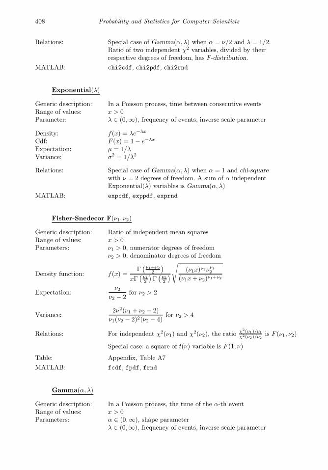
408 Probability and Statistics for Computer Scientists
Relations: Special case of Gamma(α, λ) when α = ν/2 and λ = 1/2.Ratio of two independent χ2 variables, divided by theirrespective degrees of freedom, has F-distribution.
MATLAB: chi2cdf, chi2pdf, chi2rnd
Exponential(λ)
Generic description: In a Poisson process, time between consecutive eventsRange of values: x > 0Parameter: λ ∈ (0,∞), frequency of events, inverse scale parameter
Density: f(x) = λe−λx
Cdf: F (x) = 1− e−λx
Expectation: µ = 1/λVariance: σ2 = 1/λ2
Relations: Special case of Gamma(α, λ) when α = 1 and chi-squarewith ν = 2 degrees of freedom. A sum of α independentExponential(λ) variables is Gamma(α, λ)
MATLAB: expcdf, exppdf, exprnd
Fisher-Snedecor F(ν1, ν2)
Generic description: Ratio of independent mean squaresRange of values: x > 0Parameters: ν1 > 0, numerator degrees of freedom
ν2 > 0, denominator degrees of freedom
Density function: f(x) =Γ(ν1+ν2
2
)
xΓ(ν12
)Γ(ν22
)√
(ν1x)ν1νν22
(ν1x+ ν2)ν1+ν2
Expectation:ν2
ν2 − 2for ν2 > 2
Variance:2ν2(ν1 + ν2 − 2)
ν1(ν2 − 2)2(ν2 − 4)for ν2 > 4
Relations: For independent χ2(ν1) and χ2(ν2), the ratio χ2(ν1)/ν1χ2(ν2)/ν2
is F (ν1, ν2)
Special case: a square of t(ν) variable is F (1, ν)
Table: Appendix, Table A7
MATLAB: fcdf, fpdf, frnd
Gamma(α, λ)
Generic description: In a Poisson process, the time of the α-th eventRange of values: x > 0Parameters: α ∈ (0,∞), shape parameter
λ ∈ (0,∞), frequency of events, inverse scale parameter

Appendix 409
Density function: f(x) =λα
Γ(α)xα−1e−λx
Expectation: µ = α/λVariance: σ2 = α/λ2
Relations: For integer α, Gamma(α, λ) is a sum of α independentExponential(λ) variables
Gamma(1, λ) = Exponential(λ)Gamma(ν/2, 1/2) = Chi-square(ν)As a prior distribution, Gamma family is conjugate tothe Poisson(θ) model and the Exponential(θ) model.
MATLAB: gamcdf, gampdf, gamrnd
Normal(µ, σ)
Generic description: Often used as distribution of errors, measurements, sums,averages, etc.
Range of values: −∞ < x < +∞Parameters: µ ∈ (−∞,∞), expectation, location parameter
σ ∈ (0,∞), standard deviation, scale parameter
Density function: f(x) =1
σ√2π
exp
−(x− µ)2
2σ2
Cdf: F (x) = Φ
(x− µ
σ
), use Table A4 for Φ(z)
Expectation: µVariance: σ2
Relations: Limiting case of standardized sums of random variables,including Binomial(n, p), Negative Binomial(k, p),and Gamma(α, λ), as n, k, α → ∞
Table: Appendix, Table A4MATLAB: normcdf, normpdf, normrnd, or just randn
Pareto(θ, σ)
Generic description: A heavy-tail distribution often used to model amount ofinternet traffic, various financial and sociological data
Range of values: x > σParameters: θ ∈ (0,∞), shape parameter
σ ∈ (0,∞), scale parameter
Density function: f(x) = θσθx−θ−1
Cdf: F (x) = 1−(xσ
)−θ
Expectation:θσ
θ − 1for θ > 1; does not exist for θ ≤ 1
Variance:θσ2
(θ − 1)2(θ − 2)for θ > 2; does not exist for θ ≤ 2
Relations: If X is Exponential(θ) then Y = σeX is Pareto(θ, σ)
MATLAB: gpcdf, gppdf, gprnd
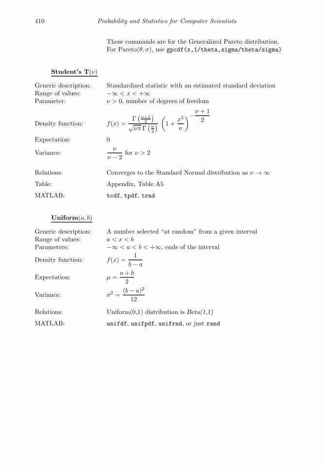
410 Probability and Statistics for Computer Scientists
These commands are for the Generalized Pareto distribution.For Pareto(θ, σ), use gpcdf(x,1/theta,sigma/theta/sigma)
Student’s T(ν)
Generic description: Standardized statistic with an estimated standard deviationRange of values: −∞ < x < +∞Parameter: ν > 0, number of degrees of freedom
Density function: f(x) =Γ(ν+12
)√νπ Γ
(ν2
)(1 +
x2
ν
)−ν + 1
2
Expectation: 0
Variance:ν
ν − 2for ν > 2
Relations: Converges to the Standard Normal distribution as ν → ∞Table: Appendix, Table A5
MATLAB: tcdf, tpdf, trnd
Uniform(a, b)
Generic description: A number selected “at random” from a given intervalRange of values: a < x < bParameters: −∞ < a < b < +∞, ends of the interval
Density function: f(x) =1
b − a
Expectation: µ =a+ b
2
Variance: σ2 =(b− a)2
12
Relations: Uniform(0,1) distribution is Beta(1,1)
MATLAB: unifdf, unifpdf, unifrnd, or just rand

Appendix 411
12.2 Distribution tables
Table A1. Uniform random numbers, p. 411Table A2. Binomial distribution, p. 412Table A3. Poisson distribution, p. 415Table A4. Standard Normal distribution, p. 417Table A5. Student’s T-distribution, p. 419Table A6. Chi-square (χ2)-distribution, p. 420Table A7. F-distribution, p. 421Table A8. Critical values for the Wilcoxon test statistic, p. 425Table A9. Critical values for the Mann-Whitney-Wilcoxon test statistic, p. 426
Table A1. Table of Uniform(0,1) random numbers
z 1 2 3 4 5 6 7 8 9 10
1 .9501 .8381 .7948 .4154 .6085 .4398 .2974 .7165 .7327 .81212 .2311 .0196 .9568 .3050 .0158 .3400 .0492 .5113 .4222 .61013 .6068 .6813 .5226 .8744 .0164 .3142 .6932 .7764 .9614 .70154 .4860 .3795 .8801 .0150 .1901 .3651 .6501 .4893 .0721 .09225 .8913 .8318 .1730 .7680 .5869 .3932 .9830 .1859 .5534 .42496 .7621 .5028 .9797 .9708 .0576 .5915 .5527 .7006 .2920 .37567 .4565 .7095 .2714 .9901 .3676 .1197 .4001 .9827 .8580 .16628 .0185 .4289 .2523 .7889 .6315 .0381 .1988 .8066 .3358 .83329 .8214 .3046 .8757 .4387 .7176 .4586 .6252 .7036 .6802 .838610 .4447 .1897 .7373 .4983 .6927 .8699 .7334 .4850 .0534 .4516
11 .6154 .1934 .1365 .2140 .0841 .9342 .3759 .1146 .3567 .956612 .7919 .6822 .0118 .6435 .4544 .2644 .0099 .6649 .4983 .147213 .9218 .3028 .8939 .3200 .4418 .1603 .4199 .3654 .4344 .869914 .7382 .5417 .1991 .9601 .3533 .8729 .7537 .1400 .5625 .769415 .1763 .1509 .2987 .7266 .1536 .2379 .7939 .5668 .6166 .444216 .4057 .6979 .6614 .4120 .6756 .6458 .9200 .8230 .1133 .620617 .9355 .3784 .2844 .7446 .6992 .9669 .8447 .6739 .8983 .951718 .9169 .8600 .4692 .2679 .7275 .6649 .3678 .9994 .7546 .640019 .4103 .8537 .0648 .4399 .4784 .8704 .6208 .9616 .7911 .247320 .8936 .5936 .9883 .9334 .5548 .0099 .7313 .0589 .8150 .3527
21 .0579 .4966 .5828 .6833 .1210 .1370 .1939 .3603 .6700 .187922 .3529 .8998 .4235 .2126 .4508 .8188 .9048 .5485 .2009 .490623 .8132 .8216 .5155 .8392 .7159 .4302 .5692 .2618 .2731 .409324 .0099 .6449 .3340 .6288 .8928 .8903 .6318 .5973 .6262 .463525 .1389 .8180 .4329 .1338 .2731 .7349 .2344 .0493 .5369 .610926 .2028 .6602 .2259 .2071 .2548 .6873 .5488 .5711 .0595 .071227 .1987 .3420 .5798 .6072 .8656 .3461 .9316 .7009 .0890 .314328 .6038 .2897 .7604 .6299 .2324 .1660 .3352 .9623 .2713 .608429 .2722 .3412 .5298 .3705 .8049 .1556 .6555 .7505 .4091 .175030 .1988 .5341 .6405 .5751 .9084 .1911 .3919 .7400 .4740 .6210
31 .0153 .7271 .2091 .4514 .2319 .4225 .6273 .4319 .9090 .246032 .7468 .3093 .3798 .0439 .2393 .8560 .6991 .6343 .5962 .587433 .4451 .8385 .7833 .0272 .0498 .4902 .3972 .8030 .3290 .506134 .9318 .5681 .6808 .3127 .0784 .8159 .4136 .0839 .4782 .464835 .4660 .3704 .4611 .0129 .6408 .4608 .6552 .9455 .5972 .541436 .4186 .7027 .5678 .3840 .1909 .4574 .8376 .9159 .1614 .942337 .8462 .5466 .7942 .6831 .8439 .4507 .3716 .6020 .8295 .341838 .5252 .4449 .0592 .0928 .1739 .4122 .4253 .2536 .9561 .401839 .2026 .6946 .6029 .0353 .1708 .9016 .5947 .8735 .5955 .307740 .6721 .6213 .0503 .6124 .9943 .0056 .5657 .5134 .0287 .4116

412 Probability and Statistics for Computer Scientists
Table A2. Binomial distribution
F (x) = P X ≤ x =
x∑
k=0
(nk
)pk(1− p)n−k
n xp
.050 .100 .150 .200 .250 .300 .350 .400 .450 .500 .550 .600 .650 .700 .750 .800 .850 .900 .950
1 0 .950 .900 .850 .800 .750 .700 .650 .600 .550 .500 .450 .400 .350 .300 .250 .200 .150 .100 .050
2 0 .903 .810 .723 .640 .563 .490 .423 .360 .303 .250 .203 .160 .123 .090 .063 .040 .023 .010 .0031 .998 .990 .978 .960 .938 .910 .878 .840 .798 .750 .698 .640 .578 .510 .438 .360 .278 .190 .098
3 0 .857 .729 .614 .512 .422 .343 .275 .216 .166 .125 .091 .064 .043 .027 .016 .008 .003 .001 .0001 .993 .972 .939 .896 .844 .784 .718 .648 .575 .500 .425 .352 .282 .216 .156 .104 .061 .028 .0072 1.0 .999 .997 .992 .984 .973 .957 .936 .909 .875 .834 .784 .725 .657 .578 .488 .386 .271 .143
4 0 .815 .656 .522 .410 .316 .240 .179 .130 .092 .063 .041 .026 .015 .008 .004 .002 .001 .000 .0001 .986 .948 .890 .819 .738 .652 .563 .475 .391 .313 .241 .179 .126 .084 .051 .027 .012 .004 .0002 1.0 .996 .988 .973 .949 .916 .874 .821 .759 .688 .609 .525 .437 .348 .262 .181 .110 .052 .0143 1.0 1.0 .999 .998 .996 .992 .985 .974 .959 .938 .908 .870 .821 .760 .684 .590 .478 .344 .185
5 0 .774 .590 .444 .328 .237 .168 .116 .078 .050 .031 .018 .010 .005 .002 .001 .000 .000 .000 .0001 .977 .919 .835 .737 .633 .528 .428 .337 .256 .188 .131 .087 .054 .031 .016 .007 .002 .000 .0002 .999 .991 .973 .942 .896 .837 .765 .683 .593 .500 .407 .317 .235 .163 .104 .058 .027 .009 .0013 1.0 1.0 .998 .993 .984 .969 .946 .913 .869 .813 .744 .663 .572 .472 .367 .263 .165 .081 .0234 1.0 1.0 1.0 1.0 .999 .998 .995 .990 .982 .969 .950 .922 .884 .832 .763 .672 .556 .410 .226
6 0 .735 .531 .377 .262 .178 .118 .075 .047 .028 .016 .008 .004 .002 .001 .000 .000 .000 .000 .0001 .967 .886 .776 .655 .534 .420 .319 .233 .164 .109 .069 .041 .022 .011 .005 .002 .000 .000 .0002 .998 .984 .953 .901 .831 .744 .647 .544 .442 .344 .255 .179 .117 .070 .038 .017 .006 .001 .0003 1.0 .999 .994 .983 .962 .930 .883 .821 .745 .656 .558 .456 .353 .256 .169 .099 .047 .016 .0024 1.0 1.0 1.0 .998 .995 .989 .978 .959 .931 .891 .836 .767 .681 .580 .466 .345 .224 .114 .0335 1.0 1.0 1.0 1.0 1.0 .999 .998 .996 .992 .984 .972 .953 .925 .882 .822 .738 .623 .469 .265
7 0 .698 .478 .321 .210 .133 .082 .049 .028 .015 .008 .004 .002 .001 .000 .000 .000 .000 .000 .0001 .956 .850 .717 .577 .445 .329 .234 .159 .102 .063 .036 .019 .009 .004 .001 .000 .000 .000 .0002 .996 .974 .926 .852 .756 .647 .532 .420 .316 .227 .153 .096 .056 .029 .013 .005 .001 .000 .0003 1.0 .997 .988 .967 .929 .874 .800 .710 .608 .500 .392 .290 .200 .126 .071 .033 .012 .003 .0004 1.0 1.0 .999 .995 .987 .971 .944 .904 .847 .773 .684 .580 .468 .353 .244 .148 .074 .026 .0045 1.0 1.0 1.0 1.0 .999 .996 .991 .981 .964 .938 .898 .841 .766 .671 .555 .423 .283 .150 .0446 1.0 1.0 1.0 1.0 1.0 1.0 .999 .998 .996 .992 .985 .972 .951 .918 .867 .790 .679 .522 .302
8 0 .663 .430 .272 .168 .100 .058 .032 .017 .008 .004 .002 .001 .000 .000 .000 .000 .000 .000 .0001 .943 .813 .657 .503 .367 .255 .169 .106 .063 .035 .018 .009 .004 .001 .000 .000 .000 .000 .0002 .994 .962 .895 .797 .679 .552 .428 .315 .220 .145 .088 .050 .025 .011 .004 .001 .000 .000 .0003 1.0 .995 .979 .944 .886 .806 .706 .594 .477 .363 .260 .174 .106 .058 .027 .010 .003 .000 .0004 1.0 1.0 .997 .990 .973 .942 .894 .826 .740 .637 .523 .406 .294 .194 .114 .056 .021 .005 .0005 1.0 1.0 1.0 .999 .996 .989 .975 .950 .912 .855 .780 .685 .572 .448 .321 .203 .105 .038 .0066 1.0 1.0 1.0 1.0 1.0 .999 .996 .991 .982 .965 .937 .894 .831 .745 .633 .497 .343 .187 .0577 1.0 1.0 1.0 1.0 1.0 1.0 1.0 .999 .998 .996 .992 .983 .968 .942 .900 .832 .728 .570 .337
9 0 .630 .387 .232 .134 .075 .040 .021 .010 .005 .002 .001 .000 .000 .000 .000 .000 .000 .000 .0001 .929 .775 .599 .436 .300 .196 .121 .071 .039 .020 .009 .004 .001 .000 .000 .000 .000 .000 .0002 .992 .947 .859 .738 .601 .463 .337 .232 .150 .090 .050 .025 .011 .004 .001 .000 .000 .000 .0003 .999 .992 .966 .914 .834 .730 .609 .483 .361 .254 .166 .099 .054 .025 .010 .003 .001 .000 .0004 1.0 .999 .994 .980 .951 .901 .828 .733 .621 .500 .379 .267 .172 .099 .049 .020 .006 .001 .0005 1.0 1.0 .999 .997 .990 .975 .946 .901 .834 .746 .639 .517 .391 .270 .166 .086 .034 .008 .0016 1.0 1.0 1.0 1.0 .999 .996 .989 .975 .950 .910 .850 .768 .663 .537 .399 .262 .141 .053 .0087 1.0 1.0 1.0 1.0 1.0 1.0 .999 .996 .991 .980 .961 .929 .879 .804 .700 .564 .401 .225 .0718 1.0 1.0 1.0 1.0 1.0 1.0 1.0 1.0 .999 .998 .995 .990 .979 .960 .925 .866 .768 .613 .370
10 0 .599 .349 .197 .107 .056 .028 .013 .006 .003 .001 .000 .000 .000 .000 .000 .000 .000 .000 .0001 .914 .736 .544 .376 .244 .149 .086 .046 .023 .011 .005 .002 .001 .000 .000 .000 .000 .000 .0002 .988 .930 .820 .678 .526 .383 .262 .167 .100 .055 .027 .012 .005 .002 .000 .000 .000 .000 .0003 .999 .987 .950 .879 .776 .650 .514 .382 .266 .172 .102 .055 .026 .011 .004 .001 .000 .000 .0004 1.0 .998 .990 .967 .922 .850 .751 .633 .504 .377 .262 .166 .095 .047 .020 .006 .001 .000 .0005 1.0 1.0 .999 .994 .980 .953 .905 .834 .738 .623 .496 .367 .249 .150 .078 .033 .010 .002 .0006 1.0 1.0 1.0 .999 .996 .989 .974 .945 .898 .828 .734 .618 .486 .350 .224 .121 .050 .013 .0017 1.0 1.0 1.0 1.0 1.0 .998 .995 .988 .973 .945 .900 .833 .738 .617 .474 .322 .180 .070 .0128 1.0 1.0 1.0 1.0 1.0 1.0 .999 .998 .995 .989 .977 .954 .914 .851 .756 .624 .456 .264 .0869 1.0 1.0 1.0 1.0 1.0 1.0 1.0 1.0 1.0 .999 .997 .994 .987 .972 .944 .893 .803 .651 .401
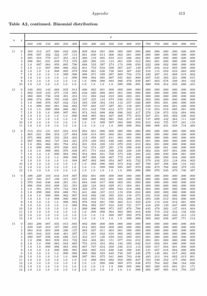
Appendix 413
Table A2, continued. Binomial distribution
n xp
.050 .100 .150 .200 .250 .300 .350 .400 .450 .500 .550 .600 .650 .700 .750 .800 .850 .900 .950
11 0 .569 .314 .167 .086 .042 .020 .009 .004 .001 .000 .000 .000 .000 .000 .000 .000 .000 .000 .0001 .898 .697 .492 .322 .197 .113 .061 .030 .014 .006 .002 .001 .000 .000 .000 .000 .000 .000 .0002 .985 .910 .779 .617 .455 .313 .200 .119 .065 .033 .015 .006 .002 .001 .000 .000 .000 .000 .0003 .998 .981 .931 .839 .713 .570 .426 .296 .191 .113 .061 .029 .012 .004 .001 .000 .000 .000 .0004 1.0 .997 .984 .950 .885 .790 .668 .533 .397 .274 .174 .099 .050 .022 .008 .002 .000 .000 .0005 1.0 1.0 .997 .988 .966 .922 .851 .753 .633 .500 .367 .247 .149 .078 .034 .012 .003 .000 .0006 1.0 1.0 1.0 .998 .992 .978 .950 .901 .826 .726 .603 .467 .332 .210 .115 .050 .016 .003 .0007 1.0 1.0 1.0 1.0 .999 .996 .988 .971 .939 .887 .809 .704 .574 .430 .287 .161 .069 .019 .0028 1.0 1.0 1.0 1.0 1.0 .999 .998 .994 .985 .967 .935 .881 .800 .687 .545 .383 .221 .090 .0159 1.0 1.0 1.0 1.0 1.0 1.0 1.0 .999 .998 .994 .986 .970 .939 .887 .803 .678 .508 .303 .102
10 1.0 1.0 1.0 1.0 1.0 1.0 1.0 1.0 1.0 1.0 .999 .996 .991 .980 .958 .914 .833 .686 .431
12 0 .540 .282 .142 .069 .032 .014 .006 .002 .001 .000 .000 .000 .000 .000 .000 .000 .000 .000 .0001 .882 .659 .443 .275 .158 .085 .042 .020 .008 .003 .001 .000 .000 .000 .000 .000 .000 .000 .0002 .980 .889 .736 .558 .391 .253 .151 .083 .042 .019 .008 .003 .001 .000 .000 .000 .000 .000 .0003 .998 .974 .908 .795 .649 .493 .347 .225 .134 .073 .036 .015 .006 .002 .000 .000 .000 .000 .0004 1.0 .996 .976 .927 .842 .724 .583 .438 .304 .194 .112 .057 .026 .009 .003 .001 .000 .000 .0005 1.0 .999 .995 .981 .946 .882 .787 .665 .527 .387 .261 .158 .085 .039 .014 .004 .001 .000 .0006 1.0 1.0 .999 .996 .986 .961 .915 .842 .739 .613 .473 .335 .213 .118 .054 .019 .005 .001 .0007 1.0 1.0 1.0 .999 .997 .991 .974 .943 .888 .806 .696 .562 .417 .276 .158 .073 .024 .004 .0008 1.0 1.0 1.0 1.0 1.0 .998 .994 .985 .964 .927 .866 .775 .653 .507 .351 .205 .092 .026 .0029 1.0 1.0 1.0 1.0 1.0 1.0 .999 .997 .992 .981 .958 .917 .849 .747 .609 .442 .264 .111 .020
10 1.0 1.0 1.0 1.0 1.0 1.0 1.0 1.0 .999 .997 .992 .980 .958 .915 .842 .725 .557 .341 .11811 1.0 1.0 1.0 1.0 1.0 1.0 1.0 1.0 1.0 1.0 .999 .998 .994 .986 .968 .931 .858 .718 .460
13 0 .513 .254 .121 .055 .024 .010 .004 .001 .000 .000 .000 .000 .000 .000 .000 .000 .000 .000 .0001 .865 .621 .398 .234 .127 .064 .030 .013 .005 .002 .001 .000 .000 .000 .000 .000 .000 .000 .0002 .975 .866 .692 .502 .333 .202 .113 .058 .027 .011 .004 .001 .000 .000 .000 .000 .000 .000 .0003 .997 .966 .882 .747 .584 .421 .278 .169 .093 .046 .020 .008 .003 .001 .000 .000 .000 .000 .0004 1.0 .994 .966 .901 .794 .654 .501 .353 .228 .133 .070 .032 .013 .004 .001 .000 .000 .000 .0005 1.0 .999 .992 .970 .920 .835 .716 .574 .427 .291 .179 .098 .046 .018 .006 .001 .000 .000 .0006 1.0 1.0 .999 .993 .976 .938 .871 .771 .644 .500 .356 .229 .129 .062 .024 .007 .001 .000 .0007 1.0 1.0 1.0 .999 .994 .982 .954 .902 .821 .709 .573 .426 .284 .165 .080 .030 .008 .001 .0008 1.0 1.0 1.0 1.0 .999 .996 .987 .968 .930 .867 .772 .647 .499 .346 .206 .099 .034 .006 .0009 1.0 1.0 1.0 1.0 1.0 .999 .997 .992 .980 .954 .907 .831 .722 .579 .416 .253 .118 .034 .003
10 1.0 1.0 1.0 1.0 1.0 1.0 1.0 .999 .996 .989 .973 .942 .887 .798 .667 .498 .308 .134 .02511 1.0 1.0 1.0 1.0 1.0 1.0 1.0 1.0 .999 .998 .995 .987 .970 .936 .873 .766 .602 .379 .13512 1.0 1.0 1.0 1.0 1.0 1.0 1.0 1.0 1.0 1.0 1.0 .999 .996 .990 .976 .945 .879 .746 .487
14 0 .488 .229 .103 .044 .018 .007 .002 .001 .000 .000 .000 .000 .000 .000 .000 .000 .000 .000 .0001 .847 .585 .357 .198 .101 .047 .021 .008 .003 .001 .000 .000 .000 .000 .000 .000 .000 .000 .0002 .970 .842 .648 .448 .281 .161 .084 .040 .017 .006 .002 .001 .000 .000 .000 .000 .000 .000 .0003 .996 .956 .853 .698 .521 .355 .220 .124 .063 .029 .011 .004 .001 .000 .000 .000 .000 .000 .0004 1.0 .991 .953 .870 .742 .584 .423 .279 .167 .090 .043 .018 .006 .002 .000 .000 .000 .000 .0005 1.0 .999 .988 .956 .888 .781 .641 .486 .337 .212 .119 .058 .024 .008 .002 .000 .000 .000 .0006 1.0 1.0 .998 .988 .962 .907 .816 .692 .546 .395 .259 .150 .075 .031 .010 .002 .000 .000 .0007 1.0 1.0 1.0 .998 .990 .969 .925 .850 .741 .605 .454 .308 .184 .093 .038 .012 .002 .000 .0008 1.0 1.0 1.0 1.0 .998 .992 .976 .942 .881 .788 .663 .514 .359 .219 .112 .044 .012 .001 .0009 1.0 1.0 1.0 1.0 1.0 .998 .994 .982 .957 .910 .833 .721 .577 .416 .258 .130 .047 .009 .000
10 1.0 1.0 1.0 1.0 1.0 1.0 .999 .996 .989 .971 .937 .876 .780 .645 .479 .302 .147 .044 .00411 1.0 1.0 1.0 1.0 1.0 1.0 1.0 .999 .998 .994 .983 .960 .916 .839 .719 .552 .352 .158 .03012 1.0 1.0 1.0 1.0 1.0 1.0 1.0 1.0 1.0 .999 .997 .992 .979 .953 .899 .802 .643 .415 .15313 1.0 1.0 1.0 1.0 1.0 1.0 1.0 1.0 1.0 1.0 1.0 .999 .998 .993 .982 .956 .897 .771 .512
15 0 .463 .206 .087 .035 .013 .005 .002 .000 .000 .000 .000 .000 .000 .000 .000 .000 .000 .000 .0001 .829 .549 .319 .167 .080 .035 .014 .005 .002 .000 .000 .000 .000 .000 .000 .000 .000 .000 .0002 .964 .816 .604 .398 .236 .127 .062 .027 .011 .004 .001 .000 .000 .000 .000 .000 .000 .000 .0003 .995 .944 .823 .648 .461 .297 .173 .091 .042 .018 .006 .002 .000 .000 .000 .000 .000 .000 .0004 .999 .987 .938 .836 .686 .515 .352 .217 .120 .059 .025 .009 .003 .001 .000 .000 .000 .000 .0005 1.0 .998 .983 .939 .852 .722 .564 .403 .261 .151 .077 .034 .012 .004 .001 .000 .000 .000 .0006 1.0 1.0 .996 .982 .943 .869 .755 .610 .452 .304 .182 .095 .042 .015 .004 .001 .000 .000 .0007 1.0 1.0 .999 .996 .983 .950 .887 .787 .654 .500 .346 .213 .113 .050 .017 .004 .001 .000 .0008 1.0 1.0 1.0 .999 .996 .985 .958 .905 .818 .696 .548 .390 .245 .131 .057 .018 .004 .000 .0009 1.0 1.0 1.0 1.0 .999 .996 .988 .966 .923 .849 .739 .597 .436 .278 .148 .061 .017 .002 .000
10 1.0 1.0 1.0 1.0 1.0 .999 .997 .991 .975 .941 .880 .783 .648 .485 .314 .164 .062 .013 .00111 1.0 1.0 1.0 1.0 1.0 1.0 1.0 .998 .994 .982 .958 .909 .827 .703 .539 .352 .177 .056 .00512 1.0 1.0 1.0 1.0 1.0 1.0 1.0 1.0 .999 .996 .989 .973 .938 .873 .764 .602 .396 .184 .03613 1.0 1.0 1.0 1.0 1.0 1.0 1.0 1.0 1.0 1.0 .998 .995 .986 .965 .920 .833 .681 .451 .17114 1.0 1.0 1.0 1.0 1.0 1.0 1.0 1.0 1.0 1.0 1.0 1.0 .998 .995 .987 .965 .913 .794 .537
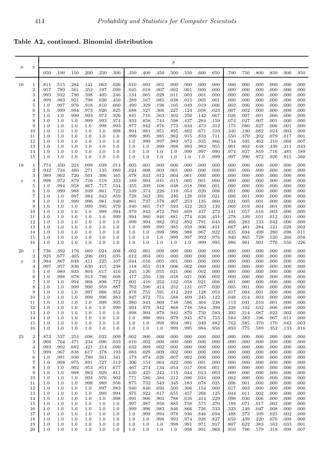
414 Probability and Statistics for Computer Scientists
Table A2, continued. Binomial distribution
n xp
.050 .100 .150 .200 .250 .300 .350 .400 .450 .500 .550 .600 .650 .700 .750 .800 .850 .900 .950
16 1 .811 .515 .284 .141 .063 .026 .010 .003 .001 .000 .000 .000 .000 .000 .000 .000 .000 .000 .0002 .957 .789 .561 .352 .197 .099 .045 .018 .007 .002 .001 .000 .000 .000 .000 .000 .000 .000 .0003 .993 .932 .790 .598 .405 .246 .134 .065 .028 .011 .003 .001 .000 .000 .000 .000 .000 .000 .0004 .999 .983 .921 .798 .630 .450 .289 .167 .085 .038 .015 .005 .001 .000 .000 .000 .000 .000 .0005 1.0 .997 .976 .918 .810 .660 .490 .329 .198 .105 .049 .019 .006 .002 .000 .000 .000 .000 .0006 1.0 .999 .994 .973 .920 .825 .688 .527 .366 .227 .124 .058 .023 .007 .002 .000 .000 .000 .0007 1.0 1.0 .999 .993 .973 .926 .841 .716 .563 .402 .256 .142 .067 .026 .007 .001 .000 .000 .0008 1.0 1.0 1.0 .999 .993 .974 .933 .858 .744 .598 .437 .284 .159 .074 .027 .007 .001 .000 .0009 1.0 1.0 1.0 1.0 .998 .993 .977 .942 .876 .773 .634 .473 .312 .175 .080 .027 .006 .001 .000
10 1.0 1.0 1.0 1.0 1.0 .998 .994 .981 .951 .895 .802 .671 .510 .340 .190 .082 .024 .003 .00011 1.0 1.0 1.0 1.0 1.0 1.0 .999 .995 .985 .962 .915 .833 .711 .550 .370 .202 .079 .017 .00112 1.0 1.0 1.0 1.0 1.0 1.0 1.0 .999 .997 .989 .972 .935 .866 .754 .595 .402 .210 .068 .00713 1.0 1.0 1.0 1.0 1.0 1.0 1.0 1.0 .999 .998 .993 .982 .955 .901 .803 .648 .439 .211 .04314 1.0 1.0 1.0 1.0 1.0 1.0 1.0 1.0 1.0 1.0 .999 .997 .990 .974 .937 .859 .716 .485 .18915 1.0 1.0 1.0 1.0 1.0 1.0 1.0 1.0 1.0 1.0 1.0 1.0 .999 .997 .990 .972 .926 .815 .560
18 1 .774 .450 .224 .099 .039 .014 .005 .001 .000 .000 .000 .000 .000 .000 .000 .000 .000 .000 .0002 .942 .734 .480 .271 .135 .060 .024 .008 .003 .001 .000 .000 .000 .000 .000 .000 .000 .000 .0003 .989 .902 .720 .501 .306 .165 .078 .033 .012 .004 .001 .000 .000 .000 .000 .000 .000 .000 .000
y 4 .998 .972 .879 .716 .519 .333 .189 .094 .041 .015 .005 .001 .000 .000 .000 .000 .000 .000 .0005 1.0 .994 .958 .867 .717 .534 .355 .209 .108 .048 .018 .006 .001 .000 .000 .000 .000 .000 .0006 1.0 .999 .988 .949 .861 .722 .549 .374 .226 .119 .054 .020 .006 .001 .000 .000 .000 .000 .0007 1.0 1.0 .997 .984 .943 .859 .728 .563 .391 .240 .128 .058 .021 .006 .001 .000 .000 .000 .0008 1.0 1.0 .999 .996 .981 .940 .861 .737 .578 .407 .253 .135 .060 .021 .005 .001 .000 .000 .0009 1.0 1.0 1.0 .999 .995 .979 .940 .865 .747 .593 .422 .263 .139 .060 .019 .004 .001 .000 .000
10 1.0 1.0 1.0 1.0 .999 .994 .979 .942 .872 .760 .609 .437 .272 .141 .057 .016 .003 .000 .00011 1.0 1.0 1.0 1.0 1.0 .999 .994 .980 .946 .881 .774 .626 .451 .278 .139 .051 .012 .001 .00012 1.0 1.0 1.0 1.0 1.0 1.0 .999 .994 .982 .952 .892 .791 .645 .466 .283 .133 .042 .006 .00013 1.0 1.0 1.0 1.0 1.0 1.0 1.0 .999 .995 .985 .959 .906 .811 .667 .481 .284 .121 .028 .00214 1.0 1.0 1.0 1.0 1.0 1.0 1.0 1.0 .999 .996 .988 .967 .922 .835 .694 .499 .280 .098 .01115 1.0 1.0 1.0 1.0 1.0 1.0 1.0 1.0 1.0 .999 .997 .992 .976 .940 .865 .729 .520 .266 .05816 1.0 1.0 1.0 1.0 1.0 1.0 1.0 1.0 1.0 1.0 1.0 .999 .995 .986 .961 .901 .776 .550 .226
20 1 .736 .392 .176 .069 .024 .008 .002 .001 .000 .000 .000 .000 .000 .000 .000 .000 .000 .000 .0002 .925 .677 .405 .206 .091 .035 .012 .004 .001 .000 .000 .000 .000 .000 .000 .000 .000 .000 .000
y 3 .984 .867 .648 .411 .225 .107 .044 .016 .005 .001 .000 .000 .000 .000 .000 .000 .000 .000 .0004 .997 .957 .830 .630 .415 .238 .118 .051 .019 .006 .002 .000 .000 .000 .000 .000 .000 .000 .0005 1.0 .989 .933 .804 .617 .416 .245 .126 .055 .021 .006 .002 .000 .000 .000 .000 .000 .000 .0006 1.0 .998 .978 .913 .786 .608 .417 .250 .130 .058 .021 .006 .002 .000 .000 .000 .000 .000 .0007 1.0 1.0 .994 .968 .898 .772 .601 .416 .252 .132 .058 .021 .006 .001 .000 .000 .000 .000 .0008 1.0 1.0 .999 .990 .959 .887 .762 .596 .414 .252 .131 .057 .020 .005 .001 .000 .000 .000 .0009 1.0 1.0 1.0 .997 .986 .952 .878 .755 .591 .412 .249 .128 .053 .017 .004 .001 .000 .000 .000
10 1.0 1.0 1.0 .999 .996 .983 .947 .872 .751 .588 .409 .245 .122 .048 .014 .003 .000 .000 .00011 1.0 1.0 1.0 1.0 .999 .995 .980 .943 .869 .748 .586 .404 .238 .113 .041 .010 .001 .000 .00012 1.0 1.0 1.0 1.0 1.0 .999 .994 .979 .942 .868 .748 .584 .399 .228 .102 .032 .006 .000 .00013 1.0 1.0 1.0 1.0 1.0 1.0 .998 .994 .979 .942 .870 .750 .583 .392 .214 .087 .022 .002 .00014 1.0 1.0 1.0 1.0 1.0 1.0 1.0 .998 .994 .979 .945 .874 .755 .584 .383 .196 .067 .011 .00015 1.0 1.0 1.0 1.0 1.0 1.0 1.0 1.0 .998 .994 .981 .949 .882 .762 .585 .370 .170 .043 .00316 1.0 1.0 1.0 1.0 1.0 1.0 1.0 1.0 1.0 .999 .995 .984 .956 .893 .775 .589 .352 .133 .016
25 2 .873 .537 .254 .098 .032 .009 .002 .000 .000 .000 .000 .000 .000 .000 .000 .000 .000 .000 .0003 .966 .764 .471 .234 .096 .033 .010 .002 .000 .000 .000 .000 .000 .000 .000 .000 .000 .000 .0004 .993 .902 .682 .421 .214 .090 .032 .009 .002 .000 .000 .000 .000 .000 .000 .000 .000 .000 .0005 .999 .967 .838 .617 .378 .193 .083 .029 .009 .002 .000 .000 .000 .000 .000 .000 .000 .000 .0006 1.0 .991 .930 .780 .561 .341 .173 .074 .026 .007 .002 .000 .000 .000 .000 .000 .000 .000 .0007 1.0 .998 .975 .891 .727 .512 .306 .154 .064 .022 .006 .001 .000 .000 .000 .000 .000 .000 .0008 1.0 1.0 .992 .953 .851 .677 .467 .274 .134 .054 .017 .004 .001 .000 .000 .000 .000 .000 .0009 1.0 1.0 .998 .983 .929 .811 .630 .425 .242 .115 .044 .013 .003 .000 .000 .000 .000 .000 .000
10 1.0 1.0 1.0 .994 .970 .902 .771 .586 .384 .212 .096 .034 .009 .002 .000 .000 .000 .000 .00011 1.0 1.0 1.0 .998 .989 .956 .875 .732 .543 .345 .183 .078 .025 .006 .001 .000 .000 .000 .00012 1.0 1.0 1.0 1.0 .997 .983 .940 .846 .694 .500 .306 .154 .060 .017 .003 .000 .000 .000 .00013 1.0 1.0 1.0 1.0 .999 .994 .975 .922 .817 .655 .457 .268 .125 .044 .011 .002 .000 .000 .00014 1.0 1.0 1.0 1.0 1.0 .998 .991 .966 .904 .788 .616 .414 .229 .098 .030 .006 .000 .000 .00015 1.0 1.0 1.0 1.0 1.0 1.0 .997 .987 .956 .885 .758 .575 .370 .189 .071 .017 .002 .000 .00016 1.0 1.0 1.0 1.0 1.0 1.0 .999 .996 .983 .946 .866 .726 .533 .323 .149 .047 .008 .000 .00017 1.0 1.0 1.0 1.0 1.0 1.0 1.0 .999 .994 .978 .936 .846 .694 .488 .273 .109 .025 .002 .00018 1.0 1.0 1.0 1.0 1.0 1.0 1.0 1.0 .998 .993 .974 .926 .827 .659 .439 .220 .070 .009 .00019 1.0 1.0 1.0 1.0 1.0 1.0 1.0 1.0 1.0 .998 .991 .971 .917 .807 .622 .383 .162 .033 .00120 1.0 1.0 1.0 1.0 1.0 1.0 1.0 1.0 1.0 1.0 .998 .991 .968 .910 .786 .579 .318 .098 .007
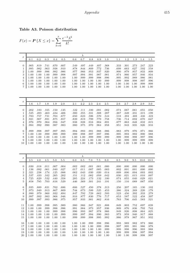
Appendix 415
Table A3. Poisson distribution
F (x) = P X ≤ x =x∑
k=0
e−λλk
k!
xλ
0.1 0.2 0.3 0.4 0.5 0.6 0.7 0.8 0.9 1.0 1.1 1.2 1.3 1.4 1.5
0 .905 .819 .741 .670 .607 .549 .497 .449 .407 .368 .333 .301 .273 .247 .2231 .995 .982 .963 .938 .910 .878 .844 .809 .772 .736 .699 .663 .627 .592 .5582 1.00 .999 .996 .992 .986 .977 .966 .953 .937 .920 .900 .879 .857 .833 .8093 1.00 1.00 1.00 .999 .998 .997 .994 .991 .987 .981 .974 .966 .957 .946 .9344 1.00 1.00 1.00 1.00 1.00 1.00 .999 .999 .998 .996 .995 .992 .989 .986 .9815 1.00 1.00 1.00 1.00 1.00 1.00 1.00 1.00 1.00 .999 .999 .998 .998 .997 .9966 1.00 1.00 1.00 1.00 1.00 1.00 1.00 1.00 1.00 1.00 1.00 1.00 1.00 .999 .9997 1.00 1.00 1.00 1.00 1.00 1.00 1.00 1.00 1.00 1.00 1.00 1.00 1.00 1.00 1.00
xλ
1.6 1.7 1.8 1.9 2.0 2.1 2.2 2.3 2.4 2.5 2.6 2.7 2.8 2.9 3.0
0 .202 .183 .165 .150 .135 .122 .111 .100 .091 .082 .074 .067 .061 .055 .0501 .525 .493 .463 .434 .406 .380 .355 .331 .308 .287 .267 .249 .231 .215 .1992 .783 .757 .731 .704 .677 .650 .623 .596 .570 .544 .518 .494 .469 .446 .4233 .921 .907 .891 .875 .857 .839 .819 .799 .779 .758 .736 .714 .692 .670 .6474 .976 .970 .964 .956 .947 .938 .928 .916 .904 .891 .877 .863 .848 .832 .8155 .994 .992 .990 .987 .983 .980 .975 .970 .964 .958 .951 .943 .935 .926 .916
6 .999 .998 .997 .997 .995 .994 .993 .991 .988 .986 .983 .979 .976 .971 .9667 1.00 1.00 .999 .999 .999 .999 .998 .997 .997 .996 .995 .993 .992 .990 .9888 1.00 1.00 1.00 1.00 1.00 1.00 1.00 .999 .999 .999 .999 .998 .998 .997 .9969 1.00 1.00 1.00 1.00 1.00 1.00 1.00 1.00 1.00 1.00 1.00 .999 .999 .999 .999
10 1.00 1.00 1.00 1.00 1.00 1.00 1.00 1.00 1.00 1.00 1.00 1.00 1.00 1.00 1.00
xλ
3.5 4.0 4.5 5.0 5.5 6.0 6.5 7.0 7.5 8.0 8.5 9.0 9.5 10.0 10.5
0 .030 .018 .011 .007 .004 .002 .002 .001 .001 .000 .000 .000 .000 .000 .0001 .136 .092 .061 .040 .027 .017 .011 .007 .005 .003 .002 .001 .001 .000 .0002 .321 .238 .174 .125 .088 .062 .043 .030 .020 .014 .009 .006 .004 .003 .0023 .537 .433 .342 .265 .202 .151 .112 .082 .059 .042 .030 .021 .015 .010 .0074 .725 .629 .532 .440 .358 .285 .224 .173 .132 .100 .074 .055 .040 .029 .0215 .858 .785 .703 .616 .529 .446 .369 .301 .241 .191 .150 .116 .089 .067 .050
6 .935 .889 .831 .762 .686 .606 .527 .450 .378 .313 .256 .207 .165 .130 .1027 .973 .949 .913 .867 .809 .744 .673 .599 .525 .453 .386 .324 .269 .220 .1798 .990 .979 .960 .932 .894 .847 .792 .729 .662 .593 .523 .456 .392 .333 .2799 .997 .992 .983 .968 .946 .916 .877 .830 .776 .717 .653 .587 .522 .458 .397
10 .999 .997 .993 .986 .975 .957 .933 .901 .862 .816 .763 .706 .645 .583 .521
11 1.00 .999 .998 .995 .989 .980 .966 .947 .921 .888 .849 .803 .752 .697 .63912 1.00 1.00 .999 .998 .996 .991 .984 .973 .957 .936 .909 .876 .836 .792 .74213 1.00 1.00 1.00 .999 .998 .996 .993 .987 .978 .966 .949 .926 .898 .864 .82514 1.00 1.00 1.00 1.00 .999 .999 .997 .994 .990 .983 .973 .959 .940 .917 .88815 1.00 1.00 1.00 1.00 1.00 .999 .999 .998 .995 .992 .986 .978 .967 .951 .932
16 1.00 1.00 1.00 1.00 1.00 1.00 1.00 .999 .998 .996 .993 .989 .982 .973 .96017 1.00 1.00 1.00 1.00 1.00 1.00 1.00 1.00 .999 .998 .997 .995 .991 .986 .97818 1.00 1.00 1.00 1.00 1.00 1.00 1.00 1.00 1.00 .999 .999 .998 .996 .993 .98819 1.00 1.00 1.00 1.00 1.00 1.00 1.00 1.00 1.00 1.00 .999 .999 .998 .997 .99420 1.00 1.00 1.00 1.00 1.00 1.00 1.00 1.00 1.00 1.00 1.00 1.00 .999 .998 .997

416 Probability and Statistics for Computer Scientists
Table A3, continued. Poisson distribution
xλ
11 12 13 14 15 16 17 18 19 20 22 24 26 28 30
0 .000 .000 .000 .000 .000 .000 .000 .000 .000 .000 .000 .000 .000 .000 .0001 .000 .000 .000 .000 .000 .000 .000 .000 .000 .000 .000 .000 .000 .000 .0002 .001 .001 .000 .000 .000 .000 .000 .000 .000 .000 .000 .000 .000 .000 .0003 .005 .002 .001 .000 .000 .000 .000 .000 .000 .000 .000 .000 .000 .000 .0004 .015 .008 .004 .002 .001 .000 .000 .000 .000 .000 .000 .000 .000 .000 .0005 .038 .020 .011 .006 .003 .001 .001 .000 .000 .000 .000 .000 .000 .000 .000
6 .079 .046 .026 .014 .008 .004 .002 .001 .001 .000 .000 .000 .000 .000 .0007 .143 .090 .054 .032 .018 .010 .005 .003 .002 .001 .000 .000 .000 .000 .0008 .232 .155 .100 .062 .037 .022 .013 .007 .004 .002 .001 .000 .000 .000 .0009 .341 .242 .166 .109 .070 .043 .026 .015 .009 .005 .002 .000 .000 .000 .000
10 .460 .347 .252 .176 .118 .077 .049 .030 .018 .011 .004 .001 .000 .000 .000
11 .579 .462 .353 .260 .185 .127 .085 .055 .035 .021 .008 .003 .001 .000 .00012 .689 .576 .463 .358 .268 .193 .135 .092 .061 .039 .015 .005 .002 .001 .00013 .781 .682 .573 .464 .363 .275 .201 .143 .098 .066 .028 .011 .004 .001 .00014 .854 .772 .675 .570 .466 .368 .281 .208 .150 .105 .048 .020 .008 .003 .00115 .907 .844 .764 .669 .568 .467 .371 .287 .215 .157 .077 .034 .014 .005 .002
16 .944 .899 .835 .756 .664 .566 .468 .375 .292 .221 .117 .056 .025 .010 .00417 .968 .937 .890 .827 .749 .659 .564 .469 .378 .297 .169 .087 .041 .018 .00718 .982 .963 .930 .883 .819 .742 .655 .562 .469 .381 .232 .128 .065 .030 .01319 .991 .979 .957 .923 .875 .812 .736 .651 .561 .470 .306 .180 .097 .048 .02220 .995 .988 .975 .952 .917 .868 .805 .731 .647 .559 .387 .243 .139 .073 .035
21 .998 .994 .986 .971 .947 .911 .861 .799 .725 .644 .472 .314 .190 .106 .05422 .999 .997 .992 .983 .967 .942 .905 .855 .793 .721 .556 .392 .252 .148 .08123 1.00 .999 .996 .991 .981 .963 .937 .899 .849 .787 .637 .473 .321 .200 .11524 1.00 .999 .998 .995 .989 .978 .959 .932 .893 .843 .712 .554 .396 .260 .15725 1.00 1.00 .999 .997 .994 .987 .975 .955 .927 .888 .777 .632 .474 .327 .208
26 1.00 1.00 1.00 .999 .997 .993 .985 .972 .951 .922 .832 .704 .552 .400 .26727 1.00 1.00 1.00 .999 .998 .996 .991 .983 .969 .948 .877 .768 .627 .475 .33328 1.00 1.00 1.00 1.00 .999 .998 .995 .990 .980 .966 .913 .823 .697 .550 .40329 1.00 1.00 1.00 1.00 1.00 .999 .997 .994 .988 .978 .940 .868 .759 .623 .47630 1.00 1.00 1.00 1.00 1.00 .999 .999 .997 .993 .987 .959 .904 .813 .690 .548
31 1.00 1.00 1.00 1.00 1.00 1.00 .999 .998 .996 .992 .973 .932 .859 .752 .61932 1.00 1.00 1.00 1.00 1.00 1.00 1.00 .999 .998 .995 .983 .953 .896 .805 .68533 1.00 1.00 1.00 1.00 1.00 1.00 1.00 1.00 .999 .997 .989 .969 .925 .850 .74434 1.00 1.00 1.00 1.00 1.00 1.00 1.00 1.00 .999 .999 .994 .979 .947 .888 .79735 1.00 1.00 1.00 1.00 1.00 1.00 1.00 1.00 1.00 .999 .996 .987 .964 .918 .843
36 1.00 1.00 1.00 1.00 1.00 1.00 1.00 1.00 1.00 1.00 .998 .992 .976 .941 .88037 1.00 1.00 1.00 1.00 1.00 1.00 1.00 1.00 1.00 1.00 .999 .995 .984 .959 .91138 1.00 1.00 1.00 1.00 1.00 1.00 1.00 1.00 1.00 1.00 .999 .997 .990 .972 .93539 1.00 1.00 1.00 1.00 1.00 1.00 1.00 1.00 1.00 1.00 1.00 .998 .994 .981 .95440 1.00 1.00 1.00 1.00 1.00 1.00 1.00 1.00 1.00 1.00 1.00 .999 .996 .988 .968
41 1.00 1.00 1.00 1.00 1.00 1.00 1.00 1.00 1.00 1.00 1.00 .999 .998 .992 .97842 1.00 1.00 1.00 1.00 1.00 1.00 1.00 1.00 1.00 1.00 1.00 1.00 .999 .995 .98543 1.00 1.00 1.00 1.00 1.00 1.00 1.00 1.00 1.00 1.00 1.00 1.00 .999 .997 .99044 1.00 1.00 1.00 1.00 1.00 1.00 1.00 1.00 1.00 1.00 1.00 1.00 1.00 .998 .99445 1.00 1.00 1.00 1.00 1.00 1.00 1.00 1.00 1.00 1.00 1.00 1.00 1.00 .999 .996
46 1.00 1.00 1.00 1.00 1.00 1.00 1.00 1.00 1.00 1.00 1.00 1.00 1.00 .999 .99847 1.00 1.00 1.00 1.00 1.00 1.00 1.00 1.00 1.00 1.00 1.00 1.00 1.00 1.00 .99948 1.00 1.00 1.00 1.00 1.00 1.00 1.00 1.00 1.00 1.00 1.00 1.00 1.00 1.00 .99949 1.00 1.00 1.00 1.00 1.00 1.00 1.00 1.00 1.00 1.00 1.00 1.00 1.00 1.00 .99950 1.00 1.00 1.00 1.00 1.00 1.00 1.00 1.00 1.00 1.00 1.00 1.00 1.00 1.00 1.00
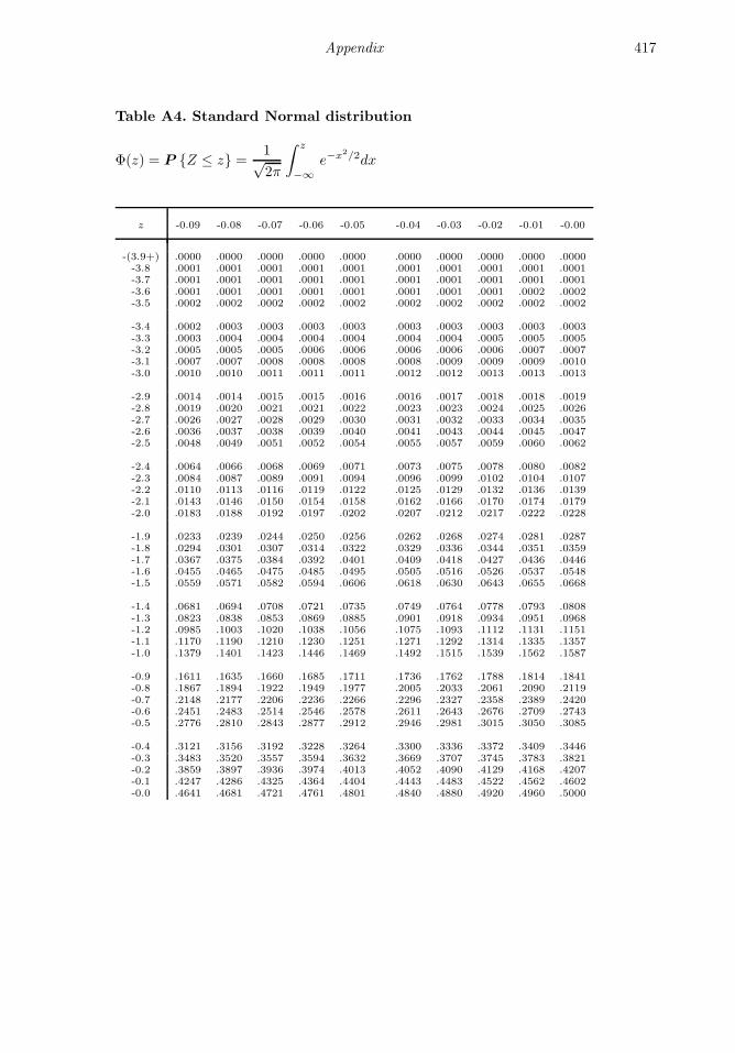
Appendix 417
Table A4. Standard Normal distribution
Φ(z) = P Z ≤ z =1√2π
∫ z
−∞
e−x2/2dx
z -0.09 -0.08 -0.07 -0.06 -0.05 -0.04 -0.03 -0.02 -0.01 -0.00
-(3.9+) .0000 .0000 .0000 .0000 .0000 .0000 .0000 .0000 .0000 .0000-3.8 .0001 .0001 .0001 .0001 .0001 .0001 .0001 .0001 .0001 .0001-3.7 .0001 .0001 .0001 .0001 .0001 .0001 .0001 .0001 .0001 .0001-3.6 .0001 .0001 .0001 .0001 .0001 .0001 .0001 .0001 .0002 .0002-3.5 .0002 .0002 .0002 .0002 .0002 .0002 .0002 .0002 .0002 .0002
-3.4 .0002 .0003 .0003 .0003 .0003 .0003 .0003 .0003 .0003 .0003-3.3 .0003 .0004 .0004 .0004 .0004 .0004 .0004 .0005 .0005 .0005-3.2 .0005 .0005 .0005 .0006 .0006 .0006 .0006 .0006 .0007 .0007-3.1 .0007 .0007 .0008 .0008 .0008 .0008 .0009 .0009 .0009 .0010-3.0 .0010 .0010 .0011 .0011 .0011 .0012 .0012 .0013 .0013 .0013
-2.9 .0014 .0014 .0015 .0015 .0016 .0016 .0017 .0018 .0018 .0019-2.8 .0019 .0020 .0021 .0021 .0022 .0023 .0023 .0024 .0025 .0026-2.7 .0026 .0027 .0028 .0029 .0030 .0031 .0032 .0033 .0034 .0035-2.6 .0036 .0037 .0038 .0039 .0040 .0041 .0043 .0044 .0045 .0047-2.5 .0048 .0049 .0051 .0052 .0054 .0055 .0057 .0059 .0060 .0062
-2.4 .0064 .0066 .0068 .0069 .0071 .0073 .0075 .0078 .0080 .0082-2.3 .0084 .0087 .0089 .0091 .0094 .0096 .0099 .0102 .0104 .0107-2.2 .0110 .0113 .0116 .0119 .0122 .0125 .0129 .0132 .0136 .0139-2.1 .0143 .0146 .0150 .0154 .0158 .0162 .0166 .0170 .0174 .0179-2.0 .0183 .0188 .0192 .0197 .0202 .0207 .0212 .0217 .0222 .0228
-1.9 .0233 .0239 .0244 .0250 .0256 .0262 .0268 .0274 .0281 .0287-1.8 .0294 .0301 .0307 .0314 .0322 .0329 .0336 .0344 .0351 .0359-1.7 .0367 .0375 .0384 .0392 .0401 .0409 .0418 .0427 .0436 .0446-1.6 .0455 .0465 .0475 .0485 .0495 .0505 .0516 .0526 .0537 .0548-1.5 .0559 .0571 .0582 .0594 .0606 .0618 .0630 .0643 .0655 .0668
-1.4 .0681 .0694 .0708 .0721 .0735 .0749 .0764 .0778 .0793 .0808-1.3 .0823 .0838 .0853 .0869 .0885 .0901 .0918 .0934 .0951 .0968-1.2 .0985 .1003 .1020 .1038 .1056 .1075 .1093 .1112 .1131 .1151-1.1 .1170 .1190 .1210 .1230 .1251 .1271 .1292 .1314 .1335 .1357-1.0 .1379 .1401 .1423 .1446 .1469 .1492 .1515 .1539 .1562 .1587
-0.9 .1611 .1635 .1660 .1685 .1711 .1736 .1762 .1788 .1814 .1841-0.8 .1867 .1894 .1922 .1949 .1977 .2005 .2033 .2061 .2090 .2119-0.7 .2148 .2177 .2206 .2236 .2266 .2296 .2327 .2358 .2389 .2420-0.6 .2451 .2483 .2514 .2546 .2578 .2611 .2643 .2676 .2709 .2743-0.5 .2776 .2810 .2843 .2877 .2912 .2946 .2981 .3015 .3050 .3085
-0.4 .3121 .3156 .3192 .3228 .3264 .3300 .3336 .3372 .3409 .3446-0.3 .3483 .3520 .3557 .3594 .3632 .3669 .3707 .3745 .3783 .3821-0.2 .3859 .3897 .3936 .3974 .4013 .4052 .4090 .4129 .4168 .4207-0.1 .4247 .4286 .4325 .4364 .4404 .4443 .4483 .4522 .4562 .4602-0.0 .4641 .4681 .4721 .4761 .4801 .4840 .4880 .4920 .4960 .5000

418 Probability and Statistics for Computer Scientists
Table A4, continued. Standard Normal distribution
z 0.00 0.01 0.02 0.03 0.04 0.05 0.06 0.07 0.08 0.09
0.0 .5000 .5040 .5080 .5120 .5160 .5199 .5239 .5279 .5319 .53590.1 .5398 .5438 .5478 .5517 .5557 .5596 .5636 .5675 .5714 .57530.2 .5793 .5832 .5871 .5910 .5948 .5987 .6026 .6064 .6103 .61410.3 .6179 .6217 .6255 .6293 .6331 .6368 .6406 .6443 .6480 .65170.4 .6554 .6591 .6628 .6664 .6700 .6736 .6772 .6808 .6844 .6879
0.5 .6915 .6950 .6985 .7019 .7054 .7088 .7123 .7157 .7190 .72240.6 .7257 .7291 .7324 .7357 .7389 .7422 .7454 .7486 .7517 .75490.7 .7580 .7611 .7642 .7673 .7704 .7734 .7764 .7794 .7823 .78520.8 .7881 .7910 .7939 .7967 .7995 .8023 .8051 .8078 .8106 .81330.9 .8159 .8186 .8212 .8238 .8264 .8289 .8315 .8340 .8365 .8389
1.0 .8413 .8438 .8461 .8485 .8508 .8531 .8554 .8577 .8599 .86211.1 .8643 .8665 .8686 .8708 .8729 .8749 .8770 .8790 .8810 .88301.2 .8849 .8869 .8888 .8907 .8925 .8944 .8962 .8980 .8997 .90151.3 .9032 .9049 .9066 .9082 .9099 .9115 .9131 .9147 .9162 .91771.4 .9192 .9207 .9222 .9236 .9251 .9265 .9279 .9292 .9306 .9319
1.5 .9332 .9345 .9357 .9370 .9382 .9394 .9406 .9418 .9429 .94411.6 .9452 .9463 .9474 .9484 .9495 .9505 .9515 .9525 .9535 .95451.7 .9554 .9564 .9573 .9582 .9591 .9599 .9608 .9616 .9625 .96331.8 .9641 .9649 .9656 .9664 .9671 .9678 .9686 .9693 .9699 .97061.9 .9713 .9719 .9726 .9732 .9738 .9744 .9750 .9756 .9761 .9767
2.0 .9772 .9778 .9783 .9788 .9793 .9798 .9803 .9808 .9812 .98172.1 .9821 .9826 .9830 .9834 .9838 .9842 .9846 .9850 .9854 .98572.2 .9861 .9864 .9868 .9871 .9875 .9878 .9881 .9884 .9887 .98902.3 .9893 .9896 .9898 .9901 .9904 .9906 .9909 .9911 .9913 .99162.4 .9918 .9920 .9922 .9925 .9927 .9929 .9931 .9932 .9934 .9936
2.5 .9938 .9940 .9941 .9943 .9945 .9946 .9948 .9949 .9951 .99522.6 .9953 .9955 .9956 .9957 .9959 .9960 .9961 .9962 .9963 .99642.7 .9965 .9966 .9967 .9968 .9969 .9970 .9971 .9972 .9973 .99742.8 .9974 .9975 .9976 .9977 .9977 .9978 .9979 .9979 .9980 .99812.9 .9981 .9982 .9982 .9983 .9984 .9984 .9985 .9985 .9986 .9986
3.0 .9987 .9987 .9987 .9988 .9988 .9989 .9989 .9989 .9990 .99903.1 .9990 .9991 .9991 .9991 .9992 .9992 .9992 .9992 .9993 .99933.2 .9993 .9993 .9994 .9994 .9994 .9994 .9994 .9995 .9995 .99953.3 .9995 .9995 .9995 .9996 .9996 .9996 .9996 .9996 .9996 .99973.4 .9997 .9997 .9997 .9997 .9997 .9997 .9997 .9997 .9997 .9998
3.5 .9998 .9998 .9998 .9998 .9998 .9998 .9998 .9998 .9998 .99983.6 .9998 .9998 .9999 .9999 .9999 .9999 .9999 .9999 .9999 .99993.7 .9999 .9999 .9999 .9999 .9999 .9999 .9999 .9999 .9999 .99993.8 .9999 .9999 .9999 .9999 .9999 .9999 .9999 .9999 .9999 .99993.9+ 1.00 1.00 1.00 1.00 1.00 1.00 1.00 1.00 1.00 1.00

Appendix 419
Table A5. Table of Student’s T-distribution
tα; critical values, such that P t > tα = α
α, the right-tail probabilityν
(d.f.) .10 .05 .025 .02 .01 .005 .0025 .001 .0005 .0001
1 3.078 6.314 12.706 15.89 31.82 63.66 127.3 318.3 636.6 31852 1.886 2.920 4.303 4.849 6.965 9.925 14.09 22.33 31.60 70.713 1.638 2.353 3.182 3.482 4.541 5.841 7.453 10.21 12.92 22.204 1.533 2.132 2.776 2.999 3.747 4.604 5.598 7.173 8.610 13.045 1.476 2.015 2.571 2.757 3.365 4.032 4.773 5.894 6.869 9.676
6 1.440 1.943 2.447 2.612 3.143 3.707 4.317 5.208 5.959 8.0237 1.415 1.895 2.365 2.517 2.998 3.499 4.029 4.785 5.408 7.0648 1.397 1.860 2.306 2.449 2.896 3.355 3.833 4.501 5.041 6.4429 1.383 1.833 2.262 2.398 2.821 3.250 3.690 4.297 4.781 6.00910 1.372 1.812 2.228 2.359 2.764 3.169 3.581 4.144 4.587 5.694
11 1.363 1.796 2.201 2.328 2.718 3.106 3.497 4.025 4.437 5.45312 1.356 1.782 2.179 2.303 2.681 3.055 3.428 3.930 4.318 5.26313 1.350 1.771 2.160 2.282 2.650 3.012 3.372 3.852 4.221 5.11114 1.345 1.761 2.145 2.264 2.624 2.977 3.326 3.787 4.140 4.98515 1.341 1.753 2.131 2.249 2.602 2.947 3.286 3.733 4.073 4.880
16 1.337 1.746 2.120 2.235 2.583 2.921 3.252 3.686 4.015 4.79017 1.333 1.740 2.110 2.224 2.567 2.898 3.222 3.646 3.965 4.71518 1.330 1.734 2.101 2.214 2.552 2.878 3.197 3.610 3.922 4.64819 1.328 1.729 2.093 2.205 2.539 2.861 3.174 3.579 3.883 4.59020 1.325 1.725 2.086 2.197 2.528 2.845 3.153 3.552 3.850 4.539
21 1.323 1.721 2.080 2.189 2.518 2.831 3.135 3.527 3.819 4.49222 1.321 1.717 2.074 2.183 2.508 2.819 3.119 3.505 3.792 4.45223 1.319 1.714 2.069 2.177 2.500 2.807 3.104 3.485 3.768 4.41624 1.318 1.711 2.064 2.172 2.492 2.797 3.091 3.467 3.745 4.38225 1.316 1.708 2.060 2.167 2.485 2.787 3.078 3.450 3.725 4.352
26 1.315 1.706 2.056 2.162 2.479 2.779 3.067 3.435 3.707 4.32427 1.314 1.703 2.052 2.158 2.473 2.771 3.057 3.421 3.689 4.29928 1.313 1.701 2.048 2.154 2.467 2.763 3.047 3.408 3.674 4.27629 1.311 1.699 2.045 2.150 2.462 2.756 3.038 3.396 3.660 4.25430 1.310 1.697 2.042 2.147 2.457 2.750 3.030 3.385 3.646 4.234
32 1.309 1.694 2.037 2.141 2.449 2.738 3.015 3.365 3.622 4.19834 1.307 1.691 2.032 2.136 2.441 2.728 3.002 3.348 3.601 4.16836 1.306 1.688 2.028 2.131 2.434 2.719 2.990 3.333 3.582 4.14038 1.304 1.686 2.024 2.127 2.429 2.712 2.980 3.319 3.566 4.11540 1.303 1.684 2.021 2.123 2.423 2.704 2.971 3.307 3.551 4.094
45 1.301 1.679 2.014 2.115 2.412 2.690 2.952 3.281 3.520 4.04950 1.299 1.676 2.009 2.109 2.403 2.678 2.937 3.261 3.496 4.01455 1.297 1.673 2.004 2.104 2.396 2.668 2.925 3.245 3.476 3.98560 1.296 1.671 2.000 2.099 2.390 2.660 2.915 3.232 3.460 3.96270 1.294 1.667 1.994 2.093 2.381 2.648 2.899 3.211 3.435 3.926
80 1.292 1.664 1.990 2.088 2.374 2.639 2.887 3.195 3.416 3.89990 1.291 1.662 1.987 2.084 2.368 2.632 2.878 3.183 3.402 3.878100 1.290 1.660 1.984 2.081 2.364 2.626 2.871 3.174 3.390 3.861200 1.286 1.653 1.972 2.067 2.345 2.601 2.838 3.131 3.340 3.789∞ 1.282 1.645 1.960 2.054 2.326 2.576 2.807 3.090 3.290 3.719
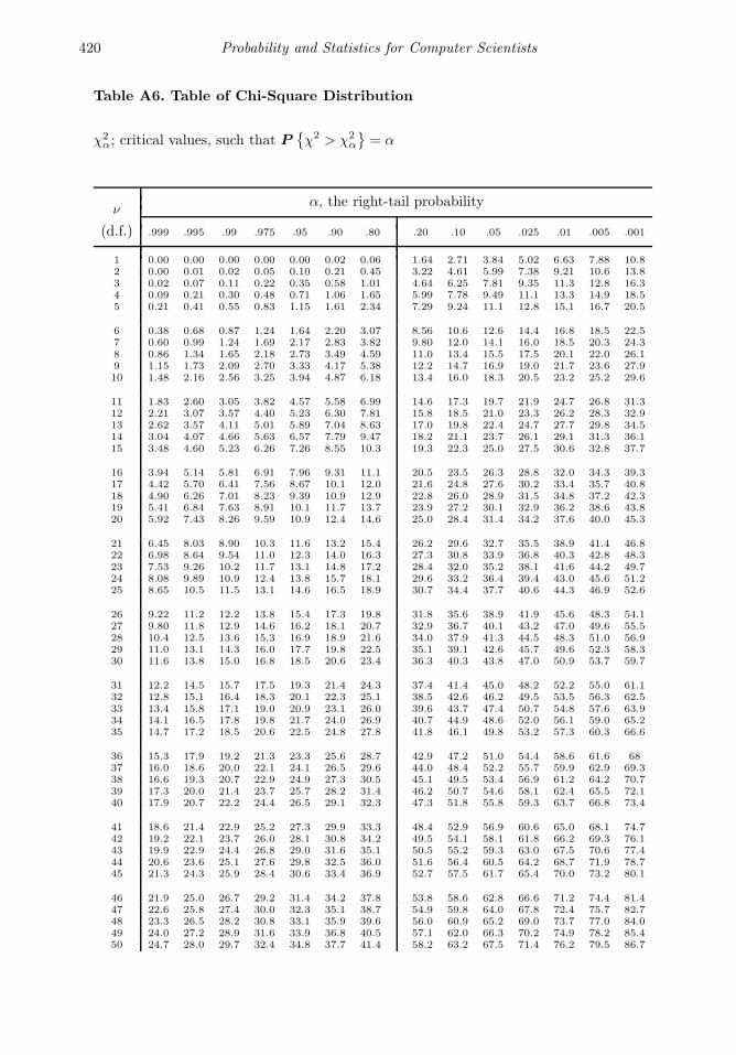
420 Probability and Statistics for Computer Scientists
Table A6. Table of Chi-Square Distribution
χ2α; critical values, such that P
χ2 > χ2
α
= α
α, the right-tail probabilityν
(d.f.) .999 .995 .99 .975 .95 .90 .80 .20 .10 .05 .025 .01 .005 .001
1 0.00 0.00 0.00 0.00 0.00 0.02 0.06 1.64 2.71 3.84 5.02 6.63 7.88 10.82 0.00 0.01 0.02 0.05 0.10 0.21 0.45 3.22 4.61 5.99 7.38 9.21 10.6 13.83 0.02 0.07 0.11 0.22 0.35 0.58 1.01 4.64 6.25 7.81 9.35 11.3 12.8 16.34 0.09 0.21 0.30 0.48 0.71 1.06 1.65 5.99 7.78 9.49 11.1 13.3 14.9 18.55 0.21 0.41 0.55 0.83 1.15 1.61 2.34 7.29 9.24 11.1 12.8 15.1 16.7 20.5
6 0.38 0.68 0.87 1.24 1.64 2.20 3.07 8.56 10.6 12.6 14.4 16.8 18.5 22.57 0.60 0.99 1.24 1.69 2.17 2.83 3.82 9.80 12.0 14.1 16.0 18.5 20.3 24.38 0.86 1.34 1.65 2.18 2.73 3.49 4.59 11.0 13.4 15.5 17.5 20.1 22.0 26.19 1.15 1.73 2.09 2.70 3.33 4.17 5.38 12.2 14.7 16.9 19.0 21.7 23.6 27.910 1.48 2.16 2.56 3.25 3.94 4.87 6.18 13.4 16.0 18.3 20.5 23.2 25.2 29.6
11 1.83 2.60 3.05 3.82 4.57 5.58 6.99 14.6 17.3 19.7 21.9 24.7 26.8 31.312 2.21 3.07 3.57 4.40 5.23 6.30 7.81 15.8 18.5 21.0 23.3 26.2 28.3 32.913 2.62 3.57 4.11 5.01 5.89 7.04 8.63 17.0 19.8 22.4 24.7 27.7 29.8 34.514 3.04 4.07 4.66 5.63 6.57 7.79 9.47 18.2 21.1 23.7 26.1 29.1 31.3 36.115 3.48 4.60 5.23 6.26 7.26 8.55 10.3 19.3 22.3 25.0 27.5 30.6 32.8 37.7
16 3.94 5.14 5.81 6.91 7.96 9.31 11.1 20.5 23.5 26.3 28.8 32.0 34.3 39.317 4.42 5.70 6.41 7.56 8.67 10.1 12.0 21.6 24.8 27.6 30.2 33.4 35.7 40.818 4.90 6.26 7.01 8.23 9.39 10.9 12.9 22.8 26.0 28.9 31.5 34.8 37.2 42.319 5.41 6.84 7.63 8.91 10.1 11.7 13.7 23.9 27.2 30.1 32.9 36.2 38.6 43.820 5.92 7.43 8.26 9.59 10.9 12.4 14.6 25.0 28.4 31.4 34.2 37.6 40.0 45.3
21 6.45 8.03 8.90 10.3 11.6 13.2 15.4 26.2 29.6 32.7 35.5 38.9 41.4 46.822 6.98 8.64 9.54 11.0 12.3 14.0 16.3 27.3 30.8 33.9 36.8 40.3 42.8 48.323 7.53 9.26 10.2 11.7 13.1 14.8 17.2 28.4 32.0 35.2 38.1 41.6 44.2 49.724 8.08 9.89 10.9 12.4 13.8 15.7 18.1 29.6 33.2 36.4 39.4 43.0 45.6 51.225 8.65 10.5 11.5 13.1 14.6 16.5 18.9 30.7 34.4 37.7 40.6 44.3 46.9 52.6
26 9.22 11.2 12.2 13.8 15.4 17.3 19.8 31.8 35.6 38.9 41.9 45.6 48.3 54.127 9.80 11.8 12.9 14.6 16.2 18.1 20.7 32.9 36.7 40.1 43.2 47.0 49.6 55.528 10.4 12.5 13.6 15.3 16.9 18.9 21.6 34.0 37.9 41.3 44.5 48.3 51.0 56.929 11.0 13.1 14.3 16.0 17.7 19.8 22.5 35.1 39.1 42.6 45.7 49.6 52.3 58.330 11.6 13.8 15.0 16.8 18.5 20.6 23.4 36.3 40.3 43.8 47.0 50.9 53.7 59.7
31 12.2 14.5 15.7 17.5 19.3 21.4 24.3 37.4 41.4 45.0 48.2 52.2 55.0 61.132 12.8 15.1 16.4 18.3 20.1 22.3 25.1 38.5 42.6 46.2 49.5 53.5 56.3 62.533 13.4 15.8 17.1 19.0 20.9 23.1 26.0 39.6 43.7 47.4 50.7 54.8 57.6 63.934 14.1 16.5 17.8 19.8 21.7 24.0 26.9 40.7 44.9 48.6 52.0 56.1 59.0 65.235 14.7 17.2 18.5 20.6 22.5 24.8 27.8 41.8 46.1 49.8 53.2 57.3 60.3 66.6
36 15.3 17.9 19.2 21.3 23.3 25.6 28.7 42.9 47.2 51.0 54.4 58.6 61.6 6837 16.0 18.6 20,0 22.1 24.1 26.5 29.6 44.0 48.4 52.2 55.7 59.9 62.9 69.338 16.6 19.3 20.7 22.9 24.9 27.3 30.5 45.1 49.5 53.4 56.9 61.2 64.2 70.739 17.3 20.0 21.4 23.7 25.7 28.2 31.4 46.2 50.7 54.6 58.1 62.4 65.5 72.140 17.9 20.7 22.2 24.4 26.5 29.1 32.3 47.3 51.8 55.8 59.3 63.7 66.8 73.4
41 18.6 21.4 22.9 25.2 27.3 29.9 33.3 48.4 52.9 56.9 60.6 65.0 68.1 74.742 19.2 22.1 23.7 26.0 28.1 30.8 34.2 49.5 54.1 58.1 61.8 66.2 69.3 76.143 19.9 22.9 24.4 26.8 29.0 31.6 35.1 50.5 55.2 59.3 63.0 67.5 70.6 77.444 20.6 23.6 25.1 27.6 29.8 32.5 36.0 51.6 56.4 60.5 64.2 68.7 71.9 78.745 21.3 24.3 25.9 28.4 30.6 33.4 36.9 52.7 57.5 61.7 65.4 70.0 73.2 80.1
46 21.9 25.0 26.7 29.2 31.4 34.2 37.8 53.8 58.6 62.8 66.6 71.2 74.4 81.447 22.6 25.8 27.4 30.0 32.3 35.1 38.7 54.9 59.8 64.0 67.8 72.4 75.7 82.748 23.3 26.5 28.2 30.8 33.1 35.9 39.6 56.0 60.9 65.2 69.0 73.7 77.0 84.049 24.0 27.2 28.9 31.6 33.9 36.8 40.5 57.1 62.0 66.3 70.2 74.9 78.2 85.450 24.7 28.0 29.7 32.4 34.8 37.7 41.4 58.2 63.2 67.5 71.4 76.2 79.5 86.7
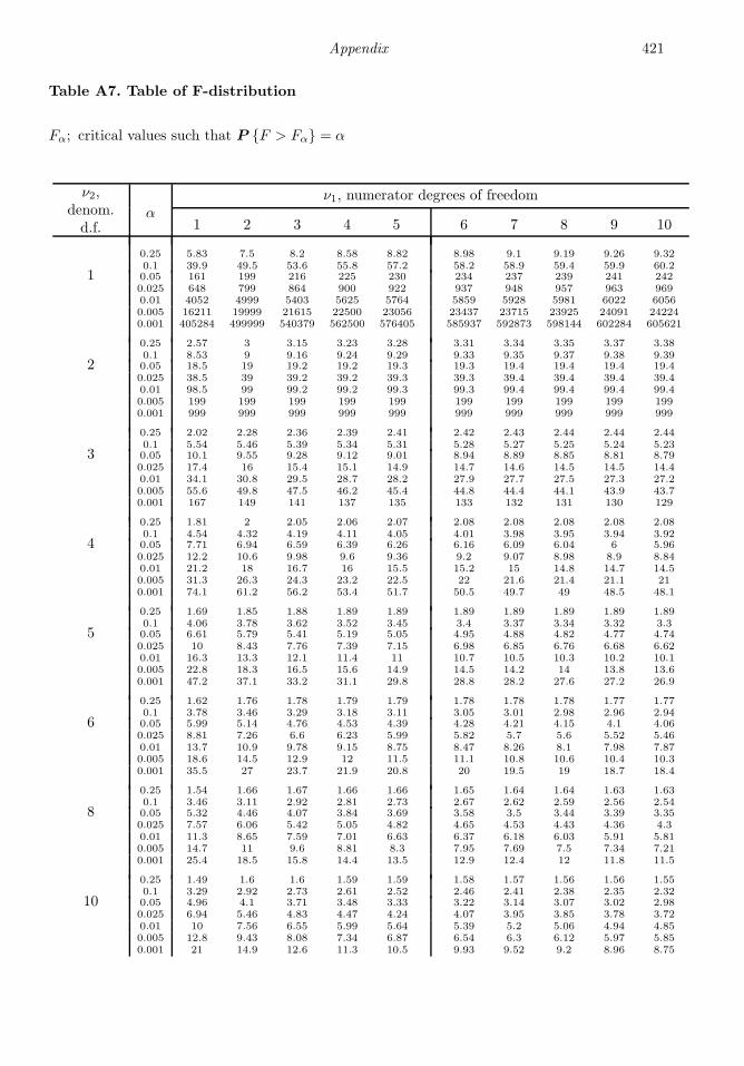
Appendix 421
Table A7. Table of F-distribution
Fα; critical values such that P F > Fα = α
ν2,denom.d.f.
ν1, numerator degrees of freedomα
1 2 3 4 5 6 7 8 9 10
0.25 5.83 7.5 8.2 8.58 8.82 8.98 9.1 9.19 9.26 9.320.1 39.9 49.5 53.6 55.8 57.2 58.2 58.9 59.4 59.9 60.2
1 0.05 161 199 216 225 230 234 237 239 241 2420.025 648 799 864 900 922 937 948 957 963 9690.01 4052 4999 5403 5625 5764 5859 5928 5981 6022 60560.005 16211 19999 21615 22500 23056 23437 23715 23925 24091 242240.001 405284 499999 540379 562500 576405 585937 592873 598144 602284 605621
0.25 2.57 3 3.15 3.23 3.28 3.31 3.34 3.35 3.37 3.380.1 8.53 9 9.16 9.24 9.29 9.33 9.35 9.37 9.38 9.39
2 0.05 18.5 19 19.2 19.2 19.3 19.3 19.4 19.4 19.4 19.40.025 38.5 39 39.2 39.2 39.3 39.3 39.4 39.4 39.4 39.40.01 98.5 99 99.2 99.2 99.3 99.3 99.4 99.4 99.4 99.40.005 199 199 199 199 199 199 199 199 199 1990.001 999 999 999 999 999 999 999 999 999 999
0.25 2.02 2.28 2.36 2.39 2.41 2.42 2.43 2.44 2.44 2.440.1 5.54 5.46 5.39 5.34 5.31 5.28 5.27 5.25 5.24 5.23
3 0.05 10.1 9.55 9.28 9.12 9.01 8.94 8.89 8.85 8.81 8.790.025 17.4 16 15.4 15.1 14.9 14.7 14.6 14.5 14.5 14.40.01 34.1 30.8 29.5 28.7 28.2 27.9 27.7 27.5 27.3 27.20.005 55.6 49.8 47.5 46.2 45.4 44.8 44.4 44.1 43.9 43.70.001 167 149 141 137 135 133 132 131 130 129
0.25 1.81 2 2.05 2.06 2.07 2.08 2.08 2.08 2.08 2.080.1 4.54 4.32 4.19 4.11 4.05 4.01 3.98 3.95 3.94 3.92
4 0.05 7.71 6.94 6.59 6.39 6.26 6.16 6.09 6.04 6 5.960.025 12.2 10.6 9.98 9.6 9.36 9.2 9.07 8.98 8.9 8.840.01 21.2 18 16.7 16 15.5 15.2 15 14.8 14.7 14.50.005 31.3 26.3 24.3 23.2 22.5 22 21.6 21.4 21.1 210.001 74.1 61.2 56.2 53.4 51.7 50.5 49.7 49 48.5 48.1
0.25 1.69 1.85 1.88 1.89 1.89 1.89 1.89 1.89 1.89 1.890.1 4.06 3.78 3.62 3.52 3.45 3.4 3.37 3.34 3.32 3.3
5 0.05 6.61 5.79 5.41 5.19 5.05 4.95 4.88 4.82 4.77 4.740.025 10 8.43 7.76 7.39 7.15 6.98 6.85 6.76 6.68 6.620.01 16.3 13.3 12.1 11.4 11 10.7 10.5 10.3 10.2 10.10.005 22.8 18.3 16.5 15.6 14.9 14.5 14.2 14 13.8 13.60.001 47.2 37.1 33.2 31.1 29.8 28.8 28.2 27.6 27.2 26.9
0.25 1.62 1.76 1.78 1.79 1.79 1.78 1.78 1.78 1.77 1.770.1 3.78 3.46 3.29 3.18 3.11 3.05 3.01 2.98 2.96 2.94
6 0.05 5.99 5.14 4.76 4.53 4.39 4.28 4.21 4.15 4.1 4.060.025 8.81 7.26 6.6 6.23 5.99 5.82 5.7 5.6 5.52 5.460.01 13.7 10.9 9.78 9.15 8.75 8.47 8.26 8.1 7.98 7.870.005 18.6 14.5 12.9 12 11.5 11.1 10.8 10.6 10.4 10.30.001 35.5 27 23.7 21.9 20.8 20 19.5 19 18.7 18.4
0.25 1.54 1.66 1.67 1.66 1.66 1.65 1.64 1.64 1.63 1.630.1 3.46 3.11 2.92 2.81 2.73 2.67 2.62 2.59 2.56 2.54
8 0.05 5.32 4.46 4.07 3.84 3.69 3.58 3.5 3.44 3.39 3.350.025 7.57 6.06 5.42 5.05 4.82 4.65 4.53 4.43 4.36 4.30.01 11.3 8.65 7.59 7.01 6.63 6.37 6.18 6.03 5.91 5.810.005 14.7 11 9.6 8.81 8.3 7.95 7.69 7.5 7.34 7.210.001 25.4 18.5 15.8 14.4 13.5 12.9 12.4 12 11.8 11.5
0.25 1.49 1.6 1.6 1.59 1.59 1.58 1.57 1.56 1.56 1.550.1 3.29 2.92 2.73 2.61 2.52 2.46 2.41 2.38 2.35 2.32
10 0.05 4.96 4.1 3.71 3.48 3.33 3.22 3.14 3.07 3.02 2.980.025 6.94 5.46 4.83 4.47 4.24 4.07 3.95 3.85 3.78 3.720.01 10 7.56 6.55 5.99 5.64 5.39 5.2 5.06 4.94 4.850.005 12.8 9.43 8.08 7.34 6.87 6.54 6.3 6.12 5.97 5.850.001 21 14.9 12.6 11.3 10.5 9.93 9.52 9.2 8.96 8.75
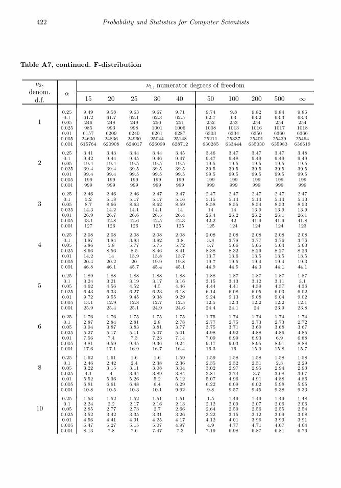
422 Probability and Statistics for Computer Scientists
Table A7, continued. F-distribution
ν2,denom.d.f.
ν1, numerator degrees of freedomα
15 20 25 30 40 50 100 200 500 ∞0.25 9.49 9.58 9.63 9.67 9.71 9.74 9.8 9.82 9.84 9.850.1 61.2 61.7 62.1 62.3 62.5 62.7 63 63.2 63.3 63.3
1 0.05 246 248 249 250 251 252 253 254 254 2540.025 985 993 998 1001 1006 1008 1013 1016 1017 10180.01 6157 6209 6240 6261 6287 6303 6334 6350 6360 63660.005 24630 24836 24960 25044 25148 25211 25337 25401 25439 254640.001 615764 620908 624017 626099 628712 630285 633444 635030 635983 636619
0.25 3.41 3.43 3.44 3.44 3.45 3.46 3.47 3.47 3.47 3.480.1 9.42 9.44 9.45 9.46 9.47 9.47 9.48 9.49 9.49 9.49
2 0.05 19.4 19.4 19.5 19.5 19.5 19.5 19.5 19.5 19.5 19.50.025 39.4 39.4 39.5 39.5 39.5 39.5 39.5 39.5 39.5 39.50.01 99.4 99.4 99.5 99.5 99.5 99.5 99.5 99.5 99.5 99.50.005 199 199 199 199 199 199 199 199 199 1990.001 999 999 999 999 999 999 999 999 999 999
0.25 2.46 2.46 2.46 2.47 2.47 2.47 2.47 2.47 2.47 2.470.1 5.2 5.18 5.17 5.17 5.16 5.15 5.14 5.14 5.14 5.13
3 0.05 8.7 8.66 8.63 8.62 8.59 8.58 8.55 8.54 8.53 8.530.025 14.3 14.2 14.1 14.1 14 14 14 13.9 13.9 13.90.01 26.9 26.7 26.6 26.5 26.4 26.4 26.2 26.2 26.1 26.10.005 43.1 42.8 42.6 42.5 42.3 42.2 42 41.9 41.9 41.80.001 127 126 126 125 125 125 124 124 124 123
0.25 2.08 2.08 2.08 2.08 2.08 2.08 2.08 2.08 2.08 2.080.1 3.87 3.84 3.83 3.82 3.8 3.8 3.78 3.77 3.76 3.76
4 0.05 5.86 5.8 5.77 5.75 5.72 5.7 5.66 5.65 5.64 5.630.025 8.66 8.56 8.5 8.46 8.41 8.38 8.32 8.29 8.27 8.260.01 14.2 14 13.9 13.8 13.7 13.7 13.6 13.5 13.5 13.50.005 20.4 20.2 20 19.9 19.8 19.7 19.5 19.4 19.4 19.30.001 46.8 46.1 45.7 45.4 45.1 44.9 44.5 44.3 44.1 44.1
0.25 1.89 1.88 1.88 1.88 1.88 1.88 1.87 1.87 1.87 1.870.1 3.24 3.21 3.19 3.17 3.16 3.15 3.13 3.12 3.11 3.1
5 0.05 4.62 4.56 4.52 4.5 4.46 4.44 4.41 4.39 4.37 4.360.025 6.43 6.33 6.27 6.23 6.18 6.14 6.08 6.05 6.03 6.020.01 9.72 9.55 9.45 9.38 9.29 9.24 9.13 9.08 9.04 9.020.005 13.1 12.9 12.8 12.7 12.5 12.5 12.3 12.2 12.2 12.10.001 25.9 25.4 25.1 24.9 24.6 24.4 24.1 24 23.9 23.8
0.25 1.76 1.76 1.75 1.75 1.75 1.75 1.74 1.74 1.74 1.740.1 2.87 2.84 2.81 2.8 2.78 2.77 2.75 2.73 2.73 2.72
6 0.05 3.94 3.87 3.83 3.81 3.77 3.75 3.71 3.69 3.68 3.670.025 5.27 5.17 5.11 5.07 5.01 4.98 4.92 4.88 4.86 4.850.01 7.56 7.4 7.3 7.23 7.14 7.09 6.99 6.93 6.9 6.880.005 9.81 9.59 9.45 9.36 9.24 9.17 9.03 8.95 8.91 8.880.001 17.6 17.1 16.9 16.7 16.4 16.3 16 15.9 15.8 15.7
0.25 1.62 1.61 1.6 1.6 1.59 1.59 1.58 1.58 1.58 1.580.1 2.46 2.42 2.4 2.38 2.36 2.35 2.32 2.31 2.3 2.29
8 0.05 3.22 3.15 3.11 3.08 3.04 3.02 2.97 2.95 2.94 2.930.025 4.1 4 3.94 3.89 3.84 3.81 3.74 3.7 3.68 3.670.01 5.52 5.36 5.26 5.2 5.12 5.07 4.96 4.91 4.88 4.860.005 6.81 6.61 6.48 6.4 6.29 6.22 6.09 6.02 5.98 5.950.001 10.8 10.5 10.3 10.1 9.92 9.8 9.57 9.45 9.38 9.33
0.25 1.53 1.52 1.52 1.51 1.51 1.5 1.49 1.49 1.49 1.480.1 2.24 2.2 2.17 2.16 2.13 2.12 2.09 2.07 2.06 2.06
10 0.05 2.85 2.77 2.73 2.7 2.66 2.64 2.59 2.56 2.55 2.540.025 3.52 3.42 3.35 3.31 3.26 3.22 3.15 3.12 3.09 3.080.01 4.56 4.41 4.31 4.25 4.17 4.12 4.01 3.96 3.93 3.910.005 5.47 5.27 5.15 5.07 4.97 4.9 4.77 4.71 4.67 4.640.001 8.13 7.8 7.6 7.47 7.3 7.19 6.98 6.87 6.81 6.76

Appendix 423
Table A7, continued. F-distribution
ν2,denom.d.f.
ν1, numerator degrees of freedomα
1 2 3 4 5 6 7 8 9 10
0.25 1.43 1.52 1.52 1.51 1.49 1.48 1.47 1.46 1.46 1.450.1 3.07 2.7 2.49 2.36 2.27 2.21 2.16 2.12 2.09 2.06
15 0.05 4.54 3.68 3.29 3.06 2.9 2.79 2.71 2.64 2.59 2.540.025 6.2 4.77 4.15 3.8 3.58 3.41 3.29 3.2 3.12 3.060.01 8.68 6.36 5.42 4.89 4.56 4.32 4.14 4 3.89 3.80.005 10.8 7.7 6.48 5.8 5.37 5.07 4.85 4.67 4.54 4.420.001 16.6 11.3 9.34 8.25 7.57 7.09 6.74 6.47 6.26 6.08
0.25 1.4 1.49 1.48 1.47 1.45 1.44 1.43 1.42 1.41 1.40.1 2.97 2.59 2.38 2.25 2.16 2.09 2.04 2 1.96 1.94
20 0.05 4.35 3.49 3.1 2.87 2.71 2.6 2.51 2.45 2.39 2.350.025 5.87 4.46 3.86 3.51 3.29 3.13 3.01 2.91 2.84 2.770.01 8.1 5.85 4.94 4.43 4.1 3.87 3.7 3.56 3.46 3.370.005 9.94 6.99 5.82 5.17 4.76 4.47 4.26 4.09 3.96 3.850.001 14.8 9.95 8.1 7.1 6.46 6.02 5.69 5.44 5.24 5.08
0.25 1.39 1.47 1.46 1.44 1.42 1.41 1.4 1.39 1.38 1.370.1 2.92 2.53 2.32 2.18 2.09 2.02 1.97 1.93 1.89 1.87
25 0.05 4.24 3.39 2.99 2.76 2.6 2.49 2.4 2.34 2.28 2.240.025 5.69 4.29 3.69 3.35 3.13 2.97 2.85 2.75 2.68 2.610.01 7.77 5.57 4.68 4.18 3.85 3.63 3.46 3.32 3.22 3.130.005 9.48 6.6 5.46 4.84 4.43 4.15 3.94 3.78 3.64 3.540.001 13.9 9.22 7.45 6.49 5.89 5.46 5.15 4.91 4.71 4.56
0.25 1.38 1.45 1.44 1.42 1.41 1.39 1.38 1.37 1.36 1.350.1 2.88 2.49 2.28 2.14 2.05 1.98 1.93 1.88 1.85 1.82
30 0.05 4.17 3.32 2.92 2.69 2.53 2.42 2.33 2.27 2.21 2.160.025 5.57 4.18 3.59 3.25 3.03 2.87 2.75 2.65 2.57 2.510.01 7.56 5.39 4.51 4.02 3.7 3.47 3.3 3.17 3.07 2.980.005 9.18 6.35 5.24 4.62 4.23 3.95 3.74 3.58 3.45 3.340.001 13.3 8.77 7.05 6.12 5.53 5.12 4.82 4.58 4.39 4.24
0.25 1.36 1.44 1.42 1.4 1.39 1.37 1.36 1.35 1.34 1.330.1 2.84 2.44 2.23 2.09 2 1.93 1.87 1.83 1.79 1.76
40 0.05 4.08 3.23 2.84 2.61 2.45 2.34 2.25 2.18 2.12 2.080.025 5.42 4.05 3.46 3.13 2.9 2.74 2.62 2.53 2.45 2.390.01 7.31 5.18 4.31 3.83 3.51 3.29 3.12 2.99 2.89 2.80.005 8.83 6.07 4.98 4.37 3.99 3.71 3.51 3.35 3.22 3.120.001 12.6 8.25 6.59 5.7 5.13 4.73 4.44 4.21 4.02 3.87
0.25 1.35 1.43 1.41 1.39 1.37 1.36 1.34 1.33 1.32 1.310.1 2.81 2.41 2.2 2.06 1.97 1.9 1.84 1.8 1.76 1.73
50 0.05 4.03 3.18 2.79 2.56 2.4 2.29 2.2 2.13 2.07 2.030.025 5.34 3.97 3.39 3.05 2.83 2.67 2.55 2.46 2.38 2.320.01 7.17 5.06 4.2 3.72 3.41 3.19 3.02 2.89 2.78 2.70.005 8.63 5.9 4.83 4.23 3.85 3.58 3.38 3.22 3.09 2.990.001 12.2 7.96 6.34 5.46 4.9 4.51 4.22 4 3.82 3.67
0.25 1.34 1.41 1.39 1.37 1.35 1.33 1.32 1.3 1.29 1.280.1 2.76 2.36 2.14 2 1.91 1.83 1.78 1.73 1.69 1.66
100 0.05 3.94 3.09 2.7 2.46 2.31 2.19 2.1 2.03 1.97 1.930.025 5.18 3.83 3.25 2.92 2.7 2.54 2.42 2.32 2.24 2.180.01 6.9 4.82 3.98 3.51 3.21 2.99 2.82 2.69 2.59 2.50.005 8.24 5.59 4.54 3.96 3.59 3.33 3.13 2.97 2.85 2.740.001 11.5 7.41 5.86 5.02 4.48 4.11 3.83 3.61 3.44 3.3
0.25 1.33 1.4 1.38 1.36 1.34 1.32 1.3 1.29 1.28 1.270.1 2.73 2.33 2.11 1.97 1.88 1.8 1.75 1.7 1.66 1.63
200 0.05 3.89 3.04 2.65 2.42 2.26 2.14 2.06 1.98 1.93 1.880.025 5.1 3.76 3.18 2.85 2.63 2.47 2.35 2.26 2.18 2.110.01 6.76 4.71 3.88 3.41 3.11 2.89 2.73 2.6 2.5 2.410.005 8.06 5.44 4.41 3.84 3.47 3.21 3.01 2.86 2.73 2.630.001 11.2 7.15 5.63 4.81 4.29 3.92 3.65 3.43 3.26 3.12
0.25 1.32 1.39 1.37 1.35 1.33 1.31 1.29 1.28 1.27 1.250.1 2.71 2.3 2.08 1.94 1.85 1.77 1.72 1.67 1.63 1.6∞ 0.05 3.84 3 2.6 2.37 2.21 2.1 2.01 1.94 1.88 1.83
0.025 5.02 3.69 3.12 2.79 2.57 2.41 2.29 2.19 2.11 2.050.01 6.63 4.61 3.78 3.32 3.02 2.8 2.64 2.51 2.41 2.320.005 7.88 5.3 4.28 3.72 3.35 3.09 2.9 2.74 2.62 2.520.001 10.8 6.91 5.42 4.62 4.1 3.74 3.47 3.27 3.1 2.96
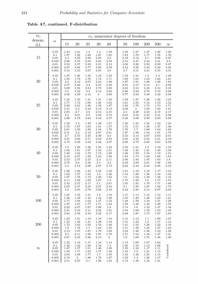
424 Probability and Statistics for Computer Scientists
Table A7, continued. F-distribution
ν2,denom.d.f.
ν1, numerator degrees of freedomα
15 20 25 30 40 50 100 200 500 ∞0.25 1.43 1.41 1.4 1.4 1.39 1.38 1.37 1.37 1.36 1.360.1 1.97 1.92 1.89 1.87 1.85 1.83 1.79 1.77 1.76 1.76
15 0.05 2.4 2.33 2.28 2.25 2.2 2.18 2.12 2.1 2.08 2.070.025 2.86 2.76 2.69 2.64 2.59 2.55 2.47 2.44 2.41 2.40.01 3.52 3.37 3.28 3.21 3.13 3.08 2.98 2.92 2.89 2.870.005 4.07 3.88 3.77 3.69 3.58 3.52 3.39 3.33 3.29 3.260.001 5.54 5.25 5.07 4.95 4.8 4.7 4.51 4.41 4.35 4.31
0.25 1.37 1.36 1.35 1.34 1.33 1.32 1.31 1.3 1.3 1.290.1 1.84 1.79 1.76 1.74 1.71 1.69 1.65 1.63 1.62 1.61
20 0.05 2.2 2.12 2.07 2.04 1.99 1.97 1.91 1.88 1.86 1.840.025 2.57 2.46 2.4 2.35 2.29 2.25 2.17 2.13 2.1 2.090.01 3.09 2.94 2.84 2.78 2.69 2.64 2.54 2.48 2.44 2.420.005 3.5 3.32 3.2 3.12 3.02 2.96 2.83 2.76 2.72 2.690.001 4.56 4.29 4.12 4 3.86 3.77 3.58 3.48 3.42 3.38
0.25 1.34 1.33 1.31 1.31 1.29 1.29 1.27 1.26 1.26 1.250.1 1.77 1.72 1.68 1.66 1.63 1.61 1.56 1.54 1.53 1.52
25 0.05 2.09 2.01 1.96 1.92 1.87 1.84 1.78 1.75 1.73 1.710.025 2.41 2.3 2.23 2.18 2.12 2.08 2 1.95 1.92 1.910.01 2.85 2.7 2.6 2.54 2.45 2.4 2.29 2.23 2.19 2.170.005 3.2 3.01 2.9 2.82 2.72 2.65 2.52 2.45 2.41 2.380.001 4.06 3.79 3.63 3.52 3.37 3.28 3.09 2.99 2.93 2.89
0.25 1.32 1.3 1.29 1.28 1.27 1.26 1.25 1.24 1.23 1.230.1 1.72 1.67 1.63 1.61 1.57 1.55 1.51 1.48 1.47 1.46
30 0.05 2.01 1.93 1.88 1.84 1.79 1.76 1.7 1.66 1.64 1.620.025 2.31 2.2 2.12 2.07 2.01 1.97 1.88 1.84 1.81 1.790.01 2.7 2.55 2.45 2.39 2.3 2.25 2.13 2.07 2.03 2.010.005 3.01 2.82 2.71 2.63 2.52 2.46 2.32 2.25 2.21 2.180.001 3.75 3.49 3.33 3.22 3.07 2.98 2.79 2.69 2.63 2.59
0.25 1.3 1.28 1.26 1.25 1.24 1.23 1.21 1.2 1.19 1.190.1 1.66 1.61 1.57 1.54 1.51 1.48 1.43 1.41 1.39 1.38
40 0.05 1.92 1.84 1.78 1.74 1.69 1.66 1.59 1.55 1.53 1.510.025 2.18 2.07 1.99 1.94 1.88 1.83 1.74 1.69 1.66 1.640.01 2.52 2.37 2.27 2.2 2.11 2.06 1.94 1.87 1.83 1.80.005 2.78 2.6 2.48 2.4 2.3 2.23 2.09 2.01 1.96 1.930.001 3.4 3.14 2.98 2.87 2.73 2.64 2.44 2.34 2.28 2.23
0.25 1.28 1.26 1.25 1.23 1.22 1.21 1.19 1.18 1.17 1.160.1 1.63 1.57 1.53 1.5 1.46 1.44 1.39 1.36 1.34 1.33
50 0.05 1.87 1.78 1.73 1.69 1.63 1.6 1.52 1.48 1.46 1.440.025 2.11 1.99 1.92 1.87 1.8 1.75 1.66 1.6 1.57 1.550.01 2.42 2.27 2.17 2.1 2.01 1.95 1.82 1.76 1.71 1.680.005 2.65 2.47 2.35 2.27 2.16 2.1 1.95 1.87 1.82 1.790.001 3.2 2.95 2.79 2.68 2.53 2.44 2.25 2.14 2.07 2.03
0.25 1.25 1.23 1.21 1.2 1.18 1.17 1.14 1.13 1.12 1.110.1 1.56 1.49 1.45 1.42 1.38 1.35 1.29 1.26 1.23 1.21
100 0.05 1.77 1.68 1.62 1.57 1.52 1.48 1.39 1.34 1.31 1.280.025 1.97 1.85 1.77 1.71 1.64 1.59 1.48 1.42 1.38 1.350.01 2.22 2.07 1.97 1.89 1.8 1.74 1.6 1.52 1.47 1.430.005 2.41 2.23 2.11 2.02 1.91 1.84 1.68 1.59 1.53 1.490.001 2.84 2.59 2.43 2.32 2.17 2.08 1.87 1.75 1.67 1.62
0.25 1.23 1.21 1.19 1.18 1.16 1.15 1.12 1.1 1.09 1.070.1 1.52 1.46 1.41 1.38 1.34 1.31 1.24 1.2 1.17 1.14
200 0.05 1.72 1.62 1.56 1.52 1.46 1.41 1.32 1.26 1.22 1.190.025 1.9 1.78 1.7 1.64 1.56 1.51 1.39 1.32 1.27 1.230.01 2.13 1.97 1.87 1.79 1.69 1.63 1.48 1.39 1.33 1.280.005 2.3 2.11 1.99 1.91 1.79 1.71 1.54 1.44 1.37 1.310.001 2.67 2.42 2.26 2.15 2 1.9 1.68 1.55 1.46 1.39
0.25 1.22 1.19 1.17 1.16 1.14 1.13 1.09 1.07 1.040.1 1.49 1.42 1.38 1.34 1.3 1.26 1.18 1.13 1.08∞ 0.05 1.67 1.57 1.51 1.46 1.39 1.35 1.24 1.17 1.11
Undefined
0.025 1.83 1.71 1.63 1.57 1.48 1.43 1.3 1.21 1.130.01 2.04 1.88 1.77 1.7 1.59 1.52 1.36 1.25 1.150.005 2.19 2 1.88 1.79 1.67 1.59 1.4 1.28 1.170.001 2.51 2.27 2.1 1.99 1.84 1.73 1.49 1.34 1.21

Appendix 425
Table A8. Table of Critical Values for the Wilcoxon Signed Rank Test
For the left-tail test, the table gives the largest integer w such that P W ≤ w | H0 ≤ α.
For the right-tail test, the table gives the smallest integer w such that P W ≥ w | H0 ≤ α.
A missing table entry means that such an integer does not exist among possible values of W .
α, left-tail probability for the left-tail test α, right-tail probability for the right-tail testn
0.001 0.005 0.010 0.025 0.050 0.100 0.200 0.200 0.100 0.050 0.025 0.010 0.005 0.001
1 — — — — — — — — — — — — — —
2 — — — — — — — — — — — — — —
3 — — — — — — 0 6 — — — — — —
4 — — — — — 0 2 8 10 — — — — —
5 — — — — 0 2 3 12 13 15 — — — —
6 — — — 0 2 3 5 16 18 19 21 — — —
7 — — 0 2 3 5 8 20 23 25 26 28 — —
8 — 0 1 3 5 8 11 25 28 31 33 35 36 —
9 — 1 3 5 8 10 14 31 35 37 40 42 44 —
10 0 3 5 8 10 14 18 37 41 45 47 50 52 55
11 1 5 7 10 13 17 22 44 49 53 56 59 61 65
12 2 7 9 13 17 21 27 51 57 61 65 69 71 76
13 4 9 12 17 21 26 32 59 65 70 74 79 82 87
14 6 12 15 21 25 31 38 67 74 80 84 90 93 99
15 8 15 19 25 30 36 44 76 84 90 95 101 105 112
16 11 19 23 29 35 42 50 86 94 101 107 113 117 125
17 14 23 27 34 41 48 57 96 105 112 119 126 130 139
18 18 27 32 40 47 55 65 106 116 124 131 139 144 153
19 21 32 37 46 53 62 73 117 128 137 144 153 158 169
20 26 37 43 52 60 69 81 129 141 150 158 167 173 184
21 30 42 49 58 67 77 90 141 154 164 173 182 189 201
22 35 48 55 65 75 86 99 154 167 178 188 198 205 218
23 40 54 62 73 83 94 109 167 182 193 203 214 222 236
24 45 61 69 81 91 104 119 181 196 209 219 231 239 255
25 51 68 76 89 100 113 130 195 212 225 236 249 257 274
26 58 75 84 98 110 124 141 210 227 241 253 267 276 293
27 64 83 92 107 119 134 153 225 244 259 271 286 295 314
28 71 91 101 116 130 145 165 241 261 276 290 305 315 335
29 79 100 110 126 140 157 177 258 278 295 309 325 335 356
30 86 109 120 137 151 169 190 275 296 314 328 345 356 379

426 Probability and Statistics for Computer Scientists
Table A9. Critical Values for the Mann-Whitney-Wilcoxon Rank-Sum Test
For the left-tail test, the table gives the largest integer u such that P U ≤ u | H0 ≤ α.
For the right-tail test, the table gives the smallest integer u such that P U ≥ u | H0 ≤ α.
A missing table entry means that such an integer does not exist among possible values of U .
α, left-tail probability for the left-tail testHA : X is stochastically smaller than Y
α, right-tail probability for the right-tail testHA : X is stochastically larger than Y
n1 n2 0.001 0.005 0.010 0.025 0.050 0.100 0.200 0.200 0.100 0.050 0.025 0.010 0.005 0.001
3 2 — — — — — 6 7 11 12 — — — — —3 3 — — — — 6 7 8 13 14 15 — — — —3 4 — — — — 6 7 9 15 17 18 — — — —3 5 — — — 6 7 8 10 17 19 20 21 — — —3 6 — — — 7 8 9 11 19 21 22 23 — — —3 7 — — 6 7 8 10 12 21 23 25 26 27 — —3 8 — — 6 8 9 11 13 23 25 27 28 30 — —3 9 — 6 7 8 10 11 14 25 28 29 31 32 33 —3 10 — 6 7 9 10 12 15 27 30 32 33 35 36 —3 11 — 6 7 9 11 13 16 29 32 34 36 38 39 —3 12 — 7 8 10 11 14 17 31 34 37 38 40 41 —
4 2 — — — — — 10 11 17 18 — — — — —4 3 — — — — 10 11 13 19 21 22 — — — —4 4 — — — 10 11 13 14 22 23 25 26 — — —4 5 — — 10 11 12 14 15 25 26 28 29 30 — —4 6 — 10 11 12 13 15 17 27 29 31 32 33 34 —4 7 — 10 11 13 14 16 18 30 32 34 35 37 38 —4 8 — 11 12 14 15 17 20 32 35 37 38 40 41 —4 9 — 11 13 14 16 19 21 35 37 40 42 43 45 —4 10 10 12 13 15 17 20 23 37 40 43 45 47 48 504 11 10 12 14 16 18 21 24 40 43 46 48 50 52 544 12 10 13 15 17 19 22 26 42 46 49 51 53 55 58
5 2 — — — — 15 16 17 23 24 25 — — — —5 3 — — — 15 16 17 19 26 28 29 30 — — —5 4 — — 15 16 17 19 20 30 31 33 34 35 — —5 5 — 15 16 17 19 20 22 33 35 36 38 39 40 —5 6 — 16 17 18 20 22 24 36 38 40 42 43 44 —5 7 — 16 18 20 21 23 26 39 42 44 45 47 49 —5 8 15 17 19 21 23 25 28 42 45 47 49 51 53 555 9 16 18 20 22 24 27 30 45 48 51 53 55 57 595 10 16 19 21 23 26 28 32 48 52 54 57 59 61 645 11 17 20 22 24 27 30 34 51 55 58 61 63 65 685 12 17 21 23 26 28 32 36 54 58 62 64 67 69 73
6 2 — — — — 21 22 23 31 32 33 — — — —6 3 — — — 22 23 24 26 34 36 37 38 — — —6 4 — 21 22 23 24 26 28 38 40 42 43 44 45 —6 5 — 22 23 24 26 28 30 42 44 46 48 49 50 —6 6 — 23 24 26 28 30 33 45 48 50 52 54 55 —6 7 21 24 25 27 29 32 35 49 52 55 57 59 60 636 8 22 25 27 29 31 34 37 53 56 59 61 63 65 686 9 23 26 28 31 33 36 40 56 60 63 65 68 70 736 10 24 27 29 32 35 38 42 60 64 67 70 73 75 786 11 25 28 30 34 37 40 44 64 68 71 74 78 80 836 12 25 30 32 35 38 42 47 67 72 76 79 82 84 89
7 2 — — — — 28 29 31 39 41 42 — — — —7 3 — — 28 29 30 32 34 43 45 47 48 49 — —7 4 — 28 29 31 32 34 36 48 50 52 53 55 56 —7 5 — 29 31 33 34 36 39 52 55 57 58 60 62 —7 6 28 31 32 34 36 39 42 56 59 62 64 66 67 707 7 29 32 34 36 39 41 45 60 64 66 69 71 73 767 8 30 34 35 38 41 44 48 64 68 71 74 77 78 827 9 31 35 37 40 43 46 50 69 73 76 79 82 84 887 10 33 37 39 42 45 49 53 73 77 81 84 87 89 937 11 34 38 40 44 47 51 56 77 82 86 89 93 95 997 12 35 40 42 46 49 54 59 81 86 91 94 98 100 105

Appendix 427
Table A9, continued. Critical Values for the Mann-Whitney-Wilcoxon Rank-Sum Test
For the left-tail test, the table gives the largest integer u such that P U ≤ u | H0 ≤ α.
For the right-tail test, the table gives the smallest integer u such that P U ≥ u | H0 ≤ α.
A missing table entry means that such an integer does not exist among possible values of U .
α, left-tail probability for the left-tail testHA : X is stochastically smaller than Y
α, right-tail probability for the right-tail testHA : X is stochastically larger than Y
n1 n2 0.001 0.005 0.010 0.025 0.050 0.100 0.200 0.200 0.100 0.050 0.025 0.010 0.005 0.001
8 2 — — — 36 37 38 40 48 50 51 52 — — —8 3 — — 36 38 39 41 43 53 55 57 58 60 — —8 4 — 37 38 40 41 43 46 58 61 63 64 66 67 —8 5 36 38 40 42 44 46 49 63 66 68 70 72 74 768 6 37 40 42 44 46 49 52 68 71 74 76 78 80 838 7 38 42 43 46 49 52 56 72 76 79 82 85 86 908 8 40 43 45 49 51 55 59 77 81 85 87 91 93 968 9 41 45 47 51 54 58 62 82 86 90 93 97 99 1038 10 42 47 49 53 56 60 65 87 92 96 99 103 105 1108 11 44 49 51 55 59 63 69 91 97 101 105 109 111 1168 12 45 51 53 58 62 66 72 96 102 106 110 115 117 123
9 2 — — — 45 46 47 49 59 61 62 63 — — —9 3 — 45 46 47 49 50 53 64 67 68 70 71 72 —9 4 — 46 48 49 51 54 56 70 72 75 77 78 80 —9 5 46 48 50 52 54 57 60 75 78 81 83 85 87 899 6 47 50 52 55 57 60 64 80 84 87 89 92 94 979 7 48 52 54 57 60 63 67 86 90 93 96 99 101 1059 8 50 54 56 60 63 67 71 91 95 99 102 106 108 1129 9 52 56 59 62 66 70 75 96 101 105 109 112 115 1199 10 53 58 61 65 69 73 78 102 107 111 115 119 122 1279 11 55 61 63 68 72 76 82 107 113 117 121 126 128 1349 12 57 63 66 71 75 80 86 112 118 123 127 132 135 141
10 2 — — — 55 56 58 60 70 72 74 75 — — —10 3 — 55 56 58 59 61 64 76 79 81 82 84 85 —10 4 55 57 58 60 62 65 68 82 85 88 90 92 93 9510 5 56 59 61 63 66 68 72 88 92 94 97 99 101 10410 6 58 61 63 66 69 72 76 94 98 101 104 107 109 11210 7 60 64 66 69 72 76 80 100 104 108 111 114 116 12010 8 61 66 68 72 75 79 84 106 111 115 118 122 124 12910 9 63 68 71 75 79 83 88 112 117 121 125 129 132 13710 10 65 71 74 78 82 87 93 117 123 128 132 136 139 14510 11 67 73 77 81 86 91 97 123 129 134 139 143 147 15310 12 69 76 79 84 89 94 101 129 136 141 146 151 154 161
11 2 — — — 66 67 69 71 83 85 87 88 — — —11 3 — 66 67 69 71 73 76 89 92 94 96 98 99 —11 4 66 68 70 72 74 77 80 96 99 102 104 106 108 11011 5 68 71 73 75 78 81 85 102 106 109 112 114 116 11911 6 70 73 75 79 82 85 89 109 113 116 119 123 125 12811 7 72 76 78 82 85 89 94 115 120 124 127 131 133 13711 8 74 79 81 85 89 93 99 121 127 131 135 139 141 14611 9 76 82 84 89 93 97 103 128 134 138 142 147 149 15511 10 78 84 88 92 97 102 108 134 140 145 150 154 158 16411 11 81 87 91 96 100 106 112 141 147 153 157 162 166 17211 12 83 90 94 99 104 110 117 147 154 160 165 170 174 181
12 2 — — — 79 80 82 84 96 98 100 101 — — —12 3 — 79 80 82 83 86 89 103 106 109 110 112 113 —12 4 78 81 83 85 87 90 94 110 114 117 119 121 123 12612 5 80 84 86 89 91 95 99 117 121 125 127 130 132 13612 6 82 87 89 92 95 99 104 124 129 133 136 139 141 14612 7 85 90 92 96 99 104 109 131 136 141 144 148 150 15512 8 87 93 95 100 104 108 114 138 144 148 152 157 159 16512 9 90 96 99 104 108 113 119 145 151 156 160 165 168 17412 10 92 99 102 107 112 117 124 152 159 164 169 174 177 18412 11 95 102 106 111 116 122 129 159 166 172 177 182 186 19312 12 98 105 109 115 120 127 134 166 173 180 185 191 195 202

428 Probability and Statistics for Computer Scientists
12.3 Calculus review
This section is a very brief summary of Calculus skills required for reading this book.
12.3.1 Inverse function
Function g is the inverse function of function f if
g(f(x)) = x and f(g(y)) = y
for all x and y where f(x) and g(y) exist.
Notation Inverse function g = f−1
(Don’t confuse the inverse f−1(x) with 1/f(x). These are different functions!)
To find the inverse function, solve the equation
f(x) = y.
The solution g(y) is the inverse of f .
For example, to find the inverse of f(x) = 3 + 1/x, we solve the equation
3 + 1/x = y ⇒ 1/x = y − 3 ⇒ x =1
y − 3.
The inverse function of f is g(y) = 1/(y − 3).
12.3.2 Limits and continuity
A function f(x) has a limit L at a point x0 if f(x) approaches L when x approaches x0.To say it more rigorously, for any ε there exists such δ that f(x) is ε-close to L when x isδ-close to x0. That is,
if |x− x0| < δ then |f(x)− L| < ε.
A function f(x) has a limit L at +∞ if f(x) approaches L when x goes to +∞. Rigorously,for any ε there exists such N that f(x) is ε-close to L when x gets beyond N , i.e.,
if x > N then |f(x)− L| < ε.
Similarly, f(x) has a limit L at −∞ if for any ε there exists such N that f(x) is ε-close toL when x gets below (−N), i.e.,
if x < −N then |f(x)− L| < ε.
Notation limx→x0
f(x) = L, or f(x) → L as x → x0
limx→∞
f(x) = L, or f(x) → L as x → ∞lim
x→−∞f(x) = L, or f(x) → L as x → −∞
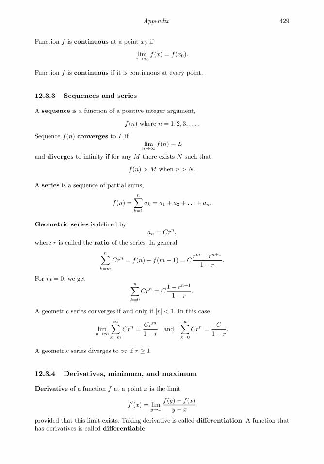
Appendix 429
Function f is continuous at a point x0 if
limx→x0
f(x) = f(x0).
Function f is continuous if it is continuous at every point.
12.3.3 Sequences and series
A sequence is a function of a positive integer argument,
f(n) where n = 1, 2, 3, . . . .
Sequence f(n) converges to L iflimn→∞
f(n) = L
and diverges to infinity if for any M there exists N such that
f(n) > M when n > N.
A series is a sequence of partial sums,
f(n) =
n∑
k=1
ak = a1 + a2 + . . .+ an.
Geometric series is defined byan = Crn,
where r is called the ratio of the series. In general,
n∑
k=m
Crn = f(n)− f(m− 1) = Crm − rn+1
1− r.
For m = 0, we getn∑
k=0
Crn = C1− rn+1
1− r.
A geometric series converges if and only if |r| < 1. In this case,
limn→∞
∞∑
k=m
Crn =Crm
1− rand
∞∑
k=0
Crn =C
1− r.
A geometric series diverges to ∞ if r ≥ 1.
12.3.4 Derivatives, minimum, and maximum
Derivative of a function f at a point x is the limit
f ′(x) = limy→x
f(y)− f(x)
y − x
provided that this limit exists. Taking derivative is called differentiation. A function thathas derivatives is called differentiable.
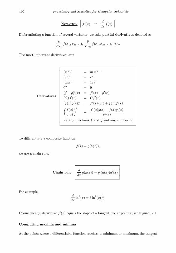
430 Probability and Statistics for Computer Scientists
Notation f ′(x) ord
dxf(x)
Differentiating a function of several variables, we take partial derivatives denoted as
∂
∂x1f(x1, x2, . . .),
∂
∂x2f(x1, x2, . . .), etc..
The most important derivatives are:
Derivatives
(xm)′ = mxm−1
(ex)′ = ex
(ln x)′ = 1/x
C′ = 0
(f + g)′(x) = f ′(x) + g′(x)
(Cf)′(x) = Cf ′(x)
(f(x)g(x))′ = f ′(x)g(x) + f(x)g′(x)(f(x)
g(x)
)′
=f ′(x)g(x) − f(x)g′(x)
g2(x)
for any functions f and g and any number C
To differentiate a composite function
f(x) = g(h(x)),
we use a chain rule,
Chain ruled
dxg(h(x)) = g′(h(x))h′(x)
For example,d
dxln3(x) = 3 ln2(x)
1
x.
Geometrically, derivative f ′(x) equals the slope of a tangent line at point x; see Figure 12.1.
Computing maxima and minima
At the points where a differentiable function reaches its minimum or maximum, the tangent
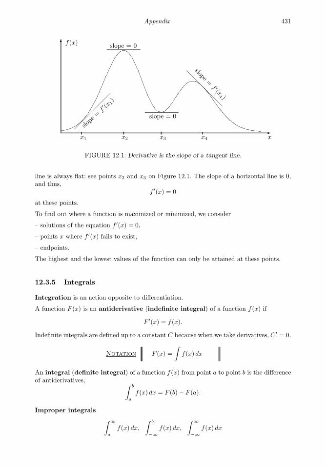
Appendix 431
f(x)
xx1 x2 x3 x4
slope
=f′ (x
1)
slope = 0
slope = 0
slope=f ′(x
4 )
FIGURE 12.1: Derivative is the slope of a tangent line.
line is always flat; see points x2 and x3 on Figure 12.1. The slope of a horizontal line is 0,and thus,
f ′(x) = 0
at these points.
To find out where a function is maximized or minimized, we consider
– solutions of the equation f ′(x) = 0,
– points x where f ′(x) fails to exist,
– endpoints.
The highest and the lowest values of the function can only be attained at these points.
12.3.5 Integrals
Integration is an action opposite to differentiation.
A function F (x) is an antiderivative (indefinite integral) of a function f(x) if
F ′(x) = f(x).
Indefinite integrals are defined up to a constant C because when we take derivatives, C′ = 0.
Notation F (x) =
∫f(x) dx
An integral (definite integral) of a function f(x) from point a to point b is the differenceof antiderivatives, ∫ b
a
f(x) dx = F (b)− F (a).
Improper integrals
∫ ∞
a
f(x) dx,
∫ b
−∞
f(x) dx,
∫ ∞
−∞
f(x) dx
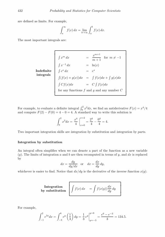
432 Probability and Statistics for Computer Scientists
are defined as limits. For example,
∫ ∞
a
f(x) dx = limb→∞
∫ b
a
f(x) dx.
The most important integrals are:
Indefiniteintegrals
∫xm dx =
xm+1
m+ 1for m 6= −1
∫x−1 dx = ln(x)
∫ex dx = ex
∫(f(x) + g(x))dx =
∫f(x)dx+
∫g(x)dx
∫Cf(x)dx = C
∫f(x)dx
for any functions f and g and any number C
For example, to evaluate a definite integral∫ 2
0x3dx, we find an antiderivative F (x) = x4/4
and compute F (2)− F (0) = 4− 0 = 4. A standard way to write this solution is
∫ 2
0
x3dx =x4
4
∣∣∣∣x=2
x=0
=24
4− 04
4= 4.
Two important integration skills are integration by substitution and integration by parts.
Integration by substitution
An integral often simplifies when we can denote a part of the function as a new variable(y). The limits of integration a and b are then recomputed in terms of y, and dx is replacedby
dx =dy
dy/dxor dx =
dx
dydy,
whichever is easier to find. Notice that dx/dy is the derivative of the inverse function x(y).
Integrationby substitution
∫f(x) dx =
∫f(x(y))
dx
dydy
For example,
∫ 2
−1
e3xdx =
∫ 6
−3
ey(1
3
)dy =
1
3ey∣∣∣∣y=6
y=−3
=e6 − e−3
3= 134.5.
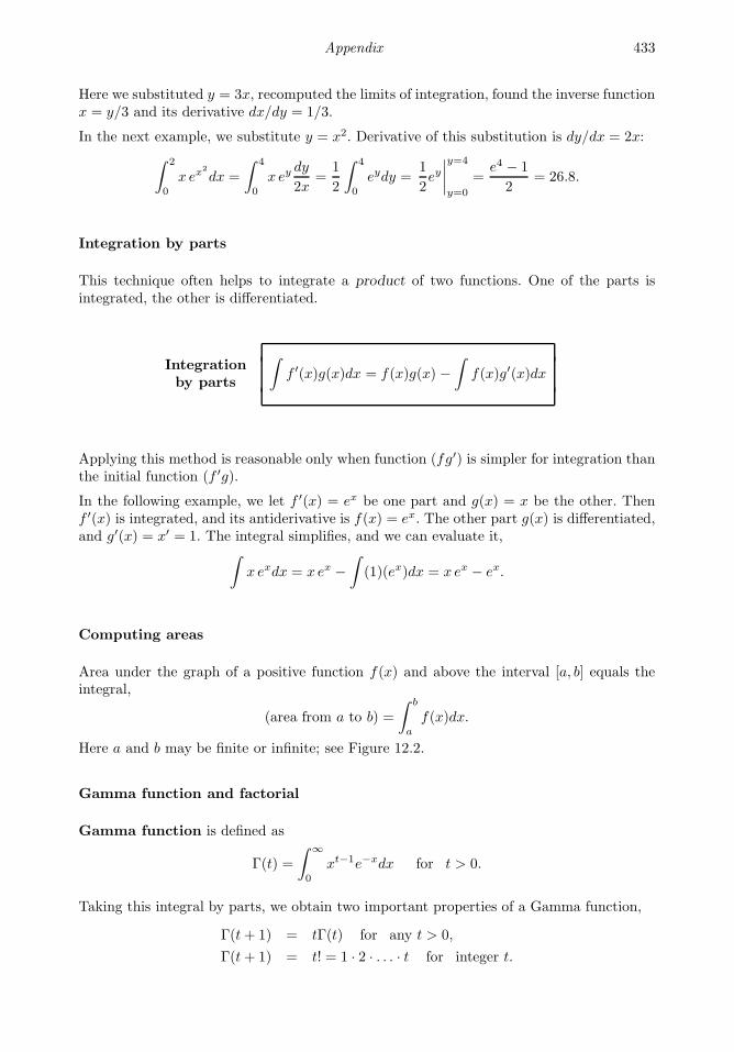
Appendix 433
Here we substituted y = 3x, recomputed the limits of integration, found the inverse functionx = y/3 and its derivative dx/dy = 1/3.
In the next example, we substitute y = x2. Derivative of this substitution is dy/dx = 2x:
∫ 2
0
x ex2
dx =
∫ 4
0
x eydy
2x=
1
2
∫ 4
0
eydy =1
2ey∣∣∣∣y=4
y=0
=e4 − 1
2= 26.8.
Integration by parts
This technique often helps to integrate a product of two functions. One of the parts isintegrated, the other is differentiated.
Integrationby parts
∫f ′(x)g(x)dx = f(x)g(x) −
∫f(x)g′(x)dx
Applying this method is reasonable only when function (fg′) is simpler for integration thanthe initial function (f ′g).
In the following example, we let f ′(x) = ex be one part and g(x) = x be the other. Thenf ′(x) is integrated, and its antiderivative is f(x) = ex. The other part g(x) is differentiated,and g′(x) = x′ = 1. The integral simplifies, and we can evaluate it,
∫x exdx = x ex −
∫(1)(ex)dx = x ex − ex.
Computing areas
Area under the graph of a positive function f(x) and above the interval [a, b] equals theintegral,
(area from a to b) =
∫ b
a
f(x)dx.
Here a and b may be finite or infinite; see Figure 12.2.
Gamma function and factorial
Gamma function is defined as
Γ(t) =
∫ ∞
0
xt−1e−xdx for t > 0.
Taking this integral by parts, we obtain two important properties of a Gamma function,
Γ(t+ 1) = tΓ(t) for any t > 0,
Γ(t+ 1) = t! = 1 · 2 · . . . · t for integer t.
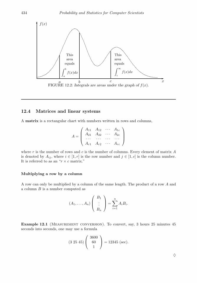
434 Probability and Statistics for Computer Scientists
f(x)
xa b c
Thisareaequals
∫ b
a
f(x)dx
Thisareaequals∫ ∞
c
f(x)dx
FIGURE 12.2: Integrals are areas under the graph of f(x).
12.4 Matrices and linear systems
A matrix is a rectangular chart with numbers written in rows and columns,
A =
A11 A12 · · · A1c
A21 A22 · · · A2c
· · · · · · · · · · · ·Ar1 Ar2 · · · Arc
where r is the number of rows and c is the number of columns. Every element of matrix Ais denoted by Aij , where i ∈ [1, r] is the row number and j ∈ [1, c] is the column number.It is referred to as an “r × c matrix.”
Multiplying a row by a column
A row can only be multiplied by a column of the same length. The product of a row A anda column B is a number computed as
(A1, . . . , An)
B1
...Bn
=
n∑
i=1
AiBi.
Example 12.1 (Measurement conversion). To convert, say, 3 hours 25 minutes 45seconds into seconds, one may use a formula
(3 25 45)
3600601
= 12345 (sec).
♦

Appendix 435
Multiplying matrices
Matrix A may be multiplied by matrix B only if the number of columns in A equals thenumber of rows in B.
If A is a k ×m matrix and B is an m × n matrix, then their product AB = C is a k × nmatrix. Each element of C is computed as
Cij =
m∑
s=1
AisBsj =
(ith rowof A
)(jth column
of B
).
Each element of AB is obtained as a product of the corresponding row of A and column ofB.
Example 12.2. The following product of two matrices is computed as
(2 61 3
)(9 −3
−3 1
)=
((2)(9) + (6)(−3), (2)(−3) + (6)(1)(1)(9) + (3)(−3), (1)(−3) + (3)(1)
)=
(0 00 0
).
♦
In the last example, the result was a zero matrix “accidentally.” This is not always the case.However, we can notice that matrices do not always obey the usual rules of arithmetics. Inparticular, a product of two non-zero matrices may equal a 0 matrix.
Also, in this regard, matrices do not commute, that is, AB 6= BA, in general.
Transposition
Transposition is reflecting the entire matrix about its main diagonal.
Notation AT = transposed matrix A
Rows become columns, and columns become rows. That is,
ATij = Aji.
For example,(
1 2 37 8 9
)T
=
1 72 83 9
.
The transposed product of matrices is
(AB)T = BTAT
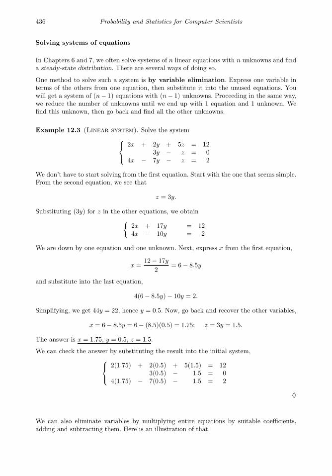
436 Probability and Statistics for Computer Scientists
Solving systems of equations
In Chapters 6 and 7, we often solve systems of n linear equations with n unknowns and finda steady-state distribution. There are several ways of doing so.
One method to solve such a system is by variable elimination. Express one variable interms of the others from one equation, then substitute it into the unused equations. Youwill get a system of (n− 1) equations with (n− 1) unknowns. Proceeding in the same way,we reduce the number of unknowns until we end up with 1 equation and 1 unknown. Wefind this unknown, then go back and find all the other unknowns.
Example 12.3 (Linear system). Solve the system
2x + 2y + 5z = 123y − z = 0
4x − 7y − z = 2
We don’t have to start solving from the first equation. Start with the one that seems simple.From the second equation, we see that
z = 3y.
Substituting (3y) for z in the other equations, we obtain
2x + 17y = 124x − 10y = 2
We are down by one equation and one unknown. Next, express x from the first equation,
x =12− 17y
2= 6− 8.5y
and substitute into the last equation,
4(6− 8.5y)− 10y = 2.
Simplifying, we get 44y = 22, hence y = 0.5. Now, go back and recover the other variables,
x = 6− 8.5y = 6− (8.5)(0.5) = 1.75; z = 3y = 1.5.
The answer is x = 1.75, y = 0.5, z = 1.5.
We can check the answer by substituting the result into the initial system,
2(1.75) + 2(0.5) + 5(1.5) = 123(0.5) − 1.5 = 0
4(1.75) − 7(0.5) − 1.5 = 2
♦
We can also eliminate variables by multiplying entire equations by suitable coefficients,adding and subtracting them. Here is an illustration of that.
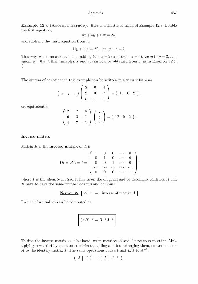
Appendix 437
Example 12.4 (Another method). Here is a shorter solution of Example 12.3. Doublethe first equation,
4x+ 4y + 10z = 24,
and subtract the third equation from it,
11y + 11z = 22, or y + z = 2.
This way, we eliminated x. Then, adding (y + z = 2) and (3y − z = 0), we get 4y = 2, andagain, y = 0.5. Other variables, x and z, can now be obtained from y, as in Example 12.3.♦
The system of equations in this example can be written in a matrix form as
(x y z
)
2 0 4
2 3 −7
5 −1 −1
=
(12 0 2
),
or, equivalently,
2 2 5
0 3 −1
4 −7 −1
xyz
=
(12 0 2
).
Inverse matrix
Matrix B is the inverse matrix of A if
AB = BA = I =
1 0 0 · · · 00 1 0 · · · 00 0 1 · · · 0· · · · · · · · · · · · · · ·0 0 0 · · · 1
,
where I is the identity matrix. It has 1s on the diagonal and 0s elsewhere. Matrices A andB have to have the same number of rows and columns.
Notation A−1 = inverse of matrix A
Inverse of a product can be computed as
(AB)−1 = B−1A−1
To find the inverse matrix A−1 by hand, write matrices A and I next to each other. Mul-tiplying rows of A by constant coefficients, adding and interchanging them, convert matrixA to the identity matrix I. The same operations convert matrix I to A−1,
(A I
)−→
(I A−1
).
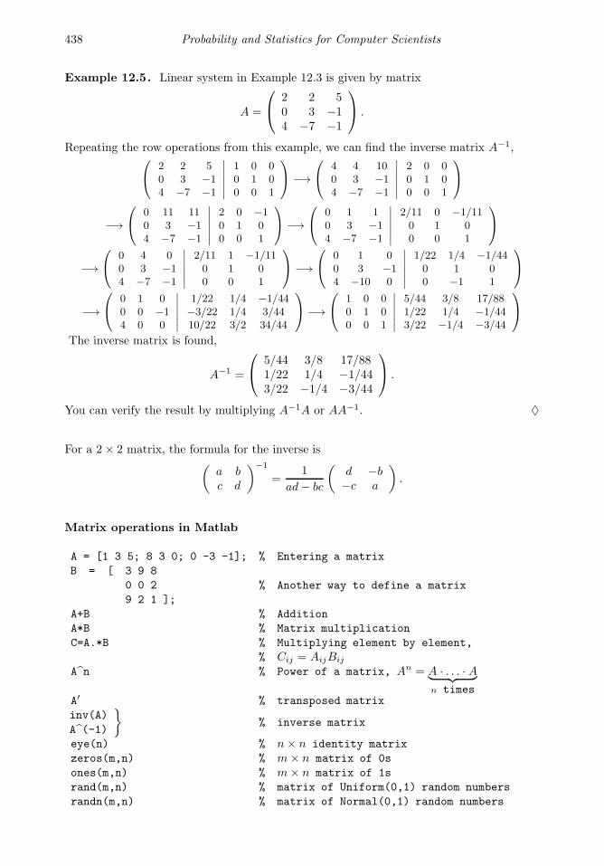
438 Probability and Statistics for Computer Scientists
Example 12.5. Linear system in Example 12.3 is given by matrix
A =
2 2 50 3 −14 −7 −1
.
Repeating the row operations from this example, we can find the inverse matrix A−1,
2 2 50 3 −14 −7 −1
∣∣∣∣∣∣
1 0 00 1 00 0 1
−→
4 4 100 3 −14 −7 −1
∣∣∣∣∣∣
2 0 00 1 00 0 1
−→
0 11 110 3 −14 −7 −1
∣∣∣∣∣∣
2 0 −10 1 00 0 1
−→
0 1 10 3 −14 −7 −1
∣∣∣∣∣∣
2/11 0 −1/110 1 00 0 1
−→
0 4 00 3 −14 −7 −1
∣∣∣∣∣∣
2/11 1 −1/110 1 00 0 1
−→
0 1 00 3 −14 −10 0
∣∣∣∣∣∣
1/22 1/4 −1/440 1 00 −1 1
−→
0 1 00 0 −14 0 0
∣∣∣∣∣∣
1/22 1/4 −1/44−3/22 1/4 3/4410/22 3/2 34/44
−→
1 0 00 1 00 0 1
∣∣∣∣∣∣
5/44 3/8 17/881/22 1/4 −1/443/22 −1/4 −3/44
The inverse matrix is found,
A−1 =
5/44 3/8 17/881/22 1/4 −1/443/22 −1/4 −3/44
.
You can verify the result by multiplying A−1A or AA−1. ♦
For a 2× 2 matrix, the formula for the inverse is(
a bc d
)−1
=1
ad− bc
(d −b−c a
).
Matrix operations in Matlab
A = [1 3 5; 8 3 0; 0 -3 -1]; % Entering a matrix
B = [ 3 9 8
0 0 2
9 2 1 ];
% Another way to define a matrix
A+B % Addition
A*B % Matrix multiplication
C=A.*B % Multiplying element by element,
% Cij = AijBij
An % Power of a matrix, An = A · . . . · A︸ ︷︷ ︸n times
A′ % transposed matrix
inv(A)
A(-1)
% inverse matrix
eye(n) % n× n identity matrix
zeros(m,n) % m× n matrix of 0s
ones(m,n) % m× n matrix of 1s
rand(m,n) % matrix of Uniform(0,1) random numbers
randn(m,n) % matrix of Normal(0,1) random numbers
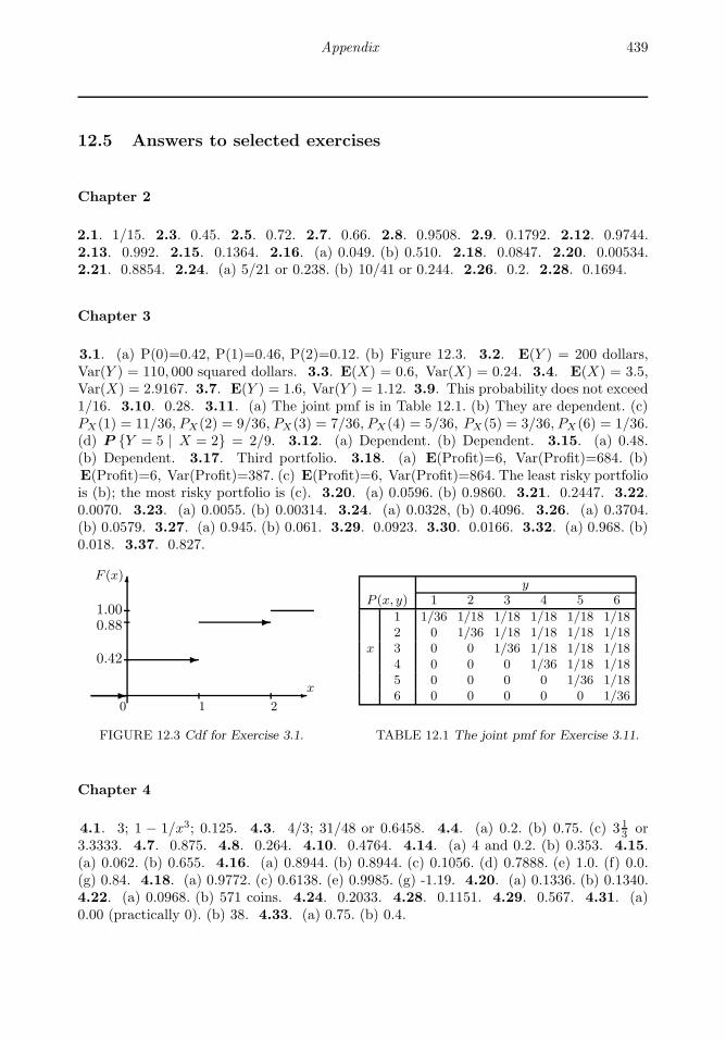
Appendix 439
12.5 Answers to selected exercises
Chapter 2
2.1. 1/15. 2.3. 0.45. 2.5. 0.72. 2.7. 0.66. 2.8. 0.9508. 2.9. 0.1792. 2.12. 0.9744.2.13. 0.992. 2.15. 0.1364. 2.16. (a) 0.049. (b) 0.510. 2.18. 0.0847. 2.20. 0.00534.2.21. 0.8854. 2.24. (a) 5/21 or 0.238. (b) 10/41 or 0.244. 2.26. 0.2. 2.28. 0.1694.
Chapter 3
3.1. (a) P(0)=0.42, P(1)=0.46, P(2)=0.12. (b) Figure 12.3. 3.2. E(Y ) = 200 dollars,Var(Y ) = 110, 000 squared dollars. 3.3. E(X) = 0.6, Var(X) = 0.24. 3.4. E(X) = 3.5,Var(X) = 2.9167. 3.7. E(Y ) = 1.6, Var(Y ) = 1.12. 3.9. This probability does not exceed1/16. 3.10. 0.28. 3.11. (a) The joint pmf is in Table 12.1. (b) They are dependent. (c)PX(1) = 11/36, PX(2) = 9/36, PX(3) = 7/36, PX(4) = 5/36, PX(5) = 3/36, PX(6) = 1/36.(d) P Y = 5 | X = 2 = 2/9. 3.12. (a) Dependent. (b) Dependent. 3.15. (a) 0.48.(b) Dependent. 3.17. Third portfolio. 3.18. (a) E(Profit)=6, Var(Profit)=684. (b)E(Profit)=6, Var(Profit)=387. (c) E(Profit)=6, Var(Profit)=864. The least risky portfoliois (b); the most risky portfolio is (c). 3.20. (a) 0.0596. (b) 0.9860. 3.21. 0.2447. 3.22.0.0070. 3.23. (a) 0.0055. (b) 0.00314. 3.24. (a) 0.0328, (b) 0.4096. 3.26. (a) 0.3704.(b) 0.0579. 3.27. (a) 0.945. (b) 0.061. 3.29. 0.0923. 3.30. 0.0166. 3.32. (a) 0.968. (b)0.018. 3.37. 0.827.
0 1 2
F (x)
x
0.42
0.881.00
FIGURE 12.3 Cdf for Exercise 3.1.
yP (x, y) 1 2 3 4 5 6
1 1/36 1/18 1/18 1/18 1/18 1/182 0 1/36 1/18 1/18 1/18 1/18
x 3 0 0 1/36 1/18 1/18 1/184 0 0 0 1/36 1/18 1/185 0 0 0 0 1/36 1/186 0 0 0 0 0 1/36
TABLE 12.1 The joint pmf for Exercise 3.11.
Chapter 4
4.1. 3; 1 − 1/x3; 0.125. 4.3. 4/3; 31/48 or 0.6458. 4.4. (a) 0.2. (b) 0.75. (c) 3 13 or
3.3333. 4.7. 0.875. 4.8. 0.264. 4.10. 0.4764. 4.14. (a) 4 and 0.2. (b) 0.353. 4.15.(a) 0.062. (b) 0.655. 4.16. (a) 0.8944. (b) 0.8944. (c) 0.1056. (d) 0.7888. (e) 1.0. (f) 0.0.(g) 0.84. 4.18. (a) 0.9772. (c) 0.6138. (e) 0.9985. (g) -1.19. 4.20. (a) 0.1336. (b) 0.1340.4.22. (a) 0.0968. (b) 571 coins. 4.24. 0.2033. 4.28. 0.1151. 4.29. 0.567. 4.31. (a)0.00 (practically 0). (b) 38. 4.33. (a) 0.75. (b) 0.4.
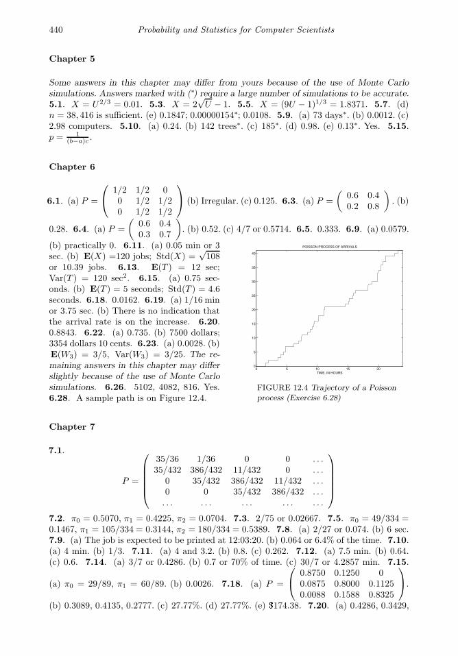
440 Probability and Statistics for Computer Scientists
Chapter 5
Some answers in this chapter may differ from yours because of the use of Monte Carlosimulations. Answers marked with (∗) require a large number of simulations to be accurate.5.1. X = U2/3 = 0.01. 5.3. X = 2
√U − 1. 5.5. X = (9U − 1)1/3 = 1.8371. 5.7. (d)
n = 38, 416 is sufficient. (e) 0.1847; 0.00000154∗; 0.0108. 5.9. (a) 73 days∗. (b) 0.0012. (c)2.98 computers. 5.10. (a) 0.24. (b) 142 trees∗. (c) 185∗. (d) 0.98. (e) 0.13∗. Yes. 5.15.p = 1
(b−a)c .
Chapter 6
6.1. (a) P =
1/2 1/2 00 1/2 1/20 1/2 1/2
(b) Irregular. (c) 0.125. 6.3. (a) P =
(0.6 0.40.2 0.8
). (b)
0.28. 6.4. (a) P =
(0.6 0.40.3 0.7
). (b) 0.52. (c) 4/7 or 0.5714. 6.5. 0.333. 6.9. (a) 0.0579.
0 5 10 15 200
5
10
15
20
25
30
35
40
POISSON PROCESS OF ARRIVALS
TIME, IN HOURS
FIGURE 12.4 Trajectory of a Poissonprocess (Exercise 6.28)
(b) practically 0. 6.11. (a) 0.05 min or 3sec. (b) E(X) =120 jobs; Std(X) =
√108
or 10.39 jobs. 6.13. E(T ) = 12 sec;Var(T ) = 120 sec2. 6.15. (a) 0.75 sec-onds. (b) E(T ) = 5 seconds; Std(T ) = 4.6seconds. 6.18. 0.0162. 6.19. (a) 1/16 minor 3.75 sec. (b) There is no indication thatthe arrival rate is on the increase. 6.20.0.8843. 6.22. (a) 0.735. (b) 7500 dollars;3354 dollars 10 cents. 6.23. (a) 0.0028. (b)E(W3) = 3/5, Var(W3) = 3/25. The re-maining answers in this chapter may differslightly because of the use of Monte Carlosimulations. 6.26. 5102, 4082, 816. Yes.6.28. A sample path is on Figure 12.4.
Chapter 7
7.1.
P =
35/36 1/36 0 0 . . .35/432 386/432 11/432 0 . . .
0 35/432 386/432 11/432 . . .0 0 35/432 386/432 . . .. . . . . . . . . . . . . . .
7.2. π0 = 0.5070, π1 = 0.4225, π2 = 0.0704. 7.3. 2/75 or 0.02667. 7.5. π0 = 49/334 =0.1467, π1 = 105/334 = 0.3144, π2 = 180/334 = 0.5389. 7.8. (a) 2/27 or 0.074. (b) 6 sec.7.9. (a) The job is expected to be printed at 12:03:20. (b) 0.064 or 6.4% of the time. 7.10.(a) 4 min. (b) 1/3. 7.11. (a) 4 and 3.2. (b) 0.8. (c) 0.262. 7.12. (a) 7.5 min. (b) 0.64.(c) 0.6. 7.14. (a) 3/7 or 0.4286. (b) 0.7 or 70% of time. (c) 30/7 or 4.2857 min. 7.15.
(a) π0 = 29/89, π1 = 60/89. (b) 0.0026. 7.18. (a) P =
0.8750 0.1250 00.0875 0.8000 0.11250.0088 0.1588 0.8325
.
(b) 0.3089, 0.4135, 0.2777. (c) 27.77%. (d) 27.77%. (e) $174.38. 7.20. (a) 0.4286, 0.3429,
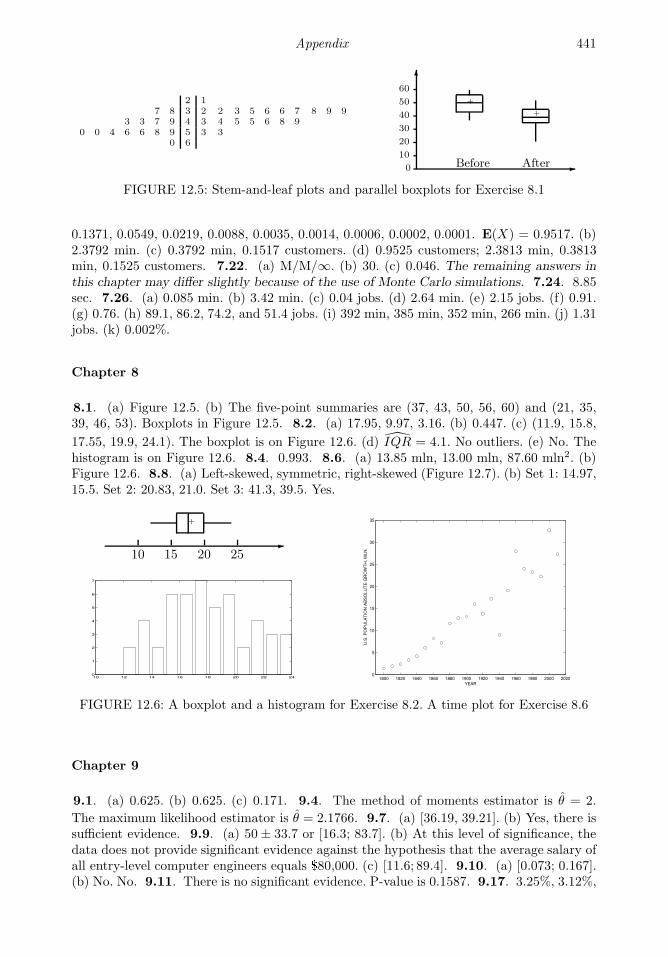
Appendix 441
2 17 8 3 2 2 3 5 6 6 7 8 9 9
3 3 7 9 4 3 4 5 5 6 8 90 0 4 6 6 8 9 5 3 3
0 6
0
10
20
30
40
50
60
Before After
+
+
FIGURE 12.5: Stem-and-leaf plots and parallel boxplots for Exercise 8.1
0.1371, 0.0549, 0.0219, 0.0088, 0.0035, 0.0014, 0.0006, 0.0002, 0.0001. E(X) = 0.9517. (b)2.3792 min. (c) 0.3792 min, 0.1517 customers. (d) 0.9525 customers; 2.3813 min, 0.3813min, 0.1525 customers. 7.22. (a) M/M/∞. (b) 30. (c) 0.046. The remaining answers inthis chapter may differ slightly because of the use of Monte Carlo simulations. 7.24. 8.85sec. 7.26. (a) 0.085 min. (b) 3.42 min. (c) 0.04 jobs. (d) 2.64 min. (e) 2.15 jobs. (f) 0.91.(g) 0.76. (h) 89.1, 86.2, 74.2, and 51.4 jobs. (i) 392 min, 385 min, 352 min, 266 min. (j) 1.31jobs. (k) 0.002%.
Chapter 8
8.1. (a) Figure 12.5. (b) The five-point summaries are (37, 43, 50, 56, 60) and (21, 35,39, 46, 53). Boxplots in Figure 12.5. 8.2. (a) 17.95, 9.97, 3.16. (b) 0.447. (c) (11.9, 15.8,
17.55, 19.9, 24.1). The boxplot is on Figure 12.6. (d) IQR = 4.1. No outliers. (e) No. Thehistogram is on Figure 12.6. 8.4. 0.993. 8.6. (a) 13.85 mln, 13.00 mln, 87.60 mln2. (b)Figure 12.6. 8.8. (a) Left-skewed, symmetric, right-skewed (Figure 12.7). (b) Set 1: 14.97,15.5. Set 2: 20.83, 21.0. Set 3: 41.3, 39.5. Yes.
10 15 20 25
+
10 12 14 16 18 20 22 240
1
2
3
4
5
6
7
1800 1820 1840 1860 1880 1900 1920 1940 1960 1980 2000 20200
5
10
15
20
25
30
35
YEAR
U.S
. P
OP
ULA
TIO
N A
BS
OLU
TE
GR
OW
TH
, M
LN
.
FIGURE 12.6: A boxplot and a histogram for Exercise 8.2. A time plot for Exercise 8.6
Chapter 9
9.1. (a) 0.625. (b) 0.625. (c) 0.171. 9.4. The method of moments estimator is θ = 2.
The maximum likelihood estimator is θ = 2.1766. 9.7. (a) [36.19, 39.21]. (b) Yes, there issufficient evidence. 9.9. (a) 50± 33.7 or [16.3; 83.7]. (b) At this level of significance, thedata does not provide significant evidence against the hypothesis that the average salary ofall entry-level computer engineers equals $80,000. (c) [11.6; 89.4]. 9.10. (a) [0.073; 0.167].(b) No. No. 9.11. There is no significant evidence. P-value is 0.1587. 9.17. 3.25%, 3.12%,

442 Probability and Statistics for Computer Scientists
0 5 10 15 20 25 300
1
2
3
4
5
6
7
8
10 15 20 25 30 350
1
2
3
4
5
6
7
8
9
0 10 20 30 40 50 60 70 80 90 1000
1
2
3
4
5
6
FIGURE 12.7: Histograms of three data sets in Exercise 8.8
and 4.50%. 9.18. (a) [4.25, 15.35]. (b) Each test has a P-value between 0.0005 and 0.001.There is a significant reduction. 9.20. P-value is between 0.02 and 0.05. At any levelα ≥ 0.05, there is significant evidence that σ 6= 5. 9.22. (a) There is significant evidencethat σ2
X 6= σ2Y (P = 0.0026), hence the method in Example 9.21 is chosen correctly. (b)
[0.11, 0.60].
Chapter 10
The P-values in Exercises 10.1 and 10.4 may differ slightly depending on the choice ofbins. 10.1. No, there is significant evidence that the distribution is not Poisson. P <0.001. 10.4. Confirms. P > 0.2. 10.6. No significant difference. P > 0.2. 10.7. (a)Yes, P ∈ (0.001, 0.005). (b) Yes, P ∈ (0.005, 0.01). (c) Yes, P < 0.001. 10.9. No, P ∈(0.1, 0.2). 10.11. Rejection region is [0, 5]∪ [15, 20]. Fifteen or more measurements on thesame side of m justify recalibration. 10.13. The null distribution is Binomial(60,0.75);P = 0.1492; there is no significant evidence that the first quartile exceeds 43 nm. 10.16.Yes, there is significant evidence at the 5% level; P = 0.01. 10.18. Yes, at the 5%level, there is significant evidence that the median service time is less than 5 min 40 sec.Assumption of a symmetric distribution may not be fully satisfied. 10.21. (a) For the 1stprovider, there is significant evidence for all α > 0.011; P = 0.011. No significant evidencefor the 2nd provider; P = 0.172. (b) For the 1st provider, there is significant evidence;P ∈ (0.001, 0.005). For the 2nd provider, there is significant evidence for all α ≥ 0.05;P ∈ (0.025, 0.05). Yes, the Wilcoxon test appears more sensitive. (c) No; P ∈ (0.01, 0.025).10.23. At any α ≥ 0.05, there is significant evidence that the median cost of textbooks isrising; P ∈ (0.025, 0.05). 10.25. Yes, there is a significant reduction of the median servicetime; P = 0.0869. 10.27. (a) 352,716 ordered and 285,311,670,611 unordered bootstrapsamples. (b) The bootstrap distribution of M∗ is given by the pmf, P (44) = 0.0002, P (47) =0.0070, P (52) = 0.0440, P (53) = 0.1215, P (54) = 0.2059, P (58) = 0.2428, P (59) = 0.2059,P (63) = 0.1215, P (68) = 0.0440, P (72) = 0.0070, P (77) = 0.0002. (c) 4.1885. (d) [53, 63].(e) 0.9928. Answers to Exercises 10.29 and 10.30 may differ slightly due to the generatedbootstrap samples. 10.29. 1.070, 0.107. 10.30. [−0.9900− 0.9564]. 10.31. 4.5, 2.25.10.33. (b) 0.4, 0.02. (c) 0.22. (d) Reject H0. 10.34. (a) 17.661 (thousand of concurrentusers). (b) [16, 765.7, 18, 556.5]. Given the observed data and the assumed prior distribution,there is a 90% posterior probability that the average number of concurrent users is between16,765.7 and 18,556.5. (c) Yes. The answers to Exercise 10.36 may differ slightly due todifferent choices available in question (a). 10.36. (a) For example, Normal(5.5, 0.255). (b)Normal(5.575, 0.245); the Bayes estimator is 5.575; its posterior risk is 0.060. (c) [5.095,6.055]. The HPD credible set is much more narrow because besides the data, it uses a
rather informative (low-variance) prior distribution. 10.38. (a) Pareto(α, σ). (b) (n+α)σn+α−1 ;
(n+α)σ2
(n+α−1)2(n+α−2) . 10.40. (a) 0.9, 0.0082. (b) [0.7743, 1]. (c) Yes.
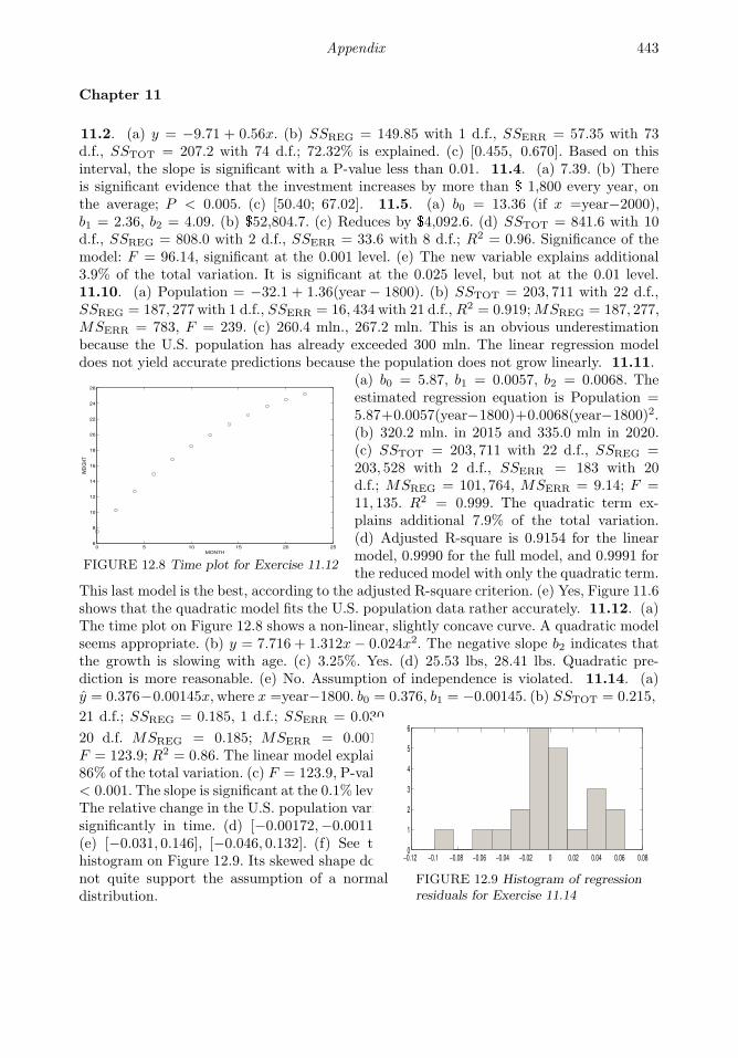
Appendix 443
Chapter 11
11.2. (a) y = −9.71 + 0.56x. (b) SSREG = 149.85 with 1 d.f., SSERR = 57.35 with 73d.f., SSTOT = 207.2 with 74 d.f.; 72.32% is explained. (c) [0.455, 0.670]. Based on thisinterval, the slope is significant with a P-value less than 0.01. 11.4. (a) 7.39. (b) Thereis significant evidence that the investment increases by more than $ 1,800 every year, onthe average; P < 0.005. (c) [50.40; 67.02]. 11.5. (a) b0 = 13.36 (if x =year−2000),b1 = 2.36, b2 = 4.09. (b) $52,804.7. (c) Reduces by $4,092.6. (d) SSTOT = 841.6 with 10d.f., SSREG = 808.0 with 2 d.f., SSERR = 33.6 with 8 d.f.; R2 = 0.96. Significance of themodel: F = 96.14, significant at the 0.001 level. (e) The new variable explains additional3.9% of the total variation. It is significant at the 0.025 level, but not at the 0.01 level.11.10. (a) Population = −32.1 + 1.36(year − 1800). (b) SSTOT = 203, 711 with 22 d.f.,SSREG = 187, 277 with 1 d.f., SSERR = 16, 434 with 21 d.f., R2 = 0.919;MSREG = 187, 277,MSERR = 783, F = 239. (c) 260.4 mln., 267.2 mln. This is an obvious underestimationbecause the U.S. population has already exceeded 300 mln. The linear regression modeldoes not yield accurate predictions because the population does not grow linearly. 11.11.
0 5 10 15 20 256
8
10
12
14
16
18
20
22
24
26
MONTH
WE
IGH
T
FIGURE 12.8 Time plot for Exercise 11.12
(a) b0 = 5.87, b1 = 0.0057, b2 = 0.0068. Theestimated regression equation is Population =5.87+0.0057(year−1800)+0.0068(year−1800)2.(b) 320.2 mln. in 2015 and 335.0 mln in 2020.(c) SSTOT = 203, 711 with 22 d.f., SSREG =203, 528 with 2 d.f., SSERR = 183 with 20d.f.; MSREG = 101, 764, MSERR = 9.14; F =11, 135. R2 = 0.999. The quadratic term ex-plains additional 7.9% of the total variation.(d) Adjusted R-square is 0.9154 for the linearmodel, 0.9990 for the full model, and 0.9991 forthe reduced model with only the quadratic term.
This last model is the best, according to the adjusted R-square criterion. (e) Yes, Figure 11.6shows that the quadratic model fits the U.S. population data rather accurately. 11.12. (a)The time plot on Figure 12.8 shows a non-linear, slightly concave curve. A quadratic modelseems appropriate. (b) y = 7.716 + 1.312x− 0.024x2. The negative slope b2 indicates thatthe growth is slowing with age. (c) 3.25%. Yes. (d) 25.53 lbs, 28.41 lbs. Quadratic pre-diction is more reasonable. (e) No. Assumption of independence is violated. 11.14. (a)y = 0.376−0.00145x, where x =year−1800. b0 = 0.376, b1 = −0.00145. (b) SSTOT = 0.215,
21 d.f.; SSREG = 0.185, 1 d.f.; SSERR = 0.030,
20 d.f. MSREG = 0.185; MSERR = 0.0015;F = 123.9; R2 = 0.86. The linear model explains86% of the total variation. (c) F = 123.9, P-value< 0.001. The slope is significant at the 0.1% level.The relative change in the U.S. population variessignificantly in time. (d) [−0.00172,−0.00118].(e) [−0.031, 0.146], [−0.046, 0.132]. (f) See thehistogram on Figure 12.9. Its skewed shape doesnot quite support the assumption of a normaldistribution.
−0.12 −0.1 −0.08 −0.06 −0.04 −0.02 0 0.02 0.04 0.06 0.080
1
2
3
4
5
6
FIGURE 12.9 Histogram of regressionresiduals for Exercise 11.14

Nikki
Typewriter
uploaded by [stormrg]