Chapter I

Probability

1 Introduction

In our day-to-day life we come across many processes whose nature cannot be predicted

in advance with certainty. Such processes are referred to as random processes. The

only way to derive information about random processes is to conduct experiments. Each

experiment results in an outcome which can not be predicted before hand. In fact even if

the experiment is repeated under identical conditions, due to presence of factors which are

beyond human control, outcomes of the experiment may vary from trial to trial. However

we may know that each outcome of the experiment results in one of the several given

possibilities. For example in the cast of a die under a fixed environment the outcome

(number of spots on the upper face) can not be predicted in advance and it varies from

trial to trial. However we know that the outcome has to be among one of the numbers

1, 2, . . . , 6. Probability theory deals with the modeling and study of random processes. The

field of statistics is closely related to probability theory and it deals with drawing inferences

from the data pertaining to random processes modeled through use of probability theory.

Definition 1 (i) A random experiment is an experiment in which

(a) the set of all possible outcomes of the experiment is known in advance;

(b) outcome of a particular performance (trial) of the experiment can not be predicted

with certainty;

(c) the experiment can be repeated under identical conditions.

(ii) Collection of all possible outcomes of a random experiment is called the sample space.

A sample space will usually be denoted by Ω. ♠

Example 2 (i) In the random experiment of casting a die one may take the sample

space as Ω = 1, 2, 3, 4, 5, 6, where i ∈ Ω indicates that the experiment results in i spots

(i = 1, . . . , 6) on the upper face.

(ii) In the random experiment of simultaneously flipping a coin and casting a die one may

take the sample space as

Ω = H,T × 1, 2, . . . , 6 = (r, i) : r ∈ H,T, i ∈ 1, 2, . . . , 6,

1

where (H, i) ((T, i)) indicates that the flip of the coin resulted in a head (tail) on the

upper face and the cast of the die resulted in i spots (i = 1, 2, . . . , 6) on the upper face.

(iii) Consider an experiment where a coin is tossed repeatedly until a head is observed. In

this case the sample space may be taken as Ω = 1, 2, . . ., where i ∈ Ω indicates that the

experiment terminates on i-th trial with first i− 1 trials resulting in a tail on the upper

face and the i-th trial resulting in a head on the upper face.

(iv) In the random experiment of measuring lifetimes (in hours) of a particular brand of

battery manufactured by a company one may take Ω = [0, 70, 000], where we assume that

no battery lasts for more than 70, 000 hours. ♠

Definition 3 (i) Let Ω be the sample space of a random experiment and let E ⊆ Ω. If

the outcome of the random experiment is a member of the set E we say that the event E

has occurred and the set E is referred to as an event.

(ii) Two events E1 and E2 are said to be mutually exclusive if they cannot occur simul-

taneously, i.e., if E1 ∩ E2 = φ, the empty set. ♠

In a random experiment since one event may be more likely to occur than the other it may

be desirable to quantify the likelihoods of occurrences of various events. For example in the

cast of a fair die (a die that is not biased towards any particular outcome) the occurrence

of an odd number of spots on the upper face is more likely than the occurrence of 2

or 4 spots on the upper face. Probability of an event is a numerical measure of chance

with which that event occurs. To assign probabilities to various events associated with

a random experiment one may assign a real number P (E) ∈ [0, 1] to each event E with

the interpretation that there is a (100 × P (E))% chance that the event E will occur

and a (100 × (1 − P (E)))% chance that the event E will not occur. For example if the

probability of an event is 0.25 it would mean that there is a 25% chance that the event

will occur and that there is a 75% chance that the event will not occur. Note that for any

such assignment of probabilities to be meaningful one must have P (Ω) = 1. Now we will

discuss two methods of assigning probabilities.

I. Classical Method. This method of assigning probabilities is used for random experi-

ments which result in a finite number of equally likely outcomes. Let Ω = ω1, . . . , ωn be

a finite sample space with n (∈ N) possible outcomes; here N denotes the set of natural

numbers. For E ⊆ Ω, let |E| denote the number of elements in E. An outcome ω ∈ Ω is

said to be favorable to event E if ω ∈ E. In the classical method of assigning probabilities,

2

the probability of an event E is given by

P (E) =number of outcomes favorable to E

total number of outcomes=|E||Ω|

=|E|n.

Note that probabilities assigned through classical method satisfy the following intuitive

appealing properties:

(i) for any event E, P (E) ≥ 0;

(ii) for mutually exclusive events E1, E2, . . . , En (i.e., Ei ∩ Ej = φ, whenever i, j ∈1, . . . , n, i 6= j), P (

⋃ni=1 Ei) =

∑ni=1 P (Ei);

(iii) P (Ω) = 1.

Example 4 Suppose that in a classroom we have 25 students born in the same year

having 365 days. Suppose that we want to find the probability of the event E that they

all are born on different days of the year. Here an outcome consists of a sequence of 25

birthdays. Suppose that all such sequences are equally likely. Then |Ω| = 36525, |E| =

365× 364× · · · × 341 =365 P25 and P (E) = |E||Ω| =

365P25

36525 . ♠

The classical method of assigning probabilities has limited applicability as it can be only

used for random experiments which result in a finite number of equally likely outcomes.

II. Relative Frequency Method. Suppose that we have independent repetitions of a

random experiment (here independent repetitions means that the outcome of one trial is

not affected by the outcome of another trial) under identical conditions. Let fn(E) denote

the number of times an event E occurs in the first n trials and let rn(E) = fn(E)/n denote

the corresponding relative frequency. Using advanced probabilistic methods (e.g., using

Weak Law of Large Numbers to be discussed in later chapters) it can be shown that,

under mild conditions, the relative frequencies stabilize as n gets large (i.e., for any event

E, limn→∞ rn(E) exists). In the relative frequency method of assigning probabilities the

probability of an event E is given by

P (E) = limn→∞

rn(E) = limn→∞

fn(E)

n.

In practice, to assign probability to an event E, the experiment is repeated a large (but

fixed) number of times (say n times) and the approximation P (E) ≈ rn(E) is used

for assigning probability to event E. Note that probabilities assigned through relative

frequency method also satisfy the following intuitive appealing properties of classical

method:

3

(i) for any event E, P (E) ≥ 0;

(ii) for mutually exclusive events E1, E2, . . . , En, P (⋃ni=1 Ei) =

∑ni=1 P (Ei);

(iii) P (Ω) = 1.

Although the relative frequency method seems to have more applicability than the

classical method it too has limitations. A major problem with the relative frequency

method is that it is imprecise as it is based on an approximation (P (E) ≈ rn(E)). Another

difficulty with relative frequency method is that it assumes that the experiment can be

repeated a large number of times. This may not be always possible due to budgetary and

other constraints (e.g., in predicting the success of a new space technology it may not be

possible to repeat the experiment a large number of times due to high costs involved).

The following definitions will be useful for further discussion.

Definition 5 (i) A set E is said to be finite if either E = φ (the empty set) or if there

exists a one-one and onto function f : 1, 2, . . . , n → E (or f : E → 1, 2, . . . , n) for

some natural number n;

(ii) A set is said to be infinite if it is not finite;

(iii) A set E is said to be countable either E = φ or if there is an onto function f : N→ E,

where N denotes the set of natural numbers;

(iv) A set is said to be countably infinite if it is countable and infinite;

(v) A set is said to be uncountable if it is not countable;

(vi) A set E is said to be continuum if there is a one-one and onto function f : R → E

(or f : E → R), where R denotes the real line. ♠

The following theorem, whose proofs can be found in any standard textbook on set theory,

provides some of the properties of finite, countable and uncountable sets.

Theorem 6 (i) Any finite set is countable.

(ii)If A is a countable and B ⊆ A then B is countable.

(iii) If A is an uncountable set and A ⊆ B then B is uncountable.

(iv) If E is a finite set and F is a set such that there exists a one-one and onto function

f : E → F (or f : F → E) then F is finite.

(v) If E is a countably infinite (continuum) set and F is a set such that there exists

a one-one and onto function f : E → F (or f : F → E) then F is countably infinite

(continuum).

(vi) Unit interval (0, 1) is uncountable. Hence any interval (a, b), where −∞ < a < b <∞,

4

is uncountable.

(vii) N× N is countable.

(viii) Let Λ be a countable set and let Aα : α ∈ Λ be a (countable) collection of

countable sets. Then⋃α∈ΛAα is countable. In other words, countable union of countable

sets is countable.

(ix) Any continuum set is uncountable. ♠

Example 7 (i) Define f : N→ N by f(n) = n, n ∈ N. Clearly f : N→ N is one-one and

onto. Thus N is countable. Also it can be easily seen (by contradiction) that N is infinite.

Thus N is countably infinite.

(ii) Let Z denote the set of integers. Define f : N→ Z by

f(n) =

n−1

2, if n is odd

−n2

if n is even.

Clearly f : N → Z is one-one and onto. Therefore, using (i) above and Theorem 6 (v),

Z is countably infinite. Now on using Theorem 6 (ii) it follows that any subset of Z is

countable.

(iii) Using the fact that N is countable and Theorem 6 (viii) it is straightforward to show

that Q (the set of rational numbers) is countable.

(iv) Define f : R → R and g : R → (0, 1) by f(x) = x, x ∈ R, and g(x) = 11+ex , x ∈ R.

Then f : R → R and g : R → (0, 1) are one-one and onto functions. It follows that R is

continuum and (using Theorem 6 (v)) (0, 1) is continuum. Further, for −∞ < a < b <∞,

let h(x) = (b− a)x + a, x ∈ (0, 1). Clearly h : (0, 1) → (a, b) is one-one and onto. Again

using Theorem 6 (v) it follows that any interval (a, b) is continuum. ♠

It is clear that it may not be possible to assign probabilities in a way that applies to

every situation. In the modern approach to probability theory one does not bother about

how probabilities are assigned. Assignment of probabilities to various subsets of the

sample space Ω that is consistent with intuitive appealing properties (i)-(iii) of classical

(or relative frequency) method is done through probability modeling. In advanced courses

on probability theory it is shown that in many situations (especially when the sample

space Ω is continuum) it is not possible to assign probabilities to all subsets of Ω such

that properties (i)-(iii) of classical (or relative frequency) method are satisfied. Therefore

probabilities are assigned to only certain types of subsets of Ω.

5

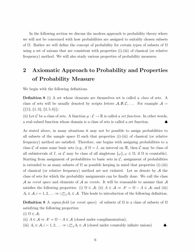
In the following section we discuss the modern approach to probability theory where

we will not be concerned with how probabilities are assigned to suitably chosen subsets

of Ω. Rather we will define the concept of probability for certain types of subsets of Ω

using a set of axioms that are consistent with properties (i)-(iii) of classical (or relative

frequency) method. We will also study various properties of probability measures.

2 Axiomatic Approach to Probability and Properties

of Probability Measure

We begin with the following definitions.

Definition 8 (i) A set whose elements are themselves set is called a class of sets. A

class of sets will be usually denoted by scripts letters A,B, C, . . .. For example A =

1, 1, 3, 2, 5, 6;

(ii) Let C be a class of sets. A function µ : C → R is called a set function. In other words,

a real-valued function whose domain is a class of sets is called a set function. ♠

As stated above, in many situations it may not be possible to assign probabilities to

all subsets of the sample space Ω such that properties (i)-(iii) of classical (or relative

frequency) method are satisfied. Therefore, one begins with assigning probabilities to a

class C of some some basic sets (e.g., if Ω = I, an interval on R, then C may be class of

all subintervals of I, or C may be class of all singletons ω, ω ∈ Ω, if Ω is countable).

Starting from assignment of probabilities to basic sets in C, assignment of probabilities

is extended to as many subsets of Ω as possible keeping in mind that properties (i)-(iii)

of classical (or relative frequency) method are not violated. Let us denote by A the

class of sets for which the probability assignments can be finally done. We call the class

A as event space and elements of A as events. It will be reasonable to assume that Asatisfies the following properties: (i) Ω ∈ A; (ii) A ∈ A ⇒ Ac = Ω − A ∈ A; and (iii)

Ai ∈ A, i = 1, 2, . . .⇒ ∪∞i=1Ai ∈ A. This leads to introduction of the following definition.

Definition 9 A sigma-field (or event space) of subsets of Ω is a class of subsets of Ω

satisfying the following properties:

(i) Ω ∈ A;

(ii) A ∈ A ⇒ Ac = Ω− A ∈ A (closed under complimentation);

(iii) Ai ∈ A, i = 1, 2, . . .⇒ ∪∞i=1Ai ∈ A (closed under countably infinite unions) ♠.

6

Remark 10 (i) Let A be a sigma-field. Since Ω ∈ A, we have φ = Ωc ∈ A, i.e., the

empty set φ is a member of every sigma-field;

(ii) For a natural number n, let A1, A2, . . . , An be a finite collection of sets in a sigma-field

A. Define Ai = φ, i = n+1, n+2, . . .. Then Ai ∈ A, i = 1, 2, . . . and ∪ni=1Ai = ∪∞i=1Ai ∈ A.

Thus a sigma-field is closed under countable (finite or infinite) unions;

(iii) If A1, A2, . . . (or A1, A2, . . . , An) is a countably infinite (finite) collection of sets in a

sigma-field A then ∩∞i=1Ai = (∪∞i=1Aci)c ∈ A ((∪ni=1A

ci)c ∈ A). Thus a sigma-field is also

closed under countable intersections;

(iv) If A and B are elements of a sigma-field A of subsets of Ω then clearly A−B = A∩Bc

and A∆B = (A−B) ∪ (B − A) are also elements of A ♠

Example 11 (i) A = φ,Ω is a sigma-field, called the trivial sigma-field;

(ii) P(Ω) = A : A ⊆ Ω, the power set of Ω, is a sigma-field, called the discrete sigma-

field;

(iii) Let A ⊆ Ω. Then A = φ,Ω, A,Ac is a sigma-field. It is the smallest sigma-field

containing the set A. ♠

Now we provide a mathematical definition of probability based on a set of axioms.

Definition 12 Let Ω be the sample space and let A be a suitably chosen sigma-field of

subsets of Ω.

(i) A probability function (or probability measure) is a set function P : A → R satisfying

the following properties (axioms):

(a) P (E) ≥ 0, ∀E ∈ A, (Axiom 1: Nonnegativity);

(b) If E1, E2, . . . is a countably infinite collection of disjoint sets in A (i.e., Ei ∩ Ej =

φ, if i 6= j) then P (∪∞i=1Ei) =∑∞

i=1 P (Ei), (Axiom 2: Countably infinite additivity);

(c) P (Ω) = 1, (Axiom 3: Probability of the sample space is 1).

(ii) The triplet (Ω,A, P ) is called the probability space and the elements of sigma-field

(event space) A are called events.

(iii) For an index set Λ ⊆ R, let Eα;α ∈ Λ be a collection of events. Events Eα;α ∈ Λare said to be mutually exclusive if Eα ∩ Eβ = φ, whenever α 6= β. ♠

Remark 13 (i) Note that if E1, E2, . . . is a countably infinite collection of sets in a sigma-

field A then⋃∞i=1 Ei ∈ A and therefore P (

⋃∞i=1Ei) is well defined.

(ii) Let C be an appropriately chosen class of basic subsets of Ω for which the probabilities

can be assigned to begin with. It turns out (a topic for an advanced course in proba-

7

bility theory) that the assignment of probabilities, consistent with axioms (a)-(c) in the

above definition, can be easily extended to the smallest sigma-field containing the class

C. Therefore generally the domain A of a probability measure is taken to be the smallest

sigma-field containing the class C of basic subsets of Ω.

(iii) In situations where Ω is countable, generally, the basic subsets of Ω for which prob-

abilities can be assigned is the class C = ω : ω ∈ Ω of singletons. Note that, in such

situations, all subsets of Ω are countable and thus any subset of Ω can be written as a

countable union of disjoint singletons. Therefore, using the countable additive property

of probability measures (see Theorem 14 (ii) below), assignment of probabilities can be

extended from the class C = ω : ω ∈ Ω of singletons to P(Ω), the power set of Ω.

Thus in situations where Ω is countable we take A = P(Ω). Interestingly when Ω is

countable the smallest sigma-field containing the class C = ω : ω ∈ Ω of singletons is

P(Ω).

(iv) Let Ω = ω1, . . . , ωn be a finite sample space comprising of n equally likely outcomes

ω1, . . . , ωn (P (ωi) = 1/n, i = 1, . . . , n) and let E = ωi1 , ωi2 , . . . , ωik ⊆ Ω. Then

P (E) = P (k⋃j=1

ωij) =k∑j=1

P (ωij) =k∑j=1

1

n=k

n=|E||Ω|

.

Thus when the sample space comprises of a finite number of equally likely outcomes the

classical and axiomatic approaches are the same. ♠

In the following theorem we establish some elementary properties of probability measures.

Theorem 14 Let (Ω,A, P ) be a probability space. Then,

(i) P (φ) = 0;

(ii) for a positive integer n, Ei ∈ A, i = 1, . . . , n, and Ei⋂Ej = φ, i 6= j ⇒ P (

⋃ni=1Ei) =∑n

i=1 P (Ei) (i.e., a probability measure is countable additive);

(iii) ∀E ∈ A, P (E) = 1− P (Ec);

(iv) E1, E2 ∈ A and E1 ⊆ E2 ⇒ P (E2 − E1) = P (E2)− P (E1) and P (E1) ≤ P (E2);

(v) ∀E ∈ A, 0 ≤ P (E) ≤ 1;

(vi) E1, E2 ∈ A ⇒ P (E1 ∪ E2) = P (E1) + P (E2)− P (E1 ∩ E2).

8

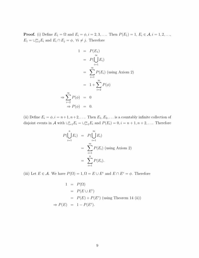
Proof. (i) Define E1 = Ω and Ei = φ, i = 2, 3, . . .. Then P (E1) = 1, Ei ∈ A, i = 1, 2, . . .,

E1 = ∪∞i=1Ei and Ei ∩ Ej = φ, ∀i 6= j. Therefore

1 = P (E1)

= P (∞⋃i=1

Ei)

=∞∑i=1

P (Ei) (using Axiom 2)

= 1 +∞∑i=2

P (φ)

⇒∞∑i=2

P (φ) = 0

⇒ P (φ) = 0.

(ii) Define Ei = φ, i = n+1, n+2, . . .. Then E1, E2, . . . is a countably infinite collection of

disjoint events in A with ∪ni=1Ei = ∪∞i=1Ei and P (Ei) = 0, i = n+ 1, n+ 2, . . .. Therefore

P (n⋃i=1

Ei) = P (∞⋃i=1

Ei)

=∞∑i=1

P (Ei) (using Axiom 2)

=n∑i=1

P (Ei).

(iii) Let E ∈ A. We have P (Ω) = 1,Ω = E ∪ Ec and E ∩ Ec = φ. Therefore

1 = P (Ω)

= P (E ∪ Ec)

= P (E) + P (Ec) (using Theorem 14 (ii))

⇒ P (E) = 1− P (Ec).

9

(iv) Let E1, E2 ∈ A and E1 ⊆ E2. Then E2 − E1 ∈ A, E2 = E1 ∪ (E2 − E1) and

E1 ∩ (E2 − E1) = φ. Therefore

P (E2) = P (E1 ∪ (E2 − E1))

= P (E1) + P (E2 − E1) (using Theorem 14 (ii))

⇒ P (E2 − E1) = P (E2)− P (E1).

As P (E2 − E1) ≥ 0, it also follows that P (E1) ≤ P (E2).

(v) Let E ∈ A. Then φ ⊆ E ⊆ Ω. Using Theorem 14 (iv) we conclude that P (φ) ≤P (E) ≤ P (Ω), i.e., 0 ≤ P (E) ≤ 1.

(vi) Let E1, E2 ∈ A. Then E2−E1 ∈ A, E1∩(E2−E1) = φ and E1∪E2 = E1∪(E2−E1).

Therefore

P (E1 ∪ E2) = P (E1 ∪ (E2 − E1))

= P (E1) + P (E2 − E1) (using Theorem 14 (ii)). (15)

Also (E1 ∩ E2) ∩ (E2 − E1) = φ and E2 = (E1 ∩ E2) ∪ (E2 − E1). Therefore

P (E2) = P ((E1 ∩ E2) ∪ (E2 − E1))

= P (E1 ∩ E2) + P (E2 − E1) (using Theorem 14 (ii))

⇒ P (E2 − E1) = P (E2)− P (E1 ∩ E2). (16)

Using (16) in (15) we conclude that P (E1 ∪ E2) = P (E1) + P (E2)− P (E1 ∩ E2). ♠

When we say that an experiment has been performed at random we mean that various

possible outcomes of the experiment are equally likely. For example when we say that

two numbers are chosen at random from the set 1, 2, 3 then P (1, 2) = P (2, 3) =

P (1, 3) = 1/3; here i, j indicates that the experiment terminates with chosen numbers

as i and j, i, j ∈ 1, 2, 3, i 6= j. In such situations clearly the probability of any event

can be found using classical approach (see Remark 13 (iv)).

Example 17 Ten cards are drawn at random without replacement from a deck of 52

cards. Find the probability that the draw yields 2 aces, 3 kings and five cards each of

black and red colors.

Solution. Let E denote the event of drawing 2 aces, 3 kings and five cards each of black

and red colors. Then E can be written as union of the following six mutually exclusive

10

events:

E1: drawing 2 red aces, 2 red kings, 1 black king, 1 red card other than ace or king, and

4 black cards other than ace or king;

E2: drawing 2 red aces, 1 red king, 2 black kings, 2 red cards other than ace or king, and

3 black cards other than ace or king;

E3: drawing 1 red ace, 1 black ace; 2 red kings, 1 black king, 2 red cards other than ace

or king, and 3 black cards other than ace or king;

E4: drawing 1 red ace, 1 black ace; 1 red king, 2 black kings, 3 red cards other than ace

or king, and 2 black cards other than ace or king;

E5: drawing 2 black aces; 2 red kings, 1 black king, 3 red cards other than ace or king,

and 2 black cards other than ace or king;

E6: drawing 2 black aces, 1 red king, 2 black kings, 4 red cards other than ace or king,

and 1 black card other than ace or king.

Using countable additivity of probability measures (see Theorem 14 (ii)) we have P (E) =∑6i=1 P (Ei). Note that:

Total number of ways in which 10 cards can be drawn from a deck of 52 cards (i.e., total

number of possible outcomes) =(

5210

);

Total number of ways in which 2 red aces, 2 red kings, 1 black king, 1 red card other than

ace or king, and 4 black cards other than ace or king can be drawn (i.e., total number of

outcomes favorable to event E1) =(

22

)(22

)(21

)(221

)(224

).

Therefore by classical approach

P (E1) =

(22

)(22

)(21

)(221

)(224

)(5210

) .

11

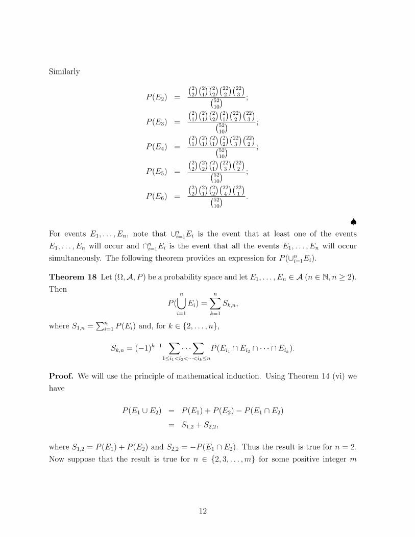
Similarly

P (E2) =

(22

)(21

)(22

)(222

)(223

)(5210

) ;

P (E3) =

(21

)(21

)(22

)(21

)(222

)(223

)(5210

) ;

P (E4) =

(21

)(21

)(21

)(22

)(223

)(222

)(5210

) ;

P (E5) =

(22

)(22

)(21

)(223

)(222

)(5210

) ;

P (E6) =

(22

)(21

)(22

)(224

)(221

)(5210

) .

♠For events E1, . . . , En, note that ∪ni=1Ei is the event that at least one of the events

E1, . . . , En will occur and ∩ni=1Ei is the event that all the events E1, . . . , En will occur

simultaneously. The following theorem provides an expression for P (∪ni=1Ei).

Theorem 18 Let (Ω,A, P ) be a probability space and let E1, . . . , En ∈ A (n ∈ N, n ≥ 2).

Then

P (n⋃i=1

Ei) =n∑k=1

Sk,n,

where S1,n =∑n

i=1 P (Ei) and, for k ∈ 2, . . . , n,

Sk,n = (−1)k−1∑· · ·∑

1≤i1<i2<···<ik≤n

P (Ei1 ∩ Ei2 ∩ · · · ∩ Eik).

Proof. We will use the principle of mathematical induction. Using Theorem 14 (vi) we

have

P (E1 ∪ E2) = P (E1) + P (E2)− P (E1 ∩ E2)

= S1,2 + S2,2,

where S1,2 = P (E1) + P (E2) and S2,2 = −P (E1 ∩ E2). Thus the result is true for n = 2.

Now suppose that the result is true for n ∈ 2, 3, . . . ,m for some positive integer m

12

(≥ 2). Then

P (m+1⋃i=1

Ei) = P ((m⋃i=1

Ei)⋃

Em+1)

= P (m⋃i=1

Ei) + P (Em+1)− P ((m⋃i=1

Ei)⋂

Em+1) (using the result for n = 2)

= P (m⋃i=1

Ei) + P (Em+1)− P (m⋃i=1

(Ei⋂

Em+1))

=m∑i=1

Si,m + P (Em+1)− P (m⋃i=1

(Ei⋂

Em+1)) (using the result for n = m).

= (19)

Let Fi = Ei ∩ Em+1, i = 1, . . .m. Then again using the result for n = m we get

P (m⋃i=1

(Ei⋂

Em+1)) = P (m⋃i=1

Fi)

=m∑k=1

Tk,m, (20)

where T1,m =∑m

i=1 P (Fi) =∑m

i=1 P (Ei ∩ Em+1) and, for k ∈ 2, . . . ,m,

Tk,m = (−1)k−1∑· · ·∑

1≤i1<i2<···<ik≤m

P (Fi1 ∩ Fi2 ∩ · · · ∩ Fik)

= (−1)k−1∑· · ·∑

1≤i1<i2<···<ik≤m

P (Ei1 ∩ Ei2 ∩ · · · ∩ Eik ∩ Em+1).

Using (20) in (19) we get

P (m+1⋃i=1

Ei) = (S1,m + P (Em+1)) + (S2,m − T1,m) + · · ·+ (Sm,m − Tm−1,m)− Tm,m. (21)

Note that S1,m + P (Em+1) = S1,m+1, Sk,m − Tk−1,m = Sk,m+1, k = 2, . . . ,m and Tm,m =

(−1)m−1P (E1 ∩ · · · ∩ Em+1) = −Sm+1,m+1. Using these in (21) we get

P (m+1⋃i=1

Ei) =m+1∑k=1

Sk,m+1.

13

Now the result follows using the principle of mathematical induction. ♠

The following example provides an application of the above result.

Example 22 Suppose that we have n (≥ 2) letters and corresponding n addressed en-

velopes. If these letters are inserted at random in n envelopes find the probability that

no letter is inserted into the correct envelope.

Solution Let us label the letters as L1, L2, . . . , Ln and respective envelopes as A1, . . . , An.

Let Ei denote the event that letter Ei is inserted into envelope Ai, i = 1, 2, . . . , n. We

need to find P (∩ni=1Eci ). We have

P (n⋂i=1

Eci ) = P ((

n⋃i=1

Ei)c)

= 1− P (n⋃i=1

Ei)

= 1−n∑k=1

Sk,n,

where for k ∈ 1, . . . , n,

Sk,n = (−1)k−1∑· · ·∑

1≤i1<i2<···<ik≤n

P (Ei1 ∩ Ei2 ∩ · · · ∩ Eik).

Note that n letters can be inserted into n envelopes in n! ways. Also, for 1 ≤ i1 < i2 <

· · · < ik ≤ n, Ei1 ∩ Ei2 ∩ · · · ∩ Eik is the event that letters Li1 , . . . , Lik are inserted into

correct envelopes. Clearly number of cases favorable to this event is (n− k)!. Therefore,

for 1 ≤ i1 < i2 < · · · < ik ≤ n,

P (Ei1 ∩ Ei2 ∩ · · · ∩ Eik) =(n− k)!

n!

⇒ Sk,n = (−1)k−1∑· · ·∑

1≤i1<i2<···<ik≤n

(n− k)!

n!

= (−1)k−1

(n

k

)(n− k)!

n!

=(−1)k−1

k!

⇒ P (n⋂i=1

Eci ) =

1

2!− 1

3!+

1

4!− · · ·+ (−1)n

n!.

14

♠The following theorem provides bounds on the probabilities of the events ∪ni=1Ei and

∩ni=1Ei.

Theorem 23 Let (Ω,A, P ) be a probability space and let E1, . . . , En ∈ A (n ∈ N, n ≥ 2).

Then, under the notations of Theorem 18,

(i) (Boole’s Inequality) S1,n + S2,n ≤ P (⋃ni=1Ei) ≤ S1,n;

(ii) (Bonferroni’s Inequality) P (⋂ni=1Ei) ≥ S1,n − (n− 1).

Proof (i) We will use the principle of mathematical induction. Using Theorem 14 (vi)

we have

P (E1

⋃E2) = P (E1) + P (E2)− P (E1 ∩ E2)

= S1,2 + S2,2

≤ S1,2,

where S1,2 = P (E1) + P (E2) and S2,2 = −P (E1 ∩ E2) ≤ 0. Thus the result is true for

n = 2. Now suppose that the result is true for n ∈ 2, 3, . . . ,m for some positive integer

m (≥ 2), i.e., suppose that for arbitrary events F1, . . . , Fm ∈ A

P (k⋃i=1

Fi) ≤k∑i=1

P (Fi), k = 2, 3, . . . ,m, (24)

and

P (k⋃i=1

Fi) ≥k∑i=1

P (Fi)−∑∑1≤i<j≤k

P (Fi ∩ Fj), k = 2, 3, . . . ,m. (25)

Then

P (m+1⋃i=1

Ei) = P ((m⋃i=1

Ei)⋃

Em+1)

≤ P (m⋃i=1

Ei) + P (Em+1) (using (24) for k = 2)

≤ S1,m + P (Em+1) (using (24) for k = m)

= S1,m+1. (26)

15

Also

P (m+1⋃i=1

Ai) = P ((m⋃i=1

Ei)⋃

Em+1)

= P (m⋃i=1

Ei) + P (Em+1)− P ((m⋃i=1

Ei)⋂

Em+1)

= P (m⋃i=1

Ei) + P (Em+1)− P (m⋃i=1

(Ei⋂

Em+1)). (27)

Using (24) for k = m we have

P (m⋃i=1

(Ei⋂

Em+1)) ≤m∑i=1

P (Ei⋂

Em+1), (28)

and using (25) for k = m we have

P (m⋃i=1

Ei) ≥ S1,m + S2,m. (29)

Using (28) and (29) in (27) we get

P (m+1⋃i=1

Ei) ≥ S1,m + S2,m + P (Em+1)−m∑i=1

P (Ei⋂

Em+1)

=m+1∑i=1

P (Ei)−∑∑

1≤i<j≤m+1

P (Ei⋂

Ej)

= S1,m+1 + S2,m+1. (30)

16

The assertion now follows from (26) and (30).

(ii) We have

P (n⋂i=1

Ei) = P ((n⋃i=1

Eci )c)

= 1− P (n⋃i=1

Eci )

≥ 1−n∑i=1

P (Eci ) (using Boole’s inequality)

= 1−n∑i=1

(1− P (Ei))

=n∑i=1

P (Ei)− (n− 1).

♠

Remark 31 Under the notation of Theorem 23, we can in fact prove the following in-

equalities2k∑j=1

Sj,n ≤ P (n⋃j=1

Ej) ≤2k−1∑j=1

Sj,n, k = 1, 2, . . . , [n

2].

We leave proving the above inequalities as an exercise. ♠

As a consequence of Theorem 23 we have the following corollary.

Corollary 32 Let (Ω,A, P ) be a probability space and let E1, . . . , En be events. Then

(i) P (Ei) = 0, i = 1, . . . , n ⇒ P (∪ni=1Ei) = 0;

(ii) P (Ei) = 1, i = 1, . . . , n ⇒ P (∩ni=1Ei) = 1.

Proof. (i) Using Boole’s inequality we get 0 ≤ P (∪ni=1Ei) ≤∑n

i=1 P (Ei) = 0. It follows

that P (∪ni=1Ei) = 0.

(ii) Using Bonferroni’s inequality we get 1 ≥ P (∩ni=1Ei) ≥∑n

i=1 P (Ei) − (n − 1) = 1. It

follows that P (∩ni=1Ei) = 1. ♠

Definition 33 Let (Ω,A, P ) be a probability space and let An;n = 1, 2, . . . be a se-

quence of events in A.

17

(i) We say that the sequence An;n = 1, 2, . . . is increasing (written as An ↑) if An ⊆An+1, n = 1, 2, . . .;

(ii) We say that the sequence An;n = 1, 2, . . . is decreasing (written as An ↓) if An+1 ⊆An, n = 1, 2, . . .;

(iii) We say that the sequence An;n = 1, 2, . . . is monotone if either An ↑ or An ↓;

(iv)If An;n = 1, 2, . . . is an increasing sequence we define the limit of the sequence

An;n = 1, 2, . . . as ∪∞n=1An and write ∪∞n=1An = Limn→∞An;

(v) If An;n = 1, 2, . . . is a decreasing sequence we define the limit of the sequence

An;n = 1, 2, . . . as ∩∞n=1An and write ∩∞n=1An = Limn→∞An;

(vi) We say that the probability measure P is continuous if, for any monotone sequence

Bn;n = 1, 2, . . . of events, P (Limn→∞Bn) = limn→∞ P (Bn). ♠

Throughout we will denote the limit of a monotone sequence An;n = 1, 2, . . . of events

by Limn→∞An and the limit of a sequence an;n = 1, 2, . . . of a real numbers by

limn→∞ an. The following theorem establishes the continuity of probability measures.

Theorem 34 (Continuity of Probability Measures) Let (Ω,A, P ) be a probability space.

Then P is continuous, i.e., for any monotone sequence An;n = 1, 2, . . . of events,

P (Limn→∞An) = limn→∞ P (An).

Proof First suppose that An ↑ so that Limn→∞An = ∪∞n=1An. Define B1 = A1, Bn =

An − An−1, n = 2, 3, . . .. Then Bn ∈ A, n = 1, 2, . . . ,∪∞n=1An = ∪∞n=1Bn and Bi ∩ Bj = φ,

whenever i 6= j. Therefore,

P (Limn→∞An) = P (∞⋃n=1

An)

= P (∞⋃n=1

Bn)

=∞∑n=1

P (Bn)

= limn→∞

n∑k=1

P (Bk). (35)

18

Also, for n ∈ 2, 3, . . .,

n∑k=1

P (Bk) = P (A1) +n∑k=2

P (Ak − Ak−1)

= P (A1) +n∑k=2

(P (Ak)− P (Ak−1)) (using Theorem 14 (iv))

= P (A1) +n∑k=2

P (Ak)−n−1∑k=1

P (Ak)

= P (An). (36)

Using (36) in (35) we get

P (Limn→∞An) = limn→∞

P (An).

Now suppose that An ↓ so that Limn→∞An = ∩∞n=1An. Define Dn = Acn = Ω − An, n =

1, 2, . . . so that Dn ∈ A, n = 1, 2, . . . , Dn ↑ and Limn→∞An = (∪∞n=1Dn)c. Since Dn ↑ we

have

P (∞⋃n=1

Dn) = P (Limn→∞Dn)

= limn→∞

P (Dn)

= limn→∞

P (Acn)

= limn→∞

[1− P (An)]

= 1− limn→∞

P (An) (37)

⇒ P (Limn→∞An) = P ((∞⋃n=1

Dn)c)

= 1− P (∞⋃n=1

Dn)

= limn→∞

P (An), (using (37)).

♠

19

3 Conditional Probability and Independence of Events

Let (Ω,A, P ) be a probability space. In many situations we may not be interested in the

whole sample space Ω. Rather we may be interested in a subset B of the sample space Ω.

This may happen, for example, when we know apriori that the outcome of the random

experiment has to be an element of B ∈ A.

To make the above discussion precise consider a random experiment of shuffling a

deck of 52 cards in such a way that all 52! arrangements of cards (when looked from top

to bottom) are equally likely. Clearly the sample space Ω consists of 52! permutations of

cards. Now suppose that it is noticed that the bottom card is the king of heart. In the

light of this additional information the sample space (say B) consists of 51! arrangements

of 52 cards with the bottom card as king of heart. In the light of the available information

(i.e., under the sample space B) let us try to find the probability of the event K that

the top card is a king. For an event E ∈ A, let P (E) and PB(E) denote its probabilities

under the sample spaces Ω and B respectively. Clearly PB(K) = 3×50!51!

. Note that

PB(K) =3× 50!

51!=

3×50!52!51!52!

=P (K ∩B)

P (B),

i.e.,

PB(K) =P (K ∩B)

P (B). (38)

We may call PB(K) the conditional probability of event K given that the experiment

results in the event B (i.e., experiment results in an outcome ω ∈ B) and P (K) the

unconditional probability of event K. This leads to the introduction of the concept of

conditional probability.

To fix ideas let us revert back to our general discussion. Let (Ω,A, P ) be a probability

space and suppose that we know in advance that the outcome of the experiment has to

be an element of B ∈ A, where P (B) > 0. In such situations the sets in the class

A ∩ B : A ∈ A are natural contestants for the event space. The following theorem

establishes that this class of sets is in fact a sigma-field (event space) of subsets of B.

Theorem 39 Let A be a sigma-field of subsets of Ω and let B ∈ A. Define AB = A∩B :

A ∈ A. Then AB is a sigma-field of subsets of B and AB ⊆ A.

Proof Since A is a sigma-field of subsets of Ω, Ω ∈ A, A is closed under complementations

(with respect to Ω), and A is also closed under countable unions.

To show that AB is a sigma-filed of subsets of B we need to show that: (i) B ∈ AB, (ii)

20

C ∈ AB ⇒ B − C ∈ AB, and (iii) Ci ∈ AB, i = 1, 2, . . .⇒ ∪∞i=1Ci ∈ AB.

Since B = B ∩B and B ∈ A we have B ∈ AB. Let C ∈ AB so that C = A ∩B for some

A ∈ A. Then Ω− A ∈ A and therefore B − C = (Ω− A) ∩ B ∈ AB. Thus AB is closed

under complementations (with respect to B). Now suppose that Ci ∈ AB, i = 1, 2, . . ..

Then Ci = Ai ∩ B for some Ai ∈ A, i = 1, 2, . . .. Therefore ∪∞i=1Ai ∈ A and ∪∞i=1Ci =

(∪∞i=1Ai) ∩B ∈ AB.

To show that AB ⊆ A suppose that C ∈ AB. Then C = A ∩ B for some A ∈ A. Since

A,B ∈ A and A is a sigma-field it follows (from Remark 10 (iii)) that C = A ∩ B ∈ A.

Therefore AB ⊆ A. ♠.

Equation (38) suggests to consider the set function PB : AB → R defined by

PB(C) =P (C)

P (B), C ∈ AB.

Note that, for C ∈ AB, P (C) is well defined asAB ⊆ A. The following theorem establishes

that PB is in fact a probability measure on AB.

Theorem 40 (B,AB, PB) is a probability space.

Proof In view of Theorem 39 it suffices to show that PB is a probability measure on AB.

Clearly PB(C) ≥ 0,∀C ∈ AB. Let C1, C2, . . . be a collection of disjoint sets in AB. Then

Ci = Ai ∩B, for some Ai ∈ A, i = 1, 2, . . ., and

PB(∞⋃i=1

Ci) =P (⋃∞i=1 Ci)

P (B)

=

∑∞i=1 P (Ci)

P (B)

=∞∑i=1

P (Ci)

P (B)

=∞∑i=1

PB(Ci),

i.e., PB is countable additive on AB.

Also

PB(B) =P (B)

P (B)= 1.

Thus PB is a probability measure on AB. ♠.

For A ∈ A (so that A ∩ B ∈ AB) we write PB(A ∩ B) as P (A|B) and call it as the

21

conditional probability of A given B. Using Theorem 40 it follows that the set function

P (·|B) : A → R is a probability measure on A with P (Ω|B) = 1, i.e., (Ω,A, P (·|B)) is a

probability space. Note that the domain of the probability measure PB(·) is AB whereas

the domain of the probability measure P (·|B) is A. Moreover PB(A∩B) = P (A|B), A ∈A.

Definition 41 Let (Ω,A, P ) be a probability space and let B ∈ A be a fixed event such

that P (B) > 0. Define the set function P (·|B) : A → R by

P (A|B) = PB(A ∩B) =P (A ∩B)

P (B), A ∈ A.

We call P (A|B) the conditional probability of event A given that the outcome of the

experiment is in B or simply the conditional probability of A given B. ♠

Example 42 Six cards are dealt at random without replacement from a well shuffled

deck of 52 cards. Find the probability of getting all cards of heart in a hand given that

there are at least five cards of heart in the hand.

Solution Let A and B respectively denote the events of getting all cards of heart in the

hand and getting at least five cards of heart in the hand. The required probability is

P (A|B) =P (A ∩B)

P (B).

Clearly

P (A ∩B) =

(136

)(526

) ,and

P (B) =

(135

)(391

)+(

136

)(526

) .

Therefore

P (A|B) =

(136

)(135

)(391

)+(

136

) .♠

Remark 43 For events E1, . . . , En (n ≥ 2)

P (E1 ∩ E2) = P (E1)P (E2|E1), if P (E1) > 0

22

and

P (E1 ∩ E2 ∩ E3) = P ((E1 ∩ E2) ∩ E3)

= P (E1 ∩ E2)P (E3|E1 ∩ E2)

= P (E1)P (E2|E1)P (E3|E1 ∩ E2),

if P (E1 ∩ E2) > 0.

Using principle of mathematical induction it can be shown that

P (n⋂i=1

Ei) = P (E1)P (E2|E1)P (E3|E1 ∩ E2) · · ·P (En|E1 ∩ E2 · · · ∩ En−1),

provided P (E1 ∩ E2 · · · ∩ En−1) > 0. ♠

Example 44 An urn contains four red and six black balls. Two balls are drawn succes-

sively at random without replacement from the urn. Find the probability that the first

draw resulted in a red ball and the second draw resulted in a black ball.

Solution Let A and B respectively denote the events that the first draw results in a red

ball and the second draw results in a black ball. The required probability is

P (A ∩B) = P (A)P (B|A) =4

10× 6

9=

12

45.

♠

Definition 45 For an index set Λ ⊆ R, let Eα;α ∈ Λ be a collection of events. Events

Eα;α ∈ Λ are said to be exhaustive if P (⋃α∈ΛEα) = 1. ♠

Let (Ω,A, P ) be a probability space. For a collection E1, E2, . . . of mutually exclusive

and exhaustive events (i.e., Ei ∩ Ej = φ, whenever i 6= j, and P (∪∞i=1Ei) = 1), the

following theorem provides a relationship between marginal probability P (E) of an event

E ∈ A and joint probabilities P (E ∩ Ei), i = 1, . . . , n, of events E and Ei, i = 1, . . . , n.

Theorem 46 (Theorem of Total Probability) Let (Ω,A, P ) be a probability space and

let Ei : i ∈ λ be a countable collection of mutually exclusive and exhaustive events (i.e.,

Ei ∩Ej = φ, whenever i 6= j, and P (∪i∈ΛEi) = 1) such that P (Ei) > 0, ∀i ∈ Λ. Then, for

23

any event E ∈ A,

P (E) =∑i∈Λ

P (E ∩ Ei)

=∑i∈Λ

P (E|Ei)P (Ei).

Proof Define F = ∪i∈ΛEi so that P (F ) = 1. Then P (F c) = 0 and therefore P (E∩F c) = 0

(since E ∩ F c ⊆ F c). Since E = (E ∩ F ) ∪ (E ∩ F c) and (E ∩ F ) ∩ (E ∩ F c) = φ, using

Theorem 14 (ii) we get

P (E) = P (E ∩ F ) + P (E ∩ F c)

= P (E ∩ F )

= P (⋃i∈Λ

(E⋂

Ei)). (47)

Also Ei ∩ Ej = φ, i 6= j, implies that (E ∩ Ei) ∩ (E ∩ Ej) = φ, i 6= j. Therefore, using

(47), we get

P (E) = P (⋃i∈Λ

(E ∩ Ei)) =∑i∈Λ

P (E ∩ Ei) =∑i∈Λ

P (E|Ei)P (Ei).

♠

Example 48 Urn U1 contains four white and six black balls and urn U2 contains six

white and four black balls. A fair die is cast and urn U1 is selected if the upper face of

die shows five or six spots. Otherwise urn U2 is selected. If a ball is drawn at random

from the selected urn find the probability that the drawn ball is white.

Solution Define the events:

W: drawn ball is white;

E1: urn U1 is selected;

E2: urn U2 is selected.

Then E1 and E2 are mutually exclusive and exhaustive events. Using theorem of total

probability we have

P (W ) = P (E1)P (W |E1) + P (E2)P (W |E2).

24

We have P (E1) = 26

= 13, P (E2) = 4

6= 2

3, P (W |E1) = 4

10= 2

5and P (W |E2) = 6

10= 3

5.

Therefore

P (W ) =1

3× 2

5+

2

3× 3

5=

8

15.

♠

The following theorem provides a method for finding the probability of occurrence of

an event in the future trial based on information on occurrences in the previous trials.

Theorem 49 (Baye’s Theorem) Let (Ω,A, P ) be a probability space and let Ei; i ∈ Λbe a countable collection of mutually exclusive and exhaustive events with P (Ei) > 0,∀i ∈Λ. Then, for any other event E with P (E) > 0, we have

P (Ej|E) =P (E|Ej)P (Ej)∑i∈Λ P (E|Ei)P (Ei)

, j ∈ Λ.

Proof We have, for j ∈ Λ,

P (Ej|E) =P (Ej ∩ E)

P (E)

=P (E|Ej)P (Ej)

P (E)

=P (E|Ej)P (Ej)∑i∈Λ P (E|Ei)P (Ei)

, (using theorem of total probability).

♠In Baye’s theorem the probabilities P (Ej), j ∈ Λ, are referred to as prior probabilities

and the probabilities P (Ej|E), j ∈ Λ, are referred to as posterior probabilities.

To see an application of Baye’s theorem, let us revisit Example 48.

Example 50 Urn U1 contains four white and six black balls and urn U2 contains six

white and four black balls. A fair die is cast and urn U1 is selected if the upper face of

die shows five or six spots. Otherwise urn U2 is selected.

(i) Given that the drawn ball is white, find the conditional probability that it came from

urn U1;

(ii) Given that the drawn ball is white, find the conditional probability that it came from

urn U2

Proof (i) Let us follow the notation used in the solution of Example 48. The required

25

probability is P (E1|W ). Using Baye’s theorem we have

P (E1|W ) =P (W |E1)P (E1)

P (W |E1)P (E1) + P (W |E2)P (E2)

=25× 1

325× 1

3+ 3

5× 2

3

=1

4.

(ii) Since E1 and E2 are mutually exclusive and exhaustive events, using theorem of total

probability, we have P (E2|W ) = 1− P (E1|W ) = 34. ♠

In the above example we have P (E1|W ) < P (E1), i.e., the probability of occurrence

of event E1 decreases in the presence of information that the outcome is an element of W .

We also have P (E2|W ) > P (E2), i.e., the probability of occurrence of event E2 increases

in the presence of information that the outcome is an element of W . These phenomena

are related to the concept of association defined below. Note that P (E1|W ) < P (E1)⇔P (E1 ∩W ) < P (E1)P (W ) and P (E2|W ) > P (E2)⇔ P (E2 ∩W ) > P (E2)P (W ).

Definition 51 Let (Ω,A, P ) be a probability space and let A and B be two events.

Events A and B are said to be

(i) negatively associated if P (A ∩B) < P (A)P (B);

(ii) positively associated if P (A ∩B) > P (A)P (B);

(iii) independent if P (A ∩B) = P (A)P (B). ♠

Note that if P (B) = 0 then P (A ∩ B) = 0 for any A ∈ A. Thus if P (B) = 0 then any

event A ∈ A and B are independent. Also if P (B) > 0 then A and B are independent

if and only if P (A|B) = P (A). In other words if P (B) > 0 then events A and B are

independent if and only if the availability of the information that event B has occurred

does not alter the probability of occurrence of event A. In the sequel we define the concept

of independence for arbitrary collection of events.

Definition 52 Let Λ ⊆ R be an index set and let Eα;α ∈ Λ be a collection of events

in A.

(i) Events Eα;α ∈ Λ are said to be pairwise independent if any pair of events Eα and

Eβ, α 6= β, are independent, i.e., if P (Eα ∩ Eβ) = P (Eα)P (Eβ), whenever α, β ∈ Λ and

α 6= β;

(ii) Let F1, . . . , Fn be a finite collection of events in A. Events F1, . . . , Fn are said to be

26

independent if for any subcollection Fα1 , . . . , Fαk of F1, . . . , Fn (k = 2, 3, . . . , n)

P (k⋂j=1

Fαj) =

k∏j=1

P (Fαj). (53)

(iii) Let Λ ⊆ R be an arbitrary index set and let Fα;α ∈ Λ be a collection of events in

A. Events Fα;α ∈ Λ are said to be independent if any finite subcollection of events in

Fα;α ∈ Λ forms a collection of independent events. ♠

To verify that n events F1, . . . Fn are independent one must verify 2n−n−1 (=∑n

j=2

(nj

))

conditions given in (53). For example, for three events F1, F2 and F3 to be independent the

following 4 (= 23− 3− 1) conditions must be satisfied: P (F1∩F2) = P (F1)P (F2), P (F2∩F3) = P (F2)P (F3), P (F1 ∩ F3) = P (F1)P (F3) and P (F1 ∩ F2 ∩ F3) = P (F1)P (F2)P (F3).

Note that if events F1, . . . , Fn are independent then for any permutation (α1, . . . , αn) of

(1, . . . , n) the events Fα1 , . . . , Fαn are also independent. Thus the notion of independence

is symmetric in the events involved.

From Definition 52 it is clear that events in any subcollection of independent events

are independent. In particular independence of a collection of events implies their pairwise

independence. The following example illustrates that, in general, pairwise independence

of a collection of events may not imply their independence.

Example 54 Let Ω = 1, 2, 3, 4 and let A = P(Ω), the power set of Ω. Consider

the probability space (Ω,A, P ), where P (i) = 14, i = 1, 2, 3, 4. Let A = 1, 4, B =

2, 4 and C = 3, 4. Then P (A) = P (B) = P (C) = 12, P (A ∩ B) = P (4) =

14

= P (A)P (B), P (B ∩ C) = P (4) = 14

= P (B)P (C) and P (A ∩ C) = P (4) =14

= P (A)P (C). It follows that the events A,B and C are pairwise independent. Since

P (A ∩B ∩ C) = 146= P (A)P (B)P (C), the events A,B and C are not independent. ♠

Theorem 55 Let (Ω,A, P ) be a probability space and let A and B be independent events

in A. Then

(i) Ac and and B are independent events;

(ii) A and Bc are independent events;

(iii) Ac and Bc are independent events.

Proof Suppose that A and B are independent events, i.e., suppose that P (A ∩ B) =

P (A)P (B).

27

(i) We have B = (A ∩B) ∪ (Ac ∩B) and (A ∩B) ∩ (Ac ∩B) = φ. Therefore

P (B) = P ((A ∩B) ∪ (Ac ∩B))

= P (A ∩B) + P (Ac ∩B)

= P (A)P (B) + P (Ac ∩B)

⇒ P (Ac ∩B) = (1− P (A))P (B)

= P (Ac)P (B),

i.e., Ac and B are independent events.

(ii) Follows from (i) by interchanging the roles of A and B.

(iii) Follows on using (i) and (ii) sequentially. ♠

The following theorem strengthens the results of Theorem 55.

Theorem 56 Let (Ω,A, P ) be a probability space and let F1, . . . , Fn (n ∈ N, n ≥ 3)

be independent events in A. Then, for any k ∈ 1, 2, . . . , n − 1 and any permutation

(α1, . . . , αn) of (1, . . . .n), the events Fα1 , . . . , Fαk, F c

αk+1, . . . , F c

αnare independent.

Proof Since the notion of independence is symmetric in the events involved, it is enough to

show that for any k ∈ 1, 2, . . . , n−1 the events F1, . . . , Fk, Fck+1, . . . , F

cn are independent.

Using backward induction the aforementioned assertion would follow if, under the hypoth-

esis of the theorem, we show that the events F1, . . . , Fn−1, Fcn are independent. To show

that the events F1, . . . , Fn−1, Fcn are independent consider a subcollection Fi1 , . . . , Fim , G

(where i1, . . . , im ⊆ 1, . . . , n − 1) of F1, . . . , Fn−1, Fcn, where G = F c

n or G = Fj,

for some j ∈ 1, . . . , n − 1 − i1, . . . , im, depending on whether or not F cn is a part of

subcollection Fi1 , . . . , Fim , G. Thus the following two cases arise:

Case I G = F cn

Since events F1, . . . , Fn are independent, we have P (∩mj=1Fij ) =∏m

j=1 P (Fij ) and

P ((m⋂j=1

Fij ) ∩ Fn) =m∏j=1

P (Fij )P (Fn)

= [m∏j=1

P (Fij )]P (Fn)

= P (m⋂j=1

Fij )P (Fn).

28

It follows that events ∩mj=1Fij and Fn are independent. Now on using Theorem 55 (i)

it is evident that events ∩mj=1Fij and F cn are independent, i.e., P ((∩mj=1Fij ) ∩ F c

n) =

P (∩mj=1Fij )P (F cn) = [

∏mj=1 P (Fij )]P (F c

n). Therefore

P (Fi1 ∩ · · · ∩ Fim ∩G) = P ((∩mj=1Fij ) ∩ F cn)

= [m∏j=1

P (Fij )]P (F cn)

= [m∏j=1

P (Fij )]P (G).

Case II G = Fj, for some j ∈ 1, . . . , n− 1 − i1, . . . , im,In this case Fi1 , . . . , Fim , G is a subcollection of independent events F1, . . . , Fn and

therefore

P (Fi1 ∩ · · · ∩ Fim ∩G) = [m∏j=1

P (Fij )]P (G).

Now the result follows on combining the two cases. ♠

Exercises

1. Let Ω = 1, 2, 3, 4. Check which of the following is a sigma-field of subsets of Ω:

(a) A1 = φ, 1, 2, 3, 4; (b) A2 = φ,Ω, 1, 2, 3, 4, 1, 2, 3, 4;(c) A3 = φ,Ω, 1, 2, 1, 2, 3, 4, 2, 3, 4, 1, 3, 4.

2. Show that a class F of subsets of Ω is a sigma-field of subsets of Ω if, and only if, the

following three conditions are satisfied: (i) Ω ∈ F ; (ii) A ∈ F ⇒ Ac = Ω− A ∈ F ;

(iii) An ∈ F , n = 1, 2, . . .⇒ ∩∞n=1An ∈ F .

3. Let Aλ;λ ∈ Λ be a collection of sigma-fields of subsets of Ω.

(a) Show that⋂λ∈ΛAλ is a sigma-field;

(b) Using a counter example show that⋃λ∈ΛAλ may not be a sigma-field.

4. Let Ω be an infinite set and let F = A ⊆ Ω : A is finite or Ac is finite.(a) Show that F is closed under complements and finite unions;

(b) Using a counter example show that F may not be closed under countably infinite

unions.

29

5. Let Ω be an uncountable set and letA = A ⊆ Ω : A is countable orAc is countable.(a) Show that A is a sigma-field;

(b) What can you say about A when Ω is countable?

6. Let A = power set of Ω = 0, 1, 2, . . .. In each of the following cases, verify if

(Ω,A, P ) is a probability space:

(a) P (A) =∑

x∈A e−λλx/x!, A ∈ A, λ > 0;

(b) P (A) =∑

x∈A p(1− p)x, A ∈ A, 0 < p < 1;

(c) P (A) = 0, if A has a finite number of elements, and P (A) = 1, if A has infinite

number of elements, A ∈ A.

7. Suppose that P (A) = 0.6, P (B) = 0.5, P (C) = 0.4, P (A ∩ B) = 0.3, P (A ∩ C) =

0.2, P (B∩C) = 0.2, P (A∩B∩C) = 0.1, P (B∩D) = P (C∩D) = 0, P (A∩D) = 0.1

and P(D)=0.2. Find:

(a) P (A ∪B ∪ C) and P (Ac ∩Bc ∩ Cc); (b) P ((A ∪B) ∩ C) and P (A ∪ (B ∩ C));

(c) P ((Ac ∪Bc) ∩ Cc) and P ((Ac ∩Bc) ∪ Cc); (d) P (D ∩B ∩ C) and P (A ∩ C ∩D);

(e) P (A ∪B ∪D) and P (A ∪B ∪ C ∪D); (f) P ((A ∩B) ∪ (C ∩D)).

8. Let (Ω,A, P ) be a probability space and let A and B be two events.

(a) Show that the probability that exactly one of the events A or B will occur is

given by P (A) + P (B)− 2P (A ∩B);

(b) Show that P (A ∩B)− P (A)P (B) = P (A)P (Bc)− P (A ∩Bc) = P (Ac)P (B)−P (Ac ∩B) = P ((A ∪B)c)− P (Ac)P (Bc).

9. Suppose that n (≥ 3) persons P1, . . . , Pn are made to stand in a row at random.

Find the probability that there are exactly r persons between P1 and P2; here

r ∈ 1, 2, . . . , n− 2.

10. A point (X, Y ) is randomly chosen on the unit square S = (x, y) : 0 ≤ x ≤ 1, 0 ≤y ≤ 1 (i.e., for any region R ⊆ S for which the area is defined, the probability that

(X, Y ) lies on R is area of Rarea of S

). Find the probability that the distance from (X, Y )

to the nearest side does not exceed 13

units.

11. Three numbers a, b and c are chosen at random and with replacement from the set

1, 2, . . . , 6. Find the probability that the quadratic equation ax2 + bx+ c = 0 will

have real root(s).

12. Three numbers are chosen at random from the set 1, 2, . . . , 50. Find the proba-

bility that the chosen numbers are in

30

(a) arithmetic progression;

(b) geometric progression.

13. Consider an empty box in which four balls are to be placed (one-by-one) according

to the following scheme. A fair die is cast each time and the number of spots on

the upper face is noted. If the upper face shows up 2 or 5 spots then a white ball

is placed in the box. Otherwise a black ball is placed in the box. Given that the

first ball placed in the box was white find the probability that the box will contain

exactly two black balls.

14. Let ((0, 1],A, P ) be a probability space such that A contains all subintervals of (0, 1]

and P ((a, b]) = b− a, where 0 ≤ a < b ≤ 1.

(a) Show that b = ∩∞n=1(b− 1n+1

, b],∀b ∈ (0, 1];

(b) Show that P (b) = 0,∀b ∈ (0, 1];

(c) Show that, for any countable set A ∈ A, P (A) = 0;

(d) For n ∈ N, let An = (0, 1n] and Bn = (1

2+ 1

n+2, 1]. Verify that An ↓, Bn ↑,

P (Limn→∞An) = limn→∞ P (An) and P (Limn→∞Bn) = limn→∞ P (Bn).

15. Consider four coding machines M1,M2,M3 and M4 producing binary codes 0 and

1. The machine M1 produces codes 0 and 1 with respective probabilities 14

and 34.

The code produced by machine Mk is fed into machine Mk+1 (k = 1, 2, 3) which

may either leave the received code unchanged or may change it. Suppose that each

of the machines M2,M3 and M4 change the code with probability 34. Given that the

machine M4 has produced code 1, find the conditional probability that the machine

M1 produced code 0.

16. A student appears in the examinations of four subjects Biology, Chemistry, Physics

and Mathematics. Suppose that probabilities of the student clearing examinations

in these subjects are 12, 1

3, 1

4and 1

5respectively. Assuming that the performances of

the student in four subjects are independent, find the probability that the student

will clear examination(s) of

(a) all the subjects; (b) no subject; (c) exactly one subject;

(d) exactly two subjects; (e) at least one subject.

17. LetA andB be independent events. Show that maxP ((A∪B)c), P (A∩B), P (A∆B) ≥4/9, where A∆B = (A−B) ∪ (B − A).

31

18. For independent events A1, . . . , An, show that:

(n⋂i=1

Aci) ≤ e−∑n

i=1 P (Ai).

19. Let (Ω,A, P ) be a probability space and let A1, A2, . . . be a sequence of events. De-

fine Bn = ∩∞i=nAi, Cn = ∪∞i=nAi, n = 1, 2, . . ., D = ∪∞n=1Bn and E = ∩∞n=1Cn. Show

that:

(a) D is the event that all but a finite number of Ans occur and E is the event that

infinitely many Ans occur;

(b) D ⊆ E;

(c) P (Ec) = limn→∞ P (Ccn) = limn→∞ limm→∞ P (∩mk=nA

ck) and P (E) = limn→∞ P (Cn);

(d) if∑∞

n=1 P (An) <∞ then with probability one only finitely many Ans will occur;

(e) if A1, A2, . . . are independent and∑∞

n=1 P (An) = ∞ then with probability one

infinitely many Ans will occur.

20. Let A,B and C be three events such that A and B are negatively (positively)

associated and B and C are negatively (positively) associated. Can we conclude

that, in general, A and C are negatively (positively) associated?

21. Let (Ω,A, P ) be a probability space and let A and B be two events. Show that

if A and B are positively (negatively) associated then A and Bc are negatively

(positively) associated.

22. A locality has n houses numbered 1, . . . , n and a terrorist is hiding in one of these

houses. Let Hj denote the event that the terrorist is hiding in house numbered j, j =

1, . . . , n, and let P (Hj) = pj ∈ (0, 1), j = 1, . . . , n. During a search operation, let Fj

denote the event that search of the house number j will fail to nab the terrorist there

and let P (Fj|Hj) = rj ∈ (0, 1), j = 1, . . . , n. For each i, j ∈ 1, . . . , n, i 6= j, show

that Hj and Fj are negatively associated but Hi and Fj are positively associated.

Interpret these findings.

23. Let A,B and C be three events such that P (B ∩C) > 0. Prove or disprove each of

the following:

(a) P (A∩B|C) = P (A|B ∩C)P (B|C); (b) P (A∩B|C) = P (A|C)P (B|C) if A and

B are independent events.

24. A k-out-of-n system is a system comprising of n components that functions if and

32

only if at least k (k ∈ 1, 2, . . . , n) of the components function. A 1-out-of-n sys-

tem is called a parallel system and an n-out-of-n system is called a series system.

Consider n components C1, . . . , Cn that function independently. At any given time

t the probability that the component Ci will be functioning is pi(t) (∈ (0, 1)) and

the probability that it will not be functioning at time t is 1− pi(t), i = 1, . . . , n.

(a) Find the probability that a parallel system comprising of components C1, . . . , Cn

will function at time t;

(b) Find the probability that a series system comprising of components C1, . . . , Cn

will function at time t;

(c) If pi(t) = p(t), i = 1, . . . , n find the probability that a k-out-of-n system com-

prising of components C1, . . . , Cn will function at time t.

33