Sidney I. Resnick - A Probability Path
464
Modern Birkhäuser Classics A Probability Path Sidney I. Resnick
-
Upload
khangminh22 -
Category
Documents
-
view
3 -
download
0
Transcript of Sidney I. Resnick - A Probability Path

Modern Birkhäuser Classics
A Probability Path
Sidney I. Resnick

accessible to new generations of students, scholars, and researchers. paperback (and as eBooks) to ensure that these treasures remain
Modern Birkhäuser Classics
Many of the original research and survey monographs, as well as textbooks,
decades have been groundbreaking and have come to be regarded
of these modern classics, entirely uncorrected, are being re-released in as foundational to the subject. Through the MBC Series, a select number
in pure and applied mathematics published by Birkhäuser in recent


Reprint of the 2005 Edition
A Probability Path
Sidney I. Resnick

ISSN 2197-1803 ISSN 2197-1811 (electronic) ISBN 978-0-8176-8408-2 ISBN 978-0-8176-8409-9 (eBook) DOI 10.1007/978-0-8176-8409-9 Springer New York Heidelberg Dordrecht London Library of Congress Control Number: © Springer Science+Business Media New York 2014 This work is subject to copyright. All rights are reserved by the Publisher, whether the whole or part of the material is concerned, specifically the rights of translation, reprinting, reuse of illustrations, recitation, broadcasting, reproduction on microfilms or in any other physical way, and transmission or information storage and retrieval, electronic adaptation, computer software, or by similar or dissimilar methodology now known or hereafter developed. Exempted from this legal reservation are brief excerpts in connection with reviews or scholarly analysis or material supplied specifically for the purpose of being entered and executed on a computer system, for exclusive use by the purchaser of the work. Duplication of this publication or parts thereof is permitted only under the provisions of the Copyright Law of the Publisher’s location, in its current version, and permission for use must always be obtained from Springer. Permissions for use may be obtained through RightsLink at the Copyright Clearance Center. Violations are liable to prosecution under the respective Copyright Law. The use of general descriptive names, registered names, trademarks, service marks, etc. in this publication does not imply, even in the absence of a specific statement, that such names are exempt from the relevant protective laws and regulations and therefore free for general use. While the advice and information in this book are believed to be true and accurate at the date of publication, neither the authors nor the editors nor the publisher can accept any legal responsibility for any errors or omissions that may be made. The publisher makes no warranty, express or implied, with respect to the material contained herein. Printed on acid-free paper Springer is part of Springer Science+Business Media (www.birkhauser-science.com)
2013953550
Sidney I. Resnick School of Operations Research and Information Engineering
Ithaca, NY, USA Cornell University

Sidney I. Resnick
A Probability Path
Birkhauser Boston • Basel • Berlin

Sidney I. Resnick School of Operations Research and
Industrial Engineering Ithaca, NY 14853 USA
AMS Subject Classifications: 60-XX, 60-01, 60AIO, 60Exx, 60EIO, 60EI5, 60Fxx, 60040,60048
Library of Congress Cataloging-in-Publication Data Resnick, Sidney I.
A probability path I Sidney Resnick. p. em.
Includes bibliographical references and index. ISBN 0-8176-4055-X (hardcover : alk. paper). I. Probabilities. I. Title.
QA273.R437 1998 519' .24--dc21
ISBN 0-8176-4055-X printed on acid-free paper.
©1999 Birkhauser Boston ©2001 Birkhauser Boston, 2nd printing
with corrections ©2003 Birkhauser Boston, 3rd printing ©2003 Birkhauser Boston, 4th printing ©2005 Birkhauser Boston, 5th printing
Birkhiiuser
98-21749 CIP
All rights reserved. This work may not be translated or copied in whole or in part without the written permission of the publisher (Birkhiiuser Boston, c/o Springer Science+Business Media Inc., Rights and Permissions, 233 Spring Street, New York, NY 10013 USA ), except for brief excerpts in connection with reviews or scholarly analysis. Use in connection with any form of information storage and retrieval, electronic adaptation, computer software, or by similar or dissimilar methodology now known or hereafter developed is forbidden. The use in this publication of trade names, trademarks, service marks and similar terms, even if they are not identified as such, is not to be taken as an expression of opinion as to whether or not they are subject to proprietary rights.
Cover design by Minna Resnick. Typeset by the author in If. TEX. Printed in the United States of America. (HP)
9 8 7 6 5 SPIN II361374
www.birkhauser.com

Contents
Preface
1 Sets and Events 1.1 Introduction . . . . . . . . 1.2 Basic Set Theory . . . . .
1.2.1 Indicator functions 1.3 Limits of Sets . . . . . . . 1.4 Monotone Sequences ... 1.5 Set Operations and Closure .
1.5.1 Examples . .. . . . 1.6 The a-field Generated by a Given Class C 1. 7 Borel Sets on the Real Line . 1.8 Comparing Borel Sets . 1. 9 Exercises . . . . . . . . . .
2 Probability Spaces 2.1 Basic Definitions and Properties 2.2 More on Closure . . . . . . . .
2.2.1 Dynkin's theorem .... 2.2.2 Proof of Dynkin's theorem .
2.3 Two Constructions . . . . . . . . . 2.4 Constructions of Probability Spaces
2.4.1 General Construction of a Probability Model 2.4.2 Proof of the Second Extension Theorem . . .
xiii
1 1 2 5 6 8
11 13 15 16 18 20
29 29 35 36 38 40 42 43
• • 0 • 0 • 0 49

viii Contents
2.5 Measure Constructions . . . . . . . . . . . . . . . . . . . . . . . 57 2.5.1 Lebesgue Measure on (0, 1] . . . . . . . . . . . . . . . . 57 2.5.2 Construction of a Probability Measure on lR with Given
Distribution Function F(x) . . . . . . . . . . . . . . . . . 61 2.6 Exercises . . . . . . . . . . . . . . . . . . . . . . . . . . . . . . 63
3 Random Variables, Elements, and Measurable Maps 71 3.1 Inverse Maps . . . . . . . . . . . . . . . . . . . . . . . . . . . . 71 3.2 Measurable Maps, Random Elements,
Induced Probability Measures . . . . . . . . . . . . . . . . . . . 74 3.2.1 Composition . . . . . . . . . . . . . . . . . . . . . . . . 77 3.2.2 Random Elements of Metric Spaces . . . . . . . . . . . . 78 3.2.3 Measurability and Continuity . . . . . . . . . . . . . . . 80 3.2.4 Measurability and Limits . . . . . . . . . . . . . . . . . . 81
3.3 a-Fields Generated by Maps . . . . . . . . . . . . . . . . . . . . 83 3.4 Exercises . . . . . . . . . . . . . . . . . . . . . . . . . . . . . . 85
4 Independence 91 4.1 Basic Definitions . . . . . . . . . . . . . . . . . . . . . . 91 4.2 Independent Random Variables . . . . . . . . . . . . . . . 93 4.3 1\vo Examples of Independence . . . . . . . . . . . . . . 95
4.3.1 Records, Ranks, Renyi Theorem . . . . . . . . . . 95 4.3.2 Dyadic Expansions of Uniform Random Numbers 98
4.4 More on Independence: Groupings . . . . . . . . . . . . . . . . . 100 4.5 Independence, Zero-One Laws, Borel-Cantelli Lemma ...... 102
4.5.1 Borel-Cantelli Lemma ................... 102 4.5.2 Borel Zero-One Law .................... 103 4.5.3 Kolmogorov Zero-One Law . . . . . . . . . . . . . . .. 107
4.6 Exercises .............................. 110
S Integration and Expectation 117 5.1 Preparation forlntegration ..................... 117
5.1.1 Simple Functions ...................... 117 5.1.2 Measurability and Simple Functions . . . . . . . . . . . . 118
5.2 Expectation and Integration ..................... 119 5.2.1 Expectation of Simple Functions .............. 119 5.2.2 Extension of the Definition . . . . . . . . . . . . . . . .. 122 5.2.3 Basic Properties of Expectation . . . . . . . . . . . . . . 123
5.3 Limits and Integrals ......................... 131 5.4 Indefinite Integrals ......................... 134 5.5 The Transformation Theorem and Densities ............ 135
5.5.1 Expectation is Always an Integral on lR .......... 137 5.5.2 Densities .......................... 139
5.6 The Riemann vs Lebesgue Integral . . . . . • . . . . . . . . . . . 139 5.7 Product Spaces ........................... 143

Contents IX
5.8 Probability Measures on Product Spaces .............. 147 5.9 Fubini's theorem .......................... 149 5.10 Exercises .............................. 155
6 Convergence Concepts 167 6.1 Almost Sure Convergence ..................... 167 6.2 Convergence in Probability ..................... 169
6.2.1 Statistical Terminology . . . . . . . . . . . . . . . . . . . 170 6.3 Connections Between a.s. and i.p. Convergence .......... 171 6.4 Quantile Estimation . . . . . . . . . . . . . . . . . . . . . . . . . 178 6.5 L p Convergence . . . . . . . . . . . . . . . . . . . . . . . . . . . 180
6.5.1 Uniform Integrability .................... 182 6.5.2 Interlude: A Review of Inequalities . . . . . . . . . ... 186
6.6 More on L P Convergence . . . . . . . . . . . . . . . . . . . . . . 189 6.7 Exercises .............................. 195
7 Laws of Large Numbers and Sums of Independent Random Variables 203 7.1 Truncation and Equivalence . . . . . . . . . . . . . . . . . . . . . 203 7.2 A General Weak Law of Large Numbers .............. 204 7.3 Almost Sure Convergence of Sums
of Independent Random Variables . . . . . . . . . . . . . . . . . 209 7.4 Strong Laws of Large Numbers . . . . . . . . . . . . . . . . . . . 213
7.4.1 1\vo Examples ....................... 215 7.5 The Strong Law of Large Numbers for liD Sequences ....... 219
7.5.1 Two Applications of the SLLN ............ ... 222 7.6 The Kolmogorov Three Series Theorem .............. 226
7.6.1 Necessity of the Kolmogorov Three Series Theorem ... 230 7. 7 Exercises . . . . . . . . . . . . . . . . . . . . . . . . . . . . . . 234
8 Convergence in Distribution 247 8.1 Basic Definitions . . . . . . . . . . . . . . . . . . . . . . . . . . 24 7 8.2 Scheffe's lemma . . . . . . . . . . . . . . . . . . . . . . . . . . . 252
8.2.1 Scheffe's lemma and Order Statistics ........... 255 8.3 The Baby Skorohod Theorem . . . . . . . . . . . . . . . . . . . . 258
8.3.1 The Delta Method ..................... 261 8.4 Weak Convergence Equivalences; Portmanteau Theorem . . . . . 263 8.5 More Relations Among Modes of Convergence . . . . . . . . . . 267 8.6 New Convergences from Old . . . . . . . . . . . . . . . . . . . . 268
8.6.1 Example: The Central Limit Theorem form-Dependent Random Variables . . . . . . . . . . . . . . . . . . . . . 270
8.7 The Convergence to JYpes Theorem ................ 274 8. 7.1 Application of Convergence to Types: Limit Distributions
for Extremes . . . . . . . . . . . . . . . . . . . . . · . . . 278 8.8 Exercises . . . . . . . . . . . . . . . . . . . . . . . . . . . . . . 282

x Contents
9 Characteristic Functions and the Central Limit Theorem 293 9.1 Review of Moment Generating Functions
and the Central Limit Theorem . . . . . . . . . . . . . . . . . . . 294 9.2 Characteristic Functions: Definition and First Properties ...... 295 9.3 Expansions ............................. 297
9.3.1 Expansion of eix ...................... 297 9.4 Moments and Derivatives . . . . . . . . . . . . . . . . . . . . . . 301 9.5 1\vo Big Theorems: Uniqueness and Continuity .......... 302 9.6 The Selection Theorem, Tightness, and
Prohorov's theorem . . . . . . . . . . . . . . . . . . . . . . . . . 307 9.6.1 The Selection Theorem ................... 307 9.6.2 Tightness, Relative Compactness,
and Prohorov's theorem . . . . . . . . . . . . . . . . . . 309 9.6.3 Proof of the Continuity Theorem .............. 311
9.7 The Classical CLT for iid Random Variables ............ 312 9.8 The Lindeberg-Feller CLT ..................... 314 9.9 Exercises .............................. 321
10 Martingales 333 10.1 Prelude to Conditional Expectation:
The Radon-Nikodym Theorem . . . . . . . . . . . . . . . . . . 333 10.2 Definition of Conditional Expectation . . . . . . . . . . . . . . . 339 10.3 Properties of Conditional Expectation ............... 344 10.4 Martingales ............................ 353 10.5 Examples of Martingales . . . . . . . . . . . . . . . . . . . . . 356 10.6 Connections between Martingales and Submartingales . . . . . . 360
10.6.1 Doob's Decomposition . . . . . . . . . . . . . . . . . 360 10.7 Stopping Times .......................... 363 10.8 Positive Super Martingales .................... 366
10.8.1 Operations on Supermartingales ............. 367 10.8.2 Upcrossings . . . . . . . . . . . . . . . . . . . . . . . 369 10.8.3 Boundedness Properties ................. 369 10.8.4 Convergence of Positive Super Martingales . . . . ... 371 10.8.5 Closure . . . . . . . . . . . . . . . . . . . . . . . ... 374 10.8.6 Stopping Supermartingales . . . . . . . . . . . . . . . 377
10.9 Examples . . . . . . . . . . . . . . . . . . . . . . . . . . . . . . 379 10.9.1 Gambler's Ruin . . . . . . . . . . . . . . . . . . . . . 379 10.9.2 Branching Processes .......... .. ....... 380 10.9.3 Some Differentiation Theory .............. 382
10.10 Martingale and Submartingale Convergence ........... 386 10.10.1 Krickeberg Decomposition ............... 386 10.10.2 Doob's (Sub)martingale Convergence Theorem ..... 387
10.11 Regularity and Closure ...................... 388 10.12 Regularity and Stopping ...................... 390 10.13 Stopping Theorems ........................ 392

Contents xi
10.14 Wald's Identity and Random Walks ................ 398 10.14.1 The Basic Martingales ................ . . 400 10.14.2 Regular Stopping Times ................. 402 10.14.3 Examples of Integrable Stopping Times . . . . . . . . . 407 10.14.4 The Simple Random Walk ... . ............ 409
10.15 Reversed Martingales ....................... 412 10.16 Fundamental Theorems of Mathematical Finance ........ 416
10.16.1 A Simple Market Model ................. 416 10.16.2 Admissible Strategies and Arbitrage .......... 419 10.16.3 Arbitrage and Martingales ................ 420 10.16.4 Complete Markets .................... 425 10.16.5 Option Pricing . . . . . . . . . . . . . . . . . . . . . . 428
10.17 Exercises .............................. 429
References
Index
443
445


Preface
There are several good current probability books- Billingsley (1995), Durrett (1991), Port (1994), Fristedt and Gray (1997), and I still have great affection for the books I was weaned on- Breiman (1992), Chung (1974), Feller (1968, 1971) and even Loeve (1977). The books by Neveu (1965, 1975) are educational and models of good organization. So why publish another? Many of the existing books are encyclopedic in scope and seem intended as reference works, with navigation problems for the beginner. Some neglect to teach any measure theory, assuming students have already learned all the foundations elsewhere. Most are written by mathematicians and have the built in bias that the reader is assumed to be a mathematician who is coming to the material for its beauty. Most books do not clearly indicate a one-semester syllabus which will offer the essentials.
I and my students have consequently found difficulties using currently available probability texts. There is a large market for measure theoretic probability by students whose primary focus is not mathematics for its own sake. Rather, such students are motivated by examples and problems in statistics, engineering, biology and finance to study probability with the expectation that it will be useful to them in their research work. Sometimes it is not clear where their work will take them, but it is obvious they need a deep understanding of advanced probability in order to read the literature, understand current methodology, and prove that the new technique or method they are dreaming up is superior to standard practice.
So the clientele for an advanced or measure theoretic probability course that is primarily motivated by applications outnumbers the clientele deeply embedded in pure mathematics. Thus, I have tried to show links to statistics and operations research. The pace is quick and disciplined. The course is designed for one semester with an overstuffed curriculum that leaves little time for interesting excursions or

xiv Preface
personal favorites. A successful book needs to cover the basics clearly. Equally important, the exposition must be efficient, allowing for time to cover the next important topic.
Chapters 1, 2 and 3 cover enough measure theory to give a student access to advanced material. Independence is covered carefully in Chapter 4 and expectation and Lebesgue integration in Chapter 5. There is some attention to comparing the Lebesgue vs the Riemann integral, which is usually an area that concerns students. Chapter 6 surveys and compares different modes of convergence and must be carefully studied since limit theorems are a central topic in classical probability and form the core results. This chapter naturally leads into laws of large numbers (Chapter 7), convergence in distribution, and the central limit theorem (Chapters 8 and 9). Chapter 10 offers a careful discussion of conditional expectation and martingales, including a short survey of the relevance of martingales to mathematical finance.
Suggested syllabi: If you have one semester, you have the following options: You could cover Chapters 1-8 plus 9, or Chapters 1-8 plus 10. You would have to move along at unacceptable speed to cover both Chapters 9 and 10. If you have two quarters, do Chapters 1-10. If you have two semesters, you could do Chapters 1-10, and then do the random walk Chapter 7 and the Brownian Motion Chapter 6 from Resnick (1992), or continue with stochastic calculus from one of many fine sources.
Exercises are included and students should be encouraged or even forced to do many of them.
Harry is on vacation.
Acknowledgements. Cornell University continues to provide a fine, stimulating environment. NSF and NSA have provided research support which, among other things, provides good computing equipment. I am pleased that AMS-'JBXand LATEX merged into AMS-LATEX, which is a marvelous tool for writers. Rachel, who has grown into a terrific adult, no longer needs to share her mechanical pencils with me. Nathan has stopped attacking my manuscripts with a hole puncher and gives ample evidence of the fine adult be will soon be. Minna is the ideal companion on the random path of life. Ann Kostant of Birkhauser continues to be a pleasure to deal with.
Sidney I. Resnick School of Operations Research and Industrial Engineering Cornell University

S.I. Resnick, A Probability Path, Modern Birkhäuser Classics, ss Media New York 2014
1DOI 10.1007/978-0-8176-8409-9_1, © Springer Science+Busine
1 Sets and Events
1.1 Introduction
The core classical theorems in probability and statistics are the following:
• The law of large numbers (LLN): Suppose {Xn. n ::::: 1} are independent, identically distributed (iid) random variables with common mean E (X n) = J1.. The LLN says the sample average is approximately equal to the mean, so that
An immediate concern is what does the convergence arrow"~" mean? This result has far-reaching consequences since, if
X· _ { 1, if event A occurs, 1 - 0, otherwise
then the average L:7=t X; In is the relative frequency of occurrence of A in n repetitions of the experiment and J1. = P(A). The LLN justifies the frequency interpretation of probabilities and much statistical estimation theory where it underlies the notion of consistency of an estimator.
• Central limit theorem (CLT): The central limit theorem assures us that sample averages when centered and scaled to have mean 0 and variance 1 have a distribution that is approximately normal. If {X n, n ::::: 1} are iid with

2 1. Sets and Events
common mean E(Xn) = Jl and variance Var(Xn) = a 2, then
[ L~- X; - nJ.l ] lx e- u2;z p '-1 .jii .::: x .... N(x) := ~ du.
a n -oo v2rr
This result is arguably the most important and most frequently applied result of probability and statistics. How is this result and its variants proved?
• Martingale convergence theorems and optional stopping: A martingale is a stochastic process {Xn, n 2: 0} used to model a fair sequence of gambles (or, as we say today, investments). The conditional expectation of your wealth Xn+l after the next gamble or investment given the past equals the current wealth X n. The martingale results on convergence and optimal stopping underlie the modern theory of stochastic processes and are essential tools in application areas such as mathematical finance. What are the basic results and why do they have such far reaching applicability?
Historical references to the CLT and LLN can be found in such texts as Breiman (1968), Chapter I; Feller, volume I (1968) (see the background on coin tossing and the de Moivre-Laplace CLT); Billingsley (1995), Chapter 1; Port (1994), Chapter 17.
1.2 Basic Set Theory
Here we review some basic set theory which is necessary before we can proceed to carve a path through classical probability theory. We start by listing some basic notation.
• Q: An abstract set representing the sample space of some experiment. The points of Q correspond to the outcomes of an experiment (possibly only a thought experiment) that we want to consider.
• 'P(Q): The power set of n, that is, the set of all subsets of Q.
• Subsets A , B, . . . of Q which will usually be written with roman letters at the beginning of the alphabet. Most (but maybe not all) subsets will be thought of as events, that is, collections of simple events (points of Q).
The necessity of restricting the class of subsets which will have probabilities assigned to them to something perhaps smaller than 'P(Q) is one of the sophistications of modern probability which separates it from a treatment of discrete sample spaces.
• Collections of subsets A, B, ... which will usually be written by calligraphic letters from the beginning of the alphabet.
• An individual element of Q: w e Q.

1.2 Basic Set Theory 3
• The empty set 0, not to be confused with the Greek letter¢.
P(Q) has the structure of a Boolean algebra. This is an abstract way of saying that the usual set operations perform in the usual way. We will proceed using naive set theory rather than by axioms. The set operations which you should know and will be commonly used are listed next. These are often used to manipulate sets in a way that parallels the construction of complex events from simple ones.
1. Complementation: The complement of a subset A c Q is
Ac :={w:w¢A}.
2. Intersection over arbitrary index sets: Suppose T is some index set and for each t e T we are given A1 c Q . We define
n A, := {w: we A1, V t e T}. reT
The collection ofsubsets {A1, t e T} is pairwise disjoint if whenever t, t' e T, butt :ft t', we have
A1 nA,, = 0.
A synonym for pairwise disjoint is mutually disjoint. Notation: When we have a small number of subsets, perhaps two, we write for the intersection of subsets A and B
AB =AnB,
using a "multiplication" notation as shorthand.
3. Union over arbitrary index sets: As above, let T be an index set and suppose A 1 c Q . Define the union as
UAr := {w: we A, , for some t e T}. lET
When sets At. Az, .. . are mutually disjoint, we sometimes write
At +Az + .. .
or even L:f:t A; to indicate Uf:t A;, the union of mutually disjoint sets.
4. Set difference Given two sets A, B, the part that is in A but not in B is
A \B :=ABc.
This is most often used when B C A; that is, when AB =B.
5. Symmetric difference: If A , Bare two subsets, the points that are in one but not in both are called the symmetric difference
A !::. B = (A \B) U (B \A).

4 1. Sets and Events
You may wonder why we are interested in arbitrary index sets. Sometimes the natural indexing of sets can be rather exotic. Here is one example. Consider the space USC+([O, oo)), the space of non-negative upper semi-continuous functions with domain [0, oo). For f e USC+([O, oo)), define the hypograph hypo(/) by
hypo(/)= {(s,x): 0::: x::: f(s)},
so that hypo(/) is the portion of the plane between the horizontal axis and the graph of f. Thus we have a family of sets indexed by the upper semi-continuous functions, which is a somewhat more exotic index set than the usual subsets of the integers or real line.
The previous list described common ways of constructing new sets from old. Now we list ways sets can be compared. Here are some simple relations between sets.
1. Containment: A is a subset of B, written A c B orB :J A, iff AB =A or equivalently iff w E A implies w e B.
2. Equality: Two subsets A, B are equal, written A = B, iff A c B and B c A. This means w e A iff w e B.
Example 1.2.1 Here are two simple examples of set equality on the real line for you to verify.
(i) U~1 [0, nj(n + 1)) = [0, 1).
(ii) n~l (0, 1/n) = 0. 0
Here are some straightforward properties of set containment that are easy to verify:
A cA, A c B and B c C implies A c C, A C C and B C C implies A U B c C, A :J C and B :J C implies AB :J C, A C B iff Be C A c
Here is a list of simple connections between the set operations:
1. Complementation:
2. Commutativity of set union and intersection:
AUB=BUA, AnB=BnA.

1.2 Basic Set Theory 5
Note as a consequence of the definitions, we have
AUA =A, AU0=A, AUQ=Q, A UAC = Q ,
AnA= A, An0=0
An!'2=A , A nAc = 0.
3. Associativity of union and intersection:
(A U B) U C = A U (B U C), (A n B) n C = A n (B n C).
4. De Morgan's laws, a relation between union, intersection and complementation: Suppose as usual that T is an index set and A1 c Q . Then we have
<U A,)c = n<A~) . <n Ar)c = U<A~) . reT reT reT reT
The two De Morgan's laws given are equivalent.
5. Distributivity laws providing connections between union and intersection:
Bn (uAr) reT
= U<BAr) . reT
BU (nAr) reT
= n(BUAr). reT
1.2.1 Indicator functions
There is a very nice and useful duality between sets and functions which emphasizes the algebraic properties of sets. It has a powerful expression when we see later that taking the expectation of a random variable is theoretically equivalent to computing the probability of an event. If A C Q , we define the indicator function of A as
lA(W) = 11,
0, ifw E A ,
if wE A c.
This definition quickly yields the simple properties:
lA:::; lB iff A C B,
and lAc= 1-lA.
Note here that we use the convention that for two functions f, g with domain Q and range IR, we have
f ::: g iff f(w) ::: g(w) for all we Q
and f = g if f ::: g and g ::: f.
6 1. Sets and Events
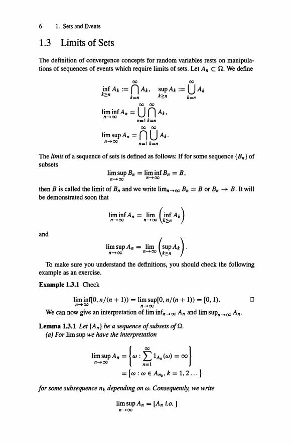
1.3 Limits of Sets
The definition of convergence concepts for random variables rests on manipulations of sequences of events which require limits of sets. Let An c Q . We define
00 00
00
supAk := UAk k:!n k=n
liminfAn = U n Ak, n-+00 n=l k=n
00 00
lim sup An= n U Ak. n-+oo n=l k=n
The limit of a sequence of sets is defined as follows: If for some sequence { Bn} of subsets
limsupBn = liminfBn = B, n-+oo n-+oo
then B is called the limit of Bn and we write limn-+oo Bn = B or Bn --+ B. It will be demonstrated soon that
lim inf An = lim ( inf Ak) n-+00 n-+oo k:!n
and
limsupAn = lim (supAk). n-+oo n-+oo k:!n
To make sure you understand the definitions, you should check the following example as an exercise.
Example 1.3.1 Check
lim inf[O, nj(n + 1)) =lim sup[O, nj(n + 1)) = [0, 1). 0 n-+00 n-+oo
We can now give an interpretation of lim infn-+oo An and lim supn-+oo An.
Lemma 1.3.1 Let {An} be a sequence of subsets of Q.
(a) For lim sup we have the interpretation
lim sup An= lw: f: 1An(w) = ooJ n-+00 n=l
= {w : wE Ank• k = 1, 2 ... }
for some subsequence nk depending on w. Consequently, we write
limsupAn =[An i.o.] n-+00

1.3 Limits of Sets 7
where i.o. stands for infinitely often. (b) For lim inf we have the interpretation
lim inf An ={w : w E An for all n except a finite number} n-HXJ
={w : L lA~ (w) < oo} n
={w: wE An, 'Vn;::: no(w)}.
Proof. (a) If 00 00
wE lim sup An= n U Ak, n->oo n=l k=n
then for every n, w E Uk::;:nAk and so for all n, there exists some kn ;::: n such that wE Akn' and therefore
which implies
thus
Conversely, if
00
L lAj(w) ::': L lAkn (w) = 00, j=l n
wE lw: f lAn(w) = ooJ; n=l
00
lim sup An C {w: L lA/W) = oo}. n->oo j=l
00
wE {w: L lAi(w) = oo}, j=l
then there exists kn ---. oo such that w E Akn, and therefore for allti, w E U j::;:nA j so that w E lim supn->oo An. By defininition
00
{w : L lA/W) = oo} C lim sup An. j=l n-+oo
This proves the set inclusion in both directions and shows equality. The proof of (b) is similar. 0
The properties of lim sup and lim inf are analogous to what we expect with real numbers. The link is through the indicator functions and will be made explicit shortly. Here are two simple connections:
1. The relationship between lim sup and lim inf is
lim inf An C lim sup An n->oo n->00

8 1. Sets and Events
since
{w: wE An, for all n ;::: no(w)} C {w: wE An infinitely often}
=lim sup An. n~oo
2. Connections via de Morgan's laws:
(liminfAn)c = limsupA~ n~oo n~oo
since applying de Morgan's laws twice yields
=lim sup A~. n~oo
For a sequence of random variables IXn, n :::: 0}, suppose we need to show X n ~ X o almost surely. As we will see, this means that we need to show
P{w: lim Xn(w) = Xo(w)} = 1. n~oo
We will show later that a criterion for this is that for all £ > 0
P{[IXn- Xol > s] i.o.} = 0.
That is, with An = [IXn- Xol > s], we need to check
P (limsupAn) = 0. n~oo
1.4 Monotone Sequences
A sequence of sets {An} is monotone non-decreasing if A 1 C Az C · · · . The sequence {An} is monotone non-increasing if A1 :J Az :J A3 ···.To indicate a monotone sequence we will use the notation An /' or An t for non-decreasing sets and An "\. or An .J, for non-increasing sets. For a monotone sequence of sets, the limit always exists.
Proposition 1.4.1 Suppose {An} is a monotone sequence of subsets.
(1) If An /', then limn~oo An = U~1 An.

1.4 Monotone Sequences 9
(2) If An \o then limn-+oo An = n~1An.
Consequently, since for any sequences Bm we have
it follows that
liminfBn = lim (inf Bk), n-+oo n-+oo k;::n
lim sup Bn = lim (sup Bk) . n-+oo n-+oo k;::n
Proof. (1) We need to show
00
liminfAn =lim sup An= U An. n-+oo n-+00 n=l
Since A j c A j+l>
and therefore
Likewise
lim sup An n-+00
Thus equality prevails and
= liminfAn n-+oo
(from (1.1))
C limsupAn. n-+oo
lim sup An C U Ak C lim sup An; n-+oo k?:l n-+oo
therefore 00
lim sup An= U Ak. n-+00 k=l
This coupled with (1.1) yields (1 ). The proof of (2) is similar.
(1.1)
0

10 1. Sets and Events
Example 1.4.1 As an easy exercise, check that you believe that
lim [0, 1- 1/n] = [0, 1) n-+oo
lim [0, 1- 1/n) = [0, 1) n-+00
lim [0, 1 + 1/n] = [0, 1] n-+oo
lim [0, 1 + 1/n) = [0, 1]. n-+00 0
Here are relations that provide additional parallels between sets and functions and further illustrate the algebraic properties of sets. As usual let {An} be a sequence of subsets of n.
1. We have
2. The following inequality holds:
lunAn ::S L lAn n
and if the sequence {A;} is mutually disjoint, then equality holds.
3. We have
4. Symmetric difference satisfies the relation
lA~B = lA + ls (mod 2) .
Note (3) follows from (1) since
and from (1) this is inf 1supk Ak. n;::l ~n
Again using (1) we get
inf sup lAk = lim sup lAn , n;::l k;::n n-+oo
from the definition of the lim sup of a sequence of numbers. To prove (1), we must prove two functions are equal. But 1 inf An (w) = 1 iff
n>k
w E infn;::k An = n~k An iff w E An for all n 2: k iff lAn (w) ;;;, 1 for all n 2: k iff infn;::k IAn (w) = 1. 0

1.5 Set Operations and Closure 11
1.5 Set Operations and Closure
In order to think about what it means for a class to be closed under certain set operations, let us first consider some typical set operations. Suppose C C 'P(Q) is a collection of subsets of Q.
(1) Arbitrary union: Let T be any arbitrary index set and assume for each t e T that A1 e C. The word arbitrary here reminds us that T is not necessarily finite, countable or a subset of the real line. The arbitrary union is
(2) Countable union: Let An. n > 1 be any sequence of subsets in C. The countable union is
(3) Finite union: Let A1, ... , An be any finite collection of subsets in C. The finite union is
(4) Arbitrary intersection: As in (1) the arbitrary intersection is
(5) Countable intersection: As in (2), the countable intersection is
00
nAj. j=l
(6) Finite intersection: As in (3), the finite intersection is
n
nAj. j=l
(7) Complementation: If A e C, then A c is the set of points not in A.
(8) Monotone limits: If {An} is a monotone sequence of sets inC, the monotone limit
lim An n-+oo
is U~1 A j in case {An} is non-decreasing and is n~1 A j if {An} is nonincreasing.

12 1. Sets and Events
Definition 1.5.1 (Closure.) Let C be a collection of subsets of n. C is closed under one of the set operations 1-8 listed above if the set obtained by performing the set operation on sets inC yields a set in C.
For example, C is closed under (3) if for any finite collection At, ... , An of setsinC,U}=tAi eC.
Example 1.5.1 1. Suppose n = IR, and
C = finite intervals
= {(a,b], -oo <a~ b < oo}.
C is not closed under finite unions since (1, 2] U (36, 37] is not a finite interval. Cis closed under finite intersections since (a, b] n (c, d] = (a v c, dAb]. Here we use the notationavb = max{a, b} and aAb =min{ a, b}.
2. Suppose n = lR and C consists of the open subsets of JR. Then C is not closed under complementation since the complement of an open set is not open.
Why do we need the notion of closure? A probability model has an event space. This is the class of subsets of n to which we know how to assign probabilities. In general, we cannot assign probabilities to all subsets, so we need to distinguish a class of subsets that have assigned probabilities. The subsets of this class are called events. We combine and manipulate events to make more complex events via set operations. We need to be sure we can still assign probabilities to the results of the set operations. We do this by postulating that allowable set operations applied to events yield events; that is, we require that certain set operations do not carry events outside the event space. This is the idea behind closure.
Definition 1.5.2 Afield is a non-empty class of subsets of n closed under finite union, finite intersection and complements. A synonym for field is algebra.
A minimal set of postulates for A to be a field is
(i) n eA.
(ii) A e A implies A c e A.
(iii) A, Be A implies AU BE A.
Note if At, Az, A3 e A, then from (iii)
At U Az U A3 = (At U Az) U A3 e A

1.5 Set Operations and Closure 13
and similarly if A1, ... , An E A, then U7=1A; E A. Also if A; E A, i = 1, ... , n, then n7=1A; e A since
A; E A implies Af E A (from (ii)) n
A~ eA I implies UAfeA (from (iii))
i=l
n (uAfr E A UAf implies (from (ii)) i=l 1=1
and finally
(VAfr =0A• by de Morgan's laws so A is closed under finite intersections.
Definition 1.5.3 A a-field B is a non-empty class of subsets of Q closed under countable union, countable intersection and complements. A synonym for a-field is a -algebra.
A mimimal set of postulates forB to be a a-field is
(i) Q E B.
(ii) B e B implies Be e B.
(iii) B; e B, i ~ 1 implies U~1 B; E B.
As in the case ofthe postulates for a field, if B; E B, fori ~ 1, then n~1 B; e B. In probability theory, the event space is a a-field. This allows us enough flexi
bility constructing new-events from old ones (closure) but not so much flexibility that we have trouble assigning probabilities to the elements of the a-field.
1.5.1 Examples
The definitions are amplified by some examples of fields and a-fields.
(1) The power set. Let B = P(Q), the power set of Q so that P(Q) is the class of all subsets of Q. This is obviously a a-field since it satisfies all closure postulates.
(2) The trivial a-field. Let B = {0, Q}. This is also a a-field since it is easy to verify the postulates hold.
(3) The countable/co-countable a-field. Let Q = 1., and
B ={A c I.: A is countable} U {A C lR: Ac is countable},
so B consists of the subsets of lR that are either countable or have countable complements. B is a a-field since

14 1. Sets and Events
(i) Q e B (since nc = 0 is countable).
(ii) A e B implies Ac e B.
(iii) A; e B implies n~1 A; E B.
To check this last statement, there are 2 cases. Either
(a) at least one A; is countable so that n~1A; is countable and hence in B, or
(b) no A; is countable, which means Af is countable for every i. So U~1Af is countable and therefore
00 00
<U<Af))c = n A; E B. i=l i=l
Note two points for this example:
• If A = ( -oo, 0], then A c = (0, oo) and neither A nor A c is countable which means A ¢ B. SoB # 'P(Q).
• B is not closed under arbitrary unions. For example, for each t :::; 0, the singleton set {t} e B, since it is countable. But A = U1:::;o{t} = ( -oo, 0] ¢ B.
(4) A field that is not a a-field. Let n = (0, 1] and suppose A consists of the empty set 0 and all finite unions of disjoint intervals of the form (a, a'], 0 :::; a :::; a' :::; 1. A typical set in A is of the form U7':1 (a;, a;J where the intervals are disjoint. We assert that A is a field. To see this, observe the following.
(i) Q = (0, 1] eA.
(ii) A is closed under complements: For example, consider the union represented by dark lines
(--....I!!!!!!!!!!!!!!!!!!!!!L--1!!!!!!!!!!!!!!!!!!!!!~
0 1
FIGURE 1.1
which has complement.
~!!!!!!!!~-~!!!!!!!!!!!!!!!!L---J
0 1
FIGURE 1.2
which is a disjoint union.
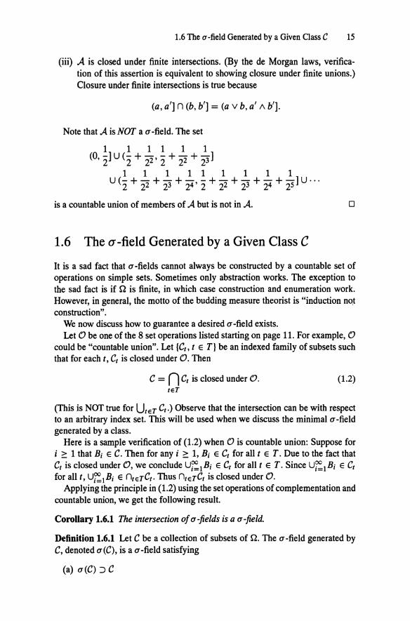
1.6 The u-field Generated by a Given Class C 15
(iii) A is closed under finite intersections. (By the de Morgan laws, verification of this assertion is equivalent to showing closure under finite unions.) Closure under finite intersections is true because
(a , a'] n (b, b'] = (a v b, a' 1\ b'].
Note that A is NOT a a-field. The set
1 1 1 1 1 1 (O, 2] u ( 2 + 22 ' 2 + 22 + 23]
111111111 u ( 2 + 22 + 23 + 24 ' 2 + 22 + 23 + 24 + 25 ] u .. .
is a countable union of members of A but is not in A. 0
1.6 The a-field Generated by a Given Class C
It is a sad fact that a-fields cannot always be constructed by a countable set of operations on simple sets. Sometimes only abstraction works. The exception to the sad fact is if Q is finite, in which case construction and enumeration work. However, in general, the motto of the budding measure theorist is "induction no,t construction".
We now discuss how to guarantee a desired a-field exists. Let 0 be one of the 8 set operations listed starting on page 11. For example, 0
could be "countable union". Let {C1, t e T} be an indexed family of subsets such that for each t, C1 is closed under 0 . Then
c = n c, is closed under 0 . reT
(1.2)
(This is NOT true for Urer C, .) Observe that the intersection can be with respect to an arbitrary index set. This will be used when we discuss the minimal a-field generated by a class.
Here is a sample verification of (1.2) when 0 is countable union: Suppose for i 2: 1 that B; E C. Then for any i ;::: 1, B; E C, for all t E T. Due to the fact that C1 is closed under 0, we conclude U~1 B; e C, for all t e r . Since U~1 B; e C, for all t , U~1 B; e nrerC, . Thus nrerCr is closed under 0.
Applying the principle in (1.2) using the set operations of complementation and countable union, we get the following result.
Corollary 1.6.1 The intersection of a -fields is a u -field.
Definition 1.6.1 Let C be a collection of subsets of Q . The a -field generated by C, denoted a(C), is a a-field satisfying
(a) a(C) :) C

16 1. Sets and Events
(b) If !3' is some other a-field containing C, then !3' :::> a(C).
Another name for a(C) is the minimal a-field over C. Part (b) of the definition makes the name minimal apt.
The next result shows why a a-field containing a given class exists.
Proposition 1.6.1 Given a class C of subsets of Q, there is a unique minimal a -field containing C.
Proof. Let ~ = {!3 : I3 is a a-field, I3 :::> C}
be the set of all a-fields containing C. Then~# 0 since P(Q) E ~.Let
Since each class I3 e ~ is a a-field, so is J3'a by Corollary 1.6.1. Since I3 e ~ implies I3 :::> C, we have f3IJ :::>C. We claim J3'a = a(C). We checked J3tt :::> C and, for minimality, note that if !3' is a a-field such that !3' :::> C, then !3' e ~and hence J3!l C !3'. D
Note this is abstract and completely non-constructive. If Q is finite, we can construct a(C) but otherwise explicit construction is usually hopeless.
In a probability model, we start with C, a restricted class of sets to which we know how to assign probabilities. For example, if Q = (0, 1], we could take
C ={(a, b], 0 ~a ~ b ~ 1}
and P((a, b]) = b- a.
Manipulations involving a countable collection of set operations may take us outside C but not outside a (C). Measure theory stresses that if we know how to assign probabilities to C, we know (in principle) how to assign probabilities to a(C).
1. 7 Borel Sets on the Real Line
Suppose Q = lR and let
C ={(a, b], -oo ~a ~ b < oo}.
Define I3(1R.) := a(C)
and call I3(lR) the Borel subsets of JR.. Thus the Borel subsets of lR are elements of the a-field generated by intervals that are open on the left and closed on the right. A fact which is dull to prove, but which you nonetheless need to know, is that

1. 7 Borel Sets on the Real Line 17
there are many equivalent ways of generating the Borel sets and the following are all valid descriptions of Borel sets:
B(IR) = a((a, b), -oo ~a ~ b ~ oo)
=a([a,b), -oo <a~ b ~ oo)
=a([a, b], -oo <a~ b < oo)
=a((-oo, x],x E IR)
=a (open subsets of IR).
Thus we can generate the Borel sets with any kind of interval: open, closed, semiopen, finite, semi-infinite, etc.
Here is a sample proof for two of the equivalences. Let
co= {(a, b), -00 ~a~ b ~ oo}
be the open intervals and let
c<J ={(a, b], -00 ~a~ b < oo}
be the semi-open intervals open on the left. We will show
a(CO) = a(C<l).
Observe (a, b)= U~1 (a,b -1/n]. Now (a,b -1/n] E c<l C a(C<l), for all n implies U~1 (a, b- 1/n] E a(C<l). So (a, b) E a(C<l) which implies that co c a (C< 1). Now a (C<l) is a a -field containing co and hence contains the minimal a-field over co, that is, a(CO) c a(C<l).
Conversely, (a, b] = n~1 (a, b + 1/n). Now (a, b + 1/n) E co C a(CO) so that n~1 (a, b + 1/n) E a(CO) which implies (a, b] E a(CO) and hence c<J c a(C<>). This implies a(C<l) c a(C<>).
From the two inclusions, we conclude
as desired. Here is a sample proof of the fact that
B(IR) = a(open sets in IR).
We need the result from real analysis that if 0 C lR is open, 0 = U~1 lj, where I j are open, disjoint intervals. This makes it relatively easy to show that
a( open sets) = a(Co).
If 0 is an open set, then we can write

18 1. Sets and Events
We have Ij E co c a(CO) so that 0 = UJ=1Ij E a(CO) and hence any open
set belongs to a(CO), which implies that
a( open sets) c a(C<>) .
Conversely, co is contained in the class of open sets and therefore a (CO) c a( open sets).
Remark. If IE is a metric space, it is usual to define 8(1E), the a-field on IE, to be the a-field generated by the open subsets of IE. Then 8(1E), is called the Borel a-field. Examples of metric spaces IE that are useful to consider are
• JR., the real numbers,
• JR.d, d-dimensional Euclidean space,
• !R.00, sequence space; that is, the space of all real sequences.
• C[O, oo), the space of continuous functions on [0, oo).
1.8 Comparing Borel Sets
We have seen that the Borel subsets of JR. is the a-field generated by the intervals of JR.. A natural definition of Borel sets on (0, 1 ], denoted 8( (0, 1]) is to take C (0, 1] to be the subintervals of (0, 1] and to define
8((0, 1]) := a(C(O, 1]).
If a Borel set A E 8(1R) has the property A C (0, 1], we would hope A E
8((0, 1]). The next result assures us this is true.
Theorem 1.8.1 Let no c n. (1) If 8 is a a-field of subsets of n, then 8o := {A no : A E 8} is a a
field of subsets of no. (Notation: 8o =: 8 n no. We hope to verify 8( (0, 1]) = 8(1R) n (0, 1 ].)
(2) Suppose C is a class of subsets of n and 8 = a (C). Set
C n no=: Co= {A no: A e C}.
Then
a(Co) = a(C) n no
In symbols (2) can be expressed as
a(C n no)= a(C) n no

1.8 Comparing Borel Sets 19
so that specializing to the Borel sets on the real line we get
B(O, 1] = B(lR) n (0, 1].
Proof. (1) We proceed in a series of steps to verify the postulates defining a a
field.
(i) First, observe that no e Bo since nno = no and n E B.
(ii) Next, we have that if B = A no e Bo, then
no\ B =no\ A no= no(n \A) e Bo
since n \A e B.
(iii) Finally, if for n :::: 1 we have Bn = An no, and An e B, then
()() ()() ()() u Bn = u Anno= (U An) n no e Bo n=l n=l n=l
since Un An e B.
(2) Now we show a(Co) = a(C) n no. We do this in two steps. Step 1: We have that
Co:= C n no c a(C) n no
and since (i) assures us that a(C) n no is a a-field, it contains the minimal a-field generated by Co, and thus we conclude that
a(Co) c a(C) n no.
Step 2: We show the reverse inclusion. Define
g :={A c n: Ano e a(Co)}.
We hope to show g :::> a(C). First of all, g :::> C, since if A e C then A no e Co c a(Co). Secondly, observe
that g is a a-field since
(i) neg since nno =no e a(Co)).
(ii) If A e g then A c = n \ A and we have
Ac n no= (n\A)no = no\Ano.
Since A e Q, we have Ano e a(Co) which implies no\ A no e a(Co), so we conclude A c e g.
20 1. Sets and Events
(iii) If An E g, for n 2:: 1, then
00 00
<U An) n flo= u An flo. n=l n=l
Since Anrlo E a(Co), it is also true that U~1Anrlo E a(Co) and thus U~1An E g.
So g is a a-field and g ::) C and therefore g ::) a (C). From the definition of g, if A E a(C), then A E g and so Arlo E a(Co). This means
a(C) n flo c a(Co)
as required.
Corollary 1.8.1 lfrlo E a(C), then
a(Co) =(A :A C flo, A E a(C)}.
Proof. We have that
iH2o E a(C).
a(Co) =a(C) n flo= (Arlo: A E a(C)}
=(B : B E a(C), B C flo}
This shows how Borel sets on (0, 1] compare with those on JR.
1. 9 Exercises
D
D
1. Suppose Q = {0, 1} and C = {(0}}. Enumerate~. the class of all a-fields containing C.
2. Suppose Q = (0, 1, 2} and C = ( (0} }. Enumerate~. the class of all a-fields containing C and give a (C).
3. Let An. A, Bn, B be subsets of Q. Show
lim sup An U Bn = lim sup An U lim sup Bn. n-..oo n-..oo n-..oo
If An --+ A and Bn --+ B, is it true that
An U Bn --+ A U B, An n Bn --+ A n B?

4. Suppose m
An={-: mEN}, n EN, n
where N are non-negative integers. What is
lim inf An and lim sup An? n-+oo n-+oo
5. Let fn, f be real functions on Q. Show
1.9 Exercises 21
00 00 00 1 {w: fn(w) fr f(w)} = u n u {w: lfn(w)- f(w)i ~ ;/
k=l N=ln=N
6. Suppose On > 0, bn > 1 and
lim On = 0, lim bn = 1. n-+00 n-+00
Define An = {x : On ::;:: X < bn}.
Find lim sup An and lim inf An. n-+oo n-+00
7. Let I= {(x,y): ixi:::: 1, IYI:::: 1}
be the square with sides of length 2. Let In be the square pinned at (0, 0) rotated through an angle 2rrn9. Describe lim supn-+oo In and lim infn-+oo In when
(a) B = 1/8,
(b) B is rational.
(c) B is irrational. (Hint: A theorem of Weyl asserts that {e2"inB, n ~ 1} is dense in the unit circle when B is irrational.)
8. Let
and define
What is
9. Check that
B c n, c c n
if n is odd, if n is even.
lim inf An and lim sup An? n-+oo n-+00
Ab..B = Ac b..Bc.

22 1. Sets and Events
10. Check that
iff
pointwise.
11. Let 0 ~ an < oo be a sequence of numbers. Prove that
sup[O, an) = [0, sup an) n~J n~J
n n sup[O, --1 ¥= [O,sup--]. n~J n + 1 n~J n + 1
12. Let 0 = {1, 2, 3, 4, 5, 6} and let C = {{2, 4}, {6}}. What is the field generated by C and what is the a-field?
13. Suppose 0 = UrerCr. where Cs n C, = 0 for all s, t E T and s ¥= t . Suppose F is a a-field on fi = {C,, t E T}. Show
U ...... ...... F := {A = C1 : A E F}
c,eA
is a a-field and show that
! :'A~--+ U c, c,eA
is a 1-1 mapping from F to F.
14. Suppose that An are fields satisfying An C An+I· Show that UnAn is a field. (But see also the next problem.)
15. Check that the union of a countable collection of a-fields Bi, j ::: I need not be a a-field even if Bj c Bj+J. Is a countable union of a-fields whether monotone or not a field?
Hint: Try setting 0 equal to the set of positive integers and let C i be all subsets of {1, . . . , j} and Bj = a(Cj) .
If B;, i = 1, 2 are two a -fields, 81 U 82 need not be a field.
16. Suppose A is a class of subsets of 0 such that
• OeA
• A E A implies A c E A.
• A is closed under finite disjoint unions.

1.9 Exercises 23
Show A does not have to be a field.
Hint: Try Q = {1, 2, 3, 4} and let A be the field generated by two point subsets of n.
17. Prove
liminfAn={w: lim 1A.(w)=1}. n--+oo n--+00
18. Suppose A is a class of sets containing Q and satisfying
A, B e A implies A \ B = ABc e A.
Show A is a field.
19. For sets A, B show
and
20. Suppose C is a non-empty class of subsets of n. Let A(C) be the minimal field over C. Show that A( C) consists of sets of the form
m n; unA;j. i=lj=l
where for each i, j either A;j e C or Afj E C and where the m sets
n;~ 1 A;j, 1 ::: i ::: m, are disjoint. Thus, we can explicitly represent the sets in A( C) even though this is impossible for the a-field over C.
21. Suppose A is a field and suppose also that A has the property that it is closed under countable disjoint unions. Show A is a a-field.
22. Let Q be a non-empty set and let C be all one point subsets. Show that
a(C) ={A C Q: A is countable} UtA c Q: Ac is countable}.
23. (a) Suppose on lR that tn ! t. Show
(-00, tn]! (-00, t].
(b) Suppose
tn t t, ln < t.
Show ( -00, tn] t ( -00, t).

24 1. Sets and Events
24. Let Q = N, the integers. Define
A= {A C N: A or Ac is finite.}
Show A is a field, but not a a-field.
25. Suppose Q = {ei2rrll, 0 ~ () < 1} is the unit circle. Let A be the collection of arcs on the unit circle with rational endpoints. Show A is a field but not a a-field.
26. (a) Suppose Cis a finite partition of Q; that is
k
c ={At •... ' Ak}. Q =LA;, A;Aj = 0, i =I= j. i=t
Show that the minimal algebra (synonym: field) A(C) generated by Cis the class of unions of subfamilies of C; that is
A(C) = {UJ A j : I C {1, . .. , k}}.
(This includes the empty set.)
(b) What is the a-field generated by the partition At •... , An?
(c) If At, A2, ... is a countable partition of n, what is the induced a-field?
(d) If A is a field of subsets of n, we say A e A is an atom of A; if A =I= 0 and if 0 =I= B c A and B e A, then B = A . (So A cannot be split into smaller sets that are nonempty and still in A.) Example: If Q = lR and A is the field generated by intervals with integer endpoints of the form (a, b] (a, bare integers) what are the atoms?
As a converse to (a), prove that if A is a finite field of subsets of Q, then the atoms of A constitute a finite partition of Q that generates A.
27. Show that 8(lR) is countably generated; that is, show the Borel sets are generated by a countable class C.
28. Show that the periodic sets of lR form a a-field; that is, let 8 be the class of sets A with the property that x e A implies x ± n e A for all natural numbers n. Then show 8 is a a-field.
29. Suppose C is a class of subsets of lR with the property that A e C implies Ac is a countable union of elements of C. For instance, the finite intervals in lR have this property.
Show that a (C) is the smallest class containing C which is closed under the formation of countable unions and intersections.
30. Let 8; be a-fields of subsets of Q fori = 1, 2. Show that the a-field 8t v 82 defined to be the smallest a-field containing both 8t and 82 is generated by sets of the form Bt n B2 where B; e 8; fori= 1, 2.

1.9 Exercises 25
31. Suppose n is uncountable and let g be the a-field consisting of sets A such that either A is countable or A c is countable. Show g is NOT countably generated. (Hint: If 9 were countably generated, it would be generated by a countable collection of one point sets. )
In fact, if g is the a-field of subsets of n consisting of the countable and co-countable sets, g is countably generated iff Q is countable.
32. Suppose B1, B2 are a -fields of subsets of n such that B1 c Bz and B2 is countably generated. Show by example that it is not necessarily true that B1 is countably generated.
3 3. The extended real line. Let i = lR U {-oo} U { oo} be the extended or closed real line with the points -oo and oo added. The Borel sets B(JR) is the a-field generated by the sets [-oo,x],x E JR, where [-oo,x] = { -oo}U( -oo, x] . Show B(JR) is also generated by the following collections of sets:
(i) [ -00, X), X E JR,
(ii) (x, oo], x E JR,
(ii) all finite intervals and { -oo} and { oo} .
Now think of i = [ -oo, oo] as homeomorphic in the topological sense to [ -1, 1] under the transformation
X X t-+ --
1-lxl
from [ -1, 1] to [ -oo, oo]. (This transformation is designed to stretch the finite interval onto the infinite interval.) Consider the usual topology on [ -1, 1] and map it onto a topology on [ -oo, oo] . This defines a collection of open sets on [ -oo, oo] and these open sets can be used to generate a Borel a-field. How does this a-field compare with B(JR) described above?
34. Suppose B is a a-field of subsets of n and suppose A ¢ B. Show that a(B U {A}), the smallest a-field containing both Band A consists of sets of the form
ABu ACB', B, B' E B .
35. A a-field cannot be countably infinite. Its cardinality is either finite or at least that of the continuum.
36. Let n = {f, a, n, g}, and C = {{f, a, n}, {a, n}}. Find a(C).
37. Suppose n = Z, the natural numbers. Define for integer k
kZ = {kz : z E Z}.
Find B(C) when C is

26 1. Sets and Events
(i) {3Z}.
(ii) {3Z, 4Z}.
(iii) {3Z, 4Z, 5Z}.
(iv) {3Z, 4Z, 5Z, 6Z}.
38. Let n = IR00 , the space of all sequences of the fonn
(**)
where Xi e R Let a be a pennutation of 1, . .. , n; that is, a is a 1-1 and onto map of {1, ... , n} ~--+ {1, . . . , n}. If w is the sequence defined in(**), define a w to be the new sequence
( ) IXu(j)• aw j =
Xj,
if j ~ n,
if j > n.
A finite permutation is of the fonn a for some n; that is, it juggles a finite initial segment of all positive integers. A set A c Q is permutable if
A= a A:= {aw: wE A}
for all finite pennutations a .
( i) Let Bn , n 2: 1 be a sequence of subsets of R Show that
and
n
{w = (xi, xz , . . . ) : L Xi E Bn i.o. } i=l
n
{w = (XJ,X2, .. . ) : V Xi E Bn i.o.} i=l
are pennutable.
(ii) Show the pennutable sets fonn a a-field.
39. For a subset A C N of non-negative integers, write card(A) for the number of elements in A. A set A C N has asymptotic density d if
lim card(A n {1, 2, . . . , n}) =d. n-+oo n
Let A be the collection of subsets that have an asymptotic density. Is A a field? Is it a a-field?
Hint: A is closed under complements, proper differences and finite disjoint unions but is not closed under fonnation of countable disjoint unions or finite unions that are not disjoint.

1.9 Exercises 27
40. Show that B( (0, 1 ]) is generated by the following countable collection: For an integer r,
{[kr-n, (k + 1)r-n), 0 ~ k < rn, n = 1, 2, .. . . }.
41. A monotone class M is a non-empty collection of subsets of 0 closed under monotone limits; that is, if An /'and An E M, then limn--+oo An = UnAn E M and if An ~ and An E M, then limn-->00 An = nnAn E M . Show that a a-field is a field that is also a monotone class and conversely, a field that is a monotone class is a a-field.
42. Assume Pis a rr-system (that is, Pis closed under finite intersections) and M is a monotone class. (Cf. Exercise 41.) Show P C M does not imply a(P) c M .
43. Symmetric differences. For subsets A, B, C, D show
and hence
(a) (At.B)t.C = At.(Bt.C),
(b) (At.B)t.(Bt.C) = (At.C) ,
(c) (At.B)t.(Ct.D) = (At.C)t.(Bt.D),
(d) At.B = C iff A= Bt.C,
(e) At.B = Ct.D iff At.C = Bt.D.
44. Let A be a field of subsets of 0 and define
A= {A c n: 3An E A and An~ A} .
Show A c A and A is a field.

29S.I. Resnick, A Probability Path, Modern Birkhäuser Classics,ss Media New York 2014 DOI 10.1007/978-0-8176-8409-9_2, © Springer Science+Busine
2 Probability Spaces
This chapter discusses the basic properties of probability spaces, and in particular, probability measures. It also introduces the important ideas of set induction.
2.1 Basic Definitions and Properties
A probability space is a triple (Q, B, P) where
• Q is the sample space corresponding to outcomes of some (perhaps hypothetical) experiment.
• B is the a-algebra of subsets of Q. These subsets are called events.
• P is a probability measure; that is, P is a function with domain B and range [0, 1] such that
(i) P(A) ~ 0 for all A e B.
(ii) Pis a-additive: If {An. n ~ 1} are events in B that are disjoint, then
00 00
P(U An) = L P(An). n=l n=l
(iii) P(Q) = 1.
Here are some simple consequences of the definition of a probability measure P.

30 2. Probability Spaces
1. We have P(A') = 1- P(A)
since from (iii)
1 = P(Q) = P(A U A')= P(A) + P(A'),
the last step following from (ii).
2. We have P(0) = 0
since P(0) = P(Q') = 1 - P(Q) = 1 - 1.
3. For events A, B we have
To see this note
and therefore
P(A U B)= PA + PB- P(AB).
P(A) =P(AB') + P(AB)
P(B) =P(BA') + P(AB)
P(A U B) =P(AB' U BA' U AB)
=P(AB') + P(BA') + P(AB)
=P(A) - P(AB) + P(B) - P(AB) + P(AB)
=P(A) + P(B) - P(AB).
4. The inclusion-exclusion formula: If A 1, ... , An are events, then
n n
P(UAj) = LP(Aj)- L P(A;Aj) j=l j=l l~i<j~n
+ L P(A;AjAk)- ...
(2.1)
(2.2)
We may prove (2.2) by induction using (2.1) for n = 2. The terms on the right side of (2.2) alternate in sign and give inequalities called Bonferroni inequalities when we neglect remainders. Here are two examples:
P (QAJ) ~ tPAJ
P (Q AJ)?: ~PAJ- 19J;;~, P(A;AJ).

2.1 Basic Definitions and Properties 31
5. The monotonicity property: The measure P is non-decreasing: For events A,B
If A C B then P(A) ,:::: P(B),
since
P(B) = P(A) + P(B \A) ::: P(A).
6. Subadditivity: The measure Pis a-subadditive: For events An, n ::: 1,
To verify this we write
00
UAn =A1 +A~Az+A3A~A2+ ... , n=l
and since P is a-additive,
00
P(U An) =P(AI) + P(A~Az) + P(A3A~Az) + · · · n=l
,::::P(AI) + P(A2) + P(A3) + · · ·
by the non-decreasing property of P.
7. Continuity: The measure P is continuous for monotone sequences in the sense that
(i) If An t A, where An E B, then P(An) t P(A).
(ii) If An .J, A, where An E B, then P(An) .J, P(A).
To prove (i), assume
A 1 c Az c A3 c · · · c An c · · ·
and define
Then {B;} is a disjoint sequence of events and
n 00
UB; =An, UB; =UA; =A. i=l i=l i

32 2. Probability Spaces
By a -additivity
oo oo n
P(A) =P(UB;) = LP(B;) = n~~ t LP(B;) i=I i=I i=I
n
= lim t P(U B;) = lim t P(An). n-+oo n-+oo
i=I
To prove (ii}, note if An .J.. A, then A~ t Ac and by part (i)
P(A~) = 1- P(An) t P(Ac) = 1- P(A)
so that PAn .J.. PA. 0
8. More continuity and Fatou's lemma: Suppose An E B, for n 2: 1.
(i) Fatou Lemma: We have the following inequalities
P(liminfAn) ~ liminfP(An) n-+oo n-+oo
~ lim sup P(An) ~ P(limsupAn). n-+00 n-+oo
(ii) If An -+ A, then P(An) -+ P(A).
Proof of 8. (ii) follows from (i) since, if An -+ A, then
limsupAn = liminfAn =A. n-+oo n-+oo
Suppose (i) is true. Then we get
P(A) = P(lim inf An) ~ lim inf P(An) n-+oo n-+oo
~ limsupP(An) ~ P(limsupAn) = P(A), n-+oo n-+oo
so equality pertains throughout.
Now consider the proof of (i): We have
P(liminfAn) =P( lim t <n Ak)) n-+00 n-+oo
k~n
= lim t P<n Ak) n-+oo
k~n
(from the monotone continuity property 7)
~lim inf P(An) n-+oo

2.1 Basic Definitions and Properties 33
P(limsupAn) = P( lim t <U Ak)) n-H>O n-+00 k?!_n
= lim t P(U Ak) n-+00
k?!_n
(from continuity property 7)
:::: lim sup P(An). n-+00
completing the proof. D
Example 2.1.1 Let Q = IR, and suppose P is a probability measure on JR. Define F(x) by
F(x) = P((-oo,x]), x e JR.
Then
(i) F is right continuous,
(ii) F is monotone non-decreasing,
(iii) F has limits at ±oo
F(oo) := lim F(x) = 1 xtoo
F(-oo) := lim F(x) = 0. x.j.-oo
(2.3)
Definition 2.1.1 A function F : lR ~ [0, 1] satisfying (i), (ii), (iii) is called a (probability) distribution function. We abbreviate distribution function by df.
Thus, starting from P, we get F from (2.3). In practice we need to go in the other direction: we start with a known df and wish to construct a probability space (Q , B, P) such that (2.3) holds. See Section 2.5.
Proof of (i), (ii), (iii). For (ii), note that if x < y, then
(-oo,x] c (-oo,y]
so by monotonicity of P
F(x) = P((-oo,x]):::; P((-oo,y]):::; F(y).

34 2. Probability Spaces
Now consider (iii). We have
F(oo) = lim F(xn) Xntoo
(for any sequence Xn t oo)
= lim t P((-OO,Xn]) Xntoo
= P( lim t ( -oo, Xn]) Xntoo
(from property 7)
=P(U(-oo,xn]) = P((-oo, oo)) n
= P(IR) = P(Q) = 1.
Likewise,
F(-oo) = lim F(Xn) = lim -1. P((-OO, Xn]) Xni-oo Xni-oo
=P( lim (-OO,Xn]) Xni-oo
(from property 7)
=P<n<-oo.xnD = P(eJ) = o. n
For the proof of (i), we may show F is right continuous as follows: Let Xn -1. x . We need to prove F(xn) -1. F(x) . This is immediate from the continuity property 7 of P and
(-OO,Xn] -1. (-oo, x] . 0
Example 2.1.2 (Coincidences) The inclusion·exclusion formula (2.2) can be used to compute the probability of a coincidence. Suppose the integers 1, 2, . . . , n are randomly permuted. What is the probability that there is an integer left un· changed by the permutation?
To formalize the question, we construct a probability space. Let Q be the set of all permutations of 1, 2, ... , n so that
Q ={(XI, . .. , Xn) : Xi E {1, .. . , n}; i = 1, . .. , n ; Xi :;f Xj }.
Thus Q is the set of outcomes from the experiment of sampling n times without replacement from the population 1, . .. , n. We let B = P(Q) be the power set of Q and define for (XI. . . . , Xn) E Q
and forB E B
1 P((xl> ... , Xn)) = - ,
n!
1 0
P(B) =-#elements m B. n!
Fori = 1, . . . , n, let A; be the set of all elements of Q with i in the ith spot. Thus, for instance,
AI ={(1, Xz, .. . , Xn): (1, xz, . . . , Xn) E Q},
Az ={(XI,2, ... ,Xn): (XI.2 , .. . ,Xn) E Q}.

2.2 More on Closure 35
and so on. We need to compute P(U?=1A;). From the inclusion-exclusion formula (2.2) we have
n n
P(UA;) = LP(A;)- L P(A;Aj) + i=l i=l l::,i<j::,n
To compute P(A; ), we fix integer i in the ith spot and count the number of ways to distribute n- 1 objects inn- 1 spots, which is (n- 1)! and then divide by n!. To compute P(A;Aj) we fix i and j and count the number of ways to distribute n - 2 integers into n - 2 spots, and so on. Thus
P(lJA;) =n (n -1)! _ (n) (n- 2)! + (n) (n- 3)! _ ... (-1)n2_ i=l n! 2 n! 3 n! n!
1 1 n 1 =1 - 2! + 3!- ... (-1) n!"
Taking into account the expansion of ,r for x = -1 we see that for large n, the probability of a coincidence is approximately
n
P(U A;)~ 1- e-1 ~ 0.632. i=l
2.2 More on Closure
0
A a-field is a collection of subsets of n satisfying certain closure properties, namely closure under complementation and countable union. We will have need of collections of sets satisfying different closure axioms. We define a structure g to be a collection of subsets of Q satisfying certain specified closure axioms. Here are some other structures. Some have been discussed, some will be discussed and some are listed but will not be discussed or used here.
• field
• a-field
• semialgebra
• semiring
• ring
• a-ring
• monotone class (closed under monotone limits)

36 2. Probability Spaces
• ]"(-system (P is a ]"(-system, if it is closed under finite intersections: A, B E
P implies A n B E P ).
• >..-system (synonyms: a-additive class, Dynkin class); this will be used extensively as the basis of our most widely used induction technique.
Fix a structure in mind. Call itS. As with a-algebras, we can make the following definition.
Definition 2.2.1 The minimal structure S generated by a class C is a non-empty structure satisfying
(i) s :> c,
(ii) If S' is some other structure containing C, then S' :> S.
Denote the minimal structure by S(C).
Proposition 2.2.1 The minimal structure S exists and is unique.
As we did with generating a minimal a-field, let
~ = {g : g is a structure , g :> C}
and
2.2.1 Dynkin's theorem
Dynkin's theorem is a remarkably flexible device for performing set inductions which is ideally suited to probability theory.
A class of subsets .C of Q is a called a >..-system if it satisfies either the new postulates >..1, >..2, AJ or the old postulates>..~,>..;,>..) given in the following table.
>..-system postulates old new
>..; Qe.C At Qe.C >..; A, B E .C, A C B ~ B \ A E .C >..2 A E .C ~AcE .C >..' 3 An t, An E .C ~ UnAn E .C AJ n =f. m, AnAm = 0,
An E .C ~ UnAn E .C.
The old postulates are equivalent to the new ones. Here we only check that old implies new. Suppose >..;, >..;, >..) are true. Then .l..t is true. Since Q E .C, if A E .C, then A C Q and by>..;, Q \A = Ac E .C, which shows that >..2 is true. If A, B E .C are disjoint, we show that A U B E .C. Now Q \ A E .C and B C Q \ A (since (J) E B implies (J) fl. A which means (J) E Ac = Q \A) so by>..; we have (Q \A)\ B = AcBc E .C and by >..2 we have (AcBc)c =AU BE .C which is AJ for finitely many sets. Now if A j E .Care mutually disjoint for j = 1, 2, ... ,

2.2 More on Closure 37
define Bn = U}=tAi . Then Bn e £by the prior argument for 2 sets and by >..3 we have UnBn = limn-+oo t Bn E £ . Since UnBn = UnAn we have UnAn E £ which is AJ. 0
Remark. It is clear that a a-field is always a >..-system since the new postulates obviously hold.
Recall that a rr -system is a class of sets closed under finite intersections; that is, 'Pis a rr-system if whenever A, B e 'P we have AB e 'P.
We are now in a position to state Dynkin's theorem.
Theorem 2.2.2 (Dynkin's theorem) (a) lf'P is a rr-system and£ is a >..-system such that P c £, then a ('P) C £.
(b) lf'P is a rr-system
a('P) = £('P),
that is, the minimal a-field over P equals the minimal >..-system over P.
Note (b) follows from (a). To see this assume (a) is true. Since 'P c C('P), we have from (a) that a('P) c C('P). On the other hand, a('P), being a a-field, is a >..-system containing P and hence contains the minimal >..-system over 'P, so that a ('P) ::> £('P).
Before the proof of (a), here is a significant application of Dynkin's theorem.
Proposition 2.2.3 Let Pt. Pz be two probability measures on (Q, 8). The class
£ :={A e 8: Pt(A) = Pz(A)}
is a >..-system.
Proof of Proposition 2.2.3. We show the new postulates hold:
(J..t) n E £since Pt(fl) = Pz(n) = 1.
(J..z) A e £implies Ace£, since A E £means Pt(A) = Pz(A), from which
(J..3) If {A i} is a mutually disjoint sequence of events in £ , then P1 (A i) = Pz (A i) for all j, and hence
P1(UAj) = LPt(Aj) = L:Pz(Aj) = Pz<UAj) j j j j
so that
0

38 2. Probability Spaces
Corollary 2.2.1 If Pt. P2 are two probability measures on (Q, B) and ifP is a ;r-system such that
'v'A e P: Pt(A) = P2(A),
then 'v'B e a(P): Pt(B) = P2(B).
Proof of Corollary 2.2.1. We have
C ={A e B: Pt(A) = P2(A)}
is a A-system. But C :::> P and hence by Dynkin's theorem C :::> a(P). 0
Corollary 2.2.2 Let n = JR. Let Pt, P2 be two probability measures on (JR., B(IR.)) such that their distribution functions are equal:
'v'x E JR.: Ft(X) = Pt((-oo,x)) = F2(x) = P2((-oo,x]).
Then
on B(IR.).
So a probability measure on JR. is uniquely determined by its distribution function.
Proof of Corollary 2.2.2. Let
P = {(-oo,x]: x e JR.}.
Then P is a ;r -system since
(-oo,x) n (-oo,y] = (-oo,x Ay) E P.
Furthermore a (P) = B(IR.) since the Borel sets can be generated by the semiinfinite intervals (see Section 1.7). SoFt (x) = F2(x) for all x e JR., means Pt = P2 on P and hence Pt = P2 on a(P) = B(IR.). 0
2.2.2 Proof of Dynkin 's theorem
Recall that we only need to prove: If Pis a ;r-system and Cis a A-system then P C C implies a (P) C C.
We begin by proving the following proposition.
Proposition 2.2.4 If a class C is both a ;r -system and a A-system, then it is a a-field.
Proof of Proposition 2.2.4. First we show C is a field: We check the field postulates.

2.2 More on Closure 39
(i) Q E C since C is a A.-system.
(ii) A e C implies A c e C since C is a A.-system.
(iii) If A i e C, for j = 1, ... , n, then nJ=l A i e C since Cis an-system.
Knowing that Cis a field, in order to show that it is a a-field we need to show that if A i e C, for j 2: 1, then Uf=1A i E C. Since
oo n
UA· =lim t UA-1 n-+oo 1
j=l j=l
and Uj =I A i e C (since Cis a field) it suffices to show C is closed under monotone non-decreasing limits. This follows from the old postulate>..;. 0
We can now prove Dynkin's theorem.
Proof of Dynkin's Theorem 2.2.2. It suffices to show .C('P) is a 1r -system since .C('P) is both a n-system and a A.-system, and thus by Proposition 2.2.4 also a a-field. This means that
.c :::> .C('P) :::> 'P.
Since .C('P) is a a-field containing 'P,
.C('P) :::> a ('P)
from which
.C :::> .C('P) :::> a('P),
and therefore we get the desired conclusion that
.C :::> a('P).
We now concentrate on showing that .C('P) is an-system. Fix a set A e a('P) and relative to this A, define
gA ={BE a('P): AB E .C('P)}.
We proceed in a series of steps.
[A) If A e .C('P), we claim that gA is a A.-system.
To prove [A) we check the new A.-system postulates.
(i) We have n egA
since An = A e .C('P) by assumption.

40 2. Probability Spaces
(ii) Suppose B E QA. We have that Be A =A\ AB. But B E QA means AB E .C('P) and since by assumption A E .C(P), we have A\ AB = Be A E .C(P) since A.-systems are closed under proper differences. Since Be A E .C(P), it follows that Be E QA by definition.
(iii) Suppose {B j} is a mutually disjoint sequence and B j E 9A· Then
00 00
A n ( U B j) = U AB j j=l j=l
is a disjoint union of sets in .C(P), and hence in .C(P).
[B] Next, we claim that if A E P, then .C(P) C QA.
To prove this claim, observe that since A E P C .C(P), we have from [A] that QA is a A.-system.
ForB E P, we have AB E P since by assumption A E P and Pis a rr-system. So if B E P, then AB E P c .C(P) implies B E QA; that is
(2.4)
Since QA is a A.-system, 9A ::> .C(P).
[B'] We may rephrase [B] using the definition of QA to get the following statement. If A E P, and B E .C(P), then AB E .C(P). (So we are making progress toward our goal of showing .C(P) is a rr -system.)
[C] We now claim that if A E £(P), then C(P) C QA ·
To prove [C]: If B E P and A E .C(P), then from [B'] (interchange the roles of the sets A and B) we have AB E .C(P). So when A E .C(P),
From [A], 9A is a A.-system so .C(P) C QA.
[C'] To finish, we rephrase [C]: If A E .C(P), then for any B E .C(P), B E QA. This says that
ABE .C(P)
as desired. 0
2.3 Two Constructions
Here we give two simple examples of how to construct probability spaces. These examples will be familiar from earlier probability studies and from Example 2.1.2,

2.31\vo Constructions 41
but can now be viewed from a more mature perspective. The task of constructing more general probability models will be considered in the next Section 2.4
(i) Discrete models: Suppose n = {w1, w2, ... } is countable. For each i, associate to wi the number Pi where
00
Vi 2:: 1, Pi 2:: 0 and LPi = 1. i=l
Define 13 = P(Q), and for A e 13, set
P(A) = L Pi· w;EA
Then we have the following properties of P:
(i) P(A) 2:: 0 for all A E 13.
(ii) P(Q) = L~l Pi = 1.
(iii) P is a-additive: If A j, j 2:: 1 are mutually disjoint subsets, then
00
P<U A j) = L Pi = L L Pi j=l w;EUjAj j w;EAj
= LP(Aj).
Note this last step is justified because the series, being positive, can be added in any order.
This gives the general construction of probabilities when n is countable. Next comes a time honored specific example of countable state space model.
(ii) Coin tossing N times: What is an appropriate probability space for the experiment "toss a weighted coin N times"? Set
Q = {0, 1}N ={(WI. ... ,WN): Wi = 0 or 1}.
For p 2:: 0, q 2:: 0, p + q = 1, define
Construct a probability measure P as in (i) above: Let 13 = P(n) and for A c n define
P(A) = LPw· we A

42 2. Probability Spaces
As in (i) above, this gives a probability model provided Lwen Pw = 1. Note the product form
so
N n w· 1-w· P(WJ, . .. ,WN) = p 'q I
i=l
n
L PwJ , ... ,WN = L npw;ql-w; WJ, . .. ,WN WJ, .•. ,WN i=l
0
2.4 Constructions of Probability Spaces
The previous section described how to construct a probability space when the sample space Q is countable. A more complex case but very useful in applications is when Q is uncountable, for example, when n = JR., JR.k, 1R.00 , and so on. For these and similar cases, how do we construct a probability space which will have given desirable properties? For instance, consider the following questions.
(i) Given a distribution function F(x), let Q = JR.. How do we construct a probability measure P on B(lR.) such that the distribution function corresponding to P is F:
P((-oo,x]) = F(x).
(ii) How do you construct a probability space containing an iid sequence of random variables or a sequence of random variables with given finite dimensional distributions.
A simple case of this question: How do we build a model of an infinite sequence of coin tosses so we can answer questions such as:
(a) What is the probability that heads occurs infinitely often in an infinite sequence of coin tosses; that is, how do we compute
P[ heads occurs i.o. ]?
(b) How do we compute the probability that ultimately the excess of heads over tails is at least 17?
(c) In a gambling game where a coin is tossed repeatedly and a heads results in a gain of one dollar and a tail results in a loss of one dollar, what is the probability that starting with a fortune of x, ruin eventually occurs; that is, eventually my stake is wiped out?

2.4 Constructions of Probability Spaces 43
For these and similar questions, we need uncountable spaces. For the coin tossing problems we need the sample space
Q ={0, 1}N
={(WJ, wz, ... ) : Wj E {0, 1}, i ~ 1}.
2.4.1 General Construction of a Probability Model
The general method is to start with a sample space Q and a restricted, simple class of subsets S of Q to which the assignment of probabilities is obvious or natural. Then this assignment of probabilities is extended to a(S). For example, ifQ =JR., the real line, and we are given a distribution function F, we could take S to be
S ={(a, b]: -oo =::a =:: b =:: oo}
and then define P on S to be
P((a, b]) = F(b) - F(a).
The problem is to extend the definition of P from S to B(JR.), the Borel sets. For what follows, recall the notational convention that I:7=t A; means a dis
joint union; that is, that At, ... , An are mutually disjoint and
The following definitions help clarify language and proceedings. Given two structures gt, g2 of subsets of Q such that gt C g2 and two set functions
P; : Q; ...... [0, 1 ], i = 1, 2,
we say P2 is an extension of Pt (or Pt extends to P2) if P2 restricted to gt equals Pt. This is written
P2lg1 = Pt
and means P2(At) = Pt (At) for all At e Qt. A set function P with structure g as domain and range [0, 1 ],
P:Q ...... [0,1],
is additive iffor any n ~ 1 and any disjoint At. ... , An e g such that I:7=t A; e Qwe have
n n
P<:LA;) = LP(A;). (2.5) i=t i=t
Call P a -additive if the index n can be replaced by oo; that is, (2.5) holds for mutually disjoint {An, n ~ 1} with A j e Q, j ::: 1 and L~t A j e g.
We now define a primitive structure called a semialgebra.

44 2. Probability Spaces
Definition 2.4.1 A class S of subsets of Q is a semialgebra if the following postulates hold:
(i) 0, Q E S.
(ii) Sis a rr-system; that is, it is closed under finite intersections.
(iii) If A E S, then there exist some finite nand disjoint sets Ct. ... , Cn, with each Ci E S such that A c = L7=1 Ci.
The plan is to start with a probability measure on the primitive structure S, show there is a unique extension to A(S), the algebra (field) generated by S (first extension theorem) and then show there is a unique extension from A(S) to a(A(S)) = a(S), the a-field generated by S (second extension theorem).
Before proceeding, here are standard examples of semialgebras.
Examples:
(a) Let Q = JR, and suppose S1 consists of intervals including 0, the empty set:
S1 ={(a, b]: -oo.::: a ,::: b,::: oo}.
If h , [z E S1. then h [z is an interval and in S1 and if I E St, then I c is a union of disjoint intervals.
(b) Let
0 I
1
FIGURE 2.1 Intervals
Q = JRk ={(XI, ... , Xk): Xi E JR, i = 1, ... , k}
Sk = all rectangles (including 0, the empty set).
Note that we call A a rectangle if it is of the form
A=hX···Xh
where Ij E S1 is an interval, j = 1, . . . , k as in item (a) above. Obviously 0, Q are rectangles and intersections of rectangles are rectangles. When k = 2 and A is a rectangle, the picture of A c appears in Figure 2.2, showing A c can be written as a disjoint union of rectangles.

2.4 Constructions of Probability Spaces 45
FIGURE 2.2 Rectangles
For general k, let
so that
k
A= It X . .. X h.= n{(XJ, . . . ,Xk) : xi E /i} i=l
Since Ii E S1. we have I{= I!+
46 2. Probability Spaces
(i) Q e A since Q e S.
(iii) If Lie/ Si and LjeJ Sj are two members of A, then
(Lsi) n (L:si) = L SiS} E A ie/ jeJ (i, j)e/xJ
since {SiS], (i, j) E I x J} is a finite, disjoint collection of members of the 1r-system S.
(ii) To check closure under complementation, let Lie/ Si E A and observe
( L:si)c = nsr ie/ ie/
But from the axioms defining a semialgebra, Si e S implies
Sf= L:sij jeJ;
for a finite index set Ji and disjoint sets {Sij, j E J;} in S. Now observe that nieiSf E A by the previously proven (iii).
So A is a field, A :J Sand hence A :J A(S). Since also
LSi E A implies LSi e A(S), ie/ ie/
we get A C A(S) and thus, as desired, A= A(S).
It is now relatively easy to extend a probability measure from S to A(S).
0
Theorem 2.4.1 (First Extension Theorem) Suppose S is a semia/gebra of subsets ofQ and P: S t-+ [0, 1) is a-additive on Sand satisfies P(Q) = 1. There is a unique extension P' of P to A(S), defined by
P'<L:Si) = LP(Si), (2.7) ie/ ie/
which is a probability measure on A(S); that is P' (Q) = 1 and P' is a -additive on A(S).
Proof. We must first check that (2. 7) defines P' unambiguously and to do this, suppose A e A(S) has two distinct representations
A= L:si = L:sj. ie/ jeJ

2.4 Constructions of Probability Spaces 47
We need to verify that
LP(S;) = LP(Sj) (2.8) ie/ jeJ
so that P' has a unique value at A. Confirming (2.8) is easy since S; c A and therefore
L P(S;) = L P(S;A) = L P(S; n L Sj) ie/ ie/ ie/ jeJ
= LP(LS;Sj) ie/ jeJ
and using the fact that S; = LjeJ S;Sj E Sand P is additive on S, we get the above equal to
= LLP(S;Sj) = LLP(S;Sj). ie/ jeJ jeJ ie/
Reversing the logic, this equals
as required. Now we check that P' is a-additive on A(S). Thus suppose fori ~ 1,
A; = L Sij E A(S), S;j E S, jEJi
and {A;, i ~ 1} are mutually disjoint and
00
A= LA; E A(S). i=l
Since A e A(S), A also has a representation
A= L sk. sk e s, k e K, keK
where K is a finite index set. From the definition of P', we have
P'(A) = L P(Sk). keK
Write 00 00
sk = skA = L:skA; = L L sksij· i=l i=l jEJi

48 2. Probability Spaces
Now SkSij e Sand I:~1 LjeJ; SkSij = Sk e S, and since Pis a-additive on S, we have
00 00
L P(Sk) = L L L P(SkSij) = L L L P(SkSij ). keK keK i=l jeJ; i=l jeJ; keK
Again observe L sksij = AS;i = S;i e s keK
and by additivity of P on S
and continuing in the same way, we get this equal to
00 00
= LP(LSij) = LP'(A;) i=l jeJ; i=l
as desired. Finally, it is clear that P has a unique extension from S to A(S), since if P{
and P2 are two additive extensions, then for any
A= LS; e A(S) ie/
we have p; (A) = L P(S;) = P2(A).
ie/ 0
Now we know how to extend a probability measure from S to A(S). The next step is to extend the probability measure from the algebra to the a-algebra.
Theorem 2.4.2 (Second Extension Theorem) A probability measure P defined on a field A of subsets has a unique extension to a probability measure on a (A), the a -field generated by A
Combining the First and Second Extension Theorems 2.4.1 and 2.4.2 yields the final result.
Theorem 2.4.3 (Combo Extension Theorem) SupposeS is a semialgebra of subsets of Q and that P is a a -additive set function mappingS into [0, 1] such that P(Q) = 1. There is a unique probability measure on a(S) that extends P.
The ease with which this result can be applied depends largely on how easily one can check that a set function P defined on Sis a-additive (as opposed to just being additive). Sometimes some sort of compactness argument is needed.
The proof of the Second Extension Theorem 2.4.2 is somewhat longer than the proof of the First Extension Theorem and is deferred to the next Subsection 2.4.2.

2.4 Constructions of Probability Spaces 49
2.4.2 Proof of the Second Extension Theorem
We now prove the Second Extension Theorem. We start with a field A and a probability measure P on A so that P(Q) = 1, and for all A E A, P(A) ~ 0 and for {A;} disjoint, A; E A, :[~1 A; E A, we have P(:[~1 A;) = :[~1 P(A; ).
The proof is broken into 3 parts. In Part I, we extend P to a set function n on a class g :::) A. In Part II we extend n to a set function n* on a class D :::) a(A) and in Part III we restrict n * to a (A) yielding the desired extension.
PART I. We begin by defining the class g:
00
g :={ U A j : A j e A} j=l
={ lim t Sn : Sn E A, Sn C Sn+l. 'v'n}. n~oo
So g is the class of unions of countable collections of sets in A, or equivalently, since A is a field, g is the class of non-decreasing limits of elements of A.
We also define a set function n : g t-+ [0, 1] via the following definition: If G = limn~oo t Sn E g, where Sn E A, define
n(G) = lim t P(Bn). n~oo
(2.9)
Since Pis a-additive on A, Pis monotone on A, so the monotone convergence indicated in (2.9) is justified. Call the sequence {Sn} the approximating sequence to G. To verify that n is well defined, we need to check that if G has two approximating sequences {Sn} and {S~},
G = lim t Sn = lim t S~ n~oo n~oo
then lim t P(Sn) = lim t P(B~). n~oo n~oo
This is verified in the next lemma whose proof is typical of this sort of uniqueness proof in that some sort of merging of two approximating sequences takes place.
Lemma 2.4.2 If {Bn} and {B~} are two non-decreasing sequences of sets in A and
00 00
Usn c Us~. n=l n=l
then lim t P(Sn) ~ lim t P(S~) . n~oo n~oo
Proof. For fixed m
(2.10)

50 2. Probability Spaces
Since also BmB~ c B~
and P is continuous with respect to monotonely converging sequences as a consequence of being a-additive (see Item 7 on page 31), we have
lim t P(B~) :::: lim t P(BmB~) = P(Bm), n-+oo n-+00
where the last equality results from (2.10) and P being continuous. The inequality holds for all m, so we conclude that
lim t P(B~) :::: lim t P(Bm) n ..... oo m ..... oo
as desired.
Now we list some properties of nand 9:
Property 1. We have
and forGE g
0 E g, neg,
n(0) = o,
n<n> = 1,
o ~ n(G) ~ 1.
More generally, we have A C g and
niA=P;
that is, n(A) = P(A), for A EA.
0
(2.11)
The first statements are clear since, for example, if we set Bn = n for all n, then
A~ Bn = Q t Q,
and n(n) = lim t P(Q) = 1
n ..... oo
and a similar argument holds for 0. The statement (2.11) follows from 0 ~ P(Bn) ~ 1 for approximating sets {Bn} in A. To show n(A) = P(A) for An e A, take the approximating sequence to be identically equal to A.
Property 2. If G; e g fori= 1, 2 then
GtUG2eg, GtnG2eg,
and
n(Gt u Gz) + n(Gt n Gz) = n(Gt) + n(Gz). (2.12)

2.4 Constructions of Probability Spaces 51
This implies n is additive on g, To see this, pick approximating sets Bnt. Bn2 E A such that Bni t G; for i = 1, 2 as n ~ oo and then, since A is a field, it follows that
A 3 Bnt U Bn2 t Gt U Gz,
A 3 Bnt nBnz t Gt nGz,
showing that Gt U Gz and Gt n Gz are in Q. Further
P(Bnt U Bnz) + P(Bnt n Bnz) = P(Bnt) + P(Bnz), (2.13)
from (2.1) on page 30. If we let n ~ oo in (2.13), we get (2.12).
Property 3. n is monotone on Q: If G; e Q, i = 1, 2 and Gt c Gz, then n(Gt) ~ n(Gz). This follows directly from Lemma 2.4.2.
Property 4. If Gn E g and Gn t G, then G E g and
n(G) = lim n(Gn). n-+oo
So g is closed under non-decreasing limits and n is sequentially monolonely continuous. Combining this with Property 2, we get that if {A; , i ::: 1} is a disjoint sequence of sets in Q, L:~1 A; E Q and
00 n n
n<"' A;) =n( lim t "'A;)= lim t n<"' A;) ~ n-+00 ~ n-+oo ~ i=l i=l i=l
n 00
= lim t "'n(A;) = "'P(A;). n-+oo ~ ~
i=l i=l
Son is a-additive on Q.
For each n, Gn has an approximating sequence Bm,n E A such that
lim t Bm,n = Gn . m-+oo
(2.14)
Define Dm = u:=l Bm,n. Since A is closed under finite unions, Dm E A. We show
lim t Dm = G, m-+00
(2.15)
and if (2.15) is true, then G has a monotone approximating sequence of sets in A. and hence G E Q.
To show (2.15), we first verify {Dm} is monotone:
m m
Dm = U Bm,n C U Bm+l,n n=l n=l

52 2. Probability Spaces
(from (2.14))
m+l
C U Bm+l,n = Dm+l· n=l
Now we show {Dm} has the correct limit. If n < m, we have from the definition of Dm and (2.14)
m m
Bm ,n C Dm = UBm ,j C UGj =Gm; j=l j=l
that is,
(2.16)
Taking limits on m, we have for any n ::: 1,
Gn = lim t Bm,n C lim t Dm C lim t Gm = G m-+oo m-+oo m-+00
and now taking limits on n yields
G = lim t Gn C lim t Dm C lim t Gm = G n-+oo m-+oo m-+oo
(2.17)
which shows Dm t G and proves G e g. Furthermore, from the definition of n, we know n(G) = limm ..... oo t n(Dm).
It remains to show n(Gn) t n(G). From Property 2, all sets appearing in (2.16) are in g and from monotonicity property 3, we get
Let m ~ 00 and since Gn = limm-+oo t Bm,n we get
which is true for all n. Thus letting n ~ oo gives
lim t n(Gn) :::;: lim TI(Dm):::;: lim t TI(Gm), n-+oo m-+oo m-+00
and therefore
lim t TI(Gn) = lim TI(Dm). n-+oo m-+00
The desired result follows from recalling
lim TI(Dm) = TI(G). m-+00

2.4 Constructions of Probability Spaces 53
This extends P on A to a a-additive set function non g. D
PART 2. We next extend n to a set function n* on the power set 'P(Q) and
finally show the restriction of n• to a certain subclass V of 'P(Q) can yield the
desired extension of P. We define n* : 'P(Q) ~--+ [0, 1] by
VA E 'P(Q) : n*(A) = inf{n(G): A C G E Q}, (2.18)
so n*(A) is the least upper bound of values of non sets G E g containing A. We now consider properties of n*:
Property 1. We have on g:
n*lg = n and 0 ~ n*(A) ~ 1 for any A E 'P(Q).
It is clear that if A E g, then
A E {G :A C G E 9}
and hence the infimum in (2.18) is achieved at A.
In particular, from (2.19) we get
n*(n) = n(n) = 1, n*(0) = n(0) = o.
Property 2. We have for At. Az E 'P(Q)
(2.19)
n*(At u Az) + n*(At n Az) ~ n*(At) + n*(Az) (2.20)
and taking At =A, Az = Ac in (2.20) we get
1 = n*(Q) ~ n*(A) + n*(Ac), (2.21)
where we used the fact that n*(Q) = 1.
To verify (2.20), fix t: > 0 and find G; E g such that G; :::> A;, and for i = 1, 2,
* € n (A;)+ 2 ::::: n(G;).
Adding over i = 1, 2 yields
n*(At) + n*(Az) + t: ::::: n(Gt) + n(Gz).
By Property 2 for n (see (2.12)), the right side equals
= n(Gt u Gz) + n(Gt n Gz).
Since Gt UGz :::>At UAz, Gt nGz :::>At nAz, we get from the definition of n* that the above is bounded below by
::::: n *(At u Az) + n*(At n Az) .

54 2. Probability Spaces
Property 3. n* is monotone on P(Q). This follows from the fact that n is monotone on Q.
Property 4. n* is sequentially monotone continuous on P(Q) in the sense that if An t A, then n*(An) t n*(A).
To prove this, fix € > 0. for each n 2: 1, find Gn e 9 such that Gn :::> An and
(2.22)
Define G~ = U~=1 Gm. Since 9 is closed under finite unions, G~ e 9 and {G~} is obviously non-decreasing. We claim for all n 2: 1,
n
n*(An) +E L2-i 2: n(G~). (2.23) i=l
We prove the claim by induction. For n = 1, the claim follows from (2.22) and the fact that c; = G I· Make the induction hypothesis that (2.23) holds for n and we verify (2.23) for n + 1. We have
An C Gn C G~ and An CAn+ I C Gn+I
and therefore An C G~ and An C Gn+I• so
An C G~ n Gn+I e Q.
Thus
n(G~+I) =n(G~ u Gn+t>
=n(G~) + n(Gn+t)- n(G~ n Gn+I)
(2.24)
from (2.12) for n on 9 and using the induction hypothesis, (2.22) and the monotonicity of n*' we get the upper bound
~ ( n*(An) + € ~ 2-i) + ( n*(An+I) + 2:)
- n*(An)
n+I =€ L 2-i + n*(An+I)
i=l
which is (2.23) with n replaced by n + 1.
Let n ~ oo in (2.23). Recalling n* is monotone on P(Q), n is monotone on 9 and 9 is closed under non-decreasing limits, we get
00
lim t n*(An) +€ 2: lim t n(G~) = n<U G',.). n-+oo n-+oo
j=l

2.4 Constructions of Probability Spaces 55
Since 00
A = lim tAn C U G'1· E 9, n-+oo
j=l
we conclude lim t n*(An) :::: n*(A).
n-+00
For a reverse inequality, note that monotonicity gives
and thus lim t n*(An) :;: n*(A).
n-+oo 0
PART 3. We now retract n• to a certain subclass Vof'P(Q) and show n*lv is the desired extension.
We define V := {D E 'P(Q) : n*(D) + n*(Dc) = 1.}
Lemma 2.4.3 The class V has the following properties:
1. V is a a-field.
2. n* lv is a probability measure on (Q, V).
Proof. We first show V is a field. Obviously Q E V since n*(Q) = 1 and n*(0) = 0. To see Vis closed under complementation is easy: If D E V, then
and the same holds for De. Next, we show V is closed under finite unions and finite intersections. If D1, Dz E
V, then from (2.20)
n*(Dt u Dz) + n*(Dt n Dz) :::n*(Dt) + n*(Dz) (2.25)
n*((Dt u Dzn + n*((Dt n Dz)c) :::n*(D~) + n*(D~). (2.26)
Add the two inequalities (2.25) and (2.26) to get
n*(Dt u Dz)+n*((Dt u Dzn
+ n*(Dt n Dz) + n*((Dt n Dz)c) :;: 2 (2.27)
where we used D; E V, i = 1, 2 on the right side. From (2.21), the left side of (2.27) is:::: 2, so equality prevails in (2.27). Again using (2.21), we see
n*(Dt u Dz) + n*((Dt u Dz{) =1
n*(Dt n Dz) + n*((Dt n Dzn =1.

56 2. Probability Spaces
Thus Dt UD2, Dt nD2 E V and Vis a field. Also, equality must prevail in (2.25) and (2.26) (else it would fail in (2.27)). This shows that n* is finitely additive on v.
Now it remains to show that Vis a a-field and n* is a-additive on V. Since V is a field, to show it is a a-field, it suffices by Exercise 41 of Chapter 1 to show that V is a monotone class. Since V is closed under complementation, it is enough to show that Dn E V, Dn t D implies D E V. However, Dn t D implies, since n* is monotone and sequentially monotone continuous, that
00
lim t n*(Dn) = n*<U Dn) = n*(D). n-+00
n=I
Also, for any m ::: 1,
00 00
n*«U Dnn = n*<n D~) ~ n*<D~) n=I n=l
and therefore, from (2.21) 00 00
1 ~ n*<U Dn) + n*((U Dn)c) ~ lim n*(Dn) + n*(D~) (2.28) n-+oo
n=I n=l
and letting m ~ oo, we get using Dn E V
1 ~ lim n*(Dn) + lim n*(D~) n-+oo m-+oo
= lim (n*(Dn) + n*(D~)) = 1, n-+00
and so equality prevails in (2.28). Thus, Dn t D and Dn E V imply D E V and V is both an algebra and a monotone class and hence is a a -algebra.
Finally, we show n*lv is a-additive. If {Dn} is a sequence of disjoint sets in V, then because n* is continuous with respect to non-decreasing sequences and Vis a field
oo n
n*<"' D;) =n*< lim ""D;) ~ n-+oo~ i=l i=l
n
= lim n*("' D;) n-+00 ~
i=l
and because n* is finitely additive on V, this is
n oo
= lim ""n*(D;) = ""n*(D;), n-+oo~ ~
i=l i=l
as desired. Since Vis a a-field and V ~ A, V ~ a(A). The restriction n*lu<A> is the
desired extension of P on A to a probability measure on a(A). The extension from A to a (A) must be unique because of Corollary 2.2.1 to Dynkin 's theorem.
0

2.5 Measure Constructions 57
2.5 Measure Constructions
In this section we give two related constructions of probability spaces. The first discussion shows how to construct Lebesgue measure on (0, 1] and the second shows how to construct a probability on lR with given distribution function F.
2.5.1 Lebesgue Measure on (0, 1]
Suppose
Q =(0, 1],
B = 8((0, 1]),
S ={(a, b] : 0.::; a .::; b.::; 1}.
Define on S the function ). : S ~ [0, 1] by
).(0) = 0, ).(a , b] = b- a.
With a view to applying Extension Theorem 2.4.3, note that ).(A) ::: 0. To show that). has unique extension we need to show that). is a-additive.
We first show that). is finitely additive on S . Let (a, b] e Sand suppose
k
(a,b] = U<a;,bi], i=l
where the intervals on the right side are disjoint. Assuming the intervals have been indexed conveniently, we have
a1 =a, bk = b, b; = a;+l• i = 1, ... , k- 1.
a
FIGURE 2.3 Abutting Intervals
Then ).(a, b] = b- a and
k k
I><a;, bi] = L (b; - ai) i=l i=l
b
= b1 - a1 + b2 - a2 + · · · + bk - ak
= bk - a1 = b - a.
This shows ). is finitely additive.

58 2. Probability Spaces
We now show A. is a-additive. Care must be taken since this involves an infinite number of sets and in fact a compactness argument is employed to cope with the infinities.
Let
00
(a, b] = U<a;, b;] i=1
and we first prove that
00
b- a::: L(b;- aj). (2.29) i=1
Pick £ < b - a and observe
00 ( £ (a+£, b] C U a;, b; + i).
i=1 2 (2.30)
The set on the left side of (2.30) is compact and the right side of (2.30) gives an open cover, so that by compactness, there is a finite subcover. Thus there exists some integer N such that
It suffices to prove
N £
[a+£,b]cU(a;,b;+ 1 ). i=1 2
N £
b - a - £ =:: L ( b; - a; + 2i )
1
since then we would have
(2.31)
(2.32)
N £ oo
b - a - £ ::: L ( b; - a; + 2i ) =:: L (b; -a;) + £; (2.33) 1 1
that is,
00
b-a::: L(b; -a;)+2£. 1
Since £ can be arbitrarily small
as desired.
00
b - a ::: L (b; - a;) 1
(2.34)

2.5 Measure Constructions 59
Rephrasing relations (2.31) and (2.32) slightly, we need to prove that
implies
N
[a , b] c U<a;, b;) 1
N
b- a::=: L(b;- a;) . 1
(2.35)
(2.36)
We prove this by induction. First note that the assertion that (2.35) implies (2.36) is true for N = 1. Now we make the induction hypothesis that whenever relation (2.35) holds for N - 1, it follows that relation (2.36) holds for N - 1. We now must show that (2.35) implies (2.36) for N.
Suppose aN = vf a;, and
(2.37)
with similar argument if (2.37) fails. Suppose relation (2.35) holds. We consider two cases:
a b
FIGURE 2.4 Case 1
a b
FIGURE 2.5 Case 2
CASE 1: Suppose ON ::=:a Then
N
b- a::=: bN- aN::=: L(b;- a;). 1
CASE 2: Suppose aN >a. Then if (2.35) holds
N-1
[a,aN]C U<a;,b;) 1
so by the induction hypothesis
N - 1
aN- a::=: L(b;- a;) i=1

60 2. Probability Spaces
so
b -a =b -ON +ON -a N-I
:::;b-aN+ L (b;- a;) i=l
N-I
:::;bN -aN+ L(b; -a;) i=I
N
= L(b; -a;) i=I
which is relation (2.36). This verifies (2.29). We now obtain a reverse inequality complementary to (2.29). We claim that if
(a, b] = L:~1 (a;, b; ], then for every n,
n n
J.((a, b]) = b- a~ L J.((a;, b;]) = L(b;- a;). (2.38) i=I i=I
This is easily verified since we know >. is finitely additive on S. For any n, U7=I (a;, b;] is a finite union of disjoint intervals and so is
n m
(a, b] \ U<a;, b;] =: U lj. i=l j=l
So by finite additivity
n m
>.((a, b]) =>-(U(a;, b;] U U Ij), i=l j=I
which by finite additivity is
n m
= 2:>-((a;,b;]) + 2:>-(/j) i=I j=I
n
~ 2:>-((a;,b;]). i=l
Let n ~ oo to achieve
00
J.((a,b]) ~ 2:>-((a;,b;]). i=l
This plus (2.29) shows>. is a-additive on S . 0

2.5 Measure Constructions 61
2.5.2 Construction of a Probability Measure on lR with Given Distribution Function F (x)
Given Lebesgue measure>.. constructed in Section 2.5.1 and a distribution function F(x), we construct a probability measure on JR., PF, such that
PF((-oo,x]) = F(x).
Define the left continuous inverse of F as
and define
F ..... (y) = inf{s: F(s):::: y}, 0 < y :s 1
F(x)
r(y)
FIGURE2.6
A(y) := {s: F(s):::: y}.
Here are the important properties of A (y).
(2.39)
X
(a) The set A(y) is closed. If sn E A(y), and sn .J.. s, then by right continuity
y :S F(sn) .J.. F(s),
so F(s) :::: y and s E A(y). If Sn t sand Sn E A(y), then
y :S F(sn) t F(s-) :S F(s)
andy :s F(s) implies s e A(y).
(b) Since A (y) closed, infA{y) E A(y);
that is,
(c) Consequently, F ..... (y) >tiff y > F(t)
or equivalently F.,_(y) :S t iffy :S F(t).

62 2. Probability Spaces
The last property is proved as follows. If t < r- (y) = inf A (y ), then t ~ A(y), so that F(t) < y. Conversely, if F-(y) ~ t, then t E A(y) and F(t) :::: y.
Now define for A C I.
~F(A) = {x E (0, 1): F-(x) E A}.
If A is a Borel subset of 1., then ~F (A) is a Borel subset of (0, 1 ].
Lemma 2.5.1 If A E 8(1.), then ~F(A) E 8((0, 1]).
Proof. Define
g ={A C I.: ~F(A) E 8((0, 1))}.
g contains finite intervals of the form (a, b) C I. since from Property (c) of p-
~F((a, b]) = {x e (0, 1]: F-(x) e (a, b]}
= {x E (0, 1]: a < F-(x) ~ b}
={x E (0, 1): F(a) < x ~ F(b)}
= (F(a), F(b)] E 8((0, 1]).
Also g is a a-field since we easily verify the a-field postulates:
(i) We have Reg
since ~F (1.) = (0, 1 ].
(ii) We have that A e g implies A c e g since
~F(Ac) = {x E (0, 1) : F-(x) E Ac}
= {x E (0, 1]: F-(x) E A}c = (~F(AW. (iii) g is closed under countable unions since if An e g, then
~F<UAn) = u~F(An) n n
and therefore
So g contains intervals and g is a a-field and therefore
g :) 8( intervals) = 8(1.).
We now can make our definition of PF. We define
PF(A) = ).(~F(A)),
0
where ).. is Lebesgue measure on (0, 1 ]. It is easy to check that PF is a probability measure. To compute its distribution function and check that it is F, note that
PF(-oo,x] = )..(~F(-oo,x]) = )..{y e (0, 1]: F-(y) ~ x}
= )..{y E (0, 1): y ~ F(x)}
= A.((O, F(x)]} = F(x). 0

2.6 Exercises 63
2.6 Exercises
1. Let Q be a non-empty set. Let Fo be the collection of all subsets such that either A or A c is finite.
(a) Show that Fo is a field.
Define for E e Fo the set function P by
P(E) = { 0, if E is finite, 1, if Ec is finite .
(b) If Q is countably infinite, show Pis finitely additive but not a-additive.
(c) If Q is uncountable, show Pis a-additive on Fo.
2. Let A be the smallest field over the rr -system P. Use the inclusion-exclusion formula (2.2) to show that probability measures agreeing on P must agree also on A.
Hint: Use Exercise 20 of Chapter 1.
3. Let (Q, B, P) be a probability space. Show for events Bi c Ai the following generalization of subadditivity:
P(UiAi)- P(Ui Bi) ~ L(P(Ai)- P(Bi)) . i
4. Review Exercise 34 in Chapter 1 to see how to extend a a-field. Suppose P is a probability measure on a a-field Band suppose A ¢ B. Let
Bt = a(B, A)
and show that P has an extension to a probability measure P1 on 8 1• (Do this without appealing directly to the Combo Extension Theorem 2.4.3.)
5. Let P be a probability measure on B(l~). For any B e B(IR) and any E > 0, there exists a finite union of intervals A such that
P(A!:::.B) <E.
Hint: Define
Q : = {B e B(IR) : 'VE > 0, there exists a finite union of intervals
A€ such that P(A!:::.B) < E} .
6. Say events A 1, Az, . . . are almost disjoint if
P(Ai nAj) = 0, i # j .
Show for such events 00 00
P<UAj) = LP(Aj)· j=l j=l

64 2. Probability Spaces
7. Coupon collecting. Suppose there are N different types of coupons available when buying cereal; each box contains one coupon and the collector is seeking to collect one of each in order to win a prize. After buying n boxes, what is the probability Pn that the collector has at least one of each type? (Consider sampling with replacement from a population of N distinct elements. The sample size is n > N. Use inclusion-exclusion formula (2.2).)
8. We know that P1 = P2 on B if P1 = P2 on C, provided that C generates B and is a rr -system. Show this last property cannot be omitted. For example, consider Q = {a, b, c, d} with
and
Set
1 P1({a}) = P1({d}) = P2({b}) = P2({c}) = 6
1 P1 ({b}) = P1 ({c}) = P2({a}) = P2({d}) = 3·
C = {{a, b} , {d, c}, {a, c}, {b, d}} .
9. Background: Call two sets A1. A2 E B equivalent if P(A1.6.A2) = 0. For a set A E B, define the equivalence class
A#= {B E B: P(B.6.A) = 0}.
This decomposes B into equivalences classes. Write
In practice we drop #s; that is identify the equivalence classes with the members.
An atom in a probability space (Q, B, P) is defined as (the equivalence class ot) a set A E B such that P(A) > 0, and if B C A and B E B, then P(B) = 0, or P(A \B) = 0. Furthermore the probability space is called non-atomic if there are no atoms; that is, A E Band P(A) > 0 imply that there exists aBE B such that B C A and 0 < P(B) < P(A).
(a) If Q = R, and Pis determined by a distribution function F(x), show that the atoms are {x: F(x)- F(x-) > 0}.
(b) If (Q, B, P) = ((0, 1], 8((0, 1]), A.), where>.. is Lebesgue measure, then the probability space is non-atomic.
(c) Show that two distinct atoms have intersection which is the empty set. (The sets A, B are distinct means P(A.6.B) > 0. The exercise then requires showing P(AB.6.1ZJ) = 0.)

2.6 Exercises 65
(d) A probability space contains at most countably many atoms. (Hint: What is the maximum number of atoms that the space can contain that have probability at least 1/n?)
(e) If a probability space (Q, B, P) contains no atoms, then for every a e (0, 1] there exists at least one set A e B such that P(A) = a. (One way of doing this uses Zorn's lemma.)
(f) For every probability space (Q, B, P) and any E > 0, there exists a finite partition of Q by B sets, each of whose elements either has probability ::::: E or is an atom with probability > E.
(g) Metric space: On the set of equivalence classes, define
d(A1, A~)= P(Att.Az)
where Ai e Af fori = 1, 2. Show dis a metric on the set of equivalence classes. Verify
IP(At)- P(Az)l ::::: P(Att.Az)
so that p# is uniformly continuous on the set of equivalence classes. Pis a-additive is equivalent to
B 3 An ,j, 0 implies d(A!, 0#)--+ 0.
10. Two events A, B on the probability space {Q, B, P) are equivalent (see Exercise 9) if
P(A n B) = P(A) v P(B) .
11. Suppose {Bn, n ::: 1} are events with P(Bn) = 1 for all n. Show
12. Suppose Cis a class of subsets of Q and suppose B C Q satisfies B e a (C). Show that there exists a countable class CB c C such that B e a(CB).
Hint: Define
g := {B C Q: 3 countable CB C C such that B E a(CB)}.
Show that g is a a-field that contains C.
13. If {Bk} are events such that
n
LP(Bk) > n -1, k=l
then

66 2. Probability Spaces
14. IfF is a distribution function, then F has at most countably many discontinuities.
15. If S1 and Sz are two semialgebras of subsets of Q, show that the class
is again a semialgebra of subsets of Q. The field (a-field) generated by S1S2 is identical with that generated by S1 U Sz.
16. Suppose B is a a-field of subsets of Q and suppose Q : B ~ [0, 1] is a set function satisfying
(a) Q is finitely additive on B.
(b) 0,::: Q(A) ,::: 1 for all A e Band Q(Q) = 1.
(c) If A; E Bare disjoint and L~I A; = Q, then L:~1 Q(A;) = 1.
Show Q is a probability measure; that is, show Q is a-additive.
17. For a distribution function F(x) , define
Ft-(y) =inf{t: F(t) ~ y}
F/-(y) =inf{t : F(t) > y} .
We know F1-(y) is left-continuous. Show Fr-(y) is right continuous and show
where, as usual, A. is Lebesgue measure. Does it matter which inverse we use?
18. Let A, B, C be disjoint events in a probability space with
P(A) = .6, P(B) = .3, P(C) = .1.
Calculate the probabilities of every event in a(A, B, C).
19. Completion. Let (Q, B, P) be a probability space. Call a set N null if N e Band P(N) = 0. Call a set B C Q negligible if there exists a null set N such that B C N. Notice that for B to be negligible, it is not required that B be measurable. Denote the set of all negligible subsets by N. Call B complete (with respect to P) if every negligible set is null.
What if B is not complete? Define
B* := {AU M : A e B, M EN}.
(a) Show B* is a a-field.

2.6 Exercises 67
(b) If A; e Band M; eN fori= 1, 2 and
At U Mt = Az U Mz,
then P(At) = P(Az).
(c) Define P* : B* t-+ [0, 1] by
P*(A U M) = P(A), A e B, MeN.
Show P* is an extension of P to B*.
(d) If B c nand A; e B, i = 1, 2andAt c B c Az and P(Az \At)= 0, then show B e B*.
(e) Show B* is complete. Thus every a-field has a completion.
(t) Suppose n = JR and B = B(JR). Let Pk ?:: 0, Lk Pk = 1. Let {ak} be any sequence in JR. Define P by
P({ak}) =Pt. P(A) = L Pt. A E B. OkEA
What is the completion of B?
(g) Say that the probability space (Q, B, P) has a complete extension (Q, Bt. Pt) if B C Bt and PtiB = P. The previous problem (c) showed that every probability space has a complete extension. However, this extension may not be unique. Suppose that (Q, Bz, Pz) is a second complete extension of (Q, B, P). Show Pt and P2 may not agree on Bt n Bz. (It should be enough to suppose Q has a small number of points.)
(h) Is there a minimal extension?
20. In (0, 1], let B be the class of sets that either (a) are of the first category or (b) have complement of the first category. Show that B is a a-field. For A e B, define P(A) to be 0 in case (a) and 1 in case (b). Is P a-additive?
21. Let .A be a field of subsets of Q and let Jl be a finitely additive probability measure on .A. (This requires J-L(Q) = 1.)
If .An e A and An .!. 0, is it the case that J-L(An) .!. 0? (Hint: Review Problem 2.6.1 with An = {n, n + 1, ... }.)
22. Suppose F (x) is a continuous distribution function on JR. Show F is uniformly continuous.
23. Multidimensional distribution functions. For a, b, x e B(JRk) write

68 2. Probability Spaces
a ::: b iff ai ::: bi, i = 1, ... , k;
( -oo, x) = {u e B(!Rk) : u ::: x}
(a, b)= {u e B(!Rk) :a < u::: b}.
Let P be a probability measure on B(JRk) and define for x e JRk
F(x) = P((-oo, x]).
Let Sk be the semialgebra of k-dimensional rectangles in JRk.
(a) If a ::: b, show the rectangle It := (a, b) can be written as
It =(-oo, b)\ (<-oo, (a1, bz, ... , bk)]U
(-oo, (bt. az, ... , bk)] U · · · u (-oo, (b1, bz, ... , ak)J)
(2.40)
where the union is indexed by the vertices of the rectangle other than b.
(b) Show
(c) Check that {(-oo, x], x e JRk} is a rr-system.
(d) Show P is determined by F (x), x e JRk.
(e) Show F satisfies the following properties:
(1) If Xi -. oo, i = 1, ... , k, then F(x) -. 1. (2) If for some i e {1, ... , k} Xi -. -oo, then F(x) -. 0.
(3) For Sk 3 It = (a, b), use the inclusion-exclusion formula (2.2) to show
P(lk) = !::.~tF. The symbol on the right is explained as follows. Let V be the vertices of It so that
V = {(XI, ... , Xi) : Xi = Oj Or bi, i = 1, ... , k} .
Define for x e V
sgn(x) =
Then
1+1, -1,
if card{i :Xi = ai} is even.
if card{i :Xi = ai} is odd.
!::.hF = L sgn(x)F(x). xeV

(t) Show F is continuous from above:
lim F(x) = F(a). a=:;x.J.,a
2.6 Exercises 69
(g) Call F : JR.k ...-. [0, 1] a multivariate distribution function if properties (1), (2) hold as well as F is continuous from above and D.1tF ::: 0. Show any multivariate distribution function determines a unique probability measure P on (IRk, B(JRk)). (Use the extension theorem.)
24. Suppose .A2 is the uniform distribution on the unit square [0, 1 f defined by its distribution function
(a) Prove that .A2 assigns 0 probability to the boundary of [0, 1j2.
(b) Calculate 2 2
A2{(0t. 82) E [0, 1) : Ot 1\82 > 3}.
(c) Calculate
25. In the game of bridge 52 distinguishable cards constituting 4 equal suits are distributed at random among 4 players. What is the probability that at least one player has a complete suit?
26. If A 1, . .. , An are events, define
and so on.
n
St = LP(A;) i=l
s2 = L P(A;Aj)
S3 = L P(A;AjAk) l!::i<j<k=:;n
(a) Show the probability (1 ~ m ~ n)
n
p(m) = P[L 1A; = m] i=l

70 2. Probability Spaces
of exactly m of the events occurring is
p(m) =Sm- (m: 1)sm+I + (m: 2)sm+2
- + · · · ± (:)sn. (2.41)
Verify that the inclusion-exclusion formula (2.2) is a special case of (2.41).
(b) Referring to Example 2.1.2, compute the probability of exactly m coincidences.
27. Regular measures. Consider the probability space (IRk, B(JRk), P). A Borel set A is regular if
P(A) = inf{P(G) : G :::> A, G open,}
and
P(A) =sup{P(F): F C A, F closed.}
P is regular if all Borel sets are regular. Define C to be the collection of regular sets.
(a) Show JRk e C, I2J e C.
(b) Show C is closed under complements and countable unions.
(c) Let :F (JR.k) be the closed subsets of JR.k. Show
:F(IRk) c C.
(d) Show B(JRk) c C; that is, show regularity.
(e) For any Borel set A
P(A) = sup{P(K) : K c A, K compact.}

71S.I. Resnick, A Probability Path, Modern Birkhäuser Classics,ss Media New York 2014 DOI 10.1007/978-0-8176-8409-9_3, © Springer Science+Busine
3 Random Variables, Elements, and Measurable Maps
In this chapter, we will precisely define a random variable. A random variable is a real valued function with domain Q which has an extra property called measurability that allows us to make probability statements about the random variables.
Random variables are convenient tools that allow us to focus on properties of interest about the experiment being modelled. The Q may be rich but we may want to focus on one part of the description. For example, suppose
n = {0, 1}n
= {(wt. ... , Wn): w; = 0 or 1, i = 1, ... , n}.
We may imagine this as the sample space for n repeated trials where the outcome is 1 (success) or 0 (failure) at each trial. One example of a random variable that summarizes information and allows us to focus on an aspect of the experiment of interest is the total number of successes
X((Wt. .. .. , Wn)) =WI+···+ Wn.
We now proceed to the general discussion.
3.1 Inverse Maps
Suppose Q and Q' are two sets. Frequently Q' = JR.. Suppose
x:n~n',

72 3. Random Variables, Elements, and Measurable Maps
meaning X is a function with domain Q and range Q'. Then X determines a function
x-1 : P(n') t-+ P(n)
defined by
x-1(A') ={wE Q: X(w) E A'}
for A' c Q'. x-1 preserves complementation, union and intersections as the followingproperties show. For A' C Q', A; C Q', and Tan arbitrary index set, the following are true.
(i) We have
(ii) Set inverses preserve complements:
x-1(A'c) = (X-1(A'))c
so that
(iii) Set inverses preserve unions and intersections:
x-1<UA;) = ux-l(A;), teT reT
and x-l(n A;)= n x-l(A;).
teT tET
Q'
FIGURE 3.1 Inverses
Here is a sample proof of these properties. We verify (ii). We have w e x-1(A'c) iff X(w) E (A')c iff X(w) ¢A' iff w ¢ x-1(A') iff wE (X-1(A'))c.
Notation: If C' c 'P(Q') is a class of subsets of Q', define
x-1<C') := {X-1(C'): c' e C'J .
0

3.1 Inverse Maps 73
Proposition 3.1.1 If B' is a a-field of subsets ofrl.', then x-1(8') is a a-field of subsets of n.
Proof. We verify the postulates for a a-field.
(i) Since Q' E B', we have
by Property (i) of the inverse map.
(ii) If A' E B', then (A')C E B', and so if x-1(A') E x-1(8'), we have
where we used Property (ii) of the inverse map.
(iii) If x-1 (B~) E x-1(8'), then
ux-1 (B~) = x-1<U B~) E x-1(8') n n
since UB~ E B'. n
A related but slightly deeper result comes next.
Proposition 3.1.2 If C' is a class of subsets of fl.' then
0
that is, the inverse image of the a -field generated by C' in fl.' is the same as the a -field generated in n by the inverse images.
Proof. From the previous Proposition 3.1.1, x-1(a(C')) is a a-field, and
since a(C') :::> C' and hence by minimality
Conversely, define
F' := {B' E P(Q'): x-1(B') E a(X-1(C1}}}.
Then F' is a a-field since
(i) fl.' E .F',sinceX-1(9.') = Q E a(X-1(C')).

74 3. Random Variables, Elements, and Measurable Maps
(ii) A' e :F' implies (A')C e :F' since
x-1(A'c) = (X-1(A'))c E a(X-1(C'))
if x-1(A1) E a(X-1(C')).
(iii) B~ e :F' implies UnB~ e :F' since
x-1 (UnB~) = UnX-1 (B~) e a(X-1(C'))
ifX- 1 (B~) E a(X-1(C')).
By definition
Also
C' cF'
since x-1(C') c a(X-1(C')). Since :F' is a a-field,
a(C') c F'
and thus by (3.1) and (3.2)
x-1(a(C')) c x-1(F') c a(X-1(C')).
This suffices.
3.2 Measurable Maps, Random Elements, Induced Probability Measures
(3.1)
(3.2)
0
A pair (Q, B) consisting of a set and a a-field of subsets is called a measurable space. (It is ready to have a measure assigned to it.) If (Q, B) and (Q', B') are two measurable spaces, then a map
X:Q~Q'
is called measurable if x-1(B') c B.
X is also called a random element of Q'. We will use the notation that
X e B/B'
or X: (Q, B) t-+ (Q', B').

3.2 Measurable Maps, Random Elements, Induced Probability Measures 75
A special case occurs when (Q', B') = (R, B(IR)). In this case, X is called a random variable.
Let (Q, B, P) be a probability space and suppose
X : (Q, B)~ (Q', B' )
is measurable. Define for A' c Q'
[X E A']:= x-1(A 1) = {w: X(w) E A'}.
Define the set function P o x-t on B' by
Po x-t is a probability on (Q', B') called the induced probability or the distribution of X. To verify it is a probability measure on B', we note
(a) Po x-1(Q') = P(Q) = 1.
(b) P oX-1(A')::: 0, for all A' E B'.
(c) If {A~, n ::: 1} are disjoint,
Po x-1 <UA~) =P<Ux-1 (A~)) n n
= L P(X-1 (A~)) n
since {X-1 (A~)}n:;:t are disjoint in B.
Usually we write
Po x-1(A') = P[X E A' ].
If X is a random variable then P o x-t is the measure induced on lR by the distribution function
Po x-1(-oo, x] = P[X::: x].
Thus when X is a random element of B', we can make probability statements about X, since x-t (B') E B and the probability measure P knows how to assign
probabilities to elements of B. The concept of measurability is logically necessary in order to be able to assign probabilities to sets determined by random elements.
Example. Consider the experiment of tossing two dice and let
Q={(i, j): 1 :Si, j :::6}.
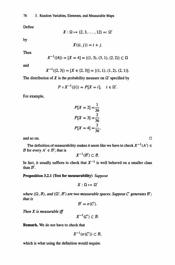
76 3. Random Variables, Elements, and Measurable Maps
Define x : n ~ {2, 3, ... , 12} =: n'
by X((i, j)) = i + j.
Then x-I({4}) =(X= 4] = {(1, 3), (3, 1), (2, 2)} c n
and x-I({2, 3}) =(X E {2, 3}] = {(1, 1), (1, 2), (2, 1)}.
The distribution of X is the probability measure on Q' specified by
For example,
and so on.
P oX-I({i}) = P(X = i], i e Q' .
1 P[X =2] =-
36 2
P(X=3]=-36 3
P[X =4) =-, 36
0
The definition of measurability makes it seem like we have to check x-I (A') e B for every A' e B'; that is
x-I(B') c B.
In fact, it usually suffices to check that x-I is well behaved on a smaller class than B'.
Proposition 3.2.1 (fest for measurability) Suppose
x:n~n'
where (Q, B), and (Q', B') are two measurable spaces. Suppose C' generates B'; that is
B' = a(C').
Then X is measurable iff x-I(C') C B.
Remark. We do not have to check that
x-I(a(C')) C B,
which is what using the definition would require.

3.2 Measurable Maps, Random Elements, Induced Probability Measures 77
Corollary 3.2.1 (Special case of random variables) The real valued function
is a random variable iff
x-1((-oo, A])= [X~ A] E 8, VA E R.
Proof of Proposition 3.2.1. If
x-1(C') c 8,
then by minimality
However, we get
which is the definition of measurability. 0
Proof of Corollary 3.2.1. This follows directly from
a((-oo, A], A e R) = 8(R). 0
3.2.1 Composition
Verification that a map is measurable is sometimes made easy by decomposing the map into the composition of two (or more) maps. If each map in the composition is measurable, then the composition is measurable.
Proposition 3.2.2 (Composition) Let X 1, X 2 be two measurable maps
X1 : (Qt. 81) ...-. (Q2, 82),
X 2 : (Q2, 82) ...-. (QJ, 83)
where (Q;, 8;), i = 1, 2, 3 are measurable spaces. Define
by
Then

78 3. Random Variables, Elements, and Measurable Maps
FIGURE3.2
Proof. It is elementary to check that
(Xz oXt)-1 = X}1(X21(·))
as maps from 'P(!23) ~ 'P(Qt). The reason is that for any B3 c !23
(Xz o Xt)-1(BJ) = {wt : Xz o Xt (wt) e B3}
={wt: Xt(wt) e X21(B3)}
= {wt : w1 e X}1(X21(BJ)}} .
If B3 e lh then
as required.
3.2.2 Random Elements of Metric Spaces
0
The most common use of the name random elements is when the range is a metric space.
Let (S, d) be a metric space with metric d so that d : S x S ~ I+ satisfies
(i) d(x , y) ~ 0, for x, yeS.
(ii) d(x, y) = 0 iff x = y , for any x, yeS.
(iii) d(x , y) =d(y,x), foranyx,y e S.
(iv) d(x , z)::::; d(x , y) +d(y,z), foranyx,y,z e S.
Let 0 be the class of open subsets of S. Define the Borel a-fieldS to be the smallest a -field generated by the open sets
S = a(O).

3.2 Measurable Maps, Random Elements, Induced Probability Measures 79
If X : (Q, B) ._.. (S, S);
that is, X e B/S, then call X a random element of S. Here are some noteworthy examples of random elements.
1. SupposeS= Rand d(x, y) = lx- yl . Then a random element X of Sis called a random variable.
2. Suppose S = JRk and
k
d(x, y) = L lx;- y;l2•
I
Then a random element X of S is called a random vector. We write X = (XI. ... , Xk).
3. Suppose S = IR00 , and the metric d is defined by
Then a random element X of S is called a random sequence. We write X=(Xt,Xz, ... ).
4. Let S = C[O, oo) be the set of all real valued continuous functions with domain [0, oo). Define
llx(·)- yOIIm = sup lx(t)- y(t)l O::;:t::;:m
and
d(x , y) = f: Tm ( llx- Yllm ) . m=l 1 + llx- yllm
A random element X of Sis called a random (continuous) function.
5. Let (IE, £) be a measurable space where IE is a nice metric space and £ are the Borel sets, that is the sets in the a-field generated by the open sets. Let S = M +(IE) be the set of all measures on (IE, £) which satisfy the property that if f1. e M+(IE), then f1.(K) < oo if K is a compact subset of IE. Such measures which are finite on compacta are called Radon measures. There is a standard metric for S called the vague metric. A random element X of Sis called a random measure.
A special case is where M +(IE) is cut down to the space M p(IE) of nonnegative integer valued measures. In this case the random element X is called a stochastic point process.

80 3. Random Variables, Elements, and Measurable Maps
3.2.3 Measurability and Continuity
The idea of distance (measured by a metric) leads naturally to the notion of continuity. A method, which is frequently easy for showing a function from one metric space to another is measurable, is to show the function is continuous.
Proposition 3.2.3 Suppose (S;, di), i = 1, 2 are two metric spaces. Let the Borel a-fields (generated by open sets) be S;, i = 1, 2. If
X: St ~ S2
is continuous, then X is measurable:
Proof. Let 0; be the class of open subsets of S;, i = 1, 2. If X is continuous, then inverse images of open sets are open, which means that
So X E St!S2 by Proposition 3.2.1.
Corollary 3.2.2 IfX = (Xt. ... , Xk) is a random vector, and
g: IRk~--+ JR., g E B(IR.k)/B(IR),
0
then from Proposition 3.2.2, g(X) is a random variable. In particular, if g is continuous, then g is measurable and the result holds.
Some examples of the sort of g's to which this result could apply:
k
g(xt, ... , Xk) = L x;, (component sum) i=l
k
= L x; I k, (component average) 1
k
= V x;, (component extreme) i=l
k
= n X;, (component product) i=l
k
-"' 2 - L...,xi' i=l
(component sum of squares).
Another interesting example of g is the projection map
g = 7rj : JR.k !--+ JR.

3.2 Measurable Maps, Random Elements, Induced Probability Measures 81
defined by 1l';(x., ... ,Xk) =x;.
Then 1l'; is continuous and if X= (X1, ... , Xk) is a random vector, Jr;(X) =X; is a random variable fori = 1, ... , k.
This observation leads in a simple way to an important fact about random vectors: A random vector is nothing more than a vector of random variables.
Proposition 3.2.4 X = (X., ... , Xk) is a random vector, that is a measurable map from (Q, 13) ~ (lRk ,B(JRk)), iff X; is a random variable for each i = 1, ... 'k.
Proof. If X is a random vector, then X; = 1l'; o X is measurable since it is the composition of two measurable functions X and the continuous function 1r;.
The converse is easily proved if we know that
13(1Rk) = a(O) = a(RECTS)
where RECTS is the class of open rectangles. We assume this fact is at our disposal. Suppose X1, ... , Xk are random variables. Write
B =It X ••• X lk
for a rectangle whose sides are the intervals ft, ... , ft. Then
k
x-1(B) = nx;-1(/;). i=1
Since X; is a random variable, Xj 1 (/;) e 13, so x-1 (B) e 13 and
x-1( RECTS) c 13
so x-1 is measurable. D
The corresponding basic fact about random sequences, stated next, is proved in an analogous manner to the proof of the basic fact about random vectors. It says that X is a random sequence iff each component is a random variable.
Proposition 3.2.5 X = (X 1, X z, ... ) is a random sequence iff for each i = 1, 2, ... the ith component X; is a random variable. Furthermore, X is a random sequence iff (X 1, ... , X k) is a random vector, for any k.
3.2.4 Measurability and Limits
Limits applied to sequences of measurable functions are measurable.
Proposition 3.2.6 Let X., Xz, ... be random variables defined on (Q, 13). Then
(i) VnXn and 1\nXn are random variables.

82 3. Random Variables, Elements, and Measurable Maps
(ii) lim infn-+oo X n and lim supn-+oo X n are random variables.
(iii) lflimn-+oo Xn(w) exists for all w, then limn-+oo Xn is a random variable.
( iv) The set on which {X n } has a limit is measurable; that is
{w: limXn(w) exists} E /3.
Proof. (i) We have
[v Xn :S x] = n[Xn :S x] E /3, n n
since for each n, [Xn :S x] E /3.
Similarly
[/\Xn > x] = n[Xn > x] E /3. n n
This suffices by Corollary 3.2.1. (ii) We have that
lim infXn =sup inf Xk. n-+oo n=:::I k=:::n
By (i) infk::::n Xk is a random variable and hence so is supn>I (infk::::n Xk) . (iii) If limn-+oo X n (w) exists for all w, then -
lim Xn(w) = limsupXn(w) n-+oo n-+00
is a random variable by (ii). (iv) Let Q be the set of all rational real numbers so that Q is countable. We have
{w : limXn(w) exists }c = {w : liminfXn(w) < limsupXn(w)}
= U [liminfXn::::: r < limsupXn] rEQ n-+00 n-+oo
= U [liminfXn :S r] n [limsupXn::::: r]c E 13 rEQ n-+oo n-+00
since [liminfXn::::: r] E 13
n-+00
and [limsupXn::::: r] E /3.
n-+00

3.3 a-Fields Generated by Maps 83
3.3 a-Fields Generated by Maps
Let X: (Q, !3) ~ (lR, B(IR)) be a random variable. The a-algebra generated by X, denoted u(X), is defined as
a(X) = x-1(!3(1R)) . (3.3)
Another equivalent description of a (X) is
a(X) ={[X E A], A e B(IR)}.
This is the a-algebra generated by information about X, which is a way of isolating that information in the probability space that pertains to X. More generally, suppose
X: (Q, !3) ~ (Q', !3').
Then we define
a(X) = x-1(!3'). (3.4)
If :F C l3 is a sub -a-field of !3, we say X is measurable with respect to :F, written X E :F, if a(X) C :F.
If for each t in some index set T
then we denote by
x,: (Q, !3) ~ (Q', !3') ,
a(X,, t e T) = v a(X,) teT
the smallest a-algebra containing all a(X,).
Extreme example: Let X (w) = 17 for all w. Then
a(X) ={[X E B], B E B(IR)}
= a(0, Q) = {0, Q}.
Less extreme example: Suppose X = 1A for some A e B. Note X has range {0, 1}. Then
and therefore
To verify this last assertion, call

84 3. Random Variables, Elements, and Measurable Maps
and
a(X) = LHS.
Then RHS is a a-field and is certainly contained in LHS. We need to show that for any B E B(lR),
[lA E B] E RHS .
There are four cases to consider: (i) 1 E B, 0 ¢ B; (ii) 1 E B, 0 E B; (iii) 0 E B, 1 ¢ B; (iv) 0 ¢ B, 1 ¢B. For example, in case (i) we find
[lA E B] =A
and the other cases are handled similarly.
Useful example: Simple function. A random variable is simple if it has a finite range. Suppose the range of X is {at, ... , ak}, where the a's are distinct. Then define
A;:= x-1({a;}) =[X= a;].
Then {A;, i = 1, .. . , k} partitions Q, meaning
k
A; nAj = 0, i # j, LA;= n. i=l
We may represent X as
and
k
X= Lai1A;• i=l
a(X) = a(At. ... , Ak) =\?:A; : I c {1, ... , k}J. IE/
In stochastic process theory, we frequently keep track of potential information that can be revealed to us by observing the evolution of a stochastic process by an increasing family of a-fields. If {Xn. n ~ 1} is a (discrete time) stochastic process, we may define
Bn := a(Xt, ... , Xn), n ~ 1.
Thus, Bn C Bn+I and we think of Bn as the information potentially available at time n. This is a way of cataloguing what information is contained in the probability model. Properties of the stochastic process are sometimes expressed in terms of {Bn , n ~ 1}. For instance, one formulation of the Markov property is that the conditional distribution of X n+l given Bn is the same as the conditional distribution of Xn+l given Xn . (See Chapter 10.)
We end this chapter with the following comment on the a-field generated by a random variable.

3.4 Exercises 85
Proposition 3.3.1 Suppose X is a random variable and C is a class of subsets of JR. such that
a(C) = B(JR.).
Then
a(X) = a([X E B), B E C).
Proof. We have
a([X E B), BE C)= a(X-1(B), BE C)
A special case of this result is
= a(X-1(C)) = x-1(a(C))
= x-1(B(lR.)) = a(X).
a(X) = a([X ~A], A E JR.).
3.4 Exercises
1. In the measurable space (Q, B), show A e B iff 1A E B.
0
2. Let (Q, B, P) = ((0, 1], B((O, 1]), A) where A is Lebesgue measure. Define
Xt(w) =0, Yw E Q,
X2(W) = 1{1/2)(W),
X3(W) = 1Q(W)
where Q c (0, 1] are the rational numbers in (0, 1]. Note
and give a(X;), i = 1, 2, 3.
3. Suppose f : JR.k ~ JR., and f E B(JR.k)/B(JR.).
Let X 1 •• .• , Xk be random variables on (Q , B). Then
4. Suppose X : Q ~ JR. has a countable range 1?, Show X E B I B(JR.) iff
x-1({x}) E B, Yx E R.

86 3. Random Variables, Elements, and Measurable Maps
5. If F(x) = P[X ~ x)
is continuous in x, show that Y = F(X) is measurable and that Y has a uniform distribution
P[Y~y]=y, O~y~l.
6. If X is a random variable satisfying P[IXI < oo] = 1, then show that for any € > 0, there exists a bounded random variable Y such that
P[X # Y) < €.
(A random variable Y is bounded if for all w
IY(w)l ~ K
for some constant K independent of w.)
7. If X is a random variable, so is lXI . The converse may be false.
8. Let X and Y be random variables and let A E !3. Prove that the function
is a random variable.
Z(w) = IX(w), y (w)'
ifweA, if wE Ac
9. Suppose that {Bn, n 2::: 1} is a countable partition of Q and define T3 = a(Bn , n 2::: 1). Show a function X : Q ~-+ (-oo, oo] is !3-measurable iff X is of the form
00
X= .L:c;1si' i=l
for constants {c; }. (What is !3?)
10. Circular Lebesgue measure. Define C := {e2n"i& : 0 e (0, 1]} to be the unit circle in the complex plane. Define
T: (0, 1) ~-+ C, T(B) = e21ri8 •
Specify a a-field T3(C)) of subsets of C by
T3(C) :={A C C : r-1(A) E !3((0, 1)).
(Why is this a a-field?) Define a probability measure JL on T3(C) by JL = ).. o r-1 and call this measure JL circular Lebesgue measure.
(a) Identify the complex plane with JR2• Show
B(C) = T3(1R2) n c.

3.4 Exercises 87
(b) Show that B(C) is generated by arcs of C.
(c) Show Jl is invariant with respect to rotations. This means, if Seo C ~ C via
then Jl = Jl o Si;/. (d) If you did not define Jl as the induced image of Lebesgue measure on
the unit interval, how could you define it by means of the extension theorems?
11. Let (Q, B, P) be ([0, 1], 8([0, 1]), >..) where >.. is Lebesgue measure on [0, 1]. Define the process {X1, 0 ~ t ~ 1} by
X1(w) = 10,
1,
if t =ft w,
if t = w.
Show that each X1 is a random variable. What is the a-field generated by {X1, 0 ~ t ~ 1}?
12. Show that a monotone real function is measurable.
13. (a) If X is a random variable, then a(X) is a countably generated a-field.
(b) Conversely, if B is any countably generated a -field, show
B = a(X)
for some random variable X.
14. A real function f on the line is upper semi-continuous (usc) at x, if, for each E, there is a 8 such that lx - yl < 8 implies that
f(y) < f(x) +E.
Check that if f is everywhere usc, then it is measurable. (Hint: What kind of set is {x : f (x) < t} ?)
15. Suppose -00 < a ~ b < oo. Show that the indicator function l(a ,bJ(x) can be approximated by bounded and continuous functions; that is, show that there exist a sequence of continuous functions 0 ~ fn ~ 1 such that fn ~ 1(a,b) pointwise.
Hint: Approximate the rectangle of height 1 and base (a, b] by a trapezoid of height 1 with base (a, b + n-1] whose top line extends from a+ n-1 to b.
16. Suppose B is a a-field of subsets of!R. Show B(IR) c B iff every real valued continuous function is measurable with respect to B and therefore B(IR) is the smallest a-field with respect to which all the continuous functions are measurable.

88 3. Random Variables, Elements, and Measurable Maps
17. Functions are often defined in pieces (for example, let f (x) be x 3 or x-1 as x ~ 0 or x < 0), and the following shows that the function is measurable if the pieces are.
Consider measurable spaces (Q, B) and (Q', B') and a map T : Q t--+> Q'. Let At. Az, ... be a countable covering of Q by B sets. Consider the afield Bn = {A : A C An, A E B} in An and the restriction Tn ofT to An. Show that Tis measurable B!B' iff Tn is measurable Bn!B' for each n.
18. Coupling. If X andY are random variables on (Q, B), show
sup IP[X e A]- P[Y e A]l ~ P[X # Y]. AEB
19. Suppose T : (Qt. Bt) t--+> (Qz, Bz) is a measurable mapping and X is a random variable on !'21 . Show X e a(T) iff there is a random variable Y on (Qz, Bz) such that
X(wt) = Y(T(wi)), 'v'w1 E !:'21 .
20. Suppose {X, , t ~ 0} is a continuous time stochastic process on the probability space (Q, B, P) whose paths are continuous. We can understand this to mean that for each t ~ 0, X, : Q t--+> lR is a random variable and, for each w e Q, the function t t--+> X 1(w) is continuous; that is a member of C[O, oo). Let r : Q t--+> [0, oo) be a random variable and define the process stopped at r as the function X, : Q t--+> [0, oo) defined by
X,(w) := Xr(w)(w), wE Q.
Prove X, is a random variable.
21. Dyadic expansions and Lebesgue measure. Let§= {0, 1} and
§ 00 = {(Xt. Xz, ... ) :Xi E §, i = 1, 2, ... }
be sequences consisting of O's and 1 's. Define B(§) = P(§) and define B(§00 ) to be the smallest a-field of subsets of § 00 containing all sets of the form
fork = 1, 2, .. . and it. iz, . . . , ik some string of O's and 1 's.
For x e [0, 1], let X = (dk(X) , k ~ 1)
be the non-terminating dyadic expansion (dk(O) = 0 and dk(X) = 0 or 1.) Define U : [0, 1] t--+> §00 by
U(x) = (dt(x),d2(x), .. . ).

3.4 Exercises 89
Define V: § 00 ~ [0, 1] by (x = Ut. iz, ... ))
Loo in V(x) = -. 2n
n=l
Show U e 8([0, 1])/8(§00) and V e 8(§00)/8([0, 1]).
22. Suppose {Xn. n ~ 1} are random variables on the probability space (Q, 8, P)
and define the induced random walk by
Let
n
So = 0, Sn = L Xi, n ~ 1. i=l
T := inf{n > 0 : Sn > 0}
be the first upgoing ladder time. Prove T is a random variable. Assume we
know T(w) < 00 for all (J) E n. Prove ST is a random variable.
23. Suppose {X 1, .. . , X n} are random variables on the probability space (Q, 8, P) such that
P[ Ties]:= P{ U [Xi= Xj]} = 0. if.j
l~i.j~n
Define the relative rank Rn of Xn among {Xt. ... , Xn} to be
R = I L7=1 1[X;2:Xn] n 17,
on [Ties ]c,
on [Ties].
Prove Rn is a random variable.
24. Suppose (SI. Sl) is a measurable space and suppose T : S1 ~ Sz is a mapping into another space Sz. For an index set r, suppose
hy : Sz ~JR., y e r
and define g:=a(hy,yEf)
to be the a-field of subsets of Sz generated by the real valued family
{hy, y E f}, that is, generated by {hy1(B), y e f, B e 8(lR.)}. Show
T e Sl!g iff hy oTis a random variable on (S1, S1).
25. Egorov's theorem: Suppose Xn, X are real valued random variables de
fined on the probability space (Q, 8, P). Suppose for all w e A e 8, we
have Xn(w) __. X(w). Show for every E > 0, there exists a set Af such that
P(Af) < E and
sup JX(w)- Xn(w)J __. 0 (n __. oo). wEA\A,

90 3. Random Variables, Elements, and Measurable Maps
Thus, convergence is uniform off a small set.
Hints:
(a) Define
B~k> = [v IX(w)- Xi(w)l] n A. 1~n
(b) Show B~k) .l, 0 as n ___. oo.
(c) There exists {nk} such that P(B~!)) < E/2k.
(d) Set B = UkB~!) so that P(B) <E.
26. Review Exercise 12 of Chapter 2. Suppose C is a class of subsets of Q such that, for a real function X defined on Q, we have X e B(C). Show there exists a countable subclass C* C C such that X is measurable C*.

91S.I. Resnick, A Probability Path, Modern Birkhäuser Classics,ss Media New York 2014 DOI 10.1007/978-0-8176-8409-9_4, © Springer Science+Busine
4 Independence
Independence is a basic property of events and random variables in a probability model. Its intuitive appeal stems from the easily envisioned property that the occurrence or non-occurrence of an event has no effect on our estimate of the probability that an independent event will or will not occur. Despite the intuitive appeal, it is important to recognize that independence is a technical concept with a technical definition which must be checked with respect to a specific probability model. There are examples of dependent events which intuition insists must be independent, and examples of events which intuition insists cannot be independent but still satisfy the definition. One really must check the technical definition to be sure.
4.1 Basic Definitions
We give a series of definitions of independence in increasingly sophisticated circumstances.
Definition 4.1.1 (Independence for two events) Suppose (Q, B, P) is a fixed probability space. Events A, B e B are independent if
P(AB) = P(A)P(B).
Definition 4.1.2 (Independence of a finite number of events) The events A lt ... , An (n ::: 2) are independent if
P(nA;) = n P(A;), for all finite I c {1, ... , n}. (4.1) ie/ ie/

92 4. Independence
(Note that (4.1) represents
equations.)
Equation (4.1) can be rephrased as follows: The events At. ... , An are independent if
n
P(Bt n B2 · · · n Bn) = n P(B;) (4.2) i=l
where for each i = 1, ... , n,
B; equals A; or Q.
Definition 4.1.3 (Independent classes) Let C; c B, i = 1, ... , n. The classes C; are independent, iffor any choice At. ... , An. with A; e C;, i = 1, ... , n, we have the events At •... , An independent events (according to Definition 4.1.2).
Here is a basic criterion for proving independence of a-fields.
Theorem 4.1.1 (Basic Criterion) If for each i = 1, ... , n, C; is a non-empty class of events satisfying
1. C; is a rr-system,
2. C;, i = 1, ... , n are independent,
then a(Ct) •... , a(Cn)
are independent.
Proof. We begin by proving the result for n = 2. Fix A2 e C2. Let
.C ={A e B: P(AA2) = P(A)P(A2)}.
Then we claim that .C is a A-system. We verify the postulates.
(a) We have Q e .C since
P(!2A2) = P(A2) = P(Q)P(A2).
(b) If A e .C, then Ace .C since
P(Ac A2) = P((Q \ A)A2) = P(A2 \ AA2)
= P(A2) - P(AA2) = P(A2) - P(A)P(A2)
= P(A2)(1- P(A)) = P(Ac)P(A2).

4.2 Independent Random Variables 93
(c) If Bn E .Care disjoint (n ::: 1), then :L~1 Bn e .C since
00 00 00
P((U Bn)Az) = P(U BnAz) = L P(BnAz) n=l n=l n=l
00 00
= L P(Bn)P(Az) = P(U Bn)P(Az). n=l n=l
Also C :::> Ct. so .C :::> a(Ct) by Dynkin's theorem 2.2.2 in Chapter 2. Thus a(Ct). Cz are independent.
Now extend this argument to show a(Ct), a(Cz) are independent. Also, we may use induction to extend the argument for n = 2 to general n. D
We next define independence of an arbitrary collection of classes of events.
Definition 4.1.4 (Arbitrary number of independent classes) Let T be an arbitrary index set. The classes C,, t e T are independent families if for each finite /,I c T, C1, t e I is independent.
Corollary 4.1.1 If {C1 , t e T} are non-empty rr-systems that are independent, then {a(C1), t e T} are independent.
The proof follows from the Basic Criterion Theorem 4.1.1.
4.2 Independent Random Variables
We now tum to the definition of independent random variables and some criteria for independence of random variables.
Definition 4.2.1 (Independent random variables) {X1, t e T} is an independent family of random variables if {a(X1), t e T} are independent a-fields.
The random variables are independent if their induced a-fields are independent. The information provided by any individual random variable should not affect behavior of other random variables in the family. Since
we have 1A1 , ••• , lAn independent iff At, . .. , An are independent. We now give a criterion for independence of random variables in terms of dis
tribution functions. For a family of random variables {X1, t e T} indexed by a set T, the finite dimensional distribution functions are the family of multivariate distribution functions
FJ(X1, t E J) = P(X1 S:. x1, t E J] (4.3)
for all finite subsets J c T.

94 4. Independence
Theorem 4.2.1 (Factorization Criterion) A family of random variables {X 1 , t E T} indexed by a set T, is independent iff for all finite J C T
F1(x1, t E J) = n P[X1 ~ xt), "'x1 E JR. tel
(4.4)
Proof. Because of Definition 4.1.4, it suffices to show for a finite index set J that {X1 , t E J} is independent iff (4.4) holds. Define
C1 = {(X1 ~ x], x E JR}.
Then
(i) C1 is a rr-system since
and
(ii) a(C1) = a(X1) .
Now (4.4) says {C1, t E J} is an independent family and therefore by the Basic Criterion 4.1.1, {a(C1) = a(X1 ), t E J} are independent. D
Corollary 4.2.1 The finite collection of random variables X 1, . . . , X k is independent iff
k
P[X1 :::: Xt. 0 0 0 'Xk :::: Xk] = n P[X; :::: x;] , i=1
for all x; E JR, i = 1, . .. , k.
For the next result, we define a random variable to be discrete if it has a countable range.
Corollary 4.2.2 The discrete random variables X 1, . .. , X k with countable range n are independent iff
k
P[X; =x;,i = 1, ... ,k] = n P[X; =x;], (4.5) i=1
for all x; En, i = 1, ... , k.
Proof. If X., . .. , Xn is an independent family, then a(X;), i = 1, ... , k is independent. Since
[X; = x;] E a(X;)
we have [X; = x;] , i = 1, . .. , k are independent events and (4.5) follows.

4.3 1\vo Examples of Independence 95
Conversely, suppose (4.5) holds. Define z::: x to mean z; ::: x;, i = 1, ... , k. Then
P[X;::;x;,i=1, ... ,k]= L P(X;=z;,i=1, ... ,k] z<x
Z;E'R i=l, ... ,k
k
= L n P(X; = z;] z::::x i=l
Z;E'R i=l, ... ,k
k
= I: I: P(xl =ztlO P(x; =zd Z2:5X2, ..• ,Zk:5XkZJ:5XJ i=2 z;e'R,i=2, ... ,k z1 e'R
k
= L P[Xt ::: xt] n P[X; = z;] Z2:5X2•··· ,Zk:5Xk i=2 Z;E'R,i =2, ... ,k
n
= ... = n P[X; ::: xi]. i=l
4.3 Two Examples of Independence
This section provides two interesting examples of unexpected independence:
• Ranks and records.
• Dyadic expansions of uniform random numbers.
4.3.1 Records, Ranks, Renyi Theorem
0
Let {Xn, n 2:: 1} be iid with common continuous distribution function F(x). The continuity ofF implies
so that if we define
then
P[X; = Xj] = 0,
[Ties]= U[X; = Xj]. i#j
P[ Ties]= 0.
Call X n a record of the sequence if
n-l
Xn > V X;, i=l
(4.6)

96 4. Independence
and define
An = [Xn is a record].
A result due to Renyi says that the events {A j, j :::: 1} are independent and
P(Aj)=1/j, j::::2.
This is a special case of a result about relative ranks. Let Rn be the relative rank of Xn among Xt. ... , Xn where
So
n
Rn = L 1[Xj::;:Xn] · j=l
Rn = 1 iff Xn is a record,
= 2 iff Xn is the second largest of Xt, .. . , Xn,
and so on.
Theorem 4.3.1 (Renyi Theorem) Assume {X n, n :::: 1} are iid with common, continuous distribution function F (x ).
(a) The sequence of random variables { Rn, n :::: 1} is independent and
1 P[Rn = k] = -,
n
fork= 1, . . . ,n. (b) The sequence of events {An, n :::: 1} is independent and
1 P(An) = - .
n
Proof. (b) comes from (a) since An = [Rn = 1]. (a) These are n! orderings of X 1 , . . • , X n . (For a given w, one such ordering is
Xt(w) < · · · < Xn(w) . Another possible ordering is Xz(w) < ... < Xn(w) < X 1 (w ), and so on.) By symmetry, since X 1, . .. , Xn are identically distributed and independent, all possible orderings have the same probability ~, so for example,
1 P[Xz < X3 < · · · < Xn < Xt] = -.
n!
Each realization of R1, • •• , Rn uniquely determines an ordering: For example, if n = 3, suppose R1 (w) = 1, Rz(w) = 1, and R3(w) = 1. This tells us that
X1(w) < Xz(w) < X3(w),
and if R1 (w) = 1, Rz(w) = 2, and R3(w) = 3, then this tells us
X3(w) < Xz(w) < X1 (w).

4.3 Two Examples of Independence 97
Each realization of R 1, . .. , Rn has the same probability as a particular ordering of X t. . .. , X n. Hence
for r; e {1 , . .. , i}, i = 1, .. . , n. Note that
P[Rn = rn] = TJ , ·· · ,rn-l
1 = L n! ·
TJ , ... ,rn-1
Since r; ranges over i values, the number of terms in the sum is
Thus
Therefore
1 · 2 · 3 · . .. · n - 1 = (n - 1)!.
(n- 1)! 1 P[Rn = rn] = = -, n = 1, 2, . ...
n! n
1 = rt. ... , Rn = rn] = -
n! = P[Rt = rt] · · · P[Rn = rn]·
0
Postscript: If {Xn , n ~ 1} is iid with common continuous distribution F(x), why is the probability of ties zero? We have
P[ Ties]= P<U[X; = Xj]) i#j
and by subadditivity, this probability is bounded above by
Thus it suffices to show that
LP[X; =Xj]· i#j
Note the set containment: For every n,

98 4. Independence
By monotonicity and subadditivity
Loo k-1 k k-1 k P[-- <X1 <- -- <Xz < -] 2n - 2n ' 2n - 2n
k=-00
00 ( k 1 k ) 2
" P[--=- < x1 < -1 ~ 2n - 2n k=-00
(4.7) =
Write
F[a, b] = F(b)- F(a)
and the above ( 4. 7) is equal to
k-1 k ~ k-1 k :::: -~~oo F ( 2fl' 2n] k~oo F ( 2fl' 2n ]
k -1 k :::: -oo~~~oo F( 2!'' 2n]. 1
k -1 k = max F(--,- ]. -oo<k<oo 2n 2n
Since F is continuous on IR, because F is a also a probability distribution, F is uniformly continuous on R (See Exercise 22 in Chapter 2.) Thus given any s > 0, for n ::: no(s) and all k, we have
k-1 k k k-1 F(-- -] = F(-)- F(--) < s. 2n '2n 2n 2n -
Thus for any s > 0,
(4.8)
and since s is arbitrary, the probability in ( 4.8) must be 0.
4.3.2 Dyadic Expansions of Uniform Random Numbers
Here we consider (Q, B, P) = ((0, 1], B((O, 1]), >.),
where A is Lebesgue measure. We write w E (0, 1] using its dyadic expansion
00 dn(w) w = L ~ = .d1 (w)dz(w)d3(w) · · · ,
n=l

4.3 Two Examples of Independence 99
where each dn(w) is either 0 or 1. We write 1 as
00 1/2 0.11111· · · = ""'2-n = = 1,
~ 1-1/2
and if a number such as ! has two possible expansions, we agree to use the nonterminating one. Thus, even though 1/2 has two expansions
and
1 00 1 2 = L 2n = .01111 · .. '
n=2
1 1 - =- +0+0+ ... = .1000··· 2 2
by our convention, we use the first expansion.
Fact 1. Each dn is a random variable. Since dn is discrete with possible values 0, 1, it suffices to check
[dn = 0] E 8((0, 1]), [dn = 1] E 8((0, 1]),
for any n 2: 1. In fact, since [ dn = 0] = [ dn = 1 ]c, it suffices to check [ dn = 1] e 8((0, 1]).
To verify this, we start gently by considering a relatively easy case as a warmup. For n = 1,
1 [dt = 1) = (.1000 · · · , .1111· · ·) = (2, 1) E 8((0, 1]).
The left endpoint is open because of the convention that we take the non-terminating expansion. Note P[dt = 1] = P[dt = 0] = 1/2.
After understanding this warmup, we proceed to the general case. For any n;:::2
[dn = 1]
= u (4.9)
= disjoint union of2n-l intervals e 8((0, 1]).
For example 1 1 3
[ d2 = 1] = (-' -] u (- ' 1]. 4 2 4

100 4. Independence
Fact 2. We may also use (4.9) to compute the mass function of dn. We have
P[dn = 1]
= L: (UJ,U2·····"n-J)E(0,1)n-l
n-1 oo n-1 1 =2n-1{" u~ + "Ti _" u~ + -}
~21 ~ ~21 2n 1=1 1=n 1=1
=2n-1{ f: ~} = ~-i=n+l 2 2
The factor 2n-1 results from the number of intervals whose length we must sum. We thus conclude that
1 P[dn =OJ= P[dn = 1] = -.
2 (4.10)
Fact 3. The sequence {dn, n ;::: 1} is iid. The previous fact proved in (4.10) that {dn} is identically distributed and thus we only have to prove {dn} is independent. For this, it suffices to pick n ;::: 1 and prove { dt. ... , dn} is independent.
For (u1, ... , Un) E {0, 1}n, we have n
n[d; = u;] = (.UtUz ... Un000 ... , .UtU2 ••• Un111 ••. );
i=1
Again, the left end of the interval is open due to our convention decreeing that we take non-terminating expansions when a number has two expansions. Since the probability of an interval is its length, we get
n n u · oo 1 n u· P(n[d; = U; 1) = L 2; + L 2i - L 2;
i=1 i=1 i=n+1 i=l
2-(n+1) 1 =-1-! zn
n
= n P[d; =u;] i=1
where the last step used (4.10). So the joint mass function of d1, ... , dn factors into a product of individual mass functions and we have proved independence of the finite collection, and hence of {dn, n ;::: 1}.
4.4 More on Independence: Groupings
It is possible to group independent events or random variables according to disjoint subsets of the index set to achieve independent groupings. This is a useful property of independence.

4.4 More on Independence: Groupings 101
Lemma 4.4.1 (Grouping Lemma) Let {8, t E T} be an independent family of a-fields. LetS be an index set and suppose for s E S that T5 C T and {T5 , s E S} is pairwise disjoint. Now define
Then
8r, = V8,. tETs
{8r,. s e S}
is an independent family of a -fields.
Remember that Vrer,8r is the smallest a-field containing all the 8(s. Before discussing the proof, we consider two examples. For these and other
purposes, it is convenient to write
when X and Y are independent random variables. Similarly, we write 81 JL 82 when the two a-fields 81 and 82 are independent.
(a) Let {Xn, n ~ 1} be independent random variables. Then
a(Xj, j:::; n) JL a(Xj, j > n),
n n+k
LX; JL LX;, i=l i=n+l
n n+k vx; JL v Xj. i=l j=n+l
(b) Let {An} be independent events. Then U~=l Aj and U~N+l Aj are independent.
Proof. Without loss of generality we may suppose S is finite. Define
Cr, := { n Ba : Ba E 8a, K C T5 , K is finite.} aeK
Then Cr, is a 1r-system for each s, and {Cr,, s E S} are independent classes. So by the Basic Criterion 4.1.1 we are done, provided you believe
a(Cr.) = 8r,.
Certainly it is the case that
Cr, c 8r,
and hence
a(Crs> C 8r,.

102 4. Independence
Also,
Cr. :::> Ba, 'Ia E Ts
(we can take K ={a}) and hence
a(Cr.) :::> Ba. 'Ia E T5 •
It follows that
and hence
a(Cr.) :::>a ( U Ba) = : V Ba. aeTs aeTs
4.5 Independence, Zero-One Laws, Borel-Cantelli Lemma
0
There are several common zero-one laws which identify the possible range of a random variable to be trivial. There are also several zero-one laws which provide the basis for all proofs of almost sure convergence. We take these up in turn.
4.5.1 Borel-Cantelli Lemma
The Borel-Cantelli Lemma is very simple but still is the basic tool for proving almost sure convergence.
Proposition 4.5.1 (Borei-Cantelli Lemma.) Let {An} be any events. If
LP(An) < 00, n
then P([An i.o. ]) = P(limsupAn) = 0.
n->00
Proof. We have
P([An i.o. ]) = P( lim U A j) n->oo
ji!_n
= lim P ( U A j) (continuity of P) n->00
ji!_n
00
:::; lim sup L P (A j) ( subadditivity ) n->oo j=n
=0,
since Ln P(An) < oo implies Lf=n P(A j) ~ 0, as n ~ oo. 0

4.5 Independence, Zero-One Laws, Borel-Cantelli Lemma 103
Example 4.5.1 Suppose {Xn, n 2:: 1} are Bernoulli random variables with
P[Xn = 1] = Pn = 1- P[Xn = 0].
Note we have not supposed {Xn} independent and certainly not identically distributed. We assert that
if
P[ lim Xn = 0] = 1, n-H>O
LPn < 00. n
To verify that (4.12) is sufficient for (4.11), observe that if
LPn = LP[Xn = 1] < 00, n n
then by the Borei-Cantelli Lemma
P([Xn = 1] i.o.) = 0.
Taking complements, we find
1 = P(Iimsup[Xn = 1]c) = P(liminf[Xn = 0]) = 1. n-oo n-oo
(4.11)
(4.12)
Since with probability 1, the two valued functions {Xn} are zero from some point on, with probability 1 the variables must converge to zero. D
4.5.2 Borel Zero-One Law
The Borel-Cantelli Lemma does not require independence. The next result does.
Proposition 4.5.2 (Borel Zero-One Law) If {An} is a sequence of independent events, then
P([An i.o.]) = ,O, 1,
iff Ln P(An) < 00,
iff Ln P(An) = 00.
Proof. From the Borel-Cantelli Lemma, if
then P([An i.o. ]) = 0.

104 4. Independence
Conversely, suppose Ln P(An) = oo. Then
P([An i.o. ]) = P(lim sup An) n-+oo
= 1- P(liminfA~) n-+oo
= 1 - P( lim n Ak) n-+oo
k~n
= 1- lim P(nAk) n-+oo
k~n
m
= 1 - lim P( lim .J, n Ak} n-+00 m-+oo
k=n m
= 1- lim lim P<nAD n-+oom-+oo
k=n m
= 1- lim lim 0<1- P(Ak)), n-+oom-+oo
k=n
where the last equality resulted from independence. It suffices to show
m
lim lim 0<1- P(Ak)) = 0. n-+OOm-+00
k=n
To prove (4.13), we use the inequality
1- X Se-x, 0 < x < 1.
To verify (4.14), note for 0 < x < 1 that
oo xn -log(l-x) = L- ~x
n=l n
so exponentiating both sides yields
or
Now for (4.13). We have
m
Jim n(1- P(Ak)) m-+oo
k=n
1 -->~ 1-x-
<
=
m lim n e-P(Ak)
m-+oo k=n
lim e- L:k'=n P<Ak) m-+00
(4.13)
(4.14)

4.5 Independence, Zero-One Laws, Borei-Cantelli Lemma 105
since Ln P(An) = oo. This is true for all n, and so
m
lim lim n(1- P(Ak)) = 0. n-+oom-+oo
k=n 0
Example 4.5.1 (continued) Suppose {Xn. n ~ 1} are independent in addition to being Bernoulli, with
Then we assert that
P(Xn-+ 0] = 1 iff LPk < 00. n
To verify this assertion, we merely need to observe that
P{[Xn = 1] i.o.} = 0
iff LP(Xn = 1] = LPn < 00.
n n
Example 4.5.2 (Behavior of exponential random variables) We assume that {En, n ~ 1} are iid unit exponential random variables; that is,
P[En>X]=e-x, X>O.
Then
P[lim sup En/ log n = 1] = 1. (4.15) n-+oo
This result is sometimes considered surprising. There is a (mistaken) tendency to think of iid sequences as somehow roughly constant, and therefore the division by logn should send the ratio to 0. However, every so often, the sequence {En} spits out a large value and the growth of these large values approximately matches that of {logn, n ~ 1}.
To prove (4.15), we need the following simple fact: If {Bk} are any events satisfying P(Bk) = 1, then P(nk Bk) = 1. See Exercise 11 of Chapter 2.
Proof of (4.15). For any w e Q,
means
. En(w) hmsup-- = 1 n-+00 logn
(a) 'Ve > 0, ~gi~> ::; 1 + e, for all large n, and
106 4. Independence
(b) Vs > 0, ~oi~> > 1- s, for infinitely many n.
Note (a) says that for any s, there is no subsequential limit bigger than 1 +sand (b) says that for any s, there is always some subsequential limit bounded below by 1- s.
We have the following set equality: Let Sk .J.. 0 and observe
[ . En ) hmsup-- = 1 n-+00 logn
=n{liminf[En :;:1+sk]}nn{[1En >1-sk]i.o.} (4.16) k n-+oo logn k ogn
To prove that the event on the left side of (4.16) has probability 1, it suffices to prove every braced event on the right side of (4.16) has probability 1. For fixed k
""' En ""' L... P[- > 1- Sk] = L... P[En > (1- Sk) logn] n logn n
= I:exp{-(1-Ek)logn} n
1 = L nl - £k = oo.
n
So the Borel Zero-One Law 4.5.2 implies
Likewise
so
P { [ ~ > 1 - Ek] i.o. } = 1. logn
""' En ""' L... P[-- > 1 + sk] = L... exp{-(1 + Sk) logn} n logn n
1 = L nl+£k < oo,
n
P (lim sup [ En > 1 + Sk]) = 0 n-+oo logn
implies
P {liminf[~ =:: 1 + Sk]} = 1- P {lim sup [ En :;: 1 + sk]c} = 1. n-+00 logn n-+00 logn
0

4.5 Independence, Zero-One Laws, Borel-Cantelli Lemma 107
4.5.3 Kolmogorov Zero-One Law
Let {X n} be a sequence of random variables and define
:F~ = a(Xn+l• Xn+2• . .. ), n = 1, 2, ....
The tail a-field Tis defined as
T=n:F~= lim ,l.a(Xn.Xn+J. ... ). n-+00
n
These are events which depend on the tail of the {X n } sequence. If A e T, we will call A a tail event and similarly a random variable measurable with respect to T is called a tail random variable.
We now give some examples of tail events and random variables.
1. Observe that 00
{w : LXn(w) converges} E T. n=l
To see this note that, for any m, the sum 2:~1 Xn(w) converges if and only if I::m Xn(w) converges. So
00
[LX n converges ] = [ L X n converges ] e :F~. n n=m+l
This holds for all m and after intersecting over m.
2. Wehave
limsupXn E T, n-+oo
{w : lim Xn(w) exists} E T. n-+oo
This is true since the lim sup of the sequence {X t. X 2, ... } is the same as the lim sup of the sequence {X m , X m+l , ... } for all m.
3. Let Sn = X 1 + · · · + X n. Then
{w: lim Sn(w) =0} eT n-+oo n
since for any m,
ll·m Sn(w) __ 1. L7=1X;(w) 1. L7=m+1X;(w) Im = Im '
n-+oo n n-+oo n n-+oo n
and so for any m,

108 4. Independence
Call a a-field, all of whose events have probability 0 or 1 almost trivial. One example of an almost trivial a-field is the a-field {0, Q}. Kolmogorov 's Zero-One Law characterizes tail events and random variables of independent sequences as almost trivial.
Theorem 4.5.3 (Kolmogorov Zero-One Law) If (Xn} are independent random variables with tail a-field T, then A E T implies P(A) = 0 or 1 so that the tail a-field Tis almost trivial.
Before proving Theorem 4.5.3, we consider some implications. To help us do this, we need the following lemma which provides further information on almost trivial a-fields.
Lemma 4.5.1 (Almost trivial a-fields) Let g be an almost trivial a -field and let X be a random variable measurable with respect to g. Then there exists c such that P[X = c] = 1.
Proof of Lemma 4.5.1. Let
F(x) = P[X:::;: x].
Then F is non-decreasing and since [X:::;: x] e a(X) C g,
F(x) = 0 or 1
for each x e JR. Let c = sup{x : F(x) = 0}.
The distribution function must have a jump of size 1 at c and thus
P[X = c] = 1. 0
With this in mind, we can consider some consequences of the Kolmogorov Zero-One Law.
Corollary 4.5.1 (Corollaries of the Kolmogorov Zero-One Law) Let {X n} be independent random variables. Then the following are true.
(a) The event
has probability 0 or 1.
(b) The random variables limsupn-+ooXn and liminfn-+ooXn are constant with probability 1.
(c) The event {w: Sn(a>)/n ~ 0}
has probability 0 or 1.

4.5 Independence, Zero-One Laws, Borel-Cantelli Lemma 109
We now commence the proof of Theorem 4.5.3.
Proof of the Kolmogorov Zero-One Law. Suppose A e T. We show A is independent of itself so that
P(A) = P(A n A)= P(A)P(A)
and thus P(A) = (P(A))2• Therefore P(A) = 0 or 1. To show A is independent of itself, we define
n
Fn = a(XJ, . . . , Xn) = Va(Xj), j=l
so that Fn t and
00 00
Foo = a(XJ, X2, ... ) = V a(Xj) = V Fn. j=l n=l
Note that
Now for all n, we have
A eF~,
so since Fn 1_ F~, we have
for all n, and therefore
Let cl ={A}, and c2 = UnFn . Then ci is a rr-system, i = 1, 2, cl II c2 and therefore the Basic Criterion 4.1.1 implies -
a(CJ) = {cf>, n, A, Ac} and a(C2) = V Fn = Foo n
are independent. Now
and
A e V Fn =Foo n
by (4.17). Thus A is independent of A. 0

110 4. Independence
4.6 Exercises
1. Let B1, ... , Bn be independent events. Show
n n
P(UB;) = 1-n(l- P(B;)). i=l i=l
2. What is the minimum number of points a sample space must contain in order that there exist n independent events B1, .. . , Bn, none of which has probability zero or one?
3. If {An. n ~ 1} is an independent sequence of events, show
00 00 P(n An)= n P(An). n=l n=l
4. Suppose (Q, B, P) is the uniform probability space; that is, ([0, 1], B, >..) where >.. is the uniform probability distribution. Define
X(w) = w.
(a) Does there exist a bounded random variable that is both independent of X and not constant almost surely?
(b) Define Y = X(1 -X). Construct a random variable Z which is not almost surely constant and such that Z and Y are independent.
5. Suppose X is a random variable.
(a) X is independent of itself if and only if there is some constant c such that P[X = c] = 1.
(b) If there exists a measurable
g : (lR, B(lR)) .-.. (lR, B(lR)) ,
such that X and g(X) are independent, then prove there exists c E lR such that
P[g(X) = c] = 1.
6. Let {Xt. k ~ 1} be iid random variables with common continuous distribution F . Let rr: be a permutation of 1, ... , n. Show
where 4 means the two vectors have the same joint distribution.
7. If A , B, C are independent events, show directly that both A U B and A \ B are independent of C .

4.6 Exercises 111
8. If X and Y are independent random variables and f, g are measurable and real valued, why are f(X) and g(Y) independent? (No calculation is necessary.)
9. Suppose {An} are independent events satisfying P(An) < 1, for all n. Show
00
P(U An) = 1 iff P(An i.o.) = 1. n=l
Give an example to show that the condition P(An) < 1 cannot be dropped.
10. Suppose {Xn. n :::: 1} are independent random variables. Show
P[supXn < oo] = 1 n
iff L P[Xn > M] < 00, for some M.
n
11. Use the Borel-Cantelli Lemma to prove that given any sequence of random variables {Xn. n :::: 1} whose range is the real line, there exist constants Cn -+ oo such that
P[ lim Xn = 0] = 1. n-+00 Cn
Give a careful description of how you choose Cn.
12. For use with the Borel Zero-One Law, the following is useful: Suppose we have two non-negative sequences {an} and {bn} satisfying an "' bn as n -+ oo; that is,
Show
I . an lm - = 1.
n-+oo bn
Lan < 00 iff Lbn < 00. n n
13. Let {Xn. n :::: 1} be iid with P[X1 = 1] = p = 1- P[X1 = 0]. What is the probability that the pattern 1,0,1 appears infinitely often?
Hint: Let Ak = [Xk = 1, Xk+l = 0, Xk+2 = 1]
and consider A1, A4, A7, ....
14. In a sequence of independent Bernoulli random variables {Xn, n :::: 1} with
P[Xn = 1] = p = 1- P[Xn = 0],
let An be the event that a run of n consecutive 1 's occurs between the 2n and 2n+1st trial. If p :::: 1/2, then there is probability 1 that infinitely many An occur.

112 4. Independence
Hint: Prove something like
P(An) ~ 1- (1- pn)2n 12n > 1- e-<2Pt f2n.
15. (a) A finite family Bi, i e I of a-algebras is independent iff for every choice of non-negative 8i-measurable random variable Yi, i e I, we have
E(nYi) = n E(Yi). ie/ ie/
(One direction is immediate. For the opposite direction, prove the result first for positive simple functions and then extend.)
(b) If {B,, t e T} is an arbitrary independent family of a-algebras in (Q, B, P), the family {B;, t e T} is again independent if B, :::> B;, (t e T). Deduce from this that {f1(X1), t e T} is a family of independent random variables ifthe family {X,, t e T} is independent and the f, are measurable. In order for the family {X,, t e T} of random variables to be independent, it is necessary and sufficient that
E (I) [j(Xj)) =I) E (/j(Xj))
for every finite family { fi, j e J} of bounded measurable functions.
16. The probability of convergence of a sequence of independent random variables is equal to 0 or 1. If the sequence {Xn} is iid, and not constant with probability 1, then
P[Xn converges] = 0.
17. Review Example 4.5.2
(a) Suppose {Xn, n 2:: 1} are iid random variables and suppose {an} is a sequence of constants. Show
P{[Xn > an] i.o. } = 1°' 1,
iff Ln P[Xt > an] < 00,
iff Ln P[X1 > an) = 00.
(b) Suppose {Xn, n ~ 1} are iid N(0,1) random variables. Show
. IXnl ~ P[hm sup r.:::::= = v 2) = 1.
n-+oo -ylogn
Hint: Review, or look up Mill's Ratio which says
lim P[Xn > x] = 1, x-+oo n(x)/x
where n(x) is the standard normal density.

4.6 Exercises 113
(c) Suppose {Xn. n 2:: 1} are iid and Poisson distributed with parameter A. Prove
and therefore
An An -e->.. < P[XI > n] < -, ' - - - ' n. n.
. Xn P[hm sup = 1] = 1.
n~oo lognjlog(logn)
18. If the event A is independent of the rr -system P and A e a (P), then P (A) is either 0 or 1.
19. Give a simple example to show that 2 random variables may be independent according to one probability measure but dependent with respect to another.
20. Counterexamples and examples:
a) Let n = {1, 2, 3, 4} with each point carrying probability 114. Let A1 = {1, 2}, A2 = {1, 3}, A3 = {1, 4}. Then any two of A1, A2, A3 are independent, but A 1 , A 2, A 3 are not independent.
b) Let {Ai, 1 :::: i :::: 5} be a measurable partition of Q such that P(AI) = P(A2) = P(A3) = 15/64, P(A4) = 1/64, P(As) = 18/64. Define B = A1 U A4, C = A2 U A4, D = A3 U A4. Check that
P(BCD) = P(B)P(C)P(D)
but that B, C, D are not independent.
c) Let X 1, X 2 be independent random variables each assuming only the values + 1 and -1 with probability 1/2. Are X 1, X 2. X 1 X 2 pairwise independent? Are X 1, X 2, X 1 X 2 an independent collection?
21. Suppose {An} is a sequence of events.
(a) If P(An) -+ 1 as n -+ oo, prove there exists a subsequence {nk} tending to infinity such that P(nkAnk) > 0. (Hint: Use Borel-Cantelli.)
(b) Show the following is false: Given € > 0 such that P(An) 2:: €, it follows that there exists a subsequence { nk} tending to infinity such that P(nkAnk) > 0.
22. Suppose {An} are independent events such that
00
L (P(An) 1\ (1- P(An))) = 00.
n=l
Show P is non-atomic.
23. Suppose {An} are events.

114 4. Independence
(a) If for each k oo n-1
LP(Anl n Aj) = 00,
n=k i=k
show P(lim sup An) = 1.
n_.oo
(b) What is the relevance to the Borel Zero-One Law?
(c) Is it enough to assume
oo n-1
L P(Anl n Aj) = oo? n=l i=l
(d) Show P(limsupAn) = 1
n_.oo
iff 00
LP(AAn) = 00
n=l
for all events A such that P(A) > 0.
24. If P(An) ~ € > 0, for all large n, then P(An i.o. ) ~ €.
25. Use Renyi's theorem to prove that if {Xn, n ~ 1} is iid with common continuous distribution
n P{[Xn = V Xi] i.o.} = 1.
i=l
26. (Barndorff-Nielsen) Suppose {En} is a sequence of events such that
lim P(En) = 0, "P(EnE~+I) < oo. n_.oo ~ n
Prove P(En i.o.) = 0.
Hint: Decompose Uj=nEj form > n.
27. If {Xn, n ~ 1} are independent random variables, show that the radius of convergence of the power series ,E~1 Xnzn is a constant (possibly infinite) with probability one.
Hint: The radius of convergence of ,E~ 1 CnZn is given by
R-1 = limsuplcnl 1/n . n_.oo

4.6 Exercises 115
28. Show {Xn, n :::: 1} are independent if
are independent for each n :::: 2.
29. Let
Q = { 1, ... , r} n = { (Xt, ... , Xn) : x; E { 1, ... , r}, i = 1, .. . , n}
and assume an assignment of probabilities such that each point of Q is equally likely. Define the coordinate random variables
X;((Xt. ·· ·•Xn))=x;, 1=1, ... ,n.
Prove that the random variables X 1, ... , X n are independent.
30. Refer to Subsection 4.3.2.
(a) Define
A = {[d2n = 0] i.o. }, B = {[d2n+l = 1] i.o. }.
Show A 1._ B.
(b) Define
ln(w) :=length of the run ofO's starting at dn(w),
= lk 2:: 1, if dn(w) = 0, ... , dn+k-1 (w) = 0, dn+k(w) = 1,
0, if dn(w) = 1.
Show
( 1 )k+l P[ln = k] = Z , P[ln 2:: r] = (~)'. (4.18)
(c) Show Wn = 0], n 2:: 1} are independent events.
(d) Show P{[ln = 0] i.o.} = 1. (Use the Borel Zero-One Law.)
(e) The events {[In = 1 ], n :::: 1} are not independent but the events {[/2n = 1], n ::::: 1} are, and therefore prove
P{[/2n = 1] i.o. } = 1
so that
P{[ln = 1] i.o. } = 1.

116 4. Independence
(f) Let log2 n be the logarithm to the base 2 of n. Show
P[limsup ~ ~ 1] = 1. n-+oo log2 n
Hint: Show
LP[In > (1+t:)log2 n] < oo n
and use Borel-Cantelli. Then replace t: by t:k ..t. 0.
(g) Show
P[limsup~ ~ 1] = 1. n-+oo log2 n
Combine this with (4.19).
(4.19)
Hint: Set rn = [log2 n] and define nk by n1 = 1, n2 = 1+rt, ... , nk+l = nk + rnk so that nk+l- nk = rnk· Then
[Ink ~ rnk] E B(d;, nk ~ i < nk+I)
and hence {[Ink ~ rnd. k ~ 1} are independent events. Use the Borel Zero-One Law to show
and hence P{[ln ~ rn] i.o. } = 1.
31. Suppose {Bn, n ~ 1} is a sequence of events such that for some o > 0
P(Bn) ~ o > 0,
for all n ~ 1. Show lim supn-+oo Bn =/; 0. Use this to help show with minimum calculation that in an infinite sequence of independent Bernoulli trials, there is an infinite number of successes with probability one.
32. The Renyi representation. Suppose £1, ... , En are iid exponentially distributed random variables with parameter A > 0 so that
P[£1 ~ x] = 1-e->..x, x > 0.
Let
Et,n ~ E2,n ~ · · · ~ En,n
be the order statistics. Prove the n spacings
Et,n. E2,n- Et,n. · · ·, En,n- En-l,n
are independent exponentially distributed random variables where Ek+l,nEk,n has parameter (n - k)>... Intuitively, this results from the forgetfulness property of the exponential distribution.

S.I. Resnick, A Probability Path, Modern Birkhäuser Classics,ss Media New York 2014 DOI 10.1007/978-0-8176-8409-9_5, © Springer Science+Busine
117
5 Integration and Expectation
One of the more fundamental concepts of probability theory and mathematical statistics is the expectation of a random variable. The expectation represents a central value of the random variable and has a measure theory counterpart in the theory of integration.
5.1 Preparation for Integration
5.1.1 Simple Functions
Many integration results are proved by first showing they hold true for simple functions and then extending the result to more general functions. Recall that a function on the probability space (Q, B, P)
x: n r-+ JR.
is simple if it has a finite range. Henceforth, assume that a simple function is BjB(lR.) measurable. Such a function can always be written in the form
k
X(w) = I:a;1A;(w), i=l
where a; E JR. and A; E Band A1, ... , Ak are disjoint and L~=l A; = Q.
Recall
a(X) = a(A;,i = 1, ... ,k) = lwA;: I C {1, ... ,k}J. IE/

118 5. Integration and Expectation
Let £ be the set of all simple functions on Q. We have the following important properties of £.
1. £ is a vector space. This means the following two properties hold.
(a) If X= L~=l a; 1A; E £, then aX= L~=l a a; 1A; E £ .
(b) If X= E~=I a;1A; andY= Er=I bj1Bi and X, Y e £,then
X+ Y = 2)a; + bj)1A;nBi i,j
and {A;B j• 1 ::: i ::: k, 1 ::: j ::: m} is a partition of n. So X +Y e £ .
2. If X, Y e £,then XY e £since
XY = L:a;bj1A;nBr i,j
3. If X, Y e £,then X v Y, X 1\ Y e £,since, for instance,
XVY = L:a; V bj1A;Bi' i,j
5.1.2 Measurability and Simple Functions
The following result shows that any measurable function can be approximated by a simple function. It is the reason why it is often the case that an integration result about random varables is proven first for simple functions.
Theorem 5.1.1 (Measurability Theorem) Suppose X(w) ~ 0, for all w. Then X e B I B(lR) iff there exist simple functions X n E £ and
0::: Xn t X.
Proof. If Xn E £, then Xn E B/B(lR), and if X = limn--.oo t Xn, then X E
BjB(lR) since taking limits preserves measurability. Conversely, suppose 0::: X E B/B(lR). Define
Because X e BjB(lR), it follows that Xn E £.Also Xn ::: Xn+l and if X(w) < oo, then for all large enough n
1 IX(w)- Xn(w)l::: 2n ~ 0.
If X(w) = oo, then Xn(w) = n ~ oo. 0

5.2 Expectation and Integration 119
Note if
then
M :=sup IX(w)l < oo, wen
sup IX(w)- Xn(w)i -+ 0. wen
5.2 Expectation and Integration
This section takes up the definition of expectation, or in measure theory terms, the Lebesgue-Stieltjes integral. Suppose (Q, B, P) is a probability space and
X : (Q, B)~ (i, B(i))
where i = [ -oo, oo] so X might have ±oo in its range. We will define the expectation of X, written E(X) or
In XdP
or
In X(w)P(dw),
as the Lebesgue-Stieltjes integral of X with respect to P. We will do this in stages, the first stage being to define the integral for simple functions.
5.2.1 Expectation of Simple Functions
Suppose X is a simple random variable of the form
n
X= L:a;1Ap i=l
where la;l < oo, and I:7=l A; = n. Define for X e £the expectation as
k
E(X) = j XdP =: L:a;P(A;). i=l
(5.1)
Note this definition coincides with your knowledge of discrete probability from more elementary courses. For a simple function (which includes all random variables on finite probabilty spaces) the expectation is computed by taking a possible value, multiplying by the probability of the possible value and then summing over all possible values.
We now discuss the properties arising from this definition (5.1).

120 5. Integration and Expectation
1. We have that £(1) = 1, and E(lA) = P(A).
This follows since 1 = 1n so £(1) = P(Q) = 1 and
so E(lA) = 1P(A) + OP(Ac).
2. If X ~ 0 and X e £ then E (X) ~ 0.
To verify this, note that if X ~ 0, then
k
X= I:a;1A;• and a;~ 0, i=l
and therefore E(X) = L~=l a;P(A;) ~ 0.
3. The expectation operator E is linear in the sense that if X, Y e £,then
E(aX + f3Y) = aE(X) + f3E(Y)
for a, f3 e lit
To check this, suppose
and then
so that
k
X= I:a;1Ap i=l
m
y = Lbj1Bj' j=l
aX+ f3Y = L(aa; + /3bj)1A;Bi' i,j
E(aX + f3Y) = L(aa; + /3bj)P(A;Bj) i,j
= I:aa;P(A;Bj) + Lf3bjP(A;Bj) i,j i,j
k m m k
=a La; LP(A;Bj) + f3Lbi LP(A;Bj) i=l j=l j=1 i=l
k m
=a I:a;P(A;) + f3 LbjP(Bj) i=l j=l
=aE(X) + f3E(Y) .

5.2 Expectation and Integration 121
4. The expectation operator E is monotone on £ in the sense that if X ::;: Y and X, Y E £,then E(X)::;: E(Y).
To prove this, we observe that we have Y - X ~ 0 and Y - X e £. So E (Y - X) ~ 0 from property 2, and thus
E(Y) = E(Y- X+ X)= E(Y- X)+ E(X) ~EX
since E(Y- X) ~ 0.
5. If Xn. X E £and either Xn t X or Xn ..!. X, then
E(Xn) t E(X) or E(Xn) ..!. E(X).
Suppose Xn E £ , and Xn ..!. 0. We prove E(Xn) ..!. 0. As a consequence of being simple, X 1 has a finite range. We may suppose without loss of generality that
supXt(w) = K < 00. wen
Since {X n} is non-increasing, we get that
0::;: Xn ::;: K
for all n. Thus for any E > 0,
0 =::Xn = Xn l[Xn>€] + Xn l[Xn~€]
:;:Kl[Xn>€] + El[Xn~€], and therefore by the monotonicity property 4,
0::;: E(Xn)::;: KP[Xn > E] + EP[Xn ::;: E]
::;:KP[Xn > E]+E.
Since X n ..!. 0, we have, as n ~ oo,
[Xn >E) ,I. 0,
and by continuity of P P[Xn > E]..!. 0.
limsupE(Xn)::;: E. n--+00
Since E is arbitrary, E(Xn) ..!. 0.
If X n ..!. X, then X n - X ..!. 0, so
E(Xn)- E(X) = E(Xn- X)..!. 0
from the previous step.
If X n t X, then X - X n ..!. 0 and
E(X)- E(Xn) = E(X- Xn)..!. 0. 0

122 5. Integration and Expectation
5.2.2 Extension of the Definition
We now extend the definition of the integral beyond simple functions. The program is to define expectation for all positive random variables and then for all integrable random variables. The term integrable will be explained later.
It is convenient and useful to assume our random variables take values in the extended real line i ( cf. Exercise 33). In stochastic modeling, for instance, we often deal with waiting times for an event to happen or return times to a state or set. If the event never occurs, it is natural to say the waiting time is infinite. If the process never returns to a state or set, it is natural to say the return time is infinite.
Let £+ be the non-negative valued simple functions, and define
£~:={X?=: 0: X: (Q, B)~--+ (i, B(i))}
to be non-negative, measurable functions with domain Q. If X e t+ and P[X = oo] > 0, define E(X) = oo.
Otherwise by the measurability theorem (Theorem 5.1.1, page 118), we may find X n e £+, such that
0:::;: Xn t X.
We call {X n} the approximating sequence to X. The sequence { E (X n)} is nondecreasing by monotonicity of expectations applied to£+ · Since limits of monotone sequences always exist, we conclude that limn-+oo E (X n) exists. We define
E(X) := lim E(Xn). n-+oo
(5.2)
This extends expectation from £ to f+. The next result discusses this definition further.
Proposition 5.2.1 (Well definition) E is well defined on f+, since if X n e £+ and Ym E £+and Xn t X, Ym t X, then
lim E(Xn) = lim E(Ym). n-+oo n-+oo
Proof. Because of the symmetric roles of X n and Y m, it suffices to prove the following assertion. If Xn. Ym e £+and both sequences {Xn} and {Ym} are nondecreasing, then the assumption
lim t Xn :::;: lim t Ym n-+00 m-+oo
(5.3)
implies
lim t E(Xn):::;: lim t E(Ym). n-+oo m-+oo
(5.4)
To prove (5.4), note that as m ~ oo

5.2 Expectation and Integration 123
since
So from monotonicity of expectations on £+,
E(Xn) = lim t E(Xn 1\ Ym)::::: lim E(Ym). m-+oo m-+oo
This is true for all n, so let n --. oo to obtain
lim t E(Xn) :::=: lim t E(Yn). n-+oo n-+oo
This proves (5.4). D
5.2.3 Basic Properties of Expectation
We now list some properties of the expectation operator applied to random variables in t+.
1. We have 0::::: E(X)::::: oo,
and if X, Yet+ and X::::: Y, then E(X)::::: E(Y).
The proof is contained in (5.4).
2. E is linear: For a > 0 and {J > 0,
E(aX + {JY) = aE(X) + {JE(Y).
To check this, suppose Xn t X, Yn t Y and Xn. Yn e £+. For c > 0
E(cX) = lim E(cXn) n->oo
= lim cE(Xn) (linearity on£+) n-+oo
=cE(X).
We also have
E(X + Y) = lim E(Xn + Yn) n-+oo
= lim (E(Xn) + E(Yn)) (linearity on£+) n-+00
=E(X) + E(Y).
3. Monotone Convergence Theorem (MCT). If
(5.5)

124 5. Integration and Expectation
then E(Xn) t E(X),
or equivalently,
E (lim t Xn) = lim t E(Xn). n-+oo n-+00
We now focus on proving this version of the Monotone Convergence Theorem, which allows the interchange of limits and expectations.
Proof ofMCT. Suppose we are given Xn, X e £~satisfying (5.5). We may find simple functions y~n> e £+, to act as approximations to Xn such that
y~n) t Xn, m __. 00.
We need to find a sequence of simple functions { Z m} approximating X
Zm tX,
which can be expressed in terms of the approximations to {Xn }. So define
Z - vy(n) m- m· n::;m
Note that {Zm} is non-decreasing since
Z < V y(n) ( since y<n) < y<n> ) m- m+l m - m+l
n::;m
:S v y~n~l = Zm+l· n::;m+l
Next observe that for n :::: m,
(A) y:(n) < V . y:<i> = Z . m - 1::;m m m•
(B) Zm :S Vj::;mXi =Xm,
since y~> :::: X j, which is monotone in j and so
(C) Y~n) :S Zm :S Xm.
By taking limits on m in (C), we conclude that for all n
Xn = lim y~n) :S lim Zm :S lim Xm. m-+00 m-+00 m-+00
So
X= lim Xn :S lim Zm :S lim Xm =X. n-+00 m-+oo m-+oo
Therefore

5.2 Expectation and Integration 125
(D) X= limn-+oo Xn = limm-+oo Zm and it follows that { Z m} is a simple function approximation to X.
(E) Now because expectation is monotone onE,
E(Xn) = lim t E(Y~n)) m-+00
:5 lim t E(Zm) m-+oo
:5 lim t E(Xm) m-+00
(expectation definition)
(from (C))
(from (C)).
However Z m e E+ and { Z m} is a simple function approximation to X. Therefore, we get from the definition of expectation on£+ and (D)
E(X) = E( lim t Zm) = lim t E(Zm). m-+oo m-+oo
So (E) implies for all n that
E(Xn)::: E(X)::: lim t E(Xm), m-+oo
and taking the limit on n
lim E(Xn)::: E(X)::: lim E(Xm), n-+oo m-+oo
hence the desired equality follows. 0
We now further extend the definition of E(X) beyond£+. For a random variable X, define
Thus
Therefore
and
and
x+ = x v o. x- = <-X) v o.
x+ =X, if X 2: 0 (and then x- = 0),
x- = -X, if X ::: 0 (and then x+ = 0).
x± ::: o,
lXI =X+ +X-
X e B/B(IR) iff both x± e B/B(IR).
(5.6)
Call X quasi-integrable if at least one of E (X+), E (X-) is finite. In this case, define

126 5. Integration and Expectation
If E(X+) and E(X-) are both finite, call X integrable. This is the case iff EIXI < oo. The set of integrable random variables is denoted by L 1 or L 1 (P) if the probability measure needs to be emphasized. So
L1(P) ={random variables X : EIXI < oo}.
If E(X+) < oo but E(X-) = oo then E(X) = -oo. If E(X+) = oo but E(X-) < oo, then E(X) = oo. If E(X+) = oo and Ex-= oo, then E(X) does not exist.
Example 5.2.1 (Heavy Tails) We will see that when the distribution function of a random variable X has a density I (x ), the expectation, provided it exists, can be computed by the familiar formula
If
E(X) =I xl(x)dx.
l(x) = ~x-2, 0,
ifx > 1,
otherwise,
then E (X) exists and E (X) = oo. On the other hand, if
then
if lxl > 1, otherwise,
and E (X) does not exist. The same conclusion would hold if I were the Cauchy density
1 l(x) = rr(l + xZ), x e JR.
0
We now list some properties of the expectation operator E.
1. If X is integrable, then P[X = ±oo] = 0.
For example, if P[X = oo] > 0, then E (X+) = oo and X is not integrable.
2. If E (X) exists, E(cX) = cE(X).
If either

5.2 Expectation and Integration 127
or
then X + Y is quasi-integrable and
E(X + Y) = E(X) + E(Y).
We verify additivity when X, Y E LJ. Observe that
IX+ Yl e£~.
and since IX+ Yl::: lXI + IYI,
we have from monotonicity of expectation on t+ that
EIX + Yl::: E(IXI + IYI) = EIXI + EIYI < oo,
the last equality following from linearity on t+. Hence X + Y e L I· Next, we have
so
LHS := (X+ Y)+ + x- + y- =(X+ Y)- + x+ + y+ = : RHS.
The advantage of this over (5.7) is that both LHS and RHS are sums of positive random variables. Since expectation is linear on t+, we have
E( LHS) = E(X + Y)+ + E(X-) + E(Y-)
= E( RHS) = E(X + Y)- + E(X+) + E(Y+) .
Rearranging we get
or equivalently,
E(X + Y) = E(X) + E(Y). 0
3. If X::: 0, then E(X)::: 0 since X= x+. If X, Y E L1, and X :S Y, then
E(X) :S E(Y).
This is readily seen. We have E(Y- X) ::: 0 since Y- X ::: 0, and thus by property (2) from this list,
E(Y- X) = E(Y)- E(X) ::: 0.

128 5. Integration and Expectation
4. Suppose {Xn} is a sequence of random variables such that Xn e Lt for some n. If either
Xn tX
or Xn .!,X,
then according to the type of monotonicity
E(Xn) t E(X)
or E(Xn) .!, E(X).
To see this in the case Xn t X, note x; .!, x- so E(X-) < oo. Then
0:::; x: = Xn + x;:::; Xn +X} t X+ X}.
From the MCf given in equation (5.5)
0:::; E(Xn +X}) t E(X +X}).
From property 2 we have
E(Xn +X})= E(Xn) + E(X}).
Since E(X-) < oo and E(X!) < oo, we also have
E(X +X})= E(X) + E(X}),
and thus lim E(Xn) = E(X).
n-+oo
If Xn .!, X, proceed similarly by considering -Xn +X{.
5. Modulus Inequality. If X e Lt.
iE(X)i:::: E(IXI).
This has an easy proof. We have
6. Variance and Covariance. Suppose X2 E L 1. which we write as X e Lz. Recall that we define
Var(X) :=£(X - E (X) )2,

5.2 Expectation and Integration 129
and because of linearity of expectation, this is equal to
For random variables X, Y E L2, write
Cov(X, Y) =E ((X- E(X))(Y- E(Y))),
and again because of linearity of expectation, this is equal to
=E(XY)- E(X)E(Y).
Note that if X= Y, then Cov(X, Y) = Var(X). We will prove in Example 5.9.2 that if X II Y and X, Y e L2, then E(XY) = E(X)E(Y) and consequently Cov(X, Y) = 0.
The covariance is a bilinear function in the sense that if X 1 , .. . , X k and Yt, ... , Y1 are L2 random variables, then for constants at. ... , ak. and bt. 0 0 0 'bl
k I k I
Cov(La;X;, LbjYj) = L I:a;bjCov(X;, Yj). (5.8) i=l j=l i=l j=l
This also follows from linearity of expectations as follows. Without loss of generality, we may suppose that E (X;) = E (Yj) = 0 for i = 1, ... , k, j = 1, ... , I. Then
Cov(ta;X;, t.bjYj) =E (ta;X; t,bjYj) k I
= L La;bjE(X;Yj) i=l j=I
k I
= LLa;bjCov(X;, Yj). i=l j=l
A special case of this formula is used for computing the variance of a sum of L2 random variables Xt. ... , Xn. We have
n n n n n
Var(LX;) = Cov(LX;, LXi) = LLCov(X;,Xj). i=l i=l j=l i=l j=l
Split the index set
{(i, j): 1 s_ i, j s_ n} = {(i, i): 1 s_ i s_ n} U {(i, j): i # j},

130 5. Integration and Expectation
and we get
n n
Var(LX;) = I:cov(X;,X;) + 2 L Cov(X;,Xj) i=l i=l l~i<j~n
n
= L Var(X;) + 2 L Cov(X;, X j ). (5.9) i=l l~i<j~n
If Cov(X;, X j) = 0 for i "# j, that is, if X 1, ... , X n are uncorrelated, then
n n
Var(LX;) = l:Var(X;). i=l i=l
In particular, this is true when X 1 , ... , X n are independent.
7. Markov Inequality. Suppose X e Lt. For any .A> 0
This proof is also simple. Note
Take expectations through the inequalities.
8. Chebychev Inequality. We have
P[IX- E(X)i:::: .A]:::; Var(X)/.A2,
assuming EIXI < oo and Var(X) < oo.
This follows from the Markov Inequality. We have
P[IX- E(X)i:::: .A] = P[IX- E(X)I2 :::: .>..2]
:::; .A - 2E(X- E(X))2,
where the last inequality is an application of the Markov Inequality.
(5.10)
9. Weak Law Large Numbers (WLLN). This is one way to express the fact that the sample average of an iid sequence approximates the mean. Let {X n, n :::: 1} be iid with finite mean and variance and suppose E (X n) = JJ. and Var(Xn) = a 2 < oo. Then for any € > 0,
n
lim P[ln-1 "'\'X;- JJ.I > E] = 0. n-+oo L....J
i=l

5.3 Limits and Integrals 131
To see this, just use Chebychev and (5.10):
P[ n-1 tx;- J.t > E] ~ E-2var (E?~t X;) E?=t Var(X;) nVar(X;) = = --=-~ n2E2 n2E2
= (12 (~) ~ 0. E2 n 0
5.3 Limits and Integrals
This section presents a sequence of results which describe how expectation and limits interact. Under certain circumstances we are allowed to interchange expectation and limits. In this section we will learn when this is safe.
Theorem 5.3.1 (Monotone Convergence Theorem (MCT)) If
0 ~ Xn t X
then 0 ~ E(Xn) t E(X).
This was proved in the previous subsection 5.2.3. See 3 page 123.
Corollary 5.3.1 (Series Version ofMCT) If ~i ~ 0 are non-negative random variables for n ~ 1, then
00 00
E(L~j) = LE(~j), j=l j=l
so that the expectation and infinite sum can be interchanged.
To see this, just write
n
= lim t £(" ~j) n_.oo ~ j=l
(MCT)
n
= lim t "E(~j) n_.oo ~ j=l
00
= LE(~j). j=l 0

132 5. Integration and Expectation
Theorem 5.3.2 (Fatou Lemma) If X n ~ 0, then
£(lim infXn) ::::: lim inf E(Xn). n-+oo n-+00
More generally, if there exists Z e Lt and Xn ~ Z, then
E(liminfXn)::::: liminfE(Xn). n-+oo n-+oo
Proof of Fatou. If X n ~ 0, then
E (lim infXn) = E (.~~ t (6 x,)) n-+00
= n~~ t E (3xk) (from MCI' 5.3.1)
::::: lim inf E(Xn). n-+oo
For the case where we assume X n ~ Z, we have X n - Z ~ 0 and
E (liminf(Xn- Z))::::: liminfE(Xn- Z) n-+00 n-+oo
so E(liminfXn)- E(Z)::::: liminfE(Xn)- E(Z).
n-+oo n-+oo
The result follows by cancelling E(Z) from both sides of the last relation. 0
Corollary 5.3.2 (More Fatou) If Xn ::::: Z where Z e Lt, then
E(limsupXn) ~ limsupE(Xn). n-+oo n-+oo
Proof. This follows quickly from the previous Fatou Lemma 5.3.2. If Xn ::::: Z,
then -Xn ~ -Z e L., and the Fatou Lemma 5.3.2 gives
E(liminf(-Xn))::::: liminf£(-Xn), n-+00 n-+oo
so that £(-liminf(-Xn)) ~ -liminf(-EXn).
n-+oo n-+oo
The proof is completed by using the relation
- lim inf- = lim sup . 0
Canonical Example. This example is typical of what can go wrong when limits and integrals are interchanged without any dominating condition. Usually something very nasty happens on a small set and the degree of nastiness overpowers the degree of smallness.

5.3 Limits and Integrals 133
Let (Q, B, P) = ([0, 1], 8((0, 1]), .l.)
where, as usual, ). is Lebesgue measure. Define
Xn = n21(0.1/n)·
For any we (0, 1],
so
However
so
and
1(0,1/n)(w) --+ 0,
Xn--+ 0.
1 E(Xn) = n2 · - = n--+ oo,
n
E(liminfXn) = 0 < liminf(EXn) = oo n-+00 n-+oo
E(limsupXn) = 0, limsupE(Xn) = 00. n-+00 n-+oo
So the second part of the Fatou Lemma given in Corollary 5.3.2 fails. So obviously we cannot hope for Corollary 5.3.2 to hold without any restriction. 0
Theorem 5.3.3 (Dominated Convergence Theorem (DCT)) If
Xn--+ X,
and there exists a dominating random variable Z E L 1 such that
IXnl ~z.
then E(Xn)--+ E(X) and EIXn- XI--+ 0.
Proof of DCT. This is an easy consequence of the Fatou Lemma. We have
-Z ::5 Xn ::5 Z
and - Z e L 1 as well as Z e L 1· So both parts of Fatou 's lemma apply:
E(X) =E(liminfXn) n-+oo
:::;lim inf E(Xn) n-+oo
:::;limsupE(Xn) n-+oo
~E(lim supXn) n-+oo
=E(X).
(Fatou Lemma 5.3.2)
(since inf < sup)
(Corollary 5.3.2)
Thus all inequalities are equality. The rest follows from IX n - X I ::::; 2Z. o

134 5. Integration and Expectation
5.4 Indefinite Integrals
Indefinite integrals allow for integration over only part of the Q-space. They are simply defined in terms of indicator functions.
Definition 5.4.1 If X E L 1, we define
i XdP := E(X1A)
and call fA XdP the integral of X over A. Call X the integrand.
Suppose X 2::: 0. For positive integrands, the integral has the following properties:
(1) We have
0~ £xdP~E(X).
This is a direct consequence of the monotonicity property of expectations.
(2) We have
iff P(A n [X > 0]) = 0.
This proof of this important result is assigned in Exercise 6 at the end of the chapter.
(3) If {An. n 2::: 1} is a sequence of disjoint events
1 XdP= f { XdP. UnAn n=l }An
(5.11)
To prove (5.11), observe
1 XdP =E(X1u.A.) u.A.
n=l 00
= (LE(X1A.) (from Corollary 5.3.1) n=l
=I:, { XdP. n=l }A.
D

5.5 The Transformation Theorem and Densities 135
(4) If
then
(5) Suppose X e L 1 and {An} is a monotone sequence of events. If
An/' A,
then { XdP /' { XdP
}A. }A while if
then { XdP '\i { XdP.
}A. }A
Property ( 4) is proved using the monotonicity property of expectations and Property (5) is a direct consequence of the MCT 5.3.1. D
5.5 The Transformation Theorem and Densities
Suppose we are given two measurable spaces (Q, 13) and (Q', 13'), and
T: (Q, 13) ~ (Q' , 13')
is a measurable map. Pis a probability measure on 13. Define P' := Po r-1 to be the probability measure on 13' given by
P'(A') = P(T-1(A')), A' e 13' .
Theorem 5.5.1 (Transformation Theorem) Suppose
X' : (Q', 13') ~ (IR, 13(1R))
is a random variable with domain Q'. (Then X' o T : Q ~ lR is also a random variable by composition.)
(i) If X' :::: 0, then
{ X'(T(w))P(dw) = { X'(w')P'(dw'), ln ln'
where P' =Po r-1. Equation (5.12) can also be expressed as
E(X' o T) = E'(X'),
(5.12)
(5.13)

136 5. Integration and Expectation
where E' is the expectation operator computed with respect toP'. (ii) We have
X' e L 1 (P') iff X' o T e L 1 (P)
in which case
{ X'(T(w))P(dw) = { X'(w')P'(dw'). (5.14) Jr-1(A') }A'
Proof. (i) Typical of many integration proofs, we proceed in a series of steps, starting with X as an indicator function, proceeding to X as a simple function and concluding with X being general.
(a) Suppose
X'= 1A'• A' e B'.
Note
X'(T(w)) = 1A'(T(w)) = 1r-IA'(w),
so
L X'(T(w))P(dw) = Leftsideof(5.12)
(b) Let X' be simple:
= L 1A'(T(w))P(dw)
= L 1r-l(A')(w)P(dw)
= P(T- 1 (A')) = P' (A')
= { 1A'(w)P'(dw') Jn, = Right side (5.12).
k
X'= I:a;1Aj i=l

5.5 The Transformation Theorem and Densities 137
so that
k
{ X'(Tw)P(dw) = { L:a;tA;(T(w))P(dw) Jn ln i=t
k
= L:a; i 1r-I<A;l(w)P(dw) i=l Q
k
= L:a;P(T-1(A;)) i=l
k
= L:a;P'(A;) i=l
(c) Let X' ~ 0 be measurable. There exists a sequence of simple functions {X~}, such that
X~ tX'. Then it is also true that
and
X~ oTt X' o T
Left side (5.12) = L X'(Tw)P(dw)
= lim t { X~(Tw)P(dw) n-+00 ln
= lim t f X~(w')P'(dw') n-+00 Jn,
= { X' (w')P' (dw') Jn,
(MCT)
(from Step (b))
(from MCT).
The proof of (ii) is similar. To get (5.14) we replace X' in (5.12) by X'lA'· 0
5.5.1 Expectation is Always an Integral on JR.
Let X be a random variable on the probability space (Q, B, P). Recall that the distribution of X is the measure
F:=Pox-1
on (IR, B(IR)) defined by (A e B(IR)):
F(A) = P oX-\A) = P[X E A].

138 5. Integration and Expectation
The distribution function of X is
F(x) := F((-oo,x]) = P[X::: x].
Note that the letter "F" is used in two ways. Usually, there will be no confusion. Here is an excellent example of the use of the Transformation Theorem which
allows us to compute the abstract integral
as
E(X) =In XdP
E(X) = l xF(dx),
which is an integral on JR.
Corollary 5.5.1 (i) If X is an integrable random variable with distribution F, then
E(X) = l xF(dx).
(ii) Suppose X: (Q, B).-.. (lE, £)
is a random element oflE with distribution F = Po x-I and suppose
is a non-negative measurable function. The expectation of g(X) is
E(g(X)) = { g(X(w))P(dw) = 1 g(x)F(dx). Jn xelE
Proof. (i) For ease of applying the Transformation Theorem, we make the following notational identifications:
X: (Q, B) .-.(JR., B(lR)),
X': (Q', B') = (1., B(lR)) ~-+(1., B(lR)),
X'(x) =x,
T=X
P' =P oX-1 =:F.
According to the conclusion of the Transformation Theorem, we get the equation
{ X'(T(w))P(dw) = { X'(w')P'(dw') ln ln'
and with the identifications listed above, the equation becomes
fo X(w)P(dw) = l xF(dx).

5.6 The Riemann vs Lebesgue Integral 139
(ii) We proceed in stages using the usual progression: start with an indicator function, proceed to simple functions and graduate to general non-negative functions. Here are the stages in more detail.
(a) If A e £and g(x) = lA (x), then (i) is true. This follows from F = Pox-1•
(b) Check (i) holds for g simple.
(c) Finish with an application of the MCf. 0
The concluding message: Instead of computing expectations on the abstract space n, you can always compute them on IR using F, the distribution of X.
5.5.2 Densities
Let X: (Q, !3) ~ (IRk, l3(JRk)) be a random vector on (Q, !3, P) with distribution F. We say X or F is absolutely continuous (AC) if there exists a non-negative function
such that
F(A) = L f(x)dx,
where dx stands for Lebesgue measure and the integral is a Lebesgue-Stieltjes integral.
Proposition S.S.l Let g : (IRk, l3(JRk)) ~ (IR+, B(IR+)) be a non-negative measurable function. Suppose X is a random vector with distribution F. IfF is AC with density f, we have for the expectation of g(X)
Eg(X) = { g(x)f(x)dx. h.tk Proof. Repeat (a), (b), (c) of the proof of Corollary 5.5.1 (ii) for the case where there is a density. o
5.6 The Riemann vs Lebesgue Integral
Every probability student is first taught to compute expectations using densities and Riemann integrals. How does this the Riemann integral compare with the Lebesgue integral?
Suppose (-oo < a < b < oo) and let f be real valued on (a, b). Generally speaking, iff is Riemann integrable on (a, b), then f is Lebesgue integrable on (a, b] and the two integrals are equal. The precise statement is next.
Theorem 5.6.1 (Riemann and Lebesgue) Suppose f: (a, b)~ lR and

140 5. Integration and Expectation
(a) f is B((a, b])/B(IR) measurable,
(b) f is Riemann-integrable on (a, b].
Let), be Lebesgue measure on (a, b]. Then
(i) f E Lt([a, b], A). In fact f is bounded.
(ii) The Riemann integral off equals the Lebesgue integral.
Proof. If f is Riemann integrable, then from analysis we know that f is bounded on (a, b] (and also continuous almost everywhere on (a, b]). For an interval I, define
ru> =sup f(x), r<n = inf f(x). xel xe/
Chop up (a, b] into n subintervals I?), ... , I~n) where
Define
b-a = (a, a+--], n
b-a 2(b-a) = (a + --,a + ], n n
a-b = (b- -,b].
n
n
fn(X) = L rut>)llcn)(X), j=l J
n
f_,(x) = L rut>)llcn)(X) j=l J
so that f,, f are simple (and hence measurable) and .=....n
Define
un = { f,(x))..(dx) = t rut>))..(lt>> ~a.~ j=l
~ = r f_,(x))..(dx) = t rut>))..(lt)> J(a,b] j=l
(5.15)

5.6 The Riemann vs Lebesgue Integral 141
where >..(It>)= (b- a)jn. Let
I= lb f(x)dx
be the Riemann integral of f. I has upper Riemann approximating sum an and lower Riemann approximating sum ~. Since f is Riemann-integrable, given E,
there exists no= no( E) such that n ::::no implies
(5.16)
Because of (5.15) and monotonicity of expectations
and from (5.16)
so
/-E :S { fd>..:;:f+E; J(a,b]
that is,
I { fdJ.- /I::: E. J(a,b]
This completes the proof. 0
We need the next lemma in order to discuss the subsequent example.
Lemma 5.6.1 (Integral Comparison Lemma) Suppose X and X' are random variables on the probability space (Q, !3, P) and suppose X E L 1·
(a)lf
P[X =X']= 1,
then
X' E L1 and E(X) = E(X').
(b) We have
P[X =X']= 1
iff
i XdP = i X'dP, 'v'A E !3.
The condition "for all A E T3" can be replaced by "for all A E P" where P is a 1r-system generating !3.

142 5. Integration and Expectation
Proof. Part (a) basically follows from Exercise 6. Here, we restrict ourselves to commenting on why if X e Lt and P[X =X'] = 1, it follows that X' e Lt. Write N =[X =f. X'] so that P(N) = 0 and then
E(IX'J) = E(IXI1uxi=IX'IJ> + E(IX'I1N)
:::: E (lXI) + 0 < oo,
where we have applied Exercise 6. A modification of this argument shows E (X) = E(X').
Now consider (b) which uses the following result also following from Exercise 6:
If X::::. 0, then E(X) = 0 implies P[X = 0] = 1, (5.17)
or equivalently
if X::::. 0, then P[X > 0] > 0 implies E(X) > 0. (5.18)
Suppose for all A e B that
L XdP = L X'dP.
To get a contradiction suppose P[X =f. X'] > 0. So either P[X > X'] > 0 or P[X <X'] > 0. If P[X > X'] > 0, then set A = [X > X'] and (X -X')1A ::::. 0, and P[(X- X')1A > 0] ::::. P(A) > 0. So from (5.18) we have
E((X- X')1A) > 0;
that is,
a contradiction. So P(A) = 0. Conversely, if P[X =X']= 1, then set N =[X =f. X'] and for any A e B
{ XdP = { XdP + { XdP )A )AnN )AnNe
=0+ { X'dP = { X'dP, )AnN< )A
with the 0 resulting from Exercise 6. 0
Example 5.6.1 For this example we set Q = [0, 1 ], and P = >.. = Lebesgue measure. Let X (s) = 1Q (s) where Q are the rational real numbers. Note that
J...(Q) = J...(UreQ{r}) = L A({r}) = 0 reQ

5.7 Product Spaces 143
so that
>..([X= 0]) = 1 = >..([0, 1] \ Q).
Therefore from the Integral Comparison Lemma 10.1 E(X) = £(0) = 0 since >..[X = 0] = 1. Note also that X is not Riemann-integrable, since for every n,
n j-1 j 1 n 1 n I:xv(-, -]- = 2:1·- =- = 1 1 n nn 1 n n
n j-1 j 1 n 1 I:x"<-. -1- = I:o·- =0
1 n nn 1 n
and thus the upper and lower Riemann approximating sums do not converge to each other. We conclude that the Riemann integral does not exist but the Lebesgue integral does and is equal to 0.
For a function to be Riemann-integrable, it is necessary and sufficient that the function be bounded and continuous almost everywhere. However,
{we [0, 1]: 1Q(·) is discontinuous at w} ={we [0, 1]} = [0, 1]
and thus
>..{w: 1Q(·) is continuous at w} = 0. 0
5.7 Product Spaces
This section shows how to build independence into a model and is also important for understanding concepts such as Markov dependence.
Let n1, Qz be two sets. Define the product space
n1 x Qz = {(wt.wz): w; e Q;,i = 1,2}
and define the coordinate or projection maps by (i = 1, 2)
so that
If A C n1 x Qz define
Aw1 = {wz: (w1, wz) E A} C Q2
AW2 = {w1 : (w1, wz) E A} C Q1 ·
Aw; is called the section of A at w;. Here are some basic properties of set sections.

144 5. Integration and Expectation
(ii) If, for an index set T, we have Aa c Qt x n2, for all a e T , then
<UAa)w1 = U<Aa)wp (nAa)w1 = n<Aa)w1 •
a a a a
Now suppose we have a function X with domain nt X n2 and range equal to some set S. It does no harm to think of S as a metric space. Define the section of the function X as
so Xw1 : n2 ~--+ S.
We think of Wt as fixed and the section is a function of varying wz. Call X w1 the section of X at Wt.
Basic properties of sections of functions are the following:
(i) (lA)cut = 1Aw1
(ii) If S = JRk for some k ::::; 1 and if fori = 1, 2 we have
X; : n1 x n2 ~--+ s,
then
(iii) Suppose s is a metric space, X n : nt X n2 1-+ s and limn-+00 X n exists. Then
A rectangle in nl X n2 is a subset of nl X n2 of the form At X A2 where A; c n; , for i = 1, 2. We call A 1 and A 2 the sides of the rectangle. The rectangle is empty if at least one of the sides is empty.
Suppose (Q;, 8;) are two measurable spaces (i = 1, 2). A rectangle is called measurable if it is of the form At x A 2 where A; e B;, for i = 1, 2.
An important fact: The class of measurable rectangles is a semi-algebra which we call RECT. To verify this, we need to check the postulates defining a semialgebra. (See definition 2.4.1, page 44.)
(i) 0, Q e RECT
(ii) RECT is a rr-class: If At x A2, A; x A2 eRECT, then (At x A2) n (A; x A2) = AtA; x A2A2 E RECT.

5.7 Product Spaces, Independence, Fubini Theorem 145
(iii) RECf is closed under complementation. Suppose A x Az e RECf. Then
nt X nz \At X Az =(Qt \At) X Az +At X (Qz \ Az)
+A~ x Az·
We now define a a-field on nt x nz to be the smallest a-field containing RECT. We denote this a-field Bt x Bz and call it the product a-field. Thus
Bt x Bz :=a( RECf ). (5.19)
Note if nt = nz = JR., this defines
Bt x Bz = a(At x Az :A; e B(lR), i = 1, 2).
There are other ways of generating the product a-field on JR2• If c<l is the class of semi-open intervals (open on the left, closed on the right), an induction argument gives
Bt X Bz = a({it X /z : lj E c<l, j = 1, 2}).
Lemma 5.7.1 (Sectioning Sets) Sections of measurable sets are measurable. If A E Bt X Bz, then for all Wt E n},
Aw1 E Bz.
Proof. We proceed by set induction. Define
If A E RECf and A= At x Az where A; E B;, then
{ Az E Bz, = fZl,
Thus Aw1 E Cw1 , implying that
RECT c Cw1•
Also Cw1 is a >..-system. In order to verify this, we check the >..-system postulates.
(i) We have
since Qt x Qz E RECf.
(ii) If A E Cw1 then A c E Cw1 since (A c)w1 = (Aw1 )c and A E Cw1 implies Aw1 E Bz and hence (Aw1 )c E Bz. This necessitates (A c)w1 E Cw1•

146 5. Integration and Expectation
c) If An E Cwp for n 2: 1 with {An} disjoint, then (An)w1 E 82 implies Ln(An)w1 E 82. But
00 00
L(An)w1 = (LAn)w1 E 82 n=l n=l
and hence
Now we know that Cw1 is a .A-system. Further we know that
which implies by Dynkin's theorem 2.2.2 that
There is a companion result to Lemma 5.7.1 about sections of measurable functions.
Corollary 5. 7.1 Sections of measurable functions are measurable. That is, if
then
Proof. Since X is 81 x 82/ S measurable, we have for A e S that
and hence by the previous results
However
(X-1(A))w1 ={w2 : X(wt, W2) E A}
={W2 : Xw1 (w2) E A}= (Xw1)-1(A),
which says Xw1 is 82/S measurable. 0

5.8 Probability Measures on Product Spaces 147
5.8 Probability Measures on Product Spaces
We now consider how to construct probability measures on the product space (Qt x !lz, Bt x Bz). In particular, we will see how to construct independent random variables.
Transition Functions. Call a function
a transition function if
(i) for each Wt, K(wt. ·)is a probability measure on Bz, and
(ii) for each Az e Bz, K(·, Az) is Bt/8([0, 1]) measurable.
Transition functions are used to define discrete time Markov processes where K (cut. Az) represents the conditional probability that, starting from Wt, the next movement of the system results in a state in Az. Here our interest in transition functions comes from the connection with measures on product spaces and Fubini's theorem.
Theorem 5.8.1 Let Pt be a probability measure on Bt, and suppose
K : !lt x Bz ~ [0, 1]
is a transition function. Then K and Pt. uniquely determine a probability on Bt x Bz via the formula
P(At x Az) = { K (cut. Az)Pt (dwt), (5.20) }AI
fora// At x Az E RECT.
The measure P given in (5.20) is specified on the semialgebra RECT and we need to verify that the conditions of the Combo Extension Theorem 2.4.3 on page 48 are applicable so that P can be extended to a(RECT) = Bt x Bz.
We verify that Pis a-additive on RECT and apply the Combo Extension Theorem 2.4.3. Let
{A(n) x A(n) n > 1} t 2 ' -
be disjoint elements of RECT whose union is in RECT. We show
00 00
P(L A~n) X A~n)) = L P(A~n) X A~n>). n=t n=t
Note if Ln A~n) x A~n) =At x Az, then
1A 1 (wt)1A2 (wz) = \1A1 xA2(Wt. wz) = L 1 A\"'xA~nJ(WJ, wz) n
= L1Atn)(Wt)lA<nJ(lUz). n 1 2

148 5. Integration and Expectation
Now making use of the series form of the monotone convergence theorem we have the following string of equalities:
P(At x A2) = { 1A1 (wt)K(wt, A2)P1(dwt) ln1
= { [ { 1A 1(WI)lA 2 (W2)K(wi,dW2)]Pt(dwt) ln1 ln2
= { [ { L)A<n>(wt)lA<n>(W2)K(wt,dW2)]Pt(dwt) lnl lnz n I 2
= { L) { lA<nJ(WI)lA<n>(W2)K(wt.dW2)]Pt(dwt) ~I n ~2 I 2
= L { lA(nJ(Wt)[ { 1A<nJ(W2)K(Wt,dW2)]Pt(dwt) n lnl I ln2 2
= L { lA<n>(wt)K(Wt,A~n))Pt(dwt) n lnl I
= L 1 K (WI, An))Pt (dwt) n A\n)
= L P(A~n) X Ain)). n 0
Special case. Suppose for some probability measure P2 on 82 that K (wt. A2) = P2 (A 2 ) . Then the probability measure P, defined in the previous result on Bt x Bz is
P(At x A2) = Pt(At)Pz(Az) .
We denote this P by Pt x Pz and call P product measure. Define u-fields in nt x n2 by
B'f = {At x nz :At e 8t}
~ = {Qt X A2 : A2 E 82}.
With respect to the product measure P = Pt x P2, we have l3lj JL ~ since
P(At x n2 n n1 x A2) = P(At x A2) = P1 (At)P2(A2)
= P(At x n2)P(nt x A2).
Suppose X ; : (Q;, 8;) ~--+ (IR, 8(1R)) is a random variable on n; fori= 1, 2. Define on S'2t X n2 the new functions

5.9 Fubini's theorem 149
With respect toP = Pt x P2, the variables Xf and X~ are independent since
P[Xf::; x, X~:=: y] = Pt x P2({(w1, w2): Xt (wt) ::; x, X2(W2) :=: y})
= Pt x P2({w1: Xt(wt)::::: x} x {W2: X2(W2)::::: y})
= Pt({Xt(wt)::::: x})P2({W2: X2(W2)::::: y})
= P({(wt. W2): Xf(wt. W2)::::: x})
P({(wt, W2): X~(wt. W2) ::; y})
= P[Xf ::: X ]P[X~ ::: y ].
The point of these remarks is that independence is automatically built into the model by construction when using product measure. Quantities depending on disjoint components can be asserted to be independent without proof. We can extend these constructions from two factors to d 2: 2 factors and define product measure Pt x · · · x Pd. Having independence built into the model is a big economy since otherwise a large number of conditions (of order 2d) would have to be checked. See Definition 4.1.2 on page 91 and the following discussion.
5.9 Fubini's theorem
Fubini's theorem is a basic result which allows interchange of the order of integration in multiple integrals. We first present a somewhat more general and basic result that uses transition kernels. We continue to work on the product space <n• x n2. 81 x 82).
Theorem 5.9.1 Let Pt be a probability measure on (Qt. Bt) and suppose K n. X 82 1-+ [0, 1) is a transition kernel. Define p on (Qt X n2. 8t X 82) by
Assume x : <n• x n2. 81 x B2) ~--+ (IR, 8(IR))
and furthermore suppose X 2: 0 (X is integrable). Then
has the properties
(a) Y is well defined.
(b) Y E 8t.
(c) Y:::O (YELt(Pt)),
(5.21)

150 5. Integration and Expectation
and furthermore
Proof. For fixed Wt. we have Xw1 (CV2) is 82-measurable soY is well defined. It is not hard to show that Y is 81 measurable and we skip this and we proceed to show (5.22) under the assumption X ::::: 0. Define
and
We begin by supposing
where
Then
and
A1 x A2 E RECf.
LHS = { dP = P(A1 x A2) JA1xA2
RHS = { [ { K(wt.dlV2)1A 1 (wl)lA2 (CV2)]PI(dwt) ln1 ln2
= { K (wt. A2)P1 (dwt) = P(At x A2). )A!
So (5.22) holds for indicators of measurable rectangles. Let
C =(A e 81 x 82: (5.22) holds for X= lA},
and we know RECf C C. We claim that C is a >..-system. We check the postulates.
5.9 Fubini's theorem 151
(ii) If A e C then for X= lAc, we have LHS = P(Ac) = 1- P(A) so that
LHS = 1-I I K(w~. dwz)1A.,1 (wz)PI(dwi)
= I I K(w~. dwz)(l- 1A.,1 (wz))P1 (dw1)
= I I K(wi,dwz)l<A.,1>'(wz)PI(dwz)
= I I K(wi. dwz)lw>.,1 (wz)PI(dwz)
= RHS.
SoAcec.
(iii) If An e C, and {An, n ~ 1} are disjoint events, then
{ 1L~JAndP = P(LAn) = LP(An) Jn1xn2 n n
= L I I K (WI. dwz)l(An).,1 (wz)PI (dw1) n
because An e C; applying monotone convergence we get
SO LnAn E C.
=I I K(wb dwz)l(UnAn).,1 (wz)PI (dw1)
= RHS,
We have thus verified that Cis a A.-system. Furthermore,
C ::> RECf,
which implies C ::> u( RECf) = 81 x Bz.
We may therefore conclude that for any A e 81 x Bz, if X = lA then (5.22) holds for this X .
Now express (5.22) as LHS(X) =RHS(X). Both LHS(X) and RHS(X) are linear in X so (5.22) holds for simple functions of the form
k
X= La;lA;• A; E 81 x Bz. i=l
152 5. Integration and Expectation
For arbitrary X 2: 0, there exists a sequence of simple X n, such that X n t X. We have
LHS (Xn) = RHS (Xn),
and by monotone convergence
LHS (Xn) t LHS (X) .
Also, we get for RHS, by applying monotone convergence twice, that
lim t n~oo
RHS (Xn) = lim t { { K(wt. da>z)(Xn)w1 (Wz)]Pt (dwt) n~oo Jn1 Jfr2
= [ [lim t [ K(a>z,dwz)(Xn)w1(Wz)]Pt(dwt) ln1 n~oo ln2 =1 [1 lim (Xn)w1(Wz)K(wt,da>z)]Pt(dwt)
nl 0.2 n~oo
=1 [1 K(wt,dwz)Xw1(a>z)]Pt(dwt) n1 n2
= RHS (X). 0
We can now give the result, calledFubini's theorem, which justifies interchange of the order of integration.
Theorem 5.9.2 (Fubini Theorem) Let P = Pt x Pz be product measure. If X is Bt x Bz measurable and is either non-negative or integrable with respect to P, then
Proof. Let K(wt,Az) = Pz(Az). Then Pt and K determine P = P1 x Pz on Bt x Bz and
Also let
[ [1 K(wJ, da>z)Xw1 (wz)]Pt (dwt) ln1 n2
= [ [1 Pz(da>z)Xw1 (a>z)]Pt (dwt). ln1 n2
be a transition function with
K: nz x Bt ~ [0, 1].

5.9 Fubini's theorem 153
Then K and Pz also determine P = P1 x Pz and
f XdP = f [ f K(wz, dwdXw2 (wi)]Pz(dwz) ln! x0.2 lo.2 ln!
= { [ { PI(dwl)XW2(wt)]Pz(dwz). ln2 ln1 o
We now give some simple examples of the use of Fubini's theorem.
Example 5.9.1 (Occupation times) Let {X(t, w), t e [0, 1]} be a continuous time stochastic process indexed by [0, 1] on the probability space (Q, B, P) satisfying
(a) The process X ( ·) has state space lit
(b) The process X is two-dimensional measurable; that is,
X : ([0, 1] X Q, B([O, 1]) X B) 1-+ B(IR)
so that for A e B(IR)
x-1(A) = {(t, w): X(t, w) E A} E B([O, 1]) x B.
Fix a set A e B(IR). We ask for the occupation time of X in A during times t e A, for A e B([O, 1 ]). Since A e B(IR),
1A : (IR, B(IR)) ~--+ ({0, 1}, {0, {0, 1}, {0}, {1}})
is measurable and therefore
1A(X(s,w)): ([0, 1] X n,B([O, 1]) X B) 1-+ ({0, 1},B({O, 1})).
Define the random measure
x(A, w) := i lA(X(s, w))ds
and call it the occupation time in A during times t eA. We have
which by Fubini's theorem is the same as
= L [In 1A(X(s, w))dP] ds
= L P[X(s) e A]ds.
Thus expected occupation times can be computed by integrating the probability the process is in the set. D

154 5. Integration and Expectation
Example 5.9.2 Let X; ::: 0, i = 1, 2 be two independent random variables. Then
To prove this using Fubini's theorem 5.9.2, let X= (Xt, X2), and let g(xt. x2) = XtX2. Note p 0 x-t = Ft X F2 where F; is the distribution of X;. This follows since
Po x-t(At x A2) = P[(Xt, X2) EAt x A2)
= P[Xt EAt, X2 E A2)
= P[Xt E At]P[X2 E A2)
= Ft (At)F2(A2)
= Ft x F2(At x A2).
SoP o x-1 and Ft x F2 agree on RECT and hence on a(RECT) = Bt x B2. From Corollary 5.5.1 we have
EXtX2 = Eg(X) = { g(x)P o x-t(dx) fa~
= f gd(Ft x F2) fa~
= L+ x2[j XtFt(dxt)]F2(dx2) (Fubini)
= E(Xt) j x2F2(dx2) = E(Xt)E(Xz).
0
Example 5.9.3 (Convolution) Suppose X t, X 2 are two independent random variables with distributions Ft, Fz. The distribution function of the random variable X t + X 2 is given by the convolution Ft * Fz of the distribution functions. For xelR
P[Xt + X2 ~ x] =: Ft * F2(x) = L Ft (x- u)F2(du) = L F2(x- u)Ft (du).
To see this, proceed as in the previous example. Let X = (X t, X 2) which has distribution Ft x F2 and set
From Corollary 5.5.1
5.10 Exercises 155
Iterating the multiple integral a Ia Fubini, we have
= L [L 1((u . v)eJR2 :u+v~x) (XI, Xz)FI (dXI)] Fz(dxz)
= L [L 1(velR:v~x-x2 ) (XI)FI (dxi)] Fz(dxz)
= L FI (x - xz)Fz(dxz).
5.10 Exercises
0
1. Consider the triangle with vertices ( -1, 0), (1, 0), (0, 1) and suppose (X 1. X z) is a random vector uniformly distributed on this triangle. Compute £(XI +Xz).
2. Argue without a computation that if X e Lz and c e JR., then Var(c) = 0 and Var(X +c)= Var(X).
3. Refer to Renyi's theorem 4.3.1 in Chapter 4. Let
L1 := inf{j ~ 2: Xj is a record.}
Check E (L I) = oo.
4. Let (X, Y) be uniformly distributed on the discrete points ( -1, 0), (1 , 0), (0, 1), (0, -1). Verify X, Yare not independent but E(XY) = E(X)E(Y).
5. (a) IfF is a continuous distribution function, prove that
f F(x)F(dx) = ~-JJR 2
Thus show that if X 1, X 2 are iid with common distribution F, then
1 P[XI~Xz]="2
and E(F(XI)) = 1/2. (One solution method relies on Fubini's theorem.)
(b) If F is not continuous
1 1 E(F(XI)) =- + -2 L (P[XI = a])2 ,
2 a
where the sum is over the atoms ofF.

156 5. Integration and Expectation
(c) If X, Yare random variables with distribution functions F(x), G(x) which have no common discontinuities, then
E(F(Y)) + E(G(X)) = 1.
Interpret the sum of expectations on the left as a probability.
(d) Even if F and G have common jumps, if X JL Y then
E(F(Y)) + E(G(X)) = 1 + P[X = Y).
6. Suppose X E L 1 and A and An are events.
(a) Show
{ XdP~O. }[IXI>n)
(b) Show that if P(An) ~ 0, then
Hint: Decompose
{ XdP~O. }An
{ IXIdP = { IXIdP + { iXidP }An }An[IXI~M) }An[IXI>M]
for large M .
(c) Show i IXIdP = 0 iff P(A n [lXI > 0]) = 0.
(d) If X E L2, show Var(X) = 0 implies P[X = E(X)] = 1 so that X is equal to a constant with probability 1.
(e) Suppose that (Q, 8, P) is a probability space and A; E 8, i = 1, 2. Define the distance d : 8 x 8 ~--+ I. by
Check the following continuity result: If An, A e 8 and
then { XdP~ { XdP
jAn }A so that the map
A~--+ i XdP
is continuous.
5.10 Exercises 157
7. Suppose Xn, n :::: 1 and X are uniformly bounded random variables; i.e. there exists a constant K such that
IXnl V lXI::: K.
If Xn --+X as n --+ oo, show by means of dominated convergence that
EIXn- XI-+ 0.
8. Suppose X, Xn. n > 1 are random variables on the space (Q, B, P) and assume
sup IXn(w)l < oo; wen n;:::l
that is, the sequence {Xn} is uniformly bounded.
(a) Show that if in addition
sup IX(w)- Xn(w)l --+ 0, n --+ oo, wen
then E(Xn)--+ E(X).
(b) Use Egorov's theorem (Exercise 25, page 89 of Chapter 3) to prove: If {Xn} is uniformly bounded and Xn --+ X, then E(Xn) --+ E(X). (Obviously, this follows from dominated convergence as in Exercise 7 above; the point is to use Egorov's theorem and not dominated convergence.)
9. Use Fubini's theorem to show for a distribution function F(x)
L (F(x +a)- F(x))dx =a,
where "dx" can be interpreted as Lebesgue measure.
10. For X :::: 0, let
Show
00 k X~="' -2 11k-I <X< k) + 001[X=oo]· L.., n Y- 211"
k=I
E(X~) ! E(X).
11. If X, Y are independent random variables and E(X) exists, then for all B e B(IR), we have
{ XdP = E(X)P[Y e B]. }[feB]

158 5. Integration and Expectation
12. Suppose X is an uncountable set and let B be the a-field of countable and co-countable (complements are countable) sets. Show that the diagonal
DIAG := {(x, x): x eX}¢. B x B
is not in the product a-field. However, every section of DIAG is measurable. (Although sections of measurable sets are measurable, the converse is thus not true.)
Hints:
• Show that
B x B = a({{x} x X, X x {x},x eX}),
so that the product a-field is generated by horizontal and vertical lines.
• Review Exercise 12 in Chapter 2.
• Proceed by contradiction. Suppose DIAG e B x B. Then there exists countable S c X such that
DIAG e a({{x} x X, X x {x},x e S}) =:g.
• Define P := {{s}, s E S, Sc}
and observe this is a partition of X and that
{A1 x Az : A; e P; i = 1, 2}
is a partition of X x X and that
g = a(A1 x Az : A; e P, i = 1, 2).
Show elements of g can be written as unions of sets A j x Ak.
• Show it is impossible for DIAG e g.
13. Suppose the probability space is the Lebesgue interval
and define
(Q = [0, 1], B([O, 1]), I.)
n Xn = --1(0 !)· logn •n
Show X n --+ 0 and E (X n) --+ 0 even though the condition of domination in the Dominated Convergence Theorem fails.

5.10 Exercises 159
14. Suppose X .1. Y and h : JR2 ~-+ [0, oo) is measurable. Define
g(x) = E(h(x, Y))
and show E(g(X)) = E(h(X, Y)).
15. Suppose X is a non-negative random variable satisfying
P[O:SX<oo]=l.
Show
(a) n~~nE (~1[X>n]) = 0,
(b) n~~n-1 E (~1(X>n-1]) = 0.
16. (a) Suppose -oo < a ::: b < oo. Show that the indicator function 1(a,bJ(X) can be approximated by bounded and continuous functions; that is, show that there exist a sequence of continuous functions 0 ::: In ::: 1 such that In ~ 1(a,b) pointwise.
Hint: Approximate the rectangle of height 1 and base (a, b 1 by a trapezoid of height 1 with base (a, b + n-1 1 whose top line extends from a+ n-1 to b. (b) Show that two random variables X 1 and X 2 are independent iff for every pair ft, h of non-negative continuous functions, we have
(c) Suppose for each n, that the pair ~n and Tln are independent random variables and that pointwise
~n ~ ~00• Tln ~ Tloo ·
Show that the pair ~00 and 1Joo are independent so that independence is preserved by taking limits.
17. Integration by parts. Suppose F and G are two distribution functions with no common points of discontinuity in an interval (a, b1. Show
1. G(x)F(dx) (a,b)
= F(b)G(b)- F(a)G(a) -1. F(x)G(dx). (a,b)
The formula can fail if F and G have common discontinuities. If F and G are absolutely continuous with densities I and g, try to prove the formula by differentiating with respect to the upper limit of integration. (Why can you differentiate?)

160 5. Integration and Expectation
18. Suppose (Q, 8, P) = ((0, 1], 8((0, 1]), A) where A is Lebesgue measure on (0, 1]. Let A x A be product measure on (0, 1] x (0, 1]. Suppose that A c (0, 1] x (0, 1] is a rectangle whose sides are NOT parallel to the axes. Show that
A x A(A) = area of A.
19. Define (Sl;, 8;, JL;}, fori = 1, 2 as follows: Let Ill be Lebesgue measure and /l2 counting measure so that /l2 (A) is the number of elements of A. Let
Define
(a) Compute
and
Sl1 =(0, 1), 81 = Borel subsets of (0, 1),
Sl2 =(0, 1), 82 = All subsets of (0, 1).
f(x,y) = 11, 0,
ifx = y,
otherwise.
{ [ { f(x,y)JL2(dy)]JLI(dx) Jn1 lnz
(b) Are the two integrals equal? Are the measures a-finite?
20. For a random variable X with distribution F, define the moment generating function 1/J(A) by
(a) Prove that
1/J(A) = L e>..x F(dx).
Let A = {A E R : 1/J(A) < oo}
and set A00 =sup A.
(b) Prove for A in the interior of A that 1/J(A) > 0 and that 1/J(A) is continuous on the interior of A. (This requires use of the dominated convergence theorem.)
(c) Give an example where (i) A00 E A and (ii) A00 '1. A. (Something like gamma distributions should suffice to yield the needed examples.)
Define the measure FJ.. by
FJ..(l) = ~ ;~) F(dx), A EA.

5.10 Exercises 161
(d) IfF has a density f , verify F>.. has a density />... What is />..? (Note that the family{/>..,). E A} is an exponential family of densities.)
(e) IfF(/)= 0, show F>..(/) = 0 as well for I a finite interval and). EA.
21. Suppose {pt, k ::! 0} is a probability mass function on {0, 1, .. . } and define the generating function
00
P(s) = LPki, 0 ~ s ~ 1. k=O
Prove using dominated convergence that
that is, prove differentiation and summation can be interchanged.
22. (a) For X , a positive random variable, use Fubini's theorem applied to a-finite measures to prove
£(X)= { P[X > t]dt. J[O,oo)
(b) Check also that for any a > 0,
E(Xa) =a { xa-l P[X > x]dx . J[O,oo)
(c) If X ::;: 0 is a random variable such that for some 8 > 0 and 0 < f3 < 1
P[X > n8] ~ (const)f3n ,
then E(Xa) < oo, for a > 0.
(d) If X::! 0 is a random variable such that for some 8 > 0, E(X8) < oo, then
lim x8 P[X > x] = 0. X-+00
(e) Suppose X ::! 0 has a heavy-tailed distribution given by
P[X > x] = const , x::! 17. xlogx
Show £(X)= oo but yet xP[X > x]-+ 0 as x-+ oo.
(f) If E (X2) < oo, then for any 11 > 0
lim xP[IXI > TJJX] = 0. X-+00

162 5. Integration and Expectation
23. Verify that the product a-algebra is the smallest a-algebra making the coordinate mappings rr1, 1r2 measurable.
24. Suppose X 1, X 2 are iid random variables with common N (0, 1) distribution. Define
Use Fubini's theorem to verify that
Note that as n -+ oo,
E(Yn) = 0.
Xt Yn-+ Y := --
IX21 and that the expectation of Y does not exist, so this is one case where random variables converge but means do not.
25. In cases where expectations are not guaranteed to exist, the following is a proposal for defining a central value. Suppose F (x) is a strictly increasing and continuous distribution function. For example F could be the standard normal distribution function. Define
by
g:IR~(-1,1)
1 g(x) = 2(F(x)- 2).
For a random variable X, define¢: lR ~ (-1, 1) by
t/J(y) = E(g(X- y)). (*)
The central value of X with respect tog, denoted y(X), is defined as the solution of
t/J(y) = 0.
(a) Show ¢ ( y) is a continuous function of y.
(b) Show
lim t/J(y) = -1, y-+00
lim t/J(y) = 1. y-+-00
(c) Show t/J(y) is non-increasing.
(d) Show y(X), the solution of
t/J(y)=O
5.10 Exercises 163
is unique.
Show y(X) has some of the properties of expectation, namely the following.
(e) For any c E lR y(X +c) = y(X) +c.
(f) Now suppose gin(*) is g : lR r-+ ( -rr /2, rr /2) defined by
g(x) := arctan(x),
so that g(-x) = -g(x). Show
y(-X) = -y(X).
26. Suppose {Xn, n ~ 1} is a sequence of(not necessarily independent) Bernoulli random variables with
P[Xn = 1] = Pn = 1- P[Xn = 0].
Show that 1::~1 Pn < oo implies 1::~1 E(Xn) < oo and therefore that P[Xn ~ 0] = 1. (Compare with Example 4.5.1 in Chapter 4.)
27. Rapid variation. A distribution tail1- F(x) is called rapidly varying if
hm = . 1-F(tx) 100, if0<x<1, Hoo 1- F(t) 0, ifx > 1.
Verify that if F is normal or gamma, then the distribution tail is rapidly varying.
If X ~ 0 is a random variable with distribution tail which is rapidly varying, then X possesses all positive moments: for any m > 0 we have E (Xm) < 00.
28. Let {Xn, n ~ 1} be a sequence of random variables. Show
iff there exists a random variable 0 ~ Y E L 1 such that
P[IXnl ~ Y] = 1, "'n ~ 1.
29. Suppose X n is a sequence of random variables such that
3 1 P[Xn = ±n] = - 2 ,
2n 1
P[Xn = 0] = 1- 2· n
Show that using Borel-Cantelli that P[limn ..... oo Xn = 0] = 1. Compute lim E(Xn). Is it 0? Is the Lebesgue Dominated Convergence Theorem ap-
n ..... oo plicable? Why or why not?

164 5. Integration and Expectation
30. Pratt's lemma. The following variant of dominated convergence and Fatou is useful: Let Xn. Yn, X, Y be random variables on the probability space (Q, B, P) such that
(i) 0 ~ Xn ~ Yn,
(ii) Xn -+ X, Yn -+ Y,
(iii) E(Yn)-+ E(Y), EY < oo.
Prove E(Xn) -+ E(X). Show the Dominated Convergence Theorem follows.
31. If X is a random variable, call m a median of X if
1 "2 ~ P[X ~ m],
(a) Show the median always exists.
(b) Is the median always unique?
1 P[X < m] > -. - - 2
(c) If I is a closed interval such that P[X E I] ~ 1/2, show m e I.
(d) When the variance exists, show
lm- E(X)I ~ j2Var(X).
(e) If m is a median of X e L 1 show
E (IX- ml) ~ E (IX- al), Va e R
Thus the median minimizes L 1 prediction.
(f) If X e L2, show that for J.J. = E(X)
E (IX- J.J.1 2) ~ E (IX- a1 2), Va e JR.
Thus the mean minimizes L 2 prediction.
(g) Suppose Xt. X2, ... , Xn. Xn+1 are L2 random variables. Find the best linear predictor C based on X 1, ... , X n of X n+ 1; that is, find the linear function L:7=1 a; X; such that
is minimized.
32. (a) Suppose X has possible values ±1, ±2 and that X assumed each of these 4 values with equal probability 1/4. Define Y = X 2. Despite this functional relationship, show X and Y are uncorrelated; that is, show
Cov(X, Y) = 0.

5.10 Exercises 165
(b) Suppose U, V have zero mean and the same variance. Check that X = U + V and Y = U - V are uncorrelated.
(c) Toss two dice. Let X be the sum of the faces andY be the difference. Are X, Y independent? Are they uncorrelated?
33. Suppose X, Yare two L2 random variables such that (X, Y) and (-X, Y) have the same joint distributions. Show that X and Y are uncorrelated.
34. Suppose {Xn, n::: 1} are iid with E(Xn) = 0, Var(Xn) = 1. Compute
where Sn = X1 + ... + Xn.
35. Suppose X, Y E LJ .
(a) Show
E(Y)- E(X) = L (P[X < x :s Y]- P[Y < x :s X])dx.
(b) The expected length of the random interval (X, Y] is the integral with respect to x of P[x E (X, Y]], the probability the random interval covers x.
36. Beppo Levi Theorem. Suppose for n ::: 1 that Xn E L1 are random variables such that
sup E(Xn) < oo. n:::I
Show that if Xn t X, then X E L1 and
E(Xn) --. E(X).
37. Mean Approximation Lemma. Suppose that X E L1 (Q, 8, P). For any E > 0, there exists an integrable simple random variable XE such that
Hint: Consider x+ and x- separately.
Furthermore, if A is a field such that a(A) = 8, then XE can be taken to be of the form
k
XE = LCilA;. i=l
where Ai E A fori = 1, ... , k. Hint: Review Exercise 5 from Chapter 2.
38. Use the Fatou Lemma to show the following: If 0 S Xn --. X and supn E(Xn) = K < oo, then E(X) :S K and X E LJ.

166 5. Integration and Expectation
39. A Poisson process {N(A, w), A e B(R2) on R2 with mean measure J1. is defined to have the following properties:
(a) J1. is a measure such that if A is a bounded measurable set, JJ.(A) < oo.
(b) For any set A e B(R2), the random variable N(A) is Poisson distributed with parameter JJ.(A):
P[N(A) = k] = k! ' I e-p(AJ /l(A)k
0,
if JJ.(A) < oo, if JJ.(A) = oo.
(c) For A1, A2, . .. , Ak disjoint regions, the counting random variables N(AI), ... , N(Ak) are independent.
Define for a point process the Laplace functional L as follows: L maps non-negative measurable functions f : R2 ~--+ [0, oo) into [0, oo) via the formula
L(f) :=E(exp{- f f(x)N(dx)}) )R2
= { exp{- f f(x)N(dx, w)}P(dw). ln JR2
Show for the Poisson process above that
L(f) = e- fR2(1-e-f<xJ)!l(dx).
Hint: Start with f an indicator function and remember how to compute the generating function or Laplace transform of a Poisson random variable. Then go from indicator variables to simple variables to general nonnegative f via monotone convergence.
40. (a) Suppose 11 is a N(JJ.,a 2) random variable satisfying E(exp{q}) = 1. Show J1. = -a2 /2.
(b) Suppose(~. q) are jointly normal. If e~ and ei'J are uncorrelated, then so are~ and IJ .

S.I. Resnick, A Probability Path, Modern Birkhäuser Classics,ss Media New York 2014 DOI 10.1007/978-0-8176-8409-9_6, © Springer Science+Busine
167
6 Convergence Concepts
Much of classical probability theory and its applications to statistics concerns limit theorems; that is, the asymptotic behavior of a sequence of random variables. The sequence could consist of sample averages, cumulative sums, extremes, sample quantiles, sample correlations, and so on. Whereas probability theory discusses limit theorems, the theory of statistics is concerned with large sample properties of statistics, where a statistic is just a function of the sample.
There are several different notions of convergence and these are discussed next in some detail.
6.1 Almost Sure Convergence
Suppose we are given a probability space (Q, B, P). We say that a statement about random elements holds almost surely (abbreviated a.s.) if there exists an event N e B with P(N) = 0 such that the statement holds if w e Nc. Synonyms for almost surely include almost everywhere (abbreviated a.e.), almost certainly (abbreviated a.c.). Alternatively, we may say that the statement holds for a.a. (almost all) w. The set N appearing in the definition is sometimes called the exception set.
Here are several examples of statements that hold a.s.:
• Let X, X' be two random variables. Then X = X' a.s. means
P[X =X']= 1;

168 6. Convergence Concepts
that is, there exists an event N E B, such that P(N) = 0 and if w E Nc, then X(w) = X'(w).
• X =:: X' a.s. means there exists an event N E B, such that P(N) = 0 and if wE Nc then
X(w) =:: X'(w).
• If {Xn} is a sequence of random variables, then limn ..... ooXn exists a.s. means there exists an event N E B, such that P(N) = 0 and if w E Nc then
lim Xn(w) n-+00
exists. It also means that for a.a. w,
limsupXn(w) = liminfXn(w). n-+00 n-+00
We will write limn-+oo Xn =X a.s. or Xn --+ X a.s. or Xn ~-X.
• If {X n} is a sequence of random variables, then Ln X n converges a.s. means there exists an event N E B, such that P(N) = 0, and w E Nc implies Ln Xn(w) converges.
Most probabilistic properties of random variables are invariant under the relation almost sure equality. For example, if X = X' a.s. then X E L 1 iff X' E L 1
and in this case E (X) = E (X' ). Here is an example of a sequence of random variables that converges a.s. but
does not converge everywhere. For this example, the exception set N is nonempty.
Example 6.1.1 We suppose the probability space is the Lebesgue unit interval: ([0, 1], B([O, 1]), A.) where>.. is Lebesgue measure. Define
Xn(s) = { n, 0,
We claim that for this example
ifO::: s::: ~. if~ < s ::: 1.
Xn--+ 0 a.s.
since if N = {0}, then s E Nc implies Xn(s) --+ 0. It is not true for this example that Xn(s) --+ 0 for all s E [0, 1], since Xn(O) = n --+ 00. 0
Here is another elementary example of almost sure convergence. This one is taken from extreme value theory.
Proposition 6.1.1 Let {Xn} be iid random variables with common distribution function F(x). Assume that F(x) < 1, for all x . Set
n
Mn=VX; . 1

6.2 Convergence in Probability 169
Then Mn too a.s.
Proof. Recall
P[Mn::: x] = P[X1::: x, ... , Xn ::: x] n
= n P[X; ::: x] = r(x) . i=l
We must prove that there exists NEB, such that P(N) = 0 and, for wE Nc, we have that
lim Mn(w) = oo; n-+00
that is, for all j, there exists no(w, j) such that if n ::;: no(w, j), then Mn (w) ::;: j. Note
L P[Mn ::: j] = L r(j) < 00 n n
since F (j) < 1. So the Borel-Cantelli Lemma implies
P([Mn ::: j] i.o.) = P(lim sup[Mn ::: j]) = 0 n-+oo
and if Nj = limsup[Mn ::: j]
n-+oo
we have P(Nj) = 0. Note
N1~ =lim inf[Mn > j], n-+oo
so for wE Nj, we get Mn(w) > j for all large n. LetN = UjNi so
P(N)::: L P(Nj) = 0. j
If w E Nc, we have the property that for any j, Mn(w) > j for all sufficiently large n. 0
6.2 Convergence in Probability
Suppose Xn, n ::;: 1 and X are random variables. Then {Xn} converges in proba
bility (i.p.) to X, written Xn ~ X, if for any € > 0
lim P[IXn- Xi > €] = 0. n-+oo
Almost sure convergence of {Xn} demands that for a.a. w, Xn(w)- X(w) gets small and stays small. Convergence i.p. is weaker and merely requires that the probability of the difference X n (w) - X (w) being non-trivial becomes small.
It is possible for a sequence to converge in probability but not almost surely.

170 6. Convergence Concepts
Example 6.2.1 Here is an example of a sequence which converges i.p. to 0 but does not converge a.s. to 0. Let (Q , B, P) = ([0, 1], 8([0, 1]), A) where A is Lebesgue measure and define {X n} as follows:
and so on.
X1 = 1[0,1)•
x2 = 1 10.~ 1 •
X4 = 110.ll'
For any we [0, 1], Xn(w) fr 0 since Xn(w) = 1 for infinitely many values of p
n. However Xn ~ 0. D
We next see that a.s. convergence implies convergence i.p. The previous Example 6.2.1 showed the converse false in general.
Theorem 6.2.1 (Convergence a.s. implies convergence i.p.) Suppose that {Xn , n ::: 1, X} are random variables on a probability space (Q, B, P). If
then
Xn ~X, a.s .,
p Xn~X.
Proof. If X n ~ X a.s. then for any E,
0 = P([IXn- XI > E] i.o.)
= P(limsup[IXn -XI> E]) n-+00
= lim P(U£1Xn -XI> E]) N-+oo n~N
::: lim P[IXn- XI > E]. n-+oo D
Remark. The definition of convergence i.p. and convergence a.s. can be readily extended to random elements of metric spaces. If {Xn, n ::: 1, X} are random elements of a metric spaceS with metric d, then Xn ~ X a.s. means that
p p d(Xn. X)~ 0 a.s. and Xn ~X means d(Xn. X)~ 0.
6.2.1 Statistical Terminology
In statistical estimation theory, almost sure and in probability convergence have analogues as strong or weak consistency.
Given a family of probability models (Q , B, Pe), 0 E 9). Suppose the statistician gets to observe random variables X 1, . . . , X n defined on n and based on

6.3 Connections Between a.s. and i.p. Convergence 171
these observations must decide which is the correct model; that is, which is the correct value of(}. Statistical estimation means: select the correct model.
For example, suppose S1 = lR00 , B = B(lR00 ). Let w = (x1, xz, ... ) and define Xn(w) = Xn. For each(} E IR, let Pe be product measure on lR00 which makes {Xn, n ~ 1} iid with common N(O, 1) distribution. Based on observing X 1, ... , X n, one estimates (} with an appropriate function of the observations
On = On(Xt. ... , Xn).
On(X1, ... , Xn) is called a statistic and is also an estimator. When one actually does the experiment and observes,
then O(x1, ... • xn) is called the estimate. So the estimator is a random element while the estimate is a number or maybe a vector if(} is multidimensional.
In this example, the usual choice of estimator is On = 2:7 = 1 X; In. The estimator On is weakly consistent if for all (} E 8
Pe[IOn- 01 > E]-+ 0, n-+ oo;
that is, A p8
On -+ 0.
This indicates that no matter what the true parameter is or to put it another way, no matter what the true (but unknown) state of nature is, 0 does a good job estimating the true parameter. On is strongly consistent if for all(} E e, On -+ (}, Pe-a.s. This is obviously stronger than weak consistency.
6.3 Connections Between a.s. and i.p. Convergence
Here we discuss the basic relations between convergence in probability and almost sure convergence. These relations have certain ramifications such as extension of the dominated convergence principle to convergence in probability.
Theorem 6.3.1 (Relations between i.p. and a.s. convergence) Suppose that {Xn, X, n ~ 1} are real-valued random variables.
(a) Cauchy criterion: {X n} converges in probability iff {X n} is Cauchy in probability. Cauchy in probability means
p Xn -Xm-+ 0, asn,m-+ 00.
or more precisely, given any E > 0, 8 > 0, there exists no = no(E, 8) such that for all r, s ~ no we have
P[IXr- Xsl > E] < 8. (6.1)

172 6. Convergence Concepts
(b) Xn ~ X iff each subsequence {Xntl contains a further subsequence {X nk(iJ} which converges almost surely to X.
Proof. (i) We first show that if Xn ~X then {Xn} is Cauchy i.p. For any E > 0,
€ € [IXr- Xsl >E) C [IXr- XI > 2) U [IXs- XI > 2). (6.2)
To see this, take complements of both sides and it is clear that if
E E IX,- XI ::: 2 and IXs- XI ::: 2'
then by the triangle inequality
IXr- Xsl::; E.
Thus, taking probabilities and using subadditivity, we get from (6.2)
E E P[IXr- Xsl >E)::; P[IXr- XI> 2J + P[IXs- XI> 2).
If
for n 2:; no(E, 0), then
for r, s 2:: no.
0 P[IXn- XI >E)::; 2
P[IXr -Xsl > t:] :58
(ii) Next, we prove the following assertion: If {Xn} is Cauchy i.p., then there exists a subsequence {X n i} such that {X n i} converges almost surely. Call the almost sure limit X. Then it is also true that also
p Xn~X.
To prove the assertion, define a sequence n i by n 1 = 1 and
ni = inf{N > nj-1: P[IXr -X5 I > 2-i] < Ti forallr,s 2:: N}.
(In the definition (6.1) of what it means for a sequence to be Cauchy i.p., we let € = 8 = 2-i .) Note, by construction n i > n j-1 so that n i ~ oo. Consequently, we have
and thus 00
LP[IXni+l -Xnil > 2-j] < 00.
j=1

6.3 Connections Between a.s. and i.p. Convergence 173
The Borel-Cantelli Lemma implies
P(N) := P{limsup[IXni+l -Xnil > 2-j]} = 0. j-+00
(6.3)
for all large j and thus {X n i ( w)} is a Cauchy sequence of real numbers. The Cauchy property follows since (6.3) implies for large l that
L IXni+l (w)- Xn/W)I :S L2-j = 2 · 2-1,
j~ j~
and therefore for any k > I large, we get
IXnk(w)- Xnl(w)l::: L IXnj+l (w)- Xnj(w)l::: 2. T 1• j~l
Completeness of the real line implies
exists; that is
_lim Xni(w) J-+00
w e Nc implies _lim X n i (w) exists. J-+00
This means that {X n i} converges a.s. and we call the limit X . p
To show X n --+ X note
E E P[IXn- XI> E] :S P[IXn- Xnjl > 2] + P[IXnj- XI> 2].
Given any TJ, pick n j and n so large that the Cauchy i.p. property guarantees
E 1/ P[IXn -Xnil > 2] < 2·
S. X a.s. X . 1· X P X mce n i --+ tmp tes n i --+ ,
f TJ P[IXni -XI> 2] < 2
for large n j. This finishes the proof of part (a).
We now focus on the proof of (b): Suppose Xn .!:. X. Pick any subsequence
{Xnd· Then it is also true that Xnk .!:. X . From (ii) above, there exists a further subsequence {X nkci)} converging a.s.
Conversely: Suppose every subsequence has a further subsequence converging
alomst surely to X. To show Xn .!:. X, we suppose this fails and get a contradic-

174 6. Convergence Concepts
tion. If {Xn} fails to converge in probability, there exists a subsequence {Xnk} and a 8 > 0 and E > 0 such that
But every subsequence, such as {Xnk} is assumed to have a further subsequence {X nk(iJ} which converges a.s. and hence i.p. But
contradicts convergence i.p. 0
This result relates convergence in probability to point wise convergence and thus allows easy connections to continuous maps.
Corollary 6.3.1 (i) If Xn ~· X and
g:IR~JR.
is continuous, then g(Xn) ~· g(X).
(ii) If Xn ~X and
is continuous, then p
g(Xn) --+ g(X).
Thus, taking a continuous function of a sequence of random variables which converges either almost surely or in probability, preserves the convergence.
Proof. (i) There exists a null event N E B with P(N) = 0, such that if w E Nc, then
Xn(w)--+ X(w)
in JR., and hence by continuity, if w E Nc, then
g(Xn(w))--+ g(X(w)).
This is almost sure convergence of {g(Xn)}. (ii) Let {g(X nk)} be some subsequence of {g(X n)}. It suffices to find an a.s. con
vergence subsequence {g(Xnk(i))}. But we know {Xnk} has some a.s. convergent
subsequence {Xnk1iJ} such that Xnk!iJ --+X almost surely. Thus g(Xnk!i>) ~· g(X) which finishes the proof. 0
Thus we see that if Xn ~ X, it is also true that
x; ~ X 2 , and arctanXn ~ arctanX

6.3 Connections Between a.s. and i.p. Convergence 175
and so on. Now for the promised connection with Dominated Convergence: The statement
of the Dominated Convergence Theorem holds without change when almost sure convergence is replaced by convergence i.p.
Corollary 6.3.2 (Lebesgue Dominated Convergence) If Xn 2:. X and if there exists a dominating random variable ; e L 1 such that
then
E(Xn)-+ E(X).
Proof. It suffices to show every convergent subsequence of E (X n) converges to E(X).
Suppose E (X nk) converges. Then since convergence in probability is assumed,
{Xnk} contains an a.s. convergent subsequence {Xnk(i)} such that Xnw> ~- X. The Lebesgue Dominated Convergence Theorem implies
So E(Xnk)-+ E(X) .
We now list several easy results related to convergence in probability.
p p (1) If Xn -+X and Yn -+ Y then
p Xn + Yn -+ X + Y.
To see this, just note
E E [I(Xn + Yn)- (X+ Y)l > E] C [IXn- Xi > 2] U [IYn- Yl > 2].
Take probabilities, use subadditivity and let n -+ oo.
(2) A multiplicative counterpart to (1): If Xn 2:. X and Yn 2:. Y, then
p XnYn-+ XY.
0
To see this, observe that given a subsequence {nk}, it suffices to find a further subsequence {nk(i)} C {nk} such that
Since Xnk 2:. X, there exists a subsequence {n~} c {nk} such that
X a.s. X nA. -+ .

176 6. Convergence Concepts
Since Yn ~ Y, given the subsequence {nA:}, there exists a further subsequence {nk(i)} C {nA:} such that
and hence, since the product of two convergent sequences is convergent, we have
x, y, ~·xY. nk(i) nk<i>
Thus every subsequence of {XnYn} has an a.s. convergent subsequence.
(3) This item is a reminder that Chebychev's inequality implies the Weak Law of Large Numbers (WLLN): If {Xn. n 2: 1} are iid with EXn = ll and Var(Xn) = cr 2, then
n
LX;/n ~ ll· i=l
(4) Bernstein's version of the Weierstrass Approximation Theorem. Let f [0, 1] ~---+ JR. be continuous and define the Bernstein polynomial of degree n by
O~x~l.
Then Bn(X)--+ f(x)
uniformly for x E [0, 1]. The proof of pointwise convergence is easy using the WLLN: Let OJ, 8z, ... , On be iid Bernoulli random variables with
P[o; = 1] =X = 1- P[o; = 0].
Define Sn = L:?=t 8; so that Sn has a binomial distribution with success probability p = x and
E(Sn) = nx, Var(Sn) = nx(1- x) ~ n.
Since f is continuous on [0, 1 ], f is bounded. Thus, since
Sn P
from the WLLN, we get
---+X, n
Sn P f(-) --+ f(x)
n by continuity of f and by dominated convergence, we get
Sn Ef(-)--+ f(x).
n

6.3 Connections Between a.s. and i.p. Convergence 177
But
Sn ~ k (n) k n k Ef(-)=~f(-) X (1-x)- =Bn(X). n k=O nk
We now show convergence is uniform. Since f is continuous on [0, 1 ], f is uniformly continuous, so define the modulus of continuity as
w(8) = sup lf(x)- f(y)l, lx-yl::;8
O~x .y~l
and uniform continuity means
Define
Now we write
lim w(8) = 0 . .stO
11/11 = sup{lf(x)l: 0 ~ x ~ 1}.
sup IBn(X)- f(x)l =sup IE(f(Sn )) - f(x)l O~x~l x n
~ supE(If(Sn)- f(x)l) x n
~ s~p{E(I/(:)- f(x)ll[l~-xl~f])
+ s~p£(1/(~n)- f(x)l1[1~-xl>f))} Sn
~w(E)P[ ]+211/llsupP[I- -xl > E] x n
Var(§a.) ~w(E)+211fllsup 2n
X E
211/11 nx(1- x) ~ w(E) + - 2- sup 2
E x n
211/111 1 =w(E) + --- ·
E2 4 n
( by Chebychev )
where we have used
So we conclude
1 sup x(1-x) = -.
O~x~l 4
1 sup IBn(x)- f(x)l = w(E) + (const) · -,
O~x~l n

178 6. Convergence Concepts
and therefore
lim sup sup IBn(x)- f(x)l::: w(E). n--.oo 0:9:51
Since w (E) --+ 0 as E --+ 0, the proof is complete.
6.4 Quantile Estimation
0
A significant statistical application of convergence in probability is to quantile estimation.
Let F be a distribution function. For 0 < p < 1, the pth order quantile of F is F+-(p) . IfF is unknown, we may wish to estimate a quantile. Statistical tests, reliability standards, insurance premia, dam construction are all based on estimated quantiles. How can one estimate F+-(p) based on a random sample?
One non-parametric method uses order statistics. Let X 1, • • • , X n be a random sample from F; that is, X 1, .. . , X n are iid with common distribution function F. The order statistics of the sample are
x(n) < x(n) < . .. < x(n) 1-2- -n •
so that X~n) is the minimum of the sample and X~n) is the maximum. Define the empirical cumulative distribution function (edt) by
which is the percentage of the sample whose value is no greater than x. Note that if we think of success at the jth trial as the random variable Xj having a value ::: x , then
nFn(x) =#successes inn trials
is a binomial random variable with success probability F(x) . So
E(nFn(X)) = nF(x), Var(nFn(x)) = nF(x)(1- F(x))
and the WLLN implies p
Fn(x)--+ F(x)
for each x. In fact, much more is true as we will see when we study the GlivenkoCantelli Lemma in the next chapter.

6.4 Quantile Estimation 179
Thus, Fn approximates or estimates F and we hope Fn~ estimates F~. But since Fn only jumps at the order statistics, we have
Fn~(p) = inf{y : Fn(y) ~ p}
= inf{XJn) : Fn(XJn)) ~ p}
= inf{XJn) : ~ ~ p}
= inf{XJn) : j ~ np}
x<n) = rnpl'
where fnpl is the first integer~ np. We will try X~~~l as the quantile estimator.
Theorem 6.4.1 Suppose F is strictly increasing at F ~ (p) which means that for all E > 0
Then we have X~~~l is a weakly consistent quantile estimator,
X (n) p F~( ) rnpl ~ p.
Proof. We begin with a reminder that
We must prove for all E > 0,
which is equivalent to showing that for all E > 0,
P[X}~~l > F~(p) + E] ~ 0,
P[X~~~l ~ F~(p)- E] ~ 0.
From (6.5), this in tum is equivalent to showing that for all E > 0:
1- P[X~~~l ~ F~(p) +E)= 1- P[nFn(F~(p) +E) ~ fnpl)
(6.4)
(6.5)
(6.6)
(6.7)
(6.8)
= P[nFn(F~(p) +E) < fnpl] ~ 0 (6.9)
and
(6.10)

180 6. Convergence Concepts
For (6.10) we have
P[Fn(F-(p)- €) ~ fnpl] n
= P[Fn(F-(p)- €)- F(F-(p)- €) ~ fnpl - F(F-(p)- €)], n
(6.11)
where we centered the random variable on the left to have zero mean. Now ¥ ~ p and by the WLLN
Also by ( 6.4 ), there exists ~ > 0 such that
For all large n, fnpl +- ~ -n- - F(F (p)- €) ~ 2' > 0.
So the probability in (6.11) is bounded above by
Similarly, we can show the convergence in (6.9). 0
6.5 L P Convergence
In this section we examine a form of convergence and a notion of distance that is widely used in statistics and time series analysis. It is based on the L p metric.
Recall the notation X e L p which means E (IXIP) < oo. For random variables X, Y e L P• we define the L p metric for p ~ 1 by
This indeed defines a metric but proving this is not completely trivial. (The triangle inequality is the Minkowski Inequality.) This metric is norm induced because
is a norm on the space L P.
A sequence {Xn} of random variables converges in L p to X, written
L Xn4X,
6.5 L p Convergence 181
if
asn-+ oo. The most important case is when p = 2, in which case L 2 is a Hilbert space
with the inner product of X, Y defined by the covariance of X, Y. Here are two simple examples which use the L 2 metric.
1. Define {X n} to be a (2nd order, weakly, covariance) stationary process if EXn =: m independent of nand
Corr(Xn , Xn+k) = p(k)
for all n. No distributional structure is specified. The best linear predictor of X n+l based on X t. . . . , X n is the linear combination of X t. . . . , X n which achieves minimum mean square error (MSE). Call this predictor .-.. .-. • ~ n Xn+l · Then Xn+l IS of the form Xn+l = 2:1 a;X; and a1, . . . ,an are chosen so that
n ..- 2 ~ 2 E(Xn+t-Xn+I) = min E(L;a;X;-Xn+t).
Cl'i· · ·· .an . 1=1
2. Suppose {X n} is an iid sequence of random variables with E (X n) = J1. and Var(Xn) = a 2• Then
since
Sn 2 1 2 E(-;;-J.L) =n2 E(Sn-nJ1.)
1 = 2Var(Sn) n na2
= -2 -+0. n
Here are some basic facts about L P convergence.
0
L (i) L p convergence implies convergence in probability: For p > 0, if Xn 4 X
p then Xn-+ X.
This follows readily from Chebychev's inequality,
(6.12)

182 6. Convergence Concepts
(ii) Convergence in probability does not imply L p convergence. What can go wrong is that the nth function in the sequence can be huge on a very small set.
Here is a simple example. Let the probability space be ([0, 1], 8([0, 1]), A) where A is Lebesgue measure and set
Then
P[IXnl > €] = P((o, ~)) = ~ ~ 0
but
(iii) L P convergence does not imply almost sure convergence as shown by the following simple example. Consider the functions {Xn} defined on ([0, 1], 8([0, 1 ]), A) where A is Lebesgue measure.
Xt = 1 10.~ 1 ,
X3 = 1 10.~ 1 ,
Xs = 1 1 ~. 11 •
x2 = 1[!.11
X4 = 11, 21 J•J
X6 = 1[0.!J
and so on. Note that for any p > 0,
1 1 E(iXtiP) =z• E(iX2iP) = z'
1 1 E(iX3iP) =3· ... , E(IX6iP) = 4·
So E(iXniP) ~ 0 and L
Xn 4o.
Observe that {Xn} does not converge almost surely to 0. 0
Deeper and more useful connections between modes of convergence depend on the notion of uniform integrability (ui) which is discussed next.
6.5.1 Uniform Integrability
Uniform integrability is a property of a family of random variables which says that the first absolute moments are uniformly bounded and the distribution tails of the random variables in the family converge to 0 at a uniform rate. We give the formal definition.

6.5 L p Convergence 183
Definition. A family {X1, t E T} of L1 random variables indexed by T is uniformly integrable (abbreviated ui) if
sup£ (1Xti1[1X,I>a)) =sup r IXrldP ~ 0 lET lET J[IX1 I>a)
as a ~ oo; that is,
{ IXtldP ~ 0 )[IX,I>a]
as a ~ oo, uniformly in t E T. We next give some simple criteria for various families to be uniformly inte
grable.
(1) If T = {1} consists of one element, then
as a consequence of X 1 E L 1 and Exercise 6 of Chapter 5.
(2) Dominated families. If there exists a dominating random variable Y E L 1,
such that
for all t E T, then {X1} is ui. To see this we merely need to observe that
sup { IX,IdP ~ { IYI ~ 0, a~ oo. tET j[IX,I>a] j[IYI>a)
(3) Finite families. Suppose X; E Lt. fori= 1, ... , n. Then the finite family {X 1, X z, ... , X n} is ui. This follows quickly from the finite family being dominated by an integrable random variable,
n
IX; I~ L IXjl E L1 i=1
and then applying (2).
(4) More domination. Suppose for each t E T that X 1 E L1 and Y1 E L1 and
Then if {Y1} is ui so is {X1} ui.
This is an easy consequence of the definition.

184 6. Convergence Concepts
(5) Crystal Ball Condition. For p > 0, the family {IXniP} is ui, if
sup£ (IXnlp+&) < 00, n
for some o > 0.
(6.13)
For example, suppose {Xn} is a sequence of random variables satisfying E(Xn) = 0, and Var(Xn) = 1 for all n. Then {Xn} is ui.
To verify sufficiency of the crystal ball condition, write
asa ~ oo. 0
We now characterize uniform integrability in terms of uniform absolute continuity and uniform boundedness of the first absolute moments.
Theorem 6.5.1 Let {X1 , t e T} beL 1 random variables. This family is ui iff
(A) Uniform absolute continuity: For all E > 0, there exists~ =~(E), such that
and
VA E 13 : sup { IX11dP < E if P(A) < ~. reT JA
(B) Uniform bounded first absolute moments:
supE(IXrl) < oo. reT
Proof. Suppose {X1} is ui. For any X e L 1 and a > 0
iiXIdP = { IXIdP + { IXIdP }A(IXI9] }A[IXI>a]
< aP(A) + { IXIdP. }[IXI>a]

6.5 L p Convergence 185
So
sup ( IXtldP:::::; aP(A) + supl IX1IdP. lET JA tET IX,I>a
Insert A = 0 and we get (B). To get (A) pick "a" so large that
If
then
which is (A).
1 € sup IX1IdP::: -. lET [IX1 1>a) 2
E/2 P(A):::- = ;,
a
1 € € sup IX1idP::::::- + -2 = E lET A 2
Conversely: Suppose (A) and (B) hold. Chebychev's inequality implies
supP[IX1I >a]::: supE(IX1I)/a = const/a lET lET
from (B). Now we apply (A): Given E > 0, there exists ; such that whenever P(A) < ; , we have i IX1idP < E
for all t e T. Pick "a" large enough so that P[IXtl > a] < ; , for all t. Then for all t we get
{ iXtldP < E, J(IX,I>a]
which is the ui property.
Example 6.5.1 Let {X n} be a sequence of random variables with
P[Xn = 0] = p, P[Xn = n] = q, p + q = 1.
Find a value of p = Pn so that
and thus
SinceXn 2::0,
1 = E(Xn) = 0 · p + nq
1 q= -. n
1 p = 1--.
n
supE(IXnD = 1 n~l
0

186 6. Convergence Concepts
but the family in not ui since
This entails
{ IXnidP = !1' luxnJ>a] 0,
if a~ n,
if a> n.
sup { IXnldP = 1. n;::l luxnl>a)
6.5.2 Interlude: A Review of Inequalities
0
We pause in our discussion of L P convergence and uniform integrability to discuss some standard moment inequalities. We take these up in turn.
1. Schwartz Inequality: Suppose we have two random variables X, Y e Lz. Then
To prove this, note for any t e lR that
0 ~ E(X- tY)2 = E(X2)- 2tE(XY) + t 2E(Y2) (6.14)
= : q(t)
and that q(·) is differentiable
q'(t) = -2E(XY) + 2tE(Y2).
Set q'(t) = 0 and solve to get
t = E(XY)/EY2•
Substitute this value oft into (6.14) which yields
Multiply through by E (Y2) . 0
A minor modification of this procedure shows when equality holds. This is discussed in Problem 9 of Section 6. 7
2. Holder's inequality: Suppose p, q satisfy
and that
1 1 p > 1, q > 1, - + - = 1
p q

6.5 L p Convergence 187
Then
In terms of norms this says
Note Schwartz's inequality is the special case p = q = 2.
The proof of Holder's inequality is a convexity argument. First note that if E(IXIP) = 0, then X = 0 a.s .. Thus, E(IXYI) = 0 and the asserted inequality holds. Similarly if E(IYiq) = 0. So suppose the right side of Holder's inequality is strictly positive. (This will allow us at the end of the prooftodivideby IIXIIpiiYIIq·) Observe for a > 0, b > 0 there exist s, t e lR such that
(6.15)
Since exp{x} is convex on lR and p-1 + q-1 = 1, we have by convexity
or from the definition of s, t
Now replace a by IXI/IIXIIp and b by IYI/IIYIIq to get
IXYI < _1 ( lXI )P _1 ( IYI )q IIXIIpiiYIIq - P IIXIIp + q IIYIIq
and so, after taking expectations, we get
E(IXYI) _1 _ 1
IIXIIpiiYIIq :; P +q = 1. 0
3. Minkowski Inequality: For 1 ~ p < oo, assume X, Y e L p· Then X+ Y e Lp and
To see why L P is closed under addition, note
If p = 1, Minkowski's inequality is obvious from the ordinary triangle inequality. So assume 1 < p < oo and choose q conjugate to p so that

188 6. Convergence Concepts
p -l + q -l = 1 and thus p - 1 = p j q. Now we apply Holder's inequality. We have
IIX + Yll~ =E(IX +YIP)= E (IX+ YIIX + Ylpfq)
~E (IXIIX + Ylpfq) + E (IYIIX + Ylpfq)
and applying Holder's inequality, we get the bound
~(IIXIIpiiiX + YIP1qllq + IIYIIpiiiX + Ylp/qllq
=(IIXIIp + IIYIIp)IIIX + Ylp!qllq
=(IIXIIp + IIYIIp) (EIX + YIP)q
=(IIXIIp + IIYiip)IIX + Yll~!q
=(IIXIIp + IIYIIp)IIX + nr1.
-I
Assuming the last factor is non-zero, we may divide through to get the result. If the last factor equals zero, both sides of the inequality are zero. 0
4. Jensen's inequality: Suppose u : IR ~--+ IRis convex and E(IXI) < oo and E(lu(X)I) < oo. Then
E(u(X)) ~ u(E(X)).
This is more general than the variance inequality Var(X) ~ 0 implying E (X2) ~ (E X)2 which is the special case of Jensen's inequality for u (x) = x2.
If u is concave, the inequality reverses.
For the proof of Jensen's inequality, note that u convex means for each ~ e IR, there exists a supporting line L through ( ~, u ( ~)) such that graph of u is above the line. So
u(x) ~ line L thru (~, u(~))
and therefore, parameterizing the line, we have
u(x) ~ u(n + A(x- ~)
where A is the slope of L. Let ~ = E (X). Then for all x
u(x) ~ u(E(X)) + A(X- E(X)).
(Note A depends on ~ = E (X) but does not depend on x .) Now let x = X and we get
u(X) ~ u(E(X)) + A(X- E(X)).
Taking expectations
Eu(X) ~ u(E(X)) + AE(X- EX)= u(E(X)). o

6.6 More on L p Convergence 189
Example 6.5.2 (An application of Holder's Inequality) Let 0 < a < f3 and set
Then
Set
fJ r =- > 1,
a fJ S=--.
{3-a
1 1 a {3-a fJ -+-=-+--=-=1. r s fJ fJ fJ
With these definitions, we have by Holder's inequality that
that is,
so that
and
IIXIIa ::: IIXIIp.
We conclude that X E L p implies X E La, provided a < {3. Furthermore
IIXII, = (EIX1'> 11'
is non-decreasing in t. Also if
and p' < p, then
6.6 More on L P Convergence
This section utilizes the definitions and basic properties of L P convergence, uniform integrability and the inequalities discussed in the previous section. We begin with some relatively easy implications of L p convergence. We work up to an answer to the question: If random variables converge, when do their moments converge?
Assume the random variables {X, Xn, n ~ 1} are all defined on (Q, B, P).

190 6. Convergence Concepts
1. A form of Scheffe 's lemma: We have the following equivalence for L 1 convergence: As n -+ oo
iff
sup I { XndP- { XdPI-+ 0. AeB )A )A
(6.16)
Note that if we replace A by Q in (6.16) that we get
IE(Xn) - E(X)I ~ EIXn- XI-+ 0
so that first moments converge. This, of course, also follows by the modulus inequality.
To verify (6.16), suppose first that Xn ~ X. Then we have
sup I { XndP- { XdPI A )A )A
=sup I r (Xn- X)dPI A )A
~ sup [ IXn - XldP A )A
~I IXn -XIdP
=E(IXn -XI)-+ 0.
For the converse, suppose (6.16) holds. Then
2. If
then
EiXn-XI= { (Xn-X)dP+ { (X-Xn)dP lrxn>X] lrxn!:X]
= (frXn>X] Xn -lXn>X] X)
+ ( { X- { Xn) lrxn!:X) lrxn!:X]
~2supl { Xn- {XI . A )A )A
L Xn4X
0

6.6 More on L p Convergence 191
or equivalently
For this verification, write
X=Xn+X-Xn
and Minkowski's inequality implies
liXIip ::: liXn lip+ liX- Xn lip ·
Interchange the roles of X n and X in ( 6.17) to get
liXn lip ::: liXIip + liX- Xn lip ·
So combining (6.17)and (6.18) we get
lliXnllp -IIXIIpl::: IIX -Xnllp ~ 0,
as was to be proved.
(6.17)
(6.18)
(6.19)
0
Towards a resolution of the problem of when moments of a sequence of random variables converge, we present the following result which deals with the case p=l.
Theorem 6.6.1 Suppose for n 2: 1 that Xn e Lt. The following statements are equivalent:
(a) {X n } is L 1-convergent.
(b) {X n} is L 1-cauchy; that is,
asn,m ~ oo.
(c) {Xn} is uniformly integrable and {Xn} converges in probability.
So if X n ~· X or X n .!:. X and {X n} is ui, then the first moments converge:
IE(Xn)- E(X)I ::: E(IXn- XI)~ 0.
Later, we will see that convergence i.p. of {Xn} can be replaced by convergence in distribution to X .
Proof. (a)~(b): L 1 convergence implies Cauchy convergence because of the triangle inequality.
(b)~(c): Given (b) we first show that {Xn} is ui. Given € > 0, there exists N€ such that if m, n ::: N€ then
J IXn- XmldP < E/2. (6.20)

192 6. Convergence Concepts
To show {Xn} is ui, we use Theorem 6.5.1. For any A E B
i IXnldP::: i IXn -XN. +XN.IdP
::: iiXN.IdP+ fiXn-XN.IdP.
For any n ::: Nf
that is,
sup { IXnldP::: { iXN.IdP + €/2. n'?;N• }A }A
and thus
sup { IXnldP::: sup { IXmldP + €/2. n }A m~N.}A
If A = n, we conclude
supE(IXnD::: sup EOXmD +€/2 < oo. n m~N.
Furthermore, since finite families of L1 rv's are ui, {Xm, m ::: Nf} is ui and given € > 0, there exists 8 > 0 such that if P(A) < 8, then
sup { IXmldP < €/2 m~N. }A
so we may conclude that whenever P(A) < 8,
Hence {X n} is ui.
sup { IXnl::: €/2 + €/2 = € . n JA
To finish the proof that (b) implies (c), we need to check that {Xn} converges in probability. But
so {Xn} is Cauchy i.p. and hence convergent in probability.
(c)~(a): If Xn ~ X, then there exists a subsequence {nk} such that
X a.s. X nk ~ '

6.6 More on L p Convergence 193
and so by Fatou's lemma
since {Xn} is ui. So X E L 1· Also, for any € > 0
f IXn- XldP:;: { IXn- XldP + { IXnldP luxn-XI:SE) luxn-XI>E)
+ { IXIdP J[IXn-XI>E)
:;: € +A +B.
SinceXn ~X, P[IXn -XI> €] ~ 0
and hence B ~ 0 as n ~ oo by Exercise 6 of Chapter 5. To verify A ~ 0, note that since {Xnl is ui, given € > 0, there exists 8 > 0
such that
sup11XkldP < € k~1 A
if P(A) < 8. Choose n so large that
P[IXn -XI> €] < 8
and then A < €. 0
Example. Suppose X1 and Xz are iid N(O, 1) random variables and define Y = Xt!IXzl. The variable Y has a Cauchy distribution with density
1 f(y) = rr(1 + y2)' y E R
Define
Then Yn ~ Y
but {Yn} is NOT ui, since E(Yn) = 0 but E(IYD = oo. If {Ynl were ui, then by Theorem 6.6.1 we would have
E(Yn) ~ E(Y)
but the expectation of Y does not exist. We give more detail about why E (Yn) = 0. Let F1 = Fz be standard normal
distributions. Then
E(Yn) =If 1 x1 F1 x Fz(dx1, dx2). JR2 n- + lx2l

194 6. Convergence Concepts
Note that the integrand is in L 1 (FI x F2) since
If wl n-l: lx211 Fl X F2(dXJ, dx2) ~ n If JR21xiiF1 X F2(dX], dx2)
=nE(IX11).
Thus, from Fubini's theorem
E(Xn) = { 1 1 [ { X!Ft(dxi)] F2(dx2) = 0,
JJR n- + lx2l JJR since the inner integral is zero.
We give the extension of Theorem 6.6.1 to higher moments.
Theorem 6.6.2 Suppose p ;::: 1 and X n E L p· The following are equivalent.
(a) {X n} is L p convergent.
(b) {X n} is L ;-cauchy; that is
as n,m-+ oo.
(c) {IXn iP} is uniformly integrable and {Xn} is convergentin probability.
0
Note that this Theorem states that L P is a complete metric space; that is, every Cauchy sequence has a limit.
Proof. The proof is similar to that of Theorem 6.6.1 and is given briefly. (a)-+ (b): Minkowski's inequality means IIXIIp is a norm satisfying the triangle
inequality so
asn,m-+ oo. (b)-+(c): If {Xn} is Lp Cauchy, then it is Cauchy in probability (see (6.12))
so there exists X such that Xn ~ X. To show uniform integrability we verify the conditions of Theorem 6.5.1. Note by (6.19) (with Xm replacing X), we have { IIX n II P, n ;::: 1} is a Cauchy sequence of real numbers and hence convergent. So supn IIXn lip < oo. This also implies that X, the limit in probability of Xn, is in L P by Fatou. To finish, note we have
L IXniPdP ~ L IXn -Xm +XmiPdP
and applying the 2P inequality of Exercise 3 we get the bound
~2P L IXn -XmiPdP+2P L IXmiPdP
~2PIIXn -Xmll~ +2P L IXmiPdP.

6. 7 Exercises 195
Given E > 0, there exists mo such that n 2: mo implies
Since X mo E L P• we have 2P JA IX mo iP d P --. 0 as P (A) --. 0 (see Exercise 6 of Chapter 5). The uniform integrability follows.
(c)-.(a): As in Theorem 6.6.1, since {Xn} is convergent in probability, there exists X such that along some subsequence Xnk ~·X. Since {IX niP} is ui
00
E(IXIP) ~ liminfE(IXnkiP) ~ V E(IXniP) < oo, k-+oo n=l
so X e L p· One may now finish the proof in a manner wholly analogous to the proof of Theorem 6.6.1. D
6. 7 Exercises
1. (a) Let {Xn} be a monotone sequence of random variables. If
then
(Think subsequences.)
p Xn--. X
X a.s. X n __. •
(b) Let {X n} be any sequence of random variables. Show that
iff
Xn~· x
p sup IXk- Xi--. 0. k?!n
(c) Points are chosen at random on the circumference of the unit circle. Yn is the arc length of the largest arc not containing any points when n points are ~hosen. Show Yn --. 0 a.s.
(d) Let {Xn} be iid with common distribution F(x) which satisfies F(xo) = 1, F(x) < 1 for x < xo with xo < oo. Prove
max{Xt , . . . , Xn} t xo
almost surely.

196 6. Convergence Concepts
2. Let {Xn} be iid, EXn = f:J-, Var(Xn) = a 2• Set X= L:7=l X;/n . Show
3. Suppose X ::: 0 and Y ::: 0 are random variables and that p ::: 0.
(a) Prove
(b) If p > 1, the factor 2P may be replaced by 2P-1.
(c) IfO::; p::; 1, the factor 2P may be replaced by 1.
4. Let {Xn. n 2: 1} be iid, EXn = 0, EX~ = a 2• Let an E lR for n 2: 1. Set Sn = L:7=1 aiXi. Prove {Sn} is L2-convergent iff L:~1 af < oo.
5. Suppose {Xn} is iid. Show {n-1Sn , n::: 1} is ui provided Xi e Lt.
6. Let {Xn} be ui and let X E L1 . Show {Xn -X} is ui.
7. Let Xn be N(O, a;). When is {Xn} ui?
8. Suppose {X n} and {Yn} are two families of ui random variables defined on the same probability space. Is {Xn + Yn} ui?
9. When is there equality in the Schwartz Inequality? (Examine the derivation of the Schwartz Inequality.)
10. Suppose {X n} is a sequence for which there exists an increasing function f: [0, oo) r-+ [0, oo) such that f(x)jx--+ oo asx--+ oo and
Show {Xn} is ui.
sup£ (/(IXnD) < oo. n~l
Specialize to the case where f(x) = xP for p > 1 or f(x) = x(Iogx)+.
11. Suppose {Xn, n::: 1} are iid and non-negative and define Mn = v7=1Xi .
(a) Check that P[Mn > x]::; nP[Xt > x].
(b) If E(Xf) < oo, then Mnfn 11P.!: 0.
(c) If in addition to being iid, the sequence {Xn} is non-negative, show
Mn/n.!: OiffnP[X1 > n]--+ O,asn--+ oo.

6. 7 Exercises 197
(d) Review the definition of rapid variation in Exercise 27 of Chapter 5. Prove there exists a sequence b(n) ~ oo such that
p Mn/b(n) ~ 1, n ~ 00,
iff 1 - F(x) := P[X 1 > x] is rapidly varying at oo. In this case, we may take
b(n) = (-1-) ~ (n) 1- F
to be the 1 - * quantile of F.
(e) Now suppose {Xn} is an arbitrary sequence of non-negative random variables. Show that
n
E(Mn1[M.~oJ) ~ L E(Xk1[Xk?:oJ). k=l
If in addition, {Xn} is ui, show E(Mn)fn ~ 0.
12. Let {Xn} be a sequence of random variables.
p (a) If Xn ~ 0, then for any p > 0
IXniP ~ O 1 + IXniP
and
p (b) If for some p > 0 (6.21) holds, then Xn ~ 0.
(c) Suppose p > 0. Show Xn ~ 0 iff (6.22).
(6.21)
(6.22)
13. Suppose {Xn. n 2: 1} are identically distributed with finite variance. Show that
nP[IXll 2: E.Jii"] ~ 0
and V?=,IX;I p 0
..;n ~ .
14. Suppose {Xk} are independent with
2 1 1 P[Xk = k ] = k2 P[Xk = -1] = 1 - k2 .
Show E?=l X; ~ -oo almost surely as n ~ oo.

198 6. Convergence Concepts
p 15. Suppose Xn 2:: 0 for n 2:: 0 and Xn --+ Xo and also E(Xn) --+ E(Xo).
Show Xn--+ Xo in L1. (Hint: Try considering (Xo- Xn)+.)
16. For any sequence of random variables {Xn} set Sn = I:7=1 X;.
(a) Show Xn ~· 0 implies Snfn ~· 0.
L L (b) Show Xn 4 0 implies Sn/n 4 0 for any p 2:: 1.
(c) Show Xn ~ 0 does NOT imply Sn/n ~ 0. (Try Xn = 2n with probability n - 1 and = 0 with probability 1 - n - 1. Alternatively look at functions on [0, 1] which are indicators of [i/n, (i + 1)/n].)
(d) Show Sn/n ~ 0 implies Xn/n ~ 0.
17. In a discrete probability space, convergence in probability is equivalent to almost sure convergence.
18. Suppose {Xn} is an uncorrelated sequence, meaning
Cov(X;, Xj) = 0, i =F j.
If there exists a constant c > 0 such that Var(X n) :S c for all n 2:: 1, then for any a > 1/2 we have
p p 19. If 0 :S Xn :S Yn and Yn --+ 0, check Xn --+ 0.
20. Suppose £(X2) = 1 and E(IXI) 2:: a > 0. Prove for 0 :S .A :S 1 that
21. Recall the notation d(A, B)= P(Ab.B) for events A, B. Prove
22. Suppose {Xn , n 2:: 1} are independent non-negative random variables satisfying
E(Xn) = /ln , Var(Xn) =a;. Define for n 2:: 1, Sn = 2::7=1 X; and suppose 2::~1 11-n = oo and a; :S
p C/ln forsomec > Oandalln.ShowSn/E(Sn)--+ 1.

6. 7 Exercises 199
23. A classical transform result says the following: Suppose Un ~ 0 and Un -.
u as n -. oo. For 0 < s < 1, define the generating function
00
U(s) = :~::::Unsn. n=O
Show that lim(l- s)U(s) = u S-+1
by the following relatively painless method which uses convergence in probability: Let T (s) be a geometric random variable satisfying
P[T(s) = n] = (1- s)sn.
Then T(s) ~ oo. What is E(ur(s))?
24. Recall a random vector (Xn, Yn) (that is, a random element of JR2) converges in probability to a limit random vector (X, Y) if
p d((Xn, Yn), (X, Y)) -. 0
where d is the Euclidean metric on JR2.
(a) Prove
(6.23)
iff p p
X n __. X and Yn __. Y.
(b) Iff : JR2 ..... JRd is continuous (d ~ 1), (6.23) implies
p /(Xn, Yn)-. /(X, Y).
(c) If (6.23) holds, then
25. For random variables X, Y define
p(X, Y) = inf{8 > 0: P[IX- Yi ~ 8) ::::: 8}.
(a) Show p(X, Y) = 0 iff P[X = Y] = 1. Form equivalence classes of random variables which are equal almost surely and show that p is a metric on the space of such equivalence classes.
(b) This metric metrizes convergence in probability:
Xn ~X iff p(Xn, X)-. 0.

200 6. Convergence Concepts
(c) The metric is complete: Every Cauchy sequence is convergent.
(d) It is impossible to metrize almost sure convergence.
26. Let the probability space be the Lebesgue interval; that is, the unit interval with Lebesgue measure.
(a) Define n
Xn = -1 -leo n-t>, n ~ 3. ogn ·
Then {Xn} is ui, E(Xn)-. 0 but there is no integrable Y which dom
inates {Xnl·
(b) Define
Xn = nlco.n-1)- nlcn-t ,2n-l)·
Then {Xn} is not ui but Xn 2:. 0 and E(Xn)-. 0.
27. Let X be a random variable in L1 and consider the map
x : [1, oo] 1-4 [0, oo]
defined by x(p) = IIXIIp· Let
Po:= sup{p ~ 1: IIXIIp < oo}.
Show x is continuous on [1, po). Furthermore on [1, po) the continuous function p 1-4 log IIXIIp is convex.
28. Suppose u is a continuous and increasing mapping of [0, oo] onto [0, oo]. Let u <-- be its inverse function. Define for x ~ 0
U(x) =fox u(s)ds, V(x) =fox u<-(s)ds.
Show xy:::: U(x) + V(y), x, y E [0, oo].
(Draw some pictures.)
Hence, for two random variables X, Y on the same probability space, XY is integrable if U(IXI) E L1 and V(IYI) E L1.
Specialize to the case where u(x) = xP-1, for p > 1.
29. Suppose the probability space is ((0, 1], B((O, 1]), A) where A is Lebesgue measure. Define the interval
where 2P + q = n is the decomposition of n such that p and q are integers
satisfying p ~ 0, 0 :::: q < 2P. Show lAn 2:. 0 but that
lim sup lAn = 1, n->oo
lim inf lAn = 0. n->oo

6. 7 Exercises 201
30. The space L00 : For a random variable X define
IIXIIoo = sup{x : P[IXI > x] > 0}.
Let L 00 be the set of all random variables X for which IIXIIoo < oo.
(a) Show that for a random variable X and 1 < p < q < oo
0 ~ IIXIIt ~ IIXIIp ~ IIXIIq ~ IIXIIoo ·
(b) For 1 < p < q < oo, show
L 00 CLqCLpCLI.
(c) Show Holder's inequality holds in the form
E(IXYI):;: IIXIIt IIYIIoo·
(d) Show Minkowski's inequality holds in the form
IIX + Ylloo ~ IIXIIoo + IIYIIoo·
31. Recall the definition of median from Exercise 31 of Chapter 5.
(a) Let {X n, n :::: 1} be a sequence of random variables such that there exists a sequence of constants {en} with the property that
p Xn -Cn _. 0.
If m(Xn) is a median of Xn, show
and Cn - m(Xn) _. 0.
(b) If there exists a random variable X with a unique median such that p
Xn _.X, then m(Xn) _. m(X).
32. For a random variable X, let y(X) be the central value defined in Exercise 25 of Chapter 5. For a sequence of random variables {Xn , n :::: 0}, suppose there exist a sequence of constants { Cn} such that X n - Cn _. X o almost surely. Show limn--.oo Xn - y(Xn) exists and is finite almost surely, where y(Xn) is the unique root of the equation E(arctan(X - y) = 0. Show limn--.oo(Cn - y(Xn)) exists and is finite.
33. Suppose {Xn ,k· 1 ~ k ~ n, n :::: 1} is a triangular array of non-negative random variables. For n :::: 1, set
n
Sn = LXn,;, i=l
n
Mn = V Xn ,i· i=l
Show that Mn ~ 0 implies Sn/n ~ 0.

S.I. Resnick, A Probability Path, Modern Birkhäuser Classics,ss Media New York 2014 DOI 10.1007/978-0-8176-8409-9_7, © Springer Science+Busine
203
7 Laws of Large Numbers and Sums of Independent Random Variables
This chapter deals with the behavior of sums of independent random variables and with averages of independent random variables. There are various results that say that averages of independent (and approximately independent) random variable!; are approximated by some population quantity such as the mean. Our goal is to understand these results in detail.
We begin with some remarks on truncation.
7.1 Truncation and Equivalence
We will see that it is easier to deal with random variables that are uniformly bounded or that have moments. Many techniques rely on these desirable properties being present. If these properties are not present, a technique called truncation can induce their presence but then a comparison must be made between the original random variables and the truncated ones. For instance, we often want to compare
{Xn} with {Xnl[IXnl=::nJ}
where the second sequence is considered the truncated version of the first. The following is a useful concept, expecially for problems needing almost sure
convergence.
Definition. Two sequences {Xn} and {X~} are tail equivalent if
L P[Xn f. X~) < 00. (7.1) n

204 7. Laws of Large Numbers and Sums of Independent Random Variables
When two sequences are tail equivalent, their sums behave asymptotically the same as shown next.
Proposition 7.1.1 (Equivalence) Suppose the two sequences {Xn} and {X~} are tail equivalent. Then
(1) Ln(Xn- X~) converges a.s.
(2) The two series Ln X n and Ln X~ converge a.s. together or diverge a.s. together; that is
LX n converges a.s. iff LX~ converges a.s. n n
(3) If there exists a sequence {an} such that an t oo and if there exists a random variable X such that
then also
2. txj ~- x. On j=l
Proof. From the Borel-Cantelli Lemma, we have that (7.1) implies
P([Xn #X~] i.o.) = 0,
or equivalently P(lim inflXn =X~])= 1.
n ..... oo
So for w E liminfn ..... 00 [Xn = X~] we have that Xn(w) = X~(w) from some index onwards, say for n ~ N(w). This proves (1).
For (2) note 00 00
L Xn(w) = L X~(w). n=N n=N
For (3) we need only observe that
_!._ t(Xj- Xj) ~- 0. On j=l 0
7.2 A General Weak Law of Large Numbers
Recall that the weak law of large numbers refers to averages of random variables converging in the sense of convergence in probability. We first present a fairly general but easily proved result. Before proving the result, we look at several special cases.

7.2 A General Weak Law of Large Numbers 205
Theorem 7.2.1 (General weak law of large numbers) Suppose {Xn, n ::: 1} are independent random variables and define Sn = LJ=l Xj. If
(i)
(ii)
then if we define
we get
n
L P[IXjl > n]--+ 0, j=l 1 n
2 L EXJ1[1Xji:Sn] --+ 0, n j=l
n
an= LE (Xj1[1Xil:::nJ), j=l
(7.2)
(7.3)
(7.4)
One of the virtues of this result is that no assumptions about moments need to be made. Also, although this result is presented as conditions which are sufficient for (7.4), the conditions are in fact necessary as well. We will only prove sufficiency, but first we discuss the specialization of this result to the iid case under progressively weaker conditions.
SPECIAL CASES:
(a) WLLN with variances. Suppose {Xn. n ::: 1} are iid with E(Xn) = J.1. and E (X~) < oo. Then as n --+ oo,
1 p -Sn --+ JJ.. n
The proof is simple since Chebychev's inequality makes it easy to verify (7.2) and (7.3). For instance (7.2) becomes
nP[IXtl > n] =:: nE(Xt)2 jn2 --+ 0
and (7.3) becomes
1 2 1 2 2n£(Xt1[1Xd<nj) =:: -E(X1)--+ 0. n - n
Finally, we observe, as n --+ oo
(b) Khintchin's WLLN under the first moment hypothesis. Suppose that {Xn, n::: 1} are iid with E(IXtD < oo and E(Xn) = J.J. . (No assumption is made about variances.) Then
206 7. Laws of Large Numbers and Sums of Independent Random Variables
To prove this by means of Theorem 7.2.1, we show that (7.2) and (7.3) hold. For (7 .3) observe that
since E (IX tl> < oo.
nP[IXtl > n] =£(n1[1XJi>nJ)
~£(1Xtl1(1x1 1>n))-+ 0,
Next for (7.3), we use a divide and conquer argument. We have for any f > 0
1 2 1( 2 2 ) -;;EXt1[1Xd:::n] ~-;; £(X11[1Xii:::€Jii)) + £(Xt1[€Jii:::IXil:5n))
E2n 1 ~--;;- + -;;E(n1Xti1[€Jii:::IX!I:::n))
~ E2 + £(1Xti1€Jii:::1Xi1)
-+ E2,
as n-+ oo, since E(IXtl> < oo. So applying Theorem 7.2.1 we conclude
Since
Sn- n£(Xtl[lx11<n)) ~ O. n
lnE(Xtl(lx11<n]) I n - - E(Xt) ~ E(IXti1[1XIi>nJ)-+ 0,
the result follows.
(c) Feller's WLLN without a first moment assumption: Suppose that {Xn, n 2: 1} are iid with
lim xP[IXtl >x]=O. X--+00
(7.5)
Then
The converse is true although we will not prove it. Note that this result makes no assumption about a finite first moment.
As before, we show (7.2) and (7.3) hold. The condition (7.2) becomes in the iid case nP[IX11 > n]-+ 0 which is covered by (7.5). To show (7.3) holds, we need to write it in terms of
r(x) := xP[IXtl > x].

7.2 A General Weak Law of Large Numbers 207
Let P [X 1 :::: x] = F (x) and because of the iid assumption (7 .3) becomes
~ { 1Xt12l(lx1l!:n]dP = ~ { x 2F(dx) n Jo n J(x:lxl!:n}
= ~ 1 <llxl 2sds)F(dx) n lxl!:n s=O
=~in 2s[1 F(dx)]ds (by Fubini) n s=O s<lxl!:n
lion =- 2s(P[1Xtl > s]- P[IXtl > n])ds n o lion lion =- 2-r(s)ds-- 2sdsP[IXtl > n] n o n o
21on =- -r(s)ds-nP[IXtl>n]~O n o '-...--'
r(n)
since if -r (s) ~ 0 so does its average.
Proof of Theorem 7 .2.1. Define
Then
So
and therefore
n
X~j = Xjl[IXjl!:n] and S~ = LX~j· j=l
n n
L P[X~j # Xj] = L P[IXjl > n] ~ 0. j=l j=l
P[ISn- S~i > €]:::: P[Sn # S~]
:::: P{U[x~j ::p Xj]} j=l
n
:::: LP[X~j #Xj] ~ 0 j=l
0
(7.6)
The variance of a random variable is always bounded above by the second moment about 0 since

208 7. Laws of Large Numbers and Sums of Independent Random Variables
So by Chebychev's inequality
P[~S~- ES~ I> E)~ Var(S~) n n2E2
1 ~ I 2 ~ 22 L....E(Xn)
n E j=l
1 n
= 22 LE (xy1[1Xji:Snl) ~ 0 n E j=l
where that convergence is due to (7.3). Note On= ES~ = Lj=1 EXj1[1Xji:Sn]• and thus
S~- On P O .....:.:....--~ 0
n (7.7)
We therefore get Sn - On Sn - s~ s~ - On p 0 ---= + ~
n n n where the first difference goes to zero because of (7.6) and the second difference goes to zero because of (7.7). 0
Example: Let F be a symmetric distribution on lR and suppose
e 1 - F(x) = 2x 1 , x ~ e
ogx
Suppose {X n, n ~ 1} is an iid sequence of random variables with common distribution function F. Note that
roo e e roo dy EX+ = le 2x logx dx = 2 J1 y = oo.
so because the distribution is symmetric
and E (X) does not exist. However,
e e r(x) =xP[IXII > x] =x · -- = -- ~ 0
x logx logx
and On = 0 because F is symmetric, so
Sn ~ O. n
Thus, without a mean existing, the WLLN still holds. When we consider the strong law of large numbers, we will see that a.s. convergence fails. 0

7.3 Almost Sure Convergence of Sums of Independent Random Variables 209
7.3 Almost Sure Convergence of Sums of Independent Random Variables
This section considers the basic facts about when sums of independent random variables converge. We begin with an inequality about tail probabilities of maxima of sums.
Proposition 7.3.1 (Skorohod's inequality) Suppose {Xn, n ~ 1} is an independent sequence of random variables and suppose a > 0 is fixed. For n ~ 1, define Sn = L:?=t X;, and set
c :=sup P[ISN- Sjl >a]. j~N
Also, suppose c < 1. Then
1 P[sup ISil > 2a]:::: --P[ISNI >a].
j~N 1- c (7.8)
There are several similar inequalities which bound the tail probabilities of the maximum of the partial sums, the most famous of which is Kolmogorov's inequality. One advantage of Skorohod's inequality is that it does not require moment assumptions.
Note that in the iid case, the constant c somewhat simplifies since we can express it as
c = V P[ISil >a]= V P[ISN- Sil >a] j~N j~N
due to the fact that d
(Xt. . .. ,XN) = (XN, ... , Xt).
This means that the sums of the variables written in reverse order (SN - Sj, j = N- 1, N- 2, ... , 1) have the same distribution as (St. ... , SN ).
Proof of Proposition 7 .3.1. Define
J := inf{j: lSi I> 2a},
with the convention that infl2l = oo. Note that N
[sup lSi I> 2a] = [J:::: N] = L[J = j], j~N j=l
where the last union is a union of disjoint sets. Now we write
P[ISNI >a] ~ P[ISNI >a, J:::: N] N
= LP[ISNI > a,J = j] j=l N
~ LP[ISN-Sjl=::a,J=j]. (7.9) j=l

210 7. Laws of Large Numbers and Sums of Independent Random Variables
To justify this last step, suppose
ISN(w)- Sj(w)l::: a, and J(w) = j
so that ISj(w)l > 2a. If it were the case that ISN(w)l :::a, then it would follow that ISN(w) -Sj(w)l > a which is impossible, so ISN(w)l > a. We have checked that
[ISN- Sjl::: a, J = j] c [ISNI >a, J = j] which justifies (7 .9). Thus,
N
P[ISNI >a]:=: L P[ISN- Sjl::: a, J = j]. j=l
It is also true that
and
Since
N
SN- Sj = L Xj E B(Xj+l· ... ,XN) i=j+l
[J = j] =[sup IS; I::: 2a, ISjl > 2a] E B(Xt ... Xj). i<j
we have N
P[ISN I > a] :=: L P[ISN - Sj I ::: a ]P[J = j] j=l
N
:=: L(l- c)P[J = j] (from the definition of c) j=l
= (1 - c)P[J ::: N]
= (1- c)P[sup ISjl > 2a]. j5N 0
Based on Skorohod's inequality, we may now present a rather remarkable result due to Levy which shows the equivalence of convergence in probability to almost sure convergence for sums of independent random variables.
Reminder: If {~n} is a monotone sequence of random variables, then
p ~n ~ ~
implies (and hence is equivalent to)
l: a.s. l: 'in~<;·

7.3 Almost Sure Convergence of Sums of Independent Random Variables 211
Theorem 7.3.2 (Uvy's theorem) If {Xn. n :::: 1} is an independent sequence of random variables,
LX n converges i.p. iff LX n converges a.s. n n
This means that if Sn = L:?=t X;, then the following are equivalent:
1. { Sn} is Cauchy in probability.
2. {Sn} converges in probability.
3. {Sn} converges almost surely.
4. {Sn} is almost surely Cauchy.
Proof. Assume { Sn} is convergent in probability, so that { Sn} is Cauchy in probability. We show { Sn} is almost surely convergent by showing { Sn} is almost surely Cauchy. To show that {Sn} is almost surely Cauchy, we need to show
~N = sup ISm - Sn I --+ 0 a.s., m,n?;N
as N --+ oo. But {~N. N :::: 1} is a decreasing sequence so from the reminder it
suffices to show ~N ..!:. 0 as N --+ oo. Since
~N = sup ISm - SN + SN - Sn I m,n?;N
it suffices to show that
~ sup ISm- SNI +sup ISn- SNI m?;N n?;N
=2 sup ISn- SNI n?;N
=2sup ISN+j- SNI. j?;O
(7.10)
For any € > 0, and 0 < ~ < ! , the assumption that { Sn} is cauchy i.p. implies that there exists N£ ,o such that
(7.11)
if m, m' :=::: N£,o• and hence
(7.12)

212 7. Laws of Large Numbers and Sums of Independent Random Variables
if N ::: Nf,8· Now write
= lim P[ sup ISN+j- SNI > E]. N'-+oo N'?.j:::.O
Now we seek to apply Skorohod's inequality. Let x; = XN+i and
j j
sj = L:x; = L:xN+i = sN+j- sN. i=l i=l
With this notation we have
P[ sup ISN+j- SNI > E] N'?.j?.O
from the choice of 8. Note that from (7.11)
Since 8 can be chosen arbitrarily small, this proves the result. 0
Levy's theorem gives us an easy proof of the Kolmogorov convergence criterion which provides the easiest method of testing when a series of independent random variables with finite variances converges; namely by checking convergence of the sum of the variances.
Theorem 7.3.3 (Kolmogorov Convergence Criterion) Suppose {Xn, n ::: 1} is a sequence of independent random variables. If
then 00
00
L Var(Xj) < oo, j=l
L (X j - E (X j)) converges almost surely. j=l

7.4 Strong Laws of Large Numbers 213
Proof. Without loss of generality, we may suppose for convenience that E (Xi) = 0. The sum of the variances then becomes
00
LEX]< 00. j=l
This implies that {Sn} is Lz Cauchy since (m < n) n
IISn- Smll~ = Var(Sn- Sm) = L EXJ--+ 0, j=m+l
as m, n--+ oo since Lj E(XJ) < oo. So {Sn}. being Lz-Cauchy, is also Cauchy in probability since
n
P[ISn- Sml > €] :S E-2Var(Sn- Sm) = E-2 L Var(Xj)--+ 0 j=m
as n, m --+ oo. By Levy's theorem {Sn} is almost surely convergent. D
Remark. The series in Theorem 7.3.3 is Lz-convergent. Call the Lz limit L:j:1(Xj- E(Xj)). Because of Lz convergence, the first and second moments converge; that is,
and
tvar(Xj- E(Xj)) = Var (t(Xj- E(Xj))) --+ Var (t(Xj- E(Xj))) j=! j=l j=l
so we may conclude
E (~(Xj- EXj)) = 0,
Var (t, (Xi - E(X i))) = t. Var(X i - E(Xj )).
7.4 Strong Laws of Large Numbers
This section considers the problem of when sums of independent random variables properly scaled and centered converge almost surely. We will prove that sample averages converge to mathematical expectations when the sequence is iid and a mean exists.
We begin with a number theory result which is traditionally used in the development of the theory.

214 7. Laws of Large Numbers and Sums of Independent Random Variables
Lemma 7.4.1 (Kronecker's lemma) Suppose we have two sequences {xk} and {an} such that Xk E R. and 0 < an t oo. If
then
oox L ....!:.. converges, k=1 Ok
n
lim a;1 ""Xk = 0. n-+oo ~
k=1
Proof. Let rn = L~n+1 Xk/ak so that rn -+ 0 as n -+ oo. Given € > 0, there exists No= No(t:) such that for n ~No, we have lrnl!:: €. Now
so
and n n
Xn - = rn - 1- rn On
I:>k = L(rk-1 - rk)ak k=1 k=1
n-1
= L(aj+1- Oj)rj + a1ro- anrn. j=1
Then for n ~ No,
1
'\"n I No-1( ) n-1 ( ) L.k=1 Xk !:: L aj+1- Oj lrjl + L Oj+1- Oj lrjl
On j=1 On j=No On
This shows the result.
+ 1a1ro 1 + 1anrn I
On On const t:
= -- + -(0No+1 - ONo + 0No+2- ONo+l On On
+ 0No+3- 0No+2 +· ·· +On - On-1) + rn t:(a -ON)
!:: o(l) + n o + € On
!:: 2t: + o(l) .
The Kronecker lemma quickly gives the following strong law. 0
Corollary 7.4.1 Let {Xn. n ~ 1} be an independent sequence of random variables satisfying E (X~) < oo. Suppose we have a monotone sequence bn t oo. If
"" Xk ~ Var(b) < oo, k k

7.4 Strong Laws of Large Numbers 215
then Sn- E(Sn) a.s . O ----~.
bn
Proof. Because the sum of the variances is finite, the Kolmogorov convergence criterion yields
'"'(Xn- E(Xn)) L.. converges a.s. n bn
and the Kronecker Lemma implies
n
L(Xk- E(Xk))fbn ~ 0 k=l
almost surely. 0
7.4.1 Two Examples
This section discusses two interesting results that require knowledge of sums of independent random variables. The first shows that the number of records in an iid sequence grows logarithmically and the second discusses explosions in a pure birth process.
Example 1: Record counts. Suppose {Xn. n :::: 1} is an iid sequence with common continuous distribution function F. Define
N N
/1-N = L 1[xi is a record 1 = L 1j j=l j=l
where
1 j = 1(xi is a record]"
So JLN is the number of records in the first N observations.
Proposition 7.4.1 (Logarithmic growth rate) The number of records in an iid sequence grows logarithmically and we have the almost sure limit
I. Jl-N 1 Im --~ . N-+oo logN
Proof of Proposition 7.4.1. We need the following fact taken from analysis: There is a constant c (Euler's constant) such that
asn ~ oo.
n 1 log n - L -:- ~ c,
j=l J

216 7. Laws of Large Numbers and Sums of Independent Random Variables
Recall that { 1 j, j ~ 1} are independent. The basic facts about { 1 j} are that
1 1 P[1j = 1] = -:, £(1j) = -;-,
J J 2 2 1 1 j-1
Var(1j) = £(1j) - (E1j) =-:- "'72 = -.2-. J J J
This implies that
00 ( 1 ) 00 1 I:var -1 j. = L (I .)2 Var(1j) j=2 ogJ 2 ogJ
Loo j-1 = <00 2 j2(logj)2
since by the integral test
~ j-1 ~ j {;2 j2(log j)2 :::::: {;2 j2(log j)2
00 1
= t; j (log j)2
roo dx :::::: le x(logx)2
= rood; < 00. 11 y
The Kolmogorov convergence criterion implies that
00 (1 · -£(1 ·)) 00 (1j- ~) L 1 . 1 = L .1 converges j=2 log J j=2 log 1
and Kronecker's lemma yields
"'n (1 · -1) "'n 1 "'n · -1 "'n · -1 0 a.s . L..j=1 j - J L..j=1 j - L..j=1 J f.J.n - L..j=1 J
+- = = logn logn logn
Thus
"'n ·-1 "'n ·-1 I ..!!:.!!..._ - 1 = f.J.n - L..j=1 J + L..j=1 J - ogn ~ 0. ~n ~n ~n
This completes the derivation. D
Example 2: Explosions in the Pure Birth Process. Next we present a stochastic processes example where convergence of a series of independent random variables is a crucial issue and where the necessary and sufficient criterion for convergence can be decided on the basis of first principles.

7.4 Strong Laws of Large Numbers 217
Let {X j, j 2: 1} be non-negative independent random variables and suppose
where An 2: 0, n 2: 1 are called the birth parameters. Define the birth time process Sn = L:?=1 X; and the population size process {X(t) , t 2: 0} of the pure birth process by
1, if 0 :::: t < St.
2, if S1 :::: t < Sz, X(t)= 3, ifSz::::t<S3,·
Next define the event explosion by
00
[ explosion ] = (L:: X n < oo] n=1
= [X(t) = oo for some finite t].
Here is the basic fact about the probability of explosion in the pure birth process.
Proposition 7.4.2 For the probability of explosion we have
P[ explosion] = 11' 0,
if Ln ).;1 < 0,
if Ln ).;1 = 00.
Recall that we know that P[Ln Xn < oo] = 0 or 1 by the Kolmogorov ZeroOne Law.
Proof. If Ln ).;1 < oo, then by the series version of the monotone convergence theorem
00 00 00
E(LXn) = LE(Xn) = LA;;-1 < oo, n=1 n=1 n=1
and so P[2:~1 Xn < oo] = 1. (Otherwise, recall that E(Ln Xn) = oo.)

218 7. Laws of Large Numbers and Sums of Independent Random Variables
Conversely, suppose P[Ln Xn < oo] = 1. Then exp{- 1::~1 Xn} > 0 a.s., which implies that E(exp{- Ln Xn}) > 0. But
00
0 < E(e- L~t x.) = E(n e-x.) n=l
N
= E( lim n e-x.) N~ook=l
= lim E (fi e-x.) (by Monotone Convergence) N~oo n=l
N
= lim n E(e-X") (by independence) N~oon=l
Now
E(exp{- LXnD > 0 iff -logE(e- LX")< oo n
iff 'f-log(~)< oo n=l 1 +An 00
iff L log(l + A.;1) < oo. n=l
. log(l + x) bm = 1, x~O X
by L'Hopital's rule, we have
and thus 00 00
Llog(l + A.;1) < oo iff I:>..;1 < oo. n=l n=l 0

7.5 The Strong Law of Large Numbers for liD Sequences 219
7.5 The Strong Law of Large Numbers for liD Sequences
This section proves that the sample mean is almost surely approximated by the mathematical expectation. We begin with a preparatory lemma.
Lemma 7.5.1 Let {Xn, n 2:: 1} be an iid sequence of random variables. The following are equivalent:
(a) EIXtl < oo.
(b) limn-.00 I~ I = 0 almost surely.
(c) For every E > 0 00
L P[IXtl 2:: En]< oo. n=I
Proof. (a)# (c): Observe that:
E(IXIi) = fooo P[IXIi 2:: x]dx
oo 1n+I = L P[IXtl 2:: x]dx n=O n 00
2:: LP[IXtl 2:: n + 1] n=O 00
:::: L P[IXIi 2:: n]. n=O
Thus E (IX 1D < oo iff I:~o P[IX tl 2:: n] < oo. Set Y = ~ and we get the following chain of equivalences:
E(IXII) < oo iff E(IYI) < oo
(c)# (b): Given E > 0,
00
iff L P[IYI 2:: n] < oo n=O 00
iff LP[1Xtl2:: En]< oo. n=O
L P[IXtl 2:: En]= L P[IXnl 2:: En]< 00 n n
is equivalent, by the Borel zero-one law, to
{ [ IXnl ] . } P -n- > E 1.0. = 0,

220 7. Laws of Large Numbers and Sums of Independent Random Variables
which is in turn equivalent to
. IXnl hmsup-- ~ €
n-Hx:> n
almost surely. Since lim supn ..... oo ~ is a tail function, it is a.s. constant. If this constant is bounded by € for any € > 0, then
. IXnl hmsup-- =0.
n-+oo n
This gives (b) and the converse is similar. 0
We are now prepared to consider Kolmogorov's version of the strong law of large numbers (SLLN).
Theorem 7.5.1 (Kolmogorov's SLLN) Let {Xn, n ::::: 1} be an iid sequence of random variables and set Sn = E?=t X;. There exists c e lR such that
X- S I a.s. n= n n ..... c
iff E(IXtl> < oo in which case c = E(Xt).
Corollary 7.5.1 If {Xn} is iid, then
and
E(IXtl> < 00 implies Xn ~- Jl. = E(Xt)
EXf < oo implies Sn :=.!. t(X;- X)2 ~- a 2 =: Var(Xt) · n I
ProofofKolmogorov's SLLN (a) We show first that
implies E (IX tl> < oo. We have
n n
Sn (n-1) Sn-1 =-- -- --n n n -1
~- c-c=O.
Since X I a.s. O
n n ..... ,

7.5 The Strong Law of Large Numbers for liD Sequences 221
Lemma 7.5.1 yields E(IXtD < oo. (b) Now we show that E(IXII) < oo implies Snfn ~· E(Xt). To do this, we
use a truncation argument. Define
Then
LP[Xn #X~}= LP[IXnl > n} < 00 n n
(since EIXtl < oo) and hence {Xn} and {X~} are tail equivalent. Therefore by Proposition 7.1.1
n
Sn/n ~· E(Xt) iff S~/n = LX}/n ~· E(Xt). j=l
So it suffices to consider the truncated sequence. Next observe that
Is~- :(S~) - s~- :(Sn) I = nE(Xt)- LJ=~ E(Xtl(IXJI!:j])
= E(XI) _ t E(Xtl(lx11<j])
j=I n
~o.
This last step follows from the fact that
and hence the Cesaro averages converge. We thus conclude that
' "'n(X'. - E(X'-)) Sn - E(Xt) ~- 0 iff "--I 1 1 ~- 0. n n
To prove the last statement, it is enough by Kronecker's lemma to prove
X'. L Var( -f.) < oo. j }

222 7. Laws of Large Numbers and Sums of Independent Random Variables
However,
Now
X'. 1 E (X'. )2
L:var(-!-) = L -=i"Var(Xj)::: L .{ j } j } j }
00 1 = L -=i"E<X?1[ix11 ~n)
j=l}
00 j 1 = L L -=i"E(Xt1[k-l<IX!I~kJ)
j=l k=l }
00 00 1 = L(L -=2)£(Xt1[k-l<IXJi~kJ).
k=l j=k}
1 fj 1 -=2::: 2 dx, } j-l X
and therefore
00 1 00 fj 1 100 1 "' - < "' -dx = -dx L..t •2 - L..t 2 2 j=k } j=k j-l X k-l X
1 2 =--<-
k-1-k
provided k ::: 2. So
00001 002 I:<I: -=2)E<Xf1 1k-t<IX!I~kJ)::: I: kE(IXtl2 1 1k-t<IXJI~kJ) k=2 j=k } k=2
00 2 ::: L k. kE(IXtll[k-l<IX!I~kJ) k=2
= 2E(IXtD < oo.
7.5.1 Two Applications of the SLLN
0
Now we present two standard applications of the Kolmogorov SLLN to renewal theory and to the Glivenko-Cantelli Lemma.
Renewal Theory. Suppose {Xn. n 2: 1} is an iid sequence of non-negative random variables. Assume E (X n) = f..£ and that 0 < f..£ < oo. Then

7.5 The Strong Law of Large Numbers for liD Sequences 223
so that Sn ~- oo. Let So = 0 and define
00
N(t) := L 1[Sj:9)· j=O
We call N(t) the number ofrenewals in [0, t]. Then
[N(t):::; n] = [Sn > t]
and
(7.13)
(7.14)
Note that since we assume So = 0, we have N ( t) 2: 1. Also observe { N ( t), t 2: 0} is non-decreasing in t. We need to show N(t) --+ oo a.s. as t --+ oo and because
of the monotonicity, it suffices to show N(t).!;. oo. Since for any m
lim P[N(t):::; m] = lim P[Sm > t]--+ 0, t-+00 t-+00
we get the desired result that N(t).!;. oo. Now define the sets
Sn(w) At= {w: ----+ JL},
n Az = {w: N(t, w)--+ oo},
so that P(At) = P(Az) = 1.
Then A := At n Az has P(A) = 1. For w E A, as t --+ oo
SN(t .wj(W) --+ JL,
N(t, w)
and so
as t --+ oo. From (7.14)
and
t SN(t)-t SN(t)-t N(t)- 1
N(t) 2: N(t) = N(t) -1 . N(t) --+ JL. 1•
so we conclude that t/N(t) ~- JL and thus N(t)/t--+ J.l-t. Thus the long run rate of renewals is JL -t. 0

224 7. Laws of Large Numbers and Sums of Independent Random Variables
Glivenk~antelli Theorem. The Glivenko-Cantelli theorem says that the empirical distribution function is a uniform approximation for the true distribution function.
Let {Xn. n ::: 1} be iid random variables with common distribution F. We imagine F is unknown and on the basis of a sample X1, ... , Xn we seek to estimate F. The estimator will be the empirical distribution function (edt) defined by
A 1 n Fn(X, w) =-L 1[Xj.9](W).
n i=I
By the SLLN we get that for each fixed x, Fn (x) ~ F (x) a.s. as n ~ oo. In fact the convergence is uniform in x.
Theorem 7.5.2 (Giivenk~antelli Theorem) Define
Dn :=sup IFn(X)- F(x)l. X
Then Dn ~ Oa.s.
asn ~ oo.
Proof. Define Xv,k := F+-(v/ k), v = 1, ,.,, k,
where F+-(x) = inf{u: F(u)::: x}. Recall
F+-(u)::: t iffu::: F(t)
and
(7.15)
(7.16)
since for any f > 0 F(F+-(u)- f) < u. If xv,k ::: x < Xv+I ,k. then monotonicity implies
and for such x
Fn(Xv,k)- F(Xv+l ,k-)::: Fn(X)- F(x)
::: Fn(Xv+I,k-)- F(Xv,k), (7.17)
Since

7.5 The Strong Law of Large Numbers for liD Sequences 225
we ·modify (7 .17) to get
A 1 A
Fn(Xvk)- F(xvk)- k :::;: Fn(X)- F(x)
A 1 :::;: Fn(Xv+I,k-)- F(Xv+I,k-) + k' (7.18)
Therefore
sup IFn(x)- F(x)l X€(Xvk ,Xv+l.k)
A A 1 :::;: (IFn(Xv,k) - F(Xv,k)l V IFn(Xv+l.k-)- F(Xv+I ,k-)1) + k'
which is valid for v = 1, .. . , k- 1, and taking the supremum over v gives
sup IFn(x)- F(x)l xe[xJk,xu)
1 k A A
:::: k + V IFn(Xv,k)- F(xv,k)l V IFn(Xv,k-)- F(xv,k-)1 v=I
=RHS.
We now show that this inequality also holds for x < xu and x ::::: xu. If x :::::xu, then F(x) = Fn(x) = 1 so Fn(x)- F(x) = 0 and RHS is still an upper bound. If x <xu, either
or
(i) F(x) ::::: Fn(x) in which case
IFn(X, w)- F(x)l = F(x)- Fn(X, w)
:::: F(x):::: F(xu-)
1 <--k
so RHS is still the correct upper bound,
(ii) Fn (x) > F (x) in which case
IFn(X, w)- F(x)l = Fn(X, w)- F(x)
:::: Fn(xu-, w)- F(xi,k-) + F(xu-)- F(x)
:::: IFn(xu-, w)- F(xi ,k-)1 + IF(xlk-)- F(x)l
and since the last term is bounded by 1 I k we have the bound
1 A
:::: k + IFn(X}k-, w)- F(xlk-)1
:::;:RHS.

226 7. Laws of Large Numbers and Sums of Independent Random Variables
We therefore conclude that
Dn ::: RHS.
The SLLN implies that there exist sets Av,k. and Av,k. such that
P(Av,k) = P(Av,k) = 1,
and such that
and A 1 n
Fn(Xv,k-) =;; L 1[Xj<Xv.k] ~ P[Xt < Xv,k] = F(Xv,k-) 1
provided we Avk and Avk respectively. Let
Ak = n Av,k n n Av,k. v v
so P(Ak) = 1. Then for w e Ak
limsupDn(w)::: ~ . n->oo k
lim Dn(w) = 0, n->00
7.6 The Kolmogorov Three Series Theorem
0
The Kolmogorov three series theorem provides necessary and sufficient conditions for a series of independent random variables to converge. The result is especially useful when the Kolmogorov convergence criterion may not be applicable, for example, when existence of variances is not guaranteed.
Theorem 7.6.1 Let {Xn, n ::: 1} be an independent sequence of random variables. In order for Ln X n to converge a.s., it is necessary and sufficient that there exist c > 0 such that
(i) Ln P[IXnl > c] < 00.
(ii) Ln Var(Xn1[1Xnl=:cj) < 00.
(iii) Ln E(Xn1[1Xnl=:cj) converges.

7.6 The Kolmogorov Three Series Theorem 227
If Ln X n converges a.s., then (i), (ii), (iii) hold for any c > 0. Thus if the three series converge for one value of c > 0, they converge for all c > 0.
In this section, we consider the proof of sufficiency and an example. The proof of necessity is given in Section 7.6.1.
Proof of Sufficiency. Suppose the three series converge. Define
Then
_LP[X~ #Xn] = _LP[IXnl > c] < oo n n
by (i) so {X~} and {Xn} are tail equivalent. Thus Ln Xn converges almost surely iff Ln X~ converges almost surely.
From (ii)
L:var(X~) < oo, n
so by the Kolmogorov convergence criterion
But (iii) implies
L(Xj- E(Xj)) converges a.s. j
L E (X~) converges n
and thus Lj X} converges, as desired. 0
Remark 7 .6.1 In the exercises there awaits an interesting fact for you to verify. When the independent random variables in the three series theorem are nonnegative, it is only necessary to check convergence of two series; the third series involving the truncated variances is redundant.
Example. Heavy tailed time series models: It is increasingly common to encounter data sets which must be modeled by heavy-tailed times series. Many time series are defined by means of recursions; for example, pth order autoregressions are defined as
p
Xn = L¢;Xn-i + Zn, n = 0, 1, ... i=l
(7.19)
where {Zn} is an iid sequence. When does there exist a stationary process {Xn} satisfying (7.19)? It is usually possible to iterate the recursion and guess that the

228 7. Laws of Large Numbers and Sums of Independent Random Variables
solution is some infinite series. Provided the infinite series converges, it is relatively simple to show that this infinite sum satisfies the recursion. For instance, (7.19) for the case p = 1 is (set <PI = </J)
Xn =<fJXn-I + Zn = </J(</JXn-2 + Zn-I) + Zn
=<fJ2Xn-2 + Zn +</Jln-I·
Continuing the iteration backward we get
m-1
Xn =</JmXn-m + L <Pi Zn-i· i=O
This leads to the suspicion that L:~o <Pi Zn-i is a solution to (7.19) when p = 1. Of course, this depends on L:~o <Pi Zn-i being an almost surely convergent series.
Showing the infinite sum converges can sometimes be tricky, especially when there is little information about existence of moments which is usually the case with heavy-tailed time series. Kolmogorov's three series theorem helps in this regard.
Suppose a time series is defined by
00
Xn=LPjZn-j· n=O,l, ... (7.20) j=O
where { Pn } is a sequence of real constants and { Z n} is an iid sequence with Pareto tails satisfying
F(x) := P[IZ1I > x] ""kx-a, x--+ 00, (7.21)
for some a > 0, and k > 0. (Tail conditions somewhat more general than (7.21) such as regular variation could easily be assumed at the expense of slightly extra labor in the verifications to follow.) A sufficient condition for existence of a process satisfying (7.20) is that
00
L IPjljl < 00, j=l
almost surely. Condition (7.22) is often verified under the condition
L I Pi l.s < 00, 0 < a < a 1\ 1, j
(7.22)
(7.23)
(cf. Brockwell and Davis (1991)) especially when (7.21) is replaced by a condition of regular variation.

7.6 The Kolmogorov Three Series Theorem 229
We now prove that (7.23) is sufficient for (7.22) and by Remark 7.6.1 we need to verify that (7.23) implies convergence of the two series
00 00
LP[IPjZjl > 1) = I:.F(1/IPjD < 00, (7.24) j=l j=l 00 00
LE(IPjZji1[1PiZil~lJ) =: L 1Pilm(1/1PiD < oo, (7.25) j=l j=l
where m(t) := E(IZtl1[1zti9J)·
Verifying (7.24) is relatively easy since, as j ~ oo, we have
P[IPjZjl > 1) '""kiPila
which is summable due to (7.23). To verify (7.25), we observe that by Fubini's theorem
m(t) = {' xF(dx) = {' [lx du] F(dx) Jo lx=O u=O
= 11 [ f' F(dx)] du = f' F(u)du - tF(t)
u=O lx=u Jo ;::: lot F(u)du.
From (7.21), given() > 0, there exists xo such that x 2: xo implies
.F{x) ;::: (1 + ())kx-a =: k1x-a.
Thus from (7 .26)
1xo 1t 1' m(t);::: + ;:::c+kt u-adu, 0 xo xo
t 2: XQ.
Now for a> 1, E(IZII) < oo so that
L iPiim(c/IPiD:::: L IPjiE(IZtD < oo j j
by (7.23). For a = 1, we find from (7.28) that
m(t) :::: c' + kzlogt, t::: xo
(7.26)
(7.27)
(7.28)
for positive constants c', kz. Now choose 1J > 0 so small that 1 - 1J > 8, and for another constant c" > 0
~ IPilm(c/IPiD:::: c" ~ IPil + kz ~ IPillog c:i,) 1 1 1
:::: c"L IPil +k3 L 1Pi11- 11 < oo j j

230 7. Laws of Large Numbers and Sums of Independent Random Variables
where we have used (7.23) and
Finally for a < 1, t > xo
so that
L IPjlm(l/IPjD :S Cz L IPjl +k4 L IPjll+a-1 < oo j j j
from (7.23). 0
7.6.1 Necessity of the Kolmogorov Three Series Theorem
We now examine a proof of the necessity of the Kolmogorov three series theorem. Two lemmas pave the way. The first is a partial converse to the Kolmogorov convergence criterion.
Lemma 7.6.1 Suppose {Xn, n ::: 1} are independent random variables which are uniformly bounded, so that for some a > 0 and all w e Q we have IX n (w) I ::: a. If"f:.n(Xn - E(Xn)) converges almost surely, then "'£~1 Var(Xn) < oo.
Proof. Without loss of generality, we suppose E (X n) = 0 for all n and we prove the statement: If {Xn, n ::: 1} are independent, E(Xn) = 0, IXn I :Sa, then Ln Xn almost surely convergent implies Ln E (X;) < oo.
We set Sn = "'£7=1 X;, n ::: 1 and begin by estimating Var(SN) = "'f:.f:1 E (X f) for a positive integer N. To help with this, fix a constant A > 0, and define the first passage time out of [-A, A]
r := inf{n::: 1: ISnl >A}.
Set r = oo on the set [v~1 1Sn I ::: A]. We then have
N
LE(XI) = E(S~) = £(S~1[r=:;NJ) + £(S~1[r>NJ) (7.29) i=1
=I+ II.
Note on r > N, we have vf:1IS; I ::: A, so that in particular, S~ ::: A 2. Hence,
(7.30)
For I we have N
I= L E(S~l[r=j]). j=1

For j < N
Note
while
and thus
7.6 The Kolmogorov Three Series Theorem 231
N
E(S~l[T=j]) = E((Sj + L X;)2)1[T=j]). i=j+l
j-1
[r = j] = lV IS; I::: A, ISjl >A] E a(Xt. ... , Xj) i=1
N
L X; E a(Xj+t. ... ,XN), i=j+l
N
l[T=j) JL L X;. i=j+1
Hence, for j < N,
E(S~l[T=j]) = E((SJ + 2Sj t X;+ ( t X;)2)l[T=j)) i=j+1 i=j+1
N
= E(SJl[T=j]) + 2E(Sj1[T=jJ)E( L X;) i=j+1
N
+ E( L X;)2P[r = j] i=j+l
N
= E(SJl[T=j]) + 0 + E( L X;)2 P[r = j] i=j+l
N
::: E((ISj-11 + IXji)21[T=j]) + L E(X;)2P[r = j] i=j+1
N
_:::(A+a)2P[r=j]+ L E(X;)2P[r=j]. i=j+l
Summarizing, we conclude for j < N that
E(S~l[T=j])_:::((A+a)2 +_t E(X;)2)P[r=j], (7.31) 1=]+1

232 7. Laws of Large Numbers and Sums of Independent Random Variables
and defining L~=N+t E(X;)2 = 0, we find that (7.31) holds for 1 ~ j ~ N. Adding over j yields
I= E(S11[r:::NJ) ~ (o. +a)2 + tE(Xf))P[r ~ N]
=(()..+cd+E(S1))P[T~N]. (7.32)
Thus combining (7.30) and (7.32)
N
ECS1) = 'L,E<Xf) =I+ II i=l
~ (o. + a)2 + ECS1)) P[r ~ N] +(A +a)2P[r > N]
~(A+a)2 +ECS1)P[r ~N]
and solving for E (S1) yields
Let N-+ oo. We get oo (A+ a)2 LE(Xf) ::S _ , i=l P[r- oo]
which is helpful and gives the desired result only if P [ r = oo] > 0. However, note that we assume Ln X n is almost surely convergent, and hence for almost all w, we have {Sn(w), n :::: 1} is a bounded sequence of numbers. So VniSnl is almost surely a finite random variable, and there exists A > 0 such that
00
P[r = oo] = P[V ISnl ~A]> 0, n=l
else P[v~1 1Sn I < oo] = 0, which is a contradiction. This completes the proof of the lemma. D
Lemma 7.6.2 Suppose {Xn, n :::: 1} are independent random variables which are uniformly bounded in the sense that there exists a > 0 such that IXn(w)l ~ a for all n :::: 1 and w E n. Then Ln Xn convergent almost surely implies that Ln E (X n) converges.
Proof. The proof uses a technique called symmetrization. Define an independent sequence {Yn, n :::: 1} which is independent of {Xn, n :::: 1} satisfying Yn 4 Xn. Let

7.6 The Kolmogorov Three Series Theorem 233
Then {Zn. n 2:: 1} are independent random variables, E(Zn) = 0, and the distribution of each Zn is symmetric which amounts to the statement that
d Zn = -Zn.
Further, Var(Zn) = Var(Xn) + Var(Yn) = 2Var(Xn)
and IZnl ~ IXnl + IYnl ~ 2a.
Since {X n, n 2:: 1} 4: {Yn, n 2:: 1} as random elements of IR00 , the convergence properties of the two sequences are identical and since Ln X n is assumed almost surely convergent, the same is true of Ln Yn. Hence also Ln Zn is almost surely convergent. Since {Zn} is also uniformly bounded, we conclude from Lemma 7.6.1 that
I:var(Zn) = L2Var(Xn) < oo. n n
From the Kolmogorov convergence criterion we get Ln(Xn - E(Xn)) almost surely convergent. Since we also assume Ln X n is almost surely convergent, it can only be the case that Ln E (X n) converges. 0
We now tum to the proof of necessity of the Kolmogorov three series theorem.
Re-statement: Given independent random variables {Xn. n 2:: 1} such that Ln X n converges almost surely, it follows that the following three series converge for any c > 0:
(i) Ln P(IXnl >c),
(ii) Ln Var(Xn 1[1Xnl:::c]),
(iii) Ln E(Xn1[1Xn!:5c]}.
Proof of necessity. Since Ln X n converges almost surely, we have X n ~- 0 and thus
P([IXnl >c) i.o.) = 0.
By the Borel zero-one law, it follows that
LP[IXnl >c)< 00. (7.33) n
If (7.33) holds, then {Xn} and {Xn 1[iXnl:::cJ} are tail equivalent and one converges iff the other does. So we get that the uniformly bounded sequence {Xn1[1Xnl:::cJ} satisfies Ln Xn1[1Xnl:::c] converges almost surely. By Lemma 7.6.2, Ln £(Xn1[1Xnl:::cJ) (the series in (iii)) is convergent. Thus the infinite series of uniformly bounded summands
L (Xn1[1Xnl:5c]- £(Xn1[1Xnl:5c])) n

234 7. Laws of Large Numbers and Sums of Independent Random Variables
is almost surely convergent and by Lemma 7.6.1
I:var(Xn1[1Xnl=:cJ) < oo n
which is (ii).
7. 7 Exercises
0
1. Random signs. Does Ln 1/ n converge? Does Ln ( -1 )n 1/ n converge? Let {Xn} be iid with
Does Ln Xn/n converge?
1 P[Xn = ±1] = 2·
2. Let {Xn} be iid, EXn = J1. , Var(Xn) = a 2• Set X = E?=t X;/n. Show that
1~ - 2 P 2 - ~(X; - X) --+ a . n i=I
3. Occupancy problems. Randomly distribute r balls in n boxes so that the sample space n consists of nr equally likely elements. Write
n
Nn = L 1[ith box is empty) i=l
for the number of empty boxes. Check
P[ith box is empty] = (1 - ~ )r n
so that E(Nn) = n(l - n-1 )r. Check that as r /n --+ c
E(Nn)/n--+ e-c
N I p -c n n-+e .
For the second result, compute Var(Nn) and show Var(Nn/n)--+ 0.
(7.34)
(7.35)
4. Suppose g : [0, 1] ~ lR is measurable and Lebesgue integrable. Let fUn, n 2: 1} be iid uniform random variables and define X; = g(U;). In what sense does E?=t X; /n approximate Jd g(x)dx? (This offers a way to approximate the integral by Monte Carlo methods.) How would one guarantee a desired degree of precision?

7.7 Exercises 235
5. (a) Let {Xn, n :::: 1} be iid, EXn = 0, EX~ = cr 2. Let On e lR for n :::: 1. Set Sn = L:?=t o;X; . Prove {Sn} is L2-convergent iff L:~1 of < oo. If L:~1 of < oo, then {Sn. n :::: 1} is almost surely convergent.
(b) Suppose (Xn. n :::: 1} are arbitrary random variables such that Ln ±Xn converges almost surely for all choices ±1. Show Ln X~ < oo almost surely. (Hint: Consider Ln Bn(t)Xn(w) where the random variables {Bn. n :::: 1} are coin tossing or Bernoulli random variables. Apply Fubini on the space of (t, w).)
(c) Suppose {Bn, n :::: 1} are iid with possible values {1, -1} and
1 P[Bn = ±1] = 2·
Show for constants On that
L OnBn converges iff La~ < oo. n n
(d) Show Ln Bnn-8 converges a.s. iff 9 > 1/2.
6. Suppose {Xk, k :::: 1} are independent random variables and suppose Xk has a gamma density !k (x)
Give necessary and sufficient conditions for L:~1 Xk to converge almost surely. (Compare with the treatment of sums of exponentially distributed random variables.)
7. Let {En} be events.
(a) Verify n n
L 1Ek = 1uz=JEk L lEk k=l k=l
and then, using the Schwartz inequality, prove that
P(Un E ) > (E(Lk=t1Ek))2 k=t k - E(Lk=t1Ek)2
(b) Deduce from this that if
(i) Ln P(En) = 00, and
(ii) there exists c > 0 such that for all m < n, we have
then

236 7. Laws of Large Numbers and Sums of Independent Random Variables
(iii) P(limsupn-+ooEn) > 0.
Thus, we get a partial converse to Borel-Cantelli: if (iii) fails, that is, if P(lim supn-+oo En) = 0, and (ii) holds, then (i) fails so that Ln P(En) < 00.
(c) Let {Yn, n ~ 1} be iid positive random variables with common distribution function G and suppose {Xn, n ~ 1} is a sequence of iid positive random variables with common distribution F. Suppose {Xn} and {Yn} are independent. Prove using Borel-Cantelli that if for all E > 0
100 G(dy) ----<00,
0 1- F(Ey)
then as n -+ oo Yn
n -+ 0, vi=IX;
almost surely. Prove the converse using the converse to Borel-Cantelli proved in (b) above.
8. The SLLN says that if {Xn, n ~ 1} are iid with EIXtl < oo, then
Show also that
Sn/n ~· E(Xt).
L1 Sn/n-+ E(Xt).
(Think of uniform integrability.)
9. Suppose {Xn} are iid, EIXtl < oo, EXt = 0 and suppose that {en} is a bounded sequence of real numbers. Prove
(If necessary, examine the proof of the SLLN.)
10. (a) Suppose that {Xn} are m-dependent in the sense that random variables more than m apart in the sequence are independent. More precisely, let
and assume that ~: , ... , ~: are independent if k; -1 + m < j; for i = 2, ... , I. (Independent random variables are 0-dependent.) Suppose that the {X n} have this property and are uniformly bounded and that EX n = 0. Show that n-1sn -+ 0 a.s.
Hint: Consider the subsequences X;, X;+m+t, Xi+2(m+l)• ... for 1 :::: i :::: m+l.

7.7 Exercises 237
(b) Suppose that {X n} are iid and each X; has finite range x1, . . . , Xf and
P[Xt = x;] = p(x;), i = 1, ... , I.
For Ut. ... , Uk, a k-tuple of the x;'s, let Nn(Ut, ... , Uk) be the frequency of the k-tuple in the first n + k - 1 trials; that is, the number of m such that 1 ~ m ~nand
Xm = Ut.. ·., Xm+k-1 = Uk.
Show that with probability 1, all asymptotic relative frequencies are what they should be-that is, with probability 1,
n-1 Nn(Ut. . .. , Uk) ~ p(ut) · · · p(uk)
for every k and every k-tuple u1, . .. , Uk.
11. Suppose {Xn, n 2: 1} are iid with a symmetric distribution. Then Ln Xn/n converges almost surely iff E (IX 1 I) < oo.
12. Suppose {X n} is defined iteratively in the following way: Let X o have a uniform distribution on [0, 1] and for n ::: 1, Xn+l has a uniform distribution on [0, X n ]. Show that
1 -logXn converges a.s. n
and find the almost sure limit.
13. Use the three series theorem to derive necessary and sufficient conditions for Ln Xn to converge a.s. when {Xn} are independent and exponentially distributed.
14. Suppose {Xn. n ::: 1} are independent, normally distributed with
E(Xn) = f.l.n, Var(Xn) =a;. Show that Ln X n converges almost surely iff Ln f.J.n converges and Lna; < 00.
15. Prove the three series theorem reduces to a two series theorem when the random variables are positive. If Vn 2: 0 are independent, then Ln Vn < oo a.s. iff for any c > 0, we have
LP[Vn > c] < 00, n
LE(Vn1[Vn:=:cJ) < 00. n
16. If {Xn} are iid with EIXtl < oo, EXt # 0, show that
vn IX·I ij~nl' ~· 0.
(i)
(ii)

238 7. Laws of Large Numbers and Sums of Independent Random Variables
17. Suppose {X n} are independent with
Prove
1 P[Xk = -1] = 1- k2 .
n
lim "'Xk n ...... ooL
i=l
exists a.s. and find the limit.
18. Supppse {Xn, n 2:: 1} are iid with E(Xn) = 0, and E(X;) = 1. Set Sn = I:?=t Xi . Show
Sn --+ O n112 logn
almost surely.
19. Suppose {Xn. n 2:: 1} are non-negative independent random variables. Then Ln Xn < oo almost surely iff
LE ( XnX) < oo n 1 + n
iff LE(Xn 1\ 1) < oo.
n
20. Suppose {Xn, n 2:: 1} are independent random variables with E(Xn) = 0 for all n. If
L E (x;1[1X.J=:;l) + 1Xni1[1Xnl>l)) < oo, n
then Ln X n converges almost surely.
Hint: We have
21. Suppose {Xn(O), n 2:: 1} are iid with common exponential distribution with meanO. Then
n p LXi(O)jn--+ 0. i=l
Show for any u : R+ ~-+ R+ which is bounded and continuous that
u(y)e-nyO no-1dy --+ u(O). !ooo _1 (nyo-I)n-I
o (n- 1)!
Show this convergence is uniform on finite 0-intervals. (Compare this with the Bernstein polynomials of item 6.3 on page 176.)

7.7 Exercises 239
22. The WLLN and inversion of Laplace transforms. Let X > 0 be a nonnegative random variable with distribution function F and Laplace transform
F().) = E(e->-X) = r e-Ax F(dx). J[O,oo)
Show that F determines F using the weak law of large numbers and the following steps.
(a) Show
ff<k>p.) = { (-1)k/e->.x F(dx). J[O,oo)
(b) Suppose {~n(8), n ~ 1} are iid non-negative random variables with a Poisson distribution, parameter 8 > 0. Use the weak law of large numbers to prove
lim P[~ ~;(8)/n!:: x] = 11' n-+00 L...., 0
i=l '
and therefore
I. L n8 (n8)i 11, 1m e -- = n-+oo. j ' ! 0
J;5nx '
ifx > 8,
if X < 8,
ifx > 8,
if X < 8.
(c) Conclude for any x ~ 0 which is a point of continuity ofF that
~ (-1)i • A( ') L....t - .-, -n' F J (n) --+ F(x).
j:::;nx 1 ·
23. Suppose {Xn , n ~ 1} are iid and uniformly distributed on (-1, 1). What is E (Xf)? Verify
so that if we define
then
~ 2 p 1 L....tX; /n--+ -i=l 3
n
IIXnlln = (LXf) 112 , i=l
IIXnlln/Jii ~ ff Now define then-dimensional annulus
n ff llxlln [f Bn,8 := {x E lR : y 3 - 8 < Jn < y 3 + 8}.

240 7. Laws of Large Numbers and Sums of Independent Random Variables
Further define then-dimensional cube n
In= (-1, 1)n := {x eRn: V lxd < 1}. i=l
If An is n-dimensional Lebesgue measure, show that
rnJ...n(Bn,o n In)~ 1.
This gives the curious result that for large n, the cube is well approximated by the annulus.
24. Relative stability of sums. Prove the following are equivalent for iid nonnegative random variables {Xn, n ~ 1}.
(a) There exist constants an > 0 such that n
a;;1 L:x; ~ 1. i=l
(b) Asn ~ oo
(c) We have I. £(Xt1[x1 ~xJ) lm = 00.
x ..... oo xP[Xt > x]
(d) We have that the function JJ.(X) := E(Xt1[x1 ~xJ) is slowly varying; that is,
This is equivalent to
lim JJ.(tx) = 1, 'Vx > 0. HOO JJ.(t)
U(x) =fox P[Xt > s]ds
being slowly varying.
(e) In this case, show we may select an as follows. Set H (x) = xI U (x) and then set
an= H~(n)
where H~ is the inverse function of H satisfying H(H~(x)) ""x .
(f) Now apply this to the St. Petersburg paradox. Let {X n, n ~ 1} be iid with
P[Xt = 2*] = 2-*, k ~ 1.
What is E(Xt)? Set Sn = L?=t X;. The goal is to show
Sn ~ 1. (n logn)/ log2
Proceed as follows:

7.7 Exercises 241
i. Check P[X > 2n] = 2-n, n 2: 1.
ii. Evaluate
to get
2" n 2i r P[Xt > s]ds = L r P[Xt > s]ds lo i=t J2H
logx U(x)"" -.
log2 So H(x) = xjU(x) ""log2(x/ logx) and
an "' (n log n)/ log 2.
25. Formulate and prove a generalization of Theorem 7.2.1 applicable to triangular arrays {Xn,k. 1 ~ k ::;: n; n 2: 1} where {Xn,k, 1 ~ k ::;: n} is independent and where n is replaced by a general sequence of constants {bnl· For iid random variables, the conditions should reduce to
nP[IXn,tl > bn]--+ 0, n 2 b2£(Xn,t1[1X •. i1:5bn))--+ 0.
n
If Sn = L:7=t Xn,i, the conclusion for the row iid case is
Sn - nE (X n,tl[IXn.il:5bn)) P O ----~...;.__-'-'-'-'-.:....--+ .
bn
Apply this to the St. Petersburg paradox of Problem 24.
(7.36)
(7.37)
26. If {Xn, n 2: 1} is defined as in the St. Petersburg paradox of Problem 24, show almost surely that
I. Xn tmsup = oo, n->oo n log2 n
so that for the partial sums we also have almost surely
I. Sn tmsup = oo. n->oo n log2 n
Thus we have another example of a sequence converging in probability but not almost surely.
27. More applications ofWLLN.
(a) Suppose u(x, y) is continuous on the triangle
TRI := {(x,y) :x 2: O,y 2: O,x + y = 1}.
Show that uniformly on TRI
" j k n! j k n-j-k L..Ju(-,-) ''k'( _ ·-k)'x y (1-x-y) -+u(x,y). nnJ .. n J .

242 7. Laws of Large Numbers and Sums of Independent Random Variables
(b) Suppose u : [0, oo) ~ lR is continuous with
lim u(x) =: u(oo) x-.oo
existing finite. Show u can be approximated uniformly by linear conbinations of e"x.
28. Suppose {Xn, n?: 1} are uncorrelated random variables satisfying
E(Xn) = Jl, Var(Xn):::; C, Cov(X;,Xj) = 0, i # j.
Show that as n ~ oo that I:?=t X; /n ~ Jl in probability and in L2.
NowsupposeE(Xn) = OandE(X;Xj):::; p(i- j) fori> j andp(n) ~ 0
as n ~ oo. Show I:?=l X;/n 2: 0. 29. Suppose {Xn, n ?: 1} is iid with common distribution described as follows.
Define 1
Pk = 2kk(k + 1)'
and Po = 1 - I:~1 Pk· Suppose
k?: 1,
P[Xn = 2k- 1] = Pk· k ?: 1
and P[Xn = -1] =PO· Observe that
and that E(Xn) = 0. For Sn = E?=l X;, n?: 1, prove
Sn 2: -1. n/ log2 n
30. Classical coupon collecting. Suppose {Xk, k > 1} is iid and uniformly distributed on { 1, ... , n}. Define
Tn = inf{m: {Xt. ... , Xm} = {1, ... , n}}
to be the first time all values are sampled.
The problem name stems from the game of collecting coupons. There are n different coupons and one samples with replacement repeatedly from the population {1, ... , n} until all coupons are collected. The random variable Tn is the number of samples necessary to obtain all coupons.
Show Tn P 1 --~.
nlogn

7.7 Exercises 243
Hints: Define
to be the number of samples necessary to draw k different coupons. Verify that r1 (n) = 1 and { rk (n) - rk-1 (n), 2 ::: k ::: n} are independent and geometrically distributed. Verify that
Check
n 1 E(Tn) = n L-:- ""'n logn,
i=l l
n
Var(Tn)::: n2 Li-2•
i=l
Var(Tn/E(Tn)) ~ 0.
31. Suppose {Xn. n 2: 1} are independent Poisson distributed random variables with E(Xn) =An· Suppose {Sn = 2:?=1 X;, n 2: 1} and that Ln An= 00.
Show Sn/E(Sn) ~ 1 almost surely.
32. Suppose {Xn,n 2: 1} are iid with P[X; > x] =e-x, x > 0. Show as n ~ oo
n
V X;jlogn ~ 1, i=l
almost surely. Hint: You already know from Example 4.5.2 of Chapter 4 that
almost surely.
1. Xn 1msup-- = 1, n->-oo logn
33. Suppose {X j, j 2: 1} are independent with
Use the Kolmogorov convergence criterion to verify that if a > 1/2, then Ln Xn converges almost surely. Use the Kolmogorov three series theorem to verify that a > 1/2 is necessary for convergence. Verify that LnE(IXnD < ooiffa > 1.
34. Let {Nn. n 2: 1} be iid N(O, 1) random variables. Use the Kolmogorov convergence criterion to verify quickly that 2:~1 lf: sin(mrt) converges almost surely.

244 7. Laws of Large Numbers and Sums of Independent Random Variables
35. Suppose {Xn, n ::: 1} is iid and
E(X:) < oo, E(X;) = oo.
Show Snfn --+ -oo almost surely. (Try truncation of x; and use the classical SLLN.)
36. Suppose {Xn. n ::: 1} is independent and Xk ::: 0. If for some 8 e (0, 1) there exists x such that for all k
{ XkdP::;: 8E(Xk), J(Xpx)
then almost sure convergence of Ln X n implies Ln E (X n) < oo as well.
37. Use only the three series theorem to come up with a necessary and sufficient condition for sums of independent exponentially distributed random variables to converge.
38. Suppose {Xn. n ::: 1} are iid with
1 P[Xn = 0] = P[Xn = 2] = -.
2
Show 2::~1 Xn/3n converges almost surely. The limit has the Cantor distribution.
39. If {An, n :::: 1} are independent events, show that
1 n 1 n -L 1A; --L P(A;).!:. 0. n i=l n i=l
40. Suppose {Xn, n :::: 1} are independent and set Sn = :L?=t X; . Then Snfn--+ 0 almost surely iff the following two conditions hold:
p (a) Sn/n--+ 0,
(b) Szn 12n --+ 0 almost surely.
41. Suppose {Xn, Yn, n ::: 1} are independent random variables such that Xn 4 Yn for all n ::: 1. Suppose further that, for all n ::: 1, there is a constant K such that
IXnl v IYnl::: K.
Then Ln (X n - Yn) converges almost surely iff Ln Var(X n) < oo.
42. Suppose {X n, n :::: 1} is an arbitrary sequence of random variables that have finite means and variances and satisfying
(a) limn~oo E(Xn) = c, for some finite constant c, and

7.7 Exercises 245
(b) L~=l Var(Xn) < oo.
Show Xn ~ c almost surely. (Hint: Define ~n = Xn - E(Xn) and show Ln ~; < oo almost surely. Alternatively, try to proceed using Chebychev's inequality.)
If (b) is replaced by the hypothesis Var(Xn) ~ 0, show Xn ..!: c.
43. (a) Fix a real number p e (0, 1) and let {Bn, n 2:: 1} be iid Bernoulli random variables with
P[Bn = 1] = p = 1- P[Bn = 0].
Define Y = L~t Bn 12n. Verify that the series converges. What is the range of Y? What is the mean and variance of Y? Let Q p be the distribution of Y. Where does Q P concentrate?
Use the SLLN to show that if p # p', then Qp and Qp' are mutually singular; that is, there exists a set A such that Qp(A) = 1 and Qp'(A) = 0.
(b) Let Fp(x) be the distribution function corresponding to Qp. Show Fp(x) is continuous and strictly increasing on [0, 1], Fp(O) = 0, Fp(l) = 1 and satisfies
F (x) = I (1- p)Fp(2x), P 1 - p + pFp(2x - 1),
ifO::::; x ::::; 1/2,
if 1/2 ::::; X ::::; 1.
44. Let {X n, n 2:: 1} be iid with values in the set S = { 1, ... , 17}. Define the (discrete) density
fo(y) = P[Xt = y], yES.
Let ft # fo be another probability mass function on S so that for y E S, we have F1 {y) ?:: 0 and LjeS ft (j) = 1. Set
Z - nn ft(X;) n- , n?::l.
i=t /o(X;)
Prove that Zn ~· 0. (Consider Yn = logZn.)
45. Suppose {X n, n ?:: 1} are iid random variables taking values in the alphabet S = { 1, ... , r} with positive probabilities Pt, ... , p,. Define
Pn(ib ·.·,in)= P[Xt =it. ... , Xn =in],
and set Xn(w) := Pn(Xl (w), ... , Xn(w)).
Then Xn (w) is the probability that in a new sample of n observations, what is observed matches the original observations. Show that
1 1 a.s. H ~ -- ogxn(w) ~ :=- L.-Pi logp;. n i=l

246 7. Laws of Large Numbers and Sums of Independent Random Variables
46. Suppose {Xn, n > 1} are iid with Cauchy density. Show that {Snfn, n :::: 1} does not converge almost surely but v?=1X;/n converges in distribution. To what?

S.I. Resnick, A Probability Path, Modern Birkhäuser Classics,ss Media New York 2014 DOI 10.1007/978-0-8176-8409-9_8, © Springer Science+Busine
247
8 Convergence in Distribution
This chapter discusses the basic notions of convergence in distribution. Given a sequence of random variables, when do their distributions converge in a useful way to a limit?
In statisticians' language, given a random sample X 1 , ... , X n, the sample mean Xn is CAN; that is, consistent and asymptotically normal. This means that X has an approximately normal distribution as the sample size grows. What exactly does this mean?
8.1 Basic Definitions
Recall our notation that df stands for distribution function. For the time being, we will understand this to correspond to a probability measure on R.
Recall that F is a df if
(i) 0::: F(x) ::: 1;
(ii) F is non-decreasing;
(iii) F(x+) = F(x) Vx E R, where
F(x+) = IimF(x +E); E>O ~J,O
that is, F is right continuous.

248 8. Convergence in Distribution
Also, remember the shorthand notation
F(oo) : = lim F(y) ytoo
F(-oo): = lim F(y) . y,j.oo
F is a probability distribution function if
F(-oo) = 0, F(+oo) = 1.
In this case, F is proper or non-defective. If F(x) is a df, set
C(F) = {x e lR: F is continuous atx}.
A finite interval I with endpoints a < b is called an interval of continuity for F if both a, be C(F) . We know that
(C(F))c = {x: F isdiscontinuousatx}
is at most countable, since
1 An= {x: F({x}) = F(x)- F(x-) > -}
n
has at most n elements (otherwise (i) is violated) and therefore
(C(F))c = U An n
is at most countable. For an interval I = (a, b], we write, as usual, F(l) = F(b)- F(a). If a, be
C(F), then F((a, b)) = F((a, b]).
Lemma 8.1.1 A distribution function F (x) is determined on a dense set. Let D be dense in JR. Suppose F D ( ·) is defined on D and satisfies the following:
(a) FvO is non-decreasing on D.
(b) 0::: Fv(x) ::: 1,for all x e D.
(c) limxeD,x-++ooFv(x) = 1, limxeD,x-+-ooFv(x) =0.
Define for all x e lR
F(x) := inf Fv(y) = lim Fv(y). }'>X }'~X
yeD yeD (8.1)
Then F is a right continuous probability df Thus, any two right continuous df's agreeing on a dense set will agree everywhere.

8.1 Basic Definitions 249
Remark 8.1.1 The proof of Lemma 8.1.1 below shows the following: We let g : lR r+ lR have the property that for all x E lR
g(x+) = limg(y) yJ.x
exists. Set h(x) = g(x+ ). Then h is right continuous.
Proof of Lemma 8.1.1. We check that F, defined by (8.1 ), is right continuous. The plan is to fix x e lR and show that F is right continuous at x. Given t: > 0, there exists x' e D, x' > x such that
F(x) + t: 2: FD(x').
From the definition of F, for y e (x, x'),
FD(x') 2: F(y)
so combining inequalities (8.2) and (8.3) yields
F(x) + t: 2: F(y), 'r/y E (x, x').
Now F is monotone, so let y .j.. x to get
F(x) + t:::: F(x+).
This is true for all small t: > 0, so let t: .j.. 0 and we get
F(x)::: F(x+).
(8.2)
(8.3)
Since monotonicity ofF implies F(x+) 2: F(x), we get F(x) = F(x+) as desired. D
Four definitions. We now consider four definitions related to weak convergence of probability measures. Let fFn, n 2: 1} be probability distribution functions and let F be a distribution function which is not necessarily proper.
(1) Vague convergence. The sequence fFn} converges vaguely to F, written
Fn ~ F, if for every finite interval of continuity I of F, we have
Fn(l) ~ F(l).
(See Chung (1968), Feller (1971).)
(2) Proper convergence. The sequence fFn} converges properly to F, written
Fn ~ F if Fn ~ F and F is a proper df; that is F (IR) = 1. (See Feller (1971).)
(3) Weak convergence. The sequence { Fn} converges weakly to F, written Fn ~ F, if
Fn(x) ~ F(x),
for all x e C(F). (See Billingsley (1968, 1995).)

250 8. Convergence in Distribution
( 4) Complete convergence. The sequence fFn} converges completely to F, written Fn ~ F, if Fn ~ F and F is proper. (See Loeve (1977).)
Example. Define
Then
F2n(x) = F(x + 2n) ~ 1
Fzn+l (x) = F(x- (2n + 1)) ~ 0.
Thus { Fn (x)} does not converge for any x. Thus weak convergence fails. However, for any I = (a, b]
F2n(a, b] = F2n(b)- F2n(a) ~ 1- 1 = 0
Fzn+l (a, b] = F2n+I (b)- F2n+1 (a) ~ 0- 0 = 0.
So Fn (/) ~ 0 and vague convergence holds: Fn ~ G where G {lR) = 0. So the limit is not proper.
Theorem 8.1.1 (Equivalence of the Four Definitions) If F is proper, then the four definitions (1), (2), (3), (4) are equivalent.
Proof. IfF is proper, then (1) and (2) are the same and also (3) and (4) are the same.
We check that ( 4) implies (2). If
Fn(x) ~ F(x), Vx E C(F),
then
Fn(a, b] = Fn(b)- Fn(a) ~ F(b)- F(a) = F(a, b]
if (a , b] is an interval of continuity. Next we show (2) implies (4): Assume
Fn(l) ~ F{l),
for all intervals of continuity I. Let a, bE C(F). Then
Fn(b)::: Fn(a, b] ~ F(a, b],
so
liminfFn(b)::: F(a,b] , Va < b,a E C(F). n-+oo
Let a .!, -oo, a E C(F) to get
liminfFn(b)::: F(b). n-+00

8.1 Basic Definitions 251
For the reverse inequality, suppose l < b < r, l, r e C(F), and l chosen so small and r chosen so large that
F((l, rn <E.
Then since Fn(l, r] ~ F(l, r], we have
So given E > 0, there exists no= no( E) such that n ;:: no implies
For n ;:: no,
Fn(b) = Fn(b)- Fn(l) + Fn(l)
= Fn(l, b)+ Fn(l)
:;:: Fn(l, b)+ 2t:,
since Fn(l) :;:: Fn((l, b)c). So
limsupFn(b):;:: F(l, b)+ 2t: n-+oo
:;:: F(b) + 2t:.
Since E > 0 is arbitrary
limsupFn(b):;:: F(b). n-+oo 0
Notation: If {F, Fn. n ::: 1} are probability distributions, write Fn :::::> F to mean any of the equivalent notions given by (1}-(4).1f Xn is a random variable with distribution Fn and X is a random variable with distribution F, we write X n :::::> X to mean Fn :::::> F. This is read "X n converges in distribution to X" or" Fn converges weakly to F." Notice that unlike almost sure, in probability, or L P convergence, convergence in distribution says nothing about the behavior of the random variables themselves and only comments on the behavior of the distribution functions of the random variables.
Example 8.1.1 Let N be anN (0, 1) random variable so that the distribution function is symmetric. Define for n ;:: 1
Then Xn !f: N, so automatically
Xn :::::>N.
But of course {X n} neither converges almost surely nor in probability.

252 8. Convergence in Distribution
Remark 8.1.2 Weak limits are unique. If Fn ~ F, and also Fn ~ G, then F =G. There is a simple reason for this. The set (C(FW U (C(GW is countable so
INT = C(F) n C(G)
= JR. \ a countable set
and hence is dense. For x e INT,
Fn(X) ~ F(x), Fn(X) ~ G(x),
so F(x) = G(x) for x E INT, and hence by Lemma 8.1.1, we have F =G.
Here is a simple example of weak convergence.
Example 8.1.2 Let {X n, n ~ 1} be iid with common unit exponential distribution
P[Xn>X]=e-x, x>O.
Mn -logn => Y, (8.4)
where P[Y ~ x] = exp{-e-x}, x e JR..
To prove (8.4), note that for x e JR.,
n
P[Mn -logn ~ x] = P(n[x;:::: X+ logn]) i=l
= (1 _ e-<x+logn>t
e-x n x = (1- -) ~ exp{-e- }. n 0
8.2 Scheffe 's lemma
Consider the following modes of convergence that are stronger than weak convergence.
(a) Fn(A) ~ F(A), VA e B(IR.).
(b) sup IFn(A)- F(A)I ~ 0. AeB<lR>
Definition (a) (and hence (b)) would rule out many circumstances we would like to fall under weak convergence. Two examples illustrate the point of this remark.

8.2 Scheffe's lemma 253
Example 8.2.1 (i). Suppose Fn puts mass ~ at points { ~, ~, ... , ~}. If
F (x) = x, 0 ::: x ::: 1
is the uniform distribution on [0, 1 ], then for x E (0, 1)
[nx] Fn(X) =--+X= F(x).
n
Thus we have weak convergence Fn => F. However if Q is the set of rationals in
[0, 1],
Fn(Q) = 1, F(Q) = 0,
so convergence in the sense of (a) fails even though it seems natural that the
discrete uniform distribution should be converging to the continuous uniform dis
tribution. (ii) DeMoivre-Laplace centra/limit theorem: This is a situation similar to what
was observed in (a). Suppose {Xn, n ::: 1} are iid, with
P[Xn = 1] = p = 1- P[Xn = 0].
Set Sn = I:?=t X;, which has a binomial distribution with parameters n, p. Then the DeMoivre-Laplace central limit theorem states that
But if
we have
S -np lx P[ ~ ::: x]-+ N(x) = n(u)du
npq -oo
= --e-u 12du. lx 1 2
-00 ,fbi
k-np A={--: k::: O,n::: 0},
.jnpq
S -np P[ ~ E A]= 1 # N(A) = 0.
npq
Weak convergence, because of its connection to continuous functions (see The
orem 8.4.1) is more useful than the convergence notions (a) or (b). The conver
gence definition (b) is called total variation convergence and has connections to
density convergence through Scheffe's lemma.
Lemma 8.2.1 (SchetTe's lemma) Suppose {F, Fn, n ::: 1} are probability distributions with densities {f, fn, n::: 1}. Then
sup IFn(B)- F(B)I = ~ J lfn(x)- f(x)ldx. (8.5) BeB(IR)

254 8. Convergence in Distribution
If fn(x) ~ f(x) almost everywhere (that is, for all x except a set of Lebesgue measure 0), then
J lfn(X)- f(x)ldx ~ 0.
and thus Fn ~ Fin total variation (and hence weakly).
Remarks.
• If Fn ~ F and Fn and F have densities fn, f, it does not necessarily follow that fn(X) ~ f(x). See Exercise 12.
• Although Scheffe's lemma as presented above looks like it deals with densities with respect to Lebesgue measure, in fact it works with densities with respect to any measure. This is a very useful observation and sometimes a density with respect to counting measure is employed to deal with convergence of sums. See, for instance, Exercise 4.
Proof of Scbeffe's lemma. Let B e B(JR). Then
1- 1 = J <fn(X)- f(x))dx = 0,
so
0 = r (/n(X)- f(x))dx + r (/n(X)- f(x))dX, Js }sc which implies
I r <fn(X)- f(x))dxl =I r <fn(X)- f(x))dxl. (8.6) Js lsc This leads to
21Fn(B)- F(B)I = 211 <fn(X)- f(x))dxl
= I { <fn(X)- f(x))dxl +I { <fn(X)- f(x))dxl Js lsc =:: { lfn(X)- f(x)ldx + { lfn(X)- f(x)ldx Js lsc = J lfn(X)- f(x)ldx.
To summarize:
sup IFn(B)- F(B)I =:: ~ J lfn(X)- f(x)ldx.

8.2 Scheffe's lemma 255
If we find some set B for which equality actually holds, then we will have shown (8.5). Set B = Un 2: f]. Then from (8.6)
21Fn(B)- F(B)I =I { <fn(x)- f(x))dxl +I { <fn(X)- f(x))dxl, jB }Be
and because the first integrand on the right is non-negative and the second is nonpositive, we have the equality
= { lfn(x)- f(x)ldx + { lfn(x) - f(x)ldx jB }Be
= J lfn(X)- f(x)ldx.
So equality holds in (8.5). Now suppose fn(x) --+ f(x) almost everywhere. So f- fn --+ 0 a.e., and
therefore (f- fn)+ --+ 0 almost everywhere. Also
and f is integrable on lR with respect to Lebesgue measure. Since
0 = J (f(x)- fn(x))dx = J (f(x)- fn(x))+dx- J (f(x)- fn(x))-dx,
it follows that
J lf(x)- fn(x)ldx = J (f(x)- fn(x))+ dx + J (f(x)- fn(x))- dx
= 2 J (f(x)- fn(x))+ dx .
Thus
and
a.e. and dominated convergence implies
J lf(x)- fn(x)ldx --+ 0.
8.2.1 Scheffe's lemma and Order Statistics
0
As an example of one use for Scheffe's lemma, we consider the following limit result for order statistics.

256 8. Convergence in Distribution
Proposition 8.2.1 Suppose {Un , n:::; 1} are iid U(O, 1) random variables so that
P[Uj :::;x]=x, O:::;x:::: 1
and suppose
Uo ,n> :::: U(2,n) :::: · · · :::: U(n ,n)
are the order statistics so that Uo ,n> = min{UI. ... , Un}, U(Z,n) is the second smallest and U(n ,n) is the largest. Assume k = k(n) is a function of n satisfying k(n) _... oo and k/n _... 0. as n _... oo. Let
Then the density of ~n converges to a standard normal density and hence by Scheffe 's lemma
asn _... oo.
Proof. The distribution of U(k,n) can be obtained from a binomial probability since for 0 < x < 1, P[U(k,n) :::: x ] is the binomial probability of at least k successes in n trials when the success probability is x . Differentiating, we get the density fn(X) Of U(k,n) tO be
• ( ) n! k-1(1 )n-k 0 <X< 1. Jn x = (k- 1)!(n- k)!x - x '
(This density can also be obtained directly by a multimomial argument where there are 3 cells with proabilities x , dx and (1 - x) and cell frequencies k - 1, 1 and n - k.) Since
/~(1-~)~"' .Jk, V n n n n
as n _... oo, the convergence to types Theorem 8.7.1 discussed below assures us we can replace the square root in the expression for ~n by .Jk;n and thus we consider the density
.Jk fn(.Jk X+~) . n n n
By Stirling's formula (see Exercise 8 of Chapter 9), as n _... oo,
n! Jn <k _ 1>,<n _ k)! .J21f(~)k-11\ 1 _ ~r-k+l/2 ·

8.2 Scheffe's lemma 257
Neglecting the factorials in the expression for the density, we have two factors of the form
Thus we get for the density of ~n. the following asymptotic expression
_1_(1 + _:_l-1(1- X )n-k.
$ -/k (n -k)j-/k
It suffices to prove that
or equivalently,
X X x2 (k- 1) log(1 + r,:) + (n - k) log(1- -/k) ~ -2 . (8.7)
vk (n- k)/ k
Observe that, for It I < 1,
and therefore
oo tn -log(1- t) = L -;•
n=l
r2 o(t) :=1 - log(1- t)- <r + 2 >I
00 ltl3 <"" itln = -- < 21t13 - L... 1-ltl- '
n=3
if It I < 1/2. So the left side of (8.7) is of the form
where X X
o(1) = (k- 1)8( rr:) + (n - k)o( rr:) ~ o. vk (n- k)/vk
Neglecting o(1), (8.7) simplifies to
x x2 1 1 2 --- -(1- -+ -n-) ~ -x /2. -lk 2 k k-1
(8.8)
0

258 8. Convergence in Distribution
8.3 The Baby Skorohod Theorem
Skorohod's theorem is a conceptual aid which makes certain weak convergence results easy to prove by continuity arguments. The theorem is true in great generality. We only consider the result for real valued random variables and hence the name Baby Skorohod Theorem.
We begin with a brief discussion of the relationship of almost sure convergence and weak convergence.
Proposition 8.3.1 Suppose {X, Xn, n 2:: 1} are random variables. If
X a.s.x n-+ '
then Xn =>X.
Proof. Suppose X n ~ X and let F be the distribution function of X. Set
so that P(N) = 0. For any h > 0 and x e C(F), we have the following set containments:
c limsup[Xn ::: x] n Nc n-+oo
and hence, taking probabilities
F(x- h):::; P(lim inf[Xn ::: x]) n-+00
::: liminfP[Xn::: x] n-+00
(from Fatou's lemma)
:::;limsupP[Xn :::x] n-+oo
:::; P(lim sup[Xn ::: x]) (from Fatou's lemma) n-+oo
::: F(x).
Since x e C(F), let h .J.. 0 to get
F(x):::; liminfFn(X):::; limsupFn(x):::; F(x). n-+00 n-+oo 0
The converse if false: Recall Example 8.1.1. Despite the fact that convergence in distribution does not imply almost sure
convergence, Skorohod's theorem provides a partial converse.

8.3 The Baby Skorohod Theorem 259
Theorem 8.3.2 (Baby Skorohod Theorem) Suppose {Xn, n ~ 0} are random variables defined on the probability space (Q, B, P) such that
Then there exist random variables {X!, n ~ 0} defined on the Lebesgue probability space ([0, 1], 8([0, 1]), A = Lebesgue measure) such that for each fixed n ~ 0,
and X# a.s. X#
n-+ 0
where a.s. means almost surely with respect to A.
Note that Skorohod's theorem ignores dependencies in the original {Xn} sequence. It produces a sequence {X!} whose one dimensional distributions match those of the original sequence but makes no attempt to match the finite dimensional distributions.
The proof of Skorohod's theorem requires the following result.
Lemma 8.3.1 Suppose Fn is the distribution function of X n so that Fn => Fo. If
t e (0, 1) n C(F0-),
then Fn<- (t) -+ F0<- (t).
Proof of Lemma 8.3.1. Since C(Fo)c is at most countable, given E > 0, there exists x e C(Fo) such that
From the definition of the inverse function, x < F0-(t) implies that Fo(x) < t. Also, x E C(Fo) implies Fn(x) -+ Fo(x). So for large n, we have Fn(x) < t. Again, using the definition of the inverse function, we get x :;: Fn+-(t). Thus
for all large n and since E > 0 is arbitrary, we conclude
(8.9)
Note that we have not yet used the assumption that t is a continuity point of F0<
and this is used for the reverse inequality. Whenever t' > t, we may find y e C(Fo) such that
F0-(t') < y < F0-(t') +E.

260 8. Convergence in Distribution
This gives Fo(y)::: t' > t.
Since y e C(Fo), Fn(Y) ~ Fo(y) and for large n, Fn(Y) ::: t, therefore y ::: Fn~(t), and thus
F0~(t1 ) + € > y::: Fn~(t)
for all large n. Moreover, since € > 0 is arbitrary,
limsupFn~(t)::: F0~(t'). n--.oo
Let t' ~ t and use continuity of F0~ at t to conclude that
lim sup Fn+- (t) ::: F0+- (t) . (8.10) n--.oo
The two inequalities (8.9) and (8.10) combine to yield the result. 0
This lemma only guarantees convergence of Fn+- to F0+- at continuity points of the limit. However, convergence could take place on more points. For instance, if Fn = Fo for all n, Fn+- = F0~ and convergence would be everywhere.
Lemma 8.3.1 allows a rapid proof of the Baby Skorohod theorem.
Proof of the Baby Skorohod Theorem. On the sample space (0, 1 ], define the random variable U (t) = t so that U is uniformly distributed, since for 0 ::: x ::: 1
A.[U::: x] = A.{t E (0, 1]: U(t)::: x} = A.[O,x] = x.
For n ::: 0 define X! on [0, 1] by
Then for y e JR.
A.[X!::; y] = A.{t E (0, 1]: Fn+-(t)::; y} = A.{t E [0, 1]: t::; Fn(y)} = Fn(y).
So we conclude that X! !!: X n, for each n ::: 0. Next, we write
A.{t E (0, 1] :X!(t) fr X~(t)} = A.{t E (0, 1]: Fn+-(t) fr Fo+-(t)},
and using Lemma 8.3.1, this is bounded by
::: A.{t e (0, 1] : F0+- is not continuous at t }
=A.{ a countable set} = 0. 0
The next corollary looks tame when restricted to JR., but its multidimensional generalizations have profound consequences. For a map h : JR. 1-+ JR., define
Disc(h) = {x: h isnotcontinuousatx} = (C(h))c.

8.3 The Baby Skorohod Theorem 261
Corollary 8.3.1 (Continuous Mapping Theorem) Let {X n, n ?:: 0} be a sequence of random variables such that
For n ?:: 0, assume Fn is the distribution function of X n· Let h : lR ~--+ lR satisfy
P[Xo e Disc(h)] = 0.
Then h(Xn) :::::? h(Xo),
and if h is bounded, dominated convergence implies
Eh(Xn) = J h(x)Fn(dx) ~ Eh(x) = J h(x)Fo(dx).
Remark. Disc(h) is always measurable even if h is not. As a quick example, if Xn :::::? Xo, then x; ~ X5 which is checked by applying
the continuous function (so Disc(h) is empty) h(x) = x 2•
Proof. The proof of the corollary uses the Baby Skorohod Theorem which iden
tifies new random variables X! 4 X n, n ?:: 0, with X! defined on [0, 1 ]. Also X!(t) ~ xg(t) for a.a. t. If xg(t) e C(h), then h(X!(t)) ~ h(Xg(t)). Thus,
).{t e [0, 1] :h(X!(t)) ~ h(Xg(t))}
?:: ).{t E [0, 1]: Xg(t) E (Disc(h))c}
= P([Xo e Disc(h)n = 1.
So h(X!) ~ h(Xg) almost surely with respect to)., and since almost sure convergence implies convergence in distribution, we have
h(Xn) 4 h(X!) :::::? h(Xg) 4 h(Xo)
so that h(Xn) :::::? h(Xo).
8.3.1 The Delta Method
0
The delta method allows us to take a basic convergence, for instance to a limiting normal distribution, and apply smooth functions and conclude that the functions are asymptotically normal as well.
In statistical estimation we try to estimate a parameter () from a parameter set E> based on a random sample of size n with a statistic
This means we have a family of probability models
{(Q, 8, Pe), () E E>},

262 8. Convergence in Distribution
and we are trying to choose the correct model. The estimator Tn is consistent if
for every 0. The estimator Tn is CAN, or consistent and asymptotically normal, if for all(} E 8
for some Un--+ oo. Suppose we have a CAN estimator of (}, but we need to estimate a smooth
function g(O) . For example, in a family of exponential densities,(} may represent the mean but we are interested in the variance 02. We see from the delta method that g(Tn) is also CAN for g(O) .
We illustrate the method using the central limit theorem (CLT) to be proved in the next chapter. Let {Xj, j ::: 1} be iid with E(Xn) = J.l. and Var(Xn) = u 2•
From the CLT we get Sn -nJJ.
r= => N(O, 1), Uyn
where N (0, 1) is a normal random variable with mean 0 and variance 1. Equivalently, we can express this in terms of i = E?=t X;/n as
( i-JJ.) Jn -u- => N(O, 1).
So i is consistent and an asymptotically normal estimator of J.l. . The delta method asserts that if g(x) has a non-zero derivative g'(JJ.) at J.l., then
Jn (g(X)- g(JJ.)) => N(O, 1). ug'(JJ.)
So g(X) is CAN for g(JJ.).
(8.11)
Remark. The proof does not depend on the limiting random variable being N (0, 1) and would work equally well if N(O, 1) were replaced by any random variable Y.
Proof of (8.11 ). By the Baby Skorohod Theorem there exist random variables Z! and N# on the probability space ((0, 1), 8((0, 1)), A.) such that
z! 4 Jn (X~ J.l.) , N# 4 N
and
Z! --+ N# a.s. (A.) .
Define

8.4 Weak Convergence Equivalences; Portmanteau Theorem 263
so that X 4 X#. Then using the definition of derivative
Jn (g(X)- g(f.l)) 4 Jn (g(f.l + u Z!l Jn)- g(f.l)) (1 g' (fJ.) (1 g' (fJ.)
= g(f.l + u Z!/ Jn)- g(f.l) . _u_Z_!_
u Z!/ Jn ug'(f.l)
a.s .(>.) '( ) u N# N# d N ~8fJ.·--= ='
(1 g' (fJ.)
since u Z! 1 Jn -+ 0 almost surely. This completes the proof.
Remark. Suppose {X n, n ~ 0} is a sequence of random variables such that
Suppose further that h : lR to-+§,
where§ is some nice metric space, for example,§= JR2. Then if
P[Xo E Disc(h)] = 0,
Skorohod's theorem suggests that it should be the case that
h(Xn) => h(X)
in § . But what does weak convergence in § mean? Read on.
8.4 Weak Convergence Equivalences; Portmanteau Theorem
0
In this section we discuss several conditions which are equivalent to weak convergence of probability distributions. Some of these are of theoretical use and some allow easy generalization of the notion of weak convergence to higher dimensions and even to function spaces. The definition of weak convergence of distribution functions on lR is notable for not allowing easy generalization to more sophisticated spaces. The modem theory of weak convergence of stochastic processes rests on the equivalences to be discussed next.
We nead the following definition. For A E B(IR), let
o(A) = the boundary of A
= A- \ A 0 = the closure of A minus the interior of A
= {x : 3 Yn E A' Yn -+ X and 3 Zn E A c' Zn -+ X}
= points reachable from both outside and inside A.

264 8. Convergence in Distribution
Theorem 8.4.1 (Portmanteau Theorem) Let fFn, n ~ 0} be a family of proper distributions. The following are equivalent.
(1) Fn ::::} Fo.
(2) For all f : lR ~--+ lR which are bounded and continuous,
I fdFn--+ I fdFo.
Equivalently, if Xn is a random variable with distribution Fn (n ~ 0), then for f bounded and continuous
Ef(Xn)--+ Ef(Xo).
(3) If A e B(IR) satisfies Fo(o(A)) = 0, then
Fn(A) --+ Fo(A).
Remarks. (i) Item (2) allows for the easy generalization of the notion of weak convergence of random elements {~n. n ~ 0} whose range § is a metric space. The definition is
iff E(/(~n))--+ E(/(~o))
as n --+ oo for all test functions f : § 1-+ lR which are bounded and continuous. (The notion of continuity is natural since§ is a metric space.)
(ii) The following clarification is necessary. Portmanteau is not the name of the inventor of this theorem. A portmanteau is a large leather suitcase that opens into two hinged compartments. Billingsley (1968) may be the first to call this result and its generalizations by the name portmanteau theorem. He dates the result back to 1940 and attributes it to Alexandrov.
Proof. (1)--+ (2): This follows from Corollary 8.3.1 of the continuous mapping theorem.
(1)--+ (3): Let f(x) = 1A(x). We claim that
o(A) = Disc(1A). (8.12)
To verify (8.12), we proceed with verifications of two set inclusions.
(i) o(A) C Disc(lA). This is checked as follows. If x E o(A), then there exists
So
Yn E A, and Yn --+X,
Zn E A c, and Zn --+ x.
1 = 1A(yn)--+ 1, 0 = 1A(Zn)--+ 0
implies x E Disc(1A ).

8.4 Weak Convergence Equivalences; Portmanteau Theorem 265
(ii) Disc(lA) c o(A) : This is verified as follows. Let x E Disc(lA). Then there exists Xn ~ x, such that
Now there are two cases to consider.
Case (i) 1A (x) = 1. Then there exists n' such that 1A (Xn' ) ~ 0. So for all large n', 1A(Xn') = 0 and Xn' E Ac. Thus Xn' E Ac, and Xn' ~ x. Also let Yn = x E A and then Yn ~ x, sox E i.l(A).
Case (ii) 1A (x) = 0. This is handled similarly.
GivenA E B(lR)suchthatFo(a(A)) = O,wehavethatFo({x: x E Disc(lA)} = 0 and by the continuous mapping theorem
f 1AdFn = Fn(A) ~ f 1AdFo = Fo(A).
(3)~ (1): Letx E C(Fo). We must show Fn(x) ~ F(x). But if A= (-oo,x], then a(A) = {x} and Fo(a(A)) = 0 since Fo({x}) = 0 because x E C(Fo). So
Fn(A) = Fn(x) ~ Fo(A) = Fo(x).
(Recall, we are using both Fn and Fo in two ways, once as a measure and once as a distribution function.)
(2) ~ (1). This is the last implication needed to show the equivalence of (1), (2) and (3). Let a, bE C(F). Given (2), we show Fn(a, b] ~ Fo(a , b].
Define the bounded continuous function gk whose graph is the trapezoid of height 1 obtained by taking a rectangle of height 1 with base [a, b] and extending the base symmetrically to [a- k-1, b + k-1 . Then gk -1.- 1[a,b] ask~ oo and for all k,
Fn(a, b] = l1(a ,bJdFn ::; J gkdFn ~ J gkdFo
as n ~ oo due to (2). Since gk ::; 1, and gk -1.- 1[a,b) we have
j gkdFo -1.- Fo([a, b]) = Fo((a , b]).
We conclude that limsupFn(a, b]::; Fo(a, b].
n-> 00
Next, define new functions hk whose graphs are trapezoids of height 1 obtained by taking a rectangle of height 1 with base [a + k-1, b - k-1] and stretching the base symmetrically to obtain [a, b]. Then hk t 1(a,b) and

266 8. Convergence in Distribution
for all k. By monotone convergence
I hkdFo t Fo((a , b))= Fo((a, b])
as k ~ oo, so that lim inf Fn((a, b]) 2:: Fo((a, b]). n..,.oo
0
Sometimes one of the characterizations of Theorem 8.4.1 is much easier to verify than the definition.
Example 8.4.1 The discrete uniform distribution is close to the continuous uniform distribution. Suppose Fn has atoms at i In, 1 ~ i ~ n of size 1 In . Let Fo be the uniform distribution on (0, 1]; that is
F (x) = x, 0 ~ x ~ 1.
Then Fn => Fo.
To verify this, it is easiest to proceed by showing that integrals of arbitrary bounded continuous test functions converge. Let f be real valued, bounded and continuous with domain (0, 1]. Observe that
I n 1 fdFn = L f(iln)-
i=1 n
= Riemann approximating sum
~ lot f(x)dx (n ~ oo)
=I fdFo
where Fo is the uniform distribution on (0, 1]. 0
It is possible to restrict the test functions in the portmanteau theorem to be uniformly continuous and not just continuous.
Corollary 8.4.1 Let {Fn , n 2:: 0} be a family of proper distributions. The following are equivalent.
(1) Fn => Fo.
(2) For all f : R ~-+ R which are bounded and uniformly continuous,
I fdFn ~I fdFo .
Equivalently, if X n is a random variable with distribution Fn (n 2:: 0), then for f bounded and uniformly continuous
Ef(Xn) ~ Ef(Xo) .

8.5 More Relations Among Modes of Convergence 267
Proof. In the proof of (2) ~ (1) in the portmanteau theorem, the trapezoid functions are each bounded, continuous, vanish off a compact set, and are hence uniformly continuous. This observation suffices. 0
8.5 More Relations Among Modes of Convergence
We summarize three relations among the modes of convergence in the next proposition.
Proposition 8.5.1 Let {X, Xn, n ::;:: 1} be random variables on the probability space (Q, !3, P).
(i) If
then
(ii) If
then
All the converses are false.
X a.s.x n ~ '
p Xn~X.
p Xn~x.
Xn :::}X.
Proof. The statement (i) is just Theorem 6.2.1 of Chapter 6. To verify (ii), suppose
X n ~ X and f is a bounded and continuous function. Then
f(Xn) ~ f(X)
by Corollary 6.3.1 of Chapter 6. Dominated convergence implies
E(f(Xn)) ~ E(f(X))
(see Corollary 6.3.2 of Chapter 6) so
by the portmanteau theorem. 0
There is one special case where convergence in probability and convergence in distribution are the same.

268 8. Convergence in Distribution
Proposition 8.5.2 Suppose {Xn, n 2: 1} are random variables. If cis a constant such that
then
and conversely.
p Xn--+- C,
Proof. It is always true that convergence in probability implies convergence in distribution, so we focus on the converse. If
then
and
10, P[Xn:=:x]-+- 1,
p Xn--+- C
ifx < c, if X> C,
means P[IXn- cl > €]--+- 0 which happens iff
P[Xn < c- €]--+- 0 and P[Xn < c + €]--+- 1.
8.6 New Convergences from Old
0
We now present two results that express the following fact. If X n converges in distribution to X and Yn is close to X n, then Yn converges in distribution to X as well.
Theorem 8.6.1 (Slutsky's theorem) Suppose {X, Xn, Yn. ~n. n 2: 1} are random variables.
(a) If Xn =>X, and
then
p Xn- Yn--+- 0,
Yn =>X.
(b) Equivalently, if Xn =>X, and ~n l: 0, then
Xn +~n =>X.
Proof. It suffices to prove (b). Let f be real valued, bounded and uniformly continuous. Define the modulus of continuity
w~(f) = sup lf(x)- f(y)j . fx-yf::;:~

8.6 New Convergences from Old 269
Because f is uniformly continuous,
w.s (f) ~ 0, 8 ~ 0. (8.13)
From Corollary 8.4.1 if suffices to show Ef(Xn + ~n) ~ Ef(X). To do this, observe
IEf(Xn + ~n)- Ef(X)I
:5: IEf(Xn + ~n)- Ef(Xn)l + IEf(Xn)- Ef(X)I
= Elf(Xn + ~n)- f(Xn)l1[1~ni:O:c5) + 2sup lf(x)IP[I~nl > 8] + o(1) X
(since Xn =>X)
= o(1) + w.s{f) + (const)P[I~n I > 8].
The last probability goes to 0 by assumption. Let 8 ~ 0 and use (8.13). D
Slutsky's theorem is sometimes called the converging together lemma. Here is a generalization which is useful for truncation arguments and analyzing time series models.
Theorem 8.6.2 (Second Converging Together Theorem) Let us suppose that {Xun. Xu, Yn, X; n :::: 1, u :::: 1} are random variables such that for each n, Yn, X un, u :::: 1 are defined on a common domain. Assume for each u, as n ~ oo,
andasu ~ oo Xu =>X.
Suppose further that for all € > 0,
lim lim sup P[IXun - Yn I > €] = 0. U->-00 n->-00
Then we have Yn =>X
asn ~ oo.
Proof. For any bounded, uniformly continuous function f, we must show
lim Ef(Yn) = Ef(X). n->-00
Without loss of generality, we may, for neatness sake, suppose that
sup lf(x)l :S 1. xe!R

270 8. Convergence in Distribution
Now write
so that
IEf(Yn)- Ef(X)I ~ Elf(Yn)- f(Xun)l + Elf(Xun)- f(Xu)l
+ Elf(Xu)- f(X)I
limsupiE/(Yn)- Ef(X)I n-+oo
~ lim limsup£1/(Yn)- f(Xun)l +0+0 u-+oo n-+oo
~ lim limsupEI/(Yn)- /(Xun)I1[1Yn-Xunl!:f) u-+oo n-+oo
+ lim limsupEI/(Yn)- /(Xun)I1[1Yn-Xunl>f) u-+oo n-+oo
~ sup{lf(x)- /(y)l : lx- Yl ~ €}
+ lim limsupP[IYn -Xunl > €] u-+oo n-+oo
--.o as€--. 0.
8.6.1 Example: The Central Limit Theorem form-dependent random variables
0
This section discusses a significant application of the second converging together theorem which is often used in time series analysis. In the next chapter, we will state and prove the central limit theorem (CLT) for iid summands: Let {Xn, n :::: 1} be iid with J.L = E(Xt), a 2 = Var(Xt). Then with Sn = E7=t X;, we have partial sums being asymptotically normally distributed
Sn- nJ.L _ Sn- E(Sn) N(O ) r.: - ::} , 1. av" y'Var(Sn)
(8.14)
In this section, based on (8.14), we will prove the CLT for stationary, m-dependent summands.
Call a sequence {Xn, n =::: 1} strictly stationary if, for every k, the joint distribution of
(Xn+l• . . . , Xn+k)
is independent of n for n = 0, 1, ... . Call the sequence m-dependent if for any integer t, the a-fields a(Xj . j ~ t) and a(Xj. j :::: t + m + 1) are independent. Thus, variables which are lagged sufficiently far apart are independent.
The most common example of a stationary m-dependent sequence is the time series model called the moving average of order m which is defined as follows. Let { Z n} be iid and define for given constants Ct, . .. , Cm the process
m
Xr = ~::::cjZt-j• t = 0, 1, .... i=l

8.6 New Convergences from Old 271
Theorem 8.6.3 (Hoeffding and Robbins) Suppose {Xn , n ~ 1} is a strictly stationary and m-dependent sequence with E (X 1) = 0 and
Suppose
Then
and
Cov(X1 , Xt+h) = E(X1Xt+h) = : y(h).
m
Vm := y(O) + 2 _Ey(j) # 0. j=l
1 n r= _Ex;=> N(O, vm) .
vn i=l
where Xn = L.?=t X;/n .
Proof. Part 1: Variance calculation. We have
1 n 1 n n nVar(Xn) = -E(_EX;)2 = -E<_E_EX;X j )
n i=l n i=l j=I
1 n n
=- LLY(j -i) n i=l j=I
1 = - I: (#(i, n = j - i = k)y(k) n lkl<n
= L (n ~ lkl) y(k). lkl<n
(8.15)
(8.16)
This last step is justified by noting that, for example when k > 0, i could be 1, 2, .. . , n- k and j = k + i. Thus we conclude that
- "' ( lkl) nVar(Xn) = ~ 1 - -;;- y(k). lkl<n
Recall that y(l) = 0 if ill > m and as n ..,. oo
nVar(Xn) _,. L y(k) = Vm.
lki<OO (8.17)
Part 2: The big block-little block method. Pick u > 2m and consider the following diagram.

272 8. Convergence in Distribution
1 ..
1st little block -
u-m u .. 1st big
block
Let
.. 2nd big
block
2nd little block -
2u-m 2u ..
so that rjn ~ 1/u and define
~1 = X1 + · · • +Xu-m•
~2 = Xu+1 + · · · +X2u-m.
(r-1)u
rth big
block
~r = X(r-1)u+l + · · · +X ru-m
ru-m ru n -remainder
which are the "big block" sums. Note by stationarity and m-dependence that ~t. ... , ~' are iid because the little blocks have been removed.
Define
Note
~1 + .. · +~r Xun: = Jn
_ ~1 + ... +~r ~ - ~ y~·
as n ~ oo. From the CLT for iid summands, as n ~ oo
Var(~1) Xun => N(O, --)=:Xu.
u
Now observe, that as u ~ oo
Var(~1) = Var<L:7.:;" X;) = (u- m)2 Var (E7.:;" X;) u u u u-m
- u -m = (u- m)Var(Xu-m) · -u
~ Vm ·1 = Vm,

8.6 New Convergences from Old 273
from the variance calculation in Part 1. Thus, as u -+ oo,
Var(~I) Xu= N(O, --)::::} N(O, Vm) =:X,
u
since a sequence of normal distributions converges weakly if their means (in this case, all zero) and variances converge.
By the second converging together theorem, it remains to show that
(8.18)
Fori = 1, .. . , r - 1, let
B; = {iu- m + 1, ... , iu}
be the m integers in the ith little block, and let
B, ={ru-m+ 1, . . . , n}
be the integers in the last little block coupled with the remainder due to u not dividing n exactly. Then we have
I L:?-1 X; I 1 "' "' "' Jn -Xun = Jn .~X;+·· · + . ~ X;+ ~X; 1EB1 IEBr-i IEB,
and all sums on the right side are independent by m-dependence. So
(L~- X; ) 1 ( m n-ru+m+l ) Var '.Jn- - Xun =- (r -1)Var(LX;) + Var( L X;) .
n n i=l i=l
Note that
h(n) : = n- ru + m + 1 = n- [~] u + m + 1
n ~ n - (- - 1)u + m + 1
u =n-n+u+m+1=u+m+l.
Thus for fixed u, as n -+ oo,
1 (~ ) sup1<J'<u+m+l Var(L:{=l X;) -Var ~X; ~ - - -+ 0. n i=l n
Also, since rjn-+ 1/u as n-+ oo
- (r -1)Var(LX;) ,.._, -Var(LX;)-+ 0 1( m ) 1 m
n i=l u i=l

274 8. Convergence in Distribution
as u ---+ oo and we have by Chebychev's inequality
lim limsupP[I"£7nX; -Xunl > E] u--.oo n--.oo n
I. I' 1 ("£7-t X; ) ~ 1m 1m sup 2 var -r.: - Xun u--.oo ,__. 00 E v n
= lim (~var(~ X;)+ o) u--.oo u ~ i=l
=0.
This completes the proof. 0
8. 7 The Convergence to Types Theorem
Many convergence in distribution results in probability and statistics are of the following form: Given a sequence of random variables {~,, n 2:: 1} and a, > 0 and b, E IR, we prove that
~n- b, Y --- => ' a,
where Y is a non-degenerate random variable; that is, Y is not a constant a.s. This allows us to write
~n -b, P[ ~ x]::::::: P[Y ~ x] =: G(x),
a,
or by setting y = a,x + b,
y-b P[~n ~ y]::::::: G(--" ).
a,
This allows us to approximate the distribution of ~n with a location-scale family. The question arises: In what sense, if any are the normalizing constants a, and
b, unique? If we changed normalizations, could we get something significantly different?
The answer is contained in the corwergence to types theorem. The normalizations are determined up to an asymptotic equivalence and the limit distribution is determined up to location and scale.
Example. As a standard example, supppse {X,, n 2:: 1} are iid with E(X,) = f.1. and Var(X,) = a 2• The Central Limit Theorem states that for each x E lR
S, - nJ.L lx e_"2 /2 P[ r.: ~ x]---+ P[Y ~ x] = ~du
a vn -oo v2rra

8.7 The Convergence to Types Theorem 275
so that y- nJ.L
P[Sn :;:y]:=::::N(~), avn
where N (x) is the standard normal distribution function.
Definition. Two distribution functions U (x) and V (x) are of the same type if there exist constants A > 0 and B E I. such that
V(x) = U(Ax +B).
In terms of random variables, if X has distribution U and Y has distribution V, then
yg,X-B. A
For example, we may speak of the normal type. If X o, 1 has N (0, 1, x) as its
distribution and XJl,u has N(J.L, a 2) as its distribution, then XJl,u 4: aXo,I + J.L. Now we state the theorem developed by Gnedenko and Khintchin.
Theorem 8.7.1 (Convergence to Types Theorem) We suppose U(x) and V(x) are two proper distributions, neither of which is concentrated at a point. Suppose for n ~ 0 that X n are random variables with distribution function Fn and the U, V are random variables with distribution functions U (x), V (x ). We have constants On > 0, an > 0, bn E JR, f3n E R
(a)If
or equivalently
then there exist constants A > 0, and B E I. such that as n ~ oo
and
an -~A> 0, On
f3n- bn B ~' On
V(x) = U(Ax +B), dU-B
V=--. A
(8.20)
(8.21)
(8.22)
(b) Conversely, if (8.21) holds, then either of the relations in (8.19) implies the other and (8.22) holds.
Proof. (b) Suppose

276 8. Convergence in Distribution
and
Then ( an f3n- bn }
Fn(CXnX + f3n) = Gn -X+ ( ) . On On
Pickx such thatx E C(U(A ·+B)). Suppose x > 0. A similar argument works if x ~ 0. Given f > 0 for large n,
we have
CXn f3n- bn (A- €)X + B- f ~ -X+ ( ) ~ (A+ €)X + (B +f),
On On
so
Therefore, for any z E C(U(·)) with z > (A+ f)x + (B +f). we have
limsupFn(anX + f3n) ~ limsupGn(Z) = U(z).
Thus
Since f > 0 is arbitrary,
limsupFn(anX + f3n) ~ inf U(z) = U(Ax +B) n->00 z>Ax+B
by right continuity of U(-). Likewise,
~liminfGn(Z) = U(z) n->00
for any z < (A- f)x + B- f and z E C(U(·)). Since this is true for all f > 0,
liminfFn(anx + f3n) ~ sup U(z) = U(Ax +B), n->oo z<Ax+B
zeC(U(·))
since Ax+ B E C(U(·)). We now focus on the proof of part (a). Suppose

8. 7 The Convergence to Types Theorem 277
Recall from Lemma 8.3.1 that if G n ~ G, then also G :;- ~ G +-. Thus we have
Since U (x) and V (x) do not concentrate at one point, we can find y1 < Y2 with y; e C(U+-) n C(V+-), fori = 1, 2, such that
and
Therefore, for i = 1, 2 we have
(8.23)
In (8.23) subtract the expressions with i = 1 from the ones with i = 2 to get
Now divide the second convergence in the previous line into the first convergence. The result is
Also from (8.23)
Fn+-(yl)- bn -+U+-(yJ), an
Fn-(yl)- f3n Fn-(Yt)- f3n ctn v-( )A _.:.:..__;;, _ __;;,_ · - --+ Yt , an Cln an
so subtracting yields
as desired. So (8.21) holds. By part (b) we get (8.22). 0

278 8. Convergence in Distribution
Remarks.
(1) The theorem shows that when
and U is non-constant, we can always center by choosing bn = Fn .... (yi) and we can always scale by choosing an = Fn+-(yz)- Fn .... (yJ) . Thus quantiles can always be used to construct the centering and scaling necessary to produce convergence in distribution.
(2) Consider the following example which shows the importance of assuming limits are non-degenerate in the convergence to types theorem. Let
Then
U(x) = 1°• 1,
if t < C,
if t ::::c.
u-(t) = inf{y: U(y):::: t} = c, 1-00,
00,
if t = 0,
if 0 < t :::: 1,
ift>l.
8. 7.1 Application of Convergence to Types: Limit Distributions for Extremes
A beautiful example of the use of the convergence to types theorem is the derivation of the extreme value distributions. These are the possible limit distributions of centered and scaled maxima of iid random variables.
Here is the problem: Suppose {Xn , n :;:: 1} is an iid sequence of random variables with common distribution F. The extreme observation among the first n is
n
Mn :=VX; . i=l
Theorem 8. 7.2 Suppose there exist normalizing constants an > 0 and bn e lR such that
(8.24)
where the limit distribution G is proper and non-degenerate. Then G is the type of one of the following extreme value distributions:
(i) <l>a(X) = exp{-x-a}, x > 0, a> 0,
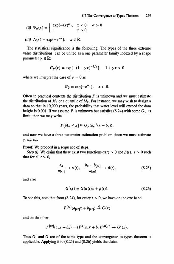
8. 7 The Convergence to Types Theorem 279
(ii) \lla(X) = { ~xp{-(x)a}, X< 0, X> 0,
(iii) A(x) = exp{-e-x}, x E R
a>O
The statistical significance is the following. The types of the three extreme value distributions can be united as a one parameter family indexed by a shape parameter y e IR:
Gy(x) = exp{-(1 + yx)-l/r}, 1 + yx > 0
where we interpret the case of y = 0 as
Go= exp{-e-x}, x e JR.
Often in practical contexts the distribution F is unknown and we must estimate the distribution of Mn or a quantile of Mn. For instance, we may wish to design a dam so that in 10,000 years, the probability that water level will exceed the dam height is 0.001. If we assume F is unknown but satisfies (8.24) with some Gy as limit, then we may write
and now we have a three parameter estimation problem since we must estimate y, an. bn.
Proof. We proceed in a sequence of steps. Step (i). We claim that there exist two functions a(t) > 0 and {J(t), t > 0 such
that for all t > 0,
and also
an ---. a(t), bn - b[nt) __. fJ(t),
a(nr) a(nr)
G 1 (x) = G(a(t)x + fJ(t)).
(8.25)
(8.26)
To see this, note that from (8.24), for every t > 0, we have on the one hand
and on the other
Thus G1 and G are of the same type and the convergence to types theorem is applicable. Applying it to (8.25) and (8.26) yields the claim.

280 8. Convergence in Distribution
Step (ii). We observe that the function a(t) and fJ(t) are Lebesgue measurable. For instance, to prove a(·) is measurable, it suffices (since limits of measurable functions are measurable) to show that the function
is measurable for each n. Since an does not depend on t, the previous statement is true if the function
t t-+ a(nt]
is measurable. Since this function has a countable range {a j, j ::: 1} it suffices to show
{t > 0: a(nt] =a j}
is measurable. But this set equals
which, being a union of intervals, is certainly a measurable set. Step (iii). Facts about the Hamel Equation. We need to use facts about possi
ble solutions of functional equations called Hamel's equation and Cauchy's equation. If f (x), x > 0 is finite, measurable and real valued and satisfies the Cauchy equation
f(x + y) = f(x) + f(y), x > O,y > 0,
then f is necessarily of the form
f(x) =ex, x > 0,
for some c E JR. A variant of this is Hamel's equation. If cp(x), x > 0 is finite, measurable, real valued and satisfies Hamel's equation
cp(xy) = ¢(x)¢(y), x > 0, y > 0,
then ¢ is of the form
for some p E JR. Step (iv). Another useful fact. IfF is a non-degenerate distribution function and
F(ax +b)= F(cx +d) Vx E IR,
for some a > 0, and c > 0, then a = c, and b = d. A proof of this is waiting for you in the exercises (Exercise 6).

8.7 The Convergence to Types Theorem 281
Step (v). Now we claim that the functions a(·) and /3(·) satisfy (t > 0, s > 0)
a(ts) = a(t)a(s),
f3(ts) = a(t)f3(s) + f3(t)
= a(s)f3(t) + f3(s),
the last line following by symmetry. To verify these assertions we use
G 1(x) = G(a(t)x + ,8(t))
to conclude that
G(a(ts)x + ,8(ts)) = G 15 (x) = (G5 (x)) 1
= (G(a(s)x + ,8(s)))1
= G(a(t)[a(s)x + ,8(s)] + f3(t))
= G(a(t)a(s)x + a(t)f3(s) + f3(t)) .
Now apply Step (iv).
(8.27)
(8.28)
(8.29)
Step (vi). Now we prove that there exists() e lR such that a(t) = t 9 . If() = 0, then f3(t) = c logt, for some c e JR. If() "# 0, then {3(t) = c(1- t9 ), for some c E lit
Proof of (vi): Since a(·) satisfies the Hamel equation, a(t) = t 9 for some () e JR. If() = 0, then a(t) = 1 and f3(t) satisfies
,8(ts) = {3(s) + f3(t).
So exp{,B(·)} satisfies the Hamel equation which implies that
exp{,8(t)} = tc,
for some c e lR and thus {3(t) = clogt .
If () "# 0, then
f3(ts) = a(t),B(s) + ,8(t) = a(s)f3(t) + f3(s).
Fix so "# 1 and we get
a(t)f3(so) + ,8(t) = a(so)f3(t) + ,8(so),
and solving for ,8(t) we get
f3(t)(1 - a(so)) = ,8(so)(l - a(t)).
Note that 1 - a(so) "# 0. Thus we conclude
( ,8(so) ) 9 f3(t) = (1 - a(t)) = : c(1- t ) .
1 - a(so)

282 8. Convergence in Distribution
Step (vii). We conclude that either
(a) G1(x)=G(x+clogt), (0=0),
or
Now we show that 0 = 0 corresponds to a limit distribution of type A (x ), that the case 0 > 0 corresponds to a limit distribution of type <l>a and that 0 < 0 corresponds to \f1 a.
Consider the case 0 = 0. Examine the equation in (a): For fixed x, the function G1 (x) is non-increasing in t. Soc < 0, since otherwise the right side of (a) would not be decreasing. If xo e lR such that G (xo) = 1, then
1 = G1 (xo) = G(xo + clogt), Vt > 0,
which implies
G(y) = 1, Vy E IR,
and this contradicts G non-degenerate. If xo e lR such that G(xo) = 0, then
0 = G 1 (xo) = G(xo + clogt), Vt > 0,
which implies
G(x) = 0, Vx E IR,
again giving a contradiction. We conclude 0 < G(y) < 1, for ally e JR. In (a), set x = 0 and set G (0) = e-K. Then
e-tK = G(clogt).
Set y = c logt, and we get
G(y) = exp{-Keyfc} = exp{-e-<fcr-logK)}
which is the type of A (x). The other cases 0 > 0 and 0 < 0 are handled similarly. 0
8.8 Exercises
1. Let Sn have a binomial distribution with parameters nand 0 E [0, 1). What CLT does Sn satisfy? In statistical terms, 0 := Sn In is an estimator of 0 and
Sn- E(Sn)
JVar(Sn)
is an approximate pivot for the parameter 9. If
g(9) = log (-9-) 1-9
8.8 Exercises 283
is the log-odds ratio, we would use g(O) to estimate g(O). What CLT does g(B) satisfy? Use the delta method.
2. Suppose {X n, n ;::: 1} is a sequence of random variables satisfying
1 P[Xn=n]=-,
n 1
P[Xn = 0] = 1- - . n
(a) Does {Xn} converge in probability? If so, to what? Why?
(b) Does {Xn} converge in distribution? If so, to what? Why?
(c) Suppose in addition that {Xn} is an independent sequence. Does {Xn} converge almost surely? What is
lim sup X n and lim inf X n n ..... oo n ..... oo
almost surely? Explain your answer.
3. Suppose fUn, n 2: 1} are iid U(O, 1) random variables so that
P[Uj ::;x]=x, O::;x::; 1.
(a) Show nj=1 uyn converges almost surely. What is the limit?
(b) Center and scale the sequence tnj=1 uJin, n ;::: 1} and show the resulting sequence converges in distribution to a non-degenerate limit. To which one?
4. (a) Let {Xn , n 2: 0} be positive integer valued random variables. Prove
Xn => Xo
iff for every k ;::: 0 P[Xn = k]--+ P[Xo = k].
(b) Let {Xn} be a sequence of random vectors on JRd such that Xn has a discrete distribution having only points with integer components as possible values. Let X be another such random vector. Show
Xn =>X

284 8. Convergence in Distribution
iff L IP[Xn = x)- P[X = x)l ~ 0
X
as n ~ oo. (Use Scheffcrs lemma.)
(c) For events {An, n ~ 0}, prove
(d) Let Fn concentrate all mass at Xn for n ~ 0. Prove
Fn::::} Fo iffxn ~ xo.
(e) Let Xn = 1 - 1/n or 1 + 1/n each with probability 1/2 and suppose P[X = 1) = 1. Show Xn ::::} X but that the mass function fn(X) of Xn does not converge for any x.
5. (a) If Un(x) , x E lR are non-decreasing functions for each n and un(X) ~ uo(x) and uoO is continuous, then for any -oo <a < b < oo
sup lun(x)- uo(x)l ~ 0. xe(a ,b)
Thus, convergence of monotone functions to a continuous limit implies local uniform convergence.
(b) Suppose Fn, n ::: 0 are proper df's and Fn ::::} Fo. If Fo is continuous, show
sup IFn(x)- Fo(x)l ~ 0. xeiR.
For instance, in the central limit theorem, where Fo is the normal distribution, convergence is always uniform.
(c) Give a simple proof of the Glivenko-Cantelli lemma under the additional hypothesis that the underlying distribution is continuous.
6. Let F be a non-degenerate df and suppose for a > 0, c > 0 and b e JR, d E JR, that for all x
F(ax +b)= F(cx +d).
Prove that a= c and b =d. Do this 2 ways:
(i) Considering inverse functions.
(ii) Showing it is enough to prove F(Ax +B) = F(x) for all x implies A = 1, and B = 17 (just kidding, B = 0). If T x = Ax + B then iterate the relation F(Tx)=F(x) again and again.

8.8 Exercises 285
7. Let {Xn. n ~ 1} be iid with E(Xn) = JL, Var(Xn) = a 2 and suppose N is a N(O, 1) random variable. Show
J;i(X~ - JL2) =? 2JLa N
Jn(ei• -ell) =?a ell N .
8. Suppose X 1, . . . , X n are iid exponentially distributed with mean 1. Let
X1,n < · · · < Xn,n
be the order statistics. Fix an integer I and show
nX1,n =? Y1
where Y1 has a gamma(/, 1) distribution.
(a)
(b)
Try doing this (a) in a straightforward way by brute force and then (b) try using the Renyi representation for the spacings of order statistics from the exponential density. See Exercise 32 on page 116.
9. Let {Xn , n ~ 0} be random variables. Show Xn =? Xo iff E(g(Xn)) ~ E(g(Xo)) for all continuous functions g with compact support.
10. Let X and Y be independent Bernoulli random variables on a probability
space (Q, B, P) with X~ Y and
1 P[X = 0] =- = P[X = 1].
2
Let Xn = Y for n ~ 1. Show that
Xn =?X
but that Xn does NOT converge in probability to X.
11. Levy metric. For two probability distributions F , G, define
d(F, G) := inf{o > 0 : Vx E IR, F(x - o)- <5 ~ G(x) ~ F(x + <5) + <5}.
Show this is a metric on the space of probability distribution functions which metrizes weak convergence; that is, Fn =? Fo iff d(Fn . Fo) ~ 0.
12. Suppose Fn has density
In (x) = 11 -cos 2mr x, 0,
ifO ~X~ 1,
otherwise.
Show that Fn converges weakly to the uniform distribution on [0, 1] but that the densities In do not converge.

286 8. Convergence in Distribution
13. Suppose {Nn. n :::: 0} is a sequence of normal random variables. Show Nn =>No iff
E(Nn)--. E(No) and Var(Nn)--. Var(No).
Derive a comparable result for (a) Poisson random variables; (b) exponential random variables.
14. Consider the sphere in JRn of radius Jn and suppose Xn is uniformly distributed on the surface of this sphere. Show that the first component of Xn converges in distribution to a standard normal. Hint: If N; , i > 1 are iid N(O, 1) random variables, show
15. (Weissman) Suppose Yn. n :::: 1 are random variables such that there exist On > 0, bn E JR. and
P[Yn :S OnX + bn] __. G(x),
non-degenerate, and for each t > 0
P[Y[nt) :S OnX + bn] __. G,(x),
non-degenerate. Then there exists a(t) > 0, /3(t) E lR such that
G(x) = G1(a(t)x + a(t))
and a(t) = t8 • If() = 0, then f3(t) = c logt, and if() =1 0, then f3(t) = c(1- t 8 ).
16. Suppose {Xn. n :::: 1} are iid non-negative random variables and set Mn = v?=1X;, n :::: 1. Show that there exists a sequence on > 0 such that (x > 0)
lim P[Mn/On ::: x] = exp{-x-a}, x > 0, a > 0, n ..... oo
iff the regular variation condition holds:
I. P[Xt > tx] -a 1m =X ,
HOO P[Xt > t] X> 0.
In this case, what limit distribution exists for logMn? ForM;?
Verify (8.30) for the Cauchy density and the Pareto distribution?
(8.30)
17. If {Xn} are iid U(O, 1) random variables, find a non-degenerate limit distribution for Mn = v?=1X; under suitable normalization.

8.8 Exercises 287
18. Give an example of a sequence of discrete distributions that converge weakly to a limit distribution which possesses a density.
19. (Second continuous mapping theorem) Suppose that Xn ::::} Xo and that for n ::: 0, Xn : lR 1-+ lR are measurable. Define
E := {x: 3xn ~X butxn(Xn) fr xo(x)}.
Suppose E is measurable and P[Xo E E] = 0. Show Xn(Xn)::::} xo(Xo).
20. Suppose we have independent Bernoulli trials where the probability of success in a trial is p. Let Vp be the geometrically distributed number of trials needed to get the first success so that
P[vp ::: n] = (1 - p)n-I, n ::: 1.
Show asp~ 0 PVp::::} E,
where E is a unit exponential random variable.
21. Sampling with replacement. Let {Xn. n ::: 1} be iid and uniformly distributed on the set { 1, . . . , m} . In repeated sampling, let Vm be the time of the first coincidence; that is, the time when we first get a repeated outcome
Vm := inf{n::: 2: Xn E {XJ, . .. , Xn-d}.
Verify that
P[ Vm > n] = n 1 - :.:=.._ · n ( · 1) i=2 m
Show as m ~ oo that Vm/ J'iii::::} V
where P[v > x] = exp{-x2j2}, x > 0.
22. Sample median; more order statistics. Let U1, ... , Un be iid U (0, 1) random variables and consider the order statistics U1,n ~ U2,n ~ · · · ~ Un,n · When n is odd, the middle order statistic is the sample median. Show that
1 2(Un+I,2n+I- 2).J2;;
has a limit distribution. What is it? (Hint: Use Scheffe's lemma 8.2.1 page 253.)
23. Suppose {Xn. n::: 1} are iid random variables satisfying
E(Xn) = IJ-, Var(Xn) = a 2.
The central limit theorem is assumed known. Set Xn = I:?=l Xifn. Let N(O, 1) be a standard normal random variable. Prove

288 8. Convergence in Distribution
(i) Jn(i; - J.t. 2) ==? 2J.l.(T N (0, 1).
(ii) Jn(eXn - eil) ==? eil N(O, 1).
(iii) Jn(logXn -logJ.t.) ==? -/;N(O, 1), assuming J.l. '# 0.
Now assume additionally that E (X1) < oo and prove
(iv) Jn (tog(~ E?=t (X;- Xn)2) -loga2) ==? -:rJ E(X1)N(O, 1).
(v) Define the sample variance
2 1 ~ - 2 Sn =- L...)X; -Xn).
n i=l
Show
Jn</Si- a)=* 2~ j E(Xt)N(O, 1).
What is a limit law for s;? 24. Show that the normal type is closed under convolution. In other words, if
Nt. N2 are two independent normally distributed random variables, show that Nt + N2 is also normally distributed. Prove a similar statement for the Poisson and Cauchy types.
Is a similar statement true for the exponential type?
25. (i) Suppose F is a distribution function and u is a bounded continuous function on lit Define the convolution transform as
F * u(t) = L u(t- y)F(dy).
Let {Fn. n ::: 0} be a sequence of probability distribution functions. Let C[-oo, oo] be the class of bounded, continuous functions on lR with finite limits existing at ±oo. Prove that Fn ==? Fo iff for each u e C[ -00, oo ], Un := Fn * u converges uniformly to a limit U. In this case, U = Fo * u.
(ii) Suppose X is a random variable and set Fn(X) = P[Xjn ::5 x] . Prove Fn * u --+ u uniformly.
(iii) Specialize (ii) to the case where F is the standard normal distribution and verify the approximation lemma: Given any € > 0 and any u e C[ -oo, oo ], there exists an infinitely differentiable v E C[ -oo, oo] such that
sup lv(x)- u(x)l < € . xeiR
(iv) Suppose that u(x , y) is a function on JR2 vanishing at the infinities. Then u can be approximated uniformly by finite linear combinations

8.8 Exercises 289
Lk Ck8k(x)hk(Y} with infinitely differentiable gt, hk . (Hint: Use normal distributions.)
(v) Suppose Fn is discrete with equal atoms at -n, 0, n. What is the vague limit of Fn as n -+ oo? What is the vague limit of Fn * Fn?
(vi) Suppose Fn concentrates all mass at 1/n and u(x) = sin(x2). Then Fn * u converges pointwise but not uniformly. (Is u e C[ -oo, oo ]?)
26. Suppose {X n, n ::: 1} are iid random variables with common distribution F and set Sn = E7=1 X;. Assume that there exist an > 0, bn E JR. such that
where Y has a non-degenerate proper distribution. Use the convergence to types theorem to show that
(Symmetrize to remove bn. You may want to first consider a2n!an.)
27. Suppose {Xn, n ::: 1} are iid and non-negative random variables with common density I (x) satisfying
>.. :=lim l(t) > 0. t.j.O
Shown 1\7=1 X; has a limit distribution. (This is extreme value theory, but for minima not maxima.)
28. Let x e (0, 1) have binary expansion
Set
00 d X= L:2:.
n=l
ln(X) = 12' 1,
if dn = 0,
if dn = 1.
Then show J~ ln(x)dx = 1 so that In is a density. The sequence In only converges on a set of Lebesgue measure 0. If X n is a random variable with density In then Xn => U, where U is U(O, 1).
29. Suppose {X1, t ::: 0} is a family of random variables parameterized by a continuous variable t and assume there exist normalizing constants a(t) > 0, b(t) e JR. such that as t -+ oo
x,- b(t) a(t) => Y,

290 8. Convergence in Distribution
where Y is non-degenerate. Show the normalizing functions can always be assumed continuous; that is, there exist continuous functions a(t) > 0, f3(t) e lR such that
Xt- {3(t) => Y', a(t)
where Y' has a non-degenerate distribution. (Hint: The convergence to types theorem provides normalizing constants which can be smoothed by integration.)
30. Suppose {Xn, n ;::: 1} are random variables and there exist normalizing constants On > 0, bn E lR such that
Xn -bn y ---=> '
On
where Y is non-degenerate. Assume further that for 8 > 0
sup£ n n < 00. (I X - b 12+.5) n~l On
Show the mean and standard deviation can be used for centering and scaling:
Xn- E(Xn) Y' => ' .jVar(Xn)
where Y is non-degenerate.
It is enough for moment generating functions to converge:
E(eya;; 1<Xn-bn)) => E(eYY),
for y E I, an open interval containing 0.
31. If Xn => Xo and sup£(1Xnl2+8) < 00,
n
show that E(Xn)- E(Xo), Var(Xn)- Var(Xo).
(Use Baby Skorohod and uniform integrability.)
32. Given random variables {Xn} such that 0::: Xn ::: 1. Suppose for all x E
(0, 1) P[Xn ::: x]- 1- p.
Show X n => B where B is a Bernoulli random variable with success probability p.
33. Verify that a continuous distribution function is always uniformly continuous.

8.8 Exercises 291
34. Suppose {En, n :::: 1} are iid unit exponential random variables. Recall from Example 8.1.2 that
n
V E; - log n => Y, i=l
where Y has a Gumbel distribution.
Let { Wn, n :::: 1} be iid Weibull random variables satisfying
P[Wn > X] = e-xa' a > 0, X > 0.
Use the delta method to derive a weak limit theorem for v7=l W;. (Hint: Express W; as a function of E; which then requires that vj=1 W; is a function
of V7=1E;.)
35. Suppose {Fn, n :::: 0} are probability distributions such that Fn => Fo. For t > 0, let u1(-) : lR ~---+ lR be an equicontinuous family of functions that are uniformly bounded; that is
sup u1 (x) :S: M, t>O,xe!R
for some constant M. Then show
lim { Ur(x)Fn(dx) = { Ur(x)Fo(dx), n-+oo }IR }IR
uniformly in t.
36. Suppose Fn => Fo and g :::: 0 is continuous and satisfies fiR gdFn = 1 for all n :::: 0. Define the new measure Gn(A) = fA gdFn. Show Gn => Go. (You can either do this directly or use Scheffe's lemma.)

S.I. Resnick, A Probability Path, Modern Birkhäuser Classics,ss Media New York 2014 DOI 10.1007/978-0-8176-8409-9_9, © Springer Science+Busine
293
9 Characteristic Functions and the Central Limit Theorem
This chapter develops a transform method called characteristic functions for dealing with sums of independent random variables. The basic problem is that the distribution of a sum of independent random variables is rather complex and hard to deal with. If Xt. Xz are independent random variables with distributions Ft. Fz, set
g(u, v) = 1(-oo,rJ(U + v).
Then using the transformation theorem and Fubini's theorem (Theorems 5.5.1 and 5.9.2), we get fort E lR
P[Xt + Xz::: t] = E(g(Xt. Xz))
(transformation theorem)
= I I {(x,y)eJR2:x+y:St} Ft X Fz
= f [j Ft (dx) ]Fz(dy) JIR {xelR:x:::;r-y}
= l Ft(t- y)Fz(dy)
=: Ft * Fz(t),
(Fubini's theorem)
where the last line defines the convolution between two distributions on the real line. Convolution is a fairly complex operation and somewhat difficult to deal with. Transform methods convert convolution of distributions into products of transforms and products are easier to handle than convolutions.

294 9. Characteristic Functions and the Central Limit Theorem
The next section reviews the relation between transforms and the central limit theorem.
9.1 Review of Moment Generating Functions and the Central Limit Theorem
The moment generating function (mgt) F(t) of a random variable X with distribution F exists if
F(t) := Ee1x = L e1x F(dx) < oo, Vt e I,
where I is an interval containing 0 in its interior. The problem with using the mgf of a distribution is that it does not always exist. For instance, the mgf of the Cauchy distribution does not exist and in fact existence of the mgf is equivalent to the tail of the distribution of X being exponentially bounded:
P[IXI > x] ~ Ke-cx, for some K > 0 and c > 0.
(So what do we do if the mgf does not exist?) The mgf, if it exists, uniquely determines the distribution of X, and we hope
that we can relate convergence in distribution to convergence of the transforms; that is, we hope X n =? X if
where I is a neighborhood of 0. This allows us to think about the central limit theorem in terms of transforms as follows.
Suppose {Xn, n 2::: 1} is an iid sequence ofrandom variables satisfying
Suppose the mgf of X; exists. Then
n =En etX;/Jn = (EetXt!Jnr
i=l
= (F<t!Jn>t
and expanding in a Taylor series about 0, we get

9.2 Characteristic Functions: Definition and First Properties 295
where "junk" represents the remainder in the expansion which we will not worry about now. Hence, as n -+ oo, if we can neglect "junk" we get
which is the mgf of a N (0, a 2) random variable. Thus we hope that
Sn 2 Jn ~ N(O,a ).
How do we justify all this rigorously? Here is the program.
1. We first need to replace the mgf by the characteristic function ( chf) which is a more robust transform. It always exists and shares many of the algebraic advantages of the mgf.
2. We need to examine the properties of chf and feel comfortable with this transform.
3. We need to understand the connection between moments of the distribution and expansions of the chf.
4. We need to prove uniqueness; that is that the chf uniquely determines the distribution.
5. We need a test for weak convergence using chf's. This is called the continuity theorem.
6. We need to prove the CLT for the iid case.
7. We need to prove the CLT for independent, non-identically distributed random variables.
This is the program. Now for the details.
9.2 Characteristic Functions: Definition and First Properties
We begin with the definition.
Definition 9.2.1 The characteristic function ( chf) of a random variable X with distribution F is the complex valued function of a real variable t defined by
</>(t) := EeitX, t E R
= E(cos(tX)) + iE(sin(tX))
= L cos(tx)F(dx) + i L sin(tx)F(dx) .

296 9. Characteristic Functions and the Central Limit Theorem
A big advantage of the chf as a transform is that it always exists:
Note that
IE(U + iV)i 2 = IE(U) + iE(V)i 2 = (EU)2 + (EV)2
and applying the Schwartz Inequality we get that this is bounded above by
~ E(U2) + E(V2) = E(U2 + V2)
= EIU +iVI2•
We now list some elementary properties of chf's.
1. The chf ¢(t) is uniformly continuous on R For any t e !R, we have
l¢(t +h)- ¢(t)l = IEei<t+h)X- EeitX I
= IEeitX (eihX - 1)1
~ EieihX -11 ~ 0
as h .J.. 0 by the dominated convergence theorem. Note that the upper bound is independent oft which accounts for the uniform continuity.
2. The chfsatisfies l¢(t)l ~ 1 and ¢(0) = 1.
3. The effect on the chf of scaling and centering of the random variable is given by
Eeit(aX+b) = ¢(at)eibt.
4. Let {iJ(t) be the complex conjugate of ¢(t). Then
5. We have that
¢(-t) = {iJ(t) = Re(¢(t))- ilm(¢(t))
= chfof -X.
Re(¢(t)) = j cos(tx)F(dx)
is an even function, while
lm(¢(t)) = j sin(tx)F(dx)
is an odd function.

9.3 Expansions 297
6. The chf t/J is real iff d
X=-X
iff F is a symmetric function. This follows since t/J is real iff t/J = ~ iff X and -X have the same chf. As we will see (anticipating the uniqueness
theorem), this implies X 4 -X.
7. If X; has chf t/J;, i = 1, 2 and X 1 and X 2 are independent, then the chf of X 1 + X 2 is the product t/J1 ( t )t/J2 ( t) since
Eeit(X1+X2> = EeitX1eitX2
= EeitX1EeitX2.
Compare this with the definition of convolution at the beginning of the chapter.
8. We generalize the previous property in a direction useful for the central limit theorem by noting that if XI> ... , Xn are iid with common chf t/J, then
9.3 Expansions
The CLT is dependent on good expansions of the chf t/J. These in tum depend on good expansions of eix so we first take this up.
9.3.1 Expansion of eix
Start with an integration by parts. For n ~ 0 we have the following identity:
t eis(x- s)nds = xn+1 + _i- t (x- s)n+leisds. lo n + 1 n + 1 lo (9.1)
For n = 0, (9.1) gives
lox . eix _ 1 lox .
e15ds = -.- = x + i (x- s)e15ds . 0 l 0
So we have

298 9. Characteristic Functions and the Central Limit Theorem
(from (9.1) with n = 1)
(ix)2 i3 x3 i 1x . =1+ix+--+-[-+- (x-s)3e'5 ds]
2 2 3 3 0
where the last expression before the vertical dots comes from applying (9.1) with n = 2. In general, we get for n ::: 0 and x e IR,
(9.2)
Thus
. n (ix)k lxln+l le'x ~ k! I::; -(n_+_1-)! (9.3)
where we have used the fact that leix I = 1. Therefore we conclude that chopping the expansion of eix after a finite number of terms gives an error bounded by the modulus of the first neglected term.
Now write (9.1) with n - 1 in place of nand transpose to get
If we multiply through by (n~l)! and interchange left and right sides of the equation, we obtain
-- (x- s)ne15ds = (x- s)n-1e'5ds- --. in+l lox . in lox . (ix)n
n! o (n - 1)! o n!
Substitute this in the right side of (9.2) and we get
ix ~ lX l ( )n-1 isd lX n ( · )k ·n 1x ( · )n
e -L..,--= x-s e s---k=O k! (n - 1)! 0 n! '
and thus
ix n (ix)k lxln lxln 21xln le -~-1<-+-=-. L.., k' - n' n' n' k=O • • • •
(9.4)
Combining (9.3) and (9.4) gives
ix n (ix)k lxln+l 21xln le - ~k!l::; (n+1)! "--;;!· (9.5)

9.3 Expansions 299
Note that the first term in the minimum gives a better estimate for small x, while the second term gives a better estimate for large x.
Now suppose that X is a random variable whose first n absolute moments are
finite: E(IXI) < oo, ... , E(!X!n) < oo.
Then
and applying (9.5) with x replaced by tX, we get
n (it)k ( !tX!n+l 2!tX!n) l<t><t)- L -, E(Xk)! ~ E '1\ -,- .
k=O k. (n + 1). n. (9.6)
Next, suppose all moments exist and that for all t E lR
lim ltlnE(IXIn) =O. n-+oo n!
(9.7)
In (9.6), let n ~ oo to get
A sufficient condition for (9.7) is
(9.8)
which holds if \ll(t) = Ee1x < oo, Yt E IR;
that is, if the mgf exists on all of JR. (To check this last statement, note that if Ee1X < oo for all t, we have
£elt11XI = E(eltiX l[X>OJ) + E(e-lt iX l[X<OJ)
~ \ll(ltl) + \11(-ltl) < 00.
This verifies the assertion.)

300 9. Characteristic Functions and the Central Limit Theorem
Example 9.3.1 Let X be a random variable with N(O, 1) distribution. For any t E R,
Ee'x = e'" --du ioo e-u2;2
-00 ../2i = -- exp{--(u2 - 2tu + t2)}du e' 12 ioo 1 1 2
-00 ../2i 2
(from completing the square)
r2;2 e d ioo -!<u-t)2
=e u -00 ../2i
2 ~00 2 = e' 12 n(t, 1, u)du = e' 12. -00
Here, n(t, 1, u) represents the normal density with meant and variance 1 which integrates to 1. Thus we conclude that for all t E R
Ee'x < oo.
We may therefore expand the mgf as well as e'2 12 to get
that is,
Equating coefficients yields that the
E(X2n) e)n coefficient of t2n = = -2-
(2n)! n!
So we conclude that
Thus, since

9.4 Moments and Derivatives 301
we get
(9.9)
This shows one way of computing the chf of the N(O, 1) distribution.
Note that the chf of the normal density has the property that the chf and the density are the same, apart from multiplicative constants. This is a useful and unusual feature.
9.4 Moments and Derivatives
When the kth absolute moment of a random variable exists, it can be computed by taking k-fold derivatives of the chf.
Suppose X is a random variable with finite first absolute moment; that is, E(IXD < oo. Then
.;._'f' ___ -'-'f'-'--- E(iXe11x) = E "'(t +h)_ "'(t) . (ei(t+h)X _ eitX _ ihX eitX)
h h
- E (it X {eihX - 1 - ihX}) - h 0
Apply (9.4) with n = 1 to get
eihX 1 ihX leitXI I - h- I ::S 21XI E Lt .
Since by (9.3) or (9.5) we have
eihX -1- ihX h2X 2 X 2
I h I ::s 2h = hT--+ o
as h .J.. 0, we get by dominated convergence that
~irJ ( q,(t + h~- q,(t) - E(iXeitX))
= E (lim eitX (ihX - 1 - ihX )) h~O h
=0.

302 9. Characteristic Functions and the Central Limit Theorem
Thus
¢'(t) = E(iXeitX). (9.10)
In general, we have that if E(IXIk) < oo,
¢(k)(t) = E ((iXleitX), Vt E I. (9.11)
and hence
9.5 Two Big Theorems: Uniqueness and Continuity
We seek to prove the central limit theorem. Our program for doing this is to show that the chf of centered and scaled sums of independent random variables converges as the sample size increases to the chf of the N (0, 1) distribution which we know from Example 9.3.1 is exp{-t2 /2}. To make this method work, we need to know that the chf uniquely determines the distribution and that when chf's of distributions converge, their distributions converge weakly. The goal of this section is to prove these two facts.
Theorem 9.5.1 (Uniqueness Theorem) The chf of a probability distribution uniquely determines the probability distribution.
Proof. We use the fact that the chf and density of the normal distribution are the same apart from multiplicative constants.
Let X be a random variable with distribution F and chf ¢. We show that ¢ determines F. For any distribution G with chf y and any real () E JR., we have by applying Fubini 's theorem the Parseval relation
f e-iBy¢(y)G(dy) = f e-iBy[l eiyx F(dx)]G(dy) JJR J yeJR xeJR
=I I JR2 eiy(x-9) F(dx)G(dy)
= 1 [ { ei<x-B)YG(dy)]F(dx) (9.12) xeJR }yeJR
= 1 y(x - O)F(dx) . (9.13) xeJR
Now let N have a N (0, 1) distribution with density n (x) so that aN has a normal density with variance a 2• Replace G(dy) by this normal density u-1n(a-1y) . Mter changing variables on the left side and taking account of the form of the normal chf y given by (9.9) on the right side, we get
{ e-iBuy¢(ay)n(y)dy = 1 e-u2(z-B)212F(dz) . (9.14) JJR zeJR

9.5 1\vo Big Theorems: Uniqueness and Continuity 303
Now, integrate both sides of (9.14) over(} from -oo to x to get
t { e-iOuy¢(ay)n(y)dyd9 = t 1 e-u2(z-0)2/2F(dz)d9, Jo=-oo JR Jo=-oo zeR
and using Fubini's theorem to reverse the order of integration on the right side yields
In the inner integral on the right side, make the change of variable s = (} - z to get
Divide through by ,Jiiia-1. Let a ---+ oo. Given the chf ¢,we find
lim ~ r r e-iOuy¢(ay)n(y)dyd(} u->oo v 2rr lo=-oo JR
= lim P[a-1 N +X:::: x] = F(x), Vx e C(F), (9.15) U->00
by Slutsky's theorem 8.6.1 of Chapter 8. So for any x e C(F), ¢determines F(x) which is sufficient for proving the result. D
A quick corollary gives Fourier inversion.
Corollary 9.5.1 Suppose F is a probability distribution with an integrable chf ¢; that is, 1¢1 E L1 so that L l¢(t)ldt < 00.
Then F has a bounded continuous density f given by
/(X)=- e-IYX¢(y)dy. 1 1m . 2rr R
Proof. Examine (9.15). Note
P[a-1 N +X::; x] =: Fu(x)

304 9. Characteristic Functions and the Central Limit Theorem
has a density fu since a-1 N has a density. From the left side of (9.15),
Note that
and as a~ oo
fu(B) = ~ { e-iOyt/J(y)n(a- 1y)dy v2Jr )~,
=- e-' YtfJ(y)e-u Y dy. 1 i ·o -2 2;z 2Jr I.
So by dominated convergence, fu (B) ~ f(B) . Furthermore, for any finite interval I
sup fu(B) ~ -21 { lt/J(y)le- u-lyl;zdy Bel 7r }~,
~ _.!.._ { lt/J(y)ldy < 00. 2Jr )~,
So as a ~ oo, we have by Slutsky's theorem 8.6.1 and bounded convergence
F(l)= lim P[a-1N+Xel]= lim [fu(O)dO=[f(O)dO. U-+00 U-+00 I I
Thus f is the density of F . 0
We now state and prove the continuity theorem which allows the conclusion of weak convergence of probability distributions from pointwise convergence of their chf's.
Theorem 9.5.2 (Continuity Theorem) (i) Easy part: We let {Xn, n ~ 1} be a sequence of random variables with X n having distribution Fn and chf tPn· If as n ~ oo we have
then
t/Jn(t) ~ t/Jo(t), 'r/t E JR.
(ii) Deeper part: Suppose
(a) limn-+oo t/Jn(t) exists for all t. Call the limit t/J00 (t).
(b) t/J00 (t) is continuous at 0.

9.5 Two Big Theorems: Uniqueness and Continuity 305
Then for some distribution function F 00,
Fn::} Foo
and t/>00 is the chf of F00• If t/>00 (0) = 1, then F00 is proper.
Proof of the easy part (i). If X n =? X o, then by the continuous mapping theorem, we have eitXn =? eitXo and since leitXn I :;: 1, we have by dominated convergence that
t/>n(t) = EeitXn -+ EeitXo = t/>o(t) . 0
The proof of the harder part (ii) is given in the next section. We close this section with some simple but illustrative examples of the use of
the continuity theorem where we make use of the harder half to prove convergence.
Example 9.5.1 (WLLN) Suppose {Xn, n :::: 1} is iid with common chf t/>(t) and assume E(IXID < oo and E(XI) = f.J. . Then
p Snfn-+ f.J..
Since convergence in probability to a constant is equivalent to weak convergence to the constant, it suffices to show the chf of Sn In converges to the chf of f.J., namely eiJI.t . We have
(9.16)
The last equality needs justification, but suppose for the moment it is true; this would lead to
as desired. To justify the representation in (9.16), note from (9.6) with n = 1 that
t t (t2 IX1I2 t ) It/>(;;) -1- i;;JJ.I:;: E 2;;z- A 2;;1XII ,
so it suffices to show that
(9.17)
Bring the factor n inside the expectation. On the one hand
306 9. Characteristic Functions and the Central Limit Theorem
and on the other
as n --+ oo. So by dominated convergence, (9.17) follows as desired. 0
Example 9.5.2 (Poisson approximation to the binomial) Suppose the random variable Sn has binomial mass function so that
P[Sn = k] = G)lo- p)n-k, k = 0, .. . , n.
If p = p(n) --+ 0 as n --+ oo in such a way that np--+ ). > 0, then
Sn => PO(A.)
where the limit is a Poisson random variable with parameter A..
To verify this, we first calculate the chf of PO(A.). We have
00 -'A).k Eeit(PO('A)) = Leitk_e __
k=O k! 00
= e-'A L().eitl/k! = e-'Ae'Ae;, k=O
_ 'A(e;'-1) -e .
Recall we can represent a binomial random variable as a sum of iid Bernoulli random variables ;1. .. . , ;n where P[;l = 1] = p = 1- P[;l = 0]. So
EeitSn =(Eeit~~r = (1 - p+eitp)n
( np(eit 1))n =(1 + p(eit -1)r = 1 + n-
--+e'A<ei' -I> .
The limit is the chf of PO().) just computed. 0
The final example is a more sophisticated version of Example 9.5.2. In queueing theory, this example is often used to justify an assumption about traffic inputs being a Poisson process.
Example 9.5.3 Suppose we have a doubly indexed array of random variables such that for each n = 1, 2, ... , {;n ,k· k 2: 1} is a sequence of independent (but not necessarily identically distributed) Bernoulli random variables satisfying
P[;n,k = 1] = Pk(n) = 1- P[;n,k = 0], (9.18)

9.6 The Selection Theorem, Tightness, and Prohorov's theorem 307
V Pk(n) = : 8(n) -+ 0, n -+ oo, l~k~n
n n
(9.19)
LPk(n) = E(L~n.k)-+ A. E (0, oo), n-+ oo. (9.20) k=l k=l
Then n
L ~n .k => PO(A.). k=l
The proof is left to Exercise 13.
9.6 The Selection Theorem, Tightness, and Prohorov'stheorem
This section collects several important results on subsequential convergence of probability distributions and culminates with the rest of the proof of the continuity theorem.
9.6.1 The Selection Theorem
We seek to show that every infinite family of distributions contains a weakly convergent subseqence. We begin with a lemma.
Lemma 9.6.1 (Diagonalization) Given a sequence {a j , j ::: 1} of distinct real numbers and a family {unO. n ::: 1} of real functions from JR. r+ JR. there exists a subsequence {unk ( ·)} converging at each a j for every j . (Note that ±oo is an acceptable limit.)
Proof. The proof uses a diagonalization argument. There exists a subsequence {nk} such that {unk(al)} converges. We call this
{ui1>(·), k::: 1} so that {uk1>(al) , k::: 1} converges.
Now there exists a subsequence kj such that {uk1>(a2) , j ::: 1} converges. Call I
this subfamily of functions { u j2> ( ·), j ::: 1} so that
are both convergent. Now continue by induction: Construct a subsequence {ujn> (-) , j ::: 1} for each
n, which converges at an and is a subsequence of previous sequences so that

308 9. Characteristic Functions and the Central Limit Theorem
converges fori = 1, ... , n. Now consider the diagonal sequence of functions
For any ai {u~n) (ai ), n ::::: i} C {uj) (ai ), j ::::: i}
where the sequence on the right is convergent so
lim u~n)(ai) exists n-+oo
fori= 1, 2, ....
Remark. If lunOI ~ M for all n, then
lim lu(n)(ai)l ~ M. n-+oo n
0
Lemma 9.6.2 If D = {ai} is a countable dense subset of'R. and if {Fn} are df's such that
lim Fn(ai) exists n-+oo
for all i, then define
This determines a df F 00 on R and
Proof. Extend F00 toR by right continuity: Define for any x,
This makes F00 right continuous and monotone. Let x e C(F00). Since D is dense, there exist ai, a; e D such that
ai t X, a; .J, X,
and for every k and i
Take the limit on k:
F00 (ai) ~ liminfFk{x) ~ limsupFk(X) ~ F(a;). k-+oo k-+oo
Let ai t x and a; ..!.. x and use the fact that x e C(F00 ) to get
F00 (x) ~ liminfFk(X) ~ limsupFk(X) ~ F(x). k-+00 k-+00
We are now in a position to state and prove the Selection Theorem.
0

9.6 The Selection Theorem, Tightness, and Prohorov's theorem 309
Theorem 9.6.1 (Selection Theorem) Any sequence of probability distributions fFn} contains a weakly convergent subsequence (but the limit may be defective).
Proof. Let D = {a;} be countable and dense in JR. There exists a subsequence fFnk} such that
lim Fnk (a j) k-+00
exists for all j . Hence fFnk} converges weakly from Lemma 9.6.2. 0
9.6.2 Tightness, Relative Compactness, and Prohorov's theorem
How can we guarantee that subsequential limits of a sequence of distributions will be non-defective?
Example. Let Xn = n. If Fn is the df of Xn, then Xn -+ oo and so Fn(x) -+ 0 for all x.
Probability mass escapes to infinity. Tightness is a concept designed to prevent this. Let n be a family of non-defective probability df's.
Definition. n is a relatively compact family of distributions if every sequence of df's in n has a subsequence weakly converging to a proper limit; that is, if fFn} C n, there exists {nk} and a proper df Fo such that Fnk ==? Fo.
Definition. n is tight, if for all € > 0, there exists a compact set K C lR such that
F(K) > 1- €, \:IF en;
or equivalently, if for all € > 0, there exists a finite interval I such that
or equivalently, if for all € > 0, there exists Mf such that
Most of the mass is contained in a big interval for all the distributions. This prevents mass from slip sliding away to one of the infinities.
Random variables {Xn} whose df's {Fn} are tight are called stochastically bounded. This means, for every € > 0, there exists Mf such that
sup P[IXnl > Mf] < €. n
Prohorov's theorem shows the equivalence of relative compactness and tightness.
Theorem 9.6.2 (Prohorov's theorem) The family n of probability distributions is relatively compact iff n is tight.

310 9. Characteristic Functions and the Central Limit Theorem
Proof. Suppose n is tight. Let {Fn} c n. By the selection theorem 9.6.1, for some nk, we have Fnk ~ Foo. We must show F00 is proper. Given E > 0, there exists M such that
supFn([-M, M]c) <E. n
Pick M' > M such that M' e C(F00). Then
E > 1- Fn(M') + Fn(-M') ~ 1- Foo(M') + F00 (-M').
So F00 ([-M', M')c) < E, and therefore F00 ([-M', M')) > 1- E. Since this is true for all E, we have F00 (1R) = 1.
Conversely, if n is not tight, then there exists E > 0, such that for all M, there exists F e n such that F ([-M, M)) ~ 1 - E. So there exist { Fn} c n with the property that Fn ([ -n, n]) ~ 1 - E. There exists a convergent subsequence nk
such that Fnk ~ F00• For any a, bE C(F00),
[a, b) c [-n,n]
for large n, and so
So F00 (1R) ~ 1- E and F00 is not proper son is not relatively compact. 0
Here are common criteria for tightness: Let {X n} be random variables with df's {Fn}.
1. If there exists r > 0 such that
limsupE(IXnl') < oo n-.oo
then {Fn} is tight by Chebychev's inequality.
2. If {Xn} and {Yn} are two stochastically bounded sequences, then {Xn + Yn} is stochastically bounded. This follows from the inequality
P[IXn + Ynl > M) ~ P[IXnl > M/2] + P[IYnl > M/2].
3. If Fn concentrates on [a, b) for all n, then {Fn} is tight. So for example, if Un are identically distributed uniform random variables on (0, 1), then {cnUn} is stochastically bounded if ten} is bounded.
4. If Xn 4 anNn + Jl.n, where Nn are identically distributed N(O, 1) random variables, then {X n} is stochastically bounded if {an} and {J.J.n} are bounded.

9.6 The Selection Theorem, Tightness, and Prohorov's theorem 311
9.6.3 Proof of the Continuity Theorem
Before proving the rest of the continuity theorem, we discuss a method which relates distribution tails and chf's.
Lemma 9.6.3 IfF is a distribution with chf ¢, then there exists a E (0, oo) such that for all x > 0
-1
F([-x,xn:::: ax fox (1-Reif>(t))dt.
Proof. Since
Re if>(t) = £: costyF(dy) ,
we have
X r-1 (1- Re if>(t))dt =X r-1 100 (1- costy)F(dy)dt
lo lo -oo
which by Fubini is
-Xi: [f (1- costy)dt] F(dy)
1oo ( sinx-ly) = x -oo x-1 - y F(dy)
100 ( sinx-1y) = 1 - _1 F(dy).
-oo X y
Since the integrand is non-negative, this is greater than
where
{ (1- sin~;Iy) F(dy) }lyl>x X Y
:::: a-1F([-x,xn,
_ 1 . f smx y a = m 1- . (
. -1 )
lx- 1yl2:1 x-Iy 0
This is what is needed to proceed with the deferred proof of the continuity theorem.
Proof of the Continuity Theorem. Suppose for all t E IR, we have if>n(t) -if>00 (t) where ¢00 is continuous at 0. Then we assert {Fn} is tight. To understand

312 9. Characteristic Functions and the Central Limit Theorem
why tightness is present, assume M > 0 and apply Lemma 9.6.3:
M-1
limsupFn([-M, Mn::;:: lim sup aM { (1- Re <f>n(t))dt. n-+oo n-+oo Jo
Now <f>n(t) --+ <f>00 (t) implies that
Re <f>n (t) --+ Re ¢00 (t), 1 - Re <f>n (t) --+ 1 - Re ¢00 (t),
and since 1 - ¢n is bounded, so is Re (1 - ¢n) = (1 - Re ¢n). By dominated convergence,
M-1
limsupFn([-M, Mn :S: aM { (1- Re </>00 (t))dt. n-+00 lo
Since ¢00 is continuous at 0, lim,.....o</>00 (t) = </>00 (0) = limn-+oo<f>n(O) = 1 as t -+ 0. So 1 - Re </>00 (t) --+ 0 as t --+ 0, and thus for given f > 0 and M sufficiently large, we have
M-1 M-1
aM 1 (1 - Re ¢00 (t))dt :S: aM 1 fdt = a€.
Hence fFn} is tight. Since fFn} is tight, any two convergent subsequences of {Fn} must converge to the same limit, because if
Fn' => F, and Fn" => G,
then F and G are proper. So by part (i) of the continuity theorem already proved,
<f>n' --+ </> F = </>oo
and <f>n" --+ </>G = ¢oo'
and hence <f>F = <f>G· By the Uniqueness Theorem 9.5.1, F = G. Thus any two convergent subsequences converge to the same limit and hence {Fn} converges to a limit whose chf is ¢00 . 0
9.7 The Classical CLT for iid Random Variables
We now tum to the proof of the CLT for sums of iid random variables. If {X n} are iid random variables with finite mean E(Xn) = J1. and variance Var(Xn) = a 2,
we will show that as n --+ oo
""n X· - nu .L.i=l ,Jn .- => N(O, 1).
a n
The method will be to show that the chf of the left side converges to the standard normal chf e-12 12.
We begin with a lemma which allows us to compare products.

9.7 The Classical CLT for iid Random Variables 313
Lemma 9.7.1 (Product Comparison) Fori = 1, . .. , n, suppose that a; E C, b; E C, with Ia; I ~ 1 and lb; I ~ 1. Then
n n n Ina;- nbd::::: L:ia; -b;l. i=I i=I i=I
Proof. For n = 2, we merely have to write
Finish by taking absolute values and using the fact that the moduli of a; and b; are bounded by 1. For general n, use induction. 0
Theorem 9.7.1 (CLT for iid random variables) Let {Xn , n :::: 1} be iid random variables with E(Xn) = Jl and Var(Xn) = a 2. Suppose N is a random variable with N(O, 1) distribution. If Sn = Xt + · · · + Xn , then
Sn- nJL aJn ~ N .
Proof. Without loss of generality let E(Xn) = 0, E(X~) = 1, (otherwise prove the result for
and
Let
Then
X · - II
X':=-'-"" I (1
E(Xj) = 0, E(Xj)2 = 1.)
</Jn(t) = (EeitXIf..fo)n = </Jn(tj.J,i) .
Since the first two moments exist, we use (9.6) and expand¢:
( t ) itE(Xt) i2t 2E(X1)2 t2 <P r= = 1 + r= + 2 + o(-)
.yn .yn n n
r2 t2 = 1 + 0- 2n + o(-;;-) (9.21)
where
We claim that
no(t2/n)::::: E c~~: 1\ itXt12)--. 0, n--. oo. (9.22)

314 9. Characteristic Functions and the Central Limit Theorem
To see this, observe that on the one hand
and ltXtl3 I X 12 ltXt13 0 --1\t 1 x<--~ .jii3! - .jii3! '
as n ~ oo. So by dominated convergence
( ltXtl3 2) E Jii3! 1\ ltXtl ~ 0.
Now
(where we have applied the product comparison Lemma 9.7.1)
Since
the chf of the N (0, 1) distribution, the result follows. 0
9.8 The Lindeberg-Feller CLT
We now generalize the CLT for iid summands given in Section 9. 7 to the case where the summands are independent but not identically distributed.
Let {Xn, n 2:: 1} be independent (but not necessarily identically distributed) and suppose Xk has distribution Fk and chf ¢k. and that E(Xk) = 0, Var(Xk) = af. Define
n
s; = af +· ·· +a;= Var(LXi) . i=l
We say that {Xk} satisfies the Lindeberg condition if for all t > 0 as n ~ oo we have
(9.23)

9.8 The Lindeberg-Feller CLT 315
Remarks.
• The Lindeberg condition (9.23) says for each k, most of the mass of Xk is centered in an interval about the mean ( = 0) and this interval is small relative to Sn.
• The Lindeberg condition (9.23) implies
(9.24)
To see this, note that
So for any t > 0,
To finish the proof, let t ,!, 0. 0
• Condition (9.24) implies
(9.25)
by Chebychev's inequality. This condition (9.25) is called uniform asymptotic negligibility (UAN). It is typical in central limit theorems that the VAN condition holds so that no one summand dominates but each sumand contributes a small amount to the total.
We now state and prove the sufficiency part of the Lindeberg-Feller central limit theorem.
Theorem 9.8.1 (Lindeberg-Feller CLT) With the notation given at the beginning of this section, The Lindeberg condition (9.23) implies
Sn - => N(O, 1), Sn
where N (0, 1) is a normal random variable with mean 0 and variance 1.

316 9. Characteristic Functions and the Central Limit Theorem
Although we shall not prove it, the converse is true in the following sense. If
(i) vz=1af;s;--+ Oand
(ii) Sn/.fo =::} N(O , 1),
then the Lindeberg condition (9.23) holds.
Proof. We proceed in a series of steps. (1) We begin with a preliminary result. Suppose {Yn, n ::::; 1} is an iid se
quence of random variables with common distribution F and chf if> . Let N be independent of {Yk} and assume N is Poisson distributed with parameter c. Define Xn = L:?=t Y; . We compute the chf of XN as follows: FortE R,
00
E(eitXN) = LE(eitxN 1(N=kJ) k=O 00
= LE(eitxt1[N=kJ). k=O
and since N is independent of {Yk}, this equals
00
= LE(eitx*)P[N = k) k=O oo e-cck
= L:4>k<t>-k=0 k!
= e-cectf>(t) = ec{tf>{t)-1) .
We may also conclude that ec{tf>{t)-1)
must be a chf. (2) To show Sn/Sn =::} N(O, 1), we need to show that the chf of Sn/Sn satisfies
n
if>Snfsn(t) = n if>k(t/sn)--+ e-t2f2 = chfof N(O, 1). (9.26) k=l
This follows from the continuity theorem 9.5.2. We claim that (9.26) holds if
n
L (if>k(t/sn)- 1) + t 2 /2--+ 0 (9.27) k=l
because
n n 4
1 exp{L(if>k(t/sn)- 1)}-n 4>k(t/sn)l--+ o. (9.28) k=l k=l

9.8 The Lindeberg-Feller CLT 317
Thus, assuming (9.28) is true, it will suffice to prove (9.27). Here is the verification of (9.28). Recall that exp{¢k(t/sn)- 1} is a chf from
step (1) and hence bounded in modulus by 1. Then
n n
= n e¢k(tfsn)-1- n ¢k(tfsn) '
k=l k=l
and applying the product comparison lemma 9.7.1, we have the bound
n ::S L le¢k(tfsn)-1- ¢k(t/Sn)l
k=l n
= L le¢k(t/sn)-l- 1- (¢k(t/sn) -1)1. k=l
Note that for z e C,
oo zk oo lzl2 lez- 1- zl =I L 11 :=:: L lzlk = --
k=Z k. k=2 1 -lzl
:=:: 21zl2, if lzl :=:: ~·
:=:: 81zl, if lzl :=:: ~ < ~· (9.29)
Now for fixed t e JR., we apply (9.6) with n = 1 to get the inequalities
t2 1¢k(t/sn) -11 :=::2s2af (9.30)
n
t2 n a2 <- v -1· (9.31) - 2 k=l sn
Recall (9.24). We conclude from (9.31) that given 8 > 0, if n is sufficiently large, then fork= 1, ... , n
(9.32)
n n
I exp{L(¢k(t/sn)- 1)}- n ¢k(t/sn)l
k=l k=l n n
:=:: L lez* -1- Zkl :=:: l)lzkl k=l k=l

318 9. Characteristic Functions and the Central Limit Theorem
for n large, because v;:=11zk I ~ 8/2 for n large, and applying (9.30), we get the bound
and since 8 is arbitrary, we have (9.28) as desired. Thus it suffices to prove (9.27). (3) We now concentrate on proving (9.27). Write
n
I)t>k(tfsn)- 1) + t2 /2 k=l
~ ( itX js t 1 it 2 2) =~E e k n-1-i-Xk--(-)Xk . k=l Sn 2 Sn
Let 0 represent what is inside the expectation on the previous line. We get the decomposition
n
= L {E(•)l[IXkl/sn:::f) + £(·)11Xkl/sn>fJ} k=l
=I +II.
We now show I and I I are small. For I we have using (9.6) with n = 2:
where we used the fact that

9.8 The Lindeberg-Feller CLT 319
Now we show why I I is small. We have
(from (9.6) with n = 2)
by the Lindeberg condition (9.23). This completes the proof of (9.27) and hence the theorem is proved. 0
We next present a sufficient condition for the Lindeberg condition (9.23) called the Liapunov condition which is relatively easy to verify.
Corollary 9.8.1 (Liapunov Condition) Let {Xk, k 2: 1} be an independent sequence of random variables satisfying E(Xk) = 0, Var(Xk) = uf < oo, s; = Lk=l uf. /!for some 8 > 0
then the Lindeberg condition (9.23) holds and hence the CLT.
Remark. A useful special case of the Liapunov condition is when 8 = 1:
Proof. We have
0

320 9. Characteristic Functions and the Central Limit Theorem
Example: Record counts are asymptotically normal. We now to examine the weak limit behavior of the record count process. Suppose {Xn, n ::=:: 1} is an iid sequence of random variables with common continuous distribution F, and define
n
h = 1[Xk is a record)• f.ln = L 1k. i=l
So f.ln is the number of records among X 1, ... , X n. We know from Chapter 8 that asn ~ oo
Here we will prove
To check this, recall
Thus
So
Now
and therefore
f.ln a.s. 1 --~. logn
f.ln -logn ~ ::::}N(0,1). ylU~n
1 1 Var(h) = k- k2 .
Lk=l El1k- £(1k)l3 < Lk=l 0 + ~) sg - (log n )3/2
logn 0 (logn)3/2 ~ .

9.9 Exercises 321
So the Liapunov condition is valid and thus
J.ln- E(J..tn) => N(O, 1). JVar(J..tn)
Note Jvar(J..tn) "' sn "' jlog n
and E(J..tn) -logn _ Lk=tl-logn "'_Y_--+ 0
jlog n - Jlog n Jlog n '
where y is Euler's constant. So by the convergence to types theorem
J.ln -logn JiOiii" => N(O, 1). D
9. 9 Exercises
1. Triangular arrays. Suppose for each n, that {Xk.n. 1 :::: k :::: n} are independent and define Sn = Lk=l xk.n· Assume E(Xk.n) = 0 and Var(Sn) = 1,and
n
LE (1Xk,nl21(1xk.nl>t])--+ 0 k=l
as n --+ oo for every t > 0. Adapt the proof of the sufficiency part of the Lindeberg-Feller CLT to show Sn => N(O, 1).
2. Let {Xn, n ~ 0} be a sequence of random variables.
(a) Suppose {Xn. n ~ 0} are Poisson distributed random variables so that for n ~ 0 there exist constants An and
e-An)...k P[Xn=k]=--n, k~O.
k!
Compute the characteristic function and give necessary and sufficient conditions for
Xn => Xo.
(b) Suppose the {Xn} are each normally distributed and
E(Xn) = J.ln E R, Var(Xn) =a;.
Give necessary and sufficient conditions for
Xn => Xo.

322 9. Characteristic Functions and the Central Limit Theorem
3. Let {Xt. k ~ 1} be independent with the range of Xk equal to {±1, ±k} and
1 1 P[Xk = ±1] = 2(1- k2 ),
1 P[Xk = ±k] = 2k2 •
By simple truncation, prove that Sn I Jn behaves asymptotically in the same way as if Xk = ±1 with probability 1/2. Thus the distribution of Sn/Jn tends to N(O, 1) but
Var(Sn/Jn)--+ 2.
4. Let {Uk} be an independent sequence of random variables with Uk uniformly distributed on [ -ak, ak]·
(a) Show that if there exists M > 0 such that lakl .:5 M but Lk af = oo, then the Lindeberg condition and thus the CLT holds.
(b) If Lk af < oo, then the Lindeberg condition does not hold.
5. Suppose Xn and Yn are independent for each nand
Prove using characteristic functions that
Xn + Yn => Xo +Yo.
6. (a) Suppose Xn has a uniform distribution on ( -n, n). Find the chf of Xn.
(b) Show limn--..clO <Pn ( t) exists.
(c) Is there a proper, non-degenerate random variable Xo such that
Xn => Xo?
Why or why not? What does this say about the continuity theorem for characteristic functions?
7. Suppose {Xn, n:::: 1} are iid with common density
(a) Check that E(XI) = 0 but E(X;) = oo.
(b) Despite the alarming news in (a), we still have
r:::r:::::= => N (0, 1). v" •ve;n
Hint: Define

9.9 Exercises 323
and check Liapunov's condition for {Yn} for 8 = 1. Then show
L P[Xn #- Yn] < oo. n
(c) It turns out that for iid random variables {Xn} with E(Xn) = 0, the necessary and sufficient condition for the CLT is that
where
lim U(tx) = 1, HOO U(t)
U(t) := E(Xi1[1Xi1:9])·
Check this condition for the example in part (a).
8. Probabilistic proof of Stirling's formula. Suppose {Xn} are iid, Poisson distributed random variables with parameter 1 and as usual suppose Sn = L7=I X;. Prove the following:
(a) E -- =e L -- -=---[(Sn- n)-] -n n (n- k) nk nn+lf2e-n
.jn k=O .jn k! n!
(b) (S~n)- ~ N-,
where N is a N(0,1) random variable.
(c) Show
9. (a) Suppose X is exponentially distributed with density
f(x) =e-x, x > 0.
What is the chf of X? Is the function
1
1 +it
a chf? If so, of what random variable?
(b) Let X 1 be Bernoulli random variable with possible values ± 1 with probability 1/2 each. What is the chf of X 1?

324 9. Characteristic Functions and the Central Limit Theorem
(c) Is (cost)17 a chf? Of what random variable?
(d) Is I cos t I a chf? (Try differentiating twice.)
(e) Is I cost 12 a chf?
The modulus of a chf need not be a chf but the modulus square is a chf.
(f) Prove that if X is a random variable with E(IXI) < oo and with chf ¢, then
L 2 ioo 1-Re¢(t) lxiF(dx) = - 2 dt.
lR 7r 0 t
10. Suppose Ys is Poisson distributed with parameters so that
sk P[Ys =k)=e-s k!'
Compute the chf of Y5 • Prove
Ys -s Js :::} N,
where N is aN (0, 1) random variable.
11. If {Xn,n::: 1} is iid with E(Xn) = 0 and Var(Xn) = 1, then Sn/Jn:::} N (0, 1). Show this cannot be strengthened to Sn I Jn converges in proba-
bility. (If Sn/Jn ~X, then S2n!.fin ~X. Subtract.)
12. Suppose {Xn, n ::: 1} are independent and symmetric random variables so that
If for every t > 0, as n -+ oo
n
L P[IXkl >tan]-+ 0 k=I
n
a;;2 L E (Xf1[1Xkl9an)) -+ 1, k=l
where an > 0, then show
Snfan:::} N(O, 1).
Here Sn = L:?=t X;.
Hint: Try truncating at level ant: Set
Xj = Xj1[1Xil9an)·
ConsiderS~ and show it is enough for S~fan:::} N(O, 1).

9.9 Exercises 325
13. Prove the law of rare events stated in Example 9.5.3.
14. Assume ¢(t) is a chf and G is the distribution of a positive random variable Y . Show all of the following are chf's and interpret probabilistically:
(a) Jd ¢(ut)du,
(b) J000 ¢(ut)e- "du,
(c) fooo e-ltiuG(du),
(d) J000 ¢(ut)G(du) .
(For example, if X has chf ¢and U is uniform on (0, 1) and independent of X, what is the chf of XU?)
15. (i) Suppose {En , n .:=:: 1} are iid unit exponential random variables so that P(Et > x] = e-x, x > 0. Show <L.7=t £; - n)j Jn is asymptotically normal.
(ii) Now suppose X 1 is a random variable with gamma density
Use characteristic functions to show that
(X1 - t)/J'i ~ N
where N is a N(O, 1) random variable.
(iii) Show total variation convergence of the distribution of (X1 - t)j..[i to the distribution of N :
X1 - t sup IP[---;:; e B] - P[N e B]l ~ 0
BeB(IR) ...;t
as a ~ oo. (Hint: Use Scheffe; approximate r(t) via Stirling's formula.
16. (a) Suppose X andY are iid N(O, 1) random variables. Show
(b) Conversely: Suppose X andY are independent with common distribution function F(x) having mean zero and variance 1, and suppose further that
X+Y 4x4Y. ,fi
Show that both X andY have a N(O, 1) distribution. (Use the central limit theorem.)

326 9. Characteristic Functions and the Central Limit Theorem
17. (a) Give an example of a random variable Y such that E (Y) = 0 and
for all8 > 0. (This means finding a probability density.)
(b) Suppose {Yn, n ::: 1} are iid with EYt = 0, and EYf = a 2 < oo. Suppose the common distribution is the distribution found in (a). Show that Lindeberg's condition holds but Liapunov's condition fails.
18. Use the central limit theorem to evaluate
Hint: consider P[Sn < x] where Sn is a sum of n iid unit exponentially distributed random variables.
19. Suppose {en, n ::: 1} are independent exponentially distributed random variables with E(en) = J.Ln· If
n
I. v J.l.i 0 lm Ln = , n-+oo . · i=l j=l J.L J
then
20. Use the method of the selection theorem to prove the Arzela-Ascoli theorem: Let {un(x), n ::: 1} be an equicontinuous sequence of real valued functions defined on IR, which is uniformly bounded; that is, supn,x iun (x) I ~ 1. Then there exists a subsequence fun'} which is converging locally uniformly to continuous limit u.
21. (a) Suppose {FA, A e A} is a family of probability distributions and suppose the chf of FA is tPA· If {</JA , A E A} is equicontinuous, then {FA, A E A} is tight.
(b) If {Fn , n ::: 0} is a sequence of probability distributions such that Fn => Fo, then the corresponding chf's are equicontinuous. By the ArzelaAscoli theorem , uniformly bounded equicontinuous functions converge locally uniformly. Thus weak convergence of fFn} means the chf's converge locally uniformly.
22. A continuous function which is a pointwise limit of chf's is a chf. (Use the continuity theorem.)

9.9 Exercises 327
23. A complex valued function t/>(·) of a real variable is called non-negative definite if for every choice of integer n and reals It, .. . , tn and complex numbers c1 , ... , Cn, we have
n
L t/>(tr - fs)CrCs :=:: 0. r,s=l
Show that every chf is non-negative definite.
24. (a) Suppose K 0 is a complex valued function on the integers such that L~-oo IK(n)l < oo. Define
1 00
/(A)=- L e-in'-K(n) 2rr n=-oo
(9.33)
and show that
K(h) = r: eihx f(x)dx, h = 0, ±1, ±2,. . .. (9.34)
(b) Let {{Xn, n = 0, ±1, ±2, .. . } be a zero mean weakly stationary process. This means E (X m) = 0 for all m and
is independent of m. The function y is called the autocovariance (act) function of the process {X n} .
Prove the following: An absolutely summable complex valued function y ( ·) defined on the integers is the autocovariance function of a weakly stationary process iff
1 00 .
/('A)= 2rr L e-m'-y(n) 2: 0, for all)... e [-rr, rr], n=-oo
in which case
y(h) = r: eihx f(x)dx.
(Soy(·) is a chf.)
Hint: If y ( ·) is an acf, check that
N
/N(A) = 2: N L e-ir'-y(r- s)eisl. :=:: 0 r,s=l
and /N(A) -+ /(A) as N -+ oo. Use (9.34). Conversely, if y(·) is absolutely summable, use (9.34) to write y as a Fourier transform or chf of f .

328 9. Characteristic Functions and the Central Limit Theorem
Check that this makes y non-negative definite and thus there is a Gaussian process with this y as its acf.
(c) Suppose q
Xn = L &;Zn-i• i=O
where {Zn} are iid N(O, 1) random variables. Compute y(h) and /(A).
(d) Suppose {Xn} and {Yn} are two uncorrelated processes (which means E (X m Yn) = 0 for all m, n ), and that each has absolutely summable acfs. Compute y(h) and /(A) for {Xn + Ynl·
25. Show the chf of the uniform density on (a, b) is
eitb _ eita
it(b-a)·
If ¢(t) is the chf of the distribution F and ¢(t)(1- eith)/(ith) is integrable in t, show the inversion formula
1 loo (1- e-ith) . h-1F(x,x+h]=-2 lj)(t) . e-11xdt. rc -oo zth
Hint: Let U -h,O be the uniform distribution on ( -h, 0). What is the chf of F * U-h.o? The convolution has a density; what is it? Express this density using Fourier inversion (Corollary 9.5.1).
26. Why does the Fourier inversion formula for densities (Corollary 9.5.1) not apply to the uniform density?
27. Suppose for each n =::: 0 that l/Jn(t) is an integrable chf corresponding to a distribution Fn, which by Fourier inversion (Corollary 9.5.1) has a density fn. If as n ~ oo L: ll/Jn(t)- l/Jo(t)idt ~ 0,
then show fn ~ fo uniformly.
28. Show the chf of F(x) = 1 -e-x, x > 0 is 1/(1- it). If Et. £2 are iid with this distribution, then the symmetrized variable E 1 - E 2 has a bilateral exponential density. Show that the chf of £ 1 -£2 is 1/(1 + t 2).
Consider the Cauchy density
f(x) = ..!_ (-1- 2), X E JR. rc 1 +x
Note that apart from a constant, f (x) is the same as the chf of the bilateral exponential density. Use this fact to show the chf of the Cauchy density is lj)(t) = e-ltl. Verify that the convolution of two Cauchy densities, is a density of the same type.

9.9 Exercises 329
29. Triangle density. (a) Suppose Ua,b is the uniform distribution on (a, b). The distribution U(-1 ,0) * U(o,t) has a density called the triangle density. Show the chf of the triangle density is 2(1 - cos t)/t2. Verify that this chf is integrable.
Check that f(x) = (1- cosx)/(rrx2), x e JR.
is a probability density. Hint: Use (a) and Fourier inversion to show 1 -lxl is a chf. Set x = 0.
30. Suppose Ut. .. . , Un are iid U(O, 1) random variables. Use the uniqueness theorem to show that I:7=t U; has density
1 n . (n) f(x) = 1 2:<-1)1 . (x- j)~,
(n- 1). j=O J X> 0.
31. Suppose F is a probability distribution with chf ¢(t). Prove for all a > 0
loa 1 100 1- cos at . (F(x + u)- F(x- u))du =- 2 e-11x</J(t)dt,
0 7r -oo t
and
1a 1" 100 1- cos ax ljJ(t)dt = 2 2 F(dx). 0 -u -oo X
32. Suppose X has chf
3sint 3cost </J(t) = -3- - -2-, t # 0.
t t
(a) Why is X symmetric?
(b) Why is the distribution of X absolutely continuous?
(c) Why is P[IXI > 1] = 0?
(d) Show E(X2n) = 3/(2n + 1)(2n + 3). (Try expanding rjJ(t).)
33. The convergence to types theorem could be used to prove that if X n :::::} X and On ~ a and bn ~ b, then anXn + bn :::::} aX+ b. Prove this directly using chf's.
34. Suppose {Xn. n ::=:: 1} are independent random variables and suppose Xn has a N (0, a;) distribution. Choose a; so that v7=1 alI s; fr 0. (Give an example of this.) Then
d Snfsn = N(O, 1)
and hence Sn/sn :::::} N(O, 1). Conclusion: sums of independent random variables can be asymptotically normal even if the Lindeberg condition fails.

330 9. Characteristic Functions and the Central Limit Theorem
35. Let {Xn. n 2: 1} be independent random variables satisfying the Lindeberg condition so that :E7=1 X; is asymptotically normal. As usual, set s; = Var<:E7=1 X;. Now define random variables {~n. n 2: 1} to be independent and independent of {Xn} so that the distribution of ~n is symmetric about 0 with
1 P[~n = 0] =1 - 2•
n 1 -1
P[l~nl > x] =--zx , x > 1. n
Does the mean or variance of ~n exist?
Prove t (X;+~;) => N(O, 1). i=1 Sn
Thus asymptotic normality is possible even when neither a mean nor a second moment exist.
36. Suppose X is a random variable with the property that X is irrational with probability 1. (For instance, this holds if X has a continuous distribution function.) Let Fn be the distribution of nX - [nX], the fractional part of nX. Prove n-1 :E7=1 F; => U, the uniform distribution on [0, 1]. Hint: You will need the continuity theorem and the following fact: If 0 is irrational, then the sequence {nO- [nO], n 2: 1} is uniformly distributed modulo 1. A sequence {xn} is uniformly distributed if the sequence contains elements of [0, 1] such that
1 n - LEx;O ~A(·), n i=1
where A(·) is Lebesgue measure on [0, 1], and forB E 8([0, 1]),
Ex(B) = 11,
0,
if X E B,
ifxfjB.
37. Between 1871 and 1900, 1,359,670 boys and 1,285,086 girls were born. Is this data consistent with the hypothesis that boys and girls are equally likely to be born?
38. (a) If {Xn. n 2: 1} are independent and Xn has chf <Pn. then if :[~1 X; is convergent, n~1 </>n(t) is also convergent in the sense of infinite products.
(b) Interpret and prove probabilistically the trigonometric identity
sint noo -t- = cos(t/2n).
n=1
(Think of picking a number at random in (0, 1).)

9.9 Exercises 331
39. Renewal theory. Suppose {Xn. n ::: 1} are iid non-negative random variables with common mean J..L and variance a2• Use the central limit theorem to derive an asymptotic normality result for
N(t) = sup{n: Sn ::: t},
namely,
40. Suppose X and Y are iid with mean 0 and variance 1. If
X+Y JLX-Y,
then both X and Y are N (0, 1).
41. If tPk. k ::: 0 are chf's, then so is :E~o PktPk for any probability mass function {Pk· k ::: 0}.
42. (a) For n E Z define
1 . en (t) = J2iiemt, t E ( -rr, rr].
Show that fen. n = 0, ±1, ±2, .. . } are orthonormal; that is, show
- e t= 1 17r iktd ,1, 2rr -1r 0,
if k = 0,
if k ¥= 0.
(b) Suppose X is integer valued with chf t/J. Show
1 17r P[X = k] = -2 e-iktf/J(t)dt. 1T -]f
(c) If X1, ... , Xn are iid, integer valued, with common chf f/J(t), show
43. Suppose {Xn, n ::: 1} are independent random variables, satisfying
E(Xn) = 0, Var(Xn) =a; < 00.
(a) Sn/Sn ~ N(O, 1),
(b) Gn/Sn-+ P·

332 9. Characteristic Functions and the Central Limit Theorem
Prove Xnfsn => N(O, p2). (Hint: Assume as known a theorem of Cramer and Uvy which says that if X, Y are independent and the sum X + Y is normally distribute, then each of X andY is normally distributed.)
44. Approximating roulette probabilities. The probability of winning $1 in roulette is 18/38 and the probability of losing $1 is thus 20/38. Let {X n, n ~ 1} be the outcomes of successive plays; so each random variable has range ±1 with probabilities 18/38, 20/38. Find an approximation by the central limit theorem for P[Sn ~ OJ, the probability that after n plays, the gambler is not worse off than when he/she started.
45. Suppose f(x) is an even probability density so that f(x) = f(-x) . Define
g(x) = Jx s s, I roo Md
g(-x),
Why is g a probability density?
if X> 0,
if X< 0.
Iff has chf l/>(t), how can you express the chf of gin terms of 4>?
46. Suppose {X n, n ~ 1} are independent gamma distributed random variables and that the shape parameter of Xn is an . Give conditions on {an} which guarantee that the Lindeberg condition satisfied.
S.I. Resnick, A Probability Path, Modern Birkhäuser Classics,ss Media New York 2014 DOI 10.1007/978-0-8176-8409-9_10, © Springer Science+Busine
333
10 Martingales
Martingales are a class of stochastic processes which has had profound influence on the development of probability and stochastic processes. There are few areas of the subject untouched by martingales. We will survey the theory and applications of discrete time martingales and end with some recent developments in mathematical finance. Here is what to expect in this chapter:
• Absolute continuity and the Radon-Nikodym Theorem.
• Conditional expectation.
• Martingale definitions and elementary properties and examples.
• Martingale stopping theorems and applications.
• Martingale convergence theorems and applications.
• The fundamental theorems of mathematical finance.
10.1 Prelude to Conditional Expectation: The Radon-Nikodym Theorem
We begin with absolute continuity and relate this to differentiation of measures. These concepts are necessary for a full appreciation of the mathematics of conditional expectations.
Let (Q, 13) be a measurable space. Let f..L and). be positive bounded measures on (Q, 13). We say that A. is absolutely continuous (AC) with respect to f..L, written

334 10. Martingales
). < < J.t, if J.t(A) = 0 implies J...(A) = 0. We say that). concentrates on A e B if J...(A c) = 0. We say that ). and J.t are mutually singular, written ). .l JJ., if there exist events A, B e B, such that An B = 0 and). concentrates on A , J.t concentrates on B.
Example. If U[o.l)• U[2,3) are uniform distributions on [0, 1], and [2, 3] respectively, then U[O,l) .l U[2,3J· It is also true that U[O,l) .l Up,2J·
Theorem 10.1.1 (Lebesgue Decomposition) Suppose that J.l and ). are positive bounded measures on (Q, B).
(a) There exists a unique pair of positive, bounded measures ).0 , As on B such that
where
(b) There exists a non-negative B-measurable function X with
I XdJ.t < 00
such that
A.a(E) = ~ XdJ.t , E e 8 .
X is unique up to sets of J.t measure 0.
We will not prove Theorem 10.1.1 but rather focus on the specialization known as the Radon-Nikodym theorem.
Theorem 10.1.2 (Radon-Nikodym Theorem) Let (Q, B, P) be the probability space. Suppose vis a positive bounded measure and v << P. Then there exists an integrable random variable X e B, such that
v(E) = L XdP, VEe B.
X is a.s. unique (P) and is written
We also write dv = XdP.
dv X= dP.
A nice proof of the Radon-Nikodym theorem is based on the following Hilbert space result (see, for example, Rudin (1966)).

10.1 Prelude to Conditional Expectation: The Radon-Nikodym Theorem 335
Proposition 10.1.3 Let lHl be a Hilbert space. For x, y E lHl, denote the inner product by (x, y). If L : lHl ~ IR is a continuous linear functional on lHl, then there exists a unique y E lHl such that
L(x) = (x, y), Vx E IH!.
Proof. Case 1: If L(x) = 0, Vx, then we may take y = 0 and we are done. Case 2: Suppose L (x) ¢. 0 and assume, for simplicity that lHl is real and define
M = {x E lHl: L(x) = 0}.
L is linear so M is a subspace. L is continuous so M is closed. Since L is not identically 0, we have M # IH!. Thus there exists some z' ¢ M and by the projection theorem (Rudin (1966); Brockwell and Davis (1991))
where z1 E M and zz e M .l, the orthogonal complement of M, and zz # 0. Then there exists z e M .l, z # 0. Thus, it is also true that z ¢ M and hence L (z) # 0. Define
L(z) y=--·Z,
(z, z) (10.1)
so that
L(y) = L(z)2/(z, z). (10.2)
Soy# 0, y e M.l and
( L(z))2 (L(z))2 (y,y) = - (z,z) = =L(y).
(z, z) (z, z) (10.3)
from (10.2). Now write
( L(x) ) L(x) , , x = x- (y,y/ + (y,y/ =:x +x
and note
, L (x)L (y) L(x) = L(x)- = L(x)- L(x) = 0,
(y, y)
from (10.3). Sox' e M . Since y E M .l we have (x' , y) = 0, and therefore
(x, y) = (x", y) = L(x)
from the definition of x". Thus L (x) = (x, y) as required.

336 10. Martingales
To show uniqueness of y: Suppose there exists y' and for all x
L(x) = (x, y) = (x, y').
Then for all x
(x, y - y') = 0,
and so
(y - y'' y - y') = 0.
Thus y - y' = 0 and y = y'. 0
Before the proof of the Radon-Nikodym theorem, we recall the Integral Comparison Lemma which is given in slightly expanded form as Lemma 10.1.1. This is needed for conditional expectations and martingales.
Lemma 10.1.1 (Integral Comparison Lemma) Suppose (Q, B, P) is a probability space with g C B a sub a-field of B. Suppose X E {}, Y E {},and that X and Y are integrable. Then
X = Y a.s. iff VA E {}, fA XdP =fA YdP. ~ ~
~ ~
Proof of the Radon-Nikodym Theorem. Suppose v < < P and define
Q(A) = v(A) v(Q)
so Q is a probability measure and Q < < P. Set
P*=P+Q, 2
which is also a probability measure. Then
H := Lz(P*) = Lz(Q, B, P*)
is a Hilbert space with inner product
(Yt. Yz) = f YtYzdP*.
Note that all elements of Lz(P*) = Lz(Q, B, P*) are B-measurable. On H, define the functional
L(Y) =In YdQ, (10.4)
sothatL: Lz(P*) ~--+- JRis

10.1 Prelude to Conditional Expectation: The Radon-Nikodym Theorem 337
(a) linear,
(b) bounded (and hence continuous).
To check (b) we must show
where
However,
IL(Y)I ~ (const)IIYIIz
IIYII~ = (Y, Y) =In Y2dP*.
IL(Y)I ~I IYidQ ~I IYidQ +I IYidP
= 2 I IYidP* ~ 2(1 IYI 2dP*) 1/ 2
(by, for instance, Example 6.5.2 on page 189)
= 211YIIz.
Now, L is continuous and linear on H = Lz(P*). Thus from Proposition 10.1.3, there exists Z e Lz(P*) such that for allY e Lz(P*)
L(Y) = (Y, Z) =I YZdP*
=I ~YZdP +I ~YZdQ =I YdQ.
Consequently, from the definition (10.4), for allY e Lz(P*)
Pick any set A e Band substituting Y = lA in (10.5) gives
I YdQ = Q(A) = i ZdP*.
Then we get from (10.7) that
Q(A) fA ZdP* fA ZdP* 0<--= < =2
- P*(A) P*(A) - Q(A)/2 '
(10.5)
(10.6)
(10.7)
338 10. Martingales
where, to get the right inequality, we applied the fact that 2P* = P + Q ~ Q. Therefore, for all A e B
0:::: L ZdP*:::: 2P*(A)
that is,
0:::: L ZdP*:::: L 2dP*.
From the Integral Comparison Lemma 10.1.1
0 :=:: Z :=:: 2, a.s.(P*).
In (10.6) set Y = 1[Z=2J to get
r (1- z;2)dQ = r ~dP, 1[Z=2) 1(Z=2) 2
that is, 0 = P[Z = 2].
Since Q << P, we have 0 = Q[Z = 2) by the definition of absolute continuity and hence P*[Z = 2) = 0. So 0;::: Z < 2, a.s. (P*).
In (10.6), set
Y=(~Y1A, AeB.
Then Y e L2(P*) and, in fact, 0 :=:: Y < 1 a.s. (P or Q or P*). From (10.6),
Sum both sides over n = 0 to n = N to get
N (z)j ~ 2 dP. J=O
(10.8)
Note, as N ~ oo,
1- (Z/2)N+l /' 1, a.s. P*
and hence a.s. Q. If LHS refers to the left side of (10.8), then dominated convergence implies
LHS ~ L dQ = Q(A).
If RHS refers to the right side of (10.8), then monotone convergence implies
RHS /' { z 12 dP = { _z_dP. 1 A 1 - Z /2 1 A 2 - Z

10.2 Definition of Conditional Expectation 339
Set X = Z I (2 - Z) and for all A E B
Q(A) = i XdP. 0
In subsequent work we use the notation J.l.IA for the restriction of the measure J.1.
to the set A. Next we extend the Radon-Nikodym theorem to the case of cr-finite measures. (Recall that a measure J.1. is cr-finite if the space Q can be decomposed Q = :L~1 Q; where on each piece Q;, J.1. is finite: J.l.(Q;) < oo. Lebesgue measure A on (R) is cr-finite since A((n, n + 1]) = 1 < oo and :L~1 (n, n + 1] =JR.)
Corollary 10.1.1 If J.l., v are cr-finite measures on (Q, B), there exists a measurable X E B such that
v(A) = i XdJ.l., 'v'A E B,
iff v << J.l..
Proof. Write Q = :L~1 Q; where J.l.(Q;) < oo, and v(Q;) < oo, for all i. On Q;, J.1. and v are finite and if v < < J.l., then
vln; << J.l.ln;
on (Q;, Q; n B). Apply the Radon-Nikodym theorem to each Q; piece and put the pieces back together. 0
The next corollary is important for the definition of conditional expectation.
Corollary 10.1.2 Suppose Q and Pare probability measures on (Q, B) such that Q << P. Let g C B be a sub-cr-algebra. Let Qlg, Pig be the restrictions of Q and P tog, Then in (Q, g)
Qlg <<Pig
and
ddQig is g-measurable. Pig
Proof. Check the proof of the Radon-Nikodym theorem. In the construction, we deal with L2(Q, g, P*). 0
10.2 Definition of Conditional Expectation
This section develops the definition of conditional expectation with respect to a cr-field and explains why the definition makes sense. The mathematics depends on Radon-Nikodym differentiation.
Suppose X E L 1 (Q, B, P) and let g c B be a sub-cr-field. Then there exists a random variable E (Xi g), called the conditional expectation of X with respect to g, such that

340 10. Martingales
(i) E (Xi g) is g-measurable and integrable.
(ii) For all G E g we have
L XdP = L E(Xig)dP.
To test that a random variable is the conditional expectation with respect to g, one has to check two conditions: (i) the measurability condition and (ii) the integral condition.
There are (at least) two questions one can ask about this definition.
(a) Why does this definition of conditional expectation make mathematical sense?
(b) Why does this definition make intuitive sense?
It is relatively easy to answer (a) given the development of Radon-Nikodym differentiation. Suppose initially that X ~ 0. Define
v(A) = i XdP, A E !3.
Then v is finite and v < < P. So
vig <<Pig.
From the Radon-Nikodym theorem, the derivative exists and we set
E(Xig) = dvig dPig
which by Corollary 10.1.2 is g-measurable, and so for all G E g
r dvig vig(G) = v(G) = }G dPig dPig
= { dvig dP since P =Pig on g }G dPig
= L E(Xig)dP
which is (ii) of the definition of conditional expectation. If X E L 1 is not necessarily non-negative, then
satisfies (i) and (ii) in the definition. 0

10.2 Definition of Conditional Expectation 341
Notes.
(1) Definition of conditional probability: Given (Q, 8, P), a probability space, with g a sub-a-field of 8, define
P(Ai9) = E(lAI9) , A E 8 .
Thus P(AI9) is a random variable such that
(a) P(AI9) is 9-measurable and integrable.
(b) P(AI9) satisfies
Ia P(Ai9)dP = P(A n G), 'IG e g.
(2) Conditioning on random variables: Suppose {X1, t E T} is a family of random variables defined on (Q, 8) and indexed by some index set T. Define
g := a(X1, t E T)
to be the a-field generated by the process {X1, t E T}. Then define
E(XIX1, t E T) = E(X19).
Note (1) continues the duality of probability and expectation but seems to place expectation in a somewhat more basic position, since conditional probability is defined in terms of conditional expectation. Note (2) saves us from having to make separate definitions for E(XIXI), E(XIX1, Xz), etc.
We now show the definition makes some intuitive sense and begin with an example.
Example 10.2.1 (Countable partitions) Let {An , n ~ 1} be a partition of Q so that A; n A j = 0, i # j' and Ln An = n. (See Exercise 26 of Chapter 1.) Define
g = a(An , n ~ 1)
so that
g =\?:A;: J C {1, 2, . .. }J. IE]
For X E L 1 (P), define
EA.(X) = J XP(dwiAn) = i. XdP/PAn,
if P(An) > 0 and EA.(X) = 17 if P(An) = 0. We claim
00
(a) E(XIQ) a,4. LEA.(X)1An n=l

342 10. Martingales
and for any A e B
00
(b) P(AIQ) a,;4. L P(AIAn)lAn• n=l
Proof of (a) and (b). We first check (a). Begin by observing
00
L EAn(X)lAn e Q. n=l
Now pick A e g and it suffices to show for our proposed form of E(XIQ) that
Since A e Q, A has the form A = LieJ A; for some J C {1, 2, ... }. Now we see if our proposed form of E (XIQ) satisfies (10.9). We have
i~EAn(X)lAndP
= !; r;; i; E An (X)lAndP (form of A)
= LLEAn(X)P(A;An) n:;:l ieJ
= LEA;(X) · P(A;) ({An} are disjoint) ieJ
jA_XdP = L ' · P(A;) (definition of EA(X))
ieJ P(A;)
= L { XdP = { XdP ieJ J A; }LieJ A;
= i XdP.
This proves (a). We get (b) from (a) by substituting X = 1 A • 0
Interpretation: Consider an experiment with sample space n. Condition on the information that "some event in g occurs." Imagine that at a future time you will be told which set An the outcome (J) falls in (but you will not be told (J)). At time 0
00
LP(A1An)1An n=I
is the best you can do to evaluate conditional probabilities.

10.2 Definition of Conditional Expectation 343
Example 10.2.2 (Discrete case) Let X be a discrete random variable with possible values XI, x2, .. . . Then for A E B
P(AIX) = P(Aia(X))
= P(Aia([X =xi], i = 1, 2, ... )) 00
= L P(AIX = x;)1[X=x;] i=l
where we applied Example 10.2.1(b).
Note that if we attempted to develop conditioning by first starting with a definition for discrete random variables X, how would we extend the definition to continuous X's? What would be P(AIX = x) if P(X = x) = 0 for all x? We could try to define
but
P(AIX =x) = limP(AIX E (x -h,x +h)) h~O
(a) How do we know the limit exists for any x?
(b) How do we know the limit exists for all x?
The approach using Radon-Nikodym derivatives avoids many of these problems.
Example 10.2.3 (Absolutely continuous case) Let Q = JR2 and suppose X and Y are random variables whose joint distribution is absolutely continuous with density f(x, y) so that for A E B(IR2)
P[(X, Y) E A]= If A f(x, y)dxdy.
What is P[Y E CIX] for C E B(IR)? We use g = a(X). Let
l(x) := l f(x, t)dt
be the marginal density of X and define and
I fc f(X ,t)dt
f/J(X) = l(x) ' 17,
We claim that
ifl(x) > 0,
if l(x) = 0.
P[Y E CIX] = f/J(X).

344 10. Martingales
First of all, note by Theorem 5.9.1 page 149 and composition (Proposition 3.2.2, page 77) that fc f (X, t )dt is CT (X)-measurable and hence¢ (X) is CT (X)-measurable. So it remains to show for any A e CT (X) that
i l/>(X)dP = P([Y e C) n A).
Since A e G(X), the form of A is A = [X e A] for some A e B(IR). By the Transformation Theorem 5.5.1, page 135,
{ l/>(X)dP = { l/>(X)dP = { f/>(x)P[X e dx] }A lx-l(A) }A
and because a density exists for the joint distribution of (X, Y), we get this equal to
as required.
= L f/>(x)(L f(x, t)dt)dx
= f f/>(x)l(x)dx + f f/>(x)l(x)dx JAn{x:/(x)>O} JAn{x:/(x)=O}
= f f/>(x)l(x)dx +0 J An{x:/ (x)>O}
i fc f(x, t)dt = l(x)dx An{x:/(x)>O} I (x)
= { ( { f(x, t)dt)dx JAn{x:/(x)>O} Jc
= L (L f(x, t)dt)dx = P[X e A, Y e C)
= P([Y E C]nA)
10.3 Properties of Conditional Expectation
0
This section itemizes the basic properties of conditional expectation. Many of these parallel those of ordinary expectation.
(1) Linearity. If X, Y e Lt and a, ,8 e IR, we have

10.3 Properties of Conditional Expectation 345
To verify this, observe that the right side is 9-measurable and for A e 9
i (aE(Xi9) + ,8E(Yi9))dP =a i E(Xi9)dP + ,8 i E(Yi9)dP
=a iXdP+,B i YdP
(from the definition of conditional expectation)
= i (aX+ ,BY)dP.
(2) If X E 9; X E Lt. then
E (Xl9) a~. X.
We prove this by merely noting that X is 9-measurable and
i XdP = i XdP, 'VA e 9 .
In particular, for a constant c, c is 9-measurable so
E(ci9) a~. c.
(3) We have E(XI{¢, Q}) = E(X) .
The reason is that E(X) is measurable with respect to the a-field {0, Q} and for every A e {0, Q} (that is, A = 0 or A = Q)
i E(X)dP = i XdP.
(4) Monotonicity. If X::: 0, and X e Lt. then E(XI9) ::: 0 almost surely. The reason is that for all A e 9
i E(Xl9)dP = i XdP:::; 0 = i OdP.
The conclusion follows from Lemma 10.1.1. So if X, Y e Lt. and X:::: Y, then
a.s. E(Xi9) :::: E(YI9).
Thus conditional expectation is monotone.
(5) Modulus inequality. If X e L 1
IE<XI9)1:::: E(IXII9)

346 10. Martingales
since
IE(X)I9)1 = IE(X+19)- E(X-19)1
::: E (X+ 19) + E (X-19)
and using linearity, we get
(6)Monotone convergence theorem. If X e L1, 0::: Xn t X, then
E(Xnl9) t E(X19)
almost surely. Note that {E(Xnl9)} is monotone by item (4). Set
Z := lim t E(Xnl9) . n-.oo
Then Z e 9 and for A e 9
1 ZdP = 1lim t E(Xnl9)dP II. II. n--+00
= lim 1 E(Xnl9)dP n-.oo II.
(by the monotone convergence theorem for integrals)
= lim 1 XndP. n--+00 II.
Again applying the monotone convergence theorem for integrals yields
= i XdP.
Since Z e 9 and i ZdP = i XdP, VA E 9,
we have by definition that Z = E (X19) which means
E(X19) = lim t E(Xnl9). n-+oo
(7) Monotone convergence implies the Fatou lemma. We have the conditional version of Fatou 's lemma: If 0 ::: X n e L 1. then
E(liminfXnl9) :5 liminf£(Xnl9), n-.oo n--+00

10.3 Properties of Conditional Expectation 347
while if Xn ~ Z E Lt. then
E(limsupXnl9) =:::: limsup£(Xnl9). n-oo n-oo
For the proof of these conditional Fatou statements we note that
E (liminfXnl9) = E (lim 1\ XkiQ) n-oo n-oo k?:.n
= n~DJo E (/\ Xk19) (monotone convergence) k?:.n
~ liminf£(Xnl9) . n-oo
(8) Fatou implies dominated convergence. We have the conditional version of the dominated convergence theorem: If X n E L 1, IX n I ~ Z E L 1 and X n ~ X00 , then
E {lim Xn19) a~. lim E(Xnl9) . \n-oo n-oo
(9) Product rule. Let X , Y be random variables satisfying X , YX E Lt. If Y e Q, then
E(XYIQ) a~. YE(XIQ) . (10.10)
Note the right side of (10.10) is Q-measurable. Suppose we know that for all A E Q that
i YE(XIQ)dP = i XYdP. (10.11)
Then
i YE(XIQ)dP = i XYdP = i E(XYIQ)dP,
and the result follows from Lemma 10.1.1. Thus we have to only show (10.11). Start by assuming Y = 16, l:!. E Q. Then
An l:!. e g and
1 YE(XIQ)dP = 1 E(XIQ)dP A An6
=1 XdP An6
= i XYdP.

348 10. Martingales
So (10.11) holds for Y = 16 and hence (10.11) holds for
k
where 1:!.; E g.
Y = L:c;16; i=l
Now suppose X, Y are non-negative. There exist Yn t Y, and
kn
Y. "" (n) n = ~C; 16 rn)
i=} I
and
i YnE(XIQ)dP = i XYndP.
By monotone convergence, XYn /' XY, and
YnE(Xi9) /' YE(XIQ).
Letting n -+ oo in (10.12) and using monotone convergence yields
i YE(Xi9)dP = i XYdP.
(10.12)
If X, Yare not necessarily non-negative, write X = ' x+- x-, Y = y+- y- .
(10) Smoothing. If
then for X E Lt
E(E(Xi9z)i9t) = E(Xi9t)
E(E(Xi9t)i9z) = E(X19t).
Statement (10.14) follows from item (9) or item (2).
(10.13)
(10.14)
For the verification of (10.13), let A E 9t · Then E(X19t) is 9t-measurable and
i E(E(Xi9z)i9t)dP = i E(XI9z)dP (definition)
= i XdP (since A E 9t c 9z)
= i E(XI(}t)dP (by definition.)
A special case: 91 = {0, Q}. Then E(XI{f2l, Q}) = E(X). So
E(E(Xi9z)) = E(E(Xi9z)l{f2l, !2}) = E(XI{f2J, Q}) = E(X) . (10.15)

10.3 Properties of Conditional Expectation 349
To understand why (10.13) and (10.14) are called the smoothing equalities, recall Example 10.2.1 where 9 = a(An, n 2::: 1) and {An, n 2::: 1} is a countable partition. Then
00
£(XIQ) = L£An(X)1An• n=l
so that E(XIQ)(-) is constant on each set An .
If Yl c 92 and both are generated by countable partitions { A~l), n 2::: 1} and {A~2), n 2::: 1}, then for any A~l), A~1 ) E 92, so there exists an index set J c {1, 2, . . . } and A~1 > = LjeJ A j2>. Thus, £(X19I) is constant on A~1 > but
£(X192) may change values as w moves from one element of {A j2>, j e J} to another. Thus, as a function, £(X19I) is smoother than £(XI92).
(11) Projections. Suppose 9 is a sub a-field of B. Let L2(Q) be the square integrable random variables which are (}-measurable. If X E L2(8), then E(XIQ) is the projection of X onto L2(Q), a subspace of L2(8). The projection of X onto L2(Q) is the unique element of L2(Q) achieving
inf IIX- Zll2· ZEL2(g)
It is computed by solving the prediction equations (Brockwell and Davis, 1991) for Z E L2(Q):
(Y, X- Z) = 0, 'v'Y E L2(Q) .
This says that
f Y(X- Z)dP = 0, 'v'Y e L2(Q) .
But trying a solution of Z = E (XIQ), we get
f Y(X- Z)dP = E (Y(X- E(XIQ)))
= E(YX)- E(YE(XIQ))
= E(YX)- E (E(YXIQ)) (since Y e 9)
= E(YX)- E(YX) = 0.
In time series analysis, E(XIQ) is the best predictor of X in L2(Q). It is not often used when g = a(XI, . .. , Xn) and X = Xn+l because of its lack of linearity and hence its computational difficulty.
(12) Conditioning and independence.
(a) If X E L 1. then we claim
X JL 9 implies E(XIQ) =EX. (10.16)
To check this note
350 10. Martingales
(i) E(X) is measurable g. (ii) For A e g, i E(X)dP = E(X)P(A)
and i XdP = E(XlA) = E(X)P(A)
by independence.
(b) Let tjJ : !Rj x JRk ~ lR be a bounded Borel function. Suppose also that X : Q ~ !Rj, Y : Q ~ JRk, X e g andY is independent of g. Define
fcp(x) = E(tjJ(x, Y)).
Then
E(tjJ(X, Y)lg) = fcp(X). (10.17)
Proof of(10.17). Case 1. Suppose tjJ = lJ, where J e B(!Rj x JRk). Case la. Suppose J = K x L, where K e B(!Rj), and L e B(JRk). Then
E(tjJ(X, Y)lg) = P(X E K, Y E Llg),
and because [X e K] e g, this is
= l[xeKJP(Y E L lg).
Since Y is independent of g, this is
= l[XeKJP[Y E L] = fixxL (X).
Case lb. Let
C = {J e B(!Rj x IRk) : (10.17) holds for tjJ = lJ }.
Then C :::> RECfS, the measurable rectangles, by Case la. We now show C is a >..-system; that is,
(i) ]Ri+k e C, which follows since JRj+k e RECfS .
(ii) J e C implies Jc e C, which follows since
P((X, Y) E Fig)= 1- P((X, Y) E Jig) = 1- /I1 (X) = /I 1c(X).
(iii) If An E C and An are disjoint, we may (but will not) show that Ln An E C.
10.3 Properties of Conditional Expectation 351
Thus, Cis a >..-system, and C :::> RECfS. Since RECfS is a rr--class Dynkin's theorem implies that
C :::>a( RECfS) = B(lRJ+k).
Case 2. We observe that (10.17) holds for for 4> = L~=l c; 1J;.
Case 3. We finish the argument with the usual induction. 0
(13) The conditionalJensen's inequality. Let 4> be a convex function, X E Lt. and 4> (X) e L 1· Then almost surely
l/>(E(XIQ)) ~ E(l/>(X)IQ).
Proof of Jensen's inequality. Take the support line at xo; it must lie under the graph of 4> so that
fj>(xo) + >..(xo)(x - xo) :S f/>(x) (10.18)
where >..(xo) is the slope of the support line through (xo , fj>(xo)). Replace xo by E(XIQ) and x by X so that
f/>(E(XIQ)) + >..(E(XIQ))(X- E(XIQ)) ~ l/>(X). (10.19)
If there are no integrability problems (if!!!), we can take £(·19) on both sides of (10.19). This yields for LHS, the left side of (10.19),
E(LHSIQ) = f/>(E(XIQ)) + E(>..(E(XIQ))(X- E(XIQ))IQ)
= f/>(E(XIQ)) + >..(E(XIQ))E(X- E(XIQ))IQ) ,
and since E((X- E(XIQ))IQ) = 0, we have
= f/>(E(XIQ)).
For RHS, the right side of (10.19) we have
E(RHSIQ) = E(fj>(X)IQ)
and thus
l/>(E(XIQ)) = E(LHSIQ) ~ E(RHSIQ) = E(l/>(X)IQ),
which is the conditional Jensen inequality. Note that >..(x) can be taken to be the right hand derivative
I. fj>(x +h)- fj>(x) tm---:----h~O h
and so by convexity is non-decreasing in x. If E(XIQ)(w) were bounded as w varies, then f/>(E(XIQ)) would be bounded and >..(E(XIQ)) would also be bounded and all terms in (10.19) would be integrable and the result would follow.

352 10. Martingales
Now let
and observe
X' = X111E(Xi9)i:Snl
E(X'IQ) = E(X111E(Xi9)i:snJIQ)
= 111E(Xi9)i:SnJE(XIQ)
is bounded, so the discussion of Jensen's inequality for the case of bounded conditional expectation applies, and
</>(E(X'IQ)) :::; E(</>(X')IQ) .
Thus, as n -+ oo
E(</>(X')IQ) = E (¢(X111E(Xi9)i:SnJ)IQ)
Also, as n -+ oo,
= E (¢(X)1[1E(Xi9)1:Snl + ¢(0)1[1E(Xi9)i>nJIQ)
= 1[1E(Xi9)i:Sn]E(¢(X)IQ) + ¢(0)1[iE(Xi9)i>nl
-+ E(</>(X)IQ)
</>(E(X'IQ)) = ¢(111E(Xi9)1:snJE(XIQ))
-+ </>(E(XIQ))
since </> is continuous. 0
(14) Conditional expectation is Lp norm reducing and hence continuous. For X e Lp, define IIXIIp = (EIXIP)11P and suppose p::::: 1. Then
IIE(XIB)IIp:::: IIXIIp ·
L and conditional expectation is Lp continuous: If Xn 4 X00 , then
L E(XniB) 4 E(XooiB).
Proof of (10.20) and (10.21). The inequality (10.20) holds iff
(EIE(XIB)IP)11P:::; (E(IXIP)) 11P,
that is, E(IE(XIB)IP) :::; E(IXIP).
From Jensen's inequality
</>(E(XIB)) :::; E(</>(X)IB)
(10.20)
(10.21)

10.4 Martingales 353
if</> is convex. Since <f>(x) = lxiP is convex for p ::: 1, we get
EIE(X)iB)iP = E</>(E(XIB))
:;: E (E(</>(X)IB)) = E(</>(X))
= E(IXIP).
To prove (10.21), observe that
IIE(XniB)- E(XooiB)IIp = IIE((Xn- Xoo)iB)Iip
::: IIXn- Xoollp ~ 0.
where we have applied (10.20).
10.4 Martingales
0
Suppose we are given integrable random variables {Xn. n ::: 0} and a-fields {Bn, n 2: 0} which are sub a-fields of B. Then {(Xn, Bn), n 2: 0} is a martingale (mg) if
(i) Information accumulates as time progresses in the sense that
Bo c Bt c Bz c · · · c B.
(ii) Xn is adapted in the sense that for each n, Xn E Bn; that is, Xn is Bnmeasurable.
(iii) For 0 :;: m < n,
If in (iii) equality is replaced by ::::; that is, things are getting better on the average:
then {Xn} is called a submartingale (submg) while if things are getting worse on the average
a.s. E(XniBm) ::; Xm.
{Xn} is called a supermartingale (supermg). Here are some elementary remarks:
(i) {X n} is martingale if it is both a sub and supermartingale. {X n} is a supermartingale iff {-X n} is a submartingale.
(ii) By Lemma 10.1.1, postulate (iii) holds iff
i Xn = i Xm. VA E Bm.
Similarly for the inequality versions of (iii).

354 10. Martingales
(iii) Postulate (iii) could be replaced by
E(Xn+tiBn) = Xn, Vn::: 0, (iii')
by the smoothing equality. For example, assuming (iii')
(iv) If {X n} is a martingale, then E (Xn) is constant. In the case of a submartingale, the mean increases and for a supermartingale, the mean decreases.
(v) If {(Xn, Bn), n =:: 0} is a (sub, super) martingale, then
{Xn. a(Xo, ... , Xn), n =:: 0}
is also a (sub, super) martingale.
The reason for this is that since X n E Bn,
a(Xo, ... , Xn) C Bn
and by smoothing
E(Xn+lia(Xo, ... , Xn)) = E (E(Xn+liBn)iXo, ... , Xn)
= E(XniXo, ... , Xn) = Xn.
Why do we need Bn? Why not just condition on a(Xo, ... , Xn)? Sometimes it is convenient to carry along auxiliary information.
(vi) Martingale differences. Call {(dj, Bj). j ~ 0} a (sub, super) martingale difference sequence or a (sub, super) fair sequence if
(i) For j ~ 0, Bj c Bj+l·
(ii) For j ~ 0, dj E Lt. dj E Bj.
(iii) For j ~ 0
E(dj+IIBj) = 0,
::: 0,
::.: 0,
(fair)
(subfair)
( superfair ).
Here are the basic facts about martingale differences:
(a) If {(dj. Bj). j =:: 0} is (sub, super) fair, then
n
{(Xn := Ldj,Bn).n ~ 0} j=O
is a (sub, super) martingale.

10.4 Martingales 355
(b) Suppose {(Xn. Bn). n ::: 0} is a (sub, super) martingale. Define
do= Xo- E(Xo) , di =Xi- Xi-1• j ::: 1.
Then { (dj, Bj ), j ::: 0) is a (sub, super) fair sequence.
We now check facts (a) and (b). For (a), we have for instance in the case that { (dj, Bj ), j ::: 0} is assumed fair that
which verifies the martingale property.
For (b), observe that if {Xn} is a martingale, then
E((Xj - Xj-1)1Bi-1) = E(XjiBi-1)- Xj-1 = Xj-1- Xi-1 = 0.
(vii) Orthogonality of martingale differences. If {(Xn = 'Lj=odi , Bn). n ::: 0} is a martingale and E (dj) < oo, j ::: 0, then {d i} are orthogonal:
Ed;dj = 0, i =f. j .
This is an easy verification: If j > i, then
E(d;dj) = E(E(d;diiB;))
= E(d;E(djiB;)) = 0.
A consequence is that
n n
E(X~) = E(L,dj) + 2 L E(d;dj) = E(LdJ), j=1 O~i<j~n j=1
which is non-decreasing. From this, it seems likely (and turns out to be true) that {X;} is a sub-martingale.
Historical note: Volume 6 of the Oxford English Dictionary gives the following entries for the term martingale and comments it is a word of obscure entymology.
• A strap or arrangement of straps fastened at one end to the noseband, bit or reins and at the other to the girth to prevent a horse from rearing or throwing back his head.
• A rope for guying down the jib-boom to the dolphin-striker.
• A system in gambling which consists in doubling the stake when losing in the hope of eventually recouping oneself.

356 10. Martingales
10.5 Examples of Martingales
Those most skilled in applying the economy and power of martingale theory in stochastic process modeling are those wizards able to find martingales in surprising circumstances. It is thus crucial for someone trying to master this subject to study as many examples as possible of where martingales arise. In this section, we list some of the common examples.
(1) Martingales and smoothing. Suppose X e L1 and {Bn, n 2:: 0} is an increasing family of sub a-fields of B. Define for n 2:: 0
Xn := E(XIBn).
Then
is a martingale. Verification is easy:
E(Xn+tiBn) = E(E(XiBn+t)IBn)
= E(XIBn) (smoothing)
=Xn.
(2) Martingales's and sums of independent random variables. Suppose that {Zn, n 2:: 0} is an independent sequence of integrable random variables satisfying for n 2:: 0, E(Zn) = 0. Set Xo = 0, Xn = L:?=1 Z;, n 2:: 1, and Bn := a(Zo, ... , Zn) · Then {(Xn . Bn) . n 2:: 0} is a martingale since l<Zn . Bn), n 2:: 0} is a fair sequence.
(3) New martingale's from old, transforms, discrete stochastic integration. Let { ( d i , B i), j 2:: 0} be martingale differences. Let { U i } be predictable. This means that Uj is measurable with respect to the prior a-field; that is Uo e Bo and
Ui e Bi-1• j 2:: 1.
To avoid integrability problems, suppose Uj e L 00 which means that Uj is bounded. Then {(Ujdj, Bj), n 2:: 1} is still a fair sequence since
E(UjdjiBj-1) = UjE(djiBj-1)
= Uj ·0=0.
(since Uj e Bj- 1)
We conclude that { <L:j =O U j d j , Bn) , n 2:: 0} is a martingale.
(10.22)
In gambling models, dj might be ±1 and Uj is how much you gamble so that U j is a strategy based on previous gambles. In investment models, d j might be the change in price of a risky asset and Ui is the number of shares of the asset held by the investor. In stochastic integration, the djs are increments of Brownian motion.
The notion of the martingale transform is formalized in the following simple result.

10.5 Examples of Martingales 357
Lemma 10.5.1 Suppose {(Mn, Bn). n E N} is an adapted integrable sequence so that Mn E Bn. Define do = Mo, and dn = Mn - Mn-t. n 2: 1. Then {(Mn, Bn). n E N} is a martingale iff for every bounded predictable sequence fUn , n EN} we have
N
E(L Undn) = 0, "'N 2: 0. (10.23) n=O
Proof. If {(Mn , Bn), n E N} is a martingale, then (10.23) follows from (10.22). Conversely, suppose (10.23) holds. For j 2: 0, let A e Bj and define Un = 0, n '# j + 1, and Uj+l = 1Ar Then {Un, n eN} is bounded and predictable, and hence from (10.23) we get
N
0 = E(L Undn) = E(Uj+ldj+t) = E(lAidj+t) n=l
so that
0 = { dj+tdP = { E(dj+lll3j)dP. )Aj )Ai
Hence, from the Integral Comparison Lemma 10.1.1 we conclude that E(dj+lll3j) = 0 almost surely. So {(dn, Bn). n e N} is a martingale difference and the result follows. 0
( 4) Generating functions, Laplace transforms, chf' s etc. Let { Z n , n 2: 1} be iid random variables. The construction we are about to describe works for a variety of transforms; for concreteness we suppose that Zn has range {0, 1, 2, ... } and we use the generating function as our typical transform. Define
Bo = {0, Q}, Bn = a(Zt, ... , Zn), n 2: 1
and let the generating function of the Z 's be
</J(s) = Es11 , 0:::: s:::: 1.
Define Mo = 1, fix s e (0, 1), set So = 0, Sn = E?=t Zi, n 2: 1 and
5 Sn
Mn = </Jn(s)' n 2:0.
Then {(Mn, Bn), n 2: 0} is a martingale. This is a straightforward verification:
E (s 5•+!il3n) = E (s1•+! s5• IBn)
= ss• E ( sln+!il3n)
= sSn E (sln+!)
= s5•ljJ(s) .
(independence)

358 10. Martingales
So therefore
( sSn+l ) sSn
E cf>n+l(s) IBn = cf>n(s)
which is equivalent to the assertion.
(5) Method of centering by conditional means. Let {~n, n ~ 1} be an arbitrary sequence of L 1 random variables. Define
Then
is a fair sequence since
So n
Xo = 0, Xn = L (~i- E(~jiBj-t)) j=l
is a martingale.
(6) Connections with Markov chains. Suppose {Yn, n ~ 0} is a Markov Chain whose state space is the integers with transition probability matrix P = (Pii ). Let f be an eigenvector corresponding to eigenvalue .A.; that is, in matrix notation
Pf = .A.f.
In component form, this is
LP;j/(j) = .A.f(i). j
In terms of expectations, this is
E(f(Yn+t)!Yn = i) = .A.f(i)
or E(f(Yn+t)IYn) = .A.f(Yn)
and by the Markov property this is
So we conclude that
{( f(Yn) ) } )!l,a(Yo, ... ,Yn) ,n~O

10.5 Examples of Martingales 359
is a martingale. A special case is the simple branching process. Suppose {pk, k ::: 0} is the
offspring distribution so that Pk represents the probability of k offspring per individual. Let m = Lk kpk be the mean number of offspring per individual. Let tz<n>(i), n ::: 0, i ::: 1} be an iid sequence whose common mass function is the offspring distribution {Pk} and define recursively Zo = 1 and
Zn+I = lz<n>(1) + · · · + z<n>(Zn).
0,
if Zn > 0,
if Zn = 0,
which represents the number in the (n + 1)- generation. Then {Zn} is a Markov chain and
p;,· := P(Zn+I = j!Zn = i] = 1°01.' p~'.
J
if i = 0,
if i ::: 1,
where for i ::: 1, pji is the jth component of the i-fold convolution of the sequence {Pn }. Note fori ::: 1
while for i = 0,
00 00 "\' • "\' >t<i. • ~PiJl = ~PJ J = tm, j=O }=I
00
L PiJ j = Poo · 0 + 0 = 0 = mi. j=O
With I (j) = j we have PI = mI. This means that the process
{(Zn/mn, a(Zo, ... , Zn)), n ::: 0}
is a martingale.
(10.24)
(7) Likelihood ratios. Suppose {Yn. n ::: 0} are iid random variables and suppose the true density of Y1 is lo· (The word "density" can be understood with respect to some fixed reference measure JJ..) Let ft be some other probability density. For simplicity suppose lo(y) > 0, for ally. Then for n ::: 0
is a martingale since
(( n7=o /t(Y;)) /I(Yn+I) ) E(Xn+IIYo, ... , Yn) = E D?=o lo(Y;) lo(Yn+I) !Yo,···, Yn
( ft(Yn+I) ) =XnE I. IYo, ... ,Yn . ,o(Yn+I)

360 10. Martingales
By independence this becomes
= XnE (/I (Yn+I)) = Xn I /I (y) fo(y)JJ.(dy) fo(Yn+I) fo(y)
= Xn I ftdf.J. = Xn · 1 = Xn
since /I is a density.
10.6 Connections between Martingales and Submartingales
This section describes some connections between martingales and submartingales by means of what is called the Doob decomposition and also some simple results arising from Jensen's inequality.
10.6.1 Doob's Decomposition
The Doob decomposition expresses a submartingale as the sum of a martingale and an increasing process. This latter phrase has a precise meaning.
Definition. Given a process {Un, n ::: 0} and a-fields {Bn, n ::: 0}. We call {Un, n ::: 0} predictable if Uo e Bo, and for n ::: 0, we have
Call a process {An, n ::: 0} an increasing process if {An} is predictable and almost surely
Theorem 10.6.1 (Doob Decomposition) Any submartingale
can be written in a unique way as the sum of a martingale
and an increasing process {An, n ::: 0}; that is
Xn = Mn +An, n::: 0.

10.6 Connections between Martingales and Submartingales 361
Proof. (a) Existence of such a decomposition: Define
dg=Xo, dJ=Xj-E(XjiBj-t), j~l n
Mn:="'LdJ. j=O
Then {Mn} is a martingale since {dJl is a fair sequence. Set An= Xn- Mn. Then Ao = Xo- Mo = Xo- Xo = 0, and
An+t- An= Xn+l- Mn+l- Xn + Mn
= Xn+t - Xn - (Mn+l - Mn)
= Xn+t - Xn - d!+l
= Xn+l- Xn- Xn+l + E(Xn+til3n)
= E(Xn+til3n)- Xn ~ 0
by the submartingale property. Since
n n
An+t = L(Aj+t-Aj) = L(E(Xj+til3j) -Xj) e Bn, j=O j=O
this shows {An} is predictable and hence increasing. (b) Uniqueness of the decomposition: Suppose
Xn = Mn +An,
and that there is also another decomposition
Xn = M~ +A~ where {M~} is a martingale and {A~} is an increasing process. Then
and A~+l -A~ = Xn+t - Xn - (M~+l - M~).
Because {A~} is predictable and {M~} is a martingale,
A~+l- A~ = E(A~+l- A~ iBn)= E(Xn+til3n)- Xn- 0
and An+t -An= E(An+t-Anil3n) = £(Xn+tll3n) -Xn.
Thus, remembering Ao = A0 = 0,
An= Ao +(At- Ao) +···+(An- An-t)
= A0 +(A; - Ao) +···+(A~ - A~- 1 ) =A~,
362 10. Martingales
therefore also Mn = Xn -An = Xn -A~ = M~ . D
We now discuss some simple relations between martingales and submartingales which arise as applications of Jensen's inequality.
Proposition 10.6.2 (Relations from Jensen) (a) Let
{(Xn,Bn),n::: 0}
be a martingale and suppose </> is a convex function satisfying
E(i</>(Xn)D < oo.
Then
is a submartingale. (b) Let {(Xn , Bn), n ::: 0} be a submartingale and suppose</> is convex and
non-decreasing and E (I</> (X n )I) < oo. Then
is submartingale.
Proof. If n < m and </> is non-decreasing and the process is a submartingale, then
</>(Xn) ~</>(E(XmiBn))
~E(</>(Xm)IBn)
( submartingale property)
(Jensen).
The case where the process is a martingale is easier. D
Example 10.6.1 Let {(Xn, Bn), n ::: 0} be martingale. Suppose</> is one of the following functions:
Then
are all submartingales, provided they satisfy E( i</>(Xn)D < oo.
Example 10.6.2 (Doob decomposition of x;) Let {(Xn, Bn) , n ::: 0} be a martingale and suppose E(X;) < oo. Then {(X;, Bn), n ::: 0} is a submartingale. What is its Doob decomposition?
Recall
n
Mn = LdJ, j=O

10.7 Stopping Times 363
from the previous construction in Theorem 10.6.1 and
Aj =Xy-Mj, An+1-An =E(X~+IIBn)-x;.
Write Xn = "Lj=odj (note the distinction between dj and dJ) and because {Xn} is a martingale, {dj} is fair, so that
xy = (Xj-1 + dj)2 = xy_1 + 2Xj-1dj + dJ
and
E(XyiBj-1) = Xy_1 + 2Xj-1E(dj IBj-1) + E(dJIBi-d·
Remembering E (d jIB j -1) = 0 yields
An+1 -An =X~+ E(d;+11Bn)- X~= E(d;+11Bn)
and n
An= LE(dJIBj-1). j=1
Therefore, the Doob Decomposition of the submartingale {X~} is
n n
X~= X~- LE(dJIBj-d + LE(dJIBj-d j=1 j=1
= Mn +An.
Note E(djiBj-1) is the conditional variance ofthe martingale increment. Also, if {dj} is an independent sequence, then
and Var(Xn) = Var(An).
10.7 Stopping Times
Let N = {0, 1, 2, . .. }, N = {0, 1, 2, . .. , oo} and suppose Bn C Bn+1• n EN is an increasing family of a-fields.
Definition. A mapping v : n ~ N is a stopping time if
[v=n]EBn, 'VneN.
To fix ideas, imagine a sequence of gambles. Then v is the rule for when to stop and Bn is the information accumulated up to time n. You decide whether or not to

364 10. Martingales
stop after the nth gamble based on information available up to and including the nth gamble.
Note v can be +oo. If v is a waiting time for an event and the event never happens, then it is natural to characterize the waiting time as infinite and hence v = 00.
Define
Boo= V Bn = a(Bn, n EN), nel\1
so that B00 is the smallest a-field containing all Bn, n e N. Then
[v = oo] = [v < oo]c = (u[v = n])c = n[v = n]c E B00 •
neN nel\1
Requiring
[ v = n] E Bn, n E N
implies
[v=n]EBn. neN.
Example: Hitting times. Let {(X n, Bn ), n e N} be any adapted process, meaning Bn C Bn+1 and Xn E Bn for all n EN. For A E B(IR), define
v = inf{n E N: Xn E A},
with the convention that inf0 = oo. Then vis a stopping time since for n eN
[v = n] = [Xo ~A, ... , Xn-1 ~A, Xn e A] E Bn.
If v is a stopping time, define Bv, the a-field of information up to time vas
Bv ={Be Boo: "'n EN, [v = nJ n Be Bn}.
So Bv consists of all events that have the property that adding the information of when v occurred, places the intersection in the appropriate a-field. One can check that Bv is a a-field. By definition Bv C B00 •

10.7 Stopping Times 365
BASIC FACTS:
1. If v = k, v is a stopping time and Bv = Bk.
2. If vis a stopping time and B E Bv, then B n [v = oo] E B00 , and hence
B n [v = n] e Bn for n EN. To see this, note
B n [v = oo] = B n [v < oo]c = B n (u[v = n])c = n B[v :;6 n]. neN neN
Since B E Bv C B00 and [v :;6 n] = [v = n]c E Bn C B00 , we have
B n [v = oo] E B00 •
3. We have v E B00 , and v E Bv.
4. vis a stopping time iff [v ~ n] E Bn, n EN iff [v > n] E Bn. n EN.
We verify this as follows: Observe that
[v~n]= U [v=j], 0:5j:5n
so [v = n] = [v ~ n]- [v ~ n- 1],
and ( v > n] = [ v ~ n ]c.
5. If B E B00 , then B E Bv iff
B n [v ~ n] E Bn, Vn EN.
(Warning: If v is a stopping time, it is false in general that if B E Bv then
B n [ v > n] E Bn.)
6. If { Vk} are stopping times, then v k Vk and 1\k Vk are stopping times.
This follows since
(vkvk ~ n] = n(vk ~ n] E Bn, Vn EN k
since [ Vk ~ n] E Bn for every k. Likewise
[1\kVk > n] = n[vk > n] E Bn. k
7. If { Vk} is a monotone family of stopping times, limk--+oo Vk is a stopping
time, since the limit is v k Vk or 1\k Vk.
8. If vi, i = 1, 2 are stopping times, so is Vt + vz .

366 10. Martingales
Example. If v is a stopping time Vn = v 1\n is a stopping time (which is bounded), since both v and n are stopping times.
We now list some facts concerning the comparison of two stopping times v and v'.
1. Each of the events [ v < v'], [ v = v'], [ v :::: v'] belong to Bv and Bv'·
2. If B e Bv, then
B n [ v :::: v'] E Bv', B n [ v < v'] e Bv'.
3. If v:::: v' on Q, then Bv c Bv'·
To verify these facts, we first prove [v < v'] e Bv. We have that
[v < v'] n [v = n] = [n < v'] n [v = n] e Bn.
since [n < v'] E Bn and [v = n] E Bn. Next, we verify that [ v = v'] E Bv. We have that
[v = v'] n [v = n] = [n = v'] n [v = n] e Bn
and therefore [ v :::: v'] = [ v < v'] U [ v = v'] e Bv. The rest follows by symmetry or complementation.
Now we prove 2. For any n
B n [v:::: v'] n [v' = n] = (B n [v:::: n]) n [v' = n] e Bn,
since B n [ v :::: n 1 E Bn and [ v' = n 1 E Bn. Proof of 3. This follows from the second assertion since [ v :::: v'] = Q. D
10.8 Positive Super Martingales
Suppose {(Xn, Bn), n 2::: 0} is a positive supermartingale so that Xn 2::: 0, Xn E Bn and E (X n+ tiBn) :::: X n. In this section we consider the following questions.
1. When does limn-+oo X n exist? In what sense does convergence take place if some form of convergence holds? Since supermartingales tend to decrease, at least on the average, one expects that under reasonable conditions, supermartingales bounded below by 0 should converge.
2. Is fairness preserved under random stopping? If {Xn} is a martingale, we know that we have constant mean; that is E(Xn) = E(Xo). Is E(Xv) = E (X o) for some reasonable class of stopping times v?

10.8 Positive Super Martingales 367
When it holds, preservation of the mean under random stopping is quite useful. However, we can quickly see that preservation of the mean under random stopping does not always hold. Let {Xo = O, Xn = L:7=1 Yi , n :::: 1}. be the Bernoulli random walk so that {Yi , i :::: 1} are iid and
Let
1 P[Yi = ±1] = - , i 2:: 1.
2
v = inf{n 2:: 1 : Xn = 1}
be the first time the random walks hits 1. Standard Markov chain analysis (for example, see Resnick, 1992, Chapter 1) asserts that P[v < oo) = 1. But Xv = 1 so that E(Xv) = 1 # E(Xo) = 0 and therefore E(Xv) # E(Xo). Thus, for random stopping to preserve the process mean, we need restrictions either on {Xn} or on v or both.
1 0.8.1 Operations on Supermartingales
We consider two transformations of supermartingales which yield supermartingales.
Proposition 10.8.1 (Pasting of supennartingales) Fori = 1, 2, let
{(X~il , Bn),n 2:: 0}
be positive supermartingales. Let v be a stopping time such that on [ v < oo 1 we have X~1>(w):::: X~2>(w). Define
l x~l)(w), ifn < v(w) Xn(w) = (2)
Xn (w), ifn 2:: v(w).
Then {(Xn , Bn), n :::: 0} is a new positive supermartingale, called the pasted supermartingale.
Remark. The idea is to construct something which tends to decrease. The segments before and after v tend to decrease. Moving from the first process to the second at time v causes a decrease as well.
Proof. Write
X - x<1>1 x<2>1 n - n (n<v) + n [n~v]·
From this we conclude Xn E Bn. Also, since each {(X~i), Bn) , n :::: 0} is a supermartingale,
Xn 2:: E (x~~1 1Bn) 1[n<v) + E (x~~tiBn) 1[n~v) = E ( (X~~1 1[n<vJ + X~~1 1[n~vJ)IBn) . (10.25)

368 10. Martingales
However, X~l) ::: X~2> on the set [ v = n] so
x~~ll[n<v] + x~~ll[n~v] X <t> xo> <2> = n+Il[v>n+l] + n+ll[v=n+l] + xn+ll[n~v] X (l) (2) (2)
::: n+Il[v>n+l] + xn+ll[v=n+l] + xn+Il[v~n] X (l) (2) = n+Il[v>n+l] + Xn+ll[v~n+l]
= Xn+l·
From (10.25) Xn ::: E(Xn+IIBn) which is the superrnartingale property. 0
Our second operation is to freeze the superrnartingale after n steps. We show that if {Xn} is a superrnartingale (martingale), {X vAn} is still a superrnartingale (martingale). Note that
Proposition 10.8.2 If {(Xn, Bn), n ::: 0} is a supermartingale (martingale), then {(XvAn• Bn), n ::: 0} is also a supermartingale (martingale).
Proof. First of all, X vAn e Bn since
Xv/\n = Xvl[n>v] + Xnl[v~n] n-l
= LXjl[v=j] + Xnl[v~n] E Bn, j=O
since Xn E Bn and l[v~n] E Bn-l · Also, if {(Xn, Bn), n E N} is a superrnartingale,
n-l
E(Xv/\niBn-1) = LXjl[v=j] + l[v~njE(XniBn-1) j=O
n-l
:=: LXjl[v=j] + l[v~n]Xn-l j=O
= Xvl[v<n) + Xn-tl[v~n) = Xv/\(n-l)·
If {X n} is a martingale, equality prevails throughout, verifying the martingale property. 0

10.8 Positive Super Martingales 369
10.8.2 Upcrossings
Let {xn, n 2::: 0} be a sequence of numbers in i = [ -oo, oo ]. Let -oo < a < b < oo. Define the crossing times of [a, b] by the sequence {xn} as
VI = inf{n 2::: 0 : Xn ::: a}
V2 = inf{n 2::: VI : Xn 2::: b}
v3 = inf{n 2::: v2: Xn :::a}
V4 = inf{n 2::: VJ : Xn 2::: b}
and so on. It is useful and usual to adopt the convention that inff2l = oo. Define
fJa,b = max{p : V2p < oo}
(with the understanding that if Vk < oo for all k and we call f3a ,b = oo) the number of upcrossings of [a, b] by {xn}.
Lemma 10.8.1 (Upcrossings and Convergence) The sequence {xn} is convergent in i iff fJa,b < oo for all rational a < bin R
Proof. If lim infn-+oo Xn < lim supn-+oo Xn, then there exist rational numbers a < b such that
liminfxn <a< b < limsupxn. n-+oo n-+oo
So Xn < a for infinitely many n, and Xn > b for infinitely many n, and therefore fJa,b = 00.
Conversely, suppose for some rational a < b, we have fJa,b = oo. Then the sequence {xn} is below a infinitely often and above b infinitely often so that
lim inf Xn ::: a, n-+00
and thus {xn} does not converge.
1 0.8.3 Roundedness Properties
lim sup Xn 2:: b n-+oo
0
This section considers how to prove the following intuitive fact: A positive supermartingale tends to decrease but must stay non-negative, so the process should be bounded. This fact will lead in the next subsection to convergence.
Proposition 1 0.8.3 Let {(X n, Bn), n 2:: 0} be a positive supermartingale. We have that
sup Xn < oo a.s. on [Xo < oo]. neN
(10.26)
P(V Xn 2::: aiBo) ::: a-I Xo A 1 (10.27) neN
for all constants a > 0 or for all Bo-measurable positive random variables a.

370 10. Martingales
Proof. Consider two supermartingales { (X~i), Bn), n ::: 0}, i = 1, 2, defined by
X~l) = Xn, and X~2> =a. Define a stopping time
Va = inf{n: Xn::: a}.
Since
x<l) > x(2) on [v < oo] Va - Va Q '
we may paste the two supermartingales together to get via the Pastings Proposition 10.8.1 that
Yn = IXn, a,
ifn < Va,
if n ::: Va
is a positive supermartingale. Since {(Yn, Bn), n ::: 0} is a supepnartingale,
Yo::: E(YniBo), n::: 0. (10.28)
But we also have
(10.29)
and
Yo= Xo1[0<va) + a1[0=va]
= Xo1[Xo<a) + a1[xo~a) = Xo 1\ a.
From (10.28)
Xo I\ a::: E(YniBo)
::: E(a1[va~niBo) (from (10.29))
= aP[va ::: niBo].
Divide by a to get, as n -+ oo,
P[va::: niBo]-+ P[va < ooiBo] = P[V Xn::: aiBo]::: a-1Xo 1\1.
neN
This is (10.27). To get (10.26), multiply (10.27) by l[Xo<oo] and integrate:
E1[Xo<ooJP(V Xn ::: aiBo) = P[V Xn :::a, Xo < oo] n n
Since
and
1[Xo<oo) (a-1Xo 1\ 1)-+ 0
as a -+ oo, we apply dominated convergence to get
P[V Xn = oo,Xo < oo] = 0. n
This is (10.26). 0

10.8 Positive Super Martingales 371
10.8.4 Convergence of Positive Super Martingales
Positive supermartingales tend to decrease but are bounded below and hence can be expected to converge. This subsection makes this precise.
Given {Xn} define the upcrossing number f3a,b by
that is,
and so on, and
Then
f3a,b(w) = # upcrossings of (a, b] by {Xn (w) };
VJ (w) = inf{n =:: 0: Xn(w) ::Sa}
1J2 (w) = inf{n =:: VJ (w) : X n (w) =:: b}
v3(w) = inf{n =:: vz(w): Xn(w) ::Sa}
f3a,b(w) = sup{p : vzp(w) < oo}.
{w : lim Xn(w) exists}= n {w: f3a,b(w) < oo}. n-+00
a<b a ,b rational
So limn-+oo Xn exists a.s. iff f3a .b < oo a.s. for all rational a < b. To analyze when f3a ,b < oo, we need an inequality due to Dubins.
Proposition 10.8.4 (Dubins' inequality) Let {(X n, Bn ), n =:: 0} be a positive supermartinga/e. Suppose 0 < a < b. Then
(1) P(f3a,b =:: kiBo) ~ (~)k (a-1Xo 1\ 1), k =:: 1
(2) f3a,b < oo almost surely.
Proof. We again apply the Pasting Proposition 10.8.1 using the Vk 's. Start by considering the supermartingales
X (l) = 1 n - '
x<Z> = Xn n a
and paste at v1• Note on [ VJ < oo ],
Thus
is a supermartingale.
x<t> = 1 > x<2> VJ - - VJ'
y~l)=l1, Xnfa,
if n < Vt.
if n =:: VJ

372 10. Martingales
Now compare and paste X~3> = YAI> and X~4> = bla at the stopping time v2•
On [vz < oo]
so
y<Z> -I YAI), if n < Vz n - b I a, if n 2:: vz
11, if n < VI
= X n I a, if VI :::: n < vz bla, if n 2:: vz
is a supermartingale. Now compare yp> and ~ ~. On [ v3 < oo ],
and so y(3> -I yp>, if n < v3
n - (~) ~. ifn 2:: V3
is a supermartingale. Continuing on in this manner we see that for any k, the following is a supermartingale:
Note that
Also
Yn = 1, Xnla, bla, !!..!a. a a '
n·< VI
VI :::: n < Vz
vz::::n<VJ
V3:::: n < V4
(~)k-I ~' V2k-I :::: n < V2k
( _ab}k' V2k:::: n.
Xo Xo Yo= ll[O<vJ] + -1[v1=0) = 1/\ -.
a a
From the definition of supermartingales
Yo 2:: E (Yn IBo);
(10.30)
(10.31)
(10.32)

10.8 Positive Super Martingales 373
that is, from (10.30), (10.31) and (10.32)
X (b)k 1 1\-! ~ ;; P[v2k :::::: n!Bo].
This translates to
Let n ~ oo to get
P[,Ba,b ~ k!Bo] = P[v2k < oo!Bo]:::::: (~t ( 1 1\ :o).
Let k ~ oo and we see
P[,Ba,b = oo!Bo] = lim (~)k (1 1\ Xo) = 0. k-+oo b a
We conclude .Ba,b < oo almost surely and in fact E(,Ba ,b) < oo since
oo a k
E(,Ba,b) = L P[,Ba,b ~ k] :::S L (,;) < 00.
k=O k 0
Theorem 10.8.5 (Convergence Theorem) If {(Xn, Bn), n EN} is a positive supermartingale, then
lim Xn =: X 00 exists almost surely n-+oo
and E(XooiBn):::::: Xn, n EN
so {(X n, Bn), n E N} is a positive supermartingale.
Remark. The last statement says we can add a last variable which preserves the
supermartingale property. This is the closure property to be discussed in the next
subsection and is an essential concept for the stopping theorems.
Proof. Since .Ba.b < oo a.s. for all rational a < b, limn-+oo X n exists almost surely
by Lemma 10.8.1. To prove X 00 can be added to {Xn, n E N} while preserving
the supermartingale property, observe for n ~ p that
( monotonicity)
:::::: X p ( supermartingale property).
As n ~ oo, 1\m~nXm t X 00 , so by monotone convergence for conditional ex
pectations, letting n ~ oo, we get E(X00 !Bp) ::::::X p· 0

374 10. Martingales
10.8.5 Closure
If {(Xn, Bn), n ~ 0} is positive martingale, then we know it is almost surely convergent. But when is it also the case that
L, (a) Xn ~ X00 and
(b) E(X00 1Bn) = Xn so that {(Xn. Bn). n EN} is a positive martingale?
Even though it is true that Xn ~· X00 and E(XmiBn) = Xn. Vm > n, it is not necessarily the case that E(X00 1Bn) = Xn. Extra conditions are needed.
Consider, for instance, the example of the simple branching process in Section 10.5. (See also the fuller discussion in Subsection 10.9.2 on page 380 to come.) If {Zn, n ~ 0} is the process with Zo = 1 and Zn representing the number of particles in the nth generation and m = E ( Z 1) is the mean offspring number per individual, then {Zn/mn} is a non-negative martingale so the almost sure limit exists: Wn := Zn/mn ~· W. However, if m ::::: 1, then extinction is sure so W = 0 and we do not have E(WiBn) = Zn/mn.
This leads us to the topic of martingale closure.
Definition 10.8.1 (Closed Martingale) A martingale {(X n, Bn ), n E N} is closed (on the right) if there exists an integrable random variable X 00 E B00 such that for every n eN,
(10.33)
In this case {(Xn, Bn), n EN} is a martingale.
In what follows, we write L t for the random variables ; e L p which are nonnegative.
The next result gives a class of examples where closure can be assured.
Proposition 10.8.6 Let p ~ 1, X E L t and define
Xn := E(XiBn). n EN (10.34)
and
X00 := E(XiBoo). (10.35)
Then X n ~ X 00 almost surely and in L p and
{(Xn. Bn); n eN, (Xoo. Boo), (X, B)} (10.36)
is a closed martingale.
Remark 10.8.1 (i) For the martingale {(Xn. Bn). n e N} given in (10.34) and (10.35), it is also the case that

10.8 Positive Super Martingales 375
since by smoothing and (10.35)
E(XooiBn) = E (E(XIBoo)IBn) = E(XIBn)
almost surely. (ii) We can extend Proposition 10.8.6 to cases where the closing random vari
able is not necessarily non-negative by writing X = x+ - x-.
The proof of Proposition 10.8.6 is deferred until we state and discuss Corollary 10.8.1. The proof of Corollary 10.8.1 assumes the validity of Proposition 10.8.6.
Corollary 10.8.1 For p ~ 1, the class of L p convergent positive martingales is the class of the form
{ ( E(XIBn}, Bn). n EN} with X E Lt. Proof of Corollary 10.8.1 If X E L t, apply Proposition 10.8.6 to get that {E(XIBn)} is Lp convergent. Conversely, suppose {Xn} is a positive martingale and L P convergent. For n < r, the martingale property asserts
L Now X, 4 X00 as r --+ oo and E(·IBn) is continuous in the Lp-metric (see (10.21)). Thus as r --+ oo
by continuity. Therefore Xn = E(X00 1Bn) as asserted. 0
Proof of Proposition 10.8.6. We know {(EXIBn) , Bn), n E N} is a positive martingale and hence convergent by Theorem 10.8.5. Call the limit X~. Since E(XiBn) E Bn C Boo and E(XIBn) --+ X~, we have X~ E 8 00 • We consider two cases.
CASE 1: Suppose temporarily that P[X :::: A]= 1 for some A < oo. We need to show that ·
Xoo := E(XiBoo) =X~.
Since X :::: A, we have E (Xi Boo) :::: A and for all A E B, as n --+ oo
i E(XIBn)dP--+ i X~dP,
by the dominated convergence theorem. Fix m, and let A e Bm . For n > m, we have A E Bm C Bn and
i E(XIBn)dP = i XdP

376 10. Martingales
by the definition of conditional expectation. Since
almost surely, and in L 1 we get
Thus i X~dP= i XdP
for all A E UmBm . Define
mt(A) = i X~dP, m2(A) = i XdP.
Then we have two positive measures m1 and m2 satisfying
mt(A) = m2(A), VA E UBm . m
But Um Bm is a rr-class, so Dynkin's theorem 2.2.2 implies that
mt(A) = m2(A) VA E a(UBm) = 8 00 •
m
We conclude
i X~dP = i XdP = i E(Xi800 )dP = i X 00dP
and the Integral Comparison Lemma 10.1.1 implies X~ = £(XI.l300 ).
L P convergence is immediate since E(XIBn) ~A , for all n, so that dominated convergence applies.
CASE 2: Now we remove the assumption that X ~ A. Only assume that 0 ~ X e Lp, p::: 1. Write
Since E(·IBn) is L p-norm reducing (see (10.20)) we have
IIE(XIBn)- E(XIBoo)llp
~ IIE((X 1\ A)l.l3n)- E((X 1\ A)l.l3oo)llp + IIE((X- A)+l.l3n)llp
+ IIE(X- A)+IBoo)llp
~ IIE(X 1\ AIBn)- E(X 1\ AIBoo)llp + 211(X- A)+ lip
=I+ II.

10.8 Positive Super Martingales 377
Since 0 =:::: X 1\ >.. =:::: >.., I ~ 0 by Case 1. For II, note as >.. ~ oo
and
The dominated convergence theorem implies that II(X- >..)+lip~ 0 as>..~ oo. We may conclude that
lim sup IIE(XiBn)- E(XiBoo>llp::::: 211(X- >..)+lip· n-+00
The left side is independent of>.., so let >.. ~ oo to get
lim sup IIE(XiBn)- E(XiBoo)llp = 0. n-+00
Thus
and
E(XiBn) ~-X~
and therefore X~= E(XIB00 ).
1 0.8.6 Stopping Supermartingales
0
What happens to the supermartingale property if deterministic indices are replaced by stopping times?
Theorem 10.8.7 (Random Stopping) Suppose {(Xn, Bn), n e N} is a positive supermartingale and also suppose Xn ~- X00 • Let Vt. v2 be two stopping times. Then
(10.37)
Some SPECIAL CASES:
(i) If v1 = 0, then v2 ;:: 0 and
and

378 10. Martingales
(ii) If v1 ::: v2 pointwise everywhere, then
The proof of Theorem 10.8. 7 requires the following result.
Lemma 10.8.2 If v is a stopping time and~ e L 1. then
E(~IBv) = L£(~1Bn)1[v=n)· (10.38) neiil
Proof of Lemma 10.8.2: The right side of (10.38) is Bv-measurable and for any A e Bv,
r LE(~IBn)l[v=n]dP = L r E(~IBn)dP }A neiil neiiiJAn(v=n)
(since An [v = n] e Bn)
= :L r ~dP - JAn(v=n) neN
Finish with an application of Integral Comparison Lemma 10.1.1 or an appeal to the definition of conditional expectation. D
Proof of Theorem 10.8.7. Since Lemma 10.8.2 gives
E(Xv2 1Bv1) = L E(XV21Bn)l[v1=n)• neiil
for (10.37) it suffices to prove for n e N that
Xn 2:: E(Xv2 1Bn) on [n::: v2]. (10.39)
Set Yn =X V21\n· Then, first of all, { (Yn. Bn). n 2:: 0} is a positive supermartingale from Proposition 10.8.2 and secondly, from Theorem 10.8.5, it is almost surely convergent:
Y. a.s. Y. X n __,. oo = V2"
To verify the form ofthe limit, note that if v2(w) < oo, then for n large, we have n 1\ v2(w) = v2(w). On the other hand, if v2(w) = oo, then
Yn(w) = Xn(w) __,. Xoo(w) = Xv2 (w).
Observe also that for n e N, we get from Theorem 10.8.5

10.9 Examples 379
that is,
X 112 An 2::: E(X112 1Bn). (10.40)
On [ v2 2::: n] (10.40) says X n 2::: E (X 112 1Bn) as required. 0
For martingales, we will see that it is useful to know when equality holds in Theorem 10.8.7. Unfortunately, this does not always hold and conditions must be present to guarantee preservation of the martingale property under random stopping.
10.9 Examples
We collect some examples in this section.
10.9.1 Gambler's Ruin
Suppose {Zn} are iid Bernoulli random variables satisfying
and let
1 P[Z; = ±1] =-
2
n
Xo = jo, Xn = L Z; + jo, n 2::: 1 i=l
be the simple random walk starting from jo. Assume 0 ::: jo ::: N and we ask: starting from jo, will the random walk hit 0 or N first?
Define
v = inf{n: Xn = 0 or N},
[ruin] = [X v = 0],
p = P[X11 = 0] = P[ ruin].
If random stopping preserves the martingale property (to be verified later), then
and since
we get
and
jo = E(Xo) = E(Xv) = 0 · P[X11 = 0] + N P[Xv = N]
P[X11 =OJ= p, P[X 11 = N) = 1- p,
jo = N(l- p)
jo p = 1--.
N

380 10. Martingales
10.9.2 Branching Processes
Let {Zn, n ::: 0} be a simple branching process with offspring distribution {Pk. k::: 0} so that {Zn} is a Markov chain with transition probabilities
ifi:;::1,
if i = 0,
where {pji, j ::: 0} is the i-fold convolution of the sequence {p j, j ::: 0}. We can also represent { Z n} as
(10.41)
where {zU>(m), j ::: 0, m ::: 0} are iid with distribution {pk, k ::: 0}. Define the generating functions (0 :::: s :::: 1),
00
f(s) = LPki = E(sz1),
k=O
fn(s) = E(sz•),
fo(s) = s , /1 = f
so that from standard branching process theory
fn+t(S) = fn<f(s)) = f<fn(s)) .
Finally, set
m = E(Zt) = /'(1).
We claim that the following elementary facts are true ( cf. Resnick, 1992, Section 1.4):
(1) The extinction probability q := P[Zn ~ 0] = P[ extinction]= P {U~1 [Zn = Ol} satisfies f(s) =sand is the minimal solution in [0, 1]. If m > 1, then q < 1 while if m :::: 1, q = 1.
(2) Suppose q < 1. Then either Zn ~ 0 or Zn ~ oo. We define the event
[explosion]:= [Zn ~ oo]
and we have
1 = P[Zn ~ 0] + P[(Zn ~ oo]
so that q = P[ extinction], 1 - q = P[ explosion].

10.9 Examples 381
We now verify fact (2) using martingale arguments. For n 2:: 0, set Bn = u(Zo, ... , Zn). We begin by observing that {(q1n, Bn). n eN} is a positive martingale. We readily see this using (10.41) and (10.17):
E(s1n+1 iBn) = E(s'Ef:~ zn(i)IBn)
= ( Esz(nl(l) tn = f(s)Zn.
Sets= q, and since f(q) = q, we get
£ ( qln+IIBn) = qln •
Since { (q1n, Bn), n e N} is a positive martingale, it converges by Theorem 10.8.5. So limn-oo q1n exists and therefore limn-oo Zn =: Z00 also exists.
Let v = inf{n : Zn = 0}. Since limn-oo Zn =: Z00 , we also have ZvAn -+ Zv. From Proposition 10.8.2 {(q1vAn, Bn). n E N} is a positive martingale, which satisfies
1 2:: qlvAn -+ qlv;
and because a martingale has a constant mean, E(qlvl\n) = E(qZVAo) = E(qlo) = q. Applying dominated convergence
q = E(qz"l\n)-+ E(qz"),
that is,
q = E(q1") = £(q1 ""1[v=ooJ) + E(q1 "1[v<ooJ).
On [v < oo], Zv = 0 and recall q = P[v < oo] = P[extinction] so
q = E(q1""1v=oo) +q,
and therefore
E (q1"" 1[v=ooJ) = 0.
This implies that on [v = oo), q1 oc = 0, and thus Zoo = oo. So on [v = oo) = [non-extinction], Zoo = oo as claimed in fact (2).
We next recall that {(Wn := ~. Bn). n eN} is a non-negative martingale. An almost sure limit exists, namely,
TIT _ Zn a.s. W "'n- -+ . mn
On the event [extinction], Zn -+ 0, so W(w) = 0 for w e [extinction]. Also E(W) ::: 1, since by Fatou's lemma
E W) £(). . f Zn) 1. . f E(Zn) ( = 1mm - ::;: 1mm -- = 1. n ..... oo mn n ..... oo mn

382 10. Martingales
Consider the special case that q = 1. Then Zn -+ 0 almost surely and P[W = 0] = 1. So {Wn := ~} is a positive martingale such that Wn -+ 0 = W. We have E(Wn) = 1, but E(W) = 0. So this martingale is NOT closable. There is no hope that
Wn = E(WIBn)
since W = 0. For later reference, note that in this case {Zn/mn, n ::=: 0} is NOT uniformly integrable since if it were, E(Zn/mn) = 1 would imply E(W) = 1, which is false.
10.9.3 Some Differentiation Theory
Recall the Lebesgue decomposition of two measures and the Radon-Nikodym theorem of Section 10.1. We are going to consider these results when the a-fields are allowed to vary.
Suppose Q is a finite measure on B. Let the restriction of Q to a sub a-field g be denoted Qlg. Suppose we are given a family of a-fields Bn. n eN, B00 = VnBn and Bn C Bn+I· Write the Lebesgue decomposition of QIBn with respect to PIBn as
QIBn = fndPIBn + QIBJ n Nn). n eN where P(Nn) = 0 for n eN.
(10.42)
Proposition 10.9.1 The family {(/n. Bn). n ::=: 0} is a positive supermartingale and fn ~· / 00 where / 00 is given by (10.42) with n = 00.
The proof requires the following characterization of the density appearing in the Lebesgue decomposition.
Lemma 10.9.1 Suppose Q is a finite measure on (Q, Q) whose Lebesgue decomposition with respect to the probability measure P is
Q(A) = i XdP + Q(A nN), A e Q,
where P(N) = 0. Then X is determined up toP-sets of measure 0 as the largest Q-measurable function such that X d P ~ Q on Q.
Proof or Lemma 10.9.1. We assume the Lebesgue decomposition is known. If Y is a non-negative Q-measurable and integrable function such that Y dP ~ Q on Q, then for any A e Q,
{ YdP = { YdP ~ Q(ANc) }A jAN<
= 1 XdP + Q(ANc N) AN<
=1 XdP=1XdP. AN< A

10.9 Examples 383
Hence by the Integral Comparison Lemma 10.1.1, we have X ~ Y almost surely. 0
ProofofProposition 10.9.1. We have from (10.42)
ln+IdPIBn+I + QIBn+I (· n Nn+I) = QIBn+I,
so that
ln+IdPIBn+I .::: QIBn+I'
Hence for all A e Bn, we get, by the definition of conditional expectation, that
L E<fn+IIBn)dP = L ln+ldP .=:: Q(A).
So E<fn+IIBn) is a function in £1 (Bn) such that for all A E Bn
L E<fn+IIBn)dP .=:: Q(A);
that is, E<fn+IIBn)dPIBn .::: QIBn·
Since In is the maximal Bn·measurable function with this property, we have
which is the supermartingale property. It therefore follows that limn-+oo In exists almost surely. Call the limit I and we show I = loo· Since
QIBoo ~ loodPIBoo•
we have for all A E Bn,
L E<fooiBn)dP = L loodP .=:: Q(A).
Thus, since In is the maximal Bn·measurable function satisfying
we have E(/ooiBn) .=:: In·
Let n -+ oo and use Proposition 10.8.6 to get
loo = E(/ooiBoo) = lim E(looiBn).::: lim In= f. n-+00 n-+00
We conclude loo.::: f. Also, by Fatou's lemma, for all A e UnBn,
{ ldP = { liminf lndP.::: liminf { lndP.::: Q(A). jA jA n-+oo n-+oo jA (10.43)

384 10. Martingales
This statement may be extended to A e B00 by Dynkin's theorem (see, for example Corollary 2.2.1 on page 38). Since f E B00 and / 00 is the maximal Boomeasurable function satisfying (10.43), we get f ~ /00 • Therefore f = /00 • 0
Proposition 10.9.2 Suppose QIB. << PIB. for all n e N; that is, there exists fn E L1 (Q, Bn, P) such that
QIB. = fndPIB.·
Then (a) the family {<fn, Bn), n E N} is positive martingale and (b) we have fn--+ j 00 almostsurelyandinL1 iffQIBoc << PlBoc·
Proof. (a) Since QIB. << PIB. for all n eN, for any A e Bn
QIB.(A) = i fndP = QlBn+l (A)
= i fn+ldP = i E<fn+IlBn)dP,
and therefore we have fn = E<fn+liBn) by Lemma 10.1.1. (b) Given fn --+ / 00 almost surely and in L1, we have by Corollary 10.8.1 that
For all A e Bn and using the definition of conditional expectation and the martingale property, we get
So for A E UnBn
i foodP = i E<fooiBn)dP = i fndP
= QIB.(A) = Q(A).
i foodP = Q(A).
Extend this by Dynkin's theorem to A E B00 to get
Q(A) = i foodP,
that is, QIBoc << foodPIBoo·
Conversely, suppose Q I Boo < < P IBoc . Then from the previous proposition
~ a.s. ~ Jn --+ JOO·

10.9 Examples 385
Densities of QIBn converge and Scheffe's lemma 8.2.1 on page 253 implies L 1
convergence:
J lfn- fldP--+ 0.
Note that Scheffe's lemma applies since each fn is a density with the same total mass
In fndP = Q(w). 0
Example 10.9.1 We give a special case of the previous Proposition 10.9.2. Supposen= [0, 1), and Pis Lebesgue measure. Let
{ k k+1 n } Bn =a [-, --), k = 0, 1, .. . , 2 - 1 , 2n 2n
so that Bn t Boo = B([O, 1)). Let Q be a finite, positive measure on B([O, 1)). Then trivially
Q IBn << PIBn•
since if A e Bn and P(A) = 0, then A= 0 and Q(A) = 0. What is
fn = dQIBn? dPIBn
We claim
zn-1 Q([jn' *)) fn(X) = "' . "+1 11; i+t)(x).
i...J P([ I '-)) 2"· 2""" i=O iii• zn
The reason is that for all j
We also know
that is,
F a.s. F • Jn --+ JOO•
Q(ln(x)) fn(X) = P(ln(X) --+ /oo(W) ,
where In (x) is the interval containing x and f 00 satisfies
Q = foodP + Q(· n N00 ).
Since Boo= B([O, 1)), we conclude that Q << P iff fn --+ f almost surely and in L1 where f satisfies dP fdQ = f. o

386 10. Martingales
10.10 Martingale and Submartingale Convergence
We have already seen some relations between martingales and submartingales, for instance Doob's decomposition. This section begins by discussing another relation between martingales and submartingales called the Krickeberg decomposition. This decomposition is used to extend convergence properties of positive supermartingales to more general martingale structures.
10.10.1 Krickeberg Decomposition
Krickeberg's decomposition takes a submartingale and expresses it as the difference between a positive martingale and a positive supermartingale.
Theorem 10.10.1 (Krickeberg Decomposition) If {(Xn. Bn). n :::: 0} is a submartingale such that
supE(X:) < oo, n
then there exists a positive martingale {(Mn, Bn), n :::: 0} and a positive supermartingale {(Yn, Bn), n 2:: 0} and
Xn = Mn- Yn.
Proof. If {Xn} is a submartingale, then also {X:} is a submartingale. (See Example 10.6.1.) Additionally, {E(XtiBn), p :::: n} is monotone non-decreasing in p. To check this, note that by smoothing,
E(X;+1 ll3n) = E(E(X;+1 ll3p)ll3n) 2:: E(XtlBn)
where the last inequality follows from the submartingale property. Monotonicity in p implies
exists. We claim that {(Mn, Bn), n 2:: 0} is a positive martingale. To see this, observe
that
(a) Mn E Bn, and Mn 2:: 0.
(b) The expectation of Mn is finite and constant inn since
E(Mn) = E( lim t E(X;ll3n)) p-+00
= lim t £(£(X;Il3n)) p-+00
= lim t Ex+ p-+00 p
=sup Ex;< oo, p?:O
(monotone convergence)
since expectations of submartingales increase. Thus E(Mn) < oo.

10.10 Martingale and Submartingale Convergence 387
(c) The martingale property holds since
E(Mn+IIBn) = E{ lim t E(XtiBn+I)iBn) p-+00
= lim t E(E<XtiBn+I)iBn) (monotone convergence) p-+00
= lim t E(XtiBn) = Mn· p-+00
(smoothing)
We now show that
is a positive supermartingale. Obviously, Yn E Bn. Why is Yn 2: 0? Since Mn = limp-+oo t E(XtiBn). if we take p = n, we get
Mn ::: E(X:IBn) = x: ::: x: - x; = Xn .
To verify the supermartingale property note that
E(Yn+IIBn) = E(Mn+IIBn)- E(Xn+tiBn)
:5 Mn- Xn = Yn
0
10.10.2 Doob's (Sub)martingale Convergence Theorem
K.rickeberg's decomposition leads to the Doob submartingale convergence theorem.
Theorem 10.10.2 (Submartingale Convergence) lf{(Xn. Bn). n ::: 0} is a (sub)-
martingale satisfying supE(X:) < oo, neN
then there exists X 00 e L 1 such that
X a.s.x n ~ oo·
Remark. If {Xn} is a martingale
supE(X:) < oo iff supE(IXnD < oo neN neN
in which case the martingale is called L 1-bounded. To see this equivalence, observe that if {(Xn, Bn). n eN} is a martingale then
E<IXnD = E(X:) + E(X;) = 2E(X:)- E(Xn)
= 2£ x: -const.

388 10. Martingales
Proof. From the Krickberg decomposition, there exist a positive martingale {Mn} and a positive supermartingale {Yn} such that
From Theorem 10.8.5, the following are true:
M a.s.M n ~ 00•
y; a.s. y; n ~ oo
so
and M 00 and Y 00 are integrable. Hence M 00 and Y 00 are finite almost surely, X 00 =Moo- Y00 exists, and Xn ~ X 00• 0
10.11 Regularity and Closure
We begin this section with two reminders and a recalled fact. Reminder 1. (See Subsection 10.9.2.) Let {Zn} be a simple branching process
with P( extinction)= 1 =: q. Then with Zo = 1, E(Z1) = m
So the martingale { Wn} satisfies
E(Wn) = 1 ~ £(0) = 0
so { Wn} does NOT converge in L l· Also, there does NOT exist a random variable W00 such that Wn = E(W00 1Bn) and {Wn} is NOT uniformly integrable (ui).
Reminder 2. Recall the definition of uniform integrability and its characterizations from Subsection 6.5.1 of Chapter 6. A family of random variables (X, , t e I} is ui if X, e L 1 for all t e I and
lim sup] IX1IdP = 0. b-+OO IE/ IXri>b
Review Subsection 6.5.1 for full discussion and characterizations and also review Theorem 6.6.1 on page 191 for the following FACT: If {Xn} converges a.s. and {X n} is ui, then {X n} converges in L 1·
Here is an example relevant to our development.
Proposition 10.11.1 Let X E L I· Let g vary over all sub u-ftelds of B. The family {E(XIQ) : g C B} is a uifamily of random variables.

10.11 Regularity and Closure 389
Proof. For any g C B
{ iE(XiQ)idP ~ { E(IXIIQ)dP j[IE(XIQJI>b] j(E(IX~~Q)>b]
= { IXIdP (definition) JIE<IXil9>>bJ
= { IXIdP J[E<IXIIQ)>b]n[IXI:::KJ
+1 IXIdP [£0XIj9J>b]n[IXI>K]
~ KP[E(IXIIQ) > b] + { IXIdP, J[IXI>K]
and applying Markov's inequality yields a bound
~ Kb E(E(IXII9>) + { iXidP hiXI>K]
= Kb E(IXI) + { iXIdP; j(IXI>K]
that is,
limsupsup { IE(XiQ)IdP b-+oo g j[IE(XIQJI>b]
::::lim sup (K E(iXi) + { IXIdP) b-+oo b )IXI>K
= { IXIdP --+ 0 )IXI>K
asK--+ oo since X e L1. 0
We now characterize ui martingales. Compare this result to Proposition 10.8.6 on page 374.
Proposition 10.11.2 (Uniformly Integrable Martingales) Suppose that {(Xn. Bn), n ~ 0} is a martingale. The following are equivalent:
(a) {X n} is L 1-convergent.
(b) {X n} is L 1-bounded and the almost sure limit is a closing random variable; that is,
supE(IXnD < oo. n
There exists a random variable X 00 such that Xn ~· X 00 (guaranteed by the Martingale Convergence Theorem 10.10.2) which satisfies
Xn = E(XooiBn), "'n eN.

390 10. Martingales
(c) The martingale is closed on the right; that is, there exists X e L 1 such that
Xn = E(XIBn). Vn eN.
(d) The sequence {X n} is ui.
If any one of (a)-(d) is satisfied, the martingale is called regular or closable.
Proof. (a)-+(b). If {Xn} is L1-convergent, limn-.oo E(IXnD exists, so {E(IXn I)} is bounded and thus supn E (IX n D < oo. Hence the martingale is L 1-bounded and
by the martingale convergence theorem 10.10.2, Xn ~- X00 • Since conditional expectations preserve L 1 convergence (cf (10.21)) we have as a consequence of
Xn !:J. X 00 that as j--+ 00
Thus, X 00 is a closing random variable. (b)-+(c). We must find a closing random variable satisfying (c). The random
variable X = X 00 serves the purpose and X 00 e L 1 since from (b)
E(IXooD = E(liminfiXnD::: liminfE(IXnD::: supEOXnD < oo. n-+oo n-+oo neiiil
(c)-+( d). The family {E(XIBn), n eN} is ui by Proposition 10.11.1. (d)-+(a). If {Xn} is ui, supn E(IXnD < oo by the characterization of uniform
integrability, so {Xn} is L1-bounded and therefore Xn --+ Xoo a.s. by the martingale convergence theorem 10.10.2). But uniform integrability and almost sure convergence imply L 1 convergence. 0
10.12 Regularity and Stopping
We now discuss when a stopped martingale retains the martingale characteristics. We begin with a simple but important case.
Theorem 10.12.1 Let {(Xn , Bn) , n ~ 0} be a regular martingale.
(a) Ifv is a stopping time, then Xv E Lt.
(b) If v1 and v2 are stopping times and Vt ::; v2, then
is a two term martingale and
therefore

10.12 Regularity and Stopping 391
For regular martingales, random stopping preserves fairness and for a stopping time v, we have E(Xv) = E(Xo) since we may take v = vz and Vt = 0.
Proof. The martingale is assumed regular so that we can suppose
where X n __. X 00 a.s. and in L l · Hence when v = oo, we may interpret X v = Xoo .
For any stopping time v
since by Lemma 10.8.2
Since X 00 e Lt.
ThusXv e Lt.
E(XooiBv) = L E(XooiBn)l[v=n) ne N
= L Xn1[v=n) = Xv. ne N
EOXvD ~E(IE(XooiBv)l) ~ E(E(IXooDIBv}
=E(IXooD < oo.
If Vt ~ vz, then Bv1 C BV2 and
E(XV21Bv1 ) = £(£(XooiBv2 )1Bv1 ) (by (10.44))
= E(XooiBv1 ) (smoothing)
= X VJ. (by (10.44)).
(10.44)
0
Remark. A criterion for regularity is L p-boundedness: If {(Xn, Bn) , n ~ 0} is a martingale and
sup£(1XniP) < oo, p > 1, n
then {Xn} is ui and hence regular. See (6.13) of Chapter 6 on page 184. The result is false for p = 1. Take the branching process { (Wn = Zn I mn, Bn), n e N}. Then supn E (I Wn I) = 1, but as noted in Reminder 1 of Section 10.11, { Wn} is NOT ui.
Example 10.12.1 (An Lz·bounded martingale) An example of an Lz-bounded martingale can easily be constructed from the simple branching process martingale Wn = Zn/mn with m > 1. Let
00 00
a 2 = Var(Zt) = Lk2pk- (~::)Pk)2 < oo . k=O k=O

392 10. Martingales
The martingale {Wn} is L2 bounded and
Wn ~ W, almost surely and in L1o
(12 and E(W) = 1, Var(W) = ::r=::· m -m
Proof. Standard facts arising from solving difference equations (cf. Resnick (1994)) yield
so
and
Form> 1
(12 EWi ~ 1+ 2 •
m -m
Thus, supn E(W;) < oo, so that {Wn} is L2 bounded and
1 = E(Wn) ~ E(W),
2 2 2 (1
E(Wn)~E(W)=1+ 2 , m -m
and
(12 Var(W) = 2 •
m -m
10.13 Stopping Theorems
0
We now examine more flexible conditions for a stopped martingale to retain martingale characteristics. In order for this to be the case, either one must impose conditions on the sequence (such as the ui condition discussed in the last section) or on the stopping time or both. We begin with a reminder of Proposition 10.8.2 on page 368 which says that if {(Xn. Bn). n e .N} is a martingale and vis a stopping time, then {(X liM, Bn ), n E N} is still a martingale.
With this reminder in mind, we call a stopping time v regular for the martingale {(Xn. Bn). n E N} if {(X liM• Bn). n ~ 0} is a regular martingale. The next result presents necessary and sufficient conditions for a stopping time to be regular.

10.13 Stopping Theorems 393
Proposition 10.13.1 (Regularity) Let {(Xn, Bn), n e N} be a martingale and suppose v is a stopping time. Then vis regular for {Xn} iff the following three conditions hold.
(i) X 00 := limn--.oo X n exists a.s. on [ v = oo] which means limn--.oo X vAn exists a.s. on Q.
(ii) X v e L I· Note from (i) we know X v is defined a.s. on Q.
(iii) X vAn= E(XviBn), n eN.
Proof. Suppose vis regular. Then {(Yn =X vAn• Bn), n ~ 0} is a regular martingale. Thus from Proposition 10.11.2 page 389
(i) Yn--+ Y00 a.s. and in LI and on the set [v = oo], Yn =X vAn= Xn, and so limn--.ooXn exists a.s. on [v = oo].
(ii) Yoo eLI. But Yoo = Xv.
(iii) We have E(Y00 1Bn) = Yn; that is, E(XviBn) =X vAn·
Conversely, suppose (i), (ii) and (iii) from the statement of the proposition hold. From (i), we get X v is defined a.s. on Q. From (ii), we learn X v e L I and from (iii), we get that X v is a closing random variable for the martingale {X vAn}. So {X v/\n} is regular from Proposition 10.11.2. D
Here are two circumstances which guarantee that v is regular.
(i) If v ~ M a.s., then v is regular since
{XvAn.n EN}= {Xo,XI.····Xv,Xv.···l
is ui. To check uniform integrability, note that
IX vAn I~ sup IXvAml = sup IXml ELI. m m:5:_M
Recall from Subsection 6.5.1 that domination by an integrable random variable is sufficient for uniform integrability.
(ii) If {Xn} is regular, then any stopping time vis regular. (See Corollary 10.13.1 below.)
The relevance of Proposition 10.13.1 is shown in the next result which yields the same information as Theorem 10.12.1 but under somewhat weaker, more flexible conditions.
Theorem 10.13.2 If v is regular and VI ~ vz ~ v for stopping times VI and vz, then fori = 1, 2, X v; exists, X v; E L I and
{(Xv1 , Bv1 ), (Xv2 , Bv2 )}
is a two term martingale; that is,
394 10. Martingales
Note the following conclusion from Theorem 10.13.2. Suppose v is regular, Vt = 0 and vz = v. Then
E(XIIiBo) = Xo and £(XII)= E(Xo).
Proof of Theorem 10.13.2. Let Yn = X II An. So { (Yn, Bn), n e N} is a regular martingale. For regular martingales, Theorem 10.12.1 implies whenever Vt :::;: vz that
Corollary 10.13.1 (a) Suppose Vt and vz are stopping times and Vt :::;: vz. lfvz is regular for the martingale {(Xn, Bn), n;:: 0}, so is Vt.
(b) If {(X n, Bn ), n :::: 0} is a regular martingale, every stopping time v is regular.
Proof. (b) Set vz = oo. Then
{XII2An} = {XooAn} = {Xn}
is regular so vz is regular for {Xnl· If we assume (a) is true, we conclude vis also regular.
(a) In the Theorem 10.13.2, put vz = v to get X 111 e Lt. It suffices to show {X 111 An} is ui. We have
{ IXIIJAnldP = { IXIIJAnidP J(IXv1MI>b) J(IXv1 MI>b,llt~n)
+ { IX111AnldP luxv11\ni>b,llt>nJ
=A+B.
Now for B we have
B::::: { iXnidP::::: { IXnldP JliXnl>b,llt>n] JliXnl>b,llpnJ
::::: [ IX112"nldPb~ooO, luxv21\ni>bJ
since vz regular implies {X 1121\n} is ui. For the term A we have
since X111 e Lt. 0
Here is another characterization of a regular stopping time v.

10.13 Stopping Theorems 395
Theorem 10.13.3 In order for the stopping time v to be regular for the martingale {(Xn. Bn). n 2:: 0}, it is necessary and sufficient that
(a) { IXvldP < 00, J[v<oo]
(10.45)
and
(b) {Xnl[v>n]• n EN} is ui. (10.46)
Proof. Sufficiency: We show that (a) and (b) imply that {XvM} is ui and therefore that v is regular. To prove uniform integrability, note that
f IXvt\nldP = f IXvldP + f IXnldP J[IXVAnl>b] J[v!Sn.IXvl>b] J[v>n.IXnl>b]
:::; f IXvldP J[v<oo]n[IXvl>b]
+ { IXnll[v>n]dP lux.ll[v>nJ>b]
=A+B.
For A we have that
since Xvl[v<oo] E Lt by (a). ForB we have B ~ 0 as b ~ oo since {Xnl[v>n]l is assumed ui by assumption (b).
Converse: Suppose vis regular. We show that (a) and (b) are necessary. Necessity of (a):
since {X vAn} is ui.
f IXvldP = lim t { IXvldP J[v<oo] n-+oo J[v::;:n]
= lim t { IXvMidP n-+oo J[v!Sn]
:::; supE(IXvMI) < oo n
Necessity of (b): If v is regular, then
and {X vAn} is ui implies that {Xn l[v>nJ} is ui since a smaller sequence is ui if a dominating one is ui. (See Subsection 6.5.1.) D

396 10. Martingales
Remark 10.13.1 A sufficient condition for (10.45) is that {X n} be an L t·bounded martingale. To see this, recall that L t·bounded martingales converge almost surely so that
X a.s. x n~ oo
and X v is thus defined almost everywhere. We claim X v e Lt. and therefore Xv1[v<oo) e Lt. To verify the claim, observe that X vAn~- Xv, and so by Fatou's lemma
E(IXvD = E( lim IXvl\nl).:::: liminfE(IXvl\nD· n-+oo n-+oo
Also,
since by Lemma 10.8.2
E(XniBvl\n) = LE(XniBj)1[vl\n=i) jeN
= LE(XniBj)1[vAn=il + LE(XniBj)1[vAn=iJ j>n
(10.47)
(10.48)
and since [ v 1\ n = j) = 0 when j > n, on applying the martingale property to the first sum, we get
= LXj1[vl\n=i) = Xvl\n• j~n
as claimed in (10.48). Thus
E(iXvl\nl>.:::; EiE(XniBvl\n)l
.:::; E (E(IXniiBvl\n)) = E(IXnD·
From (10.47) and (10.49)
E(IXvD.:::; liminfE(IXvl\nD.:::; lim E(IXnD n-+oo n-+oo
= supE(IXnD < oo. n
(10.49)
0
Additional remark. If the martingale {X n} is non-negative, then it is automatically Lt·bounded since supn E(IXnD = supn E(Xn) = E(Xo). Thus (10.45) holds.
We now apply Theorem 10.13.3 to study the first escape times from a strip.
Corollary 10.13.2 Let {(X n, Bn ), n :::: 0} be an L t·bounded martingale.

10.13 Stopping Theorems 397
(a) For any level a > 0, the escape time Va := inf{n : IXn I > a} is regular. In particular, this holds if {X n} is a positive martingale.
(b) For any b < 0 <a, the time Va,b = inf{n: Xn >a or Xn < b} is regular.
Proof. (a) We apply Theorem 10.13.3. Since {Xn} is Lt-bounded (10.45) is immediate from the previous remark. For (10.46) we need that {Xn1v>n} is ui but since 1Xn1v>nl ~a , uniform integrability is automatic.
(b) We have
Va,b ~ Vialvb = inf{n: IXnl > lal V lbl}
and vlalvlbl is regular from part (a) so va,b, being dominated by a regular stopping time, is regular from Corollary 10.13.1. 0
We end this section with an additional regularity criterion.
Proposition 10.13.4 Suppose {(Xn, Bn), n 2: 0} is a martingale. Then
is equivalent to
(i) vis regular for {Xn} and
(ii) Xn ~· 0 on [v = oo]
(iii) { IXvldP < 00 and J[v<oo)
(iv) { IXnldP-+ 0. J[v>nJ
Proof. Assume (i) and (ii). Then {(XvAn,Bn),n eN} is a regular martingale, and hence X vAn -+ X v e L 1 almost surely and in L 1 and from (ii), X v = 0 on [v = oo]. Then
oo > { IXvldP = { IXvldP Jo J[v<oo]
since X v = 0 on [ v = oo ]. This is (iii). Also
{ IXnldP = { IXvl\nldP-+ { IXvldP = 0 J[v>nJ J[v>nJ J[v=oo)
. X Lt X 'I smce vAn -+ v ental s
Thus (i)+(ii) ~ (iii)+(iv). Given (iii) and (iv): Recall from Theorem 10.13.3 that vis regular for {Xn} iff

398 10. Martingales
(a) ~v<oo) IXvldP < oo
(b) {Xn1v>n} ui.
If we show (iv) implies (b), then we get vis regular. Note (iv) implies
L1 ~n := 1Xnl1[v>n] -+ 0.
We show this implies { ~n} is ui. Observe
Choose no so large that Vn>n0E(~n) < f (since E(~n)-+ 0, we can do this) and choose b so large that
for a total bound of 2f. So we get (i). Since v is regular, X v is defined on Q and X v e L 1 (recall
Theorem 10.13.2) and X vAn-+ Xv a.s. and in Lt. But, as before
0 = lim E(~n) = lim { IXnldP n-+oo n-+oo J[v>n)
= lim { IXvAnldP = { IXvldP. n-+OO J[v>n] J[v=oo)
So Xvlv=oo = 0 almost surely; that is, Xn -+ 0 on [v = oo]. Hence (ii) holds. D
10.14 Wald's Identity and Random Walks
This section discusses a martingale approach to some facts about the random walk. Consider a sequence of iid random variables {Yn, n 2: 1} which are not almost surely constant and define the random walk {Xn, n 2: 0} by
with associated a -fields
n
Xo = 0, Xn = LY;,n 2: 1, 1
Bo = {0, Q}, Bn = a(Yt. ... , Yn) = a(Xo, ... , Xn) .
Define the cumulant generating function by
f/>(u) = logE(exp{uYt}), u e JR.
We recall the following facts about cumulant generating functions.

10.14 Wald's Identity and Random Walks 399
1. <P is convex.
Let a e [0, 1]. Recall Holder's inequality from Subsection 6.5.2: If p > 0, q > 0, p-1 + q-1 = 1, then
Set p = 1/a, and q = 1/(1- a) and we have
<jJ(au1 + (1-a)uz) = logE(eau1Y1e(l-a)u2Y1)
~log( E(e"JYJ)) a ( E(e"2Y1)) 1-a
= a</J(ut) + (1 - a)</J(uz) .
2. The set {u : </J(u) < oo} = : [¢ < oo) is an interval containing 0. (This interval might be [0, OJ = {0}, as would be the case if Yt were Cauchy distributed).
If u1 < uz and </J(u;) < oo, i = 1, 2, then for 0 ~a ~ 1,
So if u; e [¢ < oo), i = 1, 2, then
[ut. uz} C [¢ < oo ].
Note ¢(0) = logE (e0Y1) = log 1 = 0.
3. If the interior of [ <P < oo] is non-empty, <P is analytic there, hence infinitely differentiable there, and
so
¢' (0) = E (Yt) .
One may also check that
¢"(0) = Var(Yt) .
4. On[¢< oo), <Pis strictly convex and <P' is strictly increasing.

400 10. Martingales
10.14.1 The Basic Martingales
Here is a basic connection between martingales and the random walk.
Proposition 10.14.1 For any u e [</> < oo 1 define
euXn Mn(u) = exp{uXn- n<J>(u)} = ( )n.
E(e"Yl)
Then {(Mn(u), Bn). n e N} is a positive martingale with E(Mn(u)) = 1. Also, Mn(u)--. 0 a.s. as n--. oo and hence {Mn(u)} is a non-regular martingale.
Proof. The fact that {Mn(u)} is a martingale was discussed earlier. See item 4 of Section 10.5.
Now we check that Mn(u) --. 0 almost surely as n --. oo. We have that u e [</> < oo] and 0 e [</> < oo] implies ~ e [</> < oo], and by strict convexity
(10.50)
Also {Mn(~)} is a positive martingale and L1-bounded, so there exists a random variable Z such that
and
M,7(~) = exp{uXn- 2n</>(~)}--. Z2 < oo.
Therefore
Mn(u) = exp{uXn- n<J>(u)} u u = exp{uXn - 2n<J>(2) + n[2</>( 2)- </>(u)]}
2 u 1 = (X + o(1)) exp{n[2(</>( 2 ) - z<J>(u) )]}
--.o
since</>(~)- !<J>(u) < 0 from (10.50). 0
MORE MARTINGALES. From Proposition 10.14.1 we can get many other martingales. Since </> is analytic on [ </> < oo ], it is also true that
u ~--+ exp{ux- n<J>(u)}
is analytic. We may expand in a power series to get
oo uk exp{ux- n<J>(u)} = L-fk(n, x).
k=O k! (10.51)

10.14 Wald's Identity and Random Walks 401
If we expand the left side of (10.51) as a power series in u, the coefficient of uk is fk (n, x) I k!. As an example of this procedure, we note the first few terms:
and
fo(n,x) = exp{ux- n<f>(u)Jiu=O = 1 a
ft(n,x) =au exp{ux -n<f>(u)Jiu=O
= exp{ux- n<f>(u)}(x- n<f>'(u))iu=O
= 1· (x -nEYt)
az f2(n,x) = auz exp{ux -n<f>(u)Jiu=O
= aau {eux-mp(u)(x- n<f>'(u))Jiu=O
= eux-mp(u)(-n<f>"(u)) + eux-mp(u)(x- n<f>'(u))21u=0
= (x- n£(Yt))2 - nVar(Yt).
Each of these coefficients can be used to generate a martingale.
Proposition 10.14.2 For each k 2: 1,{(/k(n, Xn), Bn), n :::: 0} is a martingale. In particular
k = 1,
k=2,
are martingales.
{(ft (n, Xn) = Xn- nE(Yt) = Xn- E(Xn), Bn), n eN}
{((Xn- E(Xn))2 - Var(Xn). Bn), n eN}
(lfVar(Yt) = a2 and E(Yt) = 0, then {X;- na2} is a martingale.)
For the most important cases where k = 1 or k = 2, one can verify directly the martingale property (see Section 10.5). Thus we do not give a formal proof of the general result but only give the following heuristic derivation. From the martingale property of {Mn(u)} we have form < n
that is,
E (exp{uXn- n<f>(u)}IBm) = e"Xm-m4J(u)
so that

402 10. Martingales
Now differentiate inside E( IBm) k times and set u = 0. This needs justification which can be obtained from the Dominated Convergence Theorem. The differentiation yields
0
10.14.2 Regular Stopping Times
We will call the martingale {(Mn(u), Bn), n eN}, where
Mn(u) = exp{uXn- ucf>(u)} = e"Xn j(Ee"Y' )n
the exponential martingale. Recall from Proposition 10.14.1 that if u ::/; 0, and u e [4> < oo), then Mn(u) -.. 0, almost surely. Here is Wald's Identity for the exponential martingale.
Proposition 10.14.3 (Wald Identity) Let u e [4> < oo] and suppose cf>'(u) ~ 0. Then for a > 0.
v: = inf{n : Xn ~a}
is regular for the martingale {(Mn(u), Bn), n e N}. Consequently, by Corollary 10.13.1, any stopping time v ~ vj is regular and hence Wald's identity holds
1 = E(Mo(u)) = E(Mv)
= J exp{uXv- vcf>(u)}dP
= { exp{uXv- vcf>(u)}dP. J[v<oo)
Proof. Recall from Proposition 10.13.4, that for a stopping time v and a martingale {~n}
{ (i) v is regular for {~n} {:? { (iii) ftv<oo) l~v ldP < 00
(ii) ~n _.. 0 on [v = oo) (iv) ftv>n] l~nldP _.. 0.
Recall from Remark 10.13.1 that (iii) automatically holds when the martingale is L t·bounded which is implied by the martingale being positive.
So we need check that
{ Mn(u)dP = { euXn-mP<u>dP-.. 0. lrvt>n) lrvt>n)
(10.52)
For the proof of (10.52) we need the following random walk fact . Let {~;, i ~ 1} be iid, E (~;) ~ 0. Then
n
limsup L~i = +oo, n-+oo i=l
(10.53)

10.14 Wald's Identity and Random Walks 403
and so if n
v! := inf{n: L~i ~a}, i=l
we have v! < oo a.s. and P[ v! > n] ~ 0. For the proof of (10.53), note that if E (~1) > 0, then almost surely, by the strong law of large numbers l:7=1 ~i "'
nE (~;) ~ oo. If E (~;) = 0, the result is still true but one must use standard random walk theory as discussed in, for example, Chung (1974), Feller (1971), Resnick (1992).
We now verify (10.52). We use a technique called exponential tilting. Suppose the step random variables Y; have distribution F. On a space (Q#, !3", p#), define {Yr, i ~ 1} to be iid with distribution p# defined by
F#(dy) = euy-4J(u) F(dy).
Note p# is a probability distribution since
F#(R) = £ euy-4J(u) F(dy) = l e"YJ-4J(u)dP
= Ee"Y1 je41<u> = 1.
p# is sometimes called the Esscher transform of F. Also
E#(Yf) = { yF#(dy) = f ye"Y-4J<u> F(dy) = m'(u) = q/(u) JR m(u)
where m(u) = E(e"Y1 ), and by assumption
E#(Yf) = t/J'(u) ~ 0.
Note the joint distribution of Y~, .. . , Y: is
n p#[Y~ E dyt. ... , Y: E dyn] = n euy;-4J(u) F(dy;)
i=l n n
= exp{u LYi- ntfJ(n)} n F(dy;). i=l i=l
Now in order to verify (10.52), observe
{ e"Xn-n4J(u)dP J[v;J>n]
(10.54)
= { . . exp{u tYi- nt/J(u)} fi F(dy;) }{(yJ,···•Yn):L,f=l y;<O,J=l, ... ,n} i=l i=l
j
= P#[LY;# <a, j = 1, ... , n] i=l
# Y* = P [ Va 1 > n] ~ 0.
(from (10.54))
0

404 10. Martingales
Corollary 10.14.1 Let -b < 0 <a, u e [4> < oo] and
Va,b = inf(n : Xn 2: a or Xn ::: -b).
Then va ,b is regular for (Mn(u)} and thus satisfies Wa/d identity.
Proof. Note Va ,b is not defined directly in terms of (Mn(u)} and therefore Corollary 10.13.2 is not directly applicable. If «f>'(u) ::: 0, Proposition 10.14.3 applies, then v;i is regular for (Mn(u)}, and hence Va ,b ::: v;i is regular by Corollary 10.13.1. If 1/>'(u) ::: 0, check the previous Proposition 10.14.3 to convince yourself that
v; := inf(n : Xn :::b)
is regular and hence Va,b ::: v; is also regular . 0
Example 10.14.1 (Skip free random walks) Suppose the step random variable Yt has range {1, 0, -1, -2, . . . } and that P[Yt = 1] > 0. Then the random walk (X n} with steps (Yj} is skip free positive since it cannot jump over states in the upward direction.
Let a > 0 be an integer. Because (Xnl is skip free positive,
X.;:= a on [vd' < oo].
Note
«f>(u) =log (e" P[Yt = 1) + f:e-uj P(Yt =-j]) }=0
so (0, oo) c [4> < oo) and «f>(oo) = oo. By convexity, there exists u* e [0, oo) such that
inf «f>(u) = «f>(u*). ue[O,oo)
On the interval [u*, oo), 4> increases continuously from the minimum «f>(u*) to oo. Thus for u ::: u*, we have 4>' (u) ::: 0.
For u ::: u*, Wald's identity is
1 = { exp{uXvt- v.i«f>(u)}dP J[vt <00)
= { exp(ua- v.i«f>(u)}dP, Jlvt<oo)
so that
(10.55)

10.14 Wald's Identity and Random Walks 405
This holds for u E [4> < oo] and in particular it holds for u E [u*, oo). Consider the following cases. CASE (I) Suppose 4>'(0) = E(Yt) ~ 0. Then u* = 0 and since E(Yt) ~ 0
implies v;i < oo almost surely, we have
Setting A.= cp(u) gives
E(e->..v;) = J e->..v; dP = e-c/> .... (A.)a.
In this case, Wald's identity gives a formula for the Laplace transform of v;i. CASE (II) Suppose E(Yt) = 4>'(0) < 0. Since cp(O) = 0, convexity requires
cp(u*) < 0 and there exists a unique uo > u* > 0 such that cp(uo) = 0. Thus if we substitute uo in (10.55) we get
In this case, Wald's identity gives a formula for P[ v;i < oo ].
We now examine the following martingales:
{Xn- nE(Yt). n ~ 0}, {(Xn- nE(Yt))2 - nVar(YI), n ~ 0}.
Neither is regular but we can find regular stopping times.
Proposition 10.14.4 Let v be a stopping time which satisifes E(v) < oo. Then
(a) vis regular for {Xn- nE(Yt)} assuming E(IYll) < oo.
(b) vis regular for {(Xn- n£(Yt))2 - nVar(Yt)} assuming E(Y[) < oo.
From (a) we get E(Xv) = E(v)E(Yt).
From (b) we get E(Xv- v£(Yt))2 = E(v)Var(Yt).
0
Proof. (a) Since {X n - nEYt} has mean 0, without loss of generality we can suppose E(Yt) = 0. If E(v) < oo, then P[v < oo] = 1 and so Xv11n ~ Xv. We show, in fact, this convergence is also L 1 and thus {X v11n} is a regular martingale and v is a regular stopping time.
Note that
ifv < n
if v:::. n,

406 10. Martingales
so that
00 00
IX vAn- X vi= I L Yjl[v:::j)l :S L IYjll[v:::;j) =: ~n+l· j=n+l j=n+l
Note ~n+l :S ~1 and
00 00
£(~t) = E(L IYjll[v:::;j]) = L£1Yjll[v:::;j) j=1 j=1
and because [ v ?::. j] e 8 j -1 we get by independence that this equals
Now
00
= LE(IYtDP[v?::. j] = £(1Ytl)£(v) < oo. j=l
00
~n+1 = L IYjll[v:::;j) ~ 0 j=n+l
as n ~ oo, since the series is zero when n + 1 > v. Furthermore
and so by the dominated convergence theorem
which means
(b) Now suppose E(Yt) = 0, E<Yf> < oo. We first check XvAn !:.$. X 11 •
Note that l[v:::;m) E Bm-1 is predictable so that {Ymlv:::;m} is a fair (martingale difference) sequence and hence orthogonal. Also,
00 00
L E(Yml[v:::ml = L E(Y~)P[v?::. m] m=l m=l
00
= E(Yf) L P[v?::. m] = £(Yf)£(v} < oo. m=l
As in (a), we get using orthogonality, that as n ~ oo
00 00
E(Xvl\n -Xv)2 = £( L Yjlv:::;j)2 = L £(Yjlv:::;j)2 ~ 0 j=n+l j=n+l

10.14 Wald's Identity and Random Walks 407
· "'oo 2 L2 smce we already checked that L...m=l E(Ymlv:;::m) < 00. So X vAn--+ Xv. L ,
It follows that X~/\n 4 X~ . Furthermore
since
EIX~An - (v 1\ n)Var(YI)- (X~- vVar(YI))I
::: E(IX~An- X~ I)+ E(lv 1\ n- vi)Var(YI)
= o(l) + Var(YI)E(lv- nll[v>n]}
::: o(l) + Var(YI)£(v1[v>nJ)--+ 0.
Thus {X~An - (v 1\ n)VarYI} is regular by Proposition 10.11.2.
10.14.3 Examples of Integrable Stopping Times
0
Proposition 10.14.4 has a hypothesis that the stopping time be integrable. In this subsection, we give sufficient conditions for first passage times and first escape times from strips to be integrable.
Proposition 10.14.5 Consider the random walk with steps {Yj }. (i) If E (YI) > 0, then for a > 0
v; = inf{n : Xn ~a} E L1.
(ii) If E(YI) < 0, then forb> 0
v; = inf{n: Xn::: -b} E L1 .
(iii) If E (YI) =f:. 0, and Y1 e L 1, then
Va,b = inf{n: Xn ~a or Xn ::: -b} E L1 .
Proof. Observe that (i) implies (ii) since given (i), we can replace Y; by - Y; to get (ii). Also (i) and (ii) imply (iii) since
It suffices to show (i) and we now suppose E(YI) > 0. Then
is a zero mean martingale so
0 = E(Xo)- OE(YI) = E(XV:/\n- (v: 1\ n)E(YI)) ,

408 10. Martingales
which translates to
Since
we get by the monotone convergence theorem
E(v;:- 1\ n) ? E(v;:-).
From (10.56), we need a bound on EXv: 1\n' We consider two cases:
(10.56)
CASE 1. Suppose that Yt is bounded above; that is, suppose there exists c and Yt ~ c with probability 1. On [ v;i < oo] we have X 4 _1 ~ a and Yv: ~ c so that
and
In any case
Thus (10.56) and E(Yt) > 0 imply
a+c E(Yt) :;: E(v: An)? E(v;:-),
sov;i eL1. CASE 2. If Yt is not bounded above by c, we proceed as follows. Note as
c t oo, Yt A c t Yt and !YI A cl ~ !Ytl E L I· By Dominated Convergence E (Y1 A c) ~ E (Yt) > 0. Thus, there exists c > 0 such that E (Yt A c) > 0. Then for n ::: 0
n n
X~c> := L(Y; A c)~ LY; =: Xn i=l i=l
and
v;:-<c> = inf{n : X~c> :;: a} :;: v;:- = inf{n : Xn :;: a}.
From Case 1, v;i<c> E Lt, so v;i E Lt. 0

10.14 Wald's Identity and Random Walks 409
10.14.4 The Simple Random Walk
Suppose {Yn, n ::: 1} are iid random variables with range {±1} and
1 P[Yt = ±1] = -.
2
Then E (Yt) = 0. As usual, define
n
Xo=O, Xn=LY;, n:::,1, i=l
and think of Xn as your fortune after the nth gamble. For a positive integer a > 0, define
v;i = inf{n : Xn =a}.
Then P[ v,i < oo] = 1. This follows either from the standard random walk result (Resnick, 1994)
lim sup X n = +oo, n-+oo
or from the following argument. We have v,i < oo a.s. iff v{ < oo a.s. since if the random walk can reach state 1 in finite time, then it can start afresh and advance to state 2 with the same probability that governed its transition from 0 to 1. Suppose
p := P[v;i = oo].
Then
1- p = P[v{ < oo]
= P[v{ < oo, X1 = -1] + P[v{ < oo, X1 = 1] 1 1 = -(1 - p)(1- p) +-2 2
since (1-p)(1- p) is the probability the random walk starts from -1, ultimately hits 0, and then starting from 0 ultimately hits 1. Therefore
1 - p = ~(1 - p)2 + ~ 2 2
so 2 - 2p = 2 - 2p + p2'
and p2 = 0 which implies p = 0. Notice that even though P[v,i < oo] = 1, E(v,i) = oo since otherwise, by Wald's equation
a contradiction. 0

410 10. Martingales
GAMBLER's RUIN. Starting from 0, the gambling game ends when the random walk hits either a or -b. From Theorem 10.13.3, Va ,b is regular since
and
1 IXva.bidP:::; (lal V ibi)P[va,b < oo] < 00, [va.b<OO)
so that {Xn1[va.b>n]} is ui. Now regularity of the stopping time allows optimal stopping
0 = E(Xo) = E(Xva.b) = -bP[vb" < vd"] + aP[vd" < vb"]
= -bP[vb" < vd"] + a(1- P[vb" < vd"]).
We solve for the probability to get
P[vb" < vd"] = P[ hit - b before hit a]= ~b. a+ (10.57)
We now compute the expected duration of the game E(va,b)· Continue to assume P[Yt = ±1] =!·Recall {X~ -n, n 2: 0} is a martingale and E(X~ -n) = 0. Also {(X~a.bM- (va,b 1\ n), Bn), n EN} is a zero mean martingale so that
0 = E(X~a.bl\n- (Va,b 1\ n));
that is,
Asn ~ oo, Va,b 1\ n t Va,b
so the monotone convergence theorem implies that
E(va,b 1\ n) t E(va,b).
Also
and
X Va.bl\n ~ X Va.b
implies by the dominated convergence theorem that
E(X~a.bl\n) ~ E(X~a.b).
(10.58)

10.14 Wald's Identity and Random Walks 411
From (10.58) and (10.57)
E(va,b) = E(X~.)
(so Va ,b E L 1 and is therefore regular by Proposition 10.14.4)
= a2 P[X2 = a2] + b2 P[X2 = b2] Va .b Va.b
2 a 2 a =a (1 - --) + b (--)
a+b a+b b b2a
=a2--+-a+b a+b
ab(a +b) b = =a. a+b
GAMBLER 'S RUIN IN THE ASYMMETRIC CASE. Suppose now that
P(Yt = 1] = p, P[Yt = -1] = 1- p =: q
for p :j:. ! and 0 < p < 1. Then for u E R,
and from Corollary 10.14.1, va,b is regular for the martingale
and Wald's identity becomes
To get rid of the denominator, substitute u = logq Ipso that
e" p + e -u q = g_ · p + E.. · q = q + p = 1. p q
Then with e" = q I p we have
1 = E(exp{uXv •. bl) = e"0 P[vd < vb'] + e-ub P[vb' < v:].
Solving we get
0
0

412 10. Martingales
10.15 Reversed Martingales
Suppose that {Bn, n ?: 0} is a decreasing family of a-fields; that is, Bn :::> Bn+I· Call {(X n, Bn), n ?: 0} a reversed martingale if X n E Bn and
This says the index set has been reversed. For n ~ 0, set
Then B~ c B~ if n < m < 0 and {(X~ . B~), n ~ 0} is a martingale with index set { ... , -2, -1, 0} with time flowing as usual from left to right. Note this martingale is closed on the right by X0 and for n < 0
E(XoiB~) =X~.
So the martingale {(X~ . B~). n ~ 0} is ui and as we will see, this implies the original sequence is convergent a.s. and in L I·
Example. Let {~k. k ?: 1} be iid, Lt random variables. For n ?: 1 define Sn = I:?=t ~i and Bn = a(Sn, Sn+t. .. . ). Hence Bn is a decreasing family. For 1 ~ k ~ n, Bn = a(Sn. ~n+t. ~n+2• ... ). Furthermore, by symmetry
Adding over k = 1, 2, .. . , n, we get
and thus
n
Sn = E(SniBn) = LE(~kiBn) = nE(~tiBn), k=I
Sn - = E(StiBn) n
which is a reversed martingale sequence and thus uniformly integrable. From Theorem 10.15.1 below, this sequence is almost surely convergent. The Kolmogorov 0-1law gives limn->oo ~ is a constant, say c. But this means
1 c = -E(Sn) = E(~t) .
n
Thus, the Reversed Martingale Convergence Theorem 10.15.1 provides a very short proof of the strong law of large numbers.
Here are the basic convergence properties of reversed martingales.
Theorem 10.15.1 (Reversed Martingale Convergence Theorem) Suppose that {Bn. n ?: 0} is a decreasing family of a-fields and suppose

10.15 Reversed Martingales 413
is a positive reversed martingale. Set
(i) There exists X 00 e B00 and X n ~ X 00 .
(ii) E(XniBoo) = X00 almost surely.
(iii) {Xn} is ui and Xn !:J. X00 •
Proof. Recall X~ =X -n• B~ = B-n• n :::: 0 defines a martingale on the index set { ... , -2, -1, 0}. Define
o~nb = # downcrossings of [a, b] by Xo, . . . , Xn
= # upcrossings of [a, b] by Xn, Xn-t. ... , Xo
= # upcrossings of [a, b] by X~n' X~n+l, ... , Xo (n)
= Yab ·
Now apply Dubins' inequality 10.8.4 to the positive martingale X'_n, . .. , X0 to get for n 2::: 1,
P[v(n) > kiB' ] = P[o(n) > kiB ] r a,b - -n a,b - n
X' :::; (~)k( ;n 1\ 1)
a k Xn =(-) (-/\1).
b a
Taking E(·IB00) on both sides yields
P[o=.b 2::: kiBoo):::: <~lE((~n A l)IBoo)·
Asn too,
o~;> t oa,b = # downcrossings of [a, b] by {Xo, Xt • . .. },
and
Thus oa,b < oo almost surely for all a < b and therefore limn-+oo Xn exists almost surely. Set X oo = lim supn_. 00 X n so that X 00 exists everywhere, and Xn ~ X 00 a.s. Since Xn E Bn. and {Bn} is decreasing, we have for n 2::: p that Xn e Bp so X00 e Bp for all p. Thus
Xoo e nBp =Boo. p

414 10. Martingales
Now for all n 2:: 0, Xn = E(XoiBn) so {Xn} is ui by Proposition 10.11.1. Uniform integrability and almost sure convergence imply L 1 convergence. (See Theorem 6.6.1 on page 191. This gives (iii).
Also we have
(10.59)
Now let n ~ oo and use the fact that X n ~ X 00 implies that the conditional expectations are L 1-convergent. We get from (10.59)
for any n 2:: 0. This concludes the proof. 0
These results are easily extended when we drop the assumption of positivity which was only assumed in order to be able to apply Dubins' inequality 10.8.4.
Corollary 10.15.1 Suppose (Bn} is a decreasing family and X e L 1· Then
almost surely and in L 1· (The result also holds if { Bn } is an increasing family. See Proposition 10.11.2.)
Proof. Observe that if we define {Xn} by Xn := E(XIBn), then this sequence is a reversed martingale from smoothing. From the previous theorem, we know
a.s. and in L 1. We must identify X 00 • From L 1 -convergence we have that for all A E 13,
L E(Xi13n)dP ~ L X00dP.
Thus for all A e Boo
L E(XiBn)dP = L XdP (definition)
= L E(Xi13oo)dP (definition)
~ L X00dP
So by the Integral Comparison Lemma 10.1.1
Xoo = E(XiBoo).
(from (10.60)).
(10.60)
0

10.15 Reversed Martingales 415
Example 10.15.1 (Dubins and Freedman) Let {Xn} be some sequence of random elements of a metric space(§, S) defined on the probability space (Q, B, P) and define
Bn = a(Xn, Xn+b · · · ).
Define the tail a-field
Proposition 10.15.2 Tis a.s. trivial (that is, A E T implies P(A) = 0 or 1) iff
VA e B: sup IP(AB)- P(A)P(B)I ~ 0. Bel3n
Proof. ~ . If T is a.s. trivial, then
P(AIBn) ~ P(AIBoo) = P(AIT) = P(AI{0, Q}) = P(A) (10.61)
a.s. and in L 1· Therefore,
sup IP(AB)- P(A)P(B)I = sup IE(P(ABIBn))- P(A)£(1B)i Bel3n Bel3n
= sup IE (1B{P(AIBn)- P(A)})I Bel3n
~ sup E IP(AIBn) - P(A)I ~ 0 Bel3n
from (10.61). +-.If A E T, then A E Bn and therefore
P(A n A) = P(A)P(A)
which yields P(A) = (P(A))2. 0
Call a sequence {X n} of random elements of (§, S) mixing if there exists a probability measure F on S such that for all A e S
P[Xn e A]~ F(A)
and
P([Xn e ·] n A) ~ F(·)P(A).
So {Xn} possesses a form of asymptotic independence.
Corollary 10.15.2 If the tail a-field T of {Xn} is a.s. trivial, and
P[Xn e ·] ~ F(·),
then {Xn} is mixing.

416 10. Martingales
10.16 Fundamental Theorems of Mathematical Finance
This section briefly shows the influence and prominence of martingale theory in mathematical finance. It is based on the seminal papers by Harrison and Pliska (1981), Harrison and Krebs (1979) and an account in the book by Lamberton and Lapeyre (1996).
10.16.1 A Simple Market Model
The probability setup is the following. We have a probability space (Q, B, P) where n is finite and B is the set of all subsets. We assume
P({w}) > 0, Yw E Q. (10.62)
We think of w as a state of nature and (10.62) corresponds to the idea that all investors agree on the possible states of nature but may not agree on probability forecasts.
There is a finite time horizon 0, 1, ... , N and N is the terminal date for economic activity under consideration. There is a family of a-fields Bo C 81 C · · · c BN = B. Securities are traded at times 0, 1, ... , Nand we think of Bn as the information available to the investor at time n. We assume Bo = {Q, 0}.
Investors traded+ 1 assets (d :::: 1) and the price of the ith asset at time n is
S~i) fori = 0, 1, ... , d. Assets labelled 1, ... , dare risky and their prices change randomly. The asset labelled 0 is a riskless asset with price at time n given by S~O), and we assume as a normalization S~O) = 1. The riskless asset may be thought of as a money market or savings account or as a bond growing deterministically. For instance, one model for {S~O), 0 ::: n ::: N} if there is a constant interest rate r, is S~0> = (1 + r)n. We assume each stochastic process {S~i)' 0 ::: n ::: N} is non-negative and adapted so that 0 :S S~i) E Bn for i = 0, ... , d. Assume S~O) > 0, n = 0, ... , N. We write
{Sn = (S~0>, S~l), ... , S~d>), 0 :S n :S N}
for the JRd+I.valued price process. Since the money market account is risk free, we often wish to judge the quality
of our investments in terms of how they compare to the riskfree asset. We can
apply the discount factor f3n = 1/ S~O) to our price process and get the discounted price process
{Sn = Sn/S~0>, 0::: n::: N}
which may be thought of as the original price process denominated in units of the
current price of the riskless asset. Note that s~O) = 1. The change in the prices from period to period is given by the JRd+I.valued
process do= So, dn = Sn- Sn-t. n = 1, ... , N

10.16 Fundamental Theorems of Mathematical Finance 417
and the change in the discounted prices is
do= So, dn = Sn- Sn-t. n = 1, ... , N.
-(0) Notethatdn ::Oforn = 1, ... ,N.
A TRADING STRATEGY is an JRd+1-valued stochastic process
which is predictable, so that for each i = 0, ... , d, we have <P~i) E Bn-l for n>l.
Note that since Q is finite, each random variable I<P~i) I, 0 ::; n ::: N, 0 ::: i ::: d is bounded. Think of the vector cPn as the number of shares of each asset held in the investors portfolio between times n - 1 and n based on information that was available up to time n - 1. At time n, when new prices Sn are announced, a repositioning of the investor's portfolio is enacted leading to a position where cPn+t shares of each asset are held. When the prices Sn are announced and just prior to the rebalancing of the portfolio, the value of the portfolio is
d
Vn(cP) = (c/Jn, Sn) = c/J~Sn = L, <P~i)S~il. i=O
The discounted value process is
To summarize: we start with value Vo(c/J) = (c/>0 , So). Now So is known so we can rebalance the portfolio with cp1. The current value ( <P1o So) persists until prices St are announced. When this announcement is made, the value of the portfolio is Vt (c/J) = (c/>1, St). Then since St is known, we rebalance the portfolio using 4>2 and the value is (c/>2, St) until S2 is announced when the value is (c/Jz, Sz) and so on.
A trading strategy c/J is called self-financing if we have
(10.63)
This means that at time n, just after prices Sn are announced, the value of the portfolio is (c/Jn, Sn). Then using the new information of the current prices, the portfolio is rebalanced using cPn+l yielding new value (cPn+l• Sn). The equality in (10.63) means that the portfolio adjustment is done without infusing new capital into the portfolio and without consuming wealth from the portfolio.
Here are some simple characterizations of when a strategy is self-financing.
Lemma 10.16.1 If c/J is a trading strategy, then the following are equivalent:
(i) c/J is self-financing.

418 10. Martingales
(ii) For 1 ::::: n ::::: N
n
Vn(cf>) = Vo(cf>) + L(cf>j, dj). (10.64) j=l
(iii) For 1 ::::: n ::::: N
n
Vn(cf>) = Vo(cf>) + L(cf>j,dj). (10.65) j=1
Proof. Observe that the self-financing condition (10.63) is equivalent to
(10.66)
which says that for a self-financing strategy, changes in the value function are due to price moves. Summing (10.66) over j = 0, ... , n gives (10.64). Conversely, differencing (10.64) yields (10.66) and hence (10.63). Next, in (10.63) multiply through by the discount factor fJn to get ( cf>n, Sn) = ( cf>n+ 1, Sn) or
Proceed as in (ii). D
Note that since tij0> = 0, for j = 1, ... , N we can rewrite (10.65) as
n d
V n(cf>) = Vo(cf>) + L L <Pji>tij> (10.68) j=1 i=1
showing that the discounted wealth at n from a self-financing strategy is only dependent on Vo(cf>) and f<Pji),i = 1, ... ,d; j = 1, ... ,n}. The next result
shows that if a predictable process { <<P?>, <PY>, ... , <Pjd>), 1 ::::: j ::::: N} and an initial value Vo e Bo is given, one may always find a unique predictable process
(0) . (0) (1) (d) . • {tPj , 0 ::S: J ::S: N} such that cf> = {(tPj , tPj , ... , tPj ), 0 ::::: J ::::: N} IS self-financing.
Lemma 10.16.2 Given { <t~J?>, t~Jj2>, •. • , t~Jjd>), 1 ::::: j ::::: N}, a predictable process, and a non-negative random variable Vo e Bo, there exists a unique predictable process f<Pj0>, 0::::: j ::::: N} such that
cf> = { (tPJO)' tPJl)' .. • 'tPJd>), 0 ::S: j ::S: N}
is self-financing with initial value Vo.

10.16 Fundamental Theorems of Mathematical Finance 419
Proof. Suppose (¢0, ... , ¢N) is a self-financing strategy and that Vo is the initial wealth. On the one hand, we have (10.68) with Vo replacing Vo(¢) and on the other hand, we have from the definition that
d
=<P~o> 1 + L <P~i)s~i>. (10.69) i=1
Now equate (10.69) and (10.68) and solving for <P~O), we get
n d d
<P~o> =Vo + L L <PY>li)O- L <P~i)s~> j=1i=1 i=1 n-1 d . d . . .
=Vo +I: I: <P~i)lij> +I: <P~i> (<~>- s~~1)- s~>) j=1 i=1 i=1 n-1 d d
=VI + """" ,~,~i)(j~) + "",~,.(i)(-S(i) ) E B 0 ~~'1"1 1 ~'f'n n-1 n-t.
j=1 i=1 i=1
. ,~,<i> B & • 1 d smce '~"n- 1 E n-110r l = , ... , . This shows how <P~O) is determined if the strategy is self-financing, but it also
shows how to pick <P~O), given Vo and { ( <P~i), 1 ::: i ::: d), n = 1, ... , N} to make the strategy self-financing. D
10.16.2 Admissible Strategies and Arbitrage
There is nothing in our definitions that requires 4> ;::: 0. If <P~i) < 0 for some i = 0, 1, ... , d, then we are short I<P~i) I shares ofthe asset. We imagine borrowing I<P~i) I shares to produce capital to invest in the other hot assets. We want to restrict the risk inherent in short sales.
We call 4> an admissible strategy if 4> is self-financing and
Vn(t/>);::: 0, n = 0, ... , N.
This is a kind of margin requirement which increases the likelihood of being able to pay back what was borrowed should it be necessary to do so at any time. Not only do we require that the initial value Vo(¢) be non-negative, but we require that the investor never be in a position of debt.
In fair markets in economic equilibrium, we usually assume there are no arbitrage opportunities. An arbitrage strategy 4> is an admissible strategy satisfying

420 10. Martingales
for some wo E n. Equivalently, we require
Vo(</>) = 0 and E(VN(tP)) > 0. (10.70)
Such arbitrage strategies, if they exist, represent riskless stategies which produce positive expected profit. No initial funds are required, the investor can never come out behind at time N, and yet the investor can under certain circumstances make a positive profit. Markets that contain arbitrage opportunities are not consistent with economic equilibrium. Markets without arbitrage opportunities are called viable.
The next subsection characterizes markets without arbitrage opportunities.
10.16.3 Arbitrage and Martingales
There is a fundamental connection between absence of arbitrage opportunities and martingales.
Recall the given probability measure is P. For another probability measure P*, we write P* = P if P « P* and P* « P so that P and P* have the same null sets.
Theorem 10.16.1 The market is viable iff there exists a probability measure P* = P such that with respect toP*, {(Sn, Bn). 0 ~ n ~ N} is a P*-martingale.
Remark. Since Sn is JRd+l_valued, what does it mean for this quantity to be a martingale? One simple explanation is to interpret the statement component-wise
-(i) so that the theorem statement asserts that for each i = 0, ... , N, {(Sn , Bn). 0:::: n ~ N} is a P*-martingale.
A measure P* which makes {(Sn, Bn), 0:::: n :::: N} a P*-martingale is called an equivalent martingale measure or a risk neutral measure.
Proof. Suppose first that P* = P and {(Sn, Bn), 0:::: n:::: N} is a P*-martingale. Then {(dn, Bn), 0 ~ n ~ N} is a P*-martingale difference and thus
From (10.65) we see that fVn(</>), 0:::: n:::: N} is a P*-martingale transform, and hence a martingale. Thus
(10.71)
Suppose now that an arbitrage strategy <P exists. Then by definition Vo( <P) = 0 and from (10.71), we get E*(V N(tP)) = 0. Since <Pis admissible, VN(tP) ~ 0 and this coupled with a zero E* -expectation means V N ( <P) = 0 P* -almost surely, and thus (since P* = P) alsoP-almost surely. Since P({w}) > 0 for all we n, we have no exception sets and hence V N ( <P) = 0. This contradicts the definition of an arbitrage strategy, and we thus conclude that they do not exist.
We now consider the converse and for this we need the following lemma.

10.16 Fundamental Theorems of Mathematical Finance 421
Lemma 10.16.3 Suppose there exists a self-financing strategy 4> which, while not necessarily admissible, nonetheless satisfies Vo(¢) = 0, VN(¢) ~ 0 and E (V N ( 4>)) > 0. Then there exists an arbitrage strategy and the market is not viable.
Proof of Lemma 10.16.3. If Vn(¢) ~ 0, n = 0, . .. , N, then 4> is admissible and hence an arbitrage strategy.
Otherwise, there exists
no= sup{k : P[Vk(¢) < 0] > 0},
and since VN(¢) ~ 0 we have 1 ~no~ N- 1 and thus
(a) P[Vn0 (¢) < 0] > 0,
(b) Vn(¢) ~ 0, no< n ~ N .
We now construct a new strategy 1/J = (1j.J0, .. . , 1/JN ). To do this define
eo = (1, 0, ... , 0) E JRd+I.
The definition of 1/J is
if k ~no,
if k >no.
(10.72)
(10.73)
(10.74)
We observe from its definition that 1/J is predictable, and in a series of steps we will show
(i) 1/J is self-financing,
(ii) 1/J is admissible,
(iii) E(VN('I/J)) > 0,
and hence 1/J is an arbitrage strategy and thus the market is not viable. We now take up (i), (ii) and (iii) in turn. STEP (I). To show 1/J is self-financing, we need to show
(10.75)
fork = 0, . .. , N- 1. First of all, fork+ 1 ~ no both sides of (10.75) are 0. Now consider the case k > no. We have
(10.76)

422 10. Martingales
and because </> is self-financing we get
as required. The last case to consider is k = no. In this case (1/Jk, Sk) = 0 and we need to
check that (1/Jk+l, Sk) = 0. This follows:
and again using the fact that</> is self-financing this is
since (</>no• Sn0 ) = Vn0 (</>). Thus 1/J is self-financing. STEP (II). Next we show 1/J is admissible. First of all, fork ~ no we have
Vk('I/J) = 0 so we focus on k > no. For such k we have from (10.76) that Vk('I/J) ~ 0 since on [Vn0 (</>) < OJ the term Vn0 (</>)S!0> /S~~> < 0. This verifies the admissibility of 1/J.
STEP (III). Now we finish the verification that 1/J is an arbitrage strategy. This follows directly from (10.76) with N substituted for k since VN('I/J) > 0 on [Vn0 ( </>) < 0]. So an arbitrage strategy exists and the market is not viable. 0
We now return to the proof of the converse of Theorem 10.16.1. Suppose we have a viable market so no arbitrage strategies exist. We need to find an equivalent martingale measure. Begin by defining two sets of random variables
r :={X : Q ~ R : X ~ 0, E (X) > 0}
V :={VN(</>): Yo(</>)= 0, </>is self-financing and predictable}.
Lemma 10.16.3 implies that r n V = 0. (Otherwise, there would be a strategy</> such that VN(</>) ~ 0, E(VN(</>)) > 0 and Vo(</> = 0 and Lemma 10.16.3 would imply the existence of an arbitrage strategy in violation of our assumption that the market is viable.)

10.16 Fundamental Theorems of Mathematical Finance 423
We now think of r and V as subsets of the Euclidean space !Rn, the set of all functions with domain Q and range JR. (For example, if Q has m elements WJ, .•. , Wm, we can identify !Rn with !Rm .) The set Vis a vector space. To see this, suppose tjl(1) and tjl(2) are two self-financing predictable strategies such that VN(tP(i)) e V fori= 1, 2. For real numbers a, b we have
and 0 = aVo(<JI(1)) + bVo(<JI(2)) = Vo(atjl(1) + btjl(2))
and aVN(tP(1)) + bVN(tP(2)) is the value function corresponding to the selffinancing predictable strategy a¢(1) + btjl(2); this value function is 0 at time 0. Thus aVN(tP(1)) + bVN(¢(2)) E V.
Next define /(:={X E r: L X(w) = 1}
wen
so that JC c r. Observe that JC is closed in the Euclidean space !Rn and is compact and convex. (If X, Y e JC, then we have LwaX(w)+(1-a)Y(w) = a+1-a = 1 for 0 ~a ~ 1.) Furthermore, since V n r = 0, we have V n JC = 0.
Now we apply the separating hyperplane theorem. There exists a linear function A : !Rn f-+ lR such that
(i) A(X) > 0, for X e JC,
(ii) A(X) = 0, for X e V.
We represent the linear functional A as the vector
A= (A(w),w e Q)
and rewrite (i) and (ii) as
(i') Lwen A(w)X(w) > 0, for X E JC,
(ii') Lwen VN(<JI)(w) = 0, for VN(tP) E V, so that <Pis self-financing and predictable.
From (i') we claim A(w) > 0 for all we Q. The reason for the claim, is that if A(wo) = 0 for some wo, then X= 1(wol satisfies LwenX(w) = 1 so X E JC but
L A(w)X(w) = A(wo) = 0 wen
violates (i'). Define P* by
P*(w)- A(w) - Lw'en A(w') .

424 10. Martingales
Then P*(w) > 0 for all w so that P* = P. It remains to check that P* is that which we desire: an equivalent martingale measure.
For any VN(¢) e V, (ii') gives
L .X(w)VN(¢)(w) = 0, weQ
so that, since Vo(¢) = 0, we get from (10.65)
N
E*(L(cPj• dj)) = 0, (10.77) j=l
for any ¢which is predictable and self-financing.
Now pick 1 ::: i ::: d and suppose (¢~i), 0 ::: n ::: N) is any predictable process. Using Lemma 10.16.2 with Vo = 0 we know there exists a predictable process ( ¢~0>, 0 ::: n ::: N) such that
¢# := { (¢~0>, 0, ... , 0, ¢~i), 0, ... , 0), 0 ::: n ::: N}
is predictable and self-financing. So applying (10.77), we have
N N d
0 =E*(L<¢1, dj)) = E*(LL¢r>-aj>) j=l j=Il=I
N
=E*(E r~>Y>ti~i>). (10.78) j=I
Since (10.78) holds for an arbitrary predictable process {¢ji), 0 ::: j ::: N}, we
conclude from Lemma 10.5.1 that {(S~i), Bn), 0::: n::: N} is a P*-martingale. 0
Corollary 10.16.1 Suppose the market is viable and P* is an equivalent martingale measure making {(Sn, Bn), 0::: n ::: N} a P*-martingale. Then
is a P* -martingale for any self-financing strategy ¢.
Proof. If¢ is self-financing, then by (10.65)
n
Vn(¢) = Vo(¢) + L(cPj• dj) j=l
so that { (V n ( ¢), Bn), 0 ::: n ::: N} is a P *-martingale transform and hence a martingale. 0

10.16 Fundamental Theorems of Mathematical Finance 425
10.16.4 Complete Markets
A contingent claim or European option of maturity N is a non-negative BN = B-measurable random variable X. We think of the contingent claim X paying X (w) 2:: 0 at time N if the state of nature is w. An investor may choose to buy or sell contingent claims. The seller has to pay the buyer of the option X (w) dollars at time N. In this section and the next we wlfl see how an investor who sells a contingent claim can perfectly protect himself or hedge his move by selling the option at the correct price.
Some examples of contingent claims include the following.
• European call with strike price K . A call on (for example) the first asset with strike price K is a contingent claim or random variable of the form X = (S~> - K)+ . If the market moves so that s~> > K, then the holder of the claim receives the difference. In reality, the call gives the holder the right (but not the obligation) to buy the asset at price K which can then be sold for profit (S~)- K)+.
• European put with strike price K . A put on (for example) the first asset with strike price K is a contingent claim or random variable of the form X = (K- s~>)+. The buyer of the option makes a profit if s~> < K . The holder of the option has the right to sell the asset at price K even if the market price is lower.
There are many other types of options, some with exotic names: Asian options, Russian options, American options and passport options are some examples.
A contingent claim X is attainable if there exists an admissible strategy </J such that
The market is complete if every contingent claim is attainable. Completeness will be shown to yield a simple theory of contingent claim pricing and hedging.
Remark 10.16.1 Suppose the market is viable. Then if X is a contingent claim such that for a self-financing strategy cpwe have X= VN(</J), then <Pis admissible and hence X is attainable.
In a viable market, if a contingent claim is attainable with a self-financing strategy, this strategy is automatically admissible. To see this, suppose P* is an equivalent martingale measure making { (Sn, Bn), 0 ;::: n ;::: N} a vector martingale. Then if <Pis self-financing, Lemma 10.16.1 implies that { (V n(</J ), Bn ), 0 ;::: n ;::: N} is a P* -martingale. By the martingale property
However, 0 :::: X = V N ( <P) and hence V N ( <P) 2:: 0 so that V n ( </J) > 0 for 0 :::: n :::: N, and hence <P is admissible. o

426 10. Martingales
Theorem 10.16.2 Suppose the market is viable so an equivalent martingale measure P* exists. The market is also complete iff there is a unique equivalent martingale measure.
Proof. Suppose the market is viable and complete. Given a contingent claim X, there is a strategy cJ> which realizes X in the sense that X= VN(c/>) . Thus we get by applying Lemma 10.16.1 that
X VN(c/>) - ~ -(0) = ~ = V N(cJ>) = Vo(c/>) + L.)¢j. dj) . SN SN j=1
Suppose P!, Pi are two equivalent martingale measures. Then by Corollary 10.16.1 {(V n(c/>), Bn), 0::::; n::::; N} is a P;"'-martingale (i = 1, 2). So
Et(V N(c/>)) = E1(Vo(c/>)) = Vo(c/>),
since Bo = {0, Q}. We conclude that
Et<x;s<:>) = Ei<x;s<:>)
for any non-negative X E BN . Let X = lAs<:> for arbitrary A E BN = Band we get
Et(lA) = P!(A) = Pi(A) = Ei(lA),
and thus P! = Pi and the equivalent martingale measures are equal. Conversely, suppose the market is viable but not complete. Then there exists
a contingent claim 0 :::: X such that, for no admissible strategy c/>, is it true that X= VN(cJ>).
Now we employ some elementary L 2-theory. Define
N d
1t := { Uo + L L ¢~i) d~i) : Uo E Bo, ¢~1 >, ... , ¢~d) are predictable.} n=l i=l
By Lemma 10.16.2 there exists ¢~0>, 1 :::: n :::: N} such that
cJ> := { (¢~0>, ... , ¢~d), 0 :::: n :::: N}
is self-financing. Then with such {¢~0>}, since 'i/,.0) = 0, 1 :::: n :::: N, we have
N d N
"' "' (') -(i) "' -Uo+ ~~¢n' dn = Uo+ ~(c/>n,dn)· n=l i=l n=l
Thus, X ;s<:> ¢ 1t since if it were, there would be a self-financing (and hence by Remark 10.16.1 also admissible) strategy such that
N X "' - - VN(¢)
(0) = Uo + ~(c/>n, dn) = V N(c/>) = ~· SN n=l SN

10.16 Fundamental Theorems of Mathematical Finance 427
Since the market is viable, there exists an equivalent martingale measure P* . All random variables are bounded since n is finite. Now consider L2(P*) with inner product (X, Y) = E*(XY). Then 'H. is a subspace of L2(P*) since it is
clearly a vector space and it is closed in L 2(P*). So 'H. =f. L2(P*) since X IS~) rt 'H. means that there exists ; =f. 0 with ; e 'H. J., the orthogonal complement of 'H.. Define
llsllv =sup ls(w)l wen
and
P**({w}) = ( 1 + ~~~~)v) P*({w}),
and observe
~ p**({w}) - 1 ~ ~(w) P*({w}) - 1 E*(s) -~ - + ~" 211sllv - + 211sllv - 1, wen wen
since we claim that E*(s) = 0. To check this last claim, note that 1 e 'H. and (1, s) = 0 (since s E 'H.J.) means £*(s1) = E*(s) = 0. Also observe that
l211!uvl ~ ~· so that
1+-;- >0. 211sllv
We conclude that P** is a probability measure and that P** = P* = P. Further
more, for any predictable process { (¢~1 ), .. . , ¢~d)), 0 ~ n ~ N}, we may add the
predictable component {¢~0), 0 ~ n ~ N} making the full family self-financing with Vo = 0. So
n
Vn(¢) = L(cf>n, dn) n=l
and V N ( cl>) e 'H.. Since ; E 'H. J., we have
0 = (V N(cf>), s) = E*(V N(cf>)s) = L VN(cf>)(w)s(w)P*({w}). wen
Therefore, using the martingale property and orthogonality,
E**V N(cf>) = ~ V N(cf>)(w) ( 1 + ~~~~)v) P*({w})
=E*V (c/>) + E* (V N(cf>)s) N 211sllv
=0+0.

428 10. Martingales
Since the predictable process is arbitrary, we apply Lemma 10.5.1 to conclude that {(Sn, Bn). 0 ::: n ::: N} is a P**-martingale. There is more than one equivalent martingale measure, a conclusion made possible by supposing the market was not complete. 0
10.16.5 Option Pricing
Suppose X is a contingent claim which is attainable by using admissible strategy ¢ so that X = V N ( ¢). We call Vo ( ¢) the initial price of the contingent claim.
If an investor sells a contingent claim X at time 0 and gains Vo(¢) dollars, the investor can invest the Vo(¢) dollars using strategy ¢so that at time N, the investor has V N ( ¢) = X dollars. So even if the investor has to pay to the buyer X dollars at time N, the investor is perfectly hedged.
Can we determine Vo(¢) without knowing¢? Suppose P* is an equivalent martingale measure. Then we know {(V n(¢), Bn). 0::: n ::: N} is a P*-martingale so
and
So the price to be paid is E*(Xjs'J>). This does not require knowledge of¢, but merely knowledge of the contingent claim, the risk free asset and the equivalent martingale measure.
Furthermore, by the martingale property,
that is,
This has the interpretation that if an investor sells the contingent claim at time n (with information Bn at his disposal), the appropriate sale price is Vn ( ¢) dollars because then there is a strategy ¢ which will make the Vn ( ¢) dollars grow to X dollars by time N and the investor is perfectly hedged. The price Vn ( ¢) can be determined as S~O) E*(X/S~)Il3n), so pricing at time n does not need knowledge of ¢ but only knowledge of the P*, X and the risk free asset.
Is there more than one initial price that generates wealth X at time N? Put another way, is there more than one strategy ¢whose initial values Vo(¢) are different but each generates the contingent claim X? Essentially, the answer is negative, provided the market is viable and complete. See Exercise 56.

10.17 Exercises 429
10.17 Exercises
1. (a) If). and J.L are finite measures on (Q, B) and if J.L «).,then
for any J.L-integrable function f. (b) If)., J.L and v are finite measures on (Q, B) such that v « J.L and J.L « )., then
dv dv dJ.L
d). = dJ.L d).'
a.e. )..
(c) If J.L and v are finite measures which are equivalent in the sense that each is AC with respect to the other, then
dv = (dJ.L)-l, dJ.L dv
a.e. J.L, v.
(d) If J.Lk> k = 1, 2, ... and J.L are finite measures on (Q, B) such that
00
L J.Lk(A) = J.L(A) i=l
for all A e B, and if the J.Lk are AC with respect to a a-finite measure )., then J1. « ). and
10 d L:7=1 J.Li dJ.L Im =-, n-+oo d). d).
a.e. )..
Hints: (a) The equation holds for fan indicator function, hence when f is simple and therefore for all integrable f. (b) Apply (a) with f = dvfdJ.L.
2. Let (Q, B, P) be a probability space and let~ be a positive random variable with£(~)= 1. Define P*(A) =fA ~dP. Show
(a) E*(X) = E(X~) for any random variable X::: 0.
(b) Prove for any X ::: 0 that
for any random variables Y1, .. . , Yn.
430 10. Martingales
3. If X E L 1, Y E L 00 , Q C B, then
E(YE(XIQ)) = E(XE(YIQ)).
4. Suppose Y E Lt and Xt. X2 are random vectors such that a(Y, X1) is independent of a(X2). Show almost surely
(Hint: What is an expression for A E a (XI. X2) in terms of X1, X2?
5. If {N(t), t :::: 0} is a homogeneous Poisson process with rate>.., what is E(N(s)IN(t)) forO:;: s < t.
6. If U is U(O, 1) on (Q, B, P) define Y = U(1- U). For a positive random variable X, what is E(XIY).
7. Suppose XI. X2 are iid unit exponential random variables. What is
(a) E(Xt!Xt + X2)?
(b) P[Xt < 31Xt +X2]?
(c) E(XtlXt 1\ t)?
(d) E(XtlXt Vt)?
8. Suppose X, Y are random variables with finite second moments such that for some decreasing function f we have E(XIY) = /(Y). Show that Cov(X, Y) :: 0.
9. Weak Lt convergence. We say Xn converges weakly in Lt to X iff for any bounded random variable Y, we have E(XnY) ~ E(XY). Show this implies E(Xnl9) converges weakly in Lt to E(XIQ) for any a-field Q c B.
10. Let X be an integrable random variable defined on the space (Q, B, P) and suppose Q C B is a sub-a-field. Prove that on every non-null atom A of Q, the conditional expectation E (XIQ) is constant and
E(XIQ)(w) = i XdP/P(A), wE A.
Recall that A is a non-null atom of Q if P(A) > 0 and A contains no subsets belonging to Q other than 0 and Q.
11. Let 4> : lR ~ JR. Let X, Y be independent random variables. For each x E lR define
Q(x, A):= P[</J(x, Y) E A).
Show P[</>(X, Y) E A IX)= Q(X, A)

10.17 Exercises 431
almost surely.
Now assume¢ is either bounded or non-negative. If h(x := E(¢(x, Y)), then
E(¢(X, Y)IX) = h(X),
almost surely.
12. (a) For 0::: X E L 1 and g C B, show almost surely
E(XIQ) = fooo P[X > tiQ]dt.
(b) Show P[IXI::: tiQ]::: t-kE(IXIkjQ).
13. If 81 C Bz c Band E (X2) < oo, then
14. Let {Yn,n :=: 0} be iid, E(Yn) = 0, E(Y;) = a 2 < 00. Set Xo = 0 and show from first principles that
is a martingale.
n
Xn = (LYk)2 - na2
i=1
15. Suppose {(Xn, Bn), n :=: 0} is a martingale which is predictable. Show Xn = Xo almost surely.
16. Suppose {(Xn, Bn), n :=: 0} and {(Yn, Bn), n :=: 0} are submartingales. Show {(Xn v Yn, Bn), n :=: 0} is a submartingale and that {(Xn + Yn. Bn), n :=: 0} is as well.
17. Polya urn. (a) An urn contains b black and r red balls. A ball is drawn at random. It is replaced and moreover c balls of the color drawn are added. Let Xo = bj(b + r) and let Xn be the proportion of black balls attained at stage n; that is, just after the nth draw and replacement. Show {X n} is a martingale.
(b) For this Polya urn model, show X n converges to a limit almost surely and in L p for p :=: 1.
18. Suppose (Q, B, P) = ([0, 1), B([O, 1)), A) wh~ A is Lebesgue measure. Let Bn = a([k2-n, (k + 1)2-n), 0 ::: k < 2n). Suppose f is a Lebesgue integrable function on [0, 1).
(a) Verify that the conditional expectation E(fiBn) is a step function converging in L 1 to f. Use this to show the Mean Approximation Lemma (see

432 10. Martingales
Exercise 37 of Chapter 5): Iff > 0, there is a continuous function g defined on [0, 1) such that
{ lf(x)- g(x)ldx <f. 1(0,1)
(b) Now suppose that f is Lipschitz continuous meaning for some K > 0
1/(t)-/(s)I~Kit-sl, O~s<t<l.
Define
(/((k + 1)2-n)- f(k2-n)) fn(X) = 2_n 1(!kz-n,(k+1)2-n)](X), X E [0, 1)
and show that { <fn, Bn), n :::: 0} is a martingale, that there is a limit f 00
such that fn --+ f oo almost surely and in L 1, and
/(b)- f(a) = 1b foo(s)ds , 0 ~a < b < 1.
19. Supppose {(Xn, Bn), n :::: 0} is a martingale such that for all n :::: 0 we have Xn+liXn e L1. Prove E(Xn+I!Xn) = 1 and show for any n :::: 1 that X n+l I X n and X nIX n-1 are uncorrelated.
20. (a) Suppose {Xn , n :::: 0} are non-negative random variables with the property thatXn = 0 impliesXm = 0 for allm :::: n. DefineD= U~0[Xn = 0] and assume
P[DIXo, ... , Xn]:::: <5(x) > 0 almost surely on [Xn :::: x].
Prove P{D U [lim Xn = oo]} = 1.
n-+oo
(b) For a simple branching process {Zn, n :::: 0} with offspring distribution {Pk} satisfying P1 < 1, show
P[ lim Zn = 0 or oo] = 1. n-+oo
21. Consider a Markov chain {Xn. n :::: 0} on the state space {0, ... , N} and having transition probabilities
(N) ( · )j ( · )N-j Pii = j ~ 1- ~
Show {Xn} and
{V. = Xn(N -Xn) n > O} n (1 - N-1 )n ' -
are martingales.

10.17 Exercises 433
22. Consider a Markov chain {Xn, n ~ 0} on the state space {0, 1, ... } with transition probabilities
e-iii Pii = -.1-, j ~ 0, i ~ 0
1· and poo = 1. Show {Xn} is a martingale and that
P(v~0Xn ~ xiXo = i)::: ijx.
23. Consider a game of repeatedly tossing a fair coin where the result ~k at round k has P[~k = 1) = P[~k = -1) = 1/2. Suppose a player stakes one unit in the first round and doubles the stake each time he loses and returns to the unit stake each time he wins. Assume the player has unlimited funds. Let Xn be the players net gain after the nth round. Show {Xn} is a martingale.
24. Suppose {(X n, Bn), n ~ 0} is a positive supermartingale and v is a stopping time satisfyingXv ~ Xv-l on (0 < v < oo). Show
Mn := IX(v-l)An• 0,
if v ::: 1,
ifv = 0
is a new positve supermartingale. In particular, this applies to the stopping time Va = inf{n ~ 0 : Xn > a} and the induced sequence {Mn} satisfies 0 :5 Mn :5 a.
25. The Haar functions on (0, 1) are defined by
Ht (t) ::1, H2(t) = 11, if 0 ::: t < 1/2,
-1; if 1/2::: t < 1,
H2n+1 (t) = -2nj2, if 2-<n+I) :5 t < 2-n, 12n/2 if 0 ::: t < 2-(n+l).
0, otherwise,
(j -1) H2n+j(t) =H2n+I(t- --), j = 1, ... ,2n. 2n
Plot the first 5 functions.
Let f be measurable with domain (0, 1) and satisfying J~ lf(s)lds. Define
Ak :=lot f(t)Hk(t)dt.
Let Z be a uniform random variable on [0, 1]. Show
434 10. Martingales
almost surely and
11 n
lim 1/(s)- I>kHk(s)lds = 0. n--+oo 0 k=l
Hints: Define Bn = u(H;(Z), i ::::: n), and show that E(f(Z)IBn) = Lk=l akHk(Z). Check that EH;(Z)Hk(Z) = 0 fori# k.
26. Let {Yn} be random variables with E(IYnD < oo. Suppose for n ::: 0
E(Yn+liYo, ... , Yn) =On+ bnYn,
where bn # 0. Let
and set Ln(y) = Zt(l2<· .. (/;(y) ... )
(functional composition). Show for any k that
{(Xn = kLn<Yn), u(Yo, ... , Yn). n::: 0}
is a martingale.
Special cases include
(a) The Polya urn.
(b) The simple branching process.
(c) Supppse Yo is uniformly distributed on [0, 1]; given Yn, we suppose Yn+l is uniform on [Yn. 1]. Then Xn = 2n(1- Yn) is a martingale.
27. If v is a stopping time with respect to {Bn. n ::: 0}, show that a random variables is Bv-measurable iff s1[v=nl e Bn for n eN.
28. Suppose that {Yn. n ::: 1} are independent, positive random variables with E(Yn) = 1. PutXn = 07=1 Y; .
(a) Show {Xn} is an integrable martingale which converges a.s. to an integrable X.
(b) Suppose specifically that Yn assumes the values 1/2 and 3/2 with probability 1/2 each. Show that P[X = 0] = 1. This gives an example where
E (Jjy•) ,< fl E(Y;),
for independent, positive random variables. Show, however, that
always holds.

10.17Exercises 435
29. If {Xn} is a martingale and it is bounded either above or below, then it is L 1-bounded.
30. Let X n, n ::=: 0 be a Markov chain with countable state space which we can take to be the integers and transition matrix P = (p; j). A function </> on the state space is called excessive or superharmonic if
</>(i) :::: L Pij</>(j) . j
Show using martingale theory that </>(X n) converges with probability 1 if</> is bounded and excessive. Deduce from this that if the chain is irreducible and persistent, then </> must be constant.
31. Use martingale theory to prove the Kolmogorov convergence criterion: Suppose {Yn} is independent, EYn = 0, EYJ < 00. Then, if Lk EYf < oo, we have Lk Yk converges almost surely. Extend this result to the case where fYn} is a martingale difference sequence.
32. Let {Zo = 1, Zt. Z2, ... } be a branching process with immigration. This process evolves in such a way that
Zn+l = Z~l) + · · · + z~Zn) + ln+l
where the {Z~i), i ::: 1} are iid discrete integer valued random variables, each with the offspring distribution {p j} and also independent of Z n. Also {I j , j ::: 1} are iid with an immigration distribution (concentrating on the non-negative integers) and In+l is independent of Zn for each n. Suppose E Z 1 = m > 1 and that E It = >.. > 0.
(a) What is E(Zn+liZn)?
(b) Use a martingale argument to prove that Z n I mn converges a.s. to a finite random variable.
33. Let {Xn . n::: 1} be independent, EIXniP < oo for all n with p::: 1. Prove n
f(n) = £1 L(X;- E(X;))IP i=1
is non-decreasing inn.
34. Let {Yj} be independent with
2. 1 P[Yj = 2 1] = -,
2 2. 1
P[Yj = -2 1] = -. 2
Define Xo = 0, Xn = 2:7=1 Y;, n :;:: 1 and v = inf{n : Xn > 0}. Then vis not regular for {X n} even though
£()v < 00, 0 .:S: () < 2,
which implies Evn < oo for n::: 1. (Check that EXv = oo.)

436 10. Martingales
35. Let {~n} be non-negative random variables satisfying
where On 2: 0 are constants and Ln On < oo. Show ~n ~ ~ a.s. and ~ is finite a.s.
36. Let v be a stopping time relative to the increasing sequence { Bn, n E N} of sub-a-fields of Bin the probability space (Q, B, P). For all n E N, denote by ¢(n), the smallest integer p such that [v = n) E Bp. Show that ¢(v) is a stopping time dominated by v.
37. Let {Xn, n EN}, {~n. n E N}, and {Yn, n EN} be 3 adapted sequences of finite positive random variables defined on the same probability space such that
This relation expresses the fact that {X n} is almost a supermartingale. Show that the limit limn__,. 00 Xn exists and is finite a.s. on the event
A= [L~n < 00, LYn < oo]. n n
(Hint: Consider the sequence fUn, n E N} defined by
where
X~ = Xn/(1 + ~1) · · · (1 + ~n-1), Y~ = Yn/(1 + ~1) · · · (1 + ~n-1),
and also the stopping times
Va = min{n: L Ym/(1 + ~1) ... (1 + ~m-d >a}. m:;:n
Then observe that (a+ Uva/\n• n EN} is a finite positive supermartingale.)
38. Suppose {~n. n 2: 0} is a sequence adapted to {Bn, n 2: 0}; that is, ~n E Bn. Suppose the crystal ball condition E (supn>O l~n I) < oo holds and that v is an almost surely finite stopping time. Define
Show v* is an almost surely finite stopping time such that v* :::: v and that forany n 2: 0
~n < E(~v·IBn), on [v* > n].

10.17 Exercises 437
39. Suppose {(Xn, Bn), n 2: 0} is a positive supermartingale and vis a stopping time. Define
X~:= E(XvAniBn), n 2:0.
Show {(X~, Bn), n 2: 0} is again a positive supermartingale. (Use the pasting lemma or proceed from first principles.)
40. Let {Xn = I:?=t Y;, n 2: 0} be a sequence of partial sums of a sequence of mean 0 independent integrable random variables. Show that if the martingale converges almost surely and if its limit is integrable, then the martingale is regular. Thus for this particular type of martingale, L 1 -boundedness, supn E(IXnD < oo, implies regularity.
(Hint: First show that E(X00 - XniBn) is constant if Bn = a(Yt, . .. , Yn) and X 00 = limn ..... oo Xn almost surely.)
41. An integrable martingale {Xn, n 2: 0} cannot converge in Lt without also converging almost surely. On the other hand, an integrable martingale may converge in probability while being almost surely divergent.
Let {Yn, n 2: 1} be a sequence of independent random variables each taking the values ±1 with probability 1/2. Let Bn = a(Yt. ... , Yn), n 2: 0 and let Bn E Bn be a sequence of events adapted to {Bn, n 2: 0} such that
lim P(Bn) = 0 and P[limsupBn] = 1. n ..... oo n ..... oo
Then the formulas
define an integrable martingale such that
lim P[Xn =OJ= 1, P[{Xn} converges]= 0. n ..... oo
(Note that P[Xn+l =/:- OJ ~ (1/2)P[Xn =/:- OJ+ P(Bn) and that on the set [{Xn} converges], the limit limn ..... oo 1Bn exists.)
42. Suppose {(Xn, Bn), n 2: 0} is an Lt-bounded martingale. If there exists an integrable random variable Y such that Xn ~ E(YIBn) then Xn ~
E (X 00 IBn) for all n 2: 0 where X 00 = limn ..... oo X n almost surely.
43. (a) Suppose {~n. n 2: 0} are iid and g : lR ~ R+ satisfies E(g(~)) = 1. Show Xn := n7=0 g(~;) is a positive martingale converging to 0 provided P[g(~o) = 1) # 1.
(b) Define {Xn} inductively as follows: Xo = 1 and Xn is uniformly distributed on (0, Xn-d for n 2: 1. Show {2n Xn, n 2: 0} is a martingale which is almost surely convergent to 0.

438 10. Martingales
44. Consider a random walk on the integer lattice of the positive quadrant in two dimensions. If at any step the process is at (m, n), it moves at the next step to (m+ 1, n) or (m, n+ 1) with probability 1/2 each. Start the process at (0, 0). Let r be any curve connecting neighboring lattice points extending from they-axis to the x-axis in the first quadrant. Show E(Yt) = E(Y2), where Y1, Y2 denote the number of steps to the right and up respectively before hitting the boundary r. (Note (Yt, Y2) is the hitting point on the boundary.)
45. (a) Suppose that E(IXI) < oo and E(IYI) < oo and that E(YIX) =X and E(XIY) = Y. Show X= Y almost surely.
Hint: Consider { (Y- X)dP.
J[Y>c,X<c]
(b) If the sequence {Xn, -oo < n < oo} is a martingale in both forward time and reverse time, then for any m -::/: n, we have Xn = Xm almost surely.
46. Suppose {Bn, n 2:: 0} is a sequence of events with Bn E Bn. What is the Doob decomposition of Xn = L7=o IBn?
47. U-statistics. Let {~n. n 2:: 1} be iid and suppose 4> : Rm ~ R is a symmetric function of m variables satisfying
Define {Um,n• n 2:: m} by
and set Bn := a(Um,n• j 2:: n}.
Some special cases of interest are
m = 1, <f>(x) = x,
m = 2, <{>(Xt. X2) = (XI - X2) 2 /2.
(a) Show {Um,n• n 2:: m} is a reversed martingale.
(b) Prove
almost surely and in L I ·
48. Let {(Xn, Bn), n 2:: 0} be a submartingale such that Vn>OXn < oo. If E (sup j dt) < oo, then{X n} is almost surely convergent. -

10.17 Exercises 439
49. Ballot problem. In voting, r votes are cast for the incumbent, s votes for the rival. Votes are cast successively in random order with s > r. The probability that the winner was ahead at every stage of the voting is (s -
r)/(s + r). More generally, suppose {X j, 1 :::; j :::; n} are non-negative integer valued,
integrable and iid random variables. Set S j = L-{=1 X;. Then
Hint: Look at Sn <nand consider {Sj/j}.
50. Two genetics models. Let {Xn, n ::: 0} be a Markov chain on the state space {0, 1, ... , M} with transition matrix {p;j. 0 :::; i, j :::; M}. For the following two models, compute
1/J; := P[ absorbtion at MJXo = i]
and show 1/J; is the same for either model.
(a) Wright model:
( M) ( · )j ( · )M-j Pij = j ~ 1- ~ ,
fori= 0, ... , M; j = 0, ... , M.
(b) Moran model: Define
and set
i(M- i) p;= M2 i =O, ... ,M
Pij=p;, j=i-1,i+1,i:f=OorM,
POj =8oj, PMj = 8Mj,
Pij =0, otherwise.
51. (a) Suppose {(Xn, Bn), n ::: 0} is a positive supermartingale and v is a stopping time. Show
(b) Suppose Xn represents an insurance company's assets at the start of year n and suppose we have the recursion X n+l = X n + b - Yn, where b is a positive constant representing influx of premiums per year and Yn,

440 10. Martingales
the claims in yearn, has N(JL, a 2) distribution where f.L <b. Assume that {Yn, n ~ 1} are iid and that Xo = 1. Define the event
00
[Ruin]= Urxn < 0]. n=l
Show P[Ruin] ~ e-Z(b-J.L)/u2 •
(Hint: Check that {exp{ -2(b - JL)a-2 Xn, n ~ 0} is a supermartingale. Save come computation by noting what is the moment generating function of a normal density.)
52. Suppose Bn t !300 and fYn, n E N} is a sequence of random variables such that Yn -+ Y 00 •
(a) If IYn I ~ Z E L 1, then show almost surely that
(b) IfYn ~ Y00 , then in L1
(c) Backwards analogue: Suppose now that Bn .j.. !3_00 and IYnl =::: Z E L1 and Yn -+ Y -oo almost surely. Show
almost surely.
53. A potential is a non-negative supermartingale {(Xn. Bn). n ~ 0} such that E(Xn) -+ 0. Suppose the Doob decomposition (see Theorem 10.6.1) is Xn = Mn -An. Show
54. Suppose f is a bounded continuous function on lR and X is a random variable with distribution F. Assume for all x E lR
f(x) = k. f(x + y)F(dy) = E(f(x +X)).
Show using martingale theory that f (x + s) = f (x) for each s in the support of F. In particular, if F has a density bounded away from 0, then f is constant. (Hint: Let {X n} be iid with common distribuion F and define an appropriate martingale.)

10.17 Exercises 441
55. Suppose {X j , j ~ 1} are iid with common distribution F and let Fn be the empirical distribution based on Xt. ... , Xn . Show
Yn :=sup IFn(x)- F(x)l xe!R
is a reversed submartingale.
Hint: Consider first {Fn(x)- F(x), n ~ 1}, then take absolute values, and then take the supremum over a countable set.)
56. Refer to Subsection 10.16.5. A price system is a mapping n from the set of all contingent claims X to [0, oo) such that
n(X)=OiffX=O, VXeX,
n(aX + bX') = an(X) + bn(X'),
for all a ~ 0, b ~ 0, X, X' E X . The price system n is consistent with the market model if
n(VN(¢)) = n(Vo(¢)),
for all admissible strategies ¢ .
(i) If P* is an equivalent martingale measure, show
n(X) := E*(X/S<:\ "'X EX,
defines a price system that is consistent.
(ii) If n is a consistent price system, show that P* defined by
is an equivalent martingale measure.
(iii) If the market is complete, there is a unique initial price for a contingent claim.

S.I. Resnick, A Probability Path, Modern Birkhäuser Classics,ss Media New York 2014 DOI 10.1007/978-0-8176-8409-9, © Springer Science+Busine
443
References
[BD91] P. J. Brockwell and R. A. Davis. Time Series: Theory and Methods (Second Edition). Springer: NY, 1991.
[Bil68] Patrick Billingsley. Convergence of Probability Measures. John Wiley & Sons Inc., New York, 1968.
[Bil95] Patrick Billingsley. Probability and Measure (Third Edition). John Wiley & Sons Inc., New York, 1995.
[Bre92] Leo Breiman. Probability. SIAM: PA, 1992.
[Chu74] Kai Lai Chung. A Course in Probability Theory. Academic Press, New York-London, second edition, 1974. Probability and Mathematical Statistics, Vol. 21.
[Dur91] R. Durrett. Probability: Theory and Examples. Brooks Cole:CA, 1991.
[Fel68] William Feller. An Introduction to Probability Theory and its Applications. Vol. I. John Wiley & Sons Inc., New York, third edition, 1968.
[Fel71] William Feller. An Introduction to Probability Theory and its Applications. Vol. II. John Wiley & Sons Inc., New York, second edition, 1971.
[FG97] Bert Fristedt and Lawrence Gray. A Modern Approach to Probability Theory. Probability and its Applications. Birkhliuser Boston, Boston, MA, 1997.

444 References
[HK79] J. Michael Harrison and David M. Kreps. Martingales and arbitrage in multiperiod securities markets. J. Econom. Theory, 20(3):381-408, 1979.
[HP81] J. Michael Harrison and Stanley R. Pliska. Martingales and stochastic integrals in the theory of continuous trading. StocProc, 11:215-260, 1981.
[LL96] Damien Lamberton and Bernard Lapeyre. Introduction to Stochastic Calculus Applied to Finance. Chapman & Hall, London, 1996. Translated from the 1991 French original by Nicolas Rabeau and Franc;ois Mantion.
[Loe77] M. Loeve. Probability Theory One (4th Ed). Springer: NY, 1977.
[Nev65] Jacques Neveu. Mathematical foundations of the calculus of probability. Holden-Day Inc., San Francisco, Calif., 1965. Translated by Amiel Feinstein.
[Nev75] J. Neveu. Discrete-Parameter Martingales. North-Holland Publishing Co., Amsterdam, revised edition, 1975. Translated from the French by T. P. Speed, North-Holland Mathematical Library, Vol. 10.
[Por94] Sidney C. Port. Theoretical Probability for Applications. Wiley Series in Probability and Mathematical Statistics: Probability and Mathematical Statistics. John Wiley & Sons Inc., New York, 1994. A Wileylnterscience Publication.
[Res92] Sidney I. Resnick. Adventures in Stochastic Processes. Birkhauser: Boston, MA, 1992.
[Rud74] Walter Rudin. Real and Complex Analysis. McGraw-Hill Book Co., New York, second edition, 1974.

S.I. Resnick, A Probability Path, Modern Birkhäuser Classics,ss Media New York 2014 DOI 10.1007/978-0-8176-8409-9, © Springer Science+Busine
445
Index
.A-system, 36 L1. 126 Lz, 181 Lp, 180
convergence, 189 convergence, 180
and convergence in probability, 181
metric, 180 norm, 180
L 00 , 201 .A-system, 36
new postulates, 36 old postulates, 36
rr-system, 36, 37 a-additive class, 36 a-algebra, 13, 29 a-field, 13, 20, 22-24
almost trivial, 108 complete, 66 countably generated, 24 generated by a map, 83 generated by continuous func-
tions, 87 minimal, 15
permutable, 26 product, 145 tail, 107
absolute continuity, 333 adapted process, 364 additive, 43 admissible strategy, 419 algebra, 12 almost all, 167 almost certainly, 167 almost everywhere, 167 almost sure convergence, 167
and continuous maps, 174 and convergence in probability,
170, 171 not metrizable, 200
almost surely, 167 almost trivial a-field, 108 arbitrage, 419 arbitrage strategy, 419 Arzela-Ascoli theorem, 326 asymptotic density, 26 atom, 24,64
of algebra, 24
446 Index
of probability space, 64 autocovariance function, 327 autoregression, 227
baby Skorohod theorem, 258, 259, 261,262
ballot problem, 439 Beppo Levi theorem, 165 Bernoulli random variable, 103, 163,
176,285 Bernstein polynomial, 176, 238 big block-little block method, 271 binomial distribution, 176, 282 birth process, 216 Bonferroni inequalities, 30 Borel sets, 16
comparing, 18 extended, 25 metric space, 18 open sets, 18 ways to generate, 17
Borel zero-one law, 103, 115, 219 Borel-Cantelli Lemma, 102, 163,204
partial converse, 236 branching process
immigration, 435 bridge, 69
Cantor distribution, 244 Cauchy criterion, 171 Cauchy density, 126, 193, 286 Cauchy equation, 280 Cauchy in probability, 211 central limit theorem, 1, 253, 270,
282-284,287,294,302,313 DeMoivre-Laplace, 253 Liapunov condition, 319 Lindeberg condition, 314 Lindeberg-Feller, 314 m-dependence,270 proof, 312
central value, 162, 201 characteristic function, 293, 295
bilateral exponential density, 328 cauchy density, 328
continuity theorem, 304 derivatives and moments, 301 elementary properties, 296 expansions, 297 exponential density, 328 normal density, 299 selection theorem, 307, 309 triangle density, 329 uniform density, 328 uniqueness theorem, 302
Chebychev inequality, 130, 131, 176, 181,185,315
chf,295 circular Lebesgue measure, 86 closure, 11, 12, 35, 373, 374, 388 coincidences, 34 comparison lemma, 141 complement, 3 complete convergence, 250 complete market, 425,441
option pricing, 441 completion, 66
u-field, 66 composition, 77 conditional expectation, 2, 339
countable partitions, 341 definition, 340 densities, 344 discrete case, 343 existence, 340 independence,349 properties, 344
dominated convergence, 347 Fatou lemma, 346 Jensen inequality, 351 linearity, 344 modulus inequality, 345 monotone convergence, 346 monotonicity, 345 norm reducing, 352 product rule, 347 projections, 349 smoothing, 348
Radon-Nikodym derivative, 340 conditional probability, 341

conditional variance, 363 consistency, 1 containment, 4 contingent claim, 425
attainable, 425 continuity, 31, 32
measurability, 80 measures, 31, 32
continuity theorem, 304, 326, 330 proof, 311
continuous functions, 79, 159 continuous mapping theorem, 261,
287 second,287
continuous maps, 174 continuous paths, 88 convergence
Lp, 180 almost sure, 167 complete, 250 in distribution, 24 7, 251 in probability, 169 proper, 249 vague,249 weak, 249, 251
convergence in distribution, 247, 251 convergence in probability
and almost sure convergence, 170, 171
and continuous maps, 174 and dominated convergence, 175 Cauchy criterion, 171 metrizable, 199 subsequence criterion, 172
convergence to types theorem, 274, 275, 279, 289, 290, 321, 329
converging together theorem first, 268 second,269,273
convolution, 154, 293 convolution transform, 288 coordinate map, 143, 162 correlation, 181 coupon collecting, 242
covariance, 128 crystal ball condition
Index 447
and uniform integrability, 184
De Morgan's laws, 5 delta method, 261, 288 DeMoivre-Laplace central limit the-
orem, 253 density, 135, 139
Bernoulli, 323 Cauch~ 126,286,288,328 exponential, 285,287,288,323 extreme value, 279 gamma, 160, 163, 285, 325 normal, 162, 163, 284, 287,288,
299 Pareto, 286 Poisson, 288, 321 triangle, 329 uniform, 286,287,289,322
diagonalization, 307 discounted price process, 416 discrete uniform distribution, 266 distribution
measure, 137 distribution function, 33, 38, 42, 61,
66,138,159,247 inverse, 61, 66 non-defective, 248 proper, 248
dominated convergence, 133, 157, 158, 160,161,163,164,175
and convergence in probability, 175
dominated family and uniform integrability, 183
dominating random variable, 132, 133 Doob decomposition, 360, 362 Doob martingale convergence theo-
rem, 387 Dubins' inequality, 371 dyadic expansion, 88, 95, 98, 115
Lebesgue measure, 88 Dynkin class, 36 Dynkin's Theorem, 3fr.38, 93

448 Index
Dynkin's theorem, 146
Egorov theorem, 89 Egorov Theorem, 157 empirical distribution function, 224 equicontinuous sequence, 326 equivalence class, 64 equivalent events, 64 equivalent martingale measure, 420,
441 unique, 426
estimate, 171 estimation, 170, 171
quantile, 178 estimator, 171, 282
strongly consistent, 171 weakly consistent, 171
Euler's constant, 321 European call, 425 European option, 425 European put, 425 event, 2, 29
tail, 107 exception set, 167 expectation, 117, 119
basic properties, 123 extension, 122 linear, 123 simple function, 119
exponential random variable, 105 exponential tilting, 403 extended real line, 25 extension, 43 extension theorem, 46, 48, 49
combo, 48 first, 46 second,48,49
extreme value distribution, 278, 279 extreme value theory, 168, 197, 278,
286,289
factorization criterion, 94 fair sequence, 354 Fatou lemma, 32, 132, 164, 165
expectation, 132, 133
measures, 32 field, 12, 22, 24, 63 finance
admissible strategy, 419 arbitrage, 419, 420 arbitrage strategy, 419 complete market, 425 contingent claim, 425
attainable, 425 discounted price process, 416 European call, 425 European put, 425 first fundamental theorem, 420 market model, 416 martingale, 416 option pricing, 428 price system, 441 risk neutral measure, 420 second fundamental theorem, 426 trading strategy, 417 viable market, 420
finite dimensional distribution functions, 93
andindependence,93 first category set, 67 first converging together theorem, 268 Fourier inversion, 303, 328, 329 Fubini Theorem, 147, 149, 152-154,
155,157,162,235,293 function
monotone, 87 upper semi-continuous, 87
gambler's ruin, 410, 411 gamma density, 160 generating function, 161 Glivenko-Cantelli lemma, 284 Glivenko-Cantelli theorem, 224 groupings, 100 Gumbel distribution, 279
Haar function, 433 Hamel equation, 280 heavy tail, 126 heavy tailed time series models, 227

hedged security, 425 Hilbert space, 181, 334 hypograph, 4 Holder inequality, 186, 189, 201
inclusion-exclusion formula 30 35 , , , 63,64,68, 70
coincidences, 34 increasing process, 360 independence,91, 130,155
arbitrary number of classes, 93 basic criterion, 92 classes, 92 groupings, 100 groupings lemma, 101 many events, 91 random variables, 93
discrete, 94 factorization criterion, 94
two events, 91 indicator function, 5 induced probability, 75 inequalities, 186
Chebychev, 130,131,176, 181, 185
Dubins, 371 Holder, 186, 189, 201 Jensen, 188 Markov, 130 Minkowski, 187, 201 modulus, 128 Schwartz,186, 187,196 Skorohod,209,210
inner product, 181 integral comparison lemma, 336 integrand, 134 integration, 117, 119 intersection, 3 interval of continuity, 248, 250 inverse, 61, 71
distribution function, 61, 66 map, 71
inversion formula, 328
Jensen inequality, 188
Index 449
Kolmogorov convergence criterion, 212,243,435
Kolmogorov zero-one law, 107, 108, 217
Kronecker lemma, 214
ladder time, 89 Laplace transform
inversion, 239 law of large numbers, 1, 130
strong, 208, 213, 219 applications, 222
weak, 130,176,204 law of rare events, 306, 325 Lebesgue decomposition, 334, 382
supermartingale, 382 Lebesgue dominated convergence, 175 Lebesgue integral, 139 Lebesgue interval, 158 Lebesgue measure, 57, 62, 88, 157,
160 circular, 86 dyadic expansion, 88
Lebesgue-Stieltjes integral, 119 Liapunov condition, 319, 321, 323,
326 limits, 6
sets, 6 liminf, 6 limsup, 6
Lindeberg condition, 314, 319, 322, 326,329,330,332
and Liapunov condition, 319 Lindeberg-Feller CLT, 314, 321 linear, 123 log-odds ratio, 283 Uvy metric, 285 Uvy theorem, 210-212
m-dependence,236,270 market model, 416 Markov inequality, 130 martingale, 2, 333, 353
L t·bounded, 390, 396 arbitrage, 420

450 Index
closed, 374 examples, 374
closure, 373 complete market, 426 convergence, 387 convergence theorem, 2 definition, 353 differentiation, 382 Doob decomposition, 360, 362 entymology, 355 examples, 356
branching process, 359, 380 differentiation, 382, 385 finance,416 gambler's ruin, 379,410,411 gambling, 356 generating functions, 357 likelihood ratio, 359 Markov chains, 358 random walk, 398, 400, 401,
409 smoothing , 356 sums, 356 transforms, 356
finance,416 Krickeberg decomposition, 386 mean approximation lemma, 431 optimal stopping, 2 random walk
regular, 402 regular, 390 reversed, 412
convergence, 412 examples, 412 mixing, 415 SLLN,412
stopped, 377, 379, 392 stopping time
integrable, 407 regular, 402
submartingale, 360, 362 transform, 356 uniformly integrable, 389 viable market, 420 Wald identity, 398
martingale difference, 354 orthogonality, 355
mathematical finance, 416 mean, 164
minimizes L2 prediction., 164 mean approximation lemma, 165, 431 mean square error, 181 measurable, 74, 118, 144, 162
composition, 77 continuity, 80 limits, 81 test, 76
measurable map, 74 measurable space, 74 measures
absolutely continuous, 334 Lebesgue decomposition, 334 mutually singular, 334
median, 164, 201 exists, 164 minimizes L 1 prediction, 164
metric space, 65, 78 mgf, 294 minimal structure, 36 Minkowski inequality, 187, 191,201 mixing, 415
tail u-field, 415 modulus inequality, 128 moment generating function, 160,294,
299 central limit theorem, 294
monotone class, 35 monotone convergence theorem, 123,
131, 152 series version, 131
monotone function, 87 monotone sequence of events, 8
and indicator functions, 10 monotonicity, 31
events, 135 expectation, 121, 127, 128, 134 function, 87 measures, 31
Monte Carlo method, 234 mutually singular, 245

negligible set, 66 non-atomic, 64 non-defective, 248 non-negative definite, 327, 328 non-parametric estimation, 178 normal density, 162, 193, 299 normal random variable, 112 null set, 66
occupancy problem, 234 occupation time, 153 option pricing, 428 order statistics, 116, 178, 285, 287 orthonormal, 331
pairwise disjoint, 3 Pareto distribution, 286 pivot, 283 point process, 79 Poisson random variable, 113 Polya urn, 431 portmanteau theorem, 263, 264 potential, 440 power set, 2 Pratt Lemma, 164 predictable, 356 prediction, 164
Lt, 164 Lz, 164 best linear, 164
predictor, 181 price system, 441 probability measure, 29, 66
additive, 43 construction, 57
measure with given df, 61 Lebesgue measure, 57
extension, 43 probability space, 29
coin tossing, 41 construction, 40
discrete, 41 general, 43
discrete, 41 product, 145, 147
Index 451
a-field, 145 product comparison lemma, 313 product space, 143 Prohorov theorem, 309 projection, 335 projection map, 80, 143 proper, 248 proper convergence, 249 pure birth process, 216
quantile, 178, 279 quantile estimation, 178
weakly consistent, 179
Radon-Nikodym derivative, 333 random element, 74, 78 random function, 79 random measure, 79 random permutation, 34 random sequence, 79 random signs, 234 random variable, 71, 75, 79, 93
Bernoulli, 176 bounded,86 discrete, 94 exponential, 105 normal, 112 Poisson, 113 tail, 107 tail equivalent, 203, 204
random vector, 79 random walk, 89,398
simple, 409 skip free, 404
rank, 95 rapid variation, 163, 197 record, 95, 215, 320
counts, 215, 320 asymptotic normality, 320
rectangle, 144 regular
Borel set, 70 measure, 70
regular variation, 286 regularity, 388, 393
452 Index
criteria, 391 stopping, 390
relative compactness, 309 relative rank, 89, 96 relative stability
sums, 240 renewal theory, 222, 331 Renyi, 96 Renyi representation, 116, 285 Renyi theorem, 95, 96, 114, 155 Riemann integral, 139 risk neutral measure, 420 riskless asset, 416
sample mean, 247 sample median, 287 sampling with replacement, 287 sampling without replacement, 34 Scheffe lemma, 190, 253, 284, 287
and L 1 convergence, 190 Schwartz inequality, 186, 187, 196 second continuous mapping theorem,
287 second converging together theorem,
269,273 section
function, 144, 146 set, 143, 145
selection theorem, 307, 309, 326 self-financing, 417
characterization, 417 semi-continuous function, 4, 87 semialgebra, 35, 43, 66, 144
field generated by, 45 intervals, 44 rectangles, 44
separating hyperplane theorem, 423 set difference, 3 set operations, 11 simple function, 84, 117-119, 136
expectation, 119 Skorohod inequality, 209, 210 Skorohodtheorem,258,259,261,262 Slutsky theorem, 268 spacings, 116, 285
St. Petersburg paradox, 240, 241 stationary process, 181 statistic, 171 Stirling formula, 323
CLT proof, 323 stochastic process, 88 stopped process, 88 stopping theorems, 392 stopping time, 363
comparison, 366 definition, 363 hitting time, 364 integrable, 407 preservation of process mean,
367 properties, 365 regular, 392
characterization, 394 criteria, 393, 394, 397
strong law oflarge numbers, 208, 213, 219,220
Kolmogorov, 220 strongly consistent, 171 structure, 35
minimal, 36 subadditivity
measures, 31 submartingale, 386 subsequence criterion, 172 sums of independent random vari
ables, 209 superrnartingale, 366
Lebesgue decomposition, 382 positive, 366, 367
bounded,369 convergence,371,373 operations, 367 pasting, 367 stopped, 368 upcrossings, 369
stopped, 377 symmetric difference, 3 symmetrization, 232, 289
tail a-field, 107

tail equivalence, 203, 204 tail event, 107 tail random variable, 107 three series theorem, 226, 237, 243,
244 ties, 89, 95, 97 tightness, 309
criteria, 310 trading strategy, 417
self-financing, 417 characterization, 417
transformation theorem, 135, 138, 293 transition function, 147 truncation, 203 type, 275
U-statistic, 438 UAN,315 uncorrelated, 130, 155, 165 uniform absolute continuity
and uniform integrability, 184 uniform asymptotic negligibility, 315 uniform continuity, 67 uniform distribution, 266 uniform integrability, 182, 388
criteria, 183 uniform random number, 95, 98
dyadic expansion, 98 uniformly bounded, 157
Index 453
union, 3 uniqueness theorem, 302 upcrossings, 369
convergence, 369 upper semi-continuous, 4
vague convergence, 249 variance, 128, 155 vector space, 118 viable market, 420
Wald identity, 398, 405 weak L 1 convergence, 430 weak convergence, 249,251
equivalences, 263 metric, 285
weak law of large numbers, 204 applications, 239, 241
weakly consistent, 171 quantile estimation, 179
weakly stationary process, 327 Weierstrass approximation theorem
Bernstein version, 176
zero-one law, 102 Borel, 103, 219 Borel-Cantelli Lemma, 102 Kolmogorov, 107, 108, 217