Fluid limit of the continuous-time random walk with general Lévy jump distribution functions
Upload
independentCategory
view
1download
0
1Slide
Chapter 6Continuous Probability Distributions
■ Uniform Probability Distribution
f (x)
x
Uniform
x
f (x) Normal
x
f (x) Exponential
■ Normal Probability Distribution■ Normal Approximation of Binomial Probabilities■ Exponential Probability Distribution

2Slide
Continuous Probability Distributions
■ A continuous random variable can assume any value in an interval on the real line or in a collection of intervals.
■ It is not possible to talk about the probability of the random variable assuming a particular value.
■ Instead, we talk about the probability of the random variable assuming a value within a given interval.

3Slide
Continuous Probability Distributions
■ The probability of the random variable assuming a value within some given interval from x1 to x2 is defined to be the area under the graph of the probability density function between x1 and x2.
f (x)
x
Uniform
x1 x2
x
f (x) Normal
x1 x2
x1 x2
Exponential
x
f (x)
x1 x2

4Slide
Uniform Probability Distribution
where: a = smallest value the variable can assumeb = largest value the variable can assume
f (x) = 1/(b – a) for a < x < b= 0 elsewhere
■ A random variable is uniformly distributedwhenever the probability is proportional to the interval’s length.
■ The uniform probability density function is:

5Slide
Var(x) = (b - a)2/12
E(x) = (a + b)/2
Uniform Probability Distribution
■ Expected Value of x
■ Variance of x

6Slide
Uniform Probability Distribution
■ Example: Healthy CanteenHealthy’s customers are charged for the amount
of salad they take. Sampling suggests that the amount of salad taken is uniformly distributed between 5 ounces and 15 ounces.

7Slide
■ Uniform Probability Density Function
f(x) = 1/10 for 5 < x < 15= 0 elsewhere
where:x = salad plate filling weight
Uniform Probability Distribution

8Slide
■ Expected Value of x
E(x) = (a + b)/2= (5 + 15)/2= 10
Var(x) = (b - a)2/12= (15 – 5)2/12= 8.33
Uniform Probability Distribution
■ Variance of x

9Slide
■ Uniform Probability Distributionfor Salad Plate Filling Weight
f(x)
x
1/10
Salad Weight (oz.)
Uniform Probability Distribution
5 10 150

10Slide
f(x)
x
1/10
Salad Weight (oz.)5 10 150
P(12 < x < 15) = 1/10(3) = .3
What is the probability that a customerwill take between 12 and 15 ounces of salad?
Uniform Probability Distribution
12
11Slide
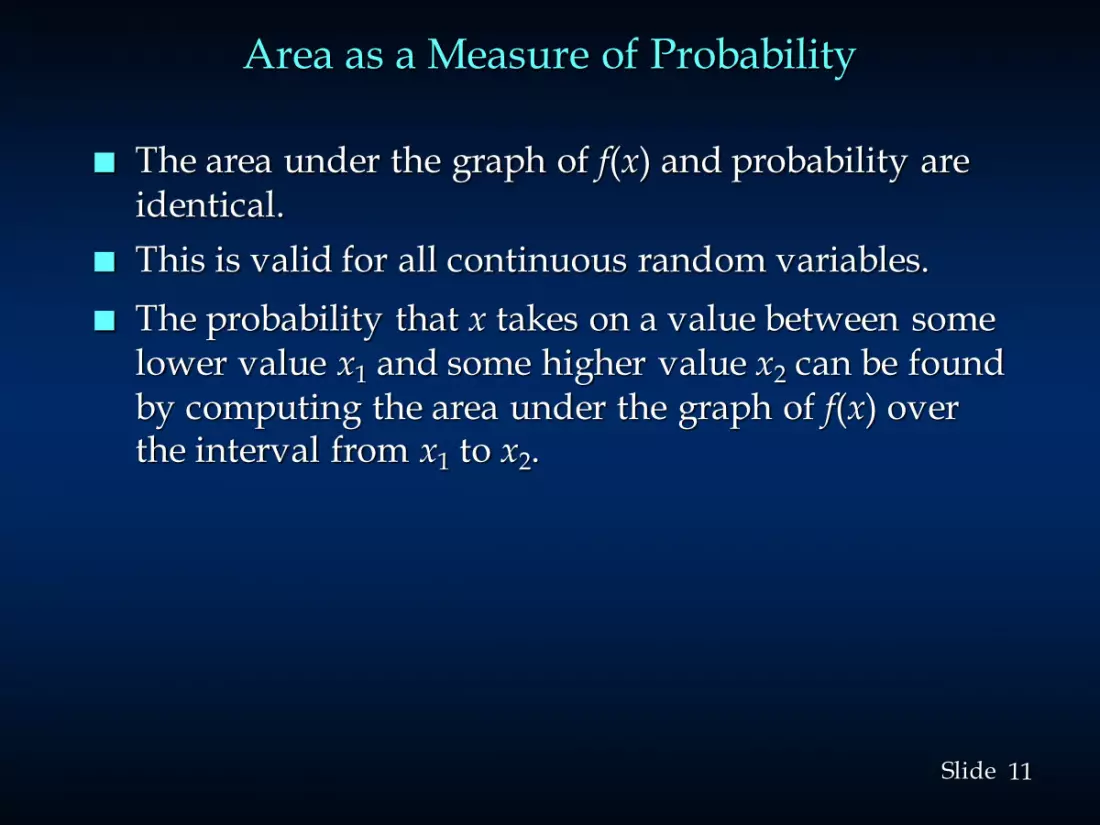
Area as a Measure of Probability
■ The area under the graph of f(x) and probability are identical.
■ This is valid for all continuous random variables.■ The probability that x takes on a value between some
lower value x1 and some higher value x2 can be found by computing the area under the graph of f(x) over the interval from x1 to x2.

12Slide
Normal Probability Distribution
■ The normal probability distribution is the most important distribution for describing a continuous random variable.
■ It is widely used in statistical inference.■ It has been used in a wide variety of applications
including:• Heights of people• Rainfall amounts
• Test scores• Scientific measurements
■ Abraham de Moivre, a French mathematician, published The Doctrine of Chances in 1733.
■ He derived the normal distribution.

13Slide
Normal Probability Distribution
■ Normal Probability Density Function
2 2( ) /21( )2
xf x e µ σ
σ π− −=
µ = meanσ = standard deviationπ = 3.14159e = 2.71828
where:

14Slide
The distribution is symmetric; its skewnessmeasure is zero.
Normal Probability Distribution
■ Characteristics
x

15Slide
The entire family of normal probabilitydistributions is defined by its mean µ and itsstandard deviation σ .
Normal Probability Distribution
■ Characteristics
Standard Deviation σ
Mean µx

16Slide
The highest point on the normal curve is at themean, which is also the median and mode.
Normal Probability Distribution
■ Characteristics
x

17Slide
Normal Probability Distribution
■ Characteristics
-10 0 25
The mean can be any numerical value: negative,zero, or positive.
x

18Slide
Normal Probability Distribution
■ Characteristics
σ = 15
σ = 25
The standard deviation determines the width of thecurve: larger values result in wider, flatter curves.
x

19Slide
Probabilities for the normal random variable aregiven by areas under the curve. The total areaunder the curve is 1 (.5 to the left of the mean and.5 to the right).
Normal Probability Distribution
■ Characteristics
.5 .5
x

20Slide
Normal Probability Distribution
■ Characteristics (basis for the empirical rule)
of values of a normal random variableare within of its mean.68.26%
+/- 1 standard deviation
of values of a normal random variableare within of its mean.95.44%
+/- 2 standard deviations
of values of a normal random variableare within of its mean.99.72%
+/- 3 standard deviations

21Slide
Normal Probability Distribution
■ Characteristics (basis for the empirical rule)
xµ – 3σ µ – 1σ
µ – 2σµ + 1σ
µ + 2σµ + 3σµ
68.26%95.44%99.72%
22Slide
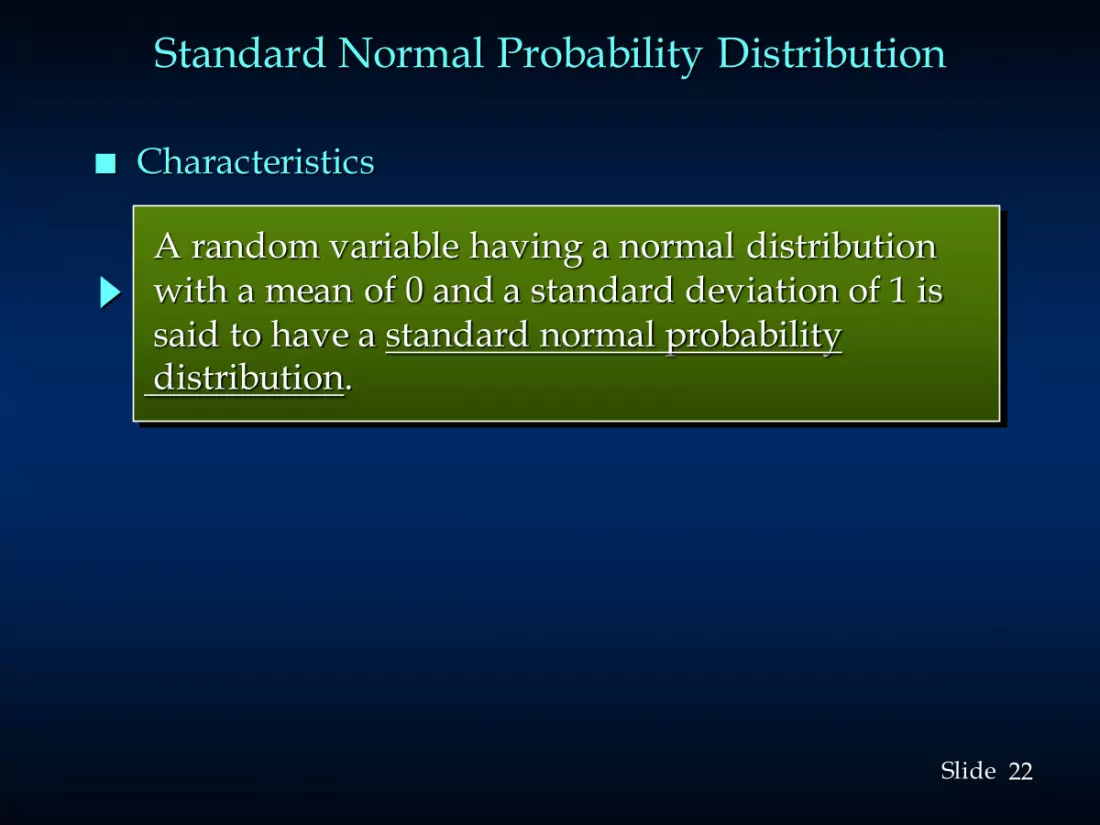
Standard Normal Probability Distribution
A random variable having a normal distributionwith a mean of 0 and a standard deviation of 1 issaid to have a standard normal probabilitydistribution.
■ Characteristics

23Slide
σ = 1
0z
The letter z is used to designate the standardnormal random variable.
Standard Normal Probability Distribution
■ Characteristics

24Slide
■ Converting to the Standard Normal Distribution
Standard Normal Probability Distribution
z x=
−µσ
We can think of z as a measure of the number ofstandard deviations x is from µ.
25Slide
Standard Normal Probability Distribution
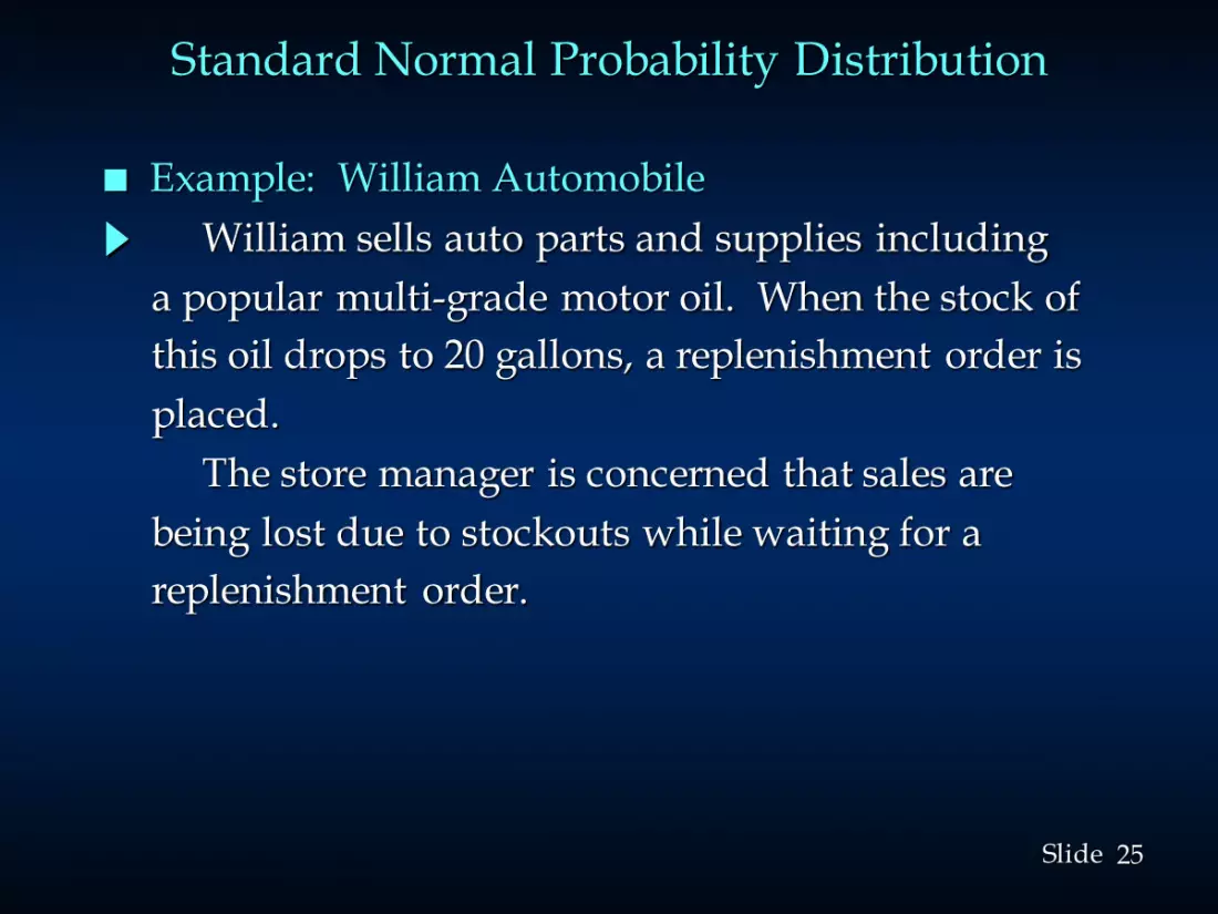
■ Example: William AutomobileWilliam sells auto parts and supplies including
a popular multi-grade motor oil. When the stock ofthis oil drops to 20 gallons, a replenishment order isplaced.
The store manager is concerned that sales arebeing lost due to stockouts while waiting for areplenishment order.

26Slide
It has been determined that demand duringreplenishment lead-time is normally distributedwith a mean of 15 gallons and a standard deviationof 6 gallons.
Standard Normal Probability Distribution
■ Example: William Automobile
The manager would like to know the probabilityof a stockout during replenishment lead-time. Inother words, what is the probability that demandduring lead-time will exceed 20 gallons?
P(x > 20) = ?
27Slide
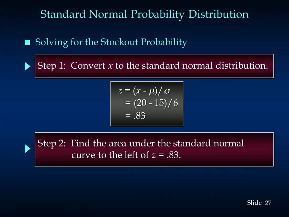
z = (x - µ)/σ= (20 - 15)/6= .83
■ Solving for the Stockout Probability
Step 1: Convert x to the standard normal distribution.
Step 2: Find the area under the standard normalcurve to the left of z = .83.
Standard Normal Probability Distribution

28Slide
z .00 .01 .02 .03 .04 .05 .06 .07 .08 .09. . . . . . . . . . ..5 .6915 .6950 .6985 .7019 .7054 .7088 .7123 .7157 .7190 .7224.6 .7257 .7291 .7324 .7357 .7389 .7422 .7454 .7486 .7517 .7549.7 .7580 .7611 .7642 .7673 .7704 .7734 .7764 .7794 .7823 .7852.8 .7881 .7910 .7939 .7967 .7995 .8023 .8051 .8078 .8106 .8133.9 .8159 .8186 .8212 .8238 .8264 .8289 .8315 .8340 .8365 .8389. . . . . . . . . . .
■ Cumulative Probability Table for the Standard Normal Distribution
P(z < .83)
Standard Normal Probability Distribution

29Slide
P(z > .83) = 1 – P(z < .83) = 1- .7967
= .2033
■ Solving for the Stockout Probability
Step 3: Compute the area under the standard normalcurve to the right of z = .83.
Probabilityof a stockout P(x > 20)
Standard Normal Probability Distribution

30Slide
■ Solving for the Stockout Probability
0 .83
Area = .7967Area = 1 - .7967
= .2033
z
Standard Normal Probability Distribution

31Slide
■ Standard Normal Probability Distribution
Standard Normal Probability Distribution
If the manager of William Automobile wants the probability of a stockout during replenishment lead-time to be no more than .05, what should the reorder point be?
(Hint: Given a probability, we can use the standardnormal table in an inverse fashion to find thecorresponding z value.)
32Slide
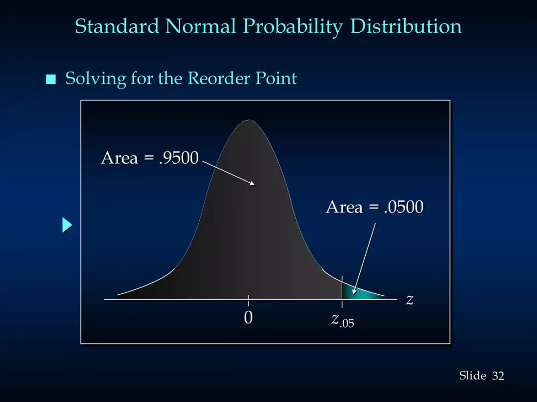
■ Solving for the Reorder Point
0
Area = .9500
Area = .0500
zz.05
Standard Normal Probability Distribution

33Slide
z .00 .01 .02 .03 .04 .05 .06 .07 .08 .09. . . . . . . . . . .1.5 .9332 .9345 .9357 .9370 .9382 .9394 .9406 .9418 .9429 .94411.6 .9452 .9463 .9474 .9484 .9495 .9505 .9515 .9525 .9535 .95451.7 .9554 .9564 .9573 .9582 .9591 .9599 .9608 .9616 .9625 .96331.8 .9641 .9649 .9656 .9664 .9671 .9678 .9686 .9693 .9699 .97061.9 .9713 .9719 .9726 .9732 .9738 .9744 .9750 .9756 .9761 .9767 . . . . . . . . . . .
■ Solving for the Reorder Point
Step 1: Find the z-value that cuts off an area of .05in the right tail of the standard normaldistribution.
We look upthe complement of the tail area(1 - .05 = .95)
Standard Normal Probability Distribution
34Slide
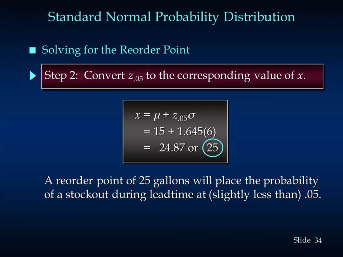
■ Solving for the Reorder Point
Step 2: Convert z.05 to the corresponding value of x.
x = µ + z.05σ
= 15 + 1.645(6)= 24.87 or 25
A reorder point of 25 gallons will place the probabilityof a stockout during leadtime at (slightly less than) .05.
Standard Normal Probability Distribution

35Slide
Normal Probability Distribution
■ Solving for the Reorder Point
15x
24.87
Probability of astockout duringreplenishmentlead-time = .05
Probability of nostockout duringreplenishmentlead-time = .95

36Slide
■ Solving for the Reorder PointBy raising the reorder point from 20 gallons to
25 gallons on hand, the probability of a stockoutdecreases from about .20 to .05.
This is a significant decrease in the chance thatWilliam Automobile will be out of stock and unable to meet a customer’s desire to make a purchase.
Standard Normal Probability Distribution

37Slide
Normal Approximation of Binomial Probabilities
When the number of trials, n, becomes large,evaluating the binomial probability function by handor with a calculator is difficult.
The normal probability distribution provides aneasy-to-use approximation of binomial probabilitieswhere np > 5 and n(1 - p) > 5.
In the definition of the normal curve, setµ = np and σ = −np p( )1σ = −np p( )1

38Slide
Add and subtract a continuity correction factorbecause a continuous distribution is being used toapproximate a discrete distribution.
For example, P(x = 12) for the discrete binomialprobability distribution is approximated byP(11.5 < x < 12.5) for the continuous normaldistribution.
Normal Approximation of Binomial Probabilities

39Slide
Normal Approximation of Binomial Probabilities
■ ExampleSuppose that a company has a history of making
errors in 10% of its invoices. A sample of 100 invoices has been taken, and we want to compute the probability that 12 invoices contain errors.
In this case, we want to find the binomial probability of 12 successes in 100 trials. So, we set:
µ = np = 100(.1) = 10= [100(.1)(.9)] ½ = 3σ = −np p( )1σ = −np p( )1

40Slide
Normal Approximation of Binomial Probabilities
■ Normal Approximation to a Binomial ProbabilityDistribution with n = 100 and p = .1
µ = 10
P(11.5 < x < 12.5)(Probabilityof 12 Errors)
x11.5
12.5
σ = 3

41Slide
■ Normal Approximation to a Binomial ProbabilityDistribution with n = 100 and p = .1
10
P(x < 12.5) = .7967
x12.5
Normal Approximation of Binomial Probabilities

42Slide
Normal Approximation of Binomial Probabilities
■ Normal Approximation to a Binomial ProbabilityDistribution with n = 100 and p = .1
10
P(x < 11.5) = .6915
x11.5

43Slide
Normal Approximation of Binomial Probabilities
10
P(x = 12)= .7967 - .6915= .1052
x11.5
12.5
■ The Normal Approximation to the Probabilityof 12 Successes in 100 Trials is .1052

44Slide
Exponential Probability Distribution
■ The exponential probability distribution is useful in describing the time it takes to complete a task.
•Time between vehicle arrivals at a toll booth•Time required to complete a questionnaire•Distance between major defects in a highway
■ The exponential random variables can be used to describe:
■ In waiting line applications, the exponential distribution is often used for service times.

45Slide
Exponential Probability Distribution
■ A property of the exponential distribution is that the mean and standard deviation are equal.
■ The exponential distribution is skewed to the right. Its skewness measure is 2.

46Slide
■ Density Function
Exponential Probability Distribution
where: µ = expected or meane = 2.71828
f x e x( ) /= −1µ
µ for x > 0

47Slide
■ Cumulative Probabilities
Exponential Probability Distribution
P x x e x( ) /≤ = − −0 1 o µ
where:x0 = some specific value of x

48Slide
Exponential Probability Distribution
■ Example: Al’s Full-Service PumpThe time between arrivals of cars at Al’s full-
service gas pump follows an exponential probabilitydistribution with a mean time between arrivals of 3minutes. Al would like to know the probability thatthe time between two successive arrivals will be 2minutes or less.

49Slide
x
f(x)
.1
.3
.4
.2
0 1 2 3 4 5 6 7 8 9 10Time Between Successive Arrivals (mins.)
Exponential Probability Distribution
P(x < 2) = 1 - 2.71828-2/3 = 1 - .5134 = .4866
■ Example: Al’s Full-Service Pump

50Slide
Relationship between the Poissonand Exponential Distributions
The Poisson distributionprovides an appropriate description
of the number of occurrencesper interval
The exponential distributionprovides an appropriate description
of the length of the intervalbetween occurrences
Copyright © 2022 FDOKUMEN