arX

iv:0

808.

3173

v1 [

cond

-mat

.sta

t-m

ech]

23

Aug

200

8

Probability Distribution of (Schwammle and Tsallis) Two-parameter

Entropies

and the Lambert W-function

Somayeh Asgarani ∗ and Behrouz Mirza †

Department of Physics, Isfahan University of Technology, Isfahan 84156-83111, Iran

Abstract

We investigate a two-parameter entropy introduced by Schwammle and Tsallis and obtain its

probability distribution in the canonical ensemble. The probability distribution is given in terms

of the Lambert W-function which has been used in many branches of physics, especially in fractal

structures. Also, extensivity of Sq,q′ is discussed and a relationship is found to exist between the

probabilities of a composite system and its subsystems so that the two-parameter entropy, Sq,q′, is

extensive.

1 Introduction

It is known that some physical systems cannot be described by the Boltzmann-Gibbs(BG) statistical

mechanics. Within a long list showing power-law behaviours, we may mention diffusion [1],

turbulence [2], transverse momentum distribution of hadron jets in e+e− collisions [3], thermalization

of heavy quarks in collisional process [4], astrophysics [5], solar neutrinos [6], and among others

[7, 8, 9, 10, 11]. Such systems typically have long-range interactions, long-time memory, and

multifractal or hierarchical structures. To overcome at least some of these difficulties, Tsallis

proposed a generalized entropic form [12, 13, 14], namely

Sq = k1 −

∑ωi=1 p

qi

q − 1, (1)

where, k is a positive constant and ω is the total number of microscopic states. It is clear that

the q-entropy (Sq) recovers the usual BG-entropy (SBG = −k∑ω

i=1 pi ln pi) in the limit q → 1. By

defining q-logarithm

lnq x ≡x1−q − 1

1 − q(ln1 x = ln x) , (2)

∗email: sasgarani@ph.iut.ac.ir†email: b.mirza@cc.iut.ac.ir

1

the entropic form, Sq, can be written as

Sq = k1 −

∑ωi=1 p

qi

q − 1= k

ω∑

i=1

pi lnq1

pi

. (3)

Hence, in the case of equiprobability, pi = 1

ω, the well-known Boltzmann law is recovered in the limit

q → 1. The q-entropy also satisfies the relevant properties of entropy like expansibility, composability,

Lesche-stability [17] and concavity (for q > 0). The inverse function of the q-logarithm is called q-

exponential [15] and is given by

expq x ≡ [1 + (1 − q)x]1

1−q (exp1 x = exp x) . (4)

Recently in [18], the two-parameter logarithm lnq,q′(x) and exponential expq,q′(x) were defined which

recovered q-logarithm and q-exponential, in the limit q → 1 or q′ → 1. So, the two-parameter

entropy, similar to Eq. (1), can be defined as

Sq,q′ ≡ω

∑

i=1

pi lnq,q′1

pi=

1

1 − q′

ω∑

i=1

pi

[

exp(1 − q′

1 − q(pq−1

i − 1))

− 1]

. (5)

The above entropy for the whole range of the space parameter does not fulfill all the necessary

properties of a physical entropy. Therefore, it may not be appropriate for describing the physical

systems, but useful for solving optimization problems. In this paper, we will find the probability

distribution pi for the two-parameter entropy Sq,q′ (17), when canonical constraints are imposed on

the system. As a result, it will be shown that the probability distribution is expressed in terms of

the Lambert W-function [19, 20, 21, 22], also called omega function, which is an analytical function

of z defined over the hole complex z-plane, as the inverse function of

z = WeW . (6)

Using this function, it is possible to write the series of infinite exponents in a closed form [23]

zz...

= −W (− ln z)

ln z. (7)

The above equation shows that W -function can be used to express self-similarity in some fractal

structures. This has been recently shown in a number of studies. Banwell and Jayakumar [24]

showed that W -function describes the relation between voltage, current and resistance in a diode,

Packel and Yuen [25] applied the W -function to a ballistic projectile in the presence of air resistance.

Other applications of the W-function include those in statistical mechanics, quantum chemistry,

combinatorics, enzyme kinetics, vision physiology, engineering of thin films, hydrology, and the

analysis of algorithms [26, 27, 28]. Sq may become extensive in cases where there are correlations

between subsystems. Hence, a point to be discussed will be the extensivity of Sq,q′ [29].

This paper is organized as follows. In Sec. 2, we will review the Generalized two parameter entropy,

Sq,q′ and its properties. In Sec. 3, the probability distribution pi of the two-parameter entropy, Sq,q′ ,

will be obtained in the canonical formalism. In Sec. 4, assuming that the two-parameter entropy be

extensive, we will develop a relationship holding between probability in the composite system and

probabilities of subsystems and in Sec. 5, we will have a conclusion.

2

2 Generalized two parameter entropy, Sq,q′

In this section, we will review the procedure for finding the two-parameter entropy, Sq,q′ [18]. As

we know, it is possible to define two composition laws, the generalized q-sum and q-product [16],

defined as follows

x ⊕q y ≡ x + y + (1 − q)xy (x ⊕1 y = x + y) , (8)

x ⊗q y ≡ (x1−q + y1−q − 1)1

1−q (x ⊗1 y = xy) . (9)

Using the definition of q-logarithm (Eq. (2)) and q-exponential (Eq. (4)), the above relations can be

rewritten as

lnq(xy) = lnq x ⊕q lnq y , (10)

lnq(x ⊗q y) = lnq x + lnq y . (11)

Very recently in [18], Eqs. (10) and (11) were generalized by defining a two-parameter logarithmic

function, denoted by lnq,q′ x, which satisfies the equation

lnq,q′(x ⊗q y) = lnq,q′ x ⊕q′ lnq,q′ y . (12)

Assuming lnq,q′ x = g(lnq x) = g(z) and using x = y in Eq. (12), then applying some general

properties of a logarithm function like

lnq,q′ 1 = 0 , (13)

d

dxlnq,q′ x|x=1 = 1 , (14)

the two-parameter generalized logarithmic function will be given as

lnq,q′ x =1

1 − q′

[

exp(1 − q′

1 − q(x1−q − 1)

)

− 1]

= lnq′ elnq x , (15)

and its inverse function will be defined as a two-parameter generalized exponential, expq,q′ x

expq,q′ x ={

1 +1 − q

1 − q′ln[1 + (1 − q′)x]

}

1

1−q

. (16)

The entropy can be constructed based on the two-parameter generalization of the standard logarithm

Sq,q′ ≡ kω

∑

i=1

pi lnq,q′1

pi

=k

1 − q′

ω∑

i=1

pi

[

exp(1 − q′

1 − q(pq−1

i − 1))

− 1]

, (17)

which, in the case of equiprobability (pi = 1

ω∀i), Sq,q′ = k lnq,q′ ω.

The above entropy is Lesche-stable and some properties such as expansibility and concavity are

satisfied if certain restrictions are imposed on (q, q′).

3

3 Finding probability distribution in the canonical ensemble

In this section, we are interested in maximizing the entropy Sq,q′ under the constraints

ω∑

i=1

pi − 1 = 0 , (18)

ω∑

i=1

piεi − E = 0 . (19)

These constraints are added to the entropy with Lagrange multipliers to construct the entropic

functional

Φq,q′(pi, α, β) =Sq,q′

k+ α(

ω∑

i=1

pi − 1) + β

ω∑

i=1

pi(εi − E) = 0 . (20)

To reach the equilibrium state, the entropic functional Φq,q′ should be maximized, namely

∂Φq,q′(pi, α, β)

∂pi= 0 ⇒ lnq,q′

1

pi+ pi

∂ lnq,q′(1

pi)

∂pi+ α + β(εi − E) = 0 . (21)

Using the definition of the two-parameter logarithm (Eq. (15)) and after some calculations, we get

exp(1 − q′

1 − q(pi

q−1 − 1))(

1 − (1 − q′)piq−1

)

= 1 − (1 − q′)(

α + β(εi − E))

. (22)

To solve the above equation and to find pi(εi), one may define

zi ≡1 − q′

1 − q(pi

q−1 − 1) ⇒ 1 − (1 − q′)piq−1 = (q − 1)zi + q′ , (23)

and so, Eq. (22) can be rewritten as

(q′ + (q − 1)zi) exp(zi) = γi , (24)

with the definition

γi ≡ 1 − (1 − q′)(

α + β(εi − E))

. (25)

Solving the above equation gives us

zi = W[e

q′

q−1 γi

q − 1

]

+q′

1 − q, (26)

where, W (z) is the Lambert W -function [19, 20, 21, 22]. From Eqs. (26) and (23), the probability

distribution is given by:

pi =1

Zq

{

1 + (1 − q)W[e

q′

q−1 γi

q − 1

]}

1

q−1

, (27)

where,

Zq =ω

∑

i=1

{

1 + (1 − q)W[e

q′

q−1 γi

q − 1

]}

1

q−1

. (28)

4

-4 -2 2 4 x

0.1

0.2

0.3

0.4

0.5

pHxL

HaL

q’=0.1q’=0.3q’=0.5q’=0.7q’=0.9Hq=1.1L

-2 -1 1 2x

0.1

0.2

0.3

0.4

0.5

0.6

pHxL

HbLq=1.1q=1.3q=1.5Hq’=0.9L

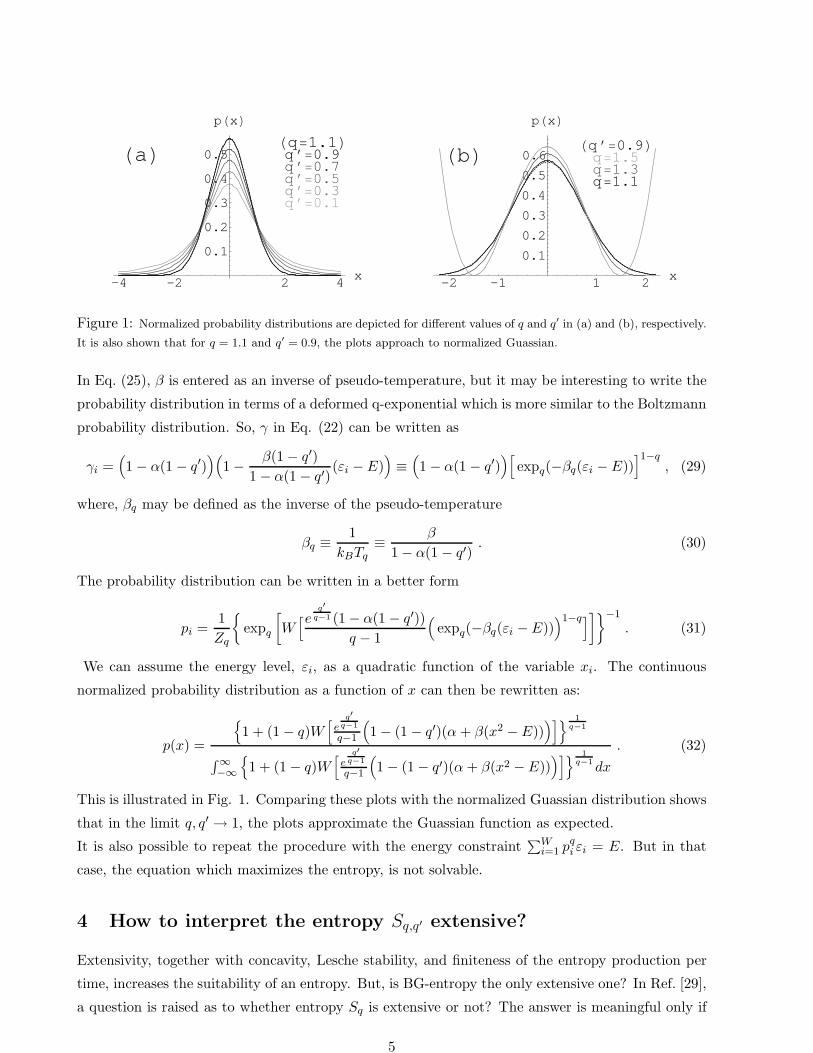
Figure 1: Normalized probability distributions are depicted for different values of q and q′ in (a) and (b), respectively.

It is also shown that for q = 1.1 and q′ = 0.9, the plots approach to normalized Guassian.

In Eq. (25), β is entered as an inverse of pseudo-temperature, but it may be interesting to write the

probability distribution in terms of a deformed q-exponential which is more similar to the Boltzmann

probability distribution. So, γ in Eq. (22) can be written as

γi =(

1 − α(1 − q′))(

1 −β(1 − q′)

1 − α(1 − q′)(εi − E)

)

≡(

1 − α(1 − q′))[

expq(−βq(εi − E))]1−q

, (29)

where, βq may be defined as the inverse of the pseudo-temperature

βq ≡1

kBTq≡

β

1 − α(1 − q′). (30)

The probability distribution can be written in a better form

pi =1

Zq

{

expq

[

W[e

q′

q−1 (1 − α(1 − q′))

q − 1

(

expq(−βq(εi − E)))1−q]

]}−1

. (31)

We can assume the energy level, εi, as a quadratic function of the variable xi. The continuous

normalized probability distribution as a function of x can then be rewritten as:

p(x) =

{

1 + (1 − q)W[

eq′

q−1

q−1

(

1 − (1 − q′)(α + β(x2 − E)))]}

1

q−1

∫ ∞−∞

{

1 + (1 − q)W[

eq′

q−1

q−1

(

1 − (1 − q′)(α + β(x2 − E)))]}

1

q−1dx

. (32)

This is illustrated in Fig. 1. Comparing these plots with the normalized Guassian distribution shows

that in the limit q, q′ → 1, the plots approximate the Guassian function as expected.

It is also possible to repeat the procedure with the energy constraint∑W

i=1 pqi εi = E. But in that

case, the equation which maximizes the entropy, is not solvable.

4 How to interpret the entropy Sq,q′ extensive?

Extensivity, together with concavity, Lesche stability, and finiteness of the entropy production per

time, increases the suitability of an entropy. But, is BG-entropy the only extensive one? In Ref. [29],

a question is raised as to whether entropy Sq is extensive or not? The answer is meaningful only if

5

A \ B 1 2 A \ B 1 2

1 pA+B11 = p2 pA+B

12 = p(1 − p) p 1 pA+B11 = 2p − 1 pA+B

12 = 1 − p p

2 pA+B21 = p(1 − p) pA+B

22 = (1 − p)2 1 − p 2 pA+B21 = 1 − p pA+B

22 = 0 1 − p

p 1 − p 1 p 1 − p 1

(a) (b)

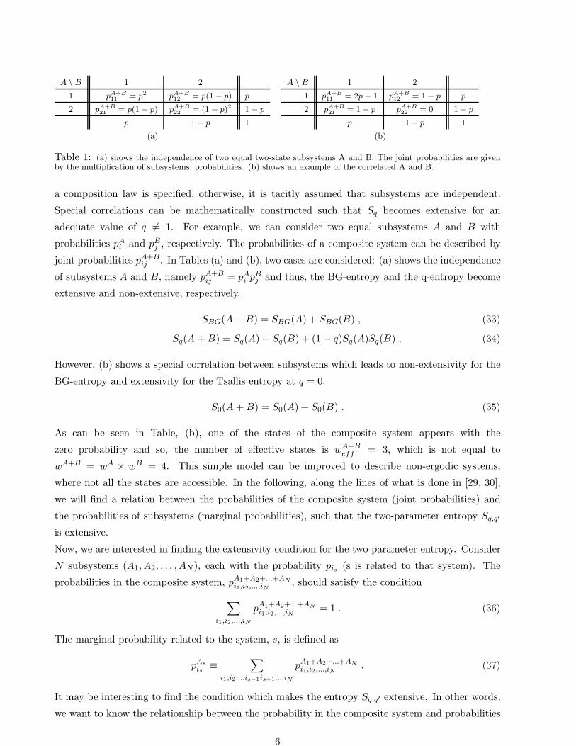
Table 1: (a) shows the independence of two equal two-state subsystems A and B. The joint probabilities are givenby the multiplication of subsystems, probabilities. (b) shows an example of the correlated A and B.

a composition law is specified, otherwise, it is tacitly assumed that subsystems are independent.

Special correlations can be mathematically constructed such that Sq becomes extensive for an

adequate value of q 6= 1. For example, we can consider two equal subsystems A and B with

probabilities pAi and pB

j , respectively. The probabilities of a composite system can be described by

joint probabilities pA+Bij . In Tables (a) and (b), two cases are considered: (a) shows the independence

of subsystems A and B, namely pA+Bij = pA

i pBj and thus, the BG-entropy and the q-entropy become

extensive and non-extensive, respectively.

SBG(A + B) = SBG(A) + SBG(B) , (33)

Sq(A + B) = Sq(A) + Sq(B) + (1 − q)Sq(A)Sq(B) , (34)

However, (b) shows a special correlation between subsystems which leads to non-extensivity for the

BG-entropy and extensivity for the Tsallis entropy at q = 0.

S0(A + B) = S0(A) + S0(B) . (35)

As can be seen in Table, (b), one of the states of the composite system appears with the

zero probability and so, the number of effective states is wA+Beff = 3, which is not equal to

wA+B = wA × wB = 4. This simple model can be improved to describe non-ergodic systems,

where not all the states are accessible. In the following, along the lines of what is done in [29, 30],

we will find a relation between the probabilities of the composite system (joint probabilities) and

the probabilities of subsystems (marginal probabilities), such that the two-parameter entropy Sq,q′

is extensive.

Now, we are interested in finding the extensivity condition for the two-parameter entropy. Consider

N subsystems (A1, A2, . . . , AN ), each with the probability pis (s is related to that system). The

probabilities in the composite system, pA1+A2+...+AN

i1,i2,...,iN, should satisfy the condition

∑

i1,i2,...,iN

pA1+A2+...+AN

i1,i2,...,iN= 1 . (36)

The marginal probability related to the system, s, is defined as

pAs

is≡

∑

i1,i2,...is−1is+1...,iN

pA1+A2+...+AN

i1,i2,...,iN. (37)

It may be interesting to find the condition which makes the entropy Sq,q′ extensive. In other words,

we want to know the relationship between the probability in the composite system and probabilities

6

of the subsystems when the entropy Sq,q′ is extensive. Let us consider the relation

1

pA1+A2+...+AN

i1,i2,...,iN

= expq,q′

(

N∑

s=1

lnq,q′1

pAs

is

+ φi1,i2,...,iN

)

, (38)

where, φi1,i2,...,iN is set to ensure Eq. (36). The above equation can be rewritten in a different form

1

pA1+A2+...+AN

i1,i2,...,iN

=1

pA1

i1

⊗q,q′1

pA2

i2

⊗q,q′ . . . ⊗q,q′1

pAN

iN

⊗q,q′ expq,q′(φi1,i2,...,iN ) , (39)

with the definition of ⊗q,q′-product [18]

x ⊗q,q′ y ≡ expq,q′(lnq,q′ x + lnq,q′ y) . (40)

A nonzero function φi1,i2,...,iN is related to the existence of the correlation in the system, because in

the case of independent subsystems (q, q′ → 1), the ⊗q,q′-product becomes the usual product and

φi1,i2,...,iN = 0. In Ref. [30], the values of φij, making the entropy Sq extensive, are obtained for two

equal two-state subsystems. In the case of equiprobability, Eq. (39) save for the function φi1,i2,...,iN ,

shows the generalized multiplication of the number of states of the subsystems, which may be defined

as the effective number of states

wA+Beff = wA1 ⊗q,q′ wA2 ⊗q,q′ . . . ⊗q,q′ wAN ⊗q,q′ expq,q′(φi1,i2,...,iN ) , (41)

The entropy of a composite system similar to Eq. (17) can be defined as follows

Sq,q′

(

N∑

s=1

As

)

≡ k∑

i1,i2,...,iN

pA1+A2+...+AN

i1,i2,...,iNlnq,q′

1

pA1+A2+...+AN

i1,i2,...,iN

. (42)

Using Eq. (38), the entropy can be written as

Sq,q′

(

N∑

s=1

As

)

≡ k∑

i1,i2,...,iN

pA1+A2+...+AN

i1,i2,...,iNlnq,q′

[

expq,q′

(

N∑

s=1

lnq,q′1

pAs

is

+ φi1,i2,...,iN

)]

= k∑

i1,i2,...,iN

pA1+A2+...+AN

i1,i2,...,iN

N∑

s=1

lnq,q′1

pAs

is

+ k∑

i1,i2,...,iN

pA1+A2+...+AN

i1,i2,...,iNφi1,i2,...,iN

= kN

∑

s=1

∑

is

pAs

islnq,q′

1

pAs

is

+ k∑

i1,i2,...,iN

pA1+A2+...+AN

i1,i2,...,iNφi1,i2,...,iN

=N

∑

s=1

Sq,q′(As) + k∑

i1,i2,...,iN

pA1+A2+...+AN

i1,i2,...,iNφi1,i2,...,iN , (43)

where, the definition of marginal probability Eq. (37) is used in the last line. Eq. (43) ensures

extensivity of Sq,q′ if the constraint

∑

i1,i2,...,iN

pA1+A2+...+AN

i1,i2,...,iNφi1,i2,...,iN = 0 , (44)

is satisfied. In other words, assuming the above constraint will be equivalent to the existence of

extensivity. According to Eqs. (15), (16), and (38), for the probability of a composite system, we

7

get

pA1+A2+...+AN

i1,i2,...,iN=

{

1 +1 − q

1 − q′ln

[

1 − N + (1 − q′)φi1,i2,...,iN −N

∑

s=1

exp[1 − q′

1 − q(pq−1

is− 1)]

]}

1

q−1

. (45)

It is clear that in the limit q → 1, the proposed relation of probabilities is recovered [29, 30]

pA1+A2+...+AN

i1,i2,...,iN=

[

1 − N + (1 − q′)φi1,i2,...,iN +N

∑

s=1

(pis)q′−1

]

1

q′−1

. (46)

where, in the limit q′ → 1, the usual product of probabilities, pA1+A2+...+AN

i1,i2,...,iN=

∏Ns=1 pis , is given,

which describes the case of independent subsystems.

5 Conclusion

In this paper, a special set of two-parameter entropies [18] were maximized in the canonical ensemble

by the energy constraint∑ω

i=1 piεi = E. We expected that the probability distribution, pi(εi), can be

expressed in terms of the generalized two-parameter exponential defined in [18]. But unexpectedly,

solution of the related equation took the form of the Lambert function which has been used in many

branches including statistical mechanics, quantum chemistry, enzyme kinetics, and thin films, among

others. The Lambert function can also describe some fractal structures because infinite exponents

can be written in terms of the Lambert function (Eq. 7). This suggests that the two-parameter

entropies are probably related to the fractal structures in a phase space which may be a subject

for future study. Also, assuming extensive Sq,q′ , the probability of a composite system was given in

terms of probabilities of the subsystems.

8

References

[1] M.F. Shlesinger, G.M. Zaslavsky and J. Klafter, Nature (London) 363, 31 (1993).

[2] C. Beck, Physica A 277, 115 (2000).

[3] I. Bediaga, E.M. Curado and J.M de miranda, Physica A 286, 156 (2000).

[4] D.B. Walton and J. Rafelski, Phys. Rev. Lett, 84, 31 (2000).

[5] J. Binney and S. Tremaine, Glactic Dynamics, Princeton University Press, Prinston, NJ, 1987,

P. 267.

[6] D.C. Clayton, Nature 249, (1974) 131.

[7] S. Abe and Y. Okamoto, Nonextensive Statistical Mechanics and Its Applications, Springer-

Verlag, 2001.

[8] M. Gell-Mann and C.Tsallis, Nonextensive Entropy: Interdisciplinary Applications, Oxford

University Press, 2004.

[9] H. Morita, K. Kaneko, Phys. Rev. Lett. 96, 050602 (2006).

[10] A. Pluchino, A. Rapisarda, C. Tsallis and E.P. Borges, Europhysics Letters 80, 26002 (2007).

[11] A. Pluchino, A. Rapisarda, C. Tsallis, arXiv: 0805.3652 [cond-mat.stat-mech].

[12] C. Tsallis, J. Stat. Phys. 52, 479 (1988).

[13] E.M.F. Curado and C. Tsallis, J. Phys. A 24, L69 (1991)

[14] C. Tsallis, R.S. Mendes and A.R. Plastino, Physica A 261, 534 (1998).

[15] E.P. Borges, J. Phys. A, 31, 5281 (1998).

[16] E.P. Borges, Physica A 340, 95 (2004).

[17] B. Lesche, J. Stat. Phys. 27, 419 (1982). S. Abe. Phys. Rev. E 66, 046134 (2002).

[18] V. Schwammle and C.Tsallis, J. Math. Phys. 48, 113301 (2007), arXiv: cond-mat/0703792v1.

[19] http://functions.wolfram.com/ElementaryFunctions/ProductLog,

http://mathworld.wolfram.com/LambertW-Function.html.

[20] R. M. Corless, G. H. Gonnet, D. E. G. Hare, D. G. Jeffrey and D. E. Knuth, Adv. Comput.

Math. 5, 329 (1996).

[21] J. H. Lambert, ”Observations variae in Mathesin Puram.” Acta Helvitica, physico-mathematico-

anatomico-botanico-medica 3, 128 (1758).

9

[22] L. Euler, Acta Acad. Scient. Petropol. 2, 29, (1783).

[23] G. Eisenstein, J. reine angew. Math. 28, 49 (1844).

[24] T. C. Banwell and A. Jayakumar, Electronics Lett. 36, 291 (2000).

[25] E. Packel and D. Yuen, The College Mathematics Journal, 35, 337 (2004).

[26] M. V. Putz, A. Lacrama and V. Ostafe, International Journal of Molecular Sciences, 7, 469

(2006).

[27] P. Stallinga and H. L. Gomes, Organic Electronics, 8, 300 (2007).

[28] B. Hayes, American Scientist, 93, 104 (2005).

[29] C. Tsallis, J. Phys. A 37, 9125 (2004), arXiv: cond-mat/0409631.

[30] S. Asgarani and B. Mirza, Physica A 377, 58 (2007).

10