Precise and fast computation of Lambert W-functions without transcendental function evaluations

(This is a sample cover image for this issue. The actual cover is not yet available at this time.)

This article appeared in a journal published by Elsevier. The attachedcopy is furnished to the author for internal non-commercial researchand education use, including for instruction at the authors institution

and sharing with colleagues.

Other uses, including reproduction and distribution, or selling orlicensing copies, or posting to personal, institutional or third party

websites are prohibited.

In most cases authors are permitted to post their version of thearticle (e.g. in Word or Tex form) to their personal website orinstitutional repository. Authors requiring further information

regarding Elsevier’s archiving and manuscript policies areencouraged to visit:

http://www.elsevier.com/copyright

http://www.elsevier.com/copyright

Author's personal copy

Journal of Computational and Applied Mathematics 244 (2013) 77–89

Contents lists available at SciVerse ScienceDirect

Journal of Computational and AppliedMathematics

journal homepage: www.elsevier.com/locate/cam

Precise and fast computation of Lambert W -functions withouttranscendental function evaluationsToshio FukushimaNational Astronomical Observatory of Japan, 2-21-1, Ohsawa, Mitaka, Tokyo 181-8588, Japan

a r t i c l e i n f o

Article history:Received 27 August 2012Received in revised form 7 November 2012

Keywords:BisectionInterval duplicationLambertW -functionSchröder’s method

a b s t r a c t

We have developed a new method to compute the real-valued Lambert W -functions,W0(z) and W−1(z). The method is a composite of (1) the series expansions around thebranch point, W = −1, and around zero, W = 0, and (2) the numerical solution of themodified defining equation, W = ze−W . In the latter process, we (1) repeatedly duplicatea test interval until it brackets the solution, (2) conduct bisections to find an approximatesolution, and (3) improve it by a single application of the fifth-order formula of Schröder’smethod. The first two steps are accelerated by preparing auxiliary numerical constantsbeforehand and utilizing the addition theorem of the exponential function. As a result, thenew method requires no call of transcendental functions such as the exponential functionor the logarithm. This makes it around twice as fast as existing methods: 1.7 and 2.0 timesfaster than the methods of Fritsch et al. (1973) and Veberic (2012) [16,14] for W0(z) and1.8 and 2.0 times faster than the methods of Veberic (2012) [14] and Chapeau-Blondeauand Monir (2002) [13] forW−1(z).

© 2012 Elsevier B.V. All rights reserved.

1. Introduction

1.1. Lambert W-function

The LambertW -function,W (z) [1, Section 4.13], is defined as the solution of a transcendental equation

WeW = z. (1)Its comprehensive explanation is found in [2,3]. The function is widely used in various fields of science and technology[4–10].

By a variable transformationW ≡ log Y , (2)

the defining equation is expressed in a different form:Y log Y = z. (3)

Its solution is extensively discussed in [11, Section 6.11] without mentioning the Lambert W -function. If z > 0, we mayrewrite the above equation into another form as

W + logW = log z. (4)As far as real numbers are concerned, the function is classified into two branches:W0(z) for the function satisfyingW ≥ −1and W−1(z) otherwise. Refer to Fig. 1. The two branch functions are also denoted by (1) Wp(z) and Wm(z) in [1], (2)ProductLog[0, z] and ProductLog[−1, z] in Mathematica [12], and (3) lambertw(z) and lambertw(−1, z) in MATLAB.

E-mail address: [email protected].

0377-0427/$ – see front matter© 2012 Elsevier B.V. All rights reserved.doi:10.1016/j.cam.2012.11.021


78 T. Fukushima / Journal of Computational and Applied Mathematics 244 (2013) 77–89

Fig. 1. Defining function of Lambert W -functions. Plotted is the curve z = WeW as a function of W . The Lambert W -functions are defined as the inversefunctions of this defining function.

1.2. An application

The real-valued LambertW -functions are useful in solving various kinds of equation containing the exponential functionor the logarithm [3–11,13,14]. For example, the problem to find the temperature of a black body from the observed peak ofits radiation is solved by means ofW0(z) as

T =W0

−3e−3

+ 3

hνpeak

k

≈ 0.354429

hνpeak

k

. (5)

In order to show this, we recall that Planck’s law of black body radiation [15] is expressed as

I(ν; T ) =

2hν3

c2

1

exp hνkT

− 1

, (6)

where I is the normalized energy radiated from a black body, ν is the frequency of the electromagnetic wave radiated, Tis the temperature of the black body, h is the Planck constant, c is the speed of light in vacuum, and k is the Boltzmannconstant. Then, the radiation peak condition is derived as

∂ I∂ν

T

=

2hν2

c2

3

eξ

− 1− ξeξ

eξ − 12 = 0, (7)

where

ξ ≡hνkT

. (8)

Thus, the equation to be solved becomes

f (ξ) ≡ (ξ − 3)eξ+ 3 = 0. (9)

This equation is translated into Eq. (1), the defining equation ofW , by the variable transformation

W ≡ ξ − 3, z ≡ −3e−3. (10)

Note that (1) df /dξ = (ξ − 2)eξ has only one positive root at ξ = 2, (2) f (2) = 3− e2 ≈ −4.389 < 0, and (3) f (ξ) → +∞

when ξ → +∞. Then, it is easy to show that f (ξ) = 0 has only one single positive root in the domain 2 < ξ < +∞. Thismeans thatW ≥ −1. Therefore, the primary branch,W0(z), is the solution we seek for.

1.3. Another application

The complete elliptic integral of the second kind, E(m), has an asymptotic expansion around its logarithmic singularity,m = 1, [1, Formula 19.12.2] as

E(m) =

1 +

log 2 −

14

mc + · · ·

−

mc

4+ · · ·

logmc, (11)

where

mc ≡ 1 − m (12)

is the complementary parameter. By keeping only the leading terms and introducing the variable transformation

X ≡ logmc, (13)


T. Fukushima / Journal of Computational and Applied Mathematics 244 (2013) 77–89 79

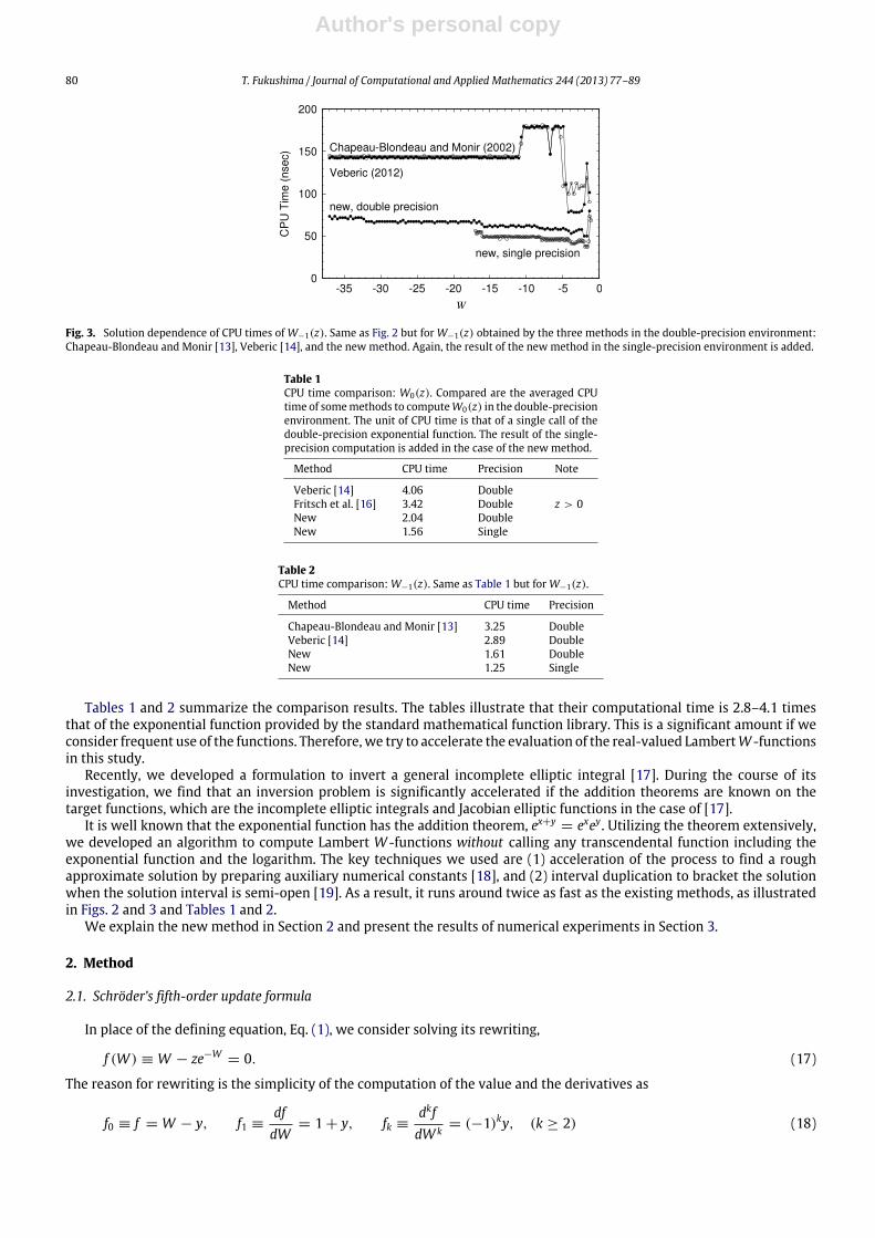
Fig. 2. Solution dependence of CPU times of W0(z). Shown are the averaged CPU times to evaluate W0(z) as a function of the solution, W . Compared arethe three methods in the double-precision environment: Fritsch et al. [16], Veberic [14], and the new method. Also, the result of the new method in thesingle-precision environment is added.

we obtain a nonlinear equation with respect to X as

(X − C)eX = 4[1 − E(m)], (14)

where C ≡ 4 log 2 − 1 ≈ 1.77. This equation reduces to Eq. (1) by a further transformation:

W ≡ X − C, z ≡

e4

[1 − E(m)]. (15)

Note that X < 0, since m < 1. Then, we find that W < −C < −1. Namely, the branch we should choose is W−1(z).Therefore, the final solution in terms ofm is given as

m = 1 − exp [C + W−1(z)] , (16)

where z is defined above. This provides an asymptotic approximation of the inversion of E(m) around its logarithmicsingularity,m = 1. It is a rough estimate, but can be used as an initial guess to obtain a precise inversion of E(m).

1.4. Existing methods

The existing numerical methods to compute the real-valued Lambert W -functions are those of [16,14] for W0(x) andthose of [13,14] forW−1(x).

The method of Fritsch et al. [16] assumes that z > 0 and solves the alternate equation, Eq. (4), by a fourth-order methodskillfully developed by themselves [14, Section 2.3]. As an initial guess, the method prepares a combination of (1) theMaclaurin series expansion aroundW = 0, (2) the asymptotic approximationwhenW → ∞, and (3) the Padé approximantof order [2/3]. Designing the errors of the initial guess sufficiently small, say less than 10−4 in a relative sense, they applythe fourth-order method only once in order to realize double-precision accuracy. See Fig. 5. Unfortunately, this method islimited to a positive argument, z > 0, since it uses log z in preparing the approximate solutions.

Chapeau-Blondeau and Monir [13] present a method to evaluate W−1(z). They solve the defining equation, Eq. (1), byHalley’s third-order method. Their initial value is computed by either (1) the series expansion around the branch point,W = −1, (2) the asymptotic approximation when W → −∞, or (3) two sets of Padé approximant of order [4/3]. Therelative errors of the initial guess are less than 10−4. Then, at most two iterations of Halley’s method is sufficient to arriveat the double-precision solution.

Veberic [14] provides methods to compute W0(z) and W1(z), respectively. His method for W0(z) is more suitable thanthat of Fritsch et al. [16] in the sense it covers all the solution values, −1 ≤ W . He solves the defining equation, Eq. (1), bythe same fourth-order method of [16] starting from the initial guess prepared as a combination of (1) the series expansionaround the branch point, W = −1, (2) the same asymptotic approximation when W → +∞, and (3) two sets of Padéapproximant of order [4/4]. The precision of this initial guess becomes higher, say of the order of 10−5 or so. Then, heapplies the improving process only once in order to obtain double-precision accuracy.

As for W−1(z), he solves the same defining equation by the same fourth-order method starting from the initial guesssimilar to that of [13]. The difference is in the intermediate case, where he uses one Padé approximant of the order [2/5].Also the selection policy among the three options is a little different. Again, he applies the fourth-order method only once.We learn that this method is somewhat erroneous whenW ≈ −1.7, as will be seen in Fig. 8.

1.5. Outline of article

All the existing methods are sufficiently precise, as will be seen in Figs. 5 through 8. Then, the question of concern is thecomputational speed as stressed in [16]. Figs. 2 and 3 reveal the W -dependence of the averaged CPU times. These resultsare measured on a PC with an Intel Core i7-930 CPU run at 3.06 GHz clock.



Fig. 3. Solution dependence of CPU times of W−1(z). Same as Fig. 2 but for W−1(z) obtained by the three methods in the double-precision environment:Chapeau-Blondeau and Monir [13], Veberic [14], and the new method. Again, the result of the new method in the single-precision environment is added.

Table 1CPU time comparison: W0(z). Compared are the averaged CPUtime of somemethods to computeW0(z) in the double-precisionenvironment. The unit of CPU time is that of a single call of thedouble-precision exponential function. The result of the single-precision computation is added in the case of the new method.

Method CPU time Precision Note

Veberic [14] 4.06 DoubleFritsch et al. [16] 3.42 Double z > 0New 2.04 DoubleNew 1.56 Single

Table 2CPU time comparison:W−1(z). Same as Table 1 but forW−1(z).

Method CPU time Precision

Chapeau-Blondeau and Monir [13] 3.25 DoubleVeberic [14] 2.89 DoubleNew 1.61 DoubleNew 1.25 Single

Tables 1 and 2 summarize the comparison results. The tables illustrate that their computational time is 2.8–4.1 timesthat of the exponential function provided by the standard mathematical function library. This is a significant amount if weconsider frequent use of the functions. Therefore, we try to accelerate the evaluation of the real-valued LambertW -functionsin this study.

Recently, we developed a formulation to invert a general incomplete elliptic integral [17]. During the course of itsinvestigation, we find that an inversion problem is significantly accelerated if the addition theorems are known on thetarget functions, which are the incomplete elliptic integrals and Jacobian elliptic functions in the case of [17].

It is well known that the exponential function has the addition theorem, ex+y= exey. Utilizing the theorem extensively,

we developed an algorithm to compute Lambert W -functions without calling any transcendental function including theexponential function and the logarithm. The key techniques we used are (1) acceleration of the process to find a roughapproximate solution by preparing auxiliary numerical constants [18], and (2) interval duplication to bracket the solutionwhen the solution interval is semi-open [19]. As a result, it runs around twice as fast as the existing methods, as illustratedin Figs. 2 and 3 and Tables 1 and 2.

We explain the new method in Section 2 and present the results of numerical experiments in Section 3.

2. Method

2.1. Schröder’s fifth-order update formula

In place of the defining equation, Eq. (1), we consider solving its rewriting,

f (W ) ≡ W − ze−W= 0. (17)

The reason for rewriting is the simplicity of the computation of the value and the derivatives as

f0 ≡ f = W − y, f1 ≡dfdW

= 1 + y, fk ≡dkfdW k

= (−1)ky, (k ≥ 2) (18)



where

y ≡ ze−W . (19)

No extra cost is required in evaluating the second-order and higher-order derivatives.Starting from a certain approximate solution, which will be described in the following subsections, we solve the above

equation by the fifth-order update formula of Schröder’s method [20, Section 4.4]:

∆W =−4f0

6f 31 − 6f0f1f2 + f 20 f3

24f 41 − 36f0f 21 f2 + 6f 20 f

22 + 8f 20 f1f3 − f 30 f4

. (20)

See also Appendix B of [17].Using the explicit expressions of the second-order and higher-order derivatives of f (W ), we rewrite the above general

formula in a simpler form as

∆W =−4f0

6f1

f11 + f0y

+ f00y

f11

24f11 + 36f0y

+ 6f00y (14y + 8 + f0)

, (21)

where f11 ≡ f 21 , f0y ≡ f0y, and f00y ≡ f0f0y.The leading term of the relative error of this update formula for the approximate solutionW can be obtained by a formula

processor, say by issuing a command in Mathematica [12] such as

Series[(dW + DW[W + dW, W E∧W])/W, {dW, 0, 5}]],

where DW(W , z) denotes ∆W regarded as a function of the approximate value ofW and the input argument z. The result isexpressed as

W + ∆WW ∗

− 1 ≈ C(W )

WW ∗

− 15

, (22)

where W ∗ denotes the true solution,

C(W ) ≡−6 + 32W − 8W 2

− W 3

720(1 + W )4(23)

is the error constant, and we assume that W is sufficiently close to W ∗. The expression of the leading error term confirmsthat the update formula is of the fifth order. Also, the error constant is significantly smaller than unity except near the branchpoint, where the magnitude of a factor of the denominator, |1 + W |, becomes small.

As will be shown later, our procedure to obtain the approximate solution automatically provides its exponential functionvalue. Thenwe limit the number of applications of this formula to only once in order to avoid the relatively time-consumingcall of the exponential function.

We set the order of Schröder’s method as high as 5. This is because we experimentally find that this order leads to theminimum CPU time under the condition of keeping the computing errors below a certain level, say less than 10 machineepsilons. Such a high order is preferable because the computational cost of the derivatives is small, as observed in the above.

2.2. Determination of the integer part by interval duplication and bisection

We use the bisection method as the key technique to obtain an approximate solution of Eq. (17). Since the solutioninterval is semi-open as −1 < W < +∞ for W0(z) and as −∞ < W < −1 for W−1(z), we must bracket the solution firstof all. Advancing further, we determine the integer part ofW as a first step.

Let us splitW into a sum of its integer and fraction parts as

W = ±(n + x), (24)

where x satisfies a condition, 0 ≤ x < 1, and the double sign is + for W0(z) and − for W−1(z). Note that n is not positivedefinite in the case ofW0(z).

In advance, we prepare an array of the defining function values of integer arguments, Fk ≡ kek forW0(z) and Gk ≡ −ke−k

forW−1(z). The size of the array of Fk orGk is not large. In the double-precision environment, F64 ≈ 4×1029 is a huge numberand G64 ≈ −1 × 10−26 is a tiny negative number. Therefore, we set the range of the array index k as 0 ≤ k ≤ 64 for Fk and1 ≤ k ≤ 64 for Gk.

We determine n by comparing z with Fk or Gk. The first step is bracketing n. From a practical viewpoint, the chance that nis large is small. Thus, we start the trial value of n from that of the smallest magnitude, i.e. 0 forW0(z) and 2 forW−1(z), andincrement it by 1 or duplicate its magnitude when greater than 1. Namely, the test sequence of n is (0, 1, 2, 4, 8, 16, 32, 64)for W0(z) and (2, 4, 8, 16, 32, 64) for W−1(z).

If n is bracketed as −1 ≤ n < 0, 0 ≤ n < 1 or 1 ≤ n < 2, then n is determined as −1, 0, 1, respectively. Thus, let usassume that n is bracketed such that 2ℓ−1

≤ n < 2ℓ, where ℓ > 1. In this case, we conduct the bisection search for n.



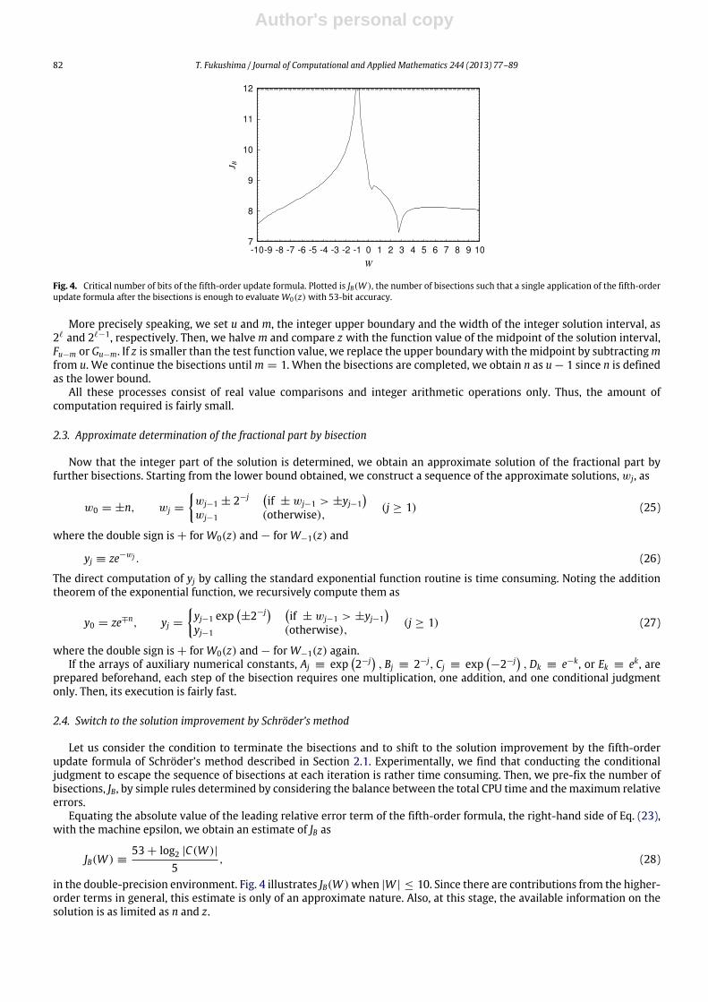
Fig. 4. Critical number of bits of the fifth-order update formula. Plotted is JB(W ), the number of bisections such that a single application of the fifth-orderupdate formula after the bisections is enough to evaluateW0(z) with 53-bit accuracy.

More precisely speaking, we set u and m, the integer upper boundary and the width of the integer solution interval, as2ℓ and 2ℓ−1, respectively. Then, we halvem and compare z with the function value of the midpoint of the solution interval,Fu−m or Gu−m. If z is smaller than the test function value, we replace the upper boundary with themidpoint by subtractingmfrom u. We continue the bisections untilm = 1. When the bisections are completed, we obtain n as u − 1 since n is definedas the lower bound.

All these processes consist of real value comparisons and integer arithmetic operations only. Thus, the amount ofcomputation required is fairly small.

2.3. Approximate determination of the fractional part by bisection

Now that the integer part of the solution is determined, we obtain an approximate solution of the fractional part byfurther bisections. Starting from the lower bound obtained, we construct a sequence of the approximate solutions, wj, as

w0 = ±n, wj =

wj−1 ± 2−j

if ± wj−1 > ±yj−1

wj−1 (otherwise), (j ≥ 1) (25)

where the double sign is + for W0(z) and − for W−1(z) and

yj ≡ ze−wj . (26)

The direct computation of yj by calling the standard exponential function routine is time consuming. Noting the additiontheorem of the exponential function, we recursively compute them as

y0 = ze∓n, yj =

yj−1 exp

±2−j

if ± wj−1 > ±yj−1

yj−1 (otherwise), (j ≥ 1) (27)

where the double sign is + for W0(z) and − for W−1(z) again.If the arrays of auxiliary numerical constants, Aj ≡ exp

2−j

, Bj ≡ 2−j, Cj ≡ exp

−2−j

,Dk ≡ e−k, or Ek ≡ ek, are

prepared beforehand, each step of the bisection requires one multiplication, one addition, and one conditional judgmentonly. Then, its execution is fairly fast.

2.4. Switch to the solution improvement by Schröder’s method

Let us consider the condition to terminate the bisections and to shift to the solution improvement by the fifth-orderupdate formula of Schröder’s method described in Section 2.1. Experimentally, we find that conducting the conditionaljudgment to escape the sequence of bisections at each iteration is rather time consuming. Then, we pre-fix the number ofbisections, JB, by simple rules determined by considering the balance between the total CPU time and themaximum relativeerrors.

Equating the absolute value of the leading relative error term of the fifth-order formula, the right-hand side of Eq. (23),with the machine epsilon, we obtain an estimate of JB as

JB(W ) ≡53 + log2 |C(W )|

5, (28)

in the double-precision environment. Fig. 4 illustrates JB(W )when |W | ≤ 10. Since there are contributions from the higher-order terms in general, this estimate is only of an approximate nature. Also, at this stage, the available information on thesolution is as limited as n and z.



Fig. 5. Relative errors ofW0(z): 0 < W .

Fig. 6. Relative function errors ofW0(z): −1 ≤ W ≤ 0.

Starting from the curve of JB(W ) as an initial guess under these conditions, we finally obtained the rule forW0(z) as

JB =

8 (if n ≥ 2)9 (elseif n ≥ 1)10 (elseif z > −0.3)11 (otherwise).

(29)

Similarly, we determined the rule forW−1(z) as

JB =

8 (if n ≥ 8)9 (elseif n ≥ 3)10 (elseif n ≥ 2)11 (otherwise).

(30)

These rules are very close to a piecewise step function representing an upper bound of JB(W ).

2.5. Series expansion around the branch point

The first-order derivative of f (W ) vanishes at the branch point, W = −1. Near the branch point, the update formulasbased on the derivative information including Schröder’smethod suffer a slowdown of the convergence. Refer to Fig. 4 again.In such cases, the inverted series expansion is efficient [3]. Let us introduce a new argument p defined as

p2 ≡ 2(ez + 1). (31)



Fig. 7. Relative errors ofW−1(z): W ≤ −2.

Fig. 8. Relative function errors ofW−1(z): −2 ≤ W ≤ −1.

Then, the defining equation is rewritten as

p2 = 21 − ex

+ xex

, (32)

where we used a fact that the integer part of the solution isW = −1.Since the fractional part x is assumed to be small, we expand the right-hand side around x = 0 as

p2 = 2∞j=0

xj+2

(j + 2)j!= x2 +

2x3

3+

x4

4+ · · · . (33)

This is inverted by the Lagrange inversion theorem [1, Section 1.10(vii)] as

x = p −p2

3+

11p3

72− · · · =

∞j=1

Pjpj, (34)

where we chose the sign convention x > 0 when p > 0.The coefficients Pj are obtained by using Mathematica [12] as

InverseSeries[Series[Sqrt[2(p Exp[1 + p] + 1)], {p, −1, 20}]].

Refer to Table 3, where we put P0 = −1 for convenience. This expansion is effective for both branches by setting the sign ofp appropriately; namely p = +

√2(ez + 1) for W0 and p = −

√2(ez + 1) for W−1.



Table 3Coefficients of the inverted series expansion of the LambertW -function around thebranch point,W = −1.

j Pj

0 −11 +12 −1/33 +11/724 −43/5405 +769/172806 −221/85057 +680863/435456008 −1963/2041209 +226287557/37623398400

10 −5776369/151559100011 +169709463197/6952804024320012 −1118511313/70929658800013 +667874164916771/65078245667635200014 −500525573/74476141740015 +103663334225097487/23428168440348672000016 −466901817532379/159527895607080000017 +21235294185086305043/10924220255614009344000018 −106040742894306601/81837810446432040000019 +1150497127780071399782389/1327746536360027640299520000020 −2853534237182741069/49102686267859224000000

In practice, we truncate the series expansion at a certain order. If the order is too large, not only does the computationalamount increase but also the round-off errors accumulate. Considering the balance of the total CPU time and the round-offerrors, we adopt a policy to change the truncation order, JP , as

JP =

6 (if |p| < 0.01159)10 (elseif |p| < 0.076)20 (elseif z < −0.35).

(35)

2.6. Series expansion around the zero

In the case ofW0(z), the combination of bisections and Schröder’s method becomes less precise in a relative sense whenz ≈ 0. In that case, the inverted series expansion is efficient again [16].

When |z| is small, we expect that |W | is also small. Then, we expand the defining equation aroundW = 0 as

z = WeW =

∞j=0

W j+1

j!= W + W 2

+W 3

2+ · · · . (36)

This is inverted by the Lagrange inversion theorem [1, Section 1.10(vii)] as

W = z − z2 +3z3

2− · · · =

∞j=1

Zjz j. (37)

The coefficients Zj are obtained by a command in Mathematica [12] such asInverseSeries[Series[z Exp[z], {z, 0, 17}]],

which produces the results shown in Table 4.

2.7. Selection rule

Now we have two types of solution: root finding and series inversion. In general, the evaluation of truncated seriesexpansion by Horner’s method is less erroneous than root finding. Also, it is the faster procedure in general. Therefore, wefirst examine the possibility of series expansion and use root finding otherwise.

After some trials and errors, we adopt the following algorithms:

W0(z) =

JZj=1

Zjz j (if |z| < 0.05)

JPj=0

Pjpj (elseif z < −0.35)

root finder (otherwise),

(38)



Table 4Coefficients of the inverted series expansion of theLambertW -function around z = 0.

j Zj

1 +12 −13 +3/24 −8/35 +125/246 −54/57 +16807/7208 −16384/3159 +531441/4480

10 −156250/56711 +2357947691/362880012 −2985984/192513 +1792160394037/47900160014 −7909306972/86872515 +320361328125/1435033616 −35184372088832/63851287517 +2862423051509815793/20922789888000

W−1(z) =

JPj=0

Pjpj (if z < −0.35)

root finder (otherwise),

(39)

where Pj and Zj are already listed in Tables 3 and 4, respectively, JZ is fixed as 17, and JP is selected by the policy given inEq. (35), while p = +

√2(ez + 1) for W0(z) and p = −

√2(ez + 1) forW−1(z).

2.8. Modification for single-precision computation

So far, we have described our method in the double-precision environment. Here, we summarize the points ofmodification in the case of single-precision computation.

First, the test sequences to bracket the solution are shortened by one as (0, 1, 2, 4, 8, 16, 32) for W0(z) and(2, 4, 8, 16, 32) for W−1(z).

Next, the number of bisections, JB, is significantly reduced as

JB =

2 (if n ≥ 8)3 (elseif z > −0.1)4 (elseif z > −0.3)5 (otherwise),

(40)

while that for W−1(z) is

JB =

2 (if n ≥ 8)3 (elseif n ≥ 3)4 (elseif n ≥ 2)5 (otherwise).

(41)

These are obtained by a similar search starting from the single-precision approximate function, which was derived from thedouble-precision one given in Eq. (28) by changing the number of bits from 53 to 24.

Third, the order of series expansion around the branch point, JP , is fixed as

JP = 10 (if z < −0.33). (42)

Finally, the order of series expansion around zero, JZ , is reduced from 17 to

JZ = 7 (if |z| < 0.05). (43)

2.9. Recipe for quadruple-precision computation

In principle, wemay develop a similar method in the quadruple-precision environment. However, we learn that they arestill time consuming since the bisections must be conducted in the full quadruple-precision arithmetic, so they run fairlyslow because such arithmetic is not implemented in the hardware.

Rather, we find that the better approach is Halley’s method starting from the double-precision solution obtained by thenew procedures. The reason we chose not the Newton method but Halley’s one is that the number of bits of the quadruple-



Table 5Solution process:W0(z). Listed is the sequence of approximate solutions obtained bythe new method to computeW0(z) for the input argument z = +10 000.

Method W WeW − z W − ze−W

Initial tests 0.0000000000000000 −1.00E+041.0000000000000000 −1.00E+042.0000000000000000 −9.99E+03

Integer duplication 4.0000000000000000 −9.78E+038.0000000000000000 +1.38E+04

Integer bisection 6.0000000000000000 −7.58E+037.0000000000000000 −2.32E+03

Fractional bisection 7.0000000000000000 −2.12E+007.5000000000000000 +1.97E+007.2500000000000000 +1.48E−017.1250000000000000 −9.22E−017.1875000000000000 −3.72E−017.2187500000000000 −1.08E−017.2343750000000000 +2.08E−027.2265625000000000 −4.36E−027.2304687500000000 −1.13E−02

Schröder 5th 7.2318460380933729 +2.20E−12 +2.20E−16

Table 6Solution process: W−1(z). Same as Table 5 but for W−1(z) for the input argument z =

−0.001.

Method W WeW − z W − ze−W

Initial tests −2.0000000000000000 −2.70E−01Integer duplication −4.0000000000000000 −7.23E−02

−8.0000000000000000 −1.68E−03−16.000000000000000 +9.98E−04

Integer bisection −12.000000000000000 +9.26E−04−10.000000000000000 +5.46E−04−9.0000000000000000 −1.11E−04

Fractional bisection −9.0000000000000000 −8.97E−01−9.5000000000000000 +3.86E+00−9.2500000000000000 +1.15E+00−9.1250000000000000 +5.70E−02−9.0625000000000000 −4.37E−01−9.0937500000000000 −1.94E−01−9.1093750000000000 −6.97E−02−9.1171875000000000 −6.65E−03−9.1210937500000000 +2.51E−02

Schröder 5th −9.1180064704027401 −1.89E−20 −1.89E−17

precision computation, 113, is larger than twice that of the double-precision computation, 53, and, therefore, there is achance that a single application of theNewton formula,which is of secondorder, is not enough to ensure quadruple-precisionaccuracy.

3. Numerical experiments

3.1. Manner of convergence

First, we examine the manner of convergence of the new method. Table 5 illustrates the sequence of a typical solutionprocess of W0(z) for the input argument z = +10 000. In this case, 3 initial examinations, 2 interval duplications, and 2bisections revealed that the integer part is 7. Then, 8 steps of bisections followbefore one application of the fifth-order updateformula. As a result, the main floating-point number operations are 1 division, 21 multiplications, 17 addition/subtractions,and 17 conditional judgments.

Similarly, Table 6 shows the result of W−1(z) for z = −0.001. This time, the number of some processes is changed to1 initial examination, 3 interval duplications, and 3 integer bisections. Nevertheless, unchanged are the numbers of mainfloating-point number operations.

3.2. Computational errors

Next, we investigate the computational error of the newmethod. Our approach ends with one application of the solutionimprovement without examining the accuracy of final solution. This situation is the same as that in [16]. Then, we must



confirm that the resulting final errors are less than 10 machine epsilons, the error tolerance we aimed at in tuning variousparameters of the new method.

Fig. 5 illustrates the relative errors ofW0(z) in the range 0 ≤ W ≤ 35 computed by three methods: (1) Fritsch et al. [16],(2) Veberic [14], and (3) the newmethod.Wemeasured the errors by comparingwith the quadruple-precision computation,which is obtained by one application of Halley’s method in the quadruple-precision environment to the double-precisionsolution of [14]. Shown are the relative errors ofW defined as

δW ≡Wdouble − Wquadruple

Wquadruple, (44)

and normalized by the double-precision machine epsilon, ϵ ≡ 2−53≈ 1.11 × 10−16.

Also, Fig. 6 compares the errors of the last two methods in the range −1 ≤ W ≤ 0 since the first method does not workin this case. This time, we show the relative difference in the defining function values,

δz ≡W (z)eW (z)

− zz

, (45)

where W (z) is the solution obtained by the method for the same input argument, z. We replaced δW with δz because δWis less meaningful near the branch point,W = −1. There δz is less sensitive to δW as δz ∝ (δW )2.

On the other hand, Fig. 7 compares the relative errors of W−1(z) computed by another three methods: (1) Chapeau-Blondeau and Monir [13], (2) Veberic [14], and (3) the new method. The graphs are for the range −41 ≤ W ≤ −2. Again,the comparison of δW becomes inappropriate near the branch point. Then, we prepared Fig. 8 for showing δz in the domain−2 ≤ W ≤ −1.

These figures indicate that, except for the method of Veberic [14] for W−1(z) when W ≈ −1.7, all the methodsincluding the new one are sufficiently precise, say with relative errors less than 8 machine epsilons in the double-precisioncomputation. In the single-precision case, we confirm a similar correctness of the new method with maximum errors lessthan 4 machine epsilons.

3.3. CPU time comparison

Finally, let us compare the CPU time of the newmethodwith those of the existingmethods. All the numerical experimentswere conducted on a PC with an Intel Core i7-930 CPU run at 3.06 GHz clock under Windows XP. All the computation codesarewritten in Fortran 77/90, and compiled by the Intel Visual Fortran Composer XE 2011 update 8with level 3 optimization.

Figs. 2 and 3 have already plotted the averaged CPU times of the existing methods and the new one as functions of thesolutionW . Each of the points of the graphs is the CPU time in nanoseconds averaged with 107 different values of the inputargument, z, which are uniformly distributed around the center value of z corresponding to the reference solutionW . Notethat the solution obtained by Fritsch et al. [16] is limited as 0 ≤ W .

In general, the CPU times of the method of Fritsch et al. [16] and the new method do not significantly depend on thevalue ofW . This is because the number of improvement formula applications is fixed to only one. On the other hand, thoseof Chapeau-Blondeau and Monir [13] and Veberic [14] change with the initial guess used, and are sometimes smaller andsometimes larger than the average.

Also, Tables 1 and 2 have presented the overall comparison of the normalized CPU times of the existing methods andthe new one. This time, we normalized the measured CPU times by that of a single call of the double-precision exponentialfunction in order to make the results independent of the computer architecture as much as possible. The CPU times listedare the results averaged for 224

= 16 777 216 grid points of W uniformly distributed in practically meaningful domains,−1 ≤ W ≤ 35 for W0(z) and −37 ≤ W ≤ −1 for W−1(z). The result for the method of Fritsch et al. [16] are obtained inthe limited domain, 0 ≤ W ≤ 35.

Obviously, the new method runs around twice as fast as the existing methods. This is due to the smallness of time-consuming operations in the new method. In fact, the new method requires no call of transcendental functions such asthe exponential function or the logarithm. Of course, it needs one square root operation in computing the series expansionaround the branch point. However, the probability to face the necessity is small. Also the number of floating-point divisionsis limited to only one, namely that computing the update formula. This is a consequence of our strategy to conduct intervalduplication and integer bisection by real number comparisons and integer arithmetics only.

4. Conclusion

In order to accelerate the computing procedure of the real-valued Lambert W -functions, W0(z) and W−1(z), we solvea modification of the defining equation, W = zeW . First, we determine its integer part by the combination of intervalduplication to bracket the solution, and bisection to find the solution approximately. This process is significantly acceleratedby preparing a few arrays of numerical constants containing the test function values, WeW , and the reciprocal exponentialfunctions, e−W , for the integer argumentW = k.



Next, we determine the first 8–11 bits of the fractional part of the solution by bisection. This process is acceleratedby preparing another arrays containing 2−j and exp

±2−j

. Finally, we apply the fifth-order update formula of Schröder’s

method only once to the approximate solution. The value and derivatives needed in the update formula are automaticallyobtained during the course of bisections.

This main part of the root finding is augmented by the two series expansion formulas: that around the branch point,W = −1, and that around zero, W = 0. As a result, the new method requires no call of transcendental functions like theexponential function itself and the logarithm.

Through numerical examinations, we confirm that the newmethod is sufficiently precise in the sense that themaximumerrors are around 8 machine epsilons. On the other hand, the feature of the new method described in the above makesit significantly quicker than the existing methods: 1.7 and 2.0 times faster than the methods of Fritsch et al. [16] andVeberic [14] forW0(x) and 1.8 and 2.0 times faster than the methods of Veberic [14] and Chapeau-Blondeau and Monir [13]forW−1(x).

The Fortran 90 programs of the new method are available from the author upon request.

Acknowledgments

The author thanks the anonymous referees for their valuable advice to improve the quality of this article.

References

[1] F.W.J. Olver, D.W. Lozier, R.F. Boisvert, C.W. Clark (Eds.), NIST Handbook of Mathematical Functions, Cambridge Univ. Press, Cambridge, 2010, Freelyaccessible at http://dlmf.nist.gov/ (Chapter 4).

[2] R.M. Corless, G.H. Gonnet, D.E.G. Hare, D.J. Jeffrey, LambertW -function in Maple, Maple Tech. Newsletter 9 (1993) 12–22.[3] R.M. Corless, G.H. Gonnet, D.E.G. Hare, D.J. Jeffrey, D.E. Knuth, On the LambertW -function, Adv. Comput. Math. 5 (1996) 329–359.[4] T.C. Scott, J.F. Babb, A. Dalgamo, J.D. Morgan III, The calculation of exchange forces: general results and specific models, Chem. Phys. Lett. 203 (1993)

175–183.[5] J.-M. Caillol, Some applications of the LambertW -function to classical statistical mechanics, J. Phys. A 36 (2003) 10431–10442.[6] T.C. Scott, A. Lüchow, D. Bressanini, J.D. Morgan III, Nodal surfaces of helium atom eigenfunctions, Phys. Rev. A 75 (2007) 060101R.[7] S. Yi, P.W. Nelson, A.G. Ulsoy, Delay differential equations via the matrix Lambert W -function and bifurcation analysis: application to machine tool

chatter, Math. Biosci. Eng. 4 (2007) 355–368.[8] O. Steinvall, Laser system range calculations and the LambertW -function, Appl. Optics 48 (2009) B1–B7.[9] S. Yi, P.W. Nelson, A.G. Ulsoy, Time-Delay Systems: Analysis and Control Using the LambertW -Function, World Scientific, 2010.

[10] S.P. Pudasaini, Some exact solutions for debris and avalanche flows, Phys. Fluids 23 (2011) 043301.[11] W.H. Press, S.A. Teukolsky, W.T. Vetterling, B.P. Flannery, Numerical Recipes: The Art of Scientific Computing, third ed., Cambridge Univ. Press,

Cambridge, 2007.[12] S. Wolfram, The Mathematica Book, fifth ed., Wolfram Research Inc./Cambridge Univ. Press, Cambridge, 2003.[13] F. Chapeau-Blondeau, A. Monir, Evaluation of the Lambert W -function and application to generation of generalized Gaussian noise with exponent

1/2, IEEE Trans. Signal Process. 50 (2002) 2160–2165.[14] D. Veberic, LambertW -function for applications in physics, Comput. Phys. Comm. 183 (2012) 2622–2628.[15] R. Shankar, Principles of Quantum Mechanics, second ed., Springer, New York, 1994.[16] F.N. Fritsch, R.E. Shafer, W.P. Crowley, Algorithm 443: Solution of the transcendental equation wew

= x, Commun. ACM 16 (1973) 123–124.[17] T. Fukushima, Numerical inversion of a general incomplete elliptic integral, J. Comput. Appl. Math. 237 (2013) 43–61.[18] T. Fukushima, Amethod solving Kepler’s equationwithout transcendental function evaluations, CelestialMech. Dynam. Astronom. 66 (1996) 309–319.[19] T. Fukushima, A method solving Kepler’s equation for hyperbolic case, Celestial Mech. Dynam. Astronom. 68 (1997) 121–137.[20] A. Householder, The Numerical Treatment of a Single Nonlinear Equation, McGraw-Hill, New York, 1970.

Precise and fast computation of Lambert W-functions without transcendental function evaluations

Documents

Transcript of Precise and fast computation of Lambert W-functions without transcendental function evaluations