Earth Surf. Dynam., 9, 673–685, 2021https://doi.org/10.5194/esurf-9-673-2021© Author(s) 2021. This work is distributed underthe Creative Commons Attribution 4.0 License.

Precise water level measurements using low-costGNSS antenna arrays

David J. Purnell1, Natalya Gomez1, William Minarik1, David Porter2, and Gregory Langston1

1Department of Earth and Planetary Sciences, McGill University,3450 University Street, Montréal, Quebec, H3A 0E8 Canada

2Lamont-Doherty Earth Observatory, Columbia University, New York, NY, USA

Correspondence: David J. Purnell (david.purnell@mail.mcgill.ca)

Received: 14 December 2020 – Discussion started: 28 January 2021Revised: 20 May 2021 – Accepted: 24 May 2021 – Published: 24 June 2021

Abstract. We have developed a ground-based Global Navigation Satellite System Reflectometry (GNSS-R)technique for monitoring water levels with a comparable precision to standard tide gauges (e.g. pressure trans-ducers) but at a fraction of the cost and using commercial products that are straightforward to assemble. Asopposed to using geodetic-standard antennas that have been used in previous GNSS-R literature, we use multi-ple co-located low-cost antennas to retrieve water levels via inverse modelling of signal-to-noise ratio data. Thelow-cost antennas are advantageous over geodetic-standard antennas not only because they are much less expen-sive (even when using multiple antennas in the same location) but also because they can be used for GNSS-Ranalysis over a greater range of satellite elevation angles. We validate our technique using arrays of four antennasat three test sites with variable tidal forcing and co-located operational tide gauges. The root mean square errorbetween the GNSS-R and tide gauge measurements ranges from 0.69–1.16 cm when using all four antennas ateach site. We find that using four antennas instead of a single antenna improves the precision by 30 %–50 % andpreliminary analysis suggests that four appears to be the optimum number of co-located antennas. In order toobtain precise measurements, we find that it is important for the antennas to track GPS, GLONASS and Galileosatellites over a wide range of azimuth angles (at least 140◦) and elevation angles (at least 30◦). We also providesoftware for analysing low-cost GNSS data and obtaining GNSS-R water level measurements.

1 Introduction

Precise water level measurements are needed for monitoringthe global oceans, lakes and rivers, all of which are vulnera-ble to anthropogenic climate change (Goudie, 2006; Adrianet al., 2009; Slangen et al., 2016). Sea level at any locationis influenced by spatiotemporally variable processes such astides, storm surges and glacial isostatic adjustment (Tamisieaet al., 2014; Kopp et al., 2015). Networks of coastal wa-ter level sensors are therefore necessary to validate mod-els of these processes (Meyssignac et al., 2017; Seifi et al.,2019; Dullaart et al., 2020) and satellite altimetry measure-ments (Gómez-Enri et al., 2018; Peng and Deng, 2020). Theneed for precise water level measurements was recently high-lighted by Taherkhani et al. (2020), who showed that even amodest sea level rise of 1 cm in some regions could double

the odds of a 50-year extreme water level event (i.e. a flood-ing event). The risk posed by extreme water level events isespecially concerning given that current projections of glob-ally averaged sea level rise by 2100 due to mass changes fromthe Antarctic ice sheet alone vary from 0 to 1.7 m (Pattynand Morlighem, 2020), whilst projections of mass loss fromGreenland’s largest outlet glaciers for the same period maybe underestimated (Khan et al., 2020). Continuous recordsof sea level changes in the polar regions that could be usedto constrain the response of ice sheets to ongoing climatechange remain critically sparse (Baumann et al., 2020).

A range of different instruments are commonly used formonitoring water levels with variable cost and accuracy(GLOSS, 2012; Míguez et al., 2005; Pytharouli et al., 2018).With a budget of approximately USD 1000–10 000, it is pos-

Published by Copernicus Publications on behalf of the European Geosciences Union.

674 D. J. Purnell et al.: Precise water level measurements using low-cost GNSS antenna arrays

sible to buy an acoustic gauge or a pressure gauge to mon-itor water levels with sub-centimetre accuracy – the levelof accuracy required for the Global Sea Level ObservingSystem (GLOSS) network (GLOSS, 2012). However, pres-sure gauges may suffer from drift over multi-year timescales(Míguez et al., 2005; Pytharouli et al., 2018), and acousticgauges are difficult to install in remote regions because theyrequire a structure to hang over the water surface. Radar andbubbler gauges are also commonly used to monitor water lev-els (see Woodworth and Smith, 2003, for a comparison), butthese instruments are more expensive than pressure transduc-ers or acoustic gauges. Global Navigation Satellite SystemReflectometry (GNSS-R) is an alternative technique to mon-itor water levels using geodetic-standard antennas that weredesigned to monitor land deformation. These instruments canbe purchased within the same budget as previously men-tioned for acoustic or pressure sensors and do not suffer fromthe same issues. There are already many geodetic-standardantennas installed in remote regions to monitor earth defor-mation and a recent study demonstrated that coastal antennasin Greenland and Antarctica could also be used to monitorsea level (Tabibi et al., 2020). However, in previous stud-ies the precision of GNSS-R water level measurements wasfound to be worse than 1 cm and the datum of measurementsis generally undefined (Larson et al., 2013; Strandberg et al.,2016; Tabibi et al., 2020; Purnell et al., 2020).

Recently, as part of a broader trend in environmental sens-ing, there has been interest in the use of mobile devices andlow-cost instrumentation for monitoring water levels. For ex-ample, Sermet et al. (2020) used images captured on smart-phones to make river stage measurements, and Strandbergand Haas (2019) applied GNSS-R techniques to make sealevel measurements using the built-in GNSS antenna on atablet computer. The latter study found comparable preci-sion to GNSS-R measurements from a co-located geodetic-standard antenna. Fagundes et al. (2021) applied GNSS-Rtechniques to monitor a lake in Brazil using instruments thatcost approximately USD 200 and found a root mean squareerror (RMSE) of 2.9 cm when compared to approximately1 year of measurements from a co-located radar gauge. Sim-ilarly, Williams et al. (2020) mounted a low-cost GPS re-ceiver and antenna near a tide gauge in Ireland and found anRMSE of 5.7 cm when comparing measurements taken overa 2-year period. The larger RMSE found by Williams et al.(2020) compared to Fagundes et al. (2021) can be at leastpartly accounted for by the larger daily water level variationsat the coastal site in Ireland due to ocean tides.

Low-cost GNSS antennas such as those used by Strand-berg and Haas (2019), Fagundes et al. (2021) and Williamset al. (2020) have been shown to be better suited forGNSS-R than geodetic-standard antennas because geodetic-standard antennas are designed to reduce multipath interfer-ence (the signal that is analysed for GNSS-R measurements).Geodetic-standard antennas can only be used to make waterlevel measurements at low elevation angles (often less than

20◦), whereas low-cost antennas are designed for mobile de-vices; hence they are approximately isotropic in their gainpattern and can be used at larger elevation angles. The ex-tra data at larger elevation angles are useful because the biascaused by tropospheric delay (or atmospheric refraction) isreduced at larger elevation angles (Santamaría-Gómez andWatson, 2017; Williams and Nievinski, 2017; Nikolaidouet al., 2020). According to Nikolaidou et al. (2020), the tro-pospheric altimetry bias varies from 5 cm to 3 mm for anantenna that is 10 m above a reflecting surface when usingelevation angles larger than 20◦. Using data collected at el-evation angles larger than 20◦ could help to eliminate theneed for complicated tropospheric delay corrections that relyon global models with poor spatial resolution (Williams andNievinski, 2017) or additional instrumentation to make insitu measurements (Santamaría-Gómez and Watson, 2017).

Purnell et al. (2020) recently showed that random noisein the signal-to-noise ratio (SNR) is one of the dominantsources of uncertainty in GNSS-R water level measurements,particularly at high elevation angles. Their results suggestthat multiple co-located antennas could be used to cancelout the effect of random noise in the SNR data and improvethe precision of water level measurements. It would be pro-hibitively expensive to co-locate several geodetic-standardantennas for the purpose of cancelling out the effect of ran-dom noise, but multi-frequency, weatherproof GNSS anten-nas are commercially available online for USD 10–30, mean-ing that multiple low-cost antennas are still a fraction of thecost of a single geodetic-standard antenna.

The purpose of this study is to test the hypothesis that mul-tiple co-located antennas can be used to improve the preci-sion of GNSS-R water level measurements and to demon-strate the effectiveness of low-cost antennas. We test this hy-pothesis by retrieving water level measurements from arraysof four stacked low-cost antennas at three different locationswith variable tidal forcing and compare the measurementswith nearby operational tide gauges. Section 2 contains asummary of the technique that was developed by Strandberget al. (2016) to retrieve sea level measurements using inversemodelling of SNR data and a description of how we adaptedit for using multiple co-located antennas. In Sect. 3 we pro-vide a description of the arrays of four stacked low-cost an-tennas that we used to retrieve water level measurements, andin Sect. 4 we describe the three test sites. Finally in Sect. 5we present our results from the test sites and in Sect. 6 wediscuss a range of parameters related to the GNSS-R analy-sis in order to guide future installations.

2 Inverse modelling of SNR data using multipleantennas

An antenna with a view of a water surface simultaneouslyreceives GNSS signals that travel directly from a satellite andsignals that reflect off the water surface prior to reaching the

Earth Surf. Dynam., 9, 673–685, 2021 https://doi.org/10.5194/esurf-9-673-2021

D. J. Purnell et al.: Precise water level measurements using low-cost GNSS antenna arrays 675

antenna. As a satellite moves in orbit, the difference in pathlength between the direct and reflected signals changes andthe signals arrive at the antenna periodically in and out ofphase, thereby causing an oscillation in the SNR. For eachperiod that a GNSS satellite is aligned with the water surfacesuch that the antenna receives reflected signals, Larson et al.(2013) showed that the SNR can be represented as a functionof the elevation angle of the satellite and the height of theantenna above the reflecting surface;

δSNR= Asin(

4πhλ

sinθ +φ), (1)

where δSNR is the detrended SNR, A depends on the powerof the reflected signal and the antenna gain pattern, h is thereflector height, λ is the wavelength of the GNSS signal, θis the satellite elevation angle, and φ depends on propertiesof the reflecting surface and the antenna phase response. Thereflector height refers to the vertical distance between the an-tenna phase centre and the reflecting surface; hence this valueincreases as the water level decreases. Observed SNR data(recorded in units of dB-Hz) are converted to detrended SNRdata (in units of watt/watt) by converting to a linear scale,taking the square root and removing a second-order polyno-mial in sinθ space. This last step removes the influence ofthe antenna gain pattern and the position of the satellite.

Given the relationship in Eq. (1), Strandberg et al. (2016)showed that the water level (analogous to h) can be retrievedvia inverse modelling of SNR data. First, Eq. (1) is modifiedfor numerical stability by representing the oscillation as asummation of a sine and cosine wave:

δSNR=(C1 sin

(4πhλ

sinθ)+C2 cos

(4πhλ

sinθ))

e−4k2s2sin2θ , (2)

where k = 2π/λ is the wavenumber of the GNSS signal, sis related to the standard deviation of the reflecting surfaceheight, and bothC1 andC2 are related toA and φ. The damp-ing factor at the end of Eq. (2) follows from Beckmann andSpizzichino (1987) and accounts for the loss of coherence ofthe reflected signal from a rough surface with standard devi-ation of s. For a predetermined period of consecutive data,referred to henceforth as a time window, the parameters C1,C2 and s are assumed to be constant and h is represented bya b-spline curve:

h(t)=N∑j=1

hjBj (t), (3)

where hj is unknown scaling factors, Bj is basis functionsand N is dependent on the chosen knot spacing. The scalingfactors should be interpreted as control points (as opposedto points along the curve) with a temporal region of influ-ence that depends on the knot spacing (and the b-spline order,

which is fixed at 2 here). The b-spline curve is a continuousfunction that can be evaluated at any time, however the knotspacing controls the amount of scaling factors and hence lim-its the temporal scale over which features in the water leveltime series can be resolved. For more information on the b-spline formulation, refer to Strandberg et al., 2016).

The parameters C1, C2, s and b-spline scaling factors (hj )are estimated simultaneously by reducing the residual be-tween observed and modelled δSNR using a least squaresalgorithm. The parameters C1, C2 and s are to be estimatedonce for each GNSS signal and satellite constellation used.The analysis is repeated and parameters are re-retrieved foreach consecutive time window over the period of interest. Asper Strandberg et al. (2016), only the scaling factors withinthe middle period of each time window (e.g. the middle dayfor a time window of 3 d) are used to form the final sea leveltime series in order to avoid instabilities at the ends of theb-spline curves.

As an additional step, we have found that it is importantto normalise the observed SNR data prior to the least squaresanalysis. This is done by scaling each period of detrendedSNR data for each satellite prior to the inverse modellinganalysis such that the absolute maximum value is always100 (the number 100 is chosen arbitrarily). This step is takenbecause the amplitude of the interference in the SNR datavaries greatly between different satellite constellations; it isgenerally stronger for GLONASS satellites. The mean vari-ance of the detrended SNR data for GLONASS satellite arcsis approximately 3 times larger than that of GPS satellitesor 6 times larger than that of Galileo satellites. Therefore, ifthe SNR data are not normalised, the results will be biasedtowards matching the data from GLONASS satellites (anyresidual between observed and modelled SNR will be largerfor GLONASS and hence will be prioritised over data fromother satellites).

The inverse modelling approach using Eqs. (2) and (3) isadapted to account for multiple GNSS antennas in the samelocation as follows. For multiple co-located antennas at fixedheights relative to each other, changes in the geometric (real)reflector height for each antenna are equal but they are off-set by a constant value. These constant offsets can be esti-mated by measuring the distance between each antenna, butthis distance does not take into account possible variationsin the antenna phase centre, i.e. the datum of the reflectorheight measurements. Instead, we retrieve a reflector heighttime series for each antenna and calculate the mean sepa-ration between each antenna. We then arbitrarily assign oneantenna to be the reference antenna and remove the meanseparation from the rest of the antennas to the reference an-tenna. With the adjusted reflector height solutions, we take amedian of each b-spline scaling factor to produce the final,combined reflector height time series. It is also possible touse SNR data from all four antennas simultaneously as partof the inverse modelling to retrieve a single set of b-spline

https://doi.org/10.5194/esurf-9-673-2021 Earth Surf. Dynam., 9, 673–685, 2021

676 D. J. Purnell et al.: Precise water level measurements using low-cost GNSS antenna arrays

scaling factors. However, as discussed in the Sect. S1 in theSupplement, we found this approach to be less effective.

The effectiveness of the inverse modelling approach isdependant on several factors identified by Strandberg et al.(2016). Firstly the initial choice of values for the parametersto be estimated in the least squares algorithm is importantto find the global minimum solution as opposed to a localminimum. In this regard, the initial estimates of scaling fac-tors should be informed by performing spectral analysis onthe SNR data. An initial estimate of the reflector height isobtained using the equation

f =2hλ, (4)

where f is the frequency of oscillations and λ is the GNSScarrier wavelength. The median value of h can be used as aninitial estimate for all the scaling factors if there are negli-gible tides at a location (< 0.1 m), as is the case for one ofour test sites. For sites a greater daily tidal range, the scalingfactor estimates should be obtained by reducing the residualbetween the left- and right-hand side of the following equa-tion from Larson et al. (2013):

λf

2= h+

∂h

∂t

tanθ∂θ/∂t

, (5)

where h and ∂h∂t

are evaluated on the b-spline curve for eachtime there is a frequency estimate from spectral analysis. Theinitial estimates of the parameters C1 and C2 are less impor-tant and initially set to 0 for computational efficiency. Wealso found that it is efficient to use 1 mm as an initial guessfor parameter s. The b-spline knot spacing (and hence thenumber of scaling factors) is constrained by any gaps in theobservations: there should not be any gaps larger than theknot spacing as this may lead to instabilities and large errors.A sea level time series at a site with large tidal forcing shouldtheoretically be better captured by a b-spline curve with morefrequent knot spacing. However, decreasing the knot spacingalso decreases the amount of SNR data that is used to deter-mine the scaling factors. The influence of the b-spline knotspacing and time window length is investigated in the resultsSect. 6.3.

The reflector height time series that is output from the in-verse modelling is converted to a water level time series bytaking the negative of the time series (reflector height in-creases as water level decreases), whereby it can be com-pared with measurements from other water level sensors. Thedatum could be determined either by installing antennas nextto a tide gauge with a visible benchmark or by installing theantennas on a fixed, flat surface and using a levelling deviceto measure the distance between some mark on the referenceantenna and the fixed surface or benchmark.

3 Instrumentation

We tested two different types of low-cost GNSS antennasthat record data from GPS, GLONASS and Galileo satellites:TOPGNSS GNSS100L and Beitan BN-84U. These antennasare currently available commercially online for USD 15–20each. Arrays of four antennas are connected to a RaspberryPi Zero to log data via USB. To maximise the strength ofthe multipath interference and to reduce noise from signalsreceived from the coastline, the antennas are attached to aground plane and oriented sideways, facing outwards fromthe coast. It should be noted that this configuration wouldlikely limit the azimuthal range of measurements at a sitewhere there is an azimuthal view of the water surface greaterthan 180◦. Information on how to build a similar installationis presented in a separate contribution. The SNR data thatare processed for water level measurements is recorded at afrequency of 1 s at a resolution of 1 dB-Hz. A description ofthe data from the low-cost GNSS antennas and how it is pro-cessed for GNSS-R analysis is given in Sect. S2. Codes writ-ten in MATLAB and Python for processing the raw GNSSdata and retrieving water level measurements are providedalong with this article (See section Code Availability).

The key aim of using multiple GNSS antennas is to cancelout noise in the SNR data to improve the precision of wa-ter level measurements. It is most convenient and structurallystable to build an antenna array where the antennas are placedside by side, but the spacing of the antennas may be impor-tant for cancelling out noise. If the source of the noise inthe SNR data is due to the local multipath environment, thenthe spacing of antennas should be large enough such that thesignal associated with the local environment differs betweenantennas and cancels out when averaged and the water levelsignal remains. Conversely, if the noise in the SNR data israndom instrument noise then the placement of the anten-nas is likely not important. We therefore tested two differentconfigurations with the antennas spaced apart vertically in aline: two “wide” configurations where antennas were spacedapart by approximately 25 cm and one “narrow” configura-tion where they were spaced apart as closely together as pos-sible (approximately 10 cm). It is not clear exactly where theantennas are located within the plastic casing; hence thesedistances were measured from the centre of one antenna caseto the next (using a ruler). We found that the mean differencesbetween the reflector height time series for each antenna ob-tained using inverse modelling varied by±1 cm compared tothe distances measured using a ruler. The distance of 25 cmbetween antennas for the wide configuration was chosen be-cause it is larger than the expected standard deviation of re-flector height measurements from each antenna, and there-fore the water level measurements from different antennasshould occupy a different multipath frequency region at anygiven time. We note that the distance of 25 cm may not belarge enough to avoid interference between antennas. We alsoinstalled both narrow and wide configurations several metres

Earth Surf. Dynam., 9, 673–685, 2021 https://doi.org/10.5194/esurf-9-673-2021

D. J. Purnell et al.: Precise water level measurements using low-cost GNSS antenna arrays 677

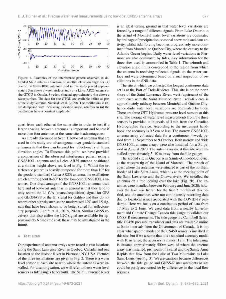
Figure 1. Examples of the interference pattern observed in de-trended SNR data as a function of satellite elevation angle for (a)one of the GNSS100L antennas used in this study placed approxi-mately 3 m above a water surface and (b) a Leica AR25 antenna atsite GTGU in Onsala, Sweden, situated approximately 4 m above awater surface. The data for site GTGU are available online as partof the study Geremia-Nievinski et al. (2020). The oscillations in (b)are dampened with increasing elevation angle, whereas in (a) theoscillations have a constant amplitude.

apart from each other at the same site in order to test if alarger spacing between antennas is important and to test ifmore than four antennas at the same site is advantageous.

As already discussed in Sect. 1, low-cost antennas that areused in this study are advantageous over geodetic-standardantennas in that they can be used for reflectometry at largerelevation angles. To illustrate this point, we have provideda comparison of the observed interference pattern using aGNSS100L antenna and a Leica AR25 antenna positionedat a similar height above sea level in Fig. 1. Whilst the in-terference pattern is heavily dampened for more than 10◦ forthe geodetic-standard (Leica AR25) antenna, the oscillationsare clear throughout 0–80◦ for the low-cost (GNSS100L) an-tennas. One disadvantage of the GNSS100L antennas usedhere and of low-cost antennas in general is that they tend toonly record the L1 C/A (coarse/acquisition) signal for GPSand GLONASS or the E1 signal for Galileo and they do notrecord other signals such as the modernised L2C and L5 sig-nals that have been shown to be better suited for reflectom-etry purposes (Tabibi et al., 2015, 2020). Similar GNSS re-ceivers that also utilise the L2C signal are available for ap-proximately 6 times the cost; these may be investigated in thefuture.

4 Test sites

Our experimental antenna arrays were tested at two locationsalong the Saint Lawrence River in Quebec, Canada, and onelocation on the Hudson River in Piermont, NY, USA. Picturesof the three installations are given in Fig. 2. There is a waterlevel sensor at each site near to where the antennas were in-stalled. For disambiguation, we will refer to these water levelsensors as tide gauges henceforth. The Saint Lawrence River

is an ideal testing ground in that water level variations areforced by a range of different signals. From Lake Ontario tothe island of Montréal water level variations are dominatedby drainage of precipitation, seasonal snow melt and dam ac-tivity, whilst tidal forcing becomes progressively more dom-inant from Montréal to Québec City, where the estuary to theAtlantic Ocean begins. Daily water level variations at Pier-mont are also dominated by tides. Key information for thethree sites used is summarised in Table 1. The azimuth andelevation angle limits correspond to the region from whichthe antenna is receiving reflected signals on the water sur-face and were determined based on visual inspection of os-cillations in the SNR data.

The site at which we collected the longest continuous dataset is at the Port of Trois-Rivières. This site is on the northshore of the Saint Lawrence River, west (upstream) of theconfluence with the Saint Maurice River. Trois-Rivières isapproximately midway between Montréal and Québec City;hence daily water level variations are dominated by tides.There are three OTT Hydromet pressure level sensors at thissite. The average of water level measurements from the threesensors is provided at intervals of 3 min from the CanadianHydrographic Service. According to the instrument hand-book, the accuracy is 0.5 cm or less. The narrow GNSS100Lantenna array collected data for a continuous 4-week pe-riod from 11 September to 9 October. Both narrow and wideGNSS100L antenna arrays were also installed for a 5 d pe-riod in August 2020. The antenna arrays at this site were in-stalled approximately 5–10 m away from the tide gauges.

The second site in Quebec is in Sainte-Anne-de-Bellevue,at the western tip of the island of Montréal. The stretch ofcoast where the antennas were situated is part of the northernborder of Lake Saint-Louis, which is at the meeting point ofthe Saint Lawrence and the Ottawa rivers. We installed theantennas on a tree looking over the lake (Fig. 2b). The an-tennas were installed between February and June 2020; how-ever the lake was frozen for the first 2 months of this pe-riod, and the antennas were not continuously recording datadue to logistical issues associated with the COVID-19 pan-demic. Here we focus on a continuous period of data from17 May to 2 June. We used data from a nearby Environ-ment and Climate Change Canada tide gauge to validate ourGNSS-R measurements. The tide gauge is a Campbell Scien-tific CS450 pressure transducer and data are available onlineat 6 min intervals from the Government of Canada. It is notclear what specific model of the CS450 sensor is installed atthis site, but if we assume that it is a standard accuracy modelwith 10 m range, the accuracy is at most 1 cm. The tide gaugeis situated approximately 500 m west of where the antennaarray was installed, just south of a canal and the Sainte AnneRapids that flow from the Lake of Two Mountains to LakeSaint-Louis (see Fig. 3). We are cautious because differencesbetween the tide gauge and GNSS-R measurements at sitecould be partly accounted for by differences in the local flowregimes.

https://doi.org/10.5194/esurf-9-673-2021 Earth Surf. Dynam., 9, 673–685, 2021

678 D. J. Purnell et al.: Precise water level measurements using low-cost GNSS antenna arrays

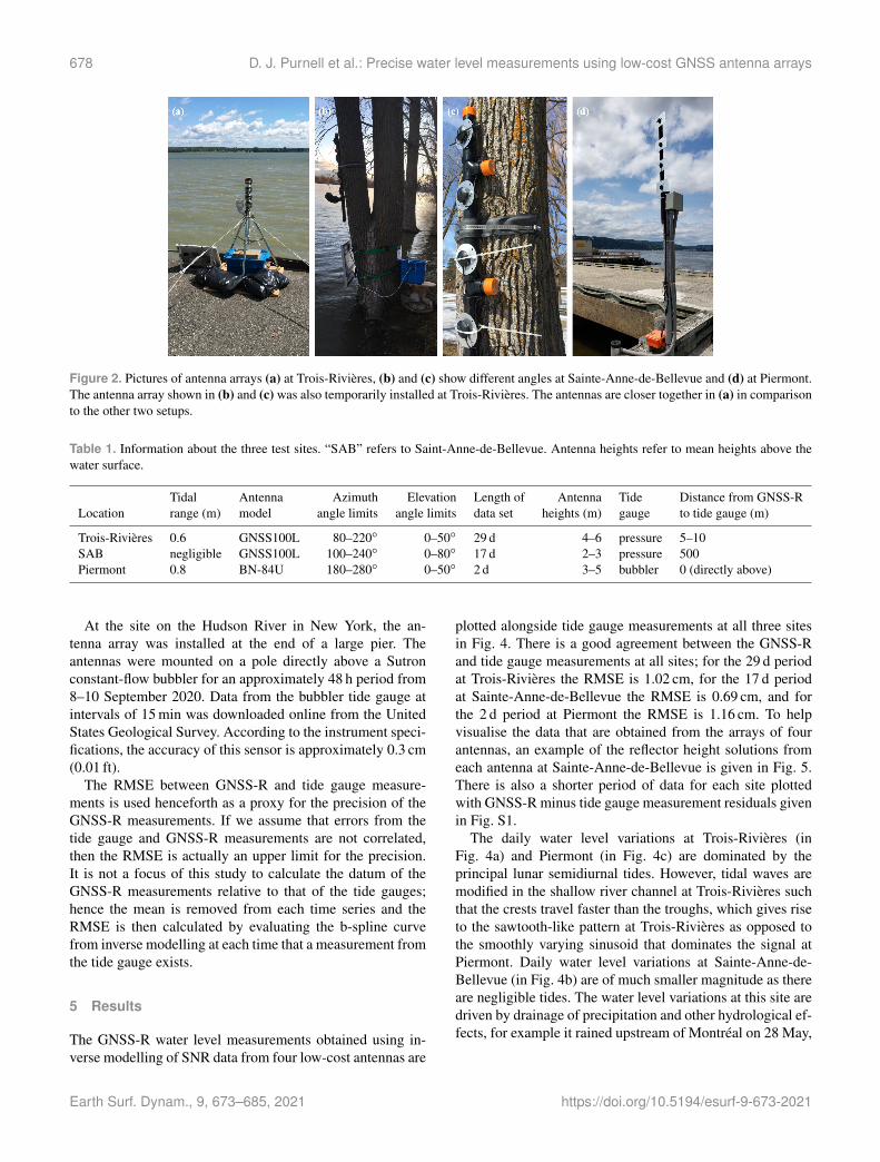
Figure 2. Pictures of antenna arrays (a) at Trois-Rivières, (b) and (c) show different angles at Sainte-Anne-de-Bellevue and (d) at Piermont.The antenna array shown in (b) and (c) was also temporarily installed at Trois-Rivières. The antennas are closer together in (a) in comparisonto the other two setups.

Table 1. Information about the three test sites. “SAB” refers to Saint-Anne-de-Bellevue. Antenna heights refer to mean heights above thewater surface.

Tidal Antenna Azimuth Elevation Length of Antenna Tide Distance from GNSS-RLocation range (m) model angle limits angle limits data set heights (m) gauge to tide gauge (m)

Trois-Rivières 0.6 GNSS100L 80–220◦ 0–50◦ 29 d 4–6 pressure 5–10SAB negligible GNSS100L 100–240◦ 0–80◦ 17 d 2–3 pressure 500Piermont 0.8 BN-84U 180–280◦ 0–50◦ 2 d 3–5 bubbler 0 (directly above)

At the site on the Hudson River in New York, the an-tenna array was installed at the end of a large pier. Theantennas were mounted on a pole directly above a Sutronconstant-flow bubbler for an approximately 48 h period from8–10 September 2020. Data from the bubbler tide gauge atintervals of 15 min was downloaded online from the UnitedStates Geological Survey. According to the instrument speci-fications, the accuracy of this sensor is approximately 0.3 cm(0.01 ft).

The RMSE between GNSS-R and tide gauge measure-ments is used henceforth as a proxy for the precision of theGNSS-R measurements. If we assume that errors from thetide gauge and GNSS-R measurements are not correlated,then the RMSE is actually an upper limit for the precision.It is not a focus of this study to calculate the datum of theGNSS-R measurements relative to that of the tide gauges;hence the mean is removed from each time series and theRMSE is then calculated by evaluating the b-spline curvefrom inverse modelling at each time that a measurement fromthe tide gauge exists.

5 Results

The GNSS-R water level measurements obtained using in-verse modelling of SNR data from four low-cost antennas are

plotted alongside tide gauge measurements at all three sitesin Fig. 4. There is a good agreement between the GNSS-Rand tide gauge measurements at all sites; for the 29 d periodat Trois-Rivières the RMSE is 1.02 cm, for the 17 d periodat Sainte-Anne-de-Bellevue the RMSE is 0.69 cm, and forthe 2 d period at Piermont the RMSE is 1.16 cm. To helpvisualise the data that are obtained from the arrays of fourantennas, an example of the reflector height solutions fromeach antenna at Sainte-Anne-de-Bellevue is given in Fig. 5.There is also a shorter period of data for each site plottedwith GNSS-R minus tide gauge measurement residuals givenin Fig. S1.

The daily water level variations at Trois-Rivières (inFig. 4a) and Piermont (in Fig. 4c) are dominated by theprincipal lunar semidiurnal tides. However, tidal waves aremodified in the shallow river channel at Trois-Rivières suchthat the crests travel faster than the troughs, which gives riseto the sawtooth-like pattern at Trois-Rivières as opposed tothe smoothly varying sinusoid that dominates the signal atPiermont. Daily water level variations at Sainte-Anne-de-Bellevue (in Fig. 4b) are of much smaller magnitude as thereare negligible tides. The water level variations at this site aredriven by drainage of precipitation and other hydrological ef-fects, for example it rained upstream of Montréal on 28 May,

Earth Surf. Dynam., 9, 673–685, 2021 https://doi.org/10.5194/esurf-9-673-2021

D. J. Purnell et al.: Precise water level measurements using low-cost GNSS antenna arrays 679

Figure 3. The area surrounding the antenna array and tide gauge atSainte-Anne-de-Bellevue.

which corresponds with a rise in the observed water level onthis day at Sainte-Anne-de-Bellevue.

5.1 Influence of multiple co-located antennas

There is an improvement in the precision of water level mea-surements when using four antennas as opposed to using justone antenna at all three sites. Reading values from Table 2,if the RMSE obtained with four antennas is compared to themaximum RMSE obtained with one antenna, there is a re-duction of 1.23 cm (or 50 %) at Trois-Rivières, 0.26 cm (or30 %) at Sainte-Anne-de-Bellevue and 0.51 cm (or 30 %) atPiermont. The results from Table 2 indicate a significant im-provement (up to 0.62 cm) when using four instead of twoantennas, but minimal improvement between three and fourantennas. Having four antennas is also recommended overthree antennas in case of redundancy. Note that whilst thedifference between the minimum RMSE obtained with oneantenna is comparable to that obtained with four antennas,our analysis suggests that the relative performance of eachantenna appears to be random, which in turn implies that theupper limit should be used for comparison. For example, ifthe data from Trois-Rivières are split into two 2-week periodsand analysed separately, the antennas that give the most andleast precise results are not the same for both periods, andneither of these sets in turn match those for the total 4-weekperiod.

During a period of 4 d, we performed an experiment withtwo arrays of four antennas (eight in total) installed at differ-ent heights and found that there is no advantage in installingmore than four antennas at the same site. For this 4 d periodthere is an RMSE of 1.06 cm when using just the narrow con-figuration, 1.32 cm when using just the wide configuration, or1.14 cm when using both narrow and wide simultaneously.

Given that the configurations were installed several metresapart, we tested different combinations of antennas acrossboth configurations to see if the spacing of antennas influ-ences the precision when using multiple antennas and foundthat there is no advantage in using antennas spaced furtherapart than the narrow configuration. These findings togetherwith our analyses at all three sites also indicate that there isno clear dependence on the heights of the antennas abovethe water surface. These results also suggest that the sourceof noise in the SNR data is likely due to random instrumentnoise as opposed to interference from the local environment.

Our results so far have focused on inverse modelling ofSNR data, but spectral analysis estimates, shown as dots inFig. 5, can also be compared with the tide gauge measure-ments. The RMSE of hourly means of spectral analysis esti-mates at Sainte-Anne-de-Bellevue varies from 2.40–3.90 cmfor each antenna. The hourly means can then be combinedinto a single time series by removing the height offset fromeach antenna and taking the median of the hourly values,which gives an RMSE of 1.94 cm. The maximum improve-ment of 1.96 cm when using four antennas as opposed to asingle antenna for spectral analysis estimates is much largerthan the 0.26 cm maximum improvement when using inversemodelling at this site. These differences between inversemodelling and spectral analysis suggest that random noise isa larger source of uncertainty when using spectral analysis,thus supporting the results from Purnell et al. (2020). Theseresults demonstrate that using multiple antennas in the samelocation is an effective technique for improving the precisionin GNSS-R water level measurements, regardless of the tech-nique that is used.

6 Discussion of GNSS-R parameters

The results described above were obtained after exploring alarge parameter space related to the inverse modelling andexperimental setup. The most important parameters to con-sider are the elevation angle limits, the azimuth angle limits,the b-spline knot spacing and time window length, the satel-lite constellations used, and the temporal resolution of data.We discuss the results of tests with these parameters below.The results discussed in this section were all obtained usingthe inverse modelling technique given in Sect. 2.

Note that elevation and azimuth angle limits are con-strained by the site surroundings, and the discussions inSect. 6.2 and 6.1 refer to investigating optimal limits withinthese pre-defined constraints. A given azimuth and eleva-tion angle corresponds to a Fresnel zone on the reflectingsurface where the power of the signal is concentrated. Soft-ware for calculating and visualising Fresnel zones is givenby Roesler and Larson (2018). As the elevation angle de-creases, the Fresnel zone increases in size and moves awayfrom the antenna, whereas changing the azimuth angle ro-tates the Fresnel zone laterally around the antenna. The limits

https://doi.org/10.5194/esurf-9-673-2021 Earth Surf. Dynam., 9, 673–685, 2021

680 D. J. Purnell et al.: Precise water level measurements using low-cost GNSS antenna arrays

Figure 4. A comparison of GNSS-R and tide gauge measurements at (a) Trois-Rivières, (b) Sainte-Anne-de-Bellevue and (c) Piermont. Themean of each time series is removed before plotting.

Figure 5. Reflector height measurements from four antennas at Sainte-Anne-de-Bellevue. The solid lines represent the b-spline solutionsfrom inverse modelling and the dots are estimates from spectral analysis. The b-spline parameters that are used to plot the solid lines in thisfigure are averaged to form the single solution in Fig. 4b. The curves are inverted because reflector height increases as water level decreases.

Earth Surf. Dynam., 9, 673–685, 2021 https://doi.org/10.5194/esurf-9-673-2021

D. J. Purnell et al.: Precise water level measurements using low-cost GNSS antenna arrays 681

Table 2. Summary of results obtained using different combinations of antennas to retrieve water level measurements. For one to threeantennas, the RMSE for every combination of antennas at each site was calculated, but only the lowest and highest values are shown in thetable.

RMSE (cm) obtained using inverse modelling with:

Site One antenna Two antennas Three antennas Four antennas

Trois-Rivières 1.24–2.25 1.26–1.64 1.04–1.10 1.02Sainte-Anne-de-Bellevue 0.63–0.95 0.64–0.81 0.65–0.73 0.69Piermont 1.08–1.67 1.07–1.44 1.10–1.25 1.16

given in Table 1 correspond roughly to the region in whichthe Fresnel zones are on the water surface and where thereare no objects obstructing the view of the water surface (e.g.moored boats).

6.1 Elevation angle limits

Using low-cost antennas we retrieved water level measure-ments over a range of elevation angles up to 50◦ at Trois-Rivières and Piermont and up to 80◦ at Sainte-Anne-de-Bellevue, whereas previous ground-based GNSS-R studieshave been limited to the use of elevation angles up to 35◦.Due to a number of trade-offs between low and high elevationangles, we found optimal limits of 10–50◦ at all three sites.For sites located at midlatitudes to high latitudes (such as oursites), satellites are more prevalent towards the Equator (i.e.to the south of our instruments) at lower elevation angles, andtherefore using lower elevation angles increases the amountof SNR data that is available for analysis. We find that re-flector height measurements are generally less precise at el-evation angles greater than 30◦, in agreement with previouswork using geodetic-standard antennas that found the effectof random noise in SNR data leads to a greater uncertaintyat larger elevation angles (Purnell et al., 2020). However, theeffect of tropospheric delay increases with decreasing eleva-tion angle and leads to an underestimation of the reflectorheight (Williams and Nievinski, 2017). For our sites, tropo-spheric delay has a minor effect on the precision, but afore-mentioned literature (e.g. Nikolaidou et al., 2020) suggeststhat this effect is more important at sites where the antennasare at a greater height above the water surface (e.g. > 5 m)or where there is a large tidal range (e.g. > 2 m) and espe-cially when attempting to find the datum of reflector heightmeasurements (not done here). In general, we find that it ismost important to use a large range of elevation angles (e.g.30◦ or more) to eliminate any gaps in time in the SNR data,and this is especially important at sites with daily tidal vari-ations, such as at Trois-Rivières and Piermont. We initiallytried to use a lower limit of 20◦, where the effect of tropo-spheric delay becomes negligible (Nikolaidou et al., 2020)but found more precise measurements using a lower limit of10◦ at Trois-Rivières and Piermont. Limits of 20–50◦ can

be used to make equally precise measurements as 10–50◦ atSainte-Anne-de-Bellevue.

6.2 Azimuth angle limits

In general, azimuth angle limits should be fixed to matchthe widest unobstructed view of the water surface. In con-trast with elevation angles, there are no complicated azimuth-angle-dependent effects; the larger the range of azimuth an-gle limits, the more data for GNSS-R analysis. The only com-plicating factor is that some azimuth angles yield more dataper day than others because satellites are more prevalent to-wards the south at midlatitudes to high latitudes in the North-ern Hemisphere or vice versa in the Southern Hemisphere.To demonstrate the importance of maximising the azimuthangle range, we retrieved water level measurements at Trois-Rivières and Sainte-Anne-de-Bellevue with the azimuth an-gle range reduced from 140 to 100◦. The RMSE increased byapproximately 50 % (from 1.02 to 1.49 cm) at Trois-Rivièresand 15 % (from 0.69 to 0.79 cm) at Sainte-Anne-de-Bellevuewhen using the reduced azimuth angle ranges.

6.3 B-spline knot spacing and time window

For the results described in the previous section, the b-splineknot spacing and time window length vary for each site: atTrois-Rivières we use a knot spacing of 1 h and a time win-dow of 6 h, at Sainte-Anne-de-Bellevue we use a knot spac-ing of 4 h and a time window of 24 h, and at Piermont weuse a knot spacing of 2 h and a time window of 6 h. In gen-eral, the knot spacing should be set to 1 h at a site with largedaily tidal variations or a site with a complicated signal (suchas the sawtooth-like signal at Trois-Rivières). Note that thereis automatically a lower limit on the precision that can beachieved using inverse modelling because a b-spline curvecannot perfectly represent the time series. This lower limiton the precision increases with increasing knot spacing. Forexample, if we directly fit a b-spline curve to the tide gaugemeasurements at Trois-Rivières shown in Fig. 4a, we find anRMSE of 0.5 cm if using a knot spacing of 1 h or 1.6 cm ifusing a knot spacing of 2 h. However, decreasing the knotspacing for inverse modelling also decreases the amount ofSNR data that is used to compute each b-spline scaling fac-

https://doi.org/10.5194/esurf-9-673-2021 Earth Surf. Dynam., 9, 673–685, 2021

682 D. J. Purnell et al.: Precise water level measurements using low-cost GNSS antenna arrays

tor, potentially leading to less precise results; hence we donot recommend using a knot spacing of less than 1 h.

The time window should be at least 3 times the lengthof the knot spacing. Provided that this minimum is met, thelength of the time window does not appear to impact the pre-cision in our experiments. However, both increasing the win-dow length or decreasing the knot spacing greatly increasesthe computation time for the inverse modelling.

6.4 Satellite constellations

Using data simultaneously from all three satellite constel-lations that are tracked by our low-cost antennas (GPS,GLONASS and Galileo) is important to achieve the most pre-cise results. For example, when using only GPS data at Trois-Rivières, the RMSE increases by over 200 % compared to theresults obtained using all three constellations (the RMSE is3.11 cm with just GPS compared to 1.02 cm with all threeconstellations). Using any combination of two constellationsalso leads to less precise results than using all three con-stellations: the RMSE increases by approximately 30 % (to1.27 cm) when using just GPS and GLONASS together or170 % (to 2.69 cm) when using just GLONASS and Galileotogether. It is not clear if these differences are due to theprevalence of satellites (there are more GPS satellites) or dif-ferences in the signals themselves.

6.5 Temporal resolution of SNR data

The temporal resolution of SNR data greatly affects the com-putation time for inverse modelling. Data were recorded atour sites every second but we found that it was most effi-cient to resample the data to intervals of 15 s prior to anal-ysis. When varying the temporal resolution between 1 and15 s at Trois-Rivières, we found that the RMSE varies byless than 1 mm but the computation time increases greatlywhen using an interval time of 1 s. The RMSE increases byapproximately 70 % when decimating the data to intervals of30 or 60 s. Recording data at intervals of 5, 10 or 15 s is there-fore advantageous for data storage and efficient analysis. It isimportant to note, however, that the temporal resolution pro-vides a limitation on the maximum reflector height that canbe resolved due to the Nyquist frequency. See Roesler andLarson (2018) for a discussion on this Nyquist limit.

7 Conclusions

We presented a technique for retrieving precise water levelmeasurements using arrays of four low-cost GNSS anten-nas and validated our technique at three sites with variabletidal forcing. By comparing it with nearby operational tidegauges, we found an upper limit on the precision of waterlevel measurements of 0.69–1.16 cm at all sites, whereas pre-vious studies using geodetic-standard antennas have foundan RMSE of 2–50 cm. The RMSE values obtained are likely

upper limits on the precision because they also contain errorfrom the tide gauge measurements. The amount of error fromthe tide gauge measurements is also likely to differ betweensites because there are different types of instruments at thesites in Quebec (pressure transducers) and Piermont (bub-bler gauge). While pressure transducers are more suscepti-ble to errors over multi-year timescales due to instrumentdrift (Míguez et al., 2005; Pytharouli et al., 2018), bubblergauges are more susceptible to errors during wavy conditions(Woodworth and Smith, 2003). The results presented here aresignificant in that an accuracy of 1 cm is the benchmark setby GLOSS (2012) for studying multi-year trends in sea level.We found an improvement in the precision of 30 %–50 %when using four co-located antennas instead of one, whichsuggests that random noise is one of the key sources of un-certainty in GNSS-R measurements and supports the resultsfrom Purnell et al. (2020). In addition to the reduction in cost(on the order of several thousand USD or more), we foundthat the low-cost antennas are better suited for reflectometrythan geodetic-standard antennas because they can be used toobtain water level measurements over a much larger range ofelevation angles.

Our results provide a strong proof of concept, but workremains to be done to further validate and improve our tech-nique. Most importantly, an array of antennas should be in-stalled with a co-located tide gauge for a longer time period(e.g. for at least several months) and at a site with a largertidal range. It is also necessary to attempt a levelling pro-cedure so that the datum of the water level measurementscan be defined. To place measurements on a global referenceframe and simultaneously monitor local land deformation,an array of low-cost antennas could then be co-located witha geodetic-standard antenna with the aim of using the low-cost antennas to obtain precise water level measurements andthe geodetic-standard antenna to perform precise position-ing. More models of low-cost antennas should also be tested,preferably in the same location (we do not recommend oneof the types of antennas used in this study over the other typebecause we have not had the opportunity to test them at thesame location). Whilst our results suggest that the spacingapart of antennas is not important, we cannot rule out thepossibility of interference between antennas at the separa-tion distances used in this study. A rigorous investigation ofthe clearance distance required to ensure that antennas arenot interfering should guide a future study. A vertical arrayof low-cost antennas such as those used in this study couldbe used to test the technique for obtaining high-rate sea levelmeasurements recently proposed by Yamawaki et al. (2021).

For future installations of low-cost antennas, we proposethe following guidelines:

– at least four co-located antennas

– the antennas should record data from GPS, GLONASSand Galileo satellites

Earth Surf. Dynam., 9, 673–685, 2021 https://doi.org/10.5194/esurf-9-673-2021

D. J. Purnell et al.: Precise water level measurements using low-cost GNSS antenna arrays 683

– the antennas should be positioned within 1–5 m abovethe water surface

– the antennas should have an unobstructed view of thewater surface that extends 140◦ or more laterally and atleast 50 m outwards (this corresponds to the edge of theFresnel zone for an antenna 5 m above the water surfaceand a satellite at 10◦ elevation)

– data should be recorded at intervals of 5 s (or more, de-pending on the mean height of the antennas above thewater surface and the associated Nyquist limit).

Upon obtaining data, the following inverse modelling param-eters should be used to extract precise water level measure-ments:

– a large range of elevation angles (e.g. 10–50◦)

– a b-spline knot spacing of 1 h at a site with tides (orlarger would be more efficient at a site with negligibletides)

– a b-spline time window length of at least 3 times theknot spacing.

The above guidelines may be refined following further fieldwork. For example, we found that having four antennas isoptimal when we tested eight co-located antennas for a shortperiod of 4 d – more data are needed to support this result.Additional data from other satellite constellations (such asBeiDou) and from other signals (such as L2C and L5) mayalso be useful.

Our technique for monitoring water levels with arrays oflow-cost antennas could be applied to address the need forwidespread, accessible water level measurements in the faceof future climate change. The antenna arrays are relativelysimple to build and therefore suited to citizen science efforts.They could be used to obtain sea level measurements in re-mote coastal regions as well as lake level or river stage mea-surements at a fraction of the cost of commercially availablesensors but with comparable precision. Such measurementscould be used to validate satellite measurements and to bet-ter constrain tidal models in the polar regions, where thereare few coastal sea level measurements. A dense network ofsensors could also be installed to detect spatially variable sealevel signals, for example near tidewater glaciers to detectso-called sea level fingerprints (Mitrovica et al., 2011).

Code availability. Codes for analysing low-cost GNSS data toproduce water level measurements using MATLAB or Python soft-ware can be found at https://doi.org/10.5281/zenodo.4790412 (Pur-nell, 2021). There is also 1 d of sample data (the 13 Septem-ber 2020) from the “narrow” antenna array at Trois-Rivières con-tained in this repository.

Supplement. The supplement related to this article is availableonline at: https://doi.org/10.5194/esurf-9-673-2021-supplement.

Author contributions. DJP, NG and WM conceptualised thestudy. DJP performed analysis and wrote all codes to go along withthe article. WM designed and built the initial low-cost antenna ar-ray (including software). GL, DJP and DP built subsequent antennaarrays and performed field work. DJP wrote the initial article draftand NG, WM and DP helped to improve the article.

Competing interests. The authors declare that they have no con-flict of interest.

Acknowledgements. The authors would like to thank the Port ofTrois-Rivières, the Canadian Hydrographic Service, Fisheries andOceans Canada, and Environment and Climate Change Canada forhelp with field work and obtaining tide gauge data. We also thankManuella Fagundes and an anonymous reviewer for comments thathelped to improve the article. Codes were translated from MATLABto Python with support from Claire Marie Guimond.

Financial support. This research has been supported by theMcGill University (The Trottier Fellowship for Science and PublicPolicy), the Fonds de recherche du Québec – Nature et technologies(New researchers programme), the McGill Space Institute (Gradu-ate fellowship), the American Geophysical Union (Jerome M. Parosscholarship in geophysical instrumentation), and the Canada Re-search Chairs (Canada Research Chairs Program).

Review statement. This paper was edited by Giulia Sofia and re-viewed by Manuella Fagundes and one anonymous referee.

References

Adrian, R., O’Reilly, C. M., Zagarese, H., Baines, S. B., Hessen,D. O., Keller, W., Livingstone, D. M., Sommaruga, R., Straile,D., Van Donk, E., Weyhenmeyer, G. A., and Winder, M.: Lakesas sentinels of climate change, Limnol. Oceanogr., 54, 2283–2297, https://doi.org/10.4319/lo.2009.54.6_part_2.2283, 2009.

Baumann, T. M., Polyakov, I. V., Padman, L., Danielson,S., Fer, I., Janout, M., Williams, W., and Pnyushkov,A. V.: Arctic tidal current atlas, Scientific Data, 7, 275,https://doi.org/10.1038/s41597-020-00578-z, 2020.

Beckmann, P. and Spizzichino, A.: The scattering of electromag-netic waves from rough surfaces, Artech House, Norwood, MA,USA, 1987.

Dullaart, J. C. M., Muis, S., Bloemendaal, N., and Aerts, J.C. J. H.: Advancing global storm surge modelling using thenew ERA5 climate reanalysis, Clim. Dynam., 54, 1007–1021,https://doi.org/10.1007/s00382-019-05044-0, 2020.

Fagundes, M. A. R., Mendonça-Tinti, I., Iescheck, A. L., Akos,D. M., and Geremia-Nievinski, F.: An open-source low-cost sen-sor for SNR-based GNSS reflectometry: design and long-term

https://doi.org/10.5194/esurf-9-673-2021 Earth Surf. Dynam., 9, 673–685, 2021

684 D. J. Purnell et al.: Precise water level measurements using low-cost GNSS antenna arrays

validation towards sea-level altimetry, GPS Solutions, 25, 73,https://doi.org/10.1007/s10291-021-01087-1, 2021.

Geremia-Nievinski, F., Hobiger, T., Haas, R., Liu, W., Strandberg,J., Tabibi, S., Vey, S., Wickert, J., and Williams, S.: SNR-basedGNSS reflectometry for coastal sea-level altimetry: results fromthe first IAG inter-comparison campaign, J. Geodesy, 94, 70,https://doi.org/10.1007/s00190-020-01387-3, 2020.

GLOSS: Global Sea-Level Observing System (GLOSS) Imple-mentation Plan, IOC Technical Series No. 100 (English), UN-ESCO/IOC, 2012.

Goudie, A. S.: Global warming and fluvial ge-omorphology, Geomorphology, 79, 384–394,https://doi.org/10.1016/j.geomorph.2006.06.023, 2006.

Gómez-Enri, J., Vignudelli, S., Cipollini, P., Coca, J., and González,C.: Validation of CryoSat-2 SIRAL sea level data in the easterncontinental shelf of the Gulf of Cadiz (Spain), Adv. Space Res.,62, 1405–1420, https://doi.org/10.1016/j.asr.2017.10.042, 2018.

Khan, S. A., Bjørk, A. A., Bamber, J. L., Morlighem, M., Be-vis, M., Kjær, K. H., Mouginot, J., Løkkegaard, A., Holland,D. M., Aschwanden, A., Zhang, B., Helm, V., Korsgaard, N. J.,Colgan, W., Larsen, N. K., Liu, L., Hansen, K., Barletta, V.,Dahl-Jensen, T. S., Søndergaard, A. S., Csatho, B. M., Sas-gen, I., Box, J., and Schenk, T.: Centennial response of Green-land’s three largest outlet glaciers, Nat. Commun., 11, 5718,https://doi.org/10.1038/s41467-020-19580-5, 2020.

Kopp, R. E., Hay, C. C., Little, C. M., and Mitrovica, J. X.:Geographic Variability of Sea-Level Change, Current ClimateChange Reports, 1, 192–204, https://doi.org/10.1007/s40641-015-0015-5, 2015.

Larson, K. M., Ray, R. D., Nievinski, F. G., and Freymueller, J. T.:The Accidental Tide Gauge: A GPS Reflection Case Study FromKachemak Bay, Alaska, IEEE Geosci. Remote S., 10, 1200–1204, https://doi.org/10.1109/LGRS.2012.2236075, 2013.

Meyssignac, B., Slangen, A. B. A., Melet, A., Church, J. A., Fet-tweis, X., Marzeion, B., Agosta, C., Ligtenberg, S. R. M., Spada,G., Richter, K., Palmer, M. D., Roberts, C. D., and Champollion,N.: Evaluating Model Simulations of Twentieth-Century Sea-Level Rise. Part II: Regional Sea-Level Changes, J. Climate, 30,8565–8593, https://doi.org/10.1175/JCLI-D-17-0112.1, 2017.

Mitrovica, J. X., Gomez, N., Morrow, E., Hay, C., Latychev,K., and Tamisiea, M. E.: On the robustness of predictionsof sea level fingerprints, Geophys. J. Int., 187, 729–742,https://doi.org/10.1111/j.1365-246X.2011.05090.x, 2011.

Míguez, B. M., Gómez, B. P., and Fanjul, E. A.: The ESEAS-RI SeaLevel Test Station: Reliability and Accuracy of Different TideGauges, The International Hydrographic Review, 6, 44–53, 2005.

Nikolaidou, T., Santos, M. C., Williams, S. D. P., andGeremia-Nievinski, F.: Raytracing atmospheric delaysin ground-based GNSS reflectometry, J. Geodesy, 94, 68,https://doi.org/10.1007/s00190-020-01390-8, 2020.

Pattyn, F. and Morlighem, M.: The uncertain future ofthe Antarctic Ice Sheet, Science, 367, 1331–1335,https://doi.org/10.1126/science.aaz5487, 2020.

Peng, F. and Deng, X.: Validation of Sentinel-3A SARmode sea level anomalies around the Australiancoastal region, Remote Sens. Environ., 237, 111548,https://doi.org/10.1016/j.rse.2019.111548, 2020.

Purnell, D., Gomez, N., Chan, N. H., Strandberg, J., Hol-land, D. M., and Hobiger, T.: Quantifying the Uncer-

tainty in Ground-Based GNSS-Reflectometry Sea LevelMeasurements, IEEE J. Sel. Top. Appl., 13, 4419–4428,https://doi.org/10.1109/JSTARS.2020.3010413, 2020.

Purnell, D.: gnssr_lowcost, https://doi.org/10.5281/zenodo.4790412,2021.

Pytharouli, S., Chaikalis, S., and Stiros, S. C.: Uncer-tainty and bias in electronic tide-gauge records: Evidencefrom collocated sensors, Measurement, 125, 496–508,https://doi.org/10.1016/j.measurement.2018.05.012, 2018.

Roesler, C. and Larson, K. M.: Software tools for GNSS inter-ferometric reflectometry (GNSS-IR), GPS Solutions, 22, 80,https://doi.org/10.1007/s10291-018-0744-8, 2018.

Santamaría-Gómez, A. and Watson, C.: Remote levelingof tide gauges using GNSS reflectometry: case studyat Spring Bay, Australia, GPS Solutions, 21, 451–459,https://doi.org/10.1007/s10291-016-0537-x, 2017.

Seifi, F., Deng, X., and Andersen, O. B.: Assessment of the Accu-racy of Recent Empirical and Assimilated Tidal Models for theGreat Barrier Reef, Australia, Using Satellite and Coastal Data,Remote Sens., 11, 1211, 2019.

Sermet, Y., Villanueva, P., Sit, M. A., and Demir, I.: Crowd-sourced approaches for stage measurements at ungauged lo-cations using smartphones, Hydrolog. Sci. J., 65, 813–822,https://doi.org/10.1080/02626667.2019.1659508, 2020.

Slangen, A. B. A., Church, J. A., Agosta, C., Fettweis, X.,Marzeion, B., and Richter, K.: Anthropogenic forcing dominatesglobal mean sea-level rise since 1970, Nat. Clim. Change, 6,701–705, https://doi.org/10.1038/nclimate2991, 2016.

Strandberg, J. and Haas, R.: Can We Measure Sea Level With aTablet Computer?, IEEE Geosci. Remote S., 17, 1–3, 2019.

Strandberg, J., Hobiger, T., and Haas, R.: Improving GNSS-R sealevel determination through inverse modeling of SNR data, Ra-dio Sci., 51, 1286–1296, https://doi.org/10.1002/2016RS006057,2016.

Tabibi, S., Nievinski, F. G., Dam, T. V., and Monico, J. F.: As-sessment of modernized GPS L5 SNR for ground-based mul-tipath reflectometry applications, Adv. Space Res., 55, 1104–1116, https://doi.org/10.1016/j.asr.2014.11.019, 2015.

Tabibi, S., Geremia-Nievinski, F., Francis, O., and van Dam, T.:Tidal analysis of GNSS reflectometry applied for coastal sealevel sensing in Antarctica and Greenland, Remote Sens. En-viron., 248, 111959, https://doi.org/10.1016/j.rse.2020.111959,2020.

Taherkhani, M., Vitousek, S., Barnard, P. L., Frazer, N., An-derson, T. R., and Fletcher, C. H.: Sea-level rise exponen-tially increases coastal flood frequency, Sci. Rep., 10, 6466,https://doi.org/10.1038/s41598-020-62188-4, 2020.

Tamisiea, M. E., Hughes, C. W., Williams, S. D. P., andBingley, R. M.: Sea level: measuring the bounding sur-faces of the ocean, Philosophical Transactions of the RoyalSociety A: Mathematical, Phys. Eng. Sci., 372, 20130336,https://doi.org/10.1098/rsta.2013.0336, 2014.

Williams, S. D. P. and Nievinski, F. G.: Tropospheric delays inground-based GNSS multipath reflectometry–Experimental evi-dence from coastal sites, J. Geophsy. Res.-Sol., 122, 2310–2327,https://doi.org/10.1002/2016JB013612, 2017.

Williams, S. D. P., Bell, P. S., McCann, D. L., Cooke, R., and Sams,C.: Demonstrating the Potential of Low-Cost GPS Units for theRemote Measurement of Tides and Water Levels Using Inter-

Earth Surf. Dynam., 9, 673–685, 2021 https://doi.org/10.5194/esurf-9-673-2021

D. J. Purnell et al.: Precise water level measurements using low-cost GNSS antenna arrays 685

ferometric Reflectometry, J. Atmos. Ocean. Technol., 37, 1925–1935, https://doi.org/10.1175/JTECH-D-20-0063.1, 2020.

Woodworth, P. L. and Smith, D. E.: A One Year Comparisonof Radar and Bubbler Tide Gauges at Liverpool, The Interna-tional Hydrographic Review, 4, available at: https://journals.lib.unb.ca/index.php/ihr/article/view/20630 (last access: 12 Novem-ber 2019), 2003.

Yamawaki, M. K., Geremia-Nievinski, F., and Monico, J. F. G.:High-Rate Altimetry in SNR-Based GNSS-R: Proof-of-Conceptof a Synthetic Vertical Array, IEEE Geosci. Remote S., 1–5,https://doi.org/10.1109/LGRS.2021.3068091, 2021.

https://doi.org/10.5194/esurf-9-673-2021 Earth Surf. Dynam., 9, 673–685, 2021