Precise Measurements of Few-Body Physics in Ultracold

39K Bose Gas

by

Roman Chapurin

B.S. Physics, University of Florida, 2012

M.S. Physics, University of Colorado, 2015

A thesis submitted to the

Faculty of the Graduate School of the

University of Colorado in partial fulfillment

of the requirements for the degree of

Doctor of Philosophy

Department of Physics

2019

This thesis entitled:Precise Measurements of Few-Body Physics in Ultracold 39K Bose Gas

written by Roman Chapurinhas been approved for the Department of Physics

Prof. Eric A. Cornell

Prof. Jun Ye

Date

The final copy of this thesis has been examined by the signatories, and we find that both thecontent and the form meet acceptable presentation standards of scholarly work in the above

mentioned discipline.

iii

Roman Chapurin, (Ph.D., Physics)

Precise Measurements of Few-Body Physics in Ultracold 39K Bose Gas

Thesis directed by Prof. Eric A. Cornell

Ultracold atomic gases with tunable interactions offer an ideal platform for studying interact-

ing quantum matter. While the few- and many-body physics are generally complex and intractable,

the problem can be greatly simplified in an atomic gas by a controlled separation of relevant length

and energy scales. Precise control of experimental parameters, via Feshbach resonances, optical

potentials and radio-frequency radiation, enables deterministic measurements of few-body physics,

including universal physics and the Efimov effect. This thesis presents our recent studies on pre-

cisely measuring two- and three-body physics in an ultracold Bose gas. I begin by describing our

new apparatus used for generating and studying ultracold 39K gas samples. Then, I focus on our

precision spectroscopy of Feshbach dimer binding energies, spanning three orders of magnitude and

with sub-kilohertz resolution. These measurements enable us to locate a Feshbach resonance and

determine scattering length values with unprecedented accuracy. Finally, I present our precise mea-

surements locating an exotic three-body state, specifically the Efimov ground state. We find that

the trimer state location significantly deviates from the value predicted by van der Waals univer-

sality. Due to small experimental and systematic uncertainties, our measurement is the strongest

evidence of departure from the universal value and is the first observed deviation near a Feshbach

resonance of intermediate strength.

Dedication

To my family, for your unconditional support and encouragement.

v

Acknowledgements

I was very fortunate to be surrounded by so many bright and exciting individuals during

my PhD studies at JILA. I am forever thankful to Debbie Jin for giving me an opportunity and

taking me under her wing. Debbie invested a significant amount of time in me and all her students,

bettering us as scientists and helping us grow as individuals. I learned to question with humility,

to always focus with great intensity on the important details in all aspects of life, to choose the

less-traveled path, to find fun in the mundane, to be persistent and trust ones abilities, and to

always ask “how difficult could that really be?”. During the first four years of my PhD, Debbie

was my academic advisor, a personal mentor and a role model; I hope to influence others in the

same manner as she has. I want to express gratitude to Eric Cornell, Jun Ye, Cindy Regal, John

Bohn and Krista Beck for support and encouragement after Debbie’s passing, and all of JILA for

coming together like family.

I want to thank my advisors Eric and Jun for forming the experimental team that accom-

plished the ambitious work presented in this thesis. Eric and Jun both have contagious personalities,

inspiring and exciting everyone around them. I am always encouraged to explore new things and

get things done after talking to them. I’ve always been impressed by Jun’s ability to successfully

lead multiple scientific endeavors, while maintaining extraordinary intensity, focus and devotion to

his students. Jun’s endless technical knowledge and intuition, along with a better memory retention

than our lab’s notebooks and computers, enabled fast progression in solving our toughest problems.

I’ve always been impressed and inspired by Eric’s unconventional approaches to solve simple and

complex problems. Eric’s energy is contagious, the lab’s progress greatly benefited from the created

vi

environment.

Building an atomic physics lab from scratch required great effort and could not have been

accomplished without significant help. I am thankful to NIST and NSF for my graduate fellowships,

which enabled me to “get to business” as soon as I stepped my foot on campus and to devote my

focus fully on research. I am thankful to individuals of the 40K Fermi gas team I joined: Rabin

Paudel, Tara Drake, and postdoc Yoav Sagi; they taught me a lot. I spent many days and nights

with Rabin building up the apparatus; without his drive “to get things done today”, it would have

been very difficult to reach our goals in a timely manner. Additionally, we had multiple bright

undergraduate students help with the construction. In particular, I want to thank Sean Braxton

and Josh Giles for their hard work and persistence in getting things to work. I want to thank the

KRb (now degenerate) polar molecules team for being good lab-neighbors and having empathy in

building a complex apparatus, particularly Luigi DeMarco, Kyle Matsuda, Will Tobias, Giacomo

Valtolina, Jacob Covey, Steven Moses, and Jamie Shaw. Additionally, others I’ve interacted with

who underwent lab construction: Cornell/Ye eEDM team (Will Cairncross, Tanya Roussy, Kia

Boon Ng, Yan Zhou, Yuval Shagam, Dan Gresh, Matt Grau), Ye Sr lab (Sara Campbell, Ed Marti,

Aki Goban, Ross Hutson, Dhruv Kedar, Lindsay Sonderhouse), Thompson lab (Matt Norcia, Julia

Cline), Nesbitt lab (Tim Large), Ye molecules lab (David Reens, Alejandra Collopy) and Regal

lab (Brian Lester, Adam Kaufman) and Kaufman lab. I like to thank my office mates, Gil Porat,

Tanya Roussy, Stephen Schoun, Yuval Shagam, and Marissa Weichman, for exchanging many ideas

over the years.

It would have been difficult to construct such a complex apparatus without JILA’s infras-

tructure and personnel. I spent a significant amount of time working with the instrument shop,

particularly with Hans Green, Todd Asnicar, Tracy Keep, Kim Hagen, Blaine Horner, Kyle Thatche

and Calvin Schwadron. Hans helped greatly during the initial construction, often working long days

and nights with Rabin and I, and has been great to talk to for new ideas or encouragement. Todd

always made sure that our shop requests were completed earlier than we anticipated. Custom,

robust and low-noise electronics are the bread and butter of any atomic physics lab and I was

vii

fortunate to learn from the JILA electronics group: Terry Brown, Carl Sauer, James Fung-A-Fat,

Christopher Ho, and (unofficially) Jan Hall. Terry is a wizard of electronics and I’ve learned a

lot from him. Carl was instrumental in solving many of our time-sensitive electronics problems

by being quick and direct. Jan, who is always lurking around or soldering in the electronics shop,

is full of technical wisdom and adventurous stories, often starring troublesome lasers. Our lab’s

stability and automation would not be possible without assistance from JILA’s computing team,

particularly J.R. Raith, Corey Keasling and Jim McKown, and building proctors, especially Dave

Errickson and Jason Ketcherside. I am thankful to John Bohn and Jose D’Incao (our JILA theory

colleagues), with who I can talk to beyond physics. The rest of the JILA staff and administration,

especially Krista Beck, help us in so many ways that allow us truly focus on tackling scientific and

technical challenges. I am thankful to all JILA fellows for keeping projects well-funded; the JILA

grad students sleep well at night. Overall, the JILA culture and atmosphere are unlike any other.

The fast-paced “whatever works” mentality (often entailing building own electronics, machining

own parts or constructing homebuilt lasers), coupled with a great infrastructure and determined

personnel, is always a good recipe for rapid scientific achievement and fast learning.

I spent the last two and a half years working with two talented individuals, Xin Xie and

Michael Van de Graaff (Vandy). Prior to Debbie’s passing, Xin, Vandy and I were Debbie’s graduate

students working on three different experiments. Afterward, Xin’s and Vandy’s laboratories were

shut down and together we started our new venture, with Eric and Jun at the helm. We converted

the new 40K Fermi lab to a 39K Bose machine in only 9 months. Such a rapid conversion would

not have been possible without Xin and Vandy. Xin has an incredible work ethic and I am glad

to have worked with a fellow stoic on challenging problems. She always encouraged everyone

around her to push their limits. Vandy brought a lot of character and enthusiasm into our lab,

and was willing to be the lab’s perfectionist when needed. We also had help from hard working

undergraduate students: Carlos Lopez-Abadia, Bjorn Sumner and Jared Popowski. Recently, we

had a new graduate student Noah Schlossberger join our lab. With Xin (at the helm), Vandy, Noah

and Jared, I know the lab is in good hands with many exciting results to come.

viii

On a more personal note, I would like thank everyone who was there with me during my

PhD years. I befriended many intelligent and fun individuals, including (forgive any exclusions)

Rabin Paudel, Steven Moses, Luigi DeMarco, Sean Braxton, Dmitriy Zusin, Javier Orjuela-Koop,

Maithreyi Gopalakrishnan, Joseph Samaniego, Peter Siegfried and Tim Livingston Large. I thank

Gary Ihas for his mentorship and encouragement throughout the years. I am grateful to Aimee

Graeber for all Colorado adventures and support. Last, I would like to thank my family for making

sacrifices to help me get where I am today.

ix

Contents

Chapter

1 Introduction 1

1.1 Universal Physics with Ultracold Atoms . . . . . . . . . . . . . . . . . . . . . . . . . 1

1.2 The Efimov Effect and Few-Body Physics . . . . . . . . . . . . . . . . . . . . . . . . 3

1.3 Thesis Contents . . . . . . . . . . . . . . . . . . . . . . . . . . . . . . . . . . . . . . . 5

2 Apparatus and Techniques for Cooling 39K 7

2.1 Properties of 39K . . . . . . . . . . . . . . . . . . . . . . . . . . . . . . . . . . . . . . 7

2.2 Overview of the Experimental Setup and the Cooling Procedure . . . . . . . . . . . 12

2.3 Doppler Laser Cooling . . . . . . . . . . . . . . . . . . . . . . . . . . . . . . . . . . . 16

2.3.1 D2 Laser System . . . . . . . . . . . . . . . . . . . . . . . . . . . . . . . . . . 18

2.3.2 MOT Load . . . . . . . . . . . . . . . . . . . . . . . . . . . . . . . . . . . . . 25

2.4 Sub-Doppler Laser Cooling . . . . . . . . . . . . . . . . . . . . . . . . . . . . . . . . 31

2.4.1 D1 Laser System . . . . . . . . . . . . . . . . . . . . . . . . . . . . . . . . . . 31

2.4.2 D1 Cooling and Quadrupole Trap Load . . . . . . . . . . . . . . . . . . . . . 32

2.5 All-Optical Evaporation . . . . . . . . . . . . . . . . . . . . . . . . . . . . . . . . . . 39

2.5.1 Optical Trap Load . . . . . . . . . . . . . . . . . . . . . . . . . . . . . . . . . 39

2.5.2 Optical Trap Laser Setup . . . . . . . . . . . . . . . . . . . . . . . . . . . . . 42

2.5.3 Evaporation in the Optical Dipole Trap . . . . . . . . . . . . . . . . . . . . . 53

x

3 Experimental Toolkit for State Manipulation and Readout 59

3.1 RF Control System . . . . . . . . . . . . . . . . . . . . . . . . . . . . . . . . . . . . . 59

3.1.1 RF Circuitry . . . . . . . . . . . . . . . . . . . . . . . . . . . . . . . . . . . . 59

3.1.2 RF Transitions . . . . . . . . . . . . . . . . . . . . . . . . . . . . . . . . . . . 63

3.2 Magnetic Field Stabilization . . . . . . . . . . . . . . . . . . . . . . . . . . . . . . . . 66

3.2.1 Lineshape Spectral Noise . . . . . . . . . . . . . . . . . . . . . . . . . . . . . 66

3.2.2 Magnetic Field Control . . . . . . . . . . . . . . . . . . . . . . . . . . . . . . 67

3.3 Imaging System . . . . . . . . . . . . . . . . . . . . . . . . . . . . . . . . . . . . . . . 72

3.3.1 Side Imaging Specifications . . . . . . . . . . . . . . . . . . . . . . . . . . . . 72

3.3.2 Absorption Imaging Corrections . . . . . . . . . . . . . . . . . . . . . . . . . 80

3.3.3 Extracting Atomic Density . . . . . . . . . . . . . . . . . . . . . . . . . . . . 85

3.3.4 Top Imaging Specifications . . . . . . . . . . . . . . . . . . . . . . . . . . . . 86

3.4 Computer Control . . . . . . . . . . . . . . . . . . . . . . . . . . . . . . . . . . . . . 89

4 Precise Characterization of a Feshbach Resonance 93

4.1 Methods for Characterizing Feshbach Resonances . . . . . . . . . . . . . . . . . . . . 93

4.2 Magneto-Association of Feshbach Molecules . . . . . . . . . . . . . . . . . . . . . . . 97

4.2.1 Populating the Dimer State . . . . . . . . . . . . . . . . . . . . . . . . . . . . 97

4.2.2 Optimizing Molecular Number and Preliminary Detection Schemes . . . . . . 102

4.3 RF Dissociation Spectroscopy . . . . . . . . . . . . . . . . . . . . . . . . . . . . . . . 105

4.3.1 Understanding Molecular Dissociation Spectra . . . . . . . . . . . . . . . . . 105

4.3.2 High RF Power Effects . . . . . . . . . . . . . . . . . . . . . . . . . . . . . . . 110

4.4 Creating a Pure Molecular Sample . . . . . . . . . . . . . . . . . . . . . . . . . . . . 115

4.4.1 The Affect of Residual Unpaired Atoms on Molecular Dissociation Spectra . 115

4.4.2 Blasting Residual Unpaired Atoms from the Trap . . . . . . . . . . . . . . . . 120

4.5 Precision RF Spectroscopy of Dimer Binding Energies . . . . . . . . . . . . . . . . . 129

4.5.1 More Experimental Considerations and the Spectroscopy Procedure . . . . . 129

xi

4.5.2 Precise Binding Energy Data . . . . . . . . . . . . . . . . . . . . . . . . . . . 136

4.5.3 Using Eb Data to Characterize our Feshbach Resonance . . . . . . . . . . . . 138

4.6 Measurement of Molecular Lifetimes . . . . . . . . . . . . . . . . . . . . . . . . . . . 145

5 Measurement of a Nonuniversal Efimov Ground State Location 151

5.1 Previous Studies of Efimov Physics in Ultracold Gases . . . . . . . . . . . . . . . . . 151

5.2 Experimental Considerations . . . . . . . . . . . . . . . . . . . . . . . . . . . . . . . 156

5.3 Precise Measurement of the Efimov Ground State Location . . . . . . . . . . . . . . 168

5.4 Our Other Efimov Studies . . . . . . . . . . . . . . . . . . . . . . . . . . . . . . . . . 172

5.4.1 An Attempt to Measure the Second Efimov State . . . . . . . . . . . . . . . . 172

5.4.2 An Attempt to Measure Four-Body Efimov Resonances and High-Density

Peculiarities . . . . . . . . . . . . . . . . . . . . . . . . . . . . . . . . . . . . . 174

6 Conclusion and Outlook 179

Bibliography 184

Appendix

xii

Tables

Table

2.1 Optimized MOT parameters . . . . . . . . . . . . . . . . . . . . . . . . . . . . . . . . 31

4.1 Precise binding energy spectroscopy data . . . . . . . . . . . . . . . . . . . . . . . . 137

5.1 Efimov resonance measurement conditions and fit results . . . . . . . . . . . . . . . . 169

5.2 State-of-the-art predictions for the Efimov resonance location and the inelasticity

parameter . . . . . . . . . . . . . . . . . . . . . . . . . . . . . . . . . . . . . . . . . . 172

xiii

Figures

Figure

2.1 Hyperfine energy level diagram of 39K at zero magnetic field . . . . . . . . . . . . . . 8

2.2 Hyperfine structure and the Zeeman splitting of the 4 2S1/2 ground state in 39K . . . 9

2.3 Hyperfine structure and the Zeeman splitting of the 4 2P1/2 state in 39K . . . . . . . 10

2.4 Hyperfine structure and the Zeeman splitting of the 4 2P3/2 state in 39K . . . . . . . 10

2.5 Magnetic moments of the 4 2S1/2 hyperfine ground states in 39K . . . . . . . . . . . . 11

2.6 Quadrupole trap depth for the |F,mF〉 = |1,−1〉 state . . . . . . . . . . . . . . . . . 12

2.7 Elastic collision cross section vs. collision energy . . . . . . . . . . . . . . . . . . . . 13

2.8 Thermally averaged collision rate vs. temperature . . . . . . . . . . . . . . . . . . . 13

2.9 An overview sketch of the experimental cooling procedure . . . . . . . . . . . . . . . 15

2.10 CAD drawing of our experimental apparatus . . . . . . . . . . . . . . . . . . . . . . 15

2.11 Overlooking the laboratory . . . . . . . . . . . . . . . . . . . . . . . . . . . . . . . . 17

2.12 The vacuum chamber and surrounding optics on the science table . . . . . . . . . . . 17

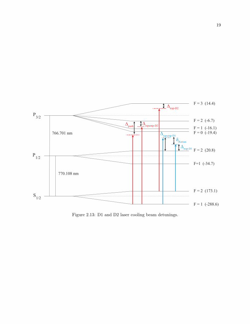
2.13 D1 and D2 laser cooling beams detunings . . . . . . . . . . . . . . . . . . . . . . . . 19

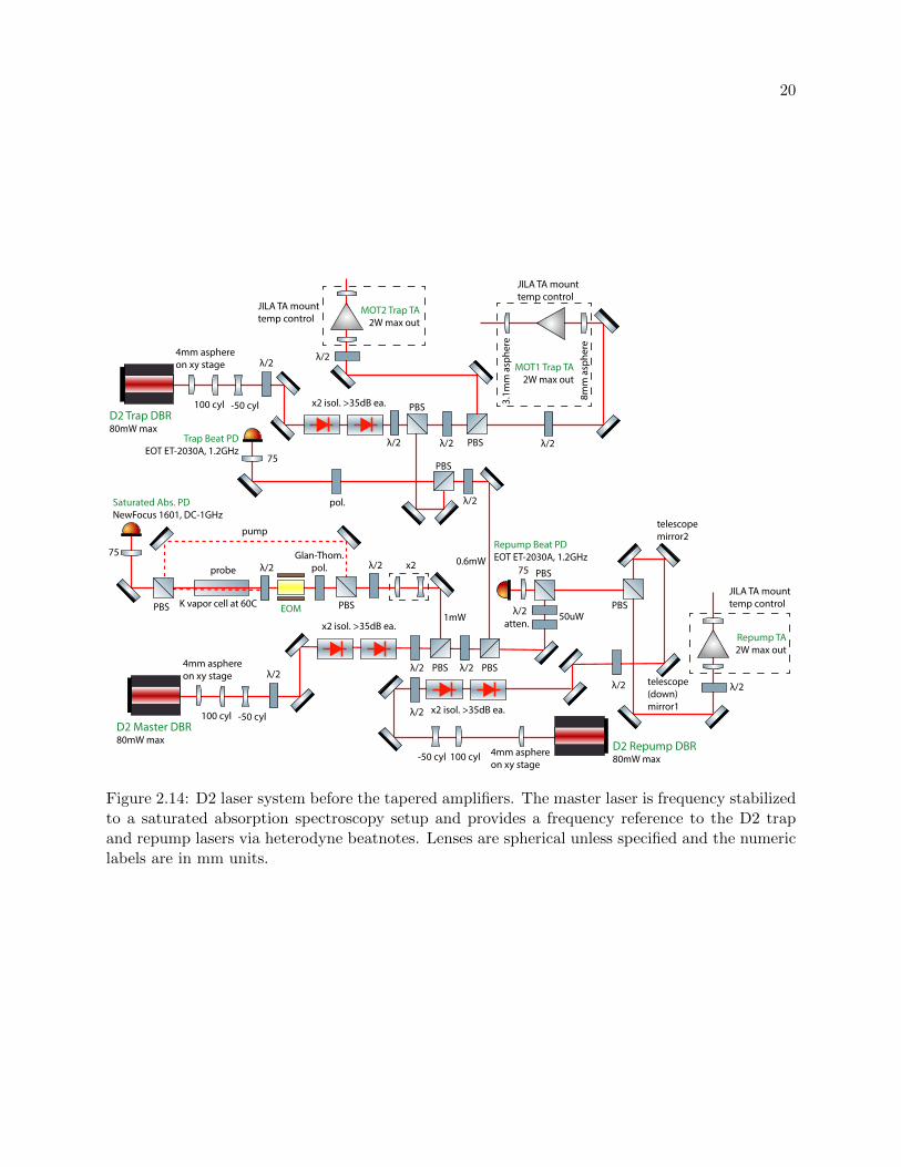
2.14 D2 laser system before the tapered amplifiers . . . . . . . . . . . . . . . . . . . . . . 20

2.15 D2 laser system after the tapered amplifiers . . . . . . . . . . . . . . . . . . . . . . . 21

2.16 D2 laser PDH lock demodulation electronics . . . . . . . . . . . . . . . . . . . . . . . 23

2.17 Heterodyne beatnote offset lock electronics . . . . . . . . . . . . . . . . . . . . . . . 24

2.18 Self-heterodyne laser linewidth measurement setup . . . . . . . . . . . . . . . . . . . 25

2.19 Optics for laser cooling . . . . . . . . . . . . . . . . . . . . . . . . . . . . . . . . . . . 26

xiv

2.20 Second MOT imaging optics . . . . . . . . . . . . . . . . . . . . . . . . . . . . . . . . 27

2.21 Absorption and fluorescence images of a MOT2 atom cloud . . . . . . . . . . . . . . 29

2.22 Contour plots demonstrating MOT2 laser frequency optimization . . . . . . . . . . . 30

2.23 D1 laser system . . . . . . . . . . . . . . . . . . . . . . . . . . . . . . . . . . . . . . . 33

2.24 D1 frequency locking scheme via a modified PDH lock . . . . . . . . . . . . . . . . . 34

2.25 D1 spectroscopy signal . . . . . . . . . . . . . . . . . . . . . . . . . . . . . . . . . . . 35

2.26 Cloud size vs Raman detuning for D1 gray molasses . . . . . . . . . . . . . . . . . . 37

2.27 Sensitive optical trap load alignment . . . . . . . . . . . . . . . . . . . . . . . . . . . 41

2.28 Atom temperature during optical trap load alignment . . . . . . . . . . . . . . . . . 41

2.29 Atom cloud expansion after optical dipole trap load . . . . . . . . . . . . . . . . . . 42

2.30 Optical setup for control of optical dipole traps . . . . . . . . . . . . . . . . . . . . . 43

2.31 Measured intensity noise of Nufern and Mephisto laser systems . . . . . . . . . . . . 44

2.32 Nufern beam quality degradation at high power . . . . . . . . . . . . . . . . . . . . . 46

2.33 Horizontal dipole trap H1 optics . . . . . . . . . . . . . . . . . . . . . . . . . . . . . 47

2.34 Horizontal dipole trap H2 optics . . . . . . . . . . . . . . . . . . . . . . . . . . . . . 47

2.35 Vertical dipole trap optics . . . . . . . . . . . . . . . . . . . . . . . . . . . . . . . . . 48

2.36 Beam waist of the loading dipole beam . . . . . . . . . . . . . . . . . . . . . . . . . . 49

2.37 Spatial profiles of H2 and V dipole trap beams . . . . . . . . . . . . . . . . . . . . . 49

2.38 Pointing stability of the H1 horizontal beam at the focus . . . . . . . . . . . . . . . . 50

2.39 Circuit diagram for the low-noise PD used for dipole trap control . . . . . . . . . . . 51

2.40 Measured dark noise of the dipole trap servo photodetector . . . . . . . . . . . . . . 52

2.41 Measured RIN of the dipole trap servo photodetector . . . . . . . . . . . . . . . . . . 52

2.42 Dipole trap intensity servo circuit diagram . . . . . . . . . . . . . . . . . . . . . . . . 54

2.43 Circuit diagram for science coils control. . . . . . . . . . . . . . . . . . . . . . . . . . 55

2.44 Evaporation efficiency using the H1 dipole beam . . . . . . . . . . . . . . . . . . . . 56

2.45 A five-stage evaporation trajectory optimization . . . . . . . . . . . . . . . . . . . . 56

2.46 BEC cloud distributions . . . . . . . . . . . . . . . . . . . . . . . . . . . . . . . . . . 57

xv

2.47 H2 and V optical dipole trap alignment . . . . . . . . . . . . . . . . . . . . . . . . . 57

2.48 An image of cold cloud expanded from the H2 and V beam potential . . . . . . . . . 58

3.1 A typical circuit topology for RF antenna drive . . . . . . . . . . . . . . . . . . . . . 60

3.2 RF control system circuitry . . . . . . . . . . . . . . . . . . . . . . . . . . . . . . . . 62

3.3 Spectral comparison of rectangular- vs. Gaussian-shaped RF pulses . . . . . . . . . . 64

3.4 Typical timescales for Rabi flopping . . . . . . . . . . . . . . . . . . . . . . . . . . . 65

3.5 Spatially-resolved Rabi flopping . . . . . . . . . . . . . . . . . . . . . . . . . . . . . . 66

3.6 RF spectrum using spin-resolved imaging . . . . . . . . . . . . . . . . . . . . . . . . 66

3.7 Lineshape spectral noise due to high magnetic field instability . . . . . . . . . . . . . 68

3.8 A typical spectrum with low magnetic field noise . . . . . . . . . . . . . . . . . . . . 69

3.9 Circuit diagram for magnetic field servo . . . . . . . . . . . . . . . . . . . . . . . . . 70

3.10 The main imaging system in the science chamber . . . . . . . . . . . . . . . . . . . . 73

3.11 Mounting for the side imaging objective and eyepiece lenses . . . . . . . . . . . . . . 74

3.12 Simulated spot size diagram for the side imaging objective lens . . . . . . . . . . . . 74

3.13 Measured point spread functions for different objective lens lateral positions . . . . . 74

3.14 Reduction of aberrations via aperturing the objective . . . . . . . . . . . . . . . . . . 75

3.15 Measured astigmatism present in an unoptimized imaging system . . . . . . . . . . . 76

3.16 CCD camera dark-frame images at −45C . . . . . . . . . . . . . . . . . . . . . . . . 77

3.17 Characterizing CCD camera noise statistics using the photon-transfer technique . . . 78

3.18 Measurement of the CCD pixel well capacity . . . . . . . . . . . . . . . . . . . . . . 79

3.19 The effect of probe beam laser noise on the probe lineshape . . . . . . . . . . . . . . 81

3.20 OD saturation due to a high intensity probe . . . . . . . . . . . . . . . . . . . . . . . 82

3.21 Doppler shift and broadening of a probe lineshape . . . . . . . . . . . . . . . . . . . 83

3.22 Probe pulse duration affect on the measurement of Isat . . . . . . . . . . . . . . . . . 84

3.23 CCD camera noise affect on absorption imaging . . . . . . . . . . . . . . . . . . . . . 85

3.24 MTF of the top imaging asphere without and with the science cell window . . . . . . 88

xvi

3.25 Top imaging objective lens configuration . . . . . . . . . . . . . . . . . . . . . . . . . 89

3.26 Expected performance of the high-resolution objective in the top imaging system . . 90

3.27 An overview of computer and hardware control . . . . . . . . . . . . . . . . . . . . . 91

4.1 A rough measurement of the Feshbach resonance center B0 . . . . . . . . . . . . . . 95

4.2 Illustration of magneto-association of Feshbach dimers . . . . . . . . . . . . . . . . . 99

4.3 Estimating the impact of three-body loss during a 10 ms B–field ramp . . . . . . . . 101

4.4 Estimating the impact of three-body loss during a 1 ms B–field ramp . . . . . . . . . 101

4.5 Molecular association B–field ramp speed . . . . . . . . . . . . . . . . . . . . . . . . 102

4.6 Evidence of molecule formation near B0 . . . . . . . . . . . . . . . . . . . . . . . . . 104

4.7 RF association of molecules . . . . . . . . . . . . . . . . . . . . . . . . . . . . . . . . 106

4.8 Initial and final states in the dimer dissociation procedure . . . . . . . . . . . . . . . 107

4.9 Franck-Condon factor . . . . . . . . . . . . . . . . . . . . . . . . . . . . . . . . . . . 109

4.10 Experimental checks on the dimer dissociation spectra . . . . . . . . . . . . . . . . . 111

4.11 Demonstration of the dimer spectrum saturation at high RF power . . . . . . . . . . 112

4.12 Atom-molecule Rabi flopping . . . . . . . . . . . . . . . . . . . . . . . . . . . . . . . 112

4.13 Two-photon transition in the molecular dissociation spectrum . . . . . . . . . . . . . 114

4.14 Measured molecular spectra with atoms present . . . . . . . . . . . . . . . . . . . . . 116

4.15 Predicted atom contamination of the molecular spectrum at small Eb . . . . . . . . . 117

4.16 Distortion of molecular spectra by the presence of |F = 1,mF = 0〉 residual atoms . . 118

4.17 Spin composition of our atomic cloud after molecular association . . . . . . . . . . . 119

4.18 Dimer loss contributions at different scattering lengths . . . . . . . . . . . . . . . . . 121

4.19 Procedure for preparing and probing a pure molecular sample . . . . . . . . . . . . . 123

4.20 Scope trace of a Gaussian-shaped ARP pulse . . . . . . . . . . . . . . . . . . . . . . 125

4.21 Dressed state picture of a shaped ARP . . . . . . . . . . . . . . . . . . . . . . . . . . 126

4.22 Behavior of the expelled atoms versus blast power and duration . . . . . . . . . . . . 127

4.23 Molecules and expelled unpaired atoms in the same image frames . . . . . . . . . . . 127

xvii

4.24 Molecular lifetimes with and without the presence of unpaired atoms . . . . . . . . . 128

4.25 B–field stability over time . . . . . . . . . . . . . . . . . . . . . . . . . . . . . . . . . 129

4.26 Interaction energy shift vs. a at different densities . . . . . . . . . . . . . . . . . . . 131

4.27 Energy spectrum of two atoms in a trap with an aspect ratio of η = 0.244 . . . . . . 134

4.28 Energy spectrum of two atoms in a trap with an aspect ratio of η = 2/3 . . . . . . . 135

4.29 Feshbach resonances and the corresponding molecular states for |F = 1,mF = −1〉 . 139

4.30 Corrections to the universal Eb expression . . . . . . . . . . . . . . . . . . . . . . . . 141

4.31 Precise measurement of Feshbach dimer binding energies Eb . . . . . . . . . . . . . . 143

4.32 An example of cc-model tuning at 34.5940 G . . . . . . . . . . . . . . . . . . . . . . . 144

4.33 B0 fit value dependence on the rotation transformation angle . . . . . . . . . . . . . 144

4.34 Constraints on the singlet aS and the triplet aT scattering lengths . . . . . . . . . . 146

4.35 Molecular lifetimes at different scattering lengths . . . . . . . . . . . . . . . . . . . . 149

4.36 L2 inelastic coefficient predicted by the coupled-channel model . . . . . . . . . . . . 150

5.1 Energy spectrum of Efimov trimer states . . . . . . . . . . . . . . . . . . . . . . . . . 152

5.2 A survey of the three body-parameter a− vs. resonance strength parameter sres . . . 155

5.3 Experimental sequence for three-body loss measurements . . . . . . . . . . . . . . . 158

5.4 A typical time evolution resulting from three-body decay . . . . . . . . . . . . . . . 160

5.5 L3 data affected by systematic shifts . . . . . . . . . . . . . . . . . . . . . . . . . . . 162

5.6 Temperature dependence of saturated L3(a) spectra values . . . . . . . . . . . . . . 165

5.7 Universal function s11(ka) used in the finite-temperature zero-range model . . . . . . 166

5.8 Finite-temperature model prediction for L3(a) behavior for various temperatures . . 167

5.9 Finite-temperature model prediction for L3(a)/a4 behavior for various temperatures 167

5.10 Modulation in L3 vs. T for different a values . . . . . . . . . . . . . . . . . . . . . . 168

5.11 Precise L3(a) measurements at different temperatures . . . . . . . . . . . . . . . . . 170

5.12 Extracted Efimov L3/a4 peak locations and a− locations at different temperatures . 171

5.13 Finite-temperature suppression of the second Efimov resonance . . . . . . . . . . . . 175

xviii

5.14 The absence of the second Efimov resonance in our data . . . . . . . . . . . . . . . . 175

5.15 An attempt to find a four-body Efimov resonance in a high-density gas . . . . . . . . 176

5.16 Suppression of the Efimov resonance in a high-density gas . . . . . . . . . . . . . . . 177

5.17 Type of loss present in a high-density gas . . . . . . . . . . . . . . . . . . . . . . . . 177

6.1 Predicted three-body Efimov spectrum . . . . . . . . . . . . . . . . . . . . . . . . . . 182

6.2 Predicted Efimov spectrum containing trimer and tetramer states . . . . . . . . . . . 182

Chapter 1

Introduction

1.1 Universal Physics with Ultracold Atoms

The world of quantum matter is fascinating. Systems exhibiting such phenomenon as super-

fluidity, superconductivity, quantum Hall physics, quantum magnetism and entanglement, enable

quantum technologies for advanced sensing and computation. However, as the interaction strength

and the system size increase, the complexity increases exponentially, making such systems harder to

understand and engineer. For example, while systems that exhibit high-Tc superconductivity, frac-

tional quantum Hall effect, Hubbard model physics or topological order are deemed revolutionary,

they are intricate and are of ongoing theoretical and experimental interest.

Since the onset of atom cooling and trapping [1, 2] and the first production of degenerate Bose

[3], Fermi [4] and molecular gases [5], ultracold gases have been viewed as great quantum simulators

of condensed matter systems [6, 7, 8, 9]. Precise control and imaging of atomic systems [10] enables

simulation of quantum magnetism [9, 11], cold chemistry [11], high-Tc superconductivity [12, 13, 14],

a variety of many-body systems [15], disordered systems [16], synthetic gauge fields and quantum

Hall physics [17, 18].

While quantum simulation with ultracold gases is a compelling topic, the physics of inter-

acting ultracold gases is intriguing in its own right. The ability to control an ultracold system’s

dimensionality, thermal wavelength, quantum state, density, external potential and interactions

(via Feshbach resonances [19]) enables one to achieve separation between the relevant length and

energy scales, an important aspect for focusing on the fine details in a problem. For example, in

2

select studies, preparation of dilute, cold and interacting atomic samples enabled precise probing of

few-particle energies [20] and correlations [21]. In the atomic sample of Ref. [21], the length scales

pertaining to the interparticle spacing, the de Broglie wavelength λ, the effective range of interact-

ing potential and confinement are irrelevant, if they are large compared to the s-wave scattering

length a characterizing interactions.

Furthermore, ultracold atomic systems with a clear separation between the relevant length

and energy scales can also exhibit universal physics, where the macroscopic observables (e.g. energy,

momentum, spectral response and dynamics) are invariant on the complex microscopic details of

the system. For example, the thermodynamic properties of ultracold systems can be fully described

by a set of universal relations (e.g. equation of state [22] and Tan’s relations [23, 24]) and only a few

quantities (e.g. temperature T , density n, s-wave scattering length a and the short-ranged particle

correlation quantity called the contact). The same universal relations apply to any chosen atomic

species (that have the same quantum statistics) for any T , n, a and in any phase, an intriguing

result.

In systems exhibiting universal physics, all physical observables can be parametrized by a few

dimensionless parameters, such as na3 and nλ3 that describe the strength of interactions and the

level of quantum degeneracy, respectively. Then, since universal physics entails continuous scaling

symmetry, transformations, such as n → ζ−3n, a → ζa and λ → ζλ, will leave all observables

and their dynamics invariant when measured in rescaled units. For example, when scaled by the

only relevant length scale in the problem (the interparticle spacing n−1/3), the time evolution,

the momentum distribution and the energy of an ultracold gas quenched to unitary (|a| → ∞)

are invariant on the atom density [25, 26]. The ability to significantly reduce the complexity of

interacting many-body problems, regardless of the complex or unknown microscopic details, to a

set of universal equations and a few quantities, is a powerful concept.

However, the principle of universality is limited. For example, while atomic physicists often

approximate the interatomic interaction potential by a zero-range delta-function pseudopotential

(giving rise to “contact” interactions and an isotropic scattering length a at low energies) [27], the

3

real interatomic potentials are more complex. The short-ranged details of physical potentials are

often nonuniversal, i.e. the details depend on the “real” quantum chemistry, the chosen atomic

species, quantum numbers and collisional energy. Hence, unless all length scales in the problem are

much larger than the physical extent (energy depth) of the interaction potential (and all energy

scales are much smaller than the depth of the potential), nonuniversal corrections due to short-

ranged physics must be incorporated. For van der Waals interactions, which are relevant for

ultracold neutral atoms and Feshbach resonances, the van der Waals length rvdW characterizes

the range of interaction potential [28] and all length and energy scales in a problem (e.g. |a|,

λ, n−1/3, the mean field energy and the Feshbach dimer binding energy) must be rvdW and

EvdW = ~2/(mr2vdW) for an ultracold atomic system to exhibit universal physics.

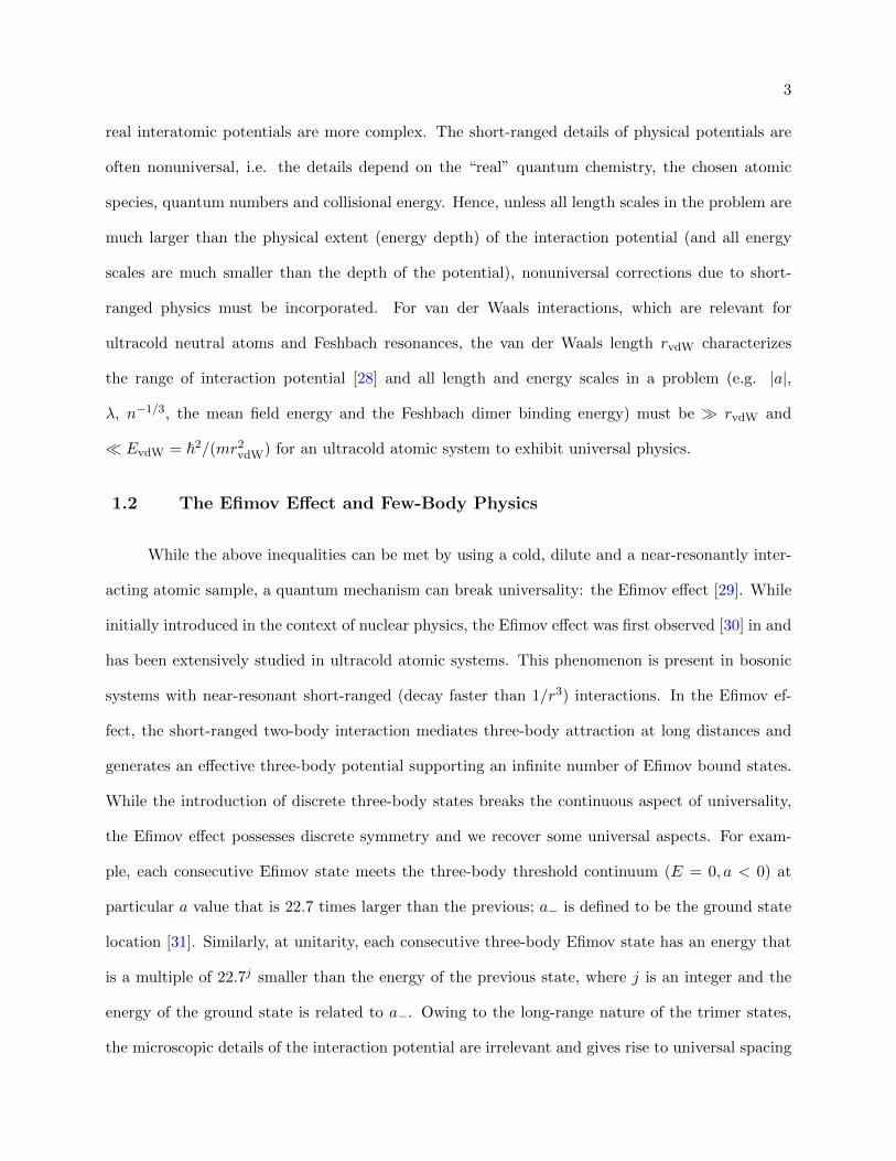
1.2 The Efimov Effect and Few-Body Physics

While the above inequalities can be met by using a cold, dilute and a near-resonantly inter-

acting atomic sample, a quantum mechanism can break universality: the Efimov effect [29]. While

initially introduced in the context of nuclear physics, the Efimov effect was first observed [30] in and

has been extensively studied in ultracold atomic systems. This phenomenon is present in bosonic

systems with near-resonant short-ranged (decay faster than 1/r3) interactions. In the Efimov ef-

fect, the short-ranged two-body interaction mediates three-body attraction at long distances and

generates an effective three-body potential supporting an infinite number of Efimov bound states.

While the introduction of discrete three-body states breaks the continuous aspect of universality,

the Efimov effect possesses discrete symmetry and we recover some universal aspects. For exam-

ple, each consecutive Efimov state meets the three-body threshold continuum (E = 0, a < 0) at

particular a value that is 22.7 times larger than the previous; a− is defined to be the ground state

location [31]. Similarly, at unitarity, each consecutive three-body Efimov state has an energy that

is a multiple of 22.7j smaller than the energy of the previous state, where j is an integer and the

energy of the ground state is related to a−. Owing to the long-range nature of the trimer states,

the microscopic details of the interaction potential are irrelevant and gives rise to universal spacing

4

of the spectrum.

While the Efimov spectrum was predicted to be universal in Efimov’s original work, the

location of the states, determined by a single a− value, was presumed to depend on the microscopic

details of interactions. However, observations across many atomic species and different Feshbach

resonances [32, 33, 34, 35, 36, 37, 38, 39, 40, 41, 42, 43, 44, 45] noticed that the a− value can be

directly deduced from the van der Waals length rvdW, with measured a− values being always within

20% of −9 rvdW [37, 46, 47, 48]. This is surprising, considering rvdW value is solely determined by

the atomic mass and a numerical constant C6 [49, 50] characterizing the strength of the 1/r6 (long-

ranged) van der Waals tail, and not determined by the short-ranged microscopic details. Theory

indeed predicts a similar value of a− = −9.73 rvdW [51, 52] and termed this phenomenon “van

der Waals universality”. Physically, a strong suppression of the three-body wavefunction at short

distances prevents particles from accessing nonuniversal regions of interacting potentials.

The knowledge of the C6 value for the chosen atomic species, together with the univer-

sal Efimov scaling, should allow prediction of the full Efimov spectrum to arbitrary-large a and

arbitrary-small E, a powerful concept. With a− value determining all the trimer state placements

in the Efimov spectrum, the robustness and applicability of the unexpected van der Waals univer-

sality must be well understood and is a topic of ongoing debate [53, 54, 55, 56, 57]. In particular,

understanding of Efimov features near narrow and intermediate Feshbach resonances, described by

the dimensionless resonance strength parameter sres, is incomplete. Theoretical models predict that

the three-body parameter should also, in addition to the van der Waals length, depend on the back-

ground scattering length and the sres value. The few experimental measurements studying these

dependencies suffer from large experimental uncertainties (e.g. see Fig. 5.2), finite-temperature sys-

tematic shifts and an insufficient characterization of the two-body potential, leading to inconclusive

evidence of what affects the universal aspects in Efimov physics.

5

1.3 Thesis Contents

Our experimental goal is to precisely measure few-body physics using state-of-the-art tech-

niques. To do so, we utilize Fano-Feshbach resonances, quantum state control and spectroscopic

tools to precisely control experimental parameters such as atom number, temperature, density and

the spin state of our sample.

In Chapter 2, I begin by describing our new apparatus used for generating ultracold 39K

gas samples. Initially, this apparatus was assembled by Rabin Paudel and me for Debbie Jin,

enabling production of degenerate 40K Fermi gas samples; see Rabin’s thesis [58] for details on

vacuum chamber assembly, testing of potassium sources and creating the new lab’s first degenerate

40K samples. This thesis contains the details describing how we converted the lab to be used for

generating and studying ultracold 39K (boson) gas samples. To my surprise, reaching degeneracy

with 39K (making a Bose-Einstein condensate, BEC) was a more challenging engineering task

than with 40K (making a degenerate Fermi gas). Based on previous experience and the new

requirements, we made significant improvements, changes and additions to the apparatus during the

conversion, including: improvements to the cooling laser systems, laser locks, magnetic field stability

and imaging; change in cooling and state initialization techniques; addition of a sophisticated

radiofrequency (RF) state control/spectroscopy system and a 50 W optical dipole trap system used

for all-optical evaporation. We started the conversion in November 2016, achieved a 39K condensate

in July 2017 and entered a productive data-taking stage in the beginning of 2018, after extensive

calibrations and tuning of the machine. The stability, robustness and automation of the repurposed

machine enabled precision studies of few-body quantum physics, the first “real” scientific studies

in the new lab.

In Chapter 3, I detail some important tools we utilized to precisely probe two- and three-body

physics. Specifically, I focus on our imaging system, RF control and spectroscopy, and magnetic

field stabilization.

In Chapter 4, I focus on our precision spectroscopy of Feshbach dimer binding energies, span-

6

ning three orders of magnitude and with sub-kilohertz resolution. The accuracy and precision are

enabled by the production and precise probing of pure molecular samples. These measurements

allow us to locate a Feshbach resonance and determine scattering length values with unprecedented

accuracy [20]. We use our data to fine-tune a state-of-the-art coupled-channel model, having real

(nonuniversal) interaction potentials, and hence we further push the limits of few-body theory.

Additionally, the results of our two-body measurements were crucial for our Efimov studies and for

providing a two-body physics calibration to JPL/NASA Cold Atom Laboratory (CAL) collabora-

tion, who are interested in performing Efimov studies in microgravity, with ultracold 39K gas on

the international space station.

In Chapter 5, I present our precise measurement of the three-body Efimov ground state lo-

cation a−. We find that the trimer state location a− significantly deviates from the value predicted

by van der Waals universality. Due to small experimental and systematic uncertainties, our mea-

surement is the strongest evidence of departure from the universal value for both homonuclear and

heteronuclear systems, and is the first observed deviation near a Feshbach resonance of intermedi-

ate strength, as depicted in Fig. 5.2. This deviation is intriguing, considering other measurements

near similar Feshbach resonances, albeit with larger uncertainties, were consistent with universal

predictions. Our hope is that future few-body theoretical studies can explain the origin of our

observed a− deviation from the value predicted by van der Waals universality, and enable a better

understanding of the limits on universal physics in ultracold systems.

In Chapter 6, I conclude the work presented in this thesis and provide some insight into our

ongoing experiments and possible future directions.

Chapter 2

Apparatus and Techniques for Cooling 39K

2.1 Properties of 39K

The 39K isotope is an intriguing candidate for the exploration of quantum interactions in

ultracold gases. Having multiple inter- and intra-spin state Feshbach resonances, 39K offers an

opportunity to study resonances with differing properties (e.g. narrow and broad in terms of reso-

nance width in magnetic field and/or resonance strength parameter sres) with the same apparatus

[59]. Additionally, the existence of particular magnetic field values for which the gas is at unitar-

ity for one spin state and |a| → 0 a0 (non-interacting) for a different state, enables precision RF

spectroscopy (Rabi and Ramsey) of strong interactions [21]. Lastly, the existence of short- and

long-lived three-body Efimov states, whose lifetime is characterized by the inelasticity parameter

η, near these Feshbach resonances allows a breadth of exotic few-body studies [38].

The relatively simple 39K hyperfine structure is shown in Fig. 2.1. Transitions between states

can be made using radio-frequency (RF) radiation (e.g. magnetic-dipole transitions) and optical

770 nm (D1) and 767 nm (D2) light. The near-IR light can be readily generated using commercial

laser sources. The Zeeman splittings of hyperfine states under external magnetic field B, best

described by the F quantum number and its projection mF along B, are conveniently presented

in Figs. 2.2–2.4, where the B–field ranges are restricted to relevant values used throughout the

thesis. Since RF transition frequencies between F and mF states are < 1 GHz for moderate B–

fields; microwave engineering is relatively simple. For precision spectroscopy of the 4 2S1/2 hyperfine

ground states, we use magnetically-insensitive RF transitions: transitions between differing F states

8

S1/2

F = 1 (-288.6)

F = 2 (173.1)

P1/2

F=1 (-34.7)

F = 2 (20.8)

P3/2

F = 0 (-19.4) F = 1 (-16.1)

F = 2 (-6.7)

F = 3 (14.4)

770.108 nm

766.701 nm

Figure 2.1: Hyperfine energy level diagram of 39K at zero magnetic field. Optical transition wave-lengths 770.108 nm and 766.701 nm correspond to the D1 and D2 spectroscopic lines, respectively.Relative splittings (parenthesis) are in MHz.

at low B–field values and between differing mF states (within same F manifold) at high B–field

values.

Feshbach resonances occur in the |4 2S1/2,F = 1〉 ground states and our goal is to popu-

late the largest and the coldest sample in those states. Since the only trappable |F = 1〉 state is

|F = 1,mF = −1〉, having a positive magnetic moment at low B–field values (see Fig. 2.5), we strive

to populate it specifically. Additionally, since we have a particular interest (stemming from our

CAL collaboration) in the Feshbach and Efimov resonances of the |F = 1,mF = −1〉 state, focusing

on the |F = 1,mF = −1〉 state from the beginning is beneficial.

The |F = 1,mF = −1〉 state can be magnetically levitated using only 14 G/cm B–field gra-

dient near B = 0 G. However, at large B–field values B > 82 G, its magnetic moment becomes

negative (see Fig. 2.5) and the state becomes untrappable. Therefore, any magnetic trap has a

finite trap depth U/kB = k−1B

∫ 82 G0 G µ(B)dB = 1.5 mK for the |1,−1〉 state. Fig. 2.6 shows the trap

9

0 10 20 30 40 50 60 70 80 90 100B (G)

-400

-300

-200

-100

0

100

200

300

400

Ene

rgy

(MH

z)

42S1/2

F = 2, mF = 2

F = 2, mF = 1

F = 2, mF = 0

F = 2, mF = -1

F = 2, mF = -2

F = 1, mF = -1

F = 1, mF = 0

F = 1, mF = 1

0 100 200 300 400 500 600 700 800 900 1000B (G)

-2000

-1500

-1000

-500

0

500

1000

1500

2000

Ene

rgy

(MH

z)

42S1/2

F = 2, mF = 2

F = 2, mF = 1

F = 2, mF = 0

F = 2, mF = -1

F = 2, mF = -2

F = 1, mF = -1

F = 1, mF = 0

F = 1, mF = 1

Figure 2.2: Hyperfine structure and the Zeeman splitting of the 4 2S1/2 ground state in39K. Note that the curves in the top and bottom plots are same, albeit different x-axisscales.

10

0 10 20 30 40 50 60 70 80 90 100B (G)

-80

-60

-40

-20

0

20

40

60

80

Ene

rgy

(MH

z)

42P1/2

F = 2, mF = 2

F = 2, mF = 1

F = 2, mF = 0

F = 2, mF = -1

F = 2, mF = -2

F = 1, mF = -1

F = 1, mF = 0

F = 1, mF = 1

Figure 2.3: Hyperfine structure and the Zeeman splitting of the 4 2P1/2 state in 39K.

0 10 20 30 40 50 60 70 80 90 100B (G)

-300

-200

-100

0

100

200

300

Ene

rgy

(MH

z)

42P3/2F = 3, m

F = 3

F = 3, mF = 2

F = 3, mF = 1

F = 3, mF = 0

F = 3, mF = -1

F = 3, mF = -2

F = 3, mF = -3

F = 2, mF = 2

F = 2, mF = 1

F = 2, mF = 0

F = 2, mF = -1

F = 2, mF = -2

F = 1, mF = 1

F = 1, mF = 0

F = 1, mF = -1

F = 0, mF = 0

Figure 2.4: Hyperfine structure and the Zeeman splitting of the 4 2P3/2 state in 39K.

11

0 100 200 300 400 500

-1.0

-0.5

0.0

0.5

1.0

Figure 2.5: The magnetic moment µ of the 4 2S1/2 hyperfine ground states in 39K, where µ is takenas the derivative of energies (shown in Fig. 2.2) with respect to B and µB ≈ 1.4 MHz/G is the Bohrmagneton.

depth of a quadrupole trap (QT) with magnetic field profile

B(x, y, z) =b

2

√x2 + y2 + 4z2, (2.1)

where b is the gradient along the strong z direction. Having such a small trap depth means that

magnetic trapping of the |1,−1〉 state is only possible if the cloud temperature is O(100µK) or

below, since the evaporation rate is approximately proportional to exp(−U/kBT ) [60]. Therefore,

we go to great lengths in reducing the temperature to O(10µK), utilizing Doppler and sub-Doppler

laser cooling techniques and being particularly careful with the load of the magnetic quadrupole

trap.

To study quantum few-body physics (such as the Efimov effect), we require temperatures

O(10–100 nK). Typically, reaching such low temperatures is achieved via evaporation in a mag-

netic potential (e.g. RF or microwave forced evaporation), followed by evaporation in an optical

dipole trap. However, such an approach fails for 39K, which has a small and negative background

scattering length, and therefore has a Ramsauer-Townsend minimum in the collision cross section

vs. collisional energy [61, 62], as depicted in Fig. 2.7. This minimum suppresses rethermalizing

12

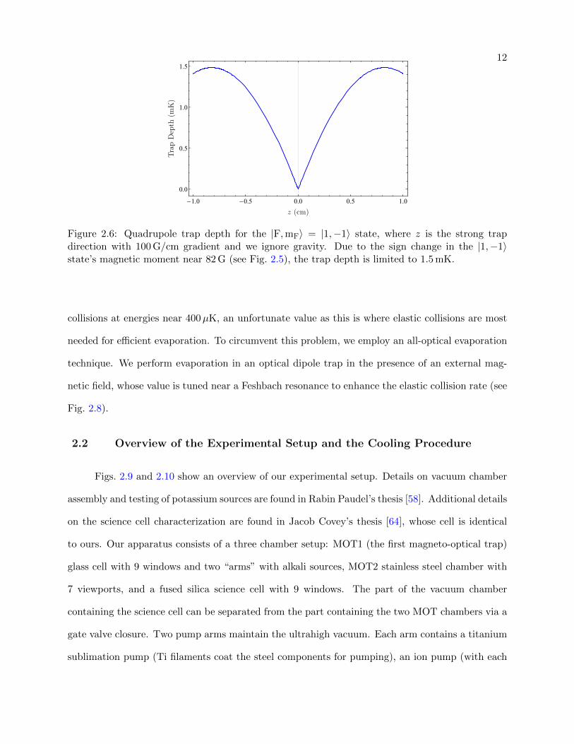
-1.0 -0.5 0.0 0.5 1.0

0.0

0.5

1.0

1.5

Figure 2.6: Quadrupole trap depth for the |F,mF〉 = |1,−1〉 state, where z is the strong trapdirection with 100 G/cm gradient and we ignore gravity. Due to the sign change in the |1,−1〉state’s magnetic moment near 82 G (see Fig. 2.5), the trap depth is limited to 1.5 mK.

collisions at energies near 400µK, an unfortunate value as this is where elastic collisions are most

needed for efficient evaporation. To circumvent this problem, we employ an all-optical evaporation

technique. We perform evaporation in an optical dipole trap in the presence of an external mag-

netic field, whose value is tuned near a Feshbach resonance to enhance the elastic collision rate (see

Fig. 2.8).

2.2 Overview of the Experimental Setup and the Cooling Procedure

Figs. 2.9 and 2.10 show an overview of our experimental setup. Details on vacuum chamber

assembly and testing of potassium sources are found in Rabin Paudel’s thesis [58]. Additional details

on the science cell characterization are found in Jacob Covey’s thesis [64], whose cell is identical

to ours. Our apparatus consists of a three chamber setup: MOT1 (the first magneto-optical trap)

glass cell with 9 windows and two “arms” with alkali sources, MOT2 stainless steel chamber with

7 viewports, and a fused silica science cell with 9 windows. The part of the vacuum chamber

containing the science cell can be separated from the part containing the two MOT chambers via a

gate valve closure. Two pump arms maintain the ultrahigh vacuum. Each arm contains a titanium

sublimation pump (Ti filaments coat the steel components for pumping), an ion pump (with each

13

1e-17

1e-16

1e-15

1e-14

1e-13

1e-12

1e-11

1e-10

1e-09

1e-08

1e-06 1e-05 0.001 0.01

cros

s se

ctio

n (c

m^2

)

0.0001

Relative Collisional Energy (K)

B = 32.6GB = 0G

Figure 2.7: Elastic collision cross section of atoms in the |F = 1,mF = −1〉 hyperfine state vs.collision energy for two different magnetic fields. This figure is borrowed from John Bohn [63].

1e-12

1e-11

1e-10

1e-09

1e-08

0 50 100 150 200 250 300 350 400 450 500

Rat

e C

onst

ant (

cm^3

/s)

Temperature (uK)

B = 32.6 G B = 0G

Figure 2.8: Thermally averaged collision rate of atoms in the |F = 1,mF = −1〉 hyperfine state vs.temperature for two different magnetic fields. This figure is borrowed from John Bohn [63].

14

measuring < 10−11 Torr, the minimum reading), and a valve to allow connection to a turbo pump

(if needed). So far, the titanium was deposited only once, where we fired for 40 s at 48 A with a

10 ramp up and ramp down times, since the vacuum chamber bakeout (we had no need as the

pressure in our vacuum chamber remained low). We put a mu-metal shield on the ion pump closest

to the science chamber to limit the effect of stray magnetic fields on our atoms. We have not broken

vacuum since initial assembly and bake-out on September 2013 (for the MOT chambers side) and

July 2014 (for the science chamber side), nor we have a desire to do so anytime soon.

Since we initially constructed the apparatus to create degenerate 40K Fermi gas samples, the

system contains potassium enriched 40K sources: one dispenser with 7.1% enrichment level and

two more with 14.1% level. Note, the system also it contains three Rb dispensers in a separate

glass chamber “arm”. We used the dispenser with 7.1% 40K enrichment in this thesis work, as

this dispenser has a higher 39K content, the new isotope of interest for our ultracold Bose gas

experiments. We run 3.5 A of current through the dispenser (1.8 V drop) to release potassium

vapor via a chemical reaction 2KCl + Ca + heat → 2K + CaCl2, where we have measured (in a

separate setup) the temperature threshold to be 350–400C. To prevent the vapor from depositing

on cell walls, we heat the entire MOT1 Pyrex chamber (along with the source arms) to 70C via 14

current-servoed heaters (Omega Products KHLV-0502/5 and KHLV-105/5-P) attached directly to

the glass. Additionally, we can increase the potassium vapor pressure, and hence the MOT loading

rate, via light-induced atom desorption (LIAD), illuminating the glass chamber with three UV

LEDs (365 nm, 1.2 W each, part LED Engin LZ1-00UV00). By UV illuminating the chamber only

during the MOT load, this technique should enable a faster MOT load rate without the need to run

the dispensers at a higher current. However, unlike others [65], we only saw a modest improvement

of 20–30% in the MOT loading rate and a degraded atom number stability. Additionally, after

several months of operation, the desorption UV light removed the majority of residual potassium

deposits from the cell walls and we discontinued the LIAD use.

We continuously push atoms from the MOT1 chamber to the MOT2 chamber via a push

beam, which has a linear polarization and whose frequency is red detuned from the D2 transition.

15

Figure 2.9: An overview sketch of the experimental cooling procedure.

Figure 2.10: CAD drawing of our experimental apparatus.

16

A magnetic hexapole field, formed by machined “fridge magnet” pieces, guides atoms through the

transfer tube and provides support against gravity. For similar push beam powers, the magnetic

guide increases the push beam transfer efficiency by ×1.8 (compared to without the guide) and

reduces the MOT2 fill time by 35%. Our past experiments with the 40K isotope showed that

this hexapole field enables atom velocities as slow as 20 m/s, corresponding to a 25 ms transfer

time between the two MOT chambers separated by 47 cm. This is impressive, considering that

atoms would fall 3 mm (compare this to 5.5 mm transfer tube inner radius) in 25 ms without the

magnetic guide. We found that the rotation angle of the hexapole field (around the transfer tuber)

is somewhat sensitive: the transferred atom number can vary by 50%.

After loading MOT2 with a sufficient number of atoms, we perform a series of MOT com-

pression and sub-Doppler cooling stages. Then, we load atoms into a quadrupole trap and transfer

them to the science cell via a cart transfer (MOT2 QT coils are attached to the cart). Then, we

transfer atoms from the cart QT to (a similar) science QT and move the cart away from the science

chamber. After which, we increase the science QT confinement and load a fraction of atoms into an

optical dipole trap. Finally, we turn off the QT, turn on a magnetic field bias (tuned near a Feshbach

resonance to increase elastic collisions) and perform all-optical evaporation, reaching O(10–100 nK)

final temperatures. While this procedure sounds relatively simple, in reality it was an extensive

engineering task, requiring lengthy optimization procedures and a thorough understanding of each

experimental knob. Lab photos in Figs. 2.11–2.12 show the complexity of the apparatus that en-

abled us to reach our goals. While some parts of the apparatus remained unchanged from the

initial construction (for purposes of 40K cooling), major adjustments and improvements were made

to transform this apparatus to a 39K cooling machine. The stability, robustness and automation of

this machine enabled precision studies of few-body quantum physics.

2.3 Doppler Laser Cooling

Since we have a relatively narrow excited state hyperfine structure [66] (compare the hyperfine

spacing to the Γ/2π = 6.035 MHz natural linewidth of the excited 4 2P1/2 and 4 2P3/2 states), laser

17

Figure 2.11: Overlooking the laboratory: laser sources (left) and science (right) optical tables.

Figure 2.12: The vacuum chamber and the surrounding optics take up more than half of the scienceoptical table; the rest of the space is taken by a 50 W 1064 nm laser system (black steel box) used forgenerating and controlling the optical dipole trap light. The two smaller images show the sciencecell (surrounded by magnetic field coils and RF antennas) and the MOT1 chamber (surrounded bylarge-aperture optics and magnetic coils).

cooling the 39K isotope is more difficult than its 40K counterpart. Due to the level crowding, off-

18

resonant scattering from the |4 2S1/2,F = 2〉 → |4 2P3/2,F′ = 3〉 cooling transition (we refer to as

“D2 trap”, see Fig. 2.13) results in a quick accumulation of atoms in the |4 2S1/2,F = 1〉 ground

state. Therefore, we require a strong repump beam on the |4 2S1/2,F = 1〉 → |4 2P3/2,F′ = 2〉

transition (we refer to as “D2 repump”) to have efficient laser cooling. In fact, our typical D2

repump beam power is almost 1:1 of D2 trap power for both MOT setups. This is a much stronger

repump light than what we’ve previously used for 40K (1:3 repump-trap ratio for MOT1 and 1:12 for

MOT2 [58]). Lastly, since the MOT atom number and temperature are determined by spontaneous

emission [67] (and since our desire is to have the highest atom number with lowest temperatures),

the trap and repump beams must be far (red-) detuned from their transitions and must be of high

power.

2.3.1 D2 Laser System

The laser system used for generating, frequency-stabilizing and amplifying D2 laser light

is shown in Fig. 2.14 and 2.15. Learning from previous experience, regarding the required laser

power, stability and laser frequency modularity, we decided to have three separate 767 nm DBR

laser sources (Photodigm PH767DBR080T8, TO-8 package, 80mW): one each for master, for trap

and for repump light. We thoroughly enjoy working with DBR lasers; they are compact, have

unmatched mechanical stability, small laser linewidth < 500 kHz ( 6.0 MHz natural linewidth

of the excited states), efficient (∼ 0.75 mW/mA, we typically use 100–150 mA) and have a large

mode-hop-free wavelength tuning range O(2 nm) (coarse tuning using temperature and fine using

current). Some of the negatives include astigmatic emission profile, linewidth broadening with

age and sensitivity to back-reflections (requiring & 60 dB isolation). We stabilize each DBR laser

temperature to within 1 mK using commercial TEC temperature controllers (Thorlabs TED8020).

We use fast low-noise JILA laser diode current drivers to dynamically control DBR laser frequencies.

We carefully choose the operating temperature and current to center lasing on the mode-hop-free

range, in order to reduce spectral noise.

The master DBR laser frequency is stabilized to an atomic frequency reference (a heated

19

S1/2

F = 1 (-288.6)

F = 2 (173.1)

P1/2F=1 (-34.7)

F = 2 (20.8)

P3/2

F = 0 (-19.4)F = 1 (-16.1)

F = 2 (-6.7)

F = 3 (14.4)

770.108 nm

766.701 nm

∆trap-D2

∆repump-D2∆push

δRaman

∆trap-D1

∆repump-D1

Figure 2.13: D1 and D2 laser cooling beam detunings.

20Nufern bercollimatoron TEC-heatedblock

D2 Master DBR80mW max

4mm asphereon xy stage

100 cyl -50 cyl

λ/2

x2 isol. >35dB ea.

λ/2 PBS

1mW

x2λ/2

PBS

Glan-Thom.pol.

EOMK vapor cell at 60C

Saturated Abs. PDNewFocus 1601, DC-1GHz

probe

pump

λ/275

λ/2 PBS

0.6mW

PBS

λ/2

λ/2atten.

50uW

75

Repump Beat PDEOT ET-2030A, 1.2GHz

D2 Trap DBR80mW max

4mm asphereon xy stage

100 cyl -50 cyl

λ/2

x2 isol. >35dB ea.

λ/2

PBS

PBS

pol.

75

Trap Beat PDEOT ET-2030A, 1.2GHz

λ/2 PBS

λ/2

MOT2 Trap TA2W max out

JILA TA mounttemp control

D2 Repump DBR80mW max

4mm asphereon xy stage

100 cyl-50 cyl

λ/2 x2 isol. >35dB ea.

λ/2 telescope(down) mirror1

telescope mirror2

Repump TA2W max out

JILA TA mounttemp control

λ/2

λ/2

MOT1 Trap TA2W max out

JILA TA mounttemp control

3.1m

m a

sphe

re

8mm

asp

here

PBSPBS

Figure 2.14: D2 laser system before the tapered amplifiers. The master laser is frequency stabilizedto a saturated absorption spectroscopy setup and provides a frequency reference to the D2 trapand repump lasers via heterodyne beatnotes. Lenses are spherical unless specified and the numericlabels are in mm units.

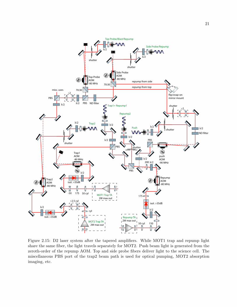
21

MOT2 Trap TA2W max out

Repump TA2W max out

MOT1 Trap TA2W max out

50 cyl 150

λ/2

isol. >35dB

175

RepumpAOM-80 MHz

λ/2200

λ/2

Repump2

λ/2

λ/2

Trap1+ Repump1

50 cyl175-50

isol. >35dB

λ/2

Trap1AOM-80 MHz

cyl

÷2.5 cyl

isol. >35dB

λ/2

Trap2AOM-80 MHz

λ/2 Trap2

λ/2pushAOM-90 MHz

PBS

PBS

PBSshutter

shutter

λ/2Pushshutter

PBS

misc. uses

λ/2

÷2

λ/2 PBS

λ/2

ND filter

÷2shutter

Top ProbeAOM-80 MHz

70:30

λ/2

Top Probe/Blast/Repump

shutter

ND filter

Side ProbeAOM-80 MHz

70:30repump from side

repump from top

λ/2

Side Probe/Repump

shutter

flip/snap-on mirror mount

Figure 2.15: D2 laser system after the tapered amplifiers. While MOT1 trap and repump lightshare the same fiber, the light travels separately for MOT2. Push beam light is generated from thezeroth-order of the repump AOM. Top and side probe fibers deliver light to the science cell. Themiscellaneous PBS port of the trap2 beam path is used for optical pumping, MOT2 absorptionimaging, etc.

22

potassium vapor cell) via a Pound-Drever-Hall (PDH) locking technique (Doppler-free saturated

absorption spectroscopy with a phase-modulated probe beam), as depicted in Fig. 2.16. The trap

and repump laser frequencies are locked to the master laser frequency via a heterodyne offset lock,

using a phased-locked loop with a JILA high-speed (10 MHz) PID loop filter, as shown in Fig.2.17.

The modularity of this setup allows us to change the trap and repump laser frequencies at will: we

can jump laser frequencies on a ∼ 50µs timescale (set by the loop’s P-I corner frequency, typically

around 70 kHz) and have a large beatnote frequency locking dynamic range of 10–1200 MHz (the

lower limit is set by the phase-frequency detector response and the higher limit is set by the

transfer function of the Si photodetector). In fact, this modularity enabled us achieve 39K, 40K

and 41K MOTs within 30 mins time, a useful sanity check prior to extensive system optimization

on a particular isotope. Additionally, the high-speed and high-gain PID servo system enables

one to establish phase-coherence between DBR laser sources, important for two-photon processes

(e.g. the D1 Raman cooling transition in sub-Doppler gray molasses, to be discussed later). We

can achieve phase coherence with negligible laser linewidth broadening: a narrow beatnote signal

(phase-coherence) 10–15 dB on top of the broad beatnote signal (whose width is set by the laser

linewidths) and small noise bumps (resulting from high servo gain).

Since we require a significant amount of D2 power, we amplify the DBR light with tapered

amplifiers (TA) (Eagleyard part EYP-TPA-0765-02000-4006-CMT04-0000, 765 nm, maximum 2 W

out, C-mount) mounted in JILA-made brass temperature-stabilized enclosures. We have three TAs

for the D2 setup: one each for MOT1 trap, for MOT2 trap and for repump (MOT1 and MOT2

repump light are amplified by the same TA chip). While the TA chips typically output 1.5 W with

only 10–20 mW seed power at 2.2 A drive current, the output spatial mode quality is not great,

often allowing only . 50% single-mode (SM) fiber-coupling efficiency, even with multiple beam-

shaping optics and an acousto-optic modulator (AOM). All laser light is routed to the science

optical table by polarization-maintaining (PM) SM fibers. Due to bad fiber-coupling efficiency, we

resort to air gap high-power fibers (ozOptics PMJ-A3AHPCA3AHPC-780-5/125) for high power

(> 100 mW output) light delivery. Using standard fiber patch cables with epoxied fiber connectors

23

Figure 2.16: D2 laser PDH lock demodulation electronics. A 50 Ω function generator drives ahomebuilt resonant EOM tank circuit that phase modulates the probe beam. After passing througha saturated absorption spectroscopy setup, the probe beam is detected on a PD. We demodulate thesignal and send it to the PID servo (Vescent Photonics). We are careful to avoid residual amplitudemodulation (RAM) in the probe beam and employ RAM-minimizing techniques suggested by JanHall [68].

(e.g. Thorlabs P3-630PM-FC) for MOT light delivery leads to power instability. Using the high-

power fiber patches, we are able to deliver 200 mW repump and 250 mW trap light to MOT1 (D2

repump1 and trap1 share the same fiber), 150 mW repump and 150 mW trap light to MOT2 (D2

repump2 and trap2 have separate fibers). Due to stimulated Brillouin scattering, the output power

is limited to . 500 mW for our 5 m fibers (a typical routing distance between the laser-source and

science optical tables).

We use AOMs (e.g. Gooch & Housego 23080-1-LTD) for dynamic intensity control and

to generate small laser frequency offsets. Fast (2 ms) mechanical shutters (Uniblitz LS6, 6 mm

aperture) provide additional beam isolation. Since we generate a significant amount of resonant

light, we are careful in terminating and attenuating the scattered light: we face all shutters away

from the science table, surround the tables with laser curtains (cloth and polyester) and clear acrylic

24

Figure 2.17: A typical electronic setup for a heterodyne beatnote offset lock. A DAC line from anFPGA card controls the reference frequency. Depending on the desired beatnote lock frequency,noise spectrum and power, additional RF filtering and attenuation and/or amplification might benecessary. This lock is fast, robust, has a large frequency-locking dynamic range (often limited bythe PD), and enables one to establish phase coherence between two oscillators/lasers.

panels with added band-pass filtering (Roscolux R94). Failure to take these extra steps leads to

< 5 s atom lifetime.

Overall, the laser system stability is excellent, requiring only ∼ monthly periodic adjustments

to achieve similar laser power and frequency stability. Most stability results from utilizing short

steel 1 inch optical posts, secondary breadboards (thick, steel and vibration-damping) on top of

the optical table, (mostly) steel opto-mechanics, a minimal number of and a minimal separation of

optical elements, fiber coupling, laser curtains and panels (surrounding the optical table), having

minimal heat sources underneath the table (most electronics are in the “cloud” above the optical

table) and a stable lab environment (∼ 0.5C and 5% humidity stability). See Fig.2.19 for a

closer look at the laser optics table. Most laser problems arise due to diode aging (laser lineshape

broadening and more-frequent laser frequency mode hopping) and from RF noise (picked up from

radiating antennas and electro-optic modulators). Some of our laser frequency diagnostic tools

include: self-heterodyne laser linewidth measurement setup (see Fig. 2.18), heterodyne beatnote

lock in-loop pickoff, grating-based commercial wavemeter, optical spectrum analyzer, optical cavity

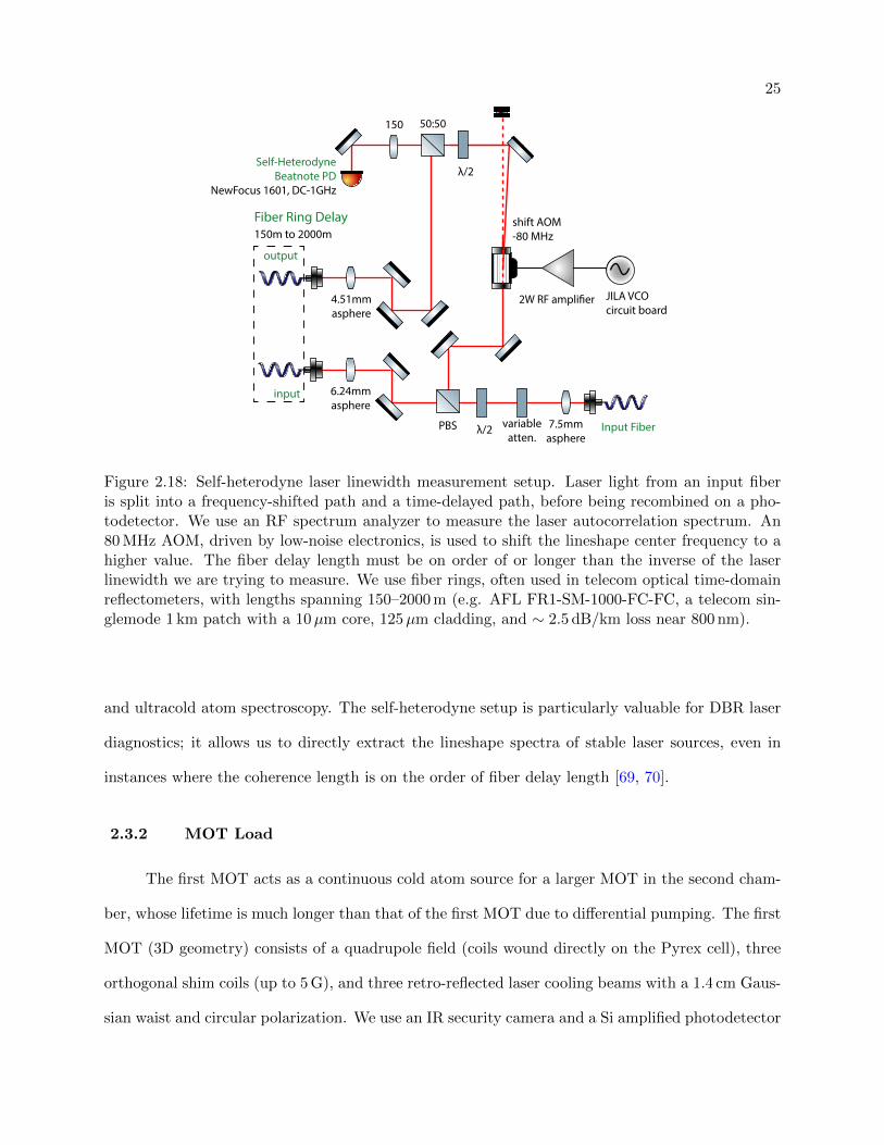
25

λ/2 Input Fiber7.5mmasphere

variableatten.

PBS

shift AOM-80 MHz

50:50

λ/2

JILA VCOcircuit board

2W RF amplier

input 6.24mmasphere

4.51mmasphere

Fiber Ring Delay150m to 2000m

output

150

Self-HeterodyneBeatnote PD

NewFocus 1601, DC-1GHz

Figure 2.18: Self-heterodyne laser linewidth measurement setup. Laser light from an input fiberis split into a frequency-shifted path and a time-delayed path, before being recombined on a pho-todetector. We use an RF spectrum analyzer to measure the laser autocorrelation spectrum. An80 MHz AOM, driven by low-noise electronics, is used to shift the lineshape center frequency to ahigher value. The fiber delay length must be on order of or longer than the inverse of the laserlinewidth we are trying to measure. We use fiber rings, often used in telecom optical time-domainreflectometers, with lengths spanning 150–2000 m (e.g. AFL FR1-SM-1000-FC-FC, a telecom sin-glemode 1 km patch with a 10µm core, 125µm cladding, and ∼ 2.5 dB/km loss near 800 nm).

and ultracold atom spectroscopy. The self-heterodyne setup is particularly valuable for DBR laser

diagnostics; it allows us to directly extract the lineshape spectra of stable laser sources, even in

instances where the coherence length is on the order of fiber delay length [69, 70].

2.3.2 MOT Load

The first MOT acts as a continuous cold atom source for a larger MOT in the second cham-

ber, whose lifetime is much longer than that of the first MOT due to differential pumping. The first

MOT (3D geometry) consists of a quadrupole field (coils wound directly on the Pyrex cell), three

orthogonal shim coils (up to 5 G), and three retro-reflected laser cooling beams with a 1.4 cm Gaus-

sian waist and circular polarization. We use an IR security camera and a Si amplified photodetector

26

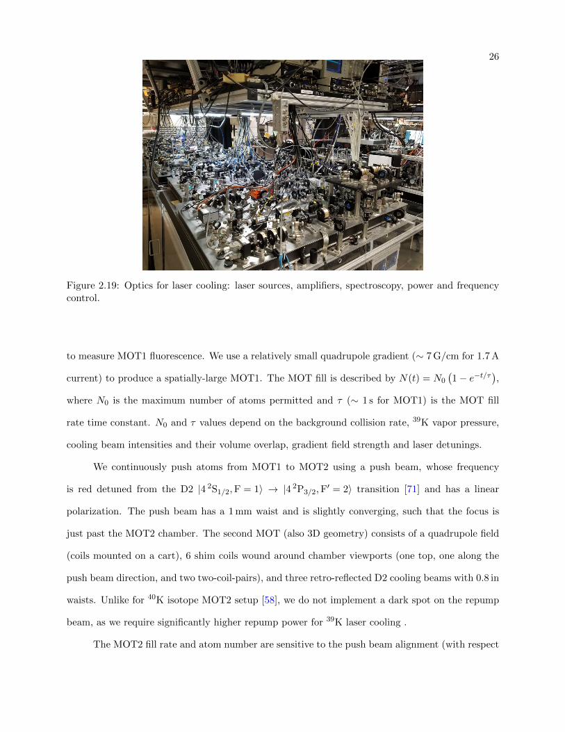
Figure 2.19: Optics for laser cooling: laser sources, amplifiers, spectroscopy, power and frequencycontrol.

to measure MOT1 fluorescence. We use a relatively small quadrupole gradient (∼ 7 G/cm for 1.7 A

current) to produce a spatially-large MOT1. The MOT fill is described by N(t) = N0

(1− e−t/τ

),

where N0 is the maximum number of atoms permitted and τ (∼ 1 s for MOT1) is the MOT fill

rate time constant. N0 and τ values depend on the background collision rate, 39K vapor pressure,

cooling beam intensities and their volume overlap, gradient field strength and laser detunings.

We continuously push atoms from MOT1 to MOT2 using a push beam, whose frequency

is red detuned from the D2 |4 2S1/2,F = 1〉 → |4 2P3/2,F′ = 2〉 transition [71] and has a linear

polarization. The push beam has a 1 mm waist and is slightly converging, such that the focus is

just past the MOT2 chamber. The second MOT (also 3D geometry) consists of a quadrupole field

(coils mounted on a cart), 6 shim coils wound around chamber viewports (one top, one along the

push beam direction, and two two-coil-pairs), and three retro-reflected D2 cooling beams with 0.8 in

waists. Unlike for 40K isotope MOT2 setup [58], we do not implement a dark spot on the repump

beam, as we require significantly higher repump power for 39K laser cooling .

The MOT2 fill rate and atom number are sensitive to the push beam alignment (with respect

27

Figure 2.20: Second MOT imaging optics used for absorption (using a probe beam and a quan-tization coil) and fluorescence imaging (using D2 MOT beams and zero magnetic field). The 2”50:50 beamsplitter is used for miscellaneous diagnostics: diverting part of the fluorescence signalor beam light (probe or push) onto a photodetector or an IR security camera.

to MOT1 and MOT2 cloud locations), quadrupole gradient, beam power and detunings. Optimizing

MOT2 is an iterative process and we’ve spent a significant amount of time getting the desired

conditions. We use a CCD camera (PCO Pixelfly QE) to image the MOT2 cloud (along the

transfer tube direction, as shown in Fig. 2.20).

To extract the MOT2 atom number, we use absorption imaging: we turn off all MOT light,

gradient and shims; turn on a few-G quantization field along the probe beam propagation direction;

illuminate atoms with a 40µs, σ+ polarization, D2 |4 2S1/2,F = 2〉 → |4 2P3/2,F′ = 3〉 transition

resonant probe light, along with D2 repump light (using MOT beams). The atomic cloud attenuates

(due to absorption) the probe beam intensity according to Beer’s law:

I(x, y) = I0e−n(x,y)σ = I0e

−OD(x,y), (2.2)

where I0 is the incoming probe beam intensity (assumed homogeneous), the probe beam propagates

along z direction, n(x, y) is atom cloud column density (integrated along z), OD is the optical depth

of the cloud and σ is the absorption cross-section, whose on-resonance value is σ0 = 3λ2/2π and

whose off-resonance value is described by a Lorentizian with a FWHM width equal to the excited

state national linewidth Γ/2π = 6.035 MHz (assuming no power broadening of the transition, valid

for I Isat = π~cΓ/(3λ3); the saturation intensity, Isat = 1.75 mWcm−2 for 39K D2 transition) [66].

For absorption imaging (either in the MOT or science chambers), we always take three consecutive

image frames: a shadow frame IS(x, y) with atoms and probe light, a light frame IL(x, y) without

28

atoms and with probe light, and a dark frame ID(x, y) without atoms nor probe light (captures

CCD dark counts and background lab light). The OD 2D distribution is defined as:

OD(x, y) = ln

(IL(x, y)− ID(x, y)

IS(x, y)− ID(x, y)

). (2.3)

For a Gaussian atom density distribution (e.g. a distribution of non-interacting thermal atoms in

a harmonic trap), the atom number N relates to the optical depth by

N =2π

σ0ODpeakσxσy, (2.4)

where ODpeak, σx and σy are fit the values for a 2D Gaussian distribution describing the OD profile:

OD(x, y) = ODpeak exp(− (x−x0)2

2σ2x− (y−y0)2

2σ2y

), where (x0, y0) is the atom cloud center. The physical

cloud sizes σx and σy are related to the CCD image sizes σCCDx and σCCD

y by σx,y = (pixsize)σCCDx,y /M ,

where pixsize is the CCD pixel size (e.g. 6.45µm for Pixelfly and 13µm for Princeton Instruments

camera, the primary camera used for the majority of science chamber imaging) and M is magni-

fication of the imaging system (often determined from measuring parabolic trajectory of a falling

atom cloud). Since MOT clouds are rarely Gaussian (their shapes depend on many parameters), a

more complicated analysis must be performed to accurately extract the MOT atom number from

an in-situ absorption image.

Since the transfer tube (11 mm inner diameter) sets the maximal size of the probe beam, the

field of view is limited and absorption imaging can be only used for a short time of flight (TOF)

expansion durations, as depicted in Fig. 2.21. Therefore, we resort to fluorescence imaging for

longer TOF imaging. The fluorescence imaging sequence goes as follows: we turn off MOT lights,

gradient and shims; we allow the cloud to expand and fall; we illuminate atoms with resonant D2

repump and trap MOT2 beams (full power) for 0.5–3 ms and expose the camera. While fluorescence

imaging is noisier (the signal depends on beam powers and background lab light) than absorption

imaging and while it is more difficult to accurately extract the atom number (typically we work

with arbitrary units which are proportional to N), fluorescence imaging works for hot/large MOT

clouds and enables long cloud expansion for temperature extraction. For these reasons, we often

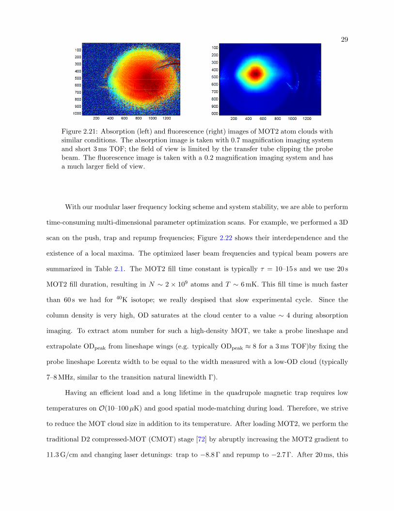
resort to fluorescence imaging for MOT2 optimizations.

29

Figure 2.21: Absorption (left) and fluorescence (right) images of MOT2 atom clouds withsimilar conditions. The absorption image is taken with 0.7 magnification imaging systemand short 3 ms TOF; the field of view is limited by the transfer tube clipping the probebeam. The fluorescence image is taken with a 0.2 magnification imaging system and hasa much larger field of view.

With our modular laser frequency locking scheme and system stability, we are able to perform

time-consuming multi-dimensional parameter optimization scans. For example, we performed a 3D

scan on the push, trap and repump frequencies; Figure 2.22 shows their interdependence and the

existence of a local maxima. The optimized laser beam frequencies and typical beam powers are

summarized in Table 2.1. The MOT2 fill time constant is typically τ = 10–15 s and we use 20 s

MOT2 fill duration, resulting in N ∼ 2 × 109 atoms and T ∼ 6 mK. This fill time is much faster

than 60 s we had for 40K isotope; we really despised that slow experimental cycle. Since the

column density is very high, OD saturates at the cloud center to a value ∼ 4 during absorption

imaging. To extract atom number for such a high-density MOT, we take a probe lineshape and

extrapolate ODpeak from lineshape wings (e.g. typically ODpeak ≈ 8 for a 3 ms TOF)by fixing the

probe lineshape Lorentz width to be equal to the width measured with a low-OD cloud (typically

7–8 MHz, similar to the transition natural linewidth Γ).

Having an efficient load and a long lifetime in the quadrupole magnetic trap requires low

temperatures on O(10–100µK) and good spatial mode-matching during load. Therefore, we strive

to reduce the MOT cloud size in addition to its temperature. After loading MOT2, we perform the

traditional D2 compressed-MOT (CMOT) stage [72] by abruptly increasing the MOT2 gradient to

11.3 G/cm and changing laser detunings: trap to −8.8 Γ and repump to −2.7 Γ. After 20 ms, this

30

- 1 2 - 1 0 - 8 - 6 - 4 - 2 0- 6

- 5

- 4

- 3

- 2

- 1 2 - 1 0 - 8 - 6 - 4 - 2 0- 6

- 5

- 4

- 3

- 2

- 1 2 - 1 0 - 8 - 6 - 4 - 2 0- 6

- 5

- 4

- 3

- 2

- 1 2 - 1 0 - 8 - 6 - 4 - 2 0- 6

- 5

- 4

- 3

- 2

01 x 1 0 52 x 1 0 53 x 1 0 54 x 1 0 55 x 1 0 56 x 1 0 57 x 1 0 58 x 1 0 5

Figure 2.22: Contour plots demonstrating MOT2 laser frequency optimization. For each pushbeam detuning (linked to the repump frequency by an AOM frequency offset), we vary trap andrepump frequencies, and record the fluorescence signal (imaging frame fit) which is proportional tothe number of atoms captured in MOT2. We use a 15 s MOT2 fill duration. Here, TOF is 1 ms,Ptrap1 = 210 mW, Prepump1 = 160 mW, Ptrap2 = 170 mW, Prepump2 = 140 mW, Ppush = 8 mW, and9.9 G/cm quadrupole gradient (31.1 A current). The maximal push beam detuning is limited bytechnical reasons relating to the required O(10 mW) push beam power and the use of an AOM forfrequency shift from the repump light.

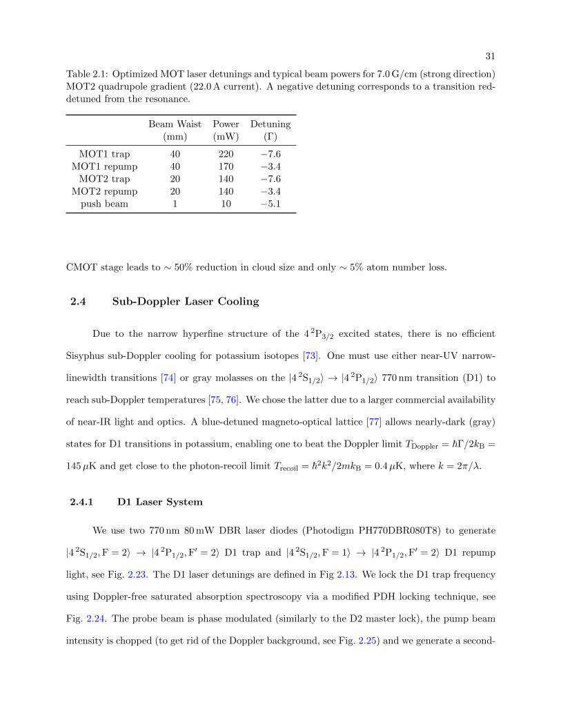
31

Table 2.1: Optimized MOT laser detunings and typical beam powers for 7.0 G/cm (strong direction)MOT2 quadrupole gradient (22.0 A current). A negative detuning corresponds to a transition red-detuned from the resonance.

Beam Waist Power Detuning(mm) (mW) (Γ)

MOT1 trap 40 220 −7.6MOT1 repump 40 170 −3.4

MOT2 trap 20 140 −7.6MOT2 repump 20 140 −3.4

push beam 1 10 −5.1

CMOT stage leads to ∼ 50% reduction in cloud size and only ∼ 5% atom number loss.

2.4 Sub-Doppler Laser Cooling

Due to the narrow hyperfine structure of the 4 2P3/2 excited states, there is no efficient

Sisyphus sub-Doppler cooling for potassium isotopes [73]. One must use either near-UV narrow-

linewidth transitions [74] or gray molasses on the |4 2S1/2〉 → |4 2P1/2〉 770 nm transition (D1) to

reach sub-Doppler temperatures [75, 76]. We chose the latter due to a larger commercial availability

of near-IR light and optics. A blue-detuned magneto-optical lattice [77] allows nearly-dark (gray)

states for D1 transitions in potassium, enabling one to beat the Doppler limit TDoppler = ~Γ/2kB =

145µK and get close to the photon-recoil limit Trecoil = ~2k2/2mkB = 0.4µK, where k = 2π/λ.

2.4.1 D1 Laser System

We use two 770 nm 80 mW DBR laser diodes (Photodigm PH770DBR080T8) to generate

|4 2S1/2,F = 2〉 → |4 2P1/2,F′ = 2〉 D1 trap and |4 2S1/2,F = 1〉 → |4 2P1/2,F

′ = 2〉 D1 repump

light, see Fig. 2.23. The D1 laser detunings are defined in Fig 2.13. We lock the D1 trap frequency

using Doppler-free saturated absorption spectroscopy via a modified PDH locking technique, see

Fig. 2.24. The probe beam is phase modulated (similarly to the D2 master lock), the pump beam

intensity is chopped (to get rid of the Doppler background, see Fig. 2.25) and we generate a second-

32

derivative/harmonic of the PDH signal to provide lock peak detection. The amplitude modulation

lock-in detection and the peak detector were necessary additions to prevent the D1 laser from

unlocking during strong RF and microwave radiation (up to 25 W, ∼ 2 m away from the D1 setup)

from loop antennas we use to induce magnetic dipole transitions. Other methods, including mu-

metal shielding, RF filtering, better grounding and shortening of routing cables, failed to resolve

the unlocking issue. The new scheme made the D1 lock very robust.

The D1 trap frequency is changed using a double-pass AOM “cat’s eye” configuration, al-

lowing ∼ 50 MHz (8 Γ) dynamic range without optical re-alignment. The D1 repump frequency is

locked to the D1 trap frequency via a heterodyne beatnote lock, similar to the heterodyne locks

(Fig. 2.17) used in the D2 setup. We optimize the beatnote servo to establish phase coherence

between the two lasers (> 10 dB narrow beatnote signal on top of a broad convoluted lineshape).

This coherence enables Raman transitions (Λ-configuration) and observation of a narrow cooling

feature (see Fig. 2.26), whose width is less than the excited state natural linewidth Γ.

The D1 trap and D1 repump light are combined on a 70:30 non-polarizing beam splitter

before being amplified by the TA. Since the TA amplifies the two wavelengths in a nontrivial way,

we use commercial and homebuilt optical cavities to sense the output power of each component

(e.g. ∼ 1:8 repump:trap ratio). The D1 light is sent through a 10 m PM-SM fiber to the science

optical table, delivering 130 mW. The D1 light (7 mm waist) is combined with the D2 MOT2 beams

and is sent to the MOT2 vacuum chamber. The molasses lattice is formed by retro-reflected D1

light with circular polarization.

2.4.2 D1 Cooling and Quadrupole Trap Load

After the D2 CMOT stage, we perform a hybrid D1-D2 CMOT stage [78]: we instantaneously

turn off the D2 trap light, turn on the D1 trap light (blue-detuned), change the D2 repump frequency

(red-detuned) and reduce its power, and change the shim magnetic field values. We keep the

quadrupole gradient unchanged at 11.3 G/cm. We optimized these parameters to minimize the

cloud temperature, using a long-TOF fluorescence imaging. We find that the D1-D2 CMOT stage

33

D1 Trap DBR80mW max

asphereon xy stage

-50 cyl

150 cyl

λ/2

x2 isol. >30dB ea.

PBS λ/2

λ/2

PBS

D1 trapdbl-pass AOM

+2x (70 to 120) MHz

λ/2

20uW

Glan-Thom. pol.

EOM

pump

λ/2

Glan-Thom. pol.

Pumpchop AOM -104 MHz

Saturated Abs. PDNewFocus 1601, DC-1GHz

PBS

λ/2

probe

λ/2

PBS 50:50

Repump Beat PDEOT ET-2030A, 1.2GHz

pol.

λ/4

75

λ/2

JILA TA mounttemp control

λ/2

70:30

D1 TA2W max out

λ/2

50

D1 Repump DBR80mW max

150 cyl

4.51mm asphereon xy stage

-50 cyl

x2 isol. >30dB ea.

λ/2

75 cyl -50 cyl

PBS λ/2>30dB isol.

shutter

50uW

D1 AOM-80 MHz

shutter

λ/2

D1 ber6.24mmasphere

K vapor cellat 60C and

mu-metal shielded

Figure 2.23: D1 laser system. The D1 trap laser frequency is locked to a saturated absorptionspectroscopy setup. The D1 repump laser frequency is locked to the D1 trap via a heterodynebeatnote lock. The trap and repump light are combined before amplification and are sent to thescience optical table via the same fiber.

34

Figure 2.24: D1 frequency locking scheme via a modified PDH lock. A function generator drives ahomebuilt resonant EOM tank circuit to phase modulate the probe beam. After passing through asaturated absorption spectroscopy, the probe beam is detected on a New Focus 1601 photodetector(see Fig. 2.23). We retrieve the first derivative (approximately speaking) of the absorption lineshapeusing the first harmonic (20 MHz) signal and send it to the servo (JILA high speed loop filter). Weretrieve the (approximate) second derivative of the absorption lineshape using the second harmonic(40 MHz) signal and send it to the scope for peak detection. Additionally, we form AM lock-indetection to get rid of Doppler background and to make the PDH lock immune to background RFlab noise (10-1000 MHz stemming from RF antennas and/or other electro-optic modulators). Wechop the pump beam intensity by mixing the 104 MHz RF drive with a 100 kHz sine wave beforesending it to the pump beam AOM. We demodulate the 20 MHz and 40 MHz signals with the100 kHz local oscillator (a sine wave after filtering the square wave of the function generator sync.output).

35

- 3 0 0 - 2 0 0 - 1 0 0 0 1 0 0 2 0 0 3 0 0- 0 . 0 6

- 0 . 0 4

- 0 . 0 2

0 . 0 0

0 . 0 2

0 . 0 4 a b s o r p t i o n p e a k 1 s t d e r i v a t i v e : n o p u m p c h o p 1 s t d e r i v a t i v e : w i t h p u m p c h o p 2 n d d e r i v a t i v e : w i t h p u m p c h o p

signal

(arb)

f ( M H z )Figure 2.25: D1 spectroscopy signal: absorption peak with no phase modulation (black); firstderivative (approximately speaking; the shape of the PDH lock demodulated signal depends onthe lineshape width and the phase modulation frequency) with Doppler background and withprobe phase modulation (red), using a similar setup as used for D2 laser lock in Fig. 2.16; firstderivative without Doppler background and with probe phase modulation and pump chopping(blue), output from Fig. 2.24 circuit; second derivative without Doppler background and with probephase modulation, pump chopping and second harmonic extraction (green), output from Fig. 2.24circuit. Here, the frequency axis is calibrated using a wavemeter (while locking to individualspectral lines) and has an arbitrary offset. Each signal is scaled and shifted vertically for illustrativepurposes.

36

prefers a low D2 repump power (a factor of 10–15 smaller than the MOT load and D2 CMOT values)

and a near-resonant D2 repump frequency (red-detuned, at −0.8 Γ); the stage is less sensitive to

the D1 trap parameters (we use 120 mW power and blue-detune to +2 Γ). This stage is kept on for

10 ms to reduce the cloud temperature to 220µK at the expense of ∼ 10% in atom number.

The D1 gray molasses capture efficiency depends mainly on the beam intensity and the initial

cloud temperature. Since the D1-D2 CMOT stage pre-cools the atoms, we only require > 100 mW

of D1 light to capture most atoms in the molasses. First, we turn off the D2 repump light, turn off

the D1 trap light, turn off the quadrupole field, change the shim values, set the D1 frequencies and

initiate opening of the D1 repump shutter (which was off during the D1-D2 CMOT; the shutter is

before the 70:30 D1 trap-repump combiner, as shown in Fig. 2.23). Then, after 1 ms duration of

dwell time, we turn on 130 mW of D1 light (containing trap and repump) and immediately begin

linearly ramping down the D1 power to 13 mW in 8 ms. The final atom temperature relates to

the final D1 beam intensity. We routinely reach 15µK and have observed temperatures as low as

8µK. Reaching such temperatures requires extensive optimization. We iteratively change the shim

values (molasses are very sensitive to non-zero magnetic fields), the D1 beam alignment (need good

optical lattices), the repump-to-trap power ratio (robust, around 1:3–1:10 is good) and the laser

detuning. While the atom number and temperature after the D1 molasses stage depend weakly

on the D1 trap parameters, the temperature is particularly sensitive to the Raman detuning (see

Fig. 2.13 for definition) between the trap and repump light, as shown in Fig. 2.26. A 8 ms D1 gray

molasses stage enables us to reach 15µK at the expense of ∼ 30% in atom number.

After the sub-Doppler cooling stage, we begin to load atoms into the quadrupole trap

(formed by the same coils used for MOT2 gradient). Since we ultimately desire atoms only in

the |4 2S1/2,F = 1,mF = −1〉 state, we pump |4 2S1/2,F = 2〉 atoms into the |4 2S1/2,F = 1〉 state

by turning off the D1 trap light 2.5 ms after turning off the D1 repump light. Since the D1 molasses

dark states favor the F = 1 manifold, we are able to predominantly populate the F = 1 state with

relative ease. Furthermore, since |F = 1,mF = −1〉 is the only magnetically trappable F = 1 state,

one would like to pump all atoms there. We tried doing so with D1 and D2 pump light in separate

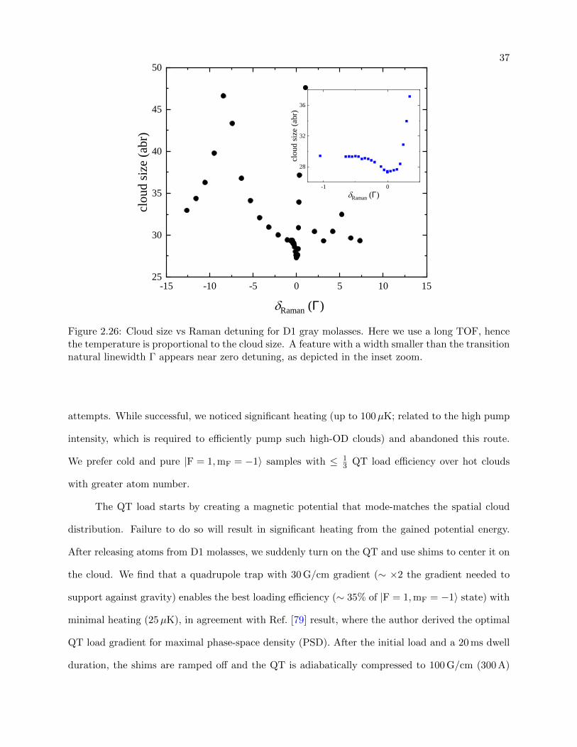
37

- 1 5 - 1 0 - 5 0 5 1 0 1 52 5

3 0

3 5

4 0

4 5

5 0

- 1 0

2 8

3 2

3 6

cloud

size (

abr)

R a m a n ( Γ)

cloud

size (

abr)

R a m a n ( Γ)Figure 2.26: Cloud size vs Raman detuning for D1 gray molasses. Here we use a long TOF, hencethe temperature is proportional to the cloud size. A feature with a width smaller than the transitionnatural linewidth Γ appears near zero detuning, as depicted in the inset zoom.

attempts. While successful, we noticed significant heating (up to 100µK; related to the high pump

intensity, which is required to efficiently pump such high-OD clouds) and abandoned this route.

We prefer cold and pure |F = 1,mF = −1〉 samples with ≤ 13 QT load efficiency over hot clouds

with greater atom number.

The QT load starts by creating a magnetic potential that mode-matches the spatial cloud

distribution. Failure to do so will result in significant heating from the gained potential energy.

After releasing atoms from D1 molasses, we suddenly turn on the QT and use shims to center it on

the cloud. We find that a quadrupole trap with 30 G/cm gradient (∼ ×2 the gradient needed to

support against gravity) enables the best loading efficiency (∼ 35% of |F = 1,mF = −1〉 state) with

minimal heating (25µK), in agreement with Ref. [79] result, where the author derived the optimal

QT load gradient for maximal phase-space density (PSD). After the initial load and a 20 ms dwell

duration, the shims are ramped off and the QT is adiabatically compressed to 100 G/cm (300 A)

38

in 100 ms. While this step increases the cloud temperature to 80–100µK, it also reduces the cloud

size, necessary for an efficient cart transfer to the science cell through narrow vacuum components

(1.5 cm inner diameter at the narrowest spots). Using 30 G/cm for cart transfer results in 50%

less atoms reaching the science cell. We find that the efficiency saturates beyond 80 G/cm. Using

100 G/cm, the cart transfers 3× 108 atoms in the |F = 1,mF = −1〉 state to the science cell (54 cm

away) in 3.5 s. We’ve measured the two-way transfer efficiency to be 77% (to the science cell

and back to the MOT chamber; or 88% one-way, assuming symmetrical two-way loss). The atom

lifetime in the cart QT is long in the MOT2 and the science chambers (60–70 s), mainly limited by

the Majorana spin-flip loss [80].

Thermodynamic properties of non-interacting atoms in a quadrupole trap are extracted from

a single-particle partition function:

Z1 =64√

2π5/2m3/2 (kbT )9/2

(hµb)3, (2.5)

where the external potential is given by Eq. 2.1 and we ignore gravity. A thermal cloud has spatial

and momentum probability distributions described by:

P (x, y, z, px, py, pz) =1

Z1exp

(−E(x, y, z, px, py, pz)

kBT

), (2.6)

P (x, y, z) =1

32π

(µb

kBT

)3

exp

(− µb

2kBT

√x2 + y2 + 4z2

), (2.7)

P (px, py, pz) =h3

(2πmkBT )3/2exp

(−p2x + p2

y + p2z

2mkBT

), (2.8)

where E is the total energy, b is the gradient along the strong direction z, µ is the magnetic

moment of the trapped spin state and the normalization is such that integration over all spatial

and momentum dimensions results in unity probability. The rms cloud size z =√〈z2〉 = 2kBT/µb,

where 〈z2〉 =∫z2P (x, y, z)dxdydz; the rms sizes along x and y directions are twice as large. We

often fit clouds released from the QT with a 2D Gaussian function; for in-situ imaging, we use a 0.65

correction factor for determining the rms size from a Gaussian width. Since atoms are presumed to

be non-interacting, the rms momentum values are equal to√mkBT . The atom density distribution

is n(x, y, z) = NP (x, y, z). Similarly, many-atom properties can be retrieved from an N -particle

39

partition function ZN = (Z1)N/(N !). For example, we determine the expected temperature rise

due to adiabatic compression of the trap to be Tf/Ti = (bf/bi)2/3, where bi and bf are the initial and

final gradient values. We find this by relating the cloud volume V , the heat capacity CV =(∂U∂T

)V

and the gas pressure p = −(∂b∂V

)T

(∂F∂b

)T

(p = NkBT/V for a non-interacting gas), where the

internal energy U = −d ln(ZN )dβ , the Helmholtz free energy F = −kBT ln(ZN ) and β = (kBT )−1.

Similarly, one can obtain the scaling power 2/3 from dimensional analysis: relating PSD, density,

T and b, while acknowledging that the PSD remains constant during an adiabatic ramp. Our QT

compression measurements agree to within 10% of the 2/3 scaling power.

After the cart transfer to the science cell, we transfer atoms to the science QT coils by

ramping up the science QT (0 to 100 G/cm in 200 ms) while ramping down the cart QT (100 G/cm

to 0 in 200 ms). We move the cart away after this swap. Since our next goal is to load the

atoms into a small-waist optical trap, we further compress the magnetic trap to 199 G/cm (364 A).

Typically, we end up with 3 × 108 atoms in the |F = 1,mF = −1〉 state at a temperature 180µK,

a peak PSD 1.4 × 10−6, a density-weighted density 〈n〉 = 1N

∫n2(~x)d3x = 1.9 × 1010 cm−3 and

τ = 60 s QT lifetime. While the trap has a modestly high trap frequency of 362 Hz, defined as

velocityrms/sizerms, a small scattering length (a = −46 a0 for B = 0 G, assuming T = 0) leads to a

low 1.3 Hz collision rate and a slow thermalization rate of 0.5 Hz (assuming we require ≈ 2.5–2.7

number of elastic two-body collisions for thermalization [81, 60, 82]).

2.5 All-Optical Evaporation

2.5.1 Optical Trap Load

Since efficient evaporative cooling requires a high thermalization rate, we need to increase

our low elastic collision rate. We do so by transferring the atoms to an optical dipole trap (OT)

and use a nearby (∼ 34 G) Feshbach resonance to enhance elastic collisions. However, since the

optical trap (OT) load efficiency also depends on thermalizing collisions, we need to be creative

[83]. We employ an intense optical dipole beam with a 2.7 mK trap depth (resulting from a 25 W,

40

1064 nm, 28µm × 28µm waist beam) that significantly exceeds the collisional energy where the

Ramsauer-Townsend minimum occurs (400µK, see Fig. 2.7). This enables us to transfer 1–5% of

atoms in the QT, whose cloud size is 600µm× 1200µm× 1200µm, to the optical trap, consistent

with the expected load efficiency estimates [84, 85, 83].

The OT load begins with the shims turning on to shift the QT center; the science cell has three

shim pairs surrounding it, facing orthogonal directions. Then, the optical trap beam adiabatically

ramps on to full power (20–25 W) in 200 ms. It takes 8 s to fill the OT potential, after which we

ramp off the QT in 100 ms. While the PSD of the loaded cloud is nearly constant vs. dipole power,

more atoms are loaded for higher powers. The number of atoms loaded into the OT saturates for

powers > 21 W and 8 s fill duration. The best OT load efficiencies occur when the focus of the

dipole trap is near the QT center. This alignment is very sensitive, as alignment to the QT center

leads to significant Majorana loss, as shown in Fig. 2.27. For alignment, we iterate between the OT

beam tilt, OT focus location and the QT center (using shims). Additional complications resulting

from thermal lensing (up to 1 mm in 10 s along the dipole beam propagation direction; compare this

to the 2.3 mm Rayleigh range) make careful OT alignment crucial to get stable cloud conditions.

We typically load up to 5 × 106 atoms with a 300–400µK temperature and 4 × 10−5 peak

PSD from a QT with 1–3 × 108 atoms and 180–220µK temperature. We estimate that a 25 W,

28µm× 28µm waist beam forms a potential with a (ωx, ωy, ωz) /2π = (8700, 74, 8700) Hz trapping

frequencies (y along the beam), a 2.7 mK trap depth and a 1.4µK/s heating rate (due to off-resonant

scattering). Such a trap results in a cigar-shaped atom cloud with a large aspect ratio. Highly

elongated clouds are difficult to analyze, as depicted in Fig. 2.29. While imaging along the dipole

trap direction would help, thermal lensing from the high-power beam would lead to unnecessary

imaging complications. Therefore, we decided to implement additional optical trapping beams that

would shape the cloud at lower temperatures; see Sec. 4.2.2 for additional details on how we settled

on the final optical trap configuration. The additional beams are: a vertical beam (“V beam”) with

a 140µm× 140µm waist and a horizontal sheet beam (“H2 beam”) with a 80µm× 810µm waist,

whose strong direction is along gravity and propagates at a 45 with respect to the 28µm× 28µm

41

2 0 0 2 5 0 3 0 0 3 5 0 4 0 0 4 5 0- 8 0

- 6 0

- 4 0

- 2 0

0

2 0

4 0z (µ

m)

x ( µm )

0 . 0

6 . 0 x 1 0 5

1 . 2 x 1 0 6

1 . 8 x 1 0 6

2 . 4 x 1 0 6

3 . 0 x 1 0 6

3 . 6 x 1 0 6

4 . 2 x 1 0 6

4 . 8 x 1 0 6N

2 0 0 2 5 0 3 0 0 3 5 0 4 0 0 4 5 0- 8 0

- 6 0

- 4 0

- 2 0

0

2 0

4 0

z (µm)

x ( µm )

0 . 0

4 . 5 x 1 0 - 6

8 . 9 x 1 0 - 6

1 . 3 x 1 0 - 5

1 . 8 x 1 0 - 5

2 . 2 x 1 0 - 5

2 . 7 x 1 0 - 5

3 . 1 x 1 0 - 5

3 . 6 x 1 0 - 5P S D

Figure 2.27: Sensitive alignment of the dipole beam is needed for an efficient OT load. The figuresshow that the largest number of loaded atoms (left) with the highest peak PSD (right) occur whenthe dipole beam is aligned near the QT trap center. At the center, significant Majorana spin-fliploss occurs (deep blue contour). Note an arbitrary offset of the axis values (z is along gravity/strongQT direction, x is horizontal). Ignore the gray region in the PSD plot, where we have insufficientdata or have small atom signal that results in unreliable temperatures. Note the significant lossand heating below the Majorana hole, also shown in Fig. 2.28.

2 0 0 2 5 0 3 0 0 3 5 0 4 0 0 4 5 0- 8 0

- 6 0

- 4 0

- 2 0

0

2 0

4 0

z (µm)

x ( µm )

0 . 0

0 . 3

0 . 7

1 . 0

1 . 4

1 . 7

2 . 1

2 . 4

2 . 8T ( m K )

Figure 2.28: Atom temperature during optical trap load alignment.

waist beam (“H1 beam”). The H2 and V trap depths are 5.5µK and 6.5µK for their highest powers

of 8 W and 1.5 W, respectively. Since the new potentials are only relevant at low temperatures, the

H1 beam needs to perform most evaporation to cool atoms from ∼ 500µK down to < 500 nK. The

H1 beam requires a 103–104 dynamic range in power control and small intensity noise at all levels.

42

Figure 2.29: Atom cloud expansion after optical dipole trap load, with increasing TOF (top tobottom). The dipole trap propagates perpendicular to the imaging direction. The in-situ image(top) suffers from diffraction: the cloud size is smaller than the imaging resolution. The hot cloudexpands significantly in a matter of a few ms (3 ms for bottom image). Imaging magnification is0.7 and the horizontal field of view is 9.5 mm.

2.5.2 Optical Trap Laser Setup

Our optical dipole trap system has challenging requirements. We need high optical power

(up to 25 W) delivered to the atoms, ability to accurately control the power with a 104 dynamic

range, minimal intensity noise and have great pointing stability ( 28µm, the H1 beam waist).

To achieve these requirements, we decided on the Mephisto-Nufern laser-amplifier combination,

whose properties were previously measured in select publications [86, 87]. We split and control

the amplified light, then route it to the science cell via photonic-crystal fibers (PCFs), as shown

in Fig. 2.30. After diligent engineering and overcoming multiple challenges, the dipole trap laser

system became one of the most robust systems in our lab.

The seed laser (Coherent Mephisto S, 500 mW maximum output) is a monolithic non-planar

ring oscillator (NPRO) that outputs coherent light (< 1 kHz linewidth) with great beam quality

(TEM00, M2 < 1.1; one of best Gaussian beams I’ve ever worked with) and low relative intensity

noise (RIN) at < −90 dB/Hz. We run the laser at 24C, 0.61 A and 1064.1 nm, operating in the

middle of the measured mode-hop-free region. We collimate the output light (160µm waist at

the NPRO, 50 mW) to a 450µm waist, pass it through an optical isolator, fiber couple (Thorlabs

43

200mmλ/4λ/2

λ/2

λ/2

λ/2

dump

Mephistoseed laser

PBSisolator >40dB

4.51mm asphere

1mmbeamoutput

isolator >35dB

λ/2

λ/2PBS-25mm

water-cooleddump

λ/2

PBS

λ/2

PBS

dump-80 MHzAOM

+80 MHzAOM

5-axis stage

5-axis stage0th

+1st

mirrors with2mm holes

water-cooleddump-25mm

λ/2

-1st

0th-25mm

Nufern bercollimatoron TEC-heatedblock

λ/2

water-cooleddump

15mm asphereon a 3-D stage

1.2m photoniccrystal ber

Water-cooledhigh-powerterminator

12.5mm asphere

To VerticalDipole Trap

To Horizontal H1Dipole Trap

To Nufern Input

2m photoniccrystal ber

-80 MHzAOM

5-axis stagemirror witha 2mm hole

-1st

0th

λ/2

15mm asphereon a 3-D stage

1.2m photoniccrystal ber

Water-cooledhigh-powerterminator

To Horizontal H2Dipole Trap

Figure 2.30: Optical setup for control of optical dipole traps. The Mephisto seeds the Nufern fiberamplifier, whose output is split into V, H1 and H2 beams. AOMs enable individual beam powercontrol.

44

1 0 0 1 0 1 1 0 2 1 0 3 1 0 4 1 0 5

- 1 2 0

- 1 1 0

- 1 0 0

- 9 0

- 8 0

- 7 0

- 6 0 M e p h i s t o N u f e r n

RIN (d

B/Hz)

f ( H z )Figure 2.31: Measured relative intensity noise of a free-running (no feedback) Nufern fiber amplifier(full 50 W power) and a Mephisto seed laser. The FFT analyzer spectral resolution is changed from128 Hz to 2 Hz below 1500 Hz frequency. At very high frequencies (beyond the shown) we see anoise peak at around 1 MHz resulting from relaxation oscillations from residual pump noise; we areunable to suppress this feature due to a faulty “noise eater” feedback circuit in the Mephisto.

2 m patch with a steel-steel jacket, using PM980XP Nufern fiber) and deliver 40 mW of PM light

(> 25 dB extinction ratio) to the Nufern amplifier input.

The Nufern fiber amplifier amplifies the seed light up to 50 W (for 15–50 mW input), while

retaining the low RIN properties of the Mephisto laser, as shown in Fig. 2.31. Based on our previous

experience, we took additional steps to ensure stable Nufern amplifier operation. The Nufern box is

placed on a vibration-damping pad, water-cooled to 23C (its crucial to a have stable temperature

near 23C) using a commercial chiller (Thermo Scientific Thermochill II, supplying 1.5 gallons/min)

and the Nufern PCF output is tied down (without stress) and isolated using a rubberized sleeve.

Additionally, we opted for a custom stainless steel collimator enclosure (much better than the

standard aluminium part) with a custom 1 mm beam output diameter. We temperature-stabilize

the collimator assembly using a TEC-heated aluminium block.

All dipole trap optics are contained in a large steel enclosure and all light is terminated by

water-cooled beam dumps (Trap-IT ABD2CNP and Haas Laser Technologies BD25BW). It takes up

to 1 hr for the temperature to stabilize within the laser box, leading to an iterative beam alignment

45

procedure. The enclosure also assists in preventing dust accumulation on the optics; we have

burned some optics during the initial setup. We resort to mostly steel opto-mechanics, short beam

height (3 in, set by the PCF 3-axis stage, Thorlabs MBT616D) and minimal number of components

(thanks goes to a JILAn, Hans Green, for precisely machining holes in our mirrors) and their

separation distances. We use high-power 1064 nm V-coated UV-grade fused silica optics (mostly

from CVI) and minimize mechanical stress on the optics to ensure high polarization purity and high

beam quality. We use large-aperture Tellurium Dioxide AOMs (Gooch & Housego AOMO 3080-

199, mounted on good heat sinks) for intensity control; this leads to an improved beam pointing

stability compared to when we use small aperture or flint glass AOMs.

The output from the Nufern amplifier is split into vertical and horizontal beam paths. The

H2 beam results from the zeroth-order of the H1 beam intensity control AOM. AOM frequencies

and orders are chosen to have a minimal chance of beam interference at the atoms. Each beam

is fiber coupled into a PM-SM photonic-crystal fiber (NKT Photonics LMA-PM-15 fiber, Tratech

Fiberoptics HP2.5 assembly) using one mirror, a 3-axis translation stage and a V-coated UV-grade

fused silica asphere (TechSpec/Edmund Optics). The PCF has a high-power 1064 nm-AR-coated

epoxyless/fused-endcap that expands the beam and protects the fiber core from dust, a mode

stripping lantern that rejects the uncoupled light, and a copper assembly that we water-cool using

23C water from a chiller.

While the large mode (12.6µm mode diameter) PCF significantly reduces the stimulated

Brillouin scattering (SBS), residual SBS back-reflections lead to an unstable Nufern operation.

Using large optical isolation (an EOT Pavos 1045-1080 nm > 30 dB isolator along with a Thorlabs

IO-5-1064-VHP 1064 nm > 35 dB isolator) resolved the back-reflection problem. However, beam

quality degradation at high power (development of a hole in the beam center), resulting from self-

focusing in the isolator material, lead to a terrible 60% PCF coupling efficiency, see Fig. 2.32. To

circumvent the back-reflection and beam quality issues, we only use the > 35 dB isolator, reduce

the PCF length from 2 m to 1.2 m for H1 and H2 beams, and reduce the Nufern output power (from

50 W at 37A to 38W at 32A). We reach 95% coupling efficiency and can get up to 32 W at the

46

Figure 2.32: Nufern beam quality degradation at high power. At low operating power, the beamquality is great after an optical isolator (top left) and before PFC fiber (bottom left). However,at high operating power, self-focusing of the beam (top right) by the isolator material results in abeam with a hole at the PCF fiber input (bottom right). All images have a normalized beam peakintensity.

fiber output.

We deliver up to 2 W for V trap, 25 W for H1 trap and 8 W for H2 trap (after H1 trap

ramps down during evaporation). Figures.2.33, 2.34 and 2.35 demonstrate how we shape and

deliver the dipole light to the atoms. Similarly to the laser source side, we use high-power optics,

high-quality opto-mechanics and short beam heights. We devote extra attention to wavefront error

and use low distortion mirror mounts (e.g. Newport SU100W-F3K-127) when necessary. We use

a high-resolution beam profile camera to verify beam quality at the focus (e.g. astigmatism and

asymmetry), as depicted in Figs.2.36 and 2.37. The H1 and H2 beams are terminated by water-

cooled beam dumps. We monitor long-term beam pointing stability using CCD cameras (Allied

Vision MAKO G-125), allowing fast alignment troubleshooting.

A great beam pointing stability is crucial to get reproducible conditions and a low atom

heating rate. We achieve a good long-term pointing stability by utilizing high-quality optics, low-

expansion opto-mechanics and by surrounding the science optical table with curtains (improves

the temperature stability and regulates the air flow). Additionally, we check the dynamic pointing

stability. The expected atom heating rate due to pointing noise is 〈dE/dt〉 = πmω4trapSx(ωtrap)/2,

where 〈dE/dt〉 is time-averaged change rate of the total energy, ωtrap is the trap frequency along

47

λ/2 λ/2PBSPCF on kinematicmount

80mmasphereThorlabs ASL10142-1064

300mm planoNewport SPX059AR.1

200mmplano

Dump

Dump99:1

50:5075mm

Out of loop PD

In loop PD

z

CCD camera

50:50

1064nm lter

Figure 2.33: Optics for the horizontal dipole trap H1 (load beam) with a 28µm× 28µm waist and25 W beam power. For illustrative purposes, we change the science cell orientation. The probingPDs and CCD cameras have 1064 nm band-pass filters.

λ/2 λ/2

PBS

PCF on kinematicmount

Thorlabs LA4306-YAG40mm plano

focus for vertical direction500mm plano cyl. LJ4147RM-C

Dump

telescope for horz. direction200mm plano cyl. LJ4667RM-C-75mm plano cyl. LK4385RM-C

Dump

99:1

Out

of l

oop

PD

In lo

op P

D

CCD

cam

era

50:50

1064

nm

lter

plano cyl.collimate vertical direction

λ/2

Figure 2.34: Optics for the horizontal dipole trap H2 with a 80µm× 810µm waist and 8 W beampower, where the strong direction is along gravity (termed vertical direction in the schematic). Thebeam has a vertical polarization (into the page) before entering the cell.

a particular direction (in this case x) and Sx(ω) is the one-sided power noise spectrum of the

48

λ/2

Dump

sampler

Out of loop PDIn loop PD

CCD camera

1064nm lter

15mm asphereEdmund 33-018

PCF on kinematicmount

λ/2

λ/2

300mm planoNewport SPX059AR.1

Dump

plano

50:50

PBS

top imaging/pump/blast light

to top camera

samplerλ/2

dichroic

dichroic

Figure 2.35: Optics for the vertical dipole trap with a 140µm×140µm waist and 2 W beam power.The vertical dipole beam setup is located on a breadboard above the chamber. We use a periscope(formed by two dichroic mirrors) to pass the light through the science cell. The beam has a verticalpolarization before the dichroic and a horizontal polarization (into the page) as it enters the sciencecell. The dichroic mirrors serve to deliver the 767 nm light used for imaging, pumping or blasting.

trap location along the x-direction;√S(ω) ∝ x(ω) and normalization

∫∞0 S(ω)dω = 〈x2〉, where

〈x2〉 is the time-averaged mean-square variation in the trap x location [88]. We use a quadrant

photodetector to probe the pointing instability and find that the low-noise of our setup would result

in a negligible heating rate 〈dT/dt〉 = 4π4mf4Sx(f)/kb. For example, we measure the pointing

stability of the small-waist H1 trap (see Fig.2.38) and we estimate the heating rate to be < 1 nK/s

for all frequencies below 1 kHz, except near 375–425 Hz where we estimate the heating rate to be

as large as 100 nK/s (would be an unfortunate choice for the H1 trap frequency). Since the trap

frequency decreases with evaporation and we expect low heating rates below 1 kHz, we are content

with the pointing stability of our system.

We use a photodetector to monitor (using an out-of-loop PD) and servo (using an in-loop PD)

49

- 2 0 2 4 6

3 0

4 0

5 0

6 0

7 0

8 0 w x w y w = 2 8 µm t h e o r y w x / w y

f o c u s ( m m )

beam

waist

(µm)

0 . 9 0

0 . 9 5

1 . 0 0

1 . 0 5

1 . 1 0

w x / w

y

Figure 2.36: Beam waist and the spatial profile (inset image) of the H1 loading dipole beam nearits focus. We record the spatial profile at different distances from the focus (located at 2.5 mm, anarbitrary x-axis offset), fit the distributions using a 2D Gaussian function and extract the beamwaist along two orthogonal directions, rotating images if necessary. We notice a slight asymmetryand astigmatism in the H1 beam. The solid curve is a prediction for a TEM00 28µm waist beampropagation.

Figure 2.37: Spatial profiles of H2 (left) and V (right) dipole trap beams near their focus. Notethe hexagonal structure in the V beam resulting from the photonic-crystal fiber core.

the optical power of each beam. Due to the need for a low-noise high-dynamic-range servo control

of the H1 beam, I designed, modified and tested multiple servo components to engineer a low-

noise feedback system. Extra emphasis was given to having low-noise across the full 10 Hz–20 kHz

frequency span, determined by the expected trap frequencies for all dipole beam powers and con-

figurations. For example, intensity noise at twice the trapping frequency ftrap leads to parametric

heating rate Γ = π2f2trapRIN(2ftrap), defined as 〈dE/dt〉 = Γ〈E〉 [88]. For a desired Γ−1 = 100 s

time, RIN needs to be smaller than −116 dB/Hz for ftrap = 20 kHz, −90 dB/Hz for ftrap = 1 kHz

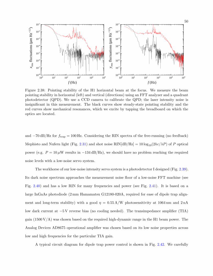
50

1 0 0 1 0 1 1 0 2 1 0 3 1 0 4 1 0 51 0 - 8

1 0 - 7

1 0 - 6

1 0 - 5

1 0 - 4

1 0 - 3

1 0 - 2

1 0 - 1

x rms fl

uctuat

ions (µ

m Hz−1

/2 )

f ( H z )1 0 0 1 0 1 1 0 2 1 0 3 1 0 4 1 0 51 0 - 8

1 0 - 7

1 0 - 6

1 0 - 5

1 0 - 4

1 0 - 3

1 0 - 2

1 0 - 1

y rms fl

uctuat

ions (µ

m Hz−1

/2 )

f ( H z )Figure 2.38: Pointing stability of the H1 horizontal beam at the focus. We measure the beampointing stability in horizontal (left) and vertical (directions) using an FFT analyzer and a quadrantphotodetector (QPD). We use a CCD camera to calibrate the QPD; the laser intensity noise isinsignificant in this measurement. The black curves show steady-state pointing stability and thered curves show mechanical resonances, which we excite by tapping the breadboard on which theoptics are located.

and −70 dB/Hz for ftrap = 100 Hz. Considering the RIN spectra of the free-running (no feedback)

Mephisto and Nufern light (Fig. 2.31) and shot noise RIN[dB/Hz] = 10 log10(2hc/λP ) of P optical

power (e.g. P = 10µW results in −134 dB/Hz), we should have no problem reaching the required

noise levels with a low-noise servo system.

The workhorse of our low-noise intensity servo system is a photodetector I designed (Fig. 2.39).

Its dark noise spectrum approaches the measurement noise floor of a low-noise FFT machine (see

Fig. 2.40) and has a low RIN for many frequencies and power (see Fig. 2.41). It is based on a

large InGaAs photodiode (2 mm Hamamatsu G12180-020A, required for ease of dipole trap align-

ment and long-term stability) with a good η = 0.55 A/W photosensitivity at 1064 nm and 2 nA

low dark current at −5 V reverse bias (no cooling needed). The transimpedance amplifier (TIA)

gain (1500 V/A) was chosen based on the required high-dynamic range in the H1 beam power. The

Analog Devices AD8675 operational amplifier was chosen based on its low noise properties across

low and high frequencies for the particular TIA gain.

A typical circuit diagram for dipole trap power control is shown in Fig. 2.42. We carefully

51

1

1

2

2

3

3

4

4

D D

C C

B B

A A

Title

Number RevisionSize

A

Date: 4/8/2017 Sheet ofFile: C:\Users\..\AD8675 tia.SchDoc Drawn By:

NULL1

IN-2

IN+3

V-4 NC 5OUT 6V+ 7NULL 8

U1

AD8675ARZOUT 1GND2

IN3

U2

NJM78L05UA-ND

COMMIN 1IN2

OUT3

U3

NJM79L05UA-ND

+8V

123

K1-8V

GND

+8V

R32.43k

-8V

+8V

+ C910uF tant

C80.1uF

GND

GND

-8V

GND

+ C1210uF tant

C110.1uF

GND

+5V

+ C1010uF tant

GND

+ C1310uF tant

-5V

GND

IN2 OUT 3

ADJ 1TAB4

U4

LM337IMP/NOPB

-8V

+ C1510uF tant

C140.1uF

GND

+ C1710uF tant

GND

R5249

R6750

+ C1610uF tant

-Vbias

R1

100

+ C310uF tant

+ C410uF tant

C10.1uF

C20.1uF

10uH

L1

R4

50

C6

0.1uF

C7

0.1uF

R2

1.5k

C5

56pF

-Vbias

GND

-5V GNDGND

CON1SMA Out

GND

+5V

GND

D1LED LP A67K

D2BAV99T

Roman Chapurin

AD8675 TIA

Version 1

PD1

PD G12180-030A

PIC101

PIC102 COC1

PIC201

PIC202 COC2 PIC301

PIC302 COC3 PIC401

PIC402 COC4

PIC501 PIC502

COC5

PIC601 PIC602

COC6

PIC701 PIC702

COC7 PIC801

PIC802 COC8 PIC901

PIC902 COC9 PIC1001

PIC1002 COC10

PIC1101

PIC1102 COC11

PIC1201 PIC1202

COC12

PIC1301 PIC1302

COC13

PIC1401

PIC1402 COC14

PIC1501 PIC1502

COC15

PIC1601 PIC1602

COC16

PIC1701 PIC1702

COC17

PICON101

PICON102

COCON1

PID10A

PID10C

COD1

PID201 PID202

PID203 COD2

PIK101

PIK102

PIK103

COK1

PIL101 PIL102

COL1

PIPD101

PIPD102 PIPD103

COPD1

PIR101 PIR102 COR1

PIR201 PIR202

COR2

PIR301

PIR302 COR3

PIR401 PIR402 COR4

PIR501

PIR502 COR5

PIR601

PIR602 COR6

PIU101

PIU102

PIU103

PIU104 PIU105

PIU106

PIU107

PIU108

COU1

PIU201

PIU202

PIU203

COU2

PIU301

PIU302

PIU303

COU3

PIU401

PIU402 PIU403

PIU404

COU4

PIC602

PIC1001

PIU107

PIU201 PIC801 PIC901

PID10A

PIK103

PIU203

PIC701

PIC1302

PIU104

PIU303 PIC1101

PIC1202

PIC1401 PIC1502

PIK101

PIR301

PIU302

PIU402

PIU404

PIC101

PIC1602

PIL101

PIR502 PIU403

PIC102 PIC202 PIC301 PIC401

PIC601

PIC702

PIC802 PIC902 PIC1002

PIC1102 PIC1201

PIC1301

PIC1402 PIC1501

PIC1601

PIC1701

PICON102 PID201 PID202

PIK102

PIPD103

PIR601

PIU103

PIU202

PIU301

PIC201 PIC402 PIPD101 PIR102

PIC302

PIL102 PIR101

PIC501

PID203

PIPD102 PIR201

PIU102

PIC502

PIR202

PIR401 PIU106

PIC1702

PIR501 PIR602

PIU401

PICON101 PIR402

PID10C

PIR302

PIU101

PIU105

PIU108

Figure 2.39: Circuit diagram for the low noise PD used for dipole trap control. The inset photoshows the resulting product PCB and the RF-shield box made by the JILA machine shop.

52

1 0 1 1 0 2 1 0 3 1 0 4 1 0 51

1 0

1 0 0

3 0 0 H z

p h o t o d e t e c t o r d a r k n o i s e F F T m a c h i n e n o i s e f l o o r

PSD (

nV Hz

−1/2)

f ( H z )

6 0 H z 1 8 0 H z

Figure 2.40: Measured dark noise of the dipole trap servo photodetector. Note: we regularly changethe FFT analyzer spectral resolution from 128 Hz to 2 Hz below 1500 Hz frequency.

1 0 1 1 0 2 1 0 3 1 0 4 1 0 5

- 1 6 0

- 1 4 0

- 1 2 0

- 1 0 0

- 8 0 0 . 0 1 V = 1 2 µW a t 1 0 6 4 n m 0 . 0 5 V = 6 0 µW a t 1 0 6 4 n m 0 . 1 V = 1 2 0 µW a t 1 0 6 4 n m 0 . 2 V = 2 4 0 µW a t 1 0 6 4 n m 0 . 5 V = 0 . 6 0 m W a t 1 0 6 4 n m 1 . 0 V = 1 . 2 m W a t 1 0 6 4 n m 2 . 0 V = 2 . 4 m W a t 1 0 6 4 n m 4 . 5 V = 5 . 5 m W a t 1 0 6 4 n m

RIN (d

B/Hz)

f ( H z )Figure 2.41: Measured RIN of the dipole trap servo photodetector using a thermal white noisesource (flat spectrum) from an incandescent light bulb. We measure photodetector voltages andinfer the input optical power from η = 0.55 A/W photosensitivity at 1064 nm and from 1500 V/ATIA gain.

53

chose and modified electronic components to have a low-noise large-dynamic-range servo system.

A commercial voltage controlled oscillator (VCO) on a JILA PCB provides an RF source; the RF

amplitude is made constant using a Mini-Circuits RF power limiter. Power control is done using a

variable gain amplifier (VGA) and a JILA AOM intensity servo, which senses the PD voltage and

has a setpoint coming from an arbitrary waveform generator (AWG). The VGA output is amplified

using an RF amplifier and sent to an AOM. For horizontal beams we achieve a low-noise high-

dynamic-range (∼ 104, limited by the AOM transfer function) servo: we use a 16-bit resolution

low-noise AWG (Agilent 33500B), a modified JILA servo (JILA PT004A4: has improvements to

the voltage supplies and low-noise resistors; a bi-polar voltage output, used to increase the dynamic

range; a differential PD input, to decrease measurement noise), and a large-dynamic-range linear-

in-dB VGA (Agilent AD8330; we use a resistor network to convert/reduce the servo output voltage

to match the VGA control voltage range). For the vertical trap, we use different components: a

14-bit Agilent 33220A for AWG, older (yet modified) JILA servo PT004A3, and a voltage variable

attenuator (Mini-Circuits ZX73-2500+) for RF power control. Not shown in the figure: multiple

frequency filtering stages, additional attenuation and amplification of RF signals and the high-

quality RF shielded cables. We use MATLAB to upload the desired beam power profiles to the

AWGs and trigger the AWGs with an FGPA card TTL line. Our low-noise servo system, along

with great beam pointing stability, results in low heating rates (1–3 nK/s at low temperatures) and

repeatable dipole trap conditions (typical shot-to-shot stabilities are 2–3% for N and < 4% for T ).

2.5.3 Evaporation in the Optical Dipole Trap

We use all-optical evaporation in order to reduce the temperature from 400µK to 10–500 nK

and increase the PSD from 4 × 10−5 to near- or above-unity. We increase the elastic collision

rate during evaporation by turning on a bias magnetic field, tuning it near the 34 G Feshbach

resonance. We use the same coils for the bias as we have used for the science QT; an “H-bridge”

relay configuration is used to change the current direction of one of the coils in the pair, see Fig. 2.43.

Since the gas will depolarize in an absence of a bias magnetic field, we take extra precaution during

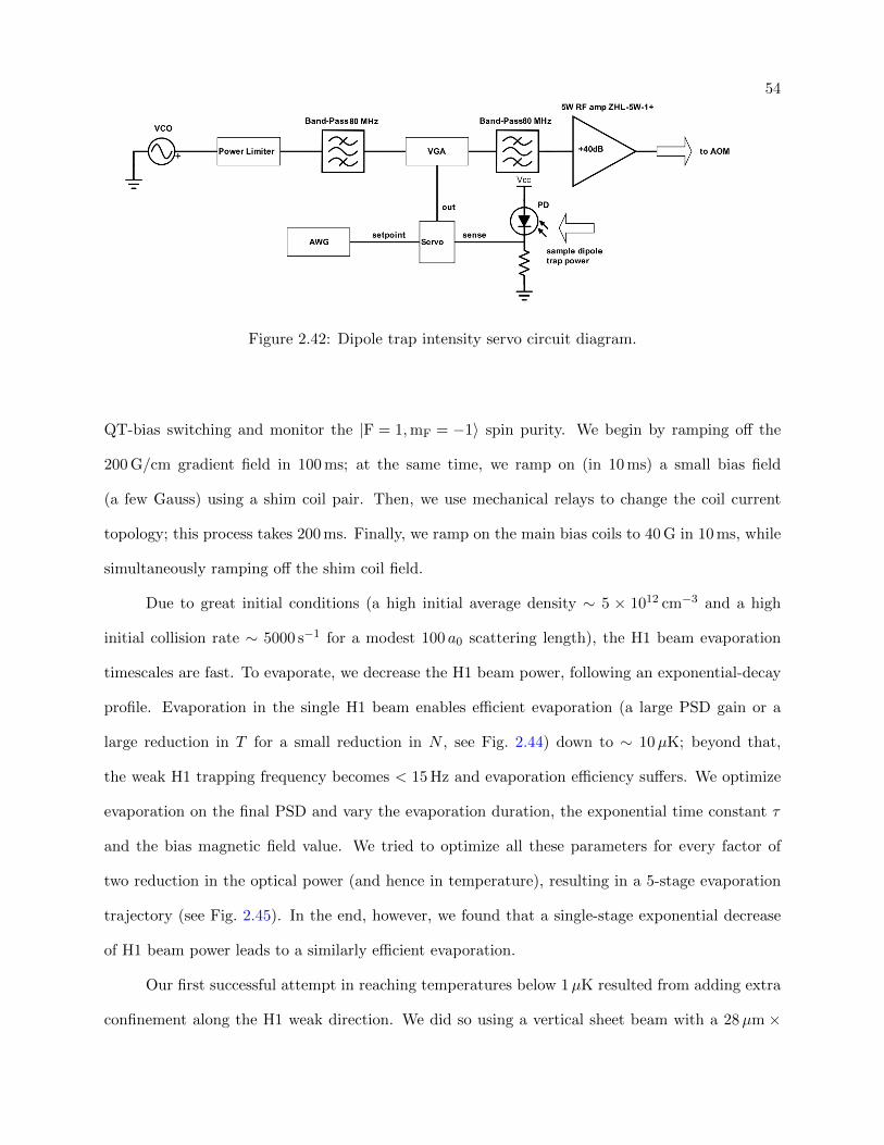
54

Figure 2.42: Dipole trap intensity servo circuit diagram.

QT-bias switching and monitor the |F = 1,mF = −1〉 spin purity. We begin by ramping off the

200 G/cm gradient field in 100 ms; at the same time, we ramp on (in 10 ms) a small bias field

(a few Gauss) using a shim coil pair. Then, we use mechanical relays to change the coil current

topology; this process takes 200 ms. Finally, we ramp on the main bias coils to 40 G in 10 ms, while

simultaneously ramping off the shim coil field.

Due to great initial conditions (a high initial average density ∼ 5 × 1012 cm−3 and a high

initial collision rate ∼ 5000 s−1 for a modest 100 a0 scattering length), the H1 beam evaporation

timescales are fast. To evaporate, we decrease the H1 beam power, following an exponential-decay

profile. Evaporation in the single H1 beam enables efficient evaporation (a large PSD gain or a

large reduction in T for a small reduction in N , see Fig. 2.44) down to ∼ 10µK; beyond that,

the weak H1 trapping frequency becomes < 15 Hz and evaporation efficiency suffers. We optimize

evaporation on the final PSD and vary the evaporation duration, the exponential time constant τ

and the bias magnetic field value. We tried to optimize all these parameters for every factor of

two reduction in the optical power (and hence in temperature), resulting in a 5-stage evaporation

trajectory (see Fig. 2.45). In the end, however, we found that a single-stage exponential decrease

of H1 beam power leads to a similarly efficient evaporation.

Our first successful attempt in reaching temperatures below 1µK resulted from adding extra

confinement along the H1 weak direction. We did so using a vertical sheet beam with a 28µm ×

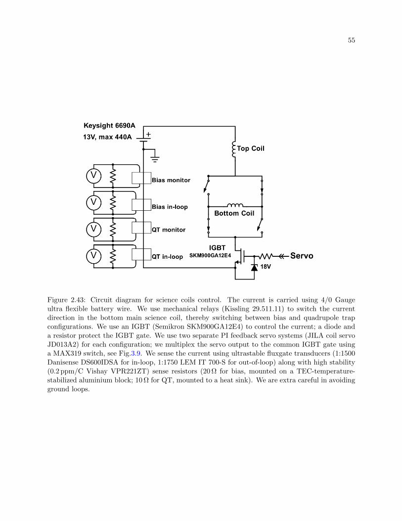
55

Figure 2.43: Circuit diagram for science coils control. The current is carried using 4/0 Gaugeultra flexible battery wire. We use mechanical relays (Kissling 29.511.11) to switch the currentdirection in the bottom main science coil, thereby switching between bias and quadrupole trapconfigurations. We use an IGBT (Semikron SKM900GA12E4) to control the current; a diode anda resistor protect the IGBT gate. We use two separate PI feedback servo systems (JILA coil servoJD013A2) for each configuration; we multiplex the servo output to the common IGBT gate usinga MAX319 switch, see Fig.3.9. We sense the current using ultrastable fluxgate transducers (1:1500Danisense DS600IDSA for in-loop, 1:1750 LEM IT 700-S for out-of-loop) along with high stability(0.2 ppm/C Vishay VPR221ZT) sense resistors (20 Ω for bias, mounted on a TEC-temperature-stabilized aluminium block; 10 Ω for QT, mounted to a heat sink). We are extra careful in avoidingground loops.

56

2 x 1 0 6 3 x 1 0 6 4 x 1 0 6 5 x 1 0 6 6 x 1 0 61 0

1 0 0

2 x 1 0 6 3 x 1 0 6 4 x 1 0 6 5 x 1 0 6 6 x 1 0 6

1 0 - 4

1 0 - 3

Figure 2.44: A typical evaporation trajectory using the H1 dipole beam. A large temperaturedecrease (left) and a large PSD increase (right) for a small number of atoms lost is evidence ofefficient evaporation.

0 5 1 0 1 5

0 . 1

1

1 0

0

5 0

1 0 0

1 5 0

2 0 0

Figure 2.45: A five-stage evaporation trajectory used for reducing the atom temperature from400µK down to 10µK, an extreme example of a dipole trap evaporation optimization. Shown is theoptimized H1 optical power trajectory (black) along with the optimized scattering length for eachstage (blue squares). In the end, the optimized H1 optical power trajectory can be approximatedby a single exponential, as evidenced by the roughly straight slope between 8 s and 16 s in the plot.The initial 8 s represents the OT load from the QT trap.

800µm waist (note that this is not the final V trap geometry). We achieved our first 39K BEC in

the new lab using a roughly-spherical 300 Hz trap, resulting in 7 × 104 condensed atoms (< 30%

in the thermal wings) and a temperature ∼ 500 nK, where the critical temperature ∼ 650 nK.

Using this beam configuration, we were able to create BECs at will and with ease, see Fig. 2.46.

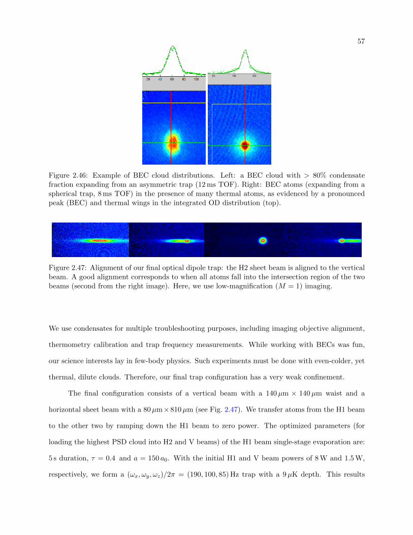
57

Figure 2.46: Example of BEC cloud distributions. Left: a BEC cloud with > 80% condensatefraction expanding from an asymmetric trap (12 ms TOF). Right: BEC atoms (expanding from aspherical trap, 8 ms TOF) in the presence of many thermal atoms, as evidenced by a pronouncedpeak (BEC) and thermal wings in the integrated OD distribution (top).

Figure 2.47: Alignment of our final optical dipole trap: the H2 sheet beam is aligned to the verticalbeam. A good alignment corresponds to when all atoms fall into the intersection region of the twobeams (second from the right image). Here, we use low-magnification (M = 1) imaging.

We use condensates for multiple troubleshooting purposes, including imaging objective alignment,

thermometry calibration and trap frequency measurements. While working with BECs was fun,

our science interests lay in few-body physics. Such experiments must be done with even-colder, yet

thermal, dilute clouds. Therefore, our final trap configuration has a very weak confinement.

The final configuration consists of a vertical beam with a 140µm × 140µm waist and a

horizontal sheet beam with a 80µm×810µm (see Fig. 2.47). We transfer atoms from the H1 beam

to the other two by ramping down the H1 beam to zero power. The optimized parameters (for

loading the highest PSD cloud into H2 and V beams) of the H1 beam single-stage evaporation are:

5 s duration, τ = 0.4 and a = 150 a0. With the initial H1 and V beam powers of 8 W and 1.5 W,

respectively, we form a (ωx, ωy, ωz)/2π = (190, 100, 85) Hz trap with a 9µK depth. This results

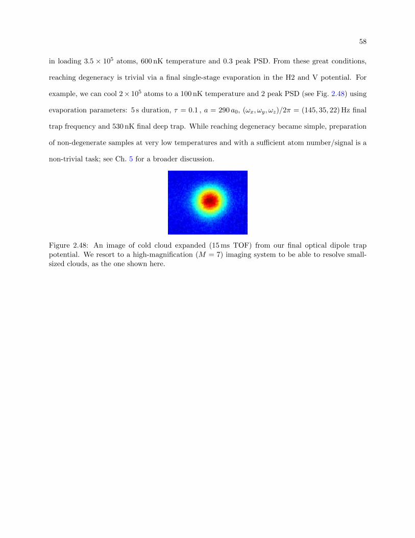
58

in loading 3.5 × 105 atoms, 600 nK temperature and 0.3 peak PSD. From these great conditions,

reaching degeneracy is trivial via a final single-stage evaporation in the H2 and V potential. For

example, we can cool 2× 105 atoms to a 100 nK temperature and 2 peak PSD (see Fig. 2.48) using

evaporation parameters: 5 s duration, τ = 0.1 , a = 290 a0, (ωx, ωy, ωz)/2π = (145, 35, 22) Hz final

trap frequency and 530 nK final deep trap. While reaching degeneracy became simple, preparation

of non-degenerate samples at very low temperatures and with a sufficient atom number/signal is a

non-trivial task; see Ch. 5 for a broader discussion.

Figure 2.48: An image of cold cloud expanded (15 ms TOF) from our final optical dipole trappotential. We resort to a high-magnification (M = 7) imaging system to be able to resolve small-sized clouds, as the one shown here.

Chapter 3

Experimental Toolkit for State Manipulation and Readout

Performing precise measurements requires stable experimental conditions and a good un-

derstanding of state control and readout. In this chapter, I detail the RF system used for state

purification and spectroscopy, along with the methods implemented which enable magnetic field

control with a mG-level field stability. Then, I discuss our science cell imaging system and image

analysis, expanding on the absorption imaging basics introduced in Sec. 2.3.2. A good under-

standing of imaging enables accurate determination of atom number and density. Lastly, I give an

overview of the laboratory’s computer and hardware control.

3.1 RF Control System

3.1.1 RF Circuitry

We utilize magnetic dipole transitions to go between hyperfine (Zeeman-split) states. We use

RF antennas to drive an oscillating magnetic field perpendicular to the magnetic field bias generated

by the mail coils, resulting in state transitions with selection rules ∆F = 0,±1 and ∆mF = ±1.

Each antenna circuit (see Fig. 3.1) is composed of a resonant circuit, formed by a wire loop(s) and

a series capacitor, and an impedance matching circuit. We use mostly non-magnetic components

to avoid magnetization by the main magnetic field bias coils. Frequency tuning and impedance

matching must be done in place, as antenna coupling to metal and dielectric components around

the science cell changes circuit performance. We are careful to avoid optimizing on electronic circuit

resonances; they are hard to distinguish from the true antenna resonance (formed by antenna loop

60C1

C2

Z

Figure 3.1: A typical circuit topology for RF antenna drive. We deliver RF power from the RF am-plifier to the antenna circuit via a triple-shielded coax (MiniCircuits precision test cable 5–10 ft long,DC–18 GHz). Frequency tuning is mainly achieved by a trimmer capacitor C1 (Voltronics/KnowlesNMA4M5HV; non-magnetic, 0.6–5 pF, PTFE dielectric, high-Q and high-V) that is placed in serieswith and close to the loop antenna. Impedance matching is done via tuning a variable capacitorC2 (Voltronics/Knowles TM56; 1–56 pF, air/glass, enclosed in an RF-shielded box or using TM42)and adjusting the length (. λ/8) of a Z = 50 Ω transmission line (UT-085C; semi-rigid coax cable,non-magnetic inner and outer copper conductors) connecting C1 to C2. Note that coax cables addadditional ∼ 30 pF/ft shunt capacitance (not shown). If impedance matching is not achieved usingthis topology, one needs to determine (using a Smith Chart) whether one needs to implement anadditional inductor, resistor, transmission line or a stub.

and C1), as they can still lead to radiation and can be sensed on a small-loop pickup antenna; they

also can still induce RF transitions in atoms, albeit with smaller Rabi frequencies.

We use three separate antennas that enable select transitions (e.g. at 34 G, which is near

the expected Feshbach resonance location of our interest): |F = 1,mF = −1〉 → |F = 2,mF = −2〉

(394.330 MHz), |F = 1,mF = −1〉 → |F = 1,mF = 0〉 (24.623 MHz), and (using a common antenna)

|F = 1,mF = −1〉 → |F = 2,mF = 0〉 (446.827 MHz) and |F = 1,mF = 0〉 → |F = 2,mF = −1〉

(446.841 MHz). We maximize radiation efficiency for each antenna by choosing the maximal amount

of turns; the antenna-C1 resonator desired frequency limits the maximal loop inductance (and hence

area) at the minimal C1 capacitance. The 390 MHz and 447 MHz antennas are single-loop, while

the 25 MHz antenna is 6-loop; all are made from 16 AWG Cu wire and have ≈ 1 inch inner diam-

eter (large enough to fit around science cell side windows). Each antenna is matched such that

the reflection coefficient S11 is . 10% at the desired frequency; the resulting spectral FWHM

widths and centers are: 20 MHz for 447 MHz, 20 MHz for 390 MHz, and 0.5 MHz for 25 MHz.

While we need to re-tune the two latter antenna center frequencies for different magnetic fields,

we do not need to do so for the 447 MHz antenna since |F = 1,mF = −1〉 → |F = 2,mF = 0〉 and

61

|F = 1,mF = 0〉 → |F = 2,mF = −1〉 transitions are relatively insensitive (∼ 170 kHz/G) around

34 G.

We can estimate loop antenna radiation efficiency ηrad by comparing radiative to resistive

loss: ηrad = Rrad/ (Rrad +Rohmic); Rohmic = 2πrN/(Sσ) is the ohmic resistance of the wire, where

N is the number of loops in the antenna, r is loop radius, S is the surface cross-section where

the current is constrained to flow by the skin depth, σ is the electrical conductivity; Rrad =

R0(8/3)π3(πr2N/λ2

)2is loop radiation resistance, where R0 = 120πΩ is the impedance of free-

space. Here, we assume the small-loop approximation (compared to the wavelength), such that the

current distribution is uniform along the wire. We see that a loop with more turns, area or operating

at a higher frequency is expected to have a higher radiation efficiency. For example, an antenna

with 16 AWG Cu wire and r = 0.5 inch is estimated to be 20% efficient at 400 MHz and 1%

at 30 MHz. However, in practice there are extra unaccounted-for losses at higher frequencies and

one needs to verify radiation efficiency of different frequency-band antennas using a vector network

analyzer (VNA) along with a calibrated pickup antenna, to get ηrad = |S12|2/(1 + |S11|2), or by

comparison of Rabi frequencies in atom spectroscopy. We find that our low- and high-frequency

antenna systems are just as efficient, resulting in similar Rabi π-pulse durations around 6–7µs

(time for full state transfer at full power).

These antenna circuits are much simpler than the antenna I designed for 40K microwave evap-

oration, which required a five-stub tuner for broadband 1.1–1.3 GHz match and extensive modeling.

However, due to the required dynamic frequency and power control, fast switching and precise tim-

ing, the control circuitry for the new antennas is more complex. Figure 3.2 shows the overview of

our RF system. The versatile frequency generator VFG-150 is the key component of our system,

enabling fast frequency and amplitude (also phase, if needed) switching every 5 ns. For state ma-

nipulation we use this RF system to generate rectangular- and Gaussian-shaped amplitude pulses,

at constant or chirped frequencies. We use a combination of RF spectrum analyzers, oscilloscopes,

VNAs, pickup antennas, RF circulators, frequency mixers and atom spectroscopy to diagnose our

RF antenna system.

62

AWG(Keysight3320A)orDAC

Voltagesweep

ZX05-10+

Synth(Keysight5171B)

290MHz

FMcontr.TTLtrigger

ZASWA-2-50DR+

50

TTLtrigger

LO

RF

IF

BLP-450 BHP-300

TTLtriggerZASWA-2-50DR+

50

-12dB

401-2208relayDow-KeyMicrowave

TTLtrigger

50

390MHzantenna

GND

V+ ZHL-20-13+20Wmax,+50dB

VISAUSB

VISAUSB

VISAUSB

VFG-150freq,ampl,phasecontr.

TTLtrigger

ZASWA-2-50DR+

BLP-150

ZASWA-2-50DR+BLP-70

TTLtrigger

GND

V+ ENI525LA25Wmax,+50dB

50

25MHzantenna

401-2208relayDow-KeyMicrowave

TTLtrigger

ZX05-10+ LO

IF

RFSynth(Keysight5181A)

346MHz VISAUSB

BHP-400 BLP-550

ZASWA-2-50DR+

50

TTLtrigger

-6dB

ZHL-20-13+20Wmax,+50dB

447MHzantenna

Dow-KeyMicrowave401-2208relay

TTLtrigger

50

Figure 3.2: RF control system circuitry. We use a single versatile frequency generator VFG-150to provide direct or mixed-up signals to the three RF antennas. We use the VFG to change theRF amplitude and center frequency; we use an external FPGA DAC or an arbitrary waveformgenerator (AWG) to sweep the frequency via frequency modulation (FM) ports. Fast RF solid-state switches (ZASWA-2-50DR+) are used for signal routing and pulse generation. To preventnoise leakage into antennas when the RF system is inactive, we use mechanical relays (401-2208)to isolate amplifier outputs. All frequency synthesizers are referenced to the lab’s 10 MHz clocksignal, which originates at NIST, travels to JILA via optical fiber and is split among and withinlabs via low-noise RF distribution amplifiers.

63

3.1.2 RF Transitions

We can estimate the effects the RF drive has on the atoms by solving a two-state problem,

given by a Hamiltonian:

H = ~

ω1 V0 cos(tω)

V0 cos(tω) ω2,

(3.1)

where ~ω0 = ~ (ω2 − ω1) is the energy splitting between the two Zeeman states in the presence of a

magnetic field bias, V0 is the coupling strength (proportional to the field strength times the dipole

moment µ) and ω is the angular drive frequency. System’s response are solutions to the coupled

equations [89, 90]:

dc1(t)

dt= − iΩ

2exp(iδt)c2(t) (3.2)

dc2(t)

dt= − iΩ

2exp(−iδt)c1(t), (3.3)

where |c1|2 and |c2|2 are probabilities of finding the system in states 1 and 2, δ = ω − ω0 is RF

detuning from the transition, Ω = |µB0/~| is the Rabi frequency of the magnetic dipole transition,

driven by a oscillating magnetic field of strength B0, and where we’ve used the rotating wave

approximation. For example, given the initial condition |c1(0)|2 = 1, the system undergoes Rabi

flopping:

|c2(t)|2 =Ω2

δ2 + Ω2sin2

(t

2

√δ2 + Ω2

). (3.4)

On resonance, full state transfer occurs every multiple of τπΩ = π, where τπ is referred to as the

Rabi π-pulse duration. Note that while τΩ = 2π pulse retrieves the initial condition |c1|2 = 1, the

resulting state is phase shifted (−1 prefactor) with respect to the original state and a τΩ = 4π pulse

is required for the system to fully retrieve the original state. The off-resonant system response is best

described by an effective Rabi frequency Ωeff =√δ2 + Ω2. When one needs to include dephasing

and damping into the model, it is best to use Bloch equations instead of Eqs. 3.2 and 3.3 [91].

Similarly to the solution Eq. 3.4, which was solved using a time-independent B0 and hence a

constant Ω, we can use Eqs. 3.2-3.3 or Bloch equations to calculate system’s response to amplitude-

64

- 1 0 0 1 01 0 0 0

1 0 0 0 0

1 0 0 0 0 0

Figure 3.3: Spectral comparison of rectangular- (165µs duration) vs. Gaussian-shaped (σ = 67µs,6σ duration) RF pulses. For this measurement atom number imaging noise limited N to> 1000 atoms. The solid curves are fits to the data, where center frequency (detuned from446.560 MHz) and amplitude are the only free parameters. Here, the Gaussian fit does not in-corporate finite-pulse duration.

shaped pulses. For example, we utilize Gaussian-shaped RF pulses when a large suppression of

spectral sidebands is required, as in cases with nearby off-resonant transitions that we do not want

to excite. Figure 3.3 illustrates this via comparison by two measured RF spectra, one taken with

a rectangular-shaped pulse and the other with a Gaussian-shaped pulse. Note that even with

significant suppression, spectral sidebands still exist in Gaussian-shaped RF pulses due to finite

pulse durations. Further suppression can be achieved by the use of Blackman-shape pulses.

To test our RF system on the atoms, we need to utilize spin-selective imaging techniques.

When performing RF transitions to the F = 2 state, we can directly diagnose RF transfer by imaging

the final state, since the initial |F = 1,mF = −1〉 state is dark to our imaging probe light (the D2

|4 2S1/2,F = 2〉 → |4 2P3/2,F′ = 3〉 transition) in absence of repump light. When performing RF

transitions within the F = 1 state, we utilize Stern-Gerlach–type technique to spatially separate spin

components, imaging them using the D2 |4 2S1/2,F = 2〉 → |4 2P3/2,F′ = 3〉 transition along with

D2 repump (comes from an orthogonal direction as the probe, from top of the science cell). We can

use a combination of the two techniques to enable imaging of all spin components simultaneously.

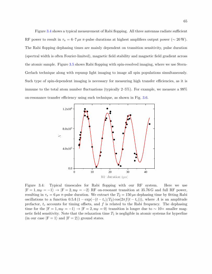
65

Figure 3.4 shows a typical measurement of Rabi flopping. All three antennas radiate sufficient

RF power to result in τπ = 6–7µs π-pulse durations at highest amplifiers output power (∼ 20 W).

The Rabi flopping dephasing times are mainly dependent on transition sensitivity, pulse duration

(spectral width is often Fourier-limited), magnetic field stability and magnetic field gradient across

the atomic sample. Figure 3.5 shows Rabi flopping with spin-resolved imaging, where we use Stern-

Gerlach technique along with repump light imaging to image all spin populations simultaneously.

Such type of spin-dependent imaging is necessary for measuring high transfer efficiencies, as it is

immune to the total atom number fluctuations (typically 2–5%). For example, we measure a 99%

on-resonance transfer efficiency using such technique, as shown in Fig. 3.6.

0 1 0 2 0 3 0 4 00 . 0

4 . 0 x 1 0 5

8 . 0 x 1 0 5

1 . 2 x 1 0 6

Figure 3.4: Typical timescales for Rabi flopping with our RF system. Here we use|F = 1,mF = −1〉 → |F = 2,mF = −2〉 RF on-resonant transition at 35.76 G and full RF power,resulting in τπ = 6µs π-pulse duration. We extract the T2 = 150µs dephasing time by fitting Rabioscillations to a function 0.5A (1− exp(−(t− tc)/T2) cos(2πf(t− tc))), where A is an amplitudeprefactor, tc accounts for timing offsets, and f is related to the Rabi frequency. The dephasingtime for the |F = 1,mF = −1〉 → |F = 2,mF = 0〉 transition is longer due to ∼ 10× smaller mag-netic field sensitivity. Note that the relaxation time T1 is negligible in atomic systems for hyperfine(in our case |F = 1〉 and |F = 2〉) ground states.

66

Figure 3.5: Spatially-resolved Rabi flopping between |F = 1,mF = −1〉 and |F = 2,mF = −2〉 spinstates. From left to right: without RF transfer, π/2-pulse transition (equal populations) and π-pulse transition. Here, we use Stern-Gerlach technique along with optical repump light to imagepopulation in both spin states simultaneously. Note that the OD scale changes between images.

- 2 0 0 2 00 . 0

0 . 2

0 . 4

0 . 6

0 . 8

1 . 0

Figure 3.6: RF spectrum using |F = 1,mF = −1〉 → |F = 2,mF = 0〉 transition with spin-resolvedimaging (as in Fig. 3.5), measuring fractional population transfer to the final spin state. Here, weuse a 82µs rectangular π-pulse for spectroscopy. We fit data to Eq. 3.4, setting τΩ = π, and extractthe resonance center 446.5423 MHz (to give 35.881 G) and maximal transfer efficiency A = 0.99.

3.2 Magnetic Field Stabilization

3.2.1 Lineshape Spectral Noise

Precision spectroscopy of few-body physics depends on having a precise magnetic field control

and high field stability, since the induced interactions (via Feshbach resonances) and the hyperfine

Zeeman splittings are sensitive to magnetic field noise. We perform RF spectroscopy to determine

our field stability. Figures. 3.7 and 3.8 illustrate how B-field noise translates to spectral noise.

67

Prior to converting the apparatus to a 39K machine, and hence prior to adding many more

electronic components (new noise sources) to the lab, the magnetic field stability was measured to

be 10–15 mG with 40K RF spectroscopy. Such a high noise level was unacceptable for the kHz-level

spectral sensitivity we desired in the new 39K machine. For example, magnetic field sensitivi-

ties at 34 G (near our Feshbach resonance of interest) for |F = 1,mF = −1〉 → |F = 2,mF = −2〉,

|F = 1,mF = −1〉 → |F = 1,mF = 0〉 and |F = 1,mF = −1〉 → |F = 2,mF = 0〉 transitions are

1.85 kHz/mG, 0.73 kHz/mG and 0.17 kHz/mG, respectively. Similarly, considering that the Fourier-

limited spectral width of Rabi π-pulses is ∆fFWHM = 0.80/τ , spectral noise arising from magnetic

field noise would limit the maximal pulse durations. In fact, our initial RF spectroscopy with the

|1,−1〉 → |2,−2〉 transition and 10 mG field noise was a failure due to having an unoptimized

antenna system with a long 45µs Rabi π-pulse duration. Only after solving antenna impedance

matching issues and reducing noise down to mG-level, we were able to utilize the |1,−1〉 → |2,−2〉

transition.

3.2.2 Magnetic Field Control

In addition to RF spectroscopy, we use a set of magnetometers to monitor our magnetic field

stability. We employ a NIST-calibrated AC magnetometer (MC910) to measure 60 Hz noise around

the lab. Additionally, we utilize a three-axis high-sensitivity (0.1 mG) magnetometer (Bartington

Instruments MAG690-1000) for general purposes (400 Hz 3 dB point). We check magnetometer

calibration and frequency response using a large wound coil and a current source. Ultimately,

we permanently affix the MAG690-1000 sensor ∼ 20 cm above the science coils (on top of the

optical breadboard used for vertical optical dipole trap beam and vertical probe beam), ∼ 10 cm

offset laterally (to provide sensitivity in all sensed B-field directions), to monitor the magnetic

field during experimental sequences. We use an analog-to-digital converted (ADC, NI-USB 6003

multifunction I/O device) to record magnetic field values in all three directions during the last

150 ms of each experimental sequence: 100 ms before RF spectroscopy and imaging, and 50 ms

afterward (when all coils are off). Using the two magnetometers, we determined that the sensed

68

- 1 5 0 - 1 0 0 - 5 0 0 5 0 1 0 0 1 5 0- 0 . 20 . 00 . 2

fit res

idual

R F d e t u n i n g ( k H z )

0 . 0

0 . 5

1 . 0

transf

er fra

ction

Figure 3.7: An example of |1,−1〉 → |1, 0〉 lineshape spectral noise due to high magnetic fieldinstability. Here, the RF π-pulse duration is 7.4µs and spectroscopy is performed at 41.76 G, wherethe transition has 0.73 kHz/mG field sensitivity. We measure the transferred fraction (top) usingStern-Gerlach–type technique and fit the spectrum using Eq. 3.4. We extract noise properties fromthe resulting fit residuals (bottom). We extract 4% measurement noise from the spread near zero-detuning, where the transition is insensitive (small slope near the peak) to magnetic field noise;note that the atom number noise is irrelevant in this measurement as we record fractional spinpopulations. We extract 14 mG magnetic field noise from the spread on the side of the spectrum(we subtract out 4% measurement noise in quadrature), where the transition is most sensitive tomagnetic field noise, as evidenced by a large spread in residuals.

noise (60 Hz field noise combined with the observed DC field drift) was consistent with the level of

measured field stability using RF spectroscopy.

We took multiple measures to achieve few-mG magnetic field stability. Beginning with passive

measures, the main bias coils are wound in a Helmholtz configuration, and are mounted on rigid

non-magnetic G-11 glass/epoxy phenolic and water-cooled (with laminar flow). We use mainly

non-magnetic components surrounding the science chamber, including optical breadboards, RF

antenna circuitry (capacitors, coax cables and solder) and optical mounts. More generally, we are

cautious about stray magnetic fields originating from various sources, minimizing or shielding them

when possible. For example, we made sure that the science optical table was never magnetized

throughout the years by avoiding magnetic optical posts and screws; we also accomplish a good table

temperature stability by minimizing the amount of thermal sources underneath and on it, using

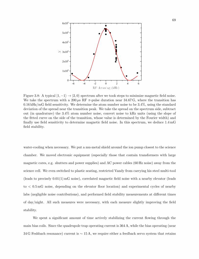
69

- 6 - 4 - 2 0 2 4 60

1 x 1 0 5

2 x 1 0 5

3 x 1 0 5

4 x 1 0 5

5 x 1 0 5

6 x 1 0 5

Figure 3.8: A typical |1,−1〉 → |2, 0〉 spectrum after we took steps to minimize magnetic field noise.We take the spectrum with a 200µs RF π-pulse duration near 34.67 G, where the transition has0.16 kHz/mG field sensitivity. We determine the atom number noise to be 3.4%, using the standarddeviation of the spread near the transition peak. We take the spread on the spectrum side, subtractout (in quadrature) the 3.4% atom number noise, convert noise to kHz units (using the slope ofthe fitted curve on the side of the transition, whose value is determined by the Fourier width) andfinally use field sensitivity to determine magnetic field noise. In this spectrum, we deduce 1.4 mGfield stability.

water-cooling when necessary. We put a mu-metal shield around the ion pump closest to the science

chamber. We moved electronic equipment (especially those that contain transformers with large

magnetic cores, e.g. shutters and power supplies) and AC power cables (60 Hz noise) away from the

science cell. We even switched to plastic seating, restricted Vandy from carrying his steel multi-tool

(leads to precisely 0.01(1) mG noise), correlated magnetic field noise with a nearby elevator (leads

to < 0.5 mG noise, depending on the elevator floor location) and experimental cycles of nearby

labs (negligible noise contributions), and performed field stability measurements at different times

of day/night. All such measures were necessary, with each measure slightly improving the field

stability.

We spent a significant amount of time actively stabilizing the current flowing through the

main bias coils. Since the quadrupole trap operating current is 364 A, while the bias operating (near

34 G Feshbach resonance) current is ∼ 15 A, we require either a feedback servo system that retains

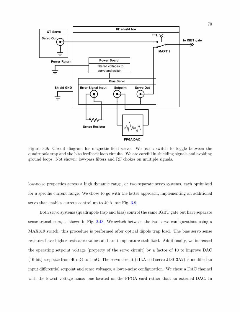
70RFshieldbox

BiasServo

ErrorSignalInput Setpoint ServoOut

MAX319

TTLQTServo

ServoOut

SenseResistor

PowerReturn

ShieldGND

toIGBTgate

FPGADAC

PowerBoard

filtered voltages to servo and switch

Figure 3.9: Circuit diagram for magnetic field servo. We use a switch to toggle between thequadrupole trap and the bias feedback loop circuits. We are careful in shielding signals and avoidingground loops. Not shown: low-pass filters and RF chokes on multiple signals.

low-noise properties across a high dynamic range, or two separate servo systems, each optimized

for a specific current range. We chose to go with the latter approach, implementing an additional

servo that enables current control up to 40 A, see Fig. 3.9.

Both servo systems (quadrupole trap and bias) control the same IGBT gate but have separate

sense transducers, as shown in Fig. 2.43. We switch between the two servo configurations using a

MAX319 switch; this procedure is performed after optical dipole trap load. The bias servo sense

resistors have higher resistance values and are temperature stabilized. Additionally, we increased

the operating setpoint voltage (property of the servo circuit) by a factor of 10 to improve DAC

(16-bit) step size from 40 mG to 4 mG. The servo circuit (JILA coil servo JD013A2) is modified to

input differential setpoint and sense voltages, a lower-noise configuration. We chose a DAC channel

with the lowest voltage noise: one located on the FPGA card rather than an external DAC. In

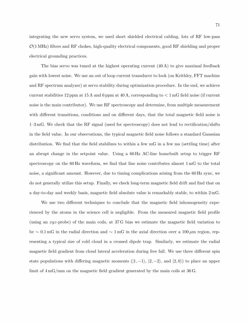
71

integrating the new servo system, we used short shielded electrical cabling, lots of RF low-pass

O(1 MHz) filters and RF chokes, high-quality electrical components, good RF shielding and proper

electrical grounding practices.

The bias servo was tuned at the highest operating current (40 A) to give maximal feedback

gain with lowest noise. We use an out of loop current transducer to look (on Keithley, FFT machine

and RF spectrum analyzer) at servo stability during optimization procedure. In the end, we achieve

current stabilities 12 ppm at 15 A and 6 ppm at 40 A, corresponding to < 1 mG field noise (if current

noise is the main contributor). We use RF spectroscopy and determine, from multiple measurement

with different transitions, conditions and on different days, that the total magnetic field noise is

1–3 mG. We check that the RF signal (used for spectroscopy) does not lead to rectification/shifts

in the field value. In our observations, the typical magnetic field noise follows a standard Gaussian

distribution. We find that the field stabilizes to within a few mG in a few ms (settling time) after

an abrupt change in the setpoint value. Using a 60 Hz AC-line homebuilt setup to trigger RF

spectroscopy on the 60 Hz waveform, we find that line noise contributes almost 1 mG to the total

noise, a significant amount. However, due to timing complications arising from the 60 Hz sync, we

do not generally utilize this setup. Finally, we check long-term magnetic field drift and find that on

a day-to-day and weekly basis, magnetic field absolute value is remarkably stable, to within 2 mG.

We use two different techniques to conclude that the magnetic field inhomogeneity expe-

rienced by the atoms in the science cell is negligible. From the measured magnetic field profile

(using an xyz-probe) of the main coils, at 37 G bias we estimate the magnetic field variation to

be ∼ 0.1 mG in the radial direction and ∼ 1 mG in the axial direction over a 100µm region, rep-

resenting a typical size of cold cloud in a crossed dipole trap. Similarly, we estimate the radial

magnetic field gradient from cloud lateral acceleration during free fall. We use three different spin

state populations with differing magnetic moments (|1,−1〉, |2,−2〉, and |2, 0〉) to place an upper

limit of 4 mG/mm on the magnetic field gradient generated by the main coils at 36 G.

72

3.3 Imaging System

A good understanding of the imaging system is important for any ultracold laboratory that

relies solely on atom images for data. For us, it is even more crucial to understand all imaging

peculiarities since we are interested in measuring density-dependent loss rates in our few-body

physics studies. We must accurately determine the imaging system magnification, atom number,

cloud temperature and trap frequencies.

3.3.1 Side Imaging Specifications

The majority of our imaging is performed using the side imaging system. This system enables

imaging small and/or cold clouds with a high-magnification configuration (M = 6.7) and hot and/or

large clouds (e.g. like those in quadrupole trap and in H1 beam after dipole trap load) with a low-

magnification (M = 1) configuration, see Fig. 3.10.

The commercial objective lens was chosen to achieve the best imaging resolution given the

tight space constrains. We found that the f = 75 mm air-spaced achromatic doublet was our best

option due small on- and off-axis aberrations. This objective enables diffraction-limited performance

for on-axis or small off-axis imaging, resulting in 3.6µm (Airy disk radius) imaging resolution when

considering aberrations, see Fig. 3.12. However, imaging off-axis beyond ∼ 1 mm field of view, as

in the cases imaging hot and/or elongated clouds expanding from quadrupole or H1 dipole traps,

can lead to significant aberrations and image distortion, as depicted in Fig. 3.13.

We find that by decreasing the objective aperture via an iris, we are able to significantly

reduce off-axis aberrations, at the expense of slightly worse imaging resolution. We see this effect in

simulations of the modulation transfer function (MTF), point spread function (PSF) and wavefront

error. We also verify this effect experimentally in a test setup. We image an effective point-source

(767 nm light passing through a 1µm pin hole) and gather the effective PSF of the system for

different focus positions, see Fig. 3.14.

Ultimately, we use information gathered directly from atom imaging to fine-tune our imaging

73

λ/2

x2 bandpass lters : Semrock FF01-775/140-25775nm ± 70 nm, 1’’, 98% transmission at 767nm

probe beamPM SM ber

8mm achro0.5 NA

focus-25mm 125mm

polarizer LPVIS100λ/4

λ/4

polarizer LPVIS100

75mm objective 1’’ on xy-stageair-spaced achromatic doublet ACA254-075-B

100mm plano-convex 2’’

60mm plano-convex 2’’

iris

500mm eyepiece 1’’achromatic doublet AC254-500-B

CCD camera

shutter

quant coil pair

focus

Atoms

Figure 3.10: The main imaging system in the science chamber. A pair of coils provide a quantizationmagnetic field for the probe σ+ or σ− transitions (or π transitions when the extra λ/4 and polarizerare flipped in). The atoms are located 23.1 mm away from the 3.18 mm thick fused-silica sidewindows. We image atoms using two setups: a high-magnification (M ≈ 7) setup with f = 75 mmobjective and f = 500 mm eyepiece and a low-magnification (M ≈ 1) setup with two additionallenses (on flipper mounts). The objective lens is 38 mm away from the window and is the limitingaperture of the imaging system (20 mm diameter clear aperture, 0.13 NA) when the iris is fullyopen. The eyepiece lens is approximately 55 mm behind the objective and is 481 mm (equal tothe back focal length) away from the CCD. The 100 mm demagnification lens is approximately160 mm behind the eyepiece, the 60 mm demagnification lens is approximately 240 mm followingthat and 100 mm in front of the CCD. Note that, due to the air-spaced nature of the objective,the achromatic pair is more prone to dust and imperfections; it took several cleaning (and outrightreplacement) of objective lenses to achieve acceptable optical quality and minimal image fringes.

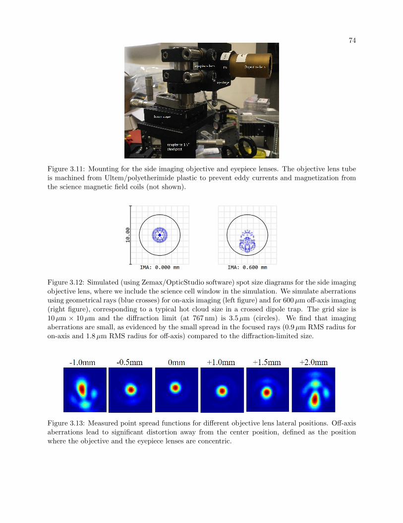
74

Figure 3.11: Mounting for the side imaging objective and eyepiece lenses. The objective lens tubeis machined from Ultem/polyetherimide plastic to prevent eddy currents and magnetization fromthe science magnetic field coils (not shown).

Figure 3.12: Simulated (using Zemax/OpticStudio software) spot size diagrams for the side imagingobjective lens, where we include the science cell window in the simulation. We simulate aberrationsusing geometrical rays (blue crosses) for on-axis imaging (left figure) and for 600µm off-axis imaging(right figure), corresponding to a typical hot cloud size in a crossed dipole trap. The grid size is10µm × 10µm and the diffraction limit (at 767 nm) is 3.5µm (circles). We find that imagingaberrations are small, as evidenced by the small spread in the focused rays (0.9µm RMS radius foron-axis and 1.8µm RMS radius for off-axis) compared to the diffraction-limited size.

Figure 3.13: Measured point spread functions for different objective lens lateral positions. Off-axisaberrations lead to significant distortion away from the center position, defined as the positionwhere the objective and the eyepiece lenses are concentric.

75

2 0 2 4 2 8 3 2 3 6

4

8

1 2

40 50 60 70 80

45

50

55

60

65

70

75

80

85

50 60 70 80

40

45

50

55

60

65

70

75

80

40 50 60 70 80

45

50

55

60

65

70

75

80

85

40 50 60 70 80

45

50

55

60

65

70

75

80

85

50 60 70 80

40

45

50

55

60

65

70

75

80

Airy d

isk rad

ius (µ

m)

f o c u s ( m m )Figure 3.14: Reduction of aberrations via aperturing the objective. An unapertured objective lens(black points with spline), corresponding to 20 mm clear aperture diameter, has severe aberrationsaway from the focus. Reducing clear aperture diameter to 0.5 in via an iris following the objectivelens leads to smaller aberrations, albeit at expense of imaging resolution. Note that, as in this case,we often fit the focused spots using a Gaussian distribution and deduce the Airy disk radius fromthe Gaussian width σ.

system. First, we optimize the focus position by using a dilute, cold (thermal or BEC) and small

cloud, maximizing the detected OD with on-resonance imaging. Second, we check the level of

astigmatism present using off-resonant imaging (see Fig. 3.15) and adjust the objective lateral

position if need be. Last, we visually inspect the diffraction ring pattern in the PSF with on-

resonant imaging of condensed clouds and verify the behavior at different focal spots. We iterate

on the above techniques with smaller clouds to further increase optimization sensitivity, enabling

us to focus the objective with sub-mm precision. We measure the imaging system magnification

M by dropping an atomic cloud (released from a trapping potential) and fitting its measured path

to a parabolic function containing only M , the gravitational acceleration constant g and the CCD

pixel size. In absence of magnetic field gradients and significant image distortions, this technique

enables an accurate demagnification of M .

Images are acquired with a low dark noise and a high quantum efficiency TEC-cooled (down

76

0 4 8 1 2 1 6 2 01 0

1 2

1 8

2 0

2 2

Figure 3.15: Measured astigmatism present in an unoptimized imaging system. We measure thesize of dense clouds in two directions (σx and σy) at different objective positions for off-resonantprobe beam detunings ±1Γ. Since dense atom clouds lead to lensing, the focal spot in the twodirections coincide with the crossings of the cloud sizes using blue- and red-detuned probe light. Inthis case, significant astigmatism is present, with the two focal spots occurring 1 cm apart.

to −45C) CCD camera: Roper Scientific/Princeton Instruments NTE/CCD-512-EBFT camera

with a back-illuminated E2V 57-10 CCD, 13µm pixel size, 512× 512 unmasked pixel array and a

masked region that can be used for kinetics-mode imaging. We use shot noise statistics, resulting

from white noise blackbody noise sources (dark noise or incandescent flashlight), to character-

ize CCD camera properties. We experimentally deduce [e−/count] gain, electronic readout noise,

electronic bias, dark noise rate, well capacity, quantum efficiency [counts/photon] and pixel gain

inhomogeneity, see Figs. 3.16, 3.17 and 3.18. Overall, a good understanding of CCD properties

and settings allows us to perform absorption imaging with only 100–300 photons per pixel (inte-

grated over 20µs, with an excellent signal-to-noise ratio. Our camera settings/properties are: 60µs

exposure, 16-bit resolution, 1 MHz readout rate (fast frame acquisition at an expense of a larger

7 counts/pixel read noise), high analog gain (measured 1.53 e−/count), 223 counts electronic bias

(set by a trimpot before the ADC), ∼ 80% quantum efficiency at 767 nm (measurement agrees

with the spec sheet), continuous frame cleaning and −40C operating temperature (resulting in

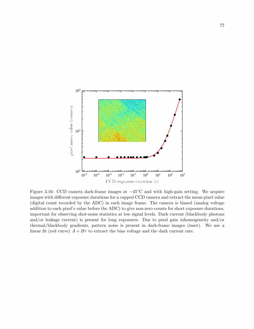
77

1 0 - 5 1 0 - 4 1 0 - 3 1 0 - 2 1 0 - 1 1 0 0 1 0 1 1 0 2 1 0 31 0 2

1 0 3

1 0 4

Figure 3.16: CCD camera dark-frame images at −45C and with high-gain setting. We acquireimages with different exposure durations for a capped CCD camera and extract the mean pixel value(digital count recorded by the ADC) in each image frame. The camera is biased (analog voltageaddition to each pixel’s value before the ADC) to give non-zero counts for short exposure durations,important for observing shot-noise statistics at low signal levels. Dark current (blackbody photonsand/or leakage current) is present for long exposures. Due to pixel gain inhomogeneity and/orthermal/blackbody gradients, pattern noise is present in dark-frame images (inset). We use alinear fit (red curve) A+Bτ to extract the bias voltage and the dark current rate.

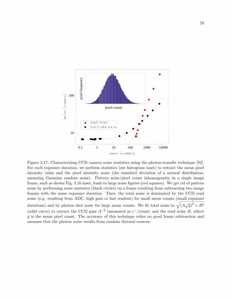
78

0 . 1 1 1 0 1 0 0 1 0 0 0 1 0 0 0 0

1 0

1 0 0

5000 5500 6000 6500 7000 75000

1000

2000

3000

4000

pixelf

requen

cy

p i x e l c o u n t s

Figure 3.17: Characterizing CCD camera noise statistics using the photon-transfer technique [92].For each exposure duration, we perform statistics (see histogram inset) to extract the mean pixelintensity value and the pixel intensity noise (the standard deviation of a normal distribution,assuming Gaussian random noise). Pattern noise/pixel count inhomogeneity in a single imageframe, such as shown Fig. 3.16 inset, leads to large noise figures (red squares). We get rid of patternnoise by performing noise statistics (black circles) on a frame resulting from subtracting two imageframes with the same exposure duration. Then, the total noise is dominated by the CCD readnoise (e.g. resulting from ADC, high gain or fast readout) for small mean counts (small exposure

durations) and by photon shot noise for large mean counts. We fit total noise to√

(A√y)2 +B2

(solid curve) to extract the CCD gain A−2 (measured in e−/count) and the read noise B, wherey is the mean pixel count. The accuracy of this technique relies on good frame subtraction andassumes that the photon noise results from random thermal sources.

79

1 0 1 1 0 2 1 0 3 1 0 4 1 0 5

1 0 1

1 0 2

Figure 3.18: Measurement of the CCD pixel well capacity. We use a flashlight and a diffuser asthe thermal light source (instead of the dark current) to provide a semi-uniform illumination (e.g.a single frame (a) inset) of the CCD chip. For low light levels, frame-subtracted images (e.g. (b)inset) display photon shot noise statistics, as demonstrated by an agreement (

√mean counts scaling

and a similar CCD gain value) of the fitted curve (red line with 95% confidence intervals, fit upto 2 × 104 counts and extrapolated to higher values) with the fit used in Fig. 3.17. For high pixelcounts, yet below the 16-bit ADC 216 maximum count, we see CCD saturation (due to finite pixelwell capacity) and blooming, as demonstrated in (c) inset by frame-subtracted image smearing, in(d) inset by histogram pixel value saturation and in the main plot by noise reduction at high countvalues.

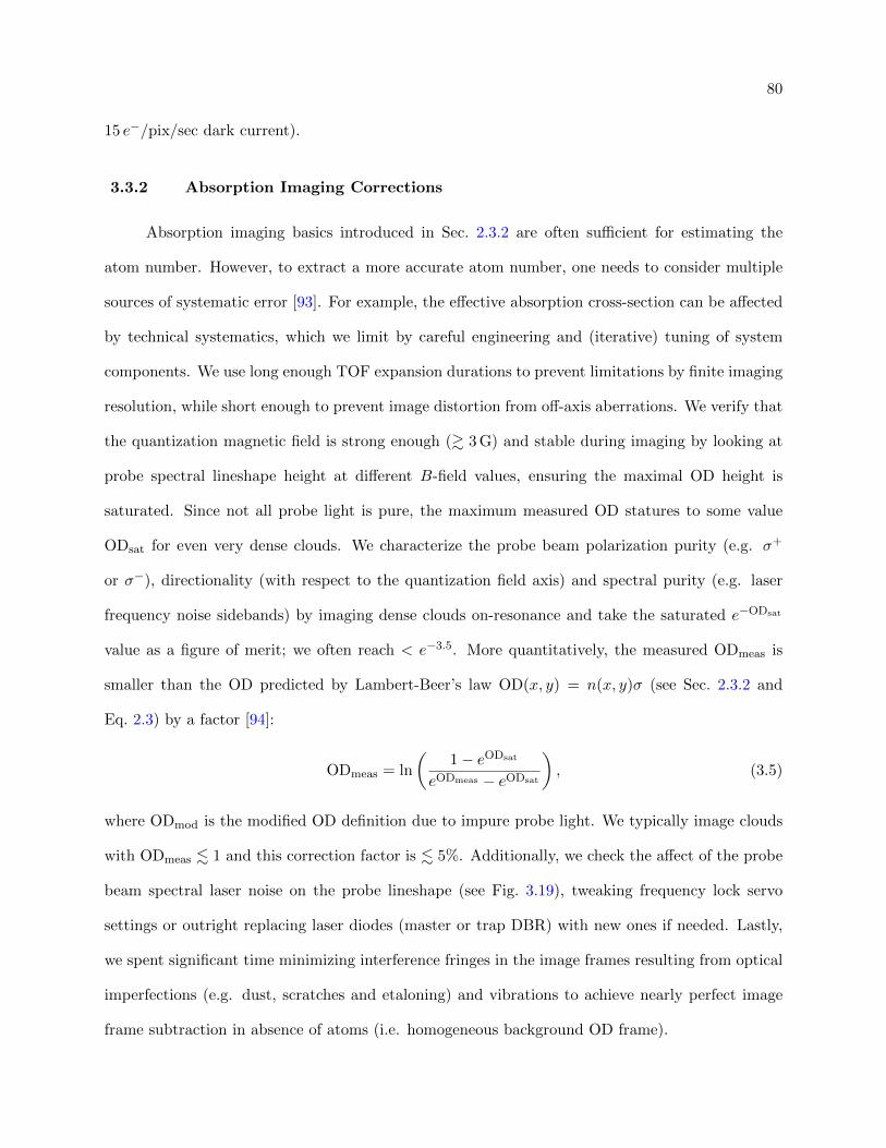
80

15 e−/pix/sec dark current).

3.3.2 Absorption Imaging Corrections

Absorption imaging basics introduced in Sec. 2.3.2 are often sufficient for estimating the

atom number. However, to extract a more accurate atom number, one needs to consider multiple

sources of systematic error [93]. For example, the effective absorption cross-section can be affected

by technical systematics, which we limit by careful engineering and (iterative) tuning of system

components. We use long enough TOF expansion durations to prevent limitations by finite imaging

resolution, while short enough to prevent image distortion from off-axis aberrations. We verify that

the quantization magnetic field is strong enough (& 3 G) and stable during imaging by looking at

probe spectral lineshape height at different B-field values, ensuring the maximal OD height is

saturated. Since not all probe light is pure, the maximum measured OD statures to some value

ODsat for even very dense clouds. We characterize the probe beam polarization purity (e.g. σ+

or σ−), directionality (with respect to the quantization field axis) and spectral purity (e.g. laser

frequency noise sidebands) by imaging dense clouds on-resonance and take the saturated e−ODsat

value as a figure of merit; we often reach < e−3.5. More quantitatively, the measured ODmeas is

smaller than the OD predicted by Lambert-Beer’s law OD(x, y) = n(x, y)σ (see Sec. 2.3.2 and

Eq. 2.3) by a factor [94]:

ODmeas = ln

(1− eODsat

eODmeas − eODsat

), (3.5)

where ODmod is the modified OD definition due to impure probe light. We typically image clouds

with ODmeas . 1 and this correction factor is . 5%. Additionally, we check the affect of the probe

beam spectral laser noise on the probe lineshape (see Fig. 3.19), tweaking frequency lock servo

settings or outright replacing laser diodes (master or trap DBR) with new ones if needed. Lastly,

we spent significant time minimizing interference fringes in the image frames resulting from optical

imperfections (e.g. dust, scratches and etaloning) and vibrations to achieve nearly perfect image

frame subtraction in absence of atoms (i.e. homogeneous background OD frame).

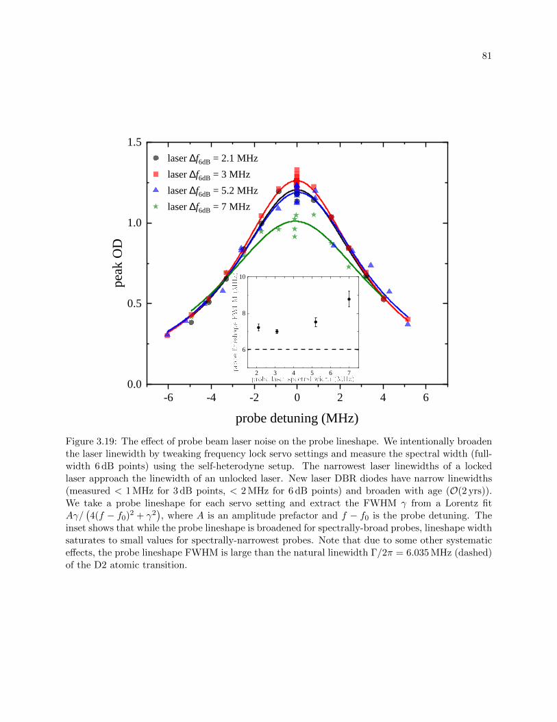
81

- 6 - 4 - 2 0 2 4 60 . 0

0 . 5

1 . 0

1 . 5

2 3 4 5 6 7

6

8

1 0

l a s e r ∆ f 6 d B = 2 . 1 M H zl a s e r ∆ f 6 d B = 3 M H zl a s e r ∆ f 6 d B = 5 . 2 M H zl a s e r ∆ f 6 d B = 7 M H z

peak O

D

p r o b e d e t u n i n g ( M H z )Figure 3.19: The effect of probe beam laser noise on the probe lineshape. We intentionally broadenthe laser linewidth by tweaking frequency lock servo settings and measure the spectral width (full-width 6 dB points) using the self-heterodyne setup. The narrowest laser linewidths of a lockedlaser approach the linewidth of an unlocked laser. New laser DBR diodes have narrow linewidths(measured < 1 MHz for 3 dB points, < 2 MHz for 6 dB points) and broaden with age (O(2 yrs)).We take a probe lineshape for each servo setting and extract the FWHM γ from a Lorentz fitAγ/

(4(f − f0)2 + γ2

), where A is an amplitude prefactor and f − f0 is the probe detuning. The

inset shows that while the probe lineshape is broadened for spectrally-broad probes, lineshape widthsaturates to small values for spectrally-narrowest probes. Note that due to some other systematiceffects, the probe lineshape FWHM is large than the natural linewidth Γ/2π = 6.035 MHz (dashed)of the D2 atomic transition.

82

1 0 1 0 0 1 0 0 0 1 0 0 0 00 . 0

0 . 4

0 . 8

1 . 2

1 . 6

measu

red OD

m e a n p i x e l v a l u e ( c o u n t s )Figure 3.20: An example of OD saturation due to a high intensity probe. We measure the peakOD of similar atomic clouds using different probe beam powers, changed by a combination of anAOM (RF power) and ND filters. We take (1/Npix)

∫A IL(x, y) − ID(x, y)dxdy (light and dark

frames integrated over 40µs probe pulse duration) as the mean intensity (measured in units ofADC counts per pixel), where we take the average over a region A with Npix pixels that containsthe atom cloud in the shadow frame IS(x, y). We fit to Eq. 3.7 and extract Isat = 2200 counts andODtrue = 1.53. Note that here we used a probe with a 40µs duration, which is too long to extractan accurate Isat value. Using a numerical fit that includes photon-recoil-related corrections, weobtain Isat = 3600 counts.

In addition to technical systematic effects, the measured optical depth is affected by transition

saturation. Taking into account the transition saturation, described by saturation intensity Isat,

and the saturation due to impure probe light, the “true” OD becomes [94, 95]:

ODtrue = ODmod +(1 + e−ODmod

) Iin

Isat, (3.6)

where Iin is the incoming beam intensity. For ODsat ODmeas, ODmod ≈ ODmeas and

ODmeas ≈ ODtrue −Iin

Isat+W

(exp

(Iin

Isat−ODtrue

)Iin

Isat

), (3.7)

where W (x) is the Lambert W function. We measure ODmeas for multiple probe intensities Iin and

experimentally extract Isat from the fit to Eq. 3.7, as depicted in Fig. 3.20.

While Eq. 3.7 is sufficient in certain probing regimes, further corrections require understand-

ing how the measured optical depth is affected by the finite recoil momentum h/λ that each photon

imparts on the atom during the imaging process [93, 96]. Each atom gets a momentum kick in

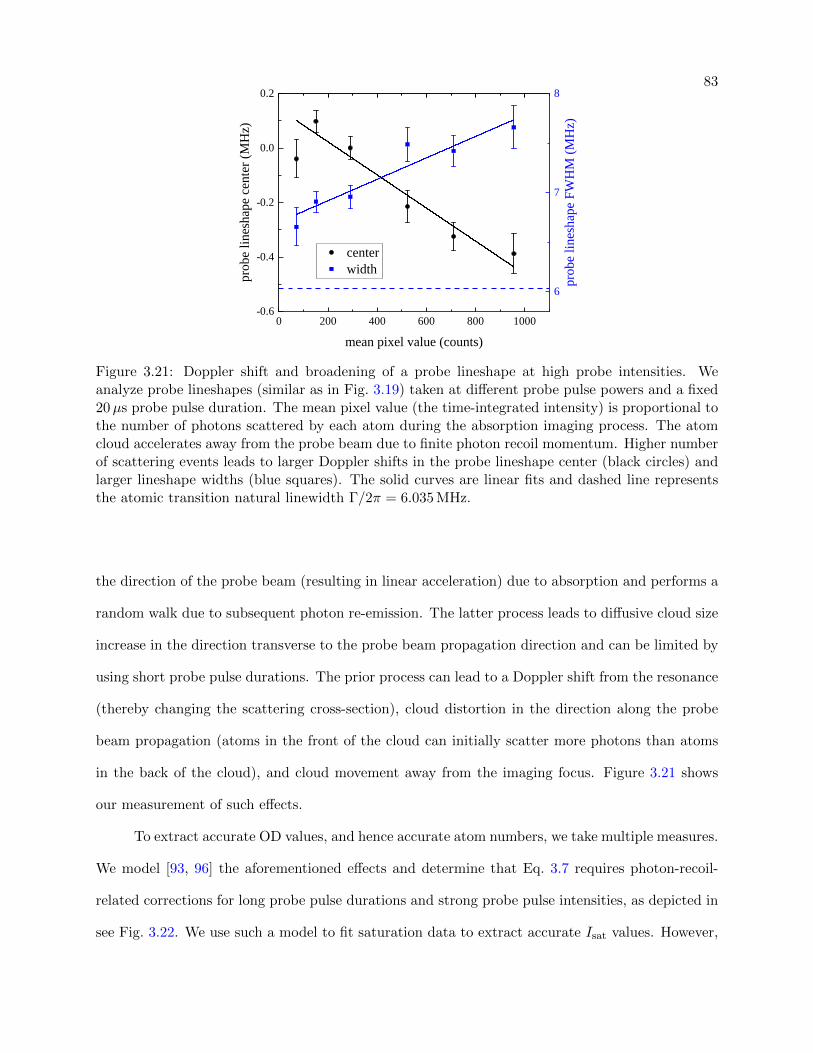
83

0 2 0 0 4 0 0 6 0 0 8 0 0 1 0 0 0- 0 . 6

- 0 . 4

- 0 . 2

0 . 0

0 . 2

c e n t e rw i d t h

m e a n p i x e l v a l u e ( c o u n t s )

probe

linesh

ape ce

nter (M

Hz)

6

7

8

probe

linesh

ape FW

HM (M

Hz)

Figure 3.21: Doppler shift and broadening of a probe lineshape at high probe intensities. Weanalyze probe lineshapes (similar as in Fig. 3.19) taken at different probe pulse powers and a fixed20µs probe pulse duration. The mean pixel value (the time-integrated intensity) is proportional tothe number of photons scattered by each atom during the absorption imaging process. The atomcloud accelerates away from the probe beam due to finite photon recoil momentum. Higher numberof scattering events leads to larger Doppler shifts in the probe lineshape center (black circles) andlarger lineshape widths (blue squares). The solid curves are linear fits and dashed line representsthe atomic transition natural linewidth Γ/2π = 6.035 MHz.

the direction of the probe beam (resulting in linear acceleration) due to absorption and performs a

random walk due to subsequent photon re-emission. The latter process leads to diffusive cloud size

increase in the direction transverse to the probe beam propagation direction and can be limited by

using short probe pulse durations. The prior process can lead to a Doppler shift from the resonance

(thereby changing the scattering cross-section), cloud distortion in the direction along the probe

beam propagation (atoms in the front of the cloud can initially scatter more photons than atoms

in the back of the cloud), and cloud movement away from the imaging focus. Figure 3.21 shows

our measurement of such effects.

To extract accurate OD values, and hence accurate atom numbers, we take multiple measures.

We model [93, 96] the aforementioned effects and determine that Eq. 3.7 requires photon-recoil-

related corrections for long probe pulse durations and strong probe pulse intensities, as depicted in

see Fig. 3.22. We use such a model to fit saturation data to extract accurate Isat values. However,

84

1 1 0 1 0 0 1 0 0 00 . 0

0 . 5

1 . 0

1 . 5 2 0 s p r o b e 4 0 s p r o b e 1 0 0 s p r o b e 2 0 0 s p r o b e

measu

red OD

m e a n p i x e l i n t e n s i t y ( c o u n t s / s )1 0 1 0 0

2 0

4 0

6 08 0

1 0 0

w i t h o u t r e c o i l c o r r e c t i o n sw i t h r e c o i l c o r r e c t i o n s

extrac

ted sa

t (coun

ts/s)

p r o b e d u r a t i o n ( s )Figure 3.22: Probe pulse duration affect on the measurement of Isat. We perform measure-ments (left figure) similar to Fig. 3.20, except we normalize the x-axis by the probe beamduration to get the mean pixel intensity, necessary for data comparison with differentprobe pulse durations. We fit (right figure) the data using two different methods: with-out recoil corrections (Eq. 3.7) and with recoil corrections (numerical model). While thetwo methods agree only at small probe pulse durations, the finite photon recoil momen-tum model gives consistent Isat values for all pulse durations. These results demonstratethe need for a more complex model or the need to image with short probe pulse durationsto accurately determine Isat values.

we do not use the model for OD corrections. Instead, we suppress systematic effects associated with

finite photon recoil momentum by limiting the probe pulse duration to 10–20µs and the probe pulse

intensity to (I/Isat)−1 = 10–20. However, we still include (small) OD corrections due to transition

saturation by performing a pixel-by-pixel correction using a re-written version of Eq. 3.6:

ODtrue(x, y) = ln

(IL(x, y)− ID(x, y)

IS(x, y)− ID(x, y)

)+IL(x, y)− IS(x, y)

Isat, (3.8)

substituting Iin = IL(x, y)−ID(x, y), Iout = IS(x, y)−ID(x, y) and ODmod ≈ ODmeas = ln (Iin/Iout).

For the best signal-to-noise ratio and the small systematic uncertainties, we typically work with

Iin = 120 counts/pixel, Isat ∼ 1900 counts/pixel (high CCD gain 1.53 e−/count), 20µs probe pulse

duration and ODmeas ∼ 0.6. The CCD camera noise floor (σ = 7 counts/pixel readout noise for

high gain, see Fig. 3.17) prevents us from using smaller probe beam intensities, as depicted in

Fig. 3.23. Furthermore, we always utilize optical cycling transitions (e.g. |F = 2,mF = −2〉 →

85

1 1 0 1 0 0 1 0 0 00 . 0

0 . 2

0 . 4

0 . 6

0 . 8

1 . 0

measu

red OD

m e a n p i x e l v a l u e ( c o u n t s )

Figure 3.23: CCD camera noise affect on absorption imaging. We perform similar measurementas in Fig. 3.20, except we use the medium gain CCD camera setting (3.03 e−/count gain and4 counts/pixel read noise) and lower probe pulse powers. Due to bad SNR at very low powers,the measured OD decreases as the cloud image becomes unresolvable. Different colors repre-sent different optical settings (e.g. diverting more power to the probe beam and different NDfilters/attenuators) that enabled the high dynamic range in the mean pixel value.

|F′ = 3,mF′ = −3〉) for imaging when an accurate measurement of the atom number is required,

since non-cycling optical transitions have imaging peculiarities in addition to those listed above.

Lastly, since we always measure probe lineshape widths > Γ/2π = 6.035 MHz, we correct OD for

lineshape broadening. We extrapolate the lineshape FWHM width ∆f to zero probe intensity

(using a fit similar to the one in Fig. 3.21) and correct OD by ∆f/6.035 MHz (typically ∼ 10%

correction).

3.3.3 Extracting Atomic Density

In addition to accurately measuring the atom number, we need to accurately measure the

atom temperature and trapping frequencies to correctly determine the atom density. We mea-

sure the temperature using standard thermometry techniques involving atom cloud expansion [94].

The uncertainty in the measured temperatures is mainly determined by imaging peculiarities (e.g.

magnification, resolution, astigmatism) or the uncertainty in the trapping frequencies.

We measure the trapping frequencies of our optical dipole trap using several different methods:

86

we can induce a sloshing motion, induce a breathing motion, parametrically heat the gas, measure

the optical trap curvature by looking at the gravitational sag as a function of optical power, or from

thermometry. While we’ve utilized all methods to check the consistency of our results, we found the

sloshing method to be the most precise. To measure the trapping frequency along gravity, we drop

the cloud for a short duration and recapture it in the same potential; the induced sloshing motion

is equal to the trapping frequency. To measure the trapping frequency in the other directions, we

use magnetic field gradients to induce sloshing by displacing the cloud from the optical trap center

and subsequently turning off the gradient field. To accurately measure trapping frequencies, we are

careful in probing only the harmonic region of the trap. We use small clouds (e.g. cold thermal

clouds or BECs) and systematically check the sloshing frequency as a function of the induced

perturbation (e.g. displacement from the trap center). Lastly, we verify the trapping frequencies

by looking at the expansion of thermal clouds: the cloud size is predominately determined by the

trap frequencies and temperature during short expansion durations. Precise knowledge of atom

number and temperature, the trapping potential and imaging, enables accurate determination of

atom density to within 20% (see Sec. 5.3 for further details).

3.3.4 Top Imaging Specifications

The side imaging enabled accurate determination of atom number, temperature and density

for most measurements presented in this thesis. Due to the amount of effort required in calibrating

an imaging system, we abandoned our initial efforts in using the top imaging system, where the

probe beam propagates along the main field direction. However, after precise measurements of

cold dilute atomic and molecular samples in our Efimov (Ch. 5) and dimer spectroscopy (Ch. 4)

studies, we realize the need for a better imaging system from the top, as our side imaging suffers

from multiple limitations.

With the side imaging, we cannot perform accurate in-situ imaging of the smallest clouds

due to a relatively low (3.6µm Airy disk radius) imaging resolution. The required cloud expansion

results in smaller OD signals and a reduced signal-to-noise ratio (SNR). We cannot increase the

87

image frame SNR by increasing the probe intensity due to effects discussed in Sec. 3.3.2 and

we resort to using a small number of photons during the absorption imaging process. Due to a

relatively small CCD camera gain, we end up detecting only ∼ 50 counts/pixel (for 1 OD cloud and

Iin = 120 counts/pixel), a small value compared the σ = 7 counts/pixel CCD camera noise floor.

Furthermore, since the magnetic field bias direction is orthogonal to the side probe propagation,

we resort to two options for side imaging: we use π transitions at the expense of 50% in the OD

signal or we use σ± transitions along with a magnetic field parallel to the probe beam propagation

direction generated by separate quantization coils. We often resort for the latter option at the

expense of requiring a minimal expansion time O(1 ms), associated with the main coils turn off

time and the quantization coils turn on time.

We plan to use a high-resolution top imaging system and an electron multiplying CCD camera

in our future studies. The camera (Princeton Instruments ProEM 512B, CCD97-B detector with a

512× 512 pixel array, 16µm pixel size and ∼ 75% QE) has a low-noise 1–1000 electron multiplier

gain and can be cooled down to −70C (0.02). Such high gain enables a better usage of the 16-bit

ADC and results in a higher SNR for low probe intensity imaging. We measure the top imaging

camera to be less noisy than the side imaging camera for similar camera settings: a higher gain

(1.0 e−/count compared to 1.53 e−/count) with similar read noises (7 counts/pixel).

We make a custom high-resolution objective for top imaging using a combination of com-

mercially available lenses. We are limited to using only a few optical elements due to the space

constraint imposed by the moving cart coils. Furthermore, the numerical aperture of the 0.75 NA

window is limited to ∼ 0.5 NA by the presence of the surrounding ∼ 1.7 in shim and gradient coils.

Based on the aforementioned constraints and some preliminary Zemax simulations, we chose to

use an aspheric lens (Thorlabs AL4532-B, f = 32 mm, 0.61 NA, 24.2 mm working distance and

45 mm outer diameter) as the primary imaging lens in the custom objective. Due to further space

constraints associated with lens mounting and clearances, we reduce (JILA instrument shop) the

asphere diameter to a 30 mm outer diameter (26.2 mm clear aperture and 0.38 NA). While the lens

is diffraction-limited in free-space, the science window introduces significant spherical aberrations

88

Figure 3.24: MTF (modulation transfer function) of the top imaging asphere (Thorlabs AL4532-B,f = 32 mm, 0.61 NA) without (left) and with (right) the science cell window. The diffraction limit(1.1µm Airy disk radius at 767 nm) of the chosen (apertured) 0.38 NA is represented by blackcurves, on-axis imaging rays MTF by blue curves, 100µm off-axis sagittal rays by dashed greencurves and 100µm off-axis tangential rays by solid green curves. Without the science cell window,the imaging system is expected to be diffraction-limited on-axis (note the blue and black curvesoverlap) and nearly diffraction-limited off-axis. However, with the window, the imaging systemis far from diffraction limit. The 6.35 mm thick fused silica window, located 10.5 mm away fromthe atoms, introduces significant spherical aberrations (0.9λ rms wavefront error contribution),resulting in a ∼ 28µm spot size radius.

(see Fig. 3.24) and we cannot use the asphere on its own. We simulate various configurations

with additional one or two compensating lenses to see how we can reduce spherical aberrations.

While a custom meniscus lens would be the best solution, addition of a single plano-convex lens

(see Fig. 3.25) would lead to satisfactory performance. The custom objective is expected to be

diffraction limited (1.1µm Airy disk radius) for on-axis imaging and nearly diffraction-limited for

off-axis, as depicted in Fig. 3.26.

The objective lenses are placed in a custom machined lens tube. We perform tolerance

analysis prior to machining to determine which dimensions require the highest precision. The lens

tube and the mounting arm (made necessary long to provide sufficient cart coils clearance) are made

from plastic (Ultem and G11, respectively) to prevent vibrations from magnetic field sweeps. A pair

of goniometers and an xyz-stage provide the necessary degrees of freedom for objective assembly

movement. We perform vibration analysis (using an accelerometer) and verify mechanical stability

of the objective assembly. The high-resolution top imaging system is ready to be implemented into

our system and will provide a new invaluable tool for precise imaging of dilute and small atomic

and molecular clouds.

89

Figure 3.25: Top imaging objective lens configuration. Rays propagating from right to left: atoms,10.5 mm space in the vacuum chamber, 6.35 mm thick fused silica window, 6.6 mm space outside thevacuum chamber, 2.2 mm thick plano-convex lens (Thorlabs LA1978-B), 0.57 mm space betweenthe lenses, and 13.9 mm thick asphere. The exit pupil diameter is 26.2 mm. We vary separationdistances and the clear aperture diameter during imaging system optimization on the rms wavefronterror.

3.4 Computer Control

Figure 3.27 shows an overview of our lab’s computer and hardware control. Most of the

experiment is controlled via two FGPA cards (NI PCIe-7852R LX50), which have on-board 40 MHz

clocks, analog and digital lines. Synchronization of all experimental sequence timings to FPGA

clocks (instead of using computer time) leads simplification and robustness of the machine. The

two FGPA board timings are synchronized by triggering the FPGA2 clock with an FPGA1 TTL

at the beginning of every experimental sequence. We periodically compare the two FPGA clock

frequencies and adjust them when necessary (artificially, by adjusting the FPGA2 board clock

cycle definition in the Matlab control code); typically the two clocks differ only by a few µs/min.

Currently there is no easy way to synchronize the two FPGA clocks to the stable 10 MHz signal

that is distributed throughout JILA and referenced to NIST.

We use LabView software to program, compile and communicate with the FPGA boards.

Fortunately, due to the modularity of our control program (credit to Yoav Sagi), we rarely O(yrs)

reprogram or recompile the FPGA boards. For each experimental sequence, we generate all com-

90

Figure 3.26: Expected performance of the high-resolution objective in the top imaging system. Wesimulate geometrical ray spot sizes (blue crosses) for on-axis imaging (top left figure) and for 100µmoff-axis imaging (top right figure), where the circles represent the diffraction limit. The bottomfigure shows the simulated MTF, similar to Fig. 3.24. The objective is diffraction limited (blackcurve) for on-axis imaging (blue curve), with 0.025λ rms wavefront error, and nearly diffraction-limited for off-axis (green curves), with 0.146λ rms wavefront error. The leading residual aberrationterm is the 22nd Zernike polynomial.

mand lists (channel timings and settings) in Matlab, re-interpret them using LabView, and upload

the command lists to the FPGA cards. Once triggered, the FPGA cards will independently execute

the uploaded commands. LabView interface queries FPGA on-board clocks during their execution

and we can send semi-synchronized (e.g. GPIB) commands to various instruments. The control

code is modular and is based on simple hardware commands: digital line state and timing; analog

line voltage and timing; analog line linear voltage ramp (resource efficient high-resolution steps)

with beginning voltage, end voltage and timings; GPIB command and timing. Furthermore, we

have an ability to do real-time on-board logic. For example, we can make all FPGA channels wait

91

K40

USBVISA

VFGx2synthesizersx4AWG

FPGA1 FPGA2TTLclocktrigger

LabView

Matlab

PCIe PCIe

DAC Buffer

GPIB

Buffer

x8AO x8AO

DAC

x8AO x8AOx48DO x48DO

K44

Matlab

Pixelf lyCam

Ethernet

K35

VisualBasic+WinView

SideCam

Ethernet

K41

TopCam

Ethernet

VisualBasic+WinView

K38

Nufern Cart

K39

B-field,T sense

Timestamp

MAKO cams

Flowmeters

GPIB

440A,15VPS1

GPIB

440A,15VPS2

Figure 3.27: An overview of computer and hardware control. The main computer “K-40” programsFGPA cards and controls the majority of the experiment via analog output (AO), digital output(DO), GPIB, and USB lines. “K-40” control includes: magnetic coil power supplies (PS), synthe-sizers and VFG for RF antennas, and AWGs for optical dipole trap control. The “K-39” is usedfor sensing and recording laboratory conditions every experimental cycle, including: magnetic fieldnear the chamber, the main coils and the science optical table temperatures, water cooling flowrates, optical trap alignment (×3 MAKO cameras), and the absolute time when experiment wasrun (an Arduino clock synchronized to NIST time). Note, two separate sensors (Colorado Sen-sors HT6130, not shown) record laboratory’s temperature and humidity every 5 minutes; we haverecords dating back to 2013. The other computers are used for interfacing with imaging cameras, acart motion controller and a Nufern laser amplifier. “K-44” computer is used as the main computerfor image analysis. All lab instruments are triggered by FPGA TTL lines.

92

for an external trigger before proceeding, useful in instances such as triggering on the MOT fill level

or synchronization to the 60 Hz line. Since FPGA cards also have digital and analog input capabil-

ity, we did attempt to implement on-board digital PID loops for laser (e.g. locking to spectroscopy

signals) and coil control (e.g. using a nonlinear gain profile to extend ppm-level field stability over

a large dynamic range; hard to achieve with analog circuits). While somewhat successful, digital

PID loops used too many on-board resources and were not as fast or as low-noise as our JILA

analog PID loops. We abandoned any further attempts to implement digital PID loops on our

main FPGA cards.

The FPGA digital output lines pass through buffers (Avago Technologies HCPL-0723 opto-

couplers) before being distributed around the lab. The 16 FPGA analog lines is not a sufficient

amount and we resort to using two additional DACs (AD5360, 16-bit, 8 channel), sacrificing one

digital port (8 digital lines) to program each DAC. The external DAC clocks are synchronized to

FPGA clocks. Due to FPGA on-board resource overhead, we end up with a total of 96 digital

(TTL) lines and 32 analog lines from two FPGA cards. While not currently implemented, we have

previously used FPGAs to interface with high-resolution DACs (AD5191, 1ppm 20-bit) and ADCs

(AD7767, 3ppm 24-bit).

We have five additional computers (see Fig. 3.27) for recording experimental conditions, data

and image analysis, and for interfacing with various hardware. All laboratory instruments are

triggered by the two FPGA cards.

Chapter 4

Precise Characterization of a Feshbach Resonance

Fano-Feshbach resonances offer an unparalleled ability to control interactions in quantum

systems, and understanding their properties is essential. This chapter reviews our characterization

of a Feshbach resonance with unprecedented precision. I begin with a short overview of different

methods used in measuring Feshbach resonance properties and describe the advantage of using

dimer dissociation spectroscopy. I then detail how we prepare pure molecular samples used in

studies throughout this chapter. In the first study, I discuss how we use precision RF spectroscopy

of dimer binding energies to locate the Feshbach resonance location B0. The second study details

molecular lifetime measurement and the observation of an unexpected lifetime maximum at a high

binding energy.

4.1 Methods for Characterizing Feshbach Resonances

Most experimental studies rely on atom-loss measurements for locating Feshbach resonances

[19]. In such studies, one records the atom-loss fraction (for a specific hold time) at different

magnetic fields. Since the inelastic collision rate is presumed to be maximal at the resonance, the

B-field value of maximal loss is taken to be the resonance position B0. A complementary method,

stemming from the two- and three-body nature of inelastic loss, relies on locating the maximal

heating rate in a gas with inhomogeneous density. While these methods are easy to implement,

imprecise knowledge of important details limits their validity and results only in rough estimations

of resonance locations. For instance, the presence of Efimov physics and two-body bound states is

94

expected to complicate loss dynamics close to the resonance.

To demonstrate problems associated with these simplest methods, we used them to roughly lo-

cate our Feshbach resonanceB0 ∼ 34 G. We prepared a sample of 5×105 atoms in the |F = 1,mF = −1〉

hyperfine state and temperature of 700 nK in a single-beam optical trap. The trap depth was raised

by a factor of two to limit loss associated with evaporation. The initial magnetic field is B = 41.8 G,

corresponding to a scattering length a ∼ 115 a0. In the first experiment, we ramp the magnetic

field to a new value in 2 ms and hold additional 20 ms before imaging. Due to enhanced three-body

loss, significant atom loss and heating are prevalent near B0, as shown in Fig. 4.1a. We fit the

atom loss feature with a Gaussian function and extract its center to be at 32.8(1) G. In the second

experiment, we ramp the magnetic field to a new value in 2 ms and vary the hold duration to take

a lifetime measurement at each field. A fit to an exponential with a floating offset is sufficient to

capture the decay dynamics. Fig. 4.1b shows the resulting lifetimes at different fields. A lack of a

sharp signal in both of these measurements (related to the resonance width ∆B) and the asymme-

try of the loss features (three-body loss is inherently asymmetric about B0 and is complicated by

Efimov features) lead to only a rough measurement of B0.

Methods based on elastic properties are considered better and more sensitive for locating

Feshbach resonance centers. For example, measurements using the anisotropic expansion of an

interacting gas [32, 21] and cross-thermalization methods [97] allowed several groups to significantly

improve on prior results. Methods using RF spectroscopy to measure mean-field related frequency

shifts enable one to extract the amplitude and sign of the elastic scattering length a near B0

[98]. While these methods are better than those based on inelastic properties, systematic shifts

at high temperatures [99] and beyond-mean-field effects at high na3 [100] limit their applicability.

Furthermore, examples of inconsistent results, such as in Refs. 32 and 21, obtained by the same

method, are troublesome.

The most accurate methods for characterizing Feshbach resonances rely on measuring the

Feshbach dimer state. This molecular state intersects the free-atom continuum at B0 and its

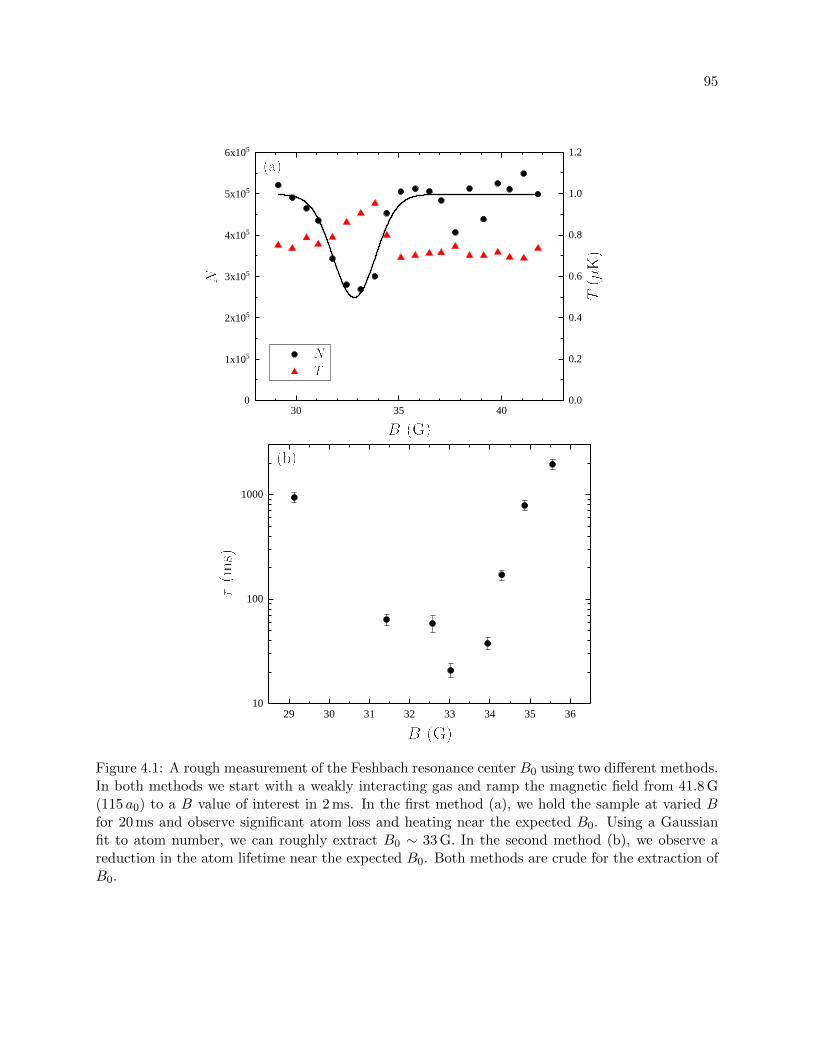
95

3 0 3 5 4 00

1 x 1 0 5

2 x 1 0 5

3 x 1 0 5

4 x 1 0 5

5 x 1 0 5

6 x 1 0 5

0 . 0

0 . 2

0 . 4

0 . 6

0 . 8

1 . 0

1 . 2

2 9 3 0 3 1 3 2 3 3 3 4 3 5 3 61 0

1 0 0

1 0 0 0

Figure 4.1: A rough measurement of the Feshbach resonance center B0 using two different methods.In both methods we start with a weakly interacting gas and ramp the magnetic field from 41.8 G(115 a0) to a B value of interest in 2 ms. In the first method (a), we hold the sample at varied Bfor 20 ms and observe significant atom loss and heating near the expected B0. Using a Gaussianfit to atom number, we can roughly extract B0 ∼ 33 G. In the second method (b), we observe areduction in the atom lifetime near the expected B0. Both methods are crude for the extraction ofB0.

96

binding energy is approximated by a simple universal expression

Eb =~2

ma2, (4.1)

where a > 0. There are three methods based on Feshbach dimers for extracting B0: magnetic

sweep across the Feshbach resonance, the crudest; dimer association, a better method; dimer dis-

sociation, the most precise method. The simplest, yet coarse, method involves measuring the onset

of the molecular state by magneto-association of dimers. In this thesis, I use the term “magneto-

association” to refer to ramping the scattering length from a < 0 to a > 0, such that some atoms

are adiabatically swept into the molecular state. During this association process, one observes a

dip in the atom number near B0 [101]. While we do utilize magneto-association in our work, we

only do so for purposes of populating the molecular state and not for the purpose of extracting

an accurate B0 value. Precise methods for extracting B0 rely on direct measurements of dimer

binding energies. In our work, we use magneto-association to prepare a molecular sample and

use RF dissociation spectroscopy to probe dimer binding energies. Spectroscopic methods based

on molecular association, such as Ramsey interferometry [102, 103] and magnetic-field modulation

spectroscopy [104, 105, 106, 107, 108, 40, 99], also enable determination of Eb values. However,

due to the complex interdependence between conditions (e.g. atom temperature, phase space den-

sity and mean-field energy) and the signal (e.g. its contrast, center and spectral width), limits

the accuracy of molecular association spectroscopy method. Hence, we resort to RF dissociation

spectroscopy.

RF dissociation spectroscopy overcomes many limitations present in association spectroscopy

and enables accurate determination of molecular binding energies [109]. Unlike in other methods,

the signal contrast is only limited by the number of molecules in the sample (in the absence of

unpaired atoms) and does not depend on the density, phase space density or collisional processes.

Additionally, temperature-dependent shifts are absent and mean-field related shifts can be negligible

in a low density gas. The spectral resolution is only limited by molecular lifetimes and the magnetic

field stability. Precise dissociation spectroscopy enabled accurate characterization of Feshbach

97

resonances for many species [101, 110, 13, 20, 111, 112]. Recent work of Ref 20 measured a Feshbach

resonance location in 6Li with an unprecedented precision. Our measurement in 39K attempts to

do even better.

4.2 Magneto-Association of Feshbach Molecules

4.2.1 Populating the Dimer State

We use magneto-association method [101, 113] to create a macroscopic population of Fesh-

bach dimers for use in our Eb measurements. This technique enables high atom-dimer conversion

efficiencies, reaching 50% for Bose gases [114], 90% for Fermi gases [114] and 50% for quantum

mixtures (90% in a 3-D lattice [115]). While other methods [116] can also be efficient, historically,

the magneto-association method has resulting in largest molecular populations. We need 103–104

Feshbach dimers to provide an adequate signal for precision Eb spectroscopy. We carefully con-

sider our initial conditions and experimental procedures during magneto-association to produce the

maximum molecular population. For example, while the atom-dimer conversion efficiency increases

with the phase space density, the atom loss also increases with the phase space density, thereby we

need to find a balance.

The general scheme of magneto-association relies on adiabatic transfer of atoms in the

monomer (unpaired) state into the Feshbach dimer state via a Landau-Zener–type process, as

depicted in Fig. 4.2. There are several important timescales that one must consider during this

process. When changing from a > 0 to a < 0, using the fastest possible ramp rate B (in units of

G/s) is important in order to limit the duration the gas spends at high a values, where inelastic

losses are high. The three-body loss rate L3, scaling as a4, and the two-body loss rate L2 (present

since the |F = 1,mF = −1〉 state is not the absolute ground state at non-zero magnetic field), scal-

ing as a2 can limit the sample’s lifetime to millisecond timescales even at modest atomic densities

of n ∼ 1011 cm−3 (note that L3 and L2 values are capped by finite n or T at unitarity, deviating

from their respective a4 and a2 scaling). More concretely, L2 and L3 lead to loss of the form (also

98

see Ch. 5):

1

N

dN

dt= −L2〈n〉 − L3〈n2〉, (4.2)

where 〈n〉 = 1N

∫n2(~x)d3x and 〈n2〉 = 1

N

∫n3(~x)d3x. While performing magneto-association at

higher temperatures (see Sec. 5.2 and Fig. 4.3) and lower densities can help limit inelastic loss,

molecular association efficiency favors high phase-space density [114]; leading to contradicting

requirements for conditions. Additionally, the association probability depends on the Feshbach

resonance parameters abg and ∆B, the ramp rate B and density n:

P = Pmax

(1− exp

(−αn~

m

∣∣∣∣abg∆B

B

∣∣∣∣)) , (4.3)

where Pmax is the maximum association efficiency possible and α is a dimensionless resonance-

dependent parameter [114, 19]. Overall, for a > 0 to a < 0 sweep, one desires a fast magnetic

field ramp to limit inelastic loss; for a < 0 to a > 0 sweep, one desires a slow magnetic field ramp

to efficiently/adiabatically transfer atomic population to the dimer state via a Landau-Zener–type

process.

We begin with a thermal sample with few-105 atoms, temperature around 300 nK and a ∼

300 a0. In order to get the desired final molecule density, temperature and number, we vary the

initial atom number and temperature by changing the parameters of the last evaporation stage.

While the initial phase space density is chosen to be O (1) to ensure a high atom-dimer conversion

efficiency, we verify that the condensate fraction is small or vanishing. A large condensate fraction

would result in high number loss and heating upon the preliminary ramp to negative a values, before

the magneto-association ramp [117]. Prior to jumping across |a| → ∞, we perform a preliminary

ramp to B = 35.76 G (480 a0), a convenient value for our spin-purification procedure: we get rid

of |F = 1,mF = 0〉 atoms that contaminate our dimer spectroscopy at low Eb values. Performing

the purification procedure after association would add extra time and result in a larger loss of

molecules; further details are discussed in Sec. 4.4.

To magneto-associate dimers, we first ramp the magnetic field from B = 35.76 G (a = 480 a0)

to B = 19.8 G (a = −90 a0) in 1 ms (see Fig. 4.2). We can get an idea of timescales required for

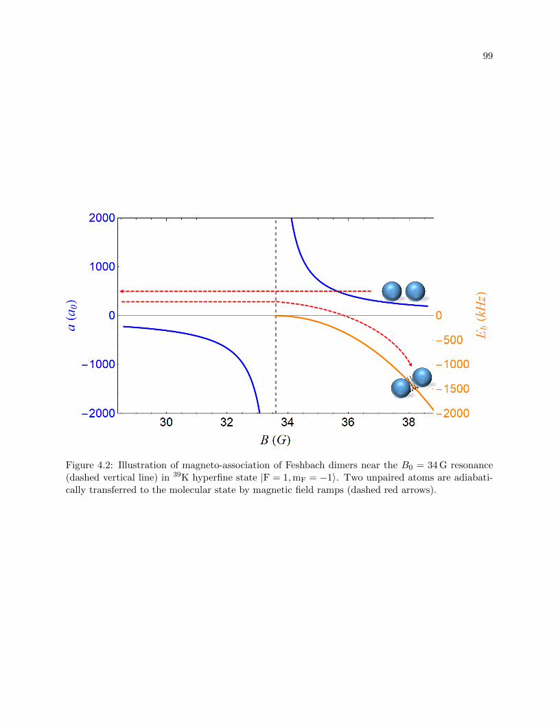
99

Figure 4.2: Illustration of magneto-association of Feshbach dimers near the B0 = 34 G resonance(dashed vertical line) in 39K hyperfine state |F = 1,mF = −1〉. Two unpaired atoms are adiabati-cally transferred to the molecular state by magnetic field ramps (dashed red arrows).

100

our conditions by solving the coupled-equations describing three-body atom loss and heating (we

focus on the L3 part of Eq. 4.2) [118]:

1

N

dN

dt= −L3〈n2〉, (4.4)

1

T

dT

dt=

1

3L3〈n2〉, (4.5)

where now we introduce a time-dependent three-body loss coefficient L3 = L3 (T (t) , a (t)) (taken

from the finite-temperature theory of Ch. 5) and time-dependent scattering length a (t) = a (B (t)).

For example, typical initial conditions of 3×105 atoms, T = 250 nK and a mean trapping frequency

of 57 Hz, using a 10 ms magnetic field ramp leads to significant atom loss and heating, as depicted

in Fig. 4.3. However, using a 1 ms magnetic field ramp instead of a 10 ms ramp would increase the

final atom number by almost 50% and lead to negligible heating. While ramps durations 1 ms

would be desirable, the inductance of our Feshbach coils limits large B–field jumps to a ∼ 0.5 ms

timescale. We also use such estimates to get an idea of the three-body loss timescales during the

magneto-association ramp (from a < 0 to a > 0), where the ramp must be performed slow enough

according to the adiabaticity criterion in the Landau-Zener–type process (Eq. 4.3).

After jumping to a < 0, we subsequently populate the dimer state by ramping back to

B = 35.76 G (a = 480 a0), a specific value chosen for atom-cleaning procedure described in 4.4. We

can use the Laundau-Zener formula Eq. 4.3 to estimate how slow we need to perform the molecular-

association ramp to be adiabatic. Using a typical density of 〈n〉 = 8 × 1011 cm−3, ∆B = 55 G,

abg = −19.7 a0 and α = 276 (where we took α value from 85Rb [114], as we don’t know the value

for 39K), we predict that an inverse ramp rate of B−1 = 55µs/G would result in P/Pmax = 67%

efficiency. We confirm the Landau-Zener model for Feshbach association by comparing predictions

to experimental data. We look at the number of molecules produced as we vary the inverse ramp

rate B−1, keeping the starting and final magnetic field values unchanged. Fig. 4.5 shows a good

agreement between theory and the data for fast ramps. However, ramps with B−1 > 500µs/G,

corresponding to ramp durations > 7.4 ms, are affected by loss processes not accounted for by

Eq. 4.5 (e.g. atom-dimer and dimer-dimer inelastic collisions, loss from dimer spin relaxation) and

101

10-5 10-4 10-3 10-2

t (s)

-1

-0.5

0

0.5

1

a (a

0)

104 a(t)

10-5 10-4 10-3 10-2

t (s)

10-26

10-24

10-22

10-20

L 3 (cm

6 s-1

)

L3(t)

102 103 104

a (-a0)

10-30

10-25

10-20

10-15

L 3 (cm

6 s-1

)

L3(a) at T = 0 and T = 250 nK

10-5 10-4 10-3 10-2

t (s)

2

2.5

3

N

105

250

260

270

280

290

T (

nK)

N(t) and T(t)

Figure 4.3: Estimating the impact of three-body loss on the atom population and temperatureduring a 10 ms B–field ramp from B = 35.76 G to B = 19.8 G. Here, we ignore the Efimov structurein L3, which modulates the a4 scaling, see Ch. 5. The top-left figure shows that L3 saturates athigh scattering lengths due to finite-temperature effects (note we us an artificial scenario: thermalBose cloud with T = 0). Top-right and bottom-left figures show instantaneous a (t) and L3 (t),respectively. The bottom-right figure shows the predicted atom decay and heating during theB–field ramp, as predicted by solving coupled-equations in Eq 4.5.

10-6 10-5 10-4 10-3

t (s)

-1

-0.5

0

0.5

1

a (a

0)

104 a(t)

10-6 10-5 10-4 10-3

t (s)

10-26

10-24

10-22

10-20

L 3 (cm

6 s-1

)

L3(t)

102 103 104

a (-a0)

10-30

10-25

10-20

10-15

L 3 (cm

6 s-1

)

L3(a) at T = 0 and T = 250 nK

10-6 10-5 10-4 10-3

t (s)

2.7

2.8

2.9

3

N

105

250

252

254

256

258

260

T (

nK)

N(t) and T(t)

Figure 4.4: Estimating the impact of three-body loss on the atom population and temperatureduring a 1 ms B–field ramp from B = 35.76 G to B = 19.8 G, similarly to Fig. 4.3. Atom loss andheating associated with three-body loss is significantly smaller for 1 ms ramp than for 10 ms B–fieldramp.

102

10 50 100 500 10000

2000

4000

6000

8000

10000

12000

14000

Inverse ramp rate (μ/G)

NumberofMolecules

Figure 4.5: Comparing experimental data (points) to predictions of Landau-Zener–type process(Eq. 4.3) for magneto-association of Feshbach dimers. The conversion efficiency at large inverseramp rates B−1 is affected by atom-dimer, dimer-dimer and dimer spin relaxation loss processes.

strong deviations from the simple model are expected.

4.2.2 Optimizing Molecular Number and Preliminary Detection Schemes

Due to short molecular lifetimes and low signal, detection of Feshbach molecules is no easy

task. Our first attempts to create and directly detect Feshbach dimers resulted in a poor signal of

only ∼ 200 molecules and 50 mOD. To get a sufficient signal for precision RF spectroscopy, we had

an iterative process of switching between different detection methods and improving the molecular

number.

The biggest improvement in molecule number resulted from altering our optical trap config-

uration. We saw our first molecular signal in a crossed-dipole trap with the horizontal beam waist

of 28µm × 28µm and the vertical beam waist of 28µm × 220µm, forming a spherical potential

with a trapping frequency of 2π × 432 Hz. This configuration enabled reaching PSD = 1 with

N = 7 × 104 atoms at T = 700 nK, corresponding to npeak = 4 × 1013 cm−3. Such a high density

results in very fast timescales for three-body loss and leads to a significant number loss and heating

103

(to T = 1.3µK), even for our fastest ramp speeds. Additionally, high density atomic samples result

in short molecular lifetimes, limited by inelastic atom-dimer collisions, rendering RF dissociation

spectroscopy useless since it requires moderate interrogation times even at full 20 W RF power.

We significantly increased our molecule number by reducing atom density. In our first at-

tempt to do so, we used only a horizontal beam (waist 28µm × 28µm and trapping frequencies

(ωx, ωy, ωz) = 2π×(3, 306, 306) Hz) to prepare an atomic sample with npeak = 4×1012 cm−3. While

this configuration successfully created ∼ 104 molecules, the signal was poor due to a small optical

density along the imaging direction y. The next iteration included a 28µm×28µm horizontal beam

with a 140µm×800µm vertical beam, resulting in an atomic density npeak = 1×1013 cm−3 and 5000

molecules. We settled on the final optical trap configuration: horizontal sheet beam with a waist

of 80µm× 810µm and a vertical beam with a waist of 140µm× 140µm (e.g. with typical trapping

frequencies (ωx, ωy, ωz) = 2π×(30, 30, 120) Hz), which turn on as the loading beam 28µm×28µm is

ramped off during the evaporation. With the new trap we are able to associate ∼ 2×104 molecules,

with 10–20% association efficiencies, from an atomic gas of npeak = 4× 1012 cm−3 and have a good

signal for spectroscopy. We can vary the molecular number, temperature and density by changing

evaporation parameters prior to the magneto-association procedure.

Our first signature of molecules was an observed dip in atomic number near B0 as we per-

formed the magneto-association procedure, as depicted in Fig. 4.6. The magnetic field is ramped

from B > B0, where a > 0, to a varied B–field value and then back to a final value B > B0

where the sample is held before imaged. Both ramps are performed with fixed speeds for consis-

tency, relating to Landau-Zener and three-body loss timescales. In such scenario, a fraction of the

atomic population is transferred to the dimer state when the varied B–field value crosses B0. The

final B–field is chosen such that the atomic lifetime without such ramps is on order of seconds,

easily achieved with a < +500 a0 even with moderate densities. Finally, after a hold time at the

final field, the magnetic field is ramped to a low value, thereby dissociating molecules, and the

remainder population (consisting of atoms and dissociated molecules) is imaged. There are two

decay timescales: a fast decay O(1 ms), resulting from spontaneous dimer decay, atom-dimer and

104

3 0 3 1 3 2 3 3 3 4 3 5 3 60

2 0 0 0 0

4 0 0 0 0

6 0 0 0 0

8 0 0 0 0

0

2 0 0 0

4 0 0 0

6 0 0 0

8 0 0 0

1 0 0 0 0

Figure 4.6: Atom number dip (dots) near a nominal B0 (dashed) is evidence of molecular formationduring the magneto-association process, supported by direct detection of molecular population(squares) via RF spectroscopy.

dimer-dimer inelastic collisions; a slow decay O(s) dictated by monomer lifetime. After waiting a

sufficient time for the fast decay to cease, one sees a dip in atomic number as the varied B–field

value becomes < B0, a signature of the molecular state. We later confirmed the conclusion from

the indirect technique with the direct detection (using RF dissociation) of molecules, shown as blue

squares Fig. 4.6. Initially, the indirect technique proved to be easier for detecting molecules than

via direct spectroscopic techniques, where variables such as RF duration, power, and frequency

must be properly chosen.

RF association of molecules is another useful technique that helped us figure out the correct

parameters for RF dissociation spectroscopy. Specifically, it helped us to roughly map out the

molecular binding energies, and hence RF frequencies at various magnetic field values. Unlike in

RF dissociation spectroscopy, one does not need to worry too much about the RF pulse duration

for RF association spectroscopy, even for short molecular lifetimes, as the baseline signal comes

105

from atomic population. The association technique is of most use when dealing with Feshbach

resonances of narrow and intermediate width (see Sec. 4.5.3), where the universal relation Eq. 4.1

cannot accurately predict Eb. We start with a monomer gas in the |F = 1,mF = −1〉 state and

use an auxiliary coil to apply field modulation in parallel direction as the field created by the

main Feshbach coils. We modulate the field for 10 ms at fixed modulation frequency fixed while

varying the magnetic field of the main coils. Molecules are associated when Eb(B) = hfmod and are

quickly lost due to spontaneous decay and inelastic atom-dimer collisions, resulting in a dip in the

imaged atom population at a particular magnetic field, as depicted in Fig. 4.7a. We also take RF-

association spectra at two different magnetic fields, as depicted in Fig. 4.7b, allowing us to extract

Eb. While this technique is able to retrieve Eb values in rough agreement with the values predicted

by the coupled-channel theory and provide guidance for RF dissociation spectroscopy, this technique

suffers from a non-trivial asymmetric lineshape (associated with the non-symmetric modulation

in a), systematic temperature shifts (resulting from a thermal distribution of the monomer gas)

and a complicated relationship between signal contrast, feature width, modulation amplitude and

temperature.

4.3 RF Dissociation Spectroscopy

4.3.1 Understanding Molecular Dissociation Spectra

The RF dissociation spectroscopy of Feshbach dimers is a well-understood technique [109]

and is relatively immune to systematic shifts (e.g. from finite-temperature and photon momentum

recoil), enabling us to precisely measure Eb values. With a sufficiently low molecular density

(nmola3 1), our pure molecular gas (see Sec. 4.4 on how we achieve this) can be described as an

ensemble of two-atom states, initially in the bound state |ψmol〉. The state |ψmol〉 has an energy

that is Eb less than the energy of two non-interacting atoms in the |F = 1,mF = −1〉 hyperfine state

(see Fig. 4.8a) and has a spatial extent O(a), described by the wavefunction 〈r |ψmol〉 =√

2ae−r/a.

We use an RF pulse to break the pair by transferring one its atoms to the |F = 2,mF = 0〉 state (see

106

3 4 . 0 3 4 . 2 3 4 . 4 3 4 . 6 3 4 . 80

5 0 0 0 0

1 0 0 0 0 0

1 5 0 0 0 0

2 0 0 0 0 0

0 1 0 2 0 3 0 4 0 5 0 6 00

4 0 0 0 0

8 0 0 0 0

1 2 0 0 0 0

1 6 0 0 0 0

Figure 4.7: RF association of molecules by field modulation. (a) Field modulation with a fixedfrequency of 40 kHz, peak amplitude of 115 mG and 10 ms modulation duration. A dip in the totalnumber occurs when Eb(B) = hfmod, occurring at B = 34.3 G when fitted with a sloped Gaussianfunction, where the slope arises from increased three-body loss near B0. This result is close tothe value Eb(34.3 G) = 41.8 kHz we later obtained using RF dissociation spectroscopy. (b) RFassociation spectra at two different fields, with modulation peak amplitude of 250 mG and 10 msduration. We extract Eb(34.0 G) = 11(1) kHz and Eb(34.3 G) = 42(1) kHz from Gaussian fits, whilecoupled-channel predicts Eb(34.0 G) = 15.2 kHz and Eb(34.3 G) = 46.5 kHz.

107

|1,-1>

|1,0>

|2,0>

|2,-1>

|2,-2>

RF

|1,-1>

|2,0>

𝐸𝐸𝑏𝑏

(a)

|1,-1>

|2,-1>

|1,-1>

|2,0>

𝐸𝐸𝑏𝑏

|1,0>

|2,0>

|2,-2>

(b)

Figure 4.8: Initial (a) and final (b) states in the dimer dissociation procedure. The initial stateis a molecular state with binding energy Eb. The final state has one atom in the |F = 2,mF = 0〉hyperfine state and the other in |F = 1,mF = −1〉.

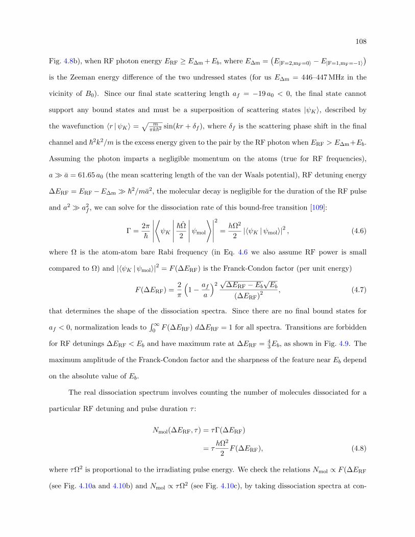
108

Fig. 4.8b), when RF photon energy ERF ≥ E∆m +Eb, where E∆m =(E|F=2,mF=0〉 − E|F=1,mF=−1〉

)is the Zeeman energy difference of the two undressed states (for us E∆m = 446–447 MHz in the

vicinity of B0). Since our final state scattering length af = −19 a0 < 0, the final state cannot

support any bound states and must be a superposition of scattering states |ψK〉, described by

the wavefunction 〈r |ψK〉 =√

mπk~2 sin(kr + δf ), where δf is the scattering phase shift in the final

channel and ~2k2/m is the excess energy given to the pair by the RF photon when ERF > E∆m+Eb.

Assuming the photon imparts a negligible momentum on the atoms (true for RF frequencies),

a a = 61.65 a0 (the mean scattering length of the van der Waals potential), RF detuning energy

∆ERF = ERF−E∆m ~2/ma2, the molecular decay is negligible for the duration of the RF pulse

and a2 a2f , we can solve for the dissociation rate of this bound-free transition [109]:

Γ =2π

~

∣∣∣∣∣⟨ψK

∣∣∣∣∣ ~Ω

2

∣∣∣∣∣ψmol

⟩∣∣∣∣∣2

=hΩ2

2|〈ψK |ψmol〉|2 , (4.6)

where Ω is the atom-atom bare Rabi frequency (in Eq. 4.6 we also assume RF power is small

compared to Ω) and |〈ψK |ψmol〉|2 = F (∆ERF) is the Franck-Condon factor (per unit energy)

F (∆ERF) =2

π

(1−

afa

)2√

∆ERF − Eb√Eb

(∆ERF)2 , (4.7)

that determines the shape of the dissociation spectra. Since there are no final bound states for

af < 0, normalization leads to∫∞

0 F (∆ERF) d∆ERF = 1 for all spectra. Transitions are forbidden

for RF detunings ∆ERF < Eb and have maximum rate at ∆ERF = 43Eb, as shown in Fig. 4.9. The

maximum amplitude of the Franck-Condon factor and the sharpness of the feature near Eb depend

on the absolute value of Eb.

The real dissociation spectrum involves counting the number of molecules dissociated for a

particular RF detuning and pulse duration τ :

Nmol(∆ERF, τ) = τΓ(∆ERF)

= τhΩ2

2F (∆ERF), (4.8)

where τΩ2 is proportional to the irradiating pulse energy. We check the relations Nmol ∝ F (∆ERF

(see Fig. 4.10a and 4.10b) and Nmol ∝ τΩ2 (see Fig. 4.10c), by taking dissociation spectra at con-

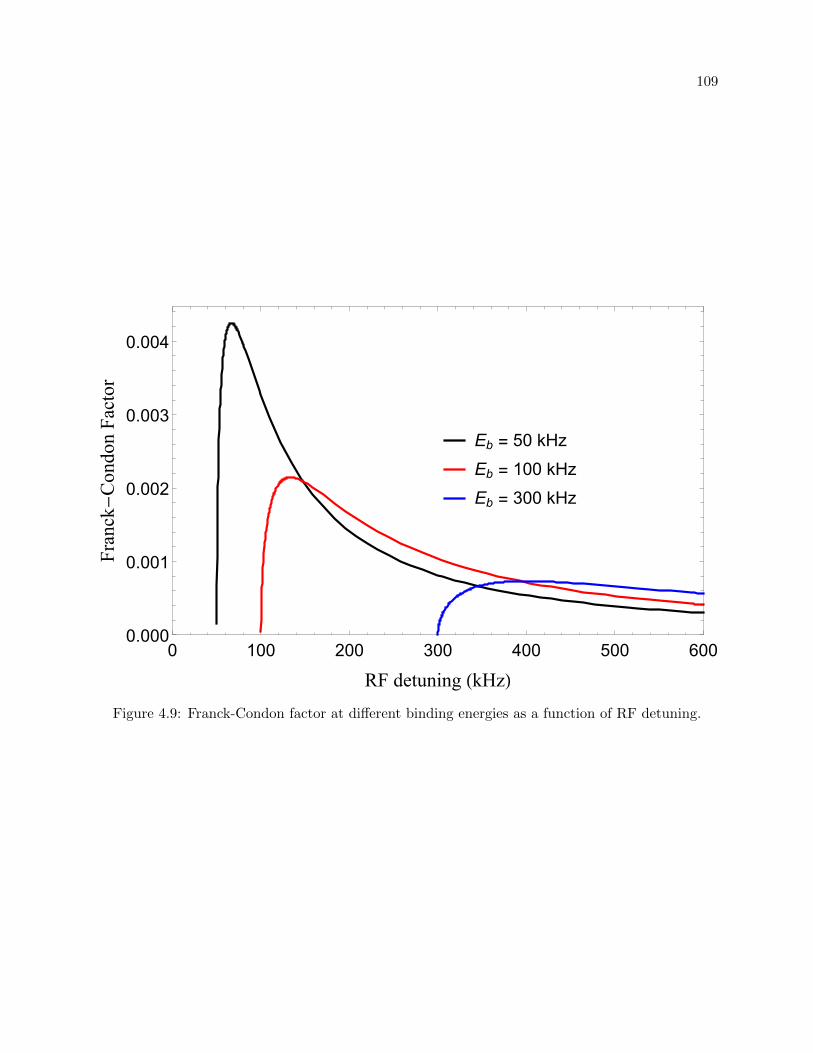
109

Eb = 50 kHz

Eb = 100 kHz

Eb = 300 kHz

0 100 200 300 400 500 6000.000

0.001

0.002

0.003

0.004

RF detuning (kHz)

Franck-CondonFactor

Figure 4.9: Franck-Condon factor at different binding energies as a function of RF detuning.

110

stant RF detuning and constant pulse energy, respectively. Additionally, we verify the dependence

of the dissociated cloud spatial size (meaning high ~2k2/m energy, probed with a long TOF or

long RF duration) on the RF photon detuning ∆ERF > Eb and observe that the size increase is

significant for large detunings at large Eb values, such as shown in Fig. 4.10a. Lastly, we check

how the shape of the spectrum is affected by RF pulses with finite durations. We notice that the

molecular spectra with small Eb values are Fourier-limited when using short RF pulses, as depicted

in Fig. 4.10d. To circumvent this problem, we use longest RF pulses permissible by finite molecular

lifetimes and fit our spectra to a function that is a convolution of Eq. 4.7 and the Fourier transform

of the (Gaussian or rectangular) RF pulse.

4.3.2 High RF Power Effects

Since Eq. 4.8 was derived using weak coupling, there are several high RF power (compared

to Ω) effects that can distort the expected spectrum. The first effect is the saturation of lineshapes

at high power. As the RF pulse amplitude is increased, the lineshape tail starts to deviate from

the predicted spectrum and eventually becomes flat at highest powers, as depicted in Fig. 4.11a.

Additionally, for high RF powers we need to add a significant amplitude/y-axis offset to the fit

function since the spectral signal is no longer zero for E < Eb. The physical origin of this offset

will be discussed shortly. Another way to visualize the saturation effect is by comparing lineshape

amplitudes at the peak (∆ERF = (4/3)Eb) versus the tail (for instance, ∆ERF = (8/3)Eb) as

one varies the RF power. The lineshape peak and tail differ at low RF power and have the same

amplitude at high RF power, as shown in Fig. 4.11b. We ensure that we are far from the saturation

regime by performing such saturation checks for each Eb and by verifying the measured spectra

fits well to Eq. 4.8. Typically, a 30–50% molecular dissociation fraction satisfies low-saturation

condition while retaining a good signal to noise ratio.

The second effect associated with high RF powers is atom-molecule Rabi flopping at small Eb.

This effect occurs when the Franck-Condon factor is large and its integral is mainly concentrated

within a small spectral region, being smaller than (or comparable to) the Fourier width of the RF

111

6 0 0 8 0 0 1 0 0 0 1 2 0 0 1 4 0 00

1 0 0 0

2 0 0 0

3 0 0 0

4 0 0 0

5 0 0 0

1 0

2 0

3 0

4 0

8 0 1 2 0 1 6 0 2 0 0 2 4 00

1 0 0 0

2 0 0 0

3 0 0 0

5

1 0

1 5

0 . 1 1 1 0 1 0 00

2 0 0 0

4 0 0 0

6 0 0 0

8 0 0 0

6 8 1 0 1 2 1 4 1 60

1 0 0 0

2 0 0 0

3 0 0 0

4 0 0 0

Figure 4.10: Experimental checks on the dimer dissociation spectra. (a) Dissociation spectrumfor Eb = 508 kHz. Note that the imaged (with a finite TOF) cloud size is increases with the RFdetuning > Eb, suggesting added energy to atoms by the RF photon. (b) Dissociation spectrumfor Eb = 95 kHz. (c) We probe Eb = 95 kHz molecules with a fixed RF detuning of +250 kHz, whilevarying RF pulse duration and power, to verify the relation Nmol ∝ τΩ2 (solid curve, assumingno RF saturation). All data coinciding, as τΩ2 is varied by a factor ∼ 103, is evidence that thisrelation holds. (d) The dissociation spectrum at low Eb value, in this case Eb = 6.5 kHz, areFourier-limited when the RF pulse durations are short, smearing the sharp feature near Eb. Thiseffect is significant for a τ = 200µs rectangular pulse. We fit our data to functions (solid curves)involving a convolution of the RF pulse spectra (Gaussian or sinc functions) with that of Eq. 4.7.We keep τΩ2 constant by reducing RF power for longer pulse durations.

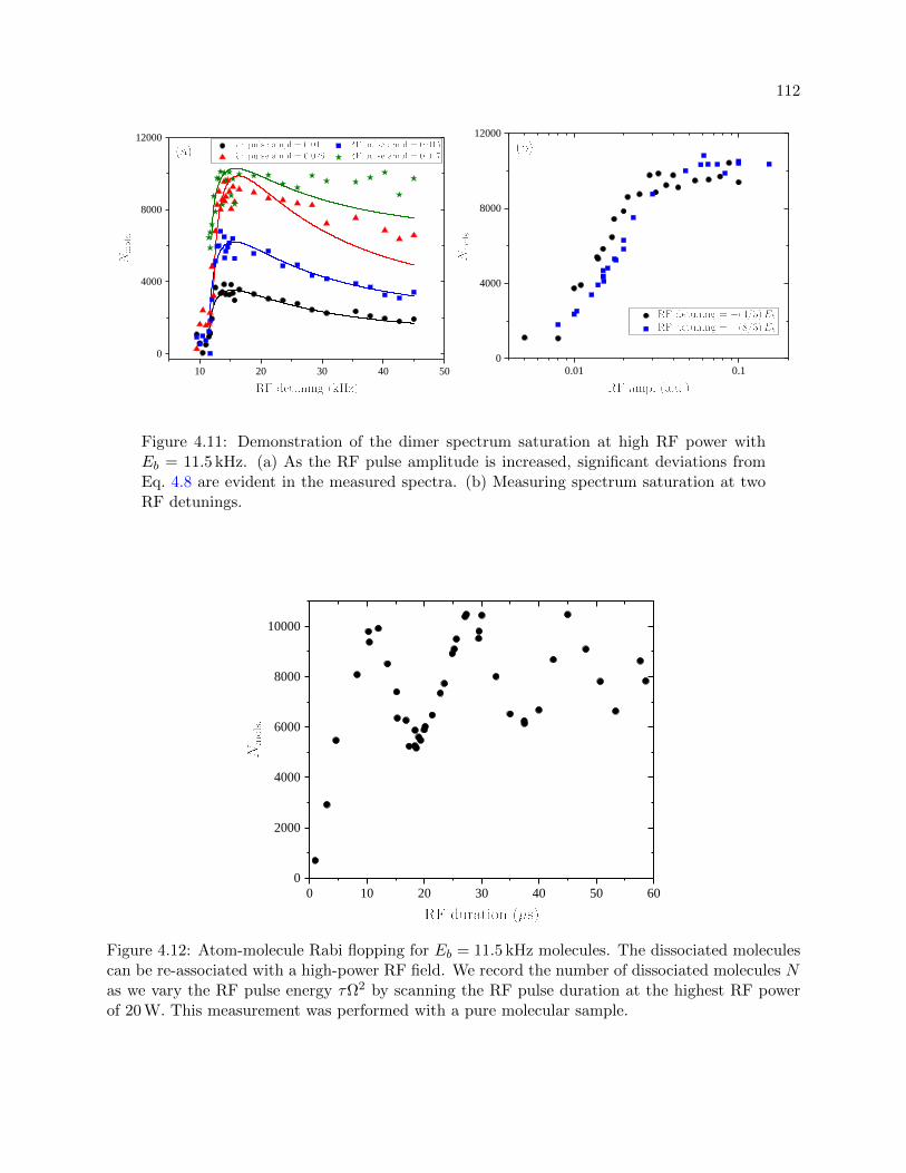
112

1 0 2 0 3 0 4 0 5 00

4 0 0 0

8 0 0 0

1 2 0 0 0

0 . 0 1 0 . 10

4 0 0 0

8 0 0 0

1 2 0 0 0

Figure 4.11: Demonstration of the dimer spectrum saturation at high RF power withEb = 11.5 kHz. (a) As the RF pulse amplitude is increased, significant deviations fromEq. 4.8 are evident in the measured spectra. (b) Measuring spectrum saturation at twoRF detunings.

0 1 0 2 0 3 0 4 0 5 0 6 00

2 0 0 0

4 0 0 0

6 0 0 0

8 0 0 0

1 0 0 0 0

Figure 4.12: Atom-molecule Rabi flopping for Eb = 11.5 kHz molecules. The dissociated moleculescan be re-associated with a high-power RF field. We record the number of dissociated molecules Nas we vary the RF pulse energy τΩ2 by scanning the RF pulse duration at the highest RF powerof 20 W. This measurement was performed with a pure molecular sample.

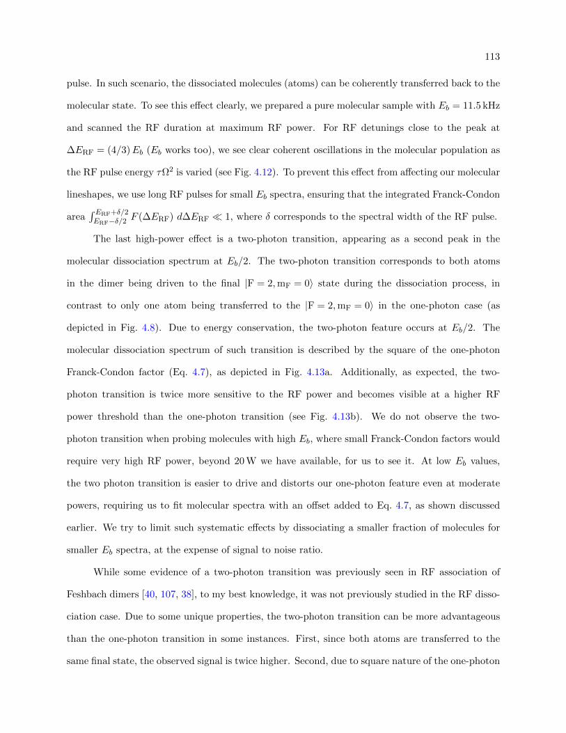
113

pulse. In such scenario, the dissociated molecules (atoms) can be coherently transferred back to the

molecular state. To see this effect clearly, we prepared a pure molecular sample with Eb = 11.5 kHz

and scanned the RF duration at maximum RF power. For RF detunings close to the peak at

∆ERF = (4/3)Eb (Eb works too), we see clear coherent oscillations in the molecular population as

the RF pulse energy τΩ2 is varied (see Fig. 4.12). To prevent this effect from affecting our molecular

lineshapes, we use long RF pulses for small Eb spectra, ensuring that the integrated Franck-Condon

area∫ ERF+δ/2ERF−δ/2 F (∆ERF) d∆ERF 1, where δ corresponds to the spectral width of the RF pulse.

The last high-power effect is a two-photon transition, appearing as a second peak in the

molecular dissociation spectrum at Eb/2. The two-photon transition corresponds to both atoms

in the dimer being driven to the final |F = 2,mF = 0〉 state during the dissociation process, in

contrast to only one atom being transferred to the |F = 2,mF = 0〉 in the one-photon case (as

depicted in Fig. 4.8). Due to energy conservation, the two-photon feature occurs at Eb/2. The

molecular dissociation spectrum of such transition is described by the square of the one-photon

Franck-Condon factor (Eq. 4.7), as depicted in Fig. 4.13a. Additionally, as expected, the two-

photon transition is twice more sensitive to the RF power and becomes visible at a higher RF

power threshold than the one-photon transition (see Fig. 4.13b). We do not observe the two-

photon transition when probing molecules with high Eb, where small Franck-Condon factors would

require very high RF power, beyond 20 W we have available, for us to see it. At low Eb values,

the two photon transition is easier to drive and distorts our one-photon feature even at moderate

powers, requiring us to fit molecular spectra with an offset added to Eq. 4.7, as shown discussed

earlier. We try to limit such systematic effects by dissociating a smaller fraction of molecules for

smaller Eb spectra, at the expense of signal to noise ratio.

While some evidence of a two-photon transition was previously seen in RF association of

Feshbach dimers [40, 107, 38], to my best knowledge, it was not previously studied in the RF disso-

ciation case. Due to some unique properties, the two-photon transition can be more advantageous

than the one-photon transition in some instances. First, since both atoms are transferred to the

same final state, the observed signal is twice higher. Second, due to square nature of the one-photon

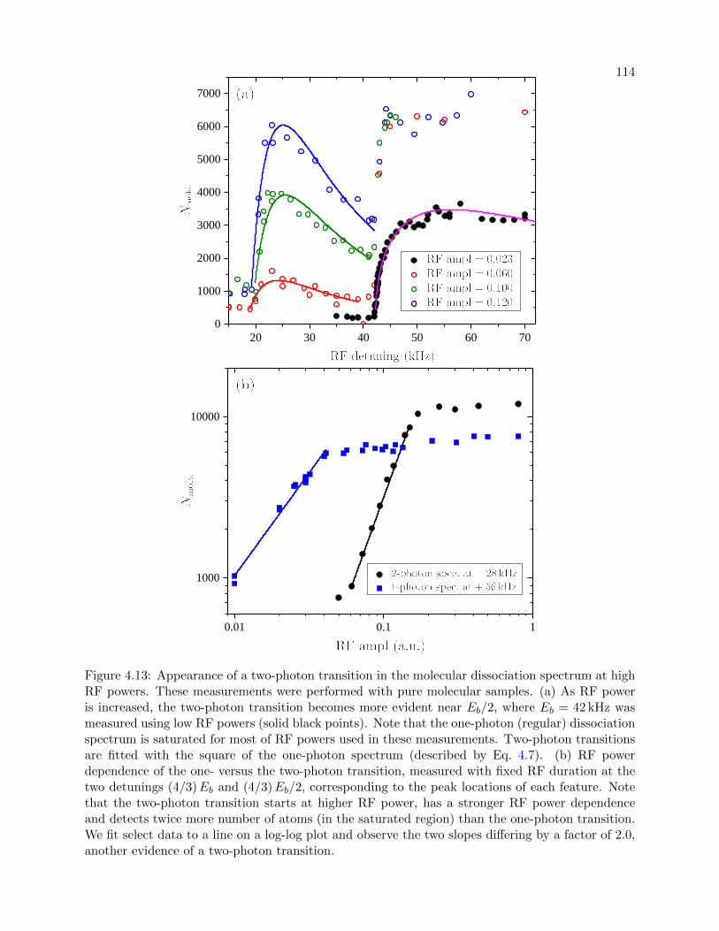
114

2 0 3 0 4 0 5 0 6 0 7 00

1 0 0 0

2 0 0 0

3 0 0 0

4 0 0 0

5 0 0 0

6 0 0 0

7 0 0 0

0 . 0 1 0 . 1 1

1 0 0 0

1 0 0 0 0

Figure 4.13: Appearance of a two-photon transition in the molecular dissociation spectrum at highRF powers. These measurements were performed with pure molecular samples. (a) As RF poweris increased, the two-photon transition becomes more evident near Eb/2, where Eb = 42 kHz wasmeasured using low RF powers (solid black points). Note that the one-photon (regular) dissociationspectrum is saturated for most of RF powers used in these measurements. Two-photon transitionsare fitted with the square of the one-photon spectrum (described by Eq. 4.7). (b) RF powerdependence of the one- versus the two-photon transition, measured with fixed RF duration at thetwo detunings (4/3)Eb and (4/3)Eb/2, corresponding to the peak locations of each feature. Notethat the two-photon transition starts at higher RF power, has a stronger RF power dependenceand detects twice more number of atoms (in the saturated region) than the one-photon transition.We fit select data to a line on a log-log plot and observe the two slopes differing by a factor of 2.0,another evidence of a two-photon transition.

115

Franck-Condon factor (Eq. 4.7), the transition is sharper near the dissociation threshold at Eb/2

than near the threshold at Eb. Third, one can use RF photons of two different frequencies to drive

this transition. By using both positive and negative RF detunings for the two RF fields, one can

shift the two-photon feature to higher RF detunings, away from the (free-free) atom transition,

allowing one to probe very small binding energies. Last, one can compare one- and two-photon

transition spectra to extract energy shifts resulting from dimer-dimer and atom-dimer interactions.

4.4 Creating a Pure Molecular Sample

4.4.1 The Affect of Residual Unpaired Atoms on Molecular Dissociation Spectra

Since the magneto-association process is not perfect, a significant portion (> 80%) of atoms

remain in the unpaired state. RF pulses used for molecular dissociation will also off-resonantly drive

the atomic transition |F = 1,mF = −1〉 → |F = 2,mF = 0〉. With relatively small Franck-Condon

factors, molecular dissociation transitions require significantly more RF power than atomic transi-

tions. Therefore, atomic transitions are strongly driven (multi-π Rabi flopping) during dissociation

and contribute to the molecular signal, as shown in Fig. 4.14. For very small detunings, such as

in measurements of small Eb spectra, the atomic contribution can be significant and will distort

the measured spectrum. For instance, for Eb = 15 kHz, we estimate that ∼ 20% of atoms can be

off-resonantly excited near the molecular threshold, as shown in Fig. 4.15a. Considering that we

only dissociate ∼ 50% of molecules and that magneto-association of molecules is < 20% efficient, a

20% excitation of unpaired atoms would completely wash out the molecular signal. While we can

suppress the sidebands of atomic transitions by using longer RF pulses, as depicted in Fig. 4.15b,

finite molecular lifetimes will limit the maximum duration of our pulses.

Before detailing what affects molecular lifetimes, I will discuss an additional spectroscopic

complication arising from unpaired atoms in the |F = 1,mF = 0〉 hyperfine state. We first noticed

the presence of |F = 1,mF = 0〉 atoms during measurements of molecular spectra with small Eb

values, where we see a large distortion of the molecular signal near 13.5 kHz RF detuning from

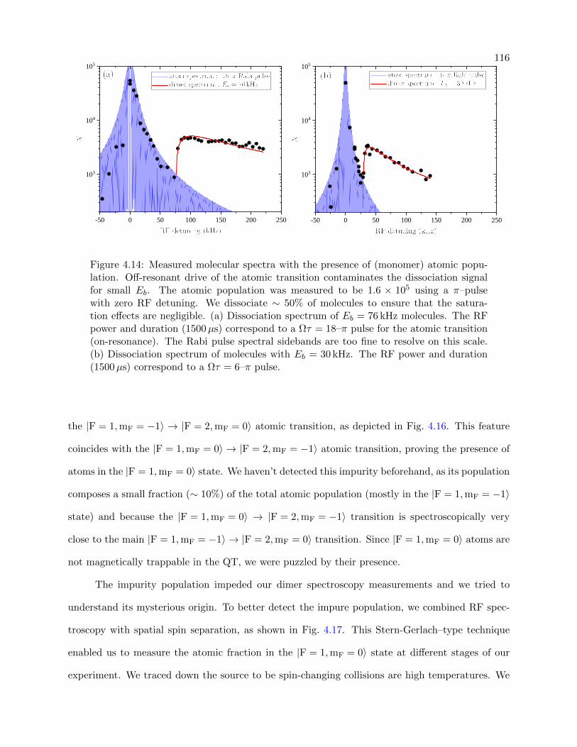
116

- 5 0 0 5 0 1 0 0 1 5 0 2 0 0 2 5 0

1 0 3

1 0 4

1 0 5

- 5 0 0 5 0 1 0 0 1 5 0 2 0 0 2 5 0

1 0 3

1 0 4

1 0 5

Figure 4.14: Measured molecular spectra with the presence of (monomer) atomic popu-lation. Off-resonant drive of the atomic transition contaminates the dissociation signalfor small Eb. The atomic population was measured to be 1.6 × 105 using a π–pulsewith zero RF detuning. We dissociate ∼ 50% of molecules to ensure that the satura-tion effects are negligible. (a) Dissociation spectrum of Eb = 76 kHz molecules. The RFpower and duration (1500µs) correspond to a Ωτ = 18–π pulse for the atomic transition(on-resonance). The Rabi pulse spectral sidebands are too fine to resolve on this scale.(b) Dissociation spectrum of molecules with Eb = 30 kHz. The RF power and duration(1500µs) correspond to a Ωτ = 6–π pulse.

the |F = 1,mF = −1〉 → |F = 2,mF = 0〉 atomic transition, as depicted in Fig. 4.16. This feature

coincides with the |F = 1,mF = 0〉 → |F = 2,mF = −1〉 atomic transition, proving the presence of

atoms in the |F = 1,mF = 0〉 state. We haven’t detected this impurity beforehand, as its population

composes a small fraction (∼ 10%) of the total atomic population (mostly in the |F = 1,mF = −1〉

state) and because the |F = 1,mF = 0〉 → |F = 2,mF = −1〉 transition is spectroscopically very

close to the main |F = 1,mF = −1〉 → |F = 2,mF = 0〉 transition. Since |F = 1,mF = 0〉 atoms are

not magnetically trappable in the QT, we were puzzled by their presence.

The impurity population impeded our dimer spectroscopy measurements and we tried to

understand its mysterious origin. To better detect the impure population, we combined RF spec-

troscopy with spatial spin separation, as shown in Fig. 4.17. This Stern-Gerlach–type technique

enabled us to measure the atomic fraction in the |F = 1,mF = 0〉 state at different stages of our

experiment. We traced down the source to be spin-changing collisions are high temperatures. We

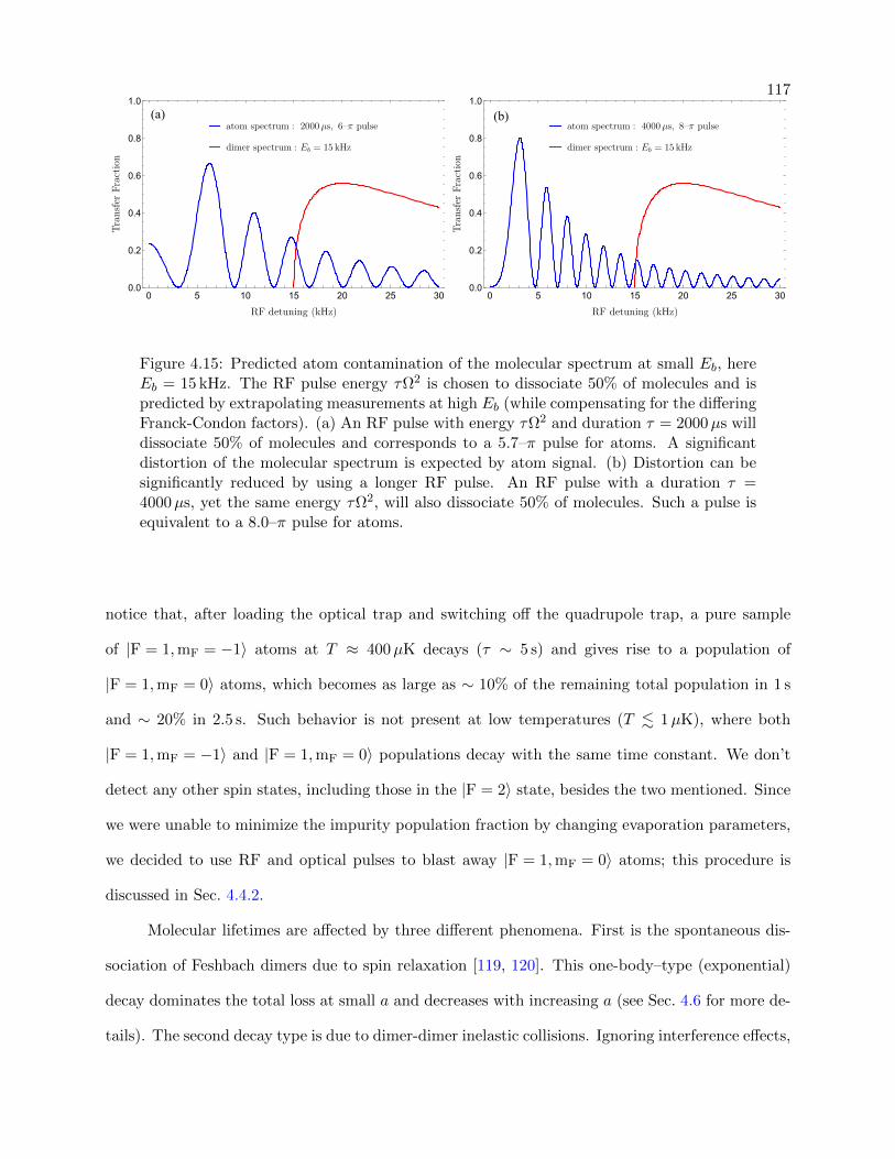
117

0 5 10 15 20 25 300.0

0.2

0.4

0.6

0.8

1.0

(a)

0 5 10 15 20 25 300.0

0.2

0.4

0.6

0.8

1.0

(b)

Figure 4.15: Predicted atom contamination of the molecular spectrum at small Eb, hereEb = 15 kHz. The RF pulse energy τΩ2 is chosen to dissociate 50% of molecules and ispredicted by extrapolating measurements at high Eb (while compensating for the differingFranck-Condon factors). (a) An RF pulse with energy τΩ2 and duration τ = 2000µs willdissociate 50% of molecules and corresponds to a 5.7–π pulse for atoms. A significantdistortion of the molecular spectrum is expected by atom signal. (b) Distortion can besignificantly reduced by using a longer RF pulse. An RF pulse with a duration τ =4000µs, yet the same energy τΩ2, will also dissociate 50% of molecules. Such a pulse isequivalent to a 8.0–π pulse for atoms.

notice that, after loading the optical trap and switching off the quadrupole trap, a pure sample

of |F = 1,mF = −1〉 atoms at T ≈ 400µK decays (τ ∼ 5 s) and gives rise to a population of

|F = 1,mF = 0〉 atoms, which becomes as large as ∼ 10% of the remaining total population in 1 s

and ∼ 20% in 2.5 s. Such behavior is not present at low temperatures (T . 1µK), where both

|F = 1,mF = −1〉 and |F = 1,mF = 0〉 populations decay with the same time constant. We don’t

detect any other spin states, including those in the |F = 2〉 state, besides the two mentioned. Since

we were unable to minimize the impurity population fraction by changing evaporation parameters,

we decided to use RF and optical pulses to blast away |F = 1,mF = 0〉 atoms; this procedure is

discussed in Sec. 4.4.2.

Molecular lifetimes are affected by three different phenomena. First is the spontaneous dis-

sociation of Feshbach dimers due to spin relaxation [119, 120]. This one-body–type (exponential)

decay dominates the total loss at small a and decreases with increasing a (see Sec. 4.6 for more de-

tails). The second decay type is due to dimer-dimer inelastic collisions. Ignoring interference effects,

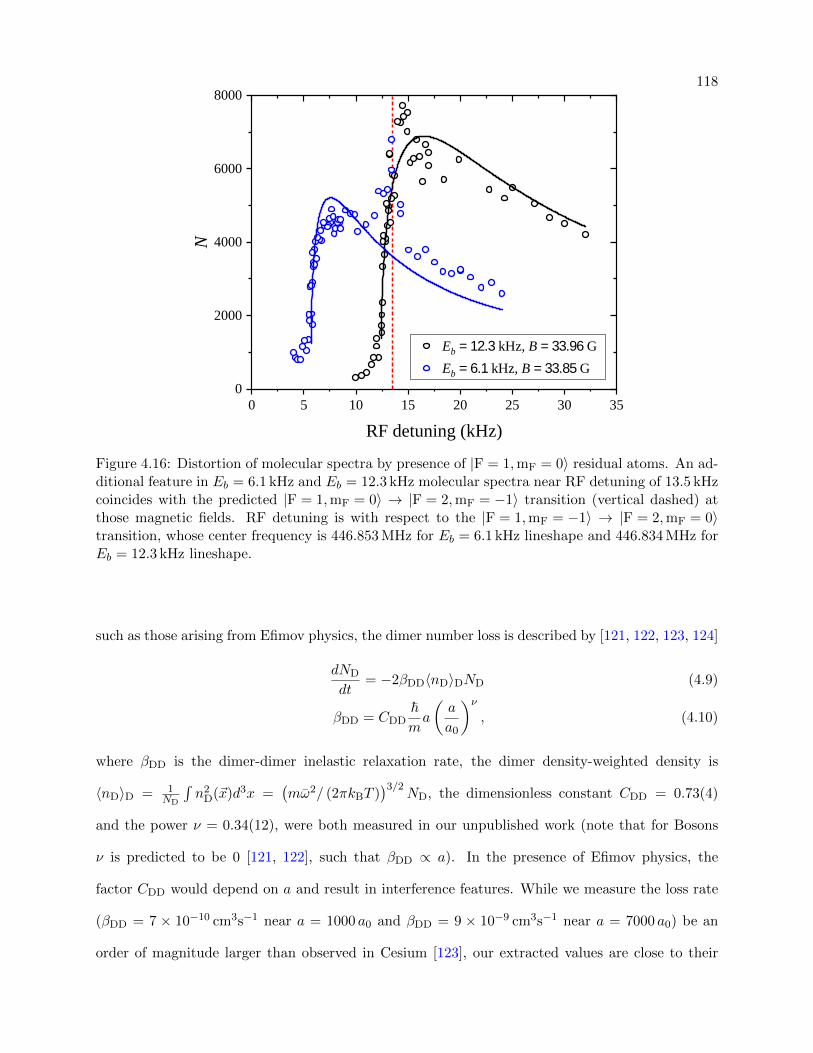
118

0 5 1 0 1 5 2 0 2 5 3 0 3 50

2 0 0 0

4 0 0 0

6 0 0 0

8 0 0 0

E b = 12.3 k H z , B = 33.96 G E b = 6.1 k H z , B = 33.85 G

N

R F d e t u n i n g ( k H z )Figure 4.16: Distortion of molecular spectra by presence of |F = 1,mF = 0〉 residual atoms. An ad-ditional feature in Eb = 6.1 kHz and Eb = 12.3 kHz molecular spectra near RF detuning of 13.5 kHzcoincides with the predicted |F = 1,mF = 0〉 → |F = 2,mF = −1〉 transition (vertical dashed) atthose magnetic fields. RF detuning is with respect to the |F = 1,mF = −1〉 → |F = 2,mF = 0〉transition, whose center frequency is 446.853 MHz for Eb = 6.1 kHz lineshape and 446.834 MHz forEb = 12.3 kHz lineshape.

such as those arising from Efimov physics, the dimer number loss is described by [121, 122, 123, 124]

dND

dt= −2βDD〈nD〉DND (4.9)

βDD = CDD~ma

(a

a0

)ν, (4.10)

where βDD is the dimer-dimer inelastic relaxation rate, the dimer density-weighted density is

〈nD〉D = 1ND

∫n2

D(~x)d3x =(mω2/ (2πkBT )

)3/2ND, the dimensionless constant CDD = 0.73(4)

and the power ν = 0.34(12), were both measured in our unpublished work (note that for Bosons

ν is predicted to be 0 [121, 122], such that βDD ∝ a). In the presence of Efimov physics, the

factor CDD would depend on a and result in interference features. While we measure the loss rate

(βDD = 7 × 10−10 cm3s−1 near a = 1000 a0 and βDD = 9 × 10−9 cm3s−1 near a = 7000 a0) be an

order of magnitude larger than observed in Cesium [123], our extracted values are close to their

119

- 2 0 0 2 0 4 00 . 0

4 . 0 x 1 0 4

8 . 0 x 1 0 4

1 . 2 x 1 0 5

0 . 0

4 . 0 x 1 0 3

8 . 0 x 1 0 3

1 . 2 x 1 0 4

Figure 4.17: Spin composition of our atomic cloud after molecular association. Using Stern-Gerlach–type technique and a 43µs RF pulse, we are able to spatially separate different spincomponents and detect a small impurity of |F = 1,mF = 0〉 atoms. Not the different y-scales.

CDD ∼ 3 and ν = 0 (fixed and observed). We suspect that some discrepancy in the values is due to

|F = 1,mF = −1〉 not being the absolute ground state. The last type of loss that limits molecular

lifetimes arises from atom-dimer inelastic collisions. Since this loss is of more-than-two-body nature

(three-body), it is strongly affected by Efimov physics and is described by [121, 31]

dnA

dt=dnD

dt= −βAD〈nA〉A〈nD〉A (4.11)

dND

dt= − 8√

27βAD〈nA〉AND

βAD =~am

20.3 sinh(2η∗)

sin2(s0 ln(a/a∗)) + sinh2(η∗)(4.12)

where βAD is the atom-dimer inelastic relaxation rate, the constant s0 ≈ 1.00624 fixes Efimov series

spacing eπ/s0 ≈ 22.7 (see Ch. 5), a∗ determines the location of the atom-dimer Efimov resonance,

where the dimer energy is degenerate with an Efimov state, and the dimensionless inelasticity

parameter η∗ characterizes the resonance width. Our unpublished measurements give a∗ = 780 a0

and η∗ = 0.21. Due to differing polarizabilities, the overlap of molecular and atomic clouds is

not unity and results in 〈nD〉A = 1ND

∫nD(~x)nA(~x)d3x = 8√

27〈nA〉A, where atom density-weighted

120

density 〈nA〉A = 1NA

∫n2

A(~x)d3x =(mω2/ (4πkBT )

)3/2NA.

Overall, the total molecular loss is given by

1

ND

dND

dt= − 1

τ1b− 2βDD〈nD〉D −

8√27βAD〈nA〉A, (4.13)

where τ1b is the a–dependent one-body decay time constant, described in detail in Sec. 4.6. Assum-

ing the three terms in Eq. 4.13 barely deplete atomic and molecular populations (a valid assumption

for short timescales), each term becomes time-independent and results in an exponential decay of

ND. We can estimate the contribution of each loss term at different scattering lengths for typ-

ical mean densities 〈nD〉D = 1 × 1010 cm−3 and 〈nA〉A = 1.4 × 1011 cm−3 (measured after the

magneto-association procedure). While at low scattering lengths the molecular loss is primarily

due to spontaneous dimer decay, atom-dimer inelastic collisions dominate the loss at high scatter-

ing lengths, as depicted in Fig. 4.18. High loss rates at large a present complications for dimer

spectroscopy at small Eb. Population decay leads to a spectral broadening of the dimer signal.

For instance, an exponential decay with τ = 0.15 ms is equivalent to a Lorentzian function with a

∆fFWHM = 1 kHz in the Fourier domain, where ∆fFWHM = 1/ (2πτ). Additionally, fast decay of

molecular signal would prevent the use of long RF pulses, which are advantageous for obtaining

uncontaminated (by atomic signal) dimer spectra. To circumvent these problems, we extend our

molecular lifetimes at high a values by getting rid of all unpaired atoms.

4.4.2 Blasting Residual Unpaired Atoms from the Trap

To extend molecular lifetimes and reduce dimer spectra distortion, we get rid of all un-

paired atoms. The full cleanup procedure, along with the probing RF and optical pulses, is shown

in Fig. 4.19. We first remove |F = 1,mF = 0〉 atoms before the molecular-association procedure.

Since dimer lifetime is short, performing this state cleanup afterward would lead to an unnec-

essary dimer loss. We begin by changing the B–field value to 35.76 G and wait 2 ms for the

field to stabilize to within ∼ 1 mG. We use a rectangular RF pulse, coming from the same an-

tenna used for the |F = 1,mF = −1〉 → |F = 2,mF = 0〉 transition, to transfer |F = 1,mF = 0〉

121

100 500 1000 5000 1040.1

1

10

100

1000

Figure 4.18: Molecular lifetime estimate for typical dimer and atomic densities of 〈nD〉D = 1 ×1010 cm−3 and 〈nA〉A = 1.4 × 1011 cm−3. Different processes limit the total molecular lifetime(black solid) at different scattering lengths, as predicted by Eq. 4.13. While spontaneous 1–bodydecay (blue dashed) is the primary loss mechanism at small a, atom-dimer inelastic collisions (reddashed) lead to most loss at high a. For this particular molecular density, the dimer-dimer inelasticloss is negligible compared to the other two mechanisms.

122

atoms to the |F = 2,mF = −1〉 state, where optical light can blast them from the trap. Since the

|F = 1,mF = 0〉 → |F = 2,mF = −1〉 transition is only 13.2 kHz detuned from the |F = 1,mF = −1〉 →

|F = 2,mF = 0〉 transition at 35.76 G, we use a 269µs pulse that only excites 2% of |F = 1,mF = −1〉

population. Such an excitation is unfavorable, as it would deplete the |F = 1,mF = −1〉 population

used for molecular association and because it is difficult to blast away |F = 2,mF = 0〉 atoms with

D2 transitions, where any chosen excited state would have a > 30% chance to decay into |F = 1〉

states. Field stability/drift prevents us from using a longer RF pulse, as a 269µs pulse already

corresponds to ∆fFWHM = 590 Hz, or equivalently 4 mG at 140 Hz/mG transition sensitivity.

We use a 100µs optical pulse, coming from top (parallel to the Feshbach field ~B, see Fig. 2.35)

and σ− polarization, to blast the atoms transferred to the |F = 2,mF = −1〉 state. We chose

the D2 |F = 2,mF = −1〉 → |F′ = 3,mF′ = −2〉 transition, since the branching ratios favor the

excited state decay predominantly into the F = 2 states: 21% to |F = 2,mF = −1〉, 65% to

|F = 2,mF = −2〉 and 14% to |F = 1,mF = −1〉. If we had chosen the D2 |F = 2,mF = −1〉 →

|F′ = 2,mF′ = −2〉 transition instead, more atoms would decay into the initial |F = 2,mF = −1〉

state, but at an expense of decaying into and contaminating the |F = 1,mF = −1〉 population:

56% to |F = 2,mF = −1〉, 1.5% to |F = 2,mF = −2〉 and 42.5% to |F = 1,mF = −1〉. Since the

blast |F = 2,mF = −1〉 → |F′ = 3,mF′ = −2〉 is not a cycling transition, > 80% of the initial

|F = 2,mF = −1〉 population quickly ends up in the |F = 2,mF = −1〉 state, without scattering

enough photons to completely blast away those atoms. Therefore, we use a second 100µs blast

pulse, using the |F = 2,mF = −2〉 → |F′ = 3,mF′ = −3〉 cycling transition that is +28 MHz de-

tuned from the first pulse frequency, to efficiently blast away all atoms that were initially in the

|F = 2,mF = −1〉 state.

After the initial impurity |F = 1,mF = 0〉 cleanup, we perform magneto-association of Fesh-

bach dimers and return the field to B = 35.76 G, where a = 480 a0 and Eb = 508 kHz. We remove

the unpaired |F = 1,mF = −1〉 atoms at this particular field, because here Eb is large enough that

are molecules unperturbed when we address atoms and because here the molecular lifetime is rel-

atively long. The dimer lifetime is primarily limited by spontaneous dissociation at this field, as

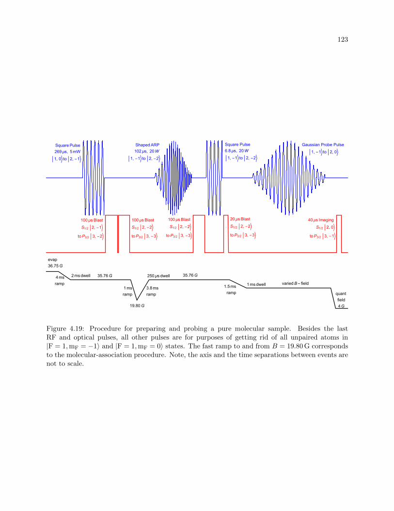
123

Square Pulse

269μs, 5mW

1, 0 to 2, -1

ShapedARP

102μs, 20W

1, -1 to 2, -2

Square Pulse

6.8μs, 20W

1, -1 to 2, -2

Gaussian Probe Pulse

1, -1 to 2, 0

100μs Blast

S1/2 2, -1

toP3/2 3, -2

100μs Blast

S1/2 2, -2

toP3/2 3, -3

100μs Blast

S1/2 2, -2

toP3/2 3, -3

20μs Blast

S1/2 2, -2

toP3/2 3, -3

40μs Imaging

S1/2 2, 0

toP3/2 3, -1

evap

36.75G

4ms

ramp

2msdwell 35.76G

1ms

ramp

3.8ms

ramp

250μs dwell 35.76G

1.5ms

ramp

1msdwell

quant

field

4G

variedB- field

19.80G

Figure 4.19: Procedure for preparing and probing a pure molecular sample. Besides the lastRF and optical pulses, all other pulses are for purposes of getting rid of all unpaired atoms in|F = 1,mF = −1〉 and |F = 1,mF = 0〉 states. The fast ramp to and from B = 19.80 G correspondsto the molecular-association procedure. Note, the axis and the time separations between events arenot to scale.

124

evidenced by an observed lifetime of τ = 3.0 ms compared to the predicted value (see Eq. 4.33) of

4 ms.

Since we desire a complete removal of unpaired |F = 1,mF = −1〉 atoms, we need to transfer

them to the |F = 2,mF = −2〉 state, where the |F = 2,mF = −2〉 → |F′ = 3,mF′ = −3〉 cycling

transition can efficiently blast them away. Initially, we tried using rectangular RF π–pulses to

achieve this transfer. While such pulses can be 99% efficient when first optimized, field drift makes

the transition only ∼ 95% efficient (without re-optimizing) on a day-to-day basis. Additionally, due

to fast molecular decay, we perform this RF transfer immediately after the magneto-association

B–field jump, when the field has not fully settled to its new value. We can estimate the required

tolerance on the B–field stability from the ratio of the effective Ωeff =√

Ω2 + δ2 and on-resonance

Ω Rabi frequencies, setting the detuning δ equal to the product of deviation δB and transition

sensitivity ∆µ = 1.8 kHz/mG. Assuming we desire 99% RF π–pulse transfer efficiency, this results

in stringent requirements: δB = 11 mG for a 7µs pulse and δB = 4 mG for a 20µs pulse.

An alternative is to use an adiabatic rapid passage (ARP), which is less sensitive to the

magnetic field noise. Due to short dimer lifetimes, we require a short-duration ARP, and therefore

a high Rabi frequency Ω. However, since the frequency sweep range must be large compared to Ω

for a high transfer efficiency, we cannot utilize this “standard” ARP for our purposes, where the

molecular transition is only 500 kHz away. To circumvent this problem, we dynamically change Ω

(an ARP pulse with a Gaussian-shaped amplitude profile, as shown in Fig. 4.20) during the RF

frequency sweep. As a result, the dressed state energies approach (see Fig. 4.21) the undressed

state values much faster (at detunings away from the resonance) than if one were to use a standard

ARP technique, where Ω is constant. This “shaped” ARP enables us to perform the state transfer

quickly (in 102µs) and within a small frequency span (±150 kHz around the resonance at 391 MHz,

Ω = 140 kHz). We achieve transfer efficiencies exceeding 99% and rarely require re-optimization

using this shaped ARP technique.

Immediately (10µs) after the RF transfer pulse, we blast |F = 2,mF = −2〉 atoms from the

trap. Since the cloud of unpaired atoms is optically dense and because dimers are relatively sensitive

125

Figure 4.20: Scope trace of a Gaussian-shaped ARP pulse used for the efficient population transferfrom the |F = 1,mF = −1〉 state to the |F = 2,mF = −2〉 state. We use a pickup antenna to observethe amplitude profile (blue trace) of a Gaussian pulse (σ = 17µs and duration of 6σ = 102µs).We use a coupled port (green trace) of an arbitrary waveform generator, which sends the FMinformation to a frequency synthesizer, to look at the frequency sweep of the pulse, which startsat 391 MHz− 150 kHz and ends at 391 MHz + 150 kHz. The frequency sweep starts and ends 2µsbefore and after RF power is sent to the antenna.

126

Figure 4.21: Dressed state picture of a shaped ARP. The goal is to transfer atoms from the undressedstate |0〉 to the undressed state |1〉. In the presence of an RF coupling field with Rabi frequencyΩ and detuning δ from the resonance, the two dressed states |+〉 and |−〉 are the eigenstatesof the interaction Hamiltonian, which are split by ~Ω energy at δ = 0. For large RF δ, thedressed state energies are similar to those of the undressed states. One can transfer atoms from|0〉 to |1〉 by sweeping the RF frequency from negative to positive detuning during the pulse. Fora standard/unshaped ARP, Ω is constant throughout the sweep and the dressed state energiesapproach the undressed state energy values slower (away from the resonance) than if one were tochange Ω dynamically during the sweep. A shaped ARP enables efficient population transfer withsmaller frequency sweeps than the standard ARP, while allowing the same/fast transfer times (setby the energy gap between the dressed states). Likewise, a shaped ARP enables faster sweeps thana standard ARP, if the detuning span is fixed to be the same for both. Here δ spans 3Ω and theshaped ARP has a Gaussian-shaped profile that decays to ±3σ amplitudes at the starting andending δ values.

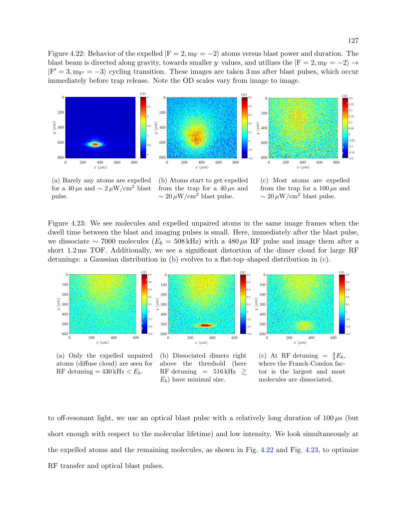
127

Figure 4.22: Behavior of the expelled |F = 2,mF = −2〉 atoms versus blast power and duration. Theblast beam is directed along gravity, towards smaller y–values, and utilizes the |F = 2,mF = −2〉 →|F′ = 3,mF′ = −3〉 cycling transition. These images are taken 3 ms after blast pulses, which occurimmediately before trap release. Note the OD scales vary from image to image.

0 200 400 600 800

0

200

400

600

8000

0.5

1

1.5

2

2.5

3

(a) Barely any atoms are expelledfor a 40µs and ∼ 2µW/cm2 blastpulse.

0 200 400 600 800

0

200

400

600

800 -0.2

-0.1

0

0.1

0.2

0.3

0.4

0.5

(b) Atoms start to get expelledfrom the trap for a 40µs and∼ 20µW/cm2 blast pulse.

0 200 400 600 800

0

200

400

600

800 -0.2

-0.15

-0.1

-0.05

0

0.05

0.1

0.15

0.2

0.25

0.3

(c) Most atoms are expelledfrom the trap for a 100µs and∼ 20µW/cm2 blast pulse.

Figure 4.23: We see molecules and expelled unpaired atoms in the same image frames when thedwell time between the blast and imaging pulses is small. Here, immediately after the blast pulse,we dissociate ∼ 7000 molecules (Eb = 508 kHz) with a 480µs RF pulse and image them after ashort 1.2 ms TOF. Additionally, we see a significant distortion of the dimer cloud for large RFdetunings: a Gaussian distribution in (b) evolves to a flat-top–shaped distribution in (c).

0 200 400 600

0

100

200

300

400

500

600 -0.3

-0.2

-0.1

0

0.1

0.2

0.3

0.4

0.5

(a) Only the expelled unpairedatoms (diffuse cloud) are seen forRF detuning = 430 kHz < Eb.

0 200 400 600

0

100

200

300

400

500

600 -0.3

-0.2

-0.1

0

0.1

0.2

0.3

0.4

0.5

(b) Dissociated dimers rightabove the threshold (hereRF detuning = 516 kHz &Eb) have minimal size.

0 200 400 600

0

100

200

300

400

500

600 -0.3

-0.2

-0.1

0

0.1

0.2

0.3

0.4

0.5

(c) At RF detuning = 43Eb,

where the Franck-Condon fac-tor is the largest and mostmolecules are dissociated.

to off-resonant light, we use an optical blast pulse with a relatively long duration of 100µs (but

short enough with respect to the molecular lifetime) and low intensity. We look simultaneously at

the expelled atoms and the remaining molecules, as shown in Fig. 4.22 and Fig. 4.23, to optimize

RF transfer and optical blast pulses.

128

While the forementioned procedures successfully eliminate ∼ 99% of unpaired atoms, the

remaining population (on the order of few thousand atoms) can still affect dimer lifetimes and

distort molecular spectra of a few thousand molecules. Therefore, we use another series of cleaning

RF (6µs rectangular π–pulse) and optical (20µs) pulses to completely deplete the |F = 1,mF = −1〉

unpaired atom population and leave us with a pure molecular sample. Aside from cleaner molecular

dissociation lineshapes, we notice an increase in dimer lifetimes after getting rid of residual atoms,

as depicted in Fig. 4.24. With the lack of atom-dimer inelastic collisions, a significant increase in

dimer lifetime at high a enables us to achieve high spectral resolution by using long-duration RF

dissociation pulses.

0 4 8 1 2 1 6

2 0 0 0

4 0 0 0

6 0 0 0

8 0 0 01 0 0 0 01 2 0 0 0

Figure 4.24: Molecular lifetimes with and without the presence of unpaired atoms. While dimerlifetime at low a is primarily limited by spontaneous dissociation, lifetimes at high a are limitedby atom-dimer inelastic collisions. The measured dimer lifetimes agree with the prediction (seeFig. 4.18) in the absence of unpaired atoms.

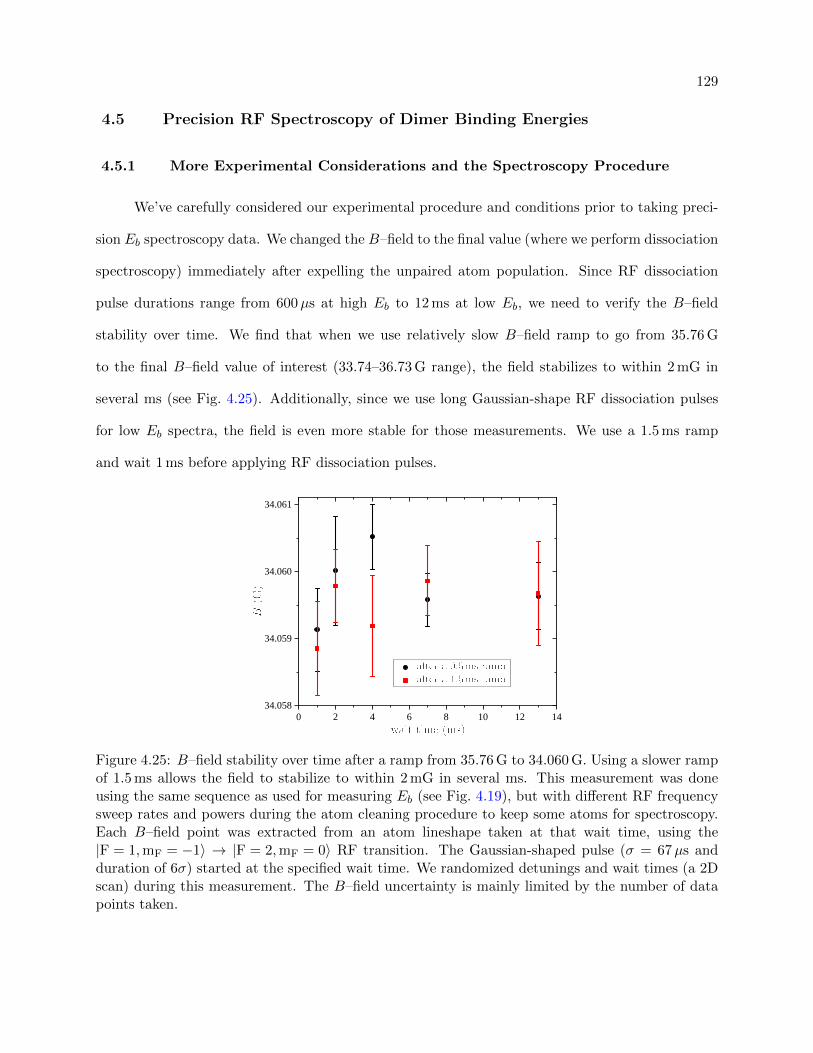
129

4.5 Precision RF Spectroscopy of Dimer Binding Energies

4.5.1 More Experimental Considerations and the Spectroscopy Procedure

We’ve carefully considered our experimental procedure and conditions prior to taking preci-

sion Eb spectroscopy data. We changed the B–field to the final value (where we perform dissociation

spectroscopy) immediately after expelling the unpaired atom population. Since RF dissociation

pulse durations range from 600µs at high Eb to 12 ms at low Eb, we need to verify the B–field

stability over time. We find that when we use relatively slow B–field ramp to go from 35.76 G

to the final B–field value of interest (33.74–36.73 G range), the field stabilizes to within 2 mG in

several ms (see Fig. 4.25). Additionally, since we use long Gaussian-shape RF dissociation pulses

for low Eb spectra, the field is even more stable for those measurements. We use a 1.5 ms ramp

and wait 1 ms before applying RF dissociation pulses.

0 2 4 6 8 1 0 1 2 1 43 4 . 0 5 8

3 4 . 0 5 9

3 4 . 0 6 0

3 4 . 0 6 1

Figure 4.25: B–field stability over time after a ramp from 35.76 G to 34.060 G. Using a slower rampof 1.5 ms allows the field to stabilize to within 2 mG in several ms. This measurement was doneusing the same sequence as used for measuring Eb (see Fig. 4.19), but with different RF frequencysweep rates and powers during the atom cleaning procedure to keep some atoms for spectroscopy.Each B–field point was extracted from an atom lineshape taken at that wait time, using the|F = 1,mF = −1〉 → |F = 2,mF = 0〉 RF transition. The Gaussian-shaped pulse (σ = 67µs andduration of 6σ) started at the specified wait time. We randomized detunings and wait times (a 2Dscan) during this measurement. The B–field uncertainty is mainly limited by the number of datapoints taken.

130

We chose the |F = 1,mF = −1〉 → |F = 2,mF = 0〉 RF transition (∼ 447 MHz) that is the

least magnetically sensitive transition in the vicinity of the Feshbach resonance: ∆µ = −171 Hz/mG

at 33.74 G (where Eb ≈ 2 kHz) and ∆µ = −122 Hz/mG at 36.73 G (where Eb ≈ 1170 kHz). Field

stability is more critical for low Eb spectroscopy, the field drift limits the lowest Eb values we can

measure. The dissociation spectra at high Eb values is less sharp near the threshold (as illustrated

in Fig. 4.9), and therefore is less impacted by magnetic field drift.

We measure the magnetic field value for each Eb spectrum by using atomic spectroscopy,

converting the lineshape center to a B value using the Breit-Rabi formula. We take atom lineshapes

before and after performing dissociation spectroscopy at each Eb value to take into account B–field

drift during measurements. For this purpose, we use the same procedure as used for molecular

spectroscopy, but modify RF parameters in the atom cleaning part to leave an atomic population.

After magneto-association procedure, we wait an extra 10 ms after molecular-association ramp to

decay away all dimers (only atoms remain; we also kill off most atoms, to be discussed shortly) and

perform all B–field ramps in a similar manner. To mitigate systematic error arising from B–field

dynamics (as in Fig. 4.25), the π–pulse used for atom spectroscopy is centered (time-wise) on what

would be the molecular dissociation pulse if we had done molecular spectroscopy. Additionally, we

limit systematic shifts arising from mean-field by using a small atomic population for spectroscopy.

We found that by varying the ARP frequency sweep span during atom cleaning procedure, we are

able to control the atom number and have repeatable conditions. We can estimate the interaction

energy shift (per particle) of a thermal gas using [125]:

∆E =4π~2

mna

(1 +

128

15√π

√na3 +O(na3) + · · ·

), (4.14)

where n = 〈n〉 is the density-weighted density. Only the first term in the expression is regarded

as the mean-field term, while the second as the LHY correction. Considering that the magnetic

sensitivity ∆µ of the |F = 1,mF = −1〉 → |F = 2,mF = 0〉 transition is small, even moderate inter-

action shifts can significantly affect the B–field measurement. Therefore, we use relatively small

atom densities spanning from 〈n〉 = 3× 1010 cm−3 at high a to 〈n〉 = 1× 1010 cm−3 at low a, where

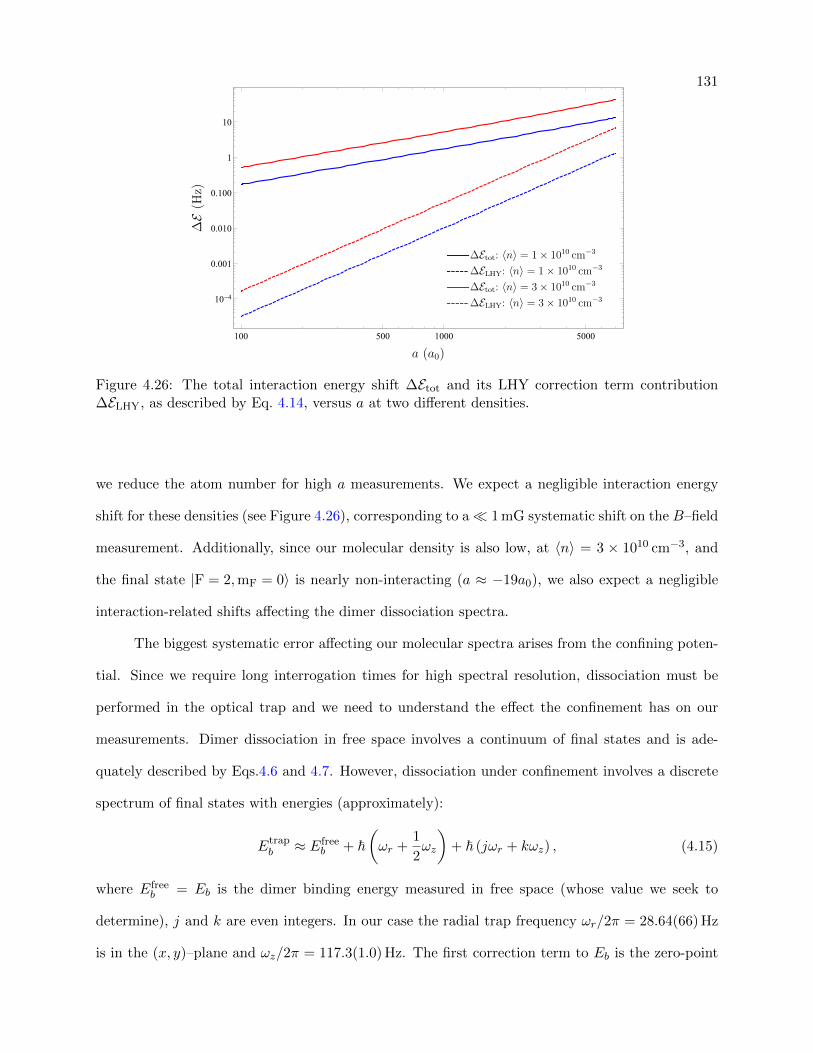
131

100 500 1000 5000

10-4

0.001

0.010

0.100

1

10

Figure 4.26: The total interaction energy shift ∆Etot and its LHY correction term contribution∆ELHY, as described by Eq. 4.14, versus a at two different densities.

we reduce the atom number for high a measurements. We expect a negligible interaction energy

shift for these densities (see Figure 4.26), corresponding to a 1 mG systematic shift on the B–field

measurement. Additionally, since our molecular density is also low, at 〈n〉 = 3 × 1010 cm−3, and

the final state |F = 2,mF = 0〉 is nearly non-interacting (a ≈ −19a0), we also expect a negligible

interaction-related shifts affecting the dimer dissociation spectra.

The biggest systematic error affecting our molecular spectra arises from the confining poten-

tial. Since we require long interrogation times for high spectral resolution, dissociation must be

performed in the optical trap and we need to understand the effect the confinement has on our

measurements. Dimer dissociation in free space involves a continuum of final states and is ade-

quately described by Eqs.4.6 and 4.7. However, dissociation under confinement involves a discrete

spectrum of final states with energies (approximately):

Etrapb ≈ Efree

b + ~(ωr +

1

2ωz

)+ ~ (jωr + kωz) , (4.15)

where Efreeb = Eb is the dimer binding energy measured in free space (whose value we seek to

determine), j and k are even integers. In our case the radial trap frequency ωr/2π = 28.64(66) Hz

is in the (x, y)–plane and ωz/2π = 117.3(1.0) Hz. The first correction term to Eb is the zero-point

132

energy Eho0 , in our case Eho

0 = 87.3(1.4) Hz. The second correction term describes the excited

harmonic states that must be symmetric (integers j and k must be even) due to parity of the initial

molecular state. However, we do not resolve these trap levels. First, our transition sensitivity

∆µ ∼ 170 Hz/mG and field stability of ∼ 1 mG wash away spectral features < 100 Hz. Second,

we use Gaussian probe pulses with a maximal duration of 6σt ∼ 12 ms (limited by dimer lifetime),

corresponding to a minimal spectral width of ∆fFWHM =√

ln(2)/(πσt) ∼ 133 Hz, that further

cloak these fine trap features.

While Eq. 4.15 is useful for comprehension, it is only an approximation and does not describe

the true energy spectrum of an interacting two-body quantum system in a trap. The Hamiltonian

of this system is

H = − ~2

2m∇2

1 −~2

2m∇2

2 + Vtrap(r1) + Vtrap(r2) + Vint(r1 − r2), (4.16)

Vtrap(r) =1

2m(ω2rρ

2 + ω2zz

2), (4.17)

Vint(r1 − r2) =4π~2a

mδ(r1 − r2)

∂

∂rr, (4.18)

where r1 and r2 are the locations of the two atoms, ρ2 = x2 + y2 and Vint is the contact interaction

potential with s–wave scattering length a. By decoupling center of mass and relative motions,

one can determine the eigenstate energies as a function of scattering length using two expressions

(Ref. 126):

F(x) = 11.137

[η

2π

∞∑n=0

(Γ(x+ nη)

Γ(x+ nη + 1/2)− 1√

η(n+ 1)

)+

√η

2πζ

(1

2

)], (4.19)

1

a= − 1√

πF(−E/2), (4.20)

where Γ is the Euler gamma function, ζ is the Riemann zeta function, η = ωr/ωz is the trap aspect

ratio, the summation index n corresponds to the radial quantum number and E = E − Eho0 is the

difference between the absolute energy and the zero-point energy. Here, all energies and lengths are

expressed in units of ~ωz and the harmonic oscillator length lz =√~/ (ωzm/2). We determined

that a prefactor of 11.137 is needed in Ref. 126.

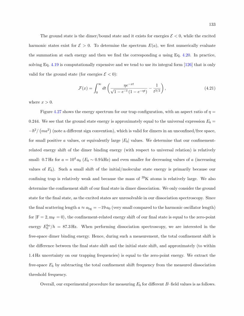
133

The ground state is the dimer/bound state and it exists for energies E < 0, while the excited

harmonic states exist for E > 0. To determine the spectrum E(a), we first numerically evaluate

the summation at each energy and then we find the corresponding a using Eq. 4.20. In practice,

solving Eq. 4.19 is computationally expensive and we tend to use its integral form [126] that is only

valid for the ground state (for energies E < 0):

F(x) =

∫ ∞0

dt

(ηe−xt√

1− e−t (1− e−ηt)− 1

t3/2

), (4.21)

where x > 0.

Figure 4.27 shows the energy spectrum for our trap configuration, with an aspect ratio of η =

0.244. We see that the ground state energy is approximately equal to the universal expression Eb =

−~2/(ma2

)(note a different sign convention), which is valid for dimers in an unconfined/free space,

for small positive a values, or equivalently large |Eb| values. We determine that our confinement-

related energy shift of the dimer binding energy (with respect to universal relation) is relatively

small: 0.7 Hz for a = 104 a0 (Eb ∼ 0.9 kHz) and even smaller for decreasing values of a (increasing

values of Eb). Such a small shift of the initial/molecular state energy is primarily because our

confining trap is relatively weak and because the mass of 39K atoms is relatively large. We also

determine the confinement shift of our final state in dimer dissociation. We only consider the ground

state for the final state, as the excited states are unresolvable in our dissociation spectroscopy. Since

the final scattering length a ≈ abg = −19 a0 (very small compared to the harmonic oscillator length)

for |F = 2,mF = 0〉, the confinement-related energy shift of our final state is equal to the zero-point

energy Eho0 /h = 87.3 Hz. When performing dissociation spectroscopy, we are interested in the

free-space dimer binding energy. Hence, during such a measurement, the total confinement shift is

the difference between the final state shift and the initial state shift, and approximately (to within

1.4 Hz uncertainty on our trapping frequencies) is equal to the zero-point energy. We extract the

free-space Eb by subtracting the total confinement shift frequency from the measured dissociation

threshold frequency.

Overall, our experimental procedure for measuring Eb for different B–field values is as follows.

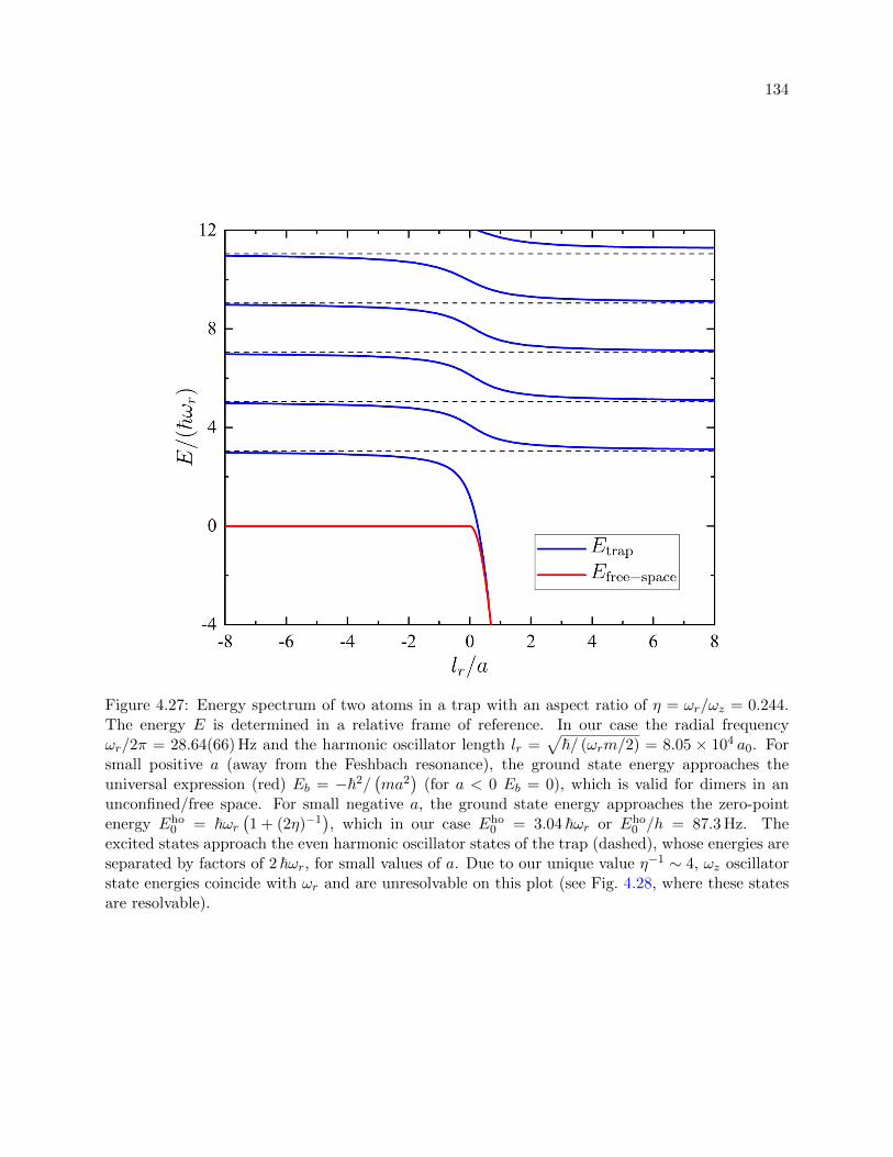
134

Figure 4.27: Energy spectrum of two atoms in a trap with an aspect ratio of η = ωr/ωz = 0.244.The energy E is determined in a relative frame of reference. In our case the radial frequencyωr/2π = 28.64(66) Hz and the harmonic oscillator length lr =

√~/ (ωrm/2) = 8.05 × 104 a0. For

small positive a (away from the Feshbach resonance), the ground state energy approaches theuniversal expression (red) Eb = −~2/

(ma2

)(for a < 0 Eb = 0), which is valid for dimers in an

unconfined/free space. For small negative a, the ground state energy approaches the zero-pointenergy Eho

0 = ~ωr(1 + (2η)−1

), which in our case Eho

0 = 3.04 ~ωr or Eho0 /h = 87.3 Hz. The

excited states approach the even harmonic oscillator states of the trap (dashed), whose energies areseparated by factors of 2 ~ωr, for small values of a. Due to our unique value η−1 ∼ 4, ωz oscillatorstate energies coincide with ωr and are unresolvable on this plot (see Fig. 4.28, where these statesare resolvable).

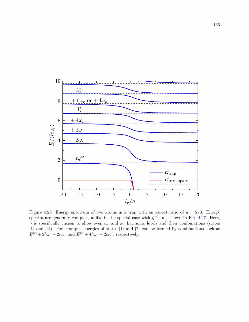
135

Figure 4.28: Energy spectrum of two atoms in a trap with an aspect ratio of η = 2/3. Energyspectra are generally complex, unlike in the special case with η−1 ≈ 4 shown in Fig. 4.27. Here,η is specifically chosen to show even ωr and ωz harmonic levels and their combinations (states|1〉 and |2〉). For example, energies of states |1〉 and |2〉 can be formed by combinations such asEho

0 + 2~ωr + 2~ωz and Eho0 + 4~ωr + 2~ωz, respectively.

136

First, we determine the B–field value by taking an atomic lineshape with a small number of atoms.

Second, we take a dissociation spectrum and extract the dissociation threshold frequency by fitting

the measured spectrum to a function that is a convolution of Eq. 4.7 and the spectrum of a Gaussian

probe pulse. Third, we determined the B–field value again. Last, we use these spectroscopic

measurements and our understanding of confinement-related frequency shifts to determine the

true free-space Eb value with a corresponding B–field value. Overall, one Eb value measurement

takes 2–3 hrs. Aside from RF amplitude, power and duration, we vary the TOF for different

Eb measurements. We decrease the TOF for high-Eb values to limit cloud’s shape distortion at

large RF detunings. While shorter TOF decreases our overall signal (the quantization field does

not fully turn on), we get better image fits and overall signal-to-noise ratio. We verified that our

experimental procedure is immune from the discussed systematic effects and that it consistently

results in the same (within error) Eb measurement.

4.5.2 Precise Binding Energy Data

Precision spectroscopy data are shown in Table 4.1. For each individual measurement, we

take weighted mean fA of the two measured atomic lineshape centers fA,1 and fA,2 to extract a

single B–field value using the Breit-Rabi formula. The weighted mean lineshape center and its

uncertainty are defined as

fA =

(N∑i=0

σ−2A,i

)−1 N∑i=0

fA,iσ−2A,i (4.22)

σA =

( N∑i=0

σ−2A,i

)−11

N − 1

N∑i=0

(fA,i − fA

)2σ2

A,i

1/2

, (4.23)

where fA,i and σA,i are lineshape centers and uncertainties of individual measurements and N is the

number of measurements (in our case N = 2). We subtract the mean atomic frequency fA from the

frequency in the dimer dissociation spectrum. Then, we fit the molecular spectrum to a function

function that is a convolution of Eq. 4.7 and the spectrum of a Gaussian probe pulse, fixing the

pulse duration and floating an overall scaling amplitude, to extract the dimer dissociation threshold

137

frequency fD. The uncertainty on fD is taken as the sum in quadrature of the fit error and the

uncertainty on the atomic transition σA, which is the dominant uncertainty at small fD. The energy

hfD corresponds to the binding energy of a dimer in a trap. To determine the confinement-related

frequency shift of initial and final states, we approximate the scattering length of initial state as

a =√hfDm/~2 and a = −19 a0 for the final state. We also take a values from theory (using B

as input) and determine similar shift values. The total confinement-related shift is similar for all

our measurements and is approximately equal to the zero point energy Eho0 = 87.3(1.4) Hz, where

the uncertainty is from uncertainty on our trapping frequencies. We subtract the total confinement

shift from the dissociation threshold frequency fD to extract the dimer binding energy in free space

Eb.

Table 4.1: Precise binding energy spectroscopy data. The B–field is determined from the weightedmean fA of two atomic lineshape centers fA,1 and fA,2, taken before and after the molecularspectrum. The molecular dissociation threshold frequency fD corresponds to the dimer bindingenergy in a trap, while Eb corresponds to the free-space dimer binding energy.

atom lineshape atom lineshape atom lineshapes corresponding mol. threshold free-spacecenter fA,1 center fA,2 mean fA B–field fD − fA Eb/h

(MHz) (MHz) (MHz) (G) (kHz) (kHz)

446.870 873(67) 446.870 945(63) 446.870 911(52) 33.7420(3) 2.190(56) 2.103(56)446.861 460(78) 446.861 312(76) 446.861 384(76) 33.7978(4) 3.989(78) 3.901(78)446.852 714(79) 446.852 546(82) 446.852 634(82) 33.8494(5) 6.095(85) 6.008(85)446.834 376(61) 446.834 445(57) 446.834 413(48) 33.9575(3) 12.274(57) 12.187(57)446.826 070(69) 446.825 957(59) 446.826 004(60) 34.0078(4) 15.708(67) 15.621(67)446.816 781(61) 446.817 086(55) 446.816 950(116) 34.0622(7) 20.139(122) 20.052(122)446.800 019(79) 446.800 145(76) 446.800 085(71) 34.1644(4) 29.919(83) 29.832(83)446.783 321(76) 446.783 547(73) 446.783 439(96) 34.2663(6) 41.847(103) 41.760(103)446.748 851(78) 446.748 911(73) 446.748 883(57) 34.4812(4) 74.382(93) 74.295(93)446.731 051(77) 446.731 033(101) 446.731 045(61) 34.5940(4) 95.395(137) 95.307(137)446.667 723(82) 446.667 598(77) 446.667 657(71) 35.0060(5) 200.293(406) 200.205(406)446.621 332(86) 446.621 191(74) 446.621 252(75) 35.3198(5) 308.716(436) 308.628(436)446.559 027(89) 446.558 891(79) 446.558 951(76) 35.7593(6) 508.003(582) 507.916(582)446.505 076(79) 446.505 255(85) 446.505 160(86) 36.1582(7) 742.262(1071) 742.175(1071)446.432 524(82) 446.432 562(79) 446.432 544(58) 36.7303(5) 1167.324(1031) 1167.237(1031)

138

4.5.3 Using Eb Data to Characterize our Feshbach Resonance

We use precision spectroscopy dimer binding energy data to accurately determine the Fesh-

bach resonance location B0. One can extract the Feshbach resonance properties by using the dimer

energy equation Eb = ~2/(ma2

)together with the scattering length relation

a(B) = abg

(1− ∆B

B −B0

), (4.24)

where the background scattering length abg, the resonance location B0 and the width ∆B are the

parameters that characterize a Feshbach resonance [19]. However, based on previous studies of

scattering properties in 39K [59, 38], the resonance near B = 34 G is affected by a nearby resonance

(see Fig. 4.29), making the isolated-resonance Eq.4.24 inapplicable. In such a scenario, a more

appropriate equation includes information about the nearby resonance [127]

a(B) = abg

(1− ∆B

B −B0− ∆B2

B −B0,2

), (4.25)

where B0,2 and ∆B2 are the location and the width of the second resonance. To be able to use

this equation for characterizing our Feshbach resonance we would need to know the details about

the second resonance. Since we didn’t perform measurements near B0,2, we would need to rely on

previous studies [59, 38] for such details. We take a rather different approach, relying on a coupled-

channel two-body model for 39K [128]. Such a model is able to predict many two-body physical

observables (for all spin states and for any B–field), including a, Eb, inelastic collision rate and

Feshbach resonances, with only two free parameters: the singlet and triplet scattering lengths as

and at characterizing interaction potentials. The model we started with was already state-of-the-art

and only required fine-tuning to match out precise Eb data, similar to Refs. [20, 111]. Therefore,

we were able to accurately predict most observables before the final fine-tuning procedure.

The first thing we do with the model is see what value of B0 does it predict and if that

value is consistent with our data. We can use Eq. 4.25 to fit the numerical map a(B) given by

the model and extract abg = −19.69 a0, B0 = 33.5808 G, ∆B = 54.50 G, B0,2 = 162.34 G and

∆B2 = −36.13 G, where all these are free parameters in the fit spanning 0–200 G. If we fix the

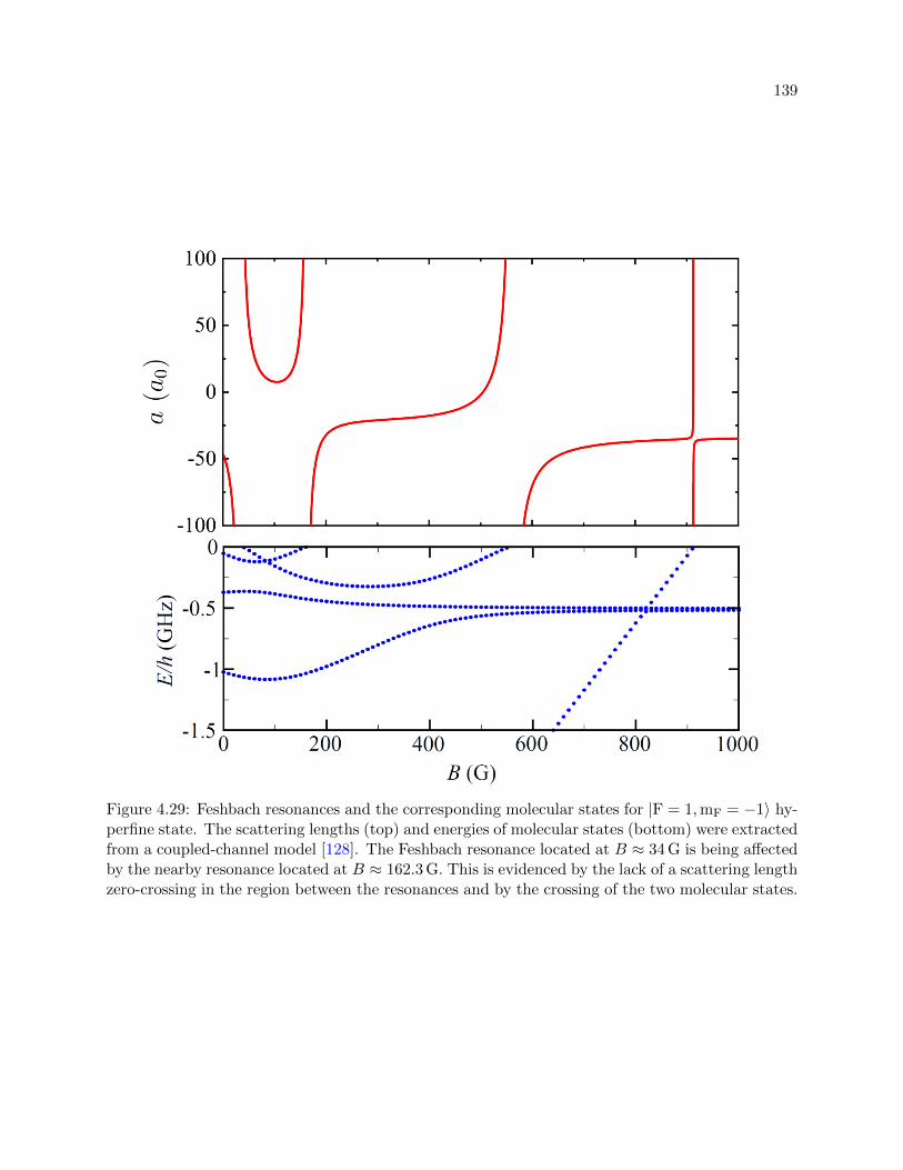
139

Figure 4.29: Feshbach resonances and the corresponding molecular states for |F = 1,mF = −1〉 hy-perfine state. The scattering lengths (top) and energies of molecular states (bottom) were extractedfrom a coupled-channel model [128]. The Feshbach resonance located at B ≈ 34 G is being affectedby the nearby resonance located at B ≈ 162.3 G. This is evidenced by the lack of a scattering lengthzero-crossing in the region between the resonances and by the crossing of the two molecular states.

140

second resonance values to be constant in the fit to Eq. 4.25 or if we fit to Eq. 4.24 (on a smaller

B–field scale), we extract the same values for B0 and for the product abg∆B (the values abg and

∆B do change). This demonstrates the robustness of finding an analytic map of a versus B. Now,

we can use Eq. 4.25 along with the universal equation for Eb to compare with our Eb(B) data. The

first thing we notice is that the universal relation for Eb becomes inapplicable for most of our data

and we resort to the well-known higher-order corrections to the binding energy:

Eb =~2

ma2, (4.26)

Eb =~2

m (a− a)2 , (4.27)

Eb =~2

m (a− a)2

(1 + g1

a

a− a+ g2

a2

(a− a)2

), (4.28)

where a = 4πrvdW/Γ(1/4) = 0.955978 . . . rvdW is the mean scattering length of the background

scattering potential [28], g1 = Γ(1/4)4/(6π2)− 2 = 0.9179 . . . and g2 = (5/4)g21 − 2 = −0.9468 . . .

[129]. In our case, the van der Waals length rvdW = 12

(mC6/~2

)1/4= 64.49 a0, where the C6

coefficient [49, 50] characterizes the strength of the van der Waals potential VvdW(r) ∝ −C6/r6 at

large inter-atomic distances r, determines the relevant length and energy scales a = 61.65 a0 and

E = ~2/ma2 = 24.37 MHz for Eb corrections.

We look at the applicability of Eqs. 4.26–4.28 by plotting Eb(a − a)2m/~2 (see Fig. 4.30),

where Eb(B) is our data and a(B) is from Eq. 4.25 with parameters taken from the model. The

data should converge to Eb(a − a)2m/~2 = 1 if the model predicts a correct value for B0. We

vary B0 in the analytic expression for a(B) (Eq. 4.25) and (visually) find that the B0 = 33.5808 G

predicted by the model is (coincidentally) a good value to within a few-mG. First, we note that

only Eq. 4.27 (with first-order a correction) matches our data. Additionally, we note that our data

does not agree with any of the Eqs. 4.26–4.28 relations away from the resonance, where Eb is large.

Such tweaking of B0 cannot make the theory match our data for all Eb values, as small adjustments

in B0 mostly affect the Eb(a − a)2m/~2 points near B0 and have little affect on the points away

from the resonance.

The applicability of simple relations for Eb discussed above is only valid when the dimer

141

10-1 1000.8

0.85

0.9

0.95

1

1.05

1.1

Figure 4.30: Comparing our Eb data with the expressions Eqs. 4.26–4.28 and approximating theFeshbach resonance location B0. Here, Eb(B) is our data and a(B) is from Eq. 4.25 with parameterstaken from the model. The different relations for Eb agree near the resonance, where Eb correctionsare small (a a, Eb E), and differ away from the resonance. We find that the universalexpression (dashed blue) with a first-order correction Eb = ~2/m (a− a)2 (dashed black, horizontal)is sufficient in describing our data near the resonance. An expression with a higher-order correction(dashed orange, Eq. 4.28, Gao) does not match our data. Additionally, we vary B0 = 33.5808 G by±4 mG (in Eq. 4.25) to see if the model predicts a correct Feshbach resonance location.

bound state has a spin character of the entrance channel [19]. A dimensionless resonance strength

parameter sres classifies Feshbach resonances into broad (entrance channel dominated) resonances

for sres 1 and narrow (closed channel dominated) resonances for sres 1:

sres =abg

a

∆µb∆B

E, (4.29)

where ∆µb is the magnetic moment of the bound state near B0 (in our case ∆µb = 2.6 MHz/G,

which is extracted from molecular spectra similar to that shown in Fig. 4.29). For narrow Feshbach

resonances, the dimer binding energy follows the universal expression only in a very narrow region

near B0 and follows the energy of the closed-channel bound state ∆µb(B − B0) away from the

resonance. While our resonance is broad in terms of width ∆B, it is of moderate width according

142

to the stated classification, with sres = 1.9.

A coupled-channel (cc) model is required to accurately describe observables near Feshbach

resonances of narrow and intermediate strength. We use such a model to predict the dimer binding

energies Eb for same B–field values as in our data. While the initial predictions matched our data

well, there was a clear trend in the relative residuals, defined as (Edatab − Etheory

b )/Edatab , that was

much larger than our experimental uncertainty. Therefore, we fine-tune the model’s singlet and

triplet potentials to accurately match most of our measurements to within 1%, as shown in Fig. 4.31

inset.

We adjust the model’s parameters by performing a global fit to our Eb(B) data. Specifically,

we adjust two parameters (we call δS and δT) that fine-tune the singlet and triplet potentials,

respectively, and which ultimately determine the singlet and triplet scattering lengths aS and aT.

The realistic two-body model is fully determined by aS and aT, allowing extraction of two-body

observables, including a(B) and molecular spectra (as shown in Fig. 4.29).

To perform the fit, we generate a grid of predicted Eb values vs. δS and δT for every exper-

imental B–field value that we have Eb data for, an example is shown in Fig. 4.32. We note that

the predicted Eb values at each magnetic field are predominately determined by a particular linear

combination of δS and δT, as evidenced by the linearity of Eb-contour lines in Fig. 4.32. Similarly,

the Feshbach resonance location B0 is predominately determined by the same linear combination.

We are able to get a better fit, and thus place tighter constraints on B0, by performing the fit in the

rotated δS and δT basis. The rotation angle is chosen to give the smallest B0 error; the angle value

is particular for our Feshbach resonance, varies negligibly for different fields and does not affect the

B0 value (to within error, see Fig. 4.33). A “local” fit uses the observed Eb value to constraint δS

and δT for each B. We use a “global” fit that constraints δS and δT using all Eb(B) data at once,

weighing each Eb data value by its uncertainty.

The fit allows us to constrain the corresponding linear combination of aS and aT to a high pre-

cision: sin(0.2496) aS + cos(0.2496) aT = 1.926(2) a0. Additionally, we deduce B0 = 33.5820(14) G,

where the uncertainty is the fit error added in quadrature with 0.5 mG, the average uncertainty on

143

3 3 . 5 3 4 . 0 3 4 . 5 3 5 . 0 3 5 . 5 3 6 . 0 3 6 . 5 3 7 . 00

2 0 0

4 0 0

6 0 0

8 0 0

1 0 0 0

1 2 0 0

1 1 0 1 0 0 1 0 0 0- 0 . 0 6

- 0 . 0 4

- 0 . 0 2

0 . 0 0

0 . 0 2

2 0 0 0 1 0 0 0 5 0 0 3 0 0

Figure 4.31: Precise measurement of Feshbach dimer binding energies Eb as a function of magneticfield B. Small experimental uncertainties on Eb, spanning from 56 Hz at Eb/h = 2.19 kHz to 1.0 kHzat Eb/h = 1167 kHz, are not resolvable in the figure. A coupled-channel (cc) model is requiredto describe our data. The solid curve shows the resulting fit and the inset shows remarkablysmall fractional residuals. Contrary to applicability near broad Feshbach resonances, universalexpressions Eqs. 4.26, 4.27 (dashed and dotted curves) are insufficient for describing Eb near ourintermediate strength resonance.

144

- 8 - 6 - 4 - 2 0 2 4 6 8- 8- 6- 4- 202468

9 2

9 3

9 4

9 5

9 6

9 7

9 8

9 9

1 0 0E b ( k H z )

Figure 4.32: A contour map shows an example of CC-model tuning at 34.5940 G. The modelpredicts Eb values for a fine δS and δT grid (points). The contour lines (magenta, spaced at 1 kHz)show that Eb values depend on a particular linear combination of δS and δT. The measured valueEb(34.5940 G) = 95.395(137) kHz can be used to constrain the model’s δS and δT values.

-0.065 -0.064 -0.063 -0.062 -0.061 -0.06 -0.059 -0.058

rotation angle (rad)

33.579

33.58

33.581

33.582

33.583

33.584

33.585

33.586

B0 (

G)

Figure 4.33: There is negligible dependence of the extracted B0 value on the angle used to rotateδS and δT basis before the fit. Here, we perform a global fit on all points, excluding the Eb pointat 36.7303 G.

B in our Eb spectroscopy data. The Eb(36.7303 G) = 1167 kHz data point leads to a significant

increase in our reduced-χ2 and we exclude it in our final fit. However, note that masking any data

(single or multiple points) in our global fit results in the same B0 value, within the quoted error.

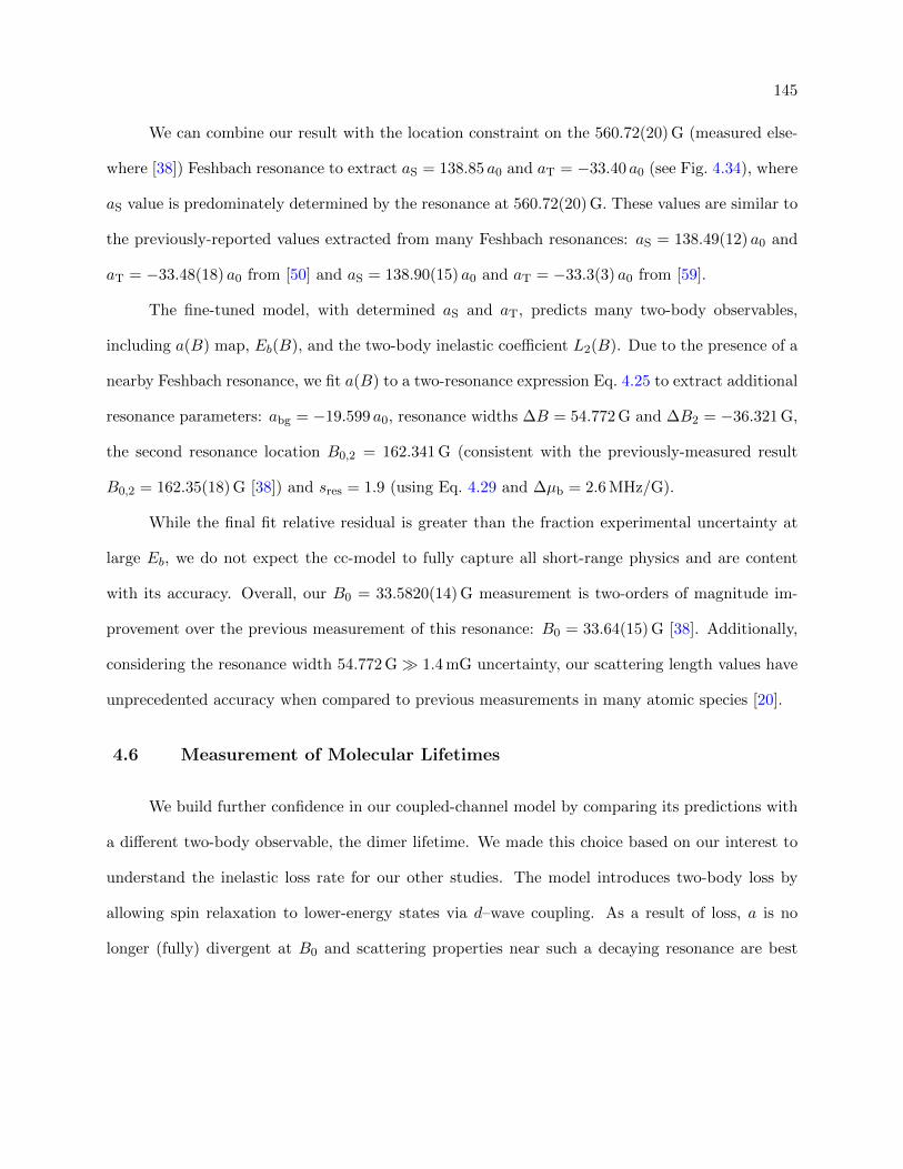
145

We can combine our result with the location constraint on the 560.72(20) G (measured else-

where [38]) Feshbach resonance to extract aS = 138.85 a0 and aT = −33.40 a0 (see Fig. 4.34), where

aS value is predominately determined by the resonance at 560.72(20) G. These values are similar to

the previously-reported values extracted from many Feshbach resonances: aS = 138.49(12) a0 and

aT = −33.48(18) a0 from [50] and aS = 138.90(15) a0 and aT = −33.3(3) a0 from [59].

The fine-tuned model, with determined aS and aT, predicts many two-body observables,

including a(B) map, Eb(B), and the two-body inelastic coefficient L2(B). Due to the presence of a

nearby Feshbach resonance, we fit a(B) to a two-resonance expression Eq. 4.25 to extract additional

resonance parameters: abg = −19.599 a0, resonance widths ∆B = 54.772 G and ∆B2 = −36.321 G,

the second resonance location B0,2 = 162.341 G (consistent with the previously-measured result

B0,2 = 162.35(18) G [38]) and sres = 1.9 (using Eq. 4.29 and ∆µb = 2.6 MHz/G).

While the final fit relative residual is greater than the fraction experimental uncertainty at

large Eb, we do not expect the cc-model to fully capture all short-range physics and are content

with its accuracy. Overall, our B0 = 33.5820(14) G measurement is two-orders of magnitude im-

provement over the previous measurement of this resonance: B0 = 33.64(15) G [38]. Additionally,

considering the resonance width 54.772 G 1.4 mG uncertainty, our scattering length values have

unprecedented accuracy when compared to previous measurements in many atomic species [20].

4.6 Measurement of Molecular Lifetimes

We build further confidence in our coupled-channel model by comparing its predictions with

a different two-body observable, the dimer lifetime. We made this choice based on our interest to

understand the inelastic loss rate for our other studies. The model introduces two-body loss by

allowing spin relaxation to lower-energy states via d–wave coupling. As a result of loss, a is no

longer (fully) divergent at B0 and scattering properties near such a decaying resonance are best

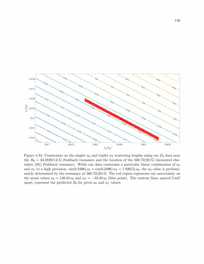
146

33.55

33.55

33.56

33.56

33.56

33.56

33.57

33.57

33.57

33.57

33.57

33.57

33.58

33.58

33.58

33.58

33.58

33.58

33.58

33.58

33.59

33.59

33.59

33.59

33.59

33.59

33.59

33.59

33.6

33.6

33.6

33.6

33.6

33.6

33.61

33.61

33.61

33.61

33.62

33.62

138.7 138.75 138.8 138.85 138.9 138.95a

S (a

0)

-33.42

-33.41

-33.4

-33.39

-33.38

-33.37

-33.36

a T (

a 0)

Figure 4.34: Constraints on the singlet aS and triplet aT scattering lengths using our Eb data nearthe B0 = 33.5820(14) G Feshbach resonance and the location of the 560.72(20) G (measured else-where [38]) Feshbach resonance. While our data constrains a particular linear combination of aS

and aT to a high precision: sin(0.2496) aS + cos(0.2496) aT = 1.926(2) a0, the aS value is predomi-nately determined by the resonance at 560.72(20) G. The red region represents our uncertainty onthe mean values aS = 138.85 a0 and aT = −33.40 a0 (blue point). The contour lines, spaced 5 mGapart, represent the predicted B0 for given aS and aT values.

147

described by a complex scattering length a = a− ib [19]:

a(B) = abg − aresγ (B −B0)

(B −B0)2 + (γ/2)2, (4.30)

b(B) =1

2ares

γ2

(B −B0)2 + (γ/2)2, (4.31)

where b is the inelastic scattering length, γ is the (Lorentzian) width of the Feshbach resonance near

B0 and ares is the maximum amplitude of the scattering length. In presence of a nearby Feshbach

resonance, the background scattering length is taken as abg(B) = abg,2 (1−∆B2/(B −B0,2)).

Using the values a(B) (or b(B)) predicted by the model, we extract γ = 0.101 mG and ares =

−1.06 × 107 a0 for our resonance; note that the resonance pole strength γares = abg∆B from

Eq. 4.24 definition. The closed channel bare state lifetime τres = (2πγµb)−1 = 610µs sets the

relevant timescale of two-body loss processes. For example, the inelastic two-body loss coefficient

L2, characterizing atom loss dN/dt = −L2〈n〉N , is determined from [130]

L2(B) =16π~m

b(B). (4.32)

Additionally, the spontaneous one-body dimer decay time τ1b, initially introduced in Sec. 4.4.1,

relates to L2 only by a volume term [104, 120]

τ1b(B) =4πa3

L2(B). (4.33)

We perform dimer lifetime measurements of pure molecular samples, prepared in a similar

fashion as described in Sec. 4.4.2. We hold molecular samples at specified B–field values for a

varied duration. Instead of using RF dissociation for molecular detection (as shown in Fig. 4.19),

we dissociate dimers by ramping the magnetic field back across the resonance to a ≈ −100 a0, an

“inverse” magneto-association method. There, we use a 5.3 ms rectangular ARP pulse to transfer

all remaining atoms from the |F = 1,mF = −1〉 state to the |F = 2,mF = −2〉 before imaging. This

method of counting molecules has several advantages over the method used for Eb spectroscopy.

We gain a factor of 2 in signal by detecting both atoms in the molecular pair and a factor of ∼ 1.7

by using the |F = 2,mF = −2〉 state for imaging rather than |F = 2,mF = 0〉 state, which has no

148

optical cycling transitions. Additionally, the efficiency and stability of the ARP and the magneto-

dissociation procedure improve our shot-to-shot number noise. These signal improvements were

crucial and allow us to measure dimer lifetimes of small-density molecular samples, whose lifetimes

were not affected by dimer-dimer inelastic loss (Eq. 4.11).

A compilation of our dimer lifetime data is presented in Fig. 4.35. We measure molecular

lifetimes from B = 33.743 G to B = 55.947 G, corresponding to ranges Eb = 0.0021–45.6 MHz and

a = 6642–35 a0. We observe an intriguing maximum near Eb = 24 MHz (a = 61 a0, B = 48.09 G)

with a lifetime of 43 ms. We can compare our data with the coupled-channel predictions in two

different ways. First, we perform a local fit to a(B) from theory using Eq. 4.30 to extract b(B)

and L2 near the resonance, and therefore τ1b(B) via the universal relation in Eq. 4.33. While we

find a good agreement between theory and our data at intermediate and high scattering lengths,

the predicted τ1b(B) values are feature-less at small a. Second, we use L2(B) values (or b(B))

directly predicted by the model, which have a complicated structure, as depicted in Fig. 4.36.

While theory does predict an L2 maximum, and hence a lifetime maximum, at small a, its position

(B = 42 G, a = 114 a0) is significantly different from the observed lifetime maximum location. Such

deviations at small scattering lengths are not surprising, considering that the universal Eq. 4.33

does not encompass short-ranged physics nor the proper spin channel composition of the deeply-

bound states. Future theoretical advancements, with models that are capable to directly predict

molecular lifetime, are required to fully understand our data.

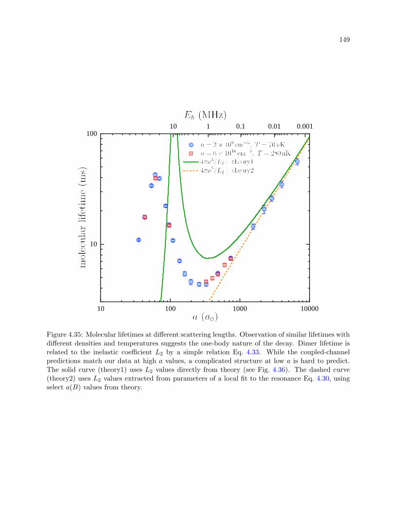
149

1 0 1 0 0 1 0 0 0 1 0 0 0 0

1 0

1 0 0

1 0 1 0 . 1 0 . 0 1 0 . 0 0 1

Figure 4.35: Molecular lifetimes at different scattering lengths. Observation of similar lifetimes withdifferent densities and temperatures suggests the one-body nature of the decay. Dimer lifetime isrelated to the inelastic coefficient L2 by a simple relation Eq. 4.33. While the coupled-channelpredictions match our data at high a values, a complicated structure at low a is hard to predict.The solid curve (theory1) uses L2 values directly from theory (see Fig. 4.36). The dashed curve(theory2) uses L2 values extracted from parameters of a local fit to the resonance Eq. 4.30, usingselect a(B) values from theory.

150

1 0 1 0 0 1 0 0 01 0 - 1 8

1 0 - 1 7

1 0 - 1 6

1 0 - 1 5

1 0 - 1 4

1 0 - 1 3

1 0 - 1 2

3 3 . 5 8 11 6 2 . 3 55 6 0 . 79 1 2 . 9

Figure 4.36: The coupled-channel model predicts a complicated behavior of the L2 inelastic coeffi-cient. The vertical dashed lines correspond to the known Feshbach resonances, shown in Fig. 4.29.

Chapter 5

Measurement of a Nonuniversal Efimov Ground State Location

Building on our understanding of two-body physics (discussed in Ch. 4), we seek to provide

some insight on the exotic three-body Efimov physics. Specifically, we precisely measure the Efimov

ground state location near our Feshbach resonance and find significant deviation from the value

predicted by van der Waals universality. I begin with an overview of how our work fits into the

bigger picture of previous Efimov studies. I detail the experimental procedure, along with the

many systematic error sources we’ve considered, to build confidence in our measurement. I briefly

mention our attempts to find signatures of the second Efimov state and four-body Efimov physics.

5.1 Previous Studies of Efimov Physics in Ultracold Gases

Although the Efimov effect was initially introduced for nuclear physics in 1970 [29], it only

gained considerable interest in the last decade after experimental observations in ultracold atomic

gases. The first evidence of an Efimov state was observed via atom-loss spectroscopy [30] in 133Cs.

The degeneracy of the Efimov trimer state energy with the three-atom threshold continuum (E = 0,

a < 0) at a = a− (see Fig 5.1) results in new decay pathways to deeply-bound molecular states

(via recombination) and leads to an enhancement of the three-body inelastic rate coefficient L3

near a = a−, an Efimov resonance. Since detection methods based on populating the Efimov

state via RF- [131, 132, 133] and magneto-association [134] are difficult and are limited by short

trimer lifetimes O(100µs), atom-loss spectroscopy proves to be the simplest and most widely-used

method for studying Efimov physics. For example, this method enabled observation of the second

152

Figure 5.1: Energy spectrum of Efimov trimer states (green lines). For a < 0, Efimov statesintersect the three-atom threshold continuum (gray region), with the ground state intersectingat a = a− (arrow). For a > 0, Efimov states intersect the atom-dimer continuum (blue region−~2/ma2 < E < 0). Each consecutive Efimov state has a spatial extent O(|a|) that is ≈ 22.7×larger than that of the previous state and an energy ≈ 22.72× smaller. This figure is borrowed fromRef. 138. For illustration purposes, Efimov scaling was changed to 2 and not all excited Efimovstates are shown.

Efimov state (and hence confirming Efimov series spacing ≈ 22.7) [43], Efimov features at a > 0

[32, 135, 33], four- and five-body Efimov states (tied to the individual three-body Efimov states)

[136, 33, 40, 137], and locations a− in multiple atomic species [52, 47, 97].

One of the biggest surprises in Efimov studies was an observed correlation between the three-

body parameter a− and the van der Waals length rvdW = 12

(mC6/~2

)1/4, which characterizes the

physical range of the van der Waals potential VvdW(r) ∝ −C6/r6 at large inter-atomic distances

r. Measurements across many atomic species and different Feshbach resonances indicate a− value

always within 20% of −9 rvdW [37, 46, 47, 48]. While the Efimov spacing was predicted to be

universal, a− was originally thought to depend on the (complicated) short-range physics at inter-

atomic distances r . rvdW, and therefore be non-universal. It is perplexing to find that a− depends

only on the long-range part of the interaction potential. This additional universal aspect of Efimov

physics was later (thought to be) theoretically understood, predicting a value a− = −9.73 rvdW

close to observations, and deemed it ”van der Waals universality” [51, 52]. Physically, a strong

153

suppression of three-body wavefunction at short distances is responsible for van der Waals uni-

versality, preventing particles from accessing nonuniversal regions of interacting potentials. Value

a− = −9.73 rvdW is predicted by a model with a hard-wall potential that masks the nonuniversal

short-range interaction region. Additionally, multiple theoretical models always predict a− values

[51, 52, 46, 47] that are within ±15% of −9.73 rvdW, where theoretical uncertainty includes the

results of multiple universal models with different details in the short-ranged region.

In principle, as a consequence of van der Waals universality and the universal Efimov spectrum

scaling, one can predict the full Efimov spectrum to arbitrary energy and length scales, given only

the chosen atomic species mass and the strength of van der Waals potential tail C6, a powerful

result. Therefore, understanding the applicability and robustness of van der Waals universality is

important.

Most studies of van der Waals universality focus on broad Feshbach resonances, where sres

1 (defined in Eq. 4.29) and universal behavior is expected. For example, sres can be thought of as

the dimensionless parameter that characterizes the region of scattering lengths over which two-body

physics follows the universal binding energy relation Eb = ~2/(ma2): |a| & 4rvdW/sres. Similarly,

since two-body interactions mediate three-body attraction in the Efimov effect, there is a notion

that three-body Efimov resonances would be more universal as they fall more deeply within the

range of a for which the two-body Feshbach resonant structure is universal.

Recent theoretical models incorporating narrow (sres 1) and broad Feshbach resonances

suggest that a− should also, in addition to the van der Waals length, depend on the background

scattering length abg, on sres, and on the details of short-range forces (e.g. three-body forces not

directly arising from two-body physics, as is the case for the Efimov effect) [53, 54, 55, 56, 57].

Previous experiments on homonuclear Efimov states [32, 33, 34, 35, 36, 37, 38, 39, 40, 41, 42, 43,

44, 45] suggest some evidence that smaller sres should correspond to less universal a− values, see the

blue circles in Fig. 5.2. Similarly, a recent indirect measurement of the a− value in a heteronuclear

system [97] suggests the same conclusion. However, such a conclusion is not concrete due to large

experimental uncertainties in the measured a−, large systematic uncertainties in the knowledge of

154

the underlying two-body Feshbach resonance [32, 38, 40, 33] and mysterious temperature-dependent

behavior [45]. Precise measurements of a− are needed to provide clarity on the applicability of van

der Waals universality near narrow and intermediate-width Feshbach resonances.

While the strongest observed departure (not including our measurement) from van der Waals

universal theory (3.7σ deviation) occurs in a 6Li– 133Cs system near a narrow Feshbach resonance

with sres = 0.05 [97], the nature of heteronuclear systems complicates interpretation of this result.

First, heteronuclear systems have more parameters, including two van der Waals lengths, two

uncorrelated scattering lengths and a mass ratio. Only specific mass ratios (large mass imbalance)

and scattering lengths conditions give rise to interspecies Efimov physics (with a modified Efimov

scaling that depends on the mass ratio) and approximate universality [139]. Second, the sign of the

scattering length between the two heavy bosons influences the a− location [140]. Third, molecular

two-body physics of heavy bosons can affect and suppress Efimov resonances [140]. In fact, in the

aforementioned result of Ref. 97, the ground Efimov resonance is completely absent and the authors

extract a− from an indirect measurement of the second Efimov resonance. Such complications in

heteronuclear systems result in a weak evidence for the inapplicability of van der Waals universality

near narrow Feshbach resonances.

Previously, the largest deviation (1.5σ) from van der Waals universal theory in a homonuclear

system was observed in 39K near a narrow Feshbach resonance with sres = 0.11 [38]. In addition

to that particular Feshbach resonance, the authors of Ref. 38 perform measurements near other

Feshbach resonances in 39K and claim evidence for extension of van der Waals universality to

narrow and intermediate Feshbach resonances. This conclusion is incorrect, as their measurements

are only consistent with universal theory as a result of large uncertainty on a− values. Furthermore,

an inconsistent use of multiple empirical fit models for a− extraction and a lack of systematic checks

(e.g. finite-temperature) leads to inconclusive results.

With many other instances of a− measurements having large statistical and systematic un-

certainties, we attempt to do better and provide compelling evidence for departure from van der

Waals universality. In our work, we accurately determine a− value near a Feshbach resonance

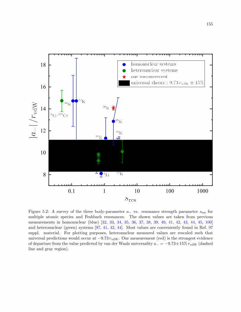
155

0.1 1 10 100 1000

8

10

12

14

16

18

Figure 5.2: A survey of the three body-parameter a− vs. resonance strength parameter sres formultiple atomic species and Feshbach resonances. The shown values are taken from previousmeasurements in homonuclear (blue) [32, 33, 34, 35, 36, 37, 38, 39, 40, 41, 42, 43, 44, 45, 100]and heteronuclear (green) systems [97, 41, 42, 44]. Most values are conveniently found in Ref. 97suppl. material. For plotting purposes, heteronuclear measured values are rescaled such thatuniversal predictions would occur at −9.73 rvdW. Our measurement (red) is the strongest evidenceof departure from the value predicted by van der Waals universality a− = −9.73±15% rvdW (dashedline and gray region).

156

of intermediate strength (sres = 1.9) by having a precise control of experimental parameters and

understanding of systematic error. As a result, we observe a− = −14.08(17) rvdW, a significant

deviation from the value −9.73 rvdW predicted by van der Waals universality. Our measurement

is the strongest evidence of departure from the value predicted by van der Waals universality and

is the first (statistically significant) evidence of departure near a Feshbach resonance of an inter-

mediate strength, as depicted in Fig. 5.2. The deviation we observe is intriguing, considering that

previous measurements of the a− near Feshbach resonances with similar sres were consistent with

van der Waals universality and that our background scattering length abg = −19.60 a0 is small

compared to a = 61.65 a0. Therefore, such a deviation cannot be explained by models with simple

corrections to universal theory [53, 54, 55, 56, 57]. We require data comparison with a state-of-the-

art three-body multi-channel model [141], constructed using realistic hyperfine and Zeeman spin

structure and with singlet and triplet potentials with details constrained by our two-body binding

energy measurements. Such a realistic model shows a better agreement with our a− measurements

and is able to, for the first time in the field, to accurately predict the Efimov resonance inelasticity

parameter η.

5.2 Experimental Considerations

To accurately determine a− from atom-loss spectroscopy, we consider and check multiple

experimental parameters that can lead to systematic error. I briefly discuss our experimental pro-

cedure and parameters that can affect our Efimov resonance measurements, including uncertainty

on a(B), trap parameters, uncertainty on atom number and temperature, high phase-space density

(PSD) effects, thermalization rate, high-density effects, two- and four-body loss, finite-temperature

systematic shifts and finite-range effects.

A typical experimental sequence for measuring three-body recombination is shown in Fig. 5.3.

A desired temperature is reached by optimizing evaporation parameters (final trap depths and fre-

quencies, duration,exponential time constant and B–field value). The density is varied by enabling

three-body loss, holding the sample at a moderate a ≈ 200–500 a0 for a duration O(10 s) before

157

and after the two evaporation stages. We do not use a large a for this loss process; doing so would

result in unnecessary heating and lack of thermalization, as the three-body loss would be faster

than thermalization/evaporation timescales. We verify the sample is thermalized by checking the

cloud’s temperature along orthogonal directions (should be equal) and if needed, hold the sample

for an extra duration before proceeding. Next, since we want to accurately measure loss and heat-

ing associated with three-body recombination, we adiabatically increase the trap depth (ramp up

horizontal and vertical beam powers) by a factor of 2–4 to prevent any further evaporation. As

a result, the mean trapping frequency increases to ωf = (Uf/Ui)1/2 ωi, where Ui and Uf are the

initial and final trap depths (assuming the same trap depth in all directions) and ωi is the initial

trap frequency. Adiabatic compression also results in heating and density increase:

Tf =ωfωiTi, (5.1)

nf =

(ωfωi

)3/2

ni. (5.2)

For example, due to such heating, the trap depth must be increased by a factor of 4 to have a

final temperature 1/2 of evaporation threshold temperature (T ∼ U/8). The adiabatic compression

ramp rate depends on the initial density and a, being O(5s) for our lowest density 〈n〉 ∼ 1010 cm−3

at 100 a0. It is always good to check the atom lifetime and the heating rate to verify that the trap

depths are sufficiently-high.

Next, we get rid of |F = 1,mF = 0〉 impurity in a similar manner as described in Sec. 4.4.2.

We ramp the field across the Feshbach resonance to B = 21.37 G (a = −102 a0) in 10 ms, perform

another thermalization check and ramp the field to the value of interest (for loss measurement) in

5 ms. After a varied hold duration, we ramp the B–field back to B = 21.37 G (a = −102 a0) in

5 ms, transfer atoms to the |F = 2,mF = −2〉 imaging state using an efficient ARP (duration 5.3 ms,

center f0 = 418.360 MHz, sweep ±4 MHz and full 20 W power, note that here our antenna is far

from its ∼ 390 MHz resonance/match frequency), and finally image atoms after a time of flight

using the |F = 2,mF = −2〉 → |F′ = 3,mF′ = −3〉 cycling transition, recording sample’s T and N .

In order to prevent a significant atom loss for our highest density samples or to prevent significant

158Square Pulse

269 μs, 5 mW

1, 0 to 2, -1

100 μs Blast

S1/2 2, -1

to P3/2 3, -2

100 μs Blast

S1/2 2, -2

to P3/2 3, -3

20 μs Imaging

S1/2 2, -2

to P3/2 3, -3

quant

field

4G

evaporation

+ adiabatic compression

4 ms ramp 2 ms dwell

10ms

ramp

35.76G

21.37G

21.37GB - field for 3 - body decay

ARP Pulse

5.3ms, 20W

1, -1 to 2, -2

B0 5 ms

ramp5 ms

ramp

Figure 5.3: Experimental sequence for three-body loss measurements.

heating for our lowest temperature samples, we slightly modify this sequence: we perform the

adiabatic trap compression step after going to a < 0 and shorten the respective B–field ramps from

10 ms to 1 ms and from 5 ms to 2 ms.

For each B–field of interest, we record atom number and temperature as a function of hold

duration. We measure the corresponding B–field value by modifying the sequence shown in Fig. 5.3:

instead of the ARP pulse, we use a 80µs |F = 1,mF = −1〉 → |F = 2,mF = 0〉 pulse after the ramp

to the field of interest to measure the atomic lineshape. Uncertainty on B–field (< 2 mG), along

with uncertainty on Feshbach resonance location (1.4 mG), set the uncertainty on a(B), allowing

us to know a to within < 0.2% near a = −1000 a0. Number loss due to three-body recombination

is described by loss expression (briefly introduced in Ch. 4) [118]

1

N

dN

dt= −L3〈n2〉 − α, (5.3)

where the constant α accounts for loss from background gas collisions (one-body and a–independent)

and 〈n2〉 = 1N

∫n3(~x)d3x = N2

(mω2/(

√12πkBT )

)3is the density-weighted square density for

159

a harmonic trap with a mean frequency ω = (ωxωyωz)1/3. Due to density inhomogeneity in a

harmonic trap, such loss results in anti-evaporation described by [118]

1

T

dT

dt=

1

3L3〈n2〉, (5.4)

assuming thermalization rate is higher than loss rate and there are no other heating sources. The

analytic solutions to the coupled Eqs. 5.3–5.4 describe the sample’s temperature and atom number

time evolution

N(t) = e−αt

(1 +

1√12α

L3

(mω2

2πkB

)3 (1− e−2αt

) N20

T 30

)−1/3

N0, (5.5)

T (t) =

(1 +

1√12α

L3

(mω2

2πkB

)3 (1− e−2αt

) N20

T 30

)1/9

T0, (5.6)

where N0 and T0 are the initial atom number and temperature. For small a and n, three-body loss

is negligible and number loss becomes purely exponential with a time constant 1/α. In the limit

α→ 0 (valid for high a and n, specifically when L3〈n2〉 α), time evolution simplifies to

N(t) =

(1 +

1√3L3

(mω2

2πkB

)3N2

0

T 30

t

)−1/3

N0, (5.7)

T (t) =

(1 +

1√3L3

(mω2

2πkB

)3N2

0

T 30

t

)1/9

T0. (5.8)

A typical time evolution is shown in Fig. 5.4, where initial Ni = 5900 and Ti = 46 nK

(corresponding to 〈n〉i = 7×1010 cm−3). We extract α = (43 s)−1 at a = −101 a0 (we use a = −62 a0

when we measure L3 for our highest density samples), where the expected three-body loss on

O(104 s) is negligible. While the measured 1/α varies slightly on trap configuration and cloud size,

it is typically 42–46 s and is always > 40 s.

While we can use Eq. 5.5 to extract an (almost accurate) L3 value from number loss, complex

loss dynamics (e.g. residual evaporation and additional heating sources) can result in a temperature

evolution that is not described by Eq. 5.6, as depicted in Fig. 5.4. Therefore, we do two things

to extract a more accurate L3 value. First, we only decay 20–30% of initial N . This ensures

that the final temperature is not near the evaporation threshold, the absolute temperature rise

160

0 5 1 0 1 50

1 0 0 0

2 0 0 0

3 0 0 0

4 0 0 0

5 0 0 0

6 0 0 0

4 0

6 0

8 0

1 0 0

1 2 0

Figure 5.4: A typical atom number and temperature (along the two imaging directions) time evolu-tion resulting from three-body decay. Here, a = −640 a0, (ωx, ωy, ωz) /2π = (26.6, 26.6, 96.4) Hz and1/α = 43 s (measured at low |a|). We fit (solid) N(t) to Eq. 5.5 and extract L3 = 1.2×10−22 cm6s−1.We can use this value of L3 to predict the expected temperature evolution T (t) (dashed) resultingfrom anti-evaporation. Sometimes, as in this case, the loss dynamics are too complex and themeasured temperatures don’t agree with the predicted heating.

is small (important as L3 value is T–dependent, to be discussed shortly) and the density doesn’t

change significantly during the decay (such that loss is fully dominated by three-body loss and not

other few-body processes). Second, we fit T (t) to an empirical formula (exponential or polynomial)

and use the fit result, along with N(t) data, to numerically solve Eq. 5.3 for L3. This procedure

ensures that we accurately follow the actual density evolution, irrespective of complexities in the

observed temperature behavior. We also extract the time-averaged temperature T and density n

that correspond to each L3 value.

Generally, three-body recombination coefficient scales as a4 [118, 142, 143]:

L3 = nlC~ma4, (5.9)

where nl is the number of atoms lost during a recombination event (for a < 0 recombination is

only to deep molecular states with energies trap depth, and hence nl = 3) and C is a numerical

constant that depends on the sign of a and recombination physics (can be a–dependent). For a < 0

161

the degeneracy of Efimov states with E = 0 threshold leads to enhanced loss (Efimov resonances)

and the three-body inelastic coefficient is described by a zero-temperature zero-range (universal)

expression [31]:

LT=03 (a) =

3~a4

m

4590 sinh(2η)

sin2(s0 ln(a/a−)) + sinh2(η), (5.10)

where the dimensionless inelasticity parameter η characterizes the Efimov resonance width and the

constant s0 ≈ 1.00624 fixes Efimov series spacing eπ/s0 ≈ 22.7.

Figure 5.5 shows a compilation of our initial L3 measurements at many scattering lengths

for a specific T ≈ 100 nK. Many systematic problems affected these initial measurements (labeled

“data 1–3”), before a measurement (labeled “data 4”) was accurately described by Eq. 5.10. Each

data set is fit to Eq. 5.10 with free parameters a−, η and fit amplitude, whose departure from unity

characterizes the uncertainty in the measured absolute density. The asymmetry in L3/a4 about

the center (and the resulting shift in the fit center), as is the case for “data 1–2”, is typically an

indication of residual evaporation loss resulting from insufficient trap depth. “Data 3” suffers from

imaging systematics, such as inaccurate probe frequency calibration, OD saturation and lineshape

broadening (from high probe intensity I/Isat and duration), resulting in incorrect absolute density

estimation and hence inaccurate absolute L3 values, as evidenced by a fit amplitude = 2.1. “Data

4” is same as “Data 3”, but with imaging corrections and has a fit amplitude close to unity, at

0.89, indicating the absolute density is correctly measured to within 6% (see Eq. 5.3), (falsely)

assuming finite-temperature corrections are minimal and Eq. 5.10 is fully applicable. Since, L3

values at small a values are minimally affected by finite-temperature effects (discussion to follow),

the observed agreement of L3 data at small a with Eq. 5.10 (or Eq. 5.9) gives further confidence

in understanding of systematic uncertainty on absolute density. Regarding statistical uncertainty,

our typical shot-to-shot stabilities are 2–3% for N and < 4% for T (corresponding to ∼ 7% for

density) at a fixed hold duration, resulting in L3 fit error ∼ 10% (combining multiple N and T at

different hold durations).

Some other systematic errors on the measured L3 arise from high PSD, lack of thermalization

162

4 0 0 6 0 0 8 0 0 1 0 0 0 1 2 0 0 1 4 0 0 1 6 0 0

1 0 - 2 3

1 0 - 2 2

1 0 - 2 1

M o d e l K 3 _ f i t _ n o K 3 m a x ( U s e r )

E q u a t i o n

h b a r = h / ( 2 * p i ) ;m = 3 8 . 9 6 3 7 0 7 * a m u ;

k B = 1 . 3 8 1 e - 2 3 ;K 3 a = ( ( 3 * h b a r * ( a * a 0 ) ^ 4 ) / m ) * ( 4 59 0 * s i n h ( 2 * e t a ) ) / ( ( s i n ( s 0 * l n ( ( a * a 0) / ( a m i n u s * a 0 ) ) ) ) ^ 2 + ( s i n h ( e t a ) ) ^

2 ) ;K 3 = a m p l * ( c m ^ - 6 ) * K 3 a ;

P l o t K 3e t a 0 . 2 3 7 0 5 ± 0 . 0 2 6 1 3a m i n u s 7 8 4 . 9 6 5 4 ± 2 5 . 0 7 4 3 5a m p l 1 . 8 2 3 6 3 ± 0 . 1 8 4 2 5R e d u c e d C h i - S q r 9 . 0 3 6 6 1R - S q u a r e ( C O D ) 0 . 9 8 0 0 1A d j . R - S q u a r e 0 . 9 7 2 0 1

M o d e l K 3 _ f i t _ n o K 3 m a x ( U s e r )

E q u a t i o n

h b a r = h / ( 2 * p i ) ;m = 3 8 . 9 6 3 7 0 7 * a m u ;

k B = 1 . 3 8 1 e - 2 3 ;K 3 a = ( ( 3 * h b a r * ( a * a 0 ) ^ 4 ) / m ) * ( 4 59 0 * s i n h ( 2 * e t a ) ) / ( ( s i n ( s 0 * l n ( ( a * a 0) / ( a m i n u s * a 0 ) ) ) ) ^ 2 + ( s i n h ( e t a ) ) ^

2 ) ;K 3 = a m p l * ( c m ^ - 6 ) * K 3 a ;

P l o t K 3 f r o m n u m e r i c se t a 0 . 2 2 0 2 ± 0 . 0 1 4 3 9a m i n u s 8 1 9 . 9 9 4 8 1 ± 1 1 . 6 7 1 2 6a m p l 2 . 1 4 4 6 8 ± 0 . 0 9 8 8 1R e d u c e d C h i - S q r 1 . 3 5 8 0 6R - S q u a r e ( C O D ) 0 . 9 9 1 9A d j . R - S q u a r e 0 . 9 8 8 6 54 0 0 6 0 0 8 0 0 1 0 0 0 1 2 0 0 1 4 0 0 1 6 0 01 0 - 3 4

1 0 - 3 3

Figure 5.5: L3 data, shown in (a), are affected by systematic shifts. The same data isplotted as L3/a

4 in (b) for a better visualization of the Efimov resonance. The dashedlines represent a4 scaling of L3 loss in absence of Efimov physics.

and other (than three-body) inelastic loss processes. If the sample’s PSD is high enough for degen-

eracy (nλ3 & 2.612, where λ = h/√

2πmkBT ), then the number loss dynamics become complicated

for a < 0 [117] and L3 values cannot be accurately extracted. For example, authors of Ref. 45 saw

unexpected behavior in the L3(a) spectrum with degenerate samples. Additionally, a lack of ther-

malization leads to an incorrect assumption about the measured density distribution, and hence

results in L3 uncertainty. To limit this effect, the inelastic collision rate ∼ L3〈n2〉 must be less than

the two-body elastic thermalization collision rate 〈n〉σ〈vrel〉/αcol, where 〈n〉 is the density-weighted

density, σ = 8πa2 is the s-wave collision cross-section, 〈vrel〉 = 4√kBT/(πm) is the average relative

velocity between two atoms in a harmonic trap and αcol ≈ 2.5–2.7 (for equal-mass atoms with s-wave

interactions in a harmonic trap) is a numerical constant describing the number of elastic two-body

collisions needed for thermalization [81, 60, 82]. Therefore, for proper thermalization, we desire low

densities and high temperatures. However, if the density is too low, then loss becomes dominated

by the two-body inelastic rate (introduced in Sec. 4.6) (1/N)dN/dt = −L2〈n〉 and the extraction

of L3 values becomes difficult. The two-body coupled-channel model (see Sec. 4.6 and Fig. 4.36)

predicts L2 ∼ 2 × 10−13 cm3s−1 near a = −1000 a0, while Eq. 5.10 predicts L3 ∼ 10−21 cm6s−1

for a = −1000 a0, a− = −908 a0 and η = 0.25. For three-body loss to completely dominate near

163

a = −1000 a0, we limit our initial sample densities to 〈n〉 > 1010 cm−3.

We typically verify that total loss is dominated by three-body recombination and not some

other-body term. There are several ways to do this. First, one can perform the same procedure as

been mentioned (decay a small fraction of atomic population and extract L3 value from Eq. 5.3)

for different initial densities. If the total loss is dominated by three-body term, then fits to Eq. 5.3

will result in same L3 values for different initial density conditions. The second method relies on

recording the sample’s decay for long durations to significantly vary the atom density during the

decay [136, 33, 43]. While the latter method is cruder, relying on good imaging (need to detect

a large dynamic range in N and T ) and assuming complete thermalization during the decay, it is

easier to implement than the first method. One can fit the number decay to a modified Eq. 5.3,

with other-body terms (e.g. L2 and L4) in addition to L3, or to an equation with a single arbitrary

z–body inelastic loss coefficient Lz:

1

N

dN

dt= −Lz〈nz−1〉 (5.11)

= −LzN z

ζ(T 3/2

)z−1 , (5.12)

where 〈nz−1〉 = 1N

∫nz(~x)d3x and the constant ζ are (for a harmonic trap):

〈nγ〉 =Nγ(2π)−3γ/2(m/(kBT ))3γ/2(ω)3γ

(1 + γ)3/2(5.13)

ζ = 128√

2π9/2

(kB

mω2

)9/2

. (5.14)

Equation 5.11 is easier to fit to than to an equation with multiple free parameters (e.g. loss

coefficients L2, L3, L4) and departure from z = 3 is an indication that other-body loss is present.

We find that for initial atom densities 1010 cm−3 < npk < 1012 cm−3 the decay solely dominated

by three-body loss, where the upper limit is consistent with preliminary predictions for L4 values

[141].

While higher temperatures are beneficial for good thermalization, finite temperature affects

the L3(a) spectrum and gives rise to the largest known systematic error. The L3(a) spectra saturate

when |a| values becomes comparable to the thermal wavelength λ = h/√

2πmkBT . Saturation at

164

unitarity (a→ ±∞) leads to a maximum three-body recombination rate coefficient L3 value, that

is only limited by the temperature and the Efimov resonance width η [39]:

Lmax3 (T ) = (1− e−4η)

36√

3π2~5

m3 (kBT )2 . (5.15)

We check this unitary limit by performing loss measurements at a > 0 and a < 0, recording L3

values of saturated L3(a) spectra at different temperatures. A good agreement between our results

and Eq. 5.15, as depicted in Fig. 5.6, indicates a good understanding of systematic error (arising

from e.g. calibration of absolute density and temperature) and confirms our direct measurements

of η = 0.25 from L3(a) spectra.

While Eq. 5.10 adequately describes L3(a) in the limit of λ a, for increasing temperatures

it becomes less valid and a finite-temperature zero-range model [39, 144] is required to describe the

three-body loss spectrum, for a < 0:

L3(a, T ) =72√

3π2~(1− e−4η

)mk6

tha2

(5.16)

×∫ ∞

0

(1− |s11(x)|2

)e−x

2/(ktha)2x∣∣∣∣1 + s11(x)(−xa−

1.017|a|

)−2is0e−2η

∣∣∣∣2dx,

where kth =√mkBT/~, x = k|a| and the complex function s11(x) is an S-matrix element from

Refs. [39] and [145], plotted in Fig. 5.7. The universal single-variable function s11(x) is analogous

to the reflection coefficient in two-port networks (e.g. optical and electrical) and has a complex

structure for small −ka values. For large a or high temperatures, s11(x) function is approximately

0 and Eq. 5.16 reduces to Eq. 5.15. If desired, one can extract L3 behavior for a > 0 using relation

s11(−ka) = e−2πs0/s∗11(ka) and replacing 1−|s11|2 with 1−|s11|2−|s12|2 in Eq. 5.16 [146, 39], where

s12 characterizes recombination to shallow dimers via atom-dimer inelastic scattering (in addition

to typical recombination into deeply bound molecular states).

Figure 5.8 shows the predicted L3(a) behavior for various temperatures. While L3 saturation

at higher temperatures severely affects the second (first-excited) Efimov resonance and limits the

possibility of its observation, the first (ground) Efimov resonance is expected to have a good contrast

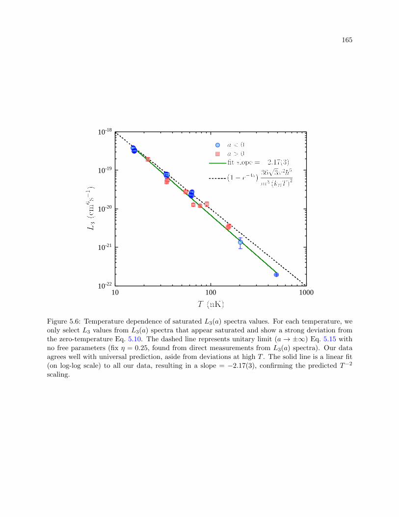
165

1 0 1 0 0 1 0 0 01 0 - 2 2

1 0 - 2 1

1 0 - 2 0

1 0 - 1 9

1 0 - 1 8

Figure 5.6: Temperature dependence of saturated L3(a) spectra values. For each temperature, weonly select L3 values from L3(a) spectra that appear saturated and show a strong deviation fromthe zero-temperature Eq. 5.10. The dashed line represents unitary limit (a → ±∞) Eq. 5.15 withno free parameters (fix η = 0.25, found from direct measurements from L3(a) spectra). Our dataagrees well with universal prediction, aside from deviations at high T . The solid line is a linear fit(on log-log scale) to all our data, resulting in a slope = −2.17(3), confirming the predicted T−2

scaling.

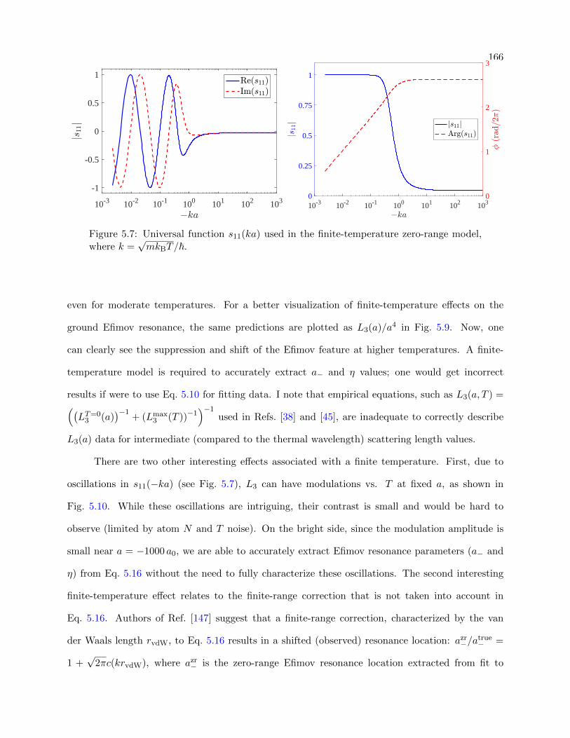
166

10-3 10-2 10-1 100 101 102 103

-1

-0.5

0

0.5

1

10-3 10-2 10-1 100 101 102 1030

0.25

0.5

0.75

1

0

1

2

3

Figure 5.7: Universal function s11(ka) used in the finite-temperature zero-range model,where k =

√mkBT/~.

even for moderate temperatures. For a better visualization of finite-temperature effects on the

ground Efimov resonance, the same predictions are plotted as L3(a)/a4 in Fig. 5.9. Now, one

can clearly see the suppression and shift of the Efimov feature at higher temperatures. A finite-

temperature model is required to accurately extract a− and η values; one would get incorrect

results if were to use Eq. 5.10 for fitting data. I note that empirical equations, such as L3(a, T ) =((LT=0

3 (a))−1

+ (Lmax3 (T ))−1

)−1used in Refs. [38] and [45], are inadequate to correctly describe

L3(a) data for intermediate (compared to the thermal wavelength) scattering length values.

There are two other interesting effects associated with a finite temperature. First, due to

oscillations in s11(−ka) (see Fig. 5.7), L3 can have modulations vs. T at fixed a, as shown in

Fig. 5.10. While these oscillations are intriguing, their contrast is small and would be hard to

observe (limited by atom N and T noise). On the bright side, since the modulation amplitude is

small near a = −1000 a0, we are able to accurately extract Efimov resonance parameters (a− and

η) from Eq. 5.16 without the need to fully characterize these oscillations. The second interesting

finite-temperature effect relates to the finite-range correction that is not taken into account in

Eq. 5.16. Authors of Ref. [147] suggest that a finite-range correction, characterized by the van

der Waals length rvdW, to Eq. 5.16 results in a shifted (observed) resonance location: azr−/a

true− =

1 +√

2πc(krvdW), where azr− is the zero-range Efimov resonance location extracted from fit to

167

500 1000 10000 50000

10-22

10-20

10-18

10-16

Figure 5.8: Finite-temperature model prediction for L3(a) behavior for various temperatures. TheT = 0 curve represents the zero-temperature Eq. 5.10 and the dashed lines represent unitary limitfor each temperature, given by Eq. 5.15. The range of a is limited to show two Efimov resonances,with a− = −908 a0, η = 0.25 and ≈ 22.7 Efimov series spacing.

500 1000 1500 200010-34

10-33

Figure 5.9: Finite-temperature model prediction for L3(a)/a4 behavior for various temperatures.The dashed T = 0 curve represents the zero-temperature Eq. 5.10.

168

100 101 102 103

0

0.2

0.4

0.6

0.8

1

1.2

Figure 5.10: Modulation in L3 vs. T for different a values. Each L3(a, T ) curve is normalized toits value at 1 nK to compare the contrast of oscillations at different a values. Since oscillations inthe s11(−ka) function quickly damp out for −ka > O(1), the modulation amplitude is largest forsmall a values and decreases for high a.

Eq. 5.16 and c = 0.60(3) is (though to be) a universal constant determined by authors of Ref. [147]

from fits to 133Cs Efimov data. However, even if such finite-range corrections are applicable to 39K,

a− temperature shifts would be small, 5% at T = 500 nK and 1% at T = 30 nK, and we do not

include such corrections in our analysis.

5.3 Precise Measurement of the Efimov Ground State Location

Fits to Eq. 5.16 enable us to extract a− and η directly from L3(a) data at any temperature.

However, we still take multiple L3(a) measurements at different temperatures to verify finite-

temperature corrections and other effects that can lead to systematic error on a− and η values. A

compilation of our L3(a) measurements is shown in Fig. 5.11. A compilation of Efimov resonance

measurement conditions and fit results is presented in Table 5.1. Each temperature data set is

described by a time-averaged temperature T , initial temperature Ti, initial mean density < n >i

and a mean trap frequency ω.

We analyze our data in two different ways. First, for each temperature, we fit our data

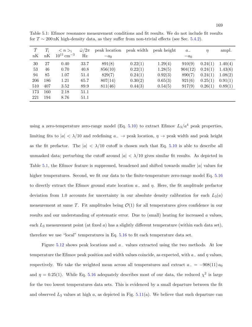
169

Table 5.1: Efimov resonance measurement conditions and fit results. We do not include fit resultsfor T ∼ 200 nK high-density data, as they suffer from non-trivial effects (see Sec. 5.4.2).

T Ti < n >i ω/2π peak location peak width peak height a− η ampl.nK nK 1011 cm−3 Hz −a0 −a0

30 27 0.40 33.7 891(8) 0.22(1) 1.29(4) 910(9) 0.24(1) 1.40(4)53 46 0.70 40.8 856(10) 0.22(1) 1.28(5) 904(12) 0.24(1) 1.43(6)94 85 1.07 51.4 829(7) 0.24(1) 0.92(3) 890(7) 0.24(1) 1.08(2)206 186 1.21 65.7 807(14) 0.30(2) 0.65(3) 921(6) 0.25(1) 0.91(1)510 407 3.52 89.9 811(46) 0.44(3) 0.54(5) 917(9) 0.26(1) 0.89(1)

173 160 2.18 51.1221 194 8.76 51.1

using a zero-temperature zero-range model (Eq. 5.10) to extract Efimov L3/a4 peak properties,

limiting fits to |a| < λ/10 and redefining a− → peak location, η → peak width and peak height

as the fit prefactor. The |a| < λ/10 cutoff is chosen such that Eq. 5.10 is able to describe all

unmasked data; perturbing the cutoff around |a| < λ/10 gives similar fit results. As depicted in

Table 5.1, the Efimov feature is suppressed, broadened and shifted towards smaller |a| values for

higher temperatures. Second, we fit our data to the finite-temperature zero-range model Eq. 5.16

to directly extract the Efimov ground state location a− and η. Here, the fit amplitude prefactor

deviation from 1.0 accounts for uncertainty in our absolute density calibration for each L3(a)

measurement at same T . Fit amplitudes being O(1) for all temperatures gives confidence in our

results and our understanding of systematic error. Due to (small) heating for increased a values,

each L3 measurement point (at fixed a) has a slightly different temperature (within each data set),

therefore we use “local” temperatures in Eq. 5.16 to fit each temperature data set.

Figure 5.12 shows peak locations and a− values extracted using the two methods. At low

temperature the Efimov peak position and width values coincide, as expected, with a− and η values,

respectively. We take the weighted mean across all temperatures and extract a− = −908(11) a0

and η = 0.25(1). While Eq. 5.16 adequately describes most of our data, the reduced χ2 is large

for the two lowest temperatures data sets. This is evidenced by a small departure between the fit

and observed L3 values at high a, as depicted in Fig. 5.11(a). We believe that such departure can

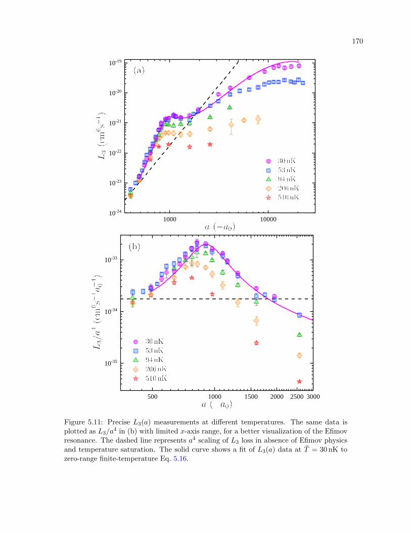
170

1 0 0 0 1 0 0 0 01 0 - 2 4

1 0 - 2 3

1 0 - 2 2

1 0 - 2 1

1 0 - 2 0

1 0 - 1 9

5 0 0 1 0 0 0 1 5 0 0 2 0 0 0 2 5 0 0 3 0 0 0

1 0 - 3 5

1 0 - 3 4

1 0 - 3 3

Figure 5.11: Precise L3(a) measurements at different temperatures. The same data isplotted as L3/a

4 in (b) with limited x-axis range, for a better visualization of the Efimovresonance. The dashed line represents a4 scaling of L3 loss in absence of Efimov physicsand temperature saturation. The solid curve shows a fit of L3(a) data at T = 30 nK tozero-range finite-temperature Eq. 5.16.

171

1 0 1 0 06 0 0

7 0 0

8 0 0

9 0 0

1 0 0 0

6 0 0

7 0 0

8 0 0

9 0 0

1 0 0 0

Figure 5.12: Extracted Efimov L3/a4 peak locations (using zero-temperature Eq. 5.10) and a−

(using finite-temperature Eq. 5.16) from L3(a) data at different temperatures. The dashed linerepresents a− = −9.73 rvdW = −627 a0 value predicted by Van der Waals universality [51].

result from high n |a|3 or from a non–22.7 Efimov series spacing, expected with a non-universal

a− location. Therefore, we vary the fit range from all a to only |a| < λ/10 and take the maximal

spread of all fit errors as the uncertainty on weighted mean a− and η values. For individual a−

and η values at each temperature (as shown in Table 5.1), we use all a points for three-highest

temperatures and only |a| < λ/5 points for the two-lowest temperature data sets, where reduced–χ2

stops varying below cutoffs |a| = λ/4. However, all extracted a− and η values (the weighted mean

or individual values for each temperature) are consistent with the quoted results (within the quoted

uncertainties), regardless if we mask high-a data or not.

The observed a− = −908(11) a0 value is a 17σ deviation from the a− = −9.73± 15% rvdW =

−627 ± 15% a0 value predicted by multiple theories investigating van der Waals universality [51,

52, 46, 47]. Our result is intriguing, considering this Feshbach resonance has an intermediate

sres = 1.9 and relatively-small abg = −19.6 a0 (compared to a = 61.65 a0). Other Efimov resonance

a− measurements near Feshbach resonances with similar sres and abg values were consistent with

universal prediction (see Fig. 5.2), albeit with large experimental and systematic uncertainties.

Previous theoretical studies dealing with corrections to van der Waals universality [53, 54, 55, 56, 57]

cannot adequately explain our data. A preliminary three-body coupled-channel model [141] suggests

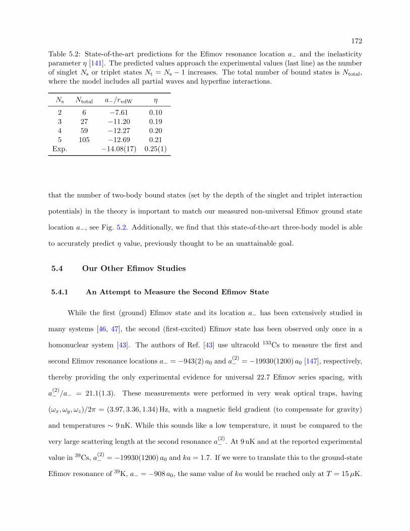
172

Table 5.2: State-of-the-art predictions for the Efimov resonance location a− and the inelasticityparameter η [141]. The predicted values approach the experimental values (last line) as the numberof singlet Ns or triplet states Nt = Ns − 1 increases. The total number of bound states is Ntotal,where the model includes all partial waves and hyperfine interactions.

Ns Ntotal a−/rvdW η

2 6 −7.61 0.103 27 −11.20 0.194 59 −12.27 0.205 105 −12.69 0.21

Exp. −14.08(17) 0.25(1)

that the number of two-body bound states (set by the depth of the singlet and triplet interaction

potentials) in the theory is important to match our measured non-universal Efimov ground state

location a−, see Fig. 5.2. Additionally, we find that this state-of-the-art three-body model is able

to accurately predict η value, previously thought to be an unattainable goal.

5.4 Our Other Efimov Studies

5.4.1 An Attempt to Measure the Second Efimov State

While the first (ground) Efimov state and its location a− has been extensively studied in

many systems [46, 47], the second (first-excited) Efimov state has been observed only once in a

homonuclear system [43]. The authors of Ref. [43] use ultracold 133Cs to measure the first and

second Efimov resonance locations a− = −943(2) a0 and a(2)− = −19930(1200) a0 [147], respectively,

thereby providing the only experimental evidence for universal 22.7 Efimov series spacing, with

a(2)− /a− = 21.1(1.3). These measurements were performed in very weak optical traps, having

(ωx, ωy, ωz)/2π = (3.97, 3.36, 1.34) Hz, with a magnetic field gradient (to compensate for gravity)

and temperatures ∼ 9 nK. While this sounds like a low temperature, it must be compared to the

very large scattering length at the second resonance a(2)− . At 9 nK and at the reported experimental

value in 39Cs, a(2)− = −19930(1200) a0 and ka = 1.7. If we were to translate this to the ground-state

Efimov resonance of 39K, a− = −908 a0, the same value of ka would be reached only at T = 15µK.

173

This is considerably higher than 500 nK, the highest temperature in Figure 5.11b, for which our

resonance is already significantly washed out. This comparison caused us to question whether the

resonance observed in Ref. [43] is perhaps some spurious effect. It should be noted, though, that

the cesium experiment has a value of η = 0.10, measured for the ground state, while our 39K value

is higher, η = 0.25. In any case, it seemed worth having a look. We went into the process with

two possible hypotheses about the second Efimov resonance in 39K: that a(2)− is at the universal

value of 22.7 × (−9.73 rvdW) = −14200 a0, or that it is universally scaled from our observed a−

value, which would make it a(2)− = 22.7 × (−14.08 rvdW) = −20600 a0. In the former hypothesis,

to achieve the same (or a smaller) value of ka that characterized the 133Cs experiment, we would

need to be at T < 30 nK. In the latter hypothesis, we would need T < 60 nK. These temperatures

seemed achievable and, with the positive example from the 133Cs work, we decided to try.

Since we did not observe the second Efimov resonance at time-averaged T = 30 nK (see

Fig. 5.11(a)), we tried measuring L3 values at high a with the lowest temperatures attainable

without significant (hardware) modifications. Since we cannot use degenerate samples for loss

measurement at a < 0, the lower temperature limit is set by the density. We minimize the atom

density by utilizing the weakest trapping potentials permitted by gravitational sag. We do not use

magnetic field gradient for levitation, as this would introduce further complications. We were able

to create 8 nK thermal samples with 1800 atoms in a (ωx, ωy, ωz)/2π = (7, 7, 49) Hz optical trap.

However, small OD, image frame imperfections, small cloud size (σ = 6µm approaching imaging

resolution σ = 1.4µm), trap intensity instability (in this case, we do not adiabatically increase trap

depths) and closeness to degeneracy (PSD ∼ 1), result in a relatively-poor signal-to-noise, with

∼ 4% N instability and ∼ 10% T instability for a minimal hold duration and even worse after some

decay. Of course, one can also compensate for gravity by performing the experiment in free-fall, as

in the Cold Atom Laboratory in the International Space Station.

In the end, we compromised reaching the lowest temperature for better signal stability, cre-

ating samples with Ti = 14 nK and 3600 atoms in a (ωx, ωy, ωz)/2π = (8, 8, 61) Hz optical trap.

Figure 5.13 shows that we expect (using Eq. 5.16) a significant suppression of the second Efimov

174

peak for T = 16 nK, when compared to the zero-temperature limit (using Eq. 5.10). We take

multiple L3 measurements in the vicinity of the aforementioned possible a(2)− values and do not see

an Efimov feature, as depicted in Fig. 5.14. There are several possible reasons for the absence of an

Efimov feature. First, T = 16 nK is still a relatively-hot temperature and results in a feature with

a small contrast, as shown in Fig. 5.13, consistent with data within experimental error. Second,

a relatively-strong confinement along gravity corresponds to a relatively-small (compared to a(2)− )

harmonic oscillator length ∼ 4 × 104 a0, can result in a suppression of Efimov-related loss at such

high a values [148]. Last, non-trivial density effects can play a role in the suppression of three-body

physics, even with the sample’s relatively-low density (at 〈n〉i = 1.7×1010 cm−3), considering∣∣na3

∣∣is already 0.02 at −20000 a0. Some future prospects for observing the second Efimov resonance

with our system include using a better imaging system, which would enable a better detection of

small atom populations, and using repulsive optical potentials to compensate for gravity, which

would enable smaller sample densities and temperatures with reasonable atom number.

5.4.2 An Attempt to Measure Four-Body Efimov Resonances and High-Density

Peculiarities

The Efimov spectrum contains a more complex structure that goes beyond the infinite series

of trimer states. For example, each individual trimer state has two corresponding four-body Efimov

states [149]. Near a−, the two ground tetramer states intersect the four-atom continuum at 0.43 a−

and 0.90 a− locations [149]. There has been some experimental evidence for the existence of such

states [136, 33, 40]. We attempted to find evidence of such states near our trimer Efimov resonance

using atom-loss spectroscopy.

Four-body loss follows Eq. 5.11 (with z = 4) and leads to an enhanced overall loss near 0.43 a−

and 0.90 a− locations. Such loss can be measured using the same procedure as we did for L3 (with

20-30% number decay) and would appear as a density-dependent L3 feature. In order to distinguish

four-body loss from three-body loss, the density must be high enough. Given preliminary four-body

loss rate coefficient L4 values from Jose D’Incao [141], the average atom density must approach or

175

10000 50000

104

10-19

10-18

10-17

10-16

Figure 5.13: Predicted finite-temperature suppression of the second Efimov resonance. Since we

do not know the location of the second Efimov resonance, we plot two possible values: a(2)− =

22.7 × a− = −20600 a0 (red) and a(2)− = 22.7 × (−9.73 rvdW) = −14200 a0 (blue), corresponding

to Efimov series spacing 22.7 and 15.6, where we fix a− = −908 a0 and η = 0.25. The solid linesrepresent finite-temperature model Eq. 5.16 and dashed lines represent zero-temperature modelEq. 5.10.

1 0 0 0 0 2 0 0 0 0 3 0 0 0 01 0 - 1 9

2 x 1 0 - 1 9

3 x 1 0 - 1 9

4 x 1 0 - 1 9

5 x 1 0 - 1 9

Figure 5.14: The absence of the second Efimov resonance in our data. The finite-temperaturepredictions are the same as in Fig. 5.13. Since we do not directly measure the trapping frequenciesfor this particular measurement (we extrapolate them from previous measurements), there can bea global systematic shift of all L3 points resulting from an imprecise knowledge absolute density.

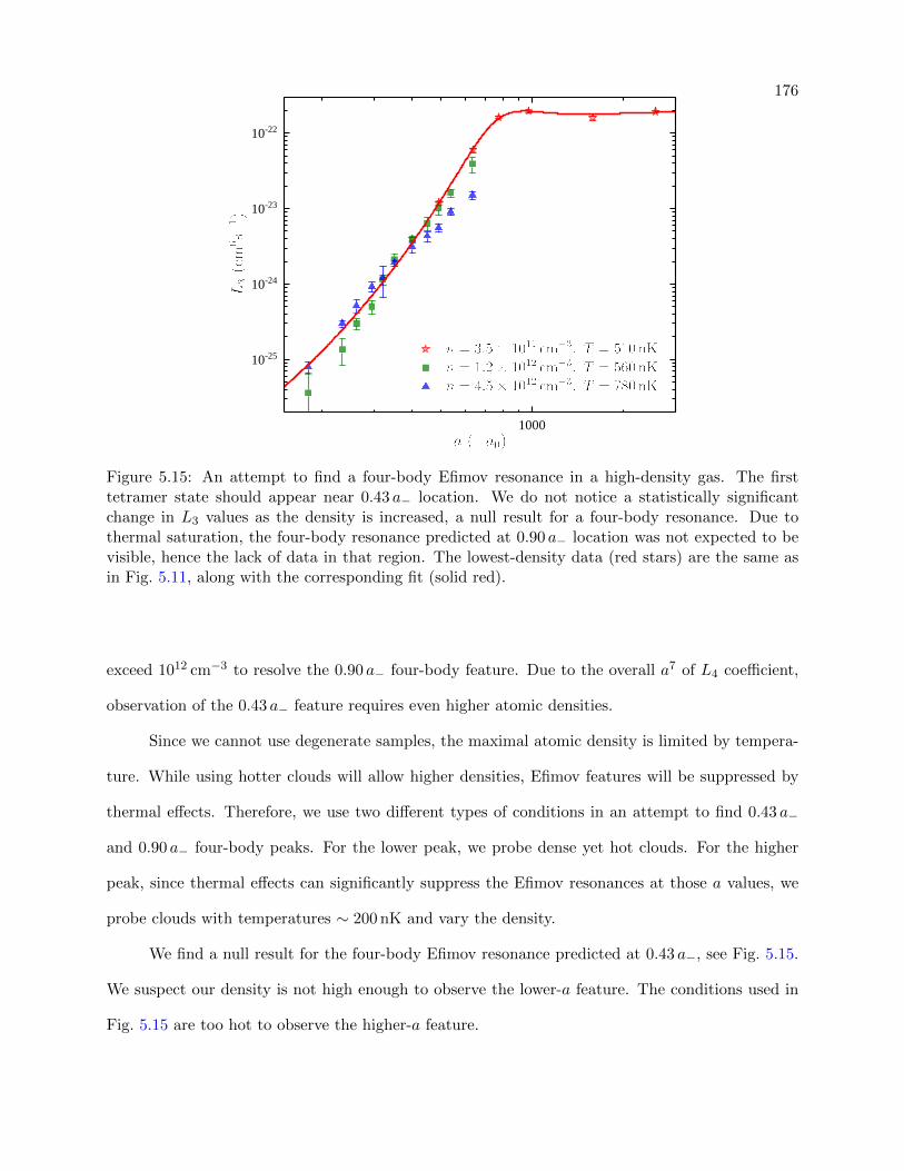
176

1 0 0 0

1 0 - 2 5

1 0 - 2 4

1 0 - 2 3

1 0 - 2 2

Figure 5.15: An attempt to find a four-body Efimov resonance in a high-density gas. The firsttetramer state should appear near 0.43 a− location. We do not notice a statistically significantchange in L3 values as the density is increased, a null result for a four-body resonance. Due tothermal saturation, the four-body resonance predicted at 0.90 a− location was not expected to bevisible, hence the lack of data in that region. The lowest-density data (red stars) are the same asin Fig. 5.11, along with the corresponding fit (solid red).

exceed 1012 cm−3 to resolve the 0.90 a− four-body feature. Due to the overall a7 of L4 coefficient,

observation of the 0.43 a− feature requires even higher atomic densities.

Since we cannot use degenerate samples, the maximal atomic density is limited by tempera-

ture. While using hotter clouds will allow higher densities, Efimov features will be suppressed by

thermal effects. Therefore, we use two different types of conditions in an attempt to find 0.43 a−

and 0.90 a− four-body peaks. For the lower peak, we probe dense yet hot clouds. For the higher

peak, since thermal effects can significantly suppress the Efimov resonances at those a values, we

probe clouds with temperatures ∼ 200 nK and vary the density.

We find a null result for the four-body Efimov resonance predicted at 0.43 a−, see Fig. 5.15.

We suspect our density is not high enough to observe the lower-a feature. The conditions used in

Fig. 5.15 are too hot to observe the higher-a feature.

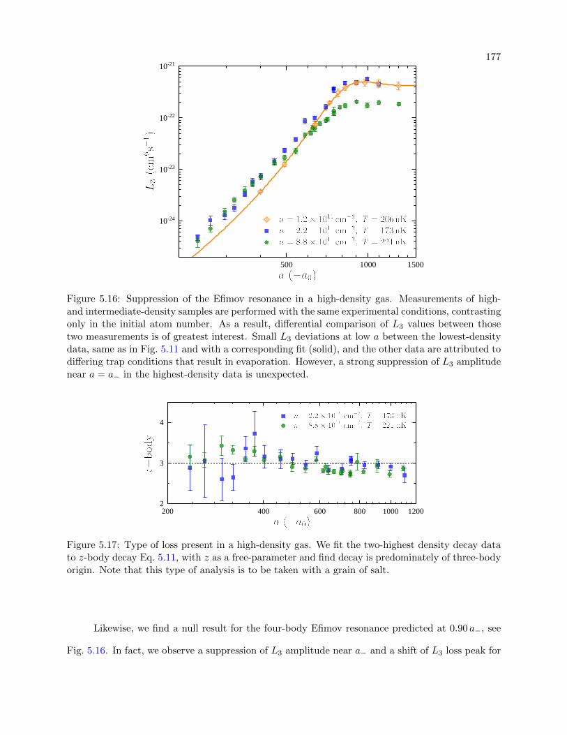
177

5 0 0 1 0 0 0 1 5 0 0

1 0 - 2 4

1 0 - 2 3

1 0 - 2 2

1 0 - 2 1

Figure 5.16: Suppression of the Efimov resonance in a high-density gas. Measurements of high-and intermediate-density samples are performed with the same experimental conditions, contrastingonly in the initial atom number. As a result, differential comparison of L3 values between thosetwo measurements is of greatest interest. Small L3 deviations at low a between the lowest-densitydata, same as in Fig. 5.11 and with a corresponding fit (solid), and the other data are attributed todiffering trap conditions that result in evaporation. However, a strong suppression of L3 amplitudenear a = a− in the highest-density data is unexpected.

2 0 0 4 0 0 6 0 0 8 0 0 1 0 0 0 1 2 0 02

3

4

Figure 5.17: Type of loss present in a high-density gas. We fit the two-highest density decay datato z-body decay Eq. 5.11, with z as a free-parameter and find decay is predominately of three-bodyorigin. Note that this type of analysis is to be taken with a grain of salt.

Likewise, we find a null result for the four-body Efimov resonance predicted at 0.90 a−, see

Fig. 5.16. In fact, we observe a suppression of L3 amplitude near a− and a shift of L3 loss peak for

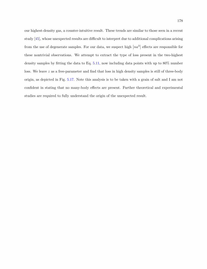
178

our highest-density gas, a counter-intuitive result. These trends are similar to those seen in a recent

study [45], whose unexpected results are difficult to interpret due to additional complications arising

from the use of degenerate samples. For our data, we suspect high∣∣na3

∣∣ effects are responsible for

these nontrivial observations. We attempt to extract the type of loss present in the two-highest

density samples by fitting the data to Eq. 5.11, now including data points with up to 80% number

loss. We leave z as a free-parameter and find that loss in high density samples is still of three-body

origin, as depicted in Fig. 5.17. Note this analysis is to be taken with a grain of salt and I am not

confident in stating that no many-body effects are present. Further theoretical and experimental

studies are required to fully understand the origin of the unexpected result.

Chapter 6

Conclusion and Outlook

Over the past several decades, the development of cooling, trapping and manipulation of

quantum gases enabled the exploration of various quantum phenomena and quantum simulation

of condensed matter systems. Additionally, the recent use of sensitive spectroscopic techniques en-

abled precise probing of few-body physics, important for understanding the fine details in interact-

ing systems. For example, in probing two-body interactions, state-of-the-art RF Rabi and Ramsey

spectroscopy enabled precise determination of Feshbach dimer binding energies [103, 20], Feshbach

resonance parameters [111] and two-body contact (short-ranged pair correlations) [150, 100]. Sim-

ilarly, in probing three-body interactions, spectroscopic tools (RF and atom-loss) enabled probing

Efimov trimer state locations [30], trimer binding energies [131, 132, 133, 151] and three-body con-

tact [152, 21]. Such studies inspired the work discussed in this thesis, and my hope is that similar

precision few-body measurements will follow in the near future.

In this thesis, I presented a new apparatus used for the production and probing of ultracold

39K gas samples. The immense stability of the machine, along with precise control of experimental

conditions, enabled precision measurements of few-body physics in an interacting quantum gas.

Having small experimental uncertainties and a good understanding of systematic error in our two-

and three-body physics measurements allowed us to probe physics beyond predicted by universal

theories.

For example, our precise measurements of dimer binding energies cannot be encapsulated

by the universal Eb = ~2/(ma2) equation or its version with small-order corrections. Therefore,

180

we required data comparison to predictions from a state-of-the-art coupled-channel model with

real interaction potentials. Even then, to accurately match most of our measurements to within

1%, we performed a global fit to our binding energy data by fine-tuning the singlet and triplet

potentials of the realistic model. Such fine-tuning is unprecedented [20, 111], considering that our

data constrains the Feshbach resonance location to within 1.4 mG, a very small value compared

to the Feshbach resonance width of 55 G. While such a match is impressive, due to our small

experimental uncertainty, we still notice deviations between the observed and predicted values at

large binding energies. Such discrepancies likely arise from incompleteness of the state-of-the-art

coupled-channel model at short interatomic distances. Further theoretical advancements are needed

to fully describe our precise binding energy measurements. Also, additional improvements to the

current two-body models must be made in order to accurately describe all features in our dimer

lifetime data.

Likewise, our precise Efimov trimer state location measurement cannot be predicted by van

der Waals universality. A state-of-the-art coupled-channel three-body model, whose singlet and

triplet potentials were set to equal that of the two-body model, was required to better understand

our data [141]. Such a model is realistic enough that, for the first time in the field, it predicted an

accurate value for the Efimov resonance width (inelasticity parameter) η. However, while now there

is a better agreement for the measured and the newly predicted Efimov ground state location a−,

the agreement is not ideal due to our small experimental uncertainty, suggesting further theoretical

advancements must be made. Lastly, the Efimov resonance peak suppression at high atom density,

as observed by us and Ref. [45], needs a better understanding.

There are many possible future directions for exploring few-body and universal physics with

ultracold Bose gases. For example, while there is some evidence of a second Efimov resonance

feature (the first excited Efimov state) [43], it is the only observation in a homonuclear system

and is affected by large systematic effects (e.g. finite-temperature and finite-range [147]). Further

experimental evidence is needed to fully understand the robustness of the homonuclear universal

Efimov spectrum spacing factor 22.7. Such experiments are difficult due to necessary nK-level

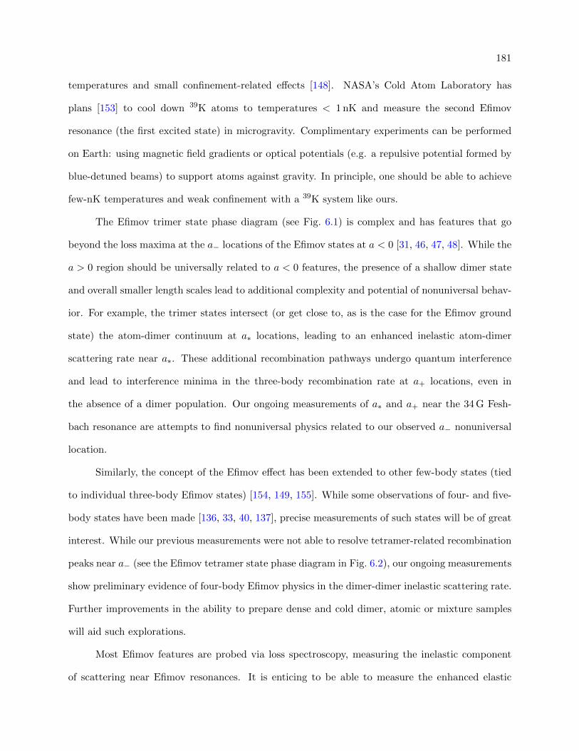
181

temperatures and small confinement-related effects [148]. NASA’s Cold Atom Laboratory has

plans [153] to cool down 39K atoms to temperatures < 1 nK and measure the second Efimov

resonance (the first excited state) in microgravity. Complimentary experiments can be performed

on Earth: using magnetic field gradients or optical potentials (e.g. a repulsive potential formed by

blue-detuned beams) to support atoms against gravity. In principle, one should be able to achieve

few-nK temperatures and weak confinement with a 39K system like ours.

The Efimov trimer state phase diagram (see Fig. 6.1) is complex and has features that go

beyond the loss maxima at the a− locations of the Efimov states at a < 0 [31, 46, 47, 48]. While the

a > 0 region should be universally related to a < 0 features, the presence of a shallow dimer state

and overall smaller length scales lead to additional complexity and potential of nonuniversal behav-

ior. For example, the trimer states intersect (or get close to, as is the case for the Efimov ground

state) the atom-dimer continuum at a∗ locations, leading to an enhanced inelastic atom-dimer

scattering rate near a∗. These additional recombination pathways undergo quantum interference

and lead to interference minima in the three-body recombination rate at a+ locations, even in

the absence of a dimer population. Our ongoing measurements of a∗ and a+ near the 34 G Fesh-

bach resonance are attempts to find nonuniversal physics related to our observed a− nonuniversal

location.

Similarly, the concept of the Efimov effect has been extended to other few-body states (tied

to individual three-body Efimov states) [154, 149, 155]. While some observations of four- and five-

body states have been made [136, 33, 40, 137], precise measurements of such states will be of great

interest. While our previous measurements were not able to resolve tetramer-related recombination

peaks near a− (see the Efimov tetramer state phase diagram in Fig. 6.2), our ongoing measurements

show preliminary evidence of four-body Efimov physics in the dimer-dimer inelastic scattering rate.

Further improvements in the ability to prepare dense and cold dimer, atomic or mixture samples

will aid such explorations.

Most Efimov features are probed via loss spectroscopy, measuring the inelastic component

of scattering near Efimov resonances. It is enticing to be able to measure the enhanced elastic

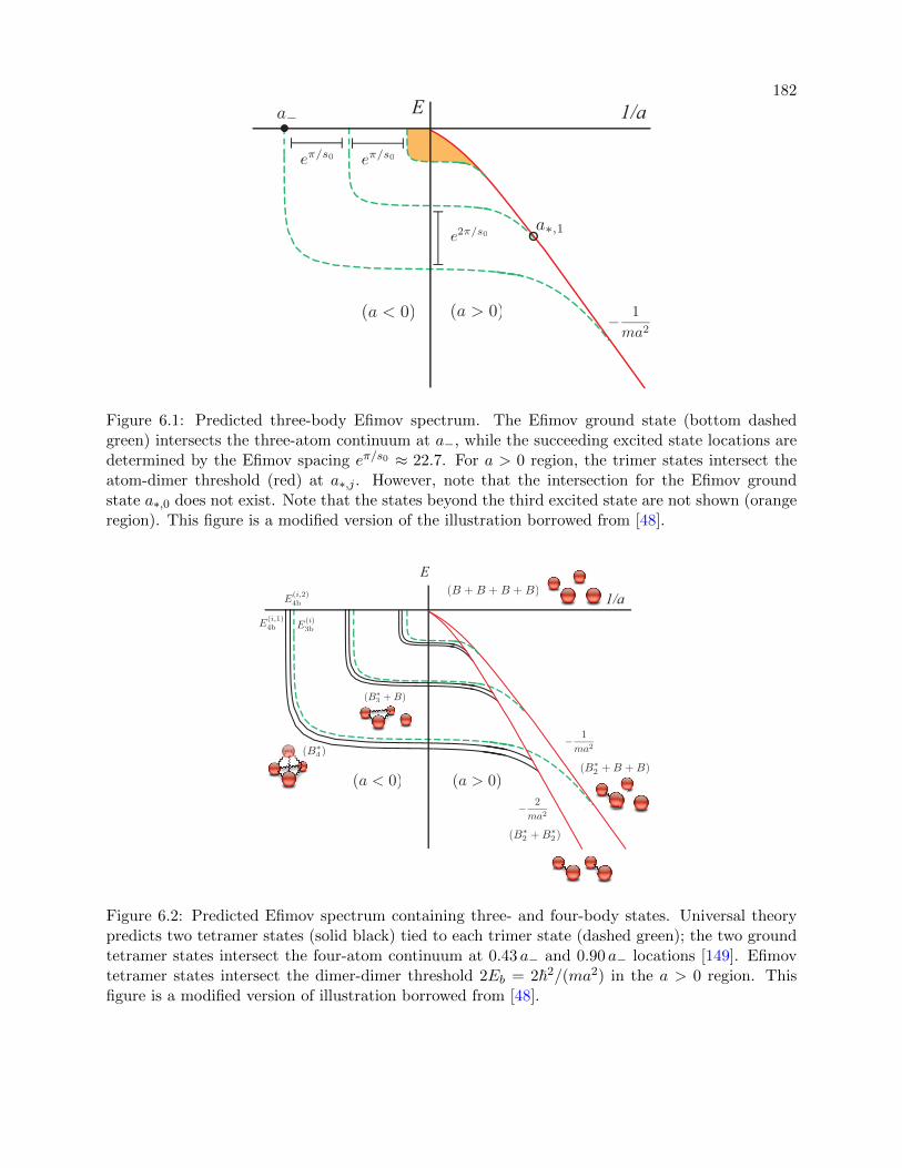
182E 1/a

Figure 6.1: Predicted three-body Efimov spectrum. The Efimov ground state (bottom dashedgreen) intersects the three-atom continuum at a−, while the succeeding excited state locations aredetermined by the Efimov spacing eπ/s0 ≈ 22.7. For a > 0 region, the trimer states intersect theatom-dimer threshold (red) at a∗,j . However, note that the intersection for the Efimov groundstate a∗,0 does not exist. Note that the states beyond the third excited state are not shown (orangeregion). This figure is a modified version of the illustration borrowed from [48].

1/a

E

Figure 6.2: Predicted Efimov spectrum containing three- and four-body states. Universal theorypredicts two tetramer states (solid black) tied to each trimer state (dashed green); the two groundtetramer states intersect the four-atom continuum at 0.43 a− and 0.90 a− locations [149]. Efimovtetramer states intersect the dimer-dimer threshold 2Eb = 2~2/(ma2) in the a > 0 region. Thisfigure is a modified version of illustration borrowed from [48].

183

component near an Efimov resonance. For example, such measurements can be performed near

atom-dimer and dimer-dimer Efimov resonances, where Efimov states intersect their respective

thresholds at a > 0. RF spectroscopy (Rabi or Ramsey) can be employed to measure energy shifts

near such resonances, while cross-thermalization technique can be employed to probe the enhanced

atom-dimer and dimer-dimer elastic collisional cross-sections. Again, any method measuring the

elastic component near an Efimov resonance would be limited by the ability to prepare dense cold

samples, and any method’s signal contrast would be ultimately limited by the Efimov resonance

width η [48], whose value is related to the trimer lifetime. Due to the expected small signal contrast,

one can enhance sensitivity by utilizing the two-photon dimer dissociation transition, discussed in

Sec. 4.3.2, or by performing spectroscopy on the Feshbach dimer to deep molecular bound state

transition; we are currently exploring the feasibility of such methods.

Another interesting direction would be to further develop spectroscopic tools to directly probe

Efimov states. For example, authors of Ref. [134] have shown that a macroscopic population of

Efimov trimers can be produced via magneto-association technique (a quench to unitarity). Given

a sufficient trimer lifetime, the trimer binding energy can be extracted by RF spectroscopic means.

The topics of universal and few-body physics in interacting quantum systems have recently

gained considerable amount of interest. Ongoing efforts in ultracold (including homonuclear bosonic,

heteronuclear bosonic and distinguishable fermion), molecular and nuclear systems are exploring

the question of how well universal aspects translate across all branches of physics [46, 47]. Recent

tremendous progress has been aided by the development of experimental tools that enable more

accurate and precise measurements of universal and few-body physics in ultracold systems. Our

precise two- and three-body measurements reveal nonuniversal aspects that we hope the field will

soon understand. I am confident that the universal and few-body physics fields will continue to

progress and provide invaluable information on how the more complex many-body quantum systems

behave.

Bibliography

[1] Wolfgang Ketterle, N. J. Van Druten, Benjamin Bederson, and Herbert Walther. Evaporativecooling of trapped atoms. In Advances In Atomic, Molecular, and Optical Physics, volume 37,pages 181–236. Academic Press, January 1996.

[2] Harold J. Metcalf and Peter van der Straten. Laser Cooling and Trapping of Neutral Atoms.American Cancer Society, 2007.

[3] M. H. Anderson, J. R. Ensher, M. R. Matthews, C. E. Wieman, and E. A. Cornell. Obser-vation of bose-einstein condensation in a dilute atomic vapor. Science, 269(5221):198, July1995.

[4] B. DeMarco and D. S. Jin. Onset of fermi degeneracy in a trapped atomic gas. Science,285(5434):1703, September 1999.

[5] Luigi De Marco, Giacomo Valtolina, Kyle Matsuda, William G. Tobias, Jacob P. Covey, andJun Ye. A degenerate fermi gas of polar molecules. Science, 363(6429):853, February 2019.

[6] Seth Lloyd. Universal quantum simulators. Science, 273(5278):1073, August 1996.

[7] Immanuel Bloch, Jean Dalibard, and Sylvain Nascimbene. Quantum simulations with ultra-cold quantum gases. Nature Physics, 8:267, April 2012.

[8] I. M. Georgescu, S. Ashhab, and Franco Nori. Quantum simulation. Rev. Mod. Phys.,86:153–185, Mar 2014.

[9] Christian Gross and Immanuel Bloch. Quantum simulations with ultracold atoms in opticallattices. Science, 357(6355):995, September 2017.

[10] Torma Paivi and Sengstock Klaus. Quantum Gas Experiments: Exploring Many-Body States,volume 3. World Scientific, 2014.

[11] John L. Bohn, Ana Maria Rey, and Jun Ye. Cold molecules: Progress in quantum engineeringof chemistry and quantum matter. Science, 357(6355):1002, September 2017.

[12] J. T. Stewart, J. P. Gaebler, and D. S. Jin. Using photoemission spectroscopy to probe astrongly interacting fermi gas. Nature, 454:744, August 2008.

[13] J. P. Gaebler, J. T. Stewart, T. E. Drake, D. S. Jin, A. Perali, P. Pieri, and G. C. Strinati.Observation of pseudogap behaviour in a strongly interacting fermi gas. Nature Physics,6:569, July 2010.

185

[14] Yoav Sagi, Tara E. Drake, Rabin Paudel, Roman Chapurin, and Deborah S. Jin. Breakdownof the fermi liquid description for strongly interacting fermions. Phys. Rev. Lett., 114:075301,Feb 2015.

[15] Immanuel Bloch, Jean Dalibard, and Wilhelm Zwerger. Many-body physics with ultracoldgases. Rev. Mod. Phys., 80:885–964, Jul 2008.

[16] Rahul Nandkishore and David A Huse. Many-body localization and thermalization in quan-tum statistical mechanics. Annu. Rev. Condens. Matter Phys., 6(1):15–38, 2015.

[17] Jean Dalibard, Fabrice Gerbier, Gediminas Juzeliunas, and Patrik Ohberg. Colloquium:Artificial gauge potentials for neutral atoms. Rev. Mod. Phys., 83:1523–1543, Nov 2011.

[18] Victor Galitski, Gediminas Juzeliunas, and Ian B Spielman. Artificial gauge fields withultracold atoms. arXiv preprint arXiv:1901.03705, 2019.

[19] Cheng Chin, Rudolf Grimm, Paul Julienne, and Eite Tiesinga. Feshbach resonances in ultra-cold gases. Rev. Mod. Phys., 82(2):1225, 2010.

[20] G. Zurn, T. Lompe, A. N. Wenz, S. Jochim, P. S. Julienne, and J. M. Hutson. Precisecharacterization of 6Li feshbach resonances using trap-sideband-resolved rf spectroscopy ofweakly bound molecules. Phys. Rev. Lett., 110:135301, Mar 2013.

[21] Richard J Fletcher, Raphael Lopes, Jay Man, Nir Navon, Robert P Smith, Martin W Zwier-lein, and Zoran Hadzibabic. Two-and three-body contacts in the unitary bose gas. Science,355(6323):377–380, 2017.

[22] Sylvain Nascimbene, Nir Navon, Frederic Chevy, and Christophe Salomon. The equationof state of ultracold bose and fermi gases: a few examples. New Journal of Physics,12(10):103026, October 2010.

[23] Eric Braaten, Daekyoung Kang, and Lucas Platter. Universal relations for identical bosonsfrom three-body physics. Phys. Rev. Lett., 106:153005, Apr 2011.

[24] Eric Braaten. Universal relations for fermions with large scattering length. In The BCS-BECCrossover and the Unitary Fermi Gas, pages 193–231. Springer, 2012.

[25] P. Makotyn, C. E. Klauss, D. L. Goldberger, E. A. Cornell, and D. S. Jin. Universal dynamicsof a degenerate unitary bose gas. Nature Physics, 10:116, January 2014.

[26] Christoph Eigen, Jake A. P. Glidden, Raphael Lopes, Eric A. Cornell, Robert P. Smith,and Zoran Hadzibabic. Universal prethermal dynamics of bose gases quenched to unitarity.Nature, 563(7730):221–224, November 2018.

[27] Kerson Huang and C. N. Yang. Quantum-mechanical many-body problem with hard-sphereinteraction. Phys. Rev., 105:767–775, Feb 1957.

[28] G. F. Gribakin and V. V. Flambaum. Calculation of the scattering length in atomic collisionsusing the semiclassical approximation. Phys. Rev. A, 48:546–553, Jul 1993.

[29] V. Efimov. Energy levels arising from resonant two-body forces in a three-body system. Phys.Lett. B, 33(8):563–564, December 1970.

186

[30] T. Kraemer, M. Mark, P. Waldburger, J. G. Danzl, C. Chin, B. Engeser, A. D. Lange,K. Pilch, A. Jaakkola, H.-C. Nagerl, and R. Grimm. Evidence for efimov quantum states inan ultracold gas of caesium atoms. Nature, 440:315, March 2006.

[31] Eric Braaten and H.-W. Hammer. Universality in few-body systems with large scatteringlength. Phys. Rep., 428(5):259–390, June 2006.

[32] M. Zaccanti, B. Deissler, C. D’Errico, M. Fattori, M. Jona-Lasinio, S. Muller, G. Roati,M. Inguscio, and G. Modugno. Observation of an efimov spectrum in an atomic system. Nat.Phys., 5:586, July 2009.

[33] Scott E. Pollack, Daniel Dries, and Randall G. Hulet. Universality in three- and four-bodybound states of ultracold atoms. Science, 326(5960):1683, December 2009.

[34] Noam Gross, Zav Shotan, Servaas Kokkelmans, and Lev Khaykovich. Observation of univer-sality in ultracold 7Li three-body recombination. Phys. Rev. Lett., 103:163202, Oct 2009.

[35] Noam Gross, Zav Shotan, Servaas Kokkelmans, and Lev Khaykovich. Nuclear-spin-independent short-range three-body physics in ultracold atoms. Phys. Rev. Lett., 105:103203,Sep 2010.

[36] Noam Gross, Zav Shotan, Olga Machtey, Servaas Kokkelmans, and Lev Khaykovich. Studyof efimov physics in two nuclear-spin sublevels of 7li. Comptes Rendus Physique, 12(1):4–12,January 2011.

[37] M. Berninger, A. Zenesini, B. Huang, W. Harm, H.-C. Nagerl, F. Ferlaino, R. Grimm, P. S.Julienne, and J. M. Hutson. Universality of the three-body parameter for efimov states inultracold cesium. Phys. Rev. Lett., 107:120401, Sep 2011.

[38] Sanjukta Roy, Manuele Landini, Andreas Trenkwalder, Giulia Semeghini, Giacomo Spag-nolli, Andrea Simoni, Marco Fattori, Massimo Inguscio, and Giovanni Modugno. Test of theuniversality of the three-body efimov parameter at narrow feshbach resonances. Phys. Rev.Lett., 111(5):053202, 2013.

[39] B. S. Rem, A. T. Grier, I. Ferrier-Barbut, U. Eismann, T. Langen, N. Navon, L. Khaykovich,F. Werner, D. S. Petrov, F. Chevy, and C. Salomon. Lifetime of the bose gas with resonantinteractions. Phys. Rev. Lett., 110:163202, Apr 2013.

[40] P. Dyke, S. E. Pollack, and R. G. Hulet. Finite-range corrections near a feshbach resonanceand their role in the efimov effect. Phys. Rev. A, 88:023625, Aug 2013.

[41] R. Pires, J. Ulmanis, S. Hafner, M. Repp, A. Arias, E. D. Kuhnle, and M. Weidemuller.Observation of efimov resonances in a mixture with extreme mass imbalance. Phys. Rev.Lett., 112:250404, Jun 2014.

[42] Shih-Kuang Tung, Karina Jimenez-Garcıa, Jacob Johansen, Colin V. Parker, and ChengChin. Geometric scaling of efimov states in a 6Li−133Cs mixture. Phys. Rev. Lett., 113:240402,Dec 2014.

[43] Bo Huang, Leonid A. Sidorenkov, Rudolf Grimm, and Jeremy M. Hutson. Observation of thesecond triatomic resonance in efimov’s scenario. Phys. Rev. Lett., 112:190401, May 2014.

187

[44] R. A. W. Maier, M. Eisele, E. Tiemann, and C. Zimmermann. Efimov resonance and three-body parameter in a lithium-rubidium mixture. Phys. Rev. Lett., 115:043201, Jul 2015.

[45] L. J. Wacker, N. B. Jørgensen, K. T. Skalmstang, M. G. Skou, A. G. Volosniev, and J. J.Arlt. Temperature dependence of an efimov resonance in 39K. Phys. Rev. A, 98:052706, Nov2018.

[46] Pascal Naidon and Shimpei Endo. Efimov physics: a review. Rep. Prog. Phys., 80(5):056001,2017.

[47] Chris H. Greene, P. Giannakeas, and J. Perez-Rıos. Universal few-body physics and clusterformation. Rev. Mod. Phys., 89:035006, Aug 2017.

[48] Jose P. D’Incao. Few-body physics in resonantly interacting ultracold quantum gases. Journalof Physics B: Atomic, Molecular and Optical Physics, 51(4):043001, January 2018.

[49] A. Derevianko, W. R. Johnson, M. S. Safronova, and J. F. Babb. High-precision calculationsof dispersion coefficients, static dipole polarizabilities, and atom-wall interaction constantsfor alkali-metal atoms. Phys. Rev. Lett., 82:3589–3592, May 1999.

[50] Stephan Falke, Horst Knockel, Jan Friebe, Matthias Riedmann, Eberhard Tiemann, andChristian Lisdat. Potassium ground-state scattering parameters and born-oppenheimer po-tentials from molecular spectroscopy. Phys. Rev. A, 78:012503, Jul 2008.

[51] Jia Wang, J. P. D’Incao, B. D. Esry, and Chris H. Greene. Origin of the three-body parameteruniversality in efimov physics. Phys. Rev. Lett., 108:263001, Jun 2012.

[52] Pascal Naidon, Shimpei Endo, and Masahito Ueda. Physical origin of the universal three-bodyparameter in atomic efimov physics. Phys. Rev. A, 90:022106, Aug 2014.

[53] D. S. Petrov. Three-boson problem near a narrow feshbach resonance. Phys. Rev. Lett.,93:143201, Sep 2004.

[54] Alexander O. Gogolin, Christophe Mora, and Reinhold Egger. Analytical solution of thebosonic three-body problem. Phys. Rev. Lett., 100:140404, Apr 2008.

[55] R. Schmidt, S. P. Rath, and W. Zwerger. Efimov physics beyond universality. Eur. Phys. J.B, 85(11):386, November 2012.

[56] Yujun Wang and Paul S. Julienne. Universal van der waals physics for three cold atoms nearfeshbach resonances. Nat. Phys., 10:768, August 2014.

[57] Christian Langmack, Richard Schmidt, and Wilhelm Zwerger. Efimov states near a feshbachresonance and the limits of van der waals universality at finite background scattering length.Phys. Rev. A, 97:033623, Mar 2018.

[58] Rabin Paudel. Probing Local Quantities in a Strongly Interacting Fermi Gas and theConstruction of an Ultracold Fermi Gas Apparatus. PhD thesis, 2017.

[59] Chiara D’Errico, Matteo Zaccanti, Marco Fattori, Giacomo Roati, Massimo Inguscio, Gio-vanni Modugno, and Andrea Simoni. Feshbach resonances in ultracold 39 k. New Journal ofPhysics, 9(7):223, 2007.

188

[60] Huang Wu and Christopher J. Foot. Direct simulation of evaporative cooling. Journal ofPhysics B: Atomic, Molecular and Optical Physics, 29(8):L321–L328, April 1996.

[61] N. F. Mott and H. S. W. Massey. The theory of atomic collisions. 1949.

[62] John L. Bohn, James P. Burke, Chris H. Greene, H. Wang, P. L. Gould, and W. C. Stwalley.Collisional properties of ultracold potassium: Consequences for degenerate bose and fermigases. Phys. Rev. A, 59:3660–3664, May 1999.

[63] Private communication John L. Bohn.

[64] J.P. Covey. Enhanced Optical and Electric Manipulation of a Quantum Gas of KRb Molecules.PhD thesis, 2018.

[65] C. Klempt, T. van Zoest, T. Henninger, O. Topic, E. Rasel, W. Ertmer, and J. Arlt. Ultravi-olet light-induced atom desorption for large rubidium and potassium magneto-optical traps.Phys. Rev. A, 73:013410, Jan 2006.

[66] TG Tiecke. Properties of potassium. University of Amsterdam, The Netherlands, Thesis,pages 12–14, 2010.

[67] C. J. Cooper, G. Hillenbrand, J. Rink, C. G. Townsend, K. Zetie, and C. J. Foot. Thetemperature of atoms in a magneto-optical trap. Europhysics Letters (EPL), 28(6):397–402,November 1994.

[68] Private communication John L. Hall.

[69] L. Richter, H. Mandelberg, M. Kruger, and P. McGrath. Linewidth determination fromself-heterodyne measurements with subcoherence delay times. IEEE Journal of QuantumElectronics, 22(11):2070–2074, 1986.

[70] Hanne Ludvigsen, Mika Tossavainen, and Matti Kaivola. Laser linewidth measurements usingself-homodyne detection with short delay. Optics Communications, 155(1):180–186, October1998.

[71] J. Catani, P. Maioli, L. De Sarlo, F. Minardi, and M. Inguscio. Intense slow beams of bosonicpotassium isotopes. Phys. Rev. A, 73:033415, Mar 2006.

[72] Wolfgang Petrich, Michael H. Anderson, Jason R. Ensher, and Eric A. Cornell. Behavior ofatoms in a compressed magneto-optical trap. J. Opt. Soc. Am. B, 11(8):1332–1335, August1994.

[73] J. Dalibard and C. Cohen-Tannoudji. Laser cooling below the doppler limit by polarizationgradients: simple theoretical models. J. Opt. Soc. Am. B, 6(11):2023–2045, November 1989.

[74] D. C. McKay, D. Jervis, D. J. Fine, J. W. Simpson-Porco, G. J. A. Edge, and J. H. Thywissen.Low-temperature high-density magneto-optical trapping of potassium using the open 4s→ 5ptransition at 405 nm. Phys. Rev. A, 84:063420, Dec 2011.

[75] D. Rio Fernandes, F. Sievers, N. Kretzschmar, S. Wu, C. Salomon, and F. Chevy. Sub-doppler laser cooling of fermionic40k atoms in three-dimensional gray optical molasses. EPL(Europhysics Letters), 100(6):63001, December 2012.

189

[76] Dipankar Nath, R Kollengode Easwaran, G. Rajalakshmi, and C. S. Unnikrishnan. Quantum-interference-enhanced deep sub-doppler cooling of 39k atoms in gray molasses. Phys. Rev. A,88:053407, Nov 2013.

[77] G. Grynberg and J.-Y. Courtois. Proposal for a magneto-optical lattice for trapping atomsin nearly-dark states. Europhysics Letters (EPL), 27(1):41–46, July 1994.

[78] G. Salomon, L. Fouche, P. Wang, A. Aspect, P. Bouyer, and T. Bourdel. Gray-molasses cool-ing of39k to a high phase-space density. EPL (Europhysics Letters), 104(6):63002, December2013.

[79] Manuele Landini. A tunable Bose-Einstein condensate for quantum interferometry. PhDthesis, University of Trento, 2012.

[80] Wolfgang Petrich, Michael H. Anderson, Jason R. Ensher, and Eric A. Cornell. Stable,tightly confining magnetic trap for evaporative cooling of neutral atoms. Phys. Rev. Lett.,74:3352–3355, Apr 1995.

[81] C. R. Monroe, E. A. Cornell, C. A. Sackett, C. J. Myatt, and C. E. Wieman. Measurementof cs-cs elastic scattering at t=30 µk. Phys. Rev. Lett., 70:414–417, Jan 1993.

[82] B. DeMarco, J. L. Bohn, J. P. Burke, M. Holland, and D. S. Jin. Measurement of p-wavethreshold law using evaporatively cooled fermionic atoms. Phys. Rev. Lett., 82:4208–4211,May 1999.

[83] M. Landini, S. Roy, G. Roati, A. Simoni, M. Inguscio, G. Modugno, and M. Fattori. Directevaporative cooling of 39k atoms to bose-einstein condensation. Phys. Rev. A, 86:033421, Sep2012.

[84] S. J. M. Kuppens, K. L. Corwin, K. W. Miller, T. E. Chupp, and C. E. Wieman. Loadingan optical dipole trap. Phys. Rev. A, 62:013406, Jun 2000.

[85] D. Comparat, A. Fioretti, G. Stern, E. Dimova, B. Laburthe Tolra, and P. Pillet. Optimizedproduction of large bose-einstein condensates. Phys. Rev. A, 73:043410, Apr 2006.

[86] Li-Wei Wei. High-power laser system for Advanced Virgo gravitational wave detector :coherently combined master oscillator fiber power amplifiers. Theses, Universite Nice SophiaAntipolis, December 2015.

[87] S Blatt, A Mazurenko, MF Parsons, CS Chiu, F Huber, and M Greiner. Low-noise opticallattices for ultracold li 6. Physical Review A, 92(2):021402, 2015.

[88] TA Savard, KM O’hara, and JE Thomas. Laser-noise-induced heating in far-off resonanceoptical traps. Physical Review A, 56(2):R1095, 1997.

[89] C.J. Foot and D.P.C.J. Foot. Atomic Physics. Oxford Master Series in Physics. OUP Oxford,2005.

[90] B.H. Bransden, C.J. Joachain, and T.J. Plivier. Physics of Atoms and Molecules. PearsonEducation. Prentice Hall, 2003.

[91] L. Allen and J.H. Eberly. Optical Resonance and Two-level Atoms. Dover books on physicsand chemistry. Dover, 1987.

190

[92] James R Janesick, Kenneth P Klaasen, and Tom Elliott. Charge-coupled-device charge-collection efficiency and the photon-transfer technique. Optical engineering, 26(10):261072,1987.

[93] Sebastian Alexander Blatt. Ultracold Collisions and Fundamental Physics with Strontium.PhD thesis, 2011.

[94] Heather J Lewandowski, DM Harber, Dwight L Whitaker, and Eric A Cornell. Simplifiedsystem for creating a bose–einstein condensate. Journal of low temperature physics, 132(5-6):309–367, 2003.

[95] G. Reinaudi, T. Lahaye, Z. Wang, and D. Guery-Odelin. Strong saturation absorption imagingof dense clouds of ultracold atoms. Opt. Lett., 32(21):3143–3145, November 2007.

[96] D. Genkina, L. M. Aycock, B. K. Stuhl, H.-I. Lu, R. A. Williams, and I. B. Spielman. Feshbachenhanceds-wave scattering of fermions: direct observation with optimized absorption imaging.New Journal of Physics, 18(1):013001, December 2015.

[97] Jacob Johansen, BJ DeSalvo, Krutik Patel, and Cheng Chin. Testing universality of efimovphysics across broad and narrow feshbach resonances. Nat. Phys., 13(8):731, 2017.

[98] C. A. Regal and D. S. Jin. Measurement of positive and negative scattering lengths in a fermigas of atoms.

[99] J. Ulmanis, S. Hafner, R. Pires, E. D. Kuhnle, M. Weidemuller, and E. Tiemann. Universalityof weakly bound dimers and efimov trimers close to li-cs feshbach resonances. New Journalof Physics, 17(5):055009, 2015.

[100] RJ Wild, P Makotyn, JM Pino, EA Cornell, and DS Jin. Measurements of tan’s contact inan atomic bose-einstein condensate. Phys. Rev. Lett., 108(14):145305, 2012.

[101] Cindy A. Regal, Christopher Ticknor, John L. Bohn, and Deborah S. Jin. Creation of ultra-cold molecules from a fermi gas of atoms. Nature, 424:47, July 2003.

[102] Elizabeth A. Donley, Neil R. Claussen, Sarah T. Thompson, and Carl E. Wieman. Atom-molecule coherence in a bose-einstein condensate. Nature, 417:529, May 2002.

[103] N. R. Claussen, S. J. J. M. F. Kokkelmans, S. T. Thompson, E. A. Donley, E. Hodby, andC. E. Wieman. Very-high-precision bound-state spectroscopy near a 85Rb feshbach resonance.Phys. Rev. A, 67:060701, Jun 2003.

[104] S. T. Thompson, E. Hodby, and C. E. Wieman. Ultracold molecule production via a resonantoscillating magnetic field. Phys. Rev. Lett., 95:190404, Nov 2005.

[105] S. B. Papp and C. E. Wieman. Observation of heteronuclear feshbach molecules from a85Rb−−87Rb gas. Phys. Rev. Lett., 97:180404, Oct 2006.

[106] C. Klempt, T. Henninger, O. Topic, M. Scherer, L. Kattner, E. Tiemann, W. Ertmer, andJ. J. Arlt. Radio-frequency association of heteronuclear feshbach molecules. Phys. Rev. A,78:061602, Dec 2008.

[107] C. Weber, G. Barontini, J. Catani, G. Thalhammer, M. Inguscio, and F. Minardi. Associationof ultracold double-species bosonic molecules. Phys. Rev. A, 78:061601, Dec 2008.

191

[108] A. D. Lange, K. Pilch, A. Prantner, F. Ferlaino, B. Engeser, H.-C. Nagerl, R. Grimm, andC. Chin. Determination of atomic scattering lengths from measurements of molecular bindingenergies near feshbach resonances. Phys. Rev. A, 79:013622, Jan 2009.

[109] Cheng Chin and Paul S. Julienne. Radio-frequency transitions on weakly bound ultracoldmolecules. Phys. Rev. A, 71:012713, Jan 2005.

[110] M. Bartenstein, A. Altmeyer, S. Riedl, R. Geursen, S. Jochim, C. Chin, J. Hecker Denschlag,R. Grimm, A. Simoni, E. Tiesinga, C. J. Williams, and P. S. Julienne. Precise determinationof 6Li cold collision parameters by radio-frequency spectroscopy on weakly bound molecules.Phys. Rev. Lett., 94:103201, Mar 2005.

[111] Paul S. Julienne and Jeremy M. Hutson. Contrasting the wide feshbach resonances in 6Liand 7Li. Phys. Rev. A, 89:052715, May 2014.

[112] Constantine Shkedrov, Yanay Florshaim, Gal Ness, Andrey Gandman, and Yoav Sagi. High-sensitivity rf spectroscopy of a strongly interacting fermi gas. Phys. Rev. Lett., 121:093402,Aug 2018.

[113] Jens Herbig, Tobias Kraemer, Michael Mark, Tino Weber, Cheng Chin, Hanns-ChristophNagerl, and Rudolf Grimm. Preparation of a pure molecular quantum gas. Science,301(5639):1510, September 2003.

[114] E. Hodby, S. T. Thompson, C. A. Regal, M. Greiner, A. C. Wilson, D. S. Jin, E. A. Cornell,and C. E. Wieman. Production efficiency of ultracold feshbach molecules in bosonic andfermionic systems. Phys. Rev. Lett., 94:120402, Mar 2005.

[115] Steven A. Moses, Jacob P. Covey, Matthew T. Miecnikowski, Bo Yan, Bryce Gadway, JunYe, and Deborah S. Jin. Creation of a low-entropy quantum gas of polar molecules in anoptical lattice. Science, 350(6261):659, November 2015.

[116] Thorsten Kohler, Krzysztof Goral, and Paul S. Julienne. Production of cold molecules viamagnetically tunable feshbach resonances. Rev. Mod. Phys., 78:1311–1361, Dec 2006.

[117] Elizabeth A. Donley, Neil R. Claussen, Simon L. Cornish, Jacob L. Roberts, Eric A. Cor-nell, and Carl E. Wieman. Dynamics of collapsing and exploding bose-einstein condensates.Nature, 412:295, July 2001.

[118] Tino Weber, Jens Herbig, Michael Mark, Hanns-Christoph Nagerl, and Rudolf Grimm. Three-body recombination at large scattering lengths in an ultracold atomic gas. Phys. Rev. Lett.,91:123201, Sep 2003.

[119] S. T. Thompson, E. Hodby, and C. E. Wieman. Spontaneous dissociation of 85Rb feshbachmolecules. Phys. Rev. Lett., 94:020401, Jan 2005.

[120] Thorsten Kohler, Eite Tiesinga, and Paul S. Julienne. Spontaneous dissociation of long-rangefeshbach molecules. Phys. Rev. Lett., 94:020402, Jan 2005.

[121] Eric Braaten and H.-W. Hammer. Enhanced dimer relaxation in an atomic and molecularbose-einstein condensate. Phys. Rev. A, 70:042706, Oct 2004.

192

[122] J. P. D’Incao and B. D. Esry. Scattering length scaling laws for ultracold three-body collisions.Phys. Rev. Lett., 94:213201, Jun 2005.

[123] F. Ferlaino, S. Knoop, M. Mark, M. Berninger, H. Schobel, H.-C. Nagerl, and R. Grimm.Collisions between tunable halo dimers: Exploring an elementary four-body process withidentical bosons. Phys. Rev. Lett., 101:023201, Jul 2008.

[124] J. P. D’Incao, J. von Stecher, and Chris H. Greene. Universal four-boson states in ultracoldmolecular gases: Resonant effects in dimer-dimer collisions. Phys. Rev. Lett., 103:033004, Jul2009.

[125] T. D. Lee and C. N. Yang. Many-body problem in quantum mechanics and quantum statisticalmechanics. Phys. Rev., 105:1119–1120, Feb 1957.

[126] Zbigniew Idziaszek and Tommaso Calarco. Analytical solutions for the dynamics of twotrapped interacting ultracold atoms. Phys. Rev. A, 74:022712, Aug 2006.

[127] Krzysztof Jachymski and Paul S. Julienne. Analytical model of overlapping feshbach reso-nances. Phys. Rev. A, 88:052701, Nov 2013.

[128] Private communication Paul S. Julienne, Jose P. D’Incao and Jeremy M. Hutson.

[129] Bo Gao. Binding energy and scattering length for diatomic systems. Journal of Physics B:Atomic, Molecular and Optical Physics, 37(21):4273, 2004.

[130] John L. Bohn and P. S. Julienne. Prospects for influencing scattering lengths with far-off-resonant light. Phys. Rev. A, 56:1486–1491, Aug 1997.

[131] Thomas Lompe, Timo B. Ottenstein, Friedhelm Serwane, Andre N. Wenz, Gerhard Zurn,and Selim Jochim. Radio-frequency association of efimov trimers. Science, 330(6006):940,November 2010.

[132] Shuta Nakajima, Munekazu Horikoshi, Takashi Mukaiyama, Pascal Naidon, and MasahitoUeda. Measurement of an efimov trimer binding energy in a three-component mixture of 6Li.Phys. Rev. Lett., 106:143201, Apr 2011.

[133] Olga Machtey, Zav Shotan, Noam Gross, and Lev Khaykovich. Association of efimov trimersfrom a three-atom continuum. Phys. Rev. Lett., 108:210406, May 2012.

[134] Catherine E. Klauss, Xin Xie, Carlos Lopez-Abadia, Jose P. D’Incao, Zoran Hadzibabic, Deb-orah S. Jin, and Eric A. Cornell. Observation of efimov molecules created from a resonantlyinteracting bose gas. Phys. Rev. Lett., 119:143401, Oct 2017.

[135] S. Knoop, F. Ferlaino, M. Mark, M. Berninger, H. Schobel, H.-C. Nagerl, and R. Grimm.Observation of an efimov-like trimer resonance in ultracold atom-dimer scattering. NaturePhysics, 5:227, February 2009.

[136] F. Ferlaino, S. Knoop, M. Berninger, W. Harm, J. P. D’Incao, H.-C. Nagerl, and R. Grimm.Evidence for universal four-body states tied to an efimov trimer. Phys. Rev. Lett., 102:140401,Apr 2009.

193

[137] Alessandro Zenesini, Bo Huang, Martin Berninger, Stefan Besler, Hanns-Christoph Nagerl,Francesca Ferlaino, Rudolf Grimm, Chris H. Greene, and Javier von Stecher. Resonantfive-body recombination in an ultracold gas of bosonic atoms. New Journal of Physics,15(4):043040, 2013.

[138] Francesca Ferlaino and Rudolf Grimm. Forty years of efimov physics: How a bizarre predictionturned into a hot topic. Physics, 3, January 2010.

[139] Yujun Wang, Jia Wang, J. P. D’Incao, and Chris H. Greene. Universal three-body parameterin heteronuclear atomic systems. Phys. Rev. Lett., 109:243201, Dec 2012.

[140] Juris Ulmanis, Stephan Hafner, Rico Pires, Eva D. Kuhnle, Yujun Wang, Chris H. Greene, andMatthias Weidemuller. Heteronuclear efimov scenario with positive intraspecies scatteringlength. Phys. Rev. Lett., 117:153201, Oct 2016.

[141] Private communication Jose P. D’Incao.

[142] P. O. Fedichev, M. W. Reynolds, and G. V. Shlyapnikov. Three-body recombination ofultracold atoms to a weakly bound s level. Phys. Rev. Lett., 77:2921–2924, Sep 1996.

[143] B. D. Esry, Chris H. Greene, and James P. Burke. Recombination of three atoms in theultracold limit. Phys. Rev. Lett., 83:1751–1754, Aug 1999.

[144] D. S. Petrov and F. Werner. Three-body recombination in heteronuclear mixtures at finitetemperature. Phys. Rev. A, 92:022704, Aug 2015.

[145] Private communication D. S. Petrov.

[146] Eric Braaten, H.-W. Hammer, Daekyoung Kang, and Lucas Platter. Three-body recombina-tion of identical bosons with a large positive scattering length at nonzero temperature. Phys.Rev. A, 78:043605, Oct 2008.

[147] Bo Huang, Leonid A Sidorenkov, Rudolf Grimm, et al. Finite-temperature effects on atriatomic efimov resonance in ultracold cesium. Phys. Rev. A, 91(6):063622, 2015.

[148] Jesper Levinsen, Pietro Massignan, and Meera M. Parish. Efimov trimers under strongconfinement. Phys. Rev. X, 4:031020, Jul 2014.

[149] J. von Stecher, J. P. D’Incao, and Chris H. Greene. Signatures of universal four-body phe-nomena and their relation to the efimov effect. Nature Physics, 5:417, April 2009.

[150] J. T. Stewart, J. P. Gaebler, T. E. Drake, and D. S. Jin. Verification of universal relations ina strongly interacting fermi gas. Phys. Rev. Lett., 104:235301, Jun 2010.

[151] Yaakov Yudkin, Roy Elbaz, P Giannakeas, Chris H Greene, and Lev Khaykovich. A coherentsuperposition of feshbach dimers and efimov trimers. arXiv preprint arXiv:1901.02268, 2019.

[152] D. Hudson Smith, Eric Braaten, Daekyoung Kang, and Lucas Platter. Two-body and three-body contacts for identical bosons near unitarity. Phys. Rev. Lett., 112:110402, Mar 2014.

[153] Ethan R. Elliott, Markus C. Krutzik, Jason R. Williams, Robert J. Thompson, and David C.Aveline. Nasa’s cold atom lab (cal): system development and ground test status. npjMicrogravity, 4(1):16, August 2018.

194

[154] H-W Hammer and L Platter. Universal properties of the four-body system with large scat-tering length. The European Physical Journal A, 32(1):113–120, 2007.

[155] Javier von Stecher. Five- and six-body resonances tied to an efimov trimer. Phys. Rev. Lett.,107:200402, Nov 2011.