
Thermal Re-Radiation Modelling for the Precise Prediction ...
209
Thermal Re-Radiation Modelling for the Precise Prediction and Determination of Spacecraft Orbits Sima Adhya Thesis submitted for the degree of Doctor of Philosophy of the University of London 2005 i /7JIW UCL Department of Geomatic Engineering University College London 1
-
Upload
khangminh22 -
Category
Documents
-
view
2 -
download
0
Transcript of Thermal Re-Radiation Modelling for the Precise Prediction ...

Thermal Re-Radiation Modelling for the
Precise Prediction and Determination of Spacecraft Orbits
Sima Adhya
Thesis submitted for the degree of Doctor of Philosophy of the University of London
2005
i/7JIW
UCLDepartment of Geomatic Engineering
University College London
1
UMI Number: U592563
All rights reserved
INFORMATION TO ALL USERS The quality of this reproduction is dependent upon the quality of the copy submitted.
In the unlikely event that the author did not send a complete manuscript and there are missing pages, these will be noted. Also, if material had to be removed,
a note will indicate the deletion.
Dissertation Publishing
UMI U592563Published by ProQuest LLC 2013. Copyright in the Dissertation held by the Author.
Microform Edition © ProQuest LLC.All rights reserved. This work is protected against
unauthorized copying under Title 17, United States Code.
ProQuest LLC 789 East Eisenhower Parkway
P.O. Box 1346 Ann Arbor, Ml 48106-1346
Abstract
Thermal re-radiation (TRR) affects spacecraft orbits when a net recoil force results from
the uneven emission of radiation from the spacecraft surface; these forces can perturb
spacecraft trajectories by several metres over a few hours. The mis-modelling of TRR
limits the accuracy with which some spacecraft orbits can be computed, and in turn
limits capabilities of applications where satellite positioning is key. These range from
real-time navigation to geodetic measurements using low earth orbiting spacecraft.
Approaches for the precise analytical modelling of TRR forces are presented. These
include methods for the treatment of spacecraft multilayer insulation (MLI), solar panels
and other spacecraft components. Techniques for determining eclipse boundary crossing
times for an oblate earth and modelling penumbral fluxes are also described. These
affect both the thermal force and the considerably larger solar radiation pressure (SRP)
force. These methods are implemented for the Global Positioning System (GPS) Block
IIR spacecraft and the altimetry satellite Jason-1.
For GPS Block IIR, model accuracy is assessed by orbit prediction through numerical
integration of the spacecraft force model. Orbits were predicted over 12 hours and
compared to precise orbits before and after thermal and eclipse-related models were
included. When the solar panel model was included, mean orbit prediction errors
dropped from 3.3m to 3.0m over one orbit; inclusion of the MLI model reduced errors
further to 0.6m. For eclipsing satellites, the penumbral flux model reduced errors from
0.7 m to 0.56m.
The Jason-1 models were tested by incorporation into GIPSY-OASIS II, the Jet
Propulsion Laboratory’s (JPL) orbit determination software. A combined SRP and TRR
model yielded significant improvements in orbit determination over all other existing
models and is now used routinely by JPL in the operational orbit determination of
Jason-1.
2

Acknowledgements
I am indebted to my supervisors Professor Paul Cross and Dr Marek Ziebart for
providing constant supervision and support throughout all stages of the project and
giving me the opportunity to work in such a fantastic subject area. I am particularly
grateful to Marek for his contagious enthusiasm and ever-optimistic outlook regarding
all our research.
I am grateful to many people from the UK and international community who have
shown an interest and offered helpful advice and data. I would specifically like to thank
Yoaz Bar-Sever from JPL and Henry Fliegel from the Aerospace Corporation for
spacecraft data and ongoing assistance, Graham Appleby from the SLR facility at
Herstmonceux for photometry data and Nick Cavan and Brian Shaunessy at the
Rutherford Appleton Laboratory for thermal property data and technical advice. I
acknowledge the National Space Science Data Center at the World Data Center for
Satellite Information. I gratefully acknowledge EPSRC for the funding which enabled
me to carry out this work.
Most of the results in this thesis could not have been achieved without the help of my
colleagues in the department. Special thanks to Ant Sibthorpe, for collaboration,
debates, white board drawings, programming advice, proof reading and all round
helpfulness. Thanks also to Peter Arrowsmith and Simon Edwards for technical
assistance and support. I am grateful to all three for many discussions (varied in nature)
and for providing a stimulating and productive environment.
I am enormously grateful to Robert for his love, laughter, support and unwavering
patience. I thank my brother Shaumik and friends Alison and Marc, who have listened
patiently over the last three years through all the highs and lows.
I dedicate this thesis to my Mum and Dad, who have constantly inspired and motivated
me. Their love gives me the strength to face challenges, and the freedom to make
mistakes.
3

Table of Contents
Abstract........................................................................................................................................... 2
Acknowledgements........................................................................................................................ 3
Table of Contents...........................................................................................................................4
List of Figures................................................................................................................................. 8
List of Tables................................................................................................................................ 11
Parti................................................................................................................................................12
Chapter 1 Introduction.............................................................................................................12
1.1 Goals of study................................................................................................................................12
1.2 Satellite geodesy and astrodynam ics....................................................................................... 13
1.3 A brief history of satellite orbit determ ination..........................................................................13
1.4 The computation of precise o rb its.............................................................................................15
1.5 The applications of precise orbits..............................................................................................18
1.6 Motivation...................................................................................................................................... 20
1.7 Research methodology................................................................................................................20
1.8 Thesis outline................................................................................................................................ 21
1.8.1 Chapter outline...................................................................................................................22
Chapter 2 Forces acting on a spacecraft..............................................................................25
2.1 Orbital m otion............................................................................................................................... 25
2.2 Perturbing fo rces ......................................................................................................................... 27
2.2.1 Conservative fo rces...........................................................................................................27
2.2.2 Non-conservative Forces..................................................................................................36
2.3 Co-ordinate S ystem s.................................................................................................... 41
2.3.1 Earth-Centred Inertial (ECI)............................................................................................. 42
2.3.2 Earth-Centred Earth-Fixed (ECEF)................................................................................42
2.3.3 Spacecraft Body-Fixed Co-ordinate system (BFS)......................................................43
2.3.4 Spacecraft Height/Cross-track/Along-track system (HCL)........................................ 44
2.3.5 Spacecraft YPS system .................................................................................................... 44
Chapter 3 Thermal re-radiation modelling............................................................................46
3.1 Basis of TRR force....................................................................................................................... 46
3.2 Characterisation of F orce ...........................................................................................................48
3.3 Existing approaches to thermal modelling............................................................................... 52
3.3.1 Analytical modelling........................................................................................................... 52
3.3.2 Empirical modelling............................................................................................................ 52
4

3.3.3 Discussion of approaches............................................................................................... 55
3.4 Review of relevant literature...................................................................................................... 56
3.4.1 Thermal re-radiation..........................................................................................................56
3.4.2 Spacecraft thermal control................................................................................................61
3.4.3 Eclipse boundary crossing time determination.............................................................. 61
3.4.4 Other non-conservative fo rc e s ........................................................................................62
Part II.............................................................................................................................................. 64
Chapter 4 Modelling methods................................................................................................ 64
4.1 Introduction................................................................................................................................... 64
4.2 Solar panels.................................................................................................................................. 65
4.2.1 Description of solar p an e ls ...............................................................................................66
4.2.2 Steady state solar panel thermal force calculation...................................................... 67
4.2.3 Transient modelling........................................................................................................... 72
4.3 Multilayer insulation.....................................................................................................................78
4.3.1 Properties of MLI................................................................................................................79
4.3.2 Computation of flux on body............................................................................................ 80
4.3.3 Calculation of force due to MLI........................................................................................ 81
4.4 Thermal Response of MLI due to earth radiation flux.......................................................... 82
4.5 Eclipse region boundary modelling........................................................................................... 85
4.5.1 Determination of satellite eclipse s ta te .......................................................................... 86
4.5.2 Results of eclipse state determination testing .............................................................. 90
4.6 Modelling of penumbra flux........................................................................................................94
4.6.1 Introduction..........................................................................................................................94
4.6.2 Maximum time spent in penum bra................................................................................. 94
4.6.3 Penumbra flux model.........................................................................................................97
4.7 Other models required for generation of thermal forces........................................................ 99
4.7.1 Solar radiation pressure.................................................................................................... 99
4.7.2 Earth radiation p ressu re ................................................................................................. 102
Part III........................................................................................................................................... 104
Test Cases................................................................................................................................... 104
Chapter 5 GPS Block IIR....................................................................................................... 106
5.1 Overview of GPS system .......................................................................................................... 106
5.1.1 System architecture......................................................................................................... 107
5.1.2 Broadcast ephem eris.......................................................................................................108
5.2 GPS IIR spacecraft description and data sources................................................................ 108
5.2.1 GPS IIR attitude................................................................................................................114
5.2.2 Antenna th ru st.................................................................................................................. 115
5.2.3 Other su rfaces..................................................................................................................115
5

5.3 Model com putation....................................................................................................................116
5.3.1 MLI...................................................................................................................................... 116
5.3.2 Solar panels...................................................................................................................... 117
5.4 Testing methodology................................................................................................................ 119
5.4.1 Testing methods 1: Comparison with telem etry.........................................................119
5.4.2 Testing Methods 2: Comparisons with other m ethods...............................................119
5.4.3 Testing Methods 3: Orbit prediction.............................................................................. 119
5.5 R esults......................................................................................................................................... 122
5.5.1 Testing method 1: Comparison with telem etry.........................................................122
5.5.2 Testing method 2: Comparisons with other m ethods..............................................123
5.5.3 Testing method 3: Orbit prediction............................................................................. 124
5.6 Analysis and interpretation of results..................................................................................... 132
5.6.1 Testing method 1: Comparison with telem etry.........................................................132
5.6.2 Testing method 2: Comparisons with other m ethods..............................................132
5.6.3 Testing method 3: Orbit prediction............................................................................. 132
Chapter 6 Jason-1..................................................................................................................134
6.1 Mission overview ....................................................................................................................... 134
6.2 Satellite description and data sources................................................................................... 136
6.2.1 Spacecraft material and optical properties..................................................................137
6.2.2 Attitude laws...................................................................................................................... 139
6.3 Model com putation....................................................................................................................139
6.3.1 Spacecraft bus m odel......................................................................................................139
6.3.2 Solar panels ...................................................................................................................... 141
6.4 Testing m ethodology................................................................................................................ 143
6.4.1 Orbit determination..........................................................................................................144
6.5 Testing methods: Comparison of orbit quality..................................................................... 147
6.5.1 Solar s c a le .........................................................................................................................148
6.5.2 Atmospheric drag coefficient......................................................................................... 148
6.5.3 Orbit overlaps................................................................................................................... 148
6.5.4 Crossover residuals.........................................................................................................149
6.5.5 High elevation SLR b iases..............................................................................................149
6.6 R esults......................................................................................................................................... 149
6.6.1 Solar s c a le .........................................................................................................................150
6.6.2 Atmospheric drag coefficient......................................................................................... 151
6.6.3 Orbit overlaps................................................................................................................... 151
6.6.4 Crossover residuals.........................................................................................................152
6.6.5 High elevation SLR residuals......................................................................................... 155
6.7 Discussion of results..................................................................................................................156
6.7.1 Solar s c a le .........................................................................................................................156
6.7.2 Atmospheric drag coefficients........................................................................................ 156
6

6.7.3 Orbit overlaps ................................................................................................................... 156
6.7.4 Crossover residuals......................................................................................................... 156
6.7.5 SLR residuals ................................................................................................................... 157
Part IV .......................................................................................................................................... 158
Chapter 7 Analysis.................................................................................................................158
7.1 Errors in model param eters..................................................................................................... 158
7.1.1 Param eter sensitivity.......................................................................................................160
7.1.2 Mass sensitivity.................................................................................................................163
7.1.3 Solar panel power draw .................................................................................................. 165
7.2 Unmodelled surfaces................................................................................................................ 168
7.3 Once per revolution fitting........................................................................................................ 171
7.4 Remaining orbit prediction residuals..................................................................................... 174
7.5 Erroneous initial state vecto r...................................................................................................177
7.5.1 R esults............................................................................................................................... 179
7.6 Earth’s gravity field ....................................................................................................................180
Chapter 8 Discussion.............................................................................................................184
8.1 Model evaluation........................................................................................................................ 184
8.1.1 Thermal m odels................................................................................................................184
8.1.2 Eclipse and penumbra m odels......................................................................................187
8.2 Impact on GNSS constellation design................................................................................... 189
8.2.1 Constellation d es ig n ........................................................................................................189
8.2.2 GNSS operation................................................................................................................190
8.3 Applications of thermal m odels............................................................................................... 191
8.3.1 GPS Block IIR...................................................................................................................191
8.3.2 Jaso n -1 .............................................................................................................................. 191
8.3.3 ENVISAT............................................................................................................................191
8.3.4 Future applications.......................................................................................................... 192
Chapter 9 Conclusions......................................................................................................... 194
9.1 Overview of s tudy ......................................................................................................................194
9.2 Principal conclusions................................................................................................................ 195
9.3 Future work................................................................................................................................. 198
References..................................................................................................................................200
7

List of Figures
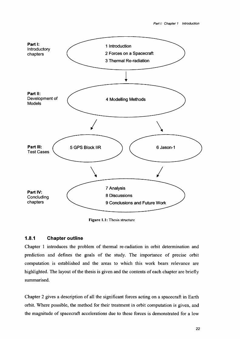
1.1: Thesis structure............................................................................................................................ 22
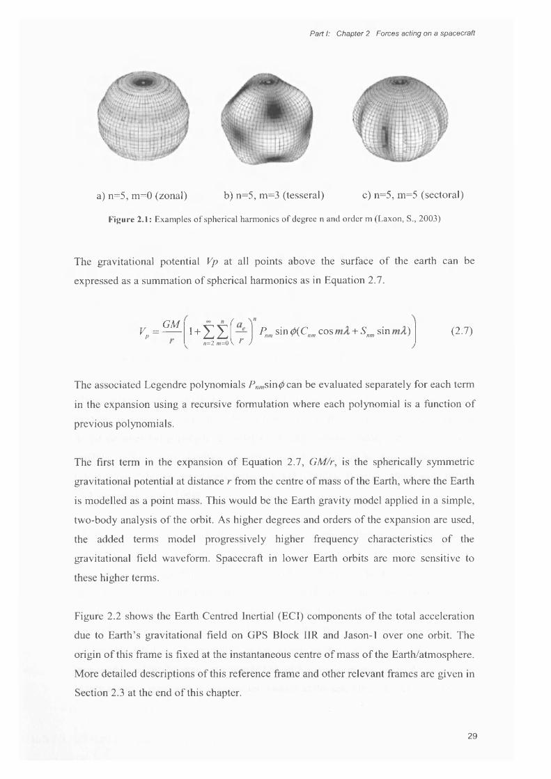
2.1: Examples of spherical harmonics of degree n and order m (Laxon, S., 2003).................29
2.2: Earth’s gravitational accelerations: GPS Block IIR (left) and Jason-1 (right)....................30
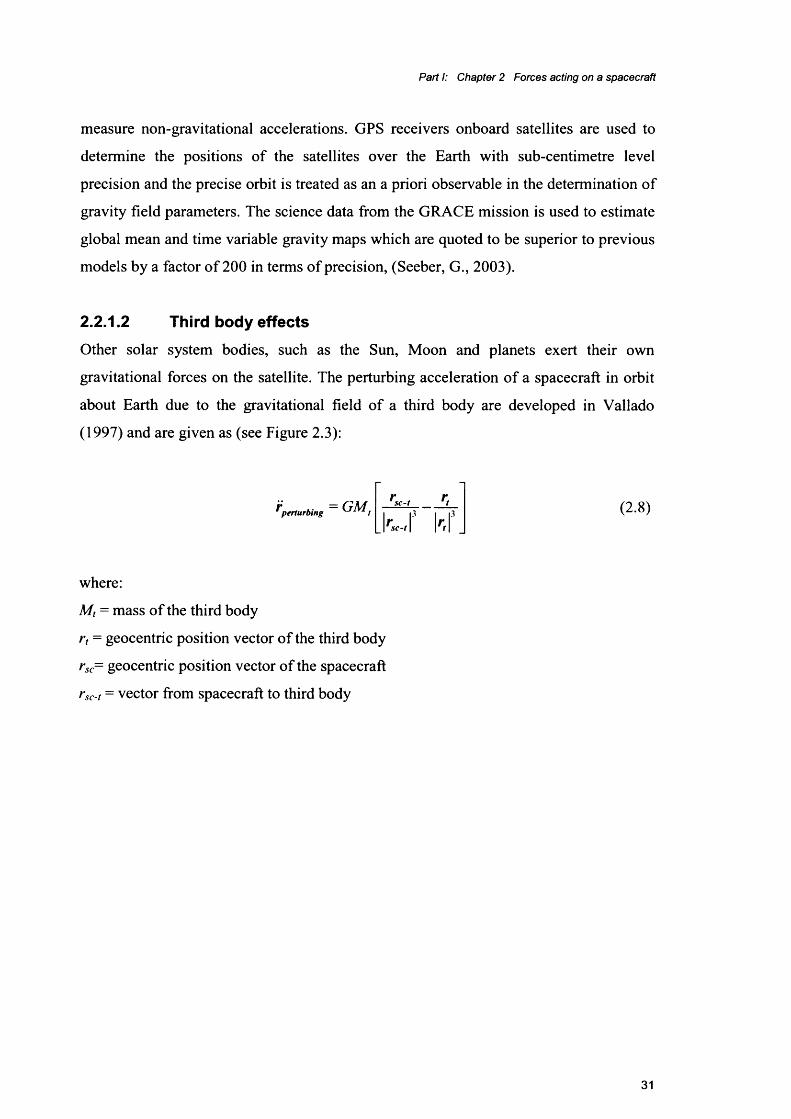
2.3: Position vectors for the third body perturbing acceleration formulation............................. 32
2.4: Solar gravity accelerations for GPS Block IIR (left) and Jason-1 (right)............................33
2.5: Lunar gravity accelerations for GPS Block IIR (left) and Jason-1 (right)...........................33
2.6: Earth tide accelerations for GPS Block IIR (left) and Jason-1 (right)................................. 35
2.7: Pole tide accelerations for GPS Block IIR (left) and Jason-1 (right)................................... 35
2.8: Relativistic accelerations for GPS Block IIR (left) and Jason-1 (right)................................36
2.9: Number of sun-spots over 25 y ea rs ..........................................................................................37
2.10: SRP accelerations: GPS Block IIR (left) and Jason-1 (right)...............................................38
2.11: Shortwave radiation emitted from TOA, January, 2001.........................................................39
2.12: GPS Block IIR showing BFS XYZ a x e s ...................................................................................43
2.13: Jason-1 showing BFS XYZ axes............................................................................................... 44
3.1: Anisotropic emission of radiation by the satellite................................................................... 48
3.2: Diffuse emission from a surface................................................................................................ 49
3.3: Directional distribution of radiant energy from a point source ..............................................50
3.4: GPS Block IIR spacecraft showing body fixed system a x e s ................................................ 54
3.5: Simplified spacecraft structure: Box and Wing model........................................................... 57
3.6: Earth-Probe-Sun angle................................................................................................................ 59
4.1: Composite structure of solar p a n e l...........................................................................................67
4.2: Energy inputs and outputs of the solar panel.......................................................................... 68
4.3: Energy inputs and outputs of the back face of solar p ane l.................................................. 68
4.4: Graph of force as a function of flux...........................................................................................72
4.5: Energy transfer processes in a finite control volume..............................................................73
4.6: Composite panel divided into nodal elem ents.........................................................................76
4.7: Front and back panel face temperatures for a GPS Block IIR spacecraft.........................77
4.8: Acceleration due to thermal panels for a GPS Block IIR spacecraft...................................77
4.9: Illumination of MLI surface with pixel a rray ..............................................................................80
4.10: Radiation from earth impinging on the satellite.......................................................................83
4.11: Spacecraft viewing partially illuminated Earth......................................................................... 84
4.12: Lines forming penumbra and umbra boundaries....................................................................85
4.13: Diagram of a satellite in full phase and a satellite in eclipse.................................................90
4.14: ENVISAT photometry plot - emergence from eclipse............................................................ 92
4.15: Glonass photometry plot - emergence from eclipse............................................................... 92
4.16: Sun, Earth and shadow region geometry................................................................................. 95
4.17: Schematic of cross-section of eclipse region...........................................................................96
8
4.18: Time spent in penumbra per crossing for SVN 46 in Jan/Feb/M ar 2001........................... 97
4.19: Schematic for penumbral height calculation............................................................................98
4.20: Incident ray on spacecraft su rface .............................................................................................99
4.21: Projection of pixel array onto spacecraft structure from one direction..............................101
5.1: Geometrical form of the GPS Block IIR satellite used in this s tu d y .................................. 109
5.2: Technical drawing of GPS Block IIR (dimensions are in m etres)......................................111
5.3: Technical drawing of GPS Block IIR (dimensions are in m etres)......................................112
5.4: Attitude of GPS Block IIR.......................................................................................................... 115
5.5: BFS X, Y and Z accelerations as a function of EPS angle due to MLI surfaces.............. 117
5.6: Direction of force vecto r.............................................................................................................118
5.7: SVN 43 front face panel temperatures from telemetry and model da ta .............................123
5.8: No thermal model - Model 1 ......................................................................................................126
5.9: Thermal models of solar panels only -Model 2 ..................................................................... 127
5.10: Thermal panels and MLI model - Model 3 ............................................................................. 127
5.11: Scale change (thermal panel and MLI modelling) -Model 3 ...............................................128
5.12: Full thermal model - Model 4 ....................................................................................................128
5.13: With and without penumbra flux modelling............................................................................ 129
5.14: Summary of HCL resu lts ........................................................................................................... 129
5.15: Height residuals for SVN 43, 3 March 2004........................................................................... 130
5.16: Cross track residuals for SVN 43, 3 March 2004 ..................................................................130
5.17: Along track residuals for SVN 43, 3 March 2004 ..................................................................131
5.18: Orbit Prediction HCL residuals for SVN 44, 21st March 2 0 0 4 ........................................... 131
6.1: Jason-1 m easurem ent system ................................................................................................. 135
6.2: Geometrical form of Jason-1 used in this study.................................................................... 137
6.3: Possible attitude of Jaso n -1 ......................................................................................................139
6.4: Directions from which the pixel array was projected............................................................ 140
6.5: BFS X, Y and Z accelerations as a function of EPS angle due to MLI surfaces...............141
6.6: Incoming radiation.......................................................................................................................142
6.7: Direction of force vecto r.............................................................................................................143
6.8: Flow chart of orbit determination p ro cess .............................................................................. 146
6.9: Solar sca le .................................................................................................................................... 150
6.10: Linear interpolation of daily atmospheric drag coefficients................................................. 151
6.11: (UCL-CNES) orbit overlap residuals........................................................................................151
6.12: Mean crossovers over 74 cycles, dynamic orbits.................................................................. 153
6.13: Variances over 74 cycles of crossovers, dynamic o rb its .....................................................153
6.14: Mean crossovers over 74 cycles, reduced dynamic o rb its ..................................................154
6.15: Variances over 74 cycles of crossovers, reduced dynamic o rb its..................................... 154
6.16: SLR RMS residuals for dynamic and reduced dynamic orbits............................................ 155
7.1: Orbit prediction errors for SVN 46, using real and nominal m a sse s .................................. 165
7.2: A mis-pointing panel....................................................................................................................167
9

169
172
172
173
173
175
175
179
179
179
182
182
187
190
192
10
Large un-modelled features on Jason-1 spacecraft.......................................
Thermal force in ECI fram e................................................................................
Thermal force in HCL fram e...............................................................................
Thermal force in YPS fram e...............................................................................
Thermal force in BFS XYZ fram e......................................................................
HCL residuals for 2nd March 2004 (SVN 41 left, SVN 43 right)....................
HCL residuals for 10th March 2004 (SVN 41 left, SVN 43 right)...................
Plot of xn against x0 ..............................................................................................
Full orbit prediction results...................................................................................
Orbit prediction results using optimised initial (sam e as 5.11) conditions
HCL residuals: adjusted gravity field.................................................................
HCL residuals: adjusted gravity field and initial state vector........................
ENVISAT in clean room ......................................................................................
Range error resulting from no thermal force m odel.......................................
Model of ENVISAT b u s .......................................................................................

List of Tables
2.1: Planetary d a ta ................................................................................................................................33
4.1: Approximate orbital elements for ENVISAT.............................................................................91
4.2: Eclipse entry / exit time offsets between models and ENVISAT photometry.....................93
5.1: GPS Block IIR surface com ponents........................................................................................ 110
5.2: Characteristics of solar panel layers for GPS Block IIR.......................................................113
5.3: Solar panel data assuming a power draw of 90 Wm'2 ......................................................... 118
5.4: Solar panel data assuming no power draw ............................................................................ 118
5.5: GPS Block IIR m asses for March 2004...................................................................................122
5.6: Telemetered temperatures of solar p a n e ls ............................................................................122
5.7: Mean HCL residuals (m) from 28 days of 12 hour predictions, Model 1......................... 125
5.8: Mean HCL residuals (m) from 28 days of 12 hour predictions, Model 2 ......................... 125
5.9: Mean HCL residuals (m) from 28 days of 12 hour predictions, Model 3 ........................ 125
5.10: Mean HCL residuals (m) from 28 days of 12 hour predictions, Model 4 ......................... 126
5.11: Mean HCL residuals (m) from 28 days of 12 hour predictions in ec lip se ..................... 126
6.1: Properties of Jason-1 MLI......................................................................................................... 137
6.2: Jason-1 solar panel properties................................................................................................. 138
6.3: Jason-1 solar scale results........................................................................................................ 150
6.4: Crossover residuals for Jason-1 ..............................................................................................152
6.5: Mean, variance and RMS of crossover residuals (sample of 39310 crossovers) 155
6.6: High Elevation SLR Range Bias Residuals over 1409 arcs................................................155
7.1: GPS Block IIR solar panel surface param eters and uncertainties.....................................161
7.2: Jason-1 solar panel surface parameters and uncertainties................................................161
7.3: GPS Block IIR MLI parameters and uncertainties.................................................................163
7.4: Mass of GPS Block IIR spacecraft in March 2004 ................................................................164
7.5: HCL residuals for 12 hour orbits averaged over 4 weeks in March 2004 ........................ 164
7.6: Summary of telemetered temperature data for front face of solar panels........................ 166
7.7: Front face panel temps for varying power draw and optical param eters........................... 166
7.8: GPS Block IIR orbit p lanes........................................................................................................ 175
11

Part I: Chapter 1 Introduction
Parti
Chapter 1 Introduction
Space based systems have wide ranging applications; these include navigation systems
such as the Global Positioning System (GPS) and geodetic missions such as satellite
altimetry, gravity field recovery and synthetic aperture radar. These missions
fundamentally rely upon knowledge of the position of the spacecraft; hence the
capabilities of these applications are limited by how accurately the spacecraft orbits can
be computed. Orbit accuracy can be improved by correctly accounting for all forces
which act on a spacecraft. The gravitational components of the force field, such as those
due to the Earth, Sun and Moon are now well understood, but the non-gravitational
forces are more problematic to characterise. The work presented here focuses on the
non-gravitational non-conservative force due to thermal re-radiation from a spacecraft
surface.
Thermal re-radiation perturbs spacecraft orbits when a net recoil force results from the
uneven emission of radiation from the spacecraft surface. Though this force has a
relatively small magnitude (-100 million times smaller than Earth’s gravity), it can
cause metre level perturbations to the trajectory of a spacecraft after only a few hours.
The analytical modelling of this force and its effect on orbit computations are the focus
of this study.
1.1 Goals of study
The aims of this study are to:
• develop methods for modelling the forces that result from spacecraft surface
thermal re-radiation (TRR), based on a purely physical analysis of the problem
• apply these models to real spacecraft
• assess the strength of these methods based on their ability to improve the
accuracy with which their orbits can be predicted and determined
12

Part I: Chapter 1 Introduction
This study is pertinent in the areas of satellite geodesy and astrodynamics. These fields
are discussed in Section 1.2.
1.2 Satellite geodesy and astrodynamics
The word Geodesy literally means dividing the earth (Bomford, G., 1971), but has come
to describe the science concerned with the measurement and mapping of points on the
Earth’s surface. Geodesy encompasses a set of techniques which, once developed, can
be applied to other areas of science or engineering in order to meet the following
objectives:
1. Determination of precise, global and regional coordinate reference frames
2. Precise determination of the earth’s gravity field and temporal variations
3. The measurement and modelling of geodynamical phenomena (eg, crustal
deformation, glacial rebound and global ocean circulation)
Satellite geodesy makes use of artificial satellites as high orbiting reference points
which are visible over large areas. Compared with classical land based surveying
techniques, the main advantages of using satellites are that they are able to bridge large
distances, and thus establish geodetic ties between continents and islands. The issue of
data gaps is less problematic, since satellites can provide data with global coverage.
Astrodynamics encompasses the study of the motion of both natural and artificial
objects in space, though it is principally concerned with spacecraft trajectories, from
launch to re-entry. Within astrodynamics, understanding of the motion of spacecraft and
determination of orbits is effectively the end of the analytical process. Within satellite
geodesy, the precisely determined orbit of a spacecraft provides a data set upon which
further analyses are based. Whilst the models produced in this thesis have direct
relevance in astrodynamics, their applications lie within the scope of satellite geodesy.
1.3 A brief history of satellite orbit determination
Many ancient civilisations including the Chinese, Indians and Greeks made
astronomical and planetary observations from which they developed primitive
understandings of the motion of celestial bodies. The first laws of planetary motion
13
Part I: Chapter 1 Introduction
were proposed by Kepler at the start of the seventeenth century, who determined them
empirically based on observation data. These laws were formalised by Newton in his
theory of gravity in 1666 and provided the first fundamental understanding of the
physics of orbit dynamics. During the next three centuries, the field matured. Detailed
refinements of satellite orbit models came about during the Cold War, when the race to
develop intercontinental ballistic missiles and to land a man on the moon required the
accomplishment of sophisticated mission objectives with elaborate constraints. This
gave rise to immense efforts to improve knowledge in this field. Important benefits that
flowed from this competition included space-based communication, navigation and
surveillance systems.
The first object whose orbit was determined by the analysis of an emitted signal was
Sputnik. Launched by the Soviet Union in October 1957, Sputnik was the first artificial
satellite to orbit the Earth. Researchers at the Johns Hopkins Applied Physics
Laboratory (APL) in Baltimore calculated that they could determine Sputnik's orbit
simply by measuring the Doppler-induced changes in the frequency of the simple radio
signal that it transmitted. Several years later, another APL scientist was seeking a
system that would allow Polaris nuclear submarines to precisely track their positions.
He realised that this could be achieved by inverting the approach used by the scientists
working on Sputnik: by measuring a radio signal from a satellite whose position is
known, a submarine could determine its own position (Tikhonravov, M., 1994).
The next few decades saw the emergence of many more sophisticated technologies,
including microelectronics, radar and digital computers. These, combined with detailed
theoretical and empirical models of Earth’s gravity, the atmosphere, and planetary
ephemerides enabled the development of systems which could be used to accurately
determine the position of satellites.
The level of accuracy required in the knowledge of a satellite’s orbit depends on the
particular goals of a space project. In accord with these requirements, a variety of
tracking systems are employed in present space projects. These include satellite laser
ranging, Doppler Orbitography and Radiopositioning Integrated by Satellite (DORIS),
the US Global Positioning System (GPS), and the recently commissioned European
Galileo, due to be operational in 2008. Existing systems can currently provide spatial
14

Part I: Chapter 1 Introduction
information on the surface of the earth with precisions at the sub centimetre level. These
systems can also be used to determine positions of low earth orbiting satellites.
1.4 The computation of precise orbits
To predict the trajectory of a spacecraft, its position and velocity must be correctly
specified at one instant, and all forces which influence its motion must be known. The
forces that drive the shape of a satellite trajectory include the Earth’s gravity field, third
body gravitational forces due to the Sun, Moon and planets, tidal Earth gravity field
effects, and relativistic force effects. These forces are now well understood and highly
accurate models for them are available, particularly when using data from the current
Gravity Recovery and Climate Experiment (GRACE) mission, which has contributed
significant improvements to the knowledge of the Earth’s gravity field (Heugentobler,
U. & Beutler, G., 2003). There is another set of forces which act on a spacecraft known
as non-conservative forces (NCFs), so called because they result in an energy change to
the spacecraft. Among the largest NCF is solar radiation pressure (SRP), caused by the
impact of solar photons on the satellite surface. In the last decade, SRP has received
some attention and now high precision analytical techniques exist to model this force
(Ziebart, 2004a). Less progress has been made on the other NCF forces which are one to
two orders of magnitude smaller than SRP. These include the force due to radiation
reflected and emitted by the Earth, and of course TRR. Depending on altitude, a satellite
may also be subject to considerable atmospheric drag effects, which for low earth
orbiters (LEOs) constitute a force comparable with SRP. These forces are described in
detail in Chapter 2.
NCFs are problematic to characterize analytically as they depend on the satellite’s
instantaneous attitude, surface geometry, optical and material properties, as well as the
incident radiation flux and particulate environment. The structural and material property
data is often hard to acquire. This is partly because spacecraft data are not generally
released into the public domain. Additionally some of the data required are difficult to
quantify accurately. Examples of the latter include surface material properties, since the
nature and rate of material degradation in space is not well known, and spacecraft
attitudes which may be subject to unpredictable variations.
15
Part I: Chapter 1 Introduction
In practice, neither the state of the spacecraft nor the forces can ever be defined
completely accurately; any attempt to predict a trajectory will result in some divergence
from the true position of the spacecraft over time.
However, if the distance of the spacecraft from a well-determined position on the
surface of the Earth is known, again as a function of time, this information could be
incorporated in the computation to correct the integrated trajectory and produce a better
orbit. In principle, if many accurate range observations were available from reference
stations with known co-ordinates, the orbit computation could be reduced to a series of
spatial resections. In practice, none of these ranges or station co-ordinates are known
exactly either; they too can only be estimated. The most accurate orbit solution is
obtained when both force models and tracking data are combined, weighted by their
respective accuracies. The detailed exploration of the physical model allows a better
evaluation of the accuracies of the force models. Accurate range data is sometimes only
available after the orbit has occurred, when data from ground tracking stations has been
processed and made available, hence it is not useful for real time applications.
The level of sophistication of the orbit computation is dictated by the desired accuracy
in the final solution; this depends on the requirements of the application. Two types of
precise orbit computation are relevant in this thesis: orbit prediction and orbit
determination.
• Orbit prediction
Predicted orbits refer to those that have been propagated from an initial position and
velocity using a set of models describing the forces acting on the spacecraft. No
tracking data during the period of prediction is used1. These techniques are described in
more detail in Chapter 5. Predicted orbits play an important role in a variety of
processes. These include real time GPS navigation, spacecraft design and operation and
the efficiency with which satellites can be tracked by systems such as SLR.
1 In GNSS applications tracking data collected at previous epochs is used to constrain future positions
16
Part I: Chapter 1 Introduction
• Orbit Determination
Orbit determination is a complex process which combines observations made by
tracking stations with spacecraft force models of varying degrees of sophistication.
Extra parameters may be computed or scale factors applied to certain force model
parameters to enable the estimated trajectory to better fit the observations. There are
three main types of orbits produced by this method: dynamic, reduced dynamic and
kinematic. They differ in the balance chosen between force models and tracking data
used, and are described in greater detail in Chapter 7. They are particularly suitable
when position data is required hours or several days after the event when large amounts
of range data from ground stations to satellites can be made available. There are many
analysis centres worldwide which independently carry out this type of orbit processing
for GPS spacecraft. These include:
• Centre for Orbit Determination in Europe (CODE), Switzerland
• Natural Resources Canada (EMR), Canada
• European Space Agency (ESA), Germany
• GeoForschungs Zentrum Institute (GFZ), Germany
• Jet Propulsion Laboratory (JPL), USA
• National Geodetic Survey (NGS), USA
• Scripps Institution of Oceanography (SIO), USA
These centres are members of the International GPS Service (IGS), which combines
data from all these centres to provide an official GPS orbit, along with other high-
quality GPS data and data products. The fact that so many agencies dedicate time to the
production of high precisions orbits is an indication of their importance and of their
non-trivial nature.
Both orbit prediction and determination techniques require an a priori dynamic model of
the spacecraft. The closer the dynamic models are to the true forces, the closer the
computed trajectory will be to the actual orbit. The more accurate the dynamic model,
the better the final computed orbit. Section 1.5 outlines a few areas where precise orbits
are essential to the successful mission performance.
17

Part I: Chapter 1 Introduction
1.5 The applications of precise orbits
Precise orbits play a key role in a number of areas, including Global Navigation
Satellite Systems (GNSS), satellite altimetry, satellite gravity recovery and synthetic
aperture radar (SAR) missions.
Real-time GPS applications such as navigation fundamentally rely upon the prediction
of spacecraft positions. In the GPS process, although observation data from tracking
stations are continually incorporated to update predictions, it is the force models which
play the main role in determining the predicted trajectory of the spacecraft.
Aside from navigation, GPS systems can be used in real-time and in near real-time to
monitor displacements of engineering structures such as bridges and dams that may
occur due to small ground deformations caused by high loading or seismic activity
(Behr, J. et al., 1998). Generally short baseline differencing techniques (using multiple
receivers) have been used for these measurements; in these cases orbit errors are less
important. However there is a current trend towards using single receiver precise point
positioning techniques (Heroux, P. et al., 2004), whereby satellite orbit errors have a
higher impact on the results. The real-time monitoring of deformations in large
engineering structures such as oil rigs, where double differencing is not possible also
depends on the quality of satellite orbits. Other developing technologies using GPS
include real-time weather forecasting, by estimating the amount of water vapour in the
atmosphere by the delay in the GPS signal (Reigber, C. et al., 2002). These applications
are currently limited by the accuracy of predicted orbits, and improving the orbits would
directly benefit these applications.
GNSS spacecraft orbits are used as references from which the position and velocity of
points on the surface of the Earth can be calculated. The study of tectonic activity is one
area where high precision positioning is key. Continuous networks of GPS receivers can
provide measurements that help to model the deformation of the Earth's crust over time,
and over areas ranging from tens to thousands of square kilometres (Liu, M. et al.,
2000). Models are used to study the earthquake cycle, the effect of faulting and uplift on
the Earth's surface, and the physics of continental deformation. These studies play an
important role when quantifying seismic hazard and interpreting how past environments
18

Part I: Chapter 1 Introduction
control the distribution of natural resources. GPS networks are also used to monitor the
thickness of ice sheets and the rate of glacial rebound. Biases in orbits would alias into
GPS receiver positions and affect the accuracy of the target geophysical parameters.
Low Earth orbiting satellites (LEOs) are now one of the primary platforms (along with
other aerial observations) used to make large-scale measurements of environmental
phenomena, and the accuracy with which their trajectories can be determined is a factor
which can limit what they can achieve. LEO satellite orbits often rely on GPS
positioning for the calculation of their orbits. Errors in GPS orbits will therefore also
lead to errors in the LEO orbits. These applications have stimulated advances in precise
orbit determination. Satellite altimetry uses the measured travel time of a radar pulse to
and from the sea surface to determine the distance of the sea surface from the
spacecraft. For the translation of this measurement into a sea surface height, the
satellite’s absolute position must be determined with high precision in a suitable
reference frame. Inaccuracies in the orbit are particularly problematic in that they tend
to be expressed systematically over many thousands of kilometres and alias into the
determination of large sea surface topography and ocean currents. Topex/Posiedon, a
French American altimetry satellite mission measures ocean surface topography to
within an accuracy of 4.2cm and enabled scientists to forecast the 1997-98 El Nino
effect (Haines, B. et al., 2002). The follow-on mission Jason-1 aims to monitor global
ocean circulation, study interactions of the oceans and atmosphere, improve climate
predictions and observe events such as El Nino. Jason-1 ’s overarching mission goal is to
measure sea-surface heights to an accuracy of 1cm and (with the inclusion of the work
in this thesis along with other studies) has recently been achieved. A new goal of 5mm
has now been set (Bertiger, W., 2004).
The new millennium has heralded an era of missions aimed at producing a highly
precise Earth gravity field. These include: CHAMP (Challenging Mini-satellite
Payload), launched 15th July 2000; GRACE, launched 17th March 2002 and the soon-
to-be-launched GOCE (Gravity Field and Steady-State Ocean Circulation Explorer).
These missions use three axes accelerometers, which measure the combined
accelerations caused by surface forces (as opposed to forces which act directly on the
centre of mass of the spacecraft). A high precision orbit is required and the surface force
effects (deduced from measurements made by the accelerometers) are removed from
19

Part I: Chapter 1 Introduction
this; further orbit perturbations are assumed to be due to the gravity field, and third body
effects. Though non-conservative forces are measured, models are still required for
calibration of the accelerometers, and for the deduction of specific non-conservative
forces such as atmospheric drag.
1.6 Motivation
The applications described in Section 1.5 would benefit in terms of the accuracy of the
data they produce from improved models of the non-conservative forces acting on the
spacecrafts. To summarise, the main reasons for conducting this research are to:
• improve our understanding of the factors which influence the motion of a
spacecraft
• improve the ability with which spacecraft orbits can be predicted and determined
• reduce the aliasing of orbit errors into geophysical parameters by constraining
the errors in the mathematical model of the orbit.
1.7 Research methodology
In order to calculate the force due to thermal re-radiation, it is necessary to:
• characterise the radiation flux in the spacecraft vicinity
• model the interaction of this flux with the spacecraft surface
• determine spacecraft surface temperatures
• develop algorithms to calculate the surface thermal forces as a function of space
and time
• obtain real spacecraft data for chosen test satellites
Two distinct regimes are considered for the spacecraft: the steady state regime where
the spacecraft is in full sunlight and temperatures are assumed to change very slowly,
and the transient regime that occurs during eclipses, when surface temperatures fall
rapidly.
For accurate modelling of forces that depend on incident solar flux, it is necessary to
know precisely when the spacecraft crosses shadow boundaries, so that the incident
solar flux can be reduced accordingly. The shadow regions consist of the penumbra and
umbra: the penumbra is the region where sunlight is partially occluded by the Earth and
20

Part I: Chapter 1 Introduction
the umbra is the region that is totally devoid of solar radiation. A method is developed
to calculate crossing times into and out of shadow regions, and to estimate the reduction
in flux in the penumbral regions. These methods should improve all forces that depend
upon solar radiation flux.
Two test cases are chosen to which the models are applied; these are the GPS Block IIR
spacecraft (in medium earth orbit (MEO)) and Jason-1 (in LEO). The test cases require
different testing methods due to their different orbit environments. GPS Block IIR
models are evaluated by analysing improvements to orbit prediction models whereas
Jason-1 models are tested by their effect on orbit determination capabilities.
1.8 Thesis outline
The overall layout of the project is separated into Parts I-IV. The following chart is
intended to clarify the thinking behind the overall approach and to outline what each
part of the thesis tackles.
21
Part I: Chapter 1 Introduction
Part i :Introductorychapters
Part II:Development of Models
1 Introduction
2 Forces on a Spacecraft
3 Thermal Re-radiation
i
Part III:Test Cases
4 Modelling Methods
/ \5 GPS Block IIR 6 Jason-1
Part IV:Concludingchapters
7 Analysis
8 Discussions
9 Conclusions and Future Work
Figure 1.1: Thesis structure
1.8.1 Chapter outlineChapter 1 introduces the problem of thermal re-radiation in orbit determination and
prediction and defines the goals of the study. The importance of precise orbit
computation is established and the areas to which this work bears relevance are
highlighted. The layout of the thesis is given and the contents of each chapter are briefly
summarised.
Chapter 2 gives a description of all the significant forces acting on a spacecraft in Earth
orbit. Where possible, the method for their treatment in orbit computation is given, and
the magnitude of spacecraft accelerations due to these forces is demonstrated for a low
22

Part I: Chapter 1 Introduction
earth orbiter (Jason-1) and medium earth orbiter (GPS Block IIR). This chapter includes
a section on coordinate systems which will be useful for expressing different effects
throughout this thesis.
Chapter 3 provides a more detailed explanation of the basis of the force due to thermal
re-radiation and how it is characterised. Analytical and empirical methods for treatment
of this force are described and with these in mind, the motivation for producing good a
priori models is re-established. The published literature relevant to this work is
reviewed.
In Chapter 4 the models developed in this thesis are derived. These consist of thermal
force models for solar panels and surfaces covered in multilayer insulation in the steady
state and transient regimes. The treatment of other surfaces, such as antennas is
considered. Models for better determining the flux during eclipse regions are also
described, including a method for determining boundary crossing times for an oblate
earth and the reduction of flux in the penumbral regions.
Chapters 5 and 6 are concerned with the application of the modelling methods to the
GPS Block IIR and Jason-1 spacecraft respectively. Each chapter reviews the spacecraft
system, the data used in the modelling process and describes how the methods have
been adapted specifically for each spacecraft. Orbit prediction (for GPS Block IIR) and
orbit determination (for Jason-1) methods used for model testing are described. Each
chapter concludes with the results of these tests and a brief analysis of the results.
Chapter 7 analyses in more detail the models, testing methods and results. Uncertainties
in the parameter set and their effect on the modelled orbits are scrutinised. The thermal
force is analysed in different reference frames. Remaining sources of error are identified
and explored.
Chapter 8 includes a discussion of the strengths and deficiencies in each part of the
model, and the general applicability of the methods produced in the thesis. Specific
applications of this work are described, and an evaluation is made of the extent to which
the goals set in this thesis have been achieved.
23

Part I: Chapter 1 Introduction
Chapter 9 summarises the work carried out in this thesis and states the main conclusions
that can be made from this study. It also contains suggestions for future work in this
problem domain.
Summary
In this chapter, the goals of this project have been defined and reasons for carrying out
the work in this thesis are established. The accuracy of computed orbits is limited in part
by the lack of detailed models of spacecraft surface thermal re-radiation forces. Greater
orbit accuracies will improve the capabilities of applications which rely upon them.
Modelling the motion of a spacecraft relies on knowledge of all significant forces acting
on it. These forces are discussed in the next chapter.
24

Part I: Chapter 2 Forces acting on a spacecraft
Chapter 2 Forces acting on a spacecraft
Chapter outlineTo dynamically model the orbit of a spacecraft, it is necessary to consider all forces
which have significant effects on its trajectory. This section describes those forces and
outlines the approaches to their modelling in orbit computations. Examples of their
effects are given for two spacecraft, GPS Block IIR, which orbits at an altitude of
~20200km, and Jason-1 which orbits at an altitude of ~1340km. For most force effects,
graphs of acceleration over one orbit on 2nd March 2004 are given for each spacecraft.
Finally this chapter gives a description of the main coordinate systems used in the
context of spacecraft orbits.
2.1 Orbital motion
From Newton’s law of gravitation, the force F on mass m orbiting about a spherically
symmetrical body of mass M at distance r from the centre of mass, where G is the
Gravitational constant is defined as:
F = - ^ (2.1)r
The corresponding vector acceleration r is given by:
L = - ^ - L (2.2)r
Given an initial position and velocity, this second order differential equation (Equation
2.2) can be solved analytically to yield the position and velocity of mass m at future
epochs. This Mr force field provides a basic model from which we can derive a
reasonable first approximation to the motion of a satellite around Earth.
25

Part I: Chapter 2 Forces acting on a spacecraft
In reality, the Earth is not a uniformly dense sphere; this factor along with other effects
causes perturbations to this idealised orbit, and more refined models for these forces are
required for the development of the actual equations of motion. The addition of the
perturbing accelerations ap gives:
Once these perturbations are added, it is extremely difficult to calculate a closed form
analytical solution for Equation 2.3 and instead numerical procedures must be invoked.
In numerical integration techniques, all modelled forces acting at a particular satellite
position are explicitly calculated, and they are used as starting conditions for the next
integration step.
Under the action of conservative forces, which are primarily gravitational, the
mechanical energy of the system (that is, the sum of its kinetic and potential energies) is
conserved. Technically, the system here refers to all the objects considered in the
problem; the spacecraft, the Sun, Moon and the planets. If the energy state of the
spacecraft is known at some epoch, then its energy state at any later epoch can be
predicted as a function of position alone, that is, the energy state is independent of the
path taken. The motion of satellite can never be completely described by a consideration
of a purely conservative force field, but is useful nevertheless in the estimation of
trajectories. In a non-conservative force field the spacecraft energy state is path-
dependent, and any attempt to predict the future energy state has to model all the
significant non-conservative forces as a function of space and time. The principal non
conservative forces acting on spacecraft are due to solar radiation pressure, thermal re
radiation, atmospheric drag and albedo effects. An additional force which falls in this
category is thrust caused by signal emission from any antenna aboard the satellite.
In this chapter, the following perturbing forces are considered:
• Non-spherical earth gravity terms
• Third body effects (Sun, Moon, Planets)
• Solid Earth, ocean and pole tides
• Relativistic effects
(2.3)
26

Part I: Chapter 2 Forces acting on a spacecraft
• Solar radiation pressure
• Earth Radiation pressure
• Thermal re-radiation
• Atmospheric drag
• Force resulting from signals transmitted by satellite (antenna thrust)
These forces and their magnitudes are discussed in Section 2.2.
2.2 Perturbing forces
2.2.1 Conservative forces2.2.1.1 Earth’s gravitational fieldAs predicted by Newton, the Earth’s rotation about its polar axis causes its shape to
deviate from a perfect sphere (Montenbruck, O. & Gill, E., 2000). The earth is more
accurately described by an oblate spheroid with an equatorial diameter that exceeds the
polar diameter by about 20km. For any satellite with a non-zero inclination, the
equatorial bulge exerts a force on the satellite such that it results in a secular drift of the
right ascension of the ascending node (the point where the satellite crosses the equator
from the Southern hemisphere to the Northern hemisphere). This perturbation is three
orders of magnitude smaller than the central gravitational attraction and is commonly
referred to as J2. The asphericity and inhomogeneous mass distribution of the earth
cause a variety of further gravitational perturbations that affect the trajectory of a
satellite.
The gravitational field of the Earth as a whole can be represented in terms of a potential
field which satisfies Laplace's equation at all external points (Bomford, G., 1971).
Laplace’s equation is a partial second order differential equation and in cartesian
coordinates is given by:
+ -dx1 a / dz'
v = o (2.4)
where V is the gravitational potential field of the earth. Any function which satisfies it is
called a harmonic. Laplace's equation for the potential in spherical polar co-ordinates is:
27

Part I: Chapter 2 Forces acting on a spacecraft
sinO- — +dO J r 2 sin2 0 dO2
) 1 d 2 V - n (2.5)
The solutions to Equation 2.5 are spherical harmonics which have the form:
G M ( a n
Pn J sitl(P)(Cnmcos(m X) + S nmsin(m X)) (2.6)r \ r
where:
Vp = The gravitational potential at point p ($A,r)
ae = mean equatorial radius of the earth
n = degree of gravity field expansion
m = order of gravity field expansion
Pthm (sin$) = associated Legendre polynomial
X= geocentric longitude of p
(f>= geocentric latitude of p
Cnm> Snm = spherical harmonic coefficients
The superposition of spherical harmonics can be used to represent physical phenomena
distributed over the surface of a sphere in the same way that a Fourier series represents a
one dimensional function with a combination of periodic functions. Some examples of
spherical harmonic functions are shown pictorially in Figure 2.1 (the name of the type
of harmonic is given in brackets). When m=0, the geopotential surface is divided into
latitudinal bands and zonal harmonics result (the geopotential is independent of
longitude); when m=n and the surface is divided into longitudinal sectors and are known
as sectoral harmonics. For m <n and m ?©, the surface is divided into rectangular
domains and are known as tesseral harmonics.
28
Part I: Chapter 2 Forces acting on a spacecraft
a) n=5, m=0 (zonal) b) n=5, m=3 (tesseral) c) n=5, m=5 (sectoral)
Figure 2.1: Examples of spherical harmonics of degree n and order m (Laxon, S., 2003)
The gravitational potential Vp at all points above the surface of the earth can be
expressed as a summation of spherical harmonics as in Equation 2.7.
Vp =GM 1 + Z Z f P nm sin f t C nm C0S + S nm sin )
« = 2 m = A r J(2.7)
The associated Legendre polynomials Pnmsin^can be evaluated separately for each term
in the expansion using a recursive formulation where each polynomial is a function of
previous polynomials.
The first term in the expansion o f Equation 2.7, GM/r, is the spherically symmetric
gravitational potential at distance r from the centre o f mass o f the Earth, where the Earth
is modelled as a point mass. This would be the Earth gravity model applied in a simple,
two-body analysis o f the orbit. As higher degrees and orders o f the expansion are used,
the added terms model progressively higher frequency characteristics o f the
gravitational field waveform. Spacecraft in lower Earth orbits are more sensitive to
these higher terms.
Figure 2.2 shows the Earth Centred Inertial (ECI) components o f the total acceleration
due to Earth’s gravitational field on GPS Block IIR and Jason-1 over one orbit. The
origin o f this frame is fixed at the instantaneous centre o f mass o f the Earth/atmosphere.
More detailed descriptions o f this reference frame and other relevant frames are given in
Section 2.3 at the end o f this chapter.
29

Part I: Chapter 2 Forces acting on a spacecraft
As the internal mass distribution of the earth is not well known, the geopotential
coefficients, Cnm and Snm in Equation 2.7 cannot be evaluated directly. They can
however be deduced by observing the motion of the satellite and by analysing
perturbations to the trajectory. Inversion of this perturbation data generates a solution
for the Earth’s gravity field.
0.8
0.66.0
0.44.0
~ 0.2
~ 0.0oo< -0.2
2.0
0.012 100
< -2.0
-0.4 -4.0
-0.6 -6.0
* Z-0.8 -8.0
Tim* (hours)
Figure 2.2: Earth’s gravitational accelerations: GPS Block HR (left) and Jason-1 (right)
Many gravity models have been developed in the last decade. Examples include
EGM96 (Lemoine, F. et al., 1997) which, at the time, represented a significant
milestone in global gravity field modelling. Its development incorporated a plethora of
satellite tracking data, satellite altimetry, and the most up to date surface gravity
information. Other recent models include JGM3, (Tapley, B. et al., 1996) and GRIM5
(Schwintzer, P. et al., 1999).
The most recent mission dedicated to recovering the gravity field is GRACE, (Gravity
Recovery and Climate Experiment), launched in March, 2002
(http://www.csr.utexas.edu/grace/). The GRACE mission involves two identical
satellites orbiting one after the other separated by an approximate distance of 200 km.
Variations in the gravity field cause variations in the distance between the two satellites;
areas of stronger gravity will affect the lead satellite first and accelerate it away from
the second satellite. The resulting range variations between the two satellites are
measured by a high-accuracy microwave link with a precision better than 10 microns. A
highly accurate three-axis accelerometer, located at the satellite mass centre, is used to
30
Part I: Chapter 2 Forces acting on a spacecraft
measure non-gravitational accelerations. GPS receivers onboard satellites are used to
determine the positions of the satellites over the Earth with sub-centimetre level
precision and the precise orbit is treated as an a priori observable in the determination of
gravity field parameters. The science data from the GRACE mission is used to estimate
global mean and time variable gravity maps which are quoted to be superior to previous
models by a factor of 200 in terms of precision, (Seeber, G., 2003).
2.2.1.2 Third body effectsOther solar system bodies, such as the Sun, Moon and planets exert their own
gravitational forces on the satellite. The perturbing acceleration of a spacecraft in orbit
about Earth due to the gravitational field of a third body are developed in Vallado
(1997) and are given as (see Figure 2.3):
r = GMperturbing t (2 .8)
where:
Mt = mass of the third body
rt = geocentric position vector of the third body
rsc= geocentric position vector of the spacecraft
r Sc - t = vector from spacecraft to third body
31

Parti: Chapter 2 Forces acting on a spacecraft
Third body
Figure 2.3: Position vectors for the third body perturbing acceleration formulation
As orbit altitude increases, for particular alignments of Earth, probe and third body,
these accelerations increase in significance relative to Earth’s gravity. At the altitude of
a geostationary satellite (~36000km), when the probe lies between the Sun or Moon and
the Earth, these forces are comparable to the force caused by the equatorial bulge.
Positions of the Sun, Moon and other planets can be approximated by a set of
Chebyshev polynomials (Press, W., 2002). The Jet Propulsion Laboratory (JPL) provide
a series of ephemerides for bodies in the solar system in the form of these polynomials
known as Developmental Ephemerides (DE). DEs are publicly available and have
emerged as a standard for high precision planetary and lunar coordinates (Seidelmann,
P., 1992). The most recent versions are DE405 and DE4062 (Standish, E., 2004) and
covers a total of 600 years from 1600 to 2201. The ephemeredes are based on a rigorous
numerical integration of the respective equations of motion. Once the positions of these
bodies have been generated, their perturbing accelerations can be calculated.
Table 2.1 summarises the mass, distance from the Sun (in astronomical units, AU) and
perturbing accelerations of the third bodies for a particular epoch. Perturbations caused
by the Sun and Moon are similar in magnitude and require consideration for any precise
2 DE405 and DE406 are similar, but the accuracy of the interpolating polynomials for DE406 have been lessened.
32

Part I: Chapter 2 Forces acting on a spacecraft
prediction. The effects of the planets represented in Table 2.1 are ~5-7 orders of
magnitude smaller, though for very precise applications, they can become important.
Though the effect of the other planets can also be modelled, they are too small to
significantly perturb Earth orbiting spacecraft. Figures 2.4 and 2.5 show the ECI
accelerations caused by the Sun and the Moon over one orbit (March 2nd, 2004).
Third bodyMean distance from Sun (AU)
Mass in Earth masses
GPS Block HRacc (ms'2)
Jason-1acc (ms'2)
Sun - 333000 2.5 x 10'6 6.0x10'7Moon 1 0.012 3.0 x lO'6 1.0 xlO*Venus 0.72 0.82 5.0 x 1 0 " 1.0 x 10'17Mars 1.5 0.11 1.0 x 10'u 2.0 x 10'14
Jupiter 5.2 318 2.0 x 10'" 6.0 x 1 0 “
Table 2.1: Planetary data
8.0E-072.5E-06
2.0E-06 6.0E-07
1.5E-064.0E-07
1.0E-06
C 5.0E-07
O.OE+OO
— 2.0E-07
— O.OE+OO
12< -5.0E-07 * -2.0E-07
-1.0E-06-4.06-07
-1.5E-06
-6.0E-07-2.0E-06 ■* z
■*z-2.5E-06 -8.0E-07
Time (mins)
Figure 2.4: Solar gravity accelerations for GPS Block HR (left) and Jason-1 (right)
1.5E-064.0E-06
3.0E-061.0E-06
2.0E-06
5.0E-07— 1.0E-06
12-1.0E-06
-5.0E-07
-2.0E-06
-1.0E-06-3.0E-06
-4.0E-06 -1.5E-06
Time (mint)
Figure 2.5: Lunar gravity accelerations for GPS Block HR (left) and Jason-1 (right)
33
Part I: Chapter 2 Forces acting on a spacecraft
2.2.1.3 Earth tidesThe gravity of the Sun and Moon exert direct forces on the Earth’s crust leading to
small periodic deformations called solid Earth tides. Similar effects on the ocean are
known as ocean tides. This movement of mass around the Earth induces a change in the
Earth’s gravitational potential. The perturbations of satellite orbits from the luni-solar
tides are derived by an expansion of the tidal-induced gravity potential using spherical
harmonics in a similar way to the static gravity field of the Earth. The second degree
expansion of the potential UB at position vector r (Montenbruck, O. & Gill, E., 2000)
due to the gravitational fields of n disturbing bodies is given by:
Md = the mass of the third body
rd = the inertial geocentric position vector of the disturbing body
k = the second degree Love number
r = the inertial geocentric position vector at which the potential is being evaluated
ae = the mean equatorial radius of the Earth
From Equation 2.9, it can be seen that the potential effects are proportional to M /av
and therefore lunar tides are about twice as strong as solar tides. The Love number is the
ratio between the tidal potential (Equation 2.9) and the gravitational potential (Equation
2.7) and can be interpreted as a measure of Earth’s elasticity and the extent to which it
will deform. A value of k = 0.30 is commonly used for the Earth, though for very
rigorous treatments, it would not be treated as a constant (Montenbruck, O. & Gill, E.,
2000). Figure 2.6 demonstrates the solid Earth tide accelerations over one orbit. Effects
of solid Earth tides are about one order of magnitude larger than that of ocean tides.
(2.9)
34

Part I: Chapter 2 Forces acting on a spacecraft
1.5E-09 3.0E-07
1.0E-09 2.0E-07
5.0E-10 ! s* 1.0E-07
O.OE+OO — O.OE+OO12 100
-5.0E-10
-1.0E-09 -2.0E-07
* Z-1.5E-09 -3.0E-07
Time (mins)Time (hours)
Figure 2.6: Earth tide accelerations for GPS Block IIR (left) and Jason-1 (right)
2.2.1.4 Pole tides
The changing position of the Earth’s rotation axis causes the poles to roughly describe a
circle of about 20m in diameter. The variation in the direction of the resulting
centrifugal forces causes a varying elastic response in the Earth’s crust. These are
described by corrections to the geopotential coefficients C21 and S21 . The time varying
magnitude of these corrections are calculated by the International Earth Rotation
Service (McCarthy, D., 1996). The changes in the Earth’s gravity acceleration as a
result of the polar tides over one orbit are shown in Figure 2.7.
1.0E-111.0E-08 -*-x
— Y
• ♦ • Z
i.0E-11 8.0E-09
6.0E-09 ■
4.0E-09
2.0E-09 \
— 0.0E+00 Y
< -2.0E-09
-4.0E-09
*-z4.0E-11
5 2.0E-11
11012
-2.0E-11
•6.0E-09-4.0E-11
-8.0E-09
-6.0E-11 -1.0E-08Tima (hours) Tina (mint)
Figure 2.7: Pole tide accelerations for GPS Block HR (left) and Jason-1 (right).
2.2.1.5 Relativistic effects
For a rigorous treatment of a satellite’s trajectory, general relativistic effects require
consideration. Though this force is extemely small (see Figure 2.8), it has been included
in the analyses later in this thesis and hence is mentioned here.
35
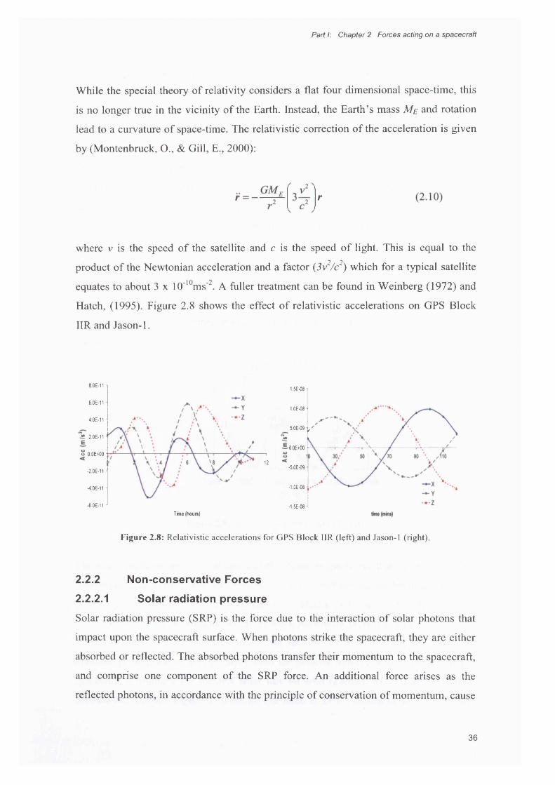
Parti: Chapter 2 Forces acting on a spacecraft
While the special theory of relativity considers a flat four dimensional space-time, this
is no longer true in the vicinity of the Earth. Instead, the Earth’s mass ME and rotation
lead to a curvature of space-time. The relativistic correction of the acceleration is given
by (Montenbruck, O., & Gill, E., 2000):
where v is the speed of the satellite and c is the speed of light. This is equal to the
product of the Newtonian acceleration and a factor (3v2/c2) which for a typical satellite
equates to about 3 x 10'10ms"2. A fuller treatment can be found in Weinberg (1972) and
Hatch, (1995). Figure 2.8 shows the effect of relativistic accelerations on GPS Block
HR and Jason-1.
I.OE-111.5E-08
6.0E-111 OE-08
4.0E-11
5.0E-09 ,
* 2.0E-11
O.OE+OOO O.OE+OO
12-5.0E-09
-2.0E-11
■1 OE-08-4.0E-11
-6.0E-11 •1.5E-08Time (hours)
Figure 2.8: Relativistic accelerations for GPS Block HR (left) and Jason-1 (right).
2.2.2 Non-conservative Forces
2.2.2.1 Solar radiation pressure
Solar radiation pressure (SRP) is the force due to the interaction of solar photons that
impact upon the spacecraft surface. When photons strike the spacecraft, they are either
absorbed or reflected. The absorbed photons transfer their momentum to the spacecraft,
and comprise one component of the SRP force. An additional force arises as the
reflected photons, in accordance with the principle of conservation of momentum, cause
36
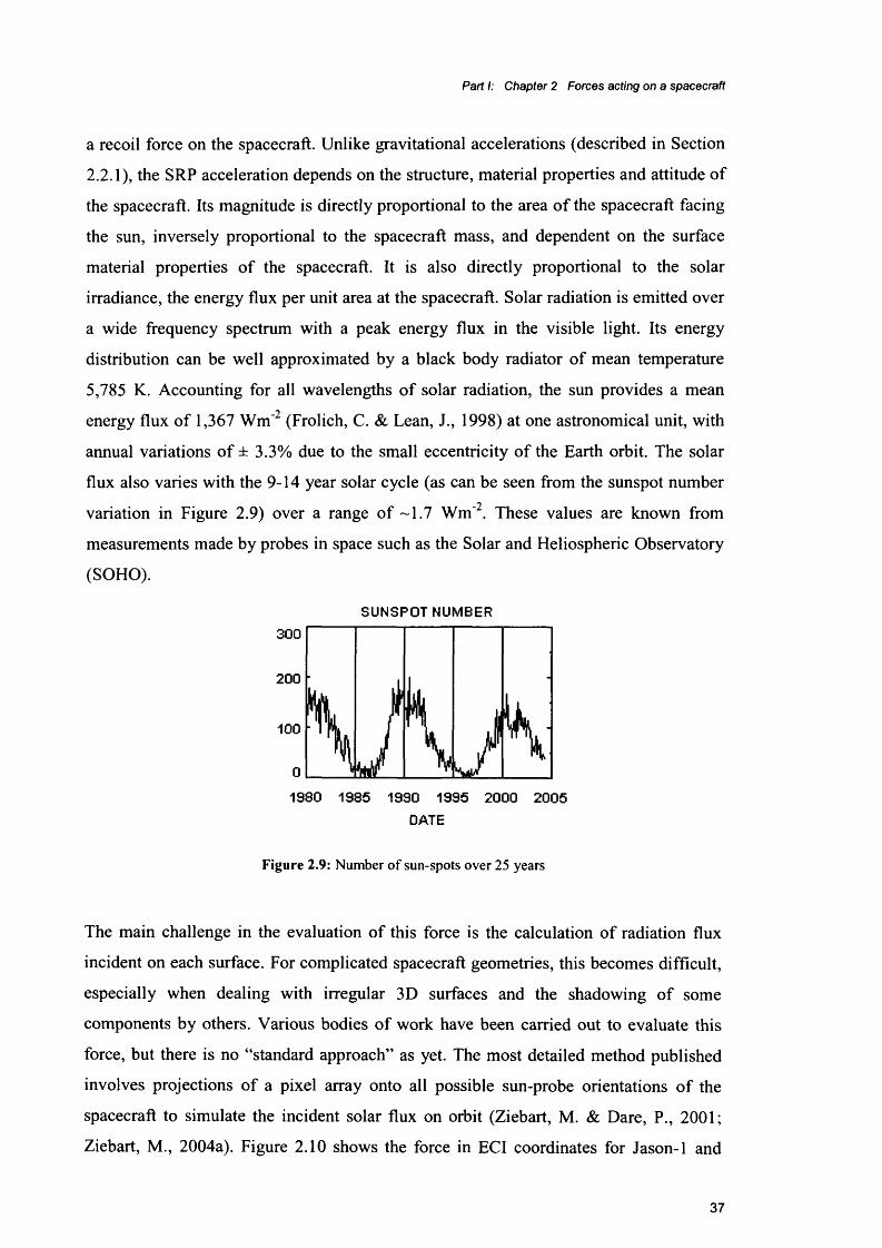
Part I: Chapter 2 Forces acting on a spacecraft
a recoil force on the spacecraft. Unlike gravitational accelerations (described in Section
2.2.1), the SRP acceleration depends on the structure, material properties and attitude of
the spacecraft. Its magnitude is directly proportional to the area o f the spacecraft facing
the sun, inversely proportional to the spacecraft mass, and dependent on the surface
material properties of the spacecraft. It is also directly proportional to the solar
irradiance, the energy flux per unit area at the spacecraft. Solar radiation is emitted over
a wide frequency spectrum with a peak energy flux in the visible light. Its energy
distribution can be well approximated by a black body radiator of mean temperature
5,785 K. Accounting for all wavelengths of solar radiation, the sun provides a mean
energy flux of 1,367 W m 2 (Frolich, C. & Lean, J., 1998) at one astronomical unit, with
annual variations of ± 3.3% due to the small eccentricity of the Earth orbit. The solar
flux also varies with the 9-14 year solar cycle (as can be seen from the sunspot number‘j
variation in Figure 2.9) over a range of ~1.7 Wm' . These values are known from
measurements made by probes in space such as the Solar and Heliospheric Observatory
(SOHO).
SUNSPOT NUMBER
300
200
100
1980 1985 1990 1995 2000 2005
DATE
Figure 2.9: Number of sun-spots over 25 years
The main challenge in the evaluation of this force is the calculation of radiation flux
incident on each surface. For complicated spacecraft geometries, this becomes difficult,
especially when dealing with irregular 3D surfaces and the shadowing of some
components by others. Various bodies of work have been carried out to evaluate this
force, but there is no “standard approach” as yet. The most detailed method published
involves projections of a pixel array onto all possible sun-probe orientations of the
spacecraft to simulate the incident solar flux on orbit (Ziebart, M. & Dare, P., 2001;
Ziebart, M., 2004a). Figure 2.10 shows the force in ECI coordinates for Jason-1 and
37
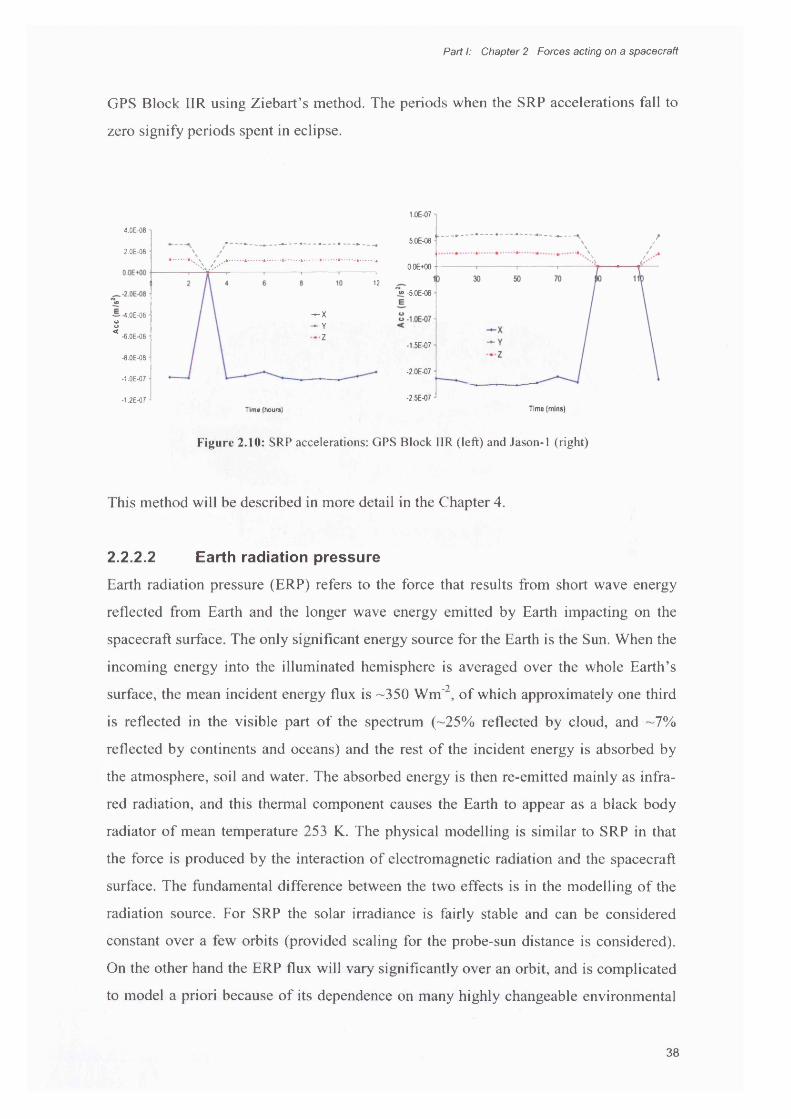
Parti: Chapter 2 Forces acting on a spacecraft
GPS Block HR using Ziebart’s method. The periods when the SRP accelerations fall to
zero signify periods spent in eclipse.
1.0E-07
4.0E-08
5.0E-082.0E-08
O.OE+OO
12« -5.0E-08«•
— ■4.OE-08 u — X
* Y
* Z
o<
-6.0E-08-1.5E-07
-8.0E-08
-2.0E-07•1.0E-07
-2.5E-07-1.2E-07Time (mlns)Time (hours)
Figure 2.10: SRP accelerations: GPS Block I1R (left) and Jason-1 (right)
This method will be described in more detail in the Chapter 4.
2.2.2.2 Earth radiation pressure
Earth radiation pressure (ERP) refers to the force that results from short wave energy
reflected from Earth and the longer wave energy emitted by Earth impacting on the
spacecraft surface. The only significant energy source for the Earth is the Sun. When the
incoming energy into the illuminated hemisphere is averaged over the whole Earth’s
surface, the mean incident energy flux is -350 Wm'2, of which approximately one third
is reflected in the visible part of the spectrum (-25% reflected by cloud, and -7%
reflected by continents and oceans) and the rest of the incident energy is absorbed by
the atmosphere, soil and water. The absorbed energy is then re-emitted mainly as infra
red radiation, and this thermal component causes the Earth to appear as a black body
radiator of mean temperature 253 K. The physical modelling is similar to SRP in that
the force is produced by the interaction of electromagnetic radiation and the spacecraft
surface. The fundamental difference between the two effects is in the modelling of the
radiation source. For SRP the solar irradiance is fairly stable and can be considered
constant over a few orbits (provided scaling for the probe-sun distance is considered).
On the other hand the ERP flux will vary significantly over an orbit, and is complicated
to model a priori because of its dependence on many highly changeable environmental
38
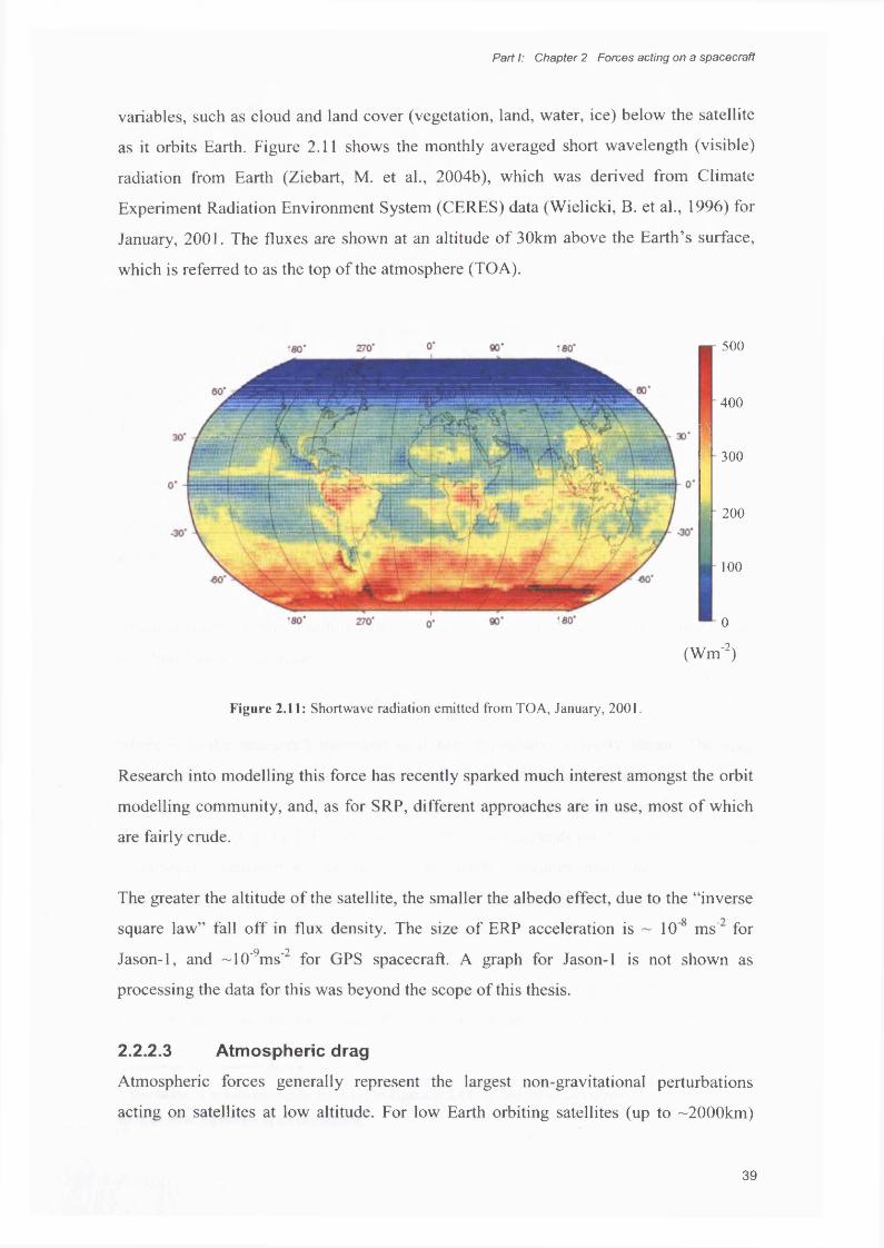
Part I: Chapter 2 Forces acting on a spacecraft
variables, such as cloud and land cover (vegetation, land, water, ice) below the satellite
as it orbits Earth. Figure 2.11 shows the monthly averaged short wavelength (visible)
radiation from Earth (Ziebart, M. et al., 2004b), which was derived from Climate
Experiment Radiation Environment System (CERES) data (Wielicki, B. et al., 1996) for
January, 2001. The fluxes are shown at an altitude of 30km above the Earth’s surface,
which is referred to as the top of the atmosphere (TOA).
500
400
300
200
100
0
(Wm'2)
Figure 2.11: Shortwave radiation emitted from TOA, January, 2001.
Research into modelling this force has recently sparked much interest amongst the orbit
modelling community, and, as for SRP, different approaches are in use, most of which
are fairly crude.
The greater the altitude of the satellite, the smaller the albedo effect, due to the “inverse n
square law” fall off in flux density. The size of ERP acceleration is ~ 10' ms' forQ 1Jason-1, and ~10' ms’ for GPS spacecraft. A graph for Jason-1 is not shown as
processing the data for this was beyond the scope of this thesis.
2.2.2.3 Atmospheric drag
Atmospheric forces generally represent the largest non-gravitational perturbations
acting on satellites at low altitude. For low Earth orbiting satellites (up to ~2000km)
39
Part I: Chapter 2 Forces acting on a spacecraft
drag is a significant problem which must be considered for precise orbit determination.
For the lowest orbiters (at altitudes of ~250km) drag can cause decelerations of the
order of 10'5 ms'2, and at 800 km, decelerations have values ~ 10'7ms'2. For medium
Earth orbiters, for example GPS satellites at an altitude of ~20000km, the atmosphere is
conventionally considered as sufficiently rarefied for drag to be ignored (Jacchia, L.,
1977).
The dependence of the drag force on the velocity of the object relative to the
atmosphere, vr, can be derived in a simple way. Consider a small mass element Am of an
atmosphere column that hits the satellite cross-sectional area A in some time interval At.
Then:
Am — pAvrAt (2.11)
where p is the atmospheric density at the location of the satellite. The impulse Ap
exerted on the satellite is then given by
Ap — Amvr — pAvr2 At (2.12)
which is related to the resulting force by Ap/At. The satellite acceleration due to drag
can therefore be written as:
l = ~ C d ~ p v r\ (2.13)2 m
where m is the spacecraft mass and uv is the unit relative velocity vector. The drag
coefficient Co is a dimensionless coefficient which describes the interaction of the
atmosphere with the satellite’s surface material, and typical values range from 1.5-3.0'i
(Montenbruck, O. & Gill, E., 2000) . This coefficient depends on the interaction of the
atmospheric constituents with the satellite surface. Accurate modelling of this is a
challenging task. Firstly, the complex properties and dynamics of the Earth’s
atmosphere are required; for the upper atmosphere (> ~ 100km), these are not well
known. Secondly, modelling these forces requires detailed knowledge of the interaction
of neutral gas as well as charged particles with the different spacecraft surfaces. Thirdly,
the cross-sectional area of the satellite presented to the particle flux must always be
3 The factor Vi is conventionally included in Equation 2.13, so that the equation resembles the functional
form of other equations in aerodynamics.
40

Part I: Chapter 2 Forces acting on a spacecraft
known. Over the last three decades extensive effort has been devoted to developing
models of the atmosphere at high altitudes, though recent progress has been fairly
modest and it is still an area of ongoing research. As the atmospheric densities and the
drag coefficient are so difficult to quantify in the upper atmosphere, it is commonly
estimated as a free parameter in orbit determination programs.
2.2.2A Thermal re-radiationA satellite absorbs energy, then re-emits it anisotropically as heat. When a surface emits
energy, the law of conservation of momentum requires an equal but opposite force to
act on that surface. As the main topic of this thesis, thermal re-radiation will be
described in more detail in Chapter 3.
2.2.2.5 Antenna thrustAside from the natural forces described so far, the motion of a spacecraft can also be
affected by self-generated forces. Man-made satellites communicate with Earth by the
transmission of electromagnetic signals via antennas mounted on the outside of the
spacecraft. The emission of these signals causes a recoil force on the spacecraft, which
can be determined from the power with which the signal is emitted as shown in
Equation 2.14.
F = — (2.14)c
where P is the signal power and c is the speed of light in a vacuum. If the signal is
emitted continuously, as is the case for many satellites, a constant force acting in the
orbit radial direction will result and may have considerable effects on the orbit of the
spacecraft. For a GPS satellite, the signal strength is about 77W which translates into a
constant acceleration of about 2.5 x 10'10 ms‘2. This can cause a maximum displacement
to a spacecraft at the 0.5m level for one 12 hour orbit.
2.3 Co-ordinate Systems
The definition of an appropriate co-ordinate system in order to study a particular
physical phenomenon requires careful consideration in satellite geodesy. In order to
model and analyse the orbits of spacecraft we require a number of different co-ordinate
systems, and those used in this thesis are described below. They fall into two types:
41

Part I: Chapter 2 Forces acting on a spacecraft
those whose origin is at the centre of mass of the Earth and atmosphere and those whose
origin is fixed relative to the spacecraft. Earth-centred frames are of two principal types:
inertial and rotating. The former is termed Earth-Centred Inertial (ECI) and the latter is
termed Earth-Centred Earth-Fixed (ECEF).
2.3.1 Earth-Centred Inertial (ECI)An ECI frame approximates the inertial frame postulated by Sir Isaac Newton, within
which Newton’s equations of motion are valid, and is defined by a right-handed,
cartesian basis. The X and Y axes typically lie in the Earth’s equator, and the Z axis is
aligned with the angular momentum axis of the earth, but since they move in inertial
space due to nutation and precession, there are effectively an infinite number of ECI
frames. Conventionally, ECI frames are defined in space by fixing them to an epoch.
Currently the most widely used frame is J2000, which is the ECI frame as defined at
12.0 hours UT4, 1st January 2000. ECI axes are conventionally labelled IJK. The I-axis
points along the intersection of the equator and the ecliptic, a direction defined as the
Vernal equinox. The J-axis is 90° east of I in the equatorial plane. The K-axis completes
the right-handed set.
2.3.2 Earth-Centred Earth-Fixed (ECEF)This frame is non-inertial due to the Earth’s diurnal rotation. Conventionally, the ECEF
system is a right handed cartesian basis, and its axes are labelled XYZ. The definition of
an ECEF frame is complicated by the fact that reference stations fixed to the surface of
the Earth are moving continuously with respect to each other due to phenomena such as
tectonic activity and post glacial rebound. Nominally an ECEF frame has the X-axis in
the equatorial plane passing through some point close to the Greenwich meridian; the
Y-axis is also in the equatorial plane and is 90° East of the X-axis and the Z-axis
completes the right-handed set. The frame realisation is through the co-ordinates of a
number of reference stations. There are many ECEF frames. This study uses the
International Terrestrial Reference Frame (ITRF) as defined by the positions and
velocities of several hundred core stations. Conversion from the ECI (eg J2000 to the
ECEF frame, eg ITRF) requires a transformation that accounts for polar motion, (to
4 UT = Universal Time
42

Parti: Chapter 2 Forces acting on a spacecraft
align the Z-axes of the frames), Greenwich Apparent Sidereal Time (to align the X
axes) and nutation and precession of the ECEF frame.
2.3.3 Spacecraft Body-Fixed Co-ordinate system (BFS)
There is no formal definition for this system, though general conventions do exist. The
BFS axes defined for GPS Block HR and Jason-1 are presented here.
For GPS Block HR, the BFS axes are a right-handed cartesian basis with the origin at
the spacecraft centre of mass. The antenna boresight is defined as a direction along the
central bus longitudinal axis, pointing in the same direction as the navigation signal
antennae. The body-fixed Z-axis is co-incident with the antenna boresight. The
spacecraft Y-axis is parallel to the solar panel support boom arm, and the X-axis
completes the right-handed set. This is demonstrated in Figures 2.12.
For Jason-1, the BFS origin is not at the centre of mass, but translated to the base of the
spacecraft as shown in Figure 2.13.
+X+Y
Figure 2.12: GPS Block HR showing BFS XYZ axes
43

Parti: Chapter 2 Forces acting on a spacecraft
' I k
+Z N >
Figure 2.13: Jason-1 showing BFS XYZ axes
2.3.4 Spacecraft Height/Cross-track/Along-track system (HCL)
The HCL basis is centred on the spacecraft centre of mass. The H-axis is parallel to the
spacecraft geocentric position vector. The C-axis is orthogonal to the satellite’s
instantaneous orbital plane, and is parallel to the cross product of the spacecraft’s
position and velocity vectors. The along track axis, L, completes the right-handed set
and is roughly aligned with the spacecraft velocity vector. This basis is useful for
analysing whether a particular phenomenon causes in-orbit plane/out-of-orbit plane
effects and, if in plane, whether in the orbit radial direction or along the direction of
travel of the spacecraft.
2.3.5 Spacecraft YPS system
This basis also has its origin at the nominal spacecraft centre of mass. This basis is
satellite specific; taking GPS Block HR as an example: the PS-axis is parallel to the
probe-Sun vector and the Y-axis is parallel to the solar panel boom arm and is
calculated as the unit vector parallel to the cross product of the spacecraft BFS Z-axis
and the PS-axis. The YPS basis right-handed set is completed with a Z-axis. This axes
system is useful when analysing effects which are expected to be related to sun
direction.
Summary
44

Part I: Chapter 2 Forces acting on a spacecraft
Both gravitational and non-gravitational forces have significant effects on the spacecraft
orbits. In this chapter the origin of these forces, approaches to their modelling and
estimates of their effects have been given. In the next chapter, the force due to thermal
re-radiation is presented in more detail, and the different approaches that have
previously been used to model it are discussed.
45

Part I: Chapter 3 Thermal re-radiation modelling
Chapter 3 Thermal re-radiation modelling
Chapter outlineIn this chapter the nature of the thermal re-radiation force and its mathematical
formulation are described. The different approaches to modelling in the context of orbit
computations are explained and a review of relevant bodies of work carried out so far
on this topic is presented.
3.1 Basis of TRR force
Modelling of the thermal forces arising from the interaction of the spacecraft with its
environment requires understanding the physical laws which govern heat transfer. Two
types of heat transfer processes are pertinent for this study of the spacecraft surface:
radiation and heat conduction. A third heat transfer mechanism, convection, involves
fluid particle motion; though this is a relevant heat transfer mechanism within some
parts of the spacecraft, it does not apply to satellite surfaces.
When radiation interacts with matter it is subject to three possible outcomes; reflection,
transmission or absorption. If energy is reflected or transmitted, the thermal energy of
the matter is unaffected. If energy is absorbed, it can be incorporated as thermal energy,
causing a change in the electron configuration of the constituent atoms or molecules and
resulting in an increase in temperature. Usually a combination of the above processes
occur and the relative amounts of each depend on the material properties of the body
upon which the radiation is incident, namely the reflectivity, absorptivity and the
transmission coefficients. These parameters range between 0 and 1 and give the fraction
of radiation that is reflected, absorbed or transmitted at a particular wavelength.
Matter also emits radiation. The emission may again be attributed to the changes in the
electron configuration of the material. The energy radiated is in the form of
electromagnetic waves in the infra-red (-5-1000 pm) part of the spectrum. The rate at
46
Part I: Chapter 3 Thermal re-radiation modelling
which energy is released per unit area (Wm 2) is termed the surface emissive power E.
This has an upper limit which is prescribed by the Stefan-Boltzmann law:
E = e r f
where T is the absolute temperature of the surface and <7 is the Stefan-Boltzmann
constant (5.6699 x 10'9 Wm^K-4). Such a surface is called an ideal radiator or a
blackbody. The energy radiated by a real body is less than this, and is given by
E = €(t T 4 (3.1)
where eis the emissivity of the body (Incropera, F. & DeWitt, D., 2001). The emissivity
ranges between 0 and 1, and is a measure of how efficiently energy is radiated by a
body.
According to Einstein’s theory of special relativity, there is an equivalence between
mass and energy. One implication of this is that emitted photons have momentum. The
law of conservation of momentum dictates that a net momentum flux out of the body
causes a reaction force against the satellite’s heated surface. This is the force due to
TRR and forms the basis of this study.
The sun is the primary source of radiation for a satellite; smaller sources include the
Earth and moon. Differential heating occurs between parts of a spacecraft which are
irradiated and those which are not. Some deep space probes spin specifically to
distribute the heat load evenly, but most Earth orbiting spacecraft cannot do this because
of attitude constraints. Taking GPS spacecraft as an example, the +Z face upon which
the antennas are mounted must always point to Earth, while the body and panels rotate
in such a way so that the panels always face the sun. As a result, different components
receive different amounts of radiation depending on whether they are sun-facing or not
and the extent to which they are shadowed by other components. The amount of energy
absorbed and emitted by each component is determined by its material and optical
properties, so surface temperatures may differ considerably. Since the surface
components of a satellite will radiate at a rate proportional to temperature and
emissivity, the resulting emission will most likely be anisotropic (Figure 3.1), and lead
to a resultant force.
47

Part I: Chapter 3 Thermal re-radiation modelling
Another source of environmental heating is due to friction with particles in the rarefied
upper atmosphere under a free molecular regime, though this heating is usually only
significant during the launch phase (Gilmore, D., 1994). Internal subsystems are a
source of heat within the spacecraft bus. This heat is vented to space via radiators or
louvers on the surface of the bus. This emission will also produce a recoil force, and
should be included in any rigorous calculation. To account correctly for this depends on
the accessibility of thermal budget data, which may be available in engineering data sets
for specific satellites.
absorbed
4
j y r*.A fM- Anisotropic 'W emission of I
Figure 3.1: Anisotropic emission of radiation by the satellite
3.2 Characterisation of Force
Einstein’s theory of relativity describes the energy of a particle as
E = (c/>)2+(m 0c2)2]
where E is the energy of the particle, p is the momentum and mo is the rest mass. For a
photon, m0 = 0, and hence E=cp. Dividing the total energy that is radiated by a surface
each second by the speed of light gives the total momentum transferred away from the
surface each second:
dp _ E _ e&T4 dt c c
The law of conservation of momentum causes a recoil force on the spacecraft which is
equal and opposite in direction to the momentum leaving the surface per second, which
48
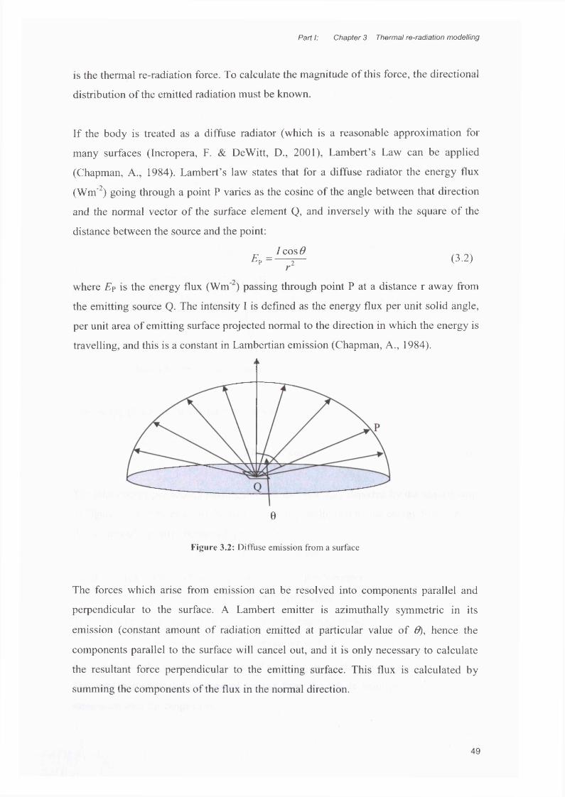
Part I: Chapter 3 Thermal re-radiation modelling
is the thermal re-radiation force. To calculate the magnitude of this force, the directional
distribution of the emitted radiation must be known.
If the body is treated as a diffuse radiator (which is a reasonable approximation for
many surfaces (Incropera, F. & DeWitt, D., 2001), Lambert’s Law can be applied
(Chapman, A., 1984). Lambert’s law states that for a diffuse radiator the energy flux
(Wm'2) going through a point P varies as the cosine of the angle between that direction
and the normal vector of the surface element Q, and inversely with the square of the
distance between the source and the point:
I cos 0Ef = (3.2)
where Ep is the energy flux (Wm' ) passing through point P at a distance r away from
the emitting source Q. The intensity I is defined as the energy flux per unit solid angle,
per unit area of emitting surface projected normal to the direction in which the energy is
travelling, and this is a constant in Lambertian emission (Chapman, A., 1984).
0
Figure 3.2: Diffuse emission from a surface
The forces which arise from emission can be resolved into components parallel and
perpendicular to the surface. A Lambert emitter is azimuthally symmetric in its
emission (constant amount of radiation emitted at particular value of 0), hence the
components parallel to the surface will cancel out, and it is only necessary to calculate
the resultant force perpendicular to the emitting surface. This flux is calculated by
summing the components of the flux in the normal direction.
49

Part I: Chapter 3 Thermal re-radiation modelling
Figure 3.2 shows a hemisphere with unit radius above an emitting point source. The
energy flux through a point P on the surface of the hemisphere is given by
Ep = I cos 0 (3.3)
8 0
Figure 3.3: Directional distribution of radiant energy from a point source
The energy flux Fluxp at a point P is given by:
Flux? = I cos 0 (3.4)
The total energy per second passing through the area Astrip depicted by the shaded strip
in Figure 3.3 will be equal to the area of the strip multiplied by the energy flux at point
P. The area of the strip shown in Figure 3.3 is:
Astrip=27rsm m (3.5)
and the energy per second passing through this strip is therefore:
Estrip = 2x1 sin 6 cos 680 (3.6)
The component of this energy flux normal to the emitting surface is:
= 2 x 1 sin cos2 68 6 (3.7)
Eperp describes the normal component of energy passing through the strip per second.
The total perpendicular component arising from the whole hemisphere is found by
integration over the range of 0.
50

Part I: Chapter 3 Thermal re-radiation modelling
Eperp ~ j2 /r/s in # co s2 OdO
F = -perp2x1 j cos3 0 j
^ perp2x1
(3.8)
(3.9)
(3.10)
The total amount of energy emitted is given by the integral of Equation 3.6
Etot - ^2x1 sin 9 cos OdO
7C_T
= I x Jsin 2 OdO
= - x cos 2 0
(3.11)
(3.12)
(3.13)
(3.14)
2
= I x
Therefore the energy emitted perpendicular to the surface as a fraction of the total
energy emitted can be written as
'¥ 1(3.15)
I x
(3.16)
Combining this with Equation 3.1 gives the amount of energy emitted perpendicular to
the surface as
2ecrr(3.17)
The corresponding momentum transferred to the body per unit area of surface is then
given by
2eaTi3 c
(3.18)
51

Part I: Chapter 3 Thermal re-radiation modelling
and the recoil force on the surface of area A is
2 AecrT4 (3.19)3 c
In order to find the complete thermal force on a body, this differential force must be
integrated over the entire surface.
5C Q
The problem reduces to acquiring knowledge of the emissivities and the determination
of temperatures for each part of the satellite surface. The temperatures must be
accurately determined since the force is proportional to the fourth power of the
temperatures.
3.3 Existing approaches to thermal modelling
Before reviewing existing work on the topic of thermal re-radiation, the two general
approaches - analytical modelling and empirical modelling- used to account for this
force in orbit computations are discussed. The most appropriate method to use is
dependent upon the data available, the orbit precision required, and what knowledge is
desired at the end of the process.
3.3.1 Analytical modellingAn a priori mathematical model of the forces is constructed based solely on a physical
analysis of the problem. The precision of this analytical force model is highly dependent
on the accuracy of the data describing the environment, the spacecraft attitude, and the
structural and material properties of the spacecraft. In orbit processing, model
complexity is an issue, and a trade off must be made between accuracy of model and
computational burden. This poses another limit to the usability of accurate a priori
models.
3.3.2 Empirical modellingLimitations of analytical models have led orbit determination agencies to employ
empirical techniques to account for un-modelled forces. In empirical modelling, an a
priori force model is used to create an initial estimate of the orbit. This estimate will be
improved by using observation data, for example tracking data from ground stations, to
constrain the trajectory. A linearised least-squares process is employed to adjust the
52
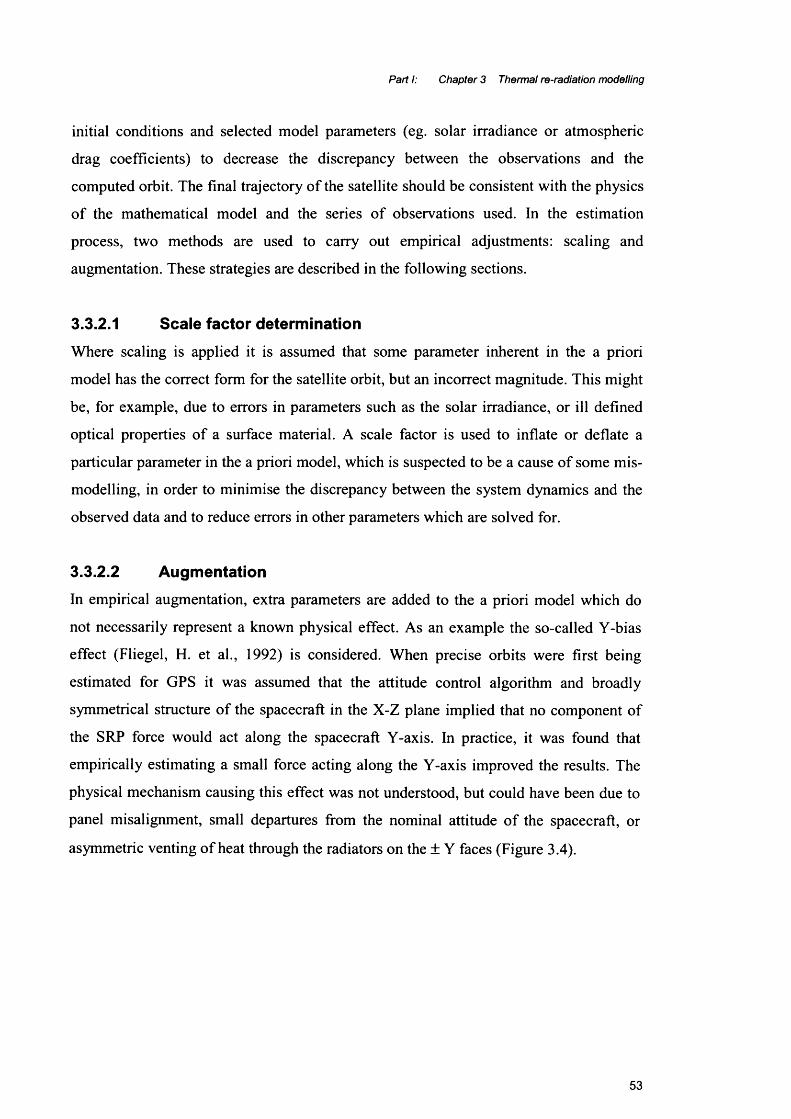
Part I: Chapter 3 Thermal re-radiation modelling
initial conditions and selected model parameters (eg. solar irradiance or atmospheric
drag coefficients) to decrease the discrepancy between the observations and the
computed orbit. The final trajectory of the satellite should be consistent with the physics
of the mathematical model and the series of observations used. In the estimation
process, two methods are used to carry out empirical adjustments: scaling and
augmentation. These strategies are described in the following sections.
3.3.2.1 Scale factor determinationWhere scaling is applied it is assumed that some parameter inherent in the a priori
model has the correct form for the satellite orbit, but an incorrect magnitude. This might
be, for example, due to errors in parameters such as the solar irradiance, or ill defined
optical properties of a surface material. A scale factor is used to inflate or deflate a
particular parameter in the a priori model, which is suspected to be a cause of some mis-
modelling, in order to minimise the discrepancy between the system dynamics and the
observed data and to reduce errors in other parameters which are solved for.
3.3.2.2 AugmentationIn empirical augmentation, extra parameters are added to the a priori model which do
not necessarily represent a known physical effect. As an example the so-called Y-bias
effect (Fliegel, H. et al., 1992) is considered. When precise orbits were first being
estimated for GPS it was assumed that the attitude control algorithm and broadly
symmetrical structure of the spacecraft in the X-Z plane implied that no component of
the SRP force would act along the spacecraft Y-axis. In practice, it was found that
empirically estimating a small force acting along the Y-axis improved the results. The
physical mechanism causing this effect was not understood, but could have been due to
panel misalignment, small departures from the nominal attitude of the spacecraft, or
asymmetric venting of heat through the radiators on the ± Y faces (Figure 3.4).
53
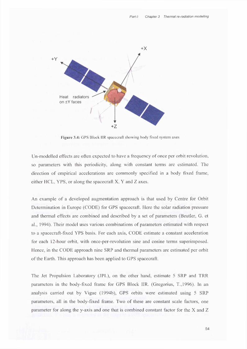
Part I: Chapter 3 Thermal re-radiation modelling
+x
+Y
Figure 3.4: GPS Block HR spacecraft showing body fixed system axes
Un-modelled effects are often expected to have a frequency of once per orbit revolution,
so parameters with this periodicity, along with constant terms are estimated. The
direction of empirical accelerations are commonly specified in a body fixed frame,
either HCL, YPS, or along the spacecraft X, Y and Z axes.
An example of a developed augmentation approach is that used by Centre for Orbit
Determination in Europe (CODE) for GPS spacecraft. Here the solar radiation pressure
and thermal effects are combined and described by a set of parameters (Beutler, G. et
al., 1994). Their model uses various combinations of parameters estimated with respect
to a spacecraft-fixed YPS basis. For each axis, CODE estimate a constant acceleration
for each 12-hour orbit, with once-per-revolution sine and cosine terms superimposed.
Hence, in the CODE approach nine SRP and thermal parameters are estimated per orbit
of the Earth. This approach has been applied to GPS spacecraft.
The Jet Propulsion Laboratory (JPL), on the other hand, estimate 5 SRP and TRR
parameters in the body-fixed frame for GPS Block HR. (Gregorius, T.,1996). In an
analysis carried out by Vigue (1994b), GPS orbits were estimated using 5 SRP
parameters, all in the body-fixed frame. Two of these are constant scale factors, one
parameter for along the y-axis and one that is combined constant factor for the X and Z
Heat radiators on ±Y faces
\ s\
+ Z
54

Part I: Chapter 3 Thermal re-radiation modelling
direction. The additional 3 parameters are varying scale factors for each body fixed X,
Y and Z axes that are estimated sequentially.
3.3.3 Discussion of approachesThese empirical approaches can, in some circumstances, work very well. They have
successfully been employed to mitigate the effects of force model errors of GPS
satellites (Colombo, O., 1989) as well as for TOPEX/Poseidon (Tapley, B., et al. 1994).
The empirical methods discussed above rely upon having a large number of
observations drawn from global networks of tracking stations. In the context of the
International GPS System (IGS) tracking station network where over 200 ground
stations track the GPS spacecraft, these methods can produce excellent results.
They are still however limited in the accuracy with which they can replicate the true
orbit and, as precision requirements increase, better a priori dynamic models are
required as a start point. A more accurate a priori physical model benefits orbit
determination because it provides the correct form of the function, which will then be
augmented or scaled. A poorer a priori model will require more empirical parameters,
and reduce the redundancy of the observation data.
A drawback of solving for such empirical terms is that there is a tendency for estimated
parameters to absorb any unmodelled effects. If these effects have a time or spatial
dependency that is uncorrelated with the signature of the force in question, then this can
not be used to deduce the effect of this force at future epochs. In these cases, no
physical significance can be associated with the effect. As many effects are assumed to
have a once per orbit revolution period and as such are modelled with once per
revolution empirical parameters, they may be inadequate to correctly account for un
modelled effects with different periodicities (Ziebart, M. et al., 2003a).
Problems can arise when empirical terms are used to soak up un-modelled parameters
which correlate with other effects. In orbit determination of GPS satellites, parameters
which impact on the measurement data are estimated; an example is tropospheric zenith
delay (TZD), which is the attenuation of a signal caused by atmospheric water vapour.
This parameter is required by other scientists in fields such as climatology and weather
prediction. If a bias is suspected in the range to a GPS spacecraft due to an un-modelled
55

Part I: Chapter 3 Thermal re-radiation modelling
effect in the a priori model, eg earth radiation pressure, a scale factor could be
introduced along the spacecraft body-fixed Z-axis to account for it. This scale factor
will soak up all radial errors including some of the effect caused by the TZD. The
estimation of the TZD then will be less accurate as part of its effect has been absorbed
by the scale parameter. This example shows what is to be gained by having an accurate
a priori force model. The more accurate the model, the more highly constrained are the
errors in other parameters.
Whilst empirical parameterisation of orbits is an approach that is well suited to a
posteriori orbit determination when much tracking data is available, applying empirical
acceleration parameters for orbit prediction purposes may lead to a substantial
degradation of the position accuracy.
3.4 Review of relevant literature
The structural complexity and lack of reliable data of a real spacecraft makes any
accurate calculation of the thermal force a difficult task. This fact, coupled with the
relatively low ranking of surface thermal effects in the hierarchy of forces that affect the
motion of a spacecraft, has resulted in this force receiving little detailed attention.
Increasingly however, GNSS applications require greater precisions, and modelling of
smaller forces are becoming more important. This section summarises the material that
has been published in this area so far in the context of spacecraft orbits. A review of the
available literature on eclipse boundary determination is also given, and the main bodies
of work carried out on the other non-conservative forces are outlined.
3.4.1 Thermal re-radiationIn the late 1980s, several studies were undertaken to investigate the size of the thermal
force and its impact on various spacecraft. Slabinski (1988) provides an introduction to
the theoretical background of thermal imbalance forces, and demonstrates that thermal
re-radiation could be significant in explaining the observed drag effects for deactivated
telecommunication satellites. Rubincam (1987) shows that the thermal behaviour of
retro-reflectors embedded in the surface of LAGEOS, a small, spherical, spinning
satellite, would explain the observed drag like behaviour of the satellite, thus
establishing that thermal forces were indeed big enough to perturb the motion of a
56
Part I: Chapter 3 Thermal re-radiation modelling
satellite. The simple structure of LAGEOS, and its continuous rotation enables a
relatively straightforward calculation of the thermal force, but as the spacecraft
structural complexity increases, so does the effort required in producing accurate
thermal models.
In a thesis by Cook (1989) the surface thermal forces on simple spacecraft models such
as box and wing (see Figure 3.5) and spherical bus models are estimated, thus avoiding
the issue of spacecraft complexity. The purpose of Cooke’s study was to estimate
maximum possible displacements that could occur due to this force. His discussion
concentrates on a number of idealised situations, for example, the spacecraft is modelled
as a perfectly conducting slab with a constant sun facing profile on orbit. His study
predicts that this force could result in metre level radial errors in 14 days, and up to tens
of metres along track. He suggests that, though estimation of other force model
parameters (such as SRP) would probably absorb much of the error, significant
discrepancies might still occur.
Figure 3.5: Simplified spacecraft structure: Box and Wing model
Vigue (1994a) presents the most detailed methods published for analysing the
perturbations due to the thermal force, specifically to determine the long term effects on
the behaviour of GPS Block IIA satellites. Vigue argues that a thermal model of the
entire spacecraft would be very complicated due to the complex geometry and poorly
defined material properties which strongly affect the magnitude of the forces. She
asserts that as the solar panel areas are large compared to the bus areas and constantly
face the sun, their effect would dominate the thermal force, and hence she does not
consider the spacecraft body. Using the material properties for each layer of the panel,
she employs finite element method software to study the one dimensional heat transfer
through the panel. This yields the temperatures for the front and back face which are
then used to calculate a force. A ball park figure for the thermal acceleration of 1 x 1 O'9
ms' was estimated. She analyses the effect of the thermal force by comparing
57

Part I: Chapter 3 Thermal re-radiation modelling
numerically integrated orbits: one with two body effects only and the other with two
body effects and the thermal force. The residuals grow to the metre level after a day, in
both the radial and along track directions.
In this paper, she also examines how well solar pressure scale factors can absorb
thermal effects and finds that though a large proportion can indeed be absorbed, the
remaining signals are significant. She ultimately concludes that as the thermal force is
dependent on many properties which cannot be well known, it may be more appropriate
to estimate empirical parameters to represent it. Though this work was progressive at
the time, in that it was the first detailed study to try and predict the effects of this force
for a real spacecraft, it had two main drawbacks: 1) the spacecraft bus was totally
ignored, with no supporting analysis and 2) no testing was carried out to see whether
these models were correct or whether they improved orbit prediction/determination
capabilities.
Rockwell International, the spacecraft contractors for the GPS Block I and II/IIA
spacecraft developed SRP models for their satellites. The computer code to deal with
them was written by IBM and amended by the Aerospace Corporation, and became
known as the Rock models. To begin with, these models totally ignored the effects of
thermal re-radiation. In a paper by Fliegel & Gallini (1996) of the Aerospace
Corporation, it was stated that the thermal force was indeed significant and accounted
for -5% of the solar force. The Rock models for the Block II spacecraft were then
amended to include these effects and renamed as the T20 models. Similar models for
GPS Block HR (which had extra antennas) are known as T30. The thermal forces were
absorbed into the SRP models directly. Fliegel’s papers (Fliegel, H. et al., 1992, Fliegel,
H. & Gallini, T., 1996) describe the processes used in the calculation of the models and
outline their main assumptions and weaknesses. The spacecraft surface is treated as a set
of surfaces, which are assumed to be either flat or cylindrical. The SRP force is
calculated on a component by component basis, where the interaction of the component
with incoming photons is computed as a function of angle of incidence, and the results
are summed over the whole spacecraft. Specular and diffuse SRP effects are modelled,
and the effect of shadowing of one component by another is accounted for. The method
does not allow for the effect of light reflected from one surface striking another. The
method also becomes progressively more impractical as the complexity of the
58
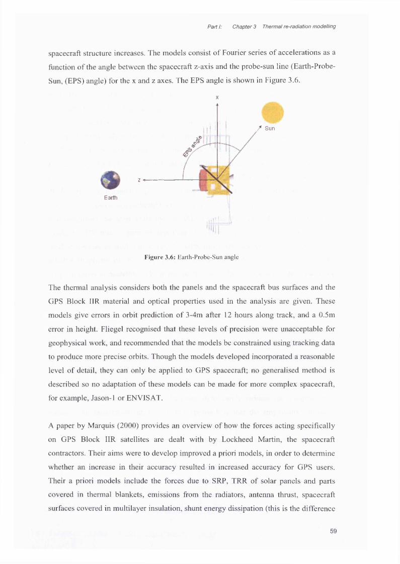
Part I: Chapter 3 Thermal re-radiation modelling
spacecraft structure increases. The models consist of Fourier series of accelerations as a
function of the angle between the spacecraft z-axis and the probe-sun line (Earth-Probe-
Sun, (EPS) angle) for the x and z axes. The EPS angle is shown in Figure 3.6.
Earth
z
/ Sun
Figure 3.6: Earth-Probe-Sun angle
The thermal analysis considers both the panels and the spacecraft bus surfaces and the
GPS Block IIR material and optical properties used in the analysis are given. These
models give errors in orbit prediction of 3-4m after 12 hours along track, and a 0.5m
error in height. Fliegel recognised that these levels of precision were unacceptable for
geophysical work, and recommended that the models be constrained using tracking data
to produce more precise orbits. Though the models developed incorporated a reasonable
level of detail, they can only be applied to GPS spacecraft; no generalised method is
described so no adaptation of these models can be made for more complex spacecraft,
for example, Jason-1 or ENVISAT.
A paper by Marquis (2000) provides an overview of how the forces acting specifically
on GPS Block IIR satellites are dealt with by Lockheed Martin, the spacecraft
contractors. Their aims were to develop improved a priori models, in order to determine
whether an increase in their accuracy resulted in increased accuracy for GPS users.
Their a priori models include the forces due to SRP, TRR of solar panels and parts
covered in thermal blankets, emissions from the radiators, antenna thrust, spacecraft
surfaces covered in multilayer insulation, shunt energy dissipation (this is the difference
59
Part I: Chapter 3 Thermal re-radiation modelling
between the amount of energy produced by the solar panels and the amount of energy
drawn away by the bus), earth albedo and earth infrared. The details of their actual
modelling techniques are scant and no generalised methods are described. The geometry
of the GPS Block IIR spacecraft surface was modelled using tessellated triangles, which
although still fairly crude, generates a more detailed structure than a box and wing
model. To analyse this model, two solar pressure parameters, K1 and K2, were
estimated empirically in the orbit determination process using a Kalman filter (Kaplan,
E., 1996). K1 represents a solar scale and K2 is a Y-bias acceleration. The quality of the
models was judged on the size and stability of the empirical terms. Testing was carried
out by the Naval Surface Warfare Centre for one GPS Block IIR satellite; a comparison
of the empirical parameters generated using the Rock 42 models developed for GPS
Block II and IIA (which included no thermal analysis) showed that the Rock 42 models
underestimated the solar scale by 12-13%, whereas the new SRP (including TRR)
model for IIR was in error by less than 1%. This result implies that the new SRP
method appears to work fairly well for GPS Block IIR, though it is certain that the
relative simplicity of the shape of GPS Block IIR enables this, in spite of their
simplifications in modelling. The main conclusion of the paper was that the new, more
detailed SRP model added improved accuracy to an already accurate system.
The Centre Nationale des Etudes Spatiale (CNES) developed an SRP and TRR surface
force model for Jason-1. Details of their method are unavailable in the public literature,
but the essence of their technique is as follows (Ferrier, C. et al., 2002): a box and wing
spacecraft model is created where the dimensions of the box and the surface optical
properties are calculated to yield the same response as the real spacecraft. This means
that the complex geometry of the real spacecraft does not need to be dealt with at each
epoch in orbit determination, and therefore significantly reduces the computational
burden. The assumption inherent in this approach is that the empirically estimated
parameters will soak up all the mis-modelled effects, which are inevitable due to the
simplification. If the spacecraft deviates substantially from a box and wing model
(which it does in the case of Jason-1), then this assumption may not hold, and residual
systematic biases can remain as exemplified by Ziebart et al. (2003a). This work will be
used as a comparison against the work done in this study and will be discussed in
Chapter 7.
60
Part I: Chapter 3 Thermal re-radiation modelling
Ziebart (2001) developed a detailed SRP model for the Russian positioning system
satellites, GLONASS. He states that the pattern of the orbit residuals that resulted from
orbit prediction tests were in line with Vigue’s prediction of the behaviour of the
thermal force. This implied that a substantial part of the residual mis-modelling could be
corrected by developing a TRR model for GLONASS.
3.4.2 Spacecraft thermal controlSurface thermal effects include the forces that arise due to heat vented out to space
through radiators and heat louvers. The amount of energy expelled depends on internal
temperature distributions and heat transfer processes. A large body of work has been
carried out on methods for the calculation of temperatures within a spacecraft and how
to control them. This has been driven by the necessity to ensure that ideal thermal
conditions are maintained so delicate electronics and subsystems operate optimally.
Spacecraft are commonly equipped with combinations of heaters, heat louvers,
radiators, refrigerators and thermo-electric coolers and make use of different
absorbance/emittance coatings and thermal blankets to control internal heat distributions
and regulate outgoing heat. Thermal control methods are well documented in many
texts and papers (Gilmore, D., 1994; Fortescue, P. et al., 2003). Fortunately engineering
data usually includes values for emission from radiators and louvers, and therefore
knowledge of the internal heat transfer processes (which would undoubtedly be too
complicated to incorporate in orbit models) is not required, and will not be considered
further.
3.4.3 Eclipse boundary crossing time determinationEarth-orbiting satellites experience partial or total eclipses when they pass through the
regions known as the umbra and penumbra. In the penumbra, the total solar irradiance is
partially occluded by the earth, whereas the umbra can be defined as the region on the
anti-sun side of the earth which is completely devoid of solar radiation. In reality the
earth is flattened, with the polar radius being about 0.3% smaller than the equatorial
radius. If the earth’s oblateness is taken into account, the boundaries of the shadow
regions are altered.
Literature detailing previous approaches to eclipse region modelling is sparse, and the
existing material ranges between two extremes. Several techniques have been developed
61
Part I: Chapter 3 Thermal re-radiation modelling
using a spherical earth model, which allows simple geometric arguments to be
developed. These are described in Montenbruck (2000) and Vallado (2001). Some
methods (Neta, B. & Vallado, D., 1994) describe a cylindrical shadow model, but this
totally ignores the penumbral region where the flux gradually diminishes. These
methods are simple to implement from a computation viewpoint, though they result in
errors in precise orbit computation.
Vokrouhlicky, D. et al. (IV), (1996) states that it is certainly worthwhile treating the
earth as an oblate spheroid as it has been shown that with respect to a spherical earth the
main changes occur in the timing of the umbra and penumbra transitions, and in the
overall duration of the eclipse periods. Woodbum (2000) showed that such mistiming
has important consequences for the precise numerical integration of orbit trajectories.
The main drawback of implementing techniques using existing approaches for eclipse
boundary determination with a spheroidal earth is that they are significantly more
complex than for a spherical earth. In Vokrouhlicky’s paper (1996), he describes a
method which involves a complex series of rotations, and in Neta and Vallado (1994) a
method involving the solution of quartics is described. The shortcoming of both these
methods is that they are costly to implement in operational software due to the intensive
nature of the computation required. Until now, there has been no published method
which describes a simple and efficient way to accurately calculate eclipse boundary
crossing times and, without such a method, the accurate calculation of SRP and TRR
during the course of an orbit for an eclipsing satellite is extremely difficult.
3.4.4 Other non-conservative forcesThe largest of the non-conservative forces is solar radiation pressure and many
techniques have now been developed for the solution of this force, ranging from the
fairly crude to the much more precise. Methods for SRP modelling can be found in
Milani and Nobili (1987) and those already referred to in Fliegel (1992, 1996). The state
of the art in SRP modelling uses a pixel array algorithm (described in Section 5.6)
which automatically takes into account the complexity of real spacecraft. A detailed
description of this method can be found in Ziebart (2001).
62

Part I: Chapter 3 Thermal re-radiation modelling
Albedo and infrared emissions from the Earth provide radiation which acts on a
spacecraft's exposed surfaces in a fashion similar to that of SRP as described in Chapter
2. This radiative flux coming from the earth is commonly evaluated by dividing the
Earth into a grid and taking the vector sum of the grid-to-satellite accelerations. The
standard models that have been adopted in most orbit determination codes (Knocke, P.,
1988; Borderies, N., & Langaretti, P., 1990) are fairly simplistic and do not account for
the large temporal variation due to the changing albedo of the Earth's land masses
arising from snow and vegetative covering, and the distribution of clouds. Martin and
Rubincam (1993) attempted a detailed calculation of the specular and diffuse albedo re
radiation based on measured global albedo time histories to assess whether this would
result in improvement over the Knocke models. Their study indicated that while the
time history of the albedo is complex, when integrated over the Lageos orbit, it
produces effects which are similar to that obtained with the simpler models. Now probes
exist in space from which very high resolution temporal and spatial radiation data sets
can be extracted and used to produce more accurate albedo models (Ziebart, M. et al.,
2004b). Data from these models are utilised in the validation of the thermal models
developed in this thesis and will therefore be described in Chapter 5.
SummaryIn this chapter the basis of the thermal surface force and its characterisation was
explained. The analytical and empirical approaches that have been used to account for it
were described and a review of the published work to date related to this topic was
given. Scant work has been done on the process of calculating a detailed analytical
thermal force model, and that which has been done is primarily for simply shaped
spacecraft, such as spheres or box-and-wing representations of more complicated
structures, and often the specific method details have not been described. In earlier
work, model simplicity was necessary due to the computational load that accurate
models of complex spacecraft introduce. As computer power becomes less of a
restriction, there is now no reason why a current state of the art model should not
attempt to model accurately a realistic complex spacecraft structure. Chapter 4 describes
the methods developed in this thesis which aim to do this.
63

Part II: Chapter 4 Modelling methods
Part II Chapter 4 Modelling methods
Chapter outlineThis chapter describes the methods developed during the course of this research to deal
with the treatment of the thermal forces produced by various parts of the spacecraft,
both in steady state and during shadow crossings where temperature changes occur on a
very short timescale. Methods for determining accurate eclipse boundary crossing times
based on the earth modelled as an oblate spheroid and a model of flux in penumbral
regions are described. Methods are also given for the modelling of solar radiation
pressure and earth radiation pressure as they impact upon some aspects of the thermal
forces models and their testing.
4.1 Introduction
The aim in this chapter is to develop generalised analytical thermal re-radiation force
models. The problem consists of:
• defining the flux in the vicinity of the spacecraft
• computing the radiation incident on each surface component as a function of
space and time
• calculating the temperature variations over the surface of a spacecraft by
analysis of energy transport mechanisms
• calculating the resultant force
• fitting models to these forces for use in orbit computations
Spacecraft with internal subsystems commonly have a central bus and solar panel arrays
attached via boom arms to the bus; thus the bus and the panels are assumed to be
strongly thermally decoupled. For many spacecraft, the bus is largely wrapped in
thermal blankets called multilayer insulation (MLI) (Gilmore, D., 1994) whose function
is to thermally stabilise the spacecraft to prevent significant deviations of bus internal
64

Part II: Chapter 4 Modelling methods
temperatures from the design regime. Methods are developed for the solar panels and
parts of the bus covered in MLI. Remaining surfaces are considered individually and a
discussion for these parts is given.
The techniques developed in this chapter are applicable to Galileo, Glonass, ENVISAT,
TOPEX/Poseidon and Mars Global Surveyor to name only a few. Spacecraft which do
not conform to this generic box and wing structure include GRACE, CHAMP
(Challenging Minisatellite Payload) and some micro-satellites, and the techniques
developed here will require some adaptation for those cases.
During most mission phases, when in full sunlight, Earth pointing satellites change
attitude and distance from the sun slowly and smoothly over an orbit5. The component
surface areas exposed to sunlight hence change slowly, and the flux in the vicinity of the
spacecraft varies smoothly as a function of sun-probe distance. The corresponding
temperatures change on timescales such that at each instant, can be assumed to be
constant (Fortescue, P. et al., 2003). In these regions a steady state temperature regime
is assumed. When the spacecraft goes into eclipse, the reduction in incoming flux
causes the surface temperatures to change on a much quicker timescale and a transient
analysis is required to calculate surface temperatures and resultant forces.
In Section 4.2, a solar panel thermal force model is developed and in Section 4.3, the
approach for the treatment of MLI is described. Section 4.4 outlines an approach to
dealing with the response of the MLI to earth radiation fluxes. Section 4.5 describes a
method which can be used for the calculation of eclipse boundary crossing times, and
Section 4.6 details the method for calculating the reduction in solar flux in the
penumbral regions.
4.2 Solar panels
For clarity the following nomenclature is defined for symbols appearing in this section:
A area (m2)
F force (N)
5 The exceptions to this are during gyro calibration manoeuvres or when corrective thrusts are applied.
During these times data from the spacecraft are generally not used.
65

Part II: Chapter 4 Modelling methods
m mass (kg)
n unit vector normal to surface
q heat transfer rate (Wnf2)
T temperature (K)
W incident solar radiation (W m ')
csp specific heat capacity (Jkg ’K '1)
a absorptivity
e emissivity
k conductivity (W m‘1K '1)
0 angle between negative surface normal and incoming photon flux
L thickness of panel (m)
p resistivity of panel (Qm)
Rtotal effective resistance of total panel (£2)
Subscripts:
b back face of solar panel
/ front face of solar panel
Constants:
c speed of light in a vacuum (299792458 m s 1)
<T Stephan-Boltzmann constant (5.6699 x 10'8 Wm^K"4)
4.2.1 Description of solar panelsSatellite solar panels consist of many thin layers of materials sandwiched together to
form a composite structure. They generally have two dominant layers: the solar cells
which lie below a quartz coverglass, and a highly conductive aluminium core (Figure
4.1) (Gilmore, D., 1994). As a consequence of the diffuse nature of the thermal
emission (Section 3.1), the resulting force acts normal to the panels. The thermal re
radiation force depends on the temperatures of the front and back surfaces of the panel;
these temperatures depend upon the amount of radiation incident on and emitted by the
panels and the way that heat is transported through the panel layers. An analysis of these
energy transport mechanisms requires knowledge of the material properties, panel
66

Part II: Chapter 4 Modelling methods
dimensions, panel orientation relative to the incoming solar flux and the amount of
power drawn from the panels.
~3cm
aluminium core
Figure 4.1: Composite structure of solar panel
4.2.2 Steady state solar panel thermal force calculationIn this analysis, a one dimensional, steady state condition is applied. A one dimensional
scheme is appropriate since as the area of the panels is much greater than their thickness
and the incident radiation and properties are constant over the panel area, heat should be
transferred perpendicular to the layers. The principal source of incoming energy is solar
radiation and only this is considered here (Earth radiation is discussed in Section 4.72).
In this analysis, ERP is ignored. This is reasonable for medium earth orbiting spacecraft
(such as GPS spacecraft) where ERP fluxes are ~15Wm'2, though for low earth
orbiter’s, like Jason-1, this may cause inaccuracies; this is discussed further in Chapter
6. Energy leaves the panels via radiation from the front and back surfaces and power is
drawn from the panels to supply energy to other satellite components. Under the steady
67

Part II: Chapter 4 Modelling methods
state assumption, no overall energy change of the panel occurs and hence an energy
balance is considered in order to calculate the surface temperatures. Figure 4.2 depicts
the energy inputs and outputs of the panel and Figure 4.3 depicts an energy balance for
the back surface of the panel.
n
Figure 4.2: Energy inputs and outputs of the solar panel
An energy balance yields:
Qin Q rad (front) $ rad (back) ~^~tf(elec) (4*0
tfcond---------►
q rad (back)
Figure 4.3: Energy inputs and outputs of the back face of solar panel
tfcond $ rad (back) (^*2)
The term qi„ (IV) is the amount of incoming radiation that is absorbed each second. In
this model only solar radiation, which is the largest source is considered. This is the
product of the solar flux, the absorptivity a, the panel area A and the cosine of the angle
of incidence 0, shown in Figure 4.2.
qin=aW Acos0 (4.3)
The terms q rad(ffont) ( W ) and q rad(back) ( W ) refer to the rate of energy radiated out of the
front and back surfaces and are given as:
# rad (front) = £ f & A T f (4.4)
68

Part II: Chapter 4 Modelling methods
4 rad (hack) ~ £ b ^ ^ ^ b (4-5)
To evaluate the rate of heat conduction through the back face of a panel, consideration
of how heat is conducted through a composite wall is required. Fourier’s Law
(Incropera, F. & Dewitt, D., 2001), given in Equation 4.6, describes the rate at which
energy is transferred by heat conduction for a temperature gradient in the x-direction.
. AdTq — —kA—— (4.6)ax
This law is founded on experimental evidence, rather than a derivation from first
principles. It states that the energy transferred per unit time is proportional to the cross-
sectional area A and the temperature gradient of the material in question. The minus
sign indicates that energy will flow from high to low temperatures. The constant of
proportionality is k, the conductivity (W m ^K1), and it is an inherent property of the
material. In this study, the conductivity is assumed to be independent of temperature.
Applying Fourier’s law to the solar panel gives the rate of perpendicular heat transfer
qcond through the material:
kA(Tf -T h)tfcond r
1 (4.7)
An analogy can be made between the transfer of heat and the transfer of electrical
charge: electrical resistance is associated with the conduction of electricity and similarly
thermal resistance relates to the conduction of heat (Incropera, F. & Dewitt, D., 2001).
Directly analogous to electrical resistance, thermal resistance is defined as:
r = p L = j LA kA (4 .8)
where the thermal resisitivity p is equal to ML In a composite structure such as a solar
panel, each layer of the panel can be treated as a resistor and the total resistance can be
calculated by adding the resistances of each layer as if it were a series circuit. If unit
area is assumed and each layer has a thickness /, and conductivity L then:
69
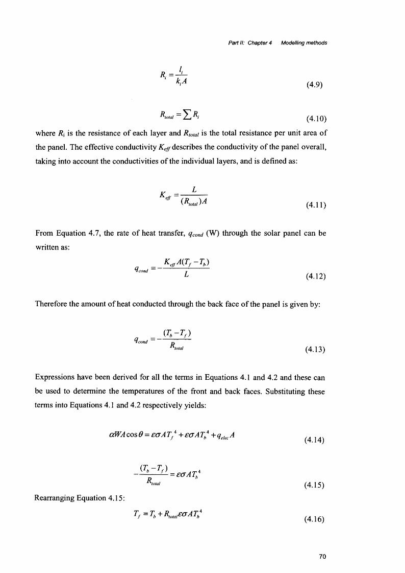
Part II: Chapter 4 Modelling methods
Ri= —k i A (4.9)
R total (4-10)
where R\ is the resistance of each layer and R totai is the total resistance per unit area of
the panel. The effective conductivity Keff describes the conductivity of the panel overall,
taking into account the conductivities of the individual layers, and is defined as:
K 1
( R total)A (4.11)
From Equation 4.7, the rate of heat transfer, qcond (W) through the solar panel can be
written as:
K « W f -T b)Qcond = ----- ---- 7--------
L (4.12)
Therefore the amount of heat conducted through the back face of the panel is given by:
(Tb-T f )Qcond
R"m (4.13)
Expressions have been derived for all the terms in Equations 4.1 and 4.2 and these can
be used to determine the temperatures of the front and back faces. Substituting these
terms into Equations 4.1 and 4.2 respectively yields:
aWAcos6 = eoA T* +eaAT„4 +qekcA (4 )4)
i = e , A T 4
K t a i (4.15)
Rearranging Equation 4.15:
Tf = Th+ Rtotal£crATh(4 .16)
70
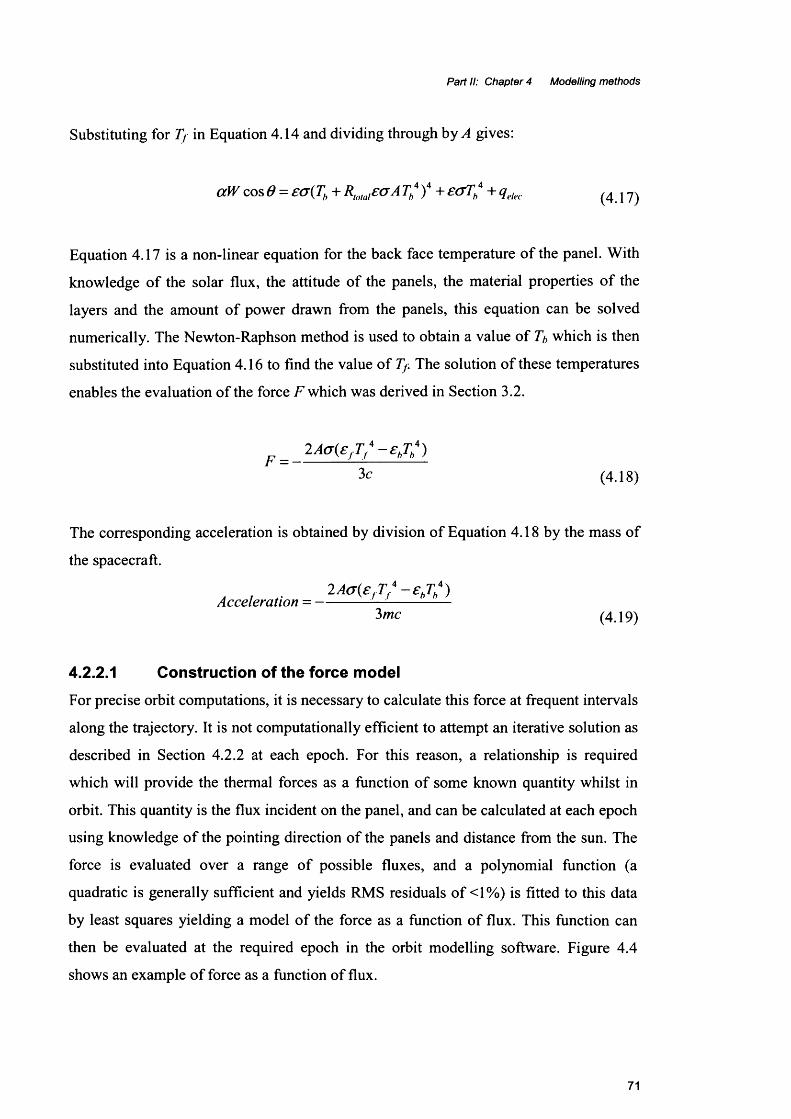
Part II: Chapter 4 Modelling methods
Substituting for Tf in Equation 4.14 and dividing through by A gives:
aW cos 6 = ea{Th + Rt0taleoA T 4 )4 + e o T 4 + qelec (417)
Equation 4.17 is a non-linear equation for the back face temperature of the panel. With
knowledge of the solar flux, the attitude of the panels, the material properties of the
layers and the amount of power drawn from the panels, this equation can be solved
numerically. The Newton-Raphson method is used to obtain a value of 7* which is then
substituted into Equation 4.16 to find the value of Tf The solution of these temperatures
enables the evaluation of the force F which was derived in Section 3.2.
r _ 2 A a(ef T / - £ hTh4)
3c (4.18)
The corresponding acceleration is obtained by division of Equation 4.18 by the mass of
the spacecraft.
, , 2Ao{efTf4 -ehT4)Acceleration = ---------- :—:-------------
3 me (4.19)
4.2.2.1 Construction of the force modelFor precise orbit computations, it is necessary to calculate this force at frequent intervals
along the trajectory. It is not computationally efficient to attempt an iterative solution as
described in Section 4.2.2 at each epoch. For this reason, a relationship is required
which will provide the thermal forces as a function of some known quantity whilst in
orbit. This quantity is the flux incident on the panel, and can be calculated at each epoch
using knowledge of the pointing direction of the panels and distance from the sun. The
force is evaluated over a range of possible fluxes, and a polynomial function (a
quadratic is generally sufficient and yields RMS residuals of <1%) is fitted to this data
by least squares yielding a model of the force as a function of flux. This function can
then be evaluated at the required epoch in the orbit modelling software. Figure 4.4
shows an example of force as a function of flux.
71
Part II: Chapter 4 Modelling methods
Thermal force = / (incident flux)
-6.8E-071400 142013801340 136013D0 1320
-7.0E-07
-7.2E-07
-7.4E-07
I -7.6E-07
O -7.8E-07
-8.0E-07
-8.2E-07
-8.4E-07
-8.6E-07
F lu x ( W m '! )
Figure 4.4: Graph of force as a function of flux
In Figure 4.4, the flux limits are driven by the maximum and minimum flux in the
vicinity of the spacecraft from perihelion to aphelion.
4.2.3 Transient modelling
When a satellite enters shadow regions, changes in temperature occur on a timescale too
quick to allow the steady state assumption to hold true. Changes in surface temperature
can only be evaluated once the energy transport mechanisms that supply or remove
energy from the surface are calculated. This requires knowledge of the initial
temperature distribution within the panel, the material properties of all the layers,
specifically their conductivities, densities, specific heat capacities and dimensions.
Time-varying temperatures can be acquired through the solution of the heat equation.
The heat equation is a partial differential equation which describes the temperature field
in a given region over time. In this section, the heat equation is derived by the
application of the conservation of energy principle to a differential control volume
(SxSy&) and the energy processes relevant to it, as represented in Figure 4.5.
72

Part II: Chapter 4 Modelling methods
tfz+Sz
X
Figure 4.5: Energy transfer processes in a finite control volume.
If the temperature distribution is known at some point in time, Fourier’s law can be used
to calculate the rate of heat transfer between two points to obtain the temperatures at
subsequent epochs. Where temperature gradients exist, heat conduction will occur
across each of the control surfaces. The conduction heat rates perpendicular to each of
the control surfaces at the x, y and z coordinate locations are indicated by the terms qx,
qy and qz. The conduction heat rates at the opposite surfaces can then be expressed as a
Taylor series expansion where, neglecting higher order terms,
dqr cqx+6x=qx+-^rSx
<},+Sy=(l , +-j^- (4-2°)
<l,+St=<lz+ Sz
73

Part II: Chapter 4 Modelling methods
If there is an energy source within the medium, it can be described as:
Eg = qSxdySz (4.21)
Where q is the rate at which energy is generated per unit volume of the medium
(Wm'3). In addition, there may be changes in the internal thermal energy stored by the
material in the control volume. This can be expressed as:
dTEa = pCp — StcSySz (4.22)
Now the conservation of energy requires that
Ei„+Eg Eoul Es, (4.23)
Ein and Eout represent conduction inflow and outflow, and Equation 4.23 can be
rewritten as:
dTqx + qy +q,+ qSxSySz - qxyix - qyy3y - qztdz = pC p — SxSySz (4.24)
Substituting in for Equations 4.20, it follows that:
^ - Sx —^ Sy - 8 z + qSxSySz = pC — SxSySz (4.25)ox dy oz dt
The heat conduction rates can be evaluated from Fourier’s law:
qx = -k S y S z ^ ~dx
Stqv = —kS xS z—— (4.26)
dy
qz = -k S x S y ^ ~ dz
74

Part II: Chapter 4 Modelling methods
Substituting Equations 4.26 into Equation 4.24 and dividing out by the dimensions of
the control volume, we obtain:
dx \ ox+ -
3'y j + dzn ST
+ q = PC^(4.27)
This is the heat equation, and can be solved for the temperature as a function of position
within the material and time.
When in total darkness, it is assumed that no power is drawn from the panels, so the ^
term can be set to zero and assuming one-dimensional heat flow, the heat equation in
Equation 4.27 reduces to:
— [ k — \ = pC 3jc I dx J p dt
(4.28)
where T is the temperature distribution in the panel at location jc and at time t.
For the temperature to be evaluated, the differential equation needs to be solved with
appropriate boundary and initial conditions. A technique based on the finite volume
method to calculate how temperatures change in a composite wall (Price, B. & Smith, T.
, 1994) was applied to the solar panels. This method splits the panels into small control
volumes and performs energy balance calculations on each of them based on heat
transfer to neighbouring control volumes and heat exchange processes occurring at the
panel surfaces. Figure 4.6 shows a panel which is separated into discrete elements of
thickness 8xj and 5i is the inter-node distance, each element containing a node. For each
node, an equation is written at the initial time-step for which the temperatures of each
node are known. This equation relates heat flow in and out of the node based on
neighbouring nodes and boundary conditions to the temperature change that will result
due to this heat flow. These sets of equations are solved simultaneously at each time-
step to yield temperatures at the next time-step. For a thorough description of this
method, the reader is referred to Price, B. & Smith, T., 1994.
75

Part II: Chapter 4 Modelling methods
front of panel8xi
< N back of panel
N
Figure 4.6: Composite panel divided into nodal elements
This method was applied to GPS and Jason-1 solar panels in a hypothetical eclipse
situation. The spacecraft was assumed to go from full phase directly into the umbra. The
gradual reduction of flux in the penumbra was not included at this stage. Figure 4.7
show the temperature change with time for the front and back panels when the GPS
Block HR spacecraft enters and exits the eclipse; Figure 4.8 shows the corresponding
accelerations for a GPS solar panel.
76

Part II: Chapter 4 Modelling methods
350 -IExit firom_ umbra
^ — Entry into umbra
300 -
fl> 250front face
faceg 200
150
1000 10 20 30 40 50 60 70 80 90 100
Time (mins)
Figure 4.7: Front and back panel face temperatures for a GPS Block HR spacecraft
8E-10Exit from umbra
Entry into umbra
7E-10
6E-10
*3 3E-10
© 2E-10
< 1E-10
90 1001E-10
-2E-10 JTime (mins)
Figure 4.8: Acceleration due to thermal panels for a GPS Block HR spacecraft
Figure 4.7 demonstrates the fact that the temperatures drop very quickly as soon as the
incoming radiation is “switched o ff’. More importantly, the conduction of heat from hot
regions to cold regions causes the difference between the front and the back surfaces
temperatures to diminish. Therefore, the resultant force, which is the difference between
the forces due to the front and the back surfaces, declines extremely rapidly. The
resultant force changes direction because the emissivity of the back face (£b=0.89) is
77
Part II: Chapter 4 Modelling methods
higher than the emissivity of the front face (eb =0.86). This causes the back face to emit
more energy than the front face once the temperatures have almost equalised.
A calculation was carried out to determine the maximum displacement to a spacecraft
that could occur by accounting for this force during an eclipse crossing, as opposed to
simply switching the thermal force on and off on entering and emerging from eclipse.
Assuming an acceleration (acc) of 4 x 10'10 ms'2 (which is a high estimate) acting
constantly in one direction for the whole period in eclipse for a time t of one hour, the
displacement S , is given by:
1 9S =—(acc)t2
This gives a maximum possible displacement of 3mm. As this force will not act
contantly in one direction the actual displacement will be smaller than this. The
modelling of an effect this small is unlikely to yield significant improvements. This
transient force was not tested any further or implemented into orbit
prediction/determination software.
4.3 Multilayer insulation
Multi-layer insulation (MLI) is the name given to insulation blankets that are built up of
multiple sheets arranged to alternate low emittance surfaces with low conductance
barriers (Bapat, S., 1990). These layers are often made of Kapton (a polymide polymer)
sheets with an aluminium vapour deposited onto one side. Most spacecraft flown today
are covered with MLI blankets, with cut outs for radiator areas to reject internally
generated waste heat (Gilmore, D., 1994) and necessary instrument surfaces. Heat
transfer through multilayer insulation is a combination of radiation, solid conduction,
and under atmosphere conditions, gaseous conduction.
The solid conduction heat transfer through the blanket is minimised by rumpling of the
inner layers, so the aluminised sheets touch at discrete points rather than across the
whole surface. Radiation heat transfer is minimised by interposing as many enclosing
layers with reflective surfaces (metalised sheets) as is practical. In order to evacuate the
air trapped between blanket layers before launch, vent paths have to be provided. This is
78

Part II: Chapter 4 Modelling methods
often done by small perforations in each blanket layer, while ensuring that perforations
between one layer and the next are not aligned in order to minimise incoming radiation
entering the spacecraft.
Because the heat transfer mechanisms described above operate simultaneously and
interact with each other, the thermal conductivity of MLI is not strictly definable
analytically in terms of variables such as temperature, density, or physical properties of
the component materials. It is therefore useful to refer to either an apparent thermal
conductivity or an effective emittance. These values are usually derived experimentally.
When blankets are configured for spacecraft application, experience has shown that
effective emissivities are usually between 0.015 to 0.030 (Gilmore, D., 1994).
4.3.1 Properties of MLIThe behaviour of MLI blankets and the assumptions used in this study are as follows:
• Heat transfer parallel to the layers of MLI is ignored. This is valid because MLI
is so thin (between 7-25 pm) that effectively no heat is conducted along the
individual layers. MLI coverage often consists of discrete pieces that are joined
together; this also reduces heat transfer in this direction (pers comms, Cavan, N.,
Rutherford Appleton Laboratories (RAL), Oct 2002).
• The temperature of the spacecraft beneath the layers of MLI is assumed to be
between 273K and 323K. Payload instruments are designed to work at room
temperature (Galvin, D., 1999) and therefore spacecraft thermal systems aim to
maintain temperatures close to this. It is therefore reasonable to assume Tsc to
have a value of 298K. The calculation is not highly sensitive to this parameter;
an error analysis using temperatures 25 degrees higher and lower than this
showed the force to be different by less than 1% (shown in Section 7.1.1.2).
• The MLI surface is assumed to emit radiation as a plane Lambert diffuser
(crinkliness is ignored).
• Steady state is assumed in full phase.
• When the satellite enters eclipse, its temperatures are assumed to drop to zero
instantly (pers comms, Cavan, N., (RAL), Oct 2002). This is reasonable given
that the MLI is not designed to be a good heat store.
79
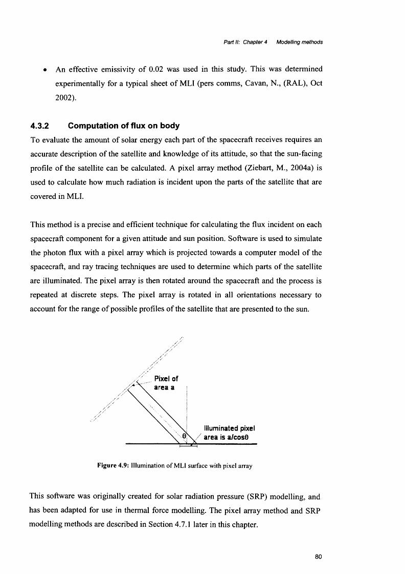
Part If: Chapter 4 Modelling methods
• An effective emissivity of 0.02 was used in this study. This was determined
experimentally for a typical sheet of MLI (pers comms, Cavan, N., (RAL), Oct
2002).
4.3.2 Computation of flux on bodyTo evaluate the amount of solar energy each part of the spacecraft receives requires an
accurate description of the satellite and knowledge of its attitude, so that the sun-facing
profile of the satellite can be calculated. A pixel array method (Ziebart, M., 2004a) is
used to calculate how much radiation is incident upon the parts of the satellite that are
covered in MLI.
This method is a precise and efficient technique for calculating the flux incident on each
spacecraft component for a given attitude and sun position. Software is used to simulate
the photon flux with a pixel array which is projected towards a computer model of the
spacecraft, and ray tracing techniques are used to determine which parts of the satellite
are illuminated. The pixel array is then rotated around the spacecraft and the process is
repeated at discrete steps. The pixel array is rotated in all orientations necessary to
account for the range of possible profiles of the satellite that are presented to the sun.
/ ///'
Pixel of a re a a
Illuminated pixel / a rea is a /co s0
Figure 4.9: Illumination of MLI surface with pixel array
This software was originally created for solar radiation pressure (SRP) modelling, and
has been adapted for use in thermal force modelling. The pixel array method and SRP
modelling methods are described in Section 4.7.1 later in this chapter.
80

Part II: Chapter 4 Modelling methods
Once the pixel array software has determined whether a particular surface is irradiated,
a test is performed to see whether that part is covered in MLI. If so, a calculation is
carried out to determine the force due to the MLI. This calculation is described in
Section 4.3.3.
4.3.3 Calculation of force due to MLIAs described in Section 3.1, if the emitting surface is planar and treated like a
Lambertian diffuser, the force normal to the emitting surface is given by:
To obtain solutions for the temperature of the MLI surface, the following energy
transport mechanisms are considered.
(1) Solar photons impact upon the MLI.
(2) Energy is both absorbed and reflected, depending on the absorptivity of the MLI.
(3) Of the energy absorbed, some is re-emitted and some is transferred through to the
spacecraft. The latter amount is dictated by the value of the effective emissivity.
If a is the area of one pixel, and 0 is the angle of incidence of the radiation flux W (see
Figure 4.9), the solar radiation absorbed by the surface illuminated by one pixel is
ocWa . The area of the MLI that is illuminated is given by a t cos 6 . The energy radiated
out to space is given by:
3c(4.29)
acos 6
(4.30)
A cut off angle of 89.5° was included to prevent Equation 4.30 tending to infinity. The
energy conducted through to the spacecraft is given by:

Part II: Chapter 4 Modelling methods
These terms are substituted into an energy balance to give:
a a W - £ MLia G ^M U | € efl< J a (^MLI r , ) (4.32)cos 6 cos 0
By dividing through by a and multiplying by cos# Equation 4.32 becomes:
acos0W = eMLlaTML; + e effa(TML; - T j ) (4.33)
where TMU is temperature of MLI, Tsc is temperature of spacecraft and is the
effective emissivity between the MLI and the spacecraft. Re-arranging Equation 4.33
gives the temperature of the surface illuminated by each pixel:
. aW cos 6 + e ^ o T j T» u = . * “ (4.34)
G ( £ MU £ eff )
Substituting in the value of 298K for Tsc, Equation 4.34 can be calculated to yield the
temperature which when substituted into Equation 4.35 below, yields the force due to
the illuminated area.
f = - 2aE»Lir Hu ( 4 3 5 )- 3c
4.4 Thermal Response of MLI due to earth radiation flux
It is only recently that consideration has been given to the analytical modelling of forces
of the order of magnitude of TRR and earth radiation pressure (ERP) (~10'7 N). As
more and more of the error is removed by improved force models, effects such as
thermal re-radiation due to radiation from the earth, which are at least an order of
magnitude smaller, begin to attract attention.
In this study, a “first pass” treatment of the problem is made; these effects are
considered for GNSS altitude satellites only and the assumptions made cannot
necessarily be applied to LEO satellites.
82
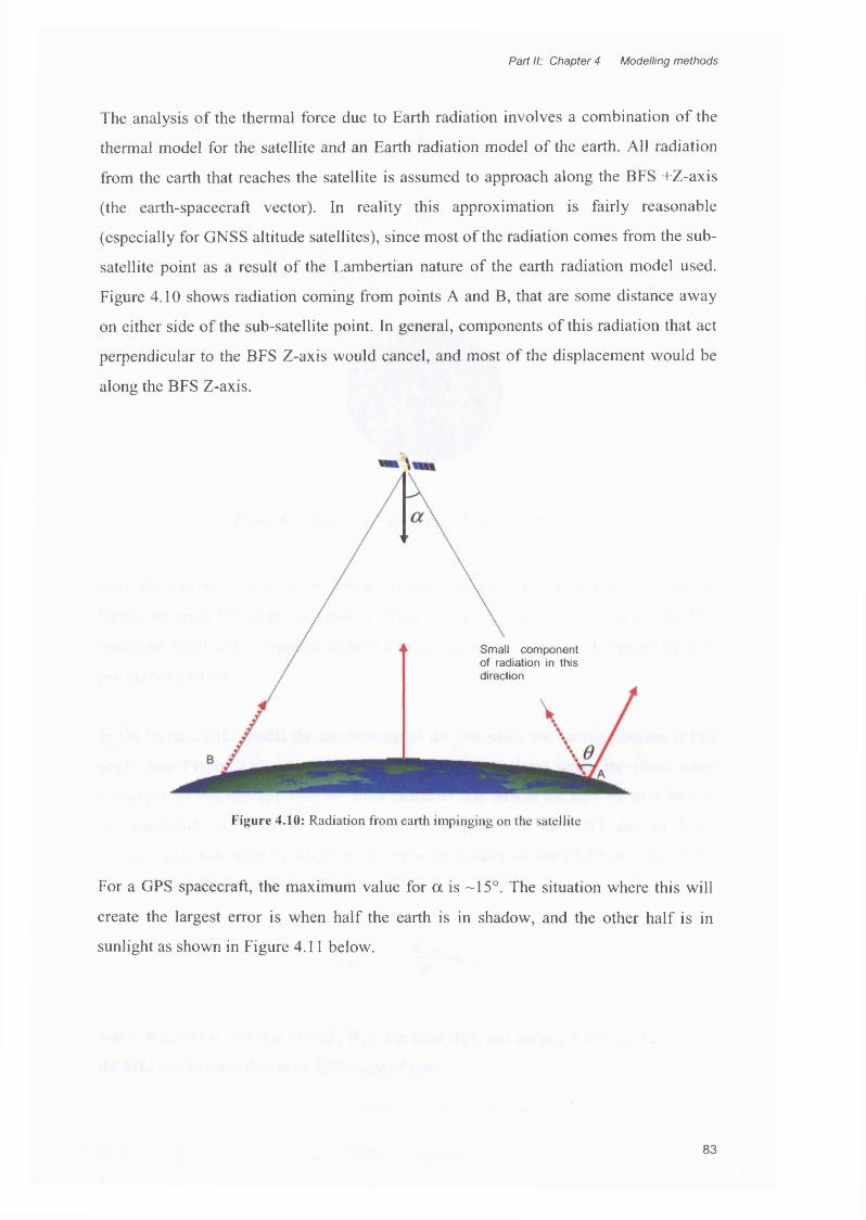
Part II: Chapter 4 Modelling methods
The analysis of the thermal force due to Earth radiation involves a combination of the
thermal model for the satellite and an Earth radiation model of the earth. All radiation
from the earth that reaches the satellite is assumed to approach along the BFS +Z-axis
(the earth-spacecraft vector). In reality this approximation is fairly reasonable
(especially for GNSS altitude satellites), since most of the radiation comes from the sub
satellite point as a result of the Lambertian nature of the earth radiation model used.
Figure 4.10 shows radiation coming from points A and B, that are some distance away
on either side of the sub-satellite point. In general, components of this radiation that act
perpendicular to the BFS Z-axis would cancel, and most of the displacement would be
along the BFS Z-axis.
Small component of radiation in this direction
Figure 4.10: Radiation from earth impinging on the satellite
For a GPS spacecraft, the maximum value for a is -15°. The situation where this will
create the largest error is when half the earth is in shadow, and the other half is in
sunlight as shown in Figure 4.11 below.
83
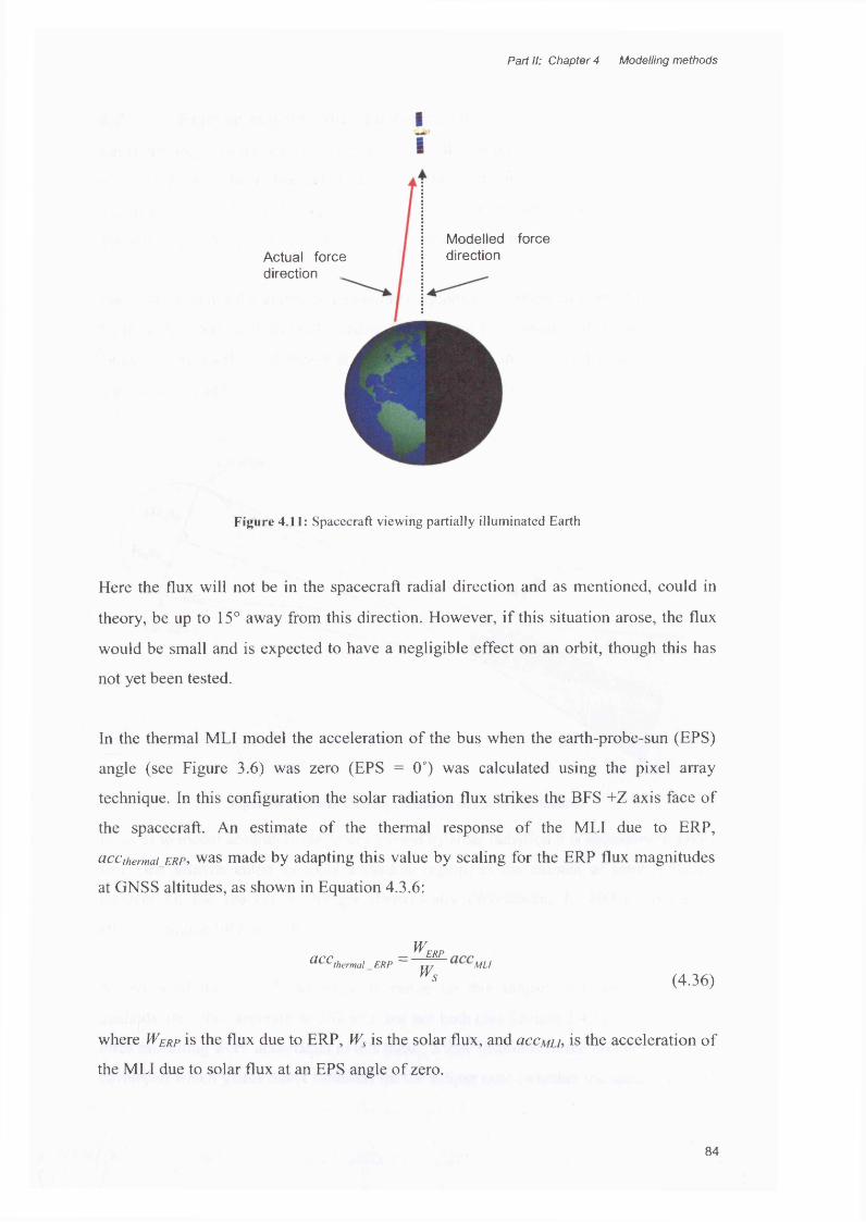
Part II: Chapter 4 Modelling methods
Modelled force directionActual force
direction _
Figure 4.11: Spacecraft viewing partially illuminated Earth
Here the flux will not be in the spacecraft radial direction and as mentioned, could in
theory, be up to 15° away from this direction. However, if this situation arose, the flux
would be small and is expected to have a negligible effect on an orbit, though this has
not yet been tested.
In the thermal MLI model the acceleration of the bus when the earth-probe-sun (EPS)
angle (see Figure 3.6) was zero (EPS = 0°) was calculated using the pixel array
technique. In this configuration the solar radiation flux strikes the BFS +Z axis face of
the spacecraft. An estimate of the thermal response of the MLI due to ERP,
accthermal_erp, was made by adapting this value by scaling for the ERP flux magnitudes
at GNSS altitudes, as shown in Equation 4.3.6:
W ERPa C C thermal ERP = ^
W* (4.36)
where Werp is the flux due to ERP, Ws is the solar flux, and ciccmu, is the acceleration of
the MLI due to solar flux at an EPS angle of zero.
84

Part II: Chapter 4 Modelling methods
4.5 Eclipse region boundary modelling
Earth-orbiting satellites experience partial or total eclipses when they pass through the
regions known as the umbra and penumbra. In the penumbra, the total solar irradiance is
partially occluded by the Earth, whereas the umbra can be defined as the region on the
anti-sun side of the Earth which is completely devoid of solar radiation.
Figure 4.12 shows the umbra and penumbra regions for a spherical Earth. In reality the
Earth is flattened, with the polar radius being about 0.3% smaller than the equatorial
radius. If the Earth’s oblateness is taken into account, the boundaries of the shadow
regions are altered.
sun
satellite
sun edge 2penumbra
umbra
Figure 4.12: Lines forming penumbra and umbra boundaries
In order to model accurately the forces caused by solar radiation it is necessary to know
when the satellite enters or exits a shadow region, as the amount of solar radiation
incident on the spacecraft changes dramatically (Woodbum, J., 2000). Forces so
affected include SRP and TRR.
A review of the publicly available literature on this subject indicates that current
methods are either accurate or efficient, but not both (see Section 3.4.3). As part of the
force modelling work undertaken in this thesis, a new treatment of the problem has been
developed which yields direct solutions for the eclipse state (whether the spacecraft is in
85

Part II: Chapter 4 Modelling methods
full sunlight, penumbra or umbra) whilst still accounting for the earth’s polar flattening.
The aim is to develop a method which combines accuracy with efficiency, and is
therefore usable for orbit determination purposes, where a solution for the eclipse state
will be required very frequently. The mathematical formalism of this method is
described in Section 4.5.1 and in Adhya, S. et al., (2004). In the development of this
method, tests to assess its validity are included in this section.
4.5.1 Determination of satellite eclipse stateThis method is based upon tests that determine whether or not lines from the sun edges
to the spacecraft intersect the Earth. If an intersection occurs, and the distance from the
sun to this intersection point is less than the sun-spacecraft distance, then the satellite is
either in the penumbra or the umbra.
An instantaneous plane is defined by the geocentre, the Earth-sun vector r* and the
Earth-spacecraft vector a (see Figure 4.12). In this two-dimensional space the sun is
modelled as a circle. In the plane, rays of light starting at the sun edges and making
tangents with the Earth define the full phase/penumbra and penumbra/umbra
boundaries, as shown in Figure 4.12.
The actual calculations of the intersection points are carried out using three-dimensional
geometry, with the surface of the Earth being mathematically approximated by the
equation of a spheroid:2 2 2 at + y
P2 q 2 (4.37)
where x, y, z are the ECI coordinates of a point in space on the surface of the spheroid, p
is the equatorial radius and q is the polar radius.
The line passing through the spacecraft and sun-edge 1 is henceforth referred to as Line
1. Any point (x, y, z) on Line 1 obeys the equation:
f V V f My = a2 + A bi
\ ai )
(4.38)
86

Part II: Chapter 4 Modelling methods
where {a]t <1 2 , a3) are the x , y, z components of the position vector of the spacecraft a,
and (bj, b2, b3) are the x,y , z components of the vector from sun-edge 1 to the spacecraft
b. Rearranging and equating the formulae for Equation 4.38 yields the following
relationship, which is another definition for Line 1:
x — a] _ y — a2 _ z — a3
b\ b2 b 3 (4 .3 9 )
Vectors a and b can be obtained at a specific epoch from precise ephemeredes or
numerical integration, and hence Line 1 is defined. Line 2 is defined similarly with a
different value of vector b.
To calculate the vector the coordinates of the sun-edges are required. The unit vector
orthogonal to the Earth-sun vector is used to find these sun-edges in an EC I coordinate
frame (see Figure 4.12). The vectors r*/ and r 2 can be defined as the lines from the
geocentre to sun-edge 1 and sun-edge 2 respectively. Hence the vector b is calculated
from:
b = bc-Lsi for Line 1 and (4.40)
b = Lsc-Ls2 for Line 2.
To determ ine^, the unit vector that lies in the plane and is perpendicular to r* (see
Figure 4.12), the cross product between r* and a is taken to give a vector (r,j normal to
the plane.
L “ Lv (4.41)
Taking the cross product of r, with r* gives the vector that lies in the plane and is
perpendicular to which is Sp.
s„ = r (4.42)
Normalizing this vector gives Sp .
The two sun edge points are given by:
^ = £ , + ( * , 4 , ) (4.43)
87

Part II: Chapter 4 Modelling methods
l ,2= l < -(r A p) (4.44)
where R* is the sun radius.
From Equation 4.39, it is possible to rewrite y and z as a function of x and the
coefficients of vectors a and b.
b? , x y = — ( x - a l) + a2 (4.45)
z = -2- (x - ax) + a3 (4.46)
Now y and z can be substituted into Equation 4.37 to yield a quadratic in x:
x 2 + (x - ax) + a2
■ +
b-t / x— (jc - ax) + a3
= 1
2 2 2 q x +q bi , x — (jc-a j + a. + P 4 (x - ax ) + a3
(4.47)
(4.48)
Ax2 + Bx + C — 0
In this quadratic:
A = b 2q2 + q2b 2 +
5 = -2 b 2q2ax + 2 bxb2qza2 - 2 p lb3 ax + 2p lbfi2a2 i 2 _ , „ 2 i
C = q 2 \ b 2a 2 +b2 a 2 - 2b2bxaxa2~ + p 2 [ ^ 2fl32 +b32a 2 -2 b 3bxaxa3 ~ \-b 2p 2q2 = 0
(4.49)
The real solutions to this quadratic equation give the ^-coordinates of the points of
intersection of the spheroid and the sun-edge to spacecraft line.
For a real solution to exist:
88

Part II: Chapter 4 Modelling methods
B 2 -4 A C > 0 (4.50)
If Equation 4.50 is satisfied, an intersection takes place. A negative value has no
physical meaning, but shows that no intersection occurs. If there is no intersection, then
the satellite is in full phase. Lines from both sun edges to an instantaneous satellite
position are tested in this manner. Once the value of x is obtained, it can be substituted
into Equation 4.39 to solve for the y and z coordinates of the intersection point;
equivalent equations can be generated to yield quadratics in y and z. Full coordinates of
the intersection point are required in order to calculate its distance from the sun. If this
distance is larger than the distance between the sun and the spacecraft, then the satellite
is automatically assigned a state of full phase. In all other cases, the following
conditions are regarded (see Figure 4.1.3):
• If both lines have real solutions, then the spacecraft is in the umbra.
• If only one of the lines has real solutions the spacecraft is in the penumbra.
• If there are no real solutions then the spacecraft is in full phase.
The algorithm written to carry out this function takes a UTC time-tag and the position
vector of the satellite as inputs. The corresponding sun positions are retrieved for each
epoch from an ephemeris file (JPL DE405), and the test for intersection points is carried
out. A specified integer value is returned depending upon the result of the computation;
the program calling the function uses this integer value to determine if a change of state
has occurred.
89
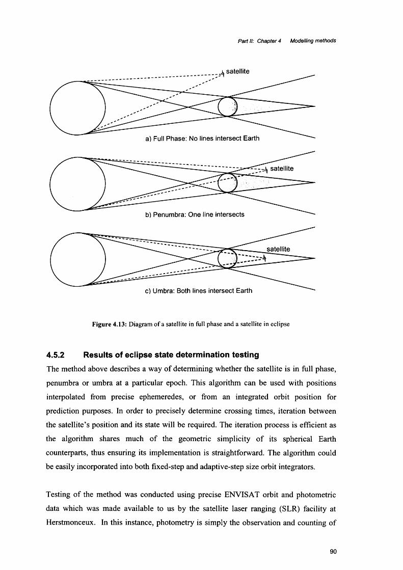
Part II: Chapter 4 Modelling methods
satellite
a) Full Phase: No lines intersect Earth
^ satellite
b) Penumbra: One line intersects
satellite
c) Umbra: Both lines intersect Earth
Figure 4.13: Diagram of a satellite in full phase and a satellite in eclipse
4.5.2 Results of eclipse state determination testingThe method above describes a way of determining whether the satellite is in full phase,
penumbra or umbra at a particular epoch. This algorithm can be used with positions
interpolated from precise ephemeredes, or from an integrated orbit position for
prediction purposes. In order to precisely determine crossing times, iteration between
the satellite’s position and its state will be required. The iteration process is efficient as
the algorithm shares much of the geometric simplicity of its spherical Earth
counterparts, thus ensuring its implementation is straightforward. The algorithm could
be easily incorporated into both fixed-step and adaptive-step size orbit integrators.
Testing of the method was conducted using precise ENVISAT orbit and photometric
data which was made available to us by the satellite laser ranging (SLR) facility at
Herstmonceux. In this instance, photometry is simply the observation and counting of
90

Part II: Chapter 4 Modelling methods
solar photons reflected from the spacecraft, which can be sorted from laser pulses
during simultaneous SLR observations on the basis of amplitude and duration by a
median filter (Otsubo, T. et al., 2001). Obviously, as the satellite enters eclipse, there
will be less sunlight incident upon it, resulting in fewer photon counts; though this will
also depend to a small degree upon the viewing geometry from the SLR station. The
photometry data shown in Figure 4.14 for ENVISAT (a LEO satellite), and Figure 4.15
for Glonass (a MEO satellite) are quite typical for the satellites tested.6 A decision was
made to use only the ENVISAT photometry to test the algorithm because, as can be
seen from the figures, the Glonass eclipse transition occurs over a much longer time
period. It is also expected that atmospheric refraction will have a greater impact on the
higher altitude satellites, and therefore the algorithm is likely to have more errors
associated with it for higher altitude satellites. However, the Herstmonceux SLR team is
currently tracking Russian Etalon satellites, which are covered in comer cube reflectors
and orbit with an altitude of approximately 19,000 km, in an attempt to try to assess the
effect of atmospheric refraction on eclipse transition times. Orbital data for ENVISAT
is given in Table 4.1.
Semi-major axis 7159 km
Inclination 98.5°
Eccentricity 0.001165
Argument of perigee 90.0° ± 3°
Mean local solar time at descending node 10am
Table 4.1: Approximate orbital elements for ENVISAT
To estimate the time of onset of shadow transition, the team at the SLR facility fitted a
low order polynomial to a short period of pre-event photometric data. This function is
extrapolated and residuals from the photometry data are computed. When the modulus
of the residuals become larger than 3 x RMS of the post-fit residuals, the event is
assumed to be underway. The precision of this process is estimated to be about 1 second
6 Photometry data was reproduced by kind permission of the NERC Space Geodesy Facility at
Herstmonceux, E. Sussex.
91

Cou
nts
Part II: Chapter 4 Modelling methods
of time, and the epochs of the photometry data are at a much higher resolution than this
(pers comms, Appleby, G., March 2002).
40 50 60 70Time (s) after 2003 2 20 0 11
Figure 4.14: ENVISAT photometry plot - emergence from eclipse
§c«~,
§
8
8OC
8
O
Oo
o
o®
OO
100 105 110 120 125 130Time ts) after 2003 9 14 22 20 03
Figure 4.15: Glonass photometry plot - emergence from eclipse
92
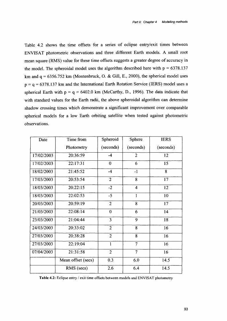
Part II: Chapter 4 Modelling methods
Table 4.2 shows the time offsets for a series of eclipse entry/exit times between
ENVISAT photometric observations and three different Earth models. A small root
mean square (RMS) value for these time offsets suggests a greater degree of accuracy in
the model. The spheroidal model uses the algorithm described here with p = 6378.137
km and q = 6356.752 km (Montenbruck, O. & Gill, E., 2000), the spherical model uses
p = q = 6378.137 km and the International Earth Rotation Service (IERS) model uses a
spherical Earth with p = q = 6402.0 km (McCarthy, D., 1996). The data indicate that
with standard values for the Earth radii, the above spheroidal algorithm can determine
shadow crossing times which demonstrate a significant improvement over comparable
spherical models for a low Earth orbiting satellite when tested against photometric
observations.
Date Time from
Photometry
Spheroid
(seconds)
Sphere
(seconds)
IERS
(seconds)
17/02/2003 20:36:59 -4 2 12
17/02/2003 22:17:31 0 6 15
18/02/2003 21:45:52 -4 -1 8
17/03/2003 20:53:54 2 8 17
18/03/2003 20:22:15 -2 4 12
18/03/2003 22:02:53 -5 1 10
20/03/2003 20:59:19 2 8 17
21/03/2003 22:08:14 0 6 14
23/03/2003 21:04:44 3 9 18
24/03/2003 20:33:02 2 8 16
27/03/2003 20:38:28 2 8 16
27/03/2003 22:19:04 1 7 16
07/04/2003 21:31:58 2 7 16
Mean offset (secs) 0.3 6.0 14.5
RMS (secs) 2.6 6.4 14.5
Table 4.2: Eclipse entry / exit time offsets between models and ENVISAT photometry
93

Part II: Chapter 4 Modelling methods
The mean and RMS offsets shown in Table 4.2 show that the spheroid model has errors
which are distributed about zero whereas both the spheroid and the IERS models appear
to have strong biases.
For low Earth orbiting satellites, an incorrect transition point will introduce a systematic
bias over many orbit revolutions. Polar orbiters, such as ENVISAT (Table 4.1), may be
subject to a difference of several minutes (when added over several orbits) spent in
eclipse when comparing those predicted by a spherical Earth model against those from
the current algorithm. In terms of efficiency, the algorithm developed here runs 13.4
times faster than an alternative oblate Earth technique (Vokrouhlicky, D., 1996) when
determining 1 million eclipse states on a dual processor AMD Athlon 2200+ machine.
4.6 Modelling of penumbra flux
4.6.1 IntroductionOn entering the penumbra, the flux gradually diminishes until it reaches zero in the
umbra. If this reduction in flux is modelled, then the forces that are a result of solar
radiation can be calculated. However, this extra computation will only be of benefit in
orbit prediction if the forces are large enough and act for long enough to make a
noticeable difference to the satellite’s orbit. The penumbra is a relatively small region,
though its size increases with orbit altitude. If a medium earth orbiting spacecraft at
GPS attitude was to travel straight through it, the time taken would be ~l-2 minutes.
There are however certain configurations of the sun-earth-satellite geometry which at a
certain inclination of orbit cause the satellite to graze through the penumbra, spending
an appreciable time in this region. A simple calculation was carried out to estimate what
the maximum time spent in the penumbra would be, taking a GPS spacecraft as
example.
4.6.2 Maximum time spent in penumbraThe maximum time possible for a GPS HR satellite to spend in penumbra is calculated
based upon the orbit of the satellite and the geometry of the umbra and penumbra. For
this calculation, the earth was assumed to be spherical. Figure 4.16 shows the Sun, Earth
and shadow region geometry. Rs is the radius of the sun, RE is the radius of the earth, rs
is the distance from the centre of the earth to the centre of the sun, a is the radius of the
94
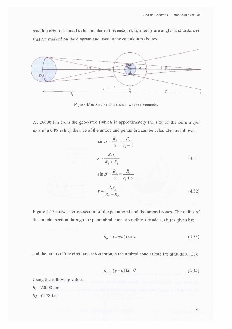
Part II: Chapter 4 Modelling methods
satellite orbit (assumed to be circular in this case), a, (3, jc and y are angles and distances
that are marked on the diagram and used in the calculations below.
Figure 4.16: Sun, Earth and shadow region geometry
At 26000 km from the geocentre (which is approximately the size of the semi-major
axis of a GPS orbit), the size of the umbra and penumbra can be calculated as follows:
Re R sin a - — = — -r - x
RPrx = — *-*— (4.51)
r s +r e
■ a R E Rs in p = — - =y n
Rcrr = (4-52)
Figure 4.17 shows a cross-section of the penumbral and the umbral cones. The radius of
the circular section through the penumbral cone at satellite altitude a, (hp) is given by:
hp = (x + a) tan a (4.53)
and the radius of the circular section through the umbral cone at satellite altitude a, (hu)\
K = { y - a ) tan>ff (4.54)
Using the following values:
Rs =70000 km
R e =6378 km
95

Part II: Chapter 4 Modelling methods
rs =150000000km
a = 26000 km
the following are obtained:
a= 0.2698
P= 0.2649
jc= 1354374 km
y = 1379282 km
hp = 6500.1 km
hu = 6256.8 km
To find a ball park figure for the amount of time spent in penumbra, Figure 4.17 can be
used.
Cross section through this plane taken here \
Figure 4.17: Schematic of cross-section of eclipse region
The distance d is then given by:
d = 2 J h f - h . 1 (4.55)
and evaluation of Equation 4.55 gives d = 3523.5 km. If we take the speed of the
satellite to be ~ 4kms‘1, then the satellite can spend up to 14.7 minutes in the penumbra.
This is a theoretical value to estimate an upper bound to how long the satellite could
spend in penumbra. The JPL shadow event files which can be obtained from their ftp
site (sideshow.jpl.nasa.gov) record the eclipse crossing times and Figure 4.18 shows the
96
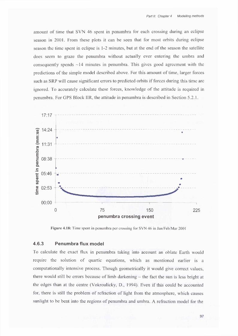
Part II: Chapter 4 Modelling methods
amount of time that SVN 46 spent in penumbra for each crossing during an eclipse
season in 2001. From these plots it can be seen that for most orbits during eclipse
season the time spent in eclipse is 1-2 minutes, but at the end of the season the satellite
does seem to graze the penumbra without actually ever entering the umbra and
consequently spends -14 minutes in penumbra. This gives good agreement with the
predictions of the simple model described above. For this amount of time, larger forces
such as SRP will cause significant errors to predicted orbits if forces during this time are
ignored. To accurately calculate these forces, knowledge o f the attitude is required in
penumbra. For GPS Block IIR, the attitude in penumbra is described in Section 5.2.1.
17:17 t
'w 14:24
11:31-Q
08:38
05:46 ,O-
2 02:53 4
00:000 75 150 225
penumbra crossing event
Figure 4.18: Time spent in penumbra per crossing for SVN 46 in Jan/Feb/Mar 2001
4.6.3 Penumbra flux model
To calculate the exact flux in penumbra taking into account an oblate Earth would
require the solution of quartic equations, which as mentioned earlier is a
computationally intensive process. Though geometrically it would give correct values,
there would still be errors because of limb darkening - the fact the sun is less bright at
the edges than at the centre (Vokroulicky, D., 1994). Even if this could be accounted
for, there is still the problem of refraction of light from the atmosphere, which causes
sunlight to be bent into the regions of penumbra and umbra. A refraction model for the
97

Part II: Chapter 4 Modelling methods
atmosphere is complicated because o f its variation with time and place. It was not
within the scope o f this research to analyse the penumbra flux in such detail and even if
this had been done, it would have been cumbersome to implement in a software
package, which is a concern o f all model development undertaken herein.
A first order approximation for the fall off of flux in the penumbra is to linearly reduce
it from the value it has when it enters the penumbra to zero at the umbra.
To do this, it is necessary to transform the coordinates into a basis so that the origin is at
the geocentre, the sun is along the positive x-axis and the satellite, geocentre and sun-
centre define the x-y plane. The new basis will have its x-axis, x ’ along the Earth-sun
vector in ECI coordinates. The normalised cross product o f this vector with the Earth-
probe vector gives the z ’ axis and the cross product o f z ’ with x ’ gives the y ’ axis.
Ph
x ’
Figure 4.19: Schematic for penumbral height calculation
At the x-value o f the satellite the size of the umbra (t//,) and penumbra (/?/,) are
calculated. This gives the penumbra width. The y-value o f the satellite gives the “height
o f the satellite above the x axis. Then Equation 4.56 gives the proportion o f the flux
incident on entering eclipse that is still present.
98

Part II: Chapter 4 Modelling methods
y'-«tp * (4.56)
The effects of implementing this preliminary model into orbit prediction software is
investigated in Chapter 5.
4.7 Other models required for generation of thermal forces
Descriptions of the models used for the SRP and ERP forces are given in this section.
The reasons for their inclusion here are two-fold. Firstly, for thermal force models to be
successfully tested in orbit prediction/determination, larger forces, such as those
described in Chapter 2 need to be implemented. For many of the forces, standard
models are used and will be listed when required; for SRP and ERP however custom
models developed within UCL’s geodesy group have been employed. Secondly, aspects
of both of these models have been adapted for use in the thermal models developed in
Sections 4.3 and 4.4, relating to the characterisation of radiation incident upon each part
of the spacecraft, and therefore deserve explanation.
4.7.1 Solar radiation pressure
This basis of this force was described in Section 2.2.2.1. A brief overview of this
method is given here; the details of the modelling method can be found in Ziebart
(2004a). When radiation strikes the spacecraft surface, a proportion is absorbed and the
rest reflected. Figure 4.20 shows a light ray striking a surface.
Fnspecularly reflected ray v
incidentray
Fs
Force due Recoil force due to reflectedabsorbed
Figure 4.20: Incident ray on spacecraft surface
99

Part II: Chapter 4 Modelling methods
A physical analysis of the interactions result in the following functions for the normal
and shear forces (see Figure 4.20) due to SRP on a flat surface:
_ A W cos0[„ 2Fn = -------------- (\+jLiv)cos0+—v{\- ju)c \_ 3
_ AW C O S 0 rFs = ------------ [(\ -juv) sm0\c
where:
Fn the force normal to the surface (N)
Fs the shear force or the force along the surface (N)
A surface area of component (m2)
W solar irradiance Wm'2
0 angle of incidence of incoming radiation
v reflectivity of component
H specularity of component
c speed of light in a vacuum (299792458 m s'1)
For complicated spacecraft geometries, calculation of the radiation flux incident on each
surface poses a difficult problem, due to irregular 3D surfaces and shadowing of some
components by others. The solar photon flux is simulated using a pixel array which is
projected towards a computer simulation of the spacecraft. Ray tracing techniques from
each pixel are used to determine which parts of the satellite are illuminated. The effect
of radiation reflected specularly and intersecting with other parts of the spacecraft is
modelled. The method deals automatically with the shadowing of one part of the
spacecraft by another. Figure 4.21 shows the pixel array projected onto the spacecraft
model.
100

Part II: Chapter 4 Modelling methods
Figure 4.21: Projection of pixel array onto spacecraft structure from one direction
The pixel array is then rotated around the spacecraft and the solar panels are adjusted to
track the pixel array as they would track the Sun on orbit. This process is repeated for
all possible sun directions. The output from the software for any one orientation of the
pixel array is the acceleration of the spacecraft due to the SRP expressed in the BFS
XYZ axes. This yields a number of discrete snapshots of the response of the satellite to
the radiation flux. Orbit integration requires a continuous model, and this is calculated
by fitting an appropriate mathematical model to the data. This could be, for example, a
Fourier series or a grid file. A particular strength of this technique is that it deals with
the high geometrical complexity of real spacecraft as no simplification is made to the
spacecraft structural data.
By using the pixel array method in the calculation of the thermal force due to MLI, the
thermal force can be combined with the SRP force for the spacecraft bus. This results in
a computationally efficient algorithm for calculation of the solar driven non
conservative forces.
101

Part II: Chapter 4 Modelling methods
4.7.2 Earth radiation pressureThe physical modelling of the ERP force is similar to SRP in that the force is produced
by the interaction of electromagnetic radiation and the spacecraft surface. The
fundamental difference between the two effects is in the modelling of the irradiance
from the radiation source as discussed in Section 2.2.2.2. The ERP models used in this
study are described in Ziebart (2004b).
Probes exist in Earth’s orbit with instruments on board, whose goals are to quantify the
radiation leaving the earth. Accelerations due to ERP have been derived from space-
and-time averaged data from Clouds and the Earth's Radiant Energy System (CERES)
and the Earth Radiation Budget Experiment (ERBE) (Barkstrom, B., 1984; Weilicki, B.
et al., 1996). Combined data from these two probes provide global grided monthly
estimates of longwave and shortwave earth radiation fluxes emitted from the top of the
atmosphere (TOA) (30km) from 1984 until at least the end of the current decade. The
spatial resolution of data is such that each grid cell represents an area of 2.5° longitude
by 2.5° latitude.
The model used in this study was developed based on the assumption that the emitting
surface emits energy into the hemisphere above the point source at the centre of a grid
and that the surface behaves like a Lambert diffuser (Chapman, A., 1984). The TOA
values are manipulated based on these assumptions to provide the contribution of each
grid cell at the required altitude. The total radiation received at the satellite can be
obtained by summing contributions from each grid cell to that point in space. The
interaction of the flux with a box-and-wing model of GPS Block HR is calculated and a
Fourier series is fitted to a time series of the resulting accelerations. During the orbit
integration, this function is computed at the required epoch.
SummaryThis chapter has described the main techniques developed to compute thermal forces
from a spacecraft surface for use in orbit computations. Methods for the treatment of the
solar panels and for MLI covered surfaces are derived, and an initial attempt at
characterising the thermal force due to earth radiation pressure effects for GNSS altitude
satellites has been explained. Methods for determining eclipse boundary crossing times
for an oblate earth and for estimating the flux in penumbral regions have been
102

Part II: Chapter 4 Modelling methods
developed. In Part III, these methods will be applied to the GPS Block HR and Jason-1
spacecraft, and tested in model computations. A brief overview is given for the solar
radiation pressure and earth radiation pressure models which are used in parts of the
thermal modelling process.
103

Part III: Test Cases
Part III Test CasesThe methods developed in Chapter 4 were used to compute models for two satellites:
GPS Block IIR, the most recent Global Positioning System (GPS) space vehicle
deployed in orbit (at the time of writing), and Jason-1, a joint CNES/NASA altimetry
satellite. Chapters 5 and 6 describe the implementation of the model, testing methods
and results of these tests for each satellite.
The test cases differ significantly in terms of orbit, structure, mass and attitude regimes
and are subject to different characteristic particulate and electromagnetic radiation
fluxes. Their main characteristics are summarized in Table III. 1.
GPS Block IIR Jason-1Altitude 20200 km 1336 km
Mass 1100 kg 489.1 kgArea/mass ratio 0.013 m2kg‘‘ 0.025 m^kg'1
Orbital period 11 hrs 56 mins 1 hr 52 minsOrbital inclination 55° 66°
T ab le I I I . l : Characteristics of GPS Block IIR and Jason-1
At GPS altitude the atmosphere is greatly rarefied and in terms of affecting the motion
of a spacecraft, atmospheric drag is considered insignificant (Jacchia, L., 1977). GPS
force models can be tested by comparing predicted orbits based on numerical
integration of the force models with post-processed precise orbits. The rationale for this
is that orbit prediction is central to the GPS operational concept.
The altitude of Jason-1 was specifically chosen to balance the trade off between
achieving a short probe-surface range whist still minimising drag effects. It does
however still suffer from drag perturbations which are complicated to predict (see
Section 2.2.2.3) and as yet no accurate analytical modelling for this force exists.
Estimates made using a typical value for the drag coefficient, yielded accelerationso 10 9ranging between 3.4 x 10' to 3.9 x 10' ms' (depending on atmospheric temperatures
7 Area refers to maximum spacecraft profile
104

Part III: Test Cases
and densities). As these are one to two orders of magnitude larger than the thermal force
effects, orbit prediction based on dynamic models is not suitable for testing thermal
models. The thermal models for Jason-1 are to be tested by incorporation into orbit
determination software (described in Section 6.4.1), in which drag forces are estimated
empirically.
These satellites have been chosen as test cases for two main reasons. Firstly, both
spacecraft require precise orbits to meet their mission objectives. Secondly, GPS Block
IIR and Jason-1 spacecraft differ substantially (see Table III.l) and, if application of the
methods developed in this study appears to improve orbit prediction/determination for
both spacecraft, the validity of the model in the general case is strengthened.
105

Part III: Chapter 5 GPS Block IIR
Chapter 5 GPS Block IIR
Chapter outlineThis chapter contains a brief overview of the GPS system and its architecture. A
detailed description of the structural, material and optical properties and attitude regime
of GPS Block IIR is given. The computation and implementation of the methods
discussed in Chapter 4 are described. The methods are tested and results of these tests
are shown. This chapter includes a brief analysis and discussion of the results.
5.1 Overview of GPS system
The GPS IIR satellite is the most recent model of operational satellites that comprise the
Global Positioning System (GPS) space segment. GPS is used to obtain three
dimensional positioning anywhere on the surface of the earth or for satellites in lower
orbits. GPS was primarily developed as a navigation system, but now has widespread
uses in precise geodetic applications.
The fundamental navigation principle is based on the measurement of so called
“pseudoranges” between the user and a minimum of four satellites. The spacecraft
positions are considered to be known in a suitable reference frame. Geometrically three
range measurements are required, and a fourth is necessary to correct for errors in the
receiver clock. This clock error is the reason for the term “pseudorange”. For real time
single receiver positioning, each GPS satellite emits a signal modulated with a specific
code sequence of binary values, known as a pseudorandom noise (PRN) code. To
determine the signal propagation time, the user needs a copy of this code sequence in
the receiver. The code sequence is phase shifted in time until maximum correlation is
achieved and the necessary phase shift is a measure of the signal travel time between the
satellite and the receiver antennas.
For geodetic applications which require much higher precision, observations of the
phase of the transmitted carrier wave (termed a phase observable) are used. This is a
lengthier process as it requires the solution to the problem of ambiguity resolution. This
106

Part III: Chapter 5 GPS Block IIR
is not discussed further here; for a comprehensive description of GPS systems the reader
is referred to the following texts: GPS Satellite Surveying, Leick, 2004 & Satellite
Geodesy, Seeber, 2003.
5.1.1 System architectureThe GPS system consists of three segments:
• Space segment
• User segment
• Control segment
The space segment currently (November, 2004) consists of a constellation of 30
satellites in near circular orbits which are inclined at 55° and have a period of almost 12
hours. These satellites are in medium earth orbits at altitudes of 20200 km. The satellites
occupy 6 planes separated by 60 degrees, and the satellites are distributed over the
planes. The constellation design criterion was that 4 satellites should be visible
anywhere on earth 24 hours a day (Seeber, G., 2003).
The user segment consists of receivers on the ground (or in space, in the air or at sea)
which pick up signals emitted by the space segment. This data is used to solve for
position and velocity of the receiver. The spacecraft positions derived from the
predicted orbit effectively define the user’s real-time reference frame. Obviously any
errors in the orbit prediction will propagate directly into errors in the position and
velocity of the user’s receiver. Depending on variables such as the receiver type, the
amount of data recorded and the sophistication of the processing technique used,
varying degrees of accuracy in the calculated position and velocity can be attained. In
terms of absolute positions this can vary from 20m down to a few centimetres.
The control segment consists of a global network of ground stations, which
continuously track the spacecraft throughout the course of their orbits. The tracking data
is transmitted from the ground stations to a Master Control Station (MCS). At the MCS,
these data are combined with models of the forces acting on the spacecraft to predict the
orbital trajectory of each satellite 12-48 hours in advance. These data are uploaded to
107

Part III: Chapter 5 GPS Block IIR
the spacecraft. As each spacecraft orbits the Earth, it emits the signals from which the
psuedoranges are calculated, and another signal containing the data message. The data
message includes spacecraft orbit parameters (derived from the predicted orbit) from
which the position of satellite can be computed. This information is termed the
‘broadcast ephemeris’ and is described in more detail in Section 5.1.2.
5.1.2 Broadcast ephemerisAs stated in Section 5.1.1.3, the broadcast ephemeris contains estimates of future orbit
information for each satellite which have been computed by the MCS based on
observation data from monitor stations. The monitor stations receive all satellite signals
from which their pseudoranges (from the station to the satellite) are determined. These
are transmitted along with local meteorological data (which will affect the calculation of
ranges) to the MCS. The MCS uses several days of data to pre-compute the satellite
ephemeredes and the behaviour of the satellite clocks. These parameter sets cover
several days and are transmitted to the ground antennas, then uplinked to the satellites
which broadcast the appropriate set when transmitting to a receiver. Currently the
satellite is uploaded with new orbital parameters approximately every two hours (Misra,
P., 2001). For the ideal case of the 2-body problem, (Section 2.1), only 6 elements are
required to specify the position and velocity of the satellite at any future time. For a real
spacecraft, the perturbing forces cause the orbit to change with time, and the orbit has to
be characterised by a set of time dependent parameters. GPS accounts for these
perturbations with an expanded orbital set which retains a Keplerian “look”. This
parameter set was chosen in the 1970s as a compromise between obtaining the required
accuracy without burdening a receiver with undue computational and storage
requirements. The estimated satellite positions are represented by an expanded set of
quasi-Keplerian parameters consisting of orbital elements at a particular epoch,
parameters describing how the elements will change with time and additional
perturbation and time-related parameters.
5.2 GPS IIR spacecraft description and data sources
The GPS spacecraft bus consists of a rectangular box with a shroud covering the
antenna array which is on the +Z axis face (see Figure 5.1). The bus is mostly covered
in multilayer insulation. Power is supplied to the spacecraft by silicon cells mounted on
108
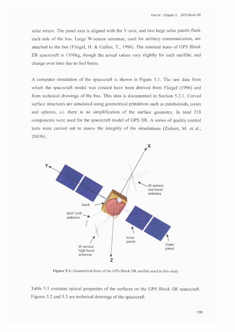
Part III: Chapter 5 GPS Block IIR
solar arrays. The panel axis is aligned with the Y-axis, and two large solar panels flank
each side of the bus. Large W-sensor antennae, used for military communication, are
attached to the bus (Fliegel, H. & Gallini, T., 1996). The nominal mass of GPS Block
IIR spacecraft is 1100kg, though the actual values vary slightly for each satellite, and
change over time due to fuel bums.
A computer simulation of the spacecraft is shown in Figure 5.1. The raw data from
which the spacecraft model was created have been derived from Fliegel (1996) and
from technical drawings of the bus. This data is documented in Section 5.2.1. Curved
surface structures are simulated using geometrical primitives such as paraboloids, cones
and spheres, i.e. there is no simplification of the surface geometry. In total 218
components were used for the spacecraft model of GPS IIR. A series of quality control
tests were carried out to assess the integrity of the simulations (Ziebart, M. et al.,
2003b).
.W-sensor low band antenna
back
NAP UHF antenna
/W-sensor high band antenna
Innerpanel
Outerpanel
Figure 5.1: Geometrical form of the GPS Block IIR satellite used in this study
Table 5.1 contains optical properties of the surfaces on the GPS Block IIR spacecraft.
Figures 5.2 and 5.3 are technical drawings of the spacecraft.
109

Part III: Chapter 5 GPS Block IIR
SV component Reflectivity SpecularityExposed panel beams (each of two) 0.85 0.85Plume shield 0.06 0.00Antenna Shroud 0.06 0.00W-sensor elements (low band)
Element 1 0.06 0.00Element 2 0.06 0.00Element 3 0.06 0.00Element 4 0.06 0.00Element 5 0.06 0.00Element 6
W-sensor elements (high band)Element 1 0.06 0.00Element 2 0.06 0.00Element 3 0.06 0.00Element 4 0.06 0.00Element 5 0.06 0.00Element 6 0.06 0.00
Table 5.1: GPS Block HR surface components
110

Part III: Chapter 5 GPS Block IIR
1.81
1.57
0.81
Q.45.
M l
MmQM
0.59Q.8Q
1.53
Figure 5.2: Technical drawing of GPS Block IIR (dimensions are in metres)
111

Part III: Chapter 5 GPS Block IIR
1 Z L
(=□
Figure 5.3: Technical drawing of GPS Block IIR (dimensions are in metres)
The solar panel comprises of 11 layers and the material specifications and optical
properties of the front and the back of the solar panel are given in Table 5.2.
112

Layer MaterialThickness
(m)Conductivity
(W/m/k)Density(kg/m3)
Specific Heat Capacity (J/kg/K)
1 Quartz coverglass 0.000254 1.417322835 2615.751168 627.98671232 DC 93-500 5.08E-05 0.157480315 1079.516355 1674.6312333 Silicon solar cell 0.000254 150 2524.407477 749.39527214 RTV 566 0.000102 0.157480315 1522.39486 1674.6312335 Kapton 2.54E-05 0.157480315 1425.515187 1092.6990846 BR36 adhesive 0.000127 0.157480315 1060.140421 1674.6312337 Face sheet A1 2024 0.000254 188.976378 2767.990654 962.91295898 FM 36 0.000127 0.157480315 1154.252103 1674.6312339 A1 honey comb core (5056) 0.0254 2.031496063 33.21588785 962.912958910 Adhesive FM 36 0.000127 0.157480315 1154.252103 1674.63123311 A1 2024 0.000254 188.976378 2767.990654 962.9129589
Total 0.026975Front face absorptivity 0.72 ± 0.03Front face emissivity 0.86 ± 0.02Back face emissivity 0.89
Table 5.2: Characteristics of solar panel layers for GPS Block IIR
113
Part III: Chapter 5 GPS Block IIR
At any time, power is drawn from either the inner panels or the outer panels, (pers
comms, Fliegel, H., April 2003); if power is drawn from a panel, it is at a nominal rate
of 90 Wm'2. This causes differences in temperatures and forces exerted by the inner and
outer panels. Since GPS Block IIR attitude regime requires that the solar panels are
always sun facing, the perpendicular area presented to the sun is constant and the
resulting force varies as a function of sun-probe distance.
5.2.1 GPS IIR attitudeThe attitude of the satellite is determined by the requirement that the navigation
antennae which are aligned along the spacecraft fixed Z-axis point towards the
geocentre and that the solar arrays, mounted along the spacecraft fixed Y-axis face the
sun8. The spacecraft fixed X-axis is required to lie in the hemisphere containing the sun.
Except at the two singular points when the Earth, Sun and spacecraft are collinear, this
regime uniquely defines the attitude of the spacecraft. The angle between the Earth-
satellite and the satellite-Sun lines is the Earth-Probe-Sun (EPS) angle (Figure 5.4).
From the spacecraft point of view, the Earth is continually on the BFS Z-axis, and the
Sun appears to rise and set confined to the BFS X-Z plane (Ziebart, M., 2004a). When
the satellite is in full sunlight, its attitude is controlled to meet the above requirements
based on the output of solar sensors mounted on the solar panels. When the spacecraft
cannot see the sun, the attitude is set to a fixed yaw regime (the yaw refers to the
rotation of the spacecraft bus). In this fixed yaw regime, the spacecraft emerges from
the shadow region close to its nominal attitude9 (Bar-Sever, Y., 1997).
gMis-alignment of these panels could be the cause of reported Y-bias effects for some spacecraft
(Fliegel, H. & Gallini, T., 1996)
9
Originally, the yaw attitude of the spacecraft was determined by measurements made by solar sensors
mounted on the solar panels. It was noticed however that for the Block II and IIA satellites, computed
orbits of eclipsing satellites were less accurate than for their non-eclipsing counterparts. This was because
in the absence of the sun, the output from the solar sensors was essentially zero, and the output was driven
by noise in the system, leading to erratic yawing during shadow crossing. To fix this problem, a constant
small bias was introduced, so that the sun sensor’s signal was superposed with another signal (the bias),
equivalent to a yaw error of 0.5°, to allow the attitude in eclipse to be modelled. As a result, when the sun
was observed, the yaw attitude was in 0.5° error with respect to its actual orientation. It was expected that
114

Part III: Chapter 5 GPS Block IIR
+x
+z
e= EPS angle
Figure 5.4: Attitude of GPS Block HR
5.2.2 Antenna thrust
Transmission of the navigation signals results in a reactive force on the satellite, as
described in Section 2.2.3.5. A value for the signal power of 77 W was supplied by JPL.
This is equivalent to a force of 2.6 x 10'7 N, which acts constantly in the satellite radial
direction.
5.2.3 Other surfaces
The remaining large structures on the surface of the GPS Block IIR spacecraft are the
W-sensor high and low band antennae and the NAP UHF antenna (see Figure 5.1).
These are composed of thin cylindrical components made of aluminium, covered in
black tape (Fliegel, H. & Gallini, T., 1996). Due to the high conductivity of aluminium,
it is probable that uniform temperature distributions about the axis of each cylinder will
result. In these cases, any thermal force will be cancelled out by another in the opposite
direction, and therefore the net force will sum to a zero.
this error would be negligible, but actually the yaw error appeared to be more than 0.5° in full sunlight,
hence the new regime was implemented for GPS Block IIR (Bar Sever, Y., 1996a, 1996b).
115

Part III: Chapter 5 GPS Block IIR
In order to increase the lifetime of the electronic subsystems in the satellite bus, the
internal temperature of the bus is maintained at (-20° C) (Galvin, D., 1999). The only
means of rejecting heat generated within the bus is through radiation to space. The GPS
satellites use radiators (see Figure 5.1). These radiators are on the +Y and -Y faces of
the spacecraft positioned so as to avoid direct solar radiation. Unfortunately, no specific
data was available for these vents. If the assumption is made that energy is output
symmetrically, the forces due to this emission will also cancel each other out. If
however they do not emit energy at the same rate, it could be another cause of the Y-
bias effect (discussed in Section 3.3.2.2), where there is a larger force in the Y-direction
than expected (Fliegel, H. et al., 1992).
5.3 Model computation
5.3.1 MLIAlmost all the faces of the GPS Block IIR bus are covered in MLI including the plume
shield and the antenna shroud. The pixel array method was used to compute
accelerations for SRP and thermal response of MLI surfaces. A pixel resolution of 2mm
was used, with the pixel array positioned at separate points every 2 degrees around the
satellite (that is a step size of 2° in EPS angle). A nominal flux value of 1 AU was used
which was scaled for the actual probe-sun distance when used in an orbit computation.
Figure 5.5 shows the spacecraft BFS X, Y and Z accelerations as a function of EPS
angle.
116

Part III: Chapter 5 GPS Block IIR
1.0E-08
8.0E-09
6.0E-09
^ 4.0E-09CN'(/>
E. 2.0E-09 c- O.OE+OO2 60 300 360120 180 2400)® -2.0E-09 o< -4.0E-09
-6.0E-09
-8.0E-09
-1.0E-08
EPS angle (deg)
Figure 5.5: BFS X, Y and Z accelerations as a function of EPS angle due to MLI surfaces
The resulting accelerations were expressed as three Fourier series (accelerations as a
function of EPS angle), each using 179 coefficients, one for each satellite BFS axis. On-
orbit forces are determined based on the EPS angle at the epoch of interest.
The accelerations in the ±Y axis directions are non-zero due to the asymmetry of
structures on the +Z face (mainly of the MLI shroud) of the GPS Block IIR spacecraft.
This produces an a priori model of the Y-bias.
5.3.2 Solar panels
The total resistance was calculated by the method described in Section 4.2.2 to have the
value of:
R,omi=0.016055929 KW'1
The temperatures of the panels at a particular epoch will differ depending on whether
power is being drawn from the panels. Assuming that a power of 90 Wm'2 is drawn
from a panel, Table 5.3 shows the temperatures of the front and back surfaces and the
force that results at a distance of one astronomical unit from the earth (a solar flux of
117
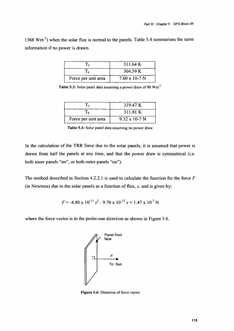
Part III: Chapter 5 GPS Block IIR
1368 Wm’2) when the solar flux is normal to the panels. Table 5.4 summarises the same
information if no power is drawn.
Tf 311.64 KTb 304.59 K
Force per unit area 7.60 x 10⁻⁷ N
Table 5.3: Solar panel data assuming a power draw of 90 Wm'2
Tf 319.47 KTb 311.81 K
Force per unit area 9.32 x 10⁻⁷ N
Table 5.4: Solar panel data assuming no power draw
In the calculation of the TRR force due to the solar panels, it is assumed that power is
drawn from half the panels at any time, and that the power draw is symmetrical (i.e.
both inner panels “on”, or both outer panels “on”).
The method described in Section 4.2.2.1 is used to calculate the function for the force F
(in Newtons) due to the solar panels as a function of flux, jc, and is given by:
F = -4.80 x 1 0 ' V - 9.70 x 10' l2x + 1.47 x 10'7N
where the force vector is in the probe-sun direction as shown in Figure 5.6.
Panel front face
To Sun
Figure 5.6: Direction of force vector
118
Part III: Chapter 5 GPS Block IIR
5.4 Testing methodologyThe critical step in the process of modelling surface thermal forces is the evaluation of
surface temperatures. In this section, the first two methods test how well the modelled
solar panels temperatures compare to solar panel temperature data available from other
sources. This study aims to develop force models which improve the definition of a
satellite’s motion. The third test method predicts orbits and examines whether
predictions improve on the incorporation of the newly developed force models.
5.4.1 Testing methods 1: Comparison with telemetryTelemetered data (of a few GPS Block IIR spacecraft) from temperature sensors
situated on the front of the solar panels were available from Lockheed Martin.
Comparison of modelled temperatures to these temperatures provide an independent
check with which to compare the model outputs.
5.4.2 Testing Methods 2: Comparisons with other methodsThere are many commercial software tools available for thermal modelling that use
Finite Element Analysis (FEA) or Finite Difference solvers to predict heat flow and
temperatures. ESATAN is one such tool that has been developed by Alstom10. It was
released in 1985 and has been the standard thermal analysis code of the European Space
Agency (ESA). Theoretically, this software can solve for steady state or transient
temperatures for the whole spacecraft at all attitudes if sufficient input data is available,
though it may be impractical to implement these results into orbit
prediction/determination tools due to the high computational burden. This software is
used as a check for the calculation of the solar panel surface temperatures. The results
are given in Section 5.5.2.
Additionally, other independent researchers have published calculated values for solar
panel temperatures. A comparison with these values is made.
5.4.3 Testing Methods 3: Orbit predictionThe thermal force models and eclipse related models are incorporated into software
developed by the Geodesy Research Group at UCL which is used to integrate an orbit
10 http://www.techcentreuk.power.alstom.com/pdf/ESATAN_Thermal_Analyser.pdf
119

Part III: Chapter 5 GPS Block IIR
forward from an initial state vector to produce a predicted orbit. The method of orbit
prediction is presented here.
The force models described in Chapter 2 constitute an approximation to the true second-
order differential equation of motion of the spacecraft. Shortcomings in the accuracy of
the initial conditions (position and velocity at some epoch) and the force model cause
the integrated trajectory to diverge from the true orbit. The degree of divergence is used
to assess the degree of mis-modelling in the force model. In practice, of course, the true
trajectory is never known as attempts to measure it always have some associated error.
However, the precise orbits produced by centres such as JPL, CODE and GFZ provide
best estimates of the true trajectory of a satellite given all the available data and models.
In this analysis JPL precise orbit files were used. These orbit files contain state vectors
at 15 minute intervals for GPS satellites.
The steps of the model testing procedure are as follows:
• A state vector is taken from a JPL precise orbit file and defined as the start point
of the integration process.
• The spacecraft orbit is numerically integrated forward over 12 hours (one orbit)
from this point.
• The position of the satellite is compared to that of the precise trajectory at each
15 minute intervals (this is the maximum resolution of data available in the
precise JPL files).
• The difference vector between the predicted and the precise orbits are projected
onto the Height-Cross-aLong track (HCL) (see Section 2.3) basis at 15 minute
intervals over each trajectory.
• The root mean square errors in each of the height, cross and along-track axes are
then calculated.
• The thermal models are then added to the existing model, and comparisons of
errors are made before and after these are added.
The orbit prediction software uses an 8th order embedded Runge-Kutta integrator; a ten-
second integration step-size was chosen. Tests carried out with a one second step size
showed a difference of <1% in orbit prediction results.
120

Part III: Chapters GPS Block IIR
5.4.3.1 Force modelsThe basic force model is known hereafter as Model 1 and accounts for:
• Spherical harmonic Earth gravity field model, to degree and order 15 using
GRACE GGM01C coefficients. (Increasing this degree and order added no
significant improvement to the results.)
• 3rd body perturbations due to the Sun, Moon, Venus and Mars. Jet Propulsion
Laboratory Developmental Ephemerides (JPL DE405) were used to compute
third body effects.
• Custom analytical SRP models (Ziebart, M., 2004a) as described in Section
4.7.1.
• Custom albedo models (Ziebart, M. et al., 2004b) as described in Section 4.7.2.
• Solid Earth tide variations to Earth gravitational potential due to the Sun and the
Moon
• General relativistic effects
• Pole tides
• Antenna thrust model
The thermal and eclipse related models are added one by one to Model 1 to generate
Models 2-5 defined below.
Model 2 = Model 1 + steady state thermal modelling of solar panels, and penumbra flux
Model 3 = Model 2 + models for the parts of the satellite covered in MLI
Model 4 = Model 3 + forces due to thermal albedo
Model 5 = Model 4 but assuming the flux is zero in the penumbral region
Twelve hour arcs were predicted for 5 GPS IIR satellites - SVN 41, 43, 44, 46, 51 over
4 weeks (March 2004), using the models developed here. An arc length of one orbit was
chosen to enhance the likelihood of detection of once per orbit revolution dynamic
effects. These dates were chosen as masses of each of these satellites during this time
were available (pers comms, Fliegel, H., April 2004) and are given in Table 5.5 below.
SVN number Mass in March 2004 (kg)
121
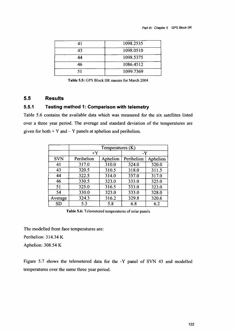
Part III: Chapter 5 GPS Block IIR
41 1098.253543 1098.051044 1098.537546 1086.451251 1099.7369
Table 5.5: GPS Block IIR masses for March 2004
5.5 Results
5.5.1 Testing method 1: Comparison with telemetryTable 5.6 contains the available data which was measured for the six satellites listed
over a three year period. The average and standard deviation of the temperatures are
given for both + Y and - Y panels at aphelion and perihelion.
Temperatures (K)+Y -Y
SVN Perihelion Aphelion Perihelion Aphelion41 317.0 310.0 324.0 320.043 320.5 310.5 318.0 311.544 322.5 314.0 337.0 317.046 330.5 323.0 333.0 325.051 325.0 316.5 333.0 323.054 330.0 323.0 333.0 328.0
Average 324.3 316.2 329.8 320.6SD 5.3 5.8 6.8 6.2
Table 5.6: Telemetered temperatures of solar panels
The modelled front face temperatures are:
Perihelion: 314.34 K
Aphelion: 308.54 K
Figure 5.7 shows the telemetered data for the -Y panel of SVN 43 and modelled
temperatures over the same three year period.
122

Part III: Chapter 5 GPS Block IIR
320 T— modelled temps— telemetered temps
318
— 316
w 314 -
i 312 -
310 -
3080.5 10 1.5 2 2.5 3
years since 01/01/98
Figure 5.7: SVN 43 front face panel temperatures from telemetry and model data
The difference in temperature between aphelion and perihelion are clearly evident in
both sets o f data. The telemetered data and the modelled data both show the same
pattern, but there is a nearly constant offset between the two o f about 3K. Data
telemetered from the other Block IIR satellites show constant offsets also, and with only
one exception, the offset is always in the same direction.
5.5.2 Testing method 2: Comparisons with other methods
Steady state temperature results are presented using ESATAN. The output o f the
ESATAN program is included. Node 1 refers to the front face and Node 12 refers to the
back face. Temperatures are given in °C. These temperatures are evaluated at a distance
from the sun o f one astronomical unit and a power draw o f 90 W m'2.
EUROPEAN SPACE AGENCY THERMAL ANALYSIS NETWORK (VERSION 8.9.1) PAGE 6
02 SEPTEMBER 2004 09:43:43SOLAR_PANEL
$Id: Solar Panel 2003/08/09 $
123

Part III: Chapter 5 GPS Block IIR
TIMEN = 25000.00 MODULE SLCRNC DTIMEU = 0.0051CSGMIN =********** AT NODE * IN SUB-MODEL
+SOLAR_PANEL
TABLE OUTPUT WITH ZENTS = 1L,T'FOR NODES OF ZLABEL = ' '
+SOLAR_PANEL
NODE LABEL T (K)
1 Front Face 311.672 Bar 311.593 Bar 311.534 Bar 311.255 Bar 311.186 Bar 310.827 Bar 310.828 Bar 310 .479 Bar 305 . 07
10 Bar 304 . 9811 Bar 304 . 9812 Back Face 304 . 6913 Deep space front 27314 Deep space back 273
5.5.3 Testing method 3: Orbit predictionThe results are presented for 12 hour orbit predictions for 5 GPS IIR satellites (SVN 41,
43, 44, 46, 51), one for each day, over the course of 4 weeks (March 2004), using the
models developed here. Tables 5.7 - 5.11 give the mean RMS residuals and standard
deviations for each satellite over the test period. Table 5.7 shows the results when no
thermal model is included (Model 1); Table 5.8 gives the results when thermal
modelling of the panels was included (Model 2) and Table 5.9 gives the results for the
124

Part III: Chapter 5 GPS Block IIR
final model which includes thermal modelling of solar panel and MLI (Model 3). Table
5.10 gives the results for when the thermal albedo effect is included along with all the
other thermal effects (Model 4). Comparative tests were also carried out on eclipsing
satellites with and without inclusion of the penumbra flux model (Table 5.11). No data
was rejected on a statistical basis.
SVN H C L aH aC aL41 1.371 0.262 2.2512 0.058 0.027 0.18743 1.313 0.352 3.343 0.043 0.029 0.36744 1.677 0.053 3.522 0.055 0.030 0.67546 1.160 0.315 4.689 0.076 0.014 0.43051 1.885 0.110 7.552 0.156 0.018 0.736
W Mean 1.411 0.233 2.997
Table 5.7: Mean HCL residuals (m) from 28 days o f 12 hour predictions, Model 1.
SVN H C L aH aC aL41 1.248 0.231 2.051 0.053 0.026 0.17943 1.180 0.322 2.978 0.042 0.028 0.33844 1.508 0.049 3.168 0.054 0.028 0.59546 1.049 0.282 4.228 0.076 0.013 0.43351 1.714 0.109 6.862 0.154 0.017 0.730
W Mean 1.272 0.211 2.691
Table 5.8: Mean HCL residuals (m) from 28 days of 12 hour predictions, Model 2.
SVN H C L aH aC aL41 0.222 0.079 0.529 0.034 0.024 0.22343 0.164 0.111 0.776 0.055 0.022 0.33944 0.139 0.030 0.615 0.075 0.015 0.42446 0.142 0.065 0.446 0.051 0.020 0.32051 0.231 0.108 0.783 0.118 0.015 0.524
W Mean 0.187 0.075 0.586
Table 5.9: Mean HCL residuals (m) from 28 days of 12 hour predictions, Model 3.
125

Part III: Chapter 5 GPS Block HR
SVN
414344 46 51
W Mean
H
0.2230.1610.1360.1440.234
0.0790.1110.0300.0650.108
0.5220.7450.5850.4590.803
0.188 0.076 0.577
oH0.0330.0540.0740.0510.117
aC aL
0.024 0.2080.022 0.3350.015 0.4190.020 0.3300.014 0.528
Table 5.10: Mean HCL residuals (m) from 28 days of 12 hour predictions, Model 4.
SVN 44 H C L aH aC aLWithout penumbra model 0.161 0.032 0.700 0.078 0.014 0.436
With penumbra model 0.130 0.030 0.556 0.069 0.015 0.398
Table 5.11: Mean HCL residuals (m) from 28 days of 12 hour predictions in eclipse
Figures 5.8-5.10 show bar-charts o f the data given in Tables 5.7-5.9, and have the same
vertical scale. Figure 5.11 represents the same data as Figure 5.10, but using a different
scale. Figure 5.12 is a bar-chart o f the final thermal model results.
E>_oL_h.d>co
'■5O'S0)i-Q.nl _o
9
8 f 7
6 i -
5
4
3
2 i
1
0 4
□ Height■ Cross track□ Along track
41
m43 44
SVN number46 51
Figure 5.8: No thermal model - Model 1
126

Orb
it pr
edic
tion
erro
r (m
) 0r
bjt
pred
ictio
n er
ror
(m)
Part III: Chapter 5 GPS Block HR
9
8 □ Height
■ Cross Track
□ Along track
7
6
5
4
3
2
1
041 43 44 46 51
SVN number
Figure 5.9: Thermal models of solar panels only -Model 2
9
8
7 -
6 - -
5
4
3
2
1 -
0
□ Height
■ Cross track
□ Along track
r —u ..l L i41 4 3 44
SVN num ber
i ■* i . J I4 6 51
Figure 5.10: Thermal panels and MLI model - Model 3
127

Orb
it pr
edic
tion
erro
r (m
) O
rbit
pred
ictio
n er
ror
(m)
Part III: Chapter 5 GPS Block HR
□ Height
■ Cross track
□ Along track
0.8
0.6
0.4
0.04341 44 46 51
SVN number
Figure 5.11: Scale change (thermal panel and MLI modelling) -Model 3
□ Height
■ Cross track
□ Along track0.8
0.6
0.4
0.2
0.041 43 44 46 51
SVN number
Figure 5.12: Full thermal model - Model 4
128
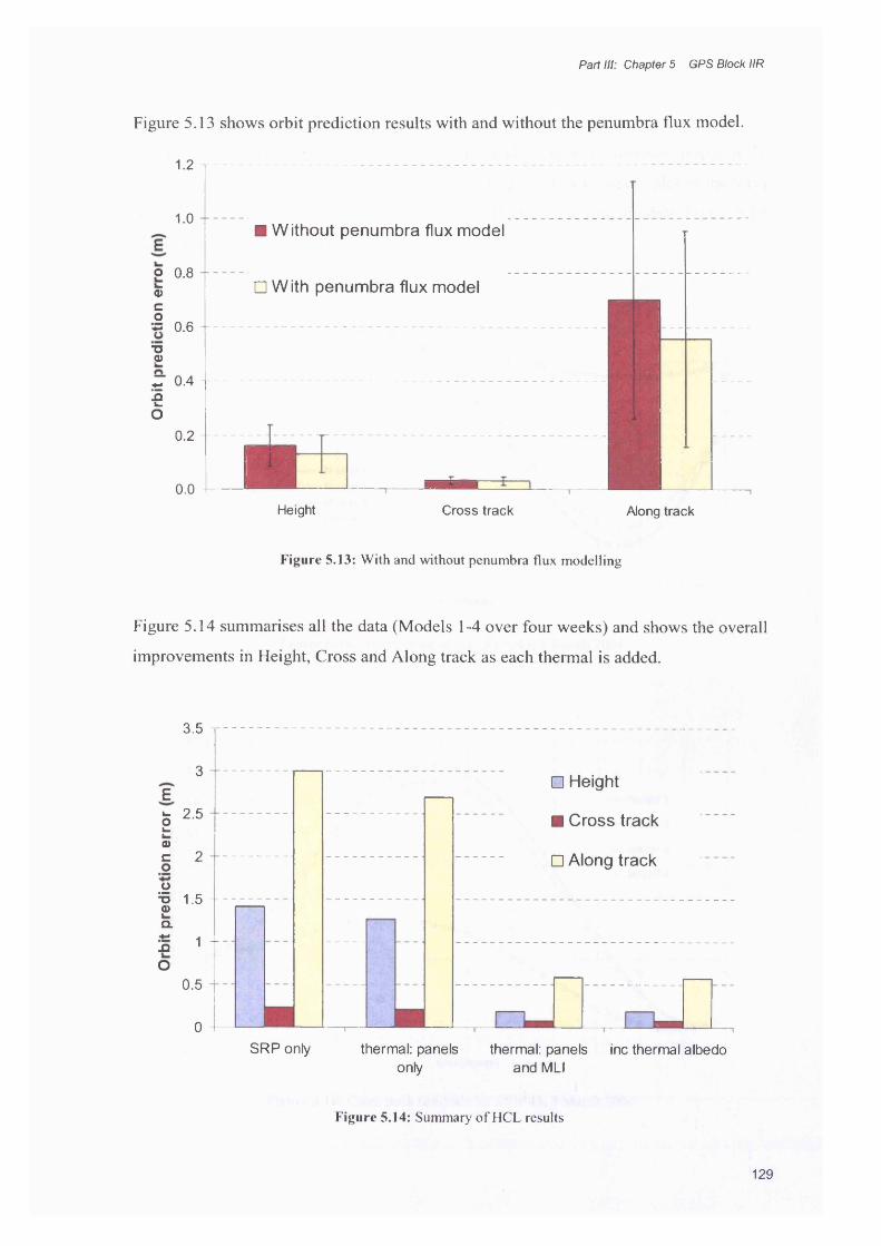
Part III: Chapter 5 GPS Block IIR
Figure 5.13 shows orbit prediction results with and without the penumbra flux model.
1.2
1.0
o 0.8<5co« 0.6 -1■op
Z 0.42co
0.2
0.0
■ W ithout penumbra flux model
□ W ith penumbra flux model
Height Cross track Along track
Figure 5.13: With and without penumbra flux modelling
Figure 5.14 summarises all the data (Models 1-4 over four weeks) and shows the overall
improvements in Height, Cross and Along track as each thermal is added.
3.5 t
3EL_ok_a
2.5
<Uco 2
oBo 1.5 -Q.+-< 1 -Ao
0.5
0
□ Height
■ Cross track
□ Along track
SRP only thermal: panels thermal: panels inc thermal albedo only and MLI
Figure 5.14: Summary of HCL results
129

Part III: Chapter 5 GPS Block IIR
Figures 5.15-5.17 show the Height, Cross track and Along track residuals respectively
for Models 1 - 4 over one 12 hour orbit. These are given to show examples of the form
of these errors over 12 hours, and how they are affected by adding models. Figure 5.18
shows an example of final HCL residuals.
0.5 -
E
-0.5ot0)co2IIo
— Mode l 1 — m - M odel 2 —*— M odel 3
♦ M odel 4
-1.5 -
-2 -
-2.5 -
Time (hours)
Figure 5.15: Height residuals for SVN 43, 3 March 2004
0.7
0.6
- V Model 10.5 -
Model 2
M odel 3° 0.3 ® c® 0 9
Model 4
oTJ1 --- 1an4-O
-0.1
-0.2
-0.3Time (hours)
Figure 5.16: Cross track residuals for SVN 43, 3 March 2004
130

Part III: Chapter 5 GPS Block HR
10 i
Model 1
Model 2
Model 3
Model 4
I-2 -
Time (hours)
Figure 5.17: Along track residuals for SVN 43, 3 March 2004
0.8Height Cross Track Along Track
£ 0.6i_Ok .
0.4
w 0.2c•2 n
■o0)k _
- 0.2CL
-0.4
o -0.6
- 0.8
Time (hours)
Figure 5.18: Orbit Prediction HCL residuals for SVN 44, 21st March 2004
131

Part III: Chapter 5 GPS Block HR
5.6 Analysis and interpretation of results
5.6.1 Testing method 1: Comparison with telemetry
Figure 5.7 clearly shows the difference in temperature between aphelion and perihelion
for both the telemetered temperatures and the modelled temperatures. In general the
telemetered temperatures are much higher than the modelled temperatures. These
discrepancies are analysed in Section 7.1.3 when the issue of power draw is discussed.
For SVN 43, the temperatures are higher than those predicted by the model by about
3K, but the temperature differences between aphelion and perihelion are much closer.
Data telemetered from the other Block HR satellites show this offset also. The forces
derived from the telemetered data are higher than those modelled by -12%, resulting in10 2an acceleration error of -1 x 10' ms" . This amounts to a maximum along track error of
-2 cm over 12 hours.
5.6.2 Testing method 2: Comparisons with other methodsThe solar panel temperatures obtained through ESATAN which uses a finite element
method give very good agreement with the model temperatures; the results are the same
to within 0.02K. This provides some validation of the modelling technique used here.
Vigue (1994) carried out a calculation based on the finite element method for GPS
Block IIA panels, which were different to the Block HR panels. Using these models, the
same temperatures were produced. Fliegel (1996) calculated GPS Block HR panel
temperatures based on the same data set though details of his methods were not
explicitly given. Again, the same temperatures were produced with these models.
5.6.3 Testing method 3: Orbit predictionThe improvements in orbit prediction using the thermal models are clear. Tables 5.7, 5.8
and 5.9 show how the average RMS along track error for a 12 hour orbit drops from
2.997m to 2.691m to 0.586m as first the solar panel thermal model is added, then the
MLI model is added. The MLI is by far the largest contributor to the overall force.
Figures 5.15, 5.16 and 5.17 show an example of how this error is consistently decreased
over a 12 hour orbit in all three axes. Inclusion of the penumbra flux model also yields
132

Part III: Chapter 5 GPS Block HR
significant improvements with the average along-tack acceleration over 28 orbits for
SVN 44 dropping from 0.70m to 0.56m (shown in Figure 5.13).
Figure 5.18 shows an example of the HCL orbit residuals over 12 hours. These are
much smaller than previously attained using purely analytical models. By way of
comparison orbit prediction errors published in Fliegel (1996) were estimated to be at
the 3-4m level over a similar arc length. These results are analysed further in Chapter 7.
SummaryThis chapter presents an overview of the GPS system. The attitude, power draw,
structure and surface properties of the GPS Block HR spacecraft are specified and
model computation is described. The main tests of the complete model were the
comparison of numerically integrated predicted orbits with precise orbits. Four weeks
worth of 12 hour orbits were predicted and residuals with respect to the precise orbit
were calculated. Results showed that the addition of each successive model reduced the
size of the residuals and that the largest impact was due to the modelling of the MLI.
These results are analysed and discussed in more detail in Chapter 7 and 8. In Chapter 6,
the methods are implemented for Jason-1 and tested in orbit determination.
133

Part III: Chapter 6 Jason-1
Chapter 6 Jason-1
Chapter outline
This chapter provides a brief overview of the objectives of the Jason-1 mission. The
spacecraft structure is described and the data used in the modelling process are given.
The implementation of this data is outlined for the SRP and TRR models of the
spacecraft bus and panels. Testing methods are explained and the results of these tests
are shown. This is followed by a brief analysis and discussion of the results. A more
detailed analysis of the results will follow in Chapter 7.
6.1 Mission overview
Jason-1 is an ocean altimetry satellite developed jointly by the French Space Agency,
CNES, and NASA. It was launched into a near circular orbit, with an inclination of 66°
and approximate altitude of 1335 km in December 2001. It has an orbit period of 112
minutes and a ground track repeat period of approximately 10 days. Jason-1 follows on
from the TOPEX/Poseidon mission launched in 1992 (Fu, I. & Cazenave, A., 2000) and
its main roles are to monitor global ocean circulation, study interactions of the oceans
and atmosphere, improve climate predictions and observe events such as El Nino.
Jason-1 uses a radar altimeter instrument to measure ranges to the sea surface. The
altimeter is a nadir-pointing instrument, which emits microwave signals. The time delay
between the transmission of this signal and the reception of the reflected signal from the
surface is measured and signal time-of-flight calculations are carried out to solve for the
range between the spacecraft and surface. Figure 6.1 shows the Jason-1 measurement
system.
134

Part III: Chapter 6 Jason-1
G P Ssa te lli te
Orbit
DORIS SLRbeacon station
AH
Figure 6.1: Jason-1 measurement system
The height of mean sea-surface above the geoid" is known as sea surface topography
(SST), labelled H in Figure 6.1. It is caused by the quasi-stationary part of the dynamic
topography which refers to large scale mean circulation in the oceans (caused by the
earth’s rotation, regional differences atmospheric pressure and salinity etc.). The
instantaneous sea surface differs from the mean sea surface, by AH, and this is due to a
time-variant component of the dynamic topography, caused by ocean tides, variations in
local atmospheric pressures (the inverse barometric effect) and other smaller scale
dynamic features such as ocean eddies. Depending on the desired quantity to be inferred
form the altimetry measurements (e.g. H or AH), different models are required; these
may be related to aspects of the stationary and time varying topography, the geoid or
atmospheric influences which affect the measured range. The spacecraft position at the
measurement epoch is also required and this is determined from the estimated orbit of
Jason-1. Orbital errors are a source of systematic error in the determination of mean sea-
surface heights and the accuracy with which they can be determined depends in part on
11 Geoid models are estimates of the equi-potential surface which coincides with where the sea-surface
level would be in the absence of all wind, circulation and tides.
135

Part III: Chapter 6 Jason-1
the quality of the estimated orbits (Scharroo, R., 2002). The ability to quantify the errors
in the orbits allows the realistic estimation of the accuracy of target geophysical
parameters.
In 2002, the Jason-1 science working team set a goal to drive the radial precision of
post-processed orbits below the 1cm level (Haines, B. et al., 2004). The force modelling
work undertaken here was aimed at helping to achieve this goal.
6.2 Satellite description and data sources
The Jason-1 spacecraft supports three advanced satellite tracking systems:
• GPS (see Section 6.1)
• Doppler Orbitography and Radiopositioning Integrated by Satellite (DORIS)
(developed by CNES)
• Satellite laser ranging (SLR)
Data from these systems can be used separately or in combination to calculate
the orbit of Jason-1.
Jason-1 is constructed around a central bus measuring approximately 0.96m x 0.96m x
2.25m. Power is supplied by solar panels arrays attached to the ± Y faces of the
spacecraft; each array consists of four panels, each 1.49m x 0.8m. These arrays rotate
about yokes aligned parallel to the spacecraft Y-axis and the +Y and -Y panel arrays
can be steered by the solar array drive mechanism (SADM) independently of each other
(see Figure 6.2).
The science payload is clustered around the upper half of the bus. These instruments
include the Jason Microwave Radiometer (JMR), two turbo-rogue GPS Space receivers
(TSRs), a laser retro-reflector array (LRA), a dual frequency DORIS antenna and the
satellite altimeter dish and associated structures. Apart from the surfaces of the JMR,
altimeter dishes and a number of thermal control radiators, the majority of the bus is
covered in multilayer insulation. A pair of star sensors is mounted on the -Z face of the
bus.
136
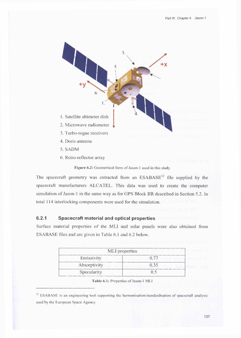
Part III: Chapter 6 Jason-1
1. Satellite altimeter dish
2. Microwave radiometer
3. Turbo-rogue receivers
4. Doris antenna
5. SADM
6. Retro-reflector array
Figure 6.2: Geometrical form of Jason-1 used in this study
The spacecraft geometry was extracted from an ESABASE12 file supplied by the
spacecraft manufacturers ALCATEL. This data was used to create the computer
simulation of Jason-1 in the same way as for GPS Block HR described in Section 5.2. In
total 114 interlocking components were used for the simulation.
6.2.1 Spacecraft material and optical properties
Surface material properties of the MLI and solar panels were also obtained from
ESABASE files and are given in Table 6.1 and 6.2 below.
MLI propertiesEmissivity 0.77
Absorptivity 0.35Specularity 0.5
Table 6.1: Properties of Jason-1 MLI
12 ESABASE is an engineering tool supporting the harmonisation/standardisation of spacecraft analysis
used by the European Space Agency
137

Part III: Chapter 6 Jason-1
Solar panel propertiesFront emissivity 0.82Back emissivity 0.82
Thickness 0.018 mAbsorptivity (front) 0.75
Specularity 0.85Total panel area 9.536 mi
Table 6.2: Jason-1 solar panel properties
A value for the thermal coupling between the front and back faces of 61 W K 'W 2 was
supplied by J. Perbos of CNES (pers comms, July, 2002). No information was available
regarding the material properties of the individual layers of the panel. The thermal
coupling parameter describes the effective conductivity per unit length through the
panel.
The power draw regime for the JASON panels was also provided by J. Perbos and is as
follows:
“The power draw from the panels depends on whether the power sections
located on the panels are On or Off. The nearest panel with respect to the
spacecraft body is always On as well as one fourth of the surface of the
furthest panel from the body. The other power sections may be On or Off
depending on the power needs along the orbit. When the power section is
On, the power draw is typically 150 Wm' (the cells efficiency is 12%).”
This information is not specific enough to define accurately the power draw at any time.
If it is assumed that the power draw from the inner and quarter of the outer panels is
distributed over all the panels, a simple calculation yields a minimum power draw of 47
Wm"2. This assumption will result in some inaccuracies; their magnitudes and
implications are discussed in Chapter 7.
138
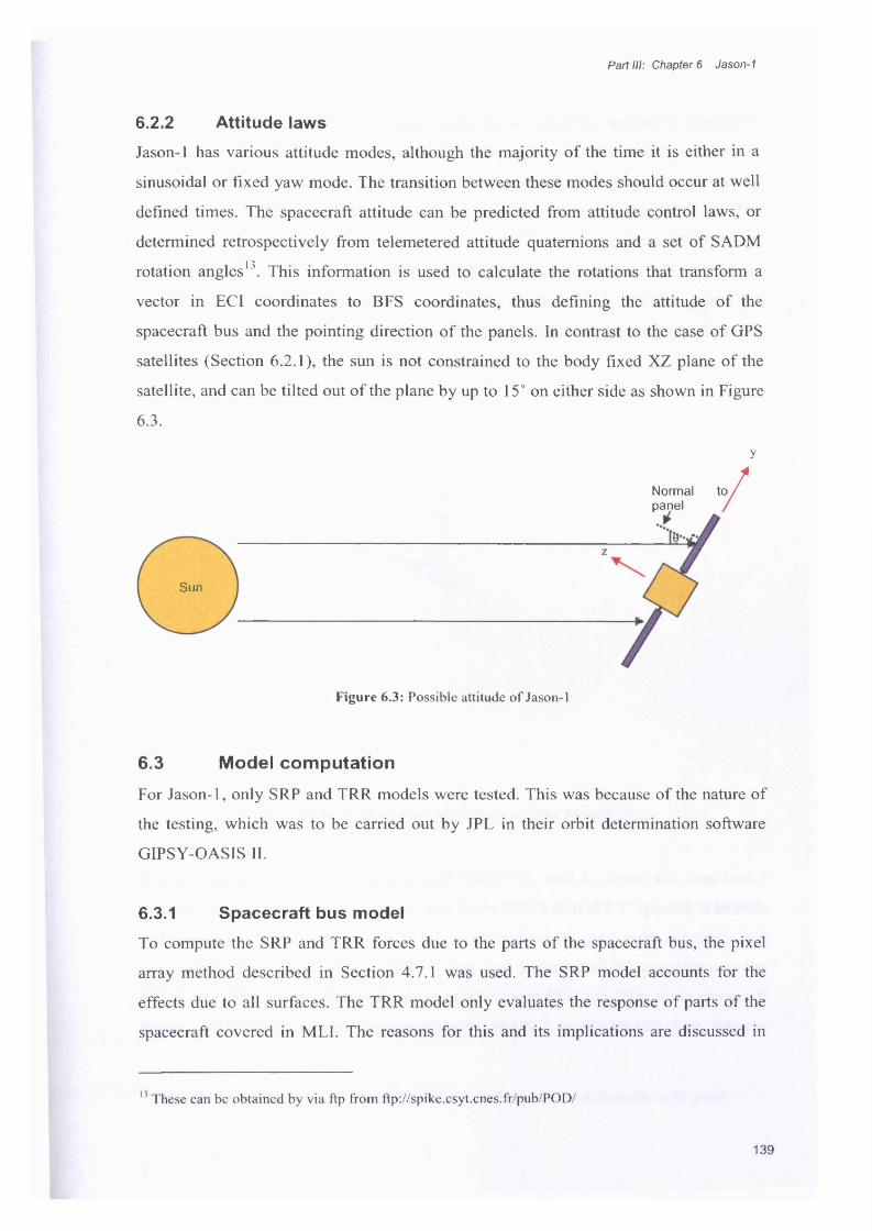
Part III: Chapter 6 Jason-1
6.2.2 Attitude laws
Jason-1 has various attitude modes, although the majority of the time it is either in a
sinusoidal or fixed yaw mode. The transition between these modes should occur at well
defined times. The spacecraft attitude can be predicted from attitude control laws, or
determined retrospectively from telemetered attitude quaternions and a set of SADM
rotation angles13. This information is used to calculate the rotations that transform a
vector in ECI coordinates to BFS coordinates, thus defining the attitude of the
spacecraft bus and the pointing direction of the panels. In contrast to the case of GPS
satellites (Section 6.2.1), the sun is not constrained to the body fixed XZ plane of the
satellite, and can be tilted out of the plane by up to 15° on either side as shown in Figure
6.3.
y
/Normal to /panel
Sun
Figure 6.3: Possible attitude of Jason-1
6.3 Model computation
For Jason-1, only SRP and TRR models were tested. This was because of the nature of
the testing, which was to be carried out by JPL in their orbit determination software
GIPSY-OASIS II.
6.3.1 Spacecraft bus model
To compute the SRP and TRR forces due to the parts of the spacecraft bus, the pixel
array method described in Section 4.7.1 was used. The SRP model accounts for the
effects due to all surfaces. The TRR model only evaluates the response of parts of the
spacecraft covered in MLI. The reasons for this and its implications are discussed in
13 These can be obtained by via ftp from ftp://spike.csyt.cnes.fr/pub/POD/
139
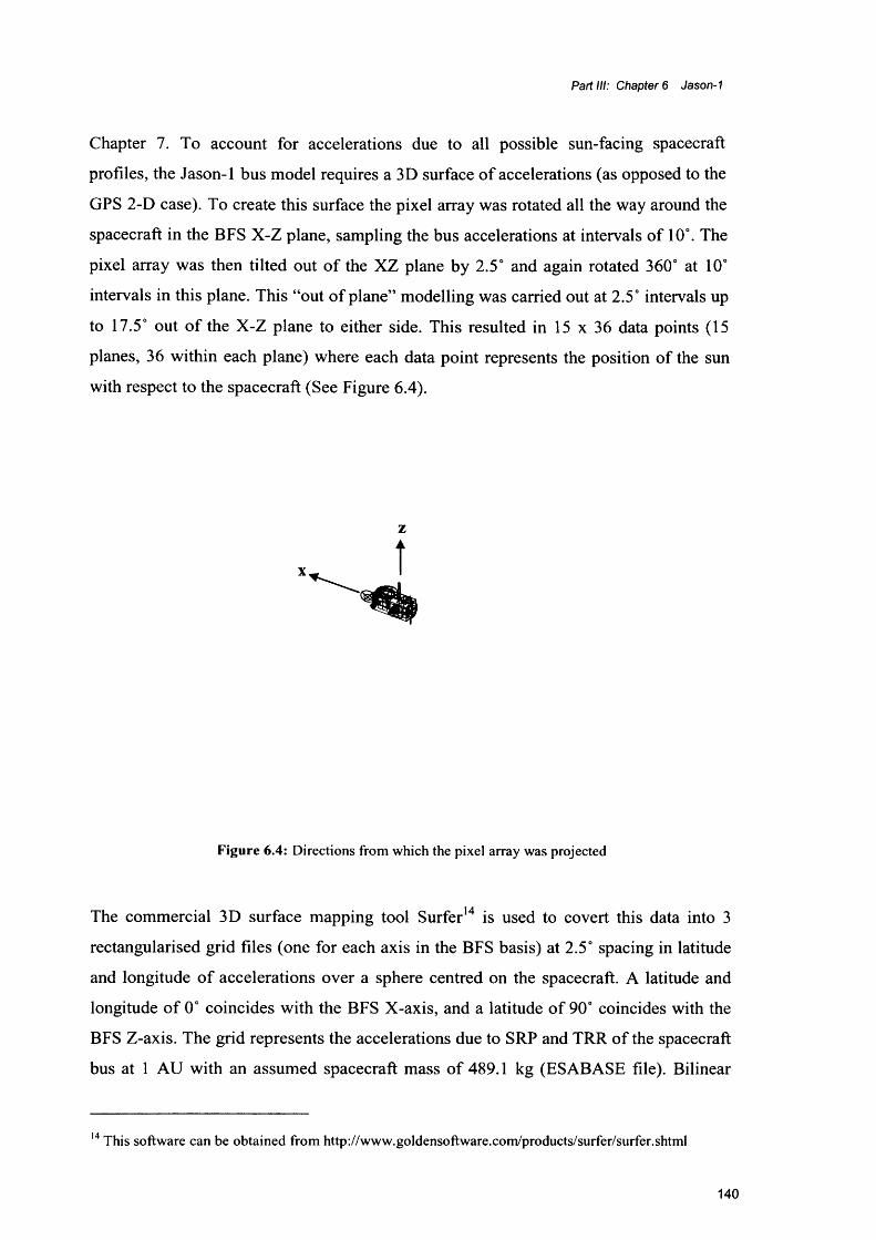
Part III: Chapter 6 Jason-1
Chapter 7. To account for accelerations due to all possible sun-facing spacecraft
profiles, the Jason-1 bus model requires a 3D surface of accelerations (as opposed to the
GPS 2-D case). To create this surface the pixel array was rotated all the way around the
spacecraft in the BFS X-Z plane, sampling the bus accelerations at intervals of 10°. The
pixel array was then tilted out of the XZ plane by 2.5° and again rotated 360° at 10°
intervals in this plane. This “out of plane” modelling was carried out at 2.5° intervals up
to 17.5° out of the X-Z plane to either side. This resulted in 15 x 36 data points (15
planes, 36 within each plane) where each data point represents the position of the sun
with respect to the spacecraft (See Figure 6.4).
Figure 6.4: Directions from which the pixel array was projected
The commercial 3D surface mapping tool Surfer14 is used to covert this data into 3
rectangularised grid files (one for each axis in the BFS basis) at 2.5° spacing in latitude
and longitude of accelerations over a sphere centred on the spacecraft. A latitude and
longitude of 0° coincides with the BFS X-axis, and a latitude of 90° coincides with the
BFS Z-axis. The grid represents the accelerations due to SRP and TRR of the spacecraft
bus at 1 AU with an assumed spacecraft mass of 489.1 kg (ESABASE file). Bilinear
14 This software can be obtained from http://www.goldensoftware.com/products/surfer/surfer.shtml
140
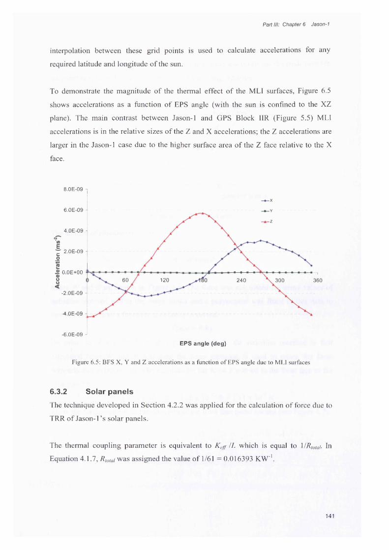
Part III: Chapter 6 Jason-1
interpolation between these grid points is used to calculate accelerations for any
required latitude and longitude of the sun.
To demonstrate the magnitude o f the thermal effect o f the MLI surfaces, Figure 6.5
shows accelerations as a function o f EPS angle (with the sun is confined to the XZ
plane). The main contrast between Jason-1 and GPS Block HR (Figure 5.5) MLI
accelerations is in the relative sizes o f the Z and X accelerations; the Z accelerations are
larger in the Jason-1 case due to the higher surface area o f the Z face relative to the X
face.
8.0E-09
6.0E-09
4.0E-09
r 2.0E-09
® 0.0E+0060 120 240 300 360
-2.0E-09
-4.0E-09
-6.0E-09EPS angle (deg)
Figure 6.5: BFS X, Y and Z accelerations as a function of EPS angle due to MLI surfaces
6.3.2 Solar panels
The technique developed in Section 4.2.2 was applied for the calculation o f force due to
TRR of Jason-1 ’s solar panels.
The thermal coupling parameter is equivalent to Keg /L which is equal to 1 /Rtotai. In
Equation 4.1.7, R totai was assigned the value o f 1/61 = 0.016393 KW '1.
141
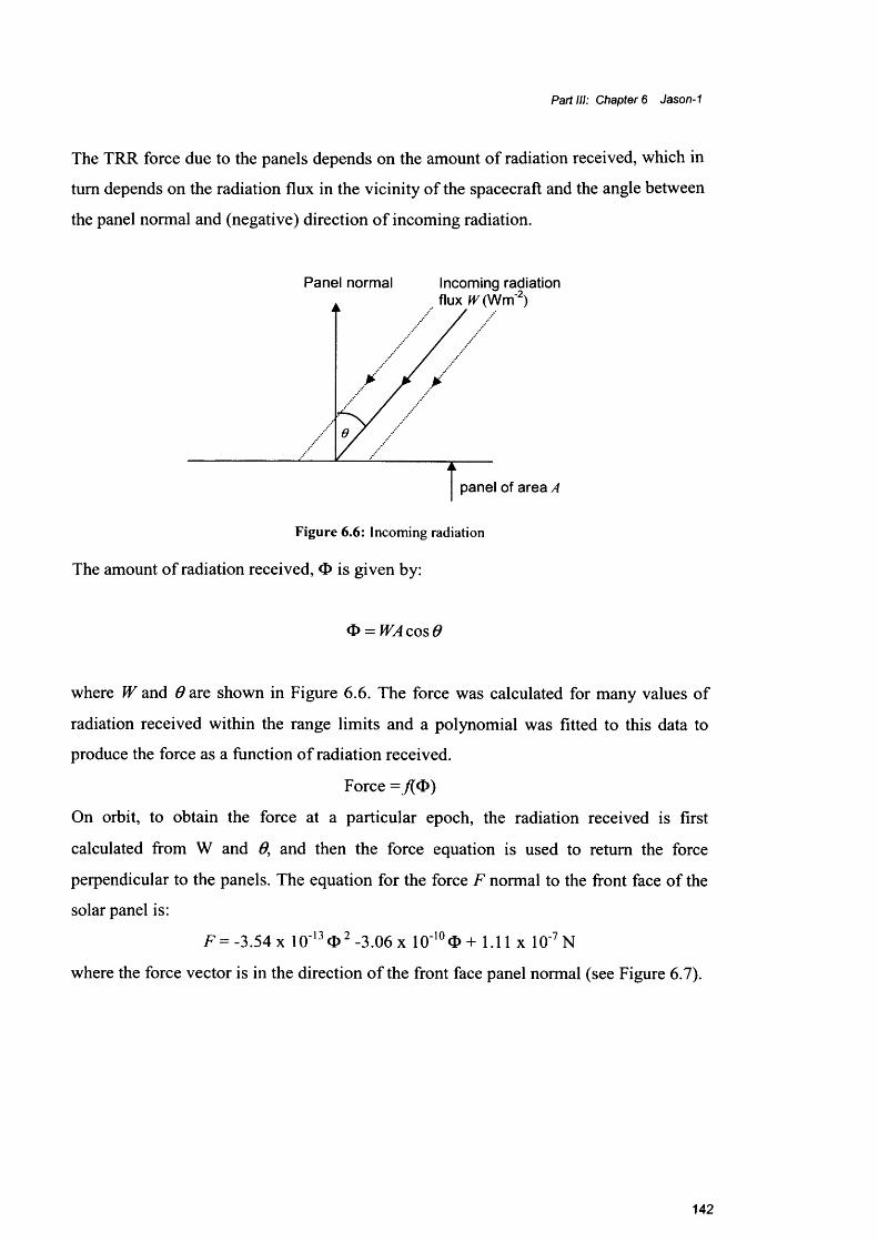
Part III: Chapter 6 Jason-1
The TRR force due to the panels depends on the amount of radiation received, which in
turn depends on the radiation flux in the vicinity of the spacecraft and the angle between
the panel normal and (negative) direction of incoming radiation.
Panel normal Incoming radiation flux W (Wm'2)
panel of area A
Figure 6.6: Incoming radiation
The amount of radiation received, O is given by:
O = WA cos 6
where W and 0 are shown in Figure 6.6. The force was calculated for many values of
radiation received within the range limits and a polynomial was fitted to this data to
produce the force as a function of radiation received.
Force =/(<[>)
On orbit, to obtain the force at a particular epoch, the radiation received is first
calculated from W and 0, and then the force equation is used to return the force
perpendicular to the panels. The equation for the force F normal to the front face of the
solar panel is:
F - -3.54 x lO"13® 2 -3.06 x 10'lo® + 1.11 x 10'7N
where the force vector is in the direction of the front face panel normal (see Figure 6.7).
142
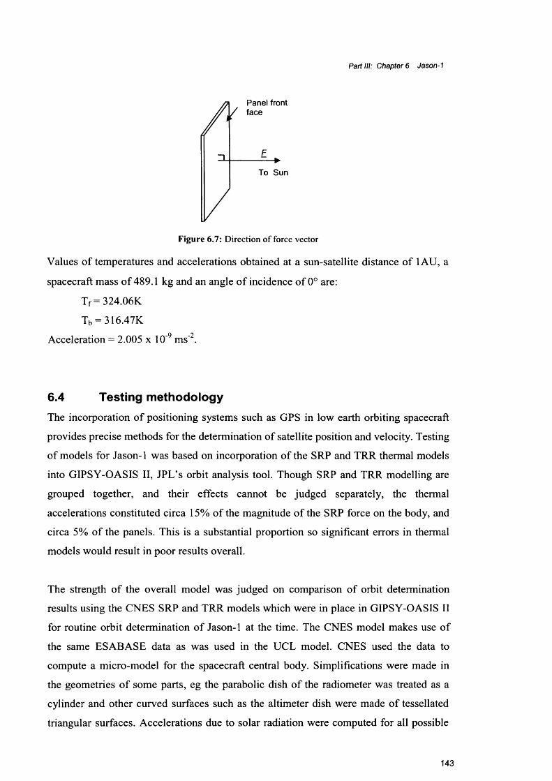
Part III: Chapter 6 Jason-1
Panel front face
To Sun
Figure 6.7: Direction of force vector
Values of temperatures and accelerations obtained at a sun-satellite distance of 1AU, a
spacecraft mass of 489.1 kg and an angle of incidence of 0° are:
Tf = 324.06K
Tb = 316.47K
Acceleration = 2.005 x 10'9 ms'2.
6.4 Testing methodology
The incorporation of positioning systems such as GPS in low earth orbiting spacecraft
provides precise methods for the determination of satellite position and velocity. Testing
of models for Jason-1 was based on incorporation of the SRP and TRR thermal models
into GIPSY-OASIS II, JPL’s orbit analysis tool. Though SRP and TRR modelling are
grouped together, and their effects cannot be judged separately, the thermal
accelerations constituted circa 15% of the magnitude of the SRP force on the body, and
circa 5% of the panels. This is a substantial proportion so significant errors in thermal
models would result in poor results overall.
The strength of the overall model was judged on comparison of orbit determination
results using the CNES SRP and TRR models which were in place in GIPSY-OASIS II
for routine orbit determination of Jason-1 at the time. The CNES model makes use of
the same ESABASE data as was used in the UCL model. CNES used the data to
compute a micro-model for the spacecraft central body. Simplifications were made in
the geometries of some parts, eg the parabolic dish of the radiometer was treated as a
cylinder and other curved surfaces such as the altimeter dish were made of tessellated
triangular surfaces. Accelerations due to solar radiation were computed for all possible
143

Part III: Chapter 6 Jason-1
incoming light directions using this model. A simplified 6-face box model was then
optimally adjusted to reproduce these accelerations as accurately as possible. The
optical properties and component areas which they represented were then estimated in a
least squares sense to generate the same response of the spacecraft. The assumption
inherent in this approach is that the empirically estimated parameters will soak up all the
mis-modelled effects, which are inevitable due to the box and wing simplification
(Ferrier, C. et al., 2002).
6.4.1 Orbit determinationA conceptual overview of the orbit determination (OD) process is presented here; for
more detail the reader is referred to Tapley et al. (2004).
The goal in orbit estimation is to determine the satellite orbit that best fits a set of
tracking data, whilst at the same time satisfying a set of differential equations specifying
the system dynamics. Tracking data or "observation" data include any observable
quantities that are a function of the position and/or velocity of a satellite at a point in
time. These include range, range rate, azimuth and elevation from ground stations of
known location, or ranges from other satellites such as GPS range observations. In the
testing of the force models carried out here for Jason-1 orbits, only GPS observables are
used as tracking data.
The GPS observations would represent the true state of the spacecraft if there were no
noise or biases in the measurement systems and all factors affecting the measurements,
such as signal delays due to atmospheric water vapour, were perfectly modelled. As this
is never the case, there is always some discrepancy between the observations and the
real state of the satellite. The aim in OD is to best estimate the parameters which
influence observations, so that these parameters can then be used to re-produce an orbit
which best fits the tracking data. Theoretically, any parameter which influences the
tracking data either directly or indirectly can be estimated. Such parameters include
satellite positions and velocities, tracking data biases, atmospheric drag parameters,
solar radiation pressure parameters, and coefficients of the Earth's gravitational field.
Once the parameters have been estimated, they are used to compute a set of
measurements which are intended to reproduce the observations - Q.
144
Part III: Chapter 6 Jason-1
To compute C j , an estimate of an initial state vector15 is made. Integration of the orbit
using the dynamic models (e.g. gravity field models, non-conservative force models),
and application of measurement models (e.g. models of system noise) and models of the
environmental factors affecting the measurements, are used to model the observations at
the next measurement epoch. The model parameters are adjusted to minimise the
residuals between the observed and computed observations using the observation
equiation:
[Ai][xi]=[bi]
where Xj is a vector containing corrections to the initial estimates for the parameters
used to compute the observations, Aj is the design matrix; it contains the partial
differentials of the observations with respect to the model parameters and bj is a vector
containing the observed minus computed measurements [ O j - C j ] (these are the
computed residuals). When the model parameters have been optimised, the resulting
spacecraft trajectory should be consistent with the physics of the mathematical model
and the series of observations that are used to constrain the orbit. Figure 6.8 is a flow
chart of the process.
15 state vector here refers to the complete set of parameters that will be estimated
145

Part III: Chapter 6 Jason-1
iterations
Subsequentorbit
estimations
Com pute residuals Tracking data
C heck for convergence
Initial s ta te vector estim ate
Estim ate new s ta te by minimising residuals
Improved estim ate of s ta te vector (& a priori for
next iteration)
Com pute model observations from force
and m easurem ent m odels
Figure 6.8: Flow chart of orbit determination process
It is critical for a successful estimation that the observations are well modelled, as poor
models may result in large residuals which cannot be sufficiently minimised. The orbit
determination software used here was GIPSY-OASIS II. A comprehensive description
of this software and its usage can be found in a manual by Gregorius (1996). Points to
note are that this software uses a sequential filter algorithm called a square root
information filter (SRIF). SRIF is described in this manual as “a multi-satellite-batch-
sequential-pseudo-epoch-state-process-noise-filter”. It is, more basically, a modified
Kalman filter. A Kalman filter is a least-squares process which uses the state vector
from a previous epoch as the starting point for the next epoch. This avoids the need to
invert large matrices by inverting lots of small matrices that are created sequentially for
each time interval or “batch”. SRIF differs from a Kalman filter in that it makes use of
the square root of the covariance matrix, which is done to ensure a more numerically
stable system of equations.
146

Part III: Chapter 6 Jason-1
Within statistical orbit estimation, there are three different approaches for solving for
the precise orbit, namely the dynamic, reduced dynamic and kinematic approaches.
These are described below.
6.4.1.1 Dynamic strategyIn a dynamic orbit computation, the trajectory of a spacecraft is evaluated based on the a
priori force model. This method is used when limited tracking data is available. Errors
in the force model can be corrected for if some tracking data exists, through the
estimation of a limited number of scale factors and once per revolution empirical terms.
Analysis of the measurement residuals may tell us which element of the model is in
error. This method is useful when models of the forces are required as end-products, for
example in gravity field measurement satellites such as GRACE.
6.4.1.2 Reduced dynamic strategyIn this case a more accurate orbit can be computed by a greater emphasis on the
observations than on the force model. This technique relies on the availability of large
amounts of tracking data which are required to solve for the extended state vector which
includes empirical accelerations to account for the errors in the force model.
6.4.1.3 Kinematic strategyThe kinematic strategy dispenses entirely with precise models of the forces underlying
the satellite motion, relying instead on the geometric diversity, continuity, and precision
of the GPS tracking measurements. Svehla and Rothacher (2003) have demonstrated
orbit accuracies of 1-3 cm for the gravity gradiometry mission CHAMP using a purely
kinematic (geometrical) approach to precise orbit determination. The kinematic
approach, however, is highly sensitive to aberrations in the GPS viewing geometry. If
the receiver loses lock or resets, which happens at least once per orbit (Haines, B. et al.,
2002), there are no orbit solutions spanning the gap till lock is regained.
6.5 Testing methods: Comparison of orbit quality
Testing of the SRP and TRR models was carried out by the Earth Orbiter and
Radiometric Systems Group at JPL using GIPSY-OASIS II. Generally smaller residuals
imply more precise orbits. This does not necessarily mean more accurate orbits though,
147
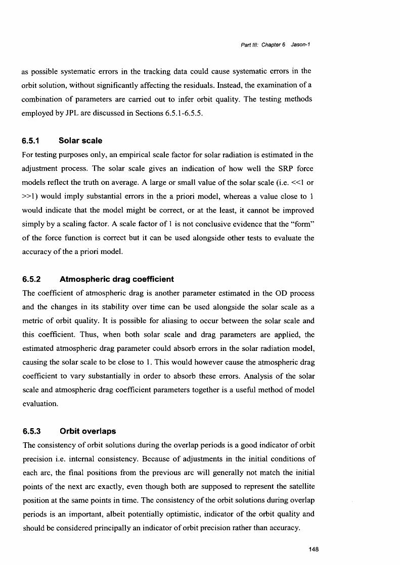
Part III: Chapter 6 Jason-1
as possible systematic errors in the tracking data could cause systematic errors in the
orbit solution, without significantly affecting the residuals. Instead, the examination of a
combination of parameters are carried out to infer orbit quality. The testing methods
employed by JPL are discussed in Sections 6.5.1-6.5.5.
6.5.1 Solar scaleFor testing purposes only, an empirical scale factor for solar radiation is estimated in the
adjustment process. The solar scale gives an indication of how well the SRP force
models reflect the truth on average. A large or small value of the solar scale (i.e. « 1 or
» 1 ) would imply substantial errors in the a priori model, whereas a value close to 1
would indicate that the model might be correct, or at the least, it cannot be improved
simply by a scaling factor. A scale factor of 1 is not conclusive evidence that the “form”
of the force function is correct but it can be used alongside other tests to evaluate the
accuracy of the a priori model.
6.5.2 Atmospheric drag coefficientThe coefficient of atmospheric drag is another parameter estimated in the OD process
and the changes in its stability over time can be used alongside the solar scale as a
metric of orbit quality. It is possible for aliasing to occur between the solar scale and
this coefficient. Thus, when both solar scale and drag parameters are applied, the
estimated atmospheric drag parameter could absorb errors in the solar radiation model,
causing the solar scale to be close to 1. This would however cause the atmospheric drag
coefficient to vary substantially in order to absorb these errors. Analysis of the solar
scale and atmospheric drag coefficient parameters together is a useful method of model
evaluation.
6.5.3 Orbit overlapsThe consistency of orbit solutions during the overlap periods is a good indicator of orbit
precision i.e. internal consistency. Because of adjustments in the initial conditions of
each arc, the final positions from the previous arc will generally not match the initial
points of the next arc exactly, even though both are supposed to represent the satellite
position at the same points in time. The consistency of the orbit solutions during overlap
periods is an important, albeit potentially optimistic, indicator of the orbit quality and
should be considered principally an indicator of orbit precision rather than accuracy.
148
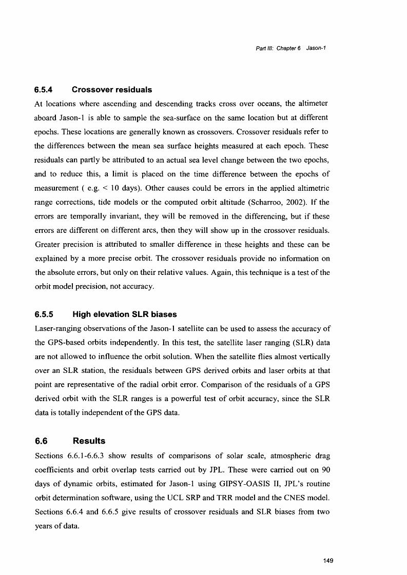
Part III: Chapter 6 Jason-1
6.5.4 Crossover residualsAt locations where ascending and descending tracks cross over oceans, the altimeter
aboard Jason-1 is able to sample the sea-surface on the same location but at different
epochs. These locations are generally known as crossovers. Crossover residuals refer to
the differences between the mean sea surface heights measured at each epoch. These
residuals can partly be attributed to an actual sea level change between the two epochs,
and to reduce this, a limit is placed on the time difference between the epochs of
measurement ( e.g. < 10 days). Other causes could be errors in the applied altimetric
range corrections, tide models or the computed orbit altitude (Scharroo, 2002). If the
errors are temporally invariant, they will be removed in the differencing, but if these
errors are different on different arcs, then they will show up in the crossover residuals.
Greater precision is attributed to smaller difference in these heights and these can be
explained by a more precise orbit. The crossover residuals provide no information on
the absolute errors, but only on their relative values. Again, this technique is a test of the
orbit model precision, not accuracy.
6.5.5 High elevation SLR biasesLaser-ranging observations of the Jason-1 satellite can be used to assess the accuracy of
the GPS-based orbits independently. In this test, the satellite laser ranging (SLR) data
are not allowed to influence the orbit solution. When the satellite flies almost vertically
over an SLR station, the residuals between GPS derived orbits and laser orbits at that
point are representative of the radial orbit error. Comparison of the residuals of a GPS
derived orbit with the SLR ranges is a powerful test of orbit accuracy, since the SLR
data is totally independent of the GPS data.
6.6 Results
Sections 6.6.1-6.6.3 show results of comparisons of solar scale, atmospheric drag
coefficients and orbit overlap tests carried out by JPL. These were carried out on 90
days of dynamic orbits, estimated for Jason-1 using GIPSY-OASIS II, JPL’s routine
orbit determination software, using the UCL SRP and TRR model and the CNES model.
Sections 6.6.4 and 6.6.5 give results of crossover residuals and SLR biases from two
years of data.
149
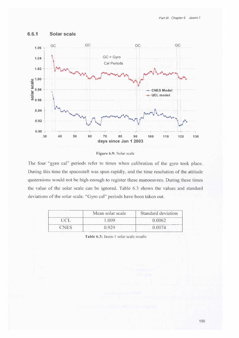
Part III: Chapter 6 Jason-1
6.6.1 Solar scale
GC GCGCGC1.06 T
GC — Gyro
Cal Periods1.04
1.02
0> 1.00 -
0.98 - CNES Model ~ UCL model
w 0.96 -
0.94
0.92
0.9040 50 60 7030 80 90 100 110 130120
d a y s s in c e J a n 1 2003
Figure 6.9: Solar scale
The four “gyro cal” periods refer to times when calibration o f the gyro took place.
During this time the spacecraft was spun rapidly, and the time resolution o f the attitude
quaternions would not be high enough to register these manoeuvres. During these times
the value o f the solar scale can be ignored. Table 6.3 shows the values and standard
deviations o f the solar scale. “Gyro cal” periods have been taken out.
Mean solar scale Standard deviationUCL 1.009 0.0062
CNES 0.929 0.0074
Table 6.3: Jason-l solar scale results
150

Part III: Chapter 6 Jason-1
6.6.2 Atmospheric drag coefficient
5.0
4.5 -CNES Model UCL Model4.0 -
O) 3.0 -
TJ2.5
Y aw regim e changes
2.0
1.540 50 60 7030 80 90 100 110 130120
days since Jan 1 2003
Figure 6.10: Linear interpolation of daily atmospheric drag coefficients
6.6.3 Orbit overlaps
Figure 6.11 shows difference in mm in orbit overlap residuals (UCL - CNES). A
negative value implies better performance by the UCL model. The periods marked as
yaw regime changes are valid and significant.
150 -.
100 -
50 -
30 50 70 10090 110 120 130-50
O -1 0 0 - co0) -150
Yaw regim e - changes
o -2 0 0 -
T3
-250 -
-300 J
d ay s in c e J a n 1 2003
Figure 6.11: (UCL-CNES) orbit overlap residuals
151

Part III: Chapter 6 Jason-1
6.6.4 Crossover residualsIn this comparison, data was taken from 74 cycles, where each cycle is one 10 day
ground track repeat period for Jason-1. Tests were carried out on both dynamic and
reduced dynamic orbits. The average (A) and variance (B) of the crossover residuals
within each cycle were calculated; then mean and standard deviations of A and B were
calculated over the 74 cycles. The results are given in Table 6.4. Figures 6.12 - 6.15
show bar charts of this data. Table 6.5 contains similar data to Table 6.4, but all
crossovers that occurred over the course of the 74 cycles are included (both inter-cycle
crossovers as well as those occurring within one cycle) leading to a larger sample. All
crossover data has been “super-edited” to remove observations collected during extreme
wind/wave conditions and only crossovers occurring at epochs within three days are
considered in order to mitigate the effects of actual changes in mean sea surface heights
occurring (Scharroo, R., 2002). In these data, smaller values for means and standard
deviations indicate more consistent orbits.
Mean A (mm) Variances B (mm2)Average of A Std. Dev of A Average of B Std. dev of B
CNES Model Dynamic 1.05 7.17 2263.13 395.87UCL Model Dynamic 0.94 7.05 2254.35 375.20CNES Model Reduced 0.90 5.39 2105.89 232.26UCL Model Reduced 0.91 5.09 2104.06 230.74T ab le 6.4: Crossover residuals for Jason-1: Average and standard deviation over all 74 cycles of mean
and variance per cycle
152
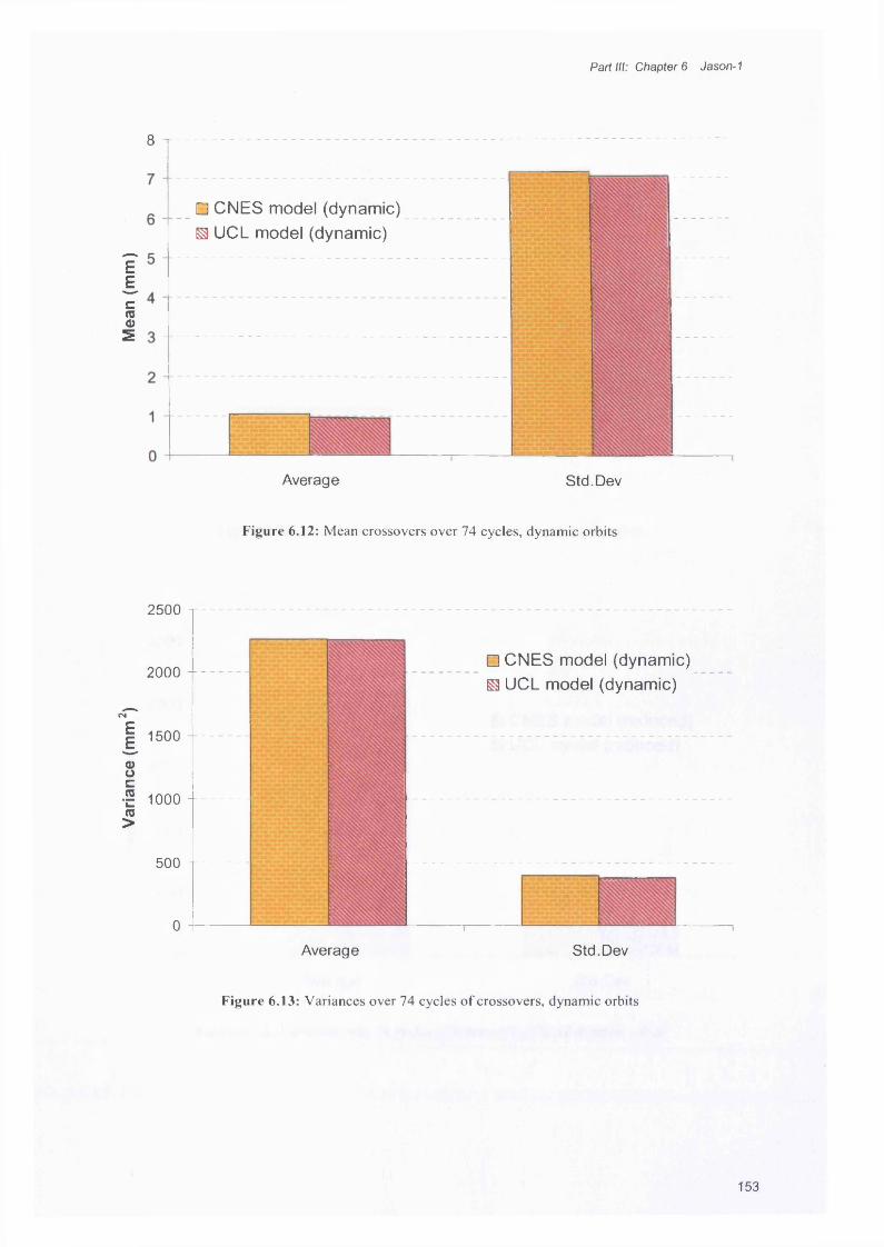
Varia
nce
(mm
2) M
ean
(mm
)
Part III: Chapter 6 Jason-1
8 T
□ CNES model (dynamic) ^ UCL model (dynamic)
Average Std. Dev
Figure 6.12: Mean crossovers over 74 cycles, dynamic orbits
2500 t
□ CNES model (dynamic)2000 + -------------
S3 UCL model (dynamic)
1500
1000 -
500
0Average Std. Dev
Figure 6.13: Variances over 74 cycles o f crossovers, dynamic orbits
153

Varia
nce
(mm
2) M
ean
(mm
)
Part III: Chapter 6 Jason-1
□ CNES model (reduced)
S3 UCL model (reduced)
T
Average Std. Dev
Figure 6.14: Mean crossovers over 74 cycles, reduced dynamic orbits
2500
2000□ CNES model (reduced) ^ UCL model (reduced)
1500 -+
1000
Average Std. Dev
Figure 6.15: Variances over 74 cycles o f crossovers, reduced dynamic orbits
154
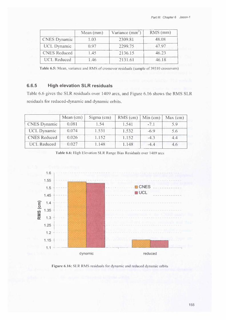
Part III: Chapter 6 Jason-1
Mean (mm) Variance (mm2) RMS (mm)
CNES Dynamic 1.03 2309.81 48.08UCL Dynamic 0.97 2299.75 47.97CNES Reduced 1.45 2136.15 46.23UCL Reduced 1.46 2131.61 46.18
Table 6.5: Mean, variance and RMS of crossover residuals (sample of 39310 crossovers)
6.6.5 High elevation SLR residuals
Table 6.6 gives the SLR residuals over 1409 arcs, and Figure 6.16 shows the RMS SLR
residuals for reduced-dynamic and dynamic orbits.
Mean (cm) Sigma (cm) RMS (cm) Min (cm) Max (cm)CNES Dynamic 0.081 1.54 1.541 -7.1 5.9UCL Dynamic 0.074 1.531 1.532 -6.9 5.6CNES Reduced 0.026 1.152 1.152 -4.3 4.4UCL Reduced 0.027 1.148 1.148 -4.4 4.6
Table 6.6: High Elevation SLR Range Bias Residuals over 1409 arcs
1.6
1.55 -
dynamic reduced
Figure 6.16: SLR RMS residuals for dynamic and reduced dynamic orbits
155

Part III: Chapter 6 Jason-1
6.7 Discussion of results
6.7.1 Solar scaleFigure 6.9 shows that the estimated solar scale with the UCL SRP and TRR model is
much closer to unity than the nominal model and the average scale factor is 1.01. The
nominal model has a scale of 0.93. More importantly, the variation around the mean of
the solar scale with the UCL models (as can be seen from the standard deviations) is
smaller than with the nominal model and this implies better model fidelity. The periods
marked as “gyro cal periods” can be ignored as there was likely to have been
unmodelled attitude manoeuvres occurring at these times.
6.7.2 Atmospheric drag coefficientsFigure 6.10 shows the variation of the drag constant over the 90 day period. The
variations are less with the UCL model than with the nominal model. This coefficient
stability, combined with the solar scale parameter (average value of 1.01) shows that
aliasing between the two parameters is reduced, which implied higher fidelity in the
modelling.
6.7.3 Orbit overlapsFigure 6.11 shows the orbit overlap comparison. Negative values indicate an improved
overlap with the UCL model, and this can be detected particularly during yaw regime
changes, where the improvements are significant at the 10-20 cm level.
6.7.4 Crossover residualsImprovements can be seen in the UCL model with comparison to the CNES model for
every test using dynamic orbits in terms of the size of the average residuals and their
standard deviations (Figures 6.12-6.15). The CNES model shows very slightly smaller
residuals for some comparisons using the reduced-dynamic orbits though these are
mainly at the 1/100 mm level. Even in these cases, the standard deviations are larger for
the CNES orbits.
As dynamic orbits rely more heavily on the force models than the reduced dynamic
orbits, we expect the largest differences in these orbits.
156

Part III: Chapter 6 Jason-1
UCL models improved crossover residual variances by ~10 mm2 for the dynamic orbit
case and ~5mm2 in the reduced dynamic case. By comparison, the incorporation of GPS
antenna phase centre variation maps improved cycle-averaged cross-over variances16 by
~7mm2 for Jason-1. This result was viewed as significant (Haines, B. et al., 2004).
6.7.5 SLR residualsIn these tests the UCL residuals and standard deviations are smaller than for the CNES
models for the dynamic orbit. Though the residuals are slightly better for the CNES
reduced dynamic models than UCLs, again the standard deviations are larger. It should
be noted here that the absolute values are very small.
SummaryIn this chapter an SRP model and a thermal model for Jason-1 were implemented into
GIPSY-OASIS II. Various tests were carried out on dynamic and reduced dynamic
orbits created using these models, and compared against the CNES models, which were
the nominal models in use for Jason-1 orbit modelling at the time of testing. The tests
compared values of solar scale, atmospheric drag, orbit overlaps, crossover residuals
and satellite laser ranging residuals. In all dynamic orbit tests, and for almost all reduced
dynamic orbit tests, the UCL model performs better than the CNES model. In Chapter
7, the results of thermal model testing for Jason-1 and GPS Block HR will be analysed.
16 This analysis was based on 62-10 day repeat cycles
157
Part IV: Chapter 7 Analysis
Part IV
Chapter 7 Analysis
Chapter outlineIn Part III, the models developed in this thesis are applied to the GPS Block HR and
Jason-1 satellites and results of orbit prediction and orbit determination tests are given.
In this chapter, the errors associated with model parameters are discussed and their
likely effects on the results are quantified. The effect of components which have not
been taken into account is estimated. Orbit residuals obtained during model testing are
analysed and remaining sources of error are identified and discussed.
7.1 Errors in model parameters
The accuracy of computed models depends directly on the uncertainties associated with
the parameters used. Parameters required in the evaluation of the TRR force include
solar irradiance, surface optical properties, solar panel material properties, spacecraft
mass, spacecraft attitude and the amount of power drawn from the solar panels to the
spacecraft bus.
The solar irradiance is known to vary over a number of periods. The high frequency
component (X-rays and gamma rays) related to solar rotation represents only a tiny
fraction of the total solar irradiance (TSI) and can be safely ignored. Over the solar
cycle, which has periods of between nine and fourteen years, the TSI varies by up to
only 1.4 Wm'2. This represents a maximum change of 0.1% over the whole cycle. The
variation could be crudely modelled but is unlikely to yield any great benefit over short
arc analysis. Some gains may be realised over longer arcs.
Data relating to the properties of surface materials can be very difficult to acquire. This
is most unhelpful given that these coefficients have a strong effect on computed models
and subsequent orbit computations. Though optical properties of many materials are
available in manuals, they are often given as crude values with large ranges.
158

Part IV: Chapter 7 Analysis
A related problem is the gradual change in surface properties of a spacecraft due to
space weathering. The principle environmental factors affecting surface properties are
solar UV radiation; bombardment by monatomic oxygen; electron and proton radiation
and micrometeoroids. Efforts have been made to examine the effects of these processes;
the Long Duration Exposure Facility (LDEF) was launched in April 1984 and lasted for
six years. On board were 57 experiments containing over 10000 specimens. The aims of
the experiments were to test the effects of the low earth orbit space environment on
materials, components and systems.
The general result of these experiments showed an increase in solar absorptivity of
materials with little or no effect on infra-red emittance (Gilmore, D., 1994). White
paints are affected strongly by UV radiation and protons and electrons and their
absorptivities can degrade from 0.2 to 0.7 in just a few years. Kapton surfaces (used in
MLI materials) also show substantial degradation and can turn almost black after
several years in orbit. High absorptance surfaces, such as black paints, generally do not
degrade. There may be however, a slight reduction in absorptivity over time due to UV
bleaching. By contrast, quartz surfaces (such as front face solar panel surfaces)
experience essentially no damage due to UV and charged particle environment, leaving
contamination the only source of increased absorptivity. Contamination results when
volatile condensable materials are out-gassed from spacecraft components, primarily
electronic boxes, and then deposited onto external surfaces. This out-gassing is
strongest early in the mission, followed by a small steady increase until the end of life.
The mass of a spacecraft changes over time as a result of small fuel bums applied to
adjust the orbit of a satellite. Individual GPS spacecraft masses differ, and though
variations are small, if they are not taken into account substantial orbit errors result.
There will inevitably be some error in the pointing accuracy of individual spacecraft as
well, causing the actual forces on each spacecraft to deviate from their modelled
directions. The amount of power drawn from the solar panels affects surface
temperatures and hence the TRR force. It has proved difficult to get reliable information
regarding power draw and how it changes with time. No information was available for
power draw regimes in penumbral regions, or how the regimes are affected as the
efficiency of the solar cells decrease over time.
159

Part IV: Chapter 7 Analysis
Sections 7.11-7.13 contain quantitative analyses of these uncertainties and their effects
on the thermal forces.
The sensitivity of the force models to the optical properties and other model parameters
is investigated for both the solar panels and the MLI.
7.1.1.1 Solar panelsThe basic equations, taken from Section 4.2.2, used to evaluate the solar panel force,
are:
Equation 4.17 is solved for the back face temperature using the Newton-Raphson
method, which is substituted into 4.16 to calculate the front face temperature, and
Equation 4.18 is then used to calculate the force. It is not straight forward to carry out
an analytical error analysis for the force due to the interdependency of variables in
Equation 4.18; hence a numerical error analysis is conducted.
The errors in some variables are small and have negligible effect on the force. These
include the dimensions of the panel, which have been measured with millimetric
precision and associated errors are at the 0.01% level. Similarly the error in the solar
irradiance due to the solar cycle are at the 0.1% level, and will have no significant effect
on the force either. Physical constants such as the speed of light and the Stefan
Boltzmann constant are sufficiently well determined to contribute no error to the final
model. The power draw issue requires lengthier discussion and is treated separately in
Section 7.1.3. For the GPS Block HR solar panels, the remaining parameters, their
associated uncertainties and corresponding uncertainties in the force are given in Table
7.1. Where the uncertainty is written in parentheses, a true value was unobtainable and
an estimated value has been given. Maximum along-track orbit errors after 12 hours
7.1.1 Parameter sensitivity
Tf ~Th+ Rtohll£(jA Th
£&(Th + Rtotal£(TA ThA )4 + £<jTh4 + qelec - aW cos 6 = 0
F _ -2A<j{£fT / - £ h Th4)
(4.16)
(4.17)
(4.18)
160
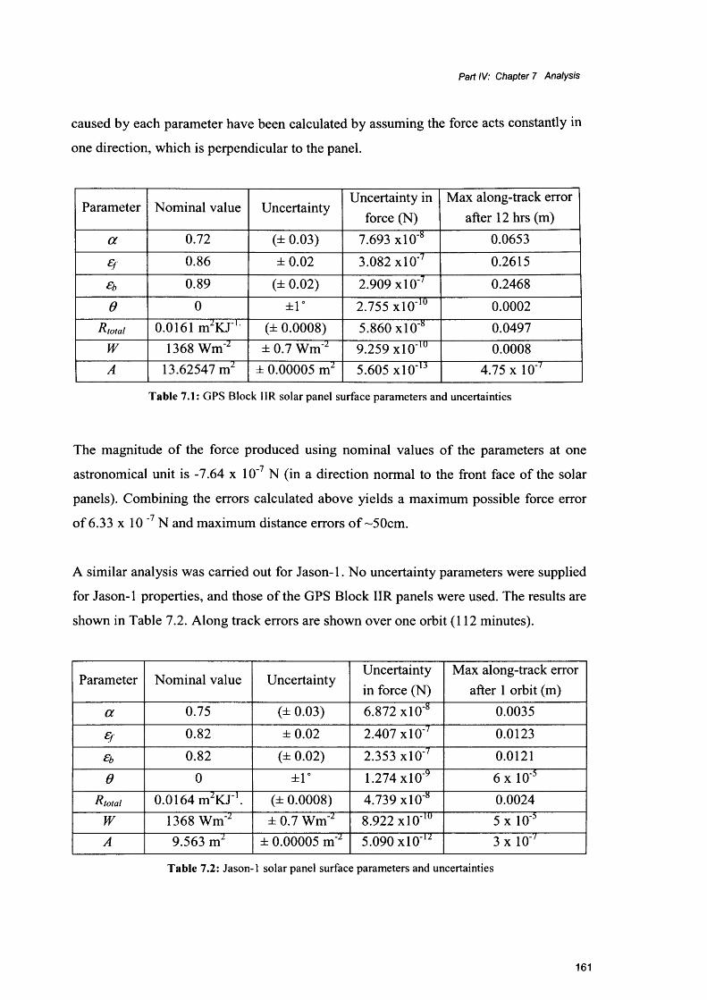
Part IV: Chapter 7 Analysis
caused by each parameter have been calculated by assuming the force acts constantly in
one direction, which is perpendicular to the panel.
Parameter Nominal value UncertaintyUncertainty in
force (N)Max along-track error
after 12 hrs (m)
a 0.72 (± 0.03) 7.693 xlO4 0.0653
£ f 0.86 ±0.02 3.082 xlO'7 0.2615
€b 0.89 (± 0.02) 2.909 xlO'7 0.2468
e 0 ±1° 2.755 xlO '10 0.0002
Rtotal 0.0161 mJK J L (± 0.0008) 5.860 xlO"8 0.0497w 1368 Wm"2 ± 0.7 Wm"2 9.259 xlO '10 0.0008A 13.62547 m2 ± 0.00005 n r 5.605 xl0"u 4.75 x 10-'
Table 7.1: GPS Block HR solar panel surface parameters and uncertainties
The magnitude of the force produced using nominal values of the parameters at one• • 7astronomical unit is -7.64 x 10' N (in a direction normal to the front face of the solar
panels). Combining the errors calculated above yields a maximum possible force errorn
of 6.33 x 10 ' N and maximum distance errors of ~50cm.
A similar analysis was carried out for Jason-1. No uncertainty parameters were supplied
for Jason-1 properties, and those of the GPS Block HR panels were used. The results are
shown in Table 7.2. Along track errors are shown over one orbit (112 minutes).
Parameter Nominal value UncertaintyUncertainty in force (N)
Max along-track error after 1 orbit (m)
a 0.75 (± 0.03) 6.872 xlO"8 0.0035
% 0.82 ±0.02 2.407 xlO"7 0.0123
£b 0.82 (± 0.02) 2.353 xlO"7 0.0121
e 0 ±1° 1.274x10'9 6 x 10"5
Rtotal 0.0164 m2K J '. (± 0.0008) 4.739 xlO"8 0.0024w 1368 Wm'2 ± 0.7 Wm'2 8.922 xlO'"1 5 x 10'5A 9.563 m2 ± 0.00005 m'2 5.090 xlO'12 3 x 10-'
Table 7.2: Jason-1 solar panel surface parameters and uncertainties
161
Part IV: Chapter 7 Analysis
The magnitude of the force produced using nominal values of the parameters at one
astronomical unit is -9.71 x 10'7 N (in a direction normal to the front face of the solar
panels).
Combining the errors calculated above yields a maximum possible force error o f -5.70 x
higher area to mass ratio of Jason-1 compared to GPS Block IIR, after twelve hours, the
errors reach the 1 metre level.
These errors are substantial. It should be noted that these distances are overestimates,
since the TRR force does not always act in the same direction. By far the largest source
of error is due to the front and back emissivities; within the range of the parameters, the
resultant force varies hugely as can be seen in Table 7.1 and 7.2. This is because the
front and back emissivities are scaled by the fourth power of the temperatures. As stated
earlier, it would be greatly beneficial if more research was directed towards defining
these parameters with greater certainties. It is likely that some of the remaining orbit
prediction residuals, which are at the 0.6m level as an RMS range over twelve hours,
can be explained by erroneous values being used in this model.
The nominal solar panel force is higher for Jason-1 than for GPS Block IIR. This is
mainly due to the fact that GPS Block IIR panels have a higher back face emissivity
than front face emissivity. This leads to a high degree of cancellation of the force
produced from the front face. For Jason-1, the front and back emissivities are equal and
hence less cancellation occurs.
7.1.1.2 MLIThe temperature of the MLI and the corresponding TRR force are given in Equations
4.34 and 4.35, which were derived in Section 4.3.2.
10"7 N. After one Jason-1 orbit, this maps into a distance error of ~3cm. Due to the
aW cos 6 + eeff( jT j(4.34)
(4.35)
162

Part IV: Chapter 7 Analysis
Table 7.3 contains the parameters used in the MLI models for GPS Block IIR
spacecraft.
Parameter Nominal UncertaintyUncertainty in
force (N)
Max along-track error after 1 orbit
(m)a 0.94 (± 0.03) 8.9470 x 10'8 0.0758
£mli 1 (- 0.1) 6.1370 x 1 O'9 0.0052
£ e jf 0.02 ±0.02 3.5167 x 10'8 0.0298e 0 ±1° 4.2699 x 1 O'10 0.0004
T 298 K ±25 K 5.7643 x 10‘9 0.0049Solar irradiance 1368 Wm z ±0.7 1.4345 x 10'9 0.0012
Table 7.3: GPS Block IIR MLI parameters and uncertainties
The nominal force per unit area of MLI is 2.823 x 10'6 Nm'2. Using the errors calculated
above, the maximum force error (at the one sigma level) is -2.8661 x 10⁸ N m 2 and the
maximum displacement arising from this error is ~10cm.
The MLI model is not highly dependent on the emissivity of the MLI. This is because a
higher value of this parameter acts to decrease the temperature and reduce the force, but
also to increase the amount of energy emitted and hence increase the force, with little
net change in the resultant force. This error analysis shows that the MLI model is not
strongly dependent upon the accuracy of the surface parameters. The same result was
found for Jason-1 ’s MLI surfaces.
7.1.2 Mass sensitivityThe nominal mass quoted for GPS Block IIR spacecraft is 1100 kg (Bar-Sever, Y.,
1997). Table 7.4 shows masses of some GPS Block IIR spacecraft in March 2004 which
have been used in the orbit prediction tests described in Section 5.4.3. It can be seen that
most spacecraft masses are fairly close to their nominal mass during this period, apart
from SVN 46. Accurate mass data is not readily available; the data in Table 7.4 was
only obtained close to the end of this study but its impact on the results was very
significant, especially for SVN 46.
163
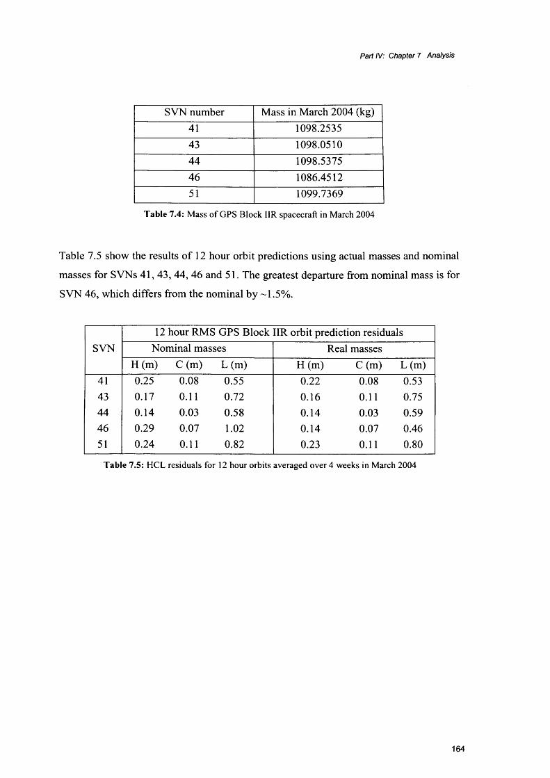
Part IV: Chapter 7 Analysis
SVN number Mass in March 2004 (kg)41 1098.253543 1098.051044 1098.537546 1086.451251 1099.7369
Table 7.4: Mass of GPS Block IIR spacecraft in March 2004
Table 7.5 show the results of 12 hour orbit predictions using actual masses and nominal
masses for SVNs 41, 43, 44, 46 and 51. The greatest departure from nominal mass is for
SVN 46, which differs from the nominal by -1.5%.
12 hour RMS GPS Block IIR orbit prediction residualsSVN Nominal masses Real masses
H(m) C (m) L (m) H(m ) C(m) L(m)41 0.25 0.08 0.55 0.22 0.08 0.5343 0.17 0.11 0.72 0.16 0.11 0.7544 0.14 0.03 0.58 0.14 0.03 0.5946 0.29 0.07 1.02 0.14 0.07 0.4651 0.24 0.11 0.82 0.23 0.11 0.80
Table 7.5: HCL residuals for 12 hour orbits averaged over 4 weeks in March 2004
164

Part IV: Chapter 7 Analysis
A bar chart o f the residuals for SVN 46 is shown in Figure 7.1.
1-2 T ~
1 -
?O 0 .8 -c<u c0s o .6 -
1.S’ 0 . 4 -!p &-O
0.2 -
0 -Height C ro ss track Along track
Figure 7.1: Orbit prediction errors for SVN 46, using real and nominal masses
The improvements in residuals show the importance o f using accurate masses in orbit
prediction. A time series of accurate masses is not publicly available, making testing at
other time periods very difficult. In orbit determination, incorrect mass is likely to be
less problematic as a scale factor should soak up any errors associated with it.
7.1.3 Solar panel power draw
This section attempts to discuss possible reasons for the discrepancy between the
modelled and telemetered temperatures (which was given in Section 5.5.1.) and to show
how much the models are affected by the assumed power draw. Table 7.6 summarises
the telemetered data from temperature sensors on the Block IIR satellites, The ±Y refer
to the sides o f the spacecraft. For GPS Block IIR, power is drawn from either the inner
or the outer panels. Unfortunately no information was available as to which panels the
temperature sensors are mounted on, hence it is unclear whether power is being drawn
from them or not.
□ Nom inal m a ss ■ R eal m a ss
165

Part IV: Chapter 7 Analysis
SVNAverage telemetered temperatures (K)
+Y -Y41 313.50 322.0043 315.50 314.7544 318.25 327.0046 326.75 329.0051 320.75 328.0054 326.50 330.50
Average 320.21 325.21SD 5.60 6.40
Table 7.6: Summary o f telemetered temperature data for front face of solar panels.
For GPS Block IIR, it can be seen that the telemetered temperatures are generally higher
than the modelled temperatures which are given in Table 7.7. Table 7.7 shows the
modelled front face temperatures change as the amount of power drawn is varied.
Column A shows the modelled temperature derived when nominal values for optical
parameters were used (a = 0.72, ef = 0.86, £b = 0.89). In column B, the optical
parameters have been changed to values within their formal error margins (a= 0.75,
£f= 0.88, £b = 0.87), to create the highest realistic temperatures.
Power draw (Wm 2)Modelled temperature (K)
A B90 311.67 315.9050 315.20 318.550 319.47 322.68
Table 7.7: Front face panel temps for varying power draw and optical parameters
Using a power draw of 90 Wm'2, the modelled temperatures are significantly lower than
the telemetered temperatures but by decreasing the amount of power draw, this
difference is reduced. When the optical properties are modified by their uncertainties,
the temperatures become very similar to the telemetered ones. If the solar sensors are
located on panels from which power is not being drawn, this could explain the
discrepancies between the two sets of temperatures. The telemetered data varies hugely
between the spacecraft and between the ±Y sides. From Tables 7.6 and 7.7, it can be
166

Part IV: Chapter 7 Analysis
seen that the models and observations are consistent within one standard deviation of
the observations.
A number of other factors could also account for some or all of the temperature
discrepancy. Firstly, the telemetered data higher for the -Y panels than for the +Y
panels, for all but one satellite. This is unusual in that the physical structure of the
satellite and its design modes are nominally symmetrical. If one of the panels was
somehow mis-pointing, the flux received by the -Y side would be different to the flux
received for the +Y side (see Figure 7.2). Mis-pointing might be as a result of either
manufacturing errors, incorrect deployment of the solar panels, or general wear and tear
over the lifetime of the spacecraft. However, a mis-pointing angle of one of the panels
by 5° would cause a temperature difference of less than 0.5K, so this would not explain
the differences that can be seen in the telemetered data.
SolarSensor
Normal
Force duelo diffusely \ reflected * radiation Force due
to specularlyreflectedradiation
Figure 7.2: A mis-pointing panel
A more reasonable argument for the discrepancy might be that power is not being drawn
equally from both sides. The temperature differences between the left and right panel
can be recreated if the average power draw is kept at 90Wm'2 but more is taken from
one side than the other. It is unlikely that the power draw regime is as simple as a
standard value of 90 Wm*2 from either the inner or outer panels, though this was the
data available to us. A variable power draw regime is more likely, as is the case for
Jason-1 (described in section 6.3.2). A measure of the accuracy of the temperature
sensors and how well they are calibrated is required to better interpret and attain
confidence in the data. The large variations in temperature between the satellites and
167
Part IV: Chapter 7 Analysis
discrepancies between the left and right panels raise questions as to how sensitive and
accurate these instruments are.
As described in Section 5.2.4, thermal radiators on the ± Y faces of the spacecraft vent
heat away from the spacecraft bus. It was assumed that heat was vented equally from
both sides. From a design viewpoint this would be preferable, though no data was
available to support this. If, however, the internal components of the bus are arranged in
such a way that one part of the bus produces more heat than other parts, this might cause
heat to be vented out of the bus asymmetrically. (In the GPS Block IIR spacecraft, the
navigation computer and clocks are situated on the -Y side of the spacecraft bus). If the
vented heat impacts upon the solar panels, this would cause the panels to warm up
somewhat and may explain why the telemetered temperatures are higher than those
modelled. If the heat venting is asymmetrical, then this could also explain the
discrepancies between the +Y and -Y panels.
7.2 Unmodelled surfaces
For the GPS Block IIR spacecraft bus, most large surface components are covered in
MLI. Those that are not, such as the W-sensor antennas are unlikely to have a large
effect on the acceleration due to TRR, for reasons described in Section 5.2.4. Earlier
models of GPS spacecraft, i.e. GPS Block II and IIA, do not have a shroud covering the
+Z face antennas, and hence relatively large metal cylinders are exposed. It is unlikely
however that they would contribute a significant thermal force because of the same
argument used for the W-Sensors on GPS Block IIR: the antennas are cylindrical, fairly
thin, and made of a highly conductive material (aluminium), thus a roughly symmetrical
temperature distribution about the central axis of each cylinder is expected and emission
will be almost equal in all directions perpendicular to this axis at each point along its
length. Due to the cancellation of forces in opposite directions, only a small net force is
expected.
For Jason-1, some sizeable surfaces remain un-modelled from a thermal re-radiation
point of view. This is partly because it is impossible to obtain detailed structural data
about these objects; the data files included only surface properties. If the structural and
material property data were obtainable, a finite element analysis method could in theory
168
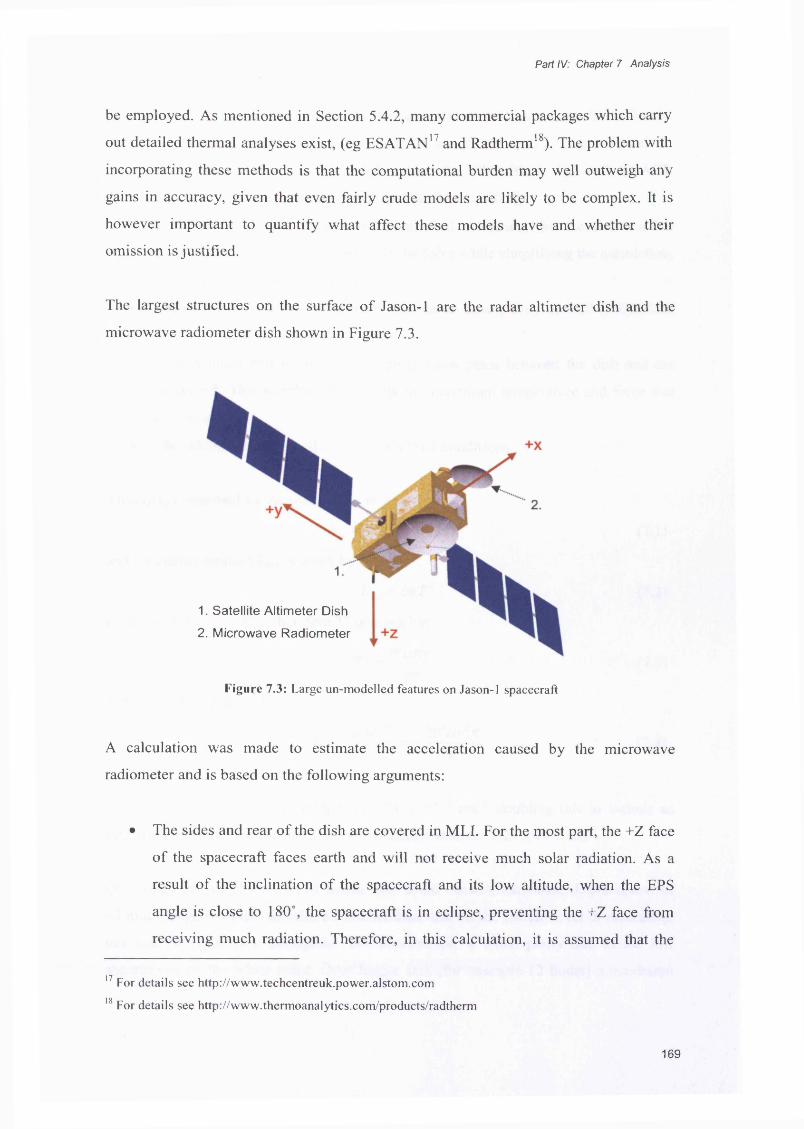
Part IV: Chapter 7 Analysis
be employed. As mentioned in Section 5.4.2, many commercial packages which carry
out detailed thermal analyses exist, (eg ESATAN17 and Radtherm18). The problem with
incorporating these methods is that the computational burden may well outweigh any
gains in accuracy, given that even fairly crude models are likely to be complex. It is
however important to quantify what affect these models have and whether their
omission is justified.
The largest structures on the surface of Jason-1 are the radar altimeter dish and the
microwave radiometer dish shown in Figure 7.3.
1. S a te llite A ltim eter D ish
2. M icrow ave R a d io m e te r
Figure 7.3: Large un-modelled features on Jason-1 spacecraft
A calculation was made to estimate the acceleration caused by the microwave
radiometer and is based on the following arguments:
• The sides and rear of the dish are covered in MLI. For the most part, the +Z face
of the spacecraft faces earth and will not receive much solar radiation. As a
result of the inclination of the spacecraft and its low altitude, when the EPS
angle is close to 180°, the spacecraft is in eclipse, preventing the +Z face from
receiving much radiation. Therefore, in this calculation, it is assumed that the
17 For details see http://www.techcentreuk.power.alstom.com
18 For details see http://www.thermoanalytics.com/products/radtherm
169

Part IV: Chapter 7 Analysis
emitting source is the Earth. At the orbit altitude of Jason-1 the Earth flux is
interpolations between calculated values for GPS Block IIR and GRACE
(altitude ~ 500km) (pers comms, Edwards, S., Aug 2004).
• The inner surface of the dish is a paraboloid. Assuming that the dish is a flat
circle will, if anything, over-estimate the force while simplifying the calculation.
The dish has a radius of ~ 0.5m.
• The dish is covered in white paint and has an absorptivity of 0.28 (ESABASE
file)
• It is assumed that no thermal coupling takes place between the dish and the
spacecraft. This simplification yields the maximum temperature and force that
can occur.
• The calculation is carried out in steady state conditions.
The energy absorbed by the surface, Ein is given by:
Over one orbit of Jason-1 (112 mins), this could cause a maximum displacement of
~3 mm though it would actually be smaller than this. At the current level of modelling,
this can be considered negligible. The acceleration is small partly due to the low
absorbtivity of the white paint. Over longer arcs (for example 12 hours) a maximum
estimated to have a maximum value of about 250 Wm’2. This is based on
Ein - W aA = WaKr
and the energy emitted Eout is given by:
(7.1)
(7.2)
In steady state, Ein = Eouh therefore T4 is given by:
4 _ Waxr2(7.3)
and the force F is given by:
2 oeT* 2W ar27t (7.4)
This force results in an acceleration of 5.11 x 10'11 ms'2; doubling this to include anin 9estimate for the radar altimeter gives a total acceleration of 1.22 x 1 O' ms' .
170
Part IV: Chapter 7 Analysis
displacement of ~10cm could occur if the effect were systematic over many orbits, and
may no longer be considered negligible.
7.3 Once per revolution fitting
The fitting of once per orbit revolution (once per rev) empirical terms to soak up un
modelled effects is a commonly employed process in orbit determination (see Section
3.3.2). Different orbit determination schemes choose different frames of reference in
which to fit such once per rev terms. CODE for example uses the YPS basis and
whereas GIPSY-OASIS II uses the BFS XYZ basis. Depending upon the periodicity
and signature of the un-modelled effect, fitting will be more successful in some frames
than in others (Ziebart, M. et al., 2003a).
The periodicity of the thermal force was investigated by transforming the calculated
force into different coordinate systems (described in Section 2.3). These were:
1. Earth Centred Inertial (ECI)
2. Height Cross Along track (HCL)
3. Y Probe-sun (YPS)
4. Body Fixed System XYZ (BFS)
The accelerations in each basis for SVN 43 over for one orbit on the 3rd March 2001
are given as an example in Figures 7.4 - 7.7. The black lines show once per rev fits for
the acceleration in each component.
171

Acc
eler
atio
n (m
s'2)
Acc
eler
atio
n (m
s'2)
Part IV: Chapter 7 Analysis
4.0E-09
2.0E-09
0.0E+00
-2.0E-09— ECI X— ECI Y -*-ECI Z— FIT
-4.0E-09
-6.0E-09
-8.0E-09
-1.0E-08Time (hours)
Figure 7.4: Thermal force in ECI frame
8.0E-09
6.0E-09
4.0E-09
2.0E-09
0.0E+00
-2.0E-09
-4.0E-09
— FIT-6.0E-09
-8.0E-09Time (hours)
Figure 7.5: Thermal force in HCL frame
172
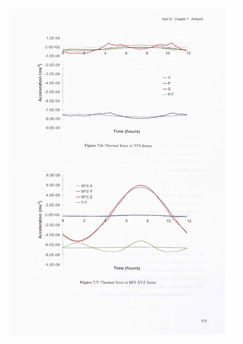
Acc
eler
atio
n (m
s'2)
Acc
eler
atio
n (m
s'2)
Part IV: Chapter 7 Analysis
1.0E-09 n
0.0E+00
-1.0E -09 -
-2 .0E -09 H
-3.0E -09 1
-4.0E-09
-5.0E-09— FIT
-6.0E-09 H
-7.0E-09
-8.0E-09
-9.0E-09 JTim e (hou rs)
Figure 7.6: Thermal force in YPS frame
8.0E-09 i
6 .0E-09 i — BFS— BFS— BFS— FIT
4.0E-09
2.0E-09
0.0E+00
-2 .0E -09 ■]
-4 .0E-09
-6 .0E -09 ■]
-8 .0E -09 -\
-1 .0E -08 JTime (hours)
Figure 7.7: Thermal force in BFS XYZ frame
173

Part IV: Chapter 7 Analysis
In the ECI and YPS frames, it is difficult to detect any obvious periodicity, though the
variations in accelerations are relatively small. In the BFS XYZ frame, there appears to
be a once per revolution fit in the Z direction but a small twice per rev signal in the X
direction. In the HCL frame, the signals do appear to be once per revolution.
RMS acceleration residuals were calculated for these once per rev fits:
HCL: 3.3 x 10'l0ms'2
YPS: 3.2 x 10'10 m s2
ECI: 3.3 x 10'10 ms'2
BFS: 7 .5x1 O'10 ms'2
These results show that parameterisation in either the ECI, HCL or YPS frames give
good fits with once per rev parameters, though it is the HCL frame which shows the
most once per revolution periodicity. GIPSY-OASIS II carries out parameterisation in
the BFS XYS frame as does the Master Control Station when processing GPS orbits.
This frame leads to the highest residuals for GPS spacecraft, more than double the size
using other coordinate systems.
For other more complex spacecraft, such as ENVISAT, the most suitable frame may be
different, if one exists at all. An analytical thermal analysis is a good way, and perhaps
the only way to find out which frame to use for successful empirical parameterisation of
this force.
7.4 Remaining orbit prediction residuals
The HCL residuals which arose from the comparison of precise and predicted orbits
using the final set of force models (defined in Section 5.4.3.1) were inspected to see
whether any systematic patterns could be detected in the form of the errors. Any such
patterns could be signifiers of further un-modelled effects. Firstly orbit errors over 12
hours were visually examined for each individual spacecraft over the course of the four
weeks in March 2004. No clear pattern emerged, suggesting that it is unlikely that
spacecraft specific effects are causing systematic deviations to the predicted orbits.
174
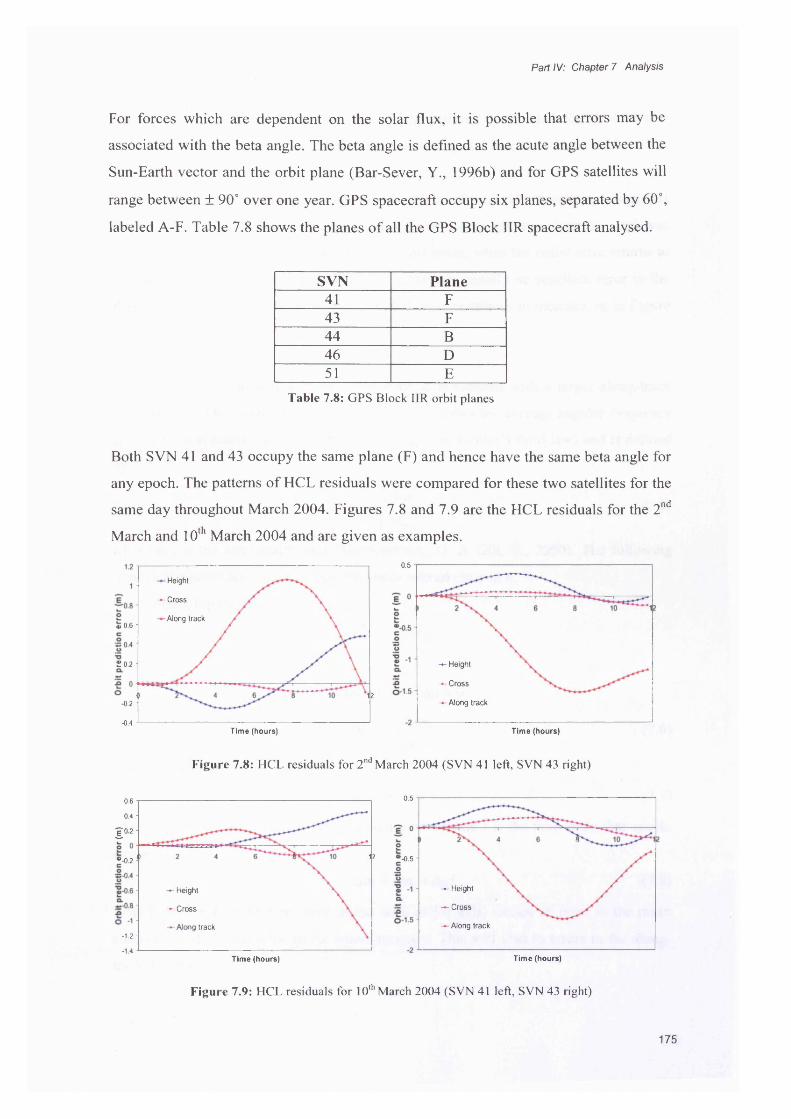
Part IV: Chapter 7 Analysis
For forces which are dependent on the solar flux, it is possible that errors may be
associated with the beta angle. The beta angle is defined as the acute angle between the
Sun-Earth vector and the orbit plane (Bar-Sever, Y., 1996b) and for GPS satellites will
range between ± 90° over one year. GPS spacecraft occupy six planes, separated by 60°,
labeled A-F. Table 7.8 shows the planes of all the GPS Block IIR spacecraft analysed.
SVN Plane41 F43 F44 B46 D51 E
Table 7.8: GPS Block IIR orbit planes
Both SVN 41 and 43 occupy the same plane (F) and hence have the same beta angle for
any epoch. The patterns of HCL residuals were compared for these two satellites for the
same day throughout March 2004. Figures 7.8 and 7.9 are the HCL residuals for the 2nd
March and 10th March 2004 and are given as examples.
0.5
Height
— Cross
Along track• 0.6
£ 0.2 — Height
— Cross12
— Along track-0.2
-0.4T im e (hours) T im e ( h o u r s )
Figure 7.8: HCL residuals for 2nd March 2004 (SVN 41 left, SVN 43 right)
0.50.6
0.4
I 02
* - 0.2 12 '-0.5
— Height— Height
— Cross— Cross
— Along track— Along track- 1.2
-1.4T im e (h o u r s )T im e (h o u r s )
Figure 7.9: HCL residuals for 10th March 2004 (SVN 41 left, SVN 43 right)
175

Part IV: Chapter 7 Analysis
This analysis showed no clear similarities in the patterns of residuals for SVN 41 and
43, it is not possible to see a particular effect occurring as a function of beta angle.
An interesting feature which was apparent in many of the orbits predictions, was that
the error in the height direction appeared to have a once per rev signature, and was
small compared to the along track errors. In most cases, when the radial error returns to
zero after one orbit, as in Figure 7.9 (right), there is usually no resultant error in the
along track direction. Equally, when the radial error continues to increase, as in Figure
7.9 (left), so does the along track error.
An explanation as to why a radial error may be associated with a larger along-track
error follows. The mean motion n of a satellite describes the average angular frequency
at which a spacecraft moves in orbit (following from Kepler’s third law) and is defined
by:
\GMl3« = . f (7-5)
asm
where asm is the semi-major axis (Montenbruck, O. & Gill, E., 2000). The following
steps demonstrate how an error in a translates into an error in n :
Rearranging Equation 7.5:
n2 a = GM E
Hence:
2nAna3 + 3a2n2Aa = 0
-3nAaAn = - (7.6)
2 a
The mean anomaly m is defined as:
m = m0+nt (7.7)
where mo is the mean anomaly at a reference epoch and t is the time since that epoch.
Hence:
Am = Am0 + Ant (7.8)
Thus it can be seen that an error in the semi-major axis, causes an error in the mean
motion, which is amplified in the mean anomaly. This will lead to errors in the along-
track direction.
176
Part IV: Chapter 7 Analysis
7.5 Erroneous initial state vector
For GPS Block IIR, the force models were evaluated by how well predicted trajectories
compared to a JPL precise orbit. This method of evaluation is based on the assumption
that the initial state vector is a very good estimate of the position and velocity of the
spacecraft. It will however have some errors associated with it. Small inaccuracies in
this initial state vector, especially in the velocity would cause the predicted trajectory to
diverge even more from the precise orbit than they would if based solely on the errors in
the force models. Thus it could be that the dynamic models are more accurate than the
orbit prediction results suggest. Precise orbit positions are quoted to be accurate to ~
3cm (http://igscb.jpl.nasa.gov/components/prods.html) but no value is quoted for the
accuracy of velocities.
If this hypothesis is true there should exist a set of initial conditions which, when
propagated forward, result in trajectories closer to the precise orbits than those obtained
using the initial conditions taken from the precise orbit files.
A method for testing this hypothesis is to use a least squares fitting technique to solve
for the set of initial conditions which allow the predicted trajectory to best fit the precise
trajectory, and then to re-compute the predicted trajectory with this set of initial
conditions.
Equation 7.9 is the matrix form of the normal equations used in the least squares
estimation process.
[0][Ax] = [B] (7.9)
where [<t>] is the design matrix which contains the partial derivatives of the state vector
(position and velocity) at each epoch with respect to the initial state vector. [Ax] is the
one dimensional matrix containing corrections to the initial conditions and B is the
difference between the precise orbits and the predicted orbit. Equation 7.10 shows the
matrix elements. The subscript n denotes the epoch which run from 0 to n. Rows 0 to
n+1 contain the partial derivatives of the x element of the position vector with respect to
the initial state vector at each epoch; rows n+2 to 2(n+l) contain the partial derivatives
177

Part IV: Chapter 7 Analysis
of the y element of the position vector with respect to the initial state vector at each
epoch and so on.
3*o
< g
dXn
dxn
dx„
a*0 dx0 dx0 a*„3*0 fyo dz0 du03jc, dx} dxl 3jc,dx0 dy0 dz0 du0
dx„
dxn dxn3v0 dwQ dx, 3x
3wa
Ax0
Av0Az0 A M0 Av0 Awa
{precise - predicted)x0 {precise - predicted)xx
{precise — predicted)xn {precise — predicted) yQ
{precise — predicted)yn
{precise - predicted)wQ
{precise — predicted)wn
(7.10)
To populate the design matrix at each epoch, we need to calculate the partial derivative
of each element of the state vector with respect to the initial state vector. At epoch n, x„
is computed by integration of the dynamic model using xo as the start point, xo is then
changed by a small amount and x„ recalculated. This is repeated for eight values of xo
and an eighth order polynomial is fitted to these points, as shown in Figure 7.10. This
can be differentiated and evaluated at Xo. This process needs to be repeated for each
element of the state vector at each epoch.
178

Part IV: Chapter 7 Analysis
14
12
10
8><
6
4
2
01 1.2 1.4 1.6 1.8 2.2 2.4 2.62
Xo
Figure 7.10: Plot o f xn against xo
Equation 7.10 can be solved by the least squares solution:
[Ax] = [Ord>r'[<I>]7’[5]
When the solution converges, the initial condition which causes the dynamically
modelled trajectory to best fit the precise orbit has been obtained.
For a twelve hour integrated orbit, the initial conditions were estimated based on the
first two hours of the arc. The precise orbit gives a state vector at 15 minute intervals
and so is a 48 x 6 matrix: (6 x 2 x 4) x (6): 6 for each element in the state transition
matrix, 2 for the number of hours, and 4 for the number of data points per hour).
7.5.1 Results
1.4
12 -g" □ Height
o 1 0 - B C ross track
® no □ Along trackc 0.8
=5 0.6
~ 0.40.2
0.041 43 4644
SVN number51
1.4□ Height■ Cross track - -□ Along track
c 0.8■5 0.6
41 5143 44SVN num ber
46
Figure 7.11: Full orbit prediction results Figure 7.12: Orbit prediction results using
optimised initial (same as Figure 5.11) conditions
Figures 7.11 and 7.12 are the results of 12 hour orbit predictions for March 2004, using
the initial state vector from the precise ephemeris and the estimated initial state vector.
Error bars showing the standard deviations are shown. The mean RMS residuals have
179

Part IV: Chapter 7 Analysis
reduced from 0.19m in height, 0.07m across track, and 0.58m along track to 0.12m in
height, 0.06m across track, and 0.42m along track. The overall errors have been reduced
by -30%. Improvements were seen consistently for each orbit.
Indeed, the residuals will always reduce when fitting parameters using least squares and
this does not “prove” the cause of the effect. It is of course possible that adjusting the
initial conditions could be partially accounting for some un-modelled or mis-modelled
effect which is correlated with the initial velocity. A key point here is that the initial
conditions were optimised using only the first two hours of precise orbit data, whereas
the RMS residuals consistently improved over twelve hours of orbit propagation. The
results imply that a substantial proportion of the error remaining after the thermal
models have been applied may not be due to inaccuracies in the force models, but
inaccuracies in our “truth” model, which we know to be erroneous at some level.
Though this result is not directly useful in orbit prediction as initial conditions can only
be optimised once the precise orbit is known, it does however highlight the sensitivity to
the initial conditions, and suggest that a substantial part of the remaining residuals may
not be due to failings in the dynamic model.
7.6 Earth’s gravity field
Non-conservative forces are highly insensitive to small translations, since they are
driven mainly by the radiative and particulate environment, which are roughly constant
over short distances. This is in contrast to the forces due to Earth’s gravity field which
are much larger and, as a consequence of the inverse square dependency, vary strongly
with radial distance. The implications for predicted orbits are as follows: initially the
predicted orbit diverges from the precise orbit due to mis-modelling in the force models
and inaccuracies in the initial state vector taken from the precise orbit. It is possible that
once small divergences have occurred, these are then exacerbated by the application of
position dependent forces, such as the Earth’s gravity force. To demonstrate this point,
the following situation is considered: if at one epoch, the predicted position of the
spacecraft has a larger radial value than its precise position, a smaller Earth’s
gravitational force will be applied to it, causing its radial component to become even
180
Part IV: Chapter 7 Analysis
larger. This will result in further deviation from the precise trajectory, again implying
that not all the error is a direct result of inadequacies in the force model.
A ball park figure can be estimated for the difference in gravity caused by 10 cm radial
error at an orbit altitude of GPS satellites. Considering the action of the monopole term
only, Equation 7.11 gives the difference in acceleration Ag:
Ag = GM 1 1r 2 (r + ArY
(7.11)
3 - 2
where:
GM= 398600.4415 km Y
r = 26000km (approximate value for the semi-major axis)
Ar = 1 x 10⁻⁴ km (10 cm)
Substituting these values into Equation 7.11 yields:
Ag = 4.5E — 9m.v 2
This difference in acceleration has a similar magnitude to many of the non-conservative
forces, albedo, thermal forces, antenna thrust, and will definitely cause an appreciable
deviation of the predicted orbit from the precise orbit. To investigate how much this
contributes to the residuals resulting from orbit prediction, the predicted trajectory is
produced by integration of the force models as before, but at each epoch, the gravity
field term derived from the precise orbit position is applied to the integrated position.
The following bar-charts show the orbit integration results obtained when this technique
was applied. Figure 7.13 shows results of the orbit predictions when the integrated
position derived gravity terms were used. Figure 7.14 shows these results when the
181

Part IV: Chapter 7 Analysis
gravity field has been adjusted and the initial state vector has been optimised.
- □ Height Cross track
□ Along track
0.20 - □ Height
Cross track□ Along track
0 .18 -
w 0 .16 -
t 0 .14
» 0 .1 0------ “ 0.10
£ 0 .08 - ^ £ 0 .08
- 0 .06 -I- ~ 0 .06
0.04 - O 0 04
0.02 -
SVN n u m b e r SVN num ber
Figure 7.13: HCL residuals: adjusted gravity field Figure 7.14: HCL residuals: adjusted gravity field
and initial state vector
The mean RMS residuals for the results shown in Figure 7.13 are 0.07 m in height, 0.07
m across track, and 0.12 m along track. The mean RMS residuals for the results shown
in Figure 7.14 are 0.06m in height, 0.06m across track, and 0.09 m along track.
These results show that small errors in the estimations of position will escalate into
larger errors caused by using an incorrect gravity term. From an orbit prediction point of
view, we cannot achieve results at the 10 cm level, but our force modelling only needs
to improve a little for the final orbit prediction errors to reduce significantly. Put another
way, the error represented by the residuals is not solely due to errors in the modelling of
the forces.
Inclusion of the thermal re-radiation obviously leads to clear gains, and remaining errors
can be reduced by improvements in models of non SRP and TRR effects. Agencies such
as the IGS19 use orbit prediction to produce ultra rapid orbits (which are accurate to ~10
cm in the radial direction) and clocks for use in near real time and real time positioning.
They achieve improved orbit predictions (compared to the broadcast ephemeris) by
empirically modelling other effects which impact on the orbit. A predicted orbit which
incorporates both accurate force modelling and better modelling of other factors is
likely to give the best solution.
19 http://igscb.jpl.nasa.gov/components/prods.html
182

Part IV: Chapter 7 Analysis
SummaryIn this chapter, significant sources of possible errors in the model are identified. The
most significant parameter uncertainty is in the emissivities of the panel surfaces.
Investigations into the periodicity of the thermal force revealed that a once per rev
signature was most noticeable in the HCL reference frame. It is also shown that
predicted orbits diverge from precise orbits due to inaccuracies in the initial state vector
used to seed the orbit integrator and that once small divergences have occurred, these
are increased by the application of erroneous position dependent forces. Once these
factors have been accounted for, predicted positions are at the 12 cm level which is
getting close to the noise level of precise orbits (~5cm). Chapter 8 contains a general
appraisal of the models developed in this thesis and discusses specific applications in
which they have been used.
183

Pari IV: Chapter 8 Discussion
Chapter 8 Discussion
Chapter outlineIn this chapter the main strengths and weaknesses of the models developed in this thesis
are discussed. The impact of the thermal re-radiation force in mission design and
operation are outlined and areas where the work developed in this thesis is directly
being applied are briefly described.
8.1 Model evaluation
8.1.1 Thermal modelsThe results of the orbit prediction tests for GPS Block IIR consistently showed
significant improvements with the addition of each thermal model. Inclusion of the solar
panel model reduced the 3D RMS error by 10%. Thermal modelling of the MLI yielded
much larger improvements, reducing the average error by a further 80%. This is contrast
to the analysis of Vigue (1994), who stipulated that for GPS Block IIA, the solar panels
would be the major contributor to the thermal force, since they were large, flat and
constantly sun-facing. The dominance of the MLI model is a consequence of several
factors. For GPS Block IIR, the blackening of the MLI gives rise to its high
absorptivity, and emissivity, and causes a very large thermal force to result. The force
effect of the panels on the other hand is particular low due to the emissivity of the back
face (£b= 0.89) being higher than the emissivity of the front face (£f = 0.86). Even
though panel front-face temperatures are higher than back-face ones, a higher
proportion of available energy is emitted by the back face causing a substantial degree
of cancellation in the resultant force.
The thermal albedo models cause a drop of only 1% in the residuals. This is due to the
low earth radiation flux at the altitude of GPS satellites.
For those satellites in eclipse, inclusion of a penumbra flux model reduced 3D RMS
errors by 20%. Final twelve hour orbit prediction errors for five GPS Block IIR
184

Part IV: Chapter 8 Discussion
spacecraft over four weeks are 0.19 m in height, 0.07m across track and 0.57m along
track.
For Jason-1, though the effect of the thermal force alone is hard to assess, it is a
significant part of the total SRP and TRR model. Several tests indicate the improvement
of the combined UCL SRP and TRR models in orbit determination compared to the
CNES model. The scale factor, which is an important metric of model accuracy and
stability, is now at the 1% level, compared to the previous value of 7%.
From these results, it can be stated that errors in orbit computations are reduced when
the thermal models developed in this thesis are applied. A major strength of all the
models produced in this thesis is their simplicity. They account for the precise shape
and structure of real spacecraft without producing long algorithms which are difficult to
implement.
A deficiency in the thermal models is the neglected affect of thermally re-radiated
energy coming from the Earth. Jason-1 orbits at an altitude of 1336km, specifically
chosen to minimise large drag affects, whilst still maintaining a high resolution of the
earth’s surface. At this altitude, the flux from Earth will be considerable and thermal re
radiation of this flux will undoubtedly cause perturbations to the spacecraft orbit.
Though a method for this was developed and implemented for GPS block IIR, accurate
flux models were not available to apply this method to Jason-1, and it was beyond the
scope of this project to create them. If the earth radiation flux data set is created and
implemented for Jason-1 it might account for some of the remaining 1% error in the
solar scale.
Other factors which affect the accuracy of the models are the uncertainty with which
particular parameters are known. These were discussed in Chapter 7 and mainly include
solar panel front and back face emissivities, and the power draw regime of the panels.
Agencies procuring a spacecraft from a manufacturer should request full information
relating to material types used in the spacecraft construction, and their properties when
known, in order to pass this on to mission analysis teams. Further research is needed in
this area to improve knowledge of both properties and their associated uncertainties. It
is hoped that an understanding of their importance may spur further research in the
185

Part IV: Chapter 8 Discussion
determination of these parameters. It may also urge spacecraft manufacturers to
document information to the best of their knowledge and ease its provision to mission
scientists.
The thermal responses of some surfaces on Jason-1 have not been modelled. The effects
of these surfaces were analysed in Section 7.2. For spacecraft with exposed surface
components that are thought to contribute a high thermal force, finite element analysis
(FEA), which was used as one technique for the thermal analysis of the solar panels in
Section 5.4.2, could be used. There are many commercial packages which carry out
thermal analysis using FEA. A significant problem faced when using these techniques is
the lack of detailed structural and material properties data, which is extremely difficult
to obtain. The suitability of these techniques must be judged depending on whether
sufficient data is available, for example for the thermal coupling between the surface
instruments and the inside of the bus and the structure and physical properties of the
insides of the instruments, and whether the accuracy gains are worth the extra
computational loads.
In general, since many missions fundamentally require thermal stabilisation of the
spacecraft bus (Gilmore, D., 1994), most surfaces apart from antennas are substantially
covered in MLI. Figure 8.1 shows a photograph of ENVISAT which was taken in a
clean room. It is clear that vast surfaces of the spacecraft are covered in MLI. This gives
another example of the importance of the MLI models, and how they are likely to be
dominate the thermal models for a spacecraft.
186
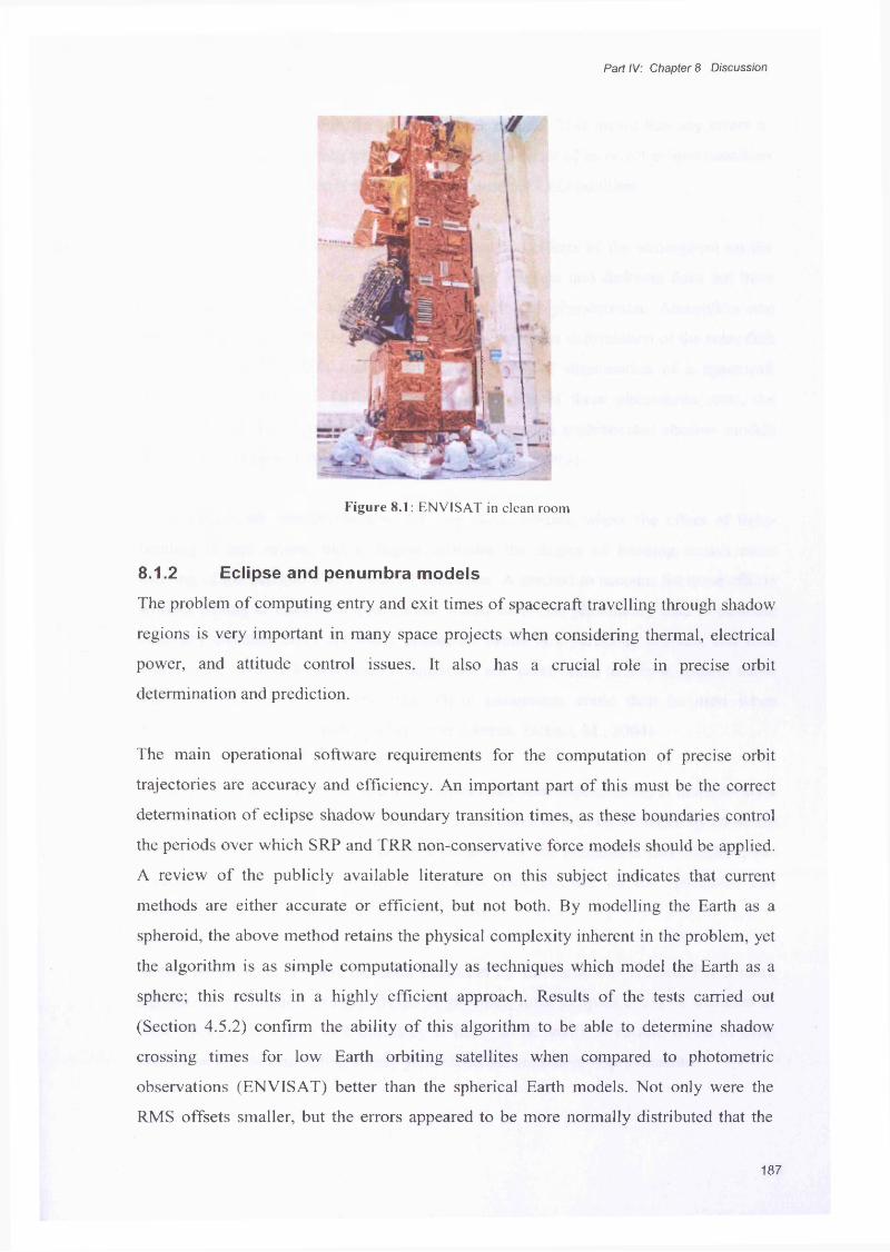
Part IV: Chapter 8 Discussion
Figure 8.1: ENVISAT in clean room
8.1.2 Eclipse and penumbra models
The problem of computing entry and exit times of spacecraft travelling through shadow
regions is very important in many space projects when considering thermal, electrical
power, and attitude control issues. It also has a crucial role in precise orbit
determination and prediction.
The main operational software requirements for the computation of precise orbit
trajectories are accuracy and efficiency. An important part of this must be the correct
determination of eclipse shadow boundary transition times, as these boundaries control
the periods over which SRP and TRR non-conservative force models should be applied.
A review of the publicly available literature on this subject indicates that current
methods are either accurate or efficient, but not both. By modelling the Earth as a
spheroid, the above method retains the physical complexity inherent in the problem, yet
the algorithm is as simple computationally as techniques which model the Earth as a
sphere; this results in a highly efficient approach. Results of the tests carried out
(Section 4.5.2) confirm the ability of this algorithm to be able to determine shadow
crossing times for low Earth orbiting satellites when compared to photometric
observations (ENVISAT) better than the spherical Earth models. Not only were the
RMS offsets smaller, but the errors appeared to be more normally distributed that the
187
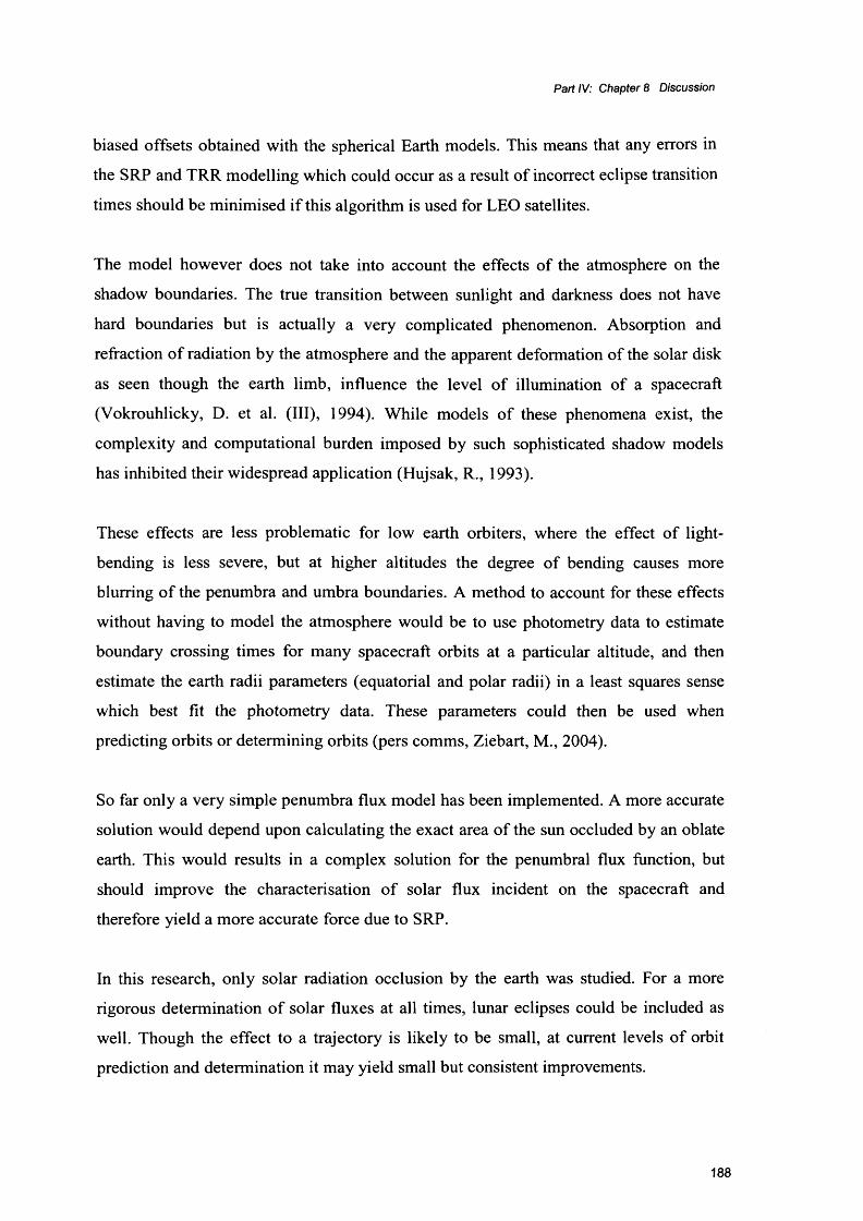
Part IV: Chapter 8 Discussion
biased offsets obtained with the spherical Earth models. This means that any errors in
the SRP and TRR modelling which could occur as a result of incorrect eclipse transition
times should be minimised if this algorithm is used for LEO satellites.
The model however does not take into account the effects of the atmosphere on the
shadow boundaries. The true transition between sunlight and darkness does not have
hard boundaries but is actually a very complicated phenomenon. Absorption and
refraction of radiation by the atmosphere and the apparent deformation of the solar disk
as seen though the earth limb, influence the level of illumination of a spacecraft
(Vokrouhlicky, D. et al. (Ill), 1994). While models of these phenomena exist, the
complexity and computational burden imposed by such sophisticated shadow models
has inhibited their widespread application (Hujsak, R., 1993).
These effects are less problematic for low earth orbiters, where the effect of light-
bending is less severe, but at higher altitudes the degree of bending causes more
blurring of the penumbra and umbra boundaries. A method to account for these effects
without having to model the atmosphere would be to use photometry data to estimate
boundary crossing times for many spacecraft orbits at a particular altitude, and then
estimate the earth radii parameters (equatorial and polar radii) in a least squares sense
which best fit the photometry data. These parameters could then be used when
predicting orbits or determining orbits (pers comms, Ziebart, M., 2004).
So far only a very simple penumbra flux model has been implemented. A more accurate
solution would depend upon calculating the exact area of the sun occluded by an oblate
earth. This would results in a complex solution for the penumbral flux function, but
should improve the characterisation of solar flux incident on the spacecraft and
therefore yield a more accurate force due to SRP.
In this research, only solar radiation occlusion by the earth was studied. For a more
rigorous determination of solar fluxes at all times, lunar eclipses could be included as
well. Though the effect to a trajectory is likely to be small, at current levels of orbit
prediction and determination it may yield small but consistent improvements.
188
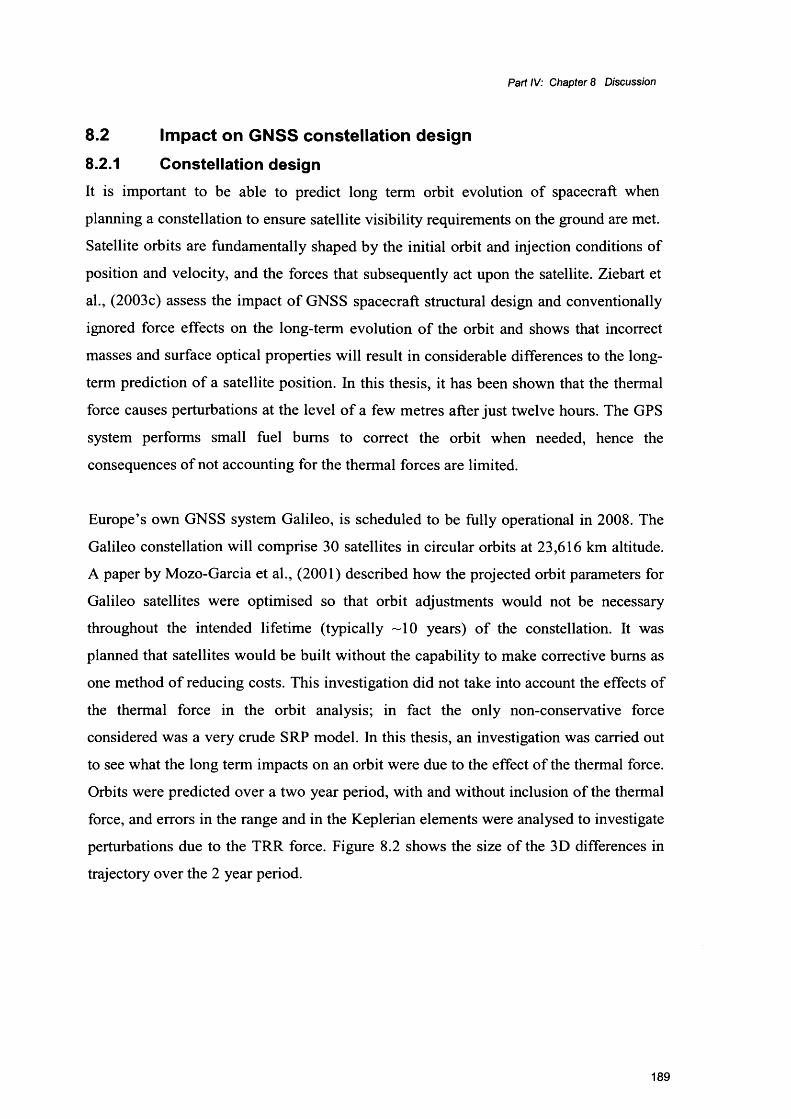
Part IV: Chapter 8 Discussion
8.2 Impact on GNSS constellation design
8.2.1 Constellation designIt is important to be able to predict long term orbit evolution of spacecraft when
planning a constellation to ensure satellite visibility requirements on the ground are met.
Satellite orbits are fundamentally shaped by the initial orbit and injection conditions of
position and velocity, and the forces that subsequently act upon the satellite. Ziebart et
al., (2003c) assess the impact of GNSS spacecraft structural design and conventionally
ignored force effects on the long-term evolution of the orbit and shows that incorrect
masses and surface optical properties will result in considerable differences to the long
term prediction of a satellite position. In this thesis, it has been shown that the thermal
force causes perturbations at the level of a few metres after just twelve hours. The GPS
system performs small fuel bums to correct the orbit when needed, hence the
consequences of not accounting for the thermal forces are limited.
Europe’s own GNSS system Galileo, is scheduled to be fully operational in 2008. The
Galileo constellation will comprise 30 satellites in circular orbits at 23,616 km altitude.
A paper by Mozo-Garcia et al., (2001) described how the projected orbit parameters for
Galileo satellites were optimised so that orbit adjustments would not be necessary
throughout the intended lifetime (typically -10 years) of the constellation. It was
planned that satellites would be built without the capability to make corrective bums as
one method of reducing costs. This investigation did not take into account the effects of
the thermal force in the orbit analysis; in fact the only non-conservative force
considered was a very crude SRP model. In this thesis, an investigation was carried out
to see what the long term impacts on an orbit were due to the effect of the thermal force.
Orbits were predicted over a two year period, with and without inclusion of the thermal
force, and errors in the range and in the Keplerian elements were analysed to investigate
perturbations due to the TRR force. Figure 8.2 shows the size of the 3D differences in
trajectory over the 2 year period.
189
Part IV: Chapter 8 Discussion
0.8
0.6
0.4Ei - 0 . 2k .ofc o . o
a>c - 0 . 2(0Q£
-0.4
- 0.6
- 0.8T im e o v e r tw o y e a r p e r io d
Figure 8.2: Range error resulting from no thermal force model
The maximum range error is -0 .8 km and this is reached after 6 months. The range error
is observed to have an annual period, which was also seen for the eccentricity, the right
ascension of the ascending node, and the inclination. This demonstrates that although
substantial range errors occur over the course o f an orbit, due to the once per orbit
revolution nature o f this force, the long term effects are not severe. The annual signature
could be explained by the /? angle, which is the angle between the orbit plane and the
earth-sun line. As the earth rotates around the sun, this angle varies with (to first order)
an annual period. After a year, the perturbations cancel and no overall changes to the
orbit are detected. In terms o f constellation design therefore, the thermal force is
unlikely to affect the long term evolution o f the orbit.
8.2.2 GNSS operation
For successful empirical parameterisation o f un-modelled forces, it is important to
choose a suitable reference frame. In the GPS system, the satellite ephemerides are
calculated by the Master Control Station using parameters for the SRP and TRR forces
modelled in the BFS XYZ system. The two parameters, K1 and K2 represent a solar
scale and a y-bias term respectively. In Section 7.3, it was shown that modelling the
thermal force in the body fixed XYZ frame with once per revolution parameters give
rise to much larger residuals than when modelled in other axes systems, and as such it is
unlikely that these could best correct for the effects. The Galileo constellation could
190

Part IV: Chapter 8 Discussion
benefit from similar analyses to determine the best reference frame for empirical
parameterisation used in orbit computations.
8.3 Applications of thermal models
8.3.1 GPS Block IIRThe US Airforce has contracted Boeing to carry out SRP, TRR and ERP modelling for
the next phase of GPS spacecraft (Block IIF), and require that Boeing’s software be
validated by JPL. In order to do this, JPL has requested UCL’s GPS Block IIR non
conservative force models to use as a standard against which the Boeing software will
be measured. Boeing’s models will be based upon structural and material properties
data provided by UCL for a direct comparison. If both sets of resulting accelerations are
similar within an acceptable margin of error, then Boeing’s own software will be used
for the work. Otherwise it is possible that Boeing may subcontract UCL to provide them
with models.
8.3.2 Jason-1As described in Chapter 7, UCL’s SRP and TRR models have been tested in GIPSY-
OASIS II by JPL. Test results showed significant improvements using the UCL model
compared to the CNES model which were in place at the time. Since then, UCL models
have been adopted for routine use in the orbit determination of Jason-1. Further
involvement is anticipated for the Ocean Surface Topography Mission (OSTM) which
is the follow-on to the Jason-1 mission, scheduled for launch in 2008.
8.3.3 ENVISATThe Department of Geomatic Engineering at UCL is part of a Natural Environment
Research Council (NERC) Centre of Excellence known as the Centre for the
Observation and Modelling of Earthquakes and Tectonics (COMET). COMET scientists
use satellite observation data to model the deformation of the Earth's crust in order to
study the earthquake cycle, the affect of faulting and uplift on the Earth's surface, and
the physics of continental deformation (http://comet.nerc.ac.uk/). COMET aims to use
InSAR data acquired by the European satellite ENVISAT. Currently UCL’s SRP and
TRR models are being implemented for ENVISAT, as part of an effort to improve the
accuracy of current ENVISAT orbits which are required for the correct interpretation of
191

Part IV: Chapter 8 Discussion
InSAR measurements. Figure 8.3 shows the structure of the ENVISAT bus. The solar
panel is not shown. The structure is largely covered in MLI and has a much more
complex structure than GPS Block IIR. It is expected that the thermal force will be more
difficult for a once per revolution empirical parameter to absorb.
Figure 8.3: Model of ENVISAT bus
8.3.4 Future applications
In theory these techniques are applicable to all spacecraft, and as orbit precision
requirements increase in geodesy and navigation applications, more missions will
require detailed analytical non-conservative force models. Several current missions have
expressed interest in the application o f UCL’s models to their spacecraft. Examples
include:
• GRACE
GRACE is a dedicated satellite mission whose objective is to map the global
gravity field. It uses an on-board accelerometer to measure the non-conservative
forces which are assumed to consist mainly o f atmospheric drag, SRP, ERP and
TRR forces. By physical modelling o f the SRP, ERP and TRR, the
accelerometer measurements can be used to derive the force due to drag, and
hence atmospheric densities.
192

Part IV: Chapter 8 Discussion
• Cryosat
The purpose of the CryoSat mission is to determine trends in the ice masses of
the Earth. Of principal importance is the testing of the predicted thinning of
Arctic sea ice due to global warming, which could change the climate of the
Arctic and possibly other regions. For the correct determination of the thickness
of the ice-sheets, precise orbits are required.
Potentially these models can be applied to any space probe, not only earth-orbiting
satellites, as long as the relevant data is available. The Goddard Space Flight Centre are
currently considering the employment of UCL’s models for the Mars Global Surveyor
satellite for the recovery of Mars’ gravity field coefficients.
At the International GPS Service (IGS) conference in Berne, 2004, one presentation
suggested that force models should be incorporated into new GPS receivers. The
receiver would use these force models directly to predict spacecraft positions in real
time (DiEsPosti, R. et al., 2004). If a move towards this technology were made, accurate
prediction using force models would be a necessity.
SummaryThe models have been evaluated based on their performance in orbit prediction and
orbit determination tests. Test results suggest that the models are successful in
accounting for a thermal force. Areas in which further research could improve the
thermal models have been identified. These are mainly in the development of a thermal
force due to earth radiation for Jason-1, and a more detailed description of the flux in
penumbra regions, accounting for atmospheric effects. In this chapter, the impact of this
force on the design and operation of missions has been discussed. Current applications
of this work are outlined, and some examples of potential projects that the thermal
models may be used for in the near future are given. In Chapter 9, the main conclusions
of this study are given.
193

Part IV: Chapter 9 Conclusions
Chapter 9 Conclusions
Chapter outline
This chapter starts with a brief overview of the study. A statement of the study’s
principal conclusions follows this and the final section lists possible avenues of further
research arising from the work presented in the thesis.
9.1 Overview of study
The main objectives of this research were to develop techniques to estimate spacecraft
surface thermal re-radiation forces in order to increase accuracies with which orbits can
be predicted and determined. In this thesis, generic methods are developed to calculate
forces arising from the re-radiation of absorbed solar energy. Specific methods were
developed for surfaces covered in multilayer insulation blankets and for solar panels.
Other surface components were dealt with on a part by part basis where additional
thermal data was available. The thermal forces arising from earth emitted radiation has
also been investigated and implemented for GPS spacecraft. Additionally, efficient
algorithms have been developed to calculate eclipse boundary crossing times, taking
into account the earth’s oblateness (Adhya, S. et al., 2004). A method for estimating the
variation of solar flux in penumbral regions has also been developed. These methods are
described in Chapter 4. The GPS Block IIR spacecraft and Jason-1, the US/French
altimetry satellite were chosen as test cases for the evaluation of these models.
The GPS Block IIR models were tested by predicting orbits using numerical integration
of a set of differential equations. The resulting trajectories were compared with precise
Jet Propulsion Laboratory (JPL) non-fiducial ECI orbits. The complete force model
included the GRACE GGM01C earth gravity to degree and order 15, solid Earth,
secular and poletide variations in the geopotential coefficients, third body gravity due to
the Sun, Moon, Jupiter, Mars and Venus, general relativistic effects, solar radiation
pressure, earth radiation pressure and antenna thrust forces. Four weeks worth of twelve
hour orbits for five GPS Block IIR spacecraft were predicted; Chapter 5 documents the
194

Part IV: Chapter 9 Conclusions
results of these tests. When thermal modelling of the solar panels was added to this,
relatively small but consistent reduction in the differences between predicted orbits and
precise orbits was observed. On average root mean square errors in the height, cross and
along track (HCL) directions dropped from 1.41m, 0.23m and 3.00 m to 1.27m, 0.21m
and 2.69 m. The impact of including modelling of MLI models further reduced HCL
errors to 0.19m, 0.08m and 0.59m. Considering only the subset of satellites in eclipse
season, inclusion of a penumbra flux model caused HCL residuals to drop from 0.16m,
0.03m and 0.70 m along track to 0.13, 0.03 and 0.56 m. The thermal albedo model did
not greatly affect results, causing the overall range error to drop by ~ 2cm.
For Jason-1, combined solar radiation pressure and thermal models were implemented
into JPLs orbit determination software GIPSY-OASIS II. Orbits were created using
UCL models and JPLs existing models, which were developed by CNES. These orbits
were compared in terms of parameters related to the size and variation of the solar scale,
atmospheric drag, crossover residuals, orbit overlaps and laser ranging residuals. The
results of these tests are documented in Chapter 6. The UCL models performed
significantly better than in all dynamic orbit tests and in almost all reduced dynamic
orbit tests. The outcome of these tests led to the incorporation of UCL’s SRP and TRR
models into JPLs routine orbit determination of Jason-1. The model is also currently
being implemented by NASA Goddard Space Flight Centre.
9.2 Principal conclusions
The average total thermal force for GPS Block IIR is estimated to be 8.2 x 10‘6 N,Q 0corresponding to an acceleration 7.4 x 10' ms' of which -90 % is due to the spacecraft
bus, and ~10 % due to the solar panels. For Jason, the thermal force had a magnitude
and of 3.2 x 10'6 N, which corresponds to an acceleration of 6.6 x 10"9 ms'2, of which
70% is due to the bus and 30% is due to the panels. From the GPS Block IIR orbit
prediction results, the largest improvements were in the along track direction, though
improvements were seen in all components. The modelling of the thermal forces has
significantly improved both orbit prediction and orbit determination capabilities.
Accurate calculation of the thermal force depends mainly upon: solar irradiance in the
vicinity of the spacecraft; spacecraft structure, surface absorptivities and emissivities,
195
Part IV: Chapter 9 Conclusions
conductivities of components that affect surface temperatures, spacecraft attitude and
for low earth orbiters, radiation coming from the earth. It was found that the force
model is most sensitive to errors in the front and back face emissivities of the solar
panel. These parameters commonly have values between 0.8 to 0.9, and uncertainties of
approximately 2.5%. This level of error can cause the force due to the solar panels to
vary by a maximum of ±80%, which corresponds to variation of about 10% in the total
TRR model. More accurate determination of these parameters would greatly reduce our
uncertainty in the overall TRR model.
The magnitude of the thermal force is strongly dependent on the absorptivity of the
multilayer insulation which covers the majority of surfaces of many spacecraft. The
MLI on GPS Block IIR has a particularly high value of the absorptivity (0.94) because it
is blackened, and thus gives rise to a high thermal force, with accelerations of the order
of 6.6 x 10"9 ms'2. This constitutes on average —25% of the force due to the SRP force
on the GPS Block IIR bus. The TRR acceleration due to the solar panels is only -1% of
the SRP force on the panels. For Jason-1, the MLI has a lower absorptivity and bus
accelerations are about 3.5 x 10'9 ms'2, which is -15% of the force due to SRP. The
solar panel TRR accelerations are -5 % of the SRP force on the panels.
The remaining orbit prediction residuals (the differences between the precise and
predicted orbits) for GPS Block IIR appeared to be chaotic; if a clear pattern had
emerged, this would have strongly suggested an unmodelled or poorly modelled effect.
This was not the case.
An important question when producing high precision analytical force models is
whether they can be adequately modelled with empirical parameters if given sufficient
tracking data. In Chapter 7, tests were carried out to examine how well once per orbit
revolution parameters could model the thermal force for a GPS satellite. It was found
that the reference frame in which the once per revolution parameters were applied made
a difference to how well the thermal force was replicated. In the HCL basis, the thermal
force appeared to have strong once per revolution characteristics, but in the spacecraft
body fixed XYZ system, fitting a once-per rev term gave residuals which were twice the
size. In the GPS system, the Master Control Station uses parameters in this frame, as
196

Part IV: Chapter 9 Conclusions
does GIPSY-OASIS II. It is unlikely that the thermal force will be correctly soaked up
in this frame. O f course, empirical parameterisation can only soak up un-modelled
effects when a large amount of tracking data is available; real time GPS orbit prediction
does not afford this luxury, and the force model plays a much greater part in accurate
positioning. Satellites which have more complex surface structures such as ENVISAT
are likely to produce more complicated signatures and may be impossible to model with
once per-rev parameters. It is only by a study of analytical models that the most
appropriate frame for a particular effect can be identified. Moreover, the choice of
frame for the empirical parameterisation may be driven by larger unmodelled effects.
Clearly if a force can be dealt with analytically and efficiently, it improves the model
redundancy and reduces the need to compromise the choice of reference frame for
empirical parameterisation.
In Chapter 8, it was shown that a substantial part of the remaining orbit prediction error
may be due to inaccuracies in the initial state vector used to seed the numerical
integrator. A least squares adjustment process was used to calculate a set of initial
conditions which was then used to seed orbit propagation. This led to a reduction of
residuals by -30% from an average RMS errors of 0.14m in height, 0.06m across track,
and 0.42m.
Further analysis confirmed the sensitivity of the gravity field to small radial distance
errors, and the impact of this on predicted orbits. It was found that once a divergence of
the predicted orbit from the precise orbit occurred, this would then be exacerbated by
application of a gravity force that was either larger or smaller than the gravitational
force that the spacecraft would actually have been subject to. Application of the precise
satellite position gravity field to the predicted orbit positions reduced RMS range
residuals to 0.07m in height, 0.07m across track and 0.12m along track, and when the
initial state vector was estimated as well, final orbit residuals reached 0.06m in height,
0.06m across track, and 0.09m. Though this knowledge cannot improve orbit prediction,
it strongly supports the argument that the force models themselves are not as deficient
as the residuals suggest. Final residuals of this size imply that the modelling of dynamic
forces is close to the noise level, that is, these residuals are comparable to the accuracy
at which post-processed precise orbits are known.
197
Part IV: Chapter 9 Conclusions
9.3 Future work
In order to further refine the force models and the ability to correctly define the
trajectory o f a spacecraft, several further areas of study have been identified. In terms of
thermal modelling, complex instruments on the surface that are not covered in multi
layer insulation have not been modelled. Commercially available finite element
software exists which can be used to calculate the spatially and temporally distributed
temperatures. This could be used in theory, if detailed information about the internal
structure and material properties of the spacecraft were obtainable, though this is often
not the case. Care must be taken to ensure that the computational burden involved in the
implementation of such analyses in orbit prediction/determination software should not
be too high as to render it impractical. As computational power increases, computational
intensity become less limiting in the development of new techniques.
The eclipse boundary crossing time model and penumbra flux model could be improved
by taking into account simple models of atmospheric refraction effects, or attempting to
account for them empirically as described in Chapter 8.
The current GPS earth radiation pressure models used in this study are detailed in that
they use high temporal and spatial resolution data. However, the spacecraft bus model
used in this process is relatively crude and treats the spacecraft bus as a flat plate.
Although these models are currently the most developed that exist, they could be refined
by applying the Earth fluxes to a more realistic spacecraft structure.
Earth radiation pressure models used in the orbit determination of Jason-1 are much less
detailed than those used for GPS Block IIR. As Jason-1 is in a low orbit, it is likely that
it will be more sensitive to the spatial distribution of the earth’s radiation. Similar data
to that used to create albedo models for GPS Block IIR, could be used to create an earth
radiation pressure for Jason-1. This albedo model would enable the thermal effects
arising form earth radiation pressure to be calculated as described in Section 5.4, and
may account for the 1.01 scale factor for Jason-1. It is highly unlikely that the thermal
response of the spacecraft to both solar radiation and earth radiation will have a once
per orbit revolution effect, and it could be a fruitful topic for further research.
198

Part IV: Chapter 9 Conclusions
In terms of analytically modelling the forces on a spacecraft, this research, along with
vast improvements in the gravity field and other non-conservative forces appears to
bring predicted orbits at a level close to the noise boundary. The models could be
improved by the techniques outlined above, but it is most likely that much higher
accuracies will not be reached without significant improvements in the spacecraft
engineering data used.
199

References
Adhya, S., Sibthorpe, A., Ziebart, M., & Cross, P. 2004, "Oblate Earth Eclipse State
Algorithm for Low Earth Orbiting Satellites", Journal o f Spacecraft and Rockets,
vol. 41, no. l ,pp. 157-159.
Bapat, S. L., Narayankhedkar, K. G., & Lukose, T. P. 1990, "Experimental
Investigations of Multilayer Insulation", Cryogenics, vol. 30, pp. 711-719.
Bar-Sever, Y. 1996a, "A New Model for GPS Yaw Attitude", Journal o f Geodesy, vol.
70, pp. 714-723.
Bar-Sever, Y., Bertiger, W., Davis, E., & Anselmi, J. 1996b, "Fixing the GPS Bad
Attitude: Modelling GPS Satellite Yaw During Eclipse Seasons", Navigation, vol.
43, no. 1, pp. 25-39.
Bar-Sever, Y. 1997, IGS Electronic Mail 1653.
Barkstrom, B. R. 1984, "The Earth Radiation budget Experiment (ERBE)", Bulletin o f
the American Meteorological Society no. 65, pp. 1170-1185.
Behr, J., King, N., & Hudnut, K. W. 1998, "Monitoring Structural Deformation at
Pacoima Dam, California Using Continuous GPS", 11th Int.Technical Meeting o f the
Satellite Division o f the U.S.Inst, o f Navigation GPS ION-98, Nashville, Tennessee,
15-18 Sept.,59-68.
Bertiger, W. 2004, "Five-Millimetre Orbit Determination for Ocean Altimetry", Aviso
Newsletter, Centre National d'Etudes Spatiales no. 10.
Beutler, G., Brockmann, E., Gurtner, W., Hugentobler, U., Mervant, L., Rothacer, M.,
& Verdun, A. 1994, "Extended Orbit Modeling Techniques at the CODE Processing
Center of the International GPS Service for Geodynamics (IGS)", Manuscripta
Geodetica no. 19, pp. 367-386.
200

Bomford, G. 1971, Geodesy, Third edn, Oxford University Press.
Borderies, N. & Longaretti, P. 1990, "A New Treatment of the Albedo Radiation
Pressure in the Case of a Uniform Albedo and a Spherical Satellite", Celestial
Mechanics pp. 69-98.
Chapman, A. J. 1984, Heat Transfer Macmillan.
Colombo, O. 1989, "The Dynamics of GPS Orbits and the Determination of Precise
Ephemerides", Journal o f Geophysical Research , vol. 94, pp. 9167-9182.
Cook, R. A. 1989, The Effects o f Thermal Imbalance Forces on Simple Spacecraft,
Centre for Space Research, University of Texas, Austin.
DiEsPosti, R., DiLellio, J., Kelley, C., Dorsey, A., Fliegel, H., Berg, J., Edgar, C., Me
Kendree, T., Fullerton, P., & Shome, P. 2004, "The Proposed State Vector
Representation of Braodcast Navigation Message for User Equipment
Implementation o f GPS Satelltie Ephemeris Propagation", Proceedings o f the
Institute o f Navigation, January 2004, San Diego, CA.
Ferrier, C., Gratton, S., & Mercier, F. "Radiation Pressure Modelling of Jason-1 and
Empirical Parametrisation", Jason-1 Science Working Team Meeting, Biarritz,
France, 2002.
Fliegel, H. F., Gallini, T. E., & Swift, E. R. 1992, "Global Positioning System Radiation
Force Model for Geodetic Applications", Journal o f Geophysical Research, vol. 97,
no. 1, pp. 559-568.
Fliegel, H. F. & Gallini, T. E. 1996, "Solar Force Modelling of Block HR Global
Positoning System Satelliltes", Journal o f Spacecraft and Rockets, vol. 33, no. 6, pp.
863-866.
Fortescue, P., Stark, J., & Swinerd, G. 2003, Spacecraft Systems Engineering, Third
edn, Wiley.
201

Frolich, C. & Lean, J. 1998, "The Sun's Total Irradiance: Cycles, Trends and Related
Climate Change Uncertainties since 1976", Geophysical Research Letters, vol. 25,
no. No. 23, pp. 4377-4380.
Fu, L. & .Cazenave, A. 2000, Satellite Altimetry and Earth Sciences A Handbook o f
Techniques and Applications, 69 edn, Academic Press.
Galvin, D. M. 1999, "History of the GPS Space Segment From Block I to the New
Millenium", Proceesings o f ION GPS International Technical Meeting o f the
Satellite Division,Sept. 1999, Nashville, TN.
Gilmore, D. 1994, Satellite Thermal Control Handbook The Aerospace Corporation
Press, El Secundo, California.
Gregorius, T. 1996, GIPSY-OASIS II How it Works, Department of Geomatics,
University of Newcastle upon Tyne.
Haines, B., Bertiger, W., Desai, S., Kuang, D., Munson, T., Young, L., & Willis, P.
2002, "Initial Orbit Determination Results for Jason-1: Towards a 1-cm Orbit",
Proceedings o f ION GNSS International Technical Meeting o f the Satellite Division,
21-24 Sept.2002, Portland, Oregon.
Haines, B., Bar-Sever, Y., Bertiger, W., Desai, S., & Willis, P. 2004, "One-Centimeter
Orbit Determination for Jason-1: New GPS-Based Strategies", Marine Geodesy, vol.
27, p. 299-318.
Hatch, R. R. 1995, "Relativity and GPS (Section I: Special Relativity)", Galilean
Electrodynamics, vol. 6, no. 3, pp. 51-57.
Heroux, P., Gao, Y., Kouba, J., Lahaye, F., Mireault, P., Collins, P., Macleod, K.,
Tetreault, P., & Chen, K. 2004, "Products and Applications for Precise Point
Positioning-Moving Towards Real-Time", Proceedings o f ION GNSS 17th
International Technical Meeting o f the Satellite Division, 21-24 Sept.2004, Long
Beach, CA.
202

Hudnut, K. W. 1995, "Earthquake Geodesy and Hazard Monitoring", Reviews o f
Geophysics (Supplement: U.S.National Report to IUGG) pp. 249-255.
Hugentobler, U. & Beutler, G. 2003, "Strategies for Precise Orbit Determination of Low
Earth Orbiters Using the GPS", Space Science Reviews, vol. 108, pp. 17-26.
Hugsak, R. S. 1993, "Solar Pressure", Proceedings o f the Artificial Satellite Theory
Workshop.
Incropera, F. P. & Dewitt, D. 2002, Introduction to Heat transfer, Fourth edn, John
Wiley and Sons.
Jacchia, L. G. 1977, Thermospheric Temperature, Density, and Composition: New
Models, Smithsonian Astrophysical Observatory, 375.
Kaplan, E. D. 1996, Understanding GPS Prinicples and Applications Artech house
Publishers.
Knocke, P. C., Ries, J. C., & Tapley, B. D. 1998, "Earth Radiation Pressure Effects on
Satellites", American Insstitute o f Aeronautics and Astronautics pp. 1-11.
Laxon, S. Physics of the Earth, wwwcpg.mssl.ucl.ac.uk/people/swl/lectures, 2003.
Ref Type: Electronic Citation
Leick, A. 2004, GPS Satellite Surveying, Third edn, John Wiley and Sons Inc..
Lemoine, F. G. 1997, The Development o f the NASA GSFC and NIMA Joint
Geopotential Model Springer-Verlag.
Lichten, S. M. & Border, J. S. 1987, "Strategies for High Precision Global Positioning
System Orbit Determination", Journal o f Geophysical Research, vol. 92, no. B12,
pp. 12751-12762.
203

Liu, M., Yang, Y., Stein, S., Zhu, Y., & Engeln, J. 2000, "Crustal Shortening in the
Andes: Why do GPS Rates Differ from Geological Rates?", Geophysical Research
Letters, vol. 27, no. 18, pp. 3005-3008.
Marquis, W. & Krier, C. 2000, "Examination of the GPS Block HR Solar Pressure
Model", ION GPS 2000, vol. 19-22, pp. 407-415.
Martin, C. F. & Rubincam, D. P. "Earth albedo affects on Lageos I satellite based on
Earth Radiation Budget (ERBE) satellite measurements,", EOS, paper G32A-3,
presented at the Spring Meeting of the AGU, Baltimore, MD, 1993
McCarthy, D. D. 1996, IERS Conventions Technical Note 21 Observatoire de Paris.
Milani, A., Nobili, A. M., & Farinella, P. 1987, Non-graviational Perturbations and
Satellite Geodesy Adam Hilger.
Misra, P. & Enge, P. 2001, Global Positioing System Signals, Measurements, and
Performance Ganga-Jamuna Press.
Montenbruck, O. & Gill, E. 2000, Satellite Orbits Models Methods Applications
Springer-Verlag.
Mozo-Garcia, A., Herraiz-Monseco, E., Martin-Piero, A. B., & Romay-Merino, M.
2001, "Galilieo Constellation Design", GPS Solutions, vol. 4, no. 4, pp. 9-15.
Neta, B. & Vallado, D. 1994, "On Satellie Umbra/Penumbra Entry and Exit Positions",
AAS97-155 pp. 715-724.
Otsubo, T., Appleby, G., & Gibbs, E. 2001, "GLONASS Laser Ranging Accuracy With
Satellite Signature Effect", Surveys in Geophysics, vol. 22, no. 6, pp. 507-514.
Press, W. H., Teukolsky, S. A., Vetterling, W. T., & Flannery, B. P. 2002, Numerical
Recipes in C++, Second edn, Cambrige University Press.
204

Price, B. A. & Smith, T. F. 1994, "Thermal Response of Composite Building Envelopes
Accounting for Thermal Radiation", Energy Conservation Management, vol. 36, no.
1, pp. 23-33.
Reigber, C., Gendt, G., Dick, G., & Tomassini, M. 2002, "Water Vapor Monitoring for
Weather Forecasts", GPS World pp. 18-27.
Rubincam, D. P. 1987, "LAGEOS Orbit Decay Due to Infrared Radiation from Earth",
Journal o f Geophysical Research, vol. 92, pp. 1287-1294.
Scharroo, R. 2002, A Decade o f ERS Satellite Orbits and Altimetry Delft University
Press.
Schwintzer, P., Reigber, C., Massmann, F., Bode, A., Meixner, H., Raimondo, J., Zhu,
S., Biancale, R., Balmino, G., Lemoine, F., Marty, J., Moynot, B., Barlier, F.,
Boudon, Y., Exertier, P., Laurain, O., & Gruber, T. 1999, "Status of the GRIM-5
Gravitational Model Development", Eos Transactions, AGU, vol. 80, no. 17.
Seeber, G. 2003, Satellite Geodesy Walter de Gruyter.
Seidelmann, P. K. 1992, Explanatory Supplement to the Astronomical Almanac
University Science books.
Slabinski, V. J. 1988, "LAGEOS Acceleration Due to Intermittent Solar Heating During
Eclipse Periods", American Astronomical Society Preprint.
Springer, T. A., Beutler, G., & Rothacher, M. 1999, "A New Solar Radiation Pressure
Model For GPS", Adv.Space Res., vol. 29, no. No. 4, pp. 673-676.
Standish, E. M. JPL Planetary and Lunar Ephemerides: Export Information, 2004.
http://ssd.jpl.nasa.gov/iau-comm4/README,
Ref Type: Electronic Citation
Svehla, D. & Rothacher, M. 2003, "Kinematic and Reduced-Dynamic Precise Orbit
Determination of Low Earth Orbiters", Advances in Geosciences no. 1, pp. 47-56.
205

Tapley, B. D. 1994, "Precision Orbit Determination for TOPEX/POSEIDON", Journal
o f Geophysical Research TOPEX/POSEIDON Special Issue, vol. 99, no. 24, pp. 383-
404.
Tapley, B. D., Watkins, M., Ries, J., Davis, G., Eanes, R., Poole, R., Rim, H., Schutz,
B., Shum, C., Nerem, S., Lerch, F., Marshall, J., Klosko, S., Pavlis, N., &
Williamson, R. 1996, "The Joint Gravity Model 3", Journal o f Geophysical
Research, vol. 101, no. B12, pp. 28029-28049.
Tapley, B. D., Schutz, B. E., & Bom, G. 2004, Statistical Orbit Determination Elseiver
Academic Press.
Tikhonravov, M. K. 1994, "The Creation o f the First Artificial Earth Satellite: Some
Historical Details", Journal o f the British Interplanetary Society, vol. 47, no. 5, pp.
191-194.
Tsai, J. 2004, "Overview of Satellite Thermal Analytical Model", Journal o f Spacecraft
and Rockets, vol. 41, no. 1, pp. 120-125.
Vallado, D. 1997, Fundamentals o f Astrodynamics and Applications McGraw-Hill.
Vigue, Y., Schutz, B. E., & Abusali, P. A. M. 1994a, "Thermal Force Modelling for
Global Positioning System Satellites Using the Finite Element Method", Journal o f
Spacecraft and Rockets, vol. 31, no. 5, pp. 855-859.
Vigue, Y. S., Lichten, M., Muellerschoen, R., G.Blewitt , & M.B.Heflin 1994b,
"Improved GPS Solar Radiation Pressure Modelling for Precise Orbit
Determination", Journal o f Spacecraft and Rockets, vol. 31, no. 5, pp. 830-833.
Vokrouhlicky, D., Farinella, P., & Mignard, F. 1994, "Solar Radiation Pressure
Perturbations for Earth Satellites: III. Global Atmospheric and the Albedo Effect",
Astronomy and Astrophysics no. 290, pp. 324-334.
Vokrouhlicky, D., Farinella, P., & Mignard, F. 1996, "Solar Radiation Pressure
Perturbations for Earth Satellites: IV. Effects of the Earth's Polar Flattening on the
206
Shadow Structure of the Penumbra Transitions", Astronomy and Astrophysics no.
307, pp. 635-644.
Weinberg, S. 1972, Gravitation and Cosmology Wiley.
Wielicki, B. A., Barkstrom, B. R., Harrison, E. F., Lee, R. B., Smith, G. L., & Cooper,
J. E. 1996, "Clouds and the Earth's Radiant Energy System (CERES): An Earth
Observing System Experiment", Bulletin o f the American Meteorological Society no.
77, pp. 853-868.
Woodbum, J. 2000, "Effects of Eclipse Boundary Crossings on the Numerical
Integration of Orbit Trajectories", American Institute o f Aeronautics, AIAA-2000-
4027.
Ziebart, M. & Dare, P. 2001, "Analytical Solar Radiation Pressure Modelling for
GLONASS Using a Pixel Array", Journal o f Geodesy, vol. 75, pp. 587-599.
Ziebart, M., Adhya, S., Sibthorpe, A., & Cross, P. 2003a, "Residual Systematic Biases
in Spacecraft Orbits", Proceedings o f Workshop on the State o f GPS Vertical
Positioning Precision Separation o f Earth Processes by Space Geodesy.
Ziebart, M., Adhya, S., Sibthorpe, A., & Cross, P. 2003b, "GPS Block HR Non-
Conservative Force Modelling: Computation and Implications", Proceedings o f ION
GNSS 16th International Technical Meeting o f the Satellite Division, 9-12 Sept.2003,
Portland, Oregon.
Ziebart, M., Adhya, S., Sibthorpe, A., & Cross, P. 2003c, "Taking the Long View: The
Impact of Spacecraft Structural Design and High Precision Force Modelling on Long
Term Orbit Evolution", Proceedings o f the Technical Meeting o f the Satellite
Division o f The Institute o f Navigation.
Ziebart, M. 2004a, "Generalized Analytical Solar Radiation Pressure Modeling
Algorithm for Spacecraft of Complex Shape", Journal o f Spacecraft and Rockets,
vol. 41, no. 5, pp. 840-848.
207

Ziebart, M., Edwards, S., Adhya, S., Sibthorpe, A., & Cross, P. 2004b, "High Precision
GPS HR Orbit Prediction Using Analytical Non-conservative Force Models",
Proceedings o f ION GNSS 17th International Technical Meeting o f the Satellite
Division, 21-24 Sept. 2004, Long Beach, CA.
208