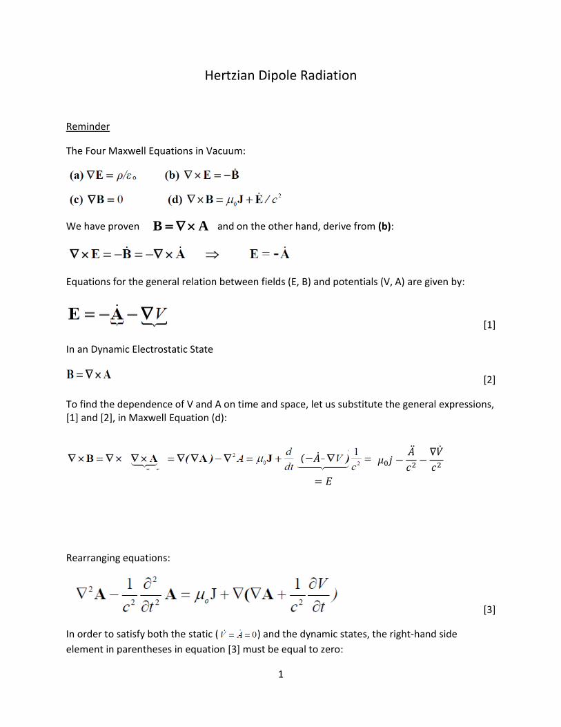
1

Hertzian Dipole Radiation

Reminder

The Four Maxwell Equations in Vacuum:

We have proven AB and on the other hand, derive from (b):

Equations for the general relation between fields (E, B) and potentials (V, A) are given by:

[1]

In an Dynamic Electrostatic State

[2]

To find the dependence of V and A on time and space, let us substitute the general expressions, [1] and [2], in Maxwell Equation (d):

Rearranging equations:

[3]

In order to satisfy both the static ( ) and the dynamic states, the right-hand side

element in parentheses in equation [3] must be equal to zero:

.

= 𝐸

𝜇0𝑗 −𝐴ሷ

𝑐2−

∇𝑉ሶ

𝑐2 (−𝐴ሶ

2

[4]

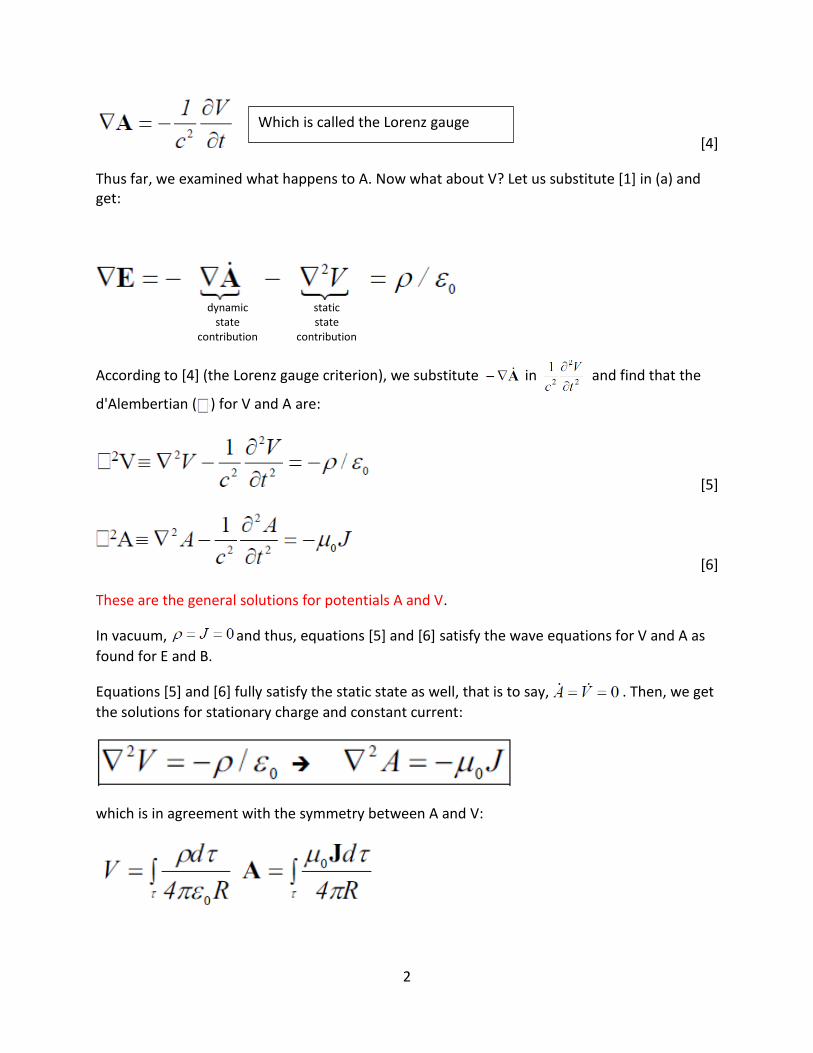
Thus far, we examined what happens to A. Now what about V? Let us substitute [1] in (a) and get:

dynamic

state contribution

static state

contribution

According to [4] (the Lorenz gauge criterion), we substitute in and find that the

d'Alembertian ( ) for V and A are:

[5]

[6]

These are the general solutions for potentials A and V.

In vacuum, and thus, equations [5] and [6] satisfy the wave equations for V and A as

found for E and B.

Equations [5] and [6] fully satisfy the static state as well, that is to say, . Then, we get

the solutions for stationary charge and constant current:

which is in agreement with the symmetry between A and V:

Which is called the Lorenz gauge

3

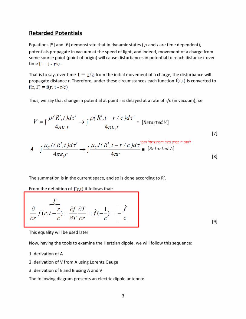
Retarded Potentials

Equations [5] and [6] demonstrate that in dynamic states ( and J are time dependent),

potentials propagate in vacuum at the speed of light, and indeed, movement of a charge from some source point (point of origin) will cause disturbances in potential to reach distance r over time .

That is to say, over time from the initial movement of a charge, the disturbance will

propagate distance r. Therefore, under these circumstances each function is converted to

.

Thus, we say that change in potential at point r is delayed at a rate of r/c (in vacuum), i.e.

[7]

[8]

The summation is in the current space, and so is done according to R’.

From the definition of it follows that:

[9]

This equality will be used later.

Now, having the tools to examine the Hertzian dipole, we will follow this sequence:

1. derivation of A

2. derivation of V from A using Lorentz Gauge

3. derivation of E and B using A and V

The following diagram presents an electric dipole antenna:

[𝑅𝑒𝑡𝑎𝑟𝑡𝑒𝑑 𝑉] [𝑅𝑒𝑡𝑎𝑟𝑡𝑒𝑑 𝑉]

[𝑅𝑒𝑡𝑎𝑟𝑡𝑒𝑑 𝐴]

להוסיף פסיק מעל דיפרנציאל הזמן

4

The changes over time in the electrical dipole which result from the flow of charge along the antenna are:

(Current in antenna or generation of spark between the two poles)

Let us calculate 𝐴 for a wire of dl length using equation [8]

Remember that:

[10]

According to the figure, (in direction of , which remains constant in our exercise) has two

possible elements in the plane :

Than:

5

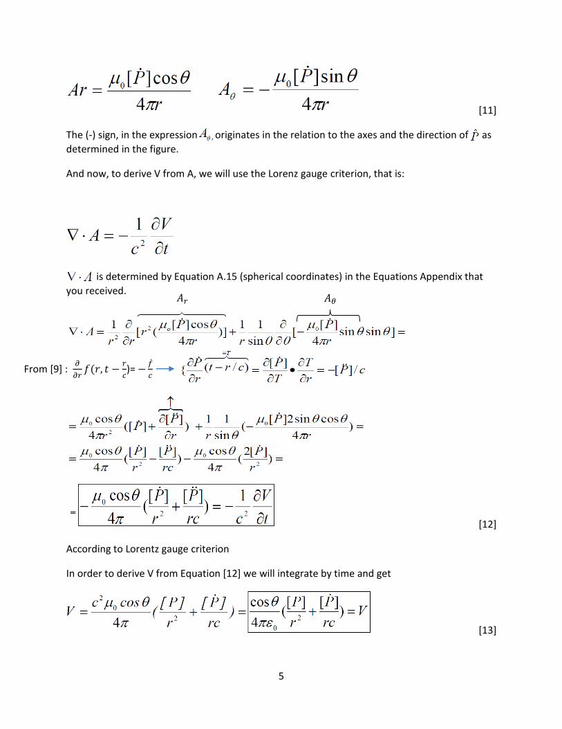
[11]

The (-) sign, in the expression , originates in the relation to the axes and the direction of as

determined in the figure.

And now, to derive V from A, we will use the Lorenz gauge criterion, that is:

is determined by Equation A.15 (spherical coordinates) in the Equations Appendix that

you received.

[12]

According to Lorentz gauge criterion

In order to derive V from Equation [12] we will integrate by time and get

[13]

𝐴𝑟 𝐴𝜃

From [9] : 𝜕

𝜕𝑟𝑓(𝑟, 𝑡 −

𝑟

𝑐)= −

𝑓ሶ

𝑐

6

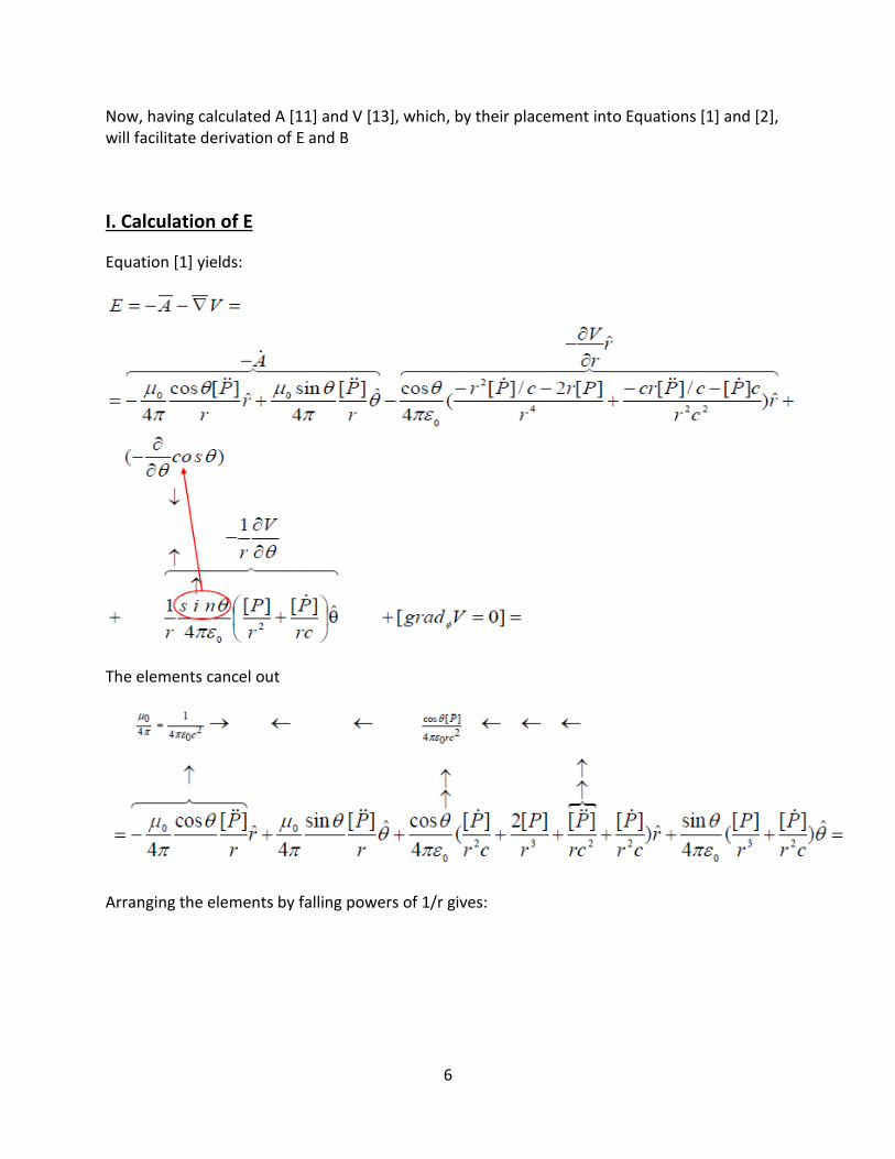
Now, having calculated A [11] and V [13], which, by their placement into Equations [1] and [2], will facilitate derivation of E and B

I. Calculation of E

Equation [1] yields:

The elements cancel out

Arranging the elements by falling powers of 1/r gives:

7

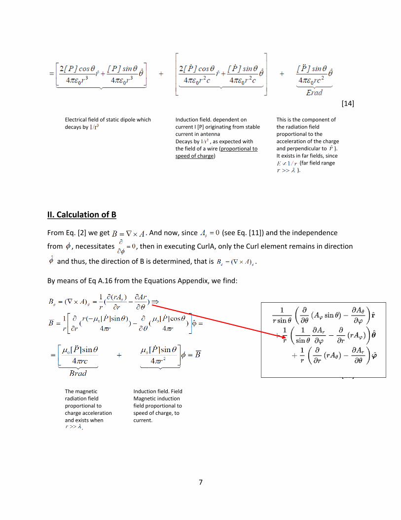
[14]

Electrical field of static dipole which

decays by

Induction field. dependent on current I [P] originating from stable current in antenna

Decays by , as expected with the field of a wire (proportional to speed of charge)

This is the component of the radiation field proportional to the acceleration of the charge and perpendicular to ). It exists in far fields, since

(far field range ).

II. Calculation of B

From Eq. [2] we get . And now, since (see Eq. [11]) and the independence

from , necessitates , then in executing CurlA, only the Curl element remains in direction

and thus, the direction of B is determined, that is .

By means of Eq A.16 from the Equations Appendix, we find:

[15]

The magnetic radiation field proportional to charge acceleration and exists when

.

Induction field. Field Magnetic induction field proportional to speed of charge, to current.

8

We see that in near field that is to say very close to the dipole (where the higher powers are dominant) is where the electrostatic dipole field exists ( ) while B=0, and indeed

corresponds with electrostatic charge distribution.

In slightly more distant fields, the induction field is manifested – the near field in which E and B exist as fields derived from quasi static currents. In the far fields only the radiation fields remain

and they satisfy the condition for TEM electromagnetic fields, since is perpendicular to and both are perpendicular to .

Calculation of the ratio E/H – vacuum impedance

Reminder:

Units

J – Joule

C – Coulomb

A – Ampere

The relationship between Erad and Brad (the electric and magnetic radiation fields)

Let us compare the radiation fields E and B by converting in equation [15] for Brad

and get:

[16]

Origin?

9

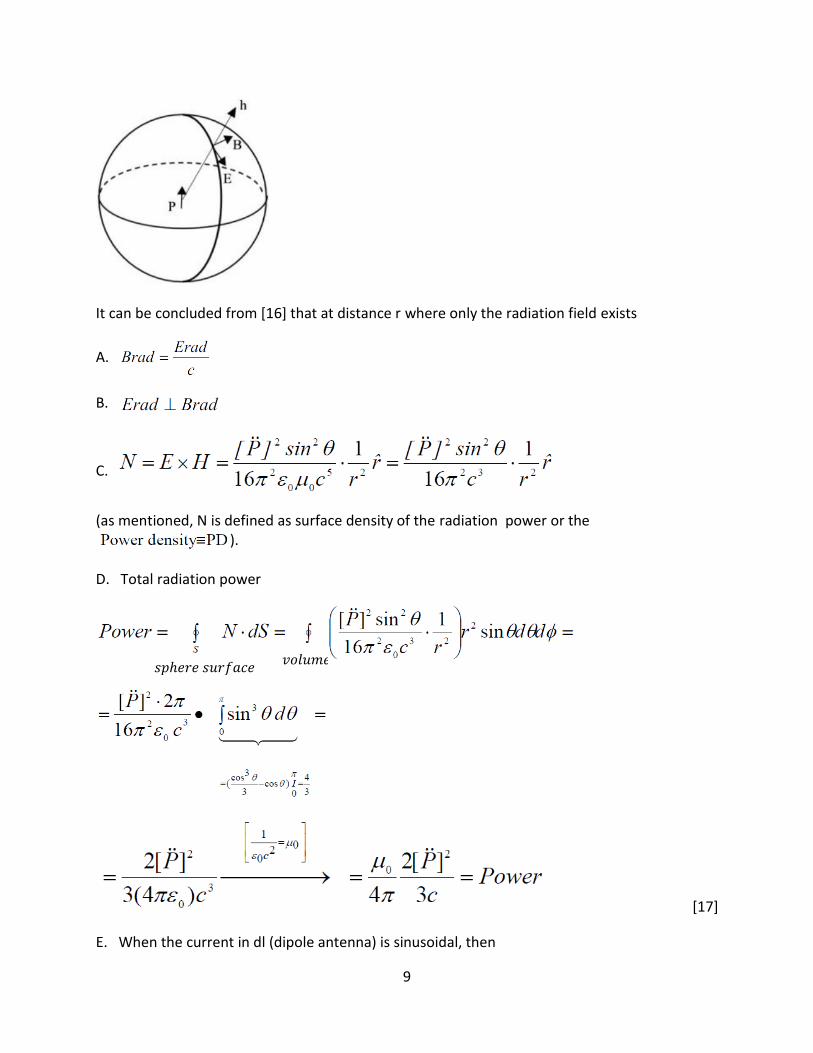
It can be concluded from [16] that at distance r where only the radiation field exists

A.

B.

C.

(as mentioned, N is defined as surface density of the radiation power or the ).

D. Total radiation power

[17]

E. When the current in dl (dipole antenna) is sinusoidal, then

𝑠𝑝ℎ𝑒𝑟𝑒 𝑠𝑢𝑟𝑓𝑎𝑐𝑒 𝑣𝑜𝑙𝑢𝑚𝑒

10

and so:

and therefore:

whereas time averaging gives ( )

[18]

The average radiation power over time from a radiating dipole can be acquired by substituting [18] into [17] which yields:

[19]

From Equation [19] we learn that radiation intensity of an antenna is proportional to the fourth power of radiation frequency (the current in the antenna).

Dependence of Radiation Intensity on Dipole Current

,

and therefore:

Intensity Power

If then

11

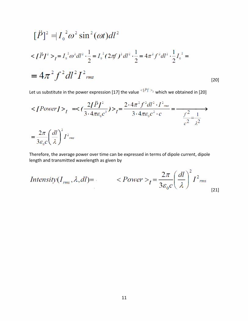
[20]

Let us substitute in the power expression [17] the value which we obtained in [20]

Therefore, the average power over time can be expressed in terms of dipole current, dipole length and transmitted wavelength as given by

[21]