Motion of Charged Particles in Magnetic Dipole Fields ...

Manuel GRILL

Motion of Charged Particlesin Magnetic Dipole Fields

Dependent on Time

MASTER THESIS

written to obtain the Academic Master Degree

Individual Master Curriculum Theoretical Plasma Physics

Karl Franzens University Graz

SupervisorHelfried K. Biernat

Auxiliary SupervisorsIgor V. Kubyshkin

Vladimir S. Semenov

Space Research Institute GrazGraz, September 2013

Abstract

This master thesis focuses on trajectories of charged particles in magnetic dipole fieldsdependent on time. Such magnetic dipoles induce electric fields. This in turn causesadditional drift motion that is carefully analyzed in a parameter study. A symplecticnumerical scheme guarantees preservation of energy as well as adiabatic invariants ofthe single particle plasma theory. These invariants are examined along the particle’strajectory in order to check the numerical promises.

Keywords: Plasma Theory, Single Particle Approach, Time Dependent MagneticDipole Fields, Symplecticity, Energy Preservation, Adiabatic Invariants, RadiationBelts, Ring Currents

Short Title: Charged Particles in Magnetic Dipole FieldsAuthor: Manuel Grill, BSc BSc (ID: 0630318)Course: 653521, VO 2Sst, Spezialvorlesung zur Theoretischen Physik

(Plasmatheorie(Grundlagen))Institute: Space Research Institute Graz, Austrian Academy of SciencesSupervisors: Helfried K. Biernat, Univ.-Prof.

Igor V. Kubyshkin, Ass.-Prof.Vladimir S. Semeonv, Univ.-Prof.

Statutory Declaration

I declare that I have authored this thesis independently, that I have not used otherthan the declared sources/resources, and that I have explicitely marked all passageswhich has been quotes either literally or by content from the used sources.

. . . . . . . . . . . . . . . . . . . . . . . . . . . . . . . . .date

. . . . . . . . . . . . . . . . . . . . . . . . . . . . . . . . . . . . . . . . . .(signature)

Contents

Introduction 5

1 Theory 71.1 Velocity . . . . . . . . . . . . . . . . . . . . . . . . . . . . . . . . . . . 71.2 Gyro Motion . . . . . . . . . . . . . . . . . . . . . . . . . . . . . . . . 71.3 Guiding Center . . . . . . . . . . . . . . . . . . . . . . . . . . . . . . . 81.4 Magnetic Moment . . . . . . . . . . . . . . . . . . . . . . . . . . . . . . 91.5 Drift Motion . . . . . . . . . . . . . . . . . . . . . . . . . . . . . . . . . 91.6 Pitch Angle . . . . . . . . . . . . . . . . . . . . . . . . . . . . . . . . . 111.7 Magnetic Mirror . . . . . . . . . . . . . . . . . . . . . . . . . . . . . . . 121.8 First Adiabatic Invariant . . . . . . . . . . . . . . . . . . . . . . . . . . 131.9 Magnetic Dipole Field . . . . . . . . . . . . . . . . . . . . . . . . . . . 15

2 Numerics 192.1 Dimensionless Equations: Overview . . . . . . . . . . . . . . . . . . . . 192.2 Dimensionless Equations: Details . . . . . . . . . . . . . . . . . . . . . 202.3 Numerical Scheme . . . . . . . . . . . . . . . . . . . . . . . . . . . . . 212.4 Implementation . . . . . . . . . . . . . . . . . . . . . . . . . . . . . . . 252.5 Maxima and Averaging . . . . . . . . . . . . . . . . . . . . . . . . . . . 25

3 Testcases 273.1 Testcase: Gyro Motion . . . . . . . . . . . . . . . . . . . . . . . . . . . 273.2 Testcase: Drift Motion . . . . . . . . . . . . . . . . . . . . . . . . . . . 29

4 Parameter Study: Pitch Angle 314.1 Case α1 = π/2 . . . . . . . . . . . . . . . . . . . . . . . . . . . . . . . . 324.2 Case α2 = π/4 . . . . . . . . . . . . . . . . . . . . . . . . . . . . . . . . 334.3 Case α3 = π/8 . . . . . . . . . . . . . . . . . . . . . . . . . . . . . . . . 354.4 Numerical Pitch Error . . . . . . . . . . . . . . . . . . . . . . . . . . . 354.5 Numerical Energy Error . . . . . . . . . . . . . . . . . . . . . . . . . . 35

5 Parameter Study: Shell Parameter 375.1 Trajectories . . . . . . . . . . . . . . . . . . . . . . . . . . . . . . . . . 375.2 Invariants . . . . . . . . . . . . . . . . . . . . . . . . . . . . . . . . . . 37

6 Parameter Study: Time Dependence 406.1 Case ε1 . . . . . . . . . . . . . . . . . . . . . . . . . . . . . . . . . . . . 42

3

Contents 4

6.2 Cases ε2, ε3 . . . . . . . . . . . . . . . . . . . . . . . . . . . . . . . . . . 426.3 Increase of Energy . . . . . . . . . . . . . . . . . . . . . . . . . . . . . 44

7 Conclusions 467.1 Results and Relative Errors . . . . . . . . . . . . . . . . . . . . . . . . 467.2 Conclusion . . . . . . . . . . . . . . . . . . . . . . . . . . . . . . . . . . 477.3 Outlook . . . . . . . . . . . . . . . . . . . . . . . . . . . . . . . . . . . 47

8 Appendix A: Plots for ε 6= 0 50

9 Appendix B: Decrease of Energy Error 54

10 Appendix C: Source Code 5610.1 Main File . . . . . . . . . . . . . . . . . . . . . . . . . . . . . . . . . . 5610.2 Fields and Force Functions . . . . . . . . . . . . . . . . . . . . . . . . . 5810.3 Plots, Data and Error Calculation . . . . . . . . . . . . . . . . . . . . . 5910.4 Units . . . . . . . . . . . . . . . . . . . . . . . . . . . . . . . . . . . . . 6110.5 Averaging, Maxima for Invariant-Analysis . . . . . . . . . . . . . . . . 61

Introduction

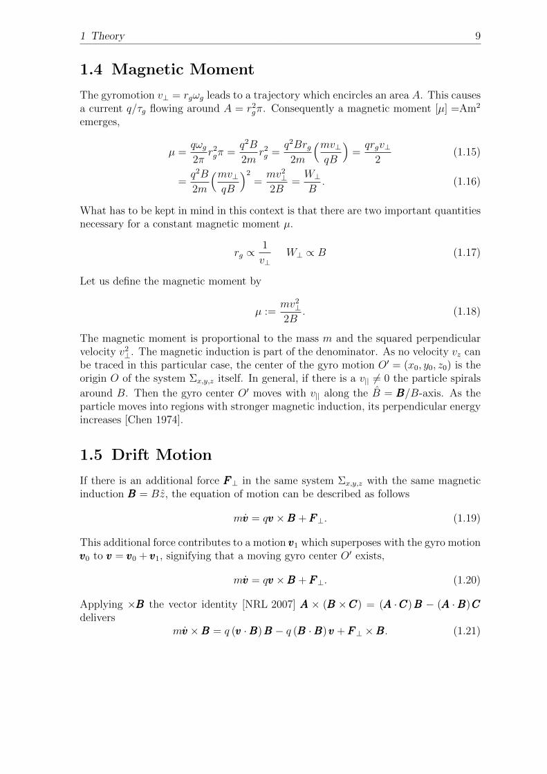
The first pioneer work in the field was led by Størmer’s Professor Birkeland who con-ducted experiments with cathodic rays directed towards an electro-magnetic globe[Størmer 1906] designed to resemble and thus represent the Earth (radius RE = 6371km). This representation of one of the planets of our solar system was reduced in sizeto a diameter of 40 - 75 mm and placed in a vacuum tube. Unlike the varied landscapeof the blue planet its surface consisted of brass and was covered with a coat of bariumplatinocyanide. While conducting the experiments, the scientists noticed that currentsof nearly parallel cathodic rays created a regular phosphorescence on the dayside ofthe globe. These lights raised attention as they behaved differently when being underthe influence of a magnet. Activating the magnet it was noticed that these lights weredeflected to the vicinity of both poles to form phosphorescent belts that were foundto represent the auroral activity on Earth [Størmer 1906]. Particularly striking in thisrespect is the fact that not only belts of lights were observed but also luminous shiningrings, which have become known as ring currents in the field of modern space sciences[Prolss 2004].

In order to accurately describe these experiments, Størmer performed numerical cal-culations in cooperation with his students based on the equation of motion

mdtvvv = qvvv ×BBB. (0.1)

The magnetic induction B was chosen to be a dipole field with a constant magneticmoment ME along the z axis of a coordinate system Σx,y,z [Størmer 1906].

BBB =µ0ME

4πr5

−3xz−3yzr2 − 3z2

(0.2)

These calculations support the experimental results and corroborate the scientist’s the-ory. However, the afore mentioned radiation belts (1.2 < L < 2.5) predicted by Birke-land were discovered years later by other scientists researching the field [Prolss 2004].While Størmer’s calculations took hours [figure 0.1], at present scientists manage topredict the trajectory of particles within seconds using modern computer systems.Of course personal experience may also influence the duration of code implementa-tion, taking up a few minutes, but overall the new systems have brought along manyadvantages for the evaluation of data. As modern computer systems equipped withthe latest software are at scientists disposal, e.g., [MathWorks 2012], trajectories canbe evaluated faster and more accurately than in the past. Scientists appreciate the

5

Introduction 6

benefits which this developement has brought along and they highly value the newtechnological equipment now accessible to them.

This master thesis employs a symplectic method presented in section Numerics usedto describe the dynamics of a charged particle in a magnetic dipole field dependent ontime, but also suitable for arbitrary applications with different fields of force.

Figure 0.1: The computation of this trajectory has taken more than 100 hours[Størmer 1906].

1 Theory

A charged particle with a charge qs and a mass ms is moving along a trajectoryC(t) ∈ R3 according to the well-known equation of motion with the forces

msdtvvvs = qs(vvvs ×BBB +EEE) (1.1)

in which s is the index of particle species. The main objective of this thesis is to finda trajectory

C(t) : R→ R3 (1.2)

t 7→ xxx(t) (1.3)

for given initial values. The used vector fields are of the form

vvv = dtxxx = xxx, EEE(t,xxx), BBB(t,xxx) ∈ R3. (1.4)

The qualitative analysis of such trajectories C for basic field configurations can showthe fundamental behaviour of a charged particle in magnetic and electric fields. Atthe end all the basic types of motion can be combined to give us a physical pictureof more complicated cases. If these trajectories are numerically calculated the theoryof adiabatic invariants can verify at least physical plausibility. In this chapter, I wantto put forward a theory which will be referred to as the well-known Single ParticleApproach [Chen 1974], [Nicholson 1983], [Prolss 2004].

1.1 Velocity

The dot product of the velocity vector vvv and the local magnetic field BBB is used todescribe the parallel velocity

v|| :=vvv ·BBBB

. (1.5)

The energy balance equation demands

v2 − v2|| = v2⊥. (1.6)

1.2 Gyro Motion

In a coordinate system Σx,y,z with the origin O, the particle with qs,ms moves alongxxx(t) = x(t)x + y(t)y + z(t)z according to the field BBB = Bz z with a constant Bz > 0.

7

1 Theory 8

The electric field is assumed to be EEE = 000. For such a configuration the equation ofmotion reduces to

vx =qsB

ms

vy, vy = −qsBms

vx, vz = 0. (1.7)

By convention, |qs|B/ms = ωg, the gyro frequency will always be positive, becausems > 0. Taking the integral, we get

x = ωgy, y = −ωgx. (1.8)

The combination of equation (1.7) and (1.8) delivers

x+ ωgx = 0, y + ωgy = 0. (1.9)

A solution of such differential equations is

x− x0 = −rg cos(ωgt) y − y0 = ±rg sin(ωgt). (1.10)

Symbol ± denotes the sign of qs, and rg is called the gyro radius.

rg :=v⊥ωg

=msv⊥|qs|B

(1.11)

rg may be derived from the equation (1.1),

mv2⊥rg

= v⊥qB ⇒ rg =mv⊥qB

. (1.12)

Here we have the physical picture of a particle gyrating around the point O′ =(x0, y0, 0). Ions gyrate clockwise around a field Bz with B > 0 in a right-hand sys-tem Σx,y,z. Electrons gyrate counter-clockwise. The gyro radius is proportional tothe particle’s velocity and its mass, which means a greater gyro radius for ions. Thegreater the magnetic induction is, the smaller is the gyroradius. This rather crudeapproach assumes the field BBB not to be affected by the gyro motion, though the par-ticles are diamagnetic. With the initial values x(0) = −rg, y(0) = 0 and x(0) = 0,

y(0) =√

2W⊥/ms = v⊥ an ion (qs > 0) gyrating around (x0, y0) = (0, 0) will suffice

x = −rg cos(ωgt) y = ±rg sin(ωgt), (1.13)

which may be interpreted as an harmonic oscillator [Chen 1974], [Prolss 2004].

1.3 Guiding Center

The motion of an electrically charged particle in a magnetic field can be simplified bythe concept of the guiding center. We have already met the point O′ which is calledguiding center, since the averaged path of the particle follows the guiding center’strajectory C ′.

〈xxx(t)〉τg :=1

τg

∫ τg

0

xxx(t)dt = O′ −O = O′ (1.14)

The gyro motion is assumed to be very fast as compared to the superposed driftmotion.

1 Theory 9

1.4 Magnetic Moment

The gyromotion v⊥ = rgωg leads to a trajectory which encircles an area A. This causesa current q/τg flowing around A = r2gπ. Consequently a magnetic moment [µ] =Am2

emerges,

µ =qωg2π

r2gπ =q2B

2mr2g =

q2Brg2m

(mv⊥qB

)=qrgv⊥

2(1.15)

=q2B

2m

(mv⊥qB

)2=mv2⊥2B

=W⊥B. (1.16)

What has to be kept in mind in this context is that there are two important quantitiesnecessary for a constant magnetic moment µ.

rg ∝1

v⊥W⊥ ∝ B (1.17)

Let us define the magnetic moment by

µ :=mv2⊥2B

. (1.18)

The magnetic moment is proportional to the mass m and the squared perpendicularvelocity v2⊥. The magnetic induction is part of the denominator. As no velocity vz canbe traced in this particular case, the center of the gyro motion O′ = (x0, y0, z0) is theorigin O of the system Σx,y,z itself. In general, if there is a v|| 6= 0 the particle spirals

around B. Then the gyro center O′ moves with v|| along the B = BBB/B-axis. As theparticle moves into regions with stronger magnetic induction, its perpendicular energyincreases [Chen 1974].

1.5 Drift Motion

If there is an additional force FFF⊥ in the same system Σx,y,z with the same magneticinduction BBB = Bz, the equation of motion can be described as follows

mvvv = qvvv ×BBB +FFF⊥. (1.19)

This additional force contributes to a motion vvv1 which superposes with the gyro motionvvv0 to vvv = vvv0 + vvv1, signifying that a moving gyro center O′ exists,

mvvv = qvvv ×BBB +FFF⊥. (1.20)

Applying ×BBB the vector identity [NRL 2007] AAA × (BBB ×CCC) = (AAA ·CCC)BBB − (AAA ·BBB)CCCdelivers

mvvv ×BBB = q (vvv ·BBB)BBB − q (BBB ·BBB)vvv +FFF⊥ ×BBB. (1.21)

1 Theory 10

Averaging this equation over gyro periods τg = 2π/ωg leads to

〈mvvv ×BBB〉τg = 〈q (vvv ·BBB)BBB〉τg − 〈q (BBB ·BBB)vvv〉τg + 〈FFF⊥ ×BBB〉τg . (1.22)

Here 〈mvvv ×BBB〉τg = 000 and 〈q (vvv ·BBB)BBB〉τg = 000 is prescribed. The last assumptionmeans that we are interested in averaged perpendicular motion. The magnetic field is〈BBB〉τg = Bz.

uuuD := 〈vvv〉τg =〈FFF⊥〉τg ×BBB

qB2(1.23)

〈xxx = xxx0 + xxx1〉τg points at the gyro center O′. Originating from this gyro center O′

is the system Σ′ which moves with a specific speed uuuD, also known as drift velocity[Chen 1974], [Prolss 2004],

uuuD =FFF⊥ ×BBBqB2

. (1.24)

Electro Drift

A force qEEE⊥ causes the gyrating particle to drift with

uuuD =qEEE⊥ ×BBBqB2

=EEE⊥ ×BBBB2

. (1.25)

The difference of the gyro radius during one gyro period causes the drift motion. Thisdifference is generated by the electric field decelerating the particle on one side. Thiscan be seen from

rg =mv⊥qB∝ v⊥. (1.26)

On the other half-cycle the particle gains energy. Electrons and ions gyrate in oppositedirections which, in combination with the opposite acceleration, leads to the same driftdirection.

Gradient Drift

If a gyrating particle with vvv⊥ moves in a system Σx,y,z, the inhomogeneous magneticinduction BBB = BBB (x, y, z) causes a force FFF⊥ = −µ∇∇∇⊥B [Prolss 2004]. The result is

uuuD =−µ∇∇∇⊥B ×BBB

qB2. (1.27)

Curvature Drift

At a time t = t0 the guiding center O′ lies at O = O′. The center is assumed to startwith a velocity v′. Due to the inhomogeneous field BBB the velocity vvv′ doesn’t remainconstant. The system Σ′(t) with the gyro center O′(t) moves along a curved path withvvv′ because of the force −µ∇∇∇B. The gyrating particle with the magnetic moment µµµ is

1 Theory 11

forced to stay antiparallel to the magnetic induction BBB. Its curved path contributesto a force

FFF =mv′2

Rc

Rc. (1.28)

Rc is the curvature radius of the gyro center’s motion v′. As a consequence a curvaturedrift motion emerges. At regions where the vectors Rc⊥BBB we have

uuuD =mv′2

Rc

Rc ×BBB

qB2. (1.29)

This drift caused by centrifugal forces has to be combined with the gradient drift fromabove [Chen 1974], [Prolss 2004].

1.6 Pitch Angle

The pitch angle α measures the angle between the velocity vector and the local mag-netic field. Then the pitch angle α is defined by

tanα :=v⊥v||. (1.30)

In a coordinate system Σx,y,z, the velocity vvv may be calculated by

vx = v cosφ sinα, (1.31)

vy = v sinφ sinα, (1.32)

vz = v cosα. (1.33)

Here φ is set φ = 0. Quantity α = π/2 means a planar motion and α = 0 describesa particle moving along a magnetic field line without any gyro motion. However, ifα 6= 0 at the time of t = 0, the particle gyrates around let us say z = 0. The initialvelocities, magnetic moment and total energy then is

vz (0) , v⊥ (0) , µ (0) ∝ v2⊥ (0) /B (0) , W (0) ∝ v2z (0) + v2⊥ (0) . (1.34)

The velocity vvv was split into vvv = vvv⊥+vvv||. The total energy and the magnetic momentis conserved. The magnetic induction at z = 0 is

‖BBB (0)‖ = Bmin. (1.35)

At the turning point v|| (t = tm) = 0 the entire parallel energy is transferred into themotion perpendicular to z. The magnetic induction at t = tm reaches its maximumB (t = tm) = Bmax,

µ =mv2⊥ (0)

2Bmin

=mv2⊥ (tm)

2Bmax

=m(v2|| (0) + v2⊥ (0)

)2Bmax

= const. (1.36)

1 Theory 12

v2⊥ (0)

v2⊥ (0) + v2|| (0)=Bmin

Bmax

(1.37)

The magnetic moment

µ =W⊥B

=m

2

v2 sin2 α

B= constant (1.38)

in combination with the energy preservation v2 = constant brings about

W⊥B

=m

2

v2 sin2 α

B⇒ sin2 α

B= constant. (1.39)

At the mirror points xxx(tm) the initial kinetic energy v2(0) = v2⊥(0)+v2||(0) is completelytransferred into perpendicular energy

v2(0) = v2⊥(tm) (1.40)

because of v2||(tm) = 0. This gives rise to

µ =v(0)2 sin2 α

B(0)=

v(0)2

B(tm)= constant, (1.41)

sin2 α =B(tm)

B(0), (1.42)

⇒ α = sin−1

(√B(tm)

B(0)

). (1.43)

If another particle starts its motion from the same position with the same initial energybut with a different angle

α′ < α, (1.44)

the particle will pass the reflection point at xxx(tm) [Chen 1974].

1.7 Magnetic Mirror

A particle is placed in a system ΣR,φ,z with a certain magnetic induction BBB, whichcontinuously changes along the z direction. BBB has to respect

∇∇∇ ·BBB =1

R(∂RRBR) +

1

R(∂φBφ) + ∂zBz. (1.45)

The magnetic field BBB can be simplified to a certain extent, Bφ = 0,

∇∇∇ ·BBB =1

R(∂RRBR) + (∂zBz) = 0, (1.46)

RBR = −∫ R

0

R∂zBzdR ≈ −1

2R2∂zBz, (1.47)

BR ≈ −R

2∂zBz. (1.48)

1 Theory 13

In this case ∂zBz 6= f (R) is assumed. For a gyrating particle R = rg and v⊥ = −vφthe equation of motion delivers a force parallel to z.

F|| = −qvφBR = qv⊥BR = −qv⊥R

2∂zBz = −qv⊥

rg2∂zBz (1.49)

= −qv2⊥

2ωg∂zBz = −mv

2⊥

2B∂zBz = −µ∂zBz = −µ∂zBz (1.50)

A gyrating particle with µµµ moving along z is affected by a force

F|| = −µ∂zBz. (1.51)

As the particle moves into regions with stronger magnetic induction, the −µ∇∇∇||Bforce causes a reflection at v||(tm) = 0. The particle spirals along z and its gyroradiusrg = mv⊥/(qB) decreases since B increases. The gyrating particle with the magneticmoment µµµ will inevitably turn around at xxx(tm). In general, the vector equation is

FFF || = −µ∇∇∇||B. (1.52)

This force turns out to be a trap for gyrating particles. This explains, e.g., naturalmirrors in the Earth’s radiation belts [Chen 1974], [Prolss 2004].

1.8 First Adiabatic Invariant

The conservation of µ is very important for the theory. The integral along the particle’strajectory C is

2m

q

∫µdt = 2

m

q

∫mv2⊥2B

dt =

∫mv2⊥ωg

dt =

∫mv⊥rgdt. (1.53)

In general, the action integral of any periodic motion∮pdq taken over its period with

the generalized momentum p and coordinate q is a constant of the motion. The integralalong the trajectory C is approximately the action integral of the gyro motion withp = mv⊥ and dq = rgdt [Chen 1974],∫

mv⊥rgdt ≈∮pdq = constant (1.54)∫

mv⊥rgdt ≈∮mv⊥rgdt = 2πrgmv⊥ = 4π

m

qµ = constant. (1.55)

Then µ is called the first adiabatic invariant [Ozturk 2011], [Northrop, Teller 1960].The invariance has to be checked carefully for arbitrary fieldsBBB [Borovsky, Hansen 1991],[Hall 1980]. The first adiabatic invariant

〈µ〉τg =

∫τg

mv2⊥2B

dt = constant (1.56)

1 Theory 14

will be adiabatically preserved for fields BBB(t, x, y, z) obeying the following conditions[Prolss 2004].

B

∇B>> rg (1.57)

B

∂tB>> τg (1.58)

µ in Magnetic Mirrors

We know the force −µ∇∇∇||B from the last sections which can be expressed by F|| =−µ∂B/∂s. dsss is the line element along BBB. As the gyrating particle moves into regionsof stronger B, the magnetic moment should stay adiabatically invariant. In order toprove the invariance, let us assume

md

dtv|| = −µ

∂

∂sB (1.59)

which leads to the equation below after multiplying v|| on the left hand side and ds/dton the right hand side [Chen 1974].

d

dt(1/2mv2||) = −µ d

dtB (1.60)

The equation above in combination with the preservation of energy

d

dt(1/2mv2|| + 1/2mv2⊥) =

d

dt(1/2mv2|| + µB) = 0 (1.61)

gives usd

dt(1/2mv2||) +

d

dt(µB) = −µ d

dtB +

d

dt(µB) = 0. (1.62)

This proves the magnetic moment µ to be an invariant [Chen 1974],

Bd

dtµ = 0. (1.63)

µ in Time Dependent Magnetic Fields

For time dependent magnetic fields the first adiabatic invariant has to be treated again[Chen 1974], [Olszewski, Rolinski 1999]. The equation∇∇∇×EEE = −BBB explains the raiseof an electric field which leads to an acceleration. A magnetic field cannot impartenergy to the particle, but this electric field can change the energy balance. In theparameter study section we will see such a perpendicular increase of energy for driftingparticles. However, the magnetic moment for slowly varying magnetic fields is still anadiabatic invariant [Chen 1974]. This fact has to be checked. For simplicity, let us

1 Theory 15

neglect v|| and we consider vvv⊥ = dlll/dt alone. Since dlll is the element of the gyratingparticle’s path, the line integral along C is alomst closed,∫

C

qEEE · dlll ≈∮C

qEEE · dlll = q

∫A(C)

(∇∇∇×EEE) · dAAA = −q∫A(C)

BBB · dAAA. (1.64)

The electric work EEE · dlll is equal to the increase of energy δ(1/2mv2⊥) which leads to

δ(mv2⊥

2

)= −q

∫A(C)

BBB · dAAA = ±qBπr2g . (1.65)

Electrons gyrate positively and ions gyrate negatively which gives us the ± in theequation above. The + is for the ions and − for the electron case. After substitutingrg = mv⊥/(qB) and ωg = qB/m the equation above reduces to

δW⊥ = ±qπB v2⊥m

qBωg=mv2⊥2B

2πB

ωg. (1.66)

As before, µ is equal to W⊥/B which results in

δW⊥ = µB

fg. (1.67)

B/fg is the change δB during one period. Thus we have with W⊥ = µB

δW⊥ = δ(µB) = µδB. (1.68)

This is the desired resultδµ = 0. (1.69)

Then µ is proven to be an adiabatic invariant in slowly varying magnetic fields [Chen 1974].

1.9 Magnetic Dipole Field

Magnetic dipole fields can be defined in different ways, depending on the focus of theresearch. Apart from a description with elliptic integrals [Grill 2012] it is also possibleto define a potential [V ] = A as illustrated in [Biernat 2012]. In addition to thesemethods of illustration there is still the possibility to use a potential [U ] = V/m asdepicted in [Størmer 1906]. The following chapter focuses on a field with two magneticpoles pi.

Magnetic Potential V

In this case, the unit of the poles is

[pi] = Vs. (1.70)

1 Theory 16

The physical units1 are dependent on a factor K in the potential V ,

K

(p1r1

+p2r2

)=

1

4πµ0

(p1r1

+p2r2

). (1.71)

This factor K contributes to the units [V ] = A and [−∇∇∇rV ] = A/m. It is assumed∑i

pi = 0⇒ p1 + p2 = 0⇒ p1 = −p2 = p, (1.72)

because magnetic monopoles have not been observed. The poles pi are placed on theaxis z around the origin O at z = 0 with a distance 2s in a system Σx,y,z = Σr,θ,φ. Thepotential V (r) at a point P = O (z = 0) + rrr is a function of the distances ri betweenthe poles and the point P . These distances are not equal. For the approximations << r one gets

r1 + ∆r = r = r2 −∆r. (1.73)

With r2 = r + ∆r, r1 = r −∆r the potential V becomes

V =1

4πµ0

(p

r −∆r+−p

r + ∆r

)=

p

4πµ0

(1

r −∆r− 1

r + ∆r

)(1.74)

V =p

4πµ0

(r + ∆r − r + ∆r)

(r −∆r) (r + ∆r)=

p

4πµ0

2∆r

(r2 −∆r2). (1.75)

In this particular case ∆r2 can be neglected. ∆r = s cos θ,

V ≈ 1

4πµ0

2ps cos θ

r2. (1.76)

For an elementary dipole s goes to s→ 0 while M = 2ps 6= 0 <∞,

V ≈ 1

4πµ0

M cos θ

r2. (1.77)

If s→ sss along z is introduced, M changes M →MMM = Mz,

V ≈ 1

4πµ0

M cos θ

r2r

r=

1

4πµ0

Mr cos θ

r3=

1

4πµ0

MMM · rrrr3

. (1.78)

The magnetic moment M has the units [M ] = Vsm. Applying −∇∇∇r,θ,φ calls themagnetic field2 HHH into existence,

HHH =1

4πµ0

M

r3

2 cos θsin θ

0

, with [M = 2 (p) s] = (Vs)m. (1.79)

1K = µ0/(4π) leads to [pi] = Am. Consequently the final result is [−∇∇∇rV ] = Vs/m2.2The magnetic induction is BBB = µ0M(2 cos θ, sin θ, 0)/(4πr3). K = µ0/(4π)⇒ [M ] = Am2.

1 Theory 17

In this respect it can be said that a pole p without any mass moves along a curveaccording to HHH,

dr ∝ Hr ∝ 2 cos θ (1.80)

rdθ ∝ Hθ ∝ sin θ. (1.81)

Due to the symmetry of HHH the curve r = r (θ, φ) is a planar one r = r (θ),

r = l sin2 θ. (1.82)

l is the length of r at θ = π/2. l = LRE is usually compared with RE = 6371 km.The curvature radius Rc at θ = π/2 is

Rc

(π2

)=

∣∣∣∣∣∣∣√r2 + (∂θr)

23

r2 + (∂θr)2 − r∂2θ,θr

∣∣∣∣∣∣∣ =l

3. (1.83)

The result of the Rc is important for the calculation of the curvature drift motion.

Magnetic Potential U

In [Størmer 1906] a magnetic potential U with a coordinate system Σx,y,z is used inorder to analyse trajectories in a cylindrical system Σρ,φ,z,

U =zM

r3. (1.84)

From this potential the magnetic induction BBB can be derived.

∇∇∇U = BBB (1.85)

In this context it is also worth noting ∆U = 0 has to be valid to obtain ∇∇∇ ·BBB = 0.Thus one has a current free region [Biernat 2012]. With

∂xr =x

r(1.86)

∂yr =y

r(1.87)

∂zr =z

r(1.88)

the equations as outlined below may be derived,

∇∇∇U =∇∇∇zMr3

= M

−3r−4xr−1z−3r−4yr−1z

−3r−4zr−1z + r−3

(1.89)

∇∇∇U =M

r5

−3xz−3yz−3z2 + r2

= −Mr5

3xz3yz

3z2 − r2

(1.90)

∇∇∇U =M

r5

00r2

− 3

xzyzz2

= BBB(x, y, z). (1.91)

1 Theory 18

Time Dependent Moment

If the magnetic moment M is a function of time M = M(t) the magnetic inductionBBB (x, y, z) becomes BBB (t, x, y, z). As a consequence the need to calculate the emergingelectric field arises. In a spherical coordinate system ΣR,θ,φ the magnetic inductionBBB(t, R, θ, φ) is

BBB =µ0

4π

M(t)

r3

2 cos θsin θ

0

, with [M ] = Am2. (1.92)

The emerging electric field Eφ can be derived from

−∂tBBB =∇∇∇×EEE (1.93)

−∂t∮A

BBB · dAAA =

∮∂A

EEE · dlll. (1.94)

The surface element at r = constant is dAAA = ndA = rr2 sin θdθdφ and the line elementis dlll = φr sin θdφ. The flux through the surface A (r = const.) is a function of Br,because θ · n = θ · r = 0 is assumed to be valid,

−∂t∫ θ′

θ=0

∫ 2π

φ=0

Brr2 sin θdφdθ =

∫ 2π

φ=0

Eφr sin θdφ (1.95)

−∂t∫ θ′

θ=0

µ0M (t)

4πr32 cos θr2 sin θdθ = Eφr sin θ (1.96)

−µ0M

2πr

∫ θ′

θ=0

dθdθ(sin2 θ

)= Eφr sin θ (1.97)

−µ0M

2πrsin2 θ = Eφr sin θ (1.98)

−µ0M

2πr2sin θ = Eφ. (1.99)

The occurring electric field in spherical coordinates ΣR=r,θ,φ is

EEE =µ0M

4πr2

00

−2 sin θ

. (1.100)

In a coordinate system Σx,y,z with the same origin O as O (ΣR=r,θ,φ or Σρ,φ,z), theplanar (Ez = ER = Eρ = Eθ = 0) electric field is

Ex

(10

)+ Ey

(01

)= Eφ

(− sinφcosφ

)=

Eφr sin θ

(−yx

). (1.101)

In this way, the following result in Σx,y,z can be obtained,

EEE =Eφ

r sin θ

(−yx

)= −2Mµ0 sin θ

4πr2r sin θ

(−yx

)=Mµ0

2πr3

(y−x

). (1.102)

2 Numerics

The main objective of this section is to illustrate how trajectories for particles with acertain initial total energy v2ims/2 and pitch angle α can be numerically calculated. Fornumerical considerations to make sense, the physical equations have to be dimension-less. So all quantities have to be transformed into a dimensionless input. Additionallya symplectic numerical scheme is introduced which is used for the parameter studypresented in the next section. The source code can be found in Appendix C.

2.1 Dimensionless Equations: Overview

The quantities A∗ of the used equations are compared with representative values A0

in order to deliver dimensionless quantities A∗ = A0A⇒ A. For A0 obtained data canbe combined [Prolss 2004].

• gyro radius rg

• gyro frequency ωg

• charge of protons and electrons qs = ±1.6021773E-19 As

• mass of electrons and protons me = 9.109390E-31 kg,mp = 1836.152585 ·me

• magnetic momentum of the Earth’s dipole field ME = 7.7E22 Am2

• the Earth’s averaged radius RE = 6.371E6 m

• magnetic field constant µ0 = 4πE-7 Vs/(Am)

The following set of dimensionless equations

dtvvv = vvv ×BBB +EEE (2.1)

BBB =M

r5

3xz3yz

3z2 − r2

(2.2)

EEE =M

r3

y−x0

(2.3)

(2.4)

can be derived as follows. At the magnetic equator the magnetic field is

B0 =µ0M0

4πr30=µ0ME

4πR3E

= 30E-6 T. (2.5)

19

2 Numerics 20

The magnetic induction causes an electric field E0 = v0B0 with

v0 =RE

t0. (2.6)

1/t0 is the gyro frequency.1

t0=qsB0

ms

(2.7)

xxx∗ = 6371 · [Lx Ly Lz] km⇒ xxx = [Lx Ly Lz] delivers the dimensionless shell parameterL. The preservation of characteristic quantities such as adiabatic invariants or energyare examined in dimensionless units. More details are shown below.

For simplicity the magnetic moment function M(t) is set

M(t) = 1 + εt. (2.8)

2.2 Dimensionless Equations: Details

The dimensionless equation of motion (2.1) is the result of

msd∗tvvv∗ = qsvvv

∗ ×BBB∗ + qsEEE∗ (2.9)

msdtvvvv0t0

= qsvvvv0 ×BBBB0 + qsEEEv0B0 (2.10)

msdtvvvv0t0

= qsv0B0(vvv ×BBB +EEE) (2.11)

Kdtvvv =ms

t0qsB0

dtvvv = vvv ×BBB +EEE. (2.12)

If K is determined to be K = 1 the result is a dimensionless equation of motion

dtvvv = vvv ×BBB +EEE (2.13)

withms

qsB0

= t0 =r0v0. (2.14)

At the magnetic equator θ = π/2 the magnetic induction can be transformed as follows,

B∗ =µ0M

∗

4πr∗3(2.15)

BB0 =µ0MM0

4πr3r30(2.16)

B =µ0M0

B04πr30

M

r3= K

M

r3. (2.17)

Out of K = 1 the following equation

B0 =µ0M0

4πr30=µ0ME

4πR3E

≈ 30E-6 T (2.18)

2 Numerics 21

may be obtained. The occuring electric field at θ = π/2 is

E∗ = −µ0M∗ε∗

2πr∗2(2.19)

Ev0B0 = −µ0MEε02πR2

E

Mε

r2(2.20)

Ev0 = −ε0RE

2π

Mε

r2(2.21)

E = −ε0RE

2πv0

Mε

r2= −KMε

r2. (2.22)

With K = 1, the result is

v0 =ε0RE

2π=

RE

2πt0(2.23)

ε0 =1

t0= ωg (θ = π/2) . (2.24)

The input parameter W ∗ = W0W leads to v,

v0 =RE

t0=REqsB0

ms

(2.25)

W0 =msv

20

2(2.26)√

W ∗

W0

=

√msv∗22

2msv20=√v2 (2.27)

√W = v. (2.28)

2.3 Numerical Scheme

In [Hairer et al 2006] and [Hairer et al 2008] all the numerics can be considered beingnecessary for finding solutions to equations of motion of the form

x = fx (xxx, xxx, t) (2.29)

y = fy (xxx, xxx, t) (2.30)

z = fz (xxx, xxx, t) . (2.31)

For such nonlinear systems of ordinary differential equations [Hairer et al 2006] sug-gests a combination of the method

xxx = fff(xxx, xxx, t) (2.32)

and another methodvvv = ggg(xxx,vvv, t) (2.33)

2 Numerics 22

with parameters A, A ∈ Rs×s and bbb, bbb, ccc, lll ∈ Rs [Hairer et al 2006]. In order to simplifythe notation a 1D problem is devised to substitute the rather complicated 3D one. Itis important to go through all the tricky calculations to understand why the rathersimple looking scheme [equation (2.92)] is called a symplectic one,

li = gx

(t0 + cih, x0 + cix0h+

(Alll)ih2 ... , x0 + (Alll)ih ...

)(2.34)

x(t0 + h) = x0 + x0h+ bbb · lllh2 (2.35)

x(t0 + h) = x0 + bbb · lll. (2.36)

The index i = 1, ... , s goes up to the parameter s. Quantity h is the stepsizeh = ∆t. The system (A, bbb) is the result of a combination of methods (A, bbb) and(A,bbb, ccc) [Hairer et al 2006],

A = AA (2.37)

bbb = bbbA. (2.38)

In a certain sense the system (A,bbb, ccc) belongs to x and (A, bbb) is connected with x. A

combination of these two schemes (bi, aij, ci) and(bi, aij, ci

)x = e (x, v) with (bi, aij, ci) (2.39)

v = g (x, v) with(bi, aij, ci

)(2.40)

for the task x = g (x, x) delivers

ki = e (x0 + haijkj, v0 + haijlj) (2.41)

li = g (x0 + haijkj, v0 + haijlj) (2.42)

x1 = x0 + hbiki (2.43)

v1 = v0 + hbili. (2.44)

If there is an explicit time dependency of the functions v = g (x, v, t) and x = e (x, v, t),there has to be a ci, ci in the numerical scheme. Quantity x = e(x, v, t) = e(v) = vgives rise to the following simplification,

ki = e (x0 + haijkj, v0 + haijlj(t)) = v0 + haijlj(t) (2.45)

li = g (x0 + haijkj, v0 + haijlj, t0 + hci) (2.46)

x1 = x0 + hbiki (2.47)

v1 = v0 + hbili. (2.48)

New symbols(aij, bi

)are used to make the notation easier,

aij = aikakj (2.49)

bi = bkaki (2.50)

2 Numerics 23

ki = v0 + haijlj (2.51)

li = g (x0 + haij (v0 + hajklk) , v0 + haijlj, t0 + cih) (2.52)

x1 = x0 + hbiki = x0 + hbi (v0 + haiklk) (2.53)

v1 = v0 + hbili. (2.54)

Awareness of specific rules for the coefficients aij, bi, ci as shown in [Hairer et al 2006],is useful in this respect, ∑

j

aij = ci (2.55)∑i

bi = 1 (2.56)

ki = v0 + haijlj (2.57)

li = g(x0 + haijv0 + h2aij ajklk, v0 + haijlj, t0 + cih

)(2.58)

= g(x0 + hciv0 + h2aiklk, v0 + haijlj, t0 + cih

)(2.59)

x1 = x0 + hbiv0 + h2biaiklk = x0 + hv0 + h2bklk (2.60)

v1 = v0 + hbili. (2.61)

Then the important coefficients of the combined method are(ci, bi, aij, aij

)with

li = g(x0 + hciv0 + h2aiklk, v0 + haijlj, t0 + cih

)(2.62)

x1 = x0 + hv0 + h2bklk (2.63)

v1 = v0 + hbili. (2.64)

[Hairer et al 2006] states that combined schemes with

biaij + bj aji = bibj ∀i, j = 1, ... , s (2.65)

bi = bi ∀i = 1, ... , s (2.66)

are symplectic methods. For s = 1 the combination of explicit and implicit methodsis shown to be valid,

A = 0, b = 1, c = 0 (2.67)

A = 1, b = 1 (2.68)

A = 0, b = bA = 1. (2.69)

This leads to

x = x0 + hx0 + h2l1 (2.70)

x = x0 + hl1, (2.71)

2 Numerics 24

withl1 = gx (t0, x0, x0 + hl1) . (2.72)

For the case of s = 2

A =

(0 012

12

)(2.73)

bbb =

(1212

)(2.74)

ccc =

(01

)(2.75)

may be chosen. For x another system is used,

A =

(12

012

0

)(2.76)

bbb =

(1212

). (2.77)

The combination results in

A = AA =

(0 012

12

)·(

12

012

0

)=

(0 012

0

), (2.78)

bbb = bbbA =(12

12

)·(

12

012

0

)=(12

0). (2.79)

Such a method is called symplectic [Hairer et al 2006], because of

bibj = biaij + bjaji (2.80)

bi = bi. (2.81)

This can be verified as follows,

a12 + a21

a21 + a12

a11 + a11

a22 + a22

·1

2= bibj =

1

2· 1

2=

1

4(2.82)

0 +1

21

2+ 0

1

2+ 0

0 +1

2

· 1

2=

1

4. (2.83)

2 Numerics 25

Finally the numerical scheme is

x = x0 + hx0 +1

2h2l1 (2.84)

x = x0 +1

2h (l1 + l2) , (2.85)

with

l1 = gx

(t0, x0, x0 +

1

2hl1

)(2.86)

l2 = gx

(t0 + h, x0 + hx0 +

1

2h2l1, x0 +

1

2hl1

). (2.87)

The iterations begin with the so-called kick-off start l1 = l1 (l0). Higher order methodss > 2 are described in [Hairer et al 2008].

2.4 Implementation

As an input for the scheme ψ : (xxx0, vvv0) 7→ (xxx1, vvv1), the initial values (xxx0, vvv0, t0) may beused. Vector equations of scheme ψ with fff (xxx,vvv, t) = ±vvv ×BBB(xxx, t)±EEE(xxx) are shown,

lll0 = fff(xxx0, vvv0, t0) (2.88)

lll1 = fff(xxx0, vvv0 +h

2lll0, t0) (2.89)

xxx1 = xxx0 + hvvv0 +h2

2lll1 (2.90)

lll2 = fff(xxx1, vvv0 +h

2lll1, t0 + h) (2.91)

vvv1 = vvv0 +h

2(lll1 + lll2) . (2.92)

The sum of xxx0, hvvv0 and h2lll1/2 represents the new position xxx1. The input of theacceleration function l changes, because l(l) has to be predicted. One possibility is touse the arithmetic mean of two predicted values l1 and l2. Appendix B shows anotherpossible scheme.

2.5 Maxima and Averaging

We have to find maxima or minima of important quantities I to analyze the trajectoriesC calculated with ψ. This search for maxima or minima is performed in three steps

• Calculate differences ∆I(i) = I(i+ 1)− I(i).

• Find the products ∆I(i)∆I(i+1) < 0 with ∆I(i) > 0 (maxima) or with ∆I(i) < 0(minima).

2 Numerics 26

• Add +1 to the position i in order to find the position of the maxima or minima.

Whenever we average over one or more periods τ , we perform the integration

1

kτ

∫ t0+kτ

t0

I(t)dt =: 〈I〉kτ . (2.93)

The period kτ is found with the three steps above, because kτ is the time betweentwo maxima or minima. If I(t) is called an invariant, it is constant. If I(t) is calledan adiabatic invariant, 〈I〉kτ is constant. The invariants can be found by trapezoidalnumerical integration.

3 Testcases

The numerical scheme ψ which was presented in the previous section has to be checkedwith well-known testcases. A simple solution to the equation of motion

mvvv = qvvv ×BBB (3.1)

is the gyro motion x = −rg cos(ωgt) and y = rg sin(ωgt) for a field BBB = Bz, withB = constant. This simple solution can be used to analyze the numerical scheme ψ.A description of the particle’s behaviour is the triple of (Wkin, µ, B) for numericallycalculated trajectories C. For cases EEE 6= 000 the equation of motion

mvvv = qvvv ×BBB + qEEE (3.2)

can be analyzed with the drift velocity uuuD ∝ EEE×BBB which is superposed with the gyromotion. The triple (Wkin, µ,vvv ·EEE) gives us a physical picture of the second testcasefor the trajectories C.

3.1 Testcase: Gyro Motion

The particle starts at xxx = (1.3, 0, 0) which means a distance 1.3L from the Earth’scenter. Now we let the magnetic field be BBB = Bz with B = constant. The electricfield is EEE = 000. We expect the particle to gyrate clockwise, because we set q > 0. Themagnetic moment µ is an invariant along the trajectory C. This can be used to checkthe trajectory,

µ =mv2⊥2B

= constant. (3.3)

The kinetic energy has to be conserved, too,

v2 = constant. (3.4)

The last component of the triple (Wkin, µ, B) is B. It is constant in this case. Fromthis we know that there are no reflections, because FFF || = −µ∇∇∇||B = 000. The particleends up spiralling along B. This can be seen in Figure 3.1. The relative numericalenergy error is

|W (tN)−W (0)|W (0)

· 100 = ∆W = 1.5599E-08%. (3.5)

The relative numerical µ error is

|µ(tN)− µ(0)|µ(0)

· 100 = ∆µ = 7.8110E-09%. (3.6)

27

3 Testcases 28

Figure 3.1: Proton with α = π/2.05 and Wkin = 20 MeV starting from x0 = (1.3 0 0)in a constant magnetic field BBB = Bz

Figure 3.2: Kinetic energy and first (adiabatic) invariant

3 Testcases 29

3.2 Testcase: Drift Motion

The second testcase treats the field configuration BBB = Bz and EEE = −Ey with B,E =constant. The proton performs a gyro motion with a superposed drift motion whichis proportional to EEE ×BBB.

uuuD =EEE ×BBBB2

=−EBy × z

B2= −E

Bx (3.7)

The kinetic energy changes, because the electric field imparts energy to the particle.This can be seen from vvv ·EEE calculated along the trajectory. The equation of motioncan be reduced to ∫

mvvvdt =

∫q(vvv ×BBB +EEE)dt = 0. (3.8)

This means a constant drift velocity uuuD⊥BBB. The magnetic moment can be integratedthe same way,

〈µ〉τg :=1

τg

∫µdt =

1

τg

∫mv2⊥2B

dt. (3.9)

We accept the trajectories, if the invariant is adiabatically preserved and if the totalenergy is in balance. These quantities are depicted in Figure 3.5. The relative errorof the averaged magnetic moment (first adiabatic invariant) is

|〈µ(tN)〉 − 〈µ(0)〉|〈µ(0)〉

· 100 = ∆〈µ〉 = 0.1401%. (3.10)

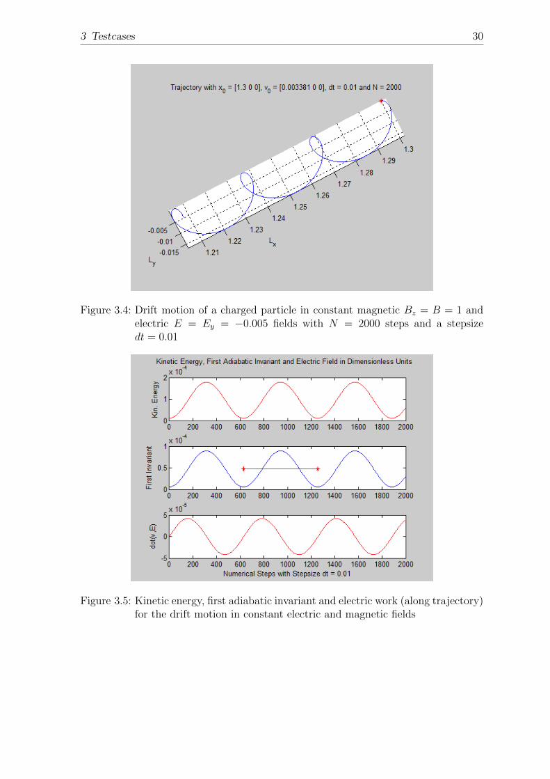
The trajectories are expected to be trachoids. These are curves described by a pointfixed on a rolling circle, which rolls without slipping along a straight line. The pointmay lie inside, outside, or on the circumference (cycloid) of the circle. The case ofa fixed point outside the rolling circle is shown in Figure 3.3. To understand theparticle’s behaviour it is useful to divide the motion into two half-cycles. During themotion along the first half-cycle the particle is accelerated and gains energy v2⊥ as itis depicted in Figure 3.4. This leads to an increase of the gyro radius rg = mv⊥/qB.The second half-cycle gives us a decreasing v⊥. Then the gyro radius is smaller. Thisdifference of the gyro radii results in the drift motion. The trajectory in Figure 3.4is calculated with E = Ey = −0.005 and B = Bz = 1 and it shows the expectedtrachoidal particle drift.

Figure 3.3: Trachoid for a fixed point P outside of the rolling circle

3 Testcases 30

Figure 3.4: Drift motion of a charged particle in constant magnetic Bz = B = 1 andelectric E = Ey = −0.005 fields with N = 2000 steps and a stepsizedt = 0.01

Figure 3.5: Kinetic energy, first adiabatic invariant and electric work (along trajectory)for the drift motion in constant electric and magnetic fields

4 Parameter Study: Pitch Angle

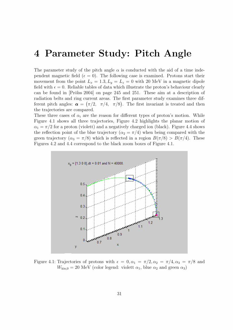
The parameter study of the pitch angle α is conducted with the aid of a time inde-pendent magnetic field (ε = 0). The following case is examined. Protons start theirmovement from the point Lx = 1.3, Ly = Lz = 0 with 20 MeV in a magnetic dipolefield with ε = 0. Reliable tables of data which illustrate the proton’s behaviour clearlycan be found in [Prolss 2004] on page 245 and 251. These aim at a description ofradiation belts and ring current areas. The first parameter study examines three dif-ferent pitch angles: ααα =

(π/2, π/4, π/8

). The first invariant is treated and then

the trajectories are compared.These three cases of αi are the reason for different types of proton’s motion. WhileFigure 4.1 shows all three trajectories, Figure 4.2 highlights the planar motion ofα1 = π/2 for a proton (violett) and a negatively charged ion (black). Figure 4.4 showsthe reflection point of the blue trajectory (α2 = π/4) when being compared with thegreen trajectory (α3 = π/8) which is reflected in a region B(π/8) > B(π/4). TheseFigures 4.2 and 4.4 correspond to the black zoom boxes of Figure 4.1.

Figure 4.1: Trajectories of protons with ε = 0, α1 = π/2, α2 = π/4, α3 = π/8 andWkin,0 = 20 MeV (color legend: violett α1, blue α2 and green α3)

31

4 Parameter Study: Pitch Angle 32

4.1 Case α1 = π/2

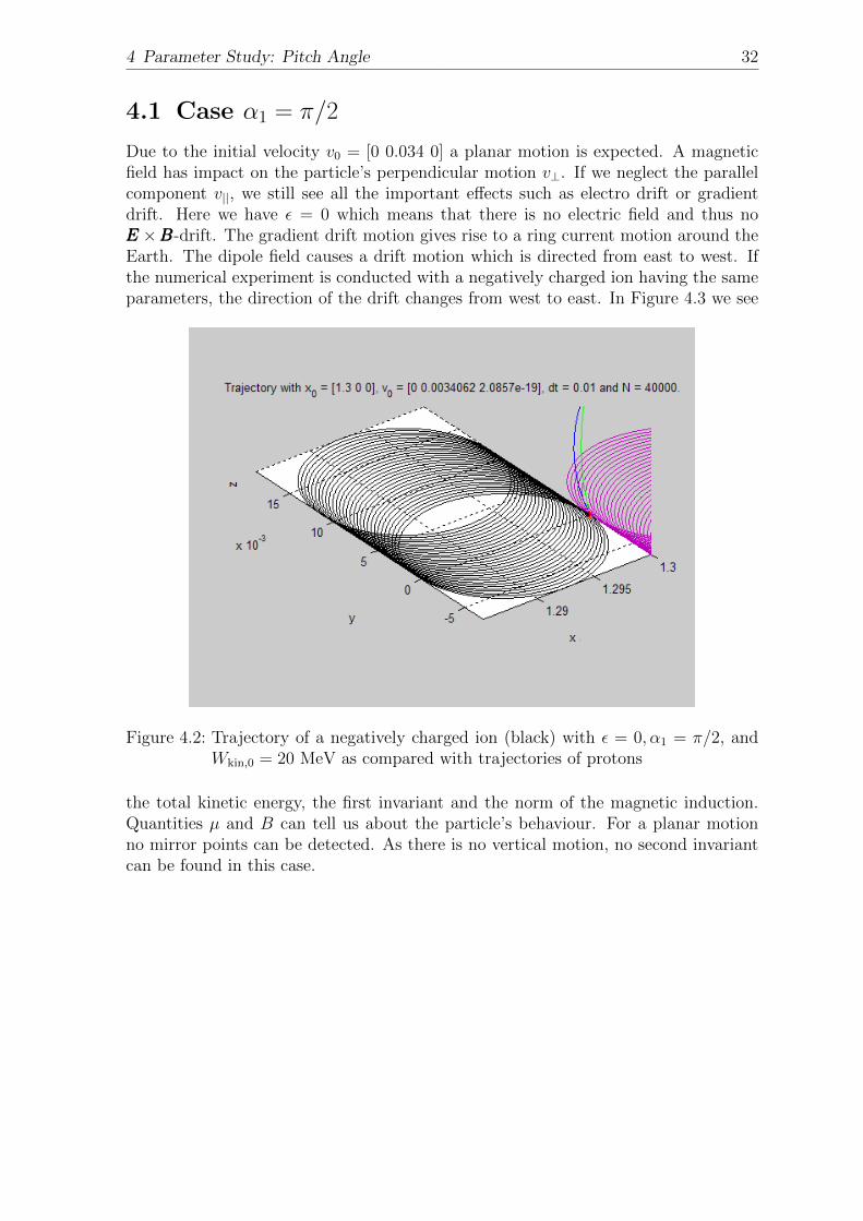
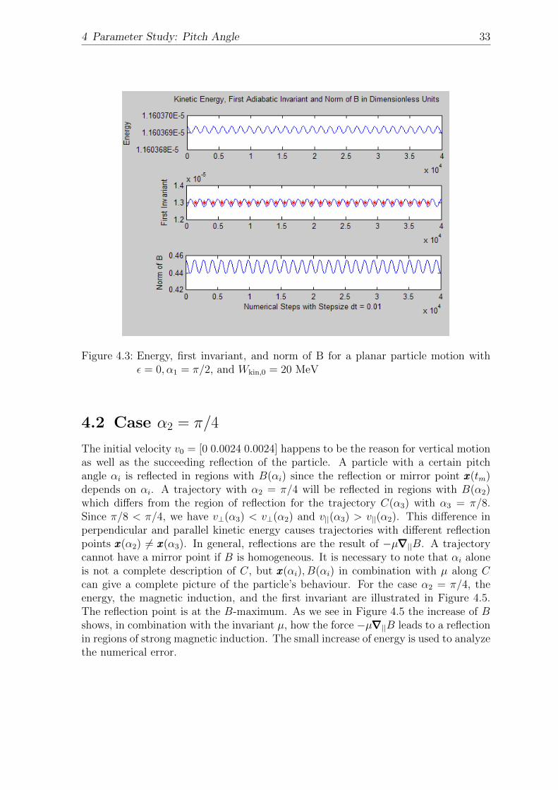
Due to the initial velocity v0 = [0 0.034 0] a planar motion is expected. A magneticfield has impact on the particle’s perpendicular motion v⊥. If we neglect the parallelcomponent v||, we still see all the important effects such as electro drift or gradientdrift. Here we have ε = 0 which means that there is no electric field and thus noEEE ×BBB-drift. The gradient drift motion gives rise to a ring current motion around theEarth. The dipole field causes a drift motion which is directed from east to west. Ifthe numerical experiment is conducted with a negatively charged ion having the sameparameters, the direction of the drift changes from west to east. In Figure 4.3 we see

Figure 4.2: Trajectory of a negatively charged ion (black) with ε = 0, α1 = π/2, andWkin,0 = 20 MeV as compared with trajectories of protons

the total kinetic energy, the first invariant and the norm of the magnetic induction.Quantities µ and B can tell us about the particle’s behaviour. For a planar motionno mirror points can be detected. As there is no vertical motion, no second invariantcan be found in this case.


Figure 4.3: Energy, first invariant, and norm of B for a planar particle motion withε = 0, α1 = π/2, and Wkin,0 = 20 MeV

4.2 Case α2 = π/4

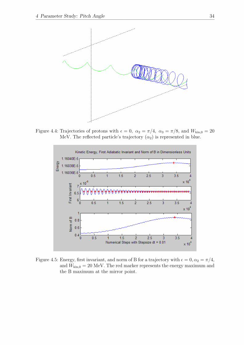
The initial velocity v0 = [0 0.0024 0.0024] happens to be the reason for vertical motionas well as the succeeding reflection of the particle. A particle with a certain pitchangle αi is reflected in regions with B(αi) since the reflection or mirror point xxx(tm)depends on αi. A trajectory with α2 = π/4 will be reflected in regions with B(α2)which differs from the region of reflection for the trajectory C(α3) with α3 = π/8.Since π/8 < π/4, we have v⊥(α3) < v⊥(α2) and v||(α3) > v||(α2). This difference inperpendicular and parallel kinetic energy causes trajectories with different reflectionpoints xxx(α2) 6= xxx(α3). In general, reflections are the result of −µ∇∇∇||B. A trajectorycannot have a mirror point if B is homogeneous. It is necessary to note that αi aloneis not a complete description of C, but xxx(αi), B(αi) in combination with µ along Ccan give a complete picture of the particle’s behaviour. For the case α2 = π/4, theenergy, the magnetic induction, and the first invariant are illustrated in Figure 4.5.The reflection point is at the B-maximum. As we see in Figure 4.5 the increase of Bshows, in combination with the invariant µ, how the force −µ∇∇∇||B leads to a reflectionin regions of strong magnetic induction. The small increase of energy is used to analyzethe numerical error.


Figure 4.4: Trajectories of protons with ε = 0, α2 = π/4, α3 = π/8, and Wkin,0 = 20MeV. The reflected particle’s trajectory (α2) is represented in blue.

Figure 4.5: Energy, first invariant, and norm of B for a trajectory with ε = 0, α2 = π/4,and Wkin,0 = 20 MeV. The red marker represents the energy maximum andthe B maximum at the mirror point.


4.3 Case α3 = π/8

The initial velocity v0 = [0 0.0013 0.0031] is the reason for a trajectory reflectedin regions with Bm,π/8 > Bm,π/4. The particle isn’t reflected at the π/4-trajectory’sreflection point corresponding to

sin2 α3 =B(0)

Bm,π/8

< sin2 α2 =B(0)

Bm,π/4

. (4.1)

4.4 Numerical Pitch Error

Corresponding to the single particle approach a charged particle with α2 = π/2 returnsat a position rrr′m with BBB(rrr′m) = BBB′m.

sin2 α′ =B0

B′m(4.2)

α′ = sin−1

√B0

B′m(4.3)

The theoretical pitch angle α2 differs from α′.

|α′ − α2|α2

· 100 = ∆α in % (4.4)

For the parameters N = 4E4, dt = 0.01, α2 = π/4, Wkin,0 = 20 MeV, ε = 0, thenumerical pitch error is

∆α = 1.95%. (4.5)

4.5 Numerical Energy Error

As the particle moves towards the reflection point (cases α2, α3), an energy shift canbe observed in Figures 4.5. Different timesteps produce different relative energy errors,

|W (tm)−W (0)|W (0)

· 100 = ∆W in %. (4.6)

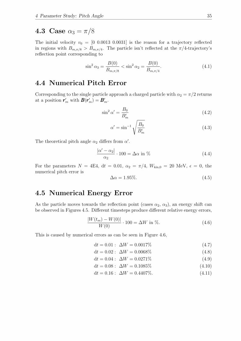
This is caused by numerical errors as can be seen in Figure 4.6,

dt = 0.01 : ∆W = 0.0017% (4.7)

dt = 0.02 : ∆W = 0.0068% (4.8)

dt = 0.04 : ∆W = 0.0271% (4.9)

dt = 0.08 : ∆W = 0.1085% (4.10)

dt = 0.16 : ∆W = 0.4407%. (4.11)


Figure 4.6: Different timesteps cause different numerical energy errors.

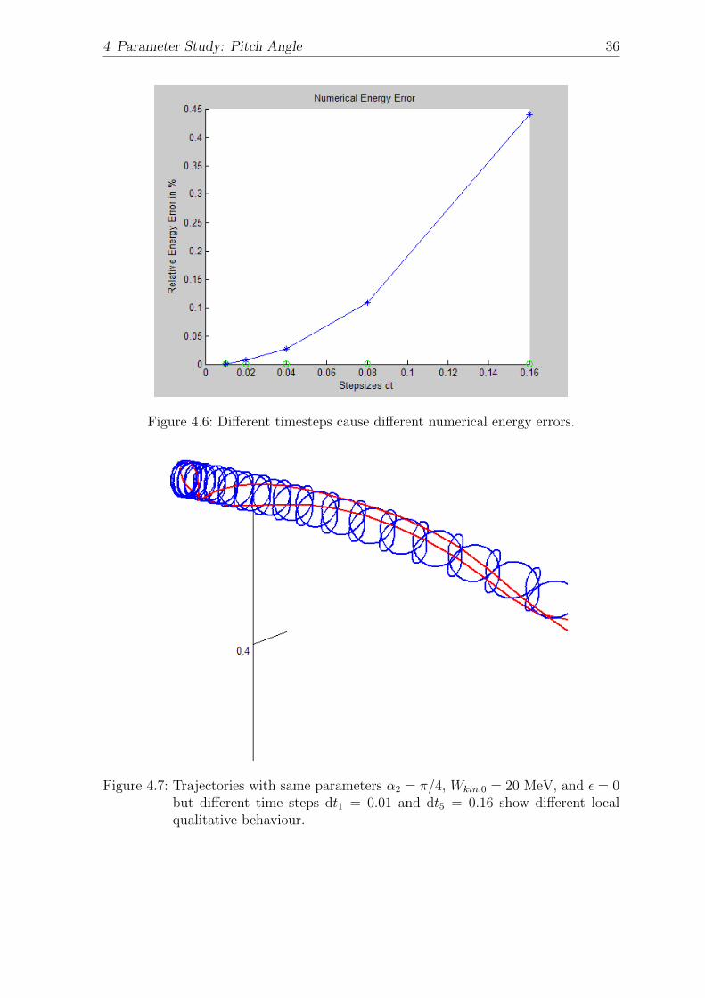
Figure 4.7: Trajectories with same parameters α2 = π/4, Wkin,0 = 20 MeV, and ε = 0but different time steps dt1 = 0.01 and dt5 = 0.16 show different localqualitative behaviour.

5 Parameter Study: ShellParameter

The second parameter study is about the influence of the initial position on the parti-cle’s motion. The section Numerics had shown dimensionless equations with the inputxxx which can be seen as a triple of shell parameters (Lx, Ly, Lz). For simplicity we setLy, Lz = 0 and we choose a pitch angle of α = π/4. The initial kinetic energy is 20MeV. This makes sense for protons (q > 0) in regions 1.2 < L < 2.5 [Prolss 2004].The pair (Wkin, µ) gives us a description of the particle’s behaviour in combinationwitch the trajectory C.

5.1 Trajectories

In this section we search for trajectories of particles with an initial energy of 20 MeV.The pitch angle is again α = π/4. We expect the particles to be trapped inside acurved magnetic mirror bouncing between the mirror points. The particles shoulddrift from east to west, because we have q > 0 for protons. This scenario is happeninginside the inner radiation belt, where we have energies 1−100 MeV for protons, movinginside the region 1.2 < L < 2.5. The magnetic dipole is assumed to be not dependenton time. We set ε = 0. The first trajectory starts from Lx = 1.3 and the secondtrajectory starts from L = 2, as can be seen in Figure 5.3.

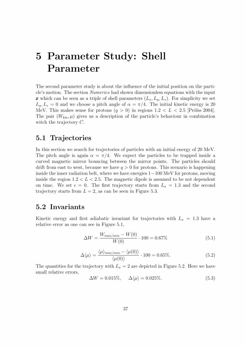
5.2 Invariants

Kinetic energy and first adiabatic invariant for trajectories with Lx = 1.3 have arelative error as one can see in Figure 5.1,

∆W =Wmax/min −W (0)

W (0)· 100 = 0.67% (5.1)

∆〈µ〉 =〈µ〉max/min − 〈µ(0)〉

〈µ(0)〉· 100 = 0.65%. (5.2)

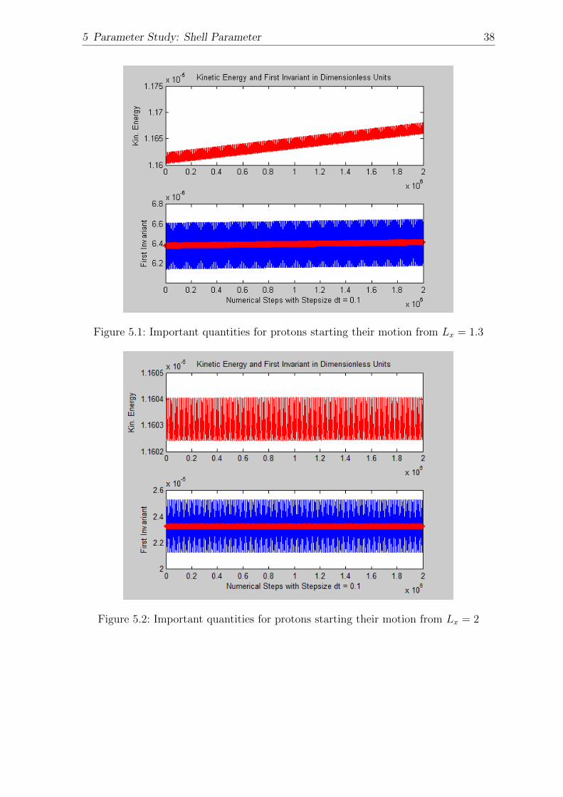
The quantities for the trajectory with Lx = 2 are depicted in Figure 5.2. Here we havesmall relative errors,

∆W = 0.015%, ∆〈µ〉 = 0.025%. (5.3)

37

5 Parameter Study: Shell Parameter 38

Figure 5.1: Important quantities for protons starting their motion from Lx = 1.3

Figure 5.2: Important quantities for protons starting their motion from Lx = 2

5 Parameter Study: Shell Parameter 39

Figure 5.3: Trajectories for protons with 20 MeV in a steady-state magnetic dipolefield starting their motion from Lx = 1.3 and Lx = 2

6 Parameter Study: TimeDependence

This section focuses on the consequences of a time varying magnetic field. Such mag-netic fields give rise to an electric field which accelerates the particles. Although thiselectric fields impart energy to the particles, they don’t change the magnetic momentµ. The planar analysis of [Chen 1974] shows the adiabatic invariance. If we choosethe pitch angle to be α1 = π/2, we have planar trajectories that suffice δµ = 0. As weexplained above, there are no reflections and there is no curvature drift in this case.For simplicity, we assume the magnetic moment of the Earth’s field to be

M(t) = 1 + εt. (6.1)

The time derivative gives us M = ε and thus the electric field leads to different driftmotion for ε > 0 and ε < 0. The emerging electric field EEE(rrr) causes electrical workalong the particle’s trajectory,

WE,C =

∫C

EEE · vvvdt, (6.2)

as well as drift motion into regions with different magnetic fields BBB(rrr, t). Thus anadditional magnetic acceleration is forced, because the magnetic moment of the particleµ stays constant. The EEE ×BBB drift accelerates the particle towards the Earth’s centerfor a magnetic moment M(t) which means an increasing magnetic induction for ε > 0.There is no parallel kinetic energy mv2||/2 which can be transferred into a perpendicularenergy.

µ =mv2⊥,02B0

=mv2⊥,t2Bt

⇒ v⊥,0 < v⊥,t with B0 < Bt, ∀t : v||,t = 0 (6.3)

Trajectories for protons with Wkin,0 = 20 MeV starting their motion from rrr0 = [1.3 0 0]with α1 = π/2 in fields with ε0 = 0, ε1 = 0.001, ε2 = 2E-6, and ε3 = 4E-6 are calculatedin order to analyze the impact of the emerging electric field. The direction of the driftmotion can be easily seen by the cross-product EEE ×BBB. As it is depicted in Figure 6.7the electric field for ε > 0 points from east to west. Since the magnetic field lies inz direction the resulting drift velocity points towards Earth. The gradient ∇∇∇⊥B hasa −x direction. This in combination with the magnetic field results in ring currentsthat are deflected by the EEE ×BBB drift force.

40

6 Parameter Study: Time Dependence 41

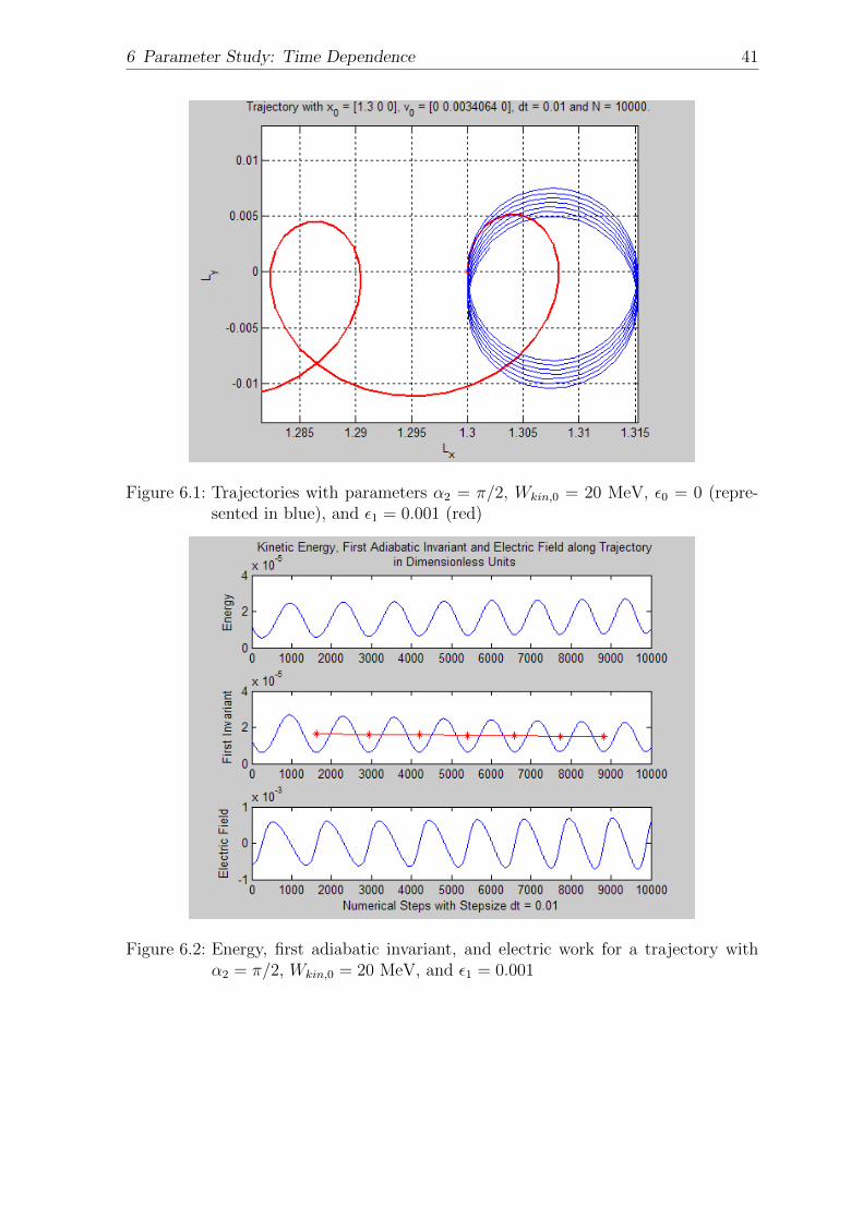
Figure 6.1: Trajectories with parameters α2 = π/2, Wkin,0 = 20 MeV, ε0 = 0 (repre-sented in blue), and ε1 = 0.001 (red)

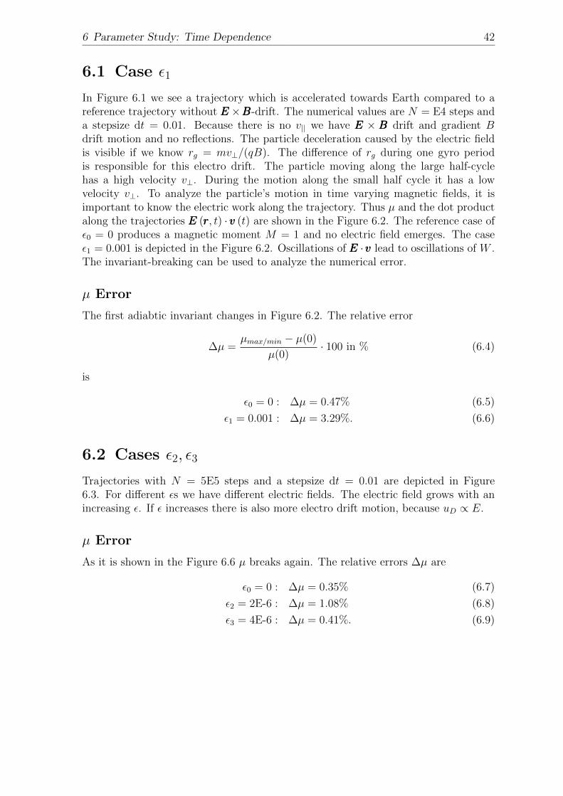
Figure 6.2: Energy, first adiabatic invariant, and electric work for a trajectory withα2 = π/2, Wkin,0 = 20 MeV, and ε1 = 0.001


6.1 Case ε1

In Figure 6.1 we see a trajectory which is accelerated towards Earth compared to areference trajectory without EEE ×BBB-drift. The numerical values are N = E4 steps anda stepsize dt = 0.01. Because there is no v|| we have EEE × BBB drift and gradient Bdrift motion and no reflections. The particle deceleration caused by the electric fieldis visible if we know rg = mv⊥/(qB). The difference of rg during one gyro periodis responsible for this electro drift. The particle moving along the large half-cyclehas a high velocity v⊥. During the motion along the small half cycle it has a lowvelocity v⊥. To analyze the particle’s motion in time varying magnetic fields, it isimportant to know the electric work along the trajectory. Thus µ and the dot productalong the trajectories EEE (rrr, t) · vvv (t) are shown in the Figure 6.2. The reference case ofε0 = 0 produces a magnetic moment M = 1 and no electric field emerges. The caseε1 = 0.001 is depicted in the Figure 6.2. Oscillations of EEE ·vvv lead to oscillations of W .The invariant-breaking can be used to analyze the numerical error.

µ Error

The first adiabtic invariant changes in Figure 6.2. The relative error

∆µ =µmax/min − µ(0)

µ(0)· 100 in % (6.4)

is

ε0 = 0 : ∆µ = 0.47% (6.5)

ε1 = 0.001 : ∆µ = 3.29%. (6.6)

6.2 Cases ε2, ε3

Trajectories with N = 5E5 steps and a stepsize dt = 0.01 are depicted in Figure6.3. For different εs we have different electric fields. The electric field grows with anincreasing ε. If ε increases there is also more electro drift motion, because uD ∝ E.

µ Error

As it is shown in the Figure 6.6 µ breaks again. The relative errors ∆µ are

ε0 = 0 : ∆µ = 0.35% (6.7)

ε2 = 2E-6 : ∆µ = 1.08% (6.8)

ε3 = 4E-6 : ∆µ = 0.41%. (6.9)


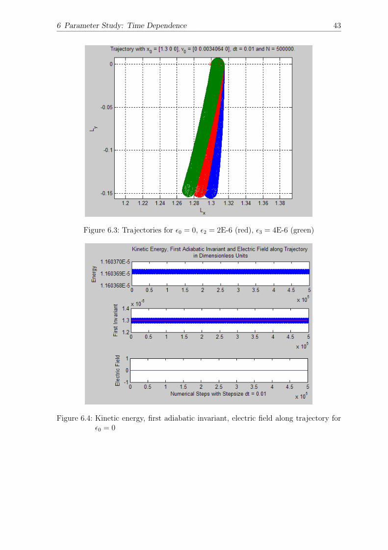
Figure 6.3: Trajectories for ε0 = 0, ε2 = 2E-6 (red), ε3 = 4E-6 (green)

Figure 6.4: Kinetic energy, first adiabatic invariant, electric field along trajectory forε0 = 0


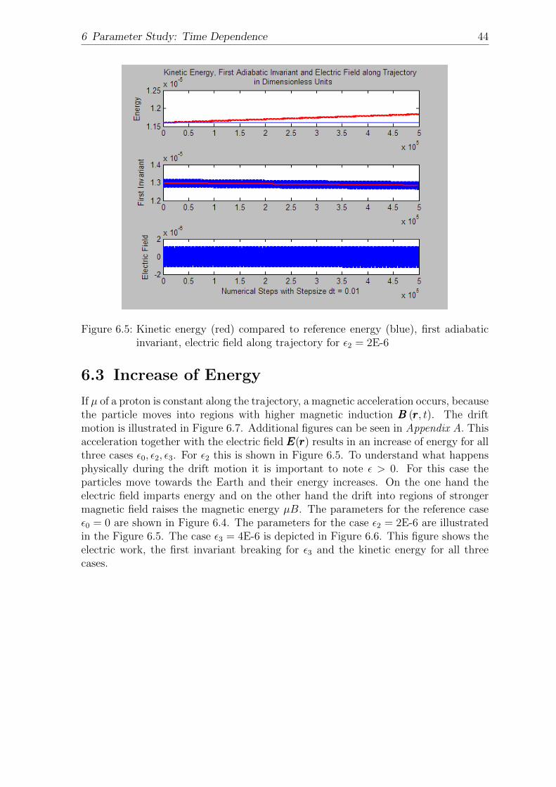
Figure 6.5: Kinetic energy (red) compared to reference energy (blue), first adiabaticinvariant, electric field along trajectory for ε2 = 2E-6

6.3 Increase of Energy

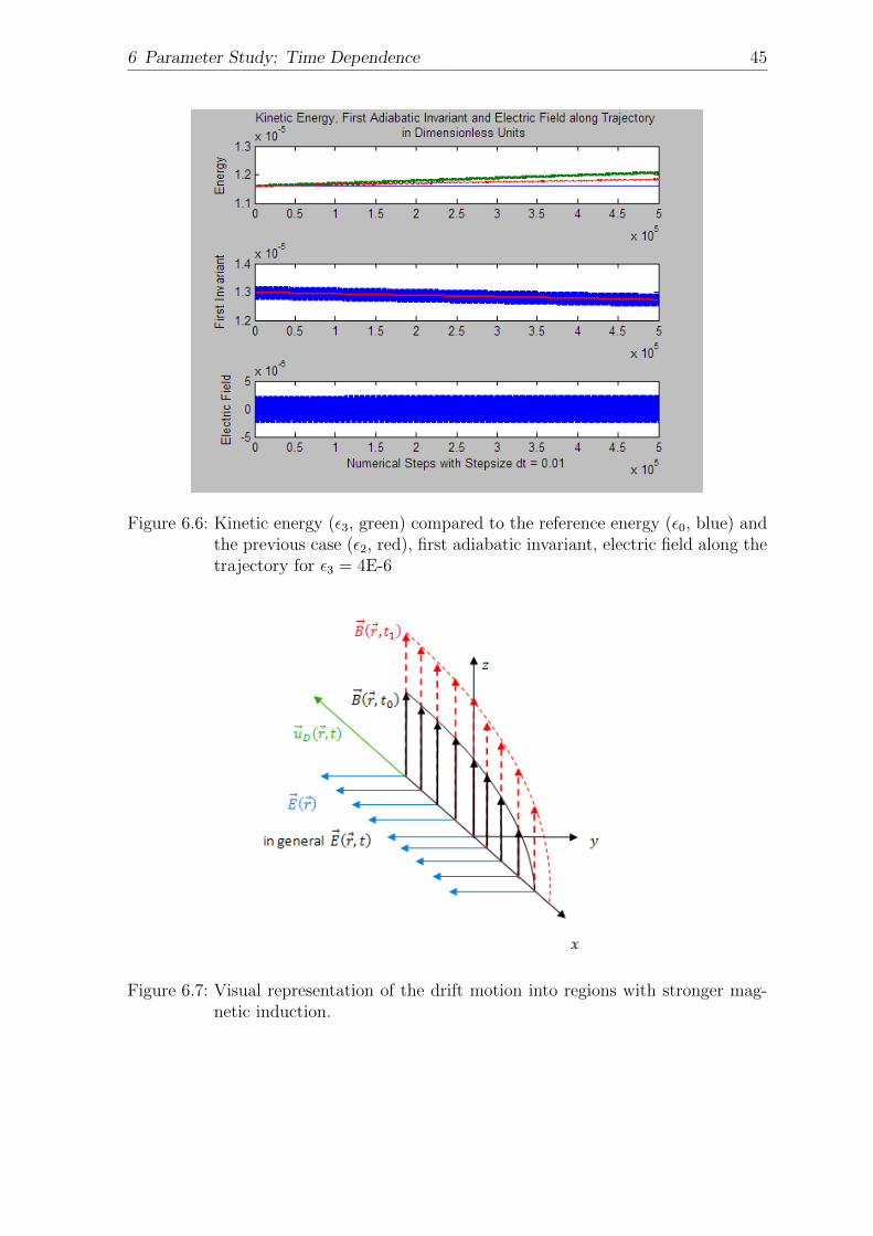
If µ of a proton is constant along the trajectory, a magnetic acceleration occurs, becausethe particle moves into regions with higher magnetic induction BBB (rrr, t). The driftmotion is illustrated in Figure 6.7. Additional figures can be seen in Appendix A. Thisacceleration together with the electric field EEE(rrr) results in an increase of energy for allthree cases ε0, ε2, ε3. For ε2 this is shown in Figure 6.5. To understand what happensphysically during the drift motion it is important to note ε > 0. For this case theparticles move towards the Earth and their energy increases. On the one hand theelectric field imparts energy and on the other hand the drift into regions of strongermagnetic field raises the magnetic energy µB. The parameters for the reference caseε0 = 0 are shown in Figure 6.4. The parameters for the case ε2 = 2E-6 are illustratedin the Figure 6.5. The case ε3 = 4E-6 is depicted in Figure 6.6. This figure shows theelectric work, the first invariant breaking for ε3 and the kinetic energy for all threecases.


Figure 6.6: Kinetic energy (ε3, green) compared to the reference energy (ε0, blue) andthe previous case (ε2, red), first adiabatic invariant, electric field along thetrajectory for ε3 = 4E-6

Figure 6.7: Visual representation of the drift motion into regions with stronger mag-netic induction.

7 Conclusions

This chapter sums up the results of the previous parameter studies and a conclusionis drawn. Finally, a short outlook concludes the thesis.

7.1 Results and Relative Errors

The aim of this thesis was to find trajectories C for charged particles in magnetic dipolefields dependent on time. Such particles obey the following dimensionless equation ofmotion

dtvvv (t) = vvv (t)×BBB (t, rrr) +EEE (t, rrr) . (7.1)

This system of nODEs is solved numerically with a symplectic scheme ψ. Such numer-ical solutions have to be analyzed with theoretical approximations. The single particleapproach delivers three relative errors in order to analyze the physical plausibility ofthe calculated trajectories,

• energy error ∆W

• pitch error ∆α

• µ error ∆µ.

∆W and ∆α check the plausibility of trajectories with a pitch angle α = π/4 or π/8.∆µ checks trajectories with a time dependent magnetic dipole field.

The previous numerical parameter study of the pitch angle α and the magnetic fieldparameter ε fit the analytic expectations of the single particle approach. α = π/2 andε 6= 0 lead to a planar motion which can be analyzed with the following concepts,

• gyro motion with gyro radius rg ∝ v⊥B(t,rrr)

• ∇∇∇⊥ ‖BBB (t, rrr)‖ drift motion

• EEE(rrr)×BBB(t, rrr) drift motion.

If the particle drifts towards the center of the magnetic dipole with uuuD ∝ EEE×BBB into re-gions with stronger magnetic induction, it is accelerated, because the magnetic momentµ stays constant. The electric field along the trajectory also accelerates the particle,because EEE is dependent on the position vector. This explains the result of the previousparameter study. The breaking of the first invariant µ is described with a relative error∆µ. An analysis of this invariant-breaking can be found in [Borovsky, Hansen 1991],[Hall 1980]. For α 6= π/2, two additional theoretical concepts can explain the particle’sbehaviour,

46

7 Conclusions 47

• ∇∇∇|| ‖BBB (t, rrr)‖ drift motion

• curvature drift motion.

Figure 7.2 shows a particle trajectory with α = π/4 and with ε = 2E-6 as comparedto a reference trajectory with ε = 0. The relative µ error is ∆µ = 3.1% for the ε 6= 0-trajectory. For the reference trajectory (ε = 0) the µ error is ∆µ = 2.4%. Importantparameters are depicted in Figure 7.1.

7.2 Conclusion

The time dependent magnetic moment M(t) of the dipole field

BBB =M

r5

−3xz−3xzr2 − 3z2

(7.2)

induces an electric field

EEE =M

r3

y−x0

(7.3)

that causes a drift motion uuuD ∝ EEE ×BBB. For simplicity the magnetic moment M wasset

M = 1 + εt. (7.4)

For ε > 0 the drift velocity uuuD points towards the Earth’s center, because

M = ε > 0. (7.5)

This is valid for ions, protons and electrons, because uuuD is not dependent on the par-ticle’s charge q. Thus an increasing magnetic moment causes a movement of chargedparticles towards the Earth. In Appendix A there are many additional figures thatillustrate the drift towards the Earth (or away from Earth for the case ε < 0).

7.3 Outlook

There are numerous options to continue these thoughts. Firstly, the equation of motionmay be modified with the relativistic factor γ,

dt (γmvvv) = qvvv ×BBB + qEEE. (7.6)

Secondly, the planar motion caused by α = π/2 may be analyzed. Then the (dimen-sionless) equation of motion reduces to(

xy

)=M

r3

(y−x

)+M

r3

(y−x

). (7.7)

Thirdly, a new numerical scheme may be used in order to reduce the relative errors,see Appendix B. And last but not least, different magnetic momenta M(t) may beused.

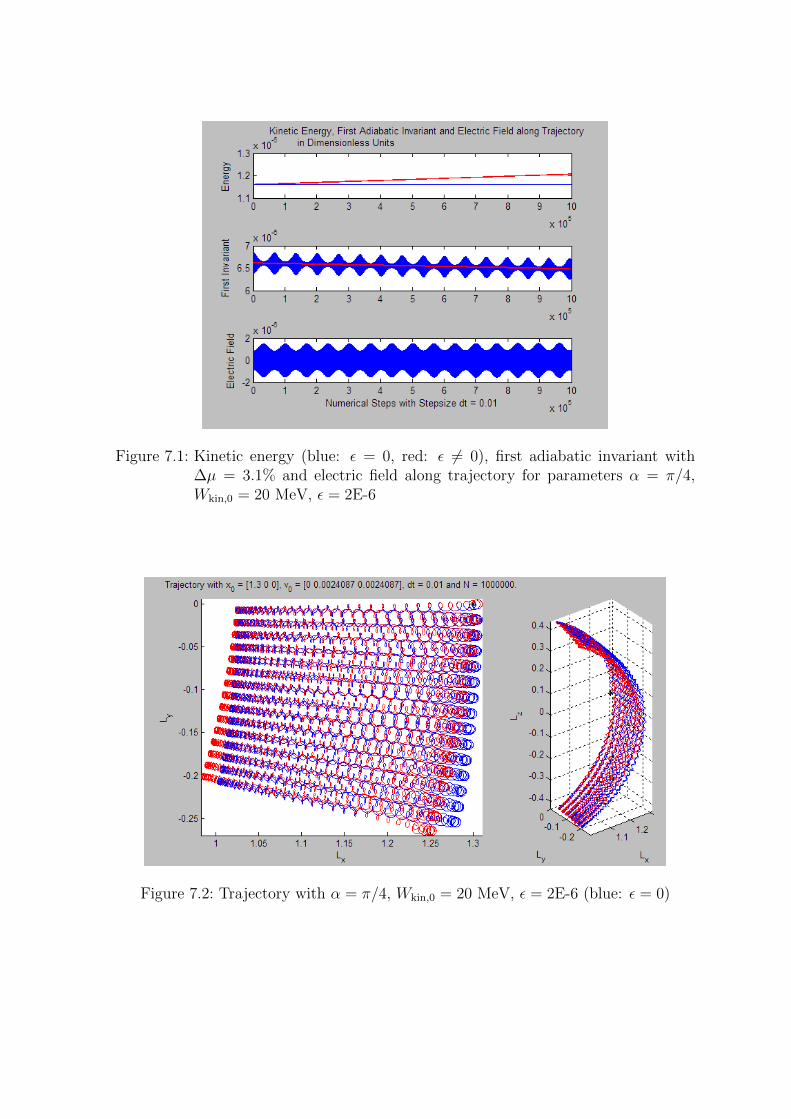
Figure 7.1: Kinetic energy (blue: ε = 0, red: ε 6= 0), first adiabatic invariant with∆µ = 3.1% and electric field along trajectory for parameters α = π/4,Wkin,0 = 20 MeV, ε = 2E-6

Figure 7.2: Trajectory with α = π/4, Wkin,0 = 20 MeV, ε = 2E-6 (blue: ε = 0)

Bibliography

[Biernat 2012] Biernat, H.K.: Lecture Notes on Plasma Theory and Earth’s Mag-netism, 2012.

[Borovsky, Hansen 1991] Borovsky, J.E., Hansen, P.J.: Breaking of the first adiabaticinvariants of charged particles in time-dependent magnetic fields: Computer sim-ulations and theory. Phys.Rev. A, 43(10):5606-5627, 1991.

[Chen 1974] Chen, F.: Introduction to Plasma Physics and Controlled Fusion - Vol-ume 1: Plasma Physics. Springer, 1974.

[Grill 2012] Grill, M.: Grundlagen uber stromdurchossene Leiter. BSc Thesis, KFUGraz, 2012.

[Hairer et al 2006] Hairer, E., Lubich, C., Wanner,G.: Geometric Numerical Integra-tion. Springer, Berlin-Heidelberg, 2006.

[Hairer et al 2008] Hairer, E., Nørsett, S.P., Wanner,G.: Solving Ordinary DifferentialEquations I., Springer, Berlin-Heidelberg, 2008.

[Hall 1980] Hall, N.A.: On the Breaking of the First Adiabatic Invariant in the Mag-netic Fields arising from the Mirror Instability. Astron. Astrophys., 84:40-43, 1980.

[MathWorks 2012] MathWorks R©: Matlab R© R2012a, 2012.

[Nicholson 1983] Nicholson, D.R.: Introduction to Plasma Theory. John Wiley andSons, 1983.

[Northrop, Teller 1960] Teller, E., Northrop, T.G.: Stability of Adiabatic Motion ofCharged Particles in the Earth’s Field. Physical Review, 117(1):215-225, 1960.

[NRL 2007] Naval Research Laboratory: NRL Plasma Formulary, Washington, 2007.

[Olszewski, Rolinski 1999] Olszewski, S., Rolinski,T.: First adiabatic invariant of acharged particle modified in a time-dependent magnetic field. Phys. Plasmas 6,425 (1999); doi: 10.1063/1.873208.

[Ozturk 2011] Ozturk, M.K.: Trajectories of charged particles trapped in Earth’s mag-netic field. arXiv:1112.3487 [physics.space-ph], 2011.

[Prolss 2004] Proelss, G.W.: Physik des erdnahen Weltraums - eine Einfuhrung.Springer, Berlin-Heidelberg, 2004.

[Størmer 1906] Størmer, C.: On the Trajectories of Electric Corpuscles in Space underthe Influence of Terrestrial Magnetism, ... . Archiv for Mathematik og Naturviden-skab, 28(2), 1906.

[Størmer 1933] Størmer, C.: Uber die Bahnen von Elektronen im axialsymmetrischenelektrischen und magnetischen Felde. Annalen der Physik, 16(5):685-696, 1933.

49

8 Appendix A: Plots for ε 6= 0

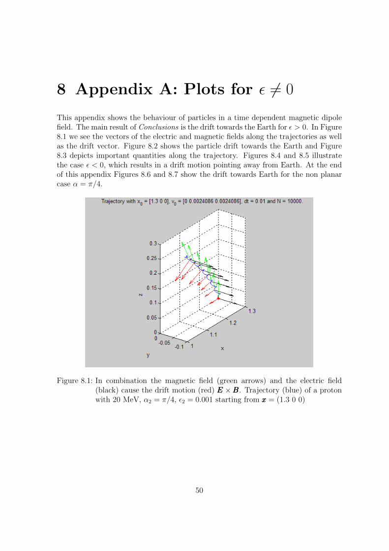
This appendix shows the behaviour of particles in a time dependent magnetic dipolefield. The main result of Conclusions is the drift towards the Earth for ε > 0. In Figure8.1 we see the vectors of the electric and magnetic fields along the trajectories as wellas the drift vector. Figure 8.2 shows the particle drift towards the Earth and Figure8.3 depicts important quantities along the trajectory. Figures 8.4 and 8.5 illustratethe case ε < 0, which results in a drift motion pointing away from Earth. At the endof this appendix Figures 8.6 and 8.7 show the drift towards Earth for the non planarcase α = π/4.

Figure 8.1: In combination the magnetic field (green arrows) and the electric field(black) cause the drift motion (red) EEE ×BBB. Trajectory (blue) of a protonwith 20 MeV, α2 = π/4, ε2 = 0.001 starting from xxx = (1.3 0 0)

50


Figure 8.2: Proton with Wkin = 20 MeV, α1 = π/2 in a magnetic dipole field with ε1 =0 (blue), ε2 = 0.001 (green), ε3 = 0.002 (red) starting from xxx = (1.3 0 0)

Figure 8.3: Parameters for a proton with Wkin = 20 MeV, α1 = π/2 in a magneticdipole field with ε1 = 0 (blue), ε2 = 0.001 (green), ε3 = 0.002 (red) startingfrom xxx = (1.3 0 0)


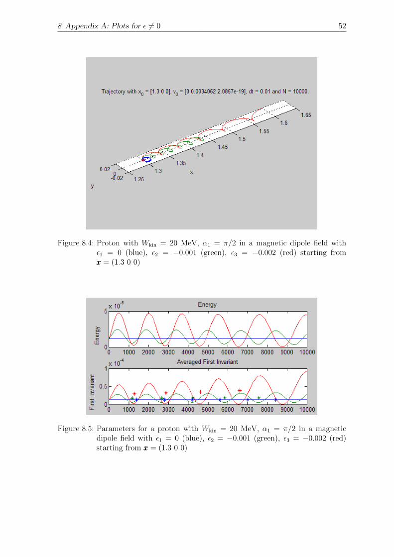
Figure 8.4: Proton with Wkin = 20 MeV, α1 = π/2 in a magnetic dipole field withε1 = 0 (blue), ε2 = −0.001 (green), ε3 = −0.002 (red) starting fromxxx = (1.3 0 0)

Figure 8.5: Parameters for a proton with Wkin = 20 MeV, α1 = π/2 in a magneticdipole field with ε1 = 0 (blue), ε2 = −0.001 (green), ε3 = −0.002 (red)starting from xxx = (1.3 0 0)


Figure 8.6: Proton with Wkin = 20 MeV, α2 = π/4 in a magnetic dipole field with ε1 =0 (blue), ε2 = 0.001 (green), ε3 = 0.002 (red) starting from xxx = (1.3 0 0)

Figure 8.7: Parameters for a proton with Wkin = 20 MeV, α2 = π/4 in a magneticdipole field with ε1 = 0 (blue), ε2 = 0.001 (green) starting from xxx =(1.3 0 0)

9 Appendix B: Decrease of EnergyError

The energy error ∆W in the previous parameter study can be decreased. To achievethis we have to change our numerical scheme. One possibility is to try symplectichigher order methods s > 2. Another way is to choose a predictor-corrector scheme Pwhich is presented in this appendix.

The initial values are xxx(0), vvv(0). Then the scheme P has the form

P : R3 × R3 → R3 × R3 (9.1)

(xxxi, vvvi) 7→ (xxxi+1, vvvi+1). (9.2)

There are 3 substeps during the step i → i + 1. xx1 and vv2 are the predictedvalues. xxm and vvm are the corrected values. The last substep has an additionalvelocity correction, which leads to a decrease of energy shift [no foundation, numericalexperiments].

for index=1:N-1

xx = x(:,index);

vv = v(:,index);

% input for acceleration function

EE = electrField(epsilon,xx,t);

BB = magnField(epsilon,xx,t);

%substep 1

dv= acceleration(epsilon,q,xx,vv,t)*dt;

vv1=vv+dv;

dx=(vv+vv1)/2*dt;

xx1=xx+dx;

vvm=(vv+vv1)/2;

xxm=(xx+xx1)/2;

%substep 2

dv=acceleration(epsilon,q,xxm,vvm,t)*dt;

vv1=vv+dv;

dx=(vv+vv1)/2*dt;

54

9 Appendix B: Decrease of Energy Error 55

xx1=xx+dx;

vvm=(vv+vv1)/2;

xxm=(xx+xx1)/2;

%substep3

dv=acceleration(epsilon,q,xxm,vvm,t)*dt;

vv2=vv+dv;

vv1=(vv1+vv2)/2;

dx=(vv+vv1)/2*dt;

xx1=xx+dx;

%new values

x(:,index+1) = xx1;

v(:,index+1) = vv1;

t=t+dt;

end

The reduction of energy error can be seen in figure 9.1.

Figure 9.1: Kinetic energy and first invariant for the scheme P in red (the scheme ψin blue)

10 Appendix C: Source Code

This chapter shows all functions and scripts used for the thesis.

10.1 Main File

This is the main script file with the symplectic scheme from chapter Numerics, whichmay be substituted with other numerical schemes.

• ODE45() from Matlab R©, or other Runge Kutta Methods

• Predictor Corrector Methods

• Leapfrog Methods

• Symplectic Methods

% Author: Manuel Grill

% Charged Particles in Magnetic Dipole Fields Dependent on Time

% Version 2.1 April 2013

clear all

close all

clc

format ’long’ ’e’

Initial_Energy = 20*10^6; %eV

Pitch_Angle = pi/4;

q = 1;

units % script

v0 =vinitp; % initial velocity; for electrons vinite

% for vinite see script units

N = 1000000; % steps

dt = 0.1; % stepsize

t = 0;

56

10 Appendix C: Source Code 57

x0 = [-1.980850676584732e+00;7.618514891912165e-02;2.022048747964554e-02];

[2 0 0]’; [-1.9809e+00;7.6185e-02;2.0220e-02];

% initial position in L

x = zeros(3,N); % position

v = zeros(3,N); % velocities

x(:,1)=x0;

v(:,1)= [7.676601327477699e-04; -2.241708429653579e-03;2.447012007283591e-03];

v0;[7.6766e-04; -2.2417e-03;2.4470e-03];

epsilon = 0.0000; % parameter

B = zeros(3,N);

E = zeros(3,N);

B(:,1) = magnField(epsilon,x0,t);

E(:,1) = electrField(epsilon,x0,t);

mu = zeros(1,N-1);

energy = zeros(1,N-1);

vE=zeros(1,N-1);

index2=0;

%--------------- this loop can be substituted with better numerical schemes

for index=1:N-1

xx = x(:,index);

vv = v(:,index);

EE = electrField(epsilon,xx,t);

vE(index)=dot(vv,EE);

BB = magnField(epsilon,xx,t);

E(:,index) = norm(EE);

B(:,index) = norm(BB);

vpara = dot(vv,BB)/norm(BB);

vv2=norm(vv)^2;

vperp2=vv2-vpara^2;

mu(index) = vperp2/(2*norm(BB));

energy(index)=vv2;

aa = acceleration(epsilon,q,xx,vv,t);

aa1 = acceleration(epsilon,q,xx,vv+dt/2*aa,t);

xx1 = xx + vv*dt + aa1*dt^2/2;

aa2 = acceleration(epsilon,q,xx1,vv+aa1*dt/2,t+dt);

x(:,index+1) = xx1;

v(:,index+1)= vv + (aa1+aa2)/2*dt;


if fix(index2/4000)==index2/4000

index2

end

index2=index2+1;

t=t+dt;

end

%-------------------------------------------------------------------------

%adding %script

plotanderror %script

10.2 Fields and Force Functions

The field and force functions can be used for arbitrary magnetic and electric fields.The electric field has to fit with the magnetic field.

function [ a ] = acceleration(epsilon,q,x,v,t)

%calculates acceleration

B = magnField(epsilon,x,t);

E = electrField(epsilon,x,t);

a = q*(cross(v,B)+E);

end

function [E] = electrField(epsilon,x,t)

%calculates electr field

xx=x(1);

yy=x(2);

rr=norm(x);

E=epsilon/rr^3*[yy -xx 0]’;

%E=[0 -0.005 0]’;

end

function [B] = magnField(epsilon,x,t)

% magnField computes the magnetic field

xx=x(1);

yy=x(2);

zz=x(3);


rr=norm(x);

B=(1+epsilon*t)/rr^5*[(-3)*xx*zz (-3)*yy*zz (-3)*zz^2+rr^2]’;

%B=[0 0 1]’;

end

10.3 Plots, Data and Error Calculation

The figures can be changed with an editor. The output is dimensionless.

every = 50;

figure(1)

plot3(x(1,1:every:end),x(2,1:every:end),x(3,1:every:end),...

’b’,x(1,1),x(2,1),x(3,1),’r*’)

title([’Trajectory with x_0 = [’,num2str(x0(1)),’ ’,...

num2str(x0(2)),’ ’,num2str(x0(3)),’], v_0 = [’,...

num2str(v0(1)),’ ’,num2str(v0(2)),’ ’,...

num2str(v0(3)),’], dt = ’,num2str(dt),’...

and N = ’,num2str(N)])

xlabel(’L_x’)

ylabel(’L_y’)

zlabel(’L_z’)

grid on

axis equal

figure(2)

subplot(2,1,1)

plot(energy,’r’)

title(’Kinetic Energy and First Invariant in Dimensionless Units’)

ylabel(’Kin. Energy’)

subplot(2,1,2)

plot(mu,’r’)

ylabel(’First Invariant’)

xlabel([’Numerical Steps with Stepsize dt = ’,num2str(dt)])

energmaximum = max(energy);

energyerrorend = abs(energy(1)-energy(end))/energy(1)*100

energyerrormax = abs(energy(1)-energmaximum)/energy(1)*100

muerrorend = abs(mu(1)-mu(end))/mu(1)*100

muerrormax = abs(mu(1)-max(mu))/mu(1)*100

[positionarray,invariantsarray]=averaging(mu);


avmuerrorend = abs(invariantsarray(1)-invariantsarray(end))/...

invariantsarray(1)*100

avmuerrormax = abs(invariantsarray(1)-max(invariantsarray))/...

invariantsarray(1)*100

figure(3)

subplot(2,1,1)


title(’Kinetic Energy and First Invariant in Dimensionless Units’)


subplot(2,1,2)

plot(1:length(mu),mu,’b’,positionarray,invariantsarray,’r*-’)



figure(4)

subplot(3,1,1)


title(’Kinetic Energy, First Invariant...

and Electric Field in Dimensionless Units’)


subplot(3,1,2)

plot(1:length(mu),mu,’b’,positionarray,invariantsarray,’r*-’)


subplot(3,1,3)

plot(vE,’r’)

ylabel(’dot(v,E)’)


%script adding

load energyrun1.mat

energy1 = energy;

load energyrun2.mat

energy2 = energy;

energy = [energy1,energy2];

load murun1.mat

mu1=mu;

load murun2.mat

mu2 = mu;

mu = [mu1,mu2];


10.4 Units

The equations are in dimensionless form. The data below can be found in [Prolss 2004].

q0 = 1.6021773E-19; % As

eV = 1.602176565E-19; %J

eV = 1.602E-19;

me = 9.109390E-31; % kg

mp = 1836.152585*me;

mp = 1.672623E-27;

ME = 7.7E22; % Am2

RE = 6.371E6; % m

mu0 = 4*pi*10^(-7); % Vs/(Am)

B0=30E-6;%T

B0=mu0*ME/(4*pi*RE^3);

IniEnergy=Initial_Energy*eV;

v0p = q0*B0*RE/mp;

v0e = q0*B0*RE/me;

W0p = mp*v0p^2/2;

W0e = me*v0e^2/2;

vp=sqrt(IniEnergy/W0p);

ve=sqrt(IniEnergy/W0e);

vinitp = vp*[sin(Pitch_Angle) 0 cos(Pitch_Angle)]’;

vinite = ve*[sin(Pitch_Angle) 0 cos(Pitch_Angle)]’;

10.5 Averaging, Maxima for Invariant-Analysis

function [positionarray,invariantsarray] = averaging(vectorarray)

% calculates invariants

maximapositionarray = maximasearch(vectorarray);

len=length(maximapositionarray);

invariantsarray=zeros(1,len-1);

positionarray=zeros(1,len-1);

for index=1:len-1

boundary1=maximapositionarray(index);


boundary2=maximapositionarray(index+1);

invariantsarray(index)=1/(boundary2-boundary1)*...

trapz(boundary1:boundary2,vectorarray(boundary1:boundary2));

positionarray(index)=(boundary1+boundary2)/2;

end

function [logivec] = maximasearch( array )

len=length(array);

darray=diff(array);

logivec = zeros(1,len);

for index =1:len-2

thenumber = darray(index);

logivec(index)=sign(thenumber*darray(index+1));

if thenumber<0

logivec(index)=0;

end

end

logivec = find(logivec<0)+1; %index = 1 means maximum at 2: 2-1 and 3-2

Motion of Charged Particles in Magnetic Dipole Fields ...

Documents

Transcript of Motion of Charged Particles in Magnetic Dipole Fields ...