Comparison of an optimized resistivity array with dipole-dipole soundings in karst terrain
6
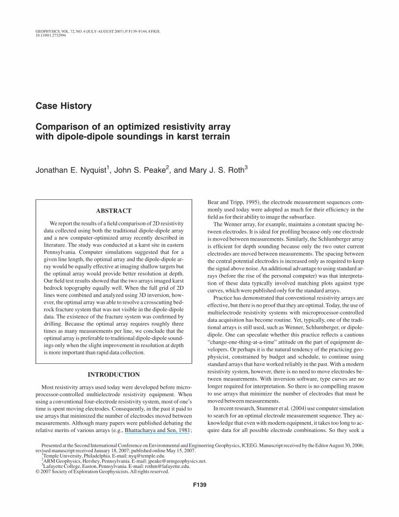
Case History Comparison of an optimized resistivity array with dipole-dipole soundings in karst terrain Jonathan E. Nyquist 1 , John S. Peake 2 , and Mary J. S. Roth 3 ABSTRACT We report the results of a field comparison of 2D resistivity data collected using both the traditional dipole-dipole array and a new computer-optimized array recently described in literature. The study was conducted at a karst site in eastern Pennsylvania. Computer simulations suggested that for a given line length, the optimal array and the dipole-dipole ar- ray would be equally effective at imaging shallow targets but the optimal array would provide better resolution at depth. Our field test results showed that the two arrays imaged karst bedrock topography equally well. When the full grid of 2D lines were combined and analyzed using 3D inversion, how- ever, the optimal array was able to resolve a crosscutting bed- rock fracture system that was not visible in the dipole-dipole data. The existence of the fracture system was confirmed by drilling. Because the optimal array requires roughly three times as many measurements per line, we conclude that the optimal array is preferable to traditional dipole-dipole sound- ings only when the slight improvement in resolution at depth is more important than rapid data collection. INTRODUCTION Most resistivity arrays used today were developed before micro- processor-controlled multielectrode resistivity equipment. When using a conventional four-electrode resistivity system, most of one’s time is spent moving electrodes. Consequently, in the past it paid to use arrays that minimized the number of electrodes moved between measurements. Although many papers were published debating the relative merits of various arrays e.g., Bhattacharya and Sen, 1981; Bear and Tripp, 1995, the electrode measurement sequences com- monly used today were adopted as much for their efficiency in the field as for their ability to image the subsurface. The Wenner array, for example, maintains a constant spacing be- tween electrodes. It is ideal for profiling because only one electrode is moved between measurements. Similarly, the Schlumberger array is efficient for depth sounding because only the two outer current electrodes are moved between measurements. The spacing between the central potential electrodes is increased only as required to keep the signal above noise. An additional advantage to using standard ar- rays before the rise of the personal computer was that interpreta- tion of these data typically involved matching plots against type curves, which were published only for the standard arrays. Practice has demonstrated that conventional resistivity arrays are effective, but there is no proof that they are optimal.Today, the use of multielectrode resistivity systems with microprocessor-controlled data acquisition has become routine. Yet, typically, one of the tradi- tional arrays is still used, such as Wenner, Schlumberger, or dipole- dipole. One can speculate whether this practice reflects a cautious “change-one-thing-at-a-time” attitude on the part of equipment de- velopers. Or perhaps it is the natural tendency of the practicing geo- physicist, constrained by budget and schedule, to continue using standard arrays that have worked reliably in the past. With a modern resistivity system, however, there is no need to move electrodes be- tween measurements. With inversion software, type curves are no longer required for interpretation. So there is no compelling reason to use arrays that minimize the number of electrodes that must be moved between measurements. In recent research, Stummer et al. 2004 use computer simulation to search for an optimal electrode measurement sequence. They ac- knowledge that even with modern equipment, it takes too long to ac- quire data for all possible electrode combinations. So they seek a Presented at the Second International Conference on Environmental and Engineering Geophysics, ICEEG. Manuscript received by the Editor August 30, 2006; revised manuscript received January 18, 2007; published online May 15, 2007. 1 Temple University, Philadelphia. E-mail: [email protected]. 2 ARM Geophysics, Hershey, Pennsylvania. E-mail: [email protected]. 3 Lafayette College, Easton, Pennsylvania. E-mail: [email protected]. © 2007 Society of Exploration Geophysicists. All rights reserved. GEOPHYSICS, VOL. 72, NO. 4 JULY-AUGUST 2007; P. F139–F144, 8 FIGS. 10.1190/1.2732994 F139
Transcript of Comparison of an optimized resistivity array with dipole-dipole soundings in karst terrain
C
Cw
J
putumr
r
©
GEOPHYSICS, VOL. 72, NO. 4 �JULY-AUGUST 2007�; P. F139–F144, 8 FIGS.10.1190/1.2732994
ase History
omparison of an optimized resistivity arrayith dipole-dipole soundings in karst terrain
onathan E. Nyquist1, John S. Peake2, and Mary J. S. Roth3
Bmfi
tiiettrtc
emdtd“vpsrtltm
tkq
ngineer.
ics.net.
ABSTRACT
We report the results of a field comparison of 2D resistivitydata collected using both the traditional dipole-dipole arrayand a new computer-optimized array recently described inliterature. The study was conducted at a karst site in easternPennsylvania. Computer simulations suggested that for agiven line length, the optimal array and the dipole-dipole ar-ray would be equally effective at imaging shallow targets butthe optimal array would provide better resolution at depth.Our field test results showed that the two arrays imaged karstbedrock topography equally well. When the full grid of 2Dlines were combined and analyzed using 3D inversion, how-ever, the optimal array was able to resolve a crosscutting bed-rock fracture system that was not visible in the dipole-dipoledata. The existence of the fracture system was confirmed bydrilling. Because the optimal array requires roughly threetimes as many measurements per line, we conclude that theoptimal array is preferable to traditional dipole-dipole sound-ings only when the slight improvement in resolution at depthis more important than rapid data collection.
INTRODUCTION
Most resistivity arrays used today were developed before micro-rocessor-controlled multielectrode resistivity equipment. Whensing a conventional four-electrode resistivity system, most of one’sime is spent moving electrodes. Consequently, in the past it paid tose arrays that minimized the number of electrodes moved betweeneasurements. Although many papers were published debating the
elative merits of various arrays �e.g., Bhattacharya and Sen, 1981;
Presented at the Second International Conference on Environmental and Eevised manuscript received January 18, 2007; published online May 15, 2007
1Temple University, Philadelphia. E-mail: [email protected] Geophysics, Hershey, Pennsylvania. E-mail: jpeake@armgeophys3Lafayette College, Easton, Pennsylvania. E-mail: [email protected] Society of Exploration Geophysicists.All rights reserved.
F139
ear and Tripp, 1995�, the electrode measurement sequences com-only used today were adopted as much for their efficiency in theeld as for their ability to image the subsurface.The Wenner array, for example, maintains a constant spacing be-
ween electrodes. It is ideal for profiling because only one electrodes moved between measurements. Similarly, the Schlumberger arrays efficient for depth sounding because only the two outer currentlectrodes are moved between measurements. The spacing betweenhe central potential electrodes is increased only as required to keephe signal above noise.An additional advantage to using standard ar-ays �before the rise of the personal computer� was that interpreta-ion of these data typically involved matching plots against typeurves, which were published only for the standard arrays.
Practice has demonstrated that conventional resistivity arrays areffective, but there is no proof that they are optimal. Today, the use ofultielectrode resistivity systems with microprocessor-controlled
ata acquisition has become routine. Yet, typically, one of the tradi-ional arrays is still used, such as Wenner, Schlumberger, or dipole-ipole. One can speculate whether this practice reflects a cautiouschange-one-thing-at-a-time” attitude on the part of equipment de-elopers. Or perhaps it is the natural tendency of the practicing geo-hysicist, constrained by budget and schedule, to continue usingtandard arrays that have worked reliably in the past. With a modernesistivity system, however, there is no need to move electrodes be-ween measurements. With inversion software, type curves are noonger required for interpretation. So there is no compelling reasono use arrays that minimize the number of electrodes that must be
oved between measurements.In recent research, Stummer et al. �2004� use computer simulation
o search for an optimal electrode measurement sequence. They ac-nowledge that even with modern equipment, it takes too long to ac-uire data for all possible electrode combinations. So they seek a
ing Geophysics, ICEEG. Manuscript received by the EditorAugust 30, 2006;
trtcwtpImt
ptoil
mssc
uetprpaeam
otcsfg
reavtotmtcvtm
tetst�md
Wz
otaee2vme
g
FPte
F140 Nyquist et al.
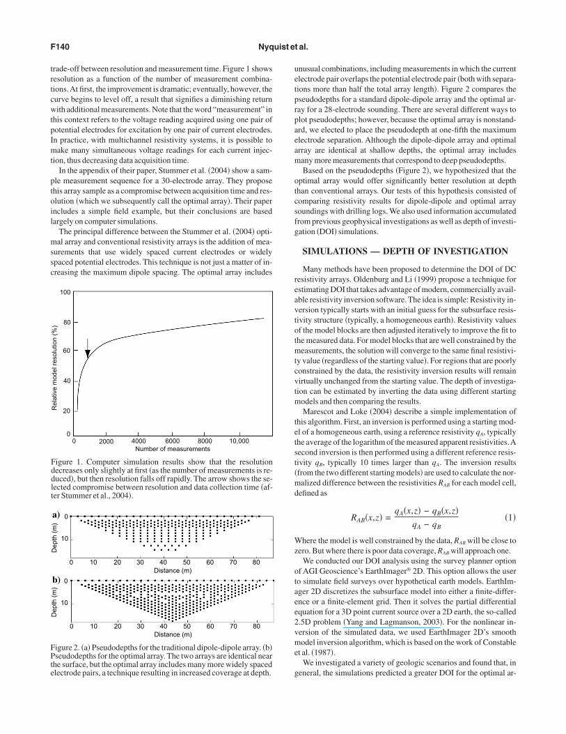
rade-off between resolution and measurement time. Figure 1 showsesolution as a function of the number of measurement combina-ions.At first, the improvement is dramatic; eventually, however, theurve begins to level off, a result that signifies a diminishing returnith additional measurements. Note that the word “measurement” in
his context refers to the voltage reading acquired using one pair ofotential electrodes for excitation by one pair of current electrodes.n practice, with multichannel resistivity systems, it is possible toake many simultaneous voltage readings for each current injec-
ion, thus decreasing data acquisition time.In the appendix of their paper, Stummer et al. �2004� show a sam-
le measurement sequence for a 30-electrode array. They proposehis array sample as a compromise between acquisition time and res-lution �which we subsequently call the optimal array�. Their paperncludes a simple field example, but their conclusions are basedargely on computer simulations.
The principal difference between the Stummer et al. �2004� opti-al array and conventional resistivity arrays is the addition of mea-
urements that use widely spaced current electrodes or widelypaced potential electrodes. This technique is not just a matter of in-reasing the maximum dipole spacing. The optimal array includes
100
80
60
40
20
00 2000 4000 6000 8000 10,000
Number of measurements
Rel
ativ
e m
odel
res
olut
ion
(%)
Figure 1. Computer simulation results show that the resolutiondecreases only slightly at first �as the number of measurements is re-duced�, but then resolution falls off rapidly. The arrow shows the se-lected compromise between resolution and data collection time �af-ter Stummer et al., 2004�.
0
10
0 10 20 30 40
50
60
70
80 Distance (m)
0 10 20 30 40
50
60
70
80 Distance (m)
Dep
th (
m)
0
10
Dep
th (
m)
a)
b)
igure 2. �a� Pseudodepths for the traditional dipole-dipole array. �b�seudodepths for the optimal array. The two arrays are identical near
he surface, but the optimal array includes many more widely spacedlectrode pairs, a technique resulting in increased coverage at depth.
nusual combinations, including measurements in which the currentlectrode pair overlaps the potential electrode pair �both with separa-ions more than half the total array length�. Figure 2 compares theseudodepths for a standard dipole-dipole array and the optimal ar-ay for a 28-electrode sounding. There are several different ways tolot pseudodepths; however, because the optimal array is nonstand-rd, we elected to place the pseudodepth at one-fifth the maximumlectrode separation. Although the dipole-dipole array and optimalrray are identical at shallow depths, the optimal array includesany more measurements that correspond to deep pseudodepths.Based on the pseudodepths �Figure 2�, we hypothesized that the
ptimal array would offer significantly better resolution at depthhan conventional arrays. Our tests of this hypothesis consisted ofomparing resistivity results for dipole-dipole and optimal arrayoundings with drilling logs. We also used information accumulatedrom previous geophysical investigations as well as depth of investi-ation �DOI� simulations.
SIMULATIONS — DEPTH OF INVESTIGATION
Many methods have been proposed to determine the DOI of DCesistivity arrays. Oldenburg and Li �1999� propose a technique forstimating DOI that takes advantage of modern, commercially avail-ble resistivity inversion software. The idea is simple: Resistivity in-ersion typically starts with an initial guess for the subsurface resis-ivity structure �typically, a homogeneous earth�. Resistivity valuesf the model blocks are then adjusted iteratively to improve the fit tohe measured data. For model blocks that are well constrained by the
easurements, the solution will converge to the same final resistivi-y value �regardless of the starting value�. For regions that are poorlyonstrained by the data, the resistivity inversion results will remainirtually unchanged from the starting value. The depth of investiga-ion can be estimated by inverting the data using different starting
odels and then comparing the results.Marescot and Loke �2004� describe a simple implementation of
his algorithm. First, an inversion is performed using a starting mod-l of a homogeneous earth, using a reference resistivity qA, typicallyhe average of the logarithm of the measured apparent resistivities.Aecond inversion is then performed using a different reference resis-ivity qB, typically 10 times larger than qA. The inversion resultsfrom the two different starting models� are used to calculate the nor-alized difference between the resistivities RAB for each model cell,
efined as
RAB�x,z� =qA�x,z� − qB�x,z�
qA − qB�1�
here the model is well constrained by the data, RAB will be close toero. But where there is poor data coverage, RAB will approach one.
We conducted our DOI analysis using the survey planner optionf AGI Geoscience’s EarthImager® 2D. This option allows the usero simulate field surveys over hypothetical earth models. EarthIm-ger 2D discretizes the subsurface model into either a finite-differ-nce or a finite-element grid. Then it solves the partial differentialquation for a 3D point current source over a 2D earth, the so-called.5D problem �Yang and Lagmanson, 2003�. For the nonlinear in-ersion of the simulated data, we used EarthImager 2D’s smoothodel inversion algorithm, which is based on the work of Constable
t al. �1987�.We investigated a variety of geologic scenarios and found that, in
eneral, the simulations predicted a greater DOI for the optimal ar-
rmnstslr1oFus3
natcssvtitean
ts
psHTedrai
ssrnt�rent
tscd
Fnor
Optimized versus dipole-dipole array F141
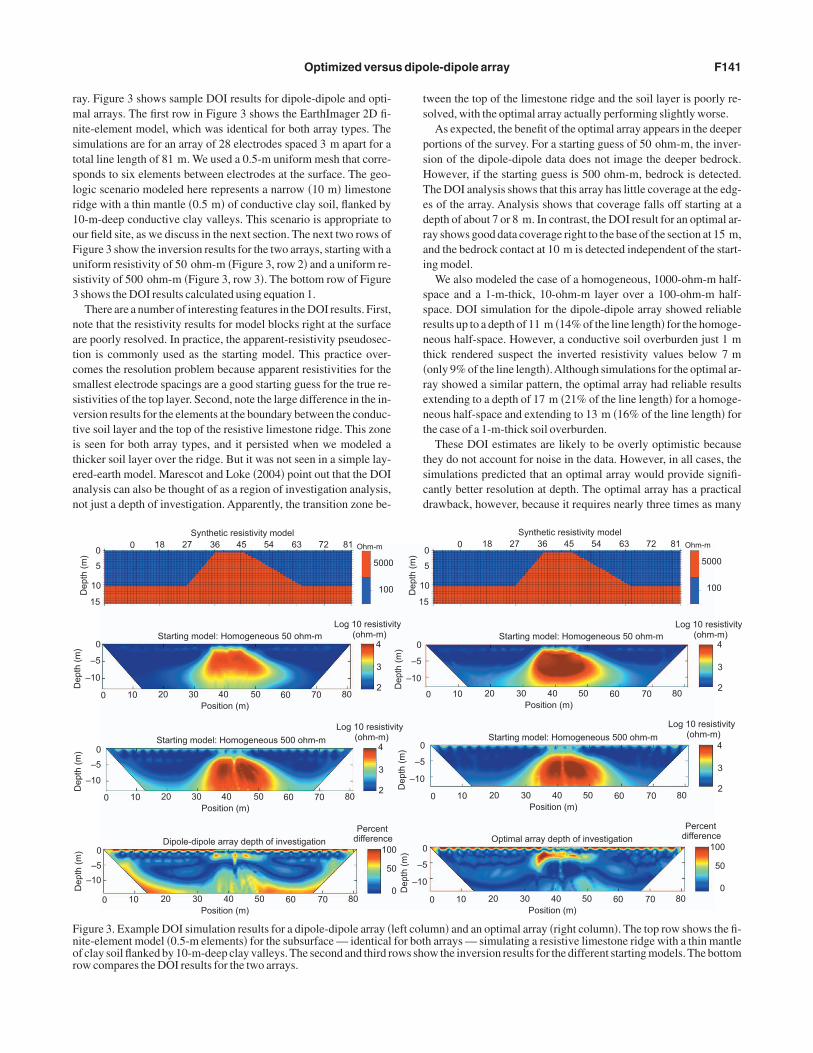
ay. Figure 3 shows sample DOI results for dipole-dipole and opti-al arrays. The first row in Figure 3 shows the EarthImager 2D fi-
ite-element model, which was identical for both array types. Theimulations are for an array of 28 electrodes spaced 3 m apart for aotal line length of 81 m. We used a 0.5-m uniform mesh that corre-ponds to six elements between electrodes at the surface. The geo-ogic scenario modeled here represents a narrow �10 m� limestoneidge with a thin mantle �0.5 m� of conductive clay soil, flanked by0-m-deep conductive clay valleys. This scenario is appropriate tour field site, as we discuss in the next section. The next two rows ofigure 3 show the inversion results for the two arrays, starting with aniform resistivity of 50 ohm-m �Figure 3, row 2� and a uniform re-istivity of 500 ohm-m �Figure 3, row 3�. The bottom row of Figureshows the DOI results calculated using equation 1.There are a number of interesting features in the DOI results. First,
ote that the resistivity results for model blocks right at the surfacere poorly resolved. In practice, the apparent-resistivity pseudosec-ion is commonly used as the starting model. This practice over-omes the resolution problem because apparent resistivities for themallest electrode spacings are a good starting guess for the true re-istivities of the top layer. Second, note the large difference in the in-ersion results for the elements at the boundary between the conduc-ive soil layer and the top of the resistive limestone ridge. This zones seen for both array types, and it persisted when we modeled ahicker soil layer over the ridge. But it was not seen in a simple lay-red-earth model. Marescot and Loke �2004� point out that the DOInalysis can also be thought of as a region of investigation analysis,ot just a depth of investigation. Apparently, the transition zone be-
0 18 27 36 45 54 63 72 81 Ohm-m
5000
100
Synthetic resistivity model
Starting model: Homogeneous 50 ohm-m Log 10 resistiv
(ohm-m) 4
3
2
Log 10 resistiv(ohm-m)
4
3
2
Starting model: Homogeneous 500 ohm-m
0 10 20 30 40 50 60 70
80 Position (m)
0 10 20 30 40 50 60 70
80 Position (m)
0 10 20 30 40 50 60 70
80 Position (m)
Dipole-dipole array depth of investigation
–10
–5
0
Dep
th (
m)
–10
–5
0
Dep
th (
m)
–10
–5
0
Dep
th (
m)
15
10
5
0
Dep
th (
m)
Percent difference
10
5
igure 3. Example DOI simulation results for a dipole-dipole array �ite-element model �0.5-m elements� for the subsurface — identicalf clay soil flanked by 10-m-deep clay valleys. The second and third row compares the DOI results for the two arrays.
ween the top of the limestone ridge and the soil layer is poorly re-olved, with the optimal array actually performing slightly worse.
As expected, the benefit of the optimal array appears in the deeperortions of the survey. For a starting guess of 50 ohm-m, the inver-ion of the dipole-dipole data does not image the deeper bedrock.owever, if the starting guess is 500 ohm-m, bedrock is detected.he DOI analysis shows that this array has little coverage at the edg-s of the array. Analysis shows that coverage falls off starting at aepth of about 7 or 8 m. In contrast, the DOI result for an optimal ar-ay shows good data coverage right to the base of the section at 15 m,nd the bedrock contact at 10 m is detected independent of the start-ng model.
We also modeled the case of a homogeneous, 1000-ohm-m half-pace and a 1-m-thick, 10-ohm-m layer over a 100-ohm-m half-pace. DOI simulation for the dipole-dipole array showed reliableesults up to a depth of 11 m �14% of the line length� for the homoge-eous half-space. However, a conductive soil overburden just 1 mhick rendered suspect the inverted resistivity values below 7 monly 9% of the line length�.Although simulations for the optimal ar-ay showed a similar pattern, the optimal array had reliable resultsxtending to a depth of 17 m �21% of the line length� for a homoge-eous half-space and extending to 13 m �16% of the line length� forhe case of a 1-m-thick soil overburden.
These DOI estimates are likely to be overly optimistic becausehey do not account for noise in the data. However, in all cases, theimulations predicted that an optimal array would provide signifi-antly better resolution at depth. The optimal array has a practicalrawback, however, because it requires nearly three times as many
0 10 20 30 40 50 60 70
80 Position (m)
0 10 20 30 40 50 60 70
80 Position (m)
0 10 20 30 40 50 60 70
80 Position (m)
5
0
5
0
Ohm-m
5000
100
0 18 27 36 45 54 63 72 81 Synthetic resistivity model
Starting model: Homogeneous 50 ohm-m Log 10 resistivity
(ohm-m) 4
3
2
Log 10 resistivity (ohm-m) Starting model: Homogeneous 500 ohm-m
4
3
2
Optimal array depth of investigation
Percent difference
100
50
0
umn� and an optimal array �right column�. The top row shows the fi-h arrays — simulating a resistive limestone ridge with a thin mantleow the inversion results for the different starting models. The bottom
ity
ity
0
0
0
1
1
Dep
th (
m)
–10
–5
0
Dep
th (
m)
–10
–5
0
Dep
th (
m)
–10
–5
0
Dep
th (
m)
left colfor botows sh

mpd
M
etTgaaq2
Lcc�ttf
cr�t�thtttta
bistpo
tlS�aI
M
ep
FMr
FTp
y
Ffrtatrt
F142 Nyquist et al.
easurements. We conducted field tests to determine whether, inractice, the improvement in resolution is sufficient to justify the ad-itional data acquisition time.
FIELD INVESTIGATION
etzgar field data collection
Lafayette College and Temple University have an ongoing coop-rative research program to evaluate the reliability of electrical resis-ivity surveys as a geotechnical site characterization method in karst.o date, we have used 2D and 3D multielectrode arrays to investi-ate bedrock depths and to locate karst solution features �Jenkinsnd Nyquist, 1999; Mackey et al., 1999; Maule et al., 2000; Roth etl., 2000; Roth et al., 2002; Nyquist and Roth, 2003; Roth and Ny-uist, 2003; Roth et al., 2004; Nyquist and Roth, 2005; Nyquist et al.,005; Peake, 2005�.
Soil
Bedrock
igure 4. Conceptual model of the bedrock topography beneathetzgar Field for a cross section perpendicular to strike. The bed-
ock ridges and soil extend parallel to strike.
igure 5. A resistivity sounding being performed at Metzgar Field.he flat, groomed surface belies the rugged underlying bedrock to-ography.
The research area is Metzgar Field, an athletic complex owned byafayette College. The geology is characterized by a thin mantle oflay soils underlain by limestone �Epler Formation, Lower Ordovi-ian�. On average, 15 new sinkholes open each year in the complexThomas and Roth, 1999�. Although the sinkholes that develop inhis part of Pennsylvania are typically small �only 1–2 m in diame-er�, they are a nuisance for groundskeepers and a serious problemor local developers.
Our study area is an approximately 1-ha portion in the northwestorner of the site. Geophysical testing and drilling show that the bed-ock in the test area has multiple high-resistivity limestone ridgesroughly 3–5 m wide� that run parallel to geologic strike �N 71° E�,he result of karst weathering of the dipping bedrock �45° southeast�Figure 4�. Bedrock depths range from less than 1 m over the ridgeso more than 10 m between the ridges. The bedrock is also known toave soil-filled and open fractures as well as larger voids. Because ofhe large contrast in resistivity between the limestone bedrock andhe overlying soil, DC resistivity is a reasonable choice for charac-erizing bedrock topography. Thus, one point of comparison be-ween the dipole-dipole and optimal arrays is a method’s relativebility to determine depth to bedrock.
A second, more difficult task, is locating cavities in the limestoneedrock. The cavities of interest are in the unsaturated zone. Locat-ng an air-filled cavity in limestone involves the difficult task ofounding through conductive clay overburden to locate an ul-raresistive target within a resistive host rock. This difficulty ex-lains our interest in finding a new array that promises improved res-lution at depth.
We collected resistivity data using both the dipole-dipole and op-imal arrays along 56 lines: 28 lines perpendicular to strike and 28ines parallel to strike. We used an Advanced Geosciences Super-ting eight-channel resistivity system with a 28-electrode cableFigure 5�, with 3 m spacing between the electrodes along the liness well as between the lines. We then inverted the data using Earth-mager 2D.
etzgar field results and discussion
At our field site, the dipole-dipole and optimal arrays were equallyffective in mapping the karst bedrock topography. Figure 6 com-ares the two resistivity array results for NS-24, a line perpendicular
Log 10 resistivit(ohm-m)
4.543.532.52
NW
Log 10 resistivity(ohm-m)
4.543.532.52
NW
80706050403020100Position (m)
80706050403020100Position (m)
SE
SE
0–2–4–6–8
–10–12D
epth
(m
)
0
–5
–10
Dep
th (
m)
a)
b)
igure 6. A comparison, with augering results, of the resistivity dataor line NS-24 for the �a� dipole-dipole survey and �b� the optimal ar-ay. The dashed horizontal line represents the approximate DOI forhe dipole-dipole array �refer to Figure 3�. The DOI for the optimalrray extends to the bottom of Figure 6. The vertical black lines showhe depths to auger refusal, which in most cases in our research cor-espond to a resistivity of roughly 1000 ohm-m on the inverted resis-ivity section.
ttirb1ndnsmo
prcsiatsWpoamm
ptbaqhsttcs
pdms
abhrista
F�i
Fspa�ltitrd
Optimized versus dipole-dipole array F143
o strike. Superimposed on the figure are the bedrock depths ob-ained by augering holes down to auger refusal along the line. Theres reasonable agreement between the resistivity data and the augeresults but little to distinguish between the two resistivity surveys. Inoth cases, the soil-bedrock interface roughly corresponds to the000 ohm-m contour. Karst bedrock, however, can be highly pin-acled and pitted. The few points where the augering and resistivityata disagree dramatically �for example, 45 and 58 m� are probablyarrow, soil-filled dissolution features — bedrock weathering on acale too fine to be resolved. It would be difficult to say that theatch between resistivity and bedrock topography is superior for the
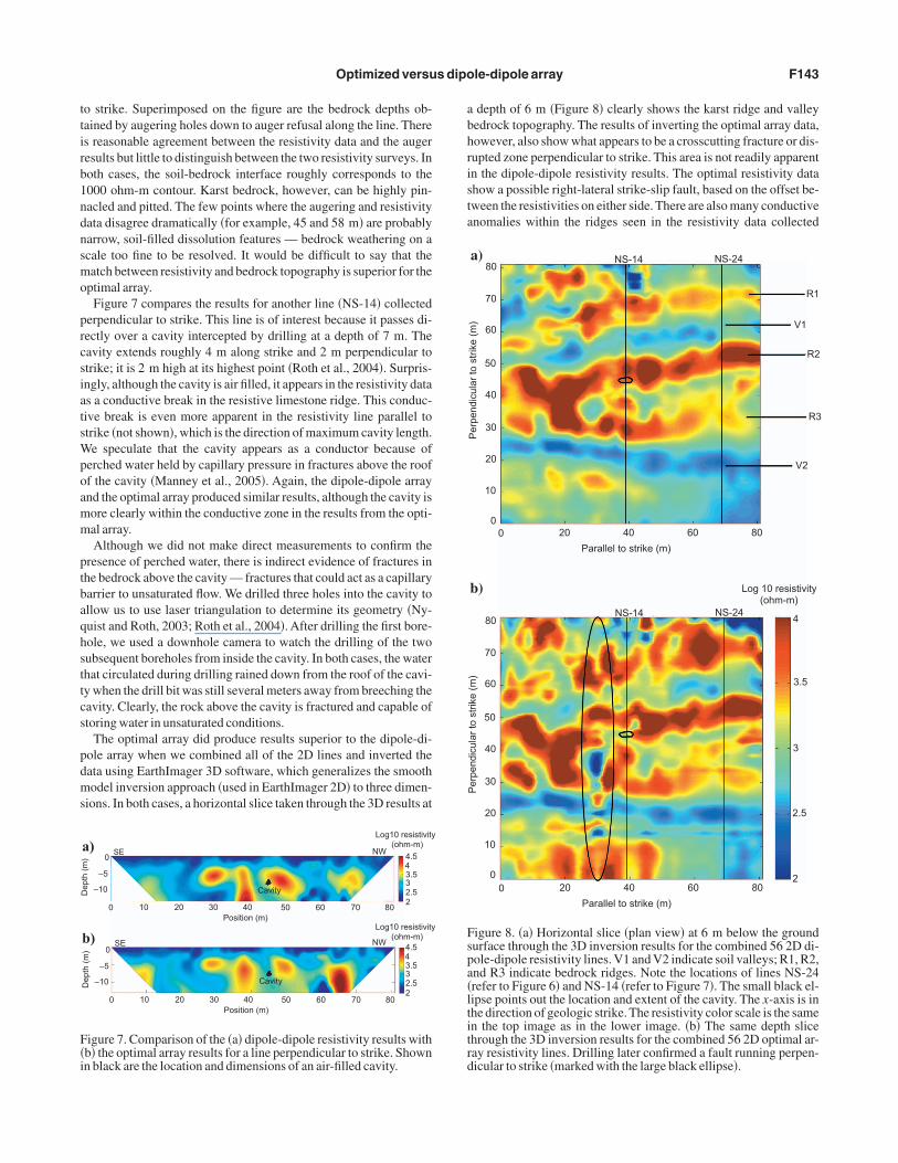
ptimal array.Figure 7 compares the results for another line �NS-14� collected
erpendicular to strike. This line is of interest because it passes di-ectly over a cavity intercepted by drilling at a depth of 7 m. Theavity extends roughly 4 m along strike and 2 m perpendicular totrike; it is 2 m high at its highest point �Roth et al., 2004�. Surpris-ngly, although the cavity is air filled, it appears in the resistivity datas a conductive break in the resistive limestone ridge. This conduc-ive break is even more apparent in the resistivity line parallel totrike �not shown�, which is the direction of maximum cavity length.e speculate that the cavity appears as a conductor because of
erched water held by capillary pressure in fractures above the rooff the cavity �Manney et al., 2005�. Again, the dipole-dipole arraynd the optimal array produced similar results, although the cavity isore clearly within the conductive zone in the results from the opti-al array.Although we did not make direct measurements to confirm the
resence of perched water, there is indirect evidence of fractures inhe bedrock above the cavity — fractures that could act as a capillaryarrier to unsaturated flow. We drilled three holes into the cavity tollow us to use laser triangulation to determine its geometry �Ny-uist and Roth, 2003; Roth et al., 2004�. After drilling the first bore-ole, we used a downhole camera to watch the drilling of the twoubsequent boreholes from inside the cavity. In both cases, the waterhat circulated during drilling rained down from the roof of the cavi-y when the drill bit was still several meters away from breeching theavity. Clearly, the rock above the cavity is fractured and capable oftoring water in unsaturated conditions.
The optimal array did produce results superior to the dipole-di-ole array when we combined all of the 2D lines and inverted theata using EarthImager 3D software, which generalizes the smoothodel inversion approach �used in EarthImager 2D� to three dimen-
ions. In both cases, a horizontal slice taken through the 3D results at
Log10 resistivity(ohm-m)
NW4.543.532.52
Log10 resistivity(ohm-m)
NW4.543.532.52
SE
Cavity
Cavity
SE
0
–5
–10Dep
th (
m)
0
–5
–10Dep
th (
m)
0 10 20 30 40 50 60 70 80Position (m)
0 10 20 30 40 50 60 70 80Position (m)
a)
b)
igure 7. Comparison of the �a� dipole-dipole resistivity results withb� the optimal array results for a line perpendicular to strike. Shownn black are the location and dimensions of an air-filled cavity.
depth of 6 m �Figure 8� clearly shows the karst ridge and valleyedrock topography. The results of inverting the optimal array data,owever, also show what appears to be a crosscutting fracture or dis-upted zone perpendicular to strike. This area is not readily apparentn the dipole-dipole resistivity results. The optimal resistivity datahow a possible right-lateral strike-slip fault, based on the offset be-ween the resistivities on either side. There are also many conductivenomalies within the ridges seen in the resistivity data collected
R1
V1
R2
R3
V2
80
70
60
50
40
30
20
10
00 20 40 60 80
Parallel to strike (m)
Per
pend
icul
ar to
str
ike
(m)
NS-14 NS-24
NS-14 NS-24
Log 10 resistivity(ohm-m)
4
3.5
3
2.5
20 20 40 60 80
Parallel to strike (m)
80
70
60
50
40
30
20
10
0
Per
pend
icul
ar to
str
ike
(m)
a)
b)
igure 8. �a� Horizontal slice �plan view� at 6 m below the groundurface through the 3D inversion results for the combined 56 2D di-ole-dipole resistivity lines. V1 and V2 indicate soil valleys; R1, R2,nd R3 indicate bedrock ridges. Note the locations of lines NS-24refer to Figure 6� and NS-14 �refer to Figure 7�. The small black el-ipse points out the location and extent of the cavity. The x-axis is inhe direction of geologic strike. The resistivity color scale is the samen the top image as in the lower image. �b� The same depth slicehrough the 3D inversion results for the combined 56 2D optimal ar-ay resistivity lines. Drilling later confirmed a fault running perpen-icular to strike �marked with the large black ellipse�.
ao
etatac
cdcacptoinsptdl
SC
B
B
C
J
M
M
M
M
N
—
N
O
P
R
R
R
R
S
T
Y
F144 Nyquist et al.
long the fault line, a result consistent with weathering along a zonef weakness.
Nine borings in this zone encountered segments of void space,ight on the ridges. Only one other boring encountered a void �out ofhe more than 30 borings drilled into bedrock within the surveyrea�. From the DOI analysis, we know that a 6-m depth slice is nearhe penetration limit for the dipole-dipole with the geometry used. Itppears that the greater penetration of the optimal array was benefi-ial in this case.
CONCLUSIONS
Although data collected using the optimal array did help us to lo-ate a fault zone at depth that was not apparent in the dipole-dipoleata, the overall results for the two arrays were quite similar. We con-lude that despite the predictions of the DOI simulations, for mostpplications, the traditional dipole-dipole array provides resolutionomparable to the optimal array of Stummer et al. �2004�. The di-ole-dipole array is preferred because the data acquisition is nearlyhree times faster. We speculate that the reason the optimal array isnly slightly better is that the resolution of the resistivity method isnherently poor for large electrode separations, a limitation that can-ot be overcome by additional electrode pair combinations �the mea-urements tend to blur together at depth�. The additional time and ex-ense associated with optimal array might be justified under excep-ional circumstances where the target of interest is at the limit of theepth of investigation or where limited access precludes using aonger array.
ACKNOWLEDGMENTS
This work was part of ongoing research sponsored by the Nationalcience Foundation under collaborative grants CMS-0125601 andMS-0201015. This support is gratefully acknowledged.
REFERENCES
eard, L. P., and A. C. Tripp, 1995, Investigating the resolution of IP arraysusing inverse theory: Geophysics, 60, 1326–1341.
hattacharya, B. B., and M. K. Sen, 1981, Depth of investigation of collinearelectrode arrays over homogeneous anisotropic half-space in direct cur-rent methods: Geophysics, 46, 768–780.
onstable, S., R. L. Parker, and C. G. Constable, 1987, Occam’s inversion:Apractical algorithm for generating smooth models from electromagneticsounding data: Geophysics, 52, 289–300.
enkins, S. A., and J. E. Nyquist, 1999, An investigation into the factors caus-
ing sinkhole development at a site in Northampton County, Pennsylvania:Proceedings of the Seventh Multidisciplinary Conference on Sinkholesand the Engineering and Environmental Impacts of Karst, 45–49.ackey, J. R., M. J. S. Roth, and J. E. Nyquist, 1999, Case study: Site charac-terization methods in karst, in G. Fernandez and R. Bauer, eds., Geo-engi-neering for underground facilities: ASCE Geotechnical Special Publica-tion, 90, 695–705.anney, R., M. J. S. Roth, and J. E. Nyquist, 2005, Exploring directional dif-ferences in resistivity results in karst: Proceedings of the Symposium forthe Application of Geophysics to Environmental and Engineering Prob-lems, Environmental and Engineering Geophysical Society, 1117–1124.arescot, L., and M. H. Loke, 2004, Using the depth of investigation indexmethod in 2D resistivity imaging for civil engineering surveys: Proceed-ings of the Symposium for the Application of Geophysics to Environmen-tal and Engineering Problems, Environmental and Engineering Geophysi-cal Society, 589–595.aule, J., J. E. Nyquist, and M. J. S. Roth, 2000, Acomparison of 2D and 3Dresistivity soundings in shallow karst terrain, Easton, PA: Proceedings ofthe Symposium for the Application of Geophysics to Environmental andEngineering Problems, Environmental and Engineering Geophysical So-ciety, 969–977.
yquist, J. E., and M. J. S. Roth, 2003, Application of a downhole search andrescue camera to karst cavity exploration: Proceedings of the Symposiumfor the Application of Geophysics to Environmental and EngineeringProblems, Environmental and Engineering Geophysical Society, 841–848.—–, 2005, Improved 3D pole-dipole resistivity surveys using radial mea-surement pairs: Geophysical Research Letters, 32, L21504.
yquist, J. E., M. J. S. Roth, S. Henning, R. Manney, and J. Peake, 2005,Smoke without mirrors:Anew tool for the geophysical characterization ofshallow karst cavities: Proceedings of the Symposium for the Applicationof Geophysics to Environmental and Engineering Problems, 337–343.
ldenburg, D. W., and Y. Li, 1999, Estimating depth of investigation in dc re-sistivity and IP surveys: Geophysics, 64, 403–416.
eake, J., 2005, A comparative analysis of the detection of subsurface cavi-ties in karst systems using two dimensional and three dimensional electri-cal resistivity: M.S. thesis, Temple University.
oth, M. J. S., J. R. Mackey, C. Mackey, and J. E. Nyquist, 2002, Acase studyof the reliability of multielectrode earth resistivity testing for geotechnicalinvestigations in karst terrains: Engineering Geology, 65, 225–232.
oth, M. J. S., and J. E. Nyquist, 2003, Evaluation of multi-electrode earth re-sistivity testing in karst: ASTM Geotechnical Testing Journal, 26,167–178.
oth, M. J. S., J. E. Nyquist, A. Faroni, S. Henning, R. Manny, and J. Peake,2004, Measuring cave dimensions remotely using laser pointers and adownhole camera: Proceedings of the Symposium for the Application ofGeophysics to Environmental and Engineering Problems, Environmentaland Engineering Geophysical Society, 1307–1314.
oth, M. J. S., J. E. Nyquist, and B. Guzas, 2000, Locating subsurface voidsin karst:Acomparison of multi-electrode earth resistivity testing and grav-ity testing; Proceedings of the Symposium for theApplication of Geophys-ics to Environmental and Engineering Problems, Environmental and Engi-neering Geophysical Society, 359–365.
tummer, P., H. Maurer, and A. G. Green, 2004, Experimental design: Elec-trical resistivity data sets that provide optimum subsurface information:Geophysics, 69, 120–139.
homas, B., and M. J. S. Roth, 1999, Evaluations of site characterizationmethods for sinkholes in Pennsylvania and New Jersey: Engineering Ge-ology, 52, 147–152.
ang, X., and M. B. Lagmanson, 2003, Planning resistivity surveys using nu-merical simulations: Proceedings of the Symposium for theApplication ofGeophysics to Environmental and Engineering Problems, Environmental
and Engineering Geophysical Society, 488–501.