PHYSICAL REVIEW B 1 APRIL 2000-IVOLUME 61, NUMBER 13

Magnetic microwires as macrospins in a long-range dipole-dipole interaction

L. C. Sampaio,* E. H. C. P. Sinnecker, and G. R. C. CernicchiaroCentro Brasileiro de Pesquisas Fı´sicas/CNPq, Rua Dr. Xavier Sigaud, 150, URCA, 22290-180, Rio de Janeiro, RJ, Brazil

M. KnobelInstituto de Fı´sica ‘‘Gleb Wataghin,’’ Universidade Estadual de Campinas (UNICAMP), Caixa Postal 6165,

Campinas 13083-970, SP, Brazil

M. Vazquez and J. Vela´zquez†

Instituto de Magnetismo Aplicado (UCM/RENFE) and Instituto de Ciencia de Materiales (CSIC), PO Box 155,28230 Las Rozas, Madrid, Spain

~Received 15 October 1999!

The long-range dipole-dipole interaction in an array of ferromagnetic microwires is studied through mag-netic hysteresis measurements and Monte Carlo simulation. The experimental study has been performed onglass-coated amorphous Fe77.5Si7.5B15 microwire with diameter of 5mm and lengths from 5 to 60 mm.Hysteresis loops performed at room temperature for an array ofN microwires (N52, 3, 4, and 5! exhibitjumps and plateaux on the demagnetization, each step correspondent to the magnetization reversal of anindividual wire. A model has been constructed taking into account the fact that the magnetization reversal isnucleated at the ends of each wire, under the influence of a dipolar field due to all other wires. Measurementsfor two wires allowed us to conclude that the dipolar field~or constant coupling! is independent of distance, atleast for an array of a few wires. With the exception of three wires, where frustration seems to be present, thepredicted reversal fields of our model are in good agreement with measurements. In order to study the roleplayed by the number of wires on the demagnetization process, we calculate hysteresis loops for a largenumber of wires through the Monte Carlo method.

niane

Ftee

aipr

-innwansitnbeca

ren

anthl

t

sefmachh-r ofehatrks

tingin-

n-

-a

om-la-thelede-ralw-ag-inre.o-cre-thegle

I. INTRODUCTION

Long-range interactions are very common in nature iwide range of sizes, varying from astrophysical to atomscales. In condensed matter physics, one of the more remable manifestations of long-range interactions is in magtism. Interactions among magnetic entities are the corebasic and applied studies of modern magnetic materials.instance, in magnetic materials the long-range dipolar inactions can play a fundamental role in the magnetic propties, being responsible for the formation of certain domstructures and the dynamics of magnetization reversalcesses. In addition, advances in fabrication techniques~in-cluding lithography! have given rise to the possibility of producing nanostructured solids with especially interestphysical properties. In particular, it is possible to obtain cotrolled arrays of magnetic wires with diameters of a fenanometers, which are of practical interest in the designoptimization of magnetoresistive heads for ultrahigh-dendata storage applications. In such systems the contributiothe dipole-dipole interaction on the magnetic propertiescomes yet more relevant, because long-range interactionsstrongly modify the magnetic response of the system toexternal excitation.

Although an array composed of a few ferromagnetic wicould in principle seem a quite simple problem to study amodel, it is striking to notice how complex this problem cturn out to be. Some recent investigations have dealt withdynamics of magnetization processes, which can includecalized excitations and/or collective modes, independen

PRB 610163-1829/2000/61~13!/8976~8!/$15.00

acrk--

oforr-r-no-

g-

dyof-ann

sd

eo-of

the parity of the system,1 weak chaotic behavior,2 and eventhe possibility to tailor the value of the coercivity, in the caof nanoscopic flat wires.3 The complication in the study odipolar interactions is that the magnetic fields resulting frothe interaction depend on the magnetization state of eentity, which, in turn, depend on the effective field of neigboring elements. In spin systems the long-range charactea dipole-dipole interaction is an inherent difficulty to solvthe Hamiltonians due to the large number of neighbors tone has to take into account in calculations. Several wohave been made using Monte Carlo simulations calculathe magnetic domain structure and magnetic hysteresiscluding the dipolar interaction term in the Ising or Heiseberg Hamiltonian.4,5

An intrinsic difficulty in the study of magnetic interactions is the fact that it is extremely difficult to characterizesingle magnetic element using most conventional magnetetry techniques. Also, the predictions of numerical simutions are intricate to compare with real systems, owing tonecessity to introduce several approximations in the modeproblem. However, in this work we make use of a convnient macroscopic configuration, placing together seveferromagnetic microwires covered with glass. Such microires exhibit a strong magnetic anisotropy with an easy mnetization direction along the axis of the wire with a masingle domain practically extending along the whole wiThis fact will allow us to consider each one of such micrwires as a elemental magnetic moment. The stray fieldsated by the microwires couple the magnetization ofneighboring wires, affecting the magnetic state of each sin

8976 ©2000 The American Physical Society

enisa

tioeela

redul

awi

sin

y

sofl-nrslen

at

et

er

n

onla

f t-

rg

sl,vaedu

senn

x-f

x-seiston

sev-

nsis ablydif-tic

arerop-also

ac-uchter-ringtwo

suretheforththel-m.ruc-the

allthe

ong

inratetionofde-

bei-

ave

re.9the

PRB 61 8977MAGNETIC MICROWIRES AS MACROSPINS IN A . . .

wire. This system is relatively easy to study both experimtally and theoretically, and, in the case of few wires itpossible to obtain analytical solutions. Some interestingpects of the long-range character of dipole-dipole interacand their influences on the magnetic properties appclearly in the obtained results. The exact solutions andperimental data can be compared with Monte Carlo simutions, which are necessary to employ when the arrayformed by a large number of wires. As mentioned befoalthough this arrangement seems to be rather simple, itplays a variety of interesting aspects which certainly woapply in other physical systems.

II. EXPERIMENTAL DETAILS AND MEASUREMENTS

Concerning the experimental measurements, they hbeen performed in glass-coated amorphous microwiresnominal composition Fe77.5Si7.5B15, diameter of 5mm, andthe thickness of the glass coating of 7.5mm. Glass-coatedamorphous microwires are presently attracting an increainterest from both basic and applied points of view~for re-views see Ref. 6!. Their metallic core, being structurallamorphous and with typical diameter from 1 to 30mm, iscovered by an insulating Pyrex-like coating with thicknebetween 1 and 20mm. They are fabricated by meansTaylor-Ulitovsky technique by which the molten metallic aloy and its glassy coating are rapidly quenched and drawa kind of composite microwire typically a few kilometelong. This family of microwires displays quite remarkabmagnetic properties, that together with their tiny dimensioand the protective coating make them potential candidfor many sensor applications.7

Owing to the amorphous nature of such microwires, thunique magnetic behavior depends on the strength anddistribution of magnetoelastic anisotropy. That is first detmined by the magnetostriction constant, which is mainlyfunction of composition.8 For the present alloy compositiothe saturation magnetostriction takes a value of 231025. Inturn, the internal stresses~as strong as 103 MPa! depend onthe ratio cover thickness to core diameter, which is ctrolled by the fabrication parameters, and also on particuprocessing as thermal treatments and chemical etching ocoating.8 When axially magnetized these wires exhibit lowfield square hysteresis loops with a single and laBarkhausen jump.

We have measured magnetic hysteresis loops in arrayN microwires (1<N<5) placed side by side, all paralleeach one touching its nearest neighbors. Their lengthsfrom 5 to 60 mm, cut from a single long microwire. Wperformed the measurements by using either a superconing quantum interference device~SQUID! magnetometer~Quantum Design, MPMS XL model! or a very sensitivemagnetic-flux integrator. Essentially, the difference in thetwo systems is the sensitivity and the time of measuremAlthough the hysteresis loops measured in the SQUID doexhibit either noise or drift, which appear in the fluintegrator, a single hysteresis measurement can take ahours in the SQUID, while the same loop in the fluintegrator takes about 1 min. The flux-integrator was ufor rapid measurements, for instance, to measure the dbution of reversal field values. We will focus our attention

-

s-narx--

is,

is-d

veth

g

s

to

ses

irhe-a

-r

he

e

of

ry

ct-

et.

ot

ew

dri-

measurements performed at room temperature, but alsoeral loops were performed at low temperatures@4<T(K)<300#, in several attempts to strengthen the interactioamong the wires. However, at low temperatures therechange in the domain structure of the microwires, probaowing to the increasing internal stresses induced by theferent thermal expansion coefficients of the ferromagnealloy and the covering glass. Therefore, the loops whichrather square at room temperature turn out to lose this perty at low temperatures. This characteristic has beenreported for Co-based microwires.9

In the case of one 5 mm long wire (N51, see Fig. 1! thehysteresis curve exhibits a typical square loop, with charteristic large Barkhausen jumps. The observation of ssquare loops, labeled as magnetic bistability, has been inpreted as in the case of in-water-quenched wires, considethe remagnetization processes of the inner core betweenstable remanence states.10 That internal core mainly consistof a single axial domain, but at the ends of the wire a closdomain structure appears at finite applied fields to reduceotherwise quite high magnetostatic energy. Of course,very short microwires closure structures coming from boends overlap at the middle of the sample, destroyingmagnetic bistability.11 The critical length to observe bistabiity in the microwires of the present study is less than 5 mNevertheless, in spite of the existence of these closure sttures some stray field is generated in the surroundings ofmicrowire. Upon application of reversed field a domain wdepins from one end of the wire and propagates alongwire resulting in the observed magnetization jump.

Small differences in the measured coercive fields (HC)were detected when the magnetic field was applied alpositive or negative directions~in Fig. 1 theHC values cor-respond to20.89 and 0.79 Oe, respectively!. There can beseveral origins for the fluctuation ofHC values. When dif-ferent samples are investigated, the fluctuation inHC is prob-ably due to different magnetoelastic anisotropies inducedthe wire ends during the cutting process, which can genedifferent levels of mechanical stresses. Since the nucleaof a domain wall starts in defects located at the extremitiesthe wires, and the number and strength of these defectspend on the cutting, the switching field of one wire canslightly different for magnetic fields applied in opposite drections, and it can also vary in different samples. We h

FIG. 1. Hysteresis loop for one microwire at room temperatuThe reversal field is20.89 Oe for negative reversal field and 0.7Oe for positive reversal field. The coercive field is defined asmean value,uHCu50.85 Oe.

ar-ureapo

exanuduth

er

clu2

eagu. Ilde

osi-eld

elees,neti-r-

theep-

la-dertheliedag-lel,p-

ae,

raaa

ra-The

re

dfig

re.ows

8978 PRB 61L. C. SAMPAIO et al.

investigated this fluctuation in several samples, and we hfound a maximum variation inHC of about 0.10 Oe. Anothedistribution in theHC values arises from thermal fluctuations, and it occurs even when the same sample is measseveral times. To determine this distribution, we measuHC several times in the same sample and with the fieldplied in the same direction, and it was found that the widththis distribution is around 0.03 Oe. However, we cannotclude that this intrinsic fluctuation of the reversal field carise simply from the fact that after each reversal the closdomain structures cannot be exactly the same, thus introing a fluctuation in the next magnetization reversal. Fromabove discussions we consider the absolute value ofHC ofthis microwire as the mean value obtained from many diffent measurements,HC50.85 Oe.

Let us now consider two wires~5 mm long! placed sideby side with their axes parallel. In this case the distanbetween their axes is twice the thickness of the coating ptwice the radius of the ferromagnetic core, i.e., aroundmm. The corresponding hysteresis loops exhibit two clBarkhausen jumps steps and a plateau nearly at zero matization ~see Fig. 2!. This plateau corresponds to the configration of two wires with opposite magnetization directionsis worth noting that the first jump occurs at magnetic fielower thanHC , while the second one occurs for fields larg

FIG. 3. Hysteresis loop for three microwires at room tempeture. Note that the second step does not appear. The magnetizis normalized to the saturation value. The arrows represent the mnetic configuration of the wires.

FIG. 2. Hysteresis loop for two microwires at room temperatuThe mean reversal fields on the demagnetization areH2

i

520.43 Oe andH2i i 521.11 Oe. The magnetization is normalize

to the saturation value. The arrows represent the magnetic conration of the wires.

ve

redd-f-

rec-e

-

es

0rne--tsr

than HC . These reversal fields will be namedH2i and H2

i i ,and their values are 0.38 and 1.10 Oe, respectively, for ptive demagnetizing field. For negative demagnetizing fithe values ofH2

i andH2i i were found to be20.49 and21.12

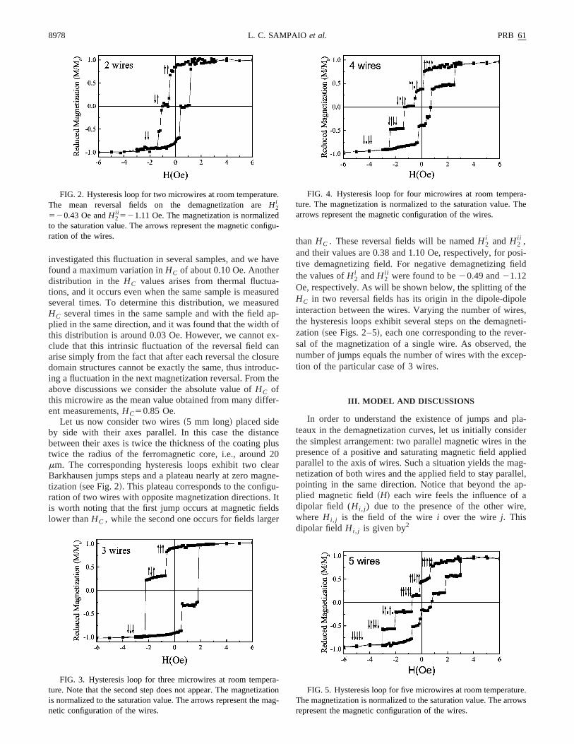
Oe, respectively. As will be shown below, the splitting of thHC in two reversal fields has its origin in the dipole-dipointeraction between the wires. Varying the number of wirthe hysteresis loops exhibit several steps on the demagzation ~see Figs. 2–5!, each one corresponding to the revesal of the magnetization of a single wire. As observed,number of jumps equals the number of wires with the exction of the particular case of 3 wires.

III. MODEL AND DISCUSSIONS

In order to understand the existence of jumps and pteaux in the demagnetization curves, let us initially consithe simplest arrangement: two parallel magnetic wires inpresence of a positive and saturating magnetic field appparallel to the axis of wires. Such a situation yields the mnetization of both wires and the applied field to stay paralpointing in the same direction. Notice that beyond the aplied magnetic field~H! each wire feels the influence ofdipolar field (Hi , j ) due to the presence of the other wirwhere Hi , j is the field of the wirei over the wirej. Thisdipolar fieldHi , j is given by2

-tiong-

FIG. 4. Hysteresis loop for four microwires at room tempeture. The magnetization is normalized to the saturation value.arrows represent the magnetic configuration of the wires.

.

u-

FIG. 5. Hysteresis loop for five microwires at room temperatuThe magnetization is normalized to the saturation value. The arrrepresent the magnetic configuration of the wires.

twoprn

aonms

emlu-ag,d

is

rtes

thizaretio

iathpeen

thveo

vee

og-iv

nco-

oth

ils-hentoitng

he

llel,the

-ex-

es

t

t of

iresoned

forareforirestal

the

r-th

gu-ner-

PRB 61 8979MAGNETIC MICROWIRES AS MACROSPINS IN A . . .

H i , j52KnM i , ~1!

whereKn is a geometric factor andM i is the magnetizationof the ith wire. As the coefficientKn depends in principle onthe distance between interacting wires, the subsciptn denotesthe distance between the wires,K1 corresponds to nearesneighbors,K2 to second neighbors, and so on. Thus, for twires one can easily write down the mutual dependenceduced by the dipole-dipole interaction through the functioM15M1(H1H2,1) and M25M2(H1H1,2) with H i , j52KnM i .

Applying now a reversal magnetic field, one notices thboth applied field and dipolar fields act in the same directiantiparallel to the magnetization of both wires. Let us siplify the analysis by considering two quasi-identical wirei.e., both wires have the same magnetizationM and coercivefield HC . It is important to emphasize that on the ideal dmagnetization process the field necessary to reverse thenetization of an individual wire has always the same va~the coercive field,HC! and this value, but for the abovementioned fluctuations, is characteristic of the internal mnetic properties~anisotropies! of that particular wire. Henceat the first jump (H2

i ), in spite of the fact that the appliefield is H2

i , the effective field is equal toHC . Therefore, thecondition to the first wire to reverse its magnetizationgiven by2H2

i 2K1M52HC , and thus:

H2i 5HC2K1M . ~2!

Once the first wire reverses its magnetization, the configution of the system is given by two wires with compensamagnetization (↑↓), which is more stable than the previouconfiguration since the dipolar fields now act parallel tomagnetization of both wires. Now, to reverse the magnettion of the second wire a stronger external field is requibecause this field has to compensate the dipolar contribuTherefore, at the second jump (H2

i i ), the effective field is2H2

i i 1K1M52HC , and therefore:

H2i i 5HC1K1M . ~3!

Actually, the dipolar interaction acts on the wires as a bfield with opposite direction, decreasing and increasingreversal field of the first step and the second jumps, restively. Note that the plateau or difference between the revsal fieldsH2

i andH2i i corresponds to dipole-dipole interactio

between the wires, and it is given by 2K1M .Before proceeding with the discussion and extending

reasoning to the case of several wires, let us discuss seimportant points regarding the dipole-dipole interactionstwo wires. First, it is worth noticing that although we haconsidered, for the sake of simplicity, two wires with thsame magnetization and coercive field, the fluctuationsthese values are essential to observe the effects of dipinteraction.2 If both wires would have exactly the same manetic properties they would feel exactly the same effectfield, and would reverse at exactly the same field value,H2

i .However, in real situations the wires are not identical, athey can display fluctuations in both magnetization andercive fields~see above!, and therefore one of the wires reverses the magnetization before the other one, leading tintermediate, more stable structure, and to the splitting ofreversal field.

o-s

t,-,

-ag-e

-

a-d

e-

dn.

sec-r-

eralf

inlar

e

d-

ane

Second, it is important to further discuss some detaabout the coupling constantKn . We consider that the magnetization reversal is nucleated at the ends of the wires wthe effective magnetic field acting on the wire is equalHC . Calculating the dipolar field nearby one of the wiresis easy to show that the component of its dipolar field alothe axis of the second wire at its ends is given by

Hd5pL/~r i j2 1L2!3/2, ~4!

where p is the strength of the point poles, located at textremeties of the wire of lengthL and r i j is the distancebetween the wiresi andj.12 Note that in our configuration themagnetizations of the wires are either parallel or antiparaand the distances among wires are well known. Sincemagnetization ispL, one identifiesKn as given by

Kn51/~r i j2 1L2!3/2. ~5!

We write Kn5K1 when i 2 j 51 ~first neighbors!, Kn5K2when i 2 j 52 ~second neighbors!, and so on. Since our systems are composed of a few wires with distances neverceeding a few tenths of millimeters, with length of the wirof about 5 mm we have always the conditionr i j !L fulfilled.Therefore, the constants of couplingKn become independenof distance, at least in the range of a few wires.

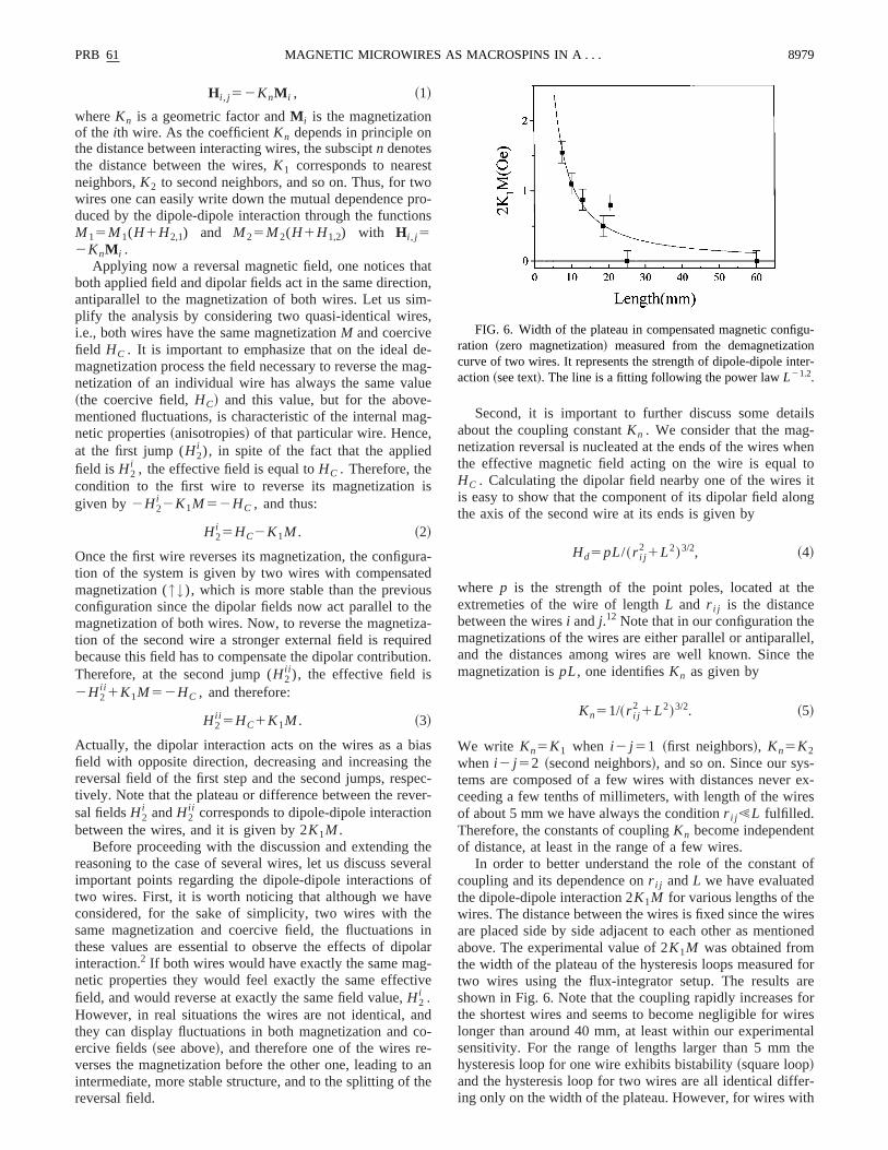
In order to better understand the role of the constancoupling and its dependence onr i j andL we have evaluatedthe dipole-dipole interaction 2K1M for various lengths of thewires. The distance between the wires is fixed since the ware placed side by side adjacent to each other as mentiabove. The experimental value of 2K1M was obtained fromthe width of the plateau of the hysteresis loops measuredtwo wires using the flux-integrator setup. The resultsshown in Fig. 6. Note that the coupling rapidly increasesthe shortest wires and seems to become negligible for wlonger than around 40 mm, at least within our experimensensitivity. For the range of lengths larger than 5 mmhysteresis loop for one wire exhibits bistability~square loop!and the hysteresis loop for two wires are all identical diffeing only on the width of the plateau. However, for wires wi

FIG. 6. Width of the plateau in compensated magnetic confiration ~zero magnetization! measured from the demagnetizatiocurve of two wires. It represents the strength of dipole-dipole intaction~see text!. The line is a fitting following the power lawL21.2.

oely

.i

d

eo

mhdches

r

thd.in

in--

vedtsgrs

bygth

u

upemisn

thlalo

ere-

heto

e

at

ldsveized

as-

end

eld,til it

reday

8980 PRB 61L. C. SAMPAIO et al.

length of about 1 mm the hysteresis loop for one wire dnot exhibit bistability anymore, preventing equivalent anasis.

According to our model the quantity 2K1M is propor-tional toL/(r i j

2 1L2)3/2 @Eq. ~4!#. The limit r i j !L produces apower-law decay to 2K1M with L following L22, and on theother hand, in the limitr i j @L, the factor 2K1M varies lin-early onL following L/r i j

3 . The conjunction of the two limitsshould exhibit a maximum in the plot 2K1M vs L, whichwas clearly not experimentally observed. Thus, from Figwe conclude that in our samples we are always workingthe limit r i j !L. In this range of length, the data were fitteby the power law,L21.2, which, however, is not in goodagreement with the expected dependence (L22).

However, one should always keep in mind that considing each microwire as a single magnetic dipole with twmagnetic charges at both ends is an idealized approach~thatis nevertheless supported by the observation of single jufor multiwire loops!. Indeed, a fully realistic approacshould have to consider that magnetic charges could betributed along the whole length of the wire, making mumore complex the calculations of the fields created by thcharges around each microwire.13 Therefore, the lack of fullagreement between experiments and model can be regaas the result of an oversimplification of the model.

It is important to clarify that the dependence on lengmeasured for 2K1M is not related to the demagnetizing fielThe wires as long cylinders have a very low demagnetizfactor. For instance, in our samples the wires are 5mm indiameter and for a typical length of 5 mm the demagnetizfactor is around 1026,14 which, considering a saturation magnetization of 1240 emu/cm3, results in a calculated demagnetizing field,Hdm , of about 1022 Oe. This value is wellbelow the reversal field of one wire (HC) and it does notplay an important role in the demagnetization process. Ethough the demagnetizing effects are very small comparethe reversal fields, it is easy to calculate how the wid2K1M would be modified by taking them into account. Adiscussed in Eqs.~2! and ~3!, and since the demagnetizinfield is opposite to the magnetization, the first wire to revethe magnetization feels the resulting field,2H2

i 1K1M2Hdm , and the corresponding reversal field is given2H2

i 2K1M1Hdm . For the second wire, because the manetization is also positive, the demagnetization field hassame sense as before; the resulting field is2H2

i i 1K1M2Hdm . Therefore, the reversal field is given byH2

i 5HC

1K1M1Hdm . Hence, note that the width of the step,H2i i

2H2i , the demagnetizing field cancels out and the platea

the hysteresis loop remains equal to 2K1M .It is worth noting that the above discussion provides s

port to the idea that we are dealing with a magnetic systwhich displays a dipolar coupling that is independent of dtance, in other words, the dipole-dipole interaction is costant, at least for a few wires. Furthermore, it reinforcesapplicability of the model to explain the presence of regusteps in the demagnetization curves, as will be shown befor the cases of more than two wires.

Now, it is straightforward to extend the above developreasoning to an array of a few wires. For example, for thwires, the first step (H3

i ) arrives from the magnetization re

s-

6n

r-

ps

is-

e

ded

g

g

ntoh

e

-e

in

-,

--erw

de

versal of the wire that is in the middle position due to tgreatest dipolar field from the two others—it corresponds↑↓↑ magnetic configuration. Thus, atH3

i , identifying theeffective field that this wire feels to its coercive field (HC),one has2H3

i 22K1M52HC , and therefore

H3i 5HC22K1M . ~6!

At the second jump (H3i i ) the magnetic configuration of th

wires goes from↑↓↑ to ↑↓↓, or ↓↓↑, and hence atH3i i the

resulting field on the wire is2H3i i 2(K12K2)M and again

setting it toHC , one finds

H3i i 5HC2~K12K2!M . ~7!

Finally, the third step from↑↓↓, or ↓↓↑, to ↓↓↓; the mag-netization reversal of the wire at the other extremity occurs

H3i i i 5HC1~K11K2!M . ~8!

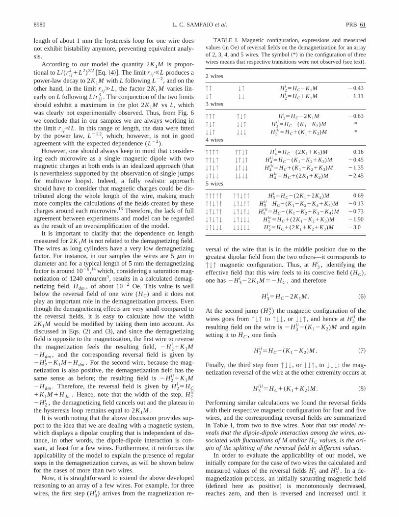
Performing similar calculations we found the reversal fiewith their respective magnetic configuration for four and fiwires, and the corresponding reversal fields are summarin Table I, from two to five wires.Note that our model re-veals that the dipole-dipole interaction among the wires,sociated with fluctuations of M and/or HC values, is the ori-gin of the splitting of the reversal field in different values.

In order to evaluate the applicability of our model, winitially compare for the case of two wires the calculated ameasured values of the reversal fieldsH2

i andH2i i . In a de-

magnetization process, an initially saturating magnetic fi~defined here as positive! is monotonously decreasedreaches zero, and then is reversed and increased un

TABLE I. Magnetic configuration, expressions and measuvalues~in Oe! of reversal fields on the demagnetization for an arrof 2, 3, 4, and 5 wires. The symbol~* ! in the configuration of threewires means that respective transitions were not observed~see text!.

2 wires

↑↑ ↓↑ H2i 5HC2K1M 20.43

↓↑ ↓↓ H2i 5HC1K1M 21.11

3 wires

↑↑↑ ↑↓↑ H3i 5HC22K1M 20.63

↑↓↑ ↓↓↑ H3i i 5HC2(K12K2)M *

↓↓↑ ↓↓↓ H3i i i 5HC1(K11K2)M *

4 wires

↑↑↑↑ ↑↑↓↑ H4i 5HC2(2K11K2)M 0.16

↑↑↓↑ ↓↑↓↑ H4i i 5HC2(K12K21K3)M 20.45

↓↑↓↑ ↓↑↓↓ H4i i i 5HC1(K12K21K3)M 21.35

↓↑↓↓ ↓↓↓↓ H4iv5HC1(2K11K2)M 22.45

5 wires

↑↑↑↑↑ ↑↑↓↑↑ H5i 5HC2(2K112K2)M 0.69

↑↑↓↑↑ ↓↑↓↑↑ H5i i 5HC2(K12K21K31K4)M 20.13

↓↑↓↑↑ ↓↑↓↑↓ H5i i i 5HC2(K12K21K32K4)M 20.73

↓↑↓↑↓ ↓↑↓↓↓ H5iv5HC1(2K12K21K3)M 21.90

↓↑↓↓↓ ↓↓↓↓↓ H5v5HC1(2K11K21K3)M 23.0

tin

s

hissect ool4

rly

se

-

uesthin

ue

oladel

i-

st

thoh

ue

s.ayve

lu

-

four

ac-veear

erheaus-inp.

ble

nt tovornd

ra-

;ndems

r aingcu-re-

ventsn.

to-q.irs

ee

ofeen

an-is

assx-

PRB 61 8981MAGNETIC MICROWIRES AS MACROSPINS IN A . . .

reaches a saturating, negative value. In this way, calculathe average ofH2

i andH2i i we find 20.77 Oe, which should

correspond toHC @see Eqs.~2! and~3!#. Calculating the dif-ference betweenH2

i and H2i i , we find 20.68 Oe which

should be equal to 2K1M @see Eqs.~2! and~3! and Table I!.Since the mean value ofHC measured for a single wire i20.85 Oe, we may consider thatHC obtained from the av-erage and the one measured are in good agreement. Treally acceptable if we take into account several sourcefluctuations or peculiarities of each wire, as different defstructures originated from the cutting, imperfect alignmenthe wires, etc. Note that the term that represents the dipdipole interaction (K1M ) corresponds in modulus to 0.3Oe.

The discussion can be extended for an even numbewires, i.e., for four parallel microwires. One can immediateremark that the first and fourth (H4

i andH4iv) and the second

and third reversal fields (H4i i and H4

i i i ) are approximatelyequidistant fromHC . In other words, the average of thevalues should be equal toHC as should be expected fromcalculations~see Table I!. From Fig. 4, we obtain these average values to be20.9 Oe and21.3 Oe, respectively. Aspreviously discussed, we have measured fluctuations aroHC to be approximately 0.1 Oe, in the case of single wirHowever, increasing the number of wires, the error inmeasured values of reversal fields should accordinglycrease. With that consideration in mind, the latest val~20.9 and21.3 Oe! are in reasonable agreement withHC .

From previous discussions we can consider the dipinteractions in our case as almost constant, i.e., indepenof distance. In this case,Kn is simply K1, and the reversafields H4

i i i andH4i i take a simplified formHC6K1M . Actu-

ally, this expression is identical as for the reversal fieldsthe case of two wiresH2

i and H2i i , and comparing their re

spective values, we findH2i andH4

i i equal to20.43 Oe and20.45 Oe, respectively. ForH2

i i andH4i i i the obtained values

are21.1 Oe and21.35 Oe, respectively. Moreover, the firreversal fieldH4

i becomes equal toHC23K1M , and substi-tuting the value ofK1M , we findH4

i equal to 0.17 Oe, whichis very close to the measured value, 0.16 Oe. Notice thatfield is now positive, i.e., the effective dipolar field is sstrong that it overcomes the applied magnetic field. Tsame analysis can be performed for the fourth jumpH4

iv ,which turns out in the expressionHC13K1M , and results in21.87 Oe, which, however, differs from the measured val22.45 Oe. Thus, using the fact that allKn’s have the samestrength, the predicted fields toH4

i , H4i i , andH4

i i i ~in excep-tion of H4

iv) are in very good agreement with experimentLet us now analyze the demagnetization curves of arr

with an odd number of wires, starting with the case of fiwires, and assuming again that allKn’s are equal toK1. Asbefore, we can compare the predicted and measured vaof the reversal fields. It is remarkable that the expressionthe third stepH5

i i i is oversimplified to give simplyHC , andthe measured values ofH5

i i i 520.73 Oe andHC520.85 Oeare rather close. The first and second steps,H5

i andH5i i , with

corresponding expressions,HC24K1M andHC22K1M , re-spectively, result in 0.51 Oe and20.17 Oe, which are alsoclose to the measured values, 0.69 Oe and20.13 Oe, respec

g

isoftfe-

of

nd.

e-s

rnt

n

is

e

,

s

esof

tively. The fourth and fifth steps,H5iv andH5

v , with oppositeincrements inK1M are positioned afterHC , and are givenby HC12K1M and HC14K1M , respectively. Comparingtheir expected values~21.53 Oe and22.21 Oe! with themeasured ones~21.9 Oe and23.0 Oe! one finds that theagreement is not as good as in the previous case ofwires.

In conclusion, comparing the reversal fields predictedcording to the model with measured values for four and fiwires, a good agreement is obtained mainly for fields nand belowHC , while for fields well aboveHC the agreementis poor.

The particular situation of three wires, contrary to otharrays with two, four, and five wires, is characterized by tabsence of one of the jumps. This situation has been exhtively tested for different samples both in the SQUID andthe flux integrator, but we could not obtain the missing jumActually, all samples measured are in the conditionr i j !L,where allKn’s have the same strength. Hence, it is possithat the geometry of an array of three wires, whereK1 andK2 have the same approximate value, should be equivalethree wires placed as a triangle. This configuration can fathe occurrence of frustration of magnetic interactions, amight prevent the formation of an intermediate configution. On the other hand, the elimination of the conditionr i j!L requires either the increase ofr i j in a controllable wayor the decrease ofL to order of a few tenths of micrometershowever, both are quite difficult to attain experimentally aare not in the scope of our present study. Our model senot to be applicable to three wires under the conditionr i j!L possibly because of the existence of frustration.

Let us finally discuss the demagnetization process folarge number of wires. It is clear that extending the reasondeveloped above for a still larger number of wires the callation of reversal fields becomes increasingly tedious. Thefore, we have used the Monte Carlo~MC! method based ona one-dimensional modified classical Ising model. We haconsidered a one-dimensional array of magnetic momeinteracting through the long-range dipole-dipole interactioIn our model, the Hamiltonian takes a simple form,

H5M2( Ji j s is j2~H1Hani!( s i , ~9!

where the variables i takes the values61 on a sitei on aone-dimensional array, allowing the magnetic momentspoint up (s i511) or down (s i521) along an axis perpendicular to the axis of the array. The first summation in E~9! denotes the dipole-dipole interaction acting over all paof magnetic moments. The constant of couplingJi j is iden-tified with 1/Kn @see Eq.~5!#, and the distances between thmagnetic moments,r i j , are measured in units of the latticconstanta. Note that the magnetization,M , of a wire is givenby Ms iz ~z is a unitary vector perpendicular to the axisthe array!. The second term denotes the interaction betwthe magnetic moments and an external magnetic field (H),Hani being a fixed bias field representing the magneticisotropy of one wire, i.e., the reversal field of one wire. Iteasy to realize that the fieldHani can be recognized asHC .

Note that in the experimental case, the wires are glcoated, inhibiting any possibility to interact through e

isel

ndnu-s

elutnneatith,usiz

ayod

ndrothemu

picisot-

d, it

an-on

sisnsegnotizedthereext,

andstionalheaveac-ofe ofry

al-lareticng-sys-nflu-

anic-

ro-

n-tefulre-

te10

8982 PRB 61L. C. SAMPAIO et al.

change interaction, and therefore, the constantJi j containsonly the dipole-dipole interaction. Another point to remarkthat sinceJi j is positive, the first term favors an antiparallalignment among the magnetic moments.

We used the single-spin-flip Metropolis dynamics aopen boundary conditions~details of calculations are givein a previous publication!.4 The hysteresis loops were calclated changing the fieldH with a sweep rate of 10 MC stepfor each magnetization value. The temperature~T! was con-sidered low enough in order to be well below thantiferromagnetic-paramagnetic phase transition. The vaof parametersM ,H,T, are chosen arbitrarily. Notice thawhat is here mostly relevant is the relative intensity amothe terms of the Hamiltonian. In that way, we determitrends and not absolute values; thus our results calculfrom the MC method may be qualitatively compared wexperiments. We usedM2, Hani , andT equal to 5, 5, and 1respectively. This trial of values is good enough to discthe role played by the number of wires on the demagnettion process.

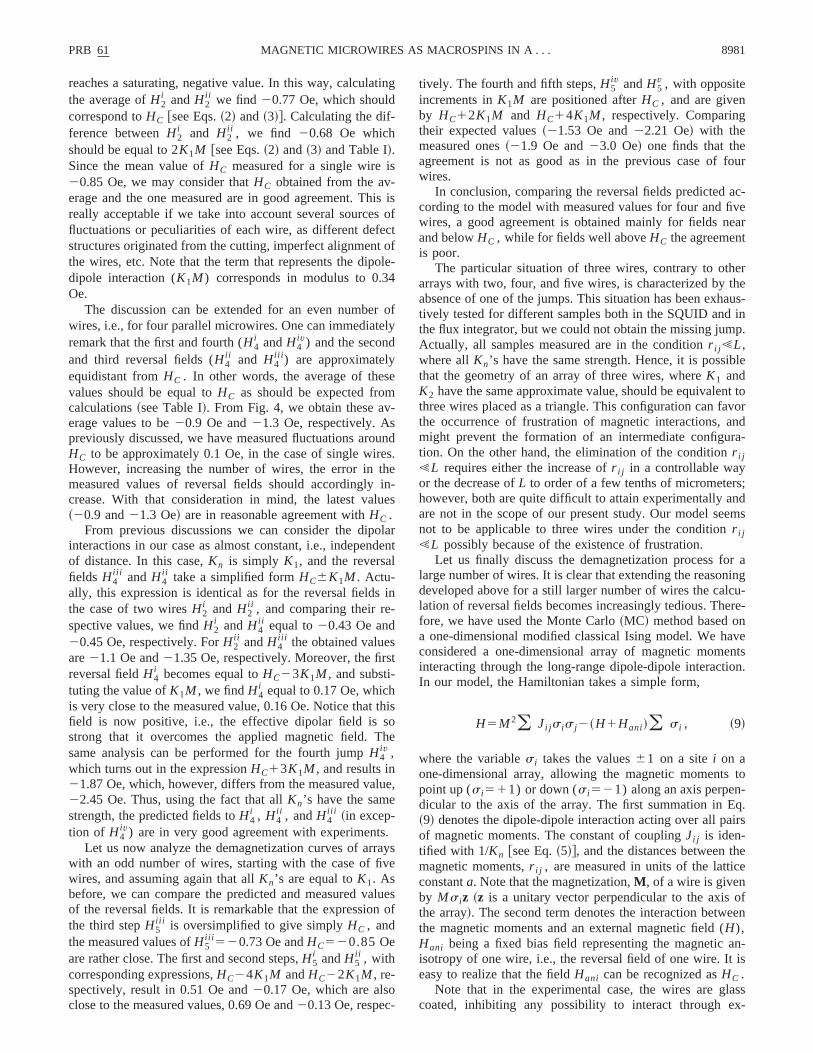
Figure 7 shows hysteresis loops for 1 wire and for arrof 2, 4, 10, and 500 wires calculated using the MC methAs observed in experiments~see Figs. 2–5! the reversalfields for an array of multiple wires are distributed arouthe reversal field of 1 wire (HC), and enlarging the numbeof wires the width of plateaux decrease. This agreement cfirms the idea that spin models can be used to studymagnetic properties of macroscopic systems like ansemble of microwires. In addition, for 500 wires the systedemagnetizes monotonically with small jumps and platea

FIG. 7. Demagnetization region of hysteresis loop calculausing the Monte Carlo method for 1 wire and for arrays of 2, 4,and 500 wires.

o

.

es

g

ed

sa-

s.

n-e

n-

s,

which should correspond in real systems to microscoBarkhaunsen jumps. Notice the presence of a clear anropy field, even for 500 wires~Fig. 7!. Although the under-lying physical meaning of this field is still unknown, anneeds further experimental and theoretical investigationscan be referred to as a ‘‘long-range effective interactionisotropy,’’ which is generated by the intricate superpositiof dipolar fields from many wires in a specific array.

IV. CONCLUSIONS

In this work we have presented experimental hystereloops of sets of long microwires arranged parallel in a depacking configuration. Owing to the protective insulatinglass-coating the magnetic microwires are neverthelesstouching each other. The hysteresis loops are characterby well-defined Barkhausen jumps corresponding each tomagnetization reversal of individual microwires that aseparated by horizontal plateaux. As discussed in the tthese jumps are theoretically interpreted according tomodel based on the nucleation of closure domains at the eof the wires and the subsequent depinning and propagaof a domain wall. The dipolar field acting on each individumicrowire due to all surrounding wires is responsible for tactual value of its observed reversal field. The plateaux hbeen proved to be determined by the dipole-dipole intertion as well. It has been pointed out how the peculiaritythe coupling between the wires, namely, the independencdistance from the magnetic coupling transforms it in a veinteresting system.

One main achievement of the present work is thatthough the array of microwires is macroscopic, the dipointeraction among them has a similar effect on the magnproperties as classical spins interacting throughout lorange interactions. Therefore, we believe that the studiedtem can be regarded as a standard system to verify the ience of dipolar interactions in the magnetic response ofarray of dipoles, being possible to test micromagnetic predtions and verify the best conditions to optimize the macscopic magnetic behavior for specific applications.

ACKNOWLEDGMENTS

This work was partially supported by the Brazilian agecies CNPq, FAPERJ, and FAPESP. The authors are grato Fabio C. S. Silva for his help in the magnetic measuments with the magnetic-flux integrator.

d,

ll,

*Author to whom correspondence should be addressed. Electraddress: sampaio@cbpf.br

†Permanent address: CAI de Difraccio´n de Rayos X, Facultad deCiencias Quı´micas–UCM, 28040, Madrid.1J.M. Gonza´lez, O.A. Chubycalo, A. Hernando, and M. Va´zquez,

J. Appl. Phys.83, 7393~1998!.2J. Velazquez, C. Garcı´a, M. Vazquez, and A. Hernando, J. Appl

Phys.85, 2768~1999!; 81, 5725~1997!; Phys. Rev. B54, 9903~1996!.

3A.O. Adeyeye, J.A.C. Bland, and C. Daboo, J. Magn. MagMater.188, L1 ~1998!.

4L.C. Sampaio, M.P. de Albuquerque, and S.F. Menezes, Ph

nic

n.

ys.

Rev. B54, 6465~1996!.5A.B. MacIsaac, J.P. Whitehead, M.C. Robinson, and K. De Be

Phys. Rev. B51, 16 033~1995!; A. Magni, ibid. 59, 985~1999!.6M. Vazquez and A.P. Zhukov, J. Magn. Magn. Mater.160, 223

~1996!; H. Chiriac and T.A. O´ vari, Prog. Mater. Sci.40, 333~1996!.

7M. Vazquez and A. Hernando, J. Phys. D29, 939 ~1996!; M.Vazquez, M. Knobel, M.L. Sa´nchez, R. Valenzuela, and A.P.Zhukov, Sens. Actuators A59, 20 ~1997!.

8H. Chiriac, Gh. Pop, and A.T. Ovari, Phys. Rev. B52, 10 104~1995!; J. Velazquez, M. Vazquez, and A.P. Zhukov, J. Mater.Res.11, 2499~1996!; A. Zhukov, J. Gonza´lez, J.M. Blanco, M.

ia-,

PRB 61 8983MAGNETIC MICROWIRES AS MACROSPINS IN A . . .

Vazquez, and V. Larin, J. Mater. Res.~to be published!.9J. Lluma, M. Vazquez, J.M. Hernandez, J.M. Ruiz, J.M. Garc

Beneytez, A. Zhukov, F.J. Castan˜o, X.X. Zhang, and J. TejadaJ. Magn. Magn. Mater.196-197, 821 ~1999!.

10M. Vazquez and D.-X. Chen, IEEE Trans. Magn.21, 1229~1995!.

11A.P. Zhukov, M. Vazquez, J. Vela´zquez, H. Chiriac, and V.

Larin, J. Magn. Magn. Mater.151, 132 ~1995!.12B.D. Cullity, Introduction to Magnetic Materials~Addison-

Wesley, New York, 1972!, p. 614, Appendix 4.13D.-X. Chen, C. Go´mez-Polo, and M. Va´zquez, J. Magn. Magn.

Mater.124, 262 ~1993!.14R.M. Bozorth, Ferromagnetism~Van Nostrand, New York,

1951!, p. 846.