Geothermal Prospecting by Geoelectric Soundings in NE GREECE
15
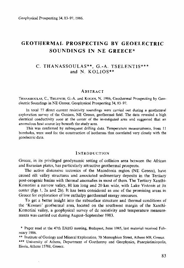
Geophysical Prospecting 34,83-97, 1986. GEOTHERMAL PROSPECTING BY GEOELECTRIC SOUNDINGS IN NE GREECE* C. THANASSOULAS**, G.-A. TSELENTIS*** and N. KOLIOS** ABSTRACT THANASSOULAS, C., TSELENTIS, G.-A. and KOLIOS, N. 1986, Geothermal Prospecting by Geo- electric Soundings in NE Greece, Geophysical Prospecting 34, 83-97. In total 77 direct current resistivity soundings were carried out during a geothermal exploration survey of the Genisea, NE Greece, geothermal field. The data revealed a high electrical conductivity zone at the center of the investigated area and suggested that an anomalous heat source lay beneath the study area. This was confirmed by subsequent drilling data. Temperature measurements, from 11 boreholes, were used for the construction of isotherms that correlated very closely with the geoelectric data. INTRODUCTION Greece, in its privileged geodynamic setting of collision area between the African and Eurasian plates, has particularly attractive geothermal prospects. The active distensive tectonics of the Macedonia region (NE Greece), have caused rift valley structures and associated sedimentary deposits in the Tertiary post-orogenic basins with thermal anomalies in most of them. The Tertiary Xanthi- Komotini a narrow valley, 80 km long and 20 km wide, with Lake Vistonis at its center (figs 1, 2a and 2b). It has been considered as one of the promising areas in Greece for exploration of low enthalpy geothermal energy resources. To get a better insight into the subsurface structure and thermal conditions of the ‘Kessani’ geothermal area, located on the southwest margin of the Xanthi- Komotini valley, a geophysical survey of dc resistivity and temperature measure- ments was carried out during August-September 1983. * Paper read at the 47th EAEG meeting, Budapest, June 1985, last material received Feb- ruary 1986. ** Institute of Geology and Mineral Exploration, 70 Messoghion Street, Athens 608, Greece. *** University of Athens, Department of Goethermy and Geophysics, Panepistimiopolis, Ilissia, Athens 15701, Greece. 83
Transcript of Geothermal Prospecting by Geoelectric Soundings in NE GREECE
Geophysical Prospecting 34,83-97, 1986.
GEOTHERMAL PROSPECTING BY GEOELECTRIC S O U N D I N G S I N N E GREECE*
C. T H A N A S S O U L A S * * , G . - A . TSELENTIS*** and N. K O L I O S * *
ABSTRACT THANASSOULAS, C., TSELENTIS, G.-A. and KOLIOS, N. 1986, Geothermal Prospecting by Geo- electric Soundings in NE Greece, Geophysical Prospecting 34, 83-97.
In total 77 direct current resistivity soundings were carried out during a geothermal exploration survey of the Genisea, NE Greece, geothermal field. The data revealed a high electrical conductivity zone at the center of the investigated area and suggested that an anomalous heat source lay beneath the study area.
This was confirmed by subsequent drilling data. Temperature measurements, from 11 boreholes, were used for the construction of isotherms that correlated very closely with the geoelectric data.
INTRODUCTION Greece, in its privileged geodynamic setting of collision area between the African and Eurasian plates, has particularly attractive geothermal prospects.
The active distensive tectonics of the Macedonia region (NE Greece), have caused rift valley structures and associated sedimentary deposits in the Tertiary post-orogenic basins with thermal anomalies in most of them. The Tertiary Xanthi- Komotini a narrow valley, 80 km long and 20 km wide, with Lake Vistonis at its center (figs 1, 2a and 2b). It has been considered as one of the promising areas in Greece for exploration of low enthalpy geothermal energy resources.
To get a better insight into the subsurface structure and thermal conditions of the ‘Kessani’ geothermal area, located on the southwest margin of the Xanthi- Komotini valley, a geophysical survey of dc resistivity and temperature measure- ments was carried out during August-September 1983.
* Paper read at the 47th EAEG meeting, Budapest, June 1985, last material received Feb- ruary 1986. ** Institute of Geology and Mineral Exploration, 70 Messoghion Street, Athens 608, Greece. *** University of Athens, Department of Goethermy and Geophysics, Panepistimiopolis, Ilissia, Athens 15701, Greece.
83
84 C. THANASSOULAS, G.-A. TSELENTIS A N D N. KOLIOS
leogene fcrmations
L I
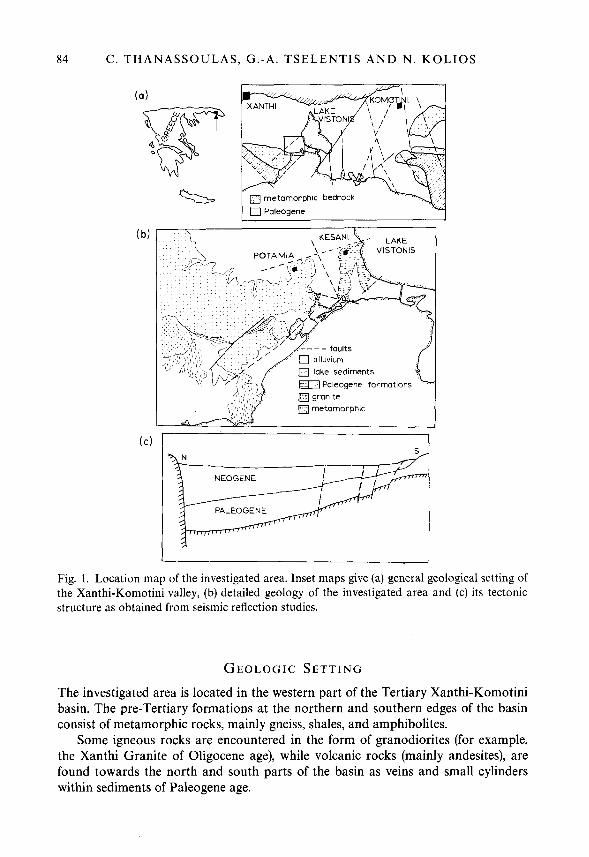
Fig. 1. Location map of the investigated area. Inset maps give (a) general geological setting of the Xanthi-Komotini valley, (b) detailed geology of the investigated area and (c) its tectonic structure as obtained from seismic reflection studies.
GEOLOGIC SETTING
The investigated area is located in the western part of the Tertiary Xanthi-Komotini basin. The pre-Tertiary formations at the northern and southern edges of the basin consist of metamorphic rocks, mainly gneiss, shales, and amphibolites.
Some igneous rocks are encountered in the form of granodiorites (for example, the Xanthi Granite of Oligocene age), while volcanic rocks (mainly andesites), are found towards the north and south parts of the basin as veins and small cylinders within sediments of Paleogene age.
G E O T H E R M A L PROSPECTING 85
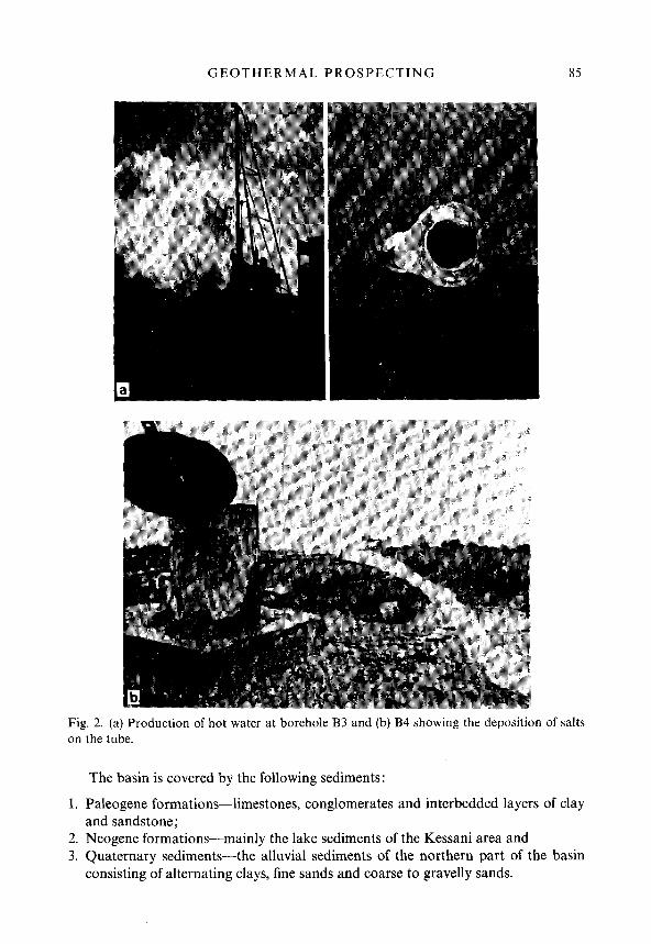
Fig. 2. (a) Production of hot water at borehole B3 and (b) B4 showing the deposition of salts on the tube.
1.
2. 3.
The basin is covered by the following sediments:
Paleogene formations-limestones, conglomerates and interbedded layers of clay and sandstone; Neogene formations-mainly the lake sediments of the Kessani area and Quaternary sediments-the alluvial sediments of the northern part of the basin consisting of alternating clays, fine sands and coarse to gravelly sands.

86 C. THANASSOULAS, G.-A. TSELENTIS AND N. KOLIOS
The major known faults in the area have an E-W and NE-SW direction. Seismic reflection (fig. lc) studies revealed that the basin has an asymmetric struc- ture, deepening towards the north where the sediments are thickest.
GEOCHEMICAL A N D THERMAL INVESTIGATIONS
In the region there are many hot springs, some well known from the past for their curative properties. Most of these springs are located on alluvial sediments, 2 m above sea level, in a marsh region of about 1 km wide, with seasonal variations of their discharge and temperature due to the nearby sea (fig. 3).
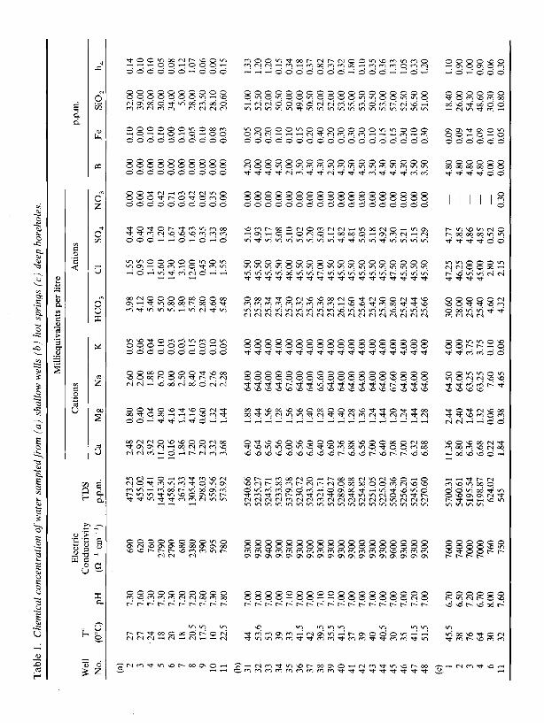
The exit points of the springs can be located easily from the small cones of calcium salts deposited. Within a small area around the main spring, we located more than 100 exit points of hot water, 18 of which were sampled for chemical analysis (table la).
To study the chemical composition and temperature of the deep waters, we also sampled some shallow wells used for irrigation purposes (table lb) and some deep exploratory boreholes (table lc).
Due to the special geological conditions of the area (thickness of sediments, near sea), we did not use Na-K or Ca-Na-K geothermometers but the S O , geother- mometer, that gave an initial water temperature of the order of 100°C.
In the north the geochemical results give a ratio Na/C1 > 1 while in the southwards direction this ratio becomes less than one (Na/Cl < 1). This might be because permeable sediments dominate the south part of the region and saline water intrudes from the nearby sea. The boundary between these two regions is between
I WELLS
0 BOREHOLES
Fig. 3. Location of shallow wells, hot springs and exploratory boreholes.
Tab
le 1
. C
hem
ical
con
cent
ratio
n of
wat
er s
ampl
edfr
om (
a) s
hallo
w w
ells
(b)
hot s
prin
gs (
c) de
ep b
oreh
oles
.
Ele
ctri
c W
ell
To
Con
duct
ivity
N
o.
(0°C
) pH
(n
-'cm
-')
(a) 2 3 4 5 6 7 8 9 10
11
31
32
33
34
35
36
37
38
39
40
41
42
43
44
45
46
47
48
(4 1 2 3 4 6 11
(b)
27
27
24
18
20
18
20.5
17
.5
10
22.5
44
53.6
53
39
33
41
.5
42
39.5
35
.5
41.5
37
39
40
40
.5
30
35
41.5
51
.5
45.5
38
76
64
30
32
7.30
7.
60
7.30
7.
30
7.30
7.
20
7.20
7.
80
7.30
7.
80
7.00
7.
00
7.00
7.
00
7.10
7.
00
7.00
7.
10
7.10
7.
00
7.00
7 .O
O 7.
00
7.00
7.
00
7.00
7.
20
7.00
6.70
6.
50
7.20
6.
70
8.00
7.
60
690
620
760
2790
27
90
680
2380
39
0 59
5 78
0
9300
93
00
9400
93
00
9300
93
00
9300
93
00
9300
93
00
9300
93
00
9300
93
00
9600
93
00
9300
93
00
7600
74
00
7000
70
00
760
750
Mill
ieau
ival
ents
per
litr
e
Cat
ions
A
nion
s p.
p.m
. T
DS
p.p.
m.
Ca
Mg
Na
K
HC
O,
Cl
SO,
NO
, B
Fe
Si
O,
h,
473.
25
455.
02
551.
41
1443
.30
1458
.51
367.
33
1305
.44
298.
03
559.
56
573.
92
5240
.66
5235
.27
5243
.71
5233
.83
5379
.38
5230
.72
5243
.20
5321
.71
5240
.27
5289
.08
5248
.88
5254
.82
5251
.05
5225
.02
5504
.36
5256
.20
5245
.61
5270
.60
5700
.31
5460
.61
5195
.54
5198
.87
624.
02
545
2.48
0.
80
2.92
0.
40
3.92
1.
04
11.2
0 4.
80
10.1
6 4.
16
1.86
1.
14
7.20
4.
16
2.20
0.
60
3.32
1.
32
3.68
1.
44
6.40
1.
88
6.64
1.
44
6.56
1.
56
6.56
1.
28
6.00
1.
56
6.56
1.
56
6.60
1.
40
6.40
1.
28
6.60
1.
40
7.36
1.
40
6.88
1.
28
6.56
1.
36
7.00
1.
24
6.40
1.
44
7.08
1.
20
7.00
1.
24
6.32
1.
44
6.88
1.
28
11.3
6 2.
44
8.80
2.
40
6.36
1.
64
6.68
1.
32
0.22
0.
06
1.84
0.
38
2.60
0.
05
2.00
0.
06
1.88
0.
04
6.70
0.
10
8.00
0.
03
2.50
0.
03
8.40
0.
15
0.74
0.
03
2.76
0.
10
2.28
0.
05
64.0
0 4.
00
64.0
0 4.
00
64.0
0 4.
00
64.0
0 4.
00
67.0
0 4.
00
64.0
0 4.
00
64.0
0 4.
00
65.6
0 4.
00
64.0
0 4.
00
64.0
0 4.
00
64.0
0 4.
00
64.0
0 4.
00
64.0
0 4.
00
64.0
0 4.
00
67.6
0 4.
00
64.0
0 4.
00
64.0
0 4.
00
64.0
0 4.
00
64.5
0 4.
00
64.0
0 4.
00
63.2
5 3.
75
63.2
5 3.
75
7.60
0.
10
4.65
0.
06
3.98
4.
12
5.40
5.
50
5.80
1.
80
5.78
2.
80
4.60
5.
48
25.3
0 25
.38
25.3
4 25
.34
25.3
0 25
.32
25.3
6 25
.36
25.3
8 26
.12
25.6
0 25
.64
25.4
2 25
.30
26.8
0 25
.42
25.4
4 25
.66
30.6
0 28
.00
25.4
0 25
.40
4.60
4.
32
1.55
0.
95
1.10
15
.60
14.3
0 3.
10
12.0
0 0.
45
1.30
1.
55
45.5
0 45
.50
45.5
0 45
.50
48.0
0 45
.50
45.5
0 47
.00
45.5
0 45
.50
45.5
0 45
.50
45.5
0 45
.50
47.5
0 45
.50
45.5
0 45
.50
47.2
5 46
.25
45.0
0 45
.00
2.80
2.
15
0.44
0.
00
0.00
0.
40
0.00
0.
00
0.34
0.
04
0.00
1.
20
0.42
0.
00
1.67
0.
71
0.00
0.
64
0.03
0.
00
1.63
0.
42
0.00
0.
35
0.02
0.
00
1.33
0.
35
0.00
0.
38
0.00
0.
00
0.10
0.
00
0.10
0.
10
0.00
0.
10
0.05
0.
10
0.08
0.
03
5.16
0.
00
4.20
0.
05
4.93
0.
00
4.00
0.
20
5.17
0.
00
4.00
0.
20
5.08
0.
00
4.50
0.
10
5.10
0.
00
2.00
0.
10
5.02
0.
00
3.50
0.
15
5.20
0.
00
4.30
0.
20
5.03
0.
00
4.30
0.
40
5.12
0.00
2.
50
0.20
4.
82
0.00
4.
30
0.30
4.
81
0.00
4.
50
0.30
5.
05
0.00
4.
50
0.30
5.
18
0.00
3.
50
0.10
4.
92
0.00
4.
30
0.15
5.
30
0.00
4.
50
0.15
5.
21
0.00
4.
30
0.30
5.
15
0.00
3.
50
0.10
5.
29
0.00
3.
50
0.30
4.77
-
4.80
0.
09
4.85
~
4.80
0.
09
4.80
0.
14
4.86
-
4.80
0.
09
4.85
-
0.52
-
0.00
0.
10
0.50
0.
30
0.00
0.
05
32.0
0 0.
14
39.0
0 0.
10
28.0
0 0.
10
30.0
0 0.
05
34.0
0 0.
08
5.00
0.
12
28.0
0 1.
07
23.5
0 0.
06
28.1
0 0.
00
20.6
0 0.
15
51.0
0 1.
33
52.5
0 1.
20
52.0
0 1.
20
50.5
0 0.
15
50.0
0 0.
34
49.0
0 0.
18
50.5
0 0.
37
52.0
0 0.
82
52.0
0 0.
37
53.0
0 0.
32
55.0
0 1.
80
53.5
0 0.
10
50.5
0 0.
35
53.0
0 0.
36
57.0
0 1.
33
52.5
0 1.
05
56.5
0 0.
33
51.0
0 1.
20
18.4
0 1.
10
26.0
0 0.
90
54.3
0 1.
00
48.6
0 0.
90
30.3
0 0.
06
10.8
0 0.
30
88 C. THANASSOULAS, G . - A . TSELENTIS AND N. KOLIOS
-0C 16 2.0 24
(a) I
ii
BOREHOLES 1-11
b 3
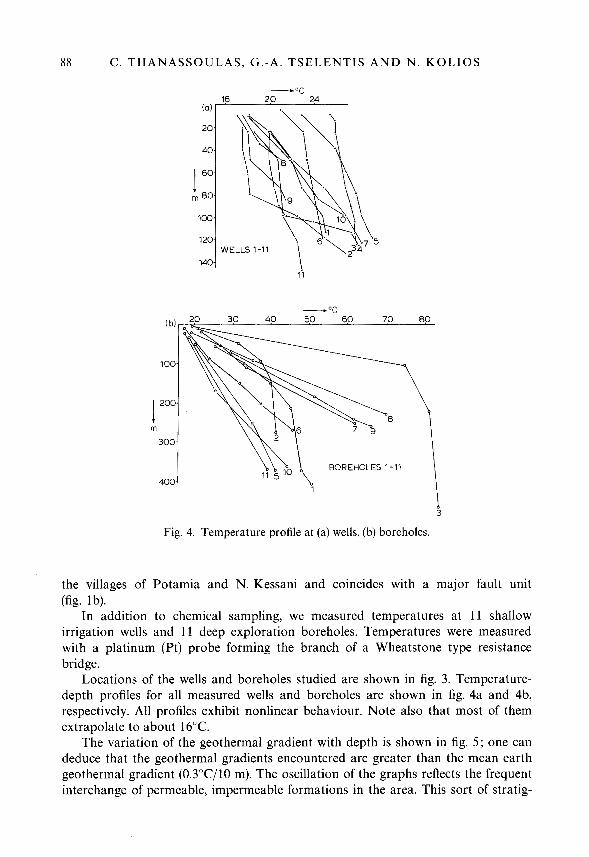
Fig. 4. Temperature profile at (a) wells, (b) boreholes.
the villages of Potamia and N. Kessani and coincides with a major fault unit (fig. lb).
In addition to chemical sampling, we measured temperatures at 11 shallow irrigation wells and 11 deep exploration boreholes. Temperatures were measured with a platinum (Pt) probe forming the branch of a Wheatstone type resistance bridge.
Locations of the wells and boreholes studied are shown in fig. 3. Temperature- depth profiles for all measured wells and boreholes are shown in fig. 4a and 4b, respectively. All profiles exhibit nonlinear behaviour. Note also that most of them extrapolate to about 16°C.
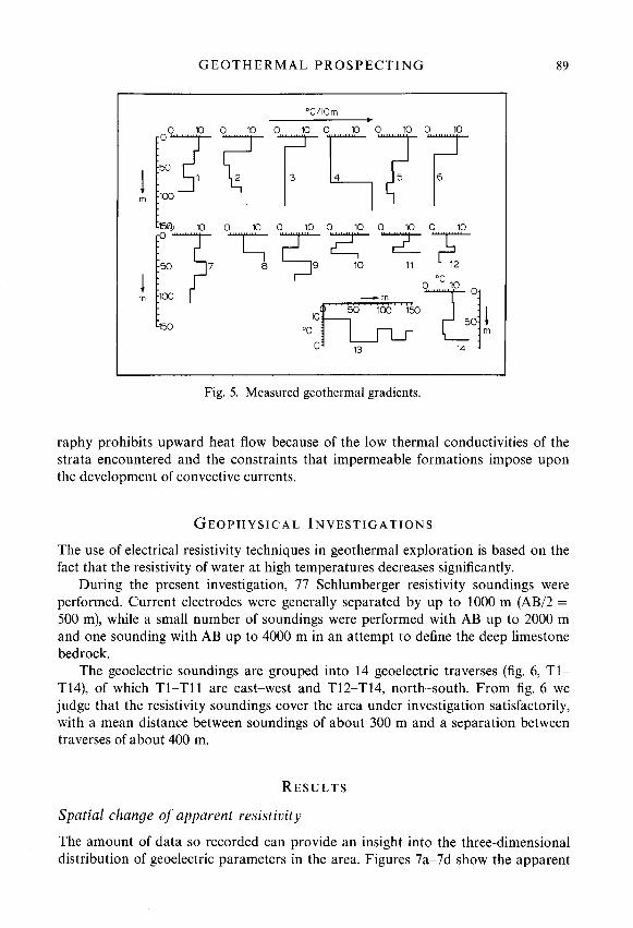
The variation of the geothermal gradient with depth is shown in fig. 5; one can deduce that the geothermal gradients encountered are greater than the mean earth geothermal gradient (0.3"C/10 m). The oscillation of the graphs reflects the frequent interchange of permeable, impermeable formations in the area. This sort of stratig-
GEOTHERMAL PROSPECTING 89
I
Fig. 5. Measured geothermal gradients.
raphy prohibits upward heat flow because of the low thermal conductivities of the strata encountered and the constraints that impermeable formations impose upon the development of convective currents.
GEOPHYSICAL I N V E S T I G A T I O N S
The use of electrical resistivity techniques in geothermal exploration is based on the fact that the resistivity of water at high temperatures decreases significantly.
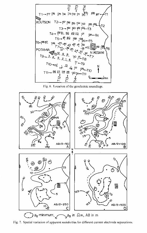
During the present investigation, 77 Schlumberger resistivity soundings were performed. Current electrodes were generally separated by up to 1000 m (AB/2 = 500 m), while a small number of soundings were performed with AB up to 2000 m and one sounding with AB up to 4000 m in an attempt to define the deep limestone bedrock.
The geoelectric soundings are grouped into 14 geoelectric traverses (fig. 6, T1- T14), of which T1-T11 are east-west and T12-Tl4, north-south. From fig. 6 we judge that the resistivity soundings cover the area under investigation satisfactorily, with a mean distance between soundings of about 300 m and a separation between traverses of about 400 m.
RESULTS
Spatial change of apparent resistivity
The amount of data so recorded can provide an insight into the three-dimensional distribution of geoelectric parameters in the area. Figures 7a-7d show the apparent
' \
- Fig. 6. Location of the geoelectric soundings.
IY A
I no A W 2 . 2 5 0 c
I '
a pa minimum, p pa in a m , AB in rn e J s
Fig. 7. Spatial variation of apparent resistivities for different current electrode separations.
GEOTHERMAL P R O S P E C T I N G 91
I I
Slm
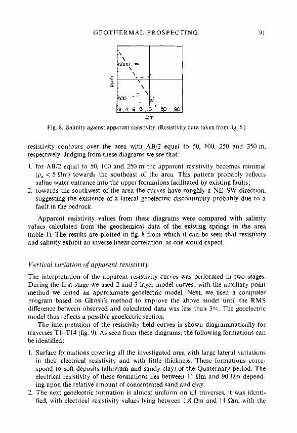
Fig. 8. Salinity against apparent resistivity. (Resistivity data taken from fig. 6.)
resistivity contours over the area with AB12 equal to 50, 100, 250 and 350 m, respectively. Judging from these diagrams we see that:
1. for AB12 equal to 50, 100 and 250 m the apparent resistivity becomes minimal (p, < 5 Rm) towards the southeast of the area. This pattern probably reflects saline water entrance into the upper formations facilitated by existing faults;
2. towards the southwest of the area the curves have roughly a NE-SW direction, suggesting the existence of a lateral geoelectric discontinuity probably due to a fault in the bedrock.
Apparent resistivity values from these diagrams were compared with salinity values calculated from the geochemical data of the existing springs in the area (table 1). The results are plotted in fig. 8 from which it can be seen that resistivity and salinity exhibit an inverse linear correlation, as one would expect.
Vertical variation of apparent resistivity
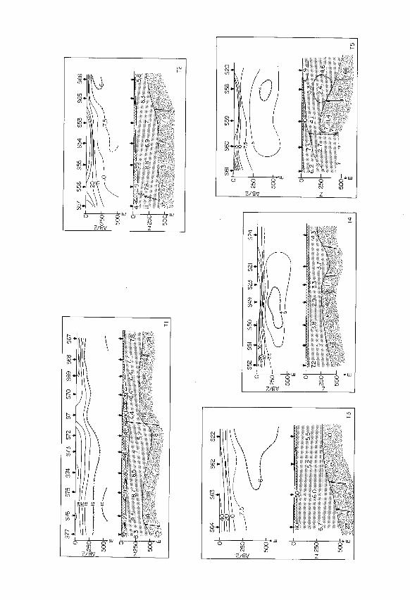
The interpretation of the apparent resistivity curves was performed in two stages. During the first stage we used 2 and 3 layer model curves; with the auxiliary point method we found an approximate geoelectric model. Next, we used a computer program based on Ghosh's method to improve the above model until the RMS difference between observed and calculated data was less than 3%. The geoelectric model thus reflects a possible geoelectric section.
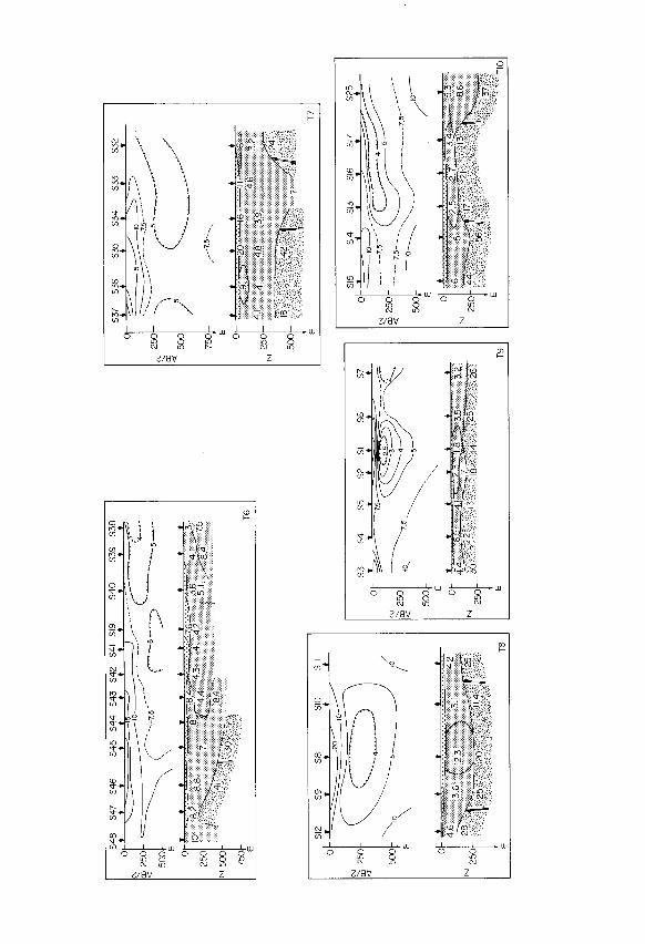
The interpretation of the resistivity field curves is shown diagrammatically for traverses T1-T14 (fig. 9). As seen from these diagrams, the following formations can be identified :
1. Surface formations covering all the investigated area with large lateral variations in their electrical resistivity and with little thickness. These formations corre- spond to soft deposits (alluvium and sandy clay) of the Quaternary period. The electrical resistivity of these formations lies between 11 Rm and 90 Rm depend- ing upon the relative amount of concentrated sand and clay.
2. The next geoelectric formation is almost uniform on all traverses, it was identi- fied, with electrical resistivity values lying between 1.8 Rm and 11 Qm, with the
S77
576
S75
S74
S73
572
S71
S70
S
69
S68
S
fi7
1
I 56
4 S6
3 S6
2 52
2 ~
~~
/----
--__-_-,-
A
N & 25
0 -7
.5’
a
52
5
5
s57
S56
55
5 S
54
S53
S
65
S6f
i
78
8
8
69
7
T2
74
500
512
S9
56
SI
O
511
1 * /
r-1
'I0 \
i"
t E
16
537
536
535
S34
533
S32
,-7.5-,
E
F i
T9

~~
S71
S55
563
S49
S
59
S42
53
5 S8
S6
S16
S29
E
TI:
E i
T12
c
T14
~-
Fig.
9.
Geo
elec
tric
prof
iles
and
prop
osed
geo
elec
tric
mod
els.
Sur
face
for
mat
ions
11-
90 R
m. m
, sur
face
fo
rmat
ions
2-
11
Rm
, ;
deep
fo
rmat
ions
14
-44
Qm
, [3;
soun
ding
No.
1,J
-l.

GEOTHERMAL PROSPECTING 95
Table 2. Sounding locations of geothermal interest.
Traverse Sounding
Tl s34, s33 T8 S8 T9 s1 T10 S13, S16 T11 S21, S28, S29
means of the smallest and largest value, on all traverses, 3.4 Rm and 8.2 Rm, respectively.
From the results of boreholes B1-11 we see that the upper part of this formation corresponds to the upper sandstone series of the Oligocene-Eocene formation. The formation is several hundred meters thick in the north of the investigated area, while in the south it does not exceed 100 m.
3. The last and deepest formation, identified geoelectrically, has a high electrical resistivity generally between 13.6 Rm and 44 Rm. The apparent resistivity curves show that in some places the formation resistivity becomes very low. The ‘lows’ lying in the east of the investigated area might reflect sea water intrusions, while the rest are located in the main area of geothermal interest and are listed in table 2.
For geoelectric traverse T11, this low resistivity region reaches the surface at sounding locations S28 and S29, which coincides with the location of the hot water springs of Genisea. From the same section we see that the conductive zone dips westwards reaching its greatest depth below sounding location S27.
As the interpretation diagram shows, the above formation has resistivities lying between 4.7 Rm and 5 Rm for the region between soundings S27 and S28, while in the immediately adjacent areas the resistivity is higher. This suggests that hot min- eralized water flows towards the surface and lowers the formation’s resistivity.
The same picture is found at traverse T10 at locations S13, 16, 17 and 25, while in section T9 the conductive zone is very concentrated and is located just below sounding S1 at a depth of about 125 m. At the same depth, borehole B3 found water with a temperature of 78°C.
In traverse T8, this conductive zone is expanded, and has a higher resistivity. Similarly, expansion is observed in section T7 towards the east with even higher resistivity. It must be noted that the shape of the resistivity curves is affected by sea water intrusion in this area.
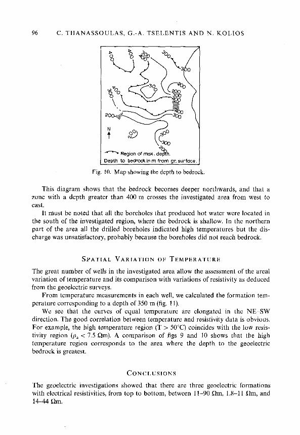
Spatial variation q j the bedrock
The results of the geoelectric interpretations with information about the possible depth to the bedrock are compiled in fig. 10, which shows the spatial variation of the depth to geoelectric bedrock for the whole of the investigated area.
96 C. T H A N A S S O U L A S , G . - A . TSELENTIS AND N. KOLIOS
- Region of max. Lgh. Fig. 10. Map showing the depth to bedrock.
This diagram shows that the bedrock becomes deeper northwards, and that a zone with a depth greater than 400 m crosses the investigated area from west to east.
It must be noted that all the boreholes that produced hot water were located in the south of the investigated region, where the bedrock is shallow. In the northern part of the area all the drilled boreholes indicated high temperatures but the dis- charge was unsatisfactory, probably because the boreholes did not reach bedrock.
S P A T I A L V A R I A T I O N OF TEMPERATURE
The great number of wells in the investigated area allow the assessment of the area1 variation of temperature and its comparison with variations of resistivity as deduced from the geoelectric surveys.
From temperature measurements in each well, we calculated the formation tem- perature corresponding to a depth of 350 m (fig. 11).
We see that the curves of equal temperature are elongated in the NE-SW direction. The good correlation between temperature and resistivity data is obvious. For example, the high temperature region (T > 50°C) coincides with the low resis- tivity region (p, < 7.5 Rm). A comparison of figs 9 and 10 shows that the high temperature region corresponds to the area where the depth to the geoelectric bedrock is greatest.
CONCLUSIONS
The geoelectric investigations showed that there are three geoelectric formations with electrical resistivities, from top to bottom, between 11-90 Rm, 1.8-11 Rm, and 14-44 Rm.
G E O T H E R M A L PROSPECTING 97
The spatial variation of the temperature of the formation was found to correlate very closely with electrical resistivity variations, with the resistivity lows following very closely the high-temperature area.
A number of boreholes revealed some shallow water horizons of limited extent (figs 2a and 2b).
The high temperatures are characteristically found where the bedrock dips towards the center of the area in an E-W direction.
This study illustrates the possibility of localizing small geothermal features by a detailed and carefully designed geoelectric survey.