Seismic characterization of geothermal sedimentary reservoirs

Seismic characterization of geothermal sedimentary reservoirs: A fieldexample from the Copenhagen area, Denmark

Kenneth Bredesen1, Esben Dalgaard2, Anders Mathiesen3, Rasmus Rasmussen3, and Niels Balling4

Abstract

We have seismically characterized a Triassic-Jurassic deep geothermal sandstone reservoir north of Copen-hagen, onshore Denmark. A suite of regional geophysical measurements, including prestack seismic data andwell logs, was integrated with geologic information to obtain facies and reservoir property predictions in aBayesian framework. The applied workflow combined a facies-dependent calibrated rock-physics model witha simultaneous amplitude-variation-with-offset seismic inversion. The results suggest that certain sandstonedistributions are potential aquifers within the target interval, which appear reasonable based on the geologicproperties. However, prediction accuracy suffers from a restricted data foundation and should, therefore, onlybe considered as an indicator of potential aquifers. Despite these issues, the results demonstrate new possibil-ities for future seismic reservoir characterization and rock-physics modeling for exploration purposes, derisk-ing, and the exploitation of geothermal energy as a green and sustainable energy resource.

IntroductionIn the future, geothermal resources may play a central

role in supplying sustainable and green energy. For ex-ample, Danish geothermal resources in known sandstoneaquifers can potentially sustain household heating needsfor several centuries (Nielsen et al., 2004; Vosgerau et al.,2016). However, the ability to establish successful geo-thermal plants requires that the subsurface reservoirrock has a sufficient porosity and permeability. The ap-plication of appropriate exploration tools to constraingeologic risks and optimize site selection is, arguably,highly relevant when attempting to meet the needs offragile geothermal budgets and uncertain profit models.Despite this, geothermal targets are often exclusivelydrilled based on conventional geophysical data interpre-tation techniques with little emphasis on more sophisti-cated quantitative reservoir characterization methods(Schmelzbach et al., 2016a).

Previous studies have demonstrated the advantagesof geophysical exploration based on electrical resis-tance, electromagnetic, and gravity data for geothermalpurposes (e.g., Nunziata and Rapolla, 1981; Pellerin et al.,1996; Barbier, 2002; Endo et al., 2018). However, for deep

geothermal reservoirs, the seismic reflection method pro-vides subsurface images with higher resolution. Previousgeothermal studies based on seismic data contain severalexamples of structural and stratigraphic mapping ofgeothermal fields (Bujakowski et al., 2010; Casini et al.,2010; Lüschen et al., 2014, 2015). Furthermore, seismicattribute analysis allows the identification and characteri-zation of high-permeability fractured zones (von Hart-mann et al., 2012; Pussak et al., 2014; Khair et al., 2015),seismic tomography modeling (Muñoz et al., 2010), andvertical seismic profiling (Majer et al., 1988; Sausse et al.,2010; Place et al., 2011; Reiser et al., 2017). Several studieshave applied passive microseismic measurements tomonitor dynamic reservoirs with respect to microearth-quakes induced by geothermal fluid stimulation (Dyeret al., 2008; Reshetnikov et al., 2015; Folesky et al.,2016; Schmelzbach et al., 2016b). Supplementary VP∕VSratio data from onshore multicomponent seismic mea-surements have also been used to discriminate betweengeothermal facies (Wei et al., 2014a, 2014b).

There are still, however, a scarce amount of studiesthat demonstrate the potential of combining modernseismic inversions with facies-dependent rock-physics

1Aarhus University, Department of Geoscience, Aarhus, Denmark and Geological Survey of Denmark and Greenland (GEUS), Copenhagen,Denmark. E-mail: [email protected] (corresponding author).

2Qeye, Copenhagen, Denmark. E-mail: [email protected] Survey of Denmark and Greenland (GEUS), Copenhagen, Denmark. E-mail: [email protected]; [email protected] University, Department of Geoscience, Aarhus, Denmark. E-mail: [email protected] received by the Editor 2 September 2019; revisedmanuscript received 3 November 2019; published ahead of production 17 December

2019; published online 04 March 2020. This paper appears in Interpretation, Vol. 8, No. 2 (May 2020); p. T275–T291, 14 FIGS., 3 TABLES.http://dx.doi.org/10.1190/INT-2019-0184.1. © The Authors. © 2020 The Authors. Published by the Society of Exploration Geophysicists and the American Association of

Petroleum Geologists. All article content, except where otherwise noted (including republished material), is licensed under a Creative Commons Attribution 4.0 UnportedLicense (CC BY). See http://creativecommons.org/licenses/by/4.0/. Distribution or reproduction of this work in whole or in part commercially or noncommercially requiresfull attribution of the original publication, including its digital object identifier (DOI).

t

Technical paper

Interpretation / May 2020 T275Interpretation / May 2020 T275

Downloaded from http://pubs.geoscienceworld.org/interpretation/article-pdf/8/2/T275/5012755/int-2019-0184.1.pdfby gueston 12 January 2022

http://creativecommons.org/licenses/by/4.0/



modeling to improve our understanding of geothermalreservoirs in a quantitative manner. The hydrocarbon in-dustry routinely uses such methods to seismically char-acterize reservoirs (e.g., Eidsvik et al., 2004; Buland et al.,2008; Grana and Della Rossa, 2010; Ba et al., 2013; Avsethet al., 2016), as well as for CO2 sequestration (e.g., Grudeet al., 2013; Mallick and Adhikari, 2015; Grana et al.,2017). The benefits from such methods are equally validfor geothermal reservoirs because supplementary quanti-tative information about key parameters, such as porosityand permeability, can be used to improve site locationsand predict geothermal reservoir performance. The ob-jective of this study is, therefore, to extend seismic res-ervoir characterization to geothermal applications usinga field example from an area north of Copenhagen inDenmark. We focus on predicting the facies and reservoirproperties away from well locations based on seismicinversion data.

The data set available for this study was limited to a 2Dseismic survey, one local well, and several regional wellsthat penetrate the same reservoir formations expected tooccur at the prospect area. In addition, recent geologicand petrophysical analyses of the region provide valuableinformation that we use in the seismic inversion and rock-physics modeling (Nielsen et al., 2004; Mathiesen et al.,2010; Kristensen et al., 2016; Vosgerau et al., 2016,2017;Weibel et al., 2017). For seismic reservoir characteri-zation, we use previously reported methods (e.g., Avsethet al., 2005; Doyen, 2007; Dvorkin et al., 2014; Grana, 2018)that were implemented in a three-step workflow:

1) Rock-physics analysis: Well-log data were used toperform a feasibility study and calibrate facies-de-pendent rock-physics models.

2) Seismic inversion: Prestack seismic data were con-verted to absolute elastic parameters, such as theacoustic impedance and P-to-S velocity ratio, usinga simultaneous amplitude-variation-with-offset (AVO)inversion.

3) Reservoir characterization: The results from steps 1and 2 were combined to estimate facies and reser-voir properties, such as porosity, permeability, andshale volume, in a Bayesian framework.

Uncertainties associated with intrinsic variabilities(e.g., the reservoir-property distributions beyond wellcontrol) and shortcomings in model theory or poormodel calibrations were addressed using statisticalmethods. Probabilities and statistical estimators, whichmay provide valuable input for economic risk assess-ments and decision-making, represent the final faciesand reservoir quality predictions (Avseth et al., 2005).

The primary geothermal target in this study is thesandstone-dominated upper Triassic-lower JurassicGassum Formation, which is currently being exploitedfor geothermal production and gas storage in Denmark(Røgen et al., 2015; Kristensen et al., 2016; Vosgerauet al., 2016, 2017). In addition, we evaluate the reservoirpotential of a local lower Jurassic sandstone unitthat overlies the Gassum Formation. Our results showthat we are able to distinguish between several porousand clean sandstone bodies as potential aquifers andnonreservoir units within the target succession. Fur-thermore, our predictions indicate that a more promisingreservoir potential exists within the lower Jurassicunit as compared with the Gassum Formation. Despiteworking with limited data coverage and quality, ourpredictions show a reasonably good match betweenthe nearest well logs and geologic characteristics of thestudy area. Regional investigations prior to this studyhave also suggested that there are considerable lateralsubsurface variations (Vosgerau et al., 2016, 2017),which emphasize the importance of supplementaryquantitative seismic analysis.

In the following sections, we first introduce the keygeologic settings and geothermal targets covered byour data set. We then describe the previously mentionedthree-step workflow for seismic reservoir characteriza-tion. The reader should refer to the appendices for moretheoretical details on the methodology and model speci-fications.

Data coverage and geothermal targetsMost of the Danish subsurface is characterized by

deep sedimentary basins that contain extensive low-en-thalpy geothermal resources (Balling et al., 2002; Mathie-sen et al., 2010), which can potentially be exploited for

Karlebo-1A

5 km

12.15 12.2 12.25 12.3 12.35 12.4 12.45

° E

55.85

55.9

55.95

° N

Line 1Line 2Line 3Line 4Line 5

UTM zone 33U

10 10.5 11 11.5 12 12.5 13 13.5

° E

55

55.2

55.4

55.6

55.8

56

56.2

56.4

° N

10 12 14 16° E

54.5

55

55.5

56

56.5

57

57.5

58

58.5

° N

Copenhagen area

Hillerød area

Margretheholm

-1A

Geothermal plants

98

Figure 1. The location of the study area magnified on northeastern Zealand. Five seismic 2D lines are shown, as well as a localwell, Karlebo-1A. Additional regional well data are available at Margretheholm, located approximately 30 km away from the pros-pect area. Courtesy of Google Maps.

T276 Interpretation / May 2020


district heating. Broad and uneven coverage of seismicreflection profiles and exploration wells, with varyingdata quality, constitute the primary subsurface data thatare available for the entire country. This study focuseson geothermal exploration in an area near Hillerød innortheastern Zealand, Denmark (Figure 1). A 2D seismicsurvey performed in 2013 provides 3 km offset prestack,depth-migrated data and the nearest exploration well,Karlebo-1A, is located approximately 140 m from thenearest common-midpoint (CMP) gather along theeastern part of seismic line number 5 (see Figure 1). Theseismic survey was designed for structural mapping andoutlining potential geothermal reservoirs, whereas Kar-lebo-1A was drilled for hydrocarbon exploration.

The primary geothermal target in this study is the Gas-sum Formation, which is recognized for its excellent res-ervoir quality at several locations throughout Denmark.The sandstone-dominated lower Jurassic Reservoir Unit(LJRU) represents a secondary geothermal target, whichlies above the Gassum Formation in the northeasternpart of Zealand. The LJRU is a local phenomenon andforms the lower part of the regional cap rock, that is,the Fjerritslev Formation, which is dominated by marinemudstones and shales. The Gassum Formation and LJRUare similar with respect to lithology and are dominatedby fine- to medium-grained, locally coarse, light-graysandstones that alternate withmudstones, siltstones, andthin local coal seams (Michelsen et al., 2003). However,observations from the Karlebo-1A well (see Figure 1) in-dicate that the LJRU locally exhibits a slightly morehomogeneous reservoir unit, whereas the Gassum For-mation contains an increased number of interchangingthinly bedded shales. The reservoir temperature approx-imately ranges from 50°C to 65°C within the target inter-val (Poulsen et al., 2017).

Figure 2 shows a geologic interpretation of the geo-thermal targets and surrounding formations based onthe seismic backdrop from line 5, with a superimposedKarlebo-1A projection. Obtaining seismic imaging of thegeothermal targets is challenging, which is partly dueto the overlying chalk package that generates interferingmultiples and converted waves (Montazeri et al., 2018).The stratigraphic sequence interpretationof the composite succession, therefore,strongly guides the seismic interpreta-tion. Certain mounded seismic character-istics within the geothermal targets canbe observed and may represent possibleseismic facies (Vosgerau et al., 2016), butwe are unable to easily clarify whetherthese characteristics are related to varia-tions in the geology or geophysical ar-tifacts.

Rock-physics analysisAs a first step toward seismic reservoir

characterization, we performed a feasibil-ity study to verify whether the seismicproperties are sensitive to the different fa-

cies and reservoir variations based on the regional well-log data (Waters and Kemper, 2014). With a positive out-come, we proceeded by calibrating the facies-dependentrock-physics models and used them to quantitatively de-scribe the seismic inversion data in terms of the faciesand reservoir properties. Bredesen et al. (2018) reportsuch a regional feasibility study that we review and ex-tend upon in this section. These analyses are primarilybased on the Margretheholm-1A well, which we assumerepresents a close reservoir analog to the prospect areaand is the only adjacent well available with a completesuite of logs.

To obtain an initial understanding of the seismic re-sponse of the target geothermal reservoirs, Figure 3plots the acoustic impedance (Ip) against the P-to-Svelocity ratio (VP∕VS) data in a crossplot. Colorizeddots and black “x” symbols represent clean (shalevolume <30%) and shaly (shale volume >30%) sand-stones from the LJRU and Gassum Formation andthe cap rock (i.e., the Fjerritslev Formation), respec-tively. Kernel-density-estimated probability densityfunctions (PDFs) (Silverman, 1986; Grana, 2018) weresuperimposed onto the data and projected onto each axisto form marginal distributions that describe the corre-sponding data histograms. Whereas the clean and shalysandstones exhibit overlapping and nonunique proper-ties, the two sandstone facies can be segregated fromthe cap rock due to larger Ip and lower Vp∕VS values. Toobtain a reference facies classification profile, we usedlinear discriminant analysis based on porosity and shalevolume logs (Grana et al., 2017) to segregate (1) cleansandstone with high reservoir quality, (2) shaly sandstonewith intermediate-to-low reservoir quality, and (3) nonre-servoir facies.

Ultimately, we are interested in facies discriminationbased on seismically inverted parameters, such as Ipand VP∕VS, at a distance fromwell locations. Therefore,for the feasibility test, we used a Bayesian facies clas-sification approach (Avseth et al., 2005; Doyen, 2007;Grana, 2018) to verify if the Ip and VP∕VS parametersare sensitive to variations in the facies. The reservoirnet-to-gross volumes were used as a priori information,

Figure 2. A geologic interpretation of the main geologic formations based onseismic line 5 (backdrop), which is approximately 7 km in length. The Karlebo-1A well path is projected on top.

Interpretation / May 2020 T277


with a 30%, 20%, and 50% probability for the clean sand-stone, shaly sandstone, and nonreservoir, respectively.Figure 4a–4e shows a suite of well logs from Margrethe-holm-1A, whereas Figure 4f–4i shows the correspond-

ing profiles for the reference and Bayesian-classified(or predicted) facies. To approach the seismic resolution,a sequential Backus averaging was used in a running win-dow corresponding to one-fourth of the seismic wave-length to upscale the log data (the red stippled curves)and facies profiles (Avseth et al., 2005). The seismicwavelength was estimated to be 35 m using a center fre-quency of 50 Hz and an interval velocity of 3500 m/s ex-tracted from the stacking velocities around the reservoirinterval. In general, the upscaled profiles favored theshaly sandstone facies due to effective smoothing of thepetrophysical and seismic properties. Nevertheless, thepredicted and reference facies profiles match quite wellat both scales, which implies good conditions for seismicfacies discrimination in this particular geologic scenario.

The Bayesian facies classification was based on sev-eral PDFs as functions of Ip and VP∕VS for each facies toaddress the relationships between the seismic parame-ters and reservoir properties (Doyen, 2007). These are,however, only based on training data from Margrethe-holm-1A, which may inadequately represent other pos-sible geologic scenarios in the prospect area, locatedat a distance of 30 km. However, additional petrophys-ical logs are available from Karlebo-1A, which can beused to further extend the training data set beyond the

5 6 7 8 9 10 11 12

Acoustic impedance (km/s g/cm3)

1.6

1.8

2

2.2

2.4

2.6

2.8

V P/V

S

Cap-rock dataShaly sandstone dataClean sandstone dataClean sandstone PDFShaly sandstone PDFCap-rock PDF

Figure 3. Crossplot analyses of the acoustic impedanceagainst VP∕VS based on Margretheholm-1A well data, groupedinto three different facies.

0 0.2 0.4Porosity

(v/v)

1650

1700

1750

1800

1850

1900

1950

Dep

th (

m)

0 1000 2000Permeability

(mD)

0 0.5 1Shale volume

(v/v)

5 10Ip

(km/s g/cm3)

1.6 2 2.4

VP / VS

Reference facies(log-scale)

Reference facies(upscaled)

Predicted facies(log-scale)

Predicted facies(upscaled)

Cap

-roc

kR

eser

voir

a) b) c) d) e) f) g) h) i)

Figure 4. The (a) porosity, (b) permeability, (c) shale volume, (d) acoustic impedance (Ip), and (e) P-to-S velocity ratio (VP∕VS)logs from the Margretheholm-1A well adjacent to profiles of the reference facies in (f and h) and predicted facies in (g and i). Thefacies classification is yellow, brown, and green for the clean sandstone, shaly sandstone, and nonreservoir, respectively. Redstippled curves denote upscaled logs. The depth is in measured depth.



well control using statistical rock physics (Mavko andMukerji, 1998; Avseth et al., 2001; Mukerji et al., 2001;Eidsvik et al., 2004; Doyen, 2007). Figure 5a shows theporosity plotted against the shale volume data from Mar-gretheholm-1A and Karlebo-1A combined, as well as theprior distributions for each lithofacies. Figure 5b showsan augmented data set generated from a Monte Carlosimulation, which randomly samples from the prior dis-tributions. This augmented data set can subsequentlyserve as the input for the facies-dependent rock-physicsmodels that computes the seismic parameters, such as

the Ip versus VP∕VS crossplot in Figure 5c, where thePDFs represent well data extrapolated using the statis-tical rock physics for each lithofacies. We note the occur-rence of high-probability areas for the nonreservoir PDF,which represents various shales from the cap rock andthe intrareservoir in the Margretheholm-1A well. Finally,these PDFs in the Ip versus VP∕VS domain can be usedto analyze the seismic inversion results.

For statistical rock physics, different facies requiretailored rock-physics models to link the desirable reser-voir properties with their seismic parameters. Obtaining

10 11 127 8 95 6

Acoustic impedance (km/s g/cm )3

1.5

2

2.5

3

VP/V

S

Nonreservoir

Shaly sandstone

Clean sandstone

0 0.05 0.1 0.15 0.2 0.25 0.3 0.35 0.4

Porosity (v/v)0 0.05 0.1 0.15 0.2 0.25 0.3 0.35 0.4

Porosity (v/v)

0

0.2

0.4

0.6

0.8

1

Sha

le v

olum

e (v

/v)

0

0.2

0.4

0.6

0.8

1

Sha

le v

olum

e (v

/v)

Clean sandstoneShaly sandstoneNonreservoir

NonreservoirShaly sandstoneClean sandstone

c)b)a)

10% porosity

35%

Clean sandstone model

Non-reservoir model

Intra-reservoir

shale properties0%

15% porosity

Cap-rock shaleproperties

Figure 5. Crossplots of the porosity and shale volume training data from the Margretheholm-1A and Karlebo-1A wells. (a) Facies-conditional prior probability distributions, (b) Monte Carlo augmented training data, and (c) PDFs of seismic properties repre-senting well-log data and statistical rock-physics modeling. Rock-physics templates are illustrated for the clean sandstone andnonreservoir models.

0 0.5 1Shale volume (v/v)

1750

1800

1850

1900

1950

Dep

th (

m)

0 0.5 1Water saturation (v/v)

0 0.2 0.4Porosity (v/v)

2.2 2.4 2.6

Density (g/cm3)

3.5 4 4.5P-velocity (km/s)

2 2.5 3S-velocity (km/s)

Zone 1Zone 2Zone 3Zone 4Zone 5Zone 6Zone 7DataModel

Figure 6. Rock-physics model calibration based on Margretheholm-1A logs in the reservoir interval. (a) Shale volume and watersaturation (equals a constant 1.0) and (b) porosity data, which are inserted into the rock-physics models to compute (c) density,(d) P-velocity, and (e) S-velocity. The black lines and red dots represent measured data and model predictions, respectively. Thedepth is in measured depth.



the appropriate rock physics model candidates signifi-cantly relies on the consolidation degree of a specificrock. Regional basin modeling and core analysis (Japsenet al., 2007; Weibel et al., 2017) have indicated the occur-rence of small volumes of quartz cement in the Gassumsandstone formation that formed due to chemical com-paction before subsequent uplift events. The GassumFormation has an estimated burial depth of >2250 mfrom wells further southwest at Zealand (Weibel et al.,2017), at which temperatures were close to 70°C and theonset of quartz cementation (Avseth et al., 2010). Fromtesting a range of various rock-physics models, we finallyselected the pressure-insensitive constant cement model(see Appendix A for details), which appears to predictthe seismic velocities of the LJRU and Gassum sand-stones quite well for the target depth interval. Figure 6aand 6b shows the petrophysical porosity, fluid satura-tion, and shale volume logs from Margretheholm-1A,which were used as the model input for the P- andS-velocities and density logs in Figure 6c–6e. Model ac-curacy is generally higher within the cleaner sandstone

zones (zones 2, 4, and 6), but the model can also providesufficient velocity predictions in zones that are moreshale dominated. To address model uncertainties associ-ated with natural variabilities at a distance from the welllocations, model parameters were expressed with nor-mal distributions (Grana, 2014) defined by a mean valueand standard deviation to sample the random values gen-erated by the Monte Carlo simulations.

Furthermore, we calibrated a rock-physics model forthe Fjerritslev Formation cap rock using a constant-claymodel (Avseth et al., 2005). This model is based onHertz-Mindlin contact theory (Mindlin, 1949), whichis normally used to model high-porosity sands. Despitethe model do not address the complex microstructureand anisotropy of shales, it has been demonstrated tobe useful for modeling sandy shales (Avseth et al.,2005), and we found it to yield sufficient velocity pre-dictions for the Fjerritslev Formation as well. There-fore, this model was used to extend the nonreservoirPDF (see “Nonreservoir model” in Figure 5c).

Seismic inversionPrior to the seismic inversion, the key

seismic processing steps were anomalousamplitude, linear, and coherent noiseattenuation; minimum-phase filtering;despiking and predictive deconvolution;datum correction; zero-phase filtering;full Kirchhoff prestack time and depthmigration; stacking velocity analysis;normal moveout correction; residualamplitude analysis and compensation; es-timation of angle gathers; wide-anglemute; and time alignment. In general,land-seismic acquisition is hampered bythe complex and heterogeneous near-sur-face zone of the earth due to distortion ofsignals caused by irregular time delays,scattering, and energy absorption, lead-ing to loss of high-frequency signals. Inaddition, surface waves (e.g., ground roll)can generate coherent surface-relatednoise. Despite applying different ap-proaches to compensate for these effects(e.g., static correction of time delays),the signal-to-noise ratio (S/N) is oftennot satisfactory improved (Schmelzbachet al., 2016a).

In particular, the seismic lines in ourdata set suffer from varying fold coveragedue to terrain obstacles and local areaswhere seismic data are unavailable. Be-cause the seismic data are inverted inthe angle-gather domain, the locationsof areas with low or no folding vary spa-tially and temporally between each anglestack, which introduces possible inver-sion errors and instability. Therefore,an S/N volume was applied to weight

–2.5–5

(S/N)

Amplitude

Tim

e (s

)Ti

me

(s)

Karlebo-1Aa)

b)2 3

Figure 7. Sections of seismic line number 5. (a) The calculated S/N based on afold magnitude normalized to 4 and (b) the corresponding midstack seismicsection corresponding to 12°–15°.



the data contribution that was proportional to the foldmagnitude in the inversion, as shown in Figure 7 for line5. The distance between the Karlebo-1A well and thenearest CMP seismic gather is approximately 140 m, lo-cated in a low-fold zone, which indicates that the well tieand calibration procedures are more demanding for theseismic inversion. Therefore, the well was relocated fur-ther to the northeast (i.e., to the right in the seismic pro-files in Figure 7), where a larger seismic fold is presentand more representative of the other inverted lines, de-spite increasing the distance to approximately 600 m.

In this study, we performed a simultaneous seismicAVO inversion based on 2D seismic offset gathersstacked into angle bands of 3° to derive the absoluteacoustic impedance Ip, the P-to-S velocity ratio VP∕VS,and the density (refer to Appendix B for more detailson this method). The background models were primarilydeveloped based on the Karlebo-1A well logs as the seis-mic inversion results benefit from a comparison with andverification by the nearest well data. In addition, the con-strained low-frequency seismic content rendered thebackground models even more dependent on the adja-cent well-log measurements. Because the S-velocity anddensity logs are unavailable for the Karlebo-1A well dueto technical issues, we empirically derived these data us-ing the Margretheholm-1A well as a calibration point. Inthe wavelet estimation, we extracted the statistical wave-

lets from the seismic frequency spectra (Edgar andBaan, 2011) that were convolved with the angle-depen-dent seismic reflectivities. The phases of the waveletswere estimated by correlating the inversion results to thewell-log data.

Figure 8 displays, from left to right, the Karlebo-1Awell logs, background models, and the seismic inver-sion results projected onto the relocated Karlebo-1Awell. Due to a low maximum angle of incidence of upto 27°, reliable density inversions are problematic, andthe VP∕VS inversions may become unstable and uncer-tain, as the noisy VP∕VS results demonstrate in Figure 8.Normally, angles of up to 40° can give good VP∕VS inver-sion results when using a three-term AVO approximation(e.g., Aki and Richards, 1980) but, in this case, the high-velocity contrast at the base of the chalk produces refrac-tion effects beyond an estimated 35° angle, which ham-pers the primary signals from the reservoir boundaries.Despite these issues and data limitations, the inverted Ipand VP∕VS are reasonably balanced and in good agree-ment with the elastic logs from Karlebo-1A. Immediatelybelow the Base Chalk formation, however, we observedseveral extreme VP∕VS values that are associated withlocal extreme values in the seismic data input. Never-theless, we suggest that the acoustic impedance andVP∕VS results within the target LJRU and Gassum For-mation are reasonably well balanced.

Figure 8. The absolute elastic parameters inverted from the seismic prestack data. The panels show, left to right, the shale volumeand porosity logs from Karlebo-1A, the corresponding logs and background models for the acoustic impedance and P-to-S velocityratio, and the corresponding seismic inversion results for a small subsection extending beyond the relocated Karlebo-1A well,which is plotted in the middle columns. The depth is in measured depth.



Reservoir characterizationIn geothermal exploration and derisking, porosity and

permeability are the two key parameters used to charac-terize a reservoir. These can serve as input to reservoirsimulations to evaluate the potential heat extraction, stor-age, and production lifetime of geothermal reservoirs.Furthermore, the reservoir performance highly dependson the lithologic composition of the reservoir, for exam-ple, higher shale volumes within a sandstone unit willtypically reduce the permeability and reservoir quality.However, we are unable to infer all the reservoir param-eters from the seismic data. For example, the permeabil-ity does not have a direct influence on rock stiffness andis, therefore, derived from the porosity predictions in thisstudy (see Appendix C for details). Furthermore, the porefluid temperature, pressure, and chemical compositionare also interesting parameters in a geothermal context.However, based on the rock-physics model calibrated tothe LJRU and Gassum Formation, sensitivity studies

showed relatively small effects on the seismic responsewhen varying these parameters. Hence, this study is lim-ited to predicting the spatial reservoir quality distribu-tions, in terms of facies, porosity, permeability, andshale volume, to identify the most promising geothermalsites.

We combine the results from the statistical rock phys-ics and seismic inversion to quantitatively characterizethe geothermal target reservoirs in a Bayesian probabi-listic framework (refer to Appendix C for a more detaileddescription of this approach). Before we consider theseismic inversion data, we must test the reliability ofour reservoir predictions that were conditioned by theacoustic impedance (Ip) and P-to-S velocity ratio(VP∕VS) measurements from Margretheholm-1A. Fig-ure 9 shows, from left to right, the Ip and VP∕VS logs;the posterior probability of each facies (or facies prob-ability); the most probable (or predicted) and referencefacies profiles; and the posterior distributions of poros-

Figure 9. The rock-physics inversion results based on the Margretheholm-1A well-log data: (a) acoustic impedance, (b) P-to-Svelocity ratio, (c) posterior facies probability, (d) reference, and (e) predicted facies profiles, as well as the posterior distributionsof (f) porosity, (g) permeability, and (h) shale volume (the red curve represents the weighted mean, the light-blue area representsthe 95% confidence interval, and the black dots represent the petrophysical well-log data). The facies classification is denoted inyellow, brown, and green for clean sandstone, shaly sandstone, and nonreservoir, respectively. The depth is in measured depth.



ity, horizontal reservoir permeability, and shale volumerepresented by the weighted mean (the red curve) and a95% confidence interval (the light-blue area), with thepetrophysical logs (the black dots) plotted at the top.The net-to-gross volumes were used as prior informationin the facies classification.

To evaluate the facies classification accuracy in Fig-ure 9d, which was conditioned by the reference facies inFigure 9e, Figure 10 presents a summary of the results ina confusion matrix (Grana et al., 2017). The diagonal andoff-diagonal elements represent the classification suc-cess and failure scores, respectively. For data samplesthat represent the nonreservoir, shaly sandstone, andclean sandstone facies, 82.5%, 40.6%, and 66.9% were cor-rectly classified, respectively. The highest misclassifica-tions were associated with the shaly sandstone facies.For example, 41.4% and 18% of the data classified asshaly sandstone were actually from the nonreservoir andclean sandstone facies, respectively. Moreover, 21.5% ofthe shaly sandstone was misclassified as clean sand-stone. These results demonstrate the nonuniquenessof the problem and imply that there is a certain riskof disorientating the various facies.

Furthermore, there was generally good agreementbetween the posterior distributions of porosity, per-meability, and shale volume and the petrophysical logsin Figure 9f–9h. Wider confidence intervals imply lessconstrained and more uncertain solutions. Within theclean and shaly sandstone facies, the weighted meanporosity tended to be slightly underestimated but thepetrophysical logs still plotted within the confidenceintervals. We observed an identical trend for the per-meability predictions because these were directly de-rived from the porosity solutions. Higher shale-volumepredictions correlate well with lower permeability

because an abundance of clay will typically chokethe pore throats and reduce fluid mobility. The predic-tions within the nonreservoir facies also match reason-ably well with the petrophysical logs, despite theapplication of a less rigorous rock-physics model forthe shales.

Figure 11 shows the sections of the (Figure 11a) full-stack data, (Figure 11b) inverted Ip, and (Figure 11c) in-verted VP∕VS along line 5 in a southwest (SW)–northwestdirection (see Figure 1). The white stippled, gray curve isthe projection of the Karlebo-1A well onto the sections.Based on these seismic inversion results, Figure 12shows, point by point, the categorically estimated (Fig-ure 12a) facies classification with a gray seismic back-drop and the posterior probabilities of (Figure 12b) cleansandstone, (Figure 12c) shaly sandstone, and (Figure 12d)nonreservoir facies, which cover the target and cap-rockintervals. The results reveal several high-probability lat-eral distributions of clean and shaly sandstones that aremainly within the LJRU and Gassum Formation. Due tothe similar geologic characteristics and elastic propertiesof clean and shaly sandstones, the nonreservoir faciesprofile provides a possibly improved sandstone indicatorrepresented by low posterior probabilities. Based on ourpredictions, the Karlebo-1A well is in a good positionto encounter the high-probability sandstone units alongthis seismic profile. The clean and shaly sandstone facieswere modeled using pore fluid properties of in situ brine,but we also investigated other possible pore fluids, suchas oil and gas, to better capture the uncertainties. How-ever, the probabilities for brine pore fluids were higherwithin our target geothermal reservoir, which is alsoreasonable because there were not hydrocarbons discov-ered in the Karlebo-1A well.

Figure 10. The success rates of the facies classification in Fig-ure 9 represented by a confusion matrix. The results in eachelement are presented in terms of percentages and the absolutenumber of data samples. The black background indicates ahigher classification score.

Figure 11. Seismic inversion results for seismic line number5: (a) full-stack seismic, (b) inverted Ip, and (c) inverted VP∕VS.Stippled horizons represent geologic boundaries, and the whitestippled, gray curve is the Karlebo-1A well projection.



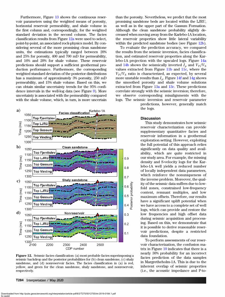
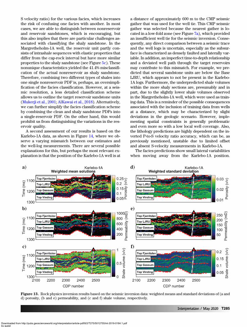
Furthermore, Figure 13 shows the continuous reser-voir parameters using the weighted means of porosity,horizontal reservoir permeability, and shale volume inthe first column and, correspondingly, for the weightedstandard deviation in the second column. The faciesclassification results from Figure 12a were used to select,point-by-point, an associated rock-physics model. By con-sidering several of the more promising clean sandstoneunits, the estimations typically ranged between 20%and 25% for porosity, 400 and 700 mD for permeability,and 16% and 20% for shale volume. These reservoirpredictions should support a sufficient geothermal pro-duction performance. Furthermore, the correspondingweighted standard deviation of the posterior distributionshas a maximum of approximately 3% porosity, 250 mDpermeability, and 15% shale volume. Based on this, wecan obtain similar uncertainty trends for the 95% confi-dence intervals in the well-log data (see Figure 9). Moreuncertainty is associated with the permeability comparedwith the shale volume, which, in turn, is more uncertain

than the porosity. Nevertheless, we predict that the mostpromising sandstone beds are located within the LJRU,as well as in the upper part of the Gassum Formation.Although the clean sandstone probability slightly de-creasedwhenmoving away from the Karlebo-1A location,the reservoir properties show little lateral variabilitywithin the predicted sandstone bodies (see Figure 12b).

To evaluate the prediction accuracy, we comparedthe results from the seismic inversion, facies classifica-tion, and estimated reservoir properties along the Kar-lebo-1A projection with the upscaled logs. Figure 14aand 14b shows the seismically inverted Ip and VP∕VSvalues extracted from Figure 11b and 11c, where theVP∕VS ratio is characterized, as expected, by severalmore unstable results than Ip. Figure 14f and 14g showsthe smoothed porosity and shale volume solutionsextracted from Figure 13a and 13c. These predictionscorrelate strongly with the seismic inversion; therefore,we observe corresponding misalignments with thelogs. The seismic inversion and reservoir parameter

predictions, however, generally matchthe logs.

DiscussionThis study demonstrates how seismic

reservoir characterization can providesupplementary quantitative facies andreservoir information in a geothermalexploration setting. However, exploitingthe full potential of this approach reliessignificantly on data quality and avail-ability, which are quite restricted inour study area. For example, the missingdensity and S-velocity logs for the Kar-lebo-1A well yields a reduced numberof locally independent data parameters,which reinforce the nonuniqueness ofthe inverse problem. Moreover, the qual-ity of the seismic data suffers due to low-fold zones, constrained low-frequencycontent, remnant multiples, and lowmaximum offsets. Therefore, our resultshave a significant uplift potential whenwe have access to a complete set of welllogs, which can provide and restore thelow frequencies and high offset dataduring seismic acquisition and process-ing. Based on this, we demonstrate thatit is possible to derive reasonable reser-voir predictions, despite a restricteddata foundation.

To perform assessments of our reser-voir characterization, the confusion ma-trix in Figure 10 indicates that there is anearly 30% probability for an incorrectfacies prediction of the data samplesin Margretheholm-1A. This is due to theinherent overlap of seismic properties(i.e., the acoustic impedance and P-to-

Figure 12. Seismic facies classification: (a) most probable facies superimposing aseismic backdrop and the posterior probabilities for (b) clean sandstone, (c) shalysandstone, and (d) nonreservoir facies. The facies classification in (a) is red,yellow, and green for the clean sandstone, shaly sandstone, and nonreservoir,respectively.



S velocity ratio) for the various facies, which increasesthe risk of confusing one facies with another. In mostcases, we are able to distinguish between nonreservoirand reservoir sandstones, which is encouraging, butthis also implies that there are particular challenges as-sociated with classifying the shaly sandstone. In theMargretheholm-1A well, the reservoir unit partly con-sists of intrashale sequences with elastic properties thatdiffer from the cap-rock interval but have more similarproperties to the shaly sandstone (see Figure 5c). Thesenonunique characteristics yielded the 41.4% misclassifi-cation of the actual nonreservoir as shaly sandstone.Therefore, combining two different types of shales intoone single nonreservoir PDF is, perhaps, an oversimpli-fication of the facies classification. However, at a seis-mic resolution, a less detailed classification schemeallows us to outline the target reservoir sandstone units(Mukerji et al., 2001; AlKawai et al., 2018). Alternatively,we can further simplify the facies classification schemeby combining the clean and shaly sandstone PDFs intoa single-reservoir PDF. On the other hand, this wouldprohibit us from distinguishing the variations in the res-ervoir quality.

A second assessment of our results is based on theKarlebo-1A data, as shown in Figure 14, where we ob-serve a varying mismatch between our estimates andthe well-log measurements. There are several possibleexplanations for this, but perhaps the most relevant ex-planation is that the position of the Karlebo-1A well is at

a distance of approximately 600 m to the CMP seismicgather that was used for the well tie. This CMP seismicgather was selected because the nearest gather is lo-cated in a low-fold zone (see Figure 7a), which providedan insufficient well tie for the seismic inversion. Conse-quently, any direct comparison between a seismic traceand the well logs is uncertain, especially as the subsur-face is characterized as densely faulted and laterally var-iable. In addition, an imperfect time-to-depth relationshipand a deviated well path through the target reservoirsmay contribute to this mismatch. For example, we pre-dicted that several sandstone units are below the BaseLJRU, which appears to not be present in the Karlebo-1A logs. Furthermore, the underpredicted shale volumeswithin the more shaly sections are, presumably and inpart, due to the slightly lower shale volumes observedin the Margretheholm-1A well, which were used as train-ing data. This is a reminder of the possible consequencesassociated with the inclusion of training data from wellsat a distance, which may be characterized by slightdeviations in the geologic scenario. However, imple-menting spatial constraints is generally problematicand even more so with a low local well coverage. Also,the lithology predictions are highly dependent on the in-verted P-to-S velocity ratio accuracy, which can be, aspreviously mentioned, unstable due to limited offsetand absent S-velocity measurements in Karlebo-1A.

The facies predictions show small lateral variabilitieswhen moving away from the Karlebo-1A position.

Figure 13. Rock physics inversion results based on the seismic inversion data: weighted means and standard deviations of (a andd) porosity, (b and e) permeability, and (c and f) shale volume, respectively.



Figure 12b shows a decreasing probability for the cleansandstone toward the southwest along line 5 in theLJRU, which may imply that the reservoir qualitydecays away from the Karlebo-1A area. At the sametime, we observed that these predictions were dis-tributed in a more discontinuous and patchy manner,which is possibly related to seismic interference or res-olution issues. Also, the nonparametric, Kernel-density-estimated PDFs, used to link reservoir and seismicproperties (see Figure 5c), were generated using a cal-ibration procedure from the well-log data (Grana, 2018).Obtaining optimal parameters to control the PDFs canbe challenging for non-Gaussian distributed data, suchthat we finally selected a configuration that yielded pre-dictions that were consistent with the expected geol-ogy. Meanwhile, during PDF calibration, we observedthat different configurations influenced the predictionsin terms of varying spatial continuity, resolution, andnoise. With such instabilities, there was a significant re-duction in our prediction confidence at increasingdistance from the Karlebo-1A location. Although vari-ous statistical estimators can be selected to provide areasonable representation of the reservoir predictions,we applied a weighted mean and standard deviation(see Figure 13). Previous studies have demonstrated,for instance, the use of the maximum a posteriori(MAP) estimator (Bachrach, 2006) and various percen-tiles of the posterior PDFs (Grana, 2018). Nevertheless,we obtained similar results when testing variousestimators.

ConclusionIn this study, we demonstrated a field example of

seismic reservoir characterization in a low-enthalpygeothermal exploration setting from an area to thenorth of Copenhagen, onshore Denmark. Facies andreservoir property predictions were derived by integrat-ing seismic data, well logs, and available regional data.The results demonstrate that several porous and cleanwater-bearing sandstones are potential high-qualitygeothermal reservoirs within two target layers, that is,the LJRU and Gassum Formation. In general, the LJRUexhibits a more promising reservoir quality in terms ofhigh porosity, permeability, and low shale content com-pared with the Gassum Formation. However, with thelimited availability and nonoptimal quality of the localdata, we were unable to derive a rigorous and firm res-ervoir prognosis and our final results are primarilyindicative of possible target layers. With an improveddata foundation, geothermal reservoir seismic charac-terization is demonstrably useful to optimize site loca-tions, which can be the tipping point between successand failure in geothermal exploitation.

AcknowledgmentsThis contribution is a part of the project GEOTHERM

(Geothermal energy from sedimentary reservoirs — Re-moving obstacles for large-scale utilization) funded by theInnovation Fund Denmark (IFD) (grant no. 6154-00011B).

Data and materials availabilityData associated with this research are available and

can be obtained by contacting the corre-sponding author.

Appendix A

Rock-physics modelingFor isotropic rocks, the effective bulk

modulus K and shear modulus μ are re-lated to the seismically inverted acousticimpedance Ip and the ratio of the P-wavevelocity VP to S-wave velocity VS (i.e.,VP∕VS) based on the following simpleexpressions:

VP ¼ffiffiffiffiffiffiffiffiffiffiffiffiffiffiffiK þ 4

3 μ

ρ

s; (A-1)

VS ¼ffiffiffiμ

ρ

r; (A-2)

Ip ¼ VPρ: (A-3)

The effective density ρ is estimated withthe following equation:

ρ ¼ ð1 − ϕÞρm þ ϕρf ; (A-4)

Figure 14. A comparison between the predictions and Karlebo-1A observations:(a and b) seismic inversion, (c and d) facies classification, and (e and f) reservoirproperties. The facies classification is denoted in yellow, brown, and green forclean sandstone, shaly sandstone, and nonreservoir, respectively. The depth isin measured depth.



where ϕ is the porosity and ρm and ρf are themineral andfluid densities, respectively.

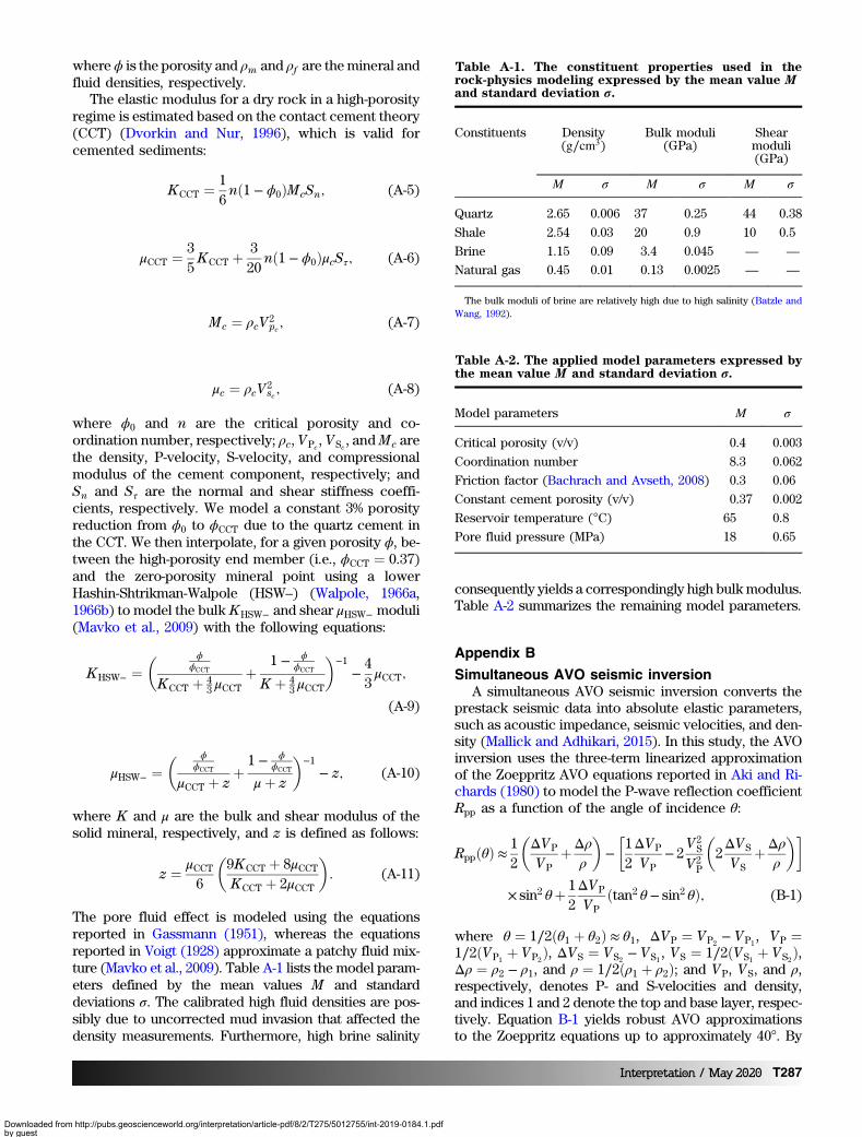
The elastic modulus for a dry rock in a high-porosityregime is estimated based on the contact cement theory(CCT) (Dvorkin and Nur, 1996), which is valid forcemented sediments:

KCCT ¼ 16nð1 − ϕ0ÞMcSn; (A-5)

μCCT ¼ 35KCCT þ

320

nð1 − ϕ0ÞμcSτ; (A-6)

Mc ¼ ρcV 2pc ; (A-7)

μc ¼ ρcV2sc ; (A-8)

where ϕ0 and n are the critical porosity and co-ordination number, respectively; ρc, VPc

, VSc , andMc arethe density, P-velocity, S-velocity, and compressionalmodulus of the cement component, respectively; andSn and Sτ are the normal and shear stiffness coeffi-cients, respectively. We model a constant 3% porosityreduction from ϕ0 to ϕCCT due to the quartz cement inthe CCT. We then interpolate, for a given porosity ϕ, be-tween the high-porosity end member (i.e., ϕCCT ¼ 0.37)and the zero-porosity mineral point using a lowerHashin-Shtrikman-Walpole (HSW–) (Walpole, 1966a,1966b) to model the bulk KHSW− and shear μHSW− moduli(Mavko et al., 2009) with the following equations:

KHSW− ¼� ϕ

ϕCCT

KCCT þ 43 μCCT

þ1 − ϕ

ϕCCT

K þ 43 μCCT

�−1

−43μCCT;

(A-9)

μHSW− ¼� ϕ

ϕCCT

μCCT þ zþ

1 − ϕϕCCT

μþ z

�−1

− z; (A-10)

where K and μ are the bulk and shear modulus of thesolid mineral, respectively, and z is defined as follows:

z ¼ μCCT6

�9KCCT þ 8μCCTKCCT þ 2μCCT

�: (A-11)

The pore fluid effect is modeled using the equationsreported in Gassmann (1951), whereas the equationsreported in Voigt (1928) approximate a patchy fluid mix-ture (Mavko et al., 2009). Table A-1 lists the model param-eters defined by the mean values M and standarddeviations σ. The calibrated high fluid densities are pos-sibly due to uncorrected mud invasion that affected thedensity measurements. Furthermore, high brine salinity

consequently yields a correspondingly high bulkmodulus.Table A-2 summarizes the remaining model parameters.

Appendix B

Simultaneous AVO seismic inversionA simultaneous AVO seismic inversion converts the

prestack seismic data into absolute elastic parameters,such as acoustic impedance, seismic velocities, and den-sity (Mallick and Adhikari, 2015). In this study, the AVOinversion uses the three-term linearized approximationof the Zoeppritz AVO equations reported in Aki and Ri-chards (1980) to model the P-wave reflection coefficientRpp as a function of the angle of incidence θ:

RppðθÞ ≈12

�ΔVP

VPþΔρ

ρ

�−�12ΔVP

VP− 2

V 2S

V2P

�2ΔVS

VSþΔρ

ρ

��

× sin2 θþ 12ΔVP

VPðtan2 θ− sin2 θÞ; (B-1)

where θ ¼ 1∕2ðθ1 þ θ2Þ ≈ θ1, ΔVP ¼ VP2− VP1

, VP ¼1∕2ðVP1

þ VP2Þ, ΔVS ¼ VS2 − VS1 , VS ¼ 1∕2ðVS1 þ VS2Þ,

Δρ ¼ ρ2 − ρ1, and ρ ¼ 1∕2ðρ1 þ ρ2Þ; and VP, VS, and ρ,respectively, denotes P- and S-velocities and density,and indices 1 and 2 denote the top and base layer, respec-tively. Equation B-1 yields robust AVO approximationsto the Zoeppritz equations up to approximately 40°. By

Table A-1. The constituent properties used in therock-physics modeling expressed by the mean value Mand standard deviation σ.

Constituents Density(g∕cm3)

Bulk moduli(GPa)

Shearmoduli(GPa)

M σ M σ M σ

Quartz 2.65 0.006 37 0.25 44 0.38

Shale 2.54 0.03 20 0.9 10 0.5

Brine 1.15 0.09 3.4 0.045 — —

Natural gas 0.45 0.01 0.13 0.0025 — —

The bulk moduli of brine are relatively high due to high salinity (Batzle andWang, 1992).

Table A-2. The applied model parameters expressed bythe mean value M and standard deviation σ.

Model parameters M σ

Critical porosity (v/v) 0.4 0.003

Coordination number 8.3 0.062

Friction factor (Bachrach and Avseth, 2008) 0.3 0.06

Constant cement porosity (v/v) 0.37 0.002

Reservoir temperature (°C) 65 0.8

Pore fluid pressure (MPa) 18 0.65



sequentially updating a low-frequency background modelof velocities and densities obtained from the upscaledwell-log data and seismic interval velocities, we obtain anadequate match between the forward modeled and realseismic data. Hence, we can systematically approachvelocity and density models of the subsurface with higherconfidence.

Appendix C

Facies and reservoir property estimationIn this study, we estimated the facies and reservoir

properties in a Bayesian framework. The reservoir prop-erties were estimated from probability distributions,which were explicitly expressed using PDFs to conformto the nonlinear relationships between the reservoir andseismic properties (Grana, 2018). This problem can beformulated as a Bayesian inference problem:

σðmÞ ¼ cpðmÞLðdobs − gðmÞÞ; (C-1)

where m denotes the subsurface reservoir propertiesand facies and c is a normalization constant. Data for mprior to including seismic observations are expressed bythe prior probability distribution p, which is normally ob-tained from adjacent well data. The model likelihoodfunction L was then used to implement seismic data,which measure, in terms of probability, the mismatch be-tween the modeled gðmÞ and seismically inverted data,dobs. In this case, gðmÞ and dobs refer to the PDFs as afunction of the augmented Ip and VP∕VS training set andseismic inversion data, respectively. We use a nonpara-metric kernel density estimation technique to calculatethe PDFs (Silverman, 1986; Grana, 2018).

Based on the posterior distributions, the most prob-able facies was estimated from the MAP probability(Doyen, 2007). Furthermore, we calculated the weightedmean and standard deviation from the most likely faciesposterior distribution to quantify the expected valuesand uncertainty ranges for the porosity and shale volumesolutions. The weighted mean for the porosity ϕF infacies F is expressed by the following equation:

ϕ̄F ¼P

Lk¼1 P

�ϕkF jIp; VP

VS

�ϕkF

PLk¼1 P

�ϕkF jIp; VP

VS

� ; (C-2)

where k is a modeled porosity sample andPðϕkjIp; VP∕VSÞ is the posterior probability for a setof Ip and VP∕VS data. The corresponding weighted stan-dard deviation is expressed by

σ̄ϕF¼

ffiffiffiffiffiffiffiffiffiffiffiffiffiffiffiffiffiffiffiffiffiffiffiffiffiffiffiffiffiffiffiffiffiffiffiffiffiffiffiffiffiffiffiffiffiffiffiffiffiffiffiffiffiffiffiffiffiffiffiffiffiffiPLk¼1 P

�ϕkF jIp; VP

VS

�ðϕk

F − ϕ̄FÞ2

PLk¼1 P

�ϕkF ∣ Ip;

VPVS

�vuuuuut : (C-3)

Permeability estimationsTo estimate the horizontal reservoir permeability

κres, we use an empirical permeability-porosity modelκL as proposed by Kristensen et al. (2016):

κL ¼ c × ð4.43 × 10−4 × ϕÞ4.36; (C-4)

where ϕ is the predicted porosity and c is a constantcontrolled by variations in the local permeability cali-brated to 0.85 in this study. To convert the relationshipin equation C-4 from laboratory measurements of hori-zontally orientated core plugs to field-scale reservoirpermeability κres, κL is multiplied by an upscaling factorof 1.25. For the corresponding vertical permeability,core analyses suggest that a vertical-to-horizontal per-meability ratio of 0.3 is appropriate.

ReferencesAki, K., and P. G. Richards, 1980, Quantitative seismology:

Theory and methods: W. H. Freeman and Co.AlKawai, W. H., T. Mukerji, A. H. Scheirer, and S. A. Gra-

ham, 2018, Integrating statistical rock physics and pres-sure and thermal history modeling to map reservoirlithofacies in the deepwater Gulf of Mexico: Geophys-ics, 83, no. 4, IM15–IM28, doi: 10.1190/geo2017-0427.1.

Avseth, P., A. Janke, and F. Horn, 2016, AVO inversion inexploration— Key learnings from a Norwegian Sea pros-pect: The Leading Edge, 35, 405–414, doi: 10.1190/tle35050405.1.

Avseth, P., T. Mukerji, A. Jørstad, G. Mavko, and T. Vegge-land, 2001, Seismic reservoir mapping from 3-D AVO ina North Sea turbidite system: Geophysics, 66, 1157–1176, doi: 10.1190/1.1487063.

Avseth, P., T. Mukerji, and G. Mavko, 2005, Quantitativeseismic interpretation: Applying rock physics tools toreduce interpretation risk: Cambridge University Press.

Avseth, P., T. Mukerji, G. Mavko, and J. Dvorkin, 2010,Rock-physics diagnostics of depositional texture, diage-netic alterations, and reservoir heterogeneity in high-porosity siliciclastic sediments and rocks — A reviewof selected models and suggested work flows: Geophys-ics, 75, no. 5, 75A31–75A47, doi: 10.1190/1.3483770.

Ba, J., H. Cao, J. M. Carcione, G. Tang, X. F. Yan, W. T. Sun,and J. X. Nie, 2013, Multiscale rock-physics templatesfor gas detection in carbonate reservoirs: Journal of Ap-plied Geophysics, 93, 77–82, doi: 10.1016/j.jappgeo.2013.03.011.

Bachrach, R., 2006, Joint estimation of porosity and satu-ration using stochastic rock-physics modeling: Geo-physics, 71, no. 5, O53–O63, doi: 10.1190/1.2235991.

Bachrach, R., and P. Avseth, 2008, Rock physics modelingof unconsolidated sands: Accounting for nonuniformcontacts and heterogeneous stress fields in the effectivemedia approximation with applications to hydrocarbonexploration: Geophysics, 73, no. 6, E197–E209, doi: 10.1190/1.2985821.

Balling, N., J. M. Hvid, A. Mahler, J. J. Møller, A. Mathiesen,T. Bidstrup, and L. H. Nielsen, 2002, Denmark, in



http://dx.doi.org/10.1190/geo2017-0427.1



http://dx.doi.org/10.1190/tle35050405.1




http://dx.doi.org/10.1190/1.1487063

http://dx.doi.org/10.1190/1.1487063

http://dx.doi.org/10.1190/1.1487063

http://dx.doi.org/10.1190/1.3483770

http://dx.doi.org/10.1190/1.3483770

http://dx.doi.org/10.1190/1.3483770

http://dx.doi.org/10.1016/j.jappgeo.2013.03.011






http://dx.doi.org/10.1190/1.2235991

http://dx.doi.org/10.1190/1.2235991

http://dx.doi.org/10.1190/1.2235991

http://dx.doi.org/10.1190/1.2985821

http://dx.doi.org/10.1190/1.2985821

http://dx.doi.org/10.1190/1.2985821

S. Hurter and R. Haenel, eds., Atlas of geothermalresources in Europe: The European Commission, Pub-lication No. EUR 17811, 27–28.

Barbier, E., 2002, Geothermal energy technology and currentstatus: An overview: Renewable and Sustainable EnergyReviews, 6, 3–65, doi: 10.1016/S1364-0321(02)00002-3.

Batzle, M., and Z. Wang, 1992, Seismic properties of pore flu-ids: Geophysics, 57, 1396–1408, doi: 10.1190/1.1443207.

Bredesen, K., E. Dalgaard, A. Mathiesen, and N. Balling,2018, A rock physics feasibility study of the geothermalGassum reservoir, Copenhagen Area, Denmark: 80thAnnual International Conference and Exhibition, EAGE,Extended Abstracts, ThB12, doi: 10.3997/2214-4609.201801408.

Bujakowski, W., A. Barbacki, B. Czerwińska, L. Pająk, M.Pussak, M. Stefaniuk, and Z. Trześniowski, 2010, Inte-grated seismic and magnetotelluric exploration of theSkierniewice, Poland, geothermal test site: Geother-mics, 39, 78–93, doi: 10.1016/j.geothermics.2010.01.003.

Buland, A., O. Kolbjørnsen, R. Hauge, Ø. Skjæveland, andK. Duffaut, 2008, Bayesian lithology and fluid predictionfrom seismic prestack data: Geophysics, 73, no. 3, C13–C21, doi: 10.1190/1.2842150.

Casini, M., S. Ciuffi, A. Fiordelisi, A. Mazzotti, and E. Stuc-chi, 2010, Results of a 3D seismic survey at the Travale(Italy) test site: Geothermics, 39, 4–12, doi: 10.1016/j.geothermics.2009.11.003.

Doyen, P., 2007, Seismic reservoir characterization: Anearth modeling perspective: EAGE Publications.

Dvorkin, J., M. A. Gutierrez, and D. Grana, 2014, Seismicreflections of rock properties: Cambridge UniversityPress.

Dvorkin, J., and A. Nur, 1996, Elasticity of high-porositysandstones: Theory for two North Sea data sets: Geo-physics, 61, 1363–1370, doi: 10.1190/1.1444059.

Dyer, B., U. Schanz, F. Ladner, M. Häring, and T. Spillman,2008, Microseismic imaging of a geothermal reservoirstimulation: The Leading Edge, 27, 856–869, doi: 10.1190/1.2954024.

Edgar, J. A., and M. van der Baan, 2011, How reliable isstatistical wavelet estimation?: Geophysics, 76, no. 4,V59–V68, doi: 10.1190/1.3587220.

Eidsvik, J., P. Avseth, H. Omre, T. Mukerji, and G. Mavko,2004, Stochastic reservoir characterization using prestackseismic data: Geophysics, 69, 978–993, doi: 10.1190/1.1778241.

Endo, M., A. Gribenko, D. Sunwall, M. S. Zhdanov, T.Miura, H. Mochinaga, N. Aoki, and T. Mouri, 2018, Inte-grated interpretation of multimodal geophysical datafor exploration of geothermal resources — Case study:Yamagawa geothermal field in Japan: 88th Annual Inter-national Meeting, SEG, Expanded Abstracts, 2322–2326,doi: 10.1190/segam2018-2997562.1.

Folesky, J., J. Kummerow, S. A. Shapiro, M. Häring, and H.Asanuma, 2016, Rupture directivity of fluid-inducedmicroseismic events: Observations from an enhancedgeothermal system: Journal of Geophysical Research:

Solid Earth, 121, 8034–8047, doi: 10.1002/2016JB013078.

Gassmann, F., 1951, Elastic waves through a packing ofspheres: Geophysics, 16, 673–685, doi: 10.1190/1.1437718.

Grana, D., 2014, Probabilistic approach to rock physicsmodeling: Geophysics, 79, no. 2, D123–D143, doi: 10.1190/geo2013-0333.1.

Grana, D., 2018, Joint facies and reservoir properties inver-sion: Geophysics, 83, no. 3, M15–M24, doi: 10.1190/geo2017-0670.1.

Grana, D., and E. Della Rossa, 2010, Probabilistic petro-physical-properties estimation integrating statisticalrock physics with seismic inversion: Geophysics, 75,no. 3, O21–O37, doi: 10.1190/1.3386676.

Grana, D., S. Verma, J. Pafeng, X. Lang, H. Sharma, W. Wu,F. McLaughlin, E. Campbell, K. Ng, and V. Alvarado,2017, A rock physics and seismic reservoir characteri-zation study of the Rock Springs Uplift, a carbon diox-ide sequestration site in Southwestern Wyoming:International Journal of Greenhouse Gas Control, 63,296–309, doi: 10.1016/j.ijggc.2017.06.004.

Grude, S., M. Landrø, and B. Osdal, 2013, Time-lapse pres-sure-saturation discrimination for CO2 storage at theSnøhvit field: International Journal of Greenhouse GasControl, 19, 369–378, doi: 10.1016/j.ijggc.2013.09.014.

Japsen, P., P. F. Green, L. H. Nielsen, E. S. Rasmussen, andT. Bidstrup, 2007, Mesozoic–Cenozoic exhumationevents in the eastern North Sea Basin: A multi-discipli-nary study based on palaeothermal, palaeoburial, strati-graphic and seismic data: Basin Research, 19, 451–490,doi: 10.1111/j.1365-2117.2007.00329.x.

Khair, H. A., D. Cooke, and M. Hand, 2015, Seismic map-ping and geomechanical analyses of faults within deephot granites, a workflow for enhanced geothermal sys-tem projects: Geothermics, 53, 46–56, doi: 10.1016/j.geothermics.2014.04.007.

Kristensen, L., M. L. Hjuler, P. Frykman, M. Olivarius, R.Weibel, L. H. Nielsen, and A. Mathiesen, 2016, Pre-drill-ing assessments of average porosity and permeability inthe geothermal reservoirs of the Danish area: Geother-mal Energy, 4, 6, doi: 10.1186/s40517-016-0048-6.

Lüschen, E., S. Görne, H. Hartmann, R. Thomas, and R.Schulz, 2015, 3D seismic survey for geothermal explora-tion in crystalline rocks in Saxony, Germany: GeophysicalProspecting, 63, 975–989, doi: 10.1111/1365-2478.12249.

Lüschen, E., M. Wolfgramm, T. Fritzer, M. Dussel, R.Thomas, and R. Schulz, 2014, 3D seismic survey ex-plores geothermal targets for reservoir characterizationat Unterhaching, Munich, Germany: Geothermics, 50,167–179, doi: 10.1016/j.geothermics.2013.09.007.

Majer, E., T. V. McEvilly, F. Eastwood, and L. Myer, 1988,Fracture detection using P-wave and S-wave verticalseismic profiling at The Geysers: Geophysics, 53, 76–84, doi: 10.1190/1.1442401.

Mallick, S., and S. Adhikari, 2015, Amplitude-variation-with-offset and prestack-waveform inversion: A directcomparison using a real data example from the Rock



http://dx.doi.org/10.1016/S1364-0321(02)00002-3

http://dx.doi.org/10.1016/S1364-0321(02)00002-3

http://dx.doi.org/10.1190/1.1443207

http://dx.doi.org/10.1190/1.1443207

http://dx.doi.org/10.1190/1.1443207

http://dx.doi.org/10.3997/2214-4609.201801408

http://dx.doi.org/10.3997/2214-4609.201801408

http://dx.doi.org/10.3997/2214-4609.201801408

http://dx.doi.org/10.1016/j.geothermics.2010.01.003






http://dx.doi.org/10.1190/1.2842150

http://dx.doi.org/10.1190/1.2842150

http://dx.doi.org/10.1190/1.2842150







http://dx.doi.org/10.1190/1.1444059

http://dx.doi.org/10.1190/1.1444059

http://dx.doi.org/10.1190/1.1444059

http://dx.doi.org/10.1190/1.2954024

http://dx.doi.org/10.1190/1.2954024

http://dx.doi.org/10.1190/1.2954024

http://dx.doi.org/10.1190/1.3587220

http://dx.doi.org/10.1190/1.3587220

http://dx.doi.org/10.1190/1.3587220

http://dx.doi.org/10.1190/1.1778241

http://dx.doi.org/10.1190/1.1778241

http://dx.doi.org/10.1190/1.1778241

http://dx.doi.org/10.1190/segam2018-2997562.1



http://dx.doi.org/10.1002/2016JB013078

http://dx.doi.org/10.1002/2016JB013078

http://dx.doi.org/10.1002/2016JB013078

http://dx.doi.org/10.1190/1.1437718

http://dx.doi.org/10.1190/1.1437718

http://dx.doi.org/10.1190/1.1437718








http://dx.doi.org/10.1190/1.3386676

http://dx.doi.org/10.1190/1.3386676

http://dx.doi.org/10.1190/1.3386676

http://dx.doi.org/10.1016/j.ijggc.2017.06.004












http://dx.doi.org/10.1111/j.1365-2117.2007.00329.x

http://dx.doi.org/10.1111/j.1365-2117.2007.00329.x

http://dx.doi.org/10.1111/j.1365-2117.2007.00329.x

http://dx.doi.org/10.1111/j.1365-2117.2007.00329.x

http://dx.doi.org/10.1111/j.1365-2117.2007.00329.x

http://dx.doi.org/10.1111/j.1365-2117.2007.00329.x







http://dx.doi.org/10.1186/s40517-016-0048-6

http://dx.doi.org/10.1186/s40517-016-0048-6

http://dx.doi.org/10.1111/1365-2478.12249

http://dx.doi.org/10.1111/1365-2478.12249

http://dx.doi.org/10.1111/1365-2478.12249







http://dx.doi.org/10.1190/1.1442401

http://dx.doi.org/10.1190/1.1442401

http://dx.doi.org/10.1190/1.1442401

Springs Uplift, Wyoming, USA: Geophysics, 80, no. 2,B45–B59, doi: 10.1190/geo2014-0233.1.

Mathiesen, A., L. H. Nielsen, and T. Bidstrup, 2010, Identi-fying potential geothermal reservoirs in Denmark: Geo-logical Survey of Denmark and Greenland Bulletin, 20,19–22.

Mavko, G., and T. Mukerji, 1998, A rock physics strategy forquantifying uncertainty in common hydrocarbon indica-tors: Geophysics, 63, 1997–2008, doi: 10.1190/1.1444493.

Mavko, G., T. Mukerji, and J. Dvorkin, 2009, The rock phys-ics handbook: Tools for seismic analysis of porousmedia: Cambridge University Press.

Michelsen, O., L. H. Nielsen, P. N. Johannessen, J. Andsb-jerg, and F. Surlyk, 2003, Jurassic lithostratigraphy andstratigraphic development onshore and offshore Den-mark, in J. R. Ineson and F. Surlyk, eds., Geological Sur-vey of Denmark and Greenland Bulletin, 1, 147–216.

Mindlin, R. D., 1949, Compliance of elastic bodies in con-tact: Journal of Applied Mechanics, 16, 259–268.

Montazeri, M., A. Uldall, J. Moreau, and L. Nielsen, 2018,Pitfalls in velocity analysis for strongly contrasting, lay-ered media — Example from the Chalk Group, NorthSea: Journal of Applied Geophysics, 149, 52–62, doi:10.1016/j.jappgeo.2017.12.003.

Mukerji, T., A. Jørstad, P. Avseth, G. Mavko, and J. Granli,2001, Mapping lithofacies and pore-fluid probabilities ina North Sea reservoir: Seismic inversions and statisticalrock physics: Geophysics, 66, 988–1001, doi: 10.1190/1.1487078.

Muñoz, G., K. Bauer, I. Moeck, A. Schulze, and O. Ritter,2010, Exploring the Groß Schönebeck (Germany) geo-thermal site using a statistical joint interpretation ofmagnetotelluric and seismic tomography models: Geo-thermics, 39, 35–45, doi: 10.1016/j.geothermics.2009.12.004.

Nielsen, L. H., A. Mathiesen, and T. Bidstrup, 2004, Geo-thermal energy in Denmark: Geological Survey of Den-mark and Greenland Bulletin, 4, 17–20.

Nunziata, C., and A. Rapolla, 1981, Interpretation of gravityand magnetic data in the Phlegraean Fields geothermalarea, Naples, Italy: Journal of Volcanology and Geother-mal Research, 10, 209–225, doi: 10.1016/0377-0273(81)90063-9.

Pellerin, L., J. M. Johnston, and G. W. Hohmann, 1996, Anumerical evaluation of electromagnetic methods ingeothermal exploration: Geophysics, 61, 121–130, doi:10.1190/1.1443931.

Place, J., J. Sausse, J. Marthelot, M. Diraison, Y. Géraud,and C. Naville, 2011, 3-D mapping of permeable struc-tures affecting a deep granite basement using isotropic3C VSP data: Geophysical Journal International, 186,245–263, doi: 10.1111/j.1365-246X.2011.05012.x.

Poulsen, S. E., N. Balling, T. S. Bording, A. Mathiesen, andS. B. Nielsen, 2017, Inverse geothermal modellingapplied to Danish sedimentary basins: GeophysicalJournal International, 211, 188–206, doi: 10.1093/gji/ggx296.

Pussak, M., K. Bauer, M. Stiller, and W. Bujakowski, 2014,Improved 3D seismic attribute mapping by CRS stackinginstead of NMO stacking: Application to a geothermalreservoir in the Polish Basin: Journal of Applied Geophys-ics, 103, 186–198, doi: 10.1016/j.jappgeo.2014.01.020.

Reiser, F., C. Schmelzbach, H. Maurer, S. Greenhalgh, andO. Hellwig, 2017, Optimizing the design of vertical seis-mic profiling (VSP) for imaging fracture zones over har-drock basement geothermal environments: Journal ofApplied Geophysics, 139, 25–35, doi: 10.1016/j.jappgeo.2017.02.023.

Reshetnikov, A., J. Kummerow, H. Asanuma, M. Häring, andS. A. Shapiro, 2015, Microseismic reflection imaging andits application to the Basel geothermal reservoir: Geo-physics, 80, no. 6, WC39–WC49, doi: 10.1190/geo2014-0593.1.

Røgen, B., C. Ditlefsen, T. Vangkilde-Pedersen, L. H. Niel-sen, and A. Mahler, 2015, Geothermal energy use, coun-try update for Denmark: World Geothermal Congress.

Sausse, J., C. Dezayes, L. Dorbath, A. Genter, and J. Place,2010, 3D model of fracture zones at Soultz-sous-Forêtsbased on geological data, image logs, induced microseis-micity and vertical seismic profiles: Comptes RendusGeoscience, 342, 531–545, doi: 10.1016/j.crte.2010.01.011.

Schmelzbach, C., S. Greenhalgh, F. Reiser, J. Girard, F.Bretaudeau, L. Capar, and A. Bitri, 2016a, Advancedseismic processing/imaging techniques and their poten-tial for geothermal exploration: Interpretation, 4, no. 4,SR1–SR18, doi: 10.1190/INT-2016-0017.1.

Schmelzbach, C., J. Kummerow, P. Wigger, A. Reshetnikov,P. Salazar, and S. Shapiro, 2016b, Microseismic reflectionimaging of the Central Andean crust: Geophysical JournalInternational, 204, 1396–1404, doi: 10.1093/gji/ggv530.

Silverman, B. W., 1986, Density estimation for statisticsand data analysis monographs on statistics and appliedprobability: Chapman & Hall.

Voigt, W., 1928, Lehrbuch der Kristallphysik (mit Auss-chluss der Kristalloptik): B.G. Teubner.

von Hartmann, H., H. Buness, C. M. Krawczyk, and R.Schulz, 2012, 3-D seismic analysis of a carbonateplatform in the Molasse Basin — Reef distributionand internal separation with seismic attributes: Tecto-nophysics, 572, 16–25, doi: 10.1016/j.tecto.2012.06.033.

Vosgerau, H., U. Gregersen, L. Kristensen, S. Lindström, A.Mathiesen, C. M. Nielsen, M. Olivarius, and L. H. Niel-sen, 2017, Towards a geothermal exploration well inthe Gassum Formation in Copenhagen: Geological Sur-vey of Denmark and Greenland Bulletin, 38, 29–32.

Vosgerau, H., U. Gregersen, M. Leth Hjuler, H. Dahl Holm-slykke, L. Kristensen, S. Lindström, A. Mathiesen, C.Møller Nielsen, M. Olivarius, G. Krarup Pedersen, andL. H. Nielsen, 2016, Reservoir prognosis of the GassumFormation and the Karlebo Member within two areas ofinterest in northern Copenhagen: Geological Survey ofDenmark and Greenland Report, http://dybgeotermi.geus.dk/wp-content/uploads/Geothermal-pilot-hole-phase-1b.pdf, accessed 3 November 2019.






http://dx.doi.org/10.1190/1.1444493

http://dx.doi.org/10.1190/1.1444493

http://dx.doi.org/10.1190/1.1444493







http://dx.doi.org/10.1190/1.1487078

http://dx.doi.org/10.1190/1.1487078

http://dx.doi.org/10.1190/1.1487078







http://dx.doi.org/10.1016/0377-0273(81)90063-9

http://dx.doi.org/10.1016/0377-0273(81)90063-9

http://dx.doi.org/10.1016/0377-0273(81)90063-9

http://dx.doi.org/10.1190/1.1443931

http://dx.doi.org/10.1190/1.1443931

http://dx.doi.org/10.1190/1.1443931

http://dx.doi.org/10.1111/j.1365-246X.2011.05012.x






http://dx.doi.org/10.1093/gji/ggx296



















http://dx.doi.org/10.1016/j.crte.2010.01.011






http://dx.doi.org/10.1190/INT-2016-0017.1



http://dx.doi.org/10.1093/gji/ggv530

http://dx.doi.org/10.1093/gji/ggv530

http://dx.doi.org/10.1016/j.tecto.2012.06.033






http://dybgeotermi.geus.dk/wp-content/uploads/Geothermal-pilot-hole-phase-1b.pdf





Walpole, L., 1966a, On bounds for the overall elasticmoduli of inhomogeneous systems — 1: Journal of theMechanics and Physics of Solids, 14, 151–162, doi: 10.1016/0022-5096(66)90035-4.

Walpole, L., 1966b, On bounds for the overall elasticmoduli of inhomogeneous systems — 2: Journal of theMechanics and Physics of Solids, 14, 289–301, doi: 10.1016/0022-5096(66)90025-1.

Waters, K. D., and M. A. Kemper, 2014, Find the rocks andthe fluids will follow — AVO as a tool for lithology clas-sification: Interpretation, 2, no. 2, SC77–SC91, doi: 10.1190/INT-2013-0118.1.

Wei, S., M. V. DeAngelo, and B. A. Hardage, 2014a, Advan-tages of joint interpretation of PP and P-SV seismic datain geothermal exploration: Interpretation, 2, no. 2,SE117–SE123, doi: 10.1190/INT-2013-0084.1.

Wei, S., M. V. DeAngelo, and B. A. Hardage, 2014b, Interpre-tation of multicomponent seismic data acrossWister geo-thermal field, Imperial Valley, California: Interpretation,2, no. 2, SE125–SE135, doi: 10.1190/INT-2013-0083.1.

Weibel, R., M. Olivarius, L. Kristensen, H. Friis, M. L. Hjuler,C. Kjøller, A. Mathiesen, and L. H. Nielsen, 2017, Predict-ing permeability of low-enthalpy geothermal reservoirs:A case study from the Upper Triassic-Lower JurassicGassum Formation, Norwegian-Danish Basin: Geother-mics, 65, 135–157, doi: 10.1016/j.geothermics.2016.09.003.

Kenneth Bredesen received a Ph.D.(2017) in geophysics from the Univer-sity of Bergen. He is a geophysicist atthe Geological Survey of Denmarkand Greenland (GEUS). He has previ-ously worked as a QI geophysicist atSpike Exploration and as a postdoc-toral researcher at Aarhus University.His core competencies are quantita-

tive seismic interpretation, rock-physics modeling, seismicattribute, and amplitude analysis.

Esben Dalgaard received a Ph.D.(2014) in geophysics from Aarhus Uni-versity. During his Ph.D., he workedon developing and implementing ana-logue and digital processing tech-niques for geophysical instruments.He is a senior geophysicist at Qeyein Copenhagen. At Qeye, he primarilyworks with seismic inversion and

rock-physics solutions for quantitative interpretation ondata from around the world.

Anders Mathiesen is a senior advi-sor at GEUS. He has previouslyworked with geophysical geology in-cluding research, advisory, and con-sult work within hydrocarbon, CO2

storage, and geothermal utilization.His core competencies are geophysi-cal and geological data integration,analysis, implementation and map-

ping, modeling, and assessment based on various data(seismic, cores, logs, etc.).

Rasmus Rasmussen is a senior advi-sor at GEUS. He has been workingmainly with seismic data processingoffshore and onshore and also withseismic acquisition, seismic inversion,and AVO processing. In addition tothis, he has been working with seismicforward modeling for geologic modelverification. The work has been re-

lated to hydrocarbon exploration projects, geothermalprojects, and CO2 storage projects.

Niels Balling received a Ph.D. (1982)in geophysics from Aarhus Universityand was offered the doctor of sciencedegree in 2013. He is an associateprofessor of geophysics in the Depart-ment of Geoscience, Aarhus Univer-sity. He is currently sector leader of‘Deep Earth Systems’. He has corecompetences within several geosci-

ence disciplines including controlled and natural sourceseismology and thermal modeling, all in relation to basiccrustal and lithospheric studies as well as geothermal en-ergy resources.



http://dx.doi.org/10.1016/0022-5096(66)90035-4

http://dx.doi.org/10.1016/0022-5096(66)90035-4

http://dx.doi.org/10.1016/0022-5096(66)90025-1

http://dx.doi.org/10.1016/0022-5096(66)90025-1
















Seismic characterization of geothermal sedimentary reservoirs

Documents

Transcript of Seismic characterization of geothermal sedimentary reservoirs