Geothermal district heating networks - University of Glasgow

Glasgow Theses Service http://theses.gla.ac.uk/

[email protected]

Kyriakis, Sotirios A. (2016) Geothermal district heating networks: modelling novel operational strategies incorporating heat storage. PhD thesis http://theses.gla.ac.uk/7404/ Copyright and moral rights for this thesis are retained by the author A copy can be downloaded for personal non-commercial research or study, without prior permission or charge This thesis cannot be reproduced or quoted extensively from without first obtaining permission in writing from the Author The content must not be changed in any way or sold commercially in any format or medium without the formal permission of the Author When referring to this work, full bibliographic details including the author, title, awarding institution and date of the thesis must be given.

http://theses.gla.ac.uk/

http://theses.gla.ac.uk/7404/

Geothermal district heating networks: modelling novel operational strategies incorporating heat

storage

SOTIRIOS A. KYRIAKIS

Submitted in fulfilment of the requirements for the degree

of Doctor of Philosophy at the University of Glasgow

School of Engineering

University of Glasgow

March 2016

1

Abstract

The value of integrating a heat storage into a geothermal district heating system has

been investigated. The behaviour of the system under a novel operational strategy has been

simulated focusing on the energetic, economic and environmental effects of the new

strategy of incorporation of the heat storage within the system. A typical geothermal

district heating system consists of several production wells, a system of pipelines for the

transportation of the hot water to end-users, one or more re-injection wells and peak-up

devices (usually fossil-fuel boilers). Traditionally in these systems, the production wells

change their production rate throughout the day according to heat demand, and if their

maximum capacity is exceeded the peak-up devices are used to meet the balance of the

heat demand. In this study, it is proposed to maintain a constant geothermal production and

add heat storage into the network. Subsequently, hot water will be stored when heat

demand is lower than the production and the stored hot water will be released into the

system to cover the peak demands (or part of these). It is not intended to totally phase-out

the peak-up devices, but to decrease their use, as these will often be installed anyway for

back-up purposes. Both the integration of a heat storage in such a system as well as the

novel operational strategy are the main novelties of this thesis.

A robust algorithm for the sizing of these systems has been developed. The main inputs

are the geothermal production data, the heat demand data throughout one year or more and

the topology of the installation. The outputs are the sizing of the whole system, including

the necessary number of production wells, the size of the heat storage and the dimensions

of the pipelines amongst others. The results provide several useful insights into the initial

design considerations for these systems, emphasizing particularly the importance of heat

losses. Simulations are carried out for three different cases of sizing of the installation

(small, medium and large) to examine the influence of system scale. In the second phase of

work, two algorithms are developed which study in detail the operation of the installation

throughout a random day and a whole year, respectively. The first algorithm can be a

potentially powerful tool for the operators of the installation, who can know a priori how

to operate the installation on a random day given the heat demand. The second algorithm is

used to obtain the amount of electricity used by the pumps as well as the amount of fuel

used by the peak-up boilers over a whole year. These comprise the main operational costs

of the installation and are among the main inputs of the third part of the study. In the third

part of the study, an integrated energetic, economic and environmental analysis of the

2

studied installation is carried out together with a comparison with the traditional case. The

results show that by implementing heat storage under the novel operational strategy, heat is

generated more cheaply as all the financial indices improve, more geothermal energy is

utilised and less fuel is used in the peak-up boilers, with subsequent environmental

benefits, when compared to the traditional case. Furthermore, it is shown that the most

attractive case of sizing is the large one, although the addition of the heat storage most

greatly impacts the medium case of sizing. In other words, the geothermal component of

the installation should be sized as large as possible.

This analysis indicates that the proposed solution is beneficial from energetic,

economic, and environmental perspectives. Therefore, it can be stated that the aim of this

study is achieved in its full potential. Furthermore, the new models for the sizing, operation

and economic/energetic/environmental analyses of these kind of systems can be used with

few adaptations for real cases, making the practical applicability of this study evident.

Having this study as a starting point, further work could include the integration of these

systems with end-user demands, further analysis of component parts of the installation

(such as the heat exchangers) and the integration of a heat pump to maximise utilisation of

geothermal energy.

Keywords: Geothermal, energy, district, heating, storage, operation, strategy.

3

Acknowledgments

This thesis denotes the end of my doctoral studies. My sincere gratefulness and

appreciation goes to the following people who helped me throughout these years with

many different ways:

My supervisor, Professor Paul Younger, for trusting me in this position and giving me

the chance to do a Ph.D. which has always been a dream for me. His help and advice

throughout my studies have been priceless.

My second and third supervisors, Dr Manosh Paul and Dr Edryd W. Stephens, for their

useful comments and supervision. Many thanks also to Dr Zhibin Yu for giving me the

chance to assist him with his courses.

Cluff Geothermal Ltd., the Energy Technology Partnership of Scotland (ETP) and the

University of Glasgow for funding this research project. A distinct acknowledgment goes

to Dr Michael Feliks of Cluff Geothermal, my industrial supervisor, for the many fruitful

discussions, the times that he hosted me in his home and the general help and advice that

he provided me.

Mr Bert Young from the Estates and Buildings office of the University of Glasgow for

providing me with the heat demand data that I used in my thesis, the British Atmospheric

Data Centre (BADC) for giving me access to the weather data that I used in a part of my

thesis as well as to Dr Richard Coulton for the very useful information on the storage tank

costs.

Mrs Elaine McNamara and Mrs Heather Lambie of the University of Glasgow for

answering my endless questions and being always willing to help.

My Greek friends from Glasgow- Nikos, Marianna, Andreas, Ignatios and many others-

for their wonderful company. Thanks a lot to all my foreign friends that I made in

Glasgow- my Spanish friend and ex-flatmate Juan, my Mexican friend Fernando, my

Italian friends Alessandro and Nicola- and all the other wonderful people that I have met

these 3.5 years.

4

My friends from Greece- Dimitris, Christos, Kostas, Serafeim, Anna, Stefanos and

Thanasis- for suffering me all these years.

Finally, my most sincere gratitude goes to my very own people: My parents-

Anastasios and Maria- for their endless support, love and values that they provided me

since I was born; My sisters- Eleana and Dimitra- for the very beautiful moments; and the

most important person for me- my girlfriend, Athina- for her endless love, support and for

believing in me and my capabilities.

5

This thesis is dedicated to the memory

of my friend, George Apostolou.

6

Declarations

Part of the work presented in this thesis has been published in the following articles:

Kyriakis, S.A., and Younger, P.L., 2016. Towards the increased utilisation of geothermal

energy in a district heating network through the use of a heat storage. Applied Thermal

Engineering, 94: 99-110.

Kyriakis, S.A., 2015. Improving the operation of a geothermal district heating network

through the use of a heat storage tank. In: Proceedings of the 14th UK Heat Transfer

Conference, Edinburgh, UK, 7-8 September 2015.

Kyriakis, S.A., 2015. Effect of heat storage in geothermal district heating systems. In:

Proceedings of the 2015 ASME-ATI-UIT Conference, Naples, Italy, 17-20 May 2015.

(ISBN: 978-88-98273-17-1)

Kyriakis, S.A., Younger, P.L., Paul, M.C., and Stephens, W.E., 2014. Matching production

and demand in geothermal district heating networks. Poster presentation to the annual

ETP Conference, Dundee, UK.

Kyriakis, S.A., Younger, P.L., Paul, M.C., and Stephens, W.E., 2014. Matching production

and demand in geothermal district heating networks. In: Proceedings of the 5th

European Geothermal Ph.D. Day, Darmstadt, Germany, 31 March-2 April 2014, pp.:

49-50.

Kyriakis, S.A., Younger, P.L., Paul, M.C., and Stephens, W.E., 2013. Advanced analysis

of geothermal district heating systems. Poster presentation to the annual ETP

Conference, Edinburgh, UK.

7

I declare that, except when explicit reference is made to the contribution of others, this

thesis is my own work and it has not been submitted for any other degree at the University

of Glasgow or any other institution.

Sotirios Kyriakis

Glasgow, March 2016

8

Table of Contents

Abstract ............................................................................................................................ 1

Acknowledgments ............................................................................................................ 3

Declarations ...................................................................................................................... 6

List of Tables .................................................................................................................. 11

List of Figures ................................................................................................................ 12

1 INTRODUCTION ................................................................................................. 15

1.1 Motivation, aim, objectives and novelties of this thesis .................................... 17

1.2 Structure of the thesis ........................................................................................ 23

2 LITERATURE REVIEW ...................................................................................... 25

2.1 District heating ................................................................................................... 25

2.2 Geothermal Energy ............................................................................................ 27

2.3 Geothermal district heating ................................................................................ 29

2.3.1 General ....................................................................................................... 29

2.3.2 Examples of geothermal district heating systems ...................................... 34

2.3.3 Design aspects ............................................................................................ 36

2.3.4 Basic thermodynamic evaluation ............................................................... 47

2.3.5 Additional parameters for the energetic evaluation of geothermal district

heating systems ............................................................................................................. 55

2.3.6 Economic analysis ...................................................................................... 59

2.4 Thermal energy storage ..................................................................................... 67

2.4.1 General ....................................................................................................... 67

2.4.2 Thermal energy storage in district heating systems ................................... 69

2.4.3 Thermal energy storage in geothermal district heating systems ................ 70

2.5 Summary ............................................................................................................ 71

3 SIZING OF A GEOTHERMAL DISTRICT HEATING SYSTEM ..................... 73

3.1 Introduction ........................................................................................................ 73

3.2 Mathematical Modelling .................................................................................... 74

3.2.1 Inputs of the model ..................................................................................... 74

9

3.2.2 First calculation of the basic parameters .................................................... 76

3.2.3 Sizing of the geothermal installation .......................................................... 80

3.2.4 Sizing of the hot water storage tank ........................................................... 83

3.2.5 Energy balance in the hot water storage tank ............................................. 85

3.2.6 Sizing of the pipelines of the network ........................................................ 93

3.2.7 Integrated model ....................................................................................... 104

3.2.8 Possible sources of error ........................................................................... 106

3.2.9 Outputs of the model ................................................................................ 109

3.3 Results .............................................................................................................. 110

3.4 Discussion ........................................................................................................ 123

3.5 Summary .......................................................................................................... 128

4 OPERATION OF A GEOTHERMAL DISTRICT HEATING SYSTEM ......... 131

4.1 Introduction ...................................................................................................... 131

4.2 Operation over a randomly-selected day ......................................................... 132

4.2.1 Input data .................................................................................................. 132

4.2.2 Functions used in the model ..................................................................... 135

4.2.3 Output data ............................................................................................... 156

4.3 Operation over a year ....................................................................................... 158

4.4 Results .............................................................................................................. 162

4.4.1 Operation over random days .................................................................... 162

4.4.2 Annual operation ...................................................................................... 170

4.5 Discussion ........................................................................................................ 173

4.6 Summary .......................................................................................................... 176

5 ECONOMIC, ENVIRONMENTAL AND ENERGETIC ANALYSIS OF A

GEOTHERMAL DISTRICT HEATING SYSTEM .......................................................... 180

5.1 Introduction ...................................................................................................... 180

5.2 Methodology .................................................................................................... 181

5.2.1 Economic analysis .................................................................................... 181

5.2.2 Environmental analysis ............................................................................ 195

10

5.2.3 Energetic indices of the installation ......................................................... 197

5.3 Results .............................................................................................................. 201

5.4 Discussion ........................................................................................................ 208

5.5 Further investigation on the financial viability of the investment ................... 213

5.6 Summary .......................................................................................................... 219

6 CONCLUSION ................................................................................................... 222

6.1 Achievement of aim and objectives ................................................................. 222

6.2 Summary of contributions of the thesis ........................................................... 225

6.3 Recommendations for future work .................................................................. 226

APPENDICES .............................................................................................................. 230

Appendix A ............................................................................................................... 231

Sensitivity analysis of two basic parameters of the system ...................................... 231

Appendix B ............................................................................................................... 237

Relationship between the heat demand and the weather conditions ......................... 237

B1) Introduction .................................................................................................... 238

B2) Methodology .................................................................................................. 240

B3) Results ............................................................................................................ 243

B4) Conclusion ..................................................................................................... 249

Appendix C ............................................................................................................... 251

Calculation of the cost of the storage tanks .............................................................. 251

Appendix D ............................................................................................................... 254

Historic electricity and gas prices for non-domestic users in the U.K. .................... 254

REFERENCES ............................................................................................................. 257

11

List of Tables

Table 2.1 Indicative results of several studies conducted on energetic and exergetic

analyses of geothermal district heating systems .................................................................. 53

Table 3.1 Main input data ............................................................................................ 111

Table 3.2 Main results of the sizing of the installation ................................................ 113

Table 3.3 Design temperatures of the transmission network (K) ................................ 116

Table 3.4 Optimum dimensions of the transmission network's pipelines (cm) ........... 116

Table 3.5 Design temperatures of the distribution network (K) .................................. 117

Table 3.6 Optimum dimensions of the distribution network (cm) .............................. 118

Table 3.7 Temperature drop per length for the pipelines of the network (K/km) ....... 119

Table 3.8 Capital Cost and length of each pair of pipelines (Costs in £, lengths in m)

............................................................................................................................................ 120

Table 3.9 Sensitivity analysis of the storage tank heat losses ..................................... 125

Table 3.10 Proportion of each part of the cost during the sizing of the transmission

pipelines (75%ile case) ...................................................................................................... 126

Table 4.1 Daily heat demands of the design-day for each case of sizing as calculated in

Chapter 3 ............................................................................................................................ 163

Table 4.2 Daily heat demands of the random days chosen for study in this section ... 163

Table 4.3 Total mass of fuel (kg) used over the day for each case .............................. 169

Table 4.4 Necessary geothermal flow rate (kg/s) for each case .................................. 170

Table 4.5 Main results of the studied case ................................................................... 171

Table 4.6 Main results of the traditional operation of the installation ......................... 171

Table 5.1 Unit prices of fuel and electricity for each case of sizing............................ 201

Table 5.2 Average annual increase of the price of fuel and electricity for each case of

sizing .................................................................................................................................. 202

Table 5.3 Main initial capital costs of the studied and the traditional case for each case

of sizing .............................................................................................................................. 202

Table 5.4 Main initial running costs of the studied and the traditional case for each case

of sizing .............................................................................................................................. 203

Table 5.5 Financial indices of the studied and the traditional case (RHI included) .... 203

Table 5.6 Financial indices of the studied and the traditional case (RHI not included)

............................................................................................................................................ 204

Table 5.7 Results of the environmental and energetic analysis of the installation ...... 207

12

List of Figures

Figure 1.1 Total U.K. end energy use in 2013 (DECC, 2014) ...................................... 16

Figure 1.2 Typical layout of a Geothermal District Heating System (P.W. = Production

Well, R.W. = Re-injection Well, G.H.E. = Geothermal Heat Exchanger, SS = Substation)

.............................................................................................................................................. 18

Figure 1.3 Fluctuation of the heat demand for a set of houses (Bosman et al., 2012) .. 19

Figure 1.4 Layout of the proposed system (H.S.T. = Hot Water Storage Tank, C.S.T. =

Cold Water Storage Tank, the other abbreviations are as in Fig. 1.2) ................................. 20

Figure 2.1 Simplified schematic flow-chart for a geothermal district heating energy

system (from Hepbasli, 2010) .............................................................................................. 30

Figure 2.2 Installed geothermal direct-use capacity in MWth in European countries at

the end of 2012 (GeoDH, 2013) ........................................................................................... 35

Figure 2.3. Classification of geothermal fields on the basis of enthalpy (Younger,

2015) .................................................................................................................................... 56

Figure 3.1 Simplified scheme indicating the temperatures across the transmission

pipelines (G.H.E. = Geothermal Heat Exchanger, D.N. = Distribution network, P.W. =

Production Well, R.W. = Re-injection Well, H.S.T. = Hot water storage tank, C.S.T. =

Cold water storage tank) ...................................................................................................... 77

Figure 3.2 Heat flows and temperatures through the sides of the tank ......................... 90

Figure 3.3 A schematic illustration of the mass balances and temperatures associated

with the hot water storage tank ............................................................................................ 92

Figure 3.4 Cross-sectional area of a pipeline with the associated dimensions .............. 94

Figure 3.5 Studied system of double pre-insulated underground pipes ........................ 98

Figure 3.6 Inlet and outlet temperatures in each spatial element of the pipelines ....... 100

Figure 3.7 Heat demand data for the year of study ..................................................... 111

Figure 3.8 Sorted daily heat demands on a percentage basis ...................................... 112

Figure 3.9 Volume of stored water over time (25%ile sizing) .................................... 113

Figure 3.10 Volume of stored water over time (50%ile sizing) .................................. 114

Figure 3.11 Volume of stored water over time (75%ile sizing) .................................. 114

Figure 3.12 Temperature evolution of stored water over time (25%ile sizing) .......... 115



Figure 3.15 Heat losses of the pipelines against their burial depth (75-C case) ......... 120

Figure 3.16 Heat losses of the pipelines against their between distance (75-C case) . 121

13

Figure 3.17 Heat losses of the pipelines against the inlet temperature (75-C case) .... 121

Figure 3.18 Heat losses of the pipelines against their internal diameter (75-C case).. 122

Figure 3.19 Heat losses of the pipelines against the mass flow rate (75-C case) ........ 122

Figure 3.20 Schematic illustration of the process........................................................ 128

Figure 4.1 Hierarchy of functions used in the developed model ................................. 155

Figure 4.2 Mass of stored water for Day 1 (25%ile sizing) ........................................ 163








Figure 4.10 Mass of stored water for Day 3 (75%ile sizing) ...................................... 167




Figure 4.14 Volume of stored water over the year (25%ile sizing) ............................ 171



Figure 5.1 Cash flow of the investment with the RHI subsidy (25%ile sizing) .......... 204

Figure 5.2 Cash flow of the investment without the RHI subsidy (25%ile sizing) ..... 205





Figure 5.7 Influence of the variable cost of heating on the cash flow of the investment

(RHI included-25%ile sizing) ............................................................................................ 214

Figure 5.8 Influence of the variable cost of heating on the cash flow of the investment

(RHI not included-25%ile sizing) ...................................................................................... 215

Figure 5.9 Cash flow of the investment with the RHI subsidy (25T-50D sizing) ....... 217

Figure 5.10 Cash flow of the investment without the RHI subsidy (25T-50D sizing) 217

Figure 5.11 Cash flow of the investment with the RHI subsidy (25T-75D sizing) ..... 218

Figure 5.12 Cash flow of the investment without the RHI subsidy (25T-75D sizing) 218

14

Figure 6.1 Layout of the proposed system (G.H.E. = Geothermal Heat Exchanger, SS =

Substation, P.W. = Production Well, R.W. = Re-injection Well, H.S.T. = Hot Water

Storage Tank, C.S.T. = Cold Water Storage Tank, Pel = Electrical Power) ...................... 228

15

1 INTRODUCTION

Worldwide concerns about the environment grow day by day. The need for change to

our energy policy and behaviour seems more necessary than ever as their impacts on the

environment worsen. Nowadays, the main concerns in energy policy are sustainability,

security of supply, as well as reduction of fossil fuels consumption. So, increasing the

share of renewable energy sources on the supply side and improving the efficiency on the

demand side are necessary for sustainable growth (Hepbasli, 2010; Parri, 2007).

Over the last two decades, a lot of research has been carried out on renewable energy

technologies which can be a crucial solution to the aforementioned problems. Renewable

energy sources have many advantages, such as the negligible environmental pollution and

the fact that these are an indigenous source, increasing the energy independence from

expensive energy imports and providing jobs and growth to the local communities. The

importance of energy independence can be seen by the data published in DECC (2015),

where it is shown that a big fraction of the fossil resources used for energy production in

the U.K. are imported. It is easily understood that this energy import is also dependent on

the political relations between the involved countries. This fact becomes even more

important when taking into account the fragile contemporary political scene, which highly

endangers the relationships between countries that can stop the fossil fuel supply to each

other at any time. This scenario could potentially be catastrophic for a big importer, like

the U.K. Therefore, the need for local, indigenous and, if possibly, environmentally-

friendly energy resources is even more necessary. All these criteria are fulfilled by the

renewable energy sources, such as wind, solar, geothermal, and biomass energy amongst

others.

A basic disadvantage of the majority of renewable energy sources is their intermittent

production which leads to unstable production. The latter together with the intermittent,

and often unpredictable, pattern of energy demand (heat, electricity, and transportation)

poses a clear problem for matching supply and demand. This problem can be solved by

geothermal energy, which is the only renewable energy source other than biomass which

offers constant production and reaches availability factors close to 100%. Geothermal

energy also has the previously mentioned advantages of the other renewable energy

sources.

16

In general, heating accounts for a large proportion of our energy demands. More

specifically, in the U.K. the use of heat accounts for 48% of the total end energy use as can

be seen in Fig. 1.1. This means that almost half of the energy produced is used in the final

form of heat and thus heating is a big contributor to overall carbon emissions. This

indicates that using renewable energy sources for heating applications should be

prioritised. In this point a paradox arises, as the majority of the funding and the research is

focused on the increased use of renewable energy sources for electricity production

(mainly wind and solar energy). This paradox is highlighted even more by the fact that

with current technology (mainly in the electrical networks), there is a huge gap to achieve

100% penetration of renewable energy sources in electricity consumption. Furthermore,

even if this is achieved sometime, for several countries it is quite difficult to fulfil their

energy targets only by decarbonising electricity. All these facts point out the necessity of

developing or improving existing technologies that can support heat provision by

renewables. This thesis intends to show that decarbonising the heating sector by means of

geothermal energy is not only possible, but can also be very effective and attractive.

Figure 1.1 Total U.K. end energy use in 2013 (DECC, 2014)

Our focus in this study will be on heat provision in domestic buildings, but the methods

and the results can be applied in any case of heating if the temperature level of the source

is adequate for the end-user needs. The focus is on domestic buildings as the typical range

of temperatures needed is physically close to that of geothermal energy, as will be seen

later. Typically, heating is provided in buildings by two different means. Firstly, it can be

provided by local boilers, stoves, electric heating and, in general, by equipment which

produces heat within the building. A second option is to be provided by a district heating

17

system, in which the heat is produced in a central plant and distributed to the end-users by

means of a pipeline network. As will be seen in the literature review, district heating

systems are generally cheaper, more efficient and more environmentally friendly than local

heating systems. Additionally, geothermal energy (apart from ground-source heat pumps)

is usually produced at scales larger than those of a single building and a single well can

provide heat to numerous buildings. For these two reasons, this study is focused on

geothermal district heating systems for heat provision in buildings.

A point that should be mentioned here is that it is assumed that the studied systems are

heat-only production units and not CHP units. Usually, in the latter the heat production is a

by-product of the electricity production and, therefore, it is strongly coupled with it. A

heat-only production unit is obviously more flexible as its production is independent of any

electricity production. This is true for many geothermal systems, as outside of volcanic

regions their temperatures in the majority of the cases are not high enough for efficient

electricity production using current technology, but it is high enough for heating provision.

So, in the studied systems it is assumed that the pumped geothermal water is utilised

directly for heating purposes.

Geothermal district heating, which is the topic of this research, addresses all of the

above aspects of energy policy as it is a green and indigenous energy resource, which

decreases the use of fossil-fuels and can be a pioneering technology for sustainable growth.

1.1 Motivation, aim, objectives and novelties of this thesis

As mentioned before, the topic of this thesis is the study of geothermal district heating

systems (GDHSs) as these combine the advantages of geothermal energy and district

heating systems and can provide an affordable, efficient and environmentally-friendly

solution for heating purposes and can be a potential solution to the energetic problem. In

the next Chapter, an exhaustive literature review has been carried out on GDHSs and it will

be observed that the main gap is on their operation. To the author’s knowledge, there has

been no published research which studies in detail the operation of GDHSs. For that

purpose, this thesis will be focused on the operation of GDHSs.

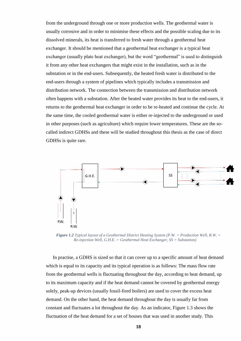
Firstly, a brief explanation of a GDHS should be given. A typical geothermal district

heating system can be seen in Fig. 1.2. In these systems, the geothermal water is pumped

18

from the underground through one or more production wells. The geothermal water is

usually corrosive and in order to minimise these effects and the possible scaling due to its

dissolved minerals, its heat is transferred to fresh water through a geothermal heat

exchanger. It should be mentioned that a geothermal heat exchanger is a typical heat

exchanger (usually plate heat exchanger), but the word “geothermal” is used to distinguish

it from any other heat exchangers that might exist in the installation, such as in the

substation or in the end-users. Subsequently, the heated fresh water is distributed to the

end-users through a system of pipelines which typically includes a transmission and

distribution network. The connection between the transmission and distribution network

often happens with a substation. After the heated water provides its heat to the end-users, it

returns to the geothermal heat exchanger in order to be re-heated and continue the cycle. At

the same time, the cooled geothermal water is either re-injected to the underground or used

in other purposes (such as agriculture) which require lower temperatures. These are the so-

called indirect GDHSs and these will be studied throughout this thesis as the case of direct

GDHSs is quite rare.

Figure 1.2 Typical layout of a Geothermal District Heating System (P.W. = Production Well, R.W. =

Re-injection Well, G.H.E. = Geothermal Heat Exchanger, SS = Substation)

In practise, a GDHS is sized so that it can cover up to a specific amount of heat demand

which is equal to its capacity and its typical operation is as follows: The mass flow rate

from the geothermal wells is fluctuating throughout the day, according to heat demand, up

to its maximum capacity and if the heat demand cannot be covered by geothermal energy

solely, peak-up devices (usually fossil-fired boilers) are used to cover the excess heat

demand. On the other hand, the heat demand throughout the day is usually far from

constant and fluctuates a lot throughout the day. As an indicator, Figure 1.3 shows the

fluctuation of the heat demand for a set of houses that was used in another study. This

19

figure shows the average heat demand and its deviation throughout the day for a set of 10

and 100 houses. It should be noted that the values of this figure have no relation with this

thesis and this figure is only used to depict the fluctuation of the heat demand.

Figure 1.3 Fluctuation of the heat demand for a set of houses (Bosman et al., 2012)

It can be easily understood that according to the fluctuation of the heat demand and the

capacity of the GDHS, the geothermal field can be under-utilised several times (i.e.

producing less geothermal energy than the available one), while at other times it might not

be enough to cover the heat demand. In the latter case, expensive and polluting peak-up

boilers are used. Furthermore, in renewable energy sources it is desirable to maximise their

utilisation and to produce as much energy from these sources as possible. Intuitively, the

basis of the main idea of this study arises, which is to the increase geothermal production

when the field is under-utilised in order to use this energy later when needed.

The latter together with the lack of published research on the operation of geothermal

district heating systems gave rise to the main idea explored in this thesis, as follows:

Instead of changing its production throughout the day the geothermal system

will operate at a constant production rate. More details on how to calculate this

constant production rate will be given in Chapter 3. Furthermore, the

20

installation will be planned to operate on a daily basis, so each day may have a

different constant production.

When the geothermal production is higher than the heat demand, the excess

geothermal energy will be stored in a heat storage.

On the other hand, the stored energy will be released to the network when the

geothermal production is not enough to cover the heat demand, thus smoothing

the overall operation of the installation and decreasing the use of the peak-up

boilers.

The layout of the proposed system can be seen in Fig. 1.4. It should be noted in this

point that it is not intended to totally phase-out the use of the peak-up boilers, as this would

probably lead to over-dimensioning of the geothermal installation which would likely

render the investment unfeasible, but to minimise their use. After all, there will always be

some peak-up boilers in this kind of installations for back-up purposes, so phasing them

out would not remove their capital cost in reality.

Figure 1.4 Layout of the proposed system (H.S.T. = Hot Water Storage Tank, C.S.T. = Cold Water

Storage Tank, the other abbreviations are as in Fig. 1.2)

So, the aim of this thesis is to study the effect of including a heat storage in a GDHS

under the proposed novel operational strategy. In other words, this thesis will examine

whether it is beneficial to include a heat storage under the proposed strategy in a GDHS

from energetic, environmental and economic perspectives. This is achieved by developing

the following three core models which are the objectives of this thesis:

21

Model for the sizing of a GDHS. This is a robust model for the sizing of a

GDHS that operates under the proposed strategy. The results of this model will

also provide useful insights about the operation of the principal components of a

GDHS and identify where improvements can be made.

Model for the operation of a GDHS. This model will involve two sub-models,

where the first will study the operational strategy of the installation over a

random day with a given heat demand and the second will simulate the annual

operation of the installation. The first sub-model will be a useful tool for the

operators of the installation as they will know in advance how to schedule the

operation of the installation. The second sub-model will simulate how the

installation operates over an annual cycle and will use this to identify the basic

operational costs of it.

Model for the energetic, economic and environmental analysis of a GDHS.

In this model, the main energetic, economic and environmental indices of the

installation will be calculated and a comparison with the traditional case, i.e. the

geothermal district heating system that operates without a heat storage and as

mentioned in the beginning of this section, will be carried out. By doing this

comparison, the main question which is posed in the end of this section will be

answered and the aim of this thesis will have been achieved.

The first two of the above models are necessary for the third model as this is a novel

operation of a GDHS so both its sizing and detailed operation should be fully

understandable. Both of these models are quite practically-oriented as will be seen in the

correspondent Chapters, and can be used in real installations as tools for their

corresponding use. So, these models are also an important outcome of this thesis and can

be a powerful tool for geothermal companies and planners.

The main novelty of this study is not only the inclusion of the heat storage in the

system, but also the operation in a novel way. Another novelty of this thesis is the

approach to the modelling of the heat storage. Usually in district heating systems, stratified

hot water storage tanks are used as the heat storage. More details on this are given in

Chapter 2. In this case, as there is no published research on this aspect too in a GDHS and

by taking into account that the flow rates are quite big in these systems (as will be shown

in Chapter 3), it is considered difficult to maintain the stratification within the tank and,

therefore, fully mixed storage tanks will be used. Furthermore, there will be no single

22

storage tank for the hot and cold streams, but, two different storage tanks, one to store hot

water and one to store cold water. The proposed configuration can be seen in Fig. 3.1. In

contrast with the stratified tanks which are always full with water (only the proportion of

hot and cold water changes throughout the day), in our case both tanks will operate in a

“fill-release” mode. This means that the amount of water that is stored in each tank will

change throughout the day and it will depend on the mass balance of the whole system. All

these will be more understandable in Chapter 3 of the thesis.

In the proposed approach, the mass flow rate to the left of the hot water storage tank

(see Fig. 3.1) will be constant throughout the day, while the flow rate to the right of the

storage tank will change according to the heat demand. It is assumed that the hot water

storage tank will be placed as close as possible to the substation in order to obtain a

quicker response in the change of the heat demand. The cold water storage tank will ensure

that the flow rate to the geothermal heat exchanger will remain constant and can be placed

anywhere between the heat exchanger and the substation. The important component that

has to be modelled is the hot water storage tank as this is the main regulator between the

production and the demand. The mass fluxes between this tank and the network as well as

its heat losses will be studied in detail. As will be seen in Chapter 3, the heat losses of the

hot storage tank will be negligible, so the heat losses of the cold storage tank will be even

smaller as the temperature gradient between the environment and the tank will be smaller.

Therefore, the cold water storage tank will not be studied further as its operation can be

ensured by the use of a control-valve and this is out of the scope of this thesis. So, in the

following, the word “tank” will refer to the hot water storage tank unless otherwise stated.

This thesis intends to study mainly if for a given installation, the inclusion of the heat

storage and the novel operation can cover economically a higher fraction of the heat

demand with geothermal energy. From another point of view, this could indicate the

possible downsizing of the installation for the same heat demand coverage by geothermal

energy.

In conclusion, the aim of this thesis is to study the effect of including a heat storage in a

GDHS under a novel operational strategy from an energetic, economic and environmental

point of view. The main question that will be addressed is the following: “Is it worthwhile

including a heat store within the proposed operation of a geothermal district heating system

or not?”

23

1.2 Structure of the thesis

In this Chapter, a brief introduction in GDHSs, which are the topic of this thesis was

given. Through a clear logical path it was explained why these systems are worth to study

and what these can offer to a sustainable future society. Furthermore, the main idea of this

study was explained briefly and the objectives were clearly defined.

In Chapter 2, the literature review of this topic is provided. More specifically, the

literature review commences with several details on geothermal energy and district

heating, their advantages and disadvantages, several historical data on them as well as

some limits on their expansion. Then, an exhaustive review of geothermal district heating

systems follows with the majority of the review concerning the design aspects of the

systems and their energetic as well as their economic analysis. Through this review the gap

that was explained above and set the objectives of this thesis is identified. Finally, some

details are presented on the use of heat storage in district heating systems, in general, an in

geothermal district heating systems in specific.

In Chapter 3, a model for the integrated and robust sizing of a GDHS is developed. The

mathematical model is explained in detail accompanied by all the governing equations of

the involved phenomena, such as mass conservation equations, heat and friction losses etc.

The whole study is carried out for three different cases of sizing which are also explained

in detail, while the only data that are real data are the heat demand data. The rest of the

data are arbitrary realistic inputs selected by the author to make the whole model as

realistic as possible. This is the case for the other Chapters too. Thereafter, the results of

this model are presented which provide many useful conclusions, through an extensive

discussion, on the design of GDHSs and will be quite useful during the preliminary design

of these systems.

In Chapter 4, the outcome of the previous model (i.e. the sized installation) is used as

input in order to study the operation of this installation in detail. Theoretically, the

installation which is the result of Chapter 3 will have been built and the model of this

Chapter will be used to study its operation. Initially, a model that provides the operational

strategy of the installation over a random day with a known (or predicted) heat demand is

presented. By “operational strategy” is meant the complete knowledge of the operation of

the installation, i.e. the necessary geothermal flow rate, when and by how much should the

24

storage tank be charged or discharged etc. In reality, this model could be a powerful tool

for the operators of the installation as they would know a priori how to operate the

installation when the heat demand is known. Then, this model is extended for the study of

the operation of the installation over a whole year. Although this model uses the daily

model as a basis, it has quite different outputs. Its outputs are the main operational costs of

the installation which are among the main inputs of the next Chapter. The results of the

first model are shown for different random days with various daily heat demands which

provide useful knowledge on the operation of the installation for a range of heat demands.

Finally, the results of the annual operation are also presented followed by an extensive

discussion for both models.

In Chapter 5, the operational costs of the installation as well as the other outputs of the

second part of Chapter 4 are used as inputs together with the capital costs of the installation

in order to carry out a comprehensive economic, energetic and environmental analysis of

the studied case. More specifically, several financial indices are calculated and the cash

flows are presented for the investment, while two energetic indices are used for the

energetic analysis together with the calculation of the emissions of the installation for the

environmental part. All these calculations are carried out both for the studied as well as for

the traditional case of operation of a GDHS. Through the analysis of the results and the

comparison of the two cases, a clear answer is given to the most important question of this

thesis on whether the inclusion of a heat storage in a GDHS is eventually beneficial or not.

Finally, in Chapter 6 a synopsis of the main findings of the thesis is provided together

with its contributions to the field. The thesis ends with some propositions about further

work that could be carried out on the basis of this study and for different approaches that

could be potentially used to maximise the use of geothermal energy in the future energy

system.

25

2 LITERATURE REVIEW

2.1 District heating

In general, district heating refers to the production of heat in a central plant and its

distribution to the consumers via a network of pipelines. An important factor for the early

development of district heating was the availability of industrial waste heat, especially

from power plants (Cassito, 1990). District heating can use many heat sources, such as

combined heat and power plants (CHP; coal-, gas- or biomass-fired), which is the most

common source; conventional boilers; waste incinerators; industrial waste heat sources;

solar collectors; heat pumps and geothermal energy (Lund and Lienau, 2009). The main

advantages of district heating, as opposed to private heating provision in each building, are

well summarised by Rosada (1988) and Rezaie and Rosen (2012) as: the higher efficiency

of the whole procedure, with subsequent reduction of emissions; the facility of waste-heat

recovery; the ability to utilize heat sources which would be difficult to utilize in single-

dwelling installations, such as heat from waste; the high level of reliability etc. The

economic viability of district heating depends a lot on the heat demand density of the

examined area. As the heat demand density increases, the viability of district heating

increases (see Dalla Rosa et al., 2012, amongst others).

The advantage of reliability was studied by Lauenburg et al. (2010). More specifically,

those authors examined what happens in a district heating network in the case of power

failure. They found that usually natural circulation occurs, so heat is still being provided to

houses (usually about 80% of the nominal heat) despite the power failure. A basic

prerequisite for that is the maintenance of district heating production, i.e. the heat

production must not be interrupted by the power failure as would happen for example with

heat pumps.

District heating also has some disadvantages, mainly from an economic point of view.

Usually it is not viable in areas of low population density and it is necessary to provide

some incentives. District heating also has high capital costs, so most of the time subsidies

are necessary. In addition, due to the high capital costs, it usually becomes the monopoly

of the owner, which is counter to the desire to have liberalisation of energy markets

(Grohnheit and Mortensen, 2003). Furthermore, it is difficult to retrofit existing buildings

from a technical and an economical point of view. Finally, district heating is usually

26

produced in CHP stations, and the heat production is coupled with, or limited by, the

electricity production. The latter reduces the flexibility of the heating installation.

The development of district heating was faster in countries with cold climates, such as

Iceland, Germany, Finland, Sweden (Gustavsson, 1994a, b; amongst others), Denmark

(Moller and Lund, 2010, amongst others), Latvia (Lund et al., 1999), Lithuania (Rezaie

and Rosen, 2012), Belgium, Romania (Iacobescu and Badescu, 2011), Poland (Zgoda,

1986) etc. In the UK, the penetration of district heating is still quite low, about 1%,

apparently due to short/mid-term high risks and regulatory uncertainties (Kelly and Pollitt,

2010). However, the UK together with Germany and France hosts 50% of the short-term

market expansion potential for district heating within the European Union (Persson and

Werner, 2011).

In the last 20 years, a lot of research has been carried out on various aspects of district

heating. A few examples are given below for the interested reader. Gustavsson (1994a, b)

analysed possible energy conservation measures for buildings. The results showed that

with typical conservation measures a decrease of 30-50% in building energy consumption

can be achieved. Dalla Rosa and Christensen (2011) studied the concept of low energy

district heating for buildings. This concept is based on low-temperature operation of the

installation. In any case, the lowest possible return temperature is needed for maximum

utilization of thermal energy. Noro and Lazzarin (2006) compared local heating by natural

gas with district heating. Concerning emissions and energy efficiency, the modern local

heating systems turn out to be more efficient than district heating. In contrast, this is not

the case from an economic point of view. The latter depends a lot on the taxation of the

fuel in local and district heating systems.

Torchio et al. (2009) undertook environmental research into district heating systems,

finding that district heating is advantageous concerning CO2 emissions, but concerning the

other pollutants the positive effect of district heating is not always so clear. The authors

also mention that a distinction between global and local emissions should always be made.

Moller and Lund (2010) examined the potential expansion of district heating in areas

previously supplied by domestic boilers in the Danish district heating system. The results

showed that it is worth expanding the existing network around cities and towns and

replacing natural gas boilers. In more remote areas, individual heat pumps seem to be the

optimum solution.

27

Dotzauer (2003) applied an optimization algorithm to a district heating network which

included the energy production unit, energy storage and energy sinks. The objective was to

minimize the operational cost and to find the optimum production plan, satisfying the

condition of fulfilling the heat demand on the mid-term horizon, i.e. 10-30 days. Verda et

al. (2012) studied another optimization problem, which examined which users in an urban

area should be connected to the district heating network and which ones should not, in

favour of being served with a ground-source heat-pump system.

Concluding, it can be said that he future of district heating depends mainly on the

prices of alternatives, the price of electricity and the distance from the nearest network. In

high heat density areas district heating seems a better solution, while as heat density

decreases, heat pumps become more favorable. Of course, clear and precise legislation is

necessary for the construction, adoption and expansion of district heating networks. In

some cases, the change of the legislative framework might also be necessary.

2.2 Geothermal Energy

Geothermal energy is the energy contained in the Earth’s crust as heat and its origin is

mainly from the processes that occur in Earth’s interior and heat conduction taking place to

the upper layers. This energy can be used for electricity production and / or for direct uses.

Typically, temperatures above 15oC can be utilized and even lower if heat pumps are used

(Banks, 2012). More details on the use of heat pumps for geothermal applications can be

found in the work of Underwood (2014). Depending on the temperature of the source,

different utilizations of geothermal energy can be achieved. Temperatures above 150oC are

usually used for electricity generation, but in recent years the development of new

technologies, i.e. binary cycles, has made it possible to produce electricity from water with

temperatures of only 120oC. Lower temperatures still are used for direct uses, such as

space heating, district heating, agriculture, aquaculture, balneology, drying, snow melting,

industrial processes, heating of pools and spa, distillation etc. (e.g. Kecebas, 2011, amongst

many others).

Geothermal wells are categorised into: hydrothermal wells, which are the most

common wells; geo-pressured wells; shallow wells; and enhanced geothermal systems

(EGS) or hot dry rocks (Di Pippo, 2007). The latter are an emerging technology which are

believed to increase geothermal potential by a large factor, compared to the currently

28

proven potential. For example, the potential of EGS systems is estimated to be ten times

higher than the potential of hydrothermal systems. In EGS systems, reservoir properties are

developed in deep strata by means of physical stimulation processes, and then water is

injected through a first well, heated in the enhanced reservoir, and pumped to surface by a

second well (Thorsteinsson and Tester, 2010, amongst many others).

Historically, the expansion of geothermal energy has been slow compared to other

renewable energy sources, such as wind energy, for many reasons, such as the low fossil-

fuel prices, the historic lack of ecological concerns and the high upfront capital expenditure

requirements, particularly those considered risky in the early years of development of a

given geothermal field. For example as stated by Rybach (2014), the average annual

geothermal growth between 1995 and 2013 is around 5%, while for wind and solar PV

systems the growth rate exceeds 25-30% from 2004 onwards. Nowadays, this situation has

changed and new, cleaner, more efficient local energy sources are enthusiastically

investigated. Another important reason for the delay of development of geothermal energy

was that local authorities and societies were, and might still be in some cases, unaware of

geothermal energy and its benefits, since it was perceived as a complex and risky energy

source. So, education is necessary for the benefits of geothermal energy, as well as for the

other renewable energy sources, to be fully realised. Finally, a lack of the necessary

knowledge to develop geothermal systems, especially geothermal district heating systems,

was an important reason for this delay (Thorsteinsson and Tester, 2010).

According to Lund et al. (2005), 71 countries reported geothermal energy utilization

for direct uses in 2005, showing a significant rise over the corresponding values in 2000

(i.e. 58) and 1995 (i.e. 28). These direct uses comprised: 20% for direct space heating, 33%

for space heating using heat pumps, 29% for bathing and swimming, 7.5% for greenhouse

uses, 4% for aquaculture, 1% for agricultural uses etc. District heating accounts for 75-

77% of space heating from geothermal energy. Kecebas (2013) states that in 2013 at least

76 countries were using geothermal energy for direct use purposes, with 24 countries

producing electricity. The USA, Philippines, Mexico, Italy, Indonesia, Japan and New

Zealand are the leading countries in electricity production, while Iceland, Turkey, Japan,

China and France are the leaders in heat production from geothermal energy. Iceland,

Turkey, China and France are the leaders in geothermal district heating, while Russia,

Japan, Italy and USA are the leaders in individual home heating by geothermal energy

(Lund et al., 2005).

29

2.3 Geothermal district heating

2.3.1 General

Geothermal district heating systems are a combination of geothermal energy with

district heating systems. More specifically, heat is extracted from the ground using one or

more wells and is distributed (either directly or via a secondary working fluid) through a

district heating network to many consumers, such as individual and commercial buildings

or industries. The subsurface formation in which heat is stored is called a reservoir.

Depending on the combination of pressure and temperature within the reservoir, heat can

be extracted either in the form of hot water or as a steam-water mixture, or even in the

form of saturated or dry steam. Most common are the wells that produce hot water

(Kanoglu and Cengel, 1999).

A geothermal district heating system mainly consists of a heat production unit, a

transmission-distribution system and the in-building equipment. More specifically, heat is

extracted from the production wells, then is distributed to the consumers and finally is re-

injected in another well, called a re-injection well or otherwise disposed of into the

environment. Often, the geothermal fluid has corrosive properties, so a primary heat

exchanger is used to extract heat from the geothermal fluid, and a secondary fluid

distributes the heat to the consumers through a transmission and distribution network.

Additionally, there are usually conventional boilers, which operate as back-up units and for

the coverage of peak load. In some occasions, storage tanks are implemented for the same

purpose. A simplified scheme of a geothermal district heating system is shown on Fig. 2.1.

It should be mentioned that a geothermal source can have multiple uses. In general,

maximisation of the temperature drop of the geothermal fluid across the user infrastructure

is desirable in order to extract the maximum amount of thermal energy. So, if there is more

than one use for the geothermal fluid , they will be implemented simultaneously or in

series (so-called ‘cascading use’, with each process using water cooler than the last) in

order to achieve maximum efficiency. For example, in Iceland, the geothermal fluid is first

used for electricity and heat production, and subsequently is used for snow melting,

achieving high utilization efficiencies (Bjornsson, 2010).

30

Figure 2.1 Simplified schematic flow-chart for a geothermal district heating energy system (from

Hepbasli, 2010)

Another example of integrated use of geothermal energy is given by Bellache et al.

(2000), where the heat extracted from the geothermal fluid is used in order to heat hotels

and a spa. Arslan and Kose (2010) studied the integrated use of geothermal energy in

Kutahya, Turkey. In this region, geothermal energy was used for multiple purposes, but not

in an integrated way. A more complex system is proposed to achieve higher utilization.

More specifically, it is proposed to build a binary cycle for electricity production, with the

waste heat of the electricity plant then being used for district heating, and subsequently for

greenhouse heating and spa heating.

The basic services that can be provided by geothermal district heating are the same as

in any other district heating scheme, i.e. space heating, domestic hot water delivery,

agriculture, balneology, industrial uses, etc. Indeed, the integration with industrial uses is

very desirable in a geothermal district heating system because the demand profile is quite

stable in the latter, so the fluctuation of the total heat demand is flattened a lot. The

importance of the penetration of industrial uses in district heating systems is highlighted in

the work of Difs et al. (2009). In general, the fluctuation of the heat demand in dwellings

throughout the day is quite large. Hence, flattening of the demand is highly beneficial for

the installation. Additionally, the industrial users usually have a stable demand throughout

the year, making the installation more feasible to operate all year round.

31

A new, emerging technology is district cooling. In this technology, the heat is provided

to an absorption chiller, which operates usually with a LiBr/water mixture and provides

cooling. A basic disadvantage of these installations is that they need slightly higher

temperatures than heating systems in order to operate, i.e. at least 80-90oC (Nicol, 2009)

for single stage absorption chillers. But, with the implementation of this technology, the

annual demand rises a lot. It can be said that the reduction of heat demand during the

summer can go hand in hand with the increase of the cooling demand over the same

period. So, in that way the total demand will be much more constant throughout the year,

while previously in summer the demand decreased a lot, since it comprised solely of the

hot water preparation load, which usually was not enough to make the installation feasible

for this period. The importance of the development of district cooling is obvious

(Bloomquist, 2003; Hederman and Cohen, 1981).

The ability to provide a continuous and adequate flow at the required temperature is a

basic prerequisite for a geothermal heating system (Ozgener et al., 2006a). Other

prerequisites are an area with high heat demand density, and a high load factor (i.e. the

proportion of the total hours in a year over which the system is used).

Geothermal district heating systems provide numerous advantages both to individual

customers and the society, such as (Lund and Lienau, 2009):

Reduced fossil fuel consumption, since fuel is needed only for the peak

demands. Consequently, a major reduction in emissions is achieved.

Reduced heating cost: geothermal energy usually provides heating at lower cost

than conventional fuels.

Reduced fire hazard in buildings, because no combustion takes place in them.

Possibility of “cogeneration”, i.e. utilization of the geothermal fluid for multiple

uses.

Provision of continuous base load, in contrast with the other renewable energy

sources. Indeed, geothermal energy has a high capacity factor, due to high

availability.

Simple, safe and adaptable systems and electromechanical equipment.

A geothermal resource usually has a lifetime of 30-50 years, but in some cases

can be maintained even for 100-300 years. But, in order to do that a proper

management of the reservoir has to be implemented in order to avoid depletion.

32

In most cases, re-injection of the geothermal fluid is necessary. So, geothermal

energy can be considered as a sustainable energy source.

Geothermal energy has huge potential. As stated by Li et al. (2011), in China

alone the geothermal energy that is stored in the subsurface (within 2000m) of

the sedimentary basins is equivalent to 250 million tons of standard coal.

Geothermal energy does not depend on weather conditions (Kecebas et al.

2011).

Low operating costs.

Geothermal energy will probably have a stable price in the future, in contrast

with combustible fuel prices.

Because low-grade geothermal energy is widespread, it is invariably a domestic

source of energy, thus contributing to security of supply and energy

independence, as well as enhancement of local economies. Concerning the

latter, many new jobs are also created (Hepbasli and Canakci, 2003).

In purely heat production stations, the heat production is independent of any

electricity production. As was mentioned before, concerning CHP plants, the

dependence of heat production on electricity production was a big disadvantage.

Very weak dependence on electricity prices, since the only electricity needed is

for the pump systems

According to Lund et al. (2005), up to 2005 the usage of 25.4 million tonnes of fuel-oil

had been avoided due to geothermal energy use. The environmental impact of geothermal

energy is quite low, since the emissions of a geothermal plant are just a fraction of the

emissions of fossil fuel plants, and of the same magnitude as the other renewable energy

sources. During the construction and the decommissioning of the plant, there are some

emissions, but the life-cycle emissions of a geothermal installation still remain quite low.

Indeed, the emissions from low temperature resources are even smaller. If careful re-

injection of the geothermal fluid takes place and the leaks are prevented, then pollution is

minimised.

A study which highlights the advantages of geothermal energy for local economies was

carried out by Karytsas et al. (2003). More specifically, a socio-economic study was

carried out about the utilization of low enthalpy geothermal resources in a region in north

Greece. The geothermal fluid would be utilized in a district heating network as well as for

greenhouses uses. The benefits for the local society would be numerous, such as: reduction

33

in annual fuel consumption of up to 2325 tonnes of oil equivalent; subsequent reduction in

CO2 emissions of up to 7440 tonnes per year; annual savings of up to US$1,250,000; and

60 new jobs in the region. A governmental subsidy would definitely enhance the feasibility

of the investment.

Inevitably geothermal energy, and subsequently geothermal district heating, has some

disadvantages. Geothermal energy is site dependent, i.e. geothermal energy of higher

enthalpies cannot be found everywhere. Additionally, in the case of district heating the

production plant must be relatively near to the consumers in order to be feasible, whereas

geothermal fields may exist in areas far away from inhabited districts (Sommer et al.,

2003). A specific heat load density is also necessary, as has been previously mentioned for

district heating in general. So, it is beneficial to find consumers with constant and high

loads throughout the year, such as industries, hotels, hospitals etc., which are also close to

the production area. Initial capital costs are quite high for these instalments, for this reason

a large part of them are of public ownership. Finally, it must be highlighted that the drilling

of the geothermal wells is quite risky, because there is always an uncertainty about the

temperature, the flow rate and the pressures of the underground water, at least during the

early stages of field development. Taking into account that geothermal district heating

networks are a capital intensive investment, it is obvious that initial engineering decisions

are crucial both from a technical and an economical point of view. A wrong initial decision

in the technical design of the system can lead to high financial losses as shown by

Kristmannsdottir and Bjornsson (2012).

It can be concluded that geothermal district heating seems a potential solution for many

current energy and environmental problems and that it can play an important role in the

future energy target in the built environment sector. As noted by Ostergaard and Lund

(2011), the integrated use of renewable energy sources, such as geothermal energy, waste

incineration, heat pumps etc., can enhance the way to a sustainable future. In the latter

study, the role of low temperature geothermal energy in a 100% renewable energy system

was also analysed. The case of a small town in Denmark was examined, and the results

showed that low temperature geothermal energy, combined with an absorption heat pump,

could cover more than 40% of the total heat needs.

34

2.3.2 Examples of geothermal district heating systems

In this section, a few examples of geothermal district heating systems in several areas

(from specific systems up to whole countries) will be given in order to highlight their

difference in size and operation as well as their potential. For example, in Paris 100,000

residences are provided with heat by geothermal energy, while in Iceland, 22 geothermal

district heating systems have been constructed. The system in Reykjavik which is one of

the biggest in the world has a total installed capacity of 1,070MWth. Almost 90% of the

space heating in Iceland is provided by geothermal energy. The huge development of

geothermal energy in Iceland has occurred mainly due to the rich physical resources of the

country, as well as the positive attitude of people towards geothermal energy, which is seen

as a reliable and clean source that has improved quality of life. It is worth mentioning that

the fuel saved between 1970-2000 through switching to geothermal energy had a value of

some £8.2M, i.e. three times the 2000 budget of the country (Loftsdottir and

Thorarinsdottir, 2006; Bjornsson, 2010).

Turkey, on the other hand, has around 12% of the worldwide geothermal potential, but

95% is suitable for direct uses only. More specifically, direct use potential is estimated to

be 31,500MWth, but by the turn of the Millennium only 2-3% of this potential had been

utilized (Hepbasli and Canakci, 2003, amongst many others). In the USA, 18 geothermal

district heating networks have been constructed, but the identified potential is capable of

providing heat to more than 271 cities (Sommer et al., 2003). Finally, as stated by the

European Geothermal Energy Association, 216 geothermal district heating systems existed

in Europe by 2012, with a total installed capacity of 4900MWth ,and 157 of these systems

exist in the EU27 states. Figure 2.2 indicates the installed capacity of geothermal district

heating systems at the end of 2012 (GeoDH, 2013).

35

Figure 2.2 Installed geothermal direct-use capacity in MWth in European countries at the end of 2012

(GeoDH, 2013)

The first geothermal district heating installation was constructed at Chaudes-Aigues

Cantal, France, in the 14th century. The first municipal installations were constructed in

Boise, Idaho, USA in 1893 and in Reykjavik in 1930 (Little and Bissell, 1980).

Geothermal district heating systems can differ greatly in size: for instance, the system

in Reykjavik provides heat to 150,000 houses, with over 60 million cubic meters of

geothermal fluid used annually. At the other end of the range, in Klamath Falls, Oregon,

USA, a mini district heating system is used to heat 11 buildings on a University campus as

mentioned in the work of Thorsteinsson and Tester (2010).

Harrison (1994) highlights the range of different operational strategies of geothermal

district heating networks, through two extremely different examples. In Iceland, the hot

springs of Deildartunga heat the nearby town of Akranes. The water is produced from a

shallow depth almost free of pumping costs, at a high flow rate of almost 180kg/s, and is

transported over a distance of 62km to the town of Akranes. The water is potable, so it is

used directly to heat the houses. After heating the houses the water is discharged to the sea.

In this case, even the peaks are met by those springs. In Beauvais, France, the water is

produced from great depths and at smaller flow rates. The water is saline, so a heat

36

exchanger is used to extract heat from the geothermal fluid. The geothermal fluid is then

re-injected into the reservoir to prevent head depletion and pollution of the environment. In

this case, the heat production is much lower than in the case of Akranes.

In some extreme cases, such as Akranes, geothermal energy provides almost all the

necessary heat. But, this is usually not economically viable, because the district heating

network is oversized for most of the time and the field is underutilized. Hence geothermal

energy usually provides base load, and the peaks are covered by auxiliary boilers or

storage tanks. It must be emphasised that Iceland is a country with unusually high potential

for geothermal energy, which can be produced at a very cheap price, and the danger of

depletion of the wells is almost non-existent. Hence re-injection does not always take place

there.

2.3.3 Design aspects

In this section, the basic design principles of a geothermal district heating system will

be analysed. More specifically, details will be provided about the basic configuration of the

network, the heat load estimation, the selection and the design of the appropriate heat

exchangers, the basic aspects of the pipeline system and the in-house system, and finally a

few details will be provided on the necessity of having a re-injection system.

Depending on the quality of the underground water, a geothermal district heating

system can be a direct cycle (as in Reykjavik), with the geothermal fluid being circulated

directly to the end-users, or an indirect cycle, providing the geothermal heat to a secondary

fluid which is then distributed to the consumers. Indirect systems are more common,

although they contain three extra costs compared to direct systems, i.e. the cost of a heat

exchanger, the cost of circulating pumps and the cost of heat losses in the heat exchanger.

Obviously, direct systems are cheaper than indirect systems, mainly because of avoiding

the cost of the heat exchanger. Indirect cycles are used in order to minimize the corrosive

action of the geothermal fluid and they are the most common case. Further information

about corrosion problems in geothermal systems can be found in the work of Richter et al.

(2006). However, injection of anti-corrosive as well as anti-freezing additives may take

place in the distribution network (Chuanshan, 1997). An extra reason which may lead to

the adaptation of indirect systems is the scaling problem which may occur due to the

dissolved salts in the geothermal water. As stated by Kristmannsdottir and Bjornsson

37

(2012) scaling and corrosion can cause big problems in the operation of the system. So,

careful research about the composition of geothermal water must be carried out during the

preliminary study of the installation.

Design components for geothermal district heating systems are generally simple, safe

and adaptable electromechanical devices. However, careful design is necessary due to the

large scale of the investment. In general, it is found that the pipeline network, the heat

exchanger and the re-injection system need the most careful design (Kecebas, 2011,

amongst others). Finally, if the temperature of the geothermal fluid is not adequate for

heating purposes, integration with a heat pump may be implemented (Harrison, 1994).

In the preliminary research of a new well, the sustainable flow rate, the temperature and

the quality of the water have to be identified (as noted by Lund and Lienau, 2009, amongst

many others). Of course, the final verification will be based on drilling tests. Available

areas with geothermal potential can be identified by constructing isotherms for different

depths. Additionally, in the preliminary design, if there is more than one production well, a

lot of attention has to be paid to the minimization of the interaction between these wells.

To summarise, a geothermal district heating system consists of (Kanoglu and Cengel

1999):

The production system, i.e. the production wells, the well pumps and the

primary heat exchanger.

The transmission-distribution system, which comprises of the pipeline system

and the circulating pumps.

The end-user systems. A secondary heat exchanger may be used in the buildings

circuit, in order to avoid high values of pressure in the distribution network

(Harrison, 1987). In many cases, two heat exchangers are used in each building,

one for space heating and one for domestic hot water preparation.

Disposal and re-injection system.

Peaking and back-up systems, such as boilers or storage tanks.

Of course, at many points in the network, there are various meters and valves to ensure

the correct operation of the network (Bloomquist, 2003). Additionally, it is shown in

38

numerous studies that automatic control will reduce the human involvement and increase

the efficiency of the system.

A crucial initial factor for the proper design of a district heating network is an adequate

estimation of the heat load. Domestic heat load consists mainly of the space heating load

and the load of domestic hot water. The latter is quite stable throughout the year and can be

easily estimated (see Oktay et al., 2008). However, it is not usually sufficient to justify the

investment feasible for the summer period, so additional loads, such as district cooling,

industrial processes, pool heating are usually necessary in order to enhance the economic

viability of the system (Popovski et al., 2000). The most common method to estimate the

space heating demand is the degree-day or degree-hour method which is summarised in the

work of Heller (2002). In this method, the amount of observations where the ambient

temperature is lower than a specific threshold are metered. The extent of the observation is

usually an hour or a day as the aforementioned names indicate. This process is done for a

normal or representative day for which the heat load is also known. Then for any other day

or hour, the degree-days or hours are calculated based on the predicted meteorological data

and the heat demand is then calculated as:

𝐻𝐿

𝐻𝐿𝑛=

𝐷𝐷

𝐷𝐷𝑛 (2.1)

Where:

𝐻𝐿 = Heat load (W)

𝐻𝐿𝑛 = Nominal heat load (W)

𝐷𝐷 = Degree-day or hour (Dimensionless)

𝐷𝐷𝑛 = Nominal degree-day or hour (Dimensionless)

Yetemen and Yalcin (2009) proposed a prediction model, which predicts the demand

the next day when knowing the weather conditions on the present day plus the

consumption the previous day. It is considered to be a reliable model, since weather

prediction for the next day is quite reliable. Of course, the heat load duration curve is of

huge importance in order to estimate the optimum size of the geothermal plant and the

integration of peak-up devices. The interested reader can find further information about

heat load prediction in the works of Barelli et al. (2006), Nielsen and Madsen (2006) and

Popescu et al. (2009).

39

Gelegenis (2005) proposed an algorithm for the quick estimation of the coverage of

total heat load in a district heating system by geothermal energy. Geothermal systems of all

kinds were examined, i.e. direct system; primary heat exchange system; heat pump assisted

system; heat pump only system. In general, it was concluded that maximum supply

temperature and minimum return temperature in the distribution network are desirable, in

order to maximize the coverage achieved by geothermal energy. The proposed algorithm

shows very good agreement with actual data.

According to Milanovic et al. (2004), the overall heat transfer coefficient of the

building can be considered stable throughout the heating season. So, if the heat load is

known for a specific set of indoor and outdoor temperature, then the heat load for any other

set of these temperatures can be calculated using the following equation:

𝐻𝐿

𝐻𝐿𝑛=

𝑇𝑖𝑛𝑑−𝑇𝑜𝑢𝑡𝑑

𝑇𝑖𝑛𝑑,𝑛−𝑇𝑜𝑢𝑡𝑑.𝑛 (2.2)

Where:

𝑇𝑖𝑛𝑑, 𝑇𝑜𝑢𝑡𝑑 = Indoor and outdoor temperatures, respectively (K)

𝑇𝑖𝑛𝑑,𝑛, 𝑇𝑜𝑢𝑡𝑑,𝑛 = Nominal indoor and outdoor temperatures, respectively (K)

The above equation is very similar to Eq. (2.1) and the index nominal also refers to a

representative case of indoor and outdoor temperatures for which the heat load is known.

Usually, each system is designed for a set of inlet and outlet temperatures and the

demand fluctuations are met by variations in flow rate. The supply temperature of the

geothermal network is usually constant, while the supply temperature of the secondary

network is usually also kept constant because certain services, such as domestic hot water,

need particular temperatures. The primary design of the network is made in such a way that

the re-injection temperature of the geothermal fluid is minimised, i.e. maximum thermal

energy is extracted. So, by varying the flow rate, the fluctuation of heat demand is met. In

order to meet very high demands, usually peak-up boilers or storage tanks are used.

Harrison (1987) studied the basic design principles of indirect geothermal district

heating systems. A fundamental principle is that the flow rate of the distribution network

has to be higher than the flow rate of the geothermal fluid in order to obtain optimum heat

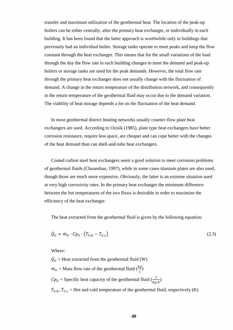
40

transfer and maximum utilization of the geothermal heat. The location of the peak-up

boilers can be either centrally, after the primary heat exchanger, or individually in each

building. It has been found that the latter approach is worthwhile only in buildings that

previously had an individual boiler. Storage tanks operate to meet peaks and keep the flow

constant through the heat exchanger. This means that for the small variations of the load

through the day the flow rate in each building changes to meet the demand and peak-up

boilers or storage tanks are used for the peak demands. However, the total flow rate

through the primary heat exchanger does not usually change with the fluctuation of

demand. A change in the return temperature of the distribution network, and consequently

in the return temperature of the geothermal fluid may occur due to the demand variation.

The viability of heat storage depends a lot on the fluctuation of the heat demand.

In most geothermal district heating networks usually counter-flow plate heat

exchangers are used. According to Ozisik (1985), plate type heat exchangers have better

corrosion resistance, require less space, are cheaper and can cope better with the changes

of the heat demand than can shell-and-tube heat exchangers.

Coated carbon steel heat exchangers seem a good solution to meet corrosion problems

of geothermal fluids (Chuanshan, 1997), while in some cases titanium plates are also used,

though those are much more expensive. Obviously, the latter is an extreme situation used

at very high corrosivity rates. In the primary heat exchanger the minimum difference

between the hot temperatures of the two flows is desirable in order to maximize the

efficiency of the heat exchanger.

The heat extracted from the geothermal fluid is given by the following equation:

�̇�𝐺 = �̇�𝐺 ∙ 𝐶𝑝𝐺 ∙ (𝑇𝐺,ℎ − 𝑇𝐺,𝑐) (2.3)

Where:

�̇�𝐺 = Heat extracted from the geothermal fluid (W)

�̇�𝐺 = Mass flow rate of the geothermal fluid (𝑘𝑔

𝑠)

𝐶𝑝𝐺 = Specific heat capacity of the geothermal fluid (𝐽

𝑘𝑔∙𝐾)

𝑇𝐺,ℎ, 𝑇𝐺,𝑐 = Hot and cold temperature of the geothermal fluid, respectively (K)

41

The heat provided to the secondary flow is given by the following equation:

�̇�𝑠𝑓 = �̇�𝑠𝑓 ∙ 𝐶𝑝𝑠𝑓 ∙ (𝑇𝑠𝑓,ℎ − 𝑇𝑠𝑓,𝑐) (2.4)

All the terms are defined as for equation (2.3), though here referring to the secondary

fluid instead of the geothermal fluid. The suffix w denotes the secondary working fluid,

which flows through the transmission and distribution network.

The equation of heat exchange between the two flows is as follows:

�̇�𝑡𝑟𝑎𝑛𝑠 = 𝐴𝐻𝐸 ∙ 𝐾𝑡 ∙ ∆𝑇𝑙𝑚 = 𝐴𝐻𝐸 ∙ 𝐾𝑡 ∙(𝑇𝐺,ℎ−𝑇𝑠𝑓,ℎ)−(𝑇𝐺,𝑐−𝑇𝑠𝑓,𝑐)

𝑙𝑛𝑇𝐺,ℎ−𝑇𝑠𝑓,ℎ

𝑇𝐺,𝑐−𝑇𝑠𝑓,𝑐

(2.5)

Where:

𝐴𝐻𝐸 = Active surface area of the heat exchanger (𝑚2)

In the above equation 𝐾𝑡 (𝑊

𝑚2∙𝐾) the overall heat transfer coefficient of the heat

exchanger given by the following equation (Jialing and Wei, 2003, amongst many others):

𝐾𝑡 =1

1

ℎ𝑐,ℎ+𝑅𝑓,ℎ+

𝛿𝑝𝑙𝑎𝑡𝑒

𝑘𝑝𝑙𝑎𝑡𝑒+𝑅𝑓,𝑐+

1

ℎ𝑐,𝑐

(2.6)

Where:

𝐾𝑡 = Overall heat transfer coefficient (𝑊

𝑚2∙𝐾)

ℎ𝑐,ℎ, ℎ𝑐,𝑐 = Convective heat transfer coefficient of the hot (geothermal) and cold

(distribution network) water stream, respectively (𝑊

𝑚2∙𝐾)

𝑅𝑓,ℎ, 𝑅𝑓,𝑐 = Fouling factor of the hot and cold water stream, respectively (𝑚2∙𝐾

𝑊)

𝛿𝑝𝑙𝑎𝑡𝑒 = Thickness of each plate of the heat exchanger (𝑚)

𝑘𝑝𝑙𝑎𝑡𝑒 = Conductive heat transfer coefficient of each plate of the heat exchanger (𝑊

𝑚∙𝐾)

42

The convective heat transfer (h) coefficient for both sides can be calculated by the

following equation:

ℎ𝑐 =𝑁𝑢∙𝑘𝑓

𝑑ℎ (2.7)

Where:

𝑁𝑢 = Nusselt number (Dimensionless)

𝑘𝑓 = Conductive heat transfer coefficient of the corresponding fluid (𝑊

𝑚∙𝐾)

𝑑ℎ = Hydraulic diameter (𝑚)

In the above equation, the Nusselt number can be calculated using the appropriate

equation according to the prevalent conditions.

Additionally, the fouling factor can be considered equal for both the hot and the cold

sides, as Rf,h=Rf,c=0.0002. The conductive heat transfer coefficient of the plate can be

considered to be equal to 50𝑊

𝑚2∙𝐾, while the thickness of the plate can be considered to be

equal to 0.0005m (Arslan et al., 2009). Of course, all these values are just indicative.

Usually, the properties of the geothermal fluid are considered to be those of pure water,

since the effects of salts and non-condensable gases are considered negligible (Kanoglu,

2002). So, in the rest of the study there will be no distinction between the properties of the

geothermal fluid and those of pure water and the index w (water) will be used for that

purpose.

On the other hand, during the heat exchange process some heat losses will occur, which

have to be taken into account. In an ideal analysis, the above heat transfer rates (Eqs. (2.3)-

(2.5)) are considered equal to each other. Further analysis of counter flow heat exchangers

can be found in the work of Dagdas (2007), who states that an optimum heat exchange

surface area of the heat exchanger can be found, taking into account the investment cost of

the heat exchanger as an expenditure, as well as the fuel saving due to geothermal energy

as an income.

43

According to Stoecker (1989) amongst many others, the effectiveness of a plate type

heat exchanger, assuming no losses, is equal to the ratio of the heat transferred to the

maximum available heat, and can be calculated by the following equation:

𝜂𝐻𝐸 =�̇�𝑡𝑟𝑎𝑛𝑠

�̇�𝑚𝑎𝑥=

�̇�𝑠𝑓∙𝐶𝑝𝑤∙(𝑇𝑠𝑓,ℎ−𝑇𝑠𝑓,𝑐)

�̇�𝐺∙𝐶𝑝𝑤∙(𝑇𝐺,ℎ−𝑇𝑠𝑓,𝑐) (2.8)

Where all the terms are defined as previously.

In the transmission and distribution networks, pre-insulated pipes are usually used.

Kanoglu and Cengel (1999), amongst others, mentioned that a temperature drop of about

1oC occurs in every 3-4 km of pipeline. The most important steps in the design of the

pipeline system are the selection of the proper material and the determination of target

pressure losses. Carbon steel pipes are 13-35% cheaper than composite pipes, but they are

not usually suitable for geothermal loops, because of the corrosive effects. So, carbon steel

pipes are usually used in secondary loops, and composite materials are used for geothermal

loops. According to Bloomquist (2003), jacketed welded steel pipes can also be used, and

in the return lines plastic pipes can also been used.

The pipes are usually buried underground in order to minimize heat losses and to avoid

visual disturbance. Usually, they are buried directly into the soil because it is cheaper, but

the construction of an underground tunnel can provide other advantages, such as easy

access for maintenance, easier future expansion and an available corridor for other uses.

However, the cost of the latter is typically double that of the direct burying of pipes and is

thus usually not preferred.

Typically, in order to determine the optimum diameter of the pipes two aspects must be

taken into account. These are the cost of material of the pipeline and the pressure losses.

Obviously, the smaller the diameter, the lower the material costs of the pipeline. However,

the smaller the diameter, the higher are the pressure (i.e. frictional head) losses, which

leads to increased power consumption by the pumps, which consequently means higher

electrical energy costs. So, an optimum diameter of the pipelines exists and has to be

determined.

Furthermore, great attention has to be paid to any leakage from the pipeline system,

since this is an energy loss, and as will be made clear in the following section, it can be a

44

huge component of loss (Kecebas, 2013, amongst many others). Finally, Brown (2006)

stated that great attention has to be paid in the moisture on the external surface of the

pipelines, which can also lead to corrosion. Consequently, he proposes that sometimes a

concrete tunnel with a ventilation system might be necessary.

Chuanshan (1997) provides a summary of the basic equations for the heat exchange

process within a building. The heat needed to maintain a stable indoor temperature 𝑇𝑖𝑛𝑑

when the outdoor temperature is 𝑇𝑜𝑢𝑡𝑑 can be calculated by the following equation:

�̇�1 = 𝐶𝑞,𝑏 ∙ 𝑉𝑏 ∙ (𝑇𝑖𝑛𝑑 − 𝑇𝑜𝑢𝑡𝑑) (2.9)

Where:

𝐶𝑞,𝑏 = Specific volumetric heat load capacity of the building (𝑊

𝑚3∙𝐾)

𝑉𝑏 = Internal volume of the building (𝑚3)

The same amount of heat can also be estimated by the following equation according to

Yildirim et al. (2005):

�̇�1 = 𝑈𝑏 ∙ 𝐴𝑏 ∙ (𝑇𝑖𝑛𝑑 − 𝑇𝑜𝑢𝑡𝑑) (2.10)

Where:

𝑈𝑏 = Overall heating coefficient between the building and the environment (𝑊

𝑚2∙𝐾)

𝐴𝑏 = External area of the building (𝑚2)

The latter will have to be calculated separately for different parts of the buildings, such

as walls, glasses etc. The heat transferred through the radiator can by calculated by the

following equation:

�̇�2 = 𝐾𝑟𝑎𝑑 ∙ 𝐴𝑟𝑎𝑑 ∙ ∆𝑇𝑙𝑚 (2.11)

In the above equation all the terms are defined as in equations (2.5)-(2.6)-(2.7), though

here they refer to the radiator instead of the heat exchanger. ΔTlm (K) is the mean

logarithmic temperature difference which is typically calculated as shown in the second

and third part of Eq. (2.5), but in this case, it can also be calculated as follows:

45

∆𝑇𝑙𝑚 =𝑇𝑟𝑎𝑑,𝑖𝑛+𝑇𝑟𝑎𝑑,𝑜𝑢𝑡

2− 𝑇𝑟𝑎𝑑,𝑖𝑛 (2.12)

Where:

𝑇𝑟𝑎𝑑,𝑖𝑛, 𝑇𝑟𝑎𝑑,𝑜𝑢𝑡 = Input and output water temperatures, respectively, of the radiator (K)

Traditionally, heating circuits operated in the range 90 to70oC. The circuits in

geothermal district heating systems can operate at temperatures as low as 60 to 45oC or

even lower. With the development of building insulation and other technologies, lower

temperature systems are becoming more and more popular. Low-temperature systems also

improve indoor-air quality (Myhren and Holberg, 2008). A common technique is the use of

an air velocity component, which forces the air to move through the radiator with increased

velocity, causing that way increased heat transfer. (Myhren and Holberg, 2007). Szita

(2010) described a three-pipe geothermal district heating system in a town in Hungary,

which utilizes geothermal energy at different levels of temperature according to the end-

user technology of each building, e.g. radiator, under floor heating etc. The importance of

the end-user system is highlighted in this study.

In this connection, it should be noted that there is no unique configuration or

operational strategy for geothermal district heating networks. No general conclusions about

the operational strategy and the economic feasibility can be made. Everything depends on

the conditions of each case, i.e. the flow rate, temperature and quality of geothermal water,

the heat density, the distance of the production well to the buildings etc.

In most cases the re-injection of the geothermal fluid is necessary mainly for the

following reasons (Steins and Zarrouk, 2012):

Prevents reservoir depletion, which would otherwise result in declining

reservoir pressures and thus a gradually increasing pumping cost.

It is more environmentally friendly to dispose the brine in the well.

Indeed in high temperature reservoirs, it is sometimes necessary to add additional water

to replace that lost to evaporation in cooling towers, so that the reservoir will not get de-

pressurized.

46

In general, it can be concluded that the design of a geothermal district heating system

depends greatly on the conditions of the selected area and that there is no single design and

operational strategy. Hence few general conclusions can be reached. The most important

influences on the design of a geothermal district heating system are the maximum

utilization of the geothermal field, and the security of supply of the consumers.

To the best of the author’s knowledge no studies about the optimization and simulation

of geothermal district heating systems have been carried out to date. Concerning the

optimization and simulation of non-geothermal district heating systems, the interested

author can find the description and implementation of many different models in the

literature such as:

MODEST (Henning, 1997, amongst many others): It is an optimisation

algorithm of dynamic energy system with time dependent components and

boundary conditions. In general, MODEST finds the investment and operation

decisions that satisfy the energy demand at minimum overall cost in local,

regional and national energy systems.

DESDOP (Weber and Shah, 2011): This algorithm is a mixed integer linear

optimisation tool which provides the optimum mix of technologies in order to

minimize the emissions. Mixed integer linear optimization techniques have also

been used by other researches, such as Gustafsson and Ronnqvist (2008) etc.

DEECO (Lindenberger et al., 2000): This model which simplex algorithm

optimization techniques, in order to examine the maximum integration of solar

energy in a district heating system.

SAFARI (Dotzauer, 2003): This is a mixed integer program used for the mid-

term planning of district heating systems.

GATE/CYCLE (Krause et al., 1999) and TERMIS (Gabrielaitiene et al., 2007):

These are commercially available software for the simulation of thermal

systems and district heating networks.

TRNSYS (Heller, 2002, amongst others): It is a commercially available

software for the simulation of transient systems.

47

2.3.4 Basic thermodynamic evaluation

2.3.4.1 Overview

In this section, a brief review of the literature concerning the energetic and exergetic

evaluation of geothermal district heating networks will be presented, emphasizing the

advantages of exergy analysis. In general, energy analysis alone is not enough to

understand the whole system (Hepbasli, 2010, amongst others). For this reason, exergy

analysis is necessary in order to get a more complete view of the system energy flows.

It can be briefly said that exergy is the maximum available energy, or in other words

the maximum work that can be produced from the system when it is interacting with its

surroundings. Energy is based on the 1st law of thermodynamics, while exergy is based on

the 2nd law of thermodynamics. In other words, exergy is the optimal use of energy and

takes into account all the energy losses that occur due to irreversibilities of the process, as

summarised by Ozgener et al. (2005a), amongst many others.

Unlike energy, exergy is not subject to a conservation law; it is either consumed or

destroyed. This happens due to irreversibilities that take place in any real process. Entropy

is generated due to these irreversibilities, which consequently leads to exergy consumption.

By implementing exergy analysis, it is possible to determine if (and by how much) it is

possible to design more efficient systems. In general, exergy analysis is accepted as the

most appropriate way to evaluate a geothermal district heating system, because it can point

out the real magnitude of losses, and the parts of the installation that can be improved and

it can show how efficiently the system operates.

Parri (2007) states that the use of fossil fuels for heating purposes, i.e. for a desired

temperature smaller than 60oC, is a huge waste from an energetic and exergetic point of

view. It is far more efficient to use low enthalpy (and thus low exergy fluids), rather than

high enthalpy ones. From that point of view, geothermal energy has much to offer in the

sustainable development agenda, and the efficient utilization of energy sources. It is also

noteworthy that for space heating at about 20oC, a fluid with slightly higher temperature is

theoretically usable. But, in that case the effective surface area of the radiator has to be

increased considerably. If new, more efficient, radiators are designed in the future, then a

temperature of 35oC will be feasible for space heating, increasing the geothermal fields that

48

are viable for space heating purposes. At the moment, a minimum temperature of 50oC is

still necessary for even the best radiators, with many still requiring temperatures in excess

of 70oC. An exception to that is the use of underfloor heating systems in the newly built

houses, which can operate with temperatures as low as 35oC. Finally, great attention has to

be paid to the domestic hot water load, for which a temperature of 60oC is necessary

anyway. So, it should be investigated in detail if the latter should be included in the general

thermal load of the dwellings or if it should be provided by other means, e.g. electric

heating.

Very little research has been carried out into the energetic and exergetic analysis of

geothermal district heating systems. As mentioned also before, Turkey has among the

highest potentials for geothermal district heating systems worldwide and is an emerging

market since 170 geothermal fields have been discovered in the country as stated by

Simsek (2001).

2.3.4.2 Basic equations

Summaries of the main equations used for energetic and exergetic evaluation have been

given by many authors (Ozgener et al., 2005a,b; Ozgener et al., 2006a,b; Ozgener et al.,

2007a,b; Oktay et al., 2008; Kecebas et al., 2011 etc.) and these form the basis of the

following listing. These equations can be used to evaluate any geothermal district heating

system. Thermal and hydraulic steady-state conditions were assumed in formulating these

equations.

Mass balance:

in out well r dis

wells

m m m m m (2.13)

Where:

�̇�𝑤𝑒𝑙𝑙 = Mass flow rate of one geothermal well (𝑘𝑔

𝑠)

�̇�𝑟 = Re-injection mass flow rate (𝑘𝑔

𝑠)

�̇�𝑑𝑖𝑠 = Discharge mass flow rate which takes into account the amount of water that it is

not re-injected (𝑘𝑔

𝑠)

49

The latter takes into account both the mass flow rate of the water that is naturally

discharged and any leakage, although it is difficult to quantify the latter. In the majority of

the studies, Eq. (2.13) is used to calculate the discharge mass flow rate. It should be noted

that, depending on the particular case, one of the values of re-injection or discharge may be

equal to zero. For example, in Akranes, Iceland, the entire amount of geothermal water is

discharged, so the re-injection mass flow rate is equal to zero.

Energy balance in a control volume:

�̇�𝐶𝑉 − �̇�𝐶𝑉 = ∑�̇� ∙ (ℎ +𝑣2

2𝑔 ∙ 𝑧)𝑛𝑒𝑡 (2.14)

Where:

�̇�𝐶𝑉, �̇�𝐶𝑉 = Heat and work transfer rate through the control volume, respectively (𝑊)

ℎ = Specific enthalpy (𝐽

𝑘𝑔)

𝑣 = velocity (𝑚

𝑠)

𝑔 = gravitational acceleration (𝑚

𝑠2)

𝑧 = height (𝑚)

The suffix ‘net’ denotes the difference between the input and output values. If there is

no heat transfer and work input/output through the boundaries of the network, the above

equation reduces to the following:

∑�̇� ∙ (ℎ +𝑣2

2+ 𝑔 ∙ 𝑧)𝑛𝑒𝑡 = 0 (2.15)

Usually, kinetic energy is considered negligible in these systems. So, if there is no

change in the potential energy of the system, the above equation can be simplified to the

following form:

∑�̇�𝑖𝑛 ∙ ℎ𝑖𝑛 = ∑�̇�𝑜𝑢𝑡 ∙ ℎ𝑜𝑢𝑡 (2.16)

The above equation is the one most commonly used in analysing geothermal district

heating systems.

50

Exergy balance into a control volume:

0.(1 ) k in in out out dest system

k k

TQ W m m Ex

T (2.17)

Where:

𝑇0 = Temperature in the dead-state conditions (𝐾)

𝑇𝑘 = Temperature in the kth process (K)

𝜓 = Specific exergy (𝐽

𝑘𝑔)

𝐸�̇�𝑑𝑒𝑠𝑡,𝑠𝑦𝑠𝑡𝑒𝑚 = Rate of the exergy destruction through the system (𝑊)

Similarly to the energy balance, if there is no heat or work transfer through the

boundaries of the system, the above equation reduces to the following:

∑�̇�𝑖𝑛 ∙ 𝜓𝑖𝑛 − ∑�̇�𝑜𝑢𝑡 ∙ 𝜓𝑜𝑢𝑡 = 𝐸�̇�𝑑𝑒𝑠𝑡,𝑠𝑦𝑠𝑡𝑒𝑚 (2.18)

In geothermal district heating systems, physical exergy is predominant, so eventually

the specific exergy will be given by the following equation:

𝜓 = (ℎ − ℎ0) − 𝑇0 ∙ (𝑠 − 𝑠0) (2.19)

Where:

𝑠 = Specific entropy (𝐽

𝑘𝑔∙𝐾)

ℎ0 = Specific enthalpy in the dead-state conditions (𝐽

𝑘𝑔)

𝑠0 = Specific entropy in the dead=state conditions (𝐽

𝑘𝑔∙𝐾)

In the above equation the suffix ‘0‘denotes the dead-state conditions. At dead-state, the

mechanical, thermal and chemical equilibria between the system and the environment are

satisfied. No further interaction between them is possible. The exergy is by definition equal

to zero at that point.

The exergy destruction of a geothermal district heating system is equal to the sum of

the exergy destruction of its parts. For a typical system, this is equal to the sum of the

51

exergy destruction of the heat exchangers, the pumps and the pipelines. All these are

defined by the following equations:

𝐸�̇�𝑑𝑒𝑠𝑡,𝑠𝑦𝑠𝑡𝑒𝑚 = ∑𝐸�̇�𝑑𝑒𝑠𝑡,𝐻𝐸 + ∑𝐸�̇�𝑑𝑒𝑠𝑡,𝑝𝑢𝑚𝑝 + ∑𝐸�̇�𝑑𝑒𝑠𝑡,𝑝𝑖𝑝𝑒 (2.20)

𝐸�̇�𝑑𝑒𝑠𝑡,𝐻𝐸 = 𝐸�̇�𝑖𝑛 − 𝐸�̇�𝑜𝑢𝑡 (2.21)

𝐸�̇�𝑑𝑒𝑠𝑡,𝑝𝑢𝑚𝑝 = �̇�𝑝𝑢𝑚𝑝 + 𝐸�̇�𝑖𝑛 − 𝐸�̇�𝑜𝑢𝑡 (2.22)

𝐸�̇�𝑑𝑒𝑠𝑡,𝑝𝑖𝑝𝑒 = 𝐸�̇�𝑖𝑛 − 𝐸�̇�𝑜𝑢𝑡 (2.23)

Where:

𝐸�̇�𝑖𝑛, 𝐸�̇�𝑜𝑢𝑡 = Input and output exergy rate on each of the aforementioned equipment

(𝑊)

𝐸�̇�𝑑𝑒𝑠𝑡 = Exergy destruction rate on each of the above equipment (W)

�̇�𝑝𝑢𝑚𝑝 = Electrical power provided by the pumps (W)

In energetic and exergetic analyses it is crucial to define the boundaries of the system.

Thus it must be noted that in these studies, the system studied was from the production

well to the primary heat exchanger: hence only the performance of the geothermal heat

extraction was studied. Of course, the above equations are the same for the equipment of

the secondary network and can be used in the same way. If there are any other devices in

the equipment that cause exergy destruction, these devices also have to be taken into

account.

Efficiencies of the whole system:

Bearing in mind that the previously-studied systems only analysed the primary heat

exchanger, the thermal energy efficiency of the whole system will be provided by the

following set of equations:

𝜂𝑡ℎ =�̇�𝑜𝑢𝑡

�̇�𝑖𝑛=

�̇�𝑠𝑓

�̇�𝑏𝑟𝑖𝑛𝑒 (2.24)

52

�̇�𝑏𝑟𝑖𝑛𝑒 = �̇�𝐺 ∙ (ℎ𝑏𝑟𝑖𝑛𝑒 − ℎ0) (2.25)

Where:

𝜂 = Energetic efficiency (dimensionless)

�̇�𝑠𝑓 = Provided by Eq. (2.4)

�̇�𝑏𝑟𝑖𝑛𝑒 = Energy rate of the geothermal brine (𝑊)

ℎ𝑏𝑟𝑖𝑛𝑒 = Specific enthalpy of the brine (𝐽

𝑘𝑔)

In the denominator of the above equation, the suffix ‘brine’ is used in order to

distinguish this energy rate from the energy rate provided by Eq. (2.3), which denotes the

actual energy provided by the geothermal fluid. This energy rate will be used in this thesis,

while the energy rate used in Eq. (2.24) is closer to the concept of exergy as it provides

roughly the maximum energy that can be provided by the geothermal fluid and not the

actual energy provided.

In the same way, the total exergetic efficiency of the system will be given by the

following set of equations:

휀 =𝐸�̇�𝑢𝑠𝑒𝑓𝑢𝑙,𝐻𝐸

𝐸�̇�𝐺= 1 −

𝐸�̇�𝑑𝑒𝑠𝑡,𝑠𝑦𝑠𝑡𝑒𝑚+𝐸�̇�𝑟+𝐸�̇�𝑑𝑖𝑠

𝐸�̇�𝐺 (2.26)

𝐸�̇�𝑢𝑠𝑒𝑓𝑢𝑙,𝐻𝐸 = �̇�𝑠𝑓 ∙ (𝜓𝑜𝑢𝑡 − 𝜓𝑖𝑛) (2.27)

𝐸�̇�𝐺 = �̇�𝐺 ∙ [(ℎ𝐺 − ℎ0) − 𝑇0 ∙ (𝑠𝐺 − 𝑠0)] (2.28)

Where:

,r dEx Ex = Exergy rates of the re-injected and discharged water, respectively (W)

The exergy rates of the re-injected and discharged water can be calculated by an

equation similar to (2.28) if the properties of these flows are known. The rest of the exergy

rates have been calculated in previous equations.

Finally, the exergetic efficiency of the heat exchanger can be calculated using the

following equation:

53

휀𝐻𝐸 =�̇�𝑤∙(𝜓𝑤,𝑜𝑢𝑡−𝜓𝑤,𝑖𝑛)

�̇�𝐺∙(𝜓𝐺,𝑖𝑛−𝜓𝐺,𝑜𝑢𝑡) (2.29)

Where:

𝜓𝑤,𝑖𝑛, 𝜓𝑤,𝑜𝑢𝑡 = Input and output exergy rate of the secondary fluid (pure water),

respectively (𝐽

𝑘𝑔)

𝜓𝐺,𝑖𝑛, 𝜓𝐺,𝑜𝑢𝑡 = Input and output exergy rate of the geothermal fluid (𝐽

𝑘𝑔)

2.3.4.3 Indicative results and discussion

A short review of the above studies and their results will be provided in the table

below. All of these studies were based on actual data. Additionally, the pressure and heat

losses in the pipelines were not taken into account, although their indirect effects were

observed in the real data. For the calculation of water properties the engineering equation

solver tool (EES) was used (Kecebas et al., 2011).

Table 2.1 Indicative results of several studies conducted on energetic and exergetic analyses of

geothermal district heating systems

GDHS Date of data used Energetic

efficiency

(%)

Exergetic

efficiency

(%)

Reference

Gonen 1st February 2004 45.91 64.06 Ozgener et al. (2005b)

Balcova 1st December 2003 39.36 42.89 Ozgener et al. (2006b,

2007b)

Salihli 1st December 2003 59.31 59.58 Ozgener et al. (2006b,

2007b)

Balcova 1st February 2004 41.9 46 Ozgener et al. (2005a)

Afyon 8th January 2009 37.59 47.54 Kecebas et al. (2011)

Bigadic November 2006 30 36 Oktay et al. (2008)

Bigadic December 2006 40 49 Oktay et al. (2008)

Balcova 2nd January 2004 42.36 46.55 Ozgener et al. (2006a)

54

More indicative results can be found in Table 1 of the study of Hepbasli (2010). As

already mentioned, the effects of salts and non-condensable gases in the geothermal fluid

are neglected (Kanoglu, 2002).

The main exergy losses take place in the heat exchanger, the re-injection of geothermal

water and the natural discharge. It has to be mentioned that the re-injected water is not a

real loss, since it returns to the reservoir, but it is considered as a loss with the logic that

since it was pumped over-ground it delivered a specific amount of energy that could be

utilized. The exergy losses in the pipelines and the pumps of the system are much smaller.

The main energy losses of the system occur due to re-injection and natural discharge.

The difference between energy and exergy analysis is highlighted through these studies.

Though the losses of re-injection are something that cannot be avoided, the losses of

natural discharge can be minimized through good design and maintenance of the pipeline

system. In most of these systems, a lot of leakages occur due to bad maintenance. In order

to improve efficiency, leakage should be minimised. In many of these installations, carbon

steel pipes should be replaced by glass reinforced plastic pipes (GRP) for that very reason,

as stated by Ozgener et al. (2005a).

As can be seen in Table 2.1, in geothermal systems the exergy efficiency is usually

higher than the energy efficiency in comparison with conventional thermal systems.

Exergy analysis is known to depend a lot on the surroundings of the system, i.e. the dead-

state conditions. In geothermal systems, the operating temperatures are near dead-state

conditions, so the magnitude of losses is smaller. For example, in a thermal power plant,

the boiler reaches a temperature of about 2000oC, while in a geothermal district heating

system the maximum temperature is about 100-120oC. It is obvious that in the first system

the exergy losses will be much higher. The higher the temperature difference between two

streams, the higher are the exergy losses for this process (Oktay et al., 2008). Of course,

the lower the re-injection temperature, the higher are the efficiencies of the installation.

Ozgener et al. (2007a) produced correlations of the efficiencies with the ambient

temperature. In geothermal district heating systems, both the numerator and the

denominator depend a lot on the ambient conditions, in comparison to the conventional

thermal systems where the dependency of the denominator on ambient conditions is weak

since it is usually a fuel stream. So, in most cases the efficiencies increase with an increase

of ambient conditions. But it has to be borne in mind that this is not always the case. For

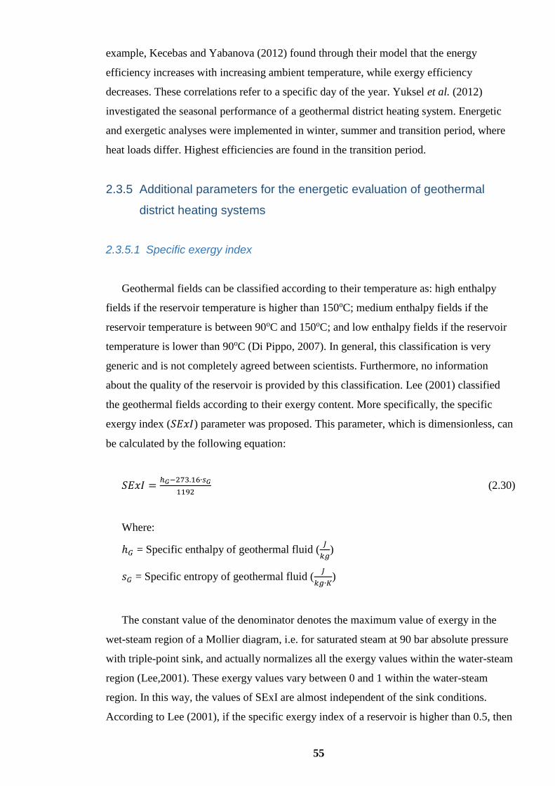
55

example, Kecebas and Yabanova (2012) found through their model that the energy

efficiency increases with increasing ambient temperature, while exergy efficiency

decreases. These correlations refer to a specific day of the year. Yuksel et al. (2012)

investigated the seasonal performance of a geothermal district heating system. Energetic

and exergetic analyses were implemented in winter, summer and transition period, where

heat loads differ. Highest efficiencies are found in the transition period.

2.3.5 Additional parameters for the energetic evaluation of geothermal

district heating systems

2.3.5.1 Specific exergy index

Geothermal fields can be classified according to their temperature as: high enthalpy

fields if the reservoir temperature is higher than 150oC; medium enthalpy fields if the

reservoir temperature is between 90oC and 150oC; and low enthalpy fields if the reservoir

temperature is lower than 90oC (Di Pippo, 2007). In general, this classification is very

generic and is not completely agreed between scientists. Furthermore, no information

about the quality of the reservoir is provided by this classification. Lee (2001) classified

the geothermal fields according to their exergy content. More specifically, the specific

exergy index (𝑆𝐸𝑥𝐼) parameter was proposed. This parameter, which is dimensionless, can

be calculated by the following equation:

𝑆𝐸𝑥𝐼 =ℎ𝐺−273.16∙𝑠𝐺

1192 (2.30)

Where:

ℎ𝐺 = Specific enthalpy of geothermal fluid (𝐽

𝑘𝑔)

𝑠𝐺 = Specific entropy of geothermal fluid (𝐽

𝑘𝑔∙𝐾)

The constant value of the denominator denotes the maximum value of exergy in the

wet-steam region of a Mollier diagram, i.e. for saturated steam at 90 bar absolute pressure

with triple-point sink, and actually normalizes all the exergy values within the water-steam

region (Lee,2001). These exergy values vary between 0 and 1 within the water-steam

region. In this way, the values of SExI are almost independent of the sink conditions.

According to Lee (2001), if the specific exergy index of a reservoir is higher than 0.5, then

56

it is a high quality reservoir. If this value is between 0.05 and 0.5, then it is medium quality

reservoir. Finally, if this value is lower than 0.05, then the reservoir is of low quality.

Ozgener et al. (2005a, b; 2007b) applied this equation to their studies, and in most cases

the reservoirs were found to be low quality.

A later study by Younger (2015) attempted the classification of geothermal fields

according to their enthalpy, which is a more comprehensive and realistic approach

compared to the classification according to the temperature of the field. The results of this

study are represented graphically in Fig. 2.3, in which the numbers on the lines dividing

the different enthalpy categories are approximate values of enthalpies in 𝐾𝐽

𝑘𝑔.

Figure 2.3. Classification of geothermal fields on the basis of enthalpy (Younger, 2015)

2.3.5.2 Improvement potential

The following equation can be implemented in order to calculate the maximum

exergetic improvement that can be obtained by each process of the network (Hammond

and Stapleton, 2001):

𝐼�̇� = (1 − 휀𝑝𝑟) ∙ (𝐸�̇�𝑖𝑛 − 𝐸�̇�𝑜𝑢𝑡) (2.31)

57

Where:

𝐼�̇� = Improvement potential (𝑊)

휀𝑝𝑟 = Exergetic efficiency of the process (Dimensionless)

Ozgener et al. (2005a) found that the highest improvement potential exists in the heat

exchangers of the system. This highlights the importance of the careful design and

selection of the heat exchangers.

2.3.5.3 Other parameters

Very few studies have been carried out concerning other parameters of geothermal

district heating systems. Hepbasli (2010), amongst few others, summarizes the concept of

energy generation due to friction and heat losses in a system. Ozgener et al. (2005b) state

the parameters of fuel depletion ratio; relative irreversibility; and productivity lack, which

were originally implemented for conventional systems.

Coskun et al. (2009) introduced four new parameters which indicate how much the

system is renewable and sustainable. These parameters, which were implemented to the

Edremit, Turkey, geothermal district heating system are the following: Energetic

renewability ratio; exergetic renewability ratio; energetic re-injection ratio; and exergetic

re-injection ratio. The first two are defined as the ratio of the renewable energy or exergy,

respectively, obtained from the system to the total energy or exergy input (renewable and

non-renewable). The latter two are defined as the ratio of renewable energy or exergy,

respectively, discharged to environment or re-injected to the well from the system to the

total geothermal energy or exergy supplied to the system.

Ozgener and Ozgener (2009) analysed three parameters which describe the total

availability of the system. These are the average technical availability; the real availability;

and the capacity factor. Technical availability is defined as the ratio of operation hours to

total machine hours available in the heating season and takes into account the machine

faults of the system. The technical availability of a geothermal system is usually higher

than 90%. Real availability is defined as the ratio of generation hours to total machine

hours and depends mainly on the non-availability of the system due to possible leakages. If

a system is well maintained the real availability can be almost 100%. Finally, the capacity

factor is defined as the ratio of the desired actual useful production to the maximum

58

theoretical production of the system. As shown in this study, the average value of the

capacity factor is around 40-42%.

Ozgener (2012) defined the coefficient of performance of a geothermal district heating

system as the ratio of the useful energy provided to the summary of all the electrical energy

consumed by the pumps of the system.

useful G th

i i

pumps pumps

E ECOP

W W

(2.32)

Finally, Hepbasli (2010) introduced four new parameters which take into account the

building’s circuit. These are: the distribution cycle exergetic ratio; the energy consumption

circuit exergetic ratio; the reservoir specific exergy utilization index; and the geothermal

brine specific exergy utilization index. Defining further these parameters is out of the

scope of this study.

2.3.5.4 Further studies

Sahin and Yazici (2012) and Kecebas et al. (2012) studied Afyon, Turkey, geothermal

district heating system using artificial neural network (ANN) and adaptive neuro-fuzzy

(ANFIS) models. An artificial neural network is a computational tool that mimics the way

information is ‘learned’ by biological neural systems. It consists of an input layer, an

output layer and some hidden layers which usually have stored information from some

previous data, the so-called ‘training’. The use of ANNs has some benefits such as non-

linearity, flexibility, speed, simplicity and adaptive learning as noted by Kecebas and

Yabanova (2012) amongst others. Artificial neural networks are more appropriate for

systems for which no physical model exists, but they can also be used for systems with

physical models. An artificial neural network needs some sets of inputs-outputs to

determine the connecting weights in the hidden layers. After that, for any given input it is

able to provide the output. Aksoy et al. (2011) state that ‘It has been demonstrated that if

there is sufficient number of neurons in the hidden layer of a feedforward ANN, with three

layers, then the network can approximate any continuous function at the desired accuracy’.

A feedforward ANN is an ANN that the transmission from a layer occurs only to layers

following that layer. ANFIS is a hybrid scheme of neural networks and fuzzy logic

techniques. It analyses the relation between inputs and outputs and finds the optimal

59

distribution of membership functions using either a back-propagation gradient descent

algorithm or the latter in combination with the least-squares method. Results are compared

and it is shown that the ANN models are slightly better in determining energy and exergy

rates. Additionally, the correlation factors are very satisfactory. It is shown that ANN and

ANFIS can provide a practical and fast solution for the estimation of energy and exergy

rates.

Coskun et al. (2012) studied a new hybrid system for Edremit, Turkey, geothermal

district heating system. The waste heat is re-injected at almost 40oC, which is a very

satisfactory temperature for feeding a heat pump and a biogas power plant, as is proposed.

The electricity production of the biogas plant is proposed to be used for the heat pump, the

district heating system pumps and all the auxiliary equipment. A biogas power plant needs

a constant temperature of about 38oC to operate. On the other hand, the coefficient of

performance of a heat pump rises as the feeding temperature rises. Additionally, heat

pumps depend a lot on the price of electricity. In this model, the electricity will be

produced effectively for free. Results show that the energetic efficiency increases by 7.5%

and the exergetic efficiency by 13%. So, by implementing this hybrid installation several

advantages are realised, i.e. increase of efficiencies; increased number of heated

residences; reduction of fuel consumption; reduction of emissions; and increase of the

system’s sustainability. Finally, a basic prerequisite for such a system is that high amounts

of agricultural and industrial waste are necessary for the biogas plant to operate.

2.3.6 Economic analysis

2.3.6.1 Conventional economic analysis

After a resource has been found to be viable from an energetic and technical point of

view, the last barrier for implementation is the economic feasibility. As already mentioned,

a geothermal district heating system is a capital intensive investment (Erdogmus et al.,

2006, amongst many others). Additionally, the cost of drilling might render an investment

infeasible. In contrast, operational and maintenance costs are quite low.

The total cost can be estimated as the sum of the investment cost, the operational cost

and the maintenance cost. Possibly, the salvage cost of the equipment may decrease the

total capital cost.

60

The investment cost consists of the cost of drilling, the cost of electromechanical

equipment, i.e. pipeline system; heat exchangers; pumps; end user systems etc., and the

cost of infrastructure, i.e. substations; storage tanks; control systems; pipeline burial costs

etc. The investment cost can be separated into surface costs, which are easily predicted,

and subsurface costs, which contain a lot of risk. The investment cost mainly depends of

the following (Erdogmus et al., 2006):

Depth of resource.

Distance between resource and consumers.

Well flow rate and temperature.

Load factor.

Composition of geothermal fluid.

Ease of disposal and re-injection.

Heat density.

The main operational costs of a geothermal district heating system are the following

(Harrison, 1994; Erdogmus et al., 2006):

Cost of personnel.

Cost of electricity for the pumps and auxiliary equipment.

Cost of fuel for peak-up and back-up boilers.

Cost of tap and make-up water.

Cost of anti-corrosive and anti-freezing chemicals.

Cost of marketing.

Cost of renting facilities.

Vorum and Petterson (1981) indicate that the distribution cost accounts usually more

than 25% of the initial investment cost, while the maintenance costs might be even less

than 1% of the investment cost. It has to be highlighted at this point that no general

conclusions can be made about geothermal district heating systems costs. Depending on

each case, allocation of costs might be quite different. In some cases the cost of drilling

might be a large portion of the investment cost, e.g. EGS deep systems, while in other

cases it might be negligible, e.g. shallow wells. A case study from Dlugosz (2003), for

example, shows that the cost of wells is about 8% of the total cost, while transmission and

61

distribution costs account for more than 66% of the total cost. In other situations the

relative costs of these components might be very different.

The main incomes for geothermal district heating systems are usually similar to

traditional heating systems and consist of a fixed cost which is used as a minimum

guaranteed income and in order to re-pay the initial investment costs and a variable heating

cost which is variable and is priced according to the real use of heat. In the latter, the cost

is usually calculated by specific meters which count the flow rate through the building, and

the temperature of the distribution water before and after the building. These are called

Btu-meters or just heat meters and can provide the actual use of heat within each end-user

(Bloomquist, 2003). Based on this value, the variable cost of heating is calculated and then

is summed with the fixed cost, to form the total income of the investment. Finally, there is

the possibility of the extra income due to a financial subsidy that can be provided. This is

the case in many countries worldwide which provide subsidies for the promotion and faster

commissioning of renewable technologies.

Usually, in the economic analysis of geothermal district heating systems, a comparison

with conventional systems is carried out. This comparison is carried out using some

economic indicators. Of course, as Hederman and Cohen (1981) state, all the comparisons

must be made on a common basis. Consistency must be achieved for taxes, interest rates

etc. The main economic indicators are described shortly below and summarised in the

works of Erdogmus et al. (2006) and Hederman and Cohen (1981).

Net present value (NPV)

This is the sum of all the future incomes and expenditures at present-day monetary

values. The transformation of future values (i-years from now) into present values can be

done using the interest rate and the following equation:

𝑃𝑉𝑖 = 𝐹𝑉 ∙ (1 + 𝐷𝑅)−𝑖 (2.33)

Where:

𝑃𝑉 = Present value (£)

𝐹𝑉 = Future value (£)

𝐷𝑅 = Discount rate (Dimensionless)

62

Therefore, the net present value of an investment with N years investment period can

be calculated as:

0

i Ni

i

NPV PV

(2.34)

The higher the net present value, the more economically feasible is a given investment

as it denotes a higher net total income throughout the whole investment period.

Internal rate of return method (IRR)

The IRR is defined as the discount rate which equates the net present value to zero.

This can be calculated by solving the following equation for the discount rate:

0

0(1 )

ii N

ii

PV

DR

(2.35)

In general, the present value of the investment in any year can be calculated as the

difference between the inflows and the outflows of the investment the specific year, i.e. the

net cash flow of the investment. For an investment to be feasible, the IRR has to be higher

than the current interest rate. On the other hand, when comparing investments, the one with

the higher value of IRR is more feasible as it denotes higher financial security. It should be

noted that if the installation is a public investment, the net present value can be very close

to zero, since there may be no strong interest in making a profit.

Unit cost of energy

This is simply the cost of producing one unit of energy. This is the minimum heating

fee that the producer could accept in order to have suitable revenues. It is calculated, in

general, by the following equations through the annuity method (Krajacic et al., 2011):

𝑈𝐶𝐸 =𝐶𝐶𝑡𝑜𝑡∙𝐶𝑅𝐹+𝐶𝑂&𝑀+𝐶𝑚𝑖𝑠𝑐

𝐸𝑎𝑛𝑛𝑢𝑎𝑙 (2.36)

𝐶𝑅𝐹 =𝐼𝑅

1−(1+𝐼𝑅)𝑁 (2.37)

63

Where:

𝑈𝐶𝐸 = Unit cost of energy (£

𝑘𝑊ℎ)

𝐶𝐶𝑡𝑜𝑡 = Total capital cost (£)

𝐶𝑂&𝑀 = Cost of operation and maintenance of the installation (£

𝑦𝑒𝑎𝑟)

𝐶𝑚𝑖𝑠𝑐= Miscellaneous costs of the installation (£

𝑦𝑒𝑎𝑟)

𝐶𝑅𝐹 = Cost recovery factor (Dimensionless)

𝐸𝑎𝑛𝑛𝑢𝑎𝑙 = Annual energy produced (𝑘𝑊ℎ)

𝐼𝑅 = Interest rate (Dimensionless)

Other possible costs, such as salvage cost if available, should be also taken into

account.

Typical assumed values of interest and discount rate are 6% and 5%, respectively

(Sommer et al., 2003), although in many countries, such as UK, the central bank sets in

advance the ‘base’ interest rate to a specific value, which is used as a starting point in any

analysis.

Atkinson and Huxtable (1984) highlight the importance of two crucial factors of

geothermal district heating systems. These two factors, as mentioned earlier, are the

distance between the well and the energy consumption centre and the heat load density.

These factors can render an investment infeasible if they are not examined thoroughly.

Erdogmus et al. (2006) evaluated the geothermal district heating of Balcova, Turkey,

from an economic point of view. The profitability was investigated with the internal rate of

return method. Many different scenarios for operating costs and utilized energy price were

examined. It was found in that case that the proper monthly utilization price for a 100m2

building was US$55.5 (equal to £37.95). It is also shown that IRR increases when the

heating fee increases and when the operational costs decrease.

Hederman and Cohen (1981) examined the cost of geothermal commercial-scale direct

heat applications and compared them with fuel alternatives. Five different projects

concerning the well depth and the use of geothermal heat were examined. In general, life-

cycle costs of a geothermal installation are much different from those of a conventional

unit. A geothermal installation has large initial capital investment costs but low recurrent

64

operational costs. In contrast, a conventional unit has lower investment costs but quite high

operational costs, due to the cost of conventional fuels. For this reason, the life-cycle costs

must be taken into account when implementing a comparison between renewable and

conventional units. Geothermal energy is found to be cheaper than oil in all circumstances,

and cheaper than natural gas in many cases. So, it is shown that geothermal energy can

provide a cheap alternative to conventional fuels.

Kanoglu and Cengel (1999) carried out a feasibility study for the combined generation

of power and heating or cooling from high enthalpy geothermal resources. They state that

in high enthalpy geothermal fields, electricity produced from geothermal energy is about

1/13th of the heat power that can be produced from the same source. But, from a

thermodynamic point of view, it is not wise to produce heat solely from high enthalpy

resources. As previously mentioned, the best solution is the combined generation of

heating or cooling and power. Kanoglu and Cengel (1999) also verify the latter from an

economic point of view. It is found that heating can provide 3.1 times and cooling 2.9

times the revenue of power alone generation. Additionally, combined heat and power

generation can provide 2.1 times the revenue of power alone generation, while combined

cooling and power generation can provide 1.2 the revenue of power alone generation. In

any case, the integrated use of geothermal energy is more feasible than the use for a single

purpose, especially if there is a high enthalpy resource.

Sommer et al. (2003) studied the spatial economics of geothermal district heating

systems. The commercial software HEATMAP (Bloomquist et al., 2004) was used to

examine the feasibility for a low density town in the USA. HEATMAP is a very useful tool

which has various inputs, such as: building uses and sizes; a supply source; the source

location; the pipeline configuration etc. The outputs that HEATMAP provides are the

following: thermal density; sizing of pipelines; total cost estimate; revenues; estimation of

viability of the investment; unit cost of energy. In general, costs of geothermal energy vary

a lot according to many factors already discussed. Sommer et al. (2003) stated the

following: ‘An important factor for the economics of geothermal district heating is the

trade-off between economies of scale and transportation costs. There is an optimum where

the expanding of the network to capture more customers is not worth anymore’. The latter

is mainly not worthwhile from the customers’ point of view, because they will have to pay

a very high price for heating. Sommer et al. (2003), show that the rate of participation, i.e.

the proportion of customers in the area that adopts geothermal district heating, is a crucial

factor for the viability of the investment. As already discussed, in order to achieve high a

65

rate of participation, education of the citizens about the benefits of geothermal energy is

necessary. A sensitivity analysis on the rate of participation was carried out. It was found

that even in the pessimistic case, geothermal energy is competitive at least in the core

building district area. But the economies of scale by larger service areas do not necessarily

outweigh the higher development costs. The further we get from the core building district,

the less feasible is the investment. In general, it is found that no general conclusion can be

reached on that aspect. It depends on each case, and careful study is necessary.

Vorum and Petterson (1981) carried out a feasibility analysis of geothermal district

heating systems, which indicated that they are competitive with other energy sources, such

as fossil fuels, biomass etc. More specifically, two service areas were examined and the

unit cost of energy was found to be equal to US$10.3 and US$8.2 per million Btu (roughly

equal to £0.024/kWh and £0.019/kWh), respectively. These prices were compared with the

prices of electricity, propane and fuel oil, which were respectively US$8.76, US$13.65 and

US$11.71 (roughly equal to £0.0204/kWh, £0.0318/kWh and £0.0273/kWh). It was also

estimated that an annual saving of about US$480 (c. £330) could be achieved if fuel oil

was used before. The competitiveness of geothermal district heating is made clear through

this study.

It can be concluded that geothermal district heating is a cheap, or at least competitive,

alternative to traditional fossil-fuelled heating systems. The cost of geothermal district

heating depends on many factors and can vary widely, but in general geothermal district

heating is a cheap solution which together with its low emissions could be a crucial

contributor to meeting future energy targets and sustainable development, thus providing

many benefits both to the customers and to the society.

2.3.6.2 Exergoeconomic analysis

Exergy analysis is proving to be a powerful tool for finding where improvements can

be made. But, only economic analysis can determine the feasibility of such an

improvement. For this reason, they are usually implemented together. Exergoeconomic

analysis is the combination of exergy and economics for long term operational conditions

(Ozgener et al., 2007c, amongst others).

Ozgener et al. (2007c) conducted an exergoeconomic study of the Salihli, Turkey,

geothermal district heating system implementing mass, energy, exergy and cost analysis.

66

The relation between thermodynamic losses and capital cost of the whole system and its

components is examined with the following equations:

�̇�𝑒𝑛 = �̇�𝑙𝑜𝑠𝑠 (2.38)

�̇�𝑒𝑥 = 𝐸�̇�𝑑𝑒𝑠𝑡 (2.39)

𝑅𝑒𝑛 =�̇�𝑒𝑛

𝐶𝐶𝑡𝑜𝑡 (2.40)

𝑅𝑒𝑥 =�̇�𝑒𝑥

𝐶𝐶𝑡𝑜𝑡 (2.41)

Where:

�̇�𝑒𝑛 = Energy losses ratio (𝑊)

�̇�𝑙𝑜𝑠𝑠 = Energy losses (𝑊)

�̇�𝑒𝑥 = Exergy losses-destruction ratio (𝑊)

𝑅𝑒𝑛, 𝑅𝑒𝑥 = Ratio of energy and exergy losses to capital cost, respectively (𝑊

£)

It is shown that a correlation between capital cost and internal or total exergy losses

exists. Internal exergy losses are the losses which occur due to irreversibilities of the

process, while external losses are the losses which occur due to interaction of the system

with its surroundings. Obviously, the total exergy losses are the sum of internal and

external exergy losses. So, usually the total exergy losses are taken into account. No

correlation between energy losses and capital cost exists. In general, the prices of the ratio

of exergy loss to capital cost of each component tend to be close to each other. So, it seems

to be a systematic correlation between exergy losses and capital cost.

It is shown that a successful design must balance the thermodynamic and economic

characteristics of the system. As Ozgener et al. (2005c) state in their study ‘The results

suggest that a good design, in terms of balancing efficiency with cost, occurs when the

loss-to-capital cost ratios based on exergy for the devices comprising the geothermal

district heating system approach the loss-to-capital cost ratio based on exergy for the

overall system’. Hence, in a successful design the value of loss to capital cost ratio based

on exergy for the components comprising the system must approach an appropriate value,

which is usually the loss to capital cost ratio based on exergy for the whole system.

67

However, the components which need improvement can still be indicated by exergy

analysis. Exergoeconomic analysis is very useful to indicate if balance exists between

thermodynamic and economic characteristics of the system.

2.4 Thermal energy storage

2.4.1 General

An important parameter for the sustainable development is the maximum utilisation of

the available energy sources. Traditionally, if the energy production was higher than the

energy consumption, the energy surplus was simply wasted in the environment. On the

other hand, in the opposite case expensive equipment and energy sources were used to

cover the energy shortages. This mismatch between the production and the demand occurs

due to their intermittent nature. For example, in a solar system the energy production is

quite changeable throughout the day and it depends on the solar radiation, the cloudiness

etc. In contrast, the energy requirements can fluctuate a lot throughout the day depending

on the habits of the end-users, amongst many other factors. Lately, the concept of energy

storage has been studied extensively as a means of matching the production with the

demand. The main idea is to store energy when in excess production and release it when in

shortage (Han et al., 2009).

The energy storage systems are, in general, divided in the following categories

according to the kind of energy stored: Mechanical, electrical, thermal and chemical

energy storage, while less developed are the magnetic and biologic energy storage methods

(Dincer and Rosen, 2011). For the sake of simplicity, the thermal energy storage systems

will be examined in this section, as well as in the overall thesis, as the studied systems are

dealing only with thermal energy both in the production and the demand side. Therefore,

the thermal energy storage systems are considered to be the most appropriate for these

systems.

The thermal energy storage systems (TES) are further divided in the following

categories (Arteconi et al., 2012):

Sensible TES: In these systems, the energy is stored through the temperature

change of the storage medium. The most common storage medium in these

68

systems is water. A basic advantage of the sensible TES is that the storage

medium is safe, cheap, abundant and easy to handle. Furthermore, these are the

best established storage systems. In contrast, the basic disadvantage of these

systems is that their operation is typically limited by the boiling point of the

storage medium, which for water is 100oC. In some cases, solid media, such as

concrete, are used for storage, but require generally large storage volumes and

are not preferred.

Latent TES: As its name indicates, in a latent TES the energy is stored through

the phase change of the storage medium. The storage media in these systems are

called PCMs (Phase Change Materials). Typically, the storage medium is in

solid form and when the energy is stored it liquefies. During the discharge

phase, the opposite process occurs. A basic advantage is that the system

operates in a constant temperature, and the range of the storage temperature is

much higher compared to a sensible TES. On the other hand, these systems are

more expensive and require better maintenance. The most typical storage

media, are water/ice, salt hydrates and polymers.

Cold TES: This is a special category of the two aforementioned TES and it

refers to the thermal energy storage for cold applications. The typical materials

that are used are ice, chilled water and some PCMs.

Thermochemical TES: These systems could also be included in the chemical

storage systems and, therefore, will be explained briefly. A reversible chemical

reaction is utilised in these systems. Typically, the energy is stored through an

endothermic reaction, and the energy is released by performing the reaction in

the opposite way. The environmental concerns around these systems have

mainly slowed down their development.

Apart from the aforementioned details, when comparing these systems two main

parameters are taken into account. These are the energy density of the storage medium and

its cost. Concerning the energy density, the thermochemical TES are by far the best option

followed by the latent TES and, then, the sensible TES. In contrast, the costs of these

systems follow exactly the reverse trend. So, it is a matter of engineering decision which of

the previously mentioned TES will be used. Other factors that should be taken into account

are the operating temperature, the safety and the available storage volume.

69

2.4.2 Thermal energy storage in district heating systems

As mentioned earlier, the typical temperatures of the water in a district heating system

(including GDHSs) is well below 100oC. Taking this into account together with the fact

that water is the working fluid anyway, the use of a sensible TES is an obvious solution.

For this purpose, water storage tanks are implemented for the matching between the

production and the demand. In a district heating system fed by a CHP unit, the mismatch

between the production and the demand can be intensified when the CHP unit is operating

in an electrically-driven mode, when the heat production is limited by the electricity

production.

Water by its nature displays a natural phenomenon, called stratification, which can

influence the operation and effectiveness of the storage. When water is stored in a storage

tank, it tends to develop a thermocline and be separated vertically into two different

temperature zones. In practice, stratification occurs mainly due to the heat losses to the

environment, which creates a zone of colder fluid close to the walls of the tank which tends

to move downwards. For the modelling of storage tanks, two main approaches are used:

stratified and fully-mixed storage tanks.

In practice, stratification not only occurs naturally but can also be desirable. As

mentioned before, the majority of district heating systems are fed by CHP units, in which

the temperature of the water provided to the network can be variable (Kostowski and

Skorek, 2005; Haeseldonckx et al., 2007). The supply temperature to the end-users should

have a specific value according to the end-users’ needs. On the other hand, the return

temperature to the production unit should be minimised in order to optimise the whole

process. So, stratified tanks with a high degree of stratification are used in many cases.

Furthermore, the stratification can be enhanced in many different ways on which a lot of

research has been carried out (e.g. Verda and Colella, 2011; Garcia-Mari et al., 2013;

Kenjo et al., 2007; Jordan and Furbo, 2005). The majority of the studies have shown that

stratified storage tanks can provide numerous advantages when coupled with a CHP unit.

For example, Verda and Colella (2011) found that the primary energy consumption can be

reduced by 12%, while the total costs can be decreased by 5%. Ghaddar (1994) states that a

stratified storage tank works more efficiently under a variable temperature, which comes in

contrast with the logic of a GDHS. A basic disadvantage of this kind of tank is that the

70

stratification can be easily destroyed and low flow rates are generally required. This also

contrasts with GDHS in which the flow rates are fairly high.

Fully mixed storage tanks have not been studied as extensively as stratified tanks.

Pagliarini and Rainieri (2010) studied the effect of a fully mixed storage tank when

coupled with a CHP unit for the heating needs of a University campus. The results

highlight the energetic and economic benefits of integrating a heat storage in this system.

Subsequently, Campos Celador et al. (2011) compared the different approaches to

modelling of water storage tanks in a CHP plant. More specifically, they used the fully

mixed, the actual stratified and the ideal stratified models to simulate the storage tank. It

was found that from an energetic point of view, the effectiveness of all the simulations are

roughly the same, but from an economic point of view, the stratified approach is more

desirable. These results agree partially with the results of Ghaddar (1994) who stated that

the stratified approach also substantially improves the results from an energetic point of

view.

2.4.3 Thermal energy storage in geothermal district heating systems

As mentioned before, the majority of the studies of hot water storage tanks concerned

CHP or solar units, which have a variable feeding temperature which makes the use of

stratified tanks unavoidable. To the best of the author’s knowledge, there are no published

studies which integrate a heat storage into a geothermal district heating system. In contrast

with the aforementioned studies, the temperatures across a GDHS and, subsequently, the

feeding temperature into the tank, are roughly constant. Furthermore, in these systems the

mass flow rates are usually very high (as will also be seen in the following Chapters),

which makes the maintenance of stratification quite difficult and costly. Another reason for

using a stratified tank is the lack of available area for building a fully mixed tank. In a

GDHS, this should not be a problem. Therefore, for all these reasons and in order to

increase the knowledge base on fully mixed tanks, in this thesis, a fully mixed storage tank

will be used to store hot water and a second fully mixed tank will be used to store cold

water. Although it is not very clear, in the studies where fully mixed tanks are used it is

assumed that there is only one tank where hot and cold water are stored together. A novelty

of this study is that two separate tanks will be used for storing the hot and cold water. As

will be seen later, throughout this study the hot water storage tank (HST) will be studied in

detail as this will be the main buffer between the heat production and the heat demand. The

71

cold water storage tank will be used mainly in order to keep the flow rate heading to the

geothermal heat exchanger to a constant value. All this will be made clear in the following

Chapters.

2.5 Summary

In this Chapter, district heating systems that utilize geothermal energy were reviewed.

Heat is extracted from a fluid in the Earth’s crust, the so-called geothermal fluid (usually

brine), and it is distributed to consumers through a distribution network. The geothermal

fluid can be distributed directly to the consumers, or its heat can be provided to a

secondary clean water closed system. Usually the latter is the case, because the majority of

geothermal fluids have corrosive properties and it is not possible to securely distribute

them over large distances. Hence, usually, plate-type counter flow heat exchangers are

used for this purpose. Additionally, in most cases, each building has its own secondary

heat exchanger, in order to avoid high pressures in the distribution network.

The basic prerequisites for a successful geothermal district heating system are an

available resource near to the heat consumption centre and a satisfactory heat density. An

adequate temperature of the resource is crucial in order to meet the specific demands of the

process in which the geothermal heat will be utilized. As already mentioned, the main

processes are space heating and domestic hot water preparation. Developments in the

technology of space heating can render many more geothermal wells suitable for space

heating. Other uses, either separately or in an integrated way, can be for agricultural

purposes, industrial processes, greenhouse heating, balneology, aquaculture, distillation,

snow melting etc. Apart from the well temperature, an adequate continuous flow rate is a

basic prerequisite. Estimation of these values can be undertaken in many ways, but both of

these can only be assured when the drilling takes place, so a high risk is contained in these

projects. The risk gets even higher as the cost of drilling increases. As noted in the

corresponding section, the drilling is usually a large part of the investment cost. So, a

careful estimation of the mass flow rate and the temperature of the well must be done in

advance, in order to minimize the drilling risk. Additionally, subsidies are necessary in

some cases in order to minimise that risk.

An available geothermal resource, with an adequate temperature and mass flow rate, is

not useful if it is far away from the consumers. The transmission and distribution costs are

72

a large part of the investment cost, sometimes over 50%, so the less distance that the

geothermal heat has to be transferred the better. Additionally, a high heat density area is

desirable to maximize the income from the investment. The higher the heat density of the

area, the higher the amount of heat sold. Additionally, a high rate of participation in the

proposed area is also desirable. High participation can be achieved through education, so

that people fully appreciate the advantages of geothermal energy. Of course, geothermal

expertise is necessary to develop and promote geothermal district heating systems (Lunis,

1985). As already mentioned, initial choices are crucial for these systems. Maximization of

heat sold together with maximization of income and maximization of geothermal energy

utilized all need to be achieved for a successful geothermal district heating scheme.

Numerous studies have shown the advantages of geothermal energy. It can be

concluded that geothermal energy, and therefore geothermal district heating systems, are

cleaner than fossil fuels and in most cases cheaper or at least competitive. They result in

better indoor air quality, and in countries with high penetration of geothermal energy use,

e.g. Iceland, the consumers state that their quality of life has also increased since switching

to geothermal energy (Jonasson and Thordarson, 2007). Geothermal energy is also a local

energy source, which provides benefits to the local society, and also enhances energy

independence.

Finally, with the development and implementation of EGS systems, many new fields

are likely to become exploitable, thus substantially increase the geothermal resource base.

The refurbishment of old buildings and the construction of new energy-efficient building

can go hand in hand with the development of geothermal district heating networks,

providing elegant means of achieving targets set to address environmental and energy

supply problems.

73

3 SIZING OF A GEOTHERMAL DISTRICT HEATING

SYSTEM

3.1 Introduction

In this Chapter, an integrated model for the sizing of a GDHS is developed. For this

purpose, the geothermal data, the heat demand data throughout a whole year and the

topology of the studied area are used as the basic inputs. The heat demand data should

have a fine time discretization in order to get more accurate results. The output of this

model is the complete sizing or dimensioning of the installation, including the number of

geothermal wells, the sizing of the storage tank and the sizing of the pipelines amongst

others. It should be noted that two components of the installation, i.e. the peak-up boilers

and the cold storage tank, will be sized in Chapter 4 as some data from that algorithm are

necessary for that purpose. Details on the other data used in this model are given in the

next section.

The analysis of the installation is carried out on a daily basis. Therefore, a specific day

has to be chosen as the design-day on which the sizing of the installation will be based.

The basis of this selection as well as the details of all the mathematical modelling are given

in section 3.2. Then, the results of this model are shown in section 3.3. The results are

given for real heat demand data, but for arbitrary geothermal data and topology. This is

because as the developed model, as well as the others described in this thesis, are generic

models and it was not logical to study a geographically specific test-case. The heat demand

data are real data however, rather than formulated or arbitrary data, as it was considered

that only by using real data could realistic fluctuations be highlighted, and thus the model’s

advantages and disadvantages made clear. Furthermore, all the results in this thesis are

given for three different cases of the design-day. More details on these cases are given in

the results section. Finally, in section 3.4 a detailed discussion on the results is provided

and in section 3.5 the highlights of this Chapter are summarised.

74

3.2 Mathematical Modelling

3.2.1 Inputs of the model

As mentioned before, the majority of the inputs of the model will be arbitrary numbers

as the developed model is generic. Some of these inputs are initial estimations of some

basic values of the installation and will be updated by the algorithm, while the rest are

characteristics of the installation and remain constant. The inputs that are updated by the

algorithm are the following:

The ratio of the mass flow rate of working fluid (water) passing through the

geothermal heat exchanger to the geothermal flow rate coming from the well

(𝑅𝑚𝑖𝑛𝑖𝑡).

The thermal efficiency of the hot water storage tank (𝜂𝐻𝑆𝑇,𝑖𝑛𝑖𝑡).

Temperature drop in the substation (Δ𝑇𝑠𝑢𝑏,𝑖𝑛𝑖𝑡).

Temperature drop per km of the hot transmission pipeline (Δ𝑇𝑡𝑟.ℎ,𝑖𝑛𝑖𝑡).

It should be noted that where the index “init” is used, this refers to initial estimations

and later in the algorithm the exact values will be calculated. On the other hand, the inputs

that remain constant are the following:

Heat demand data.

Geothermal, ambient and soil temperatures.

Mass flow rate of one geothermal well.

Thicknesses, thermal and physical characteristics of the materials used for the

hot water storage tank and the pipelines.

Length of the transmission and distribution pipelines.

Burial depth and distance between the pipelines.

Maximum pressure and tensile strength of the pipelines.

Absolute roughness of the pipeline.

Thermal efficiency of the geothermal heat exchanger.

Thermal efficiency of the substation (𝜂𝑠𝑢𝑏). This efficiency takes into account

the heat losses of the distribution network as well as the end-user installations.

Minimum temperature differences on the hot and the cold side of the

geothermal heat exchanger.

75

Mechanical efficiency of the pumps.

Air velocity.

Unit prices of heating and electricity as well as prices of the materials used.

Interest rate

Lifespan of the investment.

Operating hours per year.

Furthermore, the temperature drop in the end of each distribution branch is also used as

input. These temperature drops are considered constant throughout the whole study and it

is assumed that the heat demand variations will be covered solely by the variation of the

mass flow rate. This is one of the basic assumptions of this study. Additionally, for design

purposes only, it is considered that the mass flow rate in each branch of the distribution

network is equal to a specific proportion of the total mass flow rate on the transmission

network. In Chapter 4, where the operation of the installation is studied, the real-time mass

flow rates of each branch are taken into account.

Finally, the necessary properties of air and water are written as functions of

temperature as the data used are point-data1. These data are written in an excel file in order

to find the optimum kind of the fitting function. Then, the data are inserted in the algorithm

and the best fit function is calculated within the algorithm. The calculated functions have a

fitting coefficient of almost 100% and refer to temperatures between 0-120oC, which is the

main temperature range in the studied cases. Concerning air, the viscosity is found to be a

second order polynomial against the temperature, while the Prandtl number and the

thermal conductivity are found to be first order polynomials. Concerning the water, the

density and the viscosity are found to be third order polynomials against the temperature,

while the specific heat capacity is considered to be constant throughout the studied

temperature range and equal to 4190𝐽

𝑘𝑔∙𝐾.

It has to be made clear at this point that some variables are point values, while others

refer to a whole time interval. In the first category, the temperatures and masses of stored

water are included, while in the latter all the other mass exchanges are included.

Obviously, the parameters in the first category have one more value than the latter, since

the last point of the day is also included. For example, if the time discretization is 1 hour,

1 http://www.engineeringtoolbox.com

76

then the first category of variables will have 25 values, while the latter will have just 24

time intervals. In the following, both variables will have the superscript i, but for the first

kind of variables it will mean the point-value while for the second kind of variables it will

mean the continuous value throughout the time interval i-i+1. The first kind of variables

will be called ‘points’ while the latter are called time-intervals. This distinction will be

made clearer in Chapter 4.

3.2.2 First calculation of the basic parameters

In this section, a first calculation of some basic parameters of the network is carried

out. Initially, some values of the temperatures of the transmission network have to be

calculated. This is done by applying some of the inputs described previously as initial

estimations. The points of these temperatures on the transmission network are shown in

Fig. 3.1 together with the associated masses. Since the temperature of the geothermal fluid

is known, the inlet temperature of the transmission supply pipeline is calculated as:

𝑇𝑡𝑟,𝑠,𝑖 = 𝑇𝐺,ℎ − ∆𝑇ℎ,𝐺𝐻𝐸.,𝑚𝑖𝑛 (3.1)

Where:

𝑇𝑡𝑟,𝑠,𝑖 = Temperature in the inlet of the transmission supply pipeline (𝐾)

𝑇𝐺,ℎ = Temperature (hot) of the geothermal fluid (𝐾)

∆𝑇ℎ,𝐺𝐻𝐸.,𝑚𝑖𝑛 = Minimum temperature difference in the hot side of the G.H.E. (𝐾)

Then, the temperature in the inlet of the hot water storage tank is calculated by the

following equation, which takes into account the heat losses in the supply pipeline:

𝑇𝐻𝑆𝑇,𝑖 = 𝑇𝑡𝑟,𝑠,𝑖 − 𝐿𝑡𝑟,𝑠,1 ∙ ∆𝑇𝑡𝑟,𝑠,𝑖𝑛𝑖𝑡 (3.2)

Where:

𝑇𝐻𝑆𝑇,𝑖 = Inlet temperature in the hot water storage tank (𝐾)

𝐿𝑡𝑟,𝑠,1 = Length of the transmission supply pipeline between the G.H.E. and the hot

water storage tank (𝑘𝑚)

∆𝑇𝑡𝑟,𝑠,𝑖𝑛𝑖𝑡 = Initial estimation of the temperature drop per unit of pipe length in the

supply pipeline (𝐾

𝑘𝑚)

77

Figure 3.1 Simplified scheme indicating the temperatures across the transmission pipelines (G.H.E. =

Geothermal Heat Exchanger, D.N. = Distribution network, P.W. = Production Well, R.W. = Re-injection

Well, H.S.T. = Hot water storage tank, C.S.T. = Cold water storage tank)

The thermal efficiency of the hot water storage tank is calculated as the proportion of

the energy exiting the tank to the energy entering the tank. These energies consist of the

thermal energy of the water due to its temperature, and any other forms of energy, such as

kinetic energy, are considered negligible. At this stage, the initial estimation of the

efficiency will be used, and only the corresponding temperatures will be taken into account

since the mass flow rates are not known yet. It should be noted that all these values of the

temperatures across the transmission network will be later checked and re-calculated, if

necessary, in an iterative loop. So, the temperature at the exit of the hot water storage tank

is calculated as:

𝑇𝐻𝑆𝑇,𝑜 = 𝜂𝐻𝑆𝑇,𝑖𝑛𝑖𝑡 ∙ (𝑇𝐻𝑆𝑇,𝑖 − 𝑇𝑎) + 𝑇𝑎 (3.3)

Where:

𝑇𝐻𝑆𝑇,𝑜 = Outlet temperature from the hot water storage tank (𝐾)

𝜂𝐻𝑆𝑇,𝑖𝑛𝑖𝑡 = Initial estimation of the thermal efficiency of the hot water storage tank

(Dimensionless)

𝑇𝑎 = Ambient temperature (𝐾)

The outlet temperature of the transmission supply pipeline can be calculated by an

equation similar to Eq. (3.2), but, it is proposed the hot water storage tank to be as close as

78

possible to the substation, so that the response in any change of the demand to be as quick

as possible. Therefore, we get:

𝑇𝑡𝑟,𝑠,𝑜 = 𝑇𝐻𝑆𝑇,𝑜 (3.4)

Where:

𝑇𝑡𝑟,𝑠,𝑜 = Outlet temperature from the supply transmission pipeline (𝐾)

Afterwards, the inlet temperature of the transmission return pipeline is calculated

through the temperature drop in the substation as:

𝑇𝑡𝑟,𝑟,𝑖 = 𝑇𝑡𝑟,𝑠,𝑜 − Δ𝑇𝑠𝑢𝑏,𝑖𝑛𝑖𝑡 (3.5)

Where:

𝑇𝑡𝑟,𝑟,𝑖 = Inlet temperature of the return transmission pipeline (𝐾)

Δ𝑇𝑠𝑢𝑏,𝑖𝑛𝑖𝑡 = Initial estimation of the temperature drop in the substation (𝐾)

The rest of the temperatures in the transmission return pipeline are calculated with

similar equations to those for temperatures in the transmission supply pipeline. More

specifically, the following equations are used:

𝑇𝐶𝑆𝑇,𝑖 = 𝑇𝑡𝑟,𝑟,𝑖 (3.6)

𝑇𝐶𝑆𝑇,𝑜 = 𝜂𝐶𝑆𝑇,𝑖𝑛𝑖𝑡 ∙ (𝑇𝐶𝑆𝑇,𝑖 − 𝑇𝑎) + 𝑇𝑎 (3.7)

𝑇𝑡𝑟,𝑟,𝑜 = 𝑇𝐶𝑆𝑇,𝑜 − 𝐿𝑡𝑟,𝑟,2 ∙ ∆𝑇𝑡𝑟,𝑟,𝑖𝑛𝑖𝑡 (3.8)

Where:

𝑇𝐶𝑆𝑇,𝑖 = Inlet temperature in the cold water storage tank (𝐾)

𝑇𝐶𝑆𝑇,𝑜 = Outlet temperature from the cold water storage tank (𝐾)

𝜂𝐶𝑆𝑇,𝑖𝑛𝑖𝑡 = Initial estimation of the thermal efficiency of the cold water storage tank

(Dimensionless)

𝑇𝑡𝑟,𝑟,𝑜 = Outlet temperature from the return transmission pipeline (𝐾)

𝐿𝑡𝑟,𝑟,2 = Length of the return transmission pipeline between the cold water storage tank

and the G.H.E. (𝑘𝑚)

79

∆𝑇𝑡𝑟,𝑟,𝑖𝑛𝑖𝑡 = Initial estimation of the temperature drop per unit of pipe length for the

return transmission pipeline (𝐾

𝑘𝑚)

The cold water storage tank is also proposed to be as close as possible to the substation,

so that the mass flow rate in both pipelines of the transmission network will be the same.

Equation (3.6) arises from this proposition. Furthermore, there are two basic differences in

the calculations of the transmission return pipeline compared to the transmission supply

pipeline. Firstly, the heat losses of the return pipeline are assumed, at this stage, to be half

of the heat losses of the supply pipeline. As will be seen in section 3.2.6, the heat losses of

the pipelines are proportional to the temperature difference between the water and the

ambient. So, it is quite sensible to assume that the temperature in the return pipeline will be

around the middle between the supply and the ambient temperatures and, therefore, the

heat losses of the return pipeline to be half of the supply pipeline. Secondly, the heat losses

of the cold storage tank are assumed to be half those of the hot storage tank. This is

assumed on the same basis as the heat losses of the pipelines. As will also be seen in the

results section, both the losses of the pipelines and of the hot water storage tank are quite

small, so any wrong estimations in these factors will not cause an important general error.

Nevertheless, if these assumptions are not very precise, the only problem that will arise is

that the algorithm will need more time to converge (see section 3.2.7 also). So, these two

assumptions are definitely acceptable from an engineering point of view.

Concerning the storage tanks, considering that their thermal efficiency can also be

defined as (1 − 𝐿𝑜𝑠𝑠𝑒𝑠), then the thermal efficiency of the cold storage tank is easily

calculated as:

𝜂𝐶𝑆𝑇,𝑖𝑛𝑖𝑡 = 1 −1−𝜂𝐻𝑆𝑇,𝑖𝑛𝑖𝑡

2 (3.9)

Since all the temperatures of the transmission network are known, the temperature drop

of the geothermal water and its temperature at the exit of the geothermal heat exchanger

can be, respectively, calculated as:

Δ𝑇𝐺 = 𝑅𝑚,𝑖𝑛𝑖𝑡 ∙𝑇𝑡𝑟,𝑠,𝑖−𝑇𝑡𝑟,𝑟,𝑜

𝜂𝐺𝐻𝐸 (3.10)

𝑇𝐺,𝑐 = 𝑇𝐺,ℎ − Δ𝑇𝐺 (3.11)

80

Where:

Δ𝑇𝐺 = Temperature drop of the geothermal fluid (𝐾)

𝑅𝑚,𝑖𝑛𝑖𝑡 = Initial estimation of the ratio of the mass flow rate on the transmission

network on the right of the G.H.E. (or left of the hot water storage tank, which will be

constant throughout the day as seen on the next) to the geothermal flow rate

(Dimensionless)

𝜂𝐺𝐻𝐸 = Thermal efficiency of the G.H.E. (Dimensionless)

𝑇𝐺,𝑐 = Outlet (cold/ re-injection) temperature of the geothermal fluid (𝐾)

Finally, the total thermal efficiency of the installation is calculated as:

𝜂𝑡𝑜𝑡 = 𝜂𝑠𝑢𝑏,𝑖𝑛𝑖𝑡 ∙ 𝑅𝑚 ∙𝑇𝑡𝑟,𝑠,𝑜−𝑇𝑡𝑟,𝑟,𝑖

∆𝑇𝐺 (3.12)

Where:

𝜂𝑡𝑜𝑡 = Total thermal efficiency of the installation (Dimensionless)

So, through Eqs. (3.1)-(3.12), a first calculation of the basic parameters of the network

is carried out. All these values will be checked and updated, if necessary, in later stages of

the algorithm. By knowing these initial values, the calculations in the following sections

are now possible.

3.2.3 Sizing of the geothermal installation

A basic input of this model is the detailed heat demand over a year. The daily heat

demand of each day can be easily calculated as the summary of the separate heat demands

over this day.

i

Day

DHD HD (3.13)

Where:

𝐻𝐷𝑖 = Heat demand per time interval i of the studied day (𝑘𝑊ℎ or 𝐽)

𝐷𝐻𝐷 = Daily heat demand of the studied day (𝑘𝑊ℎ or 𝐽)

81

So, a list of the daily heat demands over the year of study can be calculated. Then, a

specific day is chosen by the user as the design-day. In the design-day, all the heat demand

will be covered by geothermal energy only with the assistance of the heat storage and no

peak-up boilers will be used. Therefore, the total geothermal energy harvested throughout

the day can be calculated by the following equation:

𝐸𝐺,𝐷,𝐷 =𝐷𝐻𝐷𝐷

𝜂𝑡𝑜𝑡 (3.14)

Where:

𝐸𝐺,𝐷,𝐷 = Geothermal energy harvested throughout the design-day (𝑘𝑊ℎ or 𝐽)

𝐷𝐻𝐷𝐷 = Daily heat demand of the design-day (𝑘𝑊ℎ or 𝐽)

In the above equation, the total efficiency calculated in Eq. (3.12) is used. Then, the

above energy term has to be converted in the equivalent power term. This conversion

depends on the units of the energy terms which depend on the units of the heat demand

data. Commonly, these data are provided in kWh, and therefore the conversion in power

terms (in W) is done by dividing the energy term by the hours of the day. For the sake of

simplicity, in the rest of this study it is assumed that the heat demand data will be used in

kWh.

�̇�𝐺,𝐷 =𝐸𝐺,𝐷,𝐷∙1000

24 (3.15)

Where:

�̇�𝐺,𝐷 = Geothermal power of the design-day (𝑊)

The term 1000 in the above equation is used to turn the units from kW to W. Since the

geothermal power of the design-day is known, the necessary geothermal mass flow rate

can be easily calculated as:

�̇�𝐺,𝐷 =�̇�𝐺,𝐷

𝐶𝑝𝑤∙∆𝑇𝐺 (3.16)

Where:

�̇�𝐺,𝐷 = Geothermal mass flow rate on the design-day (𝑘𝑔

𝑠)

82

𝐶𝑝𝑤 = Specific heat capacity of the geothermal fluid (𝐽

𝑘𝑔∙𝐾)

The temperature of the geothermal fluid is known from Eq. (3.10) and its specific heat

capacity is also a known value. As mentioned in Chapter 2, the properties of the

geothermal fluid are the same as those of pure water as the effect of minerals and non-

condensable gases is negligible. Then, the necessary number of geothermal wells is

calculated by dividing the geothermal mass flow rate by the mass flow rate of one well,

which is a known value:

𝑁𝑤𝑒𝑙𝑙𝑠 =�̇�𝐺,𝐷

�̇�𝑤𝑒𝑙𝑙 (3.17)

Where:

𝑁𝑤𝑒𝑙𝑙𝑠 = Number of geothermal wells

�̇�𝑤𝑒𝑙𝑙 = Mass flow rate of each geothermal well (𝑘𝑔

𝑠)

Most probably, the above result will be a decimal number which, of course, does not

have a physical meaning since it refers to the number of geothermal wells. Therefore, this

result has to be rounded. The kind of rounding (floor, bottom or closest integer) depends

on the user. In our case, it is selected to round this result to the closest integer, unless for

the case where the result is less than 1 where it is rounded to 1. The final number of wells

is given by the following equation:

𝐼𝑓 𝑁𝑤𝑒𝑙𝑙𝑠 < 1:𝑇ℎ𝑒𝑛: 𝑁𝑤𝑒𝑙𝑙𝑠 = 1

𝐸𝑙𝑠𝑒: 𝑁𝑤𝑒𝑙𝑙𝑠 = 𝑟𝑜𝑢𝑛𝑑(𝑁𝑤𝑒𝑙𝑙𝑠)} (3.18)

So, the final value of the geothermal mass flow rate and the geothermal power are

calculated by Eqs. (3.16) and (3.17) properly re-arranged by taking into account the final

value of the number of geothermal wells. Therefore, by applying Eqs. (3.13)-(3.18), the

geothermal installation is sized and the geothermal power of the design-day are known.

The geothermal power of the design-day, is also the maximum geothermal power that can

be delivered at any time, since the maximum mass flow rate is used. For that reason, this

value is also the geothermal capacity of the installation.

83

3.2.4 Sizing of the hot water storage tank

The sizing of the hot water storage tank as well as of the rest of the installation will be

carried out for the design-day. In our approach, the mass flow rate to the left of the storage

tank will be constant throughout the day, while the mass flow rate to the right of the

storage tank will be variable according to the heat demand of each time interval (see Fig.

3.1). Since the heat demand is known per time interval, in the following all the calculations

will be done for masses per interval (symbolised with M), instead of mass flow rates. So,

the masses to the left and the right of the storage tank are calculated, respectively, as:

𝑀𝑡𝑟,𝐺 = 𝑀𝐺,𝐷 ∙ 𝑅𝑚,𝑖𝑛𝑖𝑡 (3.19)

𝑭𝒐𝒓 𝑒𝑎𝑐ℎ 𝑡𝑖𝑚𝑒 𝑖𝑛𝑡𝑒𝑟𝑣𝑎𝑙 𝑖:

𝑀𝑡𝑟,𝑆𝑖 =

𝐻𝐷𝑖

𝐶𝑝𝑤∙(𝑇𝑡𝑟,𝑠,𝑜−𝑇𝑡𝑟,𝑟,𝑖)∙𝜂𝑠𝑢𝑏

} (3.20)

Where:

𝑀𝑡𝑟,𝐺 = Mass of water per time interval i in the left of the storage tank (𝑘𝑔)

𝑀𝑡𝑟,𝑆𝑖 = Mass of water per time interval i in the right of the storage tank (𝑘𝑔)

Then, by the difference of these values, the masses of charged and discharged water in

the storage tank can be calculated, respectively, as:

𝑭𝒐𝒓 𝑒𝑎𝑐ℎ 𝑡𝑖𝑚𝑒 𝑖𝑛𝑡𝑒𝑟𝑣𝑎𝑙 𝑖:𝑰𝒇 𝑀𝑡𝑟,𝐺 −𝑀𝑡𝑟,𝑆

𝑖 ≥ 0:

𝑻𝒉𝒆𝒏: 𝑀𝑐ℎ𝑖 = 𝑀𝑡𝑟,𝐺 −𝑀𝑡𝑟,𝑆

𝑖

𝑬𝒍𝒔𝒆: 𝑀𝑐ℎ𝑖 = 0 }

(3.21)

𝑭𝒐𝒓 𝑒𝑎𝑐ℎ 𝑡𝑖𝑚𝑒 𝑖𝑛𝑡𝑒𝑟𝑣𝑎𝑙 𝑖:𝑰𝒇 𝑀𝑡𝑟,𝐺 −𝑀𝑡𝑟,𝑆

𝑖 ≥ 0:

𝑻𝒉𝒆𝒏: 𝑀𝑑𝑖𝑠𝑖 = 0

𝑬𝒍𝒔𝒆: 𝑀𝑑𝑖𝑠𝑖 = 𝑀𝑡𝑟,𝑆

𝑖 −𝑀𝑡𝑟,𝐺}

(3.22)

Where:

𝑀𝑐ℎ𝑖 = Mass of charged water in the storage tank per time interval i (𝑘𝑔)

𝑀𝑑𝑖𝑠𝑖 = Mass of discharged water from the storage tank per time interval i (𝑘𝑔)

84

Afterwards, the mass of stored water can be easily calculated by the following

equation:

𝑭𝒐𝒓 𝑖 ≥ 1:

𝑀𝑠𝑡𝑖 = 𝑀𝑐ℎ

𝑖 −𝑀𝑑𝑖𝑠𝑖 −𝑀𝑠𝑡

𝑖−1} (3.23)

Where:

𝑀𝑠𝑡𝑖 = Mass of stored water per time interval i (𝑘𝑔)

As a boundary condition in the above equation, it is considered that initially there is no

stored water in the hot water storage tank.

𝑀𝑠𝑡0 = 0 (3.24)

Finally, the volume of the hot water storage tank will be calculated through the

maximum value of stored water during the design-day as:

𝑉𝐻𝑆𝑇 =max (𝑀𝑠𝑡

𝑖 )

𝜌𝑤(𝑇𝐻𝑆𝑇.𝑖)∙ 𝑆𝐹 (3.25)

Where:

𝑉𝐻𝑆𝑇 = Volume of the hot water storage tank (𝑚3)

𝜌𝑤 = Density of water (𝑘𝑔

𝑚3)

𝑆𝐹 = Security factor (Dimensionless)

In the above equation, the density of water is calculated for the temperature in the inlet

of the water tank. This happens because the density of water decreases with increasing

temperature. Therefore, the maximum temperature is used, in order to get the minimum

density and, subsequently, the maximum storage volume. A security factor 𝑆𝐹 is also used

in the above equation, which in our case is considered to be equal to 1.1. This allows errors

of up to 10% during the sizing of the hot water storage tank. Finally, the thickness of the

material of the storage tank, which is stainless steel in our case, is calculated through the

API Standard 650 (Baker, 2009). This Standard has been originally produced for the sizing

of oil storage tanks, but, it is assumed that the same methodology can be applied for water

storage tanks without important errors.

85

In conclusion, by applying Eqs. (3.19)-(3.25), all the mass balances across the

transmission network as well as the volume of the hot water storage tank are calculated.

3.2.5 Energy balance in the hot water storage tank

In this section, the methodology for the calculation of the temperature evolution within

the hot water storage tank is developed. Furthermore, the calculation of the heat losses

from the tank are explained and a definition of the thermal efficiency of the tank is given in

order to get a more precise value of it.

For the calculation of the temperature evolution of the stored water, the energy

conservation equation in the storage tank is applied within one time interval (similar

equation applied by Kostowski and Skorek, 2005):

𝑑(𝜌𝑤∙𝐶𝑝𝑤∙𝑉𝑤,𝑠𝑡∙𝑇𝑠𝑡)

𝑑𝑡= �̇�+

𝑖 − �̇�−𝑖 − �̇�𝑙𝑜𝑠𝑠

𝑖 (3.26)

Where:

𝑉𝑤,𝑠𝑡 = Volume of stored water between points i and i+1 (𝑚3)

𝑇𝑠𝑡𝑖 = Temperature of stored water in point i (𝐾)

�̇�+𝑖 , �̇�−

𝑖 , �̇�𝑙𝑜𝑠𝑠𝑖 = Heat surplus due to charging, heat shortage due to discharging and heat

losses rate of the storage tank, respectively (𝑊)

In the above equation, the left hand side denotes the accumulation term balanced by the

heat surplus due to charging, the heat shortage due to discharging and the heat losses,

respectively, in the right hand side. Furthermore, 𝑉𝑤,𝑠𝑡 is the volume of stored water which

changes within the time interval. As the specific heat capacity of water has been

considered constant, and by replacing the density-times the volume of stored water equal to

the mass of stored water, the left hand side of the above equation can be discretised as:

𝑑(𝜌𝑤∙𝐶𝑝𝑤∙𝑉𝑤,𝑠𝑡∙𝑇𝑠𝑡)

𝑑𝑡= 𝐶𝑝𝑤 ∙

𝑑(𝜌𝑤∙𝑉𝑤,𝑠𝑡∙𝑇𝑠𝑡)


𝑑(𝑀𝑠𝑡∙𝑇𝑠𝑡)


𝑀𝑠𝑡𝑖+1∙𝑇𝑠𝑡

𝑖+1−𝑀𝑠𝑡𝑖 ∙𝑇𝑠𝑡

𝑖

∆𝑡 (3.27)

Then, both sides of the above equation are multiplied by the time interval (𝑑𝑡) in order

to convert the power terms in energy terms which are easier to implement since, as

mentioned before, the masses across the network are known and not the mass flow rates.

86

So, the heat surplus and shortage terms can be calculated by the following equations,

respectively:

�̇�+𝑖 = 𝑀𝑐ℎ

𝑖 ∙ 𝐶𝑝𝑤 ∙ (𝑇𝐻𝑆𝑇,𝑖 − 𝑇𝑎) (3.28)

�̇�−𝑖 = 𝑀𝑑𝑖𝑠

𝑖 ∙ 𝐶𝑝𝑤 ∙ (𝑇𝑠𝑡𝑖 +𝑇𝑠𝑡

𝑖+1

2− 𝑇𝑎) (3.29)

The heat losses of the storage tank include the heat losses from the top, sides and base.

Therefore, it is calculated by the following equation:

𝑄𝑙𝑜𝑠𝑠𝑖 = 𝑄𝑙𝑜𝑠𝑠,𝑡𝑜𝑝

𝑖 + 𝑄𝑙𝑜𝑠𝑠,𝑠𝑖𝑑𝑒𝑖 +𝑄𝑙𝑜𝑠𝑠,𝑏𝑎𝑠𝑒

𝑖 (3.30)

Where:

𝑄𝑙𝑜𝑠𝑠,𝑡𝑜𝑝𝑖 , 𝑄𝑙𝑜𝑠𝑠,𝑠𝑖𝑑𝑒

𝑖 , 𝑄𝑙𝑜𝑠𝑠,𝑏𝑎𝑠𝑒𝑖 = Heat losses rate from the top, sides and base of the

storage tank (𝑊)

A basic assumption of this thesis is that the storage tank is considered to be fully

mixed. This means that the temperature will be uniform within the tank and equal to the

storage temperature (𝑇𝑠𝑡). So, the inner surface of the tank will have a temperature equal to

the storage temperature at each time-step. The heat losses from the top and sides of the

tank occur due to conduction within the different layers of the tank and convection together

with radiation to the ambient environment. On the other hand, the heat losses from the base

occur due to conduction through the different layers of the tank and the underlying soil.

The layers of the storage tank consist of stainless steel, insulation and a cover for the top

and sides, and of stainless steel, insulation and a concrete base for the base.

For the calculation of the convective heat transfer coefficient in the top part of the tank,

the equations for flow parallel to a horizontal body are used, while for the side part the

equations for flow perpendicular to a cylindrical body are used. Therefore, the heat losses

in the three parts of the tank can be calculated by the following sets of equations

(Kakatsios, 2006), in which all the equations for each part of the tank are referred here as

one equation (equation numbering in parentheses below):

87

Top (3.31):

𝑄𝑙𝑜𝑠𝑠,𝑡𝑜𝑝𝑖 = 𝐾𝑡𝑜𝑝

𝑖 ∙ 𝐴𝑡𝑜𝑝 ∙ (𝑇𝑠𝑡𝑖+1+𝑇𝑠𝑡

𝑖

2− 𝑇𝑎) ∙ ∆𝑡

𝐴𝑡𝑜𝑝 =𝜋∙𝐷𝑠𝑡

2

4

, ,top

1 1 1j

i i ijtop j c top r

t

K k h h

ℎ𝑐,𝑡𝑜𝑝𝑖 = 𝑁𝑢 ∙

𝑘𝑎𝑖𝑟

𝐷𝑠𝑡

𝑅𝑒 =𝑢𝑎𝑖𝑟∙𝐷𝑠𝑡

𝜈𝑎𝑖𝑟

If 𝑅𝑒 < 2 ∙ 105:

Then: 𝑁𝑢 = 0.664 ∙ 𝑃𝑟1/3 ∙ 𝑅𝑒1/2

Else-if 2 ∙ 105 < 𝑅𝑒 < 5 ∙ 105:

Then: 𝑁𝑢 = 0.029 ∙ 𝑃𝑟0.43 ∙ 𝑅𝑒0.8

Else: 𝑁𝑢 = 0.0296 ∙ 𝑃𝑟1/3 ∙ 𝑅𝑒0.8

ℎ𝑟,𝑡𝑜𝑝𝑖 = 휀𝑐𝑣 ∙ 𝜎 ∙ (𝑇𝑠𝑢𝑟

𝑖 2+ 𝑇𝑎

2) ∙ (𝑇𝑠𝑢𝑟𝑖 + 𝑇𝑎)

Sides (3.32):

𝑄𝑙𝑜𝑠𝑠,𝑠𝑖𝑑𝑒𝑖 = 𝐾𝑠𝑖𝑑𝑒

𝑖 ∙ 𝐴𝑠𝑖𝑑𝑒 ∙ (𝑇𝑠𝑡𝑖+1+𝑇𝑠𝑡

𝑖

2− 𝑇𝑎) ∙ ∆𝑡

𝐴𝑠𝑖𝑑𝑒 = 𝜋 ∙ 𝐷𝑠𝑡 ∙ 𝐻𝑠𝑡

,side ,side

1 1 1j

i i ijside j c r

t

K k h h

ℎ𝑐,𝑠𝑖𝑑𝑒𝑖 = 𝑁𝑢 ∙

𝑘𝑎𝑖𝑟

𝐷𝑠𝑡

88

𝑅𝑒 =𝑢𝑎𝑖𝑟∙𝐷𝑠𝑡

𝜈𝑎𝑖𝑟

If 2 ∙ 104 < 𝑅𝑒 < 4 ∙ 105:

Then: 𝑁𝑢 = 0.3 +0.62∙𝑅𝑒1/2∙𝑃𝑟1/3

[1+(0.4

𝑃𝑟)

23]1/4

∙ [1 + (𝑅𝑒

282000)

1

2]

Else: 𝑁𝑢 = 0.3 +0.62∙𝑅𝑒1/2∙𝑃𝑟1/3

[1+(0.4

𝑃𝑟)

23]1/4

∙ [1 + (𝑅𝑒

282000)

5

8]4/5

ℎ𝑟,𝑠𝑖𝑑𝑒𝑖 = 휀𝑐𝑣 ∙ 𝜎 ∙ (𝑇𝑠𝑢𝑟

𝑖 2+ 𝑇𝑎

2) ∙ (𝑇𝑠𝑢𝑟𝑖 + 𝑇𝑎)

Base (3.33):

𝑄𝑙𝑜𝑠𝑠,𝑏𝑎𝑠𝑒𝑖 = 𝐾𝑏𝑎𝑠𝑒 ∙ 𝐴𝑏𝑎𝑠𝑒 ∙ (

𝑇𝑠𝑡𝑖+1+𝑇𝑠𝑡

𝑖

2− 𝑇𝑠𝑜𝑖𝑙) ∙ ∆𝑡

𝐴𝑏𝑎𝑠𝑒 =𝜋∙𝐷𝑠𝑡

2

4

1

𝐾𝑏𝑎𝑠𝑒= ∑

𝑡𝑗

𝑘𝑗𝑗

Where:

𝑄𝑙𝑜𝑠𝑠,𝑡𝑜𝑝𝑖 , 𝑄𝑙𝑜𝑠𝑠,𝑠𝑖𝑑𝑒

𝑖 , 𝑄𝑙𝑜𝑠𝑠,𝑏𝑎𝑠𝑒𝑖 = Heat losses from the top, side and base of the storage

tank during time interval i (𝐽)

𝐾𝑡𝑜𝑝𝑖 , 𝐾𝑠𝑖𝑑𝑒

𝑖 , 𝐾𝑏𝑎𝑠𝑒 = Overall heat transfer coefficient of the top, side and base of the

storage tank during time interval i (𝑊

𝑚2∙𝐾)

𝐴𝑡𝑜𝑝, 𝐴𝑠𝑖𝑑𝑒, 𝐴𝑏𝑎𝑠𝑒 = Top, side and base area of the storage tank (𝑚2)

𝐷𝑠𝑡, 𝐻𝑠𝑡 = Diameter and height of the storage tank (𝑚)

𝑡𝑗 = Thickness of each material j of the storage tank (𝑚)

𝑘𝑗 = Thermal conductivity of each material j of the storage tank (𝑊

𝑚∙𝐾)

ℎ𝑐,𝑡𝑜𝑝𝑖 , ℎ𝑐,𝑠𝑖𝑑𝑒

𝑖 = Convective heat transfer coefficient of the top and sides of the storage

tank for each time interval i (𝑊

𝑚2∙𝐾)

ℎ𝑟,𝑡𝑜𝑝𝑖 , ℎ𝑟,𝑠𝑖𝑑𝑒

𝑖 = Radiative heat transfer coefficient of the top and sides of the storage

tank for each time interval I (𝑊

𝑚2∙𝐾)

𝑁𝑢, 𝑅𝑒, 𝑃𝑟 = Nusselt, Reynolds and Prandtl numbers, respectively (Dimensionless)

89

𝑘𝑎𝑖𝑟 = Thermal conductivity of air (𝑊

𝑚∙𝐾)

𝑢𝑎𝑖𝑟 = Velocity of air (𝑚

𝑠)

𝜈𝑎𝑖𝑟 = Kinematic viscosity of air (𝑚2

𝑠)

휀𝑐𝑣 = Emissivity of the cover of the storage tank (Dimensionless)

𝜎 = Stefan-Boltzmann constant for radiative heat transfer which is equal to

5.6703 ∙ 10−8𝑊

𝑚2∙𝐾4

𝑇𝑠𝑢𝑟𝑖 = Temperature of the surface of the storage tank for each time interval i (𝐾)

It can be seen from the above sets of equations that the average storage temperature

between two time intervals is used in each case. In the cases of the top and sides of the

tank, the calculations depend on the temperature of the stored water each time and on the

outer surface temperature of the tank. Therefore, a temporal superscript is assigned in these

calculations. In the case of the base of the tank, the heat transfer coefficient depends only

on the materials of the tank and, therefore, it is constant all the time. Furthermore, some of

the parameters used in the calculation of the convective heat transfer coefficients are

temperature dependent. These parameters, i.e. the Prandtl number and the kinematic

viscosity of air, are calculated for the average temperature between the ambient

temperature and the outer surface temperature. The latter is also an unknown variable in

the problem. For the solution of this problem, it is considered that the heat transfer due to

conduction in the different layers of the tank is equal to the heat transfer due to convection

and the radiation to the ambient environment. This is schematically illustrated in Figure

3.2, where a cross-sectional area of the side of the tank is shown together with the

associated temperatures and heat flows.

90

Figure 3.2 Heat flows and temperatures through the sides of the tank

By the equality between the heat flows, and by assuming that these are one-

dimensional only, we get the following equation:

�̇�𝑐𝑜𝑛𝑑𝑖 = �̇�𝑐𝑜𝑛𝑣

𝑖 + �̇�𝑟𝑎𝑑𝑖 →

4 4( ) ( ) ( )j i i i i i

st sur conv sur a cv sur a

j j

kT T h T T T T

t (3.34)

Where:

�̇�𝑐𝑜𝑛𝑑𝑖 , �̇�𝑐𝑜𝑛𝑣

𝑖 , �̇�𝑟𝑎𝑑𝑖 = Conductive, convective and radiative heat transfer rates,

respectively (𝑊)

As already mentioned, the convective heat transfer coefficient is dependent on the

surface temperature, so in order to solve the above equation an iterative method has to be

applied. The above equation is valid both for the top and the sides of the tank. For the

calculation of the convective heat transfer coefficient, the corresponding equations to

(3.31) and (3.33) have to be used. So, for each time interval, the following steps are carried

out for the calculation of the storage temperature:

1. An initial estimate for the surface temperature is made.

2. Equation (3.34) is solved iteratively till the real surface temperature is found.

3. The total heat transfer coefficients (𝐾) for each part of the storage tank are

calculated through the corresponding equations from the (3.31)-(3.33) sets of

equations.

91

4. Finally, Eqs. (3.26)-(3.30) are applied for the calculation of the heat storage

temperature in the next time step.

As a boundary condition for the above process, it is considered that the storage

temperature at the beginning of the day is equal to the temperature of the water entering the

tank.

𝑇𝑠𝑡0 = 𝑇𝐻𝑆𝑇,𝑖 (3.35)

So, the evolution of the stored temperature within the design-day can be calculated.

Then, a new value of the thermal efficiency of the storage tank can also be calculated. For

that purpose, a new definition which takes into account the mass and temperature

variations is defined. The new definition of the thermal efficiency of the storage tank is as

follows:

, ,, ,

,in,total , ,

( )

( )

i i

tr S w HST o aw out total i

HST

w tr G w HST i a

i

M Cp T TE

E M Cp T T

(3.36)

Where:

𝐸𝑤,𝑖𝑛,𝑡𝑜𝑡𝑎𝑙, 𝐸𝑤,𝑜𝑢𝑡,𝑡𝑜𝑡𝑎𝑙 = Total energy of water entering and leaving the storage

tank, respectively (𝐽)

𝜂𝐻𝑆𝑇 = Efficiency of the hot water storage tank (Dimensionless)

Figure 3.3 is provided for the better understanding of the above equation and the

masses as well as the temperatures that are taken into account in it. As can be seen, the

mass and the temperature that are used in the numerator are those after the mixing point

with the water coming from the geothermal production, while the mass and the temperature

used in the denominator are those before the splitting of the flow to the storage tank. In

other words, the energy before the splitting and after the mixing of the flows are taken into

account. The temperature of the water after the mixing point has been calculated initially in

section 3.2.2, but in this point a more detailed calculation that takes into account the

mixing with the water coming from the tank on each time interval can be carried out.

92

Therefore, by assuming no heat losses at the mixing point, the following energy

conservation equation can be applied:

(𝑀𝑡𝑟,𝐺 −𝑀𝑐ℎ𝑖 +𝑀𝑐ℎ

𝑖−1

2) ∙ 𝑇𝐻𝑆𝑇,𝑖 +

𝑀𝑑𝑖𝑠𝑖 +𝑀𝑑𝑖𝑠

𝑖−1

2∙ 𝑇𝑠𝑡

𝑖 =


𝑖−1

2+𝑀𝑑𝑖𝑠𝑖 +𝑀𝑑𝑖𝑠

𝑖−1

2) ∙ 𝑇𝐻𝑆𝑇,𝑜

𝑖

(3.37)

The above equation was implemented from the middle of each time interval to the

middle of the next time interval as the masses are continuous values, while the

temperatures are point values as explained earlier. So, for each time interval, all the masses

are known by Eqs. (3.19)-(3.22), while the stored temperature is known by the process

explained previously. Therefore, by Eq. (3.37) the temperature after the mixing point can

be calculated and, finally, by Eq. (3.36) the thermal efficiency of the hot water storage tank

can also be calculated.

Figure 3.3 A schematic illustration of the mass balances and temperatures associated with the hot water

storage tank

Concerning the cold water storage tank, it is still assumed that its losses will be still the

half of those of the hot water storage tank, and therefore, its value will be calculated

through Eq. (3.9), but now taking into account the new value of the thermal efficiency of

the hot water storage tank.

93

3.2.6 Sizing of the pipelines of the network

For the sizing of the pipelines of the network, an optimization algorithm is assembled.

The objective function is the total cost of the pipelines which consists of the capital cost,

the cost of electricity used by the pumps to overcome the friction losses and the cost of the

heat losses. The latter is not a direct cost, but an indirect monetary loss, so it is also taken

into account in the total cost. The optimization parameters are the internal diameter of the

pipeline and the thickness of the insulation. As a general approach, a system of double pre-

insulated underground pipelines will be used. More details on this will be given on the

calculation of the heat losses.

ℱ𝑚𝑖𝑛(𝐷𝑝,𝑒𝑥, 𝑡𝑖𝑛𝑠) = 𝐶𝐶𝑝 + 𝐶𝑝.𝑒𝑙 + 𝐶𝑝,ℎ𝑙 (3.38)

Where:

𝐶𝐶𝑝 = Capital cost of pipelines (£)

𝐶𝑝.𝑒𝑙 = Cost of the electricity used by the pumps of the network to overcome the

friction losses of the pipelines (£)

𝐶𝑝,ℎ𝑙 = Cost of the heat losses of the pipelines (£)

3.2.6.1 Capital cost calculation

The capital cost of the pipelines consists of the cost of the materials, which are selected

to be carbon steel and insulation, and the cost of welding. Knowing the dimensions of the

pipelines, the total volume of each material can easily be calculated and, then, by

multiplying the volume of each material with its unit cost, the cost of each material is

calculated. Figure 3.4 shows a cross sectional area of one pipeline for the better

understanding of the geometry. The cost of welding is usually a specific cost provided by

the manufacturer of the pipelines. In our case, it is considered to have a specific price per

weld and meter of diameter. Therefore, the capital cost of the pipelines is calculated by the

following equations:

𝑉𝑐.𝑠𝑡𝑒𝑒𝑙 = 𝜋 ∙𝐷𝑝,𝑜2 −𝐷𝑝,𝑖

2

4∙ 𝐿𝑝 (3.39)

𝑉𝑖𝑛𝑠 = 𝜋 ∙(𝐷𝑝.𝑜+2∙𝑡𝑝,𝑖𝑛𝑠)

2−𝐷𝑝.𝑜2

4∙ 𝐿𝑝 (3.40)

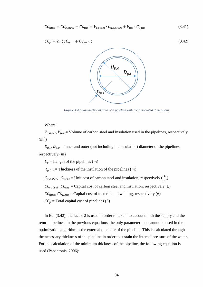
94

𝐶𝐶𝑚𝑎𝑡 = 𝐶𝐶𝑐,𝑠𝑡𝑒𝑒𝑙 + 𝐶𝐶𝑖𝑛𝑠 = 𝑉𝑐,𝑠𝑡𝑒𝑒𝑙 ∙ 𝐶𝑢,𝑐,𝑠𝑡𝑒𝑒𝑙 + 𝑉𝑖𝑛𝑠 ∙ 𝐶𝑢,𝑖𝑛𝑠 (3.41)

𝐶𝐶𝑝 = 2 ∙ (𝐶𝐶𝑚𝑎𝑡 + 𝐶𝐶𝑤𝑒𝑙𝑑) (3.42)

Figure 3.4 Cross-sectional area of a pipeline with the associated dimensions

Where:

𝑉𝑐.𝑠𝑡𝑒𝑒𝑙, 𝑉𝑖𝑛𝑠 = Volume of carbon steel and insulation used in the pipelines, respectively

(𝑚3)

𝐷𝑝,𝑖, 𝐷𝑝,𝑜 = Inner and outer (not including the insulation) diameter of the pipelines,

respectively (𝑚)

𝐿𝑝 = Length of the pipelines (𝑚)

𝑡𝑝,𝑖𝑛𝑠 = Thickness of the insulation of the pipelines (𝑚)

𝐶𝑢,𝑐,𝑠𝑡𝑒𝑒𝑙, 𝐶𝑢,𝑖𝑛𝑠 = Unit cost of carbon steel and insulation, respectively (£

𝑚3)

𝐶𝐶𝑐,𝑠𝑡𝑒𝑒𝑙, 𝐶𝐶𝑖𝑛𝑠 = Capital cost of carbon steel and insulation, respectively (£)

𝐶𝐶𝑚𝑎𝑡, 𝐶𝐶𝑤𝑒𝑙𝑑 = Capital cost of material and welding, respectively (£)

𝐶𝐶𝑝 = Total capital cost of pipelines (£)

In Eq. (3.42), the factor 2 is used in order to take into account both the supply and the

return pipelines. In the previous equations, the only parameter that cannot be used in the

optimization algorithm is the external diameter of the pipeline. This is calculated through

the necessary thickness of the pipeline in order to sustain the internal pressure of the water.

For the calculation of the minimum thickness of the pipeline, the following equation is

used (Papantonis, 2006):

95

𝑒𝑚𝑖𝑛 =𝑃𝑚𝑎𝑥∙𝐷𝑝,𝑜

𝜎∙𝑆𝐹+ 𝑒1 (3.43)

Where:

𝑃𝑚𝑎𝑥 = Maximum pressure within the pipeline (𝐵𝑎𝑟). Usually, it is equal to 5.5𝐵𝑎𝑟.

𝐷𝑝,𝑜 = 𝐷𝑝𝑖 + 2 ∙ 𝑒𝑚𝑖𝑛

𝜎 = Tensile strength of the material. For carbon steel it is 1500𝑘𝑝

𝑐𝑚2

𝑆𝐹 = Security factor. In this case, it is set equal to 1.7.

𝑒1 = Corrosion allowance. It is set equal to 1mm.

Furthermore, for the sizing of the pipelines the standardized dimensions are used

according to EN10220 (British Standards Institution, 2002). So, after the minimum

thickness of the pipeline is calculated by Eq. (3.43), then the result is increased to the next

higher value of standardised thickness. It should be noted that only standardised values of

external diameters will be used throughout these calculations. Finally, by combining and

replacing Eqs. (3.39)-(3.41) and (3.43) into Eq. (3.42), the latter can be written as a

function of the internal diameter and the thickness of the insulation, which are the

parameters of the initial optimization function.

3.2.6.2 Electrical cost calculation

For the calculation of the electrical cost used by the pumps to overcome the friction

losses, it is necessary to calculate the friction losses first. The friction losses are assumed to

consist of the linear losses only, which are calculated by the Darcy-Weisbach equation as

follows:

𝛿ℎ𝑙 = 𝜆 ∙𝐿𝑝

𝐷𝑝𝑖∙𝑢𝑤2

2∙𝑔 (3.44)

Where:

𝛿ℎ𝑙 = Friction losses (𝑚)

𝜆 = Friction losses coefficient (Dimensionless)

𝑢𝑤 = Velocity of water (𝑚

𝑠)

In the above equation, 𝜆 is the friction losses coefficient which is calculated through

iterations by the Colebrook equation:

96

1

√𝜆= −2 ∙ log (

2.51

𝑅𝑒∙√𝜆+ 𝑟

3.71) (3.45)

The unknown variables in Eqs. (3.44)- (3.45) can be easily calculated by the following

equations:

𝑢𝑤 =4∙�̇�

𝜌𝑤∙𝜋∙𝐷𝑝,𝑖2 (3.46)

𝑅𝑒 =𝑢𝑤∙𝐷𝑝,𝑖

𝜈𝑤 (3.47)

휀𝑟 =𝑎

𝐷𝑝,𝑖 (3.48)

Where:

휀𝑟 = Relative roughness of the pipeline (Dimensionless)

휀𝑎 = Absolute roughness of the pipeline (𝑚)

In Eq. (3.48), 휀𝑎 is the absolute internal roughness of the pipeline, which is assumed to

be equal to 0.1mm. The density and the kinematic viscosity of water are calculated for the

average temperature of water within the pipeline. These temperatures will be known after

the heat losses are calculated. Therefore, this part has to be combined with the next one

also. But, since these temperatures are defined, then the friction losses can be written as a

function of the internal diameter only through Eqs. (3.45)-(3.48). Afterwards, the electrical

power that has to be provided to the pumps is given by the following equation:

𝑃𝑒𝑙 =�̇�∙𝑔∙𝛿ℎ𝑙

𝜂𝑝𝑢𝑚𝑝 (3.49)

Where:

𝑃𝑒𝑙 = Electrical power of the pump (𝑊)

𝜂𝑝𝑢𝑚𝑝 = Mechanical efficiency of the pump (Dimensionless)

The mechanical efficiency of the pump (𝜂𝑝𝑢𝑚𝑝) is assumed to be equal to 70%. So, the

cost of the electricity can be easily found by multiplying the electrical power of the pumps

by the operating hours per year and by the unit cost of electricity. Additionally, since the

capital cost refers to all the years of the investment, then the electrical cost has to be taken

97

into account for all the years of operation too. Eventually, the electrical cost used in the

objective function is calculated as:

,

,

1 (1 IR)

i Nel u el

p el ii

P AOH CC

(3.50)

Where:

𝐶𝑝,𝑒𝑙 = Total cost of electricity used by the pumps (£)

𝐶𝑢,𝑒𝑙 = Unit cost of electricity (£

𝑘𝑊ℎ)

𝐴𝑂𝐻 = Annual operating hours of the installation

𝐼𝑅 = Interest rate (Dimensionless)

In the above equation, the factor 2 is not used as it is in Eq. (3.42) because the electrical

cost is not the same between the two pipelines. This happens because the temperatures

within the pipelines are different and, subsequently, the properties of water are different

and, finally, the electrical cost is different. So, in the final objective function, the electrical

cost of each pipeline has to be taken into account separately.

With the process explained in this section, it was shown that through Eqs. (3.44)-(3.49),

the electrical cost of the pumps can be expressed as a function of the internal diameter

only. Therefore, this part of the total cost can be replaced in the initial objective function.

3.2.6.3 Cost of heat losses

In order to calculate the cost of the heat losses, first the heat losses have to be

calculated. For this purpose, a system of double pre-insulated underground pipelines is

considered (see Fig. 3.5). As a beginning, the equations summarised by Bohm (2000) will

be used.

98

Figure 3.5 Studied system of double pre-insulated underground pipes

These equations are the following:

�̇�𝑠 = (𝑈1 − 𝑈2) ∙ (𝑇𝑠+𝑇𝑟

2− 𝑇𝑠𝑜𝑖𝑙) + (𝑈1 + 𝑈2) ∙ (

𝑇𝑠−𝑇𝑟

2) (3.51)

�̇�𝑟 = (𝑈1 − 𝑈2) ∙ (𝑇𝑠+𝑇𝑟

2− 𝑇𝑠𝑜𝑖𝑙) − (𝑈1 + 𝑈2) ∙ (

𝑇𝑠−𝑇𝑟

2) (3.52)

𝑈1 =𝑅𝑔+𝑅𝑖

(𝑅𝑔+𝑅𝑖)2−𝑅𝑛

2 (3.53)

𝑈2 =𝑅𝑛

(𝑅𝑔+𝑅𝑖)2−𝑅𝑛

2 (3.54)

𝑅𝑖 =1

2∙𝜋∙𝑘𝑖𝑛𝑠∙ ln (

𝐷𝑖𝑛𝑠

𝐷𝑝,𝑜) +

1

2∙𝜋∙𝑘𝑝∙ ln (

𝐷𝑝,𝑜

𝐷𝑝.𝑖) (3.55)

𝑅𝑔 =1

2∙𝜋∙𝑘𝑠𝑜𝑖𝑙∙ [ln (

4∙�́�

𝐷𝑖𝑛𝑠) −

𝑆𝑛

𝑆𝑑] (3.56)

𝑅𝑛 =1

4∙𝜋∙𝑘𝑠𝑜𝑖𝑙∙ ln [1 + (

2∙�́�

𝐸)2

] (3.57)

𝑆𝑛 = (𝐷𝑖𝑛𝑠

2∙𝐸)2 + (

𝐷𝑖𝑛𝑠

4∙�́�)2 +

𝐷𝑖𝑛𝑠2

4∙(4∙�́�2+𝐸2) (3.58)

𝑆𝑑 =1+𝛽

1−𝛽− (

𝐷𝑖𝑛𝑠

2∙𝐸)2 (3.59)

99

𝛽 =𝑘𝑠𝑜𝑖𝑙

𝑘𝑖𝑛𝑠∙ ln (

𝐷𝑖𝑛𝑠

𝐷𝑝,𝑜) (3.60)

𝐷𝑖𝑛𝑠 = 𝐷𝑝,𝑜 + 2 ∙ 𝑡𝑝,𝑖𝑛𝑠 (3.61)

𝐷𝑝,𝑜 = 𝐷𝑝,𝑖 + 2 ∙ 𝑒𝑝 (3.62)

�́� = 𝐻 +𝑘𝑠𝑜𝑖𝑙

ℎ𝑔𝑠 (3.63)

Where:

�̇�𝑠, �̇�𝑟 = Heat losses rate of the supply and return pipelines, respectively (𝑊)

𝑘𝑖𝑛𝑠, 𝑘𝑝, 𝑘𝑠𝑜𝑖𝑙 = Thermal conductivities of the insulation, the material of the pipelines

and the soil, respectively (𝑊

𝑚∙𝐾)

𝑇𝑠𝑜𝑖𝑙 = Soil temperature (𝐾)

𝐷𝑖𝑛𝑠 = Total diameter of the pipelines, including the insulation (𝑚)

𝑒𝑝 = Thickness of the material of the pipeline (𝑚)

𝐸, H = Distance between the pipelines and their burial depth, respectively (𝑚)

Equation (3.63) is used to take into account the convection and radiation occurring due

to the ground surface. In this equation, �́� is the equivalent depth and ℎ𝑔𝑠 is the convective

heat transfer coefficient in the ground surface which also takes into account the radiation.

According to Kvisgaard and Hadvig (1980, as cited in Bohm, 2000), the value of ℎ𝑔𝑠 can

be considered constant and equal to 14.6𝑊

𝑚2∙𝐾.

In general, Eqs. (3.51)-(3.63) are defined for a system of double pre-insulated

underground pipelines with a unique temperature across their length (𝑇𝑠 for the supply

pipeline and 𝑇𝑟 for the return pipeline). But, in our case the temperature drop has to be

taken into account. For this purpose, each pipeline will be discretised in space and in each

element the temperature will be considered to decrease linearly (see Fig. 3.6). Then, the

average temperature in each element of each pipeline will be used in Eqs. (3.51)-(3.63).

For each spatial element:

𝑇𝑠 =𝑇𝑠𝑗+𝑇𝑠

𝑗+1

2 (3.64)

100

𝑇𝑟 =𝑇𝑟𝑗+𝑇𝑟

𝑗+1

2 (3.65)

It should be noted that Eqs. (3.55)-(3.57) refer to 1 meter of pipeline, therefore in order

to take into account the space discretization each of these variables has to be divided by the

value of the space discretization in meters.

Then, the following definition of the heat losses will also be used in each spatial

element of the pipelines:

�̇�𝑠 = �̇�𝑝 ∙ 𝐶𝑝𝑤 ∙ (𝑇𝑠𝑗− 𝑇𝑠

𝑗+1) (3.66)

�̇�𝑟 = �̇�𝑝 ∙ 𝐶𝑝𝑤 ∙ (𝑇𝑟𝑗+1

− 𝑇𝑟𝑗) (3.67)

Figure 3.6 Inlet and outlet temperatures in each spatial element of the pipelines

Therefore, by combining Eqs. (3.51)-(3.65) with Eqs. (3.66) and (3.67), we end up in

the following two equations for each spatial element:

𝐴1 ∙ 𝑇𝑠𝑗+ 𝐴2 ∙ 𝑇𝑠

𝑗+1+ 𝐴3 ∙ 𝑇𝑟

𝑗+ 𝐴3 ∙ 𝑇𝑟

𝑗+1= 𝐴4 (3.68)

𝐴3 ∙ 𝑇𝑠𝑗+ 𝐴3 ∙ 𝑇𝑠

𝑗+1+ 𝐴2 ∙ 𝑇𝑟

𝑗+ 𝐴1 ∙ 𝑇𝑟

𝑗+1= 𝐴4 (3.69)

Where:

𝐴1 = 𝐴5 − 𝐴6 − 𝐴3

𝐴2 = −𝐴5 − 𝐴6 − 𝐴3

𝐴3 =𝑈2

2

101

𝐴4 = −𝐴7 ∙ 𝑇𝑠𝑜𝑖𝑙

𝐴5 = �̇�𝑝 ∙ 𝐶𝑝𝑤

𝐴6 =𝑈1−𝑈2

2

𝐴7 = 𝑈1 − 𝑈2

Where all the variables have been defined previously.

If the pipelines are discretised in 𝑁 spatial elements, then the unknown variables are

2𝑁 + 2 in total. Furthermore, by writing down the Eqs. (3.68) and (3.69) for each element,

we get 2𝑁 equations. In order to solve this problem the following two considerations are

made:

The inlet temperature in the supply line (𝑇𝑠0) will be a known value.

The temperature difference in the boundary of the pipelines (𝑇𝑠𝑁 − 𝑇𝑟

𝑁) will also

be a known value.

So, with these considerations the previous system of 2𝑁 equations with 2𝑁 + 2

variables, is transformed in a system of 2𝑁 + 1 equations with 2𝑁 + 1 variables.

Therefore, this system can be solved in order to provide the temperatures along the lengths

of both pipelines.

It should be noted that the process developed up to now in this section can provide the

temperature distribution over a system of double pre-insulated underground pipelines if the

inlet temperature of the supply pipeline and the temperature difference between the ends of

the pipelines are known. In the studied system, the temperatures over the transmission

network have been estimated up to now, while the temperature drops between the ends of

the distribution network are known. In the next section, the method for applying

integration of this algorithm to the whole system will be explained.

The heat losses of each pair of pipelines can, then, be easily calculated as the summary

of the heat losses of the supply and return pipeline:

, , , ,

, ,

( )hl pp hl p p w p in p out

s r s r

q q m Cp T T (3.70)

102

Where:

𝑞ℎ𝑙,𝑝𝑝 = Heat losses of a pair of pipelines (𝐽)

𝑞ℎ𝑙,𝑝 = Heat losses of one pipeline (𝐽)

�̇�𝑝 = Mass flow rate through one pipeline (𝑘𝑔

𝑠)

𝑇𝑝,𝑖𝑛, 𝑇𝑝,𝑜𝑢𝑡 = Inlet and outlet temperature in one pipeline, respectively (𝐾)

In the above equation, the indexes s and r denote the supply and return pipelines.

Finally, the cost of the heat losses can be easily calculated by multiplying the total heat

losses with the unit cost of heating. Similarly, all the years of operation have to be taken

into account before the heat losses cost can be used in the objective function. Therefore,

the final equation for the heat losses cost is the following:

, ,

,

1 (1 )

hl pp h ui Npipes

p hl ii

q C

CIR

(3.71)

Where:

𝐶𝑝,ℎ𝑙 = Total cost of heat losses (£)

𝐶𝑢.ℎ = Unit cost of heat losses (£

𝑘𝑊ℎ)

In conclusion, by applying Eqs. (3.68) and (3.69) together with the boundary conditions

and the process explained in this section, the temperatures across a pair of pipelines can be

calculated. Then, by applying Eqs. (3.70) and (3.71) the cost of the heat losses of the

pipelines are calculated for a given set of dimensions.

3.2.6.4 Integrated algorithm for the sizing of the pipelines

As mentioned earlier, standardised values of internal diameters of the pipeline will be

used according to EN10220. Concerning the thickness of the insulation, discrete values of

the thickness from 1 to 30cm will be used with a discretization of 1cm. Therefore, both the

internal diameter and the thickness of the insulation (which are the optimization

parameters) will get only discrete values.

For the optimum sizing of all the pipelines of the network, the following process is

followed:

103

a) For each branch of the distribution network it is considered that the inlet

temperature in the supply pipeline is equal to the outlet temperature of the

transmission supply pipeline (𝑇𝑑,𝑠,𝑖𝑗

= 𝑇𝑡𝑟,ℎ,𝑜). The latter is calculated in section

3.2.2.

b) For each combination of discrete sizes of internal diameter (𝐷𝑝,𝑖) and thickness of

insulation (𝑡𝑝,𝑖𝑛𝑠) and for each branch of the distribution network:

1. Equation (3.43) is used to calculate the thickness of the pipelines or their

external diameter (𝐷𝑝,𝑜).

2. The process of section 3.2.6.3 is applied for the calculation of the temperatures

and the cost of the heat losses of each branch of the distribution network.

3. Since the temperatures along the pipelines are known, the process explained in

section 3.2.6.2 is applied to calculate the electrical cost of each pipeline.

4. The capital cost is calculated through the process explained in section 3.2.6.1.

5. These costs are added together.

c) The dimensions for which the total cost is minimized are identified. These are the

optimum dimension for each branch of the distribution network. The temperatures

across each branch of the distribution network are also known.

d) Since the outlet temperature from each return pipeline of the distribution network is

known, an energy conservation equation is applied in the mixing point connecting

the end of the cold distribution pipeline with the beginning of the cold transmission

pipeline in order to find a new value of the inlet temperature of the return

transmission pipeline (𝑇𝑡𝑟,𝑐,𝑖).

e) Eqs. (3.3) and (3.4) are applied using the new value of the thermal efficiency of the

hot water storage tank (Eq. 3.36), in order to find a new value of the temperature at

the inlet of the hot water storage tank (𝑇𝑠𝑡,ℎ,𝑖). In the same way, a new value of the

temperature at the exit of the cold water storage tank (𝑇𝑠𝑡,𝑐,𝑜) is calculated through

Eqs. (3.6)-(3.7) and (3.9).

f) As mentioned in section 3.2.2, both the storage tanks are in the boundary of the

transmission network. Therefore, it can be considered that the temperature drop in

the boundary of the transmission network is equal to 𝑇𝑠𝑡,ℎ,𝑖 − 𝑇𝑠𝑡,𝑐,𝑜. The inlet

temperature of the supply line of the transmission network (𝑇𝑡𝑟,ℎ,𝑖) is calculated in

section 3.2.2 and will remain constant throughout the calculations as it depends

only on the temperature difference in the hot side of the geothermal heat exchanger.

104

g) The process explained in step b is now applied in the transmission network. Its

optimum dimensions as well as new values of 𝑇𝑠𝑡,ℎ,𝑖 and 𝑇𝑠𝑡,𝑐,𝑜 are now known.

h) Equations (3.26)-(3.37) are applied in order to determine a new value of the outlet

temperature of the transmission supply pipeline (𝑇𝑡𝑟,ℎ,𝑜).

i) If this value is different that the value calculated in section 3.2.2, then steps a-h are

repeated till convergence is achieved.

Eventually, through this process the optimum dimensions of both the transmission and

distribution network will be known. Furthermore, the capital cost of each pair of pipelines

will be known as well as new values of the temperatures across the network. So, all the

temperatures of the transmission network will have updated values compared to those

calculated in section 3.2.2, apart from the inlet temperature in the supply pipeline (𝑇𝑡𝑟,ℎ,𝑖),

which is constant, as mentioned before.

3.2.7 Integrated model

By applying the methodology explained in sections 3.2.2-3.2.6, the sizing of the

installation can be carried out if some initial estimations are done. But, in the end of

section 3.2.6, the temperatures across the transmission network have an updated value. On

the other hand, these temperatures have been calculated through the initial estimations in

section 3.2.2 and based on these values the rest of the calculations, including those on

section 3.2.6, were carried out. Therefore, all the calculations have to be done again till

convergence achieved. All the values that had the suffix init (initial estimations) and a

renewed value was calculated, the renewed value will be used in the new calculations.

For better supervision of the process, the parts of the methodology are separated in

different functions in which one uses the results from the previous and feeds the next

function. The whole programming in Python (Python Software Foundation, 2016) was also

carried out in this way. Each function will contain several equations of those shown up to

now. In the following, the short name of each function is shown in bold letters, the

equations used in the parenthesis and the use of each function in brackets. So, the functions

used are the following:

TFC (3.1-3.8) “First calculations of the temperatures of the

transmission network”

105

TFF (3.9-3.12) “Thermal efficiency of the installation”

GS (3.13-3.18) “Sizing of the geothermal installation”

HST (3.19-3.25) “Sizing of the hot water storage tank”

THL (3.26-3.37) “Hot storage tank heat losses”

PS (3.38-3.71) “Sizing of the pipelines”

So, the steps that are followed in the integrated model for the sizing of the installation

are the following:

1. TFC function is used for the first calculation of the temperatures of the

transmission network.

2. Since the temperatures of the network are known, TFF function is used for the

calculation of the thermal efficiency of the installation as well as of the thermal

efficiency of the hot water storage tank.

3. By having calculated a first value of the thermal efficiency of the installation,

then GS function is applied for the sizing of the geothermal installation.

4. The mass flow rates across the network are known through step 3, therefore

HST function is implemented for the sizing of the hot water storage tank.

5. THL function is applied for the calculation of the heat losses of the storage

tank. A new thermal efficiency of the hot water storage tank is found.

6. PS function is used for the optimum sizing of all the pipelines of the network.

New values of the temperatures across the whole network are found.

7. If the thermal efficiency of the hot water storage tank found in step 5 and the

temperatures of the transmission network found in step 6 are different from

those in steps 2 and 1, respectively, then the new values are implemented and

steps 2-6 are repeated till convergence of the problem. The convergence limits

used are 10−12 for the thermal efficiency and 10−6 for the temperatures.

Eventually, when the problem converges, the whole sizing of the installation will be

known. More details on the outputs of the algorithm will be given in section 3.2.9.

106

3.2.8 Possible sources of error

Three main sources of error can arise from the results of the above explained algorithm.

Firstly, the mass of stored water in the hot water storage tank can get negative values. This

is unphysical, and it basically means that more hot water is needed in the network, which

subsequently leads to the use of the peak-up boilers. This also comes in contrast with the

initial concept of the design-day for which it was stated that all the heat demand will be

covered by geothermal energy only. Secondly, the outlet temperature of the return

transmission pipeline (𝑇𝑡𝑟,𝑟,𝑜) can get higher values than the re-injection temperature of the

geothermal water (𝑇𝐺,𝑐). In other words, the temperature difference on the cold side of the

geothermal heat exchanger (∆𝑇𝑐,𝐺𝐻𝐸) can get negative values. This is of course something

unacceptable as in a heat exchanger the temperatures of the heating fluid in the inlet and

the outlet have to be higher than the corresponding temperatures of the heated fluid.

Thirdly, the temperature that arrives in the end-users might have a temperature lower than

the needs of the end-users. For the sake of simplicity, a minimum value of the outlet

temperature of the supply transmission pipeline (𝑇𝑡𝑟,𝑠,𝑜,𝑚𝑖𝑛) is defined, which is estimated

through the minimum end-users requirements and the estimated heat losses. So, the third

source of error is defined as the case in which the value of the outlet temperature of the

return transmission pipeline is found to be lower than the minimum acceptable value.

The first source of error cannot be solved automatically in the developed code as this

error is due to the fluctuation of the heat demand within the specific day. For example, two

days can have the same daily heat demand, yet differ greatly in the degree of variation of

the heat demand within the day. So, in one case the mass of stored water can be always

positive or zero while in the other case negative values can occur. If this problem arises,

the only solution is to select the day with the closest daily heat demand to that of the

initially selected design-day as the new design-day. If this does not work, then this process

has to be repeated. It was shown that, in the worst case, three selections of the design-day

are enough. Therefore, this source of error can be relatively easily solved. The only

disadvantage is the higher computational time needed, but this is negligible for the

timescale of the planning or research for this type of installation.

The second and the third sources of error occur due to the physics of the problem. Two

variables of the problem that are initially estimated and kept constant throughout the whole

algorithm can have a big effect on its physics. These variables are the temperature

107

difference on the hot side of the geothermal heat exchanger (∆𝑇ℎ,𝐺𝐻𝐸) and the ratio of the

mass flow rate on the left of the storage tank to the geothermal mass flow rate (𝑅𝑚). For

the first variable, its minimum value which is provided by the manufacturer, while for the

second variable an estimation of the user are used in the developed algorithm. The

temperature difference can increase above this minimum value and the ratio of the mass

flow rates can either increase or decrease compared to the initial estimation. In general, it

is desired to keep the ratio of the mass flow rates in the maximum possible value as, in this

way, more geothermal energy is harvested (see Eq. 3.10).

A loop that checks if any of these two sources of error arise in the end of the algorithm

was built. The main scope of this loop was to fix the values of the variables that might

present an error by adjusting the aforementioned variables that affect them. Furthermore,

the cost of the pipelines and the number of wells should be kept in the minimum possible

value. A preliminary analysis (Appendix A) has shown the following:

As the temperature difference in the hot side of the geothermal heat exchanger

(∆𝑇ℎ,𝐺𝐻𝐸) increases, the temperature difference in the cold side of the

geothermal heat exchanged (∆𝑇𝑐,𝐺𝐻𝐸) increases, the outlet temperature of the

supply transmission pipeline (𝑇𝑡𝑟,𝑠,𝑜) decreases, the capital cost of the pipeline

is variable and mainly decreases after a steep initial increase, and finally, the

number of wells is not affected significantly.

As the ratio of the mass flow rates (𝑅𝑚) increases, the temperature difference

on the cold side of the geothermal heat exchanger (∆𝑇𝑐,𝐺𝐻𝐸) decreases, the

outlet temperature of the supply transmission pipeline (𝑇𝑡𝑟,𝑠,𝑜) is almost

constant, the capital cost of the pipelines presents small and stochastic

variations and the number of wells decreases.

Initially, the algorithm is run with the initial estimations of the temperature difference

and the ratio of the mass flow rates. If any of the errors arise, then by taking into account

the above observations, the following if-loop of four different cases is used for the solution

of the errors running the algorithm as many times as required by the following conditions:

108

If ∆𝑇𝑐,𝐺𝐻𝐸 < ∆𝑇𝑐,𝐺𝐻𝐸,𝑚𝑖𝑛 and 𝑇𝑡𝑟,𝑠,𝑜 > 𝑇𝑡𝑟,𝑠,𝑜,𝑚𝑖𝑛:

Then:

While 𝑇𝑡𝑟,𝑠,𝑜 > 𝑇𝑡𝑟,𝑠,𝑜,𝑚𝑖𝑛: ∆𝑇ℎ,𝐺𝐻𝐸 ↑

If (still) ∆𝑇𝑐,𝐺𝐻𝐸 < ∆𝑇𝑐,𝐺𝐻𝐸,𝑚𝑖𝑛:

Then:

While ∆𝑇𝑐,𝐺𝐻𝐸 < ∆𝑇𝑐,𝐺𝐻𝐸,𝑚𝑖𝑛: 𝑅𝑚 ↓

If ∆𝑇𝑐,𝐺𝐻𝐸 < ∆𝑇𝑐,𝐺𝐻𝐸,𝑚𝑖𝑛 and 𝑇𝑡𝑟,𝑠,𝑜 < 𝑇𝑡𝑟,𝑠,𝑜,𝑚𝑖𝑛:

Then: Assistance by a heat pump is needed

If ∆𝑇𝑐,𝐺𝐻𝐸 > ∆𝑇𝑐,𝐺𝐻𝐸,𝑚𝑖𝑛 and 𝑇𝑡𝑟,𝑠,𝑜 < 𝑇𝑡𝑟,𝑠,𝑜,𝑚𝑖𝑛:

Then:

While ∆𝑇𝑐,𝐺𝐻𝐸 > ∆𝑇𝑐,𝐺𝐻𝐸,𝑚𝑖𝑛: ∆𝑇ℎ,𝐺𝐻𝐸 ↓

If (still) 𝑇𝑡𝑟,𝑠,𝑜 < 𝑇𝑡𝑟,𝑠,𝑜,𝑚𝑖𝑛:

Then: Assistance by a heat pump is needed

If ∆𝑇𝑐,𝐺𝐻𝐸 > ∆𝑇𝑐,𝐺𝐻𝐸,𝑚𝑖𝑛 and 𝑇𝑡𝑟,𝑠,𝑜 > 𝑇𝑡𝑟,𝑠,𝑜,𝑚𝑖𝑛:

Then:

While ∆𝑇𝑐,𝐺𝐻𝐸 > ∆𝑇𝑐,𝐺𝐻𝐸,𝑚𝑖𝑛 and 𝑇𝑡𝑟,𝑠,𝑜 > 𝑇𝑡𝑟,𝑠,𝑜,𝑚𝑖𝑛: 𝑅𝑚 ↑

It should be mentioned that the fourth case of the above if-loop is not an error of the

algorithm, but by increasing the ratio of the mass flow rates, then the economically

optimum solution is found. This happens because by increasing the ratio of the mass flow

rates the number of wells, on the one hand, decreases with a subsequent big decrease of the

total cost, and the cost of the pipelines changes stochastically. But, it can be definitely said

that the reduction in the cost due to less wells being needed is much greater than any

change caused by the cost of the pipelines. It is assumed that the other costs of the

installation are not affected importantly by this change. Therefore, the last case represents

a kind of economical optimization when there are no errors caused by the initial

estimations.

By observing the above four-case if-loop, it can be observed that in some cases the use

of a heat pump is needed. This denotes mainly that the specific geothermal potential is

unavailable to provide with heat the specific end-users. Consequently, the use of a heat

pump to lift of the temperature to the desired level is needed. This case is out of the scope

of this thesis and will not be studied further.

109

In general, it can be intuitively stated that if the temperature of the geothermal fluid is

some degrees higher than the needs of the end-users, then by the proper adjustment of the

two variables shown above, the algorithm can work and the installation can be properly

sized. This was also shown in the studied case. More details on this will be given in the

results section. An aspect that requires careful consideration is the case where some end-

users require a much higher temperature than the others. In a case like that, then these users

either cannot be provided with heat or a heat pump should be implemented only for them.

So, the above if-loop could be applied with the condition of the temperature for the average

users and, then, a heat pump could be applied to those users which require a higher

temperature. Finally, another solution would be the rejection of a part of the load as an

error would also indicate that the whole load cannot be covered in this way. The latter is a

rare case as, normally, this would have been identified in the very early stages of the

design of the installation.

To summarise, in this section some possible sources of errors that can arise during the

application of the developed algorithm have been identified. Then, a solution for each of

these errors was presented and it was shown that, in most of the cases, either with the

selection of a day with a very similar heat demand as the design-day or with the proper

adjustment of some input variables the problem can be solved. Usually, the problem will

not be solved when the temperature of the geothermal fluid is lower or just a bit higher

than the needs of the end-users or when some end-users have much higher temperature

needs. In these cases, the use of a heat pump is required either for a part or for all the users,

but normally, this problem will have been identified in the very first design stages, so the

developed algorithm would provide a solution in the vast majority of the cases.

3.2.9 Outputs of the model

In this section, a collective mapping of the outputs of this model will be given. In

section 3.2.1, the inputs of the model were explained and in sections 3.2.2-3.2.8, the

developed algorithm was explained in detail. For better understanding, the outputs divided

in the following groups:

Main results: Necessary number of geothermal wells; Volume and dimensions

of the hot water storage tank; Temperature drop of the geothermal fluid; Total

thermal efficiency of the installation; Geothermal capacity; Mass flow rate on

110

the left of the storage tanks; and Ratio of the mass flow rate on the left of the

storage tank to the geothermal mass flow rate.

Transmission network data: Design temperatures (Inlet/outlet of supply and

return pipelines); Inner diameter; Outer diameter; Thickness of insulation;

Capital Cost.

Distribution network data: For each branch of the distribution network, the

same data as for the transmission network are provided.

Plots of the evolution of the mass and temperature of the stored water.

Design-day heat demand.

3.3 Results

In this section, the results of the above explained algorithm are presented. As

mentioned earlier, the heat demand data used are real data, while the rest of the inputs are

arbitrary data. The heat demand data were provided by the Estates and Buildings office of

the University of Glasgow and refer to some buildings managed by the University. The

annual heat demand is around 38500MWh with an average and a peak demand of around

4.4 and 14MW, respectively. The time discretization of the data is 30 minutes. A plot of

the data for the year of study can be seen in Fig. 3.7. Some other basic input data are

shown in Table 3.1.

As already mentioned, throughout the developed model a specific day is chosen as the

design-day and based on this day, the sizing of the whole installation will be carried out. In

our case, three different and very discrete days have been chosen as the design-day. More

specifically, the chosen days are those that their daily heat demand corresponds to the 25th-

, 50th- and 75th- centile of the daily heat demands of the whole year. For the sake of

simplicity, these cases will be called 25%ile, 50%ile and 75%ile in the rest of this study,

respectively. In Fig. 3.8, the curve that sorts the daily heat demands from the lower to the

higher in a percentage base is shown. The chosen days are those which their daily heat

demand corresponds to the 25, 50 and 75% of this figure. So, three very different cases of

sizing have been selected and will be studied.

111

Figure 3.7 Heat demand data for the year of study

Table 3.1 Main input data

Data Value

Mass flow rate of each geothermal well (𝒌𝒈

𝒔⁄ ) 20

Temperature of the geothermal fluid (K) 353.15

Minimum temperature difference on the hot side of the G.H.E. (K) 5

Ambient design temperature (K) 280.15

Soil temperature (K) 280.15

Minimum temperature at the outlet of the supply transmission

pipeline (K)

334.65

Lifespan of the investment (Years) 30

As the daily heat demand for the day based on which the sizing is done increases, the

total fraction of heat demand that is covered by geothermal energy increases with the size

of the geothermal installation. Therefore, by applying the model in three different cases,

the effect of sizing the geothermal installation will be made clear both from an energetic,

economic and environmental point of view. Additionally, the algorithm is not applied for a

higher sizing of the geothermal installation as, in this case, the installation will work at

partial load the majority of time and this will likely make the investment unfeasible.

112

The main results of the model are shown in Table 3.2 and refer to the design-day for

each case. It should be noted that the height-to-diameter ratio of the hot water storage tank

was selected to be equal to 1. Therefore, since its volume is known for each case, then, its

height and diameter can also be easily calculated. The volume of stored water in the hot

water storage tank throughout the design day can be seen for each case in Figs. 3.9-3.11,

while its temperature evolution can be seen in Figs. 3.12-3.14. Concerning the pipelines of

the transmission network, the design temperatures can be seen in Table 3.3, while the

dimensions can be seen in Table 3.4. Similarly, the design temperatures and the

dimensions for each branch of the distribution network are shown in Tables 3.5 and 3.6,

respectively. In our case, it was assumed that the distribution network consists of 5

branches. Furthermore, the temperature drop per length for each pipeline of the network is

shown on Table 3.7 and the capital cost of each pair of pipelines, together with their

lengths, are shown on Table 3.8.

Figure 3.8 Sorted daily heat demands on a percentage basis

0,00E+00

5,00E+04

1,00E+05

1,50E+05

2,00E+05

2,50E+05

0 10 20 30 40 50 60 70 80 90 100

Dai

ly H

eat

Dem

and

(kW

h)

Time percentage over the year (%)

Sorted Daily Heat Demands

113

Table 3.2 Main results of the sizing of the installation

Case 25%ile 50%ile 75%ile

No of wells 1 2 3

Geothermal mass flow rate, �̇�𝑮 (kg/s) 20 40 60

Mass flow rate on the left of the storage tank, �̇�𝒕𝒓,𝑺 (kg/s) 29.87 60.10 92.26

Geothermal capacity, �̇�𝑮,𝑫 (kW) 2520.6 5006.5 7502.4

Temperature drop of the geothermal fluid, 𝒅𝑻𝑮 (K) 30.079 29.872 29.843

Total thermal efficiency, 𝜼𝒕𝒐𝒕 (%) 86.886 87.431 87.610

Volume of the hot water storage tank, 𝑽𝑯𝑺𝑻 (m3) 341.93 592.34 1132.30

Diameter and height of the hot water storage tank,

𝑫𝑯𝑺𝑻, 𝑯𝑯𝑺𝑻 (m)

7.579 9.102 11.297

Figure 3.9 Volume of stored water over time (25%ile sizing)

114



115

Figure 3.12 Temperature evolution of stored water over time (25%ile sizing)


116


Table 3.3 Design temperatures of the transmission network (K)


Supply-Inlet 339.150 339.150 339.150

Supply-Outlet 338.968 339.043 339.066

Return-Inlet 320.013 320.199 320.263

Return-Outlet 319.909 320.141 320.221

Table 3.4 Optimum dimensions of the transmission network's pipelines (cm)


Inner diameter 21.45 26.78 34.92

Outer diameter 21.91 27.3 35.56

Thickness of insulation 20 20 21

117

Table 3.5 Design temperatures of the distribution network (K)


Branch 1

Supply-Inlet 338.968 339.043 339.066

Supply-Outlet 338.914 339.011 339.045

Return-Inlet 321.914 322.011 322.045

Return-Outlet 321.878 321.990 322.030

Branch 2

Supply-Inlet 338.968 339.043 339.066

Supply-Outlet 338.766 338.935 338.992

Return-Inlet 320.766 320.935 320.992

Return-Outlet 320.629 320.862 320.941

Branch 3

Supply-Inlet 338.968 339.043 339.066

Supply-Outlet 338.851 338.976 339.017

Return-Inlet 318.851 318.976 319.017

Return-Outlet 318.777 318.933 318.985

Branch 4

Supply-Inlet 338.968 339.043 339.066

Supply-Outlet 338.897 339.005 339.041

Return-Inlet 323.897 324.005 324.041

Return-Outlet 323.845 323.977 324.023

Branch 5

Supply-Inlet 338.968 339.043 339.066

Supply-Outlet 338.703 338.887 338.956

Return-Inlet 318.703 318.887 318.956

Return-Outlet 318.533 318.788 318.885

118

Table 3.6 Optimum dimensions of the distribution network (cm)


Branch 1




Branch 2




Branch 3




Branch 4




Branch 5




119

Table 3.7 Temperature drop per length for the pipelines of the network (K/km)


Transmission Network

Supply pipeline 0.121 0.071 0.056

Return Pipeline 0.069 0.039 0.028

Distribution Network

Branch 1



Branch 2



Branch 3



Branch 4



Branch 5



120

Table 3.8 Capital Cost and length of each pair of pipelines (Costs in £, lengths in m)

Case CC (25%ile) CC (50%ile) CC (75%ile) Length

Transmission Network 177429 217827 287616 1500

Distribution Network

Branch 1 5001 7185.4 8779 120

Branch 2 38322 46821 56529 640

Branch 3 29939 44163 56087 500

Branch 4 2690 3334 3918 80

Branch 5 33182 51211 60407 700

Finally, a sensitivity analysis was carried out for the heat losses of the pipelines against

some basic parameters of this process. The analysis was carried out for the transmission

pipeline of the 75-C case. The results are shown in Figs. 3.15-3.19, where the heat losses

of the pipelines are presented against their burial depth, the distance between them, the

inlet water temperature, their internal diameter and the mass flow rate through them,

respectively.

Figure 3.15 Heat losses of the pipelines against their burial depth (75-C case)

121

Figure 3.16 Heat losses of the pipelines against their between distance (75-C case)

Figure 3.17 Heat losses of the pipelines against the inlet temperature (75-C case)

122

Figure 3.18 Heat losses of the pipelines against their internal diameter (75-C case)

Figure 3.19 Heat losses of the pipelines against the mass flow rate (75-C case)

123

3.4 Discussion

A first important observation which is not visible directly is that the algorithm was able

to produce results and there was no need to use a heat pump. As can be seen in Table 3.1,

the temperature of the geothermal fluid is roughly 19K higher than the needs of the end-

users. Although this temperature difference is not that big, it is believed that even if it was

smaller, then the algorithm would also be able to provide results. Therefore, the earlier

intuitive clam that a temperature somehow higher than the needs of the end-users can be

functional is, at least, partially verified.

The main results of the developed model were shown on Table 3.2 and refer to the

design-day for each case of sizing. As can be seen in this table, the number of wells and,

subsequently, the geothermal flow rate increase as the sizing of the installation (i.e. the

heat demand coverage by geothermal energy) increases. This is totally expected, as in

order to cover a higher fraction of the heat demand by geothermal energy, higher

geothermal flow rate is necessary. Subsequently, this is also depicted in the number of the

necessary geothermal wells. Additionally, it is observed that the temperature drop of the

geothermal fluid is almost the same in each case and is roughly equal to 30K degrees.

Therefore, and by taking into account Eq. (3.16) properly re-arranged, the geothermal

capacity increases almost proportionally with the number of wells. This is normal, as the

geothermal capacity depends on the geothermal flow rate and the temperature drop of the

geothermal fluid. Since, the latter is almost constant, then, it can be said that the

geothermal capacity is roughly proportional to the geothermal flow rate or to the number of

wells. Another important finding is that the total thermal efficiency of the installation

increases as the sizing also increases. So, it can be said that as more geothermal energy is

harvested the whole process becomes more efficient.

The volume of the hot water storage tank, on the other hand, increases with the increase

of the coverage by geothermal energy as expected, but not proportionally. This happens

because the mass or volume of stored water, and the volume of storage tank subsequently,

depend strongly on the fluctuation of the heat demand within the specific design-day. Two

days might have the same daily heat demand, but the fluctuation within the day can be very

different. For example, one day can have a very peaky heat demand while the other day

can have a rather constant heat demand. Intuitively, it is understood that in the first case the

volume of the storage tank will be bigger as higher storage capacity will be needed in order

124

to accommodate the sharp changes of the heat demand within the day. But, in general, it

can be definitely stated that the volume of the storage tank will increase with the size of the

installation.

Furthermore, it can be seen that the ratio of the mass flow rate on the left of the storage

tank to the geothermal flow rate (�̇�𝑡𝑟,𝑆/�̇�𝐺) is almost the same in all three cases and is

equal to around 1.5, but these not exactly equal as this value, which is symbolised as 𝑅𝑚 in

the model, is a value provided as output of the model. An initial estimation of this value is

given as input, but as mentioned in section 3.2.9, this value might be changed if the physics

of the problem require this. Since these values are slightly different, it means that the

algorithm has changed the initially provided value in some or all the cases. This result is in

accordance with the literature: Harrison (1987) states that this value has to be higher than

1. It can also be observed that the mass flow rate is quite large as will be the mass

exchanges between the network and the storage tank. This would make the conservation of

the stratification of the tank quite difficult. This fact justifies the choice of a fully mixed

storage tank as a logical selection for this kind of process.

In Figs. 3.9-3.11, the volume of stored water in the hot water storage tank throughout

the design-day was presented for each case. It is observed that all the graphs represent a

similar trend, in which the maximum amount of stored water is achieved in almost the

same, early morning, hours. This is something expected as the heat demand is generally

low over the night, so in this period of time the majority of produced water would be stored

for later use. Then, a relatively sharp decrease occurs between 10.00-15.00 hours, and

subsequently the decrease of the amount of stored water is smoother. Of course, this

variation depends a lot on the end-users. In our case, the end-users are buildings managed

by the University, so the heat demand is expected to be high in the aforementioned hours.

If the heat demand referred to typical dwellings, then an even sharper decrease of the

amount of stored water would be expected during the early morning hours (typically

06:00-08:00), in which there is usually the peak demand, then the stored water would

increase till the evening hours (typically 19:00-22:00), where there is a second peak

demand which is typically lower than the morning peak demand. This statement makes

clear why the case of geothermal district heating is very case-specific by its own nature

and, therefore, it is quite difficult to extract completely generalised conclusions in many

aspects.

125

The temperature evolution of the stored water is shown in Figs. 3.12-3.14. It can be

seen that the higher temperature decreases occur during the first and, mainly, the last hours

of the day in which the storage tank is almost empty. During the rest of the day the

temperature is almost constant, indicating negligible heat losses. The only exception is the

graph that depicts the temperature evolution for the lower sizing (Fig. 3.12), where

especially in the early hours there is a much steeper decrease in the temperature of stored

water. This happens because, as can be seen in Fig. 3.9, there is no stored water for many

hours and the mathematical model shows some instability. These figures highlight the

effect of the insulation thickness, which is equal to 20cm in our case, showing that the heat

losses in a well-insulated tank can be minimised. The thickness of the insulation is also in

agreement with published values (Chan et al., 2013).

In order to further quantify the effect of the insulation, a sensitivity analysis was carried

out for the simple cooling of the storage tank. More specifically, the storage tank of the

75%ile case was considered to be full of water at 350K degrees and the time needed to

cool down the water by 10K degrees was calculated for different insulation thicknesses.

The results of this sensitivity analysis are shown on Table 3.9. It can be seen that when

insulation is used a very long period of time is required to cool down the water, indicating

that the heat losses are quite small. In this case, the storage tank is considered to be always

full, so stratification phenomena will occur which are not taken into account in this

sensitivity analysis. These phenomena might affect the final results, but the general trend

and scale of the results will be the same. It is also seen that the cooling time increases

almost linearly with the thickness of the insulation. So, both from Table 3.9 and from Figs.

3.12-3.14, the effect of the insulation on the minimization of the heat losses is highlighted

and it is considered that the process followed is appropriate.

Table 3.9 Sensitivity analysis of the storage tank heat losses

Thickness of the insulation (cm) Time (h) needed to cool the water by ∆𝑻 = 𝟏𝟎𝑲

20 2022

15 1523

10 1023

5 523

0 12

126

Concerning the sizing of the pipelines, the design temperatures of the transmission and

distribution network are shown on Tables 3.3 and 3.5, respectively. The corresponding

temperature drop per km of pipeline, which depicts the heat losses of the pipeline, is shown

on Table 3.7. A first important observation is that the calculated values of the heat losses

are rather lower than published values (see Kanoglu and Cengel, 1999, for example). In

many cases, the heat losses are even a scale of magnitude lower than similar published

values. This is because in the developed algorithm, the heat losses of the pipelines are

taken into account in the objective function and quite thick insulation is used. This can also

be verified by Tables 3.4 and 3.6, where the dimensions of the pipelines of the

transmission and distribution network are presented, respectively. In order to further verify

this argument, the proportion of each cost for the transmission pipeline of the 75%ile case

of sizing is shown in Table 3.10. It can be seen that, indeed, the heat losses cost account for

a big fraction of the total cost and this justifies the thick insulation used. Probably in

practice, the heat losses would not be taken into account as much as they should be and a

thinner insulation would be used. Additionally, the fact that these are simulation results

and not real data might be partially a reason for this discrepancy.

Table 3.10 Proportion of each part of the cost during the sizing of the transmission pipelines (75%ile

case)

Part of the total Cost Proportion (%)

Capital cost 52.76

Electrical cost 17.04

Heat losses cost 30.2

On the other hand, although the heat losses are lower than the published values, it can

be observed that there are some important differences between them. This happens because

the optimization algorithm does not take into account only the heat losses, but also the

capital and electrical costs. For example, by combining the results of Tables 3.4, 3.6 and

3.7, it can be observed that the smaller pipelines have increased heat losses compared to

the bigger ones. This happens because as the diameter of the pipeline decreases, the

friction losses increase (see Eq. 3.44) and, therefore, the electrical cost increases. So, for

smaller pipelines, the heat losses are a smaller fraction of the total cost, as the electrical

cost becomes much more important. Therefore, the heat losses will be higher in this case.

127

Another important finding from the results is that the size of the pipelines increases as

the overall size of the installation increases. This is to be expected, as larger sizing entails

higher flow rates and, therefore, larger pipelines will be needed to deal with these higher

flow rates.

In Table 3.8, the capital cost for each pair of pipelines is shown. Two important

observations can be drawn from this table. Firstly, the capital cost of the pipelines

increases as the sizing increases. This is also to be expected because, as mentioned above,

larger sizing means higher flow rates and, subsequently, larger pipelines. Secondly, it can

be observed that the capital cost increases with the length of the pipeline, but not

proportionally. This happens because each component of the total cost is affected

differently with the change in the length and this is taken into account explicitly in the

objective function. So, it can be stated that all the above observations indicate the power

and usefulness of the developed algorithm for the optimum sizing of the pipelines of the

network.

Finally, in Figs. 3.15-3.19, the heat losses of the pipelines are shown against some basic

parameters that influence the phenomenon of heat loss. Some important observations can

be made on these figures which can be useful for the initial design stages of the pipeline

system. These observations can also be generalised for any system of pipelines which

transfer a hot fluid, as the governing equations will be the same. Firstly, it is observed from

Fig. 3.15 that the heat losses of the pipelines decrease as the burial depth increases. This

means that the pipelines should be buried as deeply as possible. This, on the other hand,

can significantly increase the cost, so an optimum solution should be found taking this into

account. Secondly, in Fig. 3.16 it is seen that the heat losses decrease as the pipelines are

laid closer to each other. This indicates that the pipelines should be laid as close to each

other as possible. Then, in Fig. 3.17 is it shown that the heat losses increase proportionally

with the inlet temperature. This is something expected as with the increase of the inlet

temperature, the temperature gradient between the pipelines and the surrounding soil

increases and, therefore, the heat losses will increase. Almost the same trend is presented

in Fig. 3.18, in which it is shown that the heat losses increase almost proportionally with

the increase of the internal diameter of the pipelines. The latter is also expected as an

increase in the diameter of the pipeline indicates an increase in the heat transfer area

which, subsequently leads to higher heat losses. Eventually, Fig. 3.19 shows an increase of

the heat losses with the increase of the mass flow rate through the pipelines. This is

expected intuitively, but also through Eqs. (3.66)-(3.67). An interesting observation is that

128

the heat losses increase more rapidly at lower flow rates, but after a point the rate of the

increase levels off.

3.5 Summary

This Chapter presented the first developed model of this thesis, which concerns to the

sizing of a geothermal district heating system. First, the mathematical modelling was

presented in detail together with a synoptic review of the inputs and outputs. Subsequently,

the results for three different cases of sizing were provided, followed by an extended

discussion on these which highlight some important observations that can be quite useful

in the design of such systems.

The developed model mainly uses as inputs the geothermal data, the heat demand data

throughout at least one year, and the topology of the installation. Other case-specific data,

such as the ambient design and soil temperatures or the physical properties of water, are

used as inputs also. The model was designed to be as generic as possible and, therefore, the

majority of the data are user-defined inputs. In our case, only the heat demand data were

real data while the rest of the data were arbitrary inputs by the author. By applying the

mathematical model developed in section 3.2, the sizing of the installation will be

achieved. More specifically, the main outputs of the model will be the necessary number of

wells, the sizing of the hot water storage tank and the sizing of the pipelines. A simplistic

illustration of the process is presented in Fig. 3.20.

Figure 3.20 Schematic illustration of the process

129

The developed model was then applied for three different cases of design-day, which

affects the sizing of the whole installation. More specifically, the sizing was carried out for

those days that their daily heat demand is equal to the 25th-, 50th- and 75th centile of the

daily heat demands of the whole year. The most important conclusions that were drawn by

the results and discussion sections were the following:

The total thermal efficiency is quite high for any case of sizing and is about

86.8-87.6%, and it also increases with the overall sizing.

The temperature drop of the geothermal fluid is around 30K degrees for any

case.

The mass flow rates across the network are quite high, justifying the selection

of a fully mixed storage tank instead of a stratified tank.

The heat losses of the storage tank are negligible when a thick insulation is

used. Only in the times when the storage tank is almost empty is the

temperature drop noticeable, but again the heat losses, in total, are quite small.

The importance of the heat losses of the pipelines at the initial design stage was

highlighted. It was shown that by using the developed optimization algorithm

for the sizing of the pipelines, the heat losses are much smaller than previously

published values. This indicates that the heat losses were probably

underestimated in the past, but this is inadvisable as it was shown that these are

a big fraction of the total cost. Therefore, the power of this algorithm was

highlighted.

The heat losses of the pipelines increase as the sizing gets smaller because there

is a trade-off between the heat losses and the electrical cost, which are both

taken into account in the sizing of the pipelines.

The capital cost of the pipelines increases with the increase in the sizing, as

bigger pipelines are needed to deal with the higher flow rates of the bigger

sizing.

In conclusion, it can be said that there seem to be two controversial trends concerning

the sizing of the installation. On the one hand, as the sizing of the installation increases the

cost of the installation will increase as bigger pipelines, bigger storage tanks, and more

geothermal wells (amongst other things) will be needed, which of course, will increase the

initial capital cost. On the other hand, the total thermal efficiency increases (however

slightly) as the sizing increases and together with the decrease of the heat losses, this is an

130

indicator that the whole process improves with the increase in size. This can potentially

lead to lower operational costs which might level-off the difference in the capital cost. All

these will be studied in detail on Chapter 5, where a detailed economic, energetic and

environmental comparison between the proposed and the traditional case of operation as

well as between the different cases of sizing, will be carried out.

131

4 OPERATION OF A GEOTHERMAL DISTRICT HEATING

SYSTEM

4.1 Introduction

In this Chapter, the operation of a geothermal district heating system will be studied in

detail. More specifically, two different models have been developed for this purpose that

their main input is the output of the model of Chapter 3, i.e. the sizing of the installation. In

other words, the operation of the installation that can theoretically be built based on the

outcome of Chapter 3 is now studied.

Firstly, a model that provides the operational strategy of the installation over a random

day has been built. By operational strategy is defined the complete knowledge of the

operation of the installation within one day, since the installation is scheduled on a daily

basis. The inputs of this model are the sizing of the installation and the heat demand over a

random day. The first set of inputs will be the same for every day, while the heat demand

will obviously be changeable from day to day. So, with this model the operational strategy

of the sized installation will be known for a given heat demand. In general, the main

outputs of this model will be the necessary geothermal mass flow rate; when and by how

much should the storage tank be charged or discharged; when and by how much should the

peak-up boilers used; all the mass flow rates across the installation; the cost of electricity

for the pumps; the cost of the fuel needed for the peak-up boilers; and the temperature in

the critical points of the installation. The concept of critical points in a district heating

system was first introduced by Pinson et al. (2009). It is stated that in a district heating

system, it is usually not important to know what happens at every single point of the

network, but only at some specific points, which are called the critical points of the

network. In this work, the critical points of the network are the inlet and the outlet of each

pipeline of each branch of the distribution network, the inlet and the outlet of each pipeline

of the transmission network, the points before and after the storage tank as well as the

point after the peak-up boilers. This algorithm would be quite useful for the operators of

the installation as they would know in advance how they should operate the installation the

next day or days if the heat demand of this day is known or can be predicted.

Secondly, a model that studies the operation of the installation over a whole year has

been built. For this purpose, the model of a random day has been extended over a whole

132

year. In the model of the random day, some inputs from the previous day are necessary to

run the algorithm and some of the outputs are data for the next day. More details on this

will be given below. So, in this case the model of the random day will be run serially for

all the days of the year and each day will provide the necessary data for the next day and

will be fed with the necessary data from the previous day. The outputs of this model are the

same as of those of the random day, but some of them are those of interest for further

study. More specifically, those are the total cost of electricity to run the pumps and the

total fuel used over the year. These two comprise the main operational costs of the

installation and will be used in the economic analysis in Chapter 5. Furthermore, through

this model, the cold water storage tank and the peak-up boilers will be sized as shown on

the corresponding section.

In this section, a brief introduction on the developed models was provided. In section

4.2, the mathematical modelling for both models will be presented in detail, while in

section 4.3 indicative results will be given for random days together with the results of the

annual operation of the installation. Afterwards, these results will be discussed in section

4.4 and a brief conclusion of this Chapter will be provided in section 4.5.

4.2 Operation over a randomly-selected day

4.2.1 Input data

In this section, all the input data used in the developed algorithm will be presented. As

mentioned before, there will be some data that are independent of the day of study, and

thus constant (such as the size of the system), and some other data that change day-by-day,

such as the heat demand data. These two kinds of data will be clearly separated below.

All the input, as well as the output data of all the models are in txt files, which is the

simplest way to store data, but at the same time it is quite easy to handle them for post-

processing, such as importing into an Excel file. The only matter that the user of the model

will have to be careful of is to write the variables in each txt file in the correct order,

because within the Python code each line of the txt file refers to a different and specific

variable. So, the code “knows” that a specific line of a specific txt file will be a specific

variable and never anything else. So, the user will have to be very careful on writing the

variables in the correct order otherwise the model will provide completely wrong results.

133

In order to be better understandable, the input data will be separated in different groups

according to their origin or purpose. The input data that are independent of the day of study

are the following:

Installation data: Temperature of the geothermal fluid (𝑇𝐺,ℎ); temperature in the

inlet of the supply transmission pipeline (𝑇𝑡𝑟,𝑠,𝑖); ratio of the mass flow rate on

the left of the storage tank to the geothermal mass flow rate (𝑅𝑚); thermal

efficiency of the geothermal heat exchanger (𝜂𝐺𝐻𝐸); thermal efficiency of the

in-house installations (𝜂𝑑𝑤); time discretization of heat demand data.

Sizing data: Number of wells (𝑁𝑤𝑒𝑙𝑙𝑠); mass flow rate of each well (�̇�𝑤𝑒𝑙𝑙);

minimum mass flow rate of each well (�̇�𝑤𝑒𝑙𝑙,𝑚𝑖𝑛); volume and height to

diameter ratio of the hot water storage tank.

Design day approximations: Outlet temperature of the supply transmission

pipeline (𝑇𝑡𝑟,𝑠,𝑜,𝑖𝑛𝑖𝑡); inlet temperature of the return transmission pipeline

(𝑇𝑡𝑟,𝑟,𝑖,𝑖𝑛𝑖𝑡); outlet temperature of the return transmission pipeline (𝑇𝑡𝑟,𝑟,𝑜,𝑖𝑛𝑖𝑡);

total thermal efficiency of the installation (𝜂𝑡𝑜𝑡,𝑖𝑛𝑖𝑡); temperature drop of the

geothermal fluid (Δ𝑇𝐺,𝑖𝑛𝑖𝑡).

Transmission network data: Length of the transmission pipeline (𝐿𝑡𝑟);

dimensions of the pipelines as calculated in Chapter 3.

Distribution network data: Length of each branch of the distribution pipelines;

dimensions of the pipelines (as calculated in Chapter 3) and temperature drop

on their boundaries.

Pipeline data: Data referring to the heat transfer phenomenon of the pipelines of

the system as presented in section 3.2.6.3.

Hot storage tank data: Data referring to the calculation of the heat losses of the

hot water storage tank as presented in section 3.2.5.

Boiler data: Thermal efficiency of the peak-up boilers (𝜂𝑏), lower heating value

of the fuel used (𝐿𝐻𝑉𝑓) and temperature of the water provided by the boiler

(𝑇𝑏,𝑜𝑢𝑡).

Ambient data: Air temperature (𝑇𝑎); Soil temperature (𝑇𝑠𝑜𝑖𝑙); air velocity (𝑢𝑎𝑖𝑟).

It should be noted that the temperature in the inlet of the supply transmission pipeline

will be the same every day and equal to the value calculated for the design day. This value

will also remain constant throughout the algorithm. On the other hand, the values included

134

in the design-day approximations are those calculated in the design-day, but are used only

as initial approximations and their values will change through the calculations.

Additionally, the inputs of the algorithm that change for each day are the following:

Total heat demand: Heat demand for each time interval (𝐻𝐷𝑖)

Discretised heat demand: Heat demand for each branch of the network and for

each time interval (𝐻𝐷𝑗𝑖)

Previous day storage data: Mass and temperature of the stored water in the last

point of the previous day (𝑀𝑠𝑡0 ,𝑇𝑠𝑡

0 respectively). These are used as the values of

the first point of the studied day. As mentioned before, the mass and

temperature of stored water are point data, in contrast with the next variables

which are continuous values.

Previous day masses: Masses in the left and right of the storage tank, masses of

charged and discharged water and mass of water provided by the boiler during

the last time interval of the previous day (𝑀𝑡𝑟,𝐺𝑃 ,𝑀𝑡𝑟,𝑆

𝑃 ,𝑀𝑐ℎ𝑃 , 𝑀𝑑𝑖𝑠

𝑃 and 𝑀𝑏𝑃,

respectively).

Previous day distribution mass flow rates: Mass flow rates of each branch of the

distribution network over the last time interval of the previous day (�̇�𝑑,𝑗𝑃 ).

As in the model explained in Chapter 3, the Python language has been used to develop

this model too. This model is based on a functional logic of code developing. This means

that the code is broken into some functions, which work like the subroutines of classical

programming, and each function may call other functions. Using this logic, the code is

more readable and understandable, and so is the logic of the calculations. Each function

has some inputs and outputs and within the function there are all the necessary

calculations. So, in the next section each function will be explained separately and in the

end the general logic and hierarchy between the functions will be explained. The model of

Chapter 3 was also developed using the functional logic, but it was not explained in that

Chapter because the calculations were more straightforward. In this case, the calculations

and the logic are more complex, so it is considered that in this way the whole logic will be

better understood.

135

4.2.2 Functions used in the model

In this section, the functions used in this model will be described. In the case where

functions from the model of Chapter 3 are used, these will be briefly presented. In each

case, the input values, the main equations used as well as the output values will be

specified. It should be noted that the functions will be presented in the same order as they

are written in the code. Some functions which are written later on the code will call earlier

functions which will often provide as input a value which is first calculated by them. So,

some inputs on the early functions will not be fully understandable initially, since some of

their inputs will be calculated by later functions which are then calling them. This will be

totally clear in the next session, where the hierarchy of the functions will be presented.

4.2.2.1 Water mass balances function

The inputs used in this function are the following:

𝑀𝑠𝑡0 : Mass of stored water in the first point.

𝑀𝑡𝑟,𝑆𝑖 : Mass on the transmission network on the right of the storage tank in each

time interval. This will be calculated within a following function.

�̇�𝐺,1: First estimation of the geothermal mass flow rate. This will also be

calculated within a following function.

First, a more accurate value of the geothermal mass flow rate has to be calculated. The

exact value will be calculated in a following function. At the moment, it has to be checked

if the value of the first estimation lies within the limits of available geothermal mass flow

rate. So, the following loop is used for this purpose and additionally in order to calculate

the number of wells which should operate at this day:

𝑰𝒇 �̇�𝐺,1 ≥ �̇�𝐺,𝑚𝑎𝑥 = �̇�𝑤𝑒𝑙𝑙 ∙ 𝑁𝑤𝑒𝑙𝑙𝑠:

𝑻𝒉𝒆𝒏: �̇�𝐺 = �̇�𝑤𝑒𝑙𝑙 ∙ 𝑁𝑤𝑒𝑙𝑙𝑠𝑁𝑤𝑒𝑙𝑙𝑠,𝑜𝑝𝑒𝑟 = 𝑁𝑤𝑒𝑙𝑙𝑠

𝑬𝒍𝒔𝒆 − 𝒊𝒇 �̇�𝐺,1 < �̇�𝑚𝑖𝑛,𝑤𝑒𝑙𝑙:

𝑻𝒉𝒆𝒏: �̇�𝐺 = �̇�𝑚𝑖𝑛,𝑤𝑒𝑙𝑙

𝑁𝑤𝑒𝑙𝑙𝑠.𝑜𝑝𝑒𝑟 = 1

𝑬𝒍𝒔𝒆: �̇�𝐺 = �̇�𝐺,1

𝑁𝑤𝑒𝑙𝑙𝑠,𝑜𝑝𝑒𝑟 = 𝑎 + 1 }

(4.1)

136

Where:

𝑁𝑤𝑒𝑙𝑙𝑠,𝑜𝑝𝑒𝑟 = Operating wells at the specific day of study

In the above loop, 𝑎 is the division remainder of the division of �̇�𝐺,1 with �̇�𝑤𝑒𝑙𝑙. The

first and the second cases of the loop refer to the initial estimation of the geothermal flow

rate being higher than the maximum or lower than the minimum available flow rate,

respectively. In these cases, the geothermal flow rate will be set to be equal to the

maximum or minimum available value, respectively. The third case refers to the initial

estimation being between the maximum and minimum available flow rates and, therefore,

remains the same. Therefore, a more accurate geothermal mass flow rate as well as the

number of operating wells have been calculated. Then, the mass flow rate on the

transmission network in the left of the storage tank as well as the correspondent mass

during a time interval can be calculated, respectively, as:

�̇�𝑡𝑟,𝐺 = 𝑅𝑚 ∙ �̇�𝐺 (4.2)

𝑀𝑡𝑟,𝐺 = �̇�𝑡𝑟,𝐺 ∙ 60 ∙ 𝑇𝑖𝑚𝑒𝑀𝑒𝑠ℎ (4.3)

It is reiterated that the above values are constant throughout the whole day. Since the

mass of water on the transmission network in the right of the storage tank is known as an

input, then the masses of charged and discharged water can be calculated as:

𝑭𝒐𝒓 𝑒𝑎𝑐ℎ 𝑡𝑖𝑚𝑒 𝑖𝑛𝑡𝑒𝑟𝑣𝑎𝑙 𝑖:𝑰𝒇 𝑀𝑡𝑟,𝐺 ≥ 𝑀𝑡𝑟,𝑆

𝑖 :

𝑻𝒉𝒆𝒏: 𝑀𝑐ℎ𝑖 = 𝑀𝑡𝑟,𝐺 −𝑀𝑡𝑟,𝑆

𝑖

𝑀𝑑𝑖𝑠,1𝑖 = 0

𝑬𝒍𝒔𝒆: 𝑀𝑐ℎ𝑖 = 0

𝑀𝑑𝑖𝑠,1𝑖 = 𝑀𝑡𝑟,𝑆

𝑖 −𝑀𝑡𝑟,𝐺 }

(4.4)

The terms in Eqs. (4.2)-(4.4) have been explained in Chapter 3. The above loop is

similar to Eqs. (3.21)-(3.22) with the difference being in the mass of discharged water. The

above calculated value is not the final one as it does not take into account the case that the

storage tank is empty. Therefore, the number ‘1’ is in its suffix. In this case, it is

impossible to discharge water from the tank. The exact mass of discharged water will be

calculated in the end of this function.

137

Afterwards, the mass of stored water as well as the mass provided by the boiler will be

calculated. It is assumed that the time interval are quiet small, so that within one time

interval it won’t be needed to discharge both the storage tank and put the boiler in

operation. The mass of stored water in the beginning of the day is an input to the function

and in order to proceed to the next time intervals, a simple mass conservation law, similar

to Eq. (3.23) has to be applied as follows:

𝑭𝒐𝒓 𝑒𝑎𝑐ℎ 𝑡𝑖𝑚𝑒 𝑖𝑛𝑡𝑒𝑟𝑣𝑎𝑙 𝑖:𝐴 = 𝑀𝑠𝑡

𝑖 +𝑀𝑐ℎ𝑖 −𝑀𝑑𝑖𝑠

𝑖

𝑰𝒇 𝐴 < 0:

𝑻𝒉𝒆𝒏: 𝑀𝑠𝑡𝑖+1 = 0

𝑀𝑏𝑖 = 𝑎𝑏𝑠(𝐴)

𝑬𝒍𝒔𝒆: 𝑀𝑠𝑡𝑖+1 = 𝐴

𝑀𝑏𝑖 = 0 }

(4.5)

Where:

𝑀𝑏𝑖 = Mass of water provided by the boiler to the network in each time interval i (𝑘𝑔)

In the above loop, the first case refers to when the boiler has to be used to cover a part

of the demand, while the second case refers to when the boiler does not have to be used.

Finally, since the mass of stored water is known, the accurate value of discharged water

can be calculated with the following loop:

𝑭𝒐𝒓 𝑒𝑎𝑐ℎ 𝑡𝑖𝑚𝑒 𝑖𝑛𝑡𝑒𝑟𝑣𝑎𝑙 𝑖:𝑰𝒇 𝑀𝑠𝑡

𝑖 = 0:

𝑻𝒉𝒆𝒏: 𝑀𝑑𝑖𝑠𝑖 = 0

𝑬𝒍𝒔𝒆 − 𝒊𝒇 𝑀𝑠𝑡𝑖 > 0 𝒂𝒏𝒅 𝑀𝑠𝑡

𝑖+1 = 0:

𝑻𝒉𝒆𝒏: 𝑀𝑑𝑖𝑠𝑖 = 𝑀𝑠𝑡

𝑖

𝑬𝒍𝒔𝒆: 𝑀𝑑𝑖𝑠𝑖 = 𝑀𝑑𝑖𝑠,1

𝑖}

(4.6)

The second case of the above loop refers to the case when the storage tank gets

discharged within the specific time interval, and therefore only the mass of the previously

stored water can be discharged from the storage tank.

So, by applying expressions (4.1)-(4.6), all the masses across the transmission network

will be known. More specifically, the outputs of this function are the following:

138

Geothermal flow rate (�̇�𝐺).

Mass flow rate on the left of the storage tank (�̇�𝑡𝑟,𝐺)

Masses of charged and discharged water for each time interval (𝑀𝑐ℎ𝑖 and 𝑀𝑑𝑖𝑠

𝑖 ,

respectively.

Mass of stored water throughout the day (𝑀𝑠𝑡𝑖 ).

Mass provided by the boiler in each time interval (𝑀𝑏𝑖 ).

Necessary operating wells (𝑁𝑤𝑒𝑙𝑙𝑠).

4.2.2.2 Dimensioning of the hot water storage tank function

In this function the basic dimensions of the hot water storage tanks are calculated. The

calculations included in this function were also used and explained in Chapter 3. So, a

simple reference will be made here. The inputs of this function are the volume of the hot

water storage tank (𝑉) and its height-to-diameter ratio (ℎ𝑑𝑟), while the outputs will be the

following:

Height of the storage tank (𝐻𝐻𝑆𝑇).

Diameter of the storage tank (𝐷𝐻𝑆𝑇).

Thickness of the material of the storage tank (𝑡𝑠𝑡).

The area of the side, base and top surface, respectively, of the hot water storage

tank (𝐴𝑠𝑖𝑑𝑒, 𝐴𝑏𝑎𝑠𝑒 and 𝐴𝑡𝑜𝑝).

It should be noted that the above values could be calculated separately and used as

inputs in this model, but it was decided to have them calculated within this function in

order to minimize the input values of the code.

4.2.2.3 Hot water storage tank heat balance function

This case is not actually one function but a number of smaller functions feeding a

bigger one which calculates the heat losses of the storage tank. The majority of these

functions has also been explained in Chapter 3 and more specifically in section 3.2.5. So,

in this section the main differences from the function of the previous model will be

explained.

139

The main idea behind this function is to apply the energy conservation equation to the

storage tank for each time interval and through this equation to find the evolution of the

temperature within the storage tank, as well as the temperature at the exit of the storage

tank. The smaller functions are used to calculate the heat losses coefficients of the base,

top and side parts of the storage tank (see Eqs. (3.31-3.33)). The main inputs of this

function are the following:

Temperature in the inlet of the storage tank (𝑇𝐻𝑆𝑇,𝑖𝑖 ). The basic difference with

the previous model is that this temperature is not constant throughout the day,

but it is variable at each point. This temperature will be calculated within a later

function in order to be used as input in this function.

Temperature of stored water at the first point (𝑇𝑠𝑡0 ).

Mass of stored water at each point (𝑀𝑠𝑡𝑖 ).

Mass of water on the transmission network on the left of the storage tank during

one time interval (𝑀𝑡𝑟,𝐺). This value is constant throughout the day.

Mass of water on the right of the storage tank throughout the day (𝑀𝑡𝑟,𝑆𝑖 ).

Masses of charged and discharged water from the storage tank throughout the

day (𝑀𝑐ℎ𝑖 and 𝑀𝑑𝑖𝑠

𝑖 , respectively).

Mass of water provided by the peak-up boilers throughout the day (𝑀𝑏𝑖 ). All

these masses are calculated and provided as an input by the function explained

in section 4.2.2.1.

The basic dimensions of the storage tank as calculated in section 4.2.2.2.

Initially, the temperature evolution of the water stored in the hot water storage tank will

be calculated. For this purpose, the methodology explained in section 3.2.5 will be applied.

The only difference compared to this section is that the temperature of the water at the inlet

of the storage tank will be variable, and not constant as in Chapter 3, and this has to be

taken into account. Therefore, instead of calculating the heat surplus to the tank due to

charging by Eq. (3.28), it is calculated by the following equation:

�̇�+𝑖 = 𝑀𝑐ℎ

𝑖 ∙ 𝐶𝑝𝑤 ∙ (𝑇𝐻𝑆𝑇,𝑖𝑖 − 𝑇𝑎) (4.7)

So, the temperature evolution of the stored water can be easily calculated and,

afterwards, the temperature evolution at the exit of the storage tank and after the mixing

point (see Fig. 3.3) can be calculated. In order to do this calculation an equation similar to

140

(3.37) is used, but in this case the variation of the temperature at the inlet of the storage

tank has to be taken into account again. So, the corresponding equation as follows:


𝑖−1

2) ∙ 𝑇𝐻𝑆𝑇,𝑖

𝑖 +𝑀𝑑𝑖𝑠𝑖 +𝑀𝑑𝑖𝑠

𝑖−1

2∙ 𝑇𝑠𝑡

𝑖 =


𝑖−1

2+𝑀𝑑𝑖𝑠𝑖 +𝑀𝑑𝑖𝑠

𝑖−1

2) ∙ 𝑇𝐻𝑆𝑇,𝑜

𝑖 (4.8)

By applying the above equation the temperature after the mixing point of the storage

tank is calculated. Several notes that differentiate further the calculations in this case

compared to those of Chapter 3 have to be made:

At the first time interval, the term of the mass on the transmission network on

G.H.E.’s side (𝑀𝑡𝑟,𝐺) should be replaced by 𝑀𝑡𝑟,𝐺𝑃 +𝑀𝑡𝑟,𝐺

2, since the energy

equation takes into account the second half of the last period of the previous

day. This is the first time that the data of the previous day are needed.

At the last time interval, under the same logic the mass data of the first interval

of the next day are needed. Since these are unknown, it is assumed that they are

equal to the data of the last period of the studied day. So, in this case, the

temperature at the last point of the studied day may not be totally accurate. But,

this point will be the first point of the next day, and it will be calculated very

accurately. So, from an engineering point of view this assumption and the

possible subsequent error is not important.

For each time interval, if the water provided by the boiler is positive, which

means that there is no water discharge, then the temperature after the mixing

point is set directly equal to the temperature of the water before the mixing

point (𝑇𝐻𝑆𝑇,𝑖𝑖 ), since the above equation can cause some instabilities and the

results are not accurate.

The outputs of this function will be the following:

Temperature evolution of the stored water throughout the day (𝑇𝑠𝑡𝑖 ).

Temperature of the water after the mixing point throughout the day (𝑇𝐻𝑆𝑇,𝑜𝑖 ).

141

4.2.2.4 Pipeline temperatures function

In this function, the temperature distribution across the pipelines is calculated. As

mentioned earlier, the calculation of the temperature in the critical points of the network is

adequate. This function is the basis of the next two functions and uses the method

explained in section 3.2.6.3 and, more specifically, Eqs. (3.51)-(3.69). As explained in the

aforementioned section, in order to calculate the temperature distribution across a set of

double pre-insulated underground pipes, the temperature in the inlet of the supply pipeline

as well as the temperature drop in the boundary of the pipeline has to be known. These two

values have to be provided as an input to this function together with the geometrical

characteristics (Dimensions, burial depth and distance between the pipelines) of the

pipelines. The outputs of this function are the temperatures in the critical points of the pair

of pipelines, i.e. the temperatures at the inlet and outlet of each pipeline.

4.2.2.5 Single iteration temperatures function

The function of this section together with the next one are the basic functions of this

model. In this function the first calculation of the temperatures of the network for each

point throughout the day will be carried out, while with the next function, as will be

explained later, the complete calculation of all the variables of the network will be done.

This function will be called by the next one, and will get some inputs that will be

calculated at the beginning of the next function. The calculations are quite similar to those

of section 3.2.6.4, but are limited only in the calculation of the heat losses or temperatures

of the pipelines. These will be explained briefly here. The inputs of this function are as

follows:

Temperature at the inlet of the storage tank for each point (𝑇𝐻𝑆𝑇,𝑖𝑖 ).

Initial temperature of the stored water (𝑇𝑠𝑡0 ).

The temperature of the water provided by the boiler (𝑇𝑏,𝑜𝑢𝑡).

The mass provided by the boiler in each time interval (𝑀𝑏𝑖 ).

The mass of charged and discharged water of the storage tank in each time

interval (𝑀𝑐ℎ𝑖 and 𝑀𝑑𝑖𝑠


The mass of stored water in each point (𝑀𝑠𝑡𝑖 ).

142

The mass of water in the transmission network in the left and the right of the

storage tank, as well as the correspondent mass flow rates (𝑀𝑡𝑟,𝐺, �̇�𝑡𝑟,𝐺 , 𝑀𝑡𝑟,𝑆𝑖

and �̇�𝑡𝑟,𝑆𝑖 , respectively).

The mass flow rate on each branch of the distribution network for each time

interval (�̇�𝑑.𝑗𝑖 ).

The temperature drop in the boundaries of each branch of the distribution

network (∆𝑇𝑑,𝑗).

The dimensions of the transmission network.

The dimensions of all the branches of the distribution network.

The dimensions of the storage tank.

It should be noted that most of the inputs of this function are calculated in the next

function. Actually, this function operates as an intermediate step for the complete

calculation of the variables of the network.

Some important assumptions made in Chapter 3 are recalled in this point. More

specifically, it was assumed that the peak-up boiler is right after the storage tank and that

both of these devices are very close to the substation. This is quite realistic, since with this

approach a quicker response to the peak demands can be achieved. So, the heat losses

between the storage tank and the peak-up boiler as well as the substation will be neglected.

Additionally, it can be assumed that the hot transmission pipeline is up to the inlet of the

storage tank. The cold storage tank will be at the beginning of the cold transmission

pipeline. So, it can be said that both the pipelines of the transmission network have the

same mass flow rate (𝑀𝑡𝑟,𝐺). Finally, the total length of the transmission network will be

used for the calculation of the heat losses, without causing an important error to the

calculations.

The general method for the calculation of the temperatures of the whole network is as

follows:

Given the temperature at the inlet of the storage tank, by calling the function of

hot storage tank heat balance, the temperature evolution at the outlet of the

storage tank (𝑇𝐻𝑆𝑇,𝑜𝑖 ) will be known.

143

In order to calculate the temperature at the exit of the hot transmission pipeline,

i.e. taking into account the possible influence of the incoming water by the

boiler, the following energy conservation equation will be used:

(𝑀𝑡𝑟,𝐺 −𝑀𝑐ℎ𝑖 +𝑀𝑑𝑖𝑠

𝑖 ) ∙ 𝐶𝑝𝑤 ∙ (𝑇𝐻𝑆𝑇,𝑜𝑖 − 𝑇𝑎) + 𝑀𝑏

𝑖 ∙ 𝐶𝑝𝑤 ∙ (𝑇𝑏,𝑜𝑢𝑡 − 𝑇𝑎) =

𝑀𝑡𝑟,𝑆𝑖 ∙ 𝐶𝑝𝑤 ∙ (𝑇𝑡𝑟,𝑠,𝑜

𝑖 − 𝑇𝑎)

By applying the same discretization method as in section 3.2.2.4 for the

calculation of the temperature after the mixing point of the storage tank, the

temperature at the exit of the hot transmission pipeline will be known for each

point (𝑇𝑡𝑟,𝑠,𝑜𝑖 ).

Then, it is assumed that the outlet temperature of the hot transmission pipeline,

calculated above, will be equal to the inlet temperature of all the hot pipelines of

the transmission branches: ,

i i

trho dho jT T .

For each branch of the distribution network, the inlet temperature of the hot

pipeline is known as well as the temperature drop on its boundaries. So, for

each branch and for each time-point, the function of the pipeline temperatures

can be applied in order to find the temperatures in the critical points of the

branches of the distribution network. These are 𝑇𝑑,𝑠,𝑜,𝑗𝑖 , 𝑇𝑑,𝑟,𝑖,𝑗

𝑖 and 𝑇𝑑,𝑟,𝑜,𝑗𝑖 ,

respectively.

The mass flow rates of the return pipelines of the branches of the distribution

network are mixed before they pass to the return pipeline of the transmission

network. The heat losses in the mixing point are neglected and by applying the

energy conservation equation in the mixing point, the inlet temperature in the

cold transmission pipeline is calculated for each point (𝑇𝑡𝑟,𝑠,𝑖𝑖 ). The energy

equation that is applied is the following: ∑ �̇�𝑑,𝑗𝑖 ∙ 𝑇𝑑,𝑟,𝑜,𝑗

𝑖𝑗 = �̇�𝑡𝑟,𝑆

𝑖 ∙ 𝑇𝑡𝑟,𝑟,𝑖𝑖

Then, for each point the temperature at the inlet of the storage tank (i

sthiT ) and

the inlet of the cold transmission pipeline (i

trciT ) are known. So, taking into

account the assumption made previously about what is considered as the

transmission pipeline and by neglecting the thermal interference of the cold

water storage tank, the temperature drop at the boundary of the transmission

network can be calculated for each point as ∆𝑇𝑡𝑟𝑖 = 𝑇𝐻𝑆𝑇,𝑖

𝑖 − 𝑇𝑡𝑟,𝑠,𝑖𝑖 .

The inlet temperature of the hot transmission pipeline is also known, as it is a

basic input of the model. So, for each point the pipeline temperature function

can be applied for the transmission network in order to find the temperatures at

144

the critical points of the transmission network. These are 𝑇𝐻𝑆𝑇,𝑖 , 𝑇𝑡𝑟,𝑠,𝑖

𝑖 and 𝑇𝑡𝑟,𝑠,𝑜𝑖 .

It should be noted that the first of the above calculated temperatures is used as

an input also.

The outputs of this function, as mentioned earlier, are the temperatures in the critical

points of the whole network throughout the day. It should be noted that within this function

only one calculation or one iteration of the temperatures is carried out. The name of this

function comes from this fact. In the next function, a big loop for the accurate calculation

of the temperatures of the network will be created and this function will be used within the

loop.

4.2.2.6 Network calculation function

As mentioned before, the complete calculation of the variables of the network will be

carried out within this function. The function described in section 4.2.2.5 will be used as a

basis for that purpose. The inputs of this function are the following:

Total heat demand data throughout the day (𝐻𝐷𝑖).

Discretized heat demand data throughout the day (𝐻𝐷𝑗𝑖).

The temperature at the inlet of the hot transmission pipeline, which is known

and constant throughout the day (𝑇𝑡𝑟,𝑠,𝑖).

The first approximation for the temperatures at the outlet of the supply

transmission pipeline as well as the inlet and the outlet of the return

transmission pipeline (𝑇𝑡𝑟,𝑠,𝑜,𝑖𝑛𝑖𝑡, 𝑇𝑡𝑟,𝑟,𝑖,𝑖𝑛𝑖𝑡 and 𝑇𝑡𝑟,𝑟,𝑜,𝑖𝑛𝑖𝑡, respectively).

The first approximation of the temperature drop of the geothermal fluid

(∆𝑇𝐺,𝑖𝑛𝑖𝑡).

The first approximation of the thermal efficiency of the installation (𝜂𝑡𝑜𝑡,𝑖𝑛𝑖𝑡).

The temperature of the water provided by the peak-up boiler (𝑇𝑏,𝑜𝑢𝑡).

The previous day storage data, i.e. the mass and temperature of the stored water

at the beginning of the day (𝑀𝑠𝑡0 and 𝑇𝑠𝑡

0 , respectively).

Dimensions of both the transmission and distribution network.

The temperature drop along the boundaries of each branch of the distribution

network (∆𝑇𝑑,𝑗).

The thermal efficiency of the in-house installation (𝜂𝑑𝑤).

145

It should be noted that the last two inputs will be calculated accurately in subsequent

functions, and iterative processes will be used in order to find their precise values. So,

actually, this function has as input a temperature drop and an efficiency and it does not

matter if it is a precise or an estimated value. But, within this function all the other

variables will be calculated precisely. For the sake of simplicity, in this section the symbol

of initial estimation will be neglected for all the variables. It should also be noted, that it

cannot be known in advance if the peak-up boilers will be used or not during the day, so it

is assumed that the input of the efficiency equals to the total thermal efficiency of the

installation. If the peak-up boilers are used, then this efficiency should be equal to the

thermal efficiency of the geothermal part of the installation. This distinction will be made

clear in the following functions.

A few equations used in Chapter 3 will also be used here in a very similar way. These

equations will be written in full for reasons of completeness. Firstly, the daily heat demand

of the studied day is calculated as:

i

Day

DHD HD (4.9)

Subsequently, the geothermal energy and the corresponding geothermal power needed

to cover the above demand can be calculated by:

𝐸𝐺,𝐷 =𝐷𝐻𝐷

𝜂𝑡𝑜𝑡 (4.10)

�̇�𝐺 =𝐸𝐺,𝐷

24∙1000 (4.11)

Where:

𝐸𝐺,𝐷 = Daily energy provided by geothermal energy in the studied day (𝑘𝑊ℎ)

�̇�𝐺 = Geothermal power provided in the studied day (W)

In this case, there is some stored water at the beginning of the day. The thermal power

of this stored water has to be taken into account and is provided by the following equation:

�̇�𝑠𝑡0 =

𝑀𝑠𝑡0 ∙𝐶𝑝𝑤∙(𝑇𝑠𝑡

0−min(𝑇𝑡𝑟,𝑟,𝑜𝑖 ))

24∙3600 (4.12)

146

Where:

�̇�𝑠𝑡0 = Thermal power of initially stored water in the hot water storage tank (𝑊)

It should be mentioned that the minimum outlet temperature of the return transmission

pipeline is used as the reference temperature, since this is the lowest temperature in the

network. The above value is necessary for the calculation of the mass flow rate of

geothermal water since it is an amount of energy/power that can also cover a part of the

daily heat demand. So, the above value should be reduced from the necessary geothermal

power for the cover of the heat demand. This mass flow rate will be the first estimation that

is used as an input in the Water mass balances function (1.3.1). The mass flow rate of

geothermal water will then be equal to:

�̇�𝐺 − �̇�𝑠𝑡0 = �̇�𝐺,1 ∙ 𝐶𝑝𝑤 ∙ ∆𝑇𝐺 → �̇�𝐺,1 =

�̇�𝐺−�̇�𝑠𝑡0

𝐶𝑝𝑤∙∆𝑇𝐺 (4.13)

This mass flow rate will be the first estimation that is used as an input in the Water

mass balances function (4.2.2.1).

Since the characteristics of the distribution network together with the discretised heat

demand are inputs of this function, the mass flow rate in each branch of the network is

calculated with the following loop:

𝑭𝒐𝒓 𝑒𝑎𝑐ℎ 𝑏𝑟𝑎𝑛𝑐ℎ 𝑗 𝑜𝑓 𝑡ℎ𝑒 𝑛𝑒𝑡𝑤𝑜𝑟𝑘 𝒂𝒏𝒅 𝒇𝒐𝒓 𝑒𝑎𝑐ℎ 𝑡𝑖𝑚𝑒 𝑖𝑛𝑡𝑒𝑟𝑣𝑎𝑙 𝑖:

�̇�𝑑,𝑗𝑖 =

𝐻𝐷𝑗𝑖

𝐶𝑝𝑤∙𝜂𝑑𝑤∙∆𝑇𝑑,𝑗

} (4.14)

In the above expression, probably some transformations should be made in the

numerator or the denominator in order to obtain the same units in both cases.

Subsequently, the mass flow rate on the transmission network on the right of the storage

tank can be easily calculated as the summation of the mass flow rates of the branches of

the distribution network.

, ,

i i

tr S d j

j

m m (4.15)

147

The correspondent value for the whole time interval is then calculated as:

𝑀𝑡𝑟,𝑆𝑖 = �̇�𝑡𝑟,𝑆

𝑖 ∙ 𝑇𝑖𝑚𝑒𝑀𝑒𝑠ℎ ∙ 60 (4.16)

In the above equation, 𝑇𝑖𝑚𝑒𝑀𝑒𝑠ℎ denotes the time discretization of the heat demand

data in minutes. As a next step, the water mass balances function is called. Some inputs of

that function have already been calculated within the studied function. By calling the water

mass balances function, and using the above calculations, all the mass flow rates and mass

exchanges of the network will be determined. Then, depending on the fluctuation of the

heat demand throughout the day, it can be possible to use the peak-up boiler when it is not

necessary, i.e. when there is more geothermal energy that can be provided. So, in order to

minimize the use of the peak-up boiler and maximize the utilization of geothermal energy,

the following loop is used:

𝑭𝒐𝒓 𝑒𝑎𝑐ℎ 𝑡𝑖𝑚𝑒 𝑖𝑛𝑡𝑒𝑟𝑣𝑎𝑙 𝑖:𝑾𝒉𝒊𝒍𝒆 𝑀𝑏

𝑖 > 0 𝒂𝒏𝒅 �̇�𝐺,1 < �̇�𝑤𝑒𝑙𝑙 ∙ 𝑁𝑤𝑒𝑙𝑙𝑠:

𝑻𝒉𝒆𝒏: �̇�𝐺,1 = �̇�𝐺,1 + 0.01

𝑪𝒂𝒍𝒍 𝑊𝑎𝑡𝑒𝑟 𝑀𝑎𝑠𝑠𝑒𝑠 𝐹𝑢𝑛𝑐𝑡𝑖𝑜𝑛 →𝑁𝑒𝑤 𝑣𝑎𝑙𝑢𝑒𝑠 𝑜𝑓 𝑀𝑏

𝑖 𝑎𝑛𝑑 𝑜𝑓 𝑎𝑙𝑙 𝑡ℎ𝑒 𝑜𝑡ℎ𝑒𝑟 𝑜𝑢𝑡𝑝𝑢𝑡𝑠}

(4.17)

The second criterion in the above loop was set so that the geothermal flow rate will not

become higher than the maximum available one. So, with the above calculations, the

minimization of peak-up boiler use is achieved. Of course, the peak-up boilers are not

necessarily phased out as the maximum geothermal flow rate might not be enough to cover

the load. Then, another condition that should be satisfied is that the stored water volume

must not exceed the capacity of the storage tank. For that purpose, the following loop is

used:

𝑭𝒐𝒓 𝑒𝑎𝑐ℎ 𝑡𝑖𝑚𝑒 𝑖𝑛𝑡𝑒𝑟𝑣𝑎𝑙 𝑖:

𝑾𝒉𝒊𝒍𝒆 𝑀𝑠𝑡𝑖

𝜌𝑤> 𝑉𝐻𝑆𝑇:

𝑻𝒉𝒆𝒏: �̇�𝐺,1 = �̇�𝐺,1 − 0.01

𝐂𝐚𝐥𝐥 Water Masses Function → 𝑁𝑒𝑤 𝑣𝑎𝑙𝑢𝑒𝑠 𝑜𝑓 𝑀𝑠𝑡

𝑖 𝑎𝑛𝑑 𝑜𝑓 𝑎𝑙𝑙 𝑡ℎ𝑒 𝑜𝑡ℎ𝑒𝑟 𝑜𝑢𝑡𝑝𝑢𝑡𝑠}

(4.18)

Where:

𝑉𝐻𝑆𝑇 = Volume of the hot water storage tank, which is a general input in the algorithm

(𝑚3)

148

In the above loop, the criterion for the maximum geothermal flow rate is not used, since

the geothermal flow rate is decreased only, so it cannot be higher than the maximum

available flow rate. Therefore, now, all the final mass flow rates and mass exchanges of the

network are known for each time interval.

The dimensioning of the hot storage tank function will then be called, so that the

dimensions of the storage tank will be known. All the necessary inputs for the function

explained in section 4.2.2.5 are now available, so, in order to calculate the temperatures of

the whole network the following steps are carried out:

First, the following initial estimations are made: 𝑇𝐻𝑆𝑇,𝑖𝑖 =𝑇𝑡𝑟,𝑠,𝑜,𝑖𝑛𝑖𝑡, 𝑇𝑡𝑟,𝑟,𝑖

𝑖 =

𝑇𝑡𝑟,𝑟,𝑖,𝑖𝑛𝑖𝑡 and 𝑇𝑡𝑟,𝑟,𝑜𝑖 = 𝑇𝑡𝑟,𝑟,𝑜,𝑖𝑛𝑖𝑡.

Call One Iteration Temperatures function→ New values of 𝑇𝐻𝑆𝑇,𝑖𝑖 , 𝑇𝑡𝑟,𝑟,𝑖

𝑖 and

𝑇𝑡𝑟,𝑟,𝑜𝑖 are now known together with the other results of this function.

For the final calculation of all the temperatures of the network a correction of

the estimated temperatures should be made. This is done by the following

iterative loop:

For each point:

While 𝑎𝑏𝑠(𝑇𝐻𝑆𝑇,𝑖,𝑛𝑒𝑤𝑖 − 𝑇𝐻𝑆𝑇,𝑖

𝑖 ) > 10−6 or 𝑎𝑏𝑠(𝑇𝑡𝑟,𝑟,𝑖,𝑛𝑒𝑤𝑖 − 𝑇𝑡𝑟,𝑟,𝑖

𝑖 ) > 10−6

or 𝑎𝑏𝑠(𝑇𝑡𝑟.𝑟.𝑜.𝑛𝑒𝑤𝑖 − 𝑇𝑡𝑟,𝑟,𝑜

𝑖 ) > 10−6:

Then: 𝑇𝐻𝑆𝑇,𝑖𝑖 = 𝑇𝐻𝑆𝑇,𝑖,𝑛𝑒𝑤

𝑖 , 𝑇𝑡𝑟,𝑟,𝑖𝑖 = 𝑇𝑡𝑟,𝑟,𝑖,𝑛𝑒𝑤

𝑖 and 𝑇𝑡𝑟,𝑟,𝑜𝑖 = 𝑇𝑡𝑟,𝑟,𝑜,𝑛𝑒𝑤

𝑖

Call One Iteration Temperatures Function→ ,

i

sthi newT , ,

i

trci newT and ,

i

trco newT

It should be noted that the above iteration concerns the temperatures of the network, so

the object of the iteration concerns the points rather than the time intervals. When the

above multiple iteration converges, all the temperatures of the network will be calculated

for each point, apart from the temperatures between the hot storage tank and the substation

(𝑇𝐻𝑆𝑇,𝑜𝑖 and 𝑇𝑡𝑟,𝑠,𝑜

𝑖 ). The hot storage tank losses function is called in order to calculate these

values. So, finally, all the temperatures across the network have been calculated.

The outputs of this function, which are the main outputs of the whole model, are the

temperatures of the critical points of the whole network throughout the whole day, all the

149

mass exchanges of the network and the corresponding mass flow rates; the geothermal

mass flow rate; as well as the number of wells that should be operated during that day.

4.2.2.7 Optimum ∆𝑇𝐺 function

As already referred, the function described in section 4.2.2.6 calculates all the variables

of the network having as input a temperature drop of the geothermal fluid as well as an

efficiency of the installation. As a first step, these are the initial estimates used as inputs in

the whole model. But, then, these values have to be renewed in order to find them precisely

for the studied day, because these values will not be the same every day. Furthermore, as

will be seen in Eq. (4.19), the temperature drop of the geothermal fluid is different at each

point during the day, while these results depend on the initial value used in section 4.2.2.6.

In order to overcome the dependency of the results on the initial estimation of the

temperature drop, an optimum value of the temperature drop that minimizes this difference

has to be found. In practice, this will be the final average temperature drop throughout the

day. The function described in this section will be the objective function that will be called

in a later function and will find the optimum value of the temperature drop of the

geothermal fluid. In this function, the only input is a temperature drop of geothermal fluid.

Firstly, the network calculation function is called for the calculation of the variables of

the network. The rest of the inputs of this function will be provided by the later function

that is calling the objective function described here. Then, the temperature drop of the

geothermal fluid is calculated as follows:

𝑭𝒐𝒓 𝑒𝑎𝑐ℎ 𝑝𝑜𝑖𝑛𝑡:

∆𝑇𝐺𝑖 = 𝑅𝑚 ∙

𝑇𝑡𝑟,𝑠,𝑖−𝑇𝑡𝑟,𝑟,𝑜𝑖

𝜂𝐺𝐻𝐸

} (4.19)

Where all the terms have been explained in previous sections

The difference of the above calculated values compared to the input value of

temperature drop can be easily calculated as:

𝑭𝒐𝒓 𝑒𝑎𝑐ℎ 𝑝𝑜𝑖𝑛𝑡:

Δ𝑇𝑖 = 𝑎𝑏𝑠(Δ𝑇𝐺 − ΔT𝐺𝑖 )} (4.20)

150

Finally, the objective function, i.e. the output of this function, will be the summary of

the above residuals:

i

tot

i

T T (4.21)

Later on, in the function that will call this objective function, the minimization of Δ𝑇𝑡𝑜𝑡

will be the objective. Finding the value of the geothermal temperature drop that provides

the minimum value of Δ𝑇𝑡𝑜𝑡 means that this is the optimum estimate, which is the target of

this section.

4.2.2.8 Efficiencies function

In this function, the thermal efficiency of the geothermal part of the installation as well

as the total thermal efficiency of the installation will be calculated. In the beginning of the

model, an efficiency is used as an input. This efficiency is initially considered equal to

both of the previously referred efficiencies. If the peak-up boilers are used within the day,

these efficiencies will be different and will be calculated in this function, otherwise a more

precise value of the unique thermal efficiency will be calculated. The inputs of this

function are a temperature drop of the geothermal fluid (Δ𝑇𝐺), a value of total thermal

efficiency (𝜂𝑡𝑜𝑡) and the thermal efficiency of the peak-up boilers (𝜂𝑏).

Initially, the network calculation function is called for the calculation of all the

variables of the network. As happens in the function described in section 4.2.2.7, the rest of

the inputs will be calculated in the next, and final function, that will call the function

described here.

The heat energy of the stored water at the first point (𝑄𝑠𝑡0 ) can be calculated by Eq.

(4.12) without dividing by the time frame (24 ∙ 3600), while for the last point can be

calculated in a similar way as:

𝑄𝑠𝑡𝑁 = 𝑀𝑠𝑡

𝑁 ∙ 𝐶𝑝𝑤 ∙ (𝑇𝑠𝑡𝑁 −min(𝑇𝑡𝑟,𝑟,𝑜

𝑖 )) (4.22)

Then, it is assumed, that the feeding water of the peak-up boiler is pumped from the

cold storage tank, whose temperature is assumed to be 1 degree lower than the average

temperature of the inlet of the return transmission pipeline. The cold storage tank will be

151

very close to the substation, so the temperature of the water pumped in the tank will be

equal to that of the inlet of the return transmission pipeline. On the other hand, the 1 degree

is assumed to be the heat losses of the tank, taking into account the heat losses of the hot

storage tank as found in Chapter 3; it is likely an overestimation of its real value. Of

course, from an engineering point of view, this is acceptable as the error will not be that

big and a possible overestimation will lead (as will be seen below) to values of fuel used

being higher than the real ones.

𝑇𝑏,𝑖𝑛 = 𝑎𝑣𝑒𝑟𝑎𝑔𝑒(𝑇𝑡𝑟,𝑟,𝑖𝑖 ) − 1 (4.23)

Where:

𝑇𝑏,𝑖𝑛 = Input water temperature in the peak-up boilers (𝐾)

The total mass of water provided to the network by the boiler can be easily calculated

as:

,

i

b tot b

i

M M (4.24)

So, the heat provided by the boiler to the network and the heat input of the fuel to the

boiler are calculated as:

𝑄𝑏,𝑡𝑜𝑡 = 𝑀𝑏,𝑡𝑜𝑡 ∙ 𝐶𝑝𝑤 ∙ (𝑇𝑏,𝑜𝑢𝑡 − 𝑇𝑏,𝑖𝑛) (4.25)

𝑄𝑓,𝑡𝑜𝑡 =𝑄𝑏,𝑡𝑜𝑡

𝜂𝑏 (4.26)

The heat provided by geothermal energy throughout the day will be calculated using

the new value of geothermal flow rate, which is provided by the network calculation

function which is called in the beginning of this function, and the temperature drop of the

geothermal fluid which is used as input in this function.

𝑄𝐺 = �̇�𝐺 ∙ 𝐶𝑝𝑤 ∙ ∆𝑇𝐺 ∙ 24 ∙ 3600 (4.27)

Afterwards, the total thermal efficiency of the installation can be calculated with the

following equation:

152

𝜂𝑡𝑜𝑡 =𝐷𝐻𝐷+𝑄𝑠𝑡

𝑁

𝑄𝑠𝑡0 +𝑄𝐺+𝑄𝑓,𝑡𝑜𝑡

(4.28)

In order to define the thermal efficiency of the geothermal part of the installation, the

part of the daily heat demand that is covered by geothermal energy has to be calculated.

For this purpose, the following equations are used:

, , ,S

i

tr S tot tr

i

M M (4.29)

𝐷𝐻𝐷𝐺 = 𝐷𝐻𝐷 ∙ (1 −𝑀𝑏,𝑡𝑜𝑡

𝑀𝑡𝑟,𝑆,𝑡𝑜𝑡) (4.30)

Where:

𝑀𝑡𝑟,𝑆,𝑡𝑜𝑡 = Total amount of water during the studied day in the right of the storage tank

(𝑘𝑔)

𝐷𝐻𝐷𝐺 = Part of the daily heat demand covered by geothermal energy (𝑘𝑊ℎ)

So, the thermal efficiency of the geothermal part of the installation can be easily

calculated in a similar way as for the total thermal efficiency as:

𝜂𝐺 =𝐷𝐻𝐷𝐺+𝑄𝑠𝑡

𝑁

𝑄𝑠𝑡0 +𝑄𝐺

(4.31)

Obviously, if the peak-up boiler is not used, all the heat demand will be covered by

geothermal energy and the two efficiencies will be identical. Finally, in order to calculate

the necessary amount of fuel for each time interval, the following set of equations is used:

𝑭𝒐𝒓 𝑒𝑎𝑐ℎ 𝑡𝑖𝑚𝑒 𝑖𝑛𝑡𝑒𝑟𝑣𝑎𝑙 𝑖:𝑄𝑏𝑖 = 𝑀𝑏

𝑖 ∙ 𝐶𝑝𝑤 ∙ (𝑇𝑏,𝑜𝑢𝑡 − 𝑇𝑏,𝑖𝑛)

𝑄𝑓𝑖 =

𝑄𝑏𝑖

𝜂𝑏

𝑀𝑓𝑖 =

𝑄𝑓𝑖

𝐿𝐻𝑉𝑓 }

(4.32)

Where:

𝑄𝑏𝑖 = Heat provided by the peak-up boilers to the water in each time interval (𝐽)

𝑄𝑓𝑖 = Heat provided by the fuel in the peak-up boilers in each time interval (𝐽)

153

𝑀𝑓𝑖 = Amount of fuel used by the peak-up boilers in each time interval (𝑘𝑔)

𝐿𝐻𝑉𝑓 = Lower heating value of the fuel used in the peak-up boilers (𝐽

𝑘𝑔)

The final outputs of this function will be a renewed value of the total thermal efficiency

of the installation and of the geothermal part of the installation (𝜂𝑡𝑜𝑡 and 𝜂𝐺 , respectively)

as well as the quantity of fuel used in the boiler at each time interval (𝑀𝑓𝑖 ).

4.2.2.9 Final results function

This is the final function of the model, which provides the final results for the studied

day. Actually, in this function there are very few calculations carried out and mainly the

previous functions are called for that purpose. It should be noted that this is the only

function which is called in the main body of the code. All the other functions are called

either within this function or within other functions. The inputs of this function are the

following:

Total heat demand data (𝐻𝐷𝑖).

Mass and temperature of stored water at the last point of the previous day (𝑀𝑠𝑡0

and 𝑇𝑠𝑡0 ).

Initial estimations of the temperatures of the transmission network ( ,trho initT ,

,trci initT and ,trco initT ).

Initial estimation of the temperature drop of the geothermal fluid ( ,G initT ).

Initial estimation of the total thermal efficiency of the installation ( ,Tot init ).

In order to minimize the inputs in this function, it is noted that it is necessary to use as

inputs in any function in Python, those variables that can change during the calculations.

Although in previous functions, some constant variables have been used as inputs, this

does not happen in this case as the number of inputs in this case would be very big.

Firstly, the optimum temperature drop of the geothermal fluid has to be found. For that

purpose, the objective function described in section 4.2.2.7 will be used. Python

programming language has a lot of built-in optimization algorithms. The optimization

method that is used in this case is the bounded Brent’s method (see, for example, Gonnet,

154

2002). The bounds of the optimization will be ±5𝐾 around the initial estimation. It was

shown in practice that this range of boundaries includes the optimum solution in most of

the cases and provides a very acceptable computational time.

So, by applying this optimization method, the optimum value of the temperature drop

of the geothermal fluid is calculated. Then, the function described in section 4.2.2.8 is

called in order to find the values of the total thermal efficiency of the installation as well as

of the geothermal part of the installation. It is recalled that that the optimum value of the

temperature drop of the geothermal fluid will be used as an input in this function. Then, the

following loop is used in order to find the final values of efficiencies:

𝐖𝐡𝐢𝐥𝐞 𝑎𝑏𝑠(𝜂𝐺 − 𝜂𝑡𝑜𝑡,𝑖𝑛𝑖𝑡) > 10−6:

Then: 𝜂𝑡𝑜𝑡,𝑖𝑛𝑖𝑡 = 𝜂𝐺

𝐂𝐚𝐥𝐥 Efficiencies Function → New values of the efficiencies

} (4.33)

It should be noted that in the above loop, the thermal efficiency of the geothermal part

of the installation is compared with the initial estimation of the total thermal efficiency. As

already mentioned, in the initial estimation it is assumed that the peak-up boilers are not

used. So, when the above loop converges, the final efficiencies of the installation will be

known as well as the mass of fuel used per time interval.

Then, in order to calculate the final results, the network calculation function (see

section 4.2.2.6) is called. The optimum value for the temperature drop of the geothermal

fluid is used as well as the final thermal efficiency of the geothermal part of the

installation, which have been both calculated before. Finally, since all the mass flow rates

across the network are known, Eqs. (3.44)-(3.49) are applied to each time interval for the

calculation of the electrical power provided by the pumps. The final outputs of this

function, which are the final outputs of the whole model, will be summarised in section

4.2.3.

4.2.2.10 Hierarchy of functions

In the following figure, the hierarchy of the functions used in this model is shown in

order to make the whole process more comprehensible. For the sake of simplicity, the

functions described in sections 4.2.2.1-4.2.2.9 will be assigned with the following

abbreviations:

155

WMB (section 4.2.2.1) “Water mass balances “

DHST (section 4.2.2.2) “Dimensioning of the hot water storage tank”

HSTHB (section 4.2.2.3) “Hot water storage tank heat balance”

PT (section 4.2.2.4) “Pipeline temperatures”

SIT (section 4.2.5) “Single iteration temperatures”

NC (section 4.2.6) “Network calculation”

ODT (section 4.2.7) “Optimum ∆𝑇𝐺”

EFF (section 4.2.8) “Efficiencies”

FR (section 4.2.9) “Final results”

The beginning of each arrow shows the callable function and the correspondent end

shows the function within which is called. For example, function 5 calls functions 3 and 4,

while functions 5 is called by function 6.

Figure 4.1 Hierarchy of functions used in the developed model

156

4.2.3 Output data

As mentioned before, the outputs of the model will be the outputs of the final results

function described in sections 4.2.2.9. The outputs of this model are a number of different

txt files, since most of the variables have a number of different values throughout the day.

Those variables are recognised below by the superscript “i” and their result is an array or a

matrix of values. So, storing the results in different files makes the distinction of the

variables of different category much easier. A txt file is the simplest way of storing data,

but, at the same time, is the easier way to handle them and pass them in any other kind of

post-processing that the user might want. The results are divided to four main categories

which are the general results, the results of the mass balances across the network, the

results of the temperatures of the network and the data of the last point or time interval of

the day that are necessary to run the algorithm the next day. Of course, each category can

contain numerous txt files according to the nature of the variable stored. Furthermore, the

exact way of storing the data depends also on the user. In our case, the way that the outputs

will be written below do not necessarily represent the exact way they are stored, but they

are written in the most understandable way.

The general results of this model are the following:

The necessary geothermal flow rate (�̇�𝐺).

The mass flow rate on the transmission network on the left of the storage tank

(�̇�𝑡𝑟,𝐺).

The number of wells in operation (𝑁𝑤𝑒𝑙𝑙𝑠).

The average temperature drop of the geothermal fluid, which is the optimum

value found by the function described in section 4.2.2.7 (∆𝑇𝐺,𝑜𝑝𝑡).

The thermal efficiency of the geothermal part of the installation (𝜂𝐺).

The total thermal efficiency of the installation (𝜂𝑡𝑜𝑡).

The total electrical energy used by the pumps over the day (𝐶𝑒𝑙,𝑑𝑎𝑦).

The results of the mass balances across the network that are provided by this model are

as follows:

Main results: mass flow rate and the corresponding mass over a time interval of

charged water in the storage tank (�̇�𝑐ℎ𝑖 and 𝑀𝑐ℎ

𝑖 , respectively); mass flow rate

157

and the corresponding mass over a time interval of discharged water from the

storage tank (�̇�𝑑𝑖𝑠𝑖 and 𝑀𝑑𝑖𝑠

𝑖 , respectively); mass flow rate and the

corresponding mass over a time interval of the water provided to the network by

the peak-up boilers (�̇�𝑏𝑖 and 𝑀𝑏

𝑖 , respectively); mass flow rate and the

corresponding mass over a time interval of fuel used in the peak-up boilers (�̇�𝑓𝑖

and 𝑀𝑓𝑖 , respectively); mass flow rate and the corresponding mass over a time

interval of the water on the transmission network in the right of the storage tank

(�̇�𝑡𝑟,𝑆𝑖 and 𝑀𝑡𝑟,𝑆


Mass of stored water throughout the day (𝑀𝑠𝑡𝑖 ). This variable is not written on

the main results as it contains one value more.

Mass flow rates on each branch of the distribution network throughout the day

(�̇�𝑑,𝑗𝑖 ).

Then, the results of the temperatures of the network are divided into the following two

groups:

Transmission network: temperature at the inlet of the hot water storage tank

(𝑇𝐻𝑆𝑇,𝑖𝑖 ); temperature of the stored water (𝑇𝑠𝑡

𝑖 ); temperature at the outlet of the

hot water storage tank (𝑇𝐻𝑆𝑇,𝑜𝑖 ); temperature at the outlet of the supply

transmission pipeline (𝑇𝑡𝑟,𝑠,𝑜𝑖 ); temperature at the inlet of the return transmission

pipeline (𝑇𝑡𝑟,𝑟,𝑖𝑖 ); temperature at the outlet of the return transmission pipeline

(𝑇𝑡𝑟,𝑟,𝑜𝑖 ).

Distribution network: temperature at the inlet of the supply distribution

branches (𝑇𝑑,𝑠,𝑖𝑖 ); temperature at the outlet of the supply distribution branches

(𝑇𝑑,𝑠,𝑜𝑖 ); temperature at the inlet of the return distribution branches (𝑇𝑑,𝑟,𝑖

𝑖 );

temperature at the outlet of the return distribution branches (𝑇𝑑,𝑟,𝑜𝑖 ).

Finally, the results of the last point or time interval of the studied day that are necessary

for the calculations of the subsequent day are the following (see also section 4.2.1):

Masses per time interval: mass on the transmission network on the left of the

storage tank (𝑀𝑡𝑟,𝐺); mass on the transmission network on the right of the

storage tank (𝑀𝑡𝑟,𝑆𝑁 ); mass of charged water in the storage tank (𝑀𝑐ℎ

𝑁 ); mass of

158

water discharged from the storage tank (𝑀𝑑𝑖𝑠𝑁 ); mass of water provided by the

boiler (𝑀𝑏𝑁).

Storage data: temperature of stored water (𝑇𝑠𝑡𝑁); mass of stored water (𝑀𝑠𝑡

𝑁 ).

Mass flow rates on each branch of the distribution network (�̇�𝑑,𝑗𝑁 ).

As the last category of output refers to the last point or time interval of the studied day,

they are assigned the temporal superscript N. The only exception is the mass on the

transmission network on the left of the storage tank which is constant throughout the day.

4.3 Operation over a year

The second model of this Chapter studies the operation of the installation over a whole

year. The model of section 4.2 that studies the operation over a random day is used as a

basis for that purpose. More specifically, this model is applied in series for each day across

the year and the data of the last time interval or point of one day are used on the following

day as the data of their first time interval or point and then a few more calculations are

carried out. Although the model of this section uses many times the previous model, their

natures are quite different. The model of a random day will actually be used as a tool by

the technicians of the installation in order to know in advance how they should operate the

installation a random day given the heat demand. On the other hand, the model developed

here will theoretically be used before the construction of the installation in order to

calculate several energetic, economic and environmental indices of the installation and

compare these with the corresponding indices of a traditional geothermal district heating

system that does not use a heat storage. This will indicate if eventually the inclusion of a

heat storage is worthwhile or not and will be done with the methodology explained in

Chapter 5. In other words, this model provides mainly the necessary inputs for Chapter 5.

Furthermore, in this section the cold water storage tank and the peak-up boilers will be

sized, since this requires installation data over the whole year rather than for a specific day,

as occurred in the main sizing of the installation in Chapter 3.

The inputs of this model are the same as of those of the previous model apart from the

heat demand data (total and discretized), where obviously the data of the whole year are

used. Then, within the model these data are separated on the corresponding data for each

different day and a counter is assigned on each day so that the proper heat demand data are

used each time. Additionally, the model developed in section 4.2 requires some data from

159

the previous day in order to carry out the calculations. In this case, the same data are also

required for the first day of the whole year, but cannot be known since theoretically the

installation has not been built yet. Additionally, these data will have a small impact on the

final results as the model will run for a whole year and, therefore, any error will diminish

over time. So, an initial estimation of these values has to be made in the beginning of the

algorithm. A logical initial estimation can be based on the results from the design-day.

Afterwards, the algorithm of section 4.2 is applied for every day of the year and the

outputs explained in section 4.2.3 are available for each day of the year. As the nature of

this algorithm is different, only some of these data are of interest for this model. Those data

are either the necessary data for the rest of the calculations of this model or are the

necessary input data for Chapter 5 and are direct outputs. Since these data are available for

each day, they can be easily stored together in bigger arrays, so that the results of the

whole year, and not of each day separately, are available for post-processing. In the rest of

this section, the variables over the whole year will be indexed with the subscript an

(annual). For example, if 𝑀𝑠𝑡𝑖 is the mass of stored water for each point over a day, 𝑀𝑠𝑡,𝑎𝑛

𝑖

will be the mass of stored water for each point over the whole year. The only difference is

that, in this case, the counter i will refer to the time interval over the whole year. The data

of interest in this case are the following:

The electrical power used by the pumps to overcome friction losses (𝑃𝑒𝑙,𝑎𝑛𝑖 )

The geothermal mass flow rate (�̇�𝐺,𝑎𝑛𝑖 ).

The mass on the transmission network in the right of the storage tank (𝑀𝑡𝑟,𝑆,𝑎𝑛𝑖 ).

The mass of water provided by the boiler (𝑀𝑏,𝑎𝑛𝑖 ).

The mass of fuel provided to the boiler (𝑀𝑓,𝑎𝑛𝑖 ).

The temperature at the inlet of the return transmission pipeline (𝑇𝑡𝑟,𝑟,𝑖,𝑎𝑛𝑖 ).

The temperature at the outlet of the supply transmission pipeline (𝑇𝑡𝑟,𝑠,𝑜,𝑎𝑛𝑖 ).

The last variable is used only in order to have an overview if at any time of the year the

temperature at the outlet of the supply transmission pipeline falls below the minimum

value set by the requirements of the end-users (see section 3.2.8).

160

The total electrical energy used by the pumps throughout the year is calculated as:

𝐸𝑒𝑙,𝑡𝑜𝑡 = ∑(𝑃𝑒𝑙,𝑎𝑛𝑖 ∙ 𝑇𝑖𝑚𝑒𝑀𝑒𝑠ℎ/60) (4.34)

In the above equation, the final result will be in Wh or kWh depending on whether the

power used is expressed in W or kW, respectively. It is a user choice to get the results in

these units as it is more helpful for their post-processing.

In a similar way, the total mass of fuel provided to the boilers throughout the year can

be easily calculated by summing all their individual values.

, ,

i

f tot f an

i

M M (4.35)

Then, the heat input to the boiler for each time interval can be calculated by Eqs. (4.25)

and (4.25). The maximum of these values equals the capacity of the peak-up boilers as this

value represents the maximum heat that has to be provided by the boilers. Therefore,

theoretically no more heating power more than this will have to be provided. Of course, in

reality, the boilers will probably be bigger in case of a geothermal system breakdown. So,

the size of the peak-up boilers will be calculated by the following equation:

�̇�𝑝𝑏 = max (𝑀𝑏,𝑡𝑜𝑡∙𝐶𝑝𝑤∙(𝑇𝑏,𝑜𝑢𝑡−𝑇𝑏,𝑖𝑛)

𝜂𝑏∙𝑇𝑖𝑚𝑒𝑀𝑒𝑠ℎ∙60) (4.36)

In the above equation, the terms 𝑇𝑖𝑚𝑒𝑀𝑒𝑠ℎ and 60 in the denominator are used in

order to get the result directly in units of power (Watts).

The sizing of the cold water storage tank will be done on the hypothesis that this

storage tank will operate as a more general storage device compared to the hot water

storage tank which will operate based on the fluctuation of the heat demand. In other

words, it should be taken into account that the cold water storage tank should be able to

store a bigger amount of water than the hot water storage tank in times of low load where

the flow rates around the network will be quite small. At these times, there will be an

increased need for storing a large amount of water that would otherwise circulate around

the installation. On the other hand, in a case of very big fluctuations of the heat demand

within a day there is the case that the hot water storage tank will be completely discharged

161

to cover the heat demand and right after that for the heat demand to be quite small, so that

all this amount of water will need to be stored in the cold water storage tank. A logical

intuitive assumption is that the volume of the storage tank will be equal to the volume of

the hot water storage tank increased by the equivalent volume which is necessary to store

the maximum amount of water in the left of the storage tank over three consecutive time

intervals. Taking into account the maximum amount of water on the left of the storage tank

over three consecutive time intervals seems to be an acceptable and adequate solution from

an engineering point of view. So, the volume of the storage tank is calculated by the


𝑉𝐶𝑆𝑇 = 𝑉𝐻𝑆𝑇 +max (𝑀+

𝑖 )

𝜌𝑤(𝑇)

𝑀+𝑖 = 𝑀𝑡𝑟,𝑆

𝑖−1 +𝑀𝑡𝑟,𝑆𝑖 +𝑀𝑡𝑟,𝑆

𝑖+1

𝑇 = 𝑎𝑣𝑒𝑟𝑎𝑔𝑒(𝑇𝑡𝑟,𝑟,𝑜,𝑎𝑛𝑖 ) }

(4.37)

Where:

𝑉𝐶𝑆𝑇 = Volume of the cold water storage tank (𝑚3)

The second part of the above expression is applied for every time interval apart from

the first and the last one, as the calculations cannot be carried out in these cases.

Furthermore, the reference density of water is calculated for the average temperature

around the year of the inlet supply transmission pipeline, as this is the inlet temperature on

the cold storage tank also. A more precise solution would be to take into account the

density based on the temperature at each different time interval on which the mass surplus

is calculated. But, in general, the fluctuation of the temperature at the inlet of the supply

transmission pipeline is very small, so the fluctuation of the density is even smaller as the

influence of the temperature on the density of water is quite small. Therefore, this

selection is definitely acceptable for the studied case. So, by using expression (4.36) the

volume of the cold water storage tank is found. Then, by applying the dimensioning of the

hot water storage tank function, the dimensions of the tank are also calculated. It is recalled

that this function can be used for any storage tank as it includes calculation on the

geometry of the tank and calculations based on the internal pressure of the tank which are

both independent of the temperature within the tank. So, with this process the cold storage

tank is sized and with Eq. (4.36) the peak-up boilers are also sized. These were the two

parts of the installation which were not sized with the methodology of Chapter 3 as data of

the whole year were necessary for that purpose. So, the sizing of the installation is also

162

complete now. Finally, the average geothermal flow rate around the year is calculated by

the following equation:

�̇�𝐺 = 𝑎𝑣𝑒𝑟𝑎𝑔𝑒(�̇�𝐺,𝑎𝑛𝑖 ) (4.38)

So, the final outputs of the whole model are the following:

Total electrical energy used by the pumps (𝐸𝑒𝑙,𝑡𝑜𝑡).

Total mass of fuel used by the boilers (𝑀𝑓,𝑡𝑜𝑡).

Size of the peak-up boilers (�̇�𝑝𝑏).

Volume of the cold water storage tank (𝑉𝐶𝑆𝑇).

The average geothermal mass flow rate (�̇�𝐺).

4.4 Results

4.4.1 Operation over random days

As mentioned before, the model that studies the operation of the installation over a

random day will be mainly used as a tool by the technicians of the installation in order to

know in advance how to operate the installation over any day with a known heat demand.

So, only indicative results of random days can be shown here. Therefore, several indicative

days have been chosen to show the effect of the sizing of the installation over its operation.

The daily heat demands of the three days that were chosen as design-days in Chapter 3 are

shown on Table 4.1. The days chosen in this section have daily heat demands that lie

between the heat demands of the design-days for each case of sizing. For the case of

simplicity, these days are named Day 1, Day 2, Day 3 and Day 4, respectively, and their

daily heat demands are shown on Table 4.2. As can be seen on this table, the four selected

days cover a big range of daily heat demands, from very low to very high heat demands.

The mass of stored water for the four selected days for each case of sizing are shown in

Figs. 4.2-4.13, respectively.

163

Table 4.1 Daily heat demands of the design-day for each case of sizing as calculated in Chapter 3

Case Daily heat demand (kWh)

25%ile 51242

50%ile 102497

75%ile 157000

Table 4.2 Daily heat demands of the random days chosen for study in this section

Case Daily heat demand (kWh)

Day 1 44696

Day 2 96340

Day 3 112459

Day 4 195378

Figure 4.2 Mass of stored water for Day 1 (25%ile sizing)

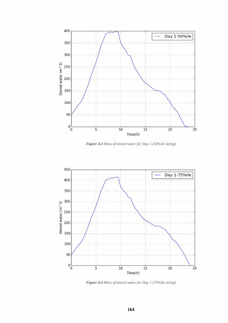
164



165



166



167



168



169


Furthermore, in Table 4.3 the total mass of fuel used during the day for each case is

shown, while in Table 4.4 the necessary geothermal flow rate for each case is shown.

Table 4.3 Total mass of fuel (kg) used over the day for each case


Day 1 440.08 43.75 0

Day 2 4471.05 486.71 0

Day 3 6069.25 2680.60 0

Day 4 14214.80 8891.59 3324.07

170

Table 4.4 Necessary geothermal flow rate (kg/s) for each case


Day 1 15.09 12.61 16.50

Day 2 20 36.01 38.66

Day 3 20 32.33 42.28

Day 4 20 40 60

4.4.2 Annual operation

In this section, the main results of the model of the annual operation of the installation

will be presented, while the main results will also be presented for the traditional case of

operation of a geothermal district heating system, i.e. without a heat storage. The

traditional case is defined as the following case:

No heat storage is used.

The mass flow rate is not constant throughout the day, but follows the heat

demand all the time.

When the geothermal energy cannot cover all the heat demand, peak-up boilers

are used.

Apart from the heat storage, the rest of the installation has exactly the same

dimensions as found in Chapter 3.

In other words, in the traditional case, the operation of an identical installation without

the heat storage which is operated in the traditional way is studied. The main results of the

studied case are shown on Table 4.5 for each case of sizing, while the results of the

traditional operation are shown on Table 4.6. By comparing these two tables, the

advantages of the proposed case will be identified. Finally, in Figs. 4.14-4.16 the volume

of water stored in the hot water storage tank throughout the whole year is shown for each

case of sizing, respectively.

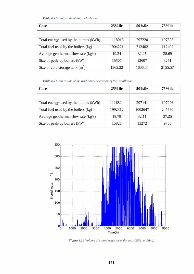
171

Table 4.5 Main results of the studied case


Total energy used by the pumps (kWh) 1118013 297220 107323

Total fuel used by the boilers (kg) 1904221 712402 112402

Average geothermal flow rate (kg/s) 19.34 32.25 38.69

Size of peak-up boilers (kW) 15507 12607 8251

Size of cold storage tank (m3) 1365.22 1606.04 2155.57

Table 4.6 Main results of the traditional operation of the installation


Total energy used by the pumps (kWh) 1116824 297141 107296

Total fuel used by the boilers (kg) 1992312 1002647 245580

Average geothermal flow rate (kg/s) 18.78 32.11 37.25

Size of peak-up boilers (kW) 15828 13272 9755

Figure 4.14 Volume of stored water over the year (25%ile sizing)

172



173

4.5 Discussion

Concerning the model of the operation over a random day, several interesting

observations can be made through the corresponding results. Firstly, it is shown that for the

same day of study as the sizing of the installation increases less fuel is used. This is totally

expected because as the sizing increases, more geothermal energy is available to cover the

heat demand. So, in the majority of the cases more geothermal energy is used for that

purpose. An interesting exception in the observation of the higher geothermal flow rate is

in Day 1, in the medium sizing of the installation, where the geothermal flow rate is lower

than that of the low sizing of the installation. This occurs either because of the limitations

of the geothermal flow rate (see Eq. (4.1)) or because the geothermal energy is much better

harvested in this case due to the higher storage capacity. Furthermore, the heat storage also

increases, which means that more geothermal energy can be stored in times of low load.

So, all these lead to the conclusion that a larger sizing of the geothermal installation leads

to a higher fraction of the load being covered by geothermal energy with subsequent

decrease of the use of fuel.

The second observation concerns the influence of the increase of the daily heat demand

for the same sizing of the installation. It can be seen that as the heat demand increases

more fuel is used to cover the heat demand which is expected as the geothermal installation

has a specific capacity and can never produce more heat than this capacity. This happens

although the geothermal flow rate also increases as the heat demand increases (see Table

4.4). The only exception is the case of the medium sizing of the installation between Days

2 and 3 where the geothermal flow rate is lower in the second case, which is not expected

as the heat demand is higher. This might occur for the same reasons as in the previous

paragraph. So, in general, it can be said that, for a specific installation, as the heat demand

increases both the geothermal flow rate and the fuel used will increase. If the heat demand

is relatively low compared to the capacity of the installation (see 75%ile case in Table 4.3),

the mass of fuel used will be zero and all the heat demand will be covered by geothermal

energy.

A third observation that arises from Table 4.3 in conjunction with Tables 4.1 and 4.2 is

that when the heat demand of a specific day is lower than the heat demand of the design-

day of the specific installation, then all the heat demand will not be necessarily covered by

geothermal energy. This is made clear on the case of Day 1: both in the low and the

174

medium sizing there is some fuel used to cover the heat demand, although the heat demand

of the design day of both cases is higher than for Day 1. This happens because, as

mentioned many times before, not only the total heat demand is important but also its

fluctuation within the day. So, a specific day can have such a fluctuation of its heat demand

from one time interval to the other that the heat demand at a specific time cannot be

covered without the help of the peak-up boilers. This observation makes clear the

importance of the fluctuation of the heat demand within the day.

Concerning the results of the annual operation of the installation, some very interesting

points can be made both for the different sizing of the installation when the heat storage is

used as well as between the cases where the heat storage is used and not. Firstly, when the

heat storage is used, it is seen by Table 4.5 that the energy used by the pumps decreases

when the sizing of the installation increases. This is justified by the fact that bigger

pipelines are used when the sizing increases, so the friction losses, and subsequently the

power required by the pumps, will decrease (see also section 3.2.6.2). Therefore, the total

energy used by the pumps throughout the year will decrease. Then, it is observed that as

the sizing of the installation increases the average geothermal flow rate throughout the year

will increase. This is totally expectable as the annual heat demand is obviously the same in

each case and since more geothermal energy is available as the sizing increases, more

geothermal energy will be harvested. Another interesting observation on the geothermal

flow rate is that the increase between the large and medium sizing is not so big as between

the medium and the low sizing. Intuitively, the medium sizing is expected to be closer to

the average demand throughout the year. So, in the case of the larger sizing, the geothermal

installation will be under-utilized leading to an average geothermal flow rate which is

higher than that of the medium sizing, but much smaller than its maximum flow rate (see

Table 3.2).

On the other hand, more geothermal energy harvested means that a higher fraction of

the annual heat demand is covered by geothermal energy, which in turn means that a

smaller fraction of this demand has to be covered by the peak-up boilers. So, the fact that

the fuel used throughout the year decreases as the sizing of the installation increases is

totally justified. For the same reason, the size of the peak-up boilers also decreases as the

sizing increases, since the peak demands that will have to be covered by the boilers will be

lower. Finally, as the system sizing increases the size of the cold storage tank increases.

This is expected as the size of the hot storage tank also increases as the system size

increases, as seen in Chapter 3, while the second component which defines the size of the

175

cold storage tank will be almost the same for each case. This happens because its

numerator will be exactly the same for each case and its denominator, which is the density

of water, will be roughly the same as the density of water is almost constant for the range

of the temperature used. In other words, the size of the cold storage tank will be almost

directly proportional to the size of the hot storage tank for a specific heat demand

throughout the year. So, as the sizing increases, the size of the hot storage tank increases

and, subsequently, the size of the cold storage tank will increase.

By comparing Tables 4.5 and 4.6, an initial comparison between the studied case and

the traditional operation of a geothermal district heating system can be made. First, it can

be seen that the energy used by the pumps throughout the year is almost the same whatever

the heat storage is used or not, for each case of sizing. This indicates that the total flow rate

throughout the installation over a whole year will be almost the same without being

affected by the presence of the heat storage. Then, it is observed that when the heat storage

is used, the amount of fuel used throughout the year decreases. This indicates that with the

inclusion of the heat storage, geothermal energy is utilised in a more optimal way

decreasing the reliance on the peak-up boilers. This observation is among the most

important of this thesis. It can also be observed that the average geothermal flow rate

increases when the heat storage is used, but only slightly. This increase of the geothermal

flow rate does not justify the decrease of the fossil fuel consumption, enhancing in this way

the role of the heat storage in better matching demand and supply of heat.

Another interesting observation concerning the mass of fuel used, is that the absolute

decrease when the heat storage is used in the low and large sizing cases is smaller than in

the medium sizing. This happen because in the low sizing, the geothermal capacity is low

compared to the heat demand on the majority of the times around the year, so all the

geothermal energy will be sent time directly to the heat demand most of the time during the

year. This can also be observed by Fig. 4.14 where it is seen that for a large amount of time

around the year the amount of stored water is relatively low for the low sizing of the

installation. So, the heat storage will not have a big impact in this case and the amount of

fuel used will be roughly the same either whether the storage is used or not. On the other

hand, in the large sizing of the installation the geothermal capacity is big enough to cover

alone the heat demand the majority of time. So, the amount of fuel used will be small

anyway and the decrease in the fuel consumption will be relatively small. All these

indicate that the heat storage is better utilised in the case of the medium sizing of the

installation, although a decrease in fuel consumption is observed in any case. This comes

176

in agreement with Figs. 4.14-4.16 where it is observed that in the medium sizing of the

installation, more water is stored compared to the maximum capacity of the storage in each

case. In the low sizing of the installation, as mentioned before, a large amount of time the

storage is not used as all the geothermal production is sent directly to the load, while in the

large sizing of the installation, the storage is not used that much mainly in periods of low

load (summer months) as the heat demand can be covered solely by the adjustment of the

geothermal flow rate in the appropriate value.

Finally, the size of the boilers increases when the heat storage is not used, which is

expected as more and probably higher peak demands will occur in this case. But, the

increase in the size of the peak-up boilers when the heat storage is not used is small

compared to the increase in the mass of fuel used. This denotes that the peak demands

throughout the year will be roughly the same numerically no matter whether the heat

storage is used or not, but these will be much more frequent when the heat storage is not

used. This reconciles the apparent disagreement between the increase of the size of the

peak-up boilers and the increase in fuel consumption. A more detailed comparison between

the studied and the traditional case will be carried out in Chapter 5, where economic,

environmental and further energetic details will be calculated.

4.6 Summary

This Chapter studies in detail the operation of the installation sized in Chapter 3 either

for a random day or for a whole year. So, two models were developed for the study of

these two cases. The model that studies the operation of the installation over a random day

was explained in section 4.2, while the model that studies the annual operation was

explained in section 4.3. Then, the results for both models were shown in section 4.4

followed by an extensive discussion in section 4.5.

In the first model, the inputs are the sizing of the installation from Chapter 3. The

topology of the installation that was also used as an input in Chapter 3 together with the

heat demand of the random studied day are the other inputs of this model. Furthermore,

some initial estimations which are derived from the design-day of the specific case are also

used as inputs. By applying the model described in section 4.2, the operational strategy of

the installation for the studied day will be known. It is recalled that the operational strategy

is defined as the complete knowledge of the operation of the installation during the studied

177

day, i.e. the necessary geothermal flow rate, when and by how much should the storage

tank be charged or discharged, when and by how much should the peak-up boilers be used

etc. Furthermore, an analytical mapping of the temperatures in the critical points of the

installation will also be known over the day. Finally, the electricity used by the pumps as

well as the fuel used by the peak-up boilers throughout the day will also be known with the

application of this model.

In other words, this model shows how the installation that is already built should be

operated in a day with a known or predicted heat demand. Practically, it is much easier to

predict the weather conditions rather than the heat demand of a specific (usually the next)

day. For that purpose, an attempt to connect the given heat demand with the weather

conditions of the area was attempted in Appendix B. The results of this Appendix are

discouraging as it is shown that the correlation between the heat demand and the weather

conditions is not always straightforward as other factors, such social factors or the heat

capacity of the building, greatly influence the heat demand. These factors are, in general,

difficult to predict, so this correlation is difficult to be produced. Of course, general

conclusions cannot be made as this correlation and its influencing factors are very case-

specific and in our case are not known. Theoretically, if this correlation is achieved, then

by integrating this correlation with the model developed in section 4.2, the operation of the

installation can be known the next day given the weather conditions. Intuitively, this is

more useful than predicting the heat demand for any day as the weather forecasts are

typically provided by professionals on the field and the accuracy is much higher than

predicting the heat demand. So, if a robust correlation is built between the heat demand

and the weather conditions, then one of the basic inputs of the model will be much more

accurate and, subsequently, the operational strategy provided will be more precise and

close to the reality. The other two main inputs of the model, i.e. the sizing and the topology

of the installation, are constant and cannot cause any errors to the results. So, if the third

input is more accurate, then, the accuracy of the results will increase a lot.

In the second model, the first model is used as a basis and is applied serially for each

day of the year. In the first model, some variables from the previous day of study are

needed as inputs, while some of the results from the last time interval will be used as inputs

in the next day. In this case, the outputs of the previous day are used automatically as

inputs of the next day. In general, the inputs of this model are the same as in the previous

model apart from the heat demand, where the heat demand of the whole year is used. The

outputs of this model are the same as for the previous one, but they concern the whole year

178

obviously. The outputs of interest in this case are mainly the total electricity used by the

pumps and the mass of fuel used by the peak-up boilers throughout the year and the

average geothermal flow rate. The first two comprise the main operational costs of the

installation and will be among the main inputs in the economic analysis of the installation

that will be presented in the next Chapter, while the average geothermal flow rate will be

used for the calculation of the main energetic indices of the installation. Finally, this model

provides also the size of the cold water storage tank as well as of the peak-up boilers,

filling the gap in the model of Chapter 3.

As the first model studies the operation of the installation over a random day, it was

applied to four random days around the year with daily heat demands between the limits

set by the three design-days for each case of sizing. The main findings of this model are the

following:

For the same day of study, as the sizing of the installation increases, more

geothermal energy is used leading to the reduction of the fuel used. So, a

bigger fraction of the daily heat demand is covered by geothermal energy.

For the same sizing of the installation, as the daily heat demand of the studied

day increases, then both the geothermal flow rate and the mass of fuel increase.

If the daily heat demand is lower than the daily heat demand of the design-day

of the specific installation, then it is not necessary for all the heat demand to be

covered by geothermal energy only. The fluctuation of the heat demand across

the day is equally important for the operation of the installation with the daily

heat demand.

The second model is then applied for the three cases of sizing using the heat demand

around the year and an initial comparison is carried out with the traditional operation of

these systems where no heat storage is used. The main findings in this case are as follows:

In the case of using the heat storage, as the sizing of the installation increases,

then the electricity used by the pumps decreases, the mass of fuel used by the

peak-up boilers decreases, and the size of the peak-up boilers decreases, while

on the other hand, the average geothermal flow rate and the volume of the cold

water storage tank increase.

179

For the same sizing of the installation, when comparing the case of using the

heat storage and the traditional case, it is observed that the electricity used by

the pumps is roughly the same, the mass of fuel used by the boilers decreases

when the heat storage is used with a subsequent decrease in the size of the

boilers, while on the other hand the average geothermal flow rate increases.

The heat storage seems to be better utilised in the medium sizing of the

installation (50%ile).

A more comprehensive and detailed comparison between the studied case of including

a heat storage in the system and the traditional case will be carried out in the next Chapter,

where the main findings of the second model of this Chapter will be used as input. So,

concluding, the first model in this Chapter is a very useful tool for the technicians of the

installation that can know in advance how to operate the installation over a day with a

given (or predicted) heat demand, while the second model sizes the rest of the installation

that could not be sized in Chapter 3, and provides the main running costs of the installation

together with the average geothermal flow rate. All these will be among the main inputs in

the next Chapter.

180

5 ECONOMIC, ENVIRONMENTAL AND ENERGETIC

ANALYSIS OF A GEOTHERMAL DISTRICT HEATING

SYSTEM

5.1 Introduction

In this Chapter, the economic, environmental and energetic feasibility of the proposed

operation of a geothermal district heating system (GDHS) with a storage tank will be

studied and a comparison with the traditional case will be carried out. The main goal of

this Chapter is to compare the studied case of this thesis with the traditional operation of

these systems in order to conclude eventually if it is worthwhile integrating a storage tank

or not. In other words, this Chapter does not compare the studied case with alternative

technologies, but only with the traditional case (i.e. with no storage). For that purpose, as

will be made clear later on this Chapter, some parameters that will be considered common

between the two cases will be neglected. So, some of the results might not depict their

actual values in terms of real installations and, therefore, a straight comparison with typical

values of other technologies should not be made. But, these values are considered adequate

to make a comparison between the studied and the traditional case. This comparison will

be made for each case of sizing of the installation in order to identify the influence of the

sizing on the economics of the installation.

The main inputs of this Chapter are the outputs of the model of the annual operation of

the installation that was studied in section 4.3, and the capital costs of several parts of the

unit. In this Chapter, the inputs are much less than in the previous two Chapters, so these

will not be explained in a separate section. Then, through the methodology presented the

basic economic, environmental and energetic indices of the studied case will be calculated

and a comparison with the traditional case (for which the same indices will also be

calculated), will be made. The final answer that will be attempted to be provided in this

Chapter is the following: “Is it worthwhile including a heat store within the proposed

operation of a geothermal district heating system or not?”

In this section, a brief introduction in this Chapter was given. In section 5.2, the

methodology for all the necessary calculations will be explained in detail, while in section

5.3 the results of the studied and the traditional case will be shown. Finally, a discussion on

181

the results will be provided in section 5.4, followed by some concluding remarks in section

5.5.

5.2 Methodology

5.2.1 Economic analysis

In this section, the calculation of the basic economic indices both of the studied

installation as well as of the traditional case will be explained. The calculations are the

same for both cases (apart from the capital cost of the storage tanks that will be zero in the

traditional case as there is no storage in this case). The cash flows for these two cases will

be also explained for that purpose. Initially, the financial outflows and incomes of the

investment have to be calculated. These will be explained in detail in the following two

sections.

5.2.1.1 Calculation of the investment expenditure

The investment expenditure consists of the following parts:

Initial capital cost.

Capital cost of some units that will be replaced after some years of operation.

Running costs in the first year of operation.

Running costs in subsequent years.

The calculation of these parts, which are necessary for all the subsequent calculation

will be explained in this section. First, it is assumed that the installation is built in year n=0

and it starts operating in year n=1. Both the initial capital and running costs will be

calculated for the year n=0, but for the cash flows, the running costs from year n=1 and

onwards will be taken into account, as the installation will operate in these years. The

initial capital cost of the installation is calculated by the following equation:

𝐶𝐶𝑡𝑜𝑡0 = 𝐶𝐶𝑑𝑟

0 + 𝐶𝐶𝐻𝑆𝑇0 + 𝐶𝐶𝐶𝑆𝑇

0 + 𝐶𝐶𝑝𝑏0 + 𝐶𝐶𝑛𝑝

0 + 𝐶𝐶𝑜𝑡0 (5.1)

182

Where:

𝐶𝐶𝑡𝑜𝑡0 = Total initial (year n=0) capital cost (£)

𝐶𝐶𝑑𝑟0 , 𝐶𝐶𝐻𝑆𝑇

0 , 𝐶𝐶𝐶𝑆𝑇0 , 𝐶𝐶𝑝𝑏

0 , 𝐶𝐶𝑛𝑝0 , 𝐶𝐶𝑜𝑡

0 = Initial capital cost of several equipment used

during the construction of the installation (Drilling, hot and cold water storage tanks, peak-

up boilers, network pipelines and other costs, respectively) (£)

In applying the above equation, typical costs for specific components of the capital

expenditure were assembled on the basis of discussion with UK practitioners in the

geothermal direct use sector. For the drilling costs, it was assumed that the first deep

borehole would cost £1.5M, decreasing to £1M for later boreholes. The latter are cheaper

as ground conditions would be better known in advance and the risk of drilling would

decrease. Furthermore, it is assumed that one re-injection well will also be drilled in each

case of study in order to maintain the flow of geothermal fluid in the underground and

avoid the degradation of the geothermal resource. It should be pointed out that the number

of wells calculated in Chapter 3 are the production wells, as based on these the available

geothermal flow rate was calculated. So, if the number of production wells calculated in

Chapter 3 are 𝑁𝑤𝑒𝑙𝑙𝑠, then the total number of wells will be 𝑁𝑤𝑒𝑙𝑙𝑠 + 1 and the cost of

drilling will be given in million £ as follows:

𝐶𝐶𝑑𝑟0 = 1.5 + 𝑁𝑤𝑒𝑙𝑙𝑠 ∙ 1 (5.2)

The capital cost of the network pipelines includes the cost of materials, which are

carbon steel and mineral wool (insulation), the cost of welding and the civils costs for

burying the pipes underground. The cost of the material is calculated by Eqs. (3.41)-(3.42)

since the dimensions of the pipelines are known. The unit cost of carbon steel is estimated

at £400/tonne and the cost of mineral wool at £60/m3. The cost of welding is assumed to be

£1000 per weld and meter of diameter and there will be one welding every 6 meters of

pipeline. Finally, the civils costs are assumed to be £300 per meter of pipeline. So, for each

pair of pipelines, their capital cost will be calculated by the following equations:

𝐶𝐶𝑛𝑝0 = 2 ∙ (𝐶𝐶𝑚𝑎𝑡

0 + 𝐶𝐶𝑤𝑒𝑙𝑑0 ) + 𝐶𝐶𝑐𝑖𝑣𝑖𝑙

0 (5.3)

𝐶𝐶𝑤𝑒𝑙𝑑0 = 1000 ∙ 𝐷𝑝,𝑜 ∙

𝐿𝑝

6 (5.4)

𝐶𝐶𝑐𝑖𝑣𝑖𝑙0 = 300 ∙ 𝐿𝑝 (5.5)

183

Where:

𝐶𝐶𝑚𝑎𝑡0 = Capital cost of the materials of the pipelines in year n=0 (£)

𝐶𝐶𝑤𝑒𝑙𝑑0 = Capital cost of the welding of the pipelines in year n=0 (£)

𝐶𝐶𝑐𝑖𝑣𝑖𝑙0 = Civils costs for the burying of the pipelines in year n=0 (£)

𝐷𝑝,𝑜 = External diameter of the pipelines (not including the insulation) (𝑚)

𝐿𝑝 = Length of each pipeline (𝑚)

In Eq. (5.3), the factor 2 is used in the first two terms in order to account for both the

supply and the return pipeline. On the other hand, it is not used in the calculation of the

civil costs as one excavation will be done for each pair of pipelines. The costs in Eqs.

(5.3)-(5.5) are all given in £.

Concerning the costs of the tanks, these include the materials, civils costs, the erection

on slab and other minor costs. The materials of the storage tanks include carbon steel as the

main material of the tank, mineral wool for insulation, mild steel as the material of the

cover of the tank and concrete which is used as the base of the tank. The thickness of

carbon steel has been calculated in Chapter 3, while the thickness of the mineral wool is

assumed to be 20cm, the thickness of the cover is assumed to be 3mm and the thickness of

the concrete base to be 50cm. So, since the diameter of each storage tank is known from

Chapters 3 and 4, respectively, the volume of each material can be easily calculated. Then,

the volume of each material is calculated by the unit costs in order to identify the cost of

each material. Finally, all the costs are summed together for the calculation of the cost of

each tank. So, indicatively, the cost of materials of the hot water storage tank will be given

as:

𝐶𝐶𝑚𝑎𝑡,𝐻𝑆𝑇0 = 𝑉𝑐,𝑠𝑡𝑒𝑒𝑙 ∙ 𝐶𝑢,𝑐,𝑠𝑡𝑒𝑒𝑙 + 𝑉𝑖𝑛𝑠 ∙ 𝐶𝑢,𝑖𝑛𝑠 + 𝑉𝑐𝑜𝑣 ∙ 𝐶𝑢,𝑐𝑜𝑣 + 𝑉𝑐𝑜𝑛 ∙ 𝐶𝑢,𝑐𝑜𝑛 (5.6)

Where:

𝐶𝐶𝑚𝑎𝑡,𝐻𝑆𝑇0 = Initial capital cost of the materials of the hot water storage tank (£)

𝑉𝑐,𝑠𝑡𝑒𝑒𝑙, 𝑉𝑖𝑛𝑠, 𝑉𝑐𝑜𝑣, 𝑉𝑐𝑜𝑛 = Volumes of the carbon steel, insulation, cover and concrete

used in the hot water storage tank, respectively (𝑚3)

𝐶𝑢,𝑐,𝑠𝑡𝑒𝑒𝑙, 𝐶𝑢,𝑖𝑛𝑠, 𝐶𝑢,𝑐𝑜𝑣, 𝐶𝑢,𝑐𝑜𝑛 = Unit cost of carbon steel, insulation, cover and

concrete, respectively (£

𝑚3)

184

In the above equation, the unit costs of carbon steel and of the insulation are the same

as those for the pipelines, while the unit cost for the cover is assumed to be the same as that

of carbon steel. Furthermore, the unit cost of concrete is assumed to be equal to £50/m3.

The other costs of the tank are assumed on the basis of recent projects in the UK. More

details on these assumptions can be found in Appendix C. Eventually, the capital cost of

the hot water storage tank, for example, will be calculated as:

𝐶𝐶𝐻𝑆𝑇0 = 𝐶𝐶𝑚𝑎𝑡,𝐻𝑆𝑇

0 + ∑𝐶𝐶𝑖 (5.7)

In the above equation, the second part refers to the other costs included in the

calculation of the capital cost of the tanks.

Moreover, for the cost of the peak-up boilers, an average capital cost of £200/kW2 is

assumed for industrial gas boilers. So, the capital cost of the peak-up boilers is calculated

as:

𝐶𝐶𝑝𝑏0 = 200 ∙ 𝑄𝑝𝑏 (5.8)

In the above equation, the thermal power of the peak-up boilers (𝑄𝑝𝑏) has been

calculated in Chapter 4, and has to be used in units of kW. Finally, other minor costs

include pumps, heat exchangers, in-house installations, salaries of workers etc., all of

which have been estimated from recent analogous projects in the UK. So, by applying Eqs.

(5.1)-(5.8) the calculation of the initial or up-front capital cost of the installation is

possible. As mentioned before, in the traditional case of operation, the costs of the hot and

cold storage tank will not be calculated by Eq. (5.7), but will be equal to zero as no storage

tank is built in this case.

As mentioned before, several parts of the installation will need to be replaced after

several years of operation, since they have a limited lifetime. More specifically, it is

assumed that the peak-up boilers will be replaced after 20 years of operation, while the

heat exchangers and the pumps will be replaced after 15 years of operation. Their cost at

the time of the replacement will be calculated based on their initial capital cost and an

average annual increase of the equipment which can be either set equal to the discount rate

2 http://2050-calculator-tool-wiki.decc.gov.uk/cost_categories/82

http://2050-calculator-tool-wiki.decc.gov.uk/cost_categories/82

185

or another value depending on the specific market and its trends. So, these costs are

calculated by an equation like the following:

𝐶𝐶𝑥𝑛 = 𝐶𝐶𝑥

0 ∙ (1 + 𝐴𝐴𝐼𝐶𝐶,𝑥)𝑛 (5.9)

Where:

𝐶𝐶𝑥𝑛 = Capital cost of x equipment of the installation in year n (£)

𝐶𝐶𝑥0 = Capital cost of x equipment of the installation in year n=0 (£)

𝐴𝐴𝐼𝐶𝐶,𝑥 = Average annual increase of the capital cost of x equipment (%)

The above equation refers to any of the aforementioned equipment. In our case, the

average annual increase of any part of the capital cost is assumed to be 3%. These costs of

replacement will have to be taken into account in the calculation of the cash flows of the

installation.

The running costs of the installation include the cost of fuel used by the boilers, the cost

of electricity used by the pumps, the salaries of workers, the carbon taxes and other minor

costs. The calculation of these costs for the first year of operation will be shown, and then

the calculation of their values in the next years which are necessary for the cash flows will

be explained.

The total fuel used over the year as well as the total electricity used by the pumps has

been calculated in Chapter 4. Then, for the calculation of the unit cost for gas, which is the

fuel used and electricity, their historic prices for non-domestic users are used. These

historic prices were found on the website of the Department of Energy and Climate Change

of the UK3. A chart of these prices is included in Appendix D. Then, the values for 2013

have been used as unit costs for gas and electricity. So, the initial running costs of the fuel

and electricity are calculated, respectively, as:

𝑅𝐶𝑓0 = 𝑀𝑓,𝑡𝑜𝑡 ∙ 𝐶𝑢,𝑓 (5.10)

𝑅𝐶𝑒𝑙0 = 𝐸𝑒𝑙,𝑡𝑜𝑡 ∙ 𝐶𝑢,𝑒𝑙 (5.11)

3 https://www.gov.uk/government/statistical-data-sets/gas-and-electricity-prices-in-the-non-domestic-

sector

186

Where:

𝑅𝐶𝑓0, 𝑅𝐶𝑒𝑙

0 = Annual running cost of fuel and electricity in year n=0 (£)

𝑀𝑓,𝑡𝑜𝑡 = Total mass of fuel used by the peak-up boilers per year (𝑘𝑔)

𝐸𝑒𝑙,𝑡𝑜𝑡 = Total electricity used by the pumps per year (𝑘𝑊ℎ)

𝐶𝑢,𝑓 = Unit cost of fuel (£

𝑘𝑔)

𝐶𝑢,𝑒𝑙 = Unit cost of electricity (£

𝑘𝑊ℎ)

The salaries of workers are quite case-specific, so in our case these are assumed based

on an average salary of £2500 per month. Then, the cost of carbon taxes is assumed to be

£15 per tonne of CO2 emitted in the environment. The latter will be calculated in a

following section. So, the initial running cost of carbon taxes is calculated as:

𝑅𝐶𝑐𝑡0 = 15 ∙ 𝑀𝐶𝑂2,𝑡𝑜𝑡 (5.12)

Where:

𝑅𝐶𝑐𝑡0 = Annual running cost for carbon taxes in year n=0 (£)

𝑀𝐶𝑂2,𝑡𝑜𝑡 = Annual CO2 emissions of the installation (𝑡𝑛)

In the above equation, the total mass of CO2 emitted has to be used (in tonnes). This

value will be calculated in section 5.2.2. Finally, the other running costs include any other

costs that might occur during the operation of the installation and are assumed to be equal

to £30000 for every case. Therefore, the total initial running cost of the installation is

calculated by the following equation:

𝑅𝐶𝑡𝑜𝑡0 = 𝑅𝐶𝑓

0 + 𝑅𝐶𝑒𝑙0 + 𝑅𝐶𝑤

0 + 𝑅𝐶𝑐𝑡0 + 𝑅𝐶𝑜𝑡

0 (5.13)

Where:

𝑅𝐶𝑡𝑜𝑡0 = Total annual running cost of the installation in year n=0 (£)

𝑅𝐶𝑤0 , 𝑅𝐶𝑜𝑡

0 = Annual running costs of workers and others in year n=0 (£)

As mentioned earlier, the installation is assumed to be operating from year n=1

onwards. So, the running costs used in the calculation of the cash flows will be calculated

from that year and after, although the initial running costs will be used in the calculation of

some economic indices as will be seen later. Therefore, an average annual increase for

187

each part of the running cost will be considered and its value after n years will be

calculated by an equation similar to Eq. (5.9).

𝑅𝐶𝑥𝑛 = 𝑅𝐶𝑥

0 ∙ (1 + 𝐴𝐴𝐼𝑅𝐶,𝑥)𝑛 (5.14)

Where:

𝑅𝐶𝑥𝑛 = Annual running cost of x kind in year n (£)

𝑅𝐶𝑥0 = Annual running cost of x kind in year n=0 (£)

𝐴𝐴𝐼𝑅𝐶,𝑥 = Average annual increase of the running cost of x kind (%)

So, an average annual increase for each part of the running cost has to be considered.

For the case of the fuel, the charts of its historic prices is used as happened for the

calculation of its unit prices that was used in Eq. (5.10). In this case, the unit price of fuel

over the last ten years is considered and its annual increase from year to year is calculated.

Then, the average of these annual increases is calculated and is assumed that the annual

increase from now onwards will be equal to this average annual increase of the previous

ten years. Exactly the same process is followed for the calculation of the average annual

increase of the electricity cost.

The average annual increase of the salaries of workers is assumed to be 2.5%, while the

average annual increase of other running costs is assumed to be equal to the discount rate,

which in our case is assumed to be 5%. Finally, the cost of the carbon taxes is assumed to

be constant over the years, as there is no certainty over its evolution in the future. So, its

average annual increase will be 0%.

5.2.1.2 Calculation of income

The income in this study consists of the following three parts:

A fixed cost per day which guarantees a certain income and is used for the

repayment of the initial capital cost. For each case, it is fixed in such a value so

that the initial capital cost is repaid within 10 years.

A variable cost which depicts the real consumption of energy. As a base case

for this research, the variable cost is fixed at £0.02/kWh of heating provided.

188

A financial incentive recently established in the UK, the so-called RHI

(Renewable Heat Incentive), which provides £0.05/kWh of renewable heat

provided. This value increases by 2.5% each year and the incentive is provided

for the first 20 years of operation of the installation.

So, the incomes of the investment in year n=0 are calculated by the following

equations:

𝐼𝐶𝑡𝑜𝑡0 = 𝐼𝐶𝑓𝑖𝑥

0 + 𝐼𝐶𝑣𝑎𝑟0 + 𝐼𝐶𝑅𝐻𝐼

0 (5.15)

00

10

1

(1 )

totfix i

i

hp

i

CCIC

AAI

(5.16)

𝐼𝐶𝑣𝑎𝑟0 = 𝐴𝐻𝐷 ∙ 𝐶ℎ𝑝,𝑢

0 (5.17)

𝐼𝐶𝑅𝐻𝐼0 = 𝐴𝐻𝐷𝐺 ∙ 0.05 (5.18)

Where:

𝐼𝐶𝑡𝑜𝑡0 = Total income of the investment in year n=0 (£)

𝐼𝐶𝑓𝑖𝑥0 , 𝐼𝐶𝑣𝑎𝑟

0 , 𝐼𝐶𝑅𝐻𝐼0 = Fixed, variable and income from the RHI in year n=0 (£)

𝐴𝐴𝐼ℎ𝑝 = Average annual increase of the price of heating (%)

𝐶ℎ𝑝,𝑢0 = Unit price of heating in year n=0 (

£

𝑘𝑊ℎ)

𝐴𝐻𝐷 = Annual heat demand (𝑘𝑊ℎ)

𝐴𝐻𝐷𝐺 = Annual heat demand covered by geothermal energy, which is calculated in

section 5.2.4 (𝑘𝑊ℎ)

It is recalled that the installation will start operating at year n=1, so the incomes will

also start from this year onwards. The calculation of the above values is taking place only

for computational purposes and in order to make the following calculations easier.

As mentioned before, the fixed cost is calculated on the basis of repaying the initial

capital cost in 10 years. By observing Eq. (5.16), it is seen that the counter in the

denominator starts from i=1. This happens because the installation starts operating in year

n=1, so the revenue will start from that year, as stated previously. Furthermore, it is seen

189

that in order to get the value of the fixed cost, a simple division by the number of years is

not made, but an average annual increase in the heating price is taken into account. This

happens, because the price of heating should increase every year in order to compensate

for the increase in the expenditure and general year-on-year inflation.

So, the fixed cost will increase over the following years with an average annual

increase of the heating price which, in our case, is assumed to be 3% lower than the

average annual increase of the fuel. The same average annual increase will also apply to

the variable cost of heating. Finally, as mentioned before, the income from the RHI

subsidy will increase by 2.5% each year. So, the income of the investment the following

years will be given by the following equations:

𝐼𝐶𝑡𝑜𝑡𝑛 = 𝐼𝐶𝑓𝑖𝑥

𝑛 + 𝐼𝐶𝑣𝑎𝑟𝑛 + 𝐼𝐶𝑅𝐻𝐼

𝑛 (5.19)

𝐼𝐶𝑓𝑖𝑥𝑛 = 𝐼𝐶𝑓𝑖𝑥

0 ∙ (1 + 𝐴𝐴𝐼ℎ𝑝)𝑛 (5.20)

𝐼𝐶𝑣𝑎𝑟𝑛 = 𝐼𝐶𝑣𝑎𝑟

0 ∙ (1 + 𝐴𝐴𝐼ℎ𝑝)𝑛 (5.21)

𝑰𝒇 𝑛 ≤ 20:

𝑻𝒉𝒆𝒏: 𝐼𝐶𝑅𝐻𝐼𝑛 = 𝐼𝐶𝑅𝐻𝐼

0 ∙ (1 + 0.025)𝑛

𝑬𝒍𝒔𝒆: 𝐼𝐶𝑅𝐻𝐼𝑛 = 0

} (5.22)

𝐴𝐴𝐼ℎ𝑝 = 𝐴𝐴𝐼𝑅𝐶,𝑓 − 0.03 (5.23)

Where:

𝐼𝐶𝑡𝑜𝑡𝑛 = Total income of the investment in year n (£)

𝐼𝐶𝑓𝑖𝑥0 , 𝐼𝐶𝑣𝑎𝑟

0 , 𝐼𝐶𝑅𝐻𝐼0 = Fixed, variable and income from the RHI in year n (£)

𝐴𝐴𝐼𝑅𝐶,𝑓 = Average annual increase of the running cost of fuel (%)

5.2.1.3 Calculation of the financial indices

Initially, the comparison between the studied and the traditional case of a geothermal

district heating system will be based on the comparison of several financial indices of each

case. The calculation of the necessary capital and running costs has been done in the

190

previous section. The definitions and explanations of the following economic indices were

well summarised in Chapter 2.

The first financial index used is the levelised cost of heating (𝐿𝐶𝐻), i.e. the minimum

price that heat should be sold to the consumers in order to have a feasible investment and is

equivalent to the unit cost of energy (𝑈𝐶𝐸) described in Chapter 2. This is calculated by

Eqs. (2.35) and (2.36) properly formulated for our problem as follows:

𝐿𝐶𝐻 =𝐶𝐶𝑡𝑜𝑡∙𝐶𝑅𝐹+𝑅𝐶𝑡𝑜𝑡

0

𝐴𝐻𝐷 (5.24)

𝐶𝑅𝐹 =𝐼𝑅

1−(1+𝐼𝑅)𝑁 (5.25)

Where:

𝐿𝐶𝐻 = Levelised cost of heating (£

𝑘𝑊ℎ)

𝐶𝑅𝐹 = Cost recovery factor (Dimensionless)

In Eq. (5.24), the whole capital cost should be included, taking into account both the

initial capital cost as well as the cost of replacement of any units in the future, as explained

earlier. For that purpose, no temporal superscript has been assigned to this variable. The

capital cost of the next years should be reduced in current values through the discount rate.

So, the total capital cost that will be used in Eq. (5.24) is calculated through the following

equation:

0 (1 )

nn Ntot

tot nn

CCCC

DR

(5.26)

Where:

𝐷𝑅 = Discount rate (Dimensionless)

Then, the running cost of year n=0 is also used in the numerator of Eq. (5.24). So, it is

seen that the values of the total capital cost and of the running cost both in year n=0 are

used for the calculation of the levelised cost of heating. Furthermore, the cost recovery

factor is used in Eq. (5.24) in order to break down the capital cost over the whole

investment period. As can be observed in this equation, the running cost of one year, and

191

more specifically of year n=0, is used. This is the only case where the running cost of year

n=0, which does not exist in reality, will be used. Furthermore, the capital cost that refers

to one year has to be used also. Although the total capital cost is all spent in specific years

of the investment, and mainly in year n=0, it actually refers to all the years of operation

and, theoretically, has to be re-paid in these years. Therefore, the cost recovery factor is

implemented so that both the capital and the running costs refer to one year of operation of

the installation. The levelised cost of heating cannot provide useful information for one

investment, but for the comparison between two or more investments. When comparing

two or more investments, the investment with the lower levelised cost is the more feasible

one, as a lower levelised cost indicates that this investment can be equally feasible with the

other one even if the heat is sold cheaper. In other words, for the same selling price of heat,

the income and the benefits of the installation with lower levelised cost will be higher.

The second financial index that is used is the net present value (NPV) of the

investment, which is defined as the summary of the discounted cash flows over the whole

investment period. In other words, the net cash flow is calculated for each year of

operation and the discount rate is used in order to transform this in today’s value. Then, all

these discounted values are summed together and provide the net present value of the

investment. So, the net present value is calculated by the following equations:

𝑭𝒐𝒓 𝑒𝑎𝑐ℎ 𝑦𝑒𝑎𝑟 𝑜𝑓 𝑜𝑝𝑒𝑟𝑎𝑡𝑖𝑜𝑛 𝑛:

𝑁𝐶𝐹𝑛 = 𝐼𝐶𝑡𝑜𝑡𝑛 − 𝐶𝐶𝑡𝑜𝑡

𝑛 − 𝑅𝐶𝑡𝑜𝑡𝑛

𝐷𝑁𝐶𝐹𝑛 =𝑁𝐶𝐹𝑛

(1+𝐷𝑅)𝑛

} (5.27)

0

n Nn

n

NPV DNCF

(5.28)

Where:

𝑁𝐶𝐹𝑛 = Net cash flow in year n (£)

𝐷𝑁𝐶𝐹𝑛 = Discounted net cash flow of year n (£)

In Eq. (5.27) the net cash flow in year n=0 has to be taken into account also.

Theoretically, if the net present value is positive, this indicates that the investment is

feasible. From another point of view, when comparing two investments the investment

192

with the higher net present value is the more feasible one. The discount rate that is used in

this study is assumed to be constant and equal to 5%.

The third financial index that is used is the internal rate of return of the investment

(IRR). This is defined as the discount rate that nullifies the net present value. So, in this

case, the net present value is set equal to zero in Eq. (5.28) and then this equation together

with expression (5.27) are solved for the discount rate. So, the internal rate of return is

calculated by the following expression.

𝐼𝑅𝑅 = 𝐷𝑅 (𝑓𝑜𝑟 𝑁𝑃𝑉 = 0) (5.29)

In theory, the value of the internal rate of return when compared with the current

interest rate can indicate how feasible an investment is. If the IRR is higher than the

interest rate, then the investment is feasible, while if it is lower the investment is

unfeasible. When comparing two or more investments, the one with the higher IRR is the

more feasible and financially “safe” investment as it is further from the current interest

rate.

The fourth, and final, financial index is the benefits-to-costs ratio of the investment

(BCR). This index is defined as the sum of the discounted benefits of each year divided by

the sum of the discounted capital costs of each year. In the numerator, the benefits are

defined as the difference of the income minus the running costs, so the capital costs are not

taken into account there, but only in the denominator. In other words, the benefits-to-costs

ratio is the ratio of the earnings to the capital expenditures. Therefore, the BCR is

calculated by the following expressions:


𝐴𝐵𝐹𝑛 = 𝐼𝐶𝑡𝑜𝑡𝑛 − 𝑅𝐶𝑡𝑜𝑡

𝑛

𝐷𝐴𝐵𝐹𝑛 =𝐴𝐵𝐹𝑛

(1+𝐷𝑅)𝑛

} (5.30)


𝐷𝐶𝐶𝑛 =𝐶𝐶𝑡𝑜𝑡

𝑛

(1+𝐷𝑅)𝑛} (5.31)

193

0

0

n Nn

n

n Nn

n

DABF

BCR

DCC

(5.32)

Where:

𝐴𝐵𝐹𝑛 = Annual benefits in year n (£)

𝐷𝐴𝐵𝐹𝑛 = Discounted annual benefits in year n (£)

𝐷𝐶𝐶𝑛 = Discounted capital cost in year n (£)

The benefits-to-costs ratio can indicate either if one investment is feasible or not, but it

can also indicate which investment if more feasible among two or more investments. For

an investment to be feasible, the benefits-to-cost ratios has to be higher than 1, i.e. the net

benefits to be higher than the capital expenditures. When comparing two or more

investments, the investment with the higher value of the benefits-to-costs ratio is more

feasible as it indicates higher values of benefits.

In this section, the calculation of four different financial indices that can indicate if the

proposed solution is more feasible than the traditional case from an economic point of view

was explained. As mentioned before, all the indices have the capability to show which of

the two cases is more feasible, while the NPV, the IRR and the BCR can also show if an

investment is feasible, in general, or not without comparing both of them. For example, if

the values of the IRR for the two cases are 1% and 2%, respectively, this indicates that the

second case is more feasible than the first one, but in reality, both these values are lower

than the current interest rates (around 6% or more). So, none of these investments are

feasible. Therefore, not only a comparison between the two cases should be made, but the

values of these indices should also indicate that the investments are feasible. Furthermore,

it should be mentioned that the IRR, the BCR and, partially, the LCH provide qualitative

information about the investment, and not quantitative. In other words, their values are

independent of the size of the investment. Two investments with completely different

capital costs and incomes can have the same values of the above indices. Only, the NPV

provides quantitative information about the investment and is a very good indicator of the

economic size of the investment. Finally, these indices are used since they can indicate the

more feasible of two possible investments; however, if the results are close one another,

then one of the indices might not depict the truth. So, all of them are used together in order

to obtain more robust results.

194

5.2.1.4 Cash flows of the investment

The cash flow of an investment is a graph which depicts the monetary value of the

investment at each specific period over time. It includes all the expenditure that occurs

from the construction and during the operation of the installation, i.e. all the capital and

running costs, as well as the income. In order to calculate the cash flow of an investment

the following steps have to be implemented:

The capital and the running costs of the installation are calculated for each year

of operation. In our case, this has been carried out with Eqs. (5.1)-(5.9) and

(5.10)-(5.14), respectively.

The total income is calculated for each year of operation through Eqs. (5.15)-

(5.23). Both the income and the aforementioned costs are calculated on their

real value at the specific year and are not discounted.

The net cash flow for each year of operation is calculated by reducing the

capital and running costs of each year from the total income.

Finally, the cumulative net cash flow is calculated for each year and this result

is plotted against time.

So, since the capital and running costs as well as the total income are calculated for

each year, the following equations are applied for the calculation of the cash flow of the

investment:

𝑁𝐶𝐹𝑛 = 𝐼𝐶𝑡𝑜𝑡𝑛 − 𝐶𝐶𝑡𝑜𝑡

𝑛 − 𝑅𝐶𝑡𝑜𝑡𝑛 (5.33)

𝑭𝒐𝒓 𝑒𝑎𝑐ℎ 𝑦𝑒𝑎𝑟 𝑜𝑓 𝑜𝑝𝑒𝑟𝑎𝑡𝑖𝑜𝑛 𝑓𝑟𝑜𝑚 1 𝑡𝑜 𝑛:

𝐶𝑁𝐶𝐹𝑛 = 𝐶𝑁𝐶𝐹𝑛−1 + 𝑁𝐶𝐹𝑛} (5.34)

Where:

𝐶𝑁𝐶𝐹𝑛 = Cumulative net cash flow in year n (£)

As seen above, Eq. (5.34) is valid from year n=1. This happens because, obviously, if it

was applied in year n=0, the calculation of the cumulative net cash flow in year n=-1

would be necessary. This value does not exist, so the cumulative net cash flow in year n=0

is calculated as:

195

𝐶𝑁𝐶𝐹0 = 𝑁𝐶𝐹0 = −𝐶𝐶𝑡𝑜𝑡0 (5.35)

So, by applying Eqs. (5.33)-(5.35), the cumulative net cash flow has been calculated

and the cash flow graph can be drawn. At this point, it is very important to note, that in

year n=0 that the installation is theoretically constructed, there are neither running costs

nor any income. Therefore, the net cash flow in year zero is calculated by the proper form

of Eq. (5.33) as shown in the second part of Eq. (5.35), where only the initial capital cost is

taken into account.

5.2.2 Environmental analysis

In this section, the methodology that has to be carried out for the environmental

analysis of the installation will be shown. Because the main scope of this Chapter is to

compare the proposed solution with the traditional case only, the local environmental

impact, i.e. the local emissions, will be taken into account. It is assumed that the emissions

during the construction of the installation as well as of its spare parts will be roughly the

same between the two cases. So, only the emissions during the operation of the installation

will be taken into account. These emission are assumed to arise from the following three

sources:

Combustion of fossil-fuel in the peak-up boilers.

Electricity used by the pumps.

Emissions by the geothermal production itself.

The emissions by the geothermal production are assumed to be negligible (Rybach,

2003, amongst others), while the emissions from the electricity used by the pumps are not

taken into account. The latter is because, as shown in Chapter 4, the amount of electricity

used both in the proposed and in the traditional case is almost the same. So, the emissions

that will arise by the use of electricity will be roughly the same between the two cases.

Since the scope of this Chapter is to do, mainly, a comparison between the two cases and

not with other technologies, these emissions will not be taken into account. Therefore, the

emissions of the installation will include only the emissions from the combustion of the

fuel in the peak-up boilers.

196

In general, the emissions that arise from the combustion of a fuel (fossil or not) depend

mainly on the composition of the fuel and, secondly, on the excess air and the conditions of

the combustion. In our case, the following assumptions are made:

The fuel used is natural gas, which consists 100% from methane.

The air-to-fuel ratio is above the stoichiometric value required for this

combustion. Therefore, all the methane is combusted and there is no methane in

the exhaust gases.

The combustion is perfect and since the fuel is methane, the only direct

emission is carbon dioxide (CO2), while there are no other carbon or sulphur

oxides in the exhaust gases. The other substances contained in the exhaust gases

will be water, nitrogen and possibly some oxygen which are not pollutants.

The peak-up boilers operate with NOx elimination technologies and, therefore,

the NOx will be neglected.

So, the only emissions of the installation that will be taken into account are the carbon

dioxide emissions that occur during the combustion of methane. The combustion of

methane in excess air obeys the following simplified formula:

𝐶𝐻4 + 2 ∙ 𝑂2 → 𝐶𝑂2 + 2 ∙ 𝐻20 (5.36)

By applying, the analogy of moles between the methane combusted and the produced

carbon dioxide in the above formula, then for 1 mole of methane combusted there is 1

mole of produced carbon dioxide. Then, in order to convert this analogy into analogy of

masses, the molecular weight for methane and carbon dioxide have to be used. The

molecular weights of these two substances have the following values4:

𝑀𝑟,𝐶𝐻4 = 16.044 (5.37)

𝑀𝑟,𝐶𝑂2 = 44.01 (5.38)

The units in the molecular masses are grammars per mole of the substance. In other

words, 1 mole of methane is equal to 16.044 grammars. Therefore, by applying the

4 http://www.engineeringtoolbox.com/molecular-weight-gas-vapor-d_1156.html

197

molecular masses shown above to the mole analogy, we can get the mass analogy through

the following reasoning path:

1 𝑚𝑜𝑙 𝑜𝑓 𝐶𝐻4 = 1 𝑚𝑜𝑙 𝑜𝑓 𝐶𝑂216.044 𝑔𝑟 𝑜𝑓 𝐶𝐻4 = 44.01 𝑔𝑟 𝑜𝑓 𝐶𝑂2

1 𝑔𝑟 𝑜𝑓 𝐶𝐻4 =44.01

16.044= 2.743 𝑔𝑟 𝑜𝑓 𝐶𝑂2

1 𝑘𝑔 𝑜𝑓 𝐶𝐻4 = 2.743 𝑘𝑔 𝑜𝑓 𝐶𝑂2 }

(5.39)

So, with the above expression it is shown that for each kilogram of methane

combusted, there will be 2.743 kilograms of carbon dioxide emitted in the atmosphere. The

total amount of fuel used in each case has been calculated in Chapter 4. So, the total annual

emissions of carbon dioxide can be easily calculated by the following equation:

𝑀𝐶𝑂2,𝑡𝑜𝑡 = 2.743 ∙ 𝑀𝑓,𝑡𝑜𝑡 (5.40)

This will be the only pollutant from the whole process that will be taken into account

for the comparison of the two cases.

5.2.3 Energetic indices of the installation

In this section, the way of calculating two energetic indices of the installation will be

explained. These two indices are the load factor (𝐿𝐹) of the installation and the fraction of

the annual heat demand that is covered by geothermal energy (휀𝐺). The load factor is

defined as the proportion of the average geothermal mass flow rate throughout the year to

the maximum available geothermal flow rate. So, this index is calculated by the following

equation:

𝐿𝐹 =�̇�𝐺̅̅ ̅̅ ̅

�̇�𝐺,𝑚𝑎𝑥 (5.41)

Where:

�̇�𝐺̅̅ ̅̅ = Average geothermal flow rate (

𝑘𝑔

𝑠)

�̇�𝐺,𝑚𝑎𝑥 = Maximum available geothermal flow rate (𝑘𝑔

𝑠)

The numerator of the above equation has been calculated in Chapter 4, through the

application of the algorithm of the annual operation. The denominator is calculated in

198

Chapter 3, Table 3.2, and is the geothermal flow rate of the design-day for each case of

sizing of the installation. The maximum available geothermal flow rate can also be

calculated as the product of the number of production wells by the mass flow rate of one

well.

�̇�𝐺,𝑚𝑎𝑥 = 𝑁𝑤𝑒𝑙𝑙𝑠 ∙ �̇�𝑤𝑒𝑙𝑙 (5.42)

So, with these equations the load factor of the installation can be easily calculated. As

observed by Eq. (5.41), the load factor indicates how close the operation of the installation

is to the full load operation. A high value of load factor shows that the installation is

working on average close to the full load. In geothermal energy, as well as in the other

renewables, it is desirable for the operation to be as close as possible to the full load, as in

this way the maximum utilisation of the source is achieved. For renewable energies, which

in general have a very low running cost, it is of the utmost importance to obtain the

maximum potential of the source, since it is usually rather expensive to build the

installation. So, since the expensive installation is built, the maximum use of the source is

desired.

The second energetic index of the installation is the fraction of the annual heat demand

that is covered by geothermal energy to the total annual heat demand.

ℰ𝐺 =𝐴𝐻𝐷𝐺

𝐴𝐻𝐷 (5.43)

It should be noted that in the above equation, the values of the heat demand over the

whole year are used, in contrast to Eq. (4.29) where the equivalent values for the studied

day are used. The denominator of the above equation can be easily calculated as the

summary of the heat demand over the whole year which is a basic input of the whole study.

This value is independent of the case of sizing, as it obviously depends on the heat users

only, and is always constant. In our case, the total annual heat demand is equal to:

𝐴𝐻𝐷 = 37486216 𝑘𝑊ℎ (5.44)

For the calculation of the annual heat demand that is covered by geothermal energy, the

calculation of the annual heat demand that is covered by the peak-up boilers is necessary.

The total amount of fuel that is used in the peak-up boilers throughout the year has been

199

calculated for each case in Chapter 4. Then, the heat provided by the combustion of the

fuel to the network is calculated by the following equation:

𝑄𝑓,𝑡𝑜𝑡 = 𝑀𝑓,𝑡𝑜𝑡 ∙ 𝐿𝐻𝑉𝑓 ∙ 𝜂𝑏 (5.45)

Where all the variables have been explained in Chapter 4.

The thermal efficiency of the boiler is assumed to be constant and equal to 88%, while

the lower heating value of the fuel will always be known by the composition of the fuel. A

part of this heat will reach the end users and will be the part of the annual heat demand that

is covered by the peak-up boilers. This is defined by taking into account all the possible

heat losses from the boilers to the end users. As mentioned earlier in this thesis, it is

assumed that the peak-up boilers are very close to the substation. So, any possible heat

losses in the transmission network are neglected. Furthermore, it is assumed that the heat

losses in the substation are also negligible. So, the only heat losses that have to be taken

into account are those in the distribution network. For that purpose, the following

efficiencies for each branch of the supply and return distribution pipelines, respectively,

are defined:

𝜂𝑑,𝑠,𝑗 =𝑇𝑑,𝑠,𝑜,𝑗−𝑇𝑎

𝑇𝑑,𝑠,𝑖,𝑗−𝑇𝑎 (5.46)

𝜂𝑑,𝑟,𝑗 =𝑇𝑑,𝑟,𝑜,𝑗−𝑇𝑎

𝑇𝑑,𝑟,𝑖,𝑗−𝑇𝑎 (5.47)

Where:

𝑇𝑑,𝑠,𝑜,𝑗, 𝑇𝑑,𝑠,𝑖,𝑗, 𝑇𝑑,𝑟,𝑜,𝑗, 𝑇𝑑,𝑟,𝑖,𝑗 = Supply/return outlet and inlet temperatures of pipeline j,

respectively (𝐾)

By the two above equations, the efficiencies of the supply and return pipelines of each

branch of the distribution network are calculated. In our case, for the sake of simplicity an

average thermal efficiency of the supply and return pipelines will be used. These are

calculated as follows:

𝜂𝑑,𝑠̅̅ ̅̅ ̅ = 𝑎𝑣𝑒𝑟𝑎𝑔𝑒(𝜂𝑑,𝑠,𝑗) (5.48)

200

𝜂𝑑,𝑟̅̅ ̅̅ ̅ = 𝑎𝑣𝑒𝑟𝑎𝑔𝑒(𝜂𝑑,𝑟,𝑗) (5.49)

The above two average efficiencies account for all the heat losses that occur from the

boilers to the end-users. The thermal efficiency of the boilers has already been taken into

account in Eq. (5.45). A final factor that has to be taken into account for the calculation of

the heat demand that is provided by the peak-up boilers is the thermal efficiency of the in-

house installation. This thermal efficiency is considered to be constant for each case and

equal to 92%. Eventually, the annual heat demand that is covered by the peak-up boilers

will be calculated as:

𝐴𝐻𝐷𝑝𝑏 = 𝑄𝑓,𝑡𝑜𝑡 ∙ 𝜂𝑑,𝑠̅̅ ̅̅ ̅ ∙ 𝜂𝑑,𝑟̅̅ ̅̅ ̅ ∙ 𝜂𝑑𝑤 (5.50)

Finally, the annual heat demand that is covered by geothermal energy can be easily

calculated by reducing the annual heat demand that is covered by the peak-up boilers from

the total annual heat demand.

𝐴𝐻𝐷𝐺 = 𝐴𝐻𝐷 − 𝐴𝐻𝐷𝑝𝑏 (5.51)

So, by applying Eqs. (5.43)-(5.51) the fraction of the total heat demand that is covered

by geothermal energy can be calculated. It is easily understood that the higher possible

value of this fraction is desired, because this would mean the maximum contribution of

geothermal energy to the heat demand coverage and the minimum contribution (or usage)

of the peak-up boilers.

In this section, the calculations for two basic indices that will be used for the energetic

evaluation of the installation have been shown. These indices are the load factor and the

fraction of the heat demand that is covered by geothermal energy. It is desirable for both of

these factors to attain the maximum possible value. For the load factor, this would indicate

that the installation is operating as close as possible to its full load, which is always

something desirable for renewable energy sources, while for the fraction this would

indicate that the contribution of geothermal energy to the heat demand coverage would be

maximised, with subsequent minimisation of the use of peak-up boilers.

201

5.3 Results

In this section, the results of the economic, environmental and energetic analysis of the

studied case as well as of the traditional operation of the installation will be shown for each

case of sizing. The economic results will be shown both for the case that the RHI

(Renewable Heat Incentive), which is a financial subsidy as explained before, is included

and not. In this way, it is attempted to highlight any potential advantages that a financial

subsidy can have in a renewable project.

Initially, in Table 5.1 the unit prices of fuel and electricity are shown for each case. As

mentioned in section 5.2.1, these prices depend on the amount of fuel and electricity use,

respectively, so for different cases of sizing these can be different. Then, in Table 5.2 the

equivalent average annual increase of the prices of fuel and electricity are also shown. All

these values are necessary for the next results and are shown here in order to have a

complete overview of the results. In both tables, the results are shown both for the studied

and the traditional case.

Table 5.1 Unit prices of fuel and electricity for each case of sizing


Operation with the storage tank

Unit price of fuel (£./kWh) 0.028882 0.028882 0.031206

Unit price of electricity (£/kWh) 0.088820 0.108690 0.108690

Operation without the storage tank

Unit price of fuel (£/kWh) 0.028882 0.028882 0.028882

Unit price of electricity (£/kWh) 0.088820 0.108690 0.108690

202

Table 5.2 Average annual increase of the price of fuel and electricity for each case of sizing


Operation with the storage tank

Average annual increase

of fuel price (%) 12.0118 12.0118 10.9747


of electricity price (%) 11.7732 9.3553 9.3553

Operation without the storage tank


of fuel price (%) 12.0118 12.0118 12.0118


of electricity price (%) 11.7732 9.3553 9.3553

The main initial capital costs for each case of sizing are shown in Table 5.3 both for the

studied and the traditional case. The corresponding running costs in year n=0 for the same

cases are shown in Table 5.4. In these and the rest of this section, the studied case of using

the heat storage will be assigned with the abbreviation Wi, while the traditional case

without the heat storage will be assigned with the abbreviation Wo.

Table 5.3 Main initial capital costs of the studied and the traditional case for each case of sizing

𝑪𝑪𝒅𝒓𝟎 𝑪𝑪𝑯𝑺𝑻

𝟎 𝑪𝑪𝒑𝒃𝟎 𝑪𝑪𝒏𝒑

𝟎 𝑪𝑪𝒕𝒐𝒕𝟎

25%ile Wi 3500000 35478 3101400 1636274 10012558

25%ile Wo 3500000 0 3165600 1636274 10018887

50%ile Wi 5000000 53644 2521400 1737049 11069181

50%ile Wo 5000000 0 2654400 1737049 11108465

75%ile Wi 6500000 90221 1650200 1860405 11896085

75%ile Wo 6500000 0 1951000 1860405 12028422

203

Table 5.4 Main initial running costs of the studied and the traditional case for each case of sizing

𝑹𝑪𝒇𝟎 𝑹𝑪𝒆𝒍

𝟎 𝑹𝑪𝒕𝒐𝒕𝟎

25%ile Wi 763682 106407 1043876

25%ile Wo 799011 106302 1082975

50%ile Wi 285707 41000 448052

50%ile Wo 402109 40991 577217

75%ile Wi 48771 20360 164076

75%ile Wo 98489 20357 219652

Then, the results of the financial indices of the investment are shown in Tables 5.5 and

5.6 for the cases that the RHI is taken into account and not. In both tables, the results are

shown for each case of sizing and both for the studied and the traditional case. It should be

noted that the levelised cost of heating does not depend on the RHI, since the income of the

investment is not taken into account for its calculation, so it has the same value either if the

RHI is taken into account or not. As can be seen in these tables and will be explained

further in the next section, the NPV, the IRR and the BCR are negative for the low sizing

of the installation which means that the investment is not feasible. For that purpose, the

cash flows will be shown for this case, but only for the other two cases of sizing. These

cash flows are shown on Figs. (5.1)-(5.4).

Table 5.5 Financial indices of the studied and the traditional case (RHI included)

𝑳𝑪𝑯 (£/kWh) 𝑵𝑷𝑽 (£∙ 𝟏𝟎𝟔) 𝑰𝑹𝑹 (%) 𝑩𝑪𝑹 (-)

25%ile Wi 0.04988 <0 <0 <0

25%ile Wo 0.05098 <0 <0 <0

50%ile Wi 0.03574 60.478 29.10 5.689

50%ile Wo 0.03932 46.661 25.83 4.581

75%ile Wi 0.02885 92.521 34.00 8.045

75%ile Wo 0.03092 86.647 32.55 7.433

204

Table 5.6 Financial indices of the studied and the traditional case (RHI not included)

𝑳𝑪𝑯 (£/kWh) 𝑵𝑷𝑽 (£∙ 𝟏𝟎𝟔) 𝑰𝑹𝑹 (%) 𝑩𝑪𝑹 (-)

25%ile Wi 0.04988 <0 <0 <0

25%ile Wo 0.05098 <0 <0 <0

50%ile Wi 0.03574 36.371 16.90 3.819

50%ile Wo 0.03932 25.108 13.78 2.927

75%ile Wi 0.02885 63.135 20.58 5.808

75%ile Wo 0.03092 58.431 18.88 5.338

Figure 5.1 Cash flow of the investment with the RHI subsidy (25%ile sizing)

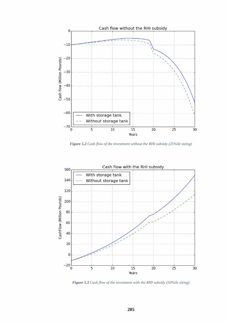
205

Figure 5.2 Cash flow of the investment without the RHI subsidy (25%ile sizing)


206



207


Finally, the results of the environmental and energetic analysis both for the studied and

the traditional case and for each case of sizing are shown in Table 5.7.

Table 5.7 Results of the environmental and energetic analysis of the installation

Annual CO2

emissions (kg)

Load factor

(%)

Proportion of heat

demand covered by

geothermal energy (%)

25%ile Wi 5223278 96.695 44.967

25%ile Wo 5478858 93.882 42.421

50%ile Wi 1954119 80.631 79.364

50%ile Wo 2750260 80.267 70.957

75%ile Wi 308319 64.647 96.742

75%ile Wo 673626 62.084 92.883

208

5.4 Discussion

The first important observations of this Chapter arise from Tables 5.1 and 5.2 in which

the unit price of fuel and electricity as well as their average annual increases are shown for

each case of sizing both for the studied and the traditional case. Firstly, it is observed that

these values can be different between some cases because, as mentioned before these

values depend on the annual use of fuel and electricity, respectively. Furthermore, it is seen

that discrete values are obtained only and do not lie in a continuous range of values. If the

annual use of either fuel or electricity lies within a specific range, then its unit price and its

average annual increase will get a specific value defined by the historical data. Secondly, it

is observed that as the sizing of the installation increases both the unit price of fuel and

electricity increase too. As it was shown in Chapter 4, both the use of fuel and electricity

decrease as the sizing of the installation increases. These denote, in simple words, that

when more fuel or electricity is used, then its price decreases, which is intuitively sensible

from a market point of view. Thirdly, it is observed that as the sizing of the installation

increases, the average annual increase of fuel and electricity prices both have a decreasing

trend. So, under the same reasoning as previously, this shows that when more fuel or

electricity is used, its average annual increase rises, which has an opposing trend to its unit

price. In other words, when more fuel or electricity is bought, its price is lower but its

average annual increase will be higher. Obviously, these observations apply both for the

studied and the traditional case.

The main capital costs of the installation can be seen in Table 5.3 from which important

conclusions can be drawn both for cases of different sizing as well as between the studied

and the traditional case for the same sizing of the installation. Firstly, it can be observed

that both the capital cost of drilling and the capital cost of the pipelines is exactly the same

between the studied and the traditional case for the same case of sizing. This is totally

expected, as between the studied and the traditional case the only differences are the use of

the heat storage under a different operational strategy, while the rest of the installation is

the same. So, the number of wells and the pipelines, and subsequently their capital cost,

will be exactly the same between these cases. Secondly, it is seen that as the sizing of the

installation increases, both the capital cost of drilling and the capital cost of the pipelines

increase. These are also expected because, as seen in Chapter 3, a larger sizing of the

installation requires more wells to be drilled, which of course increases the total cost of

drilling, while on the other hand, a larger sizing of the installation denotes higher mass

209

flow rates and, subsequently, bigger pipelines which are required to compensate with these

higher flow rates. The latter obviously leads to an increased capital cost for the pipelines

and is in agreement with the results of Chapter 3 concerning the size of the pipelines.

Thirdly, it is noted that for the same case of sizing, the cost of the heat storage tank is

obviously higher in the studied case, since in the traditional case there is no heat storage

and its cost is zero. Furthermore, it can be seen that as the sizing of the installation

increases, the cost of the heat storage tank increases. The latter is also expected because the

larger sizing of the installation requires bigger heat storage, as can be identified from

Chapter 3, which increases its capital cost. Fourthly, the cost of the peak-up boilers has a

decreasing trend as the sizing of the installation increases and is also smaller for the

studied case. Both of these results are in agreement with the results of the size of the peak-

up boilers shown in Chapter 4. Taking into account these results and the fact that the cost

of the boilers is assumed to be directly proportional to their size, then the impacts on their

cost shown in Table 5.3 are justified. Furthermore, it can be observed that as the sizing of

the installation increases, the total capital cost increases which is sensible taking into

account the previous observations and the fact that larger sizing denotes bigger installation

and, subsequently, higher capital cost. Finally, the most important observation of Table 5.3

is the fact that for the same case of sizing, the total capital cost will be higher in the

traditional case than in the studied case. So, the studied case has a lower capital cost

compared to the traditional case, although the extra cost of the heat storage tank is taken

into account. This happens, mainly, because of the higher capital cost of the peak-up

boilers in the traditional case, which offsets the difference due to the heat storage.

Then, in Table 5.4 the annual running costs of the installation for each case are shown.

It is observed that the cost of fuel for the same case of sizing is higher for the traditional

case in which the heat storage is not used, while this cost decreases as the sizing of the

installation increases. Both these observations are expected taking into account the mass of

fuel used for each case as shown in Tables 4.5 and 4.6, respectively, and the fact that the

cost of fuel is proportional to its total amount used. Furthermore, it is shown that for the

same case of sizing the cost of electricity is almost the same between the studied and the

traditional case, while the cost of electricity decreases as the sizing of the installation

increases. This is also expected for the same reasons as for the cost of fuel. Taking this into

account, the fact that the total running cost decreases as the sizing of the installation

increases is totally sensible. Finally, it is shown that for the same case of sizing the total

running cost will be lower in the studied case. So, a first major conclusion of this Chapter

210

is that both the capital and the running costs will be lower for the studied case than for the

traditional case of operation of a geothermal district heating system.

The main financial indices of the investment for each case of sizing are shown in

Tables 5.5 and 5.6 for the cases that the RHI subsidy in taken into account and not,

respectively. These two tables highlight some very important drawbacks. Firstly, it is

shown that for the same case of sizing all the financial indices improve when the heat

storage is used. More specifically, the levelised cost of heating decreases, while the NPV,

the IRR and the BCR all increase. For example, the difference in the RHI denotes an

increased potential annual income of £42350-137830 depending on the case of sizing. The

maximum increase in annual income is for the medium case of sizing, which denotes that

the best improvement in the financial performance occurs in this case. The second

interesting drawback highlighted by these tables is the influence of the sizing of the

installation on the financial viability of the investment. It can be seen, that all the financial

factors improve when the sizing of the installation increases. This happens mainly because,

as will also be seen later, a larger sizing of the installation indicates that more geothermal

energy is used to cover the heat demand, which subsequently leads to increased income

from the RHI incentive. Another factor that causes the higher viability of the larger sizing

are the lower running costs in this case, which increase the net annual income of the

investment. So, it can be said that if there is no restricting factor such as non-favourable

geological conditions, the geothermal installation should be sized on the maximum

possible sizing, even if the heat storage impacts most affect the medium sizing, as shown

previously.

A third really important observation which arises from the comparison of Tables 5.5

and 5.6 is the influence of the RHI subsidy in the viability of the investment. As it can be

clearly seen, all the financial indices improve a lot when the RHI is taken into account. For

example, the NPV can increase up to 84%, the IRR can increase up to 87%, while the BCR

can increase up to 56% when the RHI is taken into account. The only financial index

which remains the same is the levelised cost of heating which does not depend on the RHI.

Therefore, these results definitely prove the tremendous impact of a financial subsidy in a

renewable project.

Up to this point, the discussion was focused on whether the studied case is more viable

than the traditional case. By observing these two tables, it can also be seen if each

investment alone is feasible or not. It can be seen that the investment is not viable for the

211

lower sizing of the installation either if the RHI is taken into account or not, because the

NPV, the IRR and the BCR are all negative. This definitely indicates that this investment is

not viable. A further investigation on the viability of this investment will be carried out on

the next section in which two solutions which can improve its viability will be examined.

For the cases of larger sizing, it can be seen that the investments are definitely viable for

the case that the RHI is taken into account, while for the case that the RHI is not taken into

account the viability or, more properly said, the economic attractiveness of the medium

sizing is somehow questionable. This happens because of the values of the IRR shown. As

mentioned before, the value of the IRR has to be higher than the current interest rate of the

market. In our case, this is definitely the case. But in practice, the values of the IRR have to

be typically higher than 15% in order to have greater security and in order to take into

account any non-predicted factors that can influence the investment. So, although this case

is definitely viable as the results show, it might not be very attractive for investors. For the

case of the larger sizing of the installation, the investment is viable and very attractive even

when the RHI is not included. In general, it can be stated that the investment is feasible for

the medium and the large sizing of the installation and the feasibility is greatly enhanced

with the inclusion of the RHI subsidy.

All these observations concerning the financial feasibility of the investments, are also

depicted in Figs. 5.1-5.6 in which the cash flows of each investment are shown. As

expected, the cash flow for the lower sizing of the installation will have negative values as

shown in Figs. 5.1 and 5.2 since the investment is not viable. Then, it is observed that for

each case of sizing, the studied case is more viable as the monetary flow is higher at each

time. The fact that the storage impacts most the medium sizing is also observed as the

difference between the two lines is bigger in this case compared to the larger sizing case.

The change in the inclination in the 20th year of the investment occurs, firstly because the

RHI stops being provided after that year, as explained in the methodology section, and

secondly in this year the peak-up boilers are replaced. The latter are a relatively expensive

item as seen in Table 5.3, so this change in inclination is justified even in the cash flows

where the RHI is not taken into account. Furthermore, the influence of the RHI is also

made clear through these cash flows as it can be seen that the monetary values are much

higher when the RHI is taken into account. Finally, it can be seen that the pay-back period

of the investment is quite low when the RHI is taken into account, while it increases a lot

when it is not taken into account, although these pay-back periods can still be regarded as

very acceptable. More specifically, the pay-back period is around 4 and 3 years for the

medium and larger sizing of the installation, respectively, when the RHI is taken into

212

account, while the same values are around 7-8 and 6 years, respectively, when the RHI is

not taken into account. The latter shows again the influence of the RHI and the fact that the

investment with the larger sizing has the higher viability as mentioned before also.

Concerning the annual CO2 emissions of the installation, it can be seen in Table 5.7 that

these decrease when the heat storage is used for every case of sizing. This is totally

expected, since the emissions are directly proportional to the mass of fuel used and, as it

was shown in Chapter 4, this decreases when the heat storage is used. The relative decrease

of the emissions in the lower case of sizing is small since, as mentioned before, almost all

the geothermal production is sent directly to the heat load and, therefore, the change in the

operation of the peak-up boilers, and subsequently their emissions, will not be very high.

On the other hand, the highest absolute decrease of the emissions is for the medium case of

sizing, which indicates again that the storage impacts are greatest in this case. An

interesting observation is also that the highest relative decrease of the emissions is for the

larger case of sizing, where the absolute decrease is around 50%. But, in this case, the

emissions are relatively low anyway, so it can be indeed stated that the medium case of

sizing is impacted more. It can also be observed that as the sizing of the installation

increases, the emissions will decrease as the amount of fuel used will also decrease. Since

the sizing of the installation increases, more geothermal energy and less fuel are used, so

the emissions will decrease.

As for the load factor of the geothermal part of the installation, it can be seen in Table

5.7 that it increases when the heat storage is used. This indicates that when the heat storage

is used, the geothermal part of the installation operates at a higher average flow rate, thus

increasing the utilization of geothermal energy compared to the traditional case of

operation. On the other hand, it is also shown that the load factor decreases as the sizing of

the installation increases. This happens because, as the sizing of the installation increases,

the potential geothermal production also increases, so there can be many times over the

year that the heat demand can be covered just by a part of the geothermal production. In

other words, more geothermal energy that is available for the same overall heat demand as

the sizing increases, so the smaller the fraction of it that will be used to cover the same heat

demand. In the lower case of sizing, the potential geothermal production is low, so almost

all the geothermal production is sent directly to the heat demand. For example, in our case,

the load factor is 96.695% when the heat storage is used, which means that the geothermal

installation is working very close to its full capacity all over the year.

213

Finally, in Table 5.7 the proportion of the total heat demand that can be covered by

geothermal energy is shown. It is observed that when the heat storage is used, a higher

proportion of the heat demand is covered by geothermal energy. This is expected from the

previous results, where it was shown that when the heat storage is applied, more

geothermal energy is utilised and less fuel is used. This indicates that a higher proportion

of the heat demand will be covered by geothermal energy. Furthermore, as the sizing of the

installation increases, more geothermal energy is available, so obviously, a higher

proportion of the heat demand will be covered by geothermal energy.

5.5 Further investigation on the financial viability of the investment

As shown in the previous section, the case of the lower sizing of the installation

(25%ile case) is not financially viable. In this section, two potential solutions in order to

overcome this problem will be examined. The first of the following potential solutions and,

under certain circumstances that will be explained later in this section, the second too, can

also be applied in the other cases of sizing either in order to increase their viability or if

these are not viable too.

The first possible solution that could increase the viability of the investment is to

increase the income of the investment. The most obvious way to do this is by increasing

the variable cost of heating, which up to now was priced at £0.02/kWh of heat delivered to

the end-users. Practically, this value was quite low as in reality the variable cost of heating

is £0.05/kWh or higher. So, the same analysis which was explained in section 5.2.1 will be

applied for higher values of the variable cost of heating. In this case, only the curves for

the studied case with the use of the heat storage will be shown as it is not attempted to

check if it is worthwhile including a heat storage or not, but to check the general viability

of the investment. Nevertheless, it was clearly shown in the previous two sections that it is

financially worthwhile including a heat storage in a geothermal district heating system.

The results of this analysis for the 25%ile sizing case and for the cases that the RHI is

taken and not taken into account are shown in Figs. 5.7 and 5.8, respectively.

As expected, the increase of the variable cost of heating can definitely increase the

viability of the investment. As shown on Figs. 5.7 and 5.8, the increase of the variable cost

of heating increases the monetary value of the investment in any period of time.

Furthermore, by comparing these two figures with Figs. 5.3-5.6, it is observed that for the

214

lower case of sizing a similar cash flow is achieved at a variable cost of £0.05/kWh when

compared to the medium sizing and at a variable cost of £0.06-0.07/kWh when compared

to the larger sizing of the installation. This shows that more than a two-fold increase is

required in the lower case of sizing to achieve the same cash flow as with the other cases.

Even if not the same cash flow is desirable, it is shown in the two above figures that the

case with a variable cost of £0.03/kWh is barely viable and not so attractive.

Figure 5.7 Influence of the variable cost of heating on the cash flow of the investment (RHI included-

25%ile sizing)

215

Figure 5.8 Influence of the variable cost of heating on the cash flow of the investment (RHI not included-

25%ile sizing)

So, the first viable case is for the variable cost of heating to be £0.04/kWh which is

double the initially used value. Although this value is double compared to the other cases

of sizing, it remains relatively low when compared to variable costs that are applied in the

traditional heating systems. So, with this analysis it was shown that by increasing the

variable cost of heating within logical limits, and usually below the values of traditional

heating systems, it can make investment feasible.

The second solution that could increase the viability of the investment is the decrease

of the investment expenditure. By observing in detail Table 5.3, it can be seen that the total

capital cost between the three cases of sizing is not very different, especially when taking

into account that this refers to the whole period of the investment. On the other hand, it is

observed in Table 5.4 that the running cost is considerably more different between the

three cases compared to the capital cost and it is maximum for the lower case of sizing.

The running cost consists mainly of the cost of fuel and the cost of electricity used by the

pumps, as mentioned before. The cost of fuel cannot be controlled easily as it depends on

the heat demand. On the other hand, the cost of electricity depends mainly on the mass

flow rate and the dimensions of the pipelines. With the approach followed throughout this

thesis, the mass flow rates over the transmission network depend roughly on the sizing of

216

the installation, while those over the distribution network depend on the heat demand. The

heat demand is constant for each case of sizing, so the mass flow rates on the distribution

network will be roughly the same over the year for each case of sizing. It should be noted

that this statement refers to the whole year and not the design-day, where (as shown in

Chapter 3) the mass flow rates on the distribution network will obviously be different. So,

since the mass flow rates will be the same, it seems a sensible choice to increase the size of

the pipelines of the distribution network in order to decrease the friction losses, and

subsequently the cost. This change will increase the capital cost of these pipelines which is

contradictory to the decrease of the running cost. Whether this change improves the

viability of the investment will be examined below.

So, the same analysis will be carried out for two different cases for the sizing of the

distribution network. For the sake of simplicity, these two cases will refer to the sizing of

the distribution network for the medium and large cases of sizing. In other words, the only

difference in the next two studied cases will only be the size of the distribution network,

while everything else (including the number of wells, the size of the storage tank and the

size of the peak-up boilers) will be the same as in the lower case of sizing. These two cases

will be symbolised as 25T-50D and 25T-75D, respectively, in the following. The graphs of

the cash flows for these two cases are shown in Figs. 5.9-5.12 both for the cases that the

RHI is included and not included. By comparing these cash flows with the ones showed in

Figs. 5.1 and 5.2 which refer to the 25%ile sizing, both for the transmission and

distribution network, it can be clearly seen that the feasibility of the investment increases

very slightly in the two new cases. Sizing the distribution network for a larger case of

sizing seems to improve the feasibility of the investment. But this improvement is so slight

as to be barely visible in the graphs, and it definitely does not make the investment

feasible. So, it can be concluded that this solution does not improve the feasibility of the

investment importantly and it is thus not recommended.

217

Figure 5.9 Cash flow of the investment with the RHI subsidy (25T-50D sizing)

Figure 5.10 Cash flow of the investment without the RHI subsidy (25T-50D sizing)

218

Figure 5.11 Cash flow of the investment with the RHI subsidy (25T-75D sizing)

Figure 5.12 Cash flow of the investment without the RHI subsidy (25T-75D sizing)

219

By the analysis shown in this section, it can be concluded that if a geothermal district

heating system with or without the heat storage is not financially viable, the only effective

solution to that problem is to increase the income of the investment by increasing the

variable cost of heating. It was further proved that this increase of the variable cost usually

lies within the margins of the variable cost of alternative heating technologies. So, it can be

stated that, even if the initially selected variable cost has to be increased, this technology

will remain competitive to other heating technologies. Finally, the effect of a financial

subsidy in a renewable heat project was once again highlighted as it was shown that the

investment reaches the financial attractiveness of the cases of larger sizing with a lower

variable cost of £0.01-0.02kWh in the case that the RHI is taken into account. In other

words, if a financial subsidy is provided, then the necessary increase of the variable cost of

heating that will turn the investment to viable will be lower compared to the case that a

subsidy is not provided.

5.6 Summary

In this Chapter, an economic, environmental and energetic analysis of a geothermal

district heating with a heat storage, which is the studied case in this thesis, was carried out

and a comparison with the traditional case of not using a heat storage was done.

Concerning the economic analysis of the investment, the main capital and running costs

were initially calculated for both cases as well as the capital costs of replacement of some

parts of the installation and the evolution of the running costs over the investment period.

Afterwards, using these capital and running costs, several financial indices of the

investments were calculated in order to make the comparison between the two cases. Then,

the annual emissions of carbon dioxide were calculated for the environmental analysis of

the installation, while for the energetic analysis two separate energetic indices were used.

The first energetic index that was used was the load factor of the installation which depicts

how close to the nominal load the installation is operating over the year, while the second

energetic index was the proportion of the annual heat demand that is covered by

geothermal energy.

The results have highlighted some very important insights on the economic,

environmental and energetic aspects either when the studied case is compared with the

traditional case, which is the main point of interest of this Chapter, as well as when cases

220

of different sizing of the geothermal part of the installation are compared with each other.

The main concluding remarks of this Chapter are the following:

Both the capital and running costs of the installation are lower in the studied

case compared to the traditional case for any case of sizing.

The capital cost of the installation increases as the sizing of the installation

increases, while on the other hand, the running costs of the installation is

decreased as less fuel and electricity are used when the sizing increases.

All the financial indices show that the studied case of using a heat storage in a

geothermal district heating system is more attractive than the traditional case of

not using a heat storage. More specifically, the levelised cost of heating

decreases, while the NPV, the IRR and the BCR all increase. This is the case for

any case of sizing of the installation.

The effect of a financial subsidy, such as the Renewable Heat Incentive (RHI)

in our case, was highlighted. All the financial indices of the installation increase

a lot when the RHI is taken into account.

The most attractive case of sizing from an economic point of view is the larger

case of sizing. This happens mainly because more geothermal energy is used to

cover the heat demand and, therefore, the income from the RHI increases.

Furthermore, the running costs will be lower in the cases of larger sizing.

Therefore, it can be said that, as long as other circumstances allow this, the

sizing of the geothermal component of the installation should be as large as

possible.

On the other hand, the heat storage seems to impact more the medium case of

sizing as in this case, the higher relative increases of the financial indices occur.

The emissions of the installation decrease when the heat storage is used for each

case of sizing as less fuel is used to cover the peak demands.

The emissions decrease as the sizing of the installation increases as less fuel is

used as well.

As happens with the economic analysis, the medium sizing of the installation is

impacted most from an environmental point of view when the heat storage is

used.

The load factor of the installation increases when the heat storage is used, also

for each case of sizing. This means that for the studied case more geothermal

221

energy is utilised from the same geothermal installation, which is something

desirable as for any renewable energy source.

Furthermore, the load factor of the installation decreases as the sizing of the

installation increases, which means that the installation is working further from

its full or nominal capacity. This is expected as the maximum available

geothermal energy is increased, so for the same annual heat demand the load

factor will decrease.

Finally, the proportion of the heat demand that is covered by geothermal energy

increases when the heat storage is used. This proportion also increases as the

sizing of the installation increases, which is something expected as more

geothermal energy is available to cover the same heat demand.

In general, it can be concluded that by applying a heat storage under the proposed

operational strategy in a geothermal district heating system, both the capital and the

running costs decrease, while the overall production of heat is cheaper. The latter is

probably the most important conclusion of this thesis. Furthermore, the peak-up boilers are

used less and more geothermal energy is utilised compared to the traditional case. This

leads to less emissions to the environment and a higher fraction of the heat demand to be

covered by geothermal energy. So, all these results support a definite answer to the

question given in the beginning of this Chapter, which defined the scope of it. It can be

definitely said that the proposed case is better than the traditional case, from the economic,

environmental and energetic points of view.

222

6 CONCLUSION

6.1 Achievement of aim and objectives

A comprehensive study of geothermal district heating systems (GDHSs) was carried

out in this thesis. Initially, a detailed literature review was presented, in which it was

identified that there was a gap in the way of operation of these systems. More specifically,

there was no published research which examined the operation of a GDHS, but only

practical experience is known about that. For that purpose, the study of the operation of a

GDHS was a major part of this thesis. Furthermore, as for any renewable system it is

desirable to maximise the utilisation of the lowest-carbon source, which in our case is

geothermal energy. This is particularly important for renewable systems as these are

capital intensive investments and it is of the utmost importance to maximise their

utilisation in order to increase the cost-effectiveness of the investment. These two factors

are the main drivers for the focus of this study.

Traditionally, a GDHS varies its heat output according to the heat demand up to its

maximum capacity and in the cases that geothermal energy cannot cover all the heat

demand, fossil-fuel peak-up boilers are implemented. In this study, it is proposed to keep

the geothermal production constant throughout the day and integrate a fully-mixed hot

water storage tank where hot water can be stored in times of low load, which can

subsequently be released into the network to relieve peak demands. The operation of the

installation will be scheduled on a daily basis, while it is re-iterated that the studied units

are assumed to be heat production only units (which is common for geothermal energy)

and offer higher flexibility compared to CHP units. It is also recalled that through this

approach it is not intended to totally phase out the peak-up boilers (as this would probably

render the investment unfeasible), but to reduce their use.

The aim of this thesis was to study the energetic, economic and environmental effect of

including a heat storage in a geothermal district heating system under the proposed novel

operational strategy. The aim of the thesis was achieved by fulfilling the three objectives

defined in section 1.1.

The first objective was to develop a model for the sizing of a GDHS which would

operate under this mode of operation. Through the developed algorithm, a specific

223

representative day is chosen as the design-day and the whole sizing is based on this day. In

our case, three very different and discrete days were chosen as the design-days in order to

show the influence of the sizing of the installation on the results. More specifically, those

days where the days that their daily heat demand is equal to the 25th-, 50th- and 75th centile

of the daily heat demands of the whole year. The results show that the efficiency of the

installation is very high and approximately 86.8-87.6% depending on the case of sizing. It

was also shown that the mass flow rates throughout the network were quite high which

makes the use of a fully-mixed tank (instead of a stratified tank) a sensible and logical

choice. Probably the most important conclusion drawn from this part of the study was the

importance of the insulation on the heat losses of the storage tank and the pipelines. More

specifically, it was shown that the heat losses of the storage tank will be negligible if a

thick insulation (in our case the thickness selected was 20cm) is used. For the pipelines of

the network, an optimization algorithm was built which took into account their capital cost,

the cost of electricity used to overcome the friction losses and the cost of the heat losses.

By applying this algorithm, the obtained values of the heat losses were much smaller than

other published values, which indicates that the heat losses were probably underestimated

previously and have to be taken into account during the initial design of the pipeline

system. This highlights the power of this optimisation algorithm

The second objective is the development of a model for the detailed study of the

operation of the installation. In this model, the outcomes of the first model were used as

inputs. Firstly, an algorithm that provides the operational strategy of the installation over a

random day with a given heat demand was built. By operational strategy is defined the

complete knowledge of the operation of the installation this day, such as the knowledge of

the temperatures and the mass flow rates throughout the installation and for each time

interval. This algorithm can be potentially a powerful tool for the operators of the

installation who will know in advance how to operate the installation on any day if they

know (or can predict) its heat demand. Then, this model was extended in order to build an

extended model for the study the operation of the installation over a whole year. The main

outputs of this model are the amount of electricity used by the pumps of the installation as

well as the amount of fuel used by the peak-up boilers, both for the whole year, and

comprise the main running costs of the installation. A comparison of these values for the

studied and the traditional case of operation of GDHS was carried out and it was found that

when the heat storage is implemented less fuel is used and more geothermal energy is

utilised, while the amount of electricity used is roughly the same. Furthermore, the results

indicate that the heat storage impacts most the medium sized installation. On the other

224

hand, it was shown that as sizing increases proportionately less fuel is used and more

geothermal energy is utilised. So, it can be concluded that although the impact of the

storage is higher in a modest sizing of the installation, the installation should be sized as

big as possible in order to maximise the use of geothermal energy.

The third and last objective of this study was the development of an integrated model

for the calculation of the economic, energetic and environmental indices of the installation

together with a comparison with the traditional case. It was shown that when heat storage

is used, both the capital and running costs of the installation are lower when compared to

the traditional case. Therefore, all the financial indices obtained more favourable values for

the studied case compared to the traditional operation. More specifically, the levelised cost

of heating decreases, while the NPV, the IRR and the BCR all increase. Additionally, the

effect of a financial subsidy, such as the Renewable Heat Incentive (R.H.I.) in our case, in

a renewable heating project was highlighted, as all the financial indices increased

importantly when the R.H.I. was taken into account. Yet again, a conflicting point arose, as

on the one hand the storage impacts more the medium case of sizing from an economic

point of view, but on the other hand, the most financially attractive case is the larger case

of sizing. Of course, the second case is usually preferred and as proposed before, the

geothermal part of the installation should be sized as large as possible. Furthermore, it was

shown that when the heat storage is used the load factor of the installation increases, which

means that the installation is working for more hours in its full load and more geothermal

energy is used. Subsequently, a larger part of the total heat demand will be covered by

geothermal energy. Finally, by implementing the heat storage, the annual emissions of the

installation will decrease.

By the conclusions drawn from the last part of the study, a definite answer can be given

to the main question of this thesis, which was whether it is worthwhile including a heat

storage under the proposed operational strategy in a GDHS or not. It was clearly shown

that for any case of sizing of the installation, by applying the heat storage the overall

production of heat is cheaper and the peak-up boilers are used less. The utilisation of

geothermal energy, which has numerous advantages as explained earlier, is increasing with

subsequent reduction in the emissions of the installation. So, it can be definitely stated that

the integration of a heat storage under the proposed mode of operation is beneficial for a

GDHS from economic, energetic and environmental points of view. Therefore, the aim of

this thesis has been fully achieved.

225

6.2 Summary of contributions of the thesis

The aim of this thesis was fully achieved together with its main objectives. The main

contributions of this thesis in the field can be summarised as:

The proposition of the integration of a heat storage in a geothermal district

heating system under a novel operational strategy. It was shown that this

proposition is beneficial for the system under an economic, energetic and

environmental point of view.

The provision of a robust algorithm for the sizing of the installation which

would operate under the new operational strategy.

Useful insights were obtained for the sizing and operation of several parts of the

installation. The most important insight was the importance of the heat losses of

the pipeline which was revealed by the optimisation algorithm that was

developed for their sizing. This algorithm can also be used for the sizing of any

pair of underground pre-insulated pipelines, if the boundary conditions are

known. This is a contribution out of the main line of the thesis.

The provision of a model that can provide the operational strategy of the

installation in any day with a known heat demand. This model can theoretically

be used by the operators of the installation if they can calculate or predict the

heat demand of the studied day one day in advance which is reasonably

achievable using weather forecasts. If the heat demand is known, this model

will provide them with all the necessary information about how they should

operate the installation throughout the day.

The provision of a model that can provide useful information about the

operation of the installation over a whole year.

The provision of a model that can calculate the economic and energetic indices

of the installation as well as its annual emissions. A second model was also built

that can provide the same values of a traditional GDHS.

The provision of a model that is coupled with the latter model and can make a

robust comparison of the aforementioned indices which can show if the

proposed solution is beneficial against the traditional case or not. In our case,

the results of this model showed the first mentioned, and most important,

contribution of this thesis, i.e. the economic, energetic and environmental

effectiveness of this proposition.

226

6.3 Recommendations for future work

In this final section of the thesis, some recommendations for future work will be given.

These include recommendations on the improvement and enrichment of the algorithms and

proposal of further steps that should be taken using these algorithms. Finally, a similar

approach for the modelling of a future energy system based on geothermal district heating

will be proposed.

The first part of this study presented a robust algorithm for the sizing of a GDHS under

the proposed operational strategy. A first improvement on the model would be to add the

sub-models of other parts of the installation, mainly of the geothermal heat exchanger and

of the substation, which in this study were considered as black-boxes. The geothermal heat

exchanger was not further studied in this thesis as it is considered that it is a standardised

equipment and that it was not worthwhile studying it further, while a possible study for its

optimisation would be quite long and beyond the scope of this thesis. On the other hand,

the substation of the installation was not also studied further, as no details could be found

in the literature about these and it is envisaged that their configuration will be very case-

specific and, therefore, difficult to model generically. Furthermore, depending on the case

a substation might not even exist in an installation.

Moreover, the models for the sizing and the operation of the installation did not take

into account the behaviour of the end-users, but took into account only the temperature

drop in the boundaries of the branches of the distribution network. In other words, the

boundary of the study were the boundaries of the “main” branches of the distribution

network. The models could be further extended in order to take into account more details

of the distribution network as well as the characteristics and the interface of each end-user

(or at least of each different kind of end-user). Obviously, these additions would also affect

the economic, energetic and environmental analysis which should be properly modified.

A basic disadvantage of all the models, and especially of the sizing model, is that they

have not been validated against real data. This happened partially due to the lack of real

data as some parts of the installation are not (or not known to be) deployed yet in reality,

such as the proposed fully mixed tank, while for other parts, such as the pipelines, it was

really hard to get real data from third parties. So, the validation of the developed models

against real data is crucial for their possible practical and real-life application. If the

227

validation takes place, it is strongly believed that these models can be directly (or with few

modifications) applied in real projects.

The whole analysis in this thesis was applied for three different discrete cases of sizing

of the installation which were explained in detail in Chapter 3. These cases were the days

whose daily heat demands correspond to the 25th-, 50th- and 75th-centile of the daily heat

demands of the whole year. These three cases were chosen as logical choices that could

depict small, medium and large cases of sizing. A next step could study cases of smaller or

larger sizing of the geothermal installation. Concerning the smaller sizing, it is intuitively

understood that very small sizing of the geothermal installation is not possible as this

would require a very low geothermal flow rate, which would definitely make the

investment unfeasible. In other words, when borehole drilling is done for a geothermal

well, a minimum flow rate is required otherwise the drilling is not successful or

operational. This minimum flow rate excludes the cases of very small sizing of the

installation, let’s say of less than the 5th- or 10th- centile of the daily heat demands of the

year. On the other hand for the case of very large sizing of the installation, in this thesis it

was chosen in advance not to study such a case as this would lead to under-utilisation of

the geothermal field and would possibly render the investment unfeasible. Whether this

case is true depends on how “peaky” are the extreme peak demands. If these are very

peaky, this would mean that a part of the geothermal installation would work for only a

few hours per year, which is definitely unfeasible. If these peak demands were more

frequent and not very peaky, then it might be possible to size the installation for a higher

coverage by geothermal energy, albeit it is fairly certain that 100% coverage by geothermal

energy would be very costly. After all, as was already mentioned, there will be some

boilers in the installation anyway for back-up purposes. For that reason, it is never

attempted to achieve 100% coverage by geothermal energy. But, the upper feasible limit of

the sizing of the geothermal installation would be a very interesting point. Therefore, a

study that would address these issues in detail would be quite useful.

Another issue that could be researched further, which was also explained in Chapter 4,

is the development of a tool relating the heat demand data to weather conditions. This

relationship can be extremely useful because it can be integrated with the model of the

daily operational strategy of the installation developed in Chapter 4, and this model will be

able to provide the operational strategy of the installation if the weather data are known (or

predicted) instead of the heat demand. This is desirable as it is much easier and more

effective to predict the weather conditions of the next day compared to its heat demand. A

228

first attempt at developing this relationship was made in Appendix B, in which the results

were not so encouraging either because the approach was too simplistic or because the data

in the studied case are very stochastic. Furthermore, this was not studied further in this

thesis as it was out of its scope. So, an obvious further work arising from this thesis would

be the development of a robust model that connects the heat demand with the weather

conditions.

Finally, a similar study that could be based in the logic of this thesis concerning the

management of the geothermal installation would be the integration with a heat pump for

the further harvesting of geothermal energy. More specifically, an installation like this can

be seen in Fig. 6.1. In such an installation, the cooled water that exits the geothermal heat

exchanger instead of being re-injected in the underground (or sent to others uses) will be

fed into heat pumps which can upgrade the temperature of fresh water to the desired level.

The heated fresh water can either be stored in the hot storage tank or be fed directly in the

network. But, the existence of the storage tank is again necessary. The main advantage of

this system is that for the same geothermal potential more heat will be harvested through

the use of the heat pump. Therefore, for the coverage of the same heat demand the

geothermal installation can be smaller.

Figure 6.1 Layout of the proposed system (G.H.E. = Geothermal Heat Exchanger, SS = Substation, P.W.

= Production Well, R.W. = Re-injection Well, H.S.T. = Hot Water Storage Tank, C.S.T. = Cold Water

Storage Tank, Pel = Electrical Power)

229

On the other hand, the extra capital cost of the heat pump and of the pipelines

connecting it to the network and the storage tanks as well as the extra operational cost of

the electrical power used by the heat pump will be the main disadvantages of this proposal.

The proposed installation can be operated under three alternative modes. The first

alternative is the heat pump to operate in a 24/7 mode. The second alternative is the heat

pump to operate only during the night hours in which the price of electricity is usually

lower, thus decreasing this additional operational cost. A third alternative which can be

applicable in a future energy system is that the heat pump can operate only when there is

an excess of electricity in the electrical network, which can be the case in a future electrical

system with a high penetration of intermittent renewable energy sources. This proposition

on the one hand will make the operation of this system more complex, but on the other

hand, will offer very cheap (or even free) electricity to the heat pump as this would be an

amount of electricity that would be rejected. The latter would also be an advantage for the

renewable electrical producers as this can be a potential additional income for them (as this

electricity would be rejected as mentioned before) and this could also increase the stability

of the electrical network. Of course, all these alternatives would require a detailed analysis

in order to conclude if they are viable or not, but it is strongly believed that under the

operation of the system presented in this thesis, these systems would be quite promising.

230

APPENDICES

231

Appendix A

Sensitivity analysis of two basic parameters of the system

232

In this Appendix, a sensitivity analysis of two basic parameters of a geothermal district

heating system is carried out in order to examine their effect on the whole system. These

parameters are the temperature difference on the hot side of the geothermal heat exchanger

(∆𝑇ℎ,𝐺𝐻𝐸) and the ratio of the mass flow rates of the transmission network (𝑅𝑚) and they

have a crucial effect on the operation of the system. In the beginning of the algorithm

explained in Chapter 3, initial values are assigned to these parameters and these are kept

constant throughout the whole process. If the final results are physically acceptable, then

the algorithm is considered converged, while if this is not the case, then the proper

adjustment of these parameters has to be done.

In order to adjust these parameters their effects on several variables of the system have

to be evaluated. These effects are studied in this Appendix. More specifically, the influence

of the two aforementioned parameters on the temperature difference on the cold side of the

geothermal heat exchanger (∆𝑇𝑐,𝐺𝐻𝐸), the outlet temperature of the supply transmission

pipeline (𝑇𝑡𝑟,𝑠,𝑜), the capital cost of the pipelines (𝐶𝐶𝑝𝑖𝑝𝑒𝑠) and the number of wells is

analysed. The results of this analysis are shown in the following graphs, and based on these

results an iterative loop was added to the basic code for the adjustment of the parameters.

More details on this possible source of error, the final loop that is added in the main code

and a short discussion on these results are provided in section 3.2.8.

233

Figure A-A1 Temperature difference on the cold side of the geothermal heat exchanger vs the

temperature difference on the hot side of the geothermal heat exchanger

Figure A-A2 Outlet temperature of the supply transmission pipeline vs the temperature difference on the

hot side of the geothermal heat exchanger

234

Figure A-A3 Capital cost of the pipelines vs the temperature difference on the hot side of the geothermal

heat exchanger

Figure A-A4 Number of production wells vs the temperature difference on the hot side of the geothermal

heat exchanger

235

Figure A-A5 Temperature difference on the cold side of the geothermal heat exchanger vs the ratio of

the mass flow rates of the transmission network

Figure A-A6 Outlet temperature of the supply transmission pipeline vs the ratio of the mass flow rates of

the transmission network

236

Figure A-A7 Capital cost of the pipelines vs the ratio of the mass flow rates of the transmission network

Figure A-A8 Number of production wells vs the ratio of the mass flow rates of the transmission network

237

Appendix B

Relationship between the heat demand and the weather

conditions

238

B1) Introduction

The energy consumption in buildings accounts for a large fraction of the total energy use

worldwide. More specifically, in Europe, the energy use in buildings accounts for 40% of

the total energy use and 36% of total CO2 emissions (European Parliament and Council,

2010). Therefore, it is easily understood that in order to fulfil the energy goals set worldwide

the building sector should be taken very seriously into account. This can happen by

optimising the whole process of energy production, distribution and consumption within the

buildings. A crucial factor of the above process is an accurate a priori prediction of the

energy consumption. An accurate prediction improves the efficiency and performance of the

energy production, reducing the environmental impact.

The main energy forms within a building are heating/cooling, hot sanitary water and

electricity consumption. In this study, the focus will be on the prediction of the heat demand

of the building. A general review of the prediction methods of the energy consumption has

been provided by Zhao and Magoules (2012). In general, this problem is quite complex as

many factors should be taken into account, such as the weather conditions, the structure of

the building, the habits of its occupants (the so-called social factor) and many others.

Therefore, many different prediction methods or models have been developed. These can be

categorised in the physical or engineering models, the black-box models and the statistical

models.

The physical or engineering models are based on the physical principles which govern

the heat losses of the building and take into account the different layers throughout its wall,

the difference between the ambient and the indoor temperature, the heat gains within the

building etc. Many commercial tools have been developed for that purpose, such as

TRNSYS and EnergyPlus5. Usually, the physical models are quite complex and are not so

easy to apply in reality as it is quite difficult to obtain all the characteristics of the building.

Therefore, some more simplified methods have been developed. The most well-known

method is the degree-day method, which is a very simple method for the calculation of the

heat demand knowing only the ambient temperature (Gelegenis, 2009; Schoenau and Kehrig,

1990; Coskun, 2010). This method is very simple and therefore not so accurate. Catalina et

al. (2013) developed a multiple regression model between the heat demand and the

difference between the indoor and the outdoor temperature, the total heat transfer coefficient

5 http://www.buildingenergysoftwaretools.com/

239

and the south equivalent surface. The results of this approach were quite satisfactory.

Another simplified model was also applied by Afram and Janabi-Sharifi (2015) that

predicted the daily energy consumption profile for residential buildings. The interested

reader can find more details on the aforementioned methods in the work of Zhao and

Magoules (2012).

A black-box model is used when the physical model is not completely known or is very

complex to implement practically. In these cases, the inputs and the outputs of the model are

known and the black-box approach is used to build the inter-connecting function. The most

common types of black-box models are the artificial intelligence methods and these are

further divided in the Artificial Neural Networks (ANNs) and the Support Vector Machines

(SVMs). A review of these methods in the building energy systems can be found in the works

of Krarti (2003) and Dounis (2010). These systems have been used widely the last years for

the heat demand forecasting in buildings (Kalogirou, 2006; Kreider et al., 1995;

Shamshirband et al., 2015) and the accuracy of the results is usually the best among the

methods used. On the other hand, these models need a lot of historical data which are not

always available and it is very difficult to point out the optimum parameters of the problem.

Finally, the fact that the physics of the problem are not identified through these methods

makes a lot of academics, mainly, to avoid these methods.

Another method which is not so common and combines the physical and the black-box

models is the grey-box approach, in which there is a theoretical knowledge of the system

which is combined with measurements in order to produce its mathematical description. For

example, Zhou et al. (2008) developed an integrated model for the prediction of the heat

demand which uses as inputs the temperature and the relative humidity, that are calculated

through a modified grey model, as well as the solar radiation which is calculated through a

regressive model. The interested reader can find other applications of the grey-box approach

in the work of Guo et al. (2011).

The statistical models are producing single or multiple correlations between the heat

demand data and, usually, the weather conditions. In general, the statistical methods are

divided in the autoregressive models, the integrated models and the moving average models

(Popescu et al. 2008). Historical data are used for the production of the correlation and, then,

this correlation is used to predict the future heat demand. The basic advantage of these

models is that they are quite fast and simple to use, but their accuracy is not that good as it

is not easy to capture the social factor and the building envelope. An attempt to take into

240

account the social factor was done by Dotzauer (2002) where it is stated that the social factor

is of utmost importance and should be definitely taken into account. So, Dotzauer (2002)

separated the heat demand function into two parts, the temperature dependent part and the

part that depicts the social behaviour. Popescu et al. (2008) are producing multiple

correlations between the current weather conditions and data of previous time intervals

trying to capture the social factor. The correlation factors are quite satisfying, but when these

correlations are tested against new data then the results are quite variable.

In this part of the thesis, simple correlations will be produced between the heat demand

data and the weather conditions, in which the social factor and the building envelope will be

taken into account. The correlations will be quite simple because, as stated by Dotzauer

(2002), there will always be failures in the prediction of the weather which is used for the

prediction of the heat demand. Therefore, complex models can provide errors and more

simple models can provide the same satisfactory results. In order to take into account the

social factor, different correlations will be produced for each season/day/hour. For example,

it is expected that for the same temperature the heat demand will be different between

summer and winter, or between a working and a non-working day. The optimum splitting of

the data will also be researched. Few research has been carried out on the basis of thinning

the data. Ma et al. (2014) categorised the buildings according to their function and found

different correlations for each building, while Yao and Steemers (2005) did a break-down

analysis of the load starting from the appliances and building-up the total load. Concerning

the building envelope, data of the previous time steps will be used in the correlations. Apart

from the work of Popescu et al. (2008), there has been no other published work, up to the

authors’ knowledge, using data of the previous time steps.

The structure of this study is as follows: In this section, a brief introduction in the problem

of the heat demand prediction was given. In section B2, the methodology will be explained

focusing on the different kinds of data-splitting that will be tested. In section B3, the results

will be shown and discussed, while section B4 will conclude this study.

B2) Methodology

In this section, a brief description of the methodology followed will be given. The heat

demand data used in the modelling were provided by the Estates and Building Office of the

University of Glasgow and refer to a cluster of buildings managed by the University. On the

241

other hand, the weather data used were obtained by the British Atmospheric Data Centre

(BADC)6 and refer to the Kilpatrick area of Glasgow, which is a village in the west of

Glasgow on a straight line distance of almost 14km. The data from the meteorological station

of this area were chosen as these were the most precise data, the other operating stations

were almost in the same distance and, most importantly, there were very few missing data.

There were available data for the whole 2012 and for the first five months of 2013. Therefore,

the correlations were done for the 2012 data and, then, these correlations were tested for the

2013 data. As mentioned previously, there were very few missing data from the specific

station. More specifically, there were missing data in two days of 2012 and in one day of

2013. These three, in total, days were not taken into account in the calculations.

In order to determine all the correlations, the MATLAB curve fitting tool was used. A

novelty of this study, is that for the calculation of the fitting lines/curves the method used

was not the typical “least-squares method” in which the sum of the squares of the residuals

is minimised, but a special feature of the MATLAB curve fitting tool called “Robust=LAR”,

in which the sum of the absolute values of the residuals is minimised. The advantage of this

method is that it weakens the effects of possible outliers in the data which would lead to not

so realistic fittings using the typical method.

For the evaluation of the goodness of the fitting the value of 𝑅2 (Co-efficient of

determination) was calculated for each case by the following sets of equations:

𝑅2 = 1 −𝑆𝑆𝐸

𝑆𝑆𝑇 (A-B1)

𝑆𝑆𝐸 = ∑(𝐻𝐷𝑖 − 𝐻�̃�𝑖)2 (A-B2)

𝑆𝑆𝑇 = ∑(𝐻𝐷𝑖 − 𝐻𝐷̅̅ ̅̅ )2 (A-B3)

Where:

𝑅2 = Coefficient of determination (Dimensionless)

𝑆𝑆𝐸 = Sum of squared errors (𝑘𝑊ℎ)

𝑆𝑆𝑇 = Total sum of squares (𝑘𝑊ℎ)

6 http://badc.nerc.ac.uk/home/

242

𝐻𝐷𝑖, 𝐻�̃�𝑖= Predicted and observed heat demand for each time interval, respectively

(𝑘𝑊ℎ)

𝐻𝐷̅̅ ̅̅ = Average predicted heat demand (𝑘𝑊ℎ)

The first part of the modelling is the identification of the optimum set of the dependent

variables. In other words, the correlation between the heat demand and different dependent

variables will be tested in order to check which one produces the best fitting. The dependent

variables will always be two and one of them will always be the temperature at the current

time-step as it is assumed to be the main driving force of the heat demand. The other

variables that will be checked are the temperature and the heat demand in several previous

time-steps in order to capture the effect of the building envelope. At the same time the

optimum kind of correlation will be identified.

After the above issues are identified, then the possible correlations will be calculated

and tested. In Fig.A-B1, the 2012 data are shown where it is made clear that it is

impossible to obtain a single correlation that can fit satisfactorily these very sparse data.

Therefore, it is necessary to split the data into different time periods in order to capture

possible social variances.

The different temporal data-splitting will be the following:

Different seasons. The data will be splitted in four different seasons within the

year, i.e. January-March, April-June, July-September and October-December.

Splitting in working and non-working days.

Different hours. Different correlations will be carried out for each hour of the

day. Therefore, there will be 24 different correlations.

243

Figure A-B1 2012 data

B3) Results

B3-1) Optimum fitting functions

Firstly, the optimum combination of dependent variables will be examined. As

mentioned earlier, one of the dependent variables will always be the temperature at the

specific time step, while the independent variable will be the heat demand at the specific

time step, i.e. the predicted heat demand. The other dependent variable will be either the

temperature or the heat demand on various previous time steps. In our case, the time step is

one hour. The previous time steps studied are one, five and twenty-four hours earlier in order

to capture possible different influences of the building envelope. The second case was a

random choice between the two extremes of one and twenty-four hours. The results can be

seen in Table A-B1 for 3 different possible correlations, 1st-2nd and 3rd polynomial. It should

be mentioned that both dependent variables were risen in the same force. The exponential

and logarithmic correlations were also tested, but the produced results were much worse, so

for sake of simplicity they are not shown in this paper. It should be noted that these results

refer to the 2012 data.

244

By observing Table A-B1, it is clear that the best combination of dependent variables is

the temperature of the current time step and the heat demand of the previous time step. It

seems that the influence of the heat demand one hour earlier is very important for the current

heat demand. This makes clear the effect of the building envelope or the heat capacity of the

building in this kind of problems and this is something very under-estimated in previous

works. Therefore, the correlation that will be examined will be of the following kind:

𝐻𝐷 = 𝑓(𝑇,𝐻𝐷−1) (A-B4)

Where:

𝐻𝐷−1 = Heat demand of the previous time step (𝑘𝑊ℎ)

Although the results show that the optimum kind of correlation is a 3rd polynomial, this

was researched further by rising each of the variables in different forces. The results can be

seen in Table A-B2.

Table A-B1 Values of R2 (%) for different dependent variables and three different correlations (the

subscripts in the variables denote the number of previous time steps to which the variable refers)

Dependent

Variables

Correlations

1st Polynomial 2nd Polynomial 3rd Polynomial

𝑻 39.74 39.94 40.82

𝑻, 𝑻−𝟏 41.77 42.18 94.47

𝑻, 𝑻−𝟓 47.83 48.4 48.82

𝑻, 𝑻−𝟐𝟒 40.61 41.13 42.02

𝑻,𝑯𝑫−𝟏 98.95 97.08 99.12

𝑻,𝑯𝑫−𝟓 31.67 93.76 97.69

𝑻,𝑯𝑫−𝟐𝟒 93.2 96.71 98.28

Table A-B2 Values of R2 (%) for different possible polynomial correlations

Force of 𝑯𝑫−𝟏

1 2 3

Force of 𝑻

1 98.95 99.01 97.87

2 98.69 97.08 99.03

3 98.89 98.83 99.12

245

In the above table, it can be seen that there is a general, although not necessary, trend of

an increasing value of 𝑅2 when the forces of the two dependent variables increase. But,

this increase is considered not to be that big to make it worth to make the fitting function

more complex by adopting the maximum forces of the dependent variables. So, it is

decided to select as the fitting function the case in which the forces of 𝑇 and 𝐻𝐷−1 are 1

and 2, respectively. Therefore, the final fitting function will be the following:

𝐻𝐷 = 𝐴 + 𝐵 ∙ 𝑇 + 𝐶 ∙ 𝐻𝐷−1 + 𝐷 ∙ 𝑇 ∙ 𝐻𝐷−1 + 𝐸 ∙ 𝐻𝐷−12 (A-B5)

B3-2) Calculation of the correlations

Equation A-B5 is the fitting function that will be used in the rest of this study. In this

section, the correlations will be calculated based on the 2012 data. The fitting was carried

out for the different temporal splittings explained in section B2. It should be mentioned that

it was not worth to combine different temporal splittings, e.g. different seasons and different

hours at the same time as this did not improve the results. All the results are shown in Table

A-B3.

A first major observation is that in the majority of the cases the fitting achieves very high

correlation factors. More specifically, the values of 𝑅2 are usually higher than 98% and even

99%. Even in the case where all the data are used, the value of 𝑅2 is almost 99%. In the case

of different seasons, it is observed that in general the correlation factors improve, apart from

the case of October-December when the 𝑅2 worsens a bit. When the data are separated in

working and non-working days, it can be seen that in the case of the working days the

correlation worsens, while in the case of the non-working days the correlation improves.

Finally, when the data are splitted in different hours, it is seen that in most of the cases the

value of 𝑅2 is more than 99% and reaches also its highest value amongst the cases which is

99.76%. But, there are four cases (05:00 to 08:00) in which the value of 𝑅2 is considerably

lower compared to the other cases.

246

Table A-B3 Results of the fitting function's coefficients and values of R2 for the 2012 data

A B C D E 𝑹𝟐 (%)

All 2012 Data 107 2.541 1.052 -0.00815 -9.178E-6 99.01

Different Seasons

Jan-Mar 566.2 -35.36 0.9667 -0.0005676 -5.352E-6 99.43

Apr-Jun -17.64 17.78 1.213 -0.01678 -2.839E-5 99.26

Jul-Sep -220.8 26.92 1.26 -0.0212 -2.961E-5 99.54

Oct-Dec -191.1 37.77 1.11 -0.01286 -1.312E-5 98.91

Working and non-working days

Working days 156.5 -1.283 1.1 -0.009378 -1.442E-5 97.76

Non-working

days

88.56 4.61 1.052 -0.009619 -1.016E-5 99.51

Different hours

00:00 584.2 -39.95 0.542 -0.0008695 7.413E-5 98.11

01:00 106.6 -6.292 0.9948 0.0007628 -6.95E-6 98.06

02:00 -54.73 27.37 1.65 -0.03702 -1.061E-4 98.46

03:00 -243.2 28.85 1.6 -0.04386 -8.178E-5 98.42

04:00 -350.2 79.02 1.76 -0.04061 -0.0001198 98.67

05:00 2584 -214.4 0.682 0.02774 -2.71E-6 73.45

06:00 -4917 284.8 3.248 -0.0505 -1.84E-4 74.24

07:00 7541 -411.4 -0.08956 0.0176 3.778E-5 85.33

08:00 -2690 126.1 1.873 -0.03144 -5.888E-5 77.21

09:00 312.6 -6.856 1.109 -0.01791 -1.846E-5 99.4

10:00 -1091 75.39 1.335 -0.02302 -3.072E-5 99.6

11:00 -478.1 20.28 1.23 -0.009561 -2.343E-5 99.71

12:00 -176.6 12.54 1.219 -0.01212 -2.281E-5 99.75

13:00 -246.4 14.18 1.052 -0.004202 -4.456E-6 99.76

14:00 -8.53 2.746 1.083 -0.008493 -8.593E-6 99.69

15:00 802.8 -39.42 0.8157 0.004971 1.539E-5 99.6

16:00 440.9 -16.93 1.023 -0.004324 -2.819E-6 99.78

17:00 211.8 -12.69 1.015 0.002753 -6.097E-6 99.7

18:00 -608 34.1 1.072 -0.0007737 -1.208E-5 99.58

19:00 -505.4 4.053 1.612 -0.01559 -5.984E-5 99.62

20:00 1542 -66.28 0.4024 0.01536 4.064E-5 99.71

21:00 1336 -64.15 0.7566 -0.002604 -6.915E-6 99.66

22:00 1451 -72.05 0.5347 0.005745 7.179E-6 99.61

23:00 -377.8 42.49 1.25 -0.04078 -7.2E-5 99.12

247

An interesting observation in Table A-B3 is that the coefficient C (see eq.A-B5), which

is the coefficient of the heat demand of the previous time-step, usually has a value which is

very close to 1. This indicates the very high influence of the heat demand of the previous

time-step on the current heat demand justifying further our prior selection. It might also not

be coincidental that the cases of lower 𝑅2 have a value of C relatively further to 1 compared

to the other cases.

In general, it can be stated that the proposed simple two-dimensional correlation is very

powerful achieving high correlation factors. There is also a trend of the correlation factor

improving when the data are splitted with the cases of different seasons and different hours

to show the best improvement. On the other hand, it is somehow risky to state that fact

since the correlation factor are already quite high. Furthermore, it is shown by previous

works that a specific correlation in some specific data might achieve high correlation

factors, but this does not guarantee a good prediction of other data with the same

correlation. Therefore, it is of utmost importance to check the fitting of these correlations

with the 2013 data. This is studied in detail in the next section.

B3-3) Checking the correlations with the 2013 data

As explained previously, in this section the correlation functions calculated in section

B3-2 will now be tested against the 2013 data. The available data for 2013 are for the first

five months of the year, so the correlations of July-September and October-December

seasons will not be checked. The results of the testing are shown in Table A-B4.

It is observed that the values of 𝑅2 in this case are much lower than in the initial fitting

of the 2012 data. This shows that although a fitting function can fit very well some specific

data, then when this function is tested to predict other data then it might not work so well.

There can be many reasons why this occurs. First of all, the heat demand as well as the

weather conditions are, in reality, stochastic phenomena, and, therefore, any discrepancies

can happen. Secondly, the heat demand might have changed because of external reasons,

such as additional loads. In the studied case, there is no knowledge if this happened or not.

Thirdly, the heat demand depends a lot on the human factor, and although an effort was done

to capture this, it can never be totally captured. Especially, in a case like the studied one,

where there are buildings managed by the University, the human factor is very changeable

and unpredictable.

248

Table A-B4 Testing the fitting function against the 2013 data

𝑹𝟐 (%)

All 2013 data 9.91

Different seasons

January-March 18.18

April-June 23.18

Working and non-working days

Working days 37.64

Non-working days 37.90

Different hours

00:00 74.74

01:00 72.07

02:00 59.94

03:00 51.35

04:00 53.08

05:00 24.24

06:00 21.89

07:00 -27.34

08:00 45.57

09:00 64.93

10:00 61.42

11:00 59.99

12:00 63.12

13:00 63.42

14:00 65.24

15:00 66.91

16:00 63.08

17:00 50.12

18:00 44.01

19:00 51.87

20:00 50.74

21:00 36.06

22:00 60.25

23:00 62.78

249

For example, in our case the heating is free for the consumers, so it might be turned on

for more time than is really needed resulting in higher heat demand. These are the basic

reasons for this disagreement which demonstrates in the best way the stochastic nature of

the problem and the great attention that should be paid in the engineering applications which

involve the prediction of these phenomena. Simple assumptions for the heat demand or

adopting values of the previous years can be very misleading for future prediction.

In Table A-B4, it can also be seen that now there is a clear distinction between the values

of 𝑅2 in each case, while in the case of 2012 data all the cases showed almost the same

values of 𝑅2. More specifically, the case of different hours seems to have the best prediction

of all the cases with most of the values of 𝑅2 being between 50% and 70%. There is also a

negative value of 𝑅2 which shows that the fitting in this case is very bad. Furthermore, some

of the values are worse compared to the other cases, but, in general, this case seems to be

the best choice.

B4) Conclusion

Some important conclusions can be drawn by the previous analysis. These are

summarised as:

A simple polynomial two-dimensional model produces correlations with very

high correlation factors. It is shown that a simple model can predict the heat

demand very satisfactorily.

The main novelty of this paper is that it was shown that the heat demand in a

specific time-step is highly affected by the heat demand in the previous time-

step, proving the big effect of the heat capacity of the building. Therefore, one

of the dependent variables of the studied correlation is the heat demand in the

previous time step.

High correlation factors are achieved when the studied function is fitted in the

2012 data, but when the produced functions are tested against new data (2013

data), the correlation factors are much lower. This shows that any simplified

assumptions, such as that the heat demand will follow the same pattern each

year or season, can be very misleading. If the heat demand can be predicted

very well one year, it is not necessary that it can be predicted well the next year

with the same predicting functions. Therefore, it is necessary to adopt demand

side management techniques that can make the heat demand more predictable.

250

The correlations improve a lot when multiple correlations are carried out and

not a single correlation in all the data. It seems that the splitting of the data into

different hours across the day is the best option.

This study was carried out with simple correlations in order to make the above

very useful conclusions. By taking into account these observations into more

sophisticated models, the prediction of the heat demand can be much more

accurate and the discrepancies between the expected and the observed heat

demand can be much smoother.

251

Appendix C

Calculation of the cost of the storage tanks

252

As mentioned in section 5.2.1, the capital cost of the storage tanks includes the cost of

their materials as well as other costs (mainly for civil and fabrication costs). The

calculation of the material costs has been extensively analysed in the aforementioned

section. In this Appendix, a compact analysis of the other costs of the tanks as well as the

assumptions that were used for their calculation will be provided.

Firstly as a basis for these calculations, an e-mail received by Dr Richard Coulton of

SiltBuster was used. This e-mail is shown in the following figure.

Figure A-C1 Informative e-mail by Dr Richard Coulton on the cost of storage tanks

Since the material costs have already been calculated, their corresponding value

(£19252) will not be used. The other costs provided will be used as reference costs together

with the dimensions of the specific tank referred in the e-mail. Furthermore for the other

costs, the following assumptions are made:

The cost of the vertical ladder and access platform will be proportional to the

height of the storage tank.

The costs of the manway access hatch and the drain valve will be the same as

those provided in the e-mail as these are not considered to be significantly

253

affected by the dimensions of the tank. Furthermore, these costs are low

compared to the others, so any error on their calculation will be negligible from

an engineering point of view.

The civils costs as well as the erection on slab are assumed to be proportional to

the volume of the tank.

Therefore, by taking into account these assumptions as well as the costs and the

dimensions provided in the e-mail, the other costs of the storage tanks are calculated by the


𝐶𝐶𝑆𝑇,𝑉𝐿𝐴𝑃 = 1638 ∙𝐻𝑆𝑇

4.27 (A-C1)

𝐶𝐶𝑆𝑇,𝑀𝐴𝐻 = 1800 (A-C2)

𝐶𝐶𝑆𝑇,𝐷𝑉 = 1206 (A-C3)

𝐶𝐶𝑆𝑇,𝐶𝑉 = 24000 ∙𝑉𝑆𝑇

881 (A-C4)

𝐶𝐶𝑆𝑇,𝐸𝑂𝑆 = 15000 ∙𝑉𝑆𝑇

881 (A-C5)

Where:

𝐶𝐶𝑆𝑇,𝑉𝐿𝐴𝑃, 𝐶𝐶𝑆𝑇,𝑀𝐴𝐻, 𝐶𝐶𝑆𝑇,𝐷𝑉, 𝐶𝐶𝑆𝑇,𝐶𝑉, 𝐶𝐶𝑆𝑇,𝐸𝑂𝑆 = Capital costs (£) of the vertical

ladder and access platform, manway access hatch, drain valve, civils and erection on slab

of the storage tank, respectively

𝐻𝑆𝑇 = Height of the storage tank (𝑚)

𝑉𝑆𝑇 = Volume of the storage tank (𝑚3)

It should be pointed out that this analysis is valid both for the hot and cold water

storage tank. For this reason, no distinction is made between them in the specific

nomenclature. So, the other costs of the storage tank (last term in Eq. 5.7) is calculated as

the summary of the previous costs.

∑𝐶𝐶𝑖 = 𝐶𝐶𝑆𝑇,𝑉𝐿𝐴𝑃 + 𝐶𝐶𝑆𝑇,𝑀𝐴𝐻 + 𝐶𝐶𝑆𝑇,𝐷𝑉 + 𝐶𝐶𝑆𝑇,𝐶𝑉 + 𝐶𝐶𝑆𝑇,𝐸𝑂𝑆 (A-C6)

254

Appendix D

Historic electricity and gas prices for non-domestic users in the

U.K.

255

In this Appendix, the historic prices of electricity and gas for non-domestic users in the

U.K. is provided. These prices were used for the economic analysis in Chapter 5. More

details can be found in the corresponding sections. It should be mentioned that in the initial

Tables the prices of two cases were included, those excluding and those including the

climate change levy. In our case, the prices of excluding the climate change levy were used

and these will be presented. This was the case as in the whole economic analysis the

carbon taxes were taken into account, which is a similar fee to the climate change levy, so

it was considered unrealistic to take both into account.

It is reiterated that these prices were found in the website of the U.K. government, and

more specifically in footnote 3 of this thesis. Eventually, the historic prices are shown in

the following two Tables.

Table A-D1 Historic electricity and gas prices for non-domestic users in the U.K. (2004-2008)

Fuel Size of consumer 2004 2005 2006 2007 2008

Electricity Very Small 5.99868 6.65641 8.1594 9.53619 10.38

Small 4.96118 5.80569 7.00163 7.83446 8.76619

Small/ Medium 3.89101 5.25304 6.86618 7.18867 8.00499

Medium 3.48191 4.61012 6.17056 6.45378 7.36318

Large 3.35952 4.31205 5.95282 6.07369 7.13955

Very Large 3.00337 3.95494 5.1339 5.93764 7.352

Extra Large 5.14735 6.39219

Average 3.871 4.865 6.36533 6.8549 7.93467

Gas Very Small 1.43839 1.81891 2.34869 2.69117 3.15057

Small 1.30341 1.7569 2.27324 2.3273 2.54902

Medium 1.16352 1.63492 2.09182 1.86639 2.23064

Large 1.00303 1.45311 1.92842 1.57328 2.13589

Very Large 0.95189 1.43117 1.57359 1.24863 2.03733

Average 1.17626 1.61122 2.03476 1.87738 2.36792

256

Table A-D2 Historic electricity and gas prices for non-domestic users in the U.K. (2009-2013)

Fuel Size of consumer 2009 2010 2011 2012 2013

Electricity Very Small 11.874 12.0114 11.7892 12.2511 12.6687

Small 10.039 9.71556 9.8104 10.3273 10.8689

Small/ Medium 9.13605 8.16026 8.39764 9.07946 9.67907

Medium 8.23734 7.21272 7.57437 8.24836 8.88201

Large 8.07661 6.67545 7.15391 8.11991 8.93879

Very Large 7.99791 6.53817 6.94866 7.70888 8.7342

Extra Large 7.06512 6.60028 6.94392 7.95584 8.41807

Average 9.05696 8.24591 8.2819 8.94259 9.5204

Gas Very Small 3.52427 3.14098 3.30481 3.94295 4.099

Small 2.53324 2.28657 2.47039 2.90064 3.1207

Medium 2.209 1.84209 2.13813 2.56372 2.88442

Large 1.9872 1.71926 2.07199 2.3539 2.5652

Very Large 1.50159 1.54443 2.01398 2.11426 2.26374

Average 2.3244 2.03664 2.30447 2.74995 2.96931

257

REFERENCES

Afram, A., and Janabi-Sharifi, F., 2015. Black-box modelling of residential HVAC system

and comparison of gray-box and black-box modelling methods. Energy and Buildings,

94: 121-149.

Aksoy, F., Yabanova, I., and Bayrakceken, H., 2011. Estimation of dynamic viscosities of

vegetable oils using artificial neural networks. Indian Journal of Chemical Technology,

18: 227-233.

Arslan, O., and Kose, R., 2010. Exergoeconomic optimization of integrated geothermal

system in Simav, Kutahya. Energy Conversion and Management, 51: 663-676.

Arslan, O., Ozgur, M.A., Kose, R., and Tugcu, A., 2009. Exergoeconomic evaluation on

the optimum heating circuit system of Simav geothermal district heating system.

Energy and Buildings, 41: 1325-1333.

Arteconi, A., Hewitt, N.J., and Polonara, F., 2012. State of the art of thermal storage for

demand side management. Applied Energy, 93: 371-389.

Atkinson, D.J., and Huxtable, D.D., 1984. Geothermal district heating for Reno, Nevada,

U.S.A. Geothermics, 13: 265-279.

Baker, M., 2009. The Basics of API 650. Presented in the 2009 Aboveground Storage

Tank Management Conference and Trade Show, 11 September 2009, Houston Texas,

U.S.A. Unpaginated, available online at “http://docslide.us/documents/the-basics-of-

api-650.html”, last accessed on 16/02/2015, 52pp.

Banks, D., 2012. Thermogeology: ground-source heating and cooling. Wiley Blackwell

(Second Edition), Chichester, 526pp.

Barelli, L., Bidini, G., and Pinchi, E.M., 2006. Implementation of a cogenerative district

heating system: Optimization of a simulation model for the thermal power demand.


Bellache, O., Bouyousfi, B., and Ait-Messaoudene, N., 2000. Design and study of a

geothermal district heating system at Hammam-Righa (Algeria). In: Sayigh A.A.M.

http://docslide.us/documents/the-basics-of-api-650.html

http://docslide.us/documents/the-basics-of-api-650.html

258

(Editor). Proceedings of the 6th World Renewable Energy Congress. Brighton, United

Kingdom, July 2000, pp.: 305-309.

Bjornsson, S., 2010. Geothermal development and research in Iceland. National Energy

Authority of Iceland, Reykjavik, Iceland, 40pp.

Bloomquist, R.G., 2003. Geothermal space heating. Geothermics, 32: 513-526.

Bloomquist, G., O'Brien, R.G., and Strunge, S., 2004. Improving the operations and

economic performance of the Zakopane, Poland geothermal district heating system

through modelling. Proceedings of International Geothermal Days 2004. Zakopane,

Poland, 13 -17 September 2004, pp.: 238-244.

Bohm, B., 2000. On transient heat losses from buried district heating pipes. International

Journal of Energy Research, 24: 1311-1334.

Bosman, M.G.C., Bakker, V., Molderink, A., Hurink, J.L., and Smit, G.J.M., 2012.

Planning the production of a fleet of domestic combined heat and power generators.

European Journal of Operational Research, 216: 140-151.

British Standards Institution, 2002. European Standard: Seamless and welded steel tubes.

Dimensions and masses per unit length. BS EN 10220:2002. BSI Group, London, 9pp.

Brown, B., 2006. Klamath Falls geothermal district heating system at 25 years. Geothermal

Resources Council Transactions, 30: 185-190.

Campos Celador, A., Odriozola, M., and Sala, J.M., 2011. Implications of the modelling of

stratified hot water storage tanks in the simulation of CHP plants. Energy Conversion

and Management, 52: 3018-3026.

Cassito, L., 1990. District heating systems in Europe. A review. Resources, Conservation

and Recycling, 4: 271-281.

Catalina, T., Iordache, V., and Caracaleanu, B., 2013. Multiple regression model for fast

prediction of the heating energy demand. Energy and Buildings, 57: 302-312.

Chan, C.W., Ling-Chin, J., and Roskilly, A.P., 2013. A review of chemical heat pumps,

thermodynamic cycles and thermal energy storage technologies for low grade heat

utilisation. Applied Thermal Engineering, 50: 1257-1273.

259

Chuanshan, D., 1997. Thermal analysis of indirect geothermal district heating systems.

Geothermics, 26: 351-364.

Coskun, C., 2010. A novel approach to degree-hour calculation: Indoor and outdoor

reference temperature based degree hour calculation. Energy, 35: 2455-2460.

Coskun, C., Oktay, Z., and Dincer, I., 2009. New energy and exergy parameters for

geothermal district heating systems. Applied Thermal Engineering, 29: 2235-2242.

Coskun, C., Oktay, Z., and Dincer, I., 2012. Performance assessment of a novel hybrid

district energy system. Applied Thermal Engineering, 48: 268-274.

Dalla Rosa, A., and Christensen, J.E., 2011. Low-energy district heating in energy-efficient

building areas. Energy, 36: 6890-6899.

Dalla Rosa, A., Boulter, R., Church, K., and Svendsen, S., 2012. District heating (DH)

network design and operation toward a system-wide methodology for optimizing

renewable energy solutions (SMORES) in Canada: A case study. Energy: 45: 960-974.

Dagdas, A., 2007. Heat exchanger optimization for geothermal district heating systems: A

fuel saving approach. Renewable Energy, 32: 1020-1032.

DECC, 2014. Annual Energy Statement 2014. Department of Energy & Climate Change,

U.K. Government, London, 72pp.

DECC, 2015. Energy Trends. Department of Energy & Climate Change, U.K.

Government, London, 92pp.

Di Pippo, R., 2007. Geothermal power plants. Principles, applications, case studies and

environmental impact. Butterworth-Heinemann (Second Edition), Oxford, 493pp.

Dincer, I., and Rosen, M.A., 2011. Thermal energy storage: Systems and applications.

Wiley Blackwell (Second Edition), pp.: 51-82.

Difs, K., Danestig, M., and Trygg, L., 2009. Increased use of district heating in industrial

processes- Impacts on heat load duration. Applied Energy, 86: 2327-2334.

Dlugosz, P., 2003. Podhale (South Poland) geothermal district heating system.


260

Dotzauer, E., 2002. Simple model for prediction of loads in district-heating systems.

Applied Energy, 73: 277-284.

Dotzauer, E., 2003. Experiences in mid-term planning of district heating systems. Energy,

28: 1545-1555.

Dounis, A., 2010. Artificial intelligence for energy conservation in buildings. Advances in

Building Energy Research, 4: 267-299.

Erdogmus, B., Toksoy, M., Ozerdem, B., and Aksoy, N., 2006. Economic assessment of

geothermal district heating systems: A case study of Balcova-Narlidere, Turkey.


European Parliament and Council. Directive 2010/31/EU of the European Parliament and

of the Council of 19 May 2010 on the energy performance of buildings. Official

Journal of the European Union 2010, L153: 13-15.

Gabrielaitiene, I., Bohm, B., and Sunden, B., 2007. Modelling temperature dynamics of a

district heating system in Naestved, Denmark- A case study. Energy Conversion and

Management, 48: 78-86.

Garcia-Mari, E., Gasque, M., Gutierrez-Colomer, R.P., Ibanez, F., and Gonzalez-Altozano,

P., 2013. A new inlet device that enhances thermal stratification during charging in a

hot water storage tank. Applied Thermal Engineering, 61: 663-669.

Gelegenis, J., 2005. Rapid estimation of geothermal coverage by district-heating systems.


Gelegenis, J., 2009. A simplified quadratic expression for the approximate estimation of

heating degree-days to any base temperature. Applied Energy, 86: 1986-1994.

GeoDH Project, 2012. Newsletter Issue 2, April 2013. Geothermal District Heating project

(GEODH). European Geothermal Energy Council (EGEC), Brussels, 4pp. Available

online at ‘http://geodh.eu/wp-content/uploads/2013/04/GeoDH-Newsletter-Issue-

2.pdf’, last accessed on 17/07/2013.

Ghaddar, N.K., 1994. Stratified storage tank influence on performance of solar water

heating system tested in Beirut. Renewable Energy, 4: 911-925.

http://geodh.eu/wp-content/uploads/2013/04/GeoDH-Newsletter-Issue-2.pdf

http://geodh.eu/wp-content/uploads/2013/04/GeoDH-Newsletter-Issue-2.pdf

261

Gonnet, G., 2002. Brent's Method (Golden Section Search in one dimension). Available:

http://linneus20.ethz.ch:8080/1_5_2.html. Last accessed 24th July 2014.

Grohnheit, P.E., and Mortensen, B.O.G., 2003. Competition in the market for space

heating. District heating as the infrastructure for competition among fuels and

technologies. Energy Policy, 31: 817-826.

Guo, J., Wu, J., and Wang, R., 2011. A new approach to energy consumption prediction of

domestic heat pump water heater based on grey system theory. Energy and Buildings,

43: 1273-1279.

Gustafsson, S.I., and Ronnqvist, M., 2008. Optimal heating of large blocks of flats. Energy

and Buildings, 40: 1699-1708.

Gustavsson, L., 1994a. District heating systems and energy conservation- Part I. Energy,

19: 81-91.

Gustavsson, L., 1994b. District heating systems and energy conservation- Part II. Energy,

19: 93-102.

Haeseldonckx, D., Peeters, L., Helsen, L., and D’haeseleer, W., 2007. The impact of

thermal storage on the operational behavior of residential CHP facilities and the overall

CO2 emissions. Renewable and Sustainable Energy Reviews, 11: 1227-1243.

Hammond, G.P., and Stapleton, A.J., 2001. Exergy analysis of the United Kingdom energy

system. Proceedings of the Institution of Mechanical Engineers, Part A: Journal of

Power and Energy, vol.: 215, pp.: 141-162.

Han, Y.M., Wang, R.Z., and Dai, Y.J., 2009. Thermal stratification within the tank.

Renewable and Sustainable Energy Reviews, 13: 1014-1026.

Harrison, R., 1987. Design and performance of direct heat exchange geothermal district

heating schemes. Geothermics, 16: 197-211.

Harrison, R., 1994. The design and economics of European geothermal heating

installations. Geothermics, 23: 61-71.

Hederman, W.F., and Cohen, L.A., 1981. Economics of geothermal direct heat

applications. Geothermal Resources Council Transactions, 5: 647-650.

Heller, A.J., 2002. Heat-load modelling for large systems. Applied Energy, 72: 371-387.

262

Henning, D., 1997. MODEST- An energy system optimization model applicable to local

utilities and countries. Energy, 22: 1135-1150.

Hepbasli, A., 2010. A review on energetic, exergetic and exergoeconomic aspects of

geothermal district heating systems (GDHSs). Energy Conversion and Management,

51: 2041-2061.

Hepbasli, A., and Canakci, C., 2003. Geothermal district heating applications in Turkey: a

case study of Izmir-Balcova. Energy Conversion and Management, 44: 1285-1301.

Iacobescu, F., and Badescu, V., 2011. Metamorphoses of cogeneration-based district

heating in Romania: A case study. Energy Policy, 39: 269-280.

Jialing, Z., and Wei, Z., 2003. Design and utilization of plate heat exchangers in

geothermal district heating systems. Geothermal Resources Council Transactions, 27:

97-100.

Jonasson, T., and Thordarson, S., 2007. Geothermal district heating in Iceland: Its

development and benefits. Presented in the 26th Nordic History Congress. Reykjavik,

Iceland, 8-12 August 2007. Unpaginated, available online at

‘http://www.samorka.is/doc/1714’, last accessed on 16/07/2013, 24pp.

Jordan, U., and Furbo, S., 2005. Thermal stratification in small solar domestic storage

tanks caused by draw-offs. Solar Energy, 78: 291-30.

Kakatsios, X.K., 2006. Αρχές μεταφοράς θερμότητας και μάζας (Heat and mass transfer

principles. Symeon, Athens, 656pp. (In Greek).

Kalogirou, S., 2006. Artificial neural networks in energy applications in buildings.

International Journal of Low Carbon Technologies, 1: 201-216.

Kanoglu, M., 2002. Exergy analysis of a dual-level binary geothermal power plant.


Kanoglu, M., and Cengel, Y.A., 1999. Economic evaluation of geothermal power

generation, heating, and cooling. Energy, 24: 501-509.

Karytsas, C., Mendrinos, D., and Goldbrunner, J., 2003. Low enthalpy geothermal energy

utilisation schemes for greenhouse and district heating at Traianoupolis Evros, Greece.


http://www.samorka.is/doc/1714

263

Kecebas, A., 2011. Performance and thermo-economic assessments of geothermal district

heating system: A case study in Afyon, Turkey. Renewable Energy, 36: 77-83.

Kecebas, A., 2013. Energetic, exergetic, economic and environmental evaluations of

geothermal district heating systems: An application. Energy Conversion and


Kecebas, A., and Yabanova, I., 2012. Thermal monitoring and optimization of geothermal

district heating systems using artificial neural network: A case study. Energy and

Buildings, 50: 339-346.

Kecebas, A., Kayfeci, M., and Gedik, E., 2011. Performance investigation of the Afyon

geothermal district heating system for building applications: Exergy analysis. Applied

Thermal Engineering, 31: 1229-1237.

Kecebas, A., Yabanova, I., and Yumurtaci, M., 2012. Artificial neural network modelling

of geothermal district heating system thought exergy analysis. Energy Conversion and


Kelly, S., and Pollitt, M., 2010. An assessment of the present and future opportunities for

combined heat and power with district heating (CHP-DH) in the United Kingdom.

Energy Policy, 38: 6936-6945.

Kenjo, L., Inard, C., and Caccavelli, D., 2007. Experimental and numerical study of

thermal stratification in a mantle tank of a solar domestic hot water system. Applied

Thermal Engineering, 27: 1986-1995.

Kostowski, W., and Skorek, J., 2005. Thermodynamic and economic analysis of heat

storage application in co-generation systems. International Journal of Operational

Research, 29: 177-188.

Krajacic, G., Duic, N., Tsikalakis, A., Zoulias, M., Caralis, G., Panteri, E., and Carvalho,

M.D.G., 2011. Feed-in tariffs for promotion of energy storage technologies. Energy

Policy, 39: 1410-1425.

Krarti, M., 2003. An overview of artificial intelligence-based methods for building energy

systems. Journal of Solar Energy Engineering, 125: 331-342.

264

Krause, A., Tsatsaronis, G., and Sauthoff, M., 1999. On the cost optimization of a district

heating facility using a steam-injected gas turbine cycle. Energy Conversion and

Management, 40: 1617-1626.

Kreider, J., Claridge, D., Curtiss, P., Dodier, R., Haberl, J., and Krarti, M., 1995. Building

energy use prediction and system identification using recurrent neural networks.

Journal of Solar Energy Engineering, 117: 161-166.

Kristmannsdottir, H., and Bjornsson, A., 2012. Direct use of boiling saline water in the

Oxafjordur heating system in NE Iceland- Production problems and solution.

Geothermal Resources Council Transactions, 36: 241-246.

Lauenburg, P., Johansson, P.O., and Wollerstrand, J., 2010. District heating in case of

power failure. Applied Energy, 87: 1176-1186.

Lee, K.C., 2001. Classification of geothermal resources by exergy. Geothermics, 30: 431-

442.

Li, Y., Fu, L., Zhang, S., and Zhao, X., 2011. A new type of district heating system based

on distributed absorption heat pumps. Energy, 36, 4570-4576.

Lindenberger, D., Bruckner, T., Groscurth, H.M., and Kummel, R., 2000. Optimization of

solar district heating systems: seasonal storage, heat pump and cogeneration. Energy,

25: 591-608.

Little, N.H., and Bissell, R.R., 1980. Boise geothermal district heating system- Technical

design. Geothermal Resources Council Transactions, 4: 585-588.

Loftsdottir, A.S., and Thorarinsdottir, R.I., 2006. Energy in Iceland. Historical perspective,

present status, future outlook. Ministries of Industry and Commerce, Iceland

Government (Second Edition), 44pp.

Lund, J.W., and Lienau, P.J., 2009. Geothermal district heating. In: Popovski, K.,

Vranovska, A., and Popovska V.A. (Editors). Proceedings of the International

Conference on National Development of Geothermal Energy Use and International

Course/EGEC Business Seminar on Organization of Successful Development of a

Geothermal Project, Slovakia 2009. Unpaginated, available at

‘https://pangea.stanford.edu/ERE/pdf/IGAstandard/ISS/2009Slovakia/II.1.LUND.pdf’,

last accessed on 31/10/2012, 18pp.

265

Lund, H., Hvelplund, F., Kass, I., Dukalskis, E., and Blumberga, D., 1999. District heating

and market economy in Latvia. Energy, 24: 549-559.

Lund, J.W., Freeston, D.H., and Boyd, T.L., 2005. Direct application of geothermal

energy: 2005 worldwide review. Geothermics, 34: 691-727.

Lunis, B.C., 1985. Geothermal district heating -basics to success. Geothermal Resources

Council Transactions, 9: 33-37.

Ma, Z., Li, H., Sun, Q., Wang, C., Yan, A., and Starfelt, F., 2014. Statistical analysis of

energy consumption patterns on the heat demand of buildings in district heating

systems. Energy and Buildings, 85: 464-472.

Milanovic, P., Jacimovic, B., and Genic, S., 2004. The influence of heat exchanger

performances on the design of indirect geothermal heating system. Energy and

Buildings, 36: 9-14.

Moller, B., and Lund, H., 2010. Conversion of individual natural gas to district heating:

Geographical studies of supply costs and consequences for the Danish energy system.


Myhren, J.A., and Holberg, S., 2007. Energy savings and thermal comfort with ventilation

radiators – a dynamic heating and ventilation system, Paper No.1510, 9th REHVA

World Congress-Clima 2007, 10–14 June, Helsinki, Finland

Myhren, J.A., and Holberg, S., 2008. Flow patterns and thermal comfort in a room with

panel, floor and wall heating. Energy and Buildings, 40: 524-536.

Nicol, A., 2009. Absorption cooling. Technical investigation of absorption cooling for

Northern Ireland. Report prepared for Invest Northern Ireland. PO Reference:

PO607024. Unpaginated, available at

‘http://www.investni.com/absorption_cooling_technical_investigation_for_northern_ire

land_17-may-2009-v2_draft.pdf’, last accessed on 14/03/2013, 102pp.

Nielsen, H.A., and Madsen, H., 2006. Modelling the heat consumption in district heating

systems using a grey-box approach. Energy and Buildings: 38: 63-71.

http://www.investni.com/absorption_cooling_technical_investigation_for_northern_ireland_17-may-2009-v2_draft.pdf

http://www.investni.com/absorption_cooling_technical_investigation_for_northern_ireland_17-may-2009-v2_draft.pdf

266

Noro, M., and Lazzarin, R., 2006. Local or district heating by natural gas: Which is better

from energetic, environmental and economic point of views? Applied Thermal

Engineering, 26: 244-250.

Oktay, Z., Coskun, C., and Dincer, I., 2008. Energetic and exergetic performance

investigation of the Bigadic geothermal district heating system in Turkey. Energy and

Buildings, 40: 702-709.

Ostergaard, P.A., and Lund, H., 2011. A renewable energy system in Frederikshavn using

low-temperature geothermal energy for district heating. Applied Energy, 88: 479-487.

Ozgener, L., 2012. Coefficient of performance (COP) analysis of geothermal district

heating systems (GDHSs): Salihli GDHS case study. Renewable and Sustainable

Energy Reviews, 16: 1330-1334.

Ozgener, L., and Ozgener, O., 2009. Monitoring of energy exergy efficiencies and

exergoeconomic parameters of geothermal district heating systems (GDHSs). Applied

Energy, 86: 1704-1711.

Ozgener, L., Hepbasli, A., and Dincer, I., 2005a. Energy and exergy analysis of geothermal

district heating systems: an application. Building and Environment, 40: 1309-1322.

Ozgener, L., Hepbasli, A., and Dincer, I., 2005b. Energy and exergy analysis of the Gonen

geothermal district heating system, Turkey. Geothermics, 34: 632-645.

Ozgener, L., Hepbasli, A., Dincer, I., and Rosen, M.A., 2005c. Exergoeconomic modelling

of geothermal district heating systems for building applications. Proceedings of the

Ninth International IBPSA (International Building Performance Simulation

Association) Conference. Montreal, Canada, 15-18 August 2005, pp.: 907-913.

Ozgener, L., Hepbasli, A., and Dincer, I., 2006a. Effect of reference state on the

performance of energy and exergy evaluation of geothermal district heating systems:

Balcova example. Building and Environment, 41: 699-709.

Ozgener, L., Hepbasli, A., and Dincer, I., 2006b. Performance investigation of two

geothermal district heating systems for building applications: Energy analysis. Energy


267

Ozgener, L., Hepbasli, A., and Dincer I., 2007a. A key review of performance

improvement aspects of geothermal district heating systems and applications.

Renewable and Sustainable Energy Reviews, 11: 1675-1697.

Ozgener, L., Hepbasli, A., Dincer, I., and Rosen, M.A., 2007b. Exergoeconomic analysis

of geothermal district heating systems: A case study. Applied Thermal Engineering, 27:

1303-1310.

Ozgener, L., Hepbasli, A., and Dincer, I., 2007c. Exergy analysis of two geothermal

district heating systems for building applications. Energy Conversion and Management,

48: 1185-1192.

Ozisik, N.M., 1985. Heat Transfer. A basic approach. McGraw-Hill International Editions,

New York, 780pp.

Pagliarini, G., and Rainieri, S., 2010. Modelling of a thermal energy storage system

coupled with combined heat and power generation for the heating requirements of a

University Campus. Applied Thermal Engineering, 30: 1255-1261.

Papantonis, D., 2006. Μικρά υδροηλεκτρικά έργα (Small hydroelectric plants). Symeon,

Athens (In Greek).

Parri, R., 2007. Energy efficiency analysis of district heating using geothermal fluids. In:

Sayigh, A.A.M. (Editor). Proceedings of the European Geothermal Congress 2007.

Unterhaching, Germany, 30 May-1 June 2007. Unpaginated, available online at

‘http://www.geothermal-energy.org/pdf/IGAstandard/EGC/2007/133.pdf?’, last

accessed on 28/01/2013, 6pp.

Persson, U., and Werner, S., 2011. Heat distribution and the future competitiveness of

district heating. Applied Energy, 88: 568-576.

Pinson, P., Nielsen, T.S., Nielsen, H.Aa., Poulsen, N.K., and Madsen, H., 2009.

Temperature prediction at critical points in district heating systems. European Journal

of Operational Research, 194: 163-176.

Popescu, D., Ungureanu, F., and Serban, E., 2008. Simulation of consumption in district

heating systems. Environmental problems and development: Proceedings of the 1st

WSEAS International Conference on Urban Rehabilitation and Sustainability

(URES ’08), Bucharest, Romania, 7-9 November 2008, pp.: 50-55.

268

Popescu, D., Ungureanu, F., and Hernandez-Guerrero, A., 2009. Simulation models for the

analysis of space heat consumption of buildings. Energy, 34: 1447-1453.

Popovski, K., Gnjezda, G., Niederbacher, P., and Naunov, J., 2000. Optimization of the

geothermal district heating system “GEOTERMA”-Kocani, Macedonia. Proceedings of

the 6th World Renewable Energy Congress, pp.: 310-313.

Python Software Foundation, 2016. Python Programming Language. Available online at

“https://www.python.org/”, last accessed on 16/02/2016.

Rezaie, B., and Rosen, M.A., 2012. District heating and cooling: Review of technology

and potential enhancements. Applied Energy, 93: 2-10.

Richter, S., Hilbert, L.R., and Thorarinsdottir, R.I., 2006. On-line corrosion in geothermal

district heating systems. I. General corrosion rates. Corrosion Science, 48: 1770-1778.

Rosada, J., 1988. Characteristics of district heating- Advantages and disadvantages. Energy


Rybach, L., 2003. Geothermal energy: Sustainability and the environment. Geothermics,

32: 463-470.

Rybach, L., 2014. Geothermal power growth 1995-2013- A comparison with other

renewables. Energies, 7: 4802-4812.

Sahin, A.S., and Yazici, H., 2012. Thermodynamic evaluation of the Afyon geothermal

district heating system by using neural network and neuro-fuzzy. Journal of

Volcanology and Geothermal Research, 233-234: 65-71.

Schoenau, G., and Kehrig, R., 1990. A method for calculating degree-days to any base

temperature. Energy and Buildings, 14: 299-302.

Shamshirband, S., Petkovic, D., Enayatifar, R., Abdullah, A.H., Markovic, D., Lee, M.,

and Ahmad, R., 2015. Heat load prediction in district heating systems with adaptive

neuro-fuzzy method. Renewable and Sustainable Energy Reviews, 48: 760-767.

Simsek, S., 2001. An overview of geothermal developments in Turkey. Proceedings of

ITIT Symposium on Geothermal In Asia, 28 February-1 March, Tokyo, Japan, pp.: 17-

23.

https://www.python.org/

269

Sommer, C.R., Kuby, M.J., and Bloomquist, G., 2003. The spatial economics of

geothermal district energy in a small, low-density town: a case study of Mammoth

Lakes, California. Geothermics, 32: 3-19.

Steins, C., and Zarrouk, S.J., 2012. Assessment of the geothermal space heating system at

Rotorua hospital, New Zealand. Energy Conversion and Management, 55: 60-70.

Stoecker, W.F., 1989. Design of Thermal Systems. McGraw Hill (Third Edition), New

York, 528pp.

Szita, G., 2010. High efficient cascaded use of geothermal energy in reality. Proceedings of

the World Geothermal Congress 2010. Bali, Indonesia, 25-29 April 2010. Unpaginated,

available at ‘http://www.geothermal-

energy.org/pdf/IGAstandard/WGC/2010/3423.pdf?’, last accessed on 21/02/2013, 4pp.

Thorsteinsson, H.H., and Tester, J.W., 2010. Barriers and enablers to geothermal district

heating system development in the United States. Energy Policy, 38: 803-813.

Torchio, M.F., Genon, G., Poggio, A., and Poggio, M., 2009. Merging of energy and

environmental analyses for district heating systems. Energy, 34: 220-227.

Underwood, C., 2014. On the design and response of domestic ground-source heat pumps

in the U.K. Energies, 7: 4532-4553.

Verda, V., and Colella, F., 2011. Primary energy savings through thermal storage in district

heating networks. Energy, 36: 4278-4286.

Verda, V., Baccino, G., Sciacovelli, A., and Russo, S.L., 2012. Impact of district heating

and groundwater heat pump systems on the primary energy needs in urban areas.

Applied Thermal Engineering, 40: 18-26.

Vorum, M., and Petterson, C., 1981. A feasibility analysis of geothermal district heating

for Lakeview, Oregon. Geothermal Resources Council Transactions, 5: 575-578.

Weber, C., and Shah, N., 2011. Optimisation based design of a district energy system for

an eco-town in the United Kingdom. Energy, 36: 1292-1308.

Yao, R., and Steemers, K., 2005. A method of formulating energy load profile for domestic

buildings in the UK. Energy and Buildings, 37: 663-671.

http://www.geothermal-energy.org/pdf/IGAstandard/WGC/2010/3423.pdf?


270

Yetemen, O., and Yalcin, T., 2009. Climatic parameters and evaluation of energy

consumption of the Afyon geothermal district heating system, Afyon, Turkey.

Renewable Energy, 34: 706-710.

Yildirim, N., Gokcen, G., and Toksoy, M., 2005. Low temperature geothermal district

heating system design. Case study: IZTECH campus, Izmir, Turkey. Proceedings of the

World Geothermal Congress 2005. Antalya, Turkey, 24-29 April 2005. Unpaginated,

available at ‘http://www.geothermal-

energy.org/pdf/IGAstandard/WGC/2005/1431.pdf?’, last accessed on 22/01/2013, 6pp.

Younger, P.L., 2015. Geothermal energy: Delivering on the global potential. Energies, 8:

11737-11754.

Yuksel, B, Aslan, A., and Akyol, T., 2012. Investigation of seasonal variations in the

energy and exergy performance of the Gonen geothermal district heating system.

Applied Thermal Engineering, 36: 39-50.

Zgoda, R., 1986. The Warsaw district heating system. Tunnelling and Underground Space

Technology, 1: 5-6.

Zhao, H., and Magoules, F., 2012. A review on the prediction of building energy

consumption. Renewable and Sustainable Energy Reviews, 16: 3586-3592.

Zhou, Q., Wang, S., Xu, X., and Xiao, F., 2008. A grey-box model of next-day building

thermal load prediction for energy efficient control. International Journal of Energy

Research, 32: 1418-1431.



Geothermal district heating networks - University of Glasgow

Documents

Transcript of Geothermal district heating networks - University of Glasgow