13818422.pdf - University of Glasgow

•THE BREAKDOWN TO TURBULENCE O F A FORCED

VORTEX FLOW AT A PIPE ORIFICE: THE N O N -L IN E A R

EVOLUTION O F INITIALLY AXISYMMETRIC VORTICES'

By Paul Stanley Addison

A Thesis Submitted for the Degree

of Doctor of Philosophy

D epartm ent of Civil Engineering

The University

Glasgow

© P.S. Addison 1993

ProQuest Number: 13818422

All rights reserved

INFORMATION TO ALL USERS The quality of this reproduction is dependent upon the quality of the copy submitted.

In the unlikely event that the author did not send a com p le te manuscript and there are missing pages, these will be noted. Also, if material had to be removed,

a note will indicate the deletion.

uestProQuest 13818422

Published by ProQuest LLC(2018). Copyright of the Dissertation is held by the Author.

All rights reserved.This work is protected against unauthorized copying under Title 17, United States C ode

Microform Edition © ProQuest LLC.

ProQuest LLC.789 East Eisenhower Parkway

P.O. Box 1346 Ann Arbor, Ml 48106- 1346

GLASGOW - UNIVERSITY LIBRARY \

TO MY PARENTS - JOSEPHINE AND STANLEY ADDISON

AND

TO MY WIFE - STEPHANIE

DECLARATION

I hereby declare that the following thesis has been composed by myself, that it

is a record of work carried out by myself, and that it has not been presented in

any previous application for a higher degree.

Paul S Addison, July 1993

ACKNOWLEDGEMENTS

I am most grateful to my mother, father and wife, for all the support and

encouragement they have given to me during the course of my studies.

I would like to thank my supervisors, Dr. D.A. Ervine, Dr. A.H.C. Chan and

Dr. K.J. Williams whose encouragement and advice has been invaluable throughout

the course of the research programme.

I would also like to express my gratitude to Mr. A. Gray, (Hydraulics

technician), for his assistance with the design and fabrication of the apparatus. His

detailed knowledge, and extremely high standard of work, were crucial to the

success of the experimental work.

I would also like to thank Mr. I. Dickson, (Civil Engineering Electronics

technician), Mr. J . McGuire, (Civil Engineering technician) and Mr P. Miller,

(Electronics Department technician), for their assistance.

I would like to thank Mr. A. Burnett, Departmental Superintendent, for the

procurement of materials during the project, and express my gratitude to the

remainder of the Glasgow University technical staff.

I would like to thank Professor D. Muir Wood for allowing the use of the

facilities within the Civil Engineering Department.

t

I would like to thank Dr. L. Jendele and Mrs. M. Stewart for their helpful

comments and suggestions regarding the software aspects of my work.

I would like to express my grateful thanks to the University of Glasgow for

providing financial assistance, in the form of a scholarship, during the course of

this research.

I would like to thank Dr. Tom Mullift of Oxford University's Physics

Department for useful discussions relating to experimental work involving

non— linear dynamics.

Last but not least I would like to thank Professor K. Dickinson for the use of

the facilities in the Department of Civil and Transportation Engineering at Napier

University, Edinburgh, during the final stages of this work.

ABSTRACT

The primary purpose of this research is to investigate non— linear and chaotic

behaviour of water in a pipeline at the transition region from laminar to turbulent

flow. Turbulence was generated in the flow by the use of an orifice plate which

generated coherent vortices and subsequent break— down into turbulence,

downstream of the orifice. The flow regime was pulsatile. This was decided

specifically to obtain better control of the experimental apparatus, better control of

the frequency of vortices shedding from the orifice, and because of its wider range

of practical applications discussed in section 1.3.

The mechanism of vortex breakdown has been addressed many times over the

past century. The process by which vortices interact and degenerate is essentially

non— linear. New techniques from the field of non— linear dynamics have emerged

which can yield some quantitative information about the complexity of non-linear

phenomena. This thesis aims to test some of these techniques, together with more

traditional methods, on the experimental time series data obtained from

axisymmetric vortex breakdown of a pulsed flow at a pipe orifice.

An experimental rig was designed and constructed in the Civil Engineering

Department, at the University of Glasgow, to produce, accurately controllable,

pulsed flows within a pipe system at an orifice plate. The apparatus was designed

to allow a range of parameters to be varied over the course of the investigation.

Computer algorithms were written by the author to analyse the resulting data,

obtained from Laser Doppler Anemometry readings. Flow visualisation techniques

were also used to give a qualitative understanding of the system.

Evidence was found for the development of initially axisymmetric pulsed vortex

flows to a relatively low dimensional chaotic state prior to breaking down to a

more complex turbulent state. The flow complexity was probed by investigating the

dynamics of phase space attractors reconstructed from time series taken at various

spatial locations within the developing flow field. The two techniques used for this

were the Grassberger— Procaccia dimension and the Lyapunov exponent.

Reconstruction of the attractors was performed using the minimum mutual

information function.

The flow complexity was used in conjunction with Turbulent Intensitites within

the flow and the development of the flow velocity profile, to provide a

comprehensive picture of the flow field development for pulsed vortex flows. In

addition, the techniques from the field of n o n - l in e a r dynamics were thoroughly

tested in the experimental environment. The problem of noise, and its effect on

the results produced has been analysed in detail.

THE BREAKDOWN T O TURBULENCE O F A FORCED

VORTEX FLOW AT A PIPE ORIFICE: TH E N O N - LINEAR

EVOLUTION O F INITIALLY AXISYMMETRIC VORTICES

CONTENTS EfiSS

ACKNOWLEDGEMENTS i

ABSTRACT i i i

LIST OF SYMBOLS xv

LIST OF TABLES AND FIGURES x i x

CHAPTER 1 : GENERAL INTRODUCTION 1

1 .1 BACKGROUND TO THE WORK 2

1 . 2 OUTLINE OF THE INVESTIGATION 3

1 . 3 PRACTICAL APPLICATIONS OF THE WORK 4

1 . 4 RELATED WORK 6

1 . 5 THESIS OUTLINE 7

CHAPTER 2 : LITERATURE SURVEY AND REVIEW OF THEORY 9

2 . 1 INTRODUCTION 12

2 . 2 THE FLOW OF FLUID IN A PIPE 13

2 . 2 . 1 B a s ic D e f i n i t i o n s 13

2 . 2 . 2 Lam inar P ip e Flow s 14

2 . 2 . 3 T u r b u le n t P ip e Flow 15

2 . 2 . 3 . 1 The R e y n o ld s S t r e s s and 17

P r a n d t l Eddy L e n g th

2 . 2 . 3 . 2 C o r r e l a t i o n an d I n t e r m i t t e n c y i g

2 . 2 . 4 Head Loss an d t h e F r i c t i o n F a c t o r 20

v

2 . 5 S t a b i l i t y Theory 2 2

2 . 2 . 6 S t r u c t u r e * P re se n t in T r a n s i t i o n a l 2 5

P ip e Flow: The P u f f a n d th e S lu g

2 . 2 . 7 E n t r a n c e Flow Development 27

2 . 2 . 8 P u l s a t i l e P ipe Flow 28

2 . 2 . 9 O r i f i c e Flow Phenomena i n P i p e s 3 0

2 . 2 . 9 . 1 N um erical S o l u t i o n o f Low R e y n o ld s 3 2

Number O r i f i c e F low s

2 . 2 . 9 . 2 Flow P u l s a t i o n s a t a n O r i f i c e 3 2

2 .3 VORTEX FLOWS 3 3

2 . 3 . 1 I n t r o d u c t i o n 3 3

2 . 3 . 2 V o r t i c i t y 3 4

2 . 3 . 3 The R anklne V ortex and t h e 3 7

D i f f u s i o n o f V o r t i c i t y

2 . 3 . 4 F low S e p a r a t io n and V o r t e x M o tio n 3 7

2 . 3 . 5 The S t ro u h a l Number

2 . 3 . 6 F o r c e d V o r tex Flows

2 . 3 . 7 F low B ehav iour in P i p e s , a t O r i f i c e

P l a t e s and Sudden E x p a n s io n s

2 . 3 . 8 F low Induced V i b r a t i o n s 4 7

2 .4 NON-LINEAR DYNAMICAL SYSTEMS 4 8

2 . 4 . 1 I n t r o d u c t i o n 4 8

2 . 4 . 2 D ynam ical Systems 49

2 . 4 . 3 P h a s e Space and P o in c a r e S e c t i o n s 51

2 . 4 . 4 S t r a n g e A t t r a c t o r s 52

2 . 4 . 5 Exam ples o f M a th em atica l S ys tem s 54

E x h i b i t i n g C h ao t ic M o tio n

2 . 4 . 6 R e a l Systems w ith S t r a n g e A t t r a c t o r s 59

2 . 4 . 6 . 1 F l u i d Dynamics 59

2 . 4 . 6 . 2 O th e r Areas 60

2 . 4 . 7 M a th e m a t ic a l Routes t o T u r b u le n c e 61

2 . 4 . 8 M o d e l l in g Real N o n - l i n e a r S y s tem s 64

2 . 5 THE TESTING OF NON-LINEAR DYNAMICAL SYSTEMS

2 . 5 . 1 C h a r a c t e r i s a t i o n o f A t t r a c t o r s

2 . 5 . 2 The F a s t F o u r ie r T ra n s fo rm

2 . 5 . 3 E x p e r im e n ta l A t t r a c t o r C o n s t r u c t i o n 5 5

2 . 5 . 4 The Dimension o f an A t t r a c t i n g S e t 69

4 0

41

4 3

65

65

65

vi

2 . 5 . 5 The G r a s s b e r g e r - P r o c a c c i a D im ension 72

E s t im a te and i t s I m p le m e n ta t io n

2 . 5 . 5 . 1 R eg io n s o f B e h a v io u r on th e A t t r a c t o r7 92 . 5 . 5 . 2 A t t r a c t o r s and N o ise73

2 . 5 . 5 . 3 O th e r F a c t o r s A f f e c t i n g th e7 4

E s t i m a t i o n o f D im ension

2 . 5 . 6 The Lyapunov E xponen t 74

2 . 5 . 6 .1 The Lyapunov E xponen t a s 75

a Dynam ical M easure

2 . 5 . 6 .2 The K a p la n -Y o rk e C o n je c tu r e 76

2 . 5 . 7 A l t e r n a t i v e M ethods o f A n a ly s i s 7 7

2 .6 NONLINEAR DYNAMICS AND FLUIDS 78

2 . 6 . 1 I n t r o d u c t i o n 78

2 . 6 . 2 The F r a c t a l N a tu re o f F l u i d System s 79

2 . 6 . 3 C h a o t ic B e h a v io u r o f V o r te x System s 8 0

2 . 6 . 4 P ip e Flows a t T r a n s i t i o n 82

2 .7 SUMMARY 83

CHAPTER. .3 LJEXPERl MENTAL J^JPARAIUS. 1 2 2

3 .1 GENERAL INTRODUCTION 1 2 4

3 .2 EXPERIMENTAL APPARATUS 1 2 4

3 . 2 . 1 C e n e ra l L ayou t o f t h e A p p a ra tu s 1 2 4

3 . 2 . 2 D e s ig n o f t h e T e s t R ig 1 2 5

3 . 2 . 3 W ater T e m p e ra tu re a n d V i s c o s i t y 127

3 . 2 . 4 L a s e r T a b le D e s ig n 1 2 8

3 . 2 . 5 P i s t o n D e s ig n 1 2 8

3 . 2 . 6 E n t r a n c e P i e c e D e s ig n 1 3 0

3 . 2 . 7 P ip e S p e c i f i c a t i o n s 131

3 . 2 . 8 The O r i f i c e P l a t e 131

3 . 2 . 9 P ip e A lignm en t 1 3 3

3 .2 . 1 0 P ip e D e f l e c t i o n a n d E x p a n s io n 1 3 4

3 .2 .1 1 W ater Tank S p e c i f i c a t i o n s 1 3 6

3 .2 .1 2 T e s t P r o c e d u r e 1 3 8

vii

E m

3 .3 MOTOR CONTROL 140

3 . 3 . 1 I n t r o d u c t i o n 140

3 . 3 . 2 O r i g in a l M o to r-C ea rbox A rra n g e m e n t 141

3 . 3 . 3 M o d if ied M oto r-C ea rbox A rra n g e m e n t 1 4 2

3 . 3 . 4 R e d u c t io n o f B ackground N o is e by 1 4 3

P h y s ic a l Means

3 . 3 . 5 G e n e r a t io n o f a P u l s a t i l e F l u i d Flow 1 4 3

3 . 3 . 6 The A.C. I n v e r t e r and F u n c t i o n C e n e r a t o r i 4 4

3 . 3 . 7 The D riv e S h a f t L im it S w i t c h e s 1 4 5

3 .4 INSTRUMENTATION - THE L.D.A. SYSTEM 1 4 6

3 . 4 . 1 I n t r o d u c t i o n 1 4 5

3 . 4 . 2 Components o f t h e L .D .A . S y s te m 1 4 6

3 . 4 . 3 P r i n c i p l e s o f th e L .D .A . S y s te m 1 4 7

3 . 4 . 4 E x p e r im e n ta l P r a c t i c e 2 49

3 .5 DATA ACQUISITION 151

3 . 5 . 1 I n t r o d u c t i o n 2 51

3 . 5 . 2 A c q u i s i t i o n Hardware 152

3 . 5 . 3 A nalog t o D i g i t a l C o n v e r s io n 1 5 3

3 . 5 . 4 Computer S p e c i f i c a t i o n s 1 5 3

3 . 5 . 5 S o f tw a re 1 5 4

3 . 5 . 6 Sam pling and M a n ip u l a t i o n o f t h e D a ta 1 5 5

3 .6 FLOW VISUALISATION APPARATUS 156

3 . 6 . 1 I n t r o d u c t i o n 1 5 6

3 . 6 . 2 L ig h t Box D es ign 256

3 . 6 . 3 E x p e r im e n ta l P r a c t i c e 2 57

3.7 SUMMARY 2 58

CHAPTER 4 : PRELIMINARY RESULTS AND CALIBRATION 2 78

4 . 1 INTRODUCTION 2 79

viii

4 .2 CALIBRATION OF APPARATUS AND PRELIMINARY RESULTS 1 7 9

4 . 2 . 1 The I n v e r t e r F re q u en c y - P ip e 1 7 9

R e y n o ld s Number R e l a t i o n s h i p

4 . 2 . 2 C e n t r e - l i n e V e l o c i t y R e s u l t s 1 8 0

4 . 2 . 3 P a r a b o l i c H a g e n -P o lse u l 1 l e Flow 181

4 . 2 . 4 S e l e c t i o n o f F o r c in g F r e q u e n c y and 182

A m plItude

4 . 2 . 5 P u l s a t i l e Lam inar Flow 1 8 4

4 . 2 . 6 N a t u r a l F requency R e s u l t s and 1 8 5

t h e S t ro u h a l Number

4 .3 CALIBRATION OF THE COMPUTER ALGORITHMS 187

4 . 4 DERIVED RELATIONSHIPS 187

4 . 4 . 1 P i p e , O r i f i c e and R e y n o ld s 1 8 7

Number R e l a t i o n s h i p s

4 . 4 . 2 The Wake R eynolds Number 1 8 9

4 . 4 . 3 The F o r c in g F re q u en c y - P ip e R e y n o ld s 191

Number R e l a t i o n s h i p

4 . 4 . 4 V o r t e x Shedding V e l o c i t y and W a v e le n g th 1 9 1

4 . 4 . 5 F o r c in g Amplitude Re 1 a t l o n s h l p 19 2

4 . 5 OUTLINE OF THE EXPERIMENTAL WORK 19 2

CHAPTER 5: FLOW VISUALISATION RESULTS 2 0 6

5 .1 INTRODUCTION 2 0 8

5 .2 BACKGROUND TO FLOW VISUALISATION 2 0 8

5 . 2 . 1 The T echn ique o f Flow V i s u a l i s a t i o n 2 0 8

5 . 2 . 2 I n t e r p r e t a t i o n o f t h e F low Phenomena 2 0 9

5 . 2 . 3 I l l u m i n a t i o n o f t h e Flow 211

5 . 2 . 4 I n f o r m a t io n from F i lm 2 1 2

5 . 2 . 5 G e o m e tr ic a l and R e f r a c t i v e P r o p e r t i e s 2 1 3

o f t h e P ip e

5 . 2 . 6 F low V i s u a l i s a t i o n a t a P i p e O r i f i c e 2 1 3

5 .3 PRLIMINARY TESTS 2 1 4

5 .4 NATURAL, UNFORCED FLOW RESULTS AT THE 2 1 5

13.00mm ORIFICE PLATE

ix

£fl&&

5 .5 FORCED FLOW RESULTS: THE 13mm ORIFICE 2 1 0

5 .5 .1 Flows a t t h e O r i f i c e P l a t e 2 1 6

5 . 5 . 2 Downstream D i s s i p a t i o n o f t h e D i s t u r b a n c e s 2 1 7

5 .6 FORCED FLOW RESULTS: THE 9 .7 5 AND 16.25mm 2 1 8

ORIFICE PLATES

5 .6 .1 The 9.75mm O r i f i c e 2 1 9

5 . 6 . 2 The 16.25mm O r i f i c e 2 1 9

5 .7 VIDEO RESULTS 2 2 0

5 . 7 .1 I n t r o d u c t i o n 2 2 0

5 . 7 . 2 C o n te n t s o f t h e V id e o F i lm 221

5 . 7 . 3 O v e r a l l P i c t u r e o f t h e Flow P r o c e s s e s 2 2 3

5 . 7 . 4 C a t e g o r i s a t i o n o f t h e Flow 2 2 5

V i s u a l i s a t i o n R e s u l t s

5 .8 VORTEX WAVELENGTH AND VELOCITY RESULTS 2 27

5 .9 SUMMARY 2 2 9

CHAPTER 6 : MAIN L.D .A . RESULTS AND ANALYSES 2 5 2


6 .2 TEST SET A: 2 5 7

THE 13mm ORIFICE PLATE, VARIOUS REYNOLDS NUMBERS

6 . 2 . 1 F r e q u e n c y S p e c t r a , C e n t r e - l i n e V e l o c i t i e s 2 5 7

and T u r b u le n c e I n t e n s i t i e s

6 . 2 . 2 Minimum M utual I n f o r m a t i o n 2 6 0

and A t t r a c t o r C o n s t r u c t i o n

6 . 2 . 3 D im ens ion an d Lyapunov Exponent R e s u l t s 2 6 3

6 .3 TEST SET B: 2 6 4

THE 13mm ORIFICE PLATE, VARIOUS FORCING AMPLITUDES

6 . 3 . 1 F re q u e n c y S p e c t r a , C e n t r e - l i n e V e l o c i t i e s 2 6 4

and T u r b u le n c e I n t e n s i t i e s

6 . 3 . 2 Minimum M utua l I n f o r m a t io n 2 6 6


6 . 3 . 3 D im ens ion and L yapunov Exponent R e s u l t s 2 ^ 7

x

Ea&£

6 . 4 TEST SET C: 2 6 8

THE 9.75mm ORIFICE PLATE, VARIOUS REYNOLDS NUMBERS

6 . 4 . 1 F re q u en c y S p e c t r e , C e n t r e - l i n e V e l o c i t l e s 2 6 8

and T u rb u le n c e I n t e n s i t i e s

6 . 4 . 2 Minimum Mutual I n f o r m a t i o n 2 7 0


6 . 4 . 3 D im ension and Lyapunov E x p o n e n t R e s u l t s 2 7 1

6 . 5 TEST SET D: 271

THE 16.25mm ORIFICE PLATE, VARIOUS REYNOLDS NUMBERS

6 . 5 . 1 F re q u en c y S p e c t r a , C e n t r e - l i n e V e l o c i t l e s 2 7 1

an d T u rb u le n c e I n t e n s i t i e s

6 . 5 . 2 Minimum M utual I n f o r m a t i o n 272



6 . 6 TEST SET E: 2 74

A COMPARISON OF THE VARIOUS ORIFICE PLATES

AT A PIPE REYNOLDS NUMBER OF 256

6 . 6 . 1 A Com parison o f t h e 9.75mm, 13.00mm 2 74

and 16.25mm O r i f i c e P l a t e s :

F re q u en c y S p e c t r a , C e n t r e - l i n e V e l o c i t i e s

T u rb u le n c e I n t e n s i t i e s , Minimum

M utual I n fo r m a t io n , D im e n s io n

an d Lyapunov Exponent R e s u l t s

6 . 6 . 2 A C om parison o f a l l t h e O r i f i c e P l a t e s 2 7 5

u s e d in th e S tudy :

F re q u en c y S p e c t r a , C e n t r e - l i n e V e l o c i t i e s

and T u rb u le n c e I n t e n s i t i e s .

6 . 7 TEST SET F: 2 7 6

ACROSS FLOW RESULTS FOR THE 13mm ORIFICE PLATE

AT A PIPE REYNOLDS NUMBER OF 256

6 . 7 . 1 F req u en cy S p e c t r a , C e n t r e - l i n e V e l o c i t i e s2 7 7and T u rb u le n c e I n t e n s i t i e s

6 . 7 . 2 Minimum Mutual I n f o r m a t io n 2 7 7

an d A t t r a c t o r C o n s t r u c t i o n


xi

E&&£.

6 . 8 TEST SET C: 2 7 8

A CHECK ON THE REPEATABILITY OF THE EXPERIMENT

6 .9 OTHER ANALYSES 2 7 9

6 . 9 . 1 A u t o c o r r e l a t i o n R e s u l t s 2 7 9

6 . 9 . 2 P r o b a b i l i t y D i s t r i b u t i o n s o f 2 7 9

S e l e c t e d A t t r a c t o r S l i c e s

6 . 9 . 3 R e t u r n Map R e s u l t s 2 8 0

6 .1 0 SUMMARY 2 8 0

CHAPTER 7: ANALYSIS OF THE RESULTS 3 9 0


7 .2 ANALYSIS OF PULSATILE FLOW BEHAVIOUR AT A PIPE 3 9 2

ORIFICE AT LOW REYNOLDS NUMBERS

7 . 2 . 1 An O verv iew o f t h e Flow M echanisms 3 9 2

7 . 2 . 1 . 1 The Flow P r o c e s s e s i n t h e P ip e 3 9 2

G e n e r a te d by th e O r i f i c e P l a t e

7 . 2 . 1 . 2 The E v o l u t i o n o f Shed V o r t i c e s 3 9 5

7 . 2 . 1 . 3 The R e l a t i o n s h i p B etw een Flow T ype , 3 9 7

O r i f i c e D iam e te r and R e y n o ld s Number

7 . 2 . 2 The C e n t r e - L in e V e l o c i t y and T u r b u le n c e 3 9 9

I n t e n s i t y

7 . 2 . 2 . 1 D i r e c t l y D i s s i p a t i n g F low s 3 9 9

7 . 2 . 2 . 2 I n i t i a l l y I n t e r a c t i n g F l o w s t 3 9 9

7 . 2 . 3 T r a n s v e r s e M easurem ents o f V e l o c i t y an d 4 0 3

T u r b u le n c e I n t e n s i t y f o r I n i t i a l l y

I n t e r a c t i n g Flows

7 .3 THE EVIDENCE FOR CHAOTIC BEHAVIOUR 4 0 4

7 . 3 . 1 P r e l i m i n a r y A n a ly s e s : The F i r s t Minimum i n 4 0 4

M utual I n f o r m a t io n , A u t o c o r r e l a t i o n F u n c t i o n ,

A t t r a c t o r P l o t s , R e tu rn Maps and P r o b a b i l i t y

D e n s i t y F u n c t io n s

7 . 3 . 2 Dow nstream Development o f t h e Lyapunov 4 0 8

E x p o n e n t , D im ension and T u r b u le n c e I n t e n s i t y

xii

4 THE ROLE OF THE NEW TECHNIQUES IN DESCRIBING 4 1 0

TRANSITIONAL FLUID PHENOMENA

7 .4 .1 I n t r o d u c t i o n 4 1 0

7 . 4 . 2 The D e s c r i p t i o n o f Non-Random Flows 411

7 . 4 . 3 The P r a c t i c a l A p p l i c a t i o n o f th e T e c h n iq u e s 4 1 2

from N o n -L in e a r Dynamics

7 .5 FURTHER NOTES ON THE CHARACTERISATION ALGORITHMS 4 1 2

7 .5 .1 I n t r o d u c t i o n 4 1 2

7 . 5 . 2 The G r a s s b e r g e r - P r o c a c c l a D im ension 4 1 3

A lg o r i th m and N o ise

7 . 5 . 3 The Lyapunov Exponen t A lg o r i th m and N oise 4 1 3

7 . 5 . 3 . 1 P o s i t i v e Lyapunov E x p onen ts C aused by N o ise 4 1 4

7 . 5 . 3 . 2 C o in c id e n t T r a j e c t o r i e s 4 2 0

7 . 6 SUMMARY 4 2 1

CHAPTER 8 : CONCLUSIONS 4 4 3


8 .2 MAIN CONCLUSIONS 4 4 5

8 . 2 .1 N o n -L in e a r Dynam ics and F l u i d Flow 4 4 5

8 . 2 . 2 The C h a r a c t e r i s a t i o n T e c h n iq u e s 4 4 7

8 .3 SUGGESTIONS FOR FUTURE RESEARCH 4 4 9

APPENDICES

APPENDIX 1 DERIVATION OF THE LAMINAR PIPE FLOW EQUATION

FROM THE NAVIER STOKES EQUATIONS EXPRESSED

IN CYLINDRICAL COORDINATES 4 5 1

APPENDIX 2 - COMPUTER PROGRAMS AND ALGORITHM CONSTRUCTION4 5 6

APPENDIX 3 - A NOTE ON THE GEOMETRIC AND REFRACTIVE

PROPERTIES OF THE PIPE

4 8 1

xiii

E m

APPENDIX 4 - OBSERVATIONS ON NUMERICAL METHOD DEPENDENT

SOLUTIONS OF A MODIFIED DUFFING OSCILLATOR4 8 8

APPENDIX 5 - A NOTE ON THE USE OF THE CRASSBERCER-PROCACCIA

DIMENSION ALGORITHM TO CHARACTERIZE THE SOLUTION

OF A NUMERICALLY MODELLED JOURNAL BEARING SYSTEM5 0 6

APPENDIX 6 - FURTHER NOTES ON THE CRASSBERCER-PROCACCIA

DIMENSION ALCORITHM 5 0 8

REFERENCES 5 x 7

xiv

P S T Q F SYMBOLS

The following list contains all the symbols used in this thesis. In some instances

a symbol may have more than one definition, which one is appropriate will be

apparent from its context within the text.

A — 1. Area

— 2. Constant

— Cross Sectional Area of the Pipe Glass

Aq — Cross sectional Area of the Orifice Aperture

Ap — Cross Sectional Area of the Pipe

A pk — Cross Sectional Area of the Piston Chamber

Aw — Cross Sectional Area of the Water in the Pipe

Crf — Orifice Discharge Coefficient

Cf — Coefficient of Thermal Expansion

Cr — Correlation Integral

C^ — Correlation Function

D — Diameter

D0 — Orifice Diameter

Dp — Pipe Diameter (Internal)

Dc — Capacity Dimension

Dq p — Grassberger— Procaccia Dimension

D | — Information Dimension

D jcy Kaplan—Yorke Dimensiont

Eg — Youngs Modulus for Glass

F( ) — Function

H - Head

— Dynamic Head

He — Elevation Head

Hj — Head Loss

Hni — Net head loss

Hp — Pressure Head

I — Information

Ixx — Second Moment of Area About x -A x is

K — Pressure Loss Coefficient

xv

L 1. Lyapunov Exponent

— 2. Length

Mom. — Momentum

N Arbitrary Number

P Pressure

P(x) The Probability of the Occurence of 'x '

P* Piezometric Pressure

Q Flow Rate

R Radius

Re Reynolds Number

^ ecrit — Critical Reynolds Number

**echao *“ Reynolds Number for Chaotic Motion

Re0 Orifice Reynolds Number

Rep " Pipe Reynolds Number

Rew — Wake Reynolds Number

S Strouhal Number

T Temperature

T.I. Turbulence Intensity

Point— T.I. — Point Turbulence Intensity

H .G . - T . I . - Hagen— Poiseuille Turbulence Intensity

(See Text for Details)

U Flow Velocity

u0 Average Orifice Flow Velocity

u p Average Pipe Flow Velocity

u* Axial Flow Velocity

Ur Radial Flow Velocity

Us Sedimentation Velocity

U(, Tangential Flow Velocity (Swirl)

u ' Fluctuating Flow Component

Uosc Oscillating Flow Component (Pulsatile FI

W Mass per Unit Length

Ze Entrance Length

dt — Time Increment

dp — Distance moved by particle (Flow Visualization)e — Exponential Function

f — Frequency

f4 — Doppler Frequency

f f — Forcing Frequency

fj — Inverter Frequency

fn — Natural Frequency

fs — Sampling Frequency

fshed“ Vortex Shedding Frequency

fv — Vortex Frequency

g — Gravitational Acceleration

h — Height

i — 1. Complex Number (— l ) i ,

2. Index ie. Xj

j — Index ie. Xj

k — Thermal Difussivity

1 — Prandtl Eddy Length

lv — Vortex Wavelength

n — Phase Space Embedding Dimension

r — Radial Distance

r.m .s. — Root Mean Squared Value

t - Time

t^ — Exposure Time

x — Cartesian Spatial Coordinate

y — Cartesian Spatial Coordinate

z — Cartesian Spatial Coordinate

T — Circulation

J — Summation Sign

0 — Heaveside Function

<t> — Probability Distribution Function

T — Time Delay

fl — Angular Velocity

1. Area Ratio

2. Strain

Diameter Ratio

Deflection

Feigenbaum Universal Number

1. Pipe Wall Roughness

2. Box Length (Dimension Calculations)

Separation at Time Zero

Separation at Time ' t '

Pipe Centreline Velocity Factor

(Schiller's Theory)

Angular Measurement

Pipe Friction Factor

Absolute Viscosity

Dynamic Viscosity

Delay

Pi = 3.141592654...

Fluid Density

Shear Stress

Instantaneous Shear Stress

Reynolds Stress

Vorticity Vector

t

Denotes the First Derivative

with respect to Time of 'x*

Denotes the Second Derivative

with respect to Time of 'x '

Denotes the Average Value of 'x '

Denotes the Fluctuating Component of 'x

Disturbance, as used in Stability Theory

xviii

LIST OF TABLES AND-FIGURES

CHAPTER-2

F i g u re 2 -1 : T y p ic a l P ip e Sec t i o n P e ta l l_ 3 h o w ln * 8 5

th e C y l i n d r i c a l Coordinate__£y&ie.m

F i g u r e 2 -2 : P a r a b o l i c V e l o c i t y P r o f i l e o f Lam inar 8 5

N ew ton ian P ip e Flow

F ig u r e 2 -3 : E le m e n ts o f T u r b u le n t Flow 8 6

F i g u re 2 -4 : T u r b u le n t M ix ing L e n g th and V e l o c i t y F l u c t u a t i o n s

87

F i g u r e 2 -5 : The A u t o c o r r e l a t i o n F u n c t io n 87

F i g u re 2 -6 ; S p ec tru m o f Eddy L e n g th s A s s o c ia t e d 87

w i th T u r b u le n t Flow

F i g u r e 2 -7 : I n t e r m l t t e n c v 8 8

F i g u re 2 -8 : The Moodv D iagram 8 9

F i g u r e 2 -9 : I n t e r m l t t e n c v F a c t o r V e rsu s P ipe R eyno ld s Number

8 9

F i g u re 2 -1 0 : The O c c u r re n c e o f P u f f s and S lugs In a P ip e 9 0

F i g u r e 2 -1 1 : L e a d in g and T r a i l i n g Edges o f a T u rb u le n t S lu g

9 0

F i g u r e 2 -1 2 : The Developm ent o f th e V e l o c i t y P r o f i l e 9 0

a t a P ip e E n t r a n c e f o r Lam inar Flow

F i g u r e 2 -1 3 : P r e s s u r e Drop In a P ip e Due to th e 91

P r e s e n c e o f a n O r i f i c e P l a t e

P age

F i g u re 2 -1 4 ; P r e s s u re Loss C o e f f i c i e n t s f o r 9 1

V a r io u s O r i f ic e D ia m e te r s

F i g u re 2 -1 5 : N um erical S o lu t Ion Pf..Lo.W-Reynolds 9 2

Number O r i f i c e F low s

F i g u r e 2 -1 6 : Flow S t r e a m l i n e s a t a n _ Q n l f l c e a s a F u n c t io n

o f th e F o r c in g C y c U 92

F i g u r e 2 -1 7 : C lo se d Curve APB In a F l u i d 9 3

F i g u r e 2 -1 8 ; R eg ions o f For m a t io n . S t a b i l i t y and 9 3

I n s t a b i l i t y In t h e Wake o f a C y l i n d e r , f o r

Three R eyno lds Numbers

F i g u r e 2 -1 9 ; Flow S e p a r a t i o n 9 4

F i g u r e 2 -2 0 : V o r tex Flows 9 5

F i g u r e 2 -2 1 : V o r t i c e s G e n e ra te d a t t h e Edge o f a J e t Flow

95

F i g u r e 2 -2 2 : V isc o u s Flow S e p a r a t i o n a t O b s t a c l e s g ^

F i g u r e 2 -2 3 : The R o l l - u o P r o c e s s In K e lv ln - H e lm h o l tz g j

I n s t a b l 1 I t v

F i g u r e 2 -2 4 : The Karman V o r te x S t r e e t G e n e r a te d g j

In th e Wake o f a C y l i n d e r

F i g u r e 2 -2 5 : The S t r o u h a l Number V e r s u s t h e R ey n o ld s g - j

Number f o r a C i r c u l a r C y l i n d e r and

a F l a t P l a t e

F i g u r e 2 -2 6 : F re q u en c y S p e c t r a o f N a tu r a l 9 8

and Locked V o r te x Flow

xx

Page

F ig u re 2 -2 7 : F r e q u e ncy Locking Phenomena 98

a s O bserved by Ho and Huang

F ig u r e 2 -2 8 : S c h e m a t ic Diagram o f a T r i p - I n d u c e d T r a n s i t i o n

P a t t e r n in a P ipe Showing th e E fT e c t o f I n c r e a s i n g

D i s tu r b a n c e Height 9 8

F ig u r e 2 - 2 9 : F low s a t a P ipe O r i f i c e a s t h e R e y n o ld s 99

Number Is In c re a s e d

F i g u re 2 - 3 0 : F low a t a Sudden E x p a n s io n w i t h i n a P i n e 100

F i g u r e 2 - 3 1 : R e a t ta c h m e n t Length V ersus U p s tre a m P ip e 1 0 0

R e y n o ld s Number f o r Sudden E x p a n s io n Flow

In g Plpfe

F i g u r e 2 - 3 2 : R e a t ta c h m e n t Length V ersus U p s tre a m P ip e j q j

Re y n o ld s Number f o r Sudden E x p a n s io n Flow

1 n _b -E lpe

F i g u r e 2 - 3 3 : C e n t r e - l i n e V e lo c i ty and T u r b u le n c e I n t e n s i t y

R e s u l t s o f K hezzar. R e p l o t t e d bv t h e A u th o r

101

F i g u r e 2 - 3 4 : R e l a m ln a r l z ln g o f Sudden E x p a n s io n Flow In a P ipe

102

F i g u r e 2 - 3 5 : * x - t ' Time Trace S o l u t i o n s f o r 103

t h e D u f f in g O s c i l l a t o r

F i g u r e 2 - 3 6 : P h a s e Space P o r t r a i t s o f S o l u t i o n s 104

t o t h e D uff ing O s c i l l a t o r

F i g u r e 2 - 3 7 : P o i n c a r e S e c t io n s o f th e D u f f in g O s c i l l a t o r 104

S o l u t i o n s o f F ig u re 2-44

F i g u r e 2 - 3 8 : The C a n to r S e t . F r a c t a l s and D im en s io n 105

xxi

Pftgfc

Figure 2 -3 ? ; The L p g l s .U i J t e j i 1 0 6

Finure 2-40 : The Hen<?n At t r a c *or 1 0 7

F ig u r e 2 -A li . The Lorenz Efluallsna 1 0 8

Ficture 2 -42 : The A t t r a c t o r o f th e R o s s l e r E a u a t lo n s 1 1 0

F l c u r e 2 -43 : The A t t r a c t o r o f th e R o s s l e r Hyper-C haos E a u a t l o n s

F ig u r e 2 -4 4 : The A t t r a c t o r o f th e T r u n c a te 4

1 0 9

1 1 0

N a v l e r - S t o k e s E au a tL o n a

F i g u r e 2 -4 5 : S c h e m a t ic D iag ram s o f th e R a v le 1gh -B enard 1 1 1

and T a v l o r - C o u e t t e E x p e r im en ts

F i g u r e 2 -4 6 ; The B e l o u s o f - Z h a b o t I n s k i 1 A t t r a c t o r 1 1 1

F i g u r e 2 -4 7 : The H opf B i f u r c a t i o n 1 1 1

F I n u r e 2 -4 8 : A C om parison o f t h e Phase P o r t r a i t s o f t h e 1 1 2

A c tu a l and M o d e l le d D r ip p in g Fauce t S ys tem

E lg u r e 2 -4 9 : The F l u i d E l a s t i c V i b r a t i o n Systerq 1 1 2

F l n u r e 2 -5 0 : Power S p e c t r a A s s o c i a t e d w i th V o r te* 1 1 3

S h e d d in e a t a C y l i n d e r

F i g u r e 2 -5 1 : B ro a d e n in g o f Power S p e c t r a Bases a s 1 1 3

th e C h a o t i c S t a t e I s Approached

F i g u r e 2 -5 2 : The M ethod o f Time D elays In 1 1 4

A t t r a c t o r C o n s t r u c t i o n

E l g u r e 2 -5 3 ; The M utua l I n f o r m a t i o n and I t s E f f e c t 1 1 5

on th e R e c o n s t r u c t e d A t t r a c t o r

xxii

Page

F i g u r e 2 - 5 4: The C r a s s b e r g e r - P r o c c a c l a D im ens ion E s t im a te116

F i g u re 2 - 5 5: R eg ions o f B e h a v io u r on t h e A t t r a c t o r 1 1 7

F i g u r e 2 - 56: D e f i n i t i o n S k e tc h o f T r a j e c t o r y S e p a r a t i o n 1 1 8

f o r th e Lvaounov Exponen t C a l c u l a t i o n

F i g u re 2 -5 7 : The Ef f e c t o f R eyno lds Number I n c r e a s e on th e

D im ension o f th e T a v lo r - C o u e t t e System 118

F i g u re 2 -5 8 : The F r a c t a l N a tu re o f a T u r b u le n t J e t 1 1 8

F ig u r e 2 -5 9 : V o r tex Shedd ing R e s u l t s from an A i r f o i l 1 1 9

F i g u r e 2 -6 0 ; Lyapunov E xponen ts Taken A c ro ss th e Flow 1 2 0

f o r V o r te x S hed d in g a t an A i r f o i l

F ig u r e 2 -6 1 ; Power S p e c t r a A s s o c i a t e d w i th V o r te x j 2 0

S hedd ing a t a C y l in d e r

F i g u r e 2 -6 2 : I n t e r m i t t e n t P ip e Flow R e s u l t s j 21

CHAPTER 3

T a b le 3 .1 : Tank D e f l e c t i o n T e s t R e s u l t s 1 3 8

F i g u r e 3 - 1 : G ene ra l Layout o f t h e E x p e r im e n ta l A p p a ra tu s160

F i g u r e 3 - 2 : P la n View o f th e E x p e r im e n ta l A p p a r a tu s 1 5 1

F i g u r e 3 - 3 : S k e tc h o f t h e L a y e re d S t r u c t u r e o f t h e E xpe r im en ta l

R ig t o E l im in a t e V i b r a t i o n s from t h e S u r ro u n d in g s

162

F i g u r e 3 - 4 : Cutaway S e c t i o n o f P i s t o n C a s in g Showing P i s to n

163

xxiii

F i g u re 3 - 5 : P ip e E n tra n c e F l e s e 1 6 4

F i g u re 3 -6 : P ip e C oup ling DetaLL 1 6 5

F i g u r e 3*7: Two Views o f a Ty p i c a l P ip e S u p p o r t 1 6 6

F i g u r e 3 - 8 : O r i f i c e and End P l a t e D e t a i l 167

F i g u r e 3 - 9 : M ethod o f A l ig n in g th e P ip e In t he V e r t i c a l P la n e

1 6 8

F i g u r e 3 -1 0 : S ch em atic Diagram o f th e H o r i z o n t a l 1 6 9

A lignm ent o f th e P ip e

F i g u r e 3 -1 1 : P ip e C ross S e c t io n D e t a i l s 1 6 9

F i g u r e 3 -1 2 : S ch e m a tic Diagram o f t h e O r i g i n a l P i s t o n - 1 7 0

M otor C on tro l A rrangem ent

F i g u r e 3 -1 3 : S ch em atic Diagram o f t h e M o d if ie d P i s t o n - 171

M otor Arrangement

F i g u r e 3 -1 4 : P h y s i c a l Methods o f N oise R e d u c t io n on th e R ig17 2

F i g u r e 3 -1 5 : S ig n a l G e n e ra to r and Mul t l m e t e r 1 7 3

F i g u r e 3 -1 6 : D a ta A c q u i s i t i o n and Flow C h a r t 1 7 4

F i g u r e 3 -1 7 : L .D .A. O p e ra t io n 1 7 5

F i g u r e 3 - 1 8 : L a s e r I n t e r s e c t i o n w i th t h e P ip e 1 7 6

F i g u r e 3 - 1 9 : L ig h t Box used In t h e Flow V i s u a l i s a t i o n 1 7 7

xxiv

C M ELER Jt Ea^g.

T a b le 4 . 1 : P l p e - O r l f i c e Re l a t i o n s h i p s 1 9 0

T a b le 4 . 2 : O u t l i n e o f t h e E x p e r i m e n t a l T e s t s 19 5

F i g u r e 4 - 1 ; I n v e r t e r F r e q u e n c y - P i p e Reynolds 1 9 6


F i g u r e 4 - 2 ; C e n t r e - l i n e V e l o c i t y Com pari son 1 9 6

F i g u r e 4 - 3 ; L.D.A. V e l o c i t y P r o f i l e s 1 9 7

F i g u r e 4 - 4 ; R e l a t i v e A m p l i tu d e T e s t s 1 9 9

F i g u r e 4 - 5 ; P r e l i m i n a r y P u l s a t i l e Flow T e s t R e s u l t s 2 0 3

F i g u r e 4 - 6 ; S t r o u h a l Number R e s u l t s - 13.00mm O r i f i c e P l a t e

F i g u r e 4 - 7 ;

2 0 4

S t r o u h a l Number R e s u l t s - Al l O r i f i c e P l a t e s on/.

F i * u r e 4 . 8 ; Wake and J e t Flows a t an O r i f i c e P l a t e 2 0 5

CHAPTER 5

F i g u r e 5 -1 ; Flow V i s u a l i z a t i o n Se t -U p 2 3 1

F i g u r e 5 -2 ; Lamp v e r s u s F l a s h I l l u m i n a t i o n 231

F i g u r e 5 - 3 ; N a t u r a l U n f o r c e d V o r t e x Flows a t 2 3 2t h e 13mm O r i f i c e P l a t e

-F ig u r e 5 - 4 ; The 13mm O r i f i c e P l a t e - V a r ious Reyno lds Numbers

Fi g u r e 5 - 5 ; Downstream D i s s i p a t i o n o f t h e D i s t u r b a n c e s

2 3 4

2 3 7

xxv

Pa&s.

F i g u r e 5 - 6 : Downstream D i s s i p a t i o n o f t h e D i s t u r b a n c e s 2 38

F i g u r e 5 - 7 : The 9.75mm O r i f i c e - V a r i o u s Reynolds Numbers239

F i g u r e 5 - 8 : The 16.25mm O r i f i c e - V a r i o u s Reynolds Numbers

- I l l u m i n a t i o n In t h e V e r t i c a l P l a n e 2 4 0


- I l l u m i n a t i o n In t h e H o r i z o n t a l P l a n e 241

F i g u r e 5 - 1 0 : Ske tch o f t h e Flow P r o c e s s e s a t t h e 13.00mm 2 4 3

O r i f i c e P l a t e - V a r i o u s R e y n o l d s Numbers

F i g u r e 5 -1 1 : Ske tch o f t h e Flow P r o c e s s e s a t t h e 13.00mm 2 4 5

O r i f i c e P l a t e - V a r i o u s F o r c i n g A m pl i tudes





F i g u r e 5 -1 4 : S ke tch o f t h e Flow P r o c e s s e s a t t h e 6.50mm. 2 4 8

19.50mm and 22.75mm O r i f i c e P l a t e s

F i g u r e 5 - 1 5 : C a ta g o r I s a t Ion o f t h e F low P r o c e s s e s 2 4 9

F i g u r e 5 - 1 6 : Downstream Waveleng th R e s u l t s 2 5 0

F i g u r e 5 - 1 7 : N orm al i sed Vor tex W a v e l e n g th and V e l o c i t y R e s u l t s251

CHAPTER 6

F i g u r e 6 - 1 : Frequency S p e c t r a - 13.00mm O r i f i c e - Rep - 1282 8 2

xxvi

Pa&&

F i g u r e 6 - 2 ; F r e q u e n c y Spe c t r a - 13.00mm QrI f l e e - Rep - 2562 8 7

F i gu re 6 - 3 ; F r e q u e n c y S p e c t r a - 13.00mm O r i f i c e - Rep - 384291

F i g u re 6 - 4 ; F r e q u e n c y S p e c t r a - 13.00mm O r i f i c e - Rep - 2562 9 5

F i g u r e 6 - 5 : F r e q u e n c y S p e c t r a - 13.00mm O r i f i c e - Rep - 256

2 9 7

F i g u r e 6 - 6 a : C e n t r e l i n e V e l o c i t i e s - 13.00mm O r i f i c e 2 9 9

V a r i o u s Reynolds Numbers

F i g u re 6 - 6b: N o r m a l i s e d C e n t r e l i n e V e l o c i t i e s - 13.00mm O r i f i c e

V a r i o u s Reynolds Numbers 2 9 9

F i g u r e 6 - 7 a : P o i n t - T u r b u l e n c e I n t e n s i t i e s - 1 3 . 00mm Or I f l e e


F i g u r e 6 - 7 b : H . C . - T u r b u l e n c e I n t e n s i t i e s - 13.00mm O r i f i c e


F i g u r e 6 - 8 a : Minimum Mutual I n f o r m a t i o n - 13.00mm O r i f i c e


F i g u r e 6 - 8 b: N o r m a l i s e d Minimum Mutual I n f o . - 13.00mm O r i f i c e


F i g u r e 6 - 9 : I n d i v i d u a l Minimum Mutual I n f o r m a t i o n P l o t s 3 0 2

13.00mm O r i f i c e - Rep - 256

F i g u r e 6 - 1 0 : Time S e r i e s P l o t s - 13.00mm O r i f i c e - Rep - 2563 0 4

F i g u r e 6 - 1 1 : A t t r a c t o r P l o t s - 13mm O r i f i c e - Rep - 256 3 0 7

F i g u r e 6 - 1 2 : *l o g ( r ) - l o g (C r )* P l o t s 3 0 9

13mm O r i f i c e - Rep - 256

xxvii

P ass.

F i g u r e 6 -13 : Dimens i o n R e s u l t s - 13.00mm O r i f i c e 3 1 6

V a r i o u s R e yno ld s Numbers

F i gure 6 -14 : Lvapunov Expone n t R e s u l t s - 13.00mm O r i f i c e

V a r i o u s R e yno ld s Numbers 3 1 6

F i gure 6 -15 : F r e q u e n c y S p e c t r a - 13.00mm O r i f i c e - Rep - 256

0 . 2 V o l t s F o r c i n g 3 1 7

F i gure 6 -16 : F r e q u e n c y Spec t r a - 13.00mm O r i f i c e - Rep - 256

1 . 0 V o l t s F o r c i n g 321

F i gure 6 - 1 7 a : C e n t r e l i n e V e l o c i t i e s - 13.00mm O r i f i c e 3 2 5

V a r i o u s F o r c i n g A m p l i t u d e s

F i g u r e 6 -17b : N o r m a l i s e d C e n t r e l i n e V e l o c i t i e s -13.00mm O r i f i c e

V a r i o u s F o r c i n g A m p l i tu d e s 3 2 5

F i g u r e 6 - 1 8 a : P o i n t - T u r b u l e n c e I n t e n s i t i e s - 13.00mm O r i f i c e


F i gu re 6 -18b : H . C . - T u r b u l e n c e I n t e n s i t i e s - 13.00mm O r i f i c e


F i g u r e 6 - 1 9 a : Minimum Mutual I n f o r m a t i o n - 13.00mm O r i f i c e


F i g u r e 6 -1 9 b : N o r m a l i s e d Minimum Mutual I n f o . - 13.00mm O r i f i c e


F i g u r e 6 - 2 0 : A t t r a c t o r P l o t s - 13mm O r i f i c e 3 2 8

0 . 2 V o l t s F o r c i n g

F i g u r e 6 - 2 1 : A t t r a c t o r P l o t s - 13mm O r i f i c e 3 3 0


xxviii

E m

F i g u r e 6 - 2 2 : Dimension R e s u l t s - 1 3 00mm O r i f i c e 3 3 2

V a r io u s F o r c i n g A m p l i t u d e s

Flgur.e_

F I g u r e

6 - 2 3 ;

6 -2 4 :

Lvapunov Exponent R e s u l t s -

V a r io u s F o r c i n g A m D l i tudes

Fr equency S p e c t r a - 9.75mm O r i f i c e - Rep - 128

Fi g u re 6 -2 5 : Fre aue nc v S p e c t r a - 9.75mm O r ! f l e e

3 3 3

- Rep - 256

F l g v r e .

VOCM1VO Fr equency S p e c t r a - 9.75mm O r i f i c e

3 3 7

- Rep_-. .?84341

F i g u r e 6 - 2 7 a : C e n t r e l i n e V e l o c i t i e s - 9.75mm O r i f i c e 3 4 5

V ar ious R e yno ld s Numbers

F i g u r e 6 -2 7 b : Normal i sed C e n t r e l i n e V e l o c i t i e s - 9.75mm O r i f i c e

V a r io u s R e yno ld s Numbers 3 4 5

F I g u r e 6 - 2 8 a : P o i n t - T u r b u l e n c e I n t e n s l t l e s - 9 . 75mm O r l f I c e

V a r lous R e yno ld s Numbers 3 4 6

F I g u r e 6 -28b : H .C . - T u r b u l e n c e I n t e n s i t i e s - 9 . 75mm Or 1 f l e e

V ar ious R e yno ld s Numbers 3 4 6

F 1g u r e 6 - 2 9 a : Minimum Mutual I n f o r m a t i o n - 9.75mm O r i f i c e

V a r ious R eyno lds Numbers 3 4 7

F i g u r e 6 - 2 9 b : Normal ised Minimum M utu a l I n f o . - 9.75mm O r i f i c e

V a r ious R eyno lds Numbers 3 4 7

r i g u r e

F i g u r e

o - 3 u :

6 - 3 1 :

At t r a c t o r

A t t r a c t o r

r i o t s - y . /omm

P l o t s - 9.75mm

u r m c e - Kep -

Or 1 f l e e - Re~ -

I Z o

3

25$

F i g u r e 6 - 3 2 : A t t r a c t o r

r

P l o t s - 9.75mm O r i f i c e - Rep -

3

3843 5 2

X X IX

Pa&g.

F i g u re 6 - 3 3 : D im ens ion R e s u l t s - 9.75mm O r i f i c e 3 5 4


F i g u r e 6 - 3 4 ; Lyapunov Exponent R e s u l t s - 9.75mm O r i f i c e 3 5 4


t i g u r ?

F i g u r e 6 - 3 6 :

F r e q u e n c y _s>pectra_

F r e a u e n c v S p e c t r a - 16.25mm O r i f i c e - Rep

3 5 5

- 256

F I g u r e 6 - 3 7 : F r e a u e n c v S p e c t r a - 16.25mm O r i f i c e - Re„

3 5 6

- 384

F i g u r e 6 - 3 8 a :

------- ----- - r

C e n t r e l i n e V e l o c i t i e s - 16.25mm O r i f i c e

3 6 0

3 6 4


F i g u r e 6 - 3 8 b : N o r m a l i s e d C e n t r e l i n e V e l o c i t i e s -16.25mm O r i f i c e


F i g u r e 6 - 3 9 a : P o 1n t - T u r b u l e n c e I n t e n s i t i e s - 16.25mm O r i f i c e


F i g u r e 6 - 3 9 b : H . G . - T u r b u l e n c e I n t e n s i t i e s - 16.25mm O r i f i c e

V a r i o u s Reyno lds Numbers 3 6 5

F i g u r e 6 - 4 0 a :: Minimum Mutual I n f o r m a t i o n - 16.25mm O r i f i c e


F i g u r e 6 -40b : : N o r m a l i s e d Minimum Mutual I n f o . - 16.25mm O r i f i c e


F i g u r e 6 - 4 1 : A t t r a c t o r P l o t s - 16.25mm O r i f i c e - Re„ - 128

F i g u r e 6 - 4 2 : A t t r a c t o r P l o t s -

----*----- F

16.25mm O r i f i c e - Rep —

3 6 7

3843 6 8

F i g u r e 6 - 4 3 : D im en s io n R e s u l t s - 16.25mm O r i f i c e 3 6 9

XXX

P m

V a r i o u s R e y n o ld s Numbers

Fi gure 6-44: LvaDunov Exponent R e s u l t s - 9.75mm O r i f i c e 3 6 9


F i g u r e 6 -45 : C e n t r e l i n e V e l o c i t i e s - Rep - 256 3 7 0

9 . 7 5 . 1 3 .0 0 & 16.25mm O r i f i c e P l a t e n

Fi gure 6 - 4 6 a :: P o i n t - T u r b u l e n c e I n t e n s i t i e s - Rep - 256 3 7 1

9 . 7 5 . 1 3 .0 0 & 16.25mm O r i f i c e P l a t e s

F i g u r e 6 -46b : H . C . - T u r b u l e n c e I n t e n s i t i e s - Re« - 256 3 7 1r


F i g u r e 6-47a : Minimum Mutual I n f o r m a t i o n - Rep - 256 3 7 2


F i g u r e 6 -47b : N o r m a l i s e d Minimum Mutual I n f o r m a t i o n - Re n “ 2569 . 7 5 . 1 3 .0 0 & 16.25mm O r i f i c e P l a t e s

F3 7 2

E l g u r e 6 -48 : Dim ens ion R e s u l t s - Rep - 256 3 7 3

9 . 7 5 . 13100 & 16.25mm O r i f i c e P l a t e s

F i g u r e 6 -49 : Lyapunov Exponent R e s u l t s - Rep - 256 3 7 3


F i g u r e 6 -50 : F r e q u e n c y S p e c t r a - 6.50mm O r i f i c e - Rep - 2563 7 4

E l g u r e 6 -51 : F r e q u e n c y S p e c t r a - 19.50mm O r i f i c e - Rep - 2563 7 5

F i g u r e 6 -52 : C e n t r e l i n e V e l o c i t i e s - Rep - 256 3 7 5

All O r i f i c e P l a t e s

F i g u r e 6 - 5 3 a : P o i n t - T u r b u l e n c e I n t e n s i t i e s - Rep - 256 3 7 7

A l l O r i f i c e P l a t e s

xxxi

Page

F i g u r e 6 -53b : H .G . -T u rb u l e n c e I n t e n s i t i e s - Rep - 256 3 7 7

All O r i f i c e P l a t e *

Fi gure 6 -54a : A c ro s s -F lo w V e l o c i t i e s - Rep - 256 3 7 813mm O r i f i c e P l a t e

Fi gu re 6-54b : N orm al i sed A c r o s s - F l o w V e l o c i t i e s - Rep <- 256

13mm O r i f i c e P l a t * 3 7 8

F I g u r e 6-55a : A c ross -F low P o i n t - T u r b u l e n c e I n t e n s i t i e s 3 7 913 .00 O r i f i c e P l a t e - Rep - 256

Fi gu re 6-55b: A cro s s -F lo w H . C . - T u r b u l e n c e I n t e n s i t i e s 3 7 913 .0 0 O r i f i c e P l a t e - Rep - 256

Fi g u re 6-56a : A c r oss -F low Minimum Mutual I n f o r m a t i o n 3 8 013 .00 O r i f i c e P l a t e - Re« - 256

F i g u r e 6-56b:

. — . . . . . r

A cro s s -F lo w N o r m a l i s e d Minimum Mutual In format

13 .0 0 O r i f i c e P l a t e - Rep - 256 3 8 0

F i g u r e 6-57 : A c r oss -F low Dim ens ion R e s u l t s 381

13.00mm O r i f i c e P l a t e - Ren - 256

F i g u r e 6 -58 : A c r o s s - F lo w Lvapunov Exponen t R e s u l t s 38113 .0 0 O r i f i c e P l a t e - Rep - 256

Fi g u re 6 -59 : R e p e a te d C e n t r e l i n e V e l o c i t y R e s u l t s 3 8 213mm O r i f i c e P l a t e - Rep - 256

Fi g u re 6 -60 : R e p e a te d P o i n t - T u r b u l e n c e I n t e n s i t i e s 3 8 2

13 .0 0 O r i f i c e P l a t e - Ren - 256

F i g u r e 6 -61 :

V

R e p e a te d Minimum Mutua l I n f o r m a t i o n 3 8 31 3 .0 0 O r i f i c e P l a t e - Rep - 256

xxxii

E m

F i g u r e 6 - 6 2 : R e p e a t ed Lvapunov Exponent R e s u l t s 3 8 3

1 3 .0 0 O r i f i c e . E l a t e - Rep - 256

F i g u r e 6 - 6 3 : A u t o c o r r e l a t i o n R e s u l t s - 1 3mm O r i f i c e P l a t e

p *p - 38A

F i g u r e 6 - 6 4 : A t t r a c t o r T r a l e c t o r v Hi s t o g r a m 3 8 5

13.00mm O r i f i c e - Rep - 256

F i g u r e 6 - 6 5 : R e t u r n Mappings - 13.00mm O r i f i c e - Rep - 2563 8 6

CHAPTER 7

F i g u r e 7 - 1 : R e g ions o f Flow B e h a v io u r 4 2 3

F i g u r e 7 - 2 : T y p i c a l F re quency S p e c t r a C o r r e s p o n d i n g t a 4 2 4

t h e Flow Regions I d e n t i f i e d In F i g u r e 1

F i g u r e 7 - 3 : V o r t e x E v o l u t i o n i n D i r e c t l y D i s s i p a t i n g Flow4 2 5

F i g u r e 7 - 4 : V o r t e x E v o l u t i o n In i n i t i a l l y 4 2 6

I n t e r a c t i n g Vor tex Flow

F i g u r e 7 - 5 : S c h e m a t i c I s o m e t r i c Views o f D i r e c t l y D i s s i p a t i n g

and I n i t i a l l y I n t e r a c t i n g V o r t e x Flows 4 2 7

F i g u r e 7 - 6 : The R e l a t i o n s h i p Between Flow T ype . O r i f i c e 4 2 8

D i a m e t e r and Reynolds Number

F i g u r e 7 - 7 : The V a r i a t i o n in C e n t r e - L i n e V e l o c i t y a n d 4 3 1

T u r b u l e n c e I n t e n s i t y Downstream o f t h e O r i f i c e

P l a t e i n D i r e c t l y D i s s i p a t i n g Flows

xxxiii

E m

F i gure 7 -8 : The V a r i a t i o n In C e n t r e - L l n g V e l o p i t y and 4 3 2

T u r b u le n c e I n t e n s i t y Downstream o f t h e O r i f i c e

P l a t e in I n i t i a l l y I n t e r a c t i n g Flows

F i g u r e 7 -9 : The F l a t t e n i n g o f t h e V e l o c i t y P r o f i l e due 4 3 3

t o t h e Reynolds S t r e s s e s i n t h e Flow

F i g u r e 7 -10 : T u r b u le n c e I n t e n s i t i e s o f Submerged J e t 4 3 4

Flows Compared t o E x p e r im e n ta l R e s u l t s

F i g u r e 7 -11 : T r a n s v e r s e Flow Measurements 4 3 5

F i g u r e 7 -12 : Phase P o r t r a i t s o f T v o l c a l A t t r a c t o r Types 4 3 6

F i g u r e 7 - 1 3 : The B e h a v io u r o f t h e A t t r a c t o r Band P r o b a b i l i t y

D i s t r i b u t i o n F u n c t i o n F u n c t i o n as t h e V o r t i c e s

F i g u r e 7 -14 : The Downstream Development o f t h e Lvapunov 4 3 8

Exponen t . C r a s s b e r g e r - P r o c a c c l a Dimension

and T u r b u le n c e I n t e n s i t y

Develop Downstream o f t h e O r i f i c e P l a t e 4 3 7

F i g u r e 7 -15 : The Lvapunov Exponent and Noise 4 3 9

F i g u r e 7 -16 : The B e ha v iou r o f t h e Average Lvapunov 4 4 0

Exponent C a l c u l a t i o n

F i g u r e 7 -17 : Lvapunov Exponent v e r s u s Time Delay

f o r t h e S t a n d a r d T e s t R e s u l t s4 4 1

F i g u r e 7 -18 : The E f f e c t o f No ise on t h e Lyapunov

Exponent Ca1c u 1 a 1 1on4 4 2

xxxiv

CHAPTER 1

CHAPTER—I

GENERAL INTRODUCTION

1 . 1 BACKGROUND TO THE WORK

1 . 2 OUTLINE OF THE INVESTIGATION

1 . 3 PRACTICAL APPLICATIONS OF THE WORK

1 . 4 RELATED WORK

1 . 5 THESIS OUTLINE

1

1.1 BACKGROUND TO THE WORK

This work was sparked by the emergent science of non— linear dynamics and

chaos, which has captured the imagination of many scientists and a few Engineers,

over the last decade. In essence it is a new way or technique of investigating

physical phenomena, and may or may not have useful applications in the field of

Civil Engineering Hydraulics.

The work is therefore speculative in nature, with no certainty of a useful

outcome, and the only previous comparable British experience .being work of Dr.

Tom Mullin at Oxford university who is currently investigating the transition to

turbulence of pipe flows in which turbulence is triggered by puffs of fluid injected

cyclically into the pipe. Dr. Mullin has also been prominent in investigating the

simpler case of the transition to turbulence of the annular flow of a fluid trapped

between two rotating cylinders, (Taylor—Couette flow).

It was decided to investigate a simple, common phenomenon in Hydraulic

Engineering, namely flow in a pipe, and to home— in on the transition between

laminar and turbulent flows, which was believed to exhibit non— linear and chaotic

behaviour at the breakdown into turbulence. The availability of accurate

measurement techniques of Laser Doppler Anemometry combined with analysis tools

such as Fast Fourier techniques also encouraged the study to proceed.

It should be noted that the breakdown into turbulence can be achieved in a

pipe by the use of an orifice plate in the flow. It was found at an early stage

that control of the experiment, as well as control of the vortex shedding

frequencies from the orifice is best achieved with pulsatile flows in the pipe. The

research therefore concentrates on pulsatile flows in a pipe. These are very

common within pipeline systems and may be caused by either:—

1 — mechanical vibration, both external and internal to the system, (i.e. pump or

turbine machinery), or

2 — flow related phenomena such as natural vortex shedding from obstructions

within the flow field, these include orifice plates, eccentric pipe connections,

partially closed valves etc.

The presence of flow pulsations in pipe flows affects many of the engineering

2

aspects of such flows. These include the pipe friction factor, the sediment transport

properties of the flows and the metering of such flows. Very little is known about

pulsatile flows as they interact with orifice plates, (or other obstacles), in pipes.

This work aims to shed some light on this flow interaction problem.

The primary objectives of this work therefore are twofold:

1 — To study the non— linear evolution and breakdown to turbulence of

axisymmetric vortices shed from a pipe orifice in pulsatile flow, using Flow

Visualisation and Laser Doppler Anemometry. Thereby shedding light upon the

mechanisms of flow breakdown and energy loss in such flows.

2 — To utilise, and report upon the applicability of, a selection of the emergent

analytical techniques from the field of non— linear dynamics. These techniques

include algorithms for the attractor construction, dimension, mutual information,

first return maps and Lyapunov exponents of the flow system. Such algorithms are

in use today to categorise a whole range of non— linear phenomena, from fluid and

structural dynamics to biological and chemical systems.

1.2 OUTLINE OF THE INVESTIGATION

A brief outline of the research work undertaken by the author, and reported

on within this thesis, is given as follows:

1 — Low Reynolds number flows are generated at a pipe orifice. The flow is

pulsed at the natural vortex shedding frequency to promote the formation of a

regular set of vortices at the orifice plate lip.

2 — The Reynolds number, forcing amplitude and orifice diameter are

systematically varied.

3 — Initially, flow visualisation studies are performed to elucidate, in a qualitative

manner, the structure of the flow field at the orifice. This included capturing the

flow phenomena on photographic and video film.

4 — L.D.A. readings are taken within the flow field, to obtain a velocity— time

series of the fluid at certain spatial positions within the flow downstream of the

orifice.

5 — Data analysis is performed on the velocity time series to give quantitative

information about the flow at each spatial position.

6 — The results from the data analysis were used together with the information

3

gained from the flow visualisation to present a coherent picture of the route taken

by the vortex system to turbulent flow.

1.3 PRACTICAL APPLICATIONS OF THE WORK

The work has potential applications in the following areas:

1 — Flows past obstacles.

The pattern of flow breakdown past obstacles is an important topic of study.

Such obstacles may include orifice plates in a pipe, sediment build up in a sewer

or pipeline deposits in human arteries, to name but a few. The energy losses

incurred by such flows together with the effect of these flows on the obstacle is of

great importance in many engineering contexts. The work presented herein should

provide information on the breakdown of low Reynolds number flows past obstacles. This information will provide a better understanding of such phenomena. By forcing

the flow at various frequencies, more control can be gained in the manipulation of

the phenomena.

2 — The Behaviour of Pulsatile Pipe Flows at a Constriction.

Pulsatile flows occur in many instances in both the engineering and natural

context. Pulsed flows may occur in pipelines due to pumps, or other machinery, or

they may occur naturally due to vortex shedding from obstacles within the flow

system. It is important, therefore, that the behaviour of such pulsatile flows at

obstacles and constrictions, is known. Such knowledge could lead to a better

understanding, and prediction, of the energy losses that occur in such

circumstances.

One naturally occurring pulsatile flow is that of blood. The phenomena of

blood flow is quite different from the flows studied in this thesis, i.e. it is a

non—Newtonian fluid, and, arteries and veins are not rigid conduits. However,

much work has been done in investigating the effect of flow constrictions on pulsed

blood flows, modelling the effect of partially blocked arteries. Furthermore, many of

4

these investigations have assumed Newtonian fluids and/or rigid conduits for the

sake of simplicity.

3 — Laminar—Turbulent flow phenomena.

The experiment reported in this thesis has an advantage over traditional pipe

flow transition experiments. That is, the transition point at which the flow breaks

down into a turbulent state occurs at a fixed spatial position. As opposed to the

laminar— turbulent transition of pipes without trigger mechanisms, whereby the flow

breaks down intermittently, and the flow field changes at any specific point within

the pipe, through time. Therefore, by using an orifice plate and essentially fixing

the breakdown position the phenomena is more amenable to study.

4 — Increased Sediment Transport Properties of Pulsed Flows

Recent work has shown that, by pulsing pipe flows, an increase in the sediment

transport properties of the flow may be obtained, [El Masry and El Shobaky,

1989]. Pulsed pipe flows have a lower critical velocity required to transport

sediment, and in some circumstances require less energy to transport a specific

amount of sediment than the equivalent non— pulsed flow. This work will provide

qualitative and quantitative information on the flow field at an orifice plate for

pulsatile pipe flows. Such flow fields may represent an ideal case for a wide

variety of constrictions and obstacles that may occur in such pulsed pipe flow used to carry solids.

5 — Practical Implications of Nonlinear Dynamical Theories

This work also aims to look for practical applications of the techniques that are

being developed in the field of non— linear dynamics. Much has appeared in the

literature on non— linear systems in general, most of this in a fluid dynamics

context, and the author has attempted to asses the implications of the techniques regarding their use in an engineering context.

5

Ruelle [1983b] states that the recent improvement of our understanding of the

nature of turbulence, and transitional flow phenomena, has three different routes.

These are,

1 — The injection of new mathematical ideas from the theory of dynamical

systems.

2 — The availability of powerful computers which permit, amongst other things,

experimental mathematics on dynamical systems and numerical simulation of

hydrodynamic equations.

3 — Improvement of experimental techniques such as laser Doppler anemometry

and numerical techniques such as Fourier analysis.

The work of this thesis concerns itself with items (1) and (3).

This investigation uses traditional fluid mechanical means of analysis together

with the more recent theories from non— linear dynamics. A comparison is made of

the relative attributes of the two areas of analysis.

1.4 RELATED WORK

Two additional pieces of work were undertaken during the course of the main

work outlined in this thesis. Both were in the field of non— linear dynamics, and

were in effect offshoots from the main work pursued by the author. These are summarised as follows.

1 — An investigation was carried out into the applicability of certain numerical

methods to Find the solutions of a simple non— linear system. Interesting facts came

to light regarding the sensitivity of the solution to various factors including the

numerical scheme used as well as the initial conditions of the system. The results

of this investigation are summarised in Appendix 4, and published by the author,

see Addison et al, [1992].

2 — The Grassberger— Procaccia dimension algorithm, written by the author, was

used in work with Mr. R.D. Brown of Heriot— Watt University, who is currently

investigating the non— linear response of journal bearing systems. More details are

given in Appendix 5. This work was also published, see Brown, Addison and Chan,

[1992].

6

1.5 THESIS OUTUNE

An attempt has been made to make each chapter of this thesis self contained,

as far as is possible. Thus all the literature and theory is reviewed in Chapter 2.

All the information about the design and construction of the apparatus is presented

in Chapter 3, and so on. This modularisation of the thesis, it is hoped, will make

it more readable, and make it easier for the reader to access specific information

quickly. The remaining chapters contained within this thesis are outlined as follows.

CHAPTER 2: Contains a review of the relevant literature to give a background

knowledge of the subject area, together with the required theoretical knowledge for

the experimental and theoretical work.

CHAPTER 3: Presents detailed information about the design, construction and

running of the test apparatus. Including the motor control system, the L.D.A.

set— up, data acquisition, pipe and piston specifications, and so on.

CHAPTER 4: Deals with the calibration of the apparatus and computer algorithms

prior to taking the main results. Also contained within this chapter is a section on

derived relationships used in the work. Finally a comprehensive outline of the

experimental work is given.

CHAPTER 5: The results of the flow visualisation study is presented within this

chapter. Both photographic and video film is analysed.

CHAPTER 6: This chapter presents the results of the main L.D.A. readings.

CHAPTER 7: Within this chapter is contained the analysis of the main L.D.A.

results of chapter 6.

CHAPTER 8: This chapter deals with the conclusions reached from the results and

analysis^ of the work presented herein, and suggestions for future work.

APPENDICES: A comprehensive set of appendices are given at the end of the

7

thesis. They include information on the Navier Stokes equations, algorithm design

and listings, related work and the refractive properties of the pipe.

8

CHAPTER 2

CHAPTER-2

LITERATURE SURVEY AND REVIEW OF THEORY

2 . 1 INTRODUCTION

2 . 2 THE FLOW OF FLUID IN A PIPE

2 . 2 . 1 B a s i c D e f i n i t i o n s

2 . 2 . 2 Laminar P ip e Flows

2 . 2 . 3 T u r b u le n t P i p e Flow

2 . 2 . 3 . 1 The R e yno ld s S t r e s s and

P r a n d t 1 Eddy L e ng th

2 . 2 . 3 . 2 C o r r e l a t i o n and I n t e r m i t t e n c y

2 . 2 . 4 Head Loss and t h e F r i c t i o n F a c t o r

2 . 2 . 5 S t a b i l i t y T heory

2 . 2 . 6 S t r u c t u r e s P r e s e n t i n T r a n s i t i o n a l

P ip e Flow: The P u f f a nd t h e S l u g

2 . 2 . 7 E n t r a n c e Flow Development

2 . 2 . 8 P u l s a t i l e P i p e Flow

2 . 2 . 9 O r i f i c e Flow Phenomena i n P i p e s

2 . 2 . 9 . 1 Numerical S o l u t i o n o f Low R e yno lds

Number O r i f i c e Flows

2 . 2 . 9 . 2 Flow P u l s a t i o n s a t a n O r i f i c e

2 . 3 VORTEX FLOWS

2 . 3 . 1 I n t r o d u c t i o n

2 . 3 . 2 V o r t i c i t y

2 . 3 . 3 The Rankine V o r t e x and t h e

D i f f u s i o n o f V o r t i c i t y

2 . 3 . 4 Flow S e p a r a t i o n and V o r t e x M ot ion

2 . 3 . 5 The S t r o u h a l Number

9

2 . 3 . 6 F o r c e d V o r t e x Flows

2 . 3 . 7 Flow Behav iour In P i p e s , a t O r i f i c e

P l a t e s and Sudden E x p a n s i o n s

2 . 3 . 8 Flow Induced V i b r a t i o n s

2 . 4 NON-LINEAR DYNAMICAL SYSTEMS

2 . 4 . 1 I n t r o d u c t i o n

2 . 4 . 2 Dynamical Systems

2 . 4 . 3 P h a s e Space and P o i n c a r e S e c t i o n s

2 . 4 . 4 S t r a n g e A t t r a c t o r s

2 . 4 . 5 Examples o f M a th e m a t ic a l Systems

E x h i b i t i n g C h a o t i c M o t i o n

2 . 4 . 6 R e a l Systems w i t h S t r a n g e A t t r a c t o r s

2 . 4 . 6 . 1 F l u i d Dynamics

2 . 4 . 6 . 2 O t h e r Areas

2 . 4 . 7 M a th e m a t ic a l Routes t o T u r b u le n c e

2 . 4 . 8 M o d e l l i n g Real N o n - l i n e a r Systems

2 . 5 THE TESTING OF NON-LINEAR DYNAMICAL SYSTEMS

2 . 5 . 1 C h a r a c t e r i s a t i o n o f A t t r a c t o r s

2 . 5 . 2 The F a s t F o u r i e r T r a n s f o r m

2 . 5 . 3 E x p e r im en ta l A t t r a c t o r C o n s t r u c t i o n

2 . 5 . 4 The Dimension o f an A t t r a c t i n g Set

2 . 5 . 5 The C r a s s b e r g e r - P r o c a c c i a D im ens ion

E s t i m a t e and I t s I m p l e m e n t a t i o n

2 . 5 . 5 . 1 Regions o f B e h a v i o u r on t h e A t t r a c t o r

2 . 5 . 5 . 2 A t t r a c t o r s and N o i s e

2 . 5 . 5 . 3 Other F a c t o r s A f f e c t i n g t h e

E s t i m a t i o n o f D i m e n s i o n

10

2 . 5 . 6 The Lyapunov Exponent

2 . 5 . 6 . 1 The Lyapunov Exponent as

a Dynamica l Measure

2. 5 . 6 . 2 The K ap la n -Y o rk e C o n j e c t u r e

2 . 5 . 7 A l t e r n a t i v e Methods o f A n a l y s i s

2 . 6 NONLINEAR DYNAMICS AND FLUIDS

2 . 6 . 1 I n t r o d u c t i o n

2 . 6 . 2 The F r a c t a l N a t u re o f F l u i d Sys tem s

2 . 6 . 3 C h a o t i c B e h a v i o u r o f V o r tex Sys tems

2 . 6 . 4 P i p e F lows a t T r a n s i t i o n

2 .7 SUMMARY

11

2.1 INTRODUCTION

Historically, it was the Romans who first thought to obtain a relationship

between the dimensions of a pipe and the amount of flow it could carry. This was

to allow a tax on water usage to be levied, [Rouse and Ince, 1957J. However, it

was not until this century that the flows in pipes could be generally obtained for

any Newtonian fluid within a pipe of any diameter.

Pipes and pipe systems play an important role in Civil Engineering. They are

used mainly to convey fluids such as gas, oil and water, from one point to

another, in some cases they are used to transport suspended solids in fluids such as

sewage. In other cases they may be used for the transmission of hydraulic load.

Much of the early experimental and theoretical work done on pipe flow was

carried out by researchers with Civil Engineering backgrounds, such as Osborne

Reynolds and C.F. Colebrook.

Fluid flows may in general be laminar or turbulent. It was Reynolds [1883] who demonstrated the essential nature of the two types of flow, using a flow visualisation chemical within a glass pipe. The transition point between the two

types of flow is intermittent in nature, that is, patches of laminar and turbulent

flow may be observed in the pipe.

The special case of laminar pipe flow is one of the few exact solutions of the

governing equations of fluid flow, known as the Navier— Stokes equations,

(Appendix A). However, most fluid flow encountered in the Engineering situation is

turbulent, and as such is a very complex phenomenon. The problem of turbulence

occupies a vast field of knowledge, (and perhaps ignorance). At present, there is

no complete theory of turbulence, only fragments of the whole picture. Recent

work in non— linear dynamics has added one more piece to the picture, as will be described in section 2.4.

Although this research spans diverse subject matter from pipe flows, orifice behaviour, vortex structures, turbulence, flow visualisation and non— linear dynamics,

it was decided to concentrate mainly on non— linear dynamics, as the other subjects

are already well documented in text books and papers.

12

The chapter begins with basic definitions including laminar and turbulent flows

in open pipes but not at a very detailed level. This early section also deals with

orifice flow and pulsatile flow in pipes. The literature review touches briefly on

vortex flows before reviewing the relatively new field of non— linear dynamics. This

includes a brief overview of dynamical systems, chaotic motion, strange attractors

and fractals.

The following section deals with the important subject of methods of analysis of

non— linear systems including fast Fourier transforms, construction of attractors from

experimental data, the Grassberger—Procaccia dimension and Lyapunov exponent.

The final section deals with experimental and theoretical work which has been

carried out by other investigators, and which is of relevance to the experimental

work of this thesis. The use of fractals to describe fluid phenomena is described.

Theoretical predictions and experimental evidence of chaotic behaviour in vortex

systems is reviewed. Transitional pipe flow studies, which have been analysed using

techniques from the field of non— linear dynamics, are also described.

2.2 THE FLOW OF FLUID IN A PIPE

2 . 2 . 1 B a s i c D e f i n i t i o n s

The coordinate system used in the study presented herein is shown in figure 2— 1. This cylindrical coordinate system is more suitable for the pipe

geometry and also for the axisymmetric nature of the flow conditions.

In most Engineering situations water may be assumed an incompressible fluid.

In such a case the continuity condition for incompressible flow applies, that is the

volume flow rate, (Q = U.A), has the same value at each cross section in the pipe.

The most important flow parameter in the study of the transition to turbulence

in a pipe flow is the Reynolds number, which is a measure of the ratio of the

13

inertial to viscous forces in the flow. The Reynolds number was discovered by

Osborne Reynolds [1883], who found that initially laminar flows became unstable

and passed into a turbulent state for certain values of the non-dimensional flow

parameter, now named in his honour. The Reynolds number is defined thus,

U . DRe - —S. E ( 2 . 1 )

V

It is simply the product of the average pipe velocity, Up, and the pipe internal

diameter, Dp, divided by the liquid kinematic viscosity, r.

Reynolds found the critical value of this parameter, Recrj{, to be around 2300

for pipe flows. Below Recrj( viscous forces dominate and the flow remains laminar,

and above which inertial forces tend to dominate the flow and a turbulent state

ensues.

2.2.2 Laminar Pipe Flows

At Reynolds numbers below Recrjt where viscous forces dominate, viscous fluid flow is laminar. At this stage, the flow streamlines are time independent, and any

disturbance in the flow quickly dampens out back to the laminar state.

Viscosity produces stresses within the fluid due to the shearing of faster moving

fluid layers over slower ones. The stress between two such layers is related to the

rate of shearing of the two layers over each other. In the case of water the

viscous stress, r , is linearly related to the rate of fluid shear through the viscosity

and is known as a Newtonian fluid, [Rouse & Ince, 1957, p83].

Using the momentum equation, the velocity profile for laminar flow of a

Newtonian liquid in a pipe can shown to be parabolic. (The derivation can be

found in most introductory fluid mechanics texts.) In fact, the velocity profile being

symmetric about the pipe centre— line has the shape of a parabaloid. Referring to

figure 2— 2, the velocity, Uz , at a radial distance r from the central axis of the

pipe is given by

14

™ ^z(max) ’ 1 - ( 2 . 2 )

where U ^ max) lhc maximum velocity of the flow which occurs at the central

axis of the pipe, and is exactly twice the average flow velocity, i.e.

Uz " ? * Uz(max) ( 2 . 3 )

Once laminar flows reach a certain critical value of the Reynolds Number they

tend to become unstable and breakdown to a turbulent state, whereby the flow

contains, in addition to the average flow velocity, a fluctuating component.

Turbulent flows, with particular emphasis on pipe flows, will be dealt with in the

next section.

2.2.3 Turbulent Pipe Flow

Fluid turbulence is a common occurrence in nature, it appears in almost all practical Engineering flow problems, (with the exception of very slow, or viscous

flows). Fluid turbulence is also a highly complex phenomenon covering an

enormous area of both theoretical and experimental research. At present, the

phenomenon of turbulence is still not fully understood. Cvitanovic [1984] hig

described turbulence as 'the unsolved problem of physics', whereas Ruelle [1983]A

calls it 'one of the great puzzles of theoretical physics'.

When the Reynolds number of a flow increases above Recrjt, laminar

regime becomes unstable and breaks down into a turbulent state, whereby the flow

field becomes full of irregular eddying motions, [Prandtl, 1952]. Turbulent flow is

characterised ;by fluctuating velocity components, U ', superimposed on the mean

velocity components Q. In general, the flow velocity, U, at an instant in time may

be described thus,

15

u - u + u' ( 2 . 4 . )

For the case of turbulent pipe flows where there is only one component of mean

velocity axially in the pipe, the velocities are therefore,

U - 0 + U* , U - U* , U, - IK ( 2 . 4 b ) z z z ’ r r $ 9 v 7

The time series trace of the velocities becomes highly irregular and appears to

have no discernible pattern, as shown in fig 2—3a. This is true for both an

Eularian and Lagrangian frame of reference.

Turbulence may be described as homogeneous if the average properties of the

flow is independent of coordinate position within the fluid. Isotropic turbulence

exists when the average statistical properties of the flow, at each point in the flow

field are independent of direction, [Batchelor, I960]. Fully developed turbulent flow

in pipes is neither homogenous nor isotropic. The time averaged properties of

turbulent pipe flow change at each radial position, however, they do possess

axisymmetry and are the same at each cross section along the pipe.

Due to the apparently random nature of turbulent flow} statistical methods areemployed in its analysis. One such method is to plot the probability distribution of

the fluctuating velocity component, see figure 2— 3b. Often turbulent velocity

probability distributions approach that of a Gaussian distribution, as shown in the

figure.

Since the time average values of the fluctuating velocity components are

necessarily zero by definition, a convenient way to characterise the fluctuations is

to use the 'turbulence intensity' defined as

U' rms------------ ( 2 . 5 )

U

T. I .[ (O’ ) ’ ]

U

16

whereby the root mean square of the turbulent fluctuation component, U'rms, is

divided by the average flow velocity.

The turbulent flow of fluid in a pipe assumes a flatter velocity profile than the

equivalent parabolic laminar profile, (figure 2 - 3c). From experiment it has been

shown that the turbulent profile may be approximated by a simple 'one seventh'

power law, (except for a region very close to the wall). This approximation holds

for pipe Reynolds numbers up to 100,000, above which the power law exponent

progressively reduces in value.

2.2.3.1 The Reynolds Stress and Prandtl Eddv Length

In turbulent flow, transfer of momentum between neighbouring layers of fluid

becomes important. This momentum exchange gives rise to additional stresses within

the fluid. Thus, for a given volume flow rate, Q, a greater pressure drop is

required to drive turbulent flow than would otherwise be required if the flow were

laminar. The time averages of these stresses are known as Reynolds stresses, where,

r R - p.U^.Uy ( 2 . 6 )

An obvious result is that the high values of turbulent shear stresses generally

found in real turbulent flows, requires that there exists a strong correlation in the

fluctuating velocity components. A completely independent, random variation in

both would result in the time average of the product of U* and Uy being equal to

zero.

As stated above, turbulent flow is full of irregular eddying motions, these

•motions are highly complex and extremely difficult to define. No one, precise

definition of an eddy exists. However, one early attempt to define turbulent flows

in terms of characteristic eddy lengths by Prandtl [1952], is known as the mixing

17

length hypothesis, and will be described below.

Consider the two-dimensional velocity profile in figure 2 - 4 . A turbulent

fluctuation U y ' at position 1 causes a discrete pulse of fluid to move from layer 1

to layer 2 a small distance, I, (the mixing length). It may be seen that the

turbulent fluctuation in the direction of the flow, U x\ at position 2, is then

dUO - -1 . — (2 .7 )

x dy

Combining this expression with that of the Reynolds stress and absorbing the

constant of proportionality and the density directly into the value of 1, we arrive at

the expression,

r dU -i

2 [ - * r ] ( 2 -«)

The advantage of such a formula is that a plausible guess at the value of 1 may

be made for certain parts of a turbulent flow field.

2 .2 .3 .2 Correlation and Intermittencv

Turbulence is described by Robertson [D ate Unknown] as 'a random motion

which occurs in fluid flows', and further that this 'randomness is of such a nature

that the velocity at one instant is still correlated that in the next and in decreasing

amounts a t succeeding instants'. It is due to this random nature that the solution

to the problems of turbulent flows has been in term s o f a statistical approach.

The scale of turbulence may be defined quantitatively by using correlation

coefficients. The autocorrelation function may be used on an experimental time

series -of turbulent flow and is defined as

1 8

u 't+T

( ut )

( 2 .9 )

W here Uj is the instantaneous velocity at time t, and T is the time delay between

related velocities, see figure 2—5. A time delay, T, equal to zero leads to the

obvious result of the autocorrelation function being equal to unity.

One finds that a turbulent flow time signal is correlated over short time scales

indicating that coherent structures exist within the flow, the correlation decreases as

the value of time delay increases. Theoretically, the point at which C y becomes

equal to zero defines the temporal scale of the largest eddies within the fluid.

However, it has been found that the correlation coefficient tends to decay

exponentially over its latter part making the value of T, for which C y equals zero,

rather vague.

Turbulent flow is composed of many eddies of various sizes. The frequency of

eddy fluctuations vary over a large spectral range, (figure 2—6). The larger eddies

contain most of the kinetic energy of the flow, these eddies are denoted le in the

figure. These large eddies dissipate little energy by viscous effects. Interaction of

the large scale eddies with each other generate smaller eddies, this is done by the

mechanism of vortex stretching, (Ward—Smith, 1980]. Energy is dissipated by

smaller eddies into heat by viscosity, these eddies are denoted L^j in the figure.

The smallest eddies found in a flow are known as Kolmogorov eddies, L^. The

local Reynolds number of these eddies is unity. There is a continuous transfer of

energy from the large scale eddies to the smaller eddies, which dissipate this

energy in the form of heat. Large scale eddies are usually quite anisotropic, their

size and orientation depending on the method of their generation. However, as one

moves down the eddy length scale the smaller eddies become more isotropic,

except, of course, near to solid boundaries.

Pipe flows near to the critical Reynolds number may alternate between the

lam inar and turbulent state, as shown in figures 2.7a and 2.7b. Such a vacillation

in the flow regime is known as intermittency. The temporal intermittency factor,

19

M,. is defined as

Dura t ion o f Turbulent FlowM - -------------------------------------------------------------------------

Durat ion o f Laminar and Turbulent Flow

( 2 . 10)

Mj is equal to zero and unity for wholly laminar and wholly turbulent flows

respectively. Intermittency for pipe flow occurs for Reynolds numbers in the

approximate range of 2300 to 4000.

There is another type of intermittency associated with turbulent pipe flow which

occurs near to the wall, where the pseudo— laminar layer, (or viscous sub— layer,

[Davies, 1972]), and the main turbulent flow meet. As one would expect, knowing

the random, fluctuating nature of turbulent flow, there is not an abrupt change

between the two flow regimes, but rather a region in which turbulent fluctuations

penetrate the viscous sub layer from time to time. This results in a temporal

intermittency, Mj, with a spatial variation over a transitional region which is

depicted in figure 2— 7c.

2.2.4 Head Loss and the Friction Factor

The head loss, Hf. per unit length of pipe is , given by Darcy's equation as

follows,

X . U2H - . dz (2.11)

4 .g .R

W here the multiplying variable, X, is the pipe friction factor which depends on the

flow regime within the pipe.

In general the flow regimes in a pipe may be split into roughly four definable

20

areas, these are as follows.

1 — Laminar flows for Reynolds numbers below Rccrj{, described in section 2.2.2.

2 — Interm ittent flows, where the flow regime at sections of the pipe changes

between the laminar and turbulent state, as outlined in section 2.2.3.2. These occur

for flows between approximately 2300 (R®crit) a°d 4000, (after which fully

turbulent flows exist).

3 — Smooth turbulence, whereby the pipe internal surface discontinuities are

masked by the still relatively thick, pseudo— laminar layer, and thus do not affect

the main turbulent flow.

4 — Rough turbulence, usually occurs at high Reynolds numbers, whereby the

pseudo— laminar layer has thinned sufficiently for the pipe surface roughness to

affect the main flow.

Each regime has associated with it a different pipe friction factor, X, the value of

which may be obtained using a chart such as the Moody diagram, figure 2—8, or

from the Colebrook—White equation, [Colebrooke, 1939],

- - 2 , 0 * , . t r f i r + r * r l ( 2 1 2 )X p

W here «/Dp is the relative roughness of the pipe wall to the pipe diameter. Using

this expression the friction factor for both rough and smooth turbulence may be

obtained.

Due to the implicit nature of X in the above expression, much work has been

done to obtain an explicit approximation to it. There now exists many explicit

approxim ations to the Colebrook—W hite formula, see for example Barr [1975].

C hen and Ackland [1990] have gone further and formulated a continuous equation

fo r the pipe friction factor spanning all four flow regimes.

For undisturbed pipe flow below the critical Reynolds number, Recrjt. the flow

is always laminar, and the pipe friction factor is equal to 64/Re, (see appendix 1).

Such flows are shown by the preturbulent straight line on the Moody diagram.

However, it is to be noticed that the laminar line extends (shown dashed in the

21

figure) past Recrit- The reason or this ** that laminar flow in a pipe requires that

a finite disturbance be input into the flow for the transition to turbulence to take

place. Laminar flows above the critical Reynolds number are known as

su p e r- laminar flows, and they are highly unstable. Such su p er- laminar flows have

been found experim entally for flows up to Reynolds numbers of 90,000. (Once such

super laminar flow has broken down to the turbulent state, the flow Reynolds

number must be reduced to below Recrjt for the flow to relaminarise.) More will

be said on the stability of laminar pipe flow in the next section.

2.2.5 Stability Theory

Much effort has been made to derive theoretically the critical Reynolds number

for various flows including axisymmetric pipe flows. Such stability theories have

played an im portant role in the understanding of the transition processes in many

fluid situations, [D razin & Reid, 1981]. It seems appropriate in the present text to

briefly outline the general method used in such an activity.

Stability theory has been used successfully to predict critical Reynolds numbers

for the case of a flat plate of zero incidence, [Schlichting, 1979, p469]. The case

of Hagen— Poiseuille pipe flow, however, has proved to be a much more complex

problem.

The general approach is to derive disturbance equations from the Navier Stokes

equations, (see equations A l . l —A1.4 in Appendix 1), the disturbances are then put

into wave form and the equations solved to find unstable values of the

disturbances. T he m ethod, as applied to axisymmetric, Newtonian pipe flow, is as

follows:

1 — The first step is to assume flow conditions, which satisfy the boundary

conditions, which for the case of laminar pipe flow is a parabolic axial velocity

profile, with both the radius and centre— line velocity set equal to unity for

simplicity in the calculations.

2 — The Navier S toke's equations are written for U2, Ur , U # then small

disturbances, (uz , ur and u#), are added to the velocities and the Navier Stokes

equations are rew ritten for

22

U z + i^ , Ur + Uf, U* + u$. (2.13)

The disturbance equations are then subtracted from the original Navier Stokes

equations, leaving a set of disturbance equations.

3 — The disturbance equations are then linearized, by neglecting the products of

the disturbance velocity, and the disturbance is modelled by perturbations of the

form :

(uz . ur , u #, jj) - (Vz ( r ) .V r ( r ) . V , ( r ) , P ( r ) ) . e < “ (z -c t )

(2.14)

This assumes an axisymmetric disturbance which is periodic in the direction of

the flow, where temporal growth of the disturbances occurs for a real value of a

and complex c and spatial growth occurs for a real value of c and complex cr.

These disturbances are known as Tollmein— Schlichting waves, and have been

observed experimentally, [Schlichting, 1979, pp473—493].

4 — The resulting equations derived in step (3) are then solved for a . This is an

eigenvalue problem, with homogeneous boundary conditions.

5 — Once a value of a is obtained the values of cj and cr can be found.

7— The values of a and c thus give the amplitude and speed of propagation and

also the type of instability, i.e. temporal or spatial.

For a more in— depth description of the steps involved in stability analysis the

reader is referred to White [1974],

At the present time it is generally considered that fluid flow in a pipe is stable

for infinitesimal disturbances. for all values of Re, (i.e. small finite amplitude

disturbances must be present in the flow for transition to occur), although this has

never been rigojrously proved, [Stuart, 1979].

Sexl [1927a and 1927b] - proceeded to solve the laminar pipe flow disturbance

equations for the inviscid solution, (i.e. zero viscosity or very large Reynolds

num ber). Corcos and Sellars [1959] have solved the stability equations for viscous

23

flow in a pipe subject to axially symmetric disturbances. They found that a finite

number of eigenvalues exist for given wave numbers and Reynolds numbers.

They concluded that Poiseuille pipe flow damps infinitesimal axially symmetric

disturbances and that transition must be triggered by a finite amplitude disturbance

in the flow.

Keuthe [1961] noted from experimental studies of flows in pipes, that when

initial disturbances are small, their subsequent growth or decay follows linearized

theory. However, if the disturbances grow, then at some point in their evolution

the non— linear terms neglected in the analysis take over and 'govern the transition

process'. Thus, the transition to turbulence becomes a non—linear process. Leite

[1957] perturbed laminar air flow in a pipe using an oscillating sleeve surface

mounted on the pipe internal wall. This device allowed him to vary the frequency

of the disturbances within the flow. He found good agreement with the theoretical

results of Corcos and Sellars. Leite also found the following:

1 — The disturbances generated exhibited imperfect axial symmetry, the

non— symmetric part decayed more rapidly than the symmetric part.

2 — The theory of Corcos and Sellars [1959] predicted fairly accurately rates of

decay but not rates of propagation.

3 — The transition to turbulent flow occurs whenever the amplitude of the

disturbance exceeds a threshold value which decreases with increasing Reynolds

num ber.

A similar experimental study, outlined by Lessen et al [1964] and Fox et al

[1968], was conducted on water flows within pipes. The disturbances were generated

by an oscillating plate placed on the main diam eter of the pipe. This work showed

up regions of instability for finite disturbances above a critical Reynolds Number,

Recrjt , of 2150.

It is noted by White [1974] that the linearized stability theory, as outlined in

this section, only predicts the breakdown of laminar flows at finite Reynolds

num bers, subject to external disturbances. It does not predict the onset of

turbulence. Corcos and Sellars [1959] concluded from their theoretical work that

stability theory plays only a fragmentary role in the description of transition. Once

non— linearities take over, an entirely different analysis seems to be required.

24

(Echoing the point made by Keuthe, see also Reshotko [1981].) As the disturbances

grow, they reach a point at which linearization of the equations is inadmissible,

and even qualitative information about further development of the disturbances is

lost. The disturbances may grow, settle down to a finite amplitude or decay. If

they grow they may appear as turbulent spots which may or may not spread into

the flow. As the disturbances grow, and non— linear effects become dominant, they

tend to become more three-dim ensional in nature, [Klebanoff et al, 1962].

Stability theory is a wide and complex topic and there is only room within this

thesis to give it brief coverage. For more detailed information of the subject area

the reader is referred to the comprehensive texts on the subject by Lin [1966] and

Drazin and Reid [1981].

2.2 .6 Structures Present within Transitional

Pioe Flow : The Puff and the Slug

Whereas stability theory concerns itself with the initial process of transition,

many experiments have concentrated on the next stage in the process, whereby the

laminar flow breaks down intermittently to the turbulent state. (See also section

2.2.3.3.) Transition from the laminar state to an intermittently turbulent one is

believed to take place at the development region of the laminar flow profile at the

pipe inlet, [Smith, I960]. It may also be caused by disturbances brought in with

the flow, [Moss, 1989]. The nature of the breakdown of laminar flow at an

arbitrary cross section of a pipe depends, according ,to Binnie and Fowler [1947],

upon the distance of the cross section downstream from the inlet. The phenomenon

of intermittency in pipes occurs between pipe Reynolds numbers of 2000 and 3000,

[Patel & Head, 1969], and is immediately obvious from the velocity time trace of

the pipe fluid, [Rotta, 1956]. Fukuda [1985] gives details of the variation of the

intermittency factor with the pipe Reynolds number, as shown in figure 2—9.

Wygnanski and Champagne [1973] describes the two types of intermittently

turbulent flows tha t may occur, these are,

1 — Puffs - these are generated by large scale disturbances at the inlet.

2 — Slugs — these are caused by the instability of the boundary layer to small

25

disturbances in the entrance region of the pipe.

Figure 2 -1 0 shows the occurrence of puffs and slugs and their dependence on

the pipe Reynolds number and level of disturbance.

Puffs occur within a Reynolds number range of 2000 to 2700. Wygnanski et al

[1975] have found that the behaviour of the turbulent puff, at large distances from

the initial propagating disturbance, is independent of the type of disturbance which

caused it. Thus, all puffs at the same value of Rep are of equal length. The

average velocity of a turbulent puff is approximately equal to the average pipe flow

velocity Up. Depending upon the value of the pipe Reynolds number, puffs either

grow or decay. At a certain value of Rep the puffs are stable, and these patches

of turbulence interspersed with laminar flow are observed to propagate indefinitely

while preserving their lengths. These stable puffs are known as equilibrium puffs

and they occur at a pipe Reynolds number of between 2200 [W ygnanski^l975] and

2250 [Bandyopadhyay, 1986].

According to Lindgren [1957] and [1969], turbulent slugs are formed when

initial small disturbances grow into turbulent spots within the pipe, these develop

into turbulence which soon fills the whole cross section of the pipe, and may then

grow only in the axial direction. Thus, slugs generally increase in length as they

proceed downstream. Downstream of the production area of the slugs there exists a

point where the slugs have grown in length and coalesced with each other to

produce fully turbulent pipe flow, this occurs for values of Rep in excess of 3000.

(This is the reason that interm ittent flow is generally said to occur for values of

Rep between 2000 and 3000. W hereas, near to the cause of the turbulent patches,

within the inlet region, interm ittency may be observed for much larger pipe

Reynolds numbers. This is due to the presence of slugs which have not yet grown,

to join preceding and succeeding ones, to produce a continuous fully turbulent

flow.) Slugs begin to occur a t pipe Reynolds numbers in excess of 2700. They

have a well defined shape, with leading and trailing edges between the laminar

fluid outside the slug and the turbulent fluid within, see figure 2—11. The leading

front travelling at velocity greater than the average flow velocity, and the trailing

front travelling at a velocity less than the average flow velocity. The difference

between the front velocities increases as the pipe Reynolds number increases, thus

for higher values of Rep the slugs grow more quickly. The bluntness of the

26

velocity profile within a slug is attributed to the Reynolds stresses in the turbulent

flow within the slug. Teitgen (1979] has determined that the fluid flow within the

slug has the same characteristics as those of fully developed turbulent flow at the

same Reynolds number.

Rubin et al [1979] have found that a slug containing all the attributes of futly

developed turbulent pipe flow, is generated by the coalescence of puffs. Thus slugs

are in fact trains of puffs, and have a length which is an integer multiple of a

puff at the same Reynolds number. Lindgren (1969] went further to suggest that

the apparently fully developed turbulence in pipes, with Reynolds numbers up to

6000, were in fact composed of closely packed slugs.

2.2.7 Entrance Flow Development

The velocity profile of laminar flow, within the entrance region of a straight

pipe of constant cross section, must develop from entrance profile to the parabolic

velocity profile of fully developed Hagen—Poiseuille flow, (see figure 2—12). The

entrance flow development may be shown very clearly with the aid of flow

visualisation, [Japanese Society of Mechanical Engineers, 1988].

The flow profile at the pipe entrance is usually assumed to be of a constant

velocity for ease of theoretical manipulation. However, the presence of a smooth

entrance to the pipe has the effect of modifying the velocity profile, prior to the

fluid entering the pipe, and reducing the entrance length, Ze .

There are many theories around to predict Z c in terms of the pipe Reynolds

num ber and the pipe internal diameter, see for example Boussinesq [1891 ],

Schiller [1922], and Langhaar [1942]. Numerical integration of the basic

Navier—Stokes equations by Freidmann et al [1968] Finds the entrance length to be

- 0 .0 5 6 0 0 D . Re ( 2 .1 5 )e P P

This value by Friedmann is recommended by W ard—Smith [1980, ppl95— 226] in

his authoritative account of entrance length theories. This is the formula used to

27

determine the entrance length required for the experimental investigation reported

herein.

The stability of developing laminar flows within the entrance region of pipes

has been investigated theoretically by Tatsumi [1952a & b], using the methods of

stability theory outlined in section 2.2.5. He found a stability limit at a minimum

critical Reynolds number, Recr}t , of 9700, at a point 17 pipe diameters downstream

from the entrance.

2.2.8 Pulsatile Pioe Flow

Pulsatile flow may be defined as flow with periodic fluctuations of the bulk

mass—flow rate. [Oppenheim and Chilton, 1955]. Pulsatile pipe flow consists of a

mean velocity component 0 and an oscillating component, Uq, superimposed upon

it, thus

U - U + U* (2 .16)o

Unlike the fluctuating component of turbulent flow, U*, the oscillating component is

usually a regular, controllable, periodic function. The simplest example of which is

a sinusoidal component,

u' - U sln(o)t) (2 .17)o amp

where Uamp is the amplitude of the fluctuating component.

The special case, where there is no mean flow component (i.e. ( j = 0), is

known as oscillatory flow, [Fishier & Brodkey, 1991], and such flows have been

described theoretically by Shlichting [1979, pp436—438]. Oscillatory flows may

exhibit lam inar to turbulent transition phenomena for large values of Uamp,

[Kurzweg, 1989].

Pulsatile flows can be found in many pipe flow systems. Such flows often occur

28

at the inlet and exhaust ducts of reciprocating engines, or in pipe lines fed by

reciprocating, or rotary positive displacement pumps or compressors. Pulsating flow

may also originate from instabilities in flow systems under certain flow conditions

which favour self— excitation, an example of such a self exciting flow phenomena is

that of flow through a partially closed hydraulic valve. The phenomena of flow

induced vibrations of hydrauiic valves is described in detail by Weaver et al (1978),

and D 'N etto and Weaver [1987].

Fluctuating components may even be added purposely to the flow, as in the

case of transport of solids through pipelines. Such flows may exist as laminar of*

turbulent flows, under certain conditions [Ramaprian & Tu, 1980], both flow

regimes may exist at certain parts of the pulsation cycle. The stability of laminar

pulsatile flows has been experimentally investigated and it has been found, by

Sarpkaya [1966], that the critical pipe Reynolds number required for' transition

is higher than the critical Reynolds number of steady Poiseuille flow. Friction

factors for fully turbulent pulsatile flows have been obtained experimentally by

Baird et al [1971] and Kirmse [1979]. It has been shown by Kirmse that the

average value of the friction factor, X, for such a flow regime is less than the

friction factor for a non—pulsating flow at the same Reynolds number. Iguchi

[1986] has found turbulent slugs, similar to those of normal intermittent pipe flows,

generated in pulsatile pipe flows.

FIAn experim ental study by El Masry and^Shobaky [1989] has shown that the

transport of solids by fluid flows in pipes may be enhanced by the addition of a

pulsatile com ponent to the mean flow velocity. One area of research which has

conducted much work on the subject of pulsatile flows is that of blood flow, (a

non— Newtonian fluid), where there is a relatively large fluctuating flow component

superimposed on the mean flow rate. Work has been conducted on the effect of

artery constriction (modelled by a constriction in a pipe) on the breakdown of

lam inar pulsatile flows by Lieber and Giddens [1989]. While Martinez—Val et al

[1990] have looked at the flow regime, of such pulsatile flows, at replacement

heart valves.

29

2.2 .9 Orifice Flow Phenom ena in Pipes

Orifices are the most popular form of flow measurement device used in Civil

and Mechanical Engineering, for measuring mass flux rates of incompressible flows.

The installation of an orifice plate in a pipeline results in a loss of p r e s s u r e , k&id

system at the orifice plate, part of which is recoverable, part irrecoverable.

As the flow passes through the orifice opening it is accelerated and the kinetic

energy of the flow increases, this results in a significant pressure drop,

(figure 2—13). Much of this kinetic energy is dissipated downstream of the orifice

in eddies and this is the mechanism by which the irrecoverable pressure drop

occurs. As the flow moves further downstream it decelerates and gradually returns

to the upstream velocity profile, this coincides with reduction in the kinetic energy

of the flow which in turn causes a recovery of the pressure within the fluid.

However, the pressure attains a value less than it would otherwise have been, had

the orifice plate been absent from the pipe. The reason for this is that the

presence of the orifice plate causes an increase in mixing of the 'flow ' due to

eddies created at the orifice, these eddies then die out due to viscous diffusion,

which in turn looses kinetic energy from the flow to the surroundings in the form eV**'of heat, (Bullock* 19*10]. More will be said about the flow mechanisms at an

orifice in section 2.3.

The net head loss in the pipe due to the presence of the orifice plate is given

byI

20

AH . - K — (2 .1 8 )n l 2 - 8

where K is the pressure loss coefficient and is dependent on the orifice geometry

and the Reynolds number of the flow. Pressure loss coefficient charts are given by

M iller (1978) for various sharp edged orifice plates with various D</Dp ratios and

Reynolds numbers in the range 1 to 10,000, (figure 2—14). Charts for more

complicated orifice geometries are to be found in the paper by Rao and Sridharan-

(1972).

30

At the orifice plate itself there is a large difference between the pressure at

the upstream and downstream faces, see figure 2—13. It is this difference which is

of particular value for the purpose of flow measurement. Just upstream there is a

slight increase in the pressure at the orifice plate. At the downstream face a large

drop occurs due to the modification of the velocity profile as the flow is squeezed

through the orifice plate and accelerated in the process. The relatively large

difference in head across the orifice facilitates the measurement of the flow through

the orifice using the standard flow equation:

Q -( 2 .g .H )

i

( 2 .1 9 )

1 -

where Cd is the orifice discharge coefficient, see Iversen [1956] and Peterson [1947].

Hodgson [1929] gives a detailed insight into the laws of similarity for orifice

flows. A m ore up to date and comprehensive review of orifice plate theory is

outlined by W ard—Smith [1971] in his excellent book on pressure losses in ducted

flows.

There exists many designs of orifice plate for the measurement of liquid and

gas flows. Much effort has been expended in an attempt to standardise the design

of such plates. The position of the pressure tappings, and the bore geometry are

the two main criteria which effect the value of the differential pressure observed at

the orifice plate. A detailed account of the various designs is not within the scope

of this text, for further information the reader is referred to BS1042:1984, and also

the following authors: Linford [1961], Sprenkle [1960], Bell and Bergelin [1962],

W ard—Smith [1971], West [1962], Yoshitani et al [1985] and Buckingham [1956].

31

2.2.9.1 Numerical Solution of Low Reynolds Number

Orifice Flows

The phenomena of steady, incompressible, axisymmetric viscous flow through a

square edge orifice in a pipe was first solved numerically by Mills [1968]. To do

so, he used a finite difference scheme to solve the Navier Stokes equations for the

flow at an orifice. His analysis showed that as the pipe Reynolds number is

increased from rest, the downstream recirculation zone increased in size while the

upstream zone diminished in size. Figure 2—15a shows the streamlines and vorticity

lines obtained by Mills for Reynolds numbers of 0 and 5 respectively. Axial

pressure distributions are given in figure 2—15b. Solutions for pipe Reynolds

numbers greater than 25 were not attempted due to the inability to distinguish

between the actual hydrodynamic instabilities arising in the flow and numerical

instabilities arising from the numerical integration method. Mills found good

qualitative agreement with the flow patterns he obtained numerically and the

experimental results of Johansen [1930].

Nigro et al [1978] have extended the work of Mills to allow for considerable

flexibility in the choice of orifice plate geometry. Whereas Mills scheme could only

cope with a square edged orifice plate, Nigro et al, claim to be able to solve for

slow viscous flows through any orifice plate geometry.

2.2.9.2 Flow Pulsations at an Orifice

Flow pulsations cause errors in the metering of flows at orifice plates in pipes.

Often there is no obvious indication of pulsations in the flow at the flowmeter.

The effect of many forms of flow pulsations, on orifice meters, has been

investigated by Oppenheim and Chilton [1955]. BS1042:1984, section 1.4, clause 14

gives guidelines for the practical use of orifice flow meters in pulsating flows.

Downing and Mottram [1977] have presented a theoretical analysis accounting

for the metering errors at orifices due to such pulsating flows, (see also Mottram

and Robati [198?]). They used this analysis together with experimental results

obtained by themselves to define the metering error, Em at an orifice plate due

to flow pulsations as,

32

a iU rms o___

U1 (2 . 20)

where UqIHIS is the root mean square of the fluctuating component of velocity.

Jones and Bajura [1991] have numerically investigated pulsating flows at a pipe

orifice in the range, 0.8 < Rep < 64, and for Strouhal numbers in the range

0.00001 to 100. From the study they concluded the following:

1 — The reattachment length varies throughout the forcing cycle, as can be seen

in figure 2—16. In the figure^the odd num ber time steps, (each of one eighth of a

cycle), are shown and the change in reattachm ent length is clearly seen.

2 — The reattachment length, Z p increases with the Strouhal number.

3 — The flow rate pulsation causes more energy to be dissipated across the orifice

plate.

2.3 VORTEX FLOWS

2.3.1 Introduction

'Vortices are ordered structures in fluid m otion, which nature prefers over

chaos in certain situations', is how Lugt [1983] describes these commonly occurring

flow structures. Such structures exist in nature over many, if not all length scales,

from the astronomical scales of the giant vortical spiral galaxies, through the

geophysical scales of hurricanes, down to the sub atomic scales of the elementary

particles.

Vortex flows occur in all branches of Engineering. Vortex shedding from wing

tips are of interest to the Aeronautical Engineer. The Chemical Engineer requires

knowledge xm the mixing properties of vortex .flows. The Biomechanical Engineer

concerns him or herself with vortex flows in heart replacement valves. The Civil

Engineer is concerned with vortex shedding from structures and the effect from the

33

resulting flow induced vibrations, and so on.

A vortex is defined as the rotating motion of a multitude of material particles

around a common centre, and vorticity as the angular velocity of m atter at a point

in continuum space.

2.3.2 Vgrtoity

The vorticity vector, a) , is defined for Carstesian coordinates as,

a> - c u r l (U) - ( c c . ay , ofe ) (2 .21a)

au au au au au au (2.21b) z _ y x z y _____xay az dz ax ax ay

and in cylindrical coordinates as,

o> - cu r l (U) - ( 6^ , wj , ( ^ ) (2 .22a )

1 au

r a 8au.

a z

au au r _ zdz dr

' - ■ T ( ' • ' . )r d r

i au

r d0

Flows with zero vorticity are known as irrotational.

( 2 . 22b)

34

The circulation of a flow is defined as the flow around a closed curve in a

fluid, (see for example the closed curve APB in figure 2 -1 7 ) , and is denoted by

the symbol f , and is given by the expression,

AB - 1

BU dl (2.23)

where dl is the incremental length around the curve, and U is the velocity at the

point considered on the curve. The vorticity, «, is given by the circulation, T,

divided by the area enclosed by the curve. Thus, for a fluid rotated with a

constant angular velocity, (1, about a centre, the circulation around a closed radial

curve may be shown to be twice the angular velocity, [Massey, 198z#.].

For Laminar pipe flows, (section 2.2.2), there are no velocity fluctuations about

the mean, (U ‘ = 0), and there are no mean radial or swirling flow components,

(U r = U 0 = 0). Thus theV oritcity vector, equation 2.22b, reduces to

o> -dU

d r( 2 .2 4 )

Substituting the parabolic Hagen— Poiseuille velocity profile, (eqn. 2.21),

laminar pipe flows for U2, gives:

for

d 2rO) - - ---- 2.U . 1 --------

d r z R24 U . r (2 .2 5 )

Thus, for such a flow the vorticity is linearly related to the distance from the

centre— line, attaining a maximum value at the pipe wall. It is interesting to note

that this flow is a very good example of a flow with vorticity but without vortical

motion, (i.e. there is no rotation of any of the fluid particles around a common

centre).

35

The case where laminar pipe flow passes through an orifice plate within a pipe

gives rise to radial velocities within the flow as the streamlines converge to squeeze

the flow through the aperture, and also as they diverge downstream. As the flow

approaches the orifice it accelerates and the vorticity increases within the

accelerated region of the flow.

The maximum convergence of the flow at an orifice occurs just downstream of

the plate. The point at which the streamlines are parallel defines the smallest cross

sectional area of the jet of fluid emanating from the orifice, and is known as the

v e n a c o n t r a c t a . (This phrase is Latin meaning literally 'contracted vein'). In the

case of creeping flows, i.e. flows with a Reynolds number approaching zero, the

vena contracta will occur at the orifice aperture.

As described in section 2.2.2 the rate of internal shearing of a Newtonian fluid

is directly proportional to the stresses between layers of fluid, related by the fluid

viscosity. The shear stress set up between two such layers in laminar pipe flow is

dUr - - n (2.26)

dr

thus, the viscosity, f t , acts to counter the vorticity. Viscosity causes shearing stresses

to be set up opposing the shearing of the fluid, defined by the shape of the

velocity profile. In effect, the viscosity acts to even out discontinuities in the

velocity profile. If viscosity had its way it would reduce the shearing (dU j/dr) to

zero. However, due to the no slip conditions at solid boundaries the only way to

have zero shearing is to have zero velocity at all points in the flow. Thus, if the

driving force of the fluid is removed, the fluid will eventually come to rest due to

the action of viscosity, coupled with the no slip boundary condition.

The effect of viscosity ,jt, to even out the velocity profile and reduce the

vorticity is known as diffusion. Viscosity, therefore, causes diffusion of momentum

within laminar flows.

36

2.3.3 The Rankine Vortex and the Diffusion of Vorticity

In nature, real vortices tend to possess solid body rotation at their centre due

to viscous diffusion, while exhibiting irrotational vortex flow at their extremities. A

simple theoretical description of such a vortex is known as a Rankine vortex, which

consists of a central core of solid body rotation with the extremities of the vortex

consisting of irrotational fluid motion. The theoretical description of the Rankine

vortex has been left out of this text, and may be found in most basic Fluid

Mechanics texts.

The diffusion of vorticity from a vortex, in a viscous fluid, is a time dependent

phenomena. The tangential velocity at a radius, r, of a vortex, with initial

strength, T0 , is given by the expression, [Duncan et al, 1963],

Using the above expression Schaefer and Eskinazi [1959] presented an analytical

solution for the velocity field of a vortex street generated in a viscous fluid. They

found three basic regions of the vortex shedding, which are summarised in

figure 2—18, these are:

1 — Form ation: The initial development of the vortices in the near wake of the

bluff body.

2 — Stable Region: A stable region of laminar, periodic flow was found after the

formation region.

3 — Unstable Region: The stable region eventually lost its stability and broke down

to a turbulent flow.

2.3 .4 Flow Separation and Vortex Motion

Flow separation occurs in many Engineering flows and its effect may, or may

not, be beneficial to the system considered. When particles approach each other on

the surface streamline from opposite directions, they meet then depart from the

U6 e < - r a/4 v t ) (2 .2 7 )

37

boundary. This phenomenon is called flow separation, see figures 2 - 19a and

2 - 19b. When the situation is reversed, and the flow moves towards the boundary

an attachment, or reattachment, point is obtained. Both separation and

reattachment points are known as stagnation points, shown as S and R,

respectively, in the figures. The streamline connecting the separation point with the

reattachment point is known as the separation, or limiting, streamline. The

occurrence of flow separation is a prerequisite for the generation of discrete

vortices in the flow. In boundary layer flows, vorticity is produced at a body

surface and from there spreads into the fluid.

As the Reynolds number of a flow increases, convection dominates over

diffusion as the main means of transport and dispersal of vorticity, [Rosenhead,

1963]. Convection carries vorticity. Vortices remain attached to the body on which

they are formed only for low Reynolds numbers. As the Reynolds number

increases, the flow becomes unstable and vortices are shed. The exact value of

Reynolds number at which vortices are shed, for a given fluid, is highly dependent

upon three factors: the shape of the body, its surface roughness and also the level

of background turbulence in the flow. It has been noted by Mair and Maul [1971]

that background turbulence may in fact either enhance or suppress the formation

and shedding of vortices at a bluff body depending on the relative intensity of the

background noise to that of the vortex shedding process.

The phenomenon of vortex separation is to be distinguished from that of flow

separation. Vortex separation is always a time dependent process in which vorticity

assumes extremal values inside the fluid. Once detached from a body, the core of

a vortex rotates like a solid body due to the action of viscous diffusion, even for

extremely high Reynolds numbers. In contrast with the theoretical behaviour of

inviscid vortex rings which move with constant velocity without decay, real vortex

rings lose speed. They decelerate not only through the loss of energy due to

friction, but also entrainm ent of fluid from the surroundings. Vortices with high

frequency decay faster than those with relatively smaller frequencies.

Vortices may be generated in a variety of flow situations. However, they exhibit

similar qualities. Once vortices have been generated, as for example a t 'th e tip of a

bluff body, (figure 2— 20a), or the end of a splitter plate, (figure 2— 20b), they

roll up until they are large enough to be convected away by the main flow. The

38

vortices increase in size as they proceed downstream due to two main effects,

vortex merging and entrainment of fluid from the main flow. Viscous diffusion does

not normally play a major role in vortex growth.

Vortices in shear layers may interact with each other either by a merging

process or a tearing process, [Hernan & Jim enez, 1982). In the merging process,

two eddies (in rare cases three eddies), come into close proximity with each other,

begin to rotate about a common centre and eventually become entangled to form a

single eddy, (figure 2 - 20b). The tearing process involves an eddy losing its stabilityanJl

disintegrating, its vorticity being eventually absorbed by its neighbours.

The presence of vortices in the shear layer tends to make the recirculation

zone less well defined. The movement of the vortices on the boundary of the

recirculation zone tend to blur its edge, also the reattachment length, Z r , fluctuates

with the passage of the vortices.

Perry et al [1980], (see also Perry and Lim [1978]), have used flow

visualisation to elucidate the flow phenomena at a je t issuing from a tube at low

Reynolds numbers. The vortices generated by the je t are shown in figure 2— 21.

The figure shows the streamlines as would be seen by an observer moving with the

mean velocity of the vortices. From the figure, one may discern many of the

salient features of the flow. The region of solid body rotation at the centre of

each vortex are called centres, labelled C. A saddle point, labelled S, may also be

seen in the figure. The complexity of viscous flows approaching obstacles is clearly

outlined by Perry and Fairlie [1974]. Figure 2—22a shows the flow patterns in a

viscous flow approaching a cylindrical obstruction and figure 2—22b shows the

streamline separation pattern of a turbulent boundary layer approaching a building

with a causeway beneath it.

Vortices are generated by the amplification of small disturbances in shear flow.

O ne example of this amplification phenomena is that of two horizontal, parallel,

infinite streams of fluid flowing over each other with different velocities and

densities. The shearing action of the two fluid bodies causes initially very small

disturbances to be amplified. This phenomena Ts known as Kelvin— Helmholtz

instability, [Drazin and Reid, 1981, pp l4—22]. As the instabilities grow they roll

up, due to the action of the two layers, into discrete vortices, see figure 2—23.

39

One of the most comprehensibly studied vortex flows is the Karman vortex

street, whereby vortices shed in turn from either side of a circular cylinder in

laminar flow, (figure 2 -2 4 ) . These flows are of interest to the Engineer as they

can produce results which are directly applicable to the vortex— structure interaction

which occur, for example, with chimney stacks in cross winds. See Marris [1964]

for a discussion of such flows.

2.3.5 The Strouhal Number

The non— dimensional parameter used to describe periodic flows such as those

caused by vortex shedding is the Strouhal Number, S, where:

S - ------- ( 2 .2 8 )U

and where fshed ^ *ke frequency of vortex shedding and Q is the average velocity

of the flow. L is a suitable length scale of the object under investigation, such as

the diameter of a stationary cylinder or sphere in a cross flow, or for non

symmetrical objects such as steel sections of a bridge, it is usually defined as the

length perpendicular to the mean flow direction. For orifice flow, the typical length

scale, L, is taken as the diameter of the orifice aperture, D 0. It has beenon

demonstrated theoretically by Birkhoff (see Birkhoff and Zarantello [1957],

pp290— 292) that the vortex shedding from a bluff body, such as a cylinder, is

directly proportional to the flow velocity, (by considering the near wake as an

oscillator). This relationship has been found by experimental evidence to be the

case for large ranges of Reynolds numbers.

Typically, the Strouhal number for vortex shedding at a cylinder is

approximately 0.20, where L is taken as the cylinder diameter. This value

remaining fairly constant over a Reynolds number range from 400 to 40,000, for

instance see West and Apelt [1990]. A flat plate placed in a uniform flo^v typically

has a Strouhal number around* 0.15~t (see figure 2—25). For various steel sections,

as used in the construction industry, the Strouhal number may vary from

approximately 0 .12 to 0.16 depending on the geometry involved. M o r e detailed

40

information on the Strouhal numbers for steel sections may be found in Blevins

[1977J. Johansen [1930] found the average Strouhal number to be approximately

0.594 for vortex shedding at an orifice in a pipe with a Do/Dp ratio of 0.50.

Where the length scale, L, was take as the orifice aperture diameter, D0 . This

value remained fairly constant for a range of Rep from 111 to 510.

Recently there has been an emergence of flow metering devices which rely on

the fact that the Strouhal number remains constant over wide ranges of Reynolds

numbers. These devices are known as vortex meters. According to Zanker and

Cousins [1977], (who give details of various designs), vortex meters consist of three

fundamental parts, these are:

1 — The hardware to produce the basic hydrodynamic instability,

2 — A method of detecting the resulting vortex shedding frequency, and,

3 — A signal processing unit to extract the required flow output.

Vortex meters for pipe flows are advocated by Casperen [1977] for measuring flow

rates as they are simple, rugged and may provide accurate measurement if the

correct choice is made. However, careful choice of the vortex m eter should be

made, as shedding frequencies may cause vibration problems which may in turn

effect the measuring accuracy and cause mechanical damage.

2.3.6 Forced Vortex Flows

Vortices generated within the mixing layer of shear flows tend to form at a

dominant, or natural, frequency, fn . This frequency is, in general, randomly

distributed about a m ean, as shown in the frequency spectrum of figure 2— 26a.

However, by forcing the flow, o r the body itself, at, or near to the dominant

frequency, the vortex shedding can be made much more regular as indicated by a

single 'spike* in the frequency spectrum, (figure 2— 26b).

If the forcing frequency, ff, is moved away from the natural frequency, fn , it

causes the- shedding frequency, fy, to move with it, but only for small changes in

ff from fn . This phenomena is known as frequency locking. Once the forcing

frequency moves far from the natural frequency, then either one finds that the

41

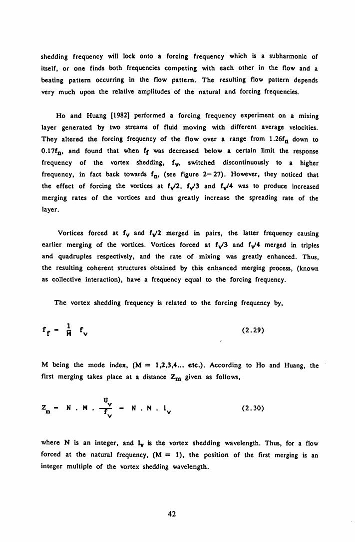
shedding frequency will lock onto a forcing frequency which is a subharmonic of

itself, or one finds both frequencies competing with each other in the flow and a

beating pattern occurring in the flow pattern. The resulting flow pattern depends

very much upon the relative amplitudes of the natural and forcing frequencies.

Ho and Huang [1982] performed a forcing frequency experiment on a mixing

layer generated by two streams of fluid moving with different average velocities.

They altered the forcing frequency of the flow over a range from 1.26fn down to

0.17fn , and found that when f f was decreased below a certain limit the response

frequency of the vortex shedding, fy, switched discontinuously to a higher

frequency, in fact back towards fn , (see figure 2—27). However, they noticed that

the effect of forcing the vortices at fy/2, fy/3 and fy/4 was to produce increased

merging rates of the vortices and thus greatly increase the spreading rate of the

layer.

Vortices forced at fv and fy/2 merged in pairs, the latter frequency causing

earlier merging of the vortices. Vortices forced at fy/3 and fy/4 merged in triples

and quadruples respectively, and the rate of mixing was greatly enhanced. Thus,

the resulting coherent structures obtained by this enhanced merging process, (known

as collective interaction), have a frequency equal to the forcing frequency.

The vortex shedding frequency is related to the forcing frequency by,

M being the mode index, (M = 1 ,2 ,3 ,4 ... e tc .) . According to Ho and Huang, the

first merging takes place at a distance Z m given as follows,

UZm - - N . M . 1 (2 .3 0 )

v

where N is an integer, and lv is the vortex shedding wavelength. Thus, for a flow

forced at the natural frequency, (M = 1), the position of the first merging is an

integer multiple of the vortex shedding wavelength.

42

Experim ental investigations into the effect of forcing jets flows by Bradley and

Ng [1989] have elucidated some features of forced wakes. They used two different

frequencies to force the flow. It was found that by controlling the frequency,

amplitude and relative phases of the forcing, that one may induce various modes of

vortex developm ent and merging in the downstream flow. Such modes include the

paring of similar sized vortices, pairing of vortices of different sizes, multiple

vortex merging, (similar to that observed by Ho and Huang), and vortex shredding.

Vortex shredding defines the process whereby one of the disturbances, generated at

a subharmonic of fn | grows faster than the other disturbance, (not at a

subharm onic), and results in the faster growing vortices tearing apart, or

'shredding ', the smaller vortices.

It has been suggested [Gharib and Williams—Stuber, 1989] that by forcing a

vortex flow, a better environment for examining the nature of the particular system

may be attained. They investigated the forced wake of an airfoil, which has a

structure essentially of a Karman vortex sheet, and found that the velocity profile

downstream adapts to accommodate the forcing of the flow. Nonlinear phenomena

such as beating and 'lock— in' have been found in forced Karman vortex sheets by

Detem ple—Laake and Ecklemann [1989].

2 .3 .7 Flow Behaviour in Pipes, at Orifice

Plates and Sudden Expansions

In pipelines it is often the case that the mean flow has a slight angular motion

associated with it. This may be caused by the inlet conditions. The presence of an

orifice plate in the pipe may accentuate the swirl as the streamlines contract to

pass through it. In some circumstances this may lead to cavitation of the flow due

to the associated radial pressure drop towards the axis of the pipe, Lugt[1962]. The

breakdown of these swirling flows has been examined by Faler and Leibovich

[1978]. However, in this text we are concerned with flows which do not have a

swirl com ponent at a pipe orifice.

It is also worth mentioning, before we consider orifice flows, that vortex flows

may be generated at bluff bodies placed in a pipe. A study by Webb and

43

Harrington [1956] investigated the behaviour of vortex shedding at an obstacle

placed on the pipe wall. They found that, for each Reynolds number investigated,

the height of the obstacle determined whether the disturbances grew, or dissipated

out, in the flow, see figure 2— 28. These obstacles were of the form of

n o n - axisymmetric bluff bodies. The effect of the orifice plate in such flows, which

is in effect an axisymmetric bluff body, will be discussed in the following.

Johansen [1929] visually investigated the flow field at an orifice in a pipe for

low Reynolds number flows. The glass pipe used in the study had a 27mm bore,

and the orifice to pipe diam eter ratio was 0.5. A 2% solution of methylene blue

in water was used for the purpose. The main conclusions attained by Johansen for

the behaviour of the flow at the orifice, as the pipe Reynolds number was

increased from rest, are summarised in what follows. (See figure 2—29).

1 — Creeping Flow (Re0 = 10) — For Reynolds numbers approaching zero, the

flow remains attached to the orifice lip as it flows over it, and the streamlines are

symmetric about the body. Johansen also noted that the velocity appears uniform

across the flow at the orifice aperture. (Figure 2—29a).

2 — Slow Flow (Reo = 30) — The flow begins to separate just behind the orifice

lip, and the recirculation zones begin to form. (Figure 2—29b).

3 — Establishment of Recirculation Zones (RCq = 100) — An increase in

Reynolds number causes the flow to detach from the orifice plate lip, reattaching

itself further downstream. A vena contracta is formed just downstream of the

orifice lip and a recirculation zone is set up. Also, upstream, another smaller

recirculation zone is set up due to the detachment of the flow streamlines as they

converge prior to passing through the orifice plate aperture. (Figure 2—29c).

4 — Appearance of Shear Instabilities (RCq = 250) - Instabilities arise in the

region of high shear between the main flow and the recirculation zone,

(figure 2—29d). These appear as ripples in the flow streamlines and from this

point onwards, the streamlines become time dependent.

5 — A ppearance of Im perfect Vortex Rings (Re0 = 600) - The instability ripples

roll up into incomplete vortex rings. (Figure 2—29e).

44

6 - Vortex Formation (Re0 = 1000) - A further increase in the ReP leads to

the rolling up of the instability ripples into discrete vortices, (figure 2 -2 9 f). These

are convected away by the main flow streaming through the orifice aperture.

7 — Vortex Growth and Breakdown (Re0 = 1600, and above) — At high

Reynolds numbers the vortices generated at the orifice plate grow rapidly as they

proceed downstream, interact with each o ther and breakdown to a 'violently'

turbulent region. This region was seen to extend from one to five orifice diameters

downstream of the orifice itself. (Figure 2—29g).

T he phenomena, observed by Johansen and cited above, were also observed for

o ther diameter ratios, (these being 0.1, 0.25, 0.75) though not at the same

Reynolds numbers. In general the events described above occurred at increasingly

higher Reynolds numbers, as the diameter ratio was increased.

Johansen found that, for the case of vortex shedding at a pipe orifice, ,'no

indication was observed of any tendency for the rings to be shed from the orifice

in the form of a spiral'. That is the shedding of one, continuous helical vortex

was 'not observed. The vortices shed from a pipe orifice kre, therefore, discrete,

axisymmetric vortex rings.

The destabilisation of axisymmetric vortex rings is discussed by Baumann et al

[1992]. However, their work centred on single vortex rings of one fluid inside

a n o th e r . and perhaps is not relevant in this context where the vortex rings at an

orifice are shed in a train, rather like a K arm an' vortex street, and may interact

with each other.

The literature on low Reynolds num ber, vortex flows at a pipe orifice is very

poor, consisting of only Johansen's [1929 & 19?3] work. (Bullock et al [1990] have

investigated high Reynolds num ber, fully turbulent flows at a pipe orifice, where

R ep = 20,500.) It will be instructive, therefore, to look briefly at a similar type

o f flow, that of flows at a sudden expansion within a pipe, (figure 2— 30)^. This

type of flow is also known as a confined je t flow, [Mansoori, 1988].

Back and Roshke [1972] investigated sudden expansion pipe flow for upstream

45

Reynolds numbers of between 20 and 4200. They found that the reattachment

length, Z p of such jets had a variable behaviour depending on the flow regime.

The reattachm ent length versus the upstream pipe Reynolds number is shown

plotted in figure 2 - 31a.

At low Reynolds numbers, Zr moved downstream with increasing Reynolds

numbers. The variation was seen to be linear in this range as shown in

figure 2—31b. At intermediate Reynolds numbers, instabilities in the jet boundary,

increased in magnitude and rolled up in to vortex structures. The reattachment

zone was determined when the lateral extent of this undulating motion extended to

the pipe wall. At higher Reynolds numbers the jet spread more rapidly due to

turbulent, random fluctuations and reattachment occurred relatively close to the

discontinuity.

ofKhezzar et al [1986] followed up the workABack and Roshke, using upstream

pipe Reynolds numbers in the range, 120 to 40,000. Their results for the

reattachm ent length versus upstream Reynolds number are shown in figure 2— 32.

They also investigated in detail the flow properties for an Upstream Reynolds

num ber of 40,000. They found that the centre— line flow velocity decreased

smoothly from the entrance value, U0 , to the final value in the large pipe of

approxim ately 0.32Uo . They also presented the turbulence intensities for various

cross sections across the flow downstream of the outlet. In figure 2—33, the author

has replotted the cen tre- line velocity results, together with the centre— line

turbulence intensities, from the paper of Khezzar et al. From this figure it may be

inferred that the turbulent fluctuations play a major part in the modification of the

je t cen tre— line velocity to that of the downstream pipe centre— line velocity.

(Com pare with results in chapter 6.)

Sibulkin [1962] investigated the turbulent to laminar transition process within a

pipe. He generated the 'artificially turbulent flow' using a sudden expansion flow in

the pipe. These sudden expansions, (or diffusers as Sibulkin calls them), were of

square edge and conical section, as shown in figure 2— 34a. The flow conditions

could be manipulated so that the flow in the downstream pipe was subcritical, i.e.

below Rep. Thus, the turbulence generated by the diffuser was dissipated

downstream .

46

Figure 2 - 34b shows the variation of downstream turbulence intensity at the

cen tre - line, and figure 2— 34c gives details of the axial turbulence intensity at

various radial positions across the pipe, for three positions downstream of the

diffuser, (x /d = 8 , 17 and 35 where d is the upstream diameter according to

Sibulkin). Sibulkin noted that the radial profiles of the turbulence decayed most

rapidly at the pipe wall and the cen tre- line, and least rapidly within the region

0.4 I r/Rp <3.6.

Finally, it should be noted that Durst et al [1989] have used both L.D .A . and

flow visualisation techniques to investigate piston driven, sudden expansion flows.

They have studied both the laminar and transition regimes. The phenomena of

vortex roll— up into rings and interaction with solid surfaces were observed visually

and detailed L.D.A. measurements were taken, giving an insight into the processes

involved.

2.3.8 Flow Induced Vibrations

One practical aspect of the phenomena of vortex shedding is that it may give

rise to flow induced vibrations. Thus, it seems appropriate to comment briefly on

this effect. This type of flow'- structure interaction commonly occurs where a flow

is impeded by a bluff body or restriction. It is an important factor in certain Civil

Engineering design situations, these include bridge deck design, tall buildings,

chimneys, partially closed hydraulic valves, bridge piers etc.

In fact, most structures or hydraulic devices may suffer from flow induced

vibrations, (caused by vortex shedding), under at least some of their expected

operating conditions. It is the role of the Engineer to establish whether these

conditions are acceptable to the operation of the structure, or device, in question.

The problem of flow induced vibrations may be easily dealt with in certain

circumstances by an appropriate change in the shape, and thus modification of the

fluid dynamical properties and response characteristics, of the body in question, see

for example Konishi et al £197el] and Hanko [1967]. There is, however, not

sufficient room herein to go into this subject area in detail, the reader is therefore

referred to the many standard texts on the subject.

47

2.4 N O N - LINEAR DYNAMICAL SYSTEMS

2.4.1 Introduction

It is known that simple, low dimensional dynamical systems may be made to

display complicated solution patterns as the control parameter of the system is

increased above a critical value, [Lorenz, 196?]. These seemingly random, now

called chaotic states, have been found for the post— transient solutions of difference

equations and numerically integrated ordinary differential equations (O .D .E .'s). More

im portantly, such chaotic flows have been found experimentally for all manner of

physical systems. These include; fluid flows such as the Taylor—Couette system and

Rayleigh— Benard convection, biological systems such as predator prey systems and

heart fibrillation patterns, chemical kinetics, electrical circuits and so on.

Chaotic flow is then a universal behaviour which may be realised in non— linear

dynamical systems. Most physical systems are non— linear and it is this fact which

accounts for the recent interest in the field of non— linear dynamics and further

underlines the importance of the work done in this area, [Kuramoto, 1984].

W ithin the last decade or so scientists and engineers have looked to the new

techniques emerging from the field of non— linear dynamics, to provide a

framework for explaining the twin phenomena of the transition of a fluid to the

turbulent state, and fluid turbulence itself, [Guckenheimer, 1986 and Ruelle, 1983a].

Turbulent flow is characterised by the apparently unpredictable motions of the fluid

system, which has, in theory, infinitely many degrees of freedom. However, recent

work has suggested that it is possible that turbulent flow could be governed by an

underlying mechanism, which has essentially only a few degrees of freedom, [Yorke

and Yorke, 1981].

The motion of fluids, governed by the Navier— Stokes equations, is a highly

non— linear phenomenon. Almost all natural flows encountered in the engineering

context are found to be turbulent. It is fair to say that turbulence was previously

regarded as a random process with stochastic analyses tools employed to understand

the phenom enon. Now, however, many workers in the field of turbulent flows

believe that, in some circumstances at least, turbulence may in fact be a complex

48

chaotic motion. This belief has been substantiated by the observation of chaotic

motion in many real, experimental fluid systems, (see for example Abraham et al

[1984]).

For more details of an introductory nature of the subject of chaotic flows and

turbulence the reader is referred to Lesieur [1987, C h.3] and to the articles by

Lanford [1981] and Cvitanovic [1984].

2.4.2 Dynamical Systems

Nonlinear dynamics can be applied to two mathematical topics previously

thought to be unrelated, these are:

1 — Ordinary Differential Equations, (continuous time),

i . e . Autonomous dX(t) «• F(X) , (2 .31a )dt

and Non-Autonomous dX(t ) — F(X, t ) (2 .31b)dt

2 — Mappings, (discrete time intervals),

i . e . Autonomous xj+i " * (2 .32a )

and Non-Autonomous xj+i " f ( xj * 0 (2 .32b)

where X ,x,F and f are N— dimensional vectors. There are many examples of

mathematical non— linear dynamical systems, some of which will be mentioned in

this text. The reader will find a more detailed account of such systems in any

introductory text on non—linear dynamics, such as Sagdeev et al [1988].

49

A well studied example of a n o n - autonomous differential equation is the

Duffing Oscillator, [see for example Asfar and Masoud, 1992, Dowell and Pezeshki,

1988, Gottwald et al, 1992, and Rahman and Burton, 1986]. It will be useful to

look at it in some detail, and use it to outline some of the basic phenomena of

non— linear dynamics.

The Duffing Oscillator has the following mathematical form:

x + Kx + x 3 - B .c o s ( t ) (2 .3 3 )

this is a forced non— linear oscillator, with a cubic elastic restoring force. K and B

are arbitrary control parameters. The superscripted dots denote the first and second

derivative of the displacement, x, with respect to time. Numerically integrating this

equation one finds regimes of periodic and nonperiodic solutions, for various values

of the control parameters. A suitable scheme for numerical integration such as

Runge— Kutta, [O'Neill, 1987], or Newmark method, [Reddy, 1986], could be used.

(The author has numerically investigated the effect of various numerical schemes on

a modified version of the Duffing oscillator, [Addison et al, 1992], See also

appendix 4.)

For example a periodic solution can be found for the param eter values,

K = 0.08 and B = 0.20, and, nonperiodic solutions for K = 0.05 and

B = 7.50. (Figures 2—35a and 2—35b). The nonperiodic solution is very

interesting. It does not repeat itself and appears irregular and unpredictable.

However, it is not a random flow, since each time the oscillator is started from a

specific set of initial conditions, the resulting time series will be identical, (i.e. it is

deterministic). Whereas, a random series will follow a completely different and

unpredictable path each time. A slight change in the initial conditions of the

nonperiodic solution will rapidly produce an entirely different time series. This

phenomena is known as sensitive dependence on initial conditions and is the

hallmark of this type of nonperiodic motion, known as chaotic motion.

Figure 2— 35c shows the effect of starting the Duffing oscillator from two very

close initial conditions, (x = 3.0, x = 4.0 and x = 3.01, x = 4.0). As can be

seen in the figure the resulting time series traces rapidly decorrelate from each

50

other.

More complex oscillator models may be obtained by coupling together two or

more Duffing oscillators, [Yamada and Fujisaka, 1983], or by chaotically exciting

one oscillator by the next, [Burton and Anderson, 1989], However, such systems

are outside the scope of this text.

2.4 .3 Phase Space And Poincard Sections

The most useful way to depict dynamical systems is by the use of a phase

space. The phase space is a 'mathematical space with orthogonal coordinate

directions representing each of the variables needed to specify the instantaneous

state of the system', [ S ^ e y and &oiiub} 1981 ]. Thus, for the Duffing oscillator,

rather than plotting the time series, i.e. the x— t curve, we may plot the x— x

curve in a two dimensional phase space. In figures 2— 36a and 2— 36b. The phase

space trajectories are shown for the periodic and chaotic state of the Duffing

oscillator. The trajectories evolve and form a 'phase portrait' of the system in

phase space.

The chaotic trajectory of the Duffing oscillator fills up 2—dimensional phase

space. However, if the phase space is increased in dimension to 3, (i.e. x—x— x

curves), we find that the trajectories do not cross each other, and the phase space

does not fill up. Thus, a three dimensional phase space is sufficient to describe the

properties of the chaotic solution of the oscillator. (This is because the chaotic

solution trajectories actually form an object called an attractor which has a

non— integer value of its dimension, between 2 and 3, this will be discussed in

m ore detail in later sections.)

One way to simplify phase diagrams is to use a device known as a Poincare

section. It is constructed by sampling the phase trajectories in a 'stroboscopic'

fashion. The trajectory is sampled once every cycle of the forcing function.

Figure 2—37 contains the Poincare sections of the periodic and chaotic solutions to

the Duffing oscillator.

For both the periodic and aperiodic solutions initial conditions far from the

51

final solutions will produce trajectories which will, after the transients disappear, be

attracted to a bounded region in phase space. This region is known as an

attractor. For the case of the chaotic flow, where the trajectories never cross, the

resulting 'bundle ' of non-crossing trajectories form an object known as a strange

attractor.

2.4.4 Strange Attractors

Two main phenomena are present in strange attractors, (also known as chaotic

attractors), these are Stretching and Folding, as outlined by Roux et al [1983]. The

attractor stretches due to the exponential divergence of the trajectories as they

evolve, however, as the attractor lies in a bounded region of phase space, it also

must exhibit folding. This mechanism of stretching and folding mixes up trajectories

in phase space, making long term future predictions of the system impossible unless

the condition of the system is known e x a c t l y at any one point. (Which is not

realistic for real systems.)

If two trajectories are started from states that are arbitrarily close they will

diverge over a period of time, this divergence is exponential. This initial difference

may be thought of as measuring error, i.e. an uncertainty. Thus, as the system

evolves through time the error blows up exponentially and the state of the system

is essentially unknown after a very short period of tim e. This sensitive dependence

on initial conditions was first elucidated by Lorenz [1963], who used the concept to

show that long term future predictions of non— linear dynamical systems, such as

the weather, was essentially impossible.

In general, for more complex dynamical systems, the phase space representation

may contain many attractors. Which one of these attractors, the final solution

settles down to, depends very much on the initial conditions of the system. Each

attractor is associated with a region which, if it contains the trajectory at one

instant in tim e, will eventually lead to that trajectory settling on to that attractor.

This region is known as the basin of attraction of the attractor.

In systems with more than one strange attractor, the presence of noise may

cause the solution trajectory to hop between basins of attraction, this phenomena

52

together with its associated frequency spectra is discussed by Arrechi [1987].

The reader is also referred to Soliman and Thompson [1991] who make use of

basins of attraction to define dynamic ship stability.

Another important feature of a strange attractor, associated with a dissipative

dynamical system, is that it contracts volumes in phase space. This is because,

even though the attractor exponentially diverges in one orthogonal direction, causing

sensitive dependence on initial conditions, on the whole, the attractor contracts in

phase space. Thus, any volume of initial conditions is eventually stretched into a

thin sheet of ever decreasing volume on the attractor. Thus the volume of a

strange attractor, in a phase space of suitable dimension to fully describe the

dynamical properties of the system, tends to zero. (See also the section on

Lyapunov exponents, section 2.5.6).

Another important property of attractors is their space filling properties. The

solution trajectories which form the strange attractor do not intersect each other,

when embedded in a suitable dimension of phase— space. However, the trajectories

do not fill up space evenly, rather, they fill up space as a fractal. The word

fractal is an abbreviation for 'fractional dimension'.

To explain what a fractal structure is, it is helpful to look at a simple example

of a fractal, known as the Cantor set, (figure 2—38a). The Cantor set is formed

by taking the middle third out of the unit line segment, as shown at the top of

the figure. Then the middle third is taken out of the remaining two line segments.

Then the middle third is taken from the remaining four line segments, and so on,

a d i n f i n i t u m , until we are left with only a set of points, known as the Cantor set

or Cantor dust. This set of points fills the unit interval in a special way, and

although the length of the cantor set is zero, it can be shown that the dimension

of the set is 0.6309..., (see section 2.5.4). The interesting fact is that many

attractors, when sliced through, show a Cantor set like structure.

It may be difficult to grasp the idea of fractional dimensions when one is used

to the usual use of the zero, one, two and three— dimensional way of interpreting

the world, (i.e . a point, line, area and volume respectively, as depicted in

figure 2— 38b). One way to think of the fractal structure of the Cantor set is to

recognise that the set cannot fit into a point, that is have zero dimension, as it is

53

specified over the unit interval. However, it can neither have a dimension of one,

as it obviously has a length which tends to zero on the unit interval. It can be

shown by applying mathematical descriptions of dimension, (see section 2.5.4), that

the set does indeed have a fractional dimension of 0.6309..., i.e. it is a fractal. A

graphical account of fractals is given by Peitgen and Richter [1986]. For a more

comprehensive account of fractals and their role in natural phenomena the reader

is referred to Mandelbrot [1977].

Ruelle [1980] describes strange attractors as 'relatively abstract mathematical

objects ', however, he goes on to say that computers may aid in their

understanding, by giving them 'some life' by drawing pictures of them. The

observation of strange attractors in real systems — hydrodynamic, chemical,

electrical, biological etc., (see for example Swinney [1983]) — has provided the

impetus for the development of non— linear dynamical systems theory. A few of the

more important systems, both mathematical and real, are outlined in the next two

sections.

2 .4 .5 Examples of Mathematical Systems Exhibiting

Chaotic Motion

As mentioned above, there are many examples of mathematical dynamical

systems which exhibit chaotic motion. An overview of many of these are given by

Holden and Muhamad [1986]. In addition, recent experimental work has also found

that real systems (i.e. systems in nature), can exhibit such motion. In this section,

and the next, a few of the very common systems that have appeared in the

literature are outlined.

1 — The Logistic M ap: This simple m ap, given by the difference equation

X ^ , = A.Xn .(l - X J (2.34)

where A is the control parameter. The map has been shown to produce varied

behaviour for A in the range, 1 < A < 4, see figure 2—39a. For values of the A

less than 3, the system evolves to a stable state, or fixed point. After this limiting

value, the system will oscillate between two values of X, when A is in the range

54

3 < A < 3.449. As A increases beyond 3.449, the solution oscillates between four

points, for the range 3.449 < A < 3.544. This process, known as period

doubling, continues as the control parameter, A is increased. The point at which

the solution changes from one period to the next is known as a bifurcation point.

If the first bifurcation occurs at A , , the second at A a and so on then as the

control param eter is increased a universal number, 5^, is formed:

“ \ . - i6 - l im ---------------------- - 4.669 (2 .35)

* * * * \ + r \

This number is universal for a large class of non— linear systems, [Feigenbaum,

1980], and is known as the Feigenbaum number. Figure 2—39b shows the

bifurcation diagram of the logistic equation, where the resulting values of X, that

the steady state oscillations occur on, is plotted against the control parameter A.

However, the period doubling increases to an infinite period for a finite value of

the control param eter, (A = 3.569944). This finite value of A is known as the

accumulation point, after which the system behaves chaotically.

There is not room in this text to cover the intricacies of such mappings, and

for more information the reader is referred to Infeld and Rowlands

[1982, Chapter 10] and Baker and Gollub [1990, Chapter 4].

2 — The Henon M ao: Before moving on to non— linear systems described by

differential equations, it will be useful to briefly look at the Henon mapping, (see

Infeld and Rowlands [1990]), described as follows,

X J - 1 - a .X 2 + b.Y (2 .36a)n+i n n ' '

Y - X n+1 n (2.36b)

The phase portrait obtained by plotting Yn against Xn , is shown in figure 2—40a,

where a = 1.4 and b = 0.3, this is the Henon attractor. The initial values of X

and Y were 0.631 and 0.189 respectively. The strangeness of the attractor is

55

revealed by enlarging a region of it, such as the small box in figure 2—40a. The

enlargement is shown in figure 2— 40b. Once enlarged we see detail that was not

apparent at the previous level of magnification. Enlarging again, figure 2— 40c,

more detail may be observed. This process may be carried on a d i n f i n i t u m . This

self similar, fractal nature of the attractor's structure is a common feature of

strange attractors.

3 — The Lorenz Eouations: In 196? Lorenz published his now famous paper

entitled 'Deterministic, Nonperiodic Flow', in which he set out the basic underlying

principles of chaotic motion. To do so he numerically integrated a stripped down

version of the equations of motion for the atmosphere, now called the Lorenz

equations. They are defined thus,

X - - a ( X - Y ) (2 .37a)

Y - - X Z + r X - Y (2.37b)

Z - XY - bZ (2 .37c)

where X is the first time derivative of the displacement X.

The equations may be integrated with a suitable numerical scheme, with the

parameters a = 10.00, r = 28.00 and b = 2.67 giving chaotic motion. The

chaotic time series and resulting attractor is shown in figure 2—41. Since Lorenz's

article, much work has been done on these equations by many researchers. In

addition, many other equations have been devised, (and studied in detail), which

highlight the phenomena of chaotic motion. Some of which are discussed in the

following.

4 — The Rossler Equations: The Rossler equations, (see for instance Holden and

Muhamad [1986]), are again a highly truncated set of equations which in this case

model the quintessential dynamics of a chaotic chemical reaction. They are as

56

fo llO W S ,

X - Y - Z (2.38a)

Y X + aY (2.38b)

Z b + XZ - cZ (2.A5c)

Chaotic motion in this case can be obtained by setting the parameters a, b and c

to 0.20, 0.20 and 5.70 respectively. The strange attractor for these parameters is

shown in figure 2— 42.

5 — The Rossler Hvoerchaos Equations

Rather more interesting behaviour can be found in the hyperchaos equation of

Rossler [1979],

X - - Y - Z (2.39a)

Y - X + 0 . 2 5 Y + W (2.39b)

Z - 3.00 + XZ (2.39c)

W - - 0.52 + 0.05 W ( 2 . 39d)

The Z— variable serves as a check on the growth of the system, and in effect

Z is 'turned o n ' (i.e. has a non—zero value) only for certain values of X, Y and

W , as shown in figure 2—43. This gives the attractor variable properties,

depending on whether the Z—variable is activated or not.

57

6 — The Truncated N avier- Stokes Equations

Franceschini and Tebaldi [1979], and Boldrighini and Franceschini [1979],

presented a system of non— linear ordinary differential equations that are a stripped

down version of the Navier— Stokes equations of a two— dimensional incompressible

fluid. The authors claim that the model may exhibit many of the important

features of the equations.

The equations are,

X - - 2.X + 4.X .X + 4.X .X (2 .40a)1 1 2 3 4 5

X - - 9.X + 3.X .X (2.40b)2 2 1 3

X - - 5.X - 7.X .X + r (2 .40c)3 3 1 2 v '

X - - 5.X - X .X (2 .40d)4 4 1 5

X - - X - 3.X .X (2 .40e)5 5 1 4 N

In the above equations, r represents the Reynolds num ber. As the value of r is

increased the system passes from a fixed point attractor to a periodic attractor,

then, via period doubling bifurcations, to a strange attractor. A strange attractor

first appears at a value of r of approximately 28.7. The strange attractor for the

system, (computed by the author for r = 31), is plotted in figure 2—44.

In addition to the examples outline above, chaotic behaviour has been found in

a very wide variety of systems, from models of Physiological control systems

[Mackey and Glass, 1977] to models of articulated offshore loading platforms, [Choi

and Lou, 1991]. (The chaotic output of the logistic equation has__even been used to

produce music!, [Pressing, 1988].) Thus, we see that a knowledge of this behaviour

is im portant for the investigator dealing with non— linear dynamical problems, and

their associated phenomena.

58

The Rossler, Rossler Hyperchaos and the Lorenz systems were used by the

author to test the Grassberger— Procaccia dimension and Lyapunov algorithms, prior

to them being used in the analysis of the experimental results. (See Section 2.5

and Appendix 2.)

2.4.6 Real Systems with Strange Attractors

The literature is now full of examples of chaotic motion found in nature.

These examples cover many areas of research involving dynamical systems, such as

fluid dynamics, chemical kinetics, electrical circuits and biological processes. The

phenomena is truly of a multi— disciplinary nature. A brief account of some of the

main experimental realisations of chaotic motion will be given in the following.

(Those found in fluid dynamics will be dealt with in more detail in section 2.6.)

2.4.6.1 — Fluid Dynamics

Chaotic fluid flow has now been observed in many fluid systems. Of these, two

of the most extensively studied are Rayleigh— Benard convection, and

Taylor—Couette flow.

Rayleigh— Benard convection may be generated by heating from below, a thin

layer of fluid between two horizontal plates. As the tem perature gradient across the

flow is increased, various phenomena occur, [GiglioA>1981]. The control parameter

is this fluid situation is the Rayleigh number, Ra, which is defined thus:

Rs " [ ~SE7 ^ ~ ] AT (2 4 1 )

where g is gravitational acceleration, a is the coefficient of thermal expansion, d is

the distance between the plates, k is the thermal diffusivity, v is the kinematic

viscosity and AT is the tem perature difference between the two plates.

Up to the critical Rayleigh number, Racr|t, no motion exists, and the heat is

59

transferred solely by conduction through the fluid. Just above Racrjt convective rolls

appear in the fluid, (figure 2—45a). The critical Rayleigh number has been well

predicted by stability analysis. As the Rayleigh number increases above Racrjt,

successive bifurcations occur as the fluid progresses to the turbulent, or chaotic,

state. (See Giglio et al [1982] and also Sano and Sawada [1985]). In fact, a wide

variety of behaviour has been found to exist for flows above Racrit> some of which

will be outlined in the next section.

The other well documented flow system which exhibits regular and chaotic flow

is the Taylor— Couette system. This system involves the flow of fluid in two

concentric, rotating cylinders which rotate at rates independent of each other,

(figure 2—45b). As the Reynolds number is increased the velocity field proceeds

from a regular to a weakly chaotic state, whereby a strange attractor may be

observed in phase space, [Mullin and Price, 1989].

The interesting thing about both the Rayleigh— Benard and Taylor— Couette

systems is that they have, in principle, an infinite number of degrees of freedom.

However, it seems likely that, at the onset of chaos, only a few degrees of

freedom are excited, [Swinney, 1983].

Both the systems discussed above are closed fluid systems, however, work has

recently been done on open fluid systems, such as transitional flow in pipes, (see

for example Sreenivasan and Ramsdankar [1986] and, Huang and Huang [1989])A

and the breakdown of vortex flows produced at an airfoil [Williams— Stuber and

Gharib, 1990]. These flows are more difficult to control precisely, as they tend to

have higher levels of background noise associated with them. This noise may tend

to mask, or alter, the dynamics under investigation, [Swinney and Gollub, 1981].

More will be said on these systems in section 2.6.

2 .4 .6 .2 O ther Areas

One system to feature prominently in the literature on experimental non— linear

dynamics is the Belousov—Zhabotinski chemical reaction, [Hudson et al, 1981],

whereby chemical reactants are continuously stirred in a chemical reactor. This

reaction has been found to exhibit both periodic and chaotic behaviour, [Swinney et

60

al 1983], depending on the conditions present in the reacting vessel. The general

method of looking at the system is to measure the concentration of one of the

chemicals in the system, (usually the Bromide ion), and plot these against

time. A strange attractor has been found for such flows by Roux et al [1981]. (See

also Ruelle [1981].) The Belousof-Zhabotinskii strange attractor is shown in

figure 2— 46.

The most prominent example of a biological chaotic flow is that of the

behaviour of electrically stimulated chick heart cells. Guevara et al [1981], forced

specially prepared aggregates of chick heart cells with pulses of electrical current.

Regular and irregular dynamics were exhibited by the system and a bifurcation

chart, similar in many ways to that of the logistic equation, was produced. This

work is especially important, as many researchers believe that certain types of heart

fibrillation may be a chaotic response of the dynamics of the heart itself, [Glass et

al, 1986]. Conrad [1986] gives an overview of the role of chaotic dynamics in

many biological settings.

Chaotic responses have also been found in many electrical circuits, [Tomita,

1986], from simple circuits containing only a resistor, inductor and diode, [Smith,

1992], to systems which involve the parallel pumping of ferromagnets, [Waldner et

al, 1985].

In this section only a few brief examples have been given of the experimental

verification of chaotic flows, and other phenomena associated with non— linear

dynamical systems. Many more areas have not been touched upon, such as the

chaotic output of lasers, or the role of chaos in statistical and quantum mechanics,

[BaRer and £ollufc>, 1990, ppl33—144]. However, it is hoped that this section has

served to make the reader aware of the universal nature of this type of behaviour.

2.4.7 M athem atical Routes to Turbulence

The work done on non— linear dynamical systems has shown that relatively

simple systems may, as the control parameter is increased, evolve from a steady

state via some route, to a chaotic (or turbulent) state. Much theoretical interest has

been centred on the routes taken by such systems, and whether these routes may

6 1

be realised in the experimental situation.

There are currently four mathematical descriptions of the route taken from

laminar flow through transition to fully developed turbulence, [Miles, 1983]. All of

them begin with a Hopf bifurcation. A Hopf bifurcation occurs when a steady state

bifurcates into a periodic solution, which generates a limit cycle in phase space, as

shown in figure 2—47.

The four main theoretical routes to turbulence are as follows:

1 — Landau M odel: Landau [1944] was the first to suggest a mathematical route to

turbulence, whereby, as the control parameter, the Reynolds number, Re, is

increased above a critical value, R©crit- ^ ^ is scenario, incommensurate

frequencies would appear via a succession of Hopf bifurcations, as the control

parameter was increased above the critical value. This would result in a

quasi— periodic motion of increasing complexity. The final fully developed

turbulence according to Landau is a quasi— periodic motion of great complexity.

2 — Feigenbaum Period Doubling Scenario: This consisted of a Hopf bifurcation of

the initial stable state and then successive period doublings of the initial disturbance

until an accumulation point is reached at a finite value of the control parameter.

This scenario has already been outlineAfor the case of the logistic map in section

2.4.5.

3 — Reulle—Takens Route to Turbulence: Reulle and Takens have conjectured that

a strange attractor will appear at the third bifurcation of the Landau sequence.

4 — Interm ittent Scenario of Manneville and Pomeau: In this case the solution of

the system alternates between a singly periodic limit cycle and a strange attractor.

The Landau model is now not regarded as a realistic route to turbulence as it

has not been observed in any experiment to date. For a more complete description

of the routes to turbulence see Miles [1983].

The initial stages of the period doubling route to turbulence, (route 2), has

been observed in Taylor—Couette and Rayleigh—Benard flow, as well as the

62

Belousof— Zhabotinskii reaction and other systems. Routes 2, 3 and 4 have all been

observed by Gollub and Benson [19 iO] in the Rayleigh-Benard system.

Furtherm ore, they also found another route to turbulent flow, involving

quasi— periodic locking at incommensurate frequencies. They concluded that the

route taken by the system depends on the aspect ratio of the apparatus that they

used.

Arneodo et al [1983] have observed another route followed by the

Rayleigh— Benard system, which is a variation of the period doubling route. This

alternative route, and others, have been observed in numerical simulations of such

flows by Kida et al [1989]. These simulations have the advantage of being much

more flexible, for instance the viscosity param eter is easily varied and its effect

monitored, whereas, in the experimental situation this may be more difficult to do.

Kida et al found that as the viscosity was reduced more complex patterns appeared

in the flow.

O ther deviations from the theoretical routes to chaos, (as described above),

have been found in the pumping of ferromagnets by Waldner et al [1985] and also

by Kaolin et al [1981] in an annular, free—surface fluid system, known as the

Faraday experiment. The results of Kaolin et al are particularly interesting because

instead of obtaining the usual period doubling subharmonic sequence of

1 ,2 ,4 ,8 ,16,32..., they observed sequences of 1,2,4,12,14,16... and 1,2,3,4,6,12....

These anomalous results serve to remind us that perhaps a full theoretical picture

has not been yet been formulated.

Kaolin et al also observed hysteresis in some of their results. That is, the

routes followed by the system, as the control parameter was increased then

reduced, were not identical. O n reduction of the control parameter, jumps

appeared in the sequence. The phenomena of hysteresis has also been found by

M ercader e t al [1990] modelling the route to chaos of a mathematical model of

the Rayleigh— Benard system, providing another link between experiment and

theory.

63

2.4.8 M odelling N o n - linear Dynamical Systems

Before concluding this section, it is appropriate to mention two cases where

real non— linear dynamical systems have been found to produce non— linear

phenomena, including chaotic motion, and have been successfully modelled

numerically to produce qualitatively similar effects.

T he Dripping Faucet

Robert Shaw [1984] investigated the behaviour of the dripping tap (faucet) with

varying flow rate. At low flow rates, the drips initially fell with a regular period.

As the flow rate was increased, period doubling ensued, which led finally to a

chaotic falling of the drops. The drips were detected by interrupting the light beam

that intersected with a photodetector, which in turn relays the signal to a computer

for data acquisition and analysis. Shaw decided to use a 'naive' model to simulate

the experim ent, whereby the dripping tap was simulated as a non— linear oscillator,

(see Shaw [1984]). Without going into great detail, similar behaviour was obtained

between both the real system and the naive model, as is shown in the phase space

portraits of figure 2—48.

Fluid Elastic Vibrations of a Flexible Pipe

The fluid elastic vibration dynamics of a flexible cantilevered pipe conveying

fluid were investigated, both theoretically and experimentally, by Paidoussis and

Moon [1988], figure 2—49. Once the pipe lost stability, bifurcations were observed

leading to a chaotic response in both the experimental and analytical models. As

with the dripping faucet model, remarkable qualitative agreement was found

between the experimental and theoretical results, despite the great simplicity of the

theoretical model.

64

2.5 TH E TESTING O F N O N - LINEAR DYNAMICAL SYSTEMS

2.5.1 Characterisation of Attractors

Many properties can be found for chaotic flows using various techniques, the

problem is to find one which can differentiate between purely random (or noisy)

flows and those which are chaotic. Fourier transforms, the autocorrelation function

and Poincare maps will give a general indication of the change from the periodic

to nonperiodic state, [Schuster, 1984], but these methods are unable to distinguish

between chaotic and random flows. (That is between the seemingly unpredictable

properties of chaotic flow and the actual unpredictable properties of noisy flow.)

Thus, other types of measure or characterisation are required.

The dimension, the spectrum of Lyapunov exponents and the Kolmogorov

entropy are all measures giving an indication of how chaotic a flow is, and they

can, in theory, distinguish between chaotic and random flows.

Before using a sophisticated technique to analyse a time series, one should first

visually inspect the series to see if any apparent features are present. Visual

inspection of a velocity time trace from a fluid flow can distinguish whether a flow

is laminar or turbulent, (see sections 2.2.2 and 2.2.3). O ther types of simple

motion may be identified from the velocity—time trace, such as periodic motion,

and also a qualitative feel may be obtained of the complexity of the flow.

2.5.2 The Fast Fourier Transform

The fast Fourier transform (F .F .T .) is a numerical algorithm by which the

discrete Fourier transform of a signal may be calculated with exceptional speed,

[Cooley et al, 1969]. The discrete Fourier transform, (D .F .T .), F (xp , of a variable

xj» ( j= l|2 ,3 ,4 ,.. . .N ) is defined thus:

N -i

l-oX e ( 2 .4 2 )

65

here, i is the imaginary number ( - l ) i .

The F .F .T . algorithm enables the number of calculations required to compute

the Fourier transform of a set of N data points to be reduced by a factor of

log2(N)/N, which is significant for large N, [Newland, 1975]. The algorithm

requires that the number of points in the signal is a power of 2, e.g. j 14

(=16384), which is the number of points typically sampled in the experimental

investigation outlined in this thesis.

From the resulting F .F .T . plot of a time signal, periodic, multiply periodic,

quasi—periodic and 'turbulent' signals may be differentiated, [Berge, Pomeau and

Vidal, 1984, ppl 11 — 123]. However, from the F .F .T . itself 'turbulent' flow cannot

be differentiated into either a random or chaotic phenomena, as both give broad

band frequency spectra, see figure 2— 50a and b.

Typical power spectra for flows e n r o u t e to a chaotic signal, via period

doubling, are outlined by Crutchfield et al [1980], whereby the period doubled

peaks broaden as the chaotic signal is approached. Huberman and Zisook [1981] go

on to describe this spectral broadening in detail. The peaks in the power spectrum

broaden at their base as the chaotic state is approached, as depicted in

figure 2—51. These broadened bases of the peaks are referred to as skirts by

Farm er [1981]. The power spectrum of the chaotic state consists of instrumentally

narrow peaks surrounded by a broad band noise background.

2.5.3 Experimental A ttractor Construction

Before we can estimate the dimension, Lyapunov exponent or other properties

to test for the presence of a chaotic flow, we must first construct an attractor.

This can be done for a single experimental time series by the method of time

delays, devised by Ruelle [Ruelle, 1989, pp28—32]. (See also Roux et al [1980],

who used the method to construct the attractor for the Belousof— Zhabotinskii

chemical reaction.) Such an experimental time series is depicted in figure 2— 52a

and consists of N sampled points, separated by a time interval, dt.

In the method, the ordinates of the attractor, X, are constructed for

66

n—dimensional space from the original time series, xj, (i = 1,2,3........N), as

follows,

X = {xi , Xi+£ , XH.^ .............. xi+ (n—1){> (2 -43)

where X is the n— dimensional attractor vector produced from the discretely

sampled time series, xj, and £ is the delay. The time delay between reconstruction

variables is thus T = £.dt. The resulting attractor is shown in figure 2—52b.

The choice of £ is non— trivial as we want the dynamical properties of the

reconstructed attractor to resemble those of the actual attractor of the system under

observation. Three common methods for the choice of £ will now be outlined.

M ethod 1 — For low dimensional attractors occurring in a system with periodic

forcing, it is recommended, [Guckenheimer, 1986], that the most favourable value

of is one quarter of the forcing period. (This has been demonstrated by the

author when constructing an attractor for a journal bearing model in a chaotic

mode, see Appendix 5.) This is a quick and easy method for such systems,

however, many fluid systems do not posses such a forcing function and so another

m ethod to calculate the time delay is required.

M ethod 2 — The autocorrelation function, Cg, is a frequently used method for

finding a suitable time delay for attractor construction. Redefining the

autocorrelation function, (section 2.2.3.2) for any fluctuating component, Xj', of a

variable xj, where,

•x - Xj - Xj ( 2 .4 4 )

the superscripted bar above the variable denotes the time averaged value. The

correlation integral, for a discretely sampled time series, is then,

67

( x j ) . ( x 1+£ )( 2 .4 5 )

It is recommended, [Huang and Huang, 1989], that the time delay for the attractor

construction, should be taken as the value which first gives = 0.5.

M ethod 3 — The minimum mutual information criterion is another method by

which to determine a suitable time delay 'y \ It is argued, [Fraser and Swinney,

1986 and Fraser, 1989], that, whereas the autocorrelation function measures a

linear dependence of two variables, the minimum mutual information measures the

general dependence of two variables.

The minimum mutual information of two variables x and y is defined as,

where P ^ i) is the probability of a variable x(i) occurring, and P x ,y(i,j) is the joint

probability of occurrence of variables x(i) and y(j). A suitable choice of time delay

requires I to be a m inim um , when this is the case the attractor is as 'spread out'

as possible, see figure 2— 53.

When considering tim e delays we let x = xt , and y = x t+ £. An obvious

result is that when 1(X|,X|+ is a minimum, this implies that I (x |+ £,xj+ 2 g) is a

minimum also, and so on. The value of the delay, £, to use in the attractor

construction is that which gives the first minimum in m utual information,

Roux et al [1983] have actually used delays, {, obtained by visually inspecting

phase portrait plots of the reconstructed attractors at various values of £. The

value of time delay they subsequently chose to use, was the one that produced an

attractor which appeared to be most spread out. However, the minimum mutual

N

U x . y ) - J px . y ( i . J > loSi . J " 1

pxCD py U >( 2 .4 6 )

68

information in effect does this numerically. Therefore, it is this method which the

author recommends for time series which do not posses an obvious periodic

fluctuation, and it is this method that was used for all attractor construction in the

experimental investigation reported within this thesis in subsequent chapters.

2.5.4 The Dimension of an Attracting Set

Once a strange attractor has been obtained from an experimental time series

the next step is to characterise it. Of all the properties used to characterise strange

attractors in chaotic flows, the two most commonly used are the dimension and the

Lyapunov exponents of the system. Both these methods will be outlined in the

following sections. First we will deal with the dimension as a means by which to

characterise a dynamical system.

The dimension of an attracting set has been described by Farmer et al [1983]

as ’the most basic property of an a ttrac to r', however, many definitions of

dimension exist. The dimension is basically a measure of the scaling properties

(fractalness) of a structure. The simplest and most easily understood definition is

the Capacity (or Kolmogorov) dimension 'D c \ which is defined as :

log N(e)Dc 11m --------------------------------------- (2.47)

c-*0 log (O

where N(«) is the number of n—dimensional boxes of side required to cover

the attractor.

Another frequently cited dimension is the information dimension 'D j \ This

measure seeks to account for the differences in distribution density of the points

covering the attractor as follows,

K OD j 11m -------------------------------------- (2.48)

c-*0 l o ga( 0

69

N ( 0

w here 1 ( c ) — — ^ Pj l o g 2 P i

i - 1

(2 .49)

K O is known as Shannon's formula, [Shannon and Weaver, 1949]. A more

informative guide to the concepts of Information Theory and its role in statistical

mechanics can be found in the literature, see for example Renyi [1970].

It is easily seen that, for an attractor with an even distribution of points,

Dc = Dj. However the calculation of either of these two interpretations of

dimension require a prohibitive amount of computing time.

The most widely used description of dimension used for experimental

investigation is based on the correlation dimension, as defined by Grassberger and

Procaccia [1983a and 1983c], and is denoted by D gp- The reason for its popularity

is its relative computational speed when implemented as an algorithm for dimension

estimation.

To define Dgp we firstly need to define the correlation integral,

N

J 0 ( r - I X j - X j l ) ( 2 . 5 0 )

i . J - 1

where 0 is the Heaviside function, r is the radius of an n— dimensional

hyper— sphere, centred on each of the points defining the attractor trajectory,

(figure 2—54a). The correlation integral scales with the radius 'r ' as,

Cr - r DSP ( 2 . 5 1 )

hence, Dgp can be found from the slope of the 'logCCj) — log(r)' plot,

(figure 2 - 54b).

70

Dgp forms a lower bound to the capacity dimension and asymptotically

approaches the value of Dc as the attracting set becomes more uniformly

distributed in p hase- space. In general,

Dj < Dgp < Dc . (2.52)

It is appropriate to mention here that there are many other definitions of

dimension such as the Hausdorff, Lyapunov and generalised Renyi dimensions to

name but a few, see for example Farmer [1982], Farm er et al [1983], Froehling et

al [1981] and Grassberger[1983].

There is still much that needs to be done on the dimension as a

characterisation of chaotic flows, [Mayer—Kress, 1987]. Farm er [1982a] states that

many questions remain to be answered, such as — 'How quickly does the

dimension of a chaotic attractor change as the control parameter, (e.g. the

Reynolds num ber), of a system is varied?', 'How steady is this change?', and, 'Are

the attractors of an infinite— dimensional dynamical system qualitatively similar to

those of low dimensional systems?'. (A point which is extremely valid for the

endorsem ent of the use of such methods in real fluid systems, which possess in

theory an infinite number of degrees of freedom .) Subsequent investigations by

Farm er of an approximated infinite dimensional system, [Mackey and Glass, 1977],

led him to conclude that the transition to 'tu rbu len t' behaviour begins with a

chaotic attractor, followed by attractors of increasingly higher dimension appearing

as the control param eter is increased.

According to Whitneys embedding theorem, (see Gershenfeld [1992]), it can be

guaranteed that an n— dimensional attractor may be embedded in a

( 2 n + 1)— dimensional embedding space, (phase space). However, this is a maximum,

and in general an n— dimensional space, (or next nearest integer value of phase

space), should be sufficient. Gershenfeld has also shown that, under certain

circumstances it is possible to reliably measure the correlation dimension of

a ttractors with dimension greater than 10.

71

2.5.5 The G rassberger- Procaccia Dimension Estim ate

and its Implementation.

When using the Grassberger- Procaccia technique to estimate the dimension of

an attractor, the investigator must be aware of scale, and other, effects and how

they relate to the results obtained. There are four main regions of behaviour of an

attractor [Smith, 1988], these are outlined in the next section, beginning with the

smallest length scales.

2.5.5.1 R edons of Behaviour on the A ttractor

1 — At very small length scales the Grassberger— Procaccia dimension algorithm

tends to a dimension estimate of zero. This occurs when the algorithm is testing

the attractor at scales too small to pick up other points on the attractor, i.e. when

the radius of the n— dimensional hypersphere used in the Grassberger— Procaccia

algorithm is less than the inter— point distances on the attractor trajectories. See

figure 2—55a.

2 — The next region depends very much on whether one is considering an

experimental, and hence noisy, attractor, o r if the attractor is a mathematical

construction, (noise free), such as the Lorenz attractor or Rossler attractor.

If the attractor is noisy, then for length scales of the order of the characteristic

noise level, (see figure 2—55b), Dgp will scale with the noise, (assuming white

noise, see Section 2.5.5.2). That is, it will increase with, and should be

approximately equal to, the value of the embedding dimension, [Ben— Mizrachi et

al, 1984].

However, if the attractor is noise free and the length scales being probed are

of the order of the distance between consecutive points on the trajectory, then for

limited data sets the algorithm will only detect points immediately nearby on the

trajectory. This region of the attractor will show up as essentially 'linear', and the

value of Dgp will tend to one, see figure 2— 55c.

3 — Once the hyper— sphere radius overcomes the effects of small length scales

72

of regions 1 and 2, values of Dgp will approach those of the actual fractal

dimension Dc , assuming that a suitable time delay has been chosen.

(Figure 2 -5 5 d ).

4 — Once the length scales of the sphere are of the order of the attractor

radius, edge effects become dominant, where large parts of the hyper— sphere are

outside of the attractor and hence empty, thus reducing the value of D gP*

(figure 2.55e). As the radius becomes very large, the attractor tends to a point

within the sphere and Dgp tends, once again, to zero. Edge effects are discussed

by Smith [1988] and a modification to the Grassberger—Procaccia dimension

algorithm is proposed by Dvorak and KlascKVkt [1990] based on Smith's results.

Whereby, they plot log(Cr) against log (r(2 -r)) instead of the usual Mog(Cr) - log(r)'

plot, and suggest that the slope of this line gives the correct estimate of the

dimension. However, as far as the author can see, this m ethod is only applicable

in the ideal case of an evenly distributed attractor in an n— dimensional

hypersphere of unit radius.

2 .5 .S.2 A ttractors and Noise

Noise, as already mentioned, can have a detrimental effect on the value of the

apparent dimension of the attracting set, and in some cases may be severe enough

to render the estimation of dimension impossible. A novel method of reducing

noise in the reconstructed attractor has been proposed in a paper by Kostelich and

Yorke [1990], where they approximate the average dynamics of various regions of

the attractor. They do this by a method known as Eckm an— Ruelle linearization.

These average approximations to the dynamics are then used to reduce the noise in

individual trajectories as they pass through each region of the attractor.

A signal composed of purely white, (or Gaussian), noise will scale with the

value of the embedding dimension due to its phase— space filling behaviour.

However, stochastic systems with power— law frequency spectra have been shown,

[Higuchi, 1990,_ and, Osborne and Provenzale, 1989], to give finite correlation

dimensions. In this case, a finite value of Dgp will not necessarily indicate that the

dynamics of the system can be described by a few degrees of freedom. In such

cases, care must, therefore, be taken in the interpretation o f dimension calculations

73

in such cases. It is therefore recommended that the dimension estimate is

interpreted in conjunction with other analysis techniques, such as the frequency

spectrum, autocorrelation function and the Lyapunov exponent spectrum.

2.S.S.3 O ther Factors Affecting the Estim ation

of A ttractor Dimension

The lacunarity of the set has a bearing on the estimation of the dimension. If

the set has a high degree of lacunarity then the value of D gp will fluctuate

markedly as various parts of the attractor are visited.

Sparse or limited data sets tend to produce errors in the calculations, which

increase as the embedding dimension is increased. According to Smith [1988] the

number of points required to estimate the correlation exponent of a nonlacunar set

to within 5 % of its true value increases at least as fast as

NmJ„ > 42M ( 2 . 5 3 )

where 'M ' is the greatest integer less than the actual dimension of the set.

how ever, results have been presented by Abraham et al [1986] which indicate

that acceptable results can be derived with data sets much smaller than those

required by the above condition. For example, they obtained dimension

results for an attractor with a dimension just over 2 from a time series containing

3000 points. They claim that adequate dimension results may be obtained

for time series segments containing only 500 points. These results suggest that

chaotic attractors may be characterised by their dimension, using small data sets,

which do not then strain the data acquisition apparatus, nor the computer resources

for analysis.

2 .5 .6 The Lvaounov Exponent

We have seen in the previous section how the fractal dimension may be used

74

to categorise chaotic attractors. Another measure commonly used to quantify such

motion is the Lyapunov exponent, [Wolf, 1986]. In section 2.6.3, it was shown that

one of the properties of a chaotic signal is the rapid divergence of close points on

the attractor. It is this stretching process, together with the folding at large scales

on the attractor, which causes the rapid decorrelation of the signal and apparently

random time series.

2.3.6.1 The Lvaounov Exponent as a Dynamical Measure

The Lyapunov exponent, denoted L, is a measure of the divergence of

extremely close points on the attractor. Referring to figure 2—56, e 0 is the

separation of two close points on the attractor at time zero. After a time, t, the

separation of the points has evolved to et . Assuming this divergence to be

exponential in time, we may write

where L is the Lyapunov exponent. Thus,

L - I . l n [ 4 1 ] (2-55)

However, it is usual to redefine L as

L " r ,og2 [ - r ] <2 -56>

which is a measure of the information loss of the system in bits per second.

Chaotic flows have Lyapunov exponents which are finite, positive real numbers.

O n the other hand, a random flow, where no correlation exists between one point

on the trajectory and the next, has an infinite Lyapunov exponent. Stable flows

have negative Lyapunov exponents. Thus, the Lyapunov exponent is a measure of

75

whether a flow is chaotic or not. If we calculate the Lyapunov exponent for

orthogonal directions of maximum divergence in phase space, we obtain a set of

Lyapunov exponents, (L lf L 2, L 3 Lq), where n is the embedding dimension

of phase space. This set of Lyapunov exponents is known as the Lyapunov

spectrum , [Sano and Sawada, 1985].

The Lyapunov spectrum is normally ordered from the largest positive exponent

down to the largest negative one. One of the exponents in the spectrum is

normally zero and corresponds to the direction in phase space aligned with the

trajectory, which neither expands nor contracts. Often it is enough to denote the

Lyapunov spectrum symbolically in terms of negative or positive exponents. Thus

(■*■»■•■ »0 ,~ ) would denote a system with two positive, one zero and one negative

exponent. Lyapunov spectrums with as many as twenty positive exponents have

been found by Farmer [1982] for a high dimensional system of equations. In

practice, however, it is sufficient to check whether L , is positive, if it is, then this

signifies that the flow is chaotic.

T he behaviour of the Lyapunov spectrum as a system becomes chaotic via a

period doubling route is outlined by Huberman and Rudnick [1980]. Lyapunov

exponents and dimension estimates are given for a model of Rayleigh— Benard

convection by Velarde and Antoranz [1981]. In their article they show the dramatic

change from negative to positive of the principle Lyapunov exponent as the system

evolves from a steady state to a chaotic attractor.

2 .S .6 .2 T he Kaplan— Yorke Conjecture

It is conjectured, [Kaplan and Yorke, 1979], that the spectrum of Lyapunov

exponents may be used to find an estimate of the fractal dimension of an

attractor, denoted d KY- This is done as follows,

dk y - J +I - i

\i+ i

( 2 .5 7 a )

76

where

JI L > 0l - i 1

J+’(2 .5 7 b )

This conjecture has been shown to produce quite accurate estimates of dimension

for many mathematical dynamical systems by Wolf et al [1985], and also by Russel

et al [1980]. It therefore remains a tool for the analysis of chaotic phenomena.

The author notes that it has not yet been used in the analysis of the experimental

results, probably due to the difficulty of accurately calculating all the Lyapunov

exponents from an experimental time series.

2.5.7 Alternative Methods of Analysis

The experimental study presented in this thesis has concentrated on six main

areas to characterise the fluid flows under investigation. These are the frequency

spectra, autocorrelation function, minimum mutual information criterion, dimension

estimate and the Lyapunov exponent of the time series. In addition, return maps

and probability histograms have been used to elucidate time series and attractor

behaviour. However, other methods do exist for the analysis of time series, some

of which will be outlined in this section.

The Kolmogorov entropy, K, is another measure of chaotic signals. It may be

seen that,

where J is the index of the smallest positive Lyapunov exponent. In general, the

equality holds, in which case the Kolmogorov entropy is equal to the sum of the

positive Lyapunov exponents. Grassberger and Procaccia [1983] provide a method by

which an estimate of the Kolmogorov entropy may be obtained as a by— product of

the correlation plot required for their dimension algorithm. (That is the

JK < [ L j

i - i( 2 .5 8 )

77

Mo^C,.)— log(r)' plot used to obtain the Grassberger-Procaccia dimension estimate,

section 2.5.4). This estimate is known as K 2 entropy. Due to the difficulties of

implementation, this measure was not used in the experimental study presented

herein.

Recently, there has been much in the literature about a new method of probing

fractal structures, known as the wavelet transform, [Arneodo et al, 1988]. The

method, which has been described as a mathematical microscope by Argoul et al

[1989], works by applying a variable transformation to the fractal object under

investigation. The method has been applied to elucidate - many fractal objects.

These include, the fractal nature of turbulent flow time series, [Argoul et al,

1989], the spatial structure of turbulent jets, [Everson et al, 1990] and many other

types of turbulence and Brownian motion [Everson and Sirovich [1989], even speech

and sound signals, [Grossmann et al, 1987, and, Kronland—Martinet, 1988]. The

reader requiring more information on the subject of wavelet transforms is referred

to the above references.

The author briefly looked at the wavelet transform method with a view to

employing it as a tool in the experimental investigation. However, after some

preliminary tests, it was decided that the method, which is still very much in its

infancy, would not reveal much in the way of useful additional information. Thus,

the method was not employed herein.

Many other methods have been introduced to analyse the features of complex

non— linear flows, such as the conditional probability distribution function of

Packard [1980], or using bispectral analysis [Elgar et al, 1989].AHowever, all the methods presented in this section are outside the scope of the

work presented here.

2.6 N O N - LINEAR DYNAMICS AND FLUIDS

2.6.1 Introduction

Fluid flows are non— linear dynamical systems governed by the Navier— Stokes

equations. Recent interest has centred on the application of techniques from the

78

field of non— linear dynamics to the problem of fluid turbulence. This interest has

ranged from closed flow systems (i.e. Rayleigh—Benard and Taylor—Couette) to

open flows such as vortex shedding systems, pipe transition, ocean surface waves

and so on.

2 .6 .2 The Fractal Nature of Fluids

BrandstaW et al [1983] have investigated the Taylor—Couette system using

Lyapunov exponent and dimension estimates to characterise the flow. They found

that both increased with increasing Reynolds numbers above that required to give

chaotic flow, R^hao* This showed that, although the fluid could contain a relatively

large number of degrees of freedom, only a few relevant degrees of freedom were

excited, certainly less than five in their case, this for a Reynolds number 30%

above Rchao* Figure 2— 57 shows their findings for dimension versus the Reynolds

num ber normalised to the critical value at the onset of time dependency, Recr}t.

(Note, not Recha0.)

Dimension estimates have been used by Guckenheim er and Buzyna [1983] to

elucidate the turbulent transition process of a rotated, differentially heated annulus

of fluid. This being a laboratory model for the large scale, mid— latitude circulation

of the earths atmosphere. They found that the dimension increased from

approximately 1.6 to 11 as the rotation rate increased and the fluid became fully

turbulent.

Elgar and Mayer—Kress [1989] have estimated the dimension of ocean surface

waves. They concluded from their investigation that even though the geometrical

shape of these waves may be expressed as a fractal object with a dimension

between 2 and 3, the attractor generating the time series behaviour of the waves is

greater than 20. That is to say, the waves are not generated by a low dimensional

attractor.

Aref et al [1989] have analysed the fractal structure of turbulent jets. They

have found that the dimension of the jet boundary increases as the jet evolves,

and the laminar— turbulent interface breaks down. Figure 2— 58a shows cross

sections of the jet at various evolution times, and figure 2— 58b plots the fractal

79

dimension of the boundary versus the evolution time.

The fractal structure strange attractors, generated using time series obtained

from real fluid systems, has been very much under investigation in recent years.

However, many natural objects may be described as fractals. The branching of

trees [Grey and Kjems] to the surfaces of clouds [Voss, 1989] may be described in

such terms. Recently Sreenivasan [1991] has pointed out that time traces of highly

turbulent flows have self— similar scaling properties. In fact, such traces belong to a

special subset of fractal objects known as self affine fractals. Self affine fractals are

self— similar under a scaling which varies for each of the variables used to

construct the object, [Voss, 1989]. Sreenivasan describes a loose definition of a

fractal object as one 'whose parts relate to the whole in s o m e w a y * . He goes on

to describe turbulence itself as a fractal object, i.e. it has self similar properties.

Goldburg et al [1989] have found experimental evidence to suggest that the

energy containing eddies in a turbulent flow occupy a fractal region, whose

dimension increases with the Reynolds number as it exceeds a threshold value. A

simple model by Bak and Chen [1989] has been used to show how a uniform input

of spatial energy may be dissipated on a fractal structure. This highly simplistic

model, known as the forest fire model, gives an important insight into how it

could be possible for energy to be dissipated on a fractal object in fully turbulent

flows, [ B ak and Chen, 1990].

Thus, we see that the concept of fractals is having an ever increasing role in

the understanding of fluid dynamic phenomena, especially that of turbulence.

2.6.3 Chaotic Behaviour of Vortex Systems

Recent interest in vortex flows has centred on interpreting them as non— linear

systems. Theoretical and experimental work has been done within this context.

Numerical studies on the interaction of three inviscid point vortices above a flat

wall by Conlisk et al [1989] has shown that both regular, (periodic), and chaotic

motion of the vortices may occur. The type of motion depending upon the initial

conditions of the system. The chaotic motion in this case was detected when the

80

largest Lyapunov Exponent became 'm arkedly' positive. Novikov [1991] shows that

it is sufficient for certain geometries of flow body configurations to have only one

vortex to obtain chaotic motion.

Experimental work by Tabeling et al [1990] has demonstrated that a

c losed- system, linear array of co— rotating vortices behaves as a chain of

non— linearly coupled oscillators. These vortices were generated in an electrolytic

solution by electromagnetic forces. At large values of the driving current, chaotic

motion was observed. The physical origin of the oscillations caused by the

co— rotating vortices is attributed to the shear instabilities which develop in the

region of high shearing of the fluid between each vortex.

In closed system flows, each particle of fluid remains in the system indefinitely

and retains a history of its location in the system over all cycles of motion,

examples of such include Taylor— Couette flow between rotating cylinders,

Rayleigh— Benard convection in heated fluids and cavity driven flows. O pen system

flows, on the other hand, have a constant replenishment of fluid to the system and

are more likely to be met in reality, such flows include pipe flows, channel flows

and wake flows. In general, closed system flows contain significantly less

background noise than open systems.

Williams* Stuber and Gharib [1990] reported on a forced open—system flow,

that of a forced wake of an airfoil, as shown in figure 2.59a, (see also Gharib and

Williams—Stuber [1989]). They perturbed the wake of an airfoil at various forcing

frequencies and found behaviour characteristic of non— linear systems, such as

quasi— periodic beating, frequency locking and chaotic motion. In their analysis they

used power spectra, Poincare sections and Lyapunov exponents. They found chaotic

responses caused by the interaction of three incommensurate frequencies in the

wake system. The phase space reconstruction for the natural wake, locked wake

and the chaotic wake are given in figure 2— 59b. It is evident that the locked case

appears much less noisy than the natural wake, this is due to random noise being

suppressed by the forcing frequency.

William— Stuber and Gharib calculated the Lyapunov exponents across the flow.

They found high values of Lyapunov exponent for the chaotic case. The locked

and quasi— periodic cases displayed much lower values of Lyapunov exponent, as

8 1

shown in figure 2—60, (about one third of the chaotic case values). The authors

note that the locked and quasi-periodic exponents are much larger than the near

zero values expected. They suggest that the velocity dependent Lyapunovs of

Diessler and Kaneko [1987] may be better. However, this system requires the

Lyapunov exponents to be measured in a moving frame of reference, which is not

practicable in real experimental situations.

O rdered and chaotic shedding of vortices from a cylinder have been observed

by Elgar et al [1989]. Ordered vortex shedding was characterised by a power

spectrum dominated by a narrow primary peak together with subharmonics,

(figure 2—61a). On the other hand, chaotic vortex shedding was associated with

relatively broad peaks near the shedding frequency and at very low frequencies,

(figure 2—61b). Rockwell et al [1991] have observed period doubling of the spatial

structure of vortices shed from a three dimensional cylinder. In this case, the

vortex shed repeated its form every cycle, every second cycle and then every

fourth cycle as the control parameter was turned up.

2.6.4 Pioe Flows at Transition

Huang and Huang [1989] have investigated the laminar—turbulent transitional

flow in pipes using techniques to estimate the dimension and K 2 entropy and also

plot the resulting frequency spectra. They found that for flows above Recrjt

dimension increases with the Reynolds number, (figure 2—62a). Compare this with

the interm ittency factor plot of figure 2— 62b. Note that for low values of

(Re—Recrjt)/Recrjt the dimension is one. This reflects the periodic behaviour of the

turbulent puffs which occur at flows just above ReCrit-

Huang and Huang also found evidence, (using frequency spectra plots), of a

period doubling route to full turbulence, taken by the puffs, as the Reynolds

num ber was increased above Recrj{. They also calculated the K 2 entropy of the

flow, for a dimension of 3.8. Figure 2—62c shows the calculated value of K 2 as

the embedding dimension, n, is increased. From the Figure, it can be seen that the

K 2 entropy is levelling off to a finite positive value, which indicates that the

attractor has divergence properties, and the flow is indeed chaotic.

8 2

The interm ittent transition to turbulence in pipe flow has also been investigated,

in the context of the intermittent route to chaotic flow of a dynamical system, by

Sreenivasan and Ramstfankar [1986]. They found a G rassberger-Procaccia dimensionA

as high as 18 for the flow in the turbulent patches of the interm ittent regime.

This dimension calculation was performed with only 3000 points, far fewer than

perhaps necessary. However, the authors state that this value was quite stable and

at least underlines the fact that the dimension is not small.

ySreenivasan and Ramshankar go on to note that, as pipe flow is believed to be

A

stable for all Reynolds numbers, noise is required to initiate transition. It is not

clear to what extent the transition phenomena reflects the statistical properties of

the noise.

The transition region of fluid flow in a pipe flow is obvious by the discrete

patches of distinctly laminar and distinctly turbulent flow, separated by quite clearly

defined interfaces. It has been proposed by Pomeau [1986] that these transition

interfaces between laminar and turbulent flows may be modelled as sets of coupled

oscillators, jum ping from regular to intermittent behaviour, as they are excited by

their neighbours.

2.7 SUMMARY

In this chapter the basic concepts of fluid flow in a pipe have been set out.

Laminar flows, turbulent flows and transition flows have been outlined from a

traditional fluid dynamic viewpoint. This has included the role of stability theories

to predict transition, the use of experimentally derived empirical form ulae used to

obtain the energy losses in pipes, (and at orifice plates), and also a brief

description o f turbulence phenomena. In addition, the phenomena o f vortex flows

and orifice flows have been dealt with.

In the latter sections of this chapter, the emergent analytical techniques from

the field of non— linear dynamics have been examined in detail. T he role of such

techniques in fluid dynamics, as a possible way forward in the elucidation of

transitional and turbulent flows, has been outlined. Recent m athematical and

83

experimental results in this area suggest that simple dynamical systems may produce

complex, irregular behaviour and conversely that complex flows may, at heart, be

controlled by rather simple dynamics. Methods to characterise such systems have

been described, and these methods will subsequently be used in the investigation

reported in this thesis.

It is hoped that the literature review presented above has served two purposes.

Firstly, to give a brief, but wide ranging description of the subject area being dealt

with in the thesis. Secondly, to explain some of the analysis techniques used

subsequently to investigate the properties of the breakdown of a forced vortex flow

at an orifice at a pipe, the subject of this thesis.

84

CHAPTER 2 FIGURES

uz T

A \

Pipe

F i g u r e 2 - 1 : T y p i c a l P i pe S e c t i o n D e t a i l Showing

t h e C y l i n d r i c a l C o o r d i n a t e System

Pipe Vail

(r)Pipe Ce n tr e Line \(max.)

Parabol i cV e l o c i t yP ro f i l e

% / r7 7 V Z

F i g u r e 2 - 2 : P a r a b o l i c V e l o c i t y P r o f i l e o f Lami na r

Ne wt o n i a n Pi pe Flow

85

u

u

T ime( a ) T y p i c a l V e l o c i t y - T i m e Trace

P(U) = G"d

U - U j = U

- ( u - u f / 2 c f 2

(b) T y p i c a l G a u s s i a n P r o b a b i l i t y

D i s t r i b u t i o n F u n c t i o n

Lami n a r

n r \

T u r b u l e n t Uz ( r )Uz ( c e n t r e ) [

( c ) A Compar i son o f Lami na r and

T u r b u l e n t V e l o c i t y P r o f i l e s

F i g u r e 2 - 3 : El emen t s o f T u r b u l e n t Flow

86

08

yA

------------ > XF i g u r e 2 - 4 : T u r b u l e n t Mixing Lengt h and V e l o c i t y F l u c t u a t i o n s

TineS e r ie sT raceA \

UV

t ine

\ l /

F i g u r e 2 - 5 : The A u t o c o r r e l a t i o n F u n c t i o n

E n e r g y

Aniso"tropic IsotropicReciprocal Eddy Size

Larges tEddies

SmallestEddies

F i g u r e 2 - 6 : Spec t r um o f Eddy Lengt hs A s s o c i a t e d

w i t h T u r b u l e n t Flow

87

( a ) Sc h e ma t i c Diagram o f I n t e r m i t t e n c y

o c c u r r i n g in P i pe Flow

( A f t e r Reynol ds 1883)

U Laninar

T u r b u l e n t

T ine(b) I n t e r m i t t e n t V e l o c i t y - T i m e T r a c e

I n t e r m i t t e n c yF a c t o r

TURBULENT FLDWr

I n t e r f a c e

LAMINAR FLUVr = 0

Pipe Wall

( c ) I n t e r m i t t e n c y a t t he Lami na r T u r b u l e n t

I n t e r f a c e Cl ose t o t h e Wall

F i g u r e 2 - 7 : I n t e r m i t t e n c y

88

I fic

tion

lacl

oi.

L a m i n a r I r a n s i t i o n

Ilow / o n eC o m p l e t e t u r h u l e n e e .

r o u u h p i p e sC r i t i c a l

/ o n e

0 . 10 0.09o.os0.070.06

0.05

0.04x

0.03

0.025

0.02 (I IK HIS

\S m o o th pipes

o.iHxn

- = 0.000001 = 0.0000050.010.0090.008

R e y n o ld s number. Re

F i g u r e 2 - 8 : The Moody Di a g r a m

1.0

l.ou<0u.

ew4»C

30002000Reynolds Number

F i g u r e 2 - 9 : I n t e r m i t t e n c y F a c t o r Ve r s us Pipe Reynolds Number

( A f t e r Fukuda)

89

Rel

ativ

e lo

nel

ines

s

I . . . %

I I I

II I

:oo

m i *10' I0‘I*||H. H e

F i g u r e 2-10 : The Oc c u r r e n c e o f P u f f s and S l u g s i n a P i pe

( A f t e r Wygnanski and Champagne)

r ~ c \ t >

T r i l l i n g i n i e rf jc c

F i g u r e 2 - 11 : Le a d i n g and T r a i l i n g Edges o f a T u r b u l e n t Slug

( A f t e r Wygnanski and Champagne)

F i g u r e 2 - 12 : The Development o f t he V e l o c i t y P r o f i l e

a t a P i p e E n t r a n c e f o r Lami na r Flow

90

Loss

co

effi

cien

tHagen-Poiseui l l e Flow

Line

P r e s s u r e Drop A c r o s s Dr i f i ce R e c o v e r y

AH,nl

Uo —

F i g u r e 2 - 1 3 ; P r e s s u r e Drop in a P i pe Due t o t he

P r e s e n c e o f an O r i f i c e P l a t e

1000

100 A = 0.4

.£.= 0.5

A = 0.6

£.= 0.8

Reynolds number

F i e u r e 2 - 1 4 : P r e s s u r e Loss C o e f f i c i e n t s f o r

V a r i o u s O r i f i c e D i a m e t e r s

( A f t e r Mi 1l e r )

91

S t r t o m h n t s o n j t o n i c i t y c o n to u rs : Ft.-, » 0

K5S trea m lin es a nd t o r tu t t y contours: R t n

( a ) S t r e a m a nd V o r t i c i t y L i n e s

(b) Axia l P r e s s u r e D i s t r i b u t i o n as a

F u n c t i o n o f t he P i p e r e y n o l d s Number

F i g u r e 2 - 1 5 : Numer i ca l S o l u t i o n o f Low Reynol ds

Number O r i f i c e Flows

( A f t e r M i l l s )

Time S t ep = 1

Ti me St ep = 3

_ Ti me St ep = 5

Time S t ep = 7

1 2 3 4

D i s t a n c e in Pi pe Radius

F i g u r e 2 - 1 6 ; Flow S t r e a m l i n e s a t an O r i f i c e as a F u n c t i o n

o f t h e F o r c i n g Cyc l e

( A f t e r J o n e s and Ba j u r a )

92

D A

F i e u r e 2 - 17 : Cl o s e d Curve APB in a F l u i d

Form ation Unstable

i 1(1

region

a i ' J j

Stable region region

- -•— 1— ■— \------

- 1 1 ------J------- 1------ — - -

Form ation

y ld 1 J Cgi- n

• e ' -- 1; —

Stable regionU nstable

region

vld 1

Form ationregion

- 1

Stable region

—W - 62------

Unstableregion

10

•n - - — i— i . j .

- i

xtd16 18 22 26

F i g u r e 2 - 1 8 : Regions o f Fo r ma t i o n . S t a b i l i t y and

I n s t a b i l i t y in t h e Wake o f a C y l i n d e r , f o r

Three Reynolds Numbers

( A f t e r Sc ha e f e r and Es kma z i )

93

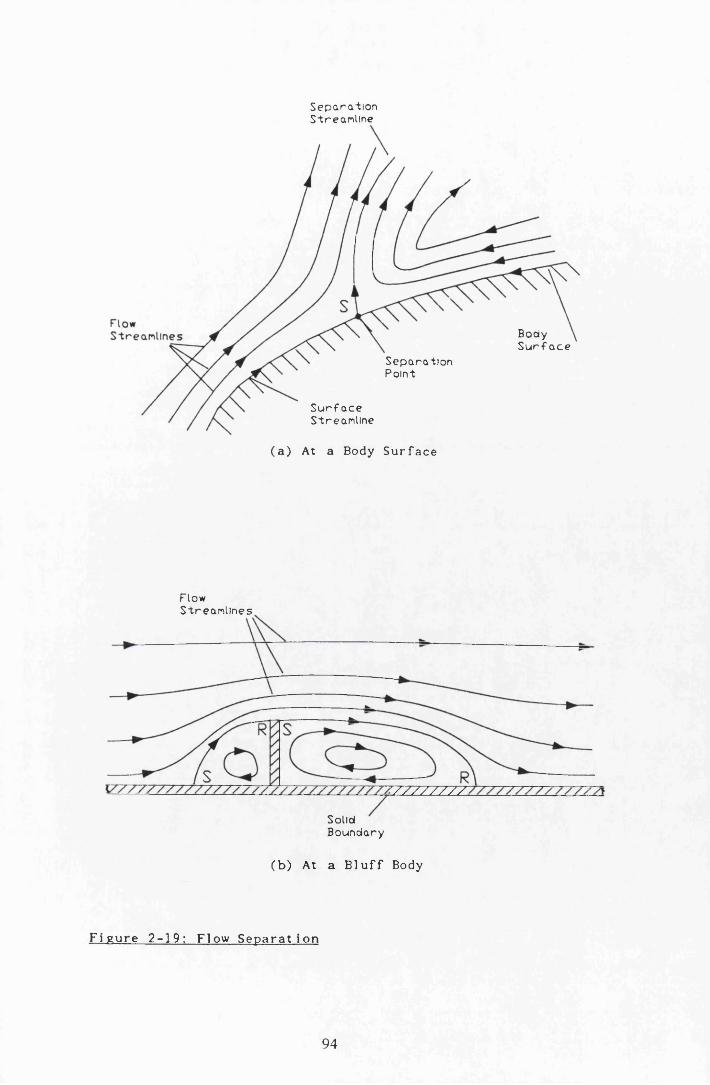
Sepa rat io nStreamline

Body S u r f a c e

S eparat ionPoint

S u r f a c eStreamline

( a ) At a Body Su r f a c e

FlowStreaml ines

z z /_ / y y / x

SolidBoundary

( b) At a B l u f f Body

F i g u r e 2 - 19 : Flow S e p a r a t i o n

94

“ ' S T ' ®

(a) G e n e r a t e d a t t h e T i p o f a B l u f f Body

/ ;

l ,

(b) The Mer g i ng P r o c e s s

F i g u r e 2-20 : V o r t e x Flows

<=□F l o w f r o m t u b e fo r j f l

F i g u r e 2 - 21 : V o r t i c e s G e n e r a t e d at t he Edge o f a J e t Flow

( A f t e r P e r r y e t a l )

T y p i c a l a l l c

95

( a) Laminar S e p a r a t i o n i n F r o n t o f

a C y l i n d r i c a l O b j e c t

(b) Flow S e p a r a t i o n i n F r o n t o f a

B u i l d i n g w i t h a Causeway Unde r ne a t h

F i g u r e 2 - 22 : Vi scous Flow S e p a r a t i o n a t O b s t a c l e s

( A f t e r P e r r y e t a l )

96

F i g u r e 2 - 23 : The R o l l - u p P r o c e s s In K e 1v i n - H e 1 mho 11z

I n s t a b i 1 i t y

(The R o l l i n g up o f t he s t r e a m l i m e may be

Obs e r ved f rom t he Top o f t he F i g u r e Down)

Flowc >

F i g u r e 2 - 24 : The Karman Vo r t ex S t r e e t G e n e r a t e d

i n t h e Wake o f a C y l i n d e r

C I R CU L A RC Y L I N D A R

ST ROUHAL 0 2

N U M B E R 0 1

s = II f l a t p l a t e

I1 1

BODY R E YNOL DS N U M B E R

F i g u r e 2 - 2 5 : The S t r o u h a l Number Ver sus t h e Re y n o l d s

Number f o r a C i r c u l a r C y l i n d e r and

a F l a t P l a t e

( A f t e r B l e v i n s )

97

( a ) N a t u r a l Case (b) Locked Case

F i g u r e 2 - 26 : F r e q u e n c y S p e c t r a o f N a t u r a l

and Locked V o r t e x Flow 4

S h e d d 1ng

F r e q u e n c y

( ^ sh ed )

i\ in n

F o r c i n g F r equency ( f f )

F i g u r e 2 - 27 : F r e q u e n c y Loc k i ng Phenomena

a s Obs e r ved bv Ho and Huang

(See Text f o r D e t a i l s )

F i g u r e 2 - 28 : S c h e ma t i c Diagram o f a T r i p - I n d u c e d T r a n s i t i o n

P a t t e r n i n a P i p e Showing t h e E f f e c t o f I n c r e a s i n g

D i s t u r b a n c e He i gh t

( A f t e r Webb and H a r r i n g t o n )

^ = 2 5 0

F.

v d - 1000

D irection o f f /o *F i g u r e 2 - 29 : Flows a t a P i p e O r i f i c e as t h e Reynolds

Number i s I n c r e a s e d

( A f t e r J o h a n s e n )


99

U p s t r e a m R e c i r c u l a t i o n Pipe Zone

D o w n s t r e am Pipeak--

? t . . . Co

♦ Uu -

R e a t t a c h m e n tL e n g t h

F i g u r e 2 - 30 : Flow a t a Sudden Expans ion w i t h i n a P i p e

•jrsrtlAM MYNCH.M NUUKI. - —-• r .

H*213

a

mnuHTMaa m i .

R a a f f a c k m a n t larvg lfca, l a m i n a r i h w r - i r y r r r» g lm «RooMachmont Ungtht; D0 = 0 .3 7 5 In., 0 = 0 .975 In.

F i g u r e 2 - 3 1 ; R e a t t a c h m e n t Length Versus U p s t r e a m P i p e

R e y n o l d s Number fo r Sudden E x p a n s i o n Flow

I n a P i pe

( A f t e r Back & Roshke)

(See Tex t f o r D e t a i l s )

100

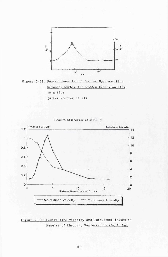
8

6

4

2

R f

F i g u r e 2-32 ; Re a t t a c hme n t Le ng t h V e r s u s Ups t ream Pipe

Reynolds Number f o r Sudden Expa ns i on Flow

in a Pi pe

( A f t e r Khezzar e t a l )

Results of Khezzar et al [1986)

N orm alised V elocity T u r b u l e n c e I n t e n s i t y

0.8

0.6

0 .4

0.2

00 5 10 16 20

D i s t a n c e D o w n s t r e a m of O r i f i c e

Normalised Velocity —1— Turbulence Intensity

F i g u r e 2 - 33 : C e n t r e - l i n e V e l o c i t y and Tu r bu l e nc e I n t e n s i t y

R e s u l t s o f Khe z z a r . R e p l o t t e d by t he Author

101

IX -0

c o n ic a l o if f u s in g s e c t io n

..........

x-o

SQUARE OlfPUSINO SECTION

0 .2 .4 .6 .9 1.0

r/aTu r b u l e n c e I n t e n s i t y P r o f i l e s a c r o s s t h e

Flow t a k e n a t Se ve r a l Cr os s S e c t i o n s

Downst ream o f t he D i f f u s e r

(a ) The Con i c a l and Square D i f f u s i n g S e c t i o n s

0 . 2 0 0

0. 100

0.050

0 . 0 2 0

0.010

0 .0 0 5

At• 00

(too 1000 1400

c o n i c a l o i r r u s t AS Q U A A C O l ^ ' J S C S

2 5 10 20x / d

(b) V a r i a t i o n o f t he C e n t r e l i n e T u r b u l e n c e

Level w i t h Axia l P o s i t i o n f o r S e v e r a l

Reynolds Numbers

( c )

F i g u r e 2 - 3 4 : R e l a m l n a r l z l n g o f Sudden E x p a n s i o n Flow i n

( A f t e r S i b u l k i n )

P i p e

102

0

( a) P e r i o d i c S o l u t i o n

0

(b) N o n p e r i o d i c ( C h a o t i c ) S o l u t i o n

0

( c ) The E f f e c t o f D i f f e r e n t I n i t i a l

C o n d i t i o n s on t h e R e s u l t i n g S o l u t i o n

F i g u r e 2 - 35 : ' x - t * Time Tr ace S o l u t i o n s f o r

t h e D u f f i n g O s c i l l a t o r

103

o<

(a ) P e r i o d i c S o l u t i o n (b) Cha o t i c S o l u t i o n

F i g u r e 2 - 36 : Phase Space P o r t r a i t s o f S o l u t i o n s

t o t h e D u f f i n g O s c i l l a t o r

O ' j

( a ) P e r i o d i c S o l u t i o n (b ) Nonpe r i od i c ( C h a o t i c ) S o l u t i o n

Fi pu r e 2 - 37 : P o i n c a r e S e c t i o n s o f t h e Du f f i n g O s c j l l a t ox

S o l u t i o n s o f F i g u r e 2-35

104

VC a n t o r S e t

( a) The C a n t o r Set

Point0 -D

Line1-D

Plane Volume3 -D

(b) T y p i c a l Di mens i ons

F i g u r e 2 - 38 : The Ca n t o r S e t . F r a c t a l s and Dimens ion

105

( a ) T y p i c a l S o l u t i o n s t o t he Mapping

3 0 3.2 3 4 3 6 3.8 4.0

A

(b) The B i f u r c a t i o n Diagram

F i g u r e 2 - 3 9 : The L o g i s t i c Map

0 4

0.3

0 2

0 1

- 0 1 -

- 0.2

- 0 3

- 0 . 4

- 1 . 5 - 0 .5 0- 1.0 0 5 10 1.5

( a ) The Henon A t t r a c t o r

0 191 r0 21

0 190 -0 2 0 -

0.1890 19-

0.188

0.1870.17-

0 186 -0.16

0.15 0.1850.650 55 0.700 60 0.6350 6 2 5

( c ) Zoomed In P i c t u r e o f (b)0.630 0 640

( b ) Zoomed I n P i c t u r e o f (a)

F i g u r e 2 - 4 0 : The Henon A t t r a c t o r

107

a -

M

—

TIM!

-I#-)-

( a ) The C h a o t i c Time S e r i e s

(b) The C h a o t i c A t t r a c t o r

F i g u r e 2 - 4 1 : The Lo r e n z E q u a t i o n s

108

X

I X i

X

COCOocrU J

Li_OCOr*LU

>x

j i

o

X CM r o

CN CM

109

4 - X

X0= 1 . 0 0ro= 1.00i

- * +i

- 1

ZC= 5. 00

F i g u r e 2-42 : The A t t r a c t o r o f t h e R o s s l e r E q u a t i o n s

-i. a -a. J u*

R= 31.0000

F i g u r e 2 - 44 : The A t t r a c t o r o f t h e T r u n c a t e d

N a v i e r - S t o k e s E q u a t i o n s ( F i g u r e 2-43 on P r e v i o u s Pa ge )

110

FluidInner Cylinder

k

BoxT + AT( a ) The R a y 1e i g h - B e n a r d System

OuterCylinder

(b) The T a y l o r - C o u e t t e Sys t e m

F i g u r e 2 - 4 5 ; S c h e ma t i c Diagrams oF t he R a v i e 1gh - Be n a r d

and T a y l o r - C o u e t t e E x p e r i m e n t s

F i g u r e 2 - 4 6 : The Be 1o u s o f - Z h a b o t 1n s k l 1 A t t r a c t o r

( A f t e r Roux & Swlnney)Point

-r. o A t t r a c t o rTine S e r i e s

( a ) A La mi na r T r a c e

Lini't o Cycle

(b) The Hopf B i f u r c a t i o n

F i g u r e 2 - 4 7 ; The Hopf B i f u r c a t i o n

P h a se S p a c e

111

d a ta analog m od e l

The Ac t ua l Sys t em (b) The Model Sys t em

80 ( m s e c ) 90

EJjLure 2 - 48 ; A Compar i s on o f t h e Phase P o r t r a i t s o f t h a

Ac t u a l and M o d e l l e d D r i p p i n g Fauce t Sys tem ( A f t e r Shaw)

» Motion s ensor tight beam

Gu'de barP l a n e of

mot i on( b )

f !f @)

t . m b e d d e d s t e e l s t n p

Cons t r a i n i ngb ars f c)

F i g u r e 2 - 49 : The F l u i d E l a s t i c V i b r a t i o n System

( A f t e r P a l d o u s s i s & Moon)

112

/ l

4/

-4-------------- -«----------------

( a ) S p e c t r a f o r Wake V e l o c i t y

Dur i ng O r d e r e d Sheddi ng

/ ( H z )

1 0 '*

10*1

N T7

10 - i

10-s

10-70 -2 0 4

(b) S p e c t r a f o r Wake V e l o c i t y

Dur i ng C h a o t i c Sheddi ng

F i g u r e 2 - 50 : Power S p e c t r a A s s o c i a t e d w i t h V o r t e x

She dd i ng a t a C y l i n d e r

( A f t e r E l g a r e t a l )

a£

<r

F r e q u e n c yS k i r t s

F i g u r e 2 - 51 : B r o a d e n i n g o f Power S p e c t r a Bases as

t h e C h a o t i c S t a t e i s Approached

113

Time S e r i e s

TineC-t)

d t

Delay= £ .dt'

( a ) The D i s c r e t i s e d Time S e r i e s

xi+ 2$

/ K At t r a c t o r

(b) The R e s u l t i n g A t t r a c t o r

F i g u r e 2 - 52 ; The Method o f Time De l a y s i n

A t t r a c t o r C o n s t r u c t i o n

114

MutualInf o r n a t i o n /s^

F i r s t Mininun

Delay

D/

/ f x

/

F i g u r e 2-53 : The Mutual I n f o r m a t i o n and i t s E f f e c t

on t h e R e c o n s t r u c t e d A t t r a c t o r

115

( a ) The A t t r a c t o r b e i n g P r o b e d wi t h H y p e r s p h e r e

Snai lE f f e c

A t t r a c t o r Edge E f f e c t s

log(Cr )

Slope = Dqp

(b) The ' l o g ( r ) - l o g ( C r ) ' p l o t

F i g u r e 2 - 5 4 : The C r a s s b e r g e r - P r o c c a c 1 a Di mens i on E s t i m a t e

116

Tra j e c t o r i e s

Point Computed / on a T r a j e c t o r y H y p e r s p h e r e

( a ) Le ng t h S c a l e s Comparable w i t h t h e I n t e r Po i n t

D i s t a n c e s o f t h e A t t r a c t o r T r a j e c t o r i es

(b) Sh o r t Le ng t h S c a l e s

on a No i s y A t t r a c t o r( c ) Shor t Lengt h S c a l e s

on a Noise F r e e A t t r a c t o r

(d) Le n g t h S c a l e s g i v i n g

E s t i m a t e s A p p r o a c h i n g t he A c t u a l Di mens i on

( e ) Leng t h S c a l e s Comparable w i t h t h e

A t t r a c t o r Rad i usF i g u r e 2 - 5 5 : Re g i ons o f Behav i our on t h e A t t r a c t o r

( F u l l D e t a i l s i n Te x t )

117

P h a s e Space

I

F i g u r e 2 - 56 ; D e f i n i t i o n S k e t c h o f T r a j e c t o r y S e p a r a t i o n

f o r t h e Lvaounov Exponent C a l c u l a t i o n

F i g u r e 2 - 57 : The E f f e c t o f Reynol ds Number I n c r e a s e on t h e

Di mens i on o f t he T a y l o r - C o u e t t e Sys tem

( A f t e r B r a n d s t a t e r e t a l )

< • 21r

r JV 0 01 002

TI ME

..I .0 0 5

• j*j

C U . M j K U

V *( a ) C r o s s s e c t i o n o f J e t a t V a r i o u s (b) F r a c t a l Dimens ion o f J e t Boundarys/

E v o l u t i o n Times as a F u n c t i o n o f E v o l u t i o n Time

F i g u r e 2 - 5 8 : The F r a c t a l Na t u r e o f a T u r b u l e n t J e t

( A f t e r A r e f e t a l )

118

Ai r fo i l b o u n d a r s l a s e r

Strip hc. itcr' L i n e a r r e g i o n N o n l i n e a r r e g i o n

c :

A m p l i f s m g T o l l m i e n S c h l i c t i n g

K . i r m a n s o r t e x s t r e e t

( a ) A Sc h e ma t i c Diagram o f t h e Sys t em

1 tiai

(Al

N at ur a l i:«n

-

11 VI / \f IIAlV

I \^ 1invi

I(«©Locked

~ 9 VI

____! J____1------ I-----------1-----------1-----------1-----------Jo<o io© inv) iino i iv i t ;nn 12 v> m© »© i — _i------ ------------------------------------- 1------

* © <*Vi m i l | l l « l I I II ) ll< © I.**© i ' .u t l«

( b) Pha s e Space R e c o n s t r u c t i o n s o f t h e

N a t u r a l , Locked and C h a o t i c Case C h a o t l c

I . . 1 _ . J ----------------i— _ . I . 1 .Mtfi |fa«n in v i i n © i iv > !>■»

ani ;vi i u©

Ei.ftur e 2 - 5 9 ; V p r t e x . S h e d d i n g R e s u l t s f rom an A i r f o i l

( A f t e r Wi11i a m s - S t u b e r & G h a r i b )

119

LOG

POW

ER

O . lo ck e d* , s t ro n g ly q u a s i -p e r io d i c +■. w e a k ly q u a s i p e r io d i c* . c h a o t i c

cClc8.s 0 8>oc3Q.*

-J

3 0 3H e i g h t ( cm )

Hl -Rure 2 - 6 0 ; Lyapunov Exponent s Taken Acr oss t h e Flow

f o r Vor t ex Sheddi ng a t an A i r f o i l

o0 0 1 0 5 02 0

3

->

0

>EQU»NO (i t'. ')3 I 5

I R L O U L ’ .'C'i ( K M / )

( a ) S p e c t r a f o r Wake V e l o c i t y (b) S p e c t r a f o r Wake V e l o c i t y

D u r i n g O r d e r e d Sheddi ng Dur i ng C h a o t i c S h e dd i ng

F i g u r e 2 - 6 1 : Power S p e c t r a A s s o c i a t e d w i t h V o r t e x

Sheddi ng a t a C y l i n d e r

( A f t e r E l g a r e t a l )

120

If it mol &<n

4

i

8 3 *0 " ' 2

L o g ( r ) R e - 2800

3

2

6

8

1210 i i37 8»-og (r) R e „ 3200

( a ) C o r r e l a t i o n Di mens i on as a F u n c t i o n

o f P i p e Re y n o l d s Number

Int. f ac t or0 8

0 6

<

0 4

0 2

0 5 00 . 3 0 0 4 00 200.100.00

( R e - R e c ) / R e c

(b) I n t e r m i t t e n c y F a c t o r as a F u n c t i o n

o f P i pe Re y n o l d s Number

K20 177

0 143

5 8 9 1 1E m b e d d i n g D i m e n s i o n

( c ) Kol mogrov E n t r o p y Versus

Embedding Di mens i on

F i g u r e 2-62; I n t e r m i t t e n t P i p e Flow R e s u l t s

( A f t e r Huang & Huang)

121

CHAPTER 3

CHAPTER 3

EXPERIMENTAL APPARATUS

GENERAL INTRODUCTION

EXPERIMENTAL APPARATUS

3 .2 .1 G e n e ra l Layout o f th e A p p ara tu s

3 .2 .2 D esig n o f th e T e s t R ig

3 .2 .3 W ater T e m p era tu re and V is c o s i ty

3 .2 .4 L a s e r T a b le D esign

3 .2 .5 P i s to n D esig n

3 .2 .6 E n tra n c e P ie c e D esign

3 .2 .7 P ip e S p e c i f i c a t i o n s

3 .2 .8 The O r i f i c e P l a te

3 .2 .9 P ip e A lignm ent

3 .2 .1 0 P ip e D e f le c t io n and E xpansion

3 .2 .1 1 W ater Tank S p e c i f i c a t io n s

3 .2 .1 2 T e s t P ro c e d u re

MOTOR CONTROL

3 .3 .1 I n t r o d u c t i o n

3 .3 .2 O r ig in a l M otor-G earbox A rrangem ent

3 .3 .3 M o d if ie d M otor-G earbox A rrangem ent

3 . 3 . 4 R e d u c tio n o f B ackground N oise by

P h y s ic a l Means

3 .3 .5 Generation o f a P u l s a t i l e F lu id Flow3 .3 .6 The A.C. In v e r t e r and Func t ion Generator3 .3 .7 The Drive Shaft Limit Switches

3.4 INSTRUMENTATION - THE L.D.A. SYSTEM

3 .4 .1 In t roduc t ion3 .4 .2 Components o f the L.D.A. System3 .4 .3 P r in c i p l e s of the L.D.A. System3 .4 .4 Experimental P r a c t i c e

3.5 DATA ACQUISITION

3 .5 .1 In t roduct ion3 .5 .2 A cqu is i t ion Hardware3 .5 .3 Analog to D ig i t a l Conversion3 .5 .4 Computer S p e c i f i c a t i o n s3 .5 .5 Software3 .5 .6 Sampling and M anipu la t ion o f the Data

3 .6 FLOW VISUALISATION APPARATUS

3 .6 .1 In t roduc t ion3 .6 .2 Light Box Design3 .6 .3 Experimental P r a c t i c e

3.7 SUMMARY

123

3.1 GENERAL INTRODUCTION

The experimental programme was designed to investigate low Reynolds number

flow behaviour in a pipe where an orifice was used to generate coherent vortex

structures and turbulence. The regime of flow was pulsatile in order to have

optimum control over the experimental flow, vortex shedding downstream at the

orifice, and also because of its range of practical applications.

The order of the experimental programme was:

(a) to use flow visualisation in the elucidation of the phenomena present within the

flow, and

(b) to use the technique of laser Doppler anemometry, (L .D .A .), to pick up the

velocity fluctuations in the flow at various points within the pipe, this data being

used in subsequent analysis, outlined in Chapter 6.

With these aims in view, a sophisticated experimental test rig was constructed

to produce constant average Reynolds number, pulsatile flows in a small diameter

pipe, whereby the frequency and amplitude of the pulsating component could be

controlled independently of the mean velocity component. Facilities were also

provided on the rig to allow both for ease of use of a purpose built light box for

the flow visualisation, and the L.D.A. system components. Two micro—computers

were used, one for data acquisition and analysis and a second for the control and

monitoring of the piston drive motor.

The experimental rig was designed by the author and built from scratch during

a period of fourteen months, (from April 1990 to June 1991), during which time

many obstacles and difficulties were met, and overcome.

3.2 EXPERIMENTAL APPARATUS

3.2.1 General Layout of the Apparatus

The experimental apparatus was constructed within the Civil Engineering

departm ent of the University of Glasgow and located in the basement of the

124

Rankine building. A general view of the complete test rig is shown in figure 3—1.

The Laser itself is omitted for clarity and is situated directly opposite side of the

pipe from the photomultiplier, (P.M .), tube. A plan view of the apparatus is given

in figure 3— 2.

The room in which the experimental rig was set up is a purpose built cold

room, which is thermally insulated from the rest of the building so that the

tem perature can be dropped to below 0°C . The room 's therm al properties made it

ideal for the experiment, as the tem perature within the room, and hence the

viscosity of the liquid, can be kept constant. The walls of the room were painted

mat black, purposely done to minimise the risk of reflections of the laser beams.

3.2.2 Design of the Test Rig

It is seen from figure 3— 1 and figure 3— 2 that the experimental rig consists of

a header tank, an accurately machined entrance transition to the pipe, a glass pipe

with high tolerance and containing an orifice plate approximately half way its

length. The laser equipment is located just downstream of the orifice and has the

ability to move very precisely over a two dimensional plane, across and downstream

of the flow. The downstream end of the pipe connected with a piston and motor

which was specifically designed to draw flow from the header tank at completely

uniform rates even though the head in the header tank varied.

An accurately controlled piston was used to drive the flow to and from the

tank. Results are taken only when the liquid is flowing from the tank to the

piston, as the smooth entrance transition piece inhibits disturbances being

propagated, and entering into the flow. The reason for adopting a piston system

was twofold. Firstly, it provided means by which repeatable and accurate, constant

flow Reynolds numbers could be produced, and, secondly it allowed for pulsations

of various frequencies and amplitudes to be superimposed on the mean flow rate.

It was felt that a valve system could not satisfy either of these criteria. Flow

control using a needle valve arrangement downstream would have been extremely

difficult due to the intermittent nature of the flow around the laminar— turbulent

transition zone in the pipe. This would have the effect of producing a varying

friction factor within the pipe (depending on what proportion of the flow in the

125

pipe was in a laminar or turbulent state) and hence a varying flow rate. In

addition the drop in head at the tank would have diminished the flow rate at the

valve, and it was felt that a constant head tank would not be able to contain

water still enough for the experiment. It would, therefore, be very difficult to

envisage a valve system which could produce a controllable Reynolds number and a

pulsating component on the mean flow. Thus, a driven piston was considered to be

the only practical method to produce such flows.

The whole experimental apparatus was raised up to a suitable working height

on a subframe fabricated from 50x50x5mm steel, square hollow section. Due to its

large size and weight the subframe was welded together in five sections in the civil

engineering workshop and then these sections were bolted together in situ in the

experimental laboratory.

The whole rig rests at a slope of approximately 2.5° during operation. This is

done by setting the adjustable feet to the appropriate heights along the length of

the test rig. This arbitrarily chosen slope enables air bubbles, which have come out

of solution to escape from the pipe during the experimentation.

An attempt was made to insulate the apparatus from vibrations in the floor

from other parts of the building. This was done by sitting the top frame of the rig

on a 110mm concrete base which itself sits on a 150mm medium density foam

cushion, as shown in detail in figure 3— 3. Approximate calculations using an

experimentally obtained stiffness for the foam indicated that the natural frequency

of the rig in the vertical direction was roughly 4.6 Hz. This is well away from the

50 Hz expected from machinery elsewhere in the building. The foam rests upon a

20mm thick plywood base which is attached to the subframe.

The concrete layer was constructed from two interleaved layers of unreinforced

concrete slabs. These m easured 900x600x55mm and were cut to suit where

appropriate. The slabs were connected to the top steel frame by holding down

bolts, with a thin layer of rubber sandwiched in between. This arrangem ent resulted

in a rigid top structure onto which the main components of the experimental

apparatus were attached.

126

3.2.3 W ater Tem perature and Viscosity

During the course of the investigation every effort was made to keep the water

at a constant tem perature of 11 °C. This was done to keep the liquid viscosity

constant. It was found that the mains supply, from which the water used in the

experiment was taken, supplied water at a tem perature between 10°C and 11 °C.

W ater at less than 11 °C was brought up to the required tem perature by adding

warm water to it in the tank.

The absolute viscosity, p(T), of water at a tem perature, T , may be obtained

from the following expression of Kashin et al [1978],

loS , 0 [ , ( g o % ) ■ ] - T T H * [ 1 -2364 - 1 -37 * 1 ° ' 3<20-T> +

5.7 X 10‘ 6(20 - T ) 2

(3 .1a )

where

/i(20°C) - 1.002 X IO - 3 kg/ms (3 .1b)

This expression is valid within the temperature range,

0°C < T < 40#C. (3 .2 )

The expression gives the absolute viscosity of water at a tem perature of 11 °C to

be

/ i ( l l °C ) - 1.2 6VI X 10-3 k g / m s (3 .3 )

At this tem perature the density of the water, pw, is 999.6082 kg/m 3, (according to

Kashin et al), thus the kinematic viscosity, v t at 11 °C is

127

y ( l V C ) - — - 1 .2 7 0 8 X 10’ 6 m2/ s ( 3 .4 )pw

This is the value of kinematic viscosity used in all subsequent calculations requiring

its use, although temperature was controlled and measured on a hourly basis while

tests were being conducted.

3.2.4 Laser Table Design

A laser table was constructed to allow the laser and photomultiplier tube to be

moved easily in the two dimensions of the horizontal plane, i.e. both across the

flow and in the direction of the flow. Micrometric movement was achieved with

the carriage laterally across the pipe, by which the laser intersection point could be

placed nominally to an accuracy of 0.01mm ± 0.005mm in air. Taking refraction

of the beam into account, as it passes into the water within the pipe, this

corresponds to an accuracy of 0.013mm ± 0.0067 in the water within the pipe. In

the axial direction the intersection point may be located to 1 .0mm ± 0.5mm. The

table was constructed out of aluminium section for lightness and strength, and the

movement in either direction was facilitated by linear bearings. Locking screws in

the linear bearings allowed the carriage to be fixed in position if required. This set

up allowed longitudinal measurements to be taken from 100mm upstream to

1150mm downstream of the orifice, and laterally across the diameter of the pipe

on the horizontal axis.

3.2.5 Piston Design

The piston and piston casing dimensions were designed as follows. The

maximum required pipe Reynolds number, Rep, was assumed to be 2000. (This, for

instance, corresponds to an orifice Reynolds number, Re0 , of 4000 for the 13mm

diam eter orifice.) This value of Rep gives an average velocity in the pipe of

97.75 mm/s. Many variations of the piston casing dimensions were considered.

Those eventually chosen were of a stroke length of 360mm and an internal

128

diameter of 203.2mm, (= 8 inches, so chosen because the piston seals came only

in I m p e r i l sizes). The pipe internal diameter being 26mm, gives a ratio of piston

to pipe diameter of 7.815, and an area ratio of

.. Pl s t o n _ 61.174 (3.5)p i p e

Using this area ratio, and invoking the continuity condition, results in a piston

velocity of 1.60 mm/s, for an Rep of 2000. This gives a run time of

approximately 225 seconds assuming the piston stroke to be 360mm. This time is

long enough for the flow conditions to stabilise and data to be captured. (A data

capture run of 16384 points, sampled at 100 Hertz, takes 164 seconds.) As the

experiment progressed it became apparent that the maximum pipe Reynolds number

required was 640, which gives a run time of 703 seconds. This allowed more time

for flow conditions to stabilise and allowed for a few data capture runs to be

taken on each stroke, if required. Figure 3— 4 gives an overall picture of the

piston, piston casing and mountings.

The piston casing was manufactured from a single ingot of external diameter

228.6mm, the internal diam eter was bored then honed to a fine finish. This work

was done external to the department. The final internal diameter of the piston

casing being of 203.2 ± 0.023mm. The bearing which drives the drive shaft is

made from brass and its housing from steel. The piston drive shaft is a brass

screwed rod, manufactured in the department for the purpose, and has a pitch of

3.23 ± 0.005mm. The large sprocket which drives the bearing directly has 80 teeth

and is connected to a smaller 40— tooth sprocket, located on the motor drive shaft,

by a flexible belt. This gives a 2/1 reduction of the motor output shaft speed to

the bearing speed. The piston drive shaft is connected to the rear of the piston.

The piston was fabricated from aluminium in two parts, this allows for the

main piston seal to be Fitted. The seal selected for use with the piston was a

JAM ES W A LK ER- "HYPAK" Type PW 6 3 - 800, synthetic rubber seal with nylon

end rings. Sealing is achieved by the deformation of the rubber under hydraulic

loading, which squeezes the seal against the piston casing internal wall.

129

Air which has come out of solution is bled from the piston casing by the air

bleed valve shown in the figure 3— 4. The casing may be drained by a similar

valve at the base of the front end wall, from which flexible plastic hose leads to

the main drain situated directly under the experimental rig. The pipe is secured to

the front of the casing by a water tight rubber O— ring seal which is squeezed

tight onto the end flange by the pipe connection flange. The seal was designed to

allow for any movement of the pipe due to thermal expansion/contraction and also

movement of the tank wall when the tank was filled. These effects are discussed in

more detail in sections 3.2.8 and 3.2.9.

The piston casing end walls were fabricated from 10mm thick aluminium plate.

They are circular with a diameter of 300mm. The walls are secured to the front

and rear of the casing shell by 8X10mm screwed rods running external to the

casing. They are secured by bolt fasteners at each end and act, in effect, by

squeezing the end walls onto the piston casing. A rubber seal between the walls

and the casing ensures a watertight seal. The piston casing is mounted, via the end

walls, onto a 20mm thick aluminium plate which also serves to secure the motor

to the top frame of the rig.

3 .2 .6 Entrance Piece Design

An entrance piece was required to give a smooth transition from the still water

in the tank to the flowing water in the pipe. The transition shape had to be

tangential with the walls of the pipe and the tank, and so an ellipse was chosen as

shape of the transition piece. The entrance piece design can be seen in

figure 3—5. The major axis length is 156mm and the minor axis length is 52mm,

this giving a ratio of 3:1.

A computer controlled lathe was used to bore out the entrance piece profile.

However, due to the difficulty of having an elliptic shape machined, the shape was

approxim ated by four arcs of circles of different radii which all met each other

and the walls tangentially. It was felt that this pseudo— elliptic shape was an

accurate enough approximation for the purposes of the investigation. The entrance

piece is fixed to the tank by sixteen 5mm threaded screws, and is secured to the

130

pipe, in a similar manner as with the pipe— piston connection. That is a watertight

rubber O — ring seal is squeezed tight onto the pipe by an end flange connected to

the entrance piece.

3.2.7 Pipe Specifications

The pipe used in the main experiment was constructed from four 1 .00m lengths

of high precision piping manufactured by Pilkington, with a nominal internal

diameter of 26.00mm and a nominal external diameter of 30.00mm, i.e. a wall

thickness of 2.00mm. Accurate measurements of the glass pipe by the author found

the average internal diam eter of the glass pipe to be 25.98mm ± 0.01mm. The

average external diam eter of the pipe was found to be 30.15mm± 0.08mm. The

diameters were measured at four equi— angular positions around the pipe to check

for ovality of the pipe. For a specific location along the pipe, the maximum

variation in measured internal diameter was found to be less than 0.01mm and for

the external diameter it was found to be 0.04mm.

The 1 .00m lengths of glass piping were joined together at the necessary

positions by pipe coupling connections, as illustrated in figure 3— 6. The pipe was

supported on six, specially made aluminium pipe supports which allowed fine

movement both in the horizontal and vertical plane. A locking mechanism was also

incorporated into their design which allowed the setting of each one to be

permanently fixed. Their design is illustrated in figure 3— 7.

3.2.8 The Orifice Plate

The orifice under investigation was placed at the mid point of the pipe, i.e.

2.00m from the entrance piece and the piston. This distance of 2.00m was

sufficient to allow a fully developed laminar flow profile (Hagen— Poiseuille flow) to

establish itself within the pipe. According to the theory of Freidm ann et al [1968],

the entrance length Ze , (defined in chapter 2, section 2.2.9), is given by the

simple relationship,

131

Z - 0 .0 5 6 D . Ree P P

(3 .6)

Thus the maximum pipe Reynolds number of 640, used in the investigation, results

in an entrance length of 930mm. In addition, the theory assumes a flat velocity

profile at the pipe entrance, whereas in the experiment outlined here the profile

will already be distorted by the entrance piece before it enters the pipe. This

should cause the development of Hagen— Poiseuille flow to occur nearer to the pipe

entrance than predicted by theory.

Six different sizes of orifices were used during the investigations, and these

were made from brass. The orifice diameters were, in ascending order: 6.50mm,

9.75mm, 13.00mm, 16.25mm, 19.50mm and 22.75mm, or to put them in terms of

the pipe diameter 'D ':2/8D, 3/8D, 4/8D, 5/8D, 6/8D and 7/8D, (i.e. integer

multiples of an eighth of the pipe internal diameter). All orifices were 0.5mm thick

and were of a flat edge type. The orifices comply to the design criteria of

B.S. 1042 : 1989, Sections 1.1 and 1.2, which deals with the measurement of fluid

flow in closed conduits using pressure differential devices. However, the slow flows

being investigated herein are quite different from those covered by the standard

which deals solely with fully turbulent flows at pipe Reynolds numbers in excess of

5000. The standard was used merely as a guide for the manufacture of the orifice plates.

The pipe slots into the orifice plate lip and thus locates itself concentrically

with the orifice. The orifice is held in position by two end plates, figure 3— 8.

One of the end plates has a long flange to ensure that the plane of the orifice

aperture is perpendicular to the pipe central axis, (i.e. to allow the pipe central

axis and the orifice plate central axis to correspond). One drawback of the long

flange is that it denies access to that part of the pipe it covers, both from the

laser and from flow visualisation methods. The flange was positioned in the

upstream direction as the main emphasis of the work was to elucidate the resulting

downstream phenomena due to the presence of the orifice plate.

Each orifice plate has a small hole drilled in it which allows for the bleeding

of air, which is trapped downstream of the orifice plate. This air hole is capped

by a rubber seal which is held in position by a screw and washer. During the

132

course of the experimentation, however, a much quicker and more effective method

was found for expunging the air trapped downstream of the orifice plate. This was

done by simply blowing air sharply into the piston chamber via the front air bleed

valve on the piston casing front wall. This causes a small volume of water to be

accelerated quickly in the pipe in the upstream direction and through the orifice. It

was found that this was of sufficient strength to force the trapped air through the

orifice with it.

3.2.9 Pipe Alignment

Great care was taken during the alignment of the four, one— metre sections of

glass pipe to ensure that they followed a true line, both in the horizontal and

vertical planes.

The vertical alignment of the pipe was ensured by the use of a level. Levels

were taken at each end of the pipe sections as they initially lay in the pipe

supports prior to adjustment as shown in figure 3— 9. The rise in level between A

and E (AH) was determined, and knowing the value of the horizontal distance from

A to E, namely 'Xe \ the required gradient could be found. Using this value and

knowing the distances to the points B, C and D, the heights of these intermediate

points required for a true linear alignment could be calculated. The difference

between these calculated values and the actual values observed is the error in

alignment.

The errors at sections B, C and D, (see figure 3.9), were calculated from the

levelling data, then the pipe supports were then adjusted to correct for the

discrepancies between the true alignment and the actual alignment. The levels of

the pipe ends were then checked and the process of adjustment repeated at each

end until the levels at B,C and D were equal to those required to within 0.25mm.

The horizontal alignment of the pipe was also performed with the aid of the

level, together with three short sighting— rods. These straight sighting— rods were

attached to heavy, copper half— collars with which they could be made to sit upon

the pipe. The procedure for the horizontal alignment of the pipe sections was then

conducted as follows.

133

One of the sighting- rods was placed at each end of the pipe. The level was

then set up so that the vertical cross wire was aligned with the edges of both

rods. This ensured that both rods were truly vertical, and it gave a straight site

line between them on which the rest of the pipe was aligned. The method is

shown pictorially in figure 3—10.

The third sighting rod was then placed at successive intermediate positions on

the pipe next to the pipe supports. The supports were then adjusted in the

horizontal direction until the intermediate rod came into alignment with the other

two. This was repeated at each pipe support until all sections of the pipe came

into alignment.

3.2.10 Pipe Deflection and Expansion

The theoretical deflection of the pipe between supports was checked. This was

done for a glass walled pipe containing water, and using an estimated Young's

modulus for the glass, Eg, of 71X109, [Haward, 1949]. Taking the density of the glass, pg, and the density of the water, pw, respectively to be 2600 kg m 3

[Tennent, 1986] and 999.61 kg to 7 [Kashin et al, 1978]. The mass per unit

length of glass pipe filled with water is then

W = g Pg Ag ■+■ g pw Ajy (3.7)

Where g is the constant of gravitational acceleration and is equal to 9.81 m s - 1 .

The cross sectional areas of the glass, Ag, and the water, Aw, may be easily

calculated, knowing the external radius of the pipe, R 1t to be 15mm and the

internal radius, R2 , to be 13mm, (see figure 3—11). Thus the mass per unit

length, W, is 9.695 N m“" 1.

To give an indication of the magnitude of expected deflections that may occur

due to this loading, calculations were performed for a worst case situation, which

was that of each pipe section supported at its ends only and the end conditions

assumed to be pin jointed. (This worst case does not occur in reality on the rig

as the pipe supports are closer together than the pipe section lengths of 1.00m).

134

The deflection, 6, at the mid span of a pin jointed beam element may be

calculated from the following expression,

6 -5 W L'

384 E Tg xx(3 .8 )

where Ixx is the second moment of area of the section and may be calculated for

the glass pipe wall thus,

I - * [ r 4 . r 4 1 - 1 .7 3 2 9 X 1 0 "8 m4 (3 .9 )X X 4 L 1 2 J

The deflection at the midpoint between supports was calculated, using

expression 3.8, to be 0.103mm. This value was taken to be well within the

acceptable tolerances of the pipe line. However, this figure serves only to give a

feel for the magnitude of the deflections that may occur. Since the pipe sections

are not supported at each end, may not behave as pin jointed elements and the weight of the pipe couplings and orifice plate has been ignored.

As the pipe is filled with water at the beginning prior to an experimental test,

the pipe wall changes in temperature from the ambient room temperature to that

of the cold fluid within it. Therefore, it seemed prudent to attempt to estimate the

thermal expansion of the pipeline during the filling process.

The maximum room temperature recorded was 27° Centigrade and considering

the water temperature to be 11 °C, this gives a maximum difference in temperature

experienced by the pipe, AT, of 16°C. The coefficient of thermal expansion of

glass, was taken to be 9x10“" 6 °C“ [Tennent, 1986]. Thus the strain

experienced by the material, a , may be calculated from the following relationship,

ct = AT . q (3.10a)

by substituting the above values we find obtain,

135

a = 0.000144 (3.10b)

thus for a 4.00m length of pipe, L, the expected change in length, AL, is

AL = L . a = 0.000576m (3.11)

Thus the maximum probable change in length experienced by the pipe during

filling is 0.576mm. Note, however, that this is a contraction, since it is a

temperature drop. This should serve to accommodate somewhat the movement in

the pipe caused by the tank walls expanding outwards when filled, as discussed in

the next section.

The glass pipe was at its most vulnerable when it had been reassembled after

cleaning and great care was taken to ensure that all the pipe joints (i.e. at the

entrance piece, at the piston, at the pipe connections and at the orifice) were

slackened off during filling at this initial stage. All pipe breakages, of which there

were five in number, were incurred at this stage. The ends of the pipe sections

were susceptible to chipping at the slightest knock, and care had to be taken

during the reassembling process to avoid this.

Pipes were replaced due to either breakages or excessive chipping of the ends,

as described above. New pipe sections were placed in position downstream of the

orifice, thus the section of pipe where most of the results were taken always had

the newest section of pipe. The next best section of pipe being placed just

upstream of the orifice where the remaining results were taken.

3.2.11 Water Tank Specifications

The header tank which contains the water for the experiment measures

700x700x700mm internally and has a capacity of 343 litres. The two side walls are made from 10mm thick perspex allowing the inside of the tank to be visible. This

serves three purposes. Firstly, the inner walls of the tank can be inspected daily

for bacterial and algal growth. Regular, weekly cleaning of the tank (and pipe)

eliminated the build up of these undesirable deposits. Secondly, the water inside

136

the tank can be visually inspected to see that it is still enough to start an

experimental run. Finally the water inside the tank can be inspected to ensure that

the flow visualisation chemical is homogeneously mixed prior to a run. The front

and rear tank walls and the base are manufactured from 10mm thick aluminium, to

ensure rigidity of the structure during the filling of the tank. The top of the tank

has a large lid allowing access to the tank for cleaning and adding the flow

visualisation agent into the water.

Originally the tank was to be filled from the top, a valve and piping was fitted

for this purpose. However, it was quickly realised that this method of filling

entrained a substantial quantity of air into the liquid, some of which came out in

the pipe during the experimental runs. To this effect, the tank is slowly filled from

a hole in the bottom corner next to the front wall, this procedure results in a

minimum of air entrained in the solution. The tank is drained by a hole at the

other corner adjacent to the front wall. The maximum difference in head at the

tank for an experimental run, where the piston takes a full stroke, is 23.8mm.

Some time was spent measuring the deflections of the tank walls while the tank

was filled with liquid. A knowledge of wall behaviour, particularly the front wall,

was critical as any wall movement would have to be accommodated within the pipe

joint at the piston. This joint would have to be flexible enough to ensure ease of

movement of the fragile glass pipe and also be secure enough to effectively seal

the pipe at the piston. Deflections were measured at the centre of each wall as

the tank was filled in 100mm increments. The results showed that the aluminium

walls deflected much less than those made of perspex, as one would expect. The

results of the tests are shown in table 3.1. (Note that these tests were performed

on the tank prior to the hole for the entrance piece being formed at the centre of

one of the aluminium walls.)

The aluminium walls initially deflected inwards up to 0.031mm, this for a water

depth of 300mm. When the tank was full, i.e. at a depth of 700mm, the

aluminium walls deflected outwards by a maximum of 0.233mm. This gives an

overall possible movement of the aluminium wall of 0.264mm. The perspex walls

initially deflected inwards to a maximum of 0.078mm, for a water depth of

100mm. When the tank was full the perspex walls had deflected outwards by

maximum value of 5.450mm, giving an overall possible deflection for the perspex

137

walls of 5.528mm. This knowledge of wall behaviour, particularly the front wall,

was critical, as any wall movement would have to be accommodated within the

pipe joint at the piston.

Once the rig was constructed and operational the deflections experienced at the

front wall entrance piece were measured. The overall deflection experienced by the

pipe, when the tank is filled with water, was found to be 0.210mm. This is

approximately 20% less than the value obtained during the test (0.264mm).

However, this is a reasonable result as the initial tests were performed on the

aluminium wall centre without the entrance piece in place.

WATER DEPTH (mm)

P e rsp e x Wal 1 D e f le c t io n (mm)

Alum inium W al1 D e f le c t io n (mm)

0 0 .0 0 0 0 .0 0 0

100 -0 .0 7 8 -0 .0 0 7

200 -0 .0 7 3 -0 .0 2 3

300 0 .5 7 3 -0 .0 3 1

400 1 .5 0 3 0 .0 0 7

500 2 .8 3 3 0 .0 9 7

600 4 .2 8 5 0 .1 6 0

700 5 .4 5 0 0 .2 3 3

Table 3.1 — Tank Deflection Test Results

3.2.12 Test Procedure

The investigation set out to shed light upon the breakdown of forced vortex

flows at a pipe orifice. For the purposes of this investigation the pulsating component of the flow, at which frequency the vortices are forced, was always set

to the natural frequency of the orifice plate at the specific Reynolds number being

investigated. Thus, the actual parameters varied in the investigation were:

1 — The orifice diameter.

2 — The Reynolds number of flow in the pipe.

138

3 — The forcing amplitude of the fluctuating flow component.

Although the option remains, for subsequent research work to be performed with

forcing frequency set to values other than the natural frequency of the orifice, in

the work outlined in this thesis only the natural frequency of the orifice plate was

used.

Two methods were used to elucidate the flow phenomena present within the

pipe. These were qualitatively by flow visualisation and quantitatively by Laser

Doppler Anemometry.

The flow field at various positions of the pipe was initially observed visually

using flow visualisation techniques. (See section 3.6) This gave a qualitative insight

into the flow processes involved at, or near, the orifice plate. This was done for

the same system parameters as used in the L.D.A. study.

After the flow visualisation had taken place the velocity values of the flow were

taken at various positions upstream and downstream of the orifice plate. After

much initial testing both in terms of the L.D.A. system, and with the aid of flow visualisation, it was decided to take the L.D.A. readings at fixed distances from the

orifice plate for all values of flow parameters. These distances are:

1 — upstream of the orifice plate, 90mm, 75mm, 50mm and 35mm. (90mm being

the maximum distance that the laser carriage may traverse up the pipe, and 35mm

being the nearest upstream distance to the orifice that may be located by the

Laser beams due to the presence of the of the orifice end plate flange.)

2 — downstream of the orifice plate, 10mm, 20mm, 30mm, 40mm, 50mm, 60mm,

75mm, 100mm, 150mm, 200mm, 250mm, 500mm and 950mm. The majority of the

readings were taken close to the orifice plate, i.e. less than 100mm, where most of

the flow processes take place.

Thus seventeen readings were taken for each set of flow parameters, these

readings were taken on the pipe centre— line. The time taken to take one such set

of seventeen readings took on average two full working days. The time required

depended very much upon the flow parameters under investigation, as the tracker

system was very sensitive to large abrupt fluctuations in flow velocity and the

presence of these could cause dropouts in the signal. In such circumstances many

runs would be required to get an acceptable set of flow data for that L.D.A.

139

position.

Although most of the L.D.A. readings were taken at the pipe centreline,

towards the end of the experimental programme a few tests were taken at various

L.D.A. positions across the flow. These details of which are discussed in more

detail in chapter 6.

3.3 MOTOR CONTROL

3.3.1 Introduction

During each experimental run it is essential that both the time averaged flow

Reynolds number and the amplitude and frequency of the pulsating component of

the flow be controlled with some degree of precision. This requires that the motor

speed, including the fluctuating component, is controlled accurately for the duration

of each specific run. It is also necessary that the motor output can be altered

from run to run. The speed of the motor used to drive the piston was controlled

using an A.C. inverter and a function generator. A three phase, 340 volt, 50 Hz

supply enters the inverter and outputted is a three phase, 340 volt, variable

frequency supply. The inverter allows the load on the motor to be continually

monitored and the input frequency to the motor to be set to within ± 0.05 Hz. It

was found during the experimentation that, once set, the motor output remained

constant for that particular setting, from run to run.

Preliminary results taken during the spring and summer of 1991 indicated that

the motor, which drives the piston, introduced stray frequencies into the flow. This

was first discovered with the pipe set up without an orifice. However once an

orifice was introduced into the system, it soon became apparent that the

frequencies of the vortex shedding from the orifice were being influenced by these

stray motor frequencies. The following sections give details of these effects and the

measures taken to solve the problem.

140

3.3.2 Original M otor-G earbox Arrangement

In the original experimental set up, an inherited A.C. motor and gear box unit

was used. Previous to it being utilised for the work outlined here, it was employed

as part of a wave generating device on an open channel flow flume. Within the

housing of the unit, the electric motor is connected to a variable speed or Kop

gear box, this is in turn connected to a fixed gear box, having a reduction ratio

30/1. A schematic diagram of the overall arrangement used to drive the flow is

given in figure 3—12. The output shaft from the second gear box could be driven

at speeds in the range 15 to 90 R.P.M. for an input frequency of 50 Hz to the

motor. With a proportional reduction in speed for input frequencies from the

controller of less than 50 Hz. Thus this arrangement had two means of output

speed control through the Kop gearbox and through the controller.

However, it soon became apparent that this arrangement introduced stray

frequencies into the flow. The main rogue frequencies were found to be related to

both the output shaft rotational speed and the electric motor rotational speed.

Other lesser frequencies appeared in the flow and their possible cause remained

unclear. The rate of one of the cyclic variations was 30 times the output shaft

frequency. After much investigation, (which included stripping down the gearbox

several times), it was reasoned that this was probably due to an eccentricity of the

shaft connecting the Kop gear to the fixed gear. The other main rogue frequency

was either equal to, or half of, (or both), the motor rotational speed, depending

on the driven flow rate. The overall effect of these ripples in the motor output

speed, was to cause a variation in the mass flux of the flow as the piston was

withdrawn. Thus a many frequency, pulsatile flow was being produced that could

not be controlled independently of the motor output speed and hence the Reynolds

number of the flow.

These stray frequencies were picked up in the preliminary investigations of

Hagen— Poiseuille flow, in the pipe without an orifice. Whereas the actual laminar

flow should have no frequencies, if the flow was driven without a superimposed

fluctuating component then the rogue frequencies, in certain circumstances,

controlled the vortex shedding at the pipe orifice. More details on this phenomena

are contained in the 2nd Year Progress Report by the author, [Addison, 1991].

141

Some considerable effort was expended trying to eliminate the effect of these

stray frequencies by physical means, (or at least reduce them to a point where

they no longer interfered with the results). The problem was to find where exactly

they came from and what could be done to solve the problem.

Many means were used to try and find out their cause and reduce their effect.

These include:

1 — The use of a various thick, highly viscous oils in the Kop gearbox to smooth

out fluctuations in displacements.

2 — Stripping down and extensively cleaning the moving parts of the motor

gearbox arrangement, to remove foreign bodies which may be causing variations in

internal clearances.

3 — Fitting of flexible motor mountings between the motor and the base plate,

see figure 3—14b.

4 — Varying the tension on the belt drive between the motor output drive shaft

sprocket and the piston drive shaft sprocket.

All these measures showed no real improvement whatsoever and thus it was

eventually decided to obtain a new motor for the rig.

3.3.3 Modified Motor— Gearbox Arrangement

A new motor was purchased for the experimental rig, (a FENNER gearmotor,

model 981—1806.) This unit has no variable gearbox, with the electric motor

connected directly to a fixed gearbox which gave a nominal output shaft speed of

37 R.P.M. The arrangement is shown schematically in figure 3—13. As there is no

variable gearbox, the only means of control in this arrangement is through the inverter— signal generator set— up. This arrangement gave a much smoother

performance. However, stray frequencies were still to be found in the flow,

although, their effect was much smaller than those from the original

motor— gearbox arrangement. The stray frequencies were completely drowned out by

the fluctuating flow component generated by the signal generator and therefore did

not affect the main experimental results. Stray frequencies, it seems, must therefore

be expected in flows driven by such mechanical means, and the experimentalist's

task is to try and limit their effect as far as possible.

142

3.3.4 Reduction of Background Noise by Physical Means

Various methods were employed in an effort to reduce, by physical means, the

general background noise level of the results. These included:

1 — Increasing the mass of the piston casing by placing heavy weights upon it to

alter its frequency response characteristics.

2 — Dampening the pipe along its length, with sponge placed between it and the

drip tray.

3 — Leaving an airpocket within the piston casing when running the experiment to

dampen vibrations.4 — Using flexible mountings for the connection of the motor to the rig, as used

in an attempt to reduce the amplitude of the stray frequencies of the original

motor set— up. Best results were obtained from mountings made from a sandwich

of rubber and dense foam, see figure 3—14b.

5 — Inserting approximately 40mm of sponge at the end of the pipe just before

the piston, see figure 3—14a.6 — Placing rubber strips between the piston casing and the screwed rods, which

hold the end plates in position, to stop the screwed rod vibrating.

7 — Stiffening up the piston casing support by the addition of angle brackets.

Methods 1, 2 and 3 had no noticeable effect on the background noise level.

However, the other methods had varying degrees of success in lowering the

background noise level. Most noticeable of which was the placing of sponge within

the pipe at the entrance to the piston, (method 5). This seemed to inhibit noise, being propagated from within the piston casing, travelling up the pipe.

3.3.5 Generation of a Pulsatile Fluid Flow

Four options were considered to put a dominant frequency into the flow and trip

the vortex shedding at the orifice. They are as follows.

1 — Sinusoidal variation of the input signal to the motor. This could be done by

putting a signal generator into the system, which could vary the motor speed at

the required frequencies. This in turn would impose a variation in mass flux of the

flow in the pipe.

2 — Sinusoidal forcing of the water in and out of the piston casing. As with the

143

above system this would impose a mass flux variation on the flow coming down

the pipe. The exact variation would be easy to calculate using the continuity

condition. Practical considerations would tend to suggest that this would be a very

difficult system to manufacture.

3 — Vibration of the orifice. Some mechanism could be employed to vibrate the

orifice. However, the mass flux rate would not be affected and it would be

difficult to achieve a symmetric vibration of the plate. Also during flow

visualisation it was noticed that tapping the orifice quite stiffly did not effect the

vortex shedding frequency.

4 — The use of existing motor vibrations. The existing rogue motor frequencies,

fm i and fm2 could be employed. The value of the rogue frequencies could be

changed for a specific Reynolds number by changing the gear sprocket between the

motor and the drive shaft. Thus with a few sprockets of different diameters,

various frequencies could be introduced into the flow, and the effect thereof could

be monitored. A major problem with this method is that although the rogue

frequencies may be well defined, their amplitudes cannot be controlled.

Method one was employed as it provided a simple and controllable way to

generate the pulsation components within the flow. A minor modification to the

A.C. Inverter's control circuit was required.

3.3.6 The A.C. Inverter and Function Generator

A JAGUAR variable frequency inverter, type 400 was employed to drive the

motor. A software package (C.C.D.) was supplied with the inverter which allows

for both monitoring and controlling its output using the OPUS—V personal

computer. However, the C.C.D. software is unable to add a fluctuating component

to the motor speed. Therefore, the inverter was adapted to facilitate its control by

a signal generator, set manually for the duration of each run.

The signal generator used for the task of driving the inverter was a BLACK

STAR - JUPITER 500 FUNCTION GENERATOR, (see figure 3 - 15a). The D.C.

offset controls the average motor speed, and hence the average pipe Reynolds

number. The fluctuating flow component is set using the frequency and amplitude

controls of the generator.

144

The output frequency of the function generator was checked by running the

apparatus, taking Laser measurements of the flow in the pipe, then plotting out the

frequency spectrum. If the frequency was in error, the fine adjustment dial of the

function generator was adjusted and another frequency spectrum was produced. This

process was repeated until the frequency was that required by the flow conditions.

The amplitude of the function generator signal was set by monitoring the signal

generator output using a SCHLUMBERGER — 7151 COMPUTING MULTIMETER,

(figure 3—15b).

3.3.7 The Drive Shaft Limit Switches

The procedure for changing the direction of the piston at the end of each

stroke is as follows:

1 — At the end of each piston stroke the drive shaft trips a limit— switch,

located within the drive shaft cover, which switches off the current from the

inverter.

2 — The operator then manually switches the direction of the motor on theinverter front control panel and over— rides the limit switches, setting the piston in

motion in the opposite direction.

There are a further set of limit switches which the shaft will trip if it

accidentally continues moving in its previous direction, these switches activate the

external trip in the controller and cut off the power. This mechanism acts as a

fail— safe and prevents the piston from running into one of the casing end walls

and possibly causing damage to either the piston or the motor. An emergency stop

button is located on top of the drive shaft cover, this activates the external trip

within the controller when depressed. The drive shaft cover is situated behind the

piston rear wall and above the motor.

145

3.4 INSTRUMENTATION - THE L.D.A. SYSTEM

3.4.1 Introduction

The technique of Laser Doppler Annemometry (L.D.A.), (also known as Laser

Doppler Velocimetry), has been used in experimental flow situations since the mid

1960's. The technique is now commonplace in experimental flow set ups.

The prime advantage of the L.D.A. system is that there is no flow interference

from the procedure, i.e. it is a purely optical process. This is not the case with

the traditional hot— wire anemometry method, used for finding velocities of flows.

This method interferes with the flow, due to its physical presence within the fluid,

and thus changes slightly the flow conditions. See for example the comparison

between the two methods by Lau et al [1981]. Another advantage of the laser

system is that the output information of the velocities is given as a linear function

of the actual velocities. The L.D.A. system also enables high spatial and temporal

resolution of the flow phenomena.

3.4.2 Components of the L.D.A. System

The components of the L.D.A. system are shown in figure 3—16, and are as

follows:

1 — A DISA LDA 03 He— Ne Laser unit which produces two laser beams with a

wavelength of 632.8 nm. These beams intersect in air at a distance of 300mm

from the front lens of the laser unit, at an angle, 0, of 11.42°.

2 — A DISA Photomultiplier unit, which picks up the scattered laser light from

particles in the flow and converts this into a detector current which is in turn

picked up by the frequency tracker.

3 — A DISA 55N20 Doppler Frequency Tracker, this demodulates the detector

current and converts it into an analog output voltage which is directly proportional

to the velocities in the control volume. This analog output is then sent, via an

analog to digital converter, to the IBM personal computer for analysis.

146

3.4.3 Principles of the L.D .A System

L.D.A. basically measures the rate of change of phase (= frequency) of

lightwaves after scattering from particles in the fluid, known as seeding particles.

These particles must be small enough to track the flow accurately, yet large

enough to scatter sufficient light for the proper operation of the photodetector,

[Durst and Ruck, 1987]. It was found that the natural particles occurring in the

mains water, used for the experimental investigation, were of sufficient size and

concentration for the L.D.A. system. A fact which has been previously found to be

true by Lewis et al [196S], who investigated flows in pipes at the transition

between laminar and turbulent flow.

The intersection of the laser beams occurs at the point of minimum beam

waist thickness (i.e. the beam diameter) and forms a region known as the probe

volume. In the probe volume fringes are formed due to the intersection of the

plane wave fronts of the monochromatic laser beams, see figure 3—17a. The

distance between fringes &f, may be calculated from a knowledge of the wavelength of the laser light, X, and the half angle between the two beams, 0/2, as follows,

5 , ----------------- ^------------ (m) (3 .1 2 )

2 s i n [ - f

Particles in the flow entering this volume with a velocity U2j scatter the laser

light. This scattering is picked up by the P.M. tube at a Doppler frequency ^

which is proportional to the flow velocity Uz. — s2). and and ^s 2

are scattering frequencies in the directions of the two beams.) Figure 3—17b gives

a diagrammatic view of the process. The Doppler frequency is related to the flow velocity by the following relationship,

147

U 2U_

D "f „ - ---- — - ------- — s i n [ - 2- 1 (Hz) ( 3 . 1 3 )«f X

is picked up by the tracker from the P.M. tube signal. Note that the

Doppler frequency ^ does not differentiate the flow direction. Thus U x and — U x

give the same result. This may be remedied by the addition of a Bragg cell

module within the laser optics. A Bragg cell acts by introducing a fixed frequency

shift between the two laser beams. The resultant Doppler shift ^ ac*d

to or subtract from the fixed frequency shift, this enables the signal processor to

distinguish between negative and positive flow directions.

The information about the flow velocity is picked up by the photomultiplier and

sent to the tracker unit as a frequency modulation of the detector current. The

tracker must be set to a suitable frequency range for the flow velocities under

investigation. This is done using a switch on the front control panel of the tracker

unit. The relevant frequency range is found by determining the maximum likely

flow velocity to be encountered, and using the above expression to calculate the

maximum expected Doppler frequency. The frequency range set on the tracker unit

is then the lowest range which encompasses the maximum expected Doppler

frequency. The output voltage from the tracker, ^ Q, is simply the ratio of the two

frequencies multiplied by 10.0 volts. If we denote the maximum of the frequency

range by ^ then the output voltage corresponding to a Doppler frequency ^ is,

V - — J L x 1 0 .0 ( 3 .1 4 )R

An obvious result is that the frequency range, set on the controller, is that

which utilises to the full the output voltage range of 0.00 to 10.00 volts.

A knowledge (output from the tracker), ^ (set by the operator)

X (632.8nm) and © (11.42°), enables U z to be calculated as follows,

148

This calculation is performed by the IBM personal computer on the digitised

input of the tracker output voltage as described in section 3.5. Thus a time series

of the flow velocities is obtained.

3.4.4 Experim ental Practice

The L.D .A. system requires a substantial amount of fine tuning during data

sampling runs. The tracker must be locked on to the photomultiplier signal

throughout the run, this is indicated by a green L .E .D . on the tracker control

panel. The input current must be held at a constant 5.0 /xA. for the duration of

each run, and the voltage across the P.M. tube must be held at a constant

The beam intersection point was located at the pipe centre line by the

following procedure.

1 — The laser table was set up so that the beams intersected at the outer wall

face of the pipe.

2 — Then the micrometer was used to move the laser by the amount necessary to

locate the beams at the centre of the pipe. The amount of movement can be

calculated from a knowledge of Snell's law, as follows

1.00 K.V.

s i n ( 8 . ) i Nr ( 3 .1 6 )s i n (0 ) r Ni

W here i and r refers to the incident and refracted beams, 0j and 0r are the

angles of incidence or refraction respectively, and N is the refractive index of the

medium that the beams are passing through. The refractive indices used in the

experiment were:

Air — Na = 1.000 (Tennent, 1986)

W ater — Nw = 1.333 (Tennent, 1986)

Glass - Ng = 1.473 (Supplied by the manufacturer)

This method was checked by running the experiment without an orifice. The

velocity profile in this case is parabolic corresponding to axisymmetric

Hagen— Poiseuille flow. At the centre of the pipe one would expect to find the

velocity maximum. Readings were taken at the centre as found by the method

outlined above then the point of beam intersection was moved in either direction

across the pipe to ensure that the velocity found at the centre— line was a

maximum. Results showed consistently that the velocities obtained were a maximum

at these points and it would indicate that this method is indeed satisfactory in

locating the pipe centre line and placing the laser probe volume upon it.

An alternative method to locate the cen tre - line is to intersect the beams on

the outer pipe wall at both sides of the pipe, noting the micrometer position.

Then the centre of the pipe may simply be found by finding the mid position of

the two readings. However, this method was not used as the micrometer only

measured to 30mm which is the nominal diameter of the pipe. This leaves no

room for manoeuvre when taking the measurements.

It had been hoped, prior to building the apparatus, that once set in position,

the laser carriage would be able to keep the intersection point of the beams on

the centreline, as the carriage was moved in the upstream and downstream

directions. However, this was not achieved in practice. The reason for this was

twofold. Firstly, the main runner bars, on which the carriage traversed in the axial

direction of the pipe, were subject to slight bending. This bending depended on

the position of the carriage, and thus varied as the carriage was moved up and

down the pipe. Secondly, the process of regularly cleaning the pipe caused the

pipe alignment to change slightly with respect to the carriage rails. As it involved

taking the pipe sections out of position to clean them, reassembling the sections

and then realigning the pipe. It was, therefore, easier to find the pipe centre— line

150

for the position of each L.D.A. reading and make a note of these, then adjust the

carriage accordingly at each point.

The laser was set at the correct angle with respect to the pipe by a simpler

method. In theory, when the system is set up properly, the beams from the laser

should be on a line coincident with the diam eter of the pipe, that is the plane of

the beams passes through the pipe centreline. O n leaving the front optics of the

laser, the beams pass through the pipe wall for the first time, then through the

liquid, and then through the pipe wall again on the way to the photomultiplier, as

shown in figures 3—18a and 3-* 18b. However, if the laser is displaced slightly it is

very easy for the plane of the beams not to be coincident with the pipe diameter,

figure 3—18c. A substantial amount of the beams is reflected as they pass from

the liquid to the glass in the pipe, figure 3— 18d. Thus two sets of beams were

apparent in the fluid, the original pair and this, less distinct, reflected pair.

Looking at the pipe wall at the laser side four dots are visible corresponding to

the two main beams entering the pipe wall and the two reflected beams exiting

from the pipe, figure 3—18e. By altering the angle of the laser, using its

adjustable feet, these four dots could be made to align themselves. Once aligned,

this ensured that the laser beam was in fact travelling through a diameter of the

pipe.

A detailed description of the calculations involved in the lateral positioning of

the laser beams within the pipe is given in Appendix 3.

3.5 DATA ACQUISITION

3.5.1 Introduction

The components of the data acquisition system are shown schematically in

figure 3—16, and are as follows. (Components 1,2 and 3 have been outlined

already in section 3.4.1.)

1 — DISA LDA 03 Helium— Neon Laser unit.

2 — DISA Photomultiplier (P.M.) unit.

3 — DISA 55N20 Doppler Frequency Tracker.

151

4 — Burr Brown Intelligent Interface Board. This board is located within the IBM

P.C. and a carrier card located on the board carries out the function of receiving

the analog input signal then transmitting it to the A.D. converter on the card and

finally sending the returned digital signal to the IBM P.C in a form which the

ASYST software can read.

5 — A.D. Converter Module. This is located on the Burr Brown card and converts

the analog output signal from the frequency tracker into a digital form which is

readable by the computer.

6 — IBM Personal Computer XT. This microcomputer is used in conjunction with

the Burr Brown carrier card and the ASYST software package to analyse the signal

from the frequency tracker. Output from the ASYST package can be displayed

graphically to the screen or printer, or to either hard disk, for storage, or floppy

disk to be transferred to another machine.

7 — ASYST software package. Programs in the ASYST language were written to

read in the time signal data from the Burr Brown card and perform certain data

analysis techniques on it.

3.5 .2 Data Aquisition Hardware

As mentioned above, the hardware employed to interface the tracker output

signal with the IBM P.C. was in the form of a Burr Brown PCI 20000 Intelligent

Interface System. The board consists of a termination panel, a carrier card and an

analog input module.

The termination panel provides screw terminal connections for the input signal

wires. The analog module accepts the analog input signal from an external source,

in this case the DISA 55N20 Frequency Tracker. It then performs the analog to

digital (A/D) conversion of the signal to change the data into a form readable by

the digital computer. The digitised output signal from the module has a 12 bit

resolution.

The carrier card is the main printed circuit board on the PCI 20000 system. It

is designed to interface directly with the internal bus of the IBM P.C. through an

available expansion slot. The carrier card receives the analog input signal, sends it

to the analog module and then sends the returned digitised signal to the P.C.

152

3.5.3 Analog to Digital Conversion

A 12 bit resolution is attained on the Burr Brown A/D converter. This means

that the continuously varying analog signal from the frequency tracker is

represented digitally over the voltage range by 4096 ( = 2} ^ ) binary integers, (or

bits). The PCI 20000 card is set for voltages within ±10 volts, i.e. a 20 volt

range. Therefore each bit of resolution represents,

- |-° 96 b u s " 4 88 (mil l ivol ts per b i t ) (3.17)

Thus a digital reading, R, corresponds to a voltage from the tracker, Vf, of

Vf = ( 0.00488 x R ) - 10.0 (3.18)

3.5.4 Com puter Specifications

The specifications of the two micro— computers and the mainframe used in the

study are as follows.

IBM Personal Com puter X.T.

This now slightly dated machine with its 80086 processor and 8087

co— processor, was used for collecting and storing the data, and performing

preliminary analyses to find the Turbulence Intensity and mean velocity of the

flow. It was also used to produce frequency spectra using an F .F .T . analysis tool

in the ASYST software package. The frequency spectra was plotted for each flow

result taken. This was done using an Epson LX—80 printer connected to the

computer.

153

OPUS Personal Computer P.C.V

This is a faster machine than the somewhat older IBM P.C., with its 80286

processor and 80287 co— processor. W hen not in use for controlling and monitoring

the motor, it was used to edit the experim ental data files obtained from the IBM

X.T. machine. In addition, it was used to calculate the mutual information of each

of the time series obtained. In some cases it was used to compute the Lyapunov

exponent of the output signal.

IBM CMS Main Frame

The mainframe used was an IBM 3090 VF 150 and the FORTRAN compiler

was 'VM FORTRAN Version 4 .3 ' also supplied by IBM. The mainframe was used

for all the main computationally intensive work including the calculation of the

Grassberger— Procaccia dimension of the time series. The main reasons for using

the mainframe for this task was its ability to process up to five batch files at a

tim e, and also the availability of graphical output with the results. The time series

data was downloaded to disc from the IBM P.C. and then uploaded to the

mainframe from a remote terminal. These terminals were situated elsewhere in the

Civil Engineering department.

With the exception of the Lyapunov exponent calculation, the mainframe was

used for all of the computational work involved with the project. This includes the

writing and testing of all programs written by the author.

3 .5 .5 Software

The purpose of this section is to give a brief outline of the software used in

the experimental study, some of which have already been mentioned in the text.

Programming was performed in the ASYST language and also in FORTRAN 77.

ASYST is an integrated software design system designed exclusively for scientific

and engineering applications. The ASYST language was used to write the data

acquisition program, and contained some specific Burr Brown call routines which

were compatible with the ASYST system. These routines operated the PCI 20000

154

board and received the digital input data into an array within the ASYST program.

The program then calculates the mean velocity component, U Z( the turbulence

intensity (T .I.) and the frequency spectrum of the results. U z and the T .I. are

displayed on the screen and the frequency spectrum is outputted to the screen in

graph form. The results are then sent to the printer for plotting.

All the programs written to perform the dynamical analyses, (i.e.

Grassberger— Procaccia dimension, Lyapunov exponent, autocorrelation function,

mutual information etc.), as well as basic plotting programs were written in

FORTRAN, on the mainframe. The graphics routines in the FORTRAN programs

were provided by GHOST— 80. This is a graphics package resident on the

mainframe, whereby graphical instructions from the G H O ST— 80 package are called

from within the program code. In certain circumstances, complete routines were

imported from the NAG library for use in certain programs. The NAG library

contains many statistical and numerical method algorithms. It is resident on the

mainframe and its routines are called from within the main program, in much the

same way as the GH OST— 80 graphics package.

The main ASYST and FORTRAN programs are given in Appendix 2.

3.5.6 Sampling and Manipulation of the Data

Up to 16384 digitised data points of the flow velocity may be collected with

the set up outlined above. The points are stored in the array named 'POSITIONA'

in the program ,LASERP4', see appendix 2. Due to memory limitations only the

first 4096 points are converted into velocities using equation 3.19. These points are

stored in the array 'POSITIONO'. It is these points on which the first preliminary

analyses are performed to find the T .I., Uz, and plot the F .F .T . graph.

The larger array, POSITIONA, is saved to disk, and it is this array on which

subsequent dynamical analyses are performed. Before doing so each array is cleaned

up by editing out the additional characters at the beginning and end of the data

set left by the ASYST software.

155

3.6 FLOW VISUALISATION APPARATUS

3.6.1 Introduction

Initial test trials were performed with aluminium powder as the flow

visualisation agent. However, it soon became apparent that the settling out rate was

far to rapid for the slow flow rates being investigated here. It was therefore

decided to use natural guanine crystals as the flow visualisation agent. A quantity

was obtained (trade name — Mearlmaid Pearlessence AA) and tested. This proved

to be adequate for the required task, with a much lower settling out rate than the

aluminium particles and they are highly visible in the flow. (In fact the crystals are

in wide use in the cosmetic industry and give a pearly or opalescence look to

shampoos, soaps, lipsticks and eye make up.) The crystals come in a concentrated,

water soluble paste form and require to be diluted with water before use.

Results, reported elsewhere, (see Matisse and Gorman [1984]), for the type of

particles used herein suggest a sedimentation velocity Vs of around 0.1 cm/hour, or

2.78 x 10“ 7 m/s- It soon became apparent that this was a rather hopeful figure

and some of the particles settled out quite rapidly. This was discovered to be

partly due to incomplete mixing of the guanine paste into a solution with water.

This mixing was originally done by hand stirring in a beaker, subsequently, the

mixing of the flow visualisation agent was performed with a mechanical stirrer. (A

TECHNE ELE stirrer, model F968D.) This provided a much more suitable flow

mixture,

3.6.2 Light Box Design

A suitable light source for the flow visualisation was provided by a purpose

built light box, figure 3—19. This was designed to direct a sheet of light through

the diam eter of the pipe. The light box basically consisted of a 500 W att light

unit, fitted to a fabricated aluminium box with a slit aperture in its floor leading

to a light guide which channels the light onto the pipe. At a later stage a flash

unit was fabricated which was interchangeable with the light unit, thus providing

two methods of illumination.

156

The light box was initially designed to direct a 168mm long by 1mm wide

'slice' of light through the vertical diameter of the pipe. The box being supported

on the pipe drip tray by four adjustable legs. This allows parts of the pipe,

remote from the orifice, to be illuminated for study. The box is cooled by a

blower fan, which is connected to the box by flexible hosing, and circulates air

through the box while the light is on.

The flow field illuminated by the light box tended to have a higher

concentration of tracer particles at the bottom of the pipe. This was due to some

the particles settling out, as described above, before reaching the orifice plate. This

often resulted in the photographs showing clear, well defined vortices being shed

from the bottom of the orifice lip, whereas little or no structure was visible at the

top of the pipe. This effect is clearly shown in Chapter 5. Thus it was decided to

illuminate the flow with the light sheet along the horizontal diameter of the flow,

as it was reasoned that the flow concentration should be much more consistent

across the flow. To do this the light box was modified slightly by removing its legs

and placing it on its side against the pipe. A much better representation of the

flow field was thus obtained.

3.6.3 Experimental Practice

Various Reynolds number flows were passed through each of the orifices in

turn. The flows were inspected visually to give a clear picture of the vortex

shedding at the orifice. Photographs were taken for many flow— orifice

configurations. A video was taken of the main experimental runs. This has the

benefit of being able to re— run, and slow down the sequence of events to see

more clearly the actions of the flow. It also enables the vortex shedding

phenomena to be elucidated much more clearly for higher Reynolds numbers flows.

All flow visualisation photographs were taken by the author using a PENTAX

'SPOTMATIC—F ' single lens reflex camera, with a 'standard' 50mm, fl.4 lens.

The choice of film was important. After a few trials the film eventually chosen

was KODAK T -M A X 400 ASA PROFESSIONAL FILM, a fast, black and white

film with a wide latitude, (that is, it is much less susceptible to over— and

under-exposure). This film proved suitable for taking high quality pictures in the

157

low lighting conditions. This was due to its exceptionally fine grained structure,

which provided a higher definition than obtainable with a conventional 400 ASA

film.

The video photography was performed with a PANASONIC CCD sVHS 625

video camera. Although capable of using the higher definition super VHS video

tape, for reasons of compatibility, the video was taken using conventional VHS

tape. This was found to be adequate for the purpose of this investigation. The

video was edited down to a more presentable form, from over one hour to

approximately 20 minutes using the editing facilities provided by the Audio Visual

Unit of Glasgow University.

Photographs using the lamp as the light source were taken with the camera

aperture set at fully open, i.e. fl.4 , with the shutter speed used to control the

exposure. Three photographs were taken at different shutter speeds, (1/60, 1/125

and 1/250 of a second), for each required flow s e t- u p . The shutter speed giving

the best result tended to depend upon the concentration of flow visualisation

chemical. W hen the flash was used as the light source the procedure was different.

This time the shutter speed was held constant at a sixtieth of a second and the

aperture was varied to control the exposure of light onto the film. Again three

photographs were taken for each flow set—up, with the aperture set at f5.6, f8

and fl 1 respectively.

O f the two methods, it was easier to obtain good results with the lamp as the

source of illumination. This is because the flow field was illuminated at all times

and could be seen prior to taking the photograph. It was more difficult to obtain

good results with the flash photographs, as the flow field was only illuminated by

the flash during the taking of the photograph. For this reason the lamp light

photographs were taken first so that a general picture of the flow conditions would

at least be known.

3.7 SUMMARY

T he apparatus described above in Chapter 3 was designed in detail and built

158

from scratch, and represents a large input of time from the author. The

construction alone took approximately fourteen months to complete. The author has

no previous experience in the design and fabrication of experimental apparatus and

the expertise attained from this work will prove invaluable in future research work.

Much time was also spent on setting up the L.D.A. apparatus together with

the associated computing hardware and software. Also the generation of a pulsatile

flow required considerable attention. After fine tuning of the apparatus, and a

range of preliminary tests, (outlined in Chapter 4), the equipment performed well

during the course of the experimental programme.

159

CHAPTER 3 FIGURES

( ---------------------S C 6 I -------------------- )

K— OU—X £29 - X 0 0 » ) | CD^r

Qj

*3uCO

cE

ci/ic0l/lc01 E Q

<IOiVoz

160

Figu

re

3-1:

G

ener

al

Layo

ut

of

the

Exp

erim

enta

l A

ppar

atus

6120

( osei )

£ 09* 0 9 - ^ 0 9 1 ^

t

Q- H

W Sia aj »-GB

161

Figu

re

3-2;

Pl

an

View

of

th

e E

xper

imen

tal

App

arat

us

pain vo o> t-

q-3o x. I- oc

162

Figu

re

3-3;

Sk

etch

of

the

Laye

red

Str

uctu

re

of

the

Exp

erim

enta

l

Rig

to E

lim

inat

e V

ibra

tion

s fro

m th

e S

urro

undi

ngs

O ' L±J >

CD CD

CO CO

<—I to

163

Figu

re

3-4;

Cu

taw

ay

Sect

ion

of

Pist

on

Cas

ing

Show

ing

Pls

t

Four 5mn Holes a t 55nrn P.C.D. ^

Scale 2d

E n tra n ce P iece .

End P la te

(b ) End E l e v a t i o n

F i g u r e 3 -5 ; P i p e E n t r a n c e P i e c e

EUptic E n tra n ce P r o f lie

( a ) Cutaway E l e v a t i o n a l S e c t i o n

"7FT

164

’A

(a) End View o f Coup l ing End P l a t e (b ) End View o f C o u p l in g Main Body

TTs~7f\

7 2Z

EndP la t e

Main Body o f t h e Seal

( c ) S e c t i o n AA T hro u g h t h e Coupling

F i g u r e 3 - 6 : P i pe Coupl ing D e t a i l

4mn B olt H oles a t 45nn P.C.D.

S c a le M

25 )|Bolt Holes

3nm Thick R u b ber □-Ring S ea l

P la te

165

oin

o +> <3

E aQin e

166

Figu

re

3-7;

Tw

o V

iew

s of

a

Typ

ical

Pi

pe

Supp

ort

rA

A i r H o l e V i - t h S c r e w --e-

e-i

i

U a u

( a ) O r i f i c e P l a t e (b) End P l a t e

2 . 5

□ r i f i c e

fc -

~^I6'oK_

■30 .0

P l a - t e

DIT)

E n d / P l a t e

R u b b e r0 - R i n g

E n d / P l a t e

E n d P l a t e F l a n g e

S e a l s

( c ) S e c t i o n AA Through O r i f i c e

and End P l a t e s

F i g u r e 3-8: O r i f i c e and End P l a t e D e t a i l

167

Req

uire

d Pi

pe

Cen

tre

Line

a+>

L +»

x n

Ld

_ _ C_J

x/ K

pq

C

168

Fjgu

re

3-9;

M

etho

d of

A

lign

ing

the

Pipe

in

the

Ver

tica

l P

lane

203,

4nn

I.D.

Bore

Co

sing

Pis

ton

+■*

\ O C D CD CO ID

Q l d L _Q

-P d

- PC J

< f

170

Fjgu

re

3-12

: Sc

hem

atic

D

iagr

am

of

the

Ori

gina

l P

lst

Mot

or

Con

trol

A

rran

gem

ent

203.

4nn

I.D.

Bore

Ca

sing

Pis

ton

•p<4-dXn01>L

a**x>X•HOO

r z L

r

4^C

73 3 ca x

oL J2 O L

-P C5 O (U

51 ID

Lc5 Xcd o

ID PQ

u ~ _ ' / k _ :

CCD

-PCCD

CJ >- c<L 1—1

f

LdtoIDc\ o

2 “rv a* n on

>.ucQ>3cr&

d 14.

* 3a. c l

on £

in nru x■»*- o^ in

LC

c PO C$

P <U CDc c3 CD

Ll_ LD

>

CD LCDc P

P CDD EQ l

E PO D

LJ X

171

Figu

re

3-13

: Sc

hem

atic

D

iagr

am

of

the

Mod

ifie

d P

isto

n-

Mot

or

Arr

ange

men

t

■ IPipe'Wall

P is tonEnol Vall

( a ) Foam P la c e d W i t h i n t h e P ip e

a t t h e P i s t o n End

Holding Down Bolt

B a s eP la t e [

Aluminium Top P la t e Rubber

oamM otor B a s e P la te

oan Rubber

(b ) Foam-Rubber Sandwich Motor Mounting

F i g u r e 3 - 1 4 : P h y s i c a l Methods o f No i s e R e d u c t i o n on t h e Rig

172

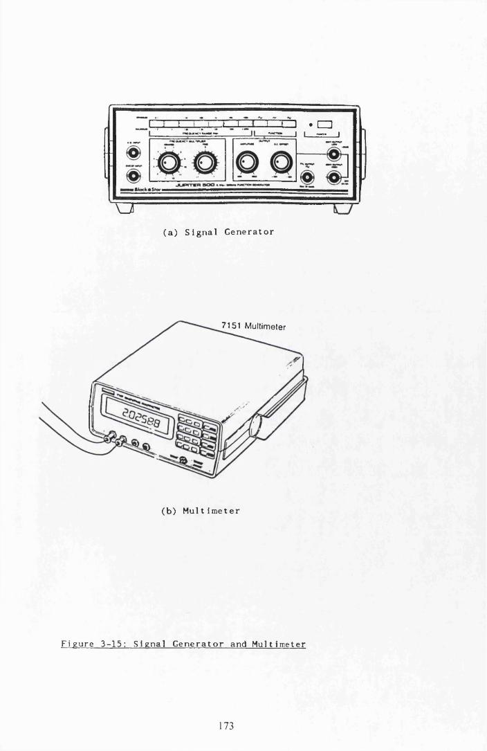
r.

czrzr }" n i i ) • CDJ i — i

v j

( a ) S i g n a l G e n e r a t o r

7151 Multimeter

(b ) Mult i m e t e r

F i g u r e 3-15: S i g n a l G e n e r a t o r and Mul t i me t e r

173

1o (UTt. au oW u

□ in

pq CL

CL U(/) 9- P

CLUG 0

>□L_

C J

Cl |—

XXPQi— i

inin

<3 X /N1—P 3 LO

>_<3 c (yO

n <r C

C PCD 30) aL_ pU

GO □

p

un

pin

n □

L PCD 3

P Q_c PL

CL □

174

Fig

ure

3-16

: Da

ta

Acq

uisi

tion

an

d Fl

ow

Cha

rt

L a s e r Beams

Probe Volume

( a ) F o r m a t io n o f t h e Probe Volume

by I n t e r s e c t i n g Beams

uz us 2

Flow / Particle

(b ) D i a g r a m a t i c View o f t h e L.D.A. O p e r a t i o n

F i g u r e 3 - 17 : L.D.A. O p e r a t i o n

175

PipeP.M.T ub e

L a s e r

Pipe C e n t r e Line —

L a s e rB e an s

R e f l e c t e dBe an s

Inc iden tB e a n s

R e f l e c t e dB e a n s

——i___

R e f l e c t e dBe a n s

F i g u r e 3 -18 ; L a s e r I n t e r s e c t i o n wi th t h e P ipe

(See T e x t f o r D e t a i l s )

176

EE

onj

Cooling Fins

C atch t o Gain A c c e s s t o Bulb

T±T X±Tl

\ 7

Light Box

r e con nect ion f o r Air Cooling Pipe

OJ

S up portin gL egs

Light A p e r t u r e

26mn I.D. Glass Pipe A d j u s ta b le

F e e t

Scale 2.5>1

F i g u r e 3-19 : Li ght Box used i n t h e Flow V i s u a l i s a t i o n

177

CHAPTER 4

CHAPTER 4

PRELIMINARY RESULTS AND CALIBRATION

4 . 1 INTRODUCTION

4 .2 CALIBRATION OF APPARATUS AND PRELIMINARY RESULTS

4 .2 .1 The I n v e r t e r F re q u e n c y - P ip e

R eyno lds Number R e l a t i o n s h i p

4 .2 .2 C e n t r e - l i n e V e lo c i ty R e s u l t s

4 .2 .3 P a r a b o l ic H a g e n - P o is e u i1 le Flow

4 .2 .4 S e le c t io n o f F o r c in g F re q u e n c y and A m p litu d e

4 .2 .5 P u l s a t i l e L am inar F low

4 .2 .6 N a tu ra l F re q u en c y R e s u l t s and

th e S tro u h a l Number

4 .3 CALIBRATION OF THE COMPUTER ALGORITHMS

4 .4 DERIVED RELATIONSHIPS

4 .4 .1 P ip e , O r i f i c e an d R e y n o ld s

Number R e l a t i o n s h i p s

4 .4 .2 The Wake R ey n o ld s Number

4 .4 .3 The F o rc in g F re q u e n c y - P ip e R eynolds


4 .4 .4 V o rtex S h ed d in g V e l o c i t y and W avelength

4 . 4 . 5 F o rc in g Amplitude R e la t io n s h lp

4 .5 OUTLINE OF THE EXPERIMENTAL WORK

178

4.1 INTRODUCTION

The contents of this chapter represent neither a description of the apparatus as

in chapter 3, nor systematic experiments as in chapters 5 and 6, but rather

preliminaries in leading to systematic experimentation. Thus chapter 4 encompasses

calibration and sensitivity tests on the apparatus, interrelationships used in the

experiments, as well as a description of the range of param eters varied in the

experiments.

4.2 CALIBRATION O F APPARATUS AND PRELIMINARY RESULTS

4.2.1 The Inverter — Pioe Reynolds Number Relationship

The A.C. Inverter is a device which controls the motor and piston speeds, (as

described in chapter 3), and may be set from 0 to 37.5Hz, in 0.1 Hz units. The

motor controls the average pipe flow velocity, via the piston. The inverter,

therefore, directly controls the pipe Reynolds number. Tests were performed to find

the relationship between the Inverter A.C. setting and the resultant pipe Reynolds

number. These are described below.

The Inverter was set to values from 0 to 35Hz in 5Hz increments, and the

piston velocity was measured at each stage. This was converted into an average

pipe flow velocity, U p, using the continuity condition and a knowledge of the

internal diameters of the pipe and piston casing, Dp and D p ^ respectively, where,

U • . A .U P l s A P >s ( 4 .1 )

P P

Using the pipe and piston dimensions quoted in chapter 3, the relationship for pipe

and flow velocity is obtained,

U - 6 1 .1 7 4 U . ( 4 .2 )p p i s

179

The pipe velocities, calculated from the piston velocities, were checked against

L.D.A. readings of the pipe centreline velocities. (Since for the case of laminar

pipe flow the maximum velocity occurring at the cen tre- line is twice the average

flow velocity.) The L.D.A. velocity readings were found to be in good agreement

with the calculated velocities, as shown in figure 4.2 and discussed in section 4.2.2

below.

The pipe velocities were converted into Reynolds numbers using equation 2.5,

and a plot of the inverter frequency fj versus the Pipe Reynolds, Rep, was

produced. This plot is shown in figure 4—1. In the figure, the measured points are

shown by crosses. A best fit line, using the least squares method, was calculated

and is shown in the figure. The equation of the best fit line is

Re - 2 5 .5 9 7 f . - 0 .1 7 1 4 3 ( 4 .3 )P i

This relationship was used in all subsequent calculations of the pipe Reynolds

number involved in the main results.

4 .2 .2 C entre— line Velocity Results

The relationship between the average piston velocity and the average pipe

velocity should be linear. This was checked by measuring the average piston

velocity and calculating the pipe centre— line velocity from it, (i.e. twice the

average pipe velocity). This value was then compared to the L.D.A. velocities

obtained at the centre— line. Figure 4— 2 shows the L.D.A. velocities plotted against

those calculated from the piston rate. These points are plotted '+ ' in the figure.

(The points correspond to pipe Reynolds numbers of 128 to 896 in increments of

128.)

It is noticeable that for higher flow rates the L.D.A. velocities fall short of the

piston rate values. However, after some investigation it was noticed that this error

could be much reduced by switching up the Doppler frequency range of the tracker

to a higher range, (section 3.4.3). The point marked in the figure was taken at

180

f[> = 100,000 Hz whereas the other points were taken at 33,000 Hz. Thus by

using a higher tracker frequency, a much more accurate L.D.A. velocity is

obtained. The reason for this behaviour is not apparent.

4 .2.3 Parabolic Hagen— Poiseuille Flow

The velocities across the pipe were checked for pipe Reynolds numbers of 128,

256, 512 and 768. At these Reynolds numbers the flow was laminar, thus the

resultant velocity profile should be parabolic, (see the expression for

Hagen—Poiseuille flow, equation 2—16b). Figures 4.3a to d show the L.D.A.

results, (plotted with an 'x ') . Superimposed on the diagram is the parabolic

Hagen—Poiseuille profile. It can be clearly seen from the figures that the L.D.A.

results are very accurate at, and near to, the centre of the pipe. However, as one

departs from the centre— line the results become much less accurate.

The general picture is the same for each plot. The plots suggest that the

L.D .A. results are accurate up to approximately 6mm from the cen tre-line ,

beyond which they tend to drop off until they are near to the pipe wall, (radial

distance = 13mm), at which point they level off. Apart from one set of

measurements, all the main flow measurements, of the investigation reported in this

thesis, were taken at the centre line. The one set of L.D.A. readings taken across

the flow were only taken from the pipe centre to a maximum radial distance of

6mm. Thus ensuring accurate measurements within the pipe. (See chapter 6 for

m ore details.)

Five possible reasons for the error in the velocity measurem ent, as the pipe

wall is approached by the laser probe volume, are as follows:

1 — The finite length of the probe volume itself, which means that at positions

within the flow, where there are steep velocity gradients, velocities over a wide

range may be picked up by the L.D.A. system. Such steep velocity gradients occur

at the pipe wall in pipe flow.

2 — Excessive flare occurring at the pipe wall. Flare as a possible cause of the

error in the velocity results close to the wall was suggested during consultations

with the m anufacturer DISA.

3 — The absolute velocity near to the wall being very small, possibly out of the

181

range of the L.D .A. system.

4 — A lack of seeding particles near to the wall, due to the relatively low volume

flow rate.

5 — Wrong designation of the location of the laser beams in the pipe, due

refractive effects on a slightly ovaloid pipe wall.

4.2.4 Selection of Forcing Frequency and Amplitude

In pulsatile flow in pipes, especially in the presence of an orifice plate to

generate turbulence, it is important to chose suitable amplitude and frequency

pulses, with which to force the vortices from the orifice plate.

A method for selecting both a forcing amplitude and forcing frequency had to

be found, which allowed for the pulsation amplitude and frequency to be varied

independently of each other. These criteria were satisfied by varying the Inverter

input signal sinusoidally using the signal generator, (function generator outlined in

section 3.3.7). The flow forcing frequency was controlled by the input frequency of

the signal generator. The forcing amplitude was controlled by varying the input

peak to peak voltage of the signal generator. The peak to peak voltage of the

oscillation could be accurately controlled and monitored using an oscilloscope and a

computing multimeter. An outline sketch of the forcing frequency and amplitude is

given in figure 4.4a. Once this method had been devised to introduce the forcing

amplitude at the required frequency, tests were then performed to see how the

amplitude affected the L.D.A. results.

The forcing amplitude had to satisfy two criteria. Firstly, the amplitude must be

large enough to produce a dominant frequency in the flow, as seen from the

frequency spectra. This dominant frequency must 'drown out' the stray motor

frequency, fm , which is always present in the flow, (just visible in the frequency

spectra plot), and which, if allowed, may influence the vortex shedding frequency

when an orifice plate is fitted. Secondly, the amplitude must not be so large that

it produces undesirable effects in the flow, such as turbulence, flow reversal etc.

Five tests were carried out to observe the flow behaviour due to the amplitude

variation. Thus five tests were conducted keeping the Reynolds number and the

182

forcing frequency, ff, constant while varying the peak to peak voltage of the

forcing amplitude, Av. These are as follows:

T e s t- 1 - Rep — 256, U = 3.3Hz

T est- 2 - Rep = 256, II 6.6Hz

T est-■3 - Rep — 256, ff = 9.9Hz

T est-■4 - Rep = 512, II 6 .6Hz

T est-•5 - Rep = 768, II 9 .9Hz

The results of the tests are summarised in figure 4— 4b to f . In the figures the

Fourier amplitudes of each frequency spike, in each respective frequency spectrum,

are plotted against the forcing amplitude, (peak to peak), of the frequency

generator. This forcing amplitude is in volts. A voltage of 10 volts from the signal

generator gives a pipe Reynolds number of 960, thus to convert from a voltage to

a pipe Reynolds number the voltage is multiplied by 96. More details of the

forcing amplitude relationship is given in section 4.4.5.

From the figure 4.4b to f the following is apparent.

1 — In all cases the stray motor frequency, is apparent.

2 — In tests 1 and 2 a secondary peak is observed at a frequency of twice that

of the forcing frequency.

3 — For low values of forcing amplitude, (A v < 0.2 Volts), the forcing frequency

amplitude is comparable with the stray motor frequency.

4 — At mid range values of forcing frequency, (0.2 < Ay < 1.0 Volts), the

variation of frequency spectrum amplitude with forcing frequency amplitude is

roughly linear.

5 — At high values of forcing amplitude, (A y>1.0 Volts), the frequency spectra

amplitude no longer follows the linear relationship, tends to level off, and the

secondary frequency becomes markedly dominant. This represents a non— linear,

unstable phase of the pulsations.

Thus for the experimental investigation reported herein, and with the exception of

one set of test results, the forcing frequency amplitude was maintained at a value

of 0.6 Volts, which corresponds to a peak to peak variation in the pipe Reynolds

num ber, Rep, of 57.60, or equivalently an R.M.S. fluctuation of the pipe Reynolds

183

number of 20.36. 0.6 Volts was chosen as it is a large enough amplitude to drown

out the rogue motor frequencies while at the same time being less than the

n o n - linear, unstable range which exists from approximately 1.0 Volts peak to peak

amplitude.

The set of test results that aimed to look at the effect of forcing amplitude on

the flow processes, used three amplitudes, namely 0.2, 0.6 and 1.0 Volts, (R.M.S.

fluctuations in Rep of 6.79, 20.36 and 33.93). All these lying within the linear

range.

4.2.5 Pulsatile Lam inar Flow

Prior to the introduction of an orifice plate it was decided to take some

preliminary results for various pulsatile pipe flows. The Reynolds number, forcing

frequency and forcing amplitude were varied independently of each other. This was

done to test the method by which the data was to be abstracted and analysed for

the main results. It also served as a test of the various analysis algorithms, such as

the dimension algorithm, autocorrelation function, F .F .T . and the algorithm to find

the first minimum in mutual information. Furthermore, plotting routines to produce

time series and attractor plots, (section 2.4.3), could be refined.

The results for one such test are given in figure 4— 5. This test was performed

for a pipe Reynolds number of 256, a forcing frequency of 3.3Hz and a forcing

amplitude of 0.6 Volts, (an R.M.S. fluctuation of 7.95%). In the figure one may

see the time series, attractor plot and dimension plot for the velocity— time series

at the centre— line of the pipe.

The time series is plotted in figure 4— 5a. The time series looks periodic.

However, a closer inspection reveals that most of the peaks and troughs are not

smooth. This is due to two effects:

1 — The time series is not ^generated from a continuous sjgnal, but a digitised

signal. Thus the resultant time series is made up of a series of points connected

by straight lines. This accounts in part for the general lack of smoothness of the

time series.

184

2 - The time signal also contains a small amount of noise, which tends to distort

the form of the time series.

The attractor plotted in figure 4 - 5b, is obviously periodic at large scales, as it

displays a simple closed loop of a simple periodic wave function. However, a

thickening of the attractor due to noise is also apparent. This noise is at smaller

scales, too small to mask the overall periodic structure of the attractor.

The fractal dimension of the attractor is obtained from the 'log(r)—log(Cr)'

plot shown in figure 4—5c, (see section 2.5.5). The plot has been performed for

an embedding dimension, n, from 2 to 30. It can be seen from the plot that, at

large length scales on the attractor, the slope of the lines tends to a value of 1.

(Actually a value of 1.05 was measured by the author, denoted by the heavy line

in the diagram.) This confirms the fact that the attractor is periodic, with one

degree of freedom at these length scales. However, also evident from the figure is

that for smaller length scales the slopes of the lines increase as n is increased.

This is the typical behaviour of noisy flows. Thus it may be concluded that the

attractor is indeed noisy at smaller length scales. This picture fits in with those

derived by both visual observation of the time series and attractor plot.

The tests performed on pulsatile flows in the pipe without the orifice present,

and reported in this section, will serve as a benchmark, (or perhaps a starting

position), by which to interpret the main results.

4.2.6 Natural Frequency Results and the Strouhal Number

Tests were conducted to find the natural frequency of vortex shedding from

each of the orifice plates used in the experimental investigation. The tests were

performed with unpulsed flows by opening the drain valve at the piston. This was

done over a wide range, thereby causing flows in the pipe at various Reynolds

numbers. These Reynolds numbers were calculated by measuring the volume of

water passing through the valve over a specific period of time.

The natural vortex shedding frequencies were measured using the L.D .A. system

at various points downstream of each orifice plate. Flow visualisation was used to

185

check the L.D .A. readings by counting the number of vortices shed in a specified

time period.

The Strouhal number was then calculated for each of these observations using

equation 2.77, as follows,

U

The results of these tests are summarised in figures 4— 6 and 4— 7.

Figure 4—6 gives the results obtained by the author for the 13mm orifice plate

at Reynolds numbers from 282 to 1983. The results tend to suggest that the

Strouhal number remains fairly constant up to a pipe Reynolds number of

approximately 1500, from which point it increases. The average value of the

Strouhal number over the 'fla t' range is 0.668. Such a flat range, whereby the

Strouhal number remains constant over a large Reynolds number range is typical of

vortex shedding flows. (This type of behaviour has been illustrated in section 2.4.5,

and figure 2.33.)

After a long search in the literature, the only source of data that could be

found regarding Strouhal numbers of orifice flows at a Pipe orifice were those of

Johansen [1929]. These results are for a pipe internal diam eter of 27mm and water

as a fluid. The results are also plotted in figure 4— 6, and were obtained using

flow visualisation only. (Unfortunately Johansen quoted neither the viscosity nor the

tem perature of the fluid, thus the Reynolds numbers he quotes may be for a

different flow rate than equivalent Reynolds numbers for the author's results, this is

a m inor point which should only be noted.)

The Strouhal numbers were obtained for various Reynolds numbers for all the

orifice plates used in the study. The results of these tests are shown in

figure 4—7. Reliable results could not be obtained for the 22.75m m orifice plate,

as the resulting frequency spectra was very broad band, i.e. no distinct peak could

be seen. In figure 4—7 the best fit line of the data is shown dashed, together with

the error bars of the Strouhal number points. The best fit line is obtained using a

186

least squares fit and the error bars represent 95% confidence limits using Students

t—test, [Snedecor and Cochran, 1967],

The equation of the best fit line is,

S - 0 .70643 - 0 .1 3 2 9 2 . (D0/Dp) ( 4 .4 )

this equation was used to calculate the natural frequency, fn , of the orifice plates

at various Reynolds numbers in the study. The forcing frequency of the vortex

shedding, ff, was then set equal to this derived natural frequency. The Strouhal

numbers for each orifice diameter used in the investigation are listed in table 4.1.

4.3 CALIBRATION O F THE COM PUTER ALGORITHMS

Prior to their use in the experimental investigation, the main computer

programs, (the Grassberger— Procaccia dimension algorithm and Lyapunov exponent

algorithm), were run using test data with known characteristics. The testing of the

algorithms was rather extensive and to aid continuity in this chapter full details of

these tests, and the results thereof, are given in appendix 2. Furthermore,

appendix 2 contains a description of all computer programs used in the study, and

listings of the main programs are given.

4.4 DERIVED RELATIONSHIPS

In what follows in this section an attem pt will be made to clarify the many

relationships and interrelationships between the parameters and variables in use in

the experiments, prior to their use in subsequent chapters.

4t4.1 Pipe. Orifice and Reynolds Number Relationships

First it is important to state two geometrical relationships of the pipe and

187

orifice plate — the diameter ratio, B, and the area ratio, or porosity, a. B is the

ratio of the orifice diameter to pipe internal diameter,

D

P

The porosity, which is the ratio of the orifice area, A0, to the pipe internal area,

Ap, is thus

Aa - - B2 ( 4 .6 )

AP

Table 4.1 gives the ratios a and 0 for the six orifice plates used in the study.

The pipe and orifice Reynolds numbers are defined as,

U . D U . DRe - — E------- L - , Re - — ------- — ( 4 .7 a & b)

P °

where Up and U0 are the average velocities of the flow through the pipe and

orifice plate respectively.

Now using the continuity condition one arrives at a simple expression relating

the average pipe velocity to the average orifice velocity

U - B2 . U - a . U ( 4 .8 )p o o

Also from the above one can derive a simple relationship between the pipe

Reynolds number and the orifice Reynolds number,

Re - B . Re ( 4 .9 )p o x '

188

4 .4 .2 The Wake Reynolds Number

The Reynolds number may be defined using any arbitrary velocity and length

scale deemed to suit the flow situation. For orifice diameters of the same order

as that of the pipe, the flow may behave in a similar way to boundary layer flows

encountering a bluff body, figure 4— 8a. Whereas flows through orifice plates of

diameters much smaller than the pipe diameter may behave more in he fashion of

submerged jet flows as depicted in figure 4— 8b. It thus may be argued that a

m ore suitable definition of the Reynolds number for orifice plates with diameters

comparable to the pipe internal diameter may be that of the wake Reynolds

num ber, [Bandyopadhay, 1986 and 1989] defined thus,

U . . hRe - --- *-------- (4.10)w

v

W here the length scale, h, is the height to which the orifice lip protrudes into the

flow, and the velocity, U^, is the velocity which would occur at a distance h from

the pipe wall in the absence of the orifice plate. Ujj is obtained by rearranging

the Poiseuille pipe flow law into the following form,

8 . U . h r . -I

Uh - 6— 1 - 4 - ( 4 1 1 )

Thus the wake Reynolds number in terms of the pipe Reynolds number is

8 . h 2Re - I 1 - — I . Re (4.12)[ 1 - - k } •

Now the lip height h is simply half the difference between the orifice diameter and

the pipe diameter, i.e.

D - D Dh - P 2 ° ----------- f - . ( 1 - B ) ( 4 .1 3 )

189

Thus equation 4.12 becomes

Re - ( 1 - B ) 2 . ( 1 + B ) . Re (4 .14)w p

Table 4.1 gives the lip height, h, and the ratio of Rew to Rep for all the orifice

plates involved in this study. Substituting equation 4.10 into the above, the

equivalent expression for the wake Reynolds number in terms of the orifice

Reynolds number becomes,

Re - ( 1 w - B ) 2 . ( 1 + B ) B . Reo (4 .15)

Do S fi a hRewRe

P

(mm) (mm)

6.50 0.684 0.250 0.0625 9.750 0.703

9.75 0.673 0.375 0.1406 8.125 0.537

13.00 0.661 0.500 0.2500 6.500 0.375

16.25 0.650 0.625 0.3906 4.875 0.229

19.50 0.639 0.750 0.5625 3.250 0.109

22.75 0.628 0.875 0.7656 1.625 0.029

Table 4 .1 : P ip e - O r l f i c e R e la t ionsh ips

190

4.4.3 The Forcing Frequency — Pipe Reynolds Number

Relationship

The Strouhal number has been previously defined in sections 2.4.5 and 4.2.6 as

f U A' DS - sh ed oUo

where fn is the natural frequency of an orifice plate, orifice diameter D 0, with an

average flow velocity through the orifice plate of U0 . All flows in the experiment

reported herein, were forced at a frequency, ff, equal to the natural frequency, f n,

(see section 4.5.). Therefore, the frequency of forcing of the flow in terms of the

orifice and pipe Reynolds numbers is

f~ - . Re - - - - - - . Re (4 .16)f D2 ° B3 .D 2 Po p

4.4.4 Vortex Shedding Velocity and Wavelength

The vortices shed in a shear flow generally travel with a certain average

velocity U v and have a wavelength lv and shedding frequency fv , where,

U - f . 1 (4 .17)V V V

The vortex shedding frequency in the experimentation herein was controlled by

setting the pulsation, or forcing frequency, ff, at the natural frequency, fn . Using

the above definition of the Strouhal number, the vortex shedding velocity U v may

be obtained from the following relationship,

U . 1 . Su - - °-----V------ - f . 1 - f r . 1 (4 .18)v D n v f v v /

191

This is another useful relationship, since the vortex shedding wavelength, lv, may

be obtained by scaling from the flow visualisation photographs, and so the mean

velocity of the vortices, Uv, could be estimated.

4.4.5 Forcing Amplitude Relationship

In all cases, with the exception of one set of results, the forcing amplitudes

were kept constant as the pipe Reynolds number was varied, this resulted in a

different percentage forcing amplitude for each different value of Rep. Lower

values of Rep therefore have a higher percentage of forcing. This was found to be

advantageous since for higher Reynolds numbers lower disturbance levels are

required to produce discrete vortices.

Thus for a value of Rep of 256, a forcing voltage of 0.6 volts represents an

R.M .S. fluctuation value of 7.95% . The general formula for finding an R.M.S.

fluctuation value is:

R.M.S ( f l u c t ) - Voltage X 96e p 2 . ( 2 ) *

(4.19)

4.5 OUTLINE OF TH E EXPERIMENTAL WORK

The results from the experimental work undertaken are reported in chapters 5

and 6. Chapter 5 deals with the flow visualisation both from photographs and video

film. Whereas chapter 6 deals with the main L.D.A. results and subsequent data

analysis.

The flow visualisation results (Chapter 5) are primarily to present an overall

visual description of the flow processes at the orifice plate, and thus give a

qualitative insight into the various phenomena prior to the L.D.A. readings.

Quantitative results are also derived from the flow visualisation by scaling

wavelengths from photographic and video film, from which vortex velocities may be

found. Vortex trajectories may also be obtained. Vortex velocities, and the timing

192

of other events, may be obtained by using the video film of events with a time

code superimposed upon it. The video may be paused from frame to frame and

distance travelled by certain flow areas measured. More will be said about these

methods in chapter 5.

The L.D .A. results of chapter 6 deal with the quantitative analysis of certain

regions of the flow. The parameters could varied independently during the course

of the study were:

1 — The Pipe Reynolds Number (Rep)

2 — The Orifice Diameter (D0)

3 — The Forcing Amplitude (Ay). (Varied in only one set of tests.)

4 — The Forcing Frequency (ff).

5 — The Measuring Position along the Pipe (z)

6 — The Measuring Position across the Pipe (r)

The orifice Reynolds number (Re0), is dictated solely by (1) and (2) thus is not an

independent variable. During the investigation the pipe used was of the same

internal and external diameter. Also kept constant was the temperature of the

water, and thus the kinematic viscosity. (See Chapter 3, section 3.2.3 and 3.2.7).

The number of independent experimental parameters which may be varied is

therefore six. This was considered still too large a number to effectively study

within the time constraints of the work, thus it was decided to force the vortex

shedding at the natural frequency only, (i.e. ff = f ^ . This reduces the number of

independent parameters to five. Therefore, ff is a function of the Reynolds number

linked to it via the Strouhal number as outlined in equation 4.16. A comprehensive

investigation of the effect of forcing frequency is therefore outside the scope of this

investigation.

Strictly speaking parameters (5) and (6) are not really experimental variables.

Since by varying either, and hence moving the observation point of the L.D.A.

system, the flow processes do not change. They are only parameters in the sense,

that by varying the position of the laser probe volume in the flow, various time

traces with different properties may be obtained. This is because the time

dependent flow properties vary spatially within the flow.

193

The tests performed varied these parameters in a controlled manner and the

effect they had on the flow processes monitored. The tests performed are outlined

in table 4.2. A standard set of results which is common to both set—A and set—B

and with which most of the other sets of results may be compared to is as

follows:

Rep = 256, D0 = 13mm, RCq = 512,

ff - 2.52Hz, Af = 0 .6 V (= 7.95% R.M.S. fluctuation)

these parameters were observed along the pipe axis, (r = 0), at the seventeen

longitudinal positions, (z), outlined in chapter 3 section 3.2.12.

Set— A could be described as the main set of results. T h is . set monitors the

effect on flow behaviour of varying the pipe Reynolds number. Set— B looks at the

effect of varying the forcing amplitude while keeping the pipe Reynolds number

constant. Set— C and set— D look in detail at the flow processes occurring for

various values of Rep, at orifice plates of diameters of 9.75mm and 16.25mm

respectively. Set— E briefly looks at the remaining orifice diameters of 6.5mm,

19.5mm and 22.75mm. Only the frequency spectra, average velocity and the

turbulence intensities are measured for these orifice plates. W hereas, the above sets

of results are taken at the centre— line of the longitudinal axis of the pipe, set— F,

aims to investigate the flow properties across the flow in the immediate vicinity

downstream of the orifice plate. Lastly set— G is another set of results taken for

the parameters of the standard set and used as a check on the repeatability of the

experiment.

194

P a ra m e te r T e s t

A B C D E F G

D (mm) o 13 13 9 .7 5 1 6 .7 5 Range 13 13

ReP

Range 256 Range Range 256 256 256

Re o 0 . ReP

0.R eP

<5.ReP

0 .R eP

0 .R eP

( 3 . ReP

0.R eP

f f f n f n f n f n f n f n f n

Af ( V o l ts ) 0 .6 Range 0 .6 0 .6 0 .6 0 .6 0 .6

Af (R e) 5 7 .6 Range 5 7 .6 5 7 .6 5 7 .6 5 7 .6 5 7 .6

' z 'No. o f L ongi t ' n a l P o s i t io n s

17 17 17 17 17 5 17

»r iNo. o f R a d ia l P o s i t io n s

C .L . C .L . C .L . C .L . C .L . 10 C .L .

TOTAL NUMBER OF TESTS

5 3 3 3 3 1 1

T a b le 4 .2 : O u t l in e o f th e E x p e r im e n ta l T e s ts

L e g e n d : C .L . - R e s u l t Taken a t th e C e n tr e L ine Only

195

CHAPTER 4 FIGURES

Pipe Reynold* Number1000

800

600

400

200

60 10 15 2520 30 35 40Inverter Frequency (Hz)

+ Reading* Beat Fit Line

F i g u r e 4 - 1 : I n v e r t e r Frequency - P i pe Re yno l d s


L.D.A. Measured Velocity (mm/s)100

80

60 —

40 —

40 60 80 1000 20Velocity from Piston Rate (m m /s)

+ L.D.A. M ea s u re m e n ts * E x tra L.D.A. Po in t 100 % Line

LD.A. Poin ts Taken a t F d - 3 3 0 0 0 E x tra L.D.A. Point Taken a t F d -1 0 0 0 0 0

F i g u r e 4 - 2 : C e n t r e - l i n e V e l o c i t y Compar i s on

196

Velocity (mm/s)

2 6 80 4 1410 12Radial Distance (mm)

Theoretica l x Measured (L.D.A.)

( a ) Rep - 128

Velocity (mm/s)30

25

20

15 X

10

5

00 2 4 6 8 10 12 14

Radial Distance (mm)

~ T h e o r e t i c a l x Measured (L.D.A.)

(b ) Rep - 256

F i g u r e 4 - 3 : L.D.A. V e l o c i t y P r o f i l e s

197

Velocity (mm/s) 6 0 ,--------------------------

40

3 0

20

1412106 8420Radial Distance (mm)

Theoretical x Measured (L.D.A.)

( c ) Rep - 512

Velocity (mm/s)80

60

40

20

0 2 4 6 8 10 12 14Radial Distance (mm)

Theoretical x Measured (L.D.A.)

(d) Rep - 768

F i g u r e 4 - 3 ; L.D.A. V e l o c i t y P r o f i l e s

198

L\PU7Signal G e n e r a t o r Time S e r i e s

tf,= 1/t

Via I n v e r t o r and M o t o r t o Fluidv

□UTPUTVeloc l ty -Tlme T r a c e a sM e a s u r e d by t h e L a s e r In t h e FluidV e l o c i t y

A \

Tine

FREQUENCY s p e c t r a

f r e q u e n c y (Hz)f

( a ) D e f i n i t i o n Ske t ch o f t h e R e l a t i v e Ampl i t ude Tes t F i g u r e 4 - 4 : R e l a t i v e Ampl i t ude T e s t s

199

Freq. S p e c t r u m Amplitude

S p e c t r a ] Ampl i t ude Measured in F l u i d by L a s e r

7

6F o r c i n g F r e q u e n c y ( f f )

6

4

3Rogue Motor F r e q u e n c y ( f m)2

1

01.2 1.4 1.6 1.8 2 2.2 2.40 0.2 0 .4 0.6 0.8 1

Signal Peak-Peak Voltage S i g n a l G e n e r a t o r

f m(1) f f ( 3 .3 H z ) — 2 f f (6 .6Hz) I

^ F o r c i n g Ampl i tude

(b) Rep - 256, f f - 3 3 H z

Freq. Spectrum Amplitude3.6

2.6

1.6

2 f f0.5

0 0.2 0 .4 0 .6 0 .8 1 1.2 1.4 1.6 1.8 2 2.2 2.4

Signal Peak-Peak Voltage

f m (1) - » - f f (6.6Hz) 2 f f (13.2Hz) I

( c ) Rep - 256, f f - 6.6>Hz

F i g u r e 4 - 4 : R e l a t i v e Ampl i t ude T e s t s

200

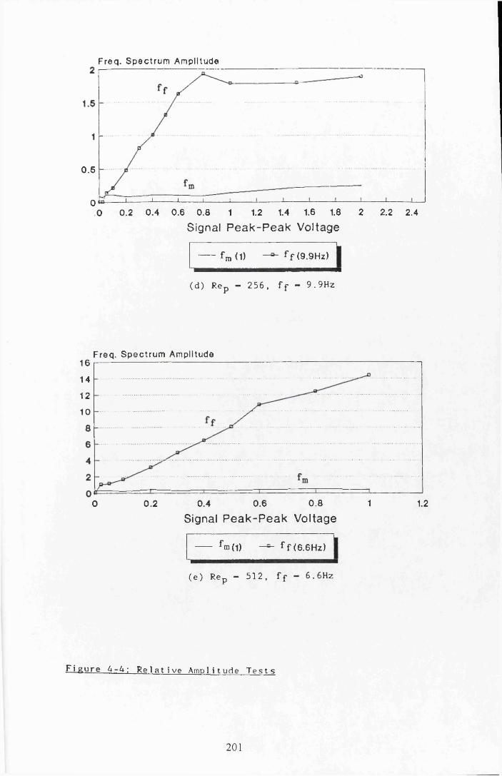
Freq. Sp ec trum Amplitude

0.5

Q ta ----------1------------ 1------------1------------1------------ L

0 0.2 0.4 0.6 0.8 1 1.2 1.4 1.6 1.8 2 2.2 2.4


f ra (1) f f <9.9Hz)

(d) Rep - 256, f f - 9.9Hz

Freq. Spectrum Amplitude16

14

12

10

0.8 1 1.20.4 0.60.20Signal Peak-Peak Voltage

f m(D — f f (6.6Hz)

(e) Rep - 512, f f - 6 . 6Hz

F i g u r e U-U\ R e l a t i v e Ampl i t ude T e s t s

201

Freq. Sp ec tru m Amplitude

0.8

0.6

0.4

0.2

0 0.2 0.4 0.6 0.8 1 1.2 1.4 1.6 1.8 2 2.2 2.4


f rn(1) ~ a — f f (9.9Hz)

( f ) Rep - 768, f f - 9 . 9Hz

F i g u r e 4 - 4 : R e l a t i v e Ampl i t ude T e s t s

202

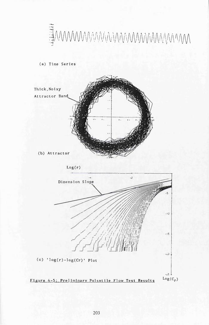
( a ) Time S e r i e s

T h i c k , No i sy

A t t r a c t o r Band

(b) A t t r a c t o r

Log ( r )

Di mens i on Slo

( c ) ' l o g ( r ) - l o g ( C r ) • P l o t

. JF i g u r e 4 - 5 : P r e l i m i n a r y P u l s a t i l e Flow Te s t R e s u l t s ^°S(Cr

S t r ouha l Number

0.8

0.6

0.4

0.2

600 16000 2000 2 6 0 01000R e y n o l d s Number

Johansen (1929) Present Results

F i g u r e 4 - 6 : S t r o u h a l Number R e s u l t s - 13.00mm O r i f i c e P l a t e

S t r o u h a l Number

Bes t F i t LineE r r o r Bars0.8

0.6

0 .4

0.2

22.7619.60 9.76 13 16.263.25O r i f i c e Di ame t e r

F i g u r e 4 - 7 : S t ro u h a l Number R e s u l t s - Al l O r i f i c e P l a t e s

204

h

V e l o c i t yP r o f i l e

Bl u f fBodyFlow

C e n t r e Line

VTZ7777T777///777777777T7,

Pipe Vail

( a) Wake Flow

J e t Flow

VY/s////Y/;sy/7y/rs777T//77/s/yy/s/7/77/;//7n,

Pipe Vail

(b) J e t Flow

F i g u r e 4 . 8 ; Wake and J e t Flows at an O r i f i c e P l a t e

205

CHAPTER 5

CBAEIER.1

FLOW _VISUAL1 SAT ION RESULTS

5.1 INTRODUCTION

5 .2 BACKGROUND TO FLOW VISUALISATION

5.2.1 The Technique o f Flow V i s u a l i s a t i o n5 .2 .2 I n t e r p r e t a t i o n o f the Flow Phenomena5 .2 .3 I l lum ina t ion o f the Flow5 .2 .4 Information from Film5.2 .5 Geometrical and R e f r a c t i v e P ro p e r t i e s

of the Pipe5 .2 .6 Flow V i s u a l i s a t i o n a t a Pipe O r i f ice

5 .3 PRLIMINARY TESTS

5 .4 NATURAL, UNFORCED FLOW RESULTS AT THE 13.00mm ORIFICE PLATE

5 .5 FORCED FLOW RESULTS: THE 13mm ORIFICE

5.5 .1 Flows a t the O r i f i c e P l a t e5 .5 .2 Downstream D i s s i p a t i o n o f the Disturbances

5 .6 FORCED FLOW RESULTS: THE 9.75 AND 16.25mm ORIFICE PLATES

5.6 .1 The 9.75mm O r i f i c e5 .6 .2 The 16.25mm O r i f i c e

206

5.7 VIDEO RESULTS

5 .7 .1 In t r o d u c t io n5 .7 .2 Contents o f the Video Film5 .7 .3 Overal l P i c t u r e o f the Flow Processes5 .7 .4 C a t e g o r i s a t i o n o f the Flow V i s u a l i s a t i o n Resu l t s

5.8 VORTEX WAVELENGTH AND VELOCITY RESULTS

5.9 SUMMARY

207

5.1 INTRODUCTION

The purpose of this chapter is to introduce the reader to the concept of flow

visualisation in Fluid Mechanics, to report on photographs and a video taken for a

range of orifice diameters, Reynolds Numbers in the pipe and forcing frequencies

covering an area in the immediate vicinity of the orifice plate. The chapter

concludes with experimental measurements of vortex wavelengths taken from the

flow visualisation tests.

5.2 BACKGROUND TO FLOW VISUALISATION

5.2.1 The Technique of Flow Visualisation

Flow visualisation has for many years played an important role in the

understanding of flow phenomena. The technique provides the experimentalist with

both spatial and temporal information about the flow, whereas more quantitative

methods such as laser Doppler anemometry or hot wire techniques may be limited

to a few spatial positions. Various flow visualisation techniques have been developed

to elucidate the properties of gas and liquid flows with the intention of giving an

insight into the processes involved. Flow visualisation achieves this aim by rendering

visible the actions of the flow, aiding visual perception of the processes. In the

study presented herein, flow visualisation was undertaken to aid the physical

interpretation of the L.D .A . data.

The technique of flow visualisation works by releasing an agent into the flow

which is distinctly visible within the fluid, and, under certain illumination serves to

highlight the processes in certain areas of the flow field. There are many agents

that are suitable for such studies, and they may be split into two broad categories

— dyes and tracer particles. Many substances may be used as dyes in the flow,

these include, food colouring, ink, potassium permanganate, methanol blue dye,

fluoresceine, even milk. Spherical and non— spherical tracer particles are used in

flow visualisation studies. The choice of particles is also wide including, helium

bubbles, oil droplets, smoke particles, talcum powder, guanine crystals, hollow glass

208

spheres, polystyrene and so on. The choice of both dyes and particles really

depends on the flow process being observed and the working fluid being used. A

much more complete list of these substances and the role they play can be found

in Merzkirch [1987].

The most famous example of the use of flow visualisation to elucidate a flow

phenomenon is certainly the classic experiment by Osborne Reynolds [1883] who, in

the latter part of the last century studied the laminar to turbulent transition

processes within a pipe. Reynolds used a dye to produce a streakline in water

running through a pipe. The streakline remained as an ordered linear element

when the flow was laminar. At the laminar— turbulent transition point the streakline

would become unstable, breaking down and mixing rapidly in the turbulent state.

This work enabled Reynolds to conclude that the transition point depended on a

non— dimensional flow param eter, now known as the Reynolds number in his

honour.

5.2.2 Interpretation of the Flow Phenomena

Depending on the agent used and the mode of observation different conclusions

may be reached. It is therefore necessary to define the various observable flow

patterns.

Streakline — (Also known as filament lines.) This is the instantaneous locus of

all fluid particles which have passed through a particular, fixed spatial location in

the flow. If one requires to observe these flow lines then a dye would be used.

Injecting the dye at a particular spatial position in the flow and taking a

photograph of the instantaneous flow field will show the streakline. A good

example of the use of streaklines in obtaining flow information can be found in

the paper by Zdravkovich [1969]. In the article smoke streaklines were observed in

the wake of laminar flow past a circular cylinder, giving an insight into the regions

of high vorticity production in the flow field which led to vortex roll up. The

downstream development of the resulting vortex streets could be seen leading to an

overall picture of the flow processes involved.

Particle Path — This is the curve that a fluid particle traverses in the flow field

209

over a finite time period. Particle paths may be obtained by observing single tracer

particles (or a low concentration which allows for individual particles to be easily

distinguished) and using a long exposure time. The image of each particle on the

resulting photograph will be drawn out as a locus of points known as the particle

path.

Stream lines — These are curves tangential to the instantaneous direction of the

flow velocity vector, at all points within the flow. Streamlines may be obtained

with a low concentration of tracer particles within the fluid. An intermediate

exposure time should be used that is long enough to allow the tracer particles to

produce very short particle paths at each position in the fluid. From these short

paths the fluid velocities may be obtained, (by the method outlined below in

section 2.4.3), and the fluid streamlines may be inferred.

For the case of steady flow, in which the flow field is independent of time, these

three curves coincide with each other. Whereas in unsteady, time dependent flows,

these curves are not coincident and one must be careful in the interpretation of

flow photographs. This is especially true for unsteady shear flows, [Gursul et al,

1990, Hama, 1962, and Gursul and Rockwell, 1991].

O ne of the most popular tracer particles for use with low to moderate

Reynolds number flows is natural guanine crystals, [Matisse and Gorman, 1984]. It

was decided to use these particles for the study reported here. These crystals occur

naturally in fish and are in fact responsible for the pearly, lustrous appearance of

their scales. The crystals have a plate— like structure, their approximate dimensions

being 30.0 p a n long by 6.0 p a n wide and 0.1 p a n thick. This shape enables the

particles to align themselves with the shear in the flow, [Rhee et al, 1984], This

property, combined with their relatively high refractive index of 1.85, allows them

to render flow structures visible when illuminated by a suitable light source.

A basic requirement of a flow visualisation agent is that it stays in suspension

for as long as possible, that is, it has a slow settling out rate. It is particularly

im portant that this rate is on a much larger time scale than the flow phenomena

under investigation. The settling out rate of a sphere can be found using Stokes

theory, [Massey, 1983]. Unfortunately, there is no such simple theory for

non— spherical particles.

2 1 0

Another requirement of the flow visualisation agent is that its mere presence

does not interfere with the flow processes being studied. For the purposes of most

investigations it is assumed that the particle size and concentration is so low that

the characteristics of the flow field are not altered by the presence of the

particles. The two main sources of deviation of a particle's velocity vector from

that of the fluid are:

1 — a velocity lag due to the inertia of the particle, and,

2 — a deviation in the particle direction due to a lift force caused by velocity

gradients acting over the particle.

Both these errors are explained in detail in Merzkirch [1987].

5.2.3 Illumination of the Flow

The most common method of illumination in flow visualisation studies is the

light sheet. Light sheets may be generated in a variety of ways, the most common

of which are lamps (or flashguns) with appropriate light guides and lenses. They

may also be generated by expanding laser beams in one plane by a suitable lens,

Schlien [1987].

With the light sheet one may visualise the two velocity components in the

plane of the sheet for many points or particles, [Emrich, 1983]. The sheet can be

moved from region to region of the flow field under investigation and a complete

picture built up of the flow processes involved, see for example Prenel et al

[1989]. A suitable light sheet for the flow visualisation undertaken in the study

reported herein was provided by a purpose built light box, more details of which

will are given in the experimental chapter, section 3.6.

When using a lamp for illumination, precision and control of the exposure

time, te , is very important. The higher the flow velocity, the faster the exposure

time required to eliminate excessive blurring of the image. However, where there is

a flow field containing a wide range of velocities one is required to compromise

with the exposure time.

2 1 1

5.2.4 Information from Film

In photographs taken with lamplight the amount of light falling on the

photographic film is determined by both the exposure time (shutter speed) and lens

aperture. Streaks on the film corresponding to the faster particles will naturally

appear more faint than those generated by the slower ones, this is due to the

shorter residence time that light from the particle spends at a certain location on

the photographic film.

A flashgun may also be used as the source of illumination in flow visualisation

studies. The pulse of light emanating from a flashgun typically lasts approximately

1/10,000 of a second. The shutter speed is set to a nominal value, typically l/60th

or 1/250th of a second. The flashgun is synchronised to go off within the time the

shutter opens and closes. Therefore, the only variable the photographer is able to

use, to control the amount of light falling on the photographic film, is the

aperture. (This is the case for all standard flash photography. Although some

advanced flash systems for professional use do allow for the flash pulse time to be

varied.) The extremely short duration of the flash pulse essentially causes the

particles of the flow to appear frozen, as there is no time for streaks to appear

on the film.

Moving film, such as cine or video, to capture the results of flow visualisation

investigations, is useful for time dependent flows. It can provide an overall

description of the flow processes as they evolve through time by giving a frame by

frame account of the events, each frame is separated by a constant time interval.

The film may then be slowed down so that rapidly occurring events can be made

to unfold at a more comprehensible speed. The film may even be stopped and

each frame analysed individually to shed light on complex flow interactions as they

develop with time. There are many good examples of the use of such techniques

in the literature. Hernan and Jiminez [1982] analysed cine film of plane turbulent

mixing layers to look at the process of vortex merging, pairing, tripling and

tearing. Willert and Gharib [1989], made use of the instant playback facility of

video to analyse visualised flows quickly.

2 1 2

5.2.5 Geometrical and Refractive Properties of the Pipe

When visualising flows in a pipe the observer must bear in mind that the flow

field, made visible by the light sheet, is not the true picture of the phenomena.

This is due to the geometry of the pipe and the different refractive properties of

the air, glass and water, [Gardarvsk^ et al, 1989]. Thus photographs of the

apparent, observed flow field are slightly in error from the actual flow field.

Appendix 3 deals in detail with the geometric and refractive considerations involved

in the study.

5.2.6 Flow Visualisation at a Pipe Orifice

There are a great number of flow visualisation experiments cited in the

literature which deal with all manner of flow phenomena. Most of which are

documented in the comprehensive text on the subject by Merzkirch [1987]. A

confirmation of the importance attached to the use of flow visualisation is the fact

that many of the experimental papers cited elsewhere in this thesis contain flow

visualisation pictures as an aid to the understanding of the main text. See for

example Bandyopadhay [1986], Durst et al [1989], Lindgren [1957], Wygnanski and

Champagne [1973], Hanko [1967], Lugt [1962], Baumann et al [1992], Gharib and

Stuber [1989], Stuber and Gharib [1990], Novikov [1991], Hunt et al [1978], and

Perry et al [1980]. Flows at a pipe orifice, however, seem to have escaped the

attention of researchers. Two experimental studies of pipe orifice flow, one at low

Reynolds numbers the other at relatively higher Reynolds numbers will be discussed

briefly in the following paragraphs.

Johansen [1929 ], investigated the pressure drop caused by low Reynolds

number flows at a pipe orifice. In conjunction with the main pressure readings he

successfully used flow visualisation to present an overall picture of the flow details

at the orifice. W ater was the liquid in the pipe and streaklines formed from a

0.2% solution of methylene blue in distilled water were produced. The pipe

diam eter was 27mm, and the majority of the experiments were made with an

orifice to pipe diameter ratio of approximately a half, (0.502). From the resulting

observable flow patterns Johansen [1933], was able to show the sequence of events

at the orifice plate as the orifice Reynolds number was increased from rest to

1600. A full explanation is given in section 2.3.7.

213

A flow visualisation study at much higher orifice Reynolds numbers was

performed by Kowalke [1938], where the orifice diameter was typically about an

eighth of the pipe diameter. Thus, even for relatively low pipe Reynolds numbers,

jet flows were produced at the orifice plate. (Since the ratio of the orifice to pipe

Reynolds number scales inversely with the ratio of the orifice to pipe diameter).

These jet flows were well above the flow conditions required for coherent vortices

to be formed. Kowalke used aluminium powder as the flow visualisation agent, with

the liquid being a glycerol— water mixture. The high settling out rate of aluminium

powder was not a problem with such fast flows.

5.3 PRELIMINARY TESTS

Photographs were taken of the main tests using a flow visualisation chemical.

(Details of the photographic equipment and the flow visualisation chemical are

given in chapter 3.) It was hoped to elucidate visually, from the photographs, some

of the pertinent mechanisms involved in the flow processes at the orifice plate. In

the flow visualisation photographs presented in this chapter the orifice plate is at

the right hand of the picture, (unless otherwise stated), with the fluid flowing from

right to left.

Figure 5— 1 gives an overall view of the apparatus, as seen through the camera

lens, when the camera is in position for taking the flow visualisation photographs.

The light guide of the light box is seen entering from the top of the picture and

has a scale attached to its bottom edge. (The smaller scale in the figure, above

the pipe.) The glass pipe runs across the centre of the photograph. At the right

hand edge, the orifice plate and end flanges are visible. On the glass pipe itself,

two markers may be seen, these are placed at intervals of 100mm from the orifice

plate. These markers, which extend further downstream, were used in photographs

taken of the dissipation of the disturbances downstream of the orifice plate.

The lower scale in the photograph, beneath the pipe, is attached to the drip

tray and was used to position the laser carriage in the axial direction, upstream

and downstream of the orifice plate.

214

In the photograph of figure 5 - 1 the flow within the pipe is illuminated by

flash. It can be seen that the flow detailing is quite poor due to the fact that the

room lights are on. It was decided therefore to take all the main photographs of

flow phenomena with the room lights switched off. (In some circumstances the

upper scale was illuminated by a suitably placed table lamp.)

Figures 5 - 2a and 5— 2b highlight both the difference obtained by flash and

lamp light illumination, and the tendency for the flow visualisation chemical to

settle out. As is evident from the two figures, the flash photograph (figure 5 - 2b)

gives a sharper image. This is a result one would expect due to the exceptionally

short duration of the flash pulse. However, most photographs were taken with

lamplight, as the phenomena could be viewed prior to taking the picture, whereas

all flash photographs had to be taken in the dark. (See chapter 3, section 3.6.)

The settling out of the flow visualisation chemical was a problem which was

solved, after some thought, by simply turning the light box on its side, thus

illuminating the flow in the horizontal plane rather than the vertical plane. It was

reasoned that this would give an axisymmetric variation of the chemical across the

flow, showing both halves of the vortex ring sections. The stand mechanism of the

light box was modified for this purpose.

In the next three sections, (5.2, 5.3 and 5.4), some of the photographic results

obtained are presented and discussed. In section 5.5 details are given of the filming

of the flow processes using video film. Note that in all instances, (i.e. in both

photographic and video film), the flow is from right to left. Section 5.6 presents

the results of vortex wavelength and velocity measurements taken directly from

photographic and video film.

5.4 NATURAL. UNFORCED FLOW RESULTS AT THE

13.00mm ORIFICE PLATE

Preliminary results were taken of the unforced flows at the 13.00mm orifice

plate, to find the natural vortex shedding frequency of the orifice plate for various

215

Reynolds numbers. Unforced flows, that is flows without an imposed forcing

frequency, were produced without the piston by opening the lower drain valve on

the front face of the piston casing and thereby controlling the flow rate. Figures

5—3a to 5— 3e give a few natural vortex shedding results for the 13mm orifice

plate. The figures cover a wide range of orifice flows, from slow divergent flows,

through vortex shedding flows to jet flows.

Figure 5— 3a shows the flow through the orifice for a pipe Reynolds number of

194. The detachm ent of the flow as it passes through the orifice is clearly evident.

No discrete vortices may be seen. The main flow streaming through the orifice

expands in a smooth conical fashion until it reattaches at the pipe wall.

The sm ooth, orderly manner of the flow in figure 5— 3a should be compared

with the flow in figures 5—3b and c, both for a pipe Reynolds number of 373,

(different exposures). In these cases, discrete vortices may be seen at the edges of

the main flow jet, streaming through the orifice. These vortices increase in size

and a breakdown to turbulence occurs at approximately 70mm, or 5.39 orifice

diam eters, downstream of the orifice plate.

Figure 5— 3d gives details of the flow breakdown for a pipe Reynolds number

of 437. The flow breaks down at approximately 55mm, (4.33xD0), from the orifice

plate, an earlier point than for Rep = 373.

Finally, figure 5— 3e shows the flow through the orifice plate for a pipe

Reynolds num ber of 2432. A confined je t flow may be clearly seen emanating from

the orifice plate. The conical, central core of the je t extending into the highly

turbulent region up to 40mm, or three orifice diam eters, into the flow.

5.5 FO RCED FLOW RESULTS: TH E 13mm ORIFICE

5.5.1 Flows a t the Orifice Plate

T he m ain forced flow regimes are given in figures 5— 4a to g, for pipe

Reynolds num bers from 128 to 640. This corresponds to test set A, (see chapter 4,

2 1 6

section 4.5). In figures 5—4a and 5—4b, two views are given for a vortex flow at

a pipe Reynolds number of 128 and a forcing frequency, ff, of 1.27Hz.

In figure 5— 4a the light box has been placed over the orifice and end plates.

The laminar flow upstream of the orifice plate is clearly visible as well as the

regular shedding of vortices downstream. Figure 5— 4b shows the dissipation of the

vortices as they proceed downstream and die out.

Figure 5— 4c is for a pipe Reynolds number of 256 and a forcing frequency of

2.54Hz. It is evident that in this case the flow develops into a turbulent state

downstream of the orifice plate, in contrast to the flows of figures 5— 4a and

5— 4b. It is difficult to see from the figure whether discrete vortices are being shed

from the orifice plate. However, a flash photograph of the same flow

characteristics is given in figure 5—4d. From figure 5—4d two discrete vortices are

clearly visible being shed from the lower orifice plate lip.

Figure 5— 4c was taken with lamp illumination at a shutter speed of one

sixtieth of a second. The average velocity of the fluid streaming through the orifice

plate is 50.0mms— 1. Thus, the average displacement of the flow visualisation

particles is 0.8mm. This could cause enough blurring of the image to mask the

presence of discrete vortices in the flow, as seen in figure 5— 4d.

The flow through the orifice plate for a pipe Reynolds numbers of 384 (ff =

3.82H z), 512 (ff = 5.09Hz) and 640 (ff = 6.37Hz) are given in figures 5—4e,

5— 4f and 5— 4g respectively. The qualitative increase in the intensity and

complexity of the turbulence may be visually observed from the figures.

5 .5 .2 Downstream Dissipation of the Disturbances

In general, the vortex flows generated at the orifice plate appear to follow one

of two routes depending on the relative values of the flow Reynolds number, the

orifice diam eter, the forcing frequency and the forcing amplitude. That is, the

vortices generated either increase in size to a maximum then die out, or, the

vortices increase in size until they interact both with each other and the main

flow, and then breakdown to a turbulent state, (see section 5.5.4). The turbulent

217

state generated by the latter of the two routes begins to degenerate, and as the

flow proceeds downstream, the disturbances dissipate out, returning to the laminar

pipe flow regime which exists upstream of the orifice plate.

This process by which the flow breaks down into a weakly turbulent state and

then dissipates back out into a laminar flow is outlined in figures 5—5 and 5 - 6 ,

for pipe Reynolds numbers of 256 and 384 respectively. In the figures intervals of

100mm are marked on the pipe wall using adhesive tape.

Figure 5— 5a shows the flow from the orifice plate (right hand side) to

approximately 180mm downstream of the orifice. In figure 5—5b, the flow from

before the 100mm mark to beyond the 200 mm mark is shown, (i.e. from

100— mm to 200+ mm). Figure 5—5c shows the flow from 200— mm to

300+ mm, also noticeable in this figure is the silhouette of the pipe support

between the two marks.

The downstream flow regime for a pipe Reynolds number of 384 and a forcing

frequency of 3.82Hz is given in figure 5— 6. Figure 5— 6a contains the image of

the flow from the orifice plate to about 180mm downstream of the plate. Figure

5— 6b is from 200— to 300+ mm, (in contrast to figure 5— 5b from

100— to 200+ m m). Figure 5—6c is from 300— to 400+ mm.

Evident from the photographs in figures 5— 5 and 5— 6 is the qualitative

decrease in the complexity of the flow as it proceeds downstream after the

breakdown point. From figure 5— 6c it may be seen that the flow is beginning to

accelerate in the central region of the pipe as the flatter velocity profile of the

turbulent flow readjusts to the sharper laminar velocity profile. This is shown by

the curved streaklines at the pipe centre. Compare with the turbulent flow of

figure 5—6a.

5.6 FORCED FLO W RESULTS; THE 9.75mm AND 16.25mm

ORIFICE PLATES

Flow visualisation photographs were also taken for the 9.75mm and 16.25mm

2 1 8

orifice plates, for various values of the pipe Reynolds number. In this section some

of the photographs will be presented and discussed.

5.6.1 The 9.75mm Orifice Plate

The flow phenomena for a pipe Reynolds number of 128 and a forcing

frequency of 3.07Hz is shown in figure 5—7a. As can be seen in the figure,

discrete vortices are formed at the edge of the jet issuing from the orifice

aperture. The jet edge remaining coherent for some distance downstream. The flow

breakdown seems to consist of the jet as a whole losing stability and a weakly

fluctuating flow filling the whole pipe at a distance of approximately 100mm

(= 10.26xDo or 3.85xDp) downstream of the orifice plate.

Figure 5—7b shows the flow for a pipe Reynolds number of 256,

(ff = 6.14Hz). The flow breaks down rapidly into a turbulent state. A close

inspection of the photograph near to the orifice plate reveals discrete vortices being

shed into the flow, however, breakdown of these vortices is rapid. The general

picture of the flow behaviour remains the same for a pipe Reynolds number of

384 (ff = 9.21Hz), as shown in figure 5—7c. However, a qualitative increase in

the flow complexity may be discerned.

5.6 .2 The 16.25mm Orifice Plate

The sequence of events for a pipe Reynolds number of 128, 256 and 384 are

given in figure 5—8, and again in figure 5—9. The photographs of figure 5—8

were taken with the light box illuminating the flow in the vertical plane, whereby,

only the lower vortices are shown. However, these photographs show great detail of

the vortices and for this reason it was decided by the author to include them in

this thesis. The photographs of figure 5— 9 were taken with the light sheet in the

horizontal plane, which gives a better insight into the axisymmetry of the

phenomena.

In figure 5—8a, the shedding of vortices from the 16.25mm orifice at a pipe

Reynolds number of 128 (ff = 0.64Hz) is shown. Once shed, the vortices almost

219

immediately become oval in shape as they flatten and die out. (Compare with

figure 5.9a).

The vortices in figure 5—8b, (Rep = 256, ff = 1.28Hz), immediately after

production at the orifice lip begin to spread out into the flow and entrain fluid

from the main flow. However, this process reaches a cut— off point as the vortices

proceed downstream from the orifice plate, after which the vortices tend to die

out, becoming flatter and moving back towards the pipe wall. The maximum

penetration into the flow by the vortices takes place at a distance of approximately

110mm downstream of the orifice plate, (or approximately 6.77xD0 or 4.23xDp).

(They same flow conditions are also shown in figure 5—9b).

The photograph of figure 5— 8c was taken just as the first traces of flow

visualisation chemical passed through the 16.25mm orifice plate at a pipe Reynolds

number of 384, (ff = 1.92Hz). The vortices increase in size as they proceed

downstream of the orifice plate, however, unlike those of figure 5— 8b, they

continue to increase in size until they breakdown into a more complex flow

pattern. The chemical at the left hand side of the photograph is just entering the

region of flow breakdown. A better illustration of the overall breakdown pattern is

given in figures 5— 9c and 5— 9d.

The flow patterns depicted in figures 5— 8a to c are again given in

figures 5—9a to c, this time the flow is illuminated in the horizontal plane. The

flow upstream and downstream of the orifice plate for a pipe Reynolds number of

384 is shown in figure 5—9d. The laminar flow upstream of the orifice plate is

clearly visible in the figure.

5.7 VIDEO RESULTS

5.7.1 Introduction

Following on from the process of still photography, it was decided to

investigate the possibility of capturing the flow processes on video film. A video

recorder, close up lenses and other accessories were borrowed from the Department

2 2 0

of Media Studies, within the University. The author filmed the various flow regimes

investigated using the L.D.A. system, and in total approximately lh r 20mins of film

was shot. This was edited down to a 20 minute film, with titles superimposed on

the film, which made it more suitable for presentation purposes. It was decided not

to submit this edited version as part of this thesis, but rather present sketches of

the underlying phenomena obtained from the film, (section 5.5.3). The film is

available in the Department of Civil Engineering for viewing.

A copy of the original film, as shot, was rerecorded with a time code

superimposed on top of the film, whereby, the time in hours, minutes, seconds and

frames (1/25 sec) were visible at the top of the screen. This film was used for

subsequent analysis of the flow processes. The edited video includes shots of all the

flow processes, (without the time code), and is in effect a shortened, cleaned—up

version of the time coded film. The contents of the 20 minute presentation film,

which contains samples of all the shots used in the video analysis, are outlined in

the next section.

5 .7 .2 Contents of the Video Film

The video film comprises the following 27 shots and 10 title pages, denoted S

and T respectively. The forcing amplitude is 0.6V unless otherwise stated.

T : The Breakdown to T u rb u le n c e o f a F o rc e d V o rtex System

a t a P ip e O r i f i c e

T : An O verv iew o f th e A p p a ra tu s

S I : O verv iew o f th e A p p a ra tu s (Zoom in and o u t)

T : The 13mm O r i f i c e - V a rio u s R e y n o ld s Numbers

S2 : Rep - 128, Do " 13mm, f f - 1 .27H z

S3 : Rep - 128 , Do “ 13mm, f f - 1 .27H z (C lo se -U p )

S4 Rep “■ 256, Do “ 13mm, f f - 2 . 54Hz

S5 Rep ”■ 256, Do " 13mm, f f - 2 .54H z (C lo se -U p )

2 2 1

S6 : R*p - 384 , D0 - 13mm, f f - 3.82H z

S7 : Rep - 512 , D0 - 13mm, f f - 5.09H z

S8 : Rep - 640 , D0 - 13mm, f f - 6.37H z

T The 13mm Or i f i c e i - V a r io u s F o rc in g A m p litu d es

S9 : Rep - 256 , D0 — 13mm, f f - 2 .54H z, Af - 0 .2V

S10: Rep - 256 , D0 - 13mm, f f - 2 .54H z, Af - 0 .6V

S l l : Rep - 256 , D0 - 13mm, f f " 2 .54H z, Af - 1 .0V

T : D ow nstream D i s s i p a t i o n o f th e D is tu rb a n c e s

S 1 2 : Rep - 128 , Do — 13mm, f f — 2 .54H z, 0 - 150mm

S 1 3 : Rep - 128 , Do - 13mm, f f - 2 .54H z, 150 - 300mm

S14: Rep - 128 , Do — 13mm, f f - 2 .54H z, 300 - 450mm

T : The 9 . 75mm O r i f i c e - V a r io u s R eyno ld s Numbers

S 1 5 : Rep - 128 , Do - 9.75mm, f f - 3 .07H z

S I 6: Rep - 128 , Do - 9.75mm, f f - 3 .07H z (C lo se -U p )

S 1 7 : Rep - 256 , Do - 9.75mm, f f - 6 .14H z

S 1 8 : Rep - 384 , Do — 9.75mm, f f - 9 .21H z

T : The 16.25mm O r i f i c e - V a r io u s R eyno ld s Numbers

S19: Rep - 128 , Do — 16.25mm, f - 0 .64H z

S 2 0 : Rep - 128 , Do — 16.25mm, f - 0 .64H z (C lo se -U p )

S 2 1 : Rep - 256 , Do — 16.25mm, f - 1 .28H z

S 2 2 : Rep - 256 , Do — 16.25mm, f * - 1 .28H z (C lo se -U p )

S 2 3 : Rep - 384 , Do — 16.25mm, f - 1 .92H z

S24: Rep - 384 , Do - 16.25mm, f - 1 .92H z (C lo se -U p )

T : The 6 .5 , 1 9 .5 and 22.75mm O r i f i c e s - Re - 256

S25: Rep - 256 , D0 - 6.5mm , f f - 21 .05H z

S26: Rep - 256 , D0 - 19.5mm , f f - 0 .73H z

2 2 2

S 2 7 : Rep - 256 , D0 - 22.75mm, f f - 0 .4 5 H z

T : F in a l C r e d i t s T i t l e

T : C o p y r ig h t D e c la r a t io n

5.7 .3 Overall Picture of the Flow Processes

From the video film taken of the flow phenomena, an overall picture of the

flow regimes for the various tests could be discerned. Sketches were produced by

the author of the various flow phenomena in an attem pt to understand more fully

the events taking place at the orifice plate. These sketches were produced by

inspecting the video recording and at times freezing the picture so that the

processes could be better interpreted.

T he process of sketching the flow phenomena from the video film aided greatly

in the understanding of the overall picture of the phenomena. These drawings are

presented and discussed in this section, and should be viewed in conjunction with

the photographs, where appropriate. The sketches show only half of the pipe cross

section, as the phenomena is axisymmetric in nature.

T he results of test set—A are shown in figures 5—10a to e. Figure 5—10a

shows details of the flow at a pipe Reynolds num ber of 128 passing through the

orifice. (Compare with figure 5—4a). As the flow passes through the orifice,

vortices are formed at the forcing frequency of the flow, these, however, die out

as they proceed downstream, flattening out as they do so.

At a pipe Reynolds number of 256 the vortices formed grow as they proceed

downstream, become unstable and breakdown into a weakly turbulent state. In the

video film of the phenomena, two, sometimes three, discrete vortices are visible

being shed from the orifice plate before breakdown occurs and the flow pattern

becomes complex. These events are shown in Figure 5—10b.

As the Reynolds number is increased to 384, (figure 5—10c), the breakdown of

223

the vortices, generated at the orifice plate, proceeds more rapidly. This trend is

repeated as the pipe Reynolds number is increased to 512 and 640 in turn, as

depicted in figures 5—lOd and e.

The effect of the various forcing amplitudes, (test set B), is depicted in figures

5— 11a to c. These are for a pipe Reynolds number of 256. The forcing

amplitudes used were 0.2, 0.6 and 1.0 Volts, these correspond to R.M.S.

fluctuation values of 2.65%, 7.95% and 13.26%. For the lowest forcing amplitude

of 2.65% R.M .S., (0.2 volts), the vortices remain fairly coherent up to a distance

downstream of the orifice plate of approximately 4.0xDo , After this point they lose

their stability and degenerate into a weakly turbulent state. At a forcing amplitude

of 7.95% R.M.S. (0.6 volts), the vortices degenerate more quickly into a turbulent

state and only two, (on some occasions three), vortices are formed. At a forcing

amplitude of 13.24% R.M .S., (1.0 volts), the vortices grow rapidly. The diameter

of the vortices reach a size comparable with the pipe radius at approximately

1.5.D 0 downstream of the orifice plate, at which point they breakdown rapidly into

a weakly turbulent state. From these observations, it would seem that the forcing

amplitude directly controls the rate of vortex growth, and this influences the

downstream pattern of flow disturbances in turn.

The 9.75mm orifice plate results are shown in figure 5—12. At a pipe

Reynolds number of 128, (corresponding to an orifice Reynolds number of 341),

discrete vortices are shed from the orifice plate, which die out as they proceed

downstream, (figure 5—12a). However, a more interesting phenomena is observed

in this type of flow. The slow jet flow that emanates from the orifice, upon which

the ring vortices are formed and subsequently die out, does not degenerate in an

axisymmetric pattern. Rather, the je t becomes unstable and fluctuates as a whole

filling the pipe with a very weakly perturbed flow. At a pipe Reynolds number of

256, (figure 5—12b), the vortices formed at the orifice plate breakdown quickly

after detaching from it. The turbulent region in this case appears to be quite

energetic. At a pipe Reynolds number of 384 the process is qualitatively the same

as for Rep = 256, but breakdown is even more rapid, (see figure 5—12c).

The 16.25mm orifice plate results are shown in figure 5—13a to c. At a pipe

Reynolds number of 128, (figure 5—13a), discrete vortices are shed close to the

pipe wall. These dissipate out immediately after their production. At a Reynolds

224

number of 256, (figure 5—13b), the vortices grow initially after their detachment

from the orifice lip due to entrainment of fluid. However, this process halts further

downstream of the orifice plate, and the vortices eventually succumb to viscosity,

dying out close to the wall. At a pipe Reynolds number of 384 the vortices

created at the orifice plate grow in size as they proceed downstream, interact with

each other and degenerate into a weakly turbulent flow, as depicted in figure

5—13c. Some of the fluid from the degenerated vortices returns into the

recirculation zone, this is depicted in the figure by the wavy arrows pointing in the

upstream direction close to the wall.

The last set of sketches, shown in figures 5—14a to c, are for orifice sizes

D0 = 6.5, 19.5, 22.75mm, all at a pipe Reynolds number of 256. (Test set E).

Figure 5—14a is a sketch of the flow through the 6.5mm orifice plate, (Re0 =

1024). The flow at this rate behaves as a confined jet flow, with rapid mixing of

the fluid streaming through the orifice plate. Figure 5—14b is a sketch of the

19.5mm orifice plate, (Re0 = 341), the vortices generated at the orifice plate are

quickly dissipated out as they proceed downstream, dying out close to the wall.

Figure 5—14c contains the sketch for the 22.75mm orifice plate (Re0 = 293), the

'vortices ' roll up briefly just downstream of the orifice plate. The rotational

motion of the vortices is almost immediately damped out and the flow visualisation

chemical shows a series of regularly spaced undulations close to the wall.

5.7.4 Categorisation of the Flow Visualisation Results

An attem pt was made to put into context the visual information obtained from

the video and photographic film of the events at the orifice plate. The behaviour

may initially be split up into two categories. The first, whereby the vortex flow

produced at the orifice plate dissipates out and the flow streamlines remain

axisymmetric. This type of flow, labelled DIRECTLY DISSIPATING flow, remains

simple, i.e. the most complex structures in the flow are the axisymmetric vortex

rings. The second type of flow, which has been labelled INITIALLY

INTERACTING flow by the author, includes all the flows which upon leaving the

orifice plate increase in complexity. (Note that the INITIALLY INTERACTING

flow eventually dissipates out after the breakdown to the weakly turbulent state).

These two types of flow are outlined in more detail in what follows.

225

1 - DIRECTLY DISSIPATING VORTEX FLOWS

This type of flow is typical of low Reynolds number flows, and is depicted in

figure 5—15a. Discrete vortex rings are formed at the edges of the flow issuing

from the orifice plate. These vortices die out as they proceed downstream. For the

case of very low Reynolds number flows vortices are not fully formed and only a

series of undulations are noticeable at the jet edge. At all points in the flow the

flow field is axisymmetric. (Examples of flows which behave in the manner

described above are: DQ = 13.00mm, Rep = 128; D0 = 16.25mm, Rep = 128

and 256; D0 = 19.50mm, Rep = 256 and D0 = 22.75mm, Rep = 256.)

2 - INITIALLY INTERACTING VORTEX FLOWS

2.1 - UNSTABLE JET FLOW

In this case, depicted in figure 5—15b, vortices appear at the jet edge as it

emanates from the orifice aperture. These vortices die out as they proceed

downstream. However, the jet itself loses stability and causes a weakly fluctuating

flow to appear further downstream of the orifice plate. This type of flow occurred

for the 9.75mm orifice plate at a pipe Reynolds number, Rep, of 128.

2.2 - INTERACTING VORTEX FLOW

As with the above flow, discrete vortices are formed at the orifice plate. However,

as they proceed downstream they increase in size, until they reach a point at

which they interact with each other and the weakly turbulent flow region further

downstream. The vortices then breakdown into the weakly turbulent regime. (See

figure 5—15c.) (Examples of flows which behave in the manner described above

are: DQ = 9.75mm, Rep = 256,384; D0 = 13.00mm, Rep = 256, 384, 512 and

640 and D0 = 16.25mm, Rep = 384.)

2.3 - CONFINED JE T FLOW

This type of flow, typical of high orifice Reynolds numbers, exhibits high rates of

2 2 6

shearing between the flow streaming through the orifice plate and the slower

moving flow in the recirculation zone just downstream of the orifice plate. (See

figure 5 -1 5 d ). The flow passing through the orifice plate almost immediately

breaks down into a turbulent flow. Such flows are known as confined jet flows.

This type of flow occurred for the 6.50mm orifice plate at a pipe Reynolds

number, Rep, of 256.

5.8 VORTEX WAVELENGTH AND VELOCITY RESULTS

Using both the video film and photographs the vortex velocities and wavelengths

at certain parts of their development were measured. This was done in the case of

the photographs by measuring directly from them and scaling these measurements

up by the appropriate factors. Wavelength measurements were taken from the video

by freezing the picture and measuring directly from the screen. The average

velocity of the vortices could easily be calculated by multiplying the obtained

wavelength by the shedding frequency.

In some instances the vortex velocities, U v, were measured directly from the

video film with the time code superimposed. This was done by freezing the film,

noting the position of the vortex centre and the time, then running the film for a

short duration, freezing the film again, and noting the new position and time. Thus

the distance covered by the vortex could be calculated together with the time

required for this distance to be traversed, and hence the vortex velocity could be

calculated. Figures 5—16 and 5—17 give the results of the vortex wavelength and

velocity measurements.

The vortex wavelength results are given for the 13.00mm orifice plate in figure

5—16a. The results in the figure are for a pipe Reynolds number of 256 and

various forcing amplitudes. The results for Rep = 128 are also plotted for

comparison. The flow at Rep = 128 is a DIRECTLY DISSIPATIVE flow, and it

can be seen that the vortex wavelengths remain at a constant value as they

proceed downstream from the orifice plate. In general, vortex flows which decay

immediately after leaving the orifice plate reach a maximum wavelength just down

stream of the orifice lip. This wavelength remains at this value as the vortex

system decays.

227

All the flows at Rep = 256 breakdown to turbulence. The higher the forcing

amplitude, the sooner the breakdown occurs. From figure 5—16a it is noticeable

that the wavelengths increase in length sooner as the forcing amplitude is

increased. The vortices may no longer be discerned after they interact with the

weakly turbulent region. This fact accounts for the last plotted point occurring

nearer to the orifice plate as the forcing amplitude increases, and hence the

breakdown region is brought further upstream.

Figure 5—16b contains vortex wavelength results for all the orifice plates used

in the study. The points plotted in figure 5—16a are plotted as single stars (*) in

figure 5—16b. From the figure it may be seen that the general trend is for the

maximum vortex wavelength to increase, both with orifice diameter, and distance

downstream of the orifice plate.

At higher Reynolds numbers, the flow breaks down soon after leaving the

orifice plate, and it becomes very difficult to measure the vortex wavelengths. As a

result, only those very close to the orifice may be taken. This accounts for the

single wavelength results obtained for the 9.75mm orifice plate at pipe Reynolds

numbers of 256 and 384, (these represent values of Re0 of 683 and 1024

respectively). These results are plotted in the lower left hand corner of

figure 5— 16b.

Figure 5—17a presents the same results as 5—16b, but with both axes

nondimensionalised. Both axes are normalised by dividing the coordinates by the

orifice aperture diameter DQ. After the initial growth of the vortex wavelengths just

downstream of the orifice plate they tend to a constant value, (approximately

1.2xD 0).

The normalised vortex velocity results, Uy/Uo, are plotted against the

normalised downstream distance, Z/D0 , in figures 5—17b. From the figure it is

immediately obvious that vortex velocity increases proportionally with increasing

orifice Reynolds number, Re0 , and thus decreasing orifice diameter, D0, as one

would expect. Also, from this plot it is evident that the vortex velocities increase

as they leave the orifice lip, tending to a value of approximately 0 .8xlIo ,

downstream of the orifice plate.

2 2 8

The two plots 5—17a and 5—17b are qualitatively very similar, this is because

the nondimensional numbers, and Uy/U0 , are related to each other by the

Strouhal number, S, as follows,

U 1v S v (5 .1)U u Do o o

Thus the vortex and wavelength plots are linked through the Strouhal number.

The value of S ranges from 0.684 for the 6.50m m orifice plate to 0.628 for the

22.75m m orifice plate. The average Strouhal number over the range is then 0.656.

This is approximately the multiplicative factor between the downstream wavelength

relationship of, lv = 1.2x£>0 , and the downstream vortex velocity relationship of,

U v = 0.8xUo , a result one would expect for a constant Strouhal number.

5.9 SUMMARY

This chapter has provided a visual description of the flow processes encountered

in the study. Two main flow types have been identified, these are:

1 — Directly Dissipating Flows, and,

2 — Interacting Vortex Flows.

The second flow type divides into three further identifiable sub— categories, which

are:

2.1 — Unstable Slow Je t Flow

2.2 — Interacting Vortex Flow, and,

2.3 — Confined Je t Flow.

The presence of each flow depends upon the flow conditions at the orifice, with

the four controlling parameters being the pipe Reynolds number, orifice diam eter,

forcing frequency and forcing amplitude.

Measurements have been made of the vortex wavelengths and velocities for

each set of control parameters, from both still photographs and video film. The

229

results suggest that the vortex wavelength and velocity, normalised to the orifice

diameter and average orifice velocity respectively, tend towards constant values.

Further analysis of the results presented in this chapter, together with the

L.D.A. results of Chapter 6, is undertaken in chapter 7 with the aim of presenting

an overall description of events leading to flow breakdown at the orifice plate.

230

CHAPTER 5 FIGURES

F i g u r e 5 - 1 : Flow V i s u a l i z a t i o n Se t - Up

( a ) Lamp I l l u m i n a t i o n ( f 1 . 4 , l / 6 0 s e c . )

(b) F l a s h I l l u m i n a t i o n ( f 5 . 6 , l / 6 0 s e c . )

F i g u r e 5 - 2 ; Lamp v e r s u s F l a s h I l l u m i n a t i o n

(13rnm O r i f i c e P l a t e , Rep - 128, ReQ - 256, fg - 1 . 27 )

231

( a ) Rep - 194, ReQ - 388 (Lamp, f l . 4 , l / 6 0 s e c . )

( b ) Rep - 373, Re0 - 746 (Lamp, f l . 4 , l / 1 2 5 s e c . )

( c ) Rep = 373, ReQ - 746 (Lamp, f l . 4 , l / 2 5 0 s e c . )

F i g u r e 5 - 3 : N a t u r a l Unf o r ced V o r t e x Flows a t

t h e 13mm O r i f i c e P l a t e

232

(d ) Rep - 437 , ReQ _ 874 (Lamp, f l . 4 , l / 6 0 s e c . )

( e ) Rep - 2432, Re 0 - 4864 (Lamp, f l . 4 , l / 6 0 s e c . )

F i g u r e 5 - 3 : N a t u r a l U n f o r c e d V o r t e x F l o w s a t

t h e 13mm O r i f i c e P l a t e

233

( a ) Rep - 128, ReQ - 256 , f f - 1.27Hz, (Lamp, f l . 4 , l / 1 2 5 s e c . )

( b ) Rep - 128, Re0 - 256 , f f - 1 . 27Hz, (Lamp, f l . 4 , l / 6 0 s e c . )

( c ) Rep - 256, Rec - 512, f f - 2.54Hz, (Lamp, f l . 4 , l / 6 0 s e c . )

F i g u r e 5 - 4 ; The 13rnm O r i f i c e P l a t e - Var i ous Re yno l d s Numbers

234

( d ) Rep - 256, ReQ - 512, fp - 2 . 5 4 H z , (Lamp, f l . 4 , l / 6 0 s e c . )

( e ) Rep - 384, Re 0 = 768, f f - 3 . 8 2 Hz , (Lamp, f l . 4 , l / 6 0 s e c .

( f ) Rep ~ 512, Re 0 = 1024, fp - 5 . 0 9 H z , (Lamp, f l . 4 , l / 6 0 s e c .

F i g u r e 5 - 4 ; The 13rnm O r i f i c e P l a t e - V a r i o u s Reynol ds Numbers

( g ) Rep - 640, Re0 - 1280, f f - 6 . 37Hz , (Lamp, f l . 4 , l / 1 2 5 s e c . )

F i g u r e 5 - 4 : The 13mm O r i f i c e P l a t e - V a r i o u s Re yno l d s Numbers

236

( a ) Omm ( O r i f i c e P l a t e ) -> 100+mm

( b ) 1 0 0 - -» 200+mm

( c ) 2 0 0 - 300+rnm

F i g u r e 5 - 5 : D o w n s t r e a m D i s s i p a t i o n o f t h e D i s t u r b a n c e s

R e p ~ 2 5 6 , R e 0 - 5 1 2 , f f = 2 . 5 4 H z .

A l l P h o t o ' s - Lamp, f l . 4 , l / 1 2 5 s e c .

237

( a ) Omm ( O r i f i c e P l a t e ) 100+mm

-* 300+mm

(c) 300- 400+mm

F i g u r e 5 - 6 : Downst ream D i s s i p a t i o n o f t h e D i s t u r b a n c e s

Rep = 384, Re0 - 768, f f - 3 . 82Hz.

Al l P h o t o ' s - Lamp, f l . 4 , l / 1 2 5 s e c .

238

( a ) Rep - 128, ReQ - 341, f f - 3 . 07Hz , (Lamp, f l . 4 , l / 6 0 s e c . )

(b) Rep - 256 , ReQ _ 5 3 3 f f - 6 . 14Hz , (Lamp, f l . 4 , l / 1 2 5 s e c . )

( c ) Rep - 384, Re 0 _ 1024, f f “ 9 . 21Hz , (Lamp, f l . 4 , l / 1 2 5 s e c . )

F i g u r e 5 - 7 : The 9.75rnm O r i f i c e - V a r i o u s Re y n o l d s Numbers

239

( a) Rep - 128, Re 0 - 205, f f = 0 .64Hz, (Lamp, f l . 4 , l / 1 2 5 s e c . )

(b) Rep ~ 256, ReQ - 410 , f f - 1 .28Hz, (Lamp, f l . 4 , l / 1 2 5 s e c . )

( c ) Rep - 384, ReQ - 614, f p - 1 .92Hz, (Lamp, f l . 4 , l / 6 0 s e c . )

F i g u r e 5 - 8 : The 16.25mm O r i f i c e - V a r i o u s Re yno l d s Numbers

- I l l u m i n a t i o n in t h e V e r t i c a l P l a n e

240

( a ) Rep - 128, ReQ - 205, f f - 0 . 64Hz , (Lamp, f l . 4 , l / 1 2 5 s e c . )

(b) Rep = 256, Re0 - 410, f f = 1 . 28Hz , (Lamp, f l . 4 , l / 1 2 5 s e c . )

( c ) Rep = 384, Re0 = 614, f f = 1 . 92Hz , (Lamp, f l . 4 , l / 6 0 s e c . )


- I l l u m i n a t i o n i n t h e H o r i z o n t a l Pl ane

241

(d) As w i t h ( c) Showing Laminar Flow Ups t r eam o f

t h e O r i f i c e P l a t e

F i g u r e 5 - 9 : The 1 6 . 2 5 r n m O r i f i c e - V a r i o u s R e y n o l d s Nu m b e r s

- I l l u m i n a t i o n i n t h e H o r i z o n t a l P l a n e

242

o

(b) Rep - 256 , Re0 - 512, f f - 2 .54Hz.

hvyyyyyyy/yyyyyyyyyyyyyyyyyyyyyyyyyzyy

( c ) Rep - 384 , Re0 - 768, f f - 3 . 82Hz.

Ei.Ru r e 5 - 1 0 ; Ske t c h o f t h e Flow P r o c e s s e s a t t h e 13.00mm

O r i f i c e P l a t e - V a r i o u s Reynol ds Numbers

(d) Rep - 512, Re0 - 1024, f f - 5.09Hz.

( e ) Rep - 640, ReQ - 1280, f f - 6 . 37Hz.

F i g u r e 5 - 10 ; S k e t c h o f t he Flow P r o c e s s e s a t t h e 13.00mm

O r i f i c e P l a t e - Va r i ous Reynolds Numbers

244

(5( a ) Rep - 256, Re( - 512, f f - 2 . 54Hz , A - 0.2V.

(b) Rep - 256, Re0 - 512, f f - 2 . 54Hz , A - 0.6V.

\zzzzzy ///y //yyyyzzyyyyyyyz7zz z /y/y77z\( c) Rep - 256, ReQ - 512, f f - 2 .54Hz, A - 1.0V.

F i g u r e 5 - 11 ; S k e t c h o f t h e Flow P r o c e s s e s a t t h e 13.00mm

Ori f i c e P l a t e - Va r i o u s F o r c i n g Amp l i t u d e s

245

( a) Rep - 128, Re0 - 341, f f - 3 .07Hz.

(b) Rep - 256, Re0 683, f f " 6 . 14Hz .

( c ) Rep - 384, Re0 _ 102 4 ( f f - 9 . 21Hz .

F i g u r e 5-12 ; S k e t c h o f t h e Flow P r o c e s s e s a t t he 9.75mm

O r i f i c e P l a t e - V a r i o u s Re yno l d s Numbers

246

\ Z 2 7 y / / / / / / Z Z X Z 7 Z Z Z S / Z / / 7 7 S / / y y 7 7 7 Z Z 7 7 \

(b) Rep - 256, Re0 - 410 , f f - 1 . 28Hz.

zzzzzzzzzz( c ) Rep - 384, Re0 - 614, f f - 1 . 92Hz.

F i g u r e 5 - 13 ; S k e t c h o f t h e Flow P r o c e s s e s a t t h e 16.25mm

O r i f i c e P l a t e - V a r i o u s Reynol ds Numbers

6 . 50mm, Rep - 256, ReQ - 1024, f f - 21 .05Hz.

(b ) Dc - 19.50mm, Rep - 256, Re0 - 341, f f - 0 . 73Hz .

( c ) D0 - 22.75mm, ^ e p 0 . 45Hz .293, f f

F i g u r e 5 - 1 4 : S k e t c h o f t h e Flow P r o c e s s e s a t t he 6.50mm.

19.50mm and 22.75mm O r i f i c e P l a t e s

248

Symmet r i c S t r e a m l i n e s

ZZ22ZZZZZZZZZZZ2177777777^7 S S J y yy777777777777-rZ7777777.

( a ) DIRECTLY DISSIPATINC FLOW

V o r t I c e s Die Out J e t Becomes Uns t ab l e

*77777777/S/SS/;/7MS72^77^2222Z '/J.2JJJS / 7277777/7ZZ721

r777777yy/7777-77777//7T777777777777777777777yyyy/yy/y//777/7 /77y/// / / / /777T*

(b) INITIALLY INTERACTING FLOW: Un s t a b l e J e t Flow

rz77/77777/y 77777/ 77/ 7777777777777/7/777/7/7//yy 7/ 7777777777777;////77y/y?j\

> \ z 7 _ y '

*77y/77777777777yyyyyyyyyyy7yy777yy/y7/7y777y7y7yy/ / / / / y y /yyyyyyyyyy7yyyyy7( c ) INITIALLY INTERACTING FLOW: I n t e r a c t i n g Vo r t e x Flow

T u r b u l e n t J e t

rzzzz7-2777yyyyyyjy/y7777X77yyyjyyyj.7y77yy7y7vyyyyyy7?/77777y77yyyyyyyyyys77.

■'-yTyyyyyyyyyyyy^yyyyyyyy/yyyyTTyTy-yyyyyyyyyyyyyyyyyyy-yT-yyyyyyyyyyyyTyyyyyyA

(d ) INITIALLY INTERACTING FLOW: Conf i ned J e t Flow

F i g u r e 5 - 15 : C a t a g o r l z a t I o n o f t h e Flow P r o c e s s e s

249

Vortax Wavalangth * lv (mm) 2 0 (--------------------------------

16

10

t =—

10 20 30Dlatanoa Downatraam - Z (mm)

40

128,13 266,0.2,13 * 266.0.6,13 * ° - 266.1.0.13

( a ) Dq - 13.00mra, Rep - 256, Va r i o u s F o r c i n g A m p l i t u d e s .

A l s o D0 - 13.00mm, Rep - 128.

Vortax Wavatangth - la (mm)3 6

3 0

2 6

o-----20

16

10

0 20 40 60 80 100Dlatanca Downatraam - Z (mm)

128,9.76mm +- 256,384,9.76mri¥ 13mm -B* 266,19.5mm128,16.25mm 266,16:26mm 384,16.25mm 258,22.76mm

( b ) R e s u l t s f o r a l l O r i f i c e S i z e s and Pipe Re yno l d s Numbers

F i g u r e 5 - 1 6 : Downst ream Wavel ength R e s u l t s

250

Normallead Vo Me* WnmlanQth - Is /Do

0.8

0.6

0.4

0.2

21 30 4 6Normalised Di s tance Downetream - Z/Do

* 9.76mm + 13.00mm * 16.26mm ° 19.6mm x 22.76mm

( a ) Nor ma l i s e d Downst ream V o r t e x Wavelength R e s u l t s

Normal i sed Vorte* Velocity - Uv/Uo

0.8 -

0.6

0.4

0.2

0 1 2Normalised Distance Downstream - Z/Do

9.76mm + 13.00mm * 16.25mm ° 19.6mm x 22.75mm

( b ) No r ma l i s e d Downstream V o r t e x V e l o c i t y R e s u l t s

F i g u r e 5 - 1 7 : Normal i sed Vor t ex Wa ve l e ng t h and V e l o c i t y R e s u l t s

251

CHAPTER 6

CHAPTER $

M M N .Lt.D iA . RESULTS AND ANALYSES

6.1 INTRODUCTION

6.2 TEST SET A:THE 13mm ORIFICE PLATE, VARIOUS REYNOLDS NUMBERS

6 .2 .1 Frequency S p e c tra , C e n t re - l in e V e lo c i t ie s and Turbulence I n t e n s i t i e s

6 .2 .2 Minimum Mutual In fo rm a tio n and A t t r a c to r C o n s tru c t io n

6 .2 .3 Dimension and Lyapunov Exponent R esu lts

6 .3 TEST SET B:THE 13mm ORIFICE PLATE, VARIOUS FORCING AMPLITUDES

6.3 .1 Frequency S p e c t ra , C e n t re - l in e V e lo c i t ie s and Turbulence I n t e n s i t i e s

6 .3 .2 Minimum Mutual In fo rm a tio n and A t t r a c to r C o n s tru c t io n

6 .3 .3 Dimension and Lyapunov Exponent R esu lts

6 .4 TEST SET C:THE 9.75mm ORIFICE PLATE, VARIOUS REYNOLDS NUMBERS

6 .4 .1 Frequency S p e c tra , C e n t r e - l in e V e lo c i t ie s and Turbulence I n t e n s i t i e s

6 .4 .2 Minimum Mutual In fo rm a tio n and A t t ra c to r C o n s t ru c t io n

6 .4 .3 Dimension and Lyapunov Exponent R esults

252

6 .5 TEST SET D:THE 16.25mm ORIFICE PLATE, VARIOUS REYNOLDS NUMBERS

6 .5 .1 Frequency S p ec tra , C e n t re - l in e V e lo c i t i e s and Turbulence I n t e n s i t i e s

6 .5 .2 Minimum Mutual Inform ation and A t t r a c to r C o n struc tion

6 .5 .3 Dimension and Lyapunov Exponent R esu l ts

6 .6 TEST SET E:A COMPARISON OF THE VARIOUS ORIFICE PLATES AT A PIPE REYNOLDS NUMBER OF 256

6 .6 .1 A Comparison o f the 9.75mm, 13.00mm and 16.25mm O r if ic e P la te s :Frequency S p ec tra , C e n t re - l in e V e lo c i t i e s Turbulence I n t e n s i t i e s , Minimum Mutual Inform ation , Dimension and Lyapunov Exponent R esu lts

6 .6 .2 A Comparison o f a l l the O r i f i c e P la te s used in the Study:Frequency S p ec tra , C e n t re - l in e V e lo c i t i e s and Turbulence I n t e n s i t i e s .

6 .7 TEST SET F:ACROSS FLOW RESULTS FOR THE 13mm ORIFICE PLATE AT A PIPE REYNOLDS NUMBER OF 256

6 .7 .1 Frequency S p ec tra , C e n t re - l in e V e lo c i t i e s and Turbulence I n t e n s i t i e s

6 .7 .2 Minimum Mutual Inform ation and A t t r a c to r C onstruction

6 .7 .3 Dimension and Lyapunov Exponent R e su l ts

253

6 .8 TEST SET G:A CHECK ON THE REPEATABILITY OF THE EXPERIMENT

6.9 OTHER ANALYSES

6 .9 .1 A u to c o r re la t io n R esu lts6 .9 .2 P r o b a b i l i ty D is t r ib u t io n s o f

S e le c ted A t t r a c to r S l i c e s6 .9 .3 R eturn Map R esu lts

6.10 SUMMARY

254

6.1 INTRODUCTION

The purpose of this chapter is to report on the physical data resulting from

Laser Doppler Anemometry (L .D .A .) measurements upstream and downstream of

the orifice plate. Analysis of the results is left to chapter 7. A comprehensive

outline of the experimental test program me is given in table 4.2, (chapter 4), and

discussed in section 4 .S. The tests fall into 7 categories, as defined in table 4.2,

corresponding to test sets A to G . As discussed in chapter 4 results are presented

for a range of Reynolds num bers from 128 to 640; a range of forcing amplitudes

from 0.2 Volts to 1.0 Volts; a range of orifice diameters from 6.25mm to

22.75mm; a range of forcing frequencies from 0.45Hz to 21.05Hz, and for a range

of cross sections, from 90mm upstream to 950mm downstream of the orifice plate,

as defined in chapter 3, section 3.2.12, and sketched below.

U p stream

< =O rifice P la te ,,

] I I

D ow n stream

= >Pipe

"1—T TT

I I

1 T

I I

\11 Ir “ I 11

11 I I

-9 0 -5 0- 7 5 - 3 5

110 40 7 5I 20 50 100

30 60

500 950150 200 2 5 0

\ \ /Downs t ream Dis tances f rom t h e Ori f ice P la te in mm.

The results from the Laser D oppler system are presented in various forms to

assist in the interpretation of the physical flow behaviour when turbulence is

tripped in a pipe a t low Reynolds numbers. A typical range of information

presented includes:—

1 — Velocity M easurements

2 — Frequency Spectra

3 — Turbulence Intensity D ata

255

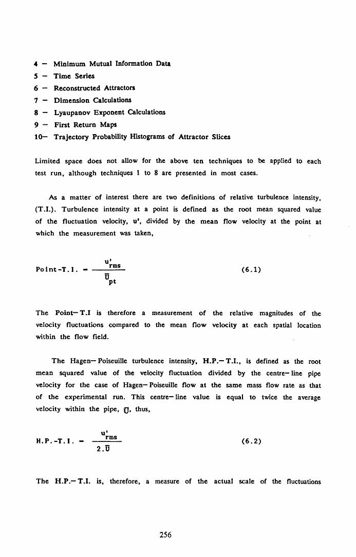
4 — M inim um M utual Information Data

5 — T im e Series

6 — Reconstructed Attractors

7 — Dim ension Calculations

8 — Lyaupanov Exponent Calculations

9 — F irst R eturn Maps

10— T rajec to ry Probability Histograms of A ttractor Slices

Limited space does not allow for the above ten techniques to be applied to each

test run , although techniques 1 to 8 are presented in most cases.

As a m atter of interest there are two definitions of relative turbulence intensity,

(T .I.) . Turbulence intensity at a point is defined as the root mean squared value

of the fluctuation velocity, u \ divided by the m ean flow velocity at the point at

which the measurem ent was taken,

P o i n t - T . I . --------- _ rm-— ( 6 .1 )

V

The Poin t— T .I is therefore a measurement of the relative magnitudes of the

velocity fluctuations compared to the mean flow velocity a t each spatial location

within the flow field.

T he Hagen—Poiseuille turbulence intensity, H .P .—T .I., is defined as the root

mean squared value of the velocity fluctuation divided by the centre— line pipe

velocity for the case of Hagen— Poiseuille flow a t the same mass flow rate as that

of the experim ental run. This centre— line value is equal to twice the average

velocity within the pipe, jj» thus,

H . P . - T . I . - ( 6 .2 )2 .U

The H .P .— T .I. is, therefore, a measure of the actual scale of the fluctuations

256

within the flow relative to the mean flow velocity.

It should also be noted that the data is plotted over a range of cross sections

in the pipe as sketched above. There are four cross sections upstream of the

orifice and thirteen downstream, with the distances between each cross section

shown. In many cases, the distance downstream of the orifice is normalised by the

internal pipe diam eter Dp.

6 .2 TEST SET A:

TH E 13mm ORIFICE PLATE AT VARIOUS REYNOLDS NUMBERS

6.2.1 Frequency Spectra. C e n tre - lin e Velocities

and Turbulence Intensities

The frequency spectra for the 13mm orifice plate for various pipe Reynolds

num ber flows are shown in figures 6—1 to 6—5, for values of Rep of 128, 256,

384, 512 and 640 respectively. In all cases the forcing amplitude was set to 0.6

Volts and the forcing frequency was set to the natural frequency of vortex shedding

for the 13mm orifice plate at each flow Reynolds number. This was done using the

Strouhal number test results outlined in chapter 4 and defined by equation 4.4.

The frequency spectra results for Rep = 128 are given in figure 6—1. In the

figures the frequency spectra are given for all 17 cross sections, (4 upstream

positions and 13 downstream positions), corresponding to section (a) to (d)

upstream and (e) to (q) downstream.

As can be see from figures 6—la , b, c and d, the dom inant frequency,

(ff = 1.27Hz), is evident. At 10mm downstream of the orifice plate, (figure 6-1 e),

the ff peak is still dominant, but now a smaller 2.ff harmonic has appeared. Also

a peak a t 3 .ff is just visible. This situation remains the same for L .D .A . positions

of 20, 30 and 40mm downstream. At 30mm downstream the harmonics reach a

maximum amplitude. The harmonics disappear by the 60mm position, and the

frequency spectra remain qualitatively the same, (i.e. a dominant single peak), from

the 60mm, (figure 6—lj) , position downstream to the last L .D .A . position at

950mm, (figure 6—lq ).

257

The higher harmonics are probably generated within the motor— piston

mechanism and amplified in the relatively faster moving flow emanating from the

orifice aperture. Existence of a higher harmonic, at twice the forcing frequency,

has also been found in results published by Gharib and Williams— Stuber [1989], in

the forced oscillations of an airfoil wake. (See also chapter 2, section 2.6.3.)

The results for the Rep = 256 flow, downstream of the 13mm orifice plate,

are given in figures 6— 2a to m. (This flow is the standard flow regime as defined

in chapter 4, section 4.5, and it also features in test sets B, E , F, and G.) The

flow is an initially interacting flow, as compared to the directly dissipating flow of

figure 6—1, (see section 5.7.4). As the flow proceeds downstream of the orifice

plate the initial dominant frequency, ff = 2.54Hz, gives way to the period

doubling peak of ff/2, which by 50mm downstream becomes dominant within the

flow. This period doubled peak in turn gives way to a peak at roughly f^4 at the

60mm and 75mm downstream position. By 100mm downstream, (figure 6—2h), the

signal is composed of a low frequency broad band spectra and a small ff peak as

the forcing frequency begins to reassert itself within the flow. The low frequency

components die out as the flow proceeds downstream, and by 500mm downstream,

(figure 6—21), the dominant ff peak has reasserted itself within the flow and the

low frequency noise has all but disappeared. Also noticeable from the first three

figures is the 2.ff harmonic, which disappears, (or is swamped), by 40mm

downstream, and does not reappear further downstream when the low frequency

turbulent components die out.

The downstream frequency spectra results for the Rep = 384, and forcing

frequency, ff = 3.82, flow are given in figures 6—3a to m. The situation is

similar to the Rep = 256 flow, however, this time the period doubling, ff/2, peak

appears at 20mm downstream of the orifice, and completely degenerates into a

noisy signal by the 30mm downstream position. Furthermore, the dominant forcing

frequency spike does not disappear into the general noisy spectra until 50mm

downstream. The forcing frequency spike reappears at approximately 100mm

downstream, emerging from the dissipating, low frequency noisy spectra which

corresponds to the weakly turbulent flow. The emergence of ff, and the dissipation

of the low frequency noise is clearly seen if one inspects the frequency spectra

from the 100mm to 950mm L.D.A. position, (corresponding to figures 6 - 3 h

258

to m).

Qualitatively similar results, as those obtained for the Rep = 384 flow, were

obtained for the Rep = 512, ff = 5.09Hz and Rep = 640, ff = 6.37Hz flows.

The frequency spectra from 10 to 100mm downstream for both flows are given in

figures 6— 4a to h, and 6— 5a to h respectively. Both flows breakdown via a period

doubling route, as with the Rep = 256 and Rep = 384. Thus, all the initially

interacting flows breakdown via a period doubling route. The period doubling peak

is generated by vortex merging taking place as the vortices move downstream from

the orifice plate, (as described in chapter 2, section 2.3.6.)

The results of the centre— line velocity measurements are shown in figure

6— 6. From the figure it may be seen that there is a general trend for the

velocities a t, and above, a pipe Reynolds number of 256. Whereas, the slower flow

(Rep = 128) follows a different decay pattern.

The Rep = 128 flow is a directly dissipating flow, (section 5.7.4), and thus

this flow decays in a smooth axisymmetric m anner back to the original upstream

condition. The faster flows, (Rep = 256, 384, 512 and 640), are all initially

interacting flows. These flows breakdown to a weakly turbulent state prior to

dissipating out back to the upstream condition.

From figure 6— 6a, it may be seen that the maximum centre— line velocity

occurs just downstream of the orifice plate. There is then a region, between 25

and 100mm downstream of the orifice plate, within which the velocity decreases

rapidly. A minimum velocity is reached at approximately 100mm downstream of the

orifice plate. After which the downstream velocity profile begins to re-establish

itself and rises back to the upstream condition.

T he difference between the directly dissipating flow and the initially interacting

flows is m ore apparent in figure 6—6b, in which the normalised velocity results are

presented. The centre— line velocities are normalised by dividing them by the

Hagen— Poiseuille centre— line velocity for an equivalent mass flux rate. (In the

same m anner as the Hagen— Poiseuille turbulence intensity, H .P .— T.I.) Thus, the

downstream normalised velocities all tend to the same value, that of unity.

259

From figure 6— 6b it can be seen that the normalised velocities of the initially

interacting flows all appear to follow an identical route as they emanate from the

orifice plate. The initially interacting flows decrease rapidly in centre— line velocity

and dip below the normalised downstream (laminar) centre— line velocity. This is

probably due to a flattening of the velocity profile caused by the turbulent zone

downstream of the orifice plate. As the flow moves through the turbulent zone and

the turbulent fluctuations die out, the velocity profile begins to revert back to the

downstream lam inar flow profile and the resulting centre— line velocity increases.

(This effect will be discussed in more depth in chapter 7.)

The results of the centre— line turbulence intensity measurements are given in

figures 6—7a and b. In figure 6—7a the point turbulence intensity, (Point—T .I .) , is

plotted versus the normalised downstream distance, (i.e. the downstream distance

divided by the pipe Diameter, Dp), and figure 6— 7b plots the H— P T .I. versus

the normalised downstream distance. As with the centre— line velocity results one

may discern a general difference between the directly dissipating flow and the other

initially interacting flows. From figure 6—7a it may be seen that the Rep = 128

flow peaks at a distance of approximately Dp from the orifice plate. The initially

interacting flows peak in turbulence intensity much further downstream, at between

2.5>d)p and 3.0xD p from the orifice plate, this is after the breakdown of the

discrete vortices into the weakly turbulent region.

6.2.2 Minimum M utual Information and Attractor Construction

Figures 6— 8a and b contain the results of the minimum mutual information

calculations for each of the time series. The minimum m utual information is

required to determ ine a suitable time delay in the construction of an attractor from

an experimental tim e series. (Mutual information is defined in detail in chapter 2,

section 2.5.3 and equation 2.46.)

In figure 6—8a, the first minimum in the mutual information function, (in

multiples of the time series time step, = 0.01 secs), is plotted against downstream

distance. The peak in the first minimum occurring for the initially interacting flows

just downstream of the orifice plate. The Rep = 128, (directly dissipating), flow

remains fairly constant along the length of the pipe, its value remaining

260

approximately equal to a quarter of the pulsation time period as one would expect

from a sinusoidal signal, (see section 2 .S.3).

The individual minimum mutual information calculations for the Rep = 256,

(forcing frequency ff — 2.54Hz), flow, for L.D .A. positions from 10 to 50mm, and

950mm downstream are given in figures 6—9a to f. It can be seen from the

figures that the coherent signals, with dominant ff spikes, have fairly well defined

minima and maxima in mutual information as the time delay is varied. However,

the 40mm reading is beginning to appear less well defined and by 50mm

downstream the mutual information function decays fairly rapidly with increasing

time delay. The signal becomes more coherent further downstream, as shown by

the 950mm plot, (figure 6—9f).

In the plots of mutual information in figures 6— 9a to f the first minimum

occurs at roughly 0.1 seconds (each unit of time delay on the horizontal axis is

0.01 seconds). Now the forcing frequency ff is 2.54Hz, the cycle time is therefore

1/ff, or approximately 0.4 seconds. Thus, the first minimum in mutual information

occurs at one quarter of the forcing cycle period. This indicates that the forcing

frequency dominates the flow, (see section 2.5.3). Therefore, flows where the

forcing frequency is dominant have more evident maxima and miminima in the

mutual information function, whereas, flows in which there are a multitude of

frequencies, and the forcing frequency is not dominant, have no discernible mutual

information maxima or minima. (See for example figure 6 — 9e and also its

corresponding frequency spectrum given in figure 6— 2e.)

The normalised minimum mutual information plot is given in figure 6— 8b. In

this case the value of the first minimum is normalised by dividing it by the value

for one quarter of the forcing function time period. The reasoning behind this, is

that for all time series where the forcing frequency is dominant, (i.e. upstream of

the orifice, far downstream and just downstream where the shed vortices are still

coherent), one should obtain a first minimum in the mutual information at one

quarter of the forcing cycle time. Whereas, for more complex forms of the time

series, (i.e. after the vortex breakdown), the first minimum in mutual information

will tend to increase. From figure 6—8b it can be seen that the normalised values

of the first minimum are approximately equal to unity at the positions expected,

namely upstream, just downstream and far downstream. Also the peak values of the

261

first minimum tend to increase for increasing pipe Reynolds numbers.

The time series for the Rep = 256 flow, for all downstream positions, (except

the 500mm position), are depicted in figures 6—10a to 1. The first 1024 data

points are plotted, equivalent to 10.24 seconds as the sampling rate was 100Hz. As

can be seen from the figure, the initially periodic waveform remains stable until

40mm downstream, at which point a period doubling waveform is obvious. The first

4096 data points are plotted for the 40mm position to emphasise the varying

complexity of the flow over the longer time period. This period doubled wave,

ff/2 , switches intermittently with the original forcing frequency waveform, ff. By

50m m the waveform has become quite complex, however, peaks are still visible at

multiples of the forcing period, (i.e. 1 /ff). At the 75mm downstream position, large

coherent structures are visible in the waveform, probably due to third or fourth

generation vortex merging. By the 100mm position the flow appears quite random.

Slowly the forcing frequency pulsation begins to reappear as one proceeds

downstream towards the 950mm L.D .A. station.

The attractors for the Rep = 256 flow, for the first six L.D.A. positions, are

shown in figure 6—11. The attractors are constructed from the first 4096 data

points of the time series. The process by which the initially periodic attractor

breaks down is clearly seen in these figures. At 10mm downstream, (figure 6—11a),

a periodic attractor is clearly visible, with a thickened band due to the presence of

experim ental noise in the signal. At 20mm downstream, (figure 6—lib ) , the

attractor is slightly unstable and by 30mm downstream, (figure 6—11c), the band is

now quite thick. A distinct change in the attractor form occurs by the 40mm

position, (figure 6 - l id ) , whereby the attractor has changed shape dramatically, and

is in fact reminiscent of a period doubled attractor with a high level of added

noise. By 50mm downstream, (figure 6—l ie ) , complete breakdown of the attractor

form seems to have occurred. The attractor at 60mm downstream, (figure 6—Ilf ) ,

is of a similar complexity to the 50mm downstream attractor. The remaining

attractors from 60mm to 950mm downstream all show similar complexity. Such

complexity would suggest that the attractors are exhibiting high dimensional

dynamics* and require high dimensional phase spaces to capture their complexity.

By the 950mm position, an obvious move back toward a pulsatile flow may just be

discerned, this is indicated by an exceptionally noisy periodic attractor, (not shown).

262

6.2 .3 Dimension and Lvapunov Exponent Results

An estimate of the fractal dimension of the attractors constructed above was

obtained using the Grassberger— Procaccia dimension estimate, as described in

chapter 2, section 2.5.4. The slope of the 'log(r)—logCCr)' plot gives an estimate

of the fractal dimension of the object, where r is the radius of the n - dimensional

hyper—sphere probing the attractor constructed in increasing embedding dimensions,

and C r is the correlation integral as defined by equation 2.50, in chapter 2.

The ’log(r)—logCCr)' plots for the Rep = 256 flow are given in figure 6 - 1 2

for all the downstream L.D .A. positions. The slope at large length scales, and thus

the dimension, for the 10 and 20mm positions is approximately equal to unity,

(1.08 and 1.03 respectively). This supports the visual information obtained from the

attractor plots, where the attractors are composed of noisy, periodic bands which

are the dom inant features on large length scales above the noise level. (See for

example the results obtained with pulsatile laminar flow in section 4.2.5.)

At lower length scales the slopes become very steep due to the presence of

noise. At 30mm downstream a more interesting picture is evident. There is a slope

of 1.09 at large length scales and a slope of approximately 3.57 at intermediate

length scales. This would tend to suggest that the attractor is periodic at large

length scales, but m ore complex, or fractal, at lower length scales. This in turn

may imply that this signal is from a low dimensional chaotic flow. At 40mm

downstream the slope has increased to 4.96 and no periodic elem ent is visible. At

50mm downstream the slope has increased to 12.71. The value of dimension

remains fairly high, until a t 200mm the dimension returns to approximately 4.38,

then back to 2.05 by 950mm downstream. These dimension results, together with

the o ther flow results, (Rep = 128f 384, 512 and 640), are presented in

figure 6—13. In the figure the dimension is plotted against the normalised

downstream distance, Z/Dp.

T he dimension results, of figure 6—13, follow a similar pattern for all the

initially interacting flows, which differ markedly from the directly dissipating flow.

The dimension of the initially interacting flows increase rapidly immediately after

issuing from the orifice aperture, and peak at values between 15.00 and 20.00.

263

This may in fact represent a limit in the computer application of the Grassberger—

Procaccia dimension algorithm, and the flows may in fact have dimensions much

higher than these values, (even infinite). All dimensions then decay as the flow

proceeds downstream.

The Lyapunov exponent was calculated to measure the divergence properties of

the attractors. A positive Lyapunov exponent indicates that initially close points on

the attractor diverge rapidly, and indicates the presence of a chaotic flow, (see

chapter 2, section 2.5.6.1).

The results of the Lyapunov exponent calculations are given in figure 6—14.

The Lyapunov exponents were calculated for each time series embedded in

4—dimensional phase space, (see section 2.4.3). The time delay used in the

attractor construction was that used in the dimension estimate, i.e. it was found

using the minimum mutual information criteria. The evolution time for the

separation calculations was taken as one quarter of the forcing cycle time.

The Lyapunov exponent results m irror the dimension results. Just downstream

of the orifice, the Lyapunov exponents increase rapidly, reaching a peak between

40 and 50mm downstream for all initially interacting flows. The Lyapunov

exponents seem to ' c u t - o f f ' at about the 40 to 50mm downstream position, after

which they decay back to lower values as the flow proceeds further downstream.

This cutting off of the initially, rapidly increasing exponents, is most probably due

to the fact that the actual attractor dimension has exceeded the embedding

dimension, (= 4).

6.3 TEST SET B:

THE 13mm ORIFICE PLA TE. VARIOUS FORCING AMPLITUDES

6.3.1 Frequency Spectra. C entre— line Velocities


The downstream frequency spectra for the Rep = 256 flow and 13mm orifice

plate forced at 0.6 Volts has already been presented above in figure 6 - 2 . (W hen

looking at various Reynolds numbers, all forced at 0.6 Volts forcing amplitude.)

264

T he downstream frequency spectra for the Rep = 256 flow and 13mm orifice plate

forced at 0.2 and 1.0 volts are given in figures 6 - 1 5 and 6 -1 6 . The forcing

amplitudes of 0.2, 0.6 and 1.0 volts respectively, correspond to an R.M.S. variation

in the mass flow rate of 2.65% , 7.95% and 13.26% . All three of these flows,

considered in this section, are initially interacting flows.

T he downstream frequency spectra for the 0.2 Volts forcing amplitude are given

in figures 6—15a to m. As the flow passes through the orifice plate the dominant

frequency at ff = 2.54Hz is visible. A harmonic begins to grow at 2.ff. This

harm onic reaches a maximum at approximately 30mm downstream, after which

point it begins to decrease. A subharmonic at ff/2, begins to appear in the

spectrum at the 40mm position. At 50mm downstream this subharmonic peak is

quite distinct. The ff/2 subharmonic grows and by 60mm downstream has started to

decay into broad band spectra. The spectra remains fairly broad band from 75mm

downstream to 250mm downstream, by which point the forcing frequency peak has

re— emerged in the flow spectra. By the 950mm downstream position the low

frequency broad band noise has decayed and the ff spike dominates the frequency

spectrum .

T he frequency spectra for the 0.6 Volts forcing amplitude have already been

discussed above for the Rep = 256 flow in section 6.2.1. Briefly the flow follows

a similar pattern to the above 0.2 flow, as shown in figure 6—2. However, in this

case the period doubling peak becomes dominant within the flow at the 50mm

downstream position, whereas in the 0.2 Volts case the period doubling peak

becomes dominant 75mm downstream of the orifice.

T he frequency spectra for the 1.0 Volts forcing are given in figure 6—16. As

the flow passes through the orifice plate the dominant frequency at ff = 2.54Hz is

again visible. The 2.ff harmonic is again evident as the flow issues from the orifice

plate. The subharmonic at ff/2, begins to appear in the spectrum at the 20mm

position. At 30mm downstream this subharmonic peak is quite distinct. By 40mm

downstream the ff/2 subharmonic has started to decay into broad band spectra,

although it may be still discerned within the flow at the 50mm position. The

frequency spectrum becomes broad band by 75mm downstream, and the

re—em ergence of the ff peak is just visible. The re—emergence of the pulsation

peak and the decay of the low frequency noise may be followed as one proceeds

265

from the 100mm downstream position to the 950mm position,

(figures 6—16h to 6—16m).

The results of the centre— line velocity measurements are given in

figures 6—17a and b, for all three forcing amplitudes at R ep = 256 and the

13mm orifice plate. All three flows are initially interacting flows and the two larger

amplitude flows (A = 0 .6 and 1.0 Volts) reach a velocity minimum at approximately

3xDp downstream. The flow with the lowest amplitude forcing, (A = 0 .2 Volts),

appears to flatten out and reaches the downstream centre— line velocity

asymptotically, without first reaching a minimum at, or near to, the breakdown

point.

The results of the turbulence intensity measurements are given in figures 6—18a

and b, again for all three forcing amplitudes. All three flows reach similar

maximum values o f both Point—T.I. and H .P .— T .I. However, the 0.2 forcing flow

peaks farther downstream than the other two flows and the turbulent fluctuations

decay more slowly.

6.3.2 Minimum M utual Information and Attractor Construction

The first minimum in mutual information plot is given in figure 6—19a, and

the normalised plot in figure 6—19b, (for comparison with o ther normalised plots).

The value of the first minimum increases rapidly as one proceeds downstream.

Interestingly the low forcing amplitude, (0.2 Volts), peaks much further downstream

than the two larger forcing amplitudes, (at approximately twice the distance.)

From the normalised graph of figure 6—19b, it is clear that the forcing frequency

dominates immediately downstream of the orifice plate, (where the normalised first

minimum is unity), and again far downstream where the forcing frequency

re— establishes itself within the flow.

The attractors for the 0.2 forcing, are shown in figure 6— 20. These are

constructed using the time series obtained from the first six downstream LD .A .

positions, (i.e. 10mm to 60mm downstream). The figures show quite clearly the

breakdown of the attractor as the flow evolves downstream of the orifice plate,

increasing in complexity as it does so. The attractor remains distinctly periodic,

266

with added noise, until at 50mm downstream, the attractor band begins to spread.

The attractor departs from its singly periodic structure by 60mm downstream.

The attractors obtained for the intermediate, 0.6 Volts, forcing amplitude, have

already been discussed in section 6.2.2, and are plotted in figure 6—11.

The attractors for the 1.0 Volts forcing amplitude are plotted in figure 6—21.

Only the first five attractors are plotted, (from 10 to 50mm downstream). The

breakdown of the initially noisy— periodic attractor is quite fast. The initially

periodic attractor occurring at 10mm, thickens markedly by 20mm. Breakdown

occurs at 30mm downstream, one may see from the associated time series, (not

shown), that a period doubling has occurred, however, noise obscures the picture

somewhat in the attractor plot. The attractor at 40mm is now quite complex, the

time series showing intermittent large and small structures within it. The 50mm

attractor also appears reasonably complex, however, the time series, (not plotted),

is interesting in that a second period doubling may be discerned. That is, structures

with a period of four times that of the flow pulsations are visible.

6.3 .3 Dimension and Lvaounov Exponent Results

The dimension results for the three forcing amplitudes are given in

figure 6— 22. The dimension of all three flows increase rapidly, immediately after

issuing from the orifice aperture, and peak at values between 13.00 and 20.00. The

dimensions then reduce in value as the flow proceeds downstream.

It is noticeable from figure 6—22, that the dimension plot for the 0.2 Volt

amplitude does not decrease markedly from its peak value as it proceeds

downstream. No obvious reason for this is apparant, however, one possible

explanation is that the noise present in the signal was sufficient to obscure the

downstream pulsations in the flow and give an erroneous high value of dimension.

However, just downstream of the orifice plate where the flow velocity is higher,

the absolute magnitude of the velocity fluctuations is higher and able to dominate

over the noise. In this case, the dimension algorithm is able detect the attractor

structure within the noise.

267


Once again the Lyapunov exponent results mirror the dimension results. Just

downstream of the orifice, the Lyapunov exponents increase rapidly. The figure

would tend to suggest that the larger the forcing amplitude the more rapid the

increase in the Lyapunov exponent with downstream distance. The lowest amplitude,

(0 .2 Volts), peaks farthest downstream, at the 75mm position. Once again the

Lyapunov exponents c u t-o f f at a specific distance downstream, after which they

decay back to lower values as the flow proceeds further downstream.

6.4 TEST SET C:

TH E 9.75mm ORIFICE PLATE. VARIOUS REYNOLDS NUMBERS

6.4.1 Frequency Spectra. Centre— line Velocities


Frequency spectra for the 9.75mm orifice plate, for three Reynolds number

flows, (Rep = 128, 256 and 384) and a forcing amplitude of 0.6 Volts are shown

in figures 6— 24 to 6 - 26.

The frequency spectra results for Rep = 128 are given in figure 6—24. As the

flow emanates from the orifice, the dominant ff = 3.07Hz peak, together with its

harmonic at 2.ff, is visible at 10mm downstream, (figure 6—24a). At the 20mm

position, (figure 6—24b), the period doubling subharmonic is evident, which

increases in magnitude by the 30mm position. By 40mm downstream, the forcing

frequency peak has diminished and the period doubled peak dominates the

spectrum, together with some very low frequency components. The breakdown of

the ff/2 peak occurs by the 75mm position, and the flow is composed of very low

frequency components. (See figure 6— 24g, where the spectrum from 0 to 50Hz is

shown). At the 150mm position the forcing frequency begins to dominate the

spectrum once more. The low frequency components completely disappear from the

spectrum by the 950mm position.

The frequency spectra results for Rep = 256 are given in figure 6—25.

Once again the forcing frequency, ff = 6.14, is dominant at the 10mm position, a

small ’hum p' at ff/2 is also visible. At 20mm downstream, the ff/2 peak has

268

increased in magnitude. The ff/2 grows larger at the 30mm position. At the 40mm

position, the ff/2 subharmonic is visible within what is otherwise a noise spectrum.

T he spectrum becomes quite indistinguishable by 50mm downstream. The forcing

frequency peak begins to re—emerge from the broad band spectra by 100mm

downstream. The forcing peak then increases as the low frequency broad band

com ponents dissipate out of the flow, as the L.D .A. position is moved downstream.

T he frequency spectra results for the Rep = 384 flow are given in

figure 6— 26. The dominant frequency, ff = 9.21Hz, breaks down via a period

doubling route, as with the slower flows. The ff/2 subharmonic is just visible in

the 10mm downstream plot. This subharmonic grows, and by 30mm is quite distinct

within the spectrum, together with lower frequency, (< ff/2), broad band

components. The overall picture is much the same as for the Rep = 256 flow,

with the forcing frequency peak reappearing in the spectrum at 75mm downstream.

The centre— line velocity results are plotted in figures 6— 27a and b. From the

figures, it can be seen that both the Rep = 256 and 384 flows follow a similar

route, reaching a velocity minimum at approximately three pipe diameters

downstream of the orifice plate. However, the Rep = 128 flow velocity decreases

much less rapidly on leaving the orifice plate and reaches the downstream

centre— line velocity value asymptotically. All three flows are initially interacting

flows, however, the Rep = 128 flow is an 'unstable slow jet flow' as defined in

section 5 .5 .4 , whereas the faster flows are 'interacting vortex flows'.

T he Point—T .I.'s , given in figure 6—28a, show a marked difference between

the R ep = 128 flow and the two faster flows. The slow flow shows a decrease in

the Point—T .I. after issuing from the orifice plate to a minimum at approximately

2.5 to 3 .0xD p downstream. The Rep flow then increases to a maximum at about

8 .0xD p downstream. The higher Reynolds number flows reach maxima at

approxim ately 4xDp downstream after an initially rapid increase.

T he H .P .—T .I. measurements reach maxima at positions earlier than the

Point—T .I . 's for all three flows. The Rep = 256 and 384 flows peak at between

2.0 and 2.5xDp downstream. Whereas, the Rep = 128 flow first reaches a

minimum at 2.5 to 3.0xDp downstream.

269

6.4.2 Minimum Mutual Information and Attractor Construction

The first minimum in mutual information plots are given in figures 6— 29a

and b. From the figures, it may be seen that the Rep = 128 and 256 flows peak

at the same position, 4xD p downstream, whereas, the Rep = 384 flow peaks

earlier.

The attractors for the Rep = 128 flow at the 10, 20, 30, 40, 60 and 100mm

position are plotted, in figure 6— 30, to illustrate the downstream development in

the attractor shape. The band of the initially circular, noisy— periodic shape at

10mm, thickens dramatically by 30mm and has completely changed by 60mm

downstream. The 100mm attractor is also shown, this attractor is constructed from

a waveform which contains interm ittent large troughs, which probably correspond to

large coherent structures passing the L.D.A. probe position.

The attractors, for the First four L.D.A. positions for the Rep = 256,

ff = 6.14Hz flow, are given in figure 6—31. The breakdown of the initially

periodic attractor is clearly visible from the plots. The attractors at the 20 and

30mm positions seem to be essentially periodic, however, the loops of the attractor

wander up and down the 45* line. This is perhaps due to another low frequency

component superimposed on the flow. At the 40mm position, the attractor form is

no longer simple.

The change in attractor complexity as the L.D.A. position is moved downstream

for the Rep = 384 flow is shown in figure 6—32 for the first four L.D.A.

positions. The initially noisy—periodic attractor at 10mm downstream quickly

becomes unstable. By 20mm, the attractor band has become quite thick, and some

of the trajectories have wandered from the main attractor loop. At 30mm, the

attractor seems to have lost any clearly defined shape and the trajectories are now

wandering quite markedly. By 40mm the attractor has lost any discernible form and

has become quite complex.

270

6.4 .3 Dimension and Lvaounov Exponent Results

The dimension results for the three pipe Reynolds numbers are given in

figure 6— 33. All three flows are initially interacting flows and correspondingly all

dimensions increase rapidly with downstream distance immediately after the orifice

plate. The dimensions reach peaks of between 15.00 and 22.00. The dimension

then reduces in value as the flow proceeds downstream.

The results of the Lyapunov exponent calculations are given in figure 6— 34.

The Lyapunov exponent values for the all three flows increase rapidly as they

proceed downstream from the orifice plate. The magnitude of the exponent maxima

increases with increasing Rep.

6.5 TEST SET D:

TH E 16.25mm ORIFICE PLATE. VARIOUS REYNOLDS NUMBERS

6.5.1 Freouencv Soectra. Centre— line Velocities


The downstream frequency spectra for the three pipe Reynolds number flows,

using the 16.25mm orifice plate, are depicted in figures 6—35 to 6—37.

The frequency spectra results, for the first four downstream positions, for

Rep = 128, ff = 0.64Hz are given in figure 6—35. As the flow emanates from

the orifice a harmonic at 2 .ff is visible, (at 10 and 20mm downstream). At the

30mm position a third harmonic is visible within the flow at 3.ff. By 40mm

downstream only the forcing frequency is visible within the spectrum, this remains

the case for all subsequent downstream positions.

The frequency spectra results for Rep = 256, ff = 1.28Hz are given in

figure 6—36. Once again the forcing frequency, ff, is dominant at the 10mm

position, small peaks at 2.ff and ff/2 are also just visible. At 20mm downstream,

the 2.ff peak has increased in magnitude and the ff/2 peak has disappeared. The

ff/2 peak re -em erg es by 30mm downstream. At the 40mm position the 2.ff peak

has disappeared and the ff/2 subharmonic is starting to grow. The subharmonic

271

reaches a maximum by 75mm downstream of the orifice plate and has completely

disappeared by 150mm downstream. The spectrum shape remains essentially the

same at subsequent downstream positions.

The frequency spectra results for Rep = 384, ff = 1.92Hz are given in

figure 6 - 3 7 . The forcing frequency, ff, dominates at the positions immediately

downstream of the orifice plate. By 30mm downstream, a subharmonic peak at f j / 2

emerges, and also a smaller ff peak becomes visible. The subharmonic peak then

increases in amplitude and begins to widen by the 100mm downstream position. At

the 150mm position the ff peak is still visible, however, the spectrum is now

composed of broad band components. The broad band part of the spectrum then

begins to decay as the laser position is moved further downstream and the weakly

turbulent flow begins to dissipate out.

The centre— line velocity results are given in figure 6— 38a. Again the

difference between directly dissipating and initially interacting flow patterns is

visible. The two directly dissipating flows (Rep = 128 and 256) showing a smooth

decay in the centre— line velocity, whereas the initially interracting flow

(Rep = 384) has a much more dramatic velocity decrease immediately after issuing

from the orifice plate, dropping to below the downstream level before gradually

increasing back to it. These results are replotted in a nondimensional form in

figure 6—38b.

The turbulence intensities are plotted in figures 6—39a and b. All three flows

show quite erratic movement in the value of the turbulence intensity immediately

downstream of the orifice plate, the reason for this is unclear. The turbulence

intensity, (both H —G and T .I.), for the fastest flow (Rep = 384) increases to a

maximum at approximately 100mm, or 8xD0 , from the orifice plate. After which

point it decays back to the upstream level.

6 .5 .2 M inimum Mutual Information and A ttractor Construction

The first minimum in mutual information plot is given in figure 6— 40a, and

the normalised plot in figure 6—40b. From the normalised plot, it is obvious that

only the initially interacting flow, (Rep = 384), departs from the near unity value

272

one expects from a periodic flow.

The attractors for the Rep = 128 flow at the 60, 75 and 100mm position are

plotted, in figure 6—41, to illustrate an interesting development in the attractor

shape. The initially circular, noisy— periodic shape at 60mm, becomes flattened by

75mm and returns to its original noisy, circular shape by 100mm. The reason for

this flattening of the attractor is, as yet, unclear. It may, however, be the

hallmark of the onset of a more complex flow, which did not proceed, as the

100mm position shows a noisy periodic attractor once again.

The change in attractor complexity as the L.D.A. position is moved downstream

for the Rep = 384 flow is shown in figure 6— 42 for the downstream positions of

20mm, 60mm and 75mm. The initially noisy— periodic attractor, at 20mm

downstream, slowly becomes unstable and by 60mm the attractor band has become

quite thick and the attractor has become more oval in shape. At 75mm the

attractor has lost its clearly defined shape and is now of a complex construction.

6.5.3 Dim ension and Lvaounov Exponent Results


figure 6— 43. Only the dimension of the Rep = 384 flow increases after issuing

from the orifice aperture, and peaks at a value of 16.58. This maximum value

occurs at a distance of 150mm, or approximately 12 orifice diameters, downstream

of the orifice plate. The dimension then reduces in value as the flow proceeds

downstream.


The Lyapunov exponent values for the Rep = 128 flow remain low for all flows

downstream of the orifice plate. The Lyapunov exponents for the Rep = 256 flow,

increases quite slowly, peaking quite far downstream, at 200mm from the orifice

plate. The Lyapunov exponents increase rapidly for the Rep = 384 flow, peaking

at 150mm downstream, (as with the dimension).

273

6.6 TEST SET E;

A COMPARISON O F TH E VARIOUS ORIFICE DIAMETERS

AT A PIPE REYNOLDS NUMBER O F 256

6.6.1 A Comparison of the 9.75mm. 13.00mm

and 16.26mm Orifice Plates;

Frequency Spectra. C e n tre - lin e Velocities.

Turbulence Intensities. Minimum Mutual Information.

Dimension and Lyapunov Results

The frequency spectra for the 9.75, 13.00 and 16.25mm orifice plates have

been given above in figures 6—2, 6—25 and 6—36 respectively.

The c en tre -lin e velocity results are given together in figure 6—45. As can be

seen from the figure, the initial velocity of the flow leaving the orifice increases

with decreasing orifice aperture diameter. A result one would expect from the

continuity condition. The 9,75mm and 13.00mm flows are both initially interacting

flows and have velocity profiles characteristic of such flows. On the other hand,

the 16.25mm orifice flow, (a directly dissipating flow), has a smooth transition

from its velocity at the orifice plate to those downstream.

The turbulence intensities are plotted in figures 6— 46a and b. Figure 6— 46a

contains the Point—T .I. results. The two initially interacting flows show marked

increases in Point—T.I. downstream of the orifice, the maximum value of

Point—T.I. increases with decreasing orifice diameter.

In figure 6— 46b, the H .P .— T .I. is plotted against downstream distance. The peak

in turbulence intensity increases with increasing pipe Reynolds number. This

turbulence measure is a direct measure of the actual r.m .s velocity fluctuations.

Thus, the velocity fluctuations are increasing as the orifice aperture diameter

decreases.

The minimum mutual information results are depicted in figures 6—47a and b.

From the plot of 6 - 47b, it may be seen that the normalised first minimum

increases with Pipe Reynolds number. The Rep = 128 flow remains at unity for

all L.D.A. positions, probably due to the dominance of the pulsation frequency

274

throughout the flow.


figure 6 - 48. All three dimensions increase as they proceed from the orifice

position. The maximum dimension increases with decreasing orifice diameter.

The results of the Lyapunov exponent calculations are given in figure 6— 49. As

with the dimension results, all three exponents increase upon proceeding

downstream of the orifice plate, and, the maximum value of the exponents

increases with decreasing orifice diameter.

6.6 .2 A Comparison o f all the Orifice Diameters

used in the Studv:

Frequency Spectra. C en tre - line Velocities*


Tests were also conducted for three additional orifice plates of diamters, D 0 , of

6.50mm, 19.50mm and 22.75mm. (Corresponding to l/4 D p , 3/4Dp and 7/8Dp.) The

tests were conducted solely for a Reynolds number of 256. The data obtained from

the L.D .A. measurements were used to produce frequency spectra, centre— line

velocities and turbulence intensities, with which to compare to the other three

orifice diameters used in the study, (section 6.2.1). The frequency spectra for the

9.75, 13.00 and 16.25mm orifice plates have been given above in figures 6—2,

6— 25 and 6— 36.

The frequency spectra for the 6.50mm orifice plate is given in figure 6—50

and plots the development of the spectra downstream of the orifice plate, for the

first four L.D .A . positions. At 10mm downstream, the dominant ff = 21.05Hz

peak is clearly visible. A period doubling peak is seen to enter the flow at the

20mm position, and has grown by the 30mm position. At 30mm low frequency,

broad band components have also arisen within the spectrum. By 40mm

downstream, these low frequency components have swamped the signal. The plots

for subsequent downstream position show quite clearly the shift in the broad band

components to lower frequencies. This is the general picture of the downstream

frequency spectra, and the forcing peak only re—emerges by the 950mm position.

275

The frequency spectra for the 19.50mm orifice flow, (ff = 0.73), are given for

the first four L.D.A. positions in figure 6—51. The dominant peak at 10mm

downstream continues to dominate the spectrum for all downstream positions, the

only deviation from the single peak in the spectrum occurs at the 30mm

downstream position where a peak at the 2 .ff harmonic appears. This peak then

disappears by the 40mm L.D.A. position, and the spectrum remains essentially the

same for all subsequent positions.

No plots are given for the 22.75mm orifice, (ff = 0.45Hz), as the spectra at

all downstream positions are composed of a single ff peak.

The centre— line velocities for all six orifice plates are given in figure 6— 52

The difference between the three directly dissipating flows, (lower Reynolds

numbers) and the three initially interacting flows may be seen. All flows eventually

reach the same downstream centre— line velocity value by the 950mm L.D.A.

position.

The turbulence intensities may be seen in figure 6—53a and b. The directly

dissipating and initially interacting flows again showing different behaviour. The

initially interacting flows all increase in Point—T.I. immediately after issuing from

the orifice, reaching maxima at between 100 and 150mm downstream. The directly

dissiapating flows, on the other hand, remain fairly constant over the range of

L.D.A. positions. The H .P .— T .I. results are plotted in figure 6—53b. It may be

seen from the figure that the H .P .— turbulence intensities peak before the

Point—T.I. results.

6.7 TEST SET F:

ACROSS FLOW RESULTS FOR THE 13MM ORIFICE PLATE

AT A PIPE REYNOLDS NUMBER O F 256

An attem pt was made to measure the radial variation in the time series

properties. Longitudinal velocity— time data was measured at radial positions from

the centre— line to 5.33mm inclusive, in increments of 0.66mm. This was done for

the first five downstream L.D.A. positions, namely the 10mm, 20mm, 30mm,

276

40mm and 50mm position. The results of these measurement are given below.

6.7.1 C e n tre - lin e Velocities and Turbulence Intensities

The velocities at each of the five downstream positions are plotted in figure

6— 54a, and the normalised velocities in figure 6— 54b. From the figure, it may be

seen that the velocity decreases in the downstream direction, as outlined above, and

also in the radial direction. The retarding of the edge of the jet may be seen by

inspecting each velocity plot in turn. The velocity plot for the 10mm downstream

section indicates that the velocity profile of the issuing je t is fairly flat until at

4.00mm from the centre— line the velocity drops off dramatically. This drop— off

point occurs at 4.00mm for the 20mm downstream position also. By 30mm the

drop—off point has progressed into the flow and occurs at the 2.66mm position.

AT the 40mm position the d ro p -o f f point is less well defined and seems to occur

a t 2.00mm from the je t centre line. By 50mm downstream the retarding of the jet

has reached the centre— line.

The Point— T .I. results are given in figure 6— 55a. From the figure, it may be

seen that the turbulent fluctuations increase dramatically towards the jet edge, as

one would expect, due to the high shearing taking place between the je t flow

passing through the orifice aperture and the slower moving flow in the recirculation

region. The H .P .—T .I. results are given in figure 6—55b, the turbulence intensities

in this case increase dramatically at the je t edge for the flows immediately

downstream of the orifice plate, however, at greater distances downstream, the

H .P .—T .I. values are more even across the flow. This would indicate that the jet

has now fully broken down and that the turbulent fluctuations are fairly evenly

spread across the flow by this stage.

6 .7 .2 Minimum Mutual Information

The first minimum in mutual information plot for each of the downstream

positions is given in figure 6—56a, and the normalised plot in figure 6—56b. Both

plots are identical as the same flow conditions are being investigated, however,

both plots are given for comparison with other results. The plots show an increase

277

in the value of the first minimum downstream as the flow complexity increases.

Across the flow the first minimum in mutual information increases for the

nea r-o rif ice flows, (10, 20 and 30mm), as the jet edge is approached. The values

of these flows, at the edge, reach those of the broken down flow at 50mm.

6 .7 .3 Dimension and Lvaounov Exponent Results

The dimension results for the across flow results are given in figure 6— 57. The

general trend for the dimension of the flows is to increase with downstream

distance, only the 20mm position plot seems to increase with radial position. This

would tend to suggest that the complexity of the flow is mainly a function of

downstream distance.

The results of the Lyapunov exponent calculations are given in figure 6— 58.

The Lyapunov exponents increase with downstream position. However, unlike the

dimension results, the exponent values do increase with radial position for the near

orifice positions, (10, 20 and 30mm). This may in fact be an inherent property of

the Lyapunov exponent itself, (or the computer algorithm), as the presence of

noise at the jet edge may greatly effect the result.

6.8 TEST SET G:

A CHECK ON TH E REPEATABILITY O F THE EXPERIMENT

The repeatability of the experiment was checked by retaking the measurements

for the standard set of results, i.e. Rep = 256, D 0 = 13mm, (see section 4.5).

The results for the c e n tre - lin e velocities, turbulence intensities, (point T .I.), first

minimum in mutual information and Lyapunov exponents are given in figures 6— 59

to 6— 62 respectively. As can be seen from the figures, the results are fairly

consistent for both the original results, (TEST 1), and the remeasured results,

(TEST 2).

278

6.9 OTH ER ANALYSES

Other means of analysis were attempted. These are outlined as follows for the

Rep = 256, D0 = 13.00mm flow. (Standard test, see section 4.5).

6.9.1 The Autocorrelation Function

The autocorrelation function is plotted for the downstream positions from 10mm

to 100mm inclusive in figure 6—63. The autocorrelation function for the 10mm and

20mm position is typical of that for a periodic waveform. The autocorrelation of

the time series taken at the 30mm positions shows a slight amplitude difference

between each alternate peak, as a second period begins to enter the flow. At

40mm the effect of the period doubling is clearly seen in the autocorrelation plot,

also a decrease in the average autocorrelation value. As the flow temporally

decorrelates. By 50mm downstream the flow is decorrelating rapidly and the period

doubled fluctuations are very much in evidence. The 60mm plot of the

autocorrelation function shows the flow to be quite complex, rapid decorrelation is

evident, however, small ripples in the plot at the forcing period may be discerned.

The 75mm plot is similar in form to the 60mm plot, and by 100mm downstream,

the forcing frequency ripples are coming back into the picture.

6.9.2 Probability Distribution of Selected Attractor Slices

It was decided to investigate the development of the attractor bands as the

attractor lost stability from a noisy— periodic form. To do this the attractor was cut

across its band, and the trajectories crossing the cut, or slice, were counted and a

histogram was produced of the number of trajectory passes at each position.

The histograms obtained for the first four attractors of the Rep = 256,

D0 = 13.00mm flow are given in figure 6—64. Their respective attractors are

given in figure 6—11a to d. Each attractor histogram is plotted with an equivalent

Gaussian distribution superimposed over it for comparison. The trajectory histogram

at the 10mm downstream position would suggest that the trajectories are bundled in

a Gaussian structure, due to the presence of random noise in the signal. By 20mm

279

downstream the histogram appears to be skewed slightly, with the peak displaced

outward from the attractor centre. The 30mm histogram has now departed

completely from the Gaussian distribution and a secondary peak is clearly evident

appearing closer to the centre of the attractor. (A third peak is also just visible.)

The 40mm attractor has now broken down into a dense complex structure and the

corresponding trajectory histogram appears to be Gaussian once again, after this

point the use of the trajectory histogram is limited as a means of probing the

attractor structure.

6 .9 .3 Return Map Results

The use of return maps to ellucidate the dynamics of the vortex shedding

phenomena was also investigated. However, the results were rather vague due to

the presence of noise in the signal. To try and increase the effectiveness of the

return map as a tool for determining period doubling, each alternate point on the

mapping was denoted by a circle and a cross respectively. The results of the

mapping for the first four downstream positions are given in figure 6—65.

At the 10mm downstream position, the distribution of crosses and circles is

fairly even. This situation is again true for the 20mm position. In both figures, a

slight tendency for the crosses to land above the 45° line and the circles to land

below the 45° line may be observed on close examination. However, by 30mm

downstream, their is a marked tendency for every second point to land either side

of the 45° line. This would indicate that the flow is noisy and consists of a period

doubled waveform. (A period doubled flow in the absence of noise would consist of

two points, one either side of the 45° line, which the mapping would visit

alternately.) The return map for the 40mm data shows a more random distribution

of points once again as the attractor has broken down into a more complex form.

6.10 SUMMARY

This chapter has presented the physical data resulting from the Laser Doppler

Anemometry measurements. The information was presented in various forms to aid

in the comprehension of the physical flow phenomena at the orifice plate for low

280

Reynolds number pulsed flows.

The tests were divided into six discrete, but inter—related tests, (test A to F),

in which the effect of the Reynolds number, pulsation frequency (a function of the

Reynolds number), pulsation amplitude were monitored at various positions

downstream and across the flow. With a check on the repeatability of the

experiment also undertaken, (test set G).

Analysis of the data as presented in this chapter has been undertaken and is

presented in chapter 7.

281

CHAPTER 6 FIGURES

4>U*-*wS '

m

4)uU)P

mco

6cd4)U*->V)aP

oO'

4)U*->waP

om

282

Elg

ure

6-1^

Fr

eque

ncy

Spec

tra

- 1

3.0

0mm

Ori

fice

-

Rep

- 12

8

u

oCM

&

o

a«<DU*->wC5a

0)

a03a)u4->V)C?s

oon

U)

283

Figu

re

6-1:

F

req

uen

cy

Spec

tra

- 13

.00m

m

Ori

fice

- R

ep -

128

F-i

gy.r

e_.6

-l.;

-Fre

quen

cy

Spec

tra

- 13

.00m

m

Ori

fice

-

Rep

- 12

8

<3

ooCM

&

Srtd)u4-»<nc*a

om

a

285

f-lKM

rg

6-1;

Fr

eque

ncy

Spec

tra

- 13

.00m

m

Ori

fice

-

Rep

- 12

8

ooCMf—<Iu

s«4>U*-»V)C5<3

OinON

286

Figu

re

6-1:

F

req

uen

cy

Spec

tra

- 12

_J3Q

mm

Ori

fice

-

Re.

seg4)

«-»V)c

a

OCN

so<*

b - h -

ea4)V-.*-»V)c

s

■Ik • t € i l ( - h a i

scd4)u«-»VIc

a

oCO

287

Elfl

yrg

6-2;

Fr

eque

ncy

Spec

tra

- 13

,00m

m

Ori

fice

-

Rep

- 25

6

e(44)1**->05

2

OVO

05c£s

om

Soo

op

mr-'

b0

288

Figu

re

6-2;

Fr

eque

ncy

Spec

tra

- 13

.QQm

m Or

If

leg

- R

eP -.

2S.&

<s

ooCM

4>u,4-*U)C5

6

OOin

om

oQ

oinCM

289

Figu

re

6-2;

Fr

eque

ncy

Spec

tra

- 13

,00m

m

Ori

fice

-

Rep

- 25

6

290

Figu

re

6-2

: Fr

eque

ncy

Spec

tra

- 1

3.0

0mm

Ori

fice

-

Rep

- 25

6

acQ4)U*->wC5a

oCM

a(44)U*-></>C5a

o

OOCO

o

art4>U*->wC?oQ

oCO

291

Figu

re

6-3;

Fr

eque

ncy

Spec

tra

- D

.QQn

yn

Qrlfl

c?

~ Rg

ovO

oO

I«yZ-H3AM to

292

El&

ure

$-2j

, Fr

eque

ncy

Spec

tra

- 13

.00m

m

Ori

fice

-

Rep

- 38

4

f e . f e . f r . . S C U X - H a A M

£caou*->WlC£oQ

Om

Ecaa>»-4-*Wc£

a

omCM

293

Fig

ure

6-3;

Fr

eque

ncy

Spec

tra

- 13

.00m

m

Ori

fice

-

Re

294

FU\ir

^.-6

rl.;.f

.rgau

gncy

Sp

ectra

t

ll.QQn

ro J2

rlflc

e.—

&

oC M

&

acd4>u*->C/1c

&

oco

Fjg

ure

_6-4

; Fr

eque

ncy

Spec

tra

- 13

.00m

m

Ori

fice

-

Rep

- 25

6

&

oo

a

oin

296

</)c?oQ

m

00

El&

ur.S

Freq

uenc

y Sp

ectr

a -

13.0

0mm

O

rifi

ce

- R

ep -

256

K V Z - H M M

oCM

a44)U*jw

Io

I « U Z » - 3 M

oQ

aca®u*jtnc?2

297

Figu

re

6-5:

F

req

uen

cy Sp

ectr

a -

13.0

0mm

O

rifi

ce

- R

ep -

256

rilU

IMY

I

PICT

tu

n

298

EU

ure

$-5

; Fr

eque

ncy

Sp

ectr

a -

13.0

0mm

O

rifi

ce

- Re

, -

9Sfi

V« I o o 111 • • (mm/*)2 0 0

160

100

6 0

4 0 0200 8 0 0 1000600Dlstanoe Downstream of Orifloe (mm)

• °- Re « 128 * ♦ - Re • 266 Re • 384 Re - 612 -----Re - 640

F i g u r e 6 - 6 a; C e n t r e l i n e V e l o c i t i e s - 13.00frun O r i f i c e

V a r i o u s Reyno ld s Numbers

Normalised V e loc i t ie s3 .6

2.6

1.6

0.6

100 20 3 0 40Normalised Downstream Distance

...q .. Re . t28 * ♦ * Re - 266 Re - 384 Re • 612 Re - 640

F i g u r e 6 - 6 b: N o r m a l i s e d C e n t r e l i n e V e l o c i t i e s - 13.00mm O r i f i c e


299

Turbutanoe Intanaltlaa (%)6 0

60

40

3 0

20

10

0 10 20 30 4 0Normallaad Downatream Dlatanoa

• Re - 128 -----Re - 612 -----

Re - 266 Re - 640

6 - 7 a : P o i n t - T u r b u l e n c e I n t e n s i t i e s - 1 3 .00mm Ori f i c e

V a r io u s R eyno lds Numbers

TUrbutanoa tntanaltlea (%)8 0

7 0

6 0

6 0

4 0

3 0

20

.-a

4 03020Normallaad Downatraam Dlatanoa

••«••• Re - 128 Re - 268 Re • 384

Re - 612 Re - 640

F i g u r e 6 -7 b : H .G . - T u r b u l e n c e I n t e n s i t i e s - 13.00mm O r i f i c e

V a r io u s Reyno lds Numbers

300

First Minimum In Mutual Info.6 0

6 0

4 0

3 0

20

10 a

0 200 4 0 0 6 0 0 8 0 0 1000Dlstanoo Downstream of Orlfloo

° Re • 128 ° Re - 612

Re - 266 Re - 640

Re - 384 ]F i g u r e 6 - 8 a: Minimum Mutual I n f o r m a t i o n - 13.00mm O r i f i c e

V a r io u s R e y n o ld s Numbers

First Minimum In Mutual Info.10

8

6

4

2I s -----

03 0 4010 200

Normalised Dlstanoo Downstream

D Re • 128 Re • 612

Re - 266 Re - 640

Re - 384

F i g u r e 6 - 8 b: N o rm a l i se d Minimum Mutual I n f o . - 13.00mm O r i f i c e

V a r io u s R e y n o ld s Numbers

301

ruTU

M.

info

p*ia

tion

(i:

’v

'u^.

en

vc*

!i

8

F i g u r e 6

3

05CAO15 JO100

( a ) 10mm Downstream units or ti* ofur

A ■-

o 4—50AS15 350

( b ) 20mm Downstream unit. nr*: uflat

2 -

50SO15IU0( c ) 30mm Downstream mmurrin

5J I n d i v i d u a l Minimum Mutual I n f o r m a t i o n P l o t s

13.00mm O r i f i c e - Rep - 256

302

«0 wiivuaojNi ivrunu

(l) wouwbOj<i

Tvnxrw

%

I

i» •; h i i s ju / • 3o .v. v i *«o

(d) 40mm D ow ns tream iwir u nm iilm

s - -

a--

s0 IS so10 5520 SOas

( e ) 50mm Dow ns t ream usits c* ?:« rsmr

i

osois 5510s 20 SO0

( f ) 950mm D ow ns t ream urns tr fine dtlai

F i g u r e 6 - 9 ; I n d i v i d u a l Minimum Mutual I n f o r m a t i o n P l o t s

13.00mm O r i f i c e - Rep - 256

303

( a ) 10mm Downstream

(b) 20mm Downstream

( c ) 30mra Downstream

(d ) 40mm Downstream

F i g u r e 6 - 1 0 : Time S e r i e s P l o t s - 13.00mm O r i f i c e - Rep - 256

304

( e ) 5 0 m m D o w n s t r e a m

( f ) 60mm Downstream

( g ) 75mm Downstream

( h ) 100mm Downstream

( i ) 150mm Downstream

( j ) 200mm Downstream

F i g u r e 6 - 1 0 : Time S e r i e s P l o t s - 13.00mm O r i f i c e - Rep - 256

305

y v / y v v / \ v \ A / so A / v \ </ \ ' V \ ^ ^

(k ) 250mm Downstream

v ) y v V v y W v lV V \ A M M ^ M V u V W V *

(1 ) 950mm Downstream

F i g u r e 6 - 10 : Time S e r i e s P l o t s - 13.00mm O r i f i c e - Rep - 256

306


(b ) 20mm Downstream

( c ) 30mm Downstream

F i g u r e 6 -1 1 : A t t r a c t o r P l o t s - 13mm O r i f i c e - Rep - 256

307

I

( d ) 40mm Downstream

( e ) 50mm Downstream


F i g u r e 6 - 1 1 : A t t r a c t o r P l o t s - 13mm O r i f i c e - Rep - 256

308

( a ) 10mm Downs t ream

-c’S

mi; ?fR'

I.Ill If l,M

(b) 20mm Downstream

F i g u r e 6 -1 2 : 1 l o g ( r ) - logCCr.V P l o t s

13mm O r i f i c e - Re~ — 256-------------------- p-----------

309

/

-25LOG (CR»


-10

•10

-15

-20

-25

LOG (fR)

(d ) AOmra Downstream

F i g u r e 6 - 12 : ' l o g f r ) - 1 o g ( C r V P l o t s


310

Cv

7 1

-10

-15

-20

( e ) 50mm Downstream -2 5 1

LOG (CR)

I nf '«•>'I

10

( f ) 60mm Downstream L l if « v\

F i g u r e 6 - 1 2 : 1 l o g f r ) - 1og( Cr V P l o t s

13mm O r i f i c e - Rep — 256

311

I IH

J

(g ) 75mra D ow ns tr eam

l.fKi 'R)

-10

i in in?'(h ) 100mm Downstream

F i g u r e 6 - 1 2 ; ' l o g ( r ) - 1 o g ( C r V P l o t s

13mm O r i T i c e - Rep - 256

312

i or, (R>

to

150mm Downstream

LOG (R>

-10

-15

-20

( j ) 200mm Downstream LOG <CR)

F i g u r e 6 - 1 2 : ' l o g ( r ) - 1of l ( Cr V P l o t s

13mm O r l F l c e - Rep — 256

313

IOC (R)

( k ) 250mra-10 i

LOG (CR)

LOG (R)

-10

-IS

-20

( 1 ) 500mm DownstreamLOG (fR'

F i g u r e 6 - 1 2 ; ' l o g ( r ) - 1og ( Cr 3 t P l o t s


314

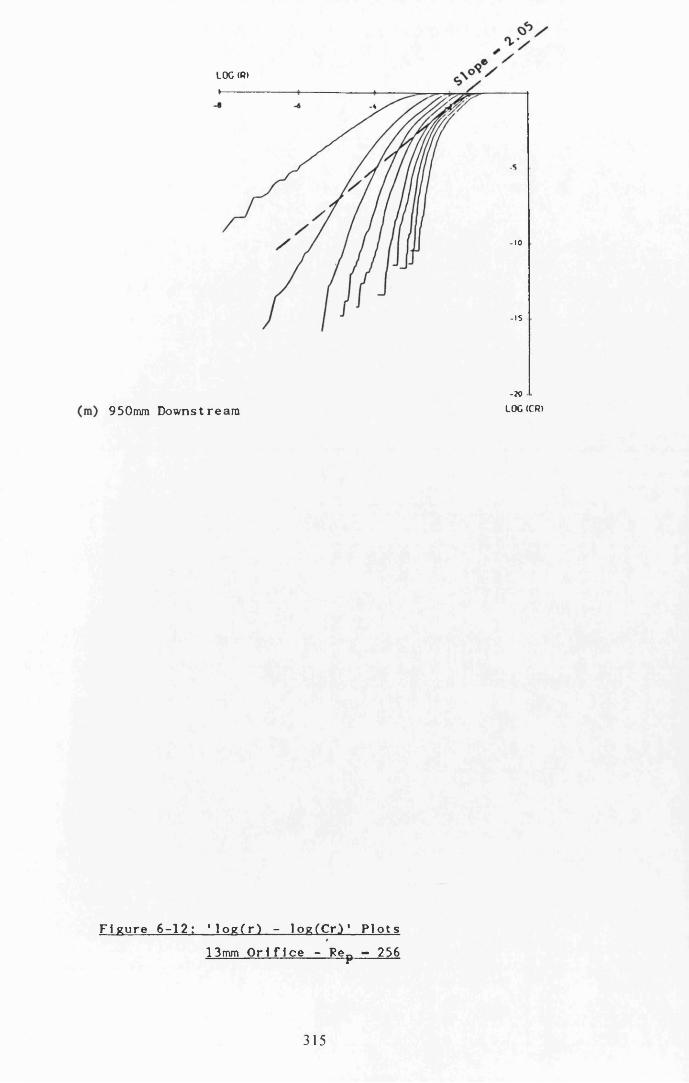
IOC <Q)

-10

- I S

-20

LOG <CR>950mm Downstream

F i g u r e 6 - 1 2 : *l o g ( r ) - l o g ^ C r y P l o t s


315

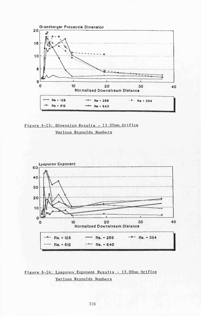
Grassberger Procaccla Dimension2 0

10

0 10 20 30 40Normalised Downstream Distance

Re • 128 — Re - 266 • * Re - 384Re • 612 -**- Re - 640

F i g u r e 6 -13 : D im ens ion R e s u l t s - 13.00mm O r i f i c e

V a r i o u s Reyno lds Numbers

Lyapunov Exponent6 0

4 0

3 0

20

10

4 03 020100Normalised Dow nstream Distance

Re. ■ 128 ------ Re. - 2 6 6 — Re. - 3 84

------ Re. - 612 — Re. • 6 4 0

F i g u r e 6 -14 : Lyapunov Exponent R e s u l t s - 13.00mm O r i f i c e


316

aoCM

«nC3OP oa

ocn

317

Figu

re

6-15

: Fr

eque

ncy

Spec

tra

- 13

.00m

m

Ori

fice

-

Re

0.2

Vol

ts

For

cing

aoV £ >

<3

OO

£csJ<3JU*->ViC*am

t>0

318

Figu

re

$-15

; Fr

eque

ncy

Spec

tra

- 13

.00m

m

Ori

fice

-

Rep

- 25

6

0.2

Vol

ts

For

cing

&

oom

voinCM

OQ

Om

319

Figu

re

6-15

: Fr

eque

ncy

Spec

tra

- 13

.00m

m

Ori

fice

-

Re

0,2

Vei

ts..

.Far

cin

g

320

Figu

re

6-15

; Fr

eque

ncy

Spec

tra

- 13

.00m

m

Ori

fice

-_

R£

0.2

Vol

ts

For

cing

oQ

OCM

aa4>V,4->(Ac*8O

WcoQ

321

Figu

re 6-

1$;

Frequ

engy

-.Spe

sUfl.,

-,13.Q

Qrnm

Or

1 f 1 gg

-

Rgp-

25.6

1.

0 V

olts

F

orci

ng

<3OVO

£44)U4-»U)C3OQ

oo

E<d4>u♦-»wc

3

om

Ertatu«-*wC53

mr-~

to

322

Figu

re

6-16

; Fr

eque

ncy

Spec

tra

- 13

.00m

m

Ori

fice

-

.25.

S

1.0

Vol

ts

For

cin

g

<3ooCM

; £

&

oom

vomCM

ad<UU*JV)Cz

&

Oin

&

omCM

323

Figu

re

6-16

: Fr

eque

ncy

Spec

tra

- 13

.00m

m

Ori

fice

-

Re

1.0

Vol

ts

For

cin

g

324

Fig

ure

6-16

; Fr

eque

ncy

Spec

tra

- 13

.00m

m

Ori

fice

-_

Re

1.0

Vol

ts

For

cing

Vel oo I tl • • (mm/a)8 0

6 0

4 0

o ...20

0 200 4 0 0 6 0 0 8 0 0 1000Dlstanoe Downatream of Orlfloa (mm)

° T.L (Amp. - 0.2) — TJ. (Amp. • 0.6) TJ. (Amp. - 1.0)

F i g u r e 6 - 1 7 a : C e n t r e l i n e V e l o c i t i e s - 13.00mm O r i f i c e


Normallaed Valooltlaa3.6

2.6

1.6

0.6

0 10 16 20 26 3 06Normallsad Dovmatroam Diatanoa

D T.I. (Amp. • 0.2) — T.I. (Amp. - 0.6) T.I. (Amp. - 1.0)

F i g u r e 6 - 17b : No r ma l i s e d C e n t r e l i n e V e l o c i t i e s -13.00mm O r i f i c e


325

6 0

4 0

3 0

20

10

00 10 2 0 3 0 40

Normallaed Downatraam Dlatanoa

F i g u r e 6 - 1 8 a : P o i n t - T u r b u l e n c e I n t e n s i t i e s - 1 3 , 00mm O r i f j c e


Turbulanoa Intanaltlaa ( V

f'.Q

Turbulanoa Intanaltlaa (%)6 0

6 0

4 0

3 0

20

10

00 10 20 3 0 40

Normalised Downatraam Dlatanoa

TJ. (Amp. • 0J2) — T.l (Amp. - 0.6) T.L (Amp. - 1.0) I

F i g u r e 6 - 18b : H. G. - T u r b u l e n c e I n t e n s i t i e s - 13.00mm O r i f i c e


326

Plrat Minimum80

60

40

o20Vi___

0 200 400 600 800 1000Dlatanoa Downatraam ol Orlfloa (mm)

-•o-- Amp -0 .2 Amp - 0.6 Amp • 1.0

F i g u r e 6 - 1 9 a : Minimum Mutual I n f o r m a t i o n - 13.Q0mm O r i f i c e

V a r i o u s F o r c i n g A m p l i tu d es

Flrat Minimum o l Mutual Information8

6

4

2

010 200 30 40

Normallaed Downatraam Dlatanoa

G • Amp - 0 .2 " * - Amp - 0.6 Amp - 1.0

F i g u r e 6 - 1 9 b : N o r m a l i s e d Minimum Mutual I n f o . - 13.00mm O r i f i c e

V a r i o u s F o r c i n g Ampl i t ude s

327


(b) 20mm Downstream


F i g u r e 6 -20 : A t t r a c t o r P l o t s - 13mm O r i f i c e


328

(d) 40mm Downstream



F i g u r e 6 - 2 0 : A t t r a c t o r P l o t s - 13mm O r i f i c e


329


(b) 20mm Downstream


F i g u r e 6 -21 : A t t r a c t o r P l o t s - 13mm O r i f i c e


330

(d) 40mm Downstream

(e ) 50mm Downstream

F i g u r e 6 - 2 1 : A t t r a c t o r P l o t s - 1 3 m m O r i f i c e


331

Q rasaberger Procaccla Dimension2 0

10

0 10 20Normalised D ow nstream D istance

3 0 40

A - 0.2 — A • 0 .6 o A - 1.0

F i g u r e 6 - 2 2 : Dimens ion R e s u l t s - 13.00mm O r i f i c e

V a r i o u s F o r c in g A m p l i t u d e s


20

16

10

..i i

100 3 020 40Normalised D ow nstream D istance

” Amp. - 0.2 Amp. - 0 .6 Amp. • 1.0

F i g u r e 6 - 2 3 : Lyapunov Exponent R e s u l t s - 13.00mm O r i f i c e


332

• •I

Sa4>U4-»OSC?

5

oCM

o>*

o

I H—I■••

333

Elg

vre

6-24

; Fr

eque

ncy

Spec

tra

- 9.

75m

m

Ori

fice

-

Rey

12&

T«

£ato*-•V)C5OP

oin

oQ

OinCM

335

Fig

ure

6-24

: Fr

eque

ncy

Spec

tra

- 9.

75mm

Q

rlfl

ce,-

R

er -

12&

336

Figu

re

6-24

: F

req

uen

cy Sp

ectr

a -

9.75

mm

O

rlfk

t -

R?p

~ 12

6

337

Figu

re

6-25

: F

req

uen

cy Sp

ectr

a -

9.75

mm

O

rifi

ce

- R

er -

25$

5 aoVO

S

aoo

oQ

Oin

#*

sca<uu*-»U)C5oQ

m

to

338

Elf

tyr?

$

-2?

; Fr

eque

ncy

Sp

ectr

a -

9.75

mm

O

rifi

ce

- R

ep -

256

e«34>U4 -1

CflC5oQ

Om

Ecd0)u4-»V)C?oQ

OinCM

339

Figu

re

6-25

; Fr

eque

ncy

Spec

tra

- 9

.75m

m O

rifi

ce

- R

ep -

256

-I— l---f 8 88 8

£(fl4)U«-*wc?oQ

Om<7\

340

Figu

re

6-25

■

Fre

qu

ency

Spec

tra

- 9.

75m

m

Ori

fice

-

R?P

- .2

56

&

oCM

I-—«---1--

&

o<*

K fc. * . - l € V I - h a * M

00CO

<DPC

uO

ecd0)u*-»COC?oa

sa<vu*■>(0c

<s

oCO

uo

o\icdL.4-1Oa>oco>oca>3O4>U

VOCMIVO

4>u3U

341

mic

iiE

NC

v t

pic

th

uh

p

PMK

«aiM

C«

*p

ict

«»

«

342

ElR

ure

6-26

; Fr

eque

ncy

Spec

tra

- 9.

75mr

o O

rifi

ce

- R

e

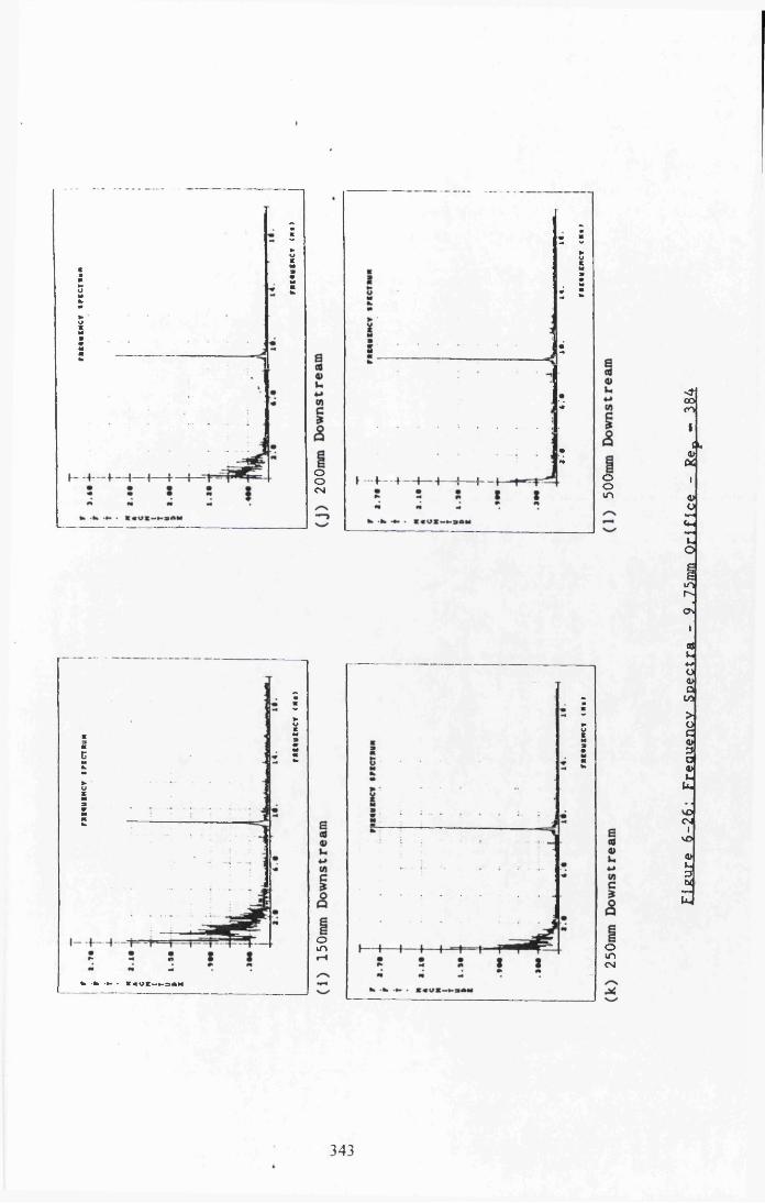
rxi'u

fNcv

tr

icT

Run

OOCM

OOmf —+-

om omCM

343

Elft

ure

$-26

; Fr

eque

ncy

Spec

tra

- 9.

75m

m

Ori

fice

-

Rep

- 38

4

200

150

100

50

00 2 00 4 0 0 6 0 0 8 0 0 1000

Dlatanoa Downatream of Orlfioa (mm)

° Re - 128 Re • 258 Re • 3 8 4



V a l o o U l o a ( m m / a )

' - a

Normallaod Veloolitloa5

4

3

2

1

04 010 20 3 00

Normallaod Downatroam Dlatanoo

° Re • 128 Re • 2 5 6 Re • 3 8 4

F i g u r e 6 - 27b : No r ma l i s e d C e n t r e l i n e V e l o c i t i e s - 9.75mm O r i f i c e

V a r i o u s Reynol ds Numbers

345

T u r b u l e n o e I n t e n « l 1 1 « • (%)7 0

60

6 0

40

3 0

20

a10

302010 4 00Normalised Downstream Dlstanoe

° Re - 128 - - - Re - 266 Re - 3 8 4

F i g u r e 6 - ? 8 a : P o l n t - T u r b u l e n c e I n t e n s i t i e s - 9 , 75mm, Or 1f i c e


Turbulenoe In ten s i t ie s (%)120

100

80

60

40

20

4 010 20 3 00Normalised Downstream Dlstanoe

a Re - 128 Re - 2 66 Re - 3 8 4

F i g u r e 6-28b: H . C . - T u r b u l e n c e I n t e n s i t i e s - 9 , 75mm Or 1 f l e e


346

F i r s t M i n i m u m In M u t u a l I n f o r m a t i o n8 0

7 0

6 0

6 0

4 0

3 0

20

10

6 0 0200 4 0 0 8 0 0 10000Dlstanoa Downstream of Orlfloe (mm)

G Re - 128 ----- Re - 266 ------ Re - 3 8 4

F i g u r e 6 - 2 9 a ; Minimum Mutual I n f o r m a t i o n - 9.75mm O r i f i c e

V a r io u s Reyno lds Numbers

First Minimum In Mutual Info.20

16

10

4 03020100Normalised Dlstanoa Downstream

a • Re - 128 Re - 266 Re - 3 8 4

F i g u r e 6 - 2 9 b : Nor ma l i s e d Minimum Mutual I n f o . - 9.75mm O r i f i c e

Va r i o u s Re yno l ds Numbers

347

( a ) 10mm D o w n s t r e a m

(b) 20mm Downs tream

•I. 3

(c ) 30mm Downstream

F l e u r e 6 -30 : A t t r a c t o r P l o t s - 9.75mm O r i f i c e - Rep - 128

348

(d ) 40mm Downstream



F i g u r e 6 - 3 0 : A t t r a c t o r P l o t s - 9.75mm O r i f i c e - Rep - 128

349

( a ) 10mm D o w n s t r e a m

(b ) 20mm Downstream



350

(d) 40mm Downstream

F i g u r e 6 - 3 1 : A t t r a c t o r P l o t s - 9.75mm O r i f i c e - Rep

351

- ■ 2 5 i


(b) 20mm Downstream



352

(d) 40mm Downst ream

F i g u r e 6 - 32 : A t t r a c t o r P l o t s - 9.75mm O r i f i c e - Rep - 384

353

G ra88berger Procaccla Dimension2 5

20

10

20 3 0100 4 0Norm alised Downstream Distance

Re - 128 Re - 2 5 6 ♦ Re - 3 8 4

F i g u r e 6 - 3 3 : Dimens ion R e s u l t s - 9.75mm O r i f i c e

V a r i o u s R e y n o ld s Numbers


6 0

4 0

3 0

20

10

200 10 30 40Norm alised Downstream Distance

Re. - 128 Re. - 2 6 6 Re. - 3 8 4

F i g u r e 6 - 34 : Lyapunov Exponent R e s u l t s - 9.75mm O r i f i c e

V a r i o u s Re yno l d s Numbers

354

;.... -•••... :.... .... ...........:.....T... ;....v...

I ........ '.... '.... ;..... . '»:................ .....

i

s .... ..... i... ;m • ^

I ; T 7 ....:.......... :... :....a5 ...... r .............................. :....

: • * «

.....................: ... ..... i... : : 1__ ' . . . . ■ :... z z y

I--- 1--- 1---4 1 1 1 I i i 4

: : : i \

ecQ<Uu*->VIc*aoCM

V)c

£

&

O

oQ

OCO

355

Elfm

re

$-.3

5;

Freq

uenc

y S

pect

ra

- 16

.25m

m

Ori

fice

-

Rep

- 12

8

Ea0)V,

001✓“N£>

e(00>u4->V)c*a

o

J *

E(Q<Du

wC2oQ OQ

OCO

356

Fig

ure

6-36

: F

requ

ency

Sp

ectr

a -

16.2

5mm

O

rifi

ce

- R

ep -

256

«

aAAu*->VICJoQ

OvO

eAAU*->VIC*

&

oo

aAAU*-»wC?OQ

Om

EAAV-*-»wC*oQ

m

00

357

Fig

ure

6-36

: F

req

uenc

y Sp

ectr

a -

16_,

25mm

Q

rlfi

cg

~ Rg

p "

256

ooCM

VOinCM

£cdo>u*->wc

a

om

ed0)u«-»W)c££

oinCM

358

Figu

re

6-36

; Fr

eque

ncy

Spec

tra

- 16

.25m

m

Ori

fice

• 3: ! <

♦ ** ■ *

Lg.... . . : . . . . . . ... .. . . . . . . . . . i " 5* • : #• *

; I . iitM ' .rn : 4':.. x_ ;.. ;. . . ;.. .... ... ,... , 4m

I.. i .. ;.. i . . i.. :. . . :.. : : .. . J •4. . . . . . . . ,. . . . . . . . . . . . . . . . . . . . . . \

<i5

* s * s sM M H

Etao>u■*->U)CSsa

om<y\

359

Figu

re

6-16

; Fr

eque

ncy

Sp_e

cirf

l^_,

16

.25m

m O

rifi

ce

- Re

~ -

256

Ecd<DU*->V)CE*oQ

OCM

&

O

Ecd«u4->Wc5OQ

Ecdd>u «-> v) c

a

oro

360

Figu

re

6-37

; Fr

eque

ncy

Sp

ectr

a -

16

.25mm

O

rifi

ce

- R

ep -

384

cM

&

ov£> m

e(44)U

OQ

om

361

Figu

re

6-37

: Fr

eque

ncy

Spec

tra

- 16

.25m

m

Ori

fice

.-

-Re.

rmiD

KT

tP

SC

TM

N

ooCM

&

OOin

ecd4)U*Jwc

2

om omCM

362

Figu

re

6-37

; Fr

eque

ncy

Spec

tra

- 16

.25m

m

Ori

fice

-

ReR

- -2

&A

scd<DU*-></)C5oQ

omo \

363

EUvre

$-3

7; Fr

eque

ncy.

Spec

tra

- l$.2

5rom

Qrlf.l

g?

- Re

p -

334

Vsloolt loa (mm/a)7 0

6 0

6 0

4 0

3 0

20• G O

10

2000 4 0 0 8 0 06 0 0 1000Dlstanoa Downatraam of Orlfloo (mm)

° Re - 128 Re - 266 ------ Re - 3 8 4



Norm alised V eloc it ies

1.6

0.6

3 0 4010 200Normalised Downstream Dlstanoa

° Re - 128 Re - 256 -------------Re - 3 84 |

F i g u r e 6 - 3 8 b : N o r ma l i s e d C e n t r e l i n e V e l o c i t i e s -16.25mm O r i f i c e


364

Turbulence Intensit ies (%)2 0

D

0 10 20 3 0 4 0N orm alised Downstream Dlstanoa

° Re - 128 * - - Re - 266 Ro - 3 8 4 JF i g u r e 6 - 3 9 a : P o 1n t - T u r b u l e n c e I n t e n s i t i e s - 1 6 . 25mm O r l f i c e

V a r i o u s R e y n o l d s Numbers

Turbutenoe Intensit ies (%)3 0

2 6

2 0

16 QJ

10

4 03 020100Norm alised Downstream Dlstanoe

Q Re - 128 Re • 266 Re - 3 8 4

F i g u r e 6 - 39b : H. G. - T u r b u l e n c e I n t e n s 11 1es - 1 6 . 25mm Or 1 f l e e

V a r i o u s R e y n o l ds Numbers

365

First Minimum In Mutual Info.6 0

6 0

3 0

20

2000 4 0 0 6 0 0 800 1000Dlatanoa Downstream of Orlfloa (mm)

F i g u r e 6 - 40a : Minimum Mutual I n f o r m a t i o n - 1 6 , 25mm O r i f i c e

Va r i o u s Re yno l d s Numbers

Flrat Minimum In Mutual Information

3 .6

2.6

1.6

□ dT- ^3 - e - a

0.6

0 10 20 30 40Normalised Downstream Diatanoe

a Re - 128 Re - 2 6 6 Re - 3 84

F i g u r e 6-A0b; Nor mal i sed Minimum Mutua l I n f o . - 16.25mm O r i f i c e

Va r i ous Re yno l d s Numbers

366


(b) 75mm Downstream



367

( a ) 20mra Downs t r eam

(b) 60mm Downs t r eam

( c ) 75mm Downs t r eam

F i g u r e 6-42 : A t t r a c t o r P l o t s - 16.25mm O r i f i c e - Rep - 384

368

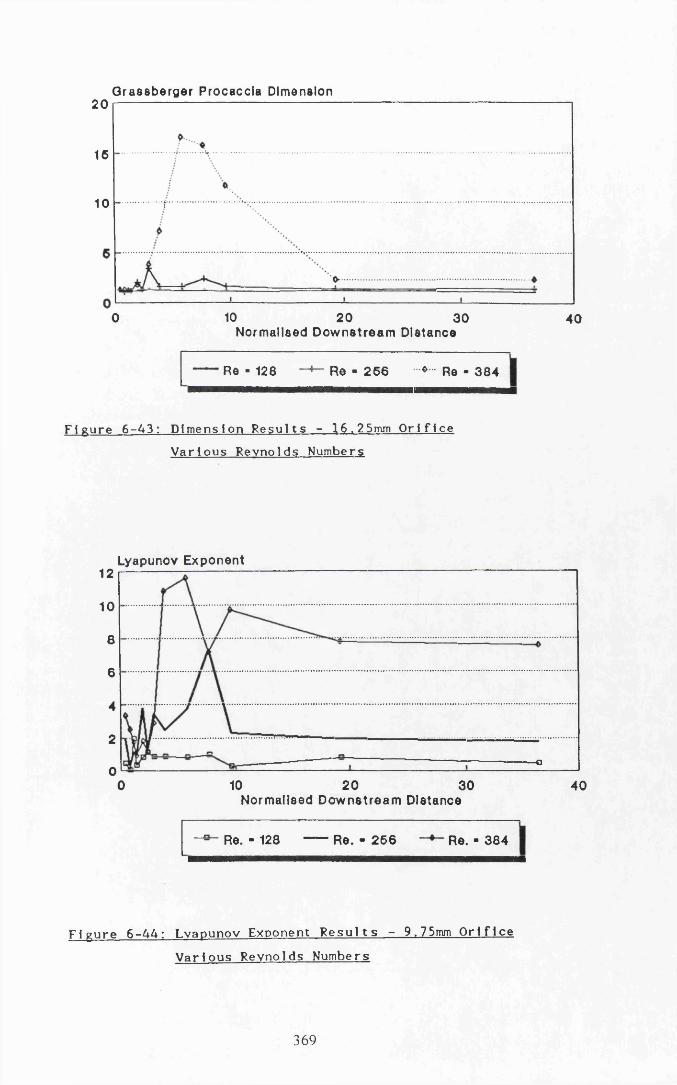
G r a s s b e r g e r P r o c a c c l a Dimen s ion2 0

16

10

10 200 30 4 0Normalised D ow nstream Distance

Re - 128 “ Re - 2 6 6 * " Re - 3 8 4

F i g u r e 6 - 4 3 : Di mens i on R e s u l t s - 16.25mm O r i f i c e


Lyapunov Exponent12

10

8

6

4

2—o

020100 30 4 0

Norm alised D ow nstream Distance

Re. - 128 Re. • 2 6 6 Re. - 384

F i g u r e 6 - 4 4 : Lvapunov Exponent R e s u l t s - 9.75mm O r i f i c e


369

V aloelt lea (mm/a)140

120

100

80

60

40

20

200 4000 600 800 1000Dlatanoe Downatream of Orlfloa (mm)

—4“ 0.76mm ' * • 13.00mm - ° - 16.26mm

F i g u r e 6 - 4 5 ; C e n t r e l i n e V e l o c i t i e s - Rep - 256

9 . 7 5 . 13 . 00 & 16.25mm O r i f i c e P l a t e s

370

70

6 0

60

4 0

3 0

20

10

00 10 2 0 3 0 4 0

Normalised Downstream Dlatanoe

— 9. 76mm “ * • 13.00mm “ ° - 16.26mm

F i g u r e 6 - 4 6 a : P o l n t - T u r b u l e n c e I n t e n s i t i e s - Rep — 256

9 . 7 5 . 1 3 . 0 0 & 1 6 . 25mm O r i f i c e P l a t e s

Turbulenoe In tensit ies (%)

jB a - a -

Turbulenoe In ten s i t ie s (%)120

100

80

60

40

20

10 20Normalised Downstream Dlatanoe

3 00 4 0

9.76mm 13.00mm ~ H ' 16.26mm

F i g u r e 6 - 46b : H . C . - T u r b u l e n c e I n t e n s i t i e s - Rep - 256

9 . 7 5 . 1 3 . 0 0 & 16.25mm O r i f i c e P l a t e s

371

First Minimum In Mutual Information8 0

70

6 0

6 0

4 0

3 0

20

10

2000 4 0 0 6 0 0 8 00 1000Dlatanoa Downstream of Orlfloa (mm)

9.76mm 13.00mm 16.26mm

F i g u r e 6 - 47a : Minimum Mutual I n f o r m a t i o n - Rep - 256


First Minimum In Mutual Information20

16

10

20 30 40100Norm alised D ownstream Dlstanoa

9.76mm 13.00m m ~ B " 16.26mm

F i g u r e 6-47b : Nor ma l i se d Minimum Mutua l I n f o r m a t i o n - Rep - 256

9 . 7 5 . 13 . 0 0 & 16.25mm O r i f i c e P l a t e s

372

G r a s s b e r g e r P r o c a c c l a Dimens ion2 5

20

10

0 10 20 3 0 40Normalised Downstream Distance

0.76mm 13.00mm 16.26mm

F i g u r e 6 - 4 8 : Di me ns i on R e s u l t s - Rep - 256


Lyapunov E xponent6 0

4 0

3 0

2 0

10

10 200 3 0 40Normalised Downstream D istance

“ +“" 0.76mm •••*••• 13.00mm 16.26mm

F i g u r e 6 - 4 9 : Lyapunov Exponent , R e s u l t s - Rep - 256

9 . 7 5 . 13 . 00 & 16.25mm O r i f i c e P l a t e s

373

374

Figu

re

6-50

; Fr

eque

ncy

Spec

tra

- 6.

50m

m

Ori

fice

-

Re

!! 5

oCM

J -

i— i— i— i— i— i— i— i— i— hJ s < s s

vOmcs

a

m mm

aCO1)u■*->(flC5

a

ocn

375

Figu

re

6-51

: Fr

eque

ncy

Spec

tra

- 1

9.5

0mm

Out

flee

-

Eg

Velooltle* (mm/*)350

300

260

200

150

100

60

2000 400 800600 1000Dlstano* Downstream of Orlfloe (mm)

- a -6.60mm 9.76mm 16.26mm —♦*- 19.6mm

• *" 13.00mm 22.76mm

>-52; C e n t r e l i n e V e l o c i t i e s - Rep - 256

A l 1 Ori f i c e P l a t e s

376

Turbulenoe In tensit ies (%>7 0

60

60

40

30

20

10o-

0 10 20 30 40Normalised Downstream Dlstanoa

6.60mm ° * 16.26mm

9.76mm19.6mm

* • 13.00mm 22.76mm

F i g u r e 6 - 5 3 a : P o i n t - T u r b u l e n c e I n t e n s i t i e s - Rep - 256

Al l Or 1f 1ce P l a t e s

Turbulence In ten s i t ie s (%)260

200

160

100

60

30 4020Normalised Downstream Dlatanoe

—*“ 6.60mm 9.76mm 13.00mm- a - l6J26mm 19.6mm 22.76mm

6 - 53b : H . C . - T u r b u l e n c e 1 nt e n s 11 1es z_E®j. - 256

Al l O r l f l e e P l a t e s

377

Veloolty (mm/e)8 0

60

40

20

10 2 3 4D istance From Pip* Centreline (mm)

10mm — 20mm 30m m - ® - 40mm 60mm

F i g u r e 6- 54a : A c r o s s - F l o w V e l o c i t i e s - Rep - 256

13mm O r i f i c e P l a t e

Normalised Velocity

2.6

1.6

0.6

0.60.40.2 0.30.10Norm alised Dlstanoe From Pipe Centreline

10mm 20mm * • 30m m 40mm — 60mm

F i g u r e 6-54b: N o r m a l i s e d A c r o s s - F l o w V e l o c i t i e s - Rep — 256

13mm Ori f i c e P l a t e

378

Turbulenoe Intensity (%) 80 |---------------------------

* -*

60

40

20

JL00.1 0.2 0.3 0.4

Normalised Distance From Pipe Centrellns

10 mm 40mm

0.6

60mm

F i g u r e 6 - 5 5 a : Ac r o s s - F l o w P o 1n t - T u r b u l e n c e I n t e n s i t i e s

13 . 0 0 O r i f i c e P l a t e - Rep - 256

Turbulenoe Intensity (%)100

80

60

40

20

0 0.1 0.2 0.3 0.4 0.6Normalised Distsnoe From Pipe C entrellns

“ 10mm 20mm -* • 30mm ~~a~" •40mm 60mm■ ■ ■ ■ ■ ■ ■ ■ B S B m S H S S S B S n B M a S S S M H a S H H H M H H H H n B m H

F i g u r e 6 - 5 5 b : Ac r o s s - F l o w H. C . - Tu r bu l ence I n t e n s i t i e s

13 . 00 O r i f i c e P l a t e - Rep - 256

379

First Minimum40 i---------------

30

20

10

10 1

-------- 1---- _!--------- - 1 12 3 4 6

D ls t s n o s From Pips Csntrs l lns (mm)

•6 7

----- 10mm 20mm • * 30mm —®- 40mm 60mm |

F i g u r e 6 - 5 6 a : A c r o s s - F l o w Minimum Mutual I n f o r m a t i o n

1 3 . 0 0 O r i f i c e P l a t e - Rep - 256

First Minimum

n -

0.3 0.4 0.60.20.10Normalised Dlstsnos From P ips C sntrs l lns

10mm 20mm •••■*- 30mm 40mm 60mm

F i g u r e 6 - 56b : A c r o s s - F l o w Nor ma l i s e d Minimum Mutual I n f o r m a t i o n

1 3 . 00 O r i f i c e P l a t e - Rep - 256

380

Dimension2 0

16

10

K

0.10 0. 30.2 0.4 0.6Normalised D istance From Plpa Cantrsllna

10mm — 2 0mm 30m m 40mm 60mm

F i g u r e 6-57: Ac r os s - F l ow Di me ns i on R e s u l t s

13.00mm O r i f i c e P l a t e - Rep - 256


20

16

0 0.1 0.2 0.3 0.4 0.6Normalised Diatanoa From Plpa Cantrsllna

10mm - 20mm * 30m m 40mm — 60mm

F i g u r e 6-58: Ac r os s - F l ow Lyapunov Exponen t R e s u l t s

13 .00 O r i f i c e P l a t e - Rep - 256

381

8 0

6 0

4 0

2 0

00 200 4 0 0 6 0 0 8 0 0 1000

Dlatanoe Downatream of Orlfloo (mm)

1at Teat 2nd Teat

F i g u r e 6 - 5 9 : Re pe a t e d C e n t r e l i n e V e l o c i t y R e s u l t s

13mm O r i f i c e P l a t e - Rep - 256

Veloolt lea (mm/a)

Turbulence Intenaltlea (%)6 0

6 0

4 0

2 0

10

0 10 20 3 0 40Normallaed Downatream Dlatanoe

~ 1st Teat • D • 2nd Teat

F i g u r e 6 - 6 0 : Re pe a t e d P o l n t - T u r b u l e n c e I n t e n s i t i e s

13 . 00 O r i f i c e P l a t e - Rep - 256

382

Plret Minimum6 0

60

40

30

20

10

200 4000 600 800 1000Dtatanoe Downatraam of Orlfloa (mm)

1st Set • 2nd S e t

F i g u r e 6 - 6 1 : R e p e a t e d Minimum Mutual I n f o r m a t i o n



16

10

0 10 20 30 40Normallaed Downatraam Dlatanoa

1st Test •"D • 2nd Test

F i g u r e 6 - 6 2 ; R e p e a t e d Lyapunov Exponent R e s u l t s


383

( a) 10mm Downstream ( b ) 20mm Downstream

• •

i •

% »

ft i

( c) 30mm Downstream

m

( d ) 40mm Downstream

(e) 50mm Downstream

iI

I ft •

4 I


• i

(g) 75mm Downstream

i “1 »•

ft •

• •

• 4

ft •

•ft I

(h ) 100mm Downstream

F i g u r e 6-63 ; A u t o c o r r e l a t i o n R e s u l t s - 13mm O r i f i c e P l a t e

Rep - 256

384


V,

, h .n—ftffifll

(b) 20mm Downstream

\. i d

( c ) 30mm Downstream ( d) 40mm Downstream

F i g u r e 6 - 6 4 ; A t t r a c t o r T r a j e c t o r y H i s t o g r a m

13,00mm O r i f i c e - Rep - 256

385

0 . 8 - -

0 . 6 - -

0 . 4 - -

0. 3 - -

0 . 2 - -

45o. o

0. 0 0. t 0. 3 0.H 0. s 0 . 6 0. I 0. 8 0. 9

( a ) lOmra Downstream

F i g u r e 6 - 65 : R e t u r n Mappings - 13.00mm O r i f i c e - Rep - 256

386

0 . 9 - -

0 . 8 - -

0. 7 - -

0 . 6 - -

0. S - -

0. 4 - -

0. 3 - -

0. 2 - -

4 5

o . o 0. I 0. 2 0. 3 0. 4 0 . «5 0. 6 0. i 0.8 0 .9 1.0

(b) 2 0 m m Downstream

F i g u r e 6-65 : R e t u r n Mappings - 13.00mm O r i f i c e - Rep - 256

387

0 . 9 - -

0. I —

0 . 6 - -

0. S - -

0. 4 - -

0 . 2 - -

45

o . o 0. I 0 . 2 0. 3 0. 4 0 . 6 0. 7 0. 8 0 .9 1. 0

(c ) 30mm Downstream

F i g u r e 6 - 65 : R e t u r n Mappings - 13.00mm O r i f i c e - Rep - 256

388

0 . 0 - -

0 . 8 - -

0. 7 - -

0 . 6 - -

0.S -1

0 . 4 - -

45

0. o 00. 7 0 . 80. S0. <• 0.60. i0 . 0 0. I 0 . 2

(d) 40mm Downstream

F i g u r e 6 - 6 5 : R e t u r n Mappings - 13.00mm O r i f i c e - Rep - 256

389

CHAPTER 7

CHAPTER 1

ANALYSIS OF THE RESULTS

7 .1 INTRODUCTION

7 .2 ANALYSIS OF PULSATILE FLOW BEHAVIOUR AT A PIPE


7 .2 .1 An O verv iew o f th e Flow M echanism s

7 .2 .1 .1 The Flow P r o c e s s e s in th e P ip e

G e n e ra te d by th e O r i f i c e P l a t e

7 .2 .1 .2 The E v o lu t io n o f Shed V o r t ic e s

7 .2 .1 .3 The R e la t i o n s h ip B etw een Flow T ype,

O r i f i c e D ia m e te r and R ey n o ld s Number

7 .2 .2 The C e n tre -L in e V e lo c i ty and T u rb u le n c e

I n t e n s i t y

7 .2 .2 .1 D i r e c t l y D i s s ip a t in g Flow s

7 .2 .2 .2 I n i t i a l l y I n t e r a c t i n g Flow s

7 .2 .3 T r a n s v e r s e M easurem ents o f V e lo c i ty an d T u rb u le n c e

I n t e n s i t y f o r I n i t i a l l y I n t e r a c t i n g F low s

7 .3 THE EVIDENCE FOR CHAOTIC BEHAVIOUR

7 .3 .1 P r e l im in a r y A n a ly s e s : The F i r s t Minimum in

M utual In fo r m a t io n , A u to c o r r e la t io n F u n c t io n ,

A t t r a c t o r P l o t s , R e tu rn Maps and P r o b a b i l i t y

D e n s i ty F u n c t io n s

7 .3 .2 D ow nstream D evelopm ent o f th e L yapunov

E x p o n e n t, D im ension and T u rb u le n c e I n t e n s i t y

390

7 .4 THE ROLE OF THE NEW TECHNIQUES IN DESCRIBING TRANSITIONAL FLUID PHENOMENA

7 .4 .1 In t roduc t ion7 .4 .2 The Descr ip t ion of Non-Random Flows7 .4 .3 The P r a c t i c a l Appl ica t ion o f the Techniques

from Non-Linear Dynamics

7.5 FURTHER NOTES ON THE CHARACTERISATION ALGORITHMS

7 .5 .1 In t roduc t ion7 .5 .2 The Grassberger-Procaccia Dimension

Algorithm and Noise7 .5 .3 The Lyapunov Exponent Algorithm and Noise7 . 5 . 3 . 1 P o s i t iv e Lyapunov Exponents Caused by Noise7 . 5 . 3 . 2 Coincident T r a j e c to r i e s

7.6 SUMMARY

391

7.1 INTRODUCTION

The aim of this chapter is to present the results of analyses performed on the

observations and data presented in chapters five and six respectively. A coherent

picture of events at the orifice plate will be presented.

An overall picture of the flow mechanisms at the orifice plate is presented in

section 7.2. In particular, the evolution of the shed vortices and the route taken by

the vortices, to either of the two types of flow identified in the study, is

described. The evidence for the existence of chaotic behaviour is presented in

section 7.3. This involves the use of preliminary analysis techniques in addition to

the Lyapunov exponent and Grassberger— Procaccia dimension characterisation

techniques. The role of that the new techniques from the field of non— linear

dynamics have to play in fluid flow problems is identified in section 7.4.

Section 7.S contains some additional notes on the behaviour of the two

characterisation techniques, namely the Lyapunov exponent and the G rassberger-

Procaccia dimension algorithms.

7.2 ANALYSIS OF PULSATILE FLOW BEHAVIOUR AT A PIPE


7.2.1 An Overview of the Flow Mechanisms

7.2.1.1 The Flow Processes in the Pioe

Generated bv the Orifice Plate

As described in chapter 5, section 5.7.4, two types of flow were encountered at

the orifice lip depending on the flow Reynolds number. At low flow velocities the

flow would remain axisymmetric, and dissipate out immediately after leaving the

orifice plate. This type of flow was named Directly Dissipative flow. The other

type of flow occurs at higher flow velocities, whereby the flow breaks down into a

more complex, turbulent form downstream of the orifice plate. This type of flow

was named Initially Interacting flow, and may be further subdivided into three

392

s u b - categories, (as defined in section 5.7.4), these are:

1 — U nstable Slow Je t Flow,

2 — Interacting Vortex Flow, and

3 — Confined J e t Flow.

Flows 1, 2 and 3 occurring for respectively higher values of Reynolds number.

Figure 7 - 1 presents an overall picture of the flow processes at a pipe orifice.

Typical frequency spectra for the centre— line velocity traces are given in

figure 7— 2. The flow breakdown shown in figure 7— 1 is for a typical Interacting

Vortex Flow. This type of flow was by far the most common encountered during

the experim ental investigation. However, the flow processes within such a flow

cover those present within all other types of flow. As can be seen from

figure 7— 1 there are seven distinct regions of behaviour, these are:

1 — U pstream Laminar Pulsatile Pipe Flow.

This region contains the undisturbed, (by the orifice plate), pulsatile pipe flow, far

upstream of the orifice plate. Centre— line velocity measurements indicated that the

mean cen tre— line velocity for the pulsed flows were equal to the centre— line

velocity of the unpulsed Hagen— Poiseuille flow at an equivalent mass flux rate.

The frequency spectrum for the upstream laminar pulsatile pipe flow contains a

single spike at the forcing frequency ff, as shown in figure 7—2a.

2 — Converging Flow.

Prior to passing through the orifice plate, the flow streamlines converge, and the

flow accelerates, to allow passage of the fluid through the constriction. This region

is very short, from flow visualisation studies obvious flow convergence was not

observed beyond a distance of one pipe diam eter upstream of the orifice plate.

With the streamlines converging nearer to the orifice plate as the orifice aperture

increases in diameter. The frequency spectrum again consists of a single peak at

the forcing frequency, (figure 7—2a).

3 — Region of Axisymmetric Vortex Production and Growth together with the

Recirculation Zone.

The vortices generated at the orifice lip, roll up and are convected away by the

393

main flow streaming through the orifice aperture. These vortices increase in size as

they proceed downstream, due to entrainment of the fluid, both from the flow

passing through the orifice plate and the recirculation zone. A more detailed

picture of the development of the shed vortices and flow entrainm ent is given

below in section 7.2.2. Within this region of initial growth of the shed vortices the

frequency spectrum contains only one spike at the forcing frequency ff, as depicted

in figure 7— 2a.

4 — Non— Axisymmetric Vortex Growth, Interaction and Breakdown.

Towards the end of region 3, the vortices begin to merge in pairs, this is indicated

by a period doubling peak occurring in the frequency spectra in region 4,

(figure 7—2b). The merging of the shed vortices produces larger vortices which

continue to grow and eventually interact with each other and result in a loss of

axisymmetry, leading to a broadening of the i f f 2 spectral peak, (the frequency

spectrum of the c e n tre -lin e velocity fluctuations is given in figure 7—2c).

5 — Weakly Turbulent Flow Region.

Once the size of the evolving vortices increases to that comparable with the pipe

internal diameter, they interact with each other becoming noticeably

non— axisymmetric. This process leads to rapid breakdown of the resultant large

coherent structures into the more complex flow composed of low frequency broad

band spectra, as shown in the frequency plot of region 5. The broadening of the

frequency spectra as the shed vortices break down to a more incoherent, weakly

turbulent flow eventually swamps the fj/2 and ff peaks. This is shown in

figure 7— 2d. Subsequent to the vortices reaching their maximum size, and breaking

down, a turbulent flow region ensues. It is this region where most of the energy

dissipation will take place. The region is relatively short, and contains highly

complex motion, as observed during the flow visualisation studies.

6 — Region of Dissipation and Decay.

The flow now begins its transition from the turbulent state back to the downstream

condition of pulsatile laminar flow. This takes place by a gradual decrease in the

amplitudes of the broad band spectral components, the higher frequencies dying out

first. This leaves a frequency spectrum with low frequency broad band noise and a

re— emergence of the forcing frequency peak, this is shown in figure 7— 2e. From

the flow visualisation studies it is apparent that the flow becomes noticeably less

394

energetic with large, slowly moving, coherent structures dominating the flow field.

This was most apparent from the video film of the downstream dissipation of the

disturbances. The large flow structures gradually die out due to the action of

viscosity.

7 — Downstream Lam inar Pulsatile Flow.

Once the disturbances, caused by the orifice plate, have died out, the flow once

again resumes its upstream boundary condition, (region—1), of pulsatile laminar

flow, and the frequency spectrum again consists of the single peak at ff,

(figure 7—2a).

These flow processes, described above, are present in the other flow types.

All the flows investigated were composed of regions 1 and 2 upstream, (i.e. no

disturbances were generated upstream of the orifice plate).

Downstream of the orifice plate the directly dissipating flow is basically

composed of a region 3 flow, in which the vortices die out as they proceed

downstream, at which point the flow has reached its downstream condition,

region 7.

The initially interacting unstable jet flow has a region of vortex production,

(region 3), and then dissipation, (region 6), whereby, the vortices die out as do

the low frequency fluctuations, caused by the unstable jet. Downstream the flow

reverts back to that of region 7.

Lastly, the initially interacting confined je t flow, immediately upon issuing from

the orifice plate, breaks down to a flow similar to that of region 5, with a very

turbulent recirculation zone. This is followed by flows typical of regions 6 and 7

respectively.

7.2.1.2 The Evolution of Shed Vortices

The evolution of shed vortices in directly dissipating and initially interacting

vortex flows are shown in figures 7— 3 and 7— 4 respectively.

395

In directly dissipating flows the vortices shed from the orifice lip initially grow

in size reaching a limiting size downstream of the orifice plate, as shown in figure

7 - 3 . Eventually viscous diffusion causes the solid body rotation present at the

centre of each shed vortex to spread to the entire vortex. Eventually the vortices

cease to rotate and the vortex structure is merely stretched by the velocity profile

as the flow proceeds downstream.

Figure 7— 4 gives details of the processes involved in the evolution and

breakdown of vortices shed from the orifice plate lip. The downstream flow

processes, that is vortex production, evolution, breakdown and dissipation, are

driven by the main flow streaming through the orifice aperture.

Once the vortices are shed from the lip, they increase in size as they proceed

downstream. The outer limits of the vortices define a vortex envelope as shown in

figure 7— 4. The increase in size of the vortices is due primarily to entrainm ent of

fluid from the main flow passing through the orifice aperture. However, some fluid

is also entrained from the recirculation zone. This is apparent from the breakdown

pattern of the vortices observed in the flow visualisation studies. Some of the fluid

from the degenerated vortices has been observed, during flow visualisation, to pass

back into the recirculation zone. Thus there must be a movement of fluid upstream

from the recirculation zone into the evolving vortices.

The boundary of the recirculation zone, is therefore, very complex. This is due

to the flow in the recirculation zone, being entrained by the cylindrical vortex

street, spreading across the whole vortex envelope due to the rotation of the

vortices. The fluid entering the recirculation zone downstream, at the breakdown

point, will be composed of the main flow passing through the orifice plate, and

also some of the flow entrained upstream from the recirculation zone. The

effective boundary of the recirculation zone could be determined from a knowledge

of the actual fluid in the vortex envelope, which originated from within the

recirculation zone itself.

Viscous diffusion does not play an im portant part in the overall increase in size

of the vortices as they proceed downstream. The main role played by viscous

diffusion is to increase the volume of fluid undergoing solid body rotation at the

centre of each vortex.

396

Three dimensional schematics of the vortex shedding for directly dissipating and

initially interacting flows are given in figures 7 - 5a and 7 - 5b respectively.

7.2.1.3 The Relationship between Flow Type. Orifice

Diameter and Reynolds Number

It is clear from the flow visualisation and Laser Doppler Anemometry studies,

of chapters 5 and 6 respectively, that two types of flow regimes occur - directly

dissipating and initially interacting flows.

In general directly dissipating flows occur for lower orifice Reynolds numbers,

which may be achieved by either, reducing the pipe Reynolds number for a

constant orifice diam eter, or, increasing the orifice diam eter for a constant pipe

Reynolds number. It is most probable that forcing amplitude would also have an

effect on the flow regime present, however, as only one set of tests on the forcing

amplitude was undertaken, no firm conclusions may be reached as to its effect.

(For the case of a constant pipe and orifice Reynolds number, an increase in the

forcing amplitude was seen to bring the breakdown region closer to the pipe

orifice, see chapter 6, section 6.3.) In addition, the forcing frequency during the

tests was kept to the natural frequency of the pipe orifice system, and thus no

conclusions may be drawn as to the effect of the forcing frequency on the

breakdown mechanism.

The effect of Reynolds number and orifice diam eter on the flow regime is

given in figures 7— 6a and 7— 6b, using two definitions of Reynolds number —

orifice Reynolds number, Re0 , and Wake Reynolds Number, Rew, respectively.

These Reynolds numbers have been used to give two different perspectives of the

results. (Re0 and Rew have been defined in expressions 4.7b and 4.10 respectively

in chapter 4, and the relationship between them is shown in section 4.4.2 and

table 4.1.)

Figure 7—6a, plots the normalised orifice diam eter, D o/D p, versus the orifice

Reynolds Number, Re0 . (Lines of constant pipe Reynolds numbers are superimposed

on the diagram.) From the plot there appears to be two distinct regions, one of

397

directly dissipating flows for low pipe Reynolds numbers and large orifice diameters,

as expected, the other region of initially interacting flow appears for higher

Reynolds numbers and smaller orifice diam eters. However, the boundary separating

the two flow regimes is not clearly defined.

Figure 7— 6b, plots the normalised lip height, h/Dp, versus the wake Reynolds

Number, Rew. Where the lip height is the distance into the flow that the orifice

plate protrudes and the wake Reynolds num ber is defined using the equivalent

Hagen— Poiseuille flow velocity at the lip height in the absence of the orifice plate.

Both the lip height and the wake Reynolds number are defined in detail in

chapter 4, section 4.4.2 and equations 4.10 and 4.13. In figure 7—6b, the regions

of directly dissipating and initially interacting flows are again quite distinct. This

time, the directly dissipating flows occupy a region close to the origin, where h

and Rew are both small.

In light of these results, it was decided to perform more flow visualisation

studies to clarify the boundary between the directly dissipating flows and the

initially interacting flows. Thus all the orifices used in the study were briefly

re— examined to look for the boundary between these two flow regimes. These

additional results are plotted in figures 7—6c and 7—6d, which are essentially the

same plots as those of figures 7— 6a and 7— 6b respectively, with the additional

data collected superimposed upon them.

One aspect of the flow behaviour that became apparent from these extra

studies was that there are clearly defined regions of directly dissipating and initially

interacting flows, labelled D.D. and 1.1, in the figures. Another feature of the

results is that the initially interacting region's border with the directly dissipating

region is composed of unstable slow jet flow, (see section 7.2.1.1). These unstable

jet flows were clearly distinguishable from interacting vortex flows. However, the

distinction was not as clear between interacting vortex flows and confined jet flows.

Figures 7—6c and d show the results of these additional tests. In these figures, the

unstable jet flows are distinguished from the o ther initially interacting flow types.

Figure 7— 6c plots the non— dimensional orifice diameter against the orifice

Reynolds number. From the Figure, a clearly defined border between directly

dissipating and initially interacting flows may be observed. Along this border

398

unstable slow jet flows occur. The simplest expression that may be found which

defines this border adequately is

- ta n hRe

W ( 7 .1 )

this expression is plotted on figure 7 - 6c. This expression gives a value close to

unity, (0.993), for a critical pipe Reynolds number of 2300, (chapter 2,

section 2.2.1), as one would expect.

The initially interacting flows occupy a region at the bottom left hand of

figure 7— 6c which corresponds to high orifice Reynolds numbers and small orifice

diameters. Whereas, the directly dissipating flows occur at low orifice Reynolds

numbers and large orifice diameters. The plot of the non— dimensional lip height

versus the wake Reynolds number (figure 7—6d) shows a directly dissipating region

which bulges from the vertical axis. Also plotted on the figure is the line

corresponding to the critical pipe Reynolds number of 2300. Below this line all

flows will be turbulent. This is assuming that superlaminar flow does not occur,

which should be the case as the flow pulsations will be sufficient to trigger the

transition process.

7.2.2 C e n tre -L in e Velocity and Turbulence

Intensity Results

7.2.2.1 D irectly Dissipating Flows

The variation in the centre— line velocity and turbulence intensities as the

directly dissipating flow proceeds downstream from the orifice plate is given in

figure 7— 7. For a directly dissipating flow the velocity profile decreases gradually

from its maximum value as the flow passes through the orifice to its minimum

value which is the downstream boundary condition. The peak in both turbulence

intensities, Point—T.I. and H .P .—T .I., occurs soon after the flow leaves the orifice

399

plate, generally within one pipe diameter downstream. From this point the

turbulence intensities decrease smoothly to the downstream condition. The maximum

in the turbulence intensities corresponds to the point of maximum growth of the

vortices, from which point they begin to decay. A more complex picture for the

c e n tre - line velocity and turbulence intensities occurs for the initially interacting

flows and will be discussed in the next section.

7 .2 .2 .2 Initially Interacting Flows

A schematic picture of the variation of centre— line velocity and turbulence

intensities, as the flow proceeds downstream, is given in figure 7—8. From the

figure, one may see the typical initially interacting velocity profile, that is the

increasingly rapid decrease in flow velocity as the flow emanates from the orifice

plate, reaching a minimum downstream, before increasing back to the downstream

condition.

The velocity minimum corresponds to the turbulent region, (region 5, as

defined above). This is probably due to a flattening of the velocity profile by the

turbulent Reynolds stresses, see figure 7— 9. The initially axisymmetric fluctuations,

u£, will cause radial fluctuations, u[, to be set up. It is likely that the radial

fluctuations will be a function of the axial fluctuations, i.e. uf. = F(u^). The radial

fluctuations cause the flattening of the flow profile, thus a link between the axial

fluctuations and the profile flattening might be found. However, the simultaneous

measurement of and uf would require a two— component laser system, it was,

therefore, outside the scope of the work presented herein.

Both the Point—T.I. and the H .P .—T.I. are also plotted on figure 7—8. In

general, for the results obtained, the H .P .— T .I. peaked at the point of maximum

slope of the velocity profile, i.e. maximum value of — dU/dz. The Point— T .I . , on

the other hand, peaked at the point of minimum velocity, i.e. dU/dz = 0. The

reason for the different position in the T .I. peaks may be explained in the

following way.

The H .P .—T.I. is a normalised measure of the absolute velocity fluctuations,

since is normalised by dividing it by the centreline velocity of

4 0 0

H agen- Poiseuille flow, for the equivalent mass flux. A value which remains

constant for each Reynolds number. Therefore, the peak value of the H .P .— T .I.,

corresponds to the maximum velocity fluctuation. The velocity fluctuations cause

Reynolds stresses within the flow, which lead to the flattening of the velocity

profile radially. Thus, the maximum value of the H .P ,— T.I. should correspond to

the maximum flattening of the velocity profile, i.e. a maximum value of — dU/dz

at the cen tre- line. This phenomena can also be observed in the replotted results

of Khezzar et al (1986], which are discussed in chapter 2, section 2.3.7 and shown

in figure 2 - 33.

The Point—T.I. is a measure of the magnitude of the velocity fluctuations

relative to the flow velocity at the local point measured. Thus, this definition will

give very large values for areas of low mean flow with large fluctuations. In

certain circumstances, the average flow velocity may be zero, (i.e. within the

recirculation zone), this case would give an infinite value of Point—T.I. Therefore,

it is not surprising that the maximum value of Point—T.I. occurs at the position of

minimum velocity. (However, this need not be the case, it is easy to envisage

circumstances where the Point—T .I. maximum is not at the flow velocity minimum.

Suffice to say that it does have a 'tendency* to move towards the velocity

minimum.)

There has been considerable interest in recent years in confined jet flows, it

would therefore be useful to compare the results of chapter 6 with submerged jet

flow data. In general, for confined jet flows the centre— line turbulence intensity is

normalised to the mean jet velocity. In the case of an orifice flow this would be

the mean velocity through the orifice plate. This orifice Turbulence Intensity is

then defined as,

u'O r i f i c e T . I . - - ■£ — ( 7 .2 )

Uo

Figure 7— 1 Oa gives details of the turbulence intensity variation of a. submerged jet

downstream of the jet entrance, as given by Withers [1991]. It can be seen that

the peak in the Orifice—T .I. for the three types of jets shown is approximately

401

15% i 1%.

The forced vortex flows investigated in this study behaved in two distinct ways,

depending on whether the flow was Directly Dissipating or Initially Interacting. This

is shown in figure 7.10b, on which is plotted the maximum value of turbulence

intensity obtained against the normalised orifice diam eter, (Do/Dp). In the figure

both the H .P .—Turbulence Intensity and the O rifice-T urbu lence Intensity are

plotted.

From the figure one may see that the Orifice T .I. remains constant over the

range of Initially interacting flows, (from 27.4% to 30.1% ), and the H .P .— T.I.

remains constant, (from 10.1% to 13.0%), over the directly dissipating flow range.

Two main conclusions may be drawn from the results of Figure 7—10b, these are:

1 — The peak values of the centre— line orifice turbulence intensity for Initially

Interacting flows, as defined in equation 7.2, are approximately twice that of those

found in submerged turbulent jets, (figure 7—10a). However, the jet data is for

fully turbulent unpulsed jet flows, whereas the results reported herein are for

initially laminar, pulsed orifice flows which break down to the turbulent state on

leaving the orifice plate. The pulsations themselves contribute to the turbulence

intensities obtained by enhancing the vortex growth mechanism prior to breakdown.

2 — The downstream centre— line turbulence intensity depends on the downstream

flow regime. For the case of initially interacting flows, the maximum value of the

root mean square of the turbulent fluctuations, (^ rm Q , is linearly related to the

mean orifice flow velocity, and hence the Orifice Reynolds number. This is shown

in figure 7—10b, by the constant Orifice—T .I. value in this region. The turbulent

fluctuations in Directly Dissipating flows are, however, independent of the orifice

plate used. This is probably due to the fact that the vortices generated in directly

dissipating flows die out shortly after leaving the orifice plate and, unlike the

Initially Interacting flows, do not grow to a size whereby they interact and cause

large turbulent fluctuations at the centre— line.

402

7.2.3 Transverse Measurements of Velocity and

Turbulence Intensity for Initially

Interacting Flows

Transverse measurements were taken for only one set of flow parameters,

namely a pipe Reynolds number of 256, an orifice diameter of 13mm and a

pulsation frequency of 2.54 Hz and amplitude of 0.6 Volts. These correspond to

the standard set as defined in chapter 4, section 4.5. These results were only taken

for the first 50mm, (or two times the pipe diameter), downstream of the orifice

plate.

The behaviour of the velocity across the central part of the je t is shown in

figure 7—11a. Initially as the jet of fluid streams through the orifice the mean

velocity profile consists of a fairly flat central region with a steep velocity gradient

at the edge of this central jet. As the fluid proceeds downstream the central region

decreases as more of the fluid in the jet is retarded at the sides, and the velocity

gradient across the retarded zone becomes less steep, as shown in figure 7—11a.

Typical behaviour of the Point Turbulence Intensities downstream of the orifice

plate are shown in figure 7—l ib . The turbulence intensities over the central core

of the fluid emanating from the orifice plate tend to be fairly constant over that

part corresponding to the constant velocity profile. However, at the jet edge the

turbulence intensities increase dramatically. This increase in the turbulence

intensities corresponds to the vortex structures which surround the jet core.

It would seem, therefore, that the issuing jet has a fairly flat velocity profile

across its central core, with a steep velocity gradient bringing the velocity down to

the much slower velocities attained in the slower moving fluid in the recirculation

zone. This steep velocity gradient is gradually lessened, as the fluid moves

downstream, by the action of the growing vortex structures at the jet edge. The

eventual breakdown of these structures leads to a rapid flattening of the velocity

profile induced by the Reynolds stresses in the turbulent region. The overall results

compare well with those of Sibulkin, (Chapter 2, figure 2—34c), where he

investigated the relaminarisation of turbulent jet flows at a pipe expansion.

403

7.3 THE EVIDENCE FOR CHAOTIC BEHAVIOUR

In this section the evidence for the existence of chaotic behaviour of the forced

vortex flow system is summarised from the results of chapter 6.

7.3.1 Preliminary Analyses: The First Minimum In

Mutual Information. Autocorrelation Function.

A ttractor Plots. Return Maps and Probability

Density Functions

The route to chaotic behaviour for the forced vortex system may be seen by

using preliminary analysis techniques. These are discussed below:

T he First Minimum in Mutual Information

The first minimum in the mutual information function as defined in chapter 2,

equation 2.46, is used to determine a suitable time delay for the construction of an

attractor. In general, oscillator systems with a dominant forcing frequency will have

a first minimum in mutual information at one quarter of the forcing time period.

Using this time period as the delay time to reconstruct the attractor will lead to

the most 'spread out' attractor in phase space, making the structure of the

attractor amenable to being probed by the characterisation technique, i.e. a fractal

dimension or Lyapunov exponent algorithm.

The time series analysed in this study were of forced vortex flows through a

pipe orifice. These flows formed vortex rings immediately on leaving the orifice

lip, the shedding of . the rings occurred at the forcing frequency of the flow

pulsations, which in turn was kept at the natural shedding frequency of vortex

shedding for each specific flow Reynolds num ber. The shed ring vortices behaved

in two generally distinct ways depending on the flow parameters:

1 — they either enlarged to a point whereafter they dissipated out, retaining their

axisymmetry throughout their evolution and decay, (Directly Dissipating Flow),

or,

404

2 — they merged into larger structures and further enlarged to a point where their

size was of the order of the pipe internal diameter whereby they lost their

axisymmetry and broke down into a complicated, turbulent flow regime, which

dissipates out further downstream, (Initially Interacting Flow).

For the case of directly dissipating flows the mutual information function gave a

distinct minimum at one quarter of the forcing period throughout the evolution of

the flow.

A more complex picture appeared for the initially interacting flow, (see for

example figure 6—9). For the initially interacting flows the first minimum in the

mutual information function appeared at one quarter of the forcing cycle time

period just downstream of the orifice plate, where the vortex rings are sill intact

and increasing in size rapidly. Then, as the vortices breakdown into a turbulent

regime, the first minimum in mutual information rapidly increases with a maximum

value of up to 17 times the original minimum due to the forcing function being

observed, (see figure 6 - 29b).

However, the minimum mutual information function did seem to decay in an

exponential manner for very complex flow regimes and the calculated minimum

may have been no more than a slight undulation in the decaying minimum mutual

information function caused by the forcing pulsations.

A novel non— dimensional complexity param eter, based on the minimum mutual

information function, was used in the study. This was obtained by dividing the first

minimum in mutual information obtained from the time series, by the first

minimum in mutual information that would be given by the forcing period, i.e. one

quarter of the forcing period. If this is labelled the non-dim ensional, mutual

information complexity parameter, M*, then

F i r s t Minimum in Mutual In format ion ^ o b ta in e d from the Time S e r ie s

M - (7 .3a )F i r s t Minimum in Mutual In format ion o f the Forcing Function

405

or,

F i r s t Minimum in Mutual InformationM ---------------------------------------------------------------------- (7 .3b)

1 /4 Forc ing Period

Thus, for a flow where the forcing frequency dominates M* is equal to unity.

More complex flows produce values of M* greater than unity. The significance of

this param eter is that it allows the variation in minimum mutual information to be

compared between flows with different forcing frequencies.

Autocorrelation Function

The autocorrelation function was not used to determine the attractor

construction time delay. This is because the first minimum in the mutual

information is the preferred method, as the autocorrelation function cannot 'see*

the non— linear correlations that can be picked up by the mutual information

function, (see chapter 2, section 2.5.3). However, much information may be gained

from the autocorrelation function, and thus it was calculated for all the time series

produced. The results of the autocorrelation function for one initially interacting

flow, the standard set (as defined in chapter 4, section 4.5), were presented at the

end of chapter 6, (figure(6—63.)

Referring to figure 6— 63. The autocorrelation function exhibits periodic

behaviour for a dom inant forcing function. However, the effect of period doubling

due to vortex merging is much in evidence, giving a two period waveform. The

effect of other, noisy frequencies in the flow causes the autocorrelation function to

decay as the delay time is increased. Once the flow has broken down to the

turbulent state, the autocorrelation function exhibits a rapidly decaying form typical

of turbulent flow. With the first zero being a temporal measure of the largest

structures within the flow.

A ttractor Plot

Again attractors were plotted for all the results obtained, some of which are

presented in chapter 6. In regimes where there is a dom inant forcing frequency,

406

i.e. in directly dissipating flows and the preliminary ring vortex growth in initially

interacting flows, the attractors are of a coherent, periodic nature with a thickening

of the attractor band due to the presence of noise in the system. Good examples

of such attractors may be seen in figures 6 - 11a, 6 - 21a, 6 - 30a and 6 - 31a. A

schematic diagram of a noisy periodic attractor is shown in figure 7 - 12a.

One other feature of the noisy periodic attractors which may be observed from

those plotted in chapter 6 is the change in overall shape of the attractor as it

develops. The noisy periodic attractors tended to a rounded triangular shape as the

attractor developed downstream, before becoming more complex. This may be

observed by following the attractors plotted in figures 6— 1 la to 6—l ie . The

attractors obtained bear a striking resemblance to the locked, forced attractor

obtained by Williams—Stuber and Gharib [1990], which is plotted in chapter 2,

figure 2— 59b.

Once the vortices enlarge and interact, the attractor band tends to lose its

shape and in certain instances a period doubled attractor may be observed. A

schematic diagram of an initially noiseless, periodic attractor, before and after it

has period doubled, is shown in figures 7—12b and 7—12c respectively.

Finally, at breakdown of the flow, a very complex time series is obtained

which gives an similarly complex attractor as depicted in figure 7—12d. However,

as the attractors are plotted in two dimensions, it is impossible to discern a higher

dimensional structure with the naked eye# In such cases dimension algorithms are

required to probe the underlying structure of the attractor.

Return Map

Return maps are useful for observing period doubling routes to chaotic flow.

However, the presence of noise may completely obscure the period doubling. In

this thesis only one return map was presented, (figure 6—65). The presence of

noise completely obscured the period doubling plot, however, by using different

markers for each alternate peak a 'tendency' for each alternate peak to visit a

different section of the return map was observed, indicating that a period doubling

had occurred. Return maps may also show up underlying structure in chaotic flows,

however, the presence of noise did much to prevent the return map being used

407

more often in the analysis of the data.

Probability Density Function

An attempt was made to probe the attractor band during its initial noisy,

periodic structure. To do this the attractor band was sampled once per cycle on

the attractor. By doing this, a probability density histogram, <f(x), may be built up

of the trajectory crossings. As far as the author is aware this technique has not

been used before.

The results of the probability histograms showed the development of the

attractor band as the vortex system evolved downstream. For the case examined in

detail in chapter 6, section 6.9.2, (standard set, chapter 4, section 4.5), the

following was observed in the histogram as the flow developed downstream of the

orifice plate:

1 — The probability histogram of the attractor band initially had a Gaussian

distribution, indicating that the attractor was of a noisy, singly periodic structure,

(figure 7—13a).

2 — The histogram then became skewed, (figure 7—13b).

3 — The histogram then developed two peaks, indicating a period doubling of the

system, (figure 7—13c).

4 — The histogram developed an additional peak indicating a further bifurcation in

the band, (figure 7—13d).

5 — The histogram then degenerated into a random shape, tending back towards

the initial Gaussian shape of the band, (figure 7—13e). However, at this point the

attractor has an indistinguishable shape, (figure 7— 12d), and this Gaussian

distribution indicates a completely random, (noisy), time series rather than a

periodic times series with a noisy spreading of the attractor band, (figure 7—12a).

(See also chapter 6, figure 6—64.)

7.3.2 Downstream Development of the Lvapunov Exponent.

Dimension and Turbulence Intensity

Many of the flows investigated by the author and described in this thesis did

408

exhibit behaviour which gave broad band frequency spectra. However, investigation

of the Lyapunov exponents and Grassberger— Procaccia dimension of the resulting

time series suggest that these flows were in fact chaotic at certain spatial positions

within the flow field.

Figure 7—14 presents the general trends of the Dimension, Lyapunov Exponent

and Turbulence Intensity results, plotted against downstream distance for initially

interacting flows. The figure is a summary of the salient details of these

characterisation techniques. All the values are normalised by setting the maximum

value of each variable equal to unity. (A similar plot for a directly dissipating flow

contains no interesting features as the Lyapunov exponent and dimension of such

flows remains fairly constant over the downstream region, since the flow remains

periodic.)

From figure 7 -1 4 , the following may be discerned:

1 — Lyapunov Exponents

The most obvious feature of the Lyapunov exponent plot is that it is always

positive. However, one would expect a negative Lyapunov exponent for a periodic

flow. The reason for this discrepancy is the presence of noise in the signal, which

blurs the paths of the trajectories. Thus two initially very close trajectories will

statistically appear to have separated due to the presence of noise. More will be

said on this topic in section 7 .S.3.1.

In general the Lyapunov Exponent peaks first. This occurs at the point where the

vortices are just beginning to loose their simple axisymmetric structure. The rapid

increase in the Lyapunov exponent indicates that the trajectories are now separating

beyond the noise level and a chaotic attractor has appeared. The Lyapunov

exponent plot then seems to c u t-o ff . A result one may attribute to the attractor

dimension exceeding that of the reconstruction phase space. The reconstruction

phase space remained at four for all results reported.

The results of the Lyapunov exponent calculations do, therefore, imply that a

strange attractor is forming as the vortex system evolves downstream of the orifice

plate.

409

2 - H .P .-T u rbu lence Intensity

The peak in the H .P.— T .I. occurs between the Lyapunov exponent and both the

P o in t-T .I . and Dimension, (which occur at approximately the same position). The

peak corresponds to the maximum actual fluctuation in the flow, which occurs at

the point of vortex breakdown, i.e. the boundary between regions 4 and 5, as

described in section 7.2.1.1 and shown in figure 7—1. The H .P .—T.I. peak occurs

on the up slope of the attractor dimension plot, but after the peak c u t-o f f value

of the Lyapunov exponent, which suggests that the attractor at this point has

exceeded the embedding dimension of the Lyapunov exponent calculation, which is

equal to four. It also implies that the flow at this point of breakdown has not yet

reached its maximum complexity as the dimension is still increasing.

3 — Point— Turbulence Intensity and Grassberger— Procaccia Dimension

These peak last, at approximately the same downstream position. Both peak within

the fully turbulent region. The Point—T.I. peaks at this point due to the presence

of the velocity minimum at this point, (see section 7.2.2.2). The peak in the

Grassberger— Procaccia dimension plot at this point suggests that the highest

dimensional attractor, and hence maximum flow complexity coincides with the

maximum value of the P o in t- T .I..

The value of the dimension is very difficult to accurately obtain from the

'log(r)— log(Cr)* plot for high dimensional attractors. This is due to the steepness

of the slope, the presence of associated noise and the fact that fewer points are

used in the plot at higher embedding dimensions.

7.4 TH E ROLE OF THE NEW TECHNIQUES IN DESCRIBING

TRANSITIONAL FLUID PHENOMENA

7.4.1 Introduction

The experiment set up and reported upon within this thesis has sought to

induce a turbulent state downstream of an axisymmetric disturbance in flows with

pipe Reynolds numbers much below the critical value. The aim has been to

produce a flow system where the salient features of the breakdown to turbulence

410

may be observed.

The field of non - linear dynamics has much to offer the study of flow

transition and turbulence. Much knowledge about the behaviour of complex systems

has been forthcoming from the study of non— linear systems.

7 .4 .2 The Description of N on-R andom Flows

Until recently it was thought that a broad band frequency spectra indicated that

the time signal, from which the frequency spectra was constructed, was random, or

a t least had some element of randomness connected with it. It followed from this

that the evolution through time of the system, or variable, described by the time

series had randomness associated with its motion. This randomness was either

attributed to the unpredictable nature of the system itself or to external noise

(randomness) influencing the system.

When mathematicians and scientists discovered non— linear phenomena which

exhibited seemingly unpredictable behaviour, they either ignored it, blaming it on

external noise, and concentrated on the well behaved regions of behaviour, or

alternatively, they used a statistical approach to characterise the behaviour.

However, with the discovery of chaotic motion, researchers realised that it was

possible for a dynamical system to behave in a seemingly unpredictable way,

exhibiting a broad band frequency spectrum, and yet be governed by relatively

simple dynamical rules. It was also possible for a highly complex system, such as a

fluid flow, to behave in a relatively simple way, which although seemed

unpredictable, could be described by a low dimensional dynamical system.

Once chaotic motion was established as a phenomenon scientists sought, ways to

characterise it. The frequency spectra is of limited use, as both random noise and

deterministic chaotic motion exhibit broad band frequency spectra. The two main

methods in use at present are the Lyapunov exponent and the

Grassberger— Procaccia dimension. With these techniques, one may determine

whether the system observed is behaving chaotically or randomly, as described

chapter 2, section 2.5.1. Positive, non—infinite values of the Lyapunov exponent

and the Dimension indicate a chaotic flow.

411

7.4.3 The Practical Application of the Techniques

from N o n -L in ear Dynamics

Once an experimental time series has been probed and found to behave

chaotically this provides the investigator with the knowledge that the underlying

dynamics may be described by a relatively simple model. Such models may then be

constructed in a variety of ways, some of which are described in chapter 2,

section 2.4.8. This is a major step forward in the understanding of many systems,

as prior to the understanding of chaotic dynamics the investigator would be forced

to conclude that the system was behaving randomly and therefore employed a

statistical approach to model, or predict, the evolution of the system.

In the investigation presented herein the construction of a model system was

outside the scope of the project due to the constraint of time. This thread of

investigation may lead to subsequent work in the area.

During the course of the investigation another possible practical application of

the techniques came to light. This is by using the techniques to the predict flow

complexity and linking this to the energy loss associated with them . This could be

done by setting up an experimental investigation to monitor the Reynolds stresses

induced by flows of varying complexity, using a two com ponent L.D.A. system.

The information gained would be of direct use in turbulent flow models for

transitional flow regimes. (See chapter 8, section 8.3, 'Suggestions for Future

Research'.)

7.5 FURTHER NOTES ON THE CHARACTERISATION ALGORITHMS

7.5.1 Introduction

During the course of the investigation and analysis of the results a few points

came to light about the behaviour of the characterisation techniques. The presence

of noise affected both the dimension and Lyapunov exponent algorithms. Some

notes on the effect of noise will be presented in section 7.5.2 and 7.5.3.

412

In addition the author undertook some preliminary studies on the

Grassberger— Procaccia dimension algorithm, when applied to two separate systems,

both based on the Duffing oscillator. These are:

1 — Two multiple oscillator systems with different modes of coupling,

2 — The transients produced by a linear oscillator.

This work was done subsequent to the main work of this thesis and will not be

presented in full herein, however, a brief summary of the two pieces of work is

given in appendix 6.

7.5.2 The Grassberger—Procaccia Dimension

Algorithm and Noise

Noise is the main source of uncertainty in most signal analysis. Noise has the

effect of obscuring the true picture, however, when the noise is below an

acceptable level, the underlying dynamics of a system may still be discerned. One

is required to know precisely the effect that noise has on the characterisation

technique, in order to discount its effect.

The effect that noise in the signal has on the Grassberger— Procaccia dimension

plot is to increase the attractor dimension estimate with the embedding dimension.

This occurs at scales below the noise level. Above the noise level the attractor's

structure may be observed. This effect is much documented in the literature and

has previously been described in Chapter 2, section 2.5.5.2 and also chapter 4,

section 4.2.5 and figure 4.5c.

7.5.3 The Lvapunov Exponent Algorithm and Noise

The effect of noise on the Lyapunov exponent estimate is not documented in

the literature. The author has conducted some preliminary work into the subject,

which will be described below.

The Lyapunov exponent measures the divergence of initially close points on an

413

attractor. For a chaotic attractor this divergence is exponential giving a positive

Lyapunov exponent. It is this divergence property of the trajectories on a chaotic

attractor which causes the rapid decorrelation of points on a chaotic time series

and leads to the seemingly unpredictable nature of chaotic flows. (See

section 2.5.6.1).

7.5.3.1 Positive Lyapunov Exponents Caused bv Noise

The presence of noise is almost certainly responsible for the positive Lyapunov

exponent found for all flow results obtained in this study and presented in

chapter 6. This effect was also found by Williams—Stuber and Gharib [1990] in

their investigation into the chaotic vortex shedding downstream of an airfoil, and is

shown in figure 2— 60 of chapter 2. In such a case where the noisy periodic

attractor gives a positive (largest) Lyapunov exponent, the chaotic system may still

be readily distinguished as it gives a markedly larger exponent value.

The positive Lyapunov exponent obtained from a noisy periodic attractor may

be explained using a simple model, the details of which are shown in

figures 7— 15a and b. In figure 7— 15a two noiseless trajectories on a periodic

attractor are shown. Let trajectory 1 be the periodic attractor trajectory of the

system in question and trajectory 2 be a slightly perturbed trajectory of the

system.

On these trajectories two extremely close points are depicted at time 'O',

denoted point x, and x 2, and are separated by a distance e 0. (See the explanation

of the Lyapunov exponent in chapter 2, section 2.5.6.1.) If the attractor in

figure 7— 15a was noiseless, then at time 't* the two points would be at position

x , ' and x 2' respectively, separated by a distance et . Since the attractor is not

chaotic, there is no divergence of initially close points, thus is not greater than

c q. In fact, since x 2 is a perturbation to the periodic trajectory on which x t lies,

and assuming the periodic attractor to be stable, then the perturbed trajectory

through which x 2 passes will tend back to the periodic trajectory on which x y

lies. Therefore, is less than or equal to e Q. Thus, the Lyapunov exponent for

the system is, (equation 2.55, chapter 2),

414

( 7 .4 )

and since < e 0, this expression must be less than or equal to zero. Thus, for a

noiseless, periodic flow the Lyapunov exponent should be less than or equal to

zero.

If the above picture is complicated by noise associated with the attractor

trajectories, this causes a blurring of the trajectories which thickens the attractor

band, (as described in section 7.3.1 and figure 7—12), this is shown schematically

in figure 7—15b. Thus, at time 't ' the separation of the two points becomes

indeterm inate, as they have a random distribution described by the characteristics of

the noise. The noise will have a probability density function, 4(x), associated with

it. If the trajectories are sufficiently close together, then it is reasonable to assume

that the two probability distribution functions associated with them are the same,

i.e.

4>(xt ) - * ( x 2) - 4>(x) ( 7 .5 )

The Lyapunov exponent of the noisy system is again calculated by using

expression 7.4, which may be written,

- r l n [I x ' - x* | 1 2| X - X | 1 2

( 7 .6 )

However, it is usual, in practise, to estimate the mean Lyapunov exponent of

an attractor. This is done by calculating the Lyapunov exponent of many diverging

pairs of trajectories on the attractor and taking the average. This type of averaging

was performed for the Lyapunov exponent results given in chapter 6. Thus, the-

mean Lyapunov exponent of the system is then,

415

where the time delay 't* is constant, and also specifying the initial separation of

the trajectories, e 0, to be a constant value, then,

( 7 . 8 )

This expression requires that the time average of the logarithm of the trajectory

separation at time ' t ' is found, this may be done, knowing the probability

distribution function of the noise, <t, as follows,

Thus, if the average value of equation 7.9 is greater than ln (€0), then

equation 7.8 gives a positive number. This is the mechanism by which noise in the

system causes the Lyapunov exponent calculation to produce a positive value for a

noisy, periodic waveform.

Assuming the noise affecting the trajectories to be completely random and thus

decorrelation of the time signal occurring instantaneously, then equation 7.9 is

completely independent of the time separating the initial and final trajectory points,

and is therefore a constant for a particular noisy periodic attractor system. In other

words, the final trajectpry separation is independent of the time ' t ' and is only

a function of the probability density function of the noise affecting the system.

l n ( | x , ' - x 2 ' | ) - l n ( e t )

l n ( | x , - x 2 1) . ^ ( x , ) .<t>(x2) dx, dx2 ( 7 . 9 )

Thus, according to equation 7.7, the average Lyapunov exponent of the system

must be inversely proportional to the separation time ' t \ as both e Q and are

constants. If this is the case, then one would expect the Lyapunov exponent

calculated from such a noisy periodic signal to vary inversely with the time taken

between the initial and final sampling of x, and x 2. Such behaviour is depicted in

figure 7—16. A chaotic flow would give a Lyapunov exponent which remained

constant with a variation in ' t \ this is also depicted in figure 7 - 1 6 . A noiseless,

periodic flow would give a constant negative Lyapunov exponent, also shown in the

figure.

To test this model, the Lyapunov exponent was calculated over a large range

of evolution times for the initial vortex growth and breakdown for the standard

flow set, (see chapter 4, section 4.5). The standard flow set is for a 13.0mm

orifice plate at a Pipe Reynolds number of 256, and has a forcing period of 2.54

Hertz and a forcing amplitude of 0.6 Volts.

The time series at 10mm, 20mm, 30mm, 40mm and 100mm downstream of the

orifice plate were used. This corresponds to the vortex growth range

(10mm—40mm) and a time series taken downstream of the complete breakdown of

the flow, (100mm). The frequency spectra, time series, attractor plots,

autocorrelation functions and probability distribution functions for this flow type are

given in chapter 6, figures 6—2, 6—10, 6—11, 6—63 and 6—64 respectively.

Figure 7—17 plots out the variation in the Lyapunov exponent against delay

tim e, on a log— log graph. Immediately apparent from the figure is the similar

slope followed by all five curves. The slope of these curves is —0.44, which

indicates that the average Lyapunov exponent varies inversely with delay time to

the power of 0.44, i.e.,

L cc t “ 0*44 (7.10a)

The reason for this relationship is not obvious. The occurrence of th e -0.44 power

law needs further interpretation, this is given below.

417

In the latter stages of the 40mm and 100mm traces, (the two traces at the top

of the figure), the average Lyapunov exponent does vary inversely with the delay

time, i.e.,

L « t “ 1 ,0 (7 .1 0 b )

This suggests that the signal has completely decorrelated over these larger delay

times, as one would expect.

The 30mm trace is the only plot with a substantial range of constant

Lyapunov exponent, as indicated on the figure, i.e.,

L « t 0 0 ( 7 .1 0 b )

The Lyapunov exponent for the 30mm trace remaining constant over a range of

time delays from 0.05 to 0.15 seconds which is approximately 1/8 to 3/8 of the

forcing period. The time taken for one cycle of forcing is 1/ff which is

approximately 0.4 seconds, thus one quarter of the forcing cycle time is 0.1

seconds. This is the recommended delay time for the reconstruction of chaotic

periodically forced attractors, i.e. one quarter of the forcing cycle period,

[Guckenheimer, 1986], (chapter 2, section 2.5.3). It would seem, therefore, that the

30mm attractor is chaotic with a dominant periodic forcing function. It would also

appear that the calculated Lyapunov exponent remains fairly constant for attractors

reconstructed using a time delay around the recommended one quarter of the

forcing cycle period.

There are no similarly recognisable constant Lyapunov exponent plateaus for the

40mm or 100mm results, which exhibit similar behaviour over the plot. However,

the dimension of the flow for these results is probably higher than the embedding

dimension, (of 4), used in the attractor reconstruction for the Lyapunov exponent

calculation.

The variation in the Lyapunov exponent with time to the power of —0.44 is

418

not immediately apparent. Combining this result with equation 7.4 leads to,

« t (7 .1 1 )

The presence of noise is the probable cause of this reduction in the divergence

properties of the trajectories.

Figure 7—18 shows schematically a possible mechanism for this occurrence. In

the Figure, the separation for a pair of noisy trajectories is shown. The trajectories

are considered far enough apart for their respective probability density functions to

be independent, i.e. is not coincident with <t>2. (Compare with figure 7—15b, in

which coincident probability distributions were assumed.) As the probability density

functions drift further and further apart then the average separation of the

trajectories tends to the mean distance between them, as depicted on the figure.

After a time delay, t, the average separation of the trajectories becomes simply

the separation between the mean path of the two trajectories.

Now, the Lyapunov exponent, as defined in equations 7.7 and 7.8, requires the

average of the logarithm of the final separation to be computed, i.e..

This expression will weight, more heavily, the trajectory separations which end up

very close to each other, than those which appear further apart. This will, in turn,

reduce the average value of the Lyapunov exponent obtained from the calculations.

This increased emphasis placed on very close trajectories, caused by the

logarithm in equation 7.9, could be the cause of the power law relationships of

equation 7.10a and 7.11. More work will have to be done in this area to

investigate the cause of the relationship between the trajectory separation and the

time delay in the presence of noise. However, tim e does not allow for this work

to be taken further herein.

l n ( e t ) (7 .1 2 )

419

7 .5 .3.2 Colpciflcni-Iralcctortea

The averaging of the Lyapunov exponent of a signal in the presence of noise

has a major undesirable effect. The noise superimposed on the signal is random,

thus, the possibility arises for the two trajectories to coincide, i.e. x / = x 2\

(refer to figure 7—15). If this occurred, then would equal zero and the

Lyapunov exponent would appear to be negative infinity according to

equation 7—2. To overcome this problem, the author suggests that a more

convenient measure of the divergence properties of a noisy trajectory could be

obtained by talcing the Lyapunov exponent of the average trajectory separation,

i.e .,

This type of averaging would eliminate the possibility of a singularity appearing in

the calculations. If one characterises the noise in the trajectories by a probability

density function, $(x), which may be found by taking attractor slices, as described

in chapter 6, section 6.9.2. Then the mean separation of the trajectories may be

obtained by integrating the following expression:

00 , 00I I x ^ X j l .<J>(x,) .<J>(x2) dx, dx2 (7 .14)Ix 1- x 2 | - J

This expression may be directly integrated for many types of theoretical noises. For

example, if the probability density function of the noise is assumed to be a

Gaussian distribution of the type,

4>(x) - - i i ^ r

J 2.( 7 .1 5 )

T . c r

420

Then, combining 7.15 with equation 7.14, and assuming expression 7.5 to be valid,

(i.e. coincident probability distribution functions), leads to an average separation of

two trajectories with a coincident Gaussian distribution of noise of,

- I x Z - X j ' l2 . <T (7 .1 6 )

It should therefore be possible to obtain a value of L* analytically, if the

characteristics of the noise in the attractor band can be defined. However, it

should still be possible to obtain a value of L* using a numerically obtained

probability distribution functions found by slicing through the attractor band.

7.6 SUMMARY

In chapter 7, the author has attempted to bring together, and present in a

coherent format, the main features of low Reynolds number, pulsed, vortex flows

at a pipe orifice. The salient features of such flows were probed using relatively

new techniques from the field of non— linear dynamical systems. The emphasis was

both on the characteristics of the flow regimes investigated, and, the applicability

of the new analysis techniques in describing such flows.

The two flow types found in the study, (directly dissipating and initially

interacting), were clearly identifiable using both flow visualisation techniques and the

new techniques from the field of non— linear dynamics. The turbulence intensity of

the flow does not, in itself, provide enough information to discern the complexity

of the flow. The more traditional technique does not reveal the nature of the

fluctuations, i.e. whether the fluctuations are periodic, chaotic or random. However,

the shape of the centre— line velocity profile does change according to the

downstream flow regime.

The main distinction between the directly dissipating and initially interacting

flows is the complexity of the downstream flow regime. The orifice plate placed in

the pipe acts as a trigger mechanism for the production of vortices. Vortices which

421

die out downstream of the orifice plate, while remaining axisymmetric, lead to a

directly dissipating flow. Initially interacting flows occur where there is a complete

breakdown of the vortex flow producing a turbulent region downstream of the

orifice plate. Thus, directly dissipating flows are composed solely of the pulsation

frequency, ff, and in some cases subharmonics of ff, (due to vortex merging).

Initially interacting flows possess a highly complex, non-axisym m etric structure

within the region of vortex breakdown and decay. It is this turbulent region which

leads to a rapid flattening of the velocity profile downstream of the orifice plate.

The two techniques from non— linear dynamics used in this study, namely the

Lyapunov exponent and Grassberger— Procaccia dimension algorithm, are particularly

successful at detecting changes in flow complexity. Using these techniques evidence

was found for the exsistence of low dimensional chaotic flows occuring prior to the

breakdown of initially interacting flows.

In addition to the investigation of the flow phenomena, an examination of the

two characterisation techniques was also undertaken. In particular, the effect of

noise on both the Lyapunov exponent and dimension was discussed. Some

theoretical advances on the Lyapunov exponent and noise were put forward.

The main conclusions of the study, together with recommendations for future

research, will be presented in chapter 8.

422

CHAPTER 7 FIGURES

Pipe

W

all

u_

Li_

CL

M

LxJO .■o U_

CPU_ CL

C X> C OO x C O V_

CJ < o z oQ.

CM K )

00

423

Figu

re

7-1:

R

egio

ns

of

Flow

B

ehav

iour

Frequencyf . Frequency f ( / f/ 2

(a ) Regions 1 , 2 , 3 and 7 ( b ) Region 4

SpectrolAmplitude

FrequencyFrequency

(d ) Region 5(c ) Between Regions4 and 5

SpectrolAmplitude

Frequency

(e ) Region 6

E . l & » r g 7 - 2 ; . T y p i c a l F r e q u e n c y S p e c t r a C o r r e s p o n d i n g t o

i h e F l o w R e d o n s I d e n t i f i e d I n F i g u r e 1

424

Z * oU I/IQ<11 Ml

tn >r.

O Q

NGO

O O00

c n v_ o> o

CXL >

X )4) Q. . —O —'

> o

425

Figu

re

7-3;

V

orte

x E

volu

tion

In

Dir

ectl

y D

issi

pat

ing

Flo

w

CD OC

).

426

Figu

re

7-4;

V

orte

x E

volu

tion

In

Init

iall

y

Inte

ract

ing

Vor

tex

Flo

w

(a) Direct ly Dissipat ing Vortex Flow

Dissipation and Decay

Pipe Woll

(b ) Ini tial ly In te rac t ing Vortex Flow

OrificePlate

CentreLine

Orif iceAper tu re

Ax isymmetr icVortexGrowth N o n - S y m m e t r i c

Vortex Growth

Turbulent Zone

F i g u r e 7 - 5 : Schemat i c I s o m e t r i c Views o f D i r e c t l y D i s s i p a t i n g

and I n i t i a l l y I n t e r a c t i n g V o r t e x Fl ows

Non Dimens ion a l O r l f l c t Diameter (Do/Dp)

Re 256

0.0 -384

0.0

0.4 - !V ..............................Boundary (?)

1000 12000 200 600 800400 1400Orif ice Reynold® Num be r R e 0

)1.1. Flow* 0 D.D. Flowe — C o n s t a n t R e p

( a) D0/ D p v e r s u s R e 0

Non Di men s iona l Lip Heigh t (h/Dp)0.4

256128 ReRe Re 384D.D^ Flows

0 . 3 -

0.2 -

o '0.1 -

Boundary ( ? )

0 10060 160 200Wake Reynolds N u m b er R e w

J* I.I. Flowe ° D.D. Flowe — C o n s t a n t R e p

( b ) h / D p V e r s u s R e w

F i g ur e 7 - 6; The Re l a t i o n s h i p Between Flow Type . O r i f i c e

D i a m e t e r and Reynolds Number

428

Non

Dim

ensio

nal

Orif

ice

Dia

met

er

(Do/

Dp)

429

FI p

ure

7-6:

Th

e R

elat

ion

ship

Be

twee

n Fl

ow

Typ

e.

Ori

fice

Dia

met

er

and

Rey

nold

s N

umbe

r.

Non

Dim

ensio

nal

Lip

Heig

ht

(h/D

p)

<N

00CM

o.

Q Q U,

Oo<N

8a nEZ092oc>*

o *0 3

3

•o•o<

0£*0)3CAU0>

£

*o

too o

430

Figu

re

7-6:

Th

e R

elat

ion

ship

Be

twee

n Fl

ow

Typ

e.

Qrl

fl£f

i

Dia

met

er

and

Rey

nold

s N

umbe

r

Pipe

W

oll

Kl

\ O IA

§ I° S>

la-

43 1

ElJt

ure

7-7;

Th

e V

aria

tion

In

Cen

tre-

Lin

e V

eloc

ity

and

Tur

bule

nce

Inte

nsi

ty

Dow

nstr

eam

of

th

e O

rifi

ce

Pla

te

In D

irec

tly

Dis

sip

atin

g F

low

s

Pipe

wo

n

CO

cn

Lu

^ °

INIX3

2 O

2 O

U) -O O trt >s

ISJ

oco"v\<5eot>v_A-*rc*oo

432

Figu

re

7-8;

Th

e V

aria

tion

In

Cen

tre-

Lin

e V

eloc

Uv

and

I.yrb

al§a

£g--l

iitgn

sUy.

Dow

nstrea

m 9f

Al3g-.

gr 1£

ice

FUu

In In

itia

lly

Inte

ract

ing

Flpw

?

d CJ

2 O

O '

ro

433

Figu

re

7-9;

Th

e F

latt

enin

g of

th

e V

eloc

ity

Pro

file

du

e

to th

e R

eyno

lds

Str

esse

s In

the

Flo

w

Jet centre line turbulence intensity in plunge pool.

do 002 006 oio on ...J-L y U, #

MQnSOOfllA CJ

Mckoooh3 0 - Submerged

free jet/ ▼ Co'rsm fiQ-259 Turbulence intensity along

jet centre line.

( a ) Tur bu l e nc e I n t e n s i t y a l o n g Submerged J e t C e n t r e Li ne

( A f t e r W i t h e r s , 1992)

Turbulence I n te n s it ie s (%)2 6 0

* H.P.-TJ. * Orl f lce-T. l .200

D 1 r e c t l y D l s s l p a t I n g Flows

I n i t i a l l y I n t e r a c t 1ng ^ FI ows

160

100Const an t

O r l f l c e - T . I . C o n s t a n t H . P . - T . I .60

0.6 0.8 0.00.2 0.3 0.6N orm alised O rifice D iam eter

0.70.4D iam eter

(b) Maximum T u r b u l e n c e I n t e n s i t i e s v e r s u s DQ/Dp

F i g u r e 7 - 1 0 ; T u r b u l e n c e I n t e n s i t i e s o f S u b m e r g e d J e t F l o w s

C o m p a r e d t o E x p e r i m e n t a l R e s u l t s

434

Dist onc e D ow ns tr eam ot which Point theM e a su r e m e n t wos Token

0.4D

1.2D

- 2.0D

RadiolD is ta nc e

(a) Mean Flow Velocity

2.0DP o i n t - T.I.

4 .2 D

0.4D

RodiolD is to nc e

(b) Point Turbulence Intensity

Ei-Rure 7 - 1 1 : Tr a n s v e r s e Flow Measurements

435

«(t + d*ioy) Attroctor Bond Limit*

Spr^odinf of Trojectori** in Pho»* Spoc* dv« to No«j*

«<0

(o) Noisy, Periodic Attroctor

ii

«(t)

(b) Initiol, N oi se le s s , S ingly Periodic Attroctor

«(0

* ( t 4 d*toy)

( c ) P e r i o d - D o u b l e d Attroctor ( d ) S e e m i n g l y Rondom H i g h - D i m ens ionol Attroctor

F i g u r e 7-12: Phase P o r t r a i t s o f T y p i c a l , A t t r a c t o r Typej,

436

O 'ltonce Across S < e ( i ) Distonce Ac/OSS S < l (*)

(o) Initiol Goussion Distribution (b) Skewed Distribution

Distonce Across Slice (•) D<stonc« Across Sties («)

( c ) Development of Second Peok (d) Third Peok Appeoring

Distonce Across Slice ( i)

(e) Tending Bock to Goussion

F l g u r e 7 - 1 3 : The Be h a v i o u r o f t h e A t t r a c t o r Band P r o b a b i l i t y

D i s t r i b u t i o n F u n c t i o n F u n c t i o n a s t h e V o r t i c e s

D e ve l op Downstream o f t h e O r i f i c e P 1 a t £


437

Pipe

W

oli

co

INI

U . • ^ ^2.°-. .6 5J l O l

•DVVi

O V) X

o O

>\ocpacd-4ft)

JZ

o

Q04)><5

1ft)U

54)

JZ

Ir>ft)Ihaw

oaaa0 u o,1u,ft)cxu

£tf)(0cduU

cft)coQXw

438

and

Tur

bule

nce

Inte

nsi

ty

FinolTro jectory Seporot ionTrajectory 1

Tro jectory 2

0

InitiolTrojectorySeporot ion

Time Deloy

(a) Periodic Noiseless A t t ro c to r

Probability Distribution of the Trojectories

Noise super imposed upon the trojectories

1

2 = $ ( x , ) = $ ( x 2)

(b) Periodic Noisy A t t ra c to rs

F igure 7 -15: The Lvapunoy,Expon en t , find

439

94

LyapunovE xp on e n t

+ L *

0

- L

lyopunov Exponent fo r . 0

Noisy-Periodic Flo*

ln(i) A

L c< i / tlyopunov Exponent fo r 0 C lootie Flo*

L = Constant

Time D e lo yt

\Lyopunov Exponent for o Periodic, Stoble Flow

L = Constant

Noisy-Periodic Flo*

pL CO/*]

/ Chootic Flo* [T = Constont]

/

ln(t)

Log-Log plot of Lyapunov Exponent oga inst Time

E l g u r e 7 - 16 ; The Behav i our o f t he Average Lyapunov

Exponent C a l c u l a t i o n

440

Lyap

unov

E

xpon

ent

11 <,

U

M U

> < • >

a

O v-

O9

CO

o

5o

Qeeoo

i I

eeo<M

eeoo

* Io Q e es s

441

Figu

re

7-17

; Ly

apun

ov

Exp

onen

t ve

rsus

Ti

me

Del

ay

for

the

Stan

dard

Te

st

Res

ult

s

Poss

ibili

ty

oris

es

for

very

cl

ose

traj

ecto

ry

sepa

rati

ons

to oc

cur

- Th

is pr

oduc

es

wei

ghte

d vo

lue

of

In(^

)

I h i o

5 J'

CM

>N

U J

442

Figu

re

7-18

; Th

e E

ffec

t of

Noi

se

on th

e L

yapu

nov

Expo

nent

C

alcu

lati

on

CHAPTER 8

CHATTER _£

CQNCLUiiaNS

8 .1 INTRODUCTION

8 .2 MAIN CONCLUSIONS

8 .2 .1 Non-Linear Dynamics and F lu id Flow8 .2 .2 The C h a r a c t e r i s a t i o n Techniques

8 .3 SUGGESTIONS FOR FUTURE RESEARCH

443

8.1 INTRODUCTION

The study of n o n - linear dynamics and fluid flow are inextricably linked. It is

widely felt, throughout the scientific community, that the transition to turbulence

may be understood using the theories and techniques from non— linear dynamics.

This project sought to use characterisation techniques from the field of non— linear

dynamics to probe the breakdown to turbulence of a forced vortex flow. In

addition, the project sought to investigate the applicability of these techniques to

the area of Civil Engineering Hydraulics.

The following general points can be made on the overall research project:

1 — A sophisticated experimental rig was built which produced constant mean mass

flux rates upon which controllable fluctuations could be superimposed.

2 — A wide range of flow parameters were studied, including the pipe Reynolds

number, forcing frequency, forcing amplitude and orifice diameter.

3 A Laser table was constructed to allow accurate positioning within the pipe of

the Laser Doppler Anemometer system.

4 — A method of flow visualisation was devised and successfully implemented.

Flow visualisation was used in a photographic study of the various flow phenomena

present in the vicinity of the orifice plate. In addition, video footage was taken of

the flow processes using the flow visualisation apparatus.

5 — A sophisticated data acquisition system was designed to read in the flow

velocity data, obtained from the Laser Doppler anemometer, and convert it to a

suitable digital format for subsequent data analysis.

6 — Most of the analysis techniques were performed using programs written by the

author, (with the exception of the Lyapunov exponent algorithm). Most notable of

these was the Grassberger- Procaccia dimension algorithm which was successfully

written, tested and used in the study. The dimension algorithm was also used

successfully in an external collaborative study with D. Brown of Heriot— Watt

University, [Brown, Addison and Chan, 1992).

444

7 — The use of an orifice to produce an axisymmetric disturbance in the flow was

a novel method by which to control the transition process, which then could be

investigated using methods from the field of no n - linear dynamics. The use of an

orifice plate allows turbulence to be generated in a distinct spatial location within

the flow field at sub— critical pipe Reynolds numbers. The breakdown and

re— laminarisation processes are also spread spatially downstream of the orifice

plate, this allows for detailed investigation of these flow processes at each position.

8 — The control of the transition process, obtained by using an orifice plate and

pulsations on the mean mass flux rate, led to the experiment being easily

repeatable.

The main criticism of the work might centre on the inability, as yet, to expand

on non— linear dynamics theory to produce practically useful methods for the

hydraulics engineer.

The main conclusions of the work are summarised in section 8.2 and

recommendations for future research into topics related to the work presented

herein are given in section 8.3

8.2 MAIN CONCLUSIONS

8.2.1 N o n -L in e ar Dynamics and Fluid Flow

1 — It was clear that the combined effect of the orifice and flow pulsations led to

enhanced breakdown of the flow in a pipe. In addition, further enhancement of

the breakdown process was caused by the following:

(1) An increase in the pipe Reynolds Number

(2) A reduction in the orifice diameter

(3) An increase in the forcing amplitude

2 — Two distinct flow regimes were found. These were D irectly Dissipating and

Initially Interacting flows. Directly dissipating flow occurs when the vortices

445

generated at the orifice plate remain coherent downstream and dissipate out with

the flow remaining axisymmetric throughout the flow field. Initially interacting flows

occur when the generated vortices increase in size and interact with each other,

leading to a loss of axisymmetry and an eventual breakdown to a more complex

low regime.

Initially interacting flows may further be broken up into three sub— groups,

these are:

(1) Unstable Je t Flow

(2) Interacting Vortex Flow

(3) Confined Je t Flow

In addition, it was found that unstable jet flows occurred at the boundary

between the Directly Dissipating and Initially Interacting flow regimes.

3 — It was found that both directly dissipating and initially interacting flow regimes

could be described by up to seven distinct flow regions. With each region identified

by a combination of flow visualisation and their respective frequency spectra.

4 — Two turbulence intensities were used in the study. These were the H .P .— T .I.

and the Point— T .I ., which are measures of the local velocity fluctuations compared

to the average maximum pipe velocity and the local velocity respectively. The

H .P .— T.I. and the Point— T .I. were linked respectively, with the maximum rate of

velocity reduction and the velocity minimum downstream of the orifice plate which

occurs in initially interacting flows.

5 — It was found that the maximum turbulence intensity for breakdown flows

obtained in the study for each orifice diameter was approximately twice that found

for submerged jet flows. This was attributed to the enhancement of the turbulent

fluctuations caused by the flow pulsations and the relatively large coherent vortex

structures in the flow field.

6 — Low dimensional chaotic behaviour was observed for Initially Interacting flow

regimes. There was strong evidence to indicate that the initial periodic,

axisymmetric vortex flow regime became chaotic, as it destabilised, en route to

becoming turbulent. This was observed from a rapid increase both in the Lyapunov

446

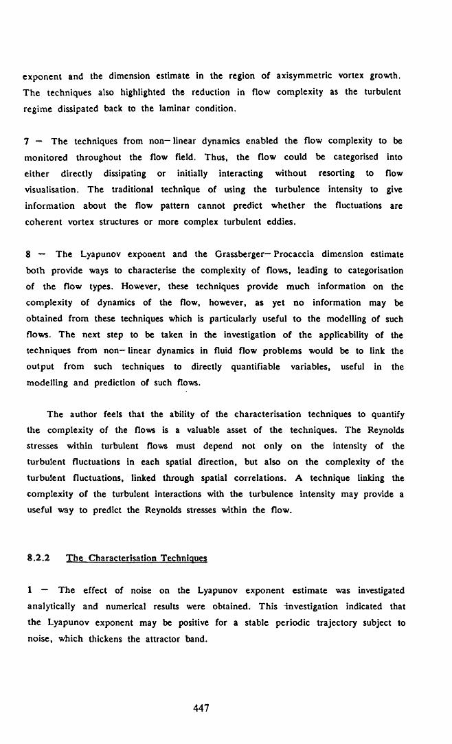
exponent and the dimension estimate in the region of axisymmetric vortex growth.

The techniques also highlighted the reduction in flow complexity as the turbulent

regime dissipated back to the laminar condition.

7 — The techniques from n o n - linear dynamics enabled the flow complexity to be

monitored throughout the flow field. Thus, the flow could be categorised into

either directly dissipating or initially interacting without resorting to flow

visualisation. The traditional technique of using the turbulence intensity to give

information about the flow pattern cannot predict whether the fluctuations are

coherent vortex structures or more complex turbulent eddies.

8 — The Lyapunov exponent and the Grassberger— Procaccia dimension estimate

both provide ways to characterise the complexity of flows, leading to categorisation

of the flow types. However, these techniques provide much information on the

complexity of dynamics of the flow, however, as yet no information may be

obtained from these techniques which is particularly useful to the modelling of such

flows. The next step to be taken in the investigation of the applicability of the

techniques from non— linear dynamics in fluid flow problems would be to link the

output from such techniques to directly quantifiable variables, useful in the

modelling and prediction of such flows.

The author feels that the ability of the characterisation techniques to quantify

the complexity of the flows is a valuable asset of the techniques. The Reynolds

stresses within turbulent flows must depend not only on the intensity of the

turbulent fluctuations in each spatial direction, but also on the complexity of the

turbulent fluctuations, linked through spatial correlations. A technique linking the

complexity of the turbulent interactions with the turbulence intensity may provide a

useful way to predict the Reynolds stresses within the flow.

8 .2 .2 T he Characterisation Techniques

1 — The effect of noise on the Lyapunov exponent estimate was investigated

analytically and numerical results were obtained. This investigation indicated that

the Lyapunov exponent may be positive for a stable periodic trajectory subject to

noise, which thickens the attractor band.

447

2 — A constant Lyapunov exponent was found for a small range of reconstruction

time delays for attractors whose dimension do not exceed the embedding dimension

of the phase space. This plateau of constant Lyapunov exponent was centred upon

one quarter of the forcing cycle time.

3 — Further investigation into the effect of noise on the Lyapunov exponent

showed that for large time delays, where the trajectories became completely

decorrelated, the Lyapunov exponent tended to be inversely proportional to the

delay time, i.e.,

[ a t " 1 - 00

However, for shorter time periods the Lyapunov exponent was inversely

proportional to the delay time to the power of 0.44, i.e.,

An explanation was put forward to explain each of these relationships in terms of

both the averaging involved in the Lyapunov exponent algorithm, and the presence

of noise.

4 — A new Lyapunov exponent type measure of the trajectory divergence was

proposed which avoids the possibility of singularities appearing in the calculations.

This exponent, L*, measures the Lyapunov exponent of the average separation of

the trajectories rather than the more usual method of taking the average of the

Lyapunov exponents each of the trajectory separations, (£). L* is defined as,

5 — A novel method of probing the attractor band structure was proposed. Slicing

448

through the attractor band and constructing probability distribution histograms of the

trajectory crossings gives visual information about the attractor development. In

addition, the probability distribution information present in the histogram may then

be used in the calculation of L*.

6 — The minimum mutual information function was successfully used in obtaining

attractor time delays. A novel non-dim ensional complexity parameter was used in

the study. This mutual information complexity parameter, M*. is obtained by

dividing the first minimum in mutual information obtained, from the time series,

by the first minimum in mutual information that would be given by the forcing

period, i.e. one quarter of the forcing period. Thus,

^ F i r s t Minimum in Mutual InformationM - ------------------------------------------------------------------

1/4 Forcing Period

This parameter allows the variation in minimum mutual information to be

compared between flow with different forcing frequencies.

8.3 SUGGESTIONS FOR FUTURE RESEARCH

During the course of the investigation many interesting areas of associated

research came to light. However, due to the time limitation imposed on the

research project, many of these areas could not be adequately covered by the

author. The following is a list of topics that the author suggests could lead to

further understanding of non— linear dynamics and fluid flow phenomena.

1 — Flow Complexity, Turbulence Intensity and the Reynolds Stresses

One possible direction for further research to aim for would be a study to link the

flow complexity, (as defined by the techniques from n o n -lin ear dynamics), and the

turbulence intensity, to the actual Reynolds stresses in the flow. This would be

particularly useful to the modelling of flow regimes, where the flow is not fully

turbulent, but rather, consists of large coherent structures o f'low complexity.

449

2 - Flow Complexity and Sediment Transport Properties

One immediately obvious result from the investigations presented herein, is that

pulsing the flow of fluid through an orifice plate, in low flow Reynolds numbers,

changes the subsequent flow pattern downstream. The flow exhibits enhanced vortex

growth which, under suitable conditions, breaks down to a region of turbulence.

Both enhanced vortex flows and turbulent flows have increased sediment transport

properties. In pipe systems, in which the fluid carries particles, obstacles cause a

build up of sediment. It would be valuable to investigate the effect that flow

pulsation has both on the dispersal of sediment at obstacles and on the sediment

carrying properties of the flow as a whole, especially for low Reynolds number

flows.

3 — N o n - linear Oscillator Systems

It would be useful to investigate the behaviour of non— linear oscillator systems in

chaotic mode, leading to the possibility of modelling the evolution of vortex streets

with such a system. Once such a flow loses its axisymmetry, and evolves into a

highly complex spatial structure, the modelling of the flow using a simple chain of

non— linear oscillators would not be applicable. However, over the initial region of

axisymmetric development such a model may be possible.

4 — The Grassberger— Procaccia Dimension Estimate and Transients in the Signal

A study into the effect of transients in the time trace signal, used to reconstruct

the attractor, would be of benefit in locating weaknesses in the

Grassberger— Procaccia dimension algorithm. The author has already found apparent

fractal dimensions in a simple transient, periodic signal, (Appendix 6). Further

research should concentrate on the effect on the dimension estimate of intermittent

perturbations to the signal, (in the form of noise), and the subsequent transients

caused.

5 — The Lyapunov Exponent and Noise

Further research into the behaviour of the Lyapunov exponent estimate in the

presence of noise should be undertaken. In particular, various types and levels of

noise could be investigated. This research would lead to a better understanding of

the ability of the technique to identify precisely the difference between periodic,

chaotic and purely noisy flows.

450

APPENDICES

APPENDIX 1 : DERIVATION OF THE LAMINAR PIPE FLOW EQUATION

FROM THE NAVIER STOKES EQUATIONS EXPRESSED

IN CYLINDRICAL COORDINATES.

Navler Stokes Equat ions In C y l in d r i c a l Coordina tes :

r-momentum:

dur /n mi 1 ii* 1 dp ^ f 2 Ur 2 dU* 1St + <U v >ur - 7 u« - - p 5 ? + * r + ' l ,’ « « - - 7 i - 7 j 5 j J

( A l . l )

0-momenturn:

+ (U .v )U , - I UrU, - - I + „ + r [ **Or . g t . E f ]

(A1.2)z-momenturn:311 1 AP 5

+ <».•*) Uz - - i (Uj) + gz + r v*Uz (A1.3)

Cont inui t y :

? I ? (r Ur> + F S 7 <"«> + I f <uz> - 0

LaplacI an Operator

2 1 d T d ”1 ^ 1 d2 _ a /A1 /VN- - F S F l - S F J + - ~ , + <A1-4b>

Consider Laminar Flow Case, ( Steady s t a t e in pipe ):

ASSUMPTIONS:

Flow V e l o c i t i e s : Ur _ q

U* - 0

U2 - U2 ( r )

451

Boundary cond i t ions : (A1.5)

P r e s s u r e : P - a , z + a 0 (A1.6)

Consider z-momentum ( equa t ion A4 ) :

, / it \ t i 1 * P A ^ 2 „5t + <u ” ) ux ‘ ' Z S + + ' ' "j

Vz Steady s t a t e hence equa t ion (A4) reduces to :

I ? JF I

0 “ - a * + * , ( 7 S ? [ r 3FZ ] ]

0 — - a

Thus : (A1.7)

Let : y - & (A1.8)

Hence : _ zH o r r (A1.9)

Equation (A1.8) i s a F i r s t Order Linear D i f f e r e n t i a l Equation,

Hdr

In te g ra t in g Fac tor : G(r) - e" (A1.10)

So equat ion (Al.8) becomes:

a57

j i dr J fdr

452

I n t e g r a t i n g both s ides :

f I drJ r a,

-f I dr , , y ■ * r [ j - + c <

*1y - -J* M r I r + c < ]

a. r ^ C.y - —.L _ + - J* It 2 r

u s ing e q u a t io n (A1.7) we get:

dU- a. r , C. dr " ji 2 r

I n t e g r a t i n g equa t ion ( A l . l l ) :

j d° * - n ^ \ + f 1 i d r

»z - + c , >"(>•) + c r

C, - 0 as Uz i s f i n i t e .

We know : Uz [+ 5 ] “ 0 ( equat ion A1.5 )

So : C, - - Sa

lience, IJZ - ( T1 - ^ ]

From the Veloci ty Equation ( equat ion A1.15 ) now

c a l c u l a t e the Mean V e lo c i ty Uz

(A1.15)

r dr d 6Uz “ - Da--------------- (A1.16)

x D2Where — Is the pipe c ro s s s ec t io n a l a rea .

T. 8 (x fd/ 2 a . , . D2. .uz " r s * J o Jo a k < r ’ - ? > r d r

This reduces to:

rs 2a. [x D4 . .UZ ■ T j f a J 0 U d e

a .D 2H e n c e : Uz - (Al.17)

Pipe head loss : hj - "2gZ (A1.18)

Also : hi - i - ( ~ L ) - — ( a. ) (Al.19)pg dL pg v 1 '

454

Hence X - 2a,

pUz(A1.20)

Combining e q u a t i o n s (A1.17) and (A1.20) t o g e t :

64X ~ P (A1.21)

as requ ired .

455

APPENDIX 2 : COMPUTER PROGRAMS AND ALGORITHM CONSTRUCTION

A2.1 Introduction

In this appendix an explanation of the computer programs, used in the study

presented within this thesis, is given. The main programs are listed.

A2.2 Data Acquisition Programs

The ASYST language was used to write the data acquisition programs. The two

main programs used for this purpose were LASERP4 and SETUP4.

LASERP4 is the main acquisition program which interfaces with the

Burr—Brown data acquisition card within the IBM P.C .. The data is stored in the

array POSITIONA which contains 16384 data points of the time series. The

program also computes the average flow velocity and the turbulence intensity for

each data acquisition run.

SETUP4 is mainly for the presentation and manipulation of the data, and

contains many user defined F .F .T . routines to plot out frequency spectra with

linear and logarithmic scales. The program also contains a routine to plot out the

velocity— time traces of the first 500 data points, which serves as a check during

the experimentation.

In the following four pages the program LASERP4 is listed together with a

typical plotting routine from SETUP4.

A2.3 Data Analysis Programs

Programs were written by the author to perform all of the data analysis

requirements. These techniques were: F .F .T ., Autocorrelation function,

Grassberger— Procaccia dimension estimate, Lyapunov exponent measurement, the

first minimum in mutual information, the probability distribution of attractor slices

and first return maps.

456

However, in two cases, programs not written by the author were eventually

used. These were to calculate the F.F.T . and the Lyapunov exponent of the time

series. The Fourier transform of the time series was obtained using the

user— defined routine in the ASYST language called 'FSPECTRUM '. Whereby the

F .F .T . of the time series could be calculated, viewed on screen and plotted whilst

the experiment was being run. This gave instant feedback of the results.

A2.3.1 The Lvaounov Exponent

Originally a program to determine the largest Lyapunov exponent was also

written by the author. However, the author subsequently obtained a software

package, FET, from Prof. Alan Wolf [1991], a co— author^ of the paper,

'Determining Lyapunov Exponents from a Time Series', Wolf^[1985], from which

the author's Lyapunov exponent program was originally written. The FET program

was much faster than the one developed by the author due to a box assisted

search, preprocessing routine. Therefore, the author used this routine for the

computation of the time series exponent. The acquired package was run on the

OPUS—V P.C ., and the author's original program was used merely to check the

results obtained. For speed, the Lyapunov exponents were calculated for up to 10,

or more, experimental time series results at a time. This was done by running the

FET program simultaneously on some of the many DBM PS2 personal computers to

be found in the computer laboratory, situated elsewhere in the civil engineering

department building. (Although this had to be done at times of low usage of the

computer laboratory, i.e. at nights and weekends.)

A2.3.2 The Calculation of the Mutual Information

and the Grassberger— Procaccia Dimension

Program XD6, written by the author, is the most recent version of the

computer program used to determine the dimension of the attractors reconstructed

from the time series. A listing of the subroutines contained within the program are

as follows:

PROGRAM XD6: Main program block.

MUTINFO: Subroutine to calculate the mutual information of the time series for

457

various values of time delay. The first minimum in the mutual information function

then determines the value of time delay to be used in the attractor construction.

MUTGRAPH: Subroutine to plot out the results of the minimum mutual

information calculations.

DROPALG: Subroutine to check the time series for d ro p -o u ts in the signal. These

drop— out sections are subsequently labelled, and ignored in the attractor

construction. (See section A2.5 for more details).

EXPTDIM: This subroutine sets up the initial data required for the Grassberger—

Procaccia dimension calculation.

GBDEM: Subroutine to calculate the Grassberger- Procaccia dimension.

DIMGRAPH: Subroutine to plot out the resulting 'log(r)— log(Cr)* graph.

Program XD6 is listed at the end of this section.

A2.3.3 A ttractor Slicing and Probability Distribution

Program X__PDF4 slices through the attractor, and using a box— counting

algorithm, produces a probability histogram of the likelihood of the trajectory

crossing each part of the slice. The mean and standard deviation of the crossing

points are then calculated and an 'equivalent' Normal, or Gaussian, distribution is

calculated. This Normal distribution is then superimposed on top of the histogram

results for comparison purposes. Program X PDF4 is listed at the end of

section 2.3.

A2.3.4 F irst Return Mao and Autocorrelation Function

Programs were produced to calculate the first return map and the

autocorrelation function from a time series, these programs were X_RET4 and X.

CORR2 respectively. The first return map was produced by plotting each peak of

the time series against each subsequent peak. The autocorrelation function was

calculated by applying the formula given in chapter 2, section 2.7.3, to the time

series. Both these programs are not listed herein, due to their simplicity.

458

Program LASERP4

\ PROGRAM LASERP4 \ THIS PROGRAM USED TO DETERMINE\ THE FLOW VELOCITIES AND TURBULENCE INTENSITIES\ FROM THE VOLTAGE OUTPUT OF THE LASER TRACKER\INTEGER SCALAR ERROR.CODE INTEGER SCALAR SEGMT INTEGER SCALAR CHN INTEGER SCALAR GAIN INTEGER SCALAR Z.CHN INTEGER SCALAR RANGE INTEGER SCALAR W INTEGER SCALAR ADATA REAL DIM[ 16384 ] ARRAY POSITIONA \\ DEFINE A GENERAL PURPOSE ERROR PROCESSING ROUTINE.\S ERROR? \ (STRING ______ )

CALL[ PC I46S , ERR. SYS , ERROR.CODE ]ERROR.CODE 0 <> I F

"TYPE ERROR.CODE . CR ELSE

"DROPTHEN

J: LASERCR . " SETTING ARRAYS TO ZERO"0 POSITIONA :«\\ IN ITIA LIZE THE P C I-2 0 0 4 6 S -4 SYSTEM. THIS SEQUENCE MUST BE\ GIVEN PRIOR TO CALLING ANY OTHER P C I- 2 0 0 4 6 S -4 INSTRUCTION.CR■ 61"H SET.VECTCALL[ PC I46S , SY SIN IT ]\\ SEGMT, DEFINE BELOW, CONTAINS THE BASE ADDRESS OF THE CARRIER\ WE USE " C 000"H , BUT YOU CAN SET IT ANY WHERE. REFER TO THE\ CARRIER MANUAL FOR MORE INFORMATION.\ [ PC I46S , IN IT , SEGMT ] MUST BE CALLED ONCE FOR EACHCARRIER\ IN THE SYSTEM, EACH WITH ITS OWN ADDRESS \" C000"H SEGMT S*CALL( PC I46S , IN IT , SEGMT J \\ CHECK FOR A SYSTEM ERROR. DURING DEBUG, CALL ERR.SYS OFTEN,\ POSSIBLY AFTER EVERY CALL TO THE P C I-2 0 0 4 6 S -4 . IT IS A GOOD\ IDEA TO LEAVE A FEW ERR. SYS CALLS IN A FINISHED PROGRAM TO\ MONITOR THE STATUS OF THE SYSTEM.\" ERROR FOUND DURING IN IT " ERROR?

459

Program LASERP4 Con t inued

CR . " PROGRAM LASERP4"CRCR ." SETTING GAIN AND RANGE"0 CHN1 GAIN -1 Z.CHN 1 RANGE\ W IS THE NUMBER OF READINGS +1 ON CHANNEL 16385 W CRCR ." CONFIGURING CHANNEL 0"CALL[ PCI46S , CNF.AI , CHN , GAIN , Z.CHN , RANGE J

’" ERROR FOUND DURING CNF.AI" ERROR?\\ READ THE ANALOG INPUT CHANNEL \CRCR ." READING CHANNEL"\ SET FREQUENCY OF SAMPLING SYNC. ERROR. ON INV 1000 . *SYNC. PERIODCR DATA AQUISITION LOOP"W 1 DO SYNCHRONIZECALL[ PCI46S , READ.CH , A I.T , CHN , ADATA ]\\ GIVEN THE ADC READING, ADATA, TO ARRAY AND CONVERT \\ THE ASSUMPTION IS THAT THE PCI-20002M -1 MODULE IS SET \ UP FOR + \ - 10 VOLTS\ THE PREVIOUS PROGRAME GIVES THE EQUATION TO BE USED IN PLACE\ OP THE ABOVE LINE FOR OTHER THAN + \ - 10 VOLTS \ADATA POSITIONA [ 1 ) 8 -

* LOOP ?

\INTEGER SCALAR W2REAL DIM[ 4096 ] ARRAY POSITIONO: LASER2CR ." DATA CONVERSION AD INPUT TO DIGITISED VOLTAGES"CR\\ CONVERT ARRAY FROM ANALOG VOLTAGE TO DIGITAL VOLTAGE TO VELOCITY \4097 W2POSITIONA SUB[ 1 , 4096 ] POSITIONOPOSITIONO 2 0 . 0 * 4096 .0 / 1 0 .0 - GAIN / POSITIONO :«CR ." NUMBER OF READINGS ON CHANNEL 0 WAS" W2 1 - .CR

460

Program LASERP4 Continued

\ EXPERIMENTAL ANALYSIS \REAL SCALAR RANGE2 20 STRING TESTRUN 20 STRING DATE \s INPUTSOCR . " DATA CONVERSION VOLTAGES TO VELOCITIES"CR\CR FREQUENCY RANGE (MAX) RANGE2 . H z"

*CRW2 1 DO \POSITIONO ( I ) .0 0 0 0 0 0 6 3 2 8 * RANGE2 * 1 .9 8 9 8 6 8 3 6 / POSITIONO ( I ]\LOOPJ

\\ DETERMINE STATICAL PROPERTIES AND RESULTS \REAL DIM[ 3 ] ARRAY TEMPO : RESULTS 0 \

INPUTSO\CR . " LASER MEASUREMENTS ( m /s ) "CR\POSITIONO MEAN TEMPO [ 1 ]POSITIONO VARIANCE SQRT TEMPO [ 2 ] J - TEMPO ( 2 ) TEMPO [ 1 ] / 100 * TEMPO [ 3 ] S - CR . " POINT VELOCITY IN THE CHANNEL*" TEMPO [ 1 ) . . "

'm / s "CRCR . " TURBULENCE INTENSITY U ' AT THE SAME PO IN T -" TEMPO ( 3 ] . . " %"CR;CR;7

HCR\;

461

A Typical P l o t t i n g Routine from the Program Setup4 from the Program SetupA

\ PLOT FREQUENCY SPECTRUM \REAL DIM[ 4096 ] ARRAY FSPECTRUMj pg

VERTICAL LINEAR - 1 .2 0 5 LABEL.FORMAT HORIZONTAL LINEAR VERTICAL LINEAR - 1 .2 0 5 LABEL.FORMAT HORIZONTAL LINEAR - . 5 - . 8 4 LABEL.FORMAT - . 5 - . 8 4 LABEL.FORMAT FREQS SUB[ 2 , 2048 ]POSITIONO FFT ZMAG FSPECTRUM S - FSPECTRUM SUB[ 2 , 2048 ]XY.AUTO.PLOT NORMAL.COORDS 0 LABEL.DIR 0 CHAR.DIR.5 .9 POSITION " FREQUENCY SPECTRUM" LABEL .7 .0 5 POSITION " FREQUENCY (H z )" LABEL 270 LABEL.DIR 0 CHAR.DIR.0 3 .9 0 POSITION " F .F .T . MAGNITUDE" LABELOUTLINECURSOR.OFFWORLD. COORDS

462

oo

oo

on

o

now

non

ni-. .

< ooo

o o

on

oo

oo

oProgram XD6

PROGRAM XD6

. . T H I S PROG. - 1 . LOOKS FOR DROPOUTS, AND LABELS THEN.2 . FINDS THE F IR S T N I N . IN THE MUTUAL INFORMATION FN.

OF THE TIME SERIES NOT INCLUDING THE DROPOUTS.3 . SENDS THE LABELLED DATA ( 1 ) AND THE TIME DELAY ( 2 )

TO THE GRASS. -PROC. DIMENSION ALG.

I M P L I C I T NONEINTEGER N S T E P , D E L A Y , I , SKIPGRAP, MAX_EMBED,N_DEL,KTOL, MM, NWINTEGER NCOUNT, STPVALREAL X ( 1 6 3 8 4 ) , D T , RMAX ,RNULTDOUBLE PRECISION PPCOMMON/DROPVAR/KTOL »MN,PP , NWCOMMON/DIMVAR/STPVAL,NCOUNT,RMAXCOMMON/EMBVAR/DT

NSTEP - 16 38 4DT - 0 . 0 1DELAY - 0NCOUNT - 0HAX_EMBED - 30 1 . . M A X . EMBEDDING DIMENSIONM_DEL - 2 ( . . I N C R E M E N T OF EMBEDDING DIMENSIONSTPVAL - 40 0 ( . . E V E R Y STPVAL POINTS ON THE ATTRACTOR SAMPLEDSKIPGRAP - 0 ( . . 1 - N O GRAPHICS FOR HUT. I N F O . / ELSE-GRAPHICSRHULT - 3 0 . 0 0 * * 0 . 5RMAX - 1 . 0 0 « RMULT 1HAX. RADIUS OF N-DIMENSIONAL HYPERSPHERE

KTOL - 30 ( 3 0 (HE IGHT TOL.MM • 30 ( 10 (LENGTH TOL.PP • . 7 ( . 7 (PERCENTAGE WITHI N NWNW - 15 ( 3 (SECOND HEIGHT TOL.

. .READ IN DATA

O P E N ( 2 1 , F I L E - I H 0 1 0 1 0 5 ' )RE A D( 21 , 1 0 1 ) ( X ( I ) , 1 - 1 , NSTEP)

101 F0RMATC6F12 .1 )

. .C A L L MUTUAL INFORMATION ALGORITHM TO DETERMINE APPROPRIATE TIME DELAY

CALL MUTINFO(X ,NS TE P,DT ,SKIP GRA P,DE LA Y)

. . -ALL DIMENSION ALGORITHM

CALL EXPTDIH (NSTEP, DEL AY, X , HAX_EHBED, M'.DEL , D T )

. .CLOSE GRAPHICS

CALL GREND

RETURNEND

K X X X X X X K X X X X X X X X X X K X X X K X K X X K X X X X X X X K K X X K X X X X X X X X X X X X X X X X K X X K K K X X X X X X X X X

SUBROUTINE M UT INF O(X ,NST EP, DT ,SKIP GR AP ,DEL AY )

. .SUBROUTINE TO CALC. THE MUTUAL IN F O. FN . OF THE T IME SERIES

I M P L I C I T NONEINTEGER I , J , K , L , H , N S T E P , N B O X , D E L ,M M A X ,N S T E P , S K I P G R A P INTEGER I C O U N T X ( 0 : 2 0 0 ) , ICOUNTY( 0 : 2 0 0 ) , ICOUNTXYC0 i 2 0 0 , 0 : 2 0 0 )

_ INTEGER ISUMX, ISUMY, ISUMXY,STEPCOUNT,MINFLAG,DELAY REAL X ( 1 6 3 8 4 ) ,L0GVAL,DT REAL XMAX, X H I N , YMAX, YMIN REAL BOXSIZEX, BOXSIZEY,STEP

463

ooo

oon

r> o

oo

o

oo

oo

Program XD6 c o n t in u e d

REAL HINHUTCOs1 5 0 ) .MMUTOLDc

NBOX ■ 100MMAX ■ 100MSTEP • 1HHUTOLD - 1 0 0 0 0 0 0 0 0 0 0 0 0 0 . 0HINFLAG ■ 0PRINT ■# * ■MU T INFO* NS T EP - * , NSTEP

. .C AL L ALGORITHM TO LABEL DROPOUTS IN THE S IGN AL .

CALL DR0PALG(X»NSTEP)

DO 100 H - 0 , MMAX XMAX - * 1 0 0 . 0 XHIN - 1 0 0 . 0YMAX - - 1 0 0 . 0 YMIN ■ 1 0 0 . 0DEL » M » MSTEP STEP - REAL(NSTEP-DEL)

. . F I N D MAX + MIN OF THE TWO TIME SERIES

. .HENCE F IN D THE S IZ E OF THE GRID SPACES

DO 10 I - 1 , NSTEP - DEL I F C X ( X ) . L T . 0 ) G O T O 1 0 I F C X M A X . L T . X ( D ) XMAX - X ( I ) I F C X M I N . G T . X ( I ) ) XMIN - X ( I )

10 CONTINUE

DO 20 I - 1 ♦ DEL,NSTEP I F ( X C I ) . L T . 0 ) G O T O 2 0 I F ( Y M A X . L T . X ( I ) ) YMAX • X ( I ) I F C Y M I N . G T . X ( I ) ) YMIN - X ( I )

20 CONTINUEBOXSIZEX - ( XMAX-XMIN) /REAL(NBOX)BOXSIZEY - (YMAX-YMIN) /REAL(NBOX)

. . I N I T I A L I Z E THE BOX COUNTING ARRAYS

ISUMX • 0 ISUMY - 0 ISUMXY - 0 DO 30 I - 1 ,NBOX

ICO UN TX CD -O ICO UN TY CD -O DO AO J - 1 ,NBOX

I C O U N T X Y t I , J ) - 0 40 CONTINUE30 CONTINUE

. .COUNT UP THE NUMBER OF POINTS IN EACH ROW AND COLUMN

STEPCOUNT - 0DO 50 1 - l ' N S T E P - D E L

I F ( X ( I ) . L T . 0 .OR. X ( I + D E L ) . L T . 0 ) G O T O 5 0 STEPCOUNT » STEPCOUNT ♦ 1 K - I N T ( ( X ( I ) - XMIN) / BOXSIZEX) ♦ 1L - I N T ( ( X ( I + D E L ) - YMIN) / BOXSIZEY) ♦ 1 ICOUNTX(K) - ICOUNTX(K) ♦ 1 ICOUNTY(L ) - ICOUNTY(L ) ' ♦ 1 I C O U N T X Y ( K 'L ) - ICOUNTXYCK,L) + 1

50 CONTINUE C. .CHECK

DO 51 I - 1 'NBOXISUMX - ISUMX ♦ I C O U N T X ( I )ISUMY - ISUMY + I C O U N T Y ( I )

51 CONTINUE

464

Program XD6 c o n t i n u e d

ccccccccccccccccccccccccccccccccccccccccccccccccccccccc c cC CALCULATE MUTUAL INFORMATION CC Ccccccccccccccccccccccccccccccccccccccccccccccccccccccc c

H INHUT( M) * 0 . 0 DO 60 I ■ UNBO X

IF ( I C O U N T X t I ) . EQ. 0 ) GOTO 60 DO 70 J » UNBOX

IF ( ICOUNTYI J ) .EQ.O .OR. ICOUNTXYC U J U E Q . O ) THEN GOTO 70

ELSELOGVAL"( ICOUNTXY<I , J> /R EA L( STE PC OU NT ) ) x

9 LOG( REAL( ICOUNTXYC I , J ) *REAL( STEPCOUNT)) /a REAL( ICOUNTX( I ) * ICOUNTYC J ) ) )

ENDIFMINMUT(M) - MINMUT(M) ♦ LOGVAL

70 CONTINUE60 CONTINUE

CMINMUT(M) - M I N M U T ( M ) / L 0 G ( 2 . 0 )I F (HHUTOLD.LT .MINMUT(M) .AND. MINFLAG.EQ. 0 > THEN

( DELAY - DEL - IPRINT x , * xMUTINFOxXX xxx F IRS T MINIMUM REACHED « * « xxx •PRINT x * ' xMUTINFO* TIME DELAY ■ UDELAYMINFLAG - MINFLAG + 1 IF ( S K I P G R A P . E Q . 1) GOTO 110

ENDIFPRINT x , M , ' D E L * M I N M U T - UDEL,M INM UT (M>MMUTOLD - M INHUT(M)

C100 CONTINUE

CC . . .CALL GRAPHICS SUBROUTINE C

CALL MUTGRAPH(MINMUT,MMAX,MSTEP,DT,DELAY)C

110 CONTINUEC

RETURNEND

CCX* *XXXXXXXXXXXXXXXXXXXXXXXXXXXXXXXXXXXXXXXXXXXXXXXXXXXXXXXXXXXXXXXXXXXC

SUBROUTINE MUTGRAPH(MINMUT,MMAX,MSTEP,DT,DELAY)CC. .SUBROUTINE TO PLOT OUT THE MUTUAL INFO. RESULTS C

INTEGER MMAX,MSTEP,DELAY REAL M I N M U T ( 0 : 5 0 )

CALL PSPACECO.3 0 , 1 . 1 0 , 0 . 2 5 , 0 . 7 0 )CALL MAP(0 . 0 , REAL(MMAXxHSTEP) , 0 . 0 , 1 . 2 * M I N M U T ( 0 ) )CALL A X E S S K l . 0 , 1 . 0 )CALL P O S I T N ( 0 . 0 , M I N M U T ( 0 ) )DO 10 I - 1 ,MMAX*MSTEP

CALL J O I N ( R E A L ( I ) , M I N M U T ( I ) )10 CONTINUE

r* *

CALL PSPACE( 0 . 1 0 , 1 . 3 0 , 0 . 1 0 , 0 . 9 0 )CALL HAP ( 0 . 1 0 , 1 . 3 0 , 0 . 1 0 , 0 . 9 0 )CALL PCSC EN( 0 . 7 0 , 0 . 7 0 , ' H 0 10 10 5 ' )CALL BORDER CALL CTRMAG(1 5 )CALL P C S C E N ( 0 . 7 0 , 0 . 8 2 , 'MUTUAL INFORMATION OF THE EXPERIMENTAL ' ) CALL PCSCEN(0 . 7 0 , 0 . 7 7 , 'T I M E . S IG N A L WITH DROP OUTS NOT INCLUDED ' )

465

oo

oo

o

o o

Program XD6 c o n t i n u e d

CALL CTRMAGUO)CALL PCSCEN(0 . 9 5 , 0 . 1 8 , ' UNITS OF TIHE DE L AY ' ) CALL P CS C E N( 0 . 9 5 , 0 . 6 5 , 'T I ME INCREMENT ■ ' )CALL P L OT NF d . 0 5 , 0 . 6 5 , D T , 3 )CALL PCSCENtO.9 5 , 0 . 7 0 , ' F I R S T M I N . - • )CALL P L O T N K l . 00 , 0 . 7 0 , DELAY)CALL CTROR1 ( 9 0 . 0 )CALL PCSCENtO. 2 1 , 0 . 6 0 , 'MUTUAL INFORMATION ( I ) ' ) CALL CTRORK 0 . 0 )

CALL FRAMERETURNEND

SUBROUTINE DROPALGtXX, NSTEP)

. . . T H I S SUBROUTINE - I . CHECKS DATA FOR DROPOUTS2 . LABELS DROPOUTS BY MAKING THEM NEGATIVE

I M P L I C I T NONE INTEGER NMAX PARAMETER (NMAX-16384 )DOUBLE PRECISION SCALEX,PP REAL XX(NMAX)INTEGER M, I , K , I C O L , N X P I X , N Y P I X , I C L E A N , I R E P , J , MM, MARK,KHIN INTEGER KMAX,KK(NMAX),KSUM, KTOL, SMAX, S , L , NW,SS PARAMETER (S HA X- 100 )INTEGER SL0T (2 ,SMA X)REAL XNEW(NMAX)INTEGER NSTEP,MARKDROP COMMON/DROPVAR/KTOL,MM »PP,NW

MARKDROP - 0PRINT « , ' * D R O P A L G « * * * *« SEARCHING FOR DROPOUTS K x x x x i 'PR INT « , ' K T O l , N W , P P , M M ' , KTOL,NW,PP,MMN - 0KSUM-0DO 10 I - 1 , NMAX

KK( I ) - I N T ( X X ( I ) )10 CONTINUE

DO 20 N « 1 , NMAX K - KK(N)KSUM-KSUM+K IF ( N . E Q . l ) THEN

KMIN-K KMAX-K

ELSEKMIN«MIN(K,KMIN>KMAX*MAX(K,KMAX>

END I F 20 CONTINUE

CMARK-0DO 150 1 - 2 , N

K K < I ) » A B S ( K K ( I ) )I F (MARK . EQ. 0 . AND. ABSCKK ( I ) - K K ( I - D ) . L E . K T O L ) THEN

M A R K - I - 1 ELSE I F (MARK.EQ.O) THEN

CONTINUEELSE IF ( A B S ( K K ( I ) - K K ( M A R K ) ) .G T . K T O L ) THEN

I F ( I -MA RK -1 . GE. MM ) THEN S - 0DO 140 J-MARK, 1 - 1

DO 130 K - l , SIF ( S L O T ( 1 , K ) . N E . K K ( J ) ) GOTO 130 S L O T ( 2 , K ) - S L O T ( 2 , K ) + 1

466

oo

oo

o

o o

oo

oProgram XD6 co n t in u e d

GOTO 135 130 CONTINUE

DO 160 K - l . SIF ( K K ( J ) . LT .SLOTC1, K ) ) GOTO 170

160 CONTINUEK«S*1

170 CONTINUEDO 180 L - S , K , - 1

SLOT( 1 ,L + 1 ) - S L O T ( 1 , L )S L 0 T ( 2 , L + l ) aS L 0 T ( 2 , L )

180 CONTINUES - S Mslot (1 ,k) »kk(J)SLOT( 2 , K ) a 1


SS-0DO 300 J - 1 , MAX( 1 , S-NW+ 1)

K-0DO 29 0 L a J » H I N ( S , J + NW-1)

Ka K + S L 0 T ( 2 , L )290 CONTINUE

SSaMAX(SS,K)300 CONTINUE( IF ( S S . G T . P P * ( I - H A R K ) ) THEN

HARKDROP - MARKDROP ♦ 1DO 310 J aMARK#1-1

K K ( J ) - - K K ( J )310 CONTINUE

END I F END IF MARK-0

END I F 150 CONTINUE

HARKa lC

DO 800 I - 1,NMAXX X ( I ) - R E A L ( K K ( I ) )

8 0 0 CONTINUEPRINT « , ' * D R 0 P A L G » NO OF DISCRETE DROPOUTS MARKDROPRETURNEND

C ,C « * < * « * * * * * « « * * « « » * « « * * « * * « » » « * « * * * * * * * » * « * * * * * « » « » * « * * « * * * » * * * * * » * *c

SUBROUTINE EXP TD IH (N S T EP , DELAY,X,MAX_EMBED,M_DEL,DT)

. . T H I S SUBROUTINE SETS UP I N I T I A L DATA FOR THE DIMENSION ALGORITHM

I M P L I C I T NONEINTEGER I ,DELAY,MAX_EMBED,M_DEL,NSTEP REAL X L , X R , Y Y , Y T , F I N A L , X ( 1 6 3 8 4 ) ,DTREAL XPO INT ( 3 0 , 3 0 0 0 0 ) ,CORPLOT( 3 0 , 1 0 0 0 ) , R P L O T ( 3 0 , 1 0 0 0 )

F INAL a REAL(NSTEP)«DTPRIN T * , ' «EXPTDIM» F I N A L - * , F I NA L

DO 101 - 1 , N S T E P , 1024PRINT » , * « E X P T D I M » , , I , * X < I ) a ' , X ( I )

10 CONTINUE

. . I N I T I A L VALUES

. . X P O I N T - X

DO 20 I - 1 , NSTEPXPO INT ( 1 , 1 ) - XC1)

467


2 0 C O N T I N U EcC . . CALL THE GRASSBERGER-PROCACCIA D I H . ALG.C

CALL GBDIM<XPOINT,NSTEP,MAX_EMBED,M_DEL,DELAY,RPLOT, CORPLOT)CC. .LARGE AXIS DIMENSIONS

CXL* - 8 . 0 XR* 0 . 0 YY* - 2 0 . 0 YT* 0 . 0

CC. .CALL GRAPHICS ROUTINE C

CALL DIMGRAPH( MAX_EMBED, N S T E P , X L , X R , Y Y , Y T ,F I N A L , D E L A Y ,9 RPLOT,CORPLOT,M_DEL>

CRETURNEND

CCXXKKXKKXXKKKKXXKKKKXKXKXKXXXXXXXXKKXXXXXXXXXXXXXKXXXKXXKXXKXXXKXXKXKKc

SUBROUTINE GBD IN ( X P O IN T , NSTEP » NAX__EMBED,N_DEL , DEL AY, RPLOT, CORPLOT)CC. .SUBROUTINE TO CALC. THE D I H . OF AN ATTRACTOR USING THE GRASSBERGER- C. .PROCACCIA DIMENSION ALGORITHM C

I M P L I C I T NONEINTEGER I , J,M,M_EHBED,MAX_EMBED,M_DEL,N,NRSTART, NPOINT , STPVAL INTEGER NSTEP,MOD_NSTEP,DELAY,NCOUNT REAL RARR(IOOO)REAL X DI ST SQ ,C O RI NT , R , D I S T , RMAX, XMAX,XHIN,XMEDIAN REAL XPO INT<3 0 , 3 0 0 0 0 ) ,CORPLOT(3 0 , 1 0 0 0 ) ,R PL OT (3 0 , 1 0 0 0 ) COMMON/DIMVAR/STPVAL,NCOUNT,RMAX

CNPOINT - 1000 I . . N O . OF POINTS USED FOR PLOTXMAX - - 1 0 0 0 0 0 0 . 0XMIN - 1 0 0 0 0 0 0 . 0MOD_NSTEP - NSTEP - (MAX_EMBED-1 ) xDELAY ! . .MOD IF IED NSTEP PRINT x , • XEXPTDIHX RMAX ■ • ,RHAXPRINT x , ' xEXPTDIMX MOD_NSTEP - ' ,MOD_NSTEP

CC . . F I N D MAX ABSOLUTE VALUE OF INPUT TIME SERIES C

DO 10 I - 1 , NSTEPI F ( X P O I N T ( l , I ) . L T . 0 ) GOTO 10IF(XMAX . L T . XPOINT( 1 , 1 ) ) XMAX - X P O I N T ( l , I )

. I F ( X M I N .G T . XPOINT( 1 , 1 ) ) XH IN - X P O I N T ( l , I )10 CONTINUE

XMEDIAN - (XMAX ♦ XMIN) / 2 . 0 PRINT x , ' XMAX ■ ' , XMAXPRINT x , * X M I N - * ,XMINPRINT x , ' XHEDIAN - ' ,XMEDIAN XMAX - ABS(XHAX - XMEDIAN)

CC. .NORMALISE INPUT TIME SERIES, EXCEPT FOR DROPOUTS C

NCOUNT - 0DO 20 I - 1 , NSTEP

I F ( X P O I N T ( 1 , I ) . L T . O ) GOTO 20X P O I N T ( 1 , 1 ) « ( X P O I N T ( 1 , 1 ) - XMEDIAN) / XMAX NCOUNT - NCOUNT ♦ 1

20 CONTINUEPRINT x , ' N O OF GOOD POINTS NCOUNT

CC. .GENERATE THE REMAINING SERIES OP TO DIMENSION M_EMBED

468


cDO 30 I • 1 , M0D_NSTEP

DO 40 M ■ 2 i NAX_EHBEDXPOI NT( h i I ) • X P O I N T ( l # I + ( M - l ) « D E L A Y )

<iO CONTINUE30 CONTINUE

CC. .CALCULATE THE CORRELATION INTEGRAL FOR EACH ( R )C

DO 50 M_EHBED - 2 »MAX_EMBED#M_DEL NCOUNT - 0DO 60 I - 1 t HOD_NSTEP

DO 65 M - 1 »M_EMBEDI F ( X P O I N T ( M # I ) . L T . - l ) GOTO 60

65 CONTINUEDO 70 J - I ,MOD_NSTEP,STPVAL

IF ( I A B S ( I - J ) . L T . D E L A Y ) GOTO70 XDISTSQ - 0 . 0 DO 75 M - 1 #M__EMBED

I F ( X P O I N T ( M » J ) . L T . - 1 ) GOTO 70 75 CONTINUE

DO 80 N ■ 1 , M_EHBEDXDISTSQ - ( X P O I N T ( M , I ) - X P O I N T ( N , J ) ) * « 2 ♦ XDISTSQ

80 CONTINUE< D IST - SQRT(XDISTSQ)

I F ( D I S T . G T . 0 . 0 .AND. D I S T . L E . RNAX) THEN NCOUNT - NCOUNT ♦ 1

NRSTART - 1 ♦ I N T ( ( R E A L ( N P O I N T ) * ( D I S T / R H A X ) ) )DO 90 N - NRSTARTt NPOINT

RARR(N) - RARR(N) + 1 . 0 90 CONTINUE

ENDIF70 CONTINUE60 CONTINUE

CC . . .C H E C K TO SEE I F THE EFFECT OF THE DROPOUTS HAS SPREAD TO THE C. . .WHOLE DATA SET C

PRINT * » M_EHBED»• * * * » ««« «« « NCOUNT ■ » , NCOUNT I F ( NCOUNT.EQ.O)THEN

PRINT > « 'DROPOUTS HAVE L IM I T E D EMBEDDING DIMENSION*MAX_EMBED - M_EHBED - M_DEL GOTO 110

ENDIFC

DO 100 N - 1 , NPOINTCORINT - R A R R ( N ) / REAL(NCOUNT)RARR(N) - 0 . 0R « (RMA X/R EAL (NP OIN T) ) »R EAL (N)I F ( C O R I N T , G T . 0 . 0 ) THEN

CORPLOT(M_EHBED,N) - LOG10 ( C O R I N T ) / L O G 1 0 ( 2 . 0 )CC . . NOW CHOOSE BETWEEN THE ORIGINAL ALGORITHM OR THE MODIFICATION C . . O F DVORAK t KLASHKA. SEE ALSO SMITH.CC . . O R I G I N A L C

RPLOT<H_EHBED,N)«L0G10 ( R / R M A X ) / L 0 G 1 0 ( 2 . 0 )CC. . MODIF IED CCCC RPLOT(M-EMBED«N)b L O G 1 0 ( ( R « ( 2 . 0» R M A X -R ) ) / R M A X * » 2 ) / L 0 G 1 0 ( 2 . 0 )C

ENDIF100 CONTINUE50 CONTINUE 110 CONTINUE

RETURN

469

o o

n o

oProgram XD6 c o n t in u e d

ENDCCi i i m m i m i m i i i m i m k m i i i i i u u i i i i i m m i m m m i m m m i m m i u m m ,

cSUBROUTINE DIHGRAPH( MAX.EMBED, NSTEP , X L , XR, Y Y , Y T , F I N A L , DELAY,

a RPLOT,CORPLOT,M_DEL)CC. .SUBROUTINE TO PLOT OUT THE * LOG (R) -L OG( CR) ' RESULTS C

I M P L I C I T NONEINTEGER I BEG I N , I S U N , J , J C O U N T , M, MAX_EMBED, NSTEPINTEGER I , JHAX, DELAY, M_DEL, HCOUNTINTEGER L I N E 1 , L I N E 2 , L I N E S , J S T A R TREAL XPLOTC1 0 0 0 ) , Y P L O T ( 1 0 0 0 ) , Y P L T ( 2 i 1 0 , 1 : 1 0 0 0 )REAL X L , X R , Y Y , Y TREAL BEG IN ,S UM ,X SU M ,Y SU M ,X X S UN ,X YS U M, B (3 0 > , A( 30 )REAL K 2 D A T ( 2 : 3 0 )REAL F I N A L , TAU »TIHE__STEPREAL RPLOT( 3 0 , 1 0 0 0 ) , CORPLOT( 3 0 , 1 0 0 0 )INTEGER KTOL,MM,NW,STPVAL,NCOUNT REAL RNAX,DT DOUBLE PRECISION PP COMMON/DROPVAR/KTOL,MM,PP,NW COMMON/DIMVAR/STPVAL,NCOUNT,RMAX COMMON/EMBVAR/DT

CJMAX - 0 MCOUNT - 0TIME_STEP - ( F I N A L / R E A L ( N S T E P ) )TAU • ( F I N A L / R E A L ( N S T E P ) ) « REAL(DELAY)PRINT * , , «DIMGRAPH« TAU * ,T AUPRINT * , ' *DIMGRAPH> MAX_EMBED - * , M A X EMBED

CCALL P S P A C E ( 0 . 1 5 , 0 . 7 5 , 0 . 1 5 , 0 . 7 5 )CALL MAP ( X L , X R , Y Y , Y T )CALL A X E S S K 2 . 0 , 5 . 0 )

eSUM - 4 0 0 . 0 { . . T H E NUMBER OF POINTS USED I N EST IMATING THE SLOPE ISUM- 40 0 ! . . ■ ■ ■ ■ m m m m mBEGIN » 1 5 0 . 0 I . . T H E POINT PRECEDING THE POINT TO BE I B E G I N - 150 { . . U S E D IN THE SLOPE CALCS.

CDO 10 M - 2,HAX_EMBED,M_DEL

PRINT * * ' * DIHGRAPH* M ■ ' ,MJCOUNT - 0XSUH - 0 . 0YSUM - 0 . 0XYSUM - 0 . 0XXSUM - 0 . 0DO 20 J - 1 , 1 0 0 0

I F (CORPLOT(M,J ) .N E . 0 . 0 ) THEN JCOUNT - JCOUNT * 1 XPLOT( JCOUNT) - RPL OT( M,J )YPLOT(JCOUNT) - CORPLOT(N ,J)

20 CONTINUE

. . * * « PLOT OUT L IN ES «»«

. . 3 POINTS AT WHICH THE L INE DRAWING INTERVAL I S CHANGED

L IN E 1 - 100 L I N E 2 - 200 LIN ES - 400

CCALL POSITN (XPLOT( l ) , Y P L O T ( 1 ) )DO SO J - 1 , JCOUNT

JSTART - JI F t J . G T . L I N E D GOTO S I

470


so

si

40

41

50

51

6010 010

CALL J O I N ( X P L O T ( J ) , YPLOT( J ) )CONTINUE GOTO 100 CONTINUEDO 40 J ■ JSTAR T,JCOUNT,2

JSTART • JI F ( J . GT . L I N E 2 ) GOTO 41 CALL J O I N ( X P L O T ( J ) , Y P L O T ( J ) )

CONTINUE GOTO 100 CONTINUEDO 50 J • JSTAR T,JCOUNT,4

JSTART - JI F ( J . G T . L I N E S ) GOTO 51 CALL J O I N ( X P L O T ( J ) , Y P L O T ( J ) )

CONTINUE GOTO 100 CONTINUEDO 60 J - JSTAR T,JCOUNT,8

CALL J O I N ( X P L O T ( J ) , Y P L O T ( J ) )CONTINUECONTINUE

CONTINUE

CALL PSPACE( 0 * 1 , 1 . 3 , 0 . 1 , 0 . 9 )CALL MAP ( 0 . 1 , 1 . 3 , 0 . 1 , 0 . 9 )CALL PLOTCSC0 . 9 , 0 . 8 0 , * H 0 1 0 1 0 5 * XD6 ■CALL PLOTCSC0 . 9 , 0 . 8 0 , ' DELAY -CALL P L O T N K l . 2 0 , 0 . 8 0 , DELAY)CALL PLOTCSCO. 9 , 0 . 7 7 , 'MAX_EMBED,M_DEL - CALL P L O T N K 1 . 1 0 , 0 . 77,MAX_EMBED)CALL P L O T N K l . 2 0 , 0 . 7 7 , N_DEL )CALL CTRMAGC13 )CALL PLOTCSCO.1 5 , 0 . 7 8 , ' LO G (R ) ' )CALL PLOTCSCO.7 1 , 0 . 1 2 , ' L O G ( C R ) ' )

CALL CTRMAGC12 )CALL PLOTCSCO.1 2 , 0 . 8 6 , ' K T O L , M M , P P , N W - * )CALL P L O T N K O . 3 0 , 0 . 8 6 , KTOL)CALL PLOTNICO.3 5 , 0 . 8 6 , MM )CALL PLOTNF( 0 . 4 0 , 0 . 8 6 , P P , 4 )CALL P L O T N K O . 4 8 , 0 . 8 6 , NW )CALL PLOTCS( 0 . 1 2 , 0 . 8 2 , ' STPVAL, NCOUNT, RMAX- ' )CALL P L O T N K O . 4 0 , 0 . 8 2 , STPVAL)CALL P L O T N K O . 4 9 , 0 . 8 2 , NCOUNT)CALL PLOTNF( 0 . 5 9 , 0 . 8 2 , RMAX, 4 )CALL PLOTCSCO.9 , 0 . 8 7 , 'EXPERIMENTAL TIME SERIES DATA • )CALL PLOTCSCO.9 , 0 . 8 3 , 'GRASSBERGER-PROCCACIA DIMENSION • )CALL PLOTCSCO.9 , 0 . 7 1 , 'N - DATA - ' )CALL P L O T N K l . 0 5 , 0 . 7 1 , NSTEP)

CALL POSITNC0 . 8 5 , 1 . 0 0 ) CALL JOIN CO.8 5 , 0 . 0 0 ) CALL POSITNCO. 8 5 , 0 . 7 5 ) CALL JOIN ( 1 . 3 0 , 0 . 7 5 ) CALL BORDER CALL FRAME

RETURNEND

471

Program X-PDF4

PROGRAM X-PDF4CC..PROGRAM TO CALC. THE P . D . F . OF AN ATTRACTOR SL ICE C

I M P L I C I T NONEINTEGER I , J , K , L , BOXARRAYC5 0 ) , NBOXES, NCROSS, I BOX, NSTEP, DELAYREAL XCM AX ,X C M IN ,X C R0 S S( 16 3 8 4 ) , X < 16 3 8 4 ) ,DELTAC,FBOXESREAL XDATt 16 3 8 4 ) , X D I F F I , X D I F F 2 , XDIFF,XMEAN,XMLREAL CMULT,FBOX,EDLTAX,FRACTX,DELTAXC.XCDIFFREAL XM AX ,X M I N , X T O T A L *D E L T A X , P ( 5 0 ) , P S U M ,D TREAL XC,CMEAN,CSUM.CSUMSQ,SIGMA,CONST 1 , DISTNORM( 5 1 )REAL ALTS IG

CNSTEP - 16 38 4 DT - 0 . 0 1ALTSIG • 1 . 0 DELAY - 4

CC . . READ IN TIME SERIES C

OPEN ( 2 0 , F I L E - * M 3 0 9 0 5 0 B * )READ ( 2 0 , 1 0 1 ) ( X D A T ( I ) , I - 1 , NSTEP)

101 FORMAT ( 6 F 1 2 . 1 )CC . . 1RMALISE THE TIME SERIES FLUCTUATIONS ABOUT THE MEAN C

XMAX - - 1 0 0 0 0 0 0 . 0XMIN - 1 0 0 0 0 0 0 . 0XTOTAL - 0 . 0DO 10 I - 1 , NSTEP

I F C X M A X . L T . X D A T C I ) ) XMAX - X D A T ( I )I F ( X M I N . G T . X D A T C I ) ) XMIN - X D A T ( I )XTOTAL - XTOTAL ♦ X D A T ( I )

10 CONTINUEXMEAN - XTOTAL/REALCNSTEP)XDIF F1 - XMAX - XMEAN X D I F F 2 - XMEAN - XMIN I F ( X D I F F 1 . G E .X D IF F 2 ) T H E N

XD I F F - XD I F F 1 ELSE

XD I F F - X D I F F 2 ENDIFDO 20 I - 1 , NSTEP

X C I ) - (X DA T ( I ) -X M E A N ) / X D IF F 2c CONTINUE

CC. . . F I ND THE ARRAY OF ALL POINTS CROSSING THE +VE X - A X I S C

J ■ 0DO 30 I - 1 , NSTEP - ( 1 ♦ DELAY)

I F ( X ( I * D E L A Y + 1 ) . L T . 0 . 0 .AND. X ( I + D E L A Y ) . G T . O . 0 ) THEN I F ( X ( I ) . G T .0 ) T H E N

J - J ♦ 1DELTAX - X ( I « - 1 ) - X ( I )FRACTX - - ( X C I + D E L A Y ) ) / ( X ( I + D E L A Y + 1 ) - X ( I + D E L A Y ) ) XCROSS(J ) - X ( I ) ♦ DELTAX « FRACTX

END IF ENDIF

30 CONTINUENCROSS - JPRINT * , * NCROSS - ' , NCROSSXCMIN - 1 0 0 0 0 0 0 . 0XCMAX - - 1 0 0 0 0 0 0 . 0 DO 40 J » 1 , NCROSS

I F ( X C M A X . L T . X C R O S S ( J ) ) XCMAX • XCROSS(J )I F ( X C M I N . G T . X C R O S S ( J ) ) XCMIN - XCROSS(J)

40 CONTINUEPRINT * • * H I N X-CROSS V A L U E ' - * , XCMIN

472

Program X-PDF4 c o n t in u e d

PRINT » # * MAX X-CROSS VALUE XCMAXDELTAC - XCMAX - XCMINPRINT • » ' MAX - MIN VALYE • DELTACNBOXES - SOF BOXES - REAL(NBOXES)CMULT ■ FBOXES/DELTAC

CC . . . I N I T I A L I Z E BOX COUNTING ARRAY C

DO 50 K ■ 1 i NBOXES BOXARRAY(K) - 0 . 0

50 CONTINUECC. . .COUNT NUMBER OF CROSSINGS PER BOX C

DO 60 J - 1 , NCROSSFBOX - (XCROSS(J)-XCMIN)«CMULT K - INT(FBOX) ♦ 1 BOXARRAY(K) - BOXARRAY(K) ♦ 1

60 CONTINUEC .C . . .CALCULATE THE PROBABILITIES OF EACH BOX BEING VIS ITED C

PSUM - 0 . 0DO 70 K ■ 1 , NBOXES

P(K) - REAL(BOXARRAYCK)) /NCROSS PSUM - PSUM ♦ PCX)

70 CONTINUEDELTAXC - DELTAC / FBOXESPRINT a . 'DELTAXC - ' , DELTAXCPRINT *» * SUM OF PROBABILITIES - • ,PSUN

CC . . .CALCULATE THE MEAN SEPARATION OF THE X-CROSSINGS (XML)C

XML - 0 . 0DO 80 K - 1 * NBOXES

DO 90 L - 1 , NBOXES IF (L .G T .K )T H E N

XCDIFF - REAL(L-K)ELSE

XCDIFF - REAL(K-L)ENDIFXML - XML ♦ P(L ) *P( K )*X C DI FF *D ELT A XC


Cccccccccccccccccccccccccccccccccccccccccccccccccccccccccccc c cC..CALCULATE THE NORMAL DISTRIBUTION USING THfe MEAN AND CC..STANDARD DEVIATION OF THE POINTS CC Cccccccccccccccccccccccccccccccccccccccccccccccccccccccccccc cC . . F I N D THE MEAN CROSSING VALUEc

CSUM - 0 . 0CMEAN - 0 . 0DO 100 I - 1 , NCROSS

CSUM - CSUM + XCROSS(I )100 CONTINUE

CMEAN - CSUM/REAL( NCROSS)CC..CALCULATE THE STANDARD DEVIATION C

CSUMSQ - 0 . 0 DO 110 I - 1 , NCROSS

CSUMSQ - CSUMSQ ♦ (XCROSS( I ) -CMEAN)«»2 110 CONTINUE

473

Program X-PDF4 co n t in u ed

SIGMA • ( (CSUMSQ/REAL(NCROSS) >««0 .5> ■ ALTSIGCC . . F I N O THE NORMAL D I S T R I B U T I O N OF THE POINTS C

CONST 1 - DEL T A X C / ( S I C M A * 2 . 5 0 6 6 2 8 2 7 5 )PRINT * , ' CONST 1 ■ * .CONST1 DO 120 I - 1 .NBOXES + 1

XC - XCMIN ♦ REAL < I — 1) • DELTAXCDI S T N O R M ( I ) - C O N S T 1 « E X P ( - 0 . 5 » ( ( X C - C M E A N ) / S I G M A ) i * 2 )PRINT • , *XC - * ,XCPRINT i . ' D I S T N O R M - ' , DISTNORM ( I )PRINT 1 , ' P R O B - ' , P ( I )

120 CONTINUECC . . . PLOT OUT THE P ( X ) HISTOGRAM C

CALL P DF PL OTt XCM IN, XCMAX,DELTAXC,P,NBOXES,XML, D ISTNORM,ALTSIG)C

CALL GRENDC

STOPEND

C I X I I I I K K I I I I I I I I I I I I I I K I K K I I I I I I X I I I I I I I I I I I I I K I I I I I V I I I I I I K I I X K I I I K ISUBROUTINE PDFPLOT(XCMIN.XCMAX,DELTAXC.P, NBOXES, XML.DISTNORM.

1 I ALTSIG)CC. .SUBROUTINE TO PLOT OUT THE PROBABILITY HISTOGRAM OF SLICE C. . INTERSECTIONS AND SUPERIMPOSE NORMAL D IST RIBU TION C

I M P L I C I T NONE INTEGER I .NB OX ESREAL X C ( 5 1 ) .X CM IN , XCMAX,DELTAXC»P(5 0 ) .PHAX.XML REAL D I S T N 0 R M ( 5 l ) . A L T S I G

CPMAX - - 1 0 0 0 0 0 . 0 0 0 DO 10 I ■ 1 , NBOXES

I F ( P C I ) . 6T.PMAX) PMAX - P ( I )10 CONTINUE

PRINT * , ' MAX• PROBABIL ITY - ' , PMAXC

CALL PSPACE( 0 . 1 , 1 . 3 , 0 . 1 , 0 . 9 )CALL MAP ( 0 . 1 , 1 . 3 , 0 . 1 , 0 . 9 )CALL BORDER

( CALL CT RHAGOA)CALL PCSCEN(1 . 0 , 0 . 8 , 'PROBABILITY HISTOGRAM OF ATTRACTOR S L I C E ' )CALL P C S C E N ( 1 . 0 , 0 . 7 6 , ' F I L E - M309050B, DELAY-11 ' )CALL PCSCEN( 1 . 0 , 0 . 7 2 , 'MEAN SEPERATION - • >CALL P L O T N F ( 1 . 1 5 , 0 . 7 2 , X M L , 4 )CALL PCSCEN( 1 . 0 , 0 . 6 6 , ' ALTSIG - • >CALL PLOTNF( 1 . 1 5 , 0 . 6 6 , AL T S IG ,A )CALL PSPACE( 0 . 2 , 0 . 8 , 0 . 2 , 0 . 8 )CALL MAP ( X C M I N , X C M A X , 0 . 0 , PMAX)CALL A X O R I G ( X C M I N . O . O )CALL AXES

Lc. .PLOT THE NORMAL D I S T R I B U T I O N OF THE POINTSc

DO 20 I • 1 , NBOXES ♦ 1X C ( I ) - XCMIN + REAL( I - 1) x DELTAXC

20 CONTINUECALL CURVEO ( X C . D I S T N O R M , 1 .NBOXES+l ) CALL H I S T G M ( X C M I N , 0 . 0 , DE LT AX C, P . 1 , 5 0 ) CALL FRAME

CRETURNEND

474

A2.4 Testing of the Programs

A2.4.1 Testing the G rassberger- Procaccia Dimension Algorithm

The algorithm to calculate the Grassberger— Procaccia algorithm was extensively

tested prior to its use on the experimental data. The algorithm underwent many

revisions in the process. The algorithm was tested on a wide variety of data sets,

the main ones are given in the following.

1 — Sine wave time series data. This is possibly the simplest of tests for a

dimension estimate. A data set comprising a sinusoidal wave form should give a

one dimensional estimate. The results of the test may be seen in figure A2— 1.

The results are for an embedding dimension of 2 to 29 in steps of 3. It can be

seen from the figure that the dimension algorithm predicts the actual dimension of

one fairly accurately.

2 — The Lorenz system. The chaotic Lorenz system, (for the parameters outlined

in section 2.6.4) has a theoretical dimension of 2.07, [Wolf et al, 1985]. The

results of the Grassberger- Procaccia for a data set of 10,000 points is given in

figure A2— 2, for an embedding dimension of one to ten. The average slope of the

plots is approximately 2.05.

3 — The Rossler equations. The theoretical dimension of the chaotic Rossler

system, is 2.01. The dimension estimate obtained by the author was 2.012,

figure A2— 3. This for 5,000 data points and an embedding dimension of 6 .

4 — The Rossler—Hyperchaos equations. The theoretical dimension of the chaotic

Rossler— Hyperchaos equations, is 3.005. The dimension estimate obtained by the

author was 3.0037, figure A2—4. This for 30,000 data points and an embedding

dimension of 4.

3 — Lorenz system with added noise. It was decided by the author to test the

dimension algorithm on the chaotic solution to the Lorenz equations with different

levels of noise added to the equations. Figure A2— 5 gives the results for a very

large noise level of 0.3 times the attractor radius. As can be seen from the figure

the slope of the plots, and hence the dimension of the attractor is scaling with the

475

embedding dimension, and shows no sign of levelling off.

A2.4.2 Testing of the Lvapunov Exponent Program

The Lyapunov exponent program, FET, was tested using both the sample data

supplied with the program, by Wolf, [1991], and on test data produced by the

author. The test data supplied with the program consisted of time series for the

Lorenz and Rossler attractors, as well as the logistic equation. The program was

also tested on sine wave data manufactured by the author, with, and without,

added noise. Exponents close to zero were found for such data sets.

A2.S Signal Dropouts

For time signals with reverse flow components, and rapidly fluctuating velocities,

the tracker would momentarily loose the signal, causing a dropout to occur in the

velocity time trace. Figure A2— 6 a gives an example of such a time trace with

dropouts, As is evident from the Figure, the time signal is fairly constant over the

dropout portion of the time series. Thus the reconstructed part of the attractor,

pertaining to the dropouts, consists of localised 'spots' containing many points, as

shown in figure A2— 6 b. At small length scales, the dimension algorithm gives a

lower value of dimension than would otherwise be the case if the time trace

contained no drop outs. This is because the spots are essentially of zero dimension.

An algorithm was written by the author to look for, and label the dropouts in

the signal, figure A2— 6 c. These labelled points were then ignored during the

construction process of the attractor. An example of the modified, reconstructed

attractor with the dropouts omitted is given in figure A2— 6 d. Data analysis

techniques, such as the Mutual Information calculation, Dimension estimate etc.

were then calculated using this labelled time series, whereby the dropout regions

were ignored.

476

£CD Ro- 053 Ro 2o i s

Ro

so 2od d •

—• • •

- *•

—<n

&

■ ■ a a a a a a a I g

d d d d d d d d d d £1C to! lc lc lc lc lc lc to! to! o

&

CM in CD- K

oCM &1■

1 • ■ a 1 a ■ a I 1 2d d d d d d d d d d aul uJ iJ id uJ id ul id id id

■d

3( J

477

Figu

re

A2

-1:

'lo

g(r

)-lo

g(C

r)*

Plot

fo

r Si

ne

Wav

e Te

st

Dat

a

LOG R-------- , ------T...----- r ------i -------- r ------- «-------- 1------- ♦------ -t— — 1'--------♦------i-------- 1— ■---- fc------

t r e e do I n c d im e n s i o n . a

* ATTRACTOR 01 MENS ION- 2. 0505 / 4 .

•OT FIT CRDSSEJ U IS AT- 1.7454 /

elapsct T iic - joo. oooo / 4 .Mimes op it t o u t io a . toooo /

attractor po in t s AKAIT3C) - s o /■4 •

-4 •

- t* .

• 11.

#y

/ / -14 .

/

/ -1* •

// -IS-

/ 7t---------------------------------------A-------------------------------------------------- -----------------------——.— ______

F i g u r e A 2 - 2 M o ^ ( r ^ - l o g ( C r ) ' P l o t . f o r t h e Lor e nz A t t r a c t o r

LOG R— i-------1-------1------ 1------- 1------- 1------- 1------ 1------- 1------ *------ 1------ •------et -I* - t i -41 -II -»• -4 -4 J -4 4 -4 4 4

DSED01NG DIMENSION- 6, ATTRACTOR DIMENSION- 2.0121

KST PIT CROSSES A1IS AT- I . AIT*

ELAPSED T I « . 500.0000

Mimes o r it t e r a t io o • soooATTRACTOR POINTS ANALYSED * 25

LOG C (R)

Fi gur e A2-3: 1 1o g ( r ) - 1 og( Cr V Plot f or the R o s s l e r A t t r a c t o r

478

LOG R-------- , - 1 -I -------1 ------- —» — 1— ------ 1----- .............• A l A t -41 At 41 -A I A t A t 4 1

ET6EDOI MG 01MEN5I0N- 4 ^ ,. ATTRACTOR 0IMENS10N- S. 0037

•fJT r i r O W W AXll AT. .I0.SO3A A .D J M ) t i n . 400. 0000

u c a or i tttjut iqns . >0000 •4 •attractor points ajultxd . IM

-4 •

S

44 .

• 14.

/ r 7 -m-/ r

/ j 43./

S' 44 ■s

£ l &u£e_A2-4;_ ' J o g ( r ) - l o g ( C r ) ' P l o t f o r t h e R o s s l e r Hyper-Chaos A t t r a c t o r

LOG 00GRASSeOMXP-PftOCACCIA DIMENSION

ALG0R1TH1

K-OATA • 4000

L a - 2 p .a . 1.821L a . s f . a . 2.813L a - a F . a . S. 746L a . s F .a . 4.848L a - 4 F . a . 5.784L a - r F .a . 4.293L a . e F.a. 4.293L a . « F.a . 7. 102

L a . to F .a . 6.718

K-OATA - NUMBER OF DATA POINTS

E.O. - EJBEEOING DIMENSION

F.a - FRACTAL DIMENSION

F i g u r e A2-5; *l o g ( r ) - l o g ( C r V Pl o t f o r No l s v S i n e Wave Data

479

o X3

LD OOro

hO

orL UU l

0

480

Figu

re

A2-

6; Th

e E

lim

inat

ion

of

Sign

al

Dro

pou

ts

In th

e Ti

me

Ser

ies

APPENDIX 3 : A NOTE ON THE GEOMETRIC AND REFRACTIVE

PROPERTIES OF THE PIPE

A3.1 Actual and Apparent Images

The flow visualisation results, described in chapter 5, were obtained by

illuminating the flow within the pipe with a sheet of light passing through the pipe

on one of the main diameters. (Either in the horizontal or vertical plane.) The

resulting photographs and video film were then analysed visually to elucidate

qualitatively the flow mechanisms involved at the orifice plate within the pipe. Also

quantitative measurements were made of the vortex wavelengths by measuring

directly from the photographic and video film. However, when one views the

illuminated sheet from outside the pipe, the resulting picture is distorted by the

geometrical and refractive properties of the pipe and fluid. These distortions are outlined in this appendix.

Referring to figure A3—1, we may see that a ray of light coming from a flow

visualisation particle on the illuminated diameter, (marked Yact), is refracted first

by the inner pipe wall— fluid interface. Then again by the outer surface of the

pipe wall— air interface. Thus the apparent position of the flow visualisation particle

appears at Yapp

Knowing the initial value of the apparent position of the particle, Yapp = H 2 ,

and the distance from the observer to the pipe centre— line, Dtotaj, the actual

position of the particle (Yact = H i) may be found by the following series of formulae.

Knowing Dfntal = ^ o u t + ^in» ^ in = ^ 2 and H 2 , and referring tofigure A3— 1, one proceeds as follows.

H2tan(0 ) - —=r---------- hence 6 (A3.1)e D . et o t a l

481

Sine Rule:

S n e l l ' s law:

Sine Rule;

S n e l l ' s law:

P o s i t i o n 1:

s in (0 ) sln(180 - 0. ) - ------------------— — (A3.2)

R D.t o t a l

hence 9.1 1

hence (A3.3)

s i n (9 ) n- — - — (A3.4)s i n (9^) n r

hence 9r i

s i n ( • ) s in (180 - 9 ) tl— - Li— (A3.5)

R R2 1

hence 9.i 2

s in (0 ) n ; Li— - —1 (A3.6)s i n ( * {2) n ^

hence 9r 2

x “ “ t o t a l * R, c o s (“ . ) (A37a)

y - R . s l n ( o ) (A3.7b)

482

P o s i t i o n 2: x - D a j - R2 . c o s ( a a) ( A 3 . 7 c )

y - R . s i n ( a ) (A3.7d).2 2

Where, c*2 - + 6^ + ®r i (A3.7e)

Therefore the ac tua l p o s i t i o n o f the p a r t i c l e , Ya c ^ , i s at

a height of Hi, where Hi i s obta ined from the ex p ress ion :

s in (90 - 9 + a ) s in (0 )------------------- -------*— - ----------(A3.8)

R Hi2

Using the above expressions one may transform an apparent image into an

actual image. This could be done by digitising the photograph, or video film

frame, and applying a transformation to the digitised points based on the above

formulae. Thus, the actual image could be produced.

A3.2 Laser Intersection Point Error

In normal operation to detect axial velocities, the laser is set up so that the

centreline of the two beams intersects the pipe centre— line at right angles, as

shown in figure A3— 2. It was decided to investigate the effect that a slight

deviation in the angle of the laser centre— line, would have on the actual

position of the intersection point within the fluid.

The position of the Front lens, to allow the intersection of the beams to fall

on the pipe centre— line, must first be calculated. The distance of the front lens

(Dtotal) From the pipe centre— line to allow this to happen is calculated as follows.

483

(Refer also to figure A 3-2.)

0^ - 5 . 7 1 a n d Y3 - 30.00mm ( M a n u f a c t u r e r s D a t a - DISA)

R - 13.00mm2

t - 2 . 00mmw

S n e l l ' s Law: 6 — s in - 1n

n— . s i n (6 )3 (A3.9)

S n e l l ' s Law: 6 - s ini n. s i n (0 )

2(A3.10)

Where the ind ices of r e f r a c t io n are

n - g

1.473

n - w 1.333

n -a 1.000

x -i t a n (0 ) . R - 0.9730mm 1 2

(A3.11)

X -2

0.9730 + tan(0 ) . t - 1.1084mm2 W

(A3.12)

X -3

30mm + x - x - 28.89163 2

(A3.13)

Dout28.8916 (A3.14)

484

D . - D + t + R (A 3.15)to t a l out w 2

- 288.95 + 2 .0 0 + 13 .00 - 303.95

Thus, starting with the lens m id- point at this position of 303.95mm from the

pipe centre— line, the deviation, or error, angle, 0dcv, was varied and the new

intersection points calculated. Figure A3—3 contains the results of these

calculations. The curved line running up and down the page represent the

movement of the intersection points as the deviation angle is increased from zero,

both in a clockwise (below the r— axis) and an an ti- clockwise (above the r— axis)

direction. = 0 is represented by the horizontal r— axis.

An intersection line has been calculated for points initially on the pipecentre-line (r = 0). In addition, intersection lines have been calculated for a

movement of the lens in the direction of the laser beam intersection line, i.e.

perpendicular to the pipe axis. These lines are also drawn on figure A3— 3 and

represent incremental movements of 2 .0 0 mm of the laser front lens both towards,

and away from, the pipe. The horizontal lines in the figure denote the incremental

points at which f l^ y has been varied by 1°, or 0.01745 radians. Note that in the

figure the z— axis and the r— axis are not to the same scale, this has the effect of

accentuating the curvature of the intersection lines as one moves away from the

correct position.

485

*pp

H2• c t

L ight Ray -

R2

PipeVaU

*out

Figure A3-1: R ef rac t io n of Light Ravs Through the Plpe_WaJJ_ (1).

PipeVaU Pipe

Centre-LineBean Fluid

L a s e rF ro n tLens

L aserBeansC en tre -Line

F ig u r e A3-2: R e f r a c t i o n o f Light Ravs Through t h e Pipe Wall (21

486

o

CL-<crLDUJ

2UJaUJCLUJa

o

uUJtr>a:UJ

aUJin

487

Figu

re

A3-

3:

Lase

r In

ters

ectio

n D

epen

denc

e C

rash

APPENDIX 4: OBSERVATIONS ON NUMERICAL METHOD DEPENDENT

SOLUTIONS OF A MODIFIED DUFFING OSCILLATOR

During the course of the author's main work of the thesis, some additional

work was done in the area of non— linear oscillators. Some interesting results came

to light regarding the effect of numerical schemes on the subsequent solutions of a

modified version of the Duffing oscillator. A paper was produced describing the

main points discovered during this additional piece of work. A summary of this

paper is given in what follows in this Appendix.

ABSTRACT

Numerical solutions of a non— linear oscillator have been produced by various

methods. Some unexpected discrepancies have been found in the solutions obtained.

This behaviour is reported herein and the implications to the application of

numerical methods to non— linear dynamical systems are discussed.

A4.1: INTRODUCTION

Since the discoveries of Edward Lorenz [1963] regarding the order present

within the complex structure of the apparently random solutions (now called chaotic

solutions) to a set of non— linear differential equations, many papers have emerged

in the field of non— linear dynamical systems. As with Lorenz's work, many of the

important discoveries in this area have been possible only with the availability of

computer generated solutions to the non-linear equations and mappings considered.

One of the most extensively studied of all non— linear systems is the Duffing

equation [Duffing, Date Unknown and Dinca and Teodosiu, 1973]:

488

x + k x + x 3 - B C o s ( t) (A 4.1)which is an example of a damped, periodically forced non-linear oscillator with a

cubic elastic restoring force. This form of equation is found in engineering and

might, for instance, model the motion of a sinusoidally forced structure undergoing

large elastic deformations. Depending on the choice of the parameters k and B,

the solution to Equation A4.1 can exhibit periodic or chaotic motion [Thompson

and Stuart, 1986].

For the purposes of the investigation presented herein, it was decided to

investigate the properties of a modified version of Equation A4.1, given as follows;

x + kx + x 3 - - c o s ( t ) - k . s i n ( t ) + c o s 3 ( t ) (A 4.2)

where the viscous damping parameter k has a value of 0.0S, giving periodic

solutions to equation A4.2. This value of k was kept constant for the investigation

reported here.

Equation(2) has an obvious exact solution:

x - c o s ( t ) (A 4.3)

with the appropriate initial conditions of:

x — 1 and x - 0 (A 4.4)

The numerical integration procedures for all the results reported in this paper

were started on this known solution. Equation A4.2 was solved using the standard

numerical integration schemes outlined in part A4.2.

A4.2. NUMERICAL SCHEMES INVESTIGATED

It is surprising to note that a substantial number of papers in the non— linear

489

dynamics field reporting on phenomena which require the use of a numerical

integration scheme fail to name the scheme used or the time step chosen. As will

be seen subsequently, the magnitude of the time step itself can have a controlling

effect on the solution produced.

Previous studies by Wood and Oduor, [1988], have shown that the time

stepping schemes which are stable for the linear equations can exhibit unstable

behaviour for the non— linear equations. Moreover, a number of previous studies,

(by Wood and Odour, [1988], Park, [1975] and Bert and Stricklin [1975]), have

concentrated on homogeneous ordinary differential equations, (i.e. without forcing

terms). Although, in the work by Bert and Stricklin, an equation similar to the

Duffing equation used in this study was employed, the time integration was only

carried out for 2 cycles of the forcing function, which is insufficient to reveal

instability or non— unique behaviour.

To integrate equation A4.2, two commonly used numerical integration schemes

were tried, namely: the fourth— order Runge— Kutta method and the Newmark

direct integration method. In this investigation the parameters of the integration

schemes were varied and the parameters in equation A4.2 were kept constant, thus

enabling the influence of the actual integration scheme on the solution to be

discerned.

Whilst Runge—Kutta methods with higher degrees of accuracy are available, the

amount of algebraic computation required to achieve a specified order of accuracy

greater than four becomes proportionally greater in terms of the number of

function evaluations. It is this reason which accounts for the popularity of the

fourth— order method.

A detailed account of the Runge-Kutta method used in the study reported

here is given by Gerald and Wheatley, [1984]. In the method, the second order

differential equation of equation A4.2 is treated as a system of first order

490

differential equations, as follows.

y - x (A4.5a)

y - - c o s ( t ) - k . s i n ( t ) + c o s 3( t ) - kx - x 3 (A 4.5b)

The Newmark direct integration method is another popular approximation

scheme available for computing the time derivatives of differential equations. This

investigation has made use of the method as outlined by Bert and Stricklin [1971]

and Hughes [1987], where the parameters 0 and y control the stability and

accuracy of the scheme. (3 = 1 /4 , 7 = ^ is known to be unconditionally

stable for lin ear problems and corresponds to the 'Constant Average Acceleration

Method*. /3 = 1/6, 7 = 1/2 corresponds to the 'Linear Acceleration Method',

which is conditionally stable for linear problems. However, unlike the investigation

of Bert and Stricklin, our interest lies with the post transient solution of

nonlinear equations. A generalisation of the Newmark method is given by Katona

and Zienkiewicz [1985].

The generalised Newmark method for equation A4.2 may be expressed as

(A 4.6a)

(A4.6b)

X ^ - X + X At + X A t2/ + 0 AX A t2 (A 4.6c)n+i n n n ' 2 n

and

C o s ( tn ) - k . s i n ( t n ) + Cos ( t n )

(A4.6d)

When /? is not equal to zero, a cubic equation in terms of AX n has to be solved.

491

It can be shown that the equation has only one real root. This cubic equation was

first solved by the classical solution of Cardan [Low, 1931]. However, even with

REAL* 8 accuracy, (16 significant figures), the solution can be inaccurate. It was

decided that a further refinement was required. This was done by employing both

the Newton-Raphson method and the interval halving method. For the

Newton- Raphson method the solution obtained from the linearised equation,

(neglecting coefficients of the second and third order), is input as the initial guess,

and the value of dXn is refined until 1 is equal to for the full machine

precision.

.. .. f(AX^)AX - AX + 2— (A 4.7a)

n f ( « ? >x n

Where

f(AX^) - - C o s ( tn ) - k s i n ( t n ) + C os3 ( t n )(A 4.7b)

- (X__ + kX + X3 )v n+i n+i n+i

There is no difference between the results obtained with the Newton— Raphson

refinement and the interval— halving method, although the CPU time required for

the interval— halving method is much greater.

A4.3. RESULTS

The modified Duffing oscillator, equation A4.2, was numerically integrated using

492

the schemes outlined in section A4.2. It was found that the solution obtained by

the Runge- Kutta method and the Newmark method generally took on one of five

forms. All computed solutions were started on the exact solution, equation A4.3,

and proceeded to follow this solution for some time. Thereafter, the solution would

always become unstable, pass through a transition period, and switch to one of

three final solutions (Type A,B,C), as shown in figure A4.1. In fact, the

Runge- Kutta and Newmark methods usually gave quite dissimilar results for the

sam e value of the time step At

A4.3.1 PHASE SPACE DIAGRAMS

The phase space diagrams for the final solutions depicted in figure A4.1 are

given in figureA4.2. The initial circular phase space trajectory shown in figure 2a

clearly indicates that the solution does indeed follow the initial cosine waveform

solution of equation A4.3. The behaviour of the final solutions, types A, B and C,

are seen to be more complex than the initial exact solution and seem to

incorporate two or more commensurate frequencies. All phase diagrams shown have

been drawn by running the calculations for a time T, where T > > 2r.

A4.3.2 FAST FOURIER ANALYSIS OF RESULTS

Figure A4.3 shows typical frequency spectra for the solutions using a Fast

Fourier Analysis algorithm, as given by Cooley et al [1969]. From the spectra, it

can be seen that all solutions exhibit a dominant peak at a circular frequency of 1

cycles/sec, and that the cosine solution, figure A4.3a, consists of this alone. In

addition to this dominant frequency, the final solutions (figures A4.3b, A4.3c and

A4.3d) have peaks at 3 cycles/sec for all three types with the type B solution

493

having a third peak at 1/3 cycles/sec. The amplitudes of the solutions, calculated

by the F.F.T. analysis, are given in table 1.

A much more satisfactory method of classification of the solutions is the

invariant measure:

x s q - ' V ’ - r s 5 ' V ’ <A4-8>k-0 r -0

where Xk is the time series of the solution and xr is the Fourier transform of the

solution. The values of computed for each scheme, at various arbitrary time

steps, were approximately 0.018 , 0.028 and 0.377 for final solution types A, B and

C respectively.

Solut ionAmplitudes for given

o> - 1/3 a) - 1

f r e q u e n c i e s .

w - 3Xsq

I n i t i a l Cosine Exact S o lu t io n

---- 0.500 ---- 0.125

Final S o lu t io n Type A

---- 0.133 0.014 0.018

Final S o lu t io n Type B

0.075 0.141 0.014 0.028

Final S o lu t io n Type C

---- 0.607 0.031 0.377

Table A4.1: Amplitudes o f the frequency components o f the s o l u t i o n s , obtained by the F .F .T . a n a l y s i s .

494

A4.3.3 METHODS OF SOLUTION

Initially, both methods were run with various values of the time step At. It was

found that the two Newmark methods (analytical and Newton— Raphson) would give

the same solutions for large time steps (At >- 0.004) but would seldom agree with

the Runge— Kutta solutions produced using the same time step. All three of these

methods could be made to produce all three of the characteristic final solutions of

Figure 1 by altering the value of At used. For the case of At < 0.004, all three

solutions vary independently of each other and in a seemingly random fashion. It

was found that every possible combination of solutions occurred for the schemes as

the time step was varied. It was also found that the Runge— Kutta method in all

cases was the last method to lose its initial stability and depart from the

x = cos(t) curve - a result one would expect from the method's fourth order

accuracy.

For all methods, as one would expect, the initial solution becomes unstable at

progressively later points with decreasing values of the time step At.

A4.3.4 SMALLER VALUES OF 7

The use of the linear acceleration Newmark method, which has a reduction in

the stability parameter y in the approximation of the solution i.e. y = 1 /6 , and

the case for the explicit solution i.e. y = 0 , both result in the highest amplitude

solution (figure A4.1c), regardless of time step chosen. The latter case results in

not having to solve a cubic equation. This indicates that a value of y = 1/2

allows the solution to take on forms with less amplitude than would be obtained

with lower values of y, namely the highest amplitude type C solution.

495

A4.3.5 COMPUTER ACCURACY AND PROCESSING TIMES

The computer used in all calculations was an IBM 3090 VF 150E, and the

compiler used was the IBM 'V.S. FORTRAN', Version 2.4. All the results

presented here were produced by algorithms written in FORTRAN 77 code where

REAL* 8 accuracy was employed. REALM and REALM6 were also tried but all the

behaviours found with the REALM accuracy could be obtained with both the lower

and higher accuracy real numbers, though not necessarily for the same value of

time step. However, the higher accuracy solutions generally took a longer time to

lose their initial stability. This would tend to suggest that the initial cosine solution,

equation A4.3, loses its stability due to round—off error present within the

computer. This error grows exponentially, characteristic of non— linear equations,

and results in the solution moving to one of the three stable final solutions.

Typical processing times of the Runge- Kutta method and the Newmark scheme

with the cubic solved analytically and explicitly are given in table A4.2. The

Runge— Kutta methods fourth order accuracy accounting for the longest solution

time. The results given in the table are for a time step of 0.1257, (or 2x/50 ),

and run for 24 cycles or 1200 time steps.

496

Solut ion Schemes

C.P.U.Times(Seconds)

C.P.U. Times as a Percentage o f the Runge Kutta Time

Runge-Kut ta Method

0.7310 100 %

Newmark, Analy tic Method

0.4797 65 %

Newmark, Newton- Raphson Method

0.2339 32 %

Newmark, E x p l ic i t Method

0.1635 22 H

Table A4.2: Typical C.P.U. t imes re q u i re d fo r va r ious schemes.

A4.3.6 SEARCH FOR A BASIN OF ATTRACTION

A search was conducted to find out how the initial conditions affected the final

solution and, more precisely, to check whether the initial conditions used for the

previous analyses were in an unstable region. The initial conditions were varied

over the x,x plane from *-1.0 to 1.0 using a 81 X 81 point grid, this giving an

incremental increase of 0.025. A central difference scheme was used which was

exactly equivalent to the Newmark explicit method, with 0 = 0 , 7 = 1/2.

497

Figure A4.4 gives results for a time step At of 2 t/25. In the figure, type A

solution initial conditions are denoted by a circle, type B solutions by a cross and

figure, it can be seen that a pattern emerges, whereby the type C solution

The boundaries to the island appear to be quite broken, and in fact could be

of a fractal nature. More work will be done, to follow on from these preliminary

results on the effect of the initial conditions, to elucidate the further the nature of

these basins of attraction.

A4.3.7 NEWMARK EXPLICIT SCHEME SOLVED AS A SET OF

NONLINEAR EQUATIONS

A matrix method was used in order to locate the steady state periodic solution

for the Newmark explicit scheme. This is done to verify the existence of the

periodic solution of types A, B and C. When the Newmark explicit method is used

with 0= 0 and 7=1/2 this is equivalent to the Central Difference method and

equation 2 may be expressed as

the initial conditions giving a type C solution have been left blank. From the

predominates and forms a 'sea' around an 'island* made up of type A and B

solutions.

an *n-i + *n + cnn *n+i “ (A4.9a)

w h e r e

1 k (A4.9b)2At

2( A 4 . 9 c )

498

f 1 . kc n “ I 2

I At 2At( A 4 .9 d )

and dn i s th e fo rc in g fu n c tio n :

dn - - c o s ( t n ) - k . s l n ( t n ) + c o s 3 ( t n ) (A 4.9e)

The period of the steady state response, if it exists, must be an integral

multiple of the period of the forcing function 2 t by choosing the time step to be

a submultiple of the period of the forcing function:

At - t / n

The value of Xj will repeat itself in a definite pattern. For a single period, for

instance, i should be the same as Xj. For the multiple period n, X^-*- j

should be the same as Xj. By letting X ^. X2 N , be equal to X 0, in turn, the

steady state periodic solution, (e.g. for a single period) may be obtained by solving

the following set of equations:

b 1 c i 0 0 » • • • • • 0 0 a i x i di '

a 2 b 2 0 0 0 0 0 0 x 2 <*20 a 3 b 3 C 3 0 0

•

• • •aN-i bN -i c N-i

CN 0 0 a N bN xN dN

(A4.10)

A NAG library routine, C05PBF, was employed to find the solutions to the

499

above set of non - linear equations. It was found that this resulted in a quick

method for finding the possible sets of solutions that the system may settle down

to, the final solution depending on the initial guess chosen for the non— linear

equation solver. As a system of non— linear equations, there is not necessarily a

unique solution. A brief description of the ones we have discovered are as follows:

Briefly summarised, the results indicate that, through this matrix— solver

method, all three types of solution given in figure 1 may be obtained with the

appropriate initial conditions. The initial conditions used were either various

amplitude cosine solutions or one of the final solutions, shown in figure 1. More

interesting perhaps is that a cosine solution is obtained when the initial condition is

a cosine wave of amplitude of unity or larger. A type B solution may only be

obtained by expanding the matrix solver method to encompass a time of three

cycles or 6 x.

A4.4. CONCLUDING REMARKS

Most physical systems are non— linear, hence the current interest in the new

theories emerging in the field of non— linear dynamics. Nonlinear models of real

systems are generally solved using numerical algorithms which have been proved to

give acceptable solutions to linear problems, and there is a considerable amount of

literature around to this effect. However, it has been shown in this paper that the

solving of a non— linear equation, equation A4.2, with such methods, can present

its own problems. The scheme used, the chosen value for the time step and the

values of the stability and accuracy parameters can all have a significant effect on

the solution produced.

It would seem prudent, therefore, to suggest that when using a numerical

500

method to approximate the solution to a non— linear equation (or system of

equations), one should include the following when reporting the results:

1 — The numerical integration scheme used.

2 — The value of the time step chosen.

3 — The value of the parameters chosen within the scheme.

4 — The type and accuracy of the computer used.

With regard to suggestion number (2), it would also be advisable to try out various

values of time step for a particular problem to see if this has an effect on the

solution.

For linear equations, it is known that the solution will converge to a unique

solution if the scheme is consistent and stable. However, as is shown by the results

presented in this paper, new methods for the analysis of nonlinear equations will

have to be found, where the possibility of multiple solutions must be taken into

account. For the modified Duffing oscillator investigated herein, equation (2), three

solution types were found, and there appears to be no obvious method for

predicting in advance which solution a specific run will tend to settle on to.

By varying the initial conditions, all three types of final solution have been

found for the explicit scheme and there exists a definite basin of attraction for the

solution types. As the viscous damping parameter k was not changed during the

course of the study, we cannot comment on its effect on the solutions obtained.

Some other questions yet to be addressed on the problem are as follows:

1 — The lack of conclusive proof that the exact solution, equation 3, is unstable.

2 — The effects of round off error, it is, however, presumed that the results will

not change qualitatively, as indicated by the use of variables with varying precision.

There may be programming strategies which may minimise this sort of diversion of

the result.

3 — The lack of an obvious reason for the Newton— Raphson method taking less

501

CPU time than the analytical solution. It seems possible that the linearised solution

is close to the exact answer, so less algebraic effort is required by the

Newton— Raphson method.

Many people are now using numerical schemes such as those investigated here,

to produce nonperiodic, or chaotic, solutions to non— linear equations where it is

difficult to see at a glance, whether the choice of the integration scheme will

greatly affect the solution and, more importantly, the properties of the solution.

This is a problem which warrants further study.

REFERENCES

[ 1 ] — E.N. Lorenz, 'Deterministic Nonperiodic Flow', J . Atmos. Sci.,20,

130- 141 (1963).

[ 2 ] — G, Duffing, 'Erzwungene Schwingungen bei Veranderlicher Eigenfrequenz',

Vieweg: Braunschweig.

[ 3 ] — F. Dinca & C. Teodosiu, 'Nonlinear and Random Vibrations', Academic

Press, 253-277 (1973).

[ 4 ] — J.M .T. Thompson & H.B. Stuart, 'Nonlinear Dynamics and Chaos', John

Wiley and Sons,1—26 (1986).

( 5 ] — W.L. Wood and M.E. Oduor, 'Stability Properties of some Algorithms for

the Solution of Nonlinear Dynamic Vibration Equations', Comm. Applied Num.

Meth., 4, 205-212, 1988.

[ 6 ] — K.C. Park, 'An Improved Stiffly Stable Method for the Direct Integration

of Nonlinear Structural Dynamic Equations', Journal of Applied Mechanics, 42,

464—470, June, 1975.

[ 7 ] — C.W. Bert and J.D . Stricklin, 'Evaluation of Various Numerical

502

Integration Methods for Nonlinear Systems’, 24th Annual technical Meeting, Society

of Engineering Science, Sept. 20—30, 1987, University of Utah, Salt Lake City,

Utah

[ 8 ] — C.F. Gerald & P.O. Wheatly, 'Applied Numerical Analysis',

Addison—Wesley Publishing Company, 15—20 & 306— 312,1984.

[ 9 ] — T.J.R . Hughes, 'The Finite Element Method', Prentice-H all Inc.,

490-513, 1987.

[ 10 ] — M.G. Katona and O.C. Zienkiewicz, 'A Unified Set of Single Stop

Algorithms Part 3: The Beta—m method, a Generalization of the Newmark

Scheme', Int. J . Num. Meth. Engng.,21,1345-1359,1985.

[ 11 ] — B.B. Low, 'Mathematics', Longman Green & Co., 1931.

[ 12 ] — J.W . Cooley, P.A.W. Lewis and P.D. Welsch, 'The Fast Fourier

Transform and its Applications', I.E.E.E. Transactions on Education, 12, 27—34,

1969.

503

(•) I I I

F i g u r e A4-1; T y p i c a l B e h a v i o u r s o f t h e S o l u t i o n t o Eauat ion(A4-2)_Al l t h r e e o f t h e s e s o l u t i o n s a r e begun on t he e x a c t s o l u t i o n ' x - c o s ( t ) ' , t h e n p a s s t h r o u g h a t r a n s i t i o n phase and end up on one o f t he f i n a l s o l u t i o n s shown.( a ) Type A(b) Type B( c ) Type C

i.*

Ol)

Oil

- 1.5

1.51.0

1.5

-4.0-1.5

(a) The I n i t i a l S o l u t i o n ' x - c o s ( t )(b) Type A S o l u t u i o n(c) Type B S o l u t i o n(d) Type C S o l u t i o n

t.s

as i.o

-i.s

1.5

as i.o-i.s l - i .o -as

-i .o

-t.s

F i g u r e A4-2; Phase Space R e p r e s e n t a t i o n s o f t he S o l u t i o n s Shown in f i g u r e A4- 1

504

(•)

AMPLITUDEo.rs

0. 50

IS

0.00

0>)AMPLiTUDe0.J0

Ol is

a io

a a s

to o• i

AMPLITUDE

1 4 9FREQUENCY

( 0

0 .1 5

OiOO2 I 4 S

AMPLITUDE Oi 79

Oi SO

S 4 9FREQUENCY

OL 2 5

0.00

FREQUENCYI 4 S

FREQUENCY

Fi g u r e A4-3; F r e q u e n c y S p e c t r a o f _the S o l u t i o n s t o E q u a t i o n A4-2(a) x - c o s ( t ) I n i t i a l S o l u t i o n ( c ) Type B S o l u t i o n(b) Type A S o l u t u l o n (d) Type C S o l u t i o n

F i g u r e A4-4: Mapping o f t h e F i n a l S o l u t i o n O b t a i n e d t o t he I n i t i a l C o n d i t i o n s on t he Un i t S q u a r e A b s c i s s a - x 0 , O r d i n a t e - x 0 .

505

APPENDIX S : A NOTE ON THE USE OF THE GRASSBERGER- PROCACCIA

DIMENSION ALGORITHM TO CHARACTERISE THE SOLUTION

OF A NUMERICALLY MODELLED JOURNAL BEARING SYSTEM

The Grassberger- Procaccia dimension algorithm developed by the author was

used to test the seemingly random solutions of a modelled journal bearing system.

This work was done in conjunction with Mr. R.D. Brown of the Mechanical

Engineering Department at Heriot— Watt University, Edinburgh.

The response of a journal bearing, to a variation in rotational speeds and

degrees of unbalance, were obtained using a numerical model developed by Mr.

Brown at Heriot— Watt University. The displacements x and y of the centre of the

bearing were monitored, and also the speed of the displacements x and y. These

time series were then used to construct attractors using the method of time delays.

These attractors were then tested using the Grassberger— Procaccia dimension

algorithm written by the author. A typical Tog(r)—log(Cr)' plot is given in

figure A5—1, giving a dimension of approximately 2.16 for the chaotic response of

the journal bearing system. A boundary between regular and chaotic behaviour was

obtained in the parameter space of the system, which compared very well with

plots obtained by other workers, using other methods of analysis, [Holmes at al,

1978].

The full results are reported in the literature, see Brown, Addison and Chan

[1992].

506

GRA

SS8E

RGER

-PR0

CCAC

IA

DIM

ENSI

ON

_ r . .— in 00 o o in > CM CDK) o ■— fM o o o o CO O'fO in 00 o CM — — ■— o« m # « , cn•— •— — CM <M CM CM CM CM CM CM

zo z

I a a n a n n a n n n CL o *—• 2□ Q o d d d d d d d a <►- in2 Ou! u2 u: u.' u_‘ u_‘ u_’ u.* il_* hi hi <Q UJx; in2UJU_ Q ro *—•O Qcr Z>r UJ _JCD a <o n Q H-

CM rj UJ l_>CM ro <r in o CD <s o r — CM z CD <0mm JC crB a UJ u_

< < n BH- n it a n n n n n n n n »—< , , , , , , . , , <Q o Q Q o d Q Q Q Q Q Q Q a dt 1Z UJ UJ UJ UJ UJ UJ UJ UJ UJ UJ UJ Z UJ u_

cri_>o

CM

K>

in

507

Elm

ore

A5-

1;

1lo

g(r

)-lo

g(C

r)'

Plot

fo

r th

eJo

urna

l B

eari

ng

Mod

el

In C

haot

ic

Mod

e

APPENDIX 6 : FURTHER NOTES ON THE GRASSBERGER-PROCACCIA

DIMENSION ALGORITHM

In this section a brief summary of some preliminary investigations into two

areas of research currently pursued by the author will be given.

A6.1 The Grassberger Procaccia Dimension

Algorithm and Transient Signals

The dimension of an attracting set may be found using the

Grassberger— Procaccia dimension algorithm. This algorithm is employed by many

researchers investigating the fractal properties of reconstructed attractors, obtained

from dynamical systems operating in chaotic mode. With a non— integer dimension

estimate indicating the presence of a strange attractor. However, the author has

found evidence that non- integer dimension estimates can occur for periodic

attractors exhibiting transient motion.

A linear version of the Duffing oscillator was used to produce a transient signal

decaying onto a periodic attractor. The exact form of the oscillator is notnecessary for the discussion. A typical transient time series is shown in

figure A6 —la, with its 'spiral' phase portrait in figure A6 - l b . The

log(Q )' plots for varying lengths of time series are given in figures A6 —2a

to d. The dimension estimate, obtained from the slope of the plots, (see

chapter 2, section 2.5.5), are 1.94, 1.60, 1.26 and 1.11 for time series of length

2000, 5000, 10000 and 15000 points respectively. Most surprising is the consistency

of the Tog(r)—log(C^)' plot lines over a wide range of length scale.

This initial investigation underlines the fact that long time series are required to

negate the effect of transients in the signal. This point has been expounded in the

literature by many workers in the field. However, the consistency of the dimension

estimate over a wide range of length scales is a mystery.

This work into transients is, as yet, in its infancy. The author hopes to extend

the work to trajectories perturbed intermittently by noise, resulting in transient

behaviour occurring as the perturbed trajectory approaches the attractor.

508

A6.2 The G rassberger- Procaccia Dimension

Algorithm and Multiple Oscillator Systems

Most work in the field of non— linear dynamics has either been performed

numerically on simple mathematical oscillator systems, or, has involved the

investigation of complex natural phenomena, which exhibits seemingly low

dimensional dynamics under certain operating conditions. The author has conducted

some initial research into the possible chaotic behaviour of multiple oscillator

systems.

The research looked at two distinct oscillator systems, both based on the

Duffing oscillator, but with different modes of coupling. The work was stimulated

by a paper from Burton and Anderson, (1989), who found chaotic motion occurring

in a chaotically excited chain of Duffing oscillators, whereby the output from

oscillator was used to force the next oscillator in the chain:

x + n *x + x* n n - x (A6.1)

where, n - 1 , 2 , 3 , 4 . . . . N , and, x - cos (fit)o

Thus, for N = 1 one gets the single Duffing oscillator. However, this type of

system does not allow for feedback from the (n+ l)th oscillator to the nth oscillator.

The author decided to investigate a more realistic method of coupling, whereby

each oscillator is linked by the elastic restoring components. This non— linearly

coupled system is given below:

509

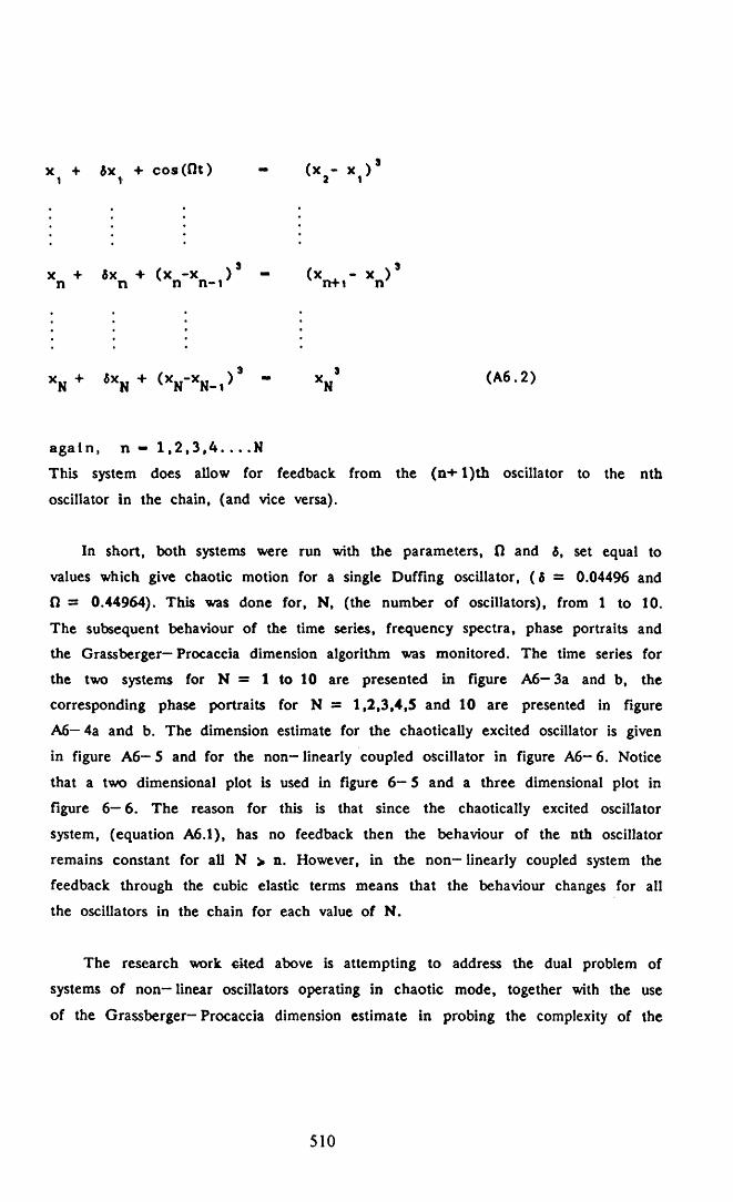
x + 6x + cos(Ot) - (x - x ) S 1 1 2 1

X +n fix + ( x - x ) n n n- i (x - x ) 3 n+i n

xN + fixN + <xN-xN - l ) 3 " XN3 (A6.2)

again , n - 1 , 2 , 3 , 4 . . . . NThis system does allow for feedback from the (n + l) th oscillator to the nth

oscillator in the chain, (and vice versa).

In short, both systems were run with the parameters, ft and 6 , set equal to

values which give chaotic motion for a single Duffing oscillator, ( 6 = 0.04496 and

fl = 0.44964). This was done for, N, (the number of oscillators), from 1 to 10.

The subsequent behaviour of the time series, frequency spectra, phase portraits and the Grassberger— Procaccia dimension algorithm was monitored. The time series for

the two systems for N = 1 to 10 are presented in figure A6 — 3a and b, the

corresponding phase portraits for N = 1,2,3,4,5 and 10 are presented in figure

A6 — 4a and b. The dimension estimate for the chaotically excited oscillator is given

in figure A6 — 5 and for the non- linearly coupled oscillator in figure A6 - 6 . Notice

that a two dimensional plot is used in figure 6 — S and a three dimensional plot in

figure 6 — 6 . The reason for this is that since the chaotically excited oscillator

system, (equation A6.1), has no feedback then the behaviour of the nth oscillator

remains constant for all N > n. However, in the non— linearly coupled system the

feedback through the cubic elastic terms means that the behaviour changes for all

the oscillators in the chain for each value of N.

The research work cited above is attempting to address the dual problem of

systems of non-linear oscillators operating in chaotic mode, together with the use

of the Grassberger—Procaccia dimension estimate in probing the complexity of the

510

output of such systems.

It has been shown that the increase in the number of oscillators in the case of

the chaotically excited system leads to a rapid increase in the dimension estimate,

reaching a limit between 10.0 and 12.0. However, the same is not true for the

more realistic, non— linearly coupled system. In this case, the increase in the

number of oscillators in the system first led to a rapid decrease in the systems

complexity, with N = 3 providing a periodic response. Increases in N above 3

then led to an increase in the average dimension estimate, again a limiting value

of the estimate was reached at between 1 0 . 0 and 1 2 .0 .

Further studies should investigate the apparent maximum dimension obtained,

between 1 0 . 0 and 1 2 . 0 to see if this is a maximum dimension of such oscillator

systems or rather an inherent limit to the Grassberger— Procaccia dimension

estimate. In addition, the N = 3, non— linearly coupled system is particularly

interesting, as the system reverts from a chaotic response at N = 2 to a periodic

response. In this case, the act of increasing the number of degrees of freedom of

the system, and therefore the intrinsic complexity of the system, has the counter— intuitive effect of decreasing the complexity of the system. This effect in

itself warrants further study.

511

zuId<J5CLif)Q - 5 0 0

1 0 0 200

TIME (s )

3 0 0 4 0 0

(a ) Time S e r i e s

•xroo_Ju>

500

250 ..

0

-250 .

-500-500 -250 0 250

DISPLACEMENT(x)500

(b) Phase P o r t r a i t

F i g u r e A 6 - 1 ; T y p i c a l T r a n s l en t . Time S e r i e s w i t h P h a s e P o r t r a i t

512

- 3- 3 - 2

LOG (r)

- 3

-10

- 2 0

LOC C (r)

- 2 5

- 2- 5

LOG (f)

-3

-10

- 2 0

- 2 3

(a) 2000 points (b) 5000 points

-3 - 4 - 2

L O C .(r)

- 3

- 1 0

-2 0

LO C .C (r)

- 2 5

- 3-a -3 - 4 - 2 -1

UOC.(r)

-3

-1 0

-13

- 2 0

- 2 3

(c) 10,000 points (d) 15,000 points

El&ure A6-2; *l o g f r ) - l o £ ( C r ) ' P l o t f o r V a r i o u s Lengths o f t h e I l_me_Ser ies o f f i g u r e A 6 - l a

513

• 000 10 i 0 i 020 * 030 1 040 1000 10101 020 1 030 1 040 i 050TIME (s )

( a ) C h a o t i c a l l y E x c i t e d

ij/WVWV'v■* • •

AaAAAAA- a J

A fV W W

IlMAA/W1W V W W

iMVWWI/'w v w ww w w v$— i------------------1— i-----------------1-----------------1

rt • 1 0

v w w w— 1------------------1------------------1------------------1------------------1v .n i n 1 :'i i " ." n i <** i '

T!ME i s )(b) N o n - L i n e a r l y Coupled

F i g u r e A6-3: Time S e r i e s o f t he F i r s t Ten O s c i l l a t o r s

514

nIc*■t

(3 g£> : :

1c

uPO f i i i

4 - m - m i i«

H ~ f ■ f M l l Ji

H - M 1 H 1 1

+ XH Z w£ w u

Cu c/ d >-*

+ Q

( X ) A 1 I D 0 1 3 A

"OC<4m

roCM

H

Ic

•o4>cxoou

u(4«cZjIco

55

M i l

t X

HZw

■fH i H IHH fHHHUI nUiniHllllHllllllllllHllHnHI

wu

cuc/ d

( X ) A J L I 3 0 1 3 A

•oc€0U->

<rCOCM

HIc

•d

oxw

o<4JZu

515

Fi„,

ir«.

A

6-4

- Ph

ase

Por

trai

ts

gf

th«

Fir

st

Ttn

OK

llU

wrs

.

GRASSBERGER*PROCACCIADIMENSIONESTIMATE

14

12

10

8

6

4

2

0s3 4 61 2 7

NUMBER OF OSCILLATORS (N)

F i g u r e A6-5; The V a r i a t i o n In t h e Average G r a s s b e r g e r - P r o c a c c l a Dimens ion E s t i m a t e w i t h t h e Number o f O s c i l l a t o r s In t h e C h a o t i c a l l y E x c i t e d Sys tem

g r a s s b e r g e rPROCACCIAd i m e n s i o nESTIMATE

NUMBER OF OSCILLATORS

(N)

OSCILLATOR (n)

F i g u r e A6-6: The V a r i a t i o n In t h e C r a s s b e r g e r - P r o c a c c 1 aDimens ion E s t i m a t e w i t h t he Number o f O s c i l l a t o r s I n t h e Non-Li n e a r l y Coup l e d System

5 1 6

REFERENCES

REFERENCES

Abraham N.B. & Gollub J.P., "Testing Non-linear Dynamics", Physica-D, 1984, Vol.11, pp 252-264.

Abraham N.B., Albano A.M., Das B. , De Guzman G.,Yong S., Gioggiars R.S., Puccioni G.P. & Tredicce J.R., Calculating the Dimension of Attractors from Small Data Sets", Phys. Lett. A, 1986, Vol.114, pp 217-221.

Addison P.S., "A Report on Work Done to Date on an Experimental Investigation into Vortex Dominated Flows at a Pipe Orifice", Research Report No.2, August 1991, Civil Engineering Department,University of Glasgow.

Addison P.S., Chan A.H.C., Ervine D.A. & Williams K.J., "On the Numerical Method Dependant Solutions of a Modified Duffing Oscillator“, Communications in Applied Numerical Methods, 1992, Vol.8, pp519-528.

Arecchi F.T., "Hyperchaos and 1/f spectra in Nonlinear Dynamics", from "Chaos, Noise and Fractals", edited by E.R. Pike & L.A. Lugiato, 1987, Adam Hilger, pp 1-14.

Aref H., Jones S.W., Mofina S. & Zawadzki I., "Vortices, Kinematics and Chaos", Physica D, 1989, pp 423-440.

Argoul F, Arneodo A, Grasseau G., Gaone Y.,Hopfinger E.J. & Frisch U., "Wavelet Analysis of Turbulence Reveals the Multifractal Nature of the Richardson Cascade", Nature, 1989, Vol.338, pp 51- 53 .

517

ArgouL F ., Arneodo A., Elezgaray J, Grasseau G. & Murenzi R., "Wavelet Transforms of Fractal Aggregates", Phys. Lett. A, 1989, Vol.135, pp327- 336.

Arneado A., Coullet P. & Tresser C., "On the Observation of an Uncompleted Cascade in a Rayleigh- Benard Experiment", Physica-D, 1983, Vol.6, pp 385- 392.

Arneodo A, Grasseau G. & Holschneider M . , "Wavelet Transform of Multifractals", Phys. Rev. Lett., 1988, Vol.61, pp 2281-2284.

As far K.R. and Masoud K.K., 'On the Period-Doubling Bifurcations in the Duffing's Oscillator with Negative Linear Stiffness', A.S.M.E., Journal of Vibration and Acoustics, Vol.114, 1992, pp489-494.

B.S. 188:1977, "Methods for Determination of the Viscosity of Liquid", British Standards Institution.

B.S.1042:1989, "Pressure Differential Devices", British Standards Institution.

Back L.H. & Roschke E.J., "Shear-Layer Flow Regimes and Wave Instabilities and Reattachment Lengths Downstream of an Abrupt Circular Channel Expansion", Trans. A.S.M.E, Journal of Applied Mechanics, 1972, pp 677-681.

Baird M.H.I., Round G.F. & Cardenas J.N., "Friction Factors in Pulsed Turbulent Flow", The Canadian Journal of Chemical Engineering, 1971, Vol.49, pp 220-223.

518

Bak P. & Chen K., "The Physics of Fractals", Physica-D, 1989, Vol.38, pp 5-12.

Bak P., Chen K. & Tang C., "A Forest Fire Model and Some Thoughts on Turbulence", Phys. Lett A, 1990, Vol.147, pp 297-300.

Baker G.L. & Gollub J.P., "Chaotic Dynamics - an Introduction", Cambridge University Press, 1990#

Bakhmeteff B.A., "The Mechanics of Turbulent Flow", Princeton University Press, 1936.

Bandyopadhyay P.R., "Aspects of the Equilibrium Puff in Transitional Pipe Flow", J. Fluid Mech., 1986, Vol.163, pp 439-458.

Bandyopadhyay P.R., Private Communication,April,1989.

Barford N.C., "Experimental Measurements: Precision Error and Truth", John Wiley and Sons, 1985.

Barr D.I.H., "Two Additional Methods of Solution of the Colebrook-White Function", Proc. Inst. Civ.Engrs., 1975, Part2, Vol.59, pp827-835.

Batchelor G.K., "The Theory of Homogeneous Turbulence", Cambridge Monographs on Mechanics and Applied Mathematics, Cambridge University Press, 1960.

519

Baumann N. , Joseph D.D., Mohr P. & Renardy Y.,"Vortex Rings of One Fluid Inside Another in Free Fall", Phys. Fluids. A, 1992, Vol.4, pp 567-580.

Bell K.J. & Bergelin O.P., "Laminar and Transition Flow in Annular Orifices of Fine Clearance", from, "Flow Measurement in Closed Conduits", Proc. Symposium N.E.L. 27th-30th Sept. 1960, H.M.S.O.,1962, pp 439-456.

Belytschko T. & Schoeberle D.F., 'On the Unconditional Stability of an Implicit Algorithm for Non-linear Structural Dynamics', Transactions A.S.M.E., Journal of Applied Mechanics, 1975, pp865- 869.

Ben-Mizrachi A., Procaccia I. & Grassberger P., "Characterisation of Experimental (Noisy) Strange Attractors", Phys. Rev. A, 1984, Vol.29, pp 975-977.

Berge P., Pomeau Y. & Vidal C., "Order Within Chaos", John Wiley & Sons, 1984, pp 111-123.

Bert C.W. & Stricklin J.D., "Evaluation of Various Numerical Integration Methods for Non-linear Dynamic Systems", 24th Annual Technical Meeting, Society of Engineering Science, Sept 20-23rd, 1987, University of Utah, Salt Lake City, Utah.

Binnie A.M. & Fowler J.S., "A Study by a Double Refraction Method of the Development of Turbulence in a Long Circular Pipe", Proc. Royal Society, 1947- 48, Vol.A192, pp 32-44.

Blevins R.D., "Flow Induced Vibration", Van Nostrand Reinhold, 1977, pp 1-54.

520

Boldrighini C. & Franceschini V. , "A Five Dimensional Truncation of the Plane Incompressible Navier Stokes Equations", Comm. Math. Phys., 1979, Vol.64, ppl59-17 0 .

Boussinesq M.J., Comptes Rend'us, 1891, pp 9-15 & 49-51.

Bradley T.A. & Ng T.T., "Phase Locking in a Jet Forced with Two Frequencies", Experiments in Fluids, 1989, Vol.7, pp 38-48.

Brandstater A., Swift J., Swinney H.L., Wolf A., Farmer J.D. & Jen E., "Low-Dimensional Chaos in a Hydrodynamical System", Phys. Rev. Lett., 1983,Vol.51, pp 1442-1445.

Brown R.D., Addison P. S. & Chan A.H.C., "Chaos in the Unbalance Response of Journal Bearings", presented at the "Fourth Conference on Non-linear Vibrations, Stability and Analysis of Structures and Mechanisms", Virginia Polytechnic Institute and State University, Blacksburg, Virginia, June 7-11, 1992, (To be published in the journal-Non-linear Dynamics).

Buckingham E. , "Notes on Some Recently Published Experiments on Orifice Meters", Trans. Am. Soc.Mech. Eng., 1956, Vol.78(2), pp 379-387.

Bullock K.J., Lai J.C.S. & Walker T.B, "Flow Measurement Behind Attached Ring-Type Turbulence Promoters", Phys. Fluids, 1990, Vol.2, pp 390-399.

521

Burton T.D. & Anderson M. , "On Asymptotic Behaviour in Cascaded Chaotically Exited Non-Linear Oscillator", Journal of Sound and Vibration, 1989, Vol.133, pp253-258.

Casperen C., "The Vortex Flowmeter", Paper C-l, from, "Fluid Measurement in the Mid 1970's, 1977, edited by E.A. Spencer & W.J. Ramsay, H.M.S.O., pp 147-166.

Chadwick A. & Morfett J., "Hydraulics in Civil Engineering", Allen and Unwin, 1986.

Chen J.J.J. & Ackland A.D., "Correlation of Laminar, Transitional and Turbulent Flow Friction Factor", Proc. Inst. Civ. Eng., Part 2, 1990, Vol.89, pp573- 576.

Choi H.S. & Lou J.Y.K., 'Non-linear Behaviour of an Articulated Offshore Loading Platform' , Journal of Applied Ocean Research, 1991, Vol.13, pp 63-74.

Colebrook C.F., "Turbulent Flow in Pipes, with Particular Reference to the Transition Between the Smooth and Rough Pipe Laws", J. Inst. Civ. Eng.,1939, Vol.11, pp 135-156.

Conlisk A.T., Guezennec Y.G. & Elliott G.S.,"Chaotic Motion of an Array of Vortices Above a Flat Wall", Phys. Fluids A, 1989, Vol.l, pp 704-717.

Conrad M. , "What is the Use of Chaos ?", from ""Chaos", edited by A.V. Holden, Manchester University Press, 1986, pp 3-14.

522

Cooley J.W., Lewis P.A.W. & Welch P.D., "The Fast Fourier Transform and its Applications", I.E.E.E. Transactions on Education, 1969, Vol.2, pp27-34.

Corcos G.M. & Sellars J.R., "On the Stability of Fully Developed Flow in a Pipe", J. Fluid Mech., 1959, Vol.5, pp 97-112.

Crutchfield J., Farmer D. , Packard N. , Shaw R.,Jones G. & Donelly R.J., "Power Spectral Analysis of a Dynamical System", Phys. Lett., 1980, Vol.76A, pp 399-401.

Cvitanovic P., "Universality in Chaos", from "Universality in Chaos", edited by P. Cvitanovic, Adam Hilger Ltd., Bristol, 1984.

D'Netto W. & Weaver D.S., "Divergence and Limit Cycle Oscillations in Valves operating at Small Openings", J. Fluids and Structures, 1987, Vol.l, pp 3-18.

Davies J.T., "Turbulence Phenomena", Academic Press, 1972, pp 1-39, 47-62, 121-136.

Deissler R.J. & Kaneko K., "Velocity Dependent Lyapunov Exponents as a Measure of Chaos in Open Flow Systems" Phys. Lett. A, 1987, Vol. 119, pp397- 401.

Detemple-Laake E. & Eckelmann H. , "Phenomenology of Karman Vortex Streets in Oscillatory Flow", Experiments in Fluids, 1989, V o l .7, pp 217-277.

Dinca F. & Teodosiu C., "Non-linear and Random Vibrations", 1973, Academic Press, pp 253-277.

523

Dowell E.H. and Pezeshki C., 'On Necessary and Sufficient Conditions for Chaos to Occur in Duffing's Equation: An Heuristic Approach', Journal of Sound and Vibration, Vol.121, 1988, ppl95-200.

Downing P.M. & Mottram R.C., "The Effects of Flow Pulsations on Orifice Plate Flowmeters", from,"Fluid Measurement in the Mid 1970's, 1977, edited by E.A. Spencer & W.J. Ramsay, H.M.S.O.

Drazin P.G & Reid W.H., "Hydrodynamic Stability", Cambridge University Press, 1981.

Duffing G., "Erzwungene Schwingungen bei Veranderlicher Eigenfrequenz", Vieweg: Braunschweig.

Durst F. & Ruck B., "Effective Particle Size Range in Laser-Doppler Anemometry", Expts. in Fluids,1987, Vol.5, pp 305-314.

Durst F., Maxworthy T. & Pereira J.C.F., "Piston- Driven, Unsteady Separation at a Sudden Expansion in a Tube: Flow Visualization and L.D.A. Measurements", Phys. Fluids A, 1989, Vol.l, ppl249-1260.

Dvorak I. & Klaschka J., "Modification of the Grassberger-Procaccia Algorithm for Estimating the Correlation Exponent of Chaotic Systems with High Embedding Dimension", Physics Letters A, 1990, pp 225-231.

El Masry O.A. & El Shobaki K., "Pulsating Slurry Flows in Pipelines", Experiments in Fluids, 1989, Vol.7, pp 481-486.

524

Elgar S. & Mayer-Kress G., "Observation of the Fractal Dimension of Deep- and Shallow-Water Ocean Surface Gravity Waves", Physica-D, 1989, Vol.37, pp 104-108.

Elgar S., Van Atta C.W. & Gharib M . , "Bispectral Analysis of Ordered and Chaotic Vortex Shedding from Vibrating Cylinders at Low Reynolds Numbers", Physica-d, 1989^ V o l .39, pp 281-286.

Emrich R.J., "Flow Field Measurement by Tracer Photography", Experiments in Fluids1', 1983, Vol.l, pp 179-184.

Everson R. & Sirovich L., "A Survey of Wavelet Analysis Applied to Turbulence Data", Report No. 89- 182, 1989, Centre for Fluid Mechanics, Turbulence and Computation, Brown University, Providence, U.S.A.

Everson R., Sirovich L. & Sreenivasan K.R., "Wavelet Analysis of the Turbulent Jet", Phys. Lett. A, 1990, Vol.145, pp 314-322.

Faler J.H. & Leibovich S., "An Experimental Map of the Internal Structure of a Vortex breakdown", J.F.M., 1978, Vol.86, pp 313-335.

Farmer J.D. , "Spectral Broadening of Period-Doubling Bifurcation Sequences", Phy. Rev. Lett., 1981,Vol.47, pp 179-182.

Farmer J.D., "Chaotic At ractors of an Infinite Dimensional Dynamical System", Physica-D, 1982 Vol.4, pp 366-393.

525

Farmer J.D., "Dimension, Fractal Measures and Chaotic Dynamics", from "Evolution of Order and Chaos in Physics, Chemistry and Biology", Editor H. Haken, Proceedings of the International Symposium of Synergetics, at Schloss Elmau, Bavaria, April 26th - May 1st, 1982a, Springer Verlag, 1982b, pp 174-182.

Farmer J.D., Ott E. & Yorke J.A., "The Dimension of Chaotic Attractors", Physica-D, 1983, Vol.7, pp 153- 180.

Feigenbaum M.J., "Universal Behaviour in Non-linear Systems", Los Alamos Science, 1980, Vol.l, pp 4-27.

Fishier L.S. & Brodkey R.S., "Transition, Turbulence and Oscillating Flow in a Pipe", Experiments in Fluids, 1991, Vol.11, pp 388-398.

Fox J.A., Lessen M. & Bhat W.V. , "Experimental Investigation of the Stability of Hagen Poiseuille Flow", Phys. Fluids, 1968, Vol.2, pp 1-4.

Franceschini V. & Tebaldi C., "Sequences of Infinite Bifurcations and Turbulence in a Five-Mode Truncation of the Navier Stokes Equations", J. Stat. Phys., 1979, Vol.21, pp 207-213.

Fraser A.M. & Swinney H.L., "Independent Coordinates for Strange Attractors from Mutual Information", Phys. Rev. A, 1986, Vol.133, pp 1134-1140.

Fraser A.M., "Reconstructing Atrractors from Scalar Time Series: A Comparison of Singular System and Redundancy Criteria", Physica-D, 1989, Vol.34, pp 391-404.

526

Freidmann M. , Gillis J. & Liron N. , "Laminar Flow in a Pipe at Low and Moderate Reynolds Numbers", App. Sci. Res., 1968, Vol.19, pp 426-438.

Froehling H. , Crutchfield J.P., Farmer D . , Packard N.H. & Shaw R. , "On Determining the Dimension of Chaotic Flows", Physica-D, Vol.3, 1981, pp 605-617.

Fukuda K. , Inouye A., Kawabe Y & Hirai A., "Transition from Laminar to Turbulent Flow of Water in a Pipe Measured by a Pulsed N.M.R. Method", J. Phys. Soc. Japan, 1985, Vol.54, pp 4555-4560.

Gardarvsky J., Hrbek J., Chara Z. & Severa M. , "Refraction Corrections for L.D.A. Measurements in Circular Tubes Within Rectangular Optical Boxes", Dantec Information, No.8 , Nov.1989.

Gaster M., "A Note on the Relation Between Temporally Increasing and Spatially Increasing Disturbances in Hydrodynamic Stability", J. Fluid Mech., 1962, Vol.5, pp 222-224.

Gerald C.F. & Wheatley P.O., "Applied Numerical Analysis", 1984, Addison-Wesley Publishing Company, pp 15-20 & 306-312.

Gershenfeld N.A. , "Dimension Measurement on High- Dimensional Systems", Physica-D, 1992, Vol.55, pp 135-154.

Gharib M . , Williams-Stuber K., "Experiments on the Forced Wake of an Airfoil", J.F.M., 1989, Vol.208, pp 225-255.

527

Ghez J .M . & Vaienti S ., "On the Wavelet Analysis of Multifractal Sets", J. Stat. Phys., 1989, Vol.57, pp 415-420.

Giglio M . , Musazzi S. & Perini U . , "Onset of Chaos in Fluid Dynamics", from "Evolution of Order and Chaos in Physics, Chemistry and Biology", Editor H. Haken, Proceedings of the International Symposium of Synergetics, at Schloss Elmau, Bavaria, April 26th - May 1st, 1982, Springer Verlag, 1982, pp 174-182.

Giglio M . , Musazzi S. & Perini U., "Transition to Chaotic Behaviour via a Reproducible Sequence of Period Doubling Bifurcations", Phys. Rev. Lett.,1981, Vol.47, pp 243-246.

Glass L., Shrier A. & Belair J., "Chaotic Cardiac Rhythms", from, "Non-linear Science: Theory and Applications", edited by A. Holden, Manchester University Press, 1986, pp 237-256.

Goldburg W.I., Pak H.K. & Tong P., "A Light Scattering Study of Turbulence", Physica-D, 1989, Vol.38, pp 134-140.

Goldstein S. (Editor), "Modern Developments in Fluid Dynamics", 1938, Vol.l, Oxford University Press, pp 299-308.

Gollub J.P. & Benson S.V., "Many Routes to Turbulent Convection", J. Fluid Mech., 1980, Vol.100, pp 449- 470.

528

Gottwald J.A., Virgin L.N. and Dowell E.H., 'Experimental Mimicry of Duffing's Equation',Journal of Sound and Vibration, Vol.158, 1992, p p 4 4 7 - 4 6 7 .

Grassberger P. & Procaccia I., "Characterisation of Strange Attractors", Phys. Rev. Lett., 1983©,) V o l . 50, pp 346-349.

Grassberger P. & Procaccia I., "Estimation of the Kolmogorov Entropy from a Chaotic Signal", Phys.Rev. A, 1983b,Vol.28, PP 2591-2593.

Grassberger P. & Procaccia I., "Measuring the Strangeness of Strange Attractors", Physica-D, 1983c; Vol.9, pp 183-208.

Grassberger P., "Generalised Dimensions of Strange Attractors", Phys. Lett. A, 1983, Vol.97, pp 227-230.

Grassberger P. , "An Optimised Box-Assisted Algorithm for Fractal Dimensions", Phys. Lett. A, 1990,Vol.148, pp 63-68.

Grey F. & Kjems J.K., "Aggregates,- Broccoli and Cauliflower", Physica-D, 1989, Vol.38, pp 154-159.

Grossman A. , Holschneider M . , Kronland-Martinet R. & Morlet J., "Detection of Abrupt Changes in Sound Signals with the Help of Wavelet Transforms", from "Advances in Electronics and Electron Physics", Supplement 19, "Inverse Problems: An Interdisciplinary Study", edited by P.C. Sabatier, Academic Press, 1987, pp 289-306.

529

Guckenheimer J. & Buzyna G. , "Dimension Measurements for Geostrophic Turbulence", Phys. Rev. Lett., 1983, Vol.51, pp 1438-1441.

Guckenheimer J., "Strange Attractors in Fluids: Another View", Ann. Rev. Fluid Mech., 1986, Vol.18, pp 15-31.

Guevara M.R., Glass L. & Shrier A., "Phase Locking, Period Doubling Bifurcations, and Irregular Dynamics in Periodically Stimulated Cardiac Cells", Science, 1981, Vol.214, pp 1350-1353.

Gursul I. & Rockwell D., "Effect of Concentration of Vortices on Streakline Patterns", Experiments in Fluids, 1991, Vol.10, pp 294-296.

Gursul I., Lusseyran D. & Rockwell D., "On Interpretation of Flow Visualization of Unsteady Shear Flows", Experiments in Fluids, 1990, Vol.9, pp 257-266.

Hama F.R., "Streaklines in Perturbed Shear Flow",Physics of Fluids, 1962, Vol.5, pp 644-650.

Haward R.N., "The Strength of Plastics and Glass : A Study of Time Sensitive Materials", Clever-Hume Press Ltd., 1949, pp 74-75.

Hernan M.A. & Jiminez J., "Computer Analysis of a High Speed Film of the Plane Turbulent Mixing Layer", J.F.M., 1982, Vol.119, pp 323-345.

530

Higuchi T., "Relationship Between the Fractal Dimension and the Power Law Index for a Time Series: A Numerical Investigation", Physica-D, 1990, Vol.46, pp 254-264.

Hinze J.O., "Turbulence: An Introduction to its Mechanism and Theory", McGraw-Hill, 1959.

Ho Chih-Ming + Huang Lein-Sang, 'Subharmonics and Vortex Merging in Mixing Layers', J.F.M., 1982,Vol.119, pp 443-473.

Hodgson J.L., "The Laws of Similarity for Orifice and Nozzle Flows", Trans. Am. Soc. Mech. Eng., 1929, Vol.51, pp 303-332.

Holden A.V. & Muhamad M.A., "A Graphical Zoo of Strange and Peculiar Attractors", from "Chaos", edited by A.V. Holden, Manchester University Press, 1986, pp 15-35.

Holmes A.G., Ettles C.M.M. & Mayes I.W., "The Aperiodic Behaviour of a Rigid Shaft in Short Journal Bearings", I.J.N.M.E., 1978, Vol.12, pp 695- 707.

Huang Y. & Huang Y., "On the Transition to Turbulence in Pipe Flow", Physica-D, 1989, Vol.37, pp 153-159.

Huberman B.A. & Rudnick J., "Scaling Behaviour of Chaotic Flows", Phys. Rev. Lett., 1980, Vol.45, pp 154-156.

531

Huberman B.A. & Zisook A.B., "Power Spectra of Strange Attractors", Phys. Rev. Lett., 1981, Vol.40,pp 626-628.

Hudson J.L., Mankin J., McCullogh J. & Lamba P., "Experiments on Chaos in a Continuous Stirred Reactor", from "Non-linear Phenomena in Chemical Dynamics", Proceedings of an International Conference, Bordeaux, France, Sept. 7-llth, 1981, editors C. Vidal & A. Pascault, Springer Verlag, 1981.

Hughes T.J.R., "The Finite Element Method",Prentice-Hall Inc., 1987, pp 490-513.

Iguchi M. , Ohmi M. & Kimura H. , "Behaviour of Turbulent Slugs in Pulsatile Pipe Flow", from,"Fluid Control and its Measurement", Vol.2, 1985, Pergamon Press, edited by M. Harada, pp 951-956.

Infeld E. & Rowlands G. , "Non-linear Waves, Solitons and Chaos", Cambridge University Press, 1990.

Iversen H.W., "Orifice Coefficients for Reynolds Numbers from 4 to 50,000", Trans. A.S.M.E., 1956, Vol.78(2), pp359-364.

Japan Society of Mechanical Engineers, The, "Visualized Flow: Fluid Motion in Basic and Engineering Situation Revealed by Flow Visualization", Pergamon Press, 1988.

532

Johansen F.C., "Flow Through a Pipe Orifice at Low Reynolds Numbers"/ Aeronautical Research Committee, Reports and Memoranda, No. 1252, June 1929,H.M.S.O., Published 1930.

Johansen F.C., "Flow Through Pipe Orifices at Low Reynolds Numbers", Proc. Roy. Soc., 1933, Vol.126a, pp 231-245. ((read 20/7/90))

Jones (Jr.) E.H. & Bajura R.A., "A Numerical Analysis of Pulsating Laminar Flow Through a Pipe Orifice", Trans. A.S.M.E., Journal of Fluids Eng., 1991, Vol.113, ppl99-205.

Kaolin R-/ Turkevich L.A., Putterman S.J., RudnickI. & Rudnick J.A., "Subharmonic Sequences in the Faraday Experiment : Departures from Period Doubling", Phys. Rev. Lett., 1981, Vol.47, p 1133.

Kaplan J.L. & Yorke J.A., "Chaotic Behaviour of Multidimensional Difference Equations", from "Functional Differential Equations and Approximations to Fixed Points", Edited by H.O. Peitgen & H.-O. Walther, Lecture Notes in Mathematics, P 730, Springer, Berlin, 1979.

Katona M.G. & Zienkiewicz O.C., "A Unified Set of Single Step Algorithms. Part 3: The Beta-m method, a Generalization of the Newmark Scheme", International Journal for Numerical Methods in Engineering, 1985, Vol.21, pp 1345-1359.

Kay J.M., "An Introduction to Fluid Mechanics and Heat Transfer", Second Edition, Cambridge University Press, 1963, pp 66-69.

533

Kestin J . , Sokolov M. & Wakeham W.A., "Viscosity of Liquid Water in the Range - 8C to 150C", Journal of Physical Chemistry Reference Data, 1978, Vol.7,No.3, pp 941-948.

Keuthe A.M., "Some Features of Boundary Layers and Transition to Turbulent Flow", J. Aero. Sciences, 1962, Vol.14, pp 444-452.

Khezzar L., Whitelaw J.H. & Yanneskis M . , "Round Sudden-Expansion Flows", Proc. Instn. Mecg. Engrs., 1986, Vol.200, pp 447-455.

Kida S., Yamada M. & Ohkitani K., "A Route to Chaos and Turbulence", Physica-D, 1989, Vol.37, pp 116- 125.

Kirmse R.E., "Investigations of Pulsating Turbulent Pipe Flow", Trans. A.S.M.E., Journal of Fluids Engineering, 1979, Vol.101, pp 436-442.

Klebanoff P.S., Tidstrom K.D. & Sargent L.M., "The Three Dimensional Nature of Boundary Layer Instability", J. Fluid Mech., 1962, Vol.12, pp 1-34.

Konishi I, Shiraishi N. & Matsumoto M . , "Vortex Shedding Oscillations of Bridge Deck Sections", fromI.A.H.R. and I.U.T.A.M. Symposium, "Practical Experiences with Flow Induced Vibrations",Karlsruhe/Germany, Sept. 3-6, 1979, University of Karlsruhe, edited by E. Naudascher & D. Rockwell, pp 619-624.

Kostelich E.J. & Yorke J.A., "Noise-Reduction: Finding the Simplest Dynamical System Consistent with the Data", Physica-D, 1990, Vol.41, pp 183-196.

534

Kowalke O.L., "Manner of Liquid Flow Through a Pipe Orifice", Industrial and Engineering Chemistry,1938, Vol.30, pp216-222.

Kronland-Martinet R., "The Wavelet Transform for the Analysis, Synthesis and Processing of Speech and Music Sounds", Computer Music Journal, 1988, Vol.12,pp 1 1 -2 0 .

Kuramoto Y . , "Meeting Report: The 6 th Kyoto Summer Institute. Chaos an Statistical Mechanics", Physica D, 1984, Vol.11, pp 384-386.

Kurzweg U.H., Lindgren E.R. & Lothrop B. ,"Onset of Turbulence in Oscillating Flow at Low Wormsley Numbers", Phys. Fluids A, 1989, Vol.l, pp 1972-1975.

Landau L., "On the Problem of Turbulence", C.R.Acad. Sciences U.R.S.S., 1944, Vol.44, pp 311-316.

Lanford O.E., "Strange Attractors and Fluid Turbulence", from "Hydrodynamic Instabilities and the Transition to Turbulence", edited by H.L.Swinney and J.P. Gollub, Springer-Verlag, 1981, Chapter 2, pp7-26.

Langhaar H.L., "Steady Flow in the Transition Length of a Straight Tube", Trans. A.S.M.E., J. Appl.Mech., 1942, Vol.64, pp A55-A58.

Lau J.C., Whiffen M.C, Fisher M.J. & Smith D.M., "A Note on Turbulence Measurements with a Laser Velocimeter", J. Fluid Mech., 1981, Vol.102, pp 353- 366.

535

Leiber B.B. & Giddens D.P., "Autoregressive Spectral Estimation in Transitional Pulsatile Flow", Experiments in Fluids, 1989, Vol.8 , pp 209-215.

Leite R.J., "An Experimental Investigation into the Stability of Poisseuille Flow", J. Fluid Mech.,1959, Vol.5, p 81.

Leite R.J., "An Experimental Investigation of the Stability of Axysymmetric Poisseuille Flow", Report No. OSR-TR-56-2, University of Michigan, Ann Arbour, Nov. 1957.

Lesieur M . , "Turbulence in Fluids", Nijhoff Publishers, 1987#

Lessen M. , Fox J.A., Bhat V.W. & Ting-Yung L., "Stability of Hagen Poiseuille Flow", The Physics of Fluids, Vol.7, 1964, pp 1384-1385.

Lewis R.D., Foreman J.W., Watson H.J. & Thornton J.R. , "Laser Doppler Velocimeter for Measuring Flow- Velocity Fluctuations", Phys. Fluids, 1968, Vol.2, pp 433-435.

Lighthill J., "An Informal Introduction to Theoretical Fluid Mechanics", Clarendon Press, Oxford, 1986, pp 59-75.

Lin C.C., "The Theory of Hydrodynamic Stability", Cambridge Monographs on Mechanics and Applied Mechanics, Cambridge University Press, 1966.

Lindgren E.R., "Propagation Velocity of Turbulent Slugs and Streaks in Transition Pipe Flow", The Physics of Fluids, 1969, Vol.12, pp 418-425.

536

Lindgren E.R., "The Transition Process and Other Phenomena in Viscous Flow", Arkiv for Fysik, 1957, Vol.12, pp 1 -169.

Linford A., "Flow Measurement and Meters", 1961,2nd edition, E. & F.N. Spon Ltd., pp 84-99.

Lorenz E.N., "Deterministic Nonperiodic Flow", J. Atmos. Sciences, 1963, Vol.20, pp 130-141.

Low B.B., "Mathematics", Longman Green & Co., 1931, pp 23,61,74.

Lugt H.J., "The Influence of Swirling Flow on the Discharge Coefficients of Standard Pressure Differential Flow Meters", The British Hydromechanics Research Association, Report T716, Feb., 1962.

Lugt H.J., "Vortex Flow in Nature and Technology", John Wiley and Sons, 1983, pp 1-126 (Part One).

Mackey M.C. & Glass L., "Oscillation and Chaos in Physiological Control Systems", Science, 1977,Vol.197, pp 287-289.

Mair W.A. & Maul D.J., "Bluff Bodies and Vortex Shedding - A Report on Euromech 17", Journal of Fluid Mechanics, 1971, Vol.45, pp 209-224.

Mandelbrot B.B., "The Fractal Geometry of Nature", W.H. Freeman & Co., 1977.

537

Mansoori A., "On the Turbulent Velocity and Pressure Fluctuations Occurring in Water at a Sudden Enlargement"/ Ph.D. Thesis, University of London, July 1988.

Martinez-Val R., Viedma A. & Cuerno C., "Eul&rian and Lagrangian Description of a Pulsatile, Partially Turbulent Flow", Experiments in Fluids, 1990, Vol.9, pp 129-136.

Matisse P. & Gorman M . , "Neutrally Buoyant Anisotropic Particles for Flow Visualization", The Physics of Fluids, 1984, Vol.27, pp 759-760.

Mayer-Kress G., "Application of Dimension Algorithms to Experimental Chaos", from “Directions in Chaos" edited by Hao Bai-Lin, World Scientific; 1987, pp 122-147.

Mercader I., Massaguer J.M. & Net M. , "Hysterisis on the Transition to Chaos", Phys. Lett A, 1990,Vol.149, pp 195-199.

Merzkirch W . , "Flow Visualization", 1987, Second Edition, Academic Press, pp 1-82.

Miles J., "Strange Attractors in Fluid Dynamics", Advances in Applied Mechanics, 1983, Vol.24, pp 189- 214.

Miller D.S., "Internal Flow Systems", 1978, Vol.5, B.H.R.A. Fluid Engineering Series, pp276-281.

Mills R.D., "Numerical Solution of Viscous Flow Through a Pipe Orifice at Low Reynolds Numbers", J. Mech. Eng. Sci., 1968, Vol.10, No.2, pp 133-140.

538

Mitchell A.R., Stein G & Maritz M . , 'Periodic Structure Beyond a Hopf Bifurcation', Communications in Applied Numerical Methods, Vol.4, 1988, pp 263- 272.

Moss E.A., “The Identification of Two Distinct Laminar to Turbulent Transition Modes in Pipe Flows Accelerated from Rest", Expts. in Fluids, 1989,Vol.7, pp 271-274.

Mottram R.C. & Robatti B., "A Comparison of Effects on Vortex and Orifice Flowmeters", from, "Fluid Control and its Measurement", Vol.2, 1985, Pergamon Press, edited by M. Harada, pp 957-963.

Mullin T. & Price T.J., "An Experimental Investigation of Chaos Arising from the Interaction of Steady and Time Dependent Flows", nature, 1989, Vol.340, pp 294-296.

Newland D.E., "Random Vibrations and Structural Analysis", Longman, 1975, 1st edition, Ch.4,10,12.

Nigro F.E.B., Strong A.B. & Alpay S.A., "A Numerical Study of the Laminar Viscous Incompressible Flow Through a Pipe Orifice", Trans. A.S.M.E., Journal of Fluids Engineering, 1978, Vol.100, pp 467-472.

Novikov E.A., "Chaotic Vortex-Body Interaction", Phys. Lett. A, 1991, Vol.152, pp 393-396. ((read 1/11/91))

Oppenheim A.K. & Chilton E.G., "Pulsating Flow Measurement - A Literature Survey", Trans. A.S.M.E., 1955, Vol.77(2), pp231-245 .

539

Osborne A.R. & Provenzale A., "Finite Correlation Dimension for Stochastic Systems with Power law spectra", Physica-D, 1989, Vol.35, pp 357-381.

Owen P.R., "Buffeting Excitation of Boiler Tube Vibration", J. Mech. Eng Sci., 1985, Vol.7, pp 431-439.

Packard N.H., Crutchfield J.P., Farmer J.D. & Shaw R.S., "Geometry from a Time Series", Phys. Rev Lett., 1980, Vol.45, pp 712-716.

Paidoussis M.P. & Moon F.C., 'Nonlinear and Chaotic Fluidelastic Vibrations of a Flexible Pipe Conveying Fluid', J.Fluid and Structures, 1988, Vol.2, pp 567- 591.

Park K.C., 'An Improved Stiffly Stable Method for Direct Integration of Nonlinear Structural Dynamic Equations", Transactions A.S.M.E, Journal of Applied Mechanics, 1975, pp464-470.

Patel V.C. & Head M.R., "Some Observations on Skin Friction and Velocity Profiles in Fully Developed Pipe and Channel Flows"; J. Fluid Mech., 196*1/Vol.38, pp 181-202.

Percival I. & Richards D., "Introduction to Dynamics, Cambridge University Press, 1982.

Peitgen H.O. & Richter P.H., "The Beauty of Fractals", Springer- Verlag, 1986, pp 1-26.

540

Perry A .E . & Fairlie B.D., "Critical Points in Flow Patterns"/ Adv. in Geophys., 1974# V 0 I.BI8 , pp 299- 315.

Perry A .E . & Lim T.T., "Coherent Structures in Coflowing Jets and Wakes", J. Fluid Mech., 1978,Vol. 8 8 , pp 451-463.

Perry A.E., Lim T.T. & Chong M.S., "The Instantaneous Vector Fields of Coherent Structures in Coflowing Jets and Wakes", J. Fluid Mech., 1980, Vol.101, pp 243-256.

Peterson G.S., "Orifice Discharge Coefficients in the Viscous Flow Range", Trans. A.S.M.E., 19^7,Vol.69, pp765-768.

Pomeau Y., "Front Motion, Metastability and Subcritical Biufurcations in Hydrodynamics", Physica_D, 1986, Vol.23, pp 3-11.

Prenel J.P., Porcar R. & Rhassouli A.E.L., "Three Dimensional Flow Analysis by Means of Sequential and Volumic Laser Sheet Illumination", Experiments in Fluids, 1989, Vol.7, pp 133-137.

Pressing J., "Nonlinear Maps as Generators of Musical Design", Computer Music Journal, 1988,Vol.12, pp 35-46.

Rahman Z. and Burton T.D., 'Large Amplitude Primary and Superharmonic Resonances in the Duffing Oscillator', Journal of Sound and Vibration, 1986, Vol.110(3), pp363-380.

541

Ramap.rian B.R. & Tu S., "An Experimental Study of Oscillating Pipe Flow at Transitional Reynolds Numbers", Journal of Fluid Mechanics", 1980,Vol.100, pp 513-544.

Rao N.S.L. & Sridharan K., "Orifice Losses for Laminar Approach Flow.", Proc. A.S.C.E., J. Hyd. Div., 1972, Vol.98, pp2015-2034.

Reddy J.N., "An Introduction to the Finite Element Method", McGraw-Hill, 2nd Edition, 1986, pp 54-57.

Renyi A., “Probability Theory", North Holland Publishing Co., 1970, pp 540-554.

Reshotko E., "Experimental Study of the Stability of Pipe Flow. 1. The Establishment of an Axially Symmetric Poiseuille Flow.", Progress Report No. 20- 304, 1958, Jet Propulsion Lab., Caltech, California, U.S.A.

Reshotko E., "Remark on Engineering Aspects of Transition", from "Transition and Turbulence" edited by Meyer R.E., Academic Press, 1981, pp 147-148.

Reynolds O. , "An Experimental Investigation of the Circumstances which Determine Whether the Motion of Water Shall be Direct or Sinuous and of the Law of Resistance in Parallel Channels", Phil. Trans. Roy. Soc., 1883, Vol.174, pp 935-982.

Rhee H.S., Koseff J.R. & Street R.L., "Flow Visualization of a Recirculating Flow by Rheoscopic Liquid and Liquid Crystal Techniques", Experiments in Fluids, 1984, Vol.2, pp 57-64.

542

Robertson J.M., "A Turbulence Primer", Engineering Experimental Station Circular, Number 79, (date unknown).

Rockwell D, Nuzzi F. & Magness C., 'Period Doubling in the Wake of a Three-Dimensional Cylinder', Phys. Fluids A, 1991, Vol.3, pp 1477-1478.

Rosenhead L., "Laminar Boundary Layers", Oxford, 1963.

Rossler O.E., "An Equation for Hyperchaos", Phys. Lett., 1979, Vol.71a, pp 155-157.

Rotta J., "Experimenteller Beitrag zur Entstehung Turbulenter Stromung im Rohr", Ing. Archiv, 1956, Vol. 24, pp 258-281.

Rouse H. & Ince S., "History of Hydraulics", Dover Publications Inc., 1957.

Roux J.C. & Swinney H.L., "Topology of Chaos in a Chemical reaction", from "Nonlinear Phenomena in Chemical Dynamics", Proceedings of an International Conference, Bordeaux, France, Sept. 7-llth, 1981, editors C. Vidal & A. Pascault, Springer Verlag, 1981.

Roux J.C., Rossi A., Batchelart S. & Vidal C., "Representation of a Strange Attractor from an Experimental Study of Chemical Turbulence", Physics Letters, 1980, Vol.77a, pp 391-393.

Roux J.C., -Simoyi R.H. & Swinney H.L, "Observation of a Strange Attractor", Physica-d, 1983, Vol.8 , pp 257-266.

543

Rubin Y., Wygnanski I. & Haritonidis J.H., "Further Observations on Transition in a Pipe", from I .U.T.A.M. Conference Proceedings, "Laminar Turbulent Transition", Stuttgart, Germany, Sept. 16- 22, 1979, edited by R. Eppler & H. Fusel, Springer- Verlag, pp 17 - 26.

Ruelle D., "Chaotic Evolution and Strange Attractors", Cambridge University Press, 1989.

Ruelle D., "Chemical Kinetics and Differentiable Dynamical Systems", from "Nonlinear Phenomena in Chemical Dynamics", Proceedings of an International Conference, Bordeaux, France, Sept. 7-llth, 1981, editors C. Vidal & A. Pascault, Springer Verlag, 1981.

Ruelle D., "Five Turbulent Problems", Physica-7D, 1983A, pp 40-44.

Ruelle D., "Strange Attractors", Math. Intell.,1980, Vol.2, pp 126-137.

Ruelle D., "Turbulent Dynamical Systems",Proceedings of the International Congress of Mathematicians, 1983b, August 16-24, Warsaw, pp 271- 286.

Russel D.A., "Dimension of Strange Attractors",Phys. Rev. Lett., 1980, Vol.45, pp 1175-1177.

Sagdeev R.Z., Usikov D.A. & Zaslavsky G.M., "Nonlinear Physics: From the Pendulum to Turbulence and Chaos", Harwood Academic Publishers, 1988.

544

Sano M. & Sawada Y., "Measurement of the Lyapunov Spectrum from a Chaotic Time Series", Phys. Rev. Lett., Vol.55, 1985, pp 1082-1085.

Schiller L., "Die Entwicklung der Laminaren Geschwindigkeits- Verteilung und Ihre Bedeutung fur Zahigkeitsmessungen", Zeitschrift fur Angewandte Mathematik und Mechanic, 1922, pp 96-106.

Schlichting S., “Boundary Layer Theory", McGraw Hill, 1979, 7th Edition,

Schlien D.J., "Inexpensive Method of Generation of a Good Quality Laser Light Sheet for Flow Visualization", Expts. in Fluids, 1987, Vol.5, pp 356-358.

Schuster H.G., "Deterministic Chaos: An Introduction", Physik-Verlag, 1984.

Seino M. & Sawada Y, "Chaotic Attractors in Rayleigh Benard Systems", from Chaos and Statistical Methods", Proceedings of the Sixth Kyoto Summer Institute, Kyoto, Japan, Sept. 12-15, 1983, editor Y. Kurimoto, Springer Verlag, 1984, pp 167-169.

Sexl T. , "Uber Dreidimensionale Storungen der Poisseuilleschen Stromung", Ann. Phys., 1927b,Vol.84, pp 807-822.

Sexl T. , "Zur Stabilitatsfrage der Poisseuilleschen und Couetteschen Stromung", Ann. Phys., 1927a,Vol.83, pp 835-848.

545

Shannon C.E. & Weaver W., "The Mathematical Theory of Communication", The University of Illinois Press: Urbana, 1949.

Shaw R./ "The Dripping Faucet as a Model Chaotic System"/ Aerial Press/ 1984.

Sibulkin M . / "Transition from Turbulent to Laminar Pipe Flow", Phys. of Fluids, 1962, Vol.5, pp 280- 284.

Smith A.M.O., "Remarks on Transition in a Round Tube", J. Fluid Mech., 1960, Vol.17, pp 565-576.

Smith L.A., "Intrinsic Limits on Dimension Calculations", Physics Letters A, 1988, Vol.133, pp 283-288.

Snedecor G.W. & Cochran W.G., "Statistical Methods", The Iowa State University Press, Ames, Iowa, U.S.A., 1967, pp 59-62.

Soliman M.S. & Thompson J.M.T., 'Transient and Steady State Analysis of Capsize Phenomena', Applied Ocean Research, 1991, Vol.13, pp82-92.

Sprenkle R.E., "The Thin-Plate Orifice for Flow Measurement", from "Flow Measurement in Closed Conduits", Proc. Symposium N.E.L., 27th-30th Sept., 1960, H.M.S.O. 1962, ppl25-137.

Sreenivasan K.R. & Ramshyankar R., "Transmission Intermittency in Open Flows and Intermittency Routes to Chaos", Physica-D, 1986, Vol.23, pp 246-258.

546

Sreenivasan K.R., "Fractals and Multifractals in Fluid Turbulence"/ Annual Revue of Fluid Mechanics, 1991, Vol.23, pp 539-600.

Stuart J.S., "Stability and Transition: Some Comments on the Problems", from I.U.T.A.M. Conference Proceedings, "Laminar Turbulent Transition", Stuttgart, Germany, Sept. 16-22, 1979, edited by R. Eppler & H. Fusel, Springer Verlag, pp 1 - 13.

Swinney H.L., "Observations of Order and Chaos in Nonlinear Systems", Physica-D, 1983, Vol.7, pp 3-15.

Swinney H.L. & Gollub J.P., "Introduction", from "Hydrodynamic Instabilities and the Transition to Chaos", Springer-Verlag, 1981, Chapter 1, pp 1-6.

Swinney H.L., Simoyi R.H. & Roux J.C., "Instabilities and Chaos in a Chemical Reaction", from Chaos and Statistical Methods", Proceedings of the Sixth Kyoto Summer Institute, Kyoto, Japan,Sept. 12-15, 1983, editor Y.Kurimoto, Springer- Verlag, .1984, pp 167-169.

Tabeling P., Cardoso O. & Perrin B . , "Chaos in a Linear Array of Vortices", J.F.M., 1990, Vol.213, pp 511-530.

Tatsumi T. , "Stability of the Laminar Inlet-Flow Prior to the Formation of Poiseuille Regime, 1M, J. Phys. Soc. Japan, 1952, Vol.7, pp 489-495.

Tatsumi T., "Stability of the Laminar Inlet-Flow Prior to the Formation of Poiseuille Regime, 2", J. Phys. Soc. Japan, 1952, Vol.7, pp 495-502.

547

Teitgen R., "Laminar-Turbulent Transition in Pipe Flow. Development and Structure of the Turbulent Slug", from I.U.T.A.M. Conference Proceedings, "Laminar Turbulent Transition", Stuttgart, Germany, Sept. 16-22, 1979, edited by R. Eppler & H. Fusel, Springer-Verlag, pp 27-36.

Tennent R.M., "Science Data Book", 1986, Oliver and Boyd.

Thompson J.M.T. & Stewart H.B., "Nonlinear Dynamics and Chaos", John Wiley and Sons, 1986, pp 1-131.

Velarde M.G. & Antoranz J.C., "Strange Attractor (Optical Turbulence) in a Model Problem for the Laser with Saturable Absorber and Two Component Benard Convection" Prog. Theor. Phys., 1981, Vol.6 6 , No.2, Progress Letters, pp 717-720.

Voss R.F., "Random Fractals: Self Affinity in Noise, Music, Mountains and Clouds", Physica-D, 1989,Vol.38, pp 362-371.

Waldner F. , Barberis D.R. & Yamazaki H. , 'Route to Chaos by Irregular Periods: Simulations of Parrallel Pumping in Ferromagnets' , Phys. Rev. A, 1985,Vol.31, pp420-431.

Ward-Smith A.J., "Pressure Losses in Ducted Flows", Butterworths, London, 1971, ppl-27 & 135-191.

Ward-Smith A.J., "Internal Fluid Flow: The Fluid Dynamics of Flow in Pipes and Ducts", Clarendon Press, Oxford, 1980,

548

Weaver D.S., Adubi F.A. & Kouwen N, "Flow Induced Vibration of a Hydraulic Valve and their Elimation", J.Fluids Eng., 1978, Vol.100, pp 239-245.

Webb W.H. & Harrington R.P., "Vortex Structures in Pipe Flow", J. Aero. Sciences, 1956, Vol.23, pp 792- 793 .

West G.S. & Apelt C.J., "Measurements of Fluctuating Effects on Circular Cylinder in a Uniform Flow at Subcritical Reynolds Number. Part 1: The Pressure Distribution and Lift and Drag forces on an Elemental Cross Section", University of Queensland, Dept, of Civil Engineering, Research Report, No. CE109, July 1990.

West R.G., “Developments in Flow Metering by Means of Orifice Plates", from "Flow Measurements in Closed Conduits" Proc. Sympoium N.E.L., 27th-30th Sept., 1960, H.M.S.O., 1962, ppl65-186.

White F.M., "Viscous Fluid Flow", McGraw Hill ,1974, pp 1-25, 61-77, 385-452.

Wigner E.P., "The Unreasonable Effectiveness of Mathematics in the Natural Sciences", Comm. Pure & Appl. Math., 1960, pp 1-14.

Willert C. & Gharib M . , "A New Video Technique to Capture Images Generated by a Smoke Wire",Experiments in Fluids, 1989, Vol.8, pp 236-237.

Williams-Stuber K. & Gharib M . , "Transition from Order to Chaos in the Wake of an Airfoil", J.F.M.,1990, Vol.213, pp 29-57.

549

Withers W. J., "Pressure Fluctuations in the Plunge Pool of an Impinging Jet Spillway", Ph.D. Thesis No. 8913, University of Glasgow, 1991.

Wolf A., "LYAPU-NEWS: Documentation for F.E.T., a Program that Quantifies Chaos in a time Series", supplied by A.Wolf, Dept, of Physics, The Cooper Union, 51, Astor Place, New York, N.Y., 10003^1.

Wolf A., "Quantifying Chaos with Lyapunov Exponents", from "Nonlinear Science: Theory and Applications", edited by A. Holden, Manchester University Press, 1986, pp 273-290.

Wolf A., Swift J.B., Swinney H.L. & Vastano J.A., "Determining Lyapunov Exponents from a Time Series", Physica-D, 1985, Vol.61, p 285.

Wood W.L. & Oduor M.E., 'Stability Properties of Some Algorithms for the Solution of Nonlinear Dynamic Vibration Equations', Comm. App. Num. Meth., 1988, Vol.4, pp 205-212.

Wygnanski I., Sokolov M. & Friedman D., "On Transition in a Pipe. Part 2. The Equilibrium Puff", J. Fluid Mech., 1975, pp 283-304.,

Wygnanski I.J. & Champagne F.H., "On Transition in a Pipe. Part 1. The Origin of Puffs and Slugs and the Flow in a Turbulent Slug", J. Fluid Mech., 1973,Vol.59, pp 281-335.

550

Yamada T. & Fujisaka H., "Coupled Chaos", from Chaos and Statistical Methods", Proceedings of the Sixth Kyoto Summer Institute, Kyoto, Japan, Sept. 12-15, 1983, editor Y.Kurimoto, Springer-Verlag, 1984, pp 167-169.

Yorke J.A. & Yorke E.D., "Chaotic Behaviour and Fluid Dynamics", from "Hydrodynamic Instabilities and the Transition to Turbulence", edited by H.L. Swinney & J.P. Gollub, Springer-Verlag, 1981,Chapter 4, pp 77-95.

Yoshitani Y., Sakuta H. & Koba T., "Flexible Orifice Flowmeter" from, "Fluid Control and its Measurement", Vol.2, 1985, Pergamon Press, edited by M. Harada, pp 893-899.

Zanker K.J. & Cousins T., "The Performance and Design of Vortex Meters", Paper C-3, from, "Fluid Measurement in the Mid 1970's, 1977, edited by E .A. Spencer & W.J. Ramsay, H.M.S.O., pp 147-166.

Zdravkovich M.M., "Smoke Observations of the Formation of a Karman Vortex Street", J. Fluid Mech., 1969, Vol.37, pp 491-496.

551

ADDITIONAL REFERENCES

Birkhoff G. & Zarantonello E.H., 'Jets, Wakes and Cavities', New York Academic Press, 1957.

Bullock K.J., Lai J.C.S. & Walker T.B., 'Flow Measurement behind Attached Ring-type Turbulence Promoters', Phys. Fluids A, Vol.2, 1990, pp390-399.

Chen K. & Bak P., 'Is the Universe Operating at a Self Organised State?*, Phys. Lett. A, Vol. 140, 1989, pp299-302.

Duncan W.J., Thom A.S. & Young A.D., 'Mechanics of Fluids', Arnold, 2nd Edition, 1970.

Baker G.L. & Gollub J.P., 'Chaotic Dynamics', Cambridge University Press, 1990.

Hanko Z.G., 'Vortex Induced Oscillations at low Head Weirs', Proc. Am. Soc. Civil Engineers, Journal of the Hydraulics Division, Vol.6, 1967, pp255-270.

Iguchi M., Ohmi M. & Kimura H., Behaviour of Turbulent Slugs in Pulsatile Pipe Flow', from, 'Fluid Control and Its Measurement', Vol. 2, Pergammon Press, Edited by M. Harada, 1985, pp951-956.

Hunt J.C.R., Abell C.J., Peterka J.A. & Woo H., 'Kinematical Studies of the Flows Around Free or Surface Mounted Obstacles: Applying Topology to Flow Visualization', Journal of Fluid Mechanics, Vol.86, 1978, ppl79-200.

Morris A.W., 'A review of Vortex Streets, Periodic Wakes, and Induced Vibration Phenomena', Trans. A.S.M.E., Journal of basic Engineering, June 1964, ppl85-196.

Massey B.S., 'Mechanics of Fluids', 5th Edition, Van Nostrand Reinhold (UK), 1984.

O'INeill P.V., 'Advanced Engineering Mathematics', Wadsworth Pub. Co., 1987.

Prandtl L., Essentials of fluid Dynamics: With Applications to Hydraulics, Aeronautics, Meteorology and other Subjects', Blackie, 1952.

Russel D.A., 'Dimension of Strange Attractors', Phys. Rev. Lett., Vol.45, 1980, pi 175.

Sarpkaya T., Experimental Determination of the Critical Reynolds Number for Pulsating Poiseuille Flow', Trans. A.S.M.E., Journal of Basic Engineering, Sept. 1966, pp589-598.

Schaefer J. W. & Eskinazi S., 'An Analysis of the Vortex Street Generated in a Viscous Fluid', Journal of Fluid Mechanics, Vol. 16, 1959, pp241-260.

Smith D., TIow to Generate Chaos at Home', Scientific American, January 1992, ppl21-123.

Tomita K., 'Periodically Forced Nonlinear Oscillators', from, 'Chaos', edited by A.V. Holden, Manchester University Press, 1986.

GLASGOWUNIVERSITYLIBRARY

13818422.pdf - University of Glasgow

Documents

Transcript of 13818422.pdf - University of Glasgow