
Additional heat utilization processes for geothermal aquaponics
Upload
khangminh22Category
view
6download
0
DOE/ID/13040--T3
GEOTHERMAL DIRECT USE ~ ~ 9 2 008686
ENGINEERING AND DESIGN \ GUIDEBOOK
Pad J. E m u , Editor Ben C. Lunis, Editor
*
Geo-Heat Center k g o n Institute of Technology Klamath Falls, Oregon 97601
Published - 1991
Prepared under the sponsorship of the united states Department of Energy
Idaho operations office Idaho Falls, Idaho 83415
Contract Number DE-FGO7-9OID 13040

DISCLAIMER
This report was prepared as an account of work sponsored by an agency of the United States Government. Neither the United States Government nor any agency Thereof, nor any of their employees, makes any warranty, express or implied, or assumes any legal liability or responsibility for the accuracy, completeness, or usefulness of any information, apparatus, product, or process disclosed, or represents that its use would not infringe privately owned rights. Reference herein to any specific commercial product, process, or service by trade name, trademark, manufacturer, or otherwise does not necessarily constitute or imply its endorsement, recommendation, or favoring by the United States Government or any agency thereof. The views and opinions of authors expressed herein do not necessarily state or reflect those of the United States Government or any agency thereof.

DISCLAIMER Portions of this document may be illegible in electronic image products. Images are produced from the best available original document.

NOTICE
This report was prepared as an 8ccount of work sponsored by the United States Government. Neither the United States nor the United States Department of Energy, nor any of their employees, make any warranty,' expressed or implied, or assumes any legal liability or responsibility for the accuracy, pnpleteness, or usefulness of any information, apparatus, product, or process disclosed, or represents that its use would not infringe privately owned rights. Reference herein to any specific commercial product, process, or service by trade name, mark, manufacturer, or otherwise, does not necessarily constitute or imply its endorsement, recommendation, or favoring by the United States Government or any agency thereof. The views and opinions of authors expressed herein do not necessarily state or reflect those of the United States Government or any agency thereof.
GEOTHERMAL DIRECT USE ENGJNEERING AND DESIGN GUIDEBOOK
sec?ond Edition
Comments, criticisms and suggestions regarding the subjectmatter areinvited. Any errorsor omissions in the data should be brought to the attention of the Editor. If required, an errata sheet will be issued.
Printed in the United States of America. ISBN 1-880228-00-9 -- 4
. 1 ~ . . . . , , . , . , . , . . .'
.. . . . . : . ' , , , . . . 11

Department of Energy Washington, DC 20585
Geothermal Energy: A Key Element o f the National Energy Strateqy
Since the ear ly 1970s, our Nation has been subjected t o a se r ies of energy shocks resul t ing from the actions of international ca r t e l s , embargoes, and wars. Each shock has had an adverse impact on our economy and international competitiveness, and focused our a t tent ion on the v i t a l importance of energy to national security in a world i n which sudden, unanticipated perturbations i n energy supply are more the ru le than the exception.
In view of the unique importance of energy to the Nation, and the need fo r a strategy to cope w i t h changing trends and sudden perturbations, President Bush directed the Secretary of Energy, on July 26, 1989, t o develop a National Energy Strategy (NES) , and stated: "Our task is . . . t o make this strategy a l iving and dynamic document, responsive t o new knowledge and new ideas, and t o global, environmental, and international changes. 'I
The development of the NES represents a s ignif icant departure in scope, from past e f for t s : I t represents a comprehensive integration of environmental and economic policies with enersy policies. The NES also represents a s ignif icant departure from past e f fo r t s i n i t s execution: I t involved: (1) nationwide participation i n building publ ic consensus and understanding; (2) a careful assessment of science and technology; (3) an evaluation of option costs; and (4) a robust analysis of domestic and international impacts.
Among i t s key elements, the National Energy Strategy supports increased use of renewable energy (including geothermal ) , and integrated resource planning--a u t i l i t y p l a n n i n g process that includes the consideration of demand reduction options and a1 ternative energy sources. Geothermal energy clear ly has a s ignif icant role to play both i n increasing the Nation ' s supply of cost -ef fec t i ve , environment a1 1 y- acceptabl e energy, and i n ass is t ing u t i l i t i e s i n t he i r integrated resource p lanning by providing them w i t h an effective tool for demand management and demand reduction, i .e., geothermal d i rec t use as typified by the geothermal heat pump.
The future for geothermal energy is b r igh t . Analyses conducted for the NES indicate tha t increased geothermal royal t ies and leasing fees on Federal lands will l ike ly double by the end of the century (from $15,000,000 in 1990 t o over $30,000,000 in 2000). By the year 2030, with an aggressive research program, geothermal capacity on 1 i ne could increase t o 43,000 MWe, whi1.e d i rec t use (including geothermal heat pumps) could reduce the projected national demand for e l ec t r i c i ty by 30,000 MWe. These are achievements well worth s t r iving for!
/
I t is more than just an energy plan.
iii

The "Geothermal Direct Use Engineering and Design Guidebook", first issued i n March, 1989, has played a key ro le i n highlighting and f a c i l i t a t i n g the exponential growth o f geothermal d i rec t use--to an annual r a t e today of over 18 t r i l l i o n BTU's. The uses are leg ion: aquaculture, d i s t r i c t heating systems, agriculture, industrial process heat, crop drying, mushroom growing, space heating, f i sh hatcheries, greenhouses, swimming pools and spas, thermal enhanced o i l recovery (TEOR), heap-leach mining, geothermal heat pumps, treatment of organic and toxic wastes, and desalination. deepens, America will become l e s s dependent on imported o i l , and U.S. u t i l i t i e s will be faced w i t h lower demand growth curves--truly a win-win s i tuat ion f o r a l l concerned.
I commend the authors who have given so freely o f t he i r time t o prepare th i s new edi t ion. reader, t o j o i n w i t h us in u t i l i z ing geothermal energy as an integral par t o f the National Energy Strategy, W
As the u t i l i za t ion o f geothermal energy broadens and
I hope tha t this document will stimulate you, the
John E. Mock, Director Geothermal Division Conservation and Renewable Energy
May 17, 1991
iv

FOREWORD
The Geothermal Direct Use Engineering and Design Guidebook is designed to be a comprehensive, thoroughly practical reference guide for engineers and designers of direct heat projects. These projects could include the coI1veTsion of geothermal energy into space heating and cooling of buildings, district heating, greenhouse heating, aquaculture and ~ '
industrial processing.
i
The initiative to create this Guidebook came from the Geo-Heat Center, with support from the United States, Department of Energy under grant number DE-FG07-90ID 1h40, and from the Idaho National Engineering Laboratory (INEL) under contract number DE-AC07-76ID01570 for the purpose of communicating information COIlcerning the conversion of geothermal energy into direct use applications. This information, which was primarily acquired through assisting developers on many geothermal-direct use projects since 1978, was heretofore uncoordinated and diffuse. The Guidebook attempts to impart a comprehensive uhderstanding of information important to the development of a geothermal direct use project. The text is aimed primarily to the mechanical engineer or technical person responsible for project design. The intent is that the contents should be of a practical and technical nature, and answer questions most commonly asked by engineers designing direct use projects. In addition, the authors hope that the Guidebook will be useful to a wide circle of persons intemted in topics ranging from: geology, exploration, well drilling, reservoir engineering, mechanical engineering, engineering cost analysis to regulatory codes, and environmental aspects. Special attention has been paid to unification of expert knowledge drawn from years of experience in order to ensure an integrated view of direct uses of geothermal energy.
The Guidebook is directed at understanding the nature of geothermal ~esoun'~s and the exploration of these resources, fluid sampling techniques, drilling, and completion of geothermal wells through well testing, and mrvoir evaluation. It presents information useful to engineers on the specification of equipment including well pumps, piping, heat exchangers, space heating equipment, heat pumps and absorption refrigeration. A compilation of current information about greenhouse, aquaculture and industrial applications is included together with a discussion of engineering cost analysis, regulation requirements, and environmental consideration.
The purpose of the Guidebook is to provide an integrated view for the development of direct use projects for which there is a very large potential in the United States.
V

coNTRlBuToR!3
Guidebook is written by the following authors who have graciously conttizluted their time and talent for the preparahon of their respective chapters.
Bloomquist, R. Gordon, Geothermal Specialist, Washington State Energy Office, Olympia, WA 98502 - Chapter 20
Culver, Gene, Associate Director, Geo-Heat center, Oregon Institute of Technology, Klamath Falls, OR 97601 - Chapters 3,6, 7, 9, and 11
Ellis, Peter F., Senior Scientist, Radian Corporation, Austin, TX 78720 - Chapter 8
Higbee, Charles, Research Associate, Geo-Heat Center, Oregon Institute of Technology, Klamath Falls, OR 97601 - Chapter 18
Kindle, Cecil, Staff Development Engineer, Battelle Pacific Northwest Laboratories, Richland, WA 99352 - Chapter 5
Lienau, Paul J., Director, Geo-Heat Center, Oregon Institute of Technology, Klamath Falls, OR 97601 - Chapters 1 and 17, Editor
Lunis, Ben C., Senior Program Specialists, Geotechnology Programs, Idaho National Engineering Laboratory, Idaho Falls, ID 83415 - Chapters 2 and 20, Editor
Rafferty, Kevin, Research Associate, Geo-Heat center, Oregon Institute of Technology, Klamath Falls, OR 97601 - Chapters 9, 10, 11, 12, 13, 14, 15, and 16
Stiger, Susan, Manager, Geotechnical Programs, Idaho National Engineering Laboratories, Idaho Falls, ID 83415 - Chapter 7
Wright, Philip M., University of Utah Research Institute, Salt Lake City, UT 84108 - Chapters 3 and 4
vi

ACKNOWLEDGEMENTS
Appreciation is expressed to Lew W. Pratsch and Kenneth Taylor, United State Department of Energy, for their program guidance.
A special thank you is extended to the following for their peer review of the chapters.
Barrow, Jeff, Water Development Corporation, Woodland, CA 95695 - Chapter 6 Bomar, David, BalzhiserlHubbard & Associates, Eugene, OR 97402 - Chapter 6 Breckenridge, Robert, Idaho National Engineering Laboratory, Idaho Falls, ID 83415 - Chpter 20 Bringel, Gunnar, VBB Allen, Salem, OR 97303 - Chapter 13 Cherry, Bob, Layne Bowler Vertiline Pumps, Memphis, TN 38108 - Chapter 9 Cooper, Gib, Mendxino College, Lakeport, CA 95453 - Chapter 15 Evanoff, Jerry, Halliburton Services, Rio Vista, CA 94571 - Chapter 6
Frost, Jack, Johnston Pump Company, Azusa, CA 91702 - Chapter 9 Gannett, Marshall, Oregon Water Resources Department, Salem, OR 97310 - Chapters 5 and 6 Hawley, James, Oregon Institute of Technology, Klamath Falls, OR 97601 - Chapter 18 Huttrer, Gerry, Geothermal Management Company, Evergreen, CO 80439 - Chapters 6 and 18 Jannsen, Preston, Jannsen Well Drilling, Aloha, OR 97006 - Chapter 6 Knipe, Edward, Brown and Caldwell, Pasadena, CA 91105 - Chapters 11, 12, 13, and 14 Li, Wemin, Agriculture Research Academy, Tianjin, China - Chapter 15 Lund, John, Geo-Heat Center, Oregon Institute of Technology, Klamath Falls, OR 97601 - Chapter 16 and 17 McGuire, Chuck, Centrilift-Hughes, Huntington Beach, CA 92649 - Chapter 9 Polk, Gene, N. L. Baroid, Sandia Park, NM 87047 - Chapter 6 Smith, Mike, California Energy Commission, Sacramento, CA 95814 - Chapter 9 Thomas, Richard, California Division of Oil & Gas, Sacramento, CA 95814 - Chapter 6 Wang, Wanda, Geothermal Research & Training Center, Tianjin, China - Chapter 15
Fischer, Kevin, San Bemardm * 0, CA 92402 - Chapters 10, 11, and 12
- Credit is also due to Russell Tetley and Grant Johnson, Idaho National Engineering Labowory, Idaho Falls, ID 83415,
for their technical editing.
James Hawley, Assistant Professor in the Oregon Institute of Technology Business Department, contributed his unique talents in the area of coordination and translation of the various computer operating systems used by the authors.
The authors especially thank Donna Gibson, Cindy Nellipowitz and Kathleen Moore of the Oregon Institute of Technology Geo-Heat Center. Donna’s work on the 2nd edition and Cindy’s and Kathleen’s efforts on the 1st edition frequently went beyond the n o d requirements of their positions. ProcesSing of the manuscript required dealing with a wide variety of writing styles, mathematical equations and terminology. Their efforts, along with those of the CAD operators, Russell Zemeke and Dan Kellum are an invaluable umtribution to the clarity of this publication.
vii


CONTENTS
GEOTHERMAL ENERGY: A Key Element in the National Energy Stategy .................................................. FOREWORD .............................................................................................................................. CONTRIBUTORS ........................................................................................................................ ACKNOWLEDGEMENTS ............................................................................................................. TABLE OF CO "Ts ..............................................................................................................
CHAPTER 1
CHAPTER 2
CHAPTER 3
CHAPTER 4
CHAPTER 5
CHAPTER 6
CHAPTER 7
CHAPTER 8
CHAPTER 9
CHAPTER 10
CHAPTER 11
CHAPTER 12
CHAPTER 13
CHAPTER 14
CHAPTER 15
CHAPTER 16
CHAPTER 17
CHAPTER 18
CHAPTER 19
CHAPTER 20
~ O D U ~ O N .................................................................................................... DEMONSTRATION PROJECTS LESSONS LEARNED .................................................... NATURE OF GEOTHERMAL R E S O ~ C ..................................................................
EXPLORATION FOR DIRECT HEAT RESOURCES ........................................................ GEOTHERMAL FLUID SAMPLING TECHNIQVES ........................................................ DRILLING AND WEU CONSTRUCTION ................................................................... WELL TESTING AND RESERVOIR EVALUATION ........................................................ MATERIALS SELECI'ION GUIDE LINES ..................................................................... WELL PUMPS .......................................................................................................
iii
V
vi
vii
ix
1
7
23
55
99
115
153
171
191
PIPING ................................................................................................................. 229
HEAT EXCHANGERS ............................................................................................ 247
SPACE HEATING EQVIPME NT ................................................................................ 263
HEAT PUMPS ...................................................................................................... 283
ABSORPTION REFRIGERATION ............................................................................... 295
GREENHOUSES .................................................................................................... 305
AQUA .TURE ................................................................................................... 319
INDUSTRIAL APPLICATIONS .................................................................................. 325
ENGINEERING COST ANALYSIS .............................................................................. 349
REGULATORY AND COMMERCIAL ASPECTS ............................................................ 395
ENVIRONMENTAL CONSIDERATIONS ..................................................................... 437
ix

CHAPTER 1 INTRODUCTION
By Paul J. Lienau *Heat center
Klamath Falls, OR 97601
I
1.1 BACKGROUND
The use of low- and maderate-temperature (50 to 300°F) geothermal resources for direct use applications has increased Significantly since the late 1970s. As a result of this growth, and the need to have available state-of-the-art information for geothermal direct use project development for engineers, designers and developers, this Guidebook was published.
In 1979, Direct Utilization of Geothermal Energy: A Technical Handbook (Anderson, 1979) was published. Since that time a great deal of new idormation has been made available. Valuable information gained from operating experience on many projects has been inclnded in this Guidebook. The technical content and the practicality of this Guidebook is more extensive.
In 1977 and 1978, the United States Department of Energy, Division of Geothermal Technology, issued Program opportunity Notices that enabled the government to cost-share a significant portion of the high frontad financial risk with private and municipal developers in a variety of direct use projects. Many lessons were learned about institutional building heating projects, district heating systems, agribusiness projects, and industria! projects that were developed under the cost-shared program. These lessons and the information obtained from a multitude of other direct use projects provide the background for the Guidebook.
1.2 CONTENTS
A geothermal direct use project utilizes a natural resource -a flow of geothermal fluid at elevated temperatures, which is capable of providing heat to buildings, greenhouses, aquaculture ponds, industrial processes, and the cooling of buildings by means of refrigeration. Geothermal utilization requires a unique blending of skills to locate and assess a resource, and to concurrently match the varied needs of the user in order to develop a su-ful project. Each resource development project is unique, and the flow chart (Figure 1.1) of a typical procedure for development is intended to serve as a guideline of logical steps in the development of a project. The development of a project should be approached in phases so as to minimize risk and costs. The first phase generally involves securing rights to the resource, which are presented in Chapter 19. This chapter provides an overview of the
various regulatory and commercial aspects that affect the development of geothermal direct use projects. Information is provided on pertinent geothermal definitions, ownership, leasing, agencies involved, injection requirements, etc., for the federal government and western states.
The second phase could involve interdisciplinary activities of geology, geochemistry, geophysics, drilling, and reservoir engineering. In Chapter 3, the nature of geothermal reso- is discussed including: geological processes, resource classifications, description of low-to-moderate temperature g e o t h e d resources in 25 physiographic provinces of the United States and the potential for geothermal development. Chapter 4 discusses exploration strategies where the main objective is to site wells that intersect the resource. Drilling is usually expensive and the present eumomics of most direct heat applications will not support an extensive exploration program. Geothermal fluid -ling techniques, Chapter 5, suggests sample treatment (stabilization) and field analysis techniques appropriate for ensuring that the sample is truly representative and minimizes errors that may result frmn changes in water samples between time of collection and time of analysis. Fluid chemical characteristics could be applied to; process design, materials selection, plant operation and maintenance, reservoir evaluation and aquifer compatibility for injection. Chapter 6 presents methods used for drilling and wmpletion of geothermal wells and the data needed by engineers and consultants to assist them in specification writing, selection of contractors, drilling and COIilpletion inspection. The puspose of Chapter 7, Resemoir Engineering, is to aquaht the direct use project engineer or developer with how to interpret the analytical information provided by a hydrologist on well testing, reservoir assessment, and reservoir management. It provides guidance in the practical sense of setting up testing ani3 monitoring programs, what to specify, and how to evaluate the resource in so far as the design &d life of the project are affected.
The preliminary and conceptual design of a direct use project could take place concurrently with reservoir testing and evaluation. Special consideration should be given to design and selection of equipment such as well pumps (Chapter 9), piping (Chapter lo), heat exchangers (Chapter 1 l), and space heating equipment (Chapter 12). Development of direct use systems requires careful corrosion engineering if the most cost effective material selections and design choices are to be made. Chapter8provides guidelineson material selection forlow
1

Qather Prellmlnary In1 Ormallon Secure Righls lo Reswrce '
I *-I-
-
.L
plan Project
be!eLJ Analyze DrHllng Result9
hknn L k w u r d
r -- b l . .*I -
Padorm Final Deslgn Oblaln Enrfronmenlal PermltS
con et r u c 1 Ion Operation
--0-- - - -
2

! 1 1 i I i i I j
i
!
temperature geothermal systems (120 to 220"F), as well as guidance in materials design of heat pump systems for very low-temperature geothermal resources (< 120°F).
The Guidebook should prove useful for understanding important factors in the conceptual and final design of space heating and cooling systems (Chapters 12 and 14), commercial heat pump systems (Chapter 13), greenhouse heating systems (Chapter 15), aquacultum (Chapter 16), atld selected industrial applications (Chapter 17). Engineerins cost analysis, Chapter 18, is designed to provide an understanding of the skills necessary to complete a lifecyclecost analysis of a proposed project. Regulatory statutes, commercial and environmental aspects, Chapters 19 and 20, are important considerations in any direct use project. Because these p t s are unique in each state, statutes and state agencies are identified for the developers convenience.
The editors and authors hope that this Guidebook will help to bring about the successful implementation of plans for and the development of, low-to-moderate geothermal resources.
1.3 DIRECT USE DEVELOPMENT IN THE UNITED STATES
Expansion of geothermal energy projects will broaden the energy base of our country in the near term, further confirm an alternate energy technology based on domestic energy supplies, and thus, contribute in the long term to our nation's' energy security.
Studies by the United States Geological Survey state that the resource base for geothermal is very large. Chapter 3 provides a summary of the thermal energy available from 1,324 identified hydrothermal convection- and conduction- dominated geothermal systems. The estimated well head energy from < 190 to 300°F geothermal systems, assuming a recovery factor of 0.25, is 302 Quad. A Quad is 10" Btu and the total annual energy consumption of the United Statis is - 80 Quads. The estimates include resource temperature > 50°F above the near annual air temperature at the d a c e , G d . therefore, exclude an enormous amount of shallow ground- water in the United States. Industry recognizes that such shallow waters may be useful as a source of thermal energy for heat pumps.
Most people think of geothermal energy as a western states resource; however, there are significant projects developing tbis resource for space conditioning and district heating where low-temperature (40 to 90°F) groundwater aquifers exist in the central and eastern states. Groundwater and earth coupled (vertical configuration) heat pump systems depend upon the average groundwater temperature. The temperature of the ground and aquifers at various depths is controlled by the geothermal gradient, and thus, are considered geothermal.
Historically, direct uses of geothermal energy in the United States were by small resorts, and limited space and district heatkg systems. The oil price shocks of the 1970s revived interest in the use of geothermal resource3 as an alternative energy source. Beginning in 1977, the United States Department of Energy initiated numerous programs that caused significant growth in this industry. These programs involved technical assistance to developers, the preparation of project feasibility studies for potential users, cost sharing of demonstration projects (space and district heating, industrial, agricultural, and aquaculture), zesource assessments, loan guarantees, support of state resources, investigations and documentations, commercialization activities, and others. Also adding to the growth were various federal and state tax c&t programs (Lunis, 1988).
.
As of 1990, the United States had substantial direct use geothermal energy developments representing an estimated annual energy utilization of nearly 19,OOO billion Btu/y (Lund, 1990). Table 1.1 gives the distribution of use according to application, which includes the largest single application, the enhanced oil recovery operations in Montana, North Dakota, South Dakota and Wyoming. Below, each application is described, explaining how the resource is used, and what the ecmomics and growth trends are.
Table 1.1 United States Geothermal Use by Application in 1990
No. of Amlication Sites
Geothermal Heat Pumps' 197 Spaceb and District 122
Heating Resorts and $pas 114 Aquaculture 17 Greenhouses 35 Industrial Processes 11 EnhandOilRecovery" 4
500
capacity 1106 Btuh)
5,028 560
234 224 183 100 1.164 7,493
Annual
fl@ Btulu] 5,656 1,476
1,452 1,180 464' 403
8.156 18,787
Energy
a. Includes 30 states with residential geothermal heat pumps using over 110,OOO units.
b. Includes Klamath Falls residential downhole heat exchanger systems (550), schools 0, apartment buildings (13), churches (4), and RenoMoana residential downhole heat exchanger (300). Includes two systems reported under construction: Mammoth Lakes (118 x lo9 B W ) , and Bridgeport (14 x lo9 Btu/h). The city of Klamath Falls system is undergoing reconstruction of the distribution piping. Enhanced oil recovery located in 4 states (based on USGS data).
c.
d.
3

1.3.1 Jidustrial
Industrial applications mostly need the higher temperatures while space heating and agriculture pre- dominately use low temperatures. Chapter 17 includes examples of industrial uses that include: enhanced oil recovery (200"F), heap leaching operations to extract precious metals (230"F), dehydration of vegetables (270"F), mushom growing (235"F), and others worldwide such as pulp and paper procesSing ( W F ) , and diatomaceous earth drying (360°F).
Drying and dehydration may be the two most important rocess uses of g e o t h e d energy. A variety of vegetable and fruit products can be considered for dehydration at geothermal temperatures. Dehydration processes involve either continuous belt conveyors or batch dryers, using low temperature air from 100 to 200°F. Blowers and exhaust fans move the air over coils through which the geothermal fluid flows. The heated air then flows through the beds of vegetables or fruits on conveyors, to evaporate the moisture. Geothermal Food Processors near Fernly, Nevada, dehydrates onions, garlic, celery, and carrots using 270°F geothermal fluid. In 1990, this will save an estimated 86.0 billion BWy, which is equivalent to replacing 119 x 106 ft3 of natural gas, coITesponding to a savings of - $350,000/y. This plant has been operating since 1978.
When oil is produced, only about a third of the oil in the ground can be recovered by simply pumping production wells. Enhanced recovery (the injection of water to move oil toward production wells) is often used to recover up to an additional third of the original oil. In the oil fields of North and South Dakota, Wyoming and Montana, geothermal fluid is produced with the oil from several deep zones. This fluid is often between 140 and 212°F as it is produced at the d a c e , and this heat is extremely useful in the enhanced recovery of additional oil. Efficient enhanced oil recovery is a function of the temperature and chemical compatibility of the injected fluid compared to the oil formation. In 1990, the contribution from enhanced oil recovery is estimated at 8,156 x lo9 Btuly for the four states; however, the amount of use may vary depending on the price of oil.
1.3.2 Geothermal Heat Pumps
Groundwater or earth coupled heat pumps arc systems designed to use the earth as a heat source or sink or both. Chapter 13 provides details on using groundwater heat pumps for commercial buildings. Geothermal fluid is either pumped or water is circulated through a pipe buried vertically in the ground, transferring t h e d energy to or from a water-to- refrigerant heat exchanger in the heat pump. In a typical reversible heat pump installation, the heat exchanger serves as the condenser or the evaporator, depending upon whether the heat pump is in a cooling or a heating mode. These types of heat pumps offer several distinct advantages over the use of air as a source or si& the ground is usually at a more favorable
temperature than the air and the liquid-refrigerant exchanger permits a closer temperature approach than an air-refrigerant exchanger. The total effect is that the groundwater and earth coupled systems shows improved performance when compared to air source systems.
The fastest growing segment of the market is ground- water and earth coupled heat pumps used for space heating and cooling. It is estimated that over 110,OOO geothermal heat pumps systems are being used in the United States. Part of the popularity of these systems is because of the recent promotion by electric utility companies throughout the country, mainly in the midwest and east. It has national appeal because groundwater temperaturea down to 40°F can be used in geothermal,heat pump systems.
1.3.3 Resorts and Pools
G e o t h e d energy used for swimming pools and spas is the earliest use of the resource. Natatoriums and large resorts developed at hot springs, located in both the eastern and western United States, were popular in the 1800s and were reminiscent of those in Europe. Many of,these continue to be used today, and in some cases, elaborate facilities have been developed. For example, Faimont Hot Springs Resort, a major new all-year resort near Butte, Montana, is using a 640 ff geothermaI well (1 60°F) for space heating a l4O-mm hotel, mini-zoo, game room, and restaurant in addition to large indoor and outdoor Swimming pools. The resort also boasts a golf course, convention center, and time-share condominiums.
In 1990, 114 resorts using geothermal energy were identified, the largest being Paynes Fountain of Youth and Hot Springs State Park in Wyoming.
1.3.4 Greenhouses
A number of commercial crops can be raised in green- houses, making geothermal resources in cold climates parti- cularly attractive. Crops include vegetables, flowers (potted and cut), house plants, and tree seedings.
Greenhouse heating can be accomplished by several methods: b e d pipe, unit heaters, finneed coils, soil heating, plastic tubing, cascadhg, and a combination of these methods as covered in Chapter 15. The use of geothermal energy for heating can reduce operating costs and allows operation in colder climates where commercial greenhouses would not normally be economical.
Economics of a geothermal greenhouse operation depend on many variables, such as the type of crop, climate, resource temperahre, type of structure, etc. An example is the raising of roses near Helena, Montana, where using geothermal energy in a 75,500 ftz greenhouse reduces heating costs by 80% and overall costs by 35 96.
4

Gfeenhouses are one of the fastest growing applications in the direct use industry. A number of the existing green- house systems 'are expanding. Systems expanding are Utah Roses, Bluffdale, Utah; Flint Greenhouses near Buhl, Idaho, and a new experimental facility and commercial &ace with a geothermal energy delivery system is at Lake County, California. Burgett Floral at Animas, New Mexico, has developed - 16 acres, and the state with the largest total use for greenhouses is Idaho, with 14 sites in operation.
-
1.3.5 Aauaculture
Aquaculture involves the raising of freshwater or marine organisms in a controlled environment to enhance production rates. Chapter 16 provides methods to determine the heat loss from ponds and the design of geothermal system for aquacul- ture projects. The principal species raised are aquatic animals such as catfish, bass, tilapia, sturgeon, shrimp, and tropical fish. The application temperature in fish farming depends on the species involved. Typically, catfish grow to market size in 4 to 6 months at 65 to 80°F; trout in 4 to 6 months at 55 to 64"F, and prawns in 6 to 9 months at 80 to 86°F. The benefit of a controlled rearing temperature in aquaculture operations can increase growth rates by 50 to 10096, and thus, increase the number of harvests per year. Water quality and disease control are very important in fish farming.
In the United. States aquaculture projects using geothermal fluid exist in A~~zoM, Idaho, Oregon, Colorado, Wyoming, and California. Aquaculture is one of the fastest growing applications for using low-temperature geothermal energy. In the late 198Os, four locations in Arizona began raising catfish, tilapia, and bass using from 80 to 105°F geothermal fluids.
Aquaculture projects at the Hot Creek Hatchery near Mammoth Lakes, California and the Fish Breeders of Idaho at Buhl, Idaho, are the largest aquaculture use sites.
1.3.6 Smce and District Heating
District heating involves the distribution of heat (hot water or steam) from a central location, through a network of pipes to individual houses or blocks of buildings. The distinction between district heating and space heating systems, is that space heating usually involves one geothermal well per structure. Chapter 12 provides information on equipment for geothermal space heating system.
An important consideration' in district heating projects is the thermal load density, or the heat demand divided by the ground area of the district. A high heat density is required to make district heating economically feasible, because the distribution network that transports the hot water to the co~lsumers is expensive.
Geothermal district heating systems are capital intensive. The principal costs are initial investment costs for production and injection wells, downhole and circulation pumps, heat exchangers, pipelines and distribution network, floheters, valves and umtrol equipment, etc. Operating expenses, however, are in comparison lower and amsists of pumping power, system maintenance, control, and management. The typical savings to co~lsumefs range from - 30 to 50% of the cost of natural gas.
A showcase of district heating developments is located at Elko, Nevada, where there are two systems. Elk0 Heat Company is a private company that has experienced considerable growth since it first began opedug in 1982. The project started &a USDOE Program Opportunity Notice demonstration project (see Chapter 2) codsting of tluee buildings: a laundry, bank and hotel/casino. The system has grown to include 14 customers and a sewage treatment plant. The Elk0 C~unty School District in conjunction with the Elk0 Hospital, has been Servicing the high school, junior high (heat pump system), gymnasium, school administra tive offices, hospital, convention center, city hall and the d c i p a l pool. One of the most impressive aspects of this system is the 100°F temperature drop through the closed loop servicing the buildings.
Others that have experienced considerable growth are San Bernardino, California system and Warren Properties at Reno, Nevada (doubling in size). When completed, Mammoth Lakes district heating will be the largest development in the country. This is followed by the Etchfield cofiectional center at Susanville, California and the two systems in Boise, Idaho, the downtown commercial and Warm Springs residential district heating systems.
.The Peppermill Casino, Reno, Nevada, has the largest space and domestic hot water system followed by the 550 individual homes that utilize downhole heat exchangers in Klamath Falls, Oregon. Chapter 11 provides details on the design and use of both plate type and downhole heat exchangers.
The potential for geothermal district heating in the United States is very large. An inventory identifies a total of 1,277 hydrothermal sites witbin 5 mi of 373 cities in eight western states, with a combined population of 6,720,000 persons. The combined heat load for all cities (exclusive of industrial loads) is estimated at 1.3 x 10'' BtUry (Allen, 1980). Currently, 18 geothermal district heating systems are Operating (677 x 109 ~tu/y).
5

1.4 CONCLUSIONS
The heat energy contained beneath the United States could, in theory, provide most of the future low-temperature energy needs of th is nation. The actual contribution wiil be determined by the effort-time, p p l e , andfunding-de\roted to broad research, development, and demonstration programs with participation by federal, state, and local governments in cooperation with industry, universities, laboratories and the American people.
The U;Sc direct use industry is and will continue to experience a significant growth rate. The largest growth should continue to occur in the use of geothermal heat pumps, aquaculture, greenhousing, and district heating will add to the expansion of the industry.
REFERENCES
Allen, E., "Preliminary Inventory of Western U.S. Cities with Proximate Hydrothermal Potential", VBB Allen, Salem, OR, 1984.
Anderson, D. N. and J. Lund, Editors, "Direct Utilization of Geothermal Energy: A Technical Handbook", Geothermal Resources council Special Report No. 7, Davis, CA, 1979.
6
Lienau, P. J.; Culver, G. and J. Lund, " G e o t h d Direct Use Developments in the United States", report prepared for USDOE, Klamath Falls, OR, 1988.
Lund, J. W.; Lienau, P. J. and G. Culver, "The Current Status of Geothermal Direct use Development in the
Resources Council 1990 Jnternational Symposium on Geothermal Energy, 1990. *
Unit& States - Update: 1985-1990", Geothermal
Lunis, B. C., "Geothermal Direct Use Projects in the United States - Status and Trends", INEL paper for Jigastock 88, Idaho Falls, ID, 1988.
Muffler, L. J. P., Editor, "Assessment of Geothermal Resources of the United States - 1978", U.S. Geological Survey Circular 790, Reston, VA, 1979.
Reed,M., Editor, "Assessment of Low Temperature Geothermal Resources of the United States - 1982", U.S. Geological Survey Circular 892, Reston, VA, 1982.

CHAPTER 2 DEMONSTRATION PROJIZCTS
LESSONS LEARNED By Ben C. Lunis
EG&G Idaho, Inc. Idaho Falls, ID 83415
2.1 LNTRODUCTION 2.2 BACKGROUND
The use of geothermal energy for direct usk applications The use of geothermal energy in direct-use applications was aided through the development of a number of field was primarily limited to health spa applications before 1977. experiment projects funded on a'cmt-shared basis by the U.S. State-of-the-art engineering, construction, and economic and Department of Energy, Division of Geothermal and institutional data were lacking in a period when greater use of Hydropower Technology. Although not all of the projects alternate energy forms was needed. The U.S. Department of became operational, they all provided significant observations Energy (DOE), Division of Geothermal Technology, as part that may help future developers from "reinventing the wheel. " of the national geothermal program plan, which had the goal This chapter provides a summary of the lessons leamed about of enccjuraging the private and municipal development of institutional heating projects, district heating system, geothermal re~ources for direct-use of these resources, issued agribusiness projects, and industrial projects that were two Program Opportunity Notice (PO") solicitations developed under the cost-shared program. requesting proposals to cost& field experiment projects.
Table 2.1 PON Projects Administered By USDOE
DOGID DOGID DOESAN
DOESAN DOGID DOGID DOESAN
DoGm
15W 1983 1983 I982 1982 1981 I= 1981
WESAN 1981
7

The notices, issued in 1977 and 1978, enabled the govemment to ‘cost-share a significant portion of the high front-end financial risk with private and municipal developers in a variety of applications. Twenty-three projects redted and were started in 1978 and 1979. Fifteen of these projects became operational; the regainder were discontinued for a variety of reasons.
The development of the PON projects produced many benefits, perhaps the most important being the lessons that bwm&arned in &e initiaticmof a relativery new technology. This chapter is directed toward those lessons learned so that greater effort can be expended in advancing the state-of-the-art in geothermal direct use developments, rather than in reinventing the wheel.
2.3 PROJECTS’ SYNOPSES
The PON projects are located throughout the western half of the United StaM as shown in Figure 2.1. The projects are categorized into four groups: 1) institutional heating, 2) district heathg, 3) agzjbusiness, and 4) industrial (Table 2-1). Following is a brief synopsis of these projects.
;Figure 2.1 PON projects location map.
2.3.1 Institutional Heating
Institutid heating projects involved several operating facilities. One of these experienced a drilling failure and another one had an inadequate resource. Theprojects are:
1. The Haakon School project provides space heating for school buildings and then the geothermal fluid is cascaded in.= to a community district heating area in Philip, South Dakota.
2. The St. Mary’s Wospia,project in Pierre, South Dakota, demonstrates the feasibility of using 108°F fluid to provide for space and domestic hot water heating.
3. The Utah State Prison project system provided space and domestic hot water heating in the minimum security facility. Problems, dated to the existing system that were retrofitted for geothermal use and lack of system acceptance by prison personnel, resulted in the transfer of the use of the geothermal fluid to a new minimum security facility built specifically to use geothermal energy to heat domestic water for a facilitytht has B
very high hot water demand.
4. Montana’s Warm Springs State Hospital project has a good operating system, but it is inactive because the State has not provided funding to replace the failed production well submersible pump.
5. Douglas High School, Box Elder, South Dakota, was unable to have its well completed into the Madison aquifer and the project was abandoned.
6. The THS Hospital in Marlin, Texas, continued to operate satisfactorily until the hospital closed in 1987.
7. The Navarro College operated successfully for about a year, but was halted because of high operating costs.
8. A project in El Centro, California, had an inadequate resource.
2.3.2 District Heating
The following rmmmafizes experience with district heating projects:
1. The district heating system in~Ellco, Nevada, initially provided heating service to three customers and geothermal fluid for direct use in a laundry. Tbis successful system continues to be expanded.
2. Pagosa Springs, Colorado, has a fine closed-loop system, but the final resolution of water rights has limited expansion of the customer base for a period of time. The system is being expanded.
3. The Boise City, Idaho, system is a technically excellent system. However, reservoir wncerm have limited expansion.
8

4. Madison county, Idaho, planned to cascade the fluid from a potato processhg plant to a district heating system in the city of Rexburg. However, the well did not produce adequate flow.
5. Monroe City, Utah, produced a reasonably good well, but the project ecOnOmicS precluded of the 164°F resource with 600 gpm fl
The system in Klamath Falls, Oregon, operated satisfactorily for one year with 14 govement buildings and 8 homes. Pipe failure halted operation from 1986 to 1990, when after successful litigation, the pipe was replaced in 1990.
7. The Susanville, California, operation is successful and expansion is also projected.
2.3.3 Agribusiness
The following summarizes experience with agribusiness projects:
1. Utah Roses demonstrates the feasibility of using a 123°F resoutce to supply heat in a -acre greenhouse located at Sandy, Utah. This project precipitated another Utah Roses greenhouse geothermal project adjacent to the Utah State Prison PON project.
2. The Diamond Ring Ranch in central South Dakota, used artesian flowing fluid to heat numerous ranch structures, operate a grain drying facility, provide domestic and stock watering, and irrigate fields. Antifieem, used in the closed-loop system, leaked out and was never replaced. The owner returned to the use of the fluid from the existing well to its original purpose, watering and irrigating.
3. The Kelly Hot Springs, California, project used an existing hot spring to heat a greeohouse. Currently, it is being used to rear catfish.
4. The Aqua Farms project near Dos Palmos, California, is rearing tilapia and catfish, and is expanding.
2.3.4 Jndustrial
ect at the ORE-IDA food procesSing facility in Ontario, Oregon, has a 10,054 ft deep well with a bottom hole temperature of 380°F. Inadequate fluid flow halted the project, but accommodations were provided for possible rework of the well at a later date.
2. Holly Sugar had a similar experience in Brawley, Califor- nia, where a 10,OOO ft deep well had inadequate flow.
2.4 PON PROJECT SUMMARY DATA
Key geothermal iesoutce characteristics and project costs are given in Table 2.2 to provide a brief overview of *e PON projects.
2.5 SIGNIFICANT FINDINGS AND RECOMMENDATIONS
Many lessons were learned during development of the PON projects. Significant findings and recommendations, both positive and negative, are summarized below. Greater detail can be found in the referenced final reports.
2.5.1 Every Proiect is Uniaue
If there is a geothermal law, it is that every project is unique. The development of the PON projects stressed the uniqueness of each direct use project. Legal and institutional considerations vary state to state and location to location. Each resoutce and each well drilled in a given resource varied in many characteristics. The fluids produced from the geothermal wells required the use of different types of piping and equipment materials. The physical location of each project impacted the availability and quality of goods and services. The PON activities showed there is no potential to rubber-stamp development activities and amplified the need for qualified task performers.
2.5.2 Simlicitv is Kev to b r a tional Success
Most OC the PON projects are located in smaller communities or even in isolated locations (such as the Diamond Ring Ranch in central South Dakota). Lack of highly trained personnel to build and operate the system, and suppliers with limited inventories stressed the need for simple systems. Systems wmponents that are different from those normally operated by plant operators can Contribute to rejection of the new “complicated‘ geothermal system, as WBS
observed at the Utah State Prison. Conversely, the simplicity of the Pagosa Springs closed-loop system has led to acceptance and pride on the part of the town’s operators.
2.5.3 A Strong Promoter is Needed to Develm Each Proiect
Most of the PON projects had one or more individuals who were the chief cause of each project’s success. The uniqueness of each project, and sometimes the tasks that appeared to be insurmountable, required the guiding efforts of very dedicated project chamions. For example, the Pagosa Springs project, f a d with potential water rights battles, was carried through to s u ~ f u l operation due to the ongoing efforts patiently and continuously provided by the town’s mayors and water system’s supehsor. Frequent visits with the system’s customers, other well owners, and appropriate local and state officials contributed to the project’s success.
9

Table 2.2 PON Projects Resource Characteristics
’A‘? : I
- >
-’ “ ; t i :’ ,-, ” P&ect
Institutional Heating Douglas High School EI Centro Haakon School Klamath County YMCA N a v m College St. Mary’s Hospital THS Hospital Utah State Prison
Wann Springs State
District Heating Boise City
Elk0 Heat Company Klamath Falls Madison County MO8M Monroe City, UT Pagosa Springs, CO Susanville
Agribusiness Aqua Farms Diamond Ring Ranch Kelley Hot Springs Utah Roses
Industrial Holly Sugar OREDDA Foods
Well Depth 0
3,679 NIA’ 4,266 1,400 2,664 2,176 3,885 1 s o 0 0
1,498
800 1.103 1,893 2,010 852 367 3,932 900 1,500
300,275b 930
7ea. 1&800 4,112 spring 4,944
Maximum Flaw Rate (mm)
- - 300
315 385 160 100
-
60
1,500 to 2,000 ea. No test
400 500
250 600
600
-
600 to 1,200
10,000 10,054
2,500 170
La%e 180
a. Not available. b. A third well drilled to 299 A was abandoned.
3 -
Temperature a
- - 153 147 125 108 150 180
154
172 155 - - in 218 72 250 164
131,148 175
79 to 107 152 194 123
NIA 380
Flow Method
Artesian Artesian Artesian I
pumped
Peak Heat Loss (10 Btulhr)
- - 8.4 7.0 NIA 5.5 NIA 5.5
1.8
100.0 - - -
11.4 - - 9 -5
9.1 12.3
-
34.2 3.3
2.9 -
- -
Instal. cost (sooo)
463
1,211 285 1,070 738 996 828
-
757
6,757 - -
1,398 2,330 889 1,193 1,135 1,488 1,670
575 403
856 -
- 2,530
At the Utah State Prison, lack of sellinq maintenance personnel on the project resulted in their rejection of the original system installed under the PON Program.
Strong technical expertise was not normally available in the smaller communities where systems were developed; and those skills had to be developed.
2.5.4 Customers Are Needed for District Heating Systems
Although this appears to be so obvious a need that it is not worthy of mention, the opposite is true. Perhaps the most successful project from a technical and operational standpoint, the Boise City system was faced with serious problems because of lack of customers. A number of organizations and individuals were committed to becoming customers, but many would not expend funds to change their systems to
accommodate a geothermal system. This situation emphasii the need to totally sell potential users on a geothermal district heating system and to obtain written retrofit commitments very early in the project development period.
Obligations of funds to perform retrofits could be incorprated into the basic package to help ensure having customers. Numerous expressionS of interest were given from potential users in Pagosa Springs, but the lack of final resolution of the water rights issues delayed adding new customers that would in turn improve the project’s revenue stream. The Elk0 project initiated development work with only three customers, on the basis that they could later expand the number of users. -However, without the federal funding provided through the PON program, the now successful project would not have been feasible. The Haakon School, recognizing the potential to utilize the spent geothermal fluid after it exited the community heating district, was unable to
10

add customers because of the legal arrangements they had entered into with the heating district. The near-term small customer base contributed to the decision to cancelsthe Monroe City project.
2.5.5 Fundine and Costing Methods Can Affect JkveloDment
The PON projects stressed the need to develop as many of the details as possible early in the project development stage.
Initial assumptions regarding unrealized resource capa- bilities, coupled with the detailed project cost estimate (almost doubling the preliminary cost estimate), resulted in discontinu- ing the Monroe City, Utah, district heating project. Realistic near-term system loading would not be sufficient to generate enough revenue to cover system operating costs. The lack of funding for retrofits contributed to the tenuous financial p i t i on of the Boise district heating system. The inability to obtain funds to replace the Warm Springs State Hospital sub- mersible pump caused a proven system to become inoperative. Even though the payback period for the pump is very short, state funding methodologies and the legislature’s non-provision of funding halted the replacement. Funding limits precluded drilling a planned second well that may have been productive for the ORE-IDA project. Without the tax benefits received during the first year of operation ctf the Utah Roses project at a time of extremely high interest rates, it is likely that the first year’s savings would not have been economically satisfactory.
2.5.6 b e a1 and Institutional Considerations Plav a Major - Role
1
Environmental assessments prepared for the different PON projects generally indicated minimal impact, and this was borne out during project performance. The Haakon School project experienced additional expenditures of funds and required more time than originally planned. This was to add a treatment facility to remove sulfates containing radium-226 found in the Madison aquifer geothermal fluids. Discharge of spent fluids into the Missouri River by St. Mary’s Hospital and into the Boise River by the city of Boise created extensive permitting actions and special activities before authorization was granted by state and federal agencies. Similar approval actions were required for the Utah State Prison project. Utah Roses spent considerable effort *to obtain their d a c e discharge permit. The Warm Springs State Hospital, through a comprehensive review of Montana’s statutes, found that many shortcomings existed in the a m s of clear definition of
state agency jurisdiction situation also applied, in
regulatory and other involved persons, was generally beneficial and necessary in working through the maze of approvals. The efforts spent by these pioneering projects have
,
greatly increased the understanding and functioning of the legal and institutional needs, making the way easier and smoother for later developers.
The Boise City project entailed establishing a completely new utility for which few of the attendant circumstances were clearly deiined or definable. This translated to a major amount of work and cost. Project managers were also faced with having four governments involved: federal, state, city, and the Boise Warm Springs Water District, adding to their institutional problems.
Established water rights proved to be a concern, particularly with Pagosa Springs. A conditional water right was not granted for this project until June 3, 1987. This has resulted in a negative impact on obtaining new customers.
Existing well owners can initiate actions that delay and restrict growth. Klamath Falls well owners spearheaded the passage of an ordinance favorable to existing owners that delayed the development of the project over 2 years.
State of Idaho bonding requirements gave no recognition to the county’s special relationship with the state, causing Madison County to seek bonding that was not available from ordinary bonding conqdes. They resolved the situation by placing funds in an escrow savings account.
District heating systems have the potential to be regulated as a utility, depending on each state’s d e s .
2.5.7 Oualified Personnel Are Needed -
The development of the PON projects has generally resulted in a source of qualified designers, engineen, constructors, and developers. The varied expertise needed to rmccessfully complete a geothermal project places great responsibility on those initiating a project to seek out competent help. Remote, scattered geothermal sites generally do not have local expertise, and until that is developed, help is needed from outside areas.
Each project requires its gharnDion(s1 to successfullr carry a project through to completion. Those PON projects that had dedicated persons were basically more mrccessful than those that had lesser support, for whatever reason.
If qualified local contractors are available in the prject with their area, they should be used because they have to
work.
2,5.8 Direct Use Projects Can Be Economical
Projects utilizing geothermal fluids directly to provide space conditioning, domestic hot water, heat for agriculture, processing, aquaculture and other uses can be built economically. The payback periods for the FQN project
11

would be considered too long by many; but, expertise developed through this effort is now available to help deveiop projects with shorter payback periods. Each direct-use project has to be evaluated to determine its competitive position with the other energy sources that may (or may not) be available at the specific project site.
2.5.9 Cascaded Uses Can Imrove Economics
The Haakon School District receives an annual income from a small heathg district in Philip, South Dakota, which utilizes the geothermal fluid after it leaves the school complex. However, restrictions in the agreement W e e n the school and the district limit future expansion. The Diamond Ring Ranch first used their fluids for heating, then grain drying, watering and irrigating. ORE-IDA would have cascaded their food processing operation to provide space and water heating. Other PON deveiopers indicated that cascaded uses, when added, could materially improve project economics.
2.5.10 Well Sitine Affects Resource DeveloDment
Adjustment of a well siting by any distance within several thousand feet did not appear to be a factor for those projects (Haakon School and St. Mary's Hospital) that selected the Madison aquifer as their resource. However, this was not verified for the Douglas High School project because drilling failed before the Madison aquifer was reached.
The Utah State Prison resource test program indicated the well production capacity would be stressed when both tlfe prison's and the adjacent Utah Roses' wells were operated at higher use rates. This was later verified when the prison well lost its artesian flow, which did not return until the reservoir was allowed some time to restore itself. The prison added a production pump to their system to maintain flow, but limited pumping of the reservoir was required.
St. Mary's Hospital well could have located anywhere within the immediate vicinity of the existing travertine mound. Since this was within 100 ft of the existing steam heating plant, the distribution costs were minimal.
Acid treatment to improve well production had little benefit for the Warm Springs Hospital, but the 70 to 90 gpm flow achieved is adequate to meet the project's needs.
The location of other geothermal wells in a given area is no guarantee of results. Four production wens for the Boise City district heating system were drilled, and even though other wells existed in the area, one of the four drilled proved to be nonproductive. Pagosa Springs had three wells drilled in the vicinity of numerous existing wells, and one of these was unsuccessful.
The Elk0 wildcat well (where no advance knowledge of artesian pressure was known), produced 800 gpm artesian flow, but not without problems. A leak at a casing lap and open hole bridging resulted in a well rework program that cost more than the original well. Insufficient information for the design of the well completion program is considered to be the causative factor. Knowledgeable drilling personnel should be utilized, especially when drilling a wildcat well.
The Utah Roses well site, situated among t h e d wells and springs, was selected because of convenience and because no scientific case could be established for a more geologically desirable drill site within two miles. The well is less productive than minimum expectations, but a Significant portion of the heating needs are being met.
The 3,942 ft deep Madison County well had outstanding permeability and productivity, but oniy 72°F k q e d w e 8 were encountered. Casing would have been required to drill deeper, perhaps 2,000 ft more, to achieve the desired temperature of 120°F. The cost of casing could have made the project uneconomical. Neither air driIling nor heavy mud usage to control lost circulation was feasible for the deeper drilling effect.
Because of economic considerations, the ORE-IDA well was not drilled at the primary site. The location selected was because of its psition over a predicted fault. It is closer to the plant, on company property, and would have saved piping costs. It is believed that, had the primary site been drilled, adequate flow could have been obtained. The 10,054 ft deep well, with a bottom hole temperature of 380"F, was pressurized at 140 lb/in2 at the wellhead and 350 gpm of water was pumped into the well to produce a mini-hydrofac in the lower zones. However, the effort was unsuccessful.
The Douglas School System drilling effort failed for a number of reasons: unwillingness of the contractor to modify the drilling methodologies because of the footage drilling contract payment, an improperly maintained mud program that allowed casing on the walls, and possible drilling rig limit- ations contributed toward not being able to drill past the 3,639 ft level into the Madison aquifer.
2.5.11 S m t Geothermal Fluid Disposal Can Be A Significant Consideration
The Haakon School'project geothermal fluid contained radium-226, necessitating the addition of a treatment plant using barium chloride as the treating agent. The treatment is needed to permit ultimate discharge into a nearby river. Modification of the system was also required to prevent sulfates from precipitating in piping between the treatment plant and a twocell settling pond.
12
Direct discharge of spent geothermal fluids into nearby rivers, such as at Boise, St. Mary’s Hospital, and the Utah State Prison, necessitated considerable activity to obtain necessary permits and approvals.
The Eko Heat Company had to repeat the entire water rights permitting process because the fluid would be surface discharged rather than the original plan to use an injection well, which would have required injection pumping. This proved to be time CoLlSuming and costly.
Considerable delay OcCulTed for the Utah Roses project because of codision and delay in interfacing between state and federal agencies, primarily because it was a m. The pioneering efforts of the PON projects should result in less effort being expeaded by developers of later projects.
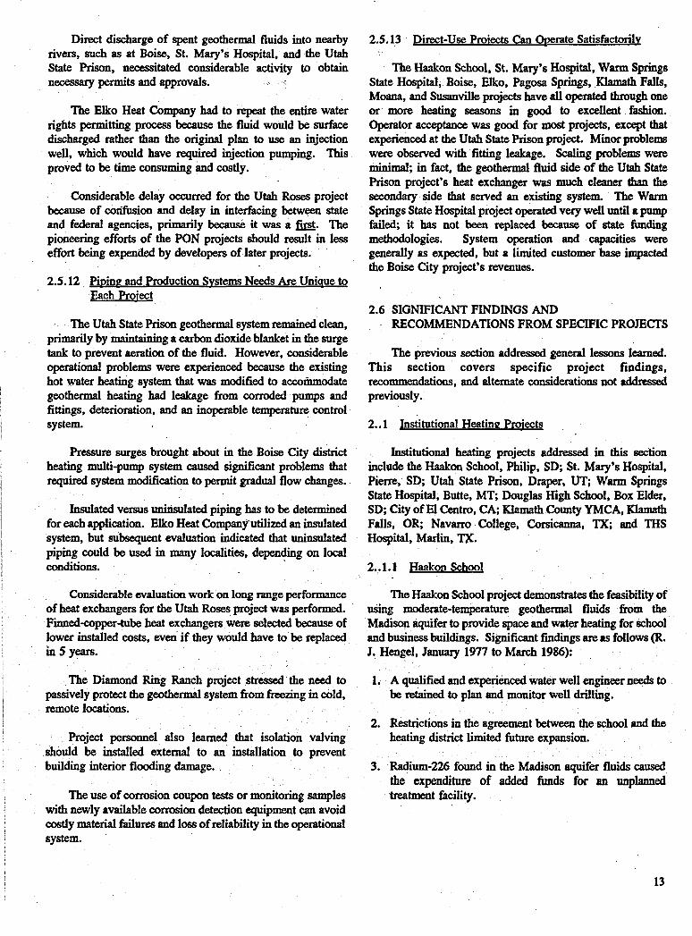
2.5.12 PiDinp and Production Svstems Needs Are Uniaue to Each Proiect
The Utah State Prison geothermal system remained clean, primarily by maintaining a carbon dioxide blanket in the surge tank to prevent aeration of the fluid. However, considerable operat id problems were experienced because the existing hot water heating system that was modified to accotiuuodate geothermal heating had leakage from corroded pumps and fittings, deterioration, and an inoperable temperature control system.
Pressure surges brought about in the Boise City district heating multi-pump system caused significant problems that required system modification to permit gradual flow changes.
M a t e d versus uninsulated piping has to be determined for each application. Eko Heat Companyutilized an insulated system, but subsequent evaluation indicated that uninsulated piping could be used in many localities, depending on local conditions.
Considerable evaluation work on long range performance of heat exchangers for the Utah Roses project was performed. Finnedapper-tube heat exchangers were selected because of lower installed costs, even if they would have to be replaced in 5 years.
The Diamond Ring Ranch project stressed the need to passively protect the geothermal system from freezing in cold, remote locations.
Project personnel also learned that isolation valving should be installed extern1 to an installation to prevent building interior flooding damage.
The use of corrosion coupon tests or monitoring samples with newly available corrosion detection equipment can avoid costly material failures and loss of reliability in the operational system.
2.5.13 Direct-Use Proiects Can Operate Satisfactodv
The W o n School, St. Mary’s Hospital, Warm Springs State Hospita€, Boise, Elko, Pagosa Springs, Klamath Falls, Mom, and Susanville projects have all operated through one or more heating seasons in good to excellent fashion. operator acceptance was good for most projects, except that experienced at the Utah State prison project. Minor problems were observed with fitting leakage. Scaling probIems were minimal; in fact, the geothermal fluid side of the Utah State Prison project’s heat exchanger was much cleaner than the secondary side that served an existing system. The Warm Springs State Hospital project operated very well until a pump failed, it has not been replaced because of state funding methodologies. System operation and capacities were generally as expected, but a limited customer base impacted the Boise City project’s revenues.
2.6 SIGNIFICANT FINDINGS AND RECOMMENDATIONS FROM SPECIFIC PROJECTS
The previous section addressed general lessons learned. This section covers specific project findings, recommendations, and alternate considerations not addressed previously.
2.. 1 Institutional Heating Proiects
Institutional heating projects addressed in this section include the Haakon School, Philip, SD; St. Mary’s Hospital, Pierre, SD; Utah State Prison, Draper, UT, Warm Springs State Hospital, Butte, MT; Douglas High School, Box Elder, SD; City of El Centro, CA; Klamath County YMCA, Klamath Falls, OR; N a v m College, Corsicanna, Tx, and THS Hospital, Marlin, T.
2.. 1.1 Haakon School
The Haakon School project demonstrates the feasibility of using moderate-temperature geothermal fluids from the Madison aquifer to provide space and water heating for school and business buildings. Significant findings are as follows (R. J. Hengel, January 1977 to March 1986): .
1. A qualified and experienced water well engineer needs to be retained to plan and monitor well drilling.
2. Restrictions in the agreement between the school and the heating district limited future expansion.
3. Radium-226 found in the Madison aquifer fluids caused the expenditure of added funds for M unplanned treatment facility.
13

4.
5.
6.
7.
8.
9.
10.
Injection of spent fluids was considered but ruled out because of cost of drilling an injection well and unacxqtability of discharging untreated g e o t h e d fluids containing radium-226 into the subsurface. Even though the fluids originatd below ground, regulations canrestrict injection, requiring treatment beforeinjection.
Any required water treatment system should be thoroughly tested. Piping containing barium chloride slurry to remove radium-226 from the discharged geo- thermal fluid caused extensive deposits that resulted in valves not operating. An external baffle-type mixer was installed between the treatment plant and the settling ponds, solving the problem.
An experimental ion exchange system was used to remove sulfates without leaving deposits in the piping. It lost its effectiveness quickly and was rejected because of the excessive quantity and cost of barium sulfate required.
Contact areas of filament wound epoxy pipe should be dry before making joints to prevent leakage.
Separate smaller heat exchangers were selected over one large plate-type heat exchanger to avoid shutdown of the entire system in the event of failure of the large single heat exchanger.
Building owners should operate their systems at the same pressure found in the main distribution piping, or provide a pressure reducing valve, if needed. This allows all users to operate at the most efficient pressure.
The school was unable to further utilize spent geother-mal fluid because of the legal arrangements they had entered into with the town heating district.
2.6.1.2 St. M a d s Hospital
The St. Mary’s Hospital demonstrates the feasibility of using a low-temperature (108°F) resource to provide hot water and space heating. Significant findings are.(St. Mary’s Hospital, September 1984):
1. The well could been located anywhere within 100 Et of an existing travertine mound, and the selected location near the project resulted in low piping-costs.
2. Consideration should be given to using cooler temper- ature. fluids at shallower depths with greater volumes (e.g., 500 gpm at 92°F) for heat pump applicati6ns rather than drilling to greater depths for hotter fluids.
3. Tapping natural gas zones could be accoIllplished by sleeving the well to the proper depth.
4. Discharge of the spent geothermal fluids into the Missouri River created extensive permitting activities.
5. When g e o t h d fluid is discharged into a.nver, flow should not be intempted for a long enough perid to allow silt to !ill the discharge ports.
2;6.1.3 Utah State Prison
The project demonstrated the feasibility of using a moderate-temperature (180°F) resource to provide space and domestic hot water heating for a minimum security facility. Significant findings are as follows (Case, Lowe and Hart, Inc., March 1979 to January 1986):
1.
2.
3.
4.
5.
6.
-7.
The resource test program showed that the reservoir would be stressed when both the prison and nearby Utah Roses were operated at higher use rates. This was later verified.
Considerable permitting activity was required in order to discharge spent g e o t h e d fluid into the Jordan River.
The existing hot water heating system, because of leak- age, deterioration, and techaid problems, resulted in downtime not attributed to, but blamed on, the geothermal system. The geothermal system remained clean through the use of a carbon dioxide blanket in the surge tank.
The demand for hot water is very high in this type of prison facility and the contribution of g e o t h e d heat could be increased through piping heat exchangers in series (to achieve a greater temperature drop of the geothermal fluid), rather than in parallel.
Maintaining a carbon dioxide blanket in the surge tank prevented ’geothermal fluid aeration, thus preventing corrosion.
A backup geothermal fluid circula@g2pump was added and a temperature sensor was relocated to provide better flow control through the heat exchanger.
The lack of proper support from operating personnel led to the abandonment of the geothermal system.
2.6.1.4 Warm Snrines State Hmital
The project demonstrated the feasibility of using a moderate temperature (154°F) resoutce to provide space and hot water heating for the hospital. Significant findings are as follows (MultiTech, Inc., January 3 1, 1979 - June 30, 1983):
14

1. Mud control was difficult because of delays in delivery, lack of mud-handling equipment, flow'of formation water into the wellbore, and labor problems. Logging the upper sections of the wellbore was unsuccessful due to high mud gel strength and lack of hole stability.
2. The duplex mud pumps used lacked sufficient pressure and capacity to allow the use of jet nodes to aid in hole cleaning.
3. Certain oil field chemicals are available to fix mobile fines that could cause a deep zone of skin damage observed through pump testing. Pilot tests can be run to evaluate this possibility.
4. Temperature and flow rate surveys can be run to determine the source(s) of fluid production in order to isolate zones of nonproduction.
5. Some wells may not be good candidates for conventional fracture stimulation.
6. Acid treatment and reworking of the well improved the production capability but not to the extent anticipated. However, the flow (70 to 90 gpm) was adequate.
7. Restricting drilling times caused major drilling inefficiencies. .
8. Drilling additional wells could be more economic81 than rework and deeper drilling.
9. The use of corrosion coupon tests or monitoring samples with proper corrosion detection equipment to determine fluid characteristics can lead to proper equipment selection, in turn preventing costly replacements of components.
10. Failure of the lineshaft pumps (pump bowls and impellers wearing out very quickly and elastomer spider failures) was a disappointment, but did provide an insight into pumping fluids laden with particulate matter and identified the problems with that type of pump. The remote well site location resulted in several delays, altering plans frequently to accommodate lack of equipment and services.
sh0 definition of terms, regulatory requirements, and state
cy jurisdiction over geothermal development.
tudy and development should be coordinated with everyone concezned throughout the project life.
13. Applicable code and other requirements should be determined as soon as possible to allow time to process permits and meet standards.
14. State funding procedures resulted in the system not becoming operative again after failure of the production pump in March 1983, even though a very short payback period was possible.
2.6.1.5 Pouelas High School
The project was halted due to uncertainties and the lack of funding to complete the well to the desired depth.' (The well drilling funding was not part of the PON project.) Significant findings are (Douglas School System District No. 51-1, Match 30, 1979):
1. The drilling failure resulted from the lack of a properly maintained mud program, and the inability to modify the drilling program because of the footage drilliig contract payment method and the driller's unwilliugnkss to change it. The drilling equipment may have reached its limits. Sticking the drill stem twice in the wellbore also. contributed to the failure.
2.6.1.6 El Centro
This project to provide space conditioning and water heating for the El Centro Community Center in California was halted because of an inadequate resource. Significant findings are (Geothermal Direct Heat Applications Program Summary, November 1980 and September 1981):
1. Equipment and materials may be difficult to obtain from suppliers for small, one-time projects. This is particularly true when the items, such as well casing, are in short supply. Regular long-term customem get preferential treatment.
2. Regulatory approvals took longer than estimated. A local government is often slowed by restraints associated with bidding and procurement.
2.6.1.7 Klamath Countv YM CA
1. Use of an engineer experienced in geothermal design can help eliminate some problems and effktively deal with others as they arise. The engineer of this project had previously designed 6 geothermal heating systems.
2. It was originally believed the production well would produce fluids at about 160 to 165°F. The well actually produced 140°F water probably due in part, at least, to
-..
15

communication between the injection and production wells. By ’adding plates to the plate type heat exchanger and adjusting flows, the engineer was able-to make the system meet the heat demands.
3. After a period of operation, the injection wen casing expanded upward several inches requiring a flexible connection between the piping and the casing. The casing continues to expand and contract depending on the flow and temperature of injected fluid.
4. Minor problems with air locks in the heat exchanger were noted after periods of low flow. A back pressure valve between the exchangers and injection well solved the problems.
2.6.1.8 Navarro CoIlege
The Navarro College, Corsicanna, Texas, project demonstrates the feasibiIity of utilizing 125°F geothermal fluid for heating domestic water systems, forced air heating, and an aquaculture pond. Significant findings are (Geothermal Direct Heat Applications Program Summary, September 1981):
1. Injection at minimum energy consumption proved to be more difficult than expected. It is recommended that an experienced industrial waste injection consultant be employed early in the project if injection disposal is likely to be needed.
2. There is no standard method of economic analysis. The assumptions USBd to arrive at any payback period or rate of return must be highly qualified to understand its significance.
3. The amount of time and effort required to turn a final design, which is complete in terms of an engineering review, into an acceptable bid package was much greater than expected. Overall, the time and effort required to get from completed design to negotiated construction subcontract was greater than planned. Intermediate steps were: generate bid package, reproduce and issue package, advertise, answer questions, evaluate bid, investigate contractor, and negotiate to get final signed subcontract.
2.6.1.9 THS Homital
The THS Hospital project demonstrates the feasibility of utilizing 150°F geothermal fluid for space and hot water heating. Significant findings are (Geothermal Direct Heat Applications Program Summary, November 1980 and September 1981):
1. The number of permits required and the effort necessary to obtain them were significantly underestimated in the inilial project planning.
2.6.2 District Heating Proiects
’ This section addresses district heating projects, including Boise City, Boise, ID; Elk0 Heat Company, Elko, NV; City of Pagosa Springs, Pagosa Springs, CO; Madison county, Rexburg, ID; Monroe City, Monroe, trr, City of Klamath Falls, KIamath Falls, OR; Moana, Reno, NV, and the City of Susanville, Susanville, CA.
2.6.2.1 Boise Citv
The project demonstrates the feasibility of utilizing a moderate-temperature (170°F) resource to provide district heating in the city of Boise, Idaho. Significant findings are (Hanson, J.P., 1985):
1. Four production wells were drilled, and even though other wells existed in the area, one well did not produce.
2. Disposal of spent geothermal fluid into the Boise River involved more time, effort, and cost than was originally planned. Permitting actions were also significant. (Current regulations may necessitate injection of the spent fluids or other control measures.)
3. Pressure surges in a multi-pump system can be signifi- cant. It became necessary to modify the installed system to permit gradual flow rate changes during sequencing of pumps with different capacities.
4. An in-line booster pump was added to the system to reduce the amount of fluid needed to maintain system pressure. Bypass restrictions were also added at the end of each service leg, greatly reducing the amount of fluid discharge.
5. Numerous pipeline routes were umsided. The fmal selection was based on the technical ability of the building to be retrofitted, the cost, the size of the heat load, and the owner’s willingness to connect to the system.
6. Various pipeline materials were umsidered. Asbestos cement pipe covered with polyurethane foam insulation was selected over other alternates. This aelection was made to retain the heat energy content and not be susceptible to corrosion by surrounding soils. Pre- insulated piping was found to be less expensive than other alternates.
7. The project is an excellent example of what can be achieved through proper technical direction and support. However, these successes were marred because of the inability to expand the customer base enough to achieve a positive cash flow. The lack of funding for retrofits, the resistance to change, and the “why fix it if it isn‘t broken” attittide contributed to the inadequate customer
16

base. Concerns over the use of the geothermal reservoir, state and local activities, and limited sales of service continue to impact the project. potential ixitomers have not been prone to expend funds for retrofits, even though they can teceive geothermal fluid at 70% of natural gas prices.
8. Boise City had to establish a new utility for which few of the conditions were defined, resulting in major expenses and added time. The involvement of four governments added to the complexity.
9. Significant effort was directed toward the resolution of legal and institutional activities, indicating their importance in the development of a district heating system.
2.6.2.2 Elk0 Heat Commnv. Elko. Nevada
This project demonstrates the feasibility of using a moderate-temperature reso- (177°F) to provide space and hot water heating for a small district heating system in Eko, Nevada. Significant findings are (h4. W. Lattin, June 1983):
1. The Eko wildcat well p r o d d 800 gpm, but with problems. A leak at a casing lap and open hole brid-ging resulted in a well rework program that cost more than the original well. Insufficient information was available for the design of the well completion program.
2. A lineshaft turbine pump was selected over a submersi- ble pump because of the shallow setting depth and reported problems with electric motors on submersibles.
3. Flow testing revealed leakage in the wellbore. The lessons learned from this are: (a) when formation stability is marginal, open hole methods of well comple- tion should not be used, and (b) special.precautions should be taken in the design of wells that encounter artesian conditions. If the well casing joints are not adequately sealed, the shut in pressure of the well can force fluids out of the wellbore into the formation, causing groundwater quality problems and possible springs to occur. Repair work required to c o m t artesian conditions was far in excess of what it would have cost to properly case the well from the start.
4. A major decision involved selecting insulated over non- M a t e d piping. kuse.insulated piping can cost up to 500 % more for the materials, nonindated piping may be a viable option. A study of temperature losses in the Eko system indicates that noninsulated piping could be acceptable in many locations, depending on local conditions, such as flow rate, moisture content of.$he soil, etc.
5. Securing permits and approvals is a lengthy process. Water rights should be well understood and addressed early ih the project. Disposal can be a most perplexing problem and should be attended to as s001l as possible.
6. Changing from injection to surface disposal caused a repeat of the entire water rights permitting process.
7. The initial customer base of three was not large enough to warrant the investment, but recognizing the potential to expand, the Eko Heat Company was williug to subsidize the system. This approach has paid off and the system is continuing to be significantly expanded.
8. Every effort should be made to establish an adequate customer base by responding to concerns over system reliability and efficiency, meeting projected heat demands, and establishing energy costs savings.
9. The budget can change continually until the production well is completed and the disposal method selected.
10. Geothermal fluid may be used directly for certain applications. The Vogue Laundry uses the fluid directly, claiming better performance than with the original domestic hot water.
2.6.2.3 Cihr of Paeosa Smings. Paeosa S~rines. Colorado
This project demonstrates the feasibility of utilizing a mod&temperature (131 to 149°F) resource to provide district heating in the town of Pagosa Springs, Colorado. Significant findings are (Goering, S.W., August 1984):
1. Drilling new wells was d+ermined to be more cost- effective than refurbishing existing wells.
2. Three wells were drilled in the vicinity of numerous producing wells, but one was unsuccessful.
3. Simplicity of design is important to trouble-free operation and acceptance, especially in smaller communities. The city chose to use mostly manual controls, recognizing the added cost of automation and the resistance of the local operators to accept a "complex" system.
4. Geothermal fluid can be used successfully to meet diverse customer needs in a harsh winter-mountain environment where temperatures can drop to -40°F.
5. The need for strong supporters is proven at Pagosa Springs. Continuing concerns over water rights and system reliability are being effectively met through the continuing positive efforts of the involved city personnel.
17

6. Keeping. the public, state and other agencies regularly involved is of g k t value in obtaining well drilling and other permitk.
7. The use of local contractors is generally more desirable than obtaining support outside &e community, assuming the proper support is available near the project.
8. Water rights issues can have a significant project impact. The conditional rights decree was not obtained until June 1987, having a negative impact on potential customers. Prior to this, the city operated on a temporary permit.
2.6.2.4 Madison Countv. Rexbura. Idaho
This project was not developed because the geothermal fluid temperature was only 72°F at 3,932 !I well depth. Significant findings are (Kuntz, J. F., August 1982):
1.
2.
3.
4.
5.
During the open hole drilling, it was impossible to lift the drilling cuttings because of the numerous permeable strata.
Significant flows of cooler tempera- water can enter and flow down a wellbore below the bottom of the casing and cool geothermal fluids.
The use of air drilling or heavy muds may not be practical to stop lost circulation. Heavy muds could increase pressure, thus resulting in an increase of lost circulation. Casing may be the only feasible means to permit deeper drilling.
The well, although not successful for geothermal use, is a prolific producer of drinking water and can be used as such when the city’s need arises.
State bond requirements gave no special recognition to the county’s special relationship with the state, causing the county to seek bonding that was not available. This was resolved through the use of an escrow savings 8ccount.
2.6.2.5 Monroe. City, Monroe. Utah
The production from the well (600 gpm, 164°F) did not meet the needed capacity to provide space and hot water hating for commercial, municipal, and domestic district heating applications. Significant findings are (Blair, C. K., December 1982):
1. Detailed project feasibility analyses should be completed befote developing field production facilities. .
2. The lack of a centrally locatdcustomer load produces prohibitive system capital costs. The user load should be obtained during the early part of the project life.
3. The near-term small customer base contributed to the decision to halt the project. Actual costs that almost doubled the estimated cost were also a factor.
2.6.2.6 City of Klamath Falls. Klamath Falls, Ore~on
The Klamath Falls, Oregon, project demonstrates the feasibility of using a 210°F resow to provide district heating to a large number of government buildings. The significant findings are (Geothermal Direct Heat Applications Program Summary, September 1981):
1.
2.
3.
4.
In areas with a high number of existing users, afairly in- depth preconstruction survey of use and attitudes should be completed.
Existing users should be completely informed, if neces- sary, by personally delivering letters on pump testing results and on-going monitoring. Public hearings do not suffice in that turnout of existing users does not develop until they feel threatened. From the City of Klamath Falls experience, once the existing users feel threatened, they cannot believe the data given to them by the Reservoir Engineer.
Existing well owners can delay and restrict growth. Owners spearheaded the passage of an ordinance favor- able to them that in turn delayed the project for over two
Y-.
The joining systems in fiberglass piping can fail. Lock rings were attached with an epoxy adhesive that was im- properly manufactured or applied. The adhesive failed, allowing axial movement, which resulted in leakage. A lack of isolation valves necessitated draining the fiberglass system each. time a leak occurred.
2.6.2.7 Moana, .Reno, Nevada
The Moana project in southwest Reno, Nevada, demon- strates the feasibility of ushg a 250°F resource for district heating numerous homes. The significant ’findings are (Geothermal Direct Heat Applications Program Summary, November 1980 and September 1981):
1. Public education is essential. A survey of 1,OOO long- time residents of Reno, where geothermal energy has been used over 50 years, showed 77% had little or no knowledge of geothermal energy.
2. Heat sales agreements can be difficult to develop. A loag-term agreement that meets the needs of both the user - and the developer is critical. It is economically important to have agreements to supply base load heat to a group of users rather than have to meet the peak load of one user for a very short period of time, under utilizing the systems’s productive capacity.
18

3. Having the customer use the existing heating system is beneficial. It relieves concern over the possibility of the geothermal reservoir being used up, and allows peak loads to be met with the fossil fuel backup system.
4. A district heating system could be regula& as a utility. The utility issue depends upon the rulings of each state. This should be determined early in the life of a project.
I , I
2.6.2.8 Citv of Susanville. Susanville. California
The Susanville, California, project demonstrates the feasibility of utilizing a 175°F resource for space and domestic hot water heating in public buildings. The significant findings are (Geothermal Direct Heat Applications Program Summary, November 1980 and September 1981):
1. Greater education is needed to separate high-temperature well drilling problems from problems encountered in low- temperature operations.
2. The use of a construction management team is bene- ficial, allowing field decisions to be made more quickly.
3. Extensive detail in specification packages minimizes misunderstandings.
4. Excellent initial resource evaluation enhances engineering and project prbgress.
2.6.3 Agribusiness
Agribusiness projects discussed in this section include Utah Roses, Sandy UT, Diamond Ring Ranch, Haakon County, SD; Aquafarms International, Inc., Dos Palmos, CA, and Kelly Hot Springs Agricultural Center, Kelly Hot Springs, CA.
2.6.3.1 Utah Roses, Sandy. Utah
. The project demonstrates the feasibility of using a moderate-temperature (123°F) resource to supply heating for an existing 7-acre greenhouse facility. Significant findings are (Energy Services, Inc., October 1982):
1. The well site, situated among thermal wells and springs, was selected for convenience, and no scientific evidence could be established to locate a more desirable site.
2. The geothermal fluid flow was less than expected, but measures such as reducing control and operating costs,
d changing to fanail type heat exchangers enabled the ratm to double the facility size.
.
3. Automatic valve equipment on the wellhead that protects the distribution line from waterhammer and excessive pressure drop during pump startup may be overdesiped. A single, fast-acting, automatic reset valve may provide the needed protection.
4. The use of off-the-shelf fi~edapper-tube heat exchang- ers may be more economical if they do not become corn ded for a reasonable period, say five years. Instalkg an F- and P-type heat exchanger would probably require more fluid flow at these low temperatures. The use of fancoil-type heat exchangers would require less fluid flow.
5. Surface discharge into the Jordan River was a major issue, causing considerable delay.
6. Because of its extremely competitive nature, greenhouse operation must in itself be sutxessM. A good geother- mal system only adds to the competitive edge; it does not necessarily create it.
7. Considerable delay occurred because of delays and con- fusion between state and federal agencies because the project was a first.
8. Without the tax benefits received during the first oper- ating year, and at a time of very high interest rates, the first year’s savings would not be satisfactory.
2.6.3.2 Diamond Ring Ranch. Haakon Countv. South - Dakota
This project demonstrated the feasibility of using an existing moderate-temperature (152°F) resoutce for multiple, d e d uses as heating structures, grain drying, stoctc watering, and irrigation. Significant findings are (Howard, S. M., September 1983):
1. Geothermal fluid with an inflow of 170 gpm at 153°F can
piping and be effectively used in plate-type heat exchangers.
2. Geothermal heating in cold, remote locations should be protected from freezing. Antifreeze used in closed-loop systems experienced leakage, halting the operation of the system because replacement costs were prohibitive.
3. Shut-off valves should be provided for each structure to Jlow &icing and prevent interior flooding.
4. Filter s c m should be added for positive displacement flow meters.
be transported 4,000 ft in buried 6-in. rminsulated PVC
19

5. Air vents are needed at high points of gravity flow transmission lines.
6. Lack of highly trained personnel and limited supplies stressed the need for simple systems.
2,6.3.3 Aauafarms International, Inc.. Dos Palmos, Cali fonzia
The Aquafarms International, Inc., project located in the Dos Palmos area, Coachella Valley, California, demonstrates the feasibility of utilizing 79 to 92°F fluids from three wells to grow prawns on a year-round basis. The significant findings are (Geothermal Direct Heat Applications Program Summary, September 1981):
1. Drilling and completing relatively shallow artesian geothermal wells can be a problem for local water well drillers. They had to be educated on conductor case use.
2. Projects located some distance from an agricultural or industrial center should plan to obtain and include qualified construction and maintenance personnel in the project area.
3. Heat transfer losses in large surf- area ponds can be high and difficult to control. This can be alleviated by keeping the pond surface area to a minimum.
4. High initial percolation in new ponds can be alleviated through fertilization to help accelerated algae produc-tion, which in turn helps seal off the bottom of ponds.
5. The permitting and approval process for an aquaculture project can be extensive and time consuming.
construction requires extensive planning and the consideration of many factors such as species needs, land contour, wind, water availability, temperatures, equipment availability, soil type and permeability,
;ragricultural history, flooding possibility, and future plans.
2.6.3.4 Kellv Hot Springs, Aericultural Center. Kellv Hot SDrings. California
- The Kelly Hot Springs geothermal project would have demonstrated the feasibility of utilizing a new we11 near an existing'194"F hot spring to raise hogs. The project was abandoned, and later greenhousing and fish farming occurred at the site. The significant findings are (Geothermal Direct Heat Applications Program Summary, November 1980):
1. Whenever there is a possibility of historical significance related to the project site, such as a hot spring or other surficial evidence of a geothermal resource, an archeo- logical field survey should be planned as a first activity.
2. The current economic climatewm jeopardize the final financing of the project. The cdncept was started in 1977, contracted in September 1979, and Phase I studies completed in August 1980. investment climate changed considerably during this period.
3. The project was in collsort with the trends in medium and large size swine raising practices in the United States. However, being located in the west, a medium-sized facility with the necessary flexibility in purchasing of feed constituents and marketing of live hogs was to be the best approach.
4. The project was an economic development effort. The geothermal energy utilization was a strong plus but was the easiest part of the problem.
2.6.4 Industrial
Industrial projects discussed below include ORE-IDA Foods, Ontario, OR, and Holly Sugar, Brawley, CA.
2.6.4.1 ORE-IDA Foods
This project planned to use geothermal energy for potato processing, and space and domestic hot water heating at the ORE-IDA Ontario, Oregon, plant. Flow from the 10,000 Et deep well was inadequate and the project was halted after provisions were made for possible reworking of the well. Significant findings are (Austin, J. C., May 1982):
1. It is believed that, had the primary well site been drilled, adequate flow could have been obtained. Economic factors (proximity to the plant) caused the well to be drilled at a secondary location that had adequate temperature (380°F) but basically no flow. Funding limits precluded drilling a second well.
2. Attempts to improve flow met with little success. The well was pressured to 1,400 psi at the wellhead and 350 gpm were pumped into the well to produce a minihydro- fracture in the zones below 7,000 ft. However, fluids were lost near the 6,000 ft level. The use of frac balls to seal the leakage did not work.
3. Mud damage to the wellbore was suspected, but the significant expenditure for chemical treating or hydraulic fracturing was not considered justified.
2.6.4.2 Hollv Sugar. Brawlev. California
The Holly Sugar project would have utilized geot6ermal energy for direct processing at a sugar beet processing plaht in Brawley, California. The well was drilled to - 10,000 ft, but inadequate flow occurred. The significant findings of this project are not available, except that the project experienced
20

supply shortages, especially in casing that was often poor quality and in accelerating costs (Geothermal Dirqt Heat Applications Program Summary, November 1980).
2.7 CREDITS
Information for this chapter was primarily obtained from the various interim and final reports that were prepared by the principal investigator for each PON project, and subsequently
1986). Additional information for the individual PON project final reports are listed in the references. The contributions of each report author are gratefully acknowledged, and appreciation is extended to each one for 'providing the information that made the PON projects summary final report and this chapter possible.
.
. rmmmatized in the overall PON projects final report (Lunis,
REFERENCES
These references are available from the National Technical Information Service, U.S. Department of. Commerce, 5285 Port Royal Road, Springfield, VA 22161.
Austin, J. C., CH2M Hill, Inc., "Direct Utilization of Geothermal Energy R e s o w in Food Processing", Final Report May 17, 1978 - May 31, 1982, Report No. DOEEW28424 - 6, Cooperative Agreement No. DE- AC07-78ET28424 May 1982.
Blair, C. K., and L. B. Owen, Editors, Terra Tek, Inc., "Direct Utilization of Geothermal Resources at Monroe,
Report No. DOEIET127054-6, Cooperative Agreement No. DE-FC07-ET 17054, December 1982.
Utah", Final Report, July 14, 1978 - July 31, 1981,
.
Broughton, R., et al., Aquafanus Inkmational, Inc., "Direct Use of Low Temperature Geothermal Water by Aquafarms Internatid, Inc., for Freshwater Aquaculture (Prawns and Associated Species)", Report NO. DOEIET127047-2 @E85005099), April 1984.
Case, bwe , and Hart, Inc., "Geotheimal Heating Retrofit at the Utah State Prison Minimum Security Facility", Final
DOEiETL27027-10, Cooperative Agreement No. DE- Report, March 1979 - January 1986, Report NO.
FC07-79ET27027.
Douglas School System District No. 51-1, "Geothermal Heating of Douglas High School Cooperative Demonstration Project", Final Report for project, terminated January 26, 1979, Report No. DOEET/ 01727-1, Cooperative Agreement No. ET-78-FM-1727, March30, 1979. _.
Energy Sewbes, Inc., Final Report, "Floral Greenhouse Geothermal Heating Demonstration", Report No. DOEIET127056, October 1982.
Goering, S. W., et al., Couryand Associates, Inc., 'Direct Utilization of Geothermal Energy for Pagosa Springs, Colorado, Final Report June 1979 - June 1984", Report No. DOEET-27030-7, Cooperative Agreement No. DE- FC07-78ET27030, August 1984.
Hanson, P. J., Boise Geothermal, "Boise Geothermal District Heating System Final Report March 1979 - September 1985", Report No. DOEETL27053-6, Cooperative Agreement No. DE-FC07-79ET27053, October 1985.
Hengel, R. J., Hengel Associates, "Direct Utilization of G e o t h d Energy for Haakon School District, South
Report No. DOE/ET/27080, Cooperative Agreement No. Dakota", Final Report January 1977 - March 1985,
DE-FCO7-78ET 27080.
, Howard, Dr. S. M., "Direct Utilization of G e o t h d Energy in Western South Dakota Agribusiness, Final Report", Report No. DOE/ET/27158-7, Cooperative Agreement No. DE-FC07-78ET27158, September 1983.
Kunze, J. F., and J. K. Marlors, Energy Services, Iac., "Industrial Food ProcesSiag and Space Heating with Geothermal Heat"; Final Report, February 16, 1979 - August 31,1982, RepoGNo. DOE-ET-27028-5, Contract NO. DE-FC07-79ET27028, August 1982.
Lattin,M. W., and R.D.Hoppe, Chilton Engineering, Chartered, "Direct Use of Geothermal Energy; Eko, Nevada District Heating Final Report March 1979 -June
. 1983", Report No. DOEIET127033-6, Cooperative Agreement No. DE-Am-79ET27033, June 1983.
Lunis, B. C., EG&G Idaho, Inc., "Geothermal Direct Use Program opportunity Notice Projects Lessons Learned", Final Report NO. DOE/ID-10147, 1978 - 1986.
MultiTech, Inc., "Direct Utilization of Geothermal Resources of Warm Springs State Hospital, Warm Springs, Montana", Final Report for the period January 31,1979 - June 30, 1983, Report No. DEETL27055-10, Cooperative Agreement No. FC07-79ET27055, June
. 1983.
St. Mary's Hospital, "Geothermal Heating Project at St. Mary's Hospital, Pierre, South Dakota", Final Report, Report No. DOE/ET/28441-7, Cooperative Agreement
. No. DE-FC07-79ET28441, September 1984.
21

Smith, K., Navarro College, "Direct Utilization of Geothermal Heat in Cascade Application to Aquaculture and Greenhouse Systems at Navarro College" Final Report for the Period March 1, 1979 - September 30, '1984, DOEIET/27508-1, September 1984.
U.S. Department of Energy, Division of Geothermaland Hydropower Technologies, "Geothermal Direct Heat Applications Program Summary", Semi-Annual Review Meeting, November 1980.
U.S. Department of Energy, Division of Geothermal and Hydropower Technologies, "Geothermal Direct Heat Applications Program Summary", Semi-Annual Review Meeting, September 1981.
22

CHAPTER,3 NATURE OF’ GEOTHERMAL RESOURCES
By Phillip Michael Wright University of Utah Research Institute
Salt Lake City, UT 84108
and
Gene Culver Geo-Heat Center
Klamath Falls, OR 97601
3.1 INTRODUCTION
Geothermal energy is a domestic resource that contributes to our energy security and decreases our trade deficit by displacing imported fuels. It is an environmentally advan- tageous energy source that produces far less air pollution than fossil-fuel sowces. Geothermal energy contributes both on the energy supply side, with electrical power generation and directhat applications, and on the energy demand side, with savings in electricity and natural gas through use of geothermal heat pumps in buildings and industry.
Geothermal energy is the heat of the earth. Since the depths of the earth are very hot, heat flows outward toward the surface, and the temperature of the earth increases with depth. The several thermal regimes in the earth give rise to a classification of geothermal resource types, illustrated in Figure 3.1.
geologic processes. Earth energy is thermal energy at the normal temperature of the shallow ground, without anonoalous enhancxinent due to geologic processes. It is energy that is found everywhere across the United States and the world and can be used with geothermal heat pumps to heat and cool homes and buildings, supply domestic hot water and provide industrial heat needs. Hot dry rock energy occufs at depths of 5 to 10 miles (8 to 16 km) beneath the rmrface everywhere, and it also occurs in areas of thermal enhancement due to geologic processes.
Naturally Occurzing hot water and steam form the hydrothemat energy resource. Hydrothermal development is economic today at a few high-grade sites. A relatively small industry generates electrical power and supplies heat for direct uses from hydrothermal resources. Many more hydrothermal resources could be us& if better technology were available and if their development were actively promoted by the Federal and state governments. Geopressured, hot, dry rock and magma energy all require further R&D to enable them to be economically developed.
3.1.1 Current Contribution of Geothermal Energy
Geothermal energy is here today-it is not merely a hope for the future. lke production of g e o t a l energy in the US. currently radix third in renewable energy sources, following hydroelectric power and biomass energy. As a result of geothermal production today, consumption of exhaustible fossil fuels is offset along with the release of the greenhouse and acid-rain gases that are caused by fossil-fuel use. Geothermal energy use in the United States is equivalent tosthe burning of about 60 million barrels (bbl) of petroleum each year, while worldwide geothermal energy use is equivalent to the burning of about 150 million barrels of oil per year. The U.S. Strategic Petroleum Reserve contains about 600 million barrels of oil, an amount that could be replaced every four years with the savings from worldwide geothermal use.
23

There is a very large geothermal resource base in.the U.S., much of 'which can not yet be eumomically developed. In fact, the resource base for the renewable/sustainable energies-geothermal, solar, biomass, hydropower and wind- is much lurger than the total resource base in coal, oil, gas, and uranium (nuclear power).
3.1.1.1 Geothermal Heat Increases our Enerev Sumlies
At our current stage of technobgy and with current energy costs, eumomic development of geothermal energy can be accomplished in some areas where the heat is concentrated by geologid processes. Geothermal water exists at many subsurface locations in the U.S. in the form of hydrothermal systems. These hydrothed systems can be tapped by existing well-drilling and energyconversion technology to generate electricity or to produce hot water for direct use. For generation of electricity, hot water is brought to the d a c e through production wells and is flashed to steam in p i a l vessels by release of pressure. The steam is separated from the water and fed to a turbine engine, which turns a generator. Spent geothermal water is injected back into cooler parts of the reservoir to obviate environmental problems and to help maintain reservoir pressure (Figure 3.2). Some high- teqkrature (+450 "F, +WOOc) remurces yield steam from the reservoir rather than water, and this steam is fed straight to the turbines. If the reservoir is to be used for direct-heat application, the geothermal fluid is usualfy fed to a heat exchanger before being reinjected into the earth. Hot water from the output side of the heat exchanger is then used for home heating, greenhouse heating, vegetable drying and a wide variety of other uses.
' 'Hot Upwding Water
Hot Rock Heat Source
Figure 3.2 Geothermal resources.
The U.S. g & e d industry currently has an installed capacity of 2,800 megawatts of elem*cal power (MWe) from hydrothermal resources (Huttrer, 1990), while direct applications of hydrothermal energy in the U.S. have a total
24
installed capacity in excess of 2,100 thermal megawatts (Mwt), including geothermal heat pumps (Liemu, et al., 1988; Lund, et al., 1990).
Geothermal energy is found in many places on the earth in addition to the U.S., and its utilization is growing rapidly worldwide. Approximately 5,700 megawatts of electricity are currently being generattd in some W countriesfiom geother- mal energy (Huttrer, 1990), and there are 11,300 thermal megawatts of installed capacity worldwide for direct-heat applications at inlet temperatures above 95°F (35°C) (Freestop, 1990). If we include the use of geothermal water at lower temperatures and geothermal heat pumps operating at normal groundwater temperature, the energy production throughout the world from geothermal resources is very much greater, but unquantified at this time.
Systems for use of hydrothermal energy have proven to be extremely reliable and flexible. During 1987, hydro- thermal electric power plants were on h e an average of 97 % of the time, whereas nuclear plants averaged only 65 % and coal plants only 75 96 on-line time. Geothermal power plants and direct-use systems are modular, and can be installed in increments as they are needed. Both baseline and peaking power can be generated. construction time can be as little as 6 months for power plants in the range 0.5 to 10 MWe and as little as 2 years for clusters of plants totalling 250 MWe or more. Some direct-use sytems can be installed in as little as a few days.
3.1.1.2 Geothermal Enerm Decreases our Enerm Demand
No active technology for home heating and air condition- ing is more efficient than the geothermal heat pump (GHP). Because electricity is used only to transfer heat, not to produce it, the GHP will deliver 3 to 4 times more energy than it consumes. The U.S. lags behind other countries in taking advantage of heat-pump technology. Sweden has deferred construction of two nucIear power plants by using GHPs to reduce electrical power needs. Canadian growth in GHPs since 1986 has exceeded 50 5% per year. Nevertheless, more than 100,CKu) ekctrically powered geothennal heat pumps have been installed in homes and buildings in the U.S. (mid- 1990 figure). Additional installations are being actively promoted by investoravned utilities and rural electrical cooperatives as a means of promoting energy efficiency and better managing &man& GHPs can cut 1 to 5 kilowatts (KWe) of peak generating capacity requirement per residential installation. There are an estimated 25 million homes in the U.S. that have central air conditioning without access to ~ t u d gas (Bose, 1990). Replacement of these units alone with GHPs over the next several decades is not uareasonable. The savings wouki be 24,000 W48,000 MWe in peak summer demand and 48,000 to %,O00 MWe in peak winter demand. This. estimate illustrates what could be done in only one

sector-homes in the U.S. with electrical central air conditioning. It does not include new home construction or electrical energy used in heating and cooling buildings of the industrial or public sectors.
3.1.2 potential Contribution of Geothermal Enerav
Reserves of hydrothermal energy in the U.S. are difficult to quantify. However, the United States Geological Survey has estimated that geothermal energy from identified high- temperature U.S. hydrothermal systems could supply 23,000 megawatts of electrical energy for 30 years (Muffler, 1979). h addition, they believe that about 5 times this amount may be available from undiscovered hydrothermal tesources in the U.S.
Low- to moderatetemperature geothermal resources, suitable for direct-heat application, are widely distributed throughout the western and mid-western United States (Reed, 1983). Discrete hydroth- ~ e ~ o u f c e s exist throughout the western third of the CoUIlfry in subdace reservoirs of a few acres to a few square miles in extent, while in the northern Great Plains, major stratabound geothermal aquifers may extend in a COIlfinuous manner for thousands of square miles (Gosnold, 1990). It is estimated that more than 7,800 MWt could be installed in district heating systems in the U.S. using presently identified resources, and that the ultimate potential is much larger.
It is difficult to estimate the ultimate potential- contribution of geothermal energy to mankind's needs for four reasons:
1. Future energy costs are uncertain, and many lower-grade geothermal resources would become economic at higher energy prices;
2. Only preliminary estimates of the worldwide resource base have been made;
3. TechoIogy is not yet available for ecmodc use of some hydrothermal resources and for use of hot dry rock, magma or geopressured resources, whose potential contributions are large; and,
4. No reliable figures exist for the potential Contribution of geothermal heat pumps to saving of electricity and MW gas throughout the U.S. or the world.
3.1.3 Obiective and Orpanization of Chauter
The objective of this chapter is to present background information on the natwe and accurrence of geothermal resources to facilitate an understanding of the other chapters in this book. We will first Consider the t h e d regime of the earth and present a discussion of plate tectonics as the primary geologic process that generates heat sources. We will then
consider some subsurface geologic models for geothermal systems and will discuss their chemistry. The chapter will end with an overview of the occurrence of geothermal resources in the United States.
A glassary of earth-science terms for this chapter and the next is provided at the end of Chapter 4. The Appendir to this chapter is a list of the various state agencies, universities and other groups that can provide the developer with information on geothermal resources.
3.2 THERMAL REGIME OF THE EARTH
Geothermal energy is the earth's internal heat. Many 1arge-sc.de geological processes are powered by the redistri- bution of internal heat as it flows from inner, hotter regions to outer, cooler regions. Although the variations with depth in the earth of density, pressure and seismic velocity are well known, the temperature distribution is uncertain. It is certain that temperature within the earth increases with increasing depth (Figure 3.3), at least for the first few tens of kilometers, and a steadily increasing teq&ture to the earth's center is hypothesized. Very highly viscous or partially molten rock at temperatures between 1,200 and 2,200 "F (650 and 1,200 "C) is postulated to exist everywhere beneath the earth's surface at depths of 50 to 60 mi (80 to 100 km), and the temperature at the earth's center, nearly 4,000 mi (6,400 km) deep, is estimated to be 7,200 O F (4,000 "c) or higher.
200 400 600 800 1000°C
C
Heat Flow Area
1800 O F 600 1200
Figure 3.3 Temperature versus depth in the czust of the earth.
Because the earth is hot inside, heat flows steadily outward and is permanently lost fiom the surface by radiation into space. The mean value of surface heat flow is 0.082 wattslm2, commonly stated in milliwatts/mz as 82 mW/m2. Becausethesurhceareaoftheearthis5.1 x 10"mz, therate of heat loss is about 42 million megawatts (Williams and Von Henen, 1974). White 11965) estimated the total thermal energy above surface temperature to a depth of 10 km (6.2 mi), the limit of the deepest exploration drilling, at
25

1.3 x lOn I, equivalent to burning 2.3 x 10" barreis of oil. Since global ekergy consumption, including all types of energy, is equivalent to the use of about 100 million barrels of oil per day (US. Department of Energy, 1987, p. la), the thermal energy in rock to a depth of 10 km would supply all of mankind's energy needs for 2.3 x lo9 days, or 6.million years. Of ,course, we do not have the means to use all of the thermal energy in the upper 10 km of the crust, but the example helps to indicate the vastness of the geothermal resource.
The outward heat flux from the earth's interior is about 5,OOO times smaller than the radiation we receive from the sun (much of which is reflected or reradiated back into space). Thus, the earth's d a c e temperature is controlled by the amount of heat we receive and retain from the sun and not by internal heat (Bott, 1982).
Threk sources of the earth's internal heat are most important among several contributors:
1. Heat released from decay of naturalIy radioactive elements throughout the earth's 4.7 billion-year history;
Heat of impact and compression released during the original formation of the eiirth by accretion of in-falling meteorim, and,
2.
3. Heat released from the sinking of abundant, heavy metals (iron, nickel, copper) as they descended to form the earth's core during an early episode when the earth melted from the first two mechanisms.
Radioactive elements have been decaying in the earth since its formation. Some short-lived species have completely decayed by now, but they contributed to heating during the first several hundred million years after the earth was formed. Other radioactive elements have longer half-lives, and are sti l l decaying today, generating heat in the process of decay. The most important of .&ese long-lived species in terms of heat production today are isotopes of uranium, thorium and potassium.
The earth is believed to have formed by accretion of material orbiting the proto-sun. The material was accelerated toward the earth's surface by gravitational attraction. Upon *
impact, heat was released. Also, as the earth grew, the deeper material was progressively heated by compression as material continued to be added to the surface. These mechanisms, mu-. pled with heat from radioactive decay of short-lived species, eventually resulted in the melting of a substantial portion of the material of the earth. Upon melting, the heavier compon- ents sank toward the center to form the core. The sinking material gave up its gravitational potential energy in the form of heat due to friction with the Ipaterial it was sinking through. At the conclusion of core formation, a very substan-
tial amount of heat had-been released, and the earth was significantly hotter than it is today.
At the present time, an estimated 45% b 8 5 % of the heat escaping from the earth is believed to be .due to radio- active decay of long-lived isotopes, which are c4mcentrated in the crust (Bott, 1982) . The remainder is due to slow cooling of the earth, with heat being brought up from the core by convection in the viscous mantle, as discussed in the next section.
A schematic cross Section of the earth is shown in Figure 3.4. A solid layer, the lithosphere, extends from the surface to .a depth of about 100 km (62 mi). The lithosphere is composed of an uppermost layer called the crust and of the uppermost regions of the manfk, the unit that lies below the crust. The lithosphere is solid rock, but the mantle material below the lithosphere behaves as a very viscous liquid due to its high temperature and pressure, flowing very slowly under sustained stress. The crust and mantle areZcomped of minerals whose chief building block is silica (SiOa, with higher concentrations of silica in the continental crust than in the oceanic crust or in the mantle. The outer core is believed to be composed of a liquid iron-nickelcopper mixture while the inner core is a solid mixture of these metals. In the sections that follow, we shall refer to the above divisions of the earth's interior.
LITHOSPHEIE
12,756hm. 7,92611.
I Figure 3.4 Interior of the earth.
3.3 GEOLOGICAL PROCESSES
The genesis of geothermal iesources lies in the geological ' transport of anomalous amounts of heat near enough to the surface for access. Thus, the distribution of geothermal aceas ' is not random but is governed by geological processes of global, regional and local scale. This fact is important in exploration for geothermal resources.
Geothermal reswrces commonly have three components:
1. An anomalous Concentration of heat, i.e. a heat source;
26

2. Fluid to transport the heat from the rock to the surface; and,
3. Permeability in the rock sufficient to form a plumbing system through which the water can circulate.
In this section, we will consider each of these elements in turn in order to help form an understanding of the ~ t u r e of geothemal resources.
’ >
3.3.1 Heat Sources
In geothermal areas, bigher rock and groundwater temperahuts are found at shallower depths than is normal. This condition usually &ts from one or more of the foliowing mechanisms:
1.
2.
3.
4.
5.
Intrusion of molten rock (map) from great depth to high levels in the earth’s crust, bringing up great quantities of heac
High surface heat flow, perhaps due to thin crust, with an attendant high temperature gradient with depth (Figure 3.3);
Ascent of groundwater that has circulated to depths of 1 to 3 mi (1.6 to 5 km) and has been heated in the normal or enhanced gmthermal gradient; #
Thermal blanketing or insulation of deeper rocks by thick formations of such rocks as shale whose thermal conduc- tivity is low; or
Anomalous heating of shallow rock by decay of radio- active elements, perhaps augmented by thermal blanketing.
Most high-temperature geothemal resources, usually used for elect&d power geneition, appear to be caused by the first mechauism, while many isolated low- and moderab temperature resources appear to result from the second, third and fourth mechanisms, sometimes working together. The fifth mechanism is suspected to occur on the Atlantic coastal plain of the U.S. and perhaps elsewhere, but resources resulting from this mechanism have not been produced.
3.3.1.1 Plate Tectonics
One geological process that generates shallow magmatic crustal heat sources in several different ways is known as plate tectonics (Figure 3.5). Outward heat flux from the deep interior is hypothesized to form convection cells in the mantle in which hotter matenal, being less viscous and more buoyant than surrounding material, slowly rises, spreads out under the solid lithosphere, cools and descends again. The lithosphere cracks above areas of upwelling and is split apart along linear or arcuate structures called spreading centers, which occur for
the most part in theoceanbasins. Due to this mechanism, the earth’s lithosphere is broken into about 12 large, rigid plates. The spreading, or divergent, plate boundmies are typically zones thousands of miles long and several hundred miles wide. They are characterized by major rifts or faults parallel to their long dimension-, and coincide with the world’s mid-oceanic mountain system. Crustal plates on each si& of the central rift zone separate at a rate of a few centimeters per year, and molten mantle material rises in the crack, where it solidifies to form new oceanic crust. The upwelling mo1te-n rock brings large quantities of heat to shallow depths along the axis of the mid-ocean ridges and forms geothermal tesources in some areas.
oeaank volcano oceanic
hot rirlng mantla malarial
Figure 3.5 Schematic illustration of plate tectonic processes.
Since new crust is being created at spreading centers while the circumference of the earth remains constant, crust must be consumed somewhere. As the laterally moving oceanic platesdpress against neighboring plates, some of which contain the imbedded continental land masses, the oceanic plates are thrust beneath the continental plates. These zones of under-thrusting, where crust is consumed, are called subduction zona or Benioff zones or convergent phte boundaria. They are marked by the world’s deep ocean trenches, formed as the sea floor is draggd down by the subducted oceanic plate.
The subducted plate descends into the mantle and is heated by the Surrounaing warmer material and by fiction due to its movement through the mantle. At the descending plate’s upper boundary, which is rich in acean water from the layer of oceanic sediments carried down, temperatures become high enough to cause partial melting. Since molten or partially molten rock bodies (magmas) are lighter than solid rock, the magmas ascend buoyantly through the crust (Figures 3.5 and 3.6), carrying their heat to within 1 to 10 mi (1.6 to 16 km) of the surface. Volcanos result if part of the molten material escapes to the surface, but the majority of the magma usually cools and consolidates underground.. Since the subducted plate descends at an angle of about 45 degrees, crustal intrusion and volcanos occur on the landward side of oceanic trenches 30 to 150 mi (50 to 250 km) inland (Figure 3.5). The volcanos of
27

the Cascade Range of California, Oregon and Washington, for example, overly the subducting Juan de Fuca plate and pwe their origin to the process just described. The Pacific Ring of Fire, which extends around the margins of the Pacific basin, is composed of volcanos in the Aleutians, Japan, the Philippines, Indonesia, New Zealand, South America and central America, all of>which are due to subduction.
I SOLID MATERIAL
30 -I l * A q MATERIAL
Figure 3.6 Pmceses in crustal intrusion.
5
a =! E
10 = = c CL. w
15
20
Figure 3.7 shows where these processes of spreading, formation of new oceanic crust, and subduction of oceanic plates are currently operating. Oceanic rises, where new crustal material is fonned, occur in all major oceans. The East Pacific Rise, the Mid-Atlantic Ridge and the Indian Ridges are examples. In places, the ridge crest is offset by large faults that result from variations in the rate of s p d g along the ridge. Such faults are called transform faults. Figure 3.7 also shows the locations of trenches, where crust is subducted. Notice on Figure 3.7 the close correlation between both spreading and subducting plate boundaries and the locations of geothermal occurrences. Maps of world seismicity (earthquakes) also outline plate boundaries well- both spreading and subduction result in earthquakes. Seismicity is believed to be helpful, and perhaps necesary, in keeping faults and fractures open in the rocks for geothermal waters to circulate.
3.3.1.2 Mamnatic Intrusions and Intrusive Rocks
An ascending body of molten material may cease to rise at any level in the earth’s crust, and may or may not vent to the surface through erupting volcanos (Figure 3.6). Intrusion of magmas into the upper crust has occurred throughout geologic time. We see evidence for this in the occurrence of volcanic rocks and in the bodies of crystalline granitic rock,
now exposed at the surface by erosion, that have resulted from large magma bodies cooling slowly at depth. Volcanic and intrusive rocks of all geologic ages have been found.
Volcanic rocks extruded at the surface and crystalline rocks that have cooled at depth are known collectively as igneous rocks. They have a range of chemical and mineral compositions. At one end of the compositional range are rocks that are relatively poor in silica (SiO, about 50%) and relatively rich in iron (FezO, + FeO about 8%) and magnesium (MgO about 7%). The volcanic variety of this rock is basalt and an example is the dark lavas that form the Hawaiian Islands. At the other end of the range are rocks that are relatively rich in silica (SiO, about 64%) and poor in iron (F+03 + FeO about 5 % ) and magnesium (MgO about 2%). The volcanic variety of this rock, rhyolite, is lighter in color than basalt and occurs mainly on land. The plutonic variety, which has cooled and crystallized at depth, is granite. Magmas that result in basalt are termed maficor basicwhem magmas that result in rhyolite or granite are termed fekic or acidic.
The upper portions of the mantle are believed to be basaltic in chemical composition. The continuous generation of basalt at divergent plate boundaries and over hot spots (see discussion in the next section) seems to indicate a direct pipeline from the basaltic upper mantle to the surface. Basalts ark also found on the continents, sometimes in great quanti- ties. The volcanic flows of the Columbia Plateau are an example of flood basalts, great outpourings that are found in other areas of the globe as well.
If the mantle is basaltic in composition and if it is the source of magmas, we may wonder how felsic igneous rocks such as granites and rhyolites arise. Several mechanisms can result in the formation of granites and rhyolites. Felsic magma can be derived by a process known as di@renziafion, progressive segregation of the melt fraction from a basaltic magma which is cooling and crystallizing. As crystals settle in the magma chamber, the liquid fraction remaining at the top of the chamber progressively approaches the composition of granite because the minerals having higher iron and magnesium content crystallize first. However, the chemical composition of granites is also much like the average compo& tion of the continental crust, and some granites appear to result from melting of crustal rocks due to heating by upwelling basaltic magmas.
Mafic magmas melt at higher temperatures and are more fluid than felsic magmas. Whereas basaltic magmas may move from the mantle to shallow depths along narrow channels, graniticcomposition magmas are too viscous to move in narrow channels and rise only as large buoyant bodies. Occurrence of felsic volcanic rocks of very young age (< 1 million yr and preferably C50,OOO yr) is a good sign of potential for large geothermal systems in an area because such
28

rocks may indicate a large body of magma, constituting a large heat source, at depth. On the other hand, occurrence of young basaltic rocks is not as encouraging because the basalt, being fairly fluid, could simply ascend along narrow conduits from great depth directly to the rmrface without need for a shallow magma chamber, and without significant thermal impact on crustal rocks (Smith and Shaw, 1975). This is not to say that regions dominated by basalt have no geothermal pbtential. In areas having more or less continuous input of basaltic magma, such as the Hawaiian Islands or Iceland, large quantities of heat are brought to the near-surface over long times, and significant geothermal resources result.
We mentioned in the paragraph above that young igneous rocks are an indication of geothermal potential in an area. How fast do intrusive and extrusive bodies cool? As might be expected, the cooling time is a function of the size and shape of the body. Large intrusive bodies may take one million years to cool, whereas thin, tabular basaltic dikes, intruded along a fault, will cool in a few years. Lava flows on the surface generally cool in a few tens of years for thin flows and a few hundreds of years for thick flows. Thus, there is a very large range in cooling times for igneous bodies. In general, felsic volcanic rocks less than about one million yeafs old indicate geothermal potential. Mafic volcanic rocks would have to, be less than, perhaps, 50,000 years old to spark enthusiasm among geologists looking for subsurface heat sources.
3.3.1.3 Mantle Plumes
Another important source of volcanic rocks is the mantle plume. It has been hypothesized that the upper mantle contains local areas of upwelling, hot material called plumes, which have persisted at the same locations for millions of years. As crustal plates move over these hot spots, a hear or muate chain of volcanos is developed, with young volcanic rocks at one end of the chain and older volcanic rocks at the other end. The Hawaiian Island chain is an example. The youngest volcanic rocks on the island of Kauai on the north- west end have been dated through radioactive means at about 4 million yrs, whereas the volcanos Mauna Loa and Mauna Kea on the island of Hawaii at the southeast end of the chain are forming today and are in almost continual eruptive activity. To the northwest, the Hawaiian chain continues beyond Kauai for more than 2,000 mi (3,200 km) to Midway Island, &ere the last volcanic activity was about 16 million years ago. The trace of the island chain is consistent with the motions of the Pacific plate over the Hawaiian hot spot (see Figure 3.7) as postulated by geophysicists from other data.
3.3.1.4 Thin Crust
Not all geothermal resources are caused by near-surface intrusion of molten rock bodies. Certain areas have a rate of increase in subsurface temperature with depth that is higher than the continental average of 30 " C h (87 Wmi) without
shallow magma being present. Much of the western United States contains areas that have an anomalously high heat flow (100 milliwatts/mf) and an anomalously high geothermal grad- ient (2.5 to 4 OF1100 ft, or 130 to 210 "F/mi). Geologic evidence suggests that the crust is thinner than normal in the West, accounting for upwarping of mantle isotherms and high measured geothermal gradients.
3.3.2 puids
For geothermal resources to be developed economically, an efficient means of bringing large quantities of heat to the surface is needed. Fortunately, nature provides water, which normally pervades fractures, pores and other open spaces in rocks below the water table. Water has a high heat capacity and a high latent heat of vaporization. Thus, it is an ideal heat-transfm fluid.
The density and viscosity of water both decrease as temperature increases. Water heated at depth is lighter than cold water in Surrounaing rocks, and is therefore subjected to buoyant forces that tend to push it upward. If heating is great enough for buoyancy to overcome the resistance to flow in the rock, heated water will rise toward the earth's surface. As it rises, cooler water moves in to replace it. In this way, natural convection is set up in the groundwater around and above a source of heat such as an intrusion. Convection brings large quantities of heat within the reach of wells, and is, therefore, responsible for the most economically important class of geo- thermal resources, the convective hyfrothermal resourw.
In some convective hydrothermal resources, the tempem- hue never reaches the b o i g point, which is governed by the pressure, and the system does not generate steam. However, in other systems the local boiling point is reached, and steam is produced. The steam ascends and meets cooler rocks where it partially condenses while heating the rocks, and the pressure drop due to condensation brings up more steam. In this way, steam convection is set up. If venting exceeds recharge, the steam zone grows and steam will accumulate in the reservoir. The t e m p e m and pressure in such a steam reservoir vary slowly with depth. At Larderello, Italy, the reseryoir temper- atwe and pressure are 460°F and 500 psi, values that appear to be typical of other vapordominated systems. Processes of hydrothermal convection are discussed more fully in Section 3.4.2.
3.3.3 Permeability
Permeability is a measure of a rock's capacity to transmit fluid as a result of pressure differences. The flow takes place in pores between mineral grainsand in open spaces createdby fractures and faults. Porosity is the term given to thefiaction of void space in a volume of rock. Intermnneaed porosity provides flowpaths for the fluids and creates permeabfity, although there is no simple relationship between porosity and permeability.
29

Figure 3.7. Selected geothermal resource locations relative to plate tectonic features.

Permeability and porosity can be primary or secondary, i.e. formed with the rock or formed subsequently. Primary permeability in sedimentary rocks, such as sandstone, limestone or shale, originates from intergranukarporosity and it usually dec- with depth in the earth because of compaction and filling of the pore spaces with minerals (cementation). In volcanic rocks, primary intergranular porosity and permeability exist, but primary permeability also exists in open spaces at contacts between individual lava flows and within the flows themselves. secondary permeability often results from structures that were formed long after the rock itself formed. Structures that form secondary porosity and permeability include open fault zones, fractures and fracture intersections, intrusive dikes and breccia mnes produced by hydraulic fracturing.
2192
1832
2012
1652
1472
1292
l1 l2
932
i f 752 572
392
d i heaf i 212 mmal i ’ 32
Permeabilities in rocks range over 12 orders of magnitude. Permeabilities in pristine, unfractured crystalline rock are commonly on the order of 1od darcy or less. However, in situ measurements at individual sites may vary by as much as 4 to 6 orders of magnitude, and anes of > 100 millidarcy are commonly encountered. These higher permeabilities are often due to increased fracture density.
- 1200
- 1000 basalt melts
- 1100 I - 900 - 800 - 700 granite melts
- m o b c u r i e temp. magnetite
- m o A P u n a , H A
- 300 1 Roosevelt Hot Springs, UT; - 200
+Raft River, ID - 100 +water boils ( I am.)
- 0 +water freezes
1 - 500
-Imperial Valley, CA & MEX ( m e hdes)
The Geysers,CA; Valles Caldera, NM
Most geothermal systems are structurally controlled, i.e., the magmatic heat source has been emplaced along zones of structural weakness in the crust. Permeability may be increased around an intrusion from fracturing and faulting in response to stresses involved in the intrusion process itself and in response to regional stresses. Thus, an understanding of the geologic structure in a prospect area leads not only to evidence indicating the location of a subsurface magma chamber, but also to inferences about areas of higher permeability at depth. Such areas would be prime geothermal exploration targets.
In exploration, the key problem appears to be more in locating permeable zones than in locating anomalous tempera- tures. Fractures sufficient to make a geothermal well a good producer need be only a few millimeters in width, but they must be connected to the general fracture network in the rock in order to sustain production of large fluid volumes.
3.4 CLASSIFICATION OF GEOTHERMAL RESOURCES
Geoiermal resources are usually classified as shown in Table 3.1, modeled after White and Williams (1975). Geo- t h d resource temperatures (Figure 3.8) range upward from the mean annual ambient temperature of 50°F to 80°F (10°C to 27T), to over 650°F (340°C). Generally, resources above 300°F (150°C) are used for electrical power generation, although power can be economically generated from resources as low as 218°F (1030e), as they are at Susanville, California. Resources at any temperature can be used for direct-heat application. Figure 3.8 indicated the reservoir temperatures for ’a number of known resources.
Table 3.1 Geothermal Resource Types
“c “F Resource T v ~ e - - Convective hydrothermal resources .
Vapor dominated 4 4 4 ) 4 6 0 Hot-water dominated 20 to 350+ 70 to 660
Other hydrothermal resources
Sedimentary basidregional 20 to 150 70 to 300 aquifers (hot fluid in sedimentary rocks)
G e o p d (hot fluid under pressure 90to200 19otom that is greater than hydrostatic)
Hot rock resources
Part still molten >600 > 1100 (magma)
Solidified (hot dry rock) 90to650 19Ot01200
Figure 3.8 Geothennal temperatures.
31

For convenience, geothermal temperatures are a r b i t d y divided into the following ranges: low temperatures (< 90°C or 194"F), moderate or intermediate temperatures (90°C to 150°C or 194°F to 3Q2"F), and high temperatures (> 150°C or 302°F).
To describe resources, we resort to simplified geologic models, and some of these models are presented in the sections below. A given model is ofien not acceptable in all details to all geologists. In spite of disagreement over details, however, the models we present are generally acceptable and facilitate our thinking.
3.4.1 Convective Hvdrothermal Re~~urces
Convective hydrothermal tesoutces are geothermal resources in which the earth's heat is carried upward by convective circulation of naturally occurring hot water or steam. Underlying some high-temperature convective hydrothermal fesources is presumably an intrusion of still-molten or recently solidified rock at a temperature between 1,100 "F and 2,000 "F (600 "c and 1,100 T). Other convective resources result from circulation of water down fractures to depths where the rock tempera- is elevated even in the absence of an intrusion, with heating and buoyant transport of the water to the surface. We will discuss several different types of convective hydrothermal resources.
3.4.1.1 Vamr-Dominated Svstems
Figure 3.9 shows a conceptual model of a hydrothermal system where steam pervades the rock and is the pressure- controlling fluid phase, a so-called vaprdominated geothermal system (White et al., 1971). Convection of deep, saline water brings heat upward to a level where boiling takes place. Boiling removes the latent heat of vaporization, thereby cooling the rock and water at the boiling water table, and allowing more heat to rise from depth. The steam generated by boiling moves upward through fractures and may be super- heated by the hd. surrounding rock. At the top and sides of the system, heat is lost from the vapor and condensation results, with the condensed water moving downward to be vaporized again. If an open fracture penetrates to the surface, steam may vent or may heat the shallow ground water to boiling. Within the vapor-filled part of the reservoir, temperature is nearly uniform due to rapid steam flux. Pressure within the reservoir is controlled by the vapor phase and increases slowly with depth. Because the rocks surroundw the steam reservoir typically contain groundwater under hydrostatic pressure, a large horizontal pressure difference exists between the steam in the reservoir and the water in adjacent rocks, with the steam reservoir being underpressured with respect to hydrostatic pressure. Geologists postulate that the permeability at the boundaries of the reservoir must be low. Othexwise, water in the surrounding rocks would inundate the steam reservoir. Low peripheral permeability could result from pre-existing geo-
logical features such as impermeable beds or faults, or it could form by deposition of minerals in the fractures and pores at the sides of the reservoir, making a sealed zone.
Figure 3.9 Schematic model of a vapordominated resource.
The formation of a vapordominated system appears to require venting of steam at a rate in excess of water recharge to prevent flooding of the reservoir (White et al., 1971). In fact, vapordominated systems may form from pre-existing waterdominated systems by boiling down. A hydrothermal system that is basically water dominated can have one or more natural zones that are two-phase (containing both liquid and vapor) or are vapor dominated, and local steam zones can even result from production of water from a well if local water recharge is insufficient to keep pace with water production.
The Geysers geothermal area in California, about 80 miles north of San Francisco, is an example of a vapor- dominated resource. At The Geysers, steam is produced from depths of 3,000 to 10,000 feet (1 km to 3 km) and is used to run turbine engines which turn electrical generators. The Geysers is the largest geothermal electrical producing area in the world, sustaining more than 2,000 megawatts of power. Other producing vapordominated resources occur at Larderello and Monte Amiata, Italy,-and at Matsukawa, Japan. Vapor-dominated systems are, however, much rarer than water-dominated systems, which are discussed next.
3.4.1.2 Water-Dominated Svstems
Figure 3.10 illustrates a high-temperature, hot-water dominated geothermal system. Models for such systems have been discussed in papers by White et al. (1971), Mahon et al. (1980), Henley and Ellis (1983), and Norton (1984), among others. The heat source is typically molten or recently solidified rock lying at a depth of perhaps 2 to 6 mi (3 to 10 km). Groundwater circulates downward in open fractures and removes heat from these deep, hot rocks as it rises buoyantly and is replaced by cool recharge water moving in from the sides. Rapid convection produces uniform temperahues over large volumes of the reservoir. There is typically an upflow
32

zone at the center of each convection cell, an outflow zone or plume of heated water moving laterally away from the center of the system, and a downflow zone where recharge is taking place. The upflow zone may contain local areas of boiling and a two-phase region Containing both water and steam may exist, but the pressure is controued by the water phase. Escape of hot fluids is often minimized by a near-surface sealed zone or caprock formed by precipitation of minerals in fractures and pore spaces. Surface manifestations include hot springs, fumatoles, geysers, travertine deposits, chemkally altered rocks, or alternatively, no surface manifestation at all. If there are no surface manifestations, discovery is difficult and requires sophisticated geology, geophysics, geochemistry and hydrology.
Chemical isotopic studies of hydrothermal fluids show that the bulk of the water and steam is derived from meteoric water (rain or snow), with the exception of those few systems where the fluids are derived from seawater or connate brines (Craig, 1963). Only a small percentage of the water comes from the intrusive rocks at depth. As the fluids move through the reservoir rocks, the compositions of both the fluids and the rocks are modified by the dissolution of primary, pre-existing
minerals and the precipitation of secondary minerals. The entire hydrothermal convection system (rocks and fluids) is, in fact, a largescale chemical reactor with interactions that are not completely understood today. The cmvecting waters generally become enriched in NaCl and deple€ed in Mg. Salinities of high-temperature geothermal fluids range from less than 10,OOO ppm total dissolved solids in some volcanic systems to over 2.~0,000 ppm total dissolved solids in basin en-ts such as the Sdton Sea, California (Helgeson, 1968; Ellis and Mahon, 1977). Table 3.2 shows some typical chemical analyses for hydrothermal fluids.
The pressure and temperature in most water-dominated, high-temperature hydrothermal convection systems lie near the curve of boiling point versus depth for d i e water (Figure 3.11), and sporadic, local boiling occuts in many systems. Because boiling concentrates acidic gases (carbon dioxide, CO,, and hydrogen sulfide, HS) in the steam, the oxygenated meteoric water overlying a boiling reservoir is both heated and acidified. These acidic waters interact with the n e a r d m rocks to form hydrothermal minerals, typically clays, that can be used to help locate zoaes of subdace boiling.
1 1 Water
Steamheated acid Two Phase Region SO4* HCO3 waters Water Liquid + Steam (Gas)
Figure 3.10 Model of a hydrothermal system in volcanic terrane.
33

Monroe, UT 108 7.8 58 264
Stcamboat.NV 192 7.9 293 5.0
%*dNZ 490 8.5 690 17
Roosevclt HotSprings,UT ,500 7.0 563 8
SaltonSuCA 600 4.5 400 28,OOO
39 578 58 0.5 394 932 652
0.8 653 71 0.7 305 100 865
a03 1.320 225 14.2 21 36 2,260
Q 2320 461 25.3 232 72 3,860
54 50,400 17,500 215 7.150 5 155,000
2.8 3.0 3.8
1.8 4.9 2.7
8.3 - 4.8
6.8 23 4.3
15 390 12
0 100 200 3w 400 Temperabre(OC)
dominated geothermal systems. Figure 3.11 'hiling temperature versus depth in water-
3.4.1.3 Hydrothermal Reservoirs.
At this point, it is desirable to discuss the term reservoir. Ihe reservoir is the volume containing hydrothennalfluids at a useful temperature. The porosity of the reservoir rocks determines the total amount offluid available, whereas the permeability determines the rate at which fluid can be produd. One must not envisage a large bathtub of hot water that can be tapped at any handy location. Both porosity and permeability vary over wide ranges at different points in the reservoir. A typical well will encounter tight rocks over much of its length, with steam or hot water inflow mainly along a few open fractures or over a restricted stratigraphic interval.
Apertures of producing fractures are sometimes as small as a 1/16 in., but in other cases they reach 1 in. or more. Areas where different fracture or fault sets intersect or where fractures intersect permeable rock units may be especially favorable for production of large volumes of fluid. The lon- gevity of an individual well depends upon how completely the producing anes are connected to the local and reservoir-wide network of porosity. If inter-zane permeability is poor, the local open spaces are drained qrtickly atld fluid production drops. However, if the well intersects a thoroughgoing geologic structure such as a major fault or fracture, the local producing volume around the well is recharged continuously, and fluid production can be maintained for many years.
Virtually all of the electrical-generation industry's geothermal exploration effort in the U.S. is presently directed at locating vapor- or waterdominated hydrothermal systems having temperatures above 300°F (150 "c). Some of the high- est grade resources are capable of commerciaI electrical power generation today, and the majority of the growth in geothermal energy production is expected to come from hydro-thermal tesources until well into the next century. Direct heat utili- zation of lower-temperature iesoutces has lagged behind de- velopment of electrical p6wer in the U.S. because electricity is transportable over high-tension lines whereas economic con- siderations prevent piping of hot water over large distances. However, there is great potential in the U.S. for development of direct heat-uses at or near the sites where low- and moderate-temperature hydrothermal resources occur. Of course, geothermal heat pumps can be used virtually any- where, for their operation does not depend on having e n h a n c e d temperature such as is found in the types of geothermal areas we have been discussing.
34

3.4.2 Geo~res~~ted Resources.
Geopressured resoun’~s occur in basin environments. They consist of deeply buried fluids contained in permeable sedimentary rocks warmed in a normal or enhanced geothermal gradient by their great burial depth. The fluids are tightly confined by surrounding impermeable rock and bear pressure much greater than hydrostatic; that is, the fluid pressure supports a portion of the weight of the overlying rock colu~& as well as the weight of the water column. Figure 3.12 is a graph of water pressure versus depth in a geopressured teser- voir. The gradient is hydrostatic until the impermeable, con- fining shale is reached, at which point the pressure gradient increases dramatically. The sand aquifer is the target of drilliig because thermal water under high pressure can be produced from it. A large tesource of geopressured fluids occurs in the Gulf Coast of the U.S. (Figure 3.18), where the geopressured waters generally contain dissolved methane. Therefore, three sources of energy are actually available from these resources: (1) heat; (2) mechanical energy caused by the great pressure with which these waters exit the borehole; and, (3) recoverable methane.
The U.S. Department of Energy is currently sponsoring research to develop a better understanding of geopressured resources and exploitation technologies. Activities include the testing of geopressured wells to determine the nature and extent of the resource, its production characteristics and the potential environmend effects of long-term production. ,The research also includes the design and analysis of a total energy recovery system. These tesources will probably contribute during the late 1990s or the next century.
PRESSURE in pounds per square inch 0 5000 /oom
DEPTH $7 I i A Water Pressure I I \
I Normally Prersu red I Sediments
Confining Shale bed
5000 IOOOO 15000 20000 FEET I
HEAD ABOVE LAND SURFACE
Figure 3.12 Ge~pressured geothermal resource.
3.4.3 Hot Drv Rock Resources
Hot dry rock fesources are defined as heat stored in rocks within about 6 mi (10 lun) of the surface from which the energy cannot be economically extracted by natural hot water or steam. These hot rocks have few pore spaces or fractures, and therefore, contain little water snd little or no inter- connected permeability. The feasibility and economics of extraction of heat from hot dry rock has, for more than a decade, been the subject of a research program at the Department of Energy’s Los Alamos National Laboratory in New Mexico (Hendron, 1987). Batchelor (1982) descrii similar research in England. Both projects indicate that it is technologically feasible to induce an artificial fracture system in hot, tight rocks at depths of about 2 mi (3 km) through hydraulic fracturing from a deep well. During formation of the fracture system, its dimensions, location and orientation are mapped using geophysical techniques. A second borehole is located and drilled such that it intersects the hydraulic fracture system. Water can then be circulated down one hole, through the fracture system where it removes heat from the rocks, and up the second hole (Figure 3.13).
The principal aim of the research at Los Alamos is to develop the engineering data needed for industry to evaluate the economic viability of candidate resources. The current plans m for a long-term (1-year) flow test of the existing two-well system in order to determine production character- istics of the artificially created fracture system and its thermal drawdown and rate of water loss. Hot dry rock energy may contribute to our energy mix late in the 199Os, or in the next century.
\L/
Figure 3.13 Dry rock geothermal resource.
35

3.4.4 Molten Rock CMagmal Resources
Experiments are underway at &e DOE'S %dia National Laboratories in Albuquerque, New Mexico, to learn how to extract heat energy directly from molten rock. Techniques for locating a shallow, crustal magma body, drilling into it and implanting heat exchangers or possibly direct electrical con- verters are being developed @unn et al., 1987). In Iceland, where geothermal energy was first used for space heating in 1928, technology has been demonstrated for economic extrac- .tion of thermal .energy from surface lava flows (Bjomsson, 1980). A h t exchanger constructed on the surface of the 1973 lava flow on Heimaey tecovers steam that results from downward percolation of water applied at the surface above hot portions of the flow. A space heating system that uses this energy has been operating successfully for over 10 years.
3.5 DIRECT-HEAT GEOTHERMAL RESOURCES
Geothermal resources suitable for direct-heat application can be of any useable temperature, but reso- whose tem- perature is above 300 O F (150 "e) are usually used to produce electricity. The outflow areas of high-tempemture hydro- thermal convection systems often produce water of low and in- termediate temperature. In this section, we place emphasis on those resources in the intermediate- and low-temperature ate- gories, as defined in the opening paragraphs of Section 3.4.
Sorey et al. (1983a) divided low-temperature tesources into those in hydrothed convection systems and those in areas where the heat transfer is dominated by conduction. This classification, shown in Table 3.3, is useful in comid-
section. The convective hydrothermal resources on this table are similar to those discussed above. Some result from nearby intrusive or volcanic rocks whereas others result tiom deep circulation along faults. The conduction-dominated resources are those where ,the thermal waters do not convect, i.e. where the main mode of%eat transfer is by conduction. It is typical for sedimentary basins, those that contain petroleum as well as those that do not, to contain porous and permeable rock units such as sandstones and limestones that hold water. In some basis, the water is warm enough for direct-heat uses. The warming mechanism may include deep circulation as well as blanketing by thermally insulating sedimentary rocks.
3.5.1 Convective Hydrothermal Resources.
ering all direct-heat resources, and will be adopted in this
Convective hydrothermal, direct-heat resources commonly OCCUT in areas of active geologic faulting and folding, and areas where the regional heat flow - is above normal, as in much of the western U.S. Many fesource areas are marked by one or more thermal wells or springs, but some have no surface manifestation and have been found by luck. There are hundreds of known occurrences in the West. The full extent of the convective hydrothermal resources in the
U.S. is unknown because of Iack of exploration. In some areas, the geothermal systems have been at least partidly explored and the fluids have been developed for beneficial use.
Some sample models of convective hydrothemd fesources are shown in Figures 3.14 and 3.15, taken from Sorey, et al. (1983a). Figure 3.14(a) shows a resource located along a fault zone. The water sinks in one part of the fault zone to a depth where it is sufficiently heated that it can rise along another part of the same fault zone. Of course, recharge for the thermal springs could also wme from the rock in either wall of the fault. This simple model is believed to represent the basic mechanism for many fault-related, low- and derate-temperature resources in the West. In detail, of course, each resource is individual-the model in each of the figures is meant to be illustrative only of general mechanisms. Drilling to tap the resoutce would have to intersect the .fault at depth, and a well may or may not produce more or higher temperature water than the springs discharge.
Table 3.3 Categories of Low Temperature Geothermal Resource Areas
C0"IVE HYDROTHERMAL, RESOURCES
Isolated t h e d wells and springs.. . . . . . .Pagosa Springs, CO Delineated thermal reservoirs.. . . . . . . . . . . . . .Klamath Falls, OR
CONDUCTION-DOMINATED RESOURCES
Sedimentary basins.. . . . . . . . . . . . . . . . . . .PowderRiverBasin, WY Costal Plains.. . . . . . . . . . . . . . . . . . . . . . . . . .Delmarva Peninsula, VA
Figure 3.14(b) represents a possible mechanism for certain convective-hydrothermal resources in areas of fault- block valleys separated by up-faulted mountain ranges. Water sinks along a fault zone on one side of the valley, moves laterally in an aquifer at depth where it is heated, and discharges on the other side of the valley by movement up a second fault zone. Studies of geochemistry by Cole (1982) have demonstrated this as a viable mechanism in the Jordan Valley in Utah. For such a system, the aquifer at depth may or may not be close enough to the surface to be economically tapped by wells. Figure 3.14(c) shows a situation where water infiltrates into a permeable bed in a mountain block and sinks deeply enough to be heated. Folding of the rock strata brings the permeable aquifer near the surface at another location, and the thermal fluid is channeled upward, where it can be reached by wells or thermal springs. There is no need for the permeable h o b to outcrop in order to have thermal springs--thermal fluid may migrate up fracture zones from
36

Figure 3.14 Models for low- and intermediate-temperature hydrothermal resources: (a) Fault-plane model, (b) Deep-basin model, and (c) Permeable bed in folded strata model.
,
Figure 3.15 Models for low-and intermediate-temperature hydrothermal resources: (a) Lateral-leakage model, (b) Basin- constriction model, and (c) Bedrock-high model.
37

the aquifer at depth. Alternatively, there may be no surface expression of the underlying thermal aquifer at all. Warm wells may be a clue to such an occurrence.
Figure 3.15 illustrates other models known to occur in nature. Figure 3.15(a) demonstrates the possibility of lateral leakage from a fault-related zone of upwelling. Thermal water rises along a fault zone and forms springs at the surface, but much of the thermal fluid also flows laterally away from the fault in an underground aquifer. Such lateral flow is known from several geothermal systems, including the direct-heat resource at Boise, Idaho, and the resource at Monroe, Utah, discussed in Chapter 4. Many of the resources in the Basin and Range province probably have this general flow pattern, with lateral flow away from a fault zone in the unconsolidated alluvium that fills the valleys. In some cases, there may be no surface expression of such a resource, the entire flow going into an underground aquifer. In other cases, surface manifestations are at some distance from the fault, where permeable horizons or contact mnes reach the surface. Mixing of the geothermal fluid with cold, near-surface groundwater may cause whatever springs there are to be lower in temperature than the aquifer itself.
Figure 3.15(b) illustrates the case of water sinking along a basin-bounding fault and flowing laterally while being heated, much as in the case of Figure 3.14(b). However, in this model, the thermal fluid is brought near to the surface by uplift in the basement rock of the basin, which causes a constriction in the horizontal water flow. Such basin- constriction models have been described from several localities, including the Rio Grande Valley in New Mexico. Figure 3.15(c) illustrates a case where thermal fluid rises along faults bounding a subsurface bedrock high and flows laterally within fractured rocks at the upper margin of the bedrock high. The thermal fluid may be cooled and sink, as illustrated, or it may continue to flow laterally in poorly consolidated valley fill at the right margin of the bedrock high. Test drilling near Marymille, Montana, has delineated an intermediate-temperature hydrothermalconvection system related to such a bedrock high in the Boulder batholith, a large body of igneous rock (Blackwell and Baag, 1973).
3.5.2 Conduction-Dominated Resources.
Low-temperature geothermal resources of the conduction- dominated type are known to occur in sedimentary basins and beneath coastal sedimentary rocks. Figure 3.16 (from Sorey et al., 1983a) shows a simple model of recharge in carbonate rocks in a basin. Identified areas in this category include aquifers in the Dakotas, eastern Wyoming, and parts of Montana, Kansas, Nebraska, Oklahoma and Colorado, where thick layers of shale having low thermal conductivity and relatively high temperature gradients overlie the aquifers. In a different setting, space-heating systems installed in France use warm fluid contained over an immense area in the Paris
basin (Varet, 1982). Thermal water may also be produced along with crude oil from petroleum basins, as happens in the Unita Basin in Utah (Goode, 1985).
Basin fluids range in chemical composition from relatively fresh to highly saline. It is believed that many petroleum-basin fluids were originally connate water (trapped in the rocks at the time of formation) of sea-water composition (Hitchon et al., 1971). Chemical interaction of these waters with rocks in the aquifer leads to changes in the chemistry of the brine. In addition, basins often contain salt beds, deposited as ancient seas evaporated, that dissolve easily, bringing the fluids to high salinities. An understanding of the chemistry of basin waters can sometimes lead to the identification of areas of upwelling fluids that may be thermally anomalous.
Figure 3.16 Sedimentary basin model for a low- or intermediate-temperature conductiondominated resource.
Figure 3.17 Radiogenic-heat or coastal-plain model of a conductiondominated resource.
38

cn m

Figure 3.17 (from Sorey et al., 1983a) illustrates a radiogenic resource, also called the "coastal plains" reso- type (Table 3.3). The coastal plain of the eastern U.S. is blanketed by a layer of thermally insulating sedimentary rocks. In places beneath these sediments, rocks occur that have an anomalously high rate of heat production because of decay of natural radioactive isotopes of uranium, thorium and potassium. These naturally radioactive rocks are old granitic intrusions, long since cooled. The heat generated by radio- active decay is trapped by the insulating sediments, and temperatures are much higher in the intrusive rocks than would ordinarily be the case. Methods for locating thermally anomalous radiogenic rocks beneath the cover of sedimentary rocks have been partly developed by Costain et al. (1980), but very little drill testing of such potential r e s o w has been performed to date.
These simple models are meant to illustrate some of the many possibilities for subsurface structure that lead to heating and storage of thermal waters in underground reservoirs. De- tailed studies conducted during exploration, as discussed in Chapter 4, are needed in any geothermal area to ascertain the geologic controls on the resource and the flow of fluid in the subsurface, and such studies usually yield models similar to but more complex in detail than the models presented here.
3.6 HYDROTHERMAL RESOURCES IN THE U.S.
Figure 3.18 displays, in summary form, the distribution of known geothermal resources in the U.S. Information for this figure was taken mainly from Muffler (1979) and Reed (1983). Not shown are locations of hot dry rock or magma resources because essentially nothing is known. In fact, we emphasize that the present knowledge of the geothermal resource base for all types of geothermal resources, except earth heat as defined in Figure 3.1, is poor. Earth heat resources, used as the source andlor sink for the operation of geothermal heat pumps, occur everywhere.
It is known With reasonable certainty that there are many more low-temperature geothermal occurrences than there are high-temperature ones. Figure 3.19 shows a log-linear plot of the cumulative frequency or number of resources versus temperature. This figure shows that there are many, many occurrences at temperatures below 100°C (212"F), with fewer at temperatures above 200°C (392°F).
In this section, we will sumerize the known geothermal occurrences beginning in the western U.S. In the U.S., most of the hydrothermal resources and all of the presently known resources capable of electric power generation occur in the west, including Alaska and Hawaii. Because we are concerned in this book with direct use, resources being used for electric power will not be discussed except for illustration. Since occasional reference is made to the geologic age of certain formations, Figure 3.20 shows the geologic time scale. The
( a b Read, 1982)
Figure 3.19 Plot of cumulative number of known geothermal occurrences versus temperature for the U.S.
600
1 about 4.600
Figure 3.20 Geologic time d e .
discussion that follows relies heavily on and quotes extensively from Mariner et al. (1983) and Sorey et al. (1983b). Further information on geothermal occurrences and resource potential can be obtained by contacting the various state agencies, universities and other groups listed by state in the Appendix to this chapter.
3.6.1 Central Alaska
Most of the thermal springs in central Alaska (Figure 3.21) are situated in an east-west-trending zone between latitudes 64" and 68" N. They are thought to result from deep circulation along faults in or associated with Mesozoic and Tertiary granitic plutons miller et al., 1975). Fifteen intermediate- and high-temperature systems were identified in
40

this province by Brook et al. (1979), and 25 isolated low- temperature hydrothermalconvection systems were identified by Mariner et al. (1983). At least seven are utilized for space heating of residences, lodges, swimming pools, and a greenhouse.
3.6.2 Southeastern Alaska
Thermal springs in southeastern Alaska (Figure 3.21) are associated with faults and thus are believed to result from deep circulation. One high- and six intermediate-temperature geothermal systems were identified in the province by Brook et al. (1979). Five isolated low-tempera- geothermal systems are identified by Mariner et al. (1983). Only a few are utilized for space heating.
Figure 3.21 Geothermal resources in Alaska.
3.6.3 Aleutian Island and Peninsula
Although numerous hydrothermal convection system would be expected in association with the active Alaskan volcanos, only six high-temperature systems were identified by Brook et al. (1979). More recently, Motyka et al. (1981) sampled springs associated with 18 additional hydrothermal convection systems. They reported that 15 of these systems have reservoir temperatures of more than 90 “c and that at least seven additional thermal springs may exist in the province. Mariner et al. (1983) identified only three isolated low-temperature geothermal reservoirs in the province, but many systems may be masked by near-surface cold water. So far as we know, the only use of springs is for noncommetcial natural bathing.
3.6.4 Hawaii
Intermediate- and high-temperature geothermal resources in Hawaii (Figure 3.22) have been identified only at the crater and along the East Rift Zone of Kilauea Volcano on the Island of Hawaii (Brook et al., 1979). In the Puna district, East Rift Zone, a 3.0 W e power plant using a very high-temperature
production well, the HGPA well, operated until recently as an experiment. One low-temperature g e o t h e d resource identi- fied in the Kapoho area of the East Rift Zone is apparently associated with the underlying high-tempem hydrothermal convection system. Undiscovered low-temperature g e o t h d resources may occuf in other rift zones BssocisLfed with the shield volcanos on Hawaii and Maui. The repeated emplace- ment of basaltic dikes in the rift zones provides local near- surface heat sources. Several potential l o w - t e w r e geothermal sites have been studied by Thomas et al. (1982) and Mariner et al. (1983).
9 HAWAIIAN ISLANDS
Figure 3.22 Geothermal resources in Hawaii.
Hawaii’s Community Geothermal Program, initiated in 1986, installed five direct-use projects that utilized the water fraction from the HGPA well steam separator. The projects involved kilndrying the local koa wood, cloth dyeing using low-pressure steam, growing decorative palms, dehydration of tropical fruit to produce papaya powder, and procesSing silica and other local compounds to produce a Hawaiian glass.
3.6.5 Pacific Coast Ranees
We have chosen to give an overview of the resources in the Lower 48 States by geologic province because resources generally bear similarities in occuffence within a province. The geologic provinces in the continental U.S. are shown on Figure 3.23.
The Coast Ranges consist of Mesozoic and Cenozoic sed- imentary rocks that have been folded and faulted into moun- tain ranges that trend northwesterly in central and northern California and northerly in Oregon and Washington (Page, 1966). South of The Geysers steam field in California there are numerous isolated springs of low surface temperature, some of which have chemical geothermometers (see Chapter 4) indicating intermediate temperatures at depth. North of The Geysers, warm springs are widely scattered. Current direct- heat applications include aquaculture at Pas0 Robles, scattered space heating, and numerous resorts and spas.
41

I U
Figure 3.23 Geolgic provinces in the contiguous 48 states.
3.6.6 Central Valley of California
The Central Valley of California is a deep sediment-filled valley. Deep oil wells, particularly near Bakersfield, produce warm to hot, highly saline water. A few springs along the western margin produce fluid with total dissolved solids W S ) ranging from 10,OOO to 26,800 ppm and surface temperatures of only 75 OF to 85 OF. The high salinity of the springs may be the result of deep petroleum-reservoir brines mixing with cooler near-surface water. If geothermal resources exist at depth, they are probably too deep for economic direct use applications unless wells drilled for petroleum can be utilized.
3.6.7 Transverse Ranges of California
The Transverse Ranges of California consist of various rock types that have been thrust faulted and folded into east- west-trending ranges of mountains. Thermal springs and wells in the eastern part of the province occut in a granitic and metamorphic basement complex, and are apparently restricted to faults and fractures. In contrast, thermal fluids in the western part of the province occur predominately in clastic sedimentary rocks and, for the most part, do not occur along faults. There are 23 isolated and 3 larger-area, low-
temperature geothermal systems identified in the province (Mariner et al., 1983).
A few of the natural springs have been developed for resort uses, some using drilled wells. The city of San Bernardmo, California, has a large geothermal district heating system that has operated successfully for a decade.
3.6.8 Peninsular Ranges of California
The Peninsular Ranges of southern California are domin- ated by granitic and metamorphic terranes. A total of 29 isolated low-temperature geothermal reseNoirs is known, mostly confined to faults and fractures in the crystalline rock. The only large-volume (8 m?) reservoir is in the San Jacinto Valley and it remains poorly defined because of lack of exploration (Mariner et al., 1983).
Many of the thermal springs were developed as resorts years ago, some large and deluxe. A few of these are still operating or have been refurbished after a period of no use. The city of Lake Elsinore had a fairly extensive district mineral water system supplying motels and spas, and is currently developing a new system for district heating.
42

3.6.9 Salton Trough
The Salton Trough of southern California includes the Imperial and Coachella Valleys in the U.S. and The Mexicali Valley in Mexico. This province, which marks the transition from the divergent plate boundary of the San Andreas fault system (Fuis et al., 1982), is characterized by active tectonism, recent volcanism, and high heat flow. A total of 10 intermediate- and high-temperature hydrothermal- convection systems has been identified in the province (Brook et al., 1979). A conductiondominated low-temperature geothermal system, with an estimated reservoir area of 250 mi2, occupies the eastern third of the Imperial Valley. In addition, 18 low- to intermediate-temperature hydrothed- convection systems are identified, three of which have reservoir volumes of more than 114 mi3 (Mariner et al., 1983).
Direct use applications include greenhousing, aqua- culture, spas, pools, and some space and domestic water heating. The most concentrated use is at Desert Hot Springs, where spas and pools are heated, and some domestic hot-water and space-heating uses are made.
3.6.10 Sierra Nevada
The Sierra Nevada is a westward-titled fault block um- mostly of Mesozoic granitic rocks. Of the 20 identi-
fied geothermal systems in the province, 19 are isolated and appear to be limited to fractures. Several of the isolated systems are utilized for space and pool heating at resorts. The larger systems at Sierra Valley, near the northern margin of the province, are currently under investigation for greenhousing, quaculture, and agriculture related projects.
3.6.11 Cascade Range and Vicinity
The Cascade Range of northern California, Oregon, Washington and British Columbia is comprised of a series of volcanos, 12 of which have been active in historic times. The May 18, 1980, eruption of Mount St. Helens attests to the youth of volcanic activity here. The Cascade Range lies above the m e of subduction of the Juan de Fuca plate beneath the North American plate (Figure 3.7), and magma moving into the upper crust has transported large amounts of heat upward. In spite of the widespread, young volcanism, however, known geothermal manifestations are not as plentiful as expected. High rainfall and snowfall in the cascades are believed to suppress surface geothermal manifestations through downward percolation of cold surf" waters in the highly permeable volcanic rocks. In the absence of d i c e inanifestations, discovery becomes much more difficult.
No producing high-temperature hydrothermal systems have yet been located in the Cascades. A vapordominated system is present at Lassen Peak in California, but it lies within a national park, and will not be developed. A hydrothermal system having temperatures > 390°F (> 200°C)
has been located at Newberry Caldera in Oregon through research drilling sponsored by the U.S. Geological.Survey (Sammel, 1981), but the known portion of the system lies within the caldera and will not be exploited for eavironmental zeaso11s. Recently, the caldera at Newberry was declared a national monument.
Industry's exploration efforts have increased somewhat in the last several years, with emphasis on the known volcanos and areas of felsic volcanism. An exploration research hole on the southeast slope of Mt. Mazama, the volcano whose summit consists of the Crater Lake caldera, found interesting tempera- tures at shallow depths (+200 OF at 1,300 ft). Since the bottom of this hole is cooler than the top, the upper portion is probably in the outflow zone of a hydrothed system located somewhere laterally. Exploration by several companies at the Medicine Lake volcano in northern California has appeaxmtly discovered at least one high-temperature system, from which production is expected in the near hture.
There are only a few direct use applications for space and pool heating. The potential for discovery of resources of all temperature rang= remains high.
3.6.12 Basin and Range Province
The Basin and Range province extends northward from Mexico into southern Arizona, southwestern New Mexico and Texas on the south, through parts of California, Nevada and Utah, and becomes illdefined beneath the covering volcanic flows of the Columbia Plateau and the Snake River plain on the north. The northern portion of this area contains abundant geothermal resources of all temperatures. A total of 471 low- temperature hydrothermal convection systems has been identi- fied, of which 376 are isolated systems. Resources along the eastern and western margins of the province appear to be both more abundant and of higher temperature (Mariner et al., 1983).
Electrical power is presently being generated from Roosevelt Hot Springs and Cove FortlSulphurdale in Utah; from Beowawe, Desert Peak, Wabuska, and Steamboat Springs in Nevada; and from Cos0 Hot Springs and Casa Diablo in California. Exploration for resoufces suitable for electrical power generation is being or has been conducted at 20 or more sites. Direct applications of geothermal energy for industrial process heating and space heating are currently operating in this province at several sites including: B d y Hot Springs, NV (vegetable drying); Elko, NV (district heating); Reno, NV (space heating); Salt Lake City, UT (greenhouse heating); New Castle, UT (greenhouse heating); Animas, NM (green- house heating); Gila Bend, AZ (aquaculhm); Susanville, CA (district heating and greenhouses) and others.
Reasons for the abundance of fesoutces in the Basin and Range seem clear. This area, especially at its margins, is an active area geologically. Volcanism only a few hundred years
43

old is known from tens of locations. The area is also active seismically and faulting that causes the uplift of mountain ranges 'also serves to keep pathways open for deep fluid circulation.
3.6.13 Orenon Plateaus
The Oregon Plateaus province is structurally transitional between the Basin and Range on the south, and the Columbia Plateaus on the north. Rocks exposed in the province range from late Paleozoic and Mesozoic marine strata, and Mesozoic intrusive rocks to late Tertiary volcanic and volcaniclastic rocks (Baldwin, 1981).
Six systems with surface discharges at temperatures up to 158"F, but whose geothermometers indicate temperatures above 194°F at depth, were listed by Muffler (1979). Mariner et al. (1983) listed 40 systems with geothermometer tempera- tures between 113 and 13 l0F, but spring and well temperatures were generally below 90°F.
The area is sparsely populated and current use is limited to resort p l s and minor amounts of space heating.
3.6.14 Columbia Plateaus
The Columbia Plateaus province of Washington and Oregon is constructed of flood basalt of Miocene to Pliocene age. The basalt flows have a maximum thickness of about 6,500 ft and are mantled by Pleistocene sediment as much as 1,150 ft thick (Swanson et al., 1979). Although the regional heat flow is normal for the Western United States and shallow groundwaters are cold, deep wells in eastern Washington have penetrated warm water in aquifers at two depth intervals. The shallower aquifer, which occurs at depths of 1,OOO to 2,300 ft in basalt, appears to be restricted in area. The subsurface extent of the deeper aquifer, which occurs between depths of 2,600 feet and 4,900 feet, is unknown. Thermal waters in the Washington part of the province appear to be conductively heated. Besides the 8 conductiondominated systems identified in Washington, 15 hydrothermalconvection systems are identi- fied along the south edge of the province in Oregon. Prelimi- nary, unpublished data collected for the DOE indicate that the Hanford area may host more geothermal resource than was estimated in Mariner et al. (1983).
In general, the temperatures are too low for direct space heating but are excellent for heat pump applications. Fairly large heat pump systems have been installed at Yakima and Ephrata, Washington. The expense of drilling deep wells in basalt places economic burdens on applications such as green- housing and aquaculture. At a few locations, wells and springs in Oregon have been utilized for space and resort heating.
3.6.15 Western Snake River Plain
The Snake River Plain of southern Idaho is believed to be the trace of a hot spot (see Section 3.3.1.3) that is now found in the Yellowstone area. Volcanism and intrusion at Yellowstone are responsible for the large area of prominent geothermal manifestations there. The Snake River Plain con- sists of thick lava flows and other volcanic deposits. It is divided into western and eastern provinces on the basis of geologic differences. The western portion consists partly of late Tertiary silicic volcanic rocks and clastic sedimentary rocks (Malde and Powers, 1962). The province has a heat flow that is higher than normal, and 32 low-temperature geo- thermal systems have been identified. Most of the thermal fluids apparently rise along steep faults and spread laterally into the volcanic basin fill. Thirteen geothermal systems with reservoir volumes of more than 1/4 mi3 are mgnized (Mariner et al., 1983).
In addition to the low-temperature systems, Brook et al. (1979) identified 3 high-temperature systems and 7 intermediate-temperature systems. Deep (3,300 ft +) irri- gation wells produce large amounts of water at temperatures up to 180°F. Several of the systems may represent stacked aquifers-the hydrology of the area is complex because of interbedding of basalt flows. Them is probably a great deal of mixing among various geothermal and surface waters.
Direct uses in the province cover a spectrum from industrial applications to p l heating. There is a mushroom- growing facility in Vale, Oregon, producing 5 million Iblyr, four district heating systems in Boise, ID, and large green- houses and aquaculture facilities near Buhl, ID.
3.6.16 Eastern Snake River Plain
The Eastern Snake River Plain province is a broad northeast-trending downwarp, partly filled with young basalt flows. Heat-flow values measured in shallow ( < 700 ft) wells in the eastern Snake River Plain are low, <20 mW/m2, because of cold-water movement in the extensive Snake Plain aquifer (Brott et al., 1976). The abundance of young basalt, however, suggests that thermal anomalies may exist in the subsurface, at least locally. A total of 20 low-tempera- geothermal systems was identified in the province; 16 of these are isolated systems (Mariner et al., 1983). Brook et al. (1979) reported only two areas where intermediate tempera- tures may exist at depth although geothermometers may be in- accurate. Applications are limited to very minor residential space heating, stock watering, and resorts.
44

3.6.17 Northern Rocky Mountains
The Idaho batholith in central Idaho and the Boulder batholith in southwestern Montana together make up most of the Northern Rocky Mountains province. The province con- tains 135 isolated low-temperature geothermal occurrences that are probably controlled by fault and joint patterns in the crystalline rocks. In addition, there are six systems of large areal extent. Brook et al. (1979) report 20 intermediate- temperature systems in Idaho and 8 in Montana, one of which is at Marymille, Montana. Maximum surface temperatures are 190°F.
Relatively few wells have been Wed, with most appli- cations using natural flow from springs. The primary direct uses are at resorts for pool and space heating. Fairmont Resort has a substantial space heating system. There is a large greenhouse complex near Helena, MT (High Country Roses), a small district heating system in Ketchum, ID, and space and domestic hot water heating at Warm Springs State Hospital in Montana.
3.6.18 Middle Rockv Mountains
The Middle Rocky Mountains are characterized by com- plex geology that includes thrusting, normal faulting and folding. A total of 25 widely scattered low-temperature geothermal systems has been identified in the province. These systems are apparently structurally controlled, and all but one are probably of limited extent. Heat flow is normal, and water temperahues are determined by circulation depths. Brook et al. (1979) identified only 3 small intermediate- temperature systems and no high-temperature systems. The only known direct uses are being made by resorts.
3.6.19 Southern Rocky Mountains
The Southern Rocky Mountains of Colorado and New Mexico consist of a wide variety of rocks ranging from Precambrian crystalline basement to Cenozoic volcanic rocks. The province has a normal heat flow and is not seismically active. Of the 34 identified geothermal systems, 33 are isolated occurrences, and the province does not appear to have much high-temperature geothermal potential (Mariner et al., 1983). Brook et al. (1979) identified 10 intermediate- temperature systems.
Although most of the systems are isolated, some have sizeable flows and support fairly large direct uses. Steamboat Springs, Glenwood Springs, Poncha Springs, and Pagosa Springs, all in Colorado, have large pools and space heating. The city of Ouray, Colorado has drilled wells for a small district heating system. Other uses are mainly pools and small resort space heating.
3.6.20 Colorado Plateaus
The Colorado Plateaus province is an area of relatively flat-lying, undeformed Paleozoic and Mesozoic sedimentary rocks. The province is seismically inactive and has low heat flow. Low-temperature geothermal systems are identified only in the part of the province in Utah - a total of 30 such systems, of which 29 are isolated occurrences, is recognized. Although young volcanic features in northern Arizona and New Mexico are possible geothermal targets, the province has little identified geothermal potential.
As far as it is known there are no direct-use applications nor does there appear to be much potential. The Asbley oil field in the Unita Basin of Utah, at the north border of the province, produces large quantities of relatively fresh (1800 ppm TDS) water at temperatures of 110°F to 130°F along with oil production. In 1981, when oil pumping was quite heavy, 3,300 acre-ft of this Fresh thermal water was produced (Goode, 1985).
3.6.21 pi0 Grande Rift
The Rio Grande Rift extends from western Texas to the upper Arkansas Valley of Colorado. The province, particu- larly in New Mexico, has high heat flow and contains several thermal anomalies. It is comprised of several interconnected, partly filled structural basins. Harder et al. (1980) and Morgan et al. (1981) proposed that these thermal anomalies are the result of forced convection driven by groundwater flow through the interconnected basins. Thermal springs and surface heat-flow anomalies are thought to occur where the groundwater flow is umstricted at the discharge areas of the basins. Temperatures within individual geothermal systems are determined by the depths of water circulation and the geothermal gradient. A total of 44 isolated and 4 larger area low-temperature geothermal reservoirs was recognized in the province by Mariner et al. (1983). Brook et al. (1979) report four intermediate-temperature systems, two of which may be leakage from Valles Caldera.
The Valles Caldera itself sits near the edge of the Rio Grande Rift in the Jemez mountains. An active research drilling program, sponsored by the Department of Energy, Office of Basic Energy Science under the Continental Scientific Drilling Program (CSDP), has extended greatly the knowledge previously available about the geothermal tesoun'~s there. UNOCAL's Geothermal Division had previously explored the area and had drilled a number of production wells. However, their effort failed to find sufficient production to support a planned 50 Mwe electrical generating plant that was to be a joint venture demonstration project of UNOCAL, Public Power of New Mexico and DOE'S Geothermal Division. The CSDP drilling has extended the
45

area of potential and found a vapordominated system. The Fenton Hill hot dry rock research site of the Los Alamos National Laboratory is located on the rim of the Caldera. The Valles Caldera area ho€ds great potential for future geothermal development for uses at a range of temperatures.
A few direct uses have been developed to date. There is some space heating at the small town of Jemez and a sizeable domestic hot water system at New Mexico State University.
3.6.22 Wvominp Basin
In western Wyoming, identified low-temperature geothermal-resource areas are associated with both hot springs and sedimentaxy basins. Hot sprhgs occur adjacent to major uplifts, in many places along small anticlinal folds on the flanks of the bordering mountain blocks (Breckemidge and Hinckley, 1978). In the Bighorn Basin, vertical flow over such anticlinal structures results in measured temperature gradients of 2.6 to 3.7"F/100 ft above the Tensleep aquifer. In southern Wyoming, geothermal-resource areas are associ- ated with regional uplifts, such as the Rock Springs and Rawlins uplifts, over most of the adjacent basins, depths to aquifers in Cretaceous and older sedimentary rocks are so great that the temperature exceeds 200 O F (Sorey et aI., 1983b).
Sandstones of the Dakota and Tensleep Formations and Madison limestones have been identified as teservOir rocks. Surface tempe)atures of waters produced from these rocks generally range between 95°F and 135°F. Springs generally OCCUT at the margins of the basins at anticlines. Except for access by deep oil wells, the most likely areas for future direct-use development would also be near the margins where drilling is shallower and temperatures a bit cooler but water quality better. Where springs or wells produce from the Madison, flows are often large. Direct uses are primarily pools at resorts although there is some space and greenhouse heating.
3.6.23 Great Plains
A large area of the northern Great Plains province including Montana east of the Rockies, western North and South Dakota, western Nebraska, northeast Colorado and much of eastern Wyoming is underlain by almost continuous thermal aquifers in the Dakota sandstones and Madison lime- stones. Over much of the area, the aquifers are too deep to economically justify drilling for direct uses, although changes in energy costs could change the economics. Near uplifts, anticlines and bordering mountains, the aquifers are shallower, cooler and generally contain better quality fluid. Where springs from the Madim OCCUT, flows are often as large as several thousand gal/& but temperatures are too low for any uses except aquaculture and heat pumps. Much of the area has
46
been explored for petroleum and fresh water, which has generated a large amount of data. Depths to water, piem metric heads and water quality can often be predicted with reasonable accuracy.
There are relatively few direct uses in the province. Most of the natural springs are utilized for resorts and pools such as near Cody and at Hot Springs State Park in Thennopoiis, WY. There is a district heating system in, and greenhouse near Phillip, space and domestic hot-water heating in a hospital in Pierre, SD, a large geothermal heat pump system at St. Joseph Indian School, and smaller applications in various locations.
A major use of geothermal energy in this province is for enhanced oil recovery where wells produce hot water and hydrocarbons. The hot water is utilized both in surface separation facilities and is injected to stimulate production. Enhanced oil recovery in this area alone Bccounts for about 50% of the annual direct use of geothermal resources in the us. 3.6.24 Balcones Zones, TX
T h e d fluids at temperatures generally below 140°F occur in a zone that trends northeasterly across central Texas in the Great Plains and Coastal Lowland provinces. Many of the large population centers are in or near this zone, and there appears to be significant potential for geothermal development in spite of the rather low temperatures.
An initial assessment of the geothermal potential has been documented by Woodruff and McBride (1979). The t h e d fluids occur in a band broadly delimited by the Balcones fault zone on the west and the Luling-Mexia-Talco fault zone on the east. In many locations, the thermal fluids are low enough in content of dissolved salts to be potable, and indeed many com- munities already tap the warm fluids for their municipal water supplies.
The geothermal aquifers are mostly Cretaceous Sandstone units, although thermal fluids are produced locally from Cretaceous limestones and Tertiary sandstones. The thermally anomalous zone coincides with an ancient zone of structural weakness dating back more than 200 million years. The m e has been a hinge line with uplift of mountain ranges to the north and west, and downwaxping to the south and east. Sedi- ments have deposited in the areas of downwarping, and the rate of sedimentation has kept pace with sinking, keeping this area close to sea level. Structural deformation of the sedi- ments, including faulting and folding, and interfingering of diverse sedimentary units have resulted in the complex aquifer system of today. The source of the anomalous heat is not hown with certainty.

3.6.25 Remaining Provinces.
Sorey et al. (1983b) identified several low-temperature resources throughout the remainder of the central and eastern U.S. based mainly on temperature gradients and depths. Although some reservoir temperatures approaching 200 "F were identified, most were considerably lower. Except for a few isolated systems, depths are too great for economic direct- use applications unless existing wells can be utilized. This is not to say direct use applications will not occur. There are many unused deep wells, some of which produce useable volumes of water at high enough temperatures. There is little doubt that in time, as economic conditions change, some of these wells will be utilized.
3.7 POTENTIAL FOR GEOTHERMAL DEVELOPMENT IN THE UNITED STATES
Reed (1983) identified the contribution from low- temperature hydrothermalconvection and conduction- dominated g e o t h e d systems in each state and his results are given in Table 3.4. Although these data are becoming dated, there has been no further assessment of the geothermal resources of the U.S. since they were published. There has been some effort by state geological surveys and universities to update the geothermal data base in their individual states, and the best current source of information are these state people. A list of state agencies and universities that can provide information on geothermal resources is given in the Appendix to this chapter.
Reservoirs in hydrothermal convection systems make up the greatest proportion (97%) of identified low-temperature geothermal-resource areas, but the smaller average volume of these systems accounts for their contribution of only 1 % to the accessible resource base. However, the small size of most reservoirs in hydrothermal convection systems also leads to a relatively high average recovery factor (0.15), and they 8ccount for 35% of the ident@ed resource. The beneficial heat calculated for hydrothermal convection systems is 32% of the total identified beneficial heat, a proportion that reflects the lower average reservoir temperature of these systems.
ctiondominated system are s, some are extremely large, and taken to-
gether they constitute 64% of the
depth to most of these reservoirs and the attendant higher average temperature explains their contribution of 68 % of the total beneficial heat for identified geothermal systems. Reed (1983) concluded that the undiscovered low-temperature reserve in the U.S. is about 70 96 of the discovered amount, and that the total beneficial heat from low-temperature
Table 3.4 Summary of Energy by State for Identified Low-Temperature Geothermal Systems in the U. S .
Number of Accessible Beneficial Systems ResourceBase Resource Heat
State (10'*1) (101*1) (MWt for 30 yr)
Alaska Arizona Arkansas California Colorado Georgia Hawaii Idaho KanSaS
Massachusetts Montana Nebraska Nevada New Mexico New York North Carolina North Dakota Oklahoma Oregon South Dakota Texas Utah Virginia Washington West Virginia Wyoming
33 63 6
203 49 1 1
171 2 1
52 1
191 70 1 3 2 1
99 5 17
118 14 25 5
34
3.5
S O 33
54 690
.050 1.70
55 1,700
10,200 930 28
.016
7.4 .018 .98
6.400 3,600
15 1,800
84 20
77
1.400
1.05
.088
0.88 430 3.6 1,640 .092 36
5.6 2,000 3.6 1,800 .012 3.7 .054 24
6.1 2,800 3.3 1,700 .004 .O
17.3 8,800 3.4 1,550 5.5 2.400 1.32 580 .005 .O .0152 80
9.8 5,000 3.9 2, 100 2.7 1,200 5.7 2.600 .86 420
2.1 690 .25 100
1.12 450 .023 . .O
9.5 4.800
Total 1,168 27.000 87 41,000
geothermal systems could amount to 72,000 thermal megawatts for 30 years. This figure does not include the potential contribution from geothermal heat pumps operatiag on normal-temperature earth. This indicates the substantial potential for low-temperature geothermal resources.
Mu€iler (1979) has dealt with the problem of how much accessible high- and intermediate-temperature resource exists in the US., both at known sites and those that are
He concludes that the undiscovered resource base is on the order of three to five times greater than the resources known today. These figures do not include possible hot dry rock or other more speculative resources. Table 3.5 is a summary of the current estimate of the geothermal resource base as taken from his work. This table demonstrates our present lack of detailed knowledge of the resqurce, given the wide ranges and many missing numbers. It can be concluded, however, that the geothermal resource base in the U.S. is very large.
47

Table 3.5 Geothermal Energy Inventory for the U.S. for Resources with Temperatures >9OT (Muffler, 1979)
Acaasab Acaualcmdd-BL& AaasSW-B.& Bar.6.A
to 10 hn (10'8 1) t07 )rm(IO'~J) Sa&- shh T d >lw C90%5@C T d (101*1) W e hap) (1018J) RgollrocBMe RwauvzBuc to 6.86 hn (IOL8 n to 3 hn (1018 n Rwauvz Elacricity H a I
1
33,000,000 370,Oa)
33,000,000
17,000,000 1S3.000
17,pO,000
700 3100-5pO 3800.5900
a
2 . a 2m
42 184310 m3.w -
410,000 - -
11.000 4E 17,000
%m
153.000
REFERENCES CITED Brott, C. A., Blackwell, D.D., and Mitchell, J.C., 1976, Heat flow study of the Snake River plain region, Idaho - Pt. 8 of Geothermal Investigations in Idaho: Idaho Department of Water Resources, Water Information Bulletin 30, 195 p.
Baldwin, E. M., 1981, Geology of Oregon (3rd ed.): Dubuque, Iowa, KendallMunt, 170 p.
Batchelor, A. S., 1982, The stimulation of a hot dry rack geothermal reservoir in the Comubian Granite, England - in P r d i n g s of the Eighth Workshop on Geothermal Reservoir Engineering, Stanford University, p. 237-248.
Brook, C. A., Mariner, R. H., Mabey, D. R., Swanson, J.R., Guffanti, M. and Muffler, L.J.P., 1979, Hydrothermal convection systems with reservoir temperatures > = 90 deg C: Assessment of Geothermal Resources of the United States - 1978, U.S. Geological Survey Circular 790, L.J.P. Muffler, editor, p. 18-85.
Bjornsson, S., 1980, Natural heat saves millions of barrels of oil: Atlantica and Iceland Review, v. 18, p. 28-37.
Blackwell, D. D. and Baag, C. G., 1973, Heat flow in a "blind" geothermal area near Marysville, Montana: Geophysics, v. 38, p. 941-956.
Cole, D. R., 1982, Tracing fluid sources in the East Shore area, Utah: Ground Water, v. 20, no. 5, p. 586-593.
Costain, J. K., Glover, L. 111, and Sinha, A. K., 1980, Low temperature geothermal fesources in the Eastern United State: EOS, v. 61, p. 1-13.
Bose, J. E., 1990, Information brochures published by the International Ground-Source Heat Pump Association, Oklahoma State University, Stillwater, OK.
Craig, H., 1963, The isotopic geochemistry of water and carbon in geothermal areas: & Nuclear Geology of Geothermal Areas, Spoleto, Pisa, Consiglio Nazionale delle Recerche, Laboratorie de Geologia Nucleare.
Dunn, J. C., Ortega, A., Hickox, C. E., Chu, T.Y., and Wemple, R.P., 1987, Magma energy extraction: Proceedings of the Twelfth Workshop on Geothermal Reservoir Engineering, Stanford University, v. 12, p. 13-20.
Bott, M.H.P., 1982, The Interior of the ---Its Structure, Constitution and Evolution: Edward Amold (Publishers), Ltd., London, 403 p.
Breckenridge, R. M., and Hinckley, B. S., 1978, Thermal springs of Wyoming: Geological Survey of Wyoming, Bulletin 60, 104 p.
48

Ellis, A. J., andMahm, W. A. J., 1977, ChemistryandGeo- thermal Systems: Academic Press, New York, 392 p.
Freeston, D. H., 1990, Direct uses of geothermal energy in 1990 Geothermal Resources Council Bulletin, v. 19 p. 188-198.
Fuis, G. S., Mooney, W. D., Healy, J.H., McMechan, G.A., and Lutter, W.J., 1982, Crustal structure of the Imperial Valley region, California: & The Imperial Valley earthquake of October 15,1979, U.S. Geological Survey Professional Paper 1254, p. 25-50.
Goode, H. D., 1985, Hot water from the Ashley Valley oil field: & Geology and Energy Resources, Uinta Basin of Utah, Utah Geological Association Guidebook 12, M.D. Picard, Editor, p. 295-299.
Gosnold, W. D., 1990, Heat flow in the Great Plains of the United States: Journal of Geophysical Research, v. 91, p. 353-374.
Harder, V., Morgan, P., and Swanberg, C.A., 1980, Geother- mal resources in the Rio Grande rift -- origins and potential: Geothermal Resources Council Transactions, v. 4, p. 61-64.
Helgeson, H. C., 1968, Geologic and thermodynamic charac- teristics of the Salton Sea geothermal system: American Journal of Science, v. 266, p. 129-166.
Henley, R. W., andEllis, A. J., 1983, Geothermal systems ancient and modem, a geochemical review: Earth Science Review, v. 19, p. 1-50.
Hendron, R. H., 1987, The U.S. hot dry rock project: Pro- ceedings of the Twelfth Workshop on Geothermal Reservoir Engineering, Stanford University, v. 12, p. 7- 12.
\
Hitchon, B., Billings, G., and Klovau, J. E., 1971, Geo- chemistry and origin of formation waters in the western Canada sedimentary basin - III - Factors controlling chemical composition: Geochimica et Cosmochimica Acta, V. 35, p. 567-598.
, Huttrer, G. W., 1990, Geothermal electric power - A 1990
world status update: Geothermal Resources Council Bulletin, v. 19 p. 175-187.
Lienau, P. J., Culver, Gene 'and Lund, J.W., 1988, Geother- mal direct use sites in the United States-interim report: Geo-Heat Center, Oregon Institute of Technology, 100 p.
Lund, J. W., Lienau, P. J. and Culver, Gene, 1990, The current status of geothermal direct use development in the United States: Geothermal Resources Council T m ~ a c t i ~ n ~ , V. 14, p. 277-291.
Mahm, W.A.J., Klyen, L.E., and Rhde, M., 1980, Neutral sodium/bicarbonate/sulfate hot waters in geothermal systems: Chinetsu (Journal of the Japan Geothermal Energy Association), v. 17, p. 11-24.
Malde, H. E., and Powers, H. A., 1962, Upper Cenozoic stratigraphy of the western Snake River plain, Idaho: Geological Society of America Bulletin, v. 73, no. 10, p. 1197-1220.
Mariner, R. H., Brook, C. A., Reed, M. J., Bliss, J. D., Rapport, A.L., and Lieb, R.J., 1983, Low-temperature geothermal resources in the western United States: & Assessment of Low-Temperature Geothermal Resources of the United States -1982, U.S. Geological Survey Circular 892, M.J. Reed, Editor, 73 p.
Miller, T. P., Barnes, I., and Patton W. W., Jr., 1975, Geo- logic setting and chemical characteristics of hot springs in westcentral Alaska: U.S. Geological Survey Journal of Research, v. 3, no. 2, p. 149-162.
Morgan, P., Harder, V., Swanberg, C.A., and Daggett, P.H., 1981, A groundwater convection model for the Rio Grande rift geothermal resources: Geothermal Resources Council Transactions, v. 5, p. 193-196.
Motyka, R. J., Moorman, M. A., and Liss, L. A., 1981, Assessment of thermal spring sites, Aleutian Arc, Atka Island to Becherof Lake - preliminary results and evaluation: Alaska Division of Geological and Geophysical Surveys Open-File Report 144, 173 p.
Muffler, L. J. P., editor, 1979, Assessment of geothermal resources of the United States - 1978: W.S. Geological Survey Circular 790, 157 p.
Norton, D. L., 1984, Theory of hydrothermal systems: Annual Reviews of Earth and Planetary Science, v. 12, p. 155-177.
Page, B. M., 1966, Geology of the Coast Ranges of California: Coast Ranges province, Chapt. 6 of Bailey, E.R., ed., Geology of Northern California, California Division of Mines and Geology Bulletin 190, p. 255-276.
Reed, M. J., editor, 1983, Assessment of low-temperature geothermal resources of the United States - 1982: U.S. Geological'Survey Circular 892, 73 p.
49

Sammel, E. A, 1981, R d t s of test drilling at Newberry volcano, Oregon: Geothermal R-esources Council Bulletin, v. 10, no. 11, p. 3-8.
Sorey, M. L., Nathemn, M. and Smith, C., 1983a. Methods for assessing low-temperature geothermal tesources: Assessment of Low-Temperature Geothetml Resources of the Unibxi States - 1982, U.S. Geological Survey Circular 892, M.J. Reed, Editor, 73 p.
Sorey, M. L., Reed, M. J., Foley, D., and Renner, f. L., 1983b, Low-temperature geothermal resources in the Central and Eastern United States: Assessment of Low-Temperature Geothermal Resources of the United States - 1982, US. Geological Survey Circular 892, M.J. Reed, Editor, 73 p.
Smith, R. L., and Shaw, H.R., 1975, Igneous-related geother- mal systems: & Assessment of Geothermal Resou~.~s of the United States - 1975, D.E. White and D.L. Williams, eds., U.S. Geological Survey Circular 726, p. 58-83.
Swanson, D. A., Wright, T. L., Hoopex, P. R., andBentIey, R. D., 1979, Revisions in stratigraphic nomenclature of the Columbia River Basalt Group: U.S. Geological Survey Bulletin 1457-G, p. (31459.
Thomas, D. M., Lienert, B.R., Cox, M.E.,Kauahikaua, J.P., and Mattice, M., 1982, Hawaii geothermal resource assessment - 1982: Geothermal Resources Council Transactions, v. 6, p. 63-66.
US. Departmat of Energy, 1987, Energy security - A Report b the President of the United States: DOGIS- 0057, U.S. Government Printing Office, 240 p., with appendices.
Varet,J., 1982, Usage direct de Ea ehaleur; Geothermie Basse-Energie, Masson, Paris.
White, D. E., 1965, Geothermal energy: U.S. Geological Survey Circular 519, 17 p.
White, D. E., Muffler, L. J. P., and Truesdell, A. H., 1971, Vapordominated hydrothermal system wmpared with hot-water system: Economic Geology, v. 66, p. 75-97.
White, D.E., and Williams, D.L., W., 1975, Assessment of Geothermal Re~~urces of the United States-1975: U.S. Geological Survey Circular 726, 155 p.
Van Eysinga, F. W. B., 1978, Geological Time Table, 3rd Edition, Elsevier Scientific Publishing Company.
Williams, D. L., and Von Henen, R.P., 1974, Heat loss from the earth - new estimate: Geology, v. 2, p. 327-328.
Woodruff, C. M., Jr., and McBride, M. W., 1979, R e g i d assessment of geothermal potential along the Balwnes and Luling-Mexia-Talc0 fault zones, Central Texas: U.S. DOE Rqt., DOEIETl28375-1, 145 p. with Appendix.
50

APPENDIX TO CHAPTER 3
SOURCES OF INFORMATION ON GEOTHERMAL, RESOURCES
General Information University of Utah Research Institute 801 -524-3422
503-885-1750
202-586-8076
208-526-1432
All Areas Earth Science Laboratory 391 Chipeta Way Salt Lake City, UT 84108
Geo-Heat Center Oregon Institute of Technology 3201 Campus Dr. Klamath Falls, OR 97601
U.S. Department of Energy Geothermal Division lo00 Independence Ave. S.W. Washington, DC 20585
U.S. Department of Energy Idaho Operations Office 785 DOE Place Idaho Falls, ID 83415
415-329-5239
9 16-758-2360
U.S. Geological Survey 345 Middlefield Road Menlo Park, CA 94025
Geothermal Resources Council .
P.O. Box 1350 Davis, CA 95617
Geological Survey of Alabama 420 Hackberry Lane . P.O. Drawer 0 . Tusc81oosa, AL 35486
205-349-2852
907-474-7430
Alabama
Alaska Geophysical Institute University of Alaska Fairbanks, AK 99775-0800
Department of Natural Resources Division of Geological
400 Willoughby Bldg. 3rd Floor Juneau, AK 99801
and Geophysical Surveys
907-465-2520
602-670-5510 U.S.Geological Survey 210 East 7th street Tucson, A2 85705
Department 'of Geosciences University of Ari~ona Gould-Simpson Bldg. Rm 208 Tucson, A2 85721
602-621-6024
51

California
Colorado
Florida
Hawaii
Idaho
Kansas
Mississippi
Montana
California Division of Oil &.Gas 1416 9th St., Rm 1310 Sacramento, CA 95814
California Division of Mines and Gedogy PO Box 2890 Sacramento, GA 95812
Colorado Geological Survey 715 State Centennial Building 1313 Sherman Street, Rm 715 Denver, CO 80203
University of Florida Depiutment of Geology 11 12 Turlington Hall Gainsville, FL 32611
Department of Business, Economic Development and Tourism
Energy Division '
355 Merchant St., Rm. 110 Honolulu, HI 96813
School of Ocean, Earth sci. & Tech. University of Hawaii at Mmox 2525 Correa Road Honolulu, HI 96822
Boise State University Department of Geology & Geophysics Boise, ID 8372S
State of Idaho Dept. of Wxter Resources, Energy Section 1301 North Orchard St. Boise, ID 83720
Kansas Geological Survey 1930 Campus West Constant Ave University of Kansas Lawrence,KA 66047
Mississippi Geological Survey 2525 No. West S b t -
Jackson, MS 39216 PIO. BOX 4915
Montana College of Mineral Science and T e c h ~ 1 0 ~ Department of Physics and GeuphyskaLFmgineeMg Butte, MT 59701
Montana Bureau of Mines and Geology Montana College of Mineral Sciences and Technology
Butte, MT. 59701
916-445-9686
916-445-5716
303-866-261 1
904-320-223 1
808-5484080
808-956-7059
208-3 85- 1308
208-327-7900
9 13-864-4991
601-354-6228
406-496-4101
406-4964 174
52

I
Nebraska Nebraska Geological Survey 113 NB Hall Lincoln, NB 68588
402-472-347 1
Nevada Desert Research Institute 702-677-3 165 I University of Nevada System ~
P.O. Box 60220 Reno, NV 895064220
~
University of Nevada, Las Vegas 702-739-3262 Division of Earth Sciences Environmental Research Center Department of Geoscience 4505 Maryland Parkway Reno, NV 89154
Nevada Bur. Mines and Geology MS 178
702-784-6691
University of Nevada Reno, NV 89557
New Mexico New Mexico Institute of Miuing and Technology 505-835-5306 Campus Station NM Bureau of Mining Department of Geoscience Socorro, NM 87801
1
I . Energy Minerals and Natural Resources 505-827-5970’
! 1 2040 S. Pachew
Development Institute * 505-646- 1920 1 P.O. Box 3SOL
Las Cruces, Nh4 88003 ,
North Dakota North Dakota Geological Survey . 701-224-4109 600 East Blvd Bismark, ND 58505
1
, University of North Dakota 70 1-777-5000
I Grand Forks, ND 58203
I Agency Bldg., #2 I Rockerfeller Plaza I Albany, NY 12223
Department of Geology and Geolog P.O. Box 8213, University-S
I
I New York New York Energy Research and Development Authority 5 18-465-625 1 I
I
I Ohio Ohio Geological Survey 614-265-6605 Fountain Square
I I Columbus, OH 43224
Oklahoma Oklahoma Geological Survey 405-325-303 1 1 University of~oklahoma I 100 E. Boyde, Rm. N131
Norman, OK 73019
1 53
i

Oregon
Texas
Utah
Virginia
Washington
Wyoming
Oregon Dept. of Geology and Mineral Industries 910 State Office Bldg 1400 S.W. 5th Avenue Portland, OR 97201-5528
Southern Methodist University Department of Geological Science Dallas, TX 75275-0395
Texas Bureau of Economic Geology University of Texas P.O. Box x University Station Austin, TX 78731
Texas Energy Extension Service University of Texas, El Pas0 P.O. Box 645 ElPaso,TX 79968
Utah Geological and Mineral Survey 606 Blackhawk Way Salt Lake City, UT 84108
University of Utah Research Institute Earth Science Laboratory 391 Chipeta Way Salt Lake City, UT 84108
Virginia Polytechnic Institute and State University Department of Geology Blacksburg, VA 24061
State of Washington Department of Natural Resources Div. Geology and Earth resource^ Rowesix, Building 1 4224 S.E. 6th Avenue Olympia, WA 98504
Washington state Energy office 809 Legion Way SE, FA-11 Olympia, WA 98504
Department of Geology and Geophysics University of Wyoming P.O. Box 3006 M e , WY 82071-3006
\
503-229-5580
214-692-2750
5 12-47 1-7721
9 15-747-5494
801-581-6831
801-524-3422
703-231-5096
206-459-6372
206-956-2016
307-766-3386
54

CHAPTER 4 EXPLORATION FOR DIRECT
HEAT RESOURCES By Phillip M. Wright ty of Utah Research Institute
Salt Lake City, Utah 84108
4.1 INTRODUCTION lower; perhaps only 10 to 20 96. The problem is usually not so much in finding heat as in finding permeability and fluids (refer to Sections 3.3.1, 3.3.2 and 3.3.3) that are producible in amounts sufficient to supply a utilization system and repay the costs of well drilling, testing, system installation, operation and maintenance.
Exploration is the first step in geothermal energy development--a step which consists of the location of reser- voirs and the siting of wells for production of geothermal waters. Exploration entails the application of various methods and techniques from the fields of geology, geochemistry and geophysics, with assistance from hydrology and especially The explorationist must locate wells that cut one or more from drilling technology. Each of these fields is highly fracturesorpermeablebedswhichareco~ectedtothesource specialized, and because exploration c8n be quite expensive area for the geothermal fluids. Although large blocks of rock and risky, it is important for the developer of geothermal in nature are typically broken by fractures and faults, most of resources to obtain the best help possible in these fields. The these breaks are not continuous enough to be connected with developer who is not experienced in exploration should retain the source of fluids, and are thus not part of the reservoir per consultants or contractors who have both extensive training se even though they may be filled with thermal water. Be- and experience in exploration for geothermal resources. M y cause there is no known way to detect, from the surfm, the in this way can the risks and costs of exploration be reduced particular permeable zones at depths of hundreds or thousands to acceptable levels. of feet that are connected to the reservoir, exploration tech-
niques are mostly indirect and provide only circumstantial evidence of the existence and location of a geothermal reservoir.
4. I. 2 Intedisci~linarv Nature of Geothermal DeveIoDment
Geothermal development projects are, by nature, inter- Figure 4.1 shows the team that must work
together successfully if a fesoutce is to be developed. Because geothermal resoufces are geological phenomena, earth science information is needed for almost all the phases of development shown in Figure 4.1.
iplinary.
Development of petroleum and mineral reserves requires similar, intensive earth science involvement. However, since the geothermal industry is small and relatively new, geother- mal exploration methods are not as mahue as me oil and mineral exploration methods. Over the years, the petroleum and minerals industries have spent billions of dollars developing tools and techniques to solve their particular exploration problems. By contrast, relatively little has been spent on R&D for tools and techniques especially for geother-
Siting successful geothermal wells is far from &y. Even mal exploration. Even lesser amounts have been spent for within such well-explored geothermal areas as The Geysers, direct-use applications. Geothermal developers, by necessity, California, where the experience of locating and drilling have resorted to use of existing tools, which are sometimes not hundreds of wells is available, the success rate for production- optimum for geothermal application. In some cases, there ~ t e
well drilling is only about 80%. For wildcat geothermal simply no techniques to answer particular exploration drilling in relatively unknown areas, the success rate is much questions.
usually expensive and because the present economics of most direct-heat applications will not support an extensive explora- tion program, it is important to design and execute explora- tion programs in the most efficient way possible. Exploration
tegies, discussed in Section 4.3 of this chapter, are used
55

Legal
Geology Geochemistry
Hydrology Resetvoir
Engineering
Finance
-p( )4- Drilling
Environmental I Piant Design Construction
Figure 4.1 Geothermal development - an interdisciplinary endeavor.
4.1.3 Obiective and Ormnization of Chapter
The objective of this chapter is to discuss the principal methods used in geothermal exploration, how exploration strategies are devised and programs carried out, and the costs for typical exploration programs. Techniques for exploration
emphasis on low- and moderate-temperature resources because these are the ones usually considered for direct applications.
We will begin in Section 4.2 with a discussion of risks in geothermal exploration. In Section 4.3, we present the concept of exploration strategies and discuss a generic strategy along with its application to several hypothetical examples. Section 4.4 comprises a discussion of the geological, geo- chemical and geophysical exploration techniques. Typical exploration costs are included in this section as guidelines. Costs for exploration are variable from project to project, and are highly dependent on techniques used, amount of data avail- able at the outset and field conditions, among other things. The chapter ends, in Section 4.5, with the presentation of an integrated case study, that of the Monrae, UT geothermal area. The Appendix to this chapter contains a glossary of terms for both Chapter 3 and Chapter 4.
of resources of all temperatures will be presented, with
4.2 RISKS IN GEOTHERMAL EXPLORATION
Like all ~ h u a l - r e s o ~ r ~ e exploration, geothermal explor- ation is risky. There is never a guarantee that a test hole or a production well will intersect the thermal fluids desired. The developer must be mentally and financially prepared to accept exploration as a risky venture. The degree of risk can sometimes be estimated semiquantitatively by malysis at the outset, and-is usually found to be dependent upon two factors:
1. The risk that the resource exists in the exploration area; and,
2. The risk that the exploration program will locate and tap the resource.
Both of these risk factors can be affected by human intervention-by proper knowledge, experience, and equipment.
Mother Nature has placed geothermal resources where and how they are, and not necessarily where and how we would want them to be. The human factor enters through the developer either being astute enough or not to conduct the exploration program in the right place and in the right way. This statement is true both on the reconnaissance level, when one is trying to locate a geothermal system, and on the detailed-exploration level, when one is trying to locate producing wells within a geothermal system.
The second risk factor, the risk of finding the resource, is also controlled by several other factors, incIuding the amount of money available for exploration and the quality of the exploration team. If the project will not financially support much exploration, the tendency is to move directly to the attempted drilling of a production well. In some projects, this may be justified and of relatively low risk. But ia the majority of cases, moving directly to production drilling with- out first developing solid evidence that the resource is to be found underneath the drill site increases the exploration risk needlessly.
There has been an unfortunate history in the exploration for direct-heat resources for the developer to do little or no exploration, but simply to drill at the spot where the thermal water is wanted. Weak geologic evidence may or may not be available to support the drilling. In most cases, such am approach is doomed to failure. Geothermal resources, we reiterate, are where Mother Nature put them, not necessarily where we want to drill. The developer is cautioned to be sure that there is solid scientific evidence for the occurrence of a resource in the area and that enough exploration data have been collected to point definitely to the site finally chosen as the best place to drill. There is only one way to ensure that the quality and quantity of exploration data are sufficient to select drill sites, and this is by forming an experienced and educated exploration team and listening to their advice. Even with the best exploration team, there is no guarantee that the project will succeed, but one will be sure that the risk has been minimized.
4.3 EXPLORATION AND RESERVOIR ASSESSMENT STRATEGIES
Geological, geochemical and geophysical methods are commonly applied in geothermal exploration. Not all of the available techniques would be used together in a typical exploration program for direct-heat resources, however. Some of them are normally applied only in exploration for high-
56

temperature resources. Some techniques might be applicable in certain geologic environments but not in others, A dis- cussion of the specific techniques referenced in this section is presented in Section 4.4.
on to detailed studies of a few small areas. During this process, it is prudent to use lower unitcost exploration techniques during the earlier stages of the program and reserve highercost techniques for later use when the area of interest has been reduced.
Successful developers of geothermal energy usually have a strategy or plan of attack before they begin. Exploration strategies have the purposes of minimizing risk of failure and optimizing the cost-effectiveness of the exploration. One common feature of these strategies is that they provide one or more decision points where project managers can elect to either terminate the program or go on to the next stage. The less expensive techniques are usually used in the first stages of exploration, when risk is highest. Each subsequent stage is minimized. usually more expensive than the previous stage, but each stage should reduce the risk of failure. Exploration, of course, eventually leads to the drilling of a production-, or injection- sized well, usually at high cost.
There are decision points at the end of each stage, noted on Figure 4.2 by the phrase "is further work warranted?", when management may elect to terminate the project. By assessing the odds for success at each decision point and comparing the project to other similar projects or to other uses of the money and manpower, an optimum explor#ion program will result and the risks and costs of exploration will be
As reconnaissance exploration progresses in a region, several favorable individual prospects will be identified. The relative priorities of these prospects for further exploration must always be considered. In the following illustrations, we speak as though we were considering a single prospect, but it is necessary always to bear in mind that various prospects may be in various stages of exploration at any given time. Work among the prospects should always be prioritized so that money and human resources are deployed in the optimum way.
An optimum exploration strategy will depend on the size and purpose of the project, the amount of money and time available, the geologic environment, and the cumulative exploration experience in that environment, among other factors. In the remainder of this section, we will examine exploration strategies in more detail.
4.3.1 Limitations of Exploration Strategies In the following discussion of the generic exploration strategy of Figure 4.2, figures in parentheses correspond with numbers on the figure.
4.3.2.1 Available Data Base (1)
It is important to understand that because geothermal resources are so varied in detail, even within resoufces of the same general type, it is not possible to specify a certain sequence of exploration techniques that will be the most cost effective or that will even work in all circumstances. Stated differently, there is no exploration strategy that can be blindly applied with the expectation of success every time. The exploration strategy to be followed in any area must be designed specifically for application to that area by the geoscientists who are performing the work and interpreting the data. Nevertheless, we can present the components of exploration strategies in a generic way.
4.3.2 Generic Exploration Strateey
All available regional and local geological, geochemical, geophysical, and hydrological data should be assembled for the exploration area and its surroundings. Once assembled, specialists in each of the earth-science disciplines should assess the data in a preliminary fashion to determine its quality and to identify any obvious gaps (2).
Often basic geologic data will be missing. These data should be obtained at this point by geologic mapping. It is very important to have a sound geologic database at the outset of an exploration project because interpretation of all other data sets will depend upon availability of good geologic data and must be in agreement with it.
4.3.2.2 Intemted Internretation (31
Figure 4.2 illustrates a generic exproration strategy. Before such a strategy can become useful on a project, specific detail must be added to each of the steps. We will discuss the generic strategy before illustrating how specific detail is added.
When the initial database is judged to be sufficient, it Several overall aspects of Figure 4.2 merit attention. should be interpreted by specialists. By integrated
interpretation, we mean to convey the necessity for the various specialists to work closely together in the data interpretation process. The objective of this integrated intexpretation is to formulate a conceptual geologic model of a geothermal resource in the subsurface (4) in the exploration area that agrees with all of the available data. The model should encompass what is known about the exploration area and a
First, exploration progresses from the consideration of large areas, perhaps 10,OOO mi2, during the reconnaissance stage, to the development of a prioritized list of prospects within the reconnaissance area, and then to testing of each high-ranking prospect by detailed exploration anddrilling. That is, explor- ation proceeds from the consideration of a large area, through elimination of most of this area as being of little interest, and
57

58
*
J. l1 I Formulate conceptual model of subsurface I
19 12
Assemble regional and local available data base; Geology. Geochemktxy, Geophysics,. Hydrology
1
Are critical items of data Yes
.1
JI
J. 6
quantitative inteqretatim aids - experience --------------------I_______
Perform integrated interpretation of data base
3
Foxmulate conceptual model of subsurface 4
f i s further exploration w a r r a n t e d ? ) . - - . No- . Fire
A W 1 - qmtitati t - expenene
- practical aspects (costs, availability. etc.)
t - . . Select exploration techniques and design survey parameters
Collect subsurface data. Drill cuttings, well logs etc.
14
................................ ; - geologic models 1 - quantitative interpretation aids
total data base
J. Formulate updated conceptual model
of subslrated
16
19 No+File
l7 Yes - Debelopment 18
Figure 4.2 Basic generic exploration strategy.

best estimate of the geologic structure of the subsurface. Of course, the model should concentrate on those features that are pertinent to the potential for occurrence of a geothermal resource in the area that can be detected by one or more of the available exploration techniques.
In order to perform this interpretation step, a number of ingredients must be available (5). These include: (a) how- ledge of geologic models of geothermal resources in other areas as a basis for conceptualization about the study area (see Chapter 3); (b) data interpretation aids such as computer modeling programs for geochemical and geophysical data; and, (c) experience in geothermal exploration for the general type of resources being sought.
4.3.2.3 ConceDtual Model (4)
Once a model has been formulated, it is used to answer a number of questions. The first question is "does the model reveal anything to indicate that a resource may not be present", i.e. is there negative information? If so, its quality and impact must be assessed, and the decision may be made at that point to stop exploration in the area (6). If the decision is made to proceed, then the model is used in designing the subsequent exploration program.
4.3.2.4 Exploration Techniques & Survev Desim (7)
There are several important aspects regarding the selec- tion of exploration techniques. If geophysical surveys are being considered, for example, there must be some reason to believe that certain features of the geothermal system will cause a change in one or more of the physical or chemical properties that geophysical surveys measure (see Section 4.4.3). The question is asked: "If a geothermal system exists in this area, what effect will it most likely have on physical properties of the subsurface that can be measured by geo- physical surveys"? Once expected physical-property changes have been identified, an estimate should be made of the geometry of the region over which the physical property may vary. This allows a geophysical or geochemical model to be calculated (8) to help determine whether or not a specific' survey would detect a geothermal resource if one existed in
e, if an electrical g expected, forward computer modeling programs (8) are used to help decide: (a) whether or not the anomalous body would be detectable by a surface resistivity survey; (b) what electrode array and spacing to use for the survey; (c) what configura- tions of survey lines would be optimum, and other pertinent questions. Notice that the same modeling aids that are used in interpreting the survey data are also used at this stage to do predictive modeling during the survey design process.
This entire planning process helps to ensure that the survey will ind& measure a detectable response from a geo- thermal system if the geothermal system exists. Also, if no such geophysical response is detected, then the model of the subsurface would be changed accordingly.
4.3.2.5 Intenrated Internretation (91
After the planned geological, geochemical andlor geo- physical survey(s) have been successfully completed, an inte- grated interpretation of the entire database is performed, with emphasis on incorporation of the newly acquired data. In order to perform this integrated interpretation, the explora- tionist must, again, have access to interpretation aids such as computer programs, type curves, etc. (10).
4.3.2.6 UDdated Model (111
The result of the integrated interpretation will be an updated, upgraded conceptual geologic model of the sub- surface. The model should represent the actual-suMace with a greater degree of accuracy because of the survey(s).
With an updated model, the investigator is in a position to determine the next step. Were the survey results negative? Does this establish with reasonable certainty that no resource exists? If so, should the prospect abandoned? Is there another survey that should be run? Perhaps the survey results were positive--were reasonably quantitative and encouraging. In this case, it may be desirable to drill test the area.
be to drill shallow (<500 ft) holes to m k r e thermal gradient and heat flow, or it may be decided to drill to intercept the geothermal target. Drill-hole parameters, including diameter, casing plan and the need for blow-out prevention equipment must be carefully considered. An experienced drilling company and, perhaps, a separate drilling engineer are needed at this stage to plan and execute
be made of drill data and results. Drill cuttings should be collected from holes. These can be used to help define lithology, petrography and hydrothermal alteration and for measurement of physical properties. Conventional geophysical well logs may be run in the hole, with a typical logging suite being made up of temperature, caliper, resistivity, gamma-ray and acoustic logs. If the well is flowed or if there is a drill- stem formation test, samples of the fluids from the well must be carefully collected and preserved for chemical analysis.
59

Often a hydrothermal combnent of such 'fluid samples cah be detected through chemical analyses, lending encouragement for further exploration. Chemical geothermometer calculations can be made from the analyses of pristine samples to help determine potential resource temperatures.
4.3.2.9 Integrated Interpretation (15)
Again, the new data are interpreted in light of existing data and existing models of the resource area, and the con- ceptual *geologic model is upgraded (16). The question of what to do next is then answered in light of the resulting model (17). The investigator may elect to perform further surface exploration (7), drill a second test well (13), drill a production well (18) or abandon the project (19).
4.3.3 Hmthetical Exdoration Strategies
The application of the above exploration strategy might best be illustrated by discussing several hypothetical exploration program for various projects.
4.3.3.1 Small Proiect
Assume, in this illustration, that a developer is interested in drilling one well into a fault-controlled resource near a known hot spring. Since the location of the hot spring is already known, the main questions to be answered in this case are the exact location and drilling depth of the well.
The first step is to acquire all available geologic data on the area. These data should be posted on a map at a scale of at least 1:24,000 (1 in equals about 0.5 mi) or even more detailed. If the intended use of the geothermal fluid is small in scale, the production well would need to be drilled near the use site in order to minimize piping expense. The main problem in siting the well becomes one of mapping in detail the location and dip angle of the fault in the near vicinity of the surface use site. A geologist should perform this job.
Although the location of the fault might be quite well known, the angle of dip of the fault may not be easily established. Determination of dip angle is critical because presumably the drilling should be performed in such a way as to intersect the fault at a depth of, say, a few hundred to one thousand feet. The angle and direction of dip must be known in order to determine how far away from the surface trace of the fault and on which side of the surface trace to drill in order to hit the fault at a specified depth in the well. The hope would be to produce water of higher temperature than the temperature of the hot spring, which may be diluted by cold surface water.
The exploration program might be outlined as:
1. Specify the temperature and flow rate needed from a production well in order for the intended application to be economically successful.
60
2.
3.
4.
5.
6 .
7.
Take a water saniple from the hot spring for chemical analyses. Interpret the geothemometer calculations from the chemical analyses to indicate the maximum expected water temperitwe.
If the maximum expected temperature is lower than the *mum teinperature deeded for economic utilization, decide whether or not to proceed. The gedthermometer data may be incorrect because of breakdown in one of the assumptions made in the geothermometer calculations (see Section 4.4.2.2, Chemical Geothermometry).
If the decision is made to proceed, have a geologist produce a detailed map of the surface trace of the fault and determine its angle and direction of dip into the subsurface.
Based on (4), select the spot on the ground where the well will be drilled and specify a drilling depth. Adequate margin for- error in predicting drilling depth should be allowed.
Select a drilling contractor, and have him design the drilling program and drill the well. During drilling, the geologist should log the drill chips in real time as the hole deepens in order to look for indications of geother- mal activity at depth and to recognize the fault when it is intersected. It is hoped, of course, that intercept of the fault will be accompanied by a large flow of thermal water into the well. If the fault is sealed where it is penetrated, however, there is the need to recognize this situation in order to avoid wasting money by drilling far beyond the fault.
If the first well is successful, the next step would be to proceed to well testing to determine production character- istics. If the well is not successful, a decision must be made about whether to select a site for a second test well or to abandon the project.
4.3.3.2 Mid-Sized Proiect
Imagine a geologic situation similar to the one in the small project discussed above, but in this case there is a requirement for several production wells. This can add considerably to the complexity of exploration because the production wells must be placed far enough apart to avoid mutual interference during production.
We would begin by seeking encouragement from chemical geothermometry as in the previous example. Next, map the geology of the fault and any upwelling thermal water over a much larger area away from the known hot spring. Detailed geologic mapping over and surrounding this larger area would be undertaken to trace the fault, which, of course, cannot be assumed to be a straight-line projection from the known hot spring area. A geophysical resistivity survey (see Section 4.4.3.2) may be selected after the detailed geologic

mapping in order to determine the total extent of the area of upwelling thermal water, an area that should correspond to a region of measured low-resistivity values.
Once the resistivity data are obtained and interpreted, the prospective geothermal area can be outlined dong with a determination of the depth beneath the surface at which thermal water may be found. Although the area within which wells might be successfully drilled would now be specified, the resistivity survey may or may not provide enough informa- tion to select actual drill sites. If the trace of the fault is not apparent from geologic mapping, as it may not be because of alluvial cover, the explorationist may elect to do a soil- mercury (see Section 4.2.2.3) survey or a soil-gas radon survey to help pin-point the fault within the resistivity low.
Data should be collected until the explorationist feels comfortable in being able to select well locations that have a suitably high chance of intersecting the resource.
From here, the exploration proceeds as before. The geo- logist makes a geologic log of each well from the drill chips and the work proceeds until the specified amount of geother- mal water is found or until the decision is made to stop.
4.3.3.3 Reconnaissance Exdoration
In this hypothetical program, assume the developer is looking for a resource suitable for powering a specific type of plant, say a vegetabledrying plant. In this case, the developer has specific criteria for what would constitute a suitable tesource in terms of minimum production temperature and flow rate, but the resource could be located anywhere near a highway or railhead within a multi-state area.
Designing and executing an exploration program for such a resource presents different problems from those illustrated in previous examples. The initial step is to compile selected available data on known geothermal occurrences in the multi- state area. Maps and reports on known thermal features may be available at the offices of many state geological surveys or at universities (see Appendix to Chapter 3, "Sources of Information on Geothermal Resources"). The data compilation should include the name and location of each thermal spring or well dong with its measured temperature, flow rate and any available chemical data that could be used to calculate geother- mometer temperatures. If geothermometer calculations have been made by others, the results of the calculations, the water chemistry data, and the qualifying assumptions should be reviewed. If there are no chemical data for some thermal springs or wells, they should be added to a list of candidates for sampling and chemical analysis. Also noted in the first data compilation would be geothermal features other than springs and wells. These would include known fumaroles and deposits of siliceous sinter (Si03 or travertine (CaCO,) known to have come from formerly active springs.
The total list at this point would include all known geo- thermal feawmi. The task is to cull this list to features of further interest for exploration. Several criteria can be applied. Springs and wells showing actual measured tempera- tures in the range of interest as well as areas of active fumaroles would top the list. Also on the list would be springs and wells whose potential temperatures, as indicated by chemical geothermometers, are above the specified mini- mum temperature, as well as areas of sinter deposits. Sinter is believed to precipitate in quantity only from waters whose subsurface temperature is 360 O F or more, and thus sinters are a positive indication of high subsurface temperatures, at least in the past. Travertine, on the other hand, can deposit from springs of essentially any temperature, even non-thenmd springs. Also listed at this time would be thermal springs for which there are no chemical geothermometer data but that lie close enough to a highway or railhead that RU economic installation could be made given reasonable assumptions of geothermal production temperature and flow rate.
Note that, in all of these considerations so far, the chemistry of the produced fluids is primarily important in terms of calculating geothermometers and classifying geo- thermal waters. At this stage, it is common to assume that variations in chemistry of the p r o d u d fluids would pose no environmental, scaling or corrosion problems that could not be handled by proper engineering when the fesoufce is discovered and tapped.
Continuing the example, the next step would be to visit each site for which there are no chemical geothermmeter data and obtain a suitable sample for analysis. The uninitiated would go to the spring, wade in with both feet, fill a beer bottle with water and sediment, plug it with a piece of whittled sage brush and send it to the cheapest lab around for analysis. The proper approach is to obtain the services of a competent geothermal explorationist, who would obtain suitable bottles for unpreserved and acid-preserved samples, carefully collect and filter the samples while measuring the spring temperature, pH, and conductivity, and send the samples to a laboratory whose reputation for k l y s i s of geothermal samples is proven.
When all gaps in geothermometer data are filled, a list of candidate sites for further exploration c8n be generated. Highest on the list would be sites whose known, measufed temperature exceeds the temperature requirements for the application. Perhaps the developer has already examined the land situation at these sites and determined that land is not available. Next would be sites whose chemical- geothermometer temperatures are in the range of interest and which have high flow rates. These sites would be followed by sites whose indicated temperatures are high but those flow rates are lower. The list will probably be too long for detailed exploration to be conducted at all sites. Therefore, the next step would be to cull the list of candidate sites again to determine which ones will be explored further.
61

At this stage, the decision may be taken, for example, to do resistivity geophysical &rveying over the five areas and to rank these five areas on the basis of of the resistivity anomalies. The assuttlption is that the Iarger in size the resistivity anomaly is, the larger the capacity of the reservoir for delivery of thermal wafer to a plant. Ah& the surveys are co‘mpleted, the areas would be
wouid be the next step, beginning with hi priority.
There may be need at this point to obtain addition& data in some of the areas to assist in siting test wells. Mercury geochemistry or self-potential geophysical surveys are possible choices. If the anticipated production interval is fairly deep, say 2,000 ft or more, one may want to drill several shallow (500 ft), smalldiameter holes for measurement of temperature gradient and heat flow. The area of highest indicated heat flow would then be selected for a deep production test. Such an approach may be effective in reducing the risk of failure of the expensive production well to produce adequate thermal water.
4.4 COMMON TECHNIQUES USED IN GEOTHERMAL EXPLORATION
The previous sections addressed general methods used in evaluating direct-use reservoirs. Specific techniques in the fields of geology, geochemistry and geophysics are discussed in this section. This review of exploration techniques is quite
comprehensive, ahd includes methods used both for high- temperature and lower-temperature resources. It is provided to give the potential geothermal developer a better under- standing of techniques at the disposal of the explorationist, and of the various jobs done by the geologist, the geochemist, and the geophysicist. Most techniques can be applied fo explora- tion for resources of any temperature, but some are more expensive than the typical direct-heat project can support and are, thus, normally applied only to exploration for high- temperature resources.
The following discussion is accompahied by tables that give an indication of the costs and rates of progress to be expected for the various exploration techniques. These costs and rates of progress are approximate, to be used as guidelines only. Because each fesoufce area differs from others in geology, topography and surface access, among other vari- ables, it is not possible to specify exact cost or progress figures. It should also be noted that the tables show cosfs only for the field-data gathering portion of qbloration. As a general rule of thumb, an amount of money and time equal to those forfielddata gathering should also be allowed for data compilation and interpretation.
4.4.1 Geoloeical Techniaues
Collection of geologic data by surface geologic mapping, study of drill cuttings and core, and laboratory work on surface and subsurface rock samples provides the basic information required for interpretation of geochemical,
Table 4.1 Geological Methods for Direct-Heat Exploration
Personnel Equipment Rate of Unit cost Method Required Required Progress ($1
Geologic Mapping Geologist (1) Aerial photographs, maps 0.5 to 2 sq. mild 360 to 600/da
Chip Sample Logging Geologist (1) Binocular microscope 200 to 500 ft/db 350 to 600Id’
core Logging Geologist (1) Binocular microscope 200 to 500 ftld 350 to 600/d’
Age Dating Sample Collecting Geologist (1) I 4 to 6 samples/d 350 to 500/da Analytical Speciality Laboratory - 2 to 6 molorder 500/sample
a. Costs as follows: Per Day ($1
Geolcsgkt $25 to $50/h 200 400 Vehicle @ $35/day - $0.35/mi 50 $0 Travel Expenses 80 I00 Supplies - 20 - 20
Total 350 600
b. Assumes 1 chip sample per 10 ft of hole.
62
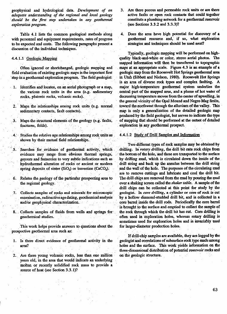
geophysical and hydrological data. Development of an adequate understanding of the regional and local geology should be the first step undertaken in any geothermal exploration program.
3. Are there porous and permeable rock Units or are there active faults or open rock contacts that could together constitute a plumbing network for a geothermal reservoir (see Sections 3.3.2 and 3.3.3)?
Table 4.1 lists the common geological methods along with personnel and equipment requirements, rates of progress to be expected and costs. The following paragraphs present a discussion of the individual techniques.
4.4.1.1 Geolof!k MaDDinp
Often ignored or shortchanged, geologic mapping and field evaluation of existing geologic maps is the important first
.step in a geothermal exploration program. The field geologist:
4. Does the area have high potential for discovery of a geothermal re.source and, if so, what exploration strategies and techniques should be used next?
Typically, geologic mapping will be performed on high- quality black-and-white or color, stereo aerial photos. The mapped information will then be transferred to topographic maps at an appropriate scale. Figure 4.3 is an example of a geologic map from the Roosevelt Hot Springs geothermal area in Utah (Sibbett and Nielson, 1980). Roosevelt Hot Springs is an area of diverse rock types and complex faulting. A
1. Identifies and locates, on an aerial photograph or a map, the various rock units in the area (e.g. sedimentary rocks, plutonic rocks, volcanic rocks).
major high-temperature geothermal system underlies the centralpartofthemappedarea, andaplumeofhotwaterof decreasing temperature moves from the center of upwelling, in the general Vicinity of the Opal Mound and Negro Mag faults,
map is only a generalization of the detailed geologic map produd by the field geologist, but serves to indicate the type of mapping that should be performed at the outset of detailed
, I I
I I 2. Maps the relationships among rock units (e.g. normal toward the northwest through the alluvium of the valley. This sedimentary contacts, fault contacts).
3. Maps the structural elements of the geology (e.g. faults,
I
. fractures, folds). exploration in any geothermal prospect.
4.' Studies the relative age relationships among rock units as shown by their mutuaI field relationship
' 5. Searches for evidence of geothermal activity, w evidence may range from obvious thermal geysers and fumaroles to very subtle indications such as
spring deposits of sinter (Si03 or travertine (CaCO,).
6. Relates the geology of the particular pro the regional geology.
Collects samples of rocks and minerals for microscopic examination, radioactive age dating, geochemical analys and/or geophysical characterization.
8. Collects samples of fluids from wells and springs geochemical studies.
This work helps provide answers to questions about the
1 4.4.1.2 Studv of D d i Samles and Information
Two different types of rock samples may be obtaiued by drilling. In rotary drilling, the drill bit cuts rock chips from the bottom of the hole, and these are transported to the surface by drilling mud, which is circulated down the h i d e of the
and the wall of the hole. The purposes of the circulating mud & to remove cuttings and lubricate and cool the drill bit. The drill chips are removed from the mud by pouring the mud over a shaking scmn called the shaker table. A sample of the drill chips can be collected at this point for study by the geologist. In core drilling, a cylinder or core of rock is cut by a hollow diamond-studded drill bit, and is collected in a core barrel inside the drill rods. Periodically the core barrel is brought to the surface and emptied to collect the sample of the rock through which the drill bit has cut. Core drilling is often used in "exploration holes, whereas rotary W i n g is sometimes used for exploration holes and is invariably used for largerdiameter production holes.
I .. hydrothermal alteration of rocks or ancient or modem drill strhg and back up the annulus between the drill string
area to
7.
prospective geothermal area such as: samples are available, they are logged by the
1. Is there direct evidence of geothermal activity in the geol of subsurface rock type made among area? holes and the surface. This work yields information on the
three-dimensional distribution of potential reservoir rocks and 2. Are there young volcanic rocks, less than one million . on the geologic structure.
years old, in the area that would indicate an underlying molten or recently solidified rock mass to provide a source of heat (see Section 3.3. l)?

i
Legend
fault (qol] alluvium, siliceous sinter 1 7 1 hydtte flows --- I a b I basalt f i m q granite, quartz, ti syenite L rock contact -1 rtifltte domes, with centers diorite 0 produdnggeothermalwells
-1 pyrodasticdeposits metisediments 0 dry geothermal wells 1-4 rhyolite flows banded gneiss
Figure 4.3 Geologic map of Roosevelt Hot Springs geothennal area, Utah.
64

In many geothermal exploration areas, exploration holes or wells have already been drilled, and samples of subsurface core or drill chips as well as driller’s reports and geophysical well logs may be available. Such samples, reports and logs may be stored with the state geological survey, the state water- rights division and/or the state oil and gas commission. They become public information soon after collection or after a specified confidential period. Some states require the bottom- hole temperature to be measured and reported in all holes, providing information especially important for geothermal exploration. The competent geologist seeks and obtains all such available information in the initial stages of an exploration program.
During the drilling phase of an many drillers will not take samples of the rotary-drill chips as they are removed from the dril-mud stream at the shaker table unless instructed to do so. It is important to collect representative drillchip samples from any hole, and it is better
’ to collect too many samples than to collect too few. The driller should be instructed in how to take the samples by the geologist, who will be cognizant of the sampling requirements in different geologic environments. Typically, 1 to 2 lb of sample will be collected each 10 to 20 ft of drilling. These samples will be carefully washed to remove the drill mud and then placed in geologic sample bags whose labels record information on the drill hole name, location, date, and footage from which the sample was drilled.
4.4.1.3 StratigraDhic Studies
A thorough knowledge of the rock types in the pros- pecting area is fundamental, and is obtained through stratigraphic studies. The geologist analyzes both surface outcrops and rock samples from drilling. He strives to identify rock types in the area that would make a good reser- voir rock at depth, i.e. rocks that have adequate primary permeability or in which secondary permeability may be developed. In a volcanic environment, for example, sequences of young lava flows often are highly permeable whereas air- fall or water-laid volcanic tuffs are easily altered to clay minerals and may become quite impermeable. Permeability in flow sequences usually exists at the upper and lower boundaries or contacts of individual lava flows--the center portions of flows tend to be massive, with little primary permeability.
In basin areas, permeabitity is controlled by the type of rock (permeable sandstone or impermeable shale) and by its degree of induration or metamorphism. Metamorphism causes the rocks to become brittle and to fracture under tectonic stress. In some environments, permeability is developed in carbonate rocks (e.g., limestone, dolomite, marble) through dissolution of the carbonate minerals by moving groundwater. It is obvious that an understanding of effects such as these is important to the success of a g e o t h e d exploration project.
4.4.1.4 Structural Analysis
~ A thorough knowledge of the geologic structure of an area is important. Moore and Samberg (1979), for example, showed that at Cove Fort/Sulphurdale, Utah, much of the surface is covered by large landslide blocks that have moved into place from the east along underlying, nearly horizontal faults. Subsequent movement has occurred along later vertical faults, and the area now consists of numerous separate fault blocks. An obvious implication from this discovery is that the geology underlying the landslide blocks cannot be determined by mapping the surface geology, i.e. the surface geology can not be projected to depth. Realization of this fact has had a great impact on subsequent exploration in the area.
zones of permeability if they fracture rock and create open spaces. Alternatively they can be filled with gouge, a rock flour generated during fault movement that is quite impermeable. Faults and fractures can also be Wed by precipitation of vein minerals such as calcite (CaCO,) and quartz (SiOd. Gouge or mineralization developed along faults can isolate the aquifers in individual fault blocks and decrease hydrologic communication across an area. In places where faults intersect, permeability may be especially enhanced.
It is important to determine the relative ages of faults and, especially, to be able to distinguish young faults and fractures from older ones and to distinguish faults that have had recent movement from those that have not. Older faults are more likely to have been mineralized--to have had their open spaces filled through deposition of minerals from circulating fluids. Relative ages of faulting can usually be determined through detailed geologic mapping.
Structural analysis is also important in other respects besides faulting. Recognition of volcanic structures such as calderas and vents is important in understanding the geologic evolution of an area and can suggest where subsurface heat sources and permeable zones may be found. In basin environments, knowledge of the shape and size of the basin and the location of faults can be used to predict depth to permeable horizons containing thermal water in advance of drill testing.
4.4.1.5 Radioactive Age Dating of Racks
Certain minerals contain the element potassium (K), a small percentage of which will be the naturally radioactive isotope K-40. This isotope decays radioactively to argon40 (ArAO), with a half-life of about 1.2 billion years. By measuring the amount of h - 4 0 relative to the amount of K-40 in certain minerals, the time since Ar-40 began to accumulate can be determined (Durance, 1986). In this way, the time interval since formation (i.e., the age) of certain rocks can be determined. There are also other radioactive isotopes that can be similarly used for dating.
65

Age dating has obvious use in geothermal exploration in terms of helping to locate young igneous rocks. If volcanic rocks are found that are less than about one million years old, they may indicate the likelihood of a heat source for geothermal energy.
Care must be exercised in the interpretation of the dates derived by radioactive methods. In the case of K-Ar dating, forexample, ifthe mineralbeing analyzedhas beenheated sufficiently by a thermal event subsequent to its formation, the gaseous Ar accumulated to that time may have escaped, thus resetting the radioactive clock to the date of the thermal event.
Laboratory determination of age dates is a highly specialized field. Dating is done both at commercial labora- tories and at universities. The geologist should work with scientists in the dating laboratory in order to obtain advice on methods for collecting the most appropriate field samples of
Table 4.2 Geochemical Methods for Direct Heat Exploration
the rocks and minerals. For geothermal work, a laboratory that specializes in the dating of young rocks (less than 1 million years old) should be selected.4.4.2 Geochemical Studies
A number of important exploration and reservoir- production questions can be answered from studies of the chemistry of geothermal fluids and reservoir rocks, and so geochemistry plays an important role in geothermal explora- tion and development (Henley and Ellis, 1983). Geochemical reconnaissance involves sampling and analyzing waters and gases from hot springs and other geothermal manifestations in the area under investigation. The data obtained are then used to help locate geothermal resources, to determine whether a geothermal system is hot-water or vapordominated, to -ti- mate the minimum temperature expected at depth, to predict the homogeneity of the water supply, to infer the chemical character of the waters at depth, and to determine the source
Personnel Equipment Rate of Unit cost Method Required Required Progress ($1
Spring or Well Sampling Geochemist (1) Prepared sample bottles, 5 to 20 springsld . 350 to 6001d' pH and conductivity meter
Water Analysis Specialty Laboratory - 1 to 3 weekslordetb 10 to 75/sample
Whole Rock Analysis Specialty Laboratory -- 1 to 3 weekslordetb 50 to 8Olsample
Soil Surveys Geochemist (1) prepared sample 20 to 40 samplesld 370 to 8701d' Technician (1) containers
Mercury Analysis Specialty Laboratory Gold-film 1 to 3 weekslorder" 10 to 15lsample or Geochemist (1) Hg detector 30 samplesld
Radon Analysis Specialty Laboratory I 1 to 6 WeekslordeP 20 to 30lsample
a. See Note a, Table 4.1 b. Analysis time depends on size of order; 1 to 5 sample orders will not usually be put ahead of other work. Orders of
more than 100 samples take longer to complete. Most labs will do an order on a rush basis at a surcharge. c. cost as follows:
Per Day ($1
Geochemist $25 to $50h 200 400 Technician $10 to $15h - 120 Vehicle Q $35/day - $0.35/mi 50 150 Travel Expenses 80 150 Supplies
7 40 - 50 Total 370 870
66

of recharge water. Geochemical principles can also be applied to interpretation of chemical data from producing wells and may yield sinformation on formation of scale in pipes or a gradual chemical change in the geothermal fluids that could indicate an impending change in production temperature. Some of the more important geochemical applications will be discussed in this section. They are also listed in Table 4.2, along with personnel and equipment needs, expected rates of progress, and costs.
4.4.2.1 Overview of Geothermal Geochemistrv
In geothermal geochemistry, we must consider the chemistry of the geothemtal flu& (water and steam), the chemistry of the rods in which the geothermal resource exists, and the interaction between the two. Thus, geothermal geo- chemistry is a complex and highly specialized field of study.
Geothermal fluids contain a wide variety and concen- tration of dissolved constituents. The simplest chemical parameters often quoted to characterize geothermal fluids are:
Total dissolved solids (TVS) in parts per million (ppm) or milligrams per liter (mgfl). This gives a measure of the amount of chemical salts dissolved in the waters, also called the salinity.
1.
2. pH. The pH of a fluid is a measure of the acidity or alkalinity of the fluid. Neutral fluids have pH = 7.0 at mom temperature. Acid fluids have pH values less than 7.0 and alkaline fluids have pH values greater than 7.0.
These two parameters can be measured in the field by use of a conductivity meter and a pH meter. The conductivity meter measures the TDS of a fluid by measuring its electrical. conductivity. The more dissolved salts, the higher the electrical conductivity.
Table4.3 Rep eothermal Fluids
The amount and nature of dissolved chemical species in geothermal fluids are functions of temperature and of the local geology (see Table 4.3). Lower-temperature resources usually have a smaller amount of dissolved solids than do higher temperature resources, although there are exceptions to this rule. TDS values range from a few hundred to more than 300,000 mgfl. Many of the high-temperature r e ~ ~ u r ~ e ~ in the West contain 6,000 to 10,000 mgfl TDS, whereas 8 portion of the Imperial Valley, California, fesources are essentially saturated with salts at 300,000 mgfl. The pH of geothermal resources ranges from moderately alkaline @H = 8.5) to moderately acid @H = 5.5).
The dissolved solids are usually composed mainly of sodium ma), calcium (Ca), potassium (K), chlorine (a), silica (SiOJ, sulfate (SO,), and bicarbonate (HCOJ. Minor constituents include a wide range of elements with mercury (Hg), fluorine (F), boron (€3) and arsenic (As) being toxic in high enough concentrations and therefore of environmental concern. In general, each state has regulations governing the use and disposal of waters that contain toxic or otherwise harmful constituents, and local regulations should always be consulted in planning the use of any geothermal resource. Dissolved gases usually include carbon dioxide (COJ, hydro- gen sulfide (H2S), ammonia (”,) and methane (CHJ. Hy- drogen sulfide (H2S) is a safety hazard because of its toxicity to animals, including humans. Effective means have been and are still being developed to handle the scaling, corrosion, and environmental problems caused by dissolved Constituents in geothermal fluids. Experience has shown that essentially every type of geothermal fluid can be successfully used.
As geothermal fluids move through rocks, they react chemically with the rocks, which themselves are usually chemically complex. Hydrothermal alteration is the term given to mineralogic changes brought about in the rocks by interaction with hydrothermal fluids. Certain minerals in the
Temp. pH Si02 Ca Mg Na K Li HCO so CI F B As Sample oc @pm) @em) @P@ @pm) @pm) @pm) @pm) (P @pm) @em) @pm) @pm) @pm)
- 13.4 - 6 316 7.150 5 155,000 16 390 12
Sample Descriptions 1. Hot Springs, M o m , UT. 2. Hot Springs, Steamboat, NV. 3. 4. 5. 6.
Well 44. Wairakei, New Zealand. Brine discharge from Well 54-3, Roosevclt Hot Springs, UT. Analyses calculated from tlashed brine, Well M-26, C iem Prieto, NM. Brine discharge from Well I lD, Salton Sea Geothennal Field, CA.
67

reservoir rocks may be selectively dissolved by the fluids while other minerals may be precipitated from solution or certain chemical elements from the fluid may substitute for certain other elements within a mineral. These chemical/ mineralogic changes in the reservoir rocks may or may not cause volume changes, i.e., may or may not affect the permeability and porosity of the rocks. Obviously, if the mineral volume increases, it must be at the expense of open space in the rock, which causes a decrease in porosity and permeability.
In locations where pressure, temperature, or rock chemistry change abruptly, minerals may be precipitated into the open spaces, resulting in plugging of the plumbing system. Silica and calcium carbonate (CaCO,) are the principal minerals deposited in open spaces. The solubility of SiO, decreases with a decrease in temperature, with pressure changes having very little effect. SiO, can be precipitated into open spaces such as fractures or pores in the rock in regions where subsurface cooling takes place and at the surface where hot springs discharge. Quartz, the most common silica mineral, is found in veins in present-day geothermal systems as well as in ore deposits, some of which are fossil geothermal systems.
Calcite (calcium carbonate) is u n d in that it has a retrograde solubility, i.e., it is more soluble in waters at low temperatures than at high temperatures. Other carbonate species such as dolomite (MgC03), as well as sulfate species such as anhydrite (CaSOk), show similar retrograde solubility relationships with temperature. In addition, the solubility of carbonate minerals decreases rapidly with decrease in the partial pressure (amount) of carbon dioxide. Thus, as fluids that are saturated with dissolved carbonate approach the surface, carbonate minerals such as calcite are deposited as a result of the loss of CO,, which evolves from the solution with the decrease in hydrostatic pressure.
The chemically complex hydrothermal system is dynamic through time. That is, for any given volume element in the reservoir, the chemical composition of the fluid in that volume varies slowly with time, bringing about variation in the rock composition, porosity and permeability. However, because the rate of fluid circulation is perhaps only a few centimeters per year, in most hydrothermal systems a state of chemical equilibrium or near-equilibrium exists between reservoir fluid and reservoir rocks (Capuano and Cole, 1982; Helgeson, 1969). The assumption of chemical equilibrium is made in the application of several of the geochemical techniques discussed below. Lack of equilibrium could be evidence for rapid movement of fluid through the reservoir.
4.4.2.2 Chemistrv of Geothermal Fluids
By taking appropriate samples of fluids from surface springs and from well discharges, a great deal can be learned about presence or absence of a geothermal tesoutce and about
the fesource itself. probably be obtained in the following topic areas:
The most important information can
1.
2.
3.
4.
Reservoir Fluid Types: Various fluid types evolve from typical geothermal systems, and identification of the fluid type can have important implications on the presence of other, related fluid types in the vicinity and, thus, on exploration. Figure 3.10 illustrates some of the hydro- thermal fluid types common in geothermal reservoirs.
Geothermometry: Chemical data can be used to estimate the maximum subsurface fluid temperatures to be expected in a given area.
Reservoir Processes: The extent of mixing of thermal and non-thermal waters and boiling in the subsurface can be determined from geochemical analysis.
Production Monitoring: In a producing geothermal resource, monitoring of the concentrations of chemical species over time can lead to information on the nature of the recharge to the system and to prediction of adverse temperature changes in advance of their manifestation in the well (cold-water breakthrough).
Geothermal Fluid Types
As discussed in Chapter 3 and in the paragraphs above, the chemical composition of geothermal fluids (Table 4.3) is a product of their mode of formation. Normal ground waters are usually near neutral in pH and slightly bkarbonate in character. When they are heated in a g e o t h e d system, they tend to become more sodium chloride in character, with dissolved salt contents that can range from a few hundred mgA to more than 300,000 mg/l. If the fluid boils at depth, gases (e.g., COz, HzS) are preferentially partitioned into the steam phase and migrate independently toward the surface. The gas- rich steam phase may encounter cool groundwater, which it heats. Oxidation of H,S at the surface or through interaction with oxygenated groundwater produces acid-sulfate waters that react with the host rocks to produce characteristic argillic- alteration assemblages of clay minerals.
Biwbonate-rich geothermal waters are produced where groundwater dissolves C02, rising with steam from the deeper geothermal system. Any of these water types may be diluted with low-salinity groundwater or changed in other ways before being sampled from a thermal spring or a well. By study of the chemistry of the various waters found in wells and springs in a geothermal area, the nature of the g e o t h d waters at depth can sometimes be determined.
In the usual reconnaissance application, water samples are taken for analysis from springs and wells in the vicinity of the prospect. For detailed reservoir studies, fluid samples can also be taken from producing wells or from wells recently drilled but not yet producing. Great care must be taken to
68

ensure that the samples contain only pristine reservoir, well, or spring fluid. In the case of a recently drilled well, the well must be flowed until all traces of the drilling fluid have been removed. Sampling of fluids should be repeated at intervals of hours or days until analysis yields constant chemical composition. At that point, the fluid is assumed to represent reservoir fluid.
Proper sampling techniques are very important and should be entrusted only to someone with experience. The samples must be filtered and properly acidified for preser- vation until analysis. In designing the sampling program, the geochemist should work closely with a chemist at the labora- tory where the analyses will be performed to ensure the best results. At each sample location, pH, temperature, and perhaps other quantities should be measured at the time of collection.
Various systems have been devised to diagram water chemistry for better visual presentation (Hem, 1970). One of the most popular in geothermal work is a plotting method given by Piper (1944). This method is based on the relative amounts of Na + K, Mg, Ca, C1 + F, SO,, and HC03 + C03 in a fluid. These components are the major ion types in thermal and non-thermal waters, and classifications based on them agree well with obsemations on the formation of various geothermal water types. To construct a Piper plot, also called a trilinear plot, the concentrations of cations and anions are transformed from units of ppm or mgfl into the units of milli- equivalents and the percentages of the cation and anion com- binations given above are plotted on a diagram similar to that shown in Figure 4.4. Any water analysis will contain cations that yield one point on the tower left portion of the diagram and anions that yield one point of the lower right portion.
Figure 4.4 Illustrative trilinear plot.
The cation and anion percentages are combined by projecting them onto the central rhombohedron, as illustrated with the water analysis shown as point A in Figure 4.4. The diagram can be used to plot all the waters from a prospecting area, and a classification of water types can then be developed by comparing the result to the general classification diagram shown in Figure 4.5.
Figure 4.5 Trilinear water classification.
Creek, B.C.
Figure 4.6 shows a classification of water types found at the Meager Creek geothermal area in Southwestern British Columbia (Adam and Moore, 1987). In this study, the
69

authors showed that the several water types were chemically independent, Le., that they had not evolved from a common water type nor had one evolved from any other. This result implies that there is no through-going permeability in the part of the Meager Creek area explored, and that the several waters originate in unconnected, probably small reservoirs.
Murray et al. (1985) show a Piper plot of water from the Calistoga geothermal area in the Napa Valley of California (Figure 4.7). Their results suggest that thermal water rises along a central fault in the valley. The thermal water is progressively diluted with non-thermal groundwater, gradually becoming enriched in iron, sulfate and biearbomte. The several water types in the valley can all be related chemically to the thermal water seeping up the central fault, and water geochemistry can be used to trace and map geothermal waters in the valley.
SW border of the NE border of the vdley
- Ca Q-
Figure 4.7 Water types plotted on a trilinear diagram, Calistoga, California.
valley
Chemical Geothermometry
Chemical analyses of geothermal fluids can sometimes be used to estimate subsurface reservoir temperature. This infor- mation is of obvious interest during exploration, when infor- mation from measurements in drill holes may be unavailable. It is also very important during drilling because: (a) accurate temperature measurements cannot be made in a well until after thermal effects of the drilling process have been dissipated, weeks to months after drilling is finished; and, (b) chemical geothermometry may indicate that temperatures higher than those found in the drill hole may be found elsewhere.
Several major-element geothermometers have been used successfully for estimating subsurface temperature, and reviews of these geothermometers were given by Fournier
(1981) and by Henley et al. (1984). Silica is an element whose concentration in thermal waters varies with temperature in known ways. It is, therefore, an often-used element in chemical geothermometry. In general, the silica content of geothermal fluids appears to be limited above about 350 OF by the solubility of the mineral quartz (Si03 and to be limited below 350 OF by the solubility of amorphous silica. The temperature dependence of these phases is shown by Figure 4.8, which also gives the solubility of various other silica phases as a function of temperature. Figure 4.9 shows some of the silica geothermometer equations as an illustration of the type of calculations that are performed.
0 100 200 T,”C
300
Figure 4.8 Solubility of silica species in water as a function of temperature.
Another system of geothemometers is based upon the equilibrium reached among the elements sodium (Na), potassium (K), calcium (Ca) and magnesium (Mg) where reservoir rocks contain abundant quartz and feldspar minerals (Fournier and Truesdell, 1973). One common geothermo- meter of this class is also shown in Figure 4.9.
Since other silica geothermometers are based upon equilibrium with the minerals chalcedony, alphacristobalite, or betacristobalite, it is obviously of importance to know which silica minerals exist in the reservoir rocks. If drill information is not available on this point, as is usually the case early in an exploration program, one must rely on geologic mapping and inference to provide this information.
Different geothermometers frequently yield different results when applied to the same thermal water. Use of other geochemical and geological data may help shed light on the
70

SILICA
Quartz - no steam loss
1309 - 273.15 (OC) = 5,190 - log si02
Quartz - maximum steam loss
- 273.15 T(OC)= 1522 5.75 - log Si02
ALKALI
Na/K (Fournier)
- 273.15 121i log (NaIK) + 1.483 T(OC)=
Na - K - Ca
The following generalizations can be made con&g the age of geothermal water in the absenci: of mixing. A tritium content of less than 3 TU usually indicates that no water younger than 25 years is present. Values of 3 to 20 TU suggest that some amount of thermonucIear tritium is p&t, which indicates that the fluids entered the groundwater environment in the 1954-1963 time frame. If more than 20 TUs are found, the water entered the system after 1963. An aquifer that has been isolated from tritium recharge for 60 years would have a tritium content of about .1 TU, the limit of detection. Many geothermal reservoir waters are older, some much older, than this useful limit to tr;tium dating. Typically, convecting hydrothermal fluids move at speeds measured in feet or tens of feet per year. However, a young
- 273.15 T ( V ) = 1647 log ( N u l 0 + [log (qCulNa) + 2.06 I+ 2.24
* p = 4/3 for $Ca/Na > l ,T clOO°C; fJ = 1/3 for - .TCa/Na <I, T> 1 0 0 ~ ~
Figure 4.9 Chemical geothermometer equations (all concentrations are in mg/lcg].
relative reliability of the various geothermometers in specific geologic situations. For example, silica concentration can be affected by the pH of the fluid, and temperatures calculated from the Na-K-Ca neothemmeter may be in serious error if the C02 or magnesL concentrations &e too high or if there has been addition of any of these elements between the reser- voir and the surface through interaction of the fluid with 'sedimentary rocks or ion-exchging minerals such as clays or . zeolites. MXig of the thermal reservoir waters with normal groundwater can also change the'concentrations of critical elements in a geothermometer, and can result in a calculated temperitme that is either too high or too low. ~n addition, some geothermometers do not work well where reservoir temperatures are below about 300 OF.
. tritium date would indicate rapid water flux in a system. ,
Production Monitoring
It is important to ob d analyze samples from g e o t h e d production wells on a periodic basis beginning at the start of production. By collecting a history of production- chemistry data, processes and changes in the reservoir can be more easily understood and predicted. Generally, samples of produced fluid are collected at more frequent intervals during the initial months of production, with the sampling interval lengthening if samples show constant composition. As a guideline, monthly samples should be taken and analyzed from
duringthe initial phasesof productionin any system, and
Care must obviously be taken in interjmtation of emical geothermometer data, and in this matter there is no
good substitute for experience. Anyone can apply the geother- mometer equations to the chemical analysis, but the interpre-
is best left to the experts. I tation of the results can be extremely subtle and involved, and each production well in large, high-production systems or
71
I
Age Dating of Geothermal Waters
Radioactive isotope chemistry has been used to attempt to determine the age of the water in geothermal systems, using techniques similar to those for dating of rocks. The most successful applications have used tritium, a naturally occunring radioactive isotope of hydrogen (H-3), which has a half life of 12.26 years. Minor amounts of tritium are ~ t ~ r a l l y produced continually in the stratosphere by the action of cosmic radiation on hydrogen in the air. However, major 8moullts of tritium have been put into the atmosphere by thermonuclear weapons testing.
Tritium concentration is expressed in terms of the Tririum Unir (Tu), which is equivalent to a ratio of tritium to hydrogen-1 of 1 x lo'*. In continental climates io the temperate zone, cosmic radiation produces about 10 TU or less. Before 1954, the tritium content of precipitation in western Europe was only about 2.5 TU. As many as 10,OOO TU were measured in the air in 1963 following extensive atmospheric nuclear weapons testing. Ambient tritium levels thereafter decreased, falling to 60 TU in 1975 (Durrance, 1986), and since then have fallen more slowly. Tritium can also be produced by some rocks through neutron capture by lithium-6. Durrance (1986) shows calculations indicating that certain granites in England product 0.9 TU.

quarterly samples should be taken in smaller systems and in systems whose history indicates that this interval is appropriate. The geothermal developer should obtain competent consulting help in designing and carrying out a sampling and analysis program.
By monitoring the chemistry of produced geothermal fluids at the well head or in the plant, cheinical changes that could indicate scale development in pipes and other equipment can be seen before equipment damage occurs. Similarly, changes in gas content of geothermal fluids may be important for environmental or scaling reasons. If the geothermal fluid is being disposed in an injection well, breakthrough of injected fluid to the production wells may sometimes be seen by its chemical signature before thermal degradation of produced fluids pkes place. This would allow alternate plans for injection of fluids before thermal breakthrough.
It is usually desirable to have the injection and pro- duction wells in hydrologic communication so that the injected waters provide recharge to the reservoir. However, if the con- nection is too direct, the injected waters do not have sufficient time to reheat, and the production temperature goes down. On occasion, it may be desirable to test for breakthrough of injected fluids into production wells using chemical tracers. Tracers are added to the injectate before it is sent to the injection well. Subsequently, production wells are monitored for the presence of the tracers. If tracer appears in the production well, one can be sure that some injected fluid is carrying it. The time to breakthrough, the amount of tracer recovered compared to the amount injected and the shape of the tracer-concentration curve with time are important data in understanding the nature of the connection between injection and production wells and in determining whether or not injection or production wells must be moved.
4.2.2.3 Geochemistry of Rocks
Rocks contain a variety of chemical elements that make up the minerals. Most minerals are made from only a few elements, and these are known as the major eL?mt?nts in the rock. Elements that occur in the approximate range 0.5 to
Table 4.4 Typical Chemical Composition of Rocks
0.05 96 are usually tehed minor elements. Elements that occur in the parts-per-million range are termed truce elements. Chemical analysis for major elements is sometimes performed for rack identification purposes. Minor and trace elements are studied for their geothermal exploration implications.
Major-Element €hemistry
The major-element chemistry of rocks can be used to identify the rock type. If there are no good samples of the whole rock available, as when drilling produces only thy chips, or in cases where rock type cannot be pinned down by hand-specimen or microscopic observation or from X-ray identification of minerals, a complete chemical analysis of the rock may be made for the purpose of rock-type identification. The major rock-forming elements analyzed include silicon, aluminum, iron, magnesium, sodium, and potassium. Analy- tical results for these elements are generally expressed, by convention, as percentages of oxides of the metals. Table 4.4 shows typical analyses for several rock types.
Minor- and Trace-Element Zoning
As hydrothermal fluids circulate in a geothermal system, they pick up, carry and then deposit (i.e., they redistribute) chemical species. The mobilities of various elements varies, so that some elements are hardly mobilized at all by the geo- thermal fluids whereas others become highly mobile and are carried long distances in the fluids. These mobile elements may be deposited in a halo or dispersion zone around a geo- thermal system. For example, mercury, arsenic, manganese and zinc are all quite mobile in geothermal fluids, even those of low and moderate temperature (Varekamp and Buseck, 1983). Soil-sample surveys of a prospect area are sometimes used to determine where the geothermal potential is highest and to locate faults and fractures along which geothermal fluids have moved.
Figure 4.10 shows the distributions of mercury and arsenic, respectively, in soil samples from the Roosevelt Hot Springs geothermal system (Christensen et al., 1983). Both arsenic and mercury are believedto be carriedassulfide
Rocks SiO, AZO3 F%03 FeO MgO CaO N%O K,O HgO Others
Basalt 49.1 15.7 5.4 6.4 6.2 9.0 3.1 1.5 1.6 2.0 Granite 71.6 14.5 1.5 1.1 0.9 2.0 3.0 4.1 0.8 0.5 Sandstone 90.7 4.6 0.4 0.1 0.1 0.1 2.8 0.5 0.4 0.3 Shale 61.2 15.6 1.4 3.0 4.2 3.4 0.4 6.7 2.7 1.4 Limestone 2.0 0.4 I 0.5 7.9 44.4 -- I 0.2 44.6 (co3

. . . . . . . . . . . . \;,. . . . . . . . . . . . . . . . . . . . . . . . . . . . . . . .-. . . . . . . . . . . . . . . . . . . . . . . . . . . . . . . . . . . . . . . . . . . . . . i J .
. . . .
. . . . . . . . . . . . . . . .
. . . . . . . . .
. . . . . . .
. . . . . . . . . . . . . O"0 . . . .O"O . . . . . . . . . .\. ! . . . . . . . .
. . . . J . . . . . . I . . . . . . . . . ' r - * - - . . . . . . . I . . .
I .0?-'. . ' 1 . . . . . . . 1 . . . . . . . . f . . . . . . . . I . . . . . . . ,' . . I . . . . . . . I
. . . . . . . . . .
. . . . MEUCUW AUS€NfC BICKWWINO 29W4 THIESmKD 5 d m l CGUmUR INTERWLS 50. Iw.
. . . mrw..m.m.3fcQrrr
MCUGRDUMD 4- rwRESnOLD 6ppn COMTWR INTERVALS 6,IZppm . . . . . . . . . .
. . f . .<e;\. ,
Figure 4.10 Arsenic and mercury distribution at the Roosevelt Hot Springs geothermal area, Utah.
complexes in aqueous solution. Mercury is also transported as a vapor. These elements, therefore, outline conduits of fluid transport in the subsurface. The figures show that anomalies in both metals coincide with the north-northeast trace of the Opal Mound fault, believed to be one of the chief producing faults in Roosevelt Hot Springs. A second direction suggested by the shapes of the anomalies is northwest. Faults and fractures are also known with this trend in the area. Mercury anomalies continue northwest of the Opal Mound fault, and outline an area of subsurface outflow of the thermal plume at Roosevelt.
In conducting soil geochemical surveys, a Certain chosen soil horizon should be carefully and consistently sampled in order to obtain the most meaningful results. Noise in the survey results can be generated from inconsistent sampling. Matlick and Buseck (1976) advocate the consistent use of the A soil horizon for mercury surveys. It is advisable to work with a geochemist who is experienced in soil sampling m e y s forcollec
Soil
interpreting survey results.
for locating faults, fractures or other permeable horizons that are open and carrying geo- thermal fluids at depth. Radon, carbon dioxide, hydrogen sulfide, mercury, and the noble gases all move freely in per- meable zones, gradually working their way to the surfke, where they are naturally discharged into the atmasphere. Sensitive detectors can be used to m u r e their abundance, which should increase above a fluidcarrying conduit or aquifer. Exploration and production drill holes can sometimes be sited using such survey information.
Trexler et al. (1980) found that a soil survey of the Caliente, Nevada area did a teasonable job of outlining areas known to be thermally anomalous from measured well temperatures and shallow-temperature surveys in 6-ft deep holes (see Section 4.4.3.1 - Thermal Methods). Matlick and Buseck (1976) also outlined uses of mercury geochemistry in geothermal exploration. They showed data for mercury distri- bution in four geothermal areas-bng Valley and East Mesa, California, and Summer Lake Basin and Klamath Falls, Oregon. In each area, the mercury survey outlined known and suspected areas of presentday geothermal activity quite well. Figure 4.11 is a profile of the mercury anomaly over and ad- jacent to the area of high heat flow and geothermal production at Klamath Falls.
Soil-gas surveys are made by plunging a stainless steel tube into the soil to a specified depth and extracting a measured amount of soil gas by suction. The gas is then analyzed. Radon is a naturally radioactive gas that migrates to the surface through transport in solution and through
73

NNW Distance (kilometers) SSE
Figure 4.11 Soil mercury profile of Klamath Falls, Oregon.
movement as a gas in open spaces. Its presence can be quantitatively determined using the track-etching method. A strip of cellulose nitrate film is taped inside a plastic cup and inverted cups are placed in shallow holes and left for periods up to several weeks. Radon gas reaches the cup and collects, and as it decays radioactively, the nitrate film records the passage of subatomic particles as microscopic tracks. Acid etching of the film after the cups are retrieved makes the tracks visible, and they are counted under a microscope. One advantage of this technique over analysis of a sample obtained by suction is that it provides an integrating effect over the time the cups are in the ground, which tends to reduce the effects of changes in atmospheric pressure and soil moisture on radon content in the soil. Because radon is so highly mobile in the geologic environment, such surveys can be used to locate faults and zones of upwelling fluids (Nielson, 1978).
Mineral Zoning and Hydrothermal Alteration
There are two principal effects on rocks when they interact with hydrothermal fluids. The first is deposition of minerals in the fluid pathways, forming veins and cementing pores, a process called mineralization. The second is modifi- cation of minerals in the rock through chemical interaction with the fluids, a process called hydrothermal alteration.
74
Study of minerals deposited in the subsurface plumbing of geothermal systems helps to map the boundaries of such systems, helps determine the temperatures at which the minerals formed, and helps locate zones of upwelling and recharge. Both the vein-mineral assemblage and the occur- rence of individual minerals exhibit zoning, both laterally and with depth, in geothermal systems. Different vein-mineral assemblages are formed in response to changing temperatures, changing rock chemistry (mineralogy), and other factors. The most common and abundant vein minerals are quartz (SiOJ and calcite (CaCO,). Usually veins also contain lesser quantities of other minerals such as K-feldspar and epidote. Veins in geothermal systems may contain metallic minerals, some of which are of economic value. Pyrite (FeS,, fools gold) is common in many geothermal systems, and sulfides of lead and zinc also occur. Gold is associated with the upper regions, the so-called epithennal zones, of geothermal systems in the Basin and Range province. Several of the gold mines in Nevada are associated with present-day geothermal systems.
Hydrothermal Alteration Minerals
Amorphous sio, Quartz K-Feldspar Albite Calcite Smectite Smectite Illite Chlorite Biotite Actinolite Tremolite Diopside Garnet Epidote Prehnite Heulandite Stilbie Ptilolite Laumontite Wairakiie
1c C 200°C 300°C (from Henley and Ellis, 1983)
Figure 4.12 Temperature ranges for typical hydrothermal minerals (after Henley and Ellis, 1983).
The vein-mineral assemblage provides an indication of the temperature of the rocks and fluids at the time of mineral deposition and of the chemical composition of the water.

Minerals such as epidote and wairakite form only at high tem- peratures (see Figure 4.12). Their occurrence indicates the high-temperature, or former high-temperature, portions of the geothermal system. By contrast, the mineral chlorite can form over a wide temperature range. The mineral anhydrite (CaSO,, calcium sulfate) can form only where the fluids umtain oxygen. Primary hydrothermal fluids do not usually contain oxygen. Thus, anhydrite is often interpreted as a sign that the vein is in a recharge zone, where oxygenated surface water is flowing into the geothermal system.
Rocks undergo hydrothermal alteration through chemical reaction between the minerals and the circulating hydrothermal fluids. Some minerals are taken into solution and others de- posited in their place. In other cases, a mineral is changed through substitution of one chemical species for another in the mineral. Certain minerals are much more reactive than others. For example, feldspar minerals alter readily to clay minerals, whereas quartz is almost always unaltered, even when most other minerals are altered. Typical reservoir rocks in a geo- thermal system, therefore, show signs of hydrothermal altera- tion and are also shot through with veins whose minerals have be deposited from the hydrothermal fluids.
The distributions of the clay and silicate minerals, both in veins and in the hydrothermally altered rock mass, are strongly temperaturedependent. At the lowest temperatures, below about 300 OF, the stable assemblage consists of dolomite, kaolinite, smectite and inter-layered illite/smectite. With increasing temperature and depth, smectite, dolomite, kaolinite, and inter-layered illite/smectite disappear, and at temperatures above 300 to 350 OF, the typical assemblage is illite, chlorite, potassium-feldspar and quartz. The calcium- aluminosilicates wairakite and epidote appear only in rocks above 400 to 450 OF.
One very important result of mineral zoning is that the higher-temperature mineral assemblages cause the rocks to become brittle, and they fracture easily under the influence of tectonic movement and stress. Faulting of brittle rock creates and renews fracture permeability in the higher-temperature parts of some geothermal systems. In the geothermal systems of the Imperial Valley of California, embrittlement through hydrothermal alteration and vein-mineral deposition is a very important process. It is typically the brittle, more highly altered portions of these systems that have permeability and constitute the reservoir. Overlying rocks, altered at lower temperatures, have mineral assemblages that make them softer and unable to sustain an open fracture. These rocks have very low permeability.
Acid-sulphate springs are typically a surlicid feature produced by the oxidation of hydrogen sulfide to sulfuric acid in the near-surface zone. Altered ground surrounding the acid springs and fumaroles provides a striking example of the re- activity of rocks with some geothermal waters. The altered areas are typically bleached and converted to asiliceous
residue containing native sulfur, cinnabar (mercury sulfide), sulfate minerals, yellow, red and brown iron oxide minerals and clay minerals. Such acid-altered areas would be recognized by the geologist as an indication of past or present geothermal activity. Similar acid alteration can also be formed at depths where steam heating of ground waters occur.
The interpretation of the mineral assemblages found in many thermal systems is complicated by the presence of minerals formed during earlier, frequently unrelated, hydro- thermal events. At least two distinct hydrothermal events have been recognized in the Roosevelt Hot Springs geothermal area: an earlier event related to intrusion of the Tertiary Mineral Mountains pluton, and the present hydrothermal system (Nielson et al., 1978). Crosscutting veins, identified in drill chips, suggest that the depositional histories of these events was quite complex.
Two primary methods are available for identification of minerals. First is use of the petrographic microsmp. Thin slices of the rock are Cut with a diamond saw and subsequently polished on a special lapidary disk until they are very thin and transparent. They are then known as thin sections, and are examined under the microscope. The petrographic microscope is equipped for transmission either of ordinary light or polarized light. The thin section is examined in both kinds of light. In the polarized mode, light of one polarization is transmitted through the thin section from below. There is a second polarizing filter above the thin section in the tube of the microscope whose orientation is perpendicular to the polar- izer below. Such an arrangement blocks passage of light up the microscope tube except for light whose polarization is changed by the mineral grains in the thin section. Various minerals rotate the plane of polarization of light moving through them in characteristic ways, so that the rotated light passes through the upper polarizer. By noting appearance and properties of minerals in both ordinary light and polarized light, the vast majority of minerals can be positively identi- fied. At the same time, the mutual age relations among the minerals, and the structure and texture of the rock can be de- termined. All of this information, taken together, enables the experienced geologist to determine the rock type, the degree of alteration and veining and the M~UI-~ of vein minerals.
The second important method of mineral identification is by use of an X-ray machine. Samples of a rock or mineral are ground to powder size and mounted in a thin film on a glass slide. X-rays are then directed at the slide. The crystal structure of minerals diffracts the X-rays in characteristic ways, producing a pattem on a chart-paper readout that can be used to identify individual minerals in a sample. X-ray dif- fraction mineral identification is more certain than is petro- graphic identification. However, the petrographic mi- has the advantage of being able to see the relationships among minerals in a rock, whereas this information is not obtained by X-ray diffraction because the rock is ground up in preparing the X-ray slide.
75

Fluid Inclusion Studies
In the process of the formation of minerals from hydrothermal fluids circulating in the fractures and pore spaces of geothermal systems, tiny amounts of the fluids themselves become trapped when the mineral grows around them. These fluids thenceforth exist as microscopic bubbles in the minerals known asfluid inclusions. Study of fluid inclusions is useful in geothermal exploration because they contain a sample of the fluids that formed the mineral in which they are found, and the information derived can tell much about the formation and evolution of the geothermal system.
Typical measurements in the study of fluid inclusions involve heating and cooling of the mineral specimen. The mineral grain is first hand-selected from a sample of drill chips or core and mounted on a microscope slide. It is then polished to an appropriate thickness. Under the microscope, fluid inclusions appear as flaws in the mineral that are bounded by an outline that may be regular or irregular, and that generally contain a vapor bubble resulting from fluid contraction as the mineral cooled from its temperature of formation. By heating the mineral under the microscope and measuring the temperature at which the bubble disappears (i.e., the fluid inclusion becomes completely filled), the temperature of formation of the mineral is determined. Also, by cooling the mineral under the microscope until the fluid freezes, the salinity of the fluid can be determined. Dissolved salts lower the freezing point of a solution by known amounts.
Temperatures of formation yield information on, among other things, whether the system has cooled down or warmed up since the mineral formed (Moore et al., 1989). Freezing- point determination of fluid salinities provides information on variations of salinities at various locations in the system, thus helping to map fluidchemistry variations. Differences be- tween fluid-inclusion salinities and the salinities of present-day fluids can also help unravel system evolution and chemical structure.
Freezing-point measurements can also be used to determine the carbondioxide content of the hydrothermal fluids. Variations in C02 content indicate the positions of mnes of upwelling and zones of boiling. It has been found that a C02 blanket often overlies the area of upwelling in geothermal systems (Moore et al., 1990)
Isotope Studies
Several stable isotopes are used in chemical studies of geothermal systems. Isotopes of a chemical element are separate species of the same element that have different numbers of neutrons in the nucleus. Stable isotopes are those that do not decay radioactively. The stable isotopes most often of help in geothermal studies are hydrogen-2 or deuterium @) and oxygen-18 (0-18). Table 4.5 shows how these species relate to the other isotopes of these elements.
76
Table 4.5 Oxygen and Hydrogen Isotopes
Element ISOtOLU? Oxygen '60 = 99.756%
"0 = 0.039%
'*O = 0.205%
Hydrogen 'H = 99.985%
%I = D = 0.015%
'H = T, = 12.26~
The average percentages of each isotope as distributed in nature are well-known from many measurements. However, geochemical and geological processes can cause the relative percentages to change. Among these processes are boiling in a geothermal system, chemical reactions between water and rock, mixing of different fluids, filtration through shales, and changes in the state of oxidation. Figure 4.13 illustrates, on a plot of change in oxygen-18 versus deuterium, the expected direction of change for the hydrogen and oxygen in water because of these processes.
t 6D x 10
Natural Predpitation Evaporation
Shale Filtration
Boiling
Exchange With Rock
R 0 ' 0 ,
' /
/ A' /
, , Vaporphase #
Figure 4.13 Common isotopic fractionation mechanisms for water.
It can be seen from this plot that the effects of chemical interaction between geothermal waters and reservoir rocks are expected to lead to enrichment in 0-18 in the water, with little orno changeinD. The explanation is that there are few

hydrogencontaining minerals in reservoir rocks, and thus, the deuterium in the water has few minerals with which to inter- act. It, thus, remains constant. However, there are many oxygencontaining minerals in reservoir rocks, and these minerals are typically enriched in 0-18.
Figure 4.14 illustrates observed 0-18 enrichment in waters from some typical geothermal systems having a variety of temperatures. The data-points for 0-18 extend to the right of the meteoric-water line. The meteoric-water line shows the average composition in D and 0-18 for rainwater in the area. Now, it has previously been observed that the deuterium content of rainwater is dependent on the altitude at which the rain falls. It has also been observed that the fluids in hydrothermal convection systems are predominately meteoric in origin (Craig, 1963). These observations, couded with
Isotopic studies can also help answer questions on bulk reservoir permeability. If the ratio of water to rock in the system is large, (i.e the system is highly porous and perme- able), the isotopes in the water will not be changed much because of the relatively large amount of water, whereas the isotopes in the rock will show large shift. However, if the ratio of water to rock is small, (i.e., the system is of low porosity and permeability), the isotopic composition of the water will be shifted markedly while that of the rock will not be appreciably changed. Thus, by characterizing the 0-18 and D compositions of both the water and the reservoir rock, a crude estimate of the bulk permeability of the system can be obtained.
4.4.3 Geophwical Studies
measurements of the deuterium content of hot springs and reservoir waters discharged from wells, can sometimes be used to help determine the altitude at which the reservoir waters originated, and thus, the source area for the recharge waters.
Geophysical exploration is the use of physical measurements either to (a) detect a resource directly, (b) to provide indirect evidence of its existence and location, or (c) to determine and map its physical and chemical characteristics.
0 -
- - - -
-50 - - MAGMATIC
n
Hveragerdi, Iceland WATER Y 3 n - 10 -
- -100 -
Newcaatle. Utah Steamboat Gp.. Nev.
Modoc Plat ,Cali. Gunnyride, Colo.
1 5 1
10
6”O (%o)
Figure 4.14 Observed oxygen isotopic shifts for geothermal systems.
77

Table 4.6 Geophysical Methods for Direct Heat Exploration
Personnel Equipment Rate of unit Cost Method Required Required Progress ($1
Temperature- GradientIHeat Flow
Drilling Driller Losging Geophysicist (1) Thermal Cond. Specialty Laboratory
Shallow Temperature Geophysicist (1) Technician (1)
Dipole-Dipole Resistivity Geophysicist (1) Technician (2)
EM Shallow Geophysicist (1)
Technician (1) Geophysicist (1) Technician (1)
Self-potential Geophysicist (1) Technician (1)
Magnetics Air Ground Geophysicist
Gravity Geophysicist Technician
Drill rig 100 to 500 fi/day Temp. logging gear 500 to 2000 ftlday
-- 4 to 8 weekslorder
Hand-held drill Thermistor probes
4 to 8 stalday
Specialty equipment 3000 to 6000 &/day
Specialty equipment 3000 to 6000 ft/&f
Specialty equipment 6 to 10 soundings/day
Digital voltmeter, 8000 to 15000 ft/day Wire
400 to 600 milday 1 to 3 mi/day
0.2 to 1 milday
1000 to 4000/d’ 350 to 600/dayb 100/sample
450 to 870/day
900 to 1200/day’
500 to 900/day
500 to 900/day
500 to 900/day
15 to 40/mi 370 to 600/dayb
500 to 900/day
a. Drilling costs and rates vary widely depending upon the rock type, degree of fracturhg, the type and size of rig and other factors. Bids should be obtained for any planned drilling program.
b. See Note a, Table 4.1. c. costs as follows:
Per Day ($)
Geophysicist $25 to $50h 200 400 Technician $10 to $t5h 160 240 Vehicle @ $35/day + $0.35/mi 50 150 Travel Expenses 140 230 Equipment & Supplies -- 150 200
Total 700 1220
d. Assumes a lowcost EM system suitable for locating shallow faults. e. Assumes soundings to detect a resource at depth.
78

Such physical parameters as the distribution of temperature over the surface of the earth and at depth, the electrical, magnetic or density properties of the ground, and the manner in which mechanical (seismic) waves are propagated in the earth all respond in their own way to the presence of a geothermal resource (Ward, 1983; Wright et al., 1985) or to an ore body, a coal deposit or a petroleum reservoir. Geophysical surveys are used in geothermal exploration and reservoir mapping to (a) help locate resources that have no evident surface expression, (b) to help site production and injection wells, and (c) to monitor production from and injection into a reservoir.
Reliable interpretation of geophysical survey data requires an understanding of the geology of the prospecting area. Interpretation is always a two-step process:
1. The geophysical field data are interpreted in terms of subsurface variations in the physical or chemical property to which the particular geophysical method responds.
2. The subsurface physical or chemical property variations determined in the first step are interpreted in terms of the geology.
The first step requires an experienced geophysi has access to computer-based interpretation aids. Conceptual geophysical models of the subsurface are formed and the expected geophysical response of the model is calculated. The model response is c o m p d with the actual field data, and the model is refined until model calculations compare well with the field data. The second step is one to be taken by the geophysicist working closely with the geologist.
Often, interpretative procedures must be repeated several times until the subsurface model both explains the field geo- physical data and agrees with the known geologic data. Reli- able interpretation is as much an art as it is a science. Understanding of the method, care, and experience are all ingredients to successful interpretation. Geophysical data interpretation is always frau th a certain amount of ambiguity. Some components ity can be reduced by collecting more geological, geochemical or geophysical data. ' However, other components of the ambiguity are irreducible because they are inherent geophysical method itself.
Table 4.6 lists geophysical methods used in thermal exploration and resource assessment along with
average costs and rates of progress.
3.1 Thermal Methods
Thermal methods involve the measu temperature and heat flow in drill holes. Under suitable circumstances, geothermal resources can be detected directly
by application of these methods. lhermal m e t W mm-e the only geophysical m e t W for direct detection of geothermal resources -- the other geophysical methods provide only indirect evidence for an underlying g e o t h e d reservoir.
Thermal Gradient and Heat Flow Studies
Apparatus to measure subsurface temperature consists of (a) a sensitive thermometer probe capable of llEeasuring temperature differences of about 0.005 OF, (b) several hundred to several thousand feet of logging cable for lowering the probe down a borehole, and (c) a winch to handle the cable. Small units for shallow holes can be highly portable, whereas more sophisticated, deep-hole units must be truck munkd. One commercially available unit with 4,000 ft of cable has a total weight under 50 lb and can easily be used by one person.
Making a temperature log of a borehole consists of lowering the probe down the hole and making temperature measurements at certain positions. Holes are generally logged from the top downward to avoid perturbations caused by mixing of the water as the probe and cable descend. A typical interval between measurements is 10 to 30 ft. At each measllfing depth, the probe is left motionless for a few seconds to several minutes to allow the thermometer to come to thermal equilibrium with the surroundings at that depth. The operator can determine when equilibrium is reached because the measured temperature will cease to change with time. Some units measure temperature continuously as the probe descends. For these types of surveys, the logging speed must be slow enough to allow the probe to reach thermal equilibrium at each point.
Drill holes themselves require a certain amount of time to come to thermal equilibrium after drilling. The circulation of drilling muds and other drilling processes cause severe temperature disturbances in the borehole environment. Tem- perature logs taken before the hole has reached equilibrium are useful in locating mnes of inflow and outflow of water, but one must remember that the absolute values of the temperature and the temperature gradients will not be correct. Generally, circulating drill mud causes the rock' temperature to be lowered at the bottom of the hole because the mud temperature is lower than the ambient rock temperature. Because the mud is heated at the bottom of the hole, it tends to heat the rocks in the upper portions of the hole as it rises toward the surface. Thus, directly after drilling, the upper parts of the hole will be warmer than their equilibrium temperature while the lower parts of the hole will be cooler. The amount of temperature disturbance depends on the length of time required to drill the hole, among other parameters. These relationships are complex, and it is not always possible to predict exactly the length of time required for a hole to reach equilibrium. Repeated logging at intervals of a week to several months allows an equilibrium, temperature profile to be obtained.
79

Figure 4.15 shows temperature profiles taken by logging in two holes in the Newberry volcano area and one hole in the Clackamas area, Oregon. Several aspects of these profiles are of note. The uppermost part of each hole is disturbed by seas~nal temperature changes. Below depths of about 100 ft, these seasonal effects are damped out and cause no further problem.
TEhf PERATUREDEPTH CASCADES COREHOLES
IEMpgpAYWl&.c 25 M n 100 I I I
LOGCED- S M
DATA BY8 DAVE BLACKWELL - looo
son- --2ooo
w
-urn i m-
loa - - 4m 1250 -
*. -. I I 1 ".- e..
Figure 4.15 Temperature vs depth profiles of Cascade area core holes, Oregon.
Geo-Newberry N-1 shows a nearly constant temperature to a depth of 3,300 ft. Lack of the normal increase in temperature with depth in this hole is attributed to the downward flow of meteoric water, which sweeps away the heat coming from depth. At a depth of about 3,300 ft, the rocks become impervious to further downward water flow, and a steep temperature gradient is observed, which decreases somewhat near the bottom of the hole. Geo-Newberry N-3 shows similar features. However, in this hole, warm water enters at a depth of about 3,800 ft, moves up the hole and exits near 2,000 ft, causing an isothermal zone in the interval. Above 2,000 ft, the temperature profile is dominated by downward flow of cold water. Hole CTGH-1 shows a zone about 1,000 ft thick at the top where cold water flows down. Below that depth, the gradient represents conductive heat flow with apparently no hydrologic disturbance.
One basic parameter of interest in geothermal exploration is the heat flow-the rate at which heat flows upward toward the surface. As discussed in Section 3.2 of Chapter 3, out- ward flow of heat from the earth's interior is a worldwide phenomenon. In geothermal lueas, the heat flow is higher than the worldwide average, and anomalously high heat-flow values may be clues to underlying geothermal resources.
The vertical heat flow in a vertical drill-hole interval is determined by multiplying the measured value of the tempera- ture gradient in that interval, (T2-T1)/@2-D1), by the thermal conductivity, K, of the rocks in the interval. Here, T1 refers to the measured temperature at depth D1 and T2 refers to the measured temperature at depth D2. The t h d conductivity is measured in the laboratory on rock samples from the hole. Since thermal conductivity is a function of the mineralogy and porosity of the rock, measurements should always be made on actual rocks from the borehole.
In the absence of hydrologic effects and heat sources, which tend to distort the pattern of heat flow, the calculated heat flow should be the same for different depth intervals in the hole, even though the temperature gradient and the thermal conductivity both vary. From the heat-flow equation, Q = K x (T2-T1)/ @2-D1), if a constant heat flow is assumed, and if the thermal conductivity in an interval is high, the tempera- ture gradient in that interval will be low. If the thermal conductivity is low, the temperature gradient will be high. Since thermal conductivities for rocks range over more than a factor of two, temperature gradients can have a range of more than a factor of two in a borehole due only to the &eas of varying thermal conductivity. It is, thus, unwise to extrapolate measured temperature gradients to depth without knowledge of thermal conductivity, although this is often done in practioe.
An often applied, but dangerous, shortcut to heat flow surveys is to forgo measurement of thermal conductivity, per- haps to save the cost of good sample collection and laboratory measurement, and to obtain only the thermal gradient data. Lateral as well as vertical variation of the temperature gradient could be due either to genuine changes in the heat-flow field or simply to changes in rock type that affect the thermal conductivity and are unrelated to any geothermal resouIce. Temperature-gradient surveys by themselves are never as usell as taking the extra step of determining thermal conduc- tivity and calculating heat-flow values. Furthermore, tempera- ture data extrapolated below the bottom of the hole as a prediction of how deep one must drill to achieve a specified temperature are not generally reliable, as we have seen, because one will not generally know or be able to account for the variations in thermal conductivity beneath the hole.
Drilling can be expensive, and so the natural tendency is to use thermal-gradient or heat-flow holes that are as shallow as possible. It is desirable to make the temperature measure ments below the level affected by seasonal air-temperature variations. As mentioned above, holes that are deeper than about 100 ft are usually safe on this account. Perhaps the biggest problem with shallow gradient holes, and deep holes in certain geologic environments, is movement of ground- water. In some areas of sufficient topographic relief and abnormal precipitation, aquifers tens to hundreds or thousands of feet deep 'gay carry large quantities of non-thermal water
80

that sweep away any anomalous amount of heat coming from depth and obliterate a high heat-flow or temperature pattern over a geothermal resource. It is imperative to understand the hydrology of the proqkzting area in order to predict and cope
the complications likely to be intrduced or thermal-gradient survey by the local hydrology. .
An illustration of a heat-flow survey is provided in Figure 4.16 for the Newcastle area in southwestern Utah (Blackett et al., 1989). The Newcastle system is a so-called blind or cryptic geothermal resource in that there is no surface manifestation of the thermal waters that occur at depth. Water-well drillers discovered this resource by accident while drilling an irrigation well. Presently, three commercial greenhouses, a church building and various residences use hot water from the resource for heating.
Figure 4.16 Heat-flow survey near Newcastle, Utah. Contours are milliwatts/m*.
Figure 4.16 shows heat-flow contours in milliwatts per square meter. The heat-flow data were obtained by logging in the wells and exploration holes indicated by black dots on the figure. The source of upwelling of the thermal water is believed to be near the highest heat-flow contours, in the southeastern portion of the anomaly. Thermal water is
believed to rise along the Antelope Range fault and to flow northward at shallow depth in alluvial valley-fill material. Blackett et al. (1990) estimate the anomalous heat loss from the geothermal system to be 12.4 thermal megawatts (MWt). As the figure shows, the areal extent of the heat-flow anomaly exceeds three square miles.
Shallow Temperature Surveys
Very shallow holes for measurement of temperature have been shown to be useful in a few geothermal axeas. Such surveys at the Coso Hot Springs area in California show an anomaly over the reservoir in holes 6 ft deep (Leschack and Lewis, 1983). Trexler et al. (1980) used shallow-temperature surveys to outline areas where thermal water flows close to the d a c e at Caliente, Nevada. Careful corrections must be applied for slope of the land, surface soil or rock type and vegetation (which affect the way the surface reflects solar radiation), and for surface hydrology, topography, and other factors.
Infrared Surveys
Existence of shallow-temperature anomalies implies that airborne or even satellite imagery in the thermal infrared region of the spectrum may be helpful. In practice, these methods have not been widely successful to date. Soil- temperature fluctuations induced by sun-angle variations, vege tation, ground slope and water-table variations, to name a few variables, cause a high level of background noise against which one must try to resolve the rare geothermal anomaly. Of course, in specific areas, depending upon the geologic situ- ation, infrared airborne surveying may be helpful, but it would Prob t constitute a first step in any exploration program.
Snow-Melt Surveys
In some areas, photographs have been made after a snowfall, and the portions of first snow-melt mapped. This can be a quick and inexpensive way of doing a tecoI1Il;lissance the dy of an area. Only shallow geothermal resources can be located this way-deeper resources would be missed.
4.4.3.2 Electrical Methods
Electrical geophysical surveys are used to measure the electrical properties of the earth and help determine the rock type, nature of pore fluids, and the temperature in the sub- surface. Most electrical geophysical methods are based on measurement of the electrical wnductivity or its reciprocal, the resistivity, of the earth. Conductivity and resistivity are measures of how well the earth conducts electrical current. In areas of high conductivity (low resistivity), the earth conducts electricity well, and in areas of low conductivity (high resistivity) the earth is a poor conductor. Geophysicists tend to use both terms in discussions of electrical geophysics.
81

With the exception of a few metallic minerals, 'dry m k - forming minerals do not conduct electricity well. However, electricity is conducted in the earth by chemical species dis- solved within ground waters that m u p y the poe spaces h t h e rock. Ground waters and geothermal waters invariably contain dissolved chemical silts, arid the ions hi solution respond to BII applied voltage gradient by moving through the water, thus sustaining a current. Measurement of the quantity of current induced by a given voltage drop constitutes a basic parameter of some of the several electrical geophysical methods.
. rocks in the subsurface. Among them are:
Several parameters affect the value of resistivity of the
1.
2.
3.
4.
5.
The concentration of dissolved salts in the pore fluids in the rocks. Since current is camed by the movement of ions in the ground water, the higher the concentration of these ions, the more current is carried and the lower the resistivity of the ground water.
The temperature of the subsurface. The higher the temperature, the faster the ions in solution m able to move. Thus, the higher the temperature, the lower the resistivity of the ground water.
The porosity of the rocks in the subsurface, Le., the quantity of ground water held in pore spaces and open fractures. The higher the porosity, the lower the resistivity of a rock because there is more current- carrying ground water contained within it.
The degree of saturation of the rock in the subsurface. This factor is coupled with (3). If the rock is only partly saturated, there will be less fluid to carry current and the resistivity will be higher.
The mineralogy of the rock. Although most minerals do not conduct electricity, a few metallic minerals do conduct, and if their proportion is high enough, the rock will have low resistivity. More important, however, is a class of minerals whose mechanism of conduction is different from the metallic minerals. The clay and zeolite minerals generally have loosely-held ions in and on the surface of their crystal structure, and these ions can migrate under the influence of an applied voltage. Thus, rocks that contain clays or zeolites generally have low resistivity.
On the basis of the foregoing and what we have already discussed about the temperature, salinity and hydrothermal alteration minerals within geothermal systems, geothemal reservoirs can be expected to display high electrical conduc- tivity on geophysical surveys. Indeed, low resistivity (high conductivity) has been discovered by surface surveys over many geothermal systems, and geophysical tecbniques that measure resistivity are in use worldwide in geothermal explor- ation for resources of all temperatures (Ward and Sill, 1982).
"'here are many ways in which the resistivity of the subsurface can be measured using surface electrical geo- physical surveys. Two basic divisions of the electrical m e t h d cah be recognized, (a) the g&anic methods, and (b) the electromapetic methods. In the galvanic methds, cwrent is introduced into the ground throwh electrodes placed in shallow pits for surface surveys or placed in drill holes for logging. In the electromagnetic m e t h d , either naturally occurzing electromagnetic signals are used or current is in- duced'to flow in the ground by creating an electromagnetic field with a coil of wire placed on the surface or in an air- plane. These methods and some variations upon them will be considered. The choice of which method to use in a given exploration problem is best left to an experienced geophysicist. Each of the methods varies in the type of information it will yield in certain geologic situations, in the difficulty of inter- pretation of the results, rind in the speed and cost of the survey.
Galvanic Resistivity Surveys
In galvanic resistivity surveys, two grounded electrodes made of metal are used to introduce a current ia the earth, and the voltage resulting from the current flow is measured be- tween two separate grounded electrodes. There are several ways to deploy the electrodes as indicated in Figure 4.17.
WENNER
V p = 2 n f a
SCHLUMBERGER
V p = x p ( n + l ) a
THREE-ELECTRODE (POLE-DIPOLE)
DIPOLE-DIPOLE
p = x V n(n+l)(N+2)a
m
Figure 4.17 Common electrode arrays in resistivity surveying.
82

Perhaps the most useful configuration is the dipoledipole array. Using this technique, an effective depth of exploration of approximately two times the electrode separation (a in Figure 4.17) can be achieved, and because the maximum prac- tical value for separation is perhaps 1,500 to 2,000 ft, the dipoledipole method can detect low-resistivity mnes to depths of 3,000 to 4,000 ft.
Computer-aided interpretation methods are available and are easily applied. The geophysicist first performs a prelimi- nary interpretation using rules of thumb for the particular electrode array being used. This first guess is entered as a model of the subsurface into the computer, and the expected resistivity expression of the model is calculated. The calcula- tions are compared with the observed resistivity, and the model is changed based on the differences. This process is re- peated until a satisfactory fit is achi6ved between the calcula- ted resistivity of the subsurface model and the observed values of resistivity. Once an acceptable subsurface electrical model is achieved, it is interpreted in terms of the subsurface geology.
Figure 4.18 Dipoledipole resistivity survey, Newcastle, Utah.
results of a dipo le resistivity survey in the Newcastle area in Utah and continues the example of this area discussed in Thermal Methods abve. The resistivity lines are shown in a dark tone and the heat- flow contours, originally shown on Figure 4.16, are shown as shaded lines on this figure. Resistivity variations along the lines are shown as patterns with a legend to the patterns given
on the figure. The resistivity interpretation is for the depth interval 91 m to 152 m (300 ft to 500 ft), and results from a computer model of the field resistivity data (Ross et al., 1990). Notice that areas of low resistivity co-d well with a m of high heat flow.
Electromagnetic (EM) Methods
In the electromagnetic methods, the loop of wire used to create the electromagnetic field can be very large or small enough to fit on an airplane, and it can be carried vertically or horizontally. An alternating current is put into the loop, with the result that the loop creates aprimry magnetic field that alternates with the same frequency as the current. Part of this alternating magnetic field penetrates the earth and induces alternating currents to flow in electrical conductors in the subsurface. The alternating currents flowing in the subsurface conductors create an alternating magnetic field of their own, and part of this secondary magnetic field cuts the &ace of the earth, where sensitive receiving equipment is deployed. The receiver detects the magnitude and phase of secondary magnetic fields. Since secondary magnetic fields are due to conductors at depth, measurement of these fields can be related to the conductivity structure in the subsurface. This is the basic measurement technique in the electromagnetic method. Factors that can be varied include the amount and frequency of current in the transmitter loop and the geometry of the transmitter and receiver.
In the electromagnetic methods, geophysicists tend to speak of conductivity rather than resistivity. Figure 4.19 shows a map of subsurface conductivity variation from the Newberry volcano area near Bend, Oregon (Fitterman, 1983; Fitterman et al., 1985). The shaded contours show the depth to the top of a conductive zone in meters. The solid contours show the resistivity of the conductive zone in ohm-meters.
f Reslstlvlty of conductive horizon (ohm-m) Depth to conductive horizon (m)
(Fitterma 1983; Rttemwrnetd 1985)
Figure 4.19 Timedomain electromagnetic survey, Newberry Volcano, Oregon.
83

The lowest resistivity (highest conductivity) and shallowest depth to the conductor OCCUT on the west side of the Newberry caldera. Several exploration core holes have been drilled in the area, and encouraging results are rumored in the western portion. Some data are still proprietary, however, and explor- ation is continuing in the area. Corehole Newberry-2, shown on the figure, was drilled by the U.S. Geological Survey. It intersected a high-temperature convective hydrothermal system (Sammel, 1981), and constitutes a major geothermal dis- covery. However, environmental sensitivities in this recre- ational and scenic area prohibit development of the resource.
Electromagnetic methods and galvanic resistivity methods each have certain advantages. Resistivity methods usually use simpler equipment and the results are perhaps easier to inter- pret because a wider variety of computer aids is available than for the electromagnetic methods. Electromagnetic methods do not require the long lengths of wire to be placed on the ground that galvanic methods do, which is an advantage in mountainous or heavily vegetated terrain.
Magnetotelluric (MT) Surveys
In this method, natural magnetic and electric signals are used, i.e., it is a passive electromagnetic method (Ward and Wannamaker, 1983). The natural signals originate in the ionosphere high above the earth. It c811 be shown that a measure of resistivity of the subsurface is given by the ratio of the electric field to the perpendicular magnetic field on the surface. Now, an electromagnetic field, natural or man-made, will penetrate into the earth to a depth dependent on the frequency of the signal and the conductivity of the structure. The skin depth can be deiined as that depth at which the electromagnetic field is attenuated in strength by the factor I/e from its value at the surface, where e is the base of the natural logarithms, and equals about 2.72. Lower-frequency waves penetrate to deeper depths than do higher-frequency waves, and by making simultaneous measurements of Ex and Hy for a range of frequencies, a depth sounding may be effected, the lower frequencies yielding information from deeper depths.
The MT method has been used a great deal in geothermal exploration, often with disappointing results (Ward, 1983). By far the biggest problems appear to be misapplication and inadequate interpretation. Most MT data have been interpre- ted using onedimensional inversion to a layeredearth resis- tivity structure. Such interpretation is totally inadequate in most geothermal applications and usually produces misleading results. Careful two-dimensional or full three-dimensional computer modeling is needed for good interpretation. The MT method has many subtleties, and must be applied with a great deal of care by geophysicists who are well experienced. It would genedly not be hpplied in exploration for direct-heat ~esoun '~s , although MT data may be available for a prospect and should be reviewed by the geophysicist.
Audiomagnetotelluric (AMT) and controlled- Source Audiomagnetotelluric (CSAMT) Surveys
The principle of this method is exactly the same as the MT method discussed above. MT equipment can be consider- ably simplified if its range of operation is restricted to frequencies between about 10 to 10,OOO Hz, loosely called the audio range. This frequency range covers the depth range of usual interest in geothermal exploration. Therefore, the AMT or audiomagnetotelluric method, has seen some use in geothermal exploration. Most reported AMT surveys are scalar AMT, that is, only one component of electric field and one perpendicular component of magnetic field are measurered during the survey. It can be demonstrated that, in purely layered geologic terran~, this scheme is adequate for obtain- ing resistivity structure. However, if resistivity also varies in either or both of the horizontal directions, as it does in the vast majority of geothermal areas, scalar AMT is inadequate and is not recommended for explor$ion.
Equipment has recently become available to perform controlled-source audiomagnetotelluric surveys. In this method, an artificial source. of electromagnetic waves is used as the signal instead of using natural signals. Use of an artificial source gives the geophysicist much more control over the survey. CSAMT surveys in which all three components of the magnetic field (two horizontal and one vertical wm- ponent) and both components of the electric field (there is no vertical component across the earth-air interface) are measured are called tensor CSAMTsutveys. They yield much more in- formation than scalar AMT surveys. Although tensor CSAMT surveys are not thoroughly tested for geothermal application, indications are that they will yield good results and may displace the use of the galvanic resistivity method in certain applications.
The Self-Potential (SP) Method
Self-potential or spontaneous-polarization surveys (SP surveys) are one of the electrical geophysical survey rypeS wherein the resistivity or conductivity of the earth is not measured. Instead, natural voltages are measured over the surface of the earth, and these natural voltages are related to chemical or physical processes in the subsurface.
There is a process called the elechokinetic &ea whereby water flowing in the subsurface can generate a voltage grad- ient. Another process called the thernwekctric f l e a expresses the coupling between temperature variations in the subsurface and development of a voltage gradient. SP anomalies over convective hydrothermal systems arise from both the electrokinetic and thermoelectric effects, and are due to the generation of natural voltages by the flow of fluids and the flow of heat, respectively (Corwin and Hoover, 1979; Sill, 1983). On the basis of the physical mechanisms by which SP
84
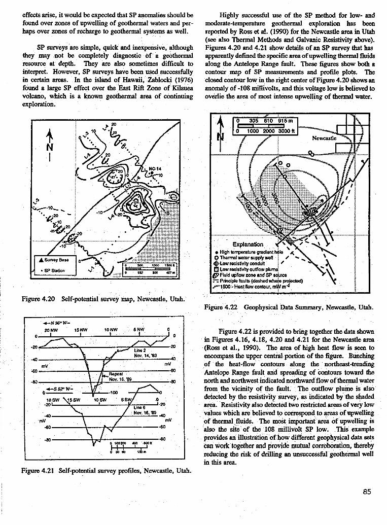
effects arise, it would be expected that SP anomalies should be found over zones of upwelling of geothermal waters and per- haps over zones of recharge to geothermal systems as well.
SP surveys are simple, quick and inexpensive, although they may not be completely diagnostic of a geothermal resource at depth. They are also sometimes difficult to interpret. However, SP surveys have been used successfully in certain areas. In the island of Hawaii, Zablocki (1976) found 8 large SP effect over the East Rift Zone of Kilauea volcano, which is a known geothermal area of continuing exploration.
Figure 4.20 Self-potential survey map, Newcastle, Utah.
+N 36. W-
0
-20
-40
60
-80
Highly successful use of the SP method for low- and moderate-temperature geothermal exploration has been reported by Ross et al. (1990) for the Newcastle area in Utah (see also Thermal Methods and Galvanic Resistivity above). Figures 4.20 and 4.21 show details of an SP survey that has apparently defined the specific area of upwelling thermal fluids along the Antelope Range fault. These figures show both a contour map of SP measurements and profile plots. The closed contour low in the right center of Figure 4.20 shows an anomaly of -108 millivolts, and this voltage low is believed to overlie the area of most intense upwelling of thermal water.
. @“?500 - Heat flow contour, ml$ mr
Figure 4.22 Geophysical Data Summary, Newcastle, Utah.
Figure 4.22 is provided to bring together the data shown in Figures 4.16, 4.18, 4.20 and 4.21 for the NewcastIe area (Ross et al., 1990). The area of high heat flow is seen to
northeast-trending contours toward the flow of thermal water
e outflow plume is also
area. Resistivity also detected two restricted areas of very low values which are believed to correspond to areas of upwelling
. The most important area of upwelling is the 108 millivolt SP low. This example
provides an illustration of fferent geophysical data sets tual corroboration, thereby
reducing the risk of drilling an unsuccessful geothermal well in this area.
Figure 4.21 Self-potential survey profiles, Newcastle, Utah.
85

4.4.3.3 The Seismic Methods
Elastic m&&auical waves, called seikmic waves are transmitted through rocks and their measkment can be used to help determine the s t r u c k and m&hanical properties of rock bodies. Two tjpeS of waves are most useful:
1. The compressional or primary (P) wave, bi which the particle motion in the rock is back and forth along the direction of travel of the wave. Of , each rock particle only moves a fraction of a millimeter, but the rock particle is in contact with surrounding rock particles and transmits its motion to its neighbors. In this way, the wave moves outward in all directions from .the source. P-waves are ordinary sound waves in rocks. They travel at velocities that vary between about 3,000 and 20,000 fi ls.
2. The shear or secondary (S) wave, in which the particle motion is perpendicular to the direction of travel of the wave. S-waves have no analog in air because fluids (liquids and gases) do not support shear. In rock, S- waves travel at velocities about 7096 of the velocities of P-waves.
There is a variety of seismic methods, and they can be applied to different exploration and mapping problems. The selection of which seismic method might be heIpful is best left to an experiend geophysicist. Seismic techniques can be classified into active techniques and passive techniques. In the active seismic techniques, dynamite detonated in a shallow borehole or some other source of mechanical energy is used as a source for the signals that are received and interpreted. The active techniques can be further subdivided into reflection and refraction surveys. The passive techniques use Mtudly occurring signals which arise from earthquakes and from the movement of water or molten magma in the subsurface. We will consider some of the common seismic methods below.
Seismic Refraction Surveys
tion surveys, waves are 'used that are refkcted the surface. the gcol&c
are perhaps more easi- thg than arii reflection
w e y s . The thickness of uncohsolidated alluvium over bed- rock can usually be mapped with refraction. Such information
ful in planning drilling and other exploration activities. egate et al. (1981) disciwed applications of both
along subsurface bhdariks and then re Refraction m e j s can be helpful in det
cture in the shallow
reflection and refraction to geothermal work.
Seismic Reflection Surveys
In this method, an artificial source is used to create seismic waves, which travel downward into the earth, are re- flected from a boundary at which the mechanical properties of the rock change (a discontinuity in seismic velocity) and return to the surface. At the d a c e , their arrival is detected by sensitive geophones spaced along lines at known distances apart. This method has proven to be very effective in explor- ing for petroleum, and is used extensively by oil cckipanies. However, it has been as successlid in the environment. Geothermal areas seldom have ihe geological structure or layering that the method detects best. Swift (1979) discussed the d t s of a trial reflection survey at Beowawe, Nevada.
Earth Noise Surveys
There is limited evidence that hydro thed pn>cesses, including boiling and the m i d movement of water in geother- mal resources, can generate seismic waves in the frequency band 1 to 10 Hz (Liaw and Suyenaga, 1982). Noise also arises in such sources as traffic, trains, rivers, canals, and wind. Liaw and McEvilly (1979) have demonstrated that field and interpretative techniques for earth-noise surveys require a great deal of understanding and care. These surveys can pro- vide a guide to hydrothermal pmcesses if the data quality is good and interpretation is thorough.
Microearthquake Surveys
Microearthquakes frequently are related spatially to major g e o t h e d systems. These microearthquakes appear to origi- nate in faulting and fracturing at depth, processes that are needed to keep the plumbsg system of hydrothermal resources
0
A * 25-15
0 0
0 O0
Figure 4.23 Microearthquakes near Rookwelt Hot Springs, Utah.
86

open. Accurate locations of earthquakes can provide data on the locations of active faults that may channel hot water toward the surface. Microseismic activity in most geothermal areas has been observed to be episodic rather than continuous. This characteristic limits the technique in its geothermal exploration applications because the surveys are expensive and may need to be run for months or years to get useful information.
Figure 4.23 shows the locations of micmearthquakes at the Roosevelt Hot Springs geothermal area in Utah (Zandt et al., 1982). The microearthquakes are believed to be associ- ated with movement on the Negro Mag fault, one of the main zones of upflow of geothermal fluids in the district. Signifi- cantly, a six-station seismic net was run at Roosevelt for more than two years. It detected only a few events until the last 2 months of survey, when more than 1,OOO microearthquakes were observed to provide the data in Figure 4.23. This demonstrates the episodic nature of seismic activity in this ama.
P-Wave Delay and S-Wave Shadowing
Seismic methods have been proposed for use in detecting molten magma in the subsurface to depths of 10 miles or more. Magma has a lower P-wave seismic velocity than con- solidated rock and, being a liquid, it will not pass shear waves. Thus, if seismic waves are observed from distant earthquakes after passing through a magma body, the P-waves should be slowed down and the S-waves should be removed. Surveys that compare these parameters with those from adjacent seismic rays that have not passed through the magma have been attempted with apparent success at Long Valley Caldera in California (see Rundle et al., 1986 and Goldstein, 1988, for reviews of geophysical data in Long Valley). The success is apparent, of course, because there is no proof through drilling that the magma predicted to occur on the basis of the survey actually exists. Such work has indirect bearing on exploration for direct-heat resources in that surveys of this type would normally not be carried out specifically for direct- heat exploration. Such data might have been collected in the prospect area for other purposes, and it should be reviewed and made part of the direct-heat exploration picture.
4.4.3.4 Mametic Methods
e earth has a main magnetic field whose shape is similar to that which would be produced by a large bar magnet near the center of the earth. This magnetic field is believed to arise from electrical currents flowing deep within the earth, in the electrically conducting, fluid core.
The earth's magnetic field induces a magnetic response in certain minerals at and near the earth's surface. Principal amQng the magnetic minerals are magnetite (iron oxide) and pyrrhotite (iron sulfide). Although pyrrhotite is not common, magnetiteis found insmall amountsin many rocksofthe
earth's crust. The magnetism in rocks adds or subtracts from the earth's main magnetic field, and by detecting spacial variations in the earth's total field, the variations in distribution of magnetic minerals may be deduced. This information, in turn, can be related to geology.
The earth's magnetic field can be mapped on the ground by use of sensitive instruments known as magnetometers. Magnetometers can also be installed in aircraft, and magnetic maps are created much faster and more cheaply from the air. Aeromagnetic surveys are widely used by industry in petrol- eum and mineral exploration in attempting to map subsurface geologic structure and changes in rock type. The use in geothermal exploration closely follows that in mineral exploration, for most geothermal resources are located in geologic environments that are similar to or the same as those in which mineral deposits are found.
The physical property of the rock that quantifies its response to the earth's magnetic field is called the magnetic susceptibiliry. Susceptibility varies over several orders of magnitude, but most rocks have magnetic susceptibilities in the range 500 to 5,000 x lo4 cgs units. Igneous and volcanic rocks are usually highly magnetic (high susceptibility), whereas sedimentary rocks are usually only weakly magnetic. The process of hydrothermal alteration, discussed in Section
Figure 4.24 Aeromagnetic survey of the Cove Fort/ Sulphurdale geothermal area, Utah.
87

4.2.2.3, tends to destroy the magnetite in a rock, and to render it nonmagnetic or only weakly magnetic. Thus, some geothermal systems enclosed in magnetic rocks are expressed as magnetic lows. However, there are many other causes of magnetic lows, so care must be exercised in interpreting magnetic data.
Regional aeromagnetic data are often available as part of state or federally sponsored surveys. These data often show major structural features and aid in geologic mapping in areas where the surface is covered by alluvium. Regional data are generally too widely spaced and too high in altitude, however, to constitute a database appropriate for detailed interpretation on the scale of a geothermal prospect. In certain geologic environments, therefore, the geophysicist may want to collect detailed airborne or ground magnetic data on a geothermal Prospect.
The locations of geologic structures (faults, fracture zones), intrusions, volcanic rocks, and other features of interest in forming a geologic model of a geothermal prospect may be evident on magnetic maps. Figure 4.24 is an aero- magnetic map of the Cove Fort geothermal area in Utah. Contours are in nanotesh or gammas, the common unit of measure for magnetic surveys. Magneticfield contour maps typically show complex patterns whose interpretation requires careful work by a geophysicist. Heavy lines on Figure 4.24 indicate faults interpreted from the magnetic data and from other geophysical data available for this area. The magnetic high shown by the closed contours in the lower right-hand quarter of the map is believed to be caused by a subsurface intrusion that has long since cooled, and is probably not the present heat s o m at Cove Fort. Complex magnetic patterns west of the highway are caused by basaltic volcanic rocks.
4.4.3.5 Gravitv Methods
The earth’s gravity field is caused by the mass of the earth itself. Since the &miry of a material is determined by its mass per unit volume, variations in the density of sub- surface rocks cause minute variations in the earth‘s gravity field. In order to detect these gravity variations, very delicate instruments are required. The modern gravity meter measures one part in l,OOO,OOO,OOO of the earth’s gravity field, and is one of the most sensitive mechanical instruments ever made by man.
Gravity data are often acquired or complied in the early stages of an exploration program. Regional data, with station densities of one station per square mile, may be available as the result of surveys by governments or universities. Avail- able data are generally the starting point for detailed surveys suitable for geothermal prospecting.
The contribution from gravity meying to geothermal exploration is much the same as from aeromagnetics, that is, structural, lithologic and other geologic information. Two
notable exploration successes of the gravity method stand out. In the Imperial Valley, California, gravity m e y s have proven useful in locating areas where hydrothermal alteration and metamorphismhave caused the rocks to become densified (Elders and Cohen, 1983). Deposition of minerals in the pore spaces in rocks above convecting hydrothermal systems has increased the density of the rocks enough to be detectable with the gravity meter. Geothermal systems stand out from the background as gravity high areas. Gravity surveys have been used in conjunction with temperature-gradient and heat-flow surveys to locate subsurface geothermal systems that have absolutely no surface manifestation.
A second application of gravity surveying has particular importance to exploration for low- and moderate-temperature geothermal resources. Such resources are often found on the active faults that bound many of the mountain ranges in the western United States. Range-front faults are particularly common in the Basin and Range province. Gravity surveys can generally be used to map the locations of these range-front faults (Wright et al., 1985). The faults have thrust the mountain blocks up while dropping the valley blocks down. The valleys become filled with unconsolidated erosional debris from the mountains. There is a marked contrast between the density of rocks on the mountain side of the fault (density 2,550 to 2,700 Kg/m3) compared to those on the valley side of the fault (density 2,100 to 2,400 Kg/m3). The value of gravity, therefore, is higher in the mountain block than it is in the valley block. Sharp, high-gradient gravity changes near to and parallel to a mountain front often mark the positions of faults hidden beneath the valley fill.
4.5 CASE STUDY - MONROE HOT SPRINGS, UTAH
Between 1976 and 1979, an exploration program was carried out in the Monroe-Red Hill area in central Utah that culminated in the drilling of a production-size well. The purpose of this work was to try to develop enough production to provide heating for several buildings in the town of Monroe. Although some production of water at higher tem- perature than that of the surface springs was found, the application was judged to be uneconomic, and the project was not completed. The exploration program, however, makes an instructional case study, primarily because of the variety of exploration data available for this welldocumented case study.
The Monroe and Red Hill hot springs are located along the transition zone between the Basin and Range and the Colorado Plateaus geologic provinces, on the east side of the Sevier Valley near Monroe, in central Utah. They lie along the range-bounding Sevier fault (Mundorff, 1970) and appear to be localized where the fault changes strike dimtion. There are two main areas of thermal springs. The Monroe hot springs issue from a single tufa (travertine) mound that extends for about 0.5 mile along the mountain front. The water temperature varies from 120 to 150 OF, and the rate of
88

discharge is about 180 gpm. The Red Hill hot spring, about 0.5 miles north, issues from a tufa mound 600 ft long. It discharges about 150 gpm of water at a temperature of approximately 170 OF. The Springs have TDS values ranging from 2,600 to 2,900 ppm. Rocks in the near vicinities of each of the mounds are hydrothermally altered with iron-oxide
Figure 4.27 shows the heat-flow data as determined from the temperature gradients and measurements of the thermal conductivities of rocks encountered in the gradient drilling. This data set shows a correlation of high heat flow with the known position of the Sevier fault, and also indicates the zone of outflow to the northwest also shown on the resistivity data.
minerals, producing bright red and yellow colo
The geologic structure of the mountain block and adjacent valley is complex. The Sevier Plateau east of the valley and the Pavant Range to the west are covered with up to 2.5 miles of Oligocene and Pliocene volcanic rocks con- sisting of pyroclastic rocks and flows. These volcanic rocks generally have very low permeabilities except for some basaltic-andesite flows that are locally permeable. The volcanic rocks overlie sedimentary rocks that range in age from Oligocene to Jurassic (see Figure 3.20, Chapter 3 for the geological time scale) and are composed of silty and shaly sequences, sandstones and limestones. Some of these sedimentary rocks are good aquifers. The structure of the sedimentary rocks beneath the volcanic rocks is unknown.
Detailed geochemical studies of the Monroe and Red Hill hot springs were performed by Parry et al. (1976) and Miller (1976). They concluded on the basis of chemical geother- mometry that the most likely maximum subsurface temperature to be found would be about 180 OF. Geophysical surveys in the area included precision gravity to help locate the Sevier fault in areas where it is covered by alluvium, ground magnetics and dipoledipole resistivity. In addition, shallow’ holes were drilled for measurement of thermal gradients and determination of heat flow. .
Figure 4.25 Temperature profiles for typical exploration holes, Monroe, Utah.
subdace temperature data in 11 boreholes in the area. Figure 4.25 shows some of the observed temperature profiles and Figure 4.26 is section with temperature contours in “c. Note that the closest approach to the surface of high temperatures on Figure 4.26 coincides with the position of the Sevier fault, providing good evidence that this fault carries the thermal fluid.
Monroe Hot Springs E Distance (m)
100 0 100 200 300 400 w TufaMound
Figure 4.26 Temperature contours along EW cross section across Sevier fault, Monroe, Utah.
M1
SCALB
Heat Flow Holes (mW m2)
TufaMamds
7 Heat flow anomaly at Monroe - Red Hill, Utah.
igure 4.28 shows a contour map of the dipoledipole resistivity data (Mase, 1978). The resistivity survey found a highly conductive area that coincides with the Sevier fault and shows the highest.conductivities near the Monroe and Red Hill tufa mounds. Also shown by low resistivities is a zone of
89

0 Thermal Gradient Holes
Figure 4.28 Resistivity anomaly over the Monroe - Red Hill geothermal system, Utah.
outflow in the alluvium that trends northwest from the Red Hill mound. Low-resistivity values persist both north and south of the known hot springs and are believed to show the total area prospective for drilling. With the exception of one hole drilled near the Monroe Hot Spring, however, no further drilling along this resistivity anomaly has taken place.
A simple geologic model of the system was discussed by Kilty et al. (1979). The model includes deep circulation of meteoric water with recharge in the northern Sevier Plateau,
storage and heating within a possible reservoir in sedimentary rock at depth and discharge to the surface along with Sevier fault (Figure 4.29). The heating probably takes place in the deep aquifers before the waters flow up the Sevier fault.
The production test well was spotted at a position west of the M o m travertine mound and on the west si& of the Sevier fault such that it would intersect the fault about 1,OOO ft deep. The hope was that the water at that depth would be less diluted by near-surface, cooler water, and would therefore be at a higher temperature than that of the springs. The 9-98 in. diameter well was drilled to a depth of 1.47’1 ft, and was completed with 7-5/8 in. slotted liner between 945 and 1,313 ft. Pump testing indicated that the well was capable of pro- ducing water at about 180 OF and that the natural, artesian flow rate would be about 250 gpm, compared to the natural flow from Monroe spring of 180 gpm at 120 to 150 OF. Al- though the temperature was improved, the flow rate was too low to support the planned direct use, and no further develop ment has taken place to this time. Nevertheless, the Monroe fesource still exists, and will probably be used at some time in the future.
GLOSSARY
Active Geophysical Techniques - Geophysical techniques in which a man-made source of energy is used. Examples are dynamite in a seismic survey or electrical current in a resistivity survey. See Passive Geophysical Techniques.
Argillic Alteration - Alteration of existing rock minerals to clay minerals through the action of circulating waters.
Anomaly - A deviation from uniformity. A local feature dis- tinguishable in geological, geochemical or geophysical data over a larger area.
Anticline - Theconvexupward bowingor foldingof rock layers.
Aquifer - A subsurface rock unit from which water can be prudud.
Basalt - A fine-grained, darkalored extrusive volcanic rock of mafic composition.
Basin (sedimentary) - A segment of the crust that has been Sediments in the basin increase in downwarped.
thichess toward the center.
Batholith - A large body of intrusive rock (e.g. granite) at least 40 mi2 in areal extent.
90

GEOLOGIC INTERPRETATION MONROE -RED HILL HOT SPRINGS
100
0
- E I too
n
v
!i W
200
300
t I I I I I I I I I I
I I I I I I I 400 200 0 200 400 1000 8 00 600
DISTANCE (m) VERTICAL EXAGGERATION 2: I
Figure 4.29 Fluid flow model for Monroe - Red Hill, Utah.
Blind Geothermal Resource - A geothermal resource having no surface manifestation of its presence. Blind resources must be found by geological, geochemical and geophysical methods. Also sometimes termed cryptic, meaning hidden.
Breccia - Rock made up of highly angular, coarse fragments. Can form from grinding along faults, from subsurface hydrothermal explosions and &her mechanisms.
Buoyancy - A body submerged in a fluid will experience an upward force, called its buoyancy, that is equal to the difference between its weight and the weight of the fluid it displaces,
Carbonate Rocks - Rocks composed of calcium carbonate (limestone, marble) or magnesium carbonate (dolomite).
Centigrade - A common temperature scale in scientific work and throughout most of the world apart from the U.S. To convert temperatures in degrees centigrade to temperatures in degrees fahrenheit, use the following formula: F = 9C/5 + 32.
CoastalPlain - Aplainhavingits marginonthesea ora large lake.
Conductivity - see Electrical Conductivity
Connate Water - Water ina sedimentary rock that was trapped at the time the sediments we& deposited.
Convection - Motion in a fluid or plastic material due to some parts being buoyant because of their higher temperature. Convection is a means of transferring heat through mass flow rather than through simple thermal conduction.
91

Core - (1) The central region of the earth, having a radius of about 2,155 mi (3,470 km). Outside the core lie the mantle and the crust. The radius of the earth is 3,955 mi (6,370 km). (2) A cylinder of rock cut by a coring drill bit.
Cryptic Geothermal Resource - see Blind Geothermal Resource.
Crystalline Rock - Rock consisting of crystalline minerals. Often used with igneous and metamoqhic rocks. Granite is an example of a crystalline rock.
Darcy - The unit of measure of permeability. The perme- ability of a material is 1 darcy if 1 cm3/sec of fluid of 1 centipoise viscosity will flow through a cube of the material 1 cm2 in cross section and 1 cm in length under a pressure difference of 1 atmosphere.
Density - The mass per unit volume of a material, a funda- mental physical property of the,material.
Deuterium - The isotope of hydrogen that contains one proton and one neutron in the atomic nucleus, written H-2 in this text and often written ?H in scientific literature.
Dissolution - Dissolving or taking into solution.
Divergent Plate Boundary - The boundary between two crustal plates which are moving apart at a spreading center, usually at a mid- ridge, with new basaltic crust welling up in the seam.
Drilling Fluid - Fluid, usually a special water- or oil-based mud, that is circulated in the hole during drilling to remove rock cuttings, and to lubricate and cool the drill bit.
e.g. - Latin, exempli gratia, meaning for example.
Electrical Conductivity - A fundamental physical pmperty of material measuring how well the material conducts electricity. Better conductors have higher conductivity. Electrical current per unit area divided by voltage drop per unit length. Units are siemens per meter. Conductivity is the reciprocal of resistivity.
Electrical Resistivity - A measure of the resistance to flow of electricity in a material. The higher the resistivity, the greater the resistance to flow and the lower the conductivity. Units are ohm-meters. Resistivity is the reciprocal of conductivity.
Electrokinetic Effect - A process for generation of natural voltage gradients in the earth due to the flow of fluids through pores and fractures in rock.
Electromagnetic Geophysical Methods - The class of geo- physical methods wherein current flow is induced in the subsurface by means of an alternating magnetic field, either naturally occurring or man-made by driving a current through a coil of wire.
Fahrenheit - The common measurement of temperature in the United States. To convert temperatures in degrees fahrenheit to tempera- in degrees centigrade, use the following formula: C = 5(F - 32)/9.
FelsicRock - An igneous rockwith relativelyhigh silica content. Rhyolite is the volcanic variety, and granite is the plutonic variety.
Flood Basalt (also called plateau basalt) - Large accumula- tions of horizontal basalt flows that erupt in rapid succession over vast regions.
Fluid Inclusion - During crystallization of minerals, small portions of the fluids from which they crystallize become trapped within the crystal. These fluid inclusions are usually microscopic in size.
Forward Modeling - Interpretation of geophysical or other data in which the interpreter (1) forms a starting model of the subsurface, (2) uses the computer to calculate the expected response of the model, (3) compares the calculated results with field data, and (4) changes the model in accordance with the comparison. Several model changes and recalculations are made until the calculated model agrees well with the field results.
Fumarole - A vent from which steam or gases issue; a geyser or spring that emits gases.
Galvanic Resistivity Geophysical Method - An electrical geo- physical method in which two grounded electrodes are used to inject current into the ground while a resulting voltage difference is measured between two separate grounded electrodes. By knowing the disposition of the four electrodes, the magnitude of the current and that of the measured voltage, an "averaged" resistivity of the subsurface c8n be computed.
Geophysics - Application of methods and techniques of physics to geology.
Geopressured - A type of geothermal resource occurring in deep basins in which the fluid is under very high preSSUre.
Geothermal Energy - Heat energy from inside the earth.
Geothermal Gradient - The rate of increase of temperature with depth in the earth, given in O Ckm or O F/100 fi.
92
Gouge - Finely abraded material between the sides of a fault, the result of grinding of rock during fault movement.
, gpm - Gallons per minute.
Granite - A light-colored crystalline rock of felsic composi- tion.
Gravity Geophysical Methods - The class ofgeophysical methods based on”-measurement of minute variations in the earth’s gravity field and interpretation of these in terms of subsurface geologic variations.
Half Life - For a radioactive isotope, the time after which half of the original amount has decayed radioactively.
Heat Capacity - The amountofheat requiredto raisethe temperature of a material by 1 degree.
Heat Flow - The rate at which heat is rising from depth to the surface of the earth, given in milliwatts per square meter, mW/m2.
Heat of Vaporization - See Latent Heat of Vaporization.
Host Rock - The rock that encloses a geothermal system or mineral deposit.
Hot Rock Geothermal Energy - Heat energy residing in rock. If the rock has no permeability, hydraulic fracturing may be used to create permeability to enable circulation of water and removal of the heat.
Hydraulic Fracturing - Fracturing of rock at depth from fluid pressure. Hydraulic fracturing at depth may be induced by pumping water into a well at very high pressures. Under natural conditions, vapor pressure may rise high enough to cause fracturing in a process known as hydrothermal brecciation.
tatic Pressure - The pressure exerted by water at any depth in a body of water or in the earth in cases where the water forms a continuous medium in pore spaces, fractures and faults.
Hydrqthermal - Literally, hot water.
Hydrothermal Alteration - Mineral changes in a rock resul- ting from chemical interaction of the rock with circulating hydrothermal fluids.
Hz - cycles per second.
Le. - Latin id est, meaning that is tu say.
Igneous Rocks - Rocks whose origin is the cooling and solidi- fication of magma, molten rock material.
Induration - The process of hardening of sediments through pressure, heat, or cementation.
Infrared - That portion of the electromagnetic spectnun whose wavelengths are 0.7 to 1.0 micrometers, beyond the red end of the visible spectrum.
In Situ - Latin, meaning in place.
Intrusion - A body of rock that has invaded the earth‘s crust from deeper depths in a molten state. Also the process of this invasion.
Inversion - A method of interpretation of geophysical or other data in which the computer is used to calculate a model of the subsurface directly from field geophysical data. Compare to Forward Modeling.
Ion - An atom which has a negative electric charge due to possession of one or more extra electrons or a positive electric charge due to loss of one or more electrons.
Jsotope - Isotopes of a chemical element are separate species of the same element that have different numbers of neutrons in the nucleus. Stable isotopes are those that do not decay radioactively. The notation used in this text consists of the symbol for the chemical element followed by a number representing the total number of protons and neutrons in the nucleus of the element, i.e. the mass number. For example, Ar-40 is used for the isotope of argon that has mass number 40.
Latent Heat of Vaporization - The heat required to change a liquid to a vapor or gas. Vaporization takes place at constant temperature, but with the addition of energy. Upon condensation, the heat of vaporization is given up again. For water, the heat of vaporization decreases with increasing temperature, falling to zero at the critical point.
Layered-Earth Model - A model used in geophysical data interpretation in which the subsurface is divided into two or more horizontal layers each having infinite horizontal extent. Same as a one4mensional or 1-D model.
Limestone - A sedimentary rock formed of crystalline calcium carbonate, usually in the ocean by direct precipitation or from coral reef fortnation.
Lithosphere - The upper, solid part of the earth, floating on plastic rocks of the mantle below. Composed of the crust and the uppermost mantle.
93

Mafii Rock - An igneous rock with relatively low silica content. Basalt is the extrusive volcanic variety, and gabbro is the crystalline, plutonic variety.
Magma - Molten rock.
Magma Chamber - A subsurface volume containing magma.
Magnetic Geophysical Methods - A class of geophysical methods based on measurement of spatial variations in the earth's magnetic field and interpretation of these variations in terms of subsurface geologic variations.
Magnetic Susceptibility - A basic physical parameter of a rock measuring the extent to which the rock becomes magnetized as a result of induction due to the earth's magnetic field. The higher the susceptibility, the more magnetic the rock is when placed in a magnetic field such as that of the earth.
Magnetometer - An instrument for measuring the magnetic field strength of the earth.
Magnetotelluric Geophysical Methods - The class of geo- physical methods based on measurement of the ratio of electric field in one horizontal direction to magnetic field in a perpendicular direction at various frequencies, and interpretation of the resulting data in terms of variations in subsurface geologic variations.
Mantle - The layer of the earth lying between the crust above and the core below. The mantle extends between depths of about 19 mi (30 km) in continental areas and 1,790 mi (2880 km), where the core begins.
Megawatts (Electrical, MWe) - 1 million watts of electricity. Due to conversion inefficiencies, it takes about 3 million tbermal watts to generate 1 million watts of electricity.
Megawatts (Thermal, MWt) - The watt is a unit of power, equal to 1 Joule/sec, where 1 Joule equals 0.239 calories. The megawatt is 1 million watts.
MetamorphicRQck - Rockthathas beenformed fromthe actions of heat, pressure and chemical reactions on pre- existing igneous, sedimentary or metamorphic rock.
Meteoric Water - Water falling from the sky as rain or snow.
Microearthquake - Anearthquake orseismic eventhaving energy release much too low to be felt at the surface, and therefore requiring detection by sensitive seismometers.
Milliequivalent - A measure of chemical Concentration. The molar conceutration of a +ies times the ionic charge of
. the species.
Mineral - A naturally formed chemical element or compound that usually has a definite crystal structure. Some minerals are amorphous, without crystal structure. Minerals are the building blocks of rocks. .
Mineralization - The process of deposition of minerals in open spaces in rocks, such as in faults, Fractures or pores. Some such minerals have economic value whereas others do not.
One-Dimensional Model - See Layered-Ekth Model.
Order of Magnitude - Factor of 10.
Passive Geophysical Techniques - Geophysical techniques in which natural fields or signals are used as energy sources. Gravity, magnetic, self-potential, magnetotelluric and microseismic surveys are examples.
Permeability - The capacity of a rock for transmitting fluid. See Darcy.
pH - A measure of the acidity of water. Neutral water has pH = 7.0. Waters with pH values less than 7.0 are acid, whereas those with pH values greater than 7.0 are alkaline.
Piezometric Surface (also Potentiometric Surface) - The level to which water in an aquifer will rise under its own pressure, due to its hydraulic head.
Plume (mantle) - A subcircular, isolated area of upwelling of hot material in the mantle. One manifestation of mantle convection.
Pluton - A subsurface body of intrusive rock.
ppm - Parts per million.
Porosity - The percentage of the volume of interstices or open space in a rock or soil compared to its total volume.
P-Wave - A compressional seismic wave. A seismic wave in which the particle motion is back and forth along the line of propagation of the wave. Analogous to sound waves in air.
Pyroclastic rocks - Volcanic rocks comprised of material that has been explosively ejected from the volcanic vent.
RadioactiveDecay - Natural and spontaneous change of certain chemical elemental species into other elemental species by emission of one or more of various particles from their nuclei.
94

Radioactive Isotope - A species of a chemical element that decays radioactively.
Reflection Seismic Surveys - The class of seismic geophysical m e y s in which reflections of seismic wzves from subsurface geologic interfaces are detected at the surface and interpreted in terms of subsurface geologic variations.
Refraction Seismic Surveys - The class ofseismicgeo- physical surveys in which refractions of seismic waves from subsurface geologic interfaces are detected at the surface and interpreted in terms of subsurface geologic variations.
RenewaMelSustainable Energy - Energy forms whose pro- duction can be sustained for hundreds of years. Geothermal, solar and wind energy are examples.
Reservoir - A natural underground container of fluids such as geothermal waters or steam.
Rhyolite - An extrusive volcanic rock of felsite composition. The extrusive equivalent of granite.
Rift Zone - A system of crustal fractures and faults. Rifts at the crest of mid-ocean ridges result from separation of the plates.
Salinity - The quantity of total dissolved solids in water.
Sedimentary Rock - A rock formed by consolidation of sedi- ments that have accumulated under water (subaqueous) or under the air (subaerial).
Seismic Methods - The class of geophysical methods based on propagation, reflection and refractioq of mechanical waves in rocks and interpretation of the resulting data in terms of subsurface geologic variations.
Seismic Velocity - The speed of propagation of seismic, or elastomechanical, waves in rocks.
SelfPohtiaI - Naturalvol subsurface by the flow of fluids (electrokinetic effect), the flow of heat (thermoelectric effect) or chemical reactions such as those around an oxidizing ore body.
SI Units - Standard International units of measure of physical and chemical quantities. The system of units accepted by the scientific community worldwide.
Sinter - Chemical sediment deposited by a mineral spring. In geothermal use, often reserved for silica deposits. In this use, also called siliceous sinter. Can also be used as calcareous sinter (see tufa and travertine).
Skin Depth - The depth in the earth at which the amplitude of a propagating electromagnetic wave is reduced to l/e of its original amplitude, where e is the base of the MW
' logarithms, having a value of about 2.72. The skin depth is a function of the frequency of the wave and the electrical conductivity of the rocks.
Soil Horizon - A layer of soil that is distinguished from layers above and below by characteristic properties such as color, texture or chemistry.
Spontaneous Polarization - Same as Self Potential.
SpreadingCenters - Divergent boundaries betweenmajor plates of the earth's crust at which motion of the plates on opposite sides of the center is a separation, with magma rising in the crack to consolidate and form new crust.
Stratigraphic - Havingto dowiththe layeringof rocks. Normally applied to sedimentary rocks.
Subduction - Descent of one plate of the lithosphere lmder another plate.
Superheat - Steam in a geothermal systemis saidtobe superheated if extra heat has been added above the minimum heat necessary to simply change water to steam for a given pressure.
S-Wave - A shear seismic wave. A seismic wave in which the particle motion is perpendicular to the line of propagation. There is no counterpart of shear waves in air, water or magma, since fluids will not sustain shear (they flow rather than propagate the wave).
'
Temperature Gradient - See Geothermal Gradient.
Thermal Conductivity - The ability of a material to conduct heat, given in wattdmeter-" Kelvin in SI units.
Three-Dimensional Model - A model used in geophysical data interpretation in which the subsurface is divided into regions of varying physical properties and the regions are bounded in all three dimensions (as a cube).
Thermoelectric Effect - The mechanism whereby flow of heat in the subsurface results in measurable electric voltage gradients at the surface. One of the mechanisms for the self-potential geophysical method.
Total Dissolved Solids - The content, usually in parts per million by weight, of all dissolved salts in a groundwater or geothermal fluid.
95

Transform Fault - A fault in which the blocks of rock on opposite sides move horizontally with respect to one another, and which is caused by variations in the rate of spreading along a spreading miter.
Travertine - Calcium carbonate deposits resulting from pre- cipitation at the surface at a spring. Some varieties are called tufa or calcareous sinter.
Trench (Oceanic) - An long, linear ocean deep, parallel to a subduction zone, resulting from the ocean bottom being dragged down by the subduction proces's.
Tufa - Chemical sediment deposited by a spring or a lake. See also sinter and travertine.
Two-Dimensional Model - A model used in geophysical data interpretation in which the subsurface is divided into regions of varying physical properties and the regions are bounded in two dimensions but not in the third dimension. In the typical 2-D model, regions have boundaries in the vertical and one horizontal dimension, but are assumed to extend to infinity in the other horizontal dimension.
-
Two-Phase - In geothermal, used to mean both water and steam coexisting in the rack, borehole or surface equipment.
Vapor Dominated - A hydrothermal convection system which contains sufficient steam that the steam is the umtinuous fluid phase, and the pressure gradient in the reservoir is vaporstatic rather than hydrostatic.
Vein - A fracture or fault that has been filled with minerals. If the minerals are of economic value, the vein is said to be an ore vein or lode. In geothermal systems, veins often consist of quarfz or calcite filling of a fracture.
,J
viscoSity - The internal properties of a fluid that offer resistance to flow. Fluids usually become less viscous with increasing temperature.
Volcanic Rock - An igneous rock that has been poured out or ejected at or near the earth's surface.
Waterhminated - A hydrothermal convectimsystem in which water form the continuous phase in the rock, and the pressure in the pore spaces changes as the hydraulic gradient.
REFERENCES
Adams, M. C. and Moore, J. N., 1987, 'Hydrothermal alteration, and fluid geochemistry of the Meager Mountain geothermal system, British Columbia", American Journal of Science, v. 287, pp. 720-755.
96
Applegate, J. K.; Goebel, V, S.; Kallenkrger, P. and Rossow, J., 1981, "The use of seismic reflection techniques in geothermal areas throughout the U.S.", Slst Annual International Meeting. and Exwsition, Society of Exploration Geophysicists, Los Angels, CA.
Blackett, R. E.; Shubat, M. A.; Chapman, D. S.; Forster, G. B. and Schlinger, C. M., 1989, "An Bssessment of geothermal resoutces at Newcastle, Utah", Geothermal Resources Council Transactions, v. 13, 109-116.
Blackett, R. E.; Shubat, M. A.; Chapman, D. S.; Fmter, C. B.; Schlinger, C. M. and Bishop, C. E., 1990, "The Newcastle geothermal system-geology, hydrology, and conceptual model", Utah Geoloeical and Mineral Survey Reoort, U;S. Department of Energy Research Grant No. DE-FG07-88ID 12756, 8 5 ~ .
Capuano, R. M. and Cole, D. R., 1982, "Fluid-mineral equilibria in a hydrothermal system, Roosevelt Hot Springs, Utah", Geochimica et Cosmochimica Acta, v. 46, p ~ . 1353-1364.
Christensen, 0. D.; Capuano, R. M. and Moore, J. N., 1983, "Trace-element distribution in an active hydrothermal system, Roosevelt Hot Springs thermal area, Utah", Journal of Volcanolow and Geothermal Research, v. 16, p ~ . 99-129.
Corwin, R. F. and Hoover, D. B., 1979, "The self-potential method in geothermal exploration", GeoDhvsics, v. 44, pp. 226-245.
Craig, H., 1963, "The isotopic geochemistry of water and carbon in geothermal areas", in Nuclear Geology on Geothermal Areas, Spoleto, Pisa, Consiglio N a z i d e delle Recerche, Laboratorie de Geologia Nucleare.
Durrance, E. M., 1986, "Radioactivity in Geology-Principles and Applications: Ellis Horwood Ud., 441 p.
Elders, W. A. andahen, L. H., 1983, "TheSaltonSeageo- thermal field, California, as a near-field ~ tu ra l analog of a radioactive waste repository in salt", Office of Nuclear Waste Isolation ReDort BMIIONWI-513, 138 p.
Fitterman, D. V., 1983, "Timedomain electromagnetic soundings at Newberry volcano, Oregon", American GeoDhv&al Union T&~sactions, EOS,v. 64, p. 899.
Fitterman, D. V.; Neev, D. K.; Bradley, J. A. and Grose, C. T., 1985, "More timedomain electromagnetic soundings of Newberry volcano, Deshutes County, Oregon", U.S. Geological Survev Ouen -File Reoort 85451, 77 p.

Fournier, R. O., 1981, "Application of water geochemistry to geothermal exploration and reservoir engineering", in Geothermal Systems-Principles and Case Histories, L. Ryback and L. J. P. Muffler, Eds., Wiley, NY, pp. 109- 143.
Fournier, R. 0. and Truesdell, A. M., 1973, "Anempirical Na-K-Ca geothermometer for natural waters", Geochimica et Cosmochimica Acta, v. 37, pp. 1255- 1275.
Goldstein, N. G., 1988, "Predrilling data review and synthesis for the Long Valley caldera, California", American Geophysical Union Transactions, EOS, v. 69, pp. 43-45.
Helgeson, H. C., 1969, "Thermodynamic properties of the co- existing phases and thermochemical properties of the NaCl component in boiling NaCl solutions", U.S. Geological Survev Bulletin, v. 1421-B, pp. 71.
Hem, J. D., 1970, "Study and interpretation of the chemical characteristics of natural water", U.S. Geological Survey Water-Supply Paper 1473, 363 p.
Henley, R. W. and Ellis, A. J., 1983, "Geothermal systems ancient and modern, a geochemical review", &&I Science Review, v. 19, pp. 1-50.
Henley, R. W.; Truesdell, A. H. and Barton, P. B., Jr., 1984, "Fluid-mineral equilibria in hydrothermal systems", Reviews in Economic Geology, v. I, 267 p.
Kilty, K.; Chapman, D. S. and Mase, C. W., 1979, "Forced convective heat transfer in the Monroe Hot Springs geothermal system", Journal of Volcanology and Geothermal Research, v. 6, pp. 257-277.
LeSchack, L. A. and Lewis, J. E., 1983, "Geothermal pros- pecting with shallow-temperature surveys", Geophysics, V. 48, pp. 975-996.
Liaw, A. L. and McEvilly, T. V., 1979, "Microseisms in geothermal exploration-studies in Grass Valley, Nevada", Geophvsics, v. 44, pp. 1097-1115.
Liaw, A. L. and Suyenaga, W., 1982, "Detection of geother- mal microtremors using seismic arrays", Paper presented at 52nd Annual International Meeting and Exmsition, Society of Exploration Geophysicists, Dallas, TX, October 17-21.
Mase, C. W., 1978, "Geophysical survey of the Monroe - Red Hill geothermal system", M.S. Thesis, University of Utah, Salt Lake City, UT.
Matlick, J. S. and Buseck, P. R., 1976, "Exploration for geothermal areas using mercury - a new geochemical technique", Proceedings of the Second U.N. Svmsium on the Development and Use of Geothermal Resources, San Francisco, CA, May 1975, v. 1, pp. 785-792.
Miller, C. D., 1976, "Alteration and geochemistry of the Monroe Known Geothermal Resoum Area", M.S. Thesis, University of Utah, Salt Lake City, UT.
Moore, J. N. and Samberg,,S. M., 1979, "Geologyofthe Cove Fort-Sulphurdale KGRA (with bibliographic annotations and petrographic descriptions by Bruce Sibbett)", University of Utah Research Institute, DOE Remrt No. DOEIETl28392-27, 44 p.
Moore, J. N.; H u h , J. B.; Lemieux, M. M.; Stemfeld, J. N. and Walters, M. A., 1989, "Petrographic and fluid inclusion evidence for past boiling, brecciation and associated hydrothermal alteration above the NW Geysers steam field, California", Geothermal Resources Council Transactions, vol 13, pp 467-472.
Moore, J. N.; Lemieux, M. M. and Adam, M. C., 1990, "The occurrence of C0,enriched fluids in active geothermal systems-data from fluid inclusions", 15th Annual Stanford Geothermal Reservoir Engineering WorkshoD, in press.
Mundorff, J. C., 1970, "Major thermal springs of Utah", Utah Geological and Mineral Survey Water Resources Bulletin 13, 60 p.
Murray, K. S.; JOW, M. L. and Lopez, C. A., 1985, "Geo- chemical exploration of the Calistoga geothermal resource area, Napa Valley, California", Geothermal Resources Council Transactions, v. 9 - Part I, pp. 339- 344.
Nielson, D. L., 1978, "Radon emanometry as a geothermal exploration technique--theory and an example from Roosevelt Hot Springs KGRA, Utah", University of Utah Research Institute, Earth Science Laboratorv R m r t - 14, DOEhD128392-18, 31 p.
Nielson, D. L.; Sibbett, B. S.;- McKinney, D. E.; H u h , J. B.; Moore, J. N. and Samberg, S. M, 1978, "Geology of Roosevelt Hot Springs KGRA, Beaver Co., Utah", University Utah Research Institute, Earth Science Laboratorv Remrt No. 12, DOE/ID/28392+19, 121 p.
Parry, W. T.; Benson, N. L. and Miller, C. D., 1976, "Geo- chemistry and hydrothermal alteration at selected Utah hot springs", National Science Foundation Contract Remrt, University of Utah.
97

Piper, A. M., 1944, "A graphic procedure in the geochemical interpretation of water analysis", Transactions American Geophvsical Union, pp. 914-923.
Ross, H. P.; Blackett, R. E.; Shubat, M. A. and Mackelprang, C. E., 1990, "Delineation of fluid upflow and outflow plume with electrical resistivity and self- potential data, Newcastle geothermal area, Utah", Geothermal Resources Council Transactions, v. 14, pp. 1531 - 1536.
Rundle, J. B.; Carrigan, C. R.; Hardee, H. C. and Luth, W. C., 1986, "Deep drilling to the magmatic environment in Long Valley caldera", American Geobhvsical Union Transactions, EOS, v. 67, pp. 490-491.
Sammel, E. A., 1981, "Results of test drilling at Newberry volcano, Oregon", Geothermal Resources Council Bulletin, v. 10, n. 11, pp. 3-8.
Sibbett, B. S. and Nielson, D. L., 1980, "Geology of the central Mineral Mountains, Beaver County, Utah", University of Utah Research Institute, Earth Science Laboratow R m r t No. 33, DOE/ID/28392-40,42 p.
Sill, W. R., 1983, "Self-potential modeling from primary flows", Geophvsics, v. 48, pp. 76-86.
Swift, C. M., Jr., 1979, "Geophysical data, Beowawegeo- thermal area, Nevada", Geothermal Resources Council Transa~ti~ns, V. 3, p ~ . 701-702.
Trexler, D. T.; Flynn, T.; Koenig, B. A. and Bruce, J., 1980, "Assessment of geothermal resources of Caliente, Nevada", U.S. DOE R m r t DOE/NV/10039-1, available from NTIS, 23 p.
Varekamp, J. C. and Buseck, P. R., 1983, "Hg anomalies in soils-a geochemical exploration method for geothermal areas", Geothermics, v. 12, n. 1, pp. 29-47.
Ward, S. H., 1983, "Geophysical studies of active geothermal systems in the northern Basin and Range", in The Role of Heat in the Development of Energy and Mineral Resources in the Northern Basin and Range Province, Geothermal Resources Council Smial R m r t No. 13, pp. 121-157.
Ward, S. H. and Sill, W. R., 1982, "Resistivity, induced polarization, and self-potential methods in geothermal exploration" University of Utah Research Institute, Earth Science Laboratorv R m r t No. 108, DOE/ID/12079-90, 100 p.
Ward, S. H. and Wannamaker, P. E., 1983, "TheMT/AMT electromagnetic method in geothermal exploration" U.N. University Geothermal Training Programme. Iceland,
.
R ~ r t . 1983-5, 107 p.
Wright, P. M.; Ward, S. H.; Ross, H. P. and West R. C., 1985, "State-of-the-art geophysical exploration for geothermal resources", GeoDhvsics, v. 50, pp. 2666- 26%.
Zablocki, C. J., 1976, "Mapping thermal anomalies on an active volcano by the self-potential method, Kilauea, Hawaii", Pn>ceedinas of the Second U.N. Svmsium on the Develobment and Use of Geothermal Resources, San Francisco, CA, May 1975, v. 2, pp. 1299-1309.
Zandt, G.; McPhemn, L; Schaff, S. and Olson, S., 1982, Seismic baseline and induction studies-Roosevelt", University of Utah Research Institute, Earth Science Laboratow Rewrt No. 100, DOE/ID/1821,60 p.
98

CHAPTER 5 GEOTHEMAL FLUID
SAMPLING TECHNIQUES By Cecil H. Kindle
Pacific Northwest Laboratories Richland, Washington 99352
5.1 INTRODUCTION
The purpose of sampling and analysis of a geothermal fluid is to determine the chemical and isotopic constituents. Because most geothermal direct use projects operate with fluid temperatures less than boiling, this chapter only applies to sampling these lower temperature fluids. Data on fluid characteristics can be applied to: (a) process design, (b) materials selection, (c) plant operation and maintenance, and (d) reservoir evaluation. Chemical analysis of production and injection well fluids may be required by state agencies to determine if injection is to a compatible aquifer.
Some constituents in the geothermal fluids are unstable and change with time. The changes result from the difference in conditions within the geothermal aquifer before sampling, compared to those within the sample container in storage. Changes in temperature and partial pressures of gases, especially oxygen, carbon dioxide and hydrogen sulfide, are particularly likely to occur. Plastic bottles are permeable to oxygen as shown by continued oxidation of iron from ferrous to ferric in tightly closed sample bottles. Plastic sample bottles are also permeable to hydrogen sulfide, as shown by the odor in storage cabinets containing tightly capped plastic bottles of samples of water containing hydrogen sulfide. Some constituents, such as sodium, potassium, and chloride are usually stable and show no changes upon storage.
Depending upon the purpose and ~ t u r e of the study, changes in samples, upon collection and storage, may or may not be a problem. The information needed for a particular study and the desired accuracy should be established first; then, the appropriate sampling techniques can be selected. This chapter suggests sample treatment (stabilization) and field analysis techniques appropriate for minimizing errors (that may result from changes in water samples between time of collection and time of analysis). Methods for analysis of the samples in the laboratory are given in standard reference publications (APHA 1979; ASTM 1980; EPA, 1979; Watson, 1979; Kindle 1981) and will not be covered in this chapter. A combination of standard techniques and commercially available instruments generally used by laboratories are:
1. Spectroscopy - for cations
2.
3.
4.
5.
Ion chromatography - for anions
Colorimetry - for silica and ammonia
Selective ion electrode - for ammonia
Titrations - for sulfide, alkalinity . hardness, C02 and chloride
6. Turbidimetric - for sulfate
7. Gravimetric - for suspended and dissolved solids
Data quality checks should be used, when results are returned from the laboratory, to ensure that the analytical results are consistent. Charge balance (anion-tu-cation ratio)
constituents ratio) should be calculated. and ma~s balance (total dissolved solids-to-analyzed
In order to reduce the possibility of sampling stagnant or non-representative flows from wells, the following actions could be taken:
1. Sampling after the well has been flowed at a high rate to deliver a good aquifer water sample (uncontaminated with residues from well drilling in recently drilled wells).
Recording recent flow history of the well
Recording pressure, temperature and flow rate at time of sampling.
2.
3.
Preservation of a sample is 0th a problem; constituents may precipitate out, undergo chemical change, or evolve as a gas. Most sample constituents can be stabilized in the field for analysis in the laboratory. Analysis should take place as scum as possible.
. 99

!
1.
2.
3.
4.
5.
6.
5.2
Carbon dioxide (CO3 is determined from a sample stabilized with d u m hydroxide (NaOH).
Hydrogen sulfide (Hs) and oxygen (03 are measured in the field using a test kit.
Cations and ammonia (NH,) are stabilized by acidification.
Silica dioxide (Si03 is diluted IO-fold to preserve it in solution.
Mercury (Hg) samples are collected in glass bottles containing an acid-oxidizer mixture.
pH is measured in the field.
UNIFORM PROCEDURES FOR SAMPLING AND ANALYSIS
At least five different factors affect the accuracy of analytical determinations in geothermal fluids. nesi so- of variations include:
1. Flow composition shift with time from the well.
2. Differences in sampling methods.
3. Sample stabilization procewx.
4. Different analytical methods.
5. Differences between laboratories using the same methods.
The concern about flow conditions has to be resolved on a site specific basis. To avoid composition shifts that may occur during well start-up (or because of temperature gradients) the well should be flowed at a high rate to deliver a good uncontaminated aquifer sample before collecting samples. Sampling methods presented here are for use in single-phase systems; most cases will be below the boiling temperature.
A uniform approach to sampling, sample stabilization and analytical methods is schematically related to Figure 5.1. The use of a samplinglanalysis method based on this flow chart wil l improve comparability and reliability of geothermal fluid composition data.
Field analysis is used only for those measurements where preservation is not practical. Meters are used to determine temperature, pressure, flow, pH, and conductivity. Colori- metric analysis kits may be used for field analysis of hydrogen sulfide (H9) and dissolved oxygen (03, which, insome
cases, can be compared with analytical results from a laboratory. Analytical techniques are used to determine the remaining constituents, as shown in Figure 5.1.
A problem could exist with analytical differences between laboratories'utilizing the same method, resulting in typical variations of 15 to 40% and worse with cations and anions below - 1 mgk. Supervisory chemists should be knowledge- able about analytical procedures for geothermal fluids and utilize data quality checks indicated in Figure 5.1.
5.3 SAMPLE STABILIZATION
Special preparations for stabilizing some samples for later analysis are necessary precautions. These preparations are made most conveniently and accurately in the laboratory beforedepture to the field. As Presser, et& (1974) states:
"The most commonly observed changes in untreated samples are in pH, iron, manganese, bicarbonate, ammonia, hydrogen sulfide, calcium, and sulfate. Silica concentrations in excess of 100 mgk (milligramsfiter) may lead to difficulties owing to precipitation and polymerkition. Polymeric silica is not reactive in the ammonium molybdic method that is often used for laboratory determination of silica.
The changes in sample composition result from loss of carbon dioxide to the air space, oxidation and precipitation of iron and manganese, oxidation of hydrogen sulfide to sulfate, oxidation of ammonia, loss of calcium ion as calcium carbonate precipitates, and precipitation of silica. Waters inoculated with diatoms may also lose silica. Once a precipitate forms, there is no accurate way to restore the initial composition of the solution. Constituents that will probably be unaffected by storage include sulfate (if no hydrogen sulfide was originally present), lithium, sodium, potassium, magnesium, fluoride, chloride, bromide, iodide, and boron. "
A stabilization sequence is described below. The specific contained volumes used depend on the needs of the laboratory except that the sparge tube (glass tube witb frit on end) stabilization efficiency will likely depend on the height of the stabilizing solution above the glass frit.
5.3.1 Carbon Dioxide (CO.,)
For C02 preservation, the sample flow is directed into 1L bottles that are previously half-filled (exactly) with 2N NaOH stabilizing solution (Figure 5.2). The flow is passed to the
100

I Y
I I I I
I1
IE
I
13 I I I I I I I
t
rb c, Id a
rl
k 0
vc
101

QASS Fell \
Figure 5.2 Gas stabilization device.
bottom through a glass tube with a glass frit sparger to ensure that any gaseous CO, contacts the NaOH before exhausting. Pacific Northwest Laboratory's (PNL) collection efficiency using the single sparge bottle, as shown in Figure 5.3.
- c
\ \ \ \ \ \ I
0 SO00 10,000 15.000 TOTM C02 (mg/r BRINE)
Figure 5.3 Single sparge bottle efficiency (Shannon, 1980).
This efficiency would vary with the gas flow rate. The PNL flow rate is an empirically judged, moderate bubbling rate. For persons new to the technique, a couple of trial determinations using two bottles in series is recornmeended if the sample flow has a lot of gas bubbles in it. A single sparge bottle will probably be d c i e n t for m 9 t geothermal flows involved with direct use projects. Umtabilized solutions will rapidly lose CO, to the atmosphere before the analysis can be performed.
5.3.2 Cations
Cations are stabilized by acidification and the container is labeled FA (filtered, acidified). Of concentrated "0, or HCI l o d a r e p u t i n t h e 1 Lsamplebottle(t0 1% ofits volume) and this bottle is sealed mtilused in the field.
Limited testing indicates no difference between the two acids, at least down to routine analytical limits in stabilizing cations Vable 5.1). "0, seems to be used more commonly than HCL. Where there is particular interest in cations that form marginally soluble chlorides (e.g., Ag), "0, would be prefdle .
Table 5.1 Comparison of HNO, and HCL as Acid Stabilizem
concentrations in CrndLI
Raft River Samles East Mesa Samle
" o , H c L " o , H c L "0% HCL
B Ba ca Fe Li Mg Na Si Sr
0.47 0.08 159 0.1 3.01 .0.40 1470 32.3 O.%
0.45 0.07 150 0.1 2.74 0.36 1400 32.0 0.94
0.57 0.52 187 0.2 3.46 0.29 2040 29.3 6.80
0.57 0.52 187 0.2 3.46 0.28 2040 29.8 6.78
8.53 0.863 29.2 1.28 6.70 2.05 2417 105.6 6.77
8.69 0.876 29.3 1.38 7.17 2.18 2535 1W.4 6.83
5.3.3 Mercurv (Hfi
For mercury analysis the sample is stabilized by 1% (volume) of a 5% KMnO, solution, 1% (volume) of concentrated HN03, and 2% (volume) of a 5% K&08 solution. Glass bottles (labeled FAHg) are used to collect and store the samples to prevent possible biases from a plastic container. A bias caused by mercury diffusing through the wall into the sample is shown in Figure 5.4. The mercury sample is analyzed as 60011 as possible.
5.3.4 Silica Dioxide CSiO,)
Dilution is used to stabilize a filtered sample for SiO, analysis. The 10-fold or greater dilution into &-ionized water is performed in the field using a pipette and a volumetric thk. The analysis of this sample is usually comparable to the Si analysis from the filtered, acidified (FA) sample, an indica- tion that acidification is also effective in xetainhg silica with the lower Si%.
5.3.5 Ammonia (NHa Acidification is used to stabilize NH, as NH,+ and
measure it in the filtered, acidified (FA) sample. Flowing the cooled liquid sample directly into the FA container is adequate to mix and sta-, a sparge tube is u n n v . Limited conqxisolls ofammonia preservation options indicated a
102

mu
Figure 5.4 Comparison of polyethylene to glass as a storage container for saline solutions when mercury con- centrations are quantified. Initial concentrations were 2 to 25 x lG3 ppb (Bother & Robertson, 1975).
deterioration rate of 0 to 3 %/week when using HCI stabili- zation (1 A by volume) without refrigeration. Tbis rate may vary with different waters. While there was some deterior- ation indicated in comparing results to synthetic composition values for one sample, the difference was less than a standard deviation.
5.3.6 Sulfate (SO;?
For SOi2 the filtered, unacidified (FU) sample is used. No preservation technique (except filtering) is applied on this sample. In some.fluids, sparingly soluble sulfates such as BaSO,, may be above their equilibrium solubility limit. However, the kinetics of precipitation are apparently sluggish under IIXUIY Situations. TO check for loss in the SOi2 concentration, the field diluted SiO, sample c8n be compared to the undiluted FU value. A difference would indicate a bias that can be remedied, if it is of concern, by taking a diluted and highly HCl acidified sample either in the SiO, split. or separately. Figure 5.5 shows BaSO, solubility in NaCl
i - i I I P a M T H Y i f N E BOTILES. ACID RINSED. i I EXPOSED TOVARIOUS ATMOSPHERES
RANGING FRW UEORATORY BENCHTOP
VAPOR ! 2 To ONE s A m u m w i n i txRcuRY
solutions. It is not advocated that HCI be added directly to the undiluted sample (making it a FA sample) as a means of improving the solubility.
SQUllON IONIC s m m 0.01
59 I
Figure 5.5 BaSO, Solubility versus ionic strength; 25°C NaCl solutions (Davis & Collins, 1971).
The acid seems to accelerate the kinetics of precipitation to reach the solubility limit: four FA-HCl samples (East Mesa 8000 ppm TDS) lost 15 to 2096 of the SOi’ after 8 months compared to identical FU samples; Harrar (1981) reports slight acidification to cause rapid BaSO, precipitation in a Salton Sea brine.
Once they are filled, the sample bottles are placed into a large cardboard container and covered with the box lid. This serves to keep the samples out of the light as well as being convenient for organizing the field operation.
There are other stabilization approaches, or variations (for example; EPA, 1979; Presser, 1974; Hankins, 1980; Kroneman, 1981). Some specify certain acids for preserVing certain constituents, cooling samples to 39F, acidifyhg samples to a precise pH, or delaying no more than one day before completing certain analyses (e.g. NH&
The experience, to date, indicates that if the sampling is conducted and the samples stabilized as described, subsequent composition changes will be gradual enough to allow adequate opportunity for accurate measurements (with a possible qualification for H2S). However, despite the stabilization steps indicated in this discussion, the samles still should be analyzed as soon as mctical in order to minimize degradation in the particular water being analyzed because the range of geothermal water types is broad. A prudent initial test would be to perform a second, delayed analysis (either duplicate samples or later re-analysis depending on the constituent) to check whether there is any deterioration involved in the particular resource and analytical sequence. This is particularly true for those constituents that may have legal (environmental) implications such as H$ or NH,. Depending
103

on the resource, the constituents of interest, the analytical factor, and the purpoSe of the testing, there may be some cases where statdimtion is not necessary.
5.4 SAMPLING EQUIPMENT
Geothermal direct use projects generally require sampling
(<212OF), which is dependent on temperature, altitude, and barometric pressure. The equipment described here is for the lower temperatmas. For sampling geothermal fluids greater than boiling temperatures, refer to Kindle, 1981.
single-phase fluids with temperatmas less than boiling
For reliable pH values, the measurements must be made in the field. The flow should be cooled to a temperature of - 77°F for pH measurement, because pH is a function of dissolved CO, and the solubility of CO, is strongly temperature dependent. Geothermal fluids containing dissolved gases [hydrogen sulfide (HS), ammonia ("a, oxygen (0,) and carbon dioxide (CO,)] require sample telnperature control to minimize gas composition shifts. Substantial gas-liquid solubility changes with temperahre exist.
Sampling points should be as close to the wellhead as possible to obtain representative samples. These could include: (a) a valve (side mounted), (b) an open discharge pipe from a flowing well, (c) a non-flowing well, or (d) a hot springs. Components for sampling these points are shown in
Figure 5.6. The sample train illustrated requires a pressurized flow and, for sampling points two to four, a field model peristaltic pump needs to be included in the list of aocessary equipment items.
The major components illustrated in Figure 5.6 follow. (Use of manufacturer or trade name does not imply endorse- ment.)
5.4.1 Svstem Access I
System access is frequently an existing side-mounted gate valve. If the sample point is not pressutized, a portable
Horizon Ecology Corp., 7435 N. Oak Park Ave, Chicago, IL 60648).
sampling Pumg may be required (M-ex SamPbg pump,
5.4.2 A m ored Flex Hose
Resistoflex R562 hoses, 6 ft long and 0.25 in. ID (Part No. R22105-5-72) are lined with teflon. A ball valve is attached to the ekit end of the flex hose to serve as the master shutoff valve for the sampling.
5.4.3 Temerature Probe
In-line temperatures are determined with stainless steel sheathed thermocouples inserted into matching tees and compression fittings designed for this purpose. Meters for direct reading oftemperatures areavailableinmany forms.
6AS STABILIZING SYSTEM
Figure 5.6 Geothermal fluid sample train.
104

For some applications, a manus2ly-held thermometer m y be acceptable; the important point is to cool the geothermal fluid before sampling (to - 77°F) and tecotd that temperature.
5.4.4 U-Bend Connectors
U-bend connector tubes and all other tubing components are fabricated from 0.25 in., 316 SS tubing, with a 0.035 in. wall thickness. In connecting U-bends to the coils and assembling other components, care must be taken to avoid leaks. Back diffusion at the fitting, even in pressurized systems, apparently dows sufficient oxygen to enter the sample stream for detection by dissolved oxygen field analysis kits.
5.4.5 Cooling Coil
Cooling coils are typ idy formed from 10 ft lengths of 1/4 in. SS tubing wound around an 8 in. wipe. The flow is directed to the bottom of the coil and then spirals upward to assist in flushing entrained gas through the system. For systems producing fluid at 212°F or less, a single coil in an iced bucket provides sufficient cooling capacity.
5.4.6 Redating Valve
The regulating valve reduces pressure after cooling. A Whitey SS-RS4 regulating valve or others could be used. Exit shutoff valves divert flow from filtered to unfiltered samples. These valves may be stemmed valves (a typical example is the Whitey SS-14DKS4) or small ball or plug valves.
5.4.7 Filter and Filter Holder
The filter pore size recommended for geothermal sampling is 0.45 m. A filter holder found convenient for assembling and disassembling in the field is the Millipore Swianex.
5.4.8
Tygon tubing (- 18 in.) is attached to the filter outlet for convenience in filling sample containers.
5.4.9 Samde Bottles
Collection and shipment is made in rectangular or square polyethylene bottles for efficient packing. Lids are also polyethylene because other plastics often break during shipment. Closure designs with an extended lip on the bottle fitting into a matching groove in the cap survive shipment with fewer leaks than other designs. Kartell makes a wide .mouth line of square bottles with this type of closure (Markson Cat. No. R14443, lo00 A).
5.4.10 Miscellaneous Euuimnent
Other items supporting sampling operations that can be considered a minimum tool kit include:
1. Safety - safety glasses, heat resistant gloves (3-ply leather), coveralls (burn protection for bare arms and legs), work gloves (leather or canvas), hard hats.
2. Field analysis - kits (CHEMkcs, Inc., Rt. 28, Calverton, VA 22016) for H2S, NH,, 4, pH meter, temperature meter and probes.
3. Housekeeping - plastic bags (can be used ice bags), DI water (coil and utensil flush), plastic pail and one quart plastic pitcher (for bailing excess melt water).
4. Hard- - assorted reducers, c o ~ ~ t o m , couplers, nuts and ferrules for adapting to field requirements, small wrenches for tube fittings, two large crescent wrenches for probe and gland, pliers, tape for securing bottle tops, tubing qygon, 114 in. stainless steel), tube clamps, spare filter housing and O-rings, duct tape, cord, bailing wire (for tiedowns), felt tip pen, knife, measuring tape (to '
measure insertion distances).
5.4.11 Alternative Samline Svstems
Other sampling systems in use range from dip bottles to evacuated flasks to selective absorption tubes. Watson (1979) includes a compilation of many sampling approaches.
5.5 SAMPLING METHODS
5.5.1
The sampling mefhod discussed in this section covers extraction of representative samples from pressurized single-phase geothermal flows and stabilization of inorganic constituents .for subsequent analysis. -
does not cover Continuous sampling.
5.5.2 Sbecific Exclusions
This method covers the cbllection of discrete samples; it
This sampling method does not cover total non- condemible gases (NCG) for use in simulating how NCG will partition between dissolved and gaseous states under particular plant operating conditions (flashcycle geothermal power plant). Specifically, it does not address quantifying gases such as N,, CH,, and certain other trace gases that are soluble in cold, de-pressurized geothermal fluid.
*

5.5.3 Ecru bment Swifications
The reference to specific sizes of equipment is iIlustmtive and is not meant to be binding.
5.5.4 Pumse
The goal of sampling is to obtain a portion of the main body of fluid that is truly representative of the geothermal resource. Critical factors necessary to achieve this are: (a) adequate geothermal flow, (b) points of sampling, (c) sampling techniques, (d) fluid homogeneity, and (e) maintenance of chemical integrity before analysis. .
A totally representative sample should not be an absolute prerequisite to the selection of a sampling point. With adequate interpretation, a non-representative sample can yield valuable data about trends and can indicate areas where more representative data would be available. Samples collected from a single-point in a system must be tecognized as being potentially non-representative to some degree. Therefore, it becomes important to recognize the degree of representation in the sample and to make it a part of the permanent record. Otherwise, an artificial degree of precision is assigned to data when it is recorded.
The samples must be collected, stabilized, packed, shipped, and manipulated before analysis in a manner that safeguards against change in the particular constituents or properties to be examined. '
5.5.5 . Puritv of Reagents
It is recommended that the highest purity reagents ("4 or HCl, KhhO,, and K,,S20s) available shall be used for stabilizing metallic constituents to minimize the introduction of additional elements and, therefore, improve the end data by minimizing the blank (and the detection limit) and maximizing theprecision.
All chemicals shall be of reagent grade purity or better. Unless 0th- indicated, it is intended that all reagents shall meet or exceed the purity specifications of the Committee on Mytical Reagents of the American Chemical Society, where such specifications are available.
Note: It is advantageous to use NaOH, that is, CO, free in order to improve the piecision of the CO, d y s i s .
5.5.6 Method Summary
Fluid is extracted directly from a pysurized geothermal flow or by using a field pump. The fluid is cooled under full flow pressure. The system is dropped to atmosphexic pressure, andthefullsample stream i s m intoasenes of
106
separate sample containers. These are designed, or contain Chemicals, to s t a b i i specific chemical-physical parameters for later measurement.
This procedure is applicable to sampling pressurized geothermal fluid from sources such as wellheads, pipe, processing streams, discharge pipes, and hot springs.
The use of this procedure is intended to permit the practiced operator to sample single-phase flows to obtain chemical and physical characteristics of the fluid. The use of this method and appropriate supporting analytical techniqnes will provide the following data:
1. Liquids - elemental composition, pH, and dissolved solids.
2. Gases - dissolved, quantity, and chemical composition @artial).
3. Suspended solids - quantity.
5.5.7 Abbreviations
FU - Filtered, unacidified fluid FA - Filtered, acidified fluid FAHg - Filtered, acidified for mercury analysis
DI -Deionized RU - Raw, d d i f i e d fluid ( d t e d )
5.5.8 Euubment
The equipment size specifics mentioned are meant to be illustrative. The sampling-line equipment, in addition to that listed in Subsection 5.4, should consist of:
1. Sparge tube and fitting to use in sample umtainer (two- hole rubber stopper and glass tube with medium glass frit is adequate).
2. Pail and bailing cup to remove excesses from cooling buckets and sample line.
3. Ice.
4. Water.
The sample containers shall collsist of:
1. One, 100 mL plastic bottle (for SiO, sample dilution).
2. One, 1 L bottle, for total CO, determination, containing 500 ml(2N) NaOH, (for CO, stabilization).
3. One, 1 L bottle containing 500 mL (0.5 N) zinc acetate solution (for Hg).

4.
5.
1.
2.
3.
4.
5.
6.
7.
8.
Three, 1 L bottles for FU, FA, and RU samples (FA bottle to contain 10 mL concentrated HCl or HNOJ
One, 250 mL glass bottle (FAHg for mercury analysis) containing 3 mL of 5% KMnO, solution, 3 mL of concentrated "4, and 5 mt of 5% K&O, solution.
The measurement tools shall include:
pH meter, probe, and buffer solutions (if in-line probe is used, verify that probe and housing will withstand full system pressure or mount downstream of regulating valve).
One, 5 mL pipette and 50 mL volumetric flask (for at least 10-fold SiOi dilution).
DI water in squeeze bottle (with supply for refill).
Graduated cylinder, lo00 mL.
Conductivity meter.
Clipboard with data sheet.
Thermometer for water and air temperature.
Pre-weighed 0.45 pfilter in protective holder-tared to 104g for suspended solids.
5.5.9 Geothermal Flow Conditions
Geothermal wells frequently experience chemical composition shifts during shutdown and start-up operations. Before sampling, examine and record the recent flow history of the well to minimize the possibility that the fluid composition is A-typical. A rule of thumb is to flow the well at a high rate before sampling so that fresh water is drawn from the aquifer or reservoir.
The short-term chemical consistency during sampling can be monitored on a macro scale using the conductivity of the flowing sample stream.
5.5.10 Samule Train Set-uu
The following steps should be u'sed for sample train set-up:
1. Assemble equipment and connect sample train components.
2. Check all valves to assure they are closed.
3. Connect cooling coil to the flex hose.
4.
5.
6.
7.
8.
9.
Slowly open inlet ball valve until fully opened.
Check visually for leaks-system is pressurized to the outlet regulating valve-correct any leaks.
Fill water bucket and insert coil in bucket.
Ice the ice bucket and add water to establish coil contact.
Open outlet regulating valve slowly and regulate flow to obtain an outlet temperature between 68 and 86°F (the proposed standard temperature for recording pH values is 77°F).
Flush system with at least 3 L of brine while recording the initial sampling data.
5.5.11 Unfiltered Fluid Samule (RUI
Use the following steps for an unfiltered fluid sample:
1. Continue the sample flow as started above.
2. Determine and record pH at stabilized exit temperature.
3. Determine and record conductivity at stabilized exit temperature (optional).
4. Fill the RU bottle.
5. Seal and label RU bottle.
5.5.12 Gas Analvsis bv Field Test Kit
Use the following steps for gas analysis by field test kit:
1. Continue the sample flow started above and umtrol temperature as precisely as possible (77 f 2°F recommended) to minimize gas composition shift [use test kits made by, for example, CHEMetrics, Inc., Rt. 28, Calverton, VA 22016 (others are available)].
2. Dissolvd oxygen test kit procedure: a.
b. c. d. Compare with color standards.
Purge the sampling tube free of air bubbles with flowing water sample. Insert an ampoule and press to snap the tip. Remove ampoule, cover the tip and mix.
3. Sulfide test kit procedure: a. b.
c. d. e.
Fill the sample cup to the 25 mL mark. Add three drops of activator solution A-9500 and stir quickly with the tip of the ampoule. Snap the tip of the ampoule immediately. Mix the contents of the ampoule. Compare with color standards after 5 minutes.
107

5.5.13 Filtered Flow Samvles
Filtered samples are advantageous for improved storagdintegrity where stabilization is used. Without filtration, suspended solids may dissolve in the stabilized solution and bias the chemical composition.
A filtered sample may be taken using the following steps:
1. Close the ball valve and insert the weighed filter and holder into line. Restart flow.
Note: While the filter is in the line it is necessary to measure flow (use of the graduated cylinder and the fill volume of the sample bottles is a convenient way to accomplish this).
2. From this filtered flow, fill the following sample containers, seal and label: a. FU bottle. b. Make SiO, dilutions by withdrawing brine using
the pipette from the FU bottle while it is filling. Add the brine to volumetric flask half filled with DI water. Fill to mark with DI water and empty diluted sample into SiO, plastic sample bottle and label.
c. FA bottle. d. FAHg bottle (a glass bottle with oxidizer in it for
Hgstabilization). .
3. Collect total CO, sample as follows: a.
b. Checktemperature. c.
d.
Attach sparge tube and fitting to sampling train outlet.
Sparge gas + liquid into CO, bottle (half filled with NaOH) until full to one liter mark. Rinse off sparge tube into the sample bottle.
Note: If sampling at a high rate, or if the CO, content is high or unknown, two stabilization bottles with sparge tubes should be used in series instead of the single one.
4. To quantify the suspended solids hi the cooled flow: a.
b.
Stop the flow and m r d the flow volume that passed through the filter. Remove filter holder and pass DI water through it in the same direction as the geothermal fluid. This serves to remove traces of the fluid that would otherwise deposit solids as it dried. It may be necessltry to apply pressure or vacuum to move the DI water through a fine or plugged filter.
5.5.14 Shutdown
Shutdown steps are as follows:
1. Measure sample stream conductivity at the same temperature as when sampling started.
2. Record all well and sample train parameters at end of sampling.
Note: This provides an indication of the chemical consistency of the flow during sampling.
3. Close sample valve on the system.
4. Disconnect flex hose from access point and flush with DI water. Blow the sampling train dry using Tygon tube as muth piece.
5.5.15 Data Sheet
A sample data sheet is provided.
5.6 DATA QUALITY CHECK PROCEDURE
The data quality check is a measure of the internal consistency of the analytical data and assures that results are consistent. Basically, the data quality check consists of two Parts: 1. Charge balance (anion to cation ratio).
2. Mass balance [total dissolved solids (TDS) to analyzed constituents ratio].
For both of these parts, the ratios would be 1.00 for a complete and accurate analysis, but in practice, they vary. A value between 0.95 to 1.05 appears to be satisfactory. Laboratories that routinely analyze the same types of samples may do better. Reservoir engineering programs, where small changes in concentrations are interpreted, may require a better balance.
Both the mass and charge balances are primarily sensitive to the major components, and a small error here will affect the quality check even though the majority of the results are accurate and consistent. Conversely, accurate results on the major components can cover up poor results on other constituents. In the calculation of the charge balance, some of the Species will change as the pH varies h m one sample to another. When analyzing the liquids for only a few specific components, these quality checks may not be usable for lack of required daia. If the sample is high in volatile salts, the mass balance may be adversely affected by mass losses during the drying step of the gravimetric TDS determination. Experience shows that these quality checks m r d their poorest values on samples having <loo0 ppm TDS and a HC0,- value that is a large fraction of the TDS value. The mass balance and charge balance, calculated as described here, seem to move in parallel, and to a similar degree, when indicating a large inconsistency or incomplete analysis. The charge balance is the more definitive and widely used of the two quality checks described here.
108

5.6.1 Smue .c.
This specification describes control checks in reporting the analytical work on a geothermal liquid sample.
This adapts and extends ASTM Standard D-596-69 (74) to geothermal samples.
5.6.2 Auulication
This specification covers only the quality control check on the reporting of analytical data. It does not cover the quality assurance program within the actual working labora- tory or field sampling activities.
It is recommended that a photocopy of the sample worksheet ”Mass and Charge Balance” (provided at the end of this chapter), for calculating the quality checks, be included with the sample for the laboratory personnel to fill out.
5.6.3 Summary
This specification covers the quality control check to be made on the results of the completed chemical analysis to assess the degree of internal consistency. The following checks apply:
1. The internal consistency of the analytical results will be determined by: a. b.
2. Discussion - the attainment of the ideal value of 1 .OO for either the mass or charge balance serves as a quality check on the overall analysis. A 1.00 value says simply that either the analysis is correct or a large error in an individual value is precisely compensated for by errors in other individual values.
Charge balance (ideal value: 1.00). Mass balance (ideal value: 1.00).
3. Rationale - this quality check compares the results of individual determinations for consistency with macro values. It checks to see if the sum of the parts add up to the whole.
4. Sensitivity - this quality check is particularly sensitive to major components. The pH or oxidation potential will affect which species are present for inclusion in the charge, mass balances. Hydrogen and hydroxyl ions (H+, OH) are negligible for geothermal waters. Experience with particular waters will indicate other ions that are negligible for that water type.
5.6.4 Definitions
The following definitions apply:
1.
2.
3.
4.
Charge Balance: a ratio of the sums of the negative (anion) and positive (don) ionic charges, quantified as milli-equivalents (meq) per liter, detected in the fluid. Specifically, the charge balance is detined as the ratio:
CHARGE BALANCE
Anion Concentrations (meq/L) cation Concentrations (meq/L)
-
Mass Balance: a ratio of the observed mass of dissolved solids and the total calculated mass based on the results of the individual analyses. Specifically, the mass balance is detined as the ratio:
MASSBALANCE ,
- Total Dfssolved Solids (mg/L) Individual Solid Concentrations (mg/L)
Total Dissolved Solids: that matter, dispersed in the geothermal fluid to give a homogeneous single-phase, which is non-volatile when dried to a residue.
Solid concentration: the concentration of non-volatile ionic and molecular species present in the fluid.
5.6.5 Standard Sbecification
The following shall be included @I specifications:
1. All reports of analytical determinations on geothermal fluids shall include a statement, for that individual
. sample, specifying: a. Chargebalance. b. Massbalance.
2. Both charge and mass balance shall be reported to the hundredth column (x.xx).
5.6.6 Charge Balance
1. Anions - all quantified anions are to be included in the charge balance. Below is a partial listing of anions found in geothermal fluids, along with the multiplicative factor to convert from (mgL) to milli-equivalents/liter)
Chloride, Cl(0.0282)
Bicarbonate, HCO,’ (0.0164) carbonate, C0i2 (0.0333) Fluoride, F (0.0526) Nitrate, NO,’ (0.0161)
Bisulfide, HS (0.0302).
Sulfate, SOi2 (0.0208)
Biphosphate, Poi2 (0.0208)
109

2. Cations - all quantified cations are to be included in the charge balance. Below is a partial *listing of cations found in g e o t h e d fluids, along with the multiplicative factor to convert from (mgk) to (milli-equivalentlliter)
sodium, Na+ (0.0435) Potassium, K+ (0.0256) calcium, (0.0499) Strontium, SP2 (0.0228) Lithium, Li+ (0.144)
I Magnesium, Mg+2 (0.0823) . Iron, Fe+2 (0.0358) Ammonium, NH,+ (0.0556).
3. Charge balance shall be reported as the ratio of the sum of the anionic charges to thq sum of the cationic charges.
Mass Balance
The mass balance shall be the ratio of the directly determined TDS to the sum of the individually detenuiued solids present.
The individually determined solids shall be those species tabulated for the charge balance plus non-volatile molecular components such as silica.
5.6.6 Partial Analvsis
In the event of only a partial analysis being performed on the major components of a sample, the following items shall be noted to comply with this quality control standad
1. Chargebalance. 2. Massbalance. 3. Note that the analysis is incomplete. 4. Note identifying the incomplete portion of the analysis.
5.6.7 Worksheet
A sample worksheet for calculating the charge and mass balances is provided.
REFERENCES
Allen, C. A., et. al., "StatusReport. RaftRiver Project. Sampling Analysis and Environmental Effects Studies." Allied Chemical Corp., Idaho National Engineering Laboratory, Idaho Falls, Idaho. JVoceed ings. 2nd Workshob on Samlhe and Analvses of Geothermal Effluents. Las Verras. EPA-600M-78-121. Las Vegas, NV, 1977.
"A, American Public Health Association, '"Standard Methods for the Examination of Water and Waste Water, 14th Edition (1976)," 1979 revision.
ASTM, "Annual Book of ASTM Standards, Part 31, Water," Philadelphia, PA, 1980.
Bothner, M. H. and D. E. Robertson, "Anal. Chem." 47(3):592-5, 1975.
Davis, J. W. and A. G. Collins, "Solubility of Barium and Strontium Sulfates in Strong Electrolyte Solutions," Environmental Science Technolo~y, 5: 1039-43, 1971.
Dean, R. B. and W. I. Dixon, "Anal. Chemical" 23:636. See also R. A. Day and A. L. Underwood, 1967. Ouantitative Analvsis. 58-9, Prentice-Hall, 1951.
Ellis, A. J., "Geoch. et Cosmo. Acta," 40: 1359-74, 1976.
EPA, "Methods for Chemical Analysis of Water and Wastes," EPA-62!5/6-74-003a, E n W t a l Protection Agency, Cincinnati, OH, 1976.
EPA, "Methods for Chemical Analysis of Water and Wastes, " PB-297 686, E n W t a l Protection Agency, Cincinnati, OH. An expansion of EPA 1976, 1979.
Freeston, D. H. and K. C. Lee, "Two PhasePressureDrop Measurements on a Geothermal Pipeline," Geothemal Resources Council Transactions. 3:233-7, 1978.
Hach Chemical Company, "Hach Water Analysis Handbook," p ~ . 2-191, 2-192, 1976.
Hankins, B. E., (ed), "Standard Sampling and Analytical Methods for Geopressured Fluids," Contract No. 5080-321-0301, Gas Research Institute, Chicago, IL, 1980.
Harrar, J. E., "Studies of Brine Chemistry and Scaling at the Salton Sea Geothermal Field, 1977-1979," UCID-18917, 1981.
Hill, J. H. and C. J. Moms, "Sampling a Two-Phase Geothermal Brine Flow for Chemical Analysis," UCRL-77544, Lawrence Livermore Laboratory, Livermore, CA, 1975.
Kindle, C. H., "Institutional Standardhtion of Geothermal Fluid characterizatian Techniques," Geothermal Resources Council Transactions. 4:795-7, 1980.
Knauss, K. G. and T. L. Stemborn, "Review of Geochemical Measurement Techniques for a Nuclear Waste Repository in Bedded Salt," UCIC-18664, 1980.
Kroneman, "Guide to Water Sampling," open file report, Earth Science Laboratory, University of Utah Research Institute, Salt Lake City, UT, 1981.
110

Needham, P. B., et. al., "Chemical Analysis of Brines from Four Imperial Valley, CA, Geothermal Wells," Journal Wietv Pet. Eneineering, pp. 105-112, 1980.
Riley, W. D., et. al., "Well Engineering and Sampling Variables in the Evaluation of Geo-brines," Bureau of Mines Report of Investigation No. 8465, 1980.
Riley, W. D., et. al., "Isokinetic Technique for Sampling Geothermal Fluids in Two-Phase Flow," SPI 7885, Avondale Metallurgy Research center, Bureau of Mines, US. Department of the Interior, Avondale, MD, 1978.
Shannon, D. W., "Appendixes Sampling and Analysis Methods for Geothermal Fluids and Gases," PNL-MA-572 APP, Pacific Northwest Laboratory, Richland, WA, 1980.
Shannon, D. W., et. al., "Field Evaluation of Sampling Methods for Pressurized Geothermal Liquids, Gases, and Suspended Solids," PNL-3412, Pacific Northwest Laboratory, Richland, WA, 1980.
Watson, J. C., "Sampling and Analysis Methods for Geothermal Fluids and Gases," PNL-MA-572, Pacific Northwest Laboratory, Richland, WA, 1979.
Watson, J. C., "Round-Robin Evaluation of Methods for Analysis of Geothermal Brine," Geothermal Scaline and Corrosion. ASTM Special Technical Publidon 717, p ~ . 236-58, 1980.

GEOTHERMAL SAMPLING DATA SHEET t :
Date: Location:
Geothermal Flow: Sample Point:
Access (Probe or ?): Well or procesS:
Temp (“F or “c) pressure Psi
Start Time:
conductivity: at (temp) at (time)
Raw-unfiltered Ut), Unacidified Samdes
ID Code Samle Tern comments
RU
Gas Analvsis by Field Test Kit
ID Code S m l e Tern comments
H8
Filtered E) Samles. Some Acidified (A1
Tared Filter ID: ; Timeon:
ID Code SamDle Tern> - Time comments
FA
SiO,
CO2
Filter; Time Off , Total Volume Through
Sample; Conductivity at (temp at (time)
Shut Down: Flow; Pressure 9 Temp , Flow Rate
Time completed: Recorded by:
Remarks/Other Measurements:
112

SAMPLE WORKSHEET MASS AND CHARGE BALANCES
Total
Name Report Date:
Project:
Sample ID:
Total
I CHARGE BALANCE = (neq/L anions):(meq/L cations) = I I MASS BALANCE = (mg/L) =
(mg/L) Total Solids
CHARGE BALANCE
MASS BALANCE
t TDS (mg/L) experimental 1
1 I I Total Solids I
113


Chapter 6 DRILLING AND WELL
CONSTRUCTION By Gene Culver Geo-Heat center
Klamath Falls, OR 97601
6.2.1 Cable Tool 6.1 INTRODUCTION
Drilling and well construction (probably one of the most expensive features of a geothermal direct use project) is often the least understood. This chapter provides the basics of equipment and methods used for drilling and completion of geothermal wells. It provides data needed by architects, engineers, and consultants to assist them in specification writing, selection of contractors, and drilling and completion inspection.
Most direct use geothermal wells can be drilled using conventional water well tech~~ology and equipment. Most of the'wells will produce water at temperatures less than boiling and without artesian flow at the surf'; however, some will be hotter or will flow. Blowout preventers and other sophisticated safety equipment are not usually required, however, this does not mean that there are not significant safety considerations that should be addressed. Many of the wells have water above 140°F and this will scald. Public and drilling crew safety must be ensured.
The cementing portion may appear to be overly detailed and long. However, the author's view is that, all too often, cementing is considered simply as a means of plugging up the annulus between the casing and borehole wall. Little attention is paid to methods and materials, and a poor cement job is the result. This can result in lost production zones, cold water leaking into production mnq, geothermal water leaking into freshwater zones, and reduced useful well life. Also, in view of the increasing awareness and concern about interzonal migration and possible fresh water aquifer contamination, proper cementing is of increasing importance.
A glossary of drilling terms is chapter. For some readers, it inay be wise to read this section first in order to fully understand the text.
6.2 DRILLING EQUIPMENT
Two basic types of drilling rigs are used for drilling wells: cable tool and rotary. There is just one basic cable tool rig, but there are several variations of rotary rigs. The following is a brief description of these rigs.
This is not a drill in the common sense, because it is not power rotated. This drilling method uses a heavy bit that is repeatedly lifted and dropped that crushes and breaks the formation. Figure 6.1 shows the basic elements of a cable tool rig. With a cable tool rig, an experienced driller can drill through any formation, including large crevices and caverns that can cause problems with other drilling methods. This method's main disadvantage is that it is slow.
Drilling is accomplished with a tight drill line, as shown in Figure 6.1. The pitman arm and spudder beam impact an up-anddown motion to the cable and drill bit. The length of cable is adjusted so that on the down stroke the tools stretch the line as the bit hits the bottom of the hole, striking with a sharp blow and immediately retracting. The twist, or lay, of the cable imparts a slight turning motion to the tools so the bit hits a new face with each stroke. Left lay cable is used so that the twisting action tightens the tools screwed connections on each upstroke. If the borehole is dry, water is added to form a slurry that is bailed out. Usually about 5 ft of well hole is drilled between bailing.
In consolidated formations, no casing is required for drilling. If the formation caves, 5 to 10 ft of hole is drilled; then casing with a drive shoe is driven to the bottom with driving clamps attached to the tools. With this casing in place, another 5 to 10 ft is drilled, and the operation is repeated again. Because the bit must be lowered through the casing, the diameter of the casing must be larger than the diameter of the bit. Driving the casing enlarges the hole and eventually friction prevents further advancement of the casing. Under these conditions, smaller casing is telescoped inside and drilling continues with a smaller bit.
A method used to increase driving depth is to utilize an oversized drive shoe, slightly opening the hole. A bentonite slurry, placed kryund the casing, helps hold unconsolidated material in place aqd lubricates the casing. The bentonite also serves to seal leaks around the casing because of artesian pressure or differences in pressure in different aquifers.
115

always so& chance &e cable, tools, or bailer wilI wipe the side walls, carrying material down to be sampled later.
Qualitative and quantitative data can be obtained during drilling, including good flow estimates, and tempemhue, static water level, and water chemistry -measurements.
4.
The disadvantages are:
1. Depth and penetration rates limited.
2.
3.
Blowout preventem are not easily adapted.
In unc4msolidated formations, casing must be driven as the hole progresses.
4. There is a lack of experienced personnel. Cable tool drilling is somewhat of an art and the prepanderance of rotary drilling means a cable tool d r i k with wide experience may be hard to find.
Figure 6.1 Basic elements of B cable tool dfilling rig. 5. The method is limited to vertical holes.
Most states require cementing water well casings to the borehole wall down to some competent formation. In a geo- thermal well, it is usually cemented down to the geothermal m e to prevent mixing of geothermal fluids with shallower fresh d a c e waters. the water temperature. Any pipe driven down to that level must be considered a temporary casing and must be removed before or during cementing of the well. This places serious restrictions on any drill and drive technique.
This also prevents mixing that reduces
Although drilling is very time d g at depths over 1,500 to 2,000 ft, because of the time it takes to trip bailers and tools, deep holes can be drilled. The depth record is 11,145 ft, completed in New York in 1953 (Campbell, 1973).
Large rigs can drill 18 to 24 in. holes to several hundred feet.
Cable tool rigs have several advantages over certain rotary methods:
1. There is no potential for plugging producing formations with drilling muds.
2. Rigs cost less, are simpler to maintain, and CBI~ be operated by one or two m&. Transportation and setup are easy and lesskater is reqnired.
3. Sampling and formation logging are simple and =rly accurate. There is little chance for contamination by previously drilled zones, especially in consolidated- formations. In unconsolidated formations, there is
Accurate sampling, the ability to assess downhole con- ditions, and suspicion that drilling mud can adversely affect low- and modexatetemperature geothermal wells, am the reasons that some engineers are specifying the use of cable tool rigs in geothermal production zones. Holes are drilled to a specified formation, temperature, or simply the first lost circulation zone at elevated temperature, by umvent id mud rotary methd, then, the hole is completed using a cable tool rig. Temperatures can be measured at the dace, a h water is brought up in the bailer. If the hole is deep and the static water level shallow, the measurements will only be approxi- mate. Flows can be estimated from bailing rates. There is very little chance of mud and debris filling cracks and crevices in the producing zone.
Although relatively high temperature bores have been successfully completed by cqatinuouS flooding with cold water, the method is not applicable: (1) where expected temperatures are higher than 25o"F, (b) where significant artesian flows at the d a c e are expected, or (c) where depths are so great the cable tool rig is simply uneconomical. Unfortuhately, it is not always easy to determine what is the best level in the borehole to change drilling methods. This problem will be discussed further under drilling fluids.
6.2.2 Rotarv IXIlhg
Rotary drilling i's the most common drilling method in both water and geothermal well drilling. There am we*& variations, each having their advantages anddisadvantages. Figure 6.2 shows the basic elements of a umventional rotary mud rig.
116

, ---
s y s t e m -
Figure 6.2 Schematic diagram of a direct rotary rig illustrates the important operational components of this truck-mounted drilling machine. This machine, operating with either an air-based or water-based drilling fluid, can drill more rapidly than ‘a cable tool rig (Gardner-Denver Co.)
The drill bit, usually a tricone roller, is rotated by the hollow drill collar and drill pipe. Torque is applied through the rotary table and kelly. Drilling fluid is circulated down the drill pipe and out openings in the bit where it cleans cuttings from beneath the bit, cools the bit and carries cuttings to the surface where they are separated from the fluid. Weight on the bit is applied by the heavy drill collar assembly. The drill pipe is held in tension by the traveling block. Too much weight on the bit tends to drill crooked holes and, in some formations, slows down drilling because of insufficient cleaning action at the drilling face.
Rigs with to^ head drive do not use a rotary table and kelly. Instead, a hydraulic motor that travels up and down the mast supplies torque directly to the drill pipe. Often a much shorter and lighter coll& is used, and the rigs have pull-down chains to utilize part of the rig’s weight at shallow depths.
Although smaller in size than a large conventional rotary table rig, top head drives are capable of drilling most direct use wells. Rigs with masts and draw works capable of lifting 150,000 lb and with drives producing 140,000 in. Ib of torque are available.
Drilling fluids can be water, mud (water with additives such as bentonite, polymer, etc.), air and water (mists), air, or air and water with foaming agents. Conventional circula-
tion means that the fluid goes down the drill pipe and up the annulus. When drilling with mists or air, the mud tank or pit is replaced by a cyclone-type separator. Air or mist drilling provides good formation sampling and can give reasonable estimates of production.
6.2.3 Other T m of Rotary Drillinp:
Downhole Hammer
One of the more popular methods for drilling geo thed wells is the air hammer method. It is especially suited to drilling hard igneous and metamorphic formations. It is not a true rotary method, but a percussion method adapted to a rotary rig.
A pneumatic hammer, similar in action to a large jack- hammer, operates at the downhole end of the drill pipe on 100 psi or higher compressed air. The hammer face has tungsten carbide inserts to provide chipping capabilities. Air hammers are available in 3 in. to at least 17 in. diameter and will provide between - 800 to 2,000 strokes/&. The drill pipe and hammer are rotated slowly so the inserts continually strike a new surface to provide even penetration and drill a straight hole. Hammer exhaust or excess air or both is directed to clean the chips away as they are formed, providing a clean surface and increasing drilling rates from 50 to 100% faster than tricone rollers. The exhaust air carries cuttings up the annular space and out the hole.
When drilling below static water level, pressure differ- ences across the hammer must be maintained so air pressure is increased to accomplish this. Foams can be utilized to reduce the pressure in the borehole. Large hammers require large volumes of air at high pressures. Compressors and their operation significantly increase costs.
Reverse Circulation
In reverse circulation, drilling fluid (usually water or very thin mud) flows down the annulus, up the drill pipe to the suction side of a pump, and into the tank or pit. Cuttings are lifted inside the drill pipe that has a smaller cross section than the annulus. Suction lift of the pumps limits this method to - 450 ft depth at sea level (Driscoll, 1987). The method that is preferred for geothermal wells utilizes an air pipe inside the drill pipe to provide the lift, and a cyclone or similar separator to separate air from the water and cuttings mixture. The air lift greatly increases depth capacity. Fluid level in the annulus is maintained at or very near the surface. The drill pipe is similar to conventional air drilling pipe (Figum 6.3).
The advantages of reverse circulation are:
The reduction of velocity in the annulus reduces the possibility of wall erosion.
1.
117

Aerated fluid discharge with drill cuttings
Drop pipe
Swivel
Rotary drive
serious problems in cementing the casing. Because of the large diameters, the method is not applicable to most geothermal wells, except possibly large water source heat pump wells.
This method is most suited to drilling softer and uncoasolidated formations and usually use drag bits, which cannot drill cobbles and boulders. Large roller bits are available, but expensive. Circulation rates of 500 gpm are not uncommon. Because of the large volume of water, special sampling boxes are recommended.
- - - - Fluid returns
Some newer revem circulation pipe is threaded. This permits drilling smaller diameter holes with t r ime bits, increases depth capability and speeds drilling because the time required to add or remove drill pipe sections is greatly reduced.
Figure6.3 ,.everse circulation drilling (Johnson Divis,.m, 1966).
2.
3.
1.
2.
3.
The increase in velocity up the drill pipe provides less time lag to the surface and less mixing of cuttings, which enhances sampling.
Because water or very thin light mud is used, there is less possibility for formation damage by mud invasion.
The disadvantages are:
Large amounts of water can be required because there is very little or no filter cake to prevent losses to permeable zones. Fluid loss can be minimized by a good fluids program.
Since annulus fluid level is at the surface, it effectively prevents under-pressured geothermal fluid from entering the hole for detection by te- or chemistry change.
If geothermal fluid does enter, the chemistry can be changed by the large amount of air that effectively scrubs out carbon dioxide (ma and hydrogen sulfide (HS), and may remove minor amounts of other species.
A second teverse circulation method uses 6 in. or larger drill pipe and centrifugal or ejector pumps. Until recently, pipe joints were flanged, 10 in. or more in:&ameter, and holes were limited to about 16 in. or larger .in order to maintain low fluid velocities a r o d the flanges. Fragile, unconsolidated formations tended to wash out, sometimes creating small cavern around the flanges. This created
A third reverse circulation system utilizes a dualducted swivel and special drill pipe to convert a mventiional top head drive to a reverse circulation top head drive. Compress- ed air flows down through the swivel and special top coupling into pipes outside the drill pipe, then back to the main part of the drill pipe where it provides the lift for circulated fluid and cuttings. Fluid and cuttings flow up the drill pipe and out the second duct in the swivel. Cunventional drill pipe is used between the point of air injection, which may be several hundred feet below ground surface, and the bit or collar.
Drill Through Casing Driver
Top head drive, direct circulation air rotary rigs can have casing drivers attached to ?he mast. The driver is similar to an airdriven pile driver. Using the driver, casing can be driven during drilling, similar to the drill and drive method used by cable tookrigs. Since sections of casing must be the same length as the drill pipe, they are usually pre-assembled. The bottom of the casing is equipped with a drive shoe.
When drilling unconsolidated formations, the bit fits inside the casing and the drive shoe shaves the formation during driving. Casing can be driven ahead of the bit which drills out the plug; or the bit can drill ahead of the casing, then be pulled back into the casing and casing driven; or the casing is driven just behind the bit'at the same rate as bit penetration. Friction h e e n the casing ,and borehole limits the amount of casing, of a given size, that can be driven.
When it is necessary to set casing through ahard or well consolidated formation, an rmder-reaming bit, usually a downhole hammer, can be used.
Because the casing seals off all but the near bottom formation cuttings, sampling is excellent, lost circulation problems are e l i i t e d , and accurate estimates of water production can be obtained.
118

The requirement for pulling the casing before cementing (similar to drill and drive cable tool) and the additional noise of the casing driver are the main disadvantages.
Dual Tube Reverse Circulation
This method is probably not applicable for most production wells because the largest outside tube diameter available is 9 518 in. It is, however, an excellent test well or pilot hole drilling method because it provides excellent cutting sampling and flow estimates.
The drill pipe is double wall, usually flush jointed. Drilling fluid can be air, foam or light bentonite, or polymer muds. Fluid is circulated down between the pipe walls, through B bit sub, inward across the bit, picking up cuttings, and up through the inner pipe. The bit is normally one nominal size large than the outer pipe; therefore, a good seal between the pipe and well wall is obtained (Figure 6.4).
air dt;;arge drill cuttinos -
SWlVSl
drive
Double-wall drill pipe
Figure6.4 Dual tube reverse circulation drilling (Johnson Division).
When using a t r i k e bit, the distance between the bit and the bottom of the outer pipe is only a few inches, so samples are very representative of the formation actually being drilled. When using a downhole hammer, air flows through a hammer sub and the hammer, out the bottom of the hammer and up around the hammer to the sub where it is channeled to the inner pipe. The formation sample wih be primarily from the hammer face, but the water sample could come from
gth of the hammer (Figure 6.5).
cross-over channel in the intekhange sub mounted cuttings to enter the inner on top of the hammer permits
casing.
Drilling depth, limited by friction between the well wall and outer casing, can be - 2,000 ft in consolidated formations.
, Figure6.5 Use of an interchange sub (Drilling Service
Company).
6.2.5 Core Drilling
Core drilling is basically an exploration method. This technique is widely used in mineral exploration, civil works foundation investigation, and wells for scientific investigation; also used for geothermal test and/or temperatum gradient well drilling where accurate and complete lithology are required. It would rarely be used for production wells since the largest standard hole diameter is 4.828 in. and the method is very expensive.
Core drilling equipment is designated by a letter size. Table 6.1 shows dimensions of core, hole, and drill rods for commonly used letter sizes (B, N, H, and P).
Table 6.1 Common Core Sizes Normally Use for Geothermal Drilling
Drilling Euuiurnent
pesimation - - B N H L
Core size 1.432 1.875 2.500 3.345 Hole size 2.360 3.040 3.850 4.828 Drill rod ID 1.813 2.375 3.063 4.063 Drill rod OD 2.188 2.750 3.500 4.625
119

There are several core drilling methods, but the usual method used in geothennal work is known as the wire line method. In this procedure, hollow drag-type bits with an ID of the core sizes and OD of the hole sizes, as shown in Table 6.1, are rotated by the drill rod. A core barrel (a pipe with grips to hold the core) is lowered inside the rod by means of a cable, and over the core being cut. When the barrel (usually 10 ft long) is full, it is pulled out and replaced with another. The core is removed from the barrel, laid out in core boxes, labeled, and the barrel is readied for the next trip. The result is a more or less continuous sample of the material drilled in nearly the same form as it existed at depth.
Usual practice is to drill 200 to 500 ft using a tricone roller bit, set and cement casing, (and install blowout prevktion equipment if required), before starting the coring operation. The core bits (Figure 6.6) are usually faced with a powder metallurgy diamond grit material. Water or thin bentonite drilling fluid is circulated for bit cooling and drill rod lubrication. Surface returns of drilling fluid are desirable, but drilling without returns is practical, because the cuttings arevery fine and not as likely to stick the downhole string as in conventional rotary drilling. Fluid circulation rates are low because the annulus is small and drilling fluid is not a major expense.
Figure 6.6 Core bits (Tonto Group of Companies).
The drilling rigs are small, can be mounted on a single truck, and can be readily moved. Depths to 7,500 ft are possible, usually starting with a large size drill and reducing the size as drilling progresses. A drill rod string and bit c.an be left in place and a smaller size started through it. When the hole is completed, the drill rod strings are removed and casing installed, or the hole is cemented and abandoned, depending on its purpose.
6.2.6 Directional Drilling
ordinarily, a well is drilled as straight and plumb as reasonably possible, particularly for direct use projects. This makes well completioIl and pump installation much easier and
m r e economical. Directional drilling is often used in geo- thermal electrical generation reseNoirs where there axe economics realized by drilling several wells from one drill pad and steam gathering systems are simplified. To date, the only directional drilling for direct use projects has been to sidetrack junk to a hole, i.e., twisted off drill pipe that cannot be fished out. Directional drilling could be used to intersect a fault for increased production, or to parallel in close proximity to a fault to reduce the possibility of fault movement shearing off a casing. However, the economics of direct use projects usually will not permit the additional expense.
Modem controlled directional drilling is accomplished by using a downhole motor driven by drilling fluid pumped down the drill string. The motor is attached to the string by a bent sub and non-magnetic sub. The drill string and subs do not rotate. The bent sub is angled one to three degrees and is oriented to guide the drill motor and bit in the desired direc- tion. Periodic surveys using plumb bobs and magnetic com- passes with cameras to recorded their readings allow the direc- tional drilling engineer to plot the course of the well and make changes to direct the hole in the desired direction. New downhole electronics provide continuous monitoring of magnetic signals and the high side, providing the drilling engineer with real time tool orientation and steering capabilities.
In order to get around junk in the hole in direct use projects, the old fashioned whipstock or a knuckle joint are more appropriate, if the proper tools can be lbcated. The use of downhole motors has become so common that whipstocks are sometimes in short supply.
A whipstock is a long steel wedge-shaped tool that is concave on one side to hold and guide a whipstock drilling assembly. If the hole is not cased, a removable whipstock can be set and a small diameter rat hole drilled 10 to 20 ft beyond the whipstock toe. The whipstock is then removed, the hole reamed, and drilling continued with a full gauge bit and stabilizers to get around the junk.
If the hole is cased (usually a permanent whipstock is set, sometimes in a cement plug), diamond or carbide mill bits are used to drill out the side of the casing. +Several feet of open hole is required before the standard drill bit is again used. Full size stabilizers maintain hole direction until the junk is by-passed. .
A knuckle joint is a spring-loaded universal joint located between the drill string and the bit, allowing the bit to drill at an angle with the drill string. The direction m o t be con- trolled as it can with the whipstock or drilbg motor, but this is usually not important when side tracking around junk.
Once the initial hole deflection has been established by one of the above methods, the angle can be controlled by the proper selection of stabilizers and subs.
120

To increase the drift angle, a full-size stabilizer is inserted into the string just above the subassembly used. As weight is applied to sub deflects and the stabilizer has a crowbar effect, increasing the drift (Figure 6.7).
Figure 6.7
To maintaiu hole direction, a full-size stabilizer is used just above the bit, a stiff drill collar, and another full-size stabilizer. The stiffness of the assembly and close fit with the hole F i s t curving and the bit moves forward along a straight but inclined line (Figure 6.8). The longer the stabilizers and stiffer the collar, the better the hole direction is maintained.
Figure6.9 Bringing drillhead to vertical (Eastman Whipstock).
Figure 6.8 Use of a stabilizer (Eastman Whipstock).
To decrease the angle, the stabilizer at the bottom is removed and a more limber collar is used. The upper stabiliirs hold the top of the collar away from the low side of the hole and gravity acts on the limber collar and bit to bring
By selecting the size and location of the stabilizers, stiffness of the collars and carefully controlling drilling weight, the rate of hole drift, either increasing or decreasing, can be controlled.
6.3 DRILLINGFLUIDS
Most low- and moderate-temperature geothemal aquifers will be confined, but wells will usually not flow. Static water levels generally vary from a few tens to a few hundreds of feet. Many are fault controlled, and very often drilling will be in areas of uplifted or down-thrown subsurface blocks. Depth to the aquifer and production rates can vary subsfant- ially over short distances, and temperatures sometimes change rather dramatically with small changes in depth. Temperature reversals are often experienced with increasing depth after drilling through an aquifer (see Figure 7.10). In the western U.S. and many other locations throughout the world, drilling is often in fractured and faulted metamorphic and igneous rocks, and production is from weathered or inter-bedded lavas and contacts between lithologic units. Production zones may be only a few feet thick. Because most direct use projects CIulIlof afford extensive geological and geophysical work or test drilling, it is important that all production m e s be recognized.
The above conditions require careful selection and maintenance of drilling fluids. In many areas, air or foam are the preferred fluids. However, it is recognized that other fluids will be used because of caving hole conditions, for control of downhole pressures, availability and capability of rigs, or pre€erence. Both the engineer and the driller must be
d selection and
1.
2.
Cooling of the drill bit.
Removal of cuttings as they are produced a! the drilling face.
3. Transporting euttings up the hole.
121

Depending on local umditions, most drilling fluids (usually mud) may also:
1.
2.
3.
4.
5.
6.
7.
8.
Stabilize the hole to prevent cave-ins.
Minimize formation fluid migration into the hole.
Minimize fluid losses to the formation.
Lubricate mud pump, bit and the anudus between the drill string and the hole.
Reduce drill string corrosion.
Suspend cuttings during periods of non-circulation.
Assist in collection and interpretation of samples and borehole geophysical logs.
Release cuttings in the mud tank or pit.
Ideally, fluids used in most direct use drilling should also permit immediate and accurate detection of geothermal fluids, temperature changes, and production zone lithology. Unfortunately, fluid characteristics allowing these to be accomplished are in almost ditect contradiction to character- istics required to accomplish most of the other requifements listed above.
Drilling fluids fall into one of three g m d classes: water based, air based, or oil based. Oil-based fluids may be used in petroleum drilling, but are not appmpriate for Iow-to- moderate temperature geotherma! drilling because of the danger of Contamination of aquifers. Mists fall into the air classification because most of the characteristics are similar, and water into the mud class because recirculated water is very thin mud umtainiug suspended particles of drilled formations. Mud is probably the most common drilling fluid and, while useful for the purposes listed above, presents many of the problems encountered in geothexmal drilling.
6.3.1 Lost Circulation
Lost circulation is the loss of drilling fluid fiom the borehole through cracks, crevices, or porous formations. It can be partial or complete, depending on the conditions. Lost circulation is sometimes referred to as lost returns, either partial or complete, because part or all of the fluid fails to retun to the surface. When cidation is lost, the drilling fluid is not performing one of its major functions, that of transporting the cuttings up the hole where they can be released in the mud tank or pit. If the cuttings are not removed from the hole, they will pack around the drill string above the bit, resulting in stuck pipe and possible loss of the bit, collars, part of the string and perhaps, the hole.
If the formation has large cracks or crevices, the fluid may carry the cuttings into the formation and away whm they cannot pack around the drill string, but there is no way of being assured that this is the case. Drilling without circulation is known as drilling blind. Complete loss of circulation usually results in the fluid level dropping to COIlsidefaby below the surface with the resultant complete or partial loss of fluid pressure stabilizing the hole walls. This can result in cave-ins, another cause of stuck pipe.
Lost circulation is probably the most important problem encountered in drilliug. It results in: (a) loss of expensive fluid components, (b) loss of drilling time, (c) use of potentially expensive lost circulation materials to keep the losses from plugging possible production zones, and (d) leads to cementing problems, in addition to possible loss of equipment in the hole, as noted above.
Despite the severity of the problems, most experts agree that probably one-half the lost circulation problems can be avoided and many are driller induced. Proper planning and rig operation are important. Some of the techniqw involved in proper planning and operation are listed below:
1. Insofar as possible, use nearby well logs and geologic information, and carefully plan the hole and the casing Progiam-
2. Treat the well bore gently. Raise and lower drill strings and casing slowly. Do not spud or swab. Start fluid pumps at slow rates and increase slowly. Maintain fluid velocity in the annulus at the lowest nrte to 8ssure
cuttings removal. Do no drill so fast as to overload the aDnulus with cuttings.
3. Make frequent measurements of mud Properties to maintain minimum weight, v i d t y , and filtration.
6.3.2 Drillina Muds
Modem drilling muds are primarily mixtures of wesfern bentonite (sodium montmocillonite) and water. Organic polymers, dispersants, wetting agents, weighting materials, thinners and lubricants are added to modify Properties to meet changing hole conditions or counteract changes previously made by the driller.
When bentonite is added to water, several changes in physical properties take place. Some of the more important are increases in density and h i t y ; and gelation, lubricity, and filtration Properties are added. As the mud is used, thm are changes in suspended solids and sometimes chemical changes that affect physical properties. Some of the mud properties can be relatively easily measured and related to performance.
. . 122

Density
Mud density or mud weight is measured by a simple balance beam or mud balance and is usually kxpressed in pounds per gallon (lb/gal). As density is increased, the buoyant effect increases carrying capacity for cuttings but decreases settling rate in the mud pit. Increased density increases borehole pressure and the ability to prevent caving and flow into the hole. Conversely, it increases the tendency to flow out of the hole and into the formation, and therefore, may result in increased loss of circulation. In fact, lost circulation can sometimes be regained by the simple expedient of reducing density. The generally recommended maximum density is 9 Ib/gal; less is high desirable.
Density can be increased by the addition of barite with- out unduly altering other mud properties. Solids such as sand, fine cuttings, silt, etc., increase density and are undesirable because they increase pump and other components’ wear rate, retard drilling rate, form a thick filter cake, and increase power requirements of the mud pump. Hydrostatic pressure can be calculated by:
P = 0.052 ed
where
P = hydrostatic pressure (psi) e = fluid density (lb/gal) d = depth (ft).
Example: if geothermal water at 200°F (density = 8.049 Ib/gal), which if unrestricted would rise to 300 ft below the surface, is encountered at 1,500 ft using 9 Ib mud, the pressure keeping geothermal water out of the hole and tending to force mud into the formation is the pressure caused by mud minus the pressure caused by water giving:
P = (0.052 x 9.OOO lb/gal x 1,500 Et) 40.052 x 8.049 Ib/gal x 1,200 ft)
P = 200 psi.
This applies only when mud is not circulating. When circulating, the pressure would be higher, depending on viscosity, borehole and drill string diameters, filter cake thichess, etc. Rapidly raising or lowering the drill string during tripping or spudding significantly changes downhole pressures. Pressure will be increased in the direction of movement, possibly causing mud invasion into the formation and lost circulation or both. Rapidly raising the string creates a swabbing effect and lower pressure below the string. In high temperature and/or pressure situations, this can induce a well to flow or flash, resulting in a possible blowout.
Although drilling with pure water eliminates the possibility of mud damage to the formation, the pressure difference is still - 148 psi, which effectively reduces the possibility of iletecting geothermal water.
Viscosity
Mud Viscosity is primarily a measure of its ability to carry cuttings up the hole, drop them in the mud pit, and to form a gel. It is changed by varying the amounts of bentonite and water or by adding polymers to thicken or phosphates to thin. There is no simple, accurate and ecoIlomic81 method of field measurement, but apparent or funnel viscosity is obtained by measuring the time it takes a measured amount of mud, usually one quart, to flow through a standard Marsh funnel.
Water has a funnel viscosity of 26 s/qt at 70°F. A good drilling mud has a funnel viscosity of 32 to 38 dqt. Funnel viscosity is affected by density and the type of suspended solids. Well rounded sand can decrease funnel viscosity by 10 s or more but the true viscosity changes very tittle. Funnel viscosity means very little by itself, but in d i n a t i o n with other mud measurements can be useful to the experienced driller.
Sand Content
Sand content affects mud density and apparent viscosity, equipment wear (especially mud pumps), bit life, drilling rate and formation damage. Sand content is measured by c a d d y washing a measured volume of mud on a 200 mesh screen. The material held on the screen is poured into a cone shaped graduated container. The desired maximum limit is 2% by volume.
Sand content can be controlled by using low viscosity mud, multiple pits and tanks of adequate volume designed to eliminate short circuit flows and the use of de-sandm. Mud pits or tanks should have a volume of at least three or four times the finished hole volume and the pump intalce should be suspended near the surface.
high sand content increases decreases the likelihood of detecting an u n d e r - p d geothermal resource. For the driller, the investment in materials and time to regularly measure sand content will soon repay itself h reduced wear of mud
Filter Cake
When the mud is in the borehole, pressure in the annulus tends to force it into any porous formation. Clay platelets build up on the formation and reduce fluid loss. This buildup of clay is called the filter cake. Some water filters
123

through the cake and is water loss while loss of both clay (and o t k constituents) and water is mud loss. It is desirable to maintain a thin, easily removed filter cake while miaimizing water loss and maintaining circulation.
Water loss and filter cake thickness are measured Using a standard API filter press. Filter paper is supported in a mud filled standard cell and 100 psi is applied and maintained by a pressurized gas cylinder. The amount of water passing through the filter paper in 30 minutes is measured and the buildup of filter cake on the paper measured to 1/32 in. Desirable properties are 15 cm3/30 min and 2/32 in. thichess.
Gelling
One of the properties of a bentonite and water mixture is its ability to gel. The mixture is fluid while being stirred, but stiff- after standing. When stirred again, it becomes a fluid. This property helps suspend drill cuttings during non- circulation periods. Gel strength yield point and time are very seldom measured by small rig operators but are related to funnel viscosity readings taking other factors into consideration.
The ability to gel is the property that makes mud highly undesirable while drilling in many geothermal production zones. When circulation is lost or reduced, mud flows into the fractured or unconsolidated formation. As long as flow is maintained, the mud acts like a viscous fluid and will mtiuue to flow until the frictional resistance equals the pressure difference between the anuulus and the formation. In conventional drilling, the mud also carries mal l cuttings into the formation. Cuttings may @ally fill the voids, increasing resistance to flow, and circulation may be regained. or lost circulation materials may be added and circulation regained. If circulation is regained, mud flow in the formation stops and, unless sufficiently diluted by formation water, the mud gels. Gelling is progressive; that is, gel strength increases with time and, in the more commonly used bentonite muds, inc- with temperature.
Gelling is one method of stopping lost circulation. Viscosity is increased by adding bentonite, sometimes to the point where the pump will hardly pump it. Some of the thick mud is pumped, filling the formation, then the bit pulled back a safe distance and the hole allowed to set for several hours to a day. Continued drilling with very light mud, slow rotation and slow mud pump speed will sometimes permit finishing the hole or drilling to where casing can be set. In either case, if the zone was a potential geothermal producer, it may be lost forever.
Once the gel forms at some distance from the bore it is difficult, if not impossible, to remove by otdinary develop- ment methods. Mixtures of hydrochloric and hydrofluoric acids, and phosphate thinners, with vigorous swabbiig at about 4 hr intervals are sometimes effective but expensive.
There is always some element of risk in acidizing because the acid doesn’t always go where it is needed.
Lost Circulation Materials
Lost circulation materials (LCM) are materials that bridge across openings hi the formation, providing a foundation for the buildup of filter cake. Almost every conceivable material has been used including sawdust, alfalfa pellets, chicken fathers, ground walnut shells, cotton seed hulls, hog hair, and many others. There are also a variety of gelling agents or mixtures that form stiff gels when mixed with water or salt water. A bentonite and diesel oil slurry, when mixed with water, forms B thick putty-like mass. In the trade, this is often referred to as punk. Flo-Chek (Hailiburton services, undated) forms a similar thick gel when mixed with salt water.
Many of the LCMs are organic and may have the potential to promote undesired organic growth or degrade water quality or both. Because in many areas, low-to- moderate temperature geothermaI fluid has the potential to mix with underground fresh water supplies, the use of these material is prohibited. In areas where the g e o t h d fluid is bottled as mineral water, the bottlers would very emphatically oppose their use.
Inorganic materials, such as mica flakes and gilsonite, or inert materials such as some of the plastics can be used, although they are not always as effective. The best materials will be a mixture of flake and fiber of various sizes in order to effectively bridge openings in the formation.
Rec~eniZin~ Geothermal Zones
Geophysical logging and interpretation can detect zones
good estimate of the geology and hydrology conditions by a qualified geologist is always helpful for log interpretation in an unknown or exploration area. However, logging is expensive and most direct use applications cannot afford frequent logging and interpretation.
that may be l~~-temperature production zone^. A
Monitoring mud entering and return temperatures can sometimes indicate higher temperature zones. This can indicate approaching a production zone. When the production zone is enunmted, circulation will probably be lost or reduced. However, increases in temperature are frequently masked by cold strata above the drilling level, cooling the mud as it rise up the annulus. The effectiveness of the technique depends on the formation temperatures, drilling rate versus downhole temperature, temperature measurement frequency, and weather conditions (more difficult in hot weather with low formation temperatures). continwus monitoring and recording is best, but few water well drillers have the recording equipment. At the minimum, temperahues should be recorded each 30 minutes or 20 feet of drilling.
124

Temperature logging between trips has not been very indicative of downhole conditions. Recently circulated drilling fluid produces a neatly isothermal temperature log. If drilling is stopped regularly overnight, temperature logging before circulation each day has been indicative of rock temperature trends but is usually several degrees lower than if the hole sits several days to a week.
In summary, recognizing and ture, under-pressured geothermal aquifer while drilling with mud is next to impossible. About the best that can be done is to drill to a lost circulation zone that should be hot, stop circulating mud immediately, clean the hole and air lift or test pump. If a geothermal aquifer is confirmed, drilling can be continued with air, pure water or cable tool. An over- presflved aquifer, in flowing resources, is more easily detected by increased mud pit level and higher tempera-.
6.3.3 Polymer Fluids
There is a wide variety of polymers used in water well and petroleum drilling, both natural and synthetic. Synthetic polymers may imitate natural polymers or be totally different; and they may be either organic or inorganic. Many of the natural polymers are biodegradable. Others are easily broken down by oxidizers such as weak acids. Polymers have essent- ially no gel strength but provide high viscosity; therefore, they carry cuttings up the hole and drop them in the mud pit quickly. Because they are readily broken down and have no gel strength, they have been suggested for low-temperature geothermal wells to eliminate some of bentonite.
Some of the polymers are temperature sensitive; they lose viscosity quickly at temperatures of - 100°F and there- fore, are not suitable. However, others are stable to 300°F. Because of the potential for pollution, some states have pro- hibited or restricted use of some, if not most, organic material in domestic water wells. Synthetic duplicates would also be included. Because low-temperature geothermal wells are trea- ted as groundwater wells in many states, and low-temperature geothermal aquifers may be hydrauli drinking water aquifers, use of polymers
Geothermal fluids contain that may react with polymers, especially at elevated tempera- tures. Reactions could either break the long molecules re- ducing viscosity, or cross link molecules forming a thick gel. Before using any polymer, it would be wise to consult the manufacturer giving him the expected temperature and water chemistry and, if possible, testing the polymer with a sample of the geothermal fluid from another well or spring.
6.3.4 Air-Based Fluids
Drilling with dry air is the simplest air drilling tech- nique. Obviously, when water is encountered in the hole, it
is no longer dry and must be converted to mist or foam. In general, the lifting capacity of air is proportional to its density and to the square of its annular velocity. Velocities of 3,000 to 5,000 ftlmin are usually required (Driscoll, 1987). For a given hole and drill pipe size, air volume requirements are directly related to depth. As the hole depth increases, expan- sion at the bit is less (therefore, velocity is less) because of the increased weight of cuttings supported and pressure buildup because of friction. Excessive air velocity can lead to &on of softer formations which, in tum, requires more air to maintain adequate velocities in the enlarged annular space. Excessive air pressure can cause air loss to the formation. Air loss, like lost circulation when drilling with waterhsed fluids, results in cuttings not being lifted and the danger of sticking tools.
Unconsolidated formations and, to a large extent, excessive cold water invasion in overlying aquifers can be controlled with drill and drive methods. Small amounts of formation water, when mixed with cuttings dust, particularly shales, can cause mud rings to form on the drill pipe and hole wall. Below t h w rings, pressure buildup reduce velocities and can cause air losses to the formation. Air systems provide little support to unconsolidated formations and there is danger from caving, possibly resulting in stuck tools. consolidated formations, where air drilling is at its best, do not present that danger.
Air mist drilling is the result of adding small amounts of water at the surface. Wetting agents are o h added to help remove mud rings and control dust. Air volume requirements are increased because of the increased density of the air column, resulting in in& pressure at the bottom of the hole. Air mist techniques can be used satisfactorily as long as only small amounts of water (15 to 25 gpm) enter from the
F o m drilling is used when larger amounts of water enter the hole. Usually foam is thought of as a small amount of air in a large amount of water. Drilling foam, however, is a small amount of water with a large amount of air, similar to the soap on top of a dish pan. Drilling foam is made by injecting water and additive into an air stream. Foam drilling occurs when the liquid volume fraction (LW) is <-2.5%. LVFs >2.5% are usually termed aerated fluids.
Stable foams are produced by adding surfactants. Polymers and clays may be added to increase viscosity and density. The addition of surfxtants provides:
1.
2. ' Reduced air volume requirements.
3. Greater solids carrying capacity.
4.
Ability to lift large volu
Reduced erosion of poorly consolidated formations.
125

Annular velocities as low as 50 to 100 Wmin can be ukd with &ff foams made with polymers (3 to 6 lbll00 gal) or bentonite (30 to 50 lb/100 gal) and 1 to 2% surfactant. Bentonite should not be used with downhole hammer, but other types of foam can be used. foams, which may require annulus velocities up to 1,OOO Wmin, are made with 0.25 5% surfactant and no other additives. Surfactant and other additives are mixed in a large tank and injected into the air stream by a metering pump. Maximum lift is obtained using 2% liquid volume fiaction (2% of the free air volume) (Driscoll, 1987).
Being a compressible fluid, air follows the ideal gas laws. This holds for all air-based drilling, dry air, mists and foams, with appropriate modifications for any additions to the air. Pressure and temperature are high and the volume is small in air feed lines and drill pipe. At the bit, expansion occurs with a drop in temperature and pressure unless downholetemperature is high, inwhichcase expansion is
Figure6.10 Pressure and volume relationships during drilling (Driscoll, 1987).
a. Basic components of an operating air rotary circulation system showing the pressure and volume conditions in the drilling fluid at various sites. Greatest pressure and volume changes generally occur at the bit, which is the most critical point in an air drilling-fluid system.
b. P = Pressure, T = Temperature, V = Volunie.
further increased. Expansion occurs until pressure at the bit equals pressure caused by resistance to flow, plus any cuttings and water load. When using stiff foams, d d e r a b l e expansion occurs all the way up the annulus. Figure 6.10 shows how the temperature, pressure and volume change during drilling.
Compared to water-based fluids, air-based fluids have the following advantages:
1. Higher penetration rates, especially in hard rock.
2. Easy detection of aquifers and estimation of potential flow ram.
3. Reduced formation damage.
4. . Longer bit life.
5. No water (or very little) required for drilling.
6. Usually better formation samples.
The major disadvantages of air are associated with the advantage that all air systems bring the water to the surface. Although this enables the detection of production zones, it presents the problem of disposal of the fluids and the dangers associated with hot water. If a flow of 500 gpm is encoun- tered and drilling is continued for 12 hours in an attempt to get additional flow, the fluid produced will be 1.1 acre-ft. If the water is hot, near or above boiling downhole for example, and is high in dissolved solids, disposing of it can be a major problem in some locations.
Water at 140°F or above will scald. If temperature near or above this are anticipated, appropriate equipment, i.e., rotating head, banjo box, blooie line, safety apparel, fencing, etc., must be used.
If water is above the boiling point at the drill site altitude, the air lift may reduce the presfllre above the water to the point where flashing will occur (Figure 6.11). Flashing will often continue unaided. This is why blowout prevention equipment is required when elevated tempetatures are, or will possibly be, encountend. The rotating head amstram the steam and air, steam and cuttings flow out through the banjo box and blooie line. Other disadvantages of air drilling include:
1. Higher Gost for equipment and fuel costs for driving co~ressors.
2. Dust.
3. Noise of compressors and blooie exhaust.
126
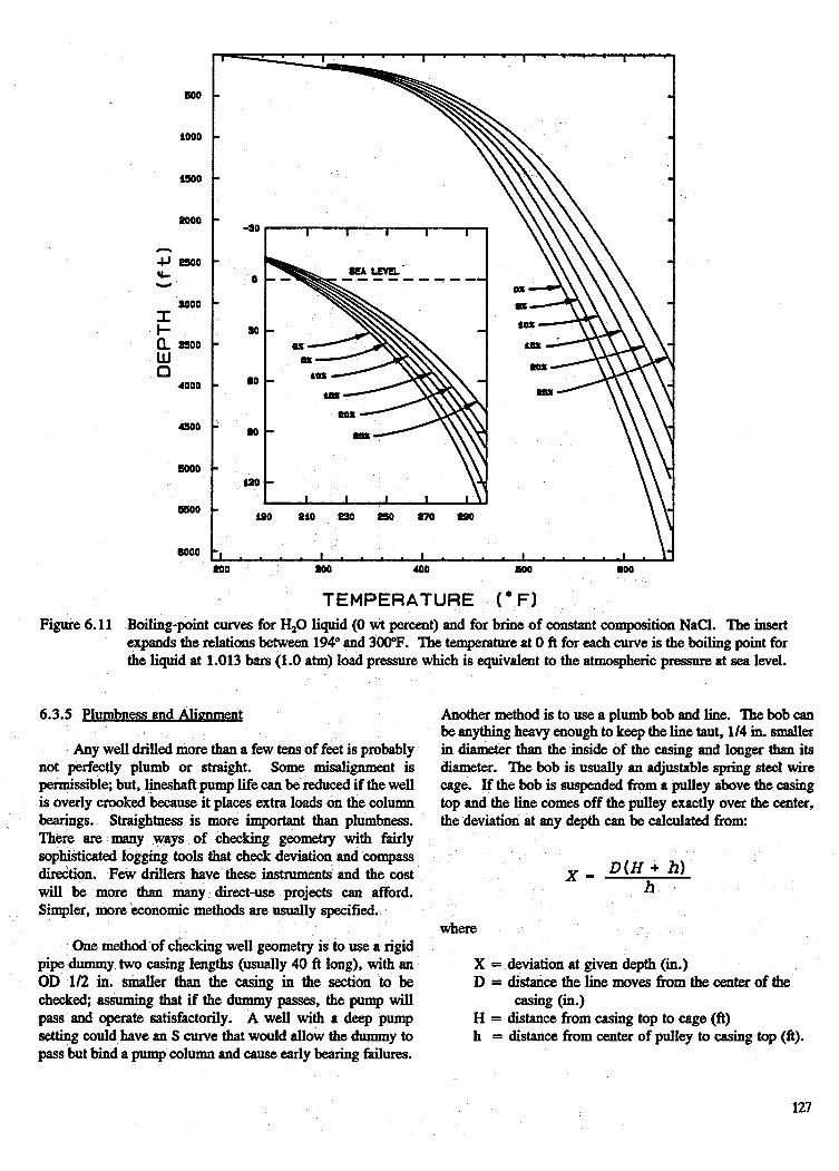
n
Y- 4J Y
I I-
w n n
500
io00
-0
moo
E500
so00
SSOO
lo00
4 0 0
5000
5500
8000
Figure 6.11 Boiling-point curves for H,O liquid (0 wt percent) and for brine of constant composition NaCl. The insert expands the relations between 194" and 300°F. The temperature at 0 ft for each curve is the boiling point for the liquid at 1.013 bars (1.0 atm) load pressure which is equivalent to the atmospheric pressure at sea level.
6.3.5 Plumbness and Aliment Another method is to use a plumb bob and line. The bob c8n be anything heavy enough to keep the line taut, 114 in. d l e r in diameter than the inside of the casing and longer than its diameter. The bob is usually an adjustable spring steel wire cage. If the bob is suspended from a pulley above the casing top and the line comes off the pulley exactly over the center, the deviation at any depth can be calculated from:
Any well drilled more than a few tens of feet is probably not perfectly plumb or straight. Some misalignment is permissible; but, lineshaft pump life can be reduced if the well is overly crooked because it places extra loads on the column bearings. Straightness is more important than plumbness. There are many ways of checking geometry with fairly sophisticated logging tools that check deviation and compass direction. Few drillers have these instruments and the cost X - will be more than many direct-use projects can afford. Simpler, more eumomic methods are usually specified.
D ( H + h) h
where One method of checking well geometry is to use a rigid
pipe dummy two casing lengths (usually 40 ft long), with an OD 1/2 in. smaller than the casing in the section to be
pass and operate satisfactorily. A well with a deep pump setting could have an S curve that would allow the dummy to pass but bind a pump column and cause early bearing failures.
X = deviation at given depth (in.) D = distance the line moves from the center of the
H = distance from casing top to cage (ft) h = distance from center of pulley to casing top (ft).
check&, assuming that if the dummy passes, the pump will casing (in.)
127

PULLEY -
$ QFCAGL
CAGING PROCEDURE
Figure6.12 Plumbnew and alignment (Roscoe Moss COmpanY).
a. Minimumamount:
8" for 24" ID well casing
7" for 20" ID well casing
6" for 18" ID well casing
5" for 16" ID well casing
4" for 14" ID well Caring
3" €or 12" ID well casing
2" for 10" ID well casing
Table 6.2 Relative Drilling Rate in Variotw
- 0
Y
& n 6
U
0 Y E
AI > - Y 0 0 0 m 0 H W . L. n. L.
Y a L.
aI . b,
2.. . >
I W I - 1 P I - 1
0 1 0 1
- 1
0 1 Y l
S I 0 1 r l l - 1
a i a i
e i
1 I
0 1
> - I o w I - 0 I
u a I a i
.
- 1 I I
I I I
I I
I I
I I I Y I 1 - 1 1 . ) 1 L . l
Y O . . L L .
a m
! ! I I P P U 0
Z Y Z Y Y L a o
P O P
e - a o
Y m a u e a a 8 32 8
0 % i; ;! i; I I I I
. I I I ! I I
I I I
I Y I
1 . 1 - L . -
1 - 1 1
Y
U
: : c a . L . >
Formations
a x 4 21
0
> n
Y
4
Y
3
a 0 Y
.+ 0
o
U . L.
Y
L.
a
0 " u w . eu V I
Y
U
0 " V
e
a
aa m
L.
. 4 3 0
r
Y a u x
f
4 rl a I
rl . 1 n
128

If the pulley is exactly 10 ft above the casing and readings are taken at 10 ft increments, the calculations are simplified. Both direction and total deviation can be plotted on a scaled deviation plot and an outline of the casing drawn. After plotting the casing, a straight line is drawn from the casing top to the depth where alignment is to be maintained. The casing should not be closer to the plotted center line than the maximum amounts shown in Figure 6.12.
The usual standard for plumbness allows 6 in. out of plumb for every 100 ft of well depth. Some engineers feel that 6 in./100 ft is excessive and allow only 3 in.1100 ft (Roscoe Moss Co., 1985).
The proposed 15th edition of the Hydraulics Institute's Standard for Well Straightness states "shall not deviate vore than 1 in./100 ft and be without double bend" (Cherry, 1987).
Table 6.2 gives relative drilling rates of seven drilling methods in various formations. Rates were modified somewhat from Driscoll (1987) after discussions with experienced geothermal direct use drillers.
6.4 WELLDESIGN
Well design involves specifying well depth, casing diameters, materials, thickness, lengths and pump setting. Once these are determined, other parameters such as wellbore diameter, completion methods, procedures, and perhaps, drilling methods can be decided. An initial design must be prepared in order to write specifications and obtain a bid; but, probably more often than not, the design changes as actual hole conditions become known. Some requirements may be specified by state, federal or local agencies. Other factors may be partially or wholly determined by local practices and equipment availability. In many cases, it is prudent to hire a qualified geologist to thoroughly review well logs and published geologic information before the initial design is made, and to interpret cuttings and logs as the well is drilled. There are often critical decisions that must be made during drilling. Having a geologist on-site to help in decision- making can help make drilling proceed smoothly and efficiently.
Most direct use wells consist of three main parts: pump housing or surface casing, the inlet portion, and the production casing between them. Flowing artesian wells do not require a pump housing, if flow is sufficient for the intended use.
Depth is usually determined by that required to obtain sufficient flow or temperature, or both, for the intended use. The controlling factors are depth to aquifer, thickness of the aquifer, transmissivity of the aquifer, and flow requirements. As noted earlier, the first three may be estimated from nearby wells; but in fractured and faulted areas, there may be consid-
erable differences in depth to geothermal aquifers and flow rates in adjacent wells. Many direct use wells have temperature reversals and get cooler with increased depth, once the aquifer has been fully penetrated.
In pumped wells, the final pump setting is determined from well testing, usually with a portable pump. These data should provide water levels for various pumping rates, and perhaps, estimates of long-term drawdown, depending on the degree of sophistication of the test. Deep and/or high pm- duction wells for district heating or industrial uses should have a g k d testing program unless the reservoir is well known. See Chapter 7, Reservoir Engineering, for test program des- criptions. Space heating for residential or light commercial applications probably cannot justify extensive testing but, if they are in known areas, expected pump settings can be obtained from nearby wells. Air lift or bailing with the drilling rig can provide information on the expected flow rates and drawdowns. Consideration should also be given to possible long-term water level declines, reduction in well efficiency over its life because of scaling and possible increased production requirements at some later date. The pump itself is relatively easy to set deeper; well workover to lower the surface casing is much more expensive and sometimes impossible.
Surface casing size is set by the pump bowl diameter. Pumping rate from a given pump diameter can vary mnsider- ably and pump suppliers should be consulted before drilling to determine the least life-cycle cost for the pump and well. Larger diameter, low-speed lineshaft pumps are usually more efficient and require less maintenance than smaller, high-speed pumps with the same flow and head. However, where settings are deep and drilling difficult, the cost of a larger diameter well may not justify the savings in maintenance and pumping power.
Surface casing diameter should be two nominal pipe sizes larger than the pump bowls. This permits easy installation and allows for some well deviations. One nominal pipe size larger is permissible, but not recommended. In case of necessity, the outside diameter of pump bowls can be trimmed a small amount. Table 6.3 is based on pump data from several manufacturers, for both lineshaft and submersible, and provides a general idea of the diameter required for given pumping rates.
Because many geothermal aquifers are confined, they will have high static (close to the ground surface) and pumping levels. In this situation, casing and/or bore sizes, or both, below the surface casing pump chamber can be reduced. Many times, at least a portion of the well, between the pump chamber and well bottom, will be in rock and can be left open hole if state regulations permit. In shallow wells, the surfm casing is often extended into rock above the aquifer and cemented in place with open hole the rest of the way to total depth. This method of completion simplifies grouting.
129

Table 6.3 Surface Casing Diameters
NominalpumP Nominalsurface Production Rate Diameter Casing Diameter
(mm) (in.) (in.)
< 100 4 6 1 0 0 6 175 5 8 175 to 350 6 10 350to 700 . 8 12 700 to 1,Ooo 10 14
1,OOO to 1,600 12 16 1,600 to 3,000 14 18
’
In deeper wells, it may be necessary or economical to install one or more casing strings of successively smaller diameters such as when drilling and driving when the casing cannot be driven further. A similar situation occurs when a slotted liner or screen is telescoped through the casing. In water well drilling it is not uncommon to seal the casing/ screen overlap with a lead packer to facilitate screen removal and replacement. Because many g e o t h e d fluids will leach lead (see Chapter 8), the water chemistry should be checked if the use of lead is considered. Cement should always be used at casing overlaps. If removal of the slotted liner or screen is anticipated, a high-temperature elastomer seal can be used.
Most states regulate the length and annulus space for casing overlap. In the case of water wells and, in some states, low-temperature geothermal wells, the required overlap may be < 10 ft. Because sulfate ions present in most geothermal fluids attack cements, the length of overlap should be increased to a minimum of 20 ft and the use of high sulfate resistant cement considered, if the sulfate concentration is high. Most states require a minimum of 50 ft overlap in geo- thermal wells, but those requirements were usually written with high-temperature geothermal fluid in mind. The length of overlap required by regulations may depend on how the well is classified, and not necessarily reflect the best design. Most agencies .will permit variances to obtain the best design for the particular situation.
The minimum diameter of any open hole or casing string should be selected so that fluid velocities at maximum pumping rates are <5 fils. For wells that flow at the surface, velocity (therefore, friction losses that reduce flow) might be lowered by increasing the diameter to obtain greater flows. The additional well costs should be balanced against pumping costs.
The diameter of the inlet portion at the bottom of the well should be chosen to accept the water available from the aquifer. Equations in Chapter 7, based on Darcy’s basic flow
equation, show that productivity is determined to a much greater extent by permeability than by diameter. For identical conditions of permeability, drawdown and radius of influence, doubling the wellbore diameter increases production - 10 % in an unconfined aquifer and only - 7% in a confined aquifer.
When a slotted liner or screen is used, the open area of the liner or screen may be the limiting factor (Figure 6.13). Open areas of continuous slot screeas typically range from - 1696to5096andslottedpipe - 196t01296. Therefore,when a screen or slotted liner is required and the thickness of the aquifer limits the length, it may be necessary to increase the diameter in order to utilize all the water the aquifer will provide. Velocity through the open area of the screen or h e r should be 0.10 to 0.25 ft/s (Campbell, 1973).
Well screen and filter pack are used to prevent sand and fines from entering the well and becoming a sand b u m . Screen Openings are small (0.006 to 0.150 in.) and the filter pack is clean graded sand selected to hold back fines from the aquifer, yet not pass through the screen. Selection of the filter pack size and gradation requires sieve analysis of the produc- ing formation and careful selection of filter material size. Because very few geothermal wells are screened, the methods will not be covered here. Methods and information are contained in Driscoll, 1987.
Formation stabilizer is coarser material (118 to 5/16 in. gravel) used to prevent sloughing of borehole walls in the pro- duction zone. Slotted liner with openings ranging from 0.120 to 0.250 in. supports the stabilizer material. Many g e o t h d wells require formation stabilizers. The term gravel back is often used for both filter pack and formation stabilizer.
Placement of filter pack is critical because it contains several selected sizes of material, which tend to separate if just poured down the annulus. Filter pack is carefully placed through a tremie pipe. Formation stabilizer, on the other hand, is usually screened to obtain uniform size and can be poured down the annulus. When cementing is required above the stabilizer or filter pack, 3 to 5 ft of sand is poured or tremied in to prevent cement from entering the stabilizer material.
Figure 6.13 Slotted liner and screen (Johnson Division, 1966).
130

Table 6.4 Comparison of Well Casing Materials
Material Fiberglass Asbestos Low-Carbon - ABS - PVC Emxv cement Steel
Specific gravity
Tensile strength @si)
Tensile modulus (106 psi)
Impact strength (ft-lb/in.)
Upper temperature limits ("F)
Thermal expansion (104 in./in. OF)
Heat transfer @tu in./h fi2 OF)
Water absorption (wt %I24 h)
1.04
4,500
.30
6.0
180
55
1.35
0.30
2.40 1.89
8,000 16,750
.41 2.30
1.0 20.0
140 2 w
30 8.5
1.10 2.30
0.05 0.20
1.85
3,000
3.00
1 .o
250
4.5
3.56
2.0
7.85
35,000 yld' 60,0oO ultimate
30.00
b
800 to 1,000
6.6
333.0
Nil
Type 304 Stainless Steel
8.0
30,000 yld' 60.0oO ultimate
29.00
a
800 to 1,000
10.1
96.0
Nil
a. Yield strength is the tensile stress required to produce a total elongation of 0.5% of the gauge length as determined by an extension meter. Expressed in psi.
b. Because testing methods for steel and other materials are not the same and the results are not comparable, the impact strength values for steel are not shown. In any event, the actual impact strength of steel is so high relative to the demands of water well work that it can be ignored in design considerations.
May be higher with special formulations. c.
6.5 CASINGMATERIALS
Casing materials, minimum thickness for various diame- ters, maximum depth for various diameters and ASTM or API standards are specified by some states, but may vary from state to state. Local and state regulations must be checked to assure that the well design meets the applicable codes.
Casing materials for low-to-moderate temperature geo- thermal wells include thermoplastics, fiberglass and steel. Concrete and asbestos cement casings are also used in water well construction and may be suitable for groundwater heat pump applications. Steel is by far the most common. Properties of casing materials are given in Table 6.4.
Steel casing is pipe manufactured to ASTM standards A- 53 and A-120, or line pipe manufactured to API standards 5L,
5LX (high strength), and 5A. Pipe is available with either threaded and coupled or beveled ends for welding. Most low- to-moderate temperature casing is welded because this is the most common practice in water well construction. Welding should be to American Welding Society standards, fully penet- rating multiple pass welds. In oil and gas producing areas, threaded and coupled pipe may be more readily available in sizes below - 8 in. Welded pipe is usually used, since it is less costly and welded joints are stronger than threaded and coupled joints for the same pipe thickness.
Most direct use wells are shallow enough that casing tensile and compressive strengths are not a problem. collapse pressure is p t e s t during cementing and collapse stresses will probably be the critical design factor. Table 6.5 gives physical characteristics of blank steel casing based on the following formulas (Roscoe Moss Co., 1985).
131


The values for collapse pressure in Table 6.5 were determined by:
where Pcr = theoretical collapse strength of a perfectly round tube written as:
3
Pcr - - 2E [ - k) 1-M2 t-1
where
E = Youngs modulus = 30 x 106 psi M = Poisson's ratio = 0.3 Do = casing OD
e = casing ellipticity = 1% S = yield strength = 35,000 psi P, = collapse pressure with ellipticity psi.
t = casing wall thickness
The values for casing tensile strength set forth in Table 6.4 were determined by:
casing t e n s i l e s trength ( ton) = St - (?;a where
St = tensile strength = 60,000 psi.
The values for casing axial compressive strength were determined by:
casing axial coqpressive strenm (ton) = trr 2,000
where
S = yield strength = 35,000 psi.
Collapse strength is reduced by ellipticity, bending and axial stress, and i n c d by compressive stress. Ellipticity of 1% is allowed in the ASTM and API standards and taken into account in the above equation. Additional ellipticity caused by rough handling and bending, and axial stresses in- duced during inshlation such as in crooked holes, should be allowed for by an appropriate safety factor. If an accurate plot of the well geometry has been made, the'additional stresses can be calculated using standard strength of materials calculations.
All steel well casing tends to corrode faster in an area above the water line where water vapor and air mix. This is exaggerated in geothermal wells because the increased temper- ature increases both the amount of water vapor and the dis-
tance it moves up the casing. Sealing the top of the casing and any openings such as for air lines and access ports for measuring devices will minimize oxygen intrusion and co~zo- don. Increasing the wall thickpes will increase well life. Unfortunately, there is no good standard practice or rule of thumb for increasing thickness, because temperature and water chemistry vary so widely. Each application should be judged individually. Past experience based on local practice can sometimes help, but often other wells have not been in use long enough to give a good indication of expected life.
Thermoplastic well casing standards are covered in ASTM Standard F-480, which includes a method for calcula- ting collapse strength. Care should be exercised when specify- ing thermoplastic casing for elevated temperatures because col- lapse strength is reduced drastically. As with any casing, the collapse pressure will be greatest during cementing and the placement method should be chosen so as to equalize pressures inside and out as much as possible. Heat generated during curing of cement grout further increases the temperature that the casing must withstand. Use of thermoplastic pipe is dis- cussed in Chapter 10, which gives strength decreases with rise in temperature. These factors are also applicable for collapse strength reductions.
Fiberglass-reinforced epoxy or polyester casings and pipe are produd with many resin formulations and winding pro- cedures that affect the temperature and strength characteristics. At the present time, there is no standards covering all the vari- ous resins and construction methods for well casings; how- ever, pressure piping is covered by several standards (see Chapter 10). Pressure piping is available for temperatures up to 300°F.
Fiberglass-reinforced casing has several advantages, in- cluding excellent corrosion resistance, light weight and high stmgth-to-weight ratios. It is available with several thread type connections, including threaded and 0-ringed, and bell and spigot with locking keys that permit speedy installation. Resin joining of bell and spigot or tapered joint couplings requiresaconsiderable time, experienced workmen and heat curing for use at elevated temperature.
The major disadvantage of fiberglass is cost, which is higher than steel on a per foot basis. Installed cost may be competitive when using the threaded or keyed couplings. An- other disadvantage is that pump housings must be plumb and probably larger diameter to ensure that pump parts do not con- tact the inside of the casing. Pump vibrations will wear a hole in the inner lining permitting hot water to wick along the fiberglass filaments and lead to separation of filaments and resin.
6.5.1 Centralizers
Casing should be run with centralizers or centering guides to assure that all voids are filled and channeling does not OCCUT during cementing. Centralizer spacing depends on
133

hole straightness and clearance between the casing and bore. Plktic caking quirei closer spacing than steel casing. Some states regulate the maximum spacing.
~entrhizers for shatlow, straight wells are typically fabricated from 1-10 to 2 in. x 114 to 5/16 in. steel flat bar,
and welded to steel casing to provide 1/4 to 1 0 in. with ,the well walls. For thermoplastic casing,
mri a& strapped to the casing with stainless steel s. Screws should not be used because they are subject
to corrosion, leaving holes in the casing. Fiberglass centralizers are available for fiberglass casing.
Centralizers used in the petroleum industry (for deep or crooked holes or both) float on the casing and are held in vertical spacing by lack collars (Figure 6.14). This permits the casing to be rotated. Wall scratchers or cleaners attached to the casing clean filter cake from the bore walls, providing better cement bonding to the formation and reduce cement channeling.
Figure 6.14 Centralizer.
6.6 GROUTINGlCEMENTING
6.6.1 General
Grouting and cementing have become synonymous. Grouting may be more technically correct, because grouting is the act of implacing any sealing material. Cement is the usual
grouting material for wells, although clays are permissible (in some states) where their location will not permit drying and shrinkage. Cementing is probably the more common termin- ology in geothermal work.
Grout is placed in the aunulus between the casing and well walls or between strings of casing of different diameter to prevent mixing and/or contamination of aquifers by undesirable aquifers or surface water. Because its purpose is to protect aquifers, most states have adopted regulations specifying acceptable materials and methods of placing grout.
Portland cement is the most common grouting material. ASTM Types I, 11, and III are commonly used water wells. The petrol- industry has developed eight classes of cement to meet the @ial conditions of deep oil and gas wells.
API Classes A, B, and C correspond to Types I, II, and 111 respectively. The other classifications were developed to permit the use of accelerators, retarders and other additives to meet special requirements. Because the elevated temperatures of geothermal wells are similar to oil and gas conditions, many of the materials and techniques used in petroleum industry are applicable.
he following information on basic cementing material is provided courtesy of Halliburton Services.
6.6.2 Cement Tvbes and Classifications
A basic cementing mateiial is classified as one that, without special additives for weight control or setting properties, when mixed with the proper amount of water, will have a cementitious properties.
Cements are made of limestone (or other materials high in calcium carbonate content), clay or shale, and some iron and aluminum oxides if they are not present in sufficient quantity in the clay or shale. These dry materials are finely ground and mixed thoroughly in the correct proportions either in the dry condition (dry process) or mixed with water (wet process). This raw mixture is then fed into the upper end of a sloping, rotary kiln, at a uniform rate, and slowly travels to the lower end. The kiln is fired with powdered coal, fuel oil, or gas to temperatures of 2,600 to 2,800"F.
All cements are manufactured in essentially the same way and are composed of the same ingdients, only in different proportions. The water requirement of each type of cement varies with the fineness of grind or surface anx. High-early- strength cements have a high surface area (fine grind), the retarded cements have a low surface anx, and the Portland cements have a surface area slightly higher than the retarded cements. The chemical retarder used in retarded cements may be added to the clinker during the secondary grinding stage to provide uniform distribution. It may also be added to the
- finished product.
134

Following is a brief summary of the characteristics of the various types of cement. These data are obtained from two sources: API Specification 10, API SDecification for Materials and Testine for Well Cements, whose well depth limits are based on the conditions imposed by the casingcement specifi- cation tests (Schedules 1, 4, 5, 6, 8 and 9) and should be considered as approximate values; and ASTM C 150, Standard Smification for Portland Cement. Copies of the specificat- ions are available from the American Society of Testing and Materials, 1916 Race Street, Philadelphia, PA 19103. In the cement industry, symbols for chemical compounds are often abbreviae C = CaO, S = SO,, A = AZO3, F = F+Op
For example:
C&= 3 CaOA120y
API Class A & B Cement common Portland Cement)
This cement is intended for use in oil wells from surface to 6,000 ft depth when no special properties are required. The recommended water-cement ratio, according to API, is 0.46 by weight (5.2 gallsk). It is more economical than premium cements and should be used when no special properties are desired and well conditions permit.
,4PI Class C Cement (High Earlv Cement)
This cement is intended for use in oil wells from surface to 6,000 ft depth. It is ground finer than Portland and has a high GS content, both of which contribute to the higher strength. The API water requirement for this cement is 0.56 (6.3 gallsk). The compressive strength of this cement is greater than Portland cement at Curing times up to 30 hours; and the pumping time slightly less under the same test condi- tions. This cement is more expensive than Portland and, unless its special properties are needed, should not be used. Generally, Portland with calcium chloride or other accelerators will give better strength than this type of cement without accelerators.
API Classes G or H Cement (Basic Cement)
This cement is intended for use as manufactured from surface to 8,000 ft or it can be modified with accelerators or retarders to meet a wide range of temperature conditions. It is chemically similar to API Class B cement but is manufac- tured to more rigorous chemical and physical specifications, which result in a more uniform product. As manufactured, it contains no accelerators, retarders or viscosity control agents other than'gypsum normally ground with cement clinker. All necessary additives are blended by the service company. The MI water requirements for Class G is 0.44 (5.0 gal/&) and for Class H is 0.38 (4.3 gal/&).
API Class G cement is cunrently being used on the West Coast, where it was developed, and in the Northern Rocky Mountain area. Class H cement is used predominately along the Gulf Coast and in the Mid-Continent area.
API Class D. E. and F Cements (Retarder Cement)
Most of these cements are retarded with an organic compound, while some are retarded by chemical composition and grind. The most common retarders are of the lignin type; the most widely used being calcium ligndfonates similar to HR-4. These cements are more expensive than Portland cement and, unless their special properties are needed, should not be use.
Pozmix Cement
This basic cementing composition umsists of Portland cement, a pozzolanic material (Pozmix), and 2% bentonite based on the total weight of cement. By definition, a pozzolan is a siliceous material that reacts with lime and water to form calcium silicates having cementing properties. Advantages of this reaction are utilized with Popnix Cement, because Portland cements release 15% free lime when they m t with water, and the lime subsequently reacts with the Popnix to yield a more durable mass of calcium silicates. Because this type of composition is less expensive than the other basic materials and performs well with most additives, it has almost universal application in well cementing (Halliburton Services).
Neat Cement
Neat cement should not be used at tempera- > 23O"F, because it loses strength and increases permeability above that temperature. The process is time and temperature &pendent. In a test of API Class G (the usual high-temperature oil well cement), it was found that neat cement compressive strength decreased by 77% from 5,050 to 1,150 psi, and permeability increased from 0.012 to 8.3 millidarcies in 60 days at 3u)"F in geothermal brine. Regression is somewhat dependent on geotheimal fluid chemistry (Gallus, 1978).
6.6.3 Silica Flour and Sand Effects
Mixtures of silica flour and silica sand in ratios of 40 to 80% by weight with API Class G cement have been found to reduce strength and permeability degradation in hot wells. API Class A cement (ASTM Type I), with addition of 30 to 50 % silica flour has performed satisfactorily for conductor and surface casing in steam wells and should be satisfactory for most higher temperature direct use wells.
135
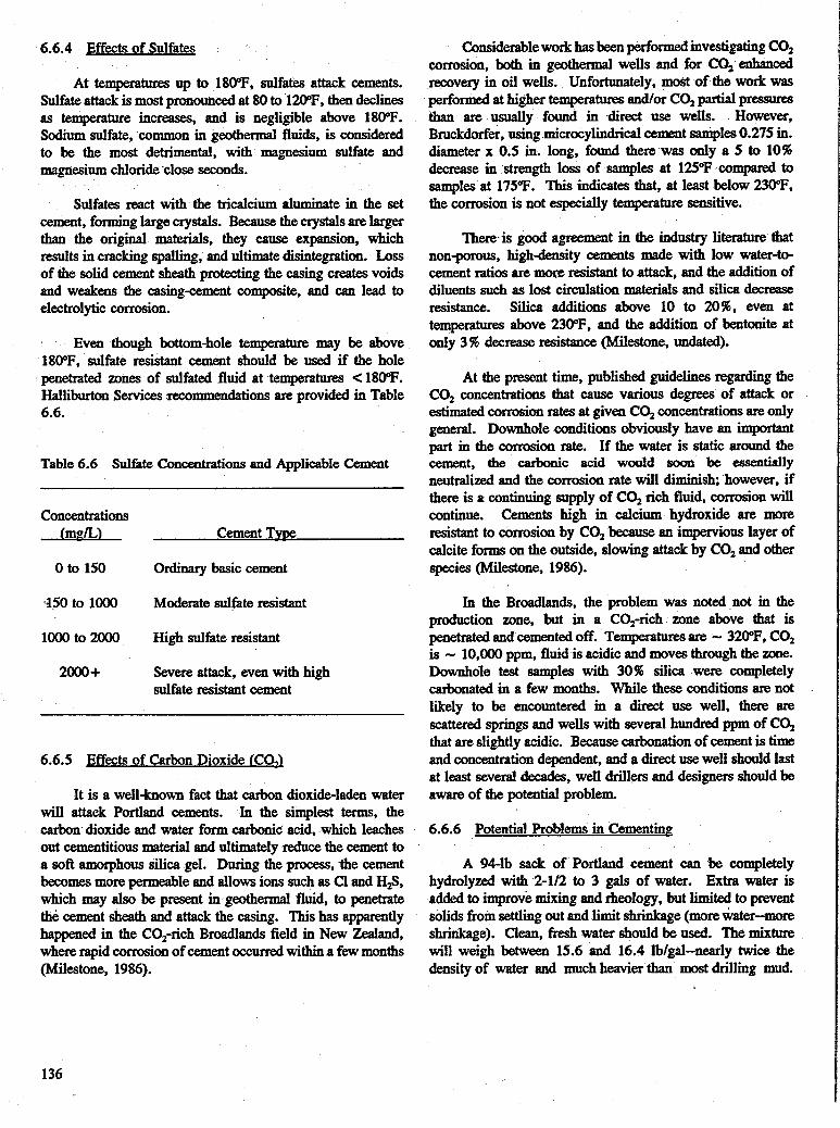
6.6.4 Effects of Sulfates
At temperatures up to 180"F, sulfates attack cements. Sulfate attack is most pronounced at 80 to 120"F, then declines as temperature increases, and is negligible above 180°F. Sodium sulfate, common in geothermal fluids, is d d e r e d to be the most detrimental, with magnesium sulfate and magnesium chloride-close seumds.
Sulfates react with the tricalcium aluminate in the set cement, forming large crystals. Because the crystals are larger than the original materials, they cause expansion, which results in cracking spalling, and ultimate disintegration. Loss of the solid cement sheath protecting the casing creates voids and weakens the casingcement composite, and can lead to electrolytic corrosion.
Even though bottom-hole temperalum may be above 180"F, sulfate resistant cement should be used if the hole penetrated zones of sulfated fluid at temperatum <180"F. Halliburton Services recommendations are provided in Table 6.6.
Table 6.6 Sulfate concentnrtions and Applicable Cement
0 to 150 ordinary basic cement
,350 to loo0 Moderate sulfate resistant
1000 to 2000 High sulfate resistant
2000+ Severe attack, even with high sulfate resistant cement
6.6.5 Effects of Carbon Dioxide CC0,j
It is a well-known fact that carbon dioxide-laden water will attack Portland cements. In the simplest terms, the carbon dioxide and water form carbonic acid, which leaches out cementitious material and ultimately reduce the cement to a soft amorphous silica gel. During the process, the cement becomes more permeable and allows ions such as C1 and HS, which may also be present in geothermal fluid, to penetrate the cement sheath and attack the casing. This has apparently happened in the C0,-rich Broadlands field in New Zealand, where rapid corrosion of cement occurred withina few months (Milestone, 1986).
Considerable work has been performed investigating CO, corrosion, both in geothermal wells and for CO, enhand recovery in oil wells. Unfortunately, most of the work was performed at higher temperatures and/or CO, partial ptessures than are usually found in direct use wells. However, Bmckdorfer, Using microcylindrical cement samples 0.275 in. diameter x 0.5 in. long, found there was only a 5 to 10% decrease in strength loss of samples at 125°F wmpared to samples at 175°F. This indicates that, at least below 230°F. the corrosion is not especially temperature sensitive.
There is good agreement in the industry literature that non-porous, highdensity cements made with low water* cement ratios are mote resistant to attack, and the addition of diluents such as lost circulation materials and silica decrease resistance. Silica additions above 10 to 2095, even at temperatures above 230"F, and the addition of bentonite at only 3 96 decrease resistance (Milestone, undated).
At the present time, published guidelines regarding the CO, concentrations that cause various degrees of attack or estimated corrosion rates at given CO, concentrations are only general. Downhole conditions obviously have an important part in the cortosion rate. If the water is static around the cement, the carbonic acid would soon be essentially neutralized and the corrosion rate will diminish; however, if there is a continuing supply of CO, rich fluid, d o n will continue. Cements high in calcium hydroxide are more resistant to corrosion by CO, because an impervious layer of calcite forms on the outside, slowing attack by CO, and other species (Milestone, 1986).
In the Broadlands, the problem was noted not in the production zone, but in a C02-rich zone above that is penetrated and cemented off. Temperatures are - 320"F, CO, is - 10,000 ppm, fluid is acidic and moves through the me. Downhole test samples with 30% silica were completely carbonated in a few months. While these conditions are not likely to be encountered in a direct use well, there are scattered springs and wells with several h u n M ppm of CO, that are slightly acidic. Because &nation of cement is time and concentration dependent, and a direct use well should last at least several decades, well drillers and designers should be aware of the potential problem.
6.6.6 Potential Problems in Cementing
A 94-lb sack of Portland cement can be completely hydrolyzed with 2-112 to 3 gals of water. Extra water is added to improve mixing and rheology, but limited to prevent solids from settling out and limit shrinkage (more water-more shrinkage). Clean, fresh water should be used. The mixture will weigh between 15.6 and 16.4 lblgal-nearly twice the densityof water and muchheavierthan mostdrilling mud.
136

Although the apparent viscosity of 125 Saybolt Universal Seconds is much higher than water or drilling mud, neat cement has no filtration properties and the increased density will probably result in cement losses in lost circulation zones. It may also result in hydraulic fracturing of wkak formations and losses to zones that maintained circulation during drilling. This limits the vertical height of the column, unless weight reducers are added.
Many shallow cementing jobs are done with a float shoe or other drillable packer at the bottom of the casing. The high density of cement increases casing collapse pressure far above normal hydrostatic pressure unless the casing is filled with water or drilling mud to reduce the pressure differences. Also, the packer or plug makes the casing a loose fitting piston when lowed into the hole. If fluids are present, high lowering rates can create downhole pressure surges to the point of creating new loss zones and opening up previously sealed ones. considerable encountered.
Figure 6.15
Lowering rates should be 0.5 ft/s or less when lost circulation or weak formation
I I
are
Grouting with cement shoe. A cementipg shoe can direct the grout out into the annulus above one or more cement baskets mounted at any position in the casing string. The grout passes through holes cut into the casing by a mills knife or other kind of perforator (Halliburton Services).
When placing cement through a flat shoe or other methods involving a pumping or pressure at the bottom to force cement up the annulus, the increased density and viscosity raise annulus pressures. Eliminating pressure surges and maintaining pump pressure as low as possible, consistent with reasonable pumping time, reduces the possibility of losses and an incomplete cement job. Weight reducers and dispers- ants can be added to control density and viscosity if required.
Figure 6.16 External packer with float shoe. An external packer equipped with a float shoe can be installed in the casing string to facilitate placing cement grout (Halliburton Services).
Loss of cement to formation results in:
No cement ever reaching the surface.
Fall back after cement reaches the d a c e in the gMulus and pumping is stopped.
1.
2.
3. The top and bottom sealing but there are voids along the casing.
These require a tm outside iob, placing cement through a tremie pipe in the annulus - or a saueeze iob - downhole perforation of the casing, setting a packer or packers and squeezing cement through the perforations until it fills the annulus. Both are very effective solutions but costly and time umsuming.
Cement top, after a fall back, and voids can be detected by temperature logs that detect the heat of hydration or by a sonic cement bond log. These logs may be required in some states and will be an additional cost.
At - 170°F or higher, cement thickening time is reduced to the extent that placement times may become critical. In order to prevent premature cement thickening times, chemical retarders are added to the cement system to umtrol the pumping time of the cement slurry. Chemical additive concentrations can be tailored to meet a broad range of well conditions.
137

Hole Preparation before casing and cementing is an important step. The hole should be cleaned of any drill cuttings or cave-ins by making a hole cleaning trip. This assures that the casing can be set to the desired depth and removes excess filter cake that may have built up if the hole was drilled with mud. The objective is to have cement in intimate contact with the formation, yet maintain a thin filter cake to prevent cement losses.
If lost circulation was experienced and heavy cement is to be used, it may be wise to spot non-fermenting cellulose or polymer gel in the loss zones. This is faster and less expensive than repairing a poor cement job. Other altematives are to prepare lower density cementing compositions, Le., spherelite, perlite, bentonite or nitrogen foam, or add lost circulation materials to the slurry.
6.6.7 Cement Placement Methods
When cementing surface casing, quite often the hole will have been drilled deeper than the depth to where Casing is to be set orcemented. If the casing is to be cemented to its full depth, a bridge or drillable plug can be set in the open hole, or the hole can be backfilled with sand such as plaster or mortar sand.
If the casing is to extend beyond the cementing depth, a cement basket can be clamped to the outside of the casing or an expandable packer and float shoe installed in the Casing string at the required depth. Often the extension will be slotted casing or screen and formation stabilizer or filter pack is placed, with sand above, to prevent cement from entering the stabilizer.
One method of placing cement is to use a tremie pipe (Figure 6.17). This is often r e f e d to as a ton outside iob and the tremie pipe as a macaroni string. The borehole must be sufficiently larger than the Casing, usually 4 to 8 inches in diameter, to permit running the tremie pipe, and centralizers should be aligned. Tremie pipes as small as 314 in. ID have been used when friction reducers are added to cement, pre- mitting pumping rates of 6 to 8 @lmh at 750 psi.
The casing is seated on the bottom, or baskets or a packer is used, depending on conditions. The casing is usually Wed with water or drilling fluid. The tremie is lowered to the bottom and conditioned mud or other fluid is circulated to be sure there are no obstructions. When good returns are observed, cement is immediately pumped through the tremie. Because cement is heavier than the mud, it displaces the mud as cement is pumped. Depending on the depth and cement pumps available, the cement can be placed in one continuous operation until good cement is observed at the surface. Then the tremie can be removed.
Figure6.17 Tremie pipe grouting. Grouting can be accomplished by means of a tremie pipe sus- pended in the annulus outside the casing. During grouting, the bottom of the tremie should always be submerged a few feet h e a t h the grout level. As the grout rises, the tremie should be withdrawn at approximately the same rate (Johnson Division).
For deeper jobs or when the cement pump pressure is not high enough to place all the cement with one tremie setting, the tremie can be raised, usually one or two pipe joints, as cement is placed. The end of the tremie should always be submerged in the slurry. If water or air is trapped in the pipe as joints are removed, the pipe should be pulled back above the slurry surface and water or air displaced by cement before submerging again in order to prevent voids in the annulus.
Most drillers will limit top outside jobs to several hundred feet if possible. Placing the tremie, obtaining high pressure pumps, and removing the tremie in sections are all troublesome. Tremies have been successfully employed to depths of 10,OOO ft (Evanoff, 1987).
In order to reduce the volume of cement to be displaced in large diameter casing and holes, cement is sometimes placed
4 inches larger than the Casing, depending on the state regulations and depth.
by the inner string method. Hole diameters areusually2to
138

In this method, a cement shoe (float shoe) with a check valve and stabbing arrangement is installed on the first (bottom) section of casing. The casing is lowered to within a few feet of the bottom, suspended and filled with water or drilling fluid. A tremie or the chill string is stabbed into the shoe and fluid circulated to clean the hole (Figure 6.18). Cement is pumped until clean cement is observed at the sur- face. The tremie is removed from the shoe and water pumped to clean out the inside of the casing string. The check valve prevents cement from entering the casing. The float shoe, cement below it, and the bridge or plug in the open hole below that is then drilled out after the cement cures.
Figure 6.18 Inner-string method of placing grout. A cementing (float) shoe is attached to the bottom of the casing before the casing is placed in the borehole. A tremie pipe is lowered until it engages the shoe (Johnson Division).
There are several variations of the so called Halliburton or through-thewing cementing method. All are adapted from the oil and gas industry where the methds were first developed. Figure 6.19 shows the basics of the operation.
The casing is set without a float shoe and suspended a few feet from the bottom. Water or drilling fluid is circulated to clean out the hole. A plug is inserted to separate the water or drilling fluid from the cement; a measured amount of cement is pumped in above the plug and a second plug inserted. More water, pumped in above the second plug, forces the plugs and contained cement down, causing cement
to come up the annulus. The pumping is stopped when the second plug is 10 to 20 ft above the bottom of the casing. Pressure is held until the cement hardens. The plugs and cement are drilled out after the cement hardens. This method ensures a good seal at the bottomof the casing because there is no dilution of cement by water, which is behind the second plug, and minimizes dilution ahead of the first plug. The location of the second plug should be monitored by a wire line through a seal at the surface or by carehlly measuring the amount of fluid pumped for displacement. Plugs are made of a drillable material. Cement, plastic, and wood have been used. Wood is usually a poor choice when drilling with a tricone bit.
-
Figure 6.19' Casing method of grouting. Grout can be placed in the casing and then forced out the bottom and up the annulus. This is called the casing method of placing grout. Plugs are used to separate the grout from the drilling fluid and the water used to drive the grout mto place. The plugs and float shoe are drilled out after
I the grout b a r k . The casing method of grouting was origmlly used in the oil well industry (Halliburton Services).
When bonding becomes critical, holding pressure is not a good practice. Heat of hydration and resulting expansion of the annular cement causes pressure buildup outside the casing. Holding any pressure on the casing allows the formation of a microannulus between the cement and pipe when pressure is relieved. Later in the life of the well, this can cause problems that include migration of fluids and loss of d isolation, corrosion, etc. Operators commonly use a back pressure valve in the lower casing string to prevent having to hold pressure on the casing.
One variation uses only one plug, behind the cement, to prevent dilution. Any cement diluted by the elimination of the first plug must be wasted at the surface to ensure a good surface seal. Because only one plug is used, a landing collar
139

Table 6.7 Summary of Oil Well Cementing Additives
Sbca flour
Mud Kil
Rldioachve tracers
Pozzolan bne
h e x cement
Combaning hgh pretsurr tnarawog Juny weight
P m r y wmenting
High-temperature cemenbng
Hlgh-temperature cementing
Gtlsonne WaInuI hulls cenophane flakes G y ~ s u m m n t BernoMedMsel dl Nykm fibers
Sodwmchlwlde
Sodium uuoriee
- Silicon dioride
ParetmaMehyde
Sc 46
Silica-bme reacIKMs
Calcium sulfate Hemihydrate
Gypsum wn resin
k#easedpumpinotime Bener Ibw
Bener bondmg to sab
Stabihzed strength h e r penneabihty
Bener bondmg Greater strenglh
shales. sands
APlCiasses0.E. 0. ud H
All API Classes
API Clsstes A. 8. C. 0, and H
UI API Classes
API Classes A. E. 0. and H
Shryock & S m f t h , Halliburton S e r v i c e s
140

Table 6.8 Factors Affating primary Casing Cementing
Personnel Well owners responsibility, service company respo
Drilling Rig Operations Running time of casing, rate of running casing, , position of collar on landing joint, circulating time
atter running casing
r
Drilling Fluid Composition, weight, Viscosity, water loss and filter cake, gel strength, admixes
Bore Hole Diameter, depth, straightness, formation characteristics I
Casing
Special Tools
0.0. casing versus hole size, depth of casing set versus total depth
Guiding and floating equipment (shoes, collar), ~
(reciprocating vs rotation)
Cementing Materials Slurry volume required (caliper survey, estimate), type of cement (API classification, admixes), mixing water
(supply, impurities, temperature), slurry A./sack, volume to be mixed)
Mixing and Pumping of Cement Slurry , I
Plugs (bottom, top, location of top plug, compression of fluid), spacers-flushes (water, special fiuid), time (mixing, displacement), mixing units (number, type, mixer
Cementing Head and Connections Swage, quick change, plug container, opening in head, valves on head, floor manifold
1
141

Table 6.9 Digest of Cementing J3quipment and Mechanical Aids
cemontlng Equlpmnt
Fkstlng Equlpmn!
and Types Application Pbcsment
1. Guide Shoes . Guides casing into wen Minimizes de* strain
Firstpintofcasing
2. Floatcdlars Prevents cement flow back 1 joint above s m in wens less Create pressure diflerenbals to than 6.000 ti 2-3 pi- in improve bond Catches cementing plugs
wells greater than 6.000 tt
Automatic Fili-Up EQu1pment
1. fb8t ShOeS Same as Float Collars end Shoes except fill-up IS controlled by hydrostattc pressure m annulus
Same as Float Collars or Guioe Shoes
Fonnstbn Packer fools 1. Formatton Packer
2. Formatm Pac&er shoes
Collars
Cementing Stage Took
2 Stage 3 Stage Full Opentno Tools
Plug Conta*mn
1. Ouick Opening 2. Continuous
Cementhg Piugs 1. Top and Bottom
Wiper Plugs 2. Ball Plugs 3 L a t a Down Pluos
bsing Centtalkerr
Vanable Types
Cemenbno Heads
Packer expands lo protea first joint of casing
As hde requirements dictate bwer zones while cemenling
When requred to cement IWO or more sections m separate sages
Based on critical Lories and tomram fracture Qradlents
To hold cemenbng plugs in s!nng until released.
Top joint of casing at surtace of well
Mechanical Spacer between Mud and cement (bottom plug) and cement and displacement fluid (top plug)
Between well fluids and cement
Cemer casing in hole or provide minimum Straight h o l e 1 per joint thrwgh standsff to improve distribution of cement in annulus, prevent ditterenbsl slicking
and 200 feet above and below pay zones; 1 p e r 3 joints in open hole to be cemented Crooked hole-Variable with deviation
1. Rotanng Remove Mud cake and armlatable Place thrwgh W m n g mud from well bore. fomabons and 50 to 100 feet h e .
Rotate pipe 15 to 20 RPM
rotat~ng Reciprocate pipe pipe 10 to 15 feet off m o m
2. Renprocating Aid in creabng turbulence Placement is same Es Improve cement bond
Shryock R S m i t h , Halliburton Services
142

can be installed at the desired height (10 to 20 Et above the casing bottom) to stop the plug inside the casing. This eliminates the problem of knowing exactly where the second plug is and when to stop it as in the first method.
Another version utilizes a float shoe installed at the bottom of the casing and viscous fluid spacers rather than rigid plugs. The fluid spacers must be compatible with both mud and cement, and are usually polymem, water, and weighing materials to achieve a density of 0.5 & 1.5 lb/gal more than the drilling fluid. The viscous spacers are especially effective in obtaining good mud displacement (Shyrock, 1983).
All of the above methods can incorporate additives to produce a betteicement job. Surfactants and mud thinners can be added as hole cleaners (not to be used whek lost ckula- tion exists). Reactive flushes can be used to clean mud off the outside of the casing to achieve good bonding, and friction reducers can be used to lower pumping pressures. Accele- rators and retarders can control hkdening at different tempera- tures and pressures along the length to be cemented. Lost cir- culation materials, density reducers, temperature stabilizers, and other additives have their uses to promote a better cementing job. Some of these can be accomplished by injecting additives while pumping batch mixes; other require continuous mixing with additions during placement. Tables 6.7, 6.8 and 6.9 are taken from Halliburton Services and summarize additives, factors to consider, and equipment. Although these are intended primarily for deep high- temperature wells, they contain useful information for low- temperature work dso.
A relatively new technique of foaming cement with nitrogen gas appears to have good possibilities for use in low- and moderate-temperature wells and perhaps, even in standard water-well practice. The technique was developed for use in steam injection wells in oil fields for insulation. It has been s u ~ f u l l y used in high-temperature geothermal wells with lost circulation where its low density and increased gel strength are advantageous. Also, it provides thermal insu- lation with K factors ranging from 0.15 to 0.4 Btulh fi2 OF.
The cement used in high-temperature work is MI, Class G, with 4096 silica flour to prevexU strength regression at high temperatures. Other mixtures should be satisfactory at lower temperatures. The cement is mixed at 15.6 lb/gal d a c e density and can be foamed from 4 to 15 lblgal downhole density.
Gel yield point increases with reduced density. The 4 lb/gal density has a yield point of 80 lb/lOO ft2 compared to 34 lb/lOO ft2 at 15.6 lb/gal. This means that once the foam has stopped flowing in a loss m e , it will stay in place. Strength is somewhat less than standard cement but appears to be high enough to support casings during thermal cycling.
The cementing design is usually a umstant volume. That is, because hydrostatic pressure at the bottom of the hole is highest, more standard e (free air volume) of nitrogen are injected into the cement that will be placed near the bottom. More nitrogen is injected ps cementing proceeds because the last cement pumped ends up at the bottom. Foam cementing requires some method of holding back pressure on the annulus to prevent the nitrogen bubbles in the cement from expanding too much; thus, producing the desired density. A neat cap slurry is pumped first to provide a good seal at the top, then foamed cement, followed by a neat tail slurry to provide a good seal at the bottom.
At the present time, foam cementing is only applicable to expensive or difficult holes because the technology is new and r e q u k equipment ordinarily Bssociafed with oil field practices plus a foam generator. As the technology matures, simpler and less expensive techniques will probably evolve.
6.7 BLOWOUT PREVENTION EQUPMENT
Blowout prevention equipment (BOPE) collsists of comb- inations of valves, rams, packers and rotating heads enabling control of fluids and gases that could flow from the well. The equipment is attached to a casing that is securely cemented to prevent fluids or gases from escaping to the surface mund the casing. All state and federal agencies having jurisdiction over drilling of geothermal wells will require BOPE when: (a) ex- pected temperatures are above some limit, usually somewhere between 150°F and the boiling point at the altitude of the well- head, (b) submface presures may cause flow of fluids or gases, (c) combustible gas may be encountered, or (d) the sub- d a c e conditions are unknown. Often, the first well in an area will have BOPE installed. If high te-, pres- sures, or combustibles are not encountered, subsequent wells will not require BOF'E. Usually, the equipment is rented and installed to meet the expected conditim or agency requirements.
Figure 6.20 schematically shows a typical BOPE, stack for high-tempemture air and mud drilling. Figures 6.21 and 6.22 show typical low-temperature BOPE for mud and air drilling, respectively. Gate valves may be required at the casing flange if flow to the surface is anticipated or in an unknown area. Figure 6.23 is a photo of a double ram preventer.
Rams and packers are usually hydraulically operated, and a gas over hydraulic accumulator or manual operation is re- quid in order to operate the devices if all power fails. BOPE is installed on the surface casing after Casing cement has hardened. The system is pressure tested before drilling out the cement and cement shoe in the bottom of the surface casing in order to ensure it will ahstand the pressure p i - fied by the controlling agency, usually with an official of the agency witnessing the test.
143

Figure620 Typical high-temperature geothermal BOPE (Mud) stack (California Division of oil and GaS).
NIPPLE - rLon LINE .
FILL UP LINE - **
Figure621 Typical low-texnperatum geothermal BOPE (Air) diverter stack (California Division of Oil and Gas).
144
CaaEmIl rxn CaaEmIl rxn
Figure6.22 Typical low-tgmp&we geofhermal BOPE stack (California Division of Oil and Gas).
. .
Figure623 Double ram-type preventer. Two ram-type preventers built into one casing conserve vertical space, minimize the number of connections, and simplify installation. Usually, choke and kill conndons are made to a drilling spool below the preventers. Such
. cunnections may be made to the side outlets, visiile on the preventer body, but this is not common practice. A Siange fiilure at one of the side outlets might necessitate changing the entire preventer (Hydd Company).
.

6.8 INJECTIONWELLS
In 1974, Congress enacted the Safe Drinking Water Act, Public LAW 93-523, to protect the public health and welfare, and to protect existing and future underground sources of drinking water. Under this act, the Environmental Protection Agency (EPA) has been developing, and continues to develop, regulations for protection of the underground sources from contamination by injection wells. Five classes of wells have been defined and established. Geothermal injection wells are included in Class V. Class V is a kind of catchall that includes all the wells not mentioned in ,the other classes, and that typically inject non-hazardous fluids into or above underground sources of drinking water.
In 1980, EPA chose to defer establishing technical requirements for Class V wells, and they were authorized by rule. This means that injection into Class V wells is author- ized until Mher requirements under future regulations are promulgated by EPA. However, Class V wells are prohibited from contaminating any undergniund source of drinking water and minimal inventory, and reporting is required of Class V well owners/operators.
An underground drinking water supply is defied as an aquifer, or a portion of the aquifer, which supplies any public water system, or contains a sufficient quantity of groundwater to supply a public water system, currently supplies drinking water for human consumption, contains fewer than 10,OOO mgL total dissolved solids, and is not an exempted aquifer.
As a part of developing technical regulations, an inventory and assessment of Class V wells was made. Twenty-one direct heat injection wells, Type 5A6, were inventoried (additionally, the type was reported, but no numbers are available in New York). Eighty-nine electric power injection wells, Type 5A5, were inventoried. Contami- nation potential for the two types together was rated as mod- erate. (All the above excerpts from Council and Fryberger, 1987).
The EPA underground injection control regulations may be administered by federally approved state programs (primacy states) or by EPA (direct implementation states). See Chapter 19, Institutional, Legal and Permitting Requirements, for in- formation on specific states. Currently, EPA considers geo- thermal injection a low priority item and specific regulations for construction and operation of geothermal injection wells are not likely to be developed for some time (Council, 1987).
Agencies in several states, notably those with active geothermal projects, have developed specific geothermal injec- tion regulations and are currently seeking primacy status. In all l ikel i id , the regulations will be based on waste disposal, geothermal electric power production, and petroleum wells, or experience, and may seem overly restrictive for many direct use injection wells. It can only be hoped that with experi-
ence and good injection well design, adequate but reasonable protection of the drinking water will be ensured. One thing is certain, injection wells will be required in more and more cases. Water levels have declined in some aquifers supplying direct use applications and the public will require increasingly stringent environmental protection measures.
The injection well survey noted earlier appears to have included at least the major direct use injection wells. Only 21 were noted in the U.S. Considering the much larger number of direct use applications on-line, two conclusions can be made. There is a substantial number of direct use applications that are discharging substantial amounts of heat and chemicals to the surface, usually to surface waters, and there is very little experience with direct use injection wells. Of the 21 wells, only a few have been in service more than 5 years and one was taken out of service at least temporady after only 1 year of use.
The drilling and completion of an injection well is not much different than a production well; the same drilling and completion methods generally can be used, but more care should be taken to ensure that the wellbore is clean and ade- quately cemented. Because after the initial development, the well accepts fluid rather than producing it, there is no oppor- tunity for mud or fines left in the formation to come out. In- stead, they tend to form bridges for the almost inevitable silt and corrosion products pumped into the well that (over time) leads to plugging of the formation. Drilling fluid monitoring and control are even more important in drilling injection wells than production wells.
Most states will require that casing be set and cemented from the top of the accepting formation to the surface. The accepting formation is generally an aquifer of similar or worse water quality. A few states may permit the Casing to be adequately cemented into the confining formation immediately above the accepting formation in some cases. California, Nevada, and perhaps other states, require double wall injec- tion. At least one wall is a casing string and the other may be an injection tube extending to a permanent packer set just above the injection zone. This double wall requirement may be waived for low pressure injection of non-aggressive fluids in relatively well-known areas.
I
In order to reduce the possibility of formation plugging when drilling with mud, many drilling consultants recommend drilling to the accepting formation, then changing to water or air. The casing can be set and cemented, if required, to pre- vent caving. When conditions permit, open-hole completion is preferred because it eliminates the possibility of encrustation and clogging of screens or the slotted liner. If the injected water is significantly cooler than the accepting formation, ther- mal stresses-may fracture the rocks. This has been postulated as one possible explanation of injection wells in New Zealand increasing acceptance over time (Armstead, 1978). If spalling fractures occuf, the well could partially fill with debris.
145

Because injecting fluid creates a cone of recharge (similar in shape but the opposite of a cone of depression murounding a pumped well), there is a tendency for the injec- ted fluid to migrate up the outside of the casing, possibly into fresh ,water aquifers. Proper cementing techniques are re quired. If drilling mud was used, better bonds between casing and cement, and cement and formation can be achieved by:
1. Flushing with clay dispersants such as one of the poly phosphates.
2. Flushing with plenty of water at sufficient flows to create turbulence in the annulus.
3. use of wall scratchers.
4.
5.
Pumping cement fast enough to create turbulence.
additives, etc. Flushing with paraformaldehyde to neutralize mud
- If a fresh water aquifer was penetrated, as is usually the case, additives must be EPNstate approved. If clay forma- tions have been drilled, polyphosphates should be used with caution, because they could make the clay near the hole un- stable. Injection temperatures are likely to be in the range where sulfate resistance of cement is lowered (100 to 180°F).
The design of the injection portion of the well is open to question and each case should be considered on an individual basis. For cold water injection wells, a general rule of thumb is that the injection area (bore area, slot area, or open area of screen, as applicable) should be twice to three times as large as for a well producing the same amount of fluid. This prob ably holds for injection in relatively tight formations and water source heat pump injection wells. Tight formations tend to clog with silt and corrosion products. Heat pump injection wells often operate in the optimum temperature range for iron bacteria clogging and even twice the area may not be sufficient if iron bacteria are present. Open formations such as fractured and weathered basalts may require only modest increase in area, if any.
If CO, and hydrogen sulfide are present, and pressures are reduced, or the system is open to atmosphere, allowing the gases to come out of solution, pH changes will occur. This upsets the chemical equilibrium of the water resulting in precipitation, scaling, and plugging of the injection zone. In general, systems should be closed and pressure maintained, including the injection well. Water should not be allowed to free fall into a well even though it accepts the fluid while maintaining a water level below the surface. Microscopic bubbles form that will block acceptance of the formation.
In some cases, injected water may be at a higher temper- ature than the receiving aquifer, such as when injecting near the boundaries of the reservoit. If the system is closed so pH
remaim constant, acceptance may increase with time because there may bea tendency to dissolve materials in the formation.
6.9 WELL SPECIFICATIONS
Well specifications are the basis for inviting bids from drilling contractors. As such, they should be written: (a) so as to make it easy to compare bids on a cost basis, (b) to ensure that the well will be constructed of suitable materials and in a manner that ensures a reasonable life, (c) so the well will produce the required flows, and (d) to serve as a guide for the final completion. The specifications must also be teasonably flexible because subsurface conditions are m l y accurately known.
Many state or other governmental entities have minimum standards of construction that must be met. These standards may cover such items as depth of surface casing, casing material and thickness, cementing materials and placement procedures, safety items such as blowout pventer requirements and even disposal of drilling cuttings, fluids, and mud. In all cases, the intention is to provide for public safety, protection of fresh water supplies and the environment and co&ation of geothermal resources.
Unfortunately, there is wide variation in the standards and regulations depending on how geothennal energy is classified (water, mineral, or petroleum), because the standards are written from different perspectives by staff with different backgrounds. In some states, the classification changes with depth, temperatwe, or intended use. In Oregon, water well regulations apply to a depth of 2,000 ft and/or temperatures below 250°F. For deeper or hotter wells, Division of Geology and Mineral Industry's regulations apply. In California, any well that may tap water with temperatures greater than the average ambient temperaave is geothermal and is regulated by the Division of Oil and Gas. In practice, wells 86°F or hotter a Considered geothermal momas, 1987). Nevada has three divisions of geothermal wells, &pending on proposed use and flow rata.
There may be overlaps and conflicts in standads and jurisdiction between different agencies. A good example is in some homestead parcels whm the nuface is under private control but the federal government retains the mineral, therefore, geothermal rights and umtrols. In many cases, the overlaps and umflicts have been at least tempered for electric power production by agreements between agencies. Little attention has been paid to lower temperature direct use applications, that logically should have different requirements, but often do not. In some instances, variances will have to be requested with substantiating infodon, because the ' standards were written with electric power production in mind and do not necessarily give the best construction for lower temperature wells.
146

Consultation with appropriate federal, state, and local officials is mandatory. Some agencies require proposed well specifications with the permit application; others only a record of what was performed. Plenty of lead time should be allowed because it may take longer to determine the amrotxiate agency than it does to drill the well.
Most technid specifications start with a scope of work. There is considerable variation in detail depending in part on knowledge about the site and in part on the engineer’s preference for including details in the scope or in the body of the specifications. At a minimum, the scope should contain the exact location, proposed flow, use, pumping equipment, anticipated temperature, depth, casing, and completion program, and a drawing that may or may not be dimensioned depending on knowledge about the site.
Any known geologic conditions may be included &I the summary or as an appendix containing this and nearby well logs, etc. Providing as much information as possible results in a more accurate and usually lower bid because there are fewer unknowns in the risk factor. Any adverse conditions such as major lost circulation problems, caving, squeezing clays, etc., should be at least noted in the scope, perhaps with details in the appendix.
Attention should be given to local practices because they can vary considerably, and drillers usually find and use what works best in their area. If the practices are sound from an engineering and hydrological standpoint, inclusion or allowances as alternatives may result in lower costs.
Drilling a pilot or test hole may or may not be included. Sometimes the additional costs will be prohibitive; but, if the hole is very large or deep, it often requires drilling and reaming because of equipment limitations. When drilling in an unknown or highly variable area, a pilot hole provides: (a) lithology, (b) an opportunity to run logs, (c) refines the details of the well completion, and (d) ordering of required materials.
The drilling method is normally not specified unless there are known or suspected conditions that exclude a particular method. It is not uncommon to specify one method to some depth or formation, then specify a non-mud method in the production zone. Drilling methods for test holes may be prescribed when there are special sampling requirements.
In many cases, specification writing can be greatly simplified by making the appropriate state agency rules and regulations a part of the specifications. Casing and liner wall thickness may be increased to allow for accelerated corrosion and increased weight of deeper settings in geothermal wells. Rules and regulations usually also include abandonment specifications, which should always be included in case of an unacceptable well.
Although it would seem to be advisable to use a driller experiend in geothexmal well drilling (and therefore presumably knowledgeable about the appropriate state agency rules and regulations included in the specifications), this may not always be €he case. A water well driller may bid on a . geothermal job or the well may have a different cla&ification than that in which the driller has experience. Them have been too many instances where a driller has bid and been accepted for a job without being familiar with the appropriate rules. The result is an underbid job, an unhappy driller trying to make up the difference even though it was his own fault, and general disagreement with the owner and the regulating agency. Sometimes the driller pushes his equipment too fast, resulting in breakdowns or fishing jobs. Depending on how the contract is written, these may result in extra cost to the owner and, at a minimum, cause delays.
One way to help prevent this problem is to require in the bid a statement that the bidder has read and understands the current rules and regulations, by their numbers, as stated in the specifications. This serves to motivate the bidder to understand the rules and provides the owner with additional protection should a dispute arise. This requires that the owner also be familiar with the rules in order to cortectly write the specifications and to detect bids that do not meet the requirements.
Agency rules and regulations include only completion. and abandonment specifications. Items kch as drilling fluids, properties, working hours, cutting samples, noise, etc., should be added if applicable.
Cutting samples at 10 to 20 Et increments andlor changes in.lithology should be required. These should be washed, bagged in small plastic sacks and labeled as to depth, date and other pertinent information such as drill rate, loss of circulation, etc. Only a few tablespoons full are required for a sample. They may or may not ever be inspected, but if disputes or problems arise, they may be very useful. If nothing else, they inspire more careful logging by the driller if a geologist is not on-site.
6.10 BID SHEETS . In order to evaluate bidders, a well-written bid sheet
should be included in the technical specifications and serve as the basis for payment. Fixed costs should be lump sum, variable costs should be shown as unit prices, and their extension based on the well design.
Fixed costs could include:
Mobilization and demobilization of drill rig.
Development, if for a specific time.
1.
2.
147

3. Mobilization and demobilization of logging and survey equipment.
Test pump furnishing, installation and removal.
WZhead equipment.
.
6. Site preparation and restoration.
7. Standby time (as directed by the engineer or owner).
Standby, start-up and non-chargeable time should be specified; i.e., if a normal workday is 8:00 a.m. to 500 p.m. and the engineer stops the rig at 3:00 p.m. and resumes again at 1000 a.m. the next day, only 4 hours standby are allowed.
Variable costs include:
1. Drilling - each diameter a separate item LF.
2. Furnish and install casing - each diameter - separate item including cementing as required LE
3. Logs and hole surveys L.F.
4. Gravel pack feed pipe LF.
5. Gravel pack LF.
6. More or less developing time hour
7. More or less pumping time hour
8. Abandonment LF.
Unless the owner or engineer is familiar with all possible bidders, bidders should be required to submit their qualifica- tions, similar work performed with names and addresses of contacts for references, complete equipment submittals, licenses, bonds, etc. If the well is of significant cost or complexity and drilling muds will be used, it is common to require a proposed mud program and to have a qualified mud expert (usually an employee of a materials' manufacturer) on- site or available on short notice.
The ~merican water w k s Association standards for Wells (AWWA 100-84) sets standards for municipal wells, many of which will be applicable. '
The Manual of Water Well Construction Practices (EPA 1975) contains a matrix diagram listing items to be considered in well specifications. Included in the list of well uses are heating, cooling and geothermal water. The heating and cool- ing standards appear to have been based on heat pump and very low-temperature wells and may not contain some desir- able items, or be overly permissive; while the geothermal
standards appear to have been based on high-temperature wells for electric power production and will be overly d c t i v e for many direct use wells.
Sample specifications and bid schedules are contained in Ground Water and Wells 1987. These were written with large industrial or municipal wells in mind and contain items such as screens, filter packs and disinfection that may not be required, and do not include items such as disposal of cuttings and test pump fluid that may be required by some states.
The Engineers Manual for Water Well Design (Roscoe Moss Co., 1985) contains separate guidelines specifications and bid proposals for cable tool, direct rotary and reverse circulation drilling and completion. Again, these are for cold water wells.
6.11 WELLCOSTS
It is virtually impossible to provide accurate universal guidelines for estimating well drilling and completion costs because of too many variables in geology, well design, location, drilling regulations, etc. In general, drilling costs depend on depth, diameter, and difficulty.
Depending on the locality, there seems to be a cost in- crease for drilling beyond 500 to 600 ft. Beyond that depth, a 10 to 15% increase can be expected for each additional 200
$15O/h, one to go to 2,000 ft for $200lh including a crew and fuel (late 1987 costs).
t o 2 5 O f t . Arigthatmdrillto -5OOft~anberentedfor-
The formation to be drilled has a large affect on drilling costs. Obviously, soft formations can be drilled easier than hard formations; but, there are also other factors, such as lost circulation, caving problems, etc., which are estimated by the driller and included in his bid. Recent (1987) bid costs, for drilling only, ranged from $1.00/in. of diameter per ft of depth for g.& formations and $2.50/in./ft for hard drilling in Klamath Falls, Oregon, to an average of $5.00/in./ft near Meport in Northern California.
The drilling costs typically represent - 40 to 60% of the total completed cost, depending on the casing program, mud costs, cement, and cementing aids (i.e., cementing shoes and centralizers), wellhead, etc. Depending on local custom or bid sheet design or both, wen drill bits may be excluded from the cost/ft bid price and included as separate items.
Detailed cost information is difficult to gather and, wen then, usually little is provided concerning the formations drilled, problems encountered, etc. Overall costs for 20 wells drilled to <600 ft during the last 3 years ranged from $3.00 to $6.03/in. of pump housing casing diameter per ft of total depth. Based on this, a 12 in., 600 ft well would cost
148

between $26,350 and $43,400. 'These 20 wells included wells drilled in California, Nevada, New Mexico, Oregon and Utah. Wells in the 1,600 to 2,000 ft range cost $4.25 to $8.%/in./ ft. There seems to have been very little increase in the cost of drilling direct use wells during the past 3 years (1985 to 1987). This is more of a general feeling than a demonstrable fact, because each well is different, but drilling cost/in./ft, casing and rig time have held stable or increased very little since 1987.
If directional drilling is required, say to get around tools stuck in a hole, it may be necessary to set a cement plug with a whipstock, then rent the services and equipment to direction- ally drill around the obstruction. If a cement service company is hired to set the plug and whipstock, and the well site is some distance from their nearest facility, the job can be expected to cost $3,000 to $5,000, depending on the distance; if the drill can set the plug, the cost might be about half.
Table 6.10 lists approximate costs to drill around the obstruction.
Table 6.10 Approximate Costs To Drill Around An ObsEruction
Item
Directional drilling supervisor
Bent subs
Drill motor (10 h minimum)
Additional operating h
Cost ($1
$ 580ld + mileage
400
2,400 + freight
240h
Standby time 70/h
The job could probably be done in 1 day plus 1 day of travel time. The total estimated cost would be between $4,000 and $5,000.
The rig will be used to set the plug and run the direc- tional drill, and will be on standby waiting on services and for cement to set. It will also have been used and be on standby several days for fishing attempts. At $200/h, the estimated rig cost could range between $12,000 and $15,000; possibly more.
Considering the additional cost of the lost tools, fishing tools, and other services, it can be seen why directional drilling is seldom used in direct use wells, and stuck tools are to be avoided.
GLOSSARY
Anchor String - The string of casing to which the BOPE . stackisflanged.
AMUIZU F'reventer (bag preventer) - A device that can seal around almost any object in the wellbore or upon itself. Compression of a reinforced elastomer packing element by hydraulic pressure effects the seal.
Banjo BOX - A thick-Walled drilling spool used when drilling with air. cuttings to a blooie line.
The spool routes returning air and drill
Bell Nipple (flow nipple, mud riser) - A piece of pipe with an inside diameter equal to, or greater than, the blowout preventer bore. It is connected to the top of the blowout preventer or marine riser. A side outlet directs the mud returns to the shale shaker or pit. It usually has a second side outlet for a fill-up line CoMecfiOll.
Blind Rams (blank, CSO, complete shutoff, master) - Rams that are not intended to seal against any drill pipe or casing. They seal against each other to effectively close the hole.
Blind-Shear Rams - Blind rams with a built-in cutting edge that will shear pipe in the hole, allowing the blind rams to seal the hole. Used primarily in subsea systems.
Blooie Line - A large diameter pipe that routs returning air and drill cuttings to a separator and muffler. The line may be equipped with high-pressure nozzles that both
. spray water to settle dust, and spray sodium hydroxide and hydrogen peroxide to eliminate hydrogen sulfide Odors.
/
Blowout - An uncontrolled flow of well fluids and f m t i o n fluids, or both, fwm the wellbore to the surface, or into lower pressured subsurface zones (underground blowout).
Bridge Plug - A device to close off or bridge an Opening such as the bore hole or casing.
Casing Shoe - A heavy-walled steel coupling or band attached to the lower end of the casing. There axe several types for specific applications. A drive shoe is heavy hardened steel, usually designed to shave off the inner edges of the bore hole during drill and drive operations. A guide shoe is slightly tapered to guide casing down the bore hole and protects the end of the casing.
I
149

Cement Basket - A device attached to the outside of Casing designed to contact the bore wall to catch and hold cement at that point. Usually, a series of flexible steel staves with a fleGble liner. Flexibility allows fluid in the hole to pass in the upward direction, while setting casing, circulating, or cementing, but prevents flow downward, thereby, supporting thecement column above it.
Draw Works - The hoisting equipment consisting of power source, cable drums, brakes, controls, etc., used to generate the liftiag capability of a drill rig.
Fill-Up Line - A line, usually connected into the bell nipple above the blowout preventers, which allows the addition of mud to the hole while pulling out of the hole, in order to compensate for the displacement of the drill string.
Fish - Any object lost in a bore hole.
Fisking - The act of attempting to remove a fish.
Flow Line - A line connecting the wellbore to the hole fluid storage or processing area.
Internal &venter - A device, which acts as a check valve, that can be installed in the drill string. It allows fluid to be circulated down the drill string but prevents back flow.
Kelly Cock, Lower - A full opening valve installed immedi- ately below the kelly, with outside diameter equal to the tool joint outside diameter. can be closed to remove the kelly under pressure, and can be stripped into the hole for snubbing operations.
Kelly Cock, Upper - A valve immediately above the kelly that can be shut to umfiue pressures inside the drill string.
Kick - The intrusion of formation liquids or gas that results in an increase in pit volume. Without corrective measures, this can result in a blowout.
Kill Lhe - A high pressure line b e e n the pumps and zone point below a blowout preventer that allows fluids to be pumped into the well or annulus when the preventer is closed.
Open Hole - Bore hole without casing or other support or protection.
Packer - Adevicetoclose offanannular opening suchas between casing and bore hole or umcentric Casings.
Packoff or Stripper - A device with an ehtomer packing element that depends on pressure below the packing to effect a tight seal in the BMUIUS. Used primarily to nm or pull pipe under low or moderate pressures. Cannot be depended upon under high diffkrential pressures.
Pip - Drill String.
PipeRams - Ramswithfaces umtouredtosealaroundpipe to close the annular space. Unless special rams
rams are necessary for each pipe size in use. accommodating various pipe sizes are used, separate
R~tatingHead - A rotating, PA * g device used when drilling with air, gas, foam, or any other drilling fluid with hydrostatic pressare less than the formation PreSSUre.
Spot - To selectively place material at some location in the bore. Usually used as in pumping lost circulation materials, cement, etc., through a pipe with the end or openings at the desired level. Hydrostatic pressure forces the material into the formation.
Spudding - To move up and down. Derived from the spud- ding arm of a cable-tool drill rig that imparts the up and down mtion to the cable-tool drill bit.
Sub - A short piece of pipe, usually drill pipe, with p i a l ends for attaching various tools or bits.
Test Joint (testing sub) - A pipe joint or sub designed for use in conjunction with a test plug to simulate pipe in the hole when pressure testing the pipe rams or annular preventer.
Test Plug (boll weevil plug) - A tool designed to seal the well bore immediately h e a t h the BOP stack, which allows high pressure testing of the stack and auxiliary equipment without the risk of pressure damage to the casing or to exposed formations.
Tool Pusher - Foreman in charge of the drilling rig.
Trip - Movement of drilling tools and equipment into or out of the hole or both, round trip, trip in, trip out.
Under-Ream - Enlarging or reaming theholeto agreater diameter below some obstruction, formation or casing. special tools that can be rotated on eccentrics or otherwise enlarge are used.
150

REFERENCES
Armstead, H. C. H., "GeothermalEnergy", Secondedition, E. &F. N. Spon. Ltd., London, England, 1978.
Biczok, I., Concrete Corrosion - Concreb Protection, eemical Publishing Company, Inc., New York: pp. 281-300, 1967.
Bruckdorder, R., "Carbon Dioxide Corrosion Resistance in Cements", CIM 85-36-31, presented at 36th Annual Tech. Meeting of Petroleum Societv of CIM, Edmonton, Canada, June 1985.
campbell, M. 0. and Lehr, J. H., Water Well Technologv, New York: McGraw Hill Book Co., 1973.
Cherry, R. C., Vice President of Engineering, Layne & Bowler. Personal communication, June 1987.
childs, J. D., Group Supervisor, Cement Section, Halliburton Services, Duncan, OK. Personal communication, November 1987.
Council, L. C., Director of Class V Injection Well Program, Engineering Enterprises, Norman, OK. Personal communication, October 28, 1987.
Council, L. C. and Fryberger, J. B., "An Overview of Class V Injection Wells", International Symposium on Class V Injection Well Technology, Washington, D.C., September 22 - 24, 1987.
Evanoff, J., Halliburton services. Personal communication, November 1987.
Driscoll, F. G., Groundwater and Wells, Johnson Division, second edition, second printing, St. Paul, MN, 1987.
Gallus, 3. P., et al., "Performance of Oil-Well Cementing Compositions in Geothermal Wells." 53rd Annual Fall Technical Conference. Societv of Petroleum Endneers, Houston, TX, October 1 - 3, 1978.
Halliburton Services, "Technical Information 0 n G e o t h e d Cementing" notebook, Duncan, OK, Undated.
Lead. F. M., The Chemistrv of Cement and concrete, 3rd edition. Chemical Publishing Company, New York, NY, 1971.
Milestone, N. B., et al., Carbonation of Geothermal Grouts, Parts I. II & III, submitted to Cement and concrete Research Journal, work performed under USDOE Contract DE-AC02-76CH00016, undated.
Milestone, N. B., et al., "Effects of Carbon Dioxide Attack on Geothermal Cement and Grouts", Geothermal Resources Council Transactions, 10, September 1986.
Nelson, E. B., et al., "Development of Geothermal Well Completion Systems", Geothermal Resources Council Transactions, Vol. 3, 1976.
Onan, D. D., "Effects of Supercritical Carbon Dioxide on Well Cements", Societv of Professional Engineers P a m 12593, presented at Permian Basin Oil & Gas Recovery Conference, Midland, TX, March 1984.
Rickard, W. N., "Foam Cement for Geothermal Wells", GRC Transactions, 9 Part 1, August 1985, pp. 147-152.
Roscoe Moss Company, "The Engineer's Manual for Water Well Design", Roscoe Moss Company, Los Angeles, CA, 1985.
Shyrock, S. H. and Smith, D. K., Halliburton Services, "Geothermal Cementing - The State-of-theAt", presented at Basic Geothermal Drilling and Cornletion School, Albuquerque, NM, March 1980.
Thomas, R., California Division of Oil and Gas. Personal communication, October 1987.
U.S. Department of Interior, Bureau of Reclamation, Ground Water Manual, U. S. Government Printing Office, Denver, CO, 1981.
"Water Well Specifications", Committee on Water Well Standards; National Water Well Association, Premier Press, Berkeley, CA, 1981.
151

i
.

CHAPTER 7 WELL TESTING AND
RESERVOIR EVALUATION By Susan G. Stiger and J. L. Remer
(Sections 7.1 through 7.7) EG&G Idaho, Inc.
Idaho Falls, ID 83415 and
Gene Culver (Section 7.8)
Klamath Falls, OR 97601 I OIT Geo-Heat Center
7.1 INTRODUCTION
This chapter presents a summary of the well testing and reservoir engineering techniques used to estimate the produc- tion potential of a geothermal system. The basic theory behind geothermal reservoir engineering and the influence of simplifying assumptions required to enable solutions to the basic flow equations are discussed. A summary of well testing methods and data acquisition considerations for geothermal systems is also included.
The techniques that are ed here have been developed from both groundwater and petroleum engineering disciplines. In recent years, the field of geothermal reservoir engineering has emerged as a separate discipline that addresses those factors unique to geothermal systems. Low-temperature g e o t h e d reservoirs more nearly approximate a groundwater aquifer than do higher temperature reservoirs and it is tempting to simply apply groundwater methods to analyze them. This approach can 1ead.to significant errors in the analyses. The following sections highlight those featares of geothermal reseNoizs that should be considered during any evaluation of a geothermal system.
Well testing and reservoir analyses provide information that is necessary to assess a project's technical and ecoflomic feasibility. Individual well characteristics, and fluid and reservoir properties can be determined, and provide a basis for a reservoir model that can be used to predict the performance of a reservoir under exploitation and to optimize resource development and profitability. An evaluation of reservoir data can also be used to determine the relationship between one well and other wells that tap the same system. This can be an impOaaat consideration for direct use developments where more than one developer is involved and questions of resource ownership and rights are issues.
The amount of well testing and reservoir engineering that is reasonable for an individual project is a subjective factor. There are no hard and fast rules, with the exception that the more information available the more reliable will be the analyses and predictions. A guiding factor should be the financial risk, evaluated against the magnitude of the development compared to the size of the resource. The following sections present a summary of COIlSiderafioIlS that can be used as a g e n d guide in determining how much testing and analysis to do and to what degree of sophistication. Because this chapter provides general information and each application is unique, it is essential that qualified persons be utilized to help assure proper approaches and performance.
It should also be noted that, to be effective, 'reservoir analyses canuot be performed in a vacuum, but require careful integration and correlation of geologic, geochemical, geophysical, and drilling data. As advanced as geothermal reservoir engineering has become, it is not an exact science and the solutions obtained are generally not unique. However, the reservoir information developed is a critical factor in achieving a financially and technically viable resource development.
7.5 RESERVOIR ENGINEERING THEORY
. To understand the application of reservoir engineering techniques, it is important to understand the theoretical basis for these techniques. There are a number of references that discuss this theory and the development of the governing equations in detail (see References). Presented here is an overview of reservoir theory and the assumptions that must be satisfied for any analysis to be valid.
153

The analytical techniques that form the basis.for g e o t h d reservoir engineering have been developed from solutions of the partial differential equations that descrii the flow of fluids through porous media. The basic equations evolve ffom the equations of state, conservation of mass, and Darcy's Law (Mafthews and Russell, 1%7).
In a series of tests of flow through sand, Darcy observed that the volumetric flow of fluid through porous media is proportional to the hydraulic gradient in the direction of the flow, or:
q - K i A - K N A L
*
where
q = volumetric flow K = hydraulic conductivity
i - E - hydraulic gradient L
A = flow area.
This relationship is valid for laminar (not turbulent) flow through a porous media whose physical properties (e.g., porosity, permeability, etc.) are uniform throughout.
The proportionality constant in Darcy's relationship is the hvdraulic conductivitv, K, which expresses the ease with which a fluid is transported through a porous medium. Hydraulic conductivity is related to the properties of both the p u s medium and the fluid flowiug through it. In groundwater hydraulics, the properties of liquid water at standard conditions can be assumed with little error. The properties of water can change significantly with temperature; thus, for geothermal systems, it is more appropriate to use permeability, k, which is a property of the porous medium alone. The hydraulic conductivity and permeability are related using:
K - k CI
where
p = fluiddensity p = dynamic viscosity g = gravitational umstant k = permeability.
Information on the variation of fluid density and viscoSity with tempera- is readily available (for example, see Crane, 1981).
Figure 7.1 is an idealized cross-section of a well petrating an aquifer. Fluid flows toward the well if th'ere is a hydraulic gradient in that direction. As fluid is withdrawn
from the porous medium, there is a local decrease in pressure, or drawdown. The magnitude of this drawdown at any point in the aquifer and at anytime is a function of the physical properties of the qservoir. Observing the drawdown that results from flow under controlled umditions enables us to estimate those physical propexties and to predict what will happen under different production scenarios. As will be explained in more detail in Subsection 7.5, drawdown m a pumped well or surface pressure in an artesian well are affected by fluid temperatures in the wellbure. Because of this, drawdown obtakied by measuring pressure at aquifer depth in the well is more representative of actual reservoir conditions, and is used in most equations.
Figure 7.1 Idealized cross-sections of producing well and aquifer drawdown.
Using Darcy's Law as the basis, a number of derivations made that relate drawdown to withdrawal from an
The pressure in a well have aquifer under specific conditions. under flowing conditions, p,,, can be expressed as:
where
po = static and po - p,, = d r a ~ d ~ w n q = volumetricproductionrate r$ = porosityoftheaquifer h = thiclcnessoftheaquifer c = compressibility r,, = radius of the wellbore t = timesinceproductionbegan.
The derivation of this equation assumes that the flow toward the well is radial in a horizontal, homogeneous aquifer of uniform thickness (Matthews and Russell, 1967).
Monitoring the change in ptessure m a well during
of two groups of physical parameters for the reservoir using theabove relationship. Onegroup, kh, isthe permea bility
controlled production from the well can enable determinati on
154

thickness, or transmissivity in groundwater terms. The other group, &h, storativity, which is a measure of the aquifer’s ability to store fluid is obtained from the last set of terms in the above equation and is written:
These two parameters, storativity and permeability- thickness, provide the principle measures of a reservoir’s ability to produce fluids.
Further refinement of the derivation of the above relationship has led to approximate solutions for more complex situations, including reservoirs with boundaries and partially penetrating wells. However, the basic assumptions referred to above are still applicable. It is difficult to imagine a real reservoir that satisfies all of these assumptions. For this reason, care should be taken in the analysis of any geothermal reservoir data and it should be recognized that the results only approximate the actual physical umditions underground.
7.3 CONCEPTUAL RESERVOIR MODELS
Well testing is the mechanism used to provide the data necessary to evaluate the performance of a reservoir. However, data recovered through well testing must be considered in the light of the conceptual geologic model of the reservoir. In actual practice, the geologic model and the well test data are used in an iterative fashion to develop a sound model from which to plan the production of a geothermal reservoir.
A general discussion of the ~ t u r e of geothermal resources is presented in Chapter 3. Several simple models of hydrothermal resoutce systems expected in direct use applic- ations are also described in that chapter as well as in Sorey (1983). The methods of collecting the geologic data needed to develop a geologic model are described in Chapter 4.
Comparing the geologic setting of the reservoir under study to other developed geothermal r e s o m areas is useful in developing a conceptual model, particularly in the early stages of exploration and development. However, it is strongly emphasized that each reservoir must be treated as a unique system.
A conceptual model of the reservoir is important at every stage in the exploration for and development of a geothermal resource. Data collected before drilling a well is used to properly locate the well and also to design and interpret the well test. Geologic and well test data collected during the drilling of the well is used to further refine the model.
Because data collected during well tests can usually be interpreted in several different ways, it is important that as many cunstraints as possible be placed on these data by a welldeveloped geologic model. In particular, geologic data may be useful in determining boundaries placed on the system because of structure (faults and folded rock) and changes in rock type (e.g. permeable sandstone, impermeable shales, or carbonate rocks where fractures often umtml permeability).
Geologists and engineers have developed many ways to transfer the three-dimensional geologic data to the two- dimensional limitations of reports. Block diagrams, similar to those in Figures 3.11 and 3.12 of Cbapter 3, can be used to
However, the areal extent and complexity of data needed in most geologic models is such that various confout maps, similar to topographic maps, must be used to describe the subsurface changes in rock types, temperatures, and fluid production needed to adequately model a reservoir. Temperature is commonly contoured at several depths in a reservoir (Figure 7.2). The same data may also be used to prepare two-dimensional sections showing temperature relative to depth along a vertical section through the mewoir, or to develop a contour map showing the depth from an established datum such as sea level to a specified temperature in the subsurface.
give a perspective view of the heedmmn * ‘anal geology.
The umceptual model of a reservoir is important in establishing expected boundaries of the system and in particular its geometry. Such information is particularly important in reservoirs where more than one operator is developing a reservoir and its volumetric extent may be quite limited even though its lateral extent is great. Such systems are common in the Basin and Range Physiographic Province of the Western United States and other ~feas where the g e o t h e d tesource may be closely associated with a major fault zone. In such areas a detailed geologic model may be necessary, coupled with extensive well testing to determrn ethe interaction between different zones of the reservoir. In large sedimentary basins of reasonably Uniform geology, less detailed geologic information may be acceptable. In general, the amount of geologic and well test data needed to adequately build a conceptual model of a system is directly related to the complexity of the reservoir, the rapidity of change in resetvoir properties in space, and the degree to which the reservoir will be produced relative to its maximum potential.
7.4 WELLTESTING
Well testing is the mechanism used to provide the data necessary to evaluate the performance of a geothermal reservoir. Tests can range from a few hours in duration during drilling to months. As a rule, the longer the test, the more reliable theanalyses (although, of course, ashorter,
155

well-run test is better than one that is long but poorly executed and instnimented). Factors that can affect test duration include environmental constraints, fluid disposal consider- ations, .eq~p&t, money, and pressu~ from investors. . .
It is difficult to physically measure the parameters bntrolling the flow of fluids in a reservoir. It is important, then, to design well tests to control as many variables as possible so that a reasonable assessment of the reservoir parameters can be made. In practice, this meam that the flow rate from a well must be controlled in some manner to meet the requirements of the test that is being run. In addition, quality measurements of flow rate, temperature and pressure or water level are essential.
7.4.1 Drilline Data
Much of information can be obtained about a geothermal reservoir even before the first well test is run. Some of this information comes from geological exploration as discussed in Chapter 3, while more can be obtained during drilling.
t-
156
Perhaps the most critical information from the drilling phase is an indication of the depth and nature of the producing intervsl(s) in the well. Lost circulation zones, temperaue anomalies, sudden changes in the fluid level in' the well, rapid drilling rate, and evidence of fracturing in the cuttings all can provide indications of potential inflow zones (DOE, 1982). Interpretation of downhole temperature surveys, in particular, can help resolve some of the uncertainty regarding downhole conditions. Figure 7.3 is an example of a continuous tempemhe survey in which penneable zones are indicated by temperature reversals resulting from the invasion of cold drilling fluids. Measuring downhole temperature buildup over a period of time ranging from 12 to 24 h or more using a method derived by Homer (Grant, 1982) can provide an indication of the static reservoir temperature. Downhole
regarding the depth to set production casing, particularly in shallow geothermal systems where there may not be much vertical Separation between cold water inflow m e s and the thermal zones.
temperature data are also important input to decisions
A'
C. e-.
.
Figure 7.2 Example subsurface temperature contours at three elevations.

7.4.2 Rig Tests
Short tests run while the drilling rig is still on the hole are principally conducted to clean out the hole and to provide initial estimates of the well’s production potential and fluid chemistry. The test data are also important for decisions regarding further drilling and completion of the well and provide the basis for planning additional tests of the well (Campbell, 1986). Produced fluids are generally discharged to tanks or to the drilling reserve pit, depending on envirw- mental restrictions, using equipment associated with the drilling rig. Both the capacity to dispose of the produced fluids and the cost to leave the drill rig on standby limit the length of these tests.
7.4.3 Single-Well Production Tests
Following completion of the well, it is common to run a controlled flow test for a period of several days to a week. This type of test can provide information regarding the well’s productivity and enables downhole pressure and temperature surveys to be run under stabilized conditions. Pressure or water level drawdown and buildup data allow initial estimates of reservoir parameters (Campbell, 1986).
1
0 I I I I I
Moo-
2ooo-
t i --
Figure 7; 3 Temperature log showing permeable zones cooled by invasion of cold drilling fluids.
It is possible to conduct these tests as multi-rate tests in which the production is umtrolled at one rate until conditions (pressure and temperature) have stabilized, then the flow is increased and maintained at that level until stable, then
increased again. A minimum of three steps is Cansidered necessary to obtain a reliable productivity c w e for the well that relates production to drawdown in the well. The highest production rate should be at least equal to the end use require-
other steps in about equal increments. This input to the mechanical design of the
utilization system and for specifying the requirements forpro- duction pumps, if required. Downhole and pres- sure surveys during each step should be umsidered.
The ability to control the flow from the well at a constant rate during each step is important for analyzing data from the test. Ideally, the fluids produced from the test well are the only fluids being withdrawn from the reservoir during the test. This means that nearby wells that produce from or influence the geothermal reservoir should be shut-in. If it is not possible to shut-in adjacent wells, an attempt to stabilize and to measure the flow rate from those wells should be made.
The equipment necessary to umduct such tests is relatively simple for lower temperature wells. If the pressure in the surface piping is maintained at a high enough level to prevent flashing in fluids whose temperature is above about 2WF, then single-phase flow metering equipment can be used. Installing a throttle valve downstream of the flowmeter, for example, can provide the capability to maintain the system above the saturation pressure and ensure single-phase conditiolls (Figure 7.4). The enthalpy of single-phase fluids produced from the well can be readily determined using the properties of the fluids at wellhead conditions.
pump motor Control valva
1 1 1
Figure 7.4 Schematic of test equipment for a pumped well (Stiger, 1986).
As with rig tests, the duration of the test is frequently determined by the ability to dispose of the fluids produced from the well. Depending on the fluid chemistry, local and state environmental regulations may restrict disposal. Other factors such as noise, locating temporary piping, and the safety of discharging thermal fluids should also be d d e r e d before conducting the test, particularly in urban environments.
157
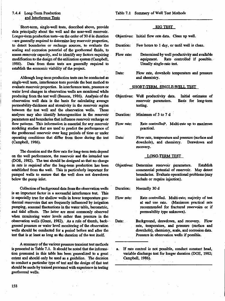
7.4.4 Long-Term Production and Interfkrence Tests
Short-term, single-well tests, described above, provide data principally about the well and the near-well reservoir. Longer-term production tests-on the order of 30 d in duration -are.generally required to determine key reservoir properties, to detect boundaries or recharge sources, to evaluate the scaling and corrosion potential of the geothermal fluids, to assess reservoir capacity, and to identify any factors requiring modification to the design of the utilization system ((hmpbell, 1986). Data from these tests are genefally required to establish the economic viability of the project.
Although long-term production tests can be conducted BS
single-well tests, interference tests provide the best method to evaluate reservoir properties. In interference tests, pressure or water level changes in observation wells are monitod while producing from the test well @enson, 1986). Analysis of the observation well data is the basis for calculating average permeability-thickness and storativity in the reservoir region b e e n the test well and the observation wells. These analyses may also identify heterogeneities in the reservoir parameten and boundaries that influence reservoir recharge or flow patterns. This information is essential for any reservoir modeling studies that are used to predict the performance of the geothermal reservoir over long periods of time or under operating conditions that differ from those during the test (campbell, 1986).
The duration and the flow rate for long-term tests depend on the well performance, the reservoir and the intended use (DOE, 1982). The test should be designed so that no change in rate is q u i d after the long-term production has been established from the well. This is particularly important fix pumped wells to ensure that the well does not drawdown below the pump inlet.
Collection of background data from the observation wells is an important factor in a successful interference test. This is eqecklly true for shallow wells in lower temperature geo- thermal teseNoits that are frequently influenced by irrigation pumping, seasonal fluctuations in the water table, barometric, and tidal effects. The latter are most commonly observed when monitoring water levels rather than pressure in the observation wells (Grant, 1982). As a rule of thumb, back- ground pressure or water level monitoring of the observation wells should be conducted for a period before and after the test that is @ least as long as the duration of the test itself.
A summary of the various pressute transient test methods is presented in Table 7.1. It should be noted that the infonna- tion presented in this table has been generalized to a great extent and should only be used as a guideline. The decision to conduct a particular type of test and the design of that test should be made by trained personnel with experience in testing geothermal wells.
Table 7.1 Summary of Well Test Methods
RIG TEST
Objectives: Initial flow rate data. Clean up well.
Duration:
Flow r a k
Few hours to 1 day, or until well is clean.
Determined by well productivity and available equipment. Rate controlled if possible. Usually single-fate test.
Data: Flow rate, downhole temperature and pressure and chemistry.
SHORT-TERM, SINGLE-WELL TEST
Objectives:
Duration:
Flow rate:
Data:
Objectives:
Duration:
Flow rate:
Data:
Well productivity data. Initial estimates of reservoir parameters. Basis for long-term testing.
Minimum of 3 to 7 d
Rate ContToUed.. Multi-rate UP to maximum practical.
Flow rate, temperature and pressure ( d a c e and downhole), and chemistry. Drawdown and recoVery.
LONG-TERM TEST
Determine reservoir parameters. Establish commercial potential of reservoir. May detect boundaries. Evaluate operational problems (may include or require injection).
Normally 30 d
Rate controlled. Multi-rate; majority of test at end use rate. (Maximum practical rate recommended for fractured reservoirs or if permeability type unkaown).
Background, drawdown, and recovery. Flow rate, temperature, and pressure (surface and downhole), chemistry, scale, and corrosion data. Pressure in observation wells if possible.
a. If rate control is not possible, conduct constant head, variable discharge test for longer duration (DOE, 1982; campbell, 1986).
158

7.4.5 Iniection Tests
The purpose of injection tests is the that of pro- duction tests, that is, to determine well performance, to locate injection zones, and to determine reservoir parameters. It should be noted that reservoir properties determined from pro- ducticy tests are not necesskily applicable to the same reser- voir undergoing bijection. This is principally caused by the thermal dependence of such parameters as fluid density, form- ation porosity, and fracture aperture. Detailed and careful injection testing, coupled with analytical techniques considered experimental at this time, can yield information on fracture frequency, thermaldependent rock properties, and break- through to production wells. A number of references have been published in the geothermal literature regarding injection tests and data analysis techniques (for example, see Benson, 1984). Other considerations for injection tests include rate measurement and rate control, fluid treatment or filtering or both, wellhead pressure limitations and the source of water to be injected (Benson, 1986).
It may be feasible (or necessary) to inject during a long- term production test. If this is the case, careful test planning will enable the production test to be conducted concurrently with an injection test. Some fluid storage capacity should be available so that the production and injection wells can be tested individually for a period of time.
Injection tests may also be considered in cases where it is not feasible or cost-effective to initiate production from a well. They are commonly substituted for production tests while the rig is still on the hole to provide some initial indi- cation of permeable zones. As indicated previously, the reser- voir parameters estimated from injection data should be used with caution when evaluating production conditions. For geo- thermal wells in particular, injectivity values rarely coincide with productivity values for the well because of thermal effects.
7.4.6 Recoverv Data
Data collected after a production injection well has been shut-in are as important as the data collected during the test. These data can be used to verify calculations of reservoir parameters using drawdown data. Buildup analyses can also be used to verify estimates of skin effect, which is an addi- tional change in pressure that results from changes in permea- bility very near the wellbore. These tfrom drilling and completi~-redud of the
f drilling mud or insufficient dot or screen area-or parameter such as turbulent flow in small fractures
near the wellbore are examples.
Recovery data are also useful when evaluating a well that has already been in production, especially at variable rates. Pressure drawdown tests assume that the reservoir is initially
in an undisturbed condition &d such a state may not be achievable in a reasonable length of time if the well has been flowing for some period of time.
7.4.7 Test Planning and Other Considerations
The one single factor that can make the difference between a successful and an unsuccessful well test is test planning. Planning is complicated by the fact that it is difficult, before the test, to predict with surety how the well and the reservoir will respond during the test. A progression from short-term testing to longer-term testing provides the best basis for anticipating factors that could influence the conduct of a subsequent test. Test planning should include a review of kgdations regarding the production and disposal of fluids so that necessary permits can be obtained and restrictions in test operations factored into the test design. A test plan &odd include a written procedure for test operation, a test profile (Figure 7.9, the design and operation of test equipment, instrumentation requirements, and should also address safety issues related to the handling of thermal fluids.
I * I A r l r
, o I T 10 15 a6 “ s a y n N n m
WI
Figure 7.5 Sample well test profile.
Another factor that will contribute to the GIICC~SS of a test is an emphasis on quality data. It is not unwmmon to see a vast amount of data collected during a well test, very little of which can be used. The now or never nature of most well tests usually provides one chance to obtain good data (Stiger, 1986).” Therefore, it is important that the data being collected be reviewed frequently during the test. If problems are encountered with the data, a change can be made in test p d u r e or instrumentation before the funding available for the test has been exhausted. Experience has shown that the use of good instrumentation, calibration of instrumentation (and recalibration during long-term tests), making redundant measurements, and performing calculations using diverse methods will improve the quality of the data collected. It is also important that an operational log be maintained during the test in which is recorded routine information regarding the operation of the test (equipment status, flow rates, valve
159
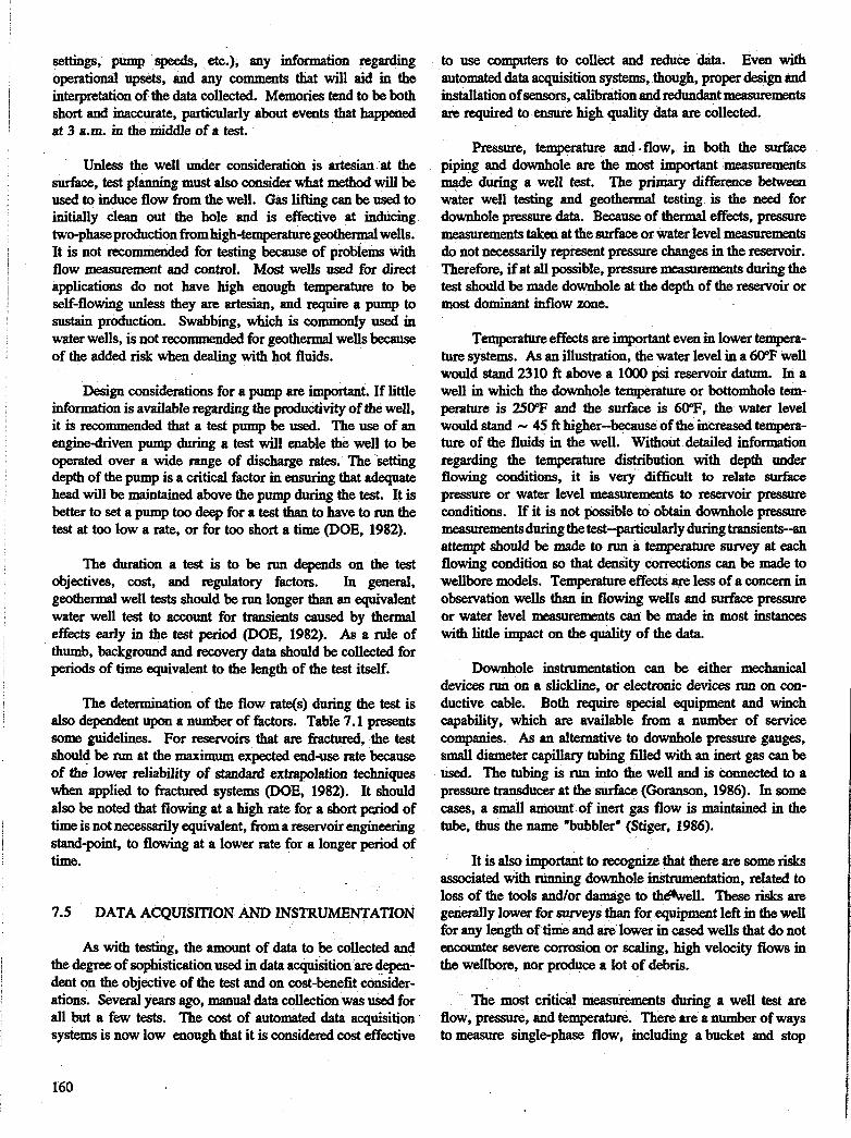
settings, pump speeds, etc‘), any information regarding operational upsets, and any comments that will aid in the interpretation of the data collected. Memories tend to be both short and inaccurate, particularly about events that happened at 3 a.m. in the middle of a test.
Unless the well under consideration is artesian at the surf-, test planning must also consider what method will be used to induce flow from the well. Gas lifting can be used to initially clean out the hole and is effective at inducing two-phase production fromhigh-temperature g e o t h d wells. It is not recommended for testing because of problems with flow measurement and control. Most wells used for direct applications do not have high enough temperature to be self-flowing unless they are artesian, and require a pump to sustain production. Swabbing, which is commonly used in water wells, is not recommended for geothermal wells because of the added risk when dealing with hot fluids.
Design considerations for a pump are important. If little information is available regarding the productivity of the well, it is recommended that a test pump beused. The use of an enginedriven pump during a test will enable the well to be operated over a wide range of discharge rates. T h e ’ h g depth of the pump is a critical factor in ensuring that adequate head will be maintained above the pump during the test. It is better to set a pump too deep for a test than to have to run the test at too low a rate, or for too short a time (DOE, 1982).
The duration a test is to be run depends on the test objectives, cost, and regulatory factors. In general, geothermal well tests should be run longer than an equivalent water well test to 8ccount for transients caused by thermal effects early in the test period (DOE, 1982). As a rule of thumb, background and recovery data should be collected for periods of time equivalent to the length of the test itself.
The determination of the flow rate@) during the test is also dependent upon a number of factors. Table 7.1 presents some guidelines. For reservoirs that are fractured, the test should be run at the maximum expected end-use rate because of the lower reliability of standard extrapolation techniques when applied to hctured systems (DOE, 1982). It should also be noted that flowing at a high rate for a short perid of time is not necessarily equivalent, from a reservoir engineering stand-point, to flowing at a lower rate for a longer period of time.
7.5 DATA ACQUISITION AND INST’RUMENTATION
As with testing, the amount of data to be collected and the degree of sophistication used in data acquisition are depen- dent on the objective of the test and on cost-benefit consider- ations. Several years ago, manual data collection was used for all but a few tests. The cost of automated data acquisition systems is now low enough that it is considered cost effective
to use computers to collect and reduce data. Even with automated data acquisition systems, though, proper design and installation of sensors, calibration and redundant measurements are required to ensure high quality data are collected.
Pressure, temperature and .flow, in both the surface piping and downhole are the most important measurements made during a well test. The primary difference between water well testing and g e o t h d testing is the need for downhole pressure data. Because of thermal effects, pressure measurements taken at the surface or water level mamements do not necessarily represent pressure changes in the reservoir. Therefore, if at all possible, pressure measurements during the test should be made downhole at the depth of the reservoir or most dominant inflow zone.
Temperature effects are important even in lower tempera- ture systems. As an illustration, the water level in a 60°F well would stand 2310 ft above a lo00 psi reservoir datum. In a well in which the downhole temperature or bottomhole tem- perature is 250°F and the muface is WF, the water level would stand - 45 ft higher-because of the increased tempera- ture of the fluids in the well. Without detailed information regarding the temperature distribution with depth under flowing conditions, it is very difficult to relate surface pressure or water level measutements to reservoir pressure conditions. If it is not possible to obtain downhole pressure measurementsduringthetest-particularly duringtransients-an attempt should be made to run a temperahre survey at each flowing condition so that density corrections can be made to wellbore models. Temperature effects are less of a concern in observation wells than in flowing wells and surface pressure or water level measurements can be made in most instances with little impact on the quality of the data.
Downhole instrumentation can be either mechanical devices run on a slickline, or electronic devices run on con- ductive cable. Both require special equipment and winch capability, which are available from a number of service companies. As an alternative to downhole pressure gauges, small diameter capillary tubing filled with an inert gas can be used. The tubing is run into the well and is connected to a pressure transducer at the surface (Goransan, 1986). In some cases, a small amount of inert gas flow is maintained in the tube, thus the name “bubbler” (Stiger, 1986).
It is also important to recognize that thereare somerisks associated with running downhole instrumentation, related to loss of the tools andor damage to &&ell. These risks are generally lower for surveys than for equipment left in the well for any length of time and are lower in cased wells that do not encounter severe corrosion or scaling, high velocity flows in the wellbore, nor prodye a Iot of debris.
The most critical measuremenfs during a well test are flow, pressure, and temperature. There are a number of ways tomeasure single-phase flow, including abucket and stop
160

watch, a flow orifice, downhole or surface turbine meter, or weir box. Two-phase flow is not generally a consideration for direct applications, but if encountered requires more costly and complex equipment to meter flows and to determine downhole enthalpy accurately. Turbine meters or spinners should not be used in wells that have not been properly cleaned out. Orifice meters generally provide the most accurate measurements of flow. Experience has shown, though, that the Ap meter used with an orifice should be checked routinely during a test with a manometer to ensure good readings.
General rules of thumb kgarding instrumentation and data collection are included in a presentation by Benson (1986):
1.
2.
3.
4.
5.
Pressure transducers with the lowest possible range will give the best resolution and minimize thermal sensitivity. Resolution is important, nominally 0.1 psi or 0.5% of the drawdown, whichever is smaller.
Flow rate should be measured to f 5%.
Human error can be minimized by choosing the most automated system possible within practical and ecoLlomic constraints.
Careful synchronization of all clocks is important, particularly for interference tests.
If thermal transients in the wellbore are significant, ~ ~ r v o i r pressure measurements will provide the most unambiguous data.
Measurement frequency should be highest any time con- ditions (flow, press~re, temperature) are changhg. Measure- ments as ikquent-as every 10 s are typical very early in the test and may &crease to once every hour or two later in the test (Table 7.2).
7.6 DATA INTERPRETATION
The most important rule in analyzing data from geother- mal wells is not to let the expected answer lead the analysis (DOE, 1982). There is uncertainty in any reservoir analysis because of the inability to make physical measurements of reservoir parameters in situ. The best analyses involve a correlation of all available idormation and address the impact of uncertainty on the results and recommenWons.
It is not possible, within the context of this guidebook, to provide details about the analytical techniques used to interpret reservoh data from geothermal wells. A summary of approaches is presented and more details can be obtained from those publications included in the references. Reservoir engineering, particularly for geothermal reservoirs, is 'mart
rather than an exact science and is best performed by experi- enced personnel. This is particularly true in cases where financial or legal decisions or both are being made based on the results of the analyses.
Most analytical techniques are based on graphic methods that take advantage of the linear relationship between the pressure drawdown and the log of time (refer to the equation in Section 7.2). It should be emphasized again that these techniques result in estimates of the permeability-thickness product and the storativity. Individual parameters such as permeability and porosity cannot readily be determined, particularly in geothermal reservoirs.
Table 7.2 Suggested Pressure Monitoring Frequency
Background Data: Every 10 min
Drawdown Data: Every 10 s for first 10 minb
Every 30 s for next 20 minb
Every 60 s for next 30 minb
Every 5 min for the next 22 h
Once every hour thereafief
RecoveryData: Use the same frequency as for Drawdown Data
a. Frequencies apply to automatic or manual data acquisition systems. continuous recording can be substituted where appropriate.
b. Early time data collection frequency will require adjust- ment in cases where only manual data mrding can be accomplished. Data should be collected more frequently mytime there is a p h e d or unplanned change in operating conditions. (Benson, 1986)
c.
7.6.1 Semi-be Analvses
In this analytical approach, the pressure change is plotted against the log of time. If the reservoir approximates a homogeneous, isotropic system, a straight line is obtained after the early transient data. Referring to Figure 7.6, the slope of the line can be related to the permeability-thickness product and the drawdown at a given time yields the storativity (Grant, 1982).
161

The Homer method (DOE, 1982; Grant, 1982) is a tech- nique developed'in the petroleum industry to analyze pressure buildup data. In this technique, the difference between the initial pressure and the pressure a k shut-in is related to the log of (t + dt)/dt in which t i s k e amount of time the well was produced and dt is the time since the well was shut-in.
Qo
'i -1
6m I I 0.1 1 10
Figure 7.6 Example semi-log plot of pressure drawdown data (Earlougher, 1977).
Boundaries and other inhomogeneities in a are generally manifested in a deviation from the linear trend in a semi-log analysis. Techniques have been developed to eval- uate some of these factors, at least in a qualitative sense.
7.6.2 TviK Curves
Another graphical technique developed for the petroleum and water well industries can be used to analyze geothermal reservoir performance. In this method, the variables in the general flow equation are converted into dimensionless vari-
Figure 7.7 Example type curve matching (Earloughek 1977).
ables that are independent of flow rate, permeability-thickness or storativity, but do depend on reservoir geometry (Grant, 1982). A series of jme curves are generated in which dimen- sionless pressure is plotted against dimensionless time on a log-log scale for different geometries. Data from a well test are plotted in a similar manner on another sheet of log-log paper. Using a light table, the curves are su- and the best fit or match between the test data and a type curve is determined. The dimensionless pressure and tempemtwe can then be related to permeab~ty-thicknes and to storativity.
Type curves are very similar and curve matching is somewhat subjective; therefore, semi-log analyses are gener- ally preferable for reservoir analyses. Type curves have been developed that account for wellbore storage and skin effects and may be useful when these factors are significant.
7.6.3 Remvoir Simulators
Once basic reservoir paramem have been determined from well test data, it is possible to incorporate this informa- tion into any of a number of numerical simulators that can provide information regarding the behavior of the reservoir over long periods of time or under different operating umdi- tions. Thus, the results can be used as input to decisions regarding further development of the wellfield. Sirnulatots can also be used to understand the sensitivity of reservoir calculations to the uncertainty in the umceptual model of the teservoir.
Because simulation techniques are powerful, it is easy to assume that the simulator accurately represents the reservoir and to forget that the quality of the output directly reflects the quality of the input, including simplifying assumptions neces- sary to peiform the calculations. Analyses of test data provide good indications of reservoir parameters, particularly in the near-well or inter-well regions. It is common, though, to calculate different values for these parameters for different tests and for different wells in the same test. A factor of four difference in values of permeability-thickness determined from an interference test is umsidered a good match, for example (Grant, 1982). In using these parameters in a simulation and in making adjustments to match actual reservoir behavior, care must be taken to ensure that the iinal picture remains meaningful (Grant, 1982).
7.7 CAVEATS
A coherent program of well testing and reservoir d y s e s is the only way to determine the properties of a geothermal memoir and to evaluate the productive capability of that reservoir. very powerful techniques have been developed to support these analyses. However, it is appropriate to summar- izexweral caveats as a reminder that geothermal reservoirs present unique challenges.
162

Temmrature - The significance of the& effects has been discussed several times in this section. Failure to consider thermal effects is perhaps the single most common and significant mistake made, particularly when groundwater techniques are applied to geothermal reservoirs.
Fractures - Most reservoir analyses are based on the assumption that reservoirs are homogeneous, while fractures play a significant role in most geothermal reservoirs. It is common, perhaps because it is easier, to assume a fractured reservoir behaves as a homogeneous one (Grant, 1982). If fractures are extensive, this may be a teasonable approach. For a shallow reservoir in which both the downflow of cold water and the upflow of thermal fluids occurs along fractures, it will be difficult to predict the long-term performance of the reservoir using standard homogeneous techniques.
Interference - It is difficult to analyze a reservoir based on the performance of a given well when other wells are producing from the same reservoir. In liquiddomiuated systems, pressure transients are transmitted rapidly through the reservoir and pressure communication can be observed over distances of miles. It is important, particularly in reservoirs tapped by a number of developers, to consider the influence of other wells in the system-both in reservoir engineering and in production and injection operations.
Comlexity - Geothermal reservoirs are complex and caution should be taken in extrapolating from one rock sample or one well to the reservoir as a whole. In addition, available analytical methods are based on a number of simplifying assuIIIptions. Care should be taken in relating analytical results to the real world.
7.8 DIRECT USE INJECTION WELLS
water. Also, there is greater public environmental awareness and increased government regulation. Undeniably more new projects will be required to have injection wells and some that now dispose of effluent to the surface will ultimately be required to inject. -
While injection may solve some problems, it certainly creates others. It removes the effluent from the surface where one can readily trace its movement and observe its effects and places it underground where its movement and effects are more difficult to predict. Care must be taken that the cooled injected fluid does not unduly cool off production wells (thermal breakthrough) or pollute drinking water aquifers (chemical breakthrough).
Injection usually at least doubles the well costs for a project and may increase the hydrogeology costs because ideally it requires a better understanding of the reservoir. It may require a d d i t i d piping, acquisition of land on which to site an injection well, rights of way for piping, costs for injection pumps, pumping, etc. Considering that there are about 1030 direct use applications, excluding heat pumps, in the U.S. and only 23 currently utilize injection wells, we have little direct experience to go on. There is, however, considerable experience in high-temperature systems, oil fields and industrial injection wells that may be applicable.
There is no accurate compilation of the numbers of direct use production and injection wells drilled to make comparkms of success ratios. In recent years, at least four injection wells have been abandoned because of lack of acceptance of fluids, at least two others accept less than the required amount of fluids and pressure is building up in another. For the known injection wells, the success ratio is not good.
There are at least six reasons often cited for injection. These are: -
7.8.1 Jntroduction
Early geothermal direct use developments utilized natural or improved hot springs. In some cases, the discharge released some undesirable, or in 8 few cases, constituents that are now considered hazardous, to the surface--usUally into streams. Even so, one could reasonably argue that injection would not be required because the springs flowed to the sur- face anyway and only some heat was removed before releasing the same flow at some slightly removed location. As further develop-ment proceeded, wells were drilled nearby to obtain more hot water. Continued development and pumping some- times caused the springs to dry up; but, the pumped water was basically the same and disposal was still to the surhce.
Today in a few places development has increased flow rates to several orders of magnitude more than the original springs flowed and wells are drilled considerable distances from the original springs. Obviously, there is greater potential for chemical and/or thermal pollution of surface
1. To prevent subsidence 2. Conservation of water or heat or both 3. To maintain aquifer level or pressure 4. Heat and effluent disposal 5. Required by law or statute 6. Thermal storage.
Numbers 1 though 4 are actually objectives. Prag- matically number 5 is the real reason in most cases because developers would rather not incur the additional costs.
Thermal storage is a special case where heat pumps on cooling cycles reject heat that is injected and later withdrawn, or waste or cheap heat is stored underground for later use. Aside from noting that one wants an aquifer with small hydraulic gradient, therefore little water movement so the warm water will still be there when n d e d , this specific appli- cation will not be considered further. This type of injection is covered in references such as Driscoll(l986) and others.
163

Subsidence is a consideration when very large volumes of water are removed from sands and other iucompetent for- mations. It is a consideration in the Imperial Valley where power generation projects remove large volumes and subsi- dence would cause extensive damage to irrigation canal systems. Few, if any, direct use projects will require such large amounts of fluids and so far most existing projects are located in areas with more competent rocks not subject to
Subsidence could however, become a problem if or large numbers of small uses, utilize muface
poorly consolidated formations.
In order to properly site an injection well, one should know a great deal about the reservoir. Unfortunately, in most cases precious Iittle is known. Indeed few if any direct use resources are well understood and although there arebimilari- ties between resources, there are also impostant differences.
7.8.2 Reservoir Model
Probably the most significant type of direct use reservoir is the fault controlled hydrothermal convection with lateral leak-age as illustrated in Figure 7.8.
Of the 1324 low temperature resources identified by Reed (1983), 1282 were hydrothermal convection. Althoughnot all of these are lateral leakage type, lateral leakage is the most predominant currently exploited because it provides a shallow reservoir.
This is the type of system believed to exist at Boise, ED; Klamath Falls, OR; the Moana Area of Reno; San Bernardino and Calistoga, CA, and others. Typically these resources are small with aerial extents of less than one to several square miles and in order to be economical for direct use probably less than 2500 ft deep.
Figure 7.8 is a very simplified model used primarily to classify resources as stated in Chapter 3. As noted earlier in this chapter and in Chapter 3, real life re~~urces are not as simple as these models. Indeed such an idealized rese~oir probably does not actualy exist, certainly none are currently known. The model implies a nearly uniform layer of perme- able strata that is the reservoir. Real reservoirs may have subparallel faults and relatively upthrown and downthrown blocks. Faults between blocks may or may not be permeable resulting in an area not connected to the tesource and that will neither produce or accept fluids, or may have substantially different temperature and chemistry because of comection with a different aquifer.
Note in Figure 7.8 that there are no arrows indicating recharge. This is to reinforce the idea that recharge areas are largely unknown an& beyond any control of developrs. Recharge theories have been developed for several high tem- perature and direct use geothermal systems. The theories are based on using tritium and carbon-14 age dating and oxygen- 18 and deuterium contents to estimate elevation and tempera-
ture of precipitation. In all cases, two theories have evolved with no solid evidence to support either. First, recharge is at considerably higher elevations and usually at least a few tens of miles away or secondly, the water could be at least 10,OOO year old when climates were much cooler. The implication is that in either case attempts to recharge the reservoir at its ultimate source or recvcling water is almost certainly impossible.
Figure 7.8 Fault colltroued hydrothermal convection system with lateral leakage.
At least two of the rather highly developed systems, Klamath Falls, OR and Boise, ID are apparently showing signs of over utilization-pumping to surface discharge is exceeding natural recharge and water levels are falling. Because recharge and recycling are at least uneconomical, if not impossible, injection to maintain water levels appears to be the means to extend the useful life of the IW~NOU and perhaps increase utilization. It is unlikely that moderate over pumping causes any irreversible effects; but, lower water levels may permit cool surface water to enter the reservoir. cessation or restriction of pumping would permit water levels to rise.
In the lateral leakage type system, geothermal water moves upward though the fault zone-which may be a brecci- ated zone a few feet to several tens of feet or more wide. Although there may be some flow up the fault for a Consider- able linear distance, in many cases there are preferential conduits where much of the water rises. This may be at places where there are intersections with other faults or at contacts with different lithologic units.
At some depth the flow up the fault reaches a permeable zone where it moves down the hydraulic gradient spreading and cooling. This is the shallow reservoir. The reservoir may exist in interbedded pumice and weathered basalt flows as at Klamath Falls, basaltlagglomerate interf’ as at Susanville, interfingered sands and gravels of ancient water channels as at Calistoga and San Bernardino, or sands and altered clays as at
164

Moana. At least in all the better hown reservoirs, there are considerable variations in the hydraulic characteristics as the permeable zones change in lithology, dip, or thickness.
Figure 7.8 shows the fault along one side of a horst and graben structure as might be found in the Basin and Range Province. In this case, the flow would be down hydraulic gradient away from the uplifted block. In other cases, the fault may be along the axis of a valley. Flows could be away from the fault in opposite directions more or less perpen- dicular to it, or they could follow the somewhat meandering more permeable zones of ancient stream channels. Figure 7.9 shows a schematic diagram of such a system believed to represent the resource of Calistoga. Temperature reversals were noted in Wells 6 and 9, which penetrate below the permeable lateral flow m e . The shallow reservoir exists in alluvial sediments and dacitic sooriaceous ash flows that apparently have been cut by ancient stream flows.
0 9
* f 0 3 1wo z2J E 3000R
0 PI
ow
Figure 7.9 Schematic diagram of the fault-charged hydrothermal system at Calistoga (Youngs, 1980).
It is important to remember that in a shallow lateral leakage reservoir the permeable strata along which leakage occurs is heated by the water flowing though it rather than by conduction or convection h m below. This permeable strata and the water it contains are cooled by conduction to less permeable rocks both above and below. Thus, at distances further from the fault, the resource is progressively cooler and there will be temperature reversals where the permeable strata is completely penetrated. If the resource is not confined by an impermeable cap rock or clays, there may be mixing with cold meteoric water.
Figure 7.10 shows a classic example of temperature r e v e d along with the lithologic log of a well in Klamath Falls, OR. In this case, it appears that the well bottom is very close to another lost circulation zone that probably would pro- duce water at about the same temperature as encountered at 200 ft although it may be slightly cooler. Note that the lower temperature profile rollover appears to be at - 5°F lower tem- perature. In this well, the strata below the lost circulation zone has very low productivity (and injectivity).
The well was originally cased to 360 ft and during the first pump test the well produced 60 gallmin of 190°F water with a drawdown of 170 ft. After perforating at 195 to 240 ft, the well produced 720 gallmin of 212°F water With a drawdown of 7.2 ft.
Similar temperature reversals in impermeable strata have been noted in the shallow resources at Calistoga and San Bernardino and in exploration holes for power production throughout the Basin and Range Province.
Most injection regulations require that effluent be injected either below the producing zone or into an aquifer of similar or poorer quality. If water CoIlSeryBtion or subsidence is a concern, they will require injection into the production m e . When dealing with a situation similar to that above, it can be seen that injection will be into the producing m e where water quality is similar. Above the zone, permeability will be low or water quality better or both. Below the shallow reservoir permeability will be low (else it would also be a part of the reservoir) requiring pressure injection and its related costs, or longer injection intervals (deeper or more wells).
' In many direct use reservoirs, chemical and isotopic geothermometers indicate temperatures higher than those actually encountered in the shallow reservoir. This implies a zone of mixing with cooler water at some depth below the shallow resewoir. That may be the reason for the slightly lower, deeper temperature rollover appearing in the Klamath Falls well-or it may be that it is another permeable, but cooler leakage zone with still cooler zones below. If a mixing m e exists, injection some distance from the fault could actually increase temperature at the shallow m e because injected, but still fairly hot, water would displace cooler incoming water. Although the incoming water would be of better quality, it is destined to become part of the shallow reservoir. Actually proving the direction of cool flow is . toward the fault would be a difficult and expensive task. So far as is known, the hypothesized mixing zones have never been encountered in any direct use well. It is probably not a good injection target because its depth and optimal temperature for injection location are unknown.
165

I
900
I
-
m I I h I *
.. TEMPERATURE ( O F
FT. 160 170 180 190 200
LOST CIRCULATION
CW-1
no CW-1 TEMPERATURE ( O F
0 FT. 160 170 180 190 200 0 I
. 100 -
200 -
300 -
50
1 0 0
150
200
i
4 t ‘4 ii
1
No Sample.
Buff-brown clay. Light qrey clay Brown ash vi th ;hi te tuff fragments. Grey vitreous claystone with white tuff _ ~ _ _ fragments.
Uassive grey claystone. Black basic volcanic fragments, vith grey tuffaceous sediment and grey claystone vith diatoms.
Grey to brovn calcitic silty claystone with basic volcanic fragments.
Dark grey basic volcanic fragments and grey silty claystone vith diatoms.
Grey calcitic silty claystone, with basic volcanic fragments.
Grey basic volcanic fragmants with clay- stone and rhyolite tuff fragments.
Salt and pepper basic volcanic fragments.
Black basic volcanic fragments.
Grey volcanic silty sediment.
9 LI Q JJ 0 E - Volcanic fragments and ash. m cc 0. W Q Black aphanitic basic volcanic fragments.
Grey bolcanic ash-silty claystone.
Unconsolidated volcanic sediment with black basic volcanic fragment and vitreous tuff.
Red scoriaceous.tuff.
Grey basic volcanic fragments.
Grey basic volcanic fragments.
Grey vitreous tuffaceous fragments vith volcanic ash, silt, and basic volcanic fragmebts.
Light to dark grey volcanic fragments with- red tuffaceous fragments.
Figure 7.10 Lithologic log and temperature profile for well CW-1 (Sammel, 1984).
166 ~
!

Preferential permeability will cause greater drawdowns and support of water levels in the direction of greater permea- bility. It will also allow more rapid thermal breakthrough in those directions. Fractures or other relatively small but highly permeable a m s often found in geothermal ~esoun'~s permit high fluid velocities along preferential flow paths. These preferential flow paths can permit a portion of the injected water to rapidly migrate to production wells and are some- times called fast Daths. Numerical simulation models are beginning to be developed to analyze such breakthrough.
7.8.4 Thermal Breakthrough
Thermal breakthrough between injection and production wells is a serious concezn in electrical power generation projects thoughout the world. This concern has filtered down to the direct use industry. Tracer studies have shown average tracer migration velocities of 4 in. to 400 ft/h over distances of up to - 0.25 mi in power production reservoirs (Pruess, 1983) and about 50W in a direct use doublet in Klamath Falls, OR (Gudmundsson, 1984). This is several orders of magnhde faster than tracer velocities in porous media-type reservoirs and is a good indication of rapid flow along frac- tures or fast mths.
7.8.3 Numerical Modeling
Injection is not likely to cause problems with water levels because it can only tend to sustain or increase levels. Even if water levels rise above ground level, the production wells can be sealed and more eumomical surface pumps possibly substituted for doynwell pumps. With data from pump andlor injection tests and expected pumping rates, computer programs can be used to predict water level effects.
There are several important considerations in using computer programs. First, many programs are for steady-stak analysis. Most direct use developments have varying flow requirements. Secondly, all production and injection in the reservoir should considered because each well has some effect on others. Some programs consider only pairs of wells or can analyze effects of or on only small numbers of wells. Also, because the reservoir is usually fault contn>lled, it will usually be anisotropic having greater permeability parallel to the strike of the faulting. Some programs consider only isotropic reservoirs. It is important to get pump test data from wells in all directions and be able to utilize that data in the program.
While rapid tracer, therefore inj&d fluid, velocities are a concern they may not be of such great concern as might first be imagined, especially in direct use applications. First, rapid tracer returns do not necessarily mean rapid thermal break- through because the injected fluid is reheated as it travels though the fractures. As with any other heat transfer system, residence time is only one of several Conttouing factors. Other factors are roughness of rmrfaces, Reynolds numbers and ingeothermal reservoirs, possiblemixing with new hotter
water, etc. Several numerical models and analytical methods have been proposed to utilize tracer return data; but, to date none have been very su-ful at predicting times and amounts of enthalpy changes at production wells. One reason is that it is difficult to exactly define the reservoir envimnment in situ. Another reason might be that workable models have not been available long enough to see the effects they predict.
Fast paths are a phenomenon of fractured reservoitS where only a portion of the flow is in fractures with the rest in the porous medium. The relative fractions in the fractures and porous rocks determines the overall t h e d degradation. Thermal breakthrough can also occur in porus reservoirs if injection and production wells are too closely spaced.
The problem is more serious in power production where the enthalpy change between production and injection is greater. Temperature change between production and injection in power production may be several hundred degrees Fahenheit, whereas in direct use 5ooF is about the maximum in current injection systems and most are much less. Even with similar percentages of flow in fractures and porous media thermal degradation in direct use systems will be less.
The orientation of the fracture system or major permeability is important in thermal breakthrough. If the major permeability is horizontal and the system is homogeneous, flow will be generally radial in all directions away from an injection well. The volume swept by the injected fluid will increase approximately with the square of the radius and velocity will decrease at the same rate. However, if the production and injection wells are in a vertically fractured zone the swept volume and fluid travel time is directly proportional to the distance W e e n them. Thus, it is important to site the injection well down hydraulic or thermal gradlent away from the vertically fractured upwelling zone and into the horizontal permeability zone.
Thermal breakthrough has been noted in several direct use injection systems but they have not been serious-ody a few degrees Fahenheit. Since most direct use systems, especially for space heating, are somewhat conservatively designed they can tolerate small changes. If temperatures are marginal to begin with, a small amount of thermal breakthrough could have serious consequences. Breakthroughs have been noted between injectiodproduction pairs and between one system's injection well and a neighboring system's production well. A good example is the Klamath Union High School (KUHS) doublet system.
In 1983, a tracer test was run at KUHS. "his doublet system was started in the early 1960s. The production well is 257 ft deep, perforated for 25 ft near the bottom and pumps 320 gpm of 1659 water at a constant rate from September thiough early June. Except for - 15 gpm, which is diverted to heat a residence and is surface discharged, the flow (305 gpm) is pumped through heat exchangers at the school and
167

. into the 240 ft deep injection well located 250 ft from the production well. Injection temperature varies depending on the heat load, but is typically - 152bF. There are several other pumped wells 450 ft away in all directions having a total pumping rate about half that of the school. These wells were also monitored for tracers.
Initial tracer breakthrough between the KUHS wells was noted in - 2 h with the peak at - 5 h. Average tracer velocity was thus -50 ft/h. Tracer recovery, estimated from the area under the breakthrough curve (Figure 7.11), after 5, 9, and 110 h was 7 , l l and 54 5% respectively of total tracer injected.
line from injectim lh)
Figure 7.11 Breakthrough curve in production well, KUHS doublet test (Gudmunhn, 1984).
Small amounts of tracer were recovered from some of the other wells, most from a well whose direction is parallel to the major faults and probably is along a minor fault m e . Much of the tracer recovered after about 10 h was because of recir- culating tracer in the system.
According to theory (at the time the test was run) this system should have cooled down years ago to the point where it was no longer useful for space heating-yet is still in opera- tion. When the system is turned on in the fall, production well temperature falls 5 to 7°F within 7 to 10 days then remains constant though the heating season. The next fall, the production well is back to its original temperature (Gudmunhn, 1984).
7.8.5 Iniection Guidelines
Because the shallow producing reservoir is also the likely target for injection, questions arise of where to inject and what effects are likely. Unfortunately, the current state-of-the-art in injection technology and lack of historical practice provides
relatively few definitive answers. Nevertheless, some general guidelines can be ‘given.
Developers will often attempt to site injection wells on the basis of cost or pressure support for their production well. This may lead to thermal breakthrough to their, or neighbor- ing, wells. Injection wells should be located based on reser- voir characteristics, which usually requires the services of a qualified geologist or hydrogeologist.
An important consideration is the state of development of the resource. Injection into a highly developed reservoir such as Moana or Klamath Falls where privately owned wells may be separated by 100 ft or less is vastly different than injecting in an area like San Bemardino where there are few wells that are primarily under one ownership. Effects on nearby wells such as adversely affecting water levels and temperatures are important considerations in all areas, but especailly so in highly developed areas.
Depding on the state, a well owner whose well is adversly affected by a neighbor’s well may or may not have certain legal recourse. In some states, a well owner may have rights to heat from the we!, usually 8ssoci8ted with mineral rights. In other states, the owner may have rights only to the permitted amount of water and not necessarily the heat it cantains.
Although there may or may not be legal implications of cooling a neighboring well by injecting cool fluids, it is certainly not coI1L1ucive to the proper management of a highly developed reservoir.
1.
2.
3.
4.
In general, injection down hydraulic gradient from the production well will tend to reduce t h e d breakthrough impacts on the production wells.
In highly developed areas, it may be desireable or neces- sary to design the system so that the injection temperature matches the reservoir temperature at the point of injection.
Injection and production wells along a fault or fracture zone are likely to experience fast mth breakthro uahs. The severity of the impact will depend on the volume of pumping versus relative fracture and porosity perme- abilities.
If injection up hydraulic gradient is necessary it would be desireable to inject into a different strata. If this is not possible because of reservoir conditions, cost, or environ-mental constraints allowance for fluid temperature degradation may be possible through increased equipment capacity or additional plates in heat exchangers or both to achieve closer approach lemperatures.
168

Table 7.3 Injection Wells - Status
OREGON
Klamath Union High School Klamath Falls District Heating System Mazama'High School, Klamath Falls Mills School, Klamath Falls
Klamath Falls YMCA Delarose residential (8 homes), Klamath Falls Klamath County Jail Oregon Institute of Technology Oregon Trail Mushrooms, Vale
NEVADA
Sierra Geothermal, Reno Dr. Tang Medical Offices, Reno (125 psi) Virginia Lakes Townhouses, Reno Warren Estates, Reno
Round Mountain Gold Corp.- Smoky Valley (2) Salem Plaza, Reno, completed Dec., 1988 will not accept fluids Pepper Mill Casino & Hotel, Reno
IDAHO
Capital Mall District Heat, Boise V.A. Hospital, Boise, operating but will not accept all the fluids.
CALIFORNIA
Lake County Ag Park, Kelsyville, greenhouses not yet completed (Jan., 1989).
operating operating operating operating
operating
operating operating
Operating (High press.)
1 operating
operating Not operating
o p e d g Partial acceptance
Susanklle District Heat System The "Richardson" Well, will accept only about 113 the volume required.
New injection well (August 1988) failed. Not operating
NEW MEXICO
New Mexico State University (2) Masson Greenhouses, Radium Springs (2)
1 operating 2 operating
TEXAS
Navarro College, Corsicana, would never accept enough fluids. Not Operating
UTAH
Utah Roses, Sandy, always required considerable injection pressure, currently have NPDS Surface Discharge Permit.
Not Operating
169
7.8.6 Iniection Well Status
As noted in Subsection 7.8.1, there is precious little experience with direct use injection wells. Table 7.3 lists all the currently known wells as of early 1990. Of the 23 injection wells currently operating, three either will not accept the required amount of fluids or require higher than desireable injection pressures. .Eight operational and one planned well are in Klamath Falls, OR, and four operational and two planned are in Reno, NV. This means that the 17 wells are in only seven resource areas, illustrating that experience is more geographically limited than the total number would indicate.
REFERENCES
Bean, H. S., editor, "Fluid Meters, Their Theory and Application", ASME, New York, 1971.
Benson, S. M., "Interference Testing and Injection Testing", Testing of Geothermal Wells, Geothermal Resources Council Short Course, Palm Springs, CA, 1986.
Benson, S. M., "Analysis of Injection Tests in Liquid- Dominated Geothermal Reservoirs", LBL-17953, Lawrence Berkeley Laboratory, Berkeley, CA, 1984.
Campbell, D. A., "Overview of Well Testing", test in^ of Geothennal Wells, Geothermal Resources Council Short Course, Palm Springs, CA, 1986.,
Craft, B. C. and M. F. Hawkins, Amlied Petroleum Reservoir Engineering, F'rentice-Hall, Englewood Cliffs, NJ, 1959.
C k e Company, "Flow of Fluids Througb Valves, Fittings and Pipe", Technical Paper 410, New York, 1981.
DOE, "Low to Moderate Temperature Hydrothermal Reservoir Engineering Handbook", Volume 1, IDO-10099, U.S. Department of Energy, Idaho Falls, ID, 1982.
Driscoll, F. G., "Groundwater and Wells", Johnson Division, St. Paul, MN. 1986.
Earlougher, R. C., Jr., "Advances in Well Test Analysis", Societv of Petroleum Engineers, Monograph 5, 1977.
Goranson, C., "Downhole High Temperature Instrumentation, Availability, Accuracy, Reliability and Calibration", Testing of Geothermal Wells, Geothermal Resources Council Short Course, Palm Springs, CA, 1986.
Grant, M. A.; Donaldson, I. G., and P. F. Bixley, Geother- mal Reservoir Engineering, Academic Press, New York, 1982.
Gringarten, A. C.; Ramey, H. J., and R. Raghovan, "Applied Pressure Analysis for Fractured Wells", Journal of Petroleum Technolom. 27, pp. 887-892, 1975.
Gudmundsson, J. S., Internell Tracer Testing in Klamath m, "Analysis and Intexpetation of Data Obtained in Test of the Geothermal Aquifer at Klamath Falls, OR. in Sammel, E. A., Editor, U.S. Geological Survey, Water Resources Investigations Report 844216, 1984.
Hanson, J. M., "Reservoir Response to Tidal and Barometric Effects", Geothermal Resources Council 4, pp. 337-340, 1980.
Mangold, D. C., Tsaug, C. F., Lippmann, M. J., and P. A. Witherspoon, "A Study of Thermal Effects in Well Test Analysis", 54th Annual Fall Technical Conference and Exhibitions, Las Vegas, NV, 1979.
Matthews, C. S. and D. G. Russell, "Pressure Buildup and Flow Tests in Wells", Monograph 1, Societv of Petroleum Engiaeers, Dallas, TX, 1967.
Pruss, K., and G. S. Bodvarsson, "Thermal Effects of Rein- jection in Geothermal Reservoirs with Major Vertical Fractures", Society of Petroleum Engineers 58th Annual Technical donference, San Francisco, CA, 1983.
Reed, M. J., Editor, "Assessment of Low-Temperature Geothermal Resources of the United States 1982", U.S. Geological Survey Circular 892, 1983.
Stiger, R. R., "Long-Term Reservoir Testing, The purpoSe and The Method", Testing of Geothermal Wells, Geothermal Resources Council Short Course, Palm Springs, CA, 1986.
Warren, J. E. and P. J. Root, "The Behavior of Naturally Fractured Reservoirs", Societv of Petroleum Engineers Journal, pp. 245-255, 1963.
Van Golf-Racht, T. D., Fundamentals of Fractured Reservoir Eneineerinq, Elsevier, NY, 1982.
Youngs, L.; Bacon, C.; Chapman, R.; Higgins, C.; Majmundar, H., and Taylor, G., "Resource Assessment of Low and Moderate Temperature Geothermal Waters in Calistoga, N a p County, California", OFR 81-13 SAC, Califomia Division of Mines and Geology, 1980.
170

CHAPTER 8 MATERIALS SELECTION
GUIDELINES By Peter F. Ellis II Radian Corporation Austin, Texas 78720
8.1 INTRODUCTION
The economic direct utilization of geothermal resources with temperatures <220"F, requires creation of systems with long plant life, and minimum operation and maintenance costs. Development of such systems requires careful corrosion engineering if the most cost effective material selections and design choices are to be made. This chapter presents guidelines for materials selection for low-temperature geothermal systems (120 to 220"F), as well as guidance in materials design of heat pump systems for very-low- temperature geothermal resources (< 120°F).
This chapter is divided into four sections:
1. .Key Corrosive Species 2. Types of Geothermal Corrosion 3. Geothermal Corrosivity Classification System 4. Corrosion Engineering for Low-Temperature Direct
Utilization Systems.
This chapter is based on Radian's geothermal materials database, containing materials performance data from more than 20 low-temperature geothermal sites worldwide. Also included are results of numerous component failure investigations conducted by Radian's Materials Sciences Laboratory (MSL). Much of the data are. &ummamd * inthe DOE report:
Materials Selection Guidelines for Geothermal Enern Utilization Systems, (Ellis, 1981) and the Addendum, (Ellis, 1983).
Unless otherwise indicated, the information herein is taken from this document.
8.2 KEY CORROSIVE SPECIES
Geothermal fluids commonly contain seven key chemical species that produce a significant corrosive effect. The key species are:
1. Oxygen (generally from aeration) 2. Hydrogenion@H) 3. Chloride ion 4. Sulfidespecies 5. Carbon dioxide species 6. Ammdaspecies 7. Sulfateion.
The principal effects of these species are rmmmatlzed ' i n Table 8.1. Except as noted, the described effects are for carbon steel.
Two of these species are not reliably detected by standard water chemistry tests and deserve special note. Dissolved oxygen does not naturally occur in low-temperature (120 to 220°F) geothermal fluids that contain traces of hydrogen sulfide. However, because of slow reaction kinetics, oxygen from air in-leakage may persist for some minutes. l'reventing oxygen contamination, once the geothermal fluid is produced, is extremely difficult, especially if pumps other than downhole submersible or lineshaft turbine pumps are used to move the geothermal fluid. Even though the fluid systems may be maintained at positive pressure, air in-leakage at the pump seals is likely, particularly in light of the level of maintenance in many installations.
sulfide is ubiquitous at low parts per million per billion @pb) levels in geothermal fluids
above 120°F. This corrosive species also occurs naturally in many cooler groundwaters. For alloys such as cupronickels that are strongly affected by it, hydrogen sulfide concent- rations in the low ppb range may have a serious detrimental effect, especially if oxygen is also present. At these levels, the characteristic rotten egg odor of hydrogen sulfide may be absent, and detection requires use of field test methods. Hydrogen sulfide levels down to 50 ppb can be detected using a simpIe field kit such as one prepared by CHEMetrics. Even the absence of hydrogen sulfide at this low level may not preclude damage by this species. Field spectrophotometry, which req& a spectrometer and different kit (K9503), has a detection limit of < 10 ppb.
171

Table 8.1 Principal Effects of the Key Corrosive Species
Hydrogen ion (pH)
Carbon dioxide p i e s (dissolved carbon dioxide, bicaronate ion, c a r b o ~ k ion)
Hydrogen sulfide species (hydrogen sulfide, bisulfide ion, sulfide ion)
Ammonia species (ammonia, ammonium ion)
Chloride ion
Sulfate ion
a. ppb - parts per billion.
Principal Effects
Extremely corrosive to carbon and low alloy steels; 30 ppb’ shown to cause four-fold increase in carbon steel corrosion rate.
Concentrations above 50 ppb cause serious pitting.
In conjunction with chloride and high temperature, < 100 ppb dissolved oxygen can cause chloride-stress corrosion cracking (chloride-SCC) of some austenitic stainless steels.
Primary &odic reaction of steel corrosion in air free brine is hydrogen ion reduction. Corrosion rate decreases sharply above pH 8.
Low pH (S5) promotes sulfide stress cracking (SSC) of high strength low alloy (HSLA) steels and some other alloys coupled to steel.
Low pH may cause breakdown of passivity of stainless steels.
Acid attack on cements.
Dissolved carbon dioxide lowers pH, increaSing carbon and HSLA steel corrosion.
Dissolved carbon dioxide provides alternative proton reduction pathway, further exacerbating carbon and HSLA steel corrosion.
May exacerbate SSC.
Strong link between total alkalinity and corrosion of steel in low-temperature geothennal wells.
Potent cathodic poison, promoting SSC of HSLA steels and some other alloys coupled to steel.
Highly corrosive to alloys containing both cupronickels and monels.
Causes SCC of some copper-based alloys.
Strong promoter of localized corrosion of carbon, HSLA, and stainless steels as well as of other alloys.
Chloride dependent threshold temperature of pitting and SCC. Different for each alloy.
Little if any effect on SSC.
Steel passivates at high temperature in pH 5,6070 ppm chloride solution with carbon dioxide. 133,500 ppm chloride destroys passivity above 300°F.
Primary effect is corrosion of cements.
172

Two other key species should also be measured in the field pH and carbon dioxide. This is necessary because most geothermal fluids will rapidly off-gas carbon dioxide, causing a rise in pH. DOE has published a manual for complete chemical analysis of geothermal well waters, giving recommended procedrves (Kindle and Woodruff, 1981).
8.3 TYPES OF GEOTHERMAL CORROSION
A number of different corrosive phenomena have been observed in geothermal systems. In low- and very-low- temperature g e o t h e d systems, the following are most likely to be significant.
8.3.1 Uniform Corrosion
Uniform corrosion is the even wastage of metal from the component. This is the form of corrosion that is expressed as a "corrosion rate,' often mil per y& (mpy), where 1 mil = 0.001 inch. Uniform corrosion is a useful measure of corrosion resistance o& if the other types of corrosion described below do not occur.
8.3.2 Pitting
Pitting is localized corrosion forming cavities or holes in the metal surface. The rate of pit penetration is highly unpredictable, and it is not practical to design around (or allow for) pitting. Pitting is particularly serious in heat exchangers because of the thin walls and large area of the heat exchangers, and because a single pinhole perforation may constitute a failure.
8.3.3 Crevice Corrosion
Crevice corrosion is similar to pitting except that it occurs in geometrically contined spaces such as the crevices where tube and tubesheet join, where the plate ridges of flat plate heat exchangers overlap, or under scale deposits. Like pitting, the rate of crevice corrosion penetration is unpredictable, and it is not possible to design mound it.
8.3.4 Stress Corrosion Cracking fSCQ
Stress COlTOSioll cracking (SCC) is the cracking of an alloy as a result of the interaction of stress, applied or residual from forming and fabrication, and a specific environmental factor. For example, some stainless steels are cracked by chlorides under certain conditions (chloride-SSC) and some copper alloys are attacked by traces of ammonia (ammonia-SCC). A special case of SCC can result when high-strength low-alloy (HSLA) steels are exposed under stress to waters containing hydrogen sulfide. This particular form of SCC is commonly called sulfide stress cracking (SSC).
8.3.5 E
Erosionarrosion is the highly accelerated c o d o n of an alloy exposed to a corrosive solution flowing faster than a critical velocity peculiar to that alloy. characteristcally, corrosion is mild at lower velocities.
8.3.6 Intereranutar Corrosion
Intergranular corrosion occurs when the grain boundaries of the metallic microstructure corrode prefkrentially, causing the grains to fall out. This process can occur in a d t i c stainless steels in low-temperature geothermal envhmments, but only if the stainless steel is defstive in heat treatment or is improperly welded.
8.3.7 Galvanic Corrosion
Galvanic corrosion is the uccelerated w m i o n of one metal resulting from its electrical contact with a different metal. The most common example is steel coupled to copper, resulting in accelerated corrosion of the steel. Pitting can also OCCUT in well casings where nearby power lines or other electrical systems can cause galvanic cell action.
8.3.8 Dealloving
Dealloying is the selective leaching of one Constituent element of an alloy, without change in the gross shape of the component. Three forms have been observed in low- temperature g e o t h e d components: dezincification of yellow brass, graphitization of cast iron (the iron is removed leaving the carbon matrix), and deplumbification (removal of lead) from lead-tin solder.
8.4 GEOTHERMAL, CORROSNITY CLASSIFICATION SYSTEM
While developing the Materials Selection Guidelines for Geothermal Enem Utilization Svstems, Radian developed a Geothermal Comivity Classification System that divided the currently developed geothermal resources into six classes based on key corrosive species, wellhead temperahm, and similarities of corrosion behavior (Ellis, 1981). Class V is for low-temperature geothermal resources. This classification system does not eliminate the need for site specific evaluation of corrosion.problems, but does allow some generalization about materials performance and design requirements.
Subsequent information led to the division of Class V, the class containing low-temperature geothermal resources, into two subclasses, Class Va and Class Vb. This division is based on statistical evaluation of carbon steel corrosion data from 29 separate tests in different tesoutces (Ellis, 1982): Tables 8.2 and 8.3 summafize the characteristics of these two wrrosivity system subclasses.

Table 8.2 Geothermal Resource Corrosivity Class Va
Defining Parameters
Resource type Total key species (TKS)’ a o r i d e fraction in TKS Total alkalinity pH (unflashed fluid) pH (flashed fluid)
Plant inlet temperature Resource temperature
Volume gas in stream
Sites Reviewed
Madison Aquifer, SD (three sites) Pagosa Springs, CO Marlin, TX
Liquiddominated Less than 5,000 ppm 3 to 72% 207 to 1329 ppm CaC03 6.7 to 7.6 Not applicable Not applicable 120 to 205OF same
Corrosion of Carbon Steel
In non-aerated produced fluid the median uniform (weight-loss) corrosion rate is 12.5 mpy, with a probable range (95 % confidence limits) of 4.9 to 20.2 mpy.
One of nine tests showed no pitting, 0th- showed severe pitting as high as 83 mpy.
Aeration may cause a 4- to 15-fold hcrease in weight-loss corrosbn as pitting.
General Performance of Other Alloys
In non-aerated fluid, uniform corrosion of copper m heat transfer service is 1 to 10 mpy with severe crevice corrosion under corrosion product scale. Brasses and cupronickel are less suitable than copper for heat transfer.
Type 316 stainless steel is resistant to uniform corrosion, pitting and crevice corrosion, and stress corrosion cracking in many applications.
a. Total chloride + sulfate + carbon dioxide species + sulfate species + ammonia species in produced fluid.
8.5 CORROSION ENGINEERING FOR LOW- TEMPERATURE DIRECT UTILIZATION SYSTEMS
The design of the geothermal system is as critical in controlling corrosion as the selection of suitable materials. Furthermore, the designhaterial selection process is interactive in that certain design decisions force the use of certain materials, while selection of materials may dictate design. In all cases, the objective should be the me: to produce an adequately reliable system with the lowest possible lifetime cost.
8.5.1 Performance of Materials
carbon Steel
For many years, the Rymar Index has been used to estimate the corrosivity and scaling tendencies of potable water supplies. However, the statistical study discussed in the G e o t h e d Corrosivity Classification System discussed above found no significant correlation (at the 95 96 cmfidmce level) between carbon steel corrosion and the Ryznar Index. Therefore, the Ryznar Index, and other indices based on calcium carbonate saturation, shouldnotbe usedto predict
i74

corrosion in geothermal systems. The Ryplar Index may, however, be predictive of calcium carbonate scaling tendencies.
Table 8.2 rmmmarizeS the expected performance of carbon steel in Class Va geothermal fluids. Under these conditions, corrosion rates of <5 to 20 mpy can be expected, often with severe pitting.
Table 8.3 rmmmarizes the expected performance of carbon steel in Class Vb geothermal fluids. Carbon steel piping has given good service in a number of systems, provided the system design rigorously excludes oxygen. However, introduction of 30 ppb oxygen under turbulent flow conditions causes a four-fold increase in uniform corrosion.
. Table 8.3 Geothermal Resources Corrosivity Class Vb
Saturation with air often increases the cortosioIl rate at least 15-fold. Oxygen contamination at the 50 ppb level or higher often causes severe pitting. Chronic oxygen contamination causes rapid failure.
These fluids are characteristic of those used by Icehdic district heating systems. In those systems, steel piping has been generally successful, but carbon steel shell and tube heat exchangers have been satisfactory only in systems.where 10 ppm excess sodium sulfite is added continuously as an oxygen scavenger.
In the case of buried steel pipe, it is critical that the external surfaces be protected from contact with groundwater. Groundwater is aerated, and has caused pipe failures by
Defining Parameters
Resource type Total key species (TKS)’ Chloride fraction in TKS Total alkarinity pH (unflashed fluid) pH (flashed fluid) Volume gas in stream Plant inlet teem Resourcetemperature
Sites Reviewed in the Guidelines
Liquiddominated Less than 5,000 ppm 3 to 72% Less than 210 ppm CaCO, 7.8 to 9.85 Not applicable Not applicable 120 to 205°F Same
Iceland (15 sites) U.S.A. - Klamath Falls, OR (5 wells)
Corrosion of Carbon Steel
In non-aerated produced fluid, the median uniform (weight-loss) corrosion rate is 0.12 mpy with an upper limit (95 % umfidence) of 1.65 mpy.
Pitting: 28% no detectable pitting. Additional 40% pitted at <5 mpy. Maximum observed pitting rate was 20 mpy.
Aeration may cause a 4- to 15-fold iucrease in weight-loss corrosion with probable heavy pitting.
General Performance of Other Alloys
In non-aerated fluid, uniform corrosion of copper in heat transfer service is 1 to 10 mpy with severe crevice wrrosion under corrosion product scale. Brasses and cupronickels are less suitable than copper for heat transfer.
Type 316 stainless steel is resistant to uniform corrosion, pitting and crevice corrosion, and stress corrosion cracking in many applications.
a. Total chloride + sulfite + &n dioxide species + sulfide species + ammonia species in produced fluid.
175

external corrosion in at least two U.S. systems. Required external protection can be obtained by use of coatings or pipe- wrap, provided the selected material will resist the system operating temperatures and thermal stresses.
At temperatures above 135"F, galvanizing (zinc coating) will not reliably protect steel from either geothermal fluid or groundwater.
Hydrogen sulfide inhibits the reaction of atomic hydrogen (to form hydrogen gas) on the steel surface. Atomic hydrogen is a product of the proton reduction step of the corrosion processes. The atomic hydrogen enters the steel lattice, and in the case of carbon (mild) steels, accumulates as molecular hydrogen in microvoids, causing hydrogen blistering. Hydrbgen blistering can be prevented by use of void free, or "killed" steels.
Low alloy steels (steels containing not more than 4% alloying elements) have corrosion resistance similar, in most respects, to carbon steels. As in the case of carbon steels, sulfide promotes entry of atomic hydrogen into the metal lattice. If the steel exceeds Hardness Rockwell C22, &fide stress cracking may occur.
Comer and Comer Allovs
Copper fan coil units and copper-tubed heat exchangers have consistently poor performance because of the presence of traces of sulfide species found in geothermal fluids in the U.S.
Copper tubing rapidly becomes fouled with cuprous sulfide films more than 0.04 in. thick. Serious crevice corrosion occurs at cracks in the film; and uniform corrosion rates of 2 to 6 mpy appear typical, based on failure analyses. These corrosion rates were measured by coupons in low velocity (1 ft/s) fluid at the same or similar geothermal reso-.
Experience in Iceland also indicates that for heat exchange service, copper is unsatisfactory and most brasses (Cu-Zn) and bronzes (Cu-Sn) are still less suitable. Cupronickels can be expected to perform more poorly than copper in low- temperature geothermal service because of trace sulfide.
Much less information is available about copper and copper alloys in non-heat-transfer service. Copper pipe shows corrosion behavior similar to copper heat exchiyge tubes under umditions of moderate turbulence (Reynolds numbers of 40,000 to 70,000). The internals of the few yellow brass valves analyzed by Radian showed no significant corrosion. However, silicon bronze CA 875 (12-16-Cr, 3-5-Si, <0.05-Pb, cO.05-P), an alloy normally resistant to dealloying, failed by this mode in less than 3 y when used as apumpimpeller. Leaded redbrass (CA836 or 838) and
leaded red bronze (SAE 67) appear viable as pump intemals. Aluminum b r o m have shown potential for corrosion in heavy-walled components, based on tests at a few Class Va sites.
Another problem area associated with copper equipment is solder. Lead-tin solder (50-Pb, 50-Sn) was observed to fail by dealloying after a few years exposure. Silver solder (1Ag-7P-Cu) was completely removed from joints in less than 2 y. Radian does not endorse the circulation of geothermal fluids through copper components. However, if the designer elects to accept this risk, then solders containing at least 70% tin should be used.
stainless Steels
Unlike copper and cupronickels, stainless steels are not affected by traces of hydrogen sulfide. Their most likely application will be as heat exchange surfaces. For ecollomic reasons, most heat exchangers will probably be of the plate- and-frame type. Again, for economic reasons, most plate-and- frame heat exchangers will be fabricated with Type 304 or Type 316 austenitic stainless steel, because these are the two standard alloys. In addition, some pump and valve trim may be fabricated from these or other stainless steels.
These alloys are subject to pitting and crevice corrosion above a threshold chloride level that depends upon the chrom- ium and molybdenum content of the alloy, and upon the temp- erature of the geothermal fluid. Above this temperature, the passivation film, which gives the stainless steel its corrosion resistance, is ~pturea in local areas or in crevices or both. These ~ptu ted areas then corrode in the form of pitting and crevice corrosion. Figure 8.1 shows the relationship between temperature, chloride, and occurrence of localized corrosion of Type 304 and Type 316. For example, this figure indicates that localized corrosion of Type 304 may occur in 80°F geothermal fluid if the chloride level exceeds - 210 ppm, while Type 316 is resistant at that temperature until the chloride level reaches - 510 ppm. Type 316, as shown in Figure 8.1, is always more resistant to chlorides than is Type 304, because of its 2 to 3% molybdenum (Mo) content. The fact that localized corrosion can occur does not predict the rate, but one should expect more severe attack as the chloride temperature conditions intrude further and further into the localized corrosion region. These alloys can be used in this region, provided that oxygen is rigorously excluded, but there would be a risk of rapid failure should even traces of oxygen iutrude.
These alloys can also fail by stress corrosion cracking above - 140°F. In practice, however, no such failures have, to Radian's knowledge, o c c d in low-temperature (120 to 220°F) geothermal applications. As a precaution, heat exchanger plates should be stress relieved after forming.
176

I
c. E
P
W 0 n U 0 -I I 0
n -
r'
TEMPERATURE f F) 200 *BO 110 1170 110 $SO 140 130 120 110 100 BO 10 70 10 SO 40
8000 * , I I I I I
0 . LOCALIZE0 0°
CORROSION 0 0°
1000 - 0 0 0 ° I 0°
800 -
u) W N
W U LL
PASSIVITY W
B 0 316SS U
100 -. MAINTAINED
+ - 0
304SS 80 - I- I
. # 0
0
I I I I I I I I I 2.1 2.0 1.0 3.1 3.e 3.3 3.4 3.8 3.6
RECIPROCAL ABSOLUTE TEMPERATURE ('K''X 1000) Figure 8.1 Chloride required to produce localized corrosion of Type 304 and Type 3 16
as a function of temperature (Efrid & Moller, 1978).
Note: The lines are linear regression best-fits having correlation factors 20.98.
Other austenitic stainless steels with increased chromium and molybdenum contents, compared to Type 316, can be expected to be resistant to pitting, crevice corrosion, and stress cornsion cracking under virtually any conditions encountered with resources.of this fluid class, but are not routinely available as heat exchanger plates. .
Non-austenitic stainless steels are generally resistant to chloride stress corrosion cracking. But many, especially grades containing about 12% chromium and less than 2% molybdenum, will probably pit severely, especially in aerated environments. More highly alloyed "super ferritics" offer considerable promise but have not been tested in these environments. Type 444 (18Cr-2Mo) has pitting resistance similar to Type 316. SeaCure (26Cr-3Mo), Allegheny- Ludlum 29-4 (29Cr-4Mo) and Allegheny-hdlum 29-4-2 (29Cr-4Mo-2Ni) should resist any environment resulting from use of fluids of this class. ASTM XM27 (26Cr-1Mo) is of intermediate resistance. All of these doys resist chloride stress cornion cracking.
Aluminum
General experience, to date, indicates that aluminum alloys will not be acceptable in most cases because of catastrophic pitting.
,
Titanium
This material has extremely good corrosion resistance and could be used for heat exchanger plates in any low tempetature geothermal fluid, regardless of dissolved oxygen content. Great care is required if acid cleaning is to be performed. The vendor's instructions must be followed. Care must be taken to avoid scratching the titanium with iron or steel tools because this can cause pitting.
CPVC (Chlorinated Polyvinyl Chloride) and FRP (Fiber Reinforced Plastic)
These materials offer ease of fabrication and are not adversely affected by oxygen intrusion. External pmtection against groundwater is not q u i d . Their mechanical properties at higher tempemhues may vary greatly from ambient temperature properties and care must be exercised not to exceed the mechanical limits of the materials. The usual mode of failure is creep rupture and the creep rupture strength decays with time. Design data are available from manufacturers, based on extrapolation of 10,OOO h test results to 100,OOO h. The effect on mechanical properties of exposures longer than 100,OOO h (11.4 yrs) is not known.
177

The manufacturer’s directions for joining should be followed explicitly to avoid premature failure of joints.
Author’s Note:
Experience subsequent to the First Printing, notably in the Reno (Nevada) area, has shown that CPVC pipe can become extremely brittle in low-temperature geothermal service. The author concludes that this material is probably generally not suitable for long- term low-temperature geothermal service.
The author also notes persistent problems with the FRP pipe downhole heat exchangers (DHXs) in the Reno area assembled with machine-cut threaded joints. It appears that the machine-cut threads are relatively weak, as would be expected since cutting severs the reinforcing fibers. The proximate cause of failure appears to be thread breakage, but no detailed root cause investigation has been, to the author’s knowledge, conducted.
In contrast, failures of FRP DHXs assembled with bonded joints have not been reported from this resource. Consequeatly, the author concludes that machine-cut threaded joints are probably generally not suitable for assembly of FRP piping in low- temperature geothermal applications.
-Peter Ellis II July 1990
Elastomeric Seals
Tests of O-ring materials by Radian in a low temperature system in Texas indicate that Viton is the best material, with Buna-N also being acceptable. Neoprene, which developed extreme compression set, was a failure. Natural rubber and Buna-S should also be avoided.
8.5.2 Corrosion Engineering and Design
The design of the geothermal system is as critical in controlling corrosion as the selection of suitable materials. Furthermore, the designhaterial selection process is inter- active in that certain design decisions force the use of certain materials, while selection of materials may dictate design. In all cases, the objective should be the same: to produce an adequately reliable system with the lowest possible life-time cost.
Three basic corrosion engineering design philosophies for geothermal systems are apparent:
1. Use corrosion resistant materials throughout the system
2. Exclude or remove oxygen and use carbon steel through- out the system
3. Transfer the heat by way of an isolation heat exchanger to a non-corrosive working medium so that the kind and number of components contacting the geothermal fluid are minimized and make those components of corrosion resistant materials.
The first philosophy would produce a very reliable system requiring little maintenance. However, the cost would be very high, and at least in the US., many of the desired components aie not available in the required alloys.
The second philosophy may be considered for district sized heating projects with attendant surface storage and potential for oxygen intrusion, because it may be economical to inhibit the geothermal fluid by continuous addition of excess sulfite as an oxygen scavenger. When this is done, carbon steel can be used for heat exchange equipment, provided fluid pH is > 8. This second philosophy is widely and successfully used for municipal heating systems in Iceland. If this approach is used, system design should minimize the introduction of oxygen to reduce sulfite costs. Use of vented tanks should be minimized.
The second philosophy has three major drawbacks. First, the sulfite addition plant is relatively complex and requires careful maintenance and operation. Second, failure of the sulfite addition plant, or insufficient treatment, is likely to cause rapid failure of the carbon steel heat exchangers. Third, sulfite addition will probably not be economical for smaller systems because of the first point above. Without oxygen scavenging, and even with careful design, some oxygen contamination will occur and carbon steel heat exchangers will probably not be satisfactory.
The third philosophy, transferring the heat by way of isolation heat exchangers to a non-corrosive secondary heat transfer medium and minimizing the kind and number of components exposed to the geothermal fluids, has several advantages for systems of all sizes. The resultant system is much simpler to operate, and therefore, more reliable than those mentioned above. Only a small number of geothermal- resistant components are required and it is feasible to design systems in which oxygen exclusion is not critical. Retrofitting of existing fossil-fired hot water systems is also simplified because the isolation heat exchanger may either entirely replace the existing heater, or be located in-line with the water supply to the existing heater. Finally, even with careful material selection and design, geothermal heating systems
Minimizing the n d r and kind of components in contact with geothermal fluid will further reduce maintenance costs.
require more maintenance than conventional systems.
All geothermal components should be easily disassembled for maintenance. Scale deposits from geothemal fluid may make threaddjoints almost impossible to disassemble, so this type of joint should be avoided. Similarly, plate and frame
178

heat exchangers may be very desirable, both because they have much higher heat transfer efficiencies than tube and shell units, and because they are easy to clean and inspect.
Tables 8.4 through 8.6 illustrate materials choiceldesign constraint intektions for piping, valves, and heat exchangers. In these tables, materials have been divided into five perfor- mance grades, based on the available data from 29 direct util- ization systems. The corrosion and design cautions should be followed to obtain favorable results. Where specific reference is not made to geothermal corrosivity Class Va or Class Vb, the data presented are equally applicable to either class of R S O W W .
8.6 WORKSHEETS FOR CHEMICAL SCALING PROPERTIES OF GEOTHERMAL WATERS (LOW TEMPERATURE)
This contains a series of worksheets that guide the user in calculations relating to the quality of water analysis data (ionic charge balance) and qualitative estimations of the probability of scaling by calcium carbonate or gypsum.
8.6.1 Jonic Game Balance
The total amount of positive (cation) and negative (anion) charges in a solution are necessarily equal, because solutions are electroneutral. Theoretically, the ionic charge balance in an analysis should be zero; cations - anions = 0. In fact, a 10% difference is not uncommon. Worksheet 1 guides the user in calculation of the ionic balance.
8.6.2 Calcium Carbonate
The solubility of calcium carbonate is a function of temperature, the concentration of calcium ion, concentration of carbonate ion and of the other species dissolved in the fluid. The umcentration of carbonate ion is dependent on fluid pH, which controls the distribution between carbonate and bicarbonate ions. In most geothermal fluids, the pH is controlled by the carbon dioxide partial pressure. Evolution of carbon dioxide causes a rise in pH that may cause deposition of calcium carbonate,
Calcium arbo on ate exhibits &grade solubility (solubility increases as temperature decreases). This means that as long as the fluid pressure within the system is maintained at a level such that carbon dioxide is not evolved, deposition of calcium carbonate should not be a problem.
The Ryplar Index gives a qualitative estimate of the calcium carbonate scaling tendencies of waters. The Rymar Index is:
where
pHs = pH above which calcium carbonate will precipitate pHi = meamred pH of the fluid.
The interpretation is as follows:
Bvnar Index Scaline Tendency < 4.0 extreme
4.0 to 5.0 heavy 5.0 to 6.0 moderate 6.0 to 7.0 light
> 7.0 none
Worksheet 2 guides calculation of the Rymar Index.
8.6.3 GVD sum Calcium Sulfate Dihvdrate)
Calcium sulfiie can precipitate as either calcium sulfate anhydrite or as calcium sulfate dihydrate (gypsum). The anhy- drite is less soluble than the dihydrate, but the anhydrite does not form at temperatuxes less than about UKPF because of kinetic factors. Therefore, only the solubility of gypsum need be considered for most low temperature geothermal resources.
Gypsum can precipitate whenever the product of calcium ions and sulfate ions (calcium sulfite ion product) exceeds the gypsum (calcium sulfate dihydrate) solubility product. This solubility product is a complex function with temperature and ionic strength (itself -a function of 'species in solution) as independent variables. It is independent of pH in the range normally occurring. in low-temperature geothermal fluids. Calculation of the gypsum solubility product is complex. However, Figure 8.2 allows an approximate graphic determination of the gypsum solubility product.
Figure 8.2 shows the logarithm of the gypsum solubility product (on a mass rather than molal basis) as a function of temperatu~ and dissolved solids. The logarithm of the gypsum solubility product at a given tempratwe in fluid of a given TDS, is found at the intersection of that temperature and the appropriate iso-TDS line. This figure was generated by using a previously published extended Debye-Huckel equation for activity coefficients and an equation for the gypsum solu- bility product at unit activity as a function of temperature (Wilde, 1979).
The relative saturation with respect to gypsum at a givm tempemhue can be calculated by:
gypsum R.S.
(log ppm Ca 4 log ppa SO, - log Xgypsum) - 10 Ryznar Index = 2 pHs - pHa
179

Table 8.4 MateriallDesign Interaction Matrix for Piping
Material Carbon steel
G a l v d steel
copper ..
Fiber Reinfod Plastic Pipe
CPVC Pipe
Corrosion Comments Design Comments Grade 1' in Class Vb resources. Oxygen contamination may cause very serious
localized corrosion.
Minimize oxygen intrusion hto the system.
Do not use vented tanks, especially recirculation tanks unless oxygen scavengers are also used.
protect exterior surfaces from groundwater.
Caution: Oxygen must be rigorously excluded. Aeration will cause ten-fold or greater increase in corrosion rates.
Grade IIIc in class Va resources, but use Schedule 80.
Grade IVd zinc not protective at Operating temperatures and may cause rapid pitting.
Grade IIIc may be acceptable in thick walled applications.
Caution: Crevice corrosion at cracks in the cuprous sulfide corrosion product scale has been observed.
Caution: No suitable solders have been Verified.
Grade V" oxyga intrusion should have no effect.
Failure by degradation of creep rupture strei~gth with time. No data are available for estimating allowable stress after 100,OOO h (11.4 y).
Caution: Properties deterimte significantly at elevated temperature.
Grade IVd may become extremely brittle in long-term service.
If used, design should provide for easy replacement.
Limit fluid velocity to <3 ft/s.
Use low-lead, high-tin solders (but results uncertain).
Fabricate joints exactly as prescribed by manufacturer. Do not use threaded joints.
a. Grade I: Can be reliably used in most cases, with little or no testing, provided corrosion and design cautions are observed.
b. Grade II: Acceptable in many cases, but confirmatory tests are advisable. Corrosion and design cautions must be observed.
c. Grade III: Acceptable in a limited number of cases. Confirmatory tests strongly advisable. Corrosion and design cautions must be observed.
d. Grade IV: Probably not acceptable.
e. Grade V Long-term suitablility has not been verified.
180

Table 8.5 MatexiallDesign Interaction Matrix for Valves
Material Carbon steel body with carbon steel trim
Carbon steel body with non-austenitic stainless steel trim
Carbon steel body with austenitic stainless steel
Brass body with brass trim and brass or austenitic stainless steel stem
Corrosion Comments Grade IVd trim life not adequate in many
cases.
Localized corrosion at stem/seal/air interface.
Caution: Aeration will cause rapid failure.
Grade III' pitting of trim significantly risk.
Caution: Aeration will cause rapid corrosion of body.
Grade P
Caution: Aeration will cause rapid corrosion of body.
Grade III'
Caution: Cathodic to steel, but effect
h i m Comments Probable failure mode trim related. Valves should be easy to remove and maintain. Flange or wafer design favored. Minimize threaded parts.
Plug (globe) valves not recommended for cycle duty because of plug/stem corrosion problems and rpciprocatingstemmotionwhichcausessealfail~or seizing.
Gate valves not tecommended for frequent cycle duty because reciprocating stem motion causes seal failure or seizing.
Ball or bsl#erfly valves recommended for 6requent cycle duty because rotation of stem minimizes stedseal problems. Austenitic stainless steel or elastomeric (BUM N, Viton, TPE) seat satisfactorily.
probably not severe in most cases.
Caution: Dezincification may be significant risk. Use only red brass or red bronze. -
a. Grade I: Can be reliably used in most cases, with little or no testing, provided corrosion and design cautions are observed.
b. Grade II: Acceptable in many cases, but confirmatory tests are advisable. Corrosion and design cautions must be observed.
c. Grade IIk Acceptable in a limited number of cases. Confirmatory tests strongly advisable. Corrosion and design -- cautions must be observed.
d. Grade Ilk Probably not acceptable.
181
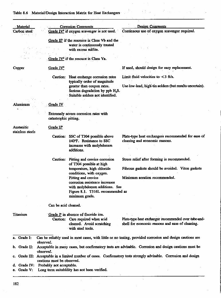
Table 8.6 MaterialDesign Interaction Matrix for Heat Exchangers
Material CodonComments Design comments carbon steel Grade IVd if oxygenscavenger is not used.
Grade IF' if the resource is Class Yb and the water is continuously treated with excess dfite.
Continuous use of oxygen scavenger required.
i
Grade IVd if the resouce is Class Va.
Grade Nd If used, should design for easy replacement.
Limit fluid velocities to* C3 fils.
Use low-lead, high-tin solders (but results uncertain).
Caution: Heat exchange corrosion rates typically order of magnitude greater than coupon rates. Serious degradation by ppb H$. Suitable solders not identified.
Aluminum Grade N c
Extremely severe corrosion rates with catastrophic pitting.
Austenitic Grade fib stainless steels
Caution: SSC of T304 possible above 140°F. Resistance to SSC increases with molybdenum additions.
Caution: pitting and crevice corrosion of T304 possible at high temperature, high chloride conditions, with oxygen. Pitting and crevice
Plate-type heat exchangers recommended for ease of cleaning and economic reasons.
Stress relief after forming is recommended.
Fibrous gaskets should be avoided. Viton gaskets
Minimum aeration recommended. corrosion resistance increases with molybdenum additions. See Figure 8.1. T316L recommended as minimum grade.
Can be acid cleaned.
Titanium Grade I' in absence of fluoride ion. Caution: Care required when acid
cleaned. Avoid scratching with steel tools.
Phe-type heat exchanger recommended over tube-and- shell for economic reasons and ease of cleaning.
a. Grade I: Can be reliably used in most cases, with little or no testing, provided corrosion and design cautions are observed.
b. Grade II: Amtable in many cases, but confirmatory tests are advisable. Corrosion and design cautions must be observed.
c. Grade III: Acceptable in a limited number of cases. Confirmatory tests strongly advisable. Corrosion and design cautions must be observed.
d. Grade IV: Probably not acceptable. e. Grade V: Long term suitablility has not been verified.
182

Values of less than unity indicate subsaturation and no scaling by gypsum, while values greater than unity indicate mrpersaturation and possible scaling. The relative saturation does not indicate the rate of deposition. Because a number of simplifying assumptions were required in genera-tion of Figure 8.2, interpretation of relative saturations between 0.8 and 1.2 is problematic.
REFERENCES
Conover, M. F.; Green,T. F..; Keeney,R. C.; Ellis,P. F.; Davis, R. J.; Wallace, R. C. and Blood, F. B.; "Final Report: Direct Utilization of Geothermal Energy for Space and Water Heating at Marlin, Texas", Radian Corporation, Austin, TX, 1983.
Ellis, P. F. and Conover, M. F.; 'Materials Selection Guidelines for Geothermal Energy Utilization Systems", Radian Corporation, Austin, TX, 1981.
Ellis, P. F. and Smith, C. S.; "Addendum to Material Selection Guidelines for G e o t h d Energy Utilization Systems", Radian Corporation, Austin, TX, 1983.
Ellis, P.F.; "A Geothermal Corrosivity Classifidon System", Geothermal Resources Council Transactions, Vol. 5, GRC, Davis, CA, 1981.
Kindle, C. H. and Woodruff, E.M.; 'Techniques for Geothermal Liquid sampling and Analysis", Pacific Northwest Laboratory, Richland, WA, 1981.
Lund, J. W., et al.; "corrosian of Downhole Heat Exchangers, Appendix A', DOE Contract E(10-1)- 1548, Oregon Institute of Technology, Klamath Falls, OR, October, 1976.
Ostroff, A. G.; "Introduction to Oil Field Water Technology, Appendix la, National Association of Corrosion Engineers, Houston, TX, 1979.
Wilde, K. A.; "Radian Technical Note210-344-02, EPRI Research Project RP 1261-1. Steams-Roger Project C-21385: Equilibrium Model Documentation", DCN 79- 210-344-06, Radian Copration, Austin, TX, January, 1979.
183

- E
TOF
Figure 8.2 The solubility product of Gypsum (Calcium Sulfate Dihydrate) in low-temperature geothermal waters (Radian Corporation, 1979).
Note: The solubility product is expressed 011 a ppm mass basis, rather than a mol& basis, and is corrected for ionic strength and temperature.
184

WORKSHEET 1 - IONIC BALANCE
ppm or mgn TDS =
Cations moles/l sl!i
PH 1w = x l =
ppm/D=mg/L /Fw(mg) =
122989.2 = x1-
K+ - 139102.0 = xl= /40080.0 = . x 2 = Ca+* -
Mg+' - 124312.0 = x 2 =
- Na+ - -
- -
Total Cations (qL)
/Inions
SOi' - - /96061.6 = x 2 =
HCO; - - /61017.3 = xl= CO;' - - 160009.4 = x 2 =
Cl. - - /35453.0 = xl= Total Anions (eqk)
The total cations should equal the total anions. A 10% difference is acceptable.
Note:
1. For solutions containing less than 14,000 ppm Total Dissolved Solids O S ) , ppm = mg& with less than 1% error.
2. D = density in kg& = [l + 6.95.1C7 TDS (mg/L)] = 11[(1 - 6.95.1C7 TDS ppm)] =
3. If carbon dioxide species are expressed as Total Alkalinity (TA) as mg& CaC03, equate the TA to HC03 x 0.8196 = HCOi.
185

WORKSHEET 2 - RYZNAR INDEX
1. Calculate pHs
i pHs = pCa + pALK 4- KC :
pCA = - log [Ca] where [Ca] is the molar concentration of calcium from Worksheet 1. .
pCA =
pALK = - log [ALK]
If total alkalinity is given as mg/L CaC03, then [ALK] = mgL CaCO3/1OO089.4 =
If analysis gives HCO; and C0i2, then use the molar concentrations and pH from Worksheet 1 to solve:
[ALK] = mCO;] + 2 [COi2] + lWI4 - lo* =
pALK = -log [ALK] =
"Kc" is a complex term involving two equlibria constants and activity coefficients; all temperature dependent term. Its calculation is quite complex and is beyond the scope of this method. Fortunately, however, graphical methods for estimating "Kc" are available. Furthermore, Kc is relatively insensitive to minor errors introducted by the assumptions required for the two graphical methods.
If TDS is <6OOO ppm, refer to Figure 8.3 and determine the value for Kc.
If TDS is >6OOO ppm, complete Worksheet 2A and use the calculated ionic strength to derive Kc from Figure 8.4.
KC =
pHs =
2. Calculate the Ryplar Index.
Ryplar Index = 2 pHs - pHa
- - - - -
186

WORKSHEET 2A - FLUID PROPERTIES - IONIC STRENGTH
Perform only for calcium carbonate scaling calculations when TDS exceeds 6O00 ppm.
- ion molesll' / Kg H20/Lb = mles/Kn H,O
PH
Na+
K+
c a + 2
Mg+2
SOi2
HCO;
co;2
C1"
xl= - -
xl= - -
xl= - -
= x 4 =
= x 4. =
x 4 = - - x 4 = - - x 4 = - -
x 4 = - - X 0.5
molal ionic strength =
a.
b.
From mole& column of Worksheet 1.
106 Kg H,O/L brine - ( D - mf3 mg/L )
where D is deiined on Worksheet 1.
187

v) a I- c 0
-r- c F-
E L QI a ln
Figure 8.3 Determination of Kc for geofluids containing C6OOo ppm or mg/L total dissolved solids (TDS)(Lund, 1976).
Note: Using a straighedge, connect the ppm TDS on the "Parts per million" (ppm) scale with the fluid temperature 011 the "Temp OF" scale. Read the value of Kc m the Pseu-tant Kc scale (Lund, 1976).
6000
4000
3000
2000
I o 0 0 aoo 600
400
300
206
c,

4.0
3.5
3.0
2.5 2
g 2.0
U C a v)
0 0 'c1 J a3
Y
a" 1.5
1 .o
0.5
n " 0 0.5 1 .o 1.5 2.0
Ionic Strength 2.5 3.0 3 .5
Figure 8.4 Determinatian of Kc for gmfluids containing >6000 ppm total dissolved solids (TDS)(Ostroff, 1979).
Note: Calculate the ionic strength using Worksheet 2A.
189


CHAPTER 9 WELL PUlMPS
By Gene Culver and Kevin D. Rafferty, P.E.
OIT Geo-Heat Center Klamath Falls, OR 97601
9.1 PUMPING GEOTHERMAL FLUIDS
9.1.1 Jntroduction
Pumping is often necessary in order to get geothermal fluid to the surface. Pumping is sometimes required to increase pressures or move fluids from place-to-place once they are on the surface. In certain geothermal fluids, such as those with high carbon dioxide content, corrosion and scaling can be reduced by maintaining the water under pressure. Because production well pumps are usually of greatest concern and, on the surface, pumping is not recurrently a problem, well pumps will be considered first.
Basically, there are two types of production well pumps; (a) lineshaft turbine pumps and (b) submersible pumps - the difference being the location of the driver. In a lineshaft pump, the driver, usually a vertical shaft electric motor, is mounted above the wellhead and drives the pump, which may be located as much as 2000 ft below the ground surface, by means of a lineshaft. In a submersible pump, the driver (a long, small diameter electric motor) is usually located below the pump itself and drives the pump through a relatively short shaft with a seal section to protect the motor from the well fluid. General characteristics of the lineshaft and the submersible pumps are shown in Table 9.1.
Jet and centrifugal suction pumps have seen limited service, but few are in use. Jets are limited by the tendency to scale and corrode or both in the down well jet assembly, and centrifugal suction pumps are limited by low lift capability at elevated temperatures. Lineshaft pumps have two definite limitations: (a) they must be installed in relatively straight wells and (b) they are economically limited to settings of s2000 fi. For direct heat applications, the economic setting depth limit is probably closer to 800 ft. (Refer to Chapter 6, Plumbnets and Alignment; American Water Works; and Hydraulics Institute standards.) A general comparison of lineshaft and submersible pumps appears below. As in any generality, there are exceptions and each application should be considered individually.
In some installations, selection of a pump type will be d i c W by setting depth, well size, well deviation, or temperature. If not restricted by th&,'the engineer or developer should selecta pumpbased on lowest lifecycle costs, including important factors such as expected life, repair
costs, rig cost for pulling, availability of parts, and downtime costs. Power CoIlSumption costs and wire-to-water efficiency, although certainly worth evaluating, may not be nearly as important as others factors, such as those above. For most direct heat applications, the lineshaft pump has been the preferred selection.
There are many factors that cau affect the relative efficiencies of linehfi versus submersible pumps: i.e. temperature, power cable length, specific design of impeller and bowl, column length and friction losses. The wire-to-water efficiency in the particular application is the important factor. The bowl efficiency of a pump with extra lateral will be less than for standard lateral (discussed in Subsection 9.3) and clearances. The bowl efficiency of a submersible will be higher than a lineshafi of similar design because extra lateral is not required in the submersible.
Pump efficiencies (Effp) are usually determined by testing at - 60°F. Efficiencies for both lineshaft and submersibles will be higher at higher temperatures and is shown as:
, Effp= l - ( l - t )No)" v t
where .
E& = efficiency at operating temperature t = efficiency at test temperature Vo = kinematic viscosity at opemting
Vt = kinematic viscosity at test
n = exponent based on experimental data,
temperature
temperature
usually between 0.05 and 0.1.
For example, if a test had been run at 60°F (1.1 centistokes) with 78% efficiency, and the pump is to operate at 200°F (0.31 centistokes), the efficiency will be:
Effp = 1 - (1 - 0 . 7 8 ) W o M = 0.793 1.1
and, if n = 0.1, then
Effp 1 - (1 - 0.78)- = 0.806 1.1
191

Table 9.1 Comparison of Lineshaft and Submersible Pumps
hunp stage efficiencies about the same, 68 to 78%. Generally, lower headlstage and less flowlunit diameter. Higher motor efficiency because it operates in air. Little loss in power cable.
Motor, thrust bearing and seal accessible at surface.
Usually lower speed (1,750 rpm or less) although may . be equal. Usually lower wear rate.
Higher temperature capability, up to 400°F + , although not used up to temperature limit in direct heat and some binary power applications.
Shallower settings, 2,000 ft maximum.
Longer installation and pump pull time.
Well must be relatively straight or oversized to accommmodate stiff pump and column.
Impeller position must be adjusted at initial startup.
Generally lower purchase price at direct use temperatures and depths.
Submersible
Pump stage efficiencies about the same 68 'to 78%. Generally, higher flowlunit diameter. Lower motor efficiency-operates in oil at elevated temperature. Higher losses in power cable. Cable at least partially submerged and attached to hot tubing.
Motor, thrust bearings, seal, and power cable in well-less accessible.
Usually higher speeds (3,600 rpm) although may be equal. Usually higher wear rate.
Lower temperature capability but sufficient for most direct heat and some binary power applications.
Deeper settings. Up to 12,000 ft in oil wells.
Less installation and pump pull time.
Can be installed in crooked wells up to 4 degrees deviation per 100 ft. Up to 75 degrees off vertical. If it can be cased, it can be pumped.
Impeller position set.
Generally higher purchase price at direct use temperatures and depths.
A pump with extra lateral will probably have an n value closer to 0.05 than 0.1.
1.9.1.2 Lineshaft Turbine Pum
To understand the potential problems and solutions in lineshaft pumping, it is necessary to understand how the pumps are constructed. Figure 9.1 shows a typical lineshaft turbine pump with an enclosed oil-lubricated shaft. Enclosed shaft water lubricated pumps are also manufactured. Note that there is a discharge head mounted either on the well casing or a cmcrete pad. The discharge head supports the discharge column and shafi enclosing tube which, in turn, supports the multi-stage pump bowls and intake arrangement. The column is usually in 20 ft sections with either screwed or flanged connections. A shaft enclosing tube support spider is usually provided at every other column joint. The enclosing tube is usually in 5 ft sections with a shaft bearing at each joint, although high speed pumps may have closer spacing. The lineshaft sections are thesame length as thecorresponding
192
column. Theenclosing tube isconnected to the discharge bowl where it has oil outlet ports and also is connected to the discharge head with a tube tensioning assembly. The enclosing tube is tensioned after installation to help maintain bearing alignment. The enclosing tube provides a waterproof enclosure for the shaft and a path for gravity feed or pressure lubrication.
In an enclosed lineshaft oil lubricated pump, only the shaft bearings are oil lubricated. The bearings in the bowls, between each impeller, are water lubricated. The oil is discharged into the well fluid outside the pump through the pump discharge case so that the shaft enclosing tube is not pressurized by the water at the last pump stage.
Some csm-type and very shallow setting pumps have pressurized grease pipes providing grease to the pump bearings, and others are provided with freshwater lubrication through rifle drilled bowl shafts, but this has not been extended to deep well pumps.

Open lineshaft pumps have seen limited success in geothermal applications. Because the bearings are lubricated by geothermal hot water, bearings tend to heat and wear faster. Many of the more common bearing materials are subject to corrosion or de-alloying by geothermal water and p i a l bearing materials increase costs. If open lineshaft is used, it should be of stainless steel to resist corrosion, but again at a higher 'cost. As a result of the added costs for p i a l materials and, even then shorter expected life, the enclosed shaft design is preferred except for very clean, relatively &l (> 140°F) fluid.
The column assembly can represent the major cost component of a pump. In the long run, it is usually more
life expectancy (one that may outlast several bowl assemblies) than to purchase a column that may not have a long life.
econamical to purchase an enclosed shaft column with long
The pump impellers are connected to the shaft by a collet or collet and key with locking screws. The shaft and all rotating parts are supported by the thrust bearings of the hollow shaft motor or a separate thrust bearing assembly. There is an impeller adjusting nut at the top in hollow shaft motor assemblies, or a three or four piece coupling with adjusting nut for solid shaft driver arrangements.
Relative Elongation and h i a l End Play or Lateral
When a lineshaft pump is initially installed,the impellers am resting on the bowls. In order to free the impellers and allow for forces generated during pumping, the adjusting nut is tightened to raise the impellers. The dead weight of the rotating parts elongates the shaft to some extent, but the dead weight remains constant during operation and has no effect on relative elongation. Dead weight must be considered in sizing the thrust bearings.
It is important to recognize that the shaft and impellers act Consider the independently of the column and bowls.
following forces and loads in an operating pump:
1. Each stage of the pump increases the pressure; therefore, @ere are unbalanced hydraulic pressures above and below each impeller, resulting in a downward force.
2. Vanes and waterways through a multi-stage turbine pump are at some angle >go" with the shaft, resulting in downward dynamic forces. In a true centrifugal situation, these forces are minimal and increase to a maximum for an axial flow impeller.
3. The vanes and waterways of the impeller also change the flow from vertical or nearly vertical to some angle closer to horizontal as the flow proceeds to the bowls. This d t s in an upward force on the impeller. In vertical turbines at shallow settings and submersibles operating
with initially low heads at startup, this force can be greater than the others and results in a net upthrust until other forces and dead weight loads overcome it.
The resultant downward force at operating conditions is known as the'hydraulic downthrust and is obtained by multiplying the total head by the thrust factor K and by the specific gravity of the fluid pumped. The thrust factor depends primarily on the impeller design and diametet and is determined by the pump manufactuter. Note that the deeper the setting and the greater the loads, resulting shaft stretch is greater. The thrust factor K is stated in pounds of down thrust per foot of head.
The bowls and column also have a deadweight load resulting in column stretch. The relative deadweight stretch is compensated for by lifting the impellers free of the bowls befine initial startup, as noted above.
The bowls change the direction of water flow passing through them, resulting in dynamic forces and a downward' load related to hydraulic thrust. The column and shaft enclosing tube, however, have a much larger cross-sectional area than the shaft, so they stretch less. The difference is relative elongation.
Relative elongation can be calculated if the setting depth, specific gravity, total dynamic head, volume of water supported, lineshaft diameter, column and tube diameter and wall thickness, and impeller Wust coefficient are all known. Axial end play or lateral, which is the total axial movement of the impellers within the bowl from towing out to bottominq - out, must be greater than relative elongation plus allowances for safety.
Another consideration is thermal expansion. Because of their differences in thickness, matetial and mass, the column, shaft enclosing tu+, and shaft will all expand at diffixent rates and reach thermal equilibrium at different times after initial startup. Additionally, the shaft in an enclosed lineshaft pump is somewhat t h e d y isolated from the water in the column by the space between the shaft and the inside diameter of the tube. Once thermal equilibrium is reached, t h d expansion has no direct affect on relative shaft elongation, but it must be compensated for as it occu~s, either by adjusting the impellers or by allowing extra lateral. Obviously, in a system that cycles on and off, it must be allowed for in extra lateral.
Axial end play or lateral is Bccommodated through the vertical seal between the impeller and the bowl (shown in Figure 9.2). This is a kind of extended skirt on the bottom of the impeller and matching bore in the upper end of each bowl. These areas may have wear rings on the bowls, impeuer or both. Standard &ld water axial end play typically varies from 3/16 in. in a 4 in. diameter pump,to 1-3/8 in. in a 30 in. diameter high headlstage pump. Chqnmdm 'gmaximum
193

Figure 9.1 Typical lineshail turbine pump with an enclosed oil-lubricated shaft.
194

axial end play using standard castings is 114 to 1-314 in. This is obtained by additional machining of the bowls. T h e 4 expansion alone for a 400 ft static water level, 200°F well could be 4-3/4 in., which far rmrpasses the maximum axial end play for standard pumps. This explains why a standard pump cannot be placed in geothermal service, especially in a cycling situation. Failure to consider this has led to premature wear of impellers, bowls and bearings, broken lin&fts, and burned out electric motors. Proper end play and lineshaft sizing quires experience and understanding of relative shaft stretch, and knowledge of the range of operation on the head versus flow curves.
Figure 9.2 Cross-sectional of a pump bowl (Johnston Pump Company).
The dynamic elongation of the shaft is independent of the dynamic elongation of the column pipe. Relative &ail stretch. denoting the position of the impellen in the bowls, is the shaft elongation minus the column elongation. The axial end play must be safely greater than the relative rhaA stretch.
Extra seal length is accomplished by modifying the patterns from which the impeller and bowl castings are made and appropriately machining the increased length, as shown in Figure 9.3. This entails extra cost and some manufacturers may not want to make the required changes.
At this point, it may be instructive to illustrate the calculation of relative shaft stretch and thermal expansion. In order to do this, it is necessary to go through a preliminary pump selection. Although this is best leftto the pump
designer, it is important for the purchaser or engineer to understand the problems so the pump designer can be provided with the correct design parameters.
Assume a space and domestic water heating application requires 700 gal/& (gprn) peak flow. Surface system piping, valves, heat exchangers, and disposal lines require 60 lb1in.' (psi) at the wellhead at 700 gpm flow. The static wakr level is 350 ft. Test pumping indicates drawdown will be 50 A at 700 gpm and the discharge temperature is 20CPF. For the most part, flows will vary between 400 and 600 gpm during winter and, with domestic hot water storage the pump can be shut off from time to time during spring and fall, and for extended periods during summers. Minimum flows will be 100 gpm, controlled by a throttle valve and, at that rate, wellhead pressure required will be 15 psi. The system is at an elevation of 5000 ft above sea level.
Figure 9.3 Standard and extra lateral bowls and impellers (Johnston Pump Company).
The special design of the geothermal bowls and impellers is hown in the illustration. ?be taller bowl and impeller are for the geothermal pump in contrast with the shocter bowl and impeller used in a standad industrial pump of comparable a h . The geothermal bowls and hnpllers are designed to acmnmodatc the extra impeller lateral adjustment made necessary by different rates of expansion and relative shaA stretch.
The pump curves for a pump that might satisfy the requirements axe shown in Figure 9.4. The m e is a little steeper than is desired, but the efficiency (77 to 83 96) is good over the usual operating range of 400 to 600 gpm.
The pump curves provide the capacity (all of which goes through each stage) and the total dynamic head per stage for three impeller diameters. Also shown are power requirements per stage, information about the bowls and impeller including the thrust factor K mentioned earlier, efficiency changes for
\ 195

O
0 1 I I I I I I I I
SO0 600 700 BOO 100 200 300 400 I
Figure 9.4 Pump curves (Aurora Pump).
a t a t l c water
lavr‘l
pumplng water
lave1
minimum aubsrrgcncr
Ha atmom. press.
I aubmrrgancl hard
. available press. a t impeller I
NPSH L a l o c i t y head
h p vapor press.
Figure 9.5 Relationship of pressures for vertical turbine pump.
io a. z
0
1770 R ..P. M .
4 1
2
196

number of bowls and net positive suction head (NPSH). Some manufacturers also provide weight of impellers on the pump curves. In this case, this is found elsewhere. The first-stage weighs 38 lb and each additional stage is 19 lb.
Before relative elongation can be calculated,it is necessary to determine the setting depth which, in turn, requires consideration of the NPSH. The net positive suction head available (NPSHA) is the total suction head in feet of liquid absolute at the first stage impeller eye less the vapor pressure of the liquid in feet absolute. Net positive suction head required (NPSHR) is a function of pump design and determines the minimum distance the first stage impeller must be above or below the pumping level to prevent cavitation. The NPSHA must equal or exceed NPSHR as shown on the pump curve.
Because mosppump curves are based on tests at 58"F, the engineer should calculate the NPSH available under operating conditions or, in this case, select a setting to provide the required NPSH considering water temperature, local altitude and intake piping losses. Atmospheric pressure changes caused by weather conditions, viscosity changes and other minor factors when pumping water are usually allowed for by some more or less arbitrary increase in setting depth. These should be calculated if they might be significant, such as when pumping other fluids. The available NPSH is given by:
NPSH = Ha + M - Hf - H v ~
where
Ha = absolute pressure on surface of liquid,
Hl = level of liquid above or below the first stage usually atmospheric pressure, in feet of water
impeller eye in feet (positive if above impeller, negative if below)
Hf = friction loss in intake piping and screen in feet Hvp = absolute vapor pressure of liquid at pumping
temperature in feet of water.
Corrections for density difference at elevated tempemtures gives:
NPSH=& + M - H f - H n , SG SG
where SG is the specific gravity.
Rearranging to determine the minimum depth below puminq level gives:
M = NPSHR-@ + Hf + SG SG
Tables 9.2 and 9.3 give atmospheric pressures at various altitudes, and vapor pressure and specific gravity at various tempemhms. Figure 9.5 shows the relationship of pressures for a vertical turbine pump.
The friction head loss is normally very small in geothermal pumps because the tail pipe is short and screens or strainers might not even be installed. Reasonable values range from 0.3 to 3 ft of water, but could be more if a long tail pipe and fine screen was installed.
From the pump curves chosen for the example, the NPSH required at 700 gpm is 13.8 ft. Assuming that friction loss in the intake is 1 ft, the minimum submergence below the pumuinq level is:
Hl = 13.8 ft - 28.2 ft + 1 + 35.6 ft 0.963 0.963
Hl = 12.1 ft.
Additional submergence should be allowed for: (a) long term drawdown (see Chapter 7), (b) non-cmdensable gases such as carbon dioxide and hydrogen sulfide, which may increase the vapor pressure, and (c) a safety factor that depend on how much is known about the well (i.e. gases, drawdown).
The total dynamic head required is equal to the lift head plus surface head requirement plus velocity friction head losses in the column and surface discharge head assembly. Discharge head assembly losses are normally small, 0.3 to 3 ft, and will be neglected here. Column friction head losses are usually relatively small and depend on the size of the annulus between the inside of the c o l m and the outside of the oil tube (which, in turn, somewhat depends on the shaft size), and the number and design of the tube support spiders.
. The lift head is equal to the total lift, static level plus drawdown. For example:
Lift head = (350 ft + 50 ft) = 400.0 ft Surface head = 60 psi x 2.307 ft/psi = 138.;4 ft
Total head required 538.4 ft
From the pump curve, it is seen that at 700 gpm, using the 7.750 in. diameter impeller, the pump will produce 29 ft of dynamic head and require 6.5 hplstage. To satisfy the requirement of 538.4 ft, this will r e q k
NO. stages = 538.4 ft = 18.6 stages. 29 Wstage
The horsepower requirement is calculated based on the curves and correcteh for specific gravity, and is show as:
hp = 19 stages x 6.5 hplstage x 0.963 hp = 118.9 hp (approximate).
197

Table 9.2 Atmospheric Pressure at VarioUS Altitudes
Altitude Barometer Rkadinn AtIhOSDhWI 'c 'Pressure (Et'l inHz m H e . A fi ofiwater
- 1,Ooo . 3LO 787 ~. 15-2 352' 0 29.9 759 14.7 33.9
1 ,000. 28.9 734 14.2 32.8 2,000 27.8 706 13.7 31.5 3,000 26.8 681 13.2 30.4 4 , m 25.8' 655 1.2.7 29.2 5,Ooo 8 24.9 632 12:2 28;2 6,000 24.0 6 10 11 -8 27.2 7,000 23.1 587 11.3 26.2 8,OOO 22.2 564 10.9 25.2 9,000 21.4 544. 10.5 24.3 1 0 , m 20.6 523 10.1 23.4.
! Table 9.3 Vapor Pressure and Specific Gravity of Water
Temperature (OF)
32 40 50 60 70 80 90
100 110 120 130 140 150 160 170 180 190 200 210 220 23D 240 250
Absolute Vamr Pressure Dsia f& of water
0.089 0.122 0.178 0.256 0.363 0.507 0.698 0.949 1.275 1.693 2.223 2.889 3.718 4.741 5.993 7.51 1. 9.340
11.526 14.132 17.186 20.791 24.968 29.834
0.205 0.281 0.41 1 0.591 0.837 1.170 1.610 2.189 2.941 3.906 5.128 6.665 8.577
10.937 13.826 17.328 21.55 25.59 32.60 39.65 47.% 57.60 68.83
Specific Giavitv
1.00 1.00 0.999 0.999 0.998' 0.997 0395 0,993 0.990 0.989 0.986 0.983 0.980 0.977 0.974 0.971 0.967 0.963 0.958 0.955 0.950 0.946 0-942
198

The lineshaft size is based on combined torsion and axial stresses. Because most pump manufacturers provide shaft sizing tables [or charts based on revolutions per minute (rpm), horsepower required at the pump and axial load] it is only necessary to calculate axid load to enter their tables. These tables or charts are based on A W A standards.
Axial shaft ldad or total downthrust is equal to the hydraulic downthrust, plus the weight of the shaft and rotating pump parts. Each impeller pattern has a specific hydraulic thrust factor (usually designated as K), expressed in pounds of thrust per foot of total dynamic head. The K factor varies with specific gravity. The K factor for the impeller selected is 6.7 lb/ft. With some experience, it is possible to estimate tlie size of shafting, calculate the weight and enter the tables to check the size estimated. Based on the total head and K factor, it can be estimated that a 1-1/2 in. shaft weighing 6.01 lb/ft will be required.
Total downthrust equals:
Head ft x 6.7 Ib/ft x SG = 538.4 x 6.7
Wt/ft x 460 ft = 6.01 x 460 x 0.963 = 3,474 lb
= 2,764 Ib
1st stage = 381b = 342 Ib
TOTAL, 6,618 Ib
Entering the table (Figure 9.6) at 6700 lb and 125 hp, the value is above the allowable limit for 1-3/16 in. shaft and below 1-112 in., 60 the estimate was correct.
Impellers & rotating parts
Add’l stages @ 19 lb ea = 18 x 19
Using additional tables and charts from the manufacturer’s engineering data, it can be determined thak
1.
2. Col~mn f i i c t i ~ ~ ~ ~ O S S With 2-1/2 in. tube and 8 in. column
1-112 in. shaft requires 2-112 in. oil tube.
= 2 Wl00 ft or 9.2 ft.
3. Thrust bearing losses = (0.0075 hpll00 rpndlOO0 lb) (1770 rpm x 670 lb) = 8.9 hp.
4. Shaft elongation.under the calculated load = (0.0825 in.1100 ft) (460 ft) = 0.380 in.
5. column elangation under the calculated load = (0.0155 in.1100 ft) (460 ft) = 0.071 in.
If tables are not provided, shaft and column elongation can be calculated by:
e = = EA
where
e = elongation in inches (in.) L = length in inches (in.) W = total load or down thrust in pounds (lb) E = modufusof elasticity = 29 x 106psi A = gross cross-seCticmal area of shaft or column in
in2 (including oil tube if applicable).
Relative shaft elongation is the d t of shaft elongation minus column elongation:
Relative shaft elongation 0.380 in. - 0.071 in. = 0.309 in.
An additional allowance must be made for machining and assembly tolerances. Pump manufacturers usually recommend 0.010 in./stage, 60 the total bteral allowance, not including .thermal expansion, is:
0.309 in. + (19 stages x 0.010 in.) = 0.499 in.
That portion of the column and oil tube above the static water level will thermally expand much faster than the shaft that is enclosed in, and somewhat insulated by, the oil tube. Thermal expansion of steel is 6.3 x lob in./in. “F. If the average temperature of the air above static water level is 8PF, the At is 120°F.
The thermal expansion is:
(6.3 x 106 in./in.PF) (350 ft x 12 in./ft) (120°F) = 3.175 in.
This means our latera! must be i n m a d to:
0.499 in. + 3.175 in. = 3.674 in.
To this point, all major items have been umsidered, except one that was left until last for emphasis. Figure 9.7 shows the sequence of (1) installing, (2) raising the impeller’s, (3) initial start, (4) column hot and (5) thermal equilibrium.
Consider the comquences of closing the throttle valve to reduce the flow to 100 gpm at low load conditim. As stated earlier, the surface head required is 15 psi at 100 gpm.
Referring to the pump curve (Figure 9.4), as the throttle valve closes, the pump moves up its head versus capacity curve until, at 100 gpm, the total dynamic head is 59 Ws?age. At that point,total down thrust is:
59 ftlstage x 19 stages x 6.7 lb/ft = 7,511 lb shaft wt = 2,764 Ib rotating parts wt = 3991b TOTAL, 10,674 lb
199

THRUST IN THOUSAND POUNDS
aximum.recommended bbp versus thrust (Aurora Pump).
Checking the shaftsize (FigureP;6), we find 1-112 in. is Column elongation: large enough to carry theincreased load.
(0.033 m./lOO ft)(460 ft) Going back to the tables to check the-&& and colunm
elongation -at the i n c d load we have shaft elongation: Relative elongation: I
''(0.176 h.1100 ft)(460 ft) = Q.810 in. (0.810'in. - 0.152 in.)
= 0.152 in.
= 0.658 in.
200

. .
600-
500-
400 - n
4J Y- Y
300 - 0
w I 200-
a
LOO -
. - i. INSTALL- XMPELLeR RESTING ON BOWL
2. R A I S E IHPELLER TO ALLOW faR R E L A T I V E STRETCH
TOTAL SYSTEM HEAD CURVE
WELL DRAWDOWN
FRICTION LOSSES I N PIPING
LIFT I N PIPING
I I I I I I I 1 400 500 600 700 000 100 200 300
3. OPERATING COLO
4 . OPERATING COLUMN HOT
1. OPERATING COLUMN AND SHAFT HOT
Figure 9.7 Pump installation sequence.
Figure 9.8 Well operating conditions.
201

This means that 0.349 in. (0.658 - 0.309 in.) must be added tosthe previous lateral to allow for increased relative shaft elongation under m i n i m load conditions. The total lateral then becomes:
3.674 in. + 0.349 in. = 4.023 in.
the fact that the system engineer must provide the pump manufacturer with the whole range of operating conditions (preferably a flow versus total dynamic head curve for the system) including well conditions similar to that shown in Figure 9.8. If this is accomplished before well completion, the pump mawfacturer is not restricted by casing size and can suggest the most cost effective and efficient pump for the system. Savings in ffie pump and pnmping costs can then be compared to possible increased well costs.
In addition to the affects on the pump design, operation at throttled flow also affects the motor or other driver (such as variable speed unit) thrust bearing design. In the above example, the thrust load was increased to 161% of the thrust at full flow. If the bearing design does not allow for operation at throttled flow, premature failures will occur.
For the application cited, a larger pump with a flatter curve and higher head per stage would be a more economical selection. For the same flow rate, the larger diameter impeller would have a lower K factor and lower specific speed. This combined with a larger shaft would reduce relative shaft elongation and result in more efficient operation over the required flow fange.
There is no real temperature break point for lineshaft pumps. For many applications up to lWF, standard pumps, perhaps with machining up to maximum axial end play, will operate satisfactorily, particularly where the pump is operated continuously. For intermittent operation, thermal expansion and relative shaft elongation should be carefully checked.
Lineshaft .pumps are available in bowl diameters from 3-54 in. to over 36 in. with flows ranging from 25 gpm to over 25,OOO gpm.
A regular maintemnce schedule is highly recommended. This includes lubrication of motor bearings (and thrust bearing if separate) and pump packing glands at specified intervals. Oil for shaft lubrication is usually gravity flow with a valve and sight glass to check the required number of drops per minute. This should be checked daily. Turbine oil 68 is the normally recommended lubricant.
Pump manufachxers car d l y suggest a t reasonable inspection frequency. It is usually more economic to puli a pump, inspect it and repair or replace parts as needed m the off season than to wait until it fails when it is needed.
When a vertical &he pump stops, water flowing back down the column causes the pump to back spin. Because the pump is acting as the driver, there is very little dhger of unscrewing shafig, buE if the pump is started during back spin, it is likely to break shafting, loosen collets, or damage the motor. This could happen during momentary power failure or when a control switch signals a pump to start before the column drains and back spin is completed. Foot valves, non-reversing ratchets, time delay switches, and rotation sensing switches can prevent this.
Most geothermal pumps are equipped with time delay or rotation Sensing switches or both. Both are recommended in case of failure of either one.
There are some advantages in allowing back spin. The free back spin indicates that nothing is dragging or binding and gives an indication of bearing conditions. It aiso permits the pump to be started with low load, reducing shack loads on shafting and bearings. A non-reversing ratchet also permits the column to drain, but it takes more time because the water flows backward through the bowls and impellers that are not rotating.
Foot valves prevent back spin and keep the column fuli of water, reducing the entrance of air and associared d o n and scaling. They are, however, difficult to maintain in good condition because of scaling and corrosion properties of many geothermal fluids and usually tend to leak in a relatively short time. Also, the pump always starts under a high load condition. Foot valves are recommended only for pumping levels <50 ft and when exclusion of air is mandatory.
Materials
Since most geothermal systems for which accurate materials information is available have been operating for less than 10 years, the "history" of materials selection is quite short. One system (operating since 1963) which has experienced extensively with pump types and materials has settled on the materials outlined in Table 9.4. Pumps of this collstfllction have operated in the system for as long as 17 years without major overhaul. With three production wells, the system has accumulated over 75 pump years of experience.
202

Table 9.4 production Well Pump Materials Successfully Used at Oregon Institute of Technology
Shaft column shaft enclosure Bearings Bowls Impellers Keys FaSteners collet
stainless steel Carbon steel Carbon steel Leaded red bronze castiron Leaded red bronze stainless steel stainless steel Carbon steel
AISI 416 ASTM A53 Grade A ASTM A53 Grade A 83% Cu, 5% Sn, 7% Pb, 5% Zn ASTM A48 Class 35 83% Cu, 5% Sn, 7% Pb, 5% Zn AISI 416 AISI 303 ASTM A108 Grade B113
Table 9.5 presents the fluid chemistry for the system on which these materials have been successful.
Table 9.5 Fluid Chemistry
~~~
Surface electrical equipment for the lineshaft pump is very similar to that for the submersible motor. The cost pro- cedure below assumes the installation of two safety switches, a magnetic starter, motor connection, and interconnecting wiring for 460 V service.
Kev SDecies
Chloride, Cl Sulfate, SO, Bicarbonate, HCO, Carbonate, CO, Hydrogen Sulfide, H$ Ammonium ion, IW, oxygen, 0 2 TDS Silica, Si Sodium, Na 1
Calcium, Ca Nitrate, NO3 Potassium, K Fluorine, F Iron, Fe Tempera-
PH mgn 8.60
51.00 330.00 20.00 15.00 1 .50 1.30
0 - 0.02 795.00 48.00
205.00 26.00 4.90 4.30 1.50 0.30 190°F
Lineshaft Pum P ricine Factors
The major items that should be addressed in the preliminary pricing for lineshaft pumps include (a) motor and starter, (b) wellhead equipment (discharge head, base plate,. tension nut assembly), (c) column, and (d) bowl assembly.
Motors used for lineshaft pump drives are "La frame, vertical, hollow shaft, induction motors, in either TEFC or weather protected configurations. As with most new motor installations, the incremental cost of a high efficiency type motor is generally justified. Costs shown in the procedure below assume the use of high thrust, high efficiency 1800 rpm, hollow shaft motors.
Wellhead equipment includes the items listed above. The discharge head serves as a fluid discharge connection and pedestal for the driver. The base plate, located just below the discharge head and bolted to it, supports the weight of the bowl assembly and column. For purposes of this estimate, it has been assumed that these items would be of basic cast iron construction.
The tension nut assembly houses the upper shaft bearing and provides a means of adjusting the tension on the shaft enclosing tube for bearingalignment. In addition, it contains the umnwtions for the external lubricating oil supply for the shaft bearings.
The pump column is frequently the single largest cost of the entire pumping system, particularly for settings greater than about 300 ft. This portion of the system includes the column pipe through which the water flows, the pump driving shaft and bearings, and the shaft enclosing tube. Different size columns are available to accommodate various flow rates. Pricing below is based on the use of threaded enclosed line-
is acceptable for 1,750 rpm operation. shaft column with 5 ft bearing spacing. This bearing spacing
The bowl assembly includes the pump bowls, impellers, shaft, intake/strainer, and discharge sections. A number of constmction alternatives are available for pump construction. The option employed for this cost estimation, and the one most frequently specified for geothermal systems is the all iron construction, with the following exceptions: stainless steel fasteners, bowl shaft and impeller keys, and special bowl bearings selected for compatiiility with the water that is to be Pumped-
203

A major cost consideration for lineshaft pumps is the allowance for larger than normal lateral in the pump section. A moderate adjustment for increased lateral can be m m - plished for standard bowls by machining. This machining involves a 10 96 cost increase over the standard bowl assembly price. For lateral beyond that described above, extra-lateral - bowls must be used. These optional bowls often involve a cost penalty of 50% over standard bowl assemblies.
Estimating Lineshaft Pumu Prim
This method is iutended to provide a preliminary budget estimate of a lineshaft pump system. For unusual applications or for a more specific cost estimate, manufacturers should be consulted. Costs are based on prim from December, 1986.
1. Bowl Assembly (Pump) a. Select pump from table (Table 9.6) that most closely
matches flow requirement.
Table 9.6 Bowl Assembly (Pump) Costs
Flow laDm)
60 80 120 160 200 250 300 400 500 700 800
1 ,000 1,200 1,500
Head/ Model stage
A 12 B 12 C 12 D 12 E 15 F 16 G 17 H 18 I 20 J 20 K 20 L 21 M 22 N 22
cost A (1,150 + (210X)) x 1.1 (1,150 + (210X)) x 1.1 (1,150 + (210X)) x 1.1 (1,150 + (210X)) x 1.1 (1,250 + (310X)) x 1.1 (1,550 + (300X)) x 1.1 (1,550 + (300X)) x 1.1 (1,570 + (310X)) x 1.1 (1,570 + (310X)) x 1.1 (1,620 + (450X)) x 1.1 (2,080 + (480X)) x 1.1 (2,080 + (480X)) x 1.1 (2,290 + (510X)) x 1.1 (2,290 + (510X)) x 1.1
b. Divide the total dynamic head OH) required by hds t age from the table. Subtract one and round off to the nearest whole number. Substitute the resulting value for, X, in the cost formula from the table to determine basic bowl assembly cost.
c. Adjustments for geothermal service are given in Table 9.7. This is an average value based on an 8 in. bowl assembly and a 1-3/16 in. shaft.
Multiply by number of stages + 1.
Table 9.7 Adjustments for Geothermal Service
CostlStage Material 0
Bowl fasteners (316 ss) 20
Special bearings - 200 Keyed impellers 180
TOTAL 400
d. Adjust for lateral
For relatively shallow settings or moderate temperature or both, increase basic bowl assembly cost by 10%.
For higher temperatures or deep settings, or both increase basic bowl assembly cost by 50 96.
2. Wellhead (discharge head, base plate, tension nut assembly)
Add $2,270.
3. column with Enclosed Lineshaft
Select column based on flow rate requirement. Length required is pump setting depth. Table 9.8 provides cost data.
Table 9.8 Enclosed Lineshaft Costs
Size Max. Flow cost/20 ft (in.) (mml 0
4 125 688 5 300 758 6 500 - 838 8 1,300 970
10 2,450 1,278
4. Motor
Calculate the required driver horsepower (hp) as:
m x 8.33 x TDH h p - ?3,QQQ x E f f p
where
gpm = gal/min 8.33 = Ib of waterlgal TDH =totaldynamichead 33,000 = ftlb/mininonehp Effp = pump efficiency
204

Select the closest larger size motor from Table 9.9.
Table 9.9 Motor Costs
cost ' A 0
10 1,471 15 1,659 20 1,879 25 1,963 30 2,268 40 2,796
cost A L L
50 3,261 60 3,759 75 4,859
100 6,193 125 7,990 150 9,392
5. Motor Electrical Equipment
Based on the hp calculated above, select c a t of electrical equipment from Table 9.10.
Table 9.10 Electrical Equipment costs
cost Cost L O L A
10 330 50 920 15 460 60 1,475 20 480 75 1,650
30 685 125 3,125 40 840 150 3,750
25 520 100 1,800
6. Example Cost Calculation
Required flow is 350 gpm, the fluid is 120"F, there is a 300 ft setting depth, and 320 ft TDH.
a. Bowl Assembly Cost
o Select G from Table 9.6 with 17 ft stage
o Determine bowl cost [$1,550 + ($300 x 18 stages)] x 1.1
o Add materials adjustment from Table 9.5
= $7,645
(18 stages x $400/stage) = 7330
o Add for lateral machining (10%)($7,645) = 765
o Total bowl assembly cost = 15,610
b. Wellhead
o Add unit cost = 2,270
c. Enclosed lineshaft
o Cost from Table 9.6 for 6 in. is ($838/20 ft)(300 fi) = 12,570
d. Motor
o Determine motor hp by
(350 gpm) (8.33 Ib/gal) (320 ft) ( 3 3 , 0 0 0 ft Ib/min) (o .075 ) '' -
hP
hp = 37.7, say 40 hp 9
o Select cost h m Table 9.9 Select 40 hp = 2,796
e. Electrical
o Select cost from Table 9.10 = 8 4 0 - o Subtotal = 34,086
f. Totalcost
o Assume a 25% discount from the list price
o Total Cost (0.75)($34,086) = 25,565
9.1.3 Submersible Pum S
A submersible pump is one in which the &ver,or electric motor, is located in the well below the sutface of the fluid being pumped and is usually below the pump itself. Submers- ible pumps, therefore, do not have the problems related to relative shaft elongation that lineshaft pumps do. Submersible pumps can be separated into low temperature or $andad pumps and high temperature pumps. The temperature limit is set primarily by the allowable temperature of the motor.
Low Temuerature Submersibles
Almost without exception, standard submersible pump motors are warranted to 90°F or below. The allowable tem- perature is limited by the motor winding insulation and the heat dissipation available. Many standard submersible pump motors can be operated at 120 to 13OT if proper allowances nre made.
205

There are three basic types of submersible pump motors: wet winding, oil filled, and hermetically sealed.
In the wet winding motor, the motor is filled with water. Water proofing is achieved by special insulation on the stator winding wire, usually plastic, and because the wire and its insulation are bulkier, the motors are larger for a given rating. The motor is carefully filled at the surface to ensure there are no air bubbles and a filter installed in the fill port to ensure that the motor operates in water. Some brands are pre- filled and have an expansion diaphragm to allow for expansion and contraction of the filling solution and motor. Rotating seals and a sand slinger at the upper end prevent free circu- lation of well fluid in and out of the motor and reduce seal and spline wear by abrasive particles. Bearings are water lubricated.
Oil filled motors are prefilled with a high dielectric oil. A rotating shaft seal (with sand slinger) is utilized to keep the oil in and water out. k u s e water has a higher density than oil, the motors have an oil reservoir with expansion bladder at thebottom. Any water that leaks through the seal in time migrates to the bottom of the reservoir. However, if the seal leaks there is probably always a small amount of water mixed with the oil surrounding the windings. Bearings are oil lubricated giving them higher capacity.
Hermetically sealed motors have the winding encased in a welded can usually stainless steel. The windings may be similar to a surface motor with air inside the can but usually are embedded in a thermo-setting resin to provide better heat dissipation and reduce the possibility of water leaking in. The rest of the motor is similar to the wet type described above and the bearings are water lubricated.
All small submersible motors have a thrust bearing at the lower end, usually self-aligning and self-equalizing Kingsbury type, to carry pump downthrust and a small thrust bearing at the upper end to carry the momentary upthrust during pump startup. Some larger motors intended primarily for deep settings have a separate seal section providing for sealing and expansion. The seal section is located between the motor and the pump and contains the main thrust bearings.
All submersible pump motors depend on the flow of fluid past the motor for cooling. This is usually in the range of 0.25 to 0.5 ft ls velocity. If the motor is installed in a large casing or well bore, or if the production zone is above the motor, this velocity may not be realized. In that case, the pump must be fitted with a flow inducer sleeve (Figure 9.9) or other method of increasing fluid velocity to provide cooling (Figure 9.10). The flow inducer sleeve also provides a means of increasing the ambient operating temperature. If the velocity past the motor is increased up to 5 to 6 ftls, the allowable ambient water temperature may be increased from the standard 85 to W F , to 120°F. The actual-amount of allowable increase depends on the motor type and insulation.
The manufacturer should also be consulted. Because the flaw inducer mtricts the inlet flow path, it is necessary to check to be sure the net positive suction head, NPSH, for the pump is maintained.
Figure 9.9 Flow inducer sleeve (Franklin Electric).
A flow inducer sleeve is a tube over the motor, closed off above the pump intake and extended to the bottom of the motor or,bwer. The sleeve material is c d o n Fesistant metal or heavy plastic.
Figure 9.10 Flow inducer discharge tube (Franklin Electric).
If the casing is too small for a flow sleeve, a tube may be installed as follows:
1. Tap a 1/4 in. tube (ID) into the pump outlet (below check valve). 2. Clamp it to the pump and motor. 3. Aim tube upward 80 flow is introduced one A below the motor. 4. Protect tube with spacers and angle hn.
206

Another method of increasing allowable ambient fluid temperature is to decrease the service factor, requiring an increase in motor capacity. For instance, if the ambient temperature requires a decrease in service factor from standard 1.2 down to 0.6, a pump that normally would require a 3 hp motor now requires a 5 hp motor. The 5 hp motor would be the same diameter but longer.
By using a combination of high flow velocity and reduced service factor, some motor manufacturers will author- ize, but not necessarily warrant, operation at 130°F. So far as is known at this writing, there are no standard submersible motor manufacturer’s that will authorize operation at ambient temperatures above 130”F, although several pump installers have reported 3- to 5-year life at 135 to 140°F. These installations were neither authorid nor warranted.
At least one motor manufacturer builds an oil s t r i m motor in 2 through 15 hp in a 4 in. frame. These motors are rated for continuous duty in 160°F ambient temperatures. The motor is basically an oil-filled type with an improved seal arrangement, with increased oil reservoir capacity and larger diaphragm to accommodate greater thermal expansion. Because the bearings are oil lubricated, the allowable thrust load is increased from 900 lb in a similar water lube motor to 1500 lb.
Many small submersible motor manufacturers install thermostatic protection in the motor windings rather than, or in addition to, having the overload protection at the surface. These thermostats are d y set at, or just above, the stated warranted teGrature limit. This effectively blocks use of the motor in higher ambient temperatures even if a flow inducer is installed and the service factor reduced. In some cases, it may be possible to bypass the thermostat, but this would void any warranty.
At the temperatures and depths standard submersibles are likely to be employed, it is unlikely that electrical cable volt- age drop would be a significant factor. At temperatures above lWF, the manufacturer should be consulted Concerning the allowable current at the pumped fluid temperature.
Most pump and motor manufacturers conform to NEMA standards for shafts and bolt patterns. It is possible, therefm, to match one manufacturer’s pump to another muf&urer’s motor. Many off the shelf pumping system utilize one manufacturer’s pump and another’s motor.
When connecting one manufacturer’s motor to another’s pump, the pump should have sufficient lateral to allow for shaft deflection. As the load increases, the shaft will shorten elastically. Pump manufacturers usually state the thrust factor
BARRELS PEA DAY (42 U.S. EALLONS]
Figure 9.11 One stage performance curve (Centrilift Hughes, Inc.)
i
207

turd motor mauhtuers can provide elastic deformation data or, if shaft size and lengths are known, it can be calcukted.
High TemDerature Submersibles
High temperature submersible pumps were developed for deep settings in oil fields. They are almost universally rated in barrels per day (bpd) rather than gallons per minute (gpm = bpdl34.3). Pump curves (Figure 9.11) are set up differently but show the same information as lineshaft pump curves. For elevated temperatures in both geothermal and oil fields, better elastomers for seals, higher temperature insulating materials for cable, and improved oils and bearings have been developed. Satisfactory operation has been attained in oil wells up to 290°F. Figure 9.12 shows a submersible installation. The gas separator shown is primarily used in oil field production.
I
I WJ I \
Qux V * L n - MIm -
Figure 9.12 Submersible pump installation (Centrilift Hughes, Inc.).
The pump section of a submersible is similar to a line- shaft in that it is a multi-stage centrifugal. Pump rpm is usually 3,475, which is higher than most lineshafts. Impellers are usually of the balanced or floating type to offset hydraulic thrust, because space for thrust bearings is limited. Figure 9.13 shows a typical pump section with its balancing ring and balancing holes.
Figure 9.13 Submersible pump typical stage nonmenclahue (Centrilift Hughes, Inc.).
Submersible pumps are multi-ataged centrihgal pumps. Each stage of a submersible pump consists of a rotating impeller and Stationary diffuser.
The preswrre-energy change is accomplished as the liquid being pumped surrounds the knpeller, and as the impeller rotates, the rotating motion of the impeller imparts a rotating motion to the liquid. Actually, there are two components to the motion imparted to the liquid by the impeller. One motion is in a radial direction outward from the center of the impeller.
At the time of this writing, there are no known installations where gas separators are being used in geothermal applications, but they have been proposed for use in some Colorado and Wyoming geothermal wells where the free methane content is 14% or more. Its function is to remove free gas from the fluid before it enters the pump where it would expand in the low-pressure suction area, possibly cause cavitation, and prevent proper pump operation.
The seal section between the pump and motor provides for equalization of wen fluid and internal motor pressure, allows for expansion and umtraction of dielectric motor oil, provides a seal between the well fluid and mdor oil and houses the thrust bearings. Separation of the well fluid and motor oil is accomplished by two or more mechanical shaft seals, elastomer expansion chamber and backup labyrinth, usually a series of U-tubes. The multipIe seals and labyrinth provide extra sealing protection.
208

Impellers are designed for balancing at peak efficiency. operation at higher than design capacity results in upthrust, and lower than design capacity results in downthrust. Bearings are usually of the multiple tilting pad type; there are two, one for upthrust and one for downthrust.
Motors used in high-temperature submersibles are oil- filled, two-pole, ' thephase squirrel cage induction type. Design voltages range from 230 to SO00 V with currents from 12 to 150 A.
Motors are run at high voltages in order to reduce current flow. Voltages often are not the common values used in aboveground motors and may appear strange, such as 710 V or 2205 V. In deep settings, there can be significant voltage drops in the downhole power cable. Submersibles, therefore, require special above ground equipment, transformers and ccmtrollers, which are supplied by the manufacturers to match existing conditidns.
Motors are built in 3-1/2 in. to 7-1/2 in. outside diameters to fit inside standard American Petroleum Institute (API) casing sizes. Rotors are generally 12 to 24 in. long and hp is increased by adding rotors. Single-motor lengths may reach 30 ft producing 400 hp and tandem motors 90 ft producing 750 hp.. Motors have bearings designed to carry the rotor loads but not any additional pump loads.
Motor cooling is critical, and at least 1 ftls flow past the motor is t.ecommended. Flow inducer sleeves can increase flow velocity as described above for #andard submersibles, and centralizers are often used to ensure even flows completely around the motors. Centralizers are required in deviated wells.
The cable providing electrical connection between the pump and surface is an important part of a submersible system. The cable is connected to the motor at a waterproof pothead that is usually a plug in type. Waterproof integrity is essential, and special EPDM elastomers are used for sealing. Pothead leaks were a continuing source of trouble in early submersibles for geothermal use, but the mew EPDM's have somewhat alleviated the problems. A flat motor lead extension cable is usually installed from the pothead to above the pumps. A cable guard is installed over the cable along the seal and pump sections to prevent mechanical damage during installation and removal. Either round or flat cable is spliced above the pump and run to the surface through the wellhead and to a junction box. Cable is available for several operating temperatures. Up to 180 to 2°F polypropylene insulation with nitrile jacket is used. At temperatures above 2oo"F, insulation and jacket are EPDM. Various coafigurations with or without tape and braid and lead sheathing are available for temperatures up to 450°F. Most cable has an interlocking armor of galvanized steel or monel. Galvanized steel will have a very short life in most geothermal fluids. Monel metals generally have longer expected life depending on the alloy and amount of hydrogen sulfide @I$) present.
Check and drain valves, if used, should be located close to the pump. Check valves prevent backward rotation of the pump and motor when the pump shuts off. Rev- rotation can cause excessive thrust bearing wear. If the check valve is some distance above static water level, the weight of the falling water creates a low pressure and v a p o h water resulting in a partially empty tube. On the next pump start, water moving at high velocity will hit the check valve and the column of water above, causing hydraulic shock. This can split tubing or damage the pump and motor.
When no check valve is used, the pump starts under low head; and upthrust during startup can cause excessive pump wear. propetly located check valves are mmmended for intendtent operation. Because bearing designs differ, no general guidelines can be given. Pump manufacturers should be consulted.
Drain valves are used to eliminate pulling tubing strings and are recommended only for deep Settings where the extra weight is a problem. The plug in the drain valve is s h d by using a sinker bar on a wire line before pulling the pump.
Because all the submersible equipment is in the well, there is no maintenance that can be performed except scheduled pulling and inspection. Large submersibles may be equipped with recording ammeters that can help determine causes of failures and give an indication of pump and well performance. Pump wear, for instance, is indicated by decreasing motor output and current draw. Excessive current in one or more legs might indicate motor or cable problems. If recording ammeters are installed, they should be checked regularly and the records analyzed.
Submersible Pum Pricing Factors
The major components to be included in the estimate for a submersible pump include: (a) pump, (b) motor, (c) protector (seal), (d) cable, (e) wellhead juncti? box, ( f ) switchboard (controller), and (s) transformer.
Performance data for pumps are generally published in flow units of barrels per day (bpd). These units can be converted to gallons per minute(gpm) by dividing by 34.3. In the smaller sizes, pumps are priced by the housing, rather than by the stage. Each housing is capable of llccommodating a specific number of stages. For example, a GBlOO pump is available as shown in Table 9.11.
Each housing has a specific sales price regardless of the actual stage requirement. In this c8se, if 15 stages were required, the 20 housing would be employed. Although seven impellers would be omitted to meet the actual pumping requirement, the price would be the same as if all 22 stages werequired.
I. 209

Table 9.11 Stage/Housing-Arrangemts
HOusinp; Stags 10 10 20 22 30' 34 40 47 50 . 59
The fimction of the wellhead is to support the pump and column, and provide B means of sealing the top of the well casing.
A high voltage junction box is required on all downhole pump installations. The junction box provides for a connec- tion between the line from the switchboard and the line from the well pump motor. In addition, it provides a vent for any gases that might migrate up the cable from the well.
~ ~ ~
In larger pumps, pricing is on a per stage basis. In addition to the pump itself, bolt-on intake and discharge sections are also sometimes required. The intake section includes a screen and equipment for maintaining proper flow profile into the pump section ana-coUpling to the seal section. The discharge sections allow the pump to be coupled to the tubing. Some pumps include integral intake and discharge.
Downhole motors are available in a number of different voltages. In general, sizes of 60 hp and below are available in standard 440 V. Above this size, higher operating voltage is generally employed. The voltage value may range from 750 to 2200 V. As a result, a surface transformer would be requid to adjust the available voltage to the required motor voltage. For deep pump settings, the surface voltage must also be adjusted to allow for losses in the downhole power cable. The basic pricing method shown here includes allowances for a three-phase, auto transformer with a 440/420 V primary winding and a variable secondary (800 to lo00 V).
The protector section is generally available in several different materials and configurations dependingupon pressure and temperature in the pumping zone. The prices included in the estimating method below are for the basic unit.
The type of downhole cable required is a function of current flow, temperature and space availability. Two basic profiles are available: flat and round. Round cable is generally less expensive for a giveawnductor size. Standard conductors are available in Numbers 1,2,4, and 6 AWG with insulating ratings of 3 and 5 kV.
The cable is three conductor and generally includes a layer of individual conductor insulation, a second layer of conductor jacJ@ covering dl three conductors, and an outer armor covering the jacket. Standard materials for the insulation, jacket, and,armor are pol~ropylene, nitrile and gdV& steel. EPDM is employed in the insulation and jacket of. high-temperature cable. I
The preliminary pricing scheme outlined below i's based on the use of Numbers 2 or 4. flat cable with. a 205°F temperature limit" (standard materials as above). In most cases, this cable will be of adequate size.to achieve an acceptable voltage drop (20 to 30 V/lOOO ft).
The switchboard, or amtroller, contains a starter, controls, and monitoring equipment for the downhole motor. Manufacturexs offer a wide range of sophistication in terms of monitoring and protection devices, both electro-mechanical and electronic. The pricing method below assumes the use of a basic switchboard with electro-mechanical protection devices.
Estimatine Submersible PUmD Svstem Prices
This method is intended to provide a preliminary budget cost estimate for a submersible pump system. For unusual applications or for a more specific price quote, manufactums should be consulted. Costs are based on prices from December, 1986.
1. pump a. From Table 9.12, seIect the pump model that has a
peak efficiency flow rate (Column 2) close to the required flow.
b. Divide the TDH required by the head per stage from column.2.
c. Divide the number of stages required by the stage divider (Column 4) and subtract one. Round off to the nearest whole number.
d. Substitute the value found in step c for X in the pump cost formula.
e. Add intake and discharge section costs from Column 6.
2.. Seal Section
add $2,605
3. Motor
x 8:.33 lb /gal x TDH hp*- 33,000 x Effp
210

I
Table 9.12
ColUmn 1
pump Model
1 2 3 4 5 6 7 8 9
10 11 12 13 14 15 16 17 18
Submersible Pump Cost Formula
column 2
Flow1 HeadlStage
60138 70142 79143
102134 116132 175126 204130 264133 379144 205153 306160 466162 6 12/52 5251102 75811 15
1,0201155 1,0501100 2,3324 80
COlUmn 3
Maximum Flow (mm)
73 90 99 108 131 21 1 248 350 478 277 357 568 729 700 947
1,384 1,720 2,793
Column 4 .
Stage Divider
10 90 10 10 6 4 4 4 4 3 3 3 3 1 1 1 1 1
column . 5
pump Cost Formula L$,
1,684 + (607X) 1,684 + (607% 1,684 + (607X) 1,684 + (607X) 1,995 + (682X) 1,995 + (682X) 1,995 + (682X) 3,008 + (908X)
4,769 + (1,195X)
5,485 + (1,299X) 6,330 + (1,482x) 7,472 + (661X) 7,472 + (661-
2,904 + (756X) .-
4,805 + (1,159X)
7,482 + (703X) 8,603 + (805X)
10,479 + (1,561X)
COlUnm 6
Intake and Discharge Cost
850 850 850 850 850 850 850 850 243 306 306
0 0 0 0 0 0 0
A
where 4. Cable
gpm =gallonspermin Cable size will depend upon motor hp, depth, and 8.33 = Ib of water'per gal operating voltage. Generally, Numbers 2 or 4 will TDH =totaldynamicheadinft d c e . Length should be setting depth plus 100 ft. 33,000 = ft Iblmin in me hp Effp = pump efficiency
costs are shown in Table 9.14.
Select closest larger value from Table 9.13. Table 9.14 Cable Costs
Table 9.13 Submersible Pump Motor Costs
Cost Cost h b a h b A
20 6,401 100 16,000 30 7,437 120 18,628 40 8,250 130 19,832 50 9,752 150 22,256 60 11,356 160 23,492 70 12,594 180 25,927 80 13,818 200 20,554
Rating Cost size n T v D e t s n n .
2 3 K Flatgalvanizedarmor 3.85 4 3 K ~ Flatgalvaninxiarmor 5.86
a. Cost per lineal foot.
i 211

5. Wellhead 8. Example Cost Calculation
Required flow is 250 gpm at 450 fi TDH, the pump is set at 350 ft, and 7 in. casing.
1
i
I I I
I 1 i 1 !
Wellhead costs are shown m Table 9.15.
Table 9.15 Wellhead Costs
Casing OD (in:)
5-1/2 7 8-518 9-518
10-314
Cost ($,
697 697
1,008 1,523 1,565
6. Switchboard and High Voltage Junction Box
prices given in Table 9.16 are for a basic board with electro-mechanical protection.
Table 9.16 Switchboard and Junction Box Costs
cost Cost h Ahr, 0 25 2,477 100 3,401 50 2,768 200 3,889
7. Transformer
Three-phase auto trans, 440 to 480 primary, variable secondary costs are listed in Table 9.17.
Table 9.17 Transformer Costs
a. Pump Cost
o Select pump from Table 9.10: Model 8, 264 gpm @ 33 fthtage
o Determine No. stages: (450 ft)/(33 ftlstage) = 13.6 stages
o From pump cost formula, Table 9.10 $3,008 + (908 x 2) = $4,824
b. seal Section
o Add
c. Motor Cost
o Determine hp by
( 2 5 0 gpm) (8.33 l b / g a l ) (450 ft) (33,000 ft Ib/min) ( o . 6 5 ) hP -
hp
= 2,605
hp = 43.7, say 50 hp
o Select motor cost from Table 9.11: Select 50 hp
d. Cable Cost
o Select cable cost from Table 9.12 (350 ft + 100 ft)($3.851ft)
e. Wellhead Cost
o Select wellhead cost from Table 9.13 for 7 in. casing
f. Switchboard Cost
cost kVA2 0
50 75 100 125
2,889 3,591 4,196 4,577
a. Kilp volt amps.
o Select switchboard and junction box fiom Table 9.14 for 50 hp motor
g. Transformer Cost
o Not required. The 50 hp motor is available for 440 V operation
h. TotalCost
o Total Cost = '(0.075)($22,380)
= 9,752
= 1,733
= 697
= 2,768
-
= $16,785
212

9.2 JET PUMPS
Ajet pump is a combination of a centrifugal pump and a nozzleventuri. In operation, a portion of the water pumped by the centrifugal at the muface is returned to the nozzle venturi below the water level. The increase in velocity at the nozzle creates a low pressure that draws in well water, which is added to the flow in the circuit. The additive water is available for use or storage but, in order to pump, some water must always be circulated.
Jet pumps were popular for domestic and small industrial applications before the advent of satisfactory submersibles, because fairly large volumes can be pumped from deep water levels. More recently, the sales of jets have declined and manufacturers have eliminated all but the smaller sizes. Currently, jets are available with capacities of only several tens of gallmin.
Jet pumps are usually made of brass and are subject to corrosion. They are also inefficient, because a large percentage of the fluid moved by the centrifugal section is recirculated. Advantages are that all the moving parts are at the d a c e and readily available for maintenance and can be located remotely from the well.
Jets have been successfully used at temperatures of 170°F in low TDS wells. They are subject to scaling in high TDS fluids.
9.3 CENTRIFUGAL PUMPS
centrifugal pumps of all types have been used on the sur- face for transporting geothermal fluids through pipes and sys- tems, maintaining pressures to prevent flashing and evolution of condensable gases, and as lift pumps from springs and very high static level wells. Generally, pumps designed for ordi- nary hot water pumping have served well. There is very little evidence that pump failures are more common when pumping geothermal fluid than with other recirculating pumps-as long as attention is paid to proper metallurgy for the fluid.
Very small amounts of hydrogen sulfide in combination with very mnall amounts of oxygen will lead to de-alloying of certain brasses and b r o m used in impellers, as noted in Chapter 8.
Leaking pimp shaft packing seals often lead to corrosion or scaling and wring in the sea! area. This makes proper maintenance more important because the seals tend to in-leak air when started under low-pressure conditions. This, in hun, leads to de-alloying, corrosion and scaling, in and downstream from the pump. Because the systems are almost always of once-through design, it is uneconomical to incorporate oxygen ,
scavengers and other water treatment as in a closed system. Proper maintenance of seals is therefore more important.
There have been numerous propods to use ordinary end suction centrifugals to lift geothermal water from high static water level wells and springs. W l e this is practical and many are successfully doing it, the limitations placed by high vapor pressures and high altitudes are often overlooked. The NPSH requid for a typical small centrifugal may be only 5 to 10 ft, with larger high flow units requiring up to 20 ft or more. IfapumphasaNPSHRof 1Oftandistopump 16OT water at 4,000 ft elevation, it will lift only - 7.5 R with a reasonable inlet friction. The same pump will lift 50°F water 22.5 ft at sea level. In other hot water circulation systems, the vapor pressure also affects the useful pressure at the impeller. Pressure relationships shown in Figure 9.4 also hold for centrifugal pumps.
To use a pump with a discharge considerably smaller than the pipe to which it is attached is not unusual, the transition being made with a reducer or flange. The sudden drop in pressure at the enlargement can permit gases to come out of solution. Depending on the gases in solution, this can result in a change in pH, and scaling or localized d o n in the low-pressure area. Transitions in all geothermal piping should be gradual where there is the possibility of gases coming out of solution.
9.4. VARIABLE SPEED DRIVES FOR GEOTHERMAL APPLICATION
9.4.1 $ntroduction
Energy costs associated with the operation of production well pumps constitute a large expense for many geothermal systems. In direct use systems, particularly those serving pre- dominantly space heating loads, there is 8 Wide variation in flow requirements. As a result, an efficient means of con- trolling flow should be an integral part of these systems.
Because most systems utilize centrifugal lineshaft-dxiven or submersible well pumps, there are three methods available for controlling flow:
1. Throttling pump output. 2. Varying the speed of the pump. 3. Intermittent pump operation with storage tank.
Throttling the output of any fluid handling device is simply dissipating energy through the addition of fiction. this is an inherently inefficient approach to flow control.
Intermittent pump operation can impose serious shock loads in the pumping system, particularly at bearings and impeller connections. This has, in several projects, led to pump failures. Storage tanks can serve BS a p i n t of entrance for oxygen, thus aggravating corrosion problems. The d t s of these combined effects has been unreasonably high maintenance costs.
213

Use of variable speed drives can significantly increase pump life. A slow speed pump will outlive a high speed pump with identical installations and pump construction. The wear rate is proportional to somewhere between the square and cube of the speed ratio, or a pump rotating twice as fast will wear at four to eight times the rate (Frost, 1988).
A review of the response of a basic pumping system suggests that pump speed control is a much more energy efficient approach to controlling flow rate:
Flow varies directly with speed Pressure drop through the system varies as the square of flow Power required varies as the cube of the flow.
One must realize that the above relationships are based upon a situation in which the pump head is cornposed entirely of friction head. In a geothexmal system,.much of the pump head may be composed of static head. Static head is, of course, independent of flow. 'As a result, for a pump operating against a 100% static head, the system response beC0meS:
1. 2.
3.
1. 2. 3.
Flow varies directly as speed Pressure is independent of flow Power varies directly as flow.
The savings to be achieved through speed control of a centrifugal fluid handling device under a 100% static head situation are significantly less than the savings achieved in a 100% friction head situation over the same speed range. In addition, there is a limit imposed by a large static head upon the minimum pump speed. This minimum speed is a function of the ability of the pump to develop sufficient head to move the water out of the well.
Geothermal systems will fall somewhere between the two extremes (100% static head and 100% friction head) depending upon:
1. Static water level 2. Drawdown 3. Surface equipment requiremats (wellhead pressure).
If the control strategy is based upon a constant wellhead pressure, the system very nearly approaches the 100% static head situation. In general, large surface pressure requirements (which vary with flow) relative to static head requirements tend to make speed controls more cost effective.
Most geothermal applications involve the use of a squirrel cage induction motor that results in two basic approaches to pump speed controk
1. Motor oriented control a. Multi-speed motor b. Wound rotor motor c. Adjustable frequency drive (ac).
2. Shafl oriented control a. Eddy current coupling b. Fluid coupling.
The choice pang the above techniques should consider:
1. Capitalcost 2. Duty cycle and hp
4. Efficiency 5. Maintenance requirement.
3. speed/torque relationship
The following sections itre intended to introduce the various control technologies available with respect to the above considerations.
9.4.2 Motor Oriented Control
Multi-S& Motors
Multi-@ motors in the integral hp (greater than one horsepower) size are available in constant hp, donstant torque, and variable torque configurations. For most geothermal applications with large static head, the constant torque type would be the most appropriate. There are three basic varieties of multi-speed motors:
1. Onewindingtwospeed 2. Twowindingtwospeed 3. Two winding four speed.
The one winding two-speed motor offers a 2:l speed reduction ratio, such as 17501850 rpm. The two winding two- speed motor offers a somewhat greater choice of speeds in that it is not limited to the 2: 1 ratio. The two winding four speed motor has the greatest range of speed adjustment. This is typified by a common configuration such as 1,750 rpm/l,l50 rpd850 rpd575 rpm (Andreas,1982). The constant torque arrangement would .be most applicable to geothermal applica- tions. Under this configuration, hp varies directly as the speed. Obviously, the multi-speed motor offers a stepped adjustment of output. For systems with infitely varying requirements (such as space heating), throttling would be required to adjust flow in between the available speeds. This, of course, would decrease the potential savings available from this trpe of speed control. MO~~-OV&, the sudden changes in speed that would result from multi-speed operation could impose additional mechanical constraints on pump shaft and bearing design.
214

The multi-speed motor approach offers relatively low cost, simplicity, and efficiency in comparison to other drives. However, if throttling is required to regulate flow between speeds, efficiency falls off substantially. The only costs incurred are those of incremental motor cost (multi-speed over single@) and speed Switching equipment. Motor effici- ency is comparable to, though slightly less than, equivalently sized singlespeed motors.
Cost for multi-speed motors is a function of the number of speeds, number of windings, and speed/torque coniiguration and as a result, is not possible to c k t e r i z e costs in general terms.
Wound Rotor Induction Motor
The wound rotor induction motor has historically been limited to industrial applications in hoists and cranes. The reason for this limited application was caused by the ineffici- ent nature of speed and torque control. This was accomp- lished by way of the introduction of resistance to the rotor winding using external resistors. Speed regulation was unstable below 50% and all energy dissipated in the external resistors was lost as waste heat.
With recent advances in solid state techuology, inverter circuits have been developed that return this lost rotor current energy to the line (termed slip loss recovery). This has resulted in a variable speed umtrol system (wound rotor motor/slip loss recovery inverter) that rivals the efficiency of the ac variable frequency system. Figure 9.14 shows the simplified slip recovery circuit. Control cabinet appearance and physical size are very similar to a adjustable freciuency drive unit. For speed reduction beyond SO%, external motor ventilation is . d y required. 4
SLIP Loss E W V E R Y INVERTER
UOTOR LOSS - VARIES wxtn
LOAO
I , J 1 1 1
r W W N D
ROTOR
MOTOR
t o LPEEO CONTROL
Figure 9.14 Slip loss recovery invertor.
Efficiency of the unit is 98% and is constant over the entire speed range (Andreas, 1982). This efficiency applies to the recovery of slip loss energy only. An energy flow diagram is shown in Figure 9.15. Efficiency at any point is a function of motor loss and slip loss as shown here in Figure 9.15.
- 0 .
% 0 z
0 H . IL
'O.
$i w 1 0 > H a 0
$00. weal
f l
ax LOSS -
Slip loss is a function of output shaft speed and torque compared to synchronous speed as:
Slip Loss = (N, - NdT/5250
where
N' = synchronous speed N- =actualspeed T = torque.
Obviously older, non-recovery type wound rotor motors would experience large losses dissipating this energy through resistors. Typical performance curves for a wound rotor motor and slip loss recovery unit are shown in Figure 9.16, which applies only to the drive. Total energy input calculations must consider pump efficiency. For example, at 75% torque and 50% of full speed, drive efficiency would be 85 % . Assuming a hydraulic hp requirement of 50 and a pump efficiency of 60 96, energy input requirement would be:
50/(0.85 x 0.60) = 98 hp, or 73 kW.
Figure 9.16 Slip recovery system performance.
215
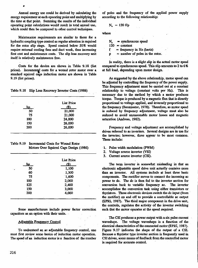
0
Annual energy use could be derived by calculating the energy requirement at each operating point and multiplying by the time at that point. Summing the results of the individual operating point calculations would result in total annual use, which could then be cofIlpated to other control techniques.
Maintenance requirements are similar to those for a hydraulic coupling type control as regular attention is required for the rotor slip rings. Speed control below 50% would require external cooling fans and duct work, thus increasing first cost and maintenance costs. The slip loss tecovery unit itself is relatively maintenance free.
Costs for the device are shown in Table 9.18 (list prices). Increment$! costs for a wound rotor motor over a standard squirrel cage induction motor a r ~ shown in Table 9.19 (list prices).
Table 9.18 Slip Loss Recovery Inverter Costs (1986)
a 50 75
100 150 200
List Price 0
21,000 21,000 24OOo 26,000 26,000
Table 9.19 Incremental Costs for Wound Rotor Motors Over Squirrel Cage Design (1986)
A 50 60 75
100 125 150 200
List Price 0
1,100 1,300 1,600
2,000 2,400 3,000 4,000
Some manu€acturers include power factor correction capacitors as an option with their units.
Adiustable Fmencv Control
To un@rstand an ac adjustable frequency controi, one must first review some basics of induction motor operation. The speed of an induction motor is a function of the number
216
of poles and the frequency of the applied power supply according to the following relationship:
N, = 120flp
where
N, =syncbnousspeed 120 = constant f p
= frequency in Hz (hertz) = number of poles in the rotor.
In reality, there is a slight slip in the actual motor speed compared to’ synchronous speed. This slip amounts to 2 to 6 % at full load, depending upon motor design.
As suggested by the above relationship, motor speed can be adjusted by controlling the frequency of the power supply. This frequency adjustment must be &ed out at a constant relationship to voltage (constant volts per E). This is necessary due to the method by which a motor produces torque. Torque is produced by a magnetic flux that is directly proportional to voltage applied, and inversely proportional to the frequency (Baumiester, 1978). Therefore, as motor speed is reduced by frequency adjustment, voltage must also be reduced to avoid unreasonable motor losses and magnetic saturation (Andreas, 1982).
Frequency and voltage adjustment are accomplished by drives referred to as inverters. Several designs are in use for the inverter; however, three appear to be most common. These include:
1. Pulse width modulation (PWM) 2. Voltage source inverter (VSI) 3. Current source inverter (CSI).
The term inverter is somewhat misleading in that an electronic adjustable speed drive unit acfually contains more than an inverter. All systems include at least three basic components. The rectifier serves to connect the incoming ac power to dc. The dc is then fed to the inverter section for conversion back to variable frequency ac. The inverter accomplishes the conversion task using either transistors or thyristors. These electronic devices switch the dc input (from the rectifier) on and off to provide a controllable ac output (EPRI, 1987). The third major component in the drive unit, the controls, regulates the activity of the inverter switching such that the motor operates at the speed required.
The CSI produces a power output with a six pulse current waveshape. The voltage waveshape is a function of the electrical characteristics ofthe connected motor (EPRI, 1987). Figure 9.17 indicates the shape of the output of a CSI. Because a thyristor type inverter section is frequently used in CSI drives, some means of feedback from the controlled motor is required for accurate control.

L i n e Voltage s i x step variation of current and frequency.
> 0 Z W H u H BO IL
t- 0 u z Bo
Variable Voltage Inverter Pulse width Modulatiop! (WI) (FWM)
Line Current . L i n e Cutrent
Six step variation<of voltage and frequency-
Varying pulse length at constant voltage. -
Figure 9.17 Generaked waveforms for djustable frequency drives (Bell and Gossett, 1988).
100% SPEW
I I I I I e0 40 60 BO 100
PERCENT FULL LOAD TORQUE
Figure 9.18 Adjustable frequency drive performance.
217

The voltage source inverter, like the CSI, produces a six pulse output pattern. . In this case, however, the voltage is pulsed (Figure 9.17) and the current is a function of the motor characteristics. The VSI drive has the capability to control two half size motors (two 50 hp motors on a 100 hp unit) at the same time.
The PWM drive employs a voltage source inverter that produces positive and negative voltage pulses of different widths (EPRI, 1987). As indicated in Figure 9.17, motor current is a system using a PWM drive in close approximation to that in a non-adjustable speed drive application.
The heating effect of the frequency controller upon the motor can be compounded by operation at constant torque. Under a constant torque load, as speed is reduced, motor current remains fairly constant because of the load. As a result, motor losses and heating are also constant. However, the self cooling p r o d u d by the motor fan is reduced by the lower speed. This raises motor winding temperature. Tem- perature rise reaches 212°F at 75% speed, 320°F at 35% and 428°F at 20% speed and full load (Andreas, 1982). Although most manufacturers state that these controllers can be used with standard induction motors, it would be wise to employ motors with high-temperahue insulation characteristics.
Efficiency of adjustable frequency drives is generally quoted by the manufacturers at 95 96. This value applies only to the base frequency, which is usually 60 Hz (Andreas, 1982). Figure 9.18 shows efficiency at other operating points. The plot is based only on the efficiency of the frequency controller. Sinusoidal motor performance at the same torque must be considered to arrive at drive efficiency. For example, at 50% speed and 75% torque, a value of approximately 88% is read from the diagram. In order to obtain drive efficiency, this value would be multiplied by the motor efficiency at that point (75% torque). Assuming a 100 hp motor, this value might be 90%. As a result, drive efficiency would be 0.90 x 0.88 = 0.792. Using the same pump figures from the example in the wound rotor section (50 hydraulic horsepower requirement, 60% pump efficiency), a total electrical input of SOl(0.792 x 60) = 105 hp, or 78.5 kW results.
When selecting a adjustable frequency drive, users should be careful to specify a high power factor. All types show relatively high (95 %) power factor at full load, however, some drop off considerably as motor load diminishes. Generally, drives employing a diode bridge-type rectifier will maintain a consistently high power factor regardless of load or speed. The diode bridge connection is most commonly found in pulse width modulation (PWM) drives. Recent advances have brought the cost of constant (kigh) power factor drives down to the point where they are competitive with variable power factor drives.
218
Low maintenance is required fot the adjustable frequency drive. The controller itself is constructed primarily of solid state components that require virtually no attention. However, the controller units sometimes have maximum and minimum temperature limits, As a result, they would have to be housed in some type of umditioned wellhead structure for protection. Both oil and air cooled units are available. For many geothermal applications, the oilcooled unit (which is suitable for outdoor installation) would be useful in eliminating exposure of electrical components to hydrogen sulfide (€I$) environments. The adjustable frequency type of speed control is the only one that would permit system operation in the event of controller failure because electrical supply to the motor could be routed around the invertor. List prices are shown in Table 9.20 accorcling to hp requirements. These figures are for the inverter only and additional costs would be incurred for control interface, starter, manual or automatic bypass equipment.
Table 9.20 Adjustable Frequency Inverter Costs (1986)
hD 25 50 75
100 150 200 250 500
List Price * 8,600
13,500 15,500 20,500 23,300 30,000 3 1,300 34,600
Shaft-Oriented Control
1. Eddy Current Coupling
As a shaft oriented device, the eddy c u m t coupling is placed between the driving motor and the driven shaft as shown in Figure 9.19. The coupling consists of rotating input and output portions that are not mechanically coupled. The dc current from an external field coil excites the winding on the output member. This induces eddy currents in the input member, resulting in a torque at the output shaft. Flow control is accomplished by adjusting the field current (Lienau, 1984).
An eddy current coupling is considered a slip loss type device. The slip loss is a function of the transmitted torque and the slip or the difference in the speeds of the input and output shafts are shown as:
Slip Loss = 2x x h m out - mm in) x tomue 33,000

1
i
i i
,
I
I
i
i
~
I
LINE I N
REGULATOR E TO SPEED CONTROLLER
Figure 9.19 Eddy current coupling.
For constant torque loads or for large slips (speed reduction), this loss is a significant amount. In fact, the overall efficiency of the eddy current coupling can never exceed the ratio of output to input speed. Because of the slip loss, this type of device is best applied to loads that do not experience a large speed reduction. In addition to slip loss, the eddy current coupling also experiences friction and windage losses of approximately 1.5% of input (Andreas, 1982). This loss is constant over the entire speed range. Losses resulting from exitation are very small and decrease with output speed.
nature of the eddy current coupling that it isbest applied in situations where output speed is in the 23% or above range, in order that efficiency is comparable to other drives. Costs for eddy current couplings are shown in Table 9.21.
Maintenance requirements for eddy current couplings are relatively low as there are no external moving parts or equipment requirements.
. Table 9.21 Eddy Current Coupling Costs (1986)
List Price hb ($,
5 7.5 10 15 20 25 30 40 50 60 75 100 125 150 200
2,275 2,900 3,320 3,816 4,297 5,110 5,412 6,500 7,707 8,556 9,844 11,716 13,612 16,167 19.618
w 40 eo 00 IO0
, PERCENT FULL SPEED
Figure 9.20 Eddy current and fluid coupling performance.
Figure 9.20 shows a plot of eddy current coupling efficiency versus percent speed. In order to calculate overall system efficiency, pump and motor efficiency would have to be considered. For example, a motor driving a pump with a 50 hydraulic hp requirement at 75% speed and 50% torque, drive efficiency from Figure 9.20 would be 73.8%. Assuming a 60% pump efficiency and 90% motor efficiency, this would result in an input requirement of 50/(0.738 x 0.90 x 0.60) = 126 hp, or 93.6 kW. It is apparent from the slip loss
2. FluidCoupling
The fluid coupling falls into a class of fluid drives know as hydrokinetic. Like the eddy current coupling, the fluid coupling consists of input and output members that are mechanically independent. The impeller (input member) accelerates the oil, which then enters the runner (output member) where it is decelerated and the kinetic energy in the fluid is converted into shaft power (Andreas, 1982). As shown in Figure 9.21, the level of oil in the impeller/runuer area is varied by a scoop tube to adjust speed output. Lost energy or inefficiency is dissipated as heat. This heat is rejected to an external heat exchanger. Speed reduction capabilities are 4:l with a constant torque load and 5:l with variable torque loads. Sizes range from 5 to several thousand hp.
A fluid coupling is a slip loss type device the same as the eddy current coupling. Efficiency is primarily a function of the slip or the difference in the input and output shaft speeds. Losses amounting to approximately 1.5 96 of unit rating are experienced because of parasitic losses for oil
219

cooling and circulating (Andreas,1982). Figure 9.20 illustrates typical unit efficiency. The values are very comparable to, though slightly less than those of the eddy current coupling. Steady state and annual energy calculations are similar to those described in previous sections. Costs for fluid couplings are shown in Table 9.22.
Maintenance requirements of the fluid coupling itself are relatively low. However, the external heat exchanger and circulating pump increase requirements above those for the eddy current coupling.
n
Figure 9.21 Fluid coupling.
J 4 I- O I-
\ E ---
Table 9.22 Fluid Coupling costs (1986)
List Price hb A
10 9,300 25 1 0 , m 50 10,700
125 12,300 200 16,500
9.2.3 Adiustable Sueed Drive Considerations
Calculatinz S W Reuuirements
In order to apply the variable speed drive, it is necessary to understand the affects of speed variation on the pump characteristics. Within limits, centrifugal pump affinity laws state that:
1. Flow rate a pump rpm 2. Pump head a (pump rpm)' 3. Brake hp a (pump rpm)'.
Using these proportionalities, a pump curve for any speed within the u s e l l limits can be generated. For instance, from the pump curve used earlier (Figure 9.4), at 700 gpm the head is 29 ftlstage, efficiency is 78% and brake hp 6.5 hplstage
I NEW FLOW AM) H E A D Y
=" 1 0 1 I I I I 8 1 I
I 8
LOO 200 300 400 500 700 800 64i 0
- 8
-6 a I -4
2
CAPACITY (gpm) Figure 9.22 Single stage pump curve (Aurora Pump).
220

when the pump is run at 1770 rpm. To find the characteristics at a reduced speed of 1622 rpm (which is equivalent to 55 Hz operation with an adjustable frequency drive) where:
Flow = 700 gpm = 641.5 gpm 1770 rpm
Head = (1622 r~m)~(129' Wstage) = 24.4 ftlstage 1770 rpm
hp = (1622 1vm)~(6.5 hp/stage) = 5.0 hp/stage. 1770 rpm
Efficiency at the old head versus rate point is moved to the new head versus rate point. The new points are shown in Figure 9.22.
Using the proportionalities, a new pump curve can be generated for 1622 rpm or a family of curves for any desired rpm. This is what was done to generate the family of curves shown in Figure 9.23. Note that the curves are for a 12-stage pump. The total dynamic head is shown, rather than the head per stage.
Temmrature .Increase Considerations
To further illustrate another point, refer to the previous example where there is a 350 ft static level and 50 ft draw- down of 0.963 specific gravity fluid. The lift head is 400 ft. The pump chosen has 19 stages, producing 700 gpm at 29 ft per stage; or 551 ft TDH, and requires 6.5 x 0.%3= 6.26 hp per stage.
The zero flow speed, or the speed where that pump would just maintain fluid at the surface, can be found by:
New Speed = (New Head)' x old speed Old Head
New Speed = (400 ft)' x 1770 rpm = 1508 rpm. 551 ft
At that point, the pump would be dissipating brake horsepower speed (bhp) &own as:
New bhp = (new mm)3 x old bhp old rpm
CAPACITY (Qpd
Figure 9.23 Pump characteristics for 12 stages.
221.

New bhp = (1508 mmr x (6.26 bhplstage x 19 stages) 1770 rpm
New bhp = 73.55 bph
(73.55 bhp) (42.41 BtulminJ = 3119.3 Btulmin. hP
Because the pump is already operating in hot fluid and there is no flow to carry away heat, the first stage bearings soon have water vapor lubrication rather than water lubrication, increasing the heat further. This leads to drastically premature pump failure.
The temperature rise at no flow can be approximated by:
T r = C m x P x w x c
where
Tr = temperature rise, OF/&
Cm = 42.41 Btulmin hP
Ps = shut offhp W = weight of liquid in pump, lb C = specific heat, Btunb OF.
The volume of water in a pump stage is not usually given in pump specifications, but with an estimate of 3 gallstage we will have 476 lb in the 19-stage pump. At no flow, the water level will soon reach static level of 350 ft, giving 160 ft of submergence (allowing 50 ft for the length of the bowl assembly), and an absolute pressure of 79.8 psi (at 0.963 specific gravity and 5000 ft altitude). This corresponds to a saturated steam temperature of 310°F and indicates that water in the pump will start to boil in - 17 min.
The actual time will be a little longer, because some heat will be transferred to the water but, in any case, the pump will cavitate, clearances will change, collets, keys and set screws loom and bearings overheat in a relatively short time.
Similar, though perhaps not so drastic, things occur in a pump that is throttled with a valve. All the energy that is not COIlverted to water energy goes into heat. As long as some flow exists, the temperature rise c811 be approximated by:
Tr = Cm x PlbhDH1-E) Qwxc
where
P(bhp) = pump brake horsepower E = efficiency, decimal Qw = flow through the pump, lblmin
other terms as above.
Because variable speed drives are often used in space heating applications where there may be no flow requirements for substantial periods of time, it is important to maintain some minimum flow for cooling. The pump manufacturer should be consulted to determine what that minirmUn flow is. With constant speed pumps, an orifice or bypass control valve can be used with discharge back to the well or through the system. With variable speed drives, the lower speed limit must be set to attain the minimum flow. That flow can be diverted back to the well through an orifice or valve, or through the system. In any case, it will result in increased pumping costs, but should pay for itself in decreased main- tenance. Discharge back to the well is usually preferred, because the resource in conserved.
9.5 RECIRCULATION
Recirculation is a somewhat poorly understood phenomenon that occurs at decreasing flow rate in all centrifugal pumps. A portion of the flow reverses at the impeller suction or discharge, resulting in high shear velocities vortices (Figure 9.24). Within the vortices, low pressure is created. When the pressure reaches the vapor pressure, bubbles are formed that subsequently collapse, resulting in cavitation. In addition to cavitation damage to the impellers, vanes, shrouds, and stationary vanes of the casing, the formation and collapse of bubbles cause high frequency vibrations and thrust reversals, resulting in bearing damage and shaft failures.
As far as is known, failures caused by recirculation have not been observed in geothermal lineshaft or submersible pumps. Apparently, the problem is more severe in larger pumps with high specific suction speeds and high efficiencies. If the ratio of impeller eye diameter to outside (OD) diameter is >0.5, discbarge recirculation occurs before suction recirculation. Recirculation usually occurs at 50 to 65% of rated capacity, depending on the eye to OD ratio. The onset of recirculation is indicated by a sudden increase of pressure fluctuations at the suction or discharge, which may reach 60 to 90 psi, resulting in vibration and noise. These indications could be noticed in a surface pump but would be difficult to detect in a pump set deep in a well.
222

Svstem Examle
In order to evaluate the relative merits of some of the above described speed control techniques, the following example has been prepared. Information was taken from a well currently operated by the Oregon Institute of Technology.
*
Static water level 360 ft Drawdown Minimal (not considered) Peak production rate 450 gpm Wellheadpressure 20psi
Duty cycle As in Table 9.23 Pump efficiency As shown in Figure 9.23 Motor efficiency Assumed at 0.90
Motor hp 75 hp 8ucTIoN - DXSCHARGE -
RECfllCUUTION RECIRCULATION
I
Figure 9.24 Recirculation in centrifugal pumps (Plant Engineering).
a. In all centrifugal pumps, recirculation at the inlet occurs at some point as the flow rate decreases.
Recirculation cavitation damage possibly has been mistaken for NPSH cavitation damage. In cavitation caused by insufficient NPSH, cavitation occurs on the low-pressure side of the vanes. Both suction and discharge recirculation cavitation erosion occurs on the high-pressure side of the Vanes.
Although there have been no reported problems, the engineer or pump user should be aware of possible probleins when high efficiency pumps are throttled, as is often the case in space heating applications. Frasier provides equations for dculating the flow at both suction and discharge recirculation onset (Frasier, 1981). Flow is directly proportional to rpm, and flow control through the use of variable speed drives would reduce the possibility of problems, unless high lift conditions result in essentially the same situation as throttling.
This well supplies 191°F geothermal fluid for use in winter space heating, summer cooling (by way of an absorp- tion chiller), and a very small domestic hot water heating duty.
Based on the information above, and that umtained in Table 9.23 and Figure 9.23, four methods of flow were com- pared. These included. (a) throttled output, (b) wound rotor motor with slip recovery, (c) ac adjustable frequency control, and (d) fluid coupling. Calculations for electrical c o v t i o n were made at each production level and summed to arrive at annual use, as suggested in the previous sections. Table 9.24 rmmmafizes the results of the energy mnsumption calculation. It is important to point out that this example is based on a 100% static head. As a result, savings are not as great as would be expected if there was a large friction head on the system.
Table 9.23 OIT Well #5 Duty Cycle
Flow Hours1 (mm) Year
25 78
450 400 380 82 340 150 300 476 260 225
675 1,132
200 235 190 1,044 150 4,862
223

I
i
.
50
c5
3 Y
l- 3 a Z H
[5 w 30 3 0
40
a .
20
I I I I 20 40 60 80 ibo
PERCENT FLOW
Figure 9.25 Energy requirements for four control methods.
As shown in Table 9.24, the wound rotor motor with slip m v e r y shows the best performance, followed closely by the ac variable frequency control. The fluid coupling does surprisingly well in this case. This is because of the combined effect of the pump performance and large static head. The minimum speed of the pump in this example is - 70% of full speed. Because fluid coupling efficiency is primarily a function of input and output speeds, efficiency remains high. In a situation in which there is a lower minimum shafi speed, 8 greater difference would be seen between the variable frequency drive and the fluid coupling. Figure 9.25 shows the energy requirement in kilowatts versus percent peak flow for
Table 9.24 Results of Energy Use Calculations
Flow Control Method berm Use in kWhlYear
Throttle 473,6 14 Fluid coupling 298,306 Adjustable frequency 243,816 Wound rotor w/slip recovery 226,043
each of the four control methods. For comparison purposes, theoretical energy requirement is also shown. This is based upon hydraulic horsepower converted directly to kilowatts (Le. assuming 100% pump and driver efficiencies).
Table 9.25 Flow Control Life Cycle Cost Comparisons
Throttling Valve 0 24 21,313 Fluid Coupling 11,000 330 13,424 ACFrequency Drive 16,000 240 10,972
a. Mation at 5961~. b. Electrical inflation at 2%/y (real). c. Maintenance at O%/y (real).
224

Table 9.26 Summary of Speed Control Techniques
Capital Maint. Overspeed Effecton Turn afficiency Cost Reauid CaDacitv Motor Life Down
Woundroto? High High Moderate Y wlslip recovery
Adjustableb High Moderate LOW Y . frequency (ac)
Fluidc Moderate Moderate Moderate ' N coupling
Eddycurrent" Moderate Moderate Moderate Y coupling
Multi-speed" Moderate LOW LOW N motors
lllrottlillgf very LOW LOW N low
None 2: 1
Lowers Inf.
None 4: 1 $5: 1
None 2 0 1
None 2: 1
None No limit
Auto Size Control Ranee Confirmation
Y 'Verticle
.Y Fractional N/A to several . hundred
Y S - 10,OOO Verticle hp Horizontal
Y Verticle Horizontal
Y Fractional Verticle toseveral Horizontal hundred
Y No N/A limit
a. Can go beyond 2: May require extend cooling. Generally applied to very large motors or where Power Factor correction is needed.
b. Allows motor operation in failure mode. Should use high temperature rise motors. Minimum ambient temperature 50°F.
c. d. e.
I f .
Poor efficiency at low output speeds. Capital cost - 30% less than variable frequency. Poor efficiency at low output speeds. Stopped output speed in 2 or 4 increments must throttle in between, +ssible problems with shaft and bearings. Should be considered only for very small applications or in csnjunctionwi~ another method, Le., multi-speed.
Aswith any energy saving strategy, the magnitude of the energy savings is only one part of the story. Costs for maintenance, fuel, energy, and capital are equally important. In order to evaluate the options discussed above, in this light, life cycle costs have been calculated for three of the systems (current costs .for wound rotor slip loss recovery were not available). Table 9.25 summarizes theLinput.
incremental investment in the fluid coupling over the mg valve shows a 20-y savings Of $335,428
($1 15,635 disqwnted at a simple payback of 1-15 years. There is no ques e fluid coupling would %e the wiser approach of the two. The incremental investment in the adjustable frequency drive over the fluid coupling shows 8 cumulative 20-y savings of $1 10,682 ($38, ted at 10%) andla simple payback of 1.79 years.
Because of the simplicity of the analysis, fhese two figures, 1.79 versus 1.15 y, can be considered as equal. As a result, the choice between the fluid coupling and adjustable frequency drive would be based on other considerations such as maintenance, ease of installation, torque and speed requirements.
Conclusion
Among the various drive technologies available, the choice is a function of a host of project specific parametenr. The. information presented here, along with pump and well in- formation from your project, should permit an accurate analy- sis to be carried out. The results of this analysis cm then be employkd in the decision process. Table 9.26 Summarizes the various characteristics of thespeed con techniques outlined herein.
225

9.6 LESSONSLEARNED
Listed below are a number of factors relating to pumps that can lead to premature failure of pumps and other components. Many of these have been noted or alluded to elsewhere, but are restated here. Some seem obvious, but the obvious is often overlooked.
1.
2.
3.
4.
5.
6.
7.
Pump suppliers/manufacturers should be provided with complete data on all foreseen operating conditions and complete chemical analyses. Standard potable water analysis is not adequate, because they do not test for important constituents.
In general, continuous or nearly continuous operation of well pumps is p r e f d . Short cycle stadstop operation is to be avoided. This is particularly true for open lineshaft pumps. When the column drains, bearings and the inside of the column are exposed to oxygen, leading to corrosion.
Stadstop operations necessitate a storage tank. This is often a source of air in-leakage. Parts per billion (ppb) of oxygen (09 in combination with ppb hydrogen sulfide (H$) can lead to early failure of copper and copper alloys, dezincification of brass and bronze and soldering alloys used in valves, fan coils, and piping.
Stadstop operation imposes high shaft and coupliug torque loads. It is believed this has led to early failure of lineshah and lineshafl to motor couplings.
Records of pressuff and flow versus rpm or power should be kept on a mgular basis. Decreases in flow or pressure indicate something is wrong and are a portent of more drastic trouble that could OCCUT later 011.
Pumps should be pulled and inspected on a regular basis, baed on experience or as recommended by the man*-.
Some miuimum flow must be maintained. Relatively short periods of operation at shutoff will overheat pumps and motors.
Motors should be well ventilated. Although this seems obvious, several motors have been installed in below ground unventilated pits. With piping at 200°F in close proximity, the motor is near its upper operating temperature before the power is turned on.
Packing glands should be well maintained. All above
packing glands, especially if starting at lowsuctirm surface Centrifugal PUXIIPS tend to in-leak air through
pressure. Air in-leakage leads to corrosion. Leaks around lineshaft packing lead to corrosion/scaling of the shaft, making sealing progressively more difficult.
8. Enclosed lineshaft pumps require that lubricant (water or oil) be supplied before the pump is started. It has been observed that installations where the lubricant flow started and stopped simultaneously with the pump motor, . pumps failed prematurely.
As noted in Chapter 8, almost without exception, . geothermal fluid contains some H$. If a start/sbp mode of operation is used, air is drawn into the system when fluid drains down the column after the pump stops. This can cause a greatly accelerated rate of pitting corrosion in carbon steels, formation of cuprous sulfide films, and crevice coTToGioll of copper, brass and bronze (except leaded brass and bronze), &-alloying of leadltin solders and dissolution of silver solder.
GLOSSARY
Static Water Level (SW) - The distance from the surface at which water stands in the well in the static (no pumping) condition.
Pumping Level or Lift - The distance from the surface to water under specified pumping conditions, Le. 400 ft @ 700 gpm. Pumping level increases as pumping rate increases. pumping level equals swl + drawdown.
Drawdown - The distance from static level to pumping level under specified conditions.
Pump Setting - The distance from the sur€w to the pump inld.
Total Dynamic Head (TDH) - The total head reqired of the pump under specific conditions. TDH equals lift + col- umn or tubing friction head + friction head in swface piping and equipment + lift head on the nuface + any discharge pressure nquired at system outlet. TDH will vary with pumping rate.
Net Positive Suction Head (NPSH) - The head, in feet, re quirea above the pump inlet for proper operation. NPSH
ture and elevation. Additional head will be required for tail pipe, inlet screens, flow inducers, etc.
varies with pump rate, pump rotatid speed, tempera-
Wireto-Water Efficiency - Ratio of the energy input at the pump motor terminals to the theoretical pumping requirement.
226

REFERENCES
Amqrican Society of Heating, Reftigeration and AirCon-
Equipment Volume", Nerican Societv of Heating Refrigeration and Air Conditionine Svstems, New York,
diti&g Engineem, "ASHRAE Handbook - 1983
NY, pp. 3.26-3.27, 1983.
Andreas, John C., "Energy Efficient Electric Motors", Defier, New York, NY, pp. 120-153, 1982.
Aurora Pumps Catalog, Engineering Manual Section, 1981.
Badester, T., Editor, "Marks's Standard Handbook for Mechanical Engineers", McGraw-Hill, New York, NY, pp. 15.46-15.51, 1978.
Bell and Gossett, Bulletin, "D-1 1OA-Power AC pumping Systems", ITT Corporation, Morton Grove, IL 1988.
htrilift Hughes, Submersible Pump Handbook, 1983.
Cherry, R. C., "Analyzing Low Flow in Vertical Turbine Pumps", Plant Engineering, April 23, 1987.
Electric Power Research Institute, "ASD Directory Adjustable Speed Drives", 2nd edition, EPRI, Palo Alto, CA 1987.
Frasier, W. H., "Recirculation in Centrifugal F%mps", paper presented at 1981 ASME conference, New'York, NY, 1981.
Frost, J., "Introduction to Geothermal Lineshaft Production pumps", Johnston pump Company.
Frost, J., Personal communication, Johnston Pump Company, Glendora, CA, 1988.
Lienau, P., "Direct Use Downhole Pumps", presented at
of Geothermal Brine, Los Angeles, California, March 1984.
Geothermal Resources Council, Short Course - pumb inq
Training and Retraining Jnc., "Motors and Generators -How They Work," Sans and Co., Inc., IndianapoIis, Indiana, pp. 180-192, 1982.
227


CHAPTER 10 PIPING
/ By Kevin D. Rafferty, P.E. OIT Geo-Heat Center
Klamath Falls, Oregon 97601
10.1 INTRODUCTION
The source of geothermal fluid for a direct use appfication is often located some distance away from the user. This requires a trammission pipeline to transport the geothermal fluid. Even in the absence of transmission line requirements, it is frequently advisable to employ other than standard piping materials for in-building or aboveground piping. Geothermal energy for direct use applications is usually transported in the liquid phase and has some of the same design considerations as water distribution system. Several factors including pipe material, dissolved chemical components, size, installation method, head loss and pumping requirements, temperature, Mation, pipe expansion and service taps should be considered before final system selection.
In several installations, long transmission pipelines appear to be economidy feasible. Geothermal fluids are being transported up to 37 mi in Iceland (Katlsson, 1982). In the U.S., < 5 mi is generally considered economical; however, the distance is dependent on the size of the heat load and the load factor.
piping materials for geothermal heating systems have been of numerous types with great variation in cost and durability. Some of the materials which can be used in geothermal applications include: asbestos cement (AC), ductile iron @I), dip-joint steel (STL-S), welded steel (STL- W), gasketed polyvinyl chloride (PVC-G),- solvent welded PVC (PVC-S), chlorinated polyvinyl chloride (CPVC), polyethylene (PE), polybutylene (PB), mechanical joint fiberglass reinforced plastic (FRP-M), FRP epoxy adhesive joint-military (FRP-EM), FRP epoxy adhesive joint (FRP-E), FRP gasketed joint (FRPS), and threaded joint FRP (FRP-T). The temperature and chemica! quality of the geothermal fluids, in addition to cost, usually determines the type of pipeline material used. Figures 10.1 and 10.2 introduce the tempera- ture limitations and relative costs of the materials covered in this chapter. Generally, the various pipe materials are more expensive the higher the temperah= rating.
Installation costs are very much a function of the type of joining method employed and the piping material. The light weight of most nonmetallic piping makes handling labor significantly less than that of steel and ductile iron in sizes greater than 3 in.
3 ’ 4 ‘ 5 ’ 6 RPiW rype
I I I
1. cruborrsteel 2 m E p a c y 3. FRP pcrvester 4. Ac 5. $0 6. CPJC 7. pircruelmil 8. wc e. PE
I I I
7 ’ 8 ’ 9
Figure 10.1 Maximum service temperature for pipe XMteXialS.
10.1.1 Pining Currently in Use
The following data was taken from a recent survey (Rafferty, 1989) of 13 operating geothermal district heating systems. The total main line (> 2 in.) piping included in the system reviewed for that report amounted to approximately 269,000 linear feet (lo. *
Figure 10.2 provides a breakdown of the total piping by type. As indicated, asbestos cement (AC) material is clearly the most widely applied product with approximately 5596 of the total piping in these systems. Steel and fiberglass are
Figure 10.2 Relative cost of piping by type.
229

distant m d to AC. only minimum quantities Of polybuty- lene, ductile iron and PVC are in use. Of note is the fact that there is increasing interest in ductile iron. Its relatively low cost and simple installation techniques are similar to the now unavailable AC pipe. The PVC currently in use is all uninsulated piping in use on the collection network of one of the low temperature systems.
District heating systems can be designed as "open" or "closed" distribution networks. In the open design, the geothermal fluid is delivered directly to the customer. Waste or cooled fluid is collected in the return piping for delivery to the disposal facility. Closed systems, on the other hand, employ central heat exchangers to isolate most of the district system from the geothermal fluid. Heat is delivered to the customer via a "closed loop" of clean treated water.
The characteristics of open and closed systems are quite different. For example, closed systems generally employ insulated piping for both the supply and return piping; whereas, open systems use insulation only on the supply piping. More importantly, open systems expose all of the piping to the geothermal fluids and as a result, corrosion considerations are mote critical to these designs. Finally, the cost of closed system is generally much higher than open systems. This is the result of costs associated with the central plant and the more extensive use of insulated piping.
Figure 10.3 provides a breakdown of total piping with respect to quantities used in open and closed distribution systems. As indicated, open systems constitute most of the piping applications.
Figm 10.3 Comparison of total amount of pipe used in open and closed geothermal district heating.
For the piping used in the closed distribution systems, Figure 10.4 provides a breakdown by type. Clearly, steel piping is the choice for this application.
Figure 10.4 Distribution of piping used in closed loop geothermal systems.
Figure 10.5 provides a similar breakdown for piping used in open systems. Again AC pipe has obviously been the mated of choice for applications in which the pipe must be exposed to the geothermal fluid. Asbestos cement far exceeded its closest competitor (FRP - 18 96) for this applica- tion. The previous popularity of AC, coupled with the Edct that it is for practical purposes no longer available, under- scores the need to identify a low cost alternative for this application.
PB (4.9%)7 rSteel (10.2%)
Figure 10.5 Distriiution of pipe used in open geothermal district heating systems.
None of the geothermal district systems reviewed uses piping larger than 14 in. A breakdown of piping by size appears in Figure 10.6.
230

Figure 10.6 Size distribution of piping in geothermal district heating systems.
As discussed above, many of these systems employ uninsulated piping on the return (or disposal) side of the distribution system. As indicated in Figure 10.7,. fully 27% of all distribution piping in these systems is uninsulated. The prospect for increased use of uninsulated material in future system is discussed later in this chapter.
2 in. (8.3%)~ j-14 &I. (6.4%)
6 in. (24.2%) 8 in. (16.8%)
Figure 10.7 Comparison of relative amounts of insulated and nnindated pipe in geothermal district heating systems.
10.2 PIPE MATERIALS
Both metallic and nonmetallic piping can be considered for geothermal applications. Carbon steel is the most widely used metallic pipe and has an acceptable service life if
installation crews. The advantage of nonmetallic materials is that they are virtually impervious to most chemicals found in geothermal fluids. However, the installation procedures, particularly for fiberglass, polyethylene and polyhtylene are, in many cases, outside the experience of typical laborers and local code officials. This is particularly true in rural areas. The following sections review some specifics of each material and cover some problems encountered in existing g e o t h e d Systems.
10.2.1 Carbon Steel
Available in almost all areas, steel pipe is manufactured in sizes ranging from 114 to over 72 in. Steel is the material most familiar to pipe fitters and installation crews. The joining method for small sizes (<2-1/2 in.) is usually threading, with welding used for sizes above this level (Khashab, 1984). For underground installations, all joints are typically welded when unlined piping is used. For epoxy- lined piping, some form of mechanical joint should be employed so that welding does not interfere with the integrity of the fining mated. Commonly used steel pipe ratings are Schedule 40 (standard) and Schedule 80 (extra strong). In most cases, in the U.S., Schedule 40 piping is used for heating applications, although, in Europe and for some newer non-geothermal district systems in the U.S., lighter weights (approximately Schedule 20) are now used. Schedule 80 is employed for high pressure applications or in cases where higher than normal corrosion rates are expected.
Corrosion is a major concern with steel piping, parti- cularly in geothermal applications. As mentioned above, some allowance can be made by using the thicker-walled Schedule 80 ,piping. However, this approach is valid only for uniform corrosion rates. In many geothermal fluids, there are various ConCentrsLtions of dissolved chemicals or gases that can result primarily in pitting or crevice corrosion. If the potential exists for this type of attack, or if the fluid has been expose(t to the air before entering the system, carbon steel should be the material of last mort.
Steel piping is used primarily on the clean loop side of the isolation heat exchanger, although in a few cases it has been employed as the geothermal transmission line material.
A distinct disadvantage in using steel pipe is that the buried pipe is also subject to external COKOS~OII unless protected with a suitable wrapping or cathodic protection. For example, the distribution system at Oregon Institute of Technology originally consisted of carbon steel pipe with a rigid foam cellular insulation wrapped with a mastic saturated with an asphalt material to provide a seal. 'The water seal
23 1

considexh for all direct buried installations. Various soil types, presence of groundwater, and induced current fields from power lines may accelerate external pipe corrosion and early system failure.
In at least two geothermal systems, unlined steel piping has performed well in normal operation but has suffered severe pitting corrosion during system shutdowns. In one case in which a system was down for - 6 months, carbon steel piping exhibited pitting corrosion rates of 70 to 200 milsly (my) (Ellis, 1981). If unlined steel piping is employed on the geothermal si& of the system, it is most critical to assure a complete drying of the material for extended shutdowns.
In both buried and aboveground installations, allowances for expansion must be made in the form of expansion joints or loops. These umsiderations have the effect of increasing both the labor and material costs of the piping system.
Galvanized steel has been employed with mixed SUCC~SS
in geothermal applications. Some geothermal fluids have demonstmted the ability to leach zinc from solder and other alloys. Selective removal of the zinc from galvauiz.ed pipe could result in severe pitting corrosion. In addition, umsideration should be given to the fact that the prohibitive nature of the zink coating is generally not effective above 135°F.
An indication of the costs for steel piping is shown in Table 10.1.
Table 10.1 Steel Piping Costs, Material Only (Means, 1990)
Size Schedule 40 Schedule 80 (in.) c$nn tsnn
2 2.27 2.54 4 6.16 8.22 6 12.32 22.08 8 16.52 33.14
Reference standards:
1. Pipe, American Society of Testing and Materials (ASTM) A-120, A-53.
2. Fittings, American Staudards Association (ASA) B16.9 (welded).
10.2.2 Ductile Iron
Ductile iron is similar to cast iron with the exception of the form of the carbon component. In cast iron, the carbon (graphite) is in a flakelike structure. In ductile iron, the structure is more spherical or nodular. This small difference results in the greater strength, flexibility, and machinability from which the product derives its name. Table 10.2 outlines physical properties of this material. Ductile iron has been described as more cortosion resistant than cast iron. However, the slight difference in camsion resistance would not be of any substantive meaning in-most geothermal applications.
Table 10.2 Physical Properties of Ductile Iron Pipe
Value Coefficient of expansion Thermal conductivity Specific gravity 7.12 Hazen - Williams flow factor
5.8 x 106 in./in."F 240 Btu in.h ft2 O F
140
Cast iron piping was employed for over 80 years in the . Warm Springs geothermal system (Boise, ID). Neither cast nor ductile iron has seen any substantial application in modern g e o t h e d systems.
As an iron material, ductile iron is susceptible to comion from both external and internal sources. External protection generally involves a moisture barrier. For a pre-insulated product, special moisture protection would only be required at the joints and other fittings.
. Internal corrosion protection is usually provided by a lining. The two most common materials are cement mortar and coal tar epoxy. coal tar epoxy is limited to a temperature of - 120°F. Mortar lining, according to the Ductile Iron Pipe Producers Research Association, is suitable to a service temperature of 150°F with a protective seal coat. Without the seal coat, maximum service temperature is 212°F. In some applications with very soft water, a leaching of the mortar lining has been observed when a seal coat is omitted (Fisher, 1987). As a result, a special high temperature epoxy coating would be required. Unfortunately, quotes received by the San
California, Geothermal District Heating System) for linings of this type for 130°F application would add $5.00 to $8.00/ lineal foot to the price of the pipe (Fisher, 1987). In applications where water chemistry is such that bare cement lining is acceptable, ductile iron could be a economical piping choice.
Bemardino Water District (operators of the San Benrardin 0,
232

Ductile iron is a much-thicker-walled product than standard carbon steel and, for uniform corrosion applications, offers the probability of longer life. In geothermal applications, corrosion occurs by both uniform and pitting modes. Pitting corrosion rates of 70 to 200 mpy in carbon steel have been observed in one low-temperature (C 150°F) system during shutdown periods.
Table 10.3 Ductile Iron Piping Dimensional Data
Wail Size Thickness (in.) (in.) 3 0.25 4 0.26 6 0.25 8 0.27 10 0.29
OD Pipe
3.9 4.8 6.9 9.1 11.1
OD Bell Weight (in.) llbllfl 6.1 9.4 7.2 12.0 9.5 17.0 12.0 24.1 14.2 31.9
PreSSUre Thickness Rating
Class (mi) 0.51 150 0.51 150 0.50 150 0.50 150 0.50 150
Ductile iron pipe is the heaviest material of those covered in this chapter. As a result, it would incur additional handing costs in comparison to the lighter weight materials. Table 10.3 presents dimensional data for ductile iron piping.
Ductile iron piping is cost competitive with asbestos cement material. In addition, its common use in water supply systems results in wider familiarity with its installation practices. Table 10.4 outlines costs for ductile iron piping.
Table 10.4 Costs For - Ductile Iron Piping (Uninsulated - Tyton Joint) (Means, 1990)
Size cost (in.) -&!!I- 4 6.50 6 8.10 8 11.35 10 15.15 12 18.70
The most common method of joining ductile iron piping is through the use of a push+n or Tyton type joint. This is a bell and spigot gasketed joint. In addition, several versions of mechanical joints are available, although these are characterized by higher cost than the push-on joints.
The lack of a proven, cost effective, high temperatnre (>150"F) W g material renders this type of piping questionable for geothermal applications in the >150"F range.
Table 10.5 is a listing of ductile iron speciscationS and Standards.
Table 10.5 Ductile Iron Specifications Standards -
Standard DescriDtion
ANSIIAWWA C15OlA21.50 American National Standard for the Thickness Design of Ductile Iron Pipe.
ANSIIAWWA C1511A21.51 American National Standard for Ductile Iron Pipe, centrifugally Cast in Metal Molds or Sand Lined Molds for Water and Other
.Liquids.
ANSIIAWWA CllOlA21.10 American National Standard for Ductile Iron and Gray Iron Fittings 3 In. through 48 In. for Water and Other Liquids.
ANSIIAWWA C111lA21.11 American National Standard for Rubber Gasket Joints for
' Ductile Iron and Gray Iron Pressure Pipe and Fittings.
ANSIIAWWA C104lA21.4 American National Standard for Cement-Mortar Lining for Ductile Iron and Gray Iron Pipe and Fittings for Water.
ANSIIAWWA C105lA21.5 American National Standard for Polyethylenehcasement for Ductile Iron Piping for Water and Other Liquids.
ANSIIAWWA C600 American Water Works Association Standard for Installation of Jhctile Iron Water Mains and their AppUrtenances.
233

10.2.3 Fibernlass mTRP)
Fiberglass piping, commonly referred to as RTRP (rein- forced thermosetting resin pipe) or FRP (fiberglass reinforced plastic), is available in two materials: epoxy resin and polyester resin. In addition, it is available in lined and unlined versions. The epoxy resin piping with an epoxy liner is generally selected for geothermal applications. Both epoxy resin and polyester resin systems can be compounded to be serviceable to temperatures of 300°F. Regardless of the type of fiberglass material used, care must be taken to maintain operating pressure high enough to prevent flashing of hot fluids. At high temperatures (>boiling point), the RTRP systems are susceptible to damage when fluid flashes to vapor. The forces associated with the flashing may spall the fibers at the interior of the pipe surface.
Fiberglass piping is available from a number of manufac- turers but, at the distributor and dealer level, it is considerably less common than steel. Most manufacturers produce sizes 2 in. and larger. As a result, if fiberglass is to be employed, another material would have to be used for branch and small diameter piping of <2 in.
As with all nonmetallic piping, the method of joining is a large consideration with respect to both installation time and expense. With FRP piping, a variety of methods are avail-
SPIGOT and TAPERED TtlREADED JOINTS
FLANGE JOINT
Figure 10.8 Joining methods for fiberglass piping.
234
able. Among the most popular are illustrated in Figure 10.8. Of these, the keyed mechanical, and bell and spigot/adhesive have seen the widest application in geothermal systems.
In making the choice between the mechanical and adhesive type of joining, consideration should include cost, contractor familiarity, and probable installation temperature.
The cost of the keyed joint piping is - 10% more than the bell and spigot/adhesive joint in the 6 in. size. Alternate versions of mechanical joining are somewhat more expensive. The added cost of the keyed-type joint is compensated for by the reduced labor necessary to complete the joint. In addition to the amount of labor required, the adhesive joint also demands a greater technical skill on the part of the installer. The epoxy adhesive must be properly mixed and applied to the joint under acceptable conditions to ensure a reliable set. One of the most important of these conditions is temperature. Figure 10.9 indicates the importance of ambient te- on joint setup time.
Two tecent developments which may be consideratiions are gasketed slip joint and integral thread joining. The slip joint approach provides for installation very similar to tyton joint ductile iron or AC pressure pipe. Integral thread (with a double "0" ring) piping is also less labor intensive and low cost.
Below - 75T, curing time is substantidly increased. As a result, if installation is to occur in a reasonable length of time, a special heating blanket must be applied to each joint after makeup to ensure proper curing. As with most other piping systems, the mechanical draw method is preferred for joint assembly.
As shown in Table 10.6, the axial expansion of FRP is approximately twice that of steel. However, because of the relatively low axial modulus, forces developed as a result of this expansion are only 3 to 5% that of steel under the same conditions (Smith-Inland, 1982). As a result, for buried in- stallations with at least 3 ft of cover, sufficient restraint is provided by the overlying soil and no special precautionS need be made for expansion other than adequate thrust blocking. For aboveground installations (on hangers), changes in direc- tion are the most economical method of allowing for expan- sion. In general, the next most economical method is the use of guide p i n g .
Fittings are available from most manufacturers in a wide variety of configurations. In general, the bell and spigot/ epoxy joint system offers a greater number of fittings than the keyed joint system. In fact, it is likely that some field made adhesive joints will be required even if a keyed joint system is selected. Fittings are available to umvert h m the fiber- glass connections system to standard flange umnections. Saddle fittings of fiberglass construction are available for service connections. Standard piping lengths are 20,30, and 40 ft.

40 I I I I I I I I I I I I I 1
0 2 4 6 8 10 12 14 16 18 20 22 24 26 ' Time to pressure (hours)
Figure 10.9 Setup time for epoxy adhesive.
Table 10.6 Physical Properties of Fibexglass Pipe
Vinyl
Coefficient of expansion 1.26 x 10⁻⁵ in.iin. "F 1.05
Hm-Williams flow factor 150 150
Proredies EDOXV
Thermal conductivity 2.8 Btum ft2 OF in. 1.30 Specific gravity 1.8 1.85
Cost for fiberglass piping systems are shown in Table 10.7. It should be noted that fitting custs can d t u t e a substantial portion of the total cost for a piping system.
Standard ratings for FRP piping are shown in Table 10.8.
Table 10.8 Ratings for FRP Pipe
Table 10.7 -Cost 'for Fiberglass Piping (epoxy lindadhesive type joint) (Means, 1990)
Fittings Size Pipe Ell Tee JointKit (in.) f$tea) A l a ) ,($led
2 4.91 34 78 11 3 6.47 40 92 14 4 . 8.07 50 1.12 17 6 12.01 90 188 21 ''8 ~19.85 163 307 25 IO 29.78 278 440 28 12 38.16 371 573 31
Size (in.)
2 4 6 8 10 12
wall support OD Thickness Weight Spacing Fremm/Teq tin.) (in.) (Iblft) (ft) 2.375 0.12 0.6 14.0 300/220200/200 .4.500 9.12 1.2 16.9 1501225 1251200 6.625 0.145 2.4 20.4 150/225 1001200 8.695 0.162 3.1 22.9 150/225 1001200
10.76 0.185 4.3 25.5 150/225 1001200 12.72 0.202 6.1 27.8 150/225 1001200
(DsiPFl
Appropriate standards and specifications for fiberglass pipe are shown in Table 10.9.
. 235

Table 10.9 Fiberglass Specifications and Standards
Standard DescriDtions ASTM D-2310 Standard Classification for Machine Made
R W .
ASTMD-2517 Standard Specification for R e i n f d Epoxy Resin Gas Pressure Pipe and Fittings.
ASTM D2996 Standard Specification for Filament Wound .-. RTRP.,
MIL-P-28584-4 Pipe and Pipe Fittings, Glass Fiber Rein- forced Plastic for Condensate Return Lines.
10.2.4 Polvbutvlene PB)
Polybutylene is classed along with polyethylene as a polyolefin material. It is a flexible thermoplastic material and, in small sizes, is available in roll form. Maximum Continuous service temperature is 180°F (Rahn, 1984). The resin material is mauufachued by a few large petrochemical companies and is then fabricated into pipe and fittings by smaller piping manufacturers.
The piping is rated on the basis of Standard Dimension Ratio (SDR)(Rabn, 1984). Basically, SDR is a ratio of the wall thickness to the pipe diameter. As wall thickness increases at a given diameter, SDR decreases. Typical SDR ratings for hot water piping are 13.5 and 11. These are rated at 160 and 200 psi, respectively at 75°F. As with many plastic piping materials, the pressure rating of polybutylene reduces with increases in service temperature. Table 10.10 outlines the pressure derating factors that generally apply to this material.
Table 10.10 Pressure Ratings for Polybutylene Pipe*
Temperature 0
73 ~ 100 1 140
" - I 150 180 200
..-
a. Rahn, 1984
Derating Factors
1.0 0.87 0.80 0.65 0.50 0.40
In general, manufacturers produce either large diameter pipe (2 to 18 in.) or small diameter pipe (<2 in.). Experi- ence shows that small diameter material has greater avail- ability. ' The general physical properties of polybutylene are shown in Table 10.11.
Table 10.11 Physical Properties of Polybutylene Pipe
ProDertv Value
Coefficient of expansion Thermal conductivity
Hazen-Williams flow factor 150
7.1 x los in./in. OF 1.5 Btu h./h ft2 OF
Specific gravity 0.925
Because of the chemical nature of polyolefin piping, it cannot be joined using solvents or adhesives. The most posi- tive method, and that mmmended for all installations, is thermal fusion. Two methods are available, socket fusion and butt fusion.
Socket fusion is used for joining small diameter piping of 2 to 3 in. or less. Butt fusion is used for all larger piping. The fusion joining procedure requires the use of a specialized jig with provisions for hating the pipe. This tool is usually available for rental from the piping vendors. Basically, the two lines to be joined are aligned in the jig, heated (to - 510°F) and brought together under light pressure to form the joint. Operation of the heating jig requires special skills. As with other plastic pipe systems, it is wise to specify factory training or certification of the installation crew for this type of piping.
A third method, not yet widely used, is thermal welding. This system reportedly employs a hot nitrogen gas torch and a polyolefin welding rod (Knipe, 1987).
Small diameter piping can be joined using a flare or com- pression type procedure. The use of an insert stiffener is re- commended, particularly with higher SDR ratings and extreme service conditions (Rahn, 1984).
The advantage of compression type fittings is that the joint can be disassembled at a later date. Problems have been experienced with this joining method in the Susanville, California, district heating system. Evidently, failure of the joint can occur in hot water systems of the recirculating type (where the joint has no opportunity to periodically cool) and compression joining is not mmmended for this application (Templeton, 1987). The same system has had very good experience with the pre-insulated polybutylene distribution system. This material was assembled using the butt fusion technique.
236

Table 10.13 Polybutylene sgeclfications and Standards expansion of polybutykne is - 17 times that of steel. Because of &e very low modulus ofelastkity, however, only a minimum of concern need be directed at expansion. For aboveground installations, the piping must be anchored only at sufficient intervals to reduce lateral movement to the extent of available space. For buried installations, as with fiberglass, the soil generally pmvides sufficient restraint. Because of the lark expamion coefficient of PB, care should be taken m exceptionally hot or cold installation conditions to allow for expansion and contraction when determining piping length.
Fittings for large diameter PB are available in a limited number of configurations. Standard pipe fittings (elbows, tees, and reducers) are manufactured in mitered designs with fiberglass reinforcement for strength. These are joined to the pipe us&g the butt fusion p d u r e . For connecting to valves, tanks and other devices, a flange adapter is used. This consists of a pipe stub end and slip-on flange. Bolt patterns are available in standard ASA B16.1 125 Ib pattern. Service connections can be made with either fusion saddles or mechanical service saddles. Bare polybutylene piping is generally installed in direct buried type installations. Support spacing for hanger type installations is dependent upon temperatwe, nominal pipe size and SDR rating. For example, a 6 in. SDR 13.5 line at 80°F would require support at - 5 ft intervals. At 170"F, this spacing would be reduced to 4 ft. It is apparent from these values that support requirements for PB piping a x substantially greater than for other materials.
Costs for porybutylene piping are shown in Table 10.12.
Table 10.12 Costs For Polybutylene Pipe and Fitings
SDR Fittinm Size 17 13.5 90" Ell Tee (in.f mfl- tsnn G d .
- - - 2 - 3 - $ 1.44 $129 $ 165 4 $ 4.16 5.26 139 203 6 8.65 10.74 182 30s 8 14.67 18-08 279 465
10 22.53 . 26.23 407 7 19 12 31~70 39.30 604 955
Appropriate standards and specifications for polybutylene pipe are iisted in Table 10.13.
Standad ASTM F809-83
ASTM D2666
ASTM D2662
Describtion Standard §pecificatim for Large Diameter PoTybutylene PiastiC Pipe.
Standard Specification fai Folybutylene (PB) Plastic Tubing.
Standard specification for Polyutylene (PB) Plastic PipeSDR-PR).
ASTM D3000 Standard Specification for Polybutylene (PB) Plastic Pipe Based on Outside Diameter.
Standard Specification for Polybutylene (PB) Hot Water Distribution System.
ASTM D3309
10.2.5 Asbestos Cement fAC)
Asbestos cement pipe, sometimes refmed to by the pro- prietary name of Transite, is a familiar material to most installation crews. It has been used for many years in municipal water systems. Recent concern about the carcino- genic nature of asbestos has resulted in an impact on the avail- ability of AC pipe. Some manufacturers have ceased produc- tion and it is likely the material will not be widely available in the future.
. The piping is manufactured in sizes of 3 to 24 in. and has a maximum service temperature of u)o"F. For geothermal ser- vice, the piping is generally specified with an epoxy Lining. In most cases, asbestos cement pressure pipe is the material employed. This piping is available generally in three pressure classifications: 100, 150, and 200, with Class 150 most fre quently specified for geothermalsewice. Table 10.14 presents design data for the material.
Table 10.14 Class 150 Asbestos Cement Pressure Pipe Information
a
Size cm.l tin.)
4 4.00 4.77 6.1 6 6.00 7.05 11-1 8 8.00 9.22 16.5
10 10.00 1k43 22.7 12 12.00 13.69 32.1
237

b
Joining of the pipe at couplings and small branch take- offs can be accomplished with O-ring slip together joints made of the same material as the pipe (Johus-MannviUe, 1982). The generaIly preferred method is that the pipe be attached to the coupling using the mechanical draw method. Fittings are available in cast iron or steel construction. In sizes applicable to geothermal systems, the cast iron material would be more commonly used. These fittings would be the same as those used in water main construction (AWWA 110). For both the fittings and the couplings, it is important to specify a gasket materid that is compatible with the fluid being handled. This compatibility should consider both temperature and fluid chemistry. Most manufacturers can supply EPDM gaskets. Service co~ectiODs to AC pipe can be accomplished for small diameter service lines with special tapped, AC couplings. In addition, standard mechanical service saddles can be used.
.
piping. Table 10.15 presents basic physical properties of AC
Table 10.15 Physical Properties of AC Piping
PrWeltV Value
Coefficient of expansion Thermal conductivity Specific gravity 2.03 Hazen-Williams flow factor 150
4.5 x 106 in./in. OF 3.0 Btu in./"F ft2 h
Expansion of AC is about the same as that of steel. Because of the construction of the AC coupIings, all expansion is compensated for at the joint. As a result, expansion loops or joints are not required. Careful bedding procedures should be employed because of the relatively fragile nature of the pipe material.
Experience with 240°F geothermal water at the Raft River, Idaho project demonstmted that AC pipe is susceptible to thermal shock (Austin,l980). At lower system tempera- tures, the thermal shock is r e d u d and the AC pipe is not affected. In many installations, a system can be brought up to temperature and not subjected to $he wide fluctuations and temperature cycling obsewed at Raft River. The AC pipe is performing satisfactoriIy in several low temperature (170°F) installations in California and Idaho including the San Bemardino, Susanville, and Boise district heating systems.
Cost for asbestos cement piping is shown in Table 10.16.
Table 10.16 Costs for AC PressUte Pipe Class 150 Including Coupling
Size Cost
4 3.47 6 5.10 8 6.90 10 10.25 12 14.10
(in. 1 snf
a. Means, 1989
Appropriate standards of specification for AC piping are shown in Table 10.17.
Table 10.17 Specifications and Standards for AC Piping
Standard kr iDt ion ASTM C296 - ASTM D 1869
AWWA C400
Rubber Rings for AC Pressure Pipe
AWWA Standard for AC Pressure Pipe for Water and Other Liquids
AWWA C603 Standard for Installation of AC Water Pipe
10.2.6 Polyvinyl Chloride (PVC) and Chlorinated PolwinVl Chloride fCPVC)
- PVC is a low-temperature (maximum service temperature is 140°F) rigid thermoplastic material. It is manufactured in 0.5 to over 12 in. in diameter sizes and is, next to steel, the most commonly available piping material. Common ratings used for plumbing applications are., as steel, Schedule 40 and Schedule 80. In most applications, the Schedule 40 would suffice. For higher temperahe suspended applications, the Schedule 80 material would require slightly less support. The most common methud of joining PVC is by solvent welding. Schedule 80 material can also be threaded. Most types of fittings and some valves are. available in PVC up to - 12 in. (celanese, 1976). Table 10.18 presents a summary of PVC and CPVC physical Properties.
238

Table 10.18 Physical Properties of PVC and CPVC
Prouerties PVC CPVC
3 x los in./in. aF Coefficient of expansion
3.8 x lV5 in.Ein. OF
Thermal 1.2 Btuh ft2 "Flin. 0.95 Btu/h A2 "Flin. conductivity .
Specific gravity 1.39 1.55
H--Wdliam~ 150 150 flow factor
CPVC is a highertemperature rated material with a maxi- mum temperature rating of 2XPF. Pressure handling ability at this temperature is very low (as is PVC at its maximum tempemhue) and support requirements are almost continuous. Tabie 10.19 out€ines the effect of service'temperature or pressure rating of PVC and CPVC, piping materials.
Table 10.19 Pressure Ratings for PVC and CPVC Pipe
Temperature Pressure Rating PVC CPVC 1 . -EL - -
75 1 .00 1 .00 j 80 0.90 1.00
90 0.75 0.92 100 0.62 0.85 120 0.40 0.65 . 130 0.30 0.57 140 U.22 0.50 160 - 0.40 130 0.32 180 - 0.25 200 - 0.20
,
Table 10.2O.presents weight and support requirements for PVC and CPVC.
Costs .for these piping materials are presented in Table 30;21. &-a result of the high costs for CPVC, it little application.in geothermal system.
..Selected stan& for PVC and CPVC piping are listed -in Table 10.22.
Table 10.20 Weight and Suppost Requirements for Schedule 80
Size (in.3
2 3 4 6 8 10
Weight PVC CPVC
(Ibtlfi fibtlfi 0.93 1.01 1.86 2.03 2.73 2.97 5.20 5.67 7.91 -
11.70 -
'60°F 140°F @kF 180°F
7 5 8 4 8 6 9 5
6 10 6 9 10 7 .10 6
7 11 8 11 12 8 - -
J & L c f t ' , c f t , I f l
Table 10.21 Costs for PVC and CPVC Pipe and Fittings (Means, 1990)
Size (in.)
2 3 4 6 8 10
PVC Sch. 80
1.03 1.87 2.52 4.42 8.61
12.73
c$nn
CPVC Sch. 80
3.18 6.51 9.10
19.34 35.06
B!EL
90 De- Ell PVC CPVC
2.12 14.50 5.40 30.00 9.25 54.00
21.00 11u.00 49.00 -
&&&21
Table 10.22 PVCand CBVC Piping Specifications and Standards
Standard DescriDtion ASTM D-1784 PVC and CPVC Compounds - Rigid
ASTM D1785 PVC Plastic Pipe Schedule 40; 80, and 120
ASTMD2464 Threaded PVC Plastic Pipe Fittings Schedule 80
Socket Type PVC Plastic Pipe Fittings :Schedule 40
Socket Type .PVC Plastic Pipe Fittings Schedule 80
Solvent cements for PVC Plastic pipe and Fittings
ASTM D2466
ASTM 2467
ASTM 2564
239

10.2.7 Polvethvlene (PE)
Polyethylene is in the same chemical family (polyolefin) as polybutylene and is similar in physical characteristics. It is a flexible material available in a wide variety of sizes from 0.5 to 42 in. diameter. To date, this material has seen little appli- cation in geothermal systems, primarily because of its maxi- mum service tempemture of 140 to 150°F. This maximum temperature is a rule of thumb recommended by the manufac- turer (Phillips - Drisco Pipe, 1981). ?he piping is recom- mended only for gravity flow applications above this tempera- ture. Very high molecular weightlhigh-density PE can be employed for low pressure applications up- to tempemtms as high as 175°F. The SDR (wall thickness) requirements under these conditions, however, greatly reduce the cost advantages normally found in polyethylene. Use of the material in geo- thermal applications has been limited to small diameter (0.5 to 1 in.) tubing employed for bare tube heating systems in greenhouses.
SO= Eur~pean district hating S Y S ~ I X S are using B CTOSS-
linked PE product for branch lines of 4 in. and under. This material is servicable to 194°F at a pressure of - 85 psi. Availability of this product in Iarge sizes is questionable.
Joining methods and fittings for polyethylene pipe are the same as those for polybutylene.
Table 10.23 presents typical physical propertia for polyethylene piping.
Table 10.23 Physical Properties of Polyethylene Piping
PrODertV Value Coefficient of expansion 8.0 x 1w in./in. OF
Thermal conductivity specific gravity 0.957 Hazen-Williams flow factor 155
2.7 Btum fi2 "F1in.
Table 10.24 Pressure Ratings (in psi) for Polyethylene Piping
Temperature SDR (OF) - 21 - 17 13.5- 11 50 90 113 145 180 80 76 95 122 150
100 63 79 101 125 120 50 63 80 100 140 40 50 64 80
The pressure ratings of polyethylene piping are a function of SDR and temperature. Table 10.24 outlines typical ratings.
As with polybutylene, support spacing is dependent upon line size, temperature and SDR as indicated in Table 10.25.
Table 10.25 Support Spacing for Polyethylene Piping
Size (in.)
2 4 6 8
10
SDR 25.2 73°F 125°F & L a
4 3 4 4 5 4 6 5 7 6
SDR 11 73°F 125°F
4 3 5 4 6 5 7 6 8 7
m a
costs for polyethylene piping are shown in Table 10.26.
Table 10.26 Costs for Polyethylene Pipe (1987)
Size (in.)
112 314
1 1-114 1-112 2 3 4 6 8 8
- SDR 11 11 11 11 11 11 11 11 21 21 8.3
Cost tsnn
0.08 0.12 0.19 0.32 0.44 0.73 1.86 3.30 3.69 7.00 11.24
Appropriate specifications and stan- for polyethylene pipe are listed in Table 10.27.
10.2.8 Comer
Copper piping, one of the most common materials in standard COLIStTUCtioll, is generally not acceptable for geo-
tities of hydrogen sulfide (HS), the dissolved gas that results in a rotten egg odor. This constituent is very aggressive toward copper and copper alloys. In addition, the solder used to join copper has also been subject to attack in even very low total dissolved solids ('FDS) fluids. For these reasons, copper is not recommended for use in geothermal systems.
the~~~Iap~lications. Mostresource~cOntain~erydq~an-
240

Table 10.27 Polyethylene Pipe Specifications and Standards There is a wide variet$o o m available .in terdls of jacket and carrier pipe materials. The only coIlimon factor among most products is the use of polyurethane for the insula-
Standard Descriution tion layer. This insulation is .generally foamed ~II place using ft3 and a tmmpmsive strength of .25 psi.
ASTMO1248 Polyethylene Plastic ity of the palyudiane varies, %ut a mean OF al 15odF is genefidly specified.
AC pre-insulated systems generally employ AC materials for both fhe carrier pipe and the jacket. carrier piping is as described in the AC section above. The jacket material is usually a class 1500 sewer pipe product (ASTM C428).
Extrusion Materials
Polyethylene Plastic Pipe and Fittings Materials
Polyethylene (PE) Plastic Pipe, Schedules 40 and 80 Based on Controlled OD
value of 0.18 Btu in.&
ASTM 03350
ASTM 02447
For steel, FRP, PB, PE, and PVC a variety of jacket ASTM 03055 Polyethylene Plastic Pipe (SDR-PR) materials are available. These include polyethylene, PVC, and
Based on controlled OD fiberglass.
ASTMO3201 Butt Fusion polyethylene (PE) Plastic Fittings for Polyethylene Plastic Pipe and . .
Tubing
ASTM 02321 Underground Installations of Flexible Thermoplastic Sewer pipe
Polyethylene (PE) Pressure Pipe 0.5 in. through 3 in. for Water
AWWA C-901
10.3 PRE-INSULATED PIPING SYSTEMS
Most district heating systems or long transmission lines carrying warm geothermal fluid will require some form of insulation. backfill methods, fieid applied insulation or, more commonly a pre-insulated piping system.
This insulation can be provided by selec
The most common material is PVC. High impact type piping is employed for this service with a minimum thickness of 60 mil.
Polyethylene jacketing material is commonly found on the European steel district heating lines and is g e n d y B mini- mum of 125 mil.
Fiberglass jacketing is used primarily with fiberglass carrier material.
Most jacketed systems (except fiberglass) employ a rubber end seal to protect the insulation from exposure to moisture. On fiberglass systems, the jacketing material is tapered at the
. end of each length to meet the carrier pipe, thereby forming a complete encasement of the insulation.
Most systems employ a 1 to 2 in. insulation layer and fittings are left uninsulated.
As shown in Figure 10.10, the pre-indated system Consists of a carrier pipe, through which the fluid is
. pre-insulatedpipingsystems.
Table 10.28 presents cost data for selected examples of
Table 10. t Data Pre-insulated Piping System
Size 3in. 4in. 6in. gin.
Carrier Jacket s!!fLa!!fL&!KL_csfln
SteeltPVC .99 19.59 26.19 - joint) 15.46 18.37 2524 - (mech. joint) 17.53 21.17 27.81 -
CARRIER PIPE
10.14 13.36 21.05 30.32 40) 5.00 6.75 7.90 12.80
Figure IO. 10 binsulated piping system.
241

10.4 INSTALLATION METHODS
Buried or aboveground pipe installations may be options in the system design that require evaluation. Aboveground in- stallations typically are supported on concrete pipe supports and mllers. This installation eliminates conflicts with buried utilities and may be easier to maintain. However, above- ground installations are more subject to damage and van- dalism. Pipe supports and constraints, road c d g s , venting, expansion pmvisions, and insulation protection are important dderat ions in the aboveground design.
Buried piping systems, the most common type of trans- mission line, are aesthetically more pleasing than aboveground installations and are deemed far superior from the standpoint of immunity to accidental or intentional damage. Major disad- vantages are external pipe corrosion and accessibility for main- tenance or service connections. Proper pipe bedding mater- ials, grading, venting, expansion provisions, and corrosion protection should be reviewed for buried installations. Proper bedding is particularly important for the nonmetallic materials.
A method of buried installation that allows accesssibility is the use of utility tunnels with removable covers or adequate crawl space and manholes. This system is being used success- fully for district heating systems in Iceland and Klamath Falls, Oregon (Karlsson, 1982; Lienau, 1984). It is also common on college campuses, military facilities, and conventional district heating systems. This type of piping is the most expensive and also the one with the longest life expectancy and lowest maintenance cost of all pipelines. Because of the high initial cost, this type is generaly not used unless the line is relatively short or the consumer market is large. In an area being newly developed, this method can be used for a number of utilites. The system merits should be carefully evaluated and cost-to- benefits analyzed.
Pipe expausion and stress resulting from temperature I
changes should be allowed for in the piping system design. Adequate thrust blocking and restraints are needed to secure some kinds of pipe. Steel pipe should have expansion loops or expansion joints and thrust blocking to control the expansion and keep the pipe stress within the allowable limits. During the sytem layout, a comprehensive stress anaysis should be performed to determine if all sections of the system are within the allowable stress limits. The AC, ductile iron, and other ypes of push-on joints may allow for expansion in the joint and require only thrust blocks.
Another consideration is the head loss in a system. As the pipe size is decreased for a given fluid flow, the head loss will increase, therefore, increasing the pump motor size and energy consumption. Head loss in a piping system is a func- tion of the quantity (gpm) circulated and the friction loss in the pipe.
Pipeline head loss should be carefully calculated Using the manufacturer's flow data and corrected for the temperature involved. Because of the variation in flow characteristics for the materials covered in this chapter, it is not possible to cover data for all piping products. It is recommended that the Dmy-Wieskh method be used for pipeline calculations.
The successful geothermal pipeline layout should umsider the topography of the system. Distribution networks and transmission mains with significant changes in elevaltion may
d e n s i b l e gasses trapped at system high points can restrict flow rates and increase Pumping requirements. If the water is drained from a pipeline without proper air venting, low pressure can be created that can cause the transmission line to collapse. Hot water has a higher vapor pressure and the problems associated with water flashing should be addressed.
require additional Ventkg and valva. Non-
10.5 UNINSULATED PIF'ING
High initial capital costs are one reason development has lagged in the area of district heating. Much of this cost (40 to 60%) is (LssociBfed with the installation of the distribution piping network. The use of uninsulated piping for a portion of the distribution offers the prospect of reducing the piping material costs by more than 50 55.
Although the uninsulated piping would have much higher heat loss than insulated lines, this could be compensated for by increasing system flow rates. The additional pumping costs to maintain these rates would be offset by reduced system capital costs. Prelimhry analysis indicates that it would be most beneficial to use uninsulated lines in sizes above about 6 in. in certain applications.
It is impoaant before discussing the specifics of uninsulated'piping to draw a clear distinction between heat loss (measured in Btulhr If) and temperature loss (measured in O F / l f ) . Heat loss from a buried pipeline is driven largely by the temperature difference between water in the pipe and the ambient air. The tempera- loss which results from the heat loss is a function of the water flow in the line. As a result, for a line operating at a given temperature, the greater the flow rate the lower the temperature drop. In geothermal systems, the cost of energy is primarily related to pumping; this results in a low energy cost relative to conventional district systems and the ability to sustain higher energy losses (of the uninsulated piping) more economically.
Figure 10.11 illustraks the relationship of heat loss and temperature loss. The figure is based upon 6 in. pre-inrmlated (1.8 in. insulation, PVC jacket, FRP uurier pipe) and a 6 in. uninsulated pipe buried 4 ft below the ground and operating at 170°F inlet temperature. Temperature loss per 1,OOO ft is
242

6 -
7 -
6 -
CI - 5- 0 0 0
lL
* \ 4 - 0 Y
3- I- 4
2 -
1-
0 - I
I I I 100 200 300
FLOW RATE (gpm)
' Figure 10.11 Buried pipeline temperature loss versus flow rate.
plotted against flow rate. As discussed above, the graph 1. 6 in. fiberglass pipeline indicates the substituted increase in temperature loss at low 2. 170°F water temperature flow rates. 3. Sftburialdepth
4. Soil conductivity = 10 The prospect for the use of uniusulated piping is greatest
for larger sizes (>6 in.). T h i s is related to the fact that in larger sizes the ratio of the exposed surface area (pipe outside surface area) compared to the volume (flow capacity) is reduced. This relationship reduces the heat lost per gallon of water passed through the line.
If the use of uninsulated piping is to be economically attractive, a high load factor (total annual flow divided by peak flow) is required. In many district systems, initial customer flow requirements amount to only a small fraction of the distribution capability. Many years are required for the system to approach full capacity. Under these conditions, the system is operated at very low load factor initially and the economics of uninsulated piping would likely not prove to be favorable.
Systems designed for an existing group of buildings or those which serve process loads are more likely candidates for the use of uninsulated piping.
Table 10.29 presents the results of an example of uninsulated pipe used for a specific case. The table is based on the following:
5. Design velocity 5 Wsec (450 gpm) 6. Minimun flow = 15% of design (68 gpm) 7. Minimum flow occurs at temperatures above 60°F 8. Between 0" (design temperature) and 6O"F a hear
reduction in flow occurs (from 450 to 68 gpm) 9. Average well pump efficiency = .63 10. Pumping level = 200 €t 11. Well head pressure requirement = 40 psi 12. Electricity costs $O.O7/kwh 13. Allowable temperature drop = 2°F 14. Line length = 1,500 ft.
Column 1 contains the outside temperature values. Column 2 contains the annual number of hours at each outside temperature. Column 3 provides the system flow requirement at each outdoor temperature. The temperature drop across the line for each temperature appears in Column 4. The required flow to maintain a 2°F temperature drop appears in Column 5. Column 6 is theexcess flow (above system requirements) to maintain a 2°F temperature drop. Column 7 shows the required well pump kw to provide the excess flow. Column 8 indicates the total annual kwh consumption for temperature maintenance for each outside temperature.
243

Table 10.29 Base Loss 140.6 Btu/hr If.
1 Outside
air temp. "F
2 7 12 17 22 27 32 37 42 47 52 57 62 67 72 77 82 87 92
2
hrslvr 17 39 82
150 352 675
1132 1044 93 1 826 783 658 55 1 468 373 313 235 124
39 8792 -
3 4
338 302 261 225 1 89 149 113 77 68 68 68 68 68 68 68 68
Flow At "F PDm -
450 0.94 414 0.98 374 1.05
1.12 1.22 1.36 1.52 1.75 2.13 2.70 3.80 4.12 3.94 3.76 3.58 3.40 3.21 3.02 2.85
5 Flow for
2" At - - - - - -
159 153 146 140 134 128 122 115 109 103 97
6 Excess flow PDm
0 0 0 0 0 0 0 0
10 39 69 72 66 60 54 47 41 35 29
22396 kwh @ . W h h = $ 1,5681~~ 500 If e $ioflf savings = $15,000
7
pump kw
,
- 0 0 0 0 0 0 0 0
.873 3.460 6.050 6.300 5.760 5.220 4.710 4.130 3.600 3.050 2.510
8
Annual M
0 0 0 0 0 0 0 0 813
2706 4743 4145 3 173 2442 1758 1294
845 379 98
22396 -
In this particular case, the elimination of insulation on the 1,500 fi, 6 in. line would save approximately $15,000 in capital costs. The first year cost of electricity to compensate for the lack of pipe insulation amounts to $1,568.
3.
Assuming the owner was financing the project at 9 96 for 20 years and that electricity inflates at 7% per year, the simple payback on the insulation for the pipe is in excess of 15 years.
1. Cost of Pumping. This is influenced primarily by the overall pumping system efficiency, cost of electricity, well pumping level, well head pressure requirements, and pump capacity control (throttling valve, variable speed drive, etc.). As the unit cost of pumping increases, the attractiveness of uninsulated pipe decreases.
10.5.1 Items I m r t a n t to the Consideration of Uninsulated PiDing:
* 4.
5.
2. System Load Factor. The higher the load factor, the more practical uninsulated piping becomes. . Higher system load factor reduces the quantity of excess water which must be pumped to maintain supply temperatures.
Allowable Temperature Drop. The more temperature which can be sacrificed, the greater the possibility to use uninsulated piping. Allowable temperature drop must be carefully balanced against resource temperature and customer needs. In the example, had a 3" rather than 2" drop been acceptable, annual pumping costs for tempera-ure maintenauce would have been reduced from $1,568 to $369 per year for the line. A four degree drop would have eliminated excess pumping completely.
Proximity of Other Utilities. Close proximity to some telephone, electric or water utility lines may preclude the consideration of uninsulated lines due to temperature effects.
Disposal Method. It is apparent from the example that most excess flow requirements occur during the summer months. If d a c e disposal is employed, low surface water flows (rivers) may influence the maximum rate of g e u t h d disposal based on chemical or thermal pollution.
244

6. Customer Contract. Allowkce for lower supply water during the warmer portion of the y reduce the requirement for excess pumping for
7. Piping Type. The use of uninsulated piping would be less attractive with respect to skel and possible ductile iron. The& materials would likely require exterior protection if uninsulated. This would reduce the savings achieved through the use of uninsulated pipe.
8. Local Soil conditions. Soils of high thermal conduct- ivity or wet areas tend to increase heat loss from piping. These areas would reduce the potential for uninsulated piping.
10.6 BURIED PIPELINE ~T LOSS
The heat loss for the line various conditions should be calculated to determine the buried pipeline heat loss, using:
AT -
where
. - heat loss pipe , Btu/h If 1
9. System Water Temperature. Lower temperature systems AT = design teprature difference between soil may be better candidates for uninsulated pipe use.
10. Line Size. As discussed earlier, larger lines (> 6 in.) are more likely to yield positive results with respect to the use of uninsulated pipe.
surface temperature and fluid in pipe (T)
d = radii of the various concentric layers involved
in the problem (in.)
r1 i r4
k, = FPB = 2.8 BTU-inh ft'F k2 = IW = 0.18BTU-inh ft'F k, = PVC 4 . 2 BTU-idhr f?"F '
k, = SOIL = 12 BTU-in/hr f?"F
.Ti = VATER = 150°F
TZ = SOIL SURFACE = 20°F
Figure 10.12 Data for pre-insulated fiberglass pipe.
r, = 6.13 i n
245

d
kl k2
k3 k4
= buried depth of pipe to cater line (in.)
= thermal conductivity of various materials @tu in.5 ft2 O F )
The use of this equation is most easily demonstrated through the use of a typical example. Assume a pre-insulated 8 in. FRP line is installed according to the diagram in Figure 10.12.
Substituting the values into the above, we have:
q = 33.7 Btu/h If.
For an uninsulated line, the expressions relating to the insulation and jacket would simply be eliminated. It should be pointed out that this method is somewhat conservative for t w ~ reasons: (a) it assumes a steady state situation, and (b) it ignores the conductance of the ground surface film. Both of these would tend to reduce the actual heat loss from the line. However, because the effect of these items is relatively small, they can safely be omitted for design purposes.
REFERENCES
Anderson, D. N. and J. W. Lund, editors, "Direct Utilization Geothermal Energy: A Technical Handbook," Geothermal Resources Council Special Report No. 7, Davis, CA, 1979.
Austin, J. C., "TransporatiOn and Distribution of Geothermal Fluids," Commercial Uses of Geothermal Heat, Special Report No. 9, Geothermal Resources Council, Davis, CA, 1980.
Ellis, P. and P. Conover, "Materials Selection Guidelines for Geothermal Energy Utilization Systems," USDOE (DOE RA270266-1), W & m , DC, January 1981.
Fisher, K., Personal communication, San Bemardm * owater Department, San - * 0, CA, 1987.
Johns Mansville, Temp-tite Catalog #CH-8, Johns Mansville, Denver, CO, 1982.
Karlsson, T., "Geothermal District Heating, The Iceland Experience," UNU Geothermal Training Program, University of Iceland, Reykjavik, Iceland, 1982.
Khashab, A. M., HVAC System Estimating Manual, McGraw-Hill Book Co., New Yo&, 1984.
Kuipe, E., Personal c o d c a t i o n , 1987.
Lienau, P. J., "Geothermal District Heating Projects," District Heatinq, Vol. 70, No. 1 & 2, International District Heating Association, Washington, DC, 1984.
Phillips - Drisco Pipe, 1981.
Rahn Metals and Plastics, Ltd., "Design ConsideratiOnS for Polybutylene Pipe," Rahn Metals and Plastics, Ud., 1984.
Ryan, G. P. "Equipment Used in Direct Heat Projects," Geothermal Resources Council Transactions, Vol. 5, Davis, CA, 1981.
Smith-Inland, Inc., "Engineering and Design Guide for Fiberglass Reinforced Piping Systems," A. 0. Smith- Inland, Inc., Little Rock, AR, 1982.
Templeton, Louie Jr, Geothermal Energy Manager, City of Susanville, personal communication, Susanville, CA, 1987.
Celanese Piping Systems, Inc., Chemtrol Thermo-plastic Pipe and Fittings Catalog, Bulletin #319, Celanese, Inc. Hilliard, OH, February 1976.
246

CHAP HEAT EXCHARJGERS 8
By Kevin.D. Rafferty, P.E. and Gene Culver
OlT Geo-Heat center KiamthFdls, Oregon 97691
ll.€ ZNTRODUCTION
Most geothermal e d s , beeause of their elevated temgerahue, contain a variety of dissolved chemicals. These & d c a l s are frequently corrosive toward standard lnaterials of comtruction. As a result, it is advisable in most cases to isolate the geothermal fluid from the process to which heat is being trartsfd.
The task of heat transfer from the geothermal fluid to a closed process loop is most often handled by a plate heat exchanger. Plate heat exchangers are available in two types of constnrction: gasketed and brazed.
For smaller systems, in geothermal zesource areas of a specific character, downhole heat exchiuxgm (DHEs) provide a unique means of heat extraction. These devices eliminate the requirement for physical removal of fluid from the well. For this reawn, DHE-based systems avoid entirely the environmentaI and practical problems associated with fluid disposal.
Shell and tube heat exchangers play only a minor role in Iow-temperature, direct-use systems. These units have been in common use in industrial applications for many years and, as a &t, are well understood. For these reasons, shell and tube heat exchangers will not be covered in this chapter.
11.2 GASKETED PLATE HEAT EXCHANGERS
The pIate heat exchanger is the most widely used configuration in geothermal systems of m t design. A number of characteristics particularly attractive to g e o t h e d applications are responsible for this. Among these are:
1. Superior thermal pedbrmance.
Plate heat exchangers are capable of nominal approach temperatures of 10°F compared to a nominal 20°F for shell and tube units. In addition, overall heat transfer coefficients 0 .for plate type exchangers are three to four times those of shell and tube units.
2. Availability of a wide variety of corrosion resistant alloys.
Since the heat transfer area is constructed of &in plates,
significantly less costly than for a shell and tube- exchanger of similar material.
stainless steel or other high. alloy amstmch 'an is
3. Easeofmaintenance.
The constxuction of the heat exchanger is such &at, upon disassembly, all heat transfer areas are available for inspection and cleaning. Disassembly consists only of loosening a Smau number of tie bolts.
4. Expandability and multiplex capability.
The nature of the plate heat exchanger cOflStruction permits expansion of the unit should heat transfer requirements increase after installation. In addition, two or more heat exchangers can be housed in a single frame, thus reducing space requirements and capital costs.
5. Compactdesign.
, The superior thermal performance of the plate heat exchanger and the space efficient design of the plate arrangement d t s in a very compact piece of equipment. Space requirements for the plate heat exchanger generally run 10 96 to 50 96 that of a shell and tube unit for equivalent duty. In addition, tube cleaning and replacing clearances are eliminated.
Figure 11.1 presents an introduction to the terminology of the plate heat exchanger. Plate heat exchanger, as it is used in this section, refers to the gasketed plate and frame variety of heat exchanger. Other types of plate heat exchangers are available; though among these, only the brazed plate heat exchanger has found application in geothermal systems.
As shown in €5- 11.1, the plate heat exchanger-is basically a series of individual plates pressed between two heavy end covers. The entire assembly is held together by the tie bolts. Individual plates are hung from the top carryingbar and are guided by the bottom carrying bar. For single pass circuiting, hot and cold side fluid'mections are located on the fixed end cover. Multi-pass circuiting d t s in fluid ~onnection~ both fixed and meab le end coye~s.
247

l mi
Figure 11.1 The plate heat exchanger.
Figure 11.2 illustrates the nature of fluid flow through the plate heat exchanger. The primary and secondary fluids flow in opposite directions on either side of the plates. Water flow and circuiting are controlled by the placement of the plate gaskets. By varying the position of the gasket, water can be channeled over a plate or past it. Gaskets are installed in such a way that a gasket failure cannot result in a mixing of the fluids. In addition, the outer circumference of all gaskets is exposed to the atmosphere. As a result, should a leak OCCUT,
a visual indication is provided.
11.2.1 General Camabilities
In Comparison to shell and tube units, plate and frame heat exchangers are a relatively low pressUrenow temperature device. Current maximum design ratings for most manufacturers are: temperature, W F , and 300psig (Tmter, undated).
Abve these values, an alternate type of heat exchanger would have to be seleited. The actual limitations for a particular heat exchanger are a function of the- materials selected for the gaskets and plates, these will be discussed later.
Individual plate area varies from about 0.3 to 21.5 tt2 with a maximum heat transfer area for a single heat exchanger currently in the range of 13,000 ft'. The plate size does 'place a lower limit on applications of plate heat exchangers. For geothermal applications, this limit generally affects selections for loads such as residential and small commercial space heating and domestic hot water.
The largest units are capable of handling flow rates of 6OOO gallons per minute (gpm) and the smallest units serviceable down to flows of approximately 5 gpm. Connection sizes are available from 3/4 to 14 in. to accommodate these flows.
248

11.2.2 Materials
Materials selection for plate heat exchangers focuses pfimarily u p the plates and gaskets. Since these items significantly effect first cost and equipment life, this p d u r e &odd receive special attention.
plates
One of the features which makes pIate-type heat exchangers so attractive for geothermal applications is the availability of a wide variety of corrosion-resistant alloys for construction of the heat transfer surfaces. Most manufacturers offer the alloys listed below:
1. 304StainlessSteel 2. 316StainIessSteel 3. 3 1 7 W e s s S t e e l 4. Titanium . , 5. Tantalum 6. Incaloy 825
8. Inconel 9. AluminumBrom 10. Monef.
7. Hastelloy
In addition to these, a larger number of optional alloys are available by special order.
. -
Most manufacturers will quote either 304 or 3 16 stainless steel as the basic material.
For direct use geothermal applications, the choice of materials is generally a selection between 304 stainless, 316 '
stainless, and titanium. The selection between 304 and 316 is most often based upon a combination of temperature and chloride mtexit of the geothermal fluid. This is illustrated in Figure 11.3. This figure contains two curves, one for 304 and one for 316. At temperature/chloride mcentrations which fall into the region below the curve, the particular alloy in question is considered safe to use. Combinations of tempera- ture and chloride content that are located above the curve offer the potential for localized pitting and crevice corrosion. Fluid characteristics above the curve for a particular alloy do not guarantee that corrosion will absolntely occur. However, this curve, based on oxygen-free environments, does provide a use- ful guide for plate selection. Should oxygen be present in as little as parts per billion (Pph) concentrations. the rates of localized corrosion would be significantry increased (Ellis, 1981). Should the system for which the heat exchanger is being selected offer the potential for oxygen entering the circuit, a more umservative approach to materials selection is mmmended.
Titanium is only rarely required for direct use applica- tions. In applications where the temperattue/chloride require- ments are in excess of the capabilities of 316 stainless steel, titanium generally offers the least cost alternative.
RECIPROCAL .ABSOLUTE TEMPERATURE f°K-'x 1000)
Figure 113 Chloride required to produce localized corrosion of Type 304 and Type 316 as a function of te- @fin3 and Moller, 1978).
249

Austenitic stainless alloys with higher chromium and molybdenum contents could be recommended for this application also. These alloys, however, are generally not available as standard plate materials as is titanium (Ellis, 1981).
A typical application in which titanium has been employed is in geothermal systems that serve loads in which the secondary fluid is heavily chlorinated. The most common of these is swimming p l s . The nature of swimming pools is such that the p l water is both high in chloride and oxygen umtent. As a result, titanium is the alloy generally selected. Plates made of 316 stainless steel, in the heat exchanger serving the swimming pool at Oregon Institute of Technology, Klamath Falls, Oregon, failed in less than 2 years as a result of localized corrosion.
The first cost premium for titanium over stainless steel plates is approximately 50 % .
Gaskets
As with plate materials, a variety of gasket materials are available. Among the most common are those shown in Table 11.1.
Table 11.1 Plate Heat Exchanger Gasket Materials (APV, Alh-h~al , Tranter)
Material
Styrene-Butadiene Neoprene Acry 1onitrileButadiene Eth y 1enePmp y lene Fluorocarbon Resin-cured Butyl compressed Asbestos
Temperature
Name 0 common Limit
Bm-S 185 Neoprene 250 Buna-N 275 EPDM 300 Viton 300 Resin-curedButyl 300 CompresSedAsbestos 500
Testing by Radian Corporation has xevealed that Viton shows the best performance in geothermal application, followed by Buna-N. Their results revealed that neoprene developed an extreme compression set and Buna-S and natural rubber also performed poorly (Ellis, 1981).
Although Viton demonstrates the best pedormance, its high cost generally eliminates it from consideration unless its specific characteristics are requited. Buna-N, generally the basic material quoted by most manufacturers, and the slightly more expensive EPDM material are genedly acceptable for geothermal applications.
The discussion of materials selection for both the plates and gaskets is based primarily upon the geothermal fluid characteristics. This assumes that the secondary fluid is of a relatively non-aggressive nature. Should the secondary fluid be a chemical process or other than treated water, additional materials selection considerations would apply.
Frame. Tie Bolts. and Fluid Connections
The frame of most plate heat exchangers is collsttucfed of carbon steel. This is generally painted with an epoxy based material.
Tie bolts are of nickel-plated carbon steel. Alternative materials are available (stainless steel), though these are generally unnecessary for geothermal applications.
Staudard connections are 150-lb flangetype of carbon steel constmction (2-112 in. and larger). connections of 1-112 in. and smaller are generally threaded. Altemate materia!~ and configuratons (threaded, clamp, etc) are available.
11.2.3 Perforrnance
The plate-type heat exchanger demonstrates superior thermal performance in comparison to the shell and -tube heat exchanger. Plate heat exchangers in water-to-water duty are capable of approach temperatures as low as 2°F and o v d heat transfer coefficients as high as 1200 Btu/h ftz OF. In comparison, shell and tube heat exchangers are capable of only about a 10°F approach and are limited to overdl U values of approximately 150 to 275 Btu/h e °F .
This level of performance is due primarily to the configuration of the heat transfer surfaces. As discussed earlier, the two fluids flow in opposite directions on either side of the plates. This results in a very close approach to perfect counterflow conditions. For equal pass arrangements, the log meantemperature difference (LMTD) correction factor for most applications is above 0.85. In shell and tube units, the combination of cross-flow and counterflow on the shell side results in a maximum LMTD correction of - 0.50.
The counterflow design, coupled with the high rate of heat transfer and the closely-spaced plates, results in a very compact unit, relative to shell and tube exchangers.
The high ratio of heat transfer results not only from the flow arrangement in the heat exchanger, but also the shape of the individual plates. Each manufacturer has its own proprietary designs for plates, however, the principle of operation is the same. The embossed pattern shown in Figure 11.4 induces turbulent conditions at Reynold's Numbers as
conditions in a shell and tube machine would not be possible below Reynold's Number of 2100. The turbulence, in
low as 150 (APV undated). In comparison, turbulent
250

addition to enhancing heat transfer, also results in a scrubbing action that reduces the necessary allowances for fouling.
A useful index for comparing plate-type and shell and tube heat exchangers is the effectiveness - NTU method. The Number of Transfer Units (NTU) is a dimensionless parameter that is widely used for heat exchanger analysis and is defined as:
where
IJ A =surfacearea C,, = minimum heat capacity rate AT,,, = larger temperature change.
= overall heat transfer coefficient
Figure 11.4 Various sizes and designs of plates.
NTU is arrived at by dividing the larger temperature change by the log mean temperature difference (LMTD = AT,,,, ) and is shown as:
NTU = AT,,,/AT&
For example, consider a heat exchanger with the hot side fluid entering at 200°F and leaving at 125"F, and the cold si& fluid entering at 75°F and leaving at 175°F. The NTU is:
AT, - AT, ATh - In ( A T , / A T ~ )
( 12 5 OF- 7 5 OF) - ( 2 00 OF- 17 5 OF) LMIEID- In (125 OF-75 OF)
= 36.1"F
ATm = 175°F - 75°F = 100°F
NTU = 100"F/36.loF = 2.77
Plate heat exchangers are capable of generating a much 1 rger NTU per pass than shell and tube heat exchangers. Specifically, a shell and tube unit is capable of a realistic maximum of 0.3 to 0.5 NTU per pass and plate heat exchangers 0.6 to 4.0 per pass, depending upon the type of plate used (APV, undated). Since most shell and tube heat exchangers are capable of a maximum of 4 to 6 passes, a point is quickly reached (in low LMTD applications) where the number of passes required to achieve the necessary NTU is beyond what can be accommodated in a single shell. As a result, multiple shells would be required (AFV, undated).
In geothermal applications, the cost of the heat transfer equipment in the secondary loop (space heating equipment, for example) is very much a function of the available supply water temperature. Since resource temperatures are fresuently far below conventional heating design temperatum, very little loss can be tolerated across the heat exchanger. This results in the low LMTDhigh NTU situation described above. As a result, the plate heat exchanger fits neatly into many geothermal applications.
In addition to thermal performance, pressure drop and pumping power should be considered in any heat exchanger application. For plate heat exchangers, the same turbulence that creates effective heat transfer also results in higher unit pressure drop (per pass) than in shell and tube heat exchangers. However, because of the generally lower n&ber of passes required, this effect is somewhat offset. Our experience indicates that an average value of approximately 3.5 psi/NTU can be employed for initial evaluation, though this figure may vary from 1 to 8 under certain circumstances (Hulbert, 1985). Manufacturers can select alternate ftame sizes and plate configurations to accommodate availabie system head.
25 1

11.2.4 Preliminam Sizinq
Plate heat exchanger manufacturers employ proprietary computer selection methods. To our knowledge, none provide a manual calculation procedure similar to those common in &ell and tube catalogs. Based on a large number of previous selections for geothermal applications, the following prelimkry values can be employed:
1. Overall heat transfer coefficient, U = 900 Btuh ft2 OF (probable range is 700 to 1100 Btum including fouling)(Hdbelt, 1986)
2. LMTD correction = 0.90 (probable range 0.80 to 0.99)
3. Pressure drop = 3.5 x NTU (probable range 1.0 to 6.0)
Example 1 1.1 Sizing plate heat exchangers:
4. Geothermal side temperature change is 160 to 130°F
5.- Clean loop side temperature change is 110 to 150°F
6. Geothermal flow = 200 gpm
1. CaldateLMTD:
ATo 130°F - 110°F = 20°F AT, =: 160°F - 150°F = 10°F
20°F- 10% In 20°F
AT, - - 10%
AT, = 14.4"F
2. Apply LMTD correction:
AT, = 14.4bF x 0.90 AT, = 12.9"F
3. CalculateNTu:
AT,,, = larger temperature change NTU = 4042.9
150 - 110'F NTU- 12.9OF
NTU = 3.1
eo - CI (u
4J cc \
-
2 a
a
60 - W a:
a: w LL ul f 4 0 - a: t- I-
-
a - W I U II
I- UI
w 2 0 -
10 I I I I I
100 200 300 400 500
AREA ( f t * )
Figure 11.5 Plate heat exchanger cdst for BUM-N gaskets and 316 Stainless Steel plates (1986).
252

4. calculate duty nq*:
q = 500 x gpmx At
q = 3 . 0 ~ 106Btu/h
5. Calculate plate tuea r e q a
A = QKJATb A = (3.0 x 10⁶ Btu/h)/(900 Btuh fiz "F) x (12.9"F) A=259ft2
6. Calculate pressure drop:
Ap = 3.5 x "TU Ap = 3.5 x 3.1 Ap = 10.9 psig.
In this example, a 10°F approach temperature was employed (la0 to 150°F). The actual Vdue of the approach temperature is a variable in the final design. The additional cost of a heat exchanger required to achieve a smaller approach should be considered along with the reduced costs of clean loop equipment on the secondary side of the exchanger. Experience has been that a 10°F approach is a realistic value for preliminary design purposes.
A number of quotes at both kger and smaller approach tanperatures should be obtained when evaluating the final design.
11.2.5 Q&
For most geothermal systems, the plate heat exchanger can constitute a large portion of the mechanical room equipment cost. For this m n , it is usefid tohave it method of evaluating the capital cost of this component when considering the system design.
is a bct ion of materials, size and plate configuration.
Figure 11.5 presents a plot of plate heat exchanger costs in 1986 dollarslft2 of heat transfer area. Since heat transfer area takes into account duty, temperature difference and fouling, it is the most useful index for preliminary costing.
data used to generate Figure 11.5 are from a number 's quotes for various geothermal applications.
The costs are based on 316 stainless steel plate construction and medium nitrile gaskek
11.2.6 Maintenance
The accessibility to the heat fer &.is one of the features that makes plate heat exchangers ftuiction 80 well in
applications. When cleaning becomes ilecessary, the exchanger is simply disassembled and each plate cleaned individually. This 6811 be accomplished in less one man day with most units.
Because of the smooth d a c e of the plate, a simple brushing and rinse is generally all that is required. Brushing should always be perf& with a plastic or nylon brush (Alfa-hval, undated). If a steel brush is required, it should employ stainless steel bristles. Carbon steel cannot be used, nor can steel t v d .
Cleaning intervals are dependent upon the tesource quality. Some heat exchangers in the Klamath Falls, Oregon area have been in service for s e v d years with no discernible loss in thermal performance.
Before disassembly, the he& exchanger should be coored to ambient temperature. Cold water flushing can be employed for this purpose. Separation of the plates should be performed slowly and carefully. If gaskets are dislodged during the process, they should be carefully glued back into place (Alfa-Laval undated).
plate gaskets are reusable; however, all surfaces checked before assembly. As with all torquing
procedures, the tie bolts should be tightened in a careful, even manner that avoids warping eithef the end covers or plates.
. Inorderto disassembly, the piping connections to the moveable plate should be designed for easy removal. One designer suggests the use of Victaulic-type fittings with ells off the moveable cover @pe, 1987).
Once the unit is fully assembled, it should be hydrostatically to 1-112 times the working pressure.
temperature c h g e gasket thermal sw
result in leaks and undue plate and
11.3 BRAZED PLATE HEAT ERS
As the name implies, these are heat exchangers in which permanently brazed together rather than bolted
Meen two end . This design offers significant cost compared to gasketed equipment.
are balmd by the inability to disassemble the b d units for cleaning and/or expansion.
253

Brazed plate heat exchangers are available in only a limited size range. In general, the upits can accommodafe total heat transfer surface area requirements of less than 40 fP and flow rates of less than 50 gpm. This limits brazed plate units to small applications. It is in this range that gasketed plate exchangers are generally not cost effective. As a result, the lower cost brazed units allow some small duty applications such as residential domestic hot water to be economically retrofit for geothermal use.
. The major mcem with brazed plate heat exchangers is the ability of the brazing material to survive exposure to geothermal fluid. The braze is accomplished with nearly pure copper. As a result, contact with HS bearing geothermal fluids may be a problem. To date, insufficient information is available to evaluate this potential. However, in view of the very low cost of these units (2030% of a gasketed unit for the same duty), a shorter service life could be tolerated.
Thermal performance of brazed plate units is the same as for gasketed heat exchangers. For preliminay selection, the procedure described for gasketed units can be used.
11.4 DOWNHOLE HEAT EXCHANGERS
The downhole heat exchanger @HE) is of a design that eliminates the problems associated with disposal of geothermal water since only heat is taken from the well. These systems can offer significant savings over surface heat exchangers where available heat loads are low and geologic and ground water conditions permit their use.
The use of a DHE for domestic or commercial geothermal space and domestic water heating has several appealing features when compared to the alternative geothermal heat extraction techniques. It is essentially a passive means of exploiting the geothermal energy because, in marked contrast to the alternative techniques, no water is extracted or flows from the well. Environmental and institutional restrictions generally require geothermal water to be returned to the aquifer from which it was obtained. Therefore, techniques involving removal of water from a well require a second well to dispose of the water. This can be a costly addition to a small geothermal heating project. The cost of keeping a pump operating in the sometimes corrosive geothermal fluid is usually far greater than that involved with the maintenance of a DHE.
The principal disadvantage with the DHE technique is its dependence on the natural heat flow in the part of the hot aquifer pen- by the well. A pumped well draws in hot water and the resultant heat output is normally many times the natural value. This limitation on the potential heat output of a DHE makes it most suitable for d to moderatesized thermal applications.
DHE outputs range from supplying domestic hot water for a single family at Jemez Springs, New Mexico to Ponderosa High School in Klamath Falls, Oregon. The single family is supplied from a 40 ft well and the school at over one MWt from a 560 ft, 2(n"F, 16 in. diameter well. The DHE's are also in use in New Zealand, Austria, Turkey, the USSR and others. A DHE producing 6 MWt has been teported in use in Turkey.
11.4.1 Jb ical Desians
The most common DHE consists of a system of pipes or tubes suspended in the well through which clean water is pumped or allowed to circulate by natural COLIVeCtion. Figure 11.6 shows a U tube system typical of some 500 %allations in Klamath Falls, Oregon. The wells are 10 or 12 in. diameter drilled 20 or more ft into geothermal fluids and an 8 in. casing is installed. A packer is placed around the casing below any cold water or unconsolidated rock, usually 20 to 50 ft, and the well cemented from the packer to the surface. The casing is torch perforated (0.5 x 6 in.) in the live water area and just below the static water level. Perforated sections are usually 15 to 30 ft long and the total cross-sectional area of the perforations should be at least 1-1/2 to 2 times the casing cross section. Because fluid levels fluctuate summer to winter the upper perforations should start below the lowest expected level. A 314 or 1 in. pipe welded to outside of the casing and extending from ground rmrface to below the packer permits sounding and temperature measurements in the annulus and is very useful in diagnosing well problems.
The space heating DHE is usually 1-1/2 or 2 in. black iron pipe with a return U-bend at the bottom. The domestic water DHE is 314 or 1 in. pipe. The return U bend usually has a 3 to 5 ft section of pipe welded on the bottom to act as a trap for corrosion products that otherwise could fill the U-bend, preventing free circulation. Couplings should be d e a b l e rather than cast iron to facilitate removal.
Other types of DHEs in use are:
1. Short multiple tubes with headers at each end. These are somewhat similar to a tube bundle in a shell and tube exchanger, but more open to allow for naaval circulation rather than f'orced circulation. The tubes are suspended just below the upper perforations.
2. Straight pipes extending to near the well bottom with coils of copper or steel pipe at the ends.
3. DHEs for heat pump applications. These will be covered in a later section.
4. Combined pump and DHE in a single well.
254
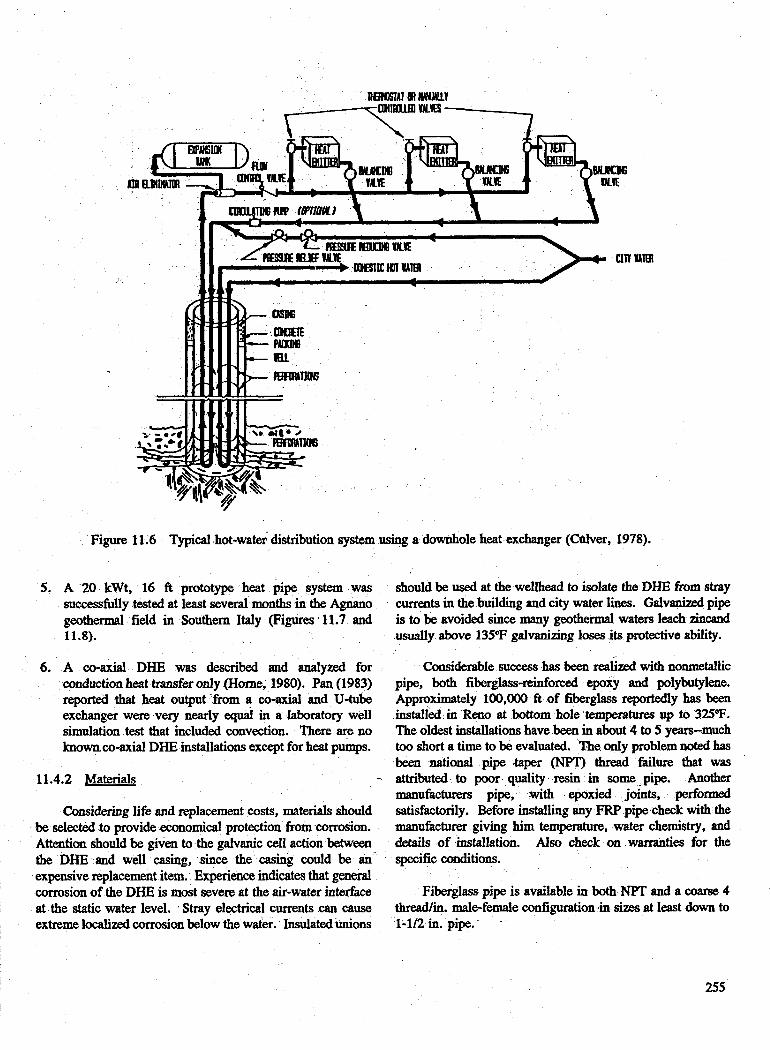
Figure 11.6 Typical hot-water. distribution system using a downhole heat exchanger ( a v e r , 1978).
5. A 20 kWt, 16 Et prototype heat pipe system was succesfidly tested at least several months in the Agnano geothermal field in Southern Italy (Figures 11.7 and 11.8).
6. A co-axial DHE was described and analyzed for conduction heat transfer only (Home, 1980). Pan (1983) reported that heat output from a co-axial and U-tube exchanger were very nearly equal in a laboratory well simulation test that included convection. There are no known co-axial DHE installations except for heat pumps.
11.4.2 Materials - Considerkg life and replacement costs, materials should
be selected to provide economical protection from corrosion. Attention should be given to the galvanic cell action between the DHE and well casing, since the casing could be an expensive replacement item. Experience indicates that g a d corrosion of the DHE is most severe at the air-water intedace at the static water level. Stray electrical currents can cause extreme localized corrosion below the water. Insulated unions
should be used at the wellhead to isolate the DHE from stray currents in the building and city water lines. Galvanid pipe is to be avoided since many geothermal waters leach zincand usually above 135°F galvanizing loses its protective ability.
Considerable success has been realized with nonmetallic pipe, both fikg€ass-reinfod epoxy and polybutylene. Approximately 100,OOO A of fiberglass reportedly has been install& in Reno at bottom hole temperatures up to 325°F. The oldest installations have been in abut 4 to 5 years-much too short a time to be evaluated. The only problem noted has been ~ t i d pipe 'taper (NPT) thread failure that was attributed to poor quality resin in some ,pipe. Another manufacturers pipe, -with epoxied joints, performed satisfactorily. Before installing any FRP pipe check with the manufacturer giving him temperature, water chemistry, and details of installation. Also check on warranties for the specific conditions.
Fiberglass pipe is available in both NPT and a coarse 4 kead/in. malefemale configuration .in sizes at least down to 1-1/2 in. pipe.
255

256
GTC: Geothermal c o n v e r t e r P : Pump TC : Thermocouple V :Capecity contro l vessel
i
Figure 11.7 Schematic of experimental loop (Cannaviello, 1982).
I I I I I no no 100 I 110 I le0 I 1= I j40 8 SO 80 70
INLET CONDENSER WATER TEMPERATURE (‘F)
Figure 11.8 Performance of 20 kW geothed cmvector (Cannaviello, 1982).

DHE pipes should be approved for potable water, since it may heat domestic water and many geothermal resources supply water for drinking and spas. Although there are no known installations, chlorinated polyvinyl (CPVC) or irradiation cross-linked polyethylene are good candidates.
Thermal mductiuity is much lower for nonmetallic pipe than for metallic pipe. The value for fiberglass epoxy pipe is 2.5 Btuh ft? "F/in. and polybutylene is 1.5 Btuh ft2 "F/in., while steel is 460 Btuh ft2"F/in. Also, nonmetallic pipe is typically thicker than metallic. However, the overall t h e d conductivity is a function of the conductivity of the pipe, the film coefficients on both the inside and outside, and of the scale. Scaling is an important consideration because in many geothermal fluids, significant scaling on metallic DHE pipes occuts, 6ut the scale will not build up on the nonmetallic pipes. It is not unusual to see 1/16 in. of scale buildup on the geothermal side of DHE pipes, at least in Klamath Falls geothermal fluids. Scale car^ be assumed to have a thermal conductivity similar to limestone and concrete or about 7 Btuh ft2"F/in.
The overall heat transfer coefficient can be calculated from:
1 l f f l
u - - + - + - + - b k p k s h i
Where
U = overall thermal conductivity @tu5 f t 2 O F / i n . ) ho = outside film coefficient hi = inside film coefficient t = pipe or scale thickness (in.) kp = thermal conductivity of pipe material
ks = thermal conductivity of scale.
Assuming film coefficieats of 250 and using values above
Btu5 @OF)
for thermal conductivities of typical pipes is written: 1
iI steel - A
1 0.154 0.0625 1 - * - * - + - 250 460 7 S O
= 58 Btu5 ft2"F
= 2 5 B t u 5 f f 0 F
While the difference is significant, it is less than might be anticipated by comparing only the thermal conductivities of the two pipe materials. Usually the depth of the well to reach geothermal fluids will Bccommodate the additional pipe required and the long life justifies the use of nonmetallic pipe.
For the approximately 500 black iron DHEs installed in Klamath Falls, the average life has been estimated to be 14 y. In some instances, however, regular replacement in 3 to 5 y has been required. In other cases, installations have been in service over 30 y with no problems. Stray electrical currents, as noted above, have undoubtedly been a contributing factor in some early failures. currents of several tens of &-amps have been measured. In others, examination of the DHES after removal reveals long, deeply corroded lines along one side. This may be caused by thermal expansion and contraction of the DHE against the side of the well bore where the constant movement could scrub off protective scale, exposing clean surface for further corrosion.
Average DHE life is difficult to predict.
Corrosion at the air-water interface is by far the most common cause of failure. Putting clean turbine oil or paraffin in the well appears to help somewhat, but is difficult to accurately evaluate. Use of oil or paraf i is frowned on by the Environmental Protection Agency since geothermal water often commingles with fresh water.
DHE wells are typically left open at the top, but there appears to be no reason they could not be d e d &-tight. Once the initial charge of oxygen is used up in forming corrosion products, there would be no more oxygen available because there is essentially no dissolved oxygen in the geothermal fluid. Swisher and Wright (1986) measured corrosion rates of mild steel in geothermal water under aerobic and anerobic conditions in the lab. They found aerobic corrosion rates of 260-280 micrometerlyear with completely emersed specimens with paraffin on the water, 830 micmmetedyear above the paraffin on partially emersed specimens and only 11 micrometerlyear under anembic conditions.
11.4.4
Although $he interaction between the fluid in the well, fluid in the aquifer, and the rock surrounding the well is p r l y understood, it is known that the heat output can be significantly increased if a convectiqx cell can be set up in the
re is probably some degree of naW mixing; Le., the aquifer continuously enters the well, mixes
with the well flui the well to the aquifer. There are two methods of inducing convection.
257

100 I I I I I I I I I
e5 50 7s 100 . 125 is0 175 200
DEPTH I N WELL ( f t )
Figure 11.9 Temperature vs depth with and without casing (Culver, 1978).
The first method may be used when a well is drilled in a stable formation, and will stand open without a casing. This allows an undersized casing to be installed. If the casing is perforated just below the minimum static water level and near the bottom or at the hot aquifer level, a convection cell is induced and the well becomes very nearly isothermal between the perforations (Figure 11.9). Cold surface water and unstable formations near the surface are cemented off above a packer. If a DHE is then installed and heat extracted, a convecfion cell is established with flow down the inside of the casing and up the annulus between the well wall and casing. The driving force is the density difference between the fluid surrounding the DHE and fluid in the annulus. The more heat extracted, the higher the fluid velocity. Velocities of 2 fils have been measured with very high heat extraction rates but the usual velocities are between 0.04 and 0.4 ft/s.
The second method is used where a different situation exists. In New Zealand where wells do not stand open and several layers of cold water must be cased off, a system using a convection promoter pipe was developed (Figure 11-10). The convector pipe is simply a pipe open at both ends, suspended in the well above the bottom and below the static water level. An alternate design involves the pipe resting on the bottom, and having perforations at the bottom and below static water level. The DHE c811 be installed either in the convector or outside the convector, the latter being more economical since smaller convector pipe is used.
CONVECTION
ABOUT 0.510) IN PROMOTING PIPE -
QIAMETLR
t-I m ' b y - - -WATER LEVEL
SLOTTED CASIN6
U-6HIpED O.H.E. AawT O . O S 8 1
IN DIAMETER
. . . . . Figure 11.10 Convection promoter pipe with DHE
(Allis, 1979).

Both lab and field tests indicate that the convection cell velocities are about the same in undersized casing systems'and convector pipe systems.
dptimum conditions exist when frictional resistance because of wetted surfaces (hydraulic radius) is equal in both legs of the cell and DHE surface area is maximized, providing maximum heat transfer. For designs using undersized casing and DHE inside the convector, this occurs when the casing or wnv@or is 0.7 times the well diameter. When the DHE is outside the convector, the convector should be 0.5 times the well diameter. The full length U-tube DHE diameter is 0.25 times the well diameter in all cases. Partial length or multi-tube excbgers will have different ratios.
Maximum convection rates are obtained when the casing or convector pipe are insulated. This maintains the temperature and density difference between the cell legs. Nonmetallic pipe is preferred. Although corrosion products help insulate the pipe, scaling does not normally occur to any great degree because the casing or convector are the same temperature as the water.
11.4.5 Desim Considerations
Downhole heat exchangers extract heat by L o methods: (a) extracting heat from water flowing through the aquifer, and (b) extracting stored heat from the rocks surrounding the well.
Once the DHE is extracting heat and a convection cell is established, a portion of the convecting water is new water entering the well from the aquifer; the same amount of cooled water leaves the well and enters the aquifer.
The ratio of convecting water to new water has been termed the mixing ratio and is defined as:
*a R m - l - - mt
where
Rm = mixing ratio m, = mass flow of new water m, = total mass flow of convecting water.
Note that a larger mixing ratio indicates a smaller proportion of new water in the convection cell.
Mixing ratios vary widely between wells even in the same aquifer and apparently depend on permeability. As more heat isextracted, the mass flow rate in the convection cell increases, but the mixing ratio appears to remain relatively constant up to some point, then increases with further DHE loading. This is interpreted as the permeability, allowing hot fluid to enter the well or, more probably, allowing y&
cool fluid to sink into the aquifer near the well bottom. At some combination of density difference and permeability the ability to conduct flow is exceeded and the well rapidly cools with increasing load.
The theoretical maximum steady state amount of heat that could be extracted from the aquifer would be when the mixing ratio equals zero. That is, when all the water makes a single pass through the convection cell and out the well bottom. Mixing ratios lower than 0.5 have never been observed and usually range from about 0.5 to 0.94. The theoretical maximum steady heat extraction rate can be estimated if the hydraulic conductivity and hydraulic gradient are known and it is assumed there is some temperature drop of the water.
If K is the hydraulic conductivity and M A 1 is the hydraulic gradient, by Darcy's Law the speci!ic velocity through the aquifer is given by:
v = K M A l .
The mass flow through an area, A, perpendicular to the flow is therefore shown as:
v A d = K A d M A 1
where d is the density of the water. The steady state heat flow can be found by:
q = K A d c (To - T,) &/AI
where
A = cross section of well in the aquifer or the
d = density of water c = specificheat To = aquifer temperature T, = temperature of water returning to the aquifer
Multiplying the above by (& - Rm), or - 0.5 to 0.6, the
perforated section
expected steady state DHE output can be determined.
The most importantfactor in the above equation is K. This value can vary by many orders of magnitude (even in the same aquifer) depending on whether major fractures are intersected, or drilling mud or debris partially clogs the aquifer, etc. The variation between aquifers can be even greater.
Based on.short-term pump tests to determine hydraulic conductivity and an estimated 1% hydraulic gradient, the specific velocity in the Moana area of Reno is estimated at 1 to - 3 ft/y. The hot aquifer is generally encountered in mixed or interbedded layers of fine sand and silt stone. In Klamath Falls, where the hot aquifer is in highly fractured basalt and coarse pumice, specific yelocity 'is estimated at 20 to
259

150 Alday, perhaps higher in localized areas. Values of K in seven wells in Moana were estimated at 3.28 x lo' to 3.28 x 10⁴ Als . The K in Klamath Falls is estimated to be at least 4.9 Als. This implies a factor of 10 thousand to 10 million difference in the steady state output. Differences by a factor of 100 have been measured, and some wells in Moana have been abandoned because they could not provide enough heat, even for domestic hot water.
Many DHE wells in Moana are pumped to increase hot water flow into the well. Pumping rates for residential use is limited to 1800 gallday and the pump is thermostatically controlled. The system is designed to switch on the pump if the DHE temperature drops below some predetemhed level, usuallyi- 120°F. This method permits use of a well that would not supply enough heat using a RHE alone, yet minimizes pumped fluid and pumping costs. It is, however, limited to temperatures at which an economical submersible or other pump can be used.
Unfortunately, at the present time, there is no way to relate mixing ratio and permeability. With good permeability similar towell-fractured basalt, themixing ratiomightbe - 0.5, in coarse sand - 0.8, and in clayey sand 0.9 to 0.94.
At the time the tefm mixing ratio was introduced, it seemed to be B logical hypothesis because all known DHE wells had (and most still have) perforations, at least in the hot aquifer zone. Some fluid could enter the well, mix with fluid in the well and some y& water exit the well. The mixing ratio is really a term for energy input into the well. Although perforations undoubtedly help, a solidly cased well with a DHE will provide heat. The energy output is then limited by the conduction of the rock and casing, allowing energy to flow into the well. This has been experimentally verified using a model well in a laboratory at the University of Auclcland in New Zealand. With an electric heater at the model well bottom and a umvector pipe and DHE installed, a convection cell was induced and an amrent mixing ratio of 0.954 was calculated, similar to what might be expected in a very low permeability aquifer.
As mentioned at the first of this section, the second method of using a DHE is extracting heat stored in surrounding rocks.
In Klamath Falls, it has been experimentally verified that when a well is drilled, there is negligible umvective flow in the well bore. When undersized perforated casing is installed, a umvection cell is set up, causing flow up the inside of the casing and down the annulus between the casing and well wall. When a DHE is installed and heat is extracted, the convection cell reverses with the flow downward in the casing (around the DHE) and up the annulus. Similar circulation patterns were noted in New Zealand using umvection promoters.
c
It is now p d , but not verified, that if a DHE were operating and then tumed off, the Convection cell would reverse in the case of the undersized casing and when the DHE is inside the convection promoter. If the DHE is outside the promoter, the cell direction would remain the same &when the DHE is extracting heat.
DHEs are principally used in space and domestic water heating applications: homes, schools, small commercial buildings and greenhouses, with the resulting intermittent operation. When the heating system is not calling for heat, and if a convection cell can exist, it functions to store heat in rocks surrounding the well; especially those cooler rocks nearer the surface that would normally be at the ~hua l tempratme gradient for the locale. The undersized casing or umvection promoter then acts to increase thermal storage.
Referring again to Figure 11.10, it can be seen that up to the upper perforations, the well becomes very nearly isother- mal, with the upper portion approaching the aquifer tempera- ture and a e rock temperature increasing significantly. When a DHE is turned on, the water in the well cools rather rapidly; the rate depending on the mixing ratio. As the water um- tinues to cool, the convection cell extracts heat from the surrounding tpcks.
A good design procedure is currently lacking. Culver and Reistad (Culver, 1978) presented a computer program that pre- dicts DHE output to within 10 to 1596 if the mixing ratio is known. The problem is, there is no way of predicting mixing ratio except by experience in a specific aquifer and then probably only over a fairly wide m g e as noted above. The procedure was written in Fortran but has been umverted to "-85 Basic by Pan (Pan, 1983) and into Basic for use on most persanal computers by Liemu in 1989. The program enables the user to choose optimum geometric parameters to match a DHE to an energy load if a mixing ratio is assumed. The program does not include a permeability variable, nor does it take thermal storage into account. In wells with good permea-bility, thermal storage may not be a significant factor. Experience in Reno indicates that for low permeability wells, thermal storage is very important. With low permeability, a convection promoter can promote thermal storage and, thereby, increase non-steady state output.
Permeability can be rather accurately estimated using relatively simple Hvorslev plots as described in Chapter 7, "Well Testing". Relating the permeability thus obtained to mixing ratios typical in other permeabilities could give an estimate of the mixing ratio that could be used in the computer program. Data are limited to very high and very low permeability situations. Middle ground data are not available.
260

- -
REFERENCES
Alfa-Laval Inc, "Plate Heat Exchangers", undated.
Allis, R. G, "A Study of the Use of Downhole Heat Exchangers in the Moana Hot Water Area, Reno, Nevada", May, 1981.
Allis, R. G. and R. James, "A Nahual Convection Promoter for Geothermal Wells", 1979.
APV Company Inc., "Heat Transfer Handbook", APV Company Inc., Tonawanda, NY. Undated.
APV Company Inc., "A 60 Second Study in Heat Transfer Efficiency", (sales literature), APV Company Inc., Tonawanda, NY, undated.
Cannaviello, M., et al., "An Advanced System for Heat Transfer from Geothermal Low and Medium Enthalpy Sources", International Conference on Geothermal Energy, Florence, Italy, May, 1982.
Culver, G. G. and G. M. Reistad, "Evaluation and Design of Downhole Heat Exchangers for Direct Application", December, 1978.
Efird, K. D. and G. E. Moller, ;Electrochemical Character- istics of 304 & 316 Stainless Steels inFresh Water as Fmctions of Chloride Concentration and Temperature", Paper 87, Corrosion/78, Houston, TX. March 6-10, 1978.
Ellis, P. and P. Conover, "Materials Selection Guidelimes for Geothermal Energy Utilization System", USDOE (DOE RA270226-l), Washington, DC, January, 1981.
Hesong, Pan, Master's Thesis. University of Auckland, New Zealand, Department of Mechanical Engiueerhg, May, 1983.
Hulbert, G., "Plate Heat Exchangers", Geo-Heat Center Quarterly Bulletin, Oregon Institute of Technology, Geo-Heat Center, Klamath Falls, OR, Winter, 1986.
Hulbert, G., "Technical Presentation at 1985 conference on Direct Use Geothermal Systems", Oregon Institute of Technology, ,Klamath Falls, OR, May, 1985.
Kuipe, E., Personal communication, 1987.
Swisher, R. and G. A. Wright, "Inhibition of Corrosion by Paraffin at the Air-Water Interface in Geothermal Downhole Heat Exchangers", University of Auckland, Auckland, New Zealand, 1986.
Tranter Inc., "Supercharger Plate and Frame Heat Exchangers", (sales literature, form Sa), Tranter Inc., Wichita Falls, 'IX, undated.
26 1


CHAPTER 12 SPACE HEATING EQUIPlVENT
By Kevin D. Merty, P.E. OIT Geo-Heat Center
Klamath Falls, OR 97601
12.1 INTRODUCTION
The performance evaluation of space heating equipment for a geothermal application is generally considered from either of two perspectives: (a) selecting equipment for installation in new construction, or (b) evaluating the pedormance and retrofit requirements of an existing system.
With regard to new umstruction, the procedure is relatively straightforward. Once the heating requirements are determined, the process need only involve the selection of appropriately sized hot water heating equipment based on the available water temperature.
It is important to remember that space heating equipment for geothermal applications is the same equipment used in non-geothermal applications. What makes geothermal applications unique is that the equipment is generally applied at temperatures and flow rates that depart significautly from traditional heating system design.
This chapter presents general considerations for the performance of heating equipment at non-standard temperature and flow conditions, retrofit of existing systems, and aspects of domestic hot water heating.
12.2 HEATING EQUIF’MENT PERFORMANCE AT NON-STANDARD CONDITIONS
For about the past 40 years, heating systems have been designed for a hot water supply temperature of 180 to 200°F with a 20°F temperature drop (AT). These temperatures were chosen largely to result in equipment requirements similar to those of the older steam systems. Equipment manufacturer’s selection data are indexed to these temperatures as are the practices of many design professionals.
Geothermal tesources, of the variety frequently applied to space heating applications, are generally characterized by temperatures less .than the standard 180 to 200°F range. Because well pumping costs constitute a sizable portion of the operating costs of a geothermal system, it is in the best interest of the designer to minimize flow requirements. This requires bigher system AT than conventional designs. Accord- ingly, it is beneficial to examine the performance of heating equipment at low flow or temperature conditions.
Figure 12.1 illustrates the effect of low water velocity on heat transfer in hot water heating equipment. As indicated by the w e , heat output is relatively unaffected by water side velocity above a critical value. It is important when designing for larger than normal AT (low flow rate) that the critical velocity for the heating equipment in Question be avoided, as capacity falls off asymtotically in this region.
Figure 12.1 is a generalized relationship. %cause the issue illustrated is really one of Reynold’s Number and transition to laminat flow, critical velocity will vary with temperature and line size. However, for the piping diameters and temperatures generally encountered in heating equipment, velocities of 0.25 ft/s or less should be avoided for 1 to 2 in. lines (typical of finned tube radiators) and 0.50 ftls or less for 1 in.and smaller lines (typical of finned coil equipment). For the 5/8 in. tubes commonly found in h e d coil equipment, this velocity corresponds to a flow rate of - 0.6 gal/& gpm. In most cases, this very low velocity would only become a factor in applications of very low capacity (< 15,OOO Btdh) using a AT of 40°F or more.
Figure 12.2 illustrates the effect of reduced water temperature on hot water heating equipment performance. The width of the c w e is an effort to reflect the fact that all types of heating equipment do not respond to reduced temperature equally.
Figure 12.2, as is most heating equipment, is indexed to a temperature of 215°F. The percent capacity shown on the vertical axis is the percent of the 215°F rated capacity at the temperature in question. For example, the output of a parti- cular piece of heating equipment at 150°F would be - 45 % of its capacity at 215°F. This relationship holds for equipmellt such as finned tube radiators, unit heaters, cast iron radiators, and convectors.
For finned coils, the considerations are somewhat more complex with respect to low temperature service. For other types of equipment, compensation for low temperature opera- tion is primarily in terms of additional length, larger individual units, or a greater number of units. For finned coils, the physical size (in terms of face area) can remain unchanged and the configuration of the coil (number of rows and fins/in. or both) adjusted to Bccommodate low temperature operation.
263

,'- CRITICAL VELOCITY /
I I
I I I I I
3 4 6 i e
VELOCITY IN FEET PER SECOND
Figure 12.1 The effect of low water velocity on heat transfer in hot water heating equipment (ASHRAE, 1983).
io0 4
I I I I I I I I I I I
i o 0 i i o ~ B Q 130 $40 is0 ieo $70 iao iao ZOO
AVERAGE WATER TEMPERATURE (OF) Figure 12.2 Capacity at reduced water temperature (ASIBAE, 1983). Width of line shows that all types of heating
equipment do not have the same response to reduced water temperature.
264
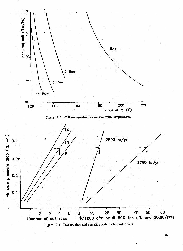
- r ' .- 0 0
I I I 1
1 2 3 4 5 0 I
co
I I
10 20 30 40 50 60
CD
e e 0.2.
7
i a
3 Row
Row
4 Row
1 I I 1 I 4 I I I 1 120 140 160 180 200 220
Temperature (T)
Figure 12.3 Coil configuration for reduced water temperatures.
Figure 12.4 Pressure drop and operating costs for hot water coils.
265

To illustrate this point, Figure 12.3 presents an indication of the coil configuration required for a specific duty (500 Wmin face velocity, 40" AT water, 65°F air in - 100°F air out). Coil surface area (in terms of fins/in. or rows) require- ment increases as supply water temperature is reduced. How- ever, as indicated in the design, a two row coil will suffice down to supply water temperatures of - 130°F.
BAuse the terminal equipment in most large buildings primarily consists of finned coil units, it is useful to explore the impact of deeper coils upon capital and operating costs for a typical application.
Assume a geothermal resource is available that will be capable of producing a building supply water temperature of 140°F. The competing conventional system is a gas boiler that would be operated at a 200°F supply water temperature. Using Figure 12.3, the required coil (for the boiler system) would be a one row, 9 Win. model. For the geothermal case, a two row, 11 fin/in. coil would be required.
- Figure 12.4 indicates the air side pressure drop associated with these coils. For the 200°F case, this amounts to - 0.08 in. water gauge (in. wg) and for the 140°F case, about 0.21 in. wg.
The two curves on the right side of Figure 12.4 convert these air side pressure drops into operating costs in terms of dollars/1,000 cfm (at $.06/kWh and 50% overall fanand drive efficiency). Assuming the application is an office building (- 2500 operating h/y), the operating cost for the 200°F case would amount to $3.00/1,000 cfm and the 140°F case $7.50/1000 cfm. For a 50,000 ft2 office building, this would amount to less than $2501~ in incremental operating costs for the geothermal terminal equipment over the conventional terminal equipment. For buildings operated 24 h a day, or in areas of higher electrical rates, the cost would increase; however, it is unlikely to increase to the extent that it constitutes more than a small fraction of the annual operating costs for the system as a whole.
The second cost factor associated with low temperature operation of the system is the incremental capital cost of the low temperature equipment over the standard temperature equipment. For finned coils, this cost increase can be estimated by the ratio of the number of rows to the 0.51 power as follows:
o One row coil cost = $llO/ftz (typical of coils of approximately 4.0 ftz each)
o TWO row coil cost = (2/1)0.45 x ($110) = $150/ftz.
This relationship is developed from coil costs appearing in the 1990 Means Mechanical Cost Data and from previous project cost data on fde in the Geo-Heat Center.
For the 50,000 ftz office building mentioned above (at 1 cfm/ft2 and 500 fpm face velocity), this would result in a coil incremental capital cost of - $4,000.
Assuming a variable air volume (VAV) system in the example building with a total heating energy CoIlSumption of 20,000 Btu@ y, .the savings in energy consumption (at $OSO/them) would repay the incremental coil cost in less than one year even when incremental fan energy costs are deducted from the savings.
12.3 USE OF HEAT EXCHANGEM
Most geothermal systems will employ a heat exchanger to isolate the building heating loop from the geothermal fluid. As a result, the supply water temperature available to the heating system will be less than the geothermal resource temperature. In most cases, an allowance of a 10°F loss through the heat exchanger will be sufficient for the selection of heating equipment. Eumomical heat exchanger selections generally fall between the 5 and 10°F approach to the geothermal temperature. Heat exchangers are discussed more fully in Chapter 1 1.
12.4 CONTROLS CONSIDERATIONS
Certain control strategies enhance the effectiveness of using a geothermal resource in a building WAC system. Some of the more important of these are discussed in the paragraphs below.
12.4.1 Main Heat Exchanger Control
Most geothermal systems use a plate type heat exchanger to isolate the building's circulating loop from exposure to the geothermal fluid. A variety of options can be used for control of this heat exchanger.
A method that can be utilized when the user has little or no control over the resource temperature and flow rate is shown in Figure 12.5. Under this design condition, the primary side of the heat exchanger is permitted to run wild (operate without temperature control) and temperature control is accomplished on the seumdary side. This approach may be used for applications that involve d e d resources, or when the constant resource flow must be maintained. A three-way valve on the secondary side of the heat exchanger is used for supply water temperature control.
266

i
Figure 12.5 Heat exchanger used to isolate building heating loop from geothermal fluid.
Because most larger geothermal systems produce fluid from a well, there is adequate umtrol of the source. As a result, control is applied to the primary si& of the heat exchanger. In most cases, it is desirable to use a two-way control valve at the heat exchanger. The two-way valve allows for either throttling control of the production well pump or, when used in conjunction with a variable speed drive, allows control of the drive through production line pressure. In this way, only the quantity of geothermal fluid necessary to meet the load is pumped.
For temperature control, it is acceptable to place the umtrol valve on either the inlet or outlet of the heat exchanger. Because of the very small fluid volume in the plate heat exchanger, there is little thermal mass to interfere with response to load changes as can sometimes be the case with downstream control valve locations in other applications.
In some cases, it may be desirable to place the control valve at the heat exchanger outlet. This location is preferred when the geothermal fluid contains a high percentage of dissolved gases, particularly CO,. It is Fmmon for such gases to come out of solution when the fluid pressure is ?educed (such as at a wntrol valve) below the gas'sahuation pressure. Release of CO, can change the fluid pH to allow other species to precipitate out on nearby surfaces. However, downstream location for the umtrol valve maintains the pressure on the heat exchanger to prevent such an occurrence.
Under most circumstances, the valve is controlled to maintain a particular supply fluid temperature. This set point can be reset by a discriminator control or by outdoor air temperature, depending upon the design of the system.
12.4.2 Sumlv Water Reset Control
Using a supply water reset control on the building loop, if possible, is desirable because this type of control results in a reduced supply water temperature with reduced load. Assuming a constant geothermal fluid temperature, such control allows for an increasing AT on the geothermal side of the heat exchanger 8s load decreases. This, in hun, allows for
reduced fluid flow requirements from the production well. Reduced flow+,rates are always desible in a geothermal system from both an economic standpoint and for aquifer CoIIServBtion purposes.
12.4.3 bwer Sumly Water Temmratu?
Designing for the lowest secondary supply water tempemture that is economically feasible reduces geothermal flow requirements. At a constant resource kmpembm, progressively lower supply water temperatures (on the building side of the heat exchanger) result in conespodngly Iower geothermal flow requirements assuming a umstant approach to the return water temperature.
12.4.4 Desinn for Higher System AT
For purposes of reduced geothermal flow, it is desirable to design for larger than the standard 20°F temperature difference. Depending upon the specific design, a A T of 30 to 40°F or more is desirable.
12.4.5 Use of Two-way Control Valves
Two-way control valves are the p r e f d method of umtrol for a geothermal space heating system. In addition to their superior umtrol characteristics in general, they provide additional benefits for geothermal system. With two-way valve umtrol, the system responds to load reductions at a relatively constant AT. This contrasts with the thnee-way valve or 'constant' flow control under which the system AT decreases with the load. The ability to maintain higher system AT is desirable with geothermal systems. Two-way control provides this feature (Haines, 1983)(AsHR~E, 1984).
12.5 CASCADED USES
Relatively low temperature applications such 8s domestic hot water heating and ventilation air preheat should be cascaded from the primary space heating heat exchanger if possible. These loads c811 be served by a physically separate heat exchanger operating on effluent from the primary space heating heat exchanger. Alternately, the load can be served by a duplex type plate heat exchanger. Duplex heat exchangers are discussed in the heat exchanger chapter.
12.6 RETROFIT OF EXISTING SYSTEMS
Certain types of heating system are more amenable to geothermal retrofit than others. For existing hot water systems, adequate operation at lower supply water tempera- tures may have ti, be verified. For non-hot water systems, it is likely that new hot water equipment will peed to be installed adjacent to or in place of the existing equipment. Over the
267

Table 12.1 Retrofit Suitability Valueb of Selected Heating Systems
Retrofit Suitability
Single Multiple Air Handler Air Handler Air systems
Low temperature hot water (< 150°F) Single zone, multi-zone, dual duct Terminal reheat, variable volume,
Induction
8
6
10
8
Standard hot water (1 8O-2WF) Single zone, multi-zone, dual duct Terminal reheat, variable volume, Induction
8
7
7
6
steam Single zone, multi-zone, dual duct Terminal reheat, variable volume Induction
6 6
4 5
Electric resistance forced air Air-to-air split system heat pump Fossil fuel fired furnace Roof top packaged equipment Fossil fuel fired unit heaters
Water Systems
Loop heat Pump Radiant panel Fan millunit ventilator
4 Pipe single mil 4 Pipe
2 Pipe
10 10
9 9 7
7 6
Unit heaters Finned tube/convector
Steam Systems
Finned tube radiation Unit ventilator Two pipe cast iron radiator One pipe cast iron radiator
Perimeter Electric Systems
Electric resistance baseboard Through-the-wall units
2 1
a. Suitability values shown abve are average. Site specific conditions fresuently influence suitability in positive or negative ways. The table addresses only the mechanical considerations of the retrofit. The relative energy efficiency of the existing system also heavily influences retrofit suitability.
b. A value of 10 is best, 1 is worst.
268

years, the Oregon Institute of Technology's Geo-Heat Center has gained considerable experience in evaluating heating systems for retrofit. Table 12.1 rmmmarizes the results of this experience with regard to some of the systems that may be encountered. It is important to note that the retrofit Suitability of these systems as indicated in the table is not absolute. Site specific considerations can easily alter the ability (either positively or negatively) of a system to Bccommodate hot water use. Some of these issues will be discussed for specific system in the paragraphs below.
, The largest of these considerations is the degree of excess capacity present in the existing system. This excess capacity, present in most systems, is the result of a number of factors, the most important of which is umservative design practice. In addition, manual methods of equipment selection used in the past resulted in conservative results compared to present automated methods. It is not unusual to find a heating system with an overdesign factor of 50% or more. This is a result of the nature of the system design. First, the peak heat loss is calculated, sometimes using unrealistically low outside design temperature that artificially increases the load by - 10%. Then a 10 to 30% safety factor is added, a 5% duct loss &tor, and a 25% -pi* factor (for regain after night set back). When equipment is selected, the capacity may be any- where from 5 to 20% over the requirements because of equip- ment availability. M e n the results of all this are considered together, 1.10 x 1.10 x 1.05 x 1.25 x 1.05 = 1.68, the system can be grossly oversized. As a result, it can be oper- ated at significantly reduced capacity and still meet heating requirements with no difficulty. In many cases, overdesigned hot water systems have been operated at much reduced supply water temperatures (lower capacity) and actually provided improved performance through better part-load valve control.
The existing equipment capacity does not always reflect the actual heating requirements of the building. The presence of excess capacity in the existing system generally offers some advantage in the retrofit process.
12.6.1 Air Svstems
Air systems involve the delivery of heated air from a central source, generally through a ducted distribution system, to the space to be heated. This group can generally be split into two classifications: (a) large building systems, and @) smaIl building systems.
Laree Buildings
Large building systems include those described in Figures 12.6 through 12.11. Of these, the most favorable for retrofit are the single-zone, multi-zonemd dual duct systems (Figures 12.6, 12.7 and 12.8). These systems include only a single heating coil in the central air handler. As a result, retrofit, if necasary, is umfined to the mechauical room. The terminal reheat, variable air volume, and induction systems all include
I I COOUICI
Figure 12.6 Single zone system (Bloomquist, 1987).
"E- R
Figure 12.7 Multizone system (Bloomquist, 1987).
7 '- \ I / I
Figure 12.8 Double duct system (Bloomquist, 1987).
mils in the terminal equipment located in each heating zone. Because an individual air handler may serve from a few to several hundred terminal units, retrofit, if any, could be costly for these heating coils. Because the heating mils are located in the occupied spaces, -retrofit of the units would be disruptive to the building tenants. The heating mils in these systems are generally +signed for a fairly low temperatm rise on the air side (that is, the air is generally heated to only 80 to 105"F), which generally allows for acceptable low supply water temperabe operation. In the event that the
t
269

individual zone heating coils will not operate acceptably at the temperature available from the geothermal system, a peaking arrangement with the existing boiler is generally more accept- able than retrofit of the coils. Under this approach, the system operates on geothermally supplied heat for most of the year. During unusually cold periods, the supply water tem- perature is boosted by the building's existing boiler.
m#N
//////
The large building air systems described above can use low temperature hot water, standard hot water or steam for the heating coils. By far the most common is standard hot water coils designed for 200°F supply and 180°F return. Because of overdesign, these systems often will operate acceptably at reduced water temperatures. Systems designed in the last 10 year may use a lower temperature hot water system with supply temperatures from 140 to 160"F, rather than the standard 200°F used in the past. These systems are more attractive for retrofit because it is unlikely that any terminal equipment retrofit or peaking will be required. It is rare to find steam used for terminal heating coils in large building air systems, though a few have been designed.
Figure 12.9 Terminal reheat system (Bloomquist, 1987).
COOLUG COIL1
I . n,
Figure 12.10 Variable air volume system (Bloomquist, 1987).
0
HUMIDIFIER OR
HOTOR C RECIRCULATED -ROOM AIR
-_
Some air systems, which use larger percentages of outside air (typical of hospitals) or are located in very cold climates, may include a preheat coil in the main air handler. This preheat coil serves to heat the mixture of return air and outside air (or 10096 outside air in some buildings) to a temperature of 55 to 60°F before entering the main duct system. Even when the balance of the system is a hot water design, the preheat coil is frequently designed for steam use. These steam preheat coils would require retrofit for hot water operation.
It is important to use specific design techniques when implementing hot water preheat coils in order to maintain an adequate water velocity that prevents freezing in the coil. This value is generally taken to be - 3 ft/s. A number of control strategies are available to accomplish this with most Using a recirculation pump at the coil. Hot water preheat coil design is discussed in detail in Hainm, 1983 and ASHRAE, 1984.
Large building air systems are frequently installed with a separate system that provides heating to the perimeter of the building. This second system is usually a hot water radiation- finned pipe system. As a result, it is important to consider the performance of both the central air system and the perimeter system when analyzing the building retrofit requirements. The hot water radiation system will be discussed further under water systems.
A final consideration for large building air systems relates to the number of air handlers used in the building. If retrofit of the main heating coils is required, fewer units are better. During the 1950s and l%Os, it was a common practice to use a small number of very large air handlers. In recent years, the trend has been the opposite (i.e., large number of small air handlers).
In summary, for large buildings, the most attractive system from the geothermal use standpoint is a single-mne, multi-zone, or dual duct system that uses hot water (or low temperature hot water) heating coils and includes a small number of air handling units.
Figure 12.11 Induction system (Bloomquist, 1987).
270

Small building air systems are distinct &OM large building systems in terms of complexity and heat source. In smaller buildings, sepatate boiler to supply hot water or steam to the air handlers is generally not included. As a result, individual equipment serves as both the heat source and the air handler as in the case of air-to-air heat pumps, roof top gadelectric units, and fossil €uel fired and electric resistance furnaces. The duct distribution system, if any, is generally much less sophisticated than in the large air systems. Retrofit costs for small building air systems are as much a function of the number of individual units as of the type of unit.
Furnaces of the fossil fuel fired or electric resistance variety are found primarily in small office and municipal buildings, residences, and to some extent, in retail buildings. As indicated in Table 12.1, the electric furnace is considered fair in terms of retrofit ease.
Retrofit cost is influenced by the number of units involved; the fewer the better. Retrofit of this type of system involves the installation of a hot water coil in the supply air duct. Electric furnaces (Figure 12.12), because they are designed for fairly low supply air temperature are considered to be more easily retrofit than fossil fuel fired equipment. The
ture operation and less costly coil installation (because of larger ductwork); however, it may be necessary to increase fan horsepower to accommmodate the higher air side pressure drop imposed by the coil Wpe, 1987). Finally, electric resistance supplied heat can be very expensive and, as a result, savings can be high when a g e o t h e d system is added.
low supply air temperature permits low supply water tempera-
I 4
Figure 12.12 Electric resistance furnace (Bloomquist, 1987).
Fossil fuel fired furnaces (Figure 12.13) are somewhat less easily retrofit than electric resistance units. This is because of higher supply air temperature used with this type of furnace, smaller ductwork, and difficulty in mil installation.
Figure 12.13 Fossil fuel fired fumace (Bloomquist, 1987).
When analyzing any furnace based heating system, be aware that oversizing of the existing equipment is very likely. Fukces are available in only a limited number of sizes and installation invariably involves selection of the next larger unit for safety. As a result, the equipment is generally much larger than required. Electric furnaces, because of the higher cost of operation, are less likely than fossil fuel fired equipmeat to be grossly oversized.
Air-to-air heat pumps are available in two dgurat im: split system and package. Of the two, the split system is the more easily retrofit. Split systems, as shown in Figure 12.14, involve an outside unit that contains €he compressor and a heat exchanger and an inside unit, which contains a heat exchanger unit and a fan. The inside unit is usually installed in a mechanical closet and, as a result, access for retrofit is good.
th the furnaces described above, retrofit consists of the lation of a hot water coil in the supply air unit. Split
system heat pumps are most commonly found in small office buildings and residences. Because of their relatively low cost of operation and the likelihood that a large number of units will be installed in a building of any reasonable size, this system is unliiely to be a good candidate for retrofit.
27 1

FN CEI
Figure 12.14 Split system air to air heat pump (Bloomquist, 1987).
Rooftop package equipment, as shown in Figure 12.15, can involve an air-to-air heat pump, an electric cooling/electric resistance heating combination, or more commonly, an electric cooling/gas heating unit. The rooftop package unit is most often found in retail applications, particularly shopping centers, fast food outlets, and in low rise office buildings. The compact nature of this equipment usually precludes installation of a heating coil in the unit itself except in very large capacity units. Coil installation should be in the supply air duct, usually located in a restricted space between the suspended ceiling and the roof (or floor) above. The limited space available, and the requirement to install the coil in the occupied area of the building, results in only a fair rating for this type of system in terms of retrofit suitability. One favorable characteristic of the rooftop system is it virtually always includes air conditioning capability, resulting in somewhat larger ductwork than would be the case for a heating only installation. This larger ductwork reduces hot water coil retrofit difficulties.
Figure 12.15 Packaged roof top system (Bloomquist, 1987).
The number of units to be retrofit significantly affects the total cost. A building with a single large rooftop unit would be a much more favorable candidate than a similar building with five smaller units.
A final comment on rootlop equipment relates to name plate rating (heating capacity). These units are generally selected on the basis of cooling capacity with little con- sideration given to the heating capacity. Heating capacity of
rooftop package equipment frequently bears little resemblance to actual building requirements and, in many cases, may exceed requirements by a factor of two or three.
Fossil fuel fired unit heaters are a self contained device including a fan, burners, and heat exchanger as shown in Figure 12.16. These units are usually suspended from the ceiling in applications such as smaller food markets, shops, small retail stores, coffee shops, and auto dealerships. The retrofit of fossil fuel fired unit heaters involves replacement with new hot water unit heaters. The suitability of 8
particular system for retrofit is mostly dependent upon the number of units required. As the number of individual units increases, costs for hot water distribution piping within the building increases, along with equipment costs for the new unit heaters. Because unit heaters are typically used in buildings that require little or no heating during unoccupied hours, savings generated by the retrofit may be very small. As a result, the retrofit suitability of this system is shown in Table 12.1 as a 4.
GAS SUPPLY/ ( J Figure 12.16 Fossil fuel finned unit heater (Bloomquist,
1987).
Location of Retrofit Hot Water Coils
Many of the small building systems discussed thus far involve installation of a hot water coil for retrofit purposes. In many cases, the access to, and the sizing of, the return air duct would result in a much easier retrofit than the supply air duct location. Return air hot water coil retrofits should be avoided. Locating the heating coil in the return air stream results in two primary difficulties because of the elevated returnair tempe- (a) reducedfan motorcooling, and (b) r e d u d fan capacity.
Most small equipment is designed for return air cooling of the fan motor. Raising the tempemture of the air stream (with the new coil) results in motor overheating. In addition,
272

an inc&’ rem air t eq i e rah~e increases the specific volume of the gir, thus reducing fan capacity. Placing the coil in the return air stream should be used only when full consideration has been given to these issues.
12.6.2 Water Systems
During the cooling season, heat is rejected from the cooling tower. e cool the circuit. During the colder periods of the year, heat is added to the loop by a boiier. The attractiveness of the loop heat pump system lies in the fact that the water circuit serving the heat pumps is generally maintained at 60 to W F , depending upon the seasan.
Water systeis can IX various~y configured, but each will have a main hot water circulating loop that serves a number of individual heating units. Though individual terminal units may use small duct-type distribution systems within their respective zones, water systems do not h v e a central duct disttibution system. Systems included in this chapter consist of: (a) bop heat pump, (b) radiant panel, (c) fan coil/unit ventilator, (d) hot water unit heater, and (e) finned tube/convection.
The loop heat pump system provides for one of the simplest retrofits to geothermal. This type of system, as depicted in Figma 12.17 and 12.18, uses a very low tempera- ture water loop serving a large number of individual heat pump units throughout the building.
CoaJNtr n TOJMR ,J J
-
Figure 12.17 Water loop heat pump system flow schematic (Bloomquist, 1987).
Retrofit of the system involves d y the installation of a heat exchanger adjacent to the existing boiler. Because of the low tempratwe operation of this system in comparison to most geothermal resource temperatures, the heat exchauger requirement is very small. A large temperature drop can be used on the geothermal side of the system. Because of the ease of the retrofit of this system, it is rated as a 10 in terms of district heating suitability. Although the practical retrofit cansiderations for this system are excellent, eamomics may be quite poor.
The loop heat pump system is an energy efficient system because it has the ability to recycle heat within the building. This frequently results in a very small auxiliary heating requirement.
The water loop heat pump system is used primarily in large, multi-story office buildings and similar structures that have year round cooling requirements. One variation of the system that would not be suitable for geothermal heating retrofit is the cooling only loop system. Under this design, the individual units are not capable of opkrating as a heat pump and electric resistance heaters are used for perimeter heating of the building.
Radiant panel systems are rarely used today, but were fairly common in construction of the 1950s. Applications that lend themselves well to this type of system are automotive repair shops,Iarge high ceiling manufacturing structures, and schools. Radiant panel systems as indicated in Figure 12.19 involve the circulation of warm water (90 to 130°F) through piping that is embedded in the floor of the building. Older systems were constructed with copper or steel piping. Leaks that developed because of expansion and umtraction, and corrosion resulted in expensive repair requirenaents. As a result, the panel system fell into disuse for many years. With the advent of new, nonmetallic piping products (ptimarily polybutylene), radiant panel systems have begun to reappear.
Retrofit of the system consists of the installation of a heat exchanger adjacent to the system boiler. As with the loop heat pump system, the low temperature operation of the panel system greatly enhances retrofit prospects in cOmpariSOIl to other hot water systems. As shown in Table 12.1, the system rates a 10 in retrofit suitability.
Figure 12.18 Typical water loop heat pump unit (Bloomquist, 1987).
8
273

ut INLET W E R
Figure 12.19 Radiant panel system (Bloomquist, 1987).
Fan coil (FC) and unit ventilator 0 systems or both are found primarily in hotel/motel chains and schools. The system consists of a main hot water loop that serves a large number of terminal units located throughout the building. Fan
m Figure 12.20 Vertical fan coil unit (Bloomquist, 1987).
coil units, as shown in Figures 12.20 and 12.21, consist of a sheet metal box containing a fan, air filter, and one or two coils. A unit ventilator is similar to a fan coil unit with the exception that it contains accommodations for the supply of outdoor air for ventilation.
Figure 12.21 Horizontal fan coil unit (Bloomquist, 1987).
Two types of FC/UV systems are available: two pipe and four pipe. The two or four pipe designation refers to the water distribution system serving the terminal equipment. A two pipe system includes only one supply line and one return line. As a result, it can supply only heating or cooling to the building at any particular time. Fan coil units and unit ventilators served by a two pipe system (Figure 12.22) umtain only one coil that serves as heathg or cooling coil, depending upon the season.
f
-LED WATER
FLTER
ATED
Figure 12.22 Unit ventilator served by two pipe system (Bloomquist, 1987).
For purposes of this discussion, the four pipe single coil system will be considered as a two pipe system because its design offers similar &antages with respect to low temperature retrofit.
274

Because the coil must perform both heating 'and cooling functions, it is designed for the most demanding duty, which is cooling. As a result, it is able to meet heating kqGrements at very low water temperatures (< 120°F). This low tempera- ture capability provides the same advantages discussed above for water systems.
The four pipe system includes a distribution system that contains both hot water supply and return lines and chilled water supply and return lines. As a result, either heating or cooling can be delivered to any zone at any time. Terminal equipment (fan coil units or unit ventilators) for the four pipe system usuallycontains both heating and cooling coils as shown in Figure 12.23. Heating coils in these units generally require much higher water temperature than two pipe system units.
Figare 12.23 Unit ventilator served by four pipe system (Bloomquist, 1987).
As a result, if expected supply water temperatures under the geothermal system are to be less than existing system supply water temperature, coil retrofit or peaking would have to be evahted for this system.
In recognition of the low temperature capability of the G o pipe system its retrofit suitability index is shown as 8 and the higher temperature four pipe system as a 6.
Hot water unit heaters are a simpIer version of the system described above. This equipment is found in applications in which noise generation and aesthetics are less of a consideration, such as automotive repair shops, warehouses, supermarkets, and small retail stores.
Unit heaters are available in two basic configurations: horizontal (Figure 12.24) and vertical (Figwe 1229, with horizontal units the most common. Assuming that the supply fluid temperature after connection to the geothermal system will be equal to or greater than the present supply temperature, this system would be a good candidate. If the expected supply fluid temperature will be less than the existing system, retrofit of the terminal equipment or peaking may be required. When operated on lower than originally designed water tempemhue,
atures. This can result in a drafty sensation for occupauts. However, because of the application in which these units are normally found, a greater latitude can be taken with respect to perf'ce. Asaresult,thisoptionratesa7intermsof retrofit suitability.
unit heatem produce correspondingly lower supply air temper-
- -
Figure 12.24 Horizontal hot water unit heater (Bloomquist, 1987).
Figure 12.25 Vertical hot water unit heater (Bloomquist, 1987).
Finned tube/convector systems, \as illustrated in Figures 12.26 and 12.27, require the highest temperature of all hot watersystems. Thisequipment is found inmany typesof
275

buildings and fresuently in conjunction with an air system in larger buildings. Because this system uses no fans for circulating, it relies entirely on elevated temperature to promote the air convection by which it operates. As a result, it does not perform well at temperatures less than that for which it was designed.
Figure 12.26 Fin tube radiator (Bloomquist, 1987).
"i"
METAL FRONT
Figure 12.27 Typical recessed convection (Bloomquist, 1987).
Most finned tube/convector systems incorpOrate a supply water temperature reset control. This control (as described in the New Building section) reduces system supply water temp- erature as outdoor temperature rises. It is useful to examine
1 I
I
I
Figure 12.28 Retrofit analysis flow diagram.
276

the reset schedule on this control and determine the compati- bility with the expected supply water temperatures under the geothermal system. In this way, the quantity of peakiag, if any, requid from the conventional boiler can be determined.
It is also useful when considering the retrofit of a building to lower the setting of the reset contfouer steadily during cold weather to determine the minimum acceptable operating temperature for the system. In some cases, lowering the water temperature actually results in improved system performance.
As with most other water systems, retrofit of the equipment is generally less economical than occasional peakiag with the conventional boiler. The design philosophy for finned tube systems involves using a relatively low outputlft (Btuh If) of element so as to result in a large length requirement, thus covering most of the inside perimeter of the building. As a result, it is difficult to compensate for lower temperature operation by installing additional heating elements.
The hot water finned tube/convection system is rated as a 6 in terms of its retrofit characteristics. .
100
is - 80 A r 0 0
0 W 60
-c,
0 40.
n I (1,
20.
Because many of the air systems described above and dl of the hot water systems involve distribution of hot water to some form of heating equipment, a procedure for evaluating these systems for geothermal retrofit systems is necessary. The following outlines such a procedure. Figure 12.28 is a flow diagram for a retrofit analysis of an existing hot water system. The first step is to calculate the peak heating requirements in Btu5. This is the quantity of heat the heating system must supply to keep the building warm in the coldest weather. It is important to be as accurate as possible and to use realistic design temperatures such as those published by ASHRAE (ASHRAE, 1985). The design load is critical because it will determine the required capacity of the heating equipment. An overly ccmservative approach, such as that described earlier, will suggest a more extensive retrofit or peaking requirement than is actually necessaTy.
Next, the installed capacity of present equipment is determined. This can most easily be accomplished with the building design drawings. A comparison of the calculated load from the first step and the installed capacity will give an immediate indication of the degree of oversizing in the present system.
100 i i o i $ o 130 140 G o 1'60 i f o I ~ O 1'90 260 Average water temperature CF)
Figure 12.29 Performance of hot water equipment at non-standard temperatufa (Bloomquist, 1987).
2?7

Determine the present supply water temperahm. Because many larger systems involve a temperature reset schedule, it is not acceptable to simply check the qpply temperature at any time. It must be monitored during the coldest weather period or verified at the reset controller.
Next, calculate the probable supply water temperature under geothermal operation. If the installed capacity is much larger than the calculated heating load, then it is likely that the
can be operated successfully at a much lower water . If the probable supply temperature is equal to or the existing system supply water temperature, the
analysis need proceed no further. The system will operate acceptably with no equipment retrofit. If the geothermalsystem water temperature is less than the existing supply temperature, it is necessary to calculate the existing equipment performance at the reduced temperature. As a first cut, Figure 12.29 can be used to estimate this value. The correction factor for the probable geothermal supply fluid temperature divided by the factor for the existing temperature, multiplied by the existing capacity will give the new capacity of-the system. If this value is at or above the calculated heating load, the analysis is completed. If the capacity is less than the calculated requirement, two options should be e v a l W . (a) retrofit requirements (and cost) to meet 100% of the design load, or (b) quantity of annual energy that could be met by the reduced capacity geothermal system and conveutional peaking.
PERCENT OF PEAK LOAD Figure 12.30 Annual hours of operations versus percent of
peak load (Bloomquist, 1987).
'Retrofit requirements to meet the eatire peak load would consist of equipment replacements and the installation of addi- tional equipment or both. The possibility of using existing cooling coils for.heating purposes can substantially reduce retrofit costs. This approach is generally more favorable in situations where the geothermal supply temperature is signif- icantly less than the present supply temperature, and there is only a small number of units to retrofit or both. The second option is usually more economical if the geothermal supply
temperature is close to the existing system and there are a large number of units to be retrofit or both. Figure 12.30 illustrates the reason for this. The figure is a generalid plot of percentage of peak load versus annual hours of operation. It is apparent from the figure that once 60% of the peak load has been met, the bulk of the annual space heating energy requirements have been met. Supplying the remainder of the requirements with a conventional peaking system would not result in significant fuel costs.
After determining the more economical of the above two options, the final step is to calculate the overall economics of the geothermal system, including capital and operating costs for the balance of the system.
12.6.3 Steam Svstems
As with the water systems, steam systems may take a
ication for this chapter are: (a) finned tube radiation/ convector, (b) unit heater/unit ventilator, (c) two pipe cast iron radiation, and (d) one pipe cast iron radiation.
variety of configurations. Thm included Under this classif-
The principle characteristic which distinguishes these from other s9stems is the use of a steam heating medium directly in the terminal equipment. Many buildings contain a steam boiler but use a convector to produce hot water for heating'purposes, The system described in this section delivers the steam directly to the heating equipment. This is generally low pressure steam at 15 lb/in.* (psi) or less. As a result, it has a temperature of - 200 to 240°F. This illustrates the primary disadvantage of steam equipment for geothermal heating operations. It is unlikely that most geothermal systems will be capable of delivering water that is hot enough to generate steam for the existing building's steain system. Because the supply water temperature for a hot water system will likely be less than 2WF, the steam equipment will operate at a much reduced capacity because it was designed for 200 to 240°F. If the system does not contain sufficient excess capacity to accommodate this, much of the terminal equipment will have to be replaced or significant peaking will be needed.
A second difficulty with steam systems that must be converted to hot water lies in the piping arrangement. Steam systems produce heat by allowing the steam to condense in the heating equipment. For each pound of steamcondensed, loo0 Btu is supplied to the space. When the steam con-, a large volume reduction occurs (1 lb of condensate or water is much smaller than 1 lb of steam). To accollMlodate this volume reduction, steam systems employ very large lines to deliver the steam to the heating equipment and very small ones to carry away the condensate. When the system is converted to hot water, the steam piping is usually much larger than required, which does not present a problem. The condensate lines, however, are frequently much smaller than required for the hot water flow. These lines, in some cases, must be replaced with adequately sized piping.
278

Steam controls are rarely -table for hot water operation. As shown in Figure 12.31, steam systems include not only a valve to control the flow of steam to the heating equipment, but a trap for regulating condensate flow out of the equipment. In a conversion to a hot water system the steam c4mtrol valve should be replaced with a hot water control
This system is rated as a 3 in terms of its ability to Biccommodate hot water Operatian.
Cast iron radiation systems (Figure 12.32) are divided into two groups: one pipe and two pipe. Neither of these are particularly suitable for hot water operation.
valve and the trap removed -from the line. % > < I
Figure 12.31 Steam unit heater (Bloomquist, 1987).
The difficulty of the replacement of this equipment is compounded by the fact that most steam systems are at least 25 years old, and many are closer to 50 years old.
In summary, the magnitude of the retrofit requirements fix steam systems fresuenty causes them to be uneconomical . to connect b g e o t h e d &stems. Figure 12.32 Typical cast iron radiators (Bloomquist, 1987).
Finned tube radiatidconvector systems opetated on steam are very much the same as those described under the hot water systems above. The difficullty Bssociated with installing additional elements discussed above is compounded by a large capacity reduction that is experienced in converting from steam to hot water. When piping and controls replacement are
, this system is rated as only a 3 in terms of retrofit suitability.
The one pipe radiation system employs only a single pipe to the individual radiators. This riser acconrmodates steam flow up the line while condensate flows down. These are the oldest of the steam systems and are generally found in buildings of only a few stories in height. The me pipe nature of this system eliminates any possibility of hot water operation without substantial piping installation.
Unit ventilator systems for steam operation are the same as those discussed under the hot water section. It is possible to repla& the steam coil in the unit ventilator with a hot water coil. However, because of the age of most steam unit venti- lator systems, experience has shown this to be uneconomical in comparison to replacing the existing unit ventilator with a new hot water unit ventilator. Many of the unit ventilator systems, particularly those in schools tructed during the 1940s and 1950s, have steam piping installed in trenches around the inside perimeter of the Wdiig. These trenches do not provide adeqate access to the piping for replacement of the condensate system and this greatly increases retrofit cost.
In addition, it is likely that &-rating for hot water service would d t in insufficient &city. These systems can be Collsidezed for retrofit only if a total building remodeling effort is pIanned.
The two pipe cast iton radiation system is only marginally better for retrofit purposes than the me pipe system. As suggested by the above, the two pipe system employs a separate steam supply line and con- rehun line to the heating equipment. Few of these systems have been successfully retrofit for hot water operation. The retrofit generally includes the removal of the steam trap and
279

installation of a new hot water thermostatic control valve (most steam systems have only manual valve control of steam to the radiator). As with all other steam systems, derating for hot water service is a problem unless significant oversizing is
sate lines, varies greatly. Many smaller buildings (low rise) employ steam and condensate mains in the basement. To these mains, individual risers to each radiator are attached. When this is the case, usually only condensate piping replacement in the basement is required and the risers can remain. In taller buildings, submains are frequently used and a number of radi- ators on different floors are connected to the same riser. Under these conditions, piping retrofit becomes more complicated and retrofit less attractive.
12.6.4 Perimeter Electrical Svstems
present. Piping retrofit requirements, with V t to conden-
nese systems are distinct from a11 of tGse discussed thus far in that they contain no allowances for piping or duct work associated with the heating system. Heating is provided by some type of electric device such as electric baseboard, unit heaters, or through-the-wall units. The large number of these units typically installed in the building, in conjunction with the requirement to install a completely new heating system, generally renders buildings containing these systems to be low priority candidates for connection to a geothermal system.
The electric resistance baseboard system can be found in many types of buildings from residences to retail buildings to offices. It is typically used in low first cost umstruction in which the rental tenant will be responsible for the heating bill. As a result, there is little motivation for the owner to convert to a geothermal system, because it is the tenant who will benefit.
For relatively small buildings with central air condition- ing, a hot water coil can be installed in the air conditioning distribution system. In the absence of this approach, a new hot water baseboard or hot water unit heater system must be installed. The relatively poor economics of this magnitude of retrofit result in this system being designated as a 2 in tern of retrofit suitability.
The through-the-wall system involves a unit similar to that shown in Figure 12.33. These units can be either air-to- air heat pumps or electric air conditioners with electric resistance heating. The through-the-wall system is most common in hotelslmotels and apartment buildings.
Because one unit is required for each occupied room, the number of units in a single building can easily reach several hundred. This system is nearly impossible to retrofit and is designated as a one.
12.6.5 Domestic Hot Water Heating
Dpmestic hot water heating is frequently served by dis- trict heating systems. One of the early cletemkations to be made in a geothermal feasibility study is whether or not to connect a particular building’s domestic hot water system to the district heating system. The decision should be based primarily upon the volume of hot water used in the building. In general, hotels, motels, apartment buildings, high schools, restaurants, hospitals, and health clubs will be characterized by sufficient domestic hot water consumption to warrant retrofit of the existing system. Buildings such as offices, retail stom, theaters, and elementiry schools are unlikely to be attractive domestic hot water candidates.
Table 12.12 outlines average hot water umsumption for various types of buildings.
Table 12.2 Domestic Hot Water Consumption for Selected Applications (ASHRAE, 1983)
Amlication Men’s dormitory womeds dormitory
Motels: 20units 60 units 100 units
Nursing homes
Office buildings
Restaurants (Full service) Luncheonettes .
Apartment houses: 20 or less 50 75 100 200
Figure 12.33 Typical through-the-wall type unit Elementary schools (Bloomquist, 1987). Jr & Sr high schools
chlsumption Average Dav
3.1 galhtudent 12.3 gallstudent
20.0 gallunit
10.0 flunit 14.0 gal/unit
18.4 gal/bed
1.0 gallperson
2.4 gall& 0.7 gallmeal
42.0 gal/apt. 40.0 gallapt. 38.0 gal/apt. 37.0 gal/apt. 35.0 gal/apt.
0.6 gallstudent 1.8 gallstudent
280

The p r e f d arrangement for domestic hot water heating is shown in Figure 12.34. Under this design, water exiting from the space heating heat exchanger is directed to the domestic hot water heat exchanger. This scheme provides for larger temperature drop in both the end user building and in the district heating system. Larger temperature drops reduce system flow rates and required piping sizes.
I ' I
Figure 12.34 Typical domestic hot water heating flow scheme (Bloomquist, 1987).
Sizing procedures for this type of instantaneous hearing arrangement are found in the ASHRAE, 1984 Systems Volume, Chapter 34. Basically, hot water demand in fixture Units is determined and the required hot water flow rate for the building in question is found using the Modified Hunter Curves.
Under some conditions, the flow rate from the space heat exchanger will not be sufficient to raiee the domestic hot water to the required temperature. In this case, a second Circuit connected to the primary hot water supply can be added to the domestic hot water heating heat exchanger. This second circuit would provide the additional boosting of the domestic hot water to the required temperaturn. As an alternative, the seumd circuit in b e heat exchanger could be connected to the existing storage tank as shown.
ASHRAE 1983 Handbook of Equipment, American Society of Heating, Refrigeration and Air Conditioning Engineen, Chapter 29, Atlanta, GA, 1983.
ASHRAE 1984 Handbook of Systems, American Society of Heating, Refrigeration and Air Conditioning Engineers, Chapter 31, Atlanta, GA, 1984.
ASHRAE 1985 Handbook of Fundamentals, American Society of Heating, Refrigeration and Air Conditioning Engineers, Atlanta, GA, 1985.
Bloomquist, G., et al., "District Heating Development Guide", Washington State Energy Office, Olympia, WA, 1987.
Haines, R. W., "Control Systems for Heating, Ventilating and Air conditioning", Van Nostrand Reinhold Company, New Yo&, NY, 1983.
Knipe, E., Personal communication, 1987.
Rafferty, K., 'Geothermal Retrofit of Existing Space Hearing System", Geo-Heat Center Quarterly Bulletin, Oregon Institute of Technology, Geo-Heat center, Klamath Falls, OR, Winter 1986.
28 1


CHAPTER 13 WEAT PUMPS
' By Keyin D. Rafferty, P.E. OIT Geo-Heat center
Klamath Falls, OR 97601
13.1 INTRODUCTION
When geothermal resoufce temperatures fall below the 100 to 120°F range, it is frequently impractical to use the fluid directly for most ipplications. Under these conditions, the water 8ource heat pump can provide thenecessary temperature boost to concentrate the heat from a very low temperature resource. This is particularly true in areas, such as the Northwest, which are characterized by substantial low temperature resources, moderate climate, and low electrical rates.
Heat pumps are available in a wide variety of capacities and configurations. Discussing all of these is beyond the scope of this chapter. The following is limited to commercially available, U.S. .manufactured, industrial sized heat pumps.
13.2 EQUIPMENT
Jn the commercially available size range, equipment is in two basic configurations; reciprocating and centrifugal. Centrifugal machines are used for the largest applications with reciprocating equipment for smaller capacities. The following sections briefly discuss each of these types of equipment.
13.2.1 ~eciDrocatinq
Reciprocating compressor heat pumps are available as standard units in sizes generalIy below 3 x 10⁶ Bhdh heating output (McQuay, 1986). This equipment employs a one, four, six, or eight cylinder compressor on smaller equipment and multiple four or six cylinder compressors on larger units (Carrier, 1384).
Capacity control is accomplished by suction cut off type cylinder unloading down to - 15-2096 capacity below which hot gas by-pass .must be employed. As a result, it is important, particularly for space heating applications, that equipment selection considers off-peak operation. Thenumber of control steps is dependent upon the number of compressor cylinders, with four step control available on the smaller units and up to eight step control on the larger units.
Table 13.1 illustrates the off-peak performance of small, medium and large (with respect to the 3 x 10⁶ Btum) capacity reciprocating heat pumps.
The increase in efficiency at part load is because of the ~ t u r e of capacity control employed by the manufacturer from which data were taken. This is a result of a special unloading arrangement and the part load operation of two separate refrig- erant circuits on the heat pump. This increases the amount of heat transfer area available in the evaporator and condenser relative to load requirements, thus inmasing efficiency.
The refrigerant employed is a function of the tempera- tures between which the machine is working. Table 13.2 presents a summary of refrigerant temperature limitations.
Evaporators are of the shell and tube type with water generally on the shell side. However, one major mmfacturer produces equipment with water on the tube side. condensers are also shell and tube with water on the tube side. Recip- rocating machines do not generally include a separate liquid sub-cooling heat exchanger, though sub-cooling is addressed in condenser circuitry condenser circuitry (Carrier, 1987).
Packaged reciprocating heat pumps are supplied fiom the factory with all safety and operating controls for the machine including, in most cases, cbmpressor starters. "he machines need only to be interfaced with system controls and a power source.
13.2.2 Centrikal
centrifugal heat pumps are available in capacities ranging from- lxl06to25x106Btu/hinasingleunit(McQuay, 1983).
The equipment features a single or dual compressor, depending upon the size. One large manuhturer of this equipment in the U.S. employs a high speed wheel, drivea by a hermetically sealed squirrel cage motor through a Single helical gear couple. Motor cooling is provided by controued liquid mfrigerant injection. A second manufaturer employs a 3atage compressor operating at motor speed. Refrigerant temperature limitations are similar to those shown in Table 13.2 for reciprocating equipment.
283

Table 13.1 Off Peak Performance of Reciprocating Heat Pun@
smn Capacity kW L.?Lm
100 100 86 81 68 60 24 20 - - - -
- - -
Medium Capacity kW o m
100 100 92 88 84 76 72 64 60 54 31 27 - - - -
Large Capacity kW
100 100 94 90 87 80 75 62 59 46 51 37 42 29 23 14
0 0
a. McQuay, 1986.
Table 13.2 Reciprocating Heat Pump Refrigerant Temperature Limitatid
MaximumCondenser MinimumlMaximum Evaporation Leaving Water Temperature . Leaving Water Temperature
Refrigerant (Om tom R-22 R-500 R-12 R-114
130 150 170 220
42/90 40/100 40/100 701120
a. McQuay, 1986; Carrier, 1981.
Stable part load operation is maintained by det guide vanes with the assistance of an djustable diffuser block at the wheel exhaust (McQuay, 1983).
Construction of the balance of the machine is similar to that of the reciprocating machine with the exception that the source water in the evaporator flows through the tubes, rather than the shell as in reciprocating equipment. This conf~gur- ation permits the use of alternate tube construction materials to accommodate (without the use of a heat exchanger loop) aggressive fluids in certain applications.
Part load performance for a typical machine is shown in Figure 13.1. Centrifugal heat pumps are supplied with the same electrical equipment as reciprocating machines.
13.2.3 Ratings and Performance
Equipment ratings are generally based upon a temperature drop through the evaporator of 10°F and a temperature rise through the condenser of 10°F. Standard equipment may be
operated at At's up to 20°F. For temperature rise applications >20"F in the condenser, alternate circuiting of four or eight passes is available.
Capacity ratings are based upon fouling factors of O.OOO5 for each heat exchanger (Carrier, 1987).
Off the shelf type heat pumps are, because of the use of singlestage compressors, limited in terms of temperatureboost (difference between condenser and evaporator leaving water temperatures). Most equipment is limited to - 100 to 140°F boost with a maximum of 220°F (180°F for centrifugal machines) leaving condenser water temperature. For applica- tions that exceed this temperature limit, a system of conven- tional fuel peaking or a multi stage heat pump must be employed. Two separate heat pump machines can be con- nected in series (the condenser of the low temperame machine COMecfed to the evaporator of the high pressure machine); however, the thermodynamic losses in the heat exchangexs generally render this approach impractical from an economic standpoint.
284

I Y
t- z W u U W a
PERCENT RATED CAPACITY
Figure 13.1 Typical machine part load performance.
3 4 5 6 COEFFICIEPJT OF PERFORMANCE (COP)
Figure 13;2 Perfofmance of reciprocating heat pumps.
285

Figure 13.2 presents performance information for reciprocating heat pumps (McQuay, 1986 and Carrier, 1987).
This figure was developed from the manukturer's tabular data. It is important to note that heat pump size exerts some influence upon performance. At a given set of temperatures, the largest capacity machines are generally more efficient than the smaller machines.
At certain temperature combinations, it is possible to The choice of one employ either of two refrigerants.
refrigerant over another can have an effect upon the COP.
Figure 13.3 indicates the performance of centrifugal heat pumps. Because of the nature of the centrifugal comptess~, this type of machine tends to be somewhat less efficient than the reciprocating heat pump in higher temperature applications, and more efficient than reciprocating units in lower temperature boost applications.
When considering the performance of the heat pump for a particular application, it is important to allow for temperature loss across the source water heat exchanger, if one is eiployed.
c. Q 0 0
w 0 Z
I. U 0 LL U W
LL 0
I- Z
0 H IL lL W 0 u
Y
a
a
z
13.2.4 Euuiument Costs
Heat pump machine cost is related to both the heat output required (Btuh) and the condenser leaving temperatm. As the required capacity is increased, larger equipment at higher cost is needed. In addition, higher condenser leaving water
tures and pressures. This d t s in higher pressure ratings on the heat exchanger, which increases cost.
t e m p e m are chatacterized by higher condensing t e v -
Each manufacturer produces a limited range of basic machine frame sizes. Generally, a given frame size will produce higher capacity at lower temperature boost and lower capacity at higher temperature boost. For varying outlet temperatures, different refrigerants and mixtures thereof are employed.
Budget cost information for a selection of different capacity and temperature applications appear graphically in Figure 13.4.
Figure 13.5 presents similar information for centrifugal machines.
I I I I I 50 70 90 110 130
LEAVING SOURCE WATER TEMPERATURE ( O F )
Figure 13.3 Performance of centrifugal heat pumps.
1
I 286 i

i
-
0
60
45/95 (RECIP MILLER1
- I I I I I I .s
SO
X 2 ' 4 0
so
,
c
c
287

13.3 SYSTEM CONFIGURATION
The general configuration of the heat pump system can have a substantial effect upon both its energy efficiency and its service life. Two general types of layouts are possible: open and closed. In an open system the groundwater is used directly in the heat pump or piping system. The closed system isolates the building system and heat pump from the ground- water with a heat exchanger. The following sections provide a brief history of large tonnage heat pumps and some suggestions for the design of new systems.
13.3.1 Historv e ‘E. 1985)
The large tonnage groundwater coupled heat pump system was pioneered in the U.S. primarily by J.D. Kroeker, an engineer in Portland, Oregon. Kroeker designed and installed the first large water source heat pump systems in 1947. The most well known of these is the Commonwealth Building (formerly known as the Equitable Building) in downtown Portland. This building is designated a National Engineering Laadmark. Its system is similar in configuration to many of the later Kroeker installations. As shown in Figure 13.6, a central chillerheat pump was c o ~ e ~ t e d to the building heating and cooling loops.
Heating requirements were supplied by the condenser loop and cooling requirements by the evaporator loop. Two groundwater wells, one slightly warmer than the other, were directly connected to the heating and cooling loops. The warmer well was connected to the evaporator loop. During the cooling season, excess heat was rejected to the condenser loop and carried away by a modulated flow from the cool well through the loop to the warmer well. During the heating season, a similar arrangement from the warmer well through the loop to the cooler well was employed. This warm well/ cool well system was an approach unique to the downtown Portland area that is underlain by two distinct aquifers of slightly different temperature. This system constituted the earliest known practical application of seasonal energy storage (Kuipe, 1987).
The success of these systems was well documented in the ASHRAE Tmnsactiom of the period. Subsequent system difficulties and related modifications, however, were not well documented. Primary among these modifications was the installation of heat exchangers to isolate the groundwater from the building mechanical system.
After a year of operation it became dear that a severe corrosion problem was occufting as a result of the direct use of the groundwater in the piping system. The corrosion was exacerbated by the use of open settling tanks at the outlet of each of the production wells. The higher than normal concen- tration of dissolved solids in the groundwater combined with the introduction of oxygen from the settling tank resulted in corrosion of the black iron piping system.
This problem was initially addressed through the use of various treatment chemicals. Treatment met with only limited success and by 1958 its cost became prohibitive. A decision was then made to employ isolation heat exchangers as shown in Figure 13.7.
It is important to highlight the use of heat exchangers in the early systems because many recently designed systems are based on Kroeker’s original papers. These papers do not cover this important design modification.
This importance was reinforced by the experience with a recently designed system. A large tonnage groundwater heat pump systeminstalled in the Yakima (Washington) County Jail was designed in a similar fashion to Kmeker’s early system. Within one year, before the County even took possession of the building, a severe corrosion problem developed with the system piping. Subsequently, isolation heat exchangers were added and the system has operated satisfactorily since.
13.3.2 Recommendations for the pesien of Heat Pum Systems
Although this chapter concentrates primarily on the heat pump machine, there are many considerations that relate to other components of the system, which should be carefully addressed in any design. Fail= to accomplish this can seriously compromise both the efficiency and reliability of the system.
This discussion will begin at the production well and proceed through the system in an effort to point out areas that should receive consideration in the design process.
Casing Diameter
Details of well drilling and testing are covered in Chapters 6 and 7 and they will not be repeated here, with one exception. It is critical, when specifying casing diameter, to verify that a production well pump capable of supplying the required flow rate can be accommodated. This is more critical in the case of lineshaft driven pumps than for submersible pumps.
Resource TemDerature
With regard to fluid temperature, it has generally proven uneconomical to drill deeper wells to supply warmer water to the heat pumps unless an unusually high gradient is indicated. This is rarely the case for groundwater applications.
Well Pum T m
At normal groundwater temperatures, the selection between submersible and heshaft driven pumps is not influenced by temperature; therefore,the choice will be made primarily on the basis of cost, availability, and other factors.
288

Eondtttonad
it. t i i 1
;? b I
coo1 well
Figure 13.6 Commomvealth Building - groundwater heat pump system - original design (Kroeket, 1948).
NOTE FLOW ARROWS SHOWN TO i i t i i I
INDICATE FLOWS WHEN SYSTEM
I S HEATING AND COOLING, WITH
COOLING THE MAJOR LOAD.
(OUTSIDE AIR 45.F TO 65.F)
f f E 2 2 I
E I
U 7 1
289

One characteristic that should be seriously considered, particularly for larger projects and low static water level applications, is overall efficiency. In most cases, the lineshaft pump will offer higher overall efficiency in comparison to the submersible pump. This difference in overall efficiency is a result primarily of motor performance rather than pump efficiency. The annual energy cost difference between the two types of pumps should be evaluated for high load factor projects (industrial process loads or space heating and cooling) that involve pumping levels of 200 Et or more.
Well F'ump Control
Control of the well pump can employ one of several strategies:
1. No control (pump runs wild) 2. Throttle control 3. Throttle and variable speed drive 4. Temperature and variable speed drive 5. Start/stop storage.
L
These strategies are arranged in order of overall energy efficiency.
The no control method is rarely justifiable unless the effluent from the heat pump system is being used for some other purpose. As a result, it is rarely employed.
For very small applications (well pump under 10 to 20 hp), a throttling type of control may be the most economical. Under this type of control, a throttling valve, responding to some temperature, controls flow from the well. It is important to carefully consider the shape of the well pump curve with regard to control valve torque or force requirements to assure proper operation throughout the control range. This method is slightly more efficient than no control. In addition, it greatly reduces the quantity of water removed from the aquifer.
Throttle plus variable speed control (Figure 13.8) is employed generally in cases where the production pumps are serving multiple heat pumps or multiple uses, such as heat pumps and irrigation. Under this type of control, a throttling valve controls flow through the system. As secondary control, the variable speed drive controls the well pump to maintain a constant pressure in the delivery lines. This umstant pressure maintains service to additional users. It is important to note that constant delivery line ptessure causes the pump energy use to be directly related to flow. This is in bharp contrast to many variable speed applications in which energy use varies as the cube of flow. Depending upon the specific capacity of the well (gpmlft of drawdown), actual energy use may be somewhat less than that suggested by a direct relationship between flow and horsepower.
Temperature plus variable speed control an efficient strategy. This method (Figure 13.9) eliminates the pressure drop associated with the control valve and the necessity to maintain anything greater than a minimum positive pressure. As a result, the hplflow relationship lies somewhere between a direct relationship of the 100% static head situation and the cubic relationship of the 100% friction head situation. As with any variable speed application, the greater the friction head in comparison to the lift (static head), the more benefit will be gained from the use of variable speed control. This method of control is most suited to large applications in which the well pump is serving only a single heat exchanger, and surfixe pressure requirements at system design conditions constitute a large portion of the total pump head.
Start/stop control with storage is the most energy efficient approach available because the pump runs only when flow is required and there are no variable speed drive losses. Unfortunately, the way in which this approach has been most commonly applied in the past has led to premature system failures in a number of cases. As B result, it is critical to observe two cautions when employing this design: (a) rigorous avoidance of points of entrance for oxygen, (b) tank capacity sufficiently large for adequate motor cycling time.
Early systems generally employed a storage tank vented to atmosphere. Venting permitted oxygen to enter the system and resulted in greatly accelerated corrosion. The use of bladder tanks or inert gas blanketing is strongly mmmended to eliminate the potential of oxygen introduced corrosion.
It is also critical to umsider pump cycling in the tank volume calculation. Large motors are limited in terms of the allowable number of starts that can be withstood without damage to the motor or shortened life. In addition, frequent cycling produces loads that can result in premature mechanical failure of certain pump components. Tank size should result in a maximum number of starts5 within motor capabilities. When properly applied, the start/stop storage control approach can frequently provide the least cost alternative, particularly sfor small systems.
Piuing
Once the fluid has been produced, it is necessary to deliver it to the point of use. Nonmetallic piping (see Chapter 10) should be seriously cansidered for this duty. The use of such materials eliminates most problems associated with both internal and external corrosion.
Settling Tanks
The design of many existing systems has included a settling tank on the production line from the well. The purpose of this tank is generally for removing sand or other
290

Electronic Variable Speed Pive
t Variable speed PIve rmtrols
only the required aunt of fluid. pl lp~produce
I
L Figure 13.8 Throttle plus variable-kpeed drive control for production well pump.
To heat PP I
To other uses
Figure 13.9 Temperature plus variable-speed drive control-production well pumps.
291

solids from the flow or for flow control for the stadstop pump. atmosphere) serve as a point of entrance for oxygen that greatly accelerates the corrosion rate. With equipment available today, there is generally no reason to include a settling tank in the system. Proper testing of fluid produced from the well and subsequent completion techniques can greatly reduce or eliminate the problem of sand production. For existing wells, economical sand separators are available.
In reality, these tanks (virtually always vented to
As for flow control, the strategies discussed above are capable of providing adequate control. For the reasons discussed above, stadstop control should rarely be employed for large pumps of either the lineshaft or submersible variety.
Isolation Heat Exchangers
One of the most important considerations in the design is the isolation of the groundwater or geothermal fluid from the building loop and heat pump. In most cases, the groundwater will contain various chemical species (both solids and gases) or-biological organisms that can cause severe corrosion, scaling or obstructions within the system. In order to evaluate these tendencies, a thorough chemical analysis should be per- formed on the source water. A simple, code required, pota- bility analysis will not identify many of the problem chemical species. A complete analysis (Knipe, 1985) should address the following:
Hydrogen sulfide @I$) Ammonia (NH,) Chloride (Cl) oxygen (02) Ph Carbon dioxide (COa Sulfate (SO,) Calcium carbonate (CaCO,) Calcium sulfate (CaSO,) Biological species - most commonly iron bacteria.
When the concentration of all these species are quanti- fied, an accurate prediction of fluid aggressiveness can be made.
If fluid chemistry indicates a potential problem with respect to standard materials, three options are available: (a) amstruction of the system using corrosion resistant mateds, (b) isolation of the groundwater, or (c) chemical treatment. Construction of the entire system in corrosion resistant alloys is generally out of the question from an economic standpoint.
Water treatment is also a problem with respect to oper- ating cost becam the groundwater heat pump, by the ~ t u r e of its operation, requires substantial flows of once-through fluid. Maintaining an adequate concentration of treatment chemicals in sucha system is prohibitively expensive. In
addition, it is highly unlikely that the treated effluent from the system could be disposed of in an envimmentally acceptable manner. Most states require that injection fluid be unchanged except for temperature. All other fluid is considered 'waste' fluid and is subject to extensive regulations. As a result, the only realistic option for handling the groundwater is through the use of an isolation heat exchanger. In most cases, a plate type heat exchanger will be employed for this application. Theseunitsarediscussedinchapter11.
Two arguments are generally presented against the use of heat exchangers: (a) increased capital cost and (b) decreased operating efficiency. There is no question that the use of heat exchangers has this effects. The degree to which capital cost and performance are effected, however, is less than commonly believed.
consider the case of a 100,OOO ft' office building with a groundwater heat pump system. Assuming a single heat exchanger installation, the incremental cost for the heat exchanger over using water directly is - $14,000. This figure translates into $0.14/ftZ of building or - 3% of the total building WAC costs. Table 13.5 outlines the details of these costs.
Table 13.5 Capital Costs Associated with Heat Exchanger for Example System
Item cosr Heat Exchanger $ 8,110 Control Valve 1,050 Piping 2.600
$11,760 Contingency 20% 2.352
$14,1 lZb
a. 1986 Means average HVAC costs for midrise office bldg. = $4.96/ftZ.
b. HVACCosts $14,112/100,000 frz (0.14/4.%)100 = 2.8%.
With regard to annual operating costs, the use of a heat exchanger would require higher groundwater flows to meet the load requirements. This would result in higher pumping costs. The impact of the heat exchanger on the performance of the heat pump itself is influenced by the ~ t u r e of the system operation. If the machine is producing both chilled water and hot water to meet heating and cooling needs on a year round basis, the heat exchanger will have no impact on heat pump performance. Under these mditions, the conden- ser and evaporator loops will be operating at temperatures of - 100 to 120 and 45°F respectively, which should present no
292

difficulties as far as transfer through the heat exchanger, to and from the groundwater. For the 100,OOO ft2 example building, the additional pump energy umsumed (assuming a 200 ft pumping level, 65% Wire-tO-water efficiency, 40 psi well head pressure and 5°F heat exchanger ap&mch) would mount to - 10,500 k W y . This translates hto only 360 BWft2 y in terms of specific building energy use or < 1 % of the total C Q I L S W X I P ~ ~ ~ ~ for a typical office building.'
For applications in which the heat pump is sewing a two pipe system or some other form of non-simultanmw heating and cooling system, an impact will be felt on performance as a result of the heat exchanger. During the cooling season, a slightly higher cooling water temperature will increase chiller energy consumption. During the heating season, lower evaporation temperatures will reduce machine COP. This assumes that the system design, with the heat exchanger, will employ the same groundwater flow rate from the well as the non-heat exchanger design. Under these conditions, an increase in condenser entering water temperature, or a decrease in evaporator leaving te-, will result from the temperature loss through the heat exchanger.
An alternate design could be to increase the groundwater flow rate such that the tempemtam loss through the heat exchanger is compensated for by a smaller AT. In either case, an increase in energy consumption will occur.
In this particular case, and in most cases, it is more reasonable from an ecoIlomic standpoint to maintain lower well flow and accept a small penalty in machine perfomce. The r e d u d machine performance, as a result of the use of a heat exchanger, amounts to an additional 35,000 k W y as shown in Case 1. At current northwest rates, this would amount to - $1,80O/y or <$O.O2/ft2.
In view of the insurance provided by the heat exchanger against UIlzeaSonaMe maintenance or early system failure, the capital and operating costs discussed above do not appear to be unreaswable. As a result, it is recornmeended that isolation heat exchangers be included in the &sign of large groundwater heat pump systems. For further discussion of heat exchangers, see Chapter 11.
Jkdcing
In many cases, a heat pump system is considered for installatian in an existing building. These buildings were typically designed for supply water temperature far in excess of what can be economically produced by a heat pump. However, it is not u n a to find that many of these existing hot water systems will operate acceptably at much reduced temperatures, particularly at part load. Under these conditions, it is possible to use the heat pump alone to meet heating requirements for 60 to 70% of the time and peaJ the system during colder periods with the existing boiler. In order to operate effectively, this system must be plumbed in
such a way that the heat pump is installed in Series with the return side of the boiler. This permits the boiler to be used as a peaking device, supplying only the tempatwe increase required. In addition, it is critical that the systembe designed such that both peak and off peak return temperatures are sufficiently low for efficient heat pump operation.
Large Temberature D r o ~
As with any other WAC system, the use of system At as large as possible holds significant potential for energy savings. Larger tempemhue dmpk reduce required flow rate and, hence, piping and pumping costs. Although d e e p coils are required, a net savings will generally result.
For heat pump systems, the use of a larger At means a reduced return temperature relative to the supply tempemhue. This has a positive effect upon machine perfomce.
m d i t i o n i n g
The energy efficiency of a heat pump system can also be substantially increased by using the resource fluid directly (unheatpumped by way of a heat exchanger glycol loop) for pre conditioning of ventilation air. Dependins upon the resource temperature, this may be feasible for preheat or pre-cool purposes.
Terminal Euuipment control
Two-way valve control is desirable for heat pump systems. This approach is particularly important in systems for which the heat pump is producing both hot and chilled water simultaneously. Two-way control provides fix a mre stable temperature drop (or rise) with load. his or maximhs return temperature to the machine, which maintains higher performance. In addition to machine considerations, two-way cantrol also provides superior.tenninal unit part load confro1 in compaxison to *way control.
REFERENCES
Carrier Corp., Amlication Data - The Heat Machine, Carrier Corporation, Syracuse, NY, 1981.
Carrier Corp., Catalog 30H-lPD, Packaged Hermetic &&mxting Liquid Chillem, Carrier Corporation, Syracuse, NY, 1987.
Geo-Heatcenter, "Heat Pump System, A.C. Davis High Scho~l", Oregon Institute of Technofogy - Geo-Heat Center, Klamath Falls, OR, 1980.
Kuipe, E. and K. Rafferty, CorrosioninLowTemmrature Gothermal Auvlications ASHRAE Transactions 1985, a. pt. 2, H1-85-02 No.~,ASHRAE, Atlanta, GA, 1985.
293

Knipe, E., Personal communication, 1987.
Kroeker, J. D. and R. C. Chewning, Heat Pumu in fm Office Building, New York ASHVE Transactions 54, ASHVE, NY, 1940.
McGraw, K., Personal communication, 1987.
McQuay, Catalog 1210, "Heat Recovery Water Heaters," McQuay Inc., Minneapolis, MN, 1983.
McQuay, Catalog 1200-2, "Templifier Reciprocating Water C&illers," McQuay Inc., Minneapolis, MN, 1986.
I
294

CHAPTER 14 ABSORPTION
~FRIGERATION
14.1 INTRODUCTION
By Kevin D. Rafferty, P.E. Geo-Heat Center
i Klamath Falls, OR 97601
The absorption cycle is a process by which refrigeration effect is produced through the use of two fluids and some quantity of input, rather than electrical input as in the more familiar vapor compression cycle. Both vapor compres- sion and absorption refrigeration cycles accomplish the removal of heat through the evaporation of a refrigerant at a low pressure and the rejection of heat &ugh the conden- sation of the refrigerant at a higher pressure. The method of creating the pressure difference and circulating the refrigerant is the primary difference between the two cycles. The vapor compression cycle employs a mechanical comp-r to create the pressure differences necessary to circulate the refrigerant. In the absorption system, a secondary fluid or absorbent is used to circulate the refrigerant. Because the temperature requirements for the cycle fall into the low-to-moderate temperature range, and there is significant potential for electrical energy savings, absorption would, at first glance, seem to be a good prospect for geothermal application.
Absorption machines are Commetciauy available today in two basic configurations. For applications above 32°F (primarily air conditioning), the cycle uses lithium bromide as the absorbent and water as the refrigerant. For applications below 32"F, an ammonidwater cycle is employed with ammonia as the refrigerant and water as the absorbent.
14.2 LITHIUM BROMIDENATER CYCLE MACHINES
Figure 14.1 shows a diagram of a typical lithium bromidelwater machine (Li Br/HzO). As in most designs, the process occurs in two vessels or shells. The upper shell contains the generator and condenser; the lower shell, the absorber and evaporator.
Heat supplied in the generator section is added to a solution of Li Br/&O. This heat causes the refrigerant, in this case water, to be boiled out of the solution in a distillation process. The water vapor that results passes into the conden- ser section where a cooling medium.is used to condense the vapor back to a liquid state. The water then flows down to the evaporator section where it passes over tubes containing the fluid to be cooled. By maintaining a very low pressure in
the absorberevaporator shell, the water boils at a very low temperature. This boiling causes the water to absorb heat from the medium to be cooled, thus, lowering its temperature. Evaporated water then passes into the absorber section where it is mixed with a Li Br/HzO solution that is very low in water content. This strong solution (strong in Li Br) tends to absorb the vapor from the evaporator section to form a weaker solu- tion. This is the absorption pr;Jcess that gives the cycle its name. The weak solution is then pumped to the generator section to repeat the cycle.
< cup cup
Figure 14.1 Diagram of two-shell lithium bromide cycle water chiller (ASHRAE, 1983).
As shown in Figure 14t.1, there are three fluid Circuits that have external connections: a) generator heat input, b) cooling water, and c) chilled water. Associated with each of these circuits is a specific temperature at which the machines are rated. For single-stage units, these te- are : 12 psi steam (or equivalent hot water) entering the generator, 85°F cooling water, and 44°F leaving chilled water (ASHRAE, 1983). Under these conditions, a coefficient of performance (COP) of - 0.65 to 0.70 could be expected (ASHRAE, 1983).
295

The COP can be thought of as a sort of index of the efficiency of the machine. It is calculated by dividing the cooling output by the required heat input. For example, a 5Wton absorption chiller operating at a COP of 0.70 would requim (500 x 12,000 Btuh) divided by 0.70 = 8,571,429 Btum heat input. This heat input suggests a flow of 9,022 lbsh of 12 psi steam, or 1,008 gpm of 240°F water with a 17°F AT.
Two-stage machines with significantly higher COPS are available (ASHRAE, 1983). Howevgr, temperature require- ments for these are well into the power generation temperature range 950°F). As a result, two-stage machines would probably not be applied to geothermal applications.
14.3 PERFORMANCE
Based on equations that have been developed (Christen, 1977)a describe the performance of a single-stage absorption machine, Figure 14.2 shows the effect on COP and capacity (cooling output) versus input hot-water temperature. Entering hot water temperatures of less than 220°F result in substantial reduction in equipment capacity. The teason for the steep drop off in capacity with temperature is related to the nature of the heat input to the absorption cycle. In the generator, heat input causes boiling to occur in the absorbenthfiigerant mixture. Because the pressure is fairly constant in the generator, this fixes the boiling temperature. As a result, a
reduction in the entering hot water causes a reduction in the temperature difference between the hot fluid and the boiling mixture. Because heat transfer varies directly with temperature difference, there is a nearly linear drop off in absorption refigeration capacity with entering hot water temperature. In the past few years, one manufacturer (Yd, undated) has modified mnaU capacity units (2 to 10 ton) for increased performance at lower inlet temperature. However, low-temperature modified machines are not yet available in large outputs, which would be applicable to institutional- and industrial-type projects. Although COP and capacity axe also affected by other variables such as condenser and chilled water temperatures and flow rates, generator heat input conditions have the largest impact on performance. This is a particularry important consideration with r e g d to geothermal applications.
Because many geothermal tesources in the 240°F and above temperature range are being investigated for power generation using organic Rankine cycle (ORC) schemes, it is likely that space conditioning applications would see temperatures below this value. As a result, chillers operating in the 180 to 230°F range would (according to Figure 14.2) have to be (depending on tesource temperature) between 20 and 400% oversized for a particular applidon. This would tend to increase capital cost and decrease payback when compared to a conventional system.
0 H I- H 0 z 0 u 0 W I- U a: I- U ).
u U a. 4 0
It 0
I- Z W 0
W a
El
a
ENTERING HOT WATER TEMPERATURE (OF)
Figure 14.2 Capacity of a lithium bromide absorption chiller (Christen, 1977).
296

An additional increase in capital cost would arise from the larger cooling tower costs that result from the low COP of absorption equipment. The COP of singe effect equipment is - 0.7. The COP of a vapor compression machine under the same conditions mal be 3.0 or higher. As a result, for each unit of refrigeration, a vapor compression systemwould have to reject 1.33 units of heat at the cooling tower. For an absorption system, at a COP of 0.7, 2.43 units of heat must be rejected at the cooling tower. This results in a significant cost penalty for the absorption system with regard to the cooling tower and accessories.
In order to maintain good heat transfer in the generator section, only small ATs can be tolerated in the hot water flow stream. This is a result of the fact that the machines were originally designed for steam input to the generator. Heat transfer from the condensing steam is a umstant tempemtwe process. As a result, m order to have equal performance, the entering hot water ten&rattm would have to be above the saturated temperature corresponding to the inlet steam pressure at rated conditions. This is to allow for some AT in the hot water flow circuit. In boiler coupled operation, this is of little consequence to Operating cost. However, because AT directly affects flow rate, and thus pumping energy, this is a major C0I;sideration in geothermaI applications.
For example, d g a COP of 0.54 and 15°F AT on the geothennal fluid, 250 ft pump head and 65 % wire-to-water efficiency at the well pump, - 0.20 kW/t pumping power would be required. This compares to - 0.65 kW/t for the compression of a large centrifugal machine (compressor consumption only). At 31% of the electrical ixmsumption, there is certainly a substantial savings in operating cost. However, this illustrates the fact that the g e o t h e d heat does not arrive at the chiller for free.
The small AT and high flow rates also point out another consideration with regard to absorption chiller use in space conditioning applications. Assume a geothermal system is to be designed for heating and cooling a new building. Because the heating system can be &signed for rather large ATs in comparison to the chiller, the incremental cost of the absorption approach would have to include the higher well andlor pump costs to accommmodate its requirements. A second approach would be to design the well for space heating requhments and use a smaller absorption machine for base load duty. In this approach, a second electric chiller would be used for peaking. In either case, capital cost would be increased.
14.4 EXAMPLE APPLICATION
In order to examine these issues for an actual installation, the following discussion concerns a chiller installed on the Oregon Institute of Technology campus. Because of the
campus extension and the existence of a geothermal heating system, a 150-ton absorption chiller was chosen for replace ment. Design conditiorxs called for 369 gpm of chilled water at 44"F, 600 gpm of 190°F geothermal fluid, and 1,250 gpm of 85°F cooling water. Installed cost of this machine was $171,747. The high cost of the absorption machine is due largely to the fact that in order to obtain a capacity of 150 tons, a nominal 312-ton machine was purchased. comparing this to the cost of a similarly sized reciprocating chiller yields an incremental capital cost of $97,000. Use of the absorption machine was not the first choice of the system designer, and the high capital cost may have been partially caused by the use of federal demonstration funds. Pertinent well data includes 360 A pumping level and 10 psi discharge pressure.
This resulted in a pumping requirement of 0.277 kW/t at a 60% wire-to-water efficiency. Using an electrical rate of $0.0414/kW and 1,OOO full load hours per year, the absorption chiller shows a 15-year simple payback with no discounted payback (@ 10%) within a 20-year period. The results of the lifecycle cost analysis are shown in Table 14.1. The project does not appear to be very favorable. This is primarily the result of four factors: a) low electrical rates in the area that reduce savings, b) small machine size that results in high capital cost per ton, c) low-resource temperature that results in oversizing and high capital cost, and d) low-mual cooling requirements. All of the above factors are variable and could change the overall economics at another site.
14.5 LARGE TONNAGE EQUIPMENT COSTS
Figure 14.3 presents some more general cost information on large tonnage (> 100 tons) cooling equipment for space conditioning applications. The plot presents installed costs of both absorption and centrifugal refrigeration equipment m two forms: (a) machine only, and (b) machine with cooling tower and cooling water pump, and piping. As shown, there is a considerably larger margin between the costs with cooling tower and accessories than between chiller only costs. The reason for this lies in the much lower COP of the absorption cycle, as discussed earlier.
14.6 SMALL TONNAGE EQUIPMENT
To our knowledge, there is only one company (Yazaki, undated) currently manufacturing small tonnage (<20 tons) lithium bromide refrigeration equipment. This firm, located in Japan, produces equipment primarily for solar applications. Currently, units are available in 1.3, 2, 3,5,7.5, and 10 ton capacities. These units can be manifolded together to provide capacities of up to 50 tons. In addition, two huger (14 and 21 ton) units are available that incorpotate a natural gas double effect chiller, along with a hot water source chiller (Yazaki, undated).
297

400
360
-320 0 0 280
240 r-
#
* -cc- g 200 0
-0 160
t; 120
80
Q,
0
C
- -
40
0
600
500
0 0 2 400 #
0 v, 300
* Y
u U Q, - -d 200 Y v) C -
100
0
- Absorption - . Centrifugal
I I I I I I I I I 1 1 2 3 4 5 6 7 8 9 10
Capacity in Tons * 100 Figure 14.3a Large tonnage lithium bromide chiller installed costs (chiller only).
- Absorption - . Centrifugal
1 I I I I I I I I 1 1 2 3 4 5 6 7 8 9 10
Capacity in Tons I 100 Figure 14.3b Large tonnage lithium bromide chiller &talled costs (including chiller, cooling tower, cooling water pumps
and piping).
298

Table 14.1 OIT Absorption Chiller Life Cycle Costs
year
zero 1983 1984 1985 1986 1987 1988 1989 1990 1991 1992. 1993 1994 1995 1996 1997 1998 1999 2000 2001 2002
Electric Chiller
Costs ($1
5,037 5,435 5,864 6,328 6,827 7,367 7,949 8,672 9,461
10,322 11,262 12,286 13,404 14,624 15,955
+ 17,407 18,991 20,719 22,605 24,662 25.906
Geothermal pulnping Costs ($1
i
TOTALS 267,047 93,628 173,419
1,766 - 1,906 2,056 2,218 2,394 2,583 2,787 3,040 3,317 3,619 3,948 4,308 4,700 5,127 5,594 6,103 6,658 7.264 7,925 8,647 9.433
. i
Net Energy Savings
Cash Flow ($1
3,529 3,808 4,109 4,434 4,784 5,162 5,632 6,144 6,703 7,313 7,979 8,705 9,497
10,361 11,304 12,333 13,455 14,679 16,015 17.473
Cumulative Cash Flow 0
3,529 7,338
11,447 15,880 20,664 25,821 3 1,458 37,602 44,305 51,618 59,597 68,302 77,799 88,160 99,464
11 1,797 125,252 139,931 155,946 173,419
Discounted Cash Flow ($,
3,151 3,036 2,925 2,818 2,715 2,615 2,547 2,482 2,417 2,355 2,294 2,234 2,176 2,120 2,065 2,012 1,960 1,909 1,859 1.811
47,501
cumulative Discounted
cash Flow ($1
3,151 6,187 9,112
1 1,930 14,644 17,259 19,807 22,288 24,706 27,060 29,354 31,588 33,765 35,885 37,950 39,962 41,921 43,830 45,690 47,501
It is unlikely that these units will see wide application in geothermal projects. The reasons for this are similar to those discussed for large absorption equipment. Because the units are water cooled chillers, they require considerably more mec@cal equipment for a given capacity than the wven- t i d electric vapor compression equipment usually applied in this size range. In addition to the absorption chiller itself, a cooling tower is required. The cooling tower, which is installed outside, requires interumnecting piping and a circulation pump. Because the absorption machine produces chilled water, a cooling coil and fan are required to deliver the cooling capacity to the room. Interconnecting, insulated piping is required to connect the machine to the cooling coil. Another circulating pump is required for the chilled water circuit. Finally, hot water must be supplied to the absorption machine. This requires a third piping loop.
In order to evaluate the eumomic merit of small absorption equipment compared to conventional electric cooling, Figure 14.4 was developed. This plot compares the savings achieved through the use of the absorption equipment to its incremental capital costs over a conventional cooling system. Specifically, the figure plots cost of electricity against simple payback in years for the five different size units. In
each case, the annual electric cost savings of the absorption system (at 2,000 full load hours per year) is compared to the incremental capital cost of the system to arrive at a simple payback value. The conventional system to which absorption is compared in this case is a rooftop package unit. This is the type of unit most commonly installed in small commerd applications.
The plot is based on the availability of g e o t h d fluid of sufficient temperature to allow operation at rated capacity (190°F or above). In addition, other than piping, no costs for geothermal well or pumping are incorporated. Only cooling equipment related costs are considered. As a result, the payback values in Figure 14.4 are valid only for a situation m which a geothermal resource has already been developed for some other purpose (space heating and aquaculture), and the only decision at hand is that of choosing between electric and absorption cooling options.
Figure 14.4 also shows that the economics of small tonnage absorption cooling are attractive only in cases of 5 to 10 ton capacity requirements and more than $0.10 kW/h electrical costs, characteristic of such areas as San Diego and Hawaii. Although the equipment could be employed in other
299

40
u) II W > z H
Y 0
>. a W -I 0. x H 10 u)
a so
a 90 m a
10
I I I I I I .02 . Q4 .OB . OB .10 . le
COST OF ELECTRICITY IN $ PER kWh
Figure 14.4 Simple payback on small absorption equipment compared to conventional rooftop equipment.
situations, it is unlikely that it would prove to be a realistic investment. Figure 14.4 is based on an annual cooling requirement of 2,000 full load hours per year. This is on the upper end of requirements for most geographical areas. To adjust for other annual cooling requirements, simply multiply the simple payback from Figure 14.4 by actual full load hours and divide by 2,000.
The performance of the absorption cooling machine was based on nominal conditions in order to develop Figure 14.4. It should be noted that, as with the larger machines, perfmce is heavily dependent upon entering hot water temperature and entering cooling water temperature. Ratings are based on 190°F entering hot water, 85°F entering cooling water and 48°F leaving chilled water. Flow rates for all three loops are based upon a 9" AT.
Figure 14.5 illustrates the effect of entering hot water temperature and entering cooling water temperature on small machine performance. At entering hot water temperatures of less than 180"F, substantial derating is necessary. For prelimbuy evaluation, the 85°F cooling water curve should be employed.
14.7 COMMERCIAL, REFRIGERATION
Most commercial and industrial refrigeration applications involve process temperatures of less than 32°F and many are 0°F. As a result, the lithium bromide/water cycle is no longer able to meet the requirements, because water is used for the refrigerant. As a result, a fluid which is not subject to freezing at these temperatures is required. The most common type of absorption cycle employed for these applications is the water/ammonia cycle. In this case, water is the absorbent and ammonia is the refrigerant.
Use of water/ammonia equipment in conjunction with geothermal resources for commerd refrigeration applications is influenced by some of the same considerations as space cooling applications. Figure 14.5 illustrates the most important of these. As refrigeration temperature is reduced, the required hot water input temperature is increased. Because most commercial and industrial refrigeration applications occur at temperatures below 32"F, required heat input temperatures must be at least 230°F. In most areas, it is unrealistic to expect cooling water temperatures of 50 or 68°F. For initial evaluation, the 86°F curve should be used. It should also be
300

remembered that the required evapoqtion temperature is 10 to 15°F below the process kmperafure. For example, for a +2@F cold storage application, a 5°F evaporation temperature would be required.
Using the 86°F cooling water curve, Figure 14.6 suggests a minimum hot water temperature of 275°F would be required. There is not a large number of geothermal resouices in this temperahue range. For geothermal resources that produce temperatures in this range, it is likely that small scale power generation would be competing consideration unless cascaded uses are employed.
Figure 14.7 indicates another drawback of refrigeration applications. The COP for most applications is likely to be less than 0.55. As a d t , hot water flow requirements are substantial. In addition, the cooling tower requirements, as discussed above, are much larger than for equivalently sized vapor compression equipment.
The Geo-Heat Center has been involved in two feasibility studies in the past few years, which have examined the use of absorption refrigeration for commercial applications. One study involved the use of a 350°F fluid for an ice making and cold storage facility. A second involved the use of absorption refrigeration in a malting plant. A summary of the findings of these two repo* follows.
W. A. Hirai and Associates of Hilo, Hawaii, as subcontractors to the Geo-Heat Center, prepared a feasibility study of the use of effluent from the Puna HGP-A well. The 40,000 to 45,000 lbs5 of 350°F fluid is currently disposed of in surface ponds. Because of the acute shortage of ice praduction and cold storage facilities in the Puna district, the high cost of electricity ($0.12kW/h), and the availabiity of the hot fluid, absorption was a natural oonsideration. The facility evaluated involved a 20-ton/day ice making capacity, 2,888 fl? chill mom (35"F), 2,888 fk' locker area (OT) and a 2,888 cold storage (-10°F). Calculated refrigeration requirements were 50 tons. No manufactums were found who produce absorption equipment in this range. One German manufacturer, Borsig, manufacturers equipment in the 166 ton and above range.
An American firm, Lewis Refrigeration, manufactures equipment in the 200 to 5,000 ton range. As a result, it was determined that a custom system, at a cost of $4,OOO/ton, would have to be employed. With the cooling tower, the refrigeration plant was calculated to cost $220,000. A myear cash flow analysis showed that the rate of retum OII the total $746,000 capital cost of the facility would amount to 23.4% (Hirai, 1982).
301

aoo
0
LL
w 300
3 I-
W 0. I: W I-
W 200 0 LT 3 0 u)
Y
a
a a
COOLING WATER TEMPERATURE (OF)
I I I a0 . . i o h -20 -40 -60
E V A P O R A T I O N TEMPERATURE (0 F)
Figure 14.6 Required fesoutce tempemtures for ammodwater absorption equipment (Hirai, 1982).
0 .7
0 .6
0 .5
Q 0 0
0 . 4
0.3
0.2
COOLING WATER TEMPERATURE (" F)
I I I I I I 40 20 0 -20 -40 -60
EVAPORATION TEMPERATURE ( O F) Figure 14.7 The COP for ammonidwater absorption equipment in refrigeration applications (Hirai, 1982).
302

1,. 6
1.2
a. 0 0 0 .8
0.4
2R
I
I I I I I I 120 160 200 240 280 320
SUPPLY WATER TEMPERATURE [' F) Figure 14.8 AmmoIllii/ ' water single and double effect regenerative cycle performance.
A second feasibility study, examining the use of absorption refrigeration for cooling requirements in a malting facility was prepared for the Geo-Heat Center by Davy-McKee Corporation. The study evaluated a 750-ton refrigeration plant that would supply a total of 1,539,550 ton h/y of capacity. Most of this load was in the form of relatively high tempera- ture air and water cooling loads. Capital cost for the absorption plant and plate heat exchanger was estimated to be $545,000. The system was compared to a centrihgal refriger- ation plant which would consume 0.82 kW/t and cost only $97,500. As a result, without considering the cost of geo- thermal fluid, the absorption system showed a simple payback of 14 years and was not recommended. The study ~ s s u m e d a tesoutce temperature of 190°F (Davy-McKee, 1981).
14.8 CURRENT ABSORPTION RESEARCH (Wahlig, 1984)
Recent work at the Lawrence Berkeley Laboratory (LBL) has resulted in signifiwtly improved absorption cycle performance. Researchers at LBL, working to improve absorption cycle performance for solar application, have developed two advanced versions of the ammonialwater machine. Ammonidwater was chosen as the working fluid pair in order to allow the use of an air-cooled condenser for potential heat pump operation.
The two cycles that h v e been developed are designed 1R and 2R for single effect regenerative cycle and double effect regenerative cycle, respectively. As shown in Figure 14.8, these two cycles show substantially higher COP, over a much broader range of generator input temperatures than the conventional lithium/bromide cycles. The superior performance is achieved by operating the chiller input stage at
wnventional system. This has the effect of reducing the thermodynamic irreversibilities in the absorption cycle (Wahlig, 1984).
constant temperature, rather than constant pressure as in
It is not known to what extent this techology has been incorporated by the major manufactums of inerect fired absorption equipment.
14.9 MATERIALS
The generator section is the only portion of the absorpb'on machine that is likely to be exposed to the geothermal fluid. In this section, the heating medium is passed through a tube bundle to provide heat to the refrigerant/absorbent mixture located in the shell.
303

The generator tube bundle is generally constructed of copper or a copper alloy (90/10 cupro nickel). These alloys, as discussed in Chapter 8, are not compatible with most geo- thermal resources, particularly if hydrogen sulphide (€I$), ammonia ("a or oxygen are present. Because most resour- ces contain some or all of these dissolved gases, exposure of standard construction chillers to these fluids is not m m - mended. Two available options are: .
1. Special order chiller with corrosion resistant tubes. 2. An isolation heat exchanger and clean water loop.
Conversations with at least one major large tonnage absorption machine manufacturer indicate that the first option may be the most cost effective (Todd, 1987). Although a 316 stainless steel tube would appear to be the most cost effective, the manufacturer suggest the use of titanium. Because titan- ium tubes are more generally available in the enhanced surface configurations necessary for this application, their cost is very competitive with the stainless steel tubes. In addition, the use of unenhanced stainless steel tu& would, according to the manufacturer, result in a large de-rating of the chiller because of less effative heat transfer.
The incremental capital cost for this type of constnrction (titanium generator tubes) would amount to - 10 to 15% of the basic machine cost. In most cases, this would be far less than the cost associated with the heat exchanger, circulating pump, piping, and controls necessary for an isolation loop. An additional advantage is that the altemate generator con- struction avoids the losses Bssociated with the heat exchanger.
14.11 CONCLUSION
In conclusion, it is necessary to evaluate the following factors when considering a geothed/absorption cooling application for space conditioning.
Resource temDe rature.
Substantial derating factors must be applied to equipment at temperatures less than 220°F. Very high tesource tempemtum or two-stage are required for low- tempemhue refrigeration.
Absomtion machine hot water reauirements comred to suace heating flow reuuirements.
Incremental well and pumping costs should be applied to the absorption machine.
Refieeration camcity reuuired.
Larger machines, less than 300 tons, have lower incre- mental capital costs on a $/ton basis. Coupled with the larger displaced energy, resulting in a more positive economic picture.
Annual cooline load for mace conditianine. in 111 load hours or for vrocess cooline. in terms of load factor.
Obviously higher utilization of the equipment results in more rapid payout.
Pumine bower for resources with unusually low static water levels or drawdowns.
Pumping power may approach 50% of high efficiency electric chiller consumption.
Utilitv rates.
As with any cansewation project, high utility rates for both consumption and demand result in better system economics.
REFERJ2NCES
American Society of Heating, Refrigeration and Air Conditioning Engineers, " 183 Handbook of
1983. Fundamentals", ASHRAE, Atlanta, CA, ap. 14.1-14.8,
Carrier Corporation, Carrier Hermatic Absorption Liquid chillers, Cat. No. 521-601, Carrier Corporation, Syracuse, NY, 1975.
christen, J. E., "central Cooling - Absorptive Chillers", Oak Ridge National Laboratory, Oak Ridge TN, 1977.
Davy-McKee, "Geothermal Feasibility Study for Malting Investments, Inc." Oregon Institute of Technology, Geo- Heat Center, Klamath Falls, OR, 1981.
Hirai, W. A., "Feasibility Study of an Ice Making and Cold Storage Facility Using Geothermal Waste Heat", OIT Geo-Heat Center, September 1982.
Means, R. S., "1985 Means Mechanical Cost Data", R. S. Means, Inc., Kingston, MA, 1985.
Todd,M., Sales Engineer, Airefco Inc., Portland, OR, Personal communication, March 16, 1987.
Wahlig, M., .Lawrence Berkeley Laboratory, Personal com- munication with Gene Culver, Geo-Heat Center, July 11, 1984.
Yazaki Corporation, YazakiGas & Solar Airconditioning Equipment - Cat. No. 15.3 AME, Yazaki Corporation,
. Tokyo, Japan, undated.
304

CHAPTER 15 GEENHOUSES
By Kevin D. Rafferty, P.E. '
OIT Ge0-I-h Center Klamath Falls, OR 97601
15.1 INTRODUCTION cold air through the many "Cracks" in the amstmction. This issue of high transmission loss has been addressed in recent years through the introduction of new, double glazing panels for glass houses. However, because of the expense of these panels and their effect upon light transmission, most glass greenhouses remain single layer.
Greenhouse heating is one of the most common uses of geothermal resources. Because of the significant heating requirements of greenhouses and their ability to use very-low- temperature fluids, they are a natural application. The evaluation of a particular greenhouse project involves consid- eration of the structure heating requirements, and the system to meet those requirements. This chapter is intended to provide information on each of these areas.
\
Plastic film greenhouses are the newest variation in greenhouseconstructiontechniques. Thistypeofstructureis almost always of the arched roof or "quomet hut" design. The roof can come all the way down to the ground oran be fitted with side walls. The side walls, if employed, and end
15.2 GREENHOUSE CONSTRUCTION walls are generally of fiberglass construction. Maintenance requirements for the plastic film are high in that it generally requires replacement on 3-year intervals or less, depending 011
the quality of the material. Most plastic film houses employ a dogble layer of film separated by air space. The air space is maintained by a small blower that pressurizes the volume between the layers. This double poly design is a very energy efficient approach to greenhouse design. Double poly not only reduces transmission losses (losses through the walls and roof) by 30 to 4096, but also substantially reduces infiltration (in leakage of cold air). Although the plastic film tends to lose more heat than glass through radiation, the net effect is a reduction in heating requirements compared to glass
1. Glass construction. Infiltration is reduced because the "cracks" 2. Plastic film present in other types of construction are eliminated through 3. Fiberglass or similar rigid plastics the use of the continuous plastic film. As a d t , there is 4. combination of two and three. less opportunity for the cold outside air to penetrate the
structure. The superior energy efficiency of the film All of the above are generally constructed of steel or construction comes at the price of reduced light transmission,
however. As a result, highly light sensitive crops cannot be grown in the double-poly greenhouse as successfdly as in other constructions. These greenhouses are generally constructed in 30 ft width and 100 and 150 ft lengths.
In order to make an evaluation of geothermal heating systems for greenhouses, it is first necessary to examine the different heating requirements imposed by various construction methods.
At one time, greenhouses were constructed exclusively of cypress wood frames and single glass lites. Recent years have seen substantial changes in construction techniques and materials. In general, construction may be considered to fall into one of the following four categories:
aluminum frames.
Glass greenhouses are the most expensive to construct because of both the cost of the glazing material and the requirement for a stronger w e w o r k to support the glass. In many cases, fiberglass panels are employed on the side and
. end walls of the structure. The building profile is generally of peaked design, with 36 and 42 ft widths, and lengths in 20 fi increments most common. "his type of greenhouse is preferred by growers whose plants require mperior light transmission qualities. In addition to offering the highest light quality, the glass greenhouse also has the poorest energy efficiency. Heating costs are high because of the poor effect. insulating quality of single glazing and the high infiltration of
Fiberglass greenhouses m similar in umstruction to the glass houses described above. They are gaerally of peaked roof design, but require less structural support as a resuft of the lower weight of the fiber glass. Heat loss of the fiberglass house is about the same as the glass house. Although the fiberglass material has a lower conductivity than glass, when considered in the overall building heat loss, this has little
305

15.3 HEATING REQUIREMENTS
In order to select a heating system for greenhouse, the first step is to determine the peak heating requirement for the structure. Heat loss for a greenhouse is composed of two components: (a) transmission loss through the walls and roof, and (b) infiltration and ventilation losses caused by the heating of cold outside air.
To evaluate transmission loss, the first step is to calculate the surface area of the structwe. This d a c e area should be subdivided into the various materials employed, i.e. square feet of double plastic, square feet of fiberglass, etc.
For example, consider a fiberglass wall, double-poly roof greenhouse 42 ft x 120 ft with 8 ft side walls (see Figure 15.1).
44.5 f t
Figure 15.1 Example greenhouse.
Determine the double poly area (roof only):
A1 A1 = 44.5 ft x 120 ft
arch width x greenhouse length
A, = 5,340 ft2
Fiberglass area (side walls and end walls), Si& walls:
A, = height x length x 2 A, = 8 ft x 120 ftx 2 A, = 1,920fi2
End walls:
& = 2 x [(height x greenhouse width) + (0.165* x greenhouse width?]
4 = 2 x [(8 ft x 42 ft) + (0.165 x (42 ft)?] 4 = 1,232 ft2
* may vary slightly,with different arch designs
a f t
Total fiberglass area:
A , = A , + % A, = 1,232 ft + 1,920 ft A, = 3,152 ft2.
Afterdetemmm ' - g the total surface area (A) of the various amtrwtion materials, this value is then combined with a design temperature difference (AT) and a heat loss factor for each component, to calculate the total transmission heat loss (q):
Q = (AI x AT x VI) + (A2 x AT x Ua.
The design temperature difference is a function of two values: (a) design inside tern, and (b) design outside temperature. The inside design value is simply the te- to be maintained inside the space (usually in the 50 to 65°F range). The design outdoor temperatm is g@ the coldest outdoor temperature mrded at the site. It is generally considered to be a that is valid for all but 22 h/y during the heating season. Acceptable values for various locationS are generally available from state energy offices or organizations such as American Society of Heating, Refkigeration and Air conditioning Engineers (ASHRAE, 1978).
For this example, assume a design outdoor temperature of 0°F and a design indoor temperature of 60°F. This results in a design temperatwe difference (AT) of:
AT=60"F-O"F AT = 60°F.
The final value in the transmission heat loss equation is Acceptable values for the heat transfer coefficient 0.
various mateds are shown in Table 15.1.
Table 15.1 Glazing Material U Val&
Material Btu5 V'F
Glass 1.10
Fiberglass . 1.00
. Single poly 1.15
Double poly 0.70
a. Roberts, 1985
306

The U factor is also influenced by wind speed. The above values am based upon a wind speed of 15 mph. If other wind speeds are expected to occut at the design outside condition, then allowances should be made for this by adjusting the U factor are shown in Table 15.2.
Table 15.2 U Values at Various Wind VelOciti&
Material Velocitv (mp h) 0 5 10 20 25 30
Glass 0.765 0.951 1.040 1.140 1.160 1.180 Fiberglass 0.695 0.865 .949 1.034 1.058 1.078
, Single poly 0.810 1.OOO 1.090 1.190 1.210 1.230 Doublepoly 0.535 0.631 0.675 0.716 0.728 0.736
- - - - - -
For the example, the transmission heat loss (qJ for the double poly roof area is:
Q = 5340 ftz x 60°F x 0.70 Btuh ft' OF
'lp = 224,280 Btulh
and for the fiberglass areas:
QF = 3,152 ft' x 60°F x 1.00 Btuh ft2 OF
i QF = 189,120Btum
Total transmission heat loss (4,) is then:
91= ' lp+e
. q, = 224,280 Btuh + 189,120 Btuh
q1 = 413,400Btuh I
- As mentioned previously, total heat loss is a function of two components: (a) transmission heat loss, and (b) infiltration. For greenhouse design, infiltration is genedly analyzed via the air change method. This method is based upon the number of times per hour that the air in the greenhouse is replaced by cold air leaking in from outside. The number of air changes which occur is a function of wind speed, greenhouse construction, and inside and outside temperatures. Table 15.3 outlines general values for different types of greenhouse construction.
'
'
Table 15.3 Air Change Data for Various Glazing Materials
Material
Single glass Double glass Fiberglass Single poly Double poly Single poly WAOW fiberglass sides Double poly wllow fiberglass sides Single poly w/high fiberglass sides Double poly w/high fiberglass sides
Air Chaneesh
2.5 to 3.5 1.0 to 1.5 2.0 to 3.0 0.5 to 1.0 0.0 to 0.5 1.0 to 1.5 0.5 to 1.0 1.5 to 2.0 1.0 to 1.5
a. Roberts, 1985, ASHRAE, 1978.
As the number of air changes is related to the volume of the greenhouse, after selecting the appropriate figure from above, it is necessary to calculate the volume of the structure. For the example structure, this is most easily accomplished in two steps. These figures do not include ventilation.
Step 1 - volume (VI) of the lower (rectangular) area of the greenhouse:
VI = length x width x height VI = 120ftx42ftx8ft VI = 40,320 ft3
Step 2 - volume (V3 of the upper (arched) roof area of the greenhouse:
V, = (area of arched s e ~ t i ~ n ) @ x d ~ ~ u ~ e length) V2 = (0.165 x wz)(greenhouse length) V, = (0.165 x (42 ft)3(120 fi) V2 = 34,927 ft3
The total volume (VT) of the greenhouse:
V, = 34,927 ft3 4- 40,320 ft? V T = 75,247 ft?
From the above table, the number of air changeslh (ACH) would be 1.0.
Heat loss (e) caused by infiltration:
e = ACH x V, x AT x 0.018 e = 1.0 x 75,247 @ x 60°F x 0.018 e = 81,267 Btuh
307

Total greenhouse heating (%) requirement:
qT = 41 + % qT = 413,400 Btuk + 81,267 Bh/h g = 494,667 Btu/h (98.15 Btulft of floor area)
This calculation assumes that infiltration will meet winter ventilation requirements. If artificial ventilation is required in excess of infiltration, this should be added to the peak load.
This is the peak or design heating load for the greenhouse. The heating equipment selected for the structure would have to be capable of meeting this requirement.
15.4 GREENHOUSE HEATING SYSTEMS
There are basically seven different geothermal heating systems which are applied to greenhouses:
1. Finned pipe 2.- Unitheaters 3. Fancoilunits 4. Soil heating 5. cascading 6. Plastic tubing 7. Combination of the above.
Often the choice of heating system type is not dictated by engineering considerations such as maximum use of the available geothermal resoum or even the most economical system, but on grower preference. Grower preference may be based strictly on past experience and familiarity with growing crops with that system. It may also be influenced by factors such as the type of crop, or potential disease problems. Some crops, such as roses and mums, require closely umhlled humidity and a considerable amount of air circulation to prevent leaf mildew. If a radiant floor system is used, auxiliary circulating fans will be required. Tropical and subtropical potted plants, on the other hand, may require high humidity and higher soil temperatures. In this case, a radiant, under the bench system will be preferred, perhaps combined with an overhead air system for snow melting, and to get maximum sunlight during winter months in areas of high snow fall. Certain flowering plants may require shading to control blooming, thereby enabling the grower to market at the most opportune time. The type and location of the shading cover can affect the placement of heating and air handling equipment and, perhaps, the type of heating.
AU these things should be taken into consideration and the heating system designer should maintain close communication with the grower in the selection of type and the placement of heating device.
The following paragraphs outline the performance of the heating systems mentioned above.
15.4.1 Heat Exchangers
In most geothermal applications, a heat exchanger is required to separate actual heating equipment from the geothermal fluid. Tbis is because of the scaling and corrosion associated with most geothermal fluids. Generally, the heat exchanger is placed between two circulating loops, the geothermal loop and the clean loop, as shown in Figure 15.2.
Finned
lubes
Circulating Pump
Figure 15.2 Heat exchanger schematic.
As a result of this heat exchanger, there is some loss in the temperature available for use in the actual heating eqyip- ment. This temperature loss depends upon the type of heat exchanger used. For platetype heat exchangers, a temperature of 5 to 10°F should be applied, for shell and tube heat exchangers 15 to 2@F, and for homemade d g u r a t i m 20 to 40°F. For example, assuming a geothermal resource tem- perature of 150°F is available, use of a plate heat exchanger would result in 140°F supply water, as shown in Figure 15.2.
Now that the heating requirement and supply water temperature has been established, various heating systems can be evaluated with respect to their ability to meet this demand. For geothermal applications, the available g e o t h e d resource temperature has a large impact upon the system chosen. This is a result of the fact that certain types of heating methods yield better results with low-temperature fluid than others.
Finned Pipe
As the name implies, finned pipe is d l y constructed of steel or copper pipe with steel or aluminum fins attached to the outside. These fins can either be circular, square or rectangular in shape. In the size range employed in green- houses, the steel pipe with steel fins is most common.
Since most finned-pipe heating equipment used in geothermal projects was originally designed for standard hot water use, heating capacity is generally based upon 200°F or higher average water temperature and 65°F entering air temperature. If the available supply temperature from the geothermal system is less than the 200°F value, the capacity of the heating equipment, in this case finned pipes, will be less than the rated value. In addition, heating capacity of finned pipe, usually expressed in Btuk per lineal foot, is influenced by fin size, pipe size and flow velocity. Table 15.5 show one manufacturer’s rating for equipment.
308

Table l5.5 Steam and Extended Hot Water Ratings' (Bare Element)
Hot Water Ratings. Btu/h/lf Average Water Temmrature Bare Heating J3ements 240°F 23PF 220°F 210°F 200°F 190°F 180°F 1°F
1 1630 1480 1370 1240 1120 1010 900 790 33 finslft 2 28 10 2570 2360 2140 1940 1760 1550 1370
3 3660 3340 3080 2780 2520 2290 2020 1790
40 finslft 1 1750 1600 1470 1330 1220 io90 970 850 2 2930 2670 2460 2220 2010 1830 1610 1430
a. Vulcan, 1971.
Table 15.6 shows the appropriate de-rating factors to be applied for average water temperatures of < 190°F.
Table 15.6 Derating Factors'
Average Water ("F) Factor 180 0.80 160 0.62 140 0.47 120 0.30 100 0.17
a. Vulcan, 1971.
It is important to note that the capacity of this equipment is indexed to pverage water temperature, not supply water temperature. In order to find average water temperature (AWT), it is first necessary to calculate the temperature drop (AT), which is found according to the following relationship:
AT = q/(500 x Q)
where
AT = temperaturedrop ("F) q = heating requirement (Btulh) 500 = constant, Btu/h gpm (T) Q = flowrate(gpm).
Using the greenhouse example from above, with a requirement of 494,667 Btulh, assume a 150°F resource, a flow of SO gpm, and the use of a plate-type heat exchanger.
AT = (494,667 Btu/h)/(500 Btuh gpm "F x 50 gpm) AT = 20°F
With a 150°F mmme and a 10°F drop across the heat exchanger, this results in a 140°F supply temperature (TJ. Since a 20°F drop from supply to fetum was calculated, the average water temperature is then:
AWT T, - (AT/2) AWT = 140°F - (20"F/2) AWT = 130°F.
This provides the information required to select the necessary length of hed-pipe heating element required. Using Table 15.5, for a 2-in. steel element having 4-114 in. square fins spaced at 33/ft, output at 200°F AWT (factor of 1.00) is 1120 Btuk If. Using a correction €actor of 0.385 from Table 15.6, actual capacity will be 0.385 x 1120 Btulh If = 431 Btulh If at the 130°F AWT.
With this value and the heating requirement of 494,667 Btum, calculate the length (l) of element required as:
1 = (494,667 Btulh)/(431 Btuh If) 1 = 1,148 ft.
This large length requirement points up the iimitation of finned pipe with respect to low tempe~ture. As average water temperature mls below - 150"F, large lengths of finned element are required to meet the heating load in colder regions. As a result, finned pipe is not a particularly p o d choice fur low-temperature resources.
Finned elements are generally installed along the long dimension of the greenhouse adjacent to the outside wall. Improved heat distribution is achieved if about me-third of the total required length is installed in 811 evenly s p a 4 pattem across the greenhouse floor (ASHRAE 1978). This system has the disadvantage of using precious floor space that would othemise be available for plants. In addition, it is less capable of Wing effectively with ventilation if it is required. Maintenance requirements are low, particularly if a heat
309

exchanger is used. In addition, the natural convection nahve of the b e d pipe system does not increase electrical costs as a result of fan operation.
The costs for finned pipe elements are a function of the type and size of piping (steel or copper), and fin spacing (finslft). It is not possible to present costs for all combinations of these characteristics; however, Table 15.7 should sene to illustrate cost trends in fin pipe equipment.
Table 15.7 Comparative Costs of Finned Pipe Elements
Element W / l f ($1
Copper/aluminum (3/4 in., 33 Wft) copper/aluminum (1 in., 33 Wft)
4.00 5.60
copper/aluminUm (1-114 in., 33 Wft) 8.25 Copper/aluminum (1 -1 /4 in., 40 Wft) 9.15 Steellsteel (2 in., 24 Wft) 8.05 Steel/steel (2 in., 33 Wft) 9.40
For labor cost estimating, a value of 0.25 to 0.35 man hours per lineal foot can be employed for h e d pipe installation(Iaa&ab, 1984).
in the unit heater can result in scaling if the fluid has this tendency. As a result, a unit heater system should not be applied without an isolation heat exchanger.
Table 15.8 Hot Water Unit Heater Ratings' (Modine, 1979)
Final Air
-- Model Btulh - GPM - CFM Tern. J3J A 90,000 9.0 1775 110 1 /6 B 133,000 13.4 3240 100 1/3 C 139,000 14.0 2900 107 1/3 D 198,000 20.0 4560 102 1/2 E 224,000 22.0 4590 108 112 F 273,000 27.0 5130 108 1/2
a. Standard Conditions, 200°F EWT/60"F EAT.
Using information h m the example greenhouse, unit heaters can be selected to meet the heating requirement. Example conditions are given in Table 15.10.
From Table 15.9, find a correction kctor of 0.571. This factor is then applied to the capacity values shown in Table 15.8 to adjust them to the system conditions.
Standard Unit Heaters Table 15.9 Unit Heater Correction Facton? (Modine, 1979)
Unit heaters consist of a finned coil and small propeller fan contained in a predesigned unit. These units are available in either horizontal or vertical configurations and are generally hung h m the greenhouse structure at roof level. Air is dis- charged either directly into the greenhouse or into a perforated plastic distribution tube.
As with the finned pipe equipment, unit heaten are generally rated at 200°F entering water temperature 0 and 6ooF entering air temperature (EAT). Changes in either of these two parameters will affect unit capacity (usually expressed in Btulh). Since most geothermal tesources applied to greenhouses are < 200"F, some adjustment of unit capacity is necessary. Table 15.8 shows a typical set of manufacturer's performance data for unit heaters at standard conditions (200°F EWTI6O"F EAT). To adjust for other conditions, Table 15.9 values are employed. It is important that the gpm values shown in Table 15.8 are met. providing a unit with a flow less than that shown will hecrease capacity.
Becausetheseunitsaregendlyconstructedwithcopper tubes, even very small COIlcentrations of dissolved hydrogen sulphide (Hg) or ammonia ("9 will result in rapid Failure. In addition, the long path through which the water must flow
EWT PF) 80 100 120 140 160 180 200
E A T 0
0.293 0.143 -0- 0.439 0.286 0.140 0.585 0.429 0.279 0.731 0.571 0.419 0.878 0.714 0.559 1.024 0.857 0.699 1.170 1.OOO 0.833
406080 100 -0-
0.069 0.137 0.273 0.410 0.547 0.684
a. To be applied to standard ratings.
Table 15.10 Unit Heater Example Conditions
Condition Value Load 494,667 Btu5 ~Resour~e temperam 150°F Heat exchanger loss 10°F Supply water temperature 140°F (150-10"F) Greenhouse inside design temp. 60°F
3 10

For greenhouses over 50 ft in length, it is advisable to place unit heaters at each end to d o w for better heat distribution. Assuming two units are used in this case, each would need acapacity (4) of:
q = (494,667 Btu/h)/;l = 247,334 Btu/h.
To umvert this to an equivalent in Table 15.9, dividing by the above CoRectiOn factor of 0.571: .
q = (247,334 Bt~h)/0.571 = 433,158 Btuh.
A two-unit system will not work because the largest unit capacity for a horizontal configuration is 273,000 Btuh. The next step is to try a four-unit system-two-unit heaters at each end of the house. In this case, each unit would have a capacity of:
q = (433,158 Btu/h)/2 = 216,579 Btdh.
This results in half the capacity calculated for the single unit above.
The proper seIection would be the "E" unit at a capacity of 223,000 Btuh. This is slightly more than the required 216,579 and will allow for a margin of safety in the design. As shown, the flow requirement (Q) for the four units will be:
Q = 22 gpmx 4 units = 88 gpm.
If the available flow rate is less than this value, unit capacity would have to be corrected for this reduced flow, possibly resulting in the need for a d d i t i d units.
Two types of hot-water unit heaters are commonly used in greenhouse applications: horizontal and vertical. Of these two configurations, the horizontal unit is the more common. Vertical unit heaters are generally available in larger capacities than the horizontal units. In addition to the unit heater itself,
Table 15.11 Horizontal and Vertical Unit Heater costs'
frorizontal Unit Heaters Vertical Unit Heaters Capacityb Cost Capacityb Cost AJ!.B?L 1 $ L o I $ )
27 425 72 460 45 510 88 510 73 565 123 550 106 595 140 600 160 775 220 840 255 1005 297 1055 293 1085 408 1420
520 1485
a. Means, 1990. b. lOOOBtu5.
a "poly tube" adapter is frequently required to attach the dis- tribution system to the front of the heating device. Prices for each of these items are shown in Table 15.11. Capacities for unit heaters are based on 200°F entering water temperature.
Poly tube adapter costs are given in Table 15.12.
Table 15.12 Poly Tube Adapter Costs' ~~~ ~
Size cost
12 78 18 89 24 132
-fin.> a
a. Roper,undated.
Fan Coil Units
These units are very similar to the siandard unit heater discussed previously. They consist of a finned coil and a centrifugal blower in a single cabinet. A few manufacturers offer units in an off-the-shelf line for low temperature green- house heating. It is much more common that they are custom selected. The difference between the fan coil unit and the hot- water unit heater is primarily in the coil itself. In the fan coil system, the coil is much thicker and usually has closer fin spacing than the coil in a unit heater. Unit heaters generally have only a one or two row coil. A custom designed coil can have as many as six or eight rows. The additional rows of tubes create more surface area. The added surface area allows for more effective heat transfer, resulting in the ability to extract more heat from the water. To illustrate this, d d e r the unit heater selected in the previous section. conditions are given in Table 15.13.
Table 15.13 Unit Heater Example' (two tow)
Condition Value
CaPity 127,904 Btulh
Air flow 4,590 cfmb Water flow supply water temperature 140°F Leavingwatertemperature 128.4"F Leaving air temperature 858°F
@571xrn,an)
22 gpm
a. Mode1 E Unit heater. b. Cubic MI&.
311

Supplying the same temperature water to a fan coil unit with a four-row coil would result in the values as shown in Table 15.14.
Table 15.14 Fan Coil Example' (four-row)
Condition Value
%city 275,171 Btum Air flow 4,590 cfm Water flow 13.76 gpm Supply water temp. 140°F Leaving water temp. 100°F
Air out temp. 115°F Air in temp. 60°F
a. Four-kw coil with 11 fins/in., 2.5 ft x 3.67 ft.
Using only 60% of the water flow, the fan coil unit has the capability to more than double the heat output. In addition, the leaving air temperature is raised to 115°F from 85.8"F.
This benefit is not without cost, however. The fan coil units are generally larger and more bulky than the hot-water unit heater. As a result, they cost more. The larger coils discussed above generally require a larger fan motor to push the air through the added coil resistance. In this case, the unit heater would require a 0.5 horsepower (hp), motor and the fan coil unit would require a 1 hp motor. These factors may be compensated for by increased capacity, thus requiring fewer units.
Most importantly, the ability to extract more heat from each gallon of water pumped reduces well pumping require- ments and allows the development of more greenhouse area, using the same resource. As a general d e of thumb, a well designed coil can cool water down to within about 15 to 25°F of the same space temperature. For example, if a greenhouse is to be maintained at 60°F and the k e d coils are supplied with water at 120"F, a system AT of 120°F - (60°F + 25"F), or 35°F could be achieved. If the well flow is known, then the total heat supplied (q) can be calculated as:
q=500xgpmxAT=Btu/h.
This figure can then be compared to greenhouse heat loss to find the total area of greenhouse that can be developed.
The fan coil construction is very similar to that of the unit heater. For the same reasons, it is not recommended that they be applied without an isolation heat exchanger. The
fan coil system is the most cost effective method for extracting large quantities of heat from very-low-temperature heating mediums.
Table 15.15 presents pricing information for fan coil equipment.
Table 15.15 Fan Coil Unit Prices
Unit Nominal Capacity cost 0 Btulhr a 2000 120,000 1240 4000 240,000 1665 6Ooo 360,000 2320 8000 480.000 2970
a. Means,1990.
As with the unit heater, a poly tube adapter would be required if this equipment is to be attached to such a distribution system. For prices, see unit heater Section.
Soil Heating
This system generally involves using the floor of the greenhouse as a large radiator. Tubes, through which warm water is circulated, are buried in the floor of the greenhouse. Heat from warm water is transferred through the tube to the soil and, eventually, to the air in the greenhouse.
In the past, tube materials were generally copper or steel. Because of corrosion and expansion problems with these materials, nonmetallic materials have seen increasing application in recent years. The most popular of these is polybutylene. This material is able to withstand relatively high temperatures (up to - 180°F) and is available in roll form for easy installation. PVC piping is only available in rigid form and is limited with respect to temperature. Polyethylene and similar materials are available in flexible roll form, but are (as PVC) generally limited in terms of temperature handling ability.
A soil heating system is p r e f d by many operators because it results in very even temperature distribution from floor to ceiling and does not obstruct floor space or cause shadows. However, its ability to supply 100% of the heating requirements of a greenhouse necessitates a rather mild climate and a low inside design temperature. This is caused by the nature of heat transfer in the system. As heating requirements are increased, the required heat output from the floor is increased. In order to produce more heat, the floor surface temperature must be increased. Very quickly a point is reached
3 12

at which it is difficult to spend 'extended periods on such a hot floor. In addition, if plants me grown on or hear the floor (including benches), heat transfer to the plants may be excesssive with a radiant floor system. As a tesult, this system is generally employed in conjunction with another system such as unit heaters. The floor system supplies the Base load for the greenhouse and the secondary system is used for occasional peaking purposes.
The procedure for designing a floor system consists of:
1. Determining the heat load for the greenhouse.
2. Calculating the requiied floor tempera-ture. to meet the load.
3. Calculating the required size, depth and spacing of the tubes.
The load analysis portion of the procedure has been covered. The next step is to determine the required floor surface temperature.
The heat output of the floor (usuaIIy expressed in Btum ft3 is a function of the floor surfice temperature, greenhouse air temperature and average temperature of unheated mvfaces in the room (AUST). Heat output from the floor occurs by two mechanisms: convection and radiation.
After the heat loss of the greenhouse has been calculated, it is divided by the area of the floor which will be used for heating purposes (usually about 10% less than the actual floor area). Usbg the previous greenhouse example, 42 ft x 120 ft, with a total heat loss of 494,667 Btum, the value for heat Ioss (q/A) is:
q/A = (494,667 Btulh)/(42 ft x 120 ft x 0.90) q/A = 109.1 Btu5 ftz.
This value is then used in the following equation to solve for the required floor surface temperature (ASHRAE, 1984):
q/A = O.lS[(ti, + 460/100)' - (AUST + 460/100)'] + (0.32flp - Ta)'" = 109.1 Btulh fi2
where
Tp = floor tempera- Ta = indoor air kmperature.
Before the above can be solved for Tp, a value for AUST must first be calculated. As mentioned earlier, AUST is the area weighted avehge temperature of unheated surfaces in the room. For a greenhouse, these surfaces are the walls and roof.
Insidesurf~temperaturecanbecalculatedaccordingto the formula below. Referring back to the heat 16s-example, the greenhouse is constructed of both double poly (roof) and single fiberglass (walls). The calculation for AUST is:
IST = IDT - l[O.595/(l/U)] x AT1
where
IST =e inside mvface temperature (T) IDT = inside design temperature (OF) U = glazing material U factor, Btu5 ft? (T) AT = design temperature difference (T).
For the example greenhouse, the inside surfam temperature. of the double poly roof area is:
IST = 60°F - [(.595/(1/.70) x 6o"F] IST = 350°F.
The inside surface temperature for the single fiberglass area is:
IST = 60°F - }[0.595/(1/1.0)] x 6 O T I IST = 24.3"F
AUST = (Ai x ISTI + A2 x ISTa/(A, + Ad (5,340ft2x3f@) + (3 ,152 f t a x 2 1 . 3 0 P 3
(5 ,340 + 4 ,352 ft') ADST -
= 31.1T
This value can now be inserted into the equation for floor tebrature. developed by ASHUE as:
q/A = 0.15[(Tp + 460/100)' - (31.1 + W/lOO)'] + (0.32flp - 60)lA2 = 109.1 Btulh e
the peak demand, a floor surface temperature of 103°F would be required. Plants could not be grown in or near such warm soil. In addition, the amourtt of time that workers could be exposed would be limited. As a result, it would be advisable to supply a portion of the design capacity with this system and the rest with a secondary system. If the system is designed for only 60% of peak requirements (65.5 Btu/ftz), a floor temperature of only 84°F would be required. This figure is close to the maximum recommended floor mvface temperature of 85°F for occupied areas. If the greenhouse is occupied only for bAef perid, this value can be exceeded somewhat. A secondary system would be used for peaking.
313

The next step is to determine the depth and spacing of the tubes supplying the heat. Tube spacing and size is dependent upon the available water temperature. Generally, depth is more a function of protecting the tubes from surface activity than system design, and a figure of 2 to 6 in. below the surface is common.
Since it is the purpose of the floor panel system to use the floor as a large radiator, it follows that the installation of the tubing should result in as uniform a floor surface temperature as possible. This is accomplished by two general approaches: (a) placing smaller diameter tubes at close spacing near the surface of the floor, or (b) placing larger tubes spaced further apart at a greater burial depth. The theory behind this approach is to reduce the difference between the distance heat must travel vertically (from the tube to the surface directly above it) and laterally (from each tube to the surface between the tubes)(Adlam, 1947).
The depth at which the tubes are to be buried is often a function of protecting them from surface activity. For burial in the soil floor of a greenhouse, a depth of at least 2 to 3 in. should be employed. If crops are to be grown -tly in the soil, depth requirements are such that this type of system becomes impractical.
Tubing size is a function of heating requirements. Common sizes are 112 in., 314 in. and 1 in. with the smaller sizes used generally in the 2 to 4 in. depth and the larger limes for depths of 5 in. and greater.
The linal determination of the size and spacing is a function of heat output (Btu1fP) required, mean water temperature, soil conductivity, and burial depth.
The required heat loss is fixed by the type of greenhouse construction used. Soil conductivity is also fixed by site characteristics. As mentioned earlier, the minimum burial depth is fixed by surface activity. As a result, the choice of size and spacing is balanced against mean water temperature, the single parameter over which the designer has some control. Table 15.16 lists some maximum mean water temperatures for various situations. Employing mean water temperatures above these values will result in floor surface temperatures >9OOF. If workers are to spend extended periods in the greenhouse, floor surface temperatures above this value would be unacceptable.
In addition to the maximum mean water temperature, it is also important when making this calculation to be aware of system AT (supply temperature minus return water tempera- ture) and its impact upon system design. Temperature drops above - 15°F should employ a double setpentine to balance the circuit output. For AT below 1S0F, a single serpentine can be used as shown in Figure 15.3.
Table 15.16 Maximum Recommended Mean Water Temperatures (OF)
Burial Depth (in.) 1 2 3 4 5 6
Steel Piue Polvbutvlene Tube k=6 k=9 k-6 k=9 111 105 124 112 116 110 131 120 122 115 139 128 125 117 144 131 128 120 148 135 134 125 156 142
a. k = soil conductivity in Btu x in./hr x f@F x OF.
Figure 15.3 Single and double serpentine piping layout.
3 14

Using the heating requirement and floor surface temperature calculated above, some combinations of tubing size and spacing can be determined. It will be assumed that, because of surface activity, the tubes would have to be buried. a minimum of 3 in. below the surface. Soil conductivity is 9 Btu b./h ft2 OF. Resource temperature is 140°F and a flow of 60 gpm is available. Polybutylene tubing will be employed. Plate heat exchanger loss is 7°F.
As a result of the heat exchanger loss, 133°F fluid will be available for supply. If the entire flow is used, the system AT would be:
AT = (1%,800 Btu/h)/(500 Btu/h gpm "F
The resulting mean water temperature (Tw) would be:
x 60 gpm) = 6.6"F >
TW = 133°F - (6.6"F/2) = 130°F
This value is close to the recommended maximum mean water temperature found in Table 15.17, so design can proceed. If this value had been above the zecommmended temperature, either the tubes would have to be buried deeper or the radiant floor system operated at a lower supply-water temperature.
Subtracting the required floor surface temperahe from the mean water temprature results in the tubtoadace te- difference. Using this and the valw from Figure 15.4, the heat output per lineal foot of) of tube cau be determined. From Figure 15.4, for a burial depth of 3 in., a value of 1.40 Btulh If "F for 3/4 in. tubing results. For 1 in. tubing due to greater surface area, the value would be 1.87 Btu/h If "F.
The heat output per If for each of these tubes would be arrived at by multiplying the Btu/hr.lf."F value times the tube-to-surface temperature difference.
For 3/4 in. tube: 1.4 x (128°F - 84°F) = 61.6 Btulh If
For 1 in. tube: 1.87 x (128°F - 84°F) = 82.2 Btu/h lf
The tube spacing is determined by dividing the tube output per heal foot into the heating requirement (per square foot).
For 314 in. tuk. (65.5 Btu/ft2 h)/(61.6 Btu/h 1f) = 1.06 lf/ft2
For 1 in. tube: (65.5 Btu/ft2 h)/(82.2 Btum If) = 0.80 lflft'.
6
s h
C .A Y
4 I t- W '0 3
o.
!
I
1 .O P.0
TUBE OUTPUT (BTU/hr-
Figure 15.4 Heat output for radiant floor system.
3 15

Taking the inverse of the above results and multiplying by 12 in./ft yields tube spacing:
For 314 in. tube: (Vl.06) x 12 = 11.3 in.
For 1 in. tube: (110.85) x 12 = 15.0 in.
In most cases, because of losses downward and at the edges, a safety factor of 10 to 1596 is added to the tube requirements. This is most conveniently ammplished by reducing the tube spacing by 10 to 15%. -
In order to demonstrate the sensitivity of the system to other parameters, Table 15.17 shows some additional tube spacing calculations that are made:
Table 15.17 Tube Spacing (in.)
Tubing - Soilk De~th MWT 314in. I in.
Basecase 9 3 128 11.30 15.0 6 3 128 8.10 10.8 9 6 128 10.23 13.6 6 3 118 8.94 11.8 6 6 118 5.43 7.2
Using the base case tube spacing and 314 in. tubes, a total of 4,818 ft of tubing will be required. In order that a reasonable pressure drop will be attained, the total 60 gpm flow would be divided among a number of individual circuits. At a velocity of approximately 3 ft/s, each circuit would carry 5 gpm. This would require 14 circuits for the total flow. If the 1 in. tubing is used, a smaller number of higher flow circuits could be employed.
As suggested above, a heat exchanger is used in this case. This is for two reasons: protection from scaling and control of temperature.
Control of temperature is the most critical. The only method of controlling the output of a floor system is by controlling the water temperature in the tubes. The use of a heat exchanger allows this control to be &ed out more easily. The flow of geothermal fluid to the exchanger is regulated to maintain a given supply temperature to the heating loop as shown in Figure 15.2.
As suggested in the example, a great deal of piping' material is required to supply just 60% ofthe peak requirement of a greenhouse in a cold location. In addition, the inability to grow directly in or on the soil surface also restricts the wide acceptance of this type of system.
316
The cost of both polybutylene and polyethylene piping is a function of pipe size and the standard dimension ratio (SDR). The SDR is related to the nominal pipe size divided by the wall thickness, or as the SDR inmases, the wall thickness decreases. Material costs shown in Table 15.18 are for SDR 11. This material is rated at 100 psi at 180°F (polybutylene) and 160 psi at 70°F (polyethylene).
Table 15.18 Polyethylene and Polybutylene Pipe Costs (Means, 1990)
Size (in.) 1 /4 318 112 314 1 1-1/4 1-1/2 2
Pol ybuty lene ($/In 0.13 0.15 0.16 0.29 0.49 0.70 0.99 1.66
Polyethylene c$nn - -
0.08 0.13 0.20 0.34 0.46
. 0.77
cascading
This method, which was developed by the Soviets for waste heat applications, involves distributing water over the outside of the greenhouse in a thin "sheet" of flow. Although this is a very effective method of heating a greenhouse, there are some disadvantages that would limit its use in geothermal applications.
Distributing large quantities of warm water over a surface exposed to the atmosphere results in substantial energy losses. These losses exceed by many times the requirements of the greenhouse. As a result of the large heat losses from the cas- caded fluid, a great deal of evaporation takes place. Because of the many chemical species contained in g e o t h d fluids, evaporation would tend to cause concentration and subsequent deposition of these constituents on greenhouse surfaces.
Because of these disadvantages, it is unlikely that such a system would be applied to any greaf extent in the U.S. Therefore, it will not be discussed here.
Bare Tube System
This system involves the use of bare tubing, usually small diameter polybutylene or similar material. The tubing is installed either on the floor or suspended under benches. It is preferable for the tubing to be 1pCatea low in the greenhouse, although a portion may be located overhead. Regardless of the installation location, it is very important that the tubing be

arranged such that each tube is separated from the others. If the tubes are bunched together, the effective surface area of each is reduced , thus lowering hating capacity.
In colder regions, this system encounters the same problem as the floor panel system in that large quantities of tubing are required to meet the design requirement.
Control of the system in many cases has been manual by way of gate valves. However, as with the floor panel system, the use of a heat exchanger can d o w accurate control of temperature and, hence, output. Design of a system is based upon the average water temperature of the heating loop. For a system using a heat exchanger:
1. Determine the flow of geothermal fluid available. We will assume 80 gpm at 150°F for the example case.
where
D = tube diameter (in.) T, = 460 + (AWT - T*)/2 ("F) AT = AWT-T, + 3"F("F) TI = 460 + AWT("F)
T3
Using a 3/4 ha. tube, 60°F air temperature and 134°F
T2 = 460 + T3 ("F) = (AUST + T,)/2 ("F)
AWT, Btuh if for the example case:
1[1.106 x (l/l.05)o" x (1/557)0.181 x (71)'.a66] + (15.7 x 10'0) x [(594)' - (505)'l I x (0.275)
qn = 45.2 ~ t u m If
2. Calculate the greenhouse heat loss; i.e., 494,667 Btuh for the example.
3. Determine the temperature drop in the available water flow: -
AT = q/(500 x gpm) AT = (494,667 Btu/h)/(SOO Btuh gpm "F x 80 gpm) AT = 12.4T.
4. Determine heating loop average water tempera- (AWT) using:
TS Tg - 10°F
where
Ts = supply temperature (T) Tg = geothermal resource temp. (OF)
TS = 140F TS = 150°F - 10°F
AWT TS - (AWT12) AWT =i 140°F - (12.4T/2) AWT = 134°F
5. Calculate heat output per foot of tubing based ofl the average water temrature (AWT) using:
q/l = 1 [1.016 x (l/D)O" x (l/T&o.'a x (AT'=)] + (15.7 x lo-"') x (Tl' - 3-231 x (ft2/lf pipe)
The total length (l) required to meet the design load becomes:
1 = g/(g/l)
1 = 10,944lf 1 = (494,667 Btuh)/(45.2 Btuh If)
This length requirement can then be co- to requirements for other tubing sizes and water tempemtures to determine the most economical system.
Costs for polybutylene and polyethylene piping used in the bare. tube system are shown under the previous section.
The procedures presented in this chapte2 are intended to familiarize the reader with some of the considerations appropriate to greenhouse hating systems. It is strongly Tecommended that the services of a consulting engineer be retained for final design purposes.
REFERENCES
Acme Engineeriug, 'The Greenhouse Climate Control Handbook", Acme Engheerhg, Muskogee, OK, 1970.
Adlam, T. D., "Radiant Heating", pp. 415-420, The Industrial Press, New Yo&, NY, 1947. .
American Society of Heating, Refrigeration and Air conditioning Engineers, '1977 Applicatians', p. 23.1, ASHRAE, New Yo&, NY, 1977.

American Society of Heating, Refrigeration and Air Conditioning Engineers, "1978 Applications", p. 22.14, ASHRAE, New Yo&, NY, 1978.
American Society of Heating, Refrigeration and Air Conditioning Engineers, "1984 Applications", pp. 8.4-8.5, ASHRAE, New York, NY, 1984.
Heilman, R. H., "Surface Heat Transmission", Trans. Am. Soc. Mech. Engrs., pp. 51, 227, 1929.
Khashab, A. M., "HVAC Systems Estimating Manual", McGraw Hill, New Yo&, NY, 1984.
Means, R. S., "Means Mechanical Cost Data 1986". Robert S. Means Co., 1986.
M d i e Manufacturing Co., Product Data, Hot Water Unit Heaters Catalog 1-150.1, Modine Manufacturing Co., pp. 3, 17, 18, Racine, WI, 1979.
NEPCO Inc., NEPCO Geothermal Products Price Bulletin, NEPCO Engineered Energy, Seattle, WA, May 1984.
Roberts, W. J., et al., "Energy Conservation for Comrcial Greenhouses", Northeast Regional Agricultural Engineering Service, 1985.
Roper IBG, International Growers Market Place Catalog, Roper IBG, pp. 14-23, Wheeling, IL, undated.
Vulcan Radiator Co., Linovector Element Product Jn€ormation, Vulcan Radiator Co., Hartford, CN, 1976.
318

CHAPTER 16 AQUACULTURE
By Kevin D. Merty, P.E. OIT Geo-Heat Center
Klamath Falls, OR 97601
16.1 INTRODUCrrON
One of the most common areas of interest in geothermal direct use is that of aquacdture. For those involved with the initial planning of such a project, one of the first questions to be addressed relates to project size. In most geothermal applications, the maximum pond area that can be developed is restricted by the maximum heat available from the resource. It is the purpose of this chapter to present a brief introduction to the subject of heat loss from ponds (or pools) so that develops can make an informed evaluation of geothermal resources for this purpose.
16.2 TEMPERATURE REQUIREMENTS FOR SELECTED SPECIES
In order to determine the heat loss of the ponds, it is necessary to h i select the temperature at which the water must be maintained. Table 16.1 provides a summary of appropriate temperatures for selected p i e s . In addition, growth periods for cultures at optimum temperatures are shown in column 3.
16.3 HEAT EXCHANGE PROCESSES
A nonavered body of water, exposed to the elements, exchanges heat with the atmosphere by way of four mechanisms: (a) evaporation, (b) convection, (c) radiation, and (d) conduction. Each of these is influenced by different parameters that are discussed separately in the following paragraphs.
16.3.1 Evamrative Loss
Evaporation is generally the largest component of the total heat loss from the pond. Considering evaporation, the loss of volume generally comes to mind rather than the loss of heat. However, in order to boil water (and hence cause evaporation) heat must be added. The quantity of heat required to evaporate 1 pound of water varies with temperature and pressure, but under normal atmospheric conditions the value is - 1,OOO British thermal units @tu). Men water is evaporated from the surface of the pond, the heat is taken from the remaining water. As a result, as each pound of water evaporates from the surface, - 1,OOO Btu are lost with escaping vapor. Losses can occur by evaporation evea when
Table 16.1 Temperature Requirements and Growth Periods for Selected Aquaculture Species'
Tolerable Optimum Growth Period Extremes (T) Growth ("F) to Market Size (mas)
OySterS Lobsters Penaeid Shrimp
KunUna pink
Salmon pacific) Freshwater P r a w catfish Eels Tilapia carp Trout Yellow Perch Striped Bass
32 to 97 typ 32 to 88
40 to ? 52'to 104 40 to 77 75 to 90 35 to 95 32 to 97 47 ,to ,106 40 to 100 32 to 89 32 to 86 ? to 86
76 to 78 typ 72 b.75
77 to87 - 75 to 85
59 83 to 87 82 to 87 73 to 86 12 to 86
63
61 to66
cia to 90
72 to a2
24 24
6to8typ 6 t o 8 6to 12 6 to 12
6 12 to 24 - - 6Jo 8
10 6to8
a. Behrends, 1978
319

the water temperature is at or below the SutfouIlding air temperature. This is because water evaporates from the surface of the pond at the wet bulb temperature. At 10096 relative humidity, the wet bulb temperature is equal to the dry bulb temperature (dry bulb is the temperature given by a standard thermometer). At anything less than 100% relative humidity, the wet bulb temperature is less than the dry bulb temperature and, as a result, evaporation loss can occur below the air temperature.
The rate at which evaporation occurs is a function of air velocity and the premire difference between the pond water and the water vapor in the air (vapor pressure difference). As the temperature of the p d water is increased or the relative humidity of the air is decreased, evaporation rate increases. The equation that describes the rate of evaporation is (Eckert, 1959).
where
Wp = rate of evaporation (lbmlh) / A = pondsurfacearea(ft3
v = air velocity, ( f i ls) Pw = saturation vapor pressure of the pond water (psia) Pa = saturation pressure air dew point (psia) Ts = surface temperature (OF)
For enclosed ponds or indoor swimming pools, this equation can be reduced to (ASHRAE, 1978).
Wp = 0.204 x A x (Pw - Pa)
where
Wp = rate of evaporation (lbmlh) A =pondarea(fP) Pw = saturation pressure of the pond water (psia) Pa = saturation pressure at air dew point e a )
Following are some common values for v, Pw, and Pa:
For v: @ 5 mph wind, v = 7.33 A/s @ 10 mph wind, v = 14.7 ft/s @ 15 mph wind, v = 22 fi/s
For PW: @ W F water, Pw = 0.256 psia @ 70°F water, Pw = 0.363 psia @ 80°F water, Pw = 0.507 psia @ 90°F water, Pw = 0.698 psia
For Pa: For outdoor locations with a design dry bulb air temperature below 30"F, Pa can be taken as 0.074 psia.
For indoor locations with a design of approximately 75°F and 50% relative humidity, Pa can be taken as 0.211 psia.
For example, assume a pond with a surface area of 500 f&* located outside in an area with design temperature of 15°F. Wind velocity is 5 mph and pond water is to be 80°F.
= 37.0 lbmlh
To obtain the heat loss (&) in Btu5, simply multiply the lbmlh loss by the value of 1,050 Btuhbm.
% = 37.0 lbmh x 1,050 Btuhbm
% = 38,850 Btu5
This is the peak or design heat loss. It is important to note that the example values given above are for the design (worst) case. At higher outdoor air temperatures and different relative humidities, this value would be less. As mentioned earlier, the rate of evaporation loss is influenced by the vapor pressure difference between the pond water and the water vapor in the air. Figure 16.1 illustrates the effect of increased pond water temperature on vapor pressure (Pw). R e d u d water temperature would reduce the vapor pressure difference and hence, the rate of evaporation.
16.3.2 Convective Loss
The next major mechanism of loss from the pond d a c e is that of convection. This is the mode associated with the heat loss caused by cold air passing over the pond surface. The two most important influences on the magnitude of convective heat loss are wind velocity and temperature difference between the pond surface and the air. This is evidenced in (Wolf, 1983):
qcv = (0.135~) x A x (Tw - Ta)
where
qcv = convection heat loss (Btuh) v = air velocity (ft/s) A = pondarea(ft3 Tw = water temperature (OF) Ta = air temperature (OF)
For an indoor pool, this equation would be (Lauer, undated):
qcv = 0.38 ("w - Ta)*.= x A x (Tw -Ta)
320

I I
. .
i
z 0 H I- u w > z 0 u 1 ul u) 0 J
I-
W I W > U l-
J W
a
a
a
I I I I 60 70 EO so
WATER TEMPERATURE (OF) .
Figure 16.1 Plot of pond water vapor pressure versus t e m p e m .
1 1 I I 2 .5 5 7 . 5 i o -
WIND SPEED (mph)
Figure 16.2 Plot of relative umvective heat loss versus wind speed.
321

Using the example from abpve (15°F design temperature, 80°F water and 5 mph wind), the following convective heat -loss can be calculated:
qcv = (0.1351 x 7.33 fth) x 500 ft2
qcv = 32,160 Btuh
Figure 16.2 illustrates the importance of air velocity on convective heat loss. The shape of this curve would be similar for evaporation loss also.
.
Evaporation and convective losses can also be influenced by the type of aeration system used. Some of the systems involve sprays or splashing effects that CBI~ increase heat loss. Heat loss fiom aeration should be calculated separately.
16.3.3 Radiant Loss
Radiant heat loss, the third largest component of the total heat loss is dependent primarily on the temperature difference between the pond surface temperature and the surzounding air temperature. Under normal circumstanw, radiant heat exchange is assumed to occur between solid bodies with little or no gain to the air in between the bodies. However, because of the evaporative losses near the pond surface, the air tends to contain a large quantity of water vapor. When this is the case, the pond surfixe radiates to the water vapor in the air, which is assumed to be at the temperature of the air itself. The equation describing this process is (Stoever, 1941):
e ~ , = 0.174 x lo" x 0.93 [(460 + Tw)~
- (460 + Ta)4] x A
where
e ( ~ = radiant heat loss (Btuh) Tw = pond water temperature (OF) Ta = air temperature (OF) A = pond surface area (it?
Again referring to the above example (15°F design temperature, 80°F pond temperature), the following radiant heat loss is calculated:
QRD = 0.174 x lo" x 0.93 ((460 + 80°F)' - (460 + 15)4] x 500
e ( ~ = 27,610 Btuh
16.3.4 Conductive Loss
The final mode of heat loss is that of condudon. This is the loss associated with the walls of the pond. Of the four losses, conduction is by far the smallest and in many calculations is simply omitted. The following method (ASHRAE, 1985) is valid for a pond depth of 3 to 5 f&.
q c D = { ~ ( L + w ) x 2 x l l
+ (L x W x .02)}uw - fla + lS)]
where
qcD = conductive heat loss (Btuh) L = length of pond (ft) W = width of p d (ft) Tw = design water temperature (OF) Ta = design outside air temperature ("F)
This calculation assumes the use of lined pond construction. This is, there is no significant leakage from the walls or floor of the pond.
Using the previous example, the following conductive heat loss is calculated:
qcD = (((10 ft + 50 ft) x 2 x 11 + (10 ft x 50 ft x 0.02)) 180°F - (15°F + 15OF)I
Table 16.2 summarizes the results of the calculations performed for the example 500 ftz pond.
Table 16.2 Summary of Example Heat Loss ~~
Heat Loss Method Loss (Btuh) Amount (96) Evaporation 38,350 37 Convection 32,160- 31 Radiation 27,610 26
6 Conduction 6.500 - TOTAL 106,120 100
These losses are the peak or maximum heat loss. At any given time during the year, other than the design case, the heat loss would be less than this value. The annual heating requirement cannot be determined from simply multiplying the peak heating requirement by 8760 hly. Because of the need for consideration of varying temperature, wind, humidity, and solar heat gain, methods for calculating the annual heating requirement are beyond the scope of this chapter.
322

16.4 SURFACECOVER
Heat losses from ?he pond surface are Y influend by wind velocity and the temperature difference between the p d and the surrounding air. Any method that can be employed substantially redm heating.requirements.
For ou& pools, a floating cover is an excellent example. The use of a 0.5 in. floating foam cover (on the pool surface) would reduce the peak heat loas for the example pool to the values shown in Table 16.3.
. Table 16.3 Summary of ExampIe Heat Loss using Pool cover
HeatLossMethod JAX s (Btuh) &nomt (96) Evaporation 0 0 Convection 5,219 35 Radiation 3,212 22 Conduction 6.500 - 43
TOTAL 14,931 100
This peak load is only - 14% of the originally calculated heat loss. This is, in large measure, a result of the elimination of evaporation loss that is provided by a floating type cover. Unfortunately, a floating cover is generally not considered practical for commercial aquaculture applicatia
16.5 POND ENCLOSURE
A pond enc€osure is another (though much more expensive) option for reducing heat loss. The advantages provided by an enclosure depend to a large extent upon the construction techniques employed (Oovering material, degree of enclosure, pressure, or a k c e of ventilation. The variety of COIlStSUCtiOIl methods and materials available are too numerous to cover here. The basic advantages of an enclosure are: (a) reduced air velocity, (b) reduced tempratme difference between t hepnd and surrounding air, and (c) ~dvaporpressuredifferencebetweenthepondwateran8 air (increased relative humidity). Theseeffects reduce the losses associated with evaporation, cOIlvection and da t ion .
Assuming an enclomue is placed over ow example pond, reducing air velocity to the 10 to 30 ftlmin range, increasing humidity to 90% and air temperature to 48°F (half way between outside air and pond water temperature), pond heat loss would be reduced to the values shown in 'fable 16.4.
Table 16.4 Summary of Example Heat Loss Using Pond Enclosure
J-IeatLossMethod WfB tub) Evaparation 35,150 47 C h V & i O I l 14,460 19 Radiation 18,229 25 Conduction 6.500 - 9 -
TOTAL 74,339 100
This value amounts to - 71% of the original example.
16.6 THERMALMASS
Onefinalmethodforduchgpeakheatingrequirements for pond or pool hating lies in the use of the large thermal mass rmpplied by the araterJtse€f. Water is an excellent heat storage mediuh. Assuming the example pond is 5 ft deep and 500 fl? in area, the total volume contained would be 2,500 ft?. At 7.49 gallft), this results in 18,725 gal or 156,000 Ibm of water at 8.33 lbmlgal. Because 1 lb of water gives up one Btu for each degree it is oooled, this means that our example pond that umtains 156,000 lbm of water wuld provide 156,000 Btu of offset heating requirements if it were allowed to cool 1°F. This stored heating capacity can be used to reduce the peak heating requirement on the heating system. Using the origiually calculated peak heating requirement of 105,120 Bhrlh, an example of thermal storage use follows. Assume that the peak heating requirement occurs over an 8- hour period after which, because of air temperahe increase and solar gain, the heatiqg load is reduced, Further, assume that the heating system is &signed to Slrpply only 80% of the peak requirement. What will h a p to the pond temperature?
First, calculate the tdal heat required for the &hour period.
8 h x 105,120 Btu/h = 840,960 Btu
Second, calcdate the heat that the system can supply based on its 80% capacity.
8 h x 10.80 x 105,120 Btuh) = 672,768 Btu
Then, calculate the dif€erence to be suppliedby allowing the pond water to 0001.
840,960 Btu - 672,768 Bta 3 168,192 Btu
323

Finally, calculate the drop in pond temperature caused by supplying the heat required.
168,192 Btu/(156,000 Ibm x 1 BtuflbmOF) = 1.1"F.
As a result, the pond will have cooled by 1.1"F. The heating system would then bring the pond back up to the temperature during the day when higher temperatures and solar gain would reduce heating requirements.
The degree to which thermal storage can be incoprated into the heating system design is a complex issue of environmental factors, pond characteristics, and the species being raised. Some species, such as prawns, are particularly sensitive to temperature fluctuations (Johnson, 1978).
16.7 FLOW REQUIREMENTS
The rate of flow required to meet the peak heating demand of a particular pond is a function of h e temperature difference between the pond water and the resource temperature. The following equation can be used to determine the flow (Q) requirement and is written:
Q = e,/[500 x (Tr - Tw)]
where
Q = resource flow requirement (gprn) e, = total calculated pond heat loss
= 9Ev + 9cv + 4RD + Qm
Tw = pond temperature ("F) Tr =resourcetemperature("F) 500 = constant, Btdh gpm (OF)
Assuming that our example pond is to be heated with a resource t e m p e m of 100°F:
Q = 105,120 Btu5/[500 x (100°F - SOOF)] Q = 10.5 gpm
Again, the point is made that this is the peak requirement. The required flow at any other time would be a value <10.5 gpm. This approach is valid for aquaculture projects and resource temperatures up to levels that would prove harmful if supplied directly to the pond. Above this temperature (which varies according to species), the heating water would have to be mixed with cooler water to reduce its temperature. Two methods are possible for mixing. If a sufficient supply of cold water is available, the hot water could be mixed with the cold water before introduction in the pond. A second approach, which would apply in the absence of cold water, would be to recirculate pond water for mixing purposes. The recirculation could be combined with an
324
aeration scheme to increase its beneficial effect. In both cases, the quantity of cold or recirculated water could be determined by the following formula:
where
Q = required cold flow rate (gprn) Q,, = hot water flow rate (gpm) Th = temperature of hot water ("F) T, = temperature of cold water ("F) T,,, = temperature of desired mixed water ("F)
The above methods are presented to provide interested individuals with an introduction to the subject of heat losses from ponds. The equations provided are simplifications of very complex relationships and should be employed only for initial calculations. In addition, losses that can OCCUT from various aeration schemes and other activities have not been addressed. It is strongly recommended that a competent engineer be enlisted for final design purposes.
REFERENCE
American Society of Heating, Refrigeration and Air Conditioning Engineers, "Handbook of Applications, AS-, NY, NY, p. 4.7, 1978.
American Society of Heating, Refrigeration and Air Conditioning Engineers, "Handbook of Fundamentals", ASHRAE, NY, NY, p. 25.6, 1985.
B e h d s , L. L., "Waste Heat Utilization for Agriculture and Aquaculture", Tennessee Valley Authority, August 1978.
Eckert, E. R. G., "Heat andMassTransfer", McGraw-Hill, NY, NY, pp. 475476, 1959.
Johnson, W. C., "Culture of Freshwater Prawns Using Geothermal Waste Water", Geo-Heat Center, Klamath Falls, OR, 1978.
Lauer, B. E., "Heat Transfer calculations", Handbook reprinted from the Oil and Gas S o d , p. 9, undated.
Stoever, H. J., "Applied Heat Transmission", McGraw-Hill, NY, NY, 1941.
Wolf, H., "Heat Transfer", Harder & Row, NY, NY, p. 254, 1983.

CHAPTER 17 INDUSTRIAL APPLICATIONS
By Paul J. Lienau OIT Geo-Heat Center
KlamathFalls,OR97603 .
17.1 INTRODUCnON I
Geothermal energy m y be used in a number of ways in the industrial field. Potential applications could include drying, process heating, evaporation, distillation, washing, desalination, and chemical extraction.
The most important energy considerations for an industrial complex.are the cost, quality, and reliability. Geothermal energy may be attractive to an industry providing: (a) the cost of energy/lb of product is lower than that presently used, (b) the quality of geothermal energy is as good or better than the present supply, and (c) the reliability of geothermal energy is available for the life of the plant. Reliability and availability can only be proven by long-term use or testing.
In some situations where available geothermal fluid temperatures are lower than those 'required by the industrial application, the tempemtum can be raised by means of integrating thermal systems (boilers, upgrading systems, heat pumps, etc.). In designing geothermal energy recovery and utilization systems, alternate possibilities could be considered for various applications. The usual approach for utilization of geothermal fluid by proposed industries is to fit the industry to the available fluids. An alternate approach is to fit the available fluids to proposed industries. "his alternate approach requires developing ways to economically upgrade the quality of existing geothermal fluids or the fluids derived tiom them. Figure 17.1 shows application kmperature ranges for some industrial and agricultural applications.
While there are many potential industrial uses of geothermal energy, the number of worldwide applications is relatively small. However, a fairly wide range of uses are represented, including thermal enhanced oil recovery, heap leaching of precious metals, vegetable dehydration, grain and lumber drying, pulp and paper processing, diatomaceous earth processing, chemical rewvery, and waste water treatment. Industrial applications largely require the use of steam, or superheated water, while agricultwal users may use lower temperature geothermal fluids. The largest industrial applications are a pulp, paper, and wood ptocesSing plant in New Zealand, a diatomaceous earth plant in Iceland and a vegetable dehydratian plant in the United States. These systems provide the best present example of industrial geothermal energy use.
17.1.1 ~UI'L). Pam. and Wood Processing
The site for the integrated newsprint, pulp and timber mills of the Tasman Pulp and Paper Company Ltd., located in Kawerau, New Zealand, is the largest industrial development to utilize geothermal energy. The plant site was selected because of the availability of geothermal energy. Geothermal exploration at Kawerau started in 1952 with the main purpose of locating and developing the geothermal resource for use in a projected pulp and paper mill.
In 1985, the Tasman Pulp and Paper Company was using a total flow of 2.54 million lblh from four wells to supply steam at two pt.essures, 235 and 115 psi. The geothermal steam, which is generated by separate flash plants in the bore field, is used:
1. For directly operating log kickers in the wood mom, for timber drying for shatter sprays, and for combustion air heaters in the m v e q boilers.
2. To generate clean steam in shell-and-tube boilers for use inthepapermakingequipment. Cleansteamisnecessary as the small percentage of nonmdemible gases in the geothermal steam ean cause intolerable tempemtue
exchangers are the most important users of geothermal steam at Tasman.
f I~~ tua t i01~ in paper-making equipment. These heat
3. For a l0MW turbo-alternator installed in 1960, designed to exhaust to atmosphere. In 1968, a single effect evaporator was installed to use exhaust steam to provide additional black liquor evaporation capacity.
Geothermal supplies - 30% of the total process steam requirement and up to 4% of the electricity demand at TaSIIlall.
17.1.2 Diatomite Hant
- The production of diatomaceous earth at Namafjall, Iceland, utilizing geothermal energy, is an important development for g e o t h d energy because it serves as an exampre of the way in which cheap geothermal energy CIM make a process economic when, with umvational energy iesources, the process could not be justified. The
325

I I
150' 20d 250' 300' 'F 50' 100'
' c 10'
I I I I I 1 J
38. 66' 83' 121' 4 AQ'
I food Roceas ing I I Coal Drying I
I E%: I
I Textile M i l l I Lumber I I Furniture I
I Pulp ind Paper I I Laether 1 I Styrene 1
4 ~ r e e a t e
i. " . . .
. .
I 1 R Cane Sugar Pickling
I I Motel Pert8 Weahing Eveporr t ion
Whey Condensing Pulp Drying
S o i l Yarning
C U l t u M I Malt 8everimea 1
I Clrce8a Yaah and Clein-up I I
I D i a t i l l e d Ltguor I R M i l k Evaporition
* Alumina
rzLl Exxtriction
R P h ~ t ' I I a C i U t i C ~ l Auto Cliving E Cleen-up I s o f t P i n k 6 I
I Synthetic Robber 1 I Organic Chemicals I
O y ~ r m Drying II
I I Oreanhousing R Kaolin Drying
I 1 93' 121' 149' 10' . 38' 66' I
I I
I 8
I I C
150' 20d 250 ' I
300'
APPLICATION TEMPERATURE (' F, C)
Figure! 17.1 Application temperature range for some industrial processes and agricultural applications.
326

diatomaceous earth is dredged from the bottom of Lake Myvatn by a suction dredger, and the diatomaceous slurry is transmitted by pumping through a three km pipeline to the plant site. Up to 50 tOnm of steam at 36I0F/147 psig may be transmitted from bore holes 1,970 ft away. The capacity of this plant is 42,000 ton/yr of dried diatomaceous earth that is subsequently turned into 24,OOO ton of diatomite filter aids, the final product. '
Steam is used to keep the reservoirs Containing settled diatomaceous earth ice-fiee and in the dryer, which is a rotary steamtubetype. Ofsteam, - 3Otonmareusedforthedryer.
17.1.3 Vecetable Dehvdration
Geothermal Food Processors, a subsidiary of Gilroy Foods, located at Brady Hot Springs near Fernley, Nevada is mainly involved in onion drying. They produce different grades of dried onion; from powdered form up to various size granules. The final product has moisture content of 3.5 to 5 96. Geothermal fluid is used for heating requirements at the plant. The plant operates 6 moJy; from May to November during the harvest season. It has been operating since 1978 and there have been no major equipment failures.
Geothermal fluid is pumped from the well at a rate of 750 gpm at 31O"F/190 psig and, at this condition, the vapor pressure is 64 psig. The system is pressurized to almost three times the vapor pressure to make sure that the geothermal fluid is always in its liquid state. Operating the plant at elevated pressure prevents serious formation of scale inside the hot water coils and the pipeline. The discharge temperature is 108°F and has a pressure of 40 psig.
The moistwe content of the onions is initially 50% and after going through three stages and a desiccator the final product has a moisture content of - 5 96. The product is dried in a 190 ft long, Proctor & Schwartz, Continuous conveyor food dehydrator. The drying is accomplished by passing geothermally heated air ttuough a perforated stainless steel belt. The geothermal heat is transferred into the drying air by 10 steel tube hot water heating coils.
The advantages of using a geothermal heating system include: (a) elimination of fire hazards, (b) no contamination or discoloration of the product because there are no products of combustion in the air stream, and (c) elimination of conventional fuels.
17.1.4 Other Industrial Uses
The oldest $nown use of geothermal energy for industrial applications occurred in Italy. In circa 1500 B.C. the Etruscam used geothermal energy in the Tuscany region not only for therapeutic purposes, but also for the exploitation of
the salt products deposited near the edges of the lagoni (fumaroles). Traces of boric salts have been found in the glaze of Etruscan plates and crockery, a fact testifying to how these people, many centuries before Christ, had already developed a high degree of artistry and technology in the grinding and chemical treatment of the borates, and also in the proportioning of these products with the other substan- that w e their fine pottery.
In 1812, the first attempts were made to extract boric acid from boiling mineral springs scattered over a large a m between Volterra and the mining center of Massa Marrittima. This boric acid was produd by evaporation of boric solutims in iron cauldrons with crystallization in wooden barrels. Brick domes were built over the natural outlets of steam, forcing the steam through an orifice to feed the evaporation boilers. Francesm Larderel was founder of the boric acid industry and in 1846 the area was named Larderello in his honor. With an increase in production, growth in trade, and refinement of the process, a wide range of boron and ammonium compounds were produced in the early 1900s. This process continued until World War I& after the war, the plant was put into operation again and continues to this day, using imported ores, to produce boric acid with - 30 ton of steam/h.
In New Zealand, at Broadlands, a cooperative of 12 farms is drying alfalfa (lucerne) using 363°F steam in a large forced air heat exchanger. The drier is a fixed bed, double pass drier, discharging into a hammer mill and pellet press for the final product. The plant produces 1 ton of compressed pelletsh from 5 ton of fresh alfalfa.
In Japan, geothermal energy is used for dryiig timber by Y y w a Geothermal Drying Co., L.td on the island of Honshu. The drying facility consists of a vacuum dryer, bark boiier and a forced air unit. The plant utilizes - 95,000 lbh of 208°F hot water.
In China, low temperature (118 to 174°F) geothermal water is used mainly for washing in wool mills and for dyeing cloth in Tianjin, Beiing, Fengshun of Guandong Province and Xiangyne of LiaOning Province. The Jiannan gas field of Hubei Province has for many years produced chemicals from geothermal brines. Besides a yearly production of 10,OOO tons of table salt, the wells yield 0.5 tons of iodine, 18.8 tons of bromine, 40 tons of boron, 5.8 tons of aluminium carbonate, and 480 tons of 6% ammonia water and other trace eIements for use in industry.
In the US., heap leaching in a gold mining operation in Nevada is a recent new use of geothermal fluids. Tube and shell heat exchangers are used to heat cyanide solutions in heap leaching operation. Geothesmal fluids are also used as make up water. Table 17.1 lists most of the known geothermal industrial applications through out the world.
327

Table 17.1 Industrial Applications of Geothermal Energy
Production Associated Steamorwater Power
FlowRate 0 Amlication Countrv Wood and Paper Industry sic24
DescriDtion
Pulp&paper Newzealand Kawerau
Procasing and a small amount of electric power generation. Krafiprocessused. Geothermal energy delivered to mills by 2.54 million l b 5 of 235 and 115 psig steam, which are obtained by flashing the wet steam at a central flash plant (Wilson, 1974).
1,270 ton5 100 to 125 of wet steam
Timberdrying Japan Yuzawa
The facility consists of a vacuum dryer and a bark boiler @or& 1985).
47.6 tOnm 1.0 hot water with 200°F inlet & 176°F outlet temp.
0.5 ton& 140°F in kiln
Timber drying Taiwan T a b
The capacity of the kiln is 1,400 fP and can produce 8,500 ft' of kiln dried lumber/month (Chin, 1976).
Mining
Diatomaceous Iceland earth plant Namatjall
Production of dried diatomaceous earth recovered by wet mining techniques. Dredging of Lake Myvatn is done only in the summer while plant runs throughout the year (Lindal, 1973).
50 ton/h of 35 steam at 361°F
Copper USA procesSing Hurly,
New Mexico
Kennecott, Corp. reportedly used thermal water in copper procasing (Kenkeremath, 1985).
93°F 0.8
Heapleaching USA Nevada
Two gold mining operations use geothermal fluids in heat exchangers to heat cyanide solutions (Trexler, 1990).
1,100 gpm of 17.5 hot water at 180 to 240°F
Enhanced oil Recovery sic29
Oilrecovery USA MOlltalM, N. Dakota & Wyoming
Injection of thermal waters into oil reservoirs for enhanced recovery (Reed, 1982).
C200"F 400
Chemicals
salt plant Philippines Tiwi
Production of salt from sea water. Sea water brought 3 km to plant. Three grades of salt produced (Howard, 1975)
C2.5
Boricacid Italy Larderello
Geothermal steam used for processing imported ore(Lindal, 1973).
30 tonm 15 to 19 of steam
Waste water USA - San BernardinO, California
328
Sludge digester heating (Racine, 1981). 155 gpm of hot 0.5 water at 145°F

Agriculture Product Drying
Vegetable USA B d y Hot Spriqy, Nevada
Alfalfa drying New Zealand Broi&ands
Geothermal Food Pmcessors produce dried onions using hot water coils from a 50 to 5% moisture content using a continuous through&cuIation conveyor dryer. Production rate is 9,900 lbh of Fresh onions, resulting in 1,760 lbh of dried product for 6 moly (Guillen, 1987).
The Broadlands Lucerne Company's geothermal dryer has a capacity of drying about 5,OOO lblh of alfalfa, producing pellets for 165 dly. A separator is used to deliver steam to steam coils heating air to 255°F (Freeston, 1980).
750 gpm of hot 22.2 water at 3 10°F
27 todh of 5.0 steam at 363°F
Mushroom USA Oregon Trail Mushrooms produces 2,500 ton of 275 gpm of hot 4.0 growing Vale, white button mushrooms annually. Geothermal water at 235°F
fluids are used for soil composting and space heating and cooling (Rutten, 1987).
Oregon
17.2 UPGRADING AVAILABLE GEOTHERMAL ENERGY (Homburg 1978)
The energy that is available initially from a geothermal well is heat, usually in the form of hot water or wet steam. In the case of agricultural related industries, such as drying vegetables, blanching, washing, etc., hot water (> 200°F) can be used. The higher level heat should first be extracted and a cascading use can then be accomplished to maximize energy utilization. Other industries, such as pulp and paper, kiln drying of lumber, chemical, etc., probably will require steam at varying pressures. In most cases, the heat can be extracted for process use by the following means:
1. Geothermal fluid to process fluid heat exchange.
2. Convert to steam for process heating.
3. Convert to steam for electricity generation or shafl Power.
4. Convert to a secondary fluid vapor (freon, isobutane, etc.) for electricity generation, and shaft power or process heating.
Each of these means to transport heat can have some application in specific processes. In practice, the process or the plant equipment limits the application of most of these methods because of the characteristics of the geothermal fluid. Because steam is the universal process heating media, we will concentrate on designing systems to supply p'ocess steam at needed pressures by way of compression. This accomplishes an upgrading of the available energy. The object is to broaden the spectrum of potential user industries and the quality of geothermal heat used in each process.
Upgrading systems could include: (a) flashing, then hea- thg by way of fossil fuels, (b) heating the geothermal fluid by way of fossil fuels followed by flashing, and (c) mechanical compression. The first two of these use fossil fuels and do not increase the amount of heat extracted from the geothermal brine.
Mechanical compression, although being capital cost intensive, is higher in effective use of the high grade energy to upgrade the low grade heat and pressure. The system am- cept is analogous to a heat pump that extracts low temperature ambient heat and raises its tempentture to a useful level by way of mechanical work. Although most (- 98%) of the mechanical work is converted back to pressure and tempefature energy, it is essential to minimize the quantity needed because it is a high grade and expensive form of energy.
For example, consider a geothermal well producing 250°F fluid, which is delivered to a flash vessel producing 25 psia saturated steam and specific industrial processes require 25, 75, and 135 psia steam. These are the most common steam pressures for most industrial pn>cesses.
Various types of compressors could be used, such as centrifugal, axial, rotary mew, and reciprocating. Factors to be considered in selecting the type of compressor are: flow rate, pressure, temperature limitations, method of seating, method of lubrication, power consumption, serviceability, and cost. Four major categories of drives could be considered, including electric motors, engines (diesel and gas turbine), steam turbines, and hydrocarbon or fluorocarbon turbine. A system using a turbine operating on a hydrombon or fluoro- carbon fluid offers the advantage of being able to extract further low grade heat from the geothermal fldd and convert this to mechanical power for comjmsion.
329

Figure 17.2 Alternate steam compression cycles.
7 R*sH VESSEL
SEOTI-EWAL RESERVOIR
I
I I
,k COOLING WATER
I
ISOBUTANE LIOUIO. t0S.P 3 11 BRINE TO REINJECTIDN
Figure 17.3 Basic system for upgrading geothermal fluids.
330

Centrifugal machines are built with characteristics that cover a range of likely applications for most hdutries. They are built for dry steam compression but can handle some liquid in the inlet if it was properly atomized and distributed. Ln a multi-stage machine, liquid could be injected between stages, thus reducing the total mount of liquid injected in any single tage. The centrifugal compress^, with de-superheating between each stage or between a number of stages appears most appropriate to supply process steam for large indwtrial users. These could efficiently compress steam in a flow range from 50,OOO to 200,000 lblh with single units. For those applications where under 50,000 lblh is required, it would be more economical and technically correct to use another type of compressor with a wet vapor at the inlet.
The compression of the steam from a flash vessel or steam generator to the desired process steam conditions can be directed along several paths. These are as follows:
1. Compression of a two-phase wet mixture of appropriate quality to final conditions.
2. Compression of dry saturated steam to final pressure with final temperature obtained by de-supeheating.
3. Multieffect compression with de-superheating between effects.
These paths are shown in Figure 17.2. Path 1 is for wet compression and results in the highest equivalent thermo- dynamic efficiency. hblems develop in trying to compress wet steam because most of the compmsm made are designed for handling only dry steam. The exception to this is the rotary screw compressor. Path 2 would require the greatest amount of shaft work and, hence, is the least desirable. Path 3 represents de-superheating between compressor effects that may be comprised of-a number of stages and is most suitable for the centrifugal compressor.
Figure 17.3 shows the basic system for upgrading a geothermal fluid for various industrial process pressures. Inc~rporated in this system is a flash vessel for the production of steam, a compressor driven by an isobutane turbine, an isobutane condenser, and a heat exchanger to heat and evaporate the condensed isobutane using the geothermal fluid. The compressor work required should be such that the total geothermal fluid needed to produce the required flash steam is equal to the amount of hot liquid needed (at the temperature after flashing) to produce the work required by the isobutane turbine for compression. This type of design results in the minimum total fluid to produce process steam. However, with lower temperature geothermal wells (<275?F), the resulting pressure of the isobutane vapor is low. This requires high isobutane mass f l ~ w rates and increased costs of the turbine drive system. In these cases, it may be more economical for some, or all, of the geothermal fluid for the isobutane heater/ boiler tocome directly from the wells. Also, different
working fluids should be investigated depending on the gedthermal fluid tempera&. In any case, a technical and economic analysis will be necessary to determine the optimum design and benefits of an upgrading system for specific geothermal resource temperatures and industrial applications.
17.3 SELECTED INDUSTRIAL APPLICATIONS
Pulp and paper mills, lumber drying, drying crops and vegetables, food procesSing, heap leaching, waste water treatment, and other industries have been extensively studied in regard to the use of geothermal energy. Examples of applications of these industries are presented below to show designs of using the geothermal energy and to indicate in an approximate manner how it might be used in other pmceses. Greater detail can be found in referenced final reports.
17.3.1 and Pamr Mill (Hornburn 1978)
Process flow diagram for a typical bleached pulp and paper mill is shown in Figure 17.4. The pulp process utilized is the Kraft, or sulfate method.
This typical plant has all motor drives for pumps and other driven equipment powered by steam. Steam for the process is normally generated in liquor recovery boilers, bark fed power boilers and oil or gas fired boilers.
The wood to be pulped is first debarked in the barker. The bark is used as fuel to produce process steam. Once debarked, the wood is chipped to specified chip size, which aids in packing chips in the digester. The correct ratio of chips to liquor must be maintained between 2.5 and 3.5 Ib liquorfib of wood.
The cooking liquor contains essentially sodium sulfide and caustic soda. The liquor, as it is received from the recovery system, is too concentfated for proper digesting results; therefore, it has to be diluted. The dilution is accomplished using the weak Mack liquor to keep water additions to a minimum.
The digester charge is then heated either by the addition of live steam to the bottom of the digester or indirectly with steam. The time required for cooking the wood varies, depen- ding on the end use of the pulp. The maximum cooking tem- perature is between 335 and 347°F (steam pressure is 95 and 115 psig, respectively).
At the completion of the cook, the pressure within the digester is allowed to decrease to - 80 psig. The pulp is then expelled by opening a quick opening valve at the bottom of the digester. The pulp then flows to the flash tank. The flash tank is arranged with a special vapor outlet. Heat is some- times recovered from this vapor.
33 1

w w t3
MUD CONCENTRATER AIR
W I
STACK m-
LOGS
CW rn WATER
ELECT. *
STEAM b
I 1
WLTIPLE (7) COND. VAPOR EVAPORATORS c COND.
230.F b cn
v BARKER (1) SHREDDER
ELECT. and (2) 4
BOILER I ~ (18) PROCESS STEAM
RETURNED CONDENSATE
FUEL
ON-SITE AUX . EWIP.
PURCH . LIGHTING,
OTHERS
1 ELECT.
1 200.F I DIGESTER 14) WHITE LIOUOR STEAM
GREEN LIQUOR 340 F I
ELECT. WATER
ELECT. 4 DEWATERING. PRESSINO] f ¶ A l
ELECT. DRYING (15) STEAM

The pulp is then screened to remove small pieces of unamked wood. Following screening, the pulp is washed to remove the cooking liquors. It is ecanomically important to remove as much of the liquor as possible. The pulp washing is carried out in rotary vacuum washers. This process is so efficient that between 98 and 99% of the cooking chemicals are washed from tbe pulp. Hot water is used for washing. The pulp leaving the washer is of relatively high consistency.
The weak black liqwr washed from the pulp is first concentrated in multiple effect evaporators and then further concentrated in direct contact evapomtom. New chemical makeup is added and the strong liquor bumed to remove dis- solved organic material. The smelt is then dissolved and caustirized to form white cooking liquor.
The bleaching of pulp is carried out in from one to five or more stages. The basic steps in the bleaching process are:
1. Mix the chemicals in the proper ratios with the pulp. 2. Raise the pulp temperature to the required level. 3. Maintain the mix at this temperature for a specified
period. 4. Wash residual chemicals from the pulp.
Chlorine dioxide is almost always used as the bleaching chemical. The procedure is to treat the pulp with chlorine dioxide followed by neutralization with calcium hypochlorite. This process represents the optimum for most kraft pulp bleaching.
Before actual paper manuhcture on a paper machine, the pulp stock must be prepared. Beaters and refiners are nor- mally used to accomplish this task. The purpose of beating and refining is to change the physical form of the fibers in the pulp, The process is related to grinding. It is carried out in a number of different ways depending on the fibers desired. The overall objective is to maximize bonding strength.
Paper is made by depositing a dilute water rmspenSion of pulp on a fine screen, which permits the water to drain through but which retains the fiber layer. This layer is then removed from the screen, pressed, and dried.
Most of the process heat requirements are in themrange of 250 to 350°F and the heating is accoIllplished by way of steam in shell and tube heat exchangers. In a conventional system the energy needs are met by generating steam at 450 psia (700°F in a black liquor recovery boiler, a bark boiler, and a conventid fossil-friel firerf boiler). Most of this steam is passed through a back pressUrerextraction turbine to generate electricity and pass-out steam at 25 psia that is utilized in the Process*
Geothermal fluids could partly accoIIIplish water heating and heating of air for paper drying as shown in Figure 17.4. Two wash witer h e a h &,,one using geothermal fluid at 213°F and the other using steam at 25 psia to heat the water
to the final tempemtwe of 21WF. Also, an air drym is used to pdeat.the air in the drying section. This section would also bedesigned to use steamat Upsiainlieu of 135.psiaas is usually the case. Other changes include use of 75 psia steam m lieu of 135 psia steam for black liquor heating and miscellaneous high pressure requirements. Table 17.2 compaffs the process steam requirements of a conventional system to one using a geothermal upgraded system.
Table 17.2 Comparison of Pulp and Paper Process Steam Requirements
conventional Geothermal System System
Isteam. Dsia) (steam. mia)
Wash water heating 25 25&hotwater Evaporators 25 25 Miscellaneous, L.P.' 25 25 Black liquor heating 135 75 Digester 135 135 Dryer 135 25&hotwater Miscellaneous, H.P.b 135 75
a. Lowpressuresteam b. Highpt.essuresteam
The geothermal energy system could be designed to supply the energy needed as shown in Figure 17.3. In this system, the bark boiler and fuel oil boiler have been elimi- nated and the heat previously supplied by these units is now furnished by a geothermal upgrading system using geothermal fluid at 250°F. The recovery boiler must be retained b u s e it is needed to recover process chemicals as well as generate high pressure steam.
A typical pulp and paper mill could have - 30% of its energy supplied by 250°F geothermal fluid. Extending this to 390°F geothermal fluid and considering that the electrical requirements could also be generated from geothermal, it is possible that 100% of the energy for a pulp and paper mill could be supplied from geothermal.
The -very boiler will generate - 50% of the electricity required by the plant. Thus, 50% of the electricity
pmhased, generated from a d d i t i d geothermal generated €?om steam produced from bark.
17.3.2 prVt 'ne Lumber NTN -CSL. 1977)
A process flow diagram for a typical lumber miU is shown in Figure 17.5. In small lumber mills where drying kilns are heated by steam from c o n v a t i d oil tired boilers, substitution ofgeothermal energy forthe heating energy
333

Figure 17.5 Lumber drying process flow.
source can achieve substantial energy cost savings. In larger, well integrated mills, all energy from operations can be provided by burning sawdust and other wood waste products. If a market develops for the waste products or where the energy can be more economically applied elsewhere, the geothermal source may also become economical in integrated plants. Drying lumber in batch kilns is standard practice for most upper grade lumber in the western U.S. The two basic purposes of drying are to set the sap and to prevent warping.
The sap sets at 135 to 140°F. Warping is prevented by establishing uniform moisture content throughout the thickness. Lumber left to dry under ambient conditions loses its moisture from exposed surfaces at a faster rate than internally. This differential drying rate sets up stresses that cause the warping. Moisture occurs in wood in cell cavities and in the cell walls. The majority of the moisture is first lost from the cavities. Tzlis loss is not accompanied by changes in the size of the cell or in warpage. When water is lost from the cell walls, however, shrinkage of the wall fibers takes place setting up the stresses that cause warping.
In the kiln drying process, the evaporation rate must be carefully controlled to prevent these stresses. The allowable
drying rates vary from species to species and decrease with thicker cut sizes. Kiln drying is usually carried out as a batch process. The kiln is a box-shaped room with loading doors at one end. It has insulated walls and ceiling and has fans to recirculate the air at high velocity through the lumber. The sawed lumber is spaced and stacked to assist the free air move- ment and is loaded by large fork lifts or other specializsd lumber handling trucks into the kiln. When fully loaded, the doors are closed and the heating cycle is started. Make up air, preheated to a temperature consistent with the drying schedule, enters the kiln where it recirculates through the stacked lumber and picks up moisture. Exhaust fans draw the moist air from the kiln and discharge it to the atmosphere. The exhaust is primarily air and water. The rates of flow and temperahue are adjusted so that the temperature and the humidity in the kiln will retard the drying rate sufficiently to prevent warping. During the drying cycle, the lumber loses a large portion of its weight from evaporation of water, 50 to 60% for many species.
Figure 17.6 shows a typical lumber drying kiln. The vents are over the fan shaft h e e n the fans. The vent on the high pressure side of the fan become a fresh air inlet when the direction of circulation is reversed.
334

1
Figure 17.6 Lcmg-shaft, double-track, Compartmmt kiln with alternately opposing internal fans.
Table 17.3 Typical Kiln Drying Schedule
Drying schedules are specific for each species of lumber and for size. The larger the size the more tightly the moisture is held in the wood fiber, and slower the schedule. Drying schedules range from less than 24 h to several weeks per batch. Table 17.3 shows typical drying schedules for pbnderosa pine.
Green wood contains high quantities of moisture. Ponderosa pine, for example, runs approximately 60% mois- ture. Because of the physical and chemical binding to the wood chemicals, it takes from 1% to 3 times the energy to evaporate moisture from wood as it does from pure watk. Energy CoIlSumed in ki4 drying wood varies cunsiderably for different species. Drying energy, therefore, varies widely with the p i e s and sizes processed as shown in Table 17.4.
Dry Bulb Wet Bulb E u c b
J%mderosa pine ("E) ("E) Time 0
414 all heart common 160 sort (fast on well sorted stock)
No CODditianing
414 all heart RW 150 (conservative) 150 Common 150
414 half and half 160 mmmon (mostly 8 in.) No Conditioning
Shop and select 1214 115 120 125 130 140 145 150 155 160
COO1 180
130
130 125 130
140
108 110 115 120 130 130 135 140 140
170
a. Kilndrying Western Softwoods, Moore Dry Kiln Company, Oregon. b. E.M.C. = E%piliium Moisture Content.
- 21 h 5.8
u p to setting 8.0 To 12 h 6.9 12htilldry 5.8 (24 to 28 h)
40to50h 8.0
First day Second day Third day Fourth day Fifth to tenth Tenth to 12th 12th to 15th 15th to 18th 18th to a d
14.1 12.1 12.1 12.1 11.9 9.5 9.5 9.4 7.9
-24h 11.1 Equalizing & conditioning
335

Table 17.4 Energy Consumed in Kiln Drying Wood'
Energy use BtU/Dry Lumber (Btuflb H,O) (bd ft)
Douglas fir 2,000 to 3,000 1mto5340 Southern yellow pine 1,600 to 2,200 4,600 to 6,300 Red oak 3,m+ 7,850+
a. Moore Dry Kiln Company, Oregon. I .
existing kilns (several arrangements are shown in Figure 17.7) so that the air recirculation route would include a pass over the heat exchangers. The water temperature must be at least 20 to 40°F above the ambient operating tempemhue in the kiln. This would mean a geothermal supply kmpemhm of 200 to 240°F would be required. Where geothermal fluid of insufficient temperature is available ( C 180°F for most uses), energy supplies could be supplemented by conventional heating system during the final high temperature portions of the drying schedules. Table 17.5 gives the minimum geother- mal fluid temperatures for two sizes and several Species of lumber.
Geothermal energy could be adapted to kiln drying by passing air over finned heat exchanger tubes carrying hot
The discharge fluid for these applications would haGe .te- ranging from 160 to 180°F and would be available for other applications in the mill, for heating of
water.- The finned tube heat exchanger could be placed &side office buildings, for log ponds, or other c8sc8ded uses.
L
336
n
NO. I
NO. 4
n -
NO. 7
Figure 17.7
NO. 2
n n
w NO. 5
.n n
0 0
0 -0
NO. 0
NO. 3
n n
NO. 6
0
NO. 9
Location of fans and heat exchangers in kilns.

Table 17.5 Minimum Geothermal Fluid Temperatures for Kiln Drying at Kiln Mer
FIELD HILT A
Minimum Geothermal Fluid Temrature (OF)-
FUEL -+ ELECT. a
Smies
DRYER
Ponderosa pine Sugar pine Englemen spruce Sitka spruce Douglas fir Incensecedar
a. Moore Dry Kiln Company, Oregon
ELECT. --d
Lumber Size - 414 - 814
HAM ME^ MILL
175 195 175 175 175 - 195 195 195 195 1 85 -
STEAM 4
17.3.3 Cnm Drving. (Liemu. 1978)
PELLET MILL BIN .
The use of geothermal energy for crop drying of alfalfa and grain processing is described below.
STACK
PURCH . ELECT.
I
1
ELECT. PELLET COOLER
ELECT. PACKAGING
Figure 17.8 Alfalfa drying and pelletizing process. 337

The pracess starts with cutting and chopping the alfalfa in the field at - 70% initial moisture. The chopped material is then allowed to sun wilt for 24 to 48 h to a 15 to 25% moisture content. This can easily be accomplished in areas of the West because of available sun and low rainfall during the season. The Midwest is only able to wilt to - 60% moisture. This short field wilting time also prevents damage to the next crop, as the cut material is removed before the new shoots sprout and are crushed by equipment. The field wilted material is then trucked to the plant, and stockpiled for no more than - 2 days. The chopped material is then belt-fed to a triple-pass rotary drum dryer. This dryer may use either MW gas or fuel oil. The alfalfa is dried at a temperature below 250°F. Any temperature over 390°F will overdry the product. The actual drying temperature depends upon the ambient conditions and moisture content of the alfalfa. Dryer temperatures can go as low as 176°F. The material is moved throughthe dryer byasuction fan. Theretention timeis - 15 to 20 e.
From the dryer, the alfalfa is fed to the hammer mill and the pellet meal bin. The latter is the surge point in the system. Here, the material is conditioned with steam and then fed to the pellet mill pressure extruder. The steam helps in providing a uniform product and makes it easier to extrude through the holes in the circular steel plates. The material is then cooled and the fines removed in a scalper. Finally, the product is weighed on batch scales, packaged and stored.
A low temperature geothermal energy conversion would require using 200°F air drying temperature from a triple-pass dryer using at least 220" geothermal fluid. One well could provide the required flow for a plant producing 25,OOO to 30,000 tons of alfalfa pelletslyear (at 8 to 15% moisture).
Grain Drving
Significant amounts of energy are consumed anuually for grain drying and barley malting. These processes can be easily adapted to geothermal energy in the temperature range of 100 to 180°F. Most farm crops must be dried to, and maintained at, a moisture content of 12 to 13% wet basis, depending on the specific crop, storage temperature, and length of storage. Mold growth and spoilage are functions of elapsed storage time, temperature, and moisture content above the critical value. Grain to be sold through commercial markets is priced according to a specified moisture content, with discounts for moisture levels above a specified value.
The grain dryer is typically a deep bed dryer, as shown in Figure 17.9. Most cropdrying equipment consists of: (a) a fan to move the air through the product, (b) a controlled heater to increase the ambient air temperature to the desired level, and (c) a container to distribute the drying air uniformly through the product. The exhaust air is vented to the atmos- phere. Where the climate and other factors are favorable, unheated air is used for drying, and the heater is omitted.
Figure 17.9 Perforated false floor system for bin drying of grain.
Several operating methods for drying grain in storage bins are in use. They may be classified as full-bin drying, layer drying, and batch drying. The deep bed dryer can be installed in any structure that will hold grain. Most grain storage structures can be designed or adapted for drying by providing a means of distributing the drying air uniformly through the grain. This is most commonly done by either a perforated false floor or duct systems placed on the floor of the bin.
Full-bin drying is generally done with unheated air or air heated 10 to 20°F above ambient. A humidistat is frequently used to sense the humidity of the drying air and turn off the heater if the weather conditions are such that heated air would cause over drying.
The depth of grain (distance of air travel) is limited only by the cost of the fan, motor, air distribution system, and power required. The maximum practical depth appears to be 20 ft for corn and beans, and 13 ft for wheat. Grain stirring devices are used witp full-bin systems. These devices typically consist of one or more open, 2 in. diameter, standard pitch augers suspended from the bin roof and si& wall and exten- ding to near the bin floor.
Conversion of the deep bed dryer to geothermal energy is accomplished by simply installing a hot water coil in the inlet duct using geothermal fluid in the 100 to 120°F temperature range.
Of all grains, rice is probably the most difficult to process without quality loss. Rice containing more than 13.5% mois-ture cannot be safely stored for long periods. When harvested at a moisture content of 20 to 26%, drying
338

must be started promptly to prevent the rice from souring. Deep-bed or columnar dryers could be used; a columnar dryer will be considered.
Grain is transferred from the storage bins to the top of the column dryer by bucket conveyors. The column must be com-pletely filled before the drying operations start. The grain flows from top to bottom by gravity and the amount of flow is controlled by the speed of the screw conveyor, located at the bottom of the column, as shown in Figure 17.10.
The two important variables in the drying operation are the air-mass flow rat& and the temperature at the inlet to the dryer. Hot air is blown from the bottom and a static pressure is maintained between columns. Air temperature is controlled by regulating the burner output from several thermocouples installed inside the column to monitor the air and kernel temperature.
Rice is loaded in the dryer at - 21 to 22% moisture content and the drying cycle is normally completed after three to four passes. The final moisture content should be below 15% before it can be safely stored in the warehouse. After each pass, partially dried rice is stored io tempering bins for at least 12 h before another pass takes place. The rice is tempered to equalize intend moisture content, thus minimizing thermal stresses and avoiding breakage of kernels.
Kernel temperature is normally maintained at loooF when the moisture content is - 21% and at lower moisture content, C 1796, temperature is limited to 95°F. At atonstant grain temperature of lWF, air is heated to 180 to 200°F during cold weather and - 140 to 180°F during the warm season.
Converting the columnar dryer to geothermal fluids involves the 'installation of a hot water coil upstream of the blower fan to obtain uniform temperature inside the plenum chamber. The air flow pattern is shown in Figure 17.10 and there is no air recirculation because of the presence of dust on the down stream side.
Air flow could be maintained at a constant rate; then the only variable would be the flow rate of the grain.
17.3.4 Vegetable and Fruit Dehvdration (Lienau. 19781
Vegetable and h i t dehydration involves the use of a tunnel dryer, or a continuous conveyor dryer using fairly low temperature hot air from 100 to 220°F.
A tunnel dryer is an enclosed, insulated housing in which the products to be dried are placed upon tiers of trays or stacked in piles in the case of large objects, as shown in Figure 17.11. Heat transfer may be direct from gases to products by circulation of large volumes of gas, or indirect by use of heated shelves or radiator coils.
Figure 17.10 I Columnar grain dryer (Guillen, 1986).
339

OP6
SNIllIW '133'131
ON13115 - 133u
mH.i.0 '8NIlHSIl
MUOd 'xnv
----rrPr I

Table 17.6 Product Drying in a Conveyor Dryer
The energy requirements for the operation of a conveyor dryer will vary because of differences in outside temperature, dryer loading, and requirements for the final moisture content of the product. A singleline conveyor dryer handling 10,OOO lb of raw productlh (1,500 to 1,800 lb finished) will require - 21.0 x 10⁶ Btulh, or for an average season of 150 d, 7.6 x 10'' BWseason, using - 1.5 x lo4 Btuflb of dry product.
The energy (Figure 17.12) is usually provided by natural gas; air is passed directly through the gas flame in Stages A and B, and over steam coils in Stages C and D. The steam coils are necessary to eliminate turning of the product in the last two stages.
In addition to the heating requirements, electrical energy is needed fbr the draft and recirculation fans and small amounts for controls and driving the bed motors. Total electric power required for motors is from 500 to 600 hp, or - 1.0 x lo4 kWday, or 2.0 x 10⁶ kwhl season. This amounts to 1.0 x l@ BWIb of finished product and increases to - 6.0 x l@ Btuflb when all electrical requirements are considered.
In general, four stages (A through D) are preferred, however, if the ambient air humidity is below - 1096, Stage D can be eliminated. Also, temperature and number of compartments in each stage may vary.
In summary, total heat requirement is 21.0 to 26.0 x 10⁶ Btuh for a single-line conveyor dryer - 210 ft long x 12.5 A wide with an average input of 10,OOO lbh wet product, pro- ducing 1,500 to 1,800 lb/h dry product. Table 17.7 illustrates the energy requirement for each stage, using natural gas as a fuel, assuming ambient temperature at 40°F. For ambient temperature 0f,65"F, 21.0 x 10⁶ Btum would be q u i d .
Using the example in Table 17.7, geothermal fluid is used to supply the required energy. Using a 20°F minimum approach temperature between €he geothermal fluid and process air, a well with 230°F fluid is required. The first-stage air temperature can be as low as 180°F; however, temperatures >200"F are desirable.
Table 17.7 Conveyor Dryer Energy Requkment
A l r Tcmperatuk
& (W A 1 210
A2 210
A3 190
A4 180
E1 160
82 145
C 130
0 120
Bryalr 300
Heat SuJ&
Gas burners
Gas burners
Gas burners
Gas burners
Gas burners
steam coils
Steam eo1 1 s Steam co11r
Gat burners
@pnUfMtC HE Openlng
Size
1 1 x 3 t
14 x 3 f t
13 x 3 '5 = 39 tt
15 x 3 '5 9 45 tt
14 x 3 f5 - 42 f t
= 33 tt
15 x 3 t% 9 45 tt
2 9 x 3 f t
25
- 33 t3 = 42 tt*
11 x 3 '5
a7 tt2
f StfMtcd A i r Flow
(Cf.1
29.000
29.000
41.000
41.000
17.OoO
19.000
20.0oo
10.500
6.300
TOTAL
5.9
3.6
4.9
3.6
1.0
0.4
0.6
1 .o
26 x 10' -
a. Assuming &lent at 4OO'F; total = 21 x lo6 E t d h a t 65.F &lent.
Figure 17.13 delineates a design using 230°F geothermal fluid. The line has to be split between compartments A-1 and A-2, because both require 210°F air. A total flow of 900 gpm is required. The Bryair desiccator in Stage D requires 300°F on the reactor side, thus only half of the 1.0 x 10⁶ Btum energy requirements can be met by geothermal energy. Geothermal fluid will be used for preheating to 175"F, with natural gas or propane used to boost the air to 300°F. The waste water from €he Bryair preheater has a temperahm of 192"F, thus this could be used for cascaded uses. The waste water could be returned to the reservoir by means of an injection well.
In Compartments A-1, A-2, A-3, and A-4, four finned *
air-water heat exchangers in parallel would be required to satisfy tlie energy requirement and water velocity flows. The remaining stages would require from one to two heat exchangers in each compartnmt, depending upon the energy requirements.
If lower temperature geothermal fluids were encountered (below 200"F), then not all of the energy could be supplied to Stage A by geothermal fluid. Geothermal fluid would then be used as a preheater, with natural gas providing the energy for the final temperature rise.
17.3.5 potato Processhe (Lienau. 19781
Potato processing could result in a number of different types of products, including:
341

1. Potato chips. 2. Frozen french fries and other frozen potato products. 3. 4. Potato flakes. 5. Dehydrated diced potatoes. 6. Potato starch. 7. Potato flour. 8. cannedpotatoes. 9. Miscellaneous products from potatoes.
Dehydrated mashed potatoes - potato granules.
Since 1970, frozen potato products have constituted from 45 to 48% of all the potatoes used for processing, or nearly onequarter of the food use of potatoes in the U.S. (Tdburt, 1975).
Figure 17.14 illustrates a frozen &ch fry processing line. Many of the processing methods used by potato processors can utilize energy supplied by 300°F or lower temperature geothermal fluids. Typically, however, a few of the operations, notably the frying operation, will require higher temperatures than can be provided by a majority of the g&thermal resources.
Potatoes for processing are conveyed to a battery of scrubbers and then moved into a prehater, which warms the potatoes and softens the skin, making it easier to remove. The potatoes are then chemically peeled by a 15% lye solution maintained at a temperature of 140 to 175°F.
342
210%
Upon leaving the chemical peeler, the potatoes are conveyed to a battery of scrubbers, where the peeling is removed. After the scrubbers, the peeled potatoes are subjected to another washing process aud then conveyed to the trim tables by pumping. The peeling removed by the scrubbers is pumped to a holding tank and sold as cattle feed following neutralization of the lye residue.
After the potatoes are trimmed for defects, the product is conveyed to cutter areas. Shakers sort the product. Small lengths are separated and then pfocessed into hash browns or tator tots. The properly trimmed and sized product is then carried by gravity to the blanching system.
After blanching, the potatoes are &watered and fed through a sugar drag, which adds a slight amount of dextrose to the surface of the potato, impadng a golden color when the potatoes are fried. They then pass through a dryer that removes the surface moisture before a two stage frying process. The first stage cooks the product more completely, while the second stage gives it the golden color. The oil in the fryers is heated to 375°F by heat exchangers receiving high-pressure steam at 275 psig.
Freezing of the products is by umtinuous freezing systems powered by wmpmrs. Freezing temperatures are maintained at a constant -30°F.
19o.F
40% BTU a s x l o
I
192%
Product ion U Wells (2) I m x l O b - m o ~
I ~ mapm-~tBO'F
l6O.F 14* 13O.F 12O'F l00.F
. f I 3 L t I 5 5
c
. 1 18O'F 165.F l61.F 159.F 1 5 6 v curln, 154.F 500 gpm wck5 ~ooopm- - 8-2 - - c - D - 8-1
3.6 x l0' l . o x l O ~ y 0.4 x 10' 0.6 x 10'
(assumed oubide air lemprrature is 40.F) Well (1)
Figure 17.13 Multi-stage conveyor dryer using 230°F geothermal fluid and 40°F ambient air.

POTATOES I
STACK
Figure 17.14 Frozen french fry process flow.
For system that would use geothermal energy, the energy would probably be supplied to the process by way of intermediate heat exchangers. To avoid any possible con- tamination of the product by the geothermal fluid, or the need for treatment of the fluid, the geothermal fluid passing through these exchangers will transfer energy to a secondary fluid, usually water, which delivers the energy to the process. The secondary fluid, circulating in a closed system, then returns to the intermediate heat exchanger to be reheated.
Table 17.8 Potato Processing Tempera- Requiremefits
Temperature In Temperature Out Function (OF) t°F) Peeling 260 - 200 Peeling 200 150 Peeling 150 3 0 0 Hot blanch 200 100 Warm blanch 150 100 Water hating 150 50 Plant heat . 150 100
Processes that could be supplied by a 300°F geothermal resource are distinguished in Table 17.8 by their function and temperature requirements. The peeling process involves three distinct steps calling for input temperatures of 250,200, and 150°F. The hot blanch process uses B I ~ input temperature of 200°F and the warm blanch process requires 150°F. Heating of hot water used for various functions also calls for 150°F as does the plant heating system.
Figure 17.15 suggests one possible routing of the geothermal fluid through the intermediate heat exchangers for maximum extraction of energy. Energy requirements for the high temperature (200°F or more) processes are satisfied by dropping the geothermal fluid temperature from 300 to 190°F. The lower temperature pro~esses are then supplied partialry by this cascaded geothermal fluid and partially by fresh geothermal fluid.
The intermediate heat exchangers could either be of the shell-and-tube design or the compact and versatile plate-type heat exchanger. The secoIlclafy fluid circulating to the processing tanks could eider be used directly, or the fluid could pass through heat exchangers located at the procesSing tanks to heat the fluid in the tanks.
343

___c
peeling
water heating
warm blanch + W'F
3Oo'E GF -
Figure 17.15 Potato processing flow diagram for geothermal conversion.
GEOTHERMAL FLUIDS
COLUMNS
POND POND
Figure 17.16 Idealized thermally enhanced heap leach (Trexler, 1990).
344

The energy needed for refrigeration used for freezing at -30°F probably could not be supplied by geothermal energy because of the advanced state-of-the-art required for obtaining *
such low temperatures.
Saturated frying employs heat exchangers and steam at 275 psig. Typically, the fryers collsume about 45% of the process energy of the plant and because the return temperature is >300"F, an assumed geothermal fluid supply temperature, over 50% of the process energy requirements could be supplied by geothermal energy.
[CRUSHING 1 I-
17.3.6 Heap Leaching (Trexler, 1987 & 1990)
Heap leaching for gold and silver recovery is a fairly simple process that eliminates many complicated steps needed in conventional milling. A "typical' precious metal heap leaching operation consists of placing crushed ore on an impemious pad. A dilute sodium cyanide solution is delivered to the heap, usually by sprinkling or drip irrigation. The solution trickles through the material, dissolving the gold and silver in the rock. The pregnant (gold bearing) solution drains from the heap and is collected in a large plastic-lined pond (Figure 17.16).
Pregnant solution is then pumped through tanks containing activated charcoal at the process plant, which absorbs the gold and silver. The now barren cyanide solution is pumped to a holding basin, where lime and cyanide are added to repeat the leaching process. Gold bearing chardoal is chemically treated to release the gold and is reactivated by heating for future use. The resultant gold bearing strip solution, more umcentrated than the original pregnant cyanide solution, is treated at the process plant to produce a dor6, or bar of impure gold. The dor6 is then sold or shipped to a smelter for refining. Figure 17.17 is a process flow diagram for the operation.
One of the problems associated with heap leaching is low gold recovery. Commonly untreated ore will yield about 70 percent or less of the contained gold. Crushing the ore will i n c m recovery, but it also increases production costs. At some mines, the ore must be agglomerated, or roasted to increase recovery. Gold recovery can be usually increased by crushing, grinding, vat leaching, agglomerated, wasting, chemical pretreatment, or wetting, depending on the ore. Gold recoveries of over 95 percent are possible with cyanide leaching. The value of the additional gold recovered must be compared with the increase processing costs to determine the most cost effective method.
Using geothermal energy is another method of increasing gold mvery. Heating of cyanide leach solutions with geothermal energy provide for year-round operation and increases precious metal recovery.
AGGLOMERATION Cyanide. Lime ,
L _
MINE ORE
p $ T T I dc Cement I Pre nant Soqution
Pre nant SoiLtion
PREGNANT I*[ PROCESS
GEO-FLUID IN
GEO-FLUID OUT
I-
REFINERY '2 Figure 17.17 Heap leach process flow.
It is known that the addition of heat to the cyanide dissolution process accelerates the chemical reaction. Trexler, et al. (1987) determined that gold and silver recovery could be enhanced by 5 to 17 percent in an experiment that simulated the use of geothermal heating of cyanide solutions.
Perhaps the most important aspect of using geothermal energy is that geothermally enhanced heap-leaching operations can provide year-round production, independent of the prevail- ing weather conditions. Figure 17.18 illustrates a cyanide heap leach "production window' that may be expected in cen- tral Nevada. This curve is provided for illustration purposes only and has not been substantiated by actual praductim data. If the production window opens at a minimum femperature of
continue through late October. This has been the historical practice at Nevada mines. Since enhanced recovery of gold from heated cyanide solutions has already been established, maximum production would be restricted to June, July and August. Using geothermal fluids would substantially increase the size of the production window (shadowed area, Figure 17.18) and would provide for enhanced exkt ion rates on a year-round basis. The benefits include increased revenue to the mine operator, year-round employment for the labor force, and increased royalty payments for mined leases to both federal and state governments.
4O"F, then 1eaGhing operations may begin in dd-MarCh and
345

1. Geothermal fluids do not cause plugging of the leach columns by precipitation of minerals.
1 I 1 I I I I I I I 1 I J F M A M J J A S O N D
Month Figure 17.18 Soil temperature at a depth of 10 cm (4 inches)
at Central Nevada Field Laboratory near Austin, NV (elevation 5,950 ft)(Trexler, 1987).
Mines that incorporate geothermal fluids directly in heap leaching operations need to consider the chemical as well as the physical nature of the resource. Two aspects that must be addressed during elevated temperature leaching are the com- patibility of geothermal fluids with leach solution chemistry and the susceptibility of the heap to mineral deposit formation from high total dissolved solids (TDS) geothermal fluids.
Cyanide reacts chemically with gold and oxygen to form a soluble gold cyanate (Na Au ( 0 2 . Silver and platinum group metals are also dissolved by cyanide in similar reactions. Non-precious metals, such as iron, copper, manganese, calcium and zinc, along with the non-metals carbon, sulfur, arsenic and antimony also react with cyanide. Undesirable elements and chemical compounds, other than precious metals, that react with cyanide are called cyanocides.
Since cyanocides consume cyanide, high concentrations may interfere with the economic recovery of precious metals. To determine the compatibility of geothermal fluid chemistry with cyanide solutions, a series of consumption tests were conducted by Division of Earth Sciences, UNLV on a variety of geothermal waters from Nevada. Three major types of geothermal fluids are present in Nevada: NaCl, NaSO, and NdCaCo,.
Experimental leach columns were used by the Division of Earth Science, UNLV to analyze compatibility of geothermal fluid chemistry with cyanide solutions and to determine the effects of geothermal fluid chemistry on ore permeability. Preliminary results from this work indicate that:
2. The percent of m v e r y of gold is not significantly , affected by concentration of the geothermal fluids in the
process stream.
3. Geothermal fluids with high TDS do not contain significant concentrations of cyanocides.
17.3.7 Wastewater Treatment Plant (Racine. 1981)
Potential uses of geothermal energy in the processing of domestic and industrial wastewater by a treatment plant include: (a) sludge digester heating, (b) sludge disinfection, (c) sludge drying, and (d) grease melting. Figure 17.19 is a process flow diagram for a wastewater treatment plant.
Wastewater enters the treatment plant by way of sewer lines. The wastewater undergoes preliminary treatment incor- porating .bar screens that collect Screenings of debris. These are mechanically removed, and deposited into collection bins for sanitary disposal. Also, grit removal is accomplished by pre-aeration, a process by which air, under pressure, is bubbled through the raw wastewater to enmurage floatable material and settleable material to separate more readily.
Following preliminary treatment, the wastewater flows to primary treatment where organic materials are allowed to SepHrate. This is accomplished by reducing the velocity of the wastewater in the primary clarifiers, so that these substances will separate from the water carrying them. The solid material, both settled sludge and skimmings, are removed for further Watment. The liquid portion, or primary effluent, then flows to the aeration system to begin secondary treatment.
Secondary treatment processes are biological pfocesses in which living aerobic (free oxygen demanding) micro- organisms feed on the suspended organic material not removed during primary treatment. The activated sludge process is accomplished in the aerators by introducing a culture of micro- organisms (activated sludge) to the primary effluent, along with large quantities of air for respiration of the microbes and for turbulent mixing of the primary effluent and activated sludge.
After aeration, the mixture of primary effluent and acti- vated sludge flows to a seumdary clarifier. At this point, settleable materials are again allowed to settle and the activated sludge is pumped back to the aeration system. Gradually, an excessive amount of solids Bccumulates and has to be removed. This waste activated sludge is treated with the solid material removed during primary treatment.
346

SEWAGE
RESERVOIR
mu
Figure 17.19 Waste water treatment process flow.
The secondary effluent then flows to the chlorine contact chamber and is disinfected by chlorination. In this process, liquid chlorine is evaporated into its gaseous state, the gas is injected at a controlled rate into a water supply, and this chlorine saturated water is allowed to mix with the secondary effluent. Sufficient detention time for thorough chlorine contact is then allowed, and finally the effluent is discharged to an outfall.
A portion of this final effluent is treated for a third time at the tertiary plant, where chemical additives are introduced to help remove any suspended material remaining in the efflu- ent. After chemical treatment in a reactor clarifier, the effluent passes through a rapid sand filter for polishing and then into a storage reservoir.
The sludges and other solids collected throughout the treatment process are pumped from their various collection points to the thickeners, where they are concentrated through settling. This thickened sludge then is pumped to the diges- ters. Digestion is a biological process that uszs living anaerobic (absence of free oxygen) micro-organisms to feed on the organics. Processes aided by heating and mixing break down the organic materials into a digested sludge and methane gas. The methane gas is collected and can be used to fuel various in-plant engines that drive pumps and compressors, while the well digested sludge is dried atmospherically on sand-bottom drying beds and mechanically with one belt press.
There are several uses for low temperature geothermal fluids within a typical waste water treatment facility. Table 17.9 presents a summary of potential heat uses that include sludge digester heating, sludge disinfection, sludge drying, and grease melting. Low temperature geothermal fluids are most suitable for sludge digester heating and sludge drying, which will be considered.
Table 17.9 Waste Water Treatment Plant Pfocess Temperatures
Temperature Range Process (OF1
Sludge digester heati 85 to 100 (mesophilic) 120 to 135 (thermophilic)
Sludge disinfection Pasteurization 158 Composting 131
Sludge drying 125 to 130
Grease melting 205
347

In the anerobic digesters the contents are heated and mixed to enhance the digestion process. The sludge tempera- ture is maintained between 90 and 100"F, within the meso- philic range, by circulating sludge from the digester to a heat exchanger where the sludge picks up heat and is returned to the digester. Methane fueled or natural gas boilers are usually used to heat water to - 155°F. This water is passed through a spiral plate type heat exchanger where its heat is transferred to sludge circulating on the other side of the exchanger. Geo- thermal fluid temperatures as low as 120°F could technically be sufficient to provide heat to sludge ranging in temperature from 90 to 100°F.
Sludge drying is usually accomplished by mechanical de- watering with belt presses and drying beds. The use of heat for drying may increase a plant's sludge handling capacity. In addition, if the sludge can be dried sufficiently, it may have commercial value as a fuel or fuel supplement. The dryer type that appears most compatible is the conveyor type using hot water coils to heat drying air. The minimum practical drying air temperature for sludge drying appears to be - 170"F, which would require geothermal fluid temperatures on the order of 190°F or above. Using the 170°F air, - 2500 Btu will be required to evaporate 1 Ib of water from belt press paste (80% moisture) to a dried product (10% moisture).
REFERENCES
Anderson, D.N. and Lund J.W., editors; "Direct Utilization of Geothermal Energy: A Techuical Handbook", Geo- thermal Resources Council, Davis, California, 1979.
Chin; "Geothermal Energy in Taiwan, Republic of China", Mining Research & Service Organization, ITRI, Taipei, Taiwan, August, 1976.
Freeston, D.H. and van de Wydeven, F.; "Geothermal Energy Savings for a New Zealand Alfalfa Drying Plant," Proceedings of the New Zealand Geothermal Workshop Part 21, University of Auckland, Auckland, New Zealand, 1979.
Guillen, H,; "A Feasibility Study on the Establishment of Geothermal Food Dehydration Centers in the Philippines". Geo-Heat Center, Oregon Institute of Technology, Klamath Falls, OR, 1986.
Homburg, C. D. and Lindal, B.; Preliminarv Research on Geothermal Energv Industrial Complexes, DOE Report, ID011627-4, DSS Engineers, Inc., Fort Lauderdale, Florida, March, 1978.
Horii, S.; "Direct Heat Update of Japan", International Svmmsium on Geothermal Energv. International Volume, Geothermal Resources Council, Davis, California, 1985.
Kenkeremath, D.C., et al.; "The Current Status of Geothermal Direct Use Development in the United States," International Svmmsium on Geothermal Energv, International Volume, Geothermal Resources Council, Davis, California, 1985.
Knight, E.; "Kiln-DVing Westem Softwoods", Moore Dry Kiln Company of Oregon, Portland, Oregon, 1970.
Lienau, P.; Agribusiness Geothermal Enerev Utilization Potential of Klamath and Western Snake River Basins, Oregon, DOE Report, ID0/1621-1, Geo-Heat Center, Oregon Institute of Technology, Klamath Falls, Oregon, 1978.
Lindal, B.; "Industrial and Other Applications of Geothermal Energy", Geothermal Energv: Review of Research and Development (LC No. 72-97138. UNESCO), Paris, 1973, pp. 135-148.
Racine, W. C., et al., Feasibilitv of Geothermal Heat Use in the San Bernardino MuniciDal Waste Water Treatment - Plant, DOE Report, Municipal Water Department, San Bemardino, California, 1981.
Reed, M. J., editor; "Assessment of Low-Temperature Geo- the& Resources of the United Sta&-1982", Geological Survey Circular 892, U.S. Geological Survey, Reston, Virginia, 1982.
Rutten, P.; "Summary of Process - Mushroom Production," Oregon Trail Mushroom Company, Vale, Oregon, 1986.
Talburt, W. F. and Smith, 0.; "Potato Processing," Third Edition, The AVE hrblishing Company, Inc., Westport, Connecticut, 1975.
Trexler, D. T.; Flynn, T. and Hendrix, J. L., "Preliminary Results of Column Leach Experiments at Two Gold Mines Using Geothermal Fluids", 1990 International Svmmsium on Geothermal Energv. GRC Transactions, Vol. 14, Hawaii, 1990, pp. 351-358.
Trexler, D. T.; Flynn, T. and Hendrix, J. L., "Enhancement of Precious Metal Recovery by Geothermal Heat", Transactions, Vol. 11, Reno, NV, 1987, pp. 15-22.
VTN-CSL; "Economic Study of Low Temperature Geothermal Energy in Lassen and Modoc Counties, California", State of California, Division of Oil, and Gas and the Energy Resources Conservation and Development Commission, Sacramento, California, 1977.
Wilson, R. D.; "Use of Geothermal Energy at Tasman Pulp and Paper Company Limited New Zealand", in Multipurpose Use of Geothermal Energy, Oregon Institute of Technology, Klamath Falls, Oregon, 1974.
348
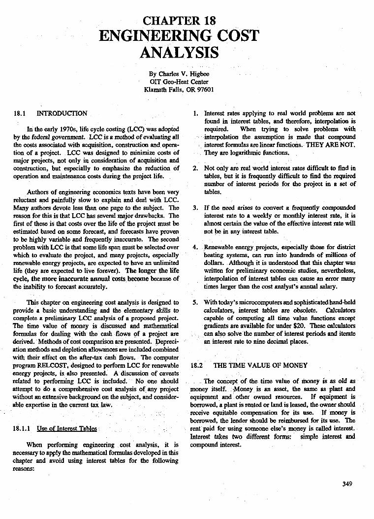
CHAPTER 18 ENGINEERING COST
ANALYSIS By Charles V. Higbee OIT Geo-Heat Center
Klamath Falls, OR 97601
18.1 INTRODUCTION
In the early 1970s, life cycle Costing (LCC) was adopted by the federal government. LCC is a method of evaluating all the costs associated with acquisition, construction and opera- tion of a project. LCC was designed to minimize costs of major projects, not only in consideration of acquisition and construction, but especially to emphasize the reduction of operation and maintenance costs during the project life.
Authors of engineering economics texts have been very reluctant and painfully slow to explain and deal with LCC. Many authors devote less than one page to the subject. The reason for this is that LCC has several major drawbacks. The first of these is that costs over the life of the project must be estimated based on some forecast, and forecasts have proven to be highly variable and frequently inaccurate. The second problem with LCC is that some life span muSt be selected over which to evaluate the project, and many projects, especially renewable energy projects, are expected to have an unlimited life (they are expected to live forever). The longer the life cycle, the more inaccurate annual costs become because of the inability to forecast accurately.
This chapter on engineering cost analysis is designed to provide a basic understanding and the elementary skills to complete a preliminary LCC analysis of a proposed project. The time value of money is discussed and mathematical formulas for dealing with the cash flows of a project are derived. Methods of cost comparison are presented. Depreci- ation methods and depletion allowances are included combined with their effect on the after-tax cash flows. The computer program RELCOST, designed to perform LCC for renewable energy projects, is also presented. A discussion of caveats reIated to performing LCC is included. No one should attempt to do a comprehensive cost analysis of any project without an extensive background on the subject, and consider- able expertise in the current tax law.
18.1.1 Use of Interest Tables
When performing engineering cost analysis, it is necessary to apply the mathematical formulas developed in this chapter and avoid using interest tables for the following reasons:
1. Interest rates applying to real world problems are not found in interest tables, and therefore, interpolation is required. When trying to solve problems with interpolation the assumption is made that compound interest formulas are linear functions. THEY ARE NOT. They are logarithmic functions.
2. Not only are real world interest rates difficult to find in tables, but it is frequently difficult to find the required number of interest periods for the project in a set of tables.
3. If the need arises to convert a frequently compounded interest rate to a weekly or monthly interest rate, it is almost certain the value of the effective interest rate will not be in any interest table.
4. Renewable energy projects, especially those for district heating systems, can run into hundreds of millions of dollars. Although it is understood that this chapter was written for preliminary economic studies, nevertheless, interpolation of interest tables can cause an error many times larger than the cost analyst’s annual salary.
5. With today’s microcomputers and sophisticated hand-held calculators, interest tables are obsolete. Calculators capable of computing all time value functions except gradients are available for under $20. These calculators can also solve the number of interest periods and iterate an interest rate to nine decimal places.
18.2 THE TIME VALUE OF MONEY
The concept of the time value of money is 8s old 8s money itself. Money is an asset, the same as plant and equipment and other owned resources. If equipment is borrowed, a plant is rented or land is leased, the owner should receive equitable compensation for its use. If money is borrowed, the lender should be reimbursed for its use. The rent paid for using someone else’s money is called interest. Interest takes two different f o m : simple interest and compound interest.
349

Throughout this chapter, the time value of money and compound interest are used in the cost analysis of projects. Such things as risk and uncertainty are ignored, and the concept of an unstable dollar or the value of the dollar fluctuating in the foreign market are not considered. However, in LCC analysis of renewable energy projects, inflation rates for operation and maintenance, equipment purchases, energy consumed and the revenue from energy sold for both conventional and renewable energy, will be considered.
The concept of the time value of money evolves from the fact that a dollar today is worth considerably more than a promise to pay a dollar at some future date. The reason this is true is because a dollar today could be invested and be earning interest such that, at sometime in the future, the interest earned would make the investment worth considerably more than one dollar. To illustrate the time value of money, it is convenient to consider money invested at a simple interest rate.
18.2.1 Simde Interest
Simple interest is interest accumulated periodically on a principal mun of money that is provided as a loan or invested at some rate of interest (i), where i represents an interest rate per interest period. It is important to notice that in problems involving simple interest, interest is only charged or earned on the original amount borrowed or invested. Consider a deposit of $100 made into an account that pays 6% simple interest annually. If the money is left on deposit for 1 year, the balance at the end of year one would be:
100 + 0.06(100) = $106.
If the money is left on deposit for 2 years, the balance at the end of year two would be:
100 + 0.06(100) + 0.06(100) = $112.
If the money is left on deposit for 3 years, the balance at the end of year three would be:
100 + 0.06(100) + 0.06(100) + 0.06(100) = $118.
If n equals the number of interest periods the money is left on deposit and i equal the rate of interest for each period, the formula for calculating the balance at the end of n periods would be:
100 + 1OO(i x n).
Substituting 6 % for i and 3 for n, the formula becomes:
100 + lOO(O.06 x 3) = $118.
Substituting present value (F%) for the amount of money loaned or deposited at time zero (beginning of the time period covered by the investment), and future value (Fv) for the balance. In the account at the end of n periods, the formula becomes:
Fv = Pv + F%(i x n).
Factoring out Pv, the formula becomes:
Fv = Pv(1 + i x n). (18.1)
Going back to the original values, if the $100 is left on deposit for 5 years, the future value would be $130, and is written:
Pv = 100; i = 0.06; n = 5 FV = lOO(1 + 0.06 x 5) Fv = $130.
Remember, in simple interest problems, interest is earned only on the amount of the original deposit. Consider the case where interest is calculated more frequently than once per year. This would not change the amount of money earned in simple interest calculations.
Suppose that $100 was deposited for 5 years at a rate of 6 9% simple interest, calculated every three months. Since there are four 3-month periods in a year, the simple interest per interest period becomes 0.06/4 = 0.015 and n becomes 4 quarters per year x 5 y = 20 total interest periods. Therefore:
FV = lOO(1 + 0.015 x 20) FV = $130.
Applying this formula to the time value of money, it can be shown that for any given rate of interest, $100 received today would be much greater value than $100 received 5 years from today. Consider:
Proposal 1: A promise to pay $100 5 yevs from today. Proposal 2: A promise to pay $100 today.
If proposal 2 is accepted over proposal 1, the $100 received today could be deposited into an account that earned 9% annually, and in 5 years the balance would be $145. Using this same theory, the present value of a promise to pay $100 5 years from today can be evaluated as:
Fv = 100; i = 0.09; n = 5 y 100 = F%(l + 0.09 x 5).
Solving for Pv, the equation becomes:
Pv = 100/(1 + 0.09 x 5) Pv = $68.97.
350

Throughcwt this chapter and in cost analysis texts in general, eash flow diagrams are normally drawn to illustrate monies flawing into or out of a project at some specific time period. The accepted convention is: a) money flowing out is indicated by a down arrow and b) money flowing in is indicated by an up arrow.
Example 18.1: A $l,OOO loan to be repaid in two equal annual payments, from the borrower's point of view, would be drawn as:
500 500
and, from the lender's point of view, would be drawn as:
So0 500 m 1.000
The examples below illustrate the application of cash flow diagrams.
Example 18.2: A woman deposited $500 for 3 years at 7 % simple interest per annum. How much money can be with- drawn h m the account at the end of the 3-year period? The cash flow diagram below indicates money deposited into the investment as 4, and money withdrawn from the investment as t ,
1 ; 3 3 yarrs so0
solution:
Fv = PV(1 + i x n) FV = SWl + 0.07 x 3) FV = 500(1.21) Fv = $605.
Example 18.3: Assume $500 is deposited for 200 days in an account that earn 6 % simple interest per m u m . What is the balance at the end of the investment period? The solution is:
Fv = PV(1 + i x n) FV = S00(l -t 0.06[200/36SJ) FV = 500(1.0329) Fv = $516.45.
18.2.2 ComDound Interest
All CDmpOund inkrest formulas developed will include the standard fusctional notation for those formulas b the right of the &vetope& fomula. Functional notation is a shorthand method of mpxenting a formula to he applied to a problem or a portion of a problem, rather than having to write the formula in its entirety.
For example, (FA', i, n) is read, "To find the future value F, .given the present value, P at an interest rate per period i for n interest periods. " This notation applies only to compound interest.
Compoqnd interest varies from simple interest in that interest is eamed on the interest accumulated in the account. To illustrate:
If $100 is deposited at 6 9% compound annually, at the end of the first year the balance would be:
100(1 + 0.06) = $106.
This is the same as in simple interest. However, if the money is allowed to remain on deposit for 2 years, the interest earned during the second year would be:
106(0.06) = $6.36
giving a balance of $112.36 at the end of the second year. If the money is left on deposit for 3 years, the interest earned during the third year would be:
112.36(0.06) = $6.74.
Thus, the balance at the end of the third year would be:
100 + 6 + 6.36 + 6.74 = $119.10.
The mathematical function of compound interest for a deposit of $100 earning 6% compounded annually left on deposit for 3 years is stated and described mathematically below.
Original deposit plus interest earned at the end of the first year becomes:
Fv = 100(1+ 0.006)
plus the interest earned during the second year:
plus the interest earned during the third year:
+o.w{loo(l + 0.06) f 0.06[loo(l + 0.06)D. The formula becomes rather complex with only a 3iyear
investment. The formula can be simplified through mathematical manipulation. For purposes of this illustration,
i and the number of interest pe
Fv = lOO(1 + i) + iflOO(1 + i)] + i(lOO(1 + i) + i [100(1 + i)]}.
351

Factoring out $100 from the above equation:
Fv = 100[(1 + i) + i(1 +i) + i(1 + i) + i(1 + i)] simplifying:
Fv = 100[1 + i + i + i’ + i(1 + i + i + i’>l
simplifying further:
Fv = 100(1 + i + i + i’ + i + i’ + i’ + i3)
and collecting terms:
Fv = 100(1 + 3i + 3i’ + i’) then, this equation can be factored into:
Fv = l00[(l + i)(l + i)(l + i)] = lOO(1 + i)3.
Substituting n for the number of interest periods, which in this case is 3, the result is:
Fv = lOO(1 + i)”. Letting Pv = the amount of the investment, then:
Fv = Pv(1 + i)” (F/P,i,n)( 18.2)
This is the single payment compound amount factor.
Solving Equation (18.2) for Pv gives:
fp/F,i,n)(l8.3) Fv (l+i)
Pv=
which is the single payment present worth factor.
With the development of the equation for hding the future value of a lump sum investment at a compound interest rate for n interest periods, it can be shown how more frequent compounding increases the interest earned.
An interest rate of 3 116 mo would be stated in nominal form as 6% compounded semia~ually.
Consider the following examples with interest rates stated as an annual percentage rate (MR), commonly referred to as the “nominal interest rate.”
Example 18.4 An amount of $100 is invested for 3 years in an account that earns 18% compounded annually. The future value at the end of the 3-year period will be:
Fv = Pv(1 + i)” Fv = 100(1 + 0.18)3 FV = lOO(1.6430) FV = $164.30.
Example 18.5: Assume $100 is invested for three years in an account that earns 18% compounded quarterly. The future value at the end of the 3-year period is:
Fv = Pv(1 + i)” where
i = 0.18/4 quarters/y = 0.045 per quarter n = 3 y x 4 quartersly = 12 interest periods.
Solution:
FV = lOO(1 + 0.045)’’ FV = lOO(1.6959) FV = $169.59.
Example 18.6: Suppose $100 is invested in an account that earns 18 5% compounded monthly. The future value at the end of a 3-year period is:
Fv = Pv(1 + i)” where
i = 0.18/12 months/y = 0.015/mo n = 3 y x 12 moly = 36 interest periods.
Solution:
FV = lOO(1 + 0.015)” FV = lOO(1.7091) FV = $170.91.
Example 18.7 An amount of $100 is invested for 3 years in an Bccounf that earns 18% compounded weekly. The future value at the end of the 3-year period is:
Fv = Pv(1 + i)”
where
i = 0.18/52 weeksly = 0.0034615/week n = 3 y x 52 weeks/y = 156 weeks.
Solution:
FV = 100(1 + Q.0034615)’* FV = lOO(1.7144) FV = $171.44.
352

Example 18.8: If $100 is invested for 3 years in an account that earns 18% compounded daily, the future value at the end of the 3-year period is:
Fv = Pv(1 + i)”
where
i = 0.181365 daysly = 0.00049315/d n = 3 y x 365 dly = 1095 d.
Solution:
FV = 100(1 + 0.00049315)1095 FV = lOO(1.71577) FV = $171.58.
Money invested today will grow to a larger amount in the future. If this is true, then the promise to pay some amount of money in the future is worth a smaller amount today.
Example 18.9: What is the present value of a promise to pay $3,000 5 years from today if the interest rate is 12% compounded monthly? This can be written:
Fv Pv = (1 + i)”
where
i = 0.12/12 = 0.01 n = 5 x 12 = 60.
Solution:
Pv = 3,000/(1 + 0.01)= Pv = $1,651.35.
18.2.3 Annual Effective Interest Rates
It is convenient at this point in the development of com- pound interest to introduce annual effective interest’rates. Annual effective interest (AEI) is interest stated in terms of an annual rate compounded yearly, which is the equivalent of a nominally stated interest rate. Table 18.1 illustrates the relationship between nominal interest, interest rate per interest period, and annual effective interest.
Notice that the nominal interest rate remains the same percentage while the compounding periods change. The interest rate per interest period is obtained by dividing the nominal rate by the number of interest periods per year. The annual effective interest rate is the only true indicator of the amount of annual interest, and therefore, annual effective interest provides a true measure for comparing interest rates when the frequency of compounding is different.
The annual effective interest rate may be found for any nominal interest rate as shown below.
Table 18.1 Comparative Interest Rates
(APR) Nominal Interest Rate per Annual Effective Interest Rate Interest Period Interest (AEI)
(1896) (961 0 Compound . 18.00 18.00
annually
Compounded 9.00 semiannually
Compounded 4.50 quarterly
18.81
19.25
Compounded 1 S O 19.56 monthly
Compounded 0.346 19.71 weekly
Compounded 0.04932 19.716 daily
Compounded 19.7217 continuously
Consider a dollar that was invested for 1 year at a nominal rate of 18 % compounded monthly. To calculate the balance (Fv) at the end of the year:
Fv = 1[1 + (0.18/12)]12
therefore,
Fv = 1(1.015)12 FV = l(1.1956) FV = $1.1956.
Because a dollar was invested originally, the annual interest earned may be found by subtracting the original investment:
1.1956 - 1 = 0.1956
and the effective interest is 19.56%. Then, the formula for finding annual effective interest is:
AEI = [1+5]. - 1 (18.4)
353

where
AEI = annual effective interest rate r = nominal interest rate/y m = number of interest perioddy.
The annual percentage rate is divided by the number of compounding perioddy and raised to the power of the number of compounding periodsly, and 1 is subtracted from that answer to arrive at the annual effective interest rate.
The following examples are used to further illustrate the differences between APR and AEI.
Example 18.10: For an APR of 12% compounded annually, the annual effective interest (AEI) is 12%. Therefore,
AEI = 12% compounded annually. There is no difference between the two.
Example 18.11: For an APR of 12% compounded semi- annually, the semiannual effective interest rate is 0.1212 = 0.06 or 696, presented as:
AEI = (1 + 0.1212)' - 1 = 0.1236 or 12.36%.
Example 18.12 For an APR of 12% compounded quarterly, the quarterly effective interest rate is 0.03 or 3 96, AEI becomes:
AEI = (1 + 0.12/4)4 - 1 = 0.1255 or 12.55%.
Example 18.13: For an APR of 12% compounded daily, the daily effective interest rate is 0.12/365 = 0.003288 or 0.3288 96, giving:
AEI = (1 + 0.12/365)= - 1 = 0.12747 or 12.74%.
When interest is compounded continuously (when n approaches infinity), the annual effective interest rate takes the form of e - 1, where e = the natural logarithm 2.7182818. Therefore, an APR of 12% compounded continuously would yield an AEI of (2.7182818)0.'2 - 1 = 12.749%.
Effective interest rates can be calculated for periods other than annually.
To find a weekly effective interest rate of 12% com- pounded daily, the weekly effective interest rate would be:
(1 + 0.121365)' - 1 = 0.0023, or 0.23%.
Therefore,
M-[l + $ I c - 1 (18.5)
where
r = annual percentage rate m = number of compound periods/year c = number of compound periods for the time frame of
the effective interest rate.
Example 18.14 The present value of a promise to pay $4,000 6 years from today at an interest rate that is compounded quarterly is $2,798. Find the nominal interest rate and the annual effective interest rate.
Fv = h(l + i)" where
n = 6 x 4 = 24 quarters
and solving
4,000 = 2,798(1 + i)%
dividing both sides by 2,798
1.42959 = (1 + i)24
taking the 24th root of both sides
(1 .42959)0.w'67 = [(I + i)upwlsl
1.015 = 1 + i i = 0.015, or 1.5%.
By definition, i is the interest rate per interest period. Therefore, the answer, 1.5 9% , is the interest rate per quarter. In order to find the nominal interest rate (or annual percentage rate), it is necessary to multiply i times the number of quarters per year. The nominal interest rate is 0.015 x 4 = 0.06, or 6 % compounded quarterly. The answer would be incorrect if the frequency of compounding was not included. If the nominal rate is given as 696, this would indicate 6% com- pounded annually.
The annual effective interest rate, using Equation (18.4), becomes:
AEX = (1 + 0.015)' - 1 AEI = 0.0614, or 6.14%.
The formulas developed for compound interest and the similar formula for converting APR to AEI are logarithmic functions (See Figure 18.1).
354

too
90
80 - 70 - /
0 5 10 15 20 25 30 35 40 YEARS
Figure 18.1 Exponential nature of compound interest rates.
When interest rates are extremely low, the number of compounding periods is almost insignificant. For example, 2% APR compounded annually is 2% MI; 2% APR com- pounded daily is 2.02% AEI while 40% APR compounded daily jumps to 49.15 % AEI.
In evaluating projects for nonprofit organizations, interest rates are usually kept rather low, but there are many private entities that evaluate alternatives at the corporation’s rate of return, which can be a very high rate.
18.3’ ANNUITIES
18.3.1 Ordinary Annuities
The definition of an ordinary annuity is a stream of equal end-of-period payments. Ordinary annuities are the most common form of payment series used in cost analysis. Loan payments, car payments, charge card payments, maintenance and operating costs of equipment are all stated in terms of ordinary muities. These payments are frequently monthly payments, but they &n be weekly, yearly or any other uni- form time period. The important thing is that they begin at the end of the first interest period. For example, a person purchases an automobile for $5,000 and is obligated to pay
12%
1 ox
8 X
6%
4%
$125 per month for 48 months. The first payment will be due one month after the purchase of the car and the last payment will be due at the end of month 48. In order to derive a mathematical formula to evaluate ordinary annuities, it is convenient to use the future value formula for compound interest Equation (18.2).
Consider three equal end-of-year payments of $100 each.
?
M 100 100 100
To find the future value of this payment series at the end of year three, use the future value formula. Notice that the first payment is two interest periods before the end of the project. Therefore, the future value of the first payment is:
Fv = Pv(1 + i)” Fv = lOO(1 + i)’. The future value of the second payment, which is one
interest period before the end of the project, is:
Fv = lOO(1 + i)I. 355

The third payment is zero interest periods away from the end of the project. Therefore, the future value of payment number three is simply $100. The future value of all three payments is:
Fv = loo(1 + i)' + lOO(1 + i)' + 100.
Reversing the order of these terms and factoring out $100, the equation becomes:
Fv = 100[1 + (1 + i)' + (1 + i)?.
Notice that with a 3-year project and three annual payments, n does not get higher than 2. This is because the payments are made at the end of each period. Letting A = the amount of each payment, a general equation can be written to find the future value of n payments as:
Fv = A[l + (1 + i)' + (1 + i)' + (1 + i)3 + . . . + (1 + i)"'].
Multiplying this equation by (1 + i) results in:
Fv(1 + i) = A[(1 + i)' + (1 + i)' + (1 + i)' + (1 + i)' +...+ (1 + i)"].
Subtracting the first equation from the second equation:
Fv(1 + i) - Fv = A[-1 + (1 + i)"] also
Fv + i(Fv) - Fv = A[(1 + i)" - 11 and
i(Fv) = A[(1 + i)" - 11
dividing both sides of the equation by i gives:
m = d (1 + i ) p - 11 (F/A,i,n)(l8.6) i
This is the uniform series compound amount factor.
Solving for A instead of Fv gives:
1 i A = + (1 + i) -1
(A/F,i,n)( 18.7)
This the uniform series sinking fund factor.
Returning to the future value formula, Fv = Pv(1 + i)", and substituting the right side of this equation for Fv in Equation (18.6) gives:
dividing both sides by (1 + i)" yields:
(P/A,i,n)(l8.8)
This is the uniform series present worth factor.
Equation (18.8) is used to determine the present value of an ofdinary annuity.
Solving the above equation for A instead of Pv gives:
(A/P,i,n)( 18.9)
This is the uniform series capital recovery factor.
Equation (1 8.9) is used for finding the payment series of a loan or the annual equivalent cost of a purchased piece of equipment.
In calculating future value or present value of a payment series, i must equal the interest rate per payment period, and n must equal the total number of payments. If an interest rate is stated as 12% compounded monthly (APR), and the pay- ment series is monthly, then i = 0.12/12 = 0.01 or 1 Wmo.
Complications can arise when the annual percentage rate is stated in such a manner as to be incompatible with the payment period. For example, assume a loan of $500 to be repaid in 26 equal end-of-week payments with an interest rate of 10% compounded daily. Before this problem can be solved, i must be stated in terms of 1 week. Therefore, the weekly effective interest rate, (WEI) must be calculated as:
WE1 = (1 + 0.10/365)' - 1 WE1 = 0.0019, or 0.19% per week.
When interest is compounded more frequently than the payment, the amount of each payment (A) can be calculated in the above example by:
A = 5OO(A/P,19,26) A = $19.73.
If the above problem had an interest rate of 10% com- pounded quarterly, this would present a case where interest is compounded less frequently than the payment period. There- fore, between compomding periods the interest rate is zero. The payment must coincide with the interest rate. Because 26 weeks constitutes 6months, andtheinterest rate is com-
356

pounded quarterly, there are two quarters in a 26-week period. Therefore, to find the interest rate per quarter, find the payment per quarter and divide that payment by 13 weeks to arrive at a payment per week. The interest rate per quarter is:
0.10/4 = 0.025 or 2.5% A = 5OO(AIP,2.5,2) A = $259.41/quarter.
Dividing the above answer by 13 gives $19.95 as the payment per week.
Returning to the problem at the beginning of 18.3.1 Ordimam Ann uities, $5,000 was financed on an automobile for 48 months at an interest rate of 9.24% compounded monthly. Find the monthly paymenk
where
i = 0.0924/12 = 0.0077 n = 4 x 12 = 48.
Solution
A = 5,000(Aff,0.77,48) A = $124.996 or $125lmo.
18.3.2 &n uities Due
The definition of an annuity due is a stream of equal, beginning-of-theperiod payments. Although this payment series is not nearly as common as an ordinary annuity, it is still found in many projects. Beginning-of-the-prihe-period payments apply to such things as rents, leases, insurance premiums, subscriptions, etc. Rather than attempt to derive a formula to evaluate annuities due, it is much simpler to modify the existing formulas that have already been derived. Consider a 5-year cash flow diagram with payments made at the beginning of each year. These payments will be designated as (a) to avoid confusion with an ordinary annuity. The diagram is shown as:
yrar: 0 :_1 a 4% 1 a a
The easiest approach is to find the future value of this annuity due using a modification of Equation (18.6):
The cash flow diagram requires modifications as:
year: 0 1 2 3 4 5
t 1 I I & 1 1 1 1 a a a a a (a)
By inserting a payment (which does not exist) at the end of year 5, the cash flow diagram now looks like an ordinary annuity of 6 payments. Therefore, using Equation (18.6):
However, the sixth payment does not exist. Therefore, that payment, which is zero interest periods away from Fv, must be subtracted from the above formula as:
Placing - 1 as the last value inside the brackets subtracts the value of the last payment. Notice that n increased to 6 with only 5 payments; therefore, the general formula for finding the future value of an annuity due is:
To find the annuity-due, given the future value, the formula would be:
In order to find the present value of an annuity due of 5 payments use the cash flow diagram:
year: 0 1 2 3 4 5 1 ! 1 ! 4. & 4. t . I a & a &
The present value of this payment series exists at the same point in time as the first payment. Modifying the cash flow diagram, we have:
year: 0 1 2 2 4
Ignoring the first payment, the cash flow diagram appears as an o r d i i annuity of 4 payments, applying Equation (18.8), we have:
357

This yields the present value of 4 of the 5 payments but does not consider the first payment, which is at time zxo, or the same point as the present value. Therefore, the first payment, which is zero interest periods away from Pv, must be added. By modifyiig the above equation and placing a + 1 as the last value inside the brackets adds the value of the first payment and gives:
The general formula for finding the present value of an annuity due is:
+ 11. (1 + i)"-l - i(1 + i1n-1 (P/a,i,n)(l8.12)
To find an annuity due, given the present value, the formula would be:
(a/P,i,n)(18.13) a = p.f (1 + i1n-1 - 1 + 1l-l.
i(1 + i)"-l
18.3.3 Problems Involvine Multiple Functions
Many problems in cost analysis involve the use of several of the formulas presented thus far in this chapter.
Example 18.15: Bonds. Bonds are sold in order to obtain investment capital.
Most bonds pay interest on the face value (the value printed on the bond) either annually or semiannually, and pay back the face value at maturity (the end of the loan period, or end of the life of the bond).
Consider a bond with a face value of $100,000, a life of 10 years, that provides annual interest payments of 8 96. How much should be paid for this bond to make it yield lo%? Thus, the cash flow diagram becomes:
lOOK 8K 8K 8K 8K 8K 8K 8K 8K 8K 8K
1 : : : : : : : : : T Purchase
than $100,000. In other words, the bond would have to be sold at a discount price. To calculate the price to pay for the bond to make it yield 1096, the procedure would be:
Price = 8k(P/A,10,10) + lOOk(P/F,lO,lO) Price = $49,156.54 + $38,554.33 Price = $87,710.87.
To illustrate a premium paid for a bond, assume that the buyer was willing to purchase the bond to yield 7%. Therefore, to make the bond yield lower than 8 5% , the buyer would have to pay a premium.
Price = 8k(P/A,7,10) + 100k(P/F,7,10) Price = $56,188.5 + $50,834.93 Price = $107,023.58
Example 18.16 Bank Loans. A couple financed $50,000 on a home. The terms of the
home mortgage were 9.6% compounded monthly for 30 years. After making payments for 5 years, they want to calculate the amount of money they will pay to principal and interest during the 6th year.
Step 1 is to calculate the amount of the monthly loan payment. Using Equation (18.9) gives:
price
where
where
Pv = $50,000 n = 360 i A = 50,000(A/P,0.8,360) A = $424.08.
= 0.096/12 = 0.008 or 0.8%
Now that the payment is calculated, Step 2 is to find the balance of the loan at the end of year 5. Using Equation (18.8) gives:
The above diagram illustrates the cash flows associated with the bond. The interest is paid out mually to the bond holder. Because there is no opportunity to earn interest on that interest, the bond performs as though it were a problem in simple interest. The performance of the bond cannot deviate from the original cash flow diagram; that is, the bond will always pay $8,000 per year plus $100,000 at maturity. To make this bond pay lo%, the buyer would have to pay less
A = $424.08 i =0.008 n
Pv = 424.08(P/A,0.8,300) Pv = $48,154.90.
= 360 - 60 or 300 payments remaining to be made through year 30.
358

r
Step 3 is to calculate the loan balance at the end of year 6 , letting n = 300 - 12 = 288 payments remaining to be made, and using the same process as in Step 2:
Pv = 424.08(P/A,.8,288) hr = $47,667.74.
Subtracting the loan balance, end of year 6, from the loan balance, end of year 5, = $487.16, the amount that will be paid to principal during year 6.
Step 4 is to calculate the amount of the payments that will go to interest. The total amount paid during year 6 will be $424.08 x 12 or $5,088.96. Subtracting the amount that will go to principal, ($487.16), leaves the amount $4,180.86 that will go to interest during year 6.
Example 18.17: Investments. A couple with two children, ages 2 and 4, want to invest
a single annual payment series that will provide $lO,OOO to each child at the age of 18. The investment will earn interest at 8.75%. If the annual payments sfart today and the last deposit is made 16 years from today, what is the amount of each annual payment? To solve this problem, begin by drawing a cash flow diagram as:
I I I I 1 8 1 10K 10K
Rf R: 0: & 2 fl!~ d 4 & Flf6 ‘!7
t i l
The easiest approach is to find the future value of the required monies and then solve for the annuity. Although it is realized that the older child will withdraw $lO,OOO 14 years from today, the equivalent value of that $lO,OOO can be evaluated at the end of the 16th year. Using Equation (18.2) gives:
FV = Pv(1 + i)” Fv = 10,OOO (1 + 0.0875)’ -k 10,OOO FY = $21,826.56.
Then, using Equation (18.7), and making n = 17, the amount of each payment is:
A = i 7 4- i)” - 11
0.0875 [ (1 + 0.875If7 - 1 A - 21,826.56 A = $604.00.
If this method is confusing, the problem could bave been solved using present value. This requires more calculations and also modification of the cash flow diagram. To approach the problem from a present value point of view, draw a 17- year cash flow diagram as:
10K 10K
In order to solve the problem using present value techniques, it is necessary to note that present value exists 1 year before the first payment. This is the reason for modification of the cash flow diagram. The first $lO,OOO payment must be discounted 15 years and the second $lO,OOO payment must be discounted 17 years. Using Equation (18.3) we have:
Fv Pv= (1 + f)”
10,000 + 10,000 Pv = (1 + 0.0875)15 (1 + 0.O875)l7
Pv = $2,841.59 + $2,402.71 Pv = $5,244.30.
This provides the total present value 1 year before the first payment. Now the payment series can be calculated as an ordinary annuity of 17 payments, using Equation (18.9) we have:
1 [ 0.0875(1 + 0.0875) ’ ’ A = 5,244.30 (1 + 0.0875)17 - 1
A = $604.00.
Notice that, although the final answers are identical, it required much more effort and calculation to solve the problem from a present value
It is advisable to spend some time evaluating problems, drawing cash flow diagrams and considering the simplest approach. Without a cash flow diagram, it would have been very easy to make the error of assuming there were only 16 payments. It is also doubtful that the problem solver could recognize that the easiest approach for this problem is to work with future value. If there is any doubt regarding the answer, it may be verified by working the problem backwards.
359

Suppose annual payments of $604.00 are deposited into an investment for 15 years. The balance in the Bccoullt, using Equation (18.6) would be $17,389.40. At this time, the older child withdraws $10,000, leaving a balance of $7,389.40. This balance will earn interest for 2 more years, and using Equation (18.2), will amount to $8,739.12. Meanwhile, two more payments of $604.00 will be made into the amunt. These two payments, with interest, will amount to $1,260.85, using Equation (18.6). The account balance, then, will amount to $9,999.97. The reason the answer is off by 3 cents is that the actual value of each payment was $604.00081. Using that value as the payment, the answer would equal exactly $10,000.
18.4 COST COMPARISON OF INVESTMENT ALTERNATIVES
For the most part, cost analysis involves selection of the minimum cost or maximum profit alternatives. There are basically four accepted methods of evaluating Alternative A as compared to Alternative B as compared to Alternative C.
18.4.1 Present Value Method
The first of these methods is the present value technique, wherein all costs and revenues are discounted back to present value to arrive at a net present value for the project. This method is very time consuming if performed manually and presents problems when the alternatives have different economic lives. Alternative A may have an expected life of 10 years, Alternative B may have an expected life of 15 years, and Alternative C may have an expected life of 20 years. Therefore, in order to do any meaningful evaluation of these three alternatives in terms of present value, it is necessary to find a common denominator for their expected life, which, in this case, would be 60 years, where Alternative A would be replaced six times, B replaced four times, and C replaced three times.
18.4.2 Future Value Techniaue
The future value technique of evaluating alternatives is almost identical to the present value method except that all costs and revenues are stated in terms of future value. The problem still arises of alternatives with incompatible useful lives. The above techniques are self-explanatory, and because they require such extensive calculations, they will not be covered further. But, because they exist, when evaluating alternatives using computers, it is convenient to indicate, somewhere in the output data generated, the net present value (NFV) of each alternative. Many organizations base their decisions on NFV, and governmental agencies, expect to evaluate benefitcost ratios. The benefitcost ratio is the ratio of benefits provided by the alternative versus cost incurred, and will be discussed later in this chapter.
360
18.4.3 Annual Euuivalent Cost Method
The annual equivalent cost method of evaluating alternative projects states all costs and revenues over the useful life of the project in terms of an equal annual payment series (an ordinary annuity). This is probably the most widely used method in the industry, for several reasons:
1. It quires less effort and fewer calculations.
2. It eliminates the problem of alternatives with incompatible useful lives.
3. It allows for much more sophistication when considering inflation, increasing equipment cost, equipment depreciation schedules, etc.
The annual cost method assumes that the project will live forever, and that, if Alternative A has a useful life of 10 years and Alternative B has a useful life of 15 years, each alternative will be replaced at the end of its useful life. Therefore, the alternative with the minimum annual cost or maximum annual profit is the alternative that will be chosen.
Evaluate a piece of equipment that costs $10,000, has a 6-year useful life with a salvage value of $2,000, and annual operating cpts of $5,000. The interest rate used for the pro- posed evaluation is 9% compounded annually. To calculate the cost of purchasing this equipment, operating it for 6 years, and salvaging it at the end of 6 years for $2,000 at 9% inter- est, the procedure would be to draw a cash flow diagram as:
2K
3 1W SK SK 5K SK SK 5K
The typical approach would be to find the annual cost of $10,000, subtract the annual cost of $2,000 salvage, and add the annual operating cost of $5,000. The annual equivalent of the purchase may be found by using Equation (18.9) as:
.=,[ i(1 + i)” ] (1 + i)” - 1
Next, find the annual equivalent cost of the salvage value, using Equation (18.7), as:
i (1 + i)” - 1

* = - [ O . O 9 ] 2K. (1 + 0.09)6 - 1
Finally, add the $5,OOO operating cost. The total calculations appear as:
*=[ (1 + 0.09)s - 1
A = $2,229.20 - $265.84 + $5K
A = $6,963.36.
The value of Equation (18.9), wbich was used to find the annual equivalent cost of equipment purchased is 0.2229198.
The value of Equation (18.7), which was used to find the annual equivalent cost of the salvage value, is 0.1329198.
Notice that the difference between 0.2229198 and 0.1329198 is exactly equal to the interest rate (i), 0.09. This is true for all interest rates, provided that these functions have the same i and the same n.
In calculating the annual equivalent cost of purchasing the equipment and subtracting the annual equivalent cost of the equipment salvage at some time in the future, this is always the case: i and n are equal; and Equation (18.9) - i = Equation (18.7).
Using functional notation as symbols for these formulas we have:
[(A/P,9,6) - 0.091 = (AIF,9,6).
Making this substitution, the annual cost formula becomes:
A = (A/P,9,6)10K - [(A/P,9,6) - 0.0912K + 5K
multiplying,
A = (A/P,9,6)10K - (A/P,9,6)2K + 0.09(2K) + 5K factoring out (A/P,9,6),
A = (A/P,9,6)(10K - 2K) + 0.09(2K) +5K
the general equation for the annual cost equation becomes:
A = i;'' + 1)" .* 'In - 1 ] (cost - slvg) + i(slvg) + OC
then
A = (A/P,i,n)(cost - salvage) + i(salvage) + OC
represents the annual equivalent cost formula
(18.14)
Figure 18.2 Annual Equivalent Cost.
361

where
oc = annual operating cost.
This modification of the annual cost formula greatly reduces the amount of calculation necewary to arrive at the annual equivalent cost.
Values can be produced by this formula as monthly equivalent costs or weekly equivalent costs by simply changing i to the interest rate per period and allowing n to equal the total number of periods. Using the previous example, rmppose the annual percentage rate was 9% compounded monthly. To calculate the periodic costs in terms of monthly equivalent costs (as a monthly ordinary annuity):
A = (A/P,0.75,72)(10K - 2K) + 0.0075(2K) + 5w12 A = $144.20 + $15.00 + $416.67 A = $575.81.
Stating costs as an ordinary annuity has nothing to do with actual cost flows. It simply states all costs and revenues as an equal payment series in order that one alternative may be compared with another (See Figure 18.2).
18.4.4 Rate of Retum Method
The rate of return @OR) method of comparing alter- natives calculates the interest rate for each alternative and selects the highest ROR. A word of caution is necessary, ROR evaluates INVESTED capital and the costs of operation and maintenance as opposed to revenues or benefits received from the project. Therefore, a project totally financed with borrowed money has no rate of return because there is no invested capital. The following examples assume 10096 equity financing and are used to illustrate rate of return calculations.
Example 18.18: An investment of $7,000 is placed into an Bccount for a 10-year period. At the end of 10 years, the balance in the Bccounf is $17,699.30. What was the annual interest rate earned? Using Equation (18.2):
Fv = Pv(1 + i)" $17,699.30 = $7,000(1 + i)". This problem can be solved by dividing both sides of the
equation by $7,000 giving:
17,699.30/7,000 = (1 + i)l0
2.528 = (1 + i)'O.
Extracting the tenth root of each side of the equation gives:
(2.528)O.l = [(l + i)'"p.'
1.0972 = 1 + i i = 0.0972.
A ROR can also be calculated by evaluating the differ- ence between alternatives that provide cost savings rather than revenues.
Example 18.19: Fire insurance premiums on a wam house are $5OO/y (Alternative A). The same coverage can be purchased by paying a 3-year premium of $1,250 (Alternative B). Find the ROR realized by purchasing a 3-year policy in place of three l-year policies.
To simplify this problem, notice that the 3-year insurance premium is 2.5 times the annual premium. The cash flow dia- gram for Alternative A appears below.
i-+-++ 1 1 1
The cash flow diagram for Alternative B appears below.
lT-t+-+ 2.5
To further simplify this problem, consider the differences between these two alternatives. If Alternative A is subtracted from Alternative B, the cash flow diagram becomes:
1.5 :_I Although the insurance premiums are an annuity due, the
cash flow diagram above makes the cash flows appear as an investment of $1.5 providing an ordinary annuity of $1 at the end of each year for 2 years. The analysis has Simplified the problem considerably and avoided using the more complex formulas associated with annuities due. Using Equation (18.8):
Entering values in this formula requires that the mathematical signs be properly observed. If money flowing out, below the time line, is considered positive (+) then money flowing in, above the time line, or money saved is considered negative (-). The calculation then becomes:
362

Notice there is one equation and one unknown (i), but the unknown appears three times in the equation. Therefore, the only solution would be by an iterative process. Continuing with Equation (18.8):
where
i = 0.21, or 21% PV = 1.5 A = - 1 .
The answer to this problem is - 0.00946, indicating that the first interest rate was too low.
Try i = 22%
The answer, 0.00847, indicates the interest rate is too high. The actual interest rate is 21.525043%. Placing this interest rate into the formula for i, the answer equals zero, indicating that the ROR realized by purchasing a 3-year policy instead of three 1-year policies is 21.5%. There are many pocket calculators costing under $20 that are designed to calculate financial functions and are capable of iterating i for problems involving a single financial function.
Consider the annual cost formula where:
a = (AIP,i,n) x ( cost - salvage) + (i) salvage + OC - revenues.
Suppose it is required to find the ROR on such a project. Once again, the solution to the problem is found by iteration. But in this case, there is more than one financial function. Choose an interest rate. Work the problem at that interest rate, and find out if the answer comes out positive or negative. With the mathematical signs we have used in this example, if revenues exceed costs the answer would be negative; if costs exceed revenues the answer would be positive. When the exact i is placed into the formula that denotes the ROR, the answer would be zero. That is, the interest rate that causes revenues and costs to be exactly equal. Interest tables may be used to help find an upper and lower range for i to reduce the number of iterations necessary.
A much easier solution is to place all of the cash flows by year into a computer and write a simple program that can do thousands of iterations in a matter of seconds to find i.
Trying to iterate i for a problem with more than one function on a financial calculator nearly always results in error becauseof the tremendous amount of time anddata that
must be entered by hand. Even with a computer program, if the cash flows turn from negative to positive and back to negative during the project life, i can take on the form of a quadratic equation and the computer is unable to determine whether i is positive or negative. There are computer spreadsheets and other software available for iterSting i, but these have their limitations. One of the most popular and widely used spread-sheets is designed to iterate i for a series of cash flows. However, this spreadsheet requires a rather accurate guess for i; because, if it does not find i after 20 iterations, the resultant answer is "Err" (error). The RELCOST program developed to accomplish LCC analysis (copyright, Washington State Energy Office) will iterate i to seven decimal places in a matter of seconds for projects with over 150 input variables and more than 500 inflation ram, and evaluate the iterated i to determine whether it is positive or negative. This program will be discussed in more detail in Subsection 18.7, entitled "LIFE CYCLE COST ANALYSIS."
18.5 GRADIENTS
18.5.1 Arithmetic Gradients
Having developed formulas for equal payment series involving both ordinary annuities and annuities due, an end-of- period payment series that increases by a fixed dollar amount at the end of each period can now be evaluated. Consider the folloying end-of-period payments:
t I I I I J 4. .L. t 1 100 120 140 160 160
As can be seen in the cash flow diagram above, the pay- ment series started at $100 and increased by $20 per year. Such a payment series is called an arithmetic gradient. Although such a payment series is covered in detail by most texts on engineering economics, it is highly unlikely that any portion of a project will contain such a payment series.
The method used to solve for present value, future value or annual equivalent cost of such a payment series is to break it up into a series of ordinary annuities.
c 100 100 100 100 100
20 20 2Q 20 20 2Q 20
20 20 * 20
This payment series now appears as five ordinary annui- ties. Because the series is progressing in the direction of future value, it is easiest to assume one annual payment series of $100 and find the future value of the sum of the remaining four annuities and string them out in the form of an annual
363

equivalent for the 5-year period. The formula to accomplish this, where n = 5 and i = 955, is:
0.09 ( 1 + 0.09)' - 1 A = 2 O [ A -
The 5-year equivalent cost of an arithmetic gradient of $20 that begins at the end of year 2 and increases through year 5 is $36.56. Therefore, the annual equivalent of the payment series that began with $100 and increased by $20 for the next 4 years is $100 + $36.56, or $136.56.
0 Notice that when dealing with an arithmetic gradient, A,
becomes an ordinary annuity, and the amount of increase starting at the end of the second period is considered to be the gradient. The gradient formula is based on the fact that the gradient always begins at the end of the second period and is to be strung out as an equal payment series from the end of the first period to the end of the cash flow. The general formula for finding the equivalent annual cost of an arithmetic gradient is:
This is the arithmetic gradient uniform series factor where G is the amount of increase beginning at the end of the second period.
If the present value or future value of an arithmetic gradient is required, one could simply multiply Equation (18.15) by (P/A,i,n) or (F/A,i,n).
The most common use of arithmetic gradients is in calculating the value of sum-of-yearsdigits (S-Y-D) depnkiation, which takes the form of a negative arithmetic gradient. This method of depreciation is no longer allowed under the 1987 tax law. 0
18.5.2 Geometric Gradients
A geometric gradient is an end-of-period payment series that increases by a fixed percentage each period. Consider a 5-year payment series that begins with $100 and increases by 9% every year thereafier. A cash flow diagram used for calculation of the problem is shown as:
I ' I i
1 1 I 1 100 169 IldBei 1E9!50 141.16
The cash flow diagram above illustrates a geometric gradient with the first payment (A,) equal to $100 and each subsequent payment increasing by 9% in other words, a $100 payment inflating at a rate (g) of 9% annually. Then:
t I I I I
and the present value (Pv) for an assumed cost of capital of 12% compounded annually (i) is:
- the present value factor ( P / P , i , n ) . (1 + i)'
Let n equal the number of interest periods (years, in this case). Then:
Note that:
where g is constant.
%ere fore:
Then, to find the mual equivalent cost (A), considering inflation: annual cost = present cost x capital recovery factor (A/P,i,n) and is written:
A = PV x (A/P,i,n)
Multiplying by the capital recovery factor:
364.

Simplifying:
* .
(A/Al,g,i,n)(18. 16)
This is the geometric gradient uniform series factor,
Using functional notation:
where g # i.
whereg # i.
Inserting the initial values in this example:
'noo0 [(1.5386) (0.5674) - 11 A = 0.09 - 0.12
(0.2774) = $117.38.
The annual equivalent cost equals $117.38. Figure 18.3, plots a geometric gradient increasing by 9% for 20 years and indicates the annual equivalent cost at a discount rate of 12%.
Notice, by removing the capital recovery factor in Quation (18. la), the equation becomes:
(P/A,g,i,n)(lS. 17)
whereg # i.
This is the geometric gradient present werth factor, whereg # i.
In the case where the discount rate equals the rate of inflation (g = i), the equation becomes AI divided by zero, which is undefined. If a geometric gradient is increasing by exactly the discount rate, this has the same effect of an interest rate equal to zero; therefore, simply take AI, multiply it by the total number of payments (n), which will yield a present value at the end of year one. Because pment value represents the dollar equivalent at time zero, the amount that was calculated by multiplying AI by n is one interest period off. To bring it to the proper time frame, time zero, simply discount it by one time period. Therefore:
P v = 1 - . A (n) (PIA,,g,i,n) (18.18) (1+1)
whereg = i.
This is the geometric gradient present worth factor, whereg = i.
MARS
Figure 18.3 Geometric gradient.
365

Nthough geometric gradients are rather common and are found in many applications, they require that the rate of increase remain amstant. Such is not the case in most energy forecasts, where inflation rates are modified year by year. This problem will be discussed later in Section 18.7 under the heading, "LIFE CYCLE COST ANALYSIS."
Figure 18.4 graphs a project with the following input variables: I
Project life in years Interest rate (APR) Capital investment Salvage value Annual costs
Insurance Fixed Arithmetic gradient Geometric gradient
increasing at 10% increasing at 6%
Depreciation method
2O-yearArmual Eauivalealt Costs
. 20
$120,000 $16,065 12 %
12,000 -167
500 560 2,250 2,250
230 301
2,000 4,051 10,000 14,895
200% declining balance
Figure 18.4 illustrates the total annual equivalent costs for operating this project for 1 year, 2 years, 3 years, etc. The capital recovery line indicates the annual equivalent of investing capital and salvaging the project at end of year 1,2, 3, etc. The operation and maintenance line shows the annual equivalent cost of operating the project in years 1 through 20. Notice that the minimum annual cost occurs in year 15, which is $38,486. That is to say, the annual equivalent stream of equal payments for operating the project with a 15-year life would be $38,4861~.
Table 18.2 provides annual equivalent values from year 1 through year 18 for capitat recovery, operation and mainten- ance costs, and total annual costs. Salvage values for any given year are indicated in the iast column. This analysis is beyond the scope of this chapter, but could be used to deter- mine the ecollomic life (minimum annual cost) of a project that had these cost characteristics. Table 18.2 provides answers for various costs that could be beneficial to those who want to sharpen their expertise in calculating capital recovery, annuities due, ordinary annuities, geometric gradients, and arithmetic gradients.
YEARS
Figure 18.4 Economic life.
366

Table 18.2 Economic Life Calculations
- Year 1 2 3 4 5 6 7 8 9 10 11 12 13 14 15 16 17 18
Capital Recovery $38,400 34,777 3 1,754 29,224 27,100 25,311 23,800 22,519 21,431 20,554 19,629 18,875 18,253 17,734 17,297 16,926 16,609 16,337
O&M costs
$14,810 15,296 15,779 16,259 16,735 17,207 17,674 18,135 18,592 19,042 19,485 19,922 20,352 20,774 21,189 21,596 21,995 22,385
Total Costs
$53,210 50,073 47,533 45,483 43,834 42,517 41,473 40,655 40,023 39,596 39,114 38,797 38,605 38,509 38,486 38,522 38,604 38,722
Salvage Values
$96,000 76,800 6 1,440 49,152 39,322 3 1,457 25,166 20,133 16,106 12,000 12,000 12,000 12,000 12,000 12,000 12,000 12,000 12,000
18.6 EQUIPMENT DEPRECIATION
A discussion of equipment depreciation is essential in evaluating projects for taxable entities because equipment depreciation significantly lowers the annual cost of a project. This subject is also the area of constant change because it changes as tax laws are revised. The amount of total capital investment in a project and the reduction in tax liability caused by depreciation or investment and energy tax credits or both, all have a major bearing on whether or not the project is economically feasible. However, the 1986 tax law drastically reduced many of these incentives. Competent tax accountants should be a part of the development team to ensure proper utilization of these considerations. 3
18.6.1 Straight Line Deureciation
Straight line depreciation is the simplest form of depreciation and has survived tax law changes for many decades and it is accepted by the 1987 tax law. The formula for straight line depreciation is:
- l i f e = one unit of depreciation
Life can be expressed in years, months, units of production, operating hours, or miles. Under the 1987 tax law, salvage values are set to zero.
18.6.2 Sum-of-Years Dieits Denreciation
This depreciation method is an accelerated depreciation schedule that recovers larger amounts of depreciation in the early life of the asset. The method of calculation is as follows:
1. Find the hum of the years' digits of the life of the equipment. Example: For a IO-year life, the sum of the digits 1 through 10 is equal to 55. The easiest way to make this calculation is:
life x (life + 1) 2
in this case,
10 x (10 + 1) = 5 5 . 2
2. This unit of depreciation is then divided into cost salvage to obtain one unit of depreciation, which is:
Example: Equipment cost = $60,000 Salvagevalue = $ 5,000
then,
6Qfooo - ' * '0° = $l,OOQ = one unit of depxeciatiox 55
3. This unit of depreciation is then multiplied by the years of life in descending order, that is:
year 1 = 10units = $10,000 year 2 - gunits= $9,000 year 3 = gunits= $8,ooo -- - - I------- -- ------- year lo= lunit = $1,000.
The depreciation charge under this method performs like negative arithmetic gradient where A, is $lO,OOO and G is -$1,000.
Although this method of depreciation is accepted accounting practice and may be used on equipment purchased before 1980, it is no longer allowed under the 1987 tax law and is only discussed to illustrate an application of the arithmetic gradient.
i.3 Declining Balance Demeciation
This method of depreciation is also an accelerated form may obtain even larger depreciation in the early life than -D. With 200% declining balance depreciation, the mual is 200% times the Straight line rate. As an example:
367

An asset with a 10-year life has a straight line rate of 1/10. Therefore, the 200% declining balance rate would be 2/10 or 20%.
This rate is applied to the book value of the asset, where book value equals cost minus accumulated depre- ciation. Any salvage value of the equipment was not considered except that the tax code provided that the equipment could not be depreciated below its salvage value. The $60,000 piece of equipment in the example above would be evaluated using 200% declining balance as shown in Table 18.3.
Table 18.3 Declining Balance Depreciation Using 200% Declining Balance
Book Value x Annual Book Value Depreciation Rate Depreciation End of Year
year 000 1 60,000 x 0.20 12,000 48,000 2 48,000 x 0.20 9,600 38,400 3 38,400 x 0.20 7,680 30,720
Although this method of depreciation provides the maxi- mum write-off in the early life of the equipment, the annual depreciation charge rapidly decreases to the point that it would be beneficial to switch to straight line after the 6th year. It is interesting to note that the declining balance method of depre- ciation, whether it be 20096, 150% or 12596, takes the form of a negative geometric gradient and the book value for any year can be calculated using Equation (18.2). In this example,
FV = $60,000 (1 - 0.2013 Fv = $30,720 = book value end of year 3,
to calculate the depreciation for year 6,
FV = [60,000 (1 - 0.20511 0.20 FV = $3,932,16.
In the example above, the book value is calculated for the end of year 5, and multiplied by the depreciation rate, 0.20, to obtain the annual depreciation for year 6.
Once again, although this method of depreciation is an accepted aocounting method, declining balance depreciation was made obsolete with the 1980 tax law changes. How- ever, a modified version of this method was reinstated with the 1986 tax code revision and is discussed below.
18.6.4 Accelerated Cost Recoverv System (ACRS)
The Accelerated Cost Recovery System (ACRS) was introduced in 1981, but underwent major revision in 1986, effective with the 1987 tax year.
The 1986 tax law provides that equipment with class lives of 3,5,7, and 10 years can be depreciated using 200% de- clining balance, and 15 and 20 years property can be depreci- ated using 150% declining balance. The Internal Revenue Code specifies asset life under the Asset Depreciation Range (ADR). Table 18.4 lists the various classes of depreciable property under the Accelerated Cost Recovery System.
Table 18.4 Classes of Depreciable Property
Property All personal property other than real estate. class
Special handling devices used in the manufactuhg of food and beverages.
3-Year Special tools used in the manufacture of fabricated Property metal products, motor vehicles, and finished plastic
products.
Property with an ADR midpoint life of 4 years or less.
Automobiles or light general purpose trucks.
Semiconductor manufacturing equipment.
Aircraft owned by non-air-transport companies.
computers.
5-Year Property equipment.
Computer-based telephone central office switching
Equipment used in research and experimentation.
Equipment qualifying as a small power production facility within the meaning of Section 3(17)(C) of the Federal Power Act (16 U.S.C. 7%(17)(C)), as in effect on 9-1-86.
Petroleum drilling equipment.
Property with an ADR midpoint life of >4 and e 10 years.
368

Table 18.4 Classes of Depreciable Propehy (continued)
Property All personal property other than real estate. Class
AI1 property not assigned to another class.
Any single purpose agricultural or horticultural structure.
7-Year Property Office furniture, equipment, and fixtures.
Any railroad track.
Property with an ADR midpoint life > 10 and < 16 p l . S .
Equipment used in the refining of petroleum, the manufacture of tobacco products and certain food products.
10-Year Property Railroad cars.
Property with an ADR midpoint life of > 16 and <20 years.
Any telephone distribution plant and equipment used for 2-way exchange of voice and data communications.
15-Year Property Any municipal waste water treatment plant.
Property with an ADR midpoint life of >20 and <25 years.
20-Year Any municipal sewer. Property Property with an ADR midpoint life of 25 years or
more.
Property Real property (real estate) Class
27.5-Year Residential rental property {excluding hotels and Property motels).
31.5 Year Non-residential real property.
One of the major revisions to the declining balance method is that, in the year of purchase, only 0.5 y of depreci- ation is allowed and, in the year of disposal, only 0.5 y of depreciation is allowed. Therefore, if the $60,000 piece of equipment with a 10-year life is depreciated under ACRS, the depreciation schedule would be as shown in Table 18.5.
Table 18.5 Depreciation Schedule
Book Value x Annual Book Value Depreciation Rate Depreciation End of Year
year ($)($,A 1 60,000 x 0.10 6,000 54,000 2 54,000 x 0.20 10,800 43,200 3 43,200 x 0.20 8,640 34,560
Table 18.6 Accelerated Cost Recovery System Depreciation ~~
3- 5- 7- 10- 15- 20- Recovery Year Year Year Year Year Year
Year Class Class Class Class Class Class 1 33.33 20.00 14.28 10.00 5.00 3.5 2 44.44 32.00 24.49 18.00 9.50 722 3 - 14.82 19.20 17.49 14.40 8.55 6fS 4 7.41 11.52 12.49 11.52 7.69 618 5 11.52 8.93 9.22 6.93 5.7l 6 5.76 8.93 7.37 6.23 528 7 8.93 6.55 5.90 4.S 8 4.46 6.55 5.90 452 9 6.55 5.90 @ 10 6.55 5.90 4.46 11 3.29 5.90 4.46 12 5.90 4.46 13 5.90 4.45 14 5.90 4.45 15 5.90 4.46 16 3.00 4A5 17 4.4s 18 4A5 19 4A5 20 4A5 21 225
Notes: The table values are to be multiplied by the cost basis of the equipment.
3-year class through 10-year class property is depreci- ated using 200% declining balance, converting to straight line in the year underlined.
15-year class and 20-year class property is depreciated using 150% declining balance and converting to straight line in the year underlined.
The half-year convention treats all classes as though they were placed in service in mid-year, allowing 0.5 y of depreciation in year 1 and 0.5 y of depreciation when the property is disposed of, removed from service, or in the last recovery year.
369

10
\ - 2002 OB
o+ I I I I I I I I I I
0 1 2 3 4 5 6 7 8 9 10 11
YEARS Figure 18.5 Depreciation methods.
Under this system of depreciation, the user would switch to straight line in year 7. Table 18.6 provides values for the various classes of equipment and these values switch to straight line automatically in the year that straight line will provide a larger annual depreciation. In year 7, 8,9, and 10, the depreciation on the $60,000 piece of equipment would be $3,9301~. However, in year 1 1, which is considered the year of disposal (for tax purposes), the 1986 tax law half-year convention would allow only $1,965 of depreciation.
Table 18.6 presents multipliers for accelerated cost recovery system depreciation.
Figure 18.5 illustrates an asset costing $50,000 with zero salvage value and a 10-year life depreciated by all of the above methods.
During years 7 through 10, ACRS and 200% declining balance are almost identical. The asset is Mly depreciated at the end of year 10 using 200% declining balance, but using ACRS the half-year convention applies in year 11.
It is important to note the tremendous amount of tax revenue generated in year one under the 1986 tax code.
370
18.7 LIFE CYCLE COST ANALYSIS
Life cycle costing (LCC) evaluates all the costs associated with'acquisition, construction and operation of a project. LCC is designed to minimize costs of major projects, not only in consideration of acquisition and construction, but especially in the reduction of operation and maintenance costs during the project life. LCC is the calculation of all annual costs and revenues over the life of the project. These values are totaled by year and discounted back to time zero at some interest rate to arrive at a net present value. This process is repeated for each alternative. The alternatives are then compared, based on net present value or equivalent annual cost.
When performing this analysis, it is important to do sensitivity analysis. Sensitivity analysis consists of changing parameters or variables within the project to determine their effect on the feasibility of the project. Sensitivity analysis is accomplished by substituting one type of construction for another or evaluating various pieces of equipment with different operating costs, evaluating what effect a change in the economic inflation rate would have on the project, and considering various financing scenarios to observe their effect on the outcome.

Example 18.20: Table 18.7 provides the input data for evaluating three heating systems. As a very simple example of LCC, consider a 15-year LCC for three alternatives (A, B, and C as shown in Tables 18.8, 18.9, 18.10, 18.11, 18.12, and 18.13) to provide heat for a 30,000 ft* office building.
Table 18.7 Heating System Cost Alternatives
Electric Heating Resistance Beat Pump Geothermal
Capital cost ($) 158,400 180,OOO 233,100 Life (y) 12 12 12 Salvage value ($) Q -0- -0- Annual electricity
requirement @Wh) 263,680 131,840 22,620 cost ($kwh) $ 0.05 $ 0.05 $ 0.05 Annual maintenance ($) 1,584 2,650 2,33 1 Annual insurance ($) 554 630 816 Annual property tax ($) 238 270 350 Compressor replacement
end of year 10 ($) -0- 750 -0-
Tables 18.8, 18.9, and 18.10 provide a 15-year LCC on each system by year and evaluate these costs at 8% com- pounded annually. Electrical power costs are assumed to be $O.O5kWh. Notice each cost is entered in the year it occurs. Insurance premiums k e paid annually and are in the form of an annuity due. Based on the present value at an 8% rate of interest over the 15-year life cylce, the heat pump has the lowest cost, and based on the criteria of the lowest present value, the heat pump would be the best selection. However, when the cost of electricity is increased to $O.O7kWh, presented in Tables 18.10 and 18.11, the geothermal system becomes less expensive, having a lower net present value, and lower annual equivalent costs.
Although the annual equivalent cost accurately indicates which alternative is the best choice, it has absolutely nothing to do with actual expenditures per year. Although the Heat Pump costs $6,592/y to operate and has higher maintenance costs than the Geothermal system, at $O.O5kWh it provides the lowest annual cost. The reason for this is the lower initial cost of the Heat Pump.
Another approach to LCC analysis would be to examine the difference in costs between System B and System C. Table 18.13 illustrates this approach. Note that the cost of electricity has been changed to $O.O7kWh. Although $53,100 additional is spent by purchasing System C over System B, the net present value of the operating costs over a 15-year period
at 8%/y is $13,019 more for System B than for System C. Because the savings in operation and maintenance costs exceed the value of the initial investment, System C would be chosen over System B.
Table 18.8 Life Cycle Cost of Heating System (A)
Electric Resistance Heat Capital Cost $158,400 Interest Rate 8% Electric Power Cost $O.O5kwh
Electric Power Ins. Cost Cost
Y e a r o f i
0 1 2 3 4 5 6 7 8 9 10 11 ,
12 13 14 15
-0- 554 13,184 554 13,184 554 13,184 554 13,184 554 13,184 554 13,184 554 13,184 554 13,184 554 13,184 554 13,184 554 13,184 554 13,184 554 13,184 554 13,184 554 13,184 -0-
Prop. TaX Cost 1$1
-0- 238 238
238 238 238 238 238 238 238 238 238 238 238 238
238
Total Cost ,
Net Present Value
h u a l Maint. Total cost Cost !$,A
-0- 158,954 1,584 15,560 1,584 15,560 1,584 15,560 1,584 15,560 1,584 15,560 1,584 15,560 1,584 15,560 1,584 15,560 1,584 15,560 1,584 15,560 1,584 15,560 1,584 15,560 1,584 15,560 1,584 15,560 1,584 15,006
$ 391,800 $291,965
Present Value 0 158,954 14,407 13,340 12,352 11,437 10,590 9,805 9,079 8,407 7,784 7,207 6,673 6,179 5,721 5,298 4,730
Annd Equivalent Cost $ 34,110
~ Another method of evaluation involves calculating the ROR of the savings versus the costs. This method is also illustrated in Table 18.13. By iteration (trial and error), a rate of 11.7986 % causes the net present value of the savings to be exactly equal to the net present value of the costs. Therefore, the ROR realized by selecting System C over System B is - 12% annually. Often in this type of analysis, the actual annual costs are not an equal stream of payments, and may frequently swing from positive to negative. Such detailed analysis on uneven cash flows can only be pedormed efficiently with a computer program.
371

Table 18.9 Life Cycle Cost o f Heating System (E1
Air t o Air Heat Pump capital cost $180,000 Interest Rate 8Z Electric Power Cost fO.OS/kWh
El ectri c Prop. Annual Power Ins. Tax Maint. Total cost cost cost cost cost
Year ($1 ($1 ($1 ($1 ($1 - 0 1 2 3 4 5 6 7 8 9 10 11 12 13 14 15
-0- 6,592 6,592 6,592 6,592 6,592 6,592 6,592 6,592 6,592 6,592 6.592 6,592 6,592 6.592 6,592
630 630 630 630 630 630 630 630 630 630 630 630 630 630 630 -0-
-0- 270 270 270 270 270 270 270 270 270 270 270 270 270 270 270
-0- 180,630 2,650 10,142 2,650 10,142 2,650 10,142 2,650 10,142 2,650 10,142 2,650 10,142 2,650 10,142 2,650 10,142 2,650 10,142 3,400a 10,892 2,650 10,142 2,650 10,142 2,650 10,142 2.650 10,142 2,650 9,512
Present Value
($1
180,630 9,391 8,695 8,051 7,455 6,902 6,391 5,928 5,479 5,074 5,045 4,350 4,028 3,729 3,453 2,999
Total Cost S 332,880 Net Present Value t 267.589 Annual Equivalent Cost t 31,262
a. Indicates compressor replacement.
Table 18.11 Life Cycle Cost of Heating System (61
Air to Air Heat Pump Capital Cost $180,000 Interest Rate 82 Electric Power Cost $0.07/kWh
Electric Prop. Annual Power Ins. Tax Maint. Total Present Cost Cost Cost Cost Cost Value
Year ($1 ($1 ($1 ($1 ($1 ($1 - 0 1 2 3 4 5 6 7 8 9 10 11 12 13 14 15
-0- 9,229 9,229 9,229 9,229 9,229 9.229 9,229 9,229 9,229 9,229 9,229 9,229 9,229 9,229 9,229
630 -0- 630 270 630 270 630 270 630 270 630 270 630 270 630 270 630 270 630 270 630 270 630 270 630 270 630 270 630 270 630 270
-0- 180,630 2,650 12,779 2,650 12,779 2,650 12,779 2,650 12,779 2,650 12,779 2,650 12,779 2,650 12,779 2,650 12,779 2,650 12,779 3.400a 12,779 2,650 12,779 2,650 12,779 2.650 12,779 2,650 12,779 2,650 12,149
180,630 11,832 10,956 10,144 9,393 8,697 8,053 7,456 6,904 6.393 6,266 5,481 5,075 4,699 4,351 3,830
Total Cost f 372,432 Net Present Value f 290.159 Annual Equivalent Cost S 33,899
a. Indicates compressor replacement.
Table 18.10 Life Cycle Cost of Heating System (C) Table 18.12 Life Cycle Cost o f Heating System ( C )
Geothermal Heating System Capital Cost $233,100 Interest Rate 82 Electric Power Cost fO.OS/kWh
Electric Power Ins. cost cost - Year ($1 (f)
0 -0- 816 1 1,131 816 2 1,131 816 3 1,131 816 4 1,131 816 5 1,131 816 6 1,131 816 7 1,131 816 8 1.131 816 9 1,131 816 10 1,131 816 11 1,131 816 12 1,131 816 13 1,131 816 14 1,131 816 15 1,131 816
Prop. Annual Tax Maint. Total cost cost cost
($1 ($1 ($1
-0- -0- 233,916 350 2,331 4,628 350 2,331 4,628 350 2,331 4,628 350 2,331 4,628 350 2,331 4,628 350 2,331 4,628 350 2,331 4,628 350 2,331 4,628 350 2,331 4,628 350 2,331 4,628 350 2,331 4,628 350 2,331 4,628 350 2,331 4,628 350 2,331 4,628 350 2,331 3,812
---
Total Cost f 302.513 Net Present Value S 273,268 Annual Equivalent Cost $ 31,962
Present Value
($1
233,916 4,285 3,967 3,673 3.401 3.149 2,916 2,700 2,500 2,315 2,143 1,985 1,838 1.702 1,575 1,202
Geothermal Heating System Capital Cost $233,100 Interest Rate 8% Electric Power Cost f0.07/kWh
E l ectri c Prop. Annual Power Ins. Tax Maint. Total Present Cost Cost Cost Cost Cost Value
Year ($1 ($1 ($1 ($1 ($1 ($1 - 0 1 2 3 4 5 6 7 8 9 10 11 12 13 14 15
-0- 1,583 1,583 1,583 1,583 1,583 1,583 1,583 1,583 1,583 1,583 1,583 1,583 1,583 1,583 1,583
816 816 81 6 816 816 816 816 816 81 6 816 816 816 816 816 816 -0-
-0- 350 350 350 350 350 350 350 350 350 350 350 350 350 350 350
-0- 2,331 2,331 2.331 2,331 2,331 2,331 2,331 2,331 2,331 2,331 2,331 2,331 2,331 2,331 2,331
233,916 5,080 5,080 5,080 5,080 5,080 5,080 5,080 5,080 5,080 5,080 5,080 5,080 5,080 5,080 4,264
Total Cost $ 309,299 Net Present Value S 277.140 Annual Equivalent Cost f 32,378
233,916 4,704 4,355 4,033 3,734 3,457 3,201 2,964 2 . 745 2,541 2,353 2,179 2,017 1,868 1,730 1,344
372

Table 18.13 Incremental Difference of System (C-B)
Geothermal minus Heat h p Incremental Cost $ 53,100 Interest Rate 8% Electric Power Cost $O.O7kWh
Electric Prop. Annual Power Ins. Tax Maint. Total P Cost Cost Cost Cost Cost Value
- year ts,n 1$1 a ($,'A 0 -0- 186 -0- -0- -53,286 -53,286 1 7,645 186 80 319 7,699 7,129 2 7,645 186 80 319 7,699 6,601 3 7,645 186 80 319 7,699 6,112 4 7,645 186 80 319 7,699 5,659 5 7,645 186 80 319 7,699 5,240 6 7,645 186 80 319 7,699 4,852 7 7,645 186 80 319 7,699 4,492 8 7,645 186 80 319 7,699 4,159 9 7,645 186 80 319 7,699 3,851 10 7,645 186 80 1,069 8,449 3,913 11 7,645 186 80 319 7,699 3,302 12 7,645 186 80 319 7,699 3,057 13 7,645 186 80 319 7,699 2,831 14. 7,645 186 80 319 7,699 2,621 15 7,645 -0- 80 319 7,699 2,486
Total Cost $ 63,134 Net Present Value $ 13,019 Annual Equivalent Cost $ 1,521
Incremental Rate of Return on System (C) 11.7986%
les 18.8 through 18.1 contain any form of a gradient. If any of the costs are allowed to inflate, the problem would become much more complex. Furthermore, all costs would not inflate at the same rate. The price of a replacement system 15 years from today would inflate at one rate, electricity at a different rate, and insurance would probably be a different rate. However, with the use of a microcomputer it would be possible to establish different inflation rates for all cost data and perform the same analysis as shown in Tables 18.8 through 18.13.
are extremely sensitive to the cost of electrical power.
18.8 RELCOST PROGRAM
LCC on a major project requires thousands of calculati involving every formula presented thus far in this chapter with
e exception of arithmetic gradients. However, with
the advent of the microcomputer and software designed to do preliminary LCC analysis, the cost analyst can provide a relatively g o d guess as to the economic feasibility of a project.
The Renewable Energy Life Cycle COST program, RELCOST, was designed for just this purpose. Any LCC analysis of a project requires an extensive accompanying report in order to explain in detail how values were calculated. RELCOST provides an output, at the option of the user, that will print all of the input data, the energy forecast, the depreciation schedule, and all of the output data in tabular form, minimizing the need for an accompanying report. RELCOST also provides an output file accessible to Harvard Graphics.
The program was developed through the Washington State Energy Office using funds provided by the state energy offices of Washington and Oregon, and form private sources. The 150 page user manual is supplied on a floppy disk. To obtain copies of this program, contact the Washington State Energy Office, 809 Legion Way SE, Olympia, Washington, DC 98504-121 1, telephone (206) 586-5000.
The RELCOST Program, Release 2.1, can accommodate inflation rates for 13 different energies, and it is possible to change the inflation rate for each of these energies every year throughout an energy forecast of up to 30 years. In addition, RELCOST will accommodate up to five different classes of equipment with varying useful lives and with different depreciation schedules. Inflation rates regarding equipment replacement can vary for each equipment class.
RELCOST allows up to 5 years for comtruction and acquisition. During this construction period, it allows any combination of project financing to include bonds, bank loans, and equity. It also allows capital investment during the con- struction period for project funds that are in excess of project costs for any particular year. The life of bank loans and bond issues can vary year by interest rates may differ for bonds, bank loans, and ts €or each year of construc- tion. The program permits 12 different depreciation schedules for equipment, including the half-year convention, and these rates may be altered by the user. The progxxm makes pro- visions for percentage d wances, investment tax credits, and energy tax can accept up to three annual revenue streams, inflating at some userdefined rate per year over the life of the project. It also allows for a growth
the number of customers on-line in any given year.
RELCOST provides for four resident energy forecasts, up to 30 years in length. Once all the-input data has been collected, and energy forecasts have been established, the program requires less than 30 minutes to enter the data and do the calculations for a major project.
373

A complete run on a hypothetical heating district for a taxable entity is provided in Tables 18.14 thru 18.22. The same project for a non-taxable entity appears in Tables 18.23 thru 18.29.
The typical life-cycle cost input data supplied considers the difference between an existing system and a proposed system; the same type of analysis that was performed using System B and System C in Table 18.13. That is, the program considers the initial cost of the proposed system and evaluates the annual savings provided by the proposed system versus the capital investment required for the proposed system to deter- mine whether or not the system is economically feasible. -It is not necessary to have a present system. LCC analysis could be accomplished on a proposed system only. However, in order to perform this analysis, the program would have to consider the initial cost of the proposed system versus the revenues generated by the proposed system.
Table 18.14 illustrates input screen one, two, and three of the RELCOST Program. Screen one consists of the report title, location, date, and gives the user the option of choosing one of four forecast files or creating an energy forecast for this report only. These forecast files must be created, maintained, and updated by the user.
Screen two begins with capital investment data. Data entered on this sheet includes the beginning year of invest- ment, construction period, economic inflation rate, discount rate or cost of capital selected for the project and all financing data in the form of owner's equity, bonds, and bank loans used to finance the project.
Input screen three, which appears in the lower third of Table 18.14, includes all present costs of energy for the exis- ting and the propod system. The first five energies: nahual gas, fuel oil, propane, coal, and electricity, are the convea- tional fuels supplied for every project. "&e next five energies included under the heading Other Energy" are user selectable. The titles of these fuels are obtained from the energy forecast. If no titles are supplied by the user, then they are listed as "Other 1 " through "Other 5. " The user may elect to use any one or all of these fuels in the project under study.
The last two items on screen three: property tax and insurance, and operation and maintenance, have their own independent inflation rates that are not in addition to the economic inflation rate. However, if the user wanted these rates to inflate differently year by year, they could be entered on an energy forecast as an energy, properly titled, and these two items could be omitted at the bottom of screen three.
Screen four Table 18.15 presents energy sales for both the present and proposed systems. This screen also allows percen- tages depletion allowance for energy sales under the proposed system. The amount of the percentage depletion allowance is determined by the user on the depreciation schedule under
depletion, and if necessary, could change year by year, or as the tax code changes. The 1986 tax code changed percentage depletion allowance from 20 to 2296, effective in 1987. The user must consult the current tax code to determine those energies eligible for depletion allowance and the percent of depletion allowance. The program does not provide cost depletion, although the user could calculate such depletion in the depreciation section. Depletion allowances are only available for taxable entities.
Screen five on Table 18.15 presents five classas of equip- ment. This screen allows the user to group all equipment associated with a project into five different classes depending upon economic life (the actual usable life of the equipment), taxable life, actual expected salvage value, taxable salvage value, and the method of depreciation to be applied against that class of equipment. This portion of the input section also allows inflation rates for subsequent purchaps of equipment and inflation rates for actual salvage value to determiae equip- ment replacement costs throughout the life cycle of the pro- ject. The user should be aware that equipment is automatical- ly replaced at the end of its economic life without any regard for the life of the project. In other words, if a class of equip- ment had a five-year economic life, the project had a three- year construction period and a lifecycle cost analysis was done for a 20-year period, that class of equipment would auto- matically be replaced at the beginning of year 9, 14, and 19.
There are 12 columns of depreciation schedules available in the depreciation file. The data in these columns can be modified by the user and hopefully will be adequate for- future changes to the tax law. Columns one through six, supplied with the program, provide ACRS depreciation schedules for 3-, 5-, 7-, lo-, 1 5 , and 20-year lives, using the half-year convention. The user may also select straight line depreci- ation. selecting this option will cause the program to d c u - late the anuual depreciation charge for that class of equipment based on its cost basis minus any salvage that may be allowed, for either a full-year or half-year convention, depending on the option selected by the user. All depreciation schedules are modifiable except for straight line.
Column zero supplies multipliers for percentage depletion allowances.
The last screen on Table 18.15 is screen six, which requires income tax and investment tax credit input data. This screen allows the user to select the marginal federal and state tax rates, the percentage of investment tax credit or energy tax credit available or both, and the amount of the capital investment eligible for these tax credits.
Table 18.16 is an example of a typical energy forecast. The inflation rates by year and by type of energy appear in the columns as decimal amounts and represent an inflation rate above or below the economic inflation rate for each fuel. In other words, if the inflation rate in the natural gas column was
374

Input Page 1 of 4 Table 18.14
LIFE CYCLE COST ANALYSIS for
The Horsefly Heating District Klamath Falls, Oregon
April28, 1987
Energy forecast used for this report: 1986 Sample Energy Forcast.* This report is for a taxable entity. Dollar values rounded to the nearest: 1
Capital investment data: Year Of Initial Capital Investment.. .................... .........( example: 1988). ......... : Year Project Will Be In Production.. ................... ........( example: 1990). ........ .: Project Life In Years. .................... .(enter a whole number from 1 to 40). ......... .: Economic Inflation Rate.. .................... .(enter as a whole number e.g. 7). ......... .: Discount Rate ................................. (enter as a w number 3.g. w............:
1988 1992
20 4%
10%
Financing: BeeinninP of Year Pr Jt Cost
Bank Loan Life
Bond Issue Life (APR)
Invested (APR)
Equity
( A W ,
1992 ........... ........... ........... ........... ........... % ........... ........... ........... %
........... %
...........
Investment EOY 1992: 1,255
1991 1990 1989 500,000 300,000 700,000
........... ........... a 0 0 0 400,000 ........... ...........
10 ........... ........... 10% ........... % ........... %
........... ........... ...........
........... ........... ...........
........... % ........... % ........... % 1,157 241,366 642,765
8.5 % 10% 9%
Total Project Cost (NPV):
1988 500,000 250,000 800,000
15 9%
l,oo,OOo 18 6%
1,390,752 8%
1,759;954
Year Zero Annual Costs: Conventional Energy:
Present Svstem Proposed Svstem
Natural Gas 50,000 400 Fuel Oil ............. ................................................ Propane.. ..............................................................
............................................................ ........... ........... ........... ...........
................................................................ ‘ty .............................................................
Other Energy: Geothermal. .................. .......................................
....................................
.................................................... Biomass ................................................................ Waste Heat.. ..........................................................
Property Tax and Insurance; ........................................... Inflation Rate .......................................................... Inflation Rate ..........................................................
Operation and Maintenance ............................................
........... ........... 150,Ooo 100,OoO
........... 10,000
...........
........... ...........
........... ...........
........... ........... 2,500 3,000
15,000 25 ,OOO 4%
1.51
375

Input Page 2 of 4
Table 18.15
Year Zero Annual Costs: w
Present System Proposed Svstem
Sales of Energy: Steam.. .............................................................. ........... Hot Water.. ......................................................... ........... Tipping Fees ........................................................ ........... . .
Percentage Depletion Allowance (for proposed system only): (See column 13 of Depreciation Schedule for rate.)
Indicate sales eligible steam.. ............................ : for percentage depletion Hot Water.. ...................... : allowance: (Y/N) Tipping Fees.. .................. .:
Taxable income limitations for depletion allowance.. ............................ : (Based on income resulting from sales eligible for depletion.)
Equipment Purchases:
Initial Cost: Yr. Purchased: Inflation/ yr:
Actual Slvg.: Economic Life:
Taxable Slvg. : Taxable Life:
Dpren. Method: Half Yr. Rule:
Fed. Tax Credits: Business: (Y/N) Energy: (Y/N)
Adjust Equipment Cost Basis By:
Class 1
500,000 1988
4%
50,000 10
1,000 5
STLN No
Yes No
5%
Class 2
250,000 1989
.......... %
.......... 25
......... 10
ACRS No
No No
.......... %
Class 3
120,000 1990
5%
20,000 18
.......... 7
ACRS No
Yes Yes
12.5%
Income Tax and Investment Tax Credit Information: Marginal Tax Rate ....................................................... Amount Eligible.. ....................................................... Rate. ....................................................................... Amount Eligible.. .......................................................
Business Investment Tax Credit:
Energy Tax Credit: . . Rate .........................................................................
Class 4
90,000 1990
.......... %
.......... 20
.......... 12
STLN Yes
No No
.......... %
Federal 40%
500,000 10%
200,000 15 %
........... 220,000 ...........
No YeS No
50%
Class 5
...........
........... 6%
..........
..........
..........
.......... STLN No
No No
.......... %
state 10%
100 10%
100 15%
375

Input Table 18.16 Page 3 of 4
Sample Energy Forecast* Forecast Energy Inflation Rates
1986
1 2 3 4 5 6 7 8 9 10 Natu Fuel .Prop Coal E l e c Geot Sola Nucl Biom Wast
(1) (2) (3) (4) (5)
_. Yr 86 0.020. -0.019 87 88 89 90 91 92 93 94 95 96 97 98 99 00 01 02 03 04 05
G, 4 4
0.020 0.019 0.020 0.019 0.020 0.019 0.022 0.019 0.022 0.019 0.022 0.019 0.022 0.019 0.022 0.019 0.030 0.019 0.030 0.019 0.030 0.019 0.030 0.019 0.030 0.019 0.032 0.018 0.032 0.018 0.032 0.028 0.032 0.018 0.032 0.018 0.032 0.018
0.019 0.019 0.019 0.019 0.019 0.019 0.019 0.019 0.019 0 . 019 0.019 0.019 0.019 0.019 0.018 0.018 0.018 0.018 0.018 0.018
0.020 0.009 0.015 0.004 0.001 0.005 0.020 0.009 0,015 0.004 0.001 0.005 0.020 0.009 0.015 0.004 0.001 0.005 0.020 0.009 0.015 0.004 0.001 0.005 0.020 0.009 0.015 0.004 0.001 0.005 0.020 0.009 0.015 0.004 0.001 0.005 0.020 0.009 0.015 0.004 0.001 0.005
0.020 0.021 0.015 0.004 0.001 0.005 0.020 0.021 0.015 0.004 0.001 0.005 0.020 0.021 0.015 0.004 0.001 0.005 0.020 0.021 0.015 0.004 0.001 0.005 0.020 0.021 0.015 0.004 0.091 0.005 0.020 0.021 0.015 0.004 0.001 0.005 0.020 0.021 0.015 0.004 0.001 0.005 0.020 0.021 0.015 0.004 0.001 0.005 0.020 0.021 0.015 0.004 0.001 0.005 0.020 0.021 0.015 0.004 0.001 0.005 0.020 0.021 0.015 0.004 0.001 0.005 0.020 0.021 0.015 0.004 0.001 0.005
0.020 0.021 0.015 0.004 0.001 0.005
0.010 0.010 0.010 0.010 0.010 0.010 0.010 0.010 0.010 0.010 0.010 0.010 0.010 0.010 0.010 0.010 0.010 0.010 0.010 0.010
0.002 0.023 . 0.023 0.002 0.023 0.023 0.002 0.023 0.023 0.002 0.023 0.023 0.002 0.023 0.023 0.002 0.023 0.023 0.002 0.023 0.023 0.002 0.023 0.023 0.002 0.023 0.023 0.002 0.023 0.023 0.002 0.023 0.023 0.002 0.023 0.023 0.002 0.023 0.023 0.002 0.023 0.023 0.002 0.023 6.023 0.002 0.023 0.023 0.002 0.023 0.023 0.002 0.023 0.023 0.002 0.023 0.023 0.002 0.023 0.023
, f ' ;
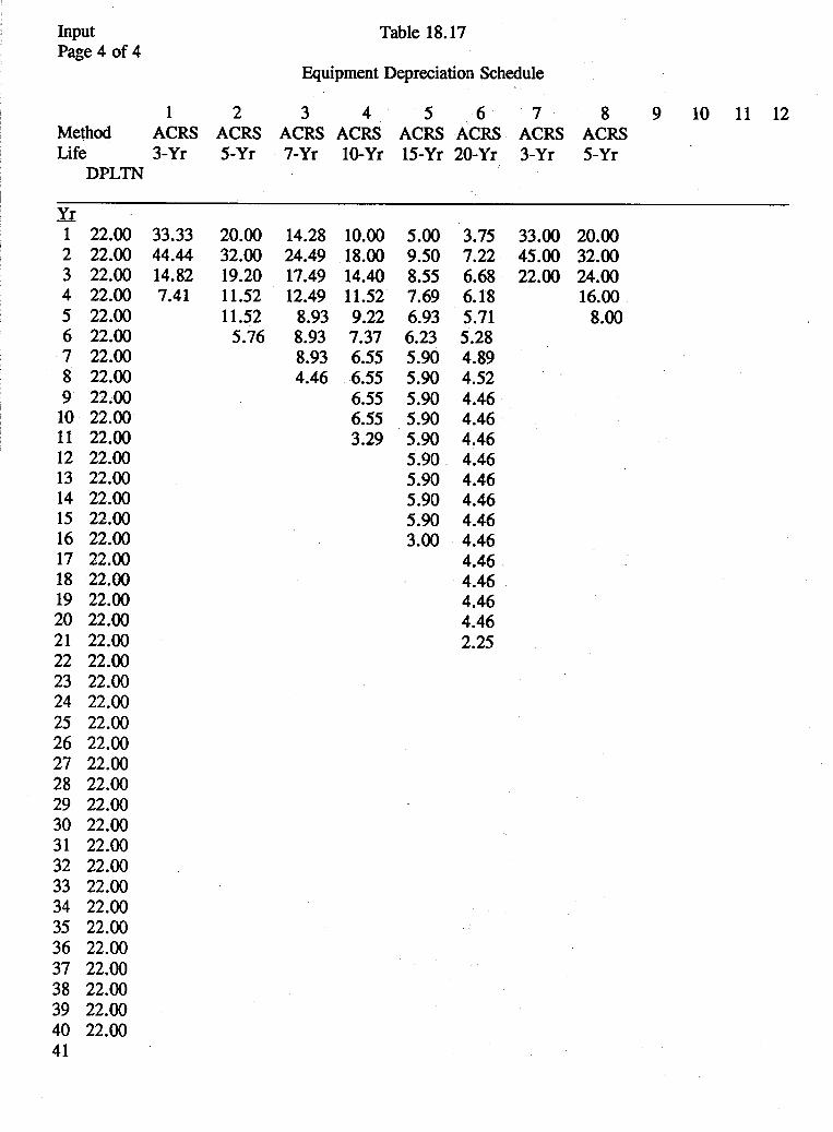
Input Table 18.17 Page 4 of 4
Equipment Depreciation Schedule
1 2 3 4 5 6 7 8 9 10 11 12 Method ACRS ACRS ACRS ACRS ACRS ACRS ACRS ACRS Life 3-Yr 5-Yr 7-Yr 10-Yr 15-Yr 20-Yr 3-Yr 5-Yr
DPLTN
- Yr 1 22.00 33.33 2 22.00 44.44 3 22.00 14.82 4 22.00 7.41 5 22.00 6 22.00 7 22.00 8 22.00 9 22.00 10 22.00 11 22.00 12 22.00 13 22.00 14 22.00 15 22.00 16 22.00 17 22.00 18 22.00 19 22.00 20 22.00 21 22.00 22 22.00 23 22.00 24 22.00 25 22.00 26 22.00 27 22.00 28 22.00 29 22.00 30 22.00 31 22.00 32 22.00 33 22.00 34 22.00 35 22.00 36 22.00 37 22.00 38 22.00 39 22.00 40 22.00 41
20.00 14.28 32.00 24.49 19.20 17.49 11.52 12.49 11.52 8.93
5.76 8.93 8.93 4.46
10.00 18.00 14.40 11.52 9.22 7.37 6.55 6.55 6.55 6.55 3.29
5.00 3.75 33.00 20.00 9.50 7.22 45.00 32.00 8.55 6.68 22.00 24.00 7.69 6.18 16.00 6.93 5.71 8.00 6.23 5.28 5.90 4.89 5.90 4.52 5.90 4.46 5.90 4.46 5.90 4.46 5.90 4.46 5.90 4.46 5.90 4.46 5.90 4.46 3.00 4.46
4.46 4.46 4.46 4.46 2.25

Table 18.18 Output Page 1 of 5
1 Natural Gas
Present System
YEAR ZERO AMOUNT 50,500
1988 1989 1990 1991 1992 1993 1994 1995 1996 1997 1998 1999 2000 2001 2002 2003 2004 2005 2006 2007
0 0 0 0
67,964 72,177 76,652 82,018 87,759 93,902 100,476 107,509 115,250 123,548 132,443 14 € ,979 152,201 163,160 174,907 187,501
TOT- 1,879,446
LIFE CYCLE COST ANALYSIS for
The Horsefly Heating District Klamath Falls, Oregon
April%, 1987
Project Cost (Pv) 1,759.954 Equity Financing (Pv) 295,078 Debt Financing (Pv) 2,100,526 Net Present Value -1,068,686
2 Electricity
Present System
150,000
0 0 0 0
190,532 202,155 214,486 227,570 241,452 256,180 271,807 2138,3137 305,979 324,644 344,447 365,458 387,751 411,404 436,500 463,126
4,931,880
Benefit Cost Ratio 0.39 to 1 Return on Equity 14.825% Simple Payback 8years 5months Discounted Payback 12 years 2 months
3 property Tax & Insurance
Present System
2,500
0 0 0 0
2,693 2,734 2,775 2,816 2,858 2,901 2,945 2,989 3,034 3,079 3,126 3,172 3,220 3,268 3,317 3,367
48,296
4 O & M
Present System
15,000
0 0 0 0
18,250 18,980 19,739 20,529 21,350 22,204 23,092 24,015 24,976 25,975 27,014 28,095 29,219 30,387 3 1,603 32,867
398,293
5 Hot Water Revenues
System Ropsed
220,000
0 0 0 0
298,599 317,411 337,408 358,665 381,261 405,280 430,813 457,954 486,805 517,474 550,075 584,729 621,567 660,726 702,352 746,600
7,857,719
379

output Page 2 of 5
YEAR ZERO AMOUNT
1988 1989 1990 1991 1992 1993 1994 1995 1996 1997 1998 1999 2000 2001 2002 2003 2004 2005 2006 2007
TOTALS:
380
Table 18.19
LIFE CYCLE COST ANALYSIS for
The Horsefly Heating District Klamath Falls, Oregon
April28, 1987
6 7 Natural Gas Electricity
Present System
-400
0 0 0 0
538 572 607 650 695 744 796 852 913 979
1,049 1,125 1,206 1,292 1,385 1,485
14,887
Present System
-100,000
0 0 0 0
127,022 134,770 142,991 151,713 160,968 170,787 181,205 192,258 203,986 216,429 229,631 243,639 258,501 274,269 291,000 308,75 1
3,287,920
8 Geothermal
System Proposed
-10,000
0 0 0 0
13,070 13,788 14,547 15,347 16,191 17,081 18,021 19,012 20,058 21,161 22,325 23,553 24,848 26,215 27,656 29,178
322,050
9 10 PropertyTax O & M & Insurance Present Proposed System System
-3,000
0 0 0 0
3,232 3,280 3,330 3,379 3,430 3,482 3,534 3,587 3,641 3,695 3,751 3,807 3,864 3,922 3,981 4,041
-25,000
0 0 0 0
30,416 31,633 32,898 34,214 35,583 37,006 38,486 40,026 41,627 43,292 45,024 46,825 48,698 50,645 52,671 54,778
57,955 663,822

output Page 3 of 5
YEAR ZERO AMOUNT
Table 18.20
LIFE CYCLE COST ANALYSIS I
for The Horsefly Heating District
Klamath Falls, Oregon April28, 1987
11 12 Equipment Equipment
Replacement Depreciation PrOpOSed Proposed System System
1988 1989 1990 1991 1992 1993 1994 1995 1996 1997 1998 1999 2000 2001 2002 2003 2004 2005 2006 2007
TOTALS:
0 0 0 0 0 0 0 0 0 0 0
0 0 0 0
138,544 173,015 156,664 144,215 134,727
35,301 33,252
0 28,558 0 23,875 0 23,875
735,962 179,888 0 171,663 0 167,913 0 164,163 0 164,163 0 0
735,962 1,739,815
13 Debt Service Bank Loan and/or
Bond Issue
159,247 159,247 159,247 224,345 224,345 224,345 224,345 224,345 224,345 224,345 224,345 224,345 224,345 159,247 159,247 600 ~ , O O o
1,060,o0o 0 0
4,219,688
14 Interest
Charges on Financing
132,000 129,548 126,875 163,96 1 158,276 152,276 145,243 137,790 129,633 120,705 110,932 100,236 88,528 75,713 68,195 60,Ooo - aoO0 a 0 0 0
0 0
2,019,688
15 Net
Operating Income
-132,000 -129,548 - 126,875 -1 63,961 106,346 104,346 154,780 204,289 253,454 395,362 442,907 496,326 553,416 609,576 507,242 572,823 628,930 688,439 807,822
1,035,22
7,009,498 .
381

output Page 4 of 5
YEAR ZERO AMOUNT
1988 1989 1990 1991 1992 1993 1994 1995 1996 1997 1998 1999 2000 2001 2002 2003 2004 2005 2006 2007
TOTALS:
382
16 Percentage Depletion Allowance
0 0 0 0
53,471 52,173 74,230 78,906 83,877 89,162 94,779
100,750 107,097 113,844 121,016 128,640 136,745 145,360 154,517 164,252
1,698,8 19
Table 18.21
LIFE CYCLE COST ANALYSIS for
The Horsefly Heating District Klamath Falls, Oregon
April28, 1987
17 Net Income
Before Taxes
-132,000 -129,548 - 126,875 - 163,96 1
53,470 52,173 80,550
125,383 169,576 306,200 348,128 395,576 446,319 495,732 386,226 444,183 492,185 543,079 653,305 870,977
5,3 10,679
18 Federal and State Income Tax
0 0 0 0 0 0 0 0 0
37,460 174,064 197,788 223,160 247,866 193,113 222,091 246,092 271,540 326,652 435,488
2,575,315
19 20 Net Income Add M e r Taxes
-132,000 - 129,548 -126,875 - 163,961
53,470 52,173 80,550 125,383 169,576 268,741 174,064 197,788 223,160 247,866 193,113 222,091 246,092 271,540 326,652 435,488
2,735,365
Depreciation & Depletion
0 0 0 0
192,015 225,187 230,894 223,121 218,604 124,463 128,030 129,308 130,972 137,719
300,303 304,658 309,523 318,680 164,252
3,438,634
300,904

output Page 5 of 5
YEAR ZERO AMOUNT
1988 1989 1990 199 1 1992 1993 1994 1995 1996 1997 1998 1999 2000 2001 2002 2003 2004 2005 2006 2007
TOTALS: .
Table 18.22
LIFE CYCLE COST ANALYSIS for
The Horsefly Heating District Klamath Falls, Oregon
Apnl28, 1987
21 22 Net Cumulative
Operating Cash Flow Cash Flow
After Taxes
'- 159,247 - 159,247 -159,247 -3 18,494
-224,345 -702,087 179,416 -522,671 205,068 -371,603 232,342 -85,260
- 159,247 -477,741
261,949 175,688 293,468 470,156 289,563 759,720 188,681 948,401 202,987 1,151,388 218,315 1,369,702 302,051 1,671,753
-332,998 ~ 1,338,756 522,395 ' 1,861,150 550,750 2,411,900
-418,938 1,992,963 645,333 2,638,296 599,740 3,238,036
3,238,036
23 24 Discounted Cumulative Cash Flow Discounted
Cash Flow
- 144,770 -131,609 -1 19,645 -153,23 1 1 11,403 115,756 119,228 122,20 1 124,459 1 1 1,639 66,132 64,678 63,238 79,539
113,688 108,963
105,517 89,148
-79,7 17
-75,350
-144,770 -276,379 -396,024 -549,255
-322,096
-80,667
-437,852
-202,868
43,792 155,431 221,563 286,24 1 349,479 429,018 349,30 1 462,990 57 1,953 496,603 602,120 69 1,268
69 1,268
25 Discounted Cash Flow at ROR
-138,687 -120,782 - 105,188 - 129,056
89,885 89,473 88,285 86,684 84,576 72,677 4 1,243 38,641 36,194
-41,872 57,206 52,525
46,679 37,781
295,078
43,611 .
-34,736
383

Input Page 1 of 3
Table 18.23
LIFE CYCLE COST ANALYSIS for
The Horsefly Heating District Klamath Falls, Oregon
April28, 1987
Energy forecast used for this report: 1986 Sample Energy Forcast. * This report is for a taxable entity. Dollar values rounded to the nearest: 1
capital investment data: Year Of Initial Capital Investment.. ..................... ........( example: 19881.. ........ : Year Project Will Be In Production ............................. (example: 1990) .......... : Project Life In Years ...................... (enter a whole number from 1 to 40) ........... : Economic Inflation Rate.. ..................... (enter as a whole number e.g. 7). .......... : Discount Rate.. ............................. ..(enter as a whole number 3.g. 12).
1988 1992 . 20
4% .......... 10% .:
Financing: Beginning; of Year 1992 . 1991 1990 1989 1988 . Pr Jt Cost ........... 500,000 300,000 700,000 500,000 Equity ........... a o O 0 ........... ........... 250,000 BankLoan * 400,000 ........... ........... 800,000
Life ........... 10 ........... ........... 15 ( A m ........... % 10% ........... % ........... % 9%
1 , ~ , W Bond Issue ........... ........... ........... ........... Life ........... ........... ........... ........... 18 (Am ........... % ........... % ........... 96 ........... % 6%
Invested ........... 1,157 I 241,366 642,765 1,390,752 (APR) ........... % 8.5% 10% 9% 8%
...........
Investment EOY 1992: 1,255 Total Project Cost (NPV): 1,759,954
Year Zero Annual Costs: Conventional Energy:
Present System Pro-msed Svstem
............................................................ Natural Gas 50,500 400 Fuel Oil ........... ........... Propane.. .............................................................. ........... ........... coal. ................................................................... ........... ........... Electricity. ............................................................ 150,000 100,OOO
Geothermal. ........................................................... ........... 10,OOo
................................................................
Other Energy:
384
Solar.. ................................................................. Nuclear.. .............................................................. Biomass.. .............................................................. Waste Heat ............................................................
Insurance.. ................................................................ . Inflation Rate ..........................................................
Operation and Maintenance ............................................. Inflation Rate ..........................................................
........... ...........
........... ...........
........... ...........
........... ........... 2,500 3,000
1.5% 15,000 25 ,OOO
4%

Input Table 18.24 Page 2 of 3
Year Zero Annual Cost: Present Proposed System System
Sales of Energy:
steam ............................................................. a: ........... ........... Hot #Water.. ....................................................... : ........... 200,000 'hpping Fees ...................................................... : ........... ........... . .
Equipment Purchases: Class 1 Class 2 !ad Class 4 Class 5
G Initial Cost: 5oo,oO0 250,000 120,000 90,000 ......... Yr. Purchased: 1988 1989 1990 1990 ......... Inflation/Y r:
Actual Slv.: 50,000 ......... 20,000 ......... ......... Economic Life: 10 - 25 - 18 20 .........
4% ......... % 5% ......... % 6%
385

Input Page 3 of 3
Table 18.25
Sample Energy Forecast* Forecast Energy Inflation Rates
1986
1 2 3 4 5 6 7 8 9 10 11 12 13 Natu Fuel Prop Coal Elec Geot Sola Nucl Biom Wast Stea Hot TiPP
(1) (2) (3) ( 4 ) (5) (1) (2) (3)
86 87 88 89 90 91 92 93 94 95 96 97 98 99 00 01 02 03 04 05
0.020 0.019 0.019 0.020 0.019 0.019 0.020 0.019 0.019 0.020 0.019 0.019 0.022 0.019 0.019 0.022 0.019 0.019 0.022 0.019 0.019 0.022 0.019 0.019 0.022 0.019 0.019 0.030 0.019 0.019 0.030 0.019 0.019 0.030 0.019 0.019 0.030 0.019 0.019 0.030 0.019 0.019 0.032 0.018 0.018 0.032 0.018 0.018 0.032 0.018 0.018 0.032 0.018 0.018 0.032 0.018 0,018 0.032 0.018 0.018
0.020 0.020 0.020 0.020 0.020 0.020 0.020 0.020 0.020 0.020 0.020 0.020 0.020 0.020 0.020 0.020 0.020 0.020 0.020 0.020
0.009 0.015 0.009 0.015 0.009 0.015
0.009 0.015 0.009 0.015 0.009 0.015 0.021 0.015 0.021 0.015 0.021 0.015 0.021 0.015 0.021 0.015 0.021 0.015 0.021 0.015 0.021 0.015 0.021 0.015 0.021 0.015 0.021 0.015 0.021 0.015 0.021 0.015
0.009 0.015
0.004 0.004 0.004 0.004 0.004 0.004 0.004 0.004 0.004 0.004 0.004 0.004 0.004 0.004 0.004 0.004 0.004 0.004 0.004 0.004
0.001 0.005 0.001 0.005 0.001 0.005 0.001 0.005 0.001 0.005 0.001 0.005 0.001 0.005 0.001 0.005 0.001 0.005 0.001 0.005 0.001 0.005 0.001 0.005 0.001 0.005 0.001 0.005 0.001 0.005 0.001 0.005 0.001 0.005 0.001 0.005 0.001 0.005 0.001 0.005
0.010 0.010 0.010 0.010 0.010 0.010 0.010 0.010 0.010 0.010 0.010 0.010 0.010 0.010 0.010 0.010 0.010 0.010 0.010 0.010
0.002 0.002 0.002 0.002 0.002 0.002 0.002 0.002 0.002 0.002 0.002 0.002 0.002 0.002 0.002 0.002 0.002 0.002 0.002 0.002
0.023 0.023 0.023 0.023 0.023 0.023 0.023 0.023 0.023 0.023 0.023 0.023 0.023 0.023 0.023 0.023 0.023 0.023 0.023 0.023
0.023 0.023 0.023 0.023 0.023 0.023 0.023 0.023 0.023 0.023 0.023 0.023 0.023 0.023 0.023 0.023 0.023 0.023 0.023 0.023

Table 18.26 ,Output Page 1 of 4
LIFE CYCLE COST ANALYSIS for
The Horsefly Heating District Klamath Falls, Orego
April28, 1987 .
Project Cost (I%) 1,759.954 Benefit Cost Ratio Equity Financing (Pv) 295,078 Return on Equity Debt Financing (pr) 2,100,526 Simple Payback Net Present Value -500,433 Discounted Payback Discount Rate 10.00%
1 2 3 4 Natural Gas Electricity Insurance 0 & M
Present Present Present Present System System System System
YEAR ZERO AMOUNT 50,500 150,m 2,5QO 15,Ooo
1988 0 0 0 0 1989 0 0 0 0 1990 0 0 0 0 1991 0 2) - 0 0 1992 67,964 190,532 2,693 18,250 1993 72,177 202,155 2,734 18,980 1994 76,652 214,486 2,775 19,739 1995 82,018 227,570 2,816 20,529 1996 87,759 24 1,452 2,858 21,350
100,476 271,807 2,945 3,092 1997 1998 I999 107,509 288,387 2,989 4,015 2000 115,250 305,979 3,034 24,976 2001 123,548 324,644 3,079 25,975 2002 132,443 344,447 3,126 27,014 2003 141,979 365,458 3,172 28,095 2004 152,201 387,75 1 3,220 29,219 2005 163,160 41 1,404 3,268 30,387 2006 174,907 436,500 3,317 31,603 2007 187,501 463,126 3,367 32,867
TOTALS: 1,879,446 4,931,880 48,296 398,293
93,902 256,180 2,901 22,204
0.72 to 1 18.737 %
8years 5months 11 years 0 months
5 Hot Water Revenues Proposed System
220,000
: o 0 0 0
298,599 317,411 337,408 35 8,665 38 1,261 405,280 430,8 13 457,954 486,805 517,474 550,075 584,729 621,567 660,726 702,352 746,600
7,857,719
387

output Page 2 of 4
Table 18.27
YEAR ZERO AMOUNT
1988 1989 1990 1991 1992 1993 1994 1995 1996 1997 1998 1999 2000 2001 2002 2003 2004 2005 2006 2007
TOTALS:
LIFE CYCLE COST ANALYSIS for
The Horsefly Heating District Klamath Falls, Oregon
April28, 1987
Present System
-400
0 0 0 0
538 572 607 650 695 744 796 852 913 979
1,049 1,125 1,206 1,292 1,385 1,485
14,887
6 7 Natural Gas Electricity
Present System
-100,OOO
0 0 0 0
127,022 134,770 142,991 151,713 160,968 170,787 1 8 1,205 192,258 203,986 216,429 229,631 243,639 258 ,SO 1 274,269 291,000 308,75 1
3,287,920
8 Geothermal Proposed System
-10,000
0 0 0 0
13,070 13,788 14,547 15,347 16,191 17,081 18,021 19,012 20,058 21,161 22,325 23,553 24,848 26,215 27,656 29,178
322,050
9 Insurance Proposed System
-3,000
0 0 0 0
3,232 3,280 3,330 3,379 3,430 3,482 3,534 3,587 3,641 3,695 3,751 3,807 3,864 3,922 3,981 4,041
57,955 .
10 O & M
operating Cash Flow
-25,000
0 0 0 0
30,416 31,633 32,898 34,214 35,583 37,006 38,486 40,026 41,627 43,292 45,024 46,825 48,698 50,645 52,671 54,778
663,822
388

output Page 3 of 4
YEAR ZERO AMOUNT
1988 1989 1990 199 1 1992 1993 1994 1995 1996 1997 1998 1999 2000 2001 2002 2003 2004 2005 2006 2007
TOTALS:
11 Eiquipment
Replacement
System Proposed
0 0 0 0 0 0 0 0 0 0 .o 0 0 0
735,962 0 0 0 0 0
735,962
Table 18.28
LIFE CYCLE COST ANALYSIS for
The Horsefly Heating District Klamath Falls, Oregon
April28, 1987
12 13 14 Debt Service Net Cumulative Bankhan Operating Cash Flow and/or Cash Flow
Bond Issue
159,247 - 159,247 - 159,247 159,247 - 159,247 '. -318,494 159,247 ~. -159,247 -477,741 224,345 -224,345 -702,087 224,345 179,4 1 6 -522,671 224,345 205,068 -3 17,603 224,345 232,342 -85,260 224,345 261,949 176,688 224,345 293,468 470,156 224,345 327,023 797,179 224,345 362,745 1,159,924 224,345 400,775 1,560,699 224,345 44 1,474 2,002,174 159,247 549,917 2,552,W 1
, 159,247 -183,177 2,368,9 14 60,000 744,486 3,113,400 60,OOo 796,843 3,910,243
1,060,000 -147,398 3,762,844 0 971,985 4,734,830 0 1,035,229 5,770,05 8
4,219,688 5,770,058
389

output Table 18.29 Page 4 of 4
LIFE CYCLE COST ANALYSIS for
The Horsefly Heating District Klamath Falls, Oregon
April28, 1987
YEAR ZERO AMOUNT
1988 1989 1990 1991 1992 1993 1994 1995 1996 1997 1998 1999 2000 2001 2002 2003 2004 2005 2006 2007
TOTALS:
15 Discounted Cash Flow
- 144,770 -131,609 -1 19,645 - 153,23 1 11 1,403 115,756 119,228 122,20 1 124,459 126,081 127,140 127,699 127,879 144,810 -43,851 162,022 157,651
158,927 153,880
1,259,521
-2631 1
16 Cumulative Discounted Cash Flow
- 144,770 -276,379 -396,024 -549,255
-322,096 -202,868
-80,667
-437,852
43,792 169,874 297,O 14 424,7 13 552,592 697,403 653,552 815,574 973,225 946,714
1,105,641 1,259,521
17 Discounted Cash Flow at ROR
-134,118 -1 12,954
-95,130 -1 12,870
76,022 73,180 69,829 66,304 62,561 58,713 54,850 5 1,037 47,349 49,673
- 13,935 47,699 42,997
37,201 33,369
-6,698
295,078

0.02 and the economic inflation rate was 0.06, this would indicate that natural gas was expected to inflate at 8% in year OF. Inflation rates entered in the forecast may be positive, negative or zero. A zero indicates that the energy is expected to inflate at the same rate as the economic inflation rate.
Table 18.17 illustrates the depreciation and depletion allowance schedule. All values in these tables may be modified by the user. However, the energy forecast is limited to 30 years. If the project life goes beyond 30 years, the inflation rate for year 30 is chosen as the inflation rate for the last 10 years of the project.
Tables 18.18 through’18.22 provide the output data for the project. Total project cost, equity financing and debt financing are all stated in terms of net present value; that is, all monies flowing into the project during the construction period are brought back to time zero at the discount rate.
The benefitcost ratio evaluates the net present value of the annual savings or revenues associated with the proposed system or both, and divides this number by the net present value of the total project cost.
The net present value calculates the present value of the total project costs and subtracts the present value of the annual savings or revenues associated with the project or both, to arrive at a net present value for the total project, or a net present value for the life cycle of the project.
A RELCOST user developed a scenario on a renewable energy project with equipment that required replacement every 6 months and he wished to evaluate this with equipment replaced every 18 months. In order to accomplish this, all that was necessary was to state replacementcosts, all operating costs, all inflation rates, the economic inflation rate, capital investment costs and financing in terms of 1 month rather than 1 year, respectively, and complete a 36-month life cycle cost analysis. There are numerous ways to modify the input data in order to provide for unusual circumstances.
18.9 CAVEATS
As was stated in the introduction, LCC has several major drawbacks. One of these is that increasing or decreasing costs over the life of the project must be estimated based ov’some forecast, and forecasts have proven to be highly variable and frequently inaccurate. Another problem with LCC is that some life span mpst ,be selected .over which to evaluate the
and many, projects, especially repewable energy projects, are expected to have an unlimited life; they are expected to live forever. The longer the life cycle, the more inaccurate annual costs become because of the inability to forecast accurately.
Comprehensive LCC should be performed by qualified persons who have a thorough knowledge of the subject, including expertise in the current tax law.
18.10 RECOMMENDATIONS
Based on the experience gained by the author in completing over 150 economic analysis for renewable energy projects, the following recommendations are offered.
18.10.1 Take the Time to Understand the Basics
Preliminary LCC requires that the user understand certain basic concepts regarding interest, taxes, the time value of money, and economic decisioa techniques for even the simp- lest analysis. If you have’no experience in these areas, carefully read this chapter and proceed with extreme caution. If certain concepts remain unclear, consult the references appearing at the end of this chapter.
18.10.2 Use Ultraconservative Forecasts
During the petroleum crisis in the mid 197Os, forecasters were predicting inflation rates for fossil fuels ranging from 5 to 15% above the economic inflation rate. Many of these energy forecasts were 20 years in length. Using hindsight, it turns out that within the last 10 years petroleum prices have actually deflated when compared to the consumer price index. Any forecast that projects inflation rates higher than those that occur provides a favorable LCC picture, gives a green light to the project, causes thousands and even millions of dollars to be spent in acquisition and construction, only to find that when the project goes into production, competing fuels have not inflated as projected and the project either operates at a continual loss or is abandoned.
18.10.3 Keep Proiect Life as Short as Possible
It is dangerous to try to do even a 20-year study on a major project. It is absolutely ridiculous to go beyond 20 years. And yet, many projects have required 50-year LCC analysis. The successful projects are those that-use extremely low inflation rates and have a very short payback (4 years or less).
LCC analysis on a large project is a very complex pro- cedure. Many projects require equipment with widely varying useful lives. Pipe lines may last 25 years. Electric motors, turbines, or pumps may have useful lives of 5 to 10 years. Replacement costs must be forecast, major repair costs have to be incorporated, and competing alternatives should be as accurately evaluated as possible. If the project is owned bya private entity, depreciation schedules, depletion allowances, investment tax credits, energy tax credits, and in some cases, intangible drilling costs enter the picture.
391

It is not possible to predict future changes in the tax law. In the early 1980s, many renewable energy projects enjoyed as much as a 55% tax credit. Later (5 years), many of these tax credits were removed. Therefore, any equipment replaced could not provide the reduced tax liability that was forecast at the beginning of the project.
18.10.4 Minimize Total Proiect Cost
As observed in the LCC analysis of the three heating systems, initial cost probably has the greatest impact on the feasibility of a project and the developer should make every effort to minimize the project cost without sacrificing quality and reliability. For example, in the development of geother- mal projects, drilling costs, and pipeline costs are two of the major components. In an attempt to minimize drilling costs, quality, performance and longevity of the production well may be sacrificed. It may be advisable to move the user on-site to minimize the length of transmission lines without sacrificing any other aspect of the project. The end result is a reduction of pipeline maintenance and pumping costs.
18.10.5 Carefullv Evaluate Financing ODtions
The method of financing, the interest rate, and the annual debt service can have a major impact on renewable energy projects. These projects are capital intensive and experience very high costs during the construction period. In addition, many projects come on-line gradually, which causes very low revenues in the early years of the project life. In such cases, it may be advisable to seek long-term bond financing. Such financing requires only interest payments during the early years of the project, and a high balloon payment when the bond matures. As the project reaches full capacity in the later years, revenues may be able to accommodate such a balloon payment. Such financing can be especially helpful to munici- palities experiencing low or negative cash flows during the beginning years of the project.
18.10.7 Be Aware of the Limitations of Pavback
Simple payback compares the values in the cumulative cash flow column (Table 18.22 column 22) with the equity in- vested in the project to determine when these two values are equal. This practice makes no distinction between present and future values. Note that the simple payback cash flows are not evaluated at any interest rate and that a negative cash flow occurring subsequent to the payback period has no effect. If the cumulative cash flows indicate that the equity in a project is recovered in year 12, and year 13 has a balloon payment on a bond that causes the cash flow to turn negative, this may cause the simple payback to be in error.
The discounted payback compares the equity in the pro- ject with the cumulative discounted cash flow (Table 18.22 column 24) and indicates a discounted payback when these two are equal. Once again, this method does not evaluate s u b quent negative cash flows that may occur. Nonetheless, it is a more accurate measure of payback because the accumulated cash flows are discounted at the discount rate stated in the input section.
The reason the simple and discounted payback periods are evaluated in this manner is because it is the accepted calcula- tion method in the industry. Because these values may be in error, the program RELCOST also evaluates cash flows be- yond these payback periods and prints a warning in the output section if negative cash flows occur beyond the payback period.
The LCC analysis is a very powerful tool. It can be used to rank projects in the order of feasibility and to determine which projects are most likely to be successful. At best how- ever, it is only an educated guess and the values calculated should be treated only as rough estimates.
GLOSSARY OF ENGINEERING COST ANALYSIS TERMS 18.10.6 Avoid Distorting the Rate of Return
This author discourages using financial leverage to make a project appear feasible. Financial leverage is the practice of iinancing large sums of money at extremely low interest rates in order to reduce the equity invested in the project and in- crease the ROR. For example, a project costing $100,000 re- turns $15,000 in revenues every year for 10 years. The ROR on this project would be about 8%. In an effort to make the project appear more attractive, the developer borrows $90,000 at 6% interest, which requires an annual payment of $12,228. Subtracting the debt service from the income provides a net annual income of $2,772. Now, the project is evaluated as a $10,000 investment providing $2,772 of income per year for 10 years and the ROR jumps to nearly 25%. Once project feasibility is determined, it is up to the developer to use any accepted method to increase the project’s ROR; but, such practices should be avoided in determining whether or not the project is economically feasible.
Accelerated Cost Recovery System (ACRS) - The current system of depreciation for various classes of assets that provides more rapid cost recovery than straight line depreciation.
Annual effective interest rate - The actual or true annual interest rate that indicates the exact amount of interest paid per year by converting nominal or annual percentage rates to the actual dollar amount of interest annually.
Annual equivalent cost - The amount of an equal end-of-year payment series that is equivalent to present or future value when the interest rate is considered.
Annual percentage rate (Am) - The interest rate per year without considering the effect of compounding followed by the number of compounding periods per year.
392
Annuity due - An equal series of beginning-of-the-period payments.
Arithmetic gradient - An end-of-period payment series that increases each period by a constant mount.
Asset Depreciation Range (ADR) - The life of an asset as fixed by the Internal Revenue Code.
Benefit-cost ratio - The ratio that results in dividing the present value of all benefits of a project by the present value of all the costs of that same project.
Book value - The cost basis of an asset less the accumulated depreciation.
Business tax credit - A direct credit to the tax liability of a lirm because of the purchase or operation of assets that are eligible for business tax credits under the current tax law.
Capital recovery - The process of charging periodic end-of- period payment series that is equivalent to the initial asset cost less the expected salvage value at the end of its economic life.
Capital recovery factor - The factor used to calculate the end- of-period payment series that is equivalent to the cost of an asset less its future salvage value based on the compounded interest rate.
Cash flow - 1. The actual flow of dollars into and out of the operation of a capital venture. 2. The flow of revenues less operating costs plus depreciation from a given capital venture.
Compound amount factor - 1. The future value of a lump sum considering time and the compound interest rate. 2. The future value of a payment series considering time and the compound interest rate.
Compound interest - Interest that is calculated and added to the initial amount such that future interest earnings will be accumulated based on the total amount including interest.
Cost of capital - The costs incurred because of borrowing money. Normally expressed as an interest rate.
Depletion - A method of depreciation applying to depletable resources such as geothermal, coal, timber, oil, and natural gas.
Depreciation - A method of expensing the decrease in value of an asset over its life span and charging these costs to operations.
Discounted cash flow - Eviiluating the annual costs and revenues associated with a venture over the years of its life at same interest rate to arrive at a present value of these cash flows.
Discounted payback period - The time period required (considering the time value of money) for the revenues or benefits of a project equal the capital investmknt and operating costs of that project.
Discount rate - The interest rate used to evaluate the cash flows resuIting from the operation of a project.
Double declining balance depreciation - A method of accelerated depreciation that applies twice the straight line rate multiplied by the book value of the asset.
Economic life - The period of time from installation to retirement of an asset that minimizes the cost of buying, installing, operating and salvaging that asset.
Energy b x credit - A direct credit to the tax liability of a firm because of the purchase or operation of assets that are eligible for energy tax credits under the current tax law.
Equipment cost basis - The adjusted cost of an asset due to additional installation costs or subtracted tax credits claimed which alter the amount of depreciation which may be claimed.
Equipment replacement life - The period of time that will elapse from initial installation until a piece of equipment is either obsolete or worn out and requires replacement.
Future valuelfuture work - The equivalent value at a designated future date of previous cash flows evaluated over time at a compound interest rate.
Geometric gradient - An end-of-period payment series that increases each period by the exact same percentage.
Inflation - An increase in prices in general usually caused by a decline in the purchasing power of a monetary system.
Interest - The periodic cost charged for borrowing money.
Internal rate of return - The interest rate earned by investing in a particular venture and receiving cash flows as a result of that investment without regard to any other investments.
Investment tax credit - A direct credit to the tax liability of a firm because of the purchase of assets that are eligible for investment tax credits under the current tax law.
Marginal cost - The amount -of cost associated with an increase in output or with a particular project.
Marginal tax rate - The amount of taxes (expressed as a 96) because of an increase in output ,or he income of a particular project.
393

Net present value - The equivalent value at time zero (today) of the net difference between future cost and revenue cash flows evaluated (discounted) over time at a compound interest rate.
Nominal interest rate - The interest rate per year without considering the effect of compounding followed by the number of comunding periods per year.
Ordinary annuity - A stream of equal end-of-period pay-&-
Opportunity cost - The cost of not taking advantage of an investment opportunity because of limited capital, resources, or other conflicting circumstances and thereby losing the eamings or benefits associated with that investment.
Present value/present worth - The equivalent value at time zero (today) of future cash flows evaluated (discounted) over time at a compound interest rate.
Rate of return (ROR) - The compound interest rate that will cause the present value of a l l the costs and benefits associated with a project to equal exactly zero.
salvage value - 1. The value obtained from an asset when sold, scrapped or retired from service. 2. The current fair market value of a piece of equipment.
Sensitivity - The amount of effect or impact experienced by changing one of the input variables of a project undergoing an engineering economic study in order to alter the acceptability or rejectability of that project.
Simple interest - Interest that is accrued periodically on only the original amount of a loan or investment, and that is not compounded.
Simple payback period - The time period required (without considering the time value of money) for the revenues or benefits of a project to equal the capital investment and operating costs of that project.
Sinking fund - A stream of equal end-of-period payments set aside in an investment fund for the purpose of replacing an asset or making a balloon payment on a debt.
Straight line depreciation - A method of depreciation in which the equipment cost basis of an asset is recovered in equal amounts over its taxable life based on time, units of output, miles driven, or hours of operation.
Sum-of-theyeandigits depreciation (SYD) - A method of accelerated depreciation in which the equipment cost basis of an asset is multiplied each year by the remaining years of life divided by [(n times n+l) divided by 23 to arrive at a depreciation charge for that year (where n equals the taxable life of the asset).
Sunk cost - A capital cost already incurred that cannot be recovered and is not to be Considered or evaluated in making current decisions.
Time value of money - The future, present or annual equivalent value of cash flows considering the compound interest rate of borrowed money, the expected rate of earnings on invested capital, or the required rate of return on the capital investment required for a project.
REFERENCES
Anderson, D. N. and Lund, J. W., editors, Geothermal Resources Council S k a l R m r t No. 7: Direct Utilization of Geothermal Enerev - A Techuical Handbook, U.S. Department of Energy, Washington, DC, 1979.
Lienau, P. J., et al., Aeribusiness Geothermal Enerpv Utili- zation Potential of Klamath and Western Snake River Basins. Oreeon, U.S. Department of Energy, Washington, DC, 1978.
Newman, D. G., Engineering Economic Analvsis, 3rd eition, Engineering Press Inc., San Jose, CA, 1988.
Riggs, J. L. and West, T. M., Enpineering Economics, 3rd edition, McGraw-Hill Book Co., NY, 1986.
Thuesen, G. H. andFabryclq, W. J., Engineering Economy, 6th edition, Prentice-Hall Inc., Englewood Cliffs, NJ, 1984.
394

CHAPTER 19 REGULATORY AND
COIMIMERCIAL ASPECTS By Gordon Bloomquist
Washington State Energy Office Olympia, WA 98504
19.1 INTRODUCTION
To a large ex&, the regulatory and commercial aspects of geothermal development have been addressed by the U.S. Congress and by the legislatures of each of the states h o w to posses geothermal resources. Often the conclusion reached, and the direction given by these agencies, has been significantly different. Too often legislation adopted has left as many questions unanswered as answered, or created as many new problems as were resolved. In some unfortunate cases, legislation has, in fact, proven to be more of an obstacle toward development than an aid. This chapter provides an overview of the various regulatory and commercial aspects that affect the development of geothermal direct use projects. Appendix A provides pertinent geothermal definitions, ownership, leasing information, injection requirements and the agencies involved. Information is provided for the federal government, Alaska, Arizona, California, Colorado, Hawaii, Idaho, Montana, Nevada, New Mexico, North and South Dakota, Oregon, Texas, Utah, Washington, and Wyoming.
1 LEASING
Providing access and a secure right to the resource for exploration and development is provided for through leasing.
on of geo- thermal leasing in the U.S. began with the passage of the California Geothermal Resources Act of 1967, and the Federal Geothermal Steam Act of 1970. A majority of the states possessing geothermal resources followed suit during the
ften modeled their statutes after either the federal Acts. However, a number of state
leasing statutes differ considerably from the California and federal models, and this divergence can be attributed to the complexity of dealing with this new resource, or to historical differences in how the states formally dealt with the disposition and protection of its natural resources.
The development of statues for
The major differences in the statutes can be t r a d to how geothermal resources are defied and characterized.
19.3 RESOURCE DEFINITION
Geothermal resources are related to water, gas, and minerals, to both the surface and subsurface estates, and to both water rights and mineral titles. How g e o t h d resources am defined affects other resource definitions as well as all aspects of regulation.
There are, therefore, two basic tasks in defining geothermal resources. First, describe the physical properties that distinguish geothermal resources from other nahual resources and thus clearly establish what is subject to geothermal leasing, ‘ taxation, and development regulations. Second, a definition must relate geothermal resources to groundwater, subsurface minerals, and other established resources. An ideal resource definition should, therefore, be both anticipative and retrospective. It must look forward to future leasing, exploration, and development activities while, at the same time, looking at past experiences in order to place geothermal resources into the framework of leases, reservations, and property titles inherited from the past (Sacarto, 1976).
How well legislation accomplish these two tasks will have a profound influence upon the reduction of hture conflicts of ownership.
The California Geothermal Resources Act of 1967 made ~
the first attempt at defining geothermal resources and reads as follows:
‘Geothermal resources’ shall mean the natural heat of the earth, the energy, in whatever form, below the surface of the earth present in, resulting from, or created by, or which may be extracted from, such natural heat, and all minerals in solution of other products obtained from naturally heated fluids, brines, associated gases, and steam, in whatever form, found below the surface of the earth, but excluding oil, hydrocarbon gas, or other hydrocarbon substances.
395

The Federal Geothermal Steam Act of 1970 (Public Law 91-581) defined geothermal resources thus:
'Geothermal steam and associated geothermal resources' mean (i) all products of geothermal processes, embracing indigenous steam, hot water, and hot brines; (ii) steam and other gases, hot water, and hot brines resulting from water, gas, or other fluids artificially introduced into geothermal formation; (iii) heat or other associated energy found in geothermal formation; and (iv) any by products derived from them.
The federal definition defined byproducts so as to exclude oil, hydrocarbon gas, and helium.
Both the California and the federal definitions provide a detailed description of the physical properties that distinguish geothermal resources from other natural resources, but fail to relate geothermal to such things as groundwater, and minerals.
A somewhat different approach to dehing geothermal sources was taken by Washington State:
'Geothermal resource' means only that natural heat energy of the earth fiom which it is technologically practical to produce electricity commercially and the medium by which such heat energy is extracted from the earth, including liquids or gases, as well as minerals contained in any natural or injected fluids, brines, and associated gas, but excluding oil, hydrocarbon gas, and other hydrocarbon substances (RCW 79.76) (Emphasis added by author).
The principal difference in the Washington State definition is that it restricts geothermal resources to those "from which it is technologically practical to produce! electricity commerCially." Geothermal resources were so defined in Washington State to provide for a clear division of responsibilities for purposes of regulation. The Department of Natural Resources, which normally regulates oil and gas drill- ing, was by this mechanism, given the responsibility for the regulation of the high temperature and pressure resources, while the Department of Ecology, which normally regulates groundwater, was given the responsibility for low temperature and pressure resources. Unfortunately, because no definite cut off temperature was set, but instead left to float, the Department of Natural Resources could now be expected to re- gulate resources with temperature as low as - 212°F or below. This is because advances in technology have made the gener- ation of electricity possible at temperatures much below that which was anticipated at the time the Act was passed into law.
Alaska also desired to separate the regulation of its resources, but unlike Washington, adopted a definite tempera- ture cut off (Basescu, 1980). The Alaska definition reads as follows:
'Geothermal resources' means the natural heat of the earth at temperatures >12o"C, measured at the point where the highest temperature resources encountered enter or contact a well shaft or other resom extraction device.
The definite temperature cut off tends to take the guess work out of where an applicant should apply for a resource or drilling permit and allows for a distinct separation of agency responsibilities. This also clarifies whether or not the fluids are available through appropriation as groundwater or lease as geothermal.
By excluding resources of < 250°F from the definition of geothermal, the Alaska legislature has facilitated their use, because regulation meant for l a r g d e c o m i a l use of high temperature resources need not be observed for most direct use applications (Basescu, 1980). Although this was also the objective of the Washington State Legislators at the time the Geothermal Resources Act of 1974 was passed, no one could anticipate that rapid developments in technology would, in time, completely change the definition and possibly place an undue burden upon both the developer of direct use projects, as well as the developer of moderate-temperature resources for electrical generation where neither high temper- ature or high pressures present the degree of risk associated with the development of high temperature resources.
The Oregon definition, which, for the most part, is based on the federal model, provides additional restrictions based upon temperatures and depth. Hot water from wells <2,000 ft with bottom-hole temperatures < 25o"F, must be developed according to state water law. It is not necessary, however, under Oregon law to know the bottom-hole temperature of wells before they are drilled as all geothermal prospecting is regulated under the geothermal statutes. However, if a water well should, in the course of development, encounter tempera- tures approaching 25o"F, a geothermal permit must be obtained (Justus, 1980).
The state of Idaho has defined "geothermal resources" to mean the natural heat energy of the earth, the energy in whatever form, below the surface of the earth present in, resulting from, or created by, or which may be extracted from the natural heat, and all minerals in solution or other products obtained from naturally heated fluids, brines, associated gases, and steam, in whatever form, found beIow the d a c e of the earth, exclusive of helium or of oil, hydrocarbon gas, or other hydn>carbon substances, but including, specifically:
a.
b.
All products of geothermal process, embracing indigenous steam, hot water, and hot Wes; Steam and other gases, hot water, and hot brines resulting from water, gas, or other flujids artifically introduced into geothermal formations;
c. Heat or other associated energy found in geothermal formations; and
d. Any by-product derived from them.
396

"Geothermal well" includes any excavation made for producing geothermal re~~urces and any geothermal reinjection well or derived from geothermal resources into an underground reservoir.
In all of the above examples, the definition accomplishes the task of describing the physical properties that distinguish geothermal resources from other natural resources, but gener- ally fail to characterize geothermal resources in relation to groundwater, subsurface minerals, and other established resources.
The failure to so characterize geothermal resources makes the establishment of ownership difficult and has led to con- flicts with owners of other resources. It also leaves many unanswered questions as to regulatory authority over exploration and development.
19.4 RESOURCE CHARACTERIZATION
As recognized in the legal definitions, geothermal resources are similar in some respects to water, minerals, and gas; the result has been considerable disagreement-including litigation-over the essential M~UR of the resource and corresponding ownership rights. Such uncertainty has impeded geothermal development, and makes resource characterization a major issue that must be dealt with in order to ensure that geothermal exploration and development can proceed in a timely fashion.
The federal government, in passage of the Geothermal Steam Act of 1970, avoided the question of how geothermal resources should be characterized. The Steam Act chose instead to direct the Justice Department to bring suit to quit title to geothermal resources ownership. The courts were asked to decide whether or not geothermal fesources had been reserved to the federal government as part of the mineral estate. The action brought by the Justice Department (US. of America versus Union Oil Company of California) began in 1971, and a verdict in favor of the U.S. was not reached until October 1977 under the title Ortobonie versus the U.S. qf America. This delay resulted in a moratorium on leasing all lands patented under the Stock Raising Homestead Act of 1916 until the case was decided. It resulted in a loss of considerable revenue to the U.S. as well as slowing development by several years in prime areas such as The Geysers in northern California. The delay and problems of revenue lost could have been avoided if Congress, in passing the Geothermal Steam Act of 1970, had simply characterized the resources as mineral and, therefore, belonging to the owner of the mineral estates.
The California Legislature, in the passage of the California Geothermal Resources Act of 1967, also avoided this very important question, and again it was left up to the
courts to decide the issue and to characterize the resource. It wasn't until the case Pariani versus California was decided in 1981 (California Court of Appeal, 1981) that geuthermal was declared to be a mineral resource for purposes of ownership and leasing of lands in California.
Like California and the federal government, the state of Oregon has also avoided the question of characteMon. Although some states have chosen to characterize geothennal resources. They have seldom done so in a manner that has resulted in a clear understanding of ownership or leasing rights.
In Washington State, the legislature declared that "notwithstanding any other provisions of law, g e o t h e d resoums are found and hereby determined to be sui genet-% being neither a mineral resource nor a water resource" (Bloomquist, 1980).
In Idaho, the state declared that geothermal resources are sui generis, being neither a mineral tesoufce nor a water resource, but. . . closely related to, and possibly affecting and affected by, water and mineral resources in many instances (Renwick and Lewis, 1976).
Montana, like Idaho and Washington, has adopted thesui generis characterization; but, other Montana statutes lead to the conclusion that geothermal tesources are considered to be water and regulated as such (Perlmutter, 1978).
The sui generis chiuacterhtion of geothermal fesoulces serves only to cloud the ownership issue and is, for all practical purposes, meaningless because it fails to clearly characterize the resource, and therefore, does not clarify the question of ownership, access to the resource, and regdatory authority.
The states of Wyoming and Utah have characterized geothermal resources as water, while the state of Hawaii has chosen to characterize geothermal resources as mineral.
In many other states, it is unclear exactly how geothermal is characterized. For example, in New Mexico it is stated that geothermal is not water (Renwich and Reid, 1976), but it is unclear as to whether or not the legislature inhded that geothermal be considered to be a mined. In Alaska, geothermal is characterized as being similar to oil, gas, coal, ores, and minerals, but no clear assignment is made (Basescu, 1980).
Characterization of the resource can accolllplish the second task and allows for the placement of geothermal resources into the framework of historical leasing, reservation, and property titles, and thus, clarifies the questions related to ownership, access, and regulatory authority.
397

19.5 OWNERSHIP
By clearly defining geothermal resources to be either water or mineral, the problems associated with the establishment of ownership will be greatly reduced.
Mineral ownership derives from an estate in land, which may be severed from property rights to the overlying surface. Groundwater, at least in the west, is generally held in the public domain while being an aspect of surface ownership in most eastern states. In the case where the resource has been determined to be sui generis, the state may assign the resource to the owner of the surface estates or the mineral estate or may, in fact, claim the ownership of all geothermal resources in the state regardless of ownership of the surface or mineral estate, and separate from existing water rights.
The federal government claims geothermal ownership wherever it holds the mineral estate, either jointly with the surface estate or as a mineral reservation where the estates have been severed. This claim was upheld in the Ottobonie versus the U.S. case that was mentioned earlier. Absent implied, or explicit reservation of water pursuant to the establishment of a federal enclave, the states have primary control over groundwater resources.
The states have taken a number of approaches to the assignment of ownership and the approach taken reflects how the resource was characterized as to water, mineral, or sui generis.
In Alaska, the state claims ownership of all geothermal resources, including those under private lands, and is in-line with the state's claim to all subsurface resources in the state. The state of Alaska does, however, give the surface owner a preferential right to a prospecting permit or lease. It must be remembered that by definition, geothermal resources in Alaska are limited to those above 25O"F, while ownership of geothermal resources below that temperature would fall under water law statute and ownership would be assigned accordingly (Basescu, 1980).
In Utah, Wyoming, and Montana, geothermal resources are also in the public domain because of their characterization as water.
Washington State has declared geothermal resources to be the property of the surface owner (Bloomquist, 1980); but, it is presently unclear, because of the way that the state has delined geothermal resources, what is truly included in this assignment, and what remains available for appropriation as groundwater. The state does, however, claim ownership of all groundwater underlying state and school lands. In order to gain access to low-temperature geothermal resources below these lands, a commercial lease would have to be obtained.
In Idaho, the state cIaims ownership of all geothermal resources underlying state and school lands. However, state lands are those in which the state of Idaho owns either the surface rights, the mineral rights, or both (Idaho, 1978). High-temperature geothermal operations developed in Idaho as an energy source, a mineral fesource or a material medium do not require a valid water right permit, but such operations can acquire such a permit. A prudent operator would be wise in obtaining both p e d t s for a d d i t i d protection from third- party intervention and to avoid potential conflicts with state agencies. A problem with applying for both permits is that performance bonds, and applications fees, are required for each.
In Utah and Wyoming, geothermal resources are also in the public domain because of their characterization as water.
Montana statutes involving ownership of geothermal resources are also unclear. Section 81-2602(1) of Title 81 of the Montana law as it relates to the management of state- owned lands states: "No rights to seek, obtain, or use geothermal resources has passed or shall pass with any existing or further lease of state or school lands" (Perlmutter, 1979). Perlmutter continues, "Thus, at least with respect to the leasing of state lands, it is clear that geothermal rights are reserved, unless included explicitly within a geothermal lease. However, the question remains open with respect to lands which have been sold by the state, or are proposed for sale. " Are geothermal rights included in the mineral reservstiOn, or do they pass with ownership of hface? The final sentence of 81-2602(1) just quoted lends weight to the contention that geothermal resources are included in general mineral rights.. . however, the declaration in Section 81-2602(1) "are neither a mineral nor a water resource" leads to the opposite conclusion.
While it may seem reasonable to assume that the same definition applies, in general, to private lands in Montana, the final sentence dealing with state leases will not apply. Thus, with respect to private lands, the sui generis characterhtion is left, and consequently, there is little guidance for the resolution of disputes between surface and subsurface owners.
Montana's water laws also apply to all geothermal development involving production and diversion of geothermal fluids. Geothermal Water is, in fact, included in the Montana Water Use Act definition of water, although geothermal is not defined. Thus, regardless of ownership, the developer of geothermal resources in Montana would be best advised to secure the necessary water rights.
The state of Oregon in the Oregon Geothermal Resources Act of 1975 grants geothermal owners rights to the surface owner. The Act states:
398
"Ownership rights to geothermal resources shall be in the owner to the surface property underlain by the geothermal resources unless such rights have been otherwise reserved or conveyed. However, nothing in this section shall divest the people or the state of any rights, title, or interest they may have in geothermal resources (ORs 522.035). "
It is unclear what the latter part of this section means in terms of ownership because of the failure of the legislature to characterize the resource so that ownership can be clearly assigned.
Summarizing the situation, it is extremely important that geothermal resoum be defined so as to be easily distinguish- able from other ~ t k l resources, so that a clear assignment to an estate can be accomplished, and ownership determined.
19.6 RESOURCE ACCESS
Providing reasonable access and priority rights to public lands for g e o t h e d exploration and development is crucial if geothermal resources are to become an important additional energy resource.
There are a number of ways private developers can be provided access to public resources. Resource rights may be simply applied for and conveyed at little or no charge, i.e., federal mining claims and noncompetitive oil and gas leases, or made available through competitive (Sacarto, 1976).
Bidding may take the of cash bonuses, annual rentals, production royalti rofit shares, or work commitments. Regardless ther the resource is transferred by competitive or noncompetitive means, developers may be required to pay annual rentals, production royalties, and diligent1 re for and develop the resource.
Access can be ptovided through two or including the issuance of exploration or prospecting permits or noncompetitive leases or both for lands of unknown potential while requiring competitive bi resource areas.
The federal govement has adopted a three tier approach to providing access to public lands. Prospecting permits, the first tier, are available to developers and allow for geological, geochemical, and geophysical surveys, as well as the drilling of exploration holes. These permits are nonexclusive and are not convertible to leases. Such prospecting permits are also available on leased lands. Noncompetitive leases are available on lands of unknown potential to the first qualified applicant. Competitive leases, the third tier, are available in Known Geothermal Resource Areas, or KGRAs to the highest qualified bidder. A noncompetitive lease application can,
however, be rejected at anytime up to when the lease is issued if the area is declared a KGRA by the Bureau of Land Management.
A majority of the states have also adopted the two or three tiered access system. Oregon, California, and Alaska all have provisions for the issuance of exploration or prospecting permits in addition to having both competitive and non- competitive leases available. Oregon, in addition to competitive cash bonus bidding, provides for simultaneous filing of applications, with the successful qualified applicant selected by random public drawing (Oregon Administrative Rules, Chapter 141).
Washington State and Montana lease all lands through a competitive bidding process (Sacarto, 1976; Washington Department of Natural Resources, 1982). In Montana, how- ever, if only one person or company bids for the tract offered, an applicant may negotiate a lease with the Department of Natural Resources and Conservation. The Department may, however, choose to reject all bids and applications (perlmutter and Birkby, 1980). Washington State has under consideration a leasing system based upon the Montana model that would allow for the negotiation of a lease if no bids a= received. Idaho employs a two-tiered leasing system with non- competitive leases being available to the first qualified applicant. Lands within KGRAs are leased through public auction on a cash bonus basis.
Exclusive or nonexclusive exploration or prospecting permits can effectively attract developers to wildcat areas. Such permit can be even more effective in encouraging explor- ation if developers are given preference to convert a permit to a noncompetitive lease or the right to match the highest bid if the leases are awarded through competitive bidding.
Non-competitive leases provide a mechanism by which developers can secure rights to a resource with little cash out- lay, and are extremely important in attracting developers to unproven areas. The filing of a non-competitive lease applica- tion should provide protection for the applicant against reclass- ification of the area as a KGRA before the lease is granted. Such protection can guarantee that the applicant will be gran- ted a lease on a noncompetitive basis if work performed by the applicant resulted in the reclassification or the applicant can be given the right to match the highest bid if the reclassifi- cation is the result of work performed by another applicant or both.
Although competitive leasing results in the greatest initial monetary benefit to th ic, it can discourage or prevent certain developers (e. utilities) from gaining access to public lands. This is most detrimental where leases are only offered on a competitive basis. For example, the lower economic value of low-to-moderate temperature resources (< 300°F) seldom warrants large outlays of money. This can severely inhibit exploration and development if the state is
399

unwilling to negotiate a lease with an applicant. Competitive leasing can also provide great difficulties for public bodies which cannot expend large sums of money on high-risk ventures. This is a problem for public entities because they must obtain approval of expenditures through a public forum, which provides other bidders advance knowledge of bids which are to be submitted.
Several possible solutions to these problems exist. First, competitive areas might be limited to those areas where a significant high temperature discovery has been made so that the value of the resource may be accurately determined by both the lessor and potential lessees. It is important that such areas be limited to those possessing high temperature resources capable of being utilized to generate electricity as the economic value of resources for direct applications seldom can justify the additional expenditures and risk required by competitive bidding.
Second, the use of noncash bonus bidding, i.e., royalties or profit sharing, allows for maximum return to the public without tying up needed exploration dollars for cash bonuses. This also allows for full participation by public entities.
Third, work commitments instead of cash bonuses or royalty bids can speed development by k i n g needed capital for exploration activities, but will not provide maximum return to the public from the exploration of public resources if not tied to royalties or profit-sharing. (Work commitments are agreements made by the potential lessee to conduct exploration activities at a specified rate, including drilling of temperature gradient and deep exploration wells.)
19.7 ACREAGE LIMITATIONS
The federal government has set limits on the size of leases and limitations upon holdings in any one state. The Geothermal Steam Act of 1970 limited lease size to a maxi- mum of 2,560 acres with a minimum of 640 acres. In addi- tion, the Steam Act limits individual holdings to 51,200 acres per state (United States, 1970).
Size limitations have also been adopted by many states. In most cases, the minimum size has been set at 40 acres, while maximum ranges from 640 to 2,560 acres and above. Alaska and California have set maximum state acreage limitations of 51,200 acres and 25,OOO acres, respectively. Idaho has taken another approach by limiting the holding of leases to a maximum 50 townships (Sacarto, 1976). Oregon, Washington, and Montana have all set the minimum lease size at 40 acres, but none have established a maximum number of acres that can be held. Oregon, unlike Washington and Montana, has not set a maximum lease size. Setting limits on minimum lease size has drawn criticism from small developers of low temperature resources. The minimum requires typing
up a great deal of acreage with accompanying rentals, for applications of geothermal energy which often can be successfully undertaken on less acreage.
19.8 RENTALS AND ROYALTIES
Annual lease rentals are normally assessed for the opporhmity to explore on public lands and serve primarily to cover the cost of regulation and administration. Rentals may also provide the lessor with a tool for ensuring diligent exploration because required expenditures on exploration must equal a set amount or increased rentals will be assessed.
Rentals on federal and state lands usually begin at $1 .OO/acre/year. The minimum rental on federal KGRA lands is $2.00/acre/year.
On federal lands, the rental increases to $3.00/acre, beginning with the sixth year, but with the provision that expenditures on exploration may be deducted from the increased amount. Exploration expenditures, in order to qualify, must equal $4.00/acre in year six, $6.00/acre in year seven, $8.00/acre in year eight, $IO.OO/acre in year nine, and $12.00/acre in years 10 through 15.
The states of Oregon, Washington, and Idaho have also adopted increasing rentals as a means of encouraging diligent exploration. Other states, such as Ariz~na and Colorado, have no set rental fee; but instead, the rental is negotiated along with other lease terms (Sacarto, 1976). Royalties, unlike cash bonuses and rentals, involve no risk for the developer and, therefore, appear to treat equitably both large and small developers as well as public and private entities. However, the manner in which royalties are calculated may significantly penalize a developer engaged in the direct utilization of geothermal resources. Although royalties on both electrical and direct use products range from 10 to 15% for state as well as federal leases, the way in which the royalty is calculated can and does make a significant difference in the amount different developers will pay. In the case of electrical generation, the royalty is based upon the selling price of the steam or electricity. On direct use projects, the royalty is based upon the value of the heat energy available, as deter- mined by the cost of equivalent fuels, Le., well head gas or mine mouth coal. However, if a direct use project involves the sale of that energy, the royalty is based on gross sales.
The following example clearly illustrates how differences in royalty calculations can seriously affect the economic viability of direct use projects. If developer A leases and develops a geothermal resource 011 federal lands and sells the energy to user B, the 10% federal royalty is assessed against gross sales. If the developer and the user are the same entity, and no sale takes place, then the royalty is based on the equivalent cost of the cheapest conventional fuel in the area.
400

The royalty is then inflated at the same inflation rate as that of the conventional &el. If the lessee happens to be a wrpora- tion inTa 48% effective federal inwme tax bracket, the royalty would be subtracted from sales and reduce the company’s tax liability by 48% of the royalty. ne net effect would be a 5.2% royalty. If the royalty is gssessed against a non-taxable entity such as a public utility or a municipal heating district, it can become one of the major annual costs of the geothermal project. For example, the Klamath Falls, Oregon, Business &re Heating District was projected to pay itself back .in 7 years. If it had been necessary to drill the production wells on federal lands and pay a 10% royalty on the energy consumed, this same project would suffer a $3,6oO/y loss for the first 10 years in terms of annual equivalent costs. If the annual cost of operating the Klamath Falls system included a federal royalty of lo%, the breakdown of the annual costs for the first year of operation would be as follows:
PERCENT
Electrical pumping costs 24.8 Maintenance costs 19.7
L 55 5 100.0
Federal royalty payments
19.9 LEASE ,TERMS, ADJUSTMENTS AND RENEWALS
Geothermal energy is unique because it must be used on site, whether it be for-electrical generation or direct utili- zation, and it often involves substantial outlays requiring amortization periods of 20 to 30 years for utilization facilities, pipelines, or electrical transmission lines or both. Because of these factors, the effective lease life, adjustments of lease provisions during the life of the lease, and lease renewals are of great importance to developers. Equally important from the 9
government’s side is the prevention of land speculation on the part of the lessee, the ability to make adjustments in lease provisions to ensure compliance with state and federal environ- mental regulations, and assurances that a reasonable portion of the revenue generated from public lands is returned to the public treasury.
The use of exploration or prospecting permits that require work commitments, and which gre granted for periods of 1 to 3 years, is an excellent way to prevent speculation. But it may discourage exploration if permits ,are not convertible to leases, or if such permits do not provide the holder of the permit with a preference to a lease if and when leases m offered.
Non-competitive and competitive leases are normally issued for periods of 5 to 20 years (Sacarto, 1976). The. longer the primary lease term, the more important it is that the
lease carry reasonable diligence requirements to minimize having public lands locked up by land speculators. It is also extremely important that the lease term be of sufficient length to ensure that the developer has a reasonable opportunity to fully evaluate the leased area.
Most leases & clauses that ensure an extension of the primary lease term if the developer is actively engaged in exploration or drilling or both, and all state and federal 1- provide for the extension of the lease once production of geothermal resources in commercial quantities begins. Such an extension is usually limited to 40 to 50 years. California allows for a lease term of up to a maximum of 99 years so long as production continues (California. 1970), and several states, including Montana, Wyoming, and New Mexico, allow for the continuation of the lease so long as geothemal resources are produced or are capable of being produced (Sacarto, 1976; Perlmutter, 1978). In the event that leases are renewable beyond the end of the primary term, they should provide for a preference to the lease holder.
Readjustment of terms during the period of the lease & extremely important, and must take into consideration what effect frequent renegotiations will have upon compounding the risks already inherent to geothermal development and in deterring investment.
The Federal Geothermal Steam Act of 1970 provides for a readjustment of lease terms and conditions at not < 10-year intervals after the date the geothermal steam is produced. However, readjustment of rentals and royalties is restricted to not <2O-year intervals beginning 35 years after the date geothermal steam is produced (United States, 1970).
Alaska provides for B renegotiatibn of rentaIs and royalties payable on geothermal leases 20 years after the initiation of commercial production and at‘ 10-year intervals thereafter (Basescu, 1980). A number of other states, including California, Montana, and New Mexico, provide for 10-year renegotiation of ‘rentals and royalties beginning 20 years after the lease date while other states negotiate all such lease clauses at the time the lease is granted (Sacarb, 1976).
Frequent readjustments in rentals and royalties deter investments in geothermal development, and appear to be unnecessary because if royalties are based upon the price for which the energy is sold, revenues will increase at a rate proportional to the rate at which the value of the energy is inflating;
Leases should also provide preference to lease holdem in the event that leases are to be renewed. Most renewal clauses, however, cany provisions for the renegotiation of lease terms (Sacarto, 1976).
401

19.10 DILIGENCE REQUIREMENTS
One of the most controversial provisions of leasing statutes is the requirement for diligent exploration. Diligent exploration can be encouraged through the use of escalating rentals (discussed in Subsection 19.8) or diligent operation can be mandated by requiring that specified sums of money be ex- pended on exploration, or that certain activities, such as deep drilling, begin after a specified number of years. The require- ments are necessary to ensure that lands are not held for spec- ulation. Diligence requirements, however, should not be structured to force industry to expend large sums of money inappropriately. For example, drilling should not be required before the use of other less expensive exploration steps have been completed.
19.11 SUMMARY
The preceding review of legal and institutional aspects of leasing is not a comprehensive treatise on the subject, but rather an attempt to highlight those issues that may have the greatest impact on geothennal resource development. Many geothermal tesources utilized directly for industrial processes, space heating, and in agriculture and aquaculture applications will not be subject to state and federal leasing laws, but instead will be affected more directly by local permitting and land use ordinances, groundwater law, and the availability of water rights.
Gaining access to lands through leasing and the provis- ions of the lease are only two of the many areas where legal and institutional requirements can have a profound influence upon a developer's ability to rmccessfully complete a geother- mal project. Other subjects that must be evaluated include groundwater law, envimmental reviews, exploration and development permits, facility siting requirements, and utility regulations. These subjects are examined in the following Sections.
19.12 GROUNDWATER LAW
Groundwater is an integral part of any geothermal resource being the medium by which the heat energy of the earth is conveyed to the surface. Most states have recognized the importance of groundwater in their definitions or characterizations of geothermal resources. In some states, such as Montana and Wyoming, geothermal has been declared to be a groundwater resource (Sacarto, 1976). In other states, such as Washington, Oregon, and Alaska, geothermal resoufces are divided into high and low t e m p e m regime@) for purposes of regulation, with high-tenjperature resoutces being considered geothermal and the low-temperature ( < 250°F in Alaska and Oregon) geothermal murces being considered to be groundwater (Basescu, 1980; Justus, 1980). By making such a distinction based on temperature, the lower teniperature
resoutces have become subject to groundwater law and development regulations and not geothermal leasing and development regulations.
Groundwater is treated as a public resource in most western states. The exceptions are Arizona, California, and Hawaii, in which, like most eastern states, groundwater is attached to the surface unless critical groundwater areas have been designated requiring water rights to be adjudicated (Sacarto, 1976).
Because historical uses of groundwater included domestic, agricultural, and industrial purposes, but not heat extraction, conflicts between existing uses and the needs of the geothermal energy industry have become a serious consideration and one that can serve to severely limit geothermal development, especially in critical groundwater areas.
In Idaho, although geothermal is characterized as sui generis, an application for groundwater appropriation must be made if a geothermal well will yield water that can be used for beneficial purposes. In addition, any consumptive use of geo- thermal water requires appropriation. Only in those cases where a geothermal well yields water that is used as a "mineral source, an energy source, or as a material medium," and does not involve CoIlSuLllptive use, is an appropriation of public water not required (McClain, 1979).
Although Idaho has attempted to minimize conflicts between geothermal and groundwater usage by differentiating between waters that have a beneficial use (groundwater that must be appropriated) and those that cannot be used for pur- poses other than for their energy or mined content (and require a geothermal permit), it is advisable to obtain both a geothermal and water permit to protect and secure the developer's interests.
In Washington, as long as the resource is used solely for electrical generation, a water right is not required. However, if the resource is cascaded for other uses, a water right must also be obtained. Resources incapable of commercial elec- tricity production are umsidered groundwater resoufces in Washington State, and are regulated as such.
Montana has attempted to minimize conflicts through its claim that geothermal resou~ces are water and must be regu- lated accordingly. A permit for appropriation is tepuired for any use of water over 100 gallmin (Montana Water Use Act 85-2-101, et. seg. M.C.A.; Petlmutterand Birky, (1980), and must be issued when the following criteria are met:
1. Unappropriated water in the supply source is available, in the amounts and at the time of year required by the applicant.
2. The rights of prior appropriations will not be affected adversely.
402
3,. The proposed means of diversion or constmction are adequate.
4. The proposed use of the water in a beneficial use'.
5. The proposed use will not interfere unreasonably with other planned uses or developments for which o,pemit has been issued or for which water has been reserved. a. Montana considered heat extraction as a beneficial
use.
In Oregon, this issue is addressed in Chapter 522.255 of the Oregon Revised Statute. The statute reads as follows (Oregon, 1983):
"Resolution of conflicts between geothermal and water uses. If intederence between an existing geothermal well permitted under this chapter andlor existing water appropriation permitted under ORs Chapter 537 is found to exist by either the State Geologist or the Water Resources Director, the State Geologist and the Water Resources Director shall work Cooperatively to resolve the conflict and develop a cooperative management program for the area. In determining what action should be taken, they shall consider the following goals:
1. Achieving. the most beneficial use of the water and heat rasources.
2. Allowing all existing users of the tesource to continue to use those fesources to the greatest extent possible..
3. Ensuring that the public interest in efficient use of water and heat resources is protected."
However, despite all attempt to minimize conflicts resulting from competing use, and to ensure that geothermal resources could be developed, conflicts have arisen and often with devastating results. Perhaps the best example can be found in the experience of Klamath Falls, Oregon-
The city of Klamath Falls, Oregon, began evaluating the feasibility of constructing a dowtown geothermal district heating system in 1977, and by the late that year received notification from the U.S. Department of Energy that it would receive demonstration funds under a federal USDOE grant program. The city began by drilling two successful produc- tion wells, and after confirming the resources, construction of the system began in m e s t . Klamath Falls, however, is an area where geothermal energy has been utilized by a few hundred homeowners and commercial establishments since the early 1900s. These users began to worry that the city system would, in spite of injection of the fluids back into the reser-
voir, adversely affect their own geothermal energy supply. Because of these fears, a citizen's initiative, organized by the
e Geothermal Development (CRGD);. was successful in gathering over 1,500 signatures within the city. When the initiative measure was voted 0x1 in 1981, the future of the city's geothermal system received a serious setback. The initiative, which passed 788 to 567, forbid 'persons, cooperatives, organizations, municipal corporations, or any political subdivision of the state of Oregon from withdrawing geothermal water 'from a well unless it is returned' undiminished in volume to the same well" (Emphasis added). The effective result of the initiative was to prevent the city from using either of the two wells (even though the entire system was completed and ready to begin operation in 1982), and forced the city to consider alternative heat sources (United States Conference of Mayors, 1982). The future of the system was in limbo. However, in 1983 long-term mewoir tests were completed indicating that existing wells would be only marginally affected by the operation of the city's district heating system, and the initiative was amended by the City Council in early April 1984, allowing for testing of the system (Eliot Allen, 1984 b). On November 9, 1984, the city began a Eull-OperatiOn test of the system with the intent of operating throughout the 1984 to 1985 heating season. At the end of the test, a determination was made by the Klamath Geothermal Advisory Committee to allow the city to continue operating the system, based on a new city geothermal ordinance (Geothermal Resources Management Act) that requires the elimination of.surface disposal of geothermal fluids by 1990.
In Pagosa Springs, Colorado, - 30 well owners and the owner of a hot springs resort-featful that the construction of a proposed district heating system would"adverse1y effect'the availability of geothermal resoufces for existing use-succeeded in delaying the start of the city's g e o t h e d district heating system by more than 2 years. And, although the city began operation of the system in late 1984, it m y be some time before the CoUTts settle the water right issues that have been at the heart of the conflict.
The Klamath Falls example, as well as the problems experienced by the city of Pagosa Springs, Colorado, only serve to emphasize the importance of groundwater to geother- mal development (Eliot Allen, 1984a). The Oregon court decisions are extremely important to the development of I d geothermal district heating systems as it provides a means by which local jurisdictions, at least in Oregon, can control the development of geothermal resources for such purposes.
19.13 ENVIRONMENTAL REVIEWS
Providing adequate protection for the envirommt is undeniably a major responsibility of government that balances the relative priorities of the developers' rights against the rights of the general public embodied in National
403

Envhnmental Protection Act (NEPA), state environmental statutes, resoutCe management laws, and management plans for the lands involved. How that protection is structured and administered by responsible state and federal agencies will have a profound impact upon a developer's ability to success- fully complete a geothermal project in an economical and timely fashion. Federal and state environmental statutes require that all major activities proposed be subjected to a review of possible environmental impacts. Environmental aspects are discussed more fully in Chapter 20.
19.14 EXPLORATION, DRILLING AND PRODUCTION PERMITS
Permits for exploration, drilling, and production on available f&ral lands are issued by the Department of the Interior, Bureau of Land Management (BLM), pursuant to the Geothermal Resource Operational Orders (U.S. Geological Survey, 1979). Permits to conduct surface exploration and to drill temperature gradient holes are issued to the applicant after finding of no significant environmental impact by the BLM. Application for such permits, entitled a "Notice of Intent to Conduct Geothermal Resource Exploration Operations," can be filed by developers on all federally managed lands, including lands in KGRAs and land that is under lease application by another developer. Federal permits may also be issued to non-lease holder to drill exploration holes upon the approval of a Plan of Operation filed by the applicant. All post-lease exploration activities are carried out under a Plan of Operation approved by the BLM. Permit app- lications for all such post-lease exploration activities require the completion of an environmental review by the surface management agency before permit issuance (Fujimoto, 1984).
The states of Oregon and Alaska have entered into agree- ments with the proper federal agencies and regulate and issue permits for well drilling regardless of land ownership, while the state of Washington regulates drilling on all state and private lands, but claims no authority to issue permits related to exploration, drilling, or production on federal lands. The state of Montana issues permits for drilling and seismic exploration on all land (perlmutter and Birkby, 1980).
Resource production on all federal lands is regulated through a Plan of Production approved by BLM. Before such a Plan of Production can be approved, the applicant must gather envhnmental baseline data describing the existing envkonment for one year. No Plan of Production can be approved by the BLM until after the completion of an environ- mental review and such approval must have the concurrence of the surface management agency if other than the BLM. A finding of significant enviromtal impact during the review process will require the preparation of an Envhmmental Impact Statement pursuant to the Nationalhvironmental
Protection Act before the plan may be approved. The EIS will be prepared by the BLM and, in addition, must be approved by all other responsible land management agencies.
Production permits are issued by states for all lands where the state claims ownership of geothermal resources, and
necessary for the conservation of natural resources that underlay in common state, private, and federal lands.
may require unit operation of lands of mixed ownership if
19.15 UTILITY EASEMENTS
The culmination of any successful geothermal exploration and development project is to deliver the energy to the user. However, the ability to deliver the energy to market, either in the form of hot water or steam, is dependent upon the developer's ability to obtain easements across federa, state, local, or private lands or both for the umstruction of pipelines.
The ability to obtain easements to cross both public and private lands is simplified if such easements are for public use. The public use requirement is satisfied by most definitions of a public utility, and thmfore, a closer examination of utility law is needed in order to determine the utility status of geothermal direct use projects.
Public utilities are entities (individuals, corporations, ~ssociations, etc.) that supply services considered indispens- able to the public and are thus "affected with a public interest' (Nimmons, 1979). Although services is defined differently from state to state, suppliers of heat, water, electricity, and natural gas are commonly considered to be subject to public utility statutes.
"In Idaho, the term public utility includes. . . every common carrier, pipeline corporation, gas corporation, electrical corporation, telephone corporation, telegraph corporations, motor corpor- ation, and wharfinger, as those t e r n are defined in this chapter and each thereof is hereby dec- to be a public utility and to be subject to the juris- diction, control, and regulation of the commissions and to the provisions of the act: provided that the term public utility as used in the act shall cover cases both were the &ce is performed and the commodity delivered directly to the public or some portion thereof, and where the service is performed on the commodity delivered to any corporation or corporations or any person or persans, who in turn, either directly or indirectly or mediately or immediately, perform the service or delivers such commodity to or for the public or some portion thereof (C.61-104)."
404

California's Public Utilities Code defines public utility to include "every common Cartier, toll bridge corporation, pipe- line corporation, gas corporation, electrical cornration, water cornration, sewer systemcorporation, wharfinger, warehouse- man, and beat cornration, where the service is performed for, or the commodity delivered to, the public or any portion thereof." (Emphasis added.) W
In Colorado's statute "the term public utility. . . includes every common carrier, piueline comration, gas corporation, electric cornration, telephone corporation, telegraph corpora- tion, water cornration, person or municipality operating for the purpose of supplying the public for domestic, mechanical or public uses and every corporation, or person declared to be a public utility and subject to the jurisdiction, control and regulation of the commission. . ." (Nimmons, 1979). (Emphasis added.)
The state of Washington Revised Code 9 80.04.010 defines public service companies to include gas, electric, and water companies, among others.
Thus, under most utility statutes, district-sized direct use projects would be considered to be public utilities entitled to apply for easements across federal and state lands for the construction of needed pipelines. This does not imply in any way, however, that geothermal developers should desire to be regulated as public utilities. However, utility law clearly indicates that geothermal developers would be eligible for utility status should it be necessary to gain easement.
Applications for such easements across federal and state lands are made through the appropriate office of the respons- ible land management agency. Applications require the pre paration of environmental reviews, and if there is a finding of significant environmental impact, an envimhental impact statement will be required and prepared under provisions of the appropriate state or ~ t i d environmental protection act. If the easement is granted, the applicant will usually be required to pay annually the fair market value of the interest in the land being aquired.
Easements are also required to cross city or county pro- perties, and may be granted as a public use by the city or town councils, boards, or county commissioners. If pipelines or other facilities for developing or using a geothermal resource must cross privately owned lands, the geothermal developer must negotiate with the landowner@) for the neces- sary easements, and if that fails, seek to acquire such an easement through the right of eminent domain. Eminent domain is the right of the state of other entities operating in the public interest to take private property for public use (Perlmutter and Birkby, 1980): In order to use eminent domain, the developer must file a complaint in court describing the proposed public use, the source of the right to such use, the property interest sought, and the present ownership@). The court must determine whether the proposed
use is an authorized public use, and establish the amount of property to be taken. The court may also determine the appropriate compensation to be paid by the petitioner.
It i s clear that district-sized direct application geothermal projects may be included under utility law, and a determination that such projects built for public use are assured that utility easements can be secured. However, the benefits obtained in acquiring easements through utility status may be offset by other aspects of utility law and developers may choose to fight utility status because of the adverse effects of regulation. A complete discussion of the utility regulations is unfortunately beyond the scope of this report.
19.16 DISTRICT HEATING AUTHORIZATION AND REGULATION
19.16.1 Introduction
One of the primary uses of geothermal teso~llces is for district heating. It is thus extremely important to give consideration to what entities logistically would be involved in the development of district heating systems, what the legal status of district heating systems is, and how development of such systems can be expected to be regulated.
Geothermal district heating development logically could be considered to be actively pursued and developed by the following participants:
1. Energy companies. 2. Industrial and commercial users. 3. Utilities. 4. Municipalities.
Energy companies, including major oil and gas exploration companies, have shown a great deal of iaterest in high-temperature geothermal resources for generating electricity. However, these same companies have expressed very little interest in exploring for or developing low-to- moderate temperature geothermal resources for district heating. This can be attributed to a relatively low rate of rem on such projects in relationship to the high cost and high risk associated with exploration and drilling.
Industrial and commercial users willingly would use geothermal heat if it were delivered to them by a district heating supplier much as conventional energy supplies are, but are generally unwilling to take the risks of exploring for or developing geothermal resources themselves because of their lack of expertise in the development of energy projects (Ring, 1980).
Investor-owned utility companies are generally unwilliig to engage in high-risk geothermal exploration and development activities because utility commissions are reluctant to refuse to
405

allow the inclusion of drv holes in the rate base or the allowable rate'of return would be too low because of regulation.
Publicly-owned utilities are often statutorily pmvented from engaging in high-risk geothermal ventum or are unable to assume the risks of geothermal exploration and development.
Finally, municipalities have shown much reluctance to engage in high risk ventures because of a lack of available funds for such projects, a lack of in-house expertise to successfully undertake such a project, and because they often lack clear legislative authority to become involved in district heating activities.
Although some entities have been historically unwilling or unible to become involved in the development of district heating systems, there are small, independent geothermal resource companies who are involved in the exploration for, or development of, geothermal resources. These projects usually involve the development of minidistrict systems such as industrial and office parks, shopping centers, hotels, condominiums or townhouse complexes, and single-family residential tracts. And although these companies have also expressed an interest in installing city-wide district heating systems that use geothermal resources, the public utility implication of such projects and the risks of becoming a regulated public utility have increasingly been voiced as a profound disincentive to the development of these types of projects by small, independent g e o t h e d developers. In spite of these problems, the development of geothermal district heating systems has begun to accelerate, and with the aid of fedend funding, systems are now in operation in Boise, Idaho; Klamath Falls, Oregon; Pagosa Springs, Colorado; Pierre, South Dakota; Eko, Nevada; Susanville, California; Reno, Nevada, and Ephrata, Washington to mention but a few. Others are being d d e r e d for Boulder, Mon-, Stanley, Idaho; Vale and Lakeview, Oregon; and North Bonueville, Yakima, Grandview, and Sunnyside, Washington.
To fully understand the increased interest in geothermal district heating we must examine the legal changes that have occurred in the states to make such development possible and attractive to public as well as private sector developers, and to examine whether or not a framework conducive to the development of district heating has been adequately established.
19.16.2 Public Sector Particimtion
One of the biggest impediments to public sector partici- pation in district heating was removed when, over the past several years, many s t a b such as Oregon and Washington passed legislation to guarantee the rights of local governments to engage in district heating and clarified their right to finance, construct, own, and operate district heating systems
406
within their jurisdictions. Such authorization served as an important step toward furthering development of district heat- ing systems by the public sector. However, another major impediment to local government development of geothermal district heating systems. The lack of funds to engage in exploration and resource development continues to delay or impede public sector participation.
One possible way in which such funding could be made available was adopted by the state of Minnmta. The Minnesota legislature a u t h o M the sale of $lOO,OOO,OOO worth of bonds that will be used for assisting communities engaged in the study, design, and construction of district heating systems. And, although no other state has adopted a similar funding mechanism, the Washington State Energy Office is looking into the need and desirability of requesting that legislation similar to that passed in Minnesota be introd&.
Another mechanism for municipalities to obtain necessary funding may be provided through private sector participation in the design and construction of district heating systems. However, as mentioned earlier, the public utility implication of such projects and the risks of becoming a regulated public utility have discouraged such participation.
19.16.3 Private Sector Regulation
Because most conventional financing institutions are reluctant to fund high risk ventures, and because federal and state funding is, to a large extent unavailable, most geothermal district heating projects will have to be financed largely by equity investors whose primary inducement will be return on investment. Investors must, therefore, have assurance that if economically exploitable resources are confirmed through high-risk drillixig ventures that applications can be developed that yield a rate of return commensurate with the risk. At present, private developers cannot confidently predict whether the most likely geothermal applications actually will result in public utility status under current law and practice if the application requires tesource distribution as would be the case with a district system. Another major concern is the prospect that cost-based rate regulations probably will yield at most a 15 96 return on investment-far below the 35 to 4096 mhun generally considered necessaty to attract investors to high-risk geothermal projects. Other consequences of traditional utility regulation include possible disallowance of the cost of unsuccessful wells, denial of federal investment credit, and the imposition of administrative and financial burdens that may be disproportionate to the benefits that the developer and its investors might anticipate from relatively small-scale heating operations dictated by load or resowce limitations. Recent legislative initiatives directed toward removing the disincentives that traditional public utility regulations impose may, however, provide a way through which the private sector can become actively involved in district heating.

The state of California legislated a total exemption from utility regulations for those engaging in geothermal district heating. 534A.010) and Washington (Engrossed Substitute House Bill 114, 1983) have adopted a much simplified operating permit system in place of traditional regulations. Under the permit system, g e o t h d sales are conditioned only on Utility Commission issuance of a permit thak
The states of Nevada (Nevada
1. Specifies a geographic service area.
2. Authorizes non-exclusive services Within that a!ea, whether or not served by another utility.
3. Provides for Utility Commission review and approval of basic system design, and of essential tenus in the suppliers' proposed form of customer contract, including length of term, a maximum rate or rate formula (unre- lated to cost of service), and a streamIined dispute resolution procedure.
Such a system eliminates the major barriers to develop- ment described earlier, while still affording geoheating customers basic protection against supplier abuses that could arise once customers have been induced to make the initial investment needed to use the re~~urce. Other states should seriously consider exempting district heating systems from tradtional utility regulations especially in light of a 1985 study released by the National Research Council in which utility regulation of district heating was singled out as one of the major disincentives to the widespread development of district heating (National Research Council, 1985). For a more com- plete dissertation on the legal and institutional factors affecting geothermal district heating see Bloomquist, 1987.
19.17 CONCLUSIONS
The maze of federal, state, and local legal and institu- tional requirements c8n. sorely test the endurance and patience of most developers of geothermal energy. The problems, however, have diminished over the years as federal and state legislatures and regulatory agencies have striven to establish a legal and institutional framework conducive to geothermal development. The above examples of the legal and institu- tional framework are meant to make the reader aware of the issues that may be critical to a successful project; however, before commencing any project, the responsible federal, state, or local authorities should be contacted in order to ensure that all applicable regulations are complied with (see Appendix A).
REFERENCES
Allen, E.; Personal Communication, Eliot Allen and Asmi- ates, Inc., 1984a.
Allen E.; HEATPLAN User Manual, Account of Work, by Eliot Allen and Associates, Jnc., for the Washington State Energy Office, Olympia; WA, 1984b.
Basescu, N. et al., ,jllaska: A Guide to Geothermal Energy Develommt, Oregon Institute of Technology, Geo-Heat
, J. T. and Rafferty, K.; District Heating Develoument Guide. Legal. . Institutional, and Marketinn Issues, Washington State: Energy office, 1987.
Bloomquist, R. G., et al.; Washineton: A Guide to Geother- mal Enerw Develoument, Oregon Institute of Technology, Geo-Heat Utilization Center, pp. 134,1980.
Derrah, H.; Personal communication, city of Klamath Falls, 1984.
Department of Agriculhue, Termination of Contingent Right Stipulation Test, Federal Register, Vol. 49, No. 73, pp. 14775, 1984.
Freihofer, D.; Personal communication, 1984.
Fujimoto, R.; Personal communication, 1984.
Higbee, C. V.; "An Argument for Eliminating Federal Royal- ties on Low Temperature Geothermal Energy", Hearbgls before the Committee on Enerm and Natural Resoum: U.S. Senate on S. 1330 and S.1388, U.S. Government Printing Office, Publication No. 96-50, pp. 113-114, 1979.
Idaho; Rules and Regulations Governing the Issuance of%* thermal Resource Leases, Idaho State Board of Land Commissioners, 1978.
Idaho Department of Water Resources; Waste Dimom1 and Injection Wells - Rules and Rermlations, State of Idaho, Department of Water Resources, pp. 115, 1980.
Justus, D. L., et al.; Oregon: A Guide to Geothermal Enern Develmment, Oregon Institute of Technology, Geo-Heat Center, pp. 115, 1980.
Lienau, P. J.; Personal communication, Geo-Heat Center, 1984.
King, D.; Nimmons, J. T. and Henaman, W.M.; The Role of Gas and Electric Utilities in Direct Amlications of Geothermal Resource, Earl Warren Legal Institute
. Publication, pp. -213, 1980.
McClain, D. W.; Personal communication, 1979.
407

Mcclain, D. W.; Personal communication, 1984.
Mohorich, L.; Personal communication, 1985.
National Research Council; District Heating and Coolinp in the United States, Prospects and Issues, Library of Congress 85-60286, pp. 115, 1985.
NimmonS, J. T.; Ross, L. and Metzger, J.; Overview of State Public Utilitv Redation Immct on Geothermal Direct Heat ADdications, the Earl Warren Legal Institute, University of California, Berkeley, pp. 20, 1979.
Oregon; Geothermal Resources. OrezonRevised Statutes, Chapter 522 (522.005 - 522.990), 1983.
Perlmutter, S.; Lena1 and Institutional Framework for Geo- thermal Resource Develonment in Montana, Montana Energy and MHD Research and Development Institute, pp. 65, 1978.
Perlmutter, S. and Birkby, J.; Montana Geothermal Hand- book-A User’s Guide to Agencies. Regulations. Permits, and Aids For Geothermal DeveloDment, Montana Department of Natural Reso- and conservation, Renewable Energy Bureau, pp. 93, 1980.
Renwick, E. S. and Reid, L. E.; Natural Resources Lawyer, Annual Review of Significant Activities, Vol. 1, pp. 69- 101, 1976.
Rogers, C.; Personal communication, 1984.
U.S. Conference of Mayors; Groundwater and Geothermal, Urban District Heating Applications, U.S. Conference of Mayors, Office of Development Progress, pp. 91,1982.
U.S. Department of Energy; Geothermal Streamlining Recom- mendations, a Report to the Interagency Geothermal coordinating Council from the Streamlining Task Force on Streamlining the Federal Leasing and Envinmmental Review Procedures, 1979.
U.S. Geologial Survey; Geothermal Steam Act of 1970 and Redations on the Leasine of Geothermal Resources, Title 30, Chapter 11 of the Code of Federal Regulations and Title 43, Chapter II of the Code of F e d d Regulations, U.S. Department of the Interior, pp. 51, 1979.
Untied States, Geothermal Steam Act of 1970, Public Law 91- 581 (84 State. 1566-1574) (30 U.S.C. 1001-1025), 1970.
U.S. Senate, “First Session on S.558, A Bill to Amend the Geothermal Steam Act of 1970 (30 U.S.C. 1001 Et Seg.) to Expedite Exploration and Development of Geothermal Resources, and S.883, A Bill to Amend the Geothermal Steam Act of 1970 (30 U.S.C. 1001 Et Seg.) to Expedite Exploration and Development of Geothermal Resources:, Hearing before the Subcommittee on Enernv and Mineral Resources of the Committee on En- and Natural Resources. United States Senate Ninety-Eighth Conmess, pp. 150, 1983.
Washington State Department ofNatural Resources; Draft Rules and Regulations for Geothermal Resource Leasing, 1982.
Sacarto, D. M.; State Policies for Geothermal Develmment - Uncovering a Maior Resource, National Conference of State Legislatures, pp. 94, 1976.
408

AF'PENDIX A
Regulatory Information for the Federal Government an& States
Note: F3ecause state and federal legislated regulations change over time, those contained in this guidebook may not be up-to-date. Please check with the appropriate state and federal agencies in order to verify the information contained herein before initiating any project.
- For leasing lands in cities and counties, contact the appropriate local officials in the jurisdiction of interest.
I
409

FEDERAL
DEFINITION OF GEOTHERMAL: Statute and NO.: Geothermal Steam Act of 1970 (Public Law 91-581)
"Geothermal steam and 8ssociated resources" means (i) all products of geothermal processes, embracing indigenous steam, hot water, and hot brines; (ii) steam and other gases, hot water, and hot brines resulting from water, gas, or other fluids artificially introduced into geothermal formation; (iii) heat or other associated energy found in geothennal formation; and (iv) by-products derived from them.
GEOTHERMAL IS CHARACTERIZED AS: Mineral
OWNERSHE Statute and No.: U.S. Court of Appeals for the Ninth Circuit, Ottobonie vs the United States of America, 549F .2d 1271 (9th Circ.) The federal government claims ownership of all geothermal resources underlying federal lands or where mineral rights have been maintained.
AGENCY RESPONSIBLE FOR LEASING Statute and No.: Geothermal Steam Act of 1970 (Public Law 91-581) Bureau of Land Management, State Office. Indian Lands 25 CFR Parts 131.171, 172, 173. For idormation concerning the leasing of Indian Lands, contact the Bureau of Indian Affairs or the governing body of the Indian Nation.
LEASING. Competitive leases are available on Known Geothermal Resource Areas (KGRA) lands. Non-Co-tive leases are available on all other lands. Exploration permits are also available on all lands including those under lease. For leasing state, county, or municipal lands, contact the appropriate officials in the jurisdiction of interest.
LEASE TERMS: Bureau of Land Management, State Office Primary: 10 years, 5-year extension available if drilling or have power purchase agreement.* Renewable: For as long as producing in commercial quantities, 40 year maximum. Rentals: $2/acre KGRA lands, $l/acre non-KGRA lands but increasing in year 6-10 and $12/acre in years 10-15. Royalties: (96 of sales): 10 to 15% plus UP to 5% of by-products.
DILIGENCE REQUIREMENTS: Bureau of Land Management, State Office
AGENCY RESPONSIBLE FOR GROUNDWATER REGULATIONS: Groundwater regulation is the responsibility of the surface management agency or, in most instances, the state agency responsible for groundwater regulation.
AGENCY RESPON!DLE FOR REGULATING DRILLING Statute and No.: Geothermal Steam Act of 1970 (Public Law 91-581). Bureau of Land Management, State Office
INJECTION REQUIREMENTS: Statute and No.: Geothermal Steam Act of 1970 (Public Law 91-581). Bureau of Land Management, State Office
E " M E N T A L STATUTE PERTAINING TO EXPLORATION, DEVELOPMENT, AND INJECTION National Environmental Policy Act 42 U.S.C. 4321 et. seg., and Geothermal Steam Act of 1970,43 C.F.R., Part 3200 and 30 C.F.R., Part 270
AGENCY RESPONSIBLE FOR ENVIRONMENTAL PROTECTION Environmental Protection Agency, Bureau of Land Management, State Office
ADDlTIONAL INFORMATION For the regulation of geothermal leasing, exploration, and development contact the appropriate state office of the Bureau of Land Management or see 30 U.S.C., 1001 et. seg., 43 C.F.R., Part 3200, and 30 C.F.R., Part 270.
* Legislation passed and signed into law in 1988 (P1100.443) provides for three 5-year extension of the primary lease term if special circumstances exist. P1 100.443 also extended protection for units of the National Park System.
410

ALASKA e
DEFINITIONOF GEOTHERMAIA Statute and No.: Alaska Administrative Code (AAC) Title 41, Chapter06, Section 060.
"Geothermal ~esoun'~s" means the natural heat of the earth at temperatures greater than 120"C, measured at the point where the highest temperature encountered enter or contact a well or other tesource extraction device and includes: a. The energy including pressure, in whatever form present in, resulting from, created by, or that may be extracted
from the natural heaG b. The material medium, including the geothermal fluid naturally present, as well as substances artificially introduced
to serve as a heat transfer medium; and c. All dissolved or entrained minerals and gases that may be obtained from the material medium, but excluding
hydrocarbon substances and helium.
"Geothermal Fluid" means liquids and steam at temperatures greater than 120°C naturally present in a geothermal system. All waters below 120°C are available for appropriation as groundwater.
GEOTHERMAL IS CHARACTERIZED AS: Water
OWNERSHIP: Statute and No.: Public Lands, Alaska Lands Act, Title 38, Chapter 5, Section 135. All geothermal resoun'~s are owned by the state of Alaska. However, the owner of the d a c e has a priority right to a lease.
AGENCY RESPONSIBLE FOR LEASING: Department of Natural Resources, Division of Oil & Gas
LEASING Leasing is by competitive bid in areas desighated by the Commissioner of the Department of Natural Resources. Noncompetitive prospecting permits are available in nondesignated areas and may be converted to a lease upon
. discovery.
LEASE TERMS: Department of Natural Resources Primary: 1oyears. Renewable: 5 years if engaged in drilling and thereafter for duration of commercial production. Rentals: $3/acre. Royalties: (96 of sales): 10 to 15% of gross revenues derived from production, sale, or use.
DILIGENCE REQUIREMENTS: NIA
AGENCY RESPON!W3LE:FOR GROUNDWATER REGULATIONS: Division of Land & Water Management: South Central Area Northern Area southwestem Area P.O. Box 107005 4420 Airport Way 400 Willoughby Avenue Anchorage, AK 99518 Fairbanks, AK 99701 Juneau, AK 99801
AGENCY RESPONSIBLE FOR REGULATING DRILLING Statute and No.: Title 41, Chapter 06, Section 040 and 1lAAC 87.070, llAAC 87.180. Department of Natural Resources, Division of Oil & Gas
INJECTION REQUIREMENTS: Statute and No.: AS 41.06.010. Department of Natural Resources
S I ' A T E E " M E N T A L STATUTE PERTAININGTO EXPLORATION, DEVELOPMENT, AND INJECTION: Statute and No.: AS 46.15.010, AS 46.03, and AS 16. Department of Environmental Quality, Permitting Office, and/or bmmissioner's Office.
AGENCY RESPONSIBLE FORENVIRONMENTAL PROTECTION Department of Environmental Quality, Permitting Office, and/or Alaska Geophysical & Geochemical Surveys
411

ADDITIONAL INFORMATION Al& Geophysical and Geochemical Surveys, andlor Geothermal Regulations &Statutes as cuntained in the Alaska Administrative Code and the Alaska Statutes, Department of Natural Resources, December 1987. Also, Alaska: A Guide to Geothermal Energy Developments, Neil Basescu, et al., Oregon Institute of Technology, 1980.
Department of Natural Resources Department of Environmental Quality cormnissianers mce Division of Oil & Gas, and/or Alaska Geophysical & Geochemical Surveys 794 University Avenue, Suite 200 Fairbanks, AK 99709
Permitting office P.O. Box 2420 Juneau, AK 99803
P.O. Box 0 Juneau, AK 99811
412

ARIZONA
413
DEFINITION OF GEOTRERMAL: Statute and No.: Arizona Revised Statutes (ARS) 27-651-666 a.
b.
c.
d.
"Geothermal resource" means all products of geothermal processes embracing indigenous steam, hot water, and hot brines; Steam and other gases, hot water, and hot brines resulting from water, other fluids, or gas artificially introdud into geothermal formations; Heat or other associated energy found in geothermal formations including any artificial stimulation or induction thereof; and Any mineral or minerals, exclusive of fossil fuels and helium gas, which may be present in solution or in association with geothermal steam, water, or brines.
GEOTHERMAL IS CHARACTERIZED FOR LEASING AS: Steam, hot water, heat, or mineral
OWNERSHIP: The geothermal resource is included in the ownership of the land.
AGENCY RESPONSIBLE FOR LEASING Statute and No.: ARS 27-668-678. State Lands Department
LEASING Leasing is on a competitive basis.
LEASE TERMS: State Land Department Primary: 1oyears .Renewable: As long as production is maintained. Rentals: $l.OO/acre/year Royalties: (9% of sales): Not less than 12.5 9% of gross value at the wellhead.
DILIGENCE REQUIREMENTS None
AGENCY RESPONSIBLE FOR GROUNDWATER REGULATIONS: See Art. ARS 27-667. Department of Water Resources
AGENCY RESPONSIBLE FOR DRILLINGlREGULATING: Statute and No.: ARS27-651-667. Oil and Gas Conservation Commission
INJECTION REQUIREMENTS: Statute and No.: AACR 12-7-245
STATE ENVIRONMENTAL !STATUTE PERTAINING TO EXPLORATION, DEVELOPMENT, AND INJECTION None specific to geothermal. Contact Department of Water Resources
,AGENCY RESPONSIBLE FOR E " M E N T A L PROTECTION: Department of Environmental Quality
ADDITIONAL INFORMATION REGARDING PERMITTING, REGULATING, OR MONJTORING
State Land Department 1616 W. Adams, Room 329 Phoenix, AZ 85007
Oil and Gas Conservation Commission 3110 N. 19th Avenue, Suite 190 Phoenix, AZ 85015
Department of Water Resources 99 E. Virginia Phoenix, AZ 85004
Departmat of Environmental Quality 2005 N. Central Phoenix, A2 85004

CALIFORNU
DEFINITION OF GEOTHERIMAL. Statute and No.: Public Resources Code (PRC), Section 6903.
For purposes of this chapter, 'geothermal resources" shall mean the natural heat of the earth. The energy in whatever form below the surface of the earth present in, resulting from, or created by, or which may be extracted from, such as natural heat, and all minerals in solution or other products obtained from naturally heated fluids, brines, associated gases and steam, in whatever form, found below the surface of the earth, but excluding oil, hydrocarbon gas or other hydmarbon substances.
"Low-temperature g e o t h e d well" meam a well drilled for the purpose of providing geothermal resources as deiined in Section 6903 from which fluids can be produced which have value by vi.tUe of the heat contained therein and have a temperature that is not more than the boiling point of water at the altitude of the occurrence.
GEOTHERMAL IS CHARACTERIZED AS: Mineral
0W"Ip: Statute and No.: PRC, Paragraph 6904. Also see Pariani vs California (CA Court of Appeals, 1981) The state claims ownership whenever it owns the mineral estate, otherwise the resource is the p&xxty of the owner of the mineral estate.
AGENCY RESPONSIBLE FOR LEASING. Statute and No.: PRC, Paragraph 6904,6911, and 6916. California State Lands Commission
LEASING Leasing in Known Geothermal Resource Areas (KGRA) is by competitive bid. Exploration permits are available in non-KGRA areas.
LEASE TERMS: State Lands Commission Primary:
Renewable: Yes Rentals: Royalties:
10 years and so long as geothermal resources are being produced or utilized or are capable of being produced or utilized in commercial quantities but not to exceed 99 years.
Not less than $l/acre on up (96 of sales): Minimum of 10% of gross revenue and not higher than 16-21396.
DILIGENCE REQUIREMENTS: California Lands Commission
AGENCY RESPONSIBLE FOR GROUNDWATER REGULATING Division of Oil and Gas
AGENCY RESPONSIBLE FOR REGULATING DRILLING Statute and No. : PRC, Paragraph 69 1 1. Division of Oil and Gas
INJECTION REQUIREMENTS: Statute and No.: PRC, Paragraph 6921, Chapter 4, commencing with Section 3700 of Division 3. Division of Oil and Gas
STATEENVIRONMENTAL SI'ATUTEPERTAININGTOEXPLORATION, DEVELOPMENT, AND INJECTION Statute and No.: PRC, Section 3715.5. Division of Oil and Gas
AGENCY RESPONSIBLE FOR ENVIRONMENTAL PROTECTION: Division of Oil and Gas
ADDITIONAL INFORMATION
California State Lands Commission California Energy Commission 1807 13th Street Mail Station 43 Sacramento, CA 95814 Sacramento, CA 95814 1516 9th Street
Sacramento, CA 95814
Division of Oil & Gas 1416 9th Street, Room 1310
414

COLORADO
DEF'INITION OF GEOTHERMAL: Statute and No.: Colorado Geothermal Resources Act, Section 1, Chapter 100, Article 10, Colorado Revised Statutes (CRS) 1986 as amended. CRS 37-90.5-103
"Geothermal resource" means the natural heat of the earth and includes: a. b.
The energy that may be extracted from the ~ t u r a l heac The material medium used to extract the energy from a geothermal resource; and
C. G e o t h d by-products.
"Geothermal fluid" means ~tural ly Occurring groundwater, brines, vapor, and steam associated with a geothermal resource;.
"Geothennal by-products" means dissolved or entrained mineds and gases that may be obtained from the material medium, excluding hydrocarbon substances and carbon dioxide.
GEOTHERMAL IS CHARACTERIZED A S Water
OWNERSHIP. Statute and No.: Colorado Revised Statutes 37-90.5-104 Where a geothermal resource is found in association with geothermal fluid which is tributary groundwater, such geothermal resource is declared to be a public tesoutce to which usufructuary rights only may be established according to the procedures of this article. No correlative property right to such a geothermal resoutce in place is recognized as an incidence of ownership of an estate in land. The property rights to a hot dry rock resource is an incident of the ownership of the overlying surfaces unless severed, reserved, or transferred with the subsurface estate expressly. Nothing in this section shall be deemed to derogate valid, existing property rights to geothermal resource which has vested prior to July 1, 1983. However, such property rights shall not be deemed vested absent the award of a decm for an application filed prior to the effective date of this article pursuant to existing water law or the entering into a geothermal lease prior to the effective date of this article or unless utilizing facilities are actually in existence prior to July 1, 1983. A facility for utilization of geothermal resources shall be considered to be in existence if it is in actual operation or is undergoing significant construction activities prior to operation. Nothing in this section shall be deemed to derogate the rights of a landowner to nowtributary groundwater.
AGENCY RESPONSIBLE EOR-LEASING Statute and No.: "Special Rules and Regulation Relating to Geotheimal Reswrce Leases," (Form 248-1)1972, Lease Form (Form 248-2)1972. State Board of Land Commissioners
LEASING Leases may be awarded by the State Board of Land Commissioners for lands under its jurisdiction through negotiation or by competitive bidding.
LEASE TERMS: State Board of Land Commissioners Primary: Set in the lease. Renewable: As long as production continues; if no production, State Board of Commissioner decides. Rentals: Set in the lease. Royalties: .(% of sales): Set in the lease.
DILIGENCE REQUIREMENTS: Water Quality Control Commission of the State Board of Land Commiss..mers
AGENCY RESPONSIBLE FOR GROUNDWATER REGULATIONS: Department of Natural Resources, Division of Water Resources
AGENCY RESPONSIBLEFOR REGULATING DRILLING Statute and No.: Colorado Revised Statutes 37-90-138, 37-90.5-105, 37-91 and 37-92602. Department of Natural Resources, Oil & Gas Conservation Commission andor Division of Water Resources
INJECTION REQUIREMENTS: Statute and No.: Colorado Geothermal Resources Act 37-90.5-106. Department of Natural Resources, Oil & Gas Conservation Commission and/or Division of Water Resources
415

!3TATEENVIRO"TAL STATUTE PERTAININGTOEXPLORATION, DEVELOPMENT, ANDINJECTION Title 37, Colorado Revised Statutes, Article 90.5
I
AGENCY RESPONSIBLE FOR ENVIRONMENTAL PR0"ECTION Water Quality Control Commission, Departplent of Health
ADDITIONAL INFORMATION:
Department of Natural Resources Water Quality Control Commission Oil & Gas conservation Commission Department of Health 1580 Logan Street 818 Centennial Building 4210 E. 11th Avenue Denver, CO 80203 1313 Sherman Street Denver, CO 80220
Denver, CO 80203
Department of Natural Resources Division.of Water Resources
I 416

HAWAII
DEFINITION OF GE and No. : Rules on Leasing and Dril of Geothermal Resources, Title 13, Sub-Title 7, Chapter 183-3.
"Geothermal resources" means the ~ t u r a l heat of the earth, the energy, in whatever form, below the surface of the earth present in, resulting from, or created by, or which may be extracted from the ~ t u r a l heat, and all minerals in solution or other products obtained from naturally heated fluids, brines, associated gases and steam, in whatever form, found below the surface of the earth, but excluding oil, hydrocarbon gas or other hydrocarbon substances.
GEOTHERMAL IS CHARACTERIZED AS: Mineral
OWNERSHIP: Statute and No.: Rules on Leasing and Drilling of Geothermal Resources, Title 13, Sub-Title 7, Chapter 183, Paragraph 13-183-19. State claims ownership on all state and reserved lands. "Reserved lands" means those lands owned or leased by any person in which the state or its predecessors in interest has reserved to itself, expressly or by implication the minerals or right to mine minerals, or both. "State lands" includes all public and other lands owned by or in possession, use and control of the state of Hawaii or any of its agencies.
AGENCY RESPONSIBLE FOR LEASING Statute and No.: HRS, Paragraph 182-14 and Sub-Paragraph 13-183, Department of Land and Natural Resources
LEASING: Leases on state lands are granted on a competitive bid basis. Leases on reserved lands may be granted on a competitive bid basis by public auction or without public auction to the occupier or to his assignee of the rights to obtain a mining lease.
LEASE TERMS: Department of Land and Natural Resources
Renewable: Not to exceed 65 years. Rentals: $l/acre per year. '
Primary: 1oyears.
. Royalties: (96 of sales): 10% for steam, 5% for by-products.
DILIGENCE REQUIREMENTS Statute and No.: HRS, Paragraph 182-14 and 13-183-61. Department of Land and Natural Resources
AGENCY RESPC)NSIBLE5@OR GROUNDWATER REGULATIONS: Department of Land & Natural Resources
AGENCY RESPONSIBLE FOR REGULATING DRILLlNG: Statute and No.: HRS, Paragraph 182-14 and Paragraph 13-183-57 to 75, Department of Land & Natural Resources
GEOTHERMAL RESOURCE PERMITS: HRS, Paragmph 205-5-7. Geothermal development activities, whether for research or commercial purposes, means exploration, development - waste disposal. Production of electrical energy from geothermal resource is governed by the Planning Commission of the County of Hawaii.
INJECTION REQUIREMENTS: Statute and NO.: HRS, Paragraph 13-183-77-79 and HRS, Paragraph 182-14, Department of Land & Natural Resources
STATE ENVIRONMENTAL !B'ATUTE PERTAINING TO EXPLORATIQN, DEVELOPMENT, AND INJECTION Statute and No.: HRS 343, HRS 205-5.1, and $ 13-183-87
AGENCY RESPONSIBLE FOR ENVIRONMENTAL PROTECTION Department of Health, Environmental Section
417

ADDITIONAL. INFORMATION
Department of Land Department of Business Deparclnent of Health PlanningCommission & Natural Resources & Economic Development Environmental Section county of Hawaii
P.O. Box 373 state Permit counter 1250 Punchbowl Street 25 Allpuni street Honolulu, HI 96809 P.O. Box 2359 Honolulu, HI 96813 Hilo, HI 96720
Honolulu, HI %804
418

IDAHO
DEFINITION OF GEOTHERMAL: Statute and No.: Geothermal Resource Act, Idaho Code, Paragraph ;12-4002.
“The-natural heat energy of the earth,’ the energy, in whatever form, which may be found in any positim and at any depth below the surface of the earth present in, resulting from, or created by, or which may be extracted from, such natural heat, and all minerals in solution or other products 0btaiued:fiom the material medium of any g e o t h d resource. Ground water having a temperature of two hundred twelve (212) degrees Fahrenheit or more in the bottom of a well shall be classified as a.geothermal resource. Geothermal resources are found and hereby declared to be sui generis, being neither a m i n d resource nor a water resource, but they are also found and hereby declared to be closely related to and possibly affecting and affected by water and mineral resources in many instances” (IC 0 42-4002).
Section 42-230 Idaho Code (a) ”ground water“ is all water under the surface of the ground what ever may be the geological structure in which
it is standing or moving. (1) All ground water having a tekperature of greater than eighty-five (85) degrees Fahrenheit and less than two
hundred twelve (212) degrees Fahrenheit in the bottom of a well shall be classified and administered as a low temperature geothermal resource pursuant to section 42-233, Idaho Code.
(2) All ground water having a temperature of two hundred twelve (212) degrees Fahrenheit or more in the bottom of a well shall be classified as a geothermal resource pursuant to section 42-4002, Idaho Code, and shall be administered as a geothermal resource pursuant to chapter 40, title 42, Idaho Code.
Section 42-233 Idaho Code Low temperature geothermal resource. The right to the use of low temperature geothermal resources of the state shall be acquired by appropriation. The appropriation may be perfected by means of the application, permit and license procedure as provided for in chapter 4.
GEO’l’HERMAL IS CHARACTERIZED AS: Sui generis
OWNERSHI€? Statute and No.: Idaho Code,Chapter 16, Section 47-1602. State claims ownership of all geothermal resources underlying state and school lands.
AGENCY RESPONSIBLE FOR LEASING SGtute and No.: Idaho Code, Chapter 16, Section 47-1603. Idaho%tate Board of.Land Commissioners
LEASING Leasing is by competitive bid in areas designated by Director of the. Department of State Lands .or where competitive interest. Other areas are available for a lease upon submittal of application to the Department of State Lands.
LEASE TERMS: Idaho State Department of Lands
Renewable: So long as commercial production or drilling continues to minimum of 1 ,O00 tt, maximum 40 years with preferential right to renew.
Rental: $l/acre first 5 years, $2/acre second 5 years, $3/acre thereafter.
Primary: 1oyears.
Royalties: (% of sales): 10%
DILIGENCE REQUIREMENTS: N/A
AGENCY RESPONSIBLE FOR GROUNDWATER REGULATIONS: Idaho Department of Water Resources
AGENCY RESPONSIBLE FOR REGULATING DRILLING Statute and No.: Idaho Code, Chapter 40, Sec. 42-4001 through 424015. See Drilling for Geothermal Resources Rules & Regulations and Minimum Well Construction Standardr,
, andlor contact the Idaho Department of Water Resources.

INJECTION REQULREMENTS: Statute and No.: Idaho Code, Chapter 40, Section 42. See A Guide to thc Idaho Well - Program and Rules and Regulations, Drilling for Geothermal Resources, andor contact the Idaho Department of Water ResourceS.
STATE ENVIRONMENTAL STATUTE PERTAINING TO EXPLORATION, DEVELOPMENT, AND INJECTION Statute and No.: Idaho Code, Chapter 40, Section 42-4003 through 42-4009
AGENCY RESPONSIBLE FOR ENVIRONMENTAL PROTECTION: Idaho Department of H d t h & Welfare, Environmental Division, and/or Idaho Department of Water Resources
ADDITIONAL INFORMATION Drilling for Geothermal Resources Rules & Regulations and Minimum Well Cbnstruction Standardr, November, 1982. A Guide to the Idaho Injection Well Program, April 1986; Rules and Regulatwns, Cbnstructwn and Use of Injection Wells, August 1984; Rules and Regulations, Water Well Driller's Licenses, March 1985 Geothermal Energy Development: A Guide to the Federal and State Regulating Process in Idaho, Montana, Oregon, and Washington, 1991, Geothermul Energy Development, A Guide to the Federal and State Regurclting Process in Idaho, Montana, Oregon, and Washington, 1991.
Idaho State Department of Lands Statehouse statehouse Boise, ID 83720
Idaho Department of Water Resources
Boise, ID 83720
Idaho Department of Health & Welfare Environmental Division Statehouse Twin Falls, ID 83301 Boise, ID 83720
Idaho Department of Water Resources 2148 4th Avenue E
420

MONTANA
DEFINITION OF-GE-: Statute and No.: State Lands Leasing Statute 77-4-102( Montana Code Annotated (M.C;A.).
"Geothermal resource" means the natural heat energy of the earth, including the energy, in whatever form,.which may be foundh m y position and at any depth below the surface of the earth, either present in, resulting h m , created by, or which may be extracted from, such natural heat, and all minerals in solution or other products obtaiued fiom the material medium ofmy geothermal resource.
GEOTHERMAL IS CHARACTERIZED AS: Sui generis but governed bylaw as to groundwater.
O W " I [ p : Statute and NO.: State Lands Leasing Statute 7-4-102(1) M.C.A. On state lands geothermal iesources are owned by the state as part of their mined reservation. However, state water laws also apply to all geothermal development involving production and diversion of geothermal fluids.
AGENCY RESPONSIBLE FOR LEASING Statute and No.: Administrative Rules of Montana (ARM) 26-26(2)-%0120, State Board of Land Commissioners
LEASING: All leasing is by competitive bid. However, if only one bid is received, the applicant may negotiate a lease with the Department of State Lands.
LEASE TERMS: State Board of Land Commissioners
Renewable: As long as resources are produced in paying quantity. Rentals: Minimum of $l/acre; $2/acre after discovery. Royalties: (9% of sales): 10% of gross revenue from the sale of heat energy, steam, brine, or associated gas on the
fair market value of such heat energy or steam.
Primary: 1oyears.
DILIGENCE REQUIREMEIWS: Department of State Lands
AGENCY RESPONSIBLE FOR GROUNDWATER'REGULATIONS: Department of Natural Resources &Conservation, Water Resources Division
AGENCY RESPONSIBLE FOR REGULATING DRILLING: Statute and No.: 37-43-101 et. seg., and ARM 40.3.106(6)-S10620 et. seg. Department of Natural Resouqx and Conservation
INJECTION REQUIREMENTS: Department of Health
STATE ENVIRONMENTAL STATUTE PERTAININGTOEXF'LORATION, DEVELOPMENT, ANDINJECTXON Air Pollution Discharge Permit 75-2-101 et. seg. M.C.A. Regulation at 16-2.14(1)-S1400 et. seg.; Water Pollution Discharge PermitMre-treatment standards for waste water discharged into municipal sewer system: 40 C.F.R. Parts 128,403; Permit requirements for discharge into state water: 75-5-101 et. seg. M.C.A. Regulation at ARM 16-2.14(10)- S14460 et. seg.; Underground Injection Control/Standard for geothermal injection well permits: 40 C.F.R. Parts 122, 123, 124, 146; 44 Fed. Reg. 34267 et. seg. and'44 Fed. Reg. 23738 et. seg.; and Environmental Impact Statements, Montana Environmental Policy Act: 75-1-101 et. seg. M.C.A.
a. b.
c.
d.
e.
AGENCY RESPONSIBLE FOR ENVIRONMENTAL PROTECTION Department of Natural Resources & Conser- vation, Water Resources; Health & Environmental Science, Air Quality Bureau; and/or Fish, Wildlife, and Parks
421

1 I I I I I
i
I I I I
ADDITIONAL~I"ORMATI0N Montana Geothermal Institutional Handbook "A User's Guide of Agencies, Regula- tions, Permits, and Aids for Geothermal Development," 1980. Geothermal Energy Development, A Guide to the Federal and State Regulating procesS in Idaho, Montana, Oregon, and Washington, 1991.
State Board of commissioners andor Department of state Lands 1625 11th Avenue Helena, MT 5%20
Health & Environmental Science Air Quality Bureau Cogswell Building, Room 116 32 S. Ewing, Capital Station Helena, MT 59620
Department of Natural Resources & Conservation Water Resource Division andor Department of Health Cogswell Building - 32 S. Ewing Capital Station, Helena, MT 59620
Fish, Wildlife, and Parks 1420 E. 6th Helena MT 59601
Department of Natural Resources & conservation
Energy Division 1520 E. 6th Avenue Helena, MT 59620-2301
c
422

NEVADA
DEFINITION OF GEOTHERMATA Statute and No.: Nevada Revised Statute (NRS) 534A.010
Geothermal tesources are defined as the natural heat of the earth and the energy associated with that natuxal heat, pressure, and all dissolved or entrained minerals that may be obtained from the medium used to transfer that heat, but excluding hydrocarbons and helium. In addition, geothermal resources are divided into classes for purposes of regulation as follows:
Domestic Class: This type of geothermal resoufce is developed for dwellings with common ownership on a Single parcel of land, and uses not more than an annual average of 18,000 gallons per day. A geothermal resoulce developed for a community's usage that does not produce geothermal heat for sale or for the generation of pbwer is also considered as a domestic well.
Communitv Class: This type of geothermal resource is developed primarily to provide for a community, non-power generating operation. Requirements for this class of well would also apply to a well developed as a domestic well but exceeding any one of the parameters for that class.
Industrial Class: This type of geothermal resource is used primarily to generate power. Requirements -of this class of well would also apply to wells developed for other uses but which exceed the parameters for a community class well.
GEOTHERMAL Is CHARACTERIZED A S Mineral if use is only for heat content. For low temperature uses and where there is consumptive use, the resource would be characterized as both water and mineral and would fall under the jurisdiction of the State Engineer, Division of Water R e s o u ~ . ~ s (water) and the State Department of Minerals (heat).
OWNERS": Statute and No.: NRS 534A. Geothermal resources in Nevada belong to the owner of the surface estate.
AGENCY RESPONSIBLE FOR LEASING Contact Office of State Lands
LEASING Leases are negotiated.
LE- TERMS: Office of State Lands Primary: N/A Renewable: N/A Rentals: N/A Royalties: (% of des): N/A
DILIGENCE REQUJREMENTS: Nevada Administrative Code (NAC) 534A.210
AGENCY RESPONSIBLE FOR GROUNDWATERREGULATING Department of Conservation and Natural Resources, Division of Environment Protection
AGENCY RESPONSIBLE FOR REGULATING DRILLING. Statute and No.: NRS 534A. Department of Minerals
INJECTION R?EQUIREMENTS: Statute and No.: NAC 534A.410 and Chapter 445 Nevada Administrative Code, Section 2596 inclusive. State Department of Conservation and Natural Resources, Division of Environmentid Protection and/or Department of Minerals
STATE ENVIRONMENTAL STATUTE PERTAINING TO EXPLORATION, DEVELOPMENT, AND INJECTION NRS 534A, Department of Minerals
AGENCY RESPONSIBLE FOR ENVIRONMENTAL PROTECTION State Department of Conservation and Natural Resources, Division of Environmental Protection .
423

ADDITIONAL INFORMATION
office of state Lands Departmeat of cwservatiOn Department of Minerals Div. of Eaah sciences Kinkead Building 255 Bell St., ste. 200
Reno, NV 89503 and Natural R e ~ ~ u r c e s
Division of Environment protection, Capital Complex
201 S. Falls Street Carson City, NV 89710
400 w. King St., ste. 106 505 E. King St., Rm. 300 Carson City, NV 89710
Carson City, NV 89710
424
I

NEW MEXICO
DEFINlTION OF GEOTBERMAL: Statute and No.: New Mexico Statutes Annotated (NMSA) 1978,71-5-3 arid NMSA 1978, 72-2-17.
'Geothermal resource" means the ~ t u r a l heat of the earth, or the energy, in whatever form, below the d a c e of the earth present in, resulting from, creating by or which may be extracted from, this natural heat, and all minerals in solution or other products obtained from naturally heated fluids, brines, associated gases and steam, in whatever form, found below the surface of the earth, but excluding oil, hydroarbon gas and other hydrocarbon substances.
"Geothermal fluid" means naturally occufting steam or hot water which is at a temperature of at least 95°F in the natural state of free-flowing springs or pumped from wells.
GEOTHERMAL IS CHARACTERIZED AS: Mineral
OWNERSHIP. Statute and No.: NMSA 1978, 19-13-3 and NMSA 1978, 71-5-2. The state claims ownership of geothermal resources whenever it holds the mineral rights.
AGENCY RESPONSD3LE FOR LEASING Statute and No.: NMSA 1978, 19-13-5. State Land Office
LEASING: Leasing is competitive in geothermal resoutce fields and noncompetitive in all other areas.
LEASE TERMS: NMSA 1978, 19-13-7 and 19-13-11. State Land Office Primary: 5years. Renewable: 5 years and for so long as resources are produced. Rentals; $l/acre for first 5 years or when in production. $5/acre second 5 years and no production. Royalties: (5% of sales): 10% of gross revenues minus transportation costs or royalty of 8% of the net revenue
received from the operation of an energy producing plant.
DILIGENCE REQUIREMENTS: N/A
AGENCY RESPONSIBLE FOR GROUNDWATER REGULATIONS: Office of the State Engineer
AGENCY RESPONSIBLE FOR REGULATING DRILLING: Statuteand No.: NMSA 1978, 71-54,714-8,72-12-3, 72-12-26. Oil Conservation Division and/or Office of the State Engineer
INJECTION REQUIREMENTS: Statute and No.: NMSA 1978,7l-5-6. Oil Conservation Division and/or Office of the State Engineer
STATE ENVIRONMENTAL STATUTE PERTAINING TO EXPLORATION, DEVELOPMENT, AND INJECTION NMSA 1978, 71-56 and 74-6-1 through 12
AGENCY RESPONSIBLE FOR ENVIRONMENTAL PROTECTION: Environmental Improvement Division
ADDITIONAL INFORMATION: New Mexico Research and Development Institute
StateLandsOffiW . Oil Conservation Division Environmental Improvement Division P.O. Box 1148 P.O. Box 2088 Health and Environment Department Santa Fe, NM 87504 Santa Fe, NM 87504 P.O. Box 968
Santa Fe, NM 87054-0968
New Mexico Research & Development Institute Pinon Building, Suite 358 Santa Fe, NM 87501
Office of the State Engineer Bataan Memorial Building, Suite 101 Smta Fe, NM 87503
425

NORTH DAKOTA
DEFINlTION OF GEOTHERMAL: Statute and No.: Geothermal Resource Development Regulation, North Dakota Century code (NDCC), Chapter 38-19-02.
"Geothermal resource" means the recoverable stod heat of the earth.
GEOTHERMALISCHARACTERIZEDAS: Heat
OWNERSRIP: Statute and No.: Chapter 38-10-03 NDCC
AGENCY RESPONSIBLE FOR LEASING: Statute and NO.: NDCC 38-19-04 and chapter 4342-08-06. I n d d Commission, Office of the State Geologist
LEASING: Leasing is by application and terms are negotiated.
LEASE TERMS: Office of the State Geologist
4
DILIGENCE REQUIREMENTS: NIA
AGENCY RESPONSIBLE FOR GROUNDWATER REGULATIONSs Office of the State Geologist
AGENCY RESPONSIBLE FOR REGULATINGDRILLING Statute and No.: NDCC Chapter 38-19-03. Industrial Commission, Office of the State Geologist
INJECTION REQUJREMENTS: Statute and NO.: NDCC 38-19-03 and Chapter 43-02-07-14. Industrial Commission, Office of the State Geologist
STATE E " M E N T A L STATUTE PERTAINING TO EXPLORATION, DEVELOPMENT, AND INJECTION NDCC 38-19-03
AGENCY RESPONSIBLE FOR E " M E N T A L P R O T E C T 1 0 N Industrial Commission, Office of the State Geologist
ADDITIONAL INFORMATION North Dakota Geologist Survey
Industrial Commission Office of the State Geologist University Station Grand Forks, ND 58202-8156
North Dakota Geological Survey University Station G m d Forks, ND 58202-8156
426

SOUTH DAKPTA
DEFINITION OF GEOTHERMAL: Statute and NO.: South Dakota compiled Laws (SDCL) 5-1-2
"An act to define geothermal mumy and to provide for leasing of geothermal resources on state lands."
"Geothermal resources" the use of the natural heat of the earth or the Aergy, in whatever form, below the surface of the earth for commercial or industrial heating or electrical generating purposes.
GEOTHERMAL IS CHARACTERIZED AS: Water murw and subject to all the provisions of SDCL, Chapter 46-5 and 46-6 inclusive.
"Geothermal use" is classified as "beneficial use"'by both the Secretary of the Department of Water and Natural Resources and the Board of Water Management.
0W"W: Statute and No.: SDCL Chapter 46-5. Appropriated as water.
AGENCY RESPONSIBLE FOR LEASING Statute and No.: SDCL Chapter 5-7. Department of Schools and Public Lands
LEASING Leasing is on a competitive basis by public auction.
LEASE TERMS: Statute and No.: SDCL Chapter 507. Department of Schools and Public Lands. Primary: 1oyears. Renewable: So long as murces are produced from the leased lands. Rentals: Minimum of $1 /acre. Royalties: (96 of sales): Not less than 10% of the gross revenue, exclusive of school and public lands that were
made or incurred with respect to transmission of their services or process, received from the sale of steam, brine, and gases at the point of delivery to the purchaser.
DILIGENCE REQUIREMENTS: Department of Schools and Public Lands
AGENCY RESPONSIBLE FOR GROUNDWATERREGULATIONS: Department of Water & Natural Resources, Division of Water Rights
AGENCY RESPONSIBLE FOR INJECTION REQUIREMENTS, DILIGENCE REQUIREMENTS, AND ENVIRONMENTAL PROTECTION Department of Water & Natural
Resources, Division of Environmental Quality
STATE ENVIRONMENTAL STATUTE PERTAINING TO EXPLORATION, DEVELOPMENT, AND INJECTION Department of Water & Natural Resources, Division of Environmental Quality
ADDITIONAL INFORMATION Department of Water & Natural Resources, Division of Water Rights
Dmartment of Water & Natural Resources DeP t of Schools & Public Lands Diiision of Water Rights andlor Division of Environmental Quality 523 E. Capital Avenue Pierre, SD 57501
500 E. Capital Avenue Pierre, SD 57501
427
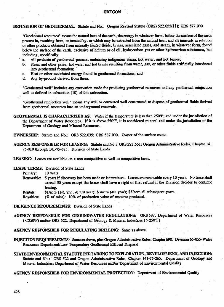
OREGON
\
DEFINITION OF GEOTHERMAL: Statute and No.: Oregon Revised Statute (ORs) 522.055(11); ORs 577.090
"Geoth&d resources" means the natural heat of the earth;the energy in wh&tever form, below the surface of the earth present in, resulting from, or created by, or which may be extracted from the ~ h u a l heat, and all ininerals in solution or other products obtained from naturally lieated fluids, brines, associated gases, and steam, in whatever form, found below the surface of the earth, exclusive of helium or of oil, hydrocarbon gas or other hydrocarbon substances, but including, specifically: a. b.
c. d.
"Geothermal well" includes any excavation made for producing geothermal resources and any geothermal reinjection well as defined in subsection (10) of this subsection.
"Geothermal reinjection well" means any well or converted well constructed to dispose of geothermal fluids derived from geothermal resources into an underground reservoir.
All products of geothermal process, embracing indigenous steam, hot water, and hot brines; Steam and other gases, hot water and hot brines resulting from water, gas, or other fluids artificially introduced into geothermal formation; *
Heat or other assoCiated energy found in geothexmal formations; and Any by-product derived from them.
GEOTHERMAL IS CHARACTERIZED AS: Water if the temperature is less than 250°F; and under the jurisdiction of the Department of Water Resources. If it is above 25W, it is considered mineral and under the jurisdiction of the Department of Geology and Mineral Resources.
0w"Ip: Statute and No.: ORs 522.035; ORs 537.090. Owner of the surface estate.
AGENCY RESPONSIBLE FOR LEASING Statute and No.: ORs 273.551; Oregon Administrative Rules, Chapter 141 75-010 through 141-75-575. Division of State Lands
LEASING: Leases are available on a non-competitive as well as Competitive basis.
LEASE TERMS: Division of State Lands
Renewable: 5 years if discovery has been made or is imminent. Leases are renewable every 10 years. No lease shall exceed 50 years except the lessee shall have a right of first rem if the Division decides to continue
$l/acre (lst, 2nd, & 3rd year); $3/acre (4th year); $5/acre all subsequent years. (96 of sales): 10% of production value of tesource produced.
Primary: 1oyears.
leasing. Rentals: Royalties:
DILIGENCE REQUIREMENTS: Division of State Lands
AGENCY RESPONSIBLE FOR GROUNDWATER REGULATIONS ORs537, Department of Water Resources (C25PF) andlor ORs 522, Department of Geology & Mineral Industries (>BOT)
AGENCY RESPONSIBLE FOR REGULATING DRILLING Same as above.
INJECTION REQUIREMENTS: Same as above, plus Oregon Administrative Rules, Chapter 690, Division 65-055-Water Resources Departmentkow Temperature Geothermal Effluent Disposal.
STATE ENVIRONMENTAL STATUTE PERTAINING TO EXPLORATION, DEVELOPMEN", AND INJECTION: Statute and No.: ORs 522 and Oregon Administrative Rules, Chapter 141-75-265. Department of Geology and Mineral Industries; Department of Water Resources andlor Department of Environmental Quality
AGENCY RESPONSIBLE FOR ENVIRONMENTAL F'ROTECTION: Department of Environmental Quality
428

ADDITIONAL INFORMATION: Oregon Department of E&rgy and Department of Water Resources. See Low Tempmature Geothermal Resource Management, by Lauren S . Forcella, Oregon Water Resources Department of Energy, 1984, Oregon: A Gusde to Geozhennal Energy Devebpment, D&ra Justus, et d., 1980, Oregon institute of Tecblogy, and/or Geothennai Emm Development, A Guide to the Federal and State Regulating ‘Proms in Idaho, M~nrana, Oregon, .and Washington, 1991:
Division of State Lands 1600 state street Salem, OR 97310
Department of Geology and Mind Industries
Portland, OR 97201
Department of Water Resources 3850 Portland Road NE Salem, OR 97310
Department of Environmental Quality
Portland, OR 97204
I I 910 State Office Building 811 S.W. 6th Street I
I I
Oregon Department of Energy 625 Marion Stfeet NE Salem, OR 97310 (503) 378-2778
i
429

TEXAS
DEFINITION OF GEOTHERMAL: Statute and No.: Geothermal Resoutces Chapter, Texas Natural Resources Code (TNRC), Title 5, Chapter 141.003. Geuthermal Resources Act of 1975:
"Geothermal energy and associated resources* means: a. b.
c. d.
Products of geothermal processes, embracing indigenous steam, hot water, and hot brines, and geopressured w, Steam and other gases, hot water and hot brines d t i n g from water, gas or other fluids artificially introduced
Heat or other associated energy found in geothermal formations; and Any by-product derive from them.
GEOTHERMAL IS CHARACTERIZED As: Mineral
into geothermal f o ~ t i o n s ;
OWNERSHIP Statute and No.: Texas Natural Resources Code (TNRC), Title 5, Chapter 141
AGENCY RESPONSIBLE FOR LEASING Statute and No.: TNRC 141.003. General Land Office, Mineral Division
LEASING: N/A
LEASE TERMS: Railroad Commission
DILIGENCE REQUIREMENTS N/A
AGENCY RESPONSIBLE FOR GROUNDWATER REGULATIONS Texas Water Commission
AGENCY RESPONSIBLE FOR DRIUING/REGULATIONS Texas Railroad Commission, Oil and Gas Division
INJECTIONREQUIREMENTS Statute and No.: Texas Administrative Code (TAC), Section 16, 9 3.9 and TAC, Section 16, 0 3.46
STATE ENVIRONMENTAL STATUTE PERTAINING TO EXPLORATION, DEVELOPMENT, AND INJECTION: TNRC 141.003
AGENCY RESPONSIBLE FOR ENViRONMENTAL PROTECTION Water Commission
ADDITIONAL INFORMATION Texas Bureau of Eumomic Geology
General Land office Mineral Division Steven Austin Building 1700 N. Congress Austin, TX 78711
-
Texas Bureau of Eumomic Geology William B. Travis Building 1701 N. Congress Austin, TX 78711
Texas Water Commission Steven Austin Building 1700 N. Congress Austin, TX 78711
Texas Railroad Commission Pennits Division and Oil & Gas Division William B. Travis Building 1701 N. Congress Austin, TX 78711
430

UTAH .
DEFINITION OF GEOTHERMAL: Statute and No.: Geothermal Resource Conservation Act, Section 73-213, Utah Code Annotated (VCA) 1953.
"Geothermal resources" means: a. b.
The natural heat of the earth at temperatures.gfeater than 120°C; and The energy, in whatever form, including pressure, present in, resulting from, created by, or which may be extracted from the natural heat, directly or through a material medium. Geothermal resource does not include geothermal fluids.
"Geothermal fluid" means water and steam at temperatures greater than 120°C naturally present in a geothermal system.
GEOTHERMAL IS CHARACTERIZED AS: Water
OWNERSIP: Statute and No.: Geothermal Resource Conservation Act, UCA, Section 73-21-4. Ownership of a geothermal wurce derives from an interest in land and not from an appropriated right to geothermal fluids. This chapter shall apply to all lands in the state of Utah, including federal and Indian lands to the extent allowed by law. . . In effect, the right to geothermal resource is based on ownership of the mineral rights or surface rights, which are usually obtained by direct ownership or by leasing. Because of the potential relationship between geothermal fluids and groundwater resource, however, an approved application to appropriate geothermal fluids is required prior to the production of geothermal fluids from a well (UCA, Section 73-21-8). The appropriations process for geothermal fluids is similar to that of water appropriations, and includes provisions for advertisement of the application and the filing of protests. Utah Division of Water Rights
AGENCY RESPONSIBLE FOR LEASING Statute and No.: UCA, Section 65-1-18. Board of State Lands, Division of State Lands, Utah Division of Water Rights. Hydrothermal resources at low and mbderate temperatures (< 120°C) are regulated by the Division of Water Rights under Utah Water Law.
LEASING: Competitive leasing involves lands which have newly become available for lease because of new purchase, relinquished leases, or any other reason and are leased under the simultaneous filing pmcedures. Applications for non- competitive leases are fled with the Board of State Lands, Division of State Lands.
LEASE TERMS: Board of State Lands
Kenewable: For as long as land is in production. Rentals: $1 /acre per year. Royalties: (96 of sales): 10% of gross proceeds received from sale of those products, or 10% of the fair market
value when the products are utilized but not directly sold.
Primary: 1oyears.
DILIGENCE REQUIREMENTS: N/A
AGENCY RESPONSIBLE FOR GROUNDWATER REGULATIONS Utah bivision of Water Rights
AGENCY RESPONSIBLE FOR REGULATING DRIUING: Statute and No.: UCA, Section 73-21-5. Utah Division of Water Rights
INJECTION REQUIREMENTS: Statute and No.: UCA, Section 73-21-5. Utah Division of Water Rights and/or Bureau of Water Pollution Control; injection may be required in order to maintain water levels in heavily used aquifers.
STATE E " M E N T A L STATUTE PERTAININGTO EXPLORATION, DEVELOPMENT, AND INJECTION Statute and No.: UCA, Section 73-21-2 and UCA 26-11, Section 1-20
431

AGENCY RESPONSIBLE FOR ENWR0"TAL PROTECTION Department of Envhmental Health; Bureau of Water Pollution control; Bureau of Air Quality; the Resource Development coordinating Committee (acts as a clearinghouse for environmental permits).
ADDlTIONAL INFORMATION Utah Geothermal Handbook: A User's Gstide of Agencies, Regularions, Permits and Aids for Geothermal Development, 1982 andlor State Engineer, Division of Water .Rights.
Utah Division of Water Rights - DepartmentofEn-tdHdth 1636 W. North Temple Salt Lake City, UT 84116
288N. 1460 W Salt Lake City, UT 84116
Bureau of Water Pollution Conrol 160 W. North Temple, Room 410 Salt Lake City, UT 84103
Board of State Lands Division of state Lands 3100 State office Building Salt Lake City, UT 84114
Bureau of Air Quality 150 W. North Temple, Room 420 Salt Lake City, UT 84103
432

DILIGENCE REQUIREMENTS: Department of Natural Resources, Division of Geology and Earth R e s o u ~ . ~ s
WASHINGTON
DE%"HON OF GECYIWE-. Statute and No.: Geothermal Resources Act, Revised code Washington (RCW), Chapter 79.76(3).
"Geothermal resource" means only that ~ t ~ d heat energy of the earth from which it is technologically practical to produce electricity commercially and the medium by which such heat energy is extracted from the earth, including liquids or gases, as well asmy mheral contained in any ~ t u r a l or injected fluids, brines, and associated gas, but excluding oil, hydrocarbon gas, and other hydrocarbon substances.
GEOTHERMAL IS CHARACTERIZED AS: Sui genetis.
OWNERSHIP: Statute and No.: Geothermal Resource Act, RCW, Chapter 79.76. Geothermal resources are the property of the d a c e ower.
AGENCY RESPONSIBLE FOR LEASING Statute and No.: Geothermal R e s o u ~ . ~ s Act, RCW, Chapter 79.76. Department of Natural Resource% Division of Lands
LEASING: At the present time all leases are negotiated.
LEASE TERMS: Department of Natural Resources, Division of Lan+
AGENCY RESPONSIBLE FOR GROUNDWATER REGULATIONS: Department of Ecology
AGENCY RESPONSIBLE FOR REGULATING DRILLING Statute and No.: Geothermal Resources Act, RCW, Chapter 79.76. Department of Natural Resources, Division of Geology & Earth Resoutces
INJECTION REQUIREMENTS Statute and No.: Geothermal Resources Act, RCW, Chapter 79.76. Department of Ecology and/or Department of Natural Resources, Division of Geology & Earth Resources
STATE ENVIRONMENTAL STATUTE PERTAI"GT0 EXPLORATION, DEVELOPMENT, AND ZNJECTION State Environmental Policy Act 1971 and Geothermal Resources Act, RCW, Chapter 79.76
AGENCY RESPONSIBLE FOR ENVIRONMENTAL PROTECTION: Department of ~coiogy
ADDITIONAL INFORMATION. "Geothermal Energy Development in Washington, A Guide to the Federal, State and Local Regulatory Process," 1986 and "Geothermal Energy Development, A Guide to the Federal and State Regulating Process in Idaho, Montana, Oregon, and Washington, 1991."
Department of Natural Resources Dept. of Ecology andlor Rowe Six, Building 1 Olympia, WA 98504
Department of Natural Resources Department of Geology & Earth Resources powe Six, Building 1 Olympia, WA 98504
Division of h d s 202 John A. Cherberg Building Olympia, WA 98504
Washington State Energy Office 809 Legion Way SE, FA-11 Olympia, WA 98504-121 1
.
433

WYOMING
DEF'INlTIONOFGEOTHEW Statute and No.: Wyoming Statutes (WS) Chapter XI Rules and Regulations Goveming the Issuance of Geothermal Permits and Leases.
"Geothermal resources" shall mean the natural heat in the subsurface of the earth, its energy, in whatever fonn, resulting from, or created by, or which may be extracted from, such natural heat and all minerals in solution or other products obtained from naturally heated fluids, brines, associated gases, and steam, in whatever form, found below the surface of the earth, but excluding oil, hydrocarbon gas, other hydrocarbon substances or miscellaneous minerals.
GEOTHERMAL IS CHARACTERIZED AS: Water
O W " : Statute and No.: Natwe of Water Rights and Beneficial Use, Article 1,941-3-101 Wyoming Statutes (WS). Geothermal is a public resource available for appropriation.
AGENCY RESPONSIBLE FOR LEASING Article 1. 8 41-3-101: Rules and Regulations Governing the Issuance of Geothermal Resource Permits and Leases, Wyoming State Lands Office
LEASING: LeasinginKnownGeothermalResource Areas (KGRA)is by competitive bid. Other lands are available through a non-competitive permit which may be converted to a lease within 50 days should the area be classified as a KGRA.
LEASE TERMS: Wyoming State Lands Office Primary: 1oyears. Renewable: As long as geothermal tesoutces are being produced or utilized, or are capable of being p r o d d or
utilized in commercial quantities. Rentals: $2/year. Royalties: (96 of sales): 10% of gross revenue as determined by a reasonable value received from the sale of steam,
brine, from which no minerals have been extracted, and associated gases at the point of delivery to purchaser thereof. In such a case where the resource is used by the lessee and not sold, the gross revenue therefrom to be determined as those said geothermal resoutces had been sold to a third person and then primarily market price in the same market area and under the same market conditions.
DELIGENCE REQUIREMENTS Drilling must commence within two (2) years. State Board of Land Commissionen
AGENCY RESPONSIBLE FOR GROUNDWATER REGULATIONS State Engineer
AGENCY RESPONSIBLE FOR REGULATING DRILLING Statute and No.: Rules and Regulations Governing the Issuance of Geothermal Resource Permits and Leases. State Board of Land Commissioners and State Engineer
INJECTION REQUIREMENTS: Surface disposal may be approved by the Wyoming Game and Fish Department, State Engineer or Department of Environmental Quality.
~ATEENVIRO"TAL~ATUTEPERTAI"GTOEXPLORATION, DEVELOPMENT, ANDINJECTION State Engineer or Department of Environmental Quality, Section 12, Board of Land Commissioners Permit to prospeCt for Geothermal Resources
AGENCY RESPONSIBLE FOR ENVIRONMENTAL PROTECTION Department of Environmental Quavty
434

DDlTIONAL HWOl2MA~ON State Engineer’s Office and/or Universiw of Wyoming and Rules and Regulations govembg the Issuance of Geothermal Resource Permits and Leases, November 1, 1975 and Permit to’Prospect for Geothermal Res6um.
Wyoming State Lands Office andlor State Board of Land 4th Floor West Department of Geology 4th Floor West Commissioners Herschler Building P;O. Box 3006 Herschler Building
4th Floor West Cheyenne, WY 82002 Laramie, WY 82071 Cheyenne;WY8~
. Department of Eiwiromental Quality University of Wyoming State WS OEce
Herschler Building Cheyenne, WY 82002
435


CHAPTER 20 - _
ENVIR0"TAL CONSIDERATIONS
By Ben Lunis and Robert Breckenridge EG&G Idaho, Iac.
Idaho Falls, ID 83415
20.1 INTRODUCTION
The degree to which geothermal development affects the environment is, in most cases, proportional to the scale of such development. For example, the environmental impacts associated with g e o t h e d direct me projects are often minimal compared to those associated with large-scale electrical generation projects. The direct use projects are often designed as closed-loop systems where the low- or moderate- temperature geothermal fluids are circulated through a heat exchanger or heat pump (or flow naturally around downhole heat exchangers). The spent geothermal fluids are then injected into or near the production aquifer, or surface discharged into nearby drainage and waterways or both. The surface discharge approach normally produces greater environmental concern than injection. These and other environmental considerations are addressed in this chapter. Regulations that may apply are also discussed.
20.2 ENVIRONMENTAL REGULATIONS
Various federal, state, local laws, and regulations may be directly or indirectly applicable to geothermal energy project siting,. development, and operation. However, the rules generally apply more to electrical generation projects than to direct use projects. No single set of regulations applies to all types of geothermal applications, and lesser attention is given to low- and moderate-temperature tesources. However, the appropriate regulating agencies must be contacted to determine what requirements may apply to a specific project. Table 20.1 summarizes the probability and relative severity of potential environmental impacts as the result of the development of geothermal direct use projects. It is best to discuss the envhmental Considerations of the project early with all applicable regulatory agencies, and obtain the necessary permits so that the project is not because of some overlooked environmental regulati
Following is a brief discussion of the major regulations that may apply to direct use projects. Table 20.2 rmmmafizes the areas of applicability.
Table 20.1 Probability and Severity of Potential Environmental Impacts of Direct Use Projects
Probability Severity of ImDact ofOccurrind c o n m e n d
Air quality pollutionb L M
Surf' water pollution M M
Underground pollutionc L M
Land subsidence
High noise levels
L L toM
H M t o H
Well blowouts L L toM
conflicts with cultural & - archeological features L toM M t o H
Social economic problems L L
Chemical or thermal pollution M M t o H
Solid waste disposal M
a.
b.
L = Low; M = Moderate;,H = High.
Hydrogen sulphide odors may be objectionable, but are not significant enough to be a problem.
c. Pollution concern may increase g e o t h e d fluid injection requirements.
4

Table 20.2 Regulations Affecting G e u t h d Energy DeJelopment (Zimmemm , 1984) ~~
Surface Water
SLlbSidelld Noise . Seismicitv
Liquid waste
Principal Pollution JAWS and Reeulatims &
Federal Water Pollution Control Act (NPDES)
Geothenmal Solid Fluids Waste
X X
Safe Drinking Water Act - (Underground Injection Control Regulations (UIC))
clean Air Act X
Resource Conservation and - Recovery Act
Toxic Substance Cantrol Act -
X - X
- X X
- X X I - X X National Environmental Policy X
Act @TEPA) X X X X
Noise Control Act - X - G e o t h d Resource X x - X X X X X Operations Order #44
Occupational safety 4% X - - X X X - Health Act
. are structured more by the end product than by the energy source used. Thus, geothermal effluents from various processes will not be treated in a consistent manner.
20.2.1 Federal Water Pollution Control Act. as Amended (Zimmerman, 1984)
The 1977 Federal Water Pollution control Act, as Amended, established the National Pollutant Discharge Elimination System ("DES) and effluent guidelines and is aimed primarily at the protection of surface waters through a permitting process. A primary precept of this law is to provide for state umtrol of water pollution if the states develop a program that enmmpasses the standardized permit system developed under NPDES. Permits are based on industry-specified effluent guidelines or 011 more stringent standards for receiving-water quality. No specific geothermal guidelines or standads have been established to date, but emphasis in the law is placed on control of toxic pollutants (including heavy metals, many of which are found in geothermal fluids and waste).
Under this NPDES system, discharge quantities, htes, pollutant concentrations, and fluid discharge temperatures are regulated by permits issued by either the EPA or states with EPA-approved programs. No specific geothermal category exists intheNPDES regulations, because theclassifications
20.2.2 Safe drink in^ Water Act. as Amended . (- , 1984)
The W e Drinking Water Act (SDWA) was designed to safeguard the primary and seumdary safe drinking water supplies of the nation. The primary intention of this act is that state governments implement programs to ensure compliance. The major regulation that directly affects geothermal energy recovery are those for underground injection control (UIC) designed to protect groundwater aquifers. The UIC regulations establish five disposal well, categories based on well ctmstmction technology, practices, and fluids to be injected. Geuthermal energy was placed in two categories. Wastes from electric power generation were placed in Class III, which includes 'all special process injection wells; for example, those involved in solution mining and minerals, in situ gasification, oil shale, coal, etc., and the recovery of geothermal energy for electric power generation. ' Direct-use geothermal injection wells were placed in Class V,
i I 43 8
which includes: All other injection wells (not included in Classes t to IV), including g e o t h e d direct-appkation wells" (EER, .Inc? 1981; EER, Inc., 1982 b]. The EPA proposed that electric power geothermal wells be changed from Class III to Class V (EER, Inc., 1982 b) and- this change in classification was adopted in February 1982. Under Class V, wells are not regulated with regard to CoflStNcfion criteria, maintenance, or testing UIC, if the EPA determines that contamination of a drinking water source is possible, more stringent monitoring, construction, testing, and operational standards can be imposed.
20.2.3 Clean Air Act, as Amended (Zimmerman, 1984)
This 1963 act has undergone many major changes, the ,most recent being the Clean Air Act Amendments of 1977 (EER, Inc., 1982 b; Hartley, 1978; Galabi, 1980). As in the Clean Water Act, the intent of the law was for the states to administer the programs through state implementation plans approved by the EPA.
There are four major provisions under the law that may affect development of geothermal energy. These are New Source Performance Standards (NSPS), Prevention of Significant Deterioration (OSD), National Primary and Secondary Ambient Air Quality Standards, and National Emission Standards for Hazardous Pollutants. The NSPS are a primary control mechanism that is set on am industry-by- industry basis and requires the application of the best available technology to reduce emissions. At the time of this report, the Clean Air Act is undergoing major revisions. The revisions are mostly being focused on emissions of C, N and S sources. Although these are only usually emitted in significant quantities by larger scale power facilities. All developments should check with their regional EPA and state air permitting agencies to ensure compliance.
20.2.4 Resource Conservation and Recoverv Act of 1976
The Resource Conservation and Recovery Act of 1976 (RCRA) provides: (a) technical and financial assistance for the safedisposal of discarded materials and (b) regulates lhazardous wastes. (Zimmerman, 1984). Solid wastes that are not hazardous wastes am currently exempt from the hazardous waste regulations under RCRA. This exclusion includes drilling fluids, produced waters, and other wastes associated with the exploration, development, or production of crude oil, natural gas or geothermal energy (40 CFR, Ch. 1, 7-1-86 Edition). This exemption can be removed in the future, however, depending on the characteristics of the solid wastes resulting from geothermal energy development (Zimmerman, 1984).
20.2.5 Toxic Substances Control Act (Zimmerman, 1984)
The Toxic Substances Control Act (TSCA) was established " to regulate commerce and protect human health in the environment by requiring testing and necessary use restrictions 0x1 certain chemical substances, and for other purposes" (EER, hc., 1982 b). The main impact of TSCAon geothermal energy development affects the sale for c o d use of by-products rcixOvered from either liquid or solid waste streams. The EPA administrator is authorized to determine the environmental, economic, andsocial impacts of the sale of any such material. Under the act, by-products require certification of their make-up. If these by-products are determined to be toxic, regulations for their mtrol, flows, and use must be developed (Hartley, 1978; Galabi, 1980; EER, Inc., 1982 b).
20.2.6 Noise Control Act of 1971 (Zimmerman, 1984)
The Noise Control Act of 1971 gives primary control of noise to the state and local governments (Hartley, 1978; Kestin, 1980; Beeland, 1978; Morris and Hill, 1980). Under this act, the federal government retains regulatory authority over low-level noise produced by construction equipment, transportation equipment, any motor or engine, and electrical or electronic equipment. When a new class of products is regulated by the EPA, state and local noise emission levels for that product must be identical tothose established by the EPA. Primary control of noise from geothermal energy development fall under the Occupational Safety and Health Act (OSHA) and Geothermal Resource's Operational Order (GRO) No. 4.
20.2.7 National Environmental Policv Act Zimmerman, 1984)
The National hvironmental Policy Act (NEPA) requires environmental impact statements to be completed and filed for all federally funded geothermal actions significantly affecting the quality of human environment (Beeland, 1978; Galabi, 1980; EER, hc., 1982 a).
20.2.8 Geothermai Resource ODerational Order No. 44 (Zimmerman, 1984)
This legislation allows the U.S. Geological Survey to apply EPA's and its own requirements to geothermal development on federal lands. In addition, the order sets noise criteria for of federal lands. In addition, the orde eothermal operations on federal lands not to exceed 65 dBA at the lease boundary, QT 0.5 ,mi from the source, whichever is greater (Hariley, 1978).
439

20.2.9 OcCuDational Safety and Health Act of 1970 (Zimmerman, 1984)
The Occupational Safety and Health Act of 1970 (OSHA) authorized the Secretary of Labor to set mandatory standards to protect the occupational safety and health of all employees. The act deals specifically with toxic materials and other harmful agents (Beeland, 1978; Galabi, 1980; Kestin, 1980; Moms and Hill, 1980).
20.2.10 Endangered SDecies Act of 1973
The Endangered Species Act of 1973 provides executive- branch regulators with significant powers to guide energy (geothermal) exploration and production. This act protects endangered wildlife species and their critical habitats from exploration and development (Beeland, 1978; Galabi, 1980; EER, Inc., 1982 b) (Ummerman, 1984). The U.S. Fish & Wildlife Services should be contacted to determine if this act applies to r e s o w around the propolsed project.
203.11 State and Local Laws and Repulations
State and local regulations may be more stringent than federal laws. It may be necessary to contact the appropriate agencies regarding a specific project. Chapter 19, Institutional, Legal and Permit Requirements, identifies specific state agencies responsible for environmental protection and drilling. That chapter also addresses state groundwater laws, permits, easements, district heating regulation, and injection requirements.
20.3 ENVIRONMENTAL FACTORS
The main environmental factors to be considered during geothermal exploration, development, and operation of direct use projects include:
1. 2. 3. 4. 5. 6. 7. a. 9. 10.
Airborne effluents Water pollution Land subsidence Induced seismicity Noise Water availability Solid waste Land use Vegetation and wildlife Economic .and culhual factors.
A brief discussion of these.factors follows.
20.3.1 Airborne Effluents
Airborne effluents that may be released during the development of a geothermal direct use project are generally the same as those from normal construction activities, and
should be treated accordingly. A unique and remote potential exists for venting gases containing hydrogen sulfide and other toxic material during well drilling operations. This could pose an immediate health threat to nearby workers. Table 20.3 presents information on H$ and its effects on the human body. It is important to note that even at low concentrations s 0.196, H$ can be a fatal gas. Thus, proper drilling procedures prepared by qualified safety personnel should be developed to address this concern.
Table 20.3 concentration of H$ in Air and Its Physiological Effects (Burgess, 1964)
Concentration of HS (96) Phvsioloeical Effects
. 0 . m Just detectable by smell 0.002 Maximum allowableconcentration
for prolonged exposure; at this concentration, causes eye irritation
Can be inhaled for 1 hr without serious lasting effect Dangerous if inhaled for *h to 1 hr
0.06 Fatal after 'A hr 0.1 Paralyses sense of smell and
0.007-0.015 Slight symptoms 0.017-0.03
0.04-0.06
causes instant unmnsciousness
20.3.2 Water Pollution
Water pollution can occur during any stage of g e o t h d development whether it be field exploration and testing, production well drilling, .construction, or facility operation (Hess, 1984).
Muds commonly used for drilling may be harmful to water quality if they are allowed to enter either surface waters or groundwater aquifers. Some of these muds contain petroleum-based additives or metals that can jeopafdize the environment if accidentally leaked into surface water or groundwater aquifers. To prevent contamination of surface waters, these substances, together with rock dust and the water used in the drilling operation, must be isolated from the surface as well as groundwaters. Wells should be cased through potable groundwater horizons to prevent mixing of drilling fluids with groundwater. Blowouts can also pollute water, and blowout protection equipment should be required during the drilling of all geothermal wells where high temper- ature or pressure are anticipated. Sumps with an impermeable lining or steel tanks should be used to store drill cuttings and drilling fluids during drilling operation to ensure that these materials do not contaminate surface water (FERC, 1981).
440

Erosion and sedimentation associated with constytion of drilling pads, roads, pipelines, and utilization fac effect the quality of nearby surface water associated with erosion and sedimentation can be careful site selection and engineering design, and the adoption of erosion and runoff prevention control measures.
AU subsurface disposal of geothermal fluids is regulated by the EPA's UIC regulation and by state drinking water programs developed pursuant to the Safe D w g Water Act mess, 1984).
Water pollution problems can be' associated with the management of spent disposal fluids. However, low-to- moderate temperature geothermal fluids used in most direct use applications generally contain low levels of dissolved volatile compounds and dissolved solids and the discharge of spent geothermal fluids is seldom a major problem. Some of these fluids can often be discharged to surface waters after cooling (if needed). However, high concentrations of such chemicals as boron, fluoride, or arsenic in spent geothermal fluids may require that the fluid;: be treated, injected or both. Again, the variable nature of geothermal fluids requires that each resource be evaluated on a site-by-site basis to determine the most environmentally sound disposal program. The disposal methods selected will depend upon the quality of the wastewater, local hydrological conditions, environmental regulations, and in some cases, local requirements.
-
It may be necessary to demonstrate to governing authorities that there will be a lack of adverse effects upon local groundwater supplies through the disposal of spent geothermal fluids. Injection of the spent geothermal fluids is considered by some to be the most advantageous when the disposal well is properly constructed to prevent polluting groundwater aquifers. In addition, injection may help to maintain the long-term productivity of the reservoir and lessen the potential for subsidence. However, because many geothermal low-to-moderate temperature reservoirs are fault and fracture controlled, there is concern about where to locate an injector well, and ,at what depth. If the spent fluids are injected into the producing aquifer, t h e d dilution can occur, reducing the life of the reservoir. Reservoir testing and analysis, with the attendant expense, may be required to
whether or not injectors are required.
Surface discharge of spent geothermal fluids into a navigable river requires a National Pollutant Elimination System (NPDES) permit. Western laws may play a role in selecting the method used for surface discharge (Zimmennan, 1984). Geothermal fluids, in some cases, are of adequate purity to be used for other surface applications such as irrigation.
. Generally, subsurface changes caused by geothermal
developments are of serious concern if the impact reaches beyond the g e o t h e d reservoir. As soon as the effects
extend to the land surface or affect the regional aquifers or induce subsidence or seismicity, regulators and the public becomes involved. Before this occurs, long-term monitoring data should be available to describe and quantify the changes
ly occurred and to document that operational practices are in compliance with all applicable regulations
, 1980) (Zimmerman, 1984).
The removal of large quantities of geothermal fluid from a geologic formation may result in land surface subsidence. Permanent and non-recoverable subsidence d t s from slow- and long-term iemoval of fluids and from the compression of aquitards-such as clay, silt-like materials, or shale-above or below a reservoir. Such subsidence has been common follow- ing the withdrawal of water and oil. At the present, however, subsidence has not been observed as a significant concern for low- and moderate-temperature reservoirs. If subsidence does OCCUT, injection wells may be utilized to mitigate the problem.
20.3.4 Induced Seismicity
Many hydrothermal reservoirs are located in regions with a high fresuency of naturally occurring seismic events. An environmental concern may be raised as to whether or not the withdrawal or injection of geothermal fluids or both may enhance the rate of microseismic events, or even trigger a major earth movement. FERC (FERC, 1981), however, con- cluded that "it is extremely unlikely that major seismic events could be triggered in this way. " Experience with fluid injec- tion in a number of non-geothermal situations has demon- strated that induced seismicity can be minimized or prevented by regulating injection pressures (FERC, 1981; O'Bairion arid Layton, 1981).
20.3.5 Noise
Noise associated with the operation of direct use projects is generally insignificant. However, drilling rigs and construction equipment, pumps, and compressors are principal noise sources for direct use projects. In the event higher temperature fesources are encountered, significant noik can be expected from accidental unmuffied well venting, as in the case of a well blowout (Webb, 1984). Construction site noise may lead to public annoyance and complaint, and noise shielding may be needed to reduce sowce noise levels to acceptable regulatory levels.
20.3.6 Water Availabilitv
One of the major potential problems in geothermal energy development is the definition of water rights for low-salinity fluids. Historical interpretations in the western states bave placed industrial uses, of which geothermal energy extraction appears to be one, at a much lower priority than water for municipal and agricultural p u q k e ~ (Zimmerman, 1984).
441

As noted in Chapter 19, Paragraph 19.11 Groundwater Law, groundwater is treated as a public resource in most western states, except Oregon; California and Hawaii are like most eastern states where groundwater is attached to the surface unless critical groundwater areas have been designated, requiring the water rights to be adjudicated. Because historical users of groundwater included domestic, agricultural, and industrial purposes, but not heat extraction, conflicts between existing uses and the geothermal project developer have become a serious consideration and can severely limit development, especially in critical groundwater areas.
Most geothexmal systems are directly connected hydraulically with adjacent groundwater aquifers; others are poorly comected or separated from circulating groundwaters (for example, the dry-steam geysers field of California and the geopressured reservoirs of the Texas-Louisiana gulf coast). The extent to which hydrothermal changes are transmitted to djacent aquifers depends in part on the characteristics of the geothermal reservoir system and the hydraulic communication with the adjacent aquifers, and also on the rate and cumulative volumes of fluids extracted and injected, the time since these changes began, and the size and regional extent of the reservoir (Zimmerman, 1984).
The recharge parameters of a geothermal system are usually difficult to evaluate under natural conditions. Until hydrodynamic stresses are imposed on the system and closely monitored long-term flow testing of production wells is performed, the hydrothermal parameters and resource potential of the reservoir system and the impacts that developments might have on regional aquifers remain in the realm of speculation. The apparent hydrothermal relationships observed under natural low-flow conditions are sometimes very misleading (Zimmerman, 1984).
Three of the principal types of adverse effects of geothermal developments on regional aquifers are (Zimmerman, i984):
1. Depletion of the regional water supply by induced. recharge to the geothermal reservoir or the direct pumping of non-thermal waters for cooling or plant uses from shallow aquifers.
2. Chemical or thermal contamination of regional aquifers by planned injection or unplanned migration of injected geothermal fluids.
3. ContaminatiF of shallow aquifers caused by inliltration of poorquality fluids from surface ponds or spills.
Because of the large volume of fluids generally stored in a geothermal reservoir and the m u n d i n g regional aquifer system, the effects of geothermal withdrawal can be subtle and longdelayed. Changei because of these withdrawals may be
difficult to detect ex&t near the production well field. For more distant locations, changes may not be detectable except after long periods of full-scale fluid withdrawal. Similarly, the effects of deep fluid injection may be difficult to measum, particularly if the changes caused by injection are super- imposed on changes caused by fluid withdrawal (-, 1984).
If the quantities of fluid withdrawn from the geothermaI reservoir system exceed the quantities of fluids injected, a net drawdown or decline in reservoir pressures will OCCUT. Fluids injected into formations in the drawdown area would migrate toward the producing wells and would not Contaminate the regional aquifer system. Only when poorquality fluids are injected into formations where the flow gradients are directed toward the regional aquifer system($) containing water of
In systems where flow gradients are subtle, travel times are slow, and volumes of fluids in transit are great, a long delay in the identification of contamination or overdraft might give unjustified comfort to environmentally concerned observers (catnpbell, 1977; DiPippo, 1980; U.S. Envinmmental Protection Agency, 1977; Galabi, 1980; Summer, 1980) (Zimmerman, 1984).
usable quality will groundwater umtamhati onoccuT.
Where geothermal systems are presumed or known to be intimately umnected hydraulically to hydrothermal springs and vents on the surface or critical aquifers of limited recharge and extent, these features should be closely monitored to detect possible effects of geothermal production. Changes in hydraulic head and water quality in observations wells in strategic locations and depths, sometimes years after geothermal development began, can be used to detect incipient effects of these geothermal developments (Galabi, 1980; Summer, 1980) (Zimmerman, 1984).
Many direct heat projects use heat exchangers with secondary loop distribution providing heat to the end use. Accordingly, the need for makeup water for the secondary loop is minimal for replacement of system losses.
20.3.7 Solid Waste
Solid waste treatment, handling, and &spot&, are mandated by state or fedetal regulations. Solid waste is classified either as hazardous or nonhazardous, depending upon its constituents. Nonhazardous solid waste requires proper disposal, but no special facilities, and has a relatively minimal disposal cost. The disposal cost of hazardous solid waste can, however, be significant, due primarily to the specialized nature of licensed disposal facilities and the cost of
since 1978, considerable research has been performed to chatacterize geothermal solid wastes and provide a firmer basis for classification within existing regulatory guidelines; this classification is essential to ensure proper management of solid waste (Zimmerman, 1984).
transporting wastes to appropriate disposal facilities.
. 442

The general character of for solid waste control remains constant for high-, moderate-, and low- temperature geothermal resources.. In general, both the dissolved solids content and the energy tent of geothennal fluids increase with fluid temperature. For a constant level of energy extraction, the relative amount of solids bat will be recovered from high-, moderate:, or geothermal fluid is dependent on the conc temperature-solubility characteristics of each dissolved compound. Options for solids control and recovery remain the same for all geothermal fluids, but the size and capital cost of
'control equipment may increase as temperature decreases because of the greater flows 'required per unit of energy extraction (Zimmerman, 1984).
The principle solid wastes associated with the use of low- and moderate-temperature resources for direct projects are the residues associated with well drilling.
Drilling wastes include drill .cuttings, drilling mud, and possibly lostcirculation control agents. Drill cuttings are chips of the rock that were displaced during well drilling. Alluvium, basalt, rhyolite, and sandstone and other sedimen- tary rock typically, make up these cuttings. Drilling mud is a combination of water, chemicals, and mineral constituents used to lubricate the drill bit and to transport cuttings to the surface during drilling operations. Lost-circulation control agents, if used, mriy result in additional drill wastes (Zimmerman, 1984).
The regulatory status of geothermal solid wastes is complex. Three materials have been categorically excluded from RCRA by .Congress via-a ruling by EPA on July 6, 1988. Thus, on the federal level, geothermal solid wastes are defined as nonhazardous wastes that may be disposed of in unsecured landfills (EER, Inc., 1983 b). However, the State of California, which contains within its boundaries the only long-term commercially operating geothermal power facilities in the U.S., has defied most .geothermal solid wastes as hazardous-wastes that require disposal in a hazardous waste disposal (secured) landfill. Current literature characterizing geothermal solid .wastes provides empirical evidence of geo- thermal sold wastes that fulfill one or more of four federal criteria that define a hazardous waste (corrosivity, radio- activity, toxicity, and bio-accumulation potential) as specified in the Toxic Substance Control Act (Zimmerman, .1984).
In order to obtain. the most current information, developers,should discuss their projects with the local, state,
environmental regulations. In addition, EPA RCWSuperfund hotline can be contacted toll free at 1-800- 424-9346 or 202-382-3000 in the local area around Washington, DC. Business hours for the Hotline are 8:30 8.m. to 7:30 p.m. EST. To avoid a major wait, the'best4ime to call is either at 8:30 a.m. EST or after 6:30 p.m. EST.
and federal agencies responsible for developing forcing
The most current information on classification of gqthermal waste can be found in Federal Register of July 6, 1988, starting on page 25446. f specific interest is the section on page 25453 (section l(b).to 3001(B)) that discusses those wastes considered hazardous and those exempt. In general, geothermal production fluids are considered exempt under RC may be subject to regulations under the Clean Wa If a develdper is interested in obtaining more information, they should refer to the Report to Congress that discusses this in detail. The Report titled 'Report to Congress on Management of Waste from Exploration, Development, and Production of Crude Oil, National Gas, and Geothermal Energy" is available from the National Technical Information Service (1 -800-336-4700) in a I-vohme set. The portion specific to geothermal development is covered in Volume I1 (order number PB-88146238). This document discusses and compares the state and federal classification of geothermal wastes.
Solid wastes containing hazardous substances should be contained and isolated' from possibIe leaching to ground or surface water, or the leachate may be treated in order to remove hazardous elements and materials. Most wastes Will have to be de-watered before they are removed to an approved disposal area. Toxic solid wastes may not, in most instances, be disposed of on-site, but have to be taken to an approved hazardous waste treatment and disposal facility.
20.3.8 Land Use
The most significant land use issues related to direct use exploration and development can be expected when g e o t h e d reservoirs are located-in, or adjacent. &,.amas designatalas critical habitat areas, -or in heavily -urbanized areas, e.&, single family residential neighborhoods. Areas used for intensive agriculture may also present land-use impediments in terms of displaced crop lands although suzh displacement CBI~ be expected to be short term and be of significance only so long as the land is neceSSary during drilling (O'Banion and Layton, 1981).
gating measures to reduce adverse impacts on land U geothermal developments include actions such as land use planning, environmental evaluation, the use of buffers around critical habitats, sound engineering and construction processes, and the restriction of certain activities to noncritical periods.
20.3.9 Vegetation and Wildlife
The effects of most direct-use geothermal development on wildlife and vegetation should be minimal because of the fact that nearly all direct use development will occur in cJose proximity to urban centers where natural vegetation and wildlife will have been significantly altered before the introduction of geothermal development.
443

The effects of geothermal energy development on biological resources can involve direct loss of habitat, disruption of fish spawning and nursery habitats, fisheries danger from water contamination, and habitat dishubances from noise and human intrusion.
Direct loss of habitat will result from the comtruction of facilities such as roads, drilling pads, pipelines, and utilization for utility. Loss of habitat would be most significant if it involves the loss of habitat of rare, threatened, or endangered organisms. Loss of fish habitat can result from erosion and increase in the amount of sediments in stream beds. This can adversely affect fish spawning and nursery habitat (Brownell, 1981).
Damage to aquatic life can occur from the discharge or spill of geothermal fluids, or drilling fluids containing such potentially hazardous substances as NH3, H$, heavy metals, or fluoride into surface water (FERC, 1981).
Human intrusion, and accompanring noise and disturbances that are necessarily the result of geothermal exploration and development activities, can adversely affect wildlife use of adjacent habitat. Species such as nesting raptors and some predators may be particularly sensitive to these factors. Many other species, however, seem to adapt to the noise and disturbance (FERC, 1981).
20.3.10 Economic Effects
Economic impacts of geothermal development consist primarily of effects on employment and income, and can be divided into permanent effects caused by the creation of permanent jobs and temporary effects caused by the influx of temporary employees involved in well drilling and facility ConStruCtion.
In terms of construction and operation, the economic effects of direct use projects can be expected to have little impact upon a community. Few new permanent jobs would be created by the introduction of a district heating system. However, the direct use of a g e o t h d energy structure can involve moving the structure to be used as an economic tool to encourage industrial or agricultural expansion in an area and could, in this way, result in a considerable number of new jobs.
20.3.11 Cultural b c t s
Although the direct use of geothermal energy can be expected to have substantially less cultural effects than electrical generation, many direct use projects occur near hot springs, and the historic use of the springs may be significantly altered by new development. Conflict with American Indian Religious sites can, however, be expected to be minimal as most such sites are located in remote areas, at considerable distances from population centers.
444
Cultural effects of geothermal development include visual, and archaeological impacts.
Visual impacts are extremely difficult to evaluate because the natural scenic value of the area must be judged, as must the desirability of altering that value.
A major but very short-term source of visual impact will be drilling rigs.
impacts into account during planning aad design, facilities can. If geothermal developers are required to take visual
be designed to meet applicable architectural S. Thus, facilities could be made to blend harmoniously with the surrounding environment and have a d l y pleasant appearance (U.S. Deparhnent of the Interior, 1973).
Archaeological or historic sites or both frequently are found either on or in the vicinity of many potential geothermal developments because of intensive use of t h d and mineral springs sites by both Indians and early settlers. Where such sites have not been adequately surveyed, and where a State Historic preservation officer (SHPO) deterrnines that there is a high probability that an archaeological site exists, it is extremely important that an archaeological resouice inventory be conducted before site development begins.
If a potential archaeological site is found, work s h d d stop and test pits should be dug by archaeologists to determine the significance of the site. If it is determined that the site is not of significant historical importance, g e o t h d develop- ment may proceed as originally planned. If initial studies confirm that the site is of significant importance, the site should be fully explored, documented, and possibly excavated and curated, a very costly and time-consuming process. There is a also a significant risk in that if a site is determined to be of great importance that development will not be dowed (FERC, 1981).
Buildings or other structures at a historic site should be examined by a historical architect before any actions are taken that might adversely effect them. Proper mitigation measure for a structure can involve moving the structure to another site, leaving and protecting the structure or, in some cases, tearing down after a photographic record and measured drawings have been made. If the structure is torn down, the site should be excavated xs described above (FERC, 1981).
Areas of high geothermal potential may also be placed of high religious significance to various Indian p u p s and are protected through provisions of the American Indian Religious Freedom Act (Public Law No. 95-341, vnited States Forest Service, 19813). If development is contenq>lated on federal or state lands, appropriate land management agencies must be contacted concerning the existance of American Indian Religious Freedom Sites. If such sites exist in the immediate vicinity of the proposedwork, representativesoftheIndian

!
!
i
I I
j I
i
I
1
people should be contacted so that location of such sites can be determined and significance and usage patterns established.
The use of such sites is guaranteed to the Indians by statutes and only through closely working with Indians can conflict be avoided or minimized.
20.4 CONCLUSION
The development of geothermal direct use projects is considered to be generally benign in comparison with geother- mal electricity plant development and with most other energy producing technologies. However, there are many regulations that apply to direct use projects that must be complied with.
Geothermal development, as with any major development, can pose serious threats to the environment. Among these are the release of air and water effluents, induced seismicity, and subsidence, water supplies, solid waste, noise, and land use. The geothermal industry has, however, benefitted from the fact that most geothermal development postdates the passage of the National Environmental Protection Act, and the new geothermal industry has had to meet the challenge of growing up in a period of high environmental awareness. B e u s e of this, regulatory agencies, as well as geothermal developem, have been forced to adopt poficies and procedures that ensure a high level of environmental protection.
Providing such protection, however, has not always been easy. The site-specific nature of geothermal resources does not allow for broad generalizations about the environmental risks of geothermal development. The way in which geother- mal resources are developed, however, from surface geological and geophysical exploration to drilling, to field development, to facility construction, provides the regulatory agency as well as the developer the flexibility that is needed in order to provide adequate environmental protection in a cost-effective manner. Experience has shown that early environmental planning, baseline data gathering, monitoring of ongoing activities, and the timely use of mitigation measures are essential in making a successful project (Webb, 1984).
Technological advances also have played a major role in ensuring that geothermal development meets environmental standards. Silencers and mufflers continue to reduce noise emitted from drilling operations. Proper injection practices can greatly reduce land subsidence and the risk of fouling surface water or near d a c e groundwater (Webb, 1984).
If greater protection is deemed to be necessary, regulatory agencies and the geothermal industry have established a sound w e w o r k upon which to build. In all cases, early contact should be made with all applicable regulating agencies to ensure the project is in compliance with the most recent regulations.
20.4 ACKNOWLEDGMENTS
Appreciation is extended to Dr. Gordon -Bloomquist, Washington State Energy Office, for his significaut umtribu- tion to the preparation of this chapter. Thanks are given to Robert Breckenridge, Idaho National Engineering Laboratory, for his technical review and input.
REFERENCES
Brownell, J. A., "Cumulative Biological Impacts of The Geysers Geothermal Development," Staff Report, California Energy Commission, pp. 149, 1981.
Burgess,S.G. and L. B.Wood, "The properties and Inst. Sewage Purification, Detection of Sludge Gas",
pp. 1-24, 1964.
FERC, "Rule-Making for Small Power Production and Cogeneration Facilities," Western Reaional Final Supplement Environmental Impact Statement, Docket No. RM 81-2, 1981.
Hess, J. W.; Wheatcraft, S. W.; Edkins, J. E.; Jacobson, R. L., and D. E. Zimmerman, et al., "Geothermal Environ- mental Impact Assessment: An Approach to Ground- water Impacts From Development, Conversion, and Waste Disposal." Water Resources Center, Desert Research Institute, University of Nevada System, Las Vegas, NV, pp. 270, 1984.
O'Banion, K., and D. Layton, "Direct Use of Hydrothermal Energy: Review of Environmental Aspects. " Lawrence Livermore National Laboratory, University of California, Livermore, CA, pp. 55, 1981.
U.S. Department of the Interior, "Final Environmental Statement for the Geothermal Leasing Program," Vol. 1, 1973.
U.S. Forest Service, "Inventory of Native Americans Religious Use, Practices, Localities and Resources," study area on the Mt. Baker-Snoqualmie National Forest, Washington State, pp. 1-50, 1981.
Webb, J. W.; Edleman, G. K., and A. W. Reed, Retrospec- tive Examination of Geothermal Environmental Assessments," Oak Ride National Laboratory, prepared for the U.S. Department of Energy, March 1984.
Zimmennan, E. R.; Dewey, J.; Bender, M., and B. Lofgren, "Environmental Control Technology for Geothermal Energy," ESCOR, In., prepared for the U.S. Department of Energy, September 1984.
1
445
Copyright © 2022 FDOKUMEN