Calibration of a Geothermal Energy Pile Model R. Caulk *1, J. McCartney2, and E. Ghazanfari1 1University of Vermont, 2University of Colorado, Boulder *Corresponding author: 33 Colchester Ave, Burlington, VT 05401 rcaulk@uvm.edu Abstract: This paper outlines the calibration of a numerical model for heat transfer from geothermal energy piles into surrounding soil. The numerical model was built using COMSOL Multiphysics Finite Element software. Specifically, the heat transfer and non-isothermal pipe flow modules were employed to model a Thermal Response Test (TRT) performed on an in-situ energy pile embedded in dry sandstone. In addition to calibrating the modules using available soil properties, several field data were incorporated, including variables for atmospheric temperature, inlet pipe temperature/flow, and subsurface temperature gradients. Final model performance was encouraging. However, the model did not account for phenomena resulting from convective surface conditions and soil moisture content/groundwater table rise. These differences manifest during long-term approximations (after 21 days). Keywords: geothermal, heat transfer, pipe flow, model calibration, energy pile 1. Introduction

Indoor climate control accounts for almost 50% of America’s residential energy consumption (EIA, 2009). As energy prices rise with demand increases and supply shortages, America will need clean renewable alternatives to heat/cool residential and commercial buildings. Although ground source heat pumps are a well-established energy efficiency technology, their coupling to building foundations provides a new way to transfer heat to or from the ground for lower construction costs. Heat is transferred by circulating heated or cooled fluid through closed-loop heat exchangers embedded in the foundations. In this way, geothermal energy piles serve two purposes, first to transfer building loads into the subsurface, but also to extract thermal energy from surrounding soils. Evaluation of energy piles is a multi-physics problem as heat transfer is coupled with fluid flow within the close-loop heat exchangers.

Evaluating long-term heat transfer between geothermal energy piles and surrounding soils remains a key area of research numerically (Abdelaziz 2014a; Ouyang, 2011; Regueiro et al., 2012; Suryatriyastuti et al., 2012; Wang et al.,

2014) and in the field (Abdelaziz et al., 2014b; Laloui et al., 2006; Hamada et al., 2007; Loveridge and Powrie, 2012)(Murphy et al., 2014a, 2014b; Olgun, 2012). In an attempt to gain insight into geothermal energy pile behavior, a numerical model was constructed and calibrated. This paper details the development and calibration of a model that will be ultimately used to evaluate long-term thermal storage behavior. 2. Use of COMSOL Multiphysics 2.1 Overview

In a general setting, the thermal interaction of energy piles with surrounding soils can be modeled by considering both heat conduction and heat convection. The concrete of the pile, the heat exchanger pipes, and the heat exchange fluid also contribute to the heat transfer problem. Therefore, the model presented within this paper incorporated three main domains: concrete energy piles, embedded heat exchanger pipes containing fluid, and the surrounding soil. Dry soil conditions were considered for this study so convection in the soil was not incorporated into the model.

The 3D model was constructed using two modules in COMSOL: non-isothermal pipe flow and heat transfer through solids/porous media. Three dimensions were used to evaluate the heat transfer in the vertical axis and to compute 3D heat exchanger/multi-pile interactions. Non-isothermal pipe flow simplified the meshing problem associated with drastically different element sizes between the 19mm diameter heat exchanger tubes and the 19,000 m3 soil block. Simplifying assumptions such as constant temperature and flow velocity across the entire pipe cross-section decreased mesh/computational complexity but maintained accuracy. Furthermore, turbulence of the fluid and thermal impedance of the high-density polyethylene (HDPE) pipe wall were still incorporated. Heat transfer through solids was applied to the concrete piles, while heat transfer through porous media was applied to the surrounding soil.

Simulations employed a time-dependent analysis of four cylindrical energy piles operating simultaneously. Probes were used to extract temperature time series at any location within the model. These temperatures were compared to field

data which enabled the calibration of key parameters: thermal conductivity (k) and heat capacity (Cp). 2.2 Governing Equations

Heat transfer within the concrete piles and surrounding soils was computed using the conservation of energy equation:

𝜌𝐶!𝜕𝑇𝜕𝑡

= ∇ 𝑘∇𝑇 (1)

Where 𝜌 is density [kg/m3], 𝐶! is heat capacity at constant pressure [J/(mK)], 𝑘 is thermal conductivity [W/(mK)], and 𝑇 is temperature [K]. Equation 1 was used with equivalent (𝜌𝐶!)! and ke values to account for heat transfer through porous media as shown below: 𝜌𝐶! !

𝑞 = 𝜃!𝜌!𝐶! + 1 − 𝜃! 𝜌!"#$𝐶! (2)

𝑘!𝑞 = 𝜃!𝑘! + 1 − 𝜃! 𝑘!"#$

(3)

Where 𝜌𝐶! !

& 𝑘! are the overall heat capacity per unit volume and overall thermal conductivity. 𝜌! & 𝑘! are the density and thermal conductivity of the pore fluid (in this case air). Thus, (1-𝜃!) is the ratio of the area occupied by the solids to the total cross sectional of the soil.

Non-isothermal pipeflow was computed using conservation of momentum and energy equations:

0 = −∇!𝑝 ∙ 𝒆𝒕 −12𝑓!

𝜌𝑑!

𝑢 𝑢   (4)

∇! ∙ 𝐴𝜌𝑢𝒆𝒕 = 0 (5)

The second term on the right hand side of Equation 4 accounts for the pressure drop as a result of internal viscous shear. 𝜌𝐴𝐶!𝑢𝒆𝒕 ∙ ∇!𝑇 =∇! ∙ 𝐴𝑘∇!𝑇 + !

!𝑓!

!!!

𝑢 𝑢! + 𝑄!"## (6)

Where 𝑝 is the pressure in the heat exchanger tube [N/m2], 𝒆𝒕 is the tangential unit vector along the edge of the pipe,  𝑓! is the Darcy friction factor, 𝑑! is the hydrualic diameter of the pipe [m], 𝑢 is the velocity of the pipe flow [m/s], 𝐴 is the cross

sectional area of the pipe [m2], T is the temperature of the entire pipe cross section [K], and Qwall accounts for heat exchange through the HDPE tube with the concrete [W/m]: 𝑄!"## = ℎ𝑍!""(𝑇!"# − 𝑇)

(7)

ℎ𝑍!"" =2𝜋

1𝑟!ℎ!"#

+ 1𝑟!ℎ!"#

+ln   𝑟!𝑟!𝑘!"#$

(8)

where 𝑻𝒆𝒙𝒕 is the exterior temperature [K], 𝒓𝟎 is the inner radius of the heat exchanger tube [m], 𝒓𝟏 is the outer radius of the tube wall [m], 𝒉𝒊𝒏𝒕 & 𝒉𝒆𝒙𝒕 are the film heat transfer coefficients determined by the Nusselt number of the flow (which depends on the Reynolds number, Prandtl number, and 𝒇𝑫). 2.3 Geometry

  All geometries were constructed within COMSOL as shown in Figure 1. Each cylindrical pile had a diameter of 0.61m and a length of 15.2-m. They contained a W-shaped heat exchanger with one inlet and one outlet. The inlet and outlet were placed 90o apart and the heat exchangers were placed on the inside of the rebar cage - approximately 0.46m in diameter (Figure. 1). These heat exchangers were 19mm diameter HDPE tubes with 3mm wall thicknesses. The soil block surrounding the piles measured 40m x 21m x 22.5 m. This ensured 15m between the pile and any of the subsurface boundary conditions to avoid unwarranted boundary condition interaction. 2.4 Boundary Conditions

All boundary conditions were applied using data collected from the field experiment detailed by Murphy et al. (2014a). This was achieved using interpolation functions coupled with variables in COMSOL.

Atmospheric temperature observations were applied to the ground level of the soil block with a transient Dirichlet temperature boundary condition. A thin layer of insulating air (50 mm) was used as a buffer between the temperature boundary condition and the soil/concrete slab. This buffer more accurately represented reality and avoided error resulting from direct application of atmospheric temperature to soil surface.

Subsurface temperature gradient measurements were applied to the extents of the soil block with a variable (with depth) Dirichlet temperature boundary condition. Two additional Dirichlet boundary conditions were applied to the inlet of the heat exchanger tubes: transient temperature and flow. Inlet temperatures collected from the field were directly applied to the boundary condition within the model (Figure 5). The flow condition within the heat exchangers was variable with time, operating at 106 ml/s for the first 500 hours, followed by 1200 hours of 0 ml/s.

Finally, an adiabatic symmetric boundary condition permitted the evaluation of only two of the four piles active during the TRT (Figure 1). This decreased the computational cost associated with the model and resulted in a higher density mesh. 2.5 Mesh The mesh used for this model was constructed using COMSOL software. It consisted of 222k elements ranging from 10 cm to 3 m. A convergence study was performed to investigate the accuracy of the solutions associated with the mesh density. Increased mesh density changed the solution by up to 5% but increased computational cost exponentially. Therefore, the aforementioned mesh density was chosen for its efficiency. 3. Calibration

Calibration was performed using field data reported by Murphy et al. (2014a). Temperature

data stamped with time and location (x,y,z) were collected at a five minute interval along the length of the in-situ energy piles and nearby boreholes for a duration of 1700 hours (71 days). First for 500 hrs of active energy pile heat rejection, followed by 1200 hrs of cooling observation.

Field data along the length of Foundation 4, Borehole 4 (BH4), and Borehole 6 (BH6)(Figure 2) were compared to temperature data output by the COMSOL model. BH4 & BH6 were selected due to diversity of distance from Foundation 4 and exposure/non-exposure to atmospheric conditions. BH4 represents a point of observation beneath the concrete slab close to Foundation 4 (1.22m), while BH6 represents a point of observation exposed to atmospheric conditions and further from Foundation 4 (2.44m).

The comparison of field data to model output at the aforementioned locations resulted in the calibration of thermal conductivities and heat capacities of individual soil layers. These values were tweaked to minimize the differences between the model temperature output and the field temperature observations. Soil and rock densities were not altered from those reported by Murphy et al. (2014a). 4. Results & Discussion Simulations were conducted using the calibrated model (Figure 6) and results were compared with field data as shown in Figures 3 & 4. The model performed well during the period of active heat rejection (0-500 hrs); model output was within 5% of field data. Differences between the

Figure 1. COMSOL model geometry

model output and field data were larger during the following cooling period between hours 500-1700; model output was within 10% of field data. These cooling temperatures are affected by ambient temperature changes, which are not captured by the boundary conditions implemented in this model. These results are promising, however the model predicted temperatures with less accuracy at the toe of the energy pile and BH6 shown in Figures 3 and 4 (14.6 m within dense sand stone layer). This anomaly may be due to unknown soil conditions at that depth. Murphy et al. (2014a) commented on the lower than expected temperature observations at the 14.6 m depth and postulated possible groundwater table rise may be responsible. Larger differences between the model and field observations in BH6 after 500 hrs may be a result of unaccounted for phenomena resulting from surface conditions (e.g. rain or wind). In comparison BH4 remained protected by a concrete slab throughout the duration of the experiment and exhibited higher accuracy temperature predictions after 500 hrs at the surface.

The model predicted temperatures with less accuracy at the top of Foundation 4, exhibiting differences greater than 10%. These temperature differences may be attributed to the 0.91m deep concrete beam running the length of the concrete slab. This beam was not incorporated into the model but would result in higher conductivity values between the surface and the top of the pile, resulting in higher temperatures. Final calibrated properties agree with values published in Murphy et al. (2014a) (Table 1) and

generally accepted heat capacity values for sandy soil and sandstone rock. 5. Conclusion

In-situ geothermal energy piles were modeled using COMSOL Multiphysics Finite Element Analysis software. The time-dependent model simulated a 71-day TRT. Calibration of the model parameters was performed using TRT data detailed in Murphy et al. (2014a). The calibrated COMSOL model performed well during the period of active heat rejection (0-21 days) and fair for long-term observations (21-71 days).

Future studies should include further refinement of boundary conditions to incorporate seasonal ambient temperature changes that influence subsurface temperature gradients and validation of the model using other data sets from the same experimental pile group. Additionally, mesh density should be increased and convection at the ground surface (e.g. wind) and within the subsurface (e.g. groundwater flow) need to be accounted for to fully evaluate long-term cross-seasonal energy pile behavior and thermal storage accurately. 6. Acknowledgements The authors acknowledge the Vermont Advanced Computing Core which is supported by NASA (NNX 06AC88G), at the University of Vermont for providing High Performance Computing resources

Figure 2. USAFA geothermal energy pile experimental layout, red box indicates extent of TRT and model

that have contributed to the research results reported within this paper. 7. References 1. Abdelaziz, S.L., Ozudogru, T., Olgun, C.G., and Martin, J.R., Multilayer finite line source model for vertical heat exchangers, Geothermics. 51, 406-416, (2014a) 2. Abdelaziz, S.L., Olgun, C.G., and Martin, J.R., Equivalent energy wave for long-term analysis of ground coupled heat exchangers, Geothermics, 53, 67-84 (2014b) 3. Hamada, Y., Saitoh, H., Nakamura, M., Kubota, H., Ochifuji, K.,   Field performance of an energy pile system for space heating, Energy and Buildings, 39 (5), 517-524 (2007) 4. Loveridge, F., Powrie W., Pile heat exchangers: thermal behaviour and interactions. Proc ICE Geotech Eng 166(GE2):178–196 (2012) 5. Laloui, L., Nuth, M. and Vulliet, L., Experimental and numerical investigations of the behaviour of a heat exchanger pile, International Journal of Numerical and Analytical Methods in Geomechanics. 30(8), 763–781, (2006) 6. Murphy, K.D., McCartney, J.S., Henry, K.H., Thermo-mechanical response tests on energy foundations with different heat exchanger configurations. Acta Geotechnica. 1-17. DOI: 10.1007/s11440-013-0298-4 (2014a) 7.Murphy, K.D., Henry, K., and McCartney, J.S., Impact of horizontal run-out length on the thermal response of full-scale energy foundations. Proc. GeoCongress 2014 (GSP 234), ASCE, Reston, VA. pg. 2715-2714, (2014 b) 8. Olgun, G.C., Martin, J.R., Abdelaziz, S.L., Iovino, P.L., Catalbas, F., Elks, C., Fox, C., Gouvin, P, Field testing of energy piles at Virginia Tech, Proc. 37th Annual Conference on Deep Foundations, Houston, TX, USA (2012) 9. Ouyang Y., Soga K. and Leung Y.F., Numerical back-analysis of energy pile test at Lambeth College, London, Proc. Geo-Frontiers 2011 (GSP 211). J. Han and D.E. Alzamora, eds. ASCE, Reston VA. pg. 440-449, (2011) 10. Regueiro, R., Wang, W., Stewart, M.A., and McCartney, J.S., Coupled thermo-poro-mechanical finite element analysis of a heated single pile centrifuge experiment in saturated silt, Proc., GeoCongress 2012 (GSP 225), R. D. Hryciw, A. Athanasopoulos-Zekkos, and N. Yesiller, eds., ASCE, Reston, VA. pg. 4406-4415, (2012)

11. Suryatriyasturi, M.E., Mroueh, H., Burlon, S., Understanding the temperature induced mechanical behavior of energy pile foundations, Renewable and Sustainable Energy Reviews, 16, 3344-3354 (2012) 12. Wang, W., Regueiro, R. and McCartney, J.S.. Coupled Axisymmetric Thermo-Poro-Elasto-Plastic Finite Element Analysis of Energy Foundation Centrifuge Experiments in Partially Saturated Silt, Geotechnical and Geological Engineering. 1-16. DOI: 10.1007/s10706-014-9801-4, (2014) 13. U.S. Energy Information Administration, Residential Energy Consumption Survey, (Washington, DC December 2009) DOE/EIA -0383ER (2013)

8. Appendix

a)

b) Figure 3: Calibrated model comparison for a) Borehole 6 & b) Borehole 4 during heating (146 hrs) at the end

of heating (500 hrs) and at the end of cooling observation (1700 hrs)

0

2

4

6

8

10

12

14

16

8 9 10 11 12 13 14 15 16 17 18

Dep

th o

f mea

sure

men

t (m

)

Temperature (oC)

146 hrs - Model

146 hrs - Field

500 hrs - Model

500 hrs - Field

1700 hrs - Model

1700 hrs - Field

0

2

4

6

8

10

12

14

16

10 11 12 13 14 15 16 17 18

Dep

th o

f mea

sure

men

t (m

)

Temperature (oC)

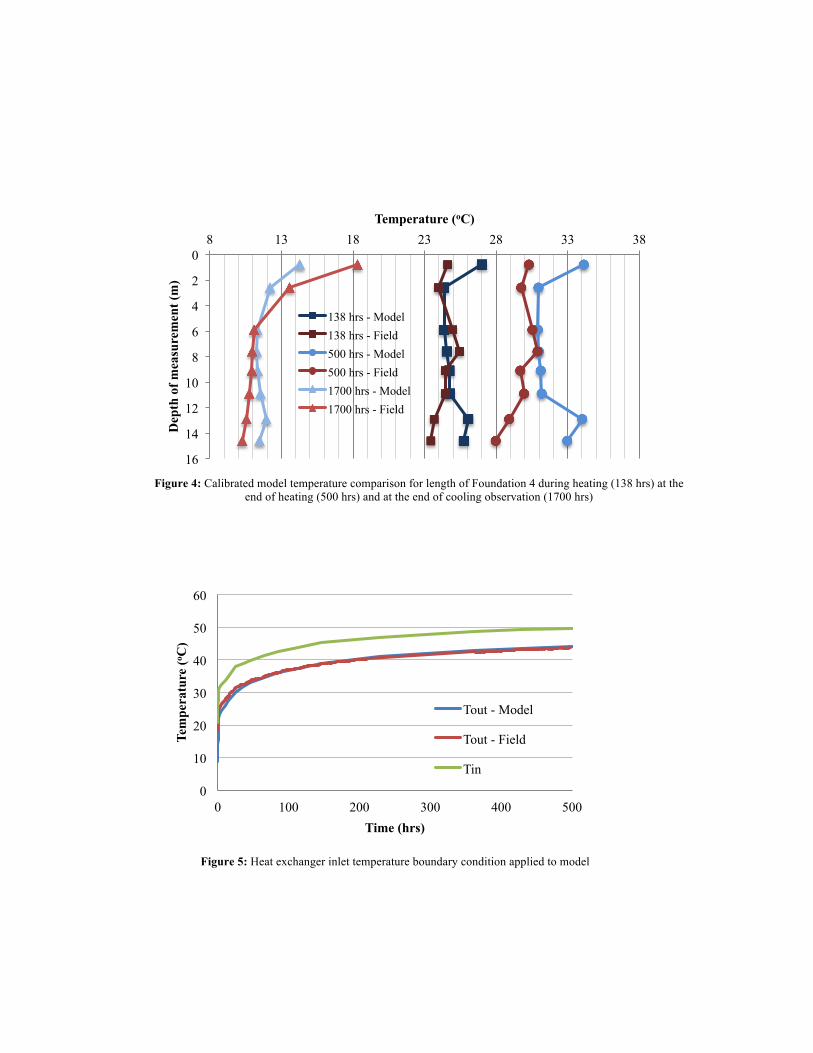
Figure 5: Heat exchanger inlet temperature boundary condition applied to model

0

10

20

30

40

50

60

0 100 200 300 400 500

Tem

pera

ture

(o C)

Time (hrs)

Tout - Model

Tout - Field

Tin

Figure 4: Calibrated model temperature comparison for length of Foundation 4 during heating (138 hrs) at the

end of heating (500 hrs) and at the end of cooling observation (1700 hrs)

0

2

4

6

8

10

12

14

16

8 13 18 23 28 33 38

Dep

th o

f mea

sure

men

t (m

)

Temperature (oC)

138 hrs - Model 138 hrs - Field 500 hrs - Model 500 hrs - Field 1700 hrs - Model 1700 hrs - Field

a)

b)

Figure 6: Snapshot of COMSOL simulation at time=500 hrs a) cross sectional view of energy pile and W-shape heat exchanger b) isometric view of entire model

Table 1: Calibrated material properties used for COMSOL model

Property

Material

Thermal Conductivity, k (W/mK)

Heat Capacity , Cp (J/kg K)

Total density, ρ (kg/m3) Porosity

Sandy Fill 1.1 860 1875 0.43 Dense Sand 0.65 935 1957 0.43 Sandstone 2.0 900 2200 0.15 Dense Sandstone 0.7 1000 2300 0.15 Concrete 1.4 840 2400 - Water 0.58 3267 1008 - Air 0.023 1 1.2 - HDPE 0.48 - - -