A Method For Accounting For Pile Setup and Relaxation in Pile Design and Quality Assurance

Purdue UniversityPurdue e-PubsJoint Transportation Research Program

Technical Report SeriesCivil Engineering

8-2009

A Method For Accounting For Pile Setup andRelaxation in Pile Design and Quality AssurancePrasenjit BasuPurdue University

Rodrigo SalgadoPurdue University

Monica PrezziPurdue University

Tanusree ChakrabortyPurdue University

This document has been made available through Purdue e-Pubs, a service of the Purdue University Libraries. Please contact [email protected] foradditional information.

Recommended CitationBasu, P., R. Salgado, M. Prezzi, and T. Chakraborty. A Method For Accounting For Pile Setup andRelaxation in Pile Design and Quality Assurance. Publication FHWA/IN/JTRP-2009/24. JointTransportation Research Program, Indiana Department of Transportation and Purdue University,West Lafayette, Indiana, 2009. doi: 10.5703/1288284314282

http://docs.lib.purdue.edu

http://docs.lib.purdue.edu/jtrp



http://docs.lib.purdue.edu/civl

JOINT TRANSPORTATION RESEARCH PROGRAM

FHWA/IN/JTRP-2009/24

Final Report

A METHOD FOR ACCOUNTING FOR PILE

SET UP AND RELAXATION IN PILE DESIGN

AND QUALITY ASSURANCE

Prasenjit Basu

Rodrigo Salgado

Monica Prezzi Tanusree

Chakraborty

August 2009

INDOT Research Project Implementation Plan

Date: August 18, 2009

Research Project Number: SPR-2930 Project Title: A Method for Accounting for Pile Setup and Relaxation in Pile Design and Quality Assurance

Principal Investigator (PI): Prof. Rodrigo Salgado Project Administrator (PA): ________________ Note: If more than one implement or recommended, please fill in the information on each implementor's implementation items: Name of Implementor: __ Mir Zaheer/Nayyar Zia _ Items (Research Results) to be implemented: - Validate conclusions of the report concerning setup gains by additional model pile and full-scale pile tests - Investigate the limitations of state-of-practice dynamic testing in estimating or projecting forward short-term setup measurements - Incorporate setup factors into the portion of the geotechnical design manual dealing with the design of piles in clay based on load testing (this can be done immediately, with some caution as confirmation is awaited) - Incorporate the new equations for α into the portion of the geotechnical design manual dealing with the design of piles in clay - Refine the methods proposed in this report for better pile design based on additional analyses and data Help or resources needed for implementation (e.g., help from PI, funding, equipment, etc.): - Additional funding, collaboration from implementers, access to well planned pile load testing data Name of Implementor: ______________________________ Items (Research Results) to be implemented: Help or resources needed for implementation (e.g., help from PI, funding, equipment, etc.): Name of Implementor: _______________________________ Items (Research Results) to be implemented: Help or resources needed for implementation (e.g., help from PI, funding, equipment, etc.): Signatures of SAC members: ___________________________________________________________________________ ___________________________________________________________________________________________________

Please send a copy of this form to the INDOT Research Division and FHWA with the final report.

62-1 8/09 JTRP-2009/24 INDOT Office of Research and Development West Lafayette, IN 47906

INDOT Research

TECHNICAL Summary Technology Transfer and Project Implementation Information

TRB Subject Code:62-1Foundation Soils August 2009

Publication No.: FHWA/IN/JTRP-2009-24, SPR-2930 Final Report

A Method for Accounting for Pile Setup and

Relaxation in Pile Design and Quality Assurance

Introduction

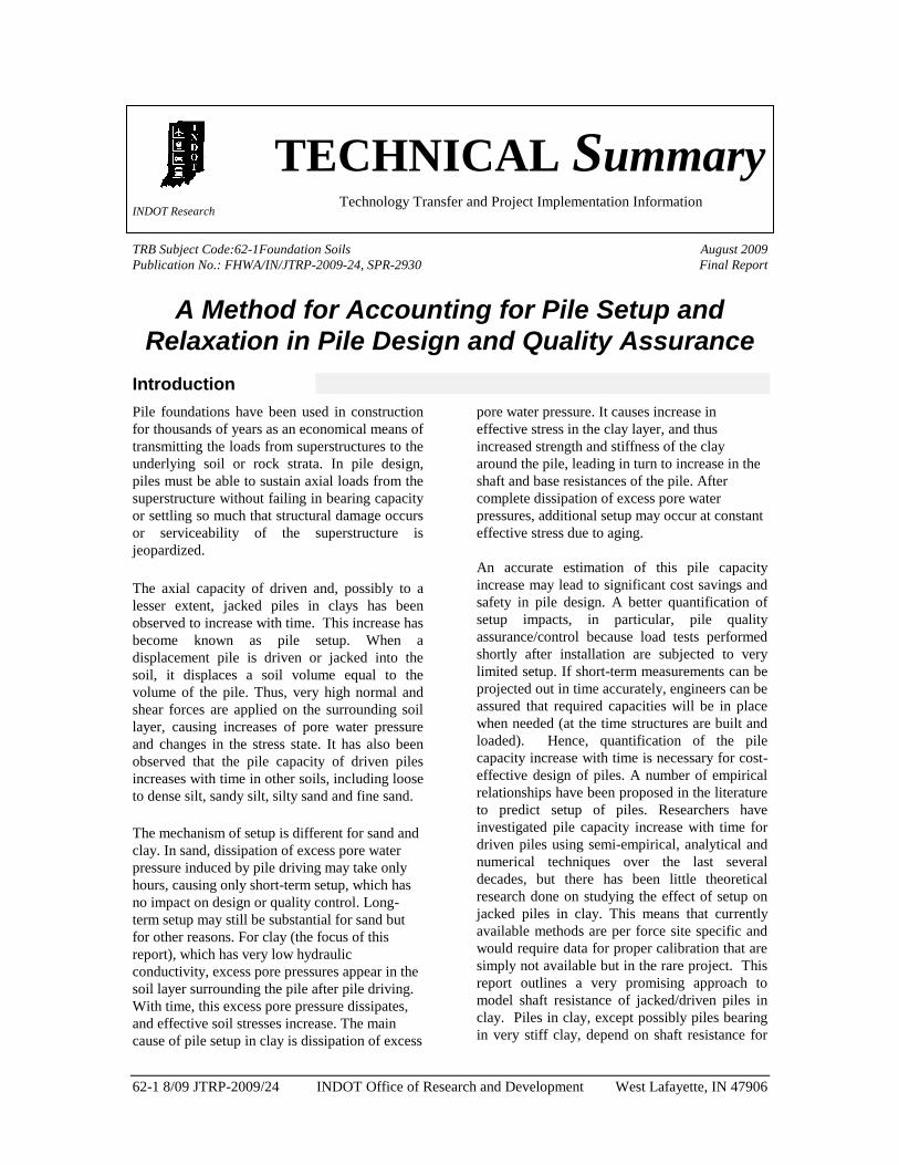
Pile foundations have been used in construction

for thousands of years as an economical means of

transmitting the loads from superstructures to the

underlying soil or rock strata. In pile design,

piles must be able to sustain axial loads from the

superstructure without failing in bearing capacity

or settling so much that structural damage occurs

or serviceability of the superstructure is

jeopardized.

The axial capacity of driven and, possibly to a

lesser extent, jacked piles in clays has been

observed to increase with time. This increase has

become known as pile setup. When a

displacement pile is driven or jacked into the

soil, it displaces a soil volume equal to the

volume of the pile. Thus, very high normal and

shear forces are applied on the surrounding soil

layer, causing increases of pore water pressure

and changes in the stress state. It has also been

observed that the pile capacity of driven piles

increases with time in other soils, including loose

to dense silt, sandy silt, silty sand and fine sand.

The mechanism of setup is different for sand and

clay. In sand, dissipation of excess pore water

pressure induced by pile driving may take only

hours, causing only short-term setup, which has

no impact on design or quality control. Long-

term setup may still be substantial for sand but

for other reasons. For clay (the focus of this

report), which has very low hydraulic

conductivity, excess pore pressures appear in the

soil layer surrounding the pile after pile driving.

With time, this excess pore pressure dissipates,

and effective soil stresses increase. The main

cause of pile setup in clay is dissipation of excess

pore water pressure. It causes increase in

effective stress in the clay layer, and thus

increased strength and stiffness of the clay

around the pile, leading in turn to increase in the

shaft and base resistances of the pile. After

complete dissipation of excess pore water

pressures, additional setup may occur at constant

effective stress due to aging.

An accurate estimation of this pile capacity

increase may lead to significant cost savings and

safety in pile design. A better quantification of

setup impacts, in particular, pile quality

assurance/control because load tests performed

shortly after installation are subjected to very

limited setup. If short-term measurements can be

projected out in time accurately, engineers can be

assured that required capacities will be in place

when needed (at the time structures are built and

loaded). Hence, quantification of the pile

capacity increase with time is necessary for cost-

effective design of piles. A number of empirical

relationships have been proposed in the literature

to predict setup of piles. Researchers have

investigated pile capacity increase with time for

driven piles using semi-empirical, analytical and

numerical techniques over the last several

decades, but there has been little theoretical

research done on studying the effect of setup on

jacked piles in clay. This means that currently

available methods are per force site specific and

would require data for proper calibration that are

simply not available but in the rare project. This

report outlines a very promising approach to

model shaft resistance of jacked/driven piles in

clay. Piles in clay, except possibly piles bearing

in very stiff clay, depend on shaft resistance for


most of their capacity; additionally, setup along

the pile shaft is where most of the setup is

observed; consequently, the report can be used as

basis for estimating pile setup for piles in clay.

The report provides values of the ratio of limit

unit shaft resistance to undrained shear strength

to be used in the short term (for comparison with

measurements taken during load tests) and long-

term (for use in design)

Findings

This research took advantage of advanced

computational techniques and a realistic

constitutive model for clay, developed

specifically in the course of this work, to model

installation of displacement (jacked) piles and

their subsequent loading at various times after

installation. Analysis for piles jacked into the

ground using a large number of strokes suggests

that the analysis asymptotically approaches

installation of driven piles, although dynamic

loading was not done. The predicted values of

limit unit shaft resistance matches closely the

results of experiments available in the literature

as well as the results of the pile load tests used to

develop the API pile design procedure.

Specifically, the present report shows that:

1) The ratio of the limit shaft resistance of

displacement piles a long time after pile

installation (after complete excess pore pressure

dissipation) to that just after pile installation

ranges from roughly 1.2 to roughly 1.4.

2) The changes in the soil caused by pile

installation, a rest period and then loading are

very complex and cannot be modeled with any

reliability in a simplistic way.

3) The pile installation process is not simply a

cavity expansion process, as many have believed.

Shearing has a large impact in that it reduces the

normal stress on the pile shaft from the very large

stresses that would be predicted by cavity

expansion alone. Cycles of shearing along the

pile shaft cause further degradation of the normal

stress on the pile-soil interface and therefore on

the pile shaft resistance; however, the effect is

small, not approaching the large degradation of

shaft resistance observed in piles in sand.

4) With results of analyses such as presented in

this report, it is possible to create effective

design methods and quality assurance programs

that provide a reliable basis to project from the

resistance measured during pile load tests

performed shortly after pile installation to the

values of resistance that are of interest in design

later. We have proposed values for what we

called a setup factor to do exactly that.

Implementation

Engineers can incorporate the results of this

research in their work in three separate ways:

(1) Quality assurance: Consider load tests

successful when they produce values of shaft

resistance consistent with values calculated using

the values of α proposed in this report for loading

applied in the short term (a short time after

installation).

2) Design: Use the values of α proposed in this

report for loading applied in the long term (after

setup has taken place) when calculating limit unit

shaft resistance.

(3) Design: When using load tests before pile

design, project out values measured during load

tests using the ratios of long-term to short-term

capacities proposed in the report.

Contact

For more information:

Prof. Rodrigo Salgado

Principal Investigator School of Civil

Engineering Purdue University West Lafayette

IN 47907 Phone: (765) 494-5030 E-mail:

[email protected]

Indiana Department of Transportation

Office of Research and Development

1205 Montgomery Street, P.O. Box 2279

West Lafayette, IN 47906

Phone: (765) 463-1521

Fax: (765) 497-1665


Purdue University

Joint Transportation Research Program School of

Civil Engineering West Lafayette, IN 47907

Phone: (765) 494-9310

Fax: (765) 496-7996

E-mail: [email protected]

http://www.purdue.edu/jtrp

Final Report

A METHOD FOR ACCOUNTING FOR PILE SETUP AND RELAXATION IN

PILE DESIGN AND QUALITY ASSURANCE


A METHOD FOR ACCOUNTING FOR PILE SETUP AND RELAXATION IN

PILE DESIGN AND QUALITY ASSURANCE

Prasenjit Basu

Graduate Research Assistant

Rodrigo Salgado

Professor of Civil Engineering

Monica Prezzi

Associate Professor of Civil Engineering

Tanusree Chakraborty

Graduate Research Engineer

Geotechnical Engineering

School of Civil Engineering

Purdue University

Joint Transportation Research Program

Project No. C-36-52U

File No. 6-20-20

SPR-2930

Prepared in Cooperation with the Indiana

Department of Transportation and the U.S.

Department of Transportation Federal

Highway Administration

The contents of this report reflect the views of the authors who are responsible for the

facts and the accuracy of the data presented herein. The contents do not necessarily

reflect the official views or policies of the Federal Highway Administration and the

Indiana Department of Transportation. This report does not constitute a standard,

specification or regulation.

Purdue University West

Lafayette, Indiana

August 2009

TECHNICAL REPORT STANDARD TITLE PAGE 1. Report No.

2. Government Accession No.

3. Recipient's Catalog No.


4. Title and Subtitle

A Method for Accounting for Pile Setup and Relaxation in Pile

Design and Quality Assurance

5. Report Date

August 2009

6. Performing Organization Code

7. Author(s)

Prasenjit Basu, Rodrigo Salgado, Monica Prezzi, and Tanusree

Chakraborty

8. Performing Organization Report No.


9. Performing Organization Name and Address

Joint Transportation Research Program

550 Stadium Mall Drive

Purdue University West Lafayette, IN 47907-2051

10. Work Unit No.

11. Contract or Grant No.

SPR-2930 12. Sponsoring Agency Name and Address

Indiana Department of Transportation

State Office Building

100 North Senate Avenue Indianapolis, IN 46204

13. Type of Report and Period Covered

Final Report

14. Sponsoring Agency Code

15. Supplementary Notes

Prepared in cooperation with the Indiana Department of Transportation and Federal Highway Administration.

16. Abstract

When piles are installed by jacking or driving, they cause substantial changes in the state of soil located near the pile. These changes

result from the complex loading imposed on the soil by expansion of a cylindrical cavity to make room for the pile, by multiple cycles of

shearing in the vertical direction as the pile gradually moves down into the ground, and by the slow drainage associated with clayey soils.

If a pile is load-tested a short time after installation, it will develop an axial resistance that reflects the existence in the soil of the excess

pore pressures caused by the installation process. After the excess pore pressures dissipate, the axial pile resistance will be different from

that measured in the short term. This difference is referred to as pile setup (if the resistance increases) or relaxation (if the resistance

drops). This report focuses on the pile setup observed in clayey soils, in which it can be quite significant.

Pile setup in clays result primarily from shaft resistance gains with time after installation because the base resistance contributes

proportionally much less in soft to medium stiff clays, which are the focus of the research. Accordingly, our focus has been on analyzing

setup in shaft resistance, validating the equations resulting from these analyses and then proposing design and quality assurance

procedures based on the results of the analyses. The analyses were done using the finite element method and an advanced constitutive

model developed specifically for this project. The constitutive model captures all the key features required for these analyses, and the

finite element analyses are 1D analyses of shaft resistance that can handle the large deformations and displacements involved in pile

installation. The results of the analyses compare well with load test data from the literature. Design equations for the unit shaft resistance

are proposed. Equations for unit shaft resistance in the short term (for comparison with load tests) are also proposed.

17. Key Words

Piles; piling; pile resistance; clay; pile setup

18. Distribution Statement

No restrictions. This document is available to the public

through the National Technical Information Service,

Springfield, VA 22161 19. Security Classif. (of this report)

Unclassified

20. Security Classif. (of this page)

Unclassified

21. No. of Pages

106

22. Price

Form DOT F 1700.7 (8-69)

TABLE OF CONTENTS

Page LIST OF TABLES .............................................................................................................. v LIST OF FIGURES ........................................................................................................... vi CHAPTER 1. INTRODUCTION ....................................................................................... 1

1.1. Background ............................................................................................................... 1 1.2. Problem Statement .................................................................................................... 3 1.3. Objectives and Organization .................................................................................... 4

CHAPTER 2. MODEL OF CLAY BEHAVIOR ............................................................... 6 2.1. Introduction .............................................................................................................. 6 2.2. Key Components of the Constitutive Model ............................................................ 8

2.2.1. Stress-Strain Relationship .................................................................................. 9 2.2.2. Yield Surface ...................................................................................................... 9 2.2.3. Bounding and Critical State Surface ................................................................ 11 2.2.4. Dilatancy Surface ............................................................................................. 13 2.2.5. Volumetric Hardening Cap .............................................................................. 14 2.2.6. Residual Behavior of Clay ............................................................................... 15 2.2.7. Strain-Rate-Dependent Behavior of Clay ........................................................ 16

2.3. Determination of Model Parameters....................................................................... 18 2.4. Model Simulations for Rate-Independent Behavior of Clay .................................. 20

2.4.1. Consolidation Behavior .................................................................................... 20 2.4.2. Undrained Shearing .......................................................................................... 21 2.4.3. Undrained Simple Shear .................................................................................. 32 2.4.4. Residual Behavior ............................................................................................ 36

2.5. Model Simulations for Rate-Independent Behavior of Clay .................................. 38 2.5.1. Loading Paths for Undrained Triaxial Compression Test ................................ 38 2.5.2. Loading Paths for Simple Shear Test ............................................................... 42

CHAPTER 3. THE FINITE ELEMENT METHOD APPLIED TO THE SHAFT RESISTANCE PROBLEM .............................................................................................. 45

3.1. Introduction ............................................................................................................ 45 3.2. Mathematical Formulation ..................................................................................... 46

3.2.1. Simulation of Pile Jacking in Clay and Pile Loading ...................................... 46 3.2.2. Mesh and Boundary Conditions ....................................................................... 51

3.3. Solution Algorithms and Applied Displacements .................................................. 55 CHAPTER 4. ANALYSIS RESULTS ............................................................................. 58

4.1. Introduction ............................................................................................................ 58 4.2. Results of the Finite Element Analyses .................................................................. 60

4.2.1. Evolution of Stress during Pile Installation ..................................................... 60 4.2.2. Dissipation of Excess Pore Pressure ................................................................ 68 4.2.3. Undrained Loading of Pile ............................................................................... 72

4.3. Undrained Loading of Pile ...................................... Error! Bookmark not defined. CHAPTER 5. USE OF RESULTS IN DESIGN AND QUALITY ASSURANCE OF PILING ............................................................................................................................. 76

5.1. Introduction ............................................................................................................ 76 5.2. Proposed Equations for α ....................................................................................... 77 5.3. Setup Factors .......................................................................................................... 81 5.4. Validation of the Proposed Equations .................................................................... 85

CHAPTER 6. SUMMARY AND CONCLUSIONS ........................................................ 89 6.1. Summary ................................................................................................................. 89 6.2. Conclusions ............................................................................................................ 90

LIST OF REFERENCES .................................................................................................. 92

v

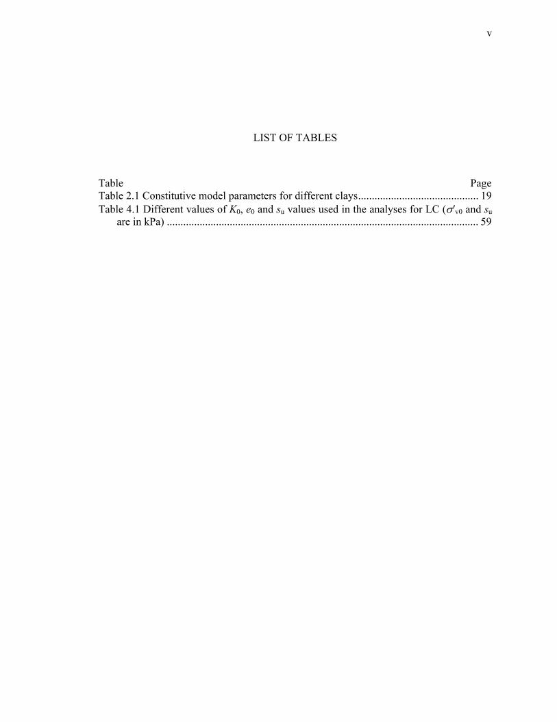
LIST OF TABLES

Table Page Table 2.1 Constitutive model parameters for different clays ............................................ 19 Table 4.1 Different values of K0, e0 and su values used in the analyses for LC (σ′v0 and su

are in kPa) .................................................................................................................. 59

vi

LIST OF FIGURES

Figure Page Figure 1.1 Sources of pile resistances ................................................................................. 1 Figure 1.2 Typical load-settlement response of pile ........................................................... 2 Figure 2.1 Schematic representation of the clay constitutive model: (a) different surfaces

in the principal effective stress space, and (b) cap to the bounding surface ................ 9 Figure 2.2 Volumetric hardening cap in the meridional plane ......................................... 15 Figure 2.3 Evolution of (a) CSL and NCL (b) hardening cap .......................................... 18 Figure 2.4 Consolidation behavior (horizontal axis in kPa) of (a) BBC, (b) LCT (c)

SFBM and (d) LC ...................................................................................................... 21 Figure 2.5 Undrained triaxial compression and extension after isotropic consolidation for

BBC for OCR = 1, 4 and 8 (test data: Pestana et al. 2002): (a) stress-strain response and (b) stress path ....................................................................................................... 23

Figure 2.6 Undrained triaxial compression and extension after isotropic consolidation for LCT for OCR = 1, 2, 4 and 10 (test data: Dafalias et al. 2006): (a) stress-strain response and (b) stress path ........................................................................................ 24

Figure 2.7 Undrained triaxial compression and extension after isotropic consolidation for SFBM for OCR = 1, 1.5 and 3 (test data: Bonaparte 1982): (a) stress-strain response and (b) stress path ....................................................................................................... 26

Figure 2.8 Undrained triaxial compression after isotropic consolidation for LC for OCR = 1, 2, 6 and 20 (test data: Gasparre 2005) (a) stress-strain response and (b) stress path .................................................................................................................................... 27

Figure 2.9 True triaxial compression after isotropic consolidation for SFBM for OCR = 1 (test data: Kirkgard and Lade 1991): (a) stress-strain response and (b) stress path ... 28

Figure 2.10 Undrained triaxial compression and extension after K0 consolidation for BBC for OCR = 1, 2, 4 and 8 (Papadimitriou et al. 2005): (a) stress-strain response and (b) stress path ............................................................................................................. 29

Figure 2.11 Undrained triaxial compression and extension after K0 consolidation for LCT for OCR = 1, 2, 4 and 7 (test data: Dafalias et al. 2006) (a) stress-strain response and (b) stress path ....................................................................................................... 30

Figure 2.12 Undrained triaxial compression after K0 consolidation for SFBM for OCR = 1 (test data: Hunt et al. 2002): (a) stress-strain response and (b) stress path ............. 31

Figure 2.13 Undrained triaxial compression and extension after K0 consolidation for LC for OCR = 1, 1.5, 3 and 7 (test data: Hight et al. 2003): (a) stress-strain response and (b) stress path ............................................................................................................. 32

Figure 2.14 Undrained simple shear after K0 consolidation for BBC for OCR = 1, 2, 4 and 8 (test data: Pestana et al. 2002): (a) stress-strain response and (b) stress path ......... 34

vii

Figure 2.15 Undrained simple shear after K0 consolidation for SFBM for OCR = 1 and 2 (test data: Rau 1999): (a) stress-strain response and (b) stress path .......................... 35

Figure 2.16 Undrained simple shear after K0 consolidation for LC for OCR = 1, 2, 4 and 8 (test data: Hight et al. 2003): (a) stress-strain response and (b) stress path ............ 36

Figure 2.17 Comparison of model simulation and experimental data for SFBM at residual state ............................................................................................................................ 37

Figure 2.18 Comparison of model simulation and experimental data for London Clay at residual state ............................................................................................................... 38

Figure 2.19 Undrained triaxial compression after K0 consolidation for BBC for OCR = 1: (a) stress-strain plot and (b) stress-path ..................................................................... 40

Figure 2.20 Undrained triaxial compression after isotropic consolidation for BBC for OCR = 1: (a) stress-strain plot and (b) stress-path ..................................................... 41

Figure 2.21 Undrained triaxial compression after isotropic consolidation for BBC for OCR = 2: (a) stress-strain plot and (b) stress-path ..................................................... 42

Figure 2.22 Undrained simple shear tests after K0 consolidation for BBC for OCR=1: (a) stress-strain plot and (b) stress-path ..................................................................... 43

Figure 2.23 Undrained simple shear tests after K0 consolidation for BBC at OCR = 4: (a) stress-strain plot and (b) stress-path ..................................................................... 44

Figure 3.1 Stages involved in the jacking (installation) of a pile in clay, dissipation of excess pore pressure, and undrained loading of the pile ............................................ 49

Figure 3.2 One-dimensional domain considered in the analysis: (a) finite element mesh and (b) boundary conditions and applied displacements ........................................... 53

Figure 4.1 Evolution of stresses during undrained cavity expansion (a) total normal (radial) stress, and (b) excess pore pressure ............................................................... 61

Figure 4.2 Stress paths during undrained cavity expansion in (a) q-p′ space and (b) e-p′ space ........................................................................................................................... 62

Figure 4.3 Evolution of total normal (radial) stress σr, excess pore pressure u, and vertical shear stress τz acting on the pile shaft during the “primary shearing” phase and during the removal of the jacking load from the pile head .................................................... 64

Figure 4.4 Stress paths (in the q-p′ space) recorded at a distance 0.166 m (≈ 0.5B) from the pile axis during the installation of a monotonically jacked pile: (a) OCR = 1 and (b) OCR = 4 ................................................................................................................ 65

Figure 4.5 Stress paths (in the q-p′ space) recorded during the installation of a monotonically jacked pile at distances approximately equal to 5B and 10B from the pile axis ...................................................................................................................... 66

Figure 4.6 Stress path (recorded at a distance 0.166 m from the pile axis) during the installation of a pile [σ'v0 = 100 kPa, (φc- φr,min) = 12°] using 30 jacking strokes: (a) OCR = 2, (b) OCR = 4 ............................................................................................... 68

Figure 4.7 Dissipation of excess pore pressure u with time ............................................. 69 Figure 4.8 Evolution of stresses with time (during the dissipation of excess pore pressure)

at different distances from the pile shaft: (a) total normal (radial) stress σr, and (b) effective normal (radial) stress σ′r .............................................................................. 70

Figure 4.9 Radial distribution of (a) normal (radial) effective stress σ′r and (b) excess pore pressure u at the end of installation and at different stages of pore pressure dissipation .................................................................................................................. 72

viii

Figure 4.10 Evolution of stresses on the pile shaft during undrained loading of the pile 73 Figure 4.11 Evolution of void ratio e and mean effective stress p′ (for the leftmost

quadrature point of the first element adjacent to the pile shaft) during installation, dissipation of excess pore pressure and undrained loading of a monotonically jacked pile .............................................................................................................................. 74

Figure 5.1 Short-term α values obtained from the results of the FE simulations (for jacked piles in LC) and from the proposed equations for: (a) (φc-φr,min) = 5°, and (b) (φc-φr,min) = 12° ........................................................................................................... 79

Figure 5.2 Long-term α values obtained from the results of the FE simulations (for jacked piles in LC) and from the proposed equations for: (a) (φc-φr,min) = 0°, (b) (φc-φr,min) = 5°, and (c) (φc-φr,min) = 12° ........................................................................................ 81

Figure 5.3 Setup factor Fs at different times after the installation of a jacked pile in LC for: (a) σ′v0 =25 kPa, and (b) σ′v0 =250 kPa ............................................................... 83

Figure 5.4 Variation of setup factor Fs with normalized time T after the installation of a jacked pile in LC for: (a) σ′v0 =25 kPa and (b) σ′v0 =250 kPa ................................... 84

Figure 5.5 Setup factor Fs at different stages of consolidation (just adjacent to the pile shaft) after the installation of a jacked pile in LC ...................................................... 85

Figure 5.6 Comparison of α values obtained from the results of the FEA for SFBM with those calculated using the proposed equations [with (φc-φr,min) = 13°] ...................... 86

Figure 5.7 Comparison of α values predicted by the proposed equations with those calculated following the API RP-2A criterion and obtained from the field data reported by Sempel and Rigden (1984) ..................................................................... 87

Figure 5.8 Comparison of Fs values deduced from the dynamic pile load test results and those predicted by the present study .......................................................................... 88

1

CHAPTER 1. INTRODUCTION

1.1. Background

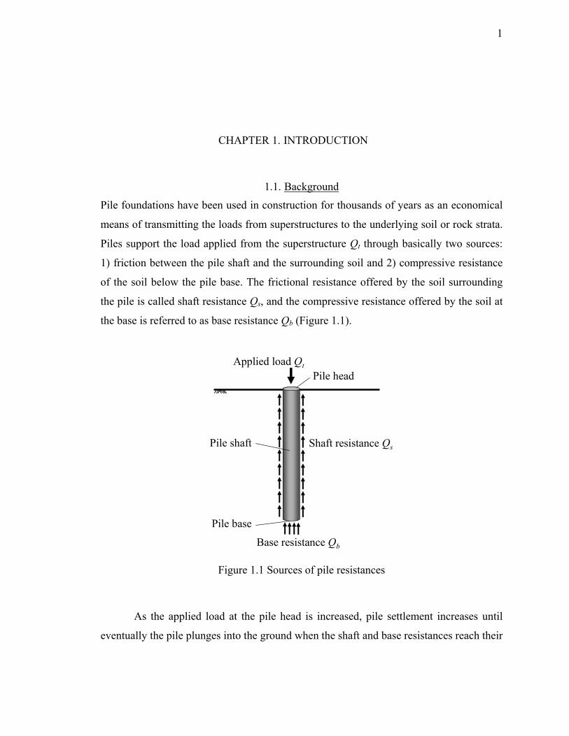
Pile foundations have been used in construction for thousands of years as an economical

means of transmitting the loads from superstructures to the underlying soil or rock strata.

Piles support the load applied from the superstructure Qt through basically two sources:

1) friction between the pile shaft and the surrounding soil and 2) compressive resistance

of the soil below the pile base. The frictional resistance offered by the soil surrounding

the pile is called shaft resistance Qs, and the compressive resistance offered by the soil at

the base is referred to as base resistance Qb (Figure 1.1).

Applied load Qt

Shaft resistance Qs

Base resistance Qb

Pile shaft

Pile head

Pile base

Figure 1.1 Sources of pile resistances

As the applied load at the pile head is increased, pile settlement increases until

eventually the pile plunges into the ground when the shaft and base resistances reach their

2

limit values. During this loading process, there is high localization of shearing within a

thin layer of soil around the pile shaft. As the thickness of this layer (shear zone) is very

small, only a small amount of axial displacement of the pile is sufficient for full

mobilization of the limit shaft capacity (QsL). In contrast to the shaft resistance

mobilization mechanism, mobilization of the base resistance involves substantial amount

of soil compression and requires large pile settlements. In fact, it is almost impossible for

the plunging load or limit load QL of piles routinely used in practice to be reached with

conventional equipment unless the soil profile is very weak. Therefore, ultimate load

(Qult) criteria have been traditionally used to define the capacity of a pile. In the case of

the 10%-relative-settlement criterion, Qult corresponds to the load for which the pile head

displacement is 10% of the pile diameter; this is an example of an ultimate load criterion

that is widely used in practice. Figure 1.2 illustrates these concepts.

QsL Qult

wt = 0.1B

Load

Settlement

Qt - wt

Qb - wtQs - wt

w = (0.01~0.02)B

Figure 1.2 Typical load-settlement response of pile

3

1.2. Problem Statement

The axial capacity of driven and, possibly to a lesser extent, jacked piles in clays has been

observed to increase with time. This increase has become known as pile setup. Effect of

time on the capacity of displacement piles has been studied in the literature, both

experimentally (Karlsrud and Haugen 1985, Axelsson 2000, Komurka et al. 2003, Skov

and Denver 1988, Chow et al. 1998, Cho et al. 2000, Bullock 1999, Long et al. 1999,

Cooke et al. 1979, Coop and Wroth 1989, Augustesen 2006) and theoretically (Randolph

et al. 1979, Whittle and Sutabutr 1999, Titi and Wathugala, 1999). When a displacement

pile is driven or jacked into the soil, it displaces a soil volume equal to the volume of the

pile. Thus, very large normal and shear forces are applied on the surrounding soil layer,

causing increases of pore water pressure and changes in the stress state. It has also been

observed that the pile capacity of driven piles increases with time in other soils, including

loose to dense silt, sandy silt, silty sand and fine sand.

The mechanism of setup is different for sand and clay. In sand, dissipation of

excess pore water pressure induced by pile driving may take only hours, causing only

short-term setup, which has no impact on design or quality control. Long-term setup may

still be substantial for sand but for other reasons. For clay (the focus of this report), which

has very low hydraulic conductivity, excess pore pressures appear in the soil layer

surrounding the pile after pile driving. With time, this excess pore pressure dissipates,

and effective soil stresses increase. The main cause of pile setup in clay is dissipation of

excess pore water pressure. It causes increase in effective stress in the clay layer, and thus

increased strength and stiffness of the clay around the pile, leading in turn to increase in

the shaft and base resistances of the pile. After complete dissipation of excess pore water

pressures, additional setup may occur at constant effective stress due to aging.

A number of empirical relationships have been proposed in the literature to

predict setup of piles. Researchers have investigated pile capacity increase with time for

driven piles using semi-empirical, analytical and numerical techniques over the last

several decades, but there has been little theoretical research done on studying the effect

of setup on jacked piles in clay. This means that currently available methods are per force

4

site specific and would require data for proper calibration that are simply not available

but in the rare project.

This report outlines a very promising approach to model shaft resistance of

jacked/driven piles in clay. Piles in clay, except possibly piles bearing in very stiff clay,

depend on shaft resistance for most of their capacity; additionally, setup along the pile

shaft is where most of the setup is observed; consequently, the report can be used as basis

for effectively estimating pile setup for piles in clay. We perform one-dimensional (1-D)

finite element analysis (FEA) to model the jacking and the subsequent loading of a

cylindrical pile jacked in saturated clay. The FEA involves three distinct stages: (i) pile

installation (jacking), (ii) dissipation of excess pore pressure generated during

installation, and (iii) loading of the pile. These stages were also recognized by several

other researchers in studies related to the shaft capacity of displacement piles in clay

(Steenfelt et al. 1980, Bond and Jardine 1991, Azzouz et al. 1990, Lehane 1992, Lehane

et al. 1994, Lee et al. 2004). However, no theoretical study has convincingly solved the

problem in a single analysis comprising of installation, setup and loading; additionally,

the constitutive model, used in these analyses were either too simple to capture different

aspects of soil behavior (e.g., the strain-rate-dependent behavior of clay and the residual

strength clay behavior) or it did not have all the features necessary to capture the setup

process.

In this study we quantify pile setup through an integrated analysis framework that

uses a suitable soil constitutive model and captures all features of pile installation, setup

and loading. The report provides values of the ratio of limit unit shaft resistance to

undrained shear strength to be used in the short term (for comparison with measurements

taken during load tests) and long-term (for use in design).

1.3. Objectives and Organization

In Chapter 2, we describe the rate-dependent constitutive model that is used in the

axisymmetric FEA to represent the constitutive behavior of clays (Chakraborty 2009).

This constitutive model is based on two-surface plasticity theory and closely follows the

formulations originally proposed by Manzari and Dafalias (1997) for triaxial loading

5

conditions and subsequently modified by several researchers (Li and Dafalias 2000,

Papadimitriou and Bouckavalas 2002, Loukidis 2006, Loukidis and Salgado 2008a). The

model has the capabilities of predicting the critical and residual states, predicting correct

stiffness at small and large strains, capturing the effect of strain-rate on the shear strength

of clay, and predicting clay behavior under varying loading conditions (capturing stress-

induced anisotropy). The constitutive model parameters were obtained by fitting the

results from simulations of different element tests (e.g., triaxial compression and

extension, simple shear, isotropic and 1-D consolidation tests) using MATHCAD through

real laboratory test data obtained from the literature.

In Chapter 3, we describe different aspects of the one-dimensional FE model that

we use to model installation, setup and loading of a pile jacked in saturated clay. We

consider pile jacking in clay to be a fully undrained process. At the end of installation and

before simulation of pile loading (either from a static pile load test or from the

superstructure), we allow the corresponding rest period, during which excess pore

pressures will partially dissipate.

In Chapter 4, we present and discuss the FEA results obtained at different stages

of installation, setup and loading of the pile. We also discuss the changes in the stress

state of the soil during and after the installation of a displacement pile.

In Chapter 5, based on the FE simulation results, we propose a set of equations for

the estimation of unit limit shaft resistance of a pile jacked in clay as function of the

initial soil state and the intrinsic shear strength parameters. The proposed equations can

be used for short- and long-term capacity calculations of displacement piles in clays. In

this chapter we also propose setup factors, to be used in conjunction with the proposed

equations, to calculate the shaft resistance of displacement piles in clays at different times

after the installation. We summarize the key findings of this research and present the

conclusions drawn from this study in Chapter 6.

6

CHAPTER 2. MODEL OF CLAY BEHAVIOR

2.1. Introduction

The constitutive model required for the present analyses should have certain capabilities

in order for it to successfully simulate the clay behavior during the installation and

subsequent loading of a jacked pile. The two-surface plasticity-based constitutive model

described in detail in Chakraborty (2009) that we use in the present study has the

capabilities of predicting the critical and residual states, capturing the effect of strain-rate

on the shear strength of clay, and predicting clay behavior under varying loading

conditions (capturing stress-induced anisotropy). The formulation of this constitutive

model closely follows that of the other similar plasticity-based soil models proposed by

several researchers (Manzari and Dafalias 1997, Li and Dafalias 2000, Papadimitriou et

al. 2001, Papadimitriou and Bouckovalas 2002, Dafalias and Manzari 2004, Dafalias et

al. 2006, Loukidis 2006, and Loukidis and Salgado 2008a).

During sustained shearing, platy clay particles tend to align along the direction of

shearing. This tendency of clay particles to align along a shear plane facilitates shearing

in that particular direction and results in further decrease in shear strength. At large shear

strains, most natural clays have residual strength lower than that at critical state.

Capturing the residual shear strength behavior of clays is particularly important when

modeling the installation of jacked piles. During pile jacking in clay, large vertical shear

strains are localized near the pile shaft and, under this high level of vertical shear strain,

soil adjacent to the pile shaft is expected to reach residual shear strength (Salgado 2008).

At high strain rates, as those imposed in the case of pile jacking/driving in clay,

both the clay undrained shear strength and stiffness increase. Strain-rate-dependent

behavior of clay also plays an important role when a pile is loaded under undrained

conditions (e.g., pile load tests). Therefore, analysis of installation and loading of jacked

7

piles in clay requires the constitutive model to simulate the strain rate-dependent

evolution of shear strength and stiffness.

In both normally consolidated (NC) and overconsolidated (OC) natural clay

deposits there usually is a K0 (stress-induced) anisotropy, so that the ratio K0 (= σ′h0/σ′v0)

of horizontal to vertical effective stresses differs from unity. Stress-induced anisotropy

can also be introduced during shearing starting from an initial isotropic (K0 = 1.0)

condition. According to Ladd and Varallyay (1965), the pore water pressure and the

stress-strain responses of anisotropically consolidated clay under undrained shearing are

significantly affected by the initial stress ratio. Therefore, a constitutive model should

successfully capture the anisotropic behavior of clay during shearing.

To evaluate the shaft resistance of displacement piles in clay at some time after

the installation, it is also important to know the exact stress state at the end of the

consolidation phase (i.e., the phase during which the excess pore pressure generated

during undrained pile installation dissipates) following pile installation. This requires the

constitutive model to properly simulate the evolution of stresses during the primary

consolidation process. The evolution of stresses during consolidation dictates the soil

state (either NC or OC) at the end of consolidation. The deviatoric stress-strain response

of clay becomes different (both under drained and undrained shearing) depending on the

soil state (either NC or OC) at the end of consolidation. Clay may as well yield under

loading along the hydrostatic axis (under zero deviatoric stress). Therefore, the

constitutive model should capture both deviatoric and volumetric (hydrostatic) stress-

strain response of clay with reasonable accuracy.

The constitutive model that we use in this study is based on the critical-state soil-

mechanics (CSSM) framework. In this chapter, we briefly describe different components

of the model, present the model parameters which were obtained by fitting the results

from simulations of different element tests (e.g., triaxial compression and extension,

simple shear, isotropic and 1-D consolidation tests) using MATHCAD through real

laboratory test data obtained from the literature, and show some simulations of different

element tests (Chakraborty 2009).

8

2.2. Key Components of the Constitutive Model

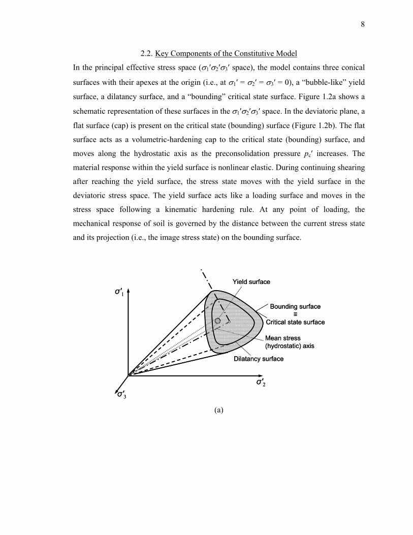
In the principal effective stress space (σ1′σ2′σ3′ space), the model contains three conical

surfaces with their apexes at the origin (i.e., at σ1′ = σ2′ = σ3′ = 0), a “bubble-like” yield

surface, a dilatancy surface, and a “bounding” critical state surface. Figure 1.2a shows a

schematic representation of these surfaces in the σ1′σ2′σ3′ space. In the deviatoric plane, a

flat surface (cap) is present on the critical state (bounding) surface (Figure 1.2b). The flat

surface acts as a volumetric-hardening cap to the critical state (bounding) surface, and

moves along the hydrostatic axis as the preconsolidation pressure pc′ increases. The

material response within the yield surface is nonlinear elastic. During continuing shearing

after reaching the yield surface, the stress state moves with the yield surface in the

deviatoric stress space. The yield surface acts like a loading surface and moves in the

stress space following a kinematic hardening rule. At any point of loading, the

mechanical response of soil is governed by the distance between the current stress state

and its projection (i.e., the image stress state) on the bounding surface.

Yield surface

σ′3

Dilatancy surface

Bounding surface≡

Critical state surface

Mean stress (hydrostatic) axis

σ′1

σ′2

Yield surface

σ′3

Dilatancy surface

Bounding surface≡

Critical state surface

Mean stress (hydrostatic) axis

σ′1

σ′2

(a)

9

Flat cap to the bounding surface

Bounding (critical state) surface

Preconsolidation pressure pc′

σ′1 = σ′2 = σ′3 = 0

Mean stress p’(hydrostatic axis)

Dev

iato

ric s

tress

q




σ′1 = σ′2 = σ′3 = 0


Dev

iato

ric s

tress

q

(b)

Figure 2.1 Schematic representation of the clay constitutive model: (a) different surfaces in the principal effective stress space, and (b) cap to the bounding surface

2.2.1. Stress-Strain Relationship

We first discuss the constitutive model without reference to the effects of loading rate.

Loading rates that are sufficiently low for classical plasticity to be in effect are

considered. The stress-strain equation of the model can be expressed as follows:

( ) ( )p pij ij ij kk kk

223

G K Gσ ε ε ε ε⎛ ⎞′ = − + − −⎜ ⎟⎝ ⎠

& & & && (2.1)

where ijσ ′& is the rate of stress, ijε& is the total deviatoric strain rate and pijε& is the plastic

deviatoric strain rate, and kkε& and pkkε& are total and plastic volumetric strain increments. G

and K are the shear modulus and the bulk modulus, respectively.

2.2.2. Yield Surface

The yield surface in the present model is a circular cone in stress space with its apex at

the origin as shown in Figure 2.1a. The general expression for this yield surface in multi-

axial stress space is

10

ij ij= 2/3 = 0 f m pχ χ ′− (2.2)

and,

ij ij ijs pχ α ′= − (2.3)

where sij = deviatoric stress tensor, αij is a kinematic tensor that represents the center of

the yield surface, and m is the radius of the cone in the deviatoric plane (m is constant,

which means that there is no isotropic hardening or softening of the yield surface).

The evolution of αij during loading represents the kinematic hardening of the

yield surface; αij is also called the deviatoric back stress tensor. The factor √(2/3) is

introduced for convenience of interpretation of the projection on the deviatoric plane

from the multi-axial space. The yield surface can also be written in the form:

ij ij 2 3 0f / mρ ρ= − = (2.4)

where rij = sij/p′ and ρij = (rij-αij). After the differentiation of f and rearrangement, the

loading direction Lij becomes:

( )( )( )

( )( )( )

ijij

ij ij pq pq pqij

kl kl kl kl kl kl kl kl

1 2 33

fL

s p s p/ m

s p' s p' s p s p

σ

α α αδ

α α α α

∂=

′∂

⎡ ⎤′ ′− −⎢ ⎥= − +

′ ′⎢ ⎥− − − −⎣ ⎦

(2.5)

The loading direction Lij normal to the yield surface is given as:

ij ij pq ijij

fL L L δσ

∂ ′ ′′= = +′∂

(2.6)

where

11

( )( )( )

ij ijij

kl kl kl kl

s pL

s p s p

α

α α

′−′ =

′ ′− − (2.7)

is the loading tensor, and

( )( )( )

pq pq pqpq

kl kl kl kl

1 2 33

s pL / m

s p s p

α α

α α

⎡ ⎤′−′′ ⎢ ⎥= − +

′ ′⎢ ⎥− −⎣ ⎦ (2.8)

Lij defines the direction of loading and L′pq represents the direction of loading within the

deviatoric plane. The tensor δij is the Kronecker’s Delta. Equation (2.6) can also be

expressed as:

ij ij pq pq ij1 2 = 3 3

L n n mα δ⎛ ⎞

− +⎜ ⎟⎜ ⎟⎝ ⎠

(2.9)

where

( )( )( )

ij ijij

kl kl kl kl

s pn

s p s p

α

α α

′−=

′ ′− − (2.10)

Once the stress state reaches the yield surface, it remains on the yield surface and

starts moving with the yield surface. The mechanical behavior of soil is controlled by the

distance of this current stress state from its projections on the bounding and dilatancy

surfaces.

2.2.3. Bounding and Critical State Surface

In this model, the bounding surface is the critical state surface. The stress state may go

outside the bounding surface slightly during a load increment, but it returns to the

bounding surface upon convergence. We capture the peak shear strength during drained

shearing of OC clay and undrained shearing of NC clay through the hardening parameter

and the isotropic hardening of the dilatancy surface. Considering the critical state surface

12

to be the same as the bounding surface also helps us avoid the post-peak numerical

oscillations caused by softening of the clay from the bounding surface to the critical state

surface. In the proposed model, the bounding surface (which is also the critical state

surface) is a cone, centered on the mean stress axis with apex at the origin. The locus of

the bounding surface (or critical state surface) can be given as follows:

( ) ( )b c ccM M g Mθ≡ = (2.11)

where Mcc is the critical stress ratio in triaxial compression; and g(θ) is a function of

Lode’s angle θ that determines the shape of the critical state surface, bounding surface

and dilatancy surface on the deviatoric plane. We can express g(θ) as follows (Loukidis

and Salgado 2008a):

( )( )

ss

s

ss

s

1111

1111

111

11 cos 31

n/ n

/ n

n/ n

/ n

cc

gcc

θ

θ

⎛ ⎞−−⎜ ⎟+⎝ ⎠=

⎡ ⎤⎛ ⎞−−⎢ ⎥⎜ ⎟+⎝ ⎠⎣ ⎦

(2.12)

where

1cc

33

cM

=+

(2.13)

The parameter ns in equation (2.12) was introduced by Loukidis and Salgado (2008a). If

ns is set equal to 1, then the function g(θ) becomes the same as that proposed by Manzari

and Dafalias (1997) and Dafalias et al. (2004). If ns is set equal to 0.25, then g(θ)

becomes the same as that proposed by Sheng et al. (2000). The exponent ns was

introduced to improve predictions of friction angle at conditions other than triaxial

compression or extension for all sets of possible Mcc values and for different types of

clays. It also ensures convexity of the surfaces in the deviatoric plane.

Lode’s angle θ can be expressed in terms of the principal components n1, n2 and

n3 of the loading tensor nij using the following equation:

13

1 2 3

1 3

1tan 2 163

n nn n

πθ −⎡ ⎤⎧ ⎫⎛ ⎞−⎪ ⎪= − +⎢ ⎥⎨ ⎬⎜ ⎟−⎪ ⎪⎢ ⎥⎝ ⎠⎩ ⎭⎣ ⎦

(2.14)

According to Manzari and Dafalias (1997), θ can also be expressed in terms of effective

stress as:

33 3cos3

2SJ

θ⎛ ⎞

= ⎜ ⎟⎝ ⎠

(2.15)

where 131

3S :⎡ ⎤= ⋅⎢ ⎥⎣ ⎦

s s s , 121

2J :⎡ ⎤= ⎢ ⎥⎣ ⎦

s s and p= −s Iσ (bold face letters are used to

represent tensor quantities; the symbol “.” represents the tensor product and the symbol

“:” represents the scalar product of two tensors). Lode’s angle θ = 0o simulates the

triaxial compression condition and θ = 60o corresponds to triaxial extension. Thus, the

value of g(θ) becomes equal to 1 for triaxial compression and to c1 for triaxial extension

(see equation 2.12). Therefore, the slopes of the critical state line at triaxial compression

(Mcc) and triaxial extension (Me) are directly correlated:

e 1 ccM c M= (2.16)

This equation gives the flexibility to consider different friction angles for triaxial

compression and extension.

2.2.4. Dilatancy Surface

The dilatancy surface is defined as:

( ) ( )cc d

d ccd

OCR21 exp OCR

M kM g Mkψθ

ψ⎛ ⎞

= +⎜ ⎟⎜ ⎟−⎝ ⎠ (2.17)

In equation (2.17), kd is a model parameter defined as:

14

ccd

MkN Γ

=−

(2.18)

The model always uses the current Overconsolidation Ratio (OCR) values in all the

simulations. In this report, OCR is defined in terms of mean stress:

cOCR pp′

=′

(2.19)

where p′c represents the preconsolidation pressure, and p′ is the current mean stress. The

dilatancy surface hardens isotropically through the dependence of the stress ratio Md on

the state parameter ψ (which is the difference between the current void ratio e and the

critical state void ratio ecr at the same mean effective stress and thus determines whether

the clay is dilative or contractive); Md also depends on the OCR of the clay, as the

dilatancy properties vary with the OCR. In the current formulation, Md increases with

increasing ψ and reaches an asymptote, though the rate of increase of Md with ψ is much

less as compared to the purely exponential formulation. This helps us to capture clay

behavior reasonably well. As long as the stress state is inside the dilatancy surface, the

response of the soil is contractive. The opposite is true if the stress state moves outside

the dilatancy surface. At the phase transformation state (the state during shear loading

when the plastic volumetric response during shearing changes from contractive to

dilative) and at the critical state, the dilatancy is zero.

2.2.5. Volumetric Hardening Cap

Clay also hardens under the application of mean stress. The volumetric hardening cap

controls the mean stress dependent hardening of clay. Following Li (2002), the flat cap to

the bounding surface is expressed as:

c c 0F p p′ ′= − = (2.20)

For NC clay, p′ = p′c, i.e., the stress state is on the cap. The value of p'c defines the

position of the cap on the hydrostatic axis. In the present model, the cap remains fixed on

15

the hydrostatic axis unless the mean stress state is on the cap. If the mean stress increases

by dp′c along the normal consolidation line, the volumetric hardening cap moves from p′c

to p′c+dp′c on the hydrostatic axis (in the meridional plane) [Figure 2.2]. When dp′ <0.

the cap remains fixed on the hydrostatic axis.


σ′1 = σ′2 = σ′3 = 0



Preconsolidation pressure p’c+dp’c

p’c

Dev

iato

ric s

tress

q


σ′1 = σ′2 = σ′3 = 0



Preconsolidation pressure p’c+dp’c

p’c

Dev

iato

ric s

tress

q

Figure 2.2 Volumetric hardening cap in the meridional plane

2.2.6. Residual Behavior of Clay

At critical state, the clay particles are in equilibrium under the applied confining stress,

shear stress and void ratio. At this stage, clay particles roll over each other. Under

prolonged shearing after critical state (at very large shear strains of 20% and even larger),

clay particles get aligned with the direction of shearing so long as there is a sufficiently

large normal stress σ′ on the plane of shearing. The platy nature of the clay particles

helps in this alignment. The friction angle reduces from its value at critical state φc to a

reduced residual friction angle φr. The strength of the soil in the residual state is called the

residual shear strength. The residual shear strength of clay is the product of the normal

effective stress on the shearing plane by the tangent of the residual friction angle φr. It is

important to note that φr decreases with increasing effective normal stress σ′ on the plane

of shearing, as larger normal stresses force greater particle alignment in the shearing

direction.

16

In our constitutive model, the residual state is fully defined by the following

equation:

( ) rcc c0

c0

exp 3 1 ln MM MM

β⎧ ⎫⎛ ⎞⎪ ⎪= −⎨ ⎬⎜ ⎟⎪ ⎪⎝ ⎠⎩ ⎭

(2.21)

where Mcc is the current slope of the critical state line in effective mean stress p′ vs

deviatoric stress q space, Mc0 is the initial slope of the critical state line, Mr is the slope of

the residual state line when the residual angle reaches its minimum at a given normal

stress. The parameter β controls the degree of particle alignment: β = 0 means that clay

particles are fully aligned along the direction of shearing, and β = 1/3 means that there is

no alignment. The rate equation of β controls the evolution of β from 0 to 1/3 in terms of

the deviatoric strain qε& .

( )r r cc qb M Mβ ε= −& & (2.22)

In equation 2.21, Mr depends on the normal stress σ′ acting perpendicularly to the plane

of shearing. To capture this, we correlate Mr with the mean stress p′ through the

following equation:

[ ] [ ]( )r c0 r,minexp 1 expM M Yp M Yp′ ′= − + − − (2.23)

where Y is a model parameter defining the dependence of Mr on p′ and Mr,min is the slope

of the residual state line in p′ versus q space, corresponding to the absolute minimum

residual friction angle φr,min. When Y = 0, then Mr does not depend on p′ and we obtain Mr

= Mc0. With increasing Y, Mr decreases towards the absolute minimum residual stress

ratio Mr,min.

2.2.7. Strain-Rate-Dependent Behavior of Clay

The constitutive model captures the strain-rate-dependent behavior of clay through the

evolution of the critical state line (CSL) and normal consolidation line (NCL). Figure

17

2.3(a) shows the evolution of the CSL and NCL in the e-ln p′ space. The movement of

both the CSL and NCL is governed by the present stress state and the applied strain rate

increment at any particular stage of loading. During strain hardening, the void ratio

intercept Γ0 (corresponding to the reference mean effective stress) of the CSL increases

from its initial value to a maximum value Γmax; during strain-softening Γmax decreases

continuously to return to its initial value Γ0 when the soil reaches the critical state. At any

stage of this evolution, the value of Γ (which also decides the location of the CSL in the

e-ln p′ space) is governed by the applied strain-rate increment. As the CSL moves in the

e-ln p′ space, the NCL also moves, maintaining a constant distance from the CSL. During

the movement of the CSL and NCL in the e-ln p′ space, image preconsolidation pressures

(e.g., p′c2, p′c3 in Figure 2.3a) are calculated along a projection of the overconsolidation

line in the e-ln p′ space. The hardening cap on the bounding (critical state) surface also

moves during the evolution of the CSL and NCL in the e-ln p′ space (see Figure 2.3b).

ln p′

eNormal consolidation line NCL

Overconsolidation line

Critical state line CSL

Γ0

Reference mean effective stress


p′c2

λκ

p′c3 ln p′

eNormal consolidation line NCL

Overconsolidation line

Critical state line CSL

Γ0

Reference mean effective stress


p′c2

λκ

p′c3

(a)

18

Moving cap



p′c2

p′c1

σ′1 = σ′2 = σ′3 = 0


Dev

iato

ric s

tress

q

Moving cap



p′c2

p′c1

σ′1 = σ′2 = σ′3 = 0


Dev

iato

ric s

tress

q

(b)

Figure 2.3 Evolution of (a) CSL and NCL (b) hardening cap

2.3. Determination of Model Parameters

We determine model parameters from data for tests on Boston Blue Clay (BBC), San

Francisco Bay Mud (SFBM) and London Clay (LC). BBC is a low-plasticity marine clay,

composed of illite and quartz (Terzaghi et al. 1996). SFBM is a highly-plastic silt

containing a large amount of clay-sized particles (montmorillonite and illite), organic

substances, shell fragments, and traces of sand (Bonaparte 1982). LC contains illite,

kaolinite, smectite and quartz (Al-Tabbaa and Stegemann 2005, Gasparre et al. 2007a,

Gasparre et al. 2007b). In order to show the applicability of the constitutive model to

materials that are not strictly clays, we also determine the model parameters for Lower

Cromer Till (LCT), which is a glacial till composed of sand (more than 50%), calcite and

illite (clay content almost 17%) and almost no silt (Gens 1982) and has been treated in

the literature as a clay.

We determine all model parameters based on experimental data found in the

literature for one-dimensional and isotropic consolidation, resonant column test, triaxial

compression and extension, simple shear and ring shear tests. Experimental data for BBC

are taken from Papadimitriou et al. (2005), Pestana et al. (2002), Ling et al. (2002)

[reproduced from Ladd and Varallyay (1965), Ladd and Edgers (1972), and Sheahan

(1991)] and Santagata et al. (2007). SFBM data are obtained from Bonaparte (1982), Jain

19

(1985), Rau (1999), Jain and Nanda (2008) and Meehan (2006) for soil sample from

Hamilton Airforce Base; Kirkgard and Lade (1991) and Stewart and Hussein (1993) for

soil sample from Marina district; Hunt et al. (2002) for soil sample from Islais creek; and

Henke and Henke (2003) for soil sample from Treasure Island site. All these tests were

conducted on Young Bay Mud of Holocene age. Data for LC are collected from Gasparre

(2005), Gasparre et al. (2007a), Gasparre et al. (2007b), Hight et al. (2003) for soil

samples were collected from Heathrow Terminal 5 site; Bishop et al. (1971) for LC from

Wraysbury and Walthamstow site. Data for LCT are obtained from Dafalias et al. (2006)

based on the work done by Gens (1982). Model parameters are determined in a

hierarchical manner and described in detail by Chakraborty (2009). In this report, we

only tabulate the model parameters for BBC, SFBM and LC (Table 2.1).

Table 2.1 Constitutive model parameters for different clays

BBC SFBM LCν 0.25 0.24 0.2 Test using local strain transducer or

isotropic consolidation or 1-D consolidationwith unloading

G0 correlation parameter Cg 250 200 100 Bender element testsElastic moduli with ζ 5 ± 2 5 ± 2 10 ± 5 Isotropic consolidation or 1-D consolidationdegradation (G and K) κ 0.036 0.052 0.064 Isotropic consolidation or 1-D consolidationNormal consolidation line N 1.138 1.9 1.07 Isotropic consolidation or 1-D consolidation

λ 0.187 0.404 0.168 Isotropic consolidation or 1-D consolidationCritical state surface Mc0 1.305 1.157 0.827 Triaxial compression test

ρ 2.7 2.2 2.5 Isotropic consolidation or 1-D consolidationDilatancy surface D0 1± 0.2 0.5± 0.1 1± 0.2 Triaxial compression testFlow rule c2 0.95 0.95 0.95 Simple shear or other plane-strain test

ns 0.2 0.2 0.2 Simple shear or other plane-strain testHardening h0 1.1± 0.2 1.5± 0.3 1.5± 0.3 Triaxial compression testStrain-rate-dependent C0 7 ± 2 0.007 ± 0.001 7 ± 2 Strain-rate-dependent triaxial compression testmodel parameter arate 0.12± 0.01 0.1± 0.01 0.12± 0.01 Strain-rate-dependent triaxial compression test

brate 0.01 0.01 0.01 Strain-rate-dependent simple shear testcrate 0.00001 0.00001 0.00001 Strain-rate-dependent triaxial compression test

or ring shear testResidual state Mr,min - 0.615 0.33 Ring shear test

br - 0.01± 0.001 0.03±0.001 Ring shear testY - 0.02± 0.002 0.015± 0.002 Ring shear test

Parameter Value Test Data Required

Small-strain (elastic) Poisson's Ratio

Model Relationships Parameters

20

2.4. Model Simulations for Rate-Independent Behavior of Clay

2.4.1. Consolidation Behavior

Figure 2.4(a) through (d) shows the e-ln(p′) response of BBC, LCT, SFBM during one-

dimensional consolidation and LC for isotropic consolidation, respectively. Test data for

SFBM and LC are obtained from Jain (1985) and Gasparre (2005), respectively. The

model captures the loading-unloading-reloading loop using the same model parameters

throughout.

10 100 1000

ln (σ'v)

0.78

0.86

0.94

1.02

1.1

e

Oedometer Test (BBC)

Test Data: Papadimitriou et al., 2005

Simulation of Loading-Unloading-Reloading

Norm

al Condolidation Line

Critical State Line

10 100 1000

ln (p')

0.3

0.35

0.4

0.45

0.5

e

Isotropic Consolidation Test (LCT)

Test Data: Dafalias et al., 2006Simulation

Normal Consolidation Line

Critical State Line

(a) (b)

21

10 100 1000

ln (p')

1

1.2

1.4

1.6

1.8

e

Oedometer TestSimulation of Loading-Unloading-ReloadingTest Data: Jain, 1985

(SFBM)

Normal C

onsolidation Line

Critical State Line

10 100 1000

ln (p')

1

1.2

1.4

1.6

1.8

e

Oedometer TestSimulation of Loading-Unloading-ReloadingTest Data: Jain, 1985

(SFBM)

Normal C

onsolidation Line

Critical State Line

10 100 1000

ln (p')

0.7

0.8

0.9

1

1.1

e

Isotropic Consolidation Test (LC)

Test Data: Gasparre, 2005Simulation

Normal Consolidation Line

Critical State Line

(c) (d)

Figure 2.4 Consolidation behavior (horizontal axis in kPa) of (a) BBC, (b) LCT (c) SFBM and (d) LC

2.4.2. Undrained Shearing

Figure 2.5 and Figure 2.6 show the model simulation of undrained triaxial compression

and extension after isotropic consolidation for BBC and LCT, respectively. For SFBM

and LC, results of undrained triaxial compression tests after isotropic consolidation are

presented in Figure 2.7 and Figure 2.8. Test data have been taken from Pestana et al.

(2002) for BBC and Dafalias et al. (2006) for LCT. SFBM data is collected from

Bonaparte (1982). Data for LC are taken from Gasparre (2005). The tests stopped at

around 12% axial strain. We performed simulations for OCR values of 1, 4 and 8 for

BBC; 1, 2, 4 and 10 for LCT; 1, 1.5, 2 and 3 for SFBM; and 1, 1.5 and 6 for LC. Figure

2.5(a) - Figure 2.8(a) present normalized deviatoric stress vs axial strain curves for BBC,

LCT, SFBM and LC while Figure 2.5(b) - Figure 2.8(b) shows normalized deviatoric

stress vs. normalized mean stress plot. Normalizations are performed with respect to the

maximum axial stress at the end of consolidation (σ'a,max). The model simulations are in

good agreement with the data for BBC and LC. For LCT, it slightly overpredicts the

stresses at higher OCR values. At OCR = 1, we capture the undrained softening behavior

22

accurately. At OCR = 2 for LCT, we observe the phase transformation behavior in model

simulation. Figure 2.9 compares the normalized deviatoric stress vs axial strain response

of isotopic triaxial compression obtained from model simulation with the true triaxial test

results (triaxial compression condition) obtained from Kirkgard and Lade (1991).

0 4 8 12 16εa%

-0.8

-0.4

0.0

0.4

0.8

1.2

qσ a

max

Model SimulationTest Data

OCR=1

OCR=1

OCR=8

OCR=4

0 4 8 12 16εa%

-0.8

-0.4

0.0

0.4

0.8

1.2

qσ a

max


OCR=1

OCR=1

OCR=8

OCR=4

Test Data

0 4 8 12 16εa%

-0.8

-0.4

0.0

0.4

0.8

1.2

qσ a

max


OCR=1

OCR=1

OCR=8

OCR=4

0 4 8 12 16εa%

-0.8

-0.4

0.0

0.4

0.8

1.2

qσ a

max


OCR=1

OCR=1

OCR=8

OCR=4

Test Data

‘

0 4 8 12 16εa%

-0.8

-0.4

0.0

0.4

0.8

1.2

qσ a

max


OCR=1

OCR=1

OCR=8

OCR=4

0 4 8 12 16εa%

-0.8

-0.4

0.0

0.4

0.8

1.2

qσ a

max


OCR=1

OCR=1

OCR=8

OCR=4

Test Data

0 4 8 12 16εa%

-0.8

-0.4

0.0

0.4

0.8

1.2

qσ a

max


OCR=1

OCR=1

OCR=8

OCR=4

0 4 8 12 16εa%

-0.8

-0.4

0.0

0.4

0.8

1.2

qσ a

max


OCR=1

OCR=1

OCR=8

OCR=4

Test Data

‘a,max

q

′ σ

0 4 8 12 16εa%

-0.8

-0.4

0.0

0.4

0.8

1.2

qσ a

max


OCR=1

OCR=1

OCR=8

OCR=4

0 4 8 12 16εa%

-0.8

-0.4

0.0

0.4

0.8

1.2

qσ a

max


OCR=1

OCR=1

OCR=8

OCR=4

Test Data

0 4 8 12 16εa%

-0.8

-0.4

0.0

0.4

0.8

1.2

qσ a

max


OCR=1

OCR=1

OCR=8

OCR=4

0 4 8 12 16εa%

-0.8

-0.4

0.0

0.4

0.8

1.2

qσ a

max


OCR=1

OCR=1

OCR=8

OCR=4

Test Data

‘

0 4 8 12 16εa%

-0.8

-0.4

0.0

0.4

0.8

1.2

qσ a

max


OCR=1

OCR=1

OCR=8

OCR=4

0 4 8 12 16εa%

-0.8

-0.4

0.0

0.4

0.8

1.2

qσ a

max


OCR=1

OCR=1

OCR=8

OCR=4

Test Data

0 4 8 12 16εa%

-0.8

-0.4

0.0

0.4

0.8

1.2

qσ a

max


OCR=1

OCR=1

OCR=8

OCR=4

0 4 8 12 16εa%

-0.8

-0.4

0.0

0.4

0.8

1.2

qσ a

max


OCR=1

OCR=1

OCR=8

OCR=4

Test Data

‘a,max

q

′ σa,

max

q

′ σ

(a)

0 0.4 0.8 1.2

p

σmax

-0.8

-0.4

0

0.4

0.8

1.2

qσ m

ax


OCR=1OCR=4

OCR=1

OCR=8

32.4o

0 0.4 0.8 1.2

p

σmax

-0.8

-0.4

0

0.4

0.8

1.2

qσ m

ax


OCR=1OCR=4

OCR=1

OCR=8

32.4o

Test Data

0 0.4 0.8 1.2

p

σmax

-0.8

-0.4

0

0.4

0.8

1.2

qσ m

ax


OCR=1OCR=4

OCR=1

OCR=8

32.4o

0 0.4 0.8 1.2

p

σmax

-0.8

-0.4

0

0.4

0.8

1.2

qσ m

ax


OCR=1OCR=4

OCR=1

OCR=8

32.4o

Test Data

σ’amax

σ’am

ax

0 0.4 0.8 1.2

p

σmax

-0.8

-0.4

0

0.4

0.8

1.2

qσ m

ax


OCR=1OCR=4

OCR=1

OCR=8

32.4o

0 0.4 0.8 1.2

p

σmax

-0.8

-0.4

0

0.4

0.8

1.2

qσ m

ax


OCR=1OCR=4

OCR=1

OCR=8

32.4o

Test Data

0 0.4 0.8 1.2

p

σmax

-0.8

-0.4

0

0.4

0.8

1.2

qσ m

ax


OCR=1OCR=4

OCR=1

OCR=8

32.4o

0 0.4 0.8 1.2

p

σmax

-0.8

-0.4

0

0.4

0.8

1.2

qσ m

ax


OCR=1OCR=4

OCR=1

OCR=8

32.4o

Test Data

σ’amax

σ’am

axa,

max

q

′ σ

a,max

p′′σ

0 0.4 0.8 1.2

p

σmax

-0.8

-0.4

0

0.4

0.8

1.2

qσ m

ax


OCR=1OCR=4

OCR=1

OCR=8

32.4o

0 0.4 0.8 1.2

p

σmax

-0.8

-0.4

0

0.4

0.8

1.2

qσ m

ax


OCR=1OCR=4

OCR=1

OCR=8

32.4o

Test Data

0 0.4 0.8 1.2

p

σmax

-0.8

-0.4

0

0.4

0.8

1.2

qσ m

ax


OCR=1OCR=4

OCR=1

OCR=8

32.4o

0 0.4 0.8 1.2

p

σmax

-0.8

-0.4

0

0.4

0.8

1.2

qσ m

ax


OCR=1OCR=4

OCR=1

OCR=8

32.4o

Test Data

σ’amax

σ’am

ax

0 0.4 0.8 1.2

p

σmax

-0.8

-0.4

0

0.4

0.8

1.2

qσ m

ax


OCR=1OCR=4

OCR=1

OCR=8

32.4o

0 0.4 0.8 1.2

p

σmax

-0.8

-0.4

0

0.4

0.8

1.2

qσ m

ax


OCR=1OCR=4

OCR=1

OCR=8

32.4o

Test Data

0 0.4 0.8 1.2

p

σmax

-0.8

-0.4

0

0.4

0.8

1.2

qσ m

ax


OCR=1OCR=4

OCR=1

OCR=8

32.4o

0 0.4 0.8 1.2

p

σmax

-0.8

-0.4

0

0.4

0.8

1.2

qσ m

ax


OCR=1OCR=4

OCR=1

OCR=8

32.4o

Test Data

σ’amax

σ’am

axa,

max

q

′ σa,

max

q

′ σa,

max

q

′ σ

a,max

p′′σa,max

p′′σ

23

(b)

Figure 2.5 Undrained triaxial compression and extension after isotropic consolidation for BBC for OCR = 1, 4 and 8 (test data: Pestana et al. 2002): (a) stress-strain response and

(b) stress path

0 4 8 12εa%

-0.8

-0.4

0.0

0.4

0.8

1.2

qσ a

max


OCR=1

OCR=1

OCR=10

OCR=10

0 4 8 12εa%

-0.8

-0.4

0.0

0.4

0.8

1.2

qσ a

max


OCR=1

OCR=1

OCR=10

OCR=10

Test Dataa,

max

q

′ σ

0 4 8 12εa%

-0.8

-0.4

0.0

0.4

0.8

1.2

qσ a

max


OCR=1

OCR=1

OCR=10

OCR=10

0 4 8 12εa%

-0.8

-0.4

0.0

0.4

0.8

1.2

qσ a

max


OCR=1

OCR=1

OCR=10

OCR=10

Test Data

0 4 8 12εa%

-0.8

-0.4

0.0

0.4

0.8

1.2

qσ a

max


OCR=1

OCR=1

OCR=10

OCR=10

0 4 8 12εa%

-0.8

-0.4

0.0

0.4

0.8

1.2

qσ a

max


OCR=1

OCR=1

OCR=10

OCR=10

Test Dataa,

max

q

′ σ a,m

ax

q

′ σ

(a)

24

0 0.4 0.8 1.2

p

σmax

-0.8

-0.4

0

0.4

0.8

1.2

qσ m

ax


OCR=1OCR=4

OCR=1OCR=10

30.0o

OCR=2

0 0.4 0.8 1.2

p

σmax

-0.8

-0.4

0

0.4

0.8

1.2

qσ m

ax


OCR=1OCR=4

OCR=1OCR=10

30.0o

OCR=2

OCR=1OCR=4

OCR=1OCR=10

30.0o

OCR=2

Test Data

a,m

ax

q

′σ

a ,max

p′′σ

0 0.4 0.8 1.2

p

σmax

-0.8

-0.4

0

0.4

0.8

1.2

qσ m

ax


OCR=1OCR=4

OCR=1OCR=10

30.0o

OCR=2

0 0.4 0.8 1.2

p

σmax

-0.8

-0.4

0

0.4

0.8

1.2

qσ m

ax


OCR=1OCR=4

OCR=1OCR=10

30.0o

OCR=2

OCR=1OCR=4

OCR=1OCR=10

30.0o

OCR=2

Test Data

a,m

ax

q

′σ

a,m

ax

q

′σ

a ,max

p′′σa ,max

p′′σ (b)

Figure 2.6 Undrained triaxial compression and extension after isotropic consolidation for LCT for OCR = 1, 2, 4 and 10 (test data: Dafalias et al. 2006): (a) stress-strain response

and (b) stress path

25

0 4 8 12 16

εa%

0

0.2

0.4

0.6

0.8

1

qσ'

amax

Simulation: OCR =1Simulation: OCR =1.5Simulation: OCR =3Test Data: OCR =1Test Data: OCR =1.5Test Data: OCR =3

Isotropic Triaxial Compression Test

Test Data: Bonaparte, 1982

a,m

ax

q

′ σ

0 4 8 12 16

εa%

0

0.2

0.4

0.6

0.8

1

qσ'

amax

Simulation: OCR =1Simulation: OCR =1.5Simulation: OCR =3Test Data: OCR =1Test Data: OCR =1.5Test Data: OCR =3

Isotropic Triaxial Compression Test

Test Data: Bonaparte, 1982

a,m

ax

q

′ σa,

max

q

′ σ

(a)

0 0.2 0.4 0.6 0.8 1

p'

σ'amax

0

0.2

0.4

0.6

0.8

1

qσ'

amax

OCR =1OCR =1.5OCR =3

Isotropic Triaxial Compression Simulation

29o

Critica

l Stat

e Line

a,m

ax

q

′ σ

a,max

p′′σ

0 0.2 0.4 0.6 0.8 1

p'

σ'amax

0

0.2

0.4

0.6

0.8

1

qσ'

amax

OCR =1OCR =1.5OCR =3

Isotropic Triaxial Compression Simulation

29o

Critica

l Stat

e Line

a,m

ax

q

′ σa,

max

q

′ σa,

max

q

′ σ

a,max

p′′σa,max

p′′σ

(b)

26

Figure 2.7 Undrained triaxial compression and extension after isotropic consolidation for SFBM for OCR = 1, 1.5 and 3 (test data: Bonaparte 1982): (a) stress-strain response and

(b) stress path

0 4 8 12 16

εa%

0

0.2

0.4

0.6

0.8

qσ'

a,m

ax

K0 - Triaxial Compression TestSimulation: OCR = 1Simulation: OCR = 2Simulation: OCR = 6Simulation: OCR = 20Test Data: OCR = 1Test Data: OCR = 2Test Data: OCR = 6Test Data: OCR = 20

Test Data: Gasparre., 2005

(a)

0 0.2 0.4 0.6 0.8 1

p'

σ'a,max

0

0.2

0.4

0.6

0.8

qσ'

a,m

ax

K0 - Triaxial Compression TestSimulation: OCR = 1Simulation: OCR = 2Simulation: OCR = 6Simulation: OCR = 20Test Data: OCR = 1Test Data: OCR = 2Test Data: OCR = 6Test Data: OCR = 20

Test Data: Gasparre., 2005

(b)

27

Figure 2.8 Undrained triaxial compression after isotropic consolidation for LC for OCR = 1, 2, 6 and 20 (test data: Gasparre 2005) (a) stress-strain response and (b) stress path

0 4 8 12 16

εa%

0

0.2

0.4

0.6

0.8

1

qσ'

amax

Simulation: OCR =1Test Data: OCR =1

True Triaxial Test: Triaxial Compression Condition (b=0)

Test Data: Kirkgard and Lade, 1991

a,m

ax

q

′ σ

0 4 8 12 16

εa%

0

0.2

0.4

0.6

0.8

1

qσ'

amax


True Triaxial Test: Triaxial Compression Condition (b=0)


a,m

ax

q

′ σa,

max

q

′ σ

(a)

0 0.2 0.4 0.6 0.8 1

p'

σ'amax

0

0.2

0.4

0.6

0.8

1

qσ'

amax


True Triaxial Test:Triaxial Compression Condition (b=0)


a,m

ax

q

′ σ

a,max

p′′σ

0 0.2 0.4 0.6 0.8 1

p'

σ'amax

0

0.2

0.4

0.6

0.8

1

qσ'

amax


True Triaxial Test:Triaxial Compression Condition (b=0)


a,m

ax

q

′ σa,

max

q

′ σ

a,max

p′′σa,max

p′′σ

28

(b)

Figure 2.9 True triaxial compression after isotropic consolidation for SFBM for OCR = 1 (test data: Kirkgard and Lade 1991): (a) stress-strain response and (b) stress path

Figure 2.10 - Figure 2.13 compare the model predictions and experimental data for

undrained triaxial compression and extension tests after K0 consolidation for BBC, LCT,

SFBM and LC. Figure 2.10(a) - Figure 2.13(a) show the normalized deviatoric stress vs

axial strain plot while Figure 2.10(b) - Figure 2.13(b) show the normalized deviatoric

stress vs normalized mean stress plot. Normalizations are performed with respect to

maximum axial stress (σ′a,max). K0 values are decided based on the one-dimensional

consolidation tests. The deviatoric stress reaches critical state at around 12% axial strain

for all the OCR values. This is in accordance with the literature. In this model, we use the

same Mc value for isotropic and K0 cases. This causes slight underprediction of stress for

all OCR values in the case of BBC and LCT.

0 4 8 12

εa%

-0.8

-0.4

0.0

0.4

0.8

1.2

qσ a

max


OCR=1

OCR=8 OCR=4

OCR=1

Test Data

a,m

ax

q

′ σ

0 4 8 12εa%

-0.8

-0.4

0.0

0.4

0.8

1.2

qσ a

max


OCR=1

OCR=8 OCR=4

OCR=1

0 4 8 12εa%

-0.8

-0.4

0.0

0.4

0.8

1.2

qσ a

max


OCR=1

OCR=8 OCR=4

0 4 8 12εa%

-0.8

-0.4

0.0

0.4

0.8

1.2

qσ a

max


OCR=1

OCR=8 OCR=4

OCR=1

Test Data

a,m

ax

q

′ σ

(a)

29

0 0.2 0.4 0.6 0.8

p

σmax

-0.8

-0.4

0

0.4

0.8

1.2

qσ m

ax


OCR=4

OCR=8OCR=2

a,m

ax

q

′ σ

a ,max

p′′σ

Test Data

OCR=1

0 0.2 0.4 0.6 0.8

p

σmax

-0.8

-0.4

0

0.4

0.8

1.2

qσ m

ax


OCR=4

OCR=8OCR=2

a,m

ax

q

′ σ

a ,max

p′′σ

Test Data

OCR=1

(b)

Figure 2.10 Undrained triaxial compression and extension after K0 consolidation for BBC for OCR = 1, 2, 4 and 8 (Papadimitriou et al. 2005): (a) stress-strain response and

(b) stress path

0 4 8 12εa%

-0.8

-0.4

0.0

0.4

0.8

1.2

qσ a

max


OCR=1

OCR=1

OCR=7

a,m

ax

q

′ σ

Test Data

0 4 8 12εa%

-0.8

-0.4

0.0

0.4

0.8

1.2

qσ a

max


OCR=1

OCR=1

OCR=7

0 4 8 12εa%

-0.8

-0.4

0.0

0.4

0.8

1.2

qσ a

max


OCR=1

OCR=1

OCR=7

a,m

ax

q

′ σa,

max

q

′ σ

Test Data

(a)

30

0 0.2 0.4 0.6 0.8

p

σmax

-0.8

-0.4

0

0.4

0.8

1.2

qσ m

ax


OCR=1

OCR=7

OCR=4

OCR=2

Test Data

a,m

ax

q

′ σ

a,max

p′′σ

0 0.2 0.4 0.6 0.8

p

σmax

-0.8

-0.4

0

0.4

0.8

1.2

qσ m

ax


OCR=1

OCR=7

OCR=4

OCR=2

Test Data

a,m

ax

q

′ σa,

max

q

′ σ

a,max

p′′σ

(b)

Figure 2.11 Undrained triaxial compression and extension after K0 consolidation for LCT for OCR = 1, 2, 4 and 7 (test data: Dafalias et al. 2006) (a) stress-strain response

and (b) stress path

0 3 6 9 12

εa%

0

0.2

0.4

0.6

0.8

1

qσ'

amax

Simulation: OCR =1.2Test Data: OCR =1.2

K0-Undrained Triaxial Compression Test

Test Data: Hunt et al. 2002

a,m

ax

q

′ σ

0 3 6 9 12

εa%

0

0.2

0.4

0.6

0.8

1

qσ'

amax


K0-Undrained Triaxial Compression Test


a,m

ax

q

′ σa,

max

q

′ σ

(a)

31

0.4 0.45 0.5 0.55 0.6 0.65

p'

σamax

0

0.2

0.4

0.6

0.8

1

qσ a

max


K0-Triaxial Compression Test


‘

‘

a,m

ax

q

′ σ

a,max

p′′σ

0.4 0.45 0.5 0.55 0.6 0.65

p'

σamax

0

0.2

0.4

0.6

0.8

1

qσ a

max


K0-Triaxial Compression Test


‘

‘

a,m

ax

q

′ σa,

max

q

′ σ

a,max

p′′σa,max

p′′σ

(b)

Figure 2.12 Undrained triaxial compression after K0 consolidation for SFBM for OCR = 1 (test data: Hunt et al. 2002): (a) stress-strain response and (b) stress path

0 4 8 12 16 20

εa%

-0.8

-0.4

0

0.4

0.8

1.2

qσ'

amax

K0 - Triaxial Compression TestSimulation: OCR = 1Simulation: OCR = 1.5Simulation: OCR = 3Simulation: OCR = 7Test Data: OCR = 1Test Data: OCR = 1.5Test Data: OCR = 3Test Data: OCR = 7

K0 - Triaxial Extension TestSimulation: OCR = 1Simulation: OCR = 1.5Test Data: OCR = 1Test Data: OCR = 1.5

Test Data: Hight et al., 2003

a,m

ax

q

′ σ

0 4 8 12 16 20

εa%

-0.8

-0.4

0

0.4

0.8

1.2

qσ'

amax




a,m

ax

q

′ σa,

max

q

′ σ

(a)

32

0 0.2 0.4 0.6 0.8

p'

σ'amax

-0.8

-0.4

0

0.4

0.8

1.2

qσ'

amax




a,m

ax

q

′ σ

a,max

p′′σ

0 0.2 0.4 0.6 0.8

p'

σ'amax

-0.8

-0.4

0

0.4

0.8

1.2

qσ'

amax




a,m

ax

q

′ σa,

max

q

′ σ

a,max

p′′σa,max

p′′σ

(b)

Figure 2.13 Undrained triaxial compression and extension after K0 consolidation for LC for OCR = 1, 1.5, 3 and 7 (test data: Hight et al. 2003): (a) stress-strain response and (b)

stress path

2.4.3. Undrained Simple Shear

Figure 2.14(a) through Figure 2.16(a) show the normalized shear stress vs shear strain

plot for BBC, SFBM and LC, respectively, while Figure 2.14(b) to Figure 2.16(b) present

normalized shear stress vs normalized normal stress plot for BBC, SFBM and LC. The

normalizations are performed with respect to vertical preconsolidation pressure σ'a,max.

The figures demonstrate the ability of the model to capture the mechanical response in

multi axial stress situations. This test is very important and highly desirable for proper

simulation of boundary-value problems in geotechnical engineering. Test data has been

taken from Pestana et al. (2002) for BBC, Rau (1999) for SFBM and Hight et al. (2003)

for LC. The tests stopped at around 12% shear strain. Model simulations show a slight

overprediction of stresses at OCR = 1 and OCR = 8 for BBC. The model predicts b =

33

0.429 during simple shear which resulting in θ = 26o. We allow the simulation to soften

towards residual strength for SFBM. Softening takes place at constant σ'v.

0 3 6 9 12

γxy %

0

0.1

0.2

0.3

0.4Boston Blue Clay (Undrained Simple Shear after K0 Consolidation)

Simulation: OCR =1Simulation: OCR = 2Simulation: OCR = 4Simulation: OCR = 8Test Data: OCR = 1Test Data: OCR = 2Test Data: OCR = 4Test Data: OCR = 8

Test Data: Pestana et al., 2002a,

max

τ ′ σ

0 3 6 9 12

γxy %

0

0.1

0.2

0.3

0.4Boston Blue Clay (Undrained Simple Shear after K0 Consolidation)

Simulation: OCR =1Simulation: OCR = 2Simulation: OCR = 4Simulation: OCR = 8Test Data: OCR = 1Test Data: OCR = 2Test Data: OCR = 4Test Data: OCR = 8

Test Data: Pestana et al., 2002a,

max

τ ′ σ

(a)

0 0.2 0.4 0.6 0.8 10

0.1

0.2

0.3

0.4Boston Blue Clay(Undrained Simple Shear Test after K0 Consolidation)

Simulation: OCR = 1Simulation: OCR = 2Simulation: OCR = 4Simulation: OCR = 8Test Data: OCR = 1Test Data: OCR = 2Test Data: OCR = 4Test Data: OCR = 8

a,m

ax

τ ′ σ

v

a,max

′σ′σ

0 0.2 0.4 0.6 0.8 10

0.1

0.2

0.3

0.4Boston Blue Clay(Undrained Simple Shear Test after K0 Consolidation)


a,m

ax

τ ′ σ

v

a,max

′σ′σ

(b)

34

Figure 2.14 Undrained simple shear after K0 consolidation for BBC for OCR = 1, 2, 4 and 8 (test data: Pestana et al. 2002): (a) stress-strain response and (b) stress path

0 6 12 18 24 30

γxy%

0

0.05

0.1

0.15

0.2

0.25

τσ '

amax

Simulation: OCR =1Simulation: OCR = 2Test Data: OCR =1Test Data: OCR = 2

K0-Simple Shear Test

Test Data: Rau, 1999

a,m

ax

τ ′ σ

0 6 12 18 24 30

γxy%

0

0.05

0.1

0.15

0.2

0.25

τσ '

amax

Simulation: OCR =1Simulation: OCR = 2Test Data: OCR =1Test Data: OCR = 2


Test Data: Rau, 1999

a,m

ax

τ ′ σ

(a)

0 0.2 0.4 0.6 0.8 10

0.05

0.1

0.15

0.2

0.25

OCR = 1OCR = 2


φr= 10o

Undrained

0 0.2 0.4 0.6 0.8 10

0.05

0.1

0.15

0.2

0.25

OCR = 1OCR = 2


φr= 10o

Undrained

a,m

ax

τ ′ σ

v

a,max

′σ′σ

0 0.2 0.4 0.6 0.8 10

0.05

0.1

0.15

0.2

0.25

OCR = 1OCR = 2


φr= 10o

Undrained

0 0.2 0.4 0.6 0.8 10

0.05

0.1

0.15

0.2

0.25

OCR = 1OCR = 2


φr= 10o

Undrained

a,m

ax

τ ′ σ

v

a,max

′σ′σ

(b)

35

Figure 2.15 Undrained simple shear after K0 consolidation for SFBM for OCR = 1 and 2 (test data: Rau 1999): (a) stress-strain response and (b) stress path

0 4 8 12 16 20

γxy%

0

0.2

0.4

0.6

0.8Isotropic Direct Simple Shear Test



LC: Undrained

0 4 8 12 16 20

γxy%

0

0.2

0.4

0.6




LC: Undrained

a,m

ax

τ ′ σ

0 4 8 12 16 20

γxy%

0

0.2

0.4

0.6




LC: Undrained

0 4 8 12 16 20

γxy%

0

0.2

0.4

0.6




LC: Undrained

a,m

ax

τ ′ σ

(a)

0 0.3 0.6 0.9 1.20

0.2

0.4

0.6

0.8

τσ'

amax

Isotropic Direct Simple Shear TestSimulation: OCR = 1Simulation: OCR = 2Simulation: OCR = 4Simulation: OCR = 8Test Data: OCR = 1Test Data: OCR = 2Test Data: OCR = 4Test Data: OCR = 8


LC: Undrained

0 0.3 0.6 0.9 1.20

0.2

0.4

0.6

0.8

τσ'

amax



LC: Undrained

a,m

ax

τ ′ σ

v

a,max

′σ′σ

0 0.3 0.6 0.9 1.20

0.2

0.4

0.6

0.8

τσ'

amax



LC: Undrained

0 0.3 0.6 0.9 1.20

0.2

0.4

0.6

0.8

τσ'

amax



LC: Undrained

a,m

ax

τ ′ σ

v

a,max

′σ′σ

(b)

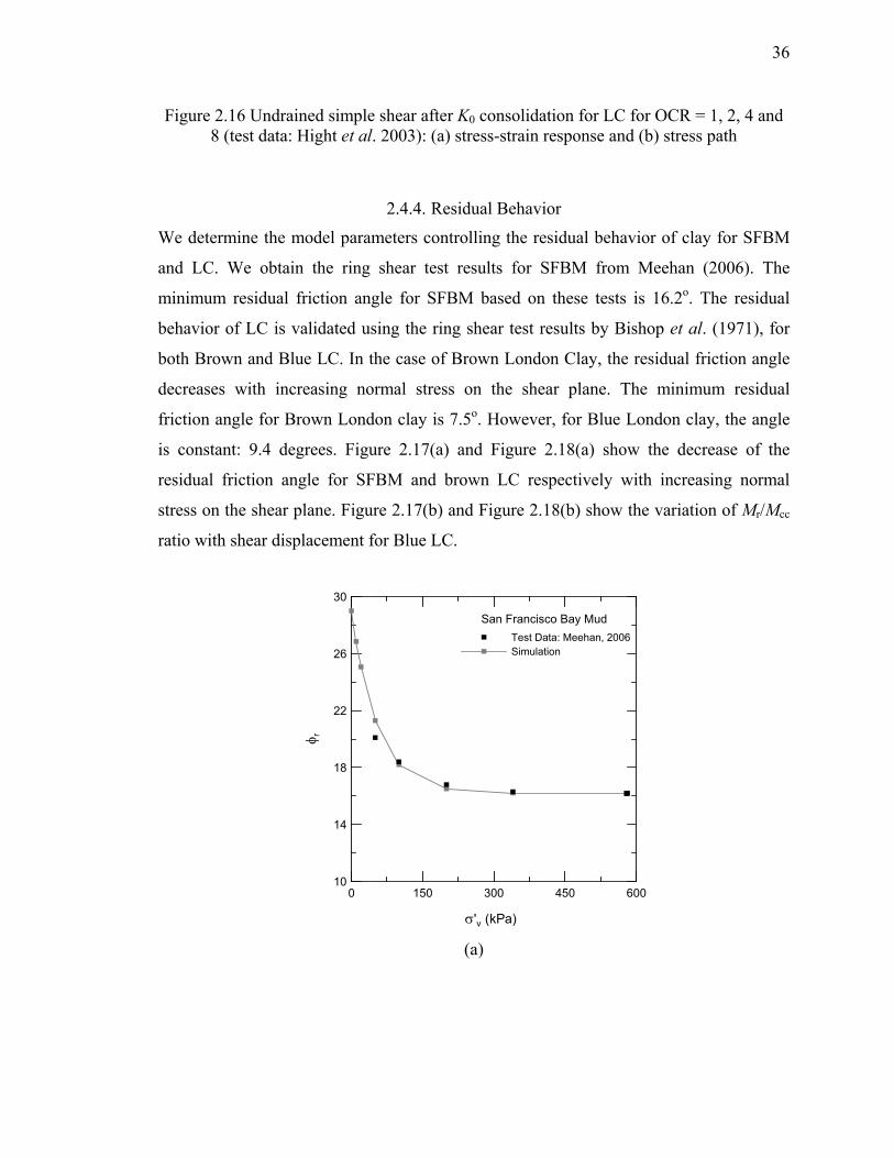
36

Figure 2.16 Undrained simple shear after K0 consolidation for LC for OCR = 1, 2, 4 and 8 (test data: Hight et al. 2003): (a) stress-strain response and (b) stress path

2.4.4. Residual Behavior

We determine the model parameters controlling the residual behavior of clay for SFBM

and LC. We obtain the ring shear test results for SFBM from Meehan (2006). The

minimum residual friction angle for SFBM based on these tests is 16.2o. The residual

behavior of LC is validated using the ring shear test results by Bishop et al. (1971), for

both Brown and Blue LC. In the case of Brown London Clay, the residual friction angle

decreases with increasing normal stress on the shear plane. The minimum residual

friction angle for Brown London clay is 7.5o. However, for Blue London clay, the angle

is constant: 9.4 degrees. Figure 2.17(a) and Figure 2.18(a) show the decrease of the

residual friction angle for SFBM and brown LC respectively with increasing normal

stress on the shear plane. Figure 2.17(b) and Figure 2.18(b) show the variation of Mr/Mcc

ratio with shear displacement for Blue LC.

0 150 300 450 600

σ'v (kPa)

10

14

18

22

26

30

φ r

Test Data: Meehan, 2006Simulation

San Francisco Bay Mud

(a)

37

0 6 12 18 24 30

Shear Displacement (mm)

0.4

0.55

0.7

0.85

1

Mr/M

cc

Test Data: Meehan, 2006Simulation

San Francisco Bay Mud

(b)

Figure 2.17 Comparison of model simulation and experimental data for SFBM at residual state

0 100 200 3000

4

8

12

16

φ r

φr,min =7.5o , Y = 0.04Test Data, Maksimovic (1989)

Brown London Clay

, Simulation

0 100 200 3000

4

8

12

16

φ r


Brown London Clay

, SimulationSimulation

φr,min=7.5o

0 100 200 3000

4

8

12

16

φ r


Brown London Clay

, Simulation

0 100 200 3000

4

8

12

16

φ r


Brown London Clay

, Simulation

0 100 200 3000

4

8

12

16

φ r


Brown London Clay

, Simulation

0 100 200 3000

4

8

12

16

φ r


Brown London Clay

, Simulation

0 100 200 3000

4

8

12

16

φ r


Brown London Clay

, Simulation

0 100 200 3000

4

8

12

16

φ r


Brown London Clay


φr,min=7.5o

σ'v (kPa)

, 1989

0 100 200 3000

4

8

12

16

φ r


Brown London Clay

, Simulation

0 100 200 3000

4

8

12

16

φ r


Brown London Clay


φr,min=7.5o

0 100 200 3000

4

8

12

16

φ r


Brown London Clay

, Simulation

0 100 200 3000

4

8

12

16

φ r


Brown London Clay

, Simulation

0 100 200 3000

4

8

12

16

φ r


Brown London Clay

, Simulation

0 100 200 3000

4

8

12

16

φ r


Brown London Clay

, Simulation

0 100 200 3000

4

8

12

16

φ r


Brown London Clay

, Simulation

0 100 200 3000

4

8

12

16

φ r


Brown London Clay


φr,min=7.5o

σ'v (kPa)

0 100 200 3000

4

8

12

16

φ r


Brown London Clay

, Simulation

0 100 200 3000

4

8

12

16

φ r


Brown London Clay


φr,min=7.5o

0 100 200 3000

4

8

12

16

φ r


Brown London Clay

, Simulation

0 100 200 3000

4

8

12

16

φ r


Brown London Clay

, Simulation

0 100 200 3000

4

8

12

16

φ r


Brown London Clay

, Simulation

0 100 200 3000

4

8

12

16

φ r


Brown London Clay

, Simulation

0 100 200 3000

4

8

12

16

φ r


Brown London Clay

, Simulation

0 100 200 3000

4

8

12

16

φ r


Brown London Clay


φr,min=7.5o

σ'v (kPa)

, 1989

(a)

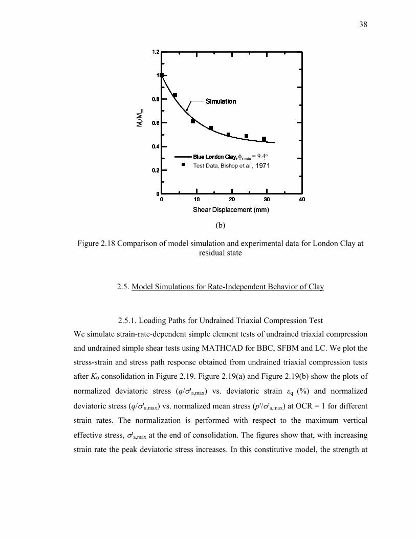
38

0 10 20 30 400

0.2

0.4

0.6

0.8

1

1.2

Blue London Clay, φr = 9.4o, br = 0.03

Test Data (Bishop, 1971)

Simulation

0 10 20 30 400

0.2

0.4

0.6

0.8

1

1.2



Simulation

φr,min = 9.4o

0 10 20 30 400

0.2

0.4

0.6

0.8

1

1.2



Simulation

0 10 20 30 400

0.2

0.4

0.6

0.8

1

1.2



Simulation

φr,min = 9.4o

Test Data, Bishop et al. (1971)

0 10 20 30 400

0.2

0.4

0.6

0.8

1

1.2



Simulation

0 10 20 30 400

0.2

0.4

0.6

0.8

1

1.2



Simulation

φr,min = 9.4o

0 10 20 30 400

0.2

0.4

0.6

0.8

1

1.2



Simulation

0 10 20 30 400

0.2

0.4

0.6

0.8

1

1.2



Simulation

φr,min = 9.4o


Mr/M

cc


, 1971

0 10 20 30 400

0.2

0.4

0.6

0.8

1

1.2



Simulation

0 10 20 30 400

0.2

0.4

0.6

0.8

1

1.2



Simulation

φr,min = 9.4o

0 10 20 30 400

0.2

0.4

0.6

0.8

1

1.2



Simulation

0 10 20 30 400

0.2

0.4

0.6

0.8

1

1.2



Simulation

φr,min = 9.4o


0 10 20 30 400

0.2

0.4

0.6

0.8

1

1.2



Simulation

0 10 20 30 400

0.2

0.4

0.6

0.8

1

1.2



Simulation

φr,min = 9.4o

0 10 20 30 400

0.2

0.4

0.6

0.8

1

1.2



Simulation

0 10 20 30 400

0.2

0.4

0.6

0.8

1

1.2



Simulation

φr,min = 9.4o


Mr/M

cc


, 1971

(b)

Figure 2.18 Comparison of model simulation and experimental data for London Clay at residual state

2.5. Model Simulations for Rate-Independent Behavior of Clay

2.5.1. Loading Paths for Undrained Triaxial Compression Test

We simulate strain-rate-dependent simple element tests of undrained triaxial compression

and undrained simple shear tests using MATHCAD for BBC, SFBM and LC. We plot the

stress-strain and stress path response obtained from undrained triaxial compression tests

after K0 consolidation in Figure 2.19. Figure 2.19(a) and Figure 2.19(b) show the plots of

normalized deviatoric stress (q/σ'a,max) vs. deviatoric strain εq (%) and normalized

deviatoric stress (q/σ'a,max) vs. normalized mean stress (p'/σ'a,max) at OCR = 1 for different

strain rates. The normalization is performed with respect to the maximum vertical

effective stress, σ'a,max at the end of consolidation. The figures show that, with increasing

strain rate the peak deviatoric stress increases. In this constitutive model, the strength at

39

critical state increases with increasing strain-rate. The rate effect is still visible at large

deviatoric strain values (16%).

0 4 8 12 16

εq (%)

0

0.2

0.4

0.6

0.8

1

qσ'

a,m

ax

Strain Rate IndependentStrain Rate = 0.72% /hrStrain Rate = 72% /hrStrain Rate = 7200% /hrStrain Rate = 720000% /hr

Strain Rate Effect: OCR=1Clay 1BBC

0 4 8 12 16

εq (%)

0

0.2

0.4

0.6

0.8

1

qσ'

a,m

ax



(a)

0 0.2 0.4 0.6 0.8

p'

σ'a,max

0

0.2

0.4

0.6

0.8

1

qσ'

a,m

ax

Strain Rate IndependentStrain Rate = 0.72%Strain Rate = 72%Strain Rate = 7200%Strain Rate = 720000%

Strain Rate Effect: OCR = 1Clay 1BBC

0 0.2 0.4 0.6 0.8

p'

σ'a,max

0

0.2

0.4

0.6

0.8

1

qσ'

a,m

ax



(b)

40

Figure 2.19 Undrained triaxial compression after K0 consolidation for BBC for OCR = 1: (a) stress-strain plot and (b) stress-path

Figure 2.20 and Figure 2.21 show the results of triaxial compressions tests after isotropic

consolidation for OCR values 1 and 2 respectively. Figure 2.20 (a) and Figure 2.20(b)

show the plots of normalized deviatoric stress (q/σ'a,max) vs. deviatoric strain εq (%) and

normalized deviatoric stress (q/σ'a,max) vs. normalized mean stress (p'/σ'a,max) respectively

at OCR = 1 at different strain-rates. Both the peak and critical-state strength increase with

increasing strain rate, though the rate of strength gain with increasing strain rate is much

higher at peak than at critical state. The peak and critical-state strength gains in the rate-

dependent cases as compared to the rate-independent loading are clearly visible in the

plots. We observe that the dilatancy of the sample increases with increasing strain rate.

There may be a possibility that under undrained shearing at high strain rate, clay particles

form clusters which try to climb over each other during shearing and the sample increases

in volume at high strain rate. As a result, at high strain rate, clay behavior could change

from contractive to dilative, as suggested by the model.

0 4 8 12 16

εq (%)

0

0.4

0.8

1.2

1.6

qσ'

a,m

ax



0 4 8 12 16

εq (%)

0

0.4

0.8

1.2

1.6

qσ'

a,m

ax



(a)

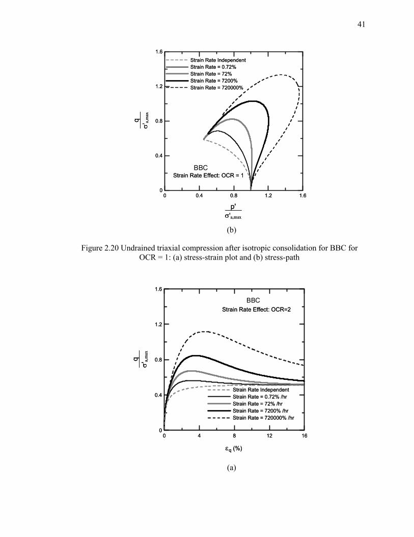
41

0 0.4 0.8 1.2 1.6

p'

σ'a,max

0

0.4

0.8

1.2

1.6

qσ'

a,m

ax



0 0.4 0.8 1.2 1.6

p'

σ'a,max

0

0.4

0.8

1.2

1.6

qσ'

a,m

ax



(b)

Figure 2.20 Undrained triaxial compression after isotropic consolidation for BBC for OCR = 1: (a) stress-strain plot and (b) stress-path

0 4 8 12 16

εq (%)

0

0.4

0.8

1.2

1.6

qσ'

a,m

ax



0 4 8 12 16

εq (%)

0

0.4

0.8

1.2

1.6

qσ'

a,m

ax



(a)

42

0 0.4 0.8 1.2 1.6

p'

σ'a,max

0

0.4

0.8

1.2

1.6

qσ'

a,m

ax


Strain Rate Effect: OCR = 2

Clay 1BBC

0 0.4 0.8 1.2 1.6

p'

σ'a,max

0

0.4

0.8

1.2

1.6

qσ'

a,m

ax


Strain Rate Effect: OCR = 2

Clay 1BBC

(b)

Figure 2.21 Undrained triaxial compression after isotropic consolidation for BBC for OCR = 2: (a) stress-strain plot and (b) stress-path

2.5.2. Loading Paths for Simple Shear Test

The model successfully simulates the mechanical response of soil in multi-axial stress

situations. We simulate anisotropically consolidated (K0-consolidated) undrained simple

shear tests. Figure 2.22 and Figure 2.23 demonstrate the ability of the model to capture

multi-axial stress situations. Figure 2.22(a) shows normalized shear stress (τ /σ'v,NC) vs.

shear strain γxy (%) for undrained simple shear tests at OCR = 1 for BBC, while Figure

2.22(b) shows normalized shear stress (τ /σ'v,NC) vs. normalized normal stress (σ'v /σ'v,NC)

at OCR = 1. The normalization is performed with respect to the maximum vertical stress

at the end of consolidation for normally consolidated samples (σ'v,NC). Plot for OCR = 4

is depicted in Figure 2.23. For all the cases, the peak stress increases with increasing

strain rate. We also observe in the stress path plots that higher strain rate increases the

dilatancy of the clay.

43

0 40 80 120 160 200

γxy (%)

0

0.1

0.2

0.3

0.4

τσ'

v,N

CStrain Rate Independent Strain Rate = 1.8% /hrStrain Rate =180% /hrStrain Rate = 18000% /hrStrain Rate = 1800000% /hr


0 40 80 120 160 200

γxy (%)

0

0.1

0.2

0.3

0.4

τσ'

v,N

CStrain Rate Independent Strain Rate = 1.8% /hrStrain Rate =180% /hrStrain Rate = 18000% /hrStrain Rate = 1800000% /hr


(a)

0 0.2 0.4 0.6 0.8 1 1.2

σ'v

σ'v,NC

0

0.1

0.2

0.3

0.4

τσ '

v,N

C

Strain-Rate IndependentStrain Rate = 1.8% /hrStrain Rate = 180% /hrStrain Rate = 18000% /hrStrain Rate = 1800000% /hr

Strain Rate Effect: OCR = 1BBC

(b)

Figure 2.22 Undrained simple shear tests after K0 consolidation for BBC for OCR=1: (a) stress-strain plot and (b) stress-path

44

0 40 80 120 160 200

γxy (%)

0

0.1

0.2

0.3

0.4

τσ '

v,N

C

Strain Rate Independent Strain Rate = 1.8% /hrStrain Rate =180% /hrStrain Rate = 18000% /hrStrain Rate = 1800000% /hr


0 40 80 120 160 200

γxy (%)

0

0.1

0.2

0.3

0.4

τσ '

v,N

C

Strain Rate Independent Strain Rate = 1.8% /hrStrain Rate =180% /hrStrain Rate = 18000% /hrStrain Rate = 1800000% /hr


(a)

0 0.2 0.4 0.6 0.8 1 1.2

σ'v

σ'v,NC

0

0.1

0.2

0.3

0.4

τσ '

v,N

C

Strain-Rate IndependentStrain Rate = 1.8% /hrStrain Rate = 180% /hrStrain Rate = 18000% /hrStrain Rate = 1800000% /hr

Strain Rate Effect: OCR = 4BBC

(b)

Figure 2.23 Undrained simple shear tests after K0 consolidation for BBC at OCR = 4: (a) stress-strain plot and (b) stress-path

45

CHAPTER 3. THE FINITE ELEMENT METHOD APPLIED TO THE SHAFT RESISTANCE PROBLEM

3.1. Introduction

Previous numerical studies, aimed to model the installation of a displacement pile in clay,

used either undrained cylindrical cavity expansion theory (Carter et al. 1979) or the strain

path method (Baligh 1985). Randolph et al. (1979) simulated the installation of a

displacement pile in clay by one-dimensional undrained expansion of a cylindrical cavity

and investigated the changes in the stresses and pore pressure within the soil during and

after the installation. Excess pore pressure generated during the undrained cylindrical

cavity expansion (which was intended to model pile installation) was assumed to

dissipate through a one-dimensional flow in the radial direction outward from the pile. A

work-hardening, elasto-plastic model (similar to the modified cam clay model) was used

to represent the constitutive behavior of the soil.

The strain path method (SPM) provides an analytical framework to evaluate the

strains associated with quasi-static, undrained penetration in saturated clays. This method

assumes the deep penetration in saturated clays to be a fully-constrained process (no

volume change); the deformations and strains developed during the penetration of a

foreign object are considered to be independent of the shear resistance offered by the soil.

Whittle and Sutabutr (1999) used the SPM to derive the end-of-installation stresses and

pore pressure around a displacement pile installed in saturated clay. A one-dimensional

finite element (FE) model was then used to investigate the radial dissipation of generated

excess pore pressure. The MIT-E3 model (Whittle and Kavvadas 1994, Whittle et al.

1994) was used to represent the nonlinear soil behavior.

In this chapter we describe different aspects of the one-dimensional (1-D) finite

element (FE) model that we use to model installation, setup and loading of a pile jacked

in saturated clay. We consider pile jacking in clay to be a fully undrained process. At the

46

end of installation and before simulation of pile loading (either from a static pile load test

or from the superstructure), we allow the corresponding rest period, during which excess

pore pressures will partially or fully dissipate. Although our analysis focus on jacked

piles, we believe that the conclusions in general apply to driven piles; although some

deviations in shaft resistance values are possible, they are not expected to be large.

3.2. Mathematical Formulation

We perform 1-D finite element analysis (FEA) to model the jacking and the subsequent

loading of a cylindrical pile jacked in saturated clay. The FEA involves three distinct

stages: (i) pile installation (jacking), (ii) dissipation of excess pore pressure generated

during installation, and (iii) loading of the pile. These stages were also recognized by

several other researchers in studies related to the shaft capacity of displacement piles in

clay (Steenfelt et al. 1980, Bond and Jardine 1991, Azzouz et al. 1990, Lehane et al.

1994, Lee et al. 2004). The rate-dependent, two-surface plasticity-based constitutive

model described in Chapter 2 of this report is used in the FEA to represent the

constitutive behavior of clay.

3.2.1. Simulation of Pile Jacking in Clay and Pile Loading

Jacking of a pile into the ground is assumed to load the soil mass through a combination

of cavity expansion and vertical shearing. Figure 3.1 shows schematically the different

stages involved in the analysis of a pile monotonically jacked in clay. This figure also

shows the evolution of normal (radial) stress σr, vertical shear stress τz and excess pore

pressure u in a soil element adjacent to the pile shaft (Element A). Figure 3.1(a) shows

Element A subjected to in situ stresses (excess pore pressure and vertical shear stress

acting on the vertical face of the element at this stage are zero).

Stage 1 (Figure 3.1b) corresponds to the penetration of the pile into the soil mass

and is modeled as a sequential combination of two phases: the undrained cavity

expansion (CE) phase and the phase of “primary shearing”. The first phase (i.e., CE)

represents the creation of a cylindrical space (to be occupied by the pile) within the

47

ground as the pile tip pushes the soil away from the path of the pile. The conical area

shown in Figure 3.1 is either a conical tip fitted to the pile or the “rigid” tapered cone

predicted by bearing capacity theory in the case of a rough base. The soil in the “rigid”

tapered cone is in a nearly elastic state. The cylindrical cavity expansion stops when the

cavity radius becomes equal to the pile radius, i.e., as the shoulder (base) of the cone

clears Element A (Figure 3-1b). At the end of CE, the normal stress σr acting on the pile-

soil interface reaches a limiting value pL at the same time as the excess pore pressure

takes a value uCE. The vertical shear stress on the pile shaft (vertical side of the Element

A) remains zero throughout this phase. The cavity expansion phase is followed by

vertical shearing along the shaft wall (“primary shearing” phase) until the limit shear

stress τ1 is reached along the pile shaft. The soil element adjacent to the pile shaft is

expected to reach the residual shear strength at this state. At the end of the “primary

shearing” phase the total normal stress acting on the pile shaft is reduced from pL to σr1.

Aσr0

Initial stage

Nor

mal

(rad

ial)

stre

ss σ

r

Radial displacement δr

σr = σr0 Exc

ess

pore

pre

ssur

e u


u = 0

Shear displacement δz

τ = 0

Ver

tical

she

ar s

tress

τz

Aσr0

Initial stage

Aσr0

Initial stage

Nor

mal

(rad

ial)

stre

ss σ

r


σr = σr0 Exc

ess

pore

pre

ssur

e u


u = 0


τ = 0

Ver

tical

she

ar s

tress

τz

(a)

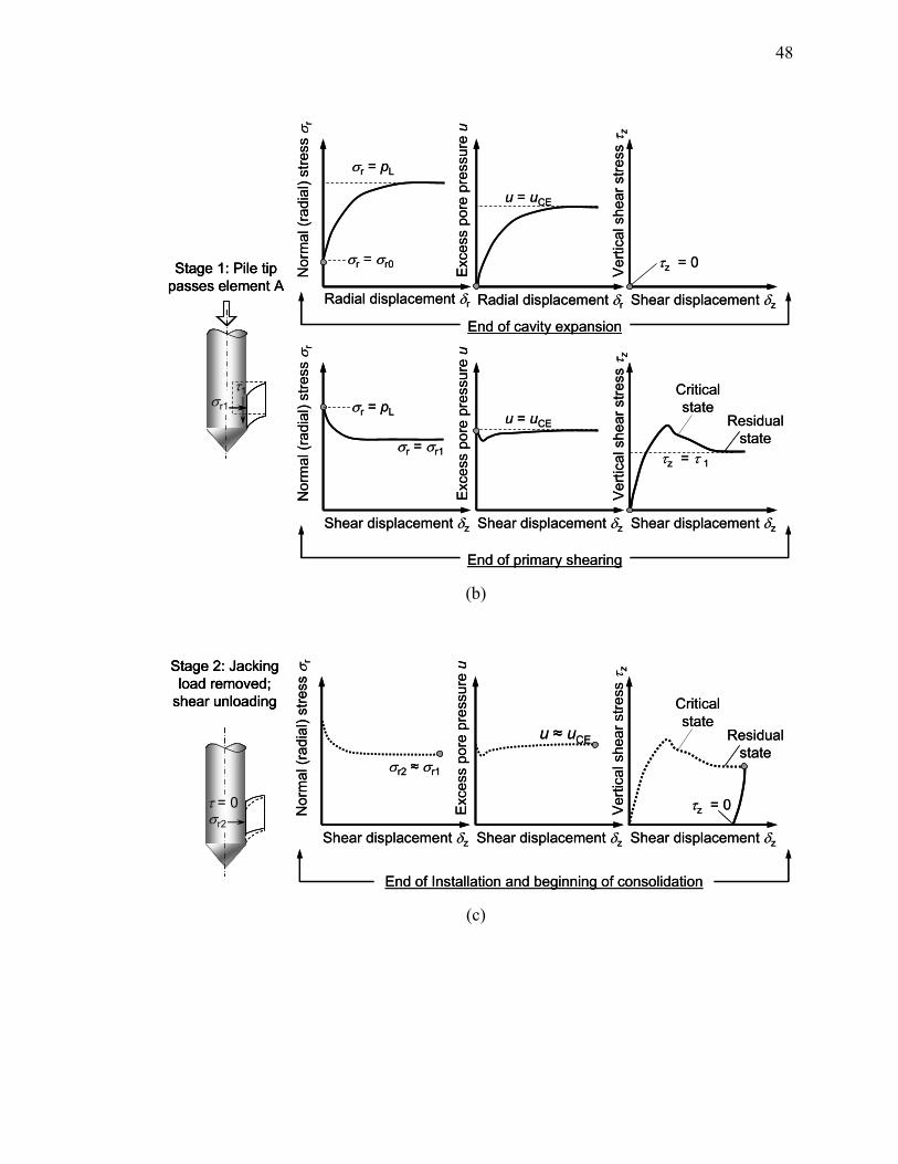
48

σr1

τ1

Stage 1: Pile tip passes element A


σr = σr0

σr = pL

Exc

ess

pore

pre

ssur

e u

Radial displacement δr Shear displacement δz

u = uCE

τz = 0

End of cavity expansion

Ver

tical

she

ar s

tress

τz

σr = pL

Exc

ess

pore

pre

ssur

e u


u = uCE

τz = τ 1

Ver

tical

she

ar s

tress

τz

End of primary shearing

Shear displacement δzShear displacement δz

Critical state

Residual stateσr = σr1

Nor

mal

(rad

ial)

stre

ss σ

rN

orm

al (r

adia

l) st

ress

σr

σr1

τ1


σr1

τ1



σr = σr0

σr = pL

Exc

ess

pore

pre

ssur

e u

Radial displacement δr Shear displacement δz

u = uCE

τz = 0

End of cavity expansion

Ver

tical

she

ar s

tress

τz

σr = pL

Exc

ess

pore

pre

ssur

e u


u = uCE

τz = τ 1

Ver

tical

she

ar s

tress

τz



Critical state

Residual stateσr = σr1

Nor

mal

(rad

ial)

stre

ss σ

rN

orm

al (r

adia

l) st

ress

σr

(b)

Exc

ess

pore

pre

ssur

e u


τz = 0Ver

tical

she

ar s

tress

τz

End of Installation and beginning of consolidation


Critical state

Residual state

σr2 ≈ σr1

σr2

τ = 0

Stage 2: Jacking load removed;

shear unloading

Nor

mal

(rad

ial)

stre

ss σ

r

u ≈ uCE

Exc

ess

pore

pre

ssur

e u


τz = 0Ver

tical

she

ar s

tress

τz

End of Installation and beginning of consolidation


Critical state

Residual state

σr2 ≈ σr1

σr2

τ = 0


shear unloading

σr2

τ = 0


shear unloading

Nor

mal

(rad

ial)

stre

ss σ

r

u ≈ uCE

(c)

49

Exc

ess

pore

pre

ssur

e u


τz = 0Ver

tical

she

ar s

tress

τz

Full dissipation of excess pore pressure


Critical state

Residual state

σr = σr3

σr2

τ = 0

Stage 3: Dissipation of excess pore pressure; no

external loading

Exc

ess

pore

pre

ssur

e u

Time

Nor

mal

(rad

ial)

stre

ss σ

r

Exc

ess

pore

pre

ssur

e u


τz = 0Ver

tical

she

ar s

tress

τz

Full dissipation of excess pore pressure


Critical state

Residual state

σr = σr3

σr2

τ = 0


external loading

σr2

τ = 0


external loading

Exc

ess

pore

pre

ssur

e u

Time

Nor

mal

(rad

ial)

stre

ss σ

r

(d)

σr4τ4

Stage 4: Further shearing/limit

loading

Exc

ess

pore

pre

ssur

e u

Nor

mal

(rad

ial)

stre

ss σ

r


τz = τ4

Ver

tical

she

ar s

tress

τz

Loading at the end of consolidation


Residual state

σr = σr4

σr4τ4


loading

σr4τ4


loading

Exc

ess

pore

pre

ssur

e u

Nor

mal

(rad

ial)

stre

ss σ

r


τz = τ4

Ver

tical

she

ar s

tress

τz

Loading at the end of consolidation


Residual state

σr = σr4

(e)

Figure 3.1 Stages involved in the jacking (installation) of a pile in clay, dissipation of excess pore pressure, and undrained loading of the pile

50

Stage 2 (Figure 3.1c) represents the removal of the jacking load, which occurs

after the maximum jacking stroke length s of the hydraulic jack is reached or at the end of

installation. During the shear unloading stage, the total normal stress remains practically

unchanged (σr2 ≈ σr1) and the shear stress τz is reduced from τ1 until it becomes equal to

zero (we assume that the residual shear stress acting on the pile shaft at this stage is equal

to zero). Due to the instantaneous nature of jacking load removal, the unloading process

remains practically undrained. Stage 2 represents the end of installation (EOI) for a

monotonically jacked pile.

At Stage 3, we allow the generated excess pore pressure to stabilize (dissipate)

completely. During Stage 3 (Figure 3.1d), the shear stress does not change (remains equal

to zero) and, at the end of this stage, the excess pore pressure becomes equal to zero. Due

to the dissipation of excess pore pressure, the effective stress increases during Stage 3.

Biot’s coupled consolidation theory (Biot 1941) was used to model this consolidation

phase (dissipation of excess pore pressure with time). According to Biot’s theory, both

the effective stress and the excess pore pressure change during consolidation; however,

they do not necessarily counterbalance each other, and thus, a change in total stress is

possible during Stage 3 (the consolidation phase). The difference between the reduction

in excess pore pressure and the increase in the effective stress is reflected through a

reduction in the normal stress from σr1 to σr3 at the end of Stage 3.

Stage 4 (Figure 3.1e) represents the application of the structural load (or the

performance of a static pile load test) for a pile installed monotonically. The soil element

adjacent to the pile shaft is expected to reach the residual shear strength at the end of this

stage. A limit shear stress τ4 is reached along the pile shaft and the normal stress acting

on the pile shaft reduces from σr3 to σr4.

For a pile installed using multiple jacking strokes, Stage 4 represents the

application of the next jacking stroke. For piles installed using multiple jacking strokes,

Stage 3 (consolidation phase) is omitted after Stage 2, and Stage 4 represents the second

jacking stroke. Subsequent jacking strokes are represented by successive repetition of

Stages 2 and 4 (multiple releases and re-applications of the jacking load at the pile head).

At the end of installation, we allow the dissipation of the generated excess pore pressure

51

(as represented by Stage 3). Finally, we repeat Stage 4 to simulate the application of the

structural load (or the load applied during a static pile load test).

3.2.2. Mesh and Boundary Conditions

We consider a disk of soil around the pile shaft to model the pile shaft-soil interaction

during installation, dissipation of excess pore pressure and subsequent loading. We also

assume that the vertical normal strain is negligible and that there is no bending

deformation. Using these assumptions, the analysis becomes independent of the thickness

of the soil disk, and thus, one-dimensional. These conditions resemble closely those

existing at depths that are sufficiently removed from the ground surface and from the pile

base. A similar approach was used to investigate the shaft resistance of nondisplacement

piles in clays and sands (Randolph and Wroth 1978, Potts and Martins 1982, Salgado

2006, Loukidis and Salgado 2008b) and also of jacked piles in sands (Basu et al. 2009).

In reality, the vertical normal strain at depths very close to the pile tip may not be

negligible. There is compression of the soil just below the tip during pile penetration and

then unloading of the same soil element as the tip moves below it. Near the ground

surface, the deformation of the soil is less constrained than at lower depths, and,

consequently, rotation may occur in a soil element along with the development of non-

negligible vertical normal strain. Therefore, the assumptions in the 1-D analyses are not

strictly valid near the pile tip and the ground surface. However, these assumptions closely

resemble conditions existing at depths that are sufficiently removed from the ground

surface and from the pile base.

Figure 3.2 shows the finite element (FE) mesh, boundary conditions, and nodal

constraints used for the analyses. The mesh consists of a row of 8-noded rectangular

axisymmetric elements with 4 Gauss-quadrature points. Along with the displacement

fields, we also consider excess pore water pressure as a continuous field inside the

domain. Each corner node of the rectangular elements has three degrees of freedom

(DOF): radial displacement, vertical displacement and excess pore pressure. The middle

nodes, lying on the vertical and horizontal sides of the elements, have only the

displacement DOFs. All corresponding DOFs of the nodes lying along a vertical line are

52

tied together to enforce the condition of zero normal vertical strain (i.e., no

extension/contraction of soil in the vertical direction) and no bending deformation (i.e.,

no rotation of the vertical sides of the elements). Imposition of this constraint (tying the

corresponding DOFs along any vertical line) guarantees that shearing takes place only in

the vertical direction and makes the analysis results independent of the height of the

rectangular elements. We also constrain all DOFs of the nodes lying on the left

(innermost) and right (outermost) boundaries of the domain. These constraints allow us to

measure the reaction at the left boundary (pile shaft-soil interface) and to enforce the

conditions of zero displacement and zero excess pore pressure at the far field. At different

stages of the pile installation and loading process, radial and vertical displacement

increments are applied at the nodes on the leftmost boundary of the domain. At these

nodes, we monitor the reactions and excess pore pressure generated due to the applied

displacement increments.

Q8 axisymmetric elements

Applied displacements All degrees of freedom tied

ts(a)

(b)

~ 300B

B/2

Nodes with both displacement and pore pressure DOFs

Nodes with only displacement DOFs

Q8 axisymmetric elements

Applied displacements All degrees of freedom tied

ts(a)

(b)

~ 300B

B/2

Nodes with both displacement and pore pressure DOFs

Nodes with only displacement DOFs

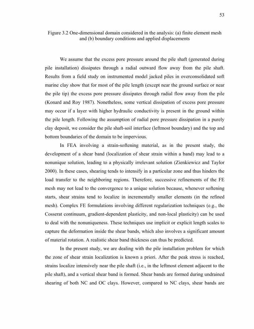
53

Figure 3.2 One-dimensional domain considered in the analysis: (a) finite element mesh and (b) boundary conditions and applied displacements

We assume that the excess pore pressure around the pile shaft (generated during

pile installation) dissipates through a radial outward flow away from the pile shaft.

Results from a field study on instrumented model jacked piles in overconsolidated soft

marine clay show that for most of the pile length (except near the ground surface or near

the pile tip) the excess pore pressure dissipates through radial flow away from the pile

(Konard and Roy 1987). Nonetheless, some vertical dissipation of excess pore pressure

may occur if a layer with higher hydraulic conductivity is present in the ground within

the pile length. Following the assumption of radial pore pressure dissipation in a purely

clay deposit, we consider the pile shaft-soil interface (leftmost boundary) and the top and

bottom boundaries of the domain to be impervious.

In FEA involving a strain-softening material, as in the present study, the

development of a shear band (localization of shear strain within a band) may lead to a

nonunique solution, leading to a physically irrelevant solution (Zienkiewicz and Taylor

2000). In these cases, shearing tends to intensify in a particular zone and thus hinders the

load transfer to the neighboring regions. Therefore, successive refinements of the FE

mesh may not lead to the convergence to a unique solution because, whenever softening

starts, shear strains tend to localize in incrementally smaller elements (in the refined

mesh). Complex FE formulations involving different regularization techniques (e.g., the

Cosserat continuum, gradient-dependent plasticity, and non-local plasticity) can be used

to deal with the nonuniqueness. These techniques use implicit or explicit length scales to

capture the deformation inside the shear bands, which also involves a significant amount

of material rotation. A realistic shear band thickness can thus be predicted.

In the present study, we are dealing with the pile installation problem for which

the zone of shear strain localization is known a priori. After the peak stress is reached,

strains localize intensively near the pile shaft (i.e., in the leftmost element adjacent to the

pile shaft), and a vertical shear band is formed. Shear bands are formed during undrained

shearing of both NC and OC clays. However, compared to NC clays, shear bands are

54

more prominent in OC clays (Oka et al. 2005). An element thickness (and, consequently

a shear band thickness ts) that is either too small or too large would produce stresses and

strains that would be unrealistic and incorrect. By keeping the thickness of the leftmost

element consistent with the expected shear band thickness, we can correctly represent the

shear banding along the pile shaft and calculate unit limit shaft resistance accurately. The

constitutive model that we use in this study does not explicitly account for material

rotation and does not include asymmetric stress tensors. However, this model is able to

adequately predict the tractions at the boundaries of shear bands. Therefore, we can avoid

the problem of solution nonuniqueness by ensuring that the element size near the zone of

shear strain localization (i.e., at the pile shaft-soil interface) does not exceed the expected

value of the shear band thickness observed for clays. This technique also allows us to use

a simpler FE formulation. In modeling the penetration of cylindrical and spherical

penetrometers in clay, Zhou and Randolph (2007) used the smallest element size

(adjacent to the penetrometers) equal to 2.5% of the diameter of the penetrometers. In the

present analysis, the thickness of the smallest element (adjacent to the pile shaft) reduces

from 8.7% of the pile diameter B at the beginning of CE to 1% of B at the end of CE

phase (before the primary shearing phase starts).

Theoretically, the thickness of the smallest element adjacent to the pile shaft can

be twice the thickness of the expected shear band. This means that shear strain

localization will occur only in the first (nearest to the left boundary) line of quadrature

points within the first (1st) element adjacent to the pile shaft. However, in the simulation

of an undrained process (like the one we are dealing with in the present study), this

formulation that allows localization of shear strain only at the leftmost quadrature points

of the 1st element leads to the development of a high gradient of excess pore pressure

within the first element, and the analysis becomes unstable. We avoid this problem by

selecting an adequate size for the 1st element. With the selected size of the 1st element the

excess pore pressures developed at different nodes do not create a very high gradient

across the element, and thus, we avoid the instability problem.

An alternate approach to eliminate the problems associated with shear strain

localization would be to use an interface element between the pile and soil. However, this

55

interface element will need a separate constitutive model to represent the stress-strain

response of the pile-soil interface (Hu and Pu 2004). This special constitutive model for

the interface also needs to be calibrated using results from interface shear tests. Properly

modeled single or multiple interface elements will thus be able to capture the load-

deformation mechanism at the pile-soil interface under large shear strains. The use of

interface elements would also allow the use of coarser meshes compared to the one used

in the present study. In the absence of a separate constitutive model to represent the

stress-strain response of the pile-soil interface we did not use this approach in our

analysis.

3.3. Solution Algorithms and Applied Displacements

The finite element code SNAC (Abbo and Sloan 2000) is used for the numerical

simulations. The modified Newton-Raphson method is used as the solution scheme for

the global nonlinear load-displacement system of equations. The elastic global stiffness

matrix was used in the modified Newton-Raphson scheme. The constitutive model

equations are integrated using a semi-implicit algorithm adapted with sub-incrementation

and error control (Loukidis 2006, Chakraborty 2009) using relative stress error tolerance

equal to 10-4.

Our analyses are based on the conventional, small-strain finite element

formulation with node updating. SNAC was modified to update the position (x and y

coordinates) of the nodes after each solution increment (updated Lagrangian approach),

which is needed for the proper simulation of a large-deformation problem like the one

addressed in this paper. The present approach of using small-strain FEA to solve large-

deformation problems is similar to the approach followed by Hu and Randolph (1998) to

successfully analyze a two-dimensional large-strain penetration problem. In our 1-D

analysis with specific displacement constraints, the elements do not distort. Therefore, the

remeshing and stress interpolation techniques used by Hu and Randolph (1998) are not

necessary. Basu et al. (2009) demonstrated the validity of the present FE approach by

comparing the FEA results from cylindrical cavity expansion analysis in sand with the

results obtained by other researchers (Yu and Houlsby 1991, Collins et al. 1992, and

56

Salgado and Randolph 2001) who followed analytical and semi-analytical large-strain

formulation. In our present analysis, during each load increment (between two successive

node updates), the displacement gradient and the corresponding strain increments are

very small. The convective terms in the strain definition are one order of magnitude

smaller than the Cauchy (infinitesimal) strains. As a result, decreasing the Cauchy strain

increments by one order of magnitude leads to a two order of magnitude decrease in the

convective terms included in the definition of large strains. Thus, we minimize the error

introduced by the omission of the convective terms (present in the large-strain FE

formulations) by using sufficiently fine displacement incrementation.

Displacement-controlled analyses were performed, and the displacement

increments were applied at the nodes on the left boundary of the domain (contact surface

between soil and pile shaft). We monitored the reactions at the nodes where displacement

increments were applied. Horizontal displacement increments were applied to the

leftmost nodes of the domain to simulate the CE phase associated with pile installation.

The CE phase starts from a very small initial cavity radius r0 (= 0.015 m) and ends when

the cavity radius becomes equal to the pile radius R. With a sufficiently small initial

cavity radius (compared to the final radius), the limit cavity pressure is closely

approximated at the end of the cavity expansion process. Vertical displacement

increments are applied at the nodes of the leftmost boundary to simulate the vertical

shearing. Any slippage between pile and soil is simulated by the formation of a vertical

shear band inside the soil adjacent to the shaft wall. This condition corresponds to a

perfectly rough interface. The vertical shearing phase following the CE phase (“primary

shearing”) is stopped when both normal and tangential reactions at the left boundary of

the domain stabilize and the limit state is reached. Negative (upward) vertical

displacement is applied at the nodes lying on the pile shaft to simulate the removal of the

jacking load (Stage 2). The unloading stage is stopped when the shear stress along the left

boundary of the domain becomes equal to zero. The unloading (reversal of vertical

displacement increment) is automated in the analyses based on two convergence criteria:

(i) for three consecutive displacement increments, the corresponding reaction values on

the pile shaft differ only by a value equal to or less than 10-7 and (ii) the ratio (Mcc-

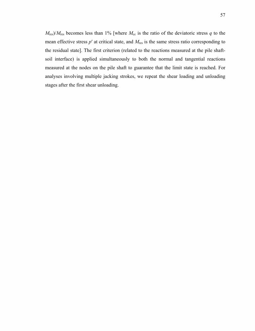
57

Mres)/Mres becomes less than 1% [where Mcc is the ratio of the deviatoric stress q to the

mean effective stress p′ at critical state, and Mres is the same stress ratio corresponding to

the residual state]. The first criterion (related to the reactions measured at the pile shaft-

soil interface) is applied simultaneously to both the normal and tangential reactions

measured at the nodes on the pile shaft to guarantee that the limit state is reached. For

analyses involving multiple jacking strokes, we repeat the shear loading and unloading

stages after the first shear unloading.

CHAPTER 4. ANALYSIS RESULTS

4.1. Introduction

We performed finite element analysis (FEAs) of piles jacked in London Clay (LC) with

different values of initial vertical effective stress (σ'v0 = 25, 50, 100, 200 and 400 kPa)

and different values of initial OCR (= 1, 2, 4 and 8). The values of the critical-state

friction angle φc (from triaxial compression tests) and the minimum possible residual

friction angle φr,min for LC were considered to be equal to 21.3° (Gasparre 2005, Gasparre

et al. 2007a, Gasparre et al. 2007b) and 9.4° (Bishop et al. 1971), respectively. During

pile jacking, the clay particles become aligned along the direction of shearing (i.e., along

the pile shaft), and the clay is expected to reach the residual state. We performed analyses

for the minimum possible residual friction angle φr,min of LC [i.e., for (φc-φr,min) = 11.9º ≈

12º]. Two additional sets of analyses were also performed with (φc-φr,min) = 0º and (φc-

φr,min) = 5º. We performed these additional analyses [with varying (φc-φr,min)] to assess the

effect of residual strength mobilization along the shaft on the limit shaft resistance of a

pile jacked in clay.

Ratnam et al. (2005) reported results of different in situ hydraulic conductivity

tests performed by several researchers in different LC deposits. Theses results show that

the hydraulic conductivity of LC varies between 9.6×10-12 m/s and 8.8×10-9 m/s. In our

analyses the clay hydraulic conductivity was assumed to be equal to 10-10 m/s. We used

K0 values in the analyses that corresponded to different OCR values for LC. These K0

values (Table 4.1) were determined through simulations of one-dimensional

consolidation tests (Chakraborty 2009, Gasparre 2005). Table 4.1 also shows the initial

values of void ratio e0 and undrained shear strength su corresponding to different values

of in situ vertical effective stress σ′v0 and OCR values used in the analyses. The values of

su reported in Table 4.1 were determined from rate-independent element simulations of

isotropic triaxial compression tests (Chakraborty 2009) in MATHCAD. In this chapter,

we present and discuss the FEA results obtained at different stages of installation, setup

and loading of the pile. We also discuss the changes in the stress state of the soil during

and after the installation of a displacement pile.

Table 4.1 Different values of K0, e0 and su values used in the analyses for LC (σ′v0 and su are in kPa)

OCR K0 σ′v0 e0 su su/σ′v0

1 0.6

25 1.354 4.34

0.173

50 1.238 8.67 100 1.121 17.34 150 1.053 26.01 200 1.005 34.68 250 0.967 43.35

2 0.9

25 1.268 7.23

0.289

50 1.151 14.47 100 1.035 28.94 150 0.967 43.40 200 0.918 57.87 250 0.881 72.34

4 1.34

25 1.178 12.30

0.492

50 1.061 24.60 100 0.945 49.20 150 0.877 73.80 200 0.829 98.40 250 0.791 123.00

8 2.0

25 1.086 21.10

0.844

50 0.970 42.21 100 0.853 84.42 150 0.785 126.62200 0.737 168.83250 0.699 211.04

4.2. Results of the Finite Element Analyses

4.2.1. Evolution of Stress during Pile Installation

Figure 4.1 shows the evolution of the total normal (radial) stress σr and the excess pore

pressure u at the cavity wall as a function of the cavity radius during the undrained CE

phase of Stage 1 (for σ'v0 = 50 kPa, OCR = 1, 2, 4 and 8). Both σr and u reach limiting

values at the end of CE. The limit cavity pressure pL increases with increasing OCR

values. At the end of CE, the element adjacent to the cavity wall reaches critical state

with a net increase or decrease (depending on the initial value of OCR) of mean effective

stress p′ (see Figure 4.2). The stress paths shown in Figure 4.2 (for σ'v0 = 100 kPa, OCR

= 1, 2, 4 and 8) are similar to those expected in the case of undrained shearing of NC and

OC clays. For NC and slightly OC clays, the stress paths in q-p′ space first reach a peak

deviatoric stress qp before reaching critical state (see Figure 4.2a). For OCR = 8, the

stress path initially crosses the CSL in the q-p′ space to reach a peak value of stress

obliquity (q/p′) before reaching the maximum deviatoric stress qp at critical state. Figure

4.2(b) shows the stress paths in the e-p′ space during undrained CE. Due to the

volumetric constraint in the undrained CE phase, the void ratio e cannot change from its

initial value e0, and hence the stress paths in the e-p′ space are horizontal (parallel to the

p′ axis). Depending on the initial value of OCR, the initial stress state (initial value of p′)

and initial void ratio e0, the point representing the initial soil state may fall either on the

right or on the left of the CSL in the e-p′ space. For any initial state falling on the right of

the CSL, critical state is achieved through a loss of p′ (this is the case for NC or slightly

OC clays with OCR = 1 and 2, respectively). For OCR = 4, the initial stress state is very

close to the CSL and thus the loss of p′ is not significant at the end of CE (when the stress

state finally falls on the CSL). For OCR = 8, the initial stress state falls on the left of the

CSL, and we observe a net increase in p′ to reach the CSL at the end of the undrained CE

phase.

0 4 8 12Normalized cavity radius r/r0

0

1

2

3

4

Nor

mal

ized

tota

l nor

mal

(rad

ial)

stre

ss a

t cav

ity w

all σ

r/pA

σ'v0 = 50 kPa, r0 = 0.015 m, pA = 100 kPa

OCR = 1

OCR = 2

OCR = 4

OCR = 8

(a)

0 4 8 12Normalized cavity radius r/r0

0

0.4

0.8

1.2

1.6

2

Nor

mal

ized

exc

ess

pore

pre

ssur

e at

cav

ity w

all u

/pA

OCR = 1

OCR = 2

OCR = 4

OCR = 8

σ'v0 = 50 kPa, r0 = 0.015 m, pA = 100 kPa

(b)

Figure 4.1 Evolution of stresses during undrained cavity expansion (a) total normal (radial) stress, and (b) excess pore pressure

0 40 80 120 160 200 240Mean effective stress p' (kPa)

0

40

80

120

160

Dev

iato

ric s

tress

q (k

Pa)

OCR = 1OCR = 2OCR = 4OCR = 8

σ'v0 = 100 kPa

Line following thecritical stress ratio

(a)

30 60 90 120 150 180 210 240

Mean effective stress p' (kPa)

0.8

0.9

1

1.1

1.2

Voi

d ra

tio e

σ'v0 = 100kPa

CSL

OCR = 4

OCR = 2

OCR = 1Initial stress state

OCR = 8

(b)

Figure 4.2 Stress paths during undrained cavity expansion in (a) q-p′ space and (b) e-p′ space

Figure 4.3 shows [for σ'v0 = 100 kPa, OCR = 4 and (φc- φr,min) = 12°] the

evolution of stresses on the pile shaft during the “primary shearing” (A to B) phase and

during the removal of the jacking load (B to C). Point A (Figure 4.3) represents the end

of CE when the total normal (radial) stress σr acting on the pile shaft and the excess pore

pressure u (generated during undrained cavity expansion) are at their limiting values; the

vertical shear stress τz acting along the pile shaft is zero at this point. During the “primary

shearing” phase, the soil element adjacent to the pile shaft first reaches the critical state

and then the residual state with continued shearing along the pile shaft. In this process, τz

acting on the pile shaft increases and reaches a limiting value (point B) at the end of the

“primary shearing” phase (which is also the end of Stage 1). In the initial part of the

“primary shearing” phase, the soil element adjacent to the pile shaft shows a tendency to

dilate. As the shearing associated with pile installation is an undrained process (the low

hydraulic conductivity of clay does not allow any dissipation of excess pore pressure

during fast shearing), the dilatancy (the tendency to increase volume) of the soil element

adjacent to the pile shaft causes a decrease in u (through the generation of negative

excess pore pressure or suction). As the critical state is approached, the soil response

becomes contractive resulting in an increase in u. At critical state, both u and σr acting on

the pile shaft are stabilized. As shearing continues after the critical state, τz continues to

decrease and reaches a residual value (point B). At the end of the “primary shearing”

phase, the jacking load is removed instantaneously (shear unloading; Stage 2) from the

pile head. During this process, τz acting on the pile shaft decreases to zero (point C). We

also observe a slight reduction in u and σr. This reduction in u and σr is attributed to the

generation of suction during undrained shear unloading. Point C represents the end of

installation (EOI) for a monotonically jacked pile.

0 0.1 0.2 0.3 0.4 0.5

Shear displacement δz (m)

0

100

200

300

400

500

Tota

l nor

mal

(rad

ial)

stre

ss σ

r, ex

cess

por

e pr

essu

re u

, a

nd v

ertic

al s

hear

stre

ss τ

z (kP

a)

Total normal (radial) stressExcess pore pressureVertical shear stress

A

A

A

A

B

B

B

C

C

C

End of CE


End of shear unloading(EOI for monotonically jacked piles)

C

B

Critical stateResidual state

σ'v0 = 100 kPa, OCR = 4, (φc-φr,min) = 12o

Figure 4.3 Evolution of total normal (radial) stress σr, excess pore pressure u, and vertical shear stress τz acting on the pile shaft during the “primary shearing” phase and during the

removal of the jacking load from the pile head

Figure 4.4 shows [for σ'v0 = 100 kPa, (φc- φr,min) = 12°, OCR = 1 and 4] the stress

path for the leftmost Gauss-quadrature point (located at a distance 0.166 m from the pile

axis after CE) of the first element adjacent to the pile shaft. As the “primary shearing”

phase starts, the stress state immediately leaves point A (end point of CE) and follows a

loop to reach the critical-state stress ratio Mcc. With continuing shearing along the pile

shaft, the deviatoric stress q decreases (at constant p′) until the residual-state stress ratio

Mres is reached (point B). During the removal of the jacking load (B to C), q decreases

continuously with some associated increase in p′. Point C indicates the end of the

installation (EOI) for a monotonically jacked pile (installed using a single jacking stroke

N; i.e., N = 1). Figure 4.5 compares the stress paths [for σ'v0 = 100 kPa, (φc- φr,min) = 12°,

OCR = 4] recorded at quadrature points located at distances 1.66 m (≈ 5B), and 3.23 m (≈

10B) from the pile axis. The stress paths plotted in this figure show that the changes in

stress state at these locations during installation of a monotonically jacked pile is

primarily due to the undrained cavity expansion process.

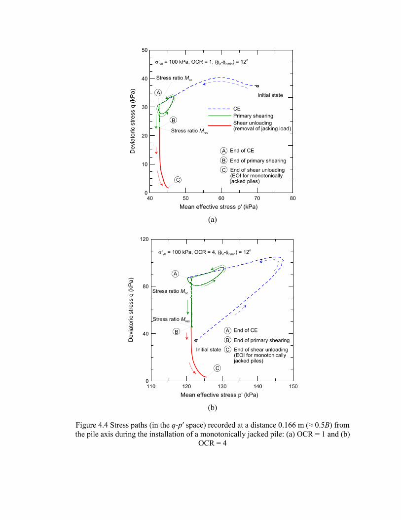
40 50 60 70 80Mean effective stress p' (kPa)

0

10

20

30

40

50

Dev

iato

ric s

tress

q (k

Pa)

CEPrimary shearingShear unloading(removal of jacking load)


A End of CE


End of shear unloading(EOI for monotonicallyjacked piles)

C

B

A

B

C

Initial state

Stress ratio Mcc

Stress ratio Mres

(a)


0

40

80

120

Dev

iato

ric s

tress

q (k

Pa)


A End of CE


End of shear unloading(EOI for monotonicallyjacked piles)

C

B

A

B

C

Initial state

Stress ratio Mcc

Stress ratio Mres

(b)

Figure 4.4 Stress paths (in the q-p′ space) recorded at a distance 0.166 m (≈ 0.5B) from the pile axis during the installation of a monotonically jacked pile: (a) OCR = 1 and (b)

OCR = 4


30

40

50

60

70

Dev

iato

ric s

tress

q (k

Pa)

Cavity expansionat 1.655m (≈5B)at 3.225m (≈10B)

Shear unloadingat 1.655m (≈5B)at 3.225m (≈10B)

Primary shearingat 1.655m (≈5B)at 3.225m (≈10B)

σ'v0 = 100 kPa, OCR = 4,(φc-φr,min) = 12o

A

C

Initialstate

A

C

(distances aremeasured from the pile axis)

B

BA End of CE

End of primaryshearing

End of shearunloading(EOI for monotonicallyjacked piles)

C

B

Figure 4.5 Stress paths (in the q-p′ space) recorded during the installation of a monotonically jacked pile at distances approximately equal to 5B and 10B from the pile

axis

We repeated the undrained shear loading and unloading stages (successive

application and removal of jacking strokes) to model multi-stroke jacking. The number of

such shear cycles depends on the number of jacking strokes N. For a pile installed using

30 jacking strokes (i.e., N = 30), Figure 4.6 shows the stress path in the q-p′ space [for

σ'v0 = 100 kPa, (φc- φr,min) = 12°, OCR = 2 and 4] recorded at the leftmost quadrature

point (at a distance 0.166 m from the pile axis after CE) of the first element adjacent to

the pile shaft. Up to the first shear unloading (point C), the stress path is identical to that

obtained for monotonic jacking (because we follow the same loading steps until point C).

Beyond this point, the nodes lying on the pile shaft are subjected to 30 undrained shear

loading and unloading cycles. As a result of these cycles, the stress path gradually moves

towards the left with a net decrease in p′. The point CM in Figure 4.6 represents the EOI

for a pile installed with 30 jacking strokes.

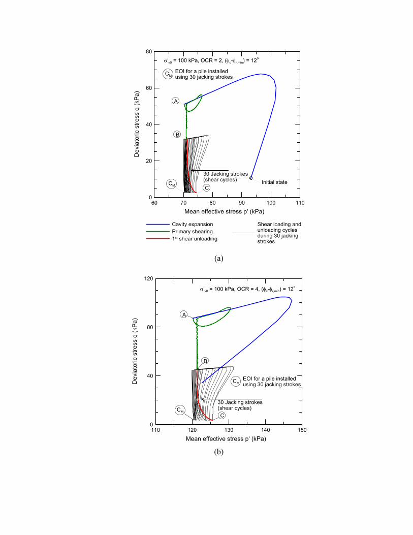
60 70 80 90 100 110Mean effective stress p' (kPa)

0

20

40

60

80

Dev

iato

ric s

tress

q (k

Pa)

Cavity expansionPrimary shearing1st shear unloading

30 Jacking strokes (shear cycles)


B

A

CCM

CMEOI for a pile installedusing 30 jacking strokes

Initial state

Shear loading andunloading cycles during 30 jackingstrokes

(a)


0

40

80

120

Dev

iato

ric s

tress

q (k

Pa)

30 Jacking strokes (shear cycles)


B

A

CCM

CMEOI for a pile installedusing 30 jacking strokes

(b)

Figure 4.6 Stress path (recorded at a distance 0.166 m from the pile axis) during the installation of a pile [σ'v0 = 100 kPa, (φc- φr,min) = 12°] using 30 jacking strokes: (a) OCR

= 2, (b) OCR = 4

We observe that the reduction in p′ (due to the application of 30 undrained shear

cycles along the pile shaft) is not significant; p′ reduces only by 5.8% and 4.2% (for OCR

= 2 and 4, respectively) as the stress path moves from point C (EOI for a monotonically

jacked pile) to point CM (EOI for a pile installed using 30 jacking strokes). This

observation corroborates the fact that friction fatigue, observed for piles jacked in sands,

is not significant for piles jacked in clays (under undrained conditions). Consequently, we

can expect that the shaft resistance of driven piles in clay will not differ significantly

from that developed in piles jacked in clay.

4.2.2. Dissipation of Excess Pore Pressure

At the end of installation, we allowed u (generated during pile installation) to dissipate

(stabilize) with time. Figure 4.7 shows the decay of u (at different distances from the pile

axis) with time [for σ'v0 = 100 kPa, (φc- φr,min) = 12° and OCR = 4]. Adjacent to the pile

shaft, 50% of the excess pore water pressure generated by the installation process

dissipates 7 days after pile installation, while it takes 6 months to dissipate 90% of the

excess pore water pressure due to pile installation (with the initial conditions σ'v0 = 100

kPa and OCR = 4). The u generated during the pile installation process decreases at

points further away from the pile axis. The time required for the dissipation of u depends

to a great extent on the value of hydraulic conductivity of clay. For example, if we

consider the hydraulic conductivity for LC to be 10-9 (a value measured using in situ tests

at different LC sites; Ratnam et al. 2005), the time required for the dissipation of 50%

and 90% excess pore pressure (generated by the installation process) adjacent to the pile

shaft will be 16.8 hours and 18 days, respectively (for the same conditions of Figure 4.7).

0.01 0.1 1 10 100 1000Time (month)

0

40

80

120

160

200

Exce

ss p

ore

pres

sure

u (k

Pa)

at 0.17 m (≈ 0.5B)at 0.33 m (≈ B)at 0.66 m (≈ 2B)at 1.66 m (≈ 5B)at 3.23 m (≈ 10B)at 6.68 m (≈ 20B)


(distances are measuredfrom the pile axis)

Figure 4.7 Dissipation of excess pore pressure u with time

Figure 4.8 shows the evolution of total and effective normal stress acting on the

pile shaft and at some distances from the pile during the dissipation of excess pore

pressure generated due to pile installation [for σ'v0 = 100 kPa, (φc- φr,min) = 12° and OCR

= 4]. Total normal (radial) stress σr decreases continuously during the dissipation of

excess pore pressure (Figure 4.8a). Effective normal (radial) stress σ′r acting on the pile

shaft and at a distance B from the pile axis increases continuously as the excess pore

pressure dissipates. At distances 2B and 5B from the pile axis, σ′r decreases in the initial

period of excess pore pressure dissipation and increases thereafter (Figure 4.8b).

0.01 0.1 1 10 100 1000Time (month)

150

250

350

450

Tota

l nor

mal

(rad

ial)

stre

ss σ

r (kP

a)

at 0.17 m (≈ 0.5B)at 0.33 m (≈ B)at 0.66 m (≈ 2B)at 1.66 m (≈ 5B)

σ'v0 = 100 kPa, OCR = 4,(φc-φr,min) = 12o


(a)

0.01 0.1 1 10 100 1000Time (month)

100

200

300

400

Effe

ctiv

e no

rmal

(rad

ial)

stre

ss σ

' r (k

Pa) at 0.17 m (≈ 0.5B)

at 0.33 m (≈ B)at 0.66 m (≈ 2B)at 1.66 m (≈ 5B)



(b)

Figure 4.8 Evolution of stresses with time (during the dissipation of excess pore pressure) at different distances from the pile shaft: (a) total normal (radial) stress σr, and (b)

effective normal (radial) stress σ′r

Pile installation significantly changes the stress state of the soil surrounding the

pile. Figure 4.9 shows the radial distribution of effective normal (radial) stress σ′r and

excess pore pressure u (generated during pile installation) within a zone 20B surrounding

the pile. As u dissipates from the pile-soil interface towards the free field, σ′r acting near

the pile shaft [within a radial zone approximately equal to 3B surrounding the pile for σ'v0

= 100 kPa, (φc- φr,min) = 12° and OCR = 4] increases significantly from its value at the

end of pile installation (Figure 4.9a).

0 4 8 12 16 20Normalized distance from the pile axis r/B

120

160

200

240

280

320

Effe

ctiv

e no

rmal

(rad

ial)

stre

ss σ

' r (k

Pa)

At the end of installationAt the end of 50% dissipation ofexcess pore pressureAt the end of 90% dissipation of excess pore pressure


(a)

0 4 8 12 16 20Normalized distance from the pile axis r/B

0

50

100

150

200

250

Exc

ess

pore

pre

ssur

e u

(kP

a)

At the end of installationAt the end of 50% dissipation ofexcess pore pressureAt the end of 90% dissipation of excess pore pressure


(b)

Figure 4.9 Radial distribution of (a) normal (radial) effective stress σ′r and (b) excess pore pressure u at the end of installation and at different stages of pore pressure

dissipation

4.2.3. Undrained Loading of the Pile

We simulated undrained loading of the pile after full dissipation of the u generated during

pile installation. Figure 4.10 shows the evolution of σr, u (generated during undrained

loading) and τz acting on the pile shaft during the undrained loading of the pile. Point D

(Figure 4.10) represents the end of the pore pressure dissipation stage when u and τz

acting on the pile shaft are equal to zero.

The mean effective stress p′ increases as u dissipates and the stress state moves

closer to the Normal Consolidation Line (NCL) (Figure 4.11). As a result, after u is fully

dissipated, the element adjacent to the pile shaft reaches nearly a normally consolidated

state. This creates a contractive tendency in the soil surrounding the pile shaft. Due to the

volume change constraint during undrained shearing, the contractiveness (tendency to

reduce volume) of the soil elements adjacent to the pile shaft is reflected through the

generation of positive excess pore pressure during undrained loading of the pile. At the

end of undrained loading (point EUD), a limit condition is reached along the pile shaft; the

vertical shear stress τz acting on the pile shaft at this limit state is equal to the unit limit

shaft resistance qsL.

0.2 0.4 0.6 0.8 1

Shear displacement δz (m)

0

100

200

300

400

Tota

l nor

mal

(rad

ial)

stre

ss σ

r, ex

cess

por

e pr

essu

re u

and

ve

rtica

l she

ar s

tress

τz (

kPa)

Total normal (radial) stressExcess pore pressureVertical shear stress

σ'v0 = 100 kPa, OCR (before installation) = 4, (φc-φr,min) = 12o

D

D

End of excess pore pressure dissipation (stabilization)

D

EUD End of undrained loading

EUD

EUD

Figure 4.10 Evolution of stresses on the pile shaft during undrained loading of the pile

80 120 160 200 240 280Mean effective stress p' (kPa)

0.8

0.85

0.9

0.95

1

1.05

Voi

d ra

tio e

Installation (involving CE,primary shearingand shear unloading)Dissipation of excesspore pressureUndrained loading

σ'v0 = 100 kPa, OCR (before installation) = 4(φc-φr,min) = 12o

Initial state

NCL

CSL

Figure 4.11 Evolution of void ratio e and mean effective stress p′ (for the leftmost quadrature point of the first element adjacent to the pile shaft) during installation,

dissipation of excess pore pressure and undrained loading of a monotonically jacked pile

4.3. Summary of Analysis Results

From the results of our analysis we observe that the soil surrounding the pile

undergoes complex changes in its in situ stress state during the installation (jacking) of

the pile, dissipation of excess pore pressure generated during installation, and loading of

the pile. During the undrained CE phase (associated with pile installation) the soil

surrounding the pile is pushed away radially from the path of the pile. This radial

displacement of soil increases the total normal (radial) stress and generates excess pore

pressure in the surrounding medium. However, the mean effective stress at a point just

adjacent to the pie shaft may increase or decrease depending on the initial value of OCR.

The shearing (along the pile shaft) phase associated with pile installation causes a

reduction of total normal stress acting on the pile shaft, however, the excess pore pressure

generated during the CE phase remains practically unchanged at the end of this phase. At

the end of installation (after the jacking load in removed from the pile head), the shear

stress acting on the pile shaft becomes zero (as we neglect any residual shear stress that

might be present along the pile shaft at this stage).

The effective normal (radial) stress and the mean effective stress within a zone

near the pile shaft increases as the excess pore pressure (generated during installation)

dissipates (through a radial flow) away from the pile. Consequently, the soil surrounding

the pile tends to approach the NCL. The increase in the effective normal stress acting on

the pile shaft increases the limit shaft resistance of the pile. Therefore, the evolution of

soil stress state during the dissipation of u plays an important role in determining the load

carrying behavior of the pile during loading. In the next chapter, we present the

coefficient of limit shaft resistance α which would be obtained from undrained load tests

performed on a jacked pile in clay at different times after the installation.

CHAPTER 5. USE OF RESULTS IN DESIGN AND QUALITY ASSURANCE OF PILING

5.1. Introduction

The existing methods for estimating the limit shaft resistance of displacement piles in

clay rely mostly on empirical relations based on data from experimental research on

model or full-scale piles. These methods relate the limit shaft resistance to relevant soil

state (existing before pile installation, as represented by a variable such as the in situ

vertical effective stress σ′v0) and/or shear strength parameters, such as the in situ

undrained shear strength su. Three different approaches are available in the literature: the

total stress approach (α method), the effective stress approach (β method), and the mixed

approach (λ method). In this report, we follow the total stress approach to estimate the

limit shaft resistance of a pile jacked in clay. According to the total stress approach, the

unit limit shaft resistance qsL is related to su through a factor α:

sL uq sα= (5.1)

The factor α is commonly known as the coefficient of shaft friction. In this

chapter, based on the FE simulation results (presented in Chapter 4), we propose a set of

equations for the estimation of qsL of a pile jacked in clay as function of the initial soil

state and the intrinsic shear strength parameters. The proposed equations can be used for

short- and long-term capacity calculations of displacement piles in clays. In this chapter

we also propose setup factors, to be used in conjunction with the proposed equations, to

calculate the shaft resistance of displacement piles in clays at different times after the

installation.

5.2. Proposed Equations for α

We calculate a long-term value of α (αLT) from the limiting value of the vertical shear

stress τz acting on the pile shaft at the end of undrained pile loading (point EUD in Figure

4.10) performed a long time after pile installation. At this stage, τz acting on the pile shaft

becomes equal to the unit limit shaft resistance qsL that would be available after full

dissipation of excess pore pressure generated during pile installation. We also calculate a

short-term value of α (αST) from the limiting value of τz acting on the pile shaft at the end

of the “primary shearing” phase (point B in Figure 4.3) of installation. This value of τz

will be equal to the limit unit shaft resistance qsL that would be available if a load test

were performed immediately after installation. Mathematically

at B sL, STST

u u

z qs s

τα = = (5.2)

UDat E sL, LT LT

u u

z qs s

τα = = (5.3)

We select appropriate values of su (corresponding to particular values of σ′v0 and OCR)

from Table 4.1 to calculate α from equations (5.2) and (5.3). Based on the FEA results,

we propose the following equations for α that can be used in the design of a jacked pile

in clay:

( ) ( ) 2Av0ST 1 1 c r,min

A

1.03 A 1 A expp

σα φ φ⎡ ⎤⎧ ⎫⎛ ⎞′⎪ ⎪= + − − −⎢ ⎥⎨ ⎬⎜ ⎟

⎪ ⎪⎢ ⎥⎝ ⎠⎩ ⎭⎣ ⎦ (5.4)

and,

( ) ( ) 3

0.05Au v0

LT 1 1 c r,minv0 A

1.28 A 1 A expsp

σα φ φσ

− ⎡ ⎤⎧ ⎫⎛ ⎞ ⎛ ⎞′⎪ ⎪= + − − −⎢ ⎥⎨ ⎬⎜ ⎟ ⎜ ⎟′ ⎪ ⎪⎢ ⎥⎝ ⎠⎝ ⎠ ⎩ ⎭⎣ ⎦ (5.5)

where

( )( )

c r,min1

c r,min

0.75 for 5A

0.43 for 12

φ φ

φ φ

⎧ − =⎪= ⎨− =⎪⎩

o

o (5.6)

u2

v0

A 0.55 0.43ln sσ

⎛ ⎞= + ⎜ ⎟′⎝ ⎠

(5.7)

u3

v0

A 0.64 0.40ln sσ

⎛ ⎞= + ⎜ ⎟′⎝ ⎠

(5.8)

Figure 5.1 and Figure 5.2 show the α values obtained from the FEAs involving

the installation and loading of jacked piles in LC, respectively, in the short and long term

(shortly after and long after pile installation). These figures also show the predictions

using equations (5.4) through (5.8). We observe that α decreases as the initial value

(before pile installation) of OCR increases. The in situ strength ratio su/σ′v0 for clay

depends on the OCR value (Table 4.1); su/σ′v0 increases as OCR increases (i.e., soil

becomes stiffer with increasing OCR). Therefore, the α value decreases as the su/σ′v0

value increases. We also observe that the α value depends strongly on the difference of

the friction angles at critical and residual state (φc-φr,min). For a clay that shows residual

behavior, the value of α decreases (for a given OCR value) with increasing values of (φc-

φr,min) and σ′v0. However, for a clay showing no residual behavior (i.e., for φc-φr,min = 0°),

the α value does not depend on the σ′v0. The rate of decrease in the value of α is more

pronounced for lower values of σ′v0. For clays with OCR ≥ 4, α reaches an asymptotic

value (this value depends on the value of OCR) for σ′v0 ≥150 kPa.

0 1 2 3

Normalized initial vertical effective stress (σ'v0/pA)(pA = 100 kPa)

0.7

0.8

0.9

1

1.1

Coe

ffici

ent o

f uni

t lim

it sh

aft r

esis

tanc

e α

ST

φc-φr,min=5o

OCR = 1; su /σ'v0 = 0.173

Symbols are from FE simulationsLines are from proposed equationsOCR denotes the overconsolidationratio of the in situ soil

OCR = 2; su /σ'v0 = 0.289

OCR = 4; su /σ'v0 = 0.492

OCR = 8; su /σ'v0 = 0.844

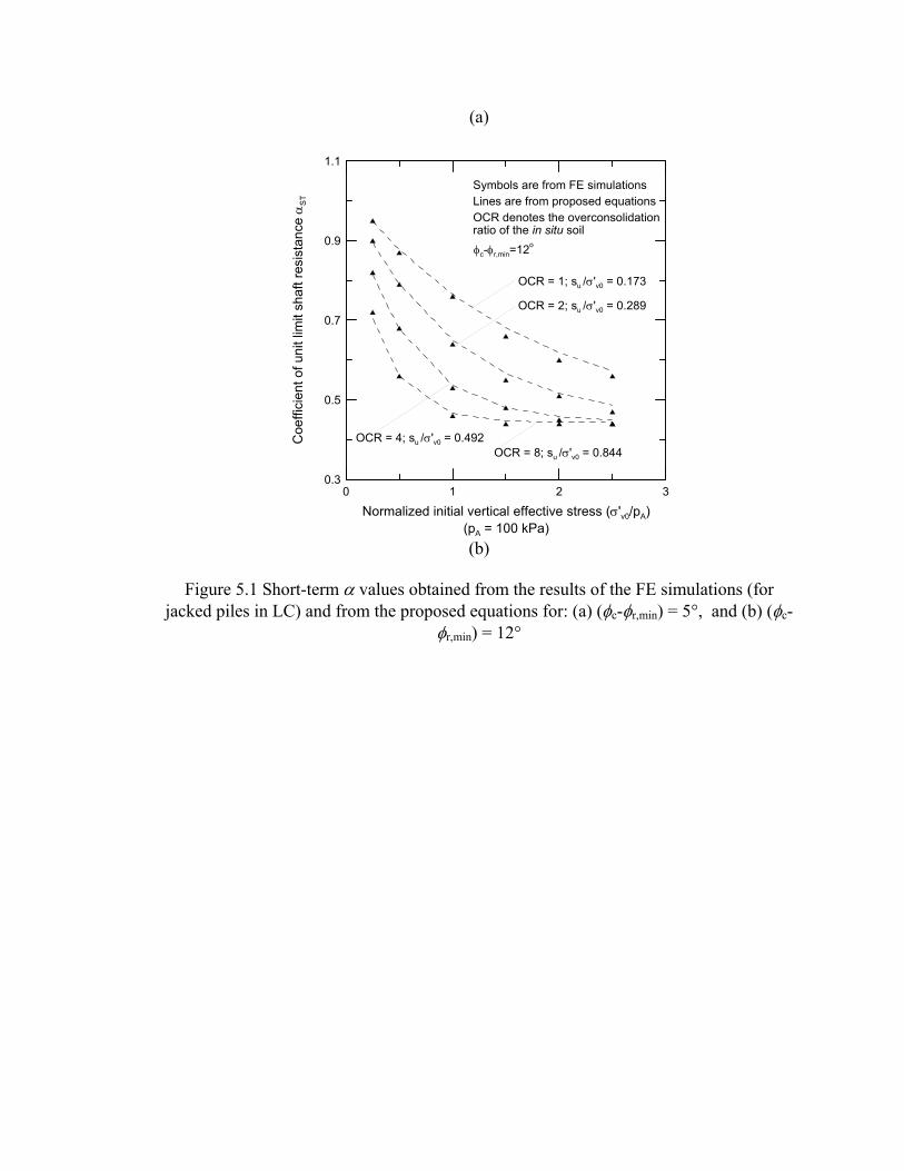
(a)

0 1 2 3


0.3

0.5

0.7

0.9

1.1

Coe

ffici

ent o

f uni

t lim

it sh

aft r

esis

tanc

e α

ST

φc-φr,min=12o

OCR = 1; su /σ'v0 = 0.173


OCR = 2; su /σ'v0 = 0.289

OCR = 4; su /σ'v0 = 0.492OCR = 8; su /σ'v0 = 0.844

(b)

Figure 5.1 Short-term α values obtained from the results of the FE simulations (for jacked piles in LC) and from the proposed equations for: (a) (φc-φr,min) = 5°, and (b) (φc-

φr,min) = 12°

0 1 2 3


1.2

1.3

1.4

1.5

Coe

ffici

ent o

f uni

t lim

it sh

aft r

esis

tanc

e α

LT

φc-φr,min=0o

OCR = 1; su /σ'v0 = 0.173


OCR = 2; su /σ'v0 = 0.289

OCR = 4; su /σ'v0 = 0.492

OCR = 8; su /σ'v0 = 0.844

(a)

0 1 2 3


0.9

1.1

1.3

1.5

Coe

ffici

ent o

f uni

t lim

it sh

aft r

esis

tanc

e α

LT

φc-φr,min=5o

OCR = 1; su /σ'v0 = 0.173


OCR = 2; su /σ'v0 = 0.289

OCR = 4; su /σ'v0 = 0.492 OCR = 8; su /σ'v0 = 0.844

(b)

0 1 2 3


0.4

0.8

1.2

1.6

Coe

ffici

ent o

f uni

t lim

it sh

aft r

esis

tanc

e α

LT

φc-φr,min=12o

OCR = 1; su /σ'v0 = 0.173


OCR = 2; su /σ'v0 = 0.289

OCR = 4; su /σ'v0 = 0.492 OCR = 8; su /σ'v0 = 0.844

(c)

Figure 5.2 Long-term α values obtained from the results of the FE simulations (for jacked piles in LC) and from the proposed equations for: (a) (φc-φr,min) = 0°, (b) (φc-φr,min) = 5°,

and (c) (φc-φr,min) = 12°

5.3. Setup Factors

In practice, depending on the construction schedule, the time interval between installation

and loading of a pile may not be always enough for the excess pore pressure (generated

during installation of piles) to dissipate completely. Therefore, the limit shaft resistance

qsL available at the time of pile loading will be intermediate between qsL estimated using

the value of α available after full pore pressure dissipation (αlong-term) and that estimated

using the value corresponding to zero pore pressure dissipation (αshort-term, available

immediately after installation). We performed analyses to investigate the variation of qsL

with time after pile installation. Based on the results from these analyses, we propose a

setup factor Fs that allows precise estimation of qsL at any given time after pile

installation. We define Fs as the ratio of the qsL available at any particular time t after pile

installation to that available immediately after installation. Mathematically:

at time after installation

immediately after installation

sL ts

sL

qF

q= (5.9)

Figure 5.3 shows the variation of Fs with time [for σ′v0 = 25 and 250 kPa, OCR =

1 and 8, and (φc-φr,min = 12°)] available for the dissipation of u after the installation of a

jacked pile in LC. We observe that the increase in Fs (and thus also in qsL) with time after

installation of a jacked pile depends on both σ′v0 and OCR. Fs increases as the initial

vertical effective stress (before pile installation) σ′v0 increases. For a lower value of σ′v0

(= 25 kPa), Fs decreases as OCR increases (except for pile loading within a very short

time after installation; see Figure 5.3a); however, for a higher value of σ′v0 (= 250 kPa),

Fs increases with increasing values of OCR (Figure 5.3b).

The time shown in Figure 5.3 was calculated based on a value of clay hydraulic

conductivity equal to 10-10 m/s, which is a representative value of hydraulic conductivity

for natural LC deposits (Ratnam et al. 2005). For a clay deposit with a different value of

hydraulic conductivity, the time scales mentioned in Figure 5.3 need to be revised. For

example, if the value of hydraulic conductivity of clay deposit at a particular site is equal

to 10-9 m/s (which is 10 times larger than the value assumed in our analysis) the

horizontal axes (i.e., the time axes) of Figure 5.3 should be divided by 10 to have a

proper estimation of Fs. Figure 5.4 shows the variation of Fs with normalized time T. To

obtain T, we normalize the real time t with respect to clay hydraulic conductivity k, in situ

undrained shear strength su and pile diameter B:

u2

w

ks tTBγ

= (5.10)

where γw is the unit weight of water. The normalization of t, as expressed in equation

(5.10), facilitates the use of the proposed setup factors for any value of k and pile

diameter B.

0 2 4 6 8Time allowed for the dissipation of u (months)

1

1.04

1.08

1.12

1.16

1.2

Set

up fa

ctor

Fs

σ'v0 = 25 kPa, (φc-φr,min) = 12o

OCR = 8

OCR = 1

(a)

0 2 4 6 8Time allowed for the dissipation of u (months)

1

1.05

1.1

1.15

1.2

1.25

1.3

Set

up fa

ctor

Fs

σ'v0 = 250 kPa, (φc-φr,min) = 12o

OCR = 1

OCR = 8

(b)

Figure 5.3 Setup factor Fs at different times after the installation of a jacked pile in LC for: (a) σ′v0 =25 kPa, and (b) σ′v0 =250 kPa

0.0001 0.001 0.01 0.1 1 10Time factor T

1

1.1

1.2

1.3

Set

up fa

ctor

Fs

σ'v0 = 25 kPa, (φc-φr,min) = 12o

OCR = 8, su/σ'v0 = 0.844

OCR = 1, su/σ'v0 = 0.173

(a)

0.001 0.01 0.1 1 10 100Time factor T

1

1.05

1.1

1.15

1.2

1.25

1.3

Set

up fa

ctor

Fs

σ'v0 = 250 kPa, (φc-φr,min) = 12o

OCR = 1, su/σ'v0 = 0.173

OCR = 8, su/σ'v0 = 0.844

(b)

Figure 5.4 Variation of setup factor Fs with normalized time T after the installation of a jacked pile in LC for: (a) σ′v0 =25 kPa and (b) σ′v0 =250 kPa

Figure 5.5 shows the variation of Fs with the degree of consolidation U (a direct

measure of % dissipation of excess pore pressure generated during pile installation) of the

soil adjacent to the pile shaft [for σ′v0 = 25 and 250 kPa, OCR = 1 and 8, and (φc-φr,min =

12°)]. Any particular value of U in Figure 5.5 corresponds to different absolute times

(elapsed between installation and loading of pile) for different initial conditions (σ′v0 and

OCR). For σ′v0 = 25 kPa, Fs corresponding to a certain degree of consolidation decreases

with OCR. However, for σ′v0 = 250 kPa, Fs corresponding to a particular value of U does

not vary significantly with OCR.

0 20 40 60 80 100Degree of consolidation U (%)

1

1.05

1.1

1.15

1.2

1.25

1.3

Set

up fa

ctor

Fs

σ'v0 = 25 kPa, OCR = 1σ'v0 = 25 kPa, OCR = 8σ'v0 = 250 kPa, OCR = 1σ'v0 = 250 kPa, OCR = 8

(φc-φr,min) = 12o

Figure 5.5 Setup factor Fs at different stages of consolidation (just adjacent to the pile shaft) after the installation of a jacked pile in LC

5.4. Validation of the Proposed Equations

We developed equations (5.4) through (5.8) from the results of FEA for LC. To assess the

validity of these equations for other clays (having properties different from those of LC)

we performed a few additional analyses for piles installed in SFBM [φc = 29° and (φc-

φr,min) = 13°]. Figure 5.6 shows that the α values (long-term) predicted using the

proposed equations are in good agreement with the α values (long-term) obtained from

the FEA for SFBM (note that the properties of LC and SFBM are different). Additionally,

we compared the long-term α values obtained using the equations proposed in this

chapter with the α values deduced by Semple and Rigden (1984) from field pile load test

on driven piles. Figure 5.7 shows the variation of α values with normalized initial

undrained shear strength su/σ'v0. We also calculated α values following the API RP-2A

(1993) guidelines and included them in Figure 5.7. The α values obtained using the

proposed equations are in good agreement with those obtained from the field test results

and also with the α values obtained following the API RP-2A (1993) guidelines.

0 0.4 0.8 1.2 1.6

Normalized initial undrained shear strength (su /σ'v0)

0.4

0.6

0.8

1

1.2

Coe

ffici

ent o

f uni

t lim

it sh

aft r

esis

tanc

e α

LT

Symbols are from FE simulations for SFBMLines are from proposed eqations

σ'v0 = 50 kPa

σ'v0 = 250 kPa

Figure 5.6 Comparison of α values obtained from the results of the FEA for SFBM with those calculated using the proposed equations [with (φc-φr,min) = 13°]

0 1 2 3

Normalized initial undrained shear strength su /σ'v0

0.4

0.8

1.2

Coe

ffici

ent o

f uni

t lim

it sh

aft r

esis

tanc

e α

LT

Field database(Semple and Rigden 1984)Prediction using proposed equations[calculated with (φc-φr,min) = 12o]API guideline (1993-RP2A)

Figure 5.7 Comparison of α values predicted by the proposed equations with those calculated following the API RP-2A criterion and obtained from the field data reported

by Sempel and Rigden (1984)

Kim et al. (2009) and Seo et al. (2009) reported the results of instrumented load

tests on closed-ended pipe piles and H piles, respectively. These piles were driven into a

multilayered soil profile (11 different soils) and were embedded slightly in a very dense

nonplastic silt layer to a depth of 17.4 m. From the results of dynamic pile load tests

performed immediately after pile driving and at different times (1, 8, 107 and 127 days)

after pile installation, we calculated the setup factors Fs which represent the gain in the

local unit limit shaft resistance at different depths within 9m and 17.5m. Figure 5.8 shows

the variation of Fs with different values of the time factor T. This figure also shows the

values of Fs that would be obtained using the results of the present analysis for a deposit

of pure clay. The prediction from our analysis matches well a number of dynamic load

tests, but some dynamic test results show either relaxation (i.e., Fs<1) or excessive

increase in the unit limit shaft resistance. We believe that this shows that dynamic load

test (PDA) results have the potential to capture the setup process but in their current state

can be substantially in error as well.

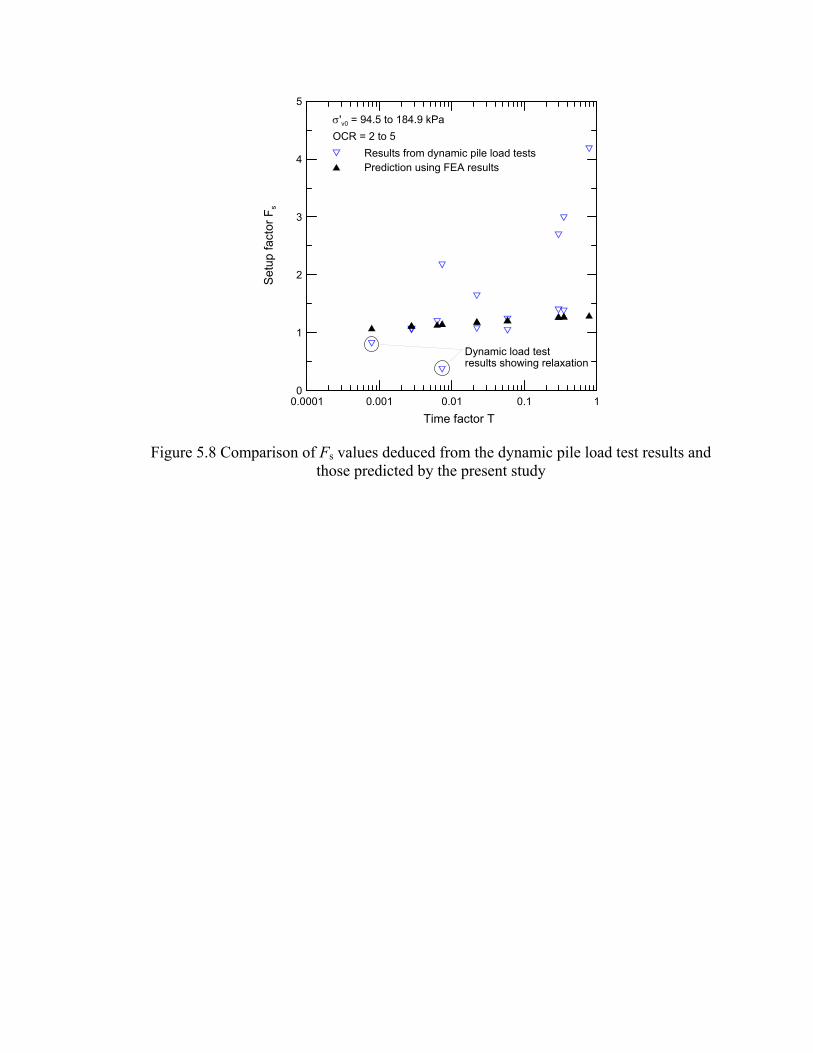
0.0001 0.001 0.01 0.1 1Time factor T

0

1

2

3

4

5

Set

up fa

ctor

Fs

Results from dynamic pile load testsPrediction using FEA results

σ'v0 = 94.5 to 184.9 kPaOCR = 2 to 5

Dynamic load testresults showing relaxation

Figure 5.8 Comparison of Fs values deduced from the dynamic pile load test results and those predicted by the present study

CHAPTER 6. SUMMARY AND CONCLUSIONS

6.1. Summary

When piles are installed by jacking or driving, they cause substantial changes in the state

of soil located near the pile. These changes result from the complex loading imposed on

the soil by expansion of a cylindrical cavity to make room for the pile, by multiple cycles

of shearing in the vertical direction as the pile gradually moves down into the ground, and

by the slow drainage associated with clayey soils. During the undrained expansion of a

cylindrical cavity (associated with pile installation) the soil surrounding the pile is pushed

away radially from the path of the pile. This radial displacement of soil increases the total

normal (radial) stress and generates excess pore pressure in the surrounding ground. The

shearing (along the pile shaft) associated with pile installation causes a reduction of total

normal stress acting on the pile shaft; however, the excess pore pressure generated due to

cavity expansion remains practically unaltered by the vertical shearing along the pile

shaft.

If a pile is load-tested a short time after installation, it will develop an axial

resistance that reflects the existence in the soil of the excess pore pressures caused by the

installation process. The evolution of the soil stress state during the dissipation of excess

pore pressure plays an important role in determining the load carrying behavior of the

pile during loading at any particular time after pile installation. The effective normal

(radial) stress and the mean effective stress within a zone near the pile shaft increase as

the excess pore pressure (generated during installation) dissipates (through radial flow)

away from the pile. After the excess pore pressures dissipate, the axial pile resistance will

be different from that measured in the short term. This difference is referred to as pile

setup (if the resistance increases) or relaxation (if the resistance drops). This report

focuses on the pile setup observed in clayey soils, in which it can be quite significant.

Pile setup in clays results primarily from shaft resistance gains with time after

installation because the base resistance contributes proportionally much less in soft to

medium stiff clays, which are the focus of the present research. Accordingly, our focus

has been on analyzing setup in shaft resistance, validating the equations resulting from

these analyses and then proposing design and quality assurance procedures based on the

results of the analyses. The analyses were done using the finite element method and an

advanced constitutive model developed specifically for this project. The constitutive

model captures all the key features required for these analyses, and the finite element

analyses are 1D analyses of shaft resistance that can handle the large deformations and

displacements involved in pile installation. The results of the analyses compare well with

load test data from the literature. Design equations for the unit shaft resistance are

proposed. Equations for unit shaft resistance in the short term (for comparison with load

tests) are also proposed.

6.2. Conclusions

Based on findings of the present study, we can draw conclusions as follows:

1. The changes in the soil caused by pile installation, a rest period and then loading are

very complex and cannot be modeled with any reliability in a simplistic way.

2. The pile installation process is not simply a cavity expansion process, as many have

believed. Shearing has a large impact in that it reduces the normal stress on the pile shaft

from the very large stresses that would be predicted by cavity expansion alone. Cycles of

shearing along the pile shaft (applied during pile installation) cause further degradation of

the normal stress on the pile-soil interface and thus of the pile shaft resistance. However,

this degradation of pile shaft resistance is not as significant as in piles in sand and can be

considered small.

3. The ratio of the limit shaft resistance of jacked piles in clay a long time after pile

installation (after complete excess pore pressure dissipation) to that just after pile

installation ranges from 1.23 to 1.37.

4. The setup factor Fs (with respect to shaft resistance) increases with time after

installation of a jacked pile and depends on both σ′v0 and OCR. Fs increases as the initial

vertical effective stress (before pile installation) σ′v0 increases. For a lower value of σ′v0

(= 25 kPa), Fs decreases as the OCR increases (except for pile loading within a very short

time after installation); however, for a higher value of σ′v0 (= 250 kPa), i.e., for deeper

pile segments, Fs increases with increasing values of OCR.

5. For low initial vertical effective stress (i.e., vertical effective stress before pile

installation), Fs corresponding to a certain degree of consolidation U (just adjacent to the

pile shaft) decreases with OCR. This is shown in the report, for example, for σ′v0 = 25

kPa. However, for higher values of σ′v0 (for example, 250 kPa), Fs corresponding to a

particular value of U does not vary significantly with OCR.

6. The absolute time t required for a certain degree of consolidation around the pile shaft

can be normalized with respect to clay hydraulic conductivity k, in situ undrained shear

strength su and pile diameter B.

7. Dynamic pile load test results have the potential to capture the setup process but in

their current state can be substantially in error as well.

LIST OF REFERENCES

Abbo, A. J. and Sloan, S. W. (2000). Solid nonlinear analysis code (SNAC), User manual version 2.0, Department of Civil, Surveying and Environmental Engineering, University of Newcastle, Australia.

Al-Tabbaa, A, and Stegemann, J.A. (2005) “Stabilisation/solidification Treatment and Remediation: Advances in S/S for Waste and Contaminated Land”, Proceedings of the International Conference on Stabilisation/Solidification Treatment and Rememdiation, University of Cambridge, United Kingdom, 12-13 April 2005

API RP-2A. (1993). Recommended practice for planning, designing and constructing fixed offshore platforms – working stress design. 20th edition, American Petrolium Institute.

Augustesen, A.H. (2006). The effects of time on soil behavior and pile capacity. Ph.D. Thesis, Aalborg University, Denmark, ISSN 1901-7294.

Axelsson, G. (2000). “Long-Term Increase in Shaft Capacity of Non-Cohesive Soils.” Thesis, Royal Institute of Technology, Division of Soil and Rock Mechanics, Stockholm, 194 p.

Azzouz, A. S., Baligh, M. M., Whittle, A. J. (1990). Shaft resistance of piles in clay. Journal of Geotechnical Engineering, ASCE, Vol. 116, No. 2, pp. 205-221.

Baligh, M. M. (1985). Strain path method. Journal of Geotechnical Engineering, ASCE, Vol. 111, No. 9, pp. 1108 – 1136.

Basu, P., Loukidis, D., Prezzi, M., and Salgado, R. (2009). Analysis of shaft resistance of jacked piles in sands. Accepted for publication in the International Journal for Analytical and Numerical Methods in Geomechanics.

Bishop, A. W., Green, G. E., Garga, V. K., Andresen, A., and Brown, J. D. (1971). New ring shear apparatus and its application to the measurement of residual strength. Géotechnique, Vol. 21, No. 4, 273–328.

Biot, M.A. (1941). General theory of three-dimensional consolidation. Journal of Applied Physics, Vol.12, pp. 155-164.

Bonaparte, R. (1982). “A Time-Dependent Constitutive Model for Cohesive Soils.” Ph.D. Thesis, University of California, Berkeley, CA.

Bond, A.J. and Jardine, R.J. (1991). Effects of installing displacement piles in a high OCR clay. Géotechnique, Vol. 41, No. 3, pp. 341-363.

Bullock, Paul Joseph (1999). “Pile Friction Freeze: A Field and Laboratory Study, Volume 1,” Ph.D. Dissertation, University of Florida.

Carter J. P., Randolph, M. F. and Wroth, C. P. (1979). Stress and pore pressure changes in clay during and after the expansion of a cylindrical cavity. International Journal of Analytical and Numerical Methods in Geomechanics. Vol. 3, pp. 305-322.

Chakraborty, T. (2009). Development of a clay constitutive model and its application to pile boundary value problems. Ph. D. Thesis. Purdue University, U.S.A.

Cho, C.W., Lee, M.W., and Randolph, M.F. (2000). "Set-up considerations in wave equation analysis of pile driving", Proc. Conf. on Application of Stress-Wave Theory to Piles, Sao Paulo, Brazil, Balkema, 41-46.

Chow, F.C., Jardine, R.J., Brucy, F., and Nauroy, J.F. (1998). “Effects of Time on Capacity of Pipe Piles in Dense Marine Sand,” Journal of Geotechnical and Geoenvironmental Engineering, ASCE, Vol. 124, No. 3, pp. 254-264.

Collins, I.F., Pender, M.J. and Yan, W. (1992), “Cavity expansion in sands under drained loading conditions”, International Journal of Numerical and Analytical Methods in Geomechanics, Vol. 16, No. 1, pp. 3-23.

Cooke, R. W., Price, G. and Tarr, K. (1979). Jacked piles in London clay: A study of load transfer and settlement under working conditions. Géotechnique, Vol. 29, No. 2, pp. 113-147.

Coop, M.R. and Wroth, C.P. (1989). “Field Studies of an Instrumented Model Pile in Clay.” Geotechnique, Vol. 39, No. 4, pp. 679-696.

Dafalias, Y. F. and Manzari, M. T. (2004). Simple plasticity sand model accounting for fabric change effects. Journal of Engineering Mechanics, ASCE, Vol. 130, No. 6, pp. 622- 634.

Dafalias, Y. F., Manzari, M. T. and Papadimitriou, A. G. (2006). SANICLAY: Simple anisotropic clay plasticity model. International Journal Numerical Analytical Methods in Geomechanics, Vol. 30, pp.1231–1257.

Dafalias, Y. F., Papadimitriou, A. G. and Li, X. S. (2004). “Sand Plasticity Model Accounting for Inherent Fabric Anisotropy.” Journal of Engineering Mechanics, ASCE, Vol. 130, No. 11, pp.1319-1333.

Gasparre, A. (2005). Advanced laboratory characterization of London Clay. Ph. D. Thesis, Imperial College of Science, Technology and Medicine, University of London, England.

Gasparre, A., Nishimura, S., Coop, M. R., and Jardine, R. J. (2007a). The influence of structure on the behaviour of London Clay. Géotechnique, Vol. 57. No. 1, pp. 19-31.

Gasparre, A., Nishimura, S., Minh, N. A., Coop, M. R., and Jardine, R. J. (2007b). The stiffness of natural London Clay. Géotechnique, Vol. 57, No. 1, pp. 33-47.

Gens A. (1982). “Stress–Strain and Strength of A Low Plasticity Clay” Ph.D. Thesis, Imperial College, London University.

Hight, D.W., McMillan, F., Powell, J.J.M., Jardine, R.J. and Allenou, C.P. (2003): “Some characteristics of London Clay,” Characterisation of Engineering Properties of Natural Soils, Balkema, pp.851-908.

Hu, L. and Pu, J. (2004). Testing and modeling of soil structure interface. Journal of Geotechnical and Geoenvironmental Engineering, ASCE, Vol. 130, No. 8, pp. 851-860.

Hu, Y. and Randolph, M.F. (1998) A practical numerical approach for large deformation problems in soil. International Journal of Numerical and Analytical Methods in Geomechanics, Vol. 22, No. 5, pp. 327-350.

Jain S. and Nanda, A. (2008). “Constitutive Modelling of San Francisco Bay Mud”. Proceedings of the 12th International Conference of International Association for Computer Methods and Advances in Geomechanics (IACMAG), 1-6 October, 2008, Goa, India.

Jain S.K. (1985). “Analysis of The Pressuremeter Test by FEM Formulation of The Elasto-Plastic Consolidation”, Ph.D. Thesis, Virginia Tech, Blacksburg, Virginia, USA.

Karlsrud, K., and Haugen, T. (1985), Axial static capacity of steel model piles in overconsolidated clay. Proceedings of the 11th International Conference on Soil Mechanics and Foundation Engineering, San Francisco, pp. 1401-1406.

Kim, D., Bica, A.V.D., Salgado, R., Prezzi, M. and Lee, W. (2009). Load Testing of a Closed-Ended Pipe Pile Driven in Multilayered Soil, Journal of Geotechnical and Geoenvironmental Engineering, Vol. 135, Issue 4, pp. 463-473.

Kirkgard, M.M., and Lade, P.V., (1991). "Anisotropy of Normally Consolidated San Francisco Bay Mud", Geotechnical Testing Journal, GTJODJ ASTM, Vol. 14, No. 3, pp. 231-246.

Komurka, V.E., Wagner, A.B., and Edil, T.B., (2003) “A Review of Pile Set-Up,” 51st Annual Geotechnical Engineering Conference, edited by J.F. Labuz and J.G. Bentler, University of Minnesota.

Konard, J. M. and Roy, M. (1987). Bearing capacity of friction piles in marine clay. Géotechnique, Vol. 37, No. 2, pp. 163-175.

Ladd, C. C. and Edgers, L. (1972). “Consolidated-Undrained Direct Simple Shear Tests on Boston Blue Clay”, Research Report R72-82, Department of Civil Engineering, MIT, Cambridge, MA.

Ladd, C. C., Varallyay J. (1965). The influence of the stress system on the behavior of saturated clays during undrained shear. Research Report No. R65-11, Department of Civil Engineering, Massachusetts Institute of Technology (MIT), U.S.A.

Lee, P. K. K., Tham, L. G., Chan, S. T., Yu, F., and Yang, J. (2004). Recent field study on the behavior of jacked piles. The Structural Engineer, pp. 19-22.

Lehane, B. M. (1992). Experimental investigations of pile behavior using instrumented field piles. Ph. D. Thesis, Imperial College of Science, Technology and Medicine, University of London, England.

Lehane, B. M., Jardine, R. J., Bond, A. J., and Chow, F. C. (1994). The development of shaft resistance on displacement piles in clay. Proceedings of the 13th International Conference on Soil Mechanics and Foundation Engineering, New Delhi, India, pp. 473-476.

Li, X. S. (2002). “A Sand Model with State-Dependent Dilatancy.” Géotechnique, Vol. 52, No. 3, pp. 173-186.

Li, X. S. and Dafalias, Y. F. (2000). Dilatancy of cohesionless soils. Géotechnique, Vol. 50, No. 4, pp. 449-460.

Ling, H. I., Yue, D., Kaliakin, V., and Themelis, N.J. (2002). “An Anisotropic Elasto-Plastic Bounding Surface Model for Cohesive Soils” Journal of Engineering Mechanics, ASCE, Vol. 128, No. 7, pp. 748-758.

Long, J. H., Kerrigan, J. A., and Wysockey, M. H. (1999). Measured time effects for axial capacity of driven piles. Transportation Research Record 1663, Paper No. 99-1183.

Loukidis, D. (2006). Advanced constitutive modeling of sands and applications to foundation engineering. Ph. D. Thesis, Purdue University, U.S.A.

Loukidis, D. and Salgado, R. (2008a). Modeling sand response using two-surface plasticity. Computers and Geotechnics, doi:10.1016/j.compgeo.2008.02.009 (in press).

Loukidis D. and Salgado R. (2008b). Analysis of the shaft resistance of non-displacement piles in sand. Géotechnique, Vol. 58, No. 4, 283-296.

Manzari, M. T. and Dafalias, Y. F. (1997). A critical state two-surface plasticity model for sands. Géotechnique, Vol. 47, No. 2, pp. 255-272.

Meehan, C. L. (2006). “An Experimental Study of the Dynamic Behavior of Slickensided Surfaces” PhD Thesis, Virginia Polytechnic Institute and State University. Blacksburg, Virginia.

Oka, F., Kodaka, T., and Kimoto, S., Ichinose, T. and Higo, Y. (2005). Strain localization of rectangular clay specimen under undrained triaxial compression conditions. Proceedings of the 16th International Conference on Soil Mechanics and Geotechnical Engineering. Osaka, Japan.

Papadimitriou, A. G., Bouckovalas, G. D. and Dafalias, Y. F. (2001). Plasticity model for sand under small and large cyclic strains. Journal of Geotechnical and Geonvironmental Engineering, ASCE, Vol. 127, No. 11, pp. 973-983.

Papadimitriou, A. G. and Bouckovalas, G. D. (2002). Plasticity model for sand under small and large cyclic strains: a multiaxial formulation. Soil Dynamics and Earthquake Engineering, Vol. 22, No. 3, pp.191-204.

Papadimitriou AG, Manzari MT and Dafalias YF. (2005) “Calibration of A Simple Anisotropic Plasticity Model for Soft Clays.” Proceedings, GeoFrontiers Conference of ASCE, January 24–26, Austin, TX, Geotechnical Special Publication No. 128, pp. 415–424.

Pestana, J. M., Hunt, C. E., Bray, J. D. (2002). Soil deformation and excess pore pressure field around a closed-ended pile. Journal of Geotechnical and Geoenvironmental Engineering, ASCE, Vol. 128, No. 1, pp. 1-12.

Potts, D. M. and Martins, J. P. (1982). The shaft resistance of axially loaded piles in clay. Géotechnique, Vol. 32, No. 4, pp. 369-386.

Randolph, M.F. and Wroth, C.P. (1978). Analysis of deformation of vertically loaded piles. Journal of Geotechnical Engineering, ASCE, Vol. 104, GT12, pp. 1-17.

Randolph, M. F., Carter, J. P. and Wroth, C. P. (1979). Driven piles in clay – the effects of installation and subsequent consolidation, Géotechnique, Vol. 29, No. 4, pp 361-393.

Ratnam, S., Soga, K. and Whittle, R.W. (2005). A field permeability measurement technique using conventional self-boring pressuremeter. Géotechnique, Vol. 55, No. 7, pp. 527-537.

Rau, G.A. (1999). “Evaluation of Strength Degradation in Seismic Loading of Holocene Bay Mud from Marin County.” PhD Thesis, University of California, Berkeley, California.

Salgado, R. and Randolph, M.F. (2001) Analysis of cavity expansion in sand. International Journal of Geomechanics. Vol. 1, No. 2, pp. 175-192.

Salgado, R. (2006). The role of analysis in non-displacement pile design. Modern Trends in Geomechanics, Springer Proceedings in Physics, Vol. 106, Eds. W. Wu and H-S Yu , pp. 521-540.

Salgado, R. (2008). Engineering of Foundations. Mc Graw-Hill, New York, U.S.A., 2008.

Santagata, M., Germaine, J. T., Ladd, C. C. (2007). “Small-Strain Nonlinearity of Normally Consolidated Clay” Journal of Geotechnical and Geoenvironmental Engineering, Vol. 133, No. 1, pp. 72-82.

Sempel, R. M., and Rigden, W. J. (1984). Shaft capacity of driven pipe piles in clay. Analysis and Design of Pile Foundations, Ed. J. R. Meyer, ASCE, pp. 59-78.

Seo, H., Yildirim, I.Z. and Prezzi, M. (2009) “Assessment of the Axial Load Response of an H Pile Driven in Multilayered Soil”, Journal of Geotechnical and Geoenvironmental Engineering, ASCE, Published Online.

Sheahan TC. (1991) “An Experimental Study of the Time-Dependent Undrained Shear Behavior of Resedimented Clay using Automated Stress Path Equipment.”, Sc.D Thesis, MIT, Cambridge, MA.

Sheng, D., Sloan, S. W. and Yu, H. S. (2000). “Aspects of Finite Element Implementation of Critical State Models”, Computational Mechanics, Vol. 26, pp. 185–196.

Skov, R. and Denver, H. (1988). “Time-Dependence of Bearing Capacity of Piles,” Proceedings 3rd International Conference on Application of Stress-Waves to Piles, pp. 1-10.

Steenfelt, J. S., Randolph, M. F., and Wroth, C. P. (1980). Instrumented model piles jacked into clay. Proceedings of the 10th International Conference on Soil Mechanics and Foundation Engineering, Stockholm, Ed. N. Flodin, A.A. Balkema, Rotterdam, Vol. 2, pp. 857-864.

Stewart, H. E. and Hussein, A. K. (1993). “Determination of the Dynamic Shear Modulus of Holocene Bay Mud for Site-Response Analysis.” The Loma Prieta, California, Earthquake of October 17, 1989, Marina District, Thomas D. O'Rourke (Ed.), pp. 75-84.

Terzaghi, K., Peck, R. B., and Mesri, G. (1996). Soil mechanics in engineering practice, 3rd Edition, Wiley Inter-Science, New York.

Titi, H. and Wathugala, G. W. (1999), Numerical Procedure for Predicting Pile Capacity-Sepup/Freeze. Transportation Research Record 1663, TRB, pp 25-32.

Whittle, A. J., and Sutabutr, T. (1999). Prediction of pile setup in clay. Trasportation Research Record. No. 1663, pp. 33-40.

Whittle, A. J., DeGroot, D. J., Ladd, C. C., and Seah, T-H. (1994). Model prediction of the anisotropic behavior of Boston Blue Clay. Journal of Geotechnical Engineering, ASCE, Vol. 120, No. 1, pp. 199-225.

Whittle. A. J., and Kavvadas, M. J. (1994). Formulation of MIT-E3 constitutive model for overconsolidated clays. Journal of Geotechnical Engineering, ASCE, Vol. 120, No. 1, pp. 173-199.

Yu, H.S. and Houlsby, G.T. (1991) Finite cavity expansion in dilatants soils: loading analysis. Géotechnique, Vol. 41, No. 2, pp. 173-183.

Zhou, H., and Randolph, M.F. (2007). Computational techniques and shear band development for cylindrical and spherical penetrometers in strain-softening clay. International Journal of Geomechanics, Vol. 7, No. 4, pp. 287-295

Zienkiewicz, O. C. and Taylor, R. L. (2000). The finite element method: Volume 2 – Solid mechanics, Butterworth-Heinemann Ltd.

A Method For Accounting For Pile Setup and Relaxation in Pile Design and Quality Assurance

Documents

Transcript of A Method For Accounting For Pile Setup and Relaxation in Pile Design and Quality Assurance