
Setup, data evaluation and uncertainty assessment
31
Night-time ventilation experiments Setup, data evaluation and uncertainty assessment N. Artmann R. L. Jensen Department of Civil Engineering ISSN 1901-726X DCE Technical Report No. 053
-
Upload
independent -
Category
Documents
-
view
2 -
download
0
Transcript of Setup, data evaluation and uncertainty assessment
Night-time ventilation experiments
Setup, data evaluation anduncertainty assessment
N. ArtmannR. L. Jensen
Department of Civil EngineeringISSN 1901-726X DCE Technical Report No. 053
DCE Technical Report No. 053
Aalborg University Department of Civil Engineering
Indoor Environmental Engineering Research Group
Night-time ventilation experiments
Setup, data evaluation and uncertainty assessment
by
N. Artmann R. L. Jensen
October 2008
© Aalborg University

Scientific Publications at the Department of Civil Engineering Technical Reports are published for timely dissemination of research results and scientific workcarried out at the Department of Civil Engineering (DCE) at Aalborg University. This medium allows publication of more detailed explanations and results than typically allowed in scientificjournals. Technical Memoranda are produced to enable the preliminary dissemination of scientific work bythe personnel of the DCE where such release is deemed to be appropriate. Documents of this kindmay be incomplete or temporary versions of papers—or part of continuing work. This should be kept in mind when references are given to publications of this kind. Contract Reports are produced to report scientific work carried out under contract. Publications ofthis kind contain confidential matter and are reserved for the sponsors and the DCE. Therefore,Contract Reports are generally not available for public circulation. Lecture Notes contain material produced by the lecturers at the DCE for educational purposes. Thismay be scientific notes, lecture books, example problems or manuals for laboratory work, orcomputer programs developed at the DCE. Theses are monograms or collections of papers published to report the scientific work carried out atthe DCE to obtain a degree as either PhD or Doctor of Technology. The thesis is publicly availableafter the defence of the degree. Latest News is published to enable rapid communication of information about scientific work carried out at the DCE. This includes the status of research projects, developments in thelaboratories, information about collaborative work and recent research results.
Published 2008 by Aalborg University Department of Civil Engineering Sohngaardsholmsvej 57, DK-9000 Aalborg, Denmark Printed in Aalborg at Aalborg University ISSN 1901-726X DCE Technical Report No. 053

Table of contents
Setup of the test room ....................................................................................................................................... 1
Ventilation system.............................................................................................................................................. 2
Material properties ............................................................................................................................................. 4
Measurement instrumentation and location of sensors..................................................................................... 5
Procedure for experiments ................................................................................................................................ 9
Data evaluation................................................................................................................................................ 10
Velocity measurements ................................................................................................................................... 13
Uncertainty assessment .................................................................................................................................. 14
Discussion and conclusion .............................................................................................................................. 21
References ...................................................................................................................................................... 22
Appendix.......................................................................................................................................................... 23
Temperature measurements using type K thermocouples and the Fluke Helios Plus 2287A data logger 1
Setup of the test room
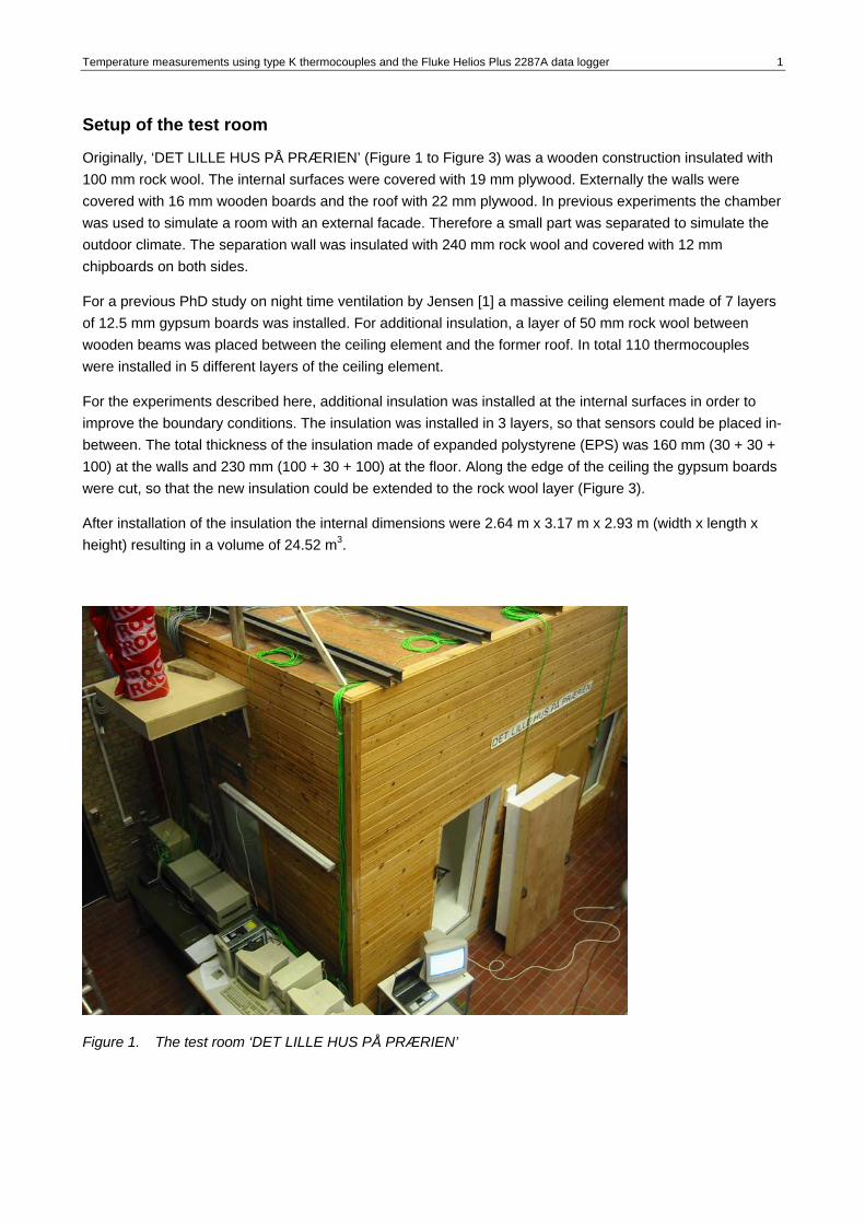
Originally, ‘DET LILLE HUS PÅ PRÆRIEN’ (Figure 1 to Figure 3) was a wooden construction insulated with 100 mm rock wool. The internal surfaces were covered with 19 mm plywood. Externally the walls were covered with 16 mm wooden boards and the roof with 22 mm plywood. In previous experiments the chamber was used to simulate a room with an external facade. Therefore a small part was separated to simulate the outdoor climate. The separation wall was insulated with 240 mm rock wool and covered with 12 mm chipboards on both sides.
For a previous PhD study on night time ventilation by Jensen [1] a massive ceiling element made of 7 layers of 12.5 mm gypsum boards was installed. For additional insulation, a layer of 50 mm rock wool between wooden beams was placed between the ceiling element and the former roof. In total 110 thermocouples were installed in 5 different layers of the ceiling element.
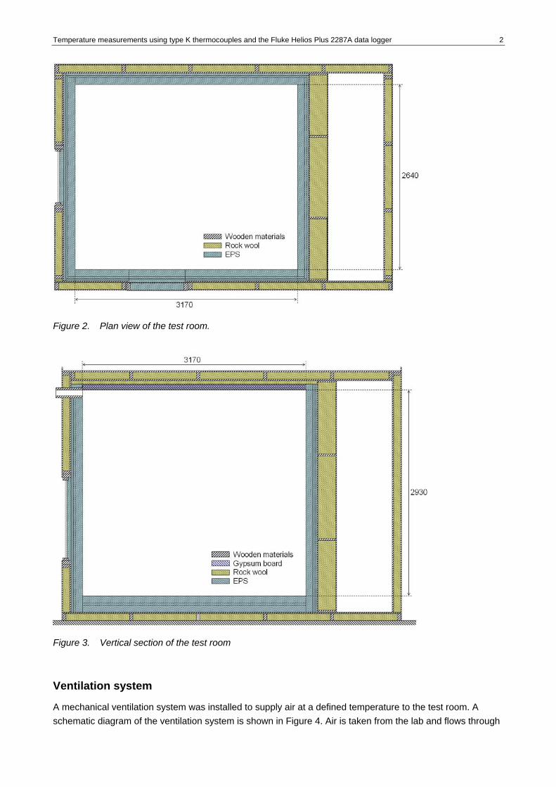
For the experiments described here, additional insulation was installed at the internal surfaces in order to improve the boundary conditions. The insulation was installed in 3 layers, so that sensors could be placed in-between. The total thickness of the insulation made of expanded polystyrene (EPS) was 160 mm (30 + 30 + 100) at the walls and 230 mm (100 + 30 + 100) at the floor. Along the edge of the ceiling the gypsum boards were cut, so that the new insulation could be extended to the rock wool layer (Figure 3).
After installation of the insulation the internal dimensions were 2.64 m x 3.17 m x 2.93 m (width x length x height) resulting in a volume of 24.52 m3.
Figure 1. The test room ‘DET LILLE HUS PÅ PRÆRIEN’
Temperature measurements using type K thermocouples and the Fluke Helios Plus 2287A data logger 2
Figure 2. Plan view of the test room.
Figure 3. Vertical section of the test room
Ventilation system
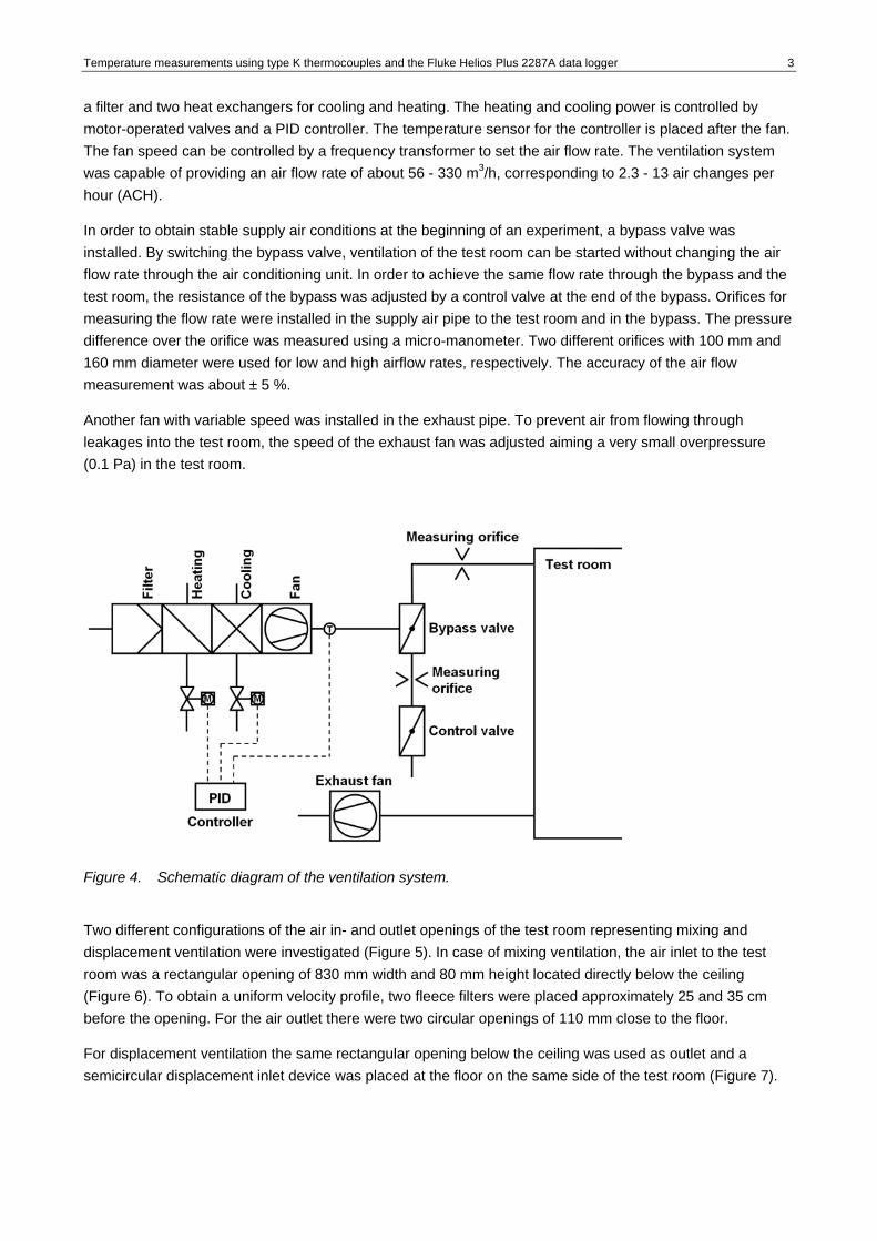
A mechanical ventilation system was installed to supply air at a defined temperature to the test room. A schematic diagram of the ventilation system is shown in Figure 4. Air is taken from the lab and flows through
Temperature measurements using type K thermocouples and the Fluke Helios Plus 2287A data logger 3
a filter and two heat exchangers for cooling and heating. The heating and cooling power is controlled by motor-operated valves and a PID controller. The temperature sensor for the controller is placed after the fan. The fan speed can be controlled by a frequency transformer to set the air flow rate. The ventilation system was capable of providing an air flow rate of about 56 - 330 m3/h, corresponding to 2.3 - 13 air changes per hour (ACH).
In order to obtain stable supply air conditions at the beginning of an experiment, a bypass valve was installed. By switching the bypass valve, ventilation of the test room can be started without changing the air flow rate through the air conditioning unit. In order to achieve the same flow rate through the bypass and the test room, the resistance of the bypass was adjusted by a control valve at the end of the bypass. Orifices for measuring the flow rate were installed in the supply air pipe to the test room and in the bypass. The pressure difference over the orifice was measured using a micro-manometer. Two different orifices with 100 mm and 160 mm diameter were used for low and high airflow rates, respectively. The accuracy of the air flow measurement was about ± 5 %.
Another fan with variable speed was installed in the exhaust pipe. To prevent air from flowing through leakages into the test room, the speed of the exhaust fan was adjusted aiming a very small overpressure (0.1 Pa) in the test room.
Figure 4. Schematic diagram of the ventilation system.
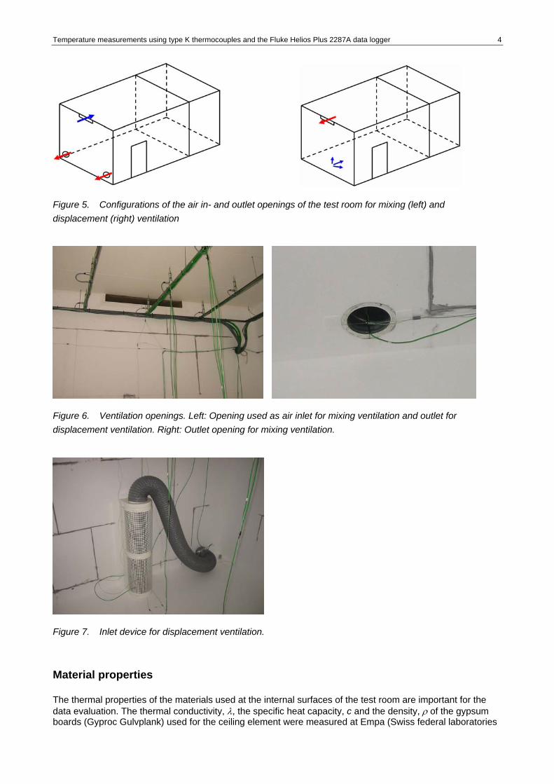
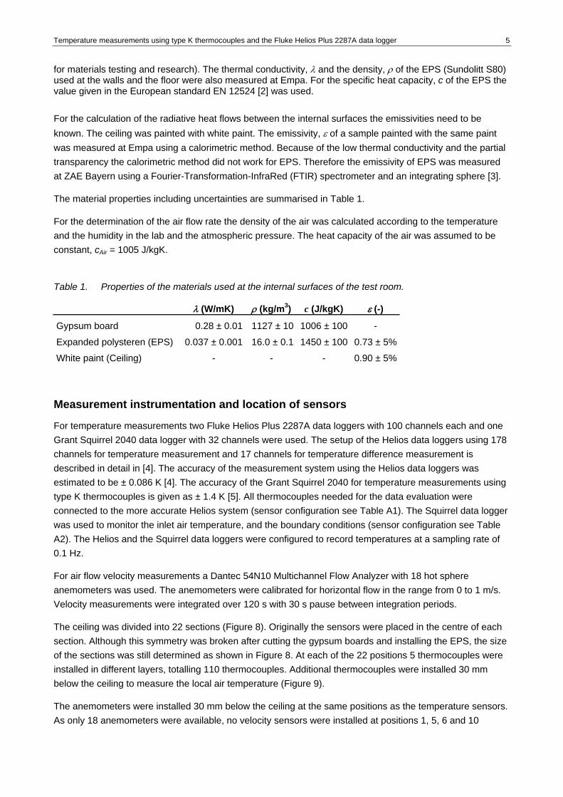
Two different configurations of the air in- and outlet openings of the test room representing mixing and displacement ventilation were investigated (Figure 5). In case of mixing ventilation, the air inlet to the test room was a rectangular opening of 830 mm width and 80 mm height located directly below the ceiling (Figure 6). To obtain a uniform velocity profile, two fleece filters were placed approximately 25 and 35 cm before the opening. For the air outlet there were two circular openings of 110 mm close to the floor.
For displacement ventilation the same rectangular opening below the ceiling was used as outlet and a semicircular displacement inlet device was placed at the floor on the same side of the test room (Figure 7).
Temperature measurements using type K thermocouples and the Fluke Helios Plus 2287A data logger 4
Figure 5. Configurations of the air in- and outlet openings of the test room for mixing (left) and displacement (right) ventilation
Figure 6. Ventilation openings. Left: Opening used as air inlet for mixing ventilation and outlet for displacement ventilation. Right: Outlet opening for mixing ventilation.
Figure 7. Inlet device for displacement ventilation.
Material properties
The thermal properties of the materials used at the internal surfaces of the test room are important for the data evaluation. The thermal conductivity, λ, the specific heat capacity, c and the density, ρ of the gypsum boards (Gyproc Gulvplank) used for the ceiling element were measured at Empa (Swiss federal laboratories
Temperature measurements using type K thermocouples and the Fluke Helios Plus 2287A data logger 5
for materials testing and research). The thermal conductivity, λ and the density, ρ of the EPS (Sundolitt S80) used at the walls and the floor were also measured at Empa. For the specific heat capacity, c of the EPS the value given in the European standard EN 12524 [2] was used.
For the calculation of the radiative heat flows between the internal surfaces the emissivities need to be known. The ceiling was painted with white paint. The emissivity, ε of a sample painted with the same paint was measured at Empa using a calorimetric method. Because of the low thermal conductivity and the partial transparency the calorimetric method did not work for EPS. Therefore the emissivity of EPS was measured at ZAE Bayern using a Fourier-Transformation-InfraRed (FTIR) spectrometer and an integrating sphere [3].
The material properties including uncertainties are summarised in Table 1.
For the determination of the air flow rate the density of the air was calculated according to the temperature and the humidity in the lab and the atmospheric pressure. The heat capacity of the air was assumed to be constant, cAir = 1005 J/kgK.
Table 1. Properties of the materials used at the internal surfaces of the test room.
λ (W/mK) ρ (kg/m3) c (J/kgK) ε (-)
Gypsum board 0.28 ± 0.01 1127 ± 10 1006 ± 100 -
Expanded polysteren (EPS) 0.037 ± 0.001 16.0 ± 0.1 1450 ± 100 0.73 ± 5%
White paint (Ceiling) - - - 0.90 ± 5%
Measurement instrumentation and location of sensors
For temperature measurements two Fluke Helios Plus 2287A data loggers with 100 channels each and one Grant Squirrel 2040 data logger with 32 channels were used. The setup of the Helios data loggers using 178 channels for temperature measurement and 17 channels for temperature difference measurement is described in detail in [4]. The accuracy of the measurement system using the Helios data loggers was estimated to be ± 0.086 K [4]. The accuracy of the Grant Squirrel 2040 for temperature measurements using type K thermocouples is given as ± 1.4 K [5]. All thermocouples needed for the data evaluation were connected to the more accurate Helios system (sensor configuration see Table A1). The Squirrel data logger was used to monitor the inlet air temperature, and the boundary conditions (sensor configuration see Table A2). The Helios and the Squirrel data loggers were configured to record temperatures at a sampling rate of 0.1 Hz.
For air flow velocity measurements a Dantec 54N10 Multichannel Flow Analyzer with 18 hot sphere anemometers was used. The anemometers were calibrated for horizontal flow in the range from 0 to 1 m/s. Velocity measurements were integrated over 120 s with 30 s pause between integration periods.
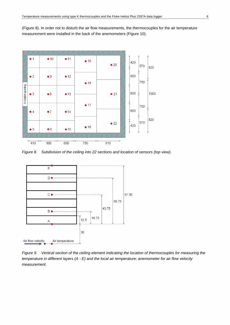
The ceiling was divided into 22 sections (Figure 8). Originally the sensors were placed in the centre of each section. Although this symmetry was broken after cutting the gypsum boards and installing the EPS, the size of the sections was still determined as shown in Figure 8. At each of the 22 positions 5 thermocouples were installed in different layers, totalling 110 thermocouples. Additional thermocouples were installed 30 mm below the ceiling to measure the local air temperature (Figure 9).
The anemometers were installed 30 mm below the ceiling at the same positions as the temperature sensors. As only 18 anemometers were available, no velocity sensors were installed at positions 1, 5, 6 and 10
Temperature measurements using type K thermocouples and the Fluke Helios Plus 2287A data logger 6
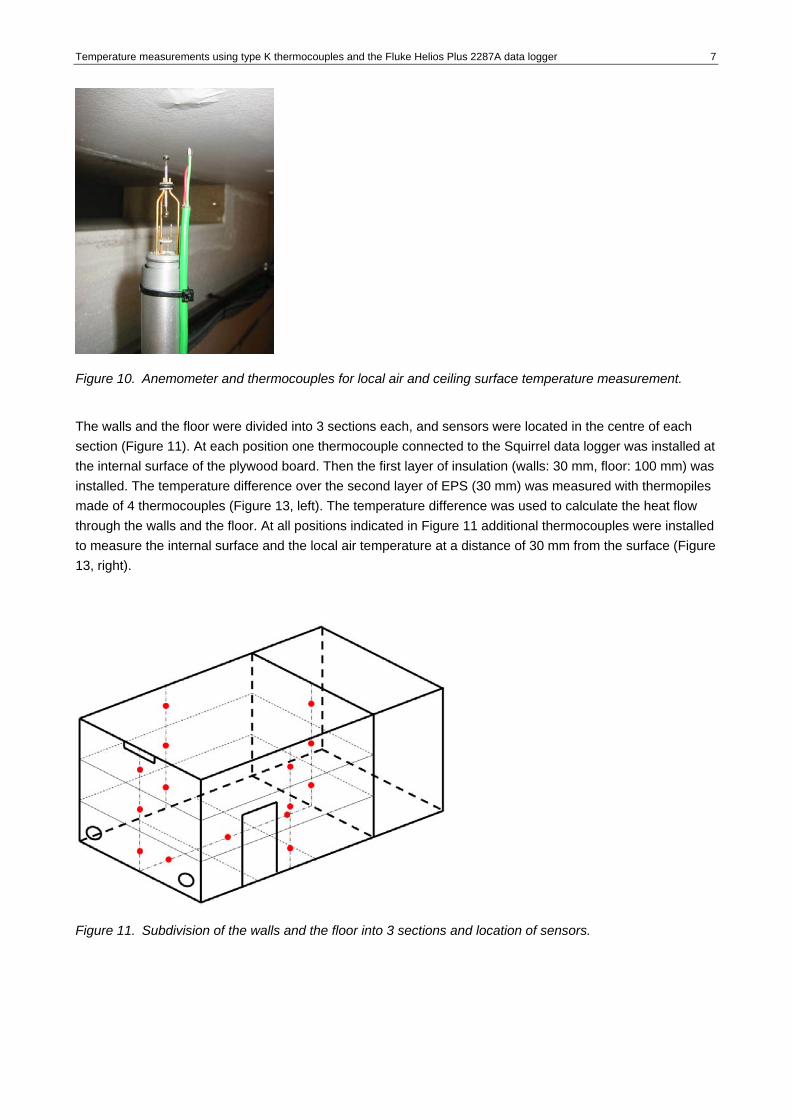
(Figure 8). In order not to disturb the air flow measurements, the thermocouples for the air temperature measurement were installed in the back of the anemometers (Figure 10).
Figure 8. Subdivision of the ceiling into 22 sections and location of sensors (top view).
Figure 9. Vertical section of the ceiling element indicating the location of thermocouples for measuring the temperature in different layers (A - E) and the local air temperature; anemometer for air flow velocity measurement.
Temperature measurements using type K thermocouples and the Fluke Helios Plus 2287A data logger 7
Figure 10. Anemometer and thermocouples for local air and ceiling surface temperature measurement.
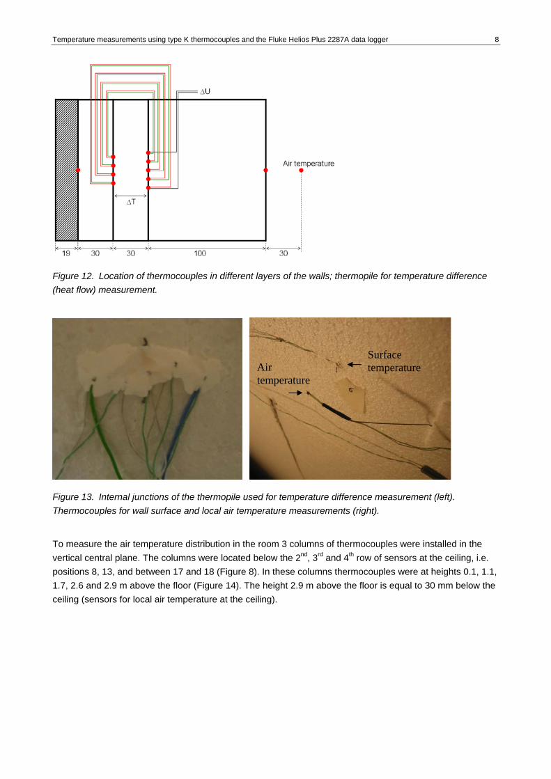
The walls and the floor were divided into 3 sections each, and sensors were located in the centre of each section (Figure 11). At each position one thermocouple connected to the Squirrel data logger was installed at the internal surface of the plywood board. Then the first layer of insulation (walls: 30 mm, floor: 100 mm) was installed. The temperature difference over the second layer of EPS (30 mm) was measured with thermopiles made of 4 thermocouples (Figure 13, left). The temperature difference was used to calculate the heat flow through the walls and the floor. At all positions indicated in Figure 11 additional thermocouples were installed to measure the internal surface and the local air temperature at a distance of 30 mm from the surface (Figure 13, right).
Figure 11. Subdivision of the walls and the floor into 3 sections and location of sensors.
Temperature measurements using type K thermocouples and the Fluke Helios Plus 2287A data logger 8
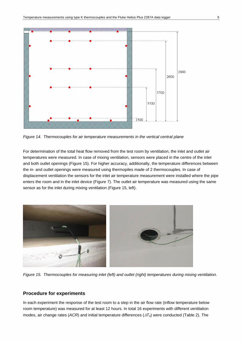
Figure 12. Location of thermocouples in different layers of the walls; thermopile for temperature difference (heat flow) measurement.
Surface temperature Air
temperature
Figure 13. Internal junctions of the thermopile used for temperature difference measurement (left). Thermocouples for wall surface and local air temperature measurements (right).
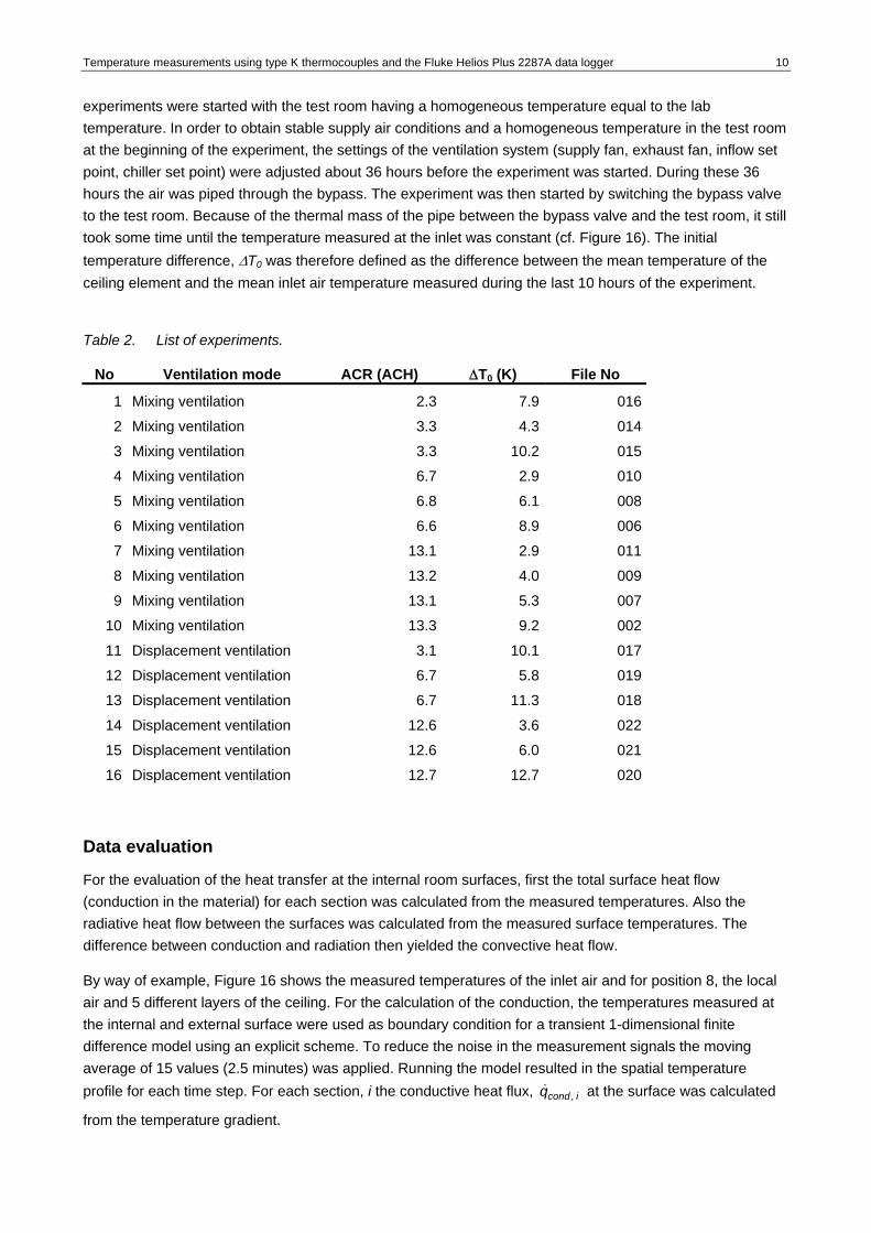
To measure the air temperature distribution in the room 3 columns of thermocouples were installed in the vertical central plane. The columns were located below the 2nd, 3rd and 4th row of sensors at the ceiling, i.e. positions 8, 13, and between 17 and 18 (Figure 8). In these columns thermocouples were at heights 0.1, 1.1, 1.7, 2.6 and 2.9 m above the floor (Figure 14). The height 2.9 m above the floor is equal to 30 mm below the ceiling (sensors for local air temperature at the ceiling).
Temperature measurements using type K thermocouples and the Fluke Helios Plus 2287A data logger 9
Figure 14. Thermocouples for air temperature measurements in the vertical central plane
For determination of the total heat flow removed from the test room by ventilation, the inlet and outlet air temperatures were measured. In case of mixing ventilation, sensors were placed in the centre of the inlet and both outlet openings (Figure 15). For higher accuracy, additionally, the temperature differences between the in- and outlet openings were measured using thermopiles made of 2 thermocouples. In case of displacement ventilation the sensors for the inlet air temperature measurement were installed where the pipe enters the room and in the inlet device (Figure 7). The outlet air temperature was measured using the same sensor as for the inlet during mixing ventilation (Figure 15, left).
Figure 15. Thermocouples for measuring inlet (left) and outlet (right) temperatures during mixing ventilation.
Procedure for experiments
In each experiment the response of the test room to a step in the air flow rate (inflow temperature below room temperature) was measured for at least 12 hours. In total 16 experiments with different ventilation modes, air change rates (ACR) and initial temperature differences (ΔT0) were conducted (Table 2). The
Temperature measurements using type K thermocouples and the Fluke Helios Plus 2287A data logger 10
experiments were started with the test room having a homogeneous temperature equal to the lab temperature. In order to obtain stable supply air conditions and a homogeneous temperature in the test room at the beginning of the experiment, the settings of the ventilation system (supply fan, exhaust fan, inflow set point, chiller set point) were adjusted about 36 hours before the experiment was started. During these 36 hours the air was piped through the bypass. The experiment was then started by switching the bypass valve to the test room. Because of the thermal mass of the pipe between the bypass valve and the test room, it still took some time until the temperature measured at the inlet was constant (cf. Figure 16). The initial temperature difference, ΔT0 was therefore defined as the difference between the mean temperature of the ceiling element and the mean inlet air temperature measured during the last 10 hours of the experiment.
Table 2. List of experiments.
No Ventilation mode ACR (ACH) ΔT0 (K) File No
1 Mixing ventilation 2.3 7.9 016
2 Mixing ventilation 3.3 4.3 014
3 Mixing ventilation 3.3 10.2 015
4 Mixing ventilation 6.7 2.9 010
5 Mixing ventilation 6.8 6.1 008
6 Mixing ventilation 6.6 8.9 006
7 Mixing ventilation 13.1 2.9 011
8 Mixing ventilation 13.2 4.0 009
9 Mixing ventilation 13.1 5.3 007
10 Mixing ventilation 13.3 9.2 002
11 Displacement ventilation 3.1 10.1 017
12 Displacement ventilation 6.7 5.8 019
13 Displacement ventilation 6.7 11.3 018
14 Displacement ventilation 12.6 3.6 022
15 Displacement ventilation 12.6 6.0 021
16 Displacement ventilation 12.7 12.7 020
Data evaluation
For the evaluation of the heat transfer at the internal room surfaces, first the total surface heat flow (conduction in the material) for each section was calculated from the measured temperatures. Also the radiative heat flow between the surfaces was calculated from the measured surface temperatures. The difference between conduction and radiation then yielded the convective heat flow.
By way of example, Figure 16 shows the measured temperatures of the inlet air and for position 8, the local air and 5 different layers of the ceiling. For the calculation of the conduction, the temperatures measured at the internal and external surface were used as boundary condition for a transient 1-dimensional finite difference model using an explicit scheme. To reduce the noise in the measurement signals the moving average of 15 values (2.5 minutes) was applied. Running the model resulted in the spatial temperature profile for each time step. For each section, i the conductive heat flux, at the surface was calculated
from the temperature gradient.
icondq ,&

Temperature measurements using type K thermocouples and the Fluke Helios Plus 2287A data logger 11
00:00 03:00 06:00 09:00 12:0020
20.5
21
21.5
22
22.5
23
23.5
Time (h)
Tem
pera
ture
(°C
)
InletLocal airA (Surface)BCDE
Figure 16. Temperatures measured at position 8 during experiment no. 4 with mixing ventilation with 6.7 ACH and an initial temperature difference of ΔT0 = 2.9 K (A-E: 5 different layers of the ceiling).
The heat flows through the walls and the floor were calculated from the measured temperature difference over a 30 mm layer of EPS. In order to account for the thermal mass of the EPS, the heat flow at the internal wall and floor surfaces was calculated using the same method as at the ceiling. Here the internal surface temperature and the external heat flow were used as boundary condition for the finite difference model.
For calculation of the radiative heat flows, the view factors Fi,j between all 22 sections of the ceiling and 3 sections of each wall and the floor were determined according to [6]. The radiative heat flux from the
surface A
iradq&
i was obtained as sum of the heat fluxes to all surfaces Aj applying the measured surface temperatures:
( )( ) ( )∑ −⋅⋅−−−
⋅⋅⋅=
jji
jijiji
jijiirad TT
FFF
q 44
,,
,, 111 εε
εεσ&
Where ( )4281067.5 KmW−⋅=σ is the Stefan-Boltzmann constant, and iε and jε are the emissivities of the
surfaces.
The convective heat flux, for each section, i was then obtained from the difference between the
conductive and radiative heat fluxes.
iconvq ,&
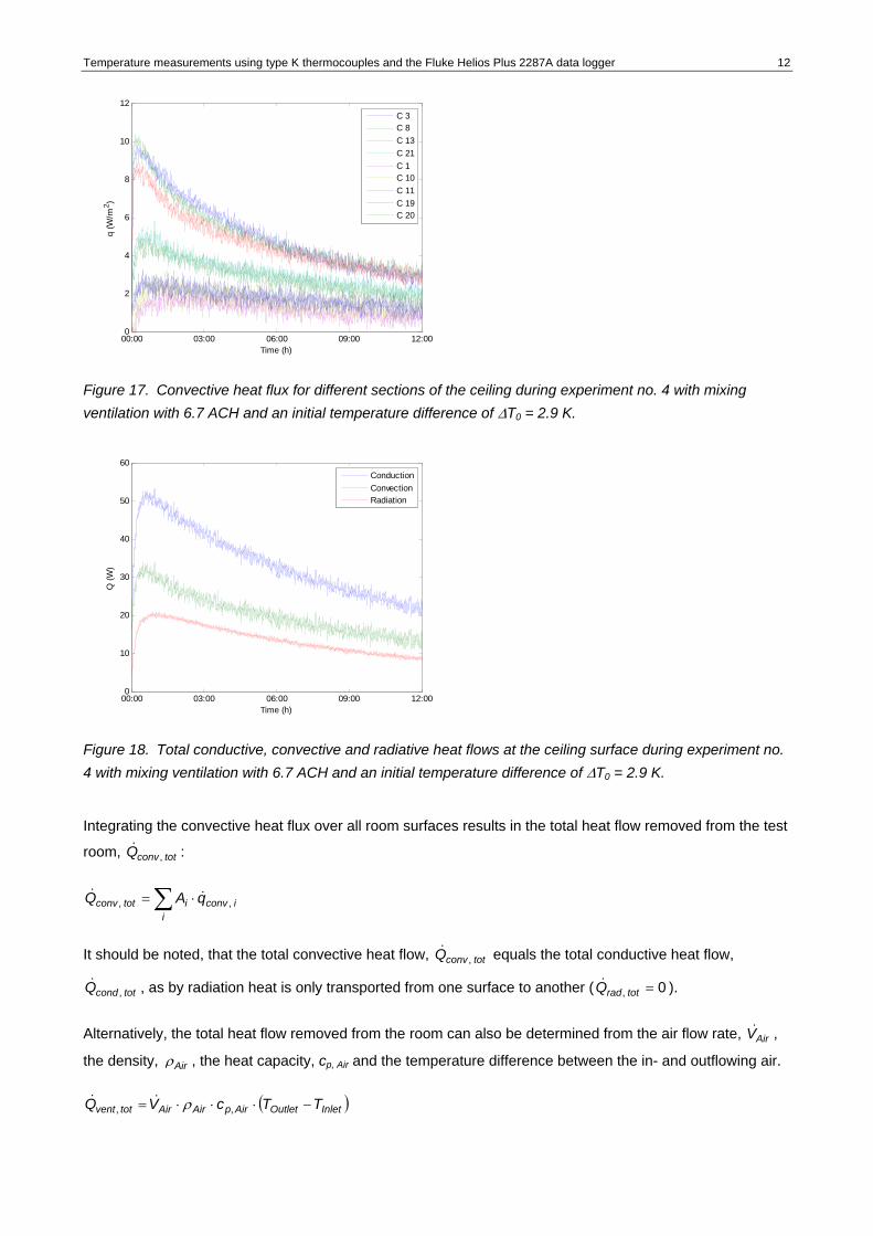
Figure 17 shows the convective heat flux for different sections of the ceiling. The conductive, radiative and convective heat fluxes were integrated over all 22 sections of the ceiling to obtain the total heat flows at the ceiling surface. The total conductive, radiative and convective heat flows at the ceiling surface are displayed in Figure 18.
Temperature measurements using type K thermocouples and the Fluke Helios Plus 2287A data logger 12
00:00 03:00 06:00 09:00 12:000
2
4
6
8
10
12
Time (h)
q (W
/m2 )
C 3C 8C 13C 21C 1C 10C 11C 19C 20
Figure 17. Convective heat flux for different sections of the ceiling during experiment no. 4 with mixing ventilation with 6.7 ACH and an initial temperature difference of ΔT0 = 2.9 K.
00:00 03:00 06:00 09:00 12:000
10
20
30
40
50
60
Time (h)
Q (W
)
ConductionConvectionRadiation
Figure 18. Total conductive, convective and radiative heat flows at the ceiling surface during experiment no. 4 with mixing ventilation with 6.7 ACH and an initial temperature difference of ΔT0 = 2.9 K.
Integrating the convective heat flux over all room surfaces results in the total heat flow removed from the test
room, : totconvQ ,&
∑ ⋅=i
iconvitotconv qAQ ,, &&
It should be noted, that the total convective heat flow, equals the total conductive heat flow,
, as by radiation heat is only transported from one surface to another ( ).
totconvQ ,&
totcondQ ,& 0, =totradQ&
Alternatively, the total heat flow removed from the room can also be determined from the air flow rate, ,
the density, AirV&
Airρ , the heat capacity, cp, Air and the temperature difference between the in- and outflowing air.
( )InletOutletAirpAirAirtotvent TTcVQ −⋅⋅⋅= ,, ρ&&
Temperature measurements using type K thermocouples and the Fluke Helios Plus 2287A data logger 13
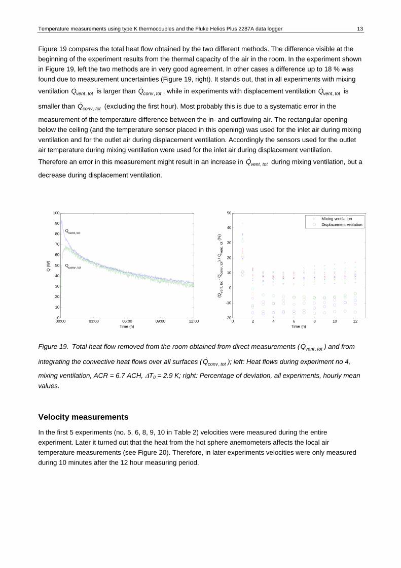
Figure 19 compares the total heat flow obtained by the two different methods. The difference visible at the beginning of the experiment results from the thermal capacity of the air in the room. In the experiment shown in Figure 19, left the two methods are in very good agreement. In other cases a difference up to 18 % was found due to measurement uncertainties (Figure 19, right). It stands out, that in all experiments with mixing
ventilation is larger than , while in experiments with displacement ventilation is
smaller than (excluding the first hour). Most probably this is due to a systematic error in the
measurement of the temperature difference between the in- and outflowing air. The rectangular opening below the ceiling (and the temperature sensor placed in this opening) was used for the inlet air during mixing ventilation and for the outlet air during displacement ventilation. Accordingly the sensors used for the outlet air temperature during mixing ventilation were used for the inlet air during displacement ventilation.
Therefore an error in this measurement might result in an increase in during mixing ventilation, but a
decrease during displacement ventilation.
totventQ ,&
totconvQ ,&
totventQ ,&
totconvQ ,&
totventQ ,&
00:00 03:00 06:00 09:00 12:000
10
20
30
40
50
60
70
80
90
100
Qvent, tot
Qconv, tot
Time (h)
Q (W
)
0 2 4 6 8 10 12-20
-10
0
10
20
30
40
50
Time (h)
(Qve
nt, t
ot -
Qco
nv, t
ot) /
Qve
nt, t
ot (%
)
Mixing ventilationDisplacement vetilation
Figure 19. Total heat flow removed from the room obtained from direct measurements ( ) and from
integrating the convective heat flows over all surfaces ( ); left: Heat flows during experiment no 4,
mixing ventilation, ACR = 6.7 ACH, ΔT
totventQ ,&
totconvQ ,&
0 = 2.9 K; right: Percentage of deviation, all experiments, hourly mean values.
Velocity measurements
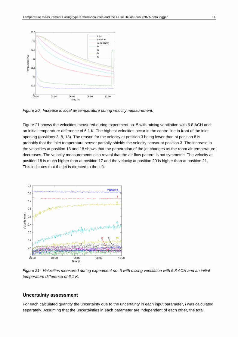
In the first 5 experiments (no. 5, 6, 8, 9, 10 in Table 2) velocities were measured during the entire experiment. Later it turned out that the heat from the hot sphere anemometers affects the local air temperature measurements (see Figure 20). Therefore, in later experiments velocities were only measured during 10 minutes after the 12 hour measuring period.
Temperature measurements using type K thermocouples and the Fluke Helios Plus 2287A data logger 14
00:00 03:00 06:00 09:00 12:0020
20.5
21
21.5
22
22.5
23
23.5
Time (h)
Tem
pera
ture
(°C
)
InletLocal airA (Surface)BCDE
Figure 20. Increase in local air temperature during velocity measurement.
Figure 21 shows the velocities measured during experiment no. 5 with mixing ventilation with 6.8 ACH and an initial temperature difference of 6.1 K. The highest velocities occur in the centre line in front of the inlet opening (positions 3, 8, 13). The reason for the velocity at position 3 being lower than at position 8 is probably that the inlet temperature sensor partially shields the velocity sensor at position 3. The increase in the velocities at position 13 and 18 shows that the penetration of the jet changes as the room air temperature decreases. The velocity measurements also reveal that the air flow pattern is not symmetric. The velocity at position 18 is much higher than at position 17 and the velocity at position 20 is higher than at position 21. This indicates that the jet is directed to the left.
Figure 21. Velocities measured during experiment no. 5 with mixing ventilation with 6.8 ACH and an initial temperature difference of 6.1 K.
Uncertainty assessment
For each calculated quantity the uncertainty due to the uncertainty in each input parameter, i was calculated separately. Assuming that the uncertainties in each parameter are independent of each other, the total
Temperature measurements using type K thermocouples and the Fluke Helios Plus 2287A data logger 15
uncertainty, δ was then calculated as the square root of the quadrature sum of the single uncertainties, iδ
(propagation of uncertainty):
∑=i
i2δδ
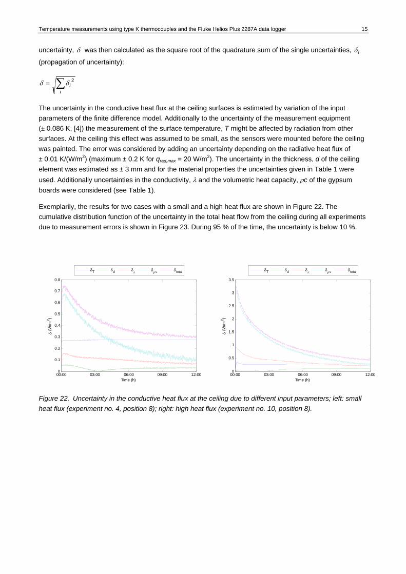
The uncertainty in the conductive heat flux at the ceiling surfaces is estimated by variation of the input parameters of the finite difference model. Additionally to the uncertainty of the measurement equipment (± 0.086 K, [4]) the measurement of the surface temperature, T might be affected by radiation from other surfaces. At the ceiling this effect was assumed to be small, as the sensors were mounted before the ceiling was painted. The error was considered by adding an uncertainty depending on the radiative heat flux of ± 0.01 K/(W/m2) (maximum ± 0.2 K for qrad,max = 20 W/m2). The uncertainty in the thickness, d of the ceiling element was estimated as ± 3 mm and for the material properties the uncertainties given in Table 1 were used. Additionally uncertainties in the conductivity, λ and the volumetric heat capacity, ρc of the gypsum boards were considered (see Table 1).
Exemplarily, the results for two cases with a small and a high heat flux are shown in Figure 22. The cumulative distribution function of the uncertainty in the total heat flow from the ceiling during all experiments due to measurement errors is shown in Figure 23. During 95 % of the time, the uncertainty is below 10 %.
00:00 03:00 06:00 09:00 12:000
0.1
0.2
0.3
0.4
0.5
0.6
0.7
0.8
Time (h)
δ (W
/m2 )
δT δd δλ δρc δtotal
00:00 03:00 06:00 09:00 12:000
0.5
1
1.5
2
2.5
3
3.5
Time (h)
δ (W
/m2 )
δT δd δλ δρc δtotal
Figure 22. Uncertainty in the conductive heat flux at the ceiling due to different input parameters; left: small heat flux (experiment no. 4, position 8); right: high heat flux (experiment no. 10, position 8).
Temperature measurements using type K thermocouples and the Fluke Helios Plus 2287A data logger 16
0 5 10 15 20 25 300
10
20
30
40
50
60
70
80
90
100
δ (%)
F(δ)
(%)
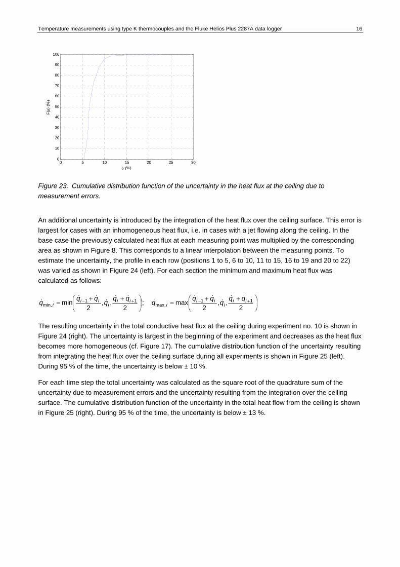
Figure 23. Cumulative distribution function of the uncertainty in the heat flux at the ceiling due to measurement errors.
An additional uncertainty is introduced by the integration of the heat flux over the ceiling surface. This error is largest for cases with an inhomogeneous heat flux, i.e. in cases with a jet flowing along the ceiling. In the base case the previously calculated heat flux at each measuring point was multiplied by the corresponding area as shown in Figure 8. This corresponds to a linear interpolation between the measuring points. To estimate the uncertainty, the profile in each row (positions 1 to 5, 6 to 10, 11 to 15, 16 to 19 and 20 to 22) was varied as shown in Figure 24 (left). For each section the minimum and maximum heat flux was calculated as follows:
⎟⎠
⎞⎜⎝
⎛ ++=⎟
⎠
⎞⎜⎝
⎛ ++= +−+−
2,,
2max;
2,,
2min 11
max,11
min,ii
iii
iii
iii
iqqqqqqqqqqqq&&
&&&
&&&
&&&
&
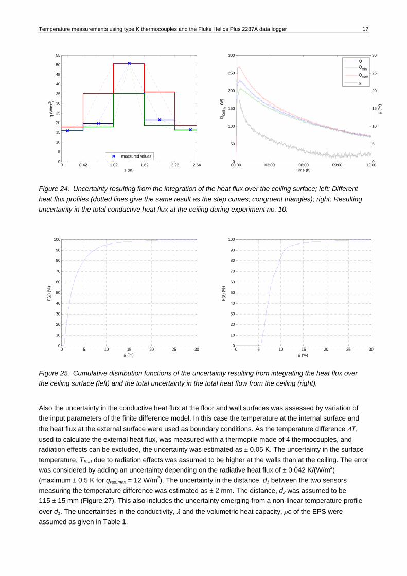
The resulting uncertainty in the total conductive heat flux at the ceiling during experiment no. 10 is shown in Figure 24 (right). The uncertainty is largest in the beginning of the experiment and decreases as the heat flux becomes more homogeneous (cf. Figure 17). The cumulative distribution function of the uncertainty resulting from integrating the heat flux over the ceiling surface during all experiments is shown in Figure 25 (left). During 95 % of the time, the uncertainty is below ± 10 %.
For each time step the total uncertainty was calculated as the square root of the quadrature sum of the uncertainty due to measurement errors and the uncertainty resulting from the integration over the ceiling surface. The cumulative distribution function of the uncertainty in the total heat flow from the ceiling is shown in Figure 25 (right). During 95 % of the time, the uncertainty is below ± 13 %.
Temperature measurements using type K thermocouples and the Fluke Helios Plus 2287A data logger 17
0 0.42 1.02 1.62 2.22 2.640
5
10
15
20
25
30
35
40
45
50
55
z (m)
q (W
/m2 )
measured values
00:00 03:00 06:00 09:00 12:000
50
100
150
200
250
300
Time (h)
QCe
iling (W
)
QQmin
Qmax
δ
0
5
10
15
20
25
30
δ (%
)
Figure 24. Uncertainty resulting from the integration of the heat flux over the ceiling surface; left: Different heat flux profiles (dotted lines give the same result as the step curves; congruent triangles); right: Resulting uncertainty in the total conductive heat flux at the ceiling during experiment no. 10.
0 5 10 15 20 25 300
10
20
30
40
50
60
70
80
90
100
δ (%)
F(δ)
(%)
0 5 10 15 20 25 300
10
20
30
40
50
60
70
80
90
100
δ (%)
F(δ)
(%)
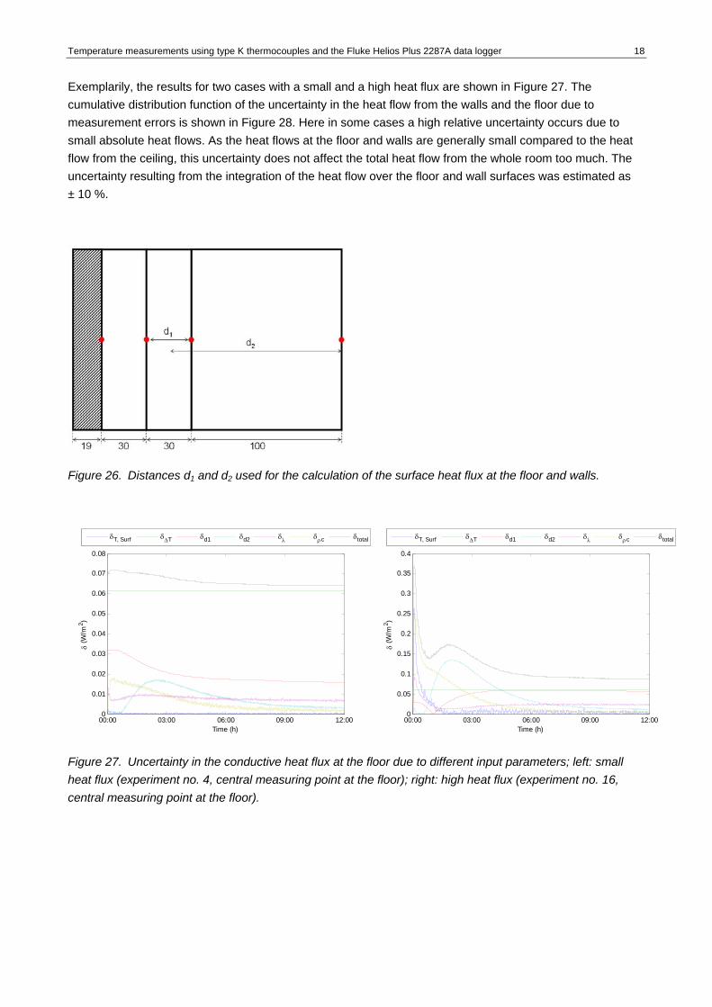
Figure 25. Cumulative distribution functions of the uncertainty resulting from integrating the heat flux over the ceiling surface (left) and the total uncertainty in the total heat flow from the ceiling (right).
Also the uncertainty in the conductive heat flux at the floor and wall surfaces was assessed by variation of the input parameters of the finite difference model. In this case the temperature at the internal surface and the heat flux at the external surface were used as boundary conditions. As the temperature difference ΔT, used to calculate the external heat flux, was measured with a thermopile made of 4 thermocouples, and radiation effects can be excluded, the uncertainty was estimated as ± 0.05 K. The uncertainty in the surface temperature, TSurf due to radiation effects was assumed to be higher at the walls than at the ceiling. The error was considered by adding an uncertainty depending on the radiative heat flux of ± 0.042 K/(W/m2) (maximum ± 0.5 K for qrad,max = 12 W/m2). The uncertainty in the distance, d1 between the two sensors measuring the temperature difference was estimated as ± 2 mm. The distance, d2 was assumed to be 115 ± 15 mm (Figure 27). This also includes the uncertainty emerging from a non-linear temperature profile over d1. The uncertainties in the conductivity, λ and the volumetric heat capacity, ρc of the EPS were assumed as given in Table 1.
Temperature measurements using type K thermocouples and the Fluke Helios Plus 2287A data logger 18
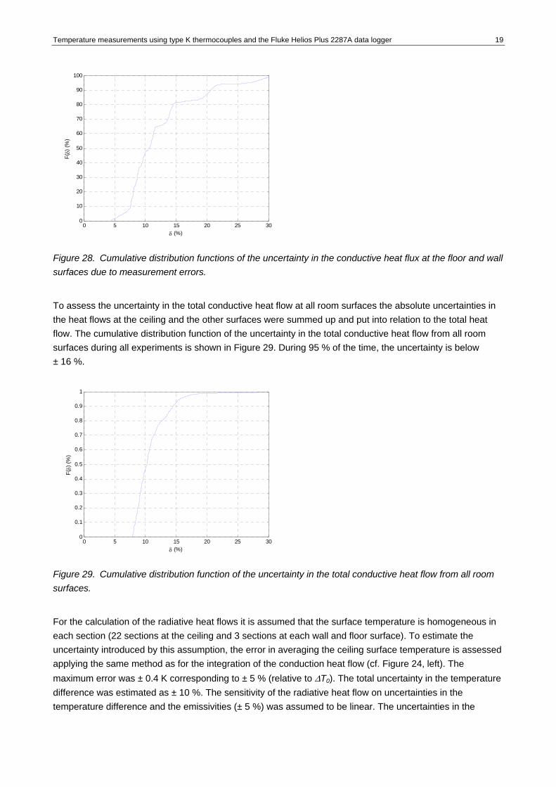
Exemplarily, the results for two cases with a small and a high heat flux are shown in Figure 27. The cumulative distribution function of the uncertainty in the heat flow from the walls and the floor due to measurement errors is shown in Figure 28. Here in some cases a high relative uncertainty occurs due to small absolute heat flows. As the heat flows at the floor and walls are generally small compared to the heat flow from the ceiling, this uncertainty does not affect the total heat flow from the whole room too much. The uncertainty resulting from the integration of the heat flow over the floor and wall surfaces was estimated as ± 10 %.
Figure 26. Distances d1 and d2 used for the calculation of the surface heat flux at the floor and walls.
00:00 03:00 06:00 09:00 12:000
0.01
0.02
0.03
0.04
0.05
0.06
0.07
0.08
Time (h)
δ (W
/m2 )
δT, Surf δΔT δd1 δd2 δλ δρc δtotal
00:00 03:00 06:00 09:00 12:000
0.05
0.1
0.15
0.2
0.25
0.3
0.35
0.4
Time (h)
δ (W
/m2 )
δT, Surf δΔT δd1 δd2 δλ δρc δtotal
Figure 27. Uncertainty in the conductive heat flux at the floor due to different input parameters; left: small heat flux (experiment no. 4, central measuring point at the floor); right: high heat flux (experiment no. 16, central measuring point at the floor).
Temperature measurements using type K thermocouples and the Fluke Helios Plus 2287A data logger 19
0 5 10 15 20 25 300
10
20
30
40
50
60
70
80
90
100
δ (%)
F(δ)
(%)
Figure 28. Cumulative distribution functions of the uncertainty in the conductive heat flux at the floor and wall surfaces due to measurement errors.
To assess the uncertainty in the total conductive heat flow at all room surfaces the absolute uncertainties in the heat flows at the ceiling and the other surfaces were summed up and put into relation to the total heat flow. The cumulative distribution function of the uncertainty in the total conductive heat flow from all room surfaces during all experiments is shown in Figure 29. During 95 % of the time, the uncertainty is below ± 16 %.
0 5 10 15 20 25 300
0.1
0.2
0.3
0.4
0.5
0.6
0.7
0.8
0.9
1
δ (%)
F(δ)
(%)
Figure 29. Cumulative distribution function of the uncertainty in the total conductive heat flow from all room surfaces.
For the calculation of the radiative heat flows it is assumed that the surface temperature is homogeneous in each section (22 sections at the ceiling and 3 sections at each wall and floor surface). To estimate the uncertainty introduced by this assumption, the error in averaging the ceiling surface temperature is assessed applying the same method as for the integration of the conduction heat flow (cf. Figure 24, left). The maximum error was ± 0.4 K corresponding to ± 5 % (relative to ΔT0). The total uncertainty in the temperature difference was estimated as ± 10 %. The sensitivity of the radiative heat flow on uncertainties in the temperature difference and the emissivities (± 5 %) was assumed to be linear. The uncertainties in the
Temperature measurements using type K thermocouples and the Fluke Helios Plus 2287A data logger 20
Stefan-Boltzmann constant and the geometric parameters were neglected. For the total uncertainty in the radiative heat flow follows:
%121055 222222
21, ±=++=++= ΔTradQ δδδδ εε&
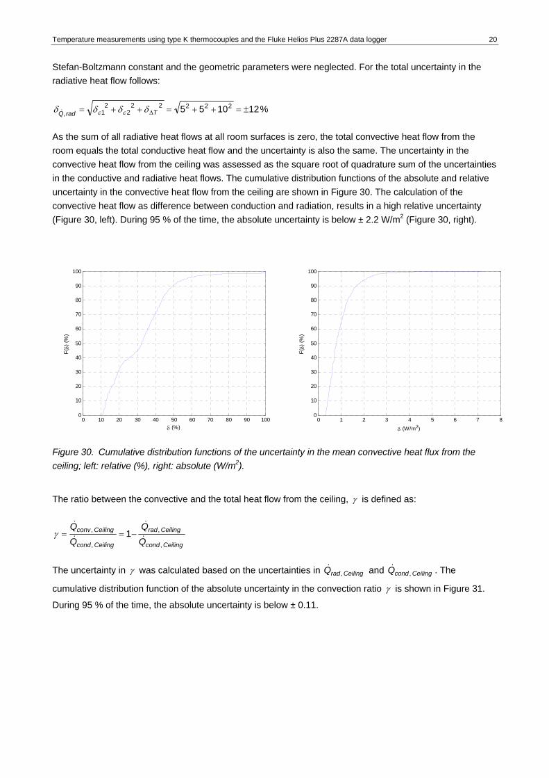
As the sum of all radiative heat flows at all room surfaces is zero, the total convective heat flow from the room equals the total conductive heat flow and the uncertainty is also the same. The uncertainty in the convective heat flow from the ceiling was assessed as the square root of quadrature sum of the uncertainties in the conductive and radiative heat flows. The cumulative distribution functions of the absolute and relative uncertainty in the convective heat flow from the ceiling are shown in Figure 30. The calculation of the convective heat flow as difference between conduction and radiation, results in a high relative uncertainty (Figure 30, left). During 95 % of the time, the absolute uncertainty is below ± 2.2 W/m2 (Figure 30, right).
0 10 20 30 40 50 60 70 80 90 1000
10
20
30
40
50
60
70
80
90
100
δ (%)
F(δ)
(%)
0 1 2 3 4 5 6 7 80
10
20
30
40
50
60
70
80
90
100
δ (W/m2)
F(δ)
(%)
Figure 30. Cumulative distribution functions of the uncertainty in the mean convective heat flux from the ceiling; left: relative (%), right: absolute (W/m2).
The ratio between the convective and the total heat flow from the ceiling, γ is defined as:
Ceilingcond
Ceilingrad
Ceilingcond
Ceilingconv
,
,
,
, 1 &
&
&
&−==γ
The uncertainty in γ was calculated based on the uncertainties in and . The
cumulative distribution function of the absolute uncertainty in the convection ratio
CeilingradQ ,&
CeilingcondQ ,&
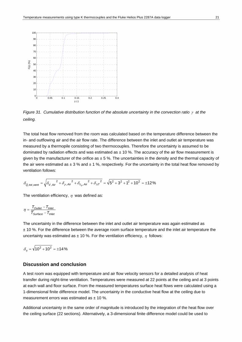
γ is shown in Figure 31.
During 95 % of the time, the absolute uncertainty is below ± 0.11.
Temperature measurements using type K thermocouples and the Fluke Helios Plus 2287A data logger 21
0 0.05 0.1 0.15 0.2 0.25 0.30
10
20
30
40
50
60
70
80
90
100
δ (-)
F(δ)
(%)
Figure 31. Cumulative distribution function of the absolute uncertainty in the convection ratio γ at the
ceiling.
The total heat flow removed from the room was calculated based on the temperature difference between the in- and outflowing air and the air flow rate. The difference between the inlet and outlet air temperature was measured by a thermopile consisting of two thermocouples. Therefore the uncertainty is assumed to be dominated by radiation effects and was estimated as ± 10 %. The accuracy of the air flow measurement is given by the manufacturer of the orifice as ± 5 %. The uncertainties in the density and the thermal capacity of the air were estimated as ± 3 % and ± 1 %, respectively. For the uncertainty in the total heat flow removed by ventilation follows:
%1210135 222222,
2,
2,,, ±=+++=+++= ΔTAircAirAirVventtotQ p
δδδδδ ρ&&
The ventilation efficiency, η was defined as:
InletSurface
InletOutlet
TTTT−−
=η
The uncertainty in the difference between the inlet and outlet air temperature was again estimated as ± 10 %. For the difference between the average room surface temperature and the inlet air temperature the uncertainty was estimated as ± 10 %. For the ventilation efficiency, η follows:
%141010 22 ±=+=ηδ
Discussion and conclusion
A test room was equipped with temperature and air flow velocity sensors for a detailed analysis of heat transfer during night-time ventilation. Temperatures were measured at 22 points at the ceiling and at 3 points at each wall and floor surface. From the measured temperatures surface heat flows were calculated using a 1-dimensional finite difference model. The uncertainty in the conductive heat flow at the ceiling due to measurement errors was estimated as ± 10 %.
Additional uncertainty in the same order of magnitude is introduced by the integration of the heat flow over the ceiling surface (22 sections). Alternatively, a 3-dimensional finite difference model could be used to
Temperature measurements using type K thermocouples and the Fluke Helios Plus 2287A data logger 22
determine the 3-dimensional temperature field in the ceiling element and thus the surface heat flow with a higher resolution. However, as the jet at the ceiling might cause a discontinuous surface temperature profile, the application of a 3-dimensional model is not expected to improve the accuracy significantly.
The radiative heat flows between different surfaces were determined from the measured surface temperatures. The difference between conduction and radiation then yielded the convective heat flow at each surface section. Integration over all surfaces results in the total heat flow discharged from the room.
The uncertainty in the total heat flow discharged from the room yielded from surface heat flow measurements was estimated as ± 16 %. The uncertainty in the heat flow resulting from in-/ outflowing air temperature and mass flow measurements was estimated as ± 12 %. Considering these uncertainties yielded overlapping uncertainty bands for all experiments.
Although there are considerable uncertainties, the presented method is regarded to be suitable to investigate surface heat transfer during night-time ventilation.
References
[1] Jensen R L. Modelling of natural ventilation and night cooling – by the Loop Equation Method. PhD-thesis, Aalborg University, Department of Civil Engineering, Hybrid Ventilation Centre, 2005 (in Danish).
[2] EN 12524:2000. Building materials and products - Hygrothermal properties - Tabulated design values. German version.
[3] Bavarian center for applied energy research (ZAE Bayern) Bestimmung des Emissionsgrades von einer EPS Probe. Report ZAE 2-0808-05, 2008 (in German).
[4] Artmann N, Vonbank R, Jensen R L. Temperature measurements using type K thermocouples and the Fluke Helios Plus 2287A data logger. Internal report, Aalborg University, 2008
[5] Grant Data Acquisition. Technical notes – Squirrel 2020 / 2040 Full Technical Specification and Accessories. Downloaded from http://www.grant.co.uk June 2008.
[6] Ehlert J R, Smith T F. View factors for perpendicular and parallel rectangular plates. Journal of thermophysics and heat transfer 1993, 7 (1), pp. 173-174.

Temperature measurements using type K thermocouples and the Fluke Helios Plus 2287A data logger 23
Appendix
Table A1. Sensor configuration for Helios data loggers. Logger Channel Inputblock ch Comp. Box Cable Nr. High Low Location 283 1 1 Isothermal 0 8A A0 1A brown blue Ceiling 1 A 283 2 1 Isothermal 1 8A A1 1B brown blue Ceiling 1 B 283 3 1 Isothermal 2 8A A2 1C brown blue Ceiling 1 C 283 4 1 Isothermal 3 8A A3 1D brown blue Ceiling 1 D 283 5 1 Isothermal 4 8A A4 1E brown blue Ceiling 1 E 283 6 1 Isothermal 5 8A A5 2A green white Ceiling 2 A 283 7 1 Isothermal 6 8A A6 2B green white Ceiling 2 B 283 8 1 Isothermal 7 8A A7 2C green white Ceiling 2 C 283 9 1 Isothermal 8 8A A8 2D green white Ceiling 2 D 283 10 1 Isothermal 9 8A A9 2E green white Ceiling 2 E 283 11 1 Isothermal 10 8B B0 3A brown blue Ceiling 3 A 283 12 1 Isothermal 11 8B B1 3B brown blue Ceiling 3 B 283 13 1 Isothermal 12 8B B2 3C brown blue Ceiling 3 C 283 14 1 Isothermal 13 8B B3 3D brown blue Ceiling 3 D 283 15 1 Isothermal 14 8B B4 3E brown blue Ceiling 3 E 283 16 1 Isothermal 15 8B B5 4A green white Ceiling 4 A 283 17 1 Isothermal 16 8B B6 4B green white Ceiling 4 B 283 18 1 Isothermal 17 8B B7 4C green white Ceiling 4 C 283 19 1 Isothermal 18 8B B8 4D green white Ceiling 4 D 283 20 1 Isothermal 19 8B B9 4E green white Ceiling 4 E Logger Channel Inputblock ch Comp. Box Cable Nr. High Low Location 283 21 2 Isothermal 0 1A A0 5A brown blue Ceiling 5 A 283 22 2 Isothermal 1 1A A1 5B brown blue Ceiling 5 B 283 23 2 Isothermal 2 1A A2 5C brown blue Ceiling 5 C 283 24 2 Isothermal 3 1A A3 5D brown blue Ceiling 5 D 283 25 2 Isothermal 4 1A A4 5E brown blue Ceiling 5 E 283 26 2 Isothermal 5 1A A5 6A green white Ceiling 6 A 283 27 2 Isothermal 6 1A A6 6B green white Ceiling 6 B 283 28 2 Isothermal 7 1A A7 6C green white Ceiling 6 C 283 29 2 Isothermal 8 1A A8 6D green white Ceiling 6 D 283 30 2 Isothermal 9 1A A9 6E green white Ceiling 6 E 283 31 2 Isothermal 10 1B B0 7A green white Ceiling 7 A 283 32 2 Isothermal 11 1B B1 7B green white Ceiling 7 B 283 33 2 Isothermal 12 1B B2 7C green white Ceiling 7 C 283 34 2 Isothermal 13 1B B3 7D green white Ceiling 7 D 283 35 2 Isothermal 14 1B B4 7E green white Ceiling 7 E 283 36 2 Isothermal 15 1B B5 8A green white Ceiling 8 A 283 37 2 Isothermal 16 1B B6 8B green white Ceiling 8 B 283 38 2 Isothermal 17 1B B7 8C green white Ceiling 8 C 283 39 2 Isothermal 18 1B B8 8D green white Ceiling 8 D 283 40 2 Isothermal 19 1B B9 8E green white Ceiling 8 E Logger Channel Inputblock ch Comp. Box Cable Nr. High Low Location 283 41 3 Isothermal 0 2A A0 9A green white Ceiling 9 A 283 42 3 Isothermal 1 2A A1 9B green white Ceiling 9 B 283 43 3 Isothermal 2 2A A2 9C green white Ceiling 9 C 283 44 3 Isothermal 3 2A A3 9D green white Ceiling 9 D 283 45 3 Isothermal 4 2A A4 9E green white Ceiling 9 E 283 46 3 Isothermal 5 2A A5 10A green white Ceiling 10 A 283 47 3 Isothermal 6 2A A6 10B green white Ceiling 10 B 283 48 3 Isothermal 7 2A A7 10C green white Ceiling 10 C 283 49 3 Isothermal 8 2A A8 10D green white Ceiling 10 D 283 50 3 Isothermal 9 2A A9 10E green white Ceiling 10 E 283 51 3 Isothermal 10 2B B0 1 green white Surface Low X, bottom 283 52 3 Isothermal 11 2B B1 2 green white Surface High X, bottom 283 53 3 Isothermal 12 2B B2 3 green white Surface Low Z, bottom 283 54 3 Isothermal 13 2B B3 4 green white Surface High Z, bottom 283 55 3 Isothermal 14 2B B4 5 green white Surface Low X, centre 283 56 3 Isothermal 15 2B B5 6 green white Surface High X, centre 283 57 3 Isothermal 16 2B B6 7 green white Surface Low Z, centre 283 58 3 Isothermal 17 2B B7 8 green white Surface High Z, centre 283 59 3 Isothermal 18 2B B8 9 green white Surface Low X, top 283 60 3 Isothermal 19 2B B9 10 green white Surface High X, top
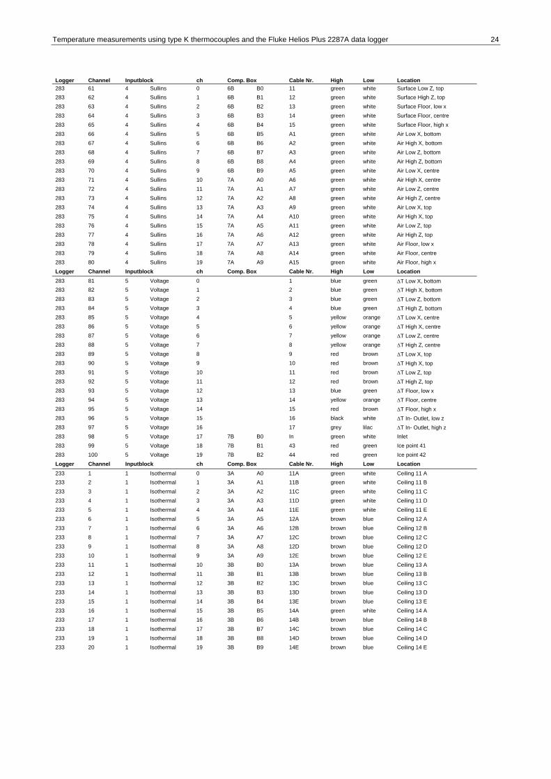
Temperature measurements using type K thermocouples and the Fluke Helios Plus 2287A data logger 24
Logger Channel Inputblock ch Comp. Box Cable Nr. High Low Location 283 61 4 Sullins 0 6B B0 11 green white Surface Low Z, top 283 62 4 Sullins 1 6B B1 12 green white Surface High Z, top 283 63 4 Sullins 2 6B B2 13 green white Surface Floor, low x 283 64 4 Sullins 3 6B B3 14 green white Surface Floor, centre 283 65 4 Sullins 4 6B B4 15 green white Surface Floor, high x 283 66 4 Sullins 5 6B B5 A1 green white Air Low X, bottom 283 67 4 Sullins 6 6B B6 A2 green white Air High X, bottom 283 68 4 Sullins 7 6B B7 A3 green white Air Low Z, bottom 283 69 4 Sullins 8 6B B8 A4 green white Air High Z, bottom 283 70 4 Sullins 9 6B B9 A5 green white Air Low X, centre 283 71 4 Sullins 10 7A A0 A6 green white Air High X, centre 283 72 4 Sullins 11 7A A1 A7 green white Air Low Z, centre 283 73 4 Sullins 12 7A A2 A8 green white Air High Z, centre 283 74 4 Sullins 13 7A A3 A9 green white Air Low X, top 283 75 4 Sullins 14 7A A4 A10 green white Air High X, top 283 76 4 Sullins 15 7A A5 A11 green white Air Low Z, top 283 77 4 Sullins 16 7A A6 A12 green white Air High Z, top 283 78 4 Sullins 17 7A A7 A13 green white Air Floor, low x 283 79 4 Sullins 18 7A A8 A14 green white Air Floor, centre 283 80 4 Sullins 19 7A A9 A15 green white Air Floor, high x Logger Channel Inputblock ch Comp. Box Cable Nr. High Low Location 283 81 5 Voltage 0 1 blue green ΔT Low X, bottom 283 82 5 Voltage 1 2 blue green ΔT High X, bottom 283 83 5 Voltage 2 3 blue green ΔT Low Z, bottom 283 84 5 Voltage 3 4 blue green ΔT High Z, bottom 283 85 5 Voltage 4 5 yellow orange ΔT Low X, centre 283 86 5 Voltage 5 6 yellow orange ΔT High X, centre 283 87 5 Voltage 6 7 yellow orange ΔT Low Z, centre 283 88 5 Voltage 7 8 yellow orange ΔT High Z, centre 283 89 5 Voltage 8 9 red brown ΔT Low X, top 283 90 5 Voltage 9 10 red brown ΔT High X, top 283 91 5 Voltage 10 11 red brown ΔT Low Z, top 283 92 5 Voltage 11 12 red brown ΔT High Z, top 283 93 5 Voltage 12 13 blue green ΔT Floor, low x 283 94 5 Voltage 13 14 yellow orange ΔT Floor, centre 283 95 5 Voltage 14 15 red brown ΔT Floor, high x 283 96 5 Voltage 15 16 black white ΔT In- Outlet, low z 283 97 5 Voltage 16 17 grey lilac ΔT In- Outlet, high z 283 98 5 Voltage 17 7B B0 In green white Inlet 283 99 5 Voltage 18 7B B1 43 red green Ice point 41 283 100 5 Voltage 19 7B B2 44 red green Ice point 42 Logger Channel Inputblock ch Comp. Box Cable Nr. High Low Location 233 1 1 Isothermal 0 3A A0 11A green white Ceiling 11 A 233 2 1 Isothermal 1 3A A1 11B green white Ceiling 11 B 233 3 1 Isothermal 2 3A A2 11C green white Ceiling 11 C 233 4 1 Isothermal 3 3A A3 11D green white Ceiling 11 D 233 5 1 Isothermal 4 3A A4 11E green white Ceiling 11 E 233 6 1 Isothermal 5 3A A5 12A brown blue Ceiling 12 A 233 7 1 Isothermal 6 3A A6 12B brown blue Ceiling 12 B 233 8 1 Isothermal 7 3A A7 12C brown blue Ceiling 12 C 233 9 1 Isothermal 8 3A A8 12D brown blue Ceiling 12 D 233 10 1 Isothermal 9 3A A9 12E brown blue Ceiling 12 E 233 11 1 Isothermal 10 3B B0 13A brown blue Ceiling 13 A 233 12 1 Isothermal 11 3B B1 13B brown blue Ceiling 13 B 233 13 1 Isothermal 12 3B B2 13C brown blue Ceiling 13 C 233 14 1 Isothermal 13 3B B3 13D brown blue Ceiling 13 D 233 15 1 Isothermal 14 3B B4 13E brown blue Ceiling 13 E 233 16 1 Isothermal 15 3B B5 14A green white Ceiling 14 A 233 17 1 Isothermal 16 3B B6 14B brown blue Ceiling 14 B 233 18 1 Isothermal 17 3B B7 14C brown blue Ceiling 14 C 233 19 1 Isothermal 18 3B B8 14D brown blue Ceiling 14 D 233 20 1 Isothermal 19 3B B9 14E brown blue Ceiling 14 E

Temperature measurements using type K thermocouples and the Fluke Helios Plus 2287A data logger 25
Logger Channel Inputblock ch Comp. Box Cable Nr. High Low Location 233 21 2 Isothermal 0 4A A0 15A green white Ceiling 15 233 22 2 Isothermal 1 4A A1 15B green white Ceiling 15 233 23 2 Isothermal 2 4A A2 15C green white Ceiling 15 233 24 2 Isothermal 3 4A A3 15D green white Ceiling 15 233 25 2 Isothermal 4 4A A4 15E green white Ceiling 15 233 26 2 Isothermal 5 4A A5 16A brown blue Ceiling 16 233 27 2 Isothermal 6 4A A6 16B brown blue Ceiling 16 233 28 2 Isothermal 7 4A A7 16C brown blue Ceiling 16 233 29 2 Isothermal 8 4A A8 16D brown blue Ceiling 16 233 30 2 Isothermal 9 4A A9 16E brown blue Ceiling 16 233 31 2 Isothermal 10 4B B0 17A brown blue Ceiling 17 233 32 2 Isothermal 11 4B B1 17B brown blue Ceiling 17 233 33 2 Isothermal 12 4B B2 17C brown blue Ceiling 17 233 34 2 Isothermal 13 4B B3 17D brown blue Ceiling 17 233 35 2 Isothermal 14 4B B4 17E brown blue Ceiling 17 233 36 2 Isothermal 15 4B B5 18A brown blue Ceiling 18 233 37 2 Isothermal 16 4B B6 18B brown blue Ceiling 18 233 38 2 Isothermal 17 4B B7 18C brown blue Ceiling 18 233 39 2 Isothermal 18 4B B8 18D brown blue Ceiling 18 233 40 2 Isothermal 19 4B B9 18E brown blue Ceiling 18 Logger Channel Inputblock ch Comp. Box Cable Nr. High Low Location 233 41 3 Isothermal 0 5A A0 19A brown blue Ceiling 19 233 42 3 Isothermal 1 5A A1 19B brown blue Ceiling 19 233 43 3 Isothermal 2 5A A2 19C brown blue Ceiling 19 233 44 3 Isothermal 3 5A A3 19D brown blue Ceiling 19 233 45 3 Isothermal 4 5A A4 19E brown blue Ceiling 19 233 46 3 Isothermal 5 5A A5 20A green white Ceiling 20 233 47 3 Isothermal 6 5A A6 20B green white Ceiling 20 233 48 3 Isothermal 7 5A A7 20C green white Ceiling 20 233 49 3 Isothermal 8 5A A8 20D green white Ceiling 20 233 50 3 Isothermal 9 5A A9 20E green white Ceiling 20 233 51 3 Isothermal 10 5B B0 21A brown blue Ceiling 21 233 52 3 Isothermal 11 5B B1 21B brown blue Ceiling 21 233 53 3 Isothermal 12 5B B2 21C brown blue Ceiling 21 233 54 3 Isothermal 13 5B B3 21D brown blue Ceiling 21 233 55 3 Isothermal 14 5B B4 21E brown blue Ceiling 21 233 56 3 Isothermal 15 5B B5 22A green white Ceiling 22 233 57 3 Isothermal 16 5B B6 22B green white Ceiling 22 233 58 3 Isothermal 17 5B B7 22C green white Ceiling 22 233 59 3 Isothermal 18 5B B8 22D green white Ceiling 22 233 60 3 Isothermal 19 5B B9 22E green white Ceiling 22 Logger Channel Inputblock ch Comp. Box Cable Nr. High Low Location 233 61 4 Isothermal 0 I. p. 1 1 1 red green Air Ceiling 1 233 62 4 Isothermal 1 I. p. 1 2 2 red green Air Ceiling 2 233 63 4 Isothermal 2 I. p. 1 3 3 red green Air Ceiling 3 233 64 4 Isothermal 3 I. p. 1 4 4 red green Air Ceiling 4 233 65 4 Isothermal 4 I. p. 1 5 5 red green Air Ceiling 5 233 66 4 Isothermal 5 I. p. 1 6 6 red green Air Ceiling 6 233 67 4 Isothermal 6 I. p. 1 7 7 red green Air Ceiling 7 233 68 4 Isothermal 7 I. p. 1 8 8 red green Air Ceiling 8 233 69 4 Isothermal 8 I. p. 1 9 9 red green Air Ceiling 9 233 70 4 Isothermal 9 I. p. 1 10 10 red green Air Ceiling 10 233 71 4 Isothermal 10 I. p. 2 11 11 red green Air Ceiling 11 233 72 4 Isothermal 11 I. p. 2 12 12 red green Air Ceiling 12 233 73 4 Isothermal 12 I. p. 2 13 13 red green Air Ceiling 13 233 74 4 Isothermal 13 I. p. 2 14 14 red green Air Ceiling 14 233 75 4 Isothermal 14 I. p. 2 15 15 red green Air Ceiling 15 233 76 4 Isothermal 15 I. p. 2 16 16 red green Air Ceiling 16 233 77 4 Isothermal 16 I. p. 2 17 17 red green Air Ceiling 17 233 78 4 Isothermal 17 I. p. 2 18 18 red green Air Ceiling 18 233 79 4 Isothermal 18 I. p. 2 19 19 red green Air Ceiling 19 233 80 4 Isothermal 19 I. p. 2 20 20 red green Air Ceiling 20
Temperature measurements using type K thermocouples and the Fluke Helios Plus 2287A data logger 26
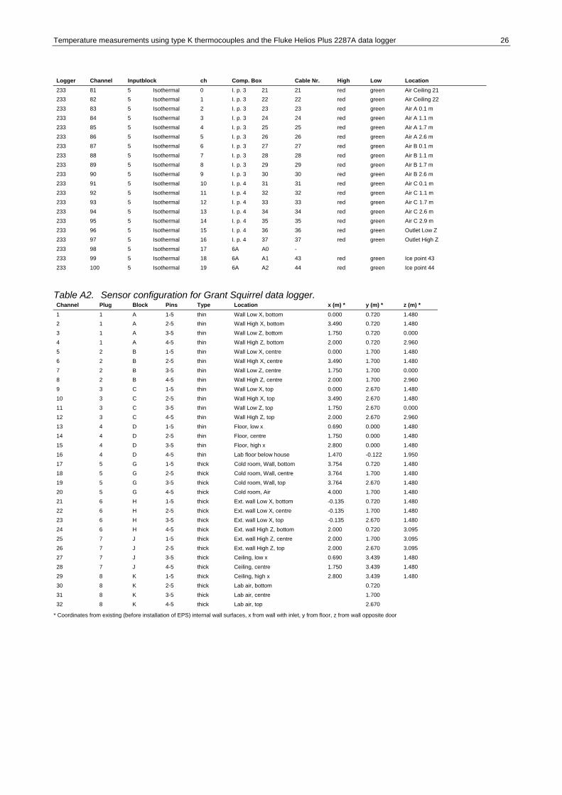
Logger Channel Inputblock ch Comp. Box Cable Nr. High Low Location 233 81 5 Isothermal 0 I. p. 3 21 21 red green Air Ceiling 21 233 82 5 Isothermal 1 I. p. 3 22 22 red green Air Ceiling 22 233 83 5 Isothermal 2 I. p. 3 23 23 red green Air A 0.1 m 233 84 5 Isothermal 3 I. p. 3 24 24 red green Air A 1.1 m 233 85 5 Isothermal 4 I. p. 3 25 25 red green Air A 1.7 m 233 86 5 Isothermal 5 I. p. 3 26 26 red green Air A 2.6 m 233 87 5 Isothermal 6 I. p. 3 27 27 red green Air B 0.1 m 233 88 5 Isothermal 7 I. p. 3 28 28 red green Air B 1.1 m 233 89 5 Isothermal 8 I. p. 3 29 29 red green Air B 1.7 m 233 90 5 Isothermal 9 I. p. 3 30 30 red green Air B 2.6 m 233 91 5 Isothermal 10 I. p. 4 31 31 red green Air C 0.1 m 233 92 5 Isothermal 11 I. p. 4 32 32 red green Air C 1.1 m 233 93 5 Isothermal 12 I. p. 4 33 33 red green Air C 1.7 m 233 94 5 Isothermal 13 I. p. 4 34 34 red green Air C 2.6 m 233 95 5 Isothermal 14 I. p. 4 35 35 red green Air C 2.9 m 233 96 5 Isothermal 15 I. p. 4 36 36 red green Outlet Low Z 233 97 5 Isothermal 16 I. p. 4 37 37 red green Outlet High Z 233 98 5 Isothermal 17 6A A0 - 233 99 5 Isothermal 18 6A A1 43 red green Ice point 43 233 100 5 Isothermal 19 6A A2 44 red green Ice point 44
Table A2. Sensor configuration for Grant Squirrel data logger. Channel Plug Block Pins Type Location x (m) * y (m) * z (m) * 1 1 A 1-5 thin Wall Low X, bottom 0.000 0.720 1.480 2 1 A 2-5 thin Wall High X, bottom 3.490 0.720 1.480 3 1 A 3-5 thin Wall Low Z, bottom 1.750 0.720 0.000 4 1 A 4-5 thin Wall High Z, bottom 2.000 0.720 2.960 5 2 B 1-5 thin Wall Low X, centre 0.000 1.700 1.480 6 2 B 2-5 thin Wall High X, centre 3.490 1.700 1.480 7 2 B 3-5 thin Wall Low Z, centre 1.750 1.700 0.000 8 2 B 4-5 thin Wall High Z, centre 2.000 1.700 2.960 9 3 C 1-5 thin Wall Low X, top 0.000 2.670 1.480 10 3 C 2-5 thin Wall High X, top 3.490 2.670 1.480 11 3 C 3-5 thin Wall Low Z, top 1.750 2.670 0.000 12 3 C 4-5 thin Wall High Z, top 2.000 2.670 2.960 13 4 D 1-5 thin Floor, low x 0.690 0.000 1.480 14 4 D 2-5 thin Floor, centre 1.750 0.000 1.480 15 4 D 3-5 thin Floor, high x 2.800 0.000 1.480 16 4 D 4-5 thin Lab floor below house 1.470 -0.122 1.950 17 5 G 1-5 thick Cold room, Wall, bottom 3.754 0.720 1.480 18 5 G 2-5 thick Cold room, Wall, centre 3.764 1.700 1.480 19 5 G 3-5 thick Cold room, Wall, top 3.764 2.670 1.480 20 5 G 4-5 thick Cold room, Air 4.000 1.700 1.480 21 6 H 1-5 thick Ext. wall Low X, bottom -0.135 0.720 1.480 22 6 H 2-5 thick Ext. wall Low X, centre -0.135 1.700 1.480 23 6 H 3-5 thick Ext. wall Low X, top -0.135 2.670 1.480 24 6 H 4-5 thick Ext. wall High Z, bottom 2.000 0.720 3.095 25 7 J 1-5 thick Ext. wall High Z, centre 2.000 1.700 3.095 26 7 J 2-5 thick Ext. wall High Z, top 2.000 2.670 3.095 27 7 J 3-5 thick Ceiling, low x 0.690 3.439 1.480 28 7 J 4-5 thick Ceiling, centre 1.750 3.439 1.480 29 8 K 1-5 thick Ceiling, high x 2.800 3.439 1.480 30 8 K 2-5 thick Lab air, bottom 0.720 31 8 K 3-5 thick Lab air, centre 1.700 32 8 K 4-5 thick Lab air, top 2.670
* Coordinates from existing (before installation of EPS) internal wall surfaces, x from wall with inlet, y from floor, z from wall opposite door

ISSN 1901-726X DCE Technical Report No. 053