
Decisions under Uncertainty
688
Decisions under Uncertainty Probabilistic Analysis for Engineering Decisions Decision-making and risk assessment are essential aspects of every engineer’s life, whether this be concerned with the probability of failure of a new product within the warranty period or the potential cost, human and financial, of the failure of a major structure such as a bridge. This book helps the reader to understand the tradeoffs between attributes such as cost and safety, and includes a wide range of worked examples based on case studies. It introduces the basic theory from first principles using a Bayesian approach to probability and covers all of the most widely used mathematical techniques likely to be encountered in real engineering projects. These include utility, extremes and risk analysis, as well as special areas of importance and interest in engineering and for understanding, such as optimization, games and entropy. Equally valuable for senior undergraduate and graduate students, practising engineers, designers and project managers. Ian Jordaan is University Research Professor in the Faculty of Engineering and Applied Science at the Memorial University of Newfoundland, Canada, and held the NSERC-Mobil Industrial Research Chair in Ocean Engineering at the university from 1986 to 1996. He is also president of Ian Jordaan and Associates Inc. and an advisor to C-CORE, an engineering R&D company based in St. John’s. Prior to joining the university in 1986, he was Vice-President, Research and Development at Det Norske Veritas (Canada Ltd., and before this he was a full professor in the Department of Civil Engineering at the University of Calgary, Canada. He is extensively involved in consulting activities with industry and government, and has pioneered methods of risk analysis for engineering in harsh environments. Recently he served on an expert panel of the Royal Society of Canada, studying science issues relative to the oil and gas developments offshore British Columbia. He is the recipient of a number of awards, including the Horst Leipholz Medal and the P. L. Pratley Award, both of the Canadian Society for Civil Engineering. http://ebooks.cambridge.org/ebook.jsf?bid=CBO9780511804861
-
Upload
khangminh22 -
Category
Documents
-
view
0 -
download
0
Transcript of Decisions under Uncertainty

Decisions under UncertaintyProbabilistic Analysis for Engineering Decisions
Decision-making and risk assessment are essential aspects of every engineer’s life, whetherthis be concerned with the probability of failure of a new product within the warranty period orthe potential cost, human and financial, of the failure of a major structure such as a bridge. Thisbook helps the reader to understand the tradeoffs between attributes such as cost and safety,and includes a wide range of worked examples based on case studies. It introduces the basictheory from first principles using a Bayesian approach to probability and covers all of the mostwidely used mathematical techniques likely to be encountered in real engineering projects.These include utility, extremes and risk analysis, as well as special areas of importance andinterest in engineering and for understanding, such as optimization, games and entropy. Equallyvaluable for senior undergraduate and graduate students, practising engineers, designers andproject managers.
Ian Jordaan is University Research Professor in the Faculty of Engineering and AppliedScience at the Memorial University of Newfoundland, Canada, and held the NSERC-MobilIndustrial Research Chair in Ocean Engineering at the university from 1986 to 1996. He is alsopresident of Ian Jordaan and Associates Inc. and an advisor to C-CORE, an engineering R&Dcompany based in St. John’s. Prior to joining the university in 1986, he was Vice-President,Research and Development at Det Norske Veritas (Canada) Ltd., and before this he was a fullprofessor in the Department of Civil Engineering at the University of Calgary, Canada. He isextensively involved in consulting activities with industry and government, and has pioneeredmethods of risk analysis for engineering in harsh environments. Recently he served on anexpert panel of the Royal Society of Canada, studying science issues relative to the oil and gasdevelopments offshore British Columbia. He is the recipient of a number of awards, includingthe Horst Leipholz Medal and the P. L. Pratley Award, both of the Canadian Society for CivilEngineering.
http://ebooks.cambridge.org/ebook.jsf?bid=CBO9780511804861

http://ebooks.cambridge.org/ebook.jsf?bid=CBO9780511804861

Decisions underUncertaintyProbabilistic Analysis for Engineering Decisions
Ian JordaanFaculty of Engineering and Applied ScienceMemorial University of NewfoundlandSt John’s, Newfoundland, Canada
http://ebooks.cambridge.org/ebook.jsf?bid=CBO9780511804861

cambridge university pressCambridge, New York, Melbourne, Madrid, Cape Town, Singapore, Sao Paulo
cambridge university pressThe Edinburgh Building, Cambridge CB2 2RU, UK
www.cambridge.orgInformation on this title: www.cambridge.org/9780521782775
C© Jordaan 2005
This book is in copyright. Subject to statutory exceptionand to the provisions of relevant collective licensing agreements,no reproduction of any part may take place withoutthe written permission of Cambridge University Press.
First published 2005
Printed in the United Kingdom at the University Press, Cambridge
A catalog record for this book is available from the British Library
Library of Congress Cataloging in Publication data
Jordaan, Ian J., 1939–Decisions under uncertainty: probabilistic analysis for engineering decisions / Ian J. Jordaan.
p. cm.Includes bibliographical references and index.ISBN 0 521 78277 51. Engineering–Statistical methods. 2. Decision making–Statistical methods. 3. Probabilities. I. Title.TA340.J68 2004620′.007′27–dc22 2004043587
ISBN-13 978-0-521-78277-5 hardbackISBN-10 0-521-78277-5 hardback
Cambridge University Press has no responsibility for the persistence or accuracy of URLs for external or third-partyinternet websites referred to in this book, and does not guarantee that any content on such websites is, or will remain,accurate or appropriate.
http://ebooks.cambridge.org/ebook.jsf?bid=CBO9780511804861

For Christina
http://ebooks.cambridge.org/ebook.jsf?bid=CBO9780511804861

http://ebooks.cambridge.org/ebook.jsf?bid=CBO9780511804861

Contents
List of illustrations page xiiPreface xiiiAcknowledgements xvi
1 Uncertainty and decision-making 1
1.1 Introduction 11.2 The nature of a decision 31.3 Domain of probability: subjectivity and objectivity 91.4 Approach and tools; role of judgement: indifference and preference 101.5 Probability and frequency 121.6 Terminology, notation and conventions 151.7 Brief historical notes 161.8 Exercise 19
2 The concept of probability 20
2.1 Introduction to probability 202.2 Coherence: avoiding certain loss; partitions; Boolean operations and
constituents; probability of compound events; sets 262.3 Assessing probabilities; example: the sinking of the Titanic 372.4 Conditional probability and Bayes’ theorem 432.5 Stochastic dependence and independence; urns and exchangeability 632.6 Combinatorial analysis; more on urns; occupancy problems;
Bose–Einstein statistics; birthdays 672.7 Exercises 82
vii
http://ebooks.cambridge.org/ebook.jsf?bid=CBO9780511804861

viii Contents
3 Probability distributions, expectation and prevision 90
3.1 Probability distributions 903.2 Discrete probability distributions; cumulative distribution
functions 913.3 Continuous random quantities; probability density; distribution functions
for the combined discrete and continuous case 1033.4 Problems involving two or more dimensions 1143.5 Means, expected values, prevision, centres of mass and moments 1273.6 Random processes 1443.7 Exercises 154
4 The concept of utility 162
4.1 Consequences and attributes; introductory ideas 1624.2 Psychological issues; farmer’s dilemma 1644.3 Expected monetary value (EMV) 1704.4 Is money everything? Utility of an attribute 1724.5 Why do the π-values represent our utility? Expected utility 1784.6 Attributes and measurement; transitivity 1844.7 Utility of increasing and decreasing attributes; risk proneness 1884.8 Geometric representation of expected utility 1924.9 Some rules for utility 1944.10 Multidimensional utility 1974.11 Whether to experiment or not; Bayesian approach; normal
form of analysis 2034.12 Concluding remarks 2104.13 Exercises 214
5 Games and optimization 220
5.1 Conflict 2205.2 Definitions and ideas 2225.3 Optimization 2295.4 Linear optimization 237
http://ebooks.cambridge.org/ebook.jsf?bid=CBO9780511804861

ix Contents
5.5 Back to games: mixed strategies 2575.6 Discussion; design as a game against nature 2655.7 Exercises 266
6 Entropy 272
6.1 Introductory comments 2726.2 Entropy and disorder 2736.3 Entropy and information: Shannon’s theorem 2776.4 The second facet: demon’s roulette 2826.5 Maximizing entropy; Maxwell–Boltzmann distribution;
Schrodinger’s nutshell 2866.6 Maximum-entropy probability distributions 2916.7 Nature of the maximum: interpretations 2976.8 Blackbodies and Bose–Einstein distribution 2996.9 Other facets; demon’s urns 3076.10 Applications outside thermodynamics 3106.11 Concluding remarks 3136.12 Exercises 314
7 Characteristic functions, transformed and limiting distributions 317
7.1 Functions of random quantities 3177.2 Transformation of distributions 3187.3 Convolutions 3367.4 Transforms and characteristic functions 3407.5 Central Limit Theorem – the model of sums 3567.6 Chebyshev inequality 3677.7 Laws of large numbers 3707.8 Concluding remarks 3717.9 Exercises 372
8 Exchangeability and inference 378
8.1 Introduction 3788.2 Series of events; exchangeability and urns 382
http://ebooks.cambridge.org/ebook.jsf?bid=CBO9780511804861
x Contents
8.3 Inference using Bayes’ theorem; example: binomial distribution;Bayes’ postulate 389
8.4 Exchangeable random quantities 3998.5 Examples; conjugate families of distributions 4028.6 Basis for classical methods; reference prior distributions
expressing ‘indifference’ 4188.7 Classical estimation 4268.8 Partial exchangeability 4438.9 Concluding remarks 4448.10 Exercises 446
9 Extremes 452
9.1 Objectives 4539.2 Independent and identically distributed (iid) random quantities;
de Mere’s problem 4559.3 Ordered random quantities; order ‘statistics’ 4579.4 Introductory illustrations 4599.5 Values of interest in extremal analysis 4699.6 Asymptotic distributions 4799.7 Weakest link theories 4949.8 Poisson processes: rare extreme events 5019.9 Inference, exchangeability, mixtures and interannual variability 5069.10 Concluding remarks 5109.11 Exercises 511
10 Risk, safety and reliability 514
10.1 What is risk? Its analysis as decision theory 51410.2 Risks to the individual 51810.3 Estimation of probabilities of system or component failure 52610.4 Risk analysis and management 54110.5 Structural systems 55010.6 Broad issues 55710.7 Exercises 558
http://ebooks.cambridge.org/ebook.jsf?bid=CBO9780511804861

xi Contents
11 Data and simulation 561
11.1 Introduction 56111.2 Data reduction and curve fitting 56211.3 Linear regression and least squares 58011.4 Plotting positions 59911.5 Monte Carlo simulation 60311.6 Exercises 612
12 Conclusion 618
Appendix 1 Common probability distributions 620
A1.1 Discrete distributions 620A1.2 Continuous distributions 626
Appendix 2 Mathematical aspects 637
A2.1 Stieltjes integrals 637A2.2 Integration 640A2.3 Solution to Lewis Carroll’s problem and discussion 641
Appendix 3 Answers and comments on exercises 643
References 650Index 657
http://ebooks.cambridge.org/ebook.jsf?bid=CBO9780511804861

Illustrations
The artistic illustrations that grace the cover and appear periodically in the text have beenprepared by Grant Boland, to whom I am most grateful.
Scales page 10Tweedledum and Tweedledee 14Bruno de Finetti 18Rule for Life 25The Titanic 40The Bald Soprano 45Figure for minimum variance 134Dice 170The Entropy Demon 274An urn 308Another urn 384Thomas Bayes 396A fish 452Dice 456A third urn 458The Twin Towers 522Galton’s apparatus 574Playing cards 605
xii
http://ebooks.cambridge.org/ebook.jsf?bid=CBO9780511804861

Preface
Probabilistic reasoning is a vital part of engineering design and analysis. Inevitably it is relatedto decision-making – that important task of the engineer. There is a body of knowledge pro-found and beautiful in structure that relates probability to decision-making. This connectionis emphasized throughout the book as it is the main reason for engineers to study probability.The decisions to be considered are varied in nature and are not amenable to standard formulaeand recipes. We must take responsibility for our decisions and not take refuge in formulae.Engineers should eschew standard methods such as hypothesis testing and think more deeplyon the nature of the problem at hand. The book is aimed at conveying this line of thinking.The search for a probabilistic ‘security blanket’ appears as futile. The only real standard is thesubjective definition of probability as a ‘fair bet’ tied to the person doing the analysis and tothe woman or man in the street. This is our ‘rule for life’, our beacon. The relative weights inthe fair bet are our odds on and against the event under consideration.
It is natural to change one’s mind in the face of new information. In probabilistic inferencethis is done using Bayes’ theorem. The use of Bayesian methods is presented in a rigorousmanner. There are approximations to this line of thinking including the ‘classical’ methodsof inference. It has been considered important to view these and others through a Bayesianlens. This allows one to gauge the correctness and accuracy of the approximation. A consistentBayesian approach is then achieved. The link to decisions follows from this reasoning, in whichthere are two fundamental concepts. In our decision-making we use probability, a concept inwhich the Bayesian approach plays a special role, and a second concept, utility. They arerelated dually, as are other concepts such as force and displacement. Utility is also subjective:probabilities and utilities attach to the person, not to the event under consideration.
The book was written over many years during a busy life as a practising engineer. It isperhaps a good moment to present the perspective of an engineer using probabilistic conceptsand with direct experience of engineering decision-making. Whilst a consistent approachto probability has been taken, engineering practice is often ‘messy’ by comparison to themathematical solutions presented in the book. This can best be dealt with by the engineer –numerical methods, approximations and judgement must come into play. The book focusseson the principles underlying these activities. The most important is the subjective nature of thetwo concepts involved in decision-making. The challenge very often is to obtain consensusbetween engineers on design parameters, requiring a judicious addition of conservatism – butnot too much! – where there are uncertainties which have not been formally analysed.
xiii

xiv Preface
An important aspect for engineers is the link to mechanics. One can think of probabilitydistributions as masses distributed over possible outcomes with the total mass being unity;mean values then become centres of mass; variances become moments of inertia; and otheranalogies appear. The Stieltjes integral is a natural way to obtain the mean values and moments;it is potentially of great usefulness to the engineer. It unifies common situations involving, forexample, concentrated or distributed masses in mechanics or probability. But this has beenincluded as an option and the usual combination of summation for discrete random quantitiesand Riemann integration for continuous ones has been used in most instances. Inference istreated from the Bayesian standpoint, and classical inference viewed as a special case ofthe Bayesian treatment is played down in favour of decision theory. This leads engineers tothink about their problem in depth with improved understanding. Half hearted or apologeticuse of Bayesian methods has been avoided. The derivation of the Bayesian results can bemore demanding than the corresponding classical ones, but so much more is achieved in theresults.
Use of this book
The book is intended as an introduction to probability for engineers. It is my sincere hope that itwill be of use to practising engineers and also for teaching in engineering curricula. It is also myhope that engineering schoolswill in the future allowmore time in their programs formodellingof uncertainty together with associated decision-making. Often probability is introduced in onecourse and then followed by courses such as those in ‘Civil Engineering Systems’. This allowssufficient time to develop the full approach and not just pieces of ‘statistics’. The presentwork will be of use in such situations and where it is considered beneficial for students tounderstand the full significance of the theory. The book might be of interest also in graduatecourses.
I have often used extended examples within the text to introduce ideas, for example thecollision probability of the Titanic in Chapter 2. More specific examples and illustrations areidentified as ‘examples’ in the text. The use of urns, with associated random walks throughmazes, assists in fundamental questions of assigning probabilities, including exchangeabilityand extremes. Raiffa’s urn problem brings decision theory into the picture in a simple andeffective manner. Simplified problems of decision have been composed to capture the essenceof decision-making. Methods such as hypothesis testing have a dubious future in engineeringas a result of their basic irrationality if applied blindly. Far better to analyse the decision at hand.Butwedoneed tomake judgements, for example,with regard to quality control or the goodness-of-fit of a particular distribution in using a data set. If wisely used, confidence intervals andhypothesis testing can assist considerably. The conjugate prior analysis in inference leadsnaturally to the classical result as a special case. Tables of values for standard distributions areso readily available using computer software that these have not been included.

xv Preface
Optimization has been introduced as a tool in linear programming for game theory and inthe maximization of entropy. But it is important in engineering generally, and this introductionmight become a springboard into other areas as well. Chapter 11, dealing with data, linearregression and Monte Carlo simulation is placed at the end and collects together the techniquesneeded for the treatment of data. This may require a knowledge of extremes or the theory ofinference, so that these subjects are treated first. But the material is presented in such a waythat most of it can be used at any stage of the use of the book.

Acknowledgements
Specialmention should bemade of two persons no longer alive. JohnMunro formerly Professorat Imperial College, London, guided me towards studying fundamental aspects of probabilitytheory. Bruce Irons, of fame in finite element work, insisted that I put strong effort into writing.I have followed both pieces of advice but leave others to judge the degree of success. My formerstudents, Maher Nessim, Marc Maes, Mark Fuglem and Bill Maddock have taught me possiblymore than I have taught them. My colleagues at C-CORE and Memorial University have beenmost helpful in reviewing material. Leonard Lye, Glyn George and Richard McKenna haveassisted considerably in reviewing sections of the book. Recent students, Paul Stuckey, JohnPond, Chuanke Li andDenise Sudomhave been of tremendous assistance in reviewingmaterialand in the preparation of figures.
I am grateful to Han Ping Hong of the University of Western Ontario who reviewed thechapter on extremes; to Ken Roberts of Chevron-Texaco and Lorraine Goobie of Shell whoreviewed the chapter on risks; and to Sarah Jordaan who reviewed the chapter on entropy. PaulJowitt of Heriot-Watt University provided information on maximum-entropy distributions inhydrology. Marc Maes reviewed several chapters and provided excellent advice.
Neale Beckwith provided unstinting support and advice.Many of the exercises have been passed on to me by others and many have been composed
specially. Other writers may feel free to use any of the examples and exercises without specialacknowledgement.
xvi
http://ebooks.cambridge.org/ebook.jsf?bid=CBO9780511804861

1 Uncertainty and decision-making
If a man will begin with certainties, he shall end in doubts; but if he will be content to begin with doubts,he shall end in certainties.
Francis Bacon, Advancement of learning
Life is a school of probability.Walter Bagehot
1.1 Introduction
Uncertainty is an essential and inescapable part of life. During the course of our lives, weinevitably make a long series of decisions under uncertainty – and suffer the consequences.Whether it be a question of deciding to wear a coat in the morning, or of deciding which soilstrength to use in the design of a foundation, a common factor in these decisions is uncertainty.One may view humankind as being perched rather precariously on the surface of our planet,at the mercy of an uncertain environment, storms, movements of the earth’s crust, the actionof the oceans and seas. Risks arise from our activities. In loss of life, the use of tobacco andautomobiles pose serious problems of choice and regulation. Engineers and economists mustdeal with uncertainties: the future wind loading on a structure; the proportion of commuterswho will use a future transportation system; noise in a transmission line; the rate of inflationnext year; the number of passengers in the future on an airline; the elastic modulus of aconcrete member; the fatigue life of a piece of aluminium; the cost of materials in ten years;and so on.
In order to make decisions, we weigh our feelings of uncertainty, but our decision-makinginvolves quite naturally another concept – that of utility, a measure of the desirability, orotherwise, of the various consequences of our actions. The two fundamental concepts ofprobability and utility are related dually, as we shall see. They are both subjective, probabilitysince it is a function of our information at any given time, and utility – perhaps more obviouslyso – since it is an expression of our preferences. The entire theory is behavioural, because it ismotivated by the need to make decisions and it is therefore linked to the exigencies of practicallife, engineering and decision-making.
1

2 Uncertainty and decision-making
The process of design usually requires the engineer to make some big decisions and a largenumber of smaller ones. This is also true of the economic decision-maker. The consequencesof all decisions can have important implications with regard to cost or safety. Formal decisionanalysis would generally not be required for each decision, although one’s thinking shouldbe guided by its logic. Yet there are many engineering and economic problems which justifyconsiderable effort and investigation. Often the decisions taken will involve the safety of entirecommunities; large amounts of money will have been invested and the decisions will, whenimplemented, have considerable social and environmental impact. In the planning stages,or when studying the feasibility of such large projects, decision analysis offers a coherentframework within which to analyse the problem.
Another area of activity that is assisted by an approach based on decision theory is that of thewriting of design standards, rules or codes of practice. Each recommendation in the code is initself a decision made by the code-writer (or group of writers). Many of these decisions couldbe put ‘under the microscope’ and examined to determine whether they are optimal. Decisiontheory can answer questions such as: does the additional accuracy obtained by method ‘X’justify the expense and effort involved? Codes of practice have to be reasonably simple: thesimplification itself is a decision.
The questions of risk and safety are at the centre of an engineer’s activities. Offshore struc-tures, for example, are placed in a hostile environment and are buffeted by wind, wave and evenby large masses of floating ice in the arctic and sub-arctic. It is important to assess the magni-tude of the highest load during the life of the structure – a problem in the probabilistic analysisof extremes. Engineering design is often concerned with tradeoffs, such as that between safetyand cost, so that estimating extreme demands is an important activity. Servicing the incomingtraffic in a computer or other network is a similar situation with a tradeoff between cost andlevel of service.
Extremes can also be concerned with the minimum value of a set of quantities; consider theset of strengths of the individual links in an anchor chain. The strength of the chain correspondsto the minimum of this set. The strength of a material is never known exactly. Failure of astructural member may result from accumulated damage resulting from previous cycles ofloading, as in fatigue failure. Flaws existing in the material, such as cracks, can propagate andcause brittle fracture. There are many uncertainties in the analysis of fracture and fatigue –for example, the stress history which is itself the result of random load processes. Becauseof the dependence of fracture on temperature, random effects resulting from its variationmay need to be taken into account, for example in arctic structures or vessels constructed ofsteel.
In materials science, we analyse potential material behaviour and this requires us to makeinferences at a microscopic or atomic level. Here, the ‘art of guessing’ has developed in aseries of stages and entropy – via its connection with information – is basic to this aspectof the art. The logic of the method is the following. Given a macroscopic measurement –such as temperature – how can one make a probabilistic judgement regarding the energy
3 1.2 The nature of a decision
level of a particular particle of the material? Based on the assumption of equilibrium we statethere is no change in average internal energy; we can then deduce probability values for allpossible energy levels by maximizing entropy subject to the condition that the weighted sumof energies is constant. The commonly used distributions of energy such as Boltzmann’s maybe derived in this way. We shall also discuss recent applications of the entropy concept in newareas such as transportation. This approach should not be regarded as a panacea, but ratheras a procedure with a logic which may or may not be appropriate or helpful in a particularsituation.
1.2 The nature of a decision
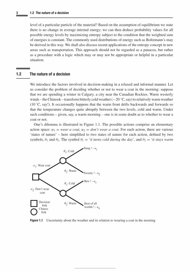
We introduce the factors involved in decision-making in a relaxed and informal manner. Letus consider the problem of deciding whether or not to wear a coat in the morning: supposethat we are spending a winter in Calgary, a city near the Canadian Rockies. Warm westerlywinds – the Chinook – transform bitterly cold weather (−20 ◦C, say) to relatively warm weather(10 ◦C, say!). It occasionally happens that the warm front drifts backwards and forwards sothat the temperature changes quite abruptly between the two levels, cold and warm. Undersuch conditions – given, say, a warm morning – one is in some doubt as to whether to wear acoat or not.
One’s dilemma is illustrated in Figure 1.1. The possible actions comprise an elementaryaction space: α1 = wear a coat, α2 = don’t wear a coat. For each action, there are various‘states of nature’ – here simplified to two states of nature for each action, defined by twosymbols, θ1 and θ2. The symbol θ1 = ‘it turns cold during the day’, and θ2 = ‘it stays warm
Figure 1.1 Uncertainty about the weather and its relation to wearing a coat in the morning

4 Uncertainty and decision-making
during the day’. Thus, there are four combinations of action and state of nature, and corre-sponding to each of these, there is a ‘consequence’, u1, u2, u3 and u4 as shown in Figure 1.1. Aconsequence will be termed a utility, U , a measure of value to the individual. Higher values ofutility will represent consequences of greater value to the individual. The estimation of utilitieswill be dealt with later in Chapter 4; the concept is in no way arbitrary and requires carefulanalysis.
It is not difficult to reach the conclusion that the choice of decision (α1 or α2) depends on twosets of quantities only. These are the set of probabilities associated with the states of nature,{Pr(θ1), Pr(θ2)}, and the set of utilities, {u1, u2, u3 and u4}. The formal analysis of decisionswill be dealt with subsequently, but it is sufficient here to note the dependence of the choice ofdecision on the two sets of quantities – probabilities and utilities. This pattern repeats itself inall decision problems, although the decision tree will usually be more complex than that givenin Figure 1.1.
This example can also be used to illustrate a saying of de Finetti’s (1974):
Prevision is not prediction.
Prevision has the same sense as ‘expected value’; think of the centre of gravity of one’sprobabilistic weights attached to various possibilities. I recall an occasion when the temperaturein Calgary was oscillating regularly and abruptly between 10 ◦C and −20 ◦C; the weatherforecast was −5 ◦C. Yet nobody really considered the value of −5 ◦C as at all likely. If oneattached probabilistic ‘weights’ of 50% at 10◦ and −20◦, the value −5◦ would represent one’sprevision – but certainly not one’s ‘prediction’.
The decision problem just discussed – to wear a coat or not – is mirrored in a number ofexamples from industry and engineering. Let us introduce next the oil wildcatter who literallymakes his or her living by making decisions under uncertainty. In oil or gas exploration, areasof land are leased, primarily by big companies, but also by smaller scale operators. Oil wellsmay be drilled by the company leasing the land or by other operators, on the basis of anagreement. Exploratory wells are sometimes drilled at some distance from areas in whichthere are producing wells. These wells are termed ‘wildcats’. The risk element is greater,because there is less information about such wells; in the case of new fields, the term ‘newfield wildcats’ is used to denote the wells. The probability of success even for a good prospectis often estimated at only 40%. Drilling operators have to decide whether to invest in a drillingventure or not, on the basis of various pieces of information. Those who drill ‘wildcat’ wellsare termed ‘wildcatters’.
We are only touching on the various uncertainties facing oil and gas operators; for instance,the flow from a well may be large or small; it may decline substantially with time; the drillingoperation itself can sometimes be very difficult and expensive, the expense being impossibleto ‘predict’. There may be an option to join a consortium for the purpose of a drilling, less-ening risk to an individual operator. The classic work is by Grayson (1960) who studied theimplementation of decision theory to this field. He analysed the actual behaviour in the fieldof various operators.

5 1.2 The nature of a decision
Figure 1.2 Oil wildcatter’s dilemma
The wildcatter must decide whether or not to drill at a certain site before the lease expires.The situation is illustrated in the form of a decision tree in Figure 1.2. She realizes that ifdrilling is undertaken, substantial costs are involved in the drilling operation. On the otherhand, failure to drill may result in a lost opportunity for substantial profits if there is oil presentin the well. The decision must reflect an assessment of the probability of there being oil in thewell. This assessment will almost invariably take into account a geologist’s opinion. Thus, theaction space is A = {α1 = drill for oil, α2 = do not drill}. The uncertain states of nature are� = {θ1, θ2} where � = {θ1 = oil present and θ2 = no oil present}. The choice of decisionis again seen to depend on the values of U and the values {Pr(θ1), Pr(θ2)}.
In some decisions the states of nature differ, depending on the decision made. Considerthe question of relocation of a railway that passes through a city. The trains may include carscontaining chlorine, so that there is the possibility of release of poisonous gas near a humanpopulation. Figure 1.3 shows a decision tree for a problem of this kind. The consequences interms of possible deaths and injuries are quite different for the two branches and might be quitenegligible for the upper branch. Figure 1.3 illustrates a tradeoff between cost of relocation andrisk to humans. This tradeoff between cost and safety is fundamental to many engineeringdecisions. Other tradeoffs include for example that between the service rate provided forincoming data and the queuing delay in data transmission. This is shown in Figure 1.4. Trafficin computer networks is characterized by ‘bursts’ in the arrival of data. The incoming trafficis aggregated and the bursts can lead to delays in transmission.
Figure 1.5 illustrates an everyday problem on a construction site. Is a batch of concreteacceptable? One might, for instance, measure air void content to ascertain whether the freeze–thaw durability is potentially good or bad. Bayes’ theorem tells us how to incorporate this newinformation (Section 2.4). Non-destructive testing of steel structures is also rich in problemsof this kind.

6 Uncertainty and decision-making
Figure 1.3 Rail relocation decision
Figure 1.4 Decision on service rate for computer network
Let us return to the problems facing a code-writing committee. One of the many dilemmasfacing such a committee is the question: should one recommend a simplified rule for use byengineers in practice? An example is: keep the span-to-depth ratio of a reinforced concreteslab less than a certain specified value, to ensure that the deflection under service loads is notexcessive (rather than extensive analysis of the deflection, including the effects of creep, andso on). A further example is: should the 100-year wave height and period be the specified

7 1.2 The nature of a decision
Figure 1.5 To accept or reject a batch of concrete posed as a problem of decision-making.Traditionally this is dealt with by hypothesis testing
Design usingadditional information
Figure 1.6 What recommendations to make for use in a design standard?
environmental indicators in the design of an offshore structure, in place of a more detaileddescription of the wave regime? These are numerous decisions of this kind facing the code-writer that can be analysed by decision theory. The decision tree would typically be of the kindillustrated in Figure 1.6. Rather than using the simplified rule, the committee might considerrecommending the use of information ‘I ’ which will be known at the time of design (e.g. thegrade of steel or concrete, or a special test of strength if the structural material is available). Thisquantity could take several values and is therefore, from the point of view of the committee, arandom quantity with associated probabilities.

8 Uncertainty and decision-making
Figure 1.7 Risky and safe investment decisions
0
Figure 1.8 Dilemma in having an operation: θ1 represents a successful operation and θ2 anunsuccessful one
Economic decision-making naturally contains many decisions under uncertainty. Figure 1.7illustrates the simple choice between stocks – a risky choice – and bonds with a knownrate of return. We have stated that probability is a function of information, and conse-quently the better our information, the better our assessment of probabilities. The extremeof this would correspond to insider trading – betting on a sure thing, but not strictly legal orethical!
Decisions in normal life can be considered using the present theory. Consider the followingmedical event.
‘Patient x survives a given operation.’
Suppose that the patient (you, possibly) has an illness which causes some pain and loss ofquality of life. Your doctors suggest an operation which, if successful, will relieve the pain;there is the possibility that you will not survive the operation and its aftermath. Your dilemma

9 1.3 Domain of probability
is illustrated in Figure 1.8. This example is perhaps a little dramatic, but the essential point isthat again one’s decision depends on the probabilities Pr(θ1) and Pr(θ2) (Figure 1.8) and one’sutilities. One would be advised to carry out research in assessing the probabilities; the utilitiesmust clearly be the patient’s. The example points to the desirability of strong participation bypatients in medical decisions affecting them.
1.3 Domain of probability: subjectivity and objectivity
The domain of probability is, in a nutshell, that which is possible but not certain. Probabilitiescan be thought of as ‘weights’ attached to what one considers to be possible. It thereforebecomes essential to define clearly what one considers to be possible. The transition from ‘whatis possible’ to ‘certainty’ will result from a well-defined measurement, or, more generally, aset of operations constituting the measurement. The specification or statement of the ‘possibleoutcomes’ must then be objective in the sense just described. We must be able, at least inprinciple, to determine its truth or falsity by means of measurement. To take an example,consider the statement:
E: ‘We shall receive more than 1 cm of rain on Friday.’
We assume that it is Monday now. We need to contrive an experiment to decide whether ornot there will be more than 1 cm of rain on Friday. We might then agree that statement Ewill be true or false according to measurements made using a rain gauge constructed at ameteorological laboratory.
Having specified how we may decide on the truth or falsity of E we are in a position toconsider probabilities. Since it is now Monday, we can only express an opinion regarding thetruth or falsity of E . This ‘opinion’ is our probability assignment. It is subjective since wewould base it on our knowledge and information at the time. There is no objective means ofdetermining the truth or falsity of our probability assignment. This would be a meaninglessexercise. If a spectacular high pressure zone develops on Thursday, we might change ourassignment.
The same logic as above should be applied to any problem that is the subject of probabilisticanalysis. The statement of the possible outcomes must be objective, and sufficient for theproblem being analysed. It is instructive to ponder everyday statements in this light. Forexample, consider ‘his eyes are blue’, ‘the concrete is understrength’, ‘the traffic will be tooheavy’, ‘the fatigue life is adequate’. . . We should tighten up our definitions in these casesbefore we consider a probabilistic statement.
The approach that we have followed in defining what is possible echoes Bridgman’s opera-tional definition of a concept: the concept itself is identified with the set of operations whichone performs in order to make a measurement of the concept; see Bridgman (1958). For ex-ample, length is identified with the physical operations which are used in measuring length,for instance laying a measuring rod along the object with one end coinciding with a particular

10 Uncertainty and decision-making
mark, taking a reading at the other end, and so on. We shall suggest also that probability canbe defined using the operational concept, but tied to the decision-maker’s actions in making afair bet, as described in the next chapter.
1.4 Approach and tools; role of judgement: indifference and preference
The theory that we are expounding deals with judgements regarding events. These judgementsfall into two categories, corresponding to the two fundamental quantities introduced in Sec-tion 1.2 that are involved in decision-making: probabilities and utilities. The basic principle individing the problem of decision into two parts is that probability represents our judgement –regardless of our desires – as to the likelihood of the occurrence of the events under consider-ation, whereas utility represents our judgement of the relative desirability of the outcomes ofthe events. For example, we assess the likelihood (probability) of an accident in an impartialmanner, taking into account all available information. The consequences of the accident maybe highly undesirable, possibly involving loss of life, leading to our estimate of utility. Butthese factors do not affect our judgement of probability.
Probability will be defined formally in the next chapter; for the present introductory purposes,we introduce one of our tools, the urn containing balls of different colours. The urn couldbe a jar, a vase, a can or a bag – or one’s hand, containing coloured stones. Our primitiveancestors would probably have used stones in their hand. It is traditional in probability theoryto use urns with coloured balls, let us say red and pink, identical – apart from colour – inweight, size and texture. Then the balls are mixed and one is drawn without looking at thecolour.

11 1.4 Approach and tools
Urn containing coloured balls
Figure 1.9 Tools for probability
The urn of Figure 1.9(a) contains an equal number of balls of each of two colours, designated‘0’ (say, pink) and ‘1’ (say, red). We would agree that the likelihood of drawing a ball with a‘0’ or a ‘1’ is the same since the numbers of ‘0’ and ‘1’ balls are the same. The probability ofeither is then 0.5. We can use the urn to conceive of any value of probability that correspondsto a rational number by placing the required number of balls into the urn. A probability of(57/100) corresponds to an urn containing 100 well-shuffled balls of which 57 are red and theothers pink.
To put into effect our judgement in a range of situations, it is useful to consider ‘orderrelations’. These represent the results of our judgement, in terms of the relationship betweenthe objects under consideration. Consider a set of objects {a1, a2, . . . , an}; these could be sets ofnumbers, people, consequences of actions, or probabilities. If we have a relationship betweentwo of them, this is a binary relation, written as a1 Ra2. For example, the relation R might bethat a1 is bigger than a2 in the case of real numbers, typified by the familiar relationship >.Other familiar relationships are = and <. Another relationship R might be that a1 is a memberof the same family as a2, in the case of persons.
We shall now introduce negation, indicated by ∼, and two order relationships: indifference,written as ≈, and preference, written as �. Negation represents the complement of a statement;for example, if A = ‘the steel strength is greater than 400 MPa’ then the negation, written either

12 Uncertainty and decision-making
∼ A or A, represents ‘the steel strength is less than or equal to 400 MPa’. The tilde ∼ can beread as ‘not’, e.g. A is not-A. The same notation is used for actions. If α = ‘accept’, then α =‘reject’.
Since we have used ∼ for negation, we shall use the double tilde ≈ for indifference. Thisconcept is used frequently in our theory and can be read as ‘twiddles’. For example, if weare indifferent between the purchase of certain stocks (Figure 1.7), termed option ‘a’, and thepurchase of bonds, termed option ‘b’, then for us, we might say that we are indifferent betweena and b, or
a ≈ b,
or ‘a twiddles b’.It is important to become accustomed to these ideas. For example, consider the situation
where we are offered $10 upon the drawing of a red ball from the urn of Figure 1.9(a), withno reward for a pink one – option a. This is illustrated in the right hand side of Figure 1.9(b).What sum of money – option b – would we pay for this lottery? We might be prepared toexchange $5 for the lottery. Then again
a ≈ b.
On average if we played repeatedly we would neither gain nor lose money. Our views mightchange if the reward for red was increased, say to $1000, or to $10 000 or higher. We wouldbe less likely to offer half of the reward to join when the sums are large. We would not wishto pay $5000 for the lottery with an even chance only of gaining an extra $5000 but with thesame chance of losing the payment. In this case, option b – keep the $5000 for sure – mightbe preferred to a – $5000 payment with a reward of $10 000 if a red ball appears but with noreward and loss of the original $5000 if pink appears. Here we write
b � a.
This aversion to risk is considered in some detail in Chapter 4. We might prefer wine, optiona, to beer, option b, then a � b. Preference and indifference are similar, but not the same as, >and = in algebra.
The question in the lottery can be posed in terms of probabilities, rather than consequences.Consider the lottery of Figure 1.9(c). For what value of probability π would one feel indifferentbetween the two options, that is, exchange one for the other, and vice versa? We might wishπ to be greater than half to compensate for the possibility of losing our investment of $5000.We can conceive any rational value of probability using our urn device.
1.5 Probability and frequency
There are two situations in which we need to analyse uncertainty. The first concerns that associ-ated with ‘repetitions of the same experiment’, such as tossing a coin or repeated drawing with

13 1.5 Probability and frequency
subsequent replacement from urns of the kind in Figure 1.9(a). We can obtain the probabilityof heads or tails by tossing the coin many times and taking the proportion of heads. This leadsto the ‘frequency’ definition of probability. We might, on the other hand, be considering anevent that happens only once or rarely, such as the inflation rate next year or the success of anearly space shuttle. This one-off kind of event is perhaps more appropriate to the real world ofour lives.
The concern with repetitive random phenomena stems from the nature of certain processessuch as wind loading applied to a structure, or repeated tosses of a coin. The uncertainty isrelated to a particular future event of the same kind, for instance the maximum wind loadingin a year, or result of the next toss of the coin. We shall view this kind of uncertainty fromthe same standpoint as any other kind, in particular one’s uncertainty regarding an event thatoccurs once only, and treat the record of the past (wind speeds, heads and tails) as informationwhich we should use to estimate our probabilities. We use frequencies to evaluate, not definea probability.
To sum up: probability is not a frequency – by definition. We use frequencies to estimateprobabilities; this distinction is important. The approach taken here is often termed ‘Bayesian’,after Thomas Bayes who initiated it in the eighteenth century. One consequence of the positionthat probability is not a frequency is that it is not an objective ‘property’ of the thing understudy, to be measured in some kind of lengthy ‘random experiment’.1 Consider the difficulty ofconstructing a random experiment to express our uncertainty about the future rate of inflation.A ‘thought-experiment’ or simulation can instead be used to construct a theory using frequency.We shall use frequency data just as often as the strict ‘frequentist’ statistician, and we shallsee that ‘frequentist’ results can be recaptured in the Bayesian analysis. We can often replacea real repetitive experiment with an imaginary one in cases where a frequency interpretationis desired. For any of our probability assignments, one can imagine a repetitive experiment.
In everyday thinking, it is often convenient to solve problems in terms of frequency ratios.Consider the case of a rare disease. The probability of contracting the disease is 1/10 000. Aperson is tested by a method that is fool-proof if the person has the disease, but gives a falseresult 6% of the time if the person is free of the disease, that is, 6% false positive indications.We assume that we have no information on symptoms. If the person obtains a positive reading,what is the probability that he or she has the disease? It is easy to consider 10 000 persons, oneof whom has the disease. Of the disease-free persons, 6%, or almost 600, will have a positiveindication. Therefore, the probability that a person with a positive indication has the diseaseis only one in 601! But we know that the probabilities are 1/10 000 and 1/601 and that onewould not necessarily find exactly one diseased person in a group of 10 000.
The situations discussed relate also to the classical dichotomy between risk and uncertaintywhich existed in economic theory for some time.2 In this approach, ‘risk’ was considered to
1 Jaynes (2003) gives an entertaining account of the difficulty in constructing such an experiment – particularly withrespect to coin-tossing. He discusses the mechanics of tossing a coin and suggests that it is possible to cheat byskilful tossing.
2 See, for example, M. Machina and M. Rothschild’s article ‘Risk’ in Eatwell et al. (1990).

14 Uncertainty and decision-making
be involved when numerical probabilities were used; if probabilities were not assigned, thealternative possible outcomes were said to involve ‘uncertainty’. Bernstein (1996) describesthe development of this line of thinking. We shall not make this distinction. It seems to runcounter to the normal use of the words risk and uncertainty and is perhaps losing importancein economic thinking, too. The same structure in decision-making applies whether we carryout a calculation of probability or not.
As a first step in evaluating probabilities, it is useful to judge everyday events from the pointof view of indifference as outlined in the preceding section. At what value would we judgethe rate of inflation next year to be equally likely to be exceeded or not? As an example, inearly 1980 I judged the value to be 12% for the year; therefore my probabilities were 50% forthe exceedance and non-exceedance of this value. (The change in the Consumer Price Indexturned out to be 11.2%: a reminder that inflation can return!) Tweedledum and Tweedledeeillustrate our attitude that a bet on heads in the next toss of a coin and a bet on the rate ofinflation – as just described – are essentially equivalent. Certainly our uncertainty is the same,instances of the same phenomenon.
Tweedledum and Tweedledee

15 1.6 Terminology, notation and conventions
The principal benefit of the present theory is that one can view other definitions – frequentist,classical, . . . – as special cases of the one espoused here. One can, in addition, tie the problemto its raison d’etre, the need to make a decision and to act in a rational way. The behaviouralview of probability teaches one to ponder the nature of a problem, to try to idealize it, to decidewhether it is appropriate to use or to massage frequency data. The theory then makes one learnto express one’s opinions in as accurate a way as possible and consequently one is less inclinedto take refuge in a formula or set of rules.
1.6 Terminology, notation and conventions
Most of what will be said in the following arises from conventions suggested in many casesby de Finetti. These changes assist considerably in orienting oneself and in posing prob-lems correctly, making all the difference between a clear understanding of what one is doingand a half-formed picture, vaguely understood. As noted previously, by far the most com-mon problem arises from the fact that much previous experience in probability theory re-sults from dealing with ‘repetitive random phenomena’: series of tosses of a coin, records ofwind speeds, and in general records of data. We do not exclude these problems from con-sideration but the repetitive part is clearly our record of the past. The expression ‘randomdata’ is a contradiction of terms. We should attempt to apply probability theory to eventswhere we do not have the outcome, using the records, with judgement, to make probabilisticstatements.
Examples of correctly posed problems are the following with the understanding that wheremeasurements are to be made, the appropriate systems for this purpose are in place:
E1: ‘heads on the tenth toss of a specified coin in a series of tosses about to start’E2: ‘heads on the tenth toss in a series of tosses made yesterday, but for which the records are
misplaced’E3: ‘the wind pressure on a specified area on April 2, 2050 at 8:00 a.m. will be in the range
x1 to x2 Pa (specified)’E4: ‘the wind pressure on surfaces in (location) will exceed X Pa (specified) in the next
30 years’E5: ‘the maximum load imposed by ice on this arctic structure during its defined life will be
greater than y MN (specified)’E6: ‘the number of packets of information at a gateway in a network during a specified period
will exceed 500 million’.
The events to which we apply probability theory should be distinct, clearly defined events,as above. It then becomes meaningless to talk of ‘random variables’. The events are, or turn outto be, either true or false: they are not themselves varying. The adjective ‘random’ expressesour uncertainty about the truth or falsity of the event. The sense that one should attach to the

16 Uncertainty and decision-making
word is ‘unknown’, referring to truth or falsity and, in general, ‘uncertainty’. With regard tothe common term ‘random variable’, consider the following statement:
Q1: ‘the elastic modulus of this masonry element is X = x GPa’.
Here, we permit X to take a range of values, a particular value being denoted by the lower caseletter x . The quantity X is what is normally termed a ‘random variable’, implying that it varies;this is incorrect. X does not vary; it will take on a particular value, which we do not know.That is why we need probability theory. We shall therefore adopt the term ‘random quantity’as suggested by de Finetti rather than ‘random variable’. As noted, ‘random’ is retained withthe understanding that the meaning is taken as being close to that of the phrase ‘whose valueis uncertain’.
Bruno de Finetti used the word ‘prevision’ for what would usually be described as themean or expected value of a quantity, but with much more significance. The most vivid, andappealing, interpretation of expected value (or prevision) for an engineer is by means of centreof gravity. We can think of probability as a ‘weight’ distributed over the possible events, thesum of the weights being unity. An example was given in Section 1.2, in considering twopossible temperatures of 10 and −20 ◦C; if the ‘weights’ attached to these possibilities are1/2 each, the mean or prevision (not the value ‘expected’ or a ‘prediction’) of the temperatureis −5 ◦C. In fact, probability can be seen as a special case of prevision. De Finetti usesthe symbol P(·) for both probability and prevision. In this book, we shall use Pr(E) forprobability of event E . We shall use 〈X〉 for the mean, or expected value, of the argument(X ). The term ‘expected value’ is often used but only has meaning as an average in a long runexperiment. We shall occasionally use ‘prevision’ to recognize the clarification brought by deFinetti.
1.7 Brief historical notes
A definitive statement on the history of probability would certainly be an interesting anddemanding project, far beyond the intention of the present treatment. Stigler (1986) givesa scholarly analysis of the development of statistics. Bernstein (1996) gives an entertainingaccount of the development of the use of probability and the concepts of risk analysis appliedparticularly to investment. Judgements of chance are intuitive features of the behaviour ofhumans and indeed, animals, so that it is likely that the ideas have been around during thedevelopment of human thinking. There is mention of use of probability to guide a wise person’slife by Cicero; the use of odds is embedded in the English language, for example Bacon in1625: ‘If a man watch too long, it is odds he will fall asleepe’.
Early work in mathematical probability theory dates back to the seventeenth century. Theearly focus of theory was towards the solution of games of chance, and the classical view ofprobability arose from this. An example is the famous correspondence between Pascal and

17 1.7 Brief historical notes
Fermat on games with dice, summarized in Section 9.2. In cases where one can classify thepossible outcomes into sets of ‘equally likely’ events, probabilities can be assigned on thisbasis. It is now commonplace to assign probabilities for games of cards, dice, roulette, and soon, using classical methods. The extension of this to account for observations was the next task.The title of Jacob Bernoulli’s work, ‘Ars Conjectandi’, or the art of conjecturing, summarizesmuch of the spirit of dealing with uncertainty. In Bayes’ original paper (Bayes, 1763) one findsthe definition of probability in terms of potential behaviour – as outlined in the next chapter.Laplace (1812, 1814) applied these ideas, together with Bayes’ method of changing probabilityassignments in the light of new evidence (Bayes’ theorem) to practical problems, such as inastronomy.
The ‘relative frequency’ view of probability was developed in the latter part of the nineteenthand first half of the twentieth century; see for instance Venn (1888) or von Mises (1957). Thisdefinition is based on a long series of repetitions of the same experiment, for instance tossinga coin repeatedly and counting the proportion of heads to obtain the probability of heads in afuture trial. As noted in Section 1.5, frequency ratios are useful in certain problems; in manyapplications, frequencies enter into problems in a natural way. We take issue with definingprobability as always being a frequency that has to be measured. Changes in theories, even as aresult of well-determined experiments, can be a lengthy process. Consider the rejection of thecaloric ‘fluid’ as a result of the discovery of the inexhaustible generation of frictional heat, asmeasured by Count Rumford. The natural tendency to resist change resulted in the persistenceof the theory of heat as being a fluid for a considerable period of time. The frequency view ofprobability is a mechanistic one in which models are postulated that function repetitively in amechanical sense. The inductive world is much wider and permits the updating of knowledgeand thought using evidence in an optimal manner. It points us in the right direction for the nextstep in understanding.
It is interesting to note that utility theory also had its early development during the sameperiod as mathematical probability theory; we shall give an example in Chapter 4, still pertinenttoday, of Daniel Bernoulli’s utility of money. The parallel development of utility and probabilityhad its flowering in the twentieth century. The resurgence of Bayesian ideas contains two mainstreams. They both represent subjective views but are rather different conceptions: the necessaryview and the personal view. The former tries to attain the situation where two persons willarrive at exactly the same assignment of probabilities. The latter accepts the possibility thattwo people modelling a real situation may obtain somewhat different assignments. Idealizedproblems, will, at the same time, tend to lend themselves to identical solutions. The necessaryview was quite prominent at Cambridge University – for instance Jeffreys (1961). Jaynes(1957, 2003 for example) adopts a necessary point of view and has done most inspiring workon the connection between entropy and probability.
Several authors including de Finetti (1937) and Savage (1954) based their approach onthe idea of defining probabilities by means of potential behaviour, generally using ‘fair’bets. De Finetti has adopted a personalist conception which seems to me to include the

18 Uncertainty and decision-making
necessary view as a rather idealized special case. I find that the work of this writer pro-vides the most flexible and rational viewpoint from which we can regard all probabilities.Good (1965, for example) has made significant contributions to Bayesian methods, and to theuse of entropy. The significant contribution of von Neumann and Morgenstern (1947) pro-vided the link in the structure of utility and probability theory to their close relative, gamestheory.
Bruno de Finetti
Several writers have focussed on the needs of statisticians, or ‘users’ of probabilitytheory. The work of Lindley (1965) put the use of traditional distributions, such as ‘student’s’t-distribution and the use of confidence intervals, in conformity with the rest of the personalisttheory. This was of great value for users of the theory who wished to apply but also to under-stand. Work at Harvard University in the decades after the second World War, exemplified byRaiffa (1968), Schlaifer (1959, 1961) and Raiffa and Schlaifer (1961), has made significantimpact on practical applications. From an engineering standpoint, works such as Benjamin andCornell (1970) and Cornell (1969a), which stress decision-making and are sympathetic to theBayesian approach, were instrumental in pointing the way for many users, including the presentone.

19 1.8 Exercise
The towering figure of twentieth century probability theory is Bruno de Finetti. Lindleystates in the foreword to the book by de Finetti (1974) that it is ‘destined ultimately to berecognized as one of the great books of the world’. I strongly agree.
1.8 Exercise
1.1 Draw a decision tree, involving choice and chance forks, for each of
(a) a personal decision (for example, for which term should one renew a mortgage; one, three or fiveyears?);
(b) an engineering problem.

2 The concept of probability
Iacta alea est.Julius Caesar, at the crossing of the Rubicon
2.1 Introduction to probability
Probability and utility are the primary and central concepts in decision-making. We now discussthe basis for assigning probabilities. The elicitation of a probability aims at a quantitativestatement of opinion about the uncertainty associated with the event under consideration. Thetheory is mathematical, so that ground rules have to be developed. Rather than stating a set ofaxioms, which are dull and condescend, we approach the subject from the standpoint of thepotential behaviour of a reasonable person. Therefore, we need a person, you perhaps, whowishes to express their probabilistic opinion. We need also to consider an event about whichwe are uncertain. The definition of possible events must be clear and unambiguous.
It is a general rule that the more we study the circumstances surrounding the event orquantity, the better will be our probabilistic reasoning. The circumstances might be physical,as in the case where we are considering a problem involving a physical process. For example,we might be considering the extreme wave height during a year at an offshore location. Or thecircumstances might be psychological, for example, when we are considering the probabilityof acceptance of a proposal to carry out a study in a competitive bid, or the probability of aperson choosing to buy a particular product. The circumstances might contain several humanelements in the case of the extreme incoming traffic in a data network. The basic principle tobe decided is: how should one elicit a probability?
We shall adopt the simple procedure of using our potential behaviour in terms of a fair bet –put one’s money where one’s mouth is, in popular idiom. By asking how we would bet, we areasking how we would act and it is this potential behaviour which forces us to use availableinformation in a sensible down-to-earth manner. This provides a link with everyday experience,with the betting behaviour of women or men in the street. It is one of the great strengths of thepresent theory. We shall consider small quantities of money so as to avoid having to deal withthe aversion to the risk associated with the possibility of losing large quantities of money. Riskaversion was alluded to in Section 1.4 and is dealt with in detail in Chapter 4.
20

21 2.1 Introduction to probability
Let us suppose that YOU wish to express your opinion by means of a probability, and thatI am acting as your advisor on probabilistic matters. My first piece of advice would be tofocus your thoughts on a fair bet. To explain further, let us use an example. We shall assumethat YOU are the engineer on a site where structural concrete is delivered. You wish to assignprobabilities to the various possible strengths of a specimen taken from a batch of concrete justdelivered to the site. In doing this, you should take into account all available information. Theextent to which we search for new information and the depth to which we research the problemof interest will vary, depending on its importance, the time available and generally on ourjudgement and common sense. We have some knowledge of the concrete delivered previously,of a similar specified grade. To be precise: we cast a cylindrical specimen of the concrete, 15cm in diameter and 30 cm long (6 by 12 inches) by convention in North America. Since itsstrength is dependent on time and on the ambient temperature and humidity, we specify thatthe strength is to be measured at 28 days after storing under specified conditions of temperatureand humidity. The strength test at 28 days will be in uniaxial compression. You now have 28days to ponder your probability assignment!1
The first step is to decide which strengths you consider to be possible: I suggest that you takethe range of strengths reasonably wide; it is generally better to assign a low probability to anunlikely event than to exclude it altogether. Let us use the interval 0–100 MPa. Let us agree todivide the interval of possible strengths into discrete subintervals, say 0–20 MPa, 20–40 MPa,and so on. (In the event of an ‘exact’ value at the end of a range, e.g. 40 MPa, we assign thevalue to the range of values below it, i.e. to 20–40 MPa in the present instance.) We shallconcentrate on a particular event which we denote as E . We use in this example
E: ‘The strength lies in the subinterval 40–60 MPa.’
(The arguments that follow could be applied to any of the subintervals.) If E turns out to betrue, we write E = 1, if E is false, we write E = 0. The notation 1 = TRUE, 0 = FALSE willbe used for random events, which can have only these two possible outcomes. Hence, E is arandom event. On the other hand, concrete strength is a random quantity, since it can takeany of a number of specific values, such as the strength 45.2 MPa, in a range, whereas an eventcan be either TRUE (1) or FALSE (0). The events or quantities are random since we don’tknow which value they will take.
We shall elicit your probability of E , which we write as Pr(E), in the following way. I offeryou a contract for a small amount ‘s’, say $100, which you receive if the strength is in thespecified interval, that is if E is true. If E is not true, you get nothing. The crux of the matteris as follows: you must choose the maximum amount $(sp) = $(100p) which you would payfor the contract. We specify ‘maximum’ because the resulting bet must be a ‘fair’ one, in theaccepted sense of the word, and anything less than your maximum would be in your favouror even represent a bargain for you. We assume also that you are not trying to give money
1 In the reality of engineering practice, the discovery of concrete that fails the strength specification once it hashardened poses difficulties with regard to its removal!

22 The concept of probability
’‘
Figure 2.1 Evaluation of probability
away and that your maximum therefore represents a fair bet. Essentially we want the two mainbranches in Figure 2.1(a) to be of same value.
We noted in Section 1.4 that the symbol E with the tilde added before or above it, ∼ E or E ,in Figure 2.1(a) denotes ‘not-E’, ‘the complement of E’, ‘the negation of E’, or if one wishes,

23 2.1 Introduction to probability
‘it is not the case that E’. For example, if F = ‘the concrete strength is greater than 40 MPa’,then F indicates ‘the concrete strength is not greater than 40 MPa’ or ‘the concrete strength isless than or equal to 40 MPa’. Hence, E + E = 1, since either E or E is true (1) and the otheris false (0). The equivalence of the two branches in Figure 2.1 implies that
−100p + 100E ≈ 0 (2.1)
where ≈ indicates ‘indifference’.2 This means simply that our definition of probability impliesthat we are indifferent as to whether we obtain the left or right hand side of the relation sign ≈.Remember that E is random (uncertain) in the relationship (2.1) taking the values 1 or 0depending on whether E is true or false respectively. The value ‘0’ on the right hand side ofthe indifference relationship indicates the status quo, resulting in no loss or gain, shown in thelower branch of Figure 2.1(a).
As a vehicle for assigning your probabilities, you might wish to use an urn such as that inFigure 1.9(a). For example, if 100 balls were place in the urn with 25 being red, this woulddenote a probability of 0.25. It is good general advice to use any past records and histogramsthat you have in your possession to obtain your value of ‘ps’. Figure 2.1 shows that choosinga probability is also a decision. Let us assume that we have in the past tested a large number(say, in the thousands) of similar concrete cylinders. The result is indicated in Figure 2.1(b) interms of a frequency histogram indicating the percentage of results falling in the correspondingranges. There is nothing to indicate that the present cylinder is distinguishable or different in anyrespect from those used in constructing the past records. We observe from detailed analysis ofthe data of Figure 2.1(b) that 34% of results fall in the range of values corresponding to event E .
The probability of E is now defined in terms of your behaviour by
Pr(E) = p = 0.34. (2.2)
A value of $34 as an offer for the contract indicates that Pr(E) = p = 0.34. This would be areasonable offer based on the histogram of Figure 2.1(b). All the data falls into the two classintervals 20–40 MPa and 40–60 MPa; we might therefore wish to make an allowance for asmall probability of results falling outside these limits, possibly by fitting a distribution. Thiswill be deferred to later chapters. We have gone out of our way to say that probability is nota frequency, yet we use a frequency to estimate our probability. This is entirely consistentwith our philosophy that the fair bet makes a correct definition of probability, but then to usewhatever information is at hand, including frequencies, to estimate our probability.
The definition of probability has been based on small amounts of money; the reason for thisis the non-linear relationship between utility and money which will become clear in Chapter 4.For the present, this aspect is not of importance; the non-linearity stems from aversion torisking large amounts of money. The concept of probability remains the same when we haveto deal with large amounts of money; we then define probability in terms of small quantities ofmoney, or in terms of utility, rather than money, a procedure which is equivalent to the above.
2 Twiddles (≈) was introduced in Chapter 1, and exemplified by Tweedledum and Tweedledee.

24 The concept of probability
In order to measure probability, all that we need is a person (you, in this case!) who isprepared to express their opinion in the choice of Pr(E) = p. It is important to stress thatPr(E) expresses your opinion regarding the likelihood of E occurring – an opinion that shouldbe entirely divorced from what you wish to happen. The latter aspect is included in our measureof the utility of the outcome. The oil wildcatter hopes desperately for a well that is not dry, butthe probability assignment should reflect her opinion regarding the presence of oil, disregardingaspirations or wishes. It should also be noted that a contract could be purchased for a rewardof, say $100, to be paid if E , rather than E , occurs. Given Pr(E) = 0.34, we would expectthe contract on E to be valued at $66; this will be discussed in some detail at the end of thissection and the beginning of the next.
OddsIt is common in everyday language to use ‘odds’, that is, the ratio of the probability for anevent, say E , to the probability of its complement E . Writing the odds as ‘r ’, we have
r = Pr(E)
Pr(E)= loss if E
gain if E, (2.3)
where the loss to gain ratio follows from the fact that the upper branch of Figure 2.1(a) canbe represented by the equivalent fork shown in Figure 2.2(a). Indeed for the probabilist thisshould become one’s ‘rule for life’. For example, given odds of 5 to 2 (or r = 2.5) on an eventH , the probability of H is 5/7. Formally, the probability of an event E is expressed as
Pr(E) = r
r + 1. (2.4)
(a) Equivalence of upper branch of Figure 2.1(a) (left in the figure above) and thegain and loss shown on the right of the figure
Figure 2.2 Gain and loss in fair bet; urn equivalent

25 2.1 Introduction to probability
This can also be written as r = p/(1 − p), or
r = p
p, (2.5)
where p is defined as (1 − p).This definition of p just given for numerical quantities is consistent with the definition for
events given earlier, since Pr(E) = p = 1 corresponds to E = 1 (E is certain). If p = 0 thenE = 0 since E is impossible. The converse is also true; E = 0 implies that p = 0. We canwrite E + E = 1 and the corresponding expression p + p = 1; the basis for the latter will bediscussed in more detail in Section 2.2. For example, p could be 4/5 and then p = 1/5. It isalso useful to think of the ratio p/ p as a ratio of weights of probability. This is illustrated witha pair of scales with p = 4/5, p = 1/5. Probability is a balance of judgement with ‘weights’representing the odds. The weights in each scale can also be interpreted as the stakes in the fairbet. The bet on E is in the left hand scale and this is lost if E occurs; similar reasoning appliesto the bet on E , which is lost if E occurs. In this sense, one’s probability can be thought of asa bet with oneself. Figure 2.2(b) shows the urn equivalent to p = 4/5, p = 1/5.
Rule for Life with example probabilities of 4/5 and 1/5
The notion of defining probability behaviourally is not new. The definition in terms of oddsis given in the original paper by Bayes (1763):
‘If a person has an expectation depending on the happening of an event, the probability of the event is tothe probability of its failure as his loss if it fails to his gain if it happens’.
Implied in the definition of odds is the condition that Pr(E) = p and Pr(E) = p add up tounity. It is not always appreciated that the normalization of probabilities (i.e. that they sum tounity) follows from a very simple behavioural requirement – coherence. This means that youwould not wish to make a combination of bets that you are sure to lose.

26 The concept of probability
2.2 Coherence: avoiding certain loss; partitions; Boolean operations and constituents;probability of compound events; sets
It would be expected that the percentages shown in the histogram of Figure 2.1(b) should addup to unity since each is a percentage of the total number of results. If we throw a die, andjudge that each face has equal probability of appearing on top, we naturally assign probabilitiesof 1/6 to each of the six faces. The probabilities calculated using our urn will also add up tounity. But there is a deeper behavioural reason for this result, termed ‘coherence’ which wenow explore.
Let us consider first an event E and its complement E . These could be, for example, theevents discussed in Section 2.1 or events such as E = ‘the die shows 1’ and E = ‘the die shows2, 3, 4, 5 or 6’. We introduced the definition of probability, Pr(E), as a fair bet and then wenton to discuss odds on E as
Pr(E)
Pr(E)= loss if E
gain if E= p
1 − p= p
p.
This step in fact introduced indirectly the probability of E . Figure 2.3(a) shows the bet whichdefines Pr(E). A similar bet could be used to define Pr(E), as shown in Figure 2.3(b). Inthis, we pay ps for a contract which gives us the quantity ‘s’ if E occurs. It can be seen,by comparing the right hand side of Figures 2.3(a) and (b) that the bet on E (in (b)) isjust the negative of the bet on E when Pr(E) was defined (in (a)). This illustrates an im-portant aspect of indifference: we would buy or sell the bet on E since Figure 2.3(b) isequivalent to selling a bet on E for ‘ps’ with a fine of ‘s’ (rather than a reward) if Eoccurs.
The crux of the present matter is that if we accept the assignment of Figures 2.3(a) and (b)we have accepted that p + p = 1. If this is not the case, what happens? Let us then assume thats = $100, and that the probabilities of p and p′(�= p) are assigned to E and E respectively.For example, let us assume that p = 0.8 and p′ = 0.3. This is illustrated in Figure 2.4. Theassignment of probability means that the assignor would be willing to pay $80 and $30, a totalof $110, for bets on E and E respectively, and receive $100 in return should either happen, asure loss of $10! Figure 2.3(c) shows this in symbolic form.
If the assignor decides on values such that p′ < p, for example, 0.3 and 0.5 as the probabili-ties of E and E respectively, then it is again possible to find a value of ‘s’ such that the assignoralways loses. In this case where the sum of probabilities is less than unity, we would buy thetwo contracts from the assignor. This implies a negative ‘s’, say s = −$100, i.e. $100 paid bythe assignor if E or E occur, with costs to us of the contracts for these two bets of $30 and$50 (on E and E respectively) paid to the assignor. This again results in a certain loss to theassignor. This behaviour is termed incoherence. The implication is that if your probabilitiesdo not normalize, it is always possible to make a combination of bets that you are sure to lose.

27 2.2 Coherence; compound events; sets
'
'
'
−
−
−
−
−
Figure 2.3 Coherent (a,b), and incoherent (c) probabilities of event E and its complement E
The only way to avoid this is to ensure that
Pr(E) + Pr(E) = 1. (2.6)
We can think of the assignment of probabilities as a linear operation Pr on (E + E = 1).Let us take this a little further, with YOU assigning probabilities. It is as well to think of a
‘protagonist’ with whom you are going to make your bets (with my advice for the present).The protagonist would probably be an experienced person such as a ‘bookie’ in horse-racing.Of course, a bookmaker has the objective of making money by arranging the odds in his favour.The same applies to insurance, which constitutes a bet on some future event, with the premiums
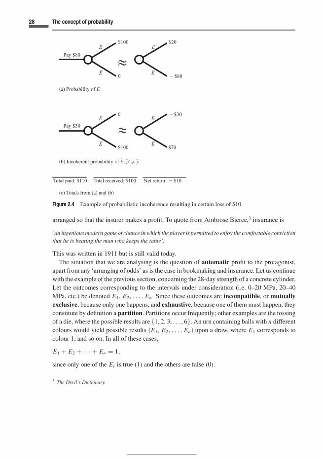
28 The concept of probability
(a) Probability of E
(b) Incoherent probability
(c) Totals from (a) and (b)
'
Figure 2.4 Example of probabilistic incoherence resulting in certain loss of $10
arranged so that the insurer makes a profit. To quote from Ambrose Bierce,3 insurance is
‘an ingenious modern game of chance in which the player is permitted to enjoy the comfortable convictionthat he is beating the man who keeps the table’.
This was written in 1911 but is still valid today.The situation that we are analysing is the question of automatic profit to the protagonist,
apart from any ‘arranging of odds’ as is the case in bookmaking and insurance. Let us continuewith the example of the previous section, concerning the 28-day strength of a concrete cylinder.Let the outcomes corresponding to the intervals under consideration (i.e. 0–20 MPa, 20–40MPa, etc.) be denoted E1, E2, . . . , En. Since these outcomes are incompatible, or mutuallyexclusive, because only one happens, and exhaustive, because one of them must happen, theyconstitute by definition a partition. Partitions occur frequently; other examples are the tossingof a die, where the possible results are {1, 2, 3, . . . , 6}. An urn containing balls with n differentcolours would yield possible results {E1, E2, . . . , En} upon a draw, where E1 corresponds tocolour 1, and so on. In all of these cases,
E1 + E2 + · · · + En = 1,
since only one of the Ei is true (1) and the others are false (0).
3 The Devil’s Dictionary.

29 2.2 Coherence; compound events; sets
The bookie sets stakes equal to s1, s2, . . . , sn corresponding to the outcomes E1, E2, . . . , En;hence, if Ei occurs, you receive si . You have agreed, as before, to purchase the rights to thesecontracts by paying the bookie the prices p1s1, p2s2, . . . , pnsn and in general pi si . The stakesare quite arbitrary sums, positive or negative. The latter would correspond to the case whereyou pay the bookie the prize si if Ei occurs and psi would be the amount, fair in your opinion,that he would pay you for the contract. The bookie’s gain if the outcome Eh turns out to betrue is
mh =∑n
i=1pi si − sh ; h = 1, 2, . . . , n. (2.7)
Let us consider the case where s1 = s2 = · · · = sn = s. The case where the si are different istreated in Exercise 2.6 at the end of the chapter, based on the elegant analysis of de Finetti(1937). Given that the si are all equal to s, Equations (2.7) become
mh = s(∑n
i=1pi − 1
), for each h. (2.8)
We assume initially that your probabilities do not add up to one. In this case, the bookie canregard (2.8) as a set of equations4 in which the mh are known. As a result, he can preassignhis gain (given the pi ), and then solve for s. Thus, you will stand to lose, no matter which Eh
turns out to be true. This is termed ‘making a Dutch book’ against you – no doubt in Holland itis an English book, or a French book. In any event, you will not find this situation acceptable.How can you stop the bookie?
If you make the assignment of probability such that∑n
i=1 pi = 1, this would avoid thepossibility that the bookie could make arbitrary gains mh . The bookie cannot invert Equation(2.8) to solve for s. Since you have normalized your probabilities by adjusting their values,then pi = Pr(Ei ), and we have that∑n
i=1Pr(Ei ) = 1, (2.9)
a result which is sometimes termed the theorem of total probabilities. We term this alsothe normalization of probabilities; your attitude, in avoiding the possibility of making acombination of bets that you are sure to lose, is termed coherence, which is embodied inEquation (2.9). This equation can also be thought of as the operation Pr applied to the equation∑n
i=1Ei = 1.
We can simplify things by making the sum ‘s’ above, in Equations (2.8), equal to unity.Then we can think of the bet Pr(Ei ) on event Ei as a ‘price’ with Pr ≡ price, or stake paid witha reward of ‘unity’ if Ei occurs. A series of bets Pr(E1) = p1, Pr(E2) = p2, . . . , Pr(Ei ) =pi , . . . , Pr(En) = pn, on events that constitute a partition can be interpreted as a series ofprices that add up to unity. We receive the same amount back because one of the Ei musthappen.
4 Bookies are known for their expertise in mathematics.
30 The concept of probability
If we consider two mutually exclusive events, say E1 and E2, we can consider the eventB = ‘either E1 or E2 is true’. We can write
B = E1 + E2
since B = 1 if either E1 or E2 are true (and therefore equal to 1) or else B = 0 if E1 andE2 are both false (0). Now if we are prepared to exchange the status quo for a bet at pricePr(E1) = p1 on E1 or a bet at price Pr(E2) = p2 on E2, then as a result of this indifferencewe will be prepared to bet on both E1 and E2 separately or at the same time; consequently
Pr(B) = Pr(E1 + E2) = Pr(E1) + Pr(E2).
This amounts to buying one contract on B that is equivalent to two contracts, one on E1 andone on E2. In general
Pr(Ei + Ei+1 + · · · + E j ) = Pr(Ei ) + Pr(Ei+1) + · · · + Pr(E j ) (2.10)
for any incompatible events Ei , Ei+1, . . . , E j .These results all follow from coherence, and de Finetti has shown that we can extend the
idea in a very simple way. Suppose that we have the following linear relationship between theevents {E1, E2, . . . , En}, which do not need to be incompatible:
a1 E1 + a2 E2 + · · · + an En = a. (2.11)
This relationship holds no matter which of the Ei turn out to be true; an example is the equation∑Ei = 1 above for the special case of partitions. Another example is the following. Suppose
that we have a device that fails when 5 out of 15 components fail (but we don’t know which).Given failure of the device and if Ei = ‘the ith component fails’, then∑15
i=1Ei = 5.
Or it might happen that in the analysis of an electrical circuit or structural component, weknow the sum of several currents or the resultant of several forces by measuring a reaction. Thenthe sum of the currents or forces is known without knowledge of the individual values. Strictlyspeaking, these are examples of random quantities, which are a generalization of random eventsinsofar as the random quantity may take any value in a range, and is not restricted to 0 or 1.The present theorem carries over and applies to random quantities or events. A last examplemight be a secret ballot: we have that the total votes cast for a proposition are m in number. IfEi = ‘individual i voted in favour of the proposition’, then
∑Ei = m. Again we don’t know
which Ei are true, which individuals voted in favour of the proposition.We now show that coherence requires that we assign probabilities that are consistent with
the following expression:
a1 p1 + a2 p2 + · · · + an pn = a, (2.12)
where we have again used the notation Pr(Ei ) = pi . To demonstrate (2.12), let us assume thatyou make the assignment
a1 p1 + a2 p2 + · · · + an pn = a + δ, (2.13)

31 2.2 Coherence; compound events; sets
where δ is any quantity (positive or negative). Subtracting Equation (2.11) from (2.13) we have
a1(p1 − E1) + a2(p2 − E2) + · · · + an(pn − En) = δ. (2.14)
Now, in order to make the amount δ for sure, I merely have to set stakes of a1, a2, . . . , an tobe paid if E1, E2, . . . , En occur respectively. This follows because your assignment of prob-abilities would oblige you to pay a1 p1, a2 p2, . . . , an pn for the various bets and consequently(2.14) represents my profit. If δ < 0, we have to have negative stakes (and therefore paid tome), and you accept the amounts ai pi for the contracts. To ensure coherence δ must = 0 andEquation (2.12) must be satisfied. De Finetti has also pointed out that if an inequality replacesthe equality in Equation (2.11), the same inequality must appear in (2.12).
2.2.1 Boolean operations; constituents
We have used quite extensively the notation 1 = TRUE, 0 = FALSE. For a partition, in whichone and only one of the events E1, E2, . . . , Ei , . . . , En will occur, we write
∑ni=1 Ei = 1.
Boolean operations, the logical product and sum, denoted ∧ and ∨ respectively, assist instudying events. The logical product
A ∧ B means ‘A and B’,
that is, both A and B occur. Using the 0:1 notation, we can write
A ∧ B = AB;
the logical product and the arithmetic product coincide. For example, let
A = ‘the Titanic enters a certain degree-rectangle’
and
B = ‘there is an iceberg in the same degree-rectangle’.
Then A ∧ B = AB is the event that both the Titanic and the iceberg are in the degree-rectangle.(We use the term degree-rectangle to denote an area bounded by degrees of latitude andlongitude; it is not exactly rectangular!) If A = 1 and B = 1 then AB = 1 (both logically andarithmetically). Similarly if A or B or both are equal to 0, then AB = 0, as required. We shalluse either AB or A ∧ B for the logical product.
The logical sum
A ∨ B means ‘A or B or both’.
In terms of the example above, either the Titanic or the iceberg, or both, are in the degree-rectangle. The notation A + B for the logical sum is not consistent with the notation A ∨ B,which is an event with values 0 or 1 depending on its falsity or truth. The value A + B can

32 The concept of probability
be 0, 1, or 2 depending on whether neither, one of, or both the Titanic and the iceberg arein the degree-rectangle, respectively. The value 2 is not consistent with the Boolean notation.Therefore, A + B cannot replace A ∨ B.
To summarize, we shall use the notation
AB or A ∧ B,
and
A ∨ B.
Finding partitions using constituentsWe have considered situations where the events of interest may be sub-divided into a set of nevents {E1, E2, . . . , En}. These have so far constituted a partition. Three examples will sufficeto illustrate that the idealization may be extended to cover other cases of practical interest.
(1) The case of repeated trials of the same phenomenon, such as n tosses of a coin, n tests ofa set of ‘identical’ circuits with each result classified into two alternatives (e.g. ≥ x Volts,< x Volts, with x specified), or the question of a set of n commuters with two transportationmodes, with E1 = commuter 1 takes mode 1, E2 = commuter 2 takes mode 1, and so on.The sequence of compatible events is written
{E1, E2, E3, . . . , Ei , . . .}.A particular result or realization could include Ei or Ei , for example
{E1, E2, E3, E4, . . .},or alternatively, if we wish, {1, 0, 0, 1, . . .}.
(2) Repeated trials, as in (1), but with the trials not necessarily of the same phenomenon.Thus, E1 could be ‘the strength of the cylinder of concrete is ≥ x MPa’, E2 could be‘commuter Jones takes the light rail transit to work’, E3 could be ‘this train containshazardous substance y’, and so on. We need not restrict our attention to compatible events;part of the series
{E1, E2, . . . , En}could consist of incompatible events. For instance, E1 could be ‘the strength of the cylinderis < 20 MPa’, E2 could be ‘the strength of the same cylinder is ≥ 20 MPa and < 40 MPa’,and E3 could be ‘the strength of the same cylinder is ≥ 40 MPa and < 60 MPa’.
(3) Taking the case just described to the extreme, the entire set
{E1, E2, . . . , En}could consist of incompatible events. In fact, this is a partition, where one and only one ofa set of outcomes can occur. An example of this is the one we have already used at the end

33 2.2 Coherence; compound events; sets
of the previous case: E1 = ‘strength is < 20 MPa’, E2 = ‘the strength is ≥ 20 MPa and <
40 MPa’, and so on, when testing a single specimen.
The problem to be addressed here is: how do we deal with cases (1) and (2) above? They donot form partitions, since the events are not mutually exclusive. But can we form a partition?The answer is yes; we have to find the constituents which form a partition. Let us start withthe example of two events E1 and E2. The constituents are
{E1 E2, E1 E2, E1 E2, E1 E2}which is also a partition. (We have used the fact that for events, the logical product E1 E2
and the arithmetic product E1 E2 are equivalent.) If the events E1 and E2 themselves form apartition, then the constituents are {E1 E2, E1 E2} or simply {E1, E2}.
There are at most 2n constituents for the sequence of events
{E1, E2, . . . , En}.In the case where all the events are compatible, there are two possibilities {Ei , Ei } for eachi , and 2n combinations of these. If any of the events are incompatible (mutually exclusive),certain constituents must consequently be omitted. For example, if n = 3, and if E1 and E2 areincompatible (only one of them can occur), the constituents are E1 E2 E3, E1 E2 E3, E1 E2 E3
and E1 E2 E3. If all the n events are incompatible, there are n constituents. The numbers ofconstituents, say k, is therefore such that n ≤ k ≤ 2n . To summarize, we have shown thatany set of events {E1, E2, . . . , En} can be expressed in terms of a partition of constituentsC1, C2, . . . , Ck , where k is in the range just noted. The probabilities of the constituents mustnormalize, as before.
2.2.2 Venn diagrams; probability of compound events
Events can be illustrated by means of Venn diagrams. These assist considerably in visualizingand understanding relationships using logical notation. Figure 2.5(a) shows a simple event:one can think of points within the area F corresponding to the results that are associated withevent F . For example, the points could correspond to any of the concrete cylinder strengths ina range, say 20–30 MPa, which constitute event F . Other examples can be imagined for thediagrams of Figure 2.5(b) and (c). In (b), F could be within the range 20–30 and E within25–28; in (c), F could be within 20–30 again with D in the range 25–35. We can also associateevents with the 0:1 notation as in Figure 2.5(d).
We have used the notation ∼ E = E = 1 − E . When we write A ∧ B = AB, or E = 1 − E ,we are using logical notation on the left hand side, with an equivalent arithmetical expressionon the right hand side, based on the 0:1 notation. We can verify using the Venn diagram ofFigure 2.5(c) that D ∨ F = ∼ (D ∧ F). This can also be written as an arithmetical expressionas follows:
D ∨ F = 1 − (1 − D)(1 − F)
= D + F − DF. (2.15)

34 The concept of probability
Figure 2.5 Venn diagrams
We may interpret this as
D ∨ F − D − F + DF = 0,
an equation of the type (2.11). Hence, using Equation (2.12) we deduce the well-known result
Pr(D ∨ F) = Pr(D) + Pr(F) − Pr(DF). (2.16)
We may visualize this in the Venn diagram of Figure 2.5(c) as suggesting that the probabilityof D ∨ F is the sum of all probabilities in D plus all those in F minus those in D ∧ F sincethese have been counted twice (once in D and once in F).
Equation (2.15) can be generalized to
E1 ∨ E2 ∨ E3 ∨ · · · ∨ En = 1 − �ni=1(1 − Ei ). (2.17)
This is the event that at least one of the Ei occur. For any value of n, the expression

35 2.2 Coherence; compound events; sets
corresponding to (2.15) can be worked out by expanding the right hand side of Equation(2.17). Then, using its linear form, and the fact that probabilities must follow the same linearform, the result embodied in Equations (2.11) and (2.12), we can write an expression for thelogical sum in terms of the products E1, E1 E2, E1 E2 E3, and so on. The results all derive fromcoherence.
2.2.3 Set theory
Set theory was developed for a broad class of situations – sometimes broader than the eventsor quantities of interest in probability theory. The sets of integers, of rational numbers, of realnumbers, are all of interest in our work; sets of higher cardinality are not of relevance here.But sets can be used in probability theory: we have always a set of possible outcomes in oursubject of study. We may then use set theory to illustrate our argument, but this theory is in noway fundamental to probabilistic reasoning.5
The set S of all outcomes of interest, the possibilities, is termed the sample space and theindividual possible outcomes are the sample points. In tossing a die, S = {1, 2, 3, 4, 5, 6},where 3, for instance, is a sample point. If the maximum number of vehicles that can wait inthe turning bay at an intersection is 9, then the sample space corresponding to the counting ofvehicles waiting to turn is S = {1, 2, 3, . . . , 9}. These are examples of discrete sample spaces.If we are studying the depth to a certain layer of soil in a foundation problem, then we mightconsider S as the continuous sample space S = {x : 10 m < x < 100 m} corresponding tothe case where the soil layer can only be in the interval denoted. A further example is theset of points on the unit circle, which can be written S = {(x, y) : x2 + y2 = 1}. Here, the setconsists of the ordered pairs (x, y) which might represent the position of an object in a problemin mechanics. These last two examples represent continuous sample spaces. The points withinthe Venn diagrams of Figure 2.5 are sample spaces so that the rectangles could be denotedas ‘S’.
An event is defined, for the purposes of set theory, as a collection of sample points, forexample {1, 2, 3} in the turning lane problem mentioned above, or an interval such as {11 m <
x ≤ 22 m} in the problem of the soil layer also mentioned above. A single sample point istermed a simple event, whereas a compound event includes two or more sample points. Anevent as defined in set theory is consistent with the usage in earlier sections above. There is animportant difference when compared to the Boolean notation, in which, for example, E = 1implies that E is true. Set theory does not automatically include this notation, but the idea can
5 Difficulties in the axioms of set theory are exemplified by Russell’s barber paradox: ‘In a certain town (Seville?)every man either shaves himself or he is shaved by the (male) barber. Does the barber shave himself?’ If the barbershaves himself, he is a man who shaves himself and therefore is not shaved by the barber. If the barber does notshave himself, he is a man who does not shave himself and therefore he is shaved by the barber. (This is a variationof ‘All Cretans are liars’ quoted by Epimenides, a Cretan himself.) The paradox is related to difficulties in specifyinga set of all things which have the property of containing themselves as elements. This does not lead to difficultiesin our analysis. We insist that the possible outcomes of the subject of study are well defined.

36 The concept of probability
be used with set theory by means of an ‘indicator function’. For example, if X is the set of realnumbers, and x is a particular value, then the indicator function I (x) could be defined such that
I (x) = 1 if X ≤ x,
and
I (x) = 0 if X > x .
Then I (x) ≡ E if E is the event X ≤ x in Boolean notation.The relation between Boolean notation and an indicator function of sets is illustrated as
follows:
Boolean notation Indicator function on sets
A ∧ B or AB I (A ∩ B)A ∨ B I (A ∪ B)
A ∧ B ∨ C I (A ∩ B ∪ C)
We shall use the Boolean notation without an indicator function in the remainder of this book.The following notation is often used.
1. s ∈ S; sample point s is a member of S.
2. s /∈ S; s is not a member of S.
3. A ⊂ B; A is a subset of B; A is contained in B; A implies B; see Figure 2.5(b).4. A ∪ B = {s : s ∈ A or s ∈ B}; those sample points s that are in A or B; the union of A and
B; see Figure 2.5(c). The word ‘or’ is interpreted as meaning those sample points that arein A and B or both A and B. A ∪ B is sometimes written as A + B, but this contradicts ourlogical notation so that we shall not use this notation.
5. A ∩ B = {s : s ∈ A and s ∈ B}; those sample points s that are in both A and B; the inter-section of A and B; see Figure 2.5(c). The intersection A ∩ B is sometimes written as AB,which is consistent with our logical notation.
For sets and for logical operations ∨ and ∧, both union and intersection follow the associa-tive, commutative and distributive rules, for example
A ∪ B = B ∪ A, (A ∩ B) ∩ C = A ∩ (B ∩ C),
and so on. See Exercise 2.7. The complement A of an event A consists of all points in thesample space not included in A; see Figure 2.5(a). Thus, A = {s : s ∈ S and s /∈ A}. Thedifference between two sets, A − B, is the set containing all those elements of A which do notbelong in B; again, this notation does not work with our logical notation (consider the caseA = 0, B = 1) so that we shall not use it.

37 2.3 The Titanic
The null event ∅ contains no sample points (impossible event); two events A and B are in-compatible, or mutually exclusive, or disjoint, if they have no points in common: A ∩ B = ∅.This is of course consistent with our earlier definition of incompatibility. The null set is con-sidered to be a member of any set S. The set S is sometimes termed the universal eventor the certain event. If S contains n elements, it contains 2n subsets including ∅ and Sitself (each element is either ‘in’ or ‘out’ of a subset – two possibilities for each of the nelements).
2.3 Assessing probabilities; example: the sinking of the Titanic
We have gone to some trouble to point out that the assignment of a probability is an expressionof an individual’s judgement. Any set of coherent probabilities represents a possible opinion.Differences in the information available to two persons making an assessment of the probabilityof an event, or in the interpretation thereof, will lead quite naturally to differences of ‘prob-abilistic opinion’. Yet there are many cases where we would agree on values of probability.For example, we might agree that the probability of heads in the ‘honest’ toss of an ‘honest’coin is 1/2. Or consider the urn model introduced in Section 1.4 and below under ‘Necessaryassignments’.
A general point should be made with regard to the question of personal judgement inassigning probabilities. In designing an engineering project, or for making planning decisions,a consensus is needed in order to set design values or to decide on parameters. The value of a100-year design flood or maximum traffic may have to be specified in the design of a spillway ora network. As a result, it is necessary to share information and to discuss its interpretation so asto achieve the required consensus amongst engineers and decision-makers. The assignment ofprobabilities is assisted by techniques which are classified into necessary methods and relativefrequencies. Thought and good modelling are the keys to general situations that might appearintractable initially.
2.3.1 Necessary assignments
The term ‘necessary’ is intended here to apply to cases where most human opinion would agreeupon an assignment. (At the same time, one always has the right to disagree!) An examplewould be an urn containing two balls identical in size, weight, and texture; one is red and theother is pink. If one removes a ball without looking, most of us would agree that the probabilityof either red or pink is 1/2. Other situations where we judge that an assignment necessarilyfollows are coin-tossing, throwing dice, roulette wheels, card games and games of chance ingeneral. These can also be termed ‘classical’ assignments, in the sense that they were studiedby the originators of the theory of probability in the sixteenth and seventeenth centuries.
Other ‘necessary’ concepts include the use of geometrical configurations; for example theprobability that a pin dropped ‘at random’ in a unit square containing a circle of unit diameter

38 The concept of probability
lands in the circle is π/4. We interpret ‘at random’ as meaning that each point in the unit squareis judged to be an ‘equally likely’ landing place for the pin. Geometric probability is used inthe example of the Titanic in the sequel.
The case of ‘equally likely’ events is sometimes analysed using the ‘principle of insufficientreason’. For example, in taking a card from a pack of 52, we can think of no reason to favourone card over another. The same argument applies to the coloured balls in urns and the othercases above. In reality distinct events (red or pink balls, heads or tails, the faces of a die, thedifferent cards from a pack and so on) must be different, otherwise we would not be able todistinguish them. We judge that the factors which distinguish the events are unimportant in theassignment of probabilities. A further version of the ‘necessary’ method should be mentionedhere; this involves the use of entropy maximization (Chapter 6).
2.3.2 Relative frequencies; exchangeability
The use of frequencies derives from ‘repeated trials of the same experiment’. The experimentsmay consist of tossing a coin, throwing a pair of dice, or drawing balls from an urn. Theseexperiments all involve cases where the probability might be considered to be ‘well defined’by the idealization of the experiment. In some ways such an idealization can be thought ofas a conceptual experiment but it can come close to reality even in practical situations (forexample, the ‘Titanic’ problem below).
There are very different situations at two limits of knowledge (and many in between) thathave the same basic idealization. The first limit corresponds to the case where the probabilityis thought to be ‘known’ or ‘well defined’. For example, we would expect that in tossing a coinheads would occur about 50% of the time, that a particular face would appear 1/6 of the timein throwing a die, or that a pink ball would occur 5/7 of the time in drawings with replacementafter a draw from an urn with five pink and two red balls. The other limit occurs when we have,again, repeated trials of the same ‘experiment’, but the probabilities are not well defined apriori. For example, we might be faced with an urn containing red and pink balls but otherwiseof unknown composition. Or we might construct a transistor using a new compound of whichwe have little experience. We have little idea how the device will perform. Or we are designinga new space shuttle and do not know the probability of success. The difference from the ‘firstlimit’ above is that we do not now have a ‘well-defined’ probability, and we wish to use theresults of experiments to infer the probabilities. The problem then is one of inference. A fulltreatment is deferred to Chapter 8, and is based on Bayes’ theorem (Section 2.4).
We would expect that in the first limit noted, repeated trials of the same experiment would‘in the long run’ give us relative frequency ratios that are close to our ‘well-defined’ values. Wewould of course become suspicious on obtaining the 100th, 1000th, . . . head in the same numberof tosses of a supposedly honest coin! Such suspicions can be analysed probabilistically: seeExample 2.7 (in Section 2.4.1) and Chapter 8.
We have dealt with two limiting cases of ‘repetitions of the same experiment’. The factthat we obtain different results in each trial of the experiment such as different numbers in

39 2.3 The Titanic
tosses of a die shows that the trials are not the same. The point is that we cannot distinguishthem. What is common to each set of experiments whether we consider the probability ‘welldefined’ or not? The simplest interpretation is that the order of the results is not important.In other words if we permute the set of results, for example, convert {heads, tails, heads} to{heads, heads, tails}, and judge these two sets of results to be equivalent, to have the sameprobability of occurrence, then the order is not important. This is the essence of the judgementof exchangeability. We can thus have exchangeable events, exchangeable sets of results of anexperiment and we sometimes refer to exchangeable populations. Indeed, Feller (1968) definesa ‘population’ as an aggregate of elements without regard to their order.
2.3.3 Summarizing comments on the assignment of probability
Our fundamental definition of probability is based on our behaviour in placing a fair bet.This guides our thinking and we should then use all techniques at hand to assess the valueof a probability. Probabilities are not relative frequencies but these may be used to evaluateprobabilities. We therefore differ from some traditional theory in which probability is definedas a relative frequency. The following example shows how a probability is assessed in a casewhere there is not a long series of trials that could be conducted, except in a simulation. Themethod is based on geometric arguments. Our definition of probabilities pushes us naturallyin the right direction.
2.3.4 Example: the Titanic
On April 15, 1912, just after 2:00 a.m., the Titanic sank with a loss of more than 1500 lives,having struck an iceberg at 11:40 p.m. the previous night. Icebergs and sea ice continueto present a hazard to shipping and other offshore activities in Eastern Canada. Figure 2.6shows the region of interest and the position where the Titanic sank as well as the locationof some Canadian offshore activities. The Hibernia, Terra Nova and White Rose oil fieldsare being developed and other fields are under consideration. These operations have to takeinto account the presence of icebergs. The 13 km bridge across the Northumberland Straitjoining Prince Edward Island to New Brunswick has to resist forces due to moving sea ice.Methods have been developed, especially during the last two decades, to account for ice loadson offshore structures and vessels. These take into account both the probability of occurrenceof the important interactions with ice, as well as the associated mechanics.
Since the Titanic sank, there have been detailed surveys of the area, including flights over itby the International Ice Patrol. Figure 2.6 shows that in fact the location of the sinking of theTitanic is generally far south of the usual southern limit of icebergs – although the locationand number of icebergs varies considerably from year to year. As suggested above, a keyaspect of the design of a vessel to resist forces from icebergs is the probability of collision.We shall calculate this value using methods that give convincing results based on geometricalarguments. In reality, information on positions of icebergs from ice patrol flights, from other

40 The concept of probability
The Titanic
vessels, and from radar plays an important part in the safety of vessels. It is well known that theTitanic actually received repeated warnings of the presence of ice, including icebergs, directlyahead of the course of the ship.
The situation that we shall consider is that of a single interaction between a ship and aniceberg. For our problem, we shall consider an area bounded by two degrees of latitude andof longitude. This curved surface can be closely approximated as a rectangle, as illustratedin Figure 2.7(a). The dimensions of the rectangle are 111.12 km in the north–south directionand 111.12 cos(θ + 1/2)◦ in the east–west direction, where θ is the latitude of the southernboundary. This will be termed a ‘degree-rectangle’. The path of the vessel is from A to B.Head-on collisions will be considered, as illustrated in Figure 2.7(b). By this, it is meant thatthe vessel collides with the iceberg by virtue of its forward motion. There is, in fact, a smallprobability that a collision with the side of the vessel will take place as a result of the forwardmotion of the iceberg, but this is quite small compared to the probability of the situation shownin Figure 2.7(b), and will be ignored in the present analysis.
The value L B is the longest waterline length of the iceberg, usually measured; its underwaterdimension will generally be larger. Let L denote the dimension presented to the vessel, at rightangles to its approach direction. For the present purpose, we can think of an average underwater

41 2.3 The Titanic
Figure 2.6 Geographical area of concern: iceberg data (1946–1971); sea ice data (1963–1973) basedon Markham (1980)
dimension, or, if one wishes, a spherical berg with a diameter equal to L . Then the collisionwill take place if the position of the iceberg is such that either edge of the berg intrudes uponthe width Ws of the ship. We assume that the draft of the vessel is sufficient to contact the bergat its widest underwater dimension.
The position of the iceberg is defined for present purposes by the position of its centreof mass. If we assume that the iceberg is anywhere within the degree-rectangle (with equalprobability), then the collision will take place if the centre of the iceberg is in the shaded areashown in Figure 2.7(a), i.e. within an area of (d) · (Ws + L), where Ws is the width (beam)of the vessel. One can think of the iceberg having been removed, and dropped back in. If thecentre falls within a distance L/2 of either side of the vessel, then a collision takes place.
Let C = the event of a collision. Then, for a vessel traversing the distance ‘d’ shown inFigure 2.7(a),
Pr(C) = (Ws + L)d
A(2.18)
where A = area of the degree-rectangle. For a vessel travelling from east to west, and for thedegree-rectangle in which the Titanic sank, d = 83.2 km. Using Ws = 28 m (92 ft beam for

42 The concept of probability
°
°
°
Figure 2.7 Vessel collision with iceberg
the Titanic), L = 110 m, a reasonable average for bergs greater than 10 000 tonnes, then
Pr(C) = 1.24 × 10⁻³.
Our calculation has involved the use of ‘necessary’ methods in the geometrical argument.The assumption of a single iceberg in a degree-rectangle represents a ‘frequency’ of

43 2.4 Conditional probability and Bayes’ theorem
occurrence. Yet the overall direction given to us by the definition of a probability as a fair betpushes us in the right direction, that is, to use whatever tools are appropriate. A series of trialsof ‘Titanics’ sent into the icefield to obtain a frequency can only exist in a plausible numericalor mental experiment.
The calculation has been completed for a single iceberg in the degree-rectangle. For thiscase, or for a few icebergs in the degree-rectangle, the probability of collision is a relativelysmall number, but nevertheless represents an unacceptable risk, especially given the numberof people at risk (see the section on risks to human life in Chapter 10). The calculation can alsobe carried out to yield the probabilities per unit time. It should also be mentioned that we havenot taken into account any measures taken by the vessel to avoid a collision. In fact, there wereorders on board the Titanic when the iceberg was sighted to turn the wheel ‘hard-a-starboard’(which would cause the ship to turn to port) and the engines were stopped and then reversed.The ship did veer to port; it might be argued that this resulted in the sinking of the vessel byincreasing the number of watertight compartments breached. In any event, avoidance can bebuilt into the model of collision.
Since the sinking of the Titanic, maps have been produced by the International Ice Patrol,showing the position of icebergs and sea ice. Figure 2.8 shows a map on the same day as theTitanic sinking (but a different year). It can be seen that icebergs drifted quite far south (compareFigure 2.6) but not as far as in the year 1912. The maps represent very useful information onice conditions and their variation from year to year.
We have emphasized that probability is a function of information. This will be treated in aformal sense in Section 2.4, in which the methods for updating probabilities upon receipt ofnew information will be introduced. In closing, it is interesting to emphasize that the Titanic didindeed receive messages regarding ice and icebergs; for example, at 1:30 p.m. on the day thatthe Titanic struck the iceberg, the captain had seen a message from the steamer Baltic: ‘Greeksteamer Athinai reports passing icebergs and large quantities of field ice today in latitude 41◦51′
N, longitude 49◦52′ W . . . Wish you and Titanic all success’.This latitude was several minutes of arc north of the position where the Titanic was found
on the seafloor. Both the ice and the vessel – after foundering – would drift, so that the exactlocation of the collision is not known. Interesting books on the Titanic tragedy are A Night toRemember by Walter Lord and The Discovery of the Titanic by Robert Ballard.
2.4 Conditional probability and Bayes’ theorem
All probabilities are conditional upon the information in our possession when we make theassignment. The seamen on the bridge of the Titanic must have known of the presence of seaice and icebergs ahead of the vessel. There must have been in their minds some considerationas to the chance of encountering ice. At the same time, there was a misplaced faith in thestrength of the vessel: plausible arguments can be made as to the construction of the vessel –riveted plates – and as to the nature of ice loads – highly concentrated in small zones – that

44 The concept of probability
Figure 2.8 Iceberg distribution based on International Ice Patrol map, April 15, 1989
lead to the conclusion that the vessel was vulnerable to damage in a collision with an iceberg.This is, of course, knowledge by hindsight. We are emphasizing how judgement of probabilitydepends on our information at the point in time when we make our judgement.
Let us consider a population that is evenly divided into blue-eyed and brown-eyed people.If a person is chosen at random, we consider the proposition:
A = ‘the person’s right eye is brown’.
We would accept that Pr(A) = 0.5. Let us consider the additional proposition:
B = ‘the person’s left eye is blue’.

45 2.4 Conditional probability and Bayes’ theorem
We now consider the conditional probability
Pr(A|B),
which is understood as the probability of A conditional on B or given that B is true.In the present problem, our probability that the person in question has a brown right eye
would decrease considerably upon receiving the information ‘B’, that the left eye is blue.There are a small number of people in the population with eyes of different colour, so thatPr(A|B) would decrease to some very small value. This illustrates the fact that informationis all-important in the assignment of probability. (Probabilistic reasoning and coincidence aretaken to a bizarre extreme in Eugene Ionesco’s play ‘The Bald Soprano’. Both Donald andElizabeth have a daughter Alice, pretty and two years old with a white eye and a red eye. ButDonald’s child has a white right eye and a red left eye, whereas Elizabeth’s child has a redright eye and a white left eye . . . ).
The Bald Soprano
In a similar way, we could let
A = ‘the wave height at an offshore location is ≤ 2 m’.

46 The concept of probability
The probability of this event is quite large; even on the Grand Banks it is about 25%. We arenow given the information
B = ‘the wind speed has been 50 knots for the last three days’.
We would clearly want to reduce Pr(A|B) from the value for Pr(A) as a result of this infor-mation. In fact, information is used in all evaluations of probability. Strictly, one should listthe information used and state for example Pr(event E |listed information which is available).This is usually condensed to the notation Pr(E), with the convention that the backgroundinformation is understood by those involved in the evaluation. If we obtain new informationH , we write Pr(E |H ).
Introductory urn models; Raiffa’s urnsUrn models, introduced in Section 1.4, provide good illustrations of conditional probability.Figure 2.9 shows an urn containing two balls, labelled ‘0’ and ‘1’. It is also traditional todenote the drawing of one colour – arbitrarily – as a success. Let us denote the drawing of ared ball as a success: this will correspond to the ball labelled ‘1’ in Figure 2.9. The possibledrawings of balls from the urn are illustrated in the ‘random walk’ shown in the lower partof Figure 2.9 for the case where the balls are not replaced after drawing. There can then beonly two drawings. The horizontal axis represents the number of ‘trials’ or drawings fromthe urn and the successes and failures are shown on the sloping axes. The vertical axis showsthe gain or loss if a reward of +1 is paid for each success and −1 for each failure. It shouldbe emphasized that the terminology of ‘successes’ and ‘failures’ is conventional in probabilitytheory and the terms can be assigned at our convenience. A ‘success’ could be ‘failure of asystem’ if we wish in an application relating (for example) to the loading of a structural orelectrical system.
Example 2.1 If there is no replacement of balls taken out, the probabilities of successivedrawings from an urn will change. For the urn of Figure 2.9, the probability of red is 0.5 onthe first draw, and then changes to 0 or 1 on the second, depending on whether the first drawis red or pink respectively. This is stochastic dependence; knowledge of the result of the firstdraw affects our assessment of the probability of the second (more detail in Section 2.5). Ifwe replace the first ball after drawing and shuffle, our probability of red on the second drawremains at 0.5; knowledge of the results of the first draw does not affect our probabilisticassessment. This is stochastic independence (see Section 2.5).
Raiffa (1968) used two urns, shown in Figure 2.10, in his introduction to decision theory.These are denoted θ1 and θ2, and each contains ten balls. Urn θ1 contains four red and six pinkballs, while θ2 contains nine that are red and one pink. The figure also shows the random walkdiagrams for drawing without replacement.

47 2.4 Conditional probability and Bayes’ theorem
Figure 2.9 Urn containing two balls
Example 2.2 Consider the θ1 urn and drawing without replacement. If we are told that thefirst draw yields a red, the probability of drawing a pink on the second is 6/9; if the first is apink, this becomes 5/9. The probability of drawing a pink on the second draw is 6/10 if noother information is provided. One can think of this as (6/9) weighted by (4/10) – probabilityof red on first draw – plus (5/9) weighted by (6/10) – the probability of pink on the first draw:
4
10· 6
9+ 6
10· 5
9= 6
10.
Example 2.3 We are presented with an urn, and we do not know whether it is of type θ1 orθ2. In the case of certain experiments, one can move to a position of certainty: for example, ifone were to draw five or more red balls from the urn we would know that it is of type θ2. Thisresults from the fact that there are only four red balls in the θ1 urn.

48 The concept of probability
Figure 2.10 Raiffa’s urns (based on Raiffa, 1968) with b balls, g of which are red
2.4.1 Bayes’ theorem
Introduction with urnsIn Raiffa’s problem of Figure 2.10, there are 800 urns of type θ1 and 200 of type θ2 andone is selected at random and presented to us. The key question is: which type of urn hasbeen presented? The experiment of sampling one ball, or more, from the urn is permitted.

49 2.4 Conditional probability and Bayes’ theorem
One doesn’t know which type of urn is being sampled, but one has the prior information of aprobability of 0.80 for θ1 and 0.20 for θ2. This problem encapsulates the subject of probabilisticinference. The type of urn (θ1 or θ2) represents the uncertain entities which are often referredto as ‘states of nature’ (traffic in a network, number of flaws in a weld, type of urn, . . . ). Oneuses an experiment (measurements, drawing from the urn, . . . ) to improve one’s probabilisticestimate of the state of nature.
The urns can be used to provide an intuitive introduction to Bayes’ theorem. We sample asingle ball from the urn and find that it is red. What are our amended probabilities of θ1 and θ2?We know that there are ten balls per urn, and there are therefore 10 000 balls in all since thereare 1000 urns. Now there are 4 · 800 = 3200 red balls in the θ1 urns and 9 · 200 = 1800 redballs in the θ2 urns. Consequently there are 5000 red balls in all, half of the total of 10 000. Theprobability of a θ1 urn given the fact that a red ball has been drawn is then (3200)/(5000) = 0.64,
and of a θ2 urn is (1800)/(5000) = 0.36. We have changed our probabilities in the light of thenew information (red ball). In effect we have changed our space of consideration from urns toballs.
Formal introduction to Bayes’ theoremTo focus ideas, let us consider the problem of non-destructive testing of flaws such as cracksor other imperfections in a weld.6 A length of weld in the construction of an important steelstructure – a ship, an offshore rig, a pressure vessel, a major bridge or building component, agas pipeline – is subjected to testing by a device. Typically this might be based on ultrasonicor electromagnetic methods. The testing device has been calibrated by taking weld samples,some with flaws and some without. We shall use the following notation.
F = ‘flaw present in weld’.F = ‘flaw not present in weld’.D = ‘flaw detected by device’.D = ‘flaw not detected by device’.
The machine is tested in the simulated field conditions to see whether or not it can detectthe flaw. Repeated checks will yield information that can be used in assessing probabilities.This calibration will yield the following information:
(1) Pr(D|F), and(2) Pr(D|F).
If the device were perfect, these values would be 1 and 0, respectively. In general, they willreflect the effectiveness of the testing machine. Suppose that, for the specimens with a flaw,80% of a long series of readings indicate the presence of a flaw, whereas 30% indicate this when
6 The importance of fracture in engineering is highlighted by disasters such as the Liberty ships, the Comet aircraftand the offshore rig ‘Alexander Kielland’.

50 The concept of probability
a flaw is absent. A reasonable conclusion is that values of Pr(D|F) = 0.8 and Pr(D|F) = 0.3are appropriate.
Probabilities must normalize conditional upon the same information; thus
Pr(D|F) + Pr(D|F) = 1, (2.19)
and
Pr(D|F) + Pr(D|F) = 1. (2.20)
Therefore, Pr(D|F) = 0.2 and Pr(D|F) = 0.7, using the values above. Equations (2.19) and(2.20) follow common sense in interpreting the calibration results. If we had tested 100 sampleswith a flaw present, and obtained 80 results in which the device indicated a positive result,then there would be 20 results in which the device did not. More generally, they are coherentestimates of probability.
The flaw is either present (F) or absent (F). The test device either detects (D) or doesnot detect (D) the flaw. We can interpret this in terms of the Venn diagram of Figure 2.5(c).The individual sample points could consist of possible readings on the device, combined withpossible flaw sizes. These could be plotted, for example, on orthogonal axes in a cartesiansystem. The events F and D are clearly defined in terms of (say) a critical flaw size abovewhich F is considered to have occurred, and a range of readings on the ultrasonic device thatindicate the occurrence of D. We can think of the probabilities as being weights attached tothe areas, or more generally attached to points within the areas of Figure 2.5(c). Events F andD would correspond to points within the areas F and D shown; points in the overlapping areacorrespond to event DF.
Figure 2.5(c) Logical products (intersection) and sum (union). The total hatched area is D ∨ F ;the area with double hatching is D ∧ F (or DF)
Let us consider the event D|F . If event F is true, the only weights of probability that matterare those within F of Figure 2.5(c); those corresponding to F can be ignored. The weightscorresponding to D|F must be in the area (set) DF. It seems natural and consistent to writePr(D|F) as the ratio of weights in DF and in F :
Pr(D|F) = Pr(DF)
Pr(F). (2.21)

51 2.4 Conditional probability and Bayes’ theorem
Figure 2.11 Extensive form: Bayes’ calculation tree
In deriving Equation (2.21), we considered the probability of detection given that a flaw ispresent in the weld, Pr(D|F). This is a useful ‘calibration’. In the actual field use of thedevice, we are interested instead in the probability that a flaw is present given a positiveindication by the test device, Pr(F |D). We shall show how to derive this using the calibration.By reasoning analogous to that used in deriving Equation (2.21), we could equally well havededuced that
Pr(F |D) = Pr(F D)
Pr(D). (2.22)
Using this result, and Equation (2.21), we have the symmetric form for the probability ofDF(≡ F D):
Pr(DF) = Pr(D|F)Pr(F) = Pr(F |D)Pr(D),
from which we may deduce that
Pr(F |D) = Pr(D|F)Pr(F)
Pr(D). (2.23)
This is Bayes’ theorem. It is the essential means of changing one’s opinion in the light of newevidence. It converts the prior assessment, Pr(F), into the so-called ‘posterior’ assessmentPr(F |D). It is natural that we should be prepared to alter our opinion in the light of new facts,and Bayes’ theorem tells us how to do this.
Example 2.4 We now complete a numerical computation to illustrate Equation (2.23). It isuseful to sketch the possible results in the ‘extensive form’ of Figure 2.11. We also refer tothis as a ‘Bayes calculation tree’ as it assists in the use of Bayes’ theorem. We are given thatPr(D|F) = 0.8 and Pr(D|F) = 0.3. Let us assume that, in the absence of any result of testsusing our device, the prior probability Pr(F) is equal to 0.10. We can first deduce that
Pr(D) = Pr(D|F)Pr(F) + Pr(D|F)Pr(F) (2.24)
= (0.8)(0.10) + (0.3)(0.90) = 0.35.

52 The concept of probability
Then, by Bayes’ theorem, Equation (2.23),
Pr(F |D) = 0.08
0.35∼= 0.23. (2.25)
Thus, our probability of the presence of a flaw has increased from 0.10 to 0.23. The values onthe right hand side of Figure 2.11, i.e. 0.08, 0.02, 0.27 and 0.63, represent the relative odds ofthe outcomes. If we know that D is true (detection) then only the values 0.08 and 0.27 (oddsof 8 : 27) are relevant with the probability of F |D given by (2.25), based on Equation (2.4).
CoherenceThe rule (2.21) for conditional probability has been derived on the basis of common sense andconsistency. More precisely, it derives from coherence which provides a deeper understanding.We return to the concept of probability as a ‘fair bet’. Figure 2.12(a) shows all the possibleoutcomes given uncertainty regarding both F and D. We place a bet of (p1s) on DF , andreceive ‘s’ if it occurs. We now consider this same bet as a two-stage process, as shown inFigure 2.12(b). Here, we first bet (p2t) on F and receive t if it is true, in other words, giventhat there is a flaw in the weld. Thus, p2 represents Pr(F). We now reinvest this amount ina bet on detection D in the knowledge that there is a flaw present. This would correspondto our calibration on a weld with a flaw present. The amount t is any small amount of moneyso that we can set the amount ‘t’ in order that we receive the reward ‘s’ if D occurs and arecontent to accept the series of two bets.
Thus, we may write t = p3s where p3 = Pr(D|F). Now the rewards for the two bettingscenarios of Figure 2.12(a) and (b) are identical so that we would expect that
p1s = p2t = p2 p3s, i.e.
p1 = p2 p3, or
Pr(DF) = Pr(D|F)Pr(F),
which is identical to Equation (2.21).Failure to follow this rule for conditional probabilities will result in the possibility of a
combination of bets that one is sure to lose – incoherence, again! Let us assume that oneassigns probabilities such that
Pr(D|F)Pr(F) > Pr(DF), or p2 p3 > p1. (2.26)
The assignor is indifferent between the status quo and the bets shown in Figure 2.12(a) and (b)and would therefore exchange either bet, buying or selling, for the status quo. In order to makea sum of money for sure, we merely have to sell lottery (b) and to buy (a). The net payout iszero, no matter which outcome occurs; if DF occurs we receive ‘s’ for lottery (a) and have topay out the same amount for lottery (b). Other outcomes result in no exchange of money. Yet wehave received (p2 p3s) for (b) and paid (p1s) for (a). We have therefore gained (p2 p3 − p1)s bythe inequality (2.26) above. For other incoherent assignments, the reader might wish to workout the appropriate combinations of bets.

53 2.4 Conditional probability and Bayes’ theorem
s
Figure 2.12 Coherence and conditional probability
Example 2.5 We can combine our thoughts on bets, odds and urns by considering Raiffa’s urnsof Figure 2.10. Figure 2.13(a) shows reasonable odds on the outcome (θ1 R), as against (θ2 R),given the probabilities shown, whereas (b) shows an incoherent set. If the assignor agrees tothese two system of bets, we could buy the first and sell the second, making 8 cents for sure.
Extending the conversationWe can expand on the way of writing Pr(D) given by Equation (2.24) to the case where thereare several Fs. Rather than a single event F in Equation (2.23), we consider a member, say

54 The concept of probability
s
s
Figure 2.13 Bets regarding Raiffa’s urns
Fi , of the partition {F1, F2, . . . , Fi , . . . , Fn}, where the Fi represent n possible crack lengthsof a flaw in our weld. Each Fi corresponds now to a specific interval of crack lengths (e.g. 1to 10 mm, 11 to 20 mm, and so on). Then, D might be the information ‘the reading on theultrasonic testing device is x (specified value)’. We have obtained enough information using thecalibration process to assess to our satisfaction the probabilities Pr(D|Fi ) for i = 1, 2, . . . , n.
Figure 2.14 illustrates the situation.It often suits us to write D as
D = DF1 + DF2 + · · · + DFn. (2.27)

55 2.4 Conditional probability and Bayes’ theorem
Figure 2.14 Venn diagram for Bayes’ theorem
There must be no possible occurrence of D outside the partition {F1, . . . , Fn}. Equation (2.27)is used to write
Pr(D) = Pr(DF1) + Pr(DF2) + · · · + Pr(DFn), (2.28)
using the same arguments, via coherence – Equation (2.10) – as before. Equation (2.21) showsthat we can write, for any event Fi in the partition,
Pr(DFi ) = Pr(D|Fi )Pr(Fi ), (2.29)
and therefore that
Pr(D) =∑n
i=1Pr(D|Fi )Pr(Fi ). (2.30)
This equation generalizes (2.24). It has been termed ‘extending the conversation’ by MyronTribus (1969). In the particular case of a partition consisting of two mutually exclusive events{F, F},
Pr(D) = Pr(D|F)Pr(F) + Pr(D|F)Pr(F), (2.31)
which recaptures Equation (2.24). We used this in the example above in deducing Pr(F |D) =0.23. Substituting Equation (2.30) into Bayes’ equation (2.23), we have the following usefulform:
Pr(Fi |D) = Pr(D|Fi )Pr(Fi )∑nj=1 Pr(D|Fj )Pr(Fj )
, (2.32)
where we have used ‘ j’ in the denominator to avoid confusion with ‘i’ in the numerator. The

56 The concept of probability
following simplifications for events {F, F} and {D, D} follow:
Pr(F |D) = Pr(D|F)Pr(F)
Pr(D|F)Pr(F) + Pr(D|F)Pr(F)and
Pr(F |D) = Pr(D|F)Pr(F)
Pr(D|F)Pr(F) + Pr(D|F)Pr(F)
(2.33)
We can cast Equation (2.32) in the following way, which shows the philosophical backgroundto the equation – that of changing one’s mind or of updating one’s probabilities in the faceof new evidence.
Pr(Fi |D) = Pr(D|Fi )∑nj=1 Pr(D|Fj )Pr(Fj )
· Pr(Fi )
Revised (posterior) = (Updating factor) · (Initial (prior)
probability of Fi probability of Fi )
given information D (2.34)
The denominator of the term denoted the ‘updating factor’ is the summation which givesPr(D); it is, in fact, a normalizing constant which ensures that∑
iPr(Fi |D) = 1.
It is natural to consider the term Pr(D|Fi ) as the probability of the new information, orevidence, D, as a function of all the states of nature Fi . For example, we have obtained acertain reading on our ultrasonic testing device, denoted D. The first thing that occurs to us is:how likely is this reading D as a function of the possible flaw lengths F1, F2, . . . , Fn? Givenevidence in a trial that a murderer is lefthanded with 90% probability, we would immediatelyinvestigate whether our suspects are lefthanded or not. (This example is discussed in the nextsubsection). The term Pr(D|Fi ) considered as a function of the Fi has come to be known asthe likelihood, denoted �. We can then generally write Bayes’ theorem as:
(Revised probability of event) ∝ (likelihood) · (initial probability of event),
or in the case above
Pr(Fi |D) ∝ � · Pr(Fi ). (2.35)
The likelihood ensures that the revised probabilities of each event are changed in proportionto the probability of the evidence on the condition that the event is, in fact, true. Successiveapplications of Bayes’ theorem lead generally to a ‘sharpening’ of probability distributions.The more relevant information we obtain and incorporate, the closer we move to certainty.
Example 2.6 Communication system. In any communication system, there is no assurancethat the signal transmitted will be received correctly. In the system under consideration using

57 2.4 Conditional probability and Bayes’ theorem
smoke signals, three symbols are transmitted. These are {t1, t2, t3}. The corresponding symbols{r1, r2, r3} are received. Past experience shows that {t1, t2, t3} are transmitted with probabilities{0.2, 0.3, 0.5} respectively. Trial runs using the system have yielded the following values ofPr
(R = ri |T = t j
):
t1 t2 t3
r1 0.85 0.05 0.10r2 0.10 0.80 0.25r3 0.05 0.15 0.65
�i Pr(R = ri |T = t j ) 1.00 1.00 1.00
The problem of determining the probabilities Pr(T = t j |R = ri
)is at the centre of any
communication system: given that we have received a particular symbol, what is the probabilitythat the various symbols were sent? The analysis is presented in the tree of Figure 2.15. Given
Figure 2.15 Extensive form for communication problem. Ovals indicate relative odds given r3

58 The concept of probability
that r3, for example, was received, we can work out the probabilities of {t1, t2, t3} having beensent. The relative odds are enclosed in the ovals of Figure 2.15, and we find (rounded to threedecimal places) that
Pr (T = t1|R = r3) = 0.010
0.010 + 0.045 + 0.325= 0.026,
Pr (T = t2|R = r3) = 0.045
0.010 + 0.045 + 0.325= 0.118, and
Pr (T = t3|R = r3) = 0.325
0.010 + 0.045 + 0.325= 0.855.
These can determined directly from Equation (2.32) or (2.34).
Example 2.7 Consider the case of two boxes which are indistinguishable in appearance: onebox contains a two-headed coin, while the other contains an ‘honest’ coin. The two boxesare mixed up and one is presented to us. Let E be the event ‘the box in our hands is the onecontaining the coin with two heads’. We wish to estimate Pr(E) and Pr(E). Let us agree thatour state of mind is such that Pr(E) = Pr(E) = 1/2. The next phase in the experiment is toremove the coin (without looking!) and then to toss it. The result is ‘heads’, denoted ‘H ’.Using the first of Equations (2.33):
Pr(E |H ) = (1)( 12 )
(1)( 12 ) + ( 1
2 )( 12 )
= 2
3,
where we have judged the probability of heads given the box with the honest coin, i.e. Pr(H |E),to be 1/2. If we obtain Hn = ‘n heads in n tosses’, it is shown by successive application ofBayes’ theorem that
Pr(E |Hn) = 1
1 + ( 12 )
n (2.36)
which tends to 1 as n → ∞. At any time if we obtain H = T = ‘a tail’, then Bayes’ theoremshows us that Pr(E |T ) = 0, and Pr(E |T ) = 1, in accordance with our common sense. TheBayes calculation tree is shown in Figure 2.16.
2.4.2 Bayes’ theorem and everyday life: more on imperfect testing
The logic of Bayes’ theorem is at the root of everyday thinking. Consider the case of a murderin which there are three suspects: Jones, Green and Brown. Evidence on motives, the locationof the individuals at the time of the crime and other evidence, leads to the initial assignmentPr(J ) = 0.1, Pr(G) = 0.4 and Pr(B) = 0.5, where J = ‘Jones is guilty of the murder’, andG = ‘Green is guilty’, and B = ‘Brown is guilty’. Now, a forensic scientist investigating thecrime reaches the conclusion that the murderer is lefthanded with 90% probability, in contrast to

59 2.4 Conditional probability and Bayes’ theorem
Figure 2.16 Extensive forms of coin tossing problem; Hn = heads in n tosses
the fact that lefthandedness in the population is quite rare, estimated at one in twenty persons forthe population of interest. All of this is now treated as background information in the problem.We cannot change our probability assignment until more information is obtained. Tests aredone on Jones, Green and Brown and it is found that Jones is lefthanded while Green andBrown are righthanded. The new information on lefthandedness – after the prior assignment –is denoted ‘I ’. In other words,
I = ‘Jones is lefthanded while Green and Brown are righthanded.’
We would as amateur sleuths feel a sudden surge of suspicion that Jones is guilty. Bayes’theorem offers the best route to change our probability assignment:
Pr(J |I ) = Pr(I |J )Pr(J )
Pr(I |J )Pr(J ) + Pr(I |G)Pr(G) + Pr(I |B)Pr(B). (2.37)
Let us consider first Pr(I |J ) on the numerator of the right hand side of (2.37). Given that Jonesis guilty of the murder, what is the probability that Jones is lefthanded, and Green and Brownrighthanded? The value is
Pr(I |J ) = (9/10) · (19/20) · (19/20).
Note that in this probabilistic statement we do not know that Jones is lefthanded: we areassessing the probability of I which includes the fact that Jones is lefthanded and also thatGreen and Brown are righthanded, all given J = ‘Jones is guilty’. The probability of Jones

60 The concept of probability
being lefthanded is 9/10, on the basis of forensic evidence, conditional on Jones being guilty.Given that one of the others is guilty, the probability of Jones being lefthanded is 1/20, andthe probability of a righthanded person being guilty is 1/10.
Bayes’ theorem can now be used to determine our degree of belief that Jones et al. are guilty.
Pr(J |I ) = ( 910 )( 19
20 )( 1920 )( 1
10 )
( 910 )( 19
20 )( 1920 )( 1
10 ) + ( 110 )( 1
20 )( 1920 )( 4
10 ) + ( 110 )( 19
20 )( 120 )( 5
10 )
= (9) (19) (1)
(9) (19) (1) + (1)(4) + (1)(5)
= 171 · (1)
171 · (1) + 1 · (4) + 1 · (5)= 19
20= 0.95.
The factors related to the prior probabilities are shown in in the last line in brackets (); theother factors relate to the likelihood. The relative value of the likelihood terms, 171 : 1 : 1, isvital. The extensive form of the problem is shown in Figure 2.17.
By similar reasoning to the above,
Pr(G|I ) = 0.02 (strictly 0.02)
and
Pr(B|I ) = 0.03 (strictly 0.027).
The analysis above shows that one can carry out a numerical calculation of our instinctivereaction to ‘suspicious’ circumstances. These are common in fiction: rare or unusual traits,
Figure 2.17 Extensive form of murderer problem and relative odds given ‘I ’

61 2.4 Conditional probability and Bayes’ theorem
scar-faced suspects, men with peg legs form the basis of many a mystery story. But such factorsand their likelihood also are common in real life. There are subtleties in the presentation ofthe forensic evidence (see Lindley (1987) who gives an analysis of the problem above in somedepth).
Another common problem is that of imperfect testing. We have already dealt with thisproblem in our weld-testing example with which we introduced Bayes’ theorem. The use ofimperfect testing devices is common in medical and other fields. One example is lie-detection,which according to Paulos (1988) is notoriously inaccurate. Let us take a medical example,also discussed by Paulos and others.
Example 2.8 The presence of a relatively rare disease (cancer, Aids, . . . ) is tested by a proce-dure that is 99% accurate. That is, a positive indication (P) will accurately reflect the presenceof the disease (D) 99% of the time with 1% of false positive indications when the disease isin fact absent (D). Thus, Pr(P|D) = 0.99 and Pr(P|D) = 0.01. Similarly, a negative reading(P) is correct 99% of the time, but in 1% of cases, it fails to detect the presence of the disease.Thus, Pr(P|D) = 0.99 and Pr(P|D) = 0.01. We consider a person who has no prior indica-tion of the disease, so that the average for the population (one per thousand is the statistic usedin the present example) is a reasonable representation of the probability that the person hasthe disease. A surprising result is that a single test with a positive result will yield only a 9%probability that the person has the disease, since
Pr(D|P) = (Pr(P|D)Pr(D)
Pr(P|D)Pr(D) + Pr(P|D)Pr(D)
= (0.99)(0.001)
(0.99)(0.001) + (0.01)(0.999)= 0.09.
Also
Pr(D|P) = 0.91, Pr(D|P) = 10−5 and Pr(D|P) = 1 − 10−5.
As Paulos puts it, the person could feel ‘cautiously optimistic’ upon receiving the positiveindication! Paulos mentions results for cervical cancer based on the Pap test that are only 75%accurate. Note that a calculation similar to the above can be carried out mentally by considering1000 persons: one person on average has the disease. If they are all tested, there will be closeto ten false positives, and almost one true positive. The probability of having the disease isthen about one in eleven, given a positive indication.
An engineering application of this problem is the question of indicator lights (or similardevices) for rare events. There is a recorded case of an aircraft crash in 1972 which occurredwhen the crew were distracted while trying to verify whether the nose landing gear was in thedown position. Both bulbs in the indicator system were burnt out. At the same time, malfunctionof the landing gear is relatively rare. See Exercise (2.23).

62 The concept of probability
2.4.3 Bayes’ theorem, calibration and common sense
Application of Bayes’ theorem often shows in an uncanny manner what data are needed tochange our opinion, or improve a probability estimate. The introductory example, in whichwe wished to obtain the probability of flaws in a field situation, Pr(Fi |D), showed us thatdata on Pr(D|Fi ) were needed in this calculation. It is entirely natural that the calibrationof the testing device should be aimed at checking the test device on welds with flaws ofknown sizes Fi , yielding values of Pr(D|Fi ), as required for inference. The characterizationof forensic evidence as given above is also a natural way to interpret the situation. The scientistwould be likely to say ‘on the basis of the evidence, I am x% sure that the guilty personhas a certain characteristic, such as lefthandedness, light weight, great height, or a certainsex, . . . ’. Lindley (1987) discusses this aspect: a forensic interpretation in the inverse manner(given the characteristic, to try to estimate the probability of guilt) does not work well. Theassessment should proceed on the basis of the correct forensic interpretation and, of course,other information regarding the person such as availability at the time of the crime, othersuspects, and so on.
In the assessment of probability of being infected by a certain disease, it is also naturalto use the Bayesian procedure. Let us take the case of Aids, and assume that the personunder consideration is of a certain sex, with a defined pattern of behaviour (sexual disposition,possible intravenous drug use, . . . ). The latter information is denoted ‘B’. Then
Pr(Aids|B) ∝ Pr(B|Aids)Pr(Aids).
The term Pr(B|Aids) is commonly obtained by investigation of the behavioural pattern ofpersons known to have Aids, e.g. y% of people with Aids are intravenous drug users, z% aremales, and so on.
The classical case of measurement error also leads to a natural assessment using Bayesianmethods. A device for measuring weight, or apparatus for measuring distance, would becalibrated against known weights or distances. We would place a known weight repeatedlyon the weighing device and take repeated readings, with a similar procedure for distance, orother quantity of interest. Often the procedure leads to the well-known Gaussian error curve, inwhich the readings are scattered around the accurate weight value. Details on fitting of curvesto data is given in Chapter 11, but for the present we note the importance of the calibration toobtain Pr(R|W = w), where R = reading and w = actual weight (known). This in turn canbe used to make inferences regarding an unknown weight W :
Pr(W = w|R = r ) ∝ Pr(R = r |W = w)Pr(W = w).
The calibration of the device for various known weights will give information onPr(R|W = w). Prior information on the weight W , as represented by Pr(W ), might be vague,or diffuse (see Chapter 8) so that, in this case, the result in terms of Pr(W |R = r ), is dispersedaround the reading R = r , where r is the particular reading obtained for W with the dispersiongiven by the previous calibration.

63 2.5 Independence and exchangeability
2.4.4 Induction
Deductive logic deals with situations where the truth of the conclusion follows from the truthof the premises. For example, if X is in [1, 5] and in [5, 10] , where [. . .] indicates a closedinterval, then X = 5. When the arguments do not lead to such a firm conclusion, but rathergive good evidence for the conclusion, then the arguments have inductive strength. We can seeprobability theory as being the basis for inductive reasoning. Bayes’ theorem is the principalmeans of absorbing new information in a rational manner. Methods derived from this theoremhave far-reaching implications. Bruno de Finetti (1974), in the context of induction, states:
‘The vital element in the inductive process, and the key to every constructive activity of the human mind,is then seen to be Bayes’ theorem.’
2.5 Stochastic dependence and independence; urns and exchangeability
There are several kinds of dependence in mathematics and logic. Equations may be linearlydependent on each other. There is a logical dependence which we shall show to be a specialcase of stochastic dependence. Let us define the concept of stochastic dependence, which isour concern in this work. Two events E and H are said to be stochastically independent ifand only if we make the judgement that
Pr(E |H ) = Pr(E). (2.38)
Knowledge of the truth (certainty) of H does not lead us to change our probability of E . Ineffect, we are saying that any information we obtain about H is irrelevant to our degree of belief,in terms of the odds we would lay, regarding E . We shall often use the word ‘independent’,for instance when we refer to independent events, and we mean stochastic independence.
Most of us would be prepared to accept that the rainfall in Lesotho last year is irrelevant toour assignment of probability to various possible rates of inflation in Canada next year. Thisis an extreme example of independence. We generally have to make a judgement based oninformation. For example, we might judge that the fact that it rains today is relevant to theprobability that it will rain tomorrow. When considering the probability of rain, two, three, . . . ,ten days hence, the relevance of ‘rain today’ on the judgement declines. At some point, wewould judge that the events are independent (data on persistence of rain can be obtained).
It is most important to learn and to appreciate that stochastic independence relates to ajudgement regarding probability. It is not uncommon to read statements like ‘two events areindependent if one event has no influence on the outcome of the other’. This is an incompleteinterpretation of stochastic independence. It applies in the case where we have an ‘honest’coin; we might decide that our assignment of probability for ‘heads on the next toss’ will notchange upon the knowledge that we have obtained heads in the preceding three. The events arenot ‘influencing’ each other. Yet if we suspected that the coin might be two-headed, we wouldjudge the events to be dependent – see Equation (2.36) and related example. In both cases, we
64 The concept of probability
might judge that one toss of the coin does not ‘affect’ or ‘influence’ the next. This judgementtherefore does not necessarily imply independence. There are cases where judgement of events‘not influencing each other’ leads to a valid use of independence. Wind and earthquakes arephenomena that do not influence each other and we would judge the loads caused by themto be stochastically independent. Wind and waves or tsunami and earthquakes are dependentpairs.
At the same time it must be recognized that stochastic independence is not physical but afunction of information and judgement. Jensen (1996) gives the example of Holmes who isconcerned about the state of his lawn in the morning – is it wet or not? This could result fromtwo causes: rain overnight or forgetting to turn the sprinkler off. These events are in Holmes’opinion independent. But he arises in the morning to find his lawn wet. He looks across atWatson’s lawn – Watson lives next door – and finds that it is also wet. Knowledge of this factincreases the likelihood of rain and reduces the probability that Holmes has left his sprinkleron. The events ‘rain overnight’ and ‘forgetting to turn the sprinkler off’ become dependentonce Holmes finds Watson’s lawn as well as his own to be wet. Independence is conditionalon our state of knowledge.
The absence of independence implies dependence. In this case, we use Bayes’ theorem –Equations (2.23) and (2.32) – to change our opinion. If the evidence F causes us to increaseour probability assignment regarding E , i.e. Pr(E |F) > Pr(E), then we say that E and F arepositively correlated. Conversely, if knowledge of F causes us to decrease the probabilityof E , i.e. Pr(E |F) < Pr(E), then we have negative correlation. These are both cases ofdependence. The increase in probability of a flaw, as a result of a positive indication on thenon-destructive test device, is an example of positive correlation; the decrease of our probabilityof rain as a result of high atmospheric pressure would indicate negative correlation.
We have already alluded to a misunderstanding regarding events ‘influencing each other’.It is often said that successive tosses of a coin are ‘independent’. What is generally meant isthat Pr(H ), where H = ‘heads on the next toss’, does not change as we toss the coin, as ifprobability were a property of the coin. (Assuming that we toss the coin a hundred times, andobtain 98 heads, we would naturally become somewhat suspicious had we assigned a priorithe value of 1/2 to Pr(H ).) More generally, if we are trying to estimate the probability of arepetitive event, we use the records of past events to change our probability assignment andindependence cannot apply. The results of our tosses of a coin would be used to ‘changeour mind’, via Bayes’ theorem, regarding Pr(H ). If Mr and Mrs Jones have had no children,we might estimate Pr(daughter in the next ‘trial’) as 0.5, but if the Jones’ proceed to haveseven sons (out of seven ‘trials’) we would alter our assignment of probabilities, taking intoaccount this new information by using Bayesian inference. Again, independence cannot besaid to apply. This class of problem is analysed in detail in Chapter 8.
A consequence of Equation (2.38) is that if we substitute Pr(E) for Pr(E |H ) in Equation(2.21), and noting that D and F of (2.21) are replaced by E and H in (2.38), we find that
Pr(E H ) = Pr(E)Pr(H ) (2.39)

65 2.5 Independence and exchangeability
which is the familiar multiplication rule for probabilities – only to be applied if we considerthe events E and H to be independent.
Example 2.9 We could take two successive tosses of a coin to be independent if we were sure,as a result of past experience, that Pr (Heads) = 1/2. Then the probability of two heads in twosuccessive tosses is (1/2)(1/2) = 1/4.
Example 2.10 We might well consider the events E1 = ‘there is an earthquake of intensity(specified) at a given location and time’ and E2 = ‘there is a hurricane wind of speed greaterthan (specified value) at the same location and time as E1’ to be independent. Then we can applyEquation (2.39); suppose that Pr(E1) and Pr(E2) are estimated at 10−5 and 10−4 respectively.The probability Pr(E1 E2) is then the very small value of 10−9. We see why it is commonpractice not to design for all combinations of extreme load at once, if independence is areasonable assumption.
If we consider E1, E2, . . . , En to be mutually independent,
Pr(E1 E2 · · · En) = Pr(E1 ∧ E2 ∧ · · · ∧ En)
= Pr(E1)Pr(E2) · · · Pr(En), (2.40)
by applying Equation (2.39) successively. It is also worth noting that Pr(E |H ) = Pr(E) impliesthat
Pr(E H ) = Pr(E)Pr(H ) = Pr(H |E)Pr(E).
Provided that Pr(E) �= 0, we have
Pr(H |E) = Pr(H ) (2.41)
as a consequence of Pr(E |H ) = Pr(E). Thus, independence of E and H implies bothPr(E |H ) = Pr(E) and Pr(H |E) = Pr(H ).
The difference between the concepts of incompatibility, when two events cannot both happen,and independence should be noted. For two events to be stochastically independent, it mustbe possible for both of them to occur. As a result they cannot be incompatible. This points toanother kind of independence – that of logical independence. We treat it as a special case ofstochastic independence very much in the same way as we find the end points 0 and 1, falsityand truth, to be special cases of a probability assignment, which corresponds to any point onthe line [0, 1].
Logical independenceLogical independence is concerned with questions of truth and falsity, and not directly withprobability. Two events A and B are logically independent if knowledge of the truth of, say, Adoes not affect the possibility (our knowledge of the truth or falsity) of B. If we have logical

66 The concept of probability
dependence, knowledge of the truth or falsity of A would lead us to a definite conclusionregarding the truth or falsity of B. Therefore, incompatibility implies logical dependence.Consider as an example a partition, such as the set of possible results of a test on a transistorwith E1, E2, . . . , En representing results in different voltage ranges. One and only one of theEi can occur and we have
∑Ei = 1. Knowledge of the truth of, say, E5, i.e. E5 = 1, implies
that all the other Ei are 0, or false. Thus, we could also say that Pr(Ei , i �= 5|E5 = 1) = 0.All the Ei are logically dependent on each other in this case.
For n events {E1, E2, . . . , En} to be logically independent, it must be possible for all of the2n constituents to be possible. If any are not, it implies that one of the events is determinedby the occurrence (or non-occurrence) of the others – logical dependence. Finally, it shouldbe clear that logical dependence implies stochastic dependence. It is the extreme case, in thesense that ‘E1 = 1 implies E2 = 0’ is a limiting case of Pr(E2|E1) < Pr(E2).
2.5.1 Urns, independence and exchangeability
Paulos (1988) describes a strategy, ascribed to the mathematician John von Neumann, formaking a fair bet using a coin that is possibly biased. What is required is a value of probabilityequal to 1/2 for each of two possible outcomes. The coin is tossed twice. If either two headsor two tails occur, the result is ignored. (This also eliminates from consideration a two-headedor two-tailed coin, which cannot be used in this method.) The two other results, heads–tailsand tails–heads, are equally likely whether the coin is biased or not, and can be used to decidethe outcome between the two parties to the bet. The basis for this method is that the twosequences of results (heads–tails and tails–heads) are judged to be equally likely, regardless ofany opinions or inferences regarding the probability of heads in each toss.
The method then consists of a series of ‘pairs of tosses’ until heads–tails or tails–headsoccurs. We would also accept that, given that the probability of heads is equal to 0.8, say (andtherefore of tails equal to 0.2), the two sequences heads–tails and tails–heads have the sameprobability (0.8)(0.2) or (0.2)(0.8) on the assumption of independence. Ignoring any heads–heads or tails–tails leads to the equal probability of tails–heads and heads–tails. But this caseof known probability and independence is not the most general way of analysing the problem.
Sequences such as the above, where the order of results is considered to be unimportant inmaking a probability assignment for the sequence of results as a whole, are termed exchange-able sequences. It is fundamental to this concept that independence is not assumed: in factindependence can be thought of as a special case of exchangeability. We can convert the coinproblem to an equivalent urn problem; this idealization has been introduced in Figures 2.9 and2.10. When a ball is drawn, it can be replaced, or not replaced, or an additional ball or balls ofthe same or different colour could be added to the urn depending on the result of the draw.
For the case of non-replacement, illustrated in the lower part of Figures 2.9 and 2.10, it isinteresting and important to note that the successive drawings are not independent: in Figure 2.9if we draw a red (1) ball, we know that the remaining one is pink (0) and vice versa. Yet we wouldjudge the sequences {1, 0} and {0, 1} to be equivalent: we would assign the same probability to

67 2.6 Combinatorial analysis
each sequence. These are therefore judged to be exchangeable. In fact, if we replace each ballafter drawing, and mix them up before drawing again, we would regain independence with aprobability of 1/2 on each draw for red or pink. Remember that independence is a special caseof exchangeability.
Von Neumann’s solution to the biased coin-tossing would correspond to an urn model,with replacement, where the proportion of red balls (say) corresponds to the probability ofheads. This proportion might not be known, yet we can still use von Neumann’s method forobtaining a 50–50 bet. Or we could draw the balls without replacement and still have theseries of {0, 1} and {1, 0} which are equally probable. In the case of Raiffa’s urn (Figure 2.10),repeated sampling without replacement would not result in independent events, but they wouldbe exchangeable.
2.6 Combinatorial analysis; more on urns; occupancy problems; Bose–Einsteinstatistics; birthdays
The world about us is complex, yet we have seen that relatively simple physical experimentscan be used to reflect fundamental ideas in probability theory. Coin tossing and urn modelsrepresent good examples; they can lead to basic formulations of probability distributions,exchangeability and statistical mechanics. Combinations and permutations are usually dealtwith at an early stage of our formal education. There are several ways of interpreting theexperiments and these will first be reviewed briefly. Reduction to a single model is possible inmany cases.
An intuitive procedure is embodied in the multiplication principle:
If an operation can be carried out in n1 possible ways, and if for each of these a second operation can becarried out in n2 ways, and if for each of the first two a third can be carried out in n3 ways, and so on forr operations, then the sequence of r operations can be carried out in n1 · n2 · n3 · . . . · nr ways.
Example 2.11 A pair of dice thrown in succession yields 6 · 6 = 36 possible results if onecounts results with different orders, e.g. {1, 3} and {3, 1}, as separate results. Or consider anelectronic unit that is made of three components, the first of which can be manufactured in threedifferent factories, the second in two and the third in five factories. A particular assembled unitcould correspond to 3 · 2 · 5 = 30 sets of origins.
A common application of the multiplication principle is in the study of permutations ofobjects. We must first recognize the difference between distinguishable and indistinguishableobjects. Both of these are used in statistical mechanics in dealing with particle physics, andthere are many more commonplace examples. The simplest ones that come to mind are sets ofnumbers: sets of distinguishable numbers such as {1, 2, 3, 4, 5}, and sets of indistinguishablenumbers such as {1, 1, 1}, {7, 7, 7, 7} or mixtures of the two {1, 1, 1, 3, 3, 6, 6}.

68 The concept of probability
The idea is important also in analyzing sets of data; for instance, in analysing the distri-bution of traffic accidents among weekdays one might ignore the type of accident and treateach accident as indistinguishable from the others. A similar treatment of accidents may beappropriate in studying incidents on offshore rigs. All fire-related accidents may be treated asindistinguishable, with a similar approach for blowouts, collisions with supply vessels, and soon. Consequences, for instance, damage due to a collision with repair costs within a certainrange, might be treated as indistinguishable.
In considering permutations, we consider initially a set of distinguishable (distinct) objects.A permutation or ordering is an arrangement of all or part of the set of objects. For instance,the six permutations of the letters {a, b, c} are {a, b, c}, {a, c, b}, {b, a, c}, {b, c, a}, {c, a, b}and {c, b, a}. To calculate the total number of ways of forming a permutation, we note thatthere are n possible ways of arranging the first place, (n − 1) ways of arranging the secondsince one object has been used in the first place, (n − 2) ways of arranging the third, and soon. One candidate is used up in each successive arrangement. For a complete permutation,in which all of the set of n objects is permuted, the total number of permutations is
n · (n − 1) · (n − 2) · . . . · 3 · 2 · 1 = n! (2.42)
in which we have applied the multiplication principle. It should be recalled that 0! = 1, bydefinition (and for convenience).
If we choose only r of the n objects, the number of permutations is often written as n Pr , orwith the abbreviation (n)r , and is given by:
n Pr ≡ (n)r =∏r−1
i=0(n − i) = n!
(n − r )!= n(n − 1)(n − 2) · · · (n − r + 1). (2.43)
These r terms, multiplied together, represent respectively the number of ways of selecting thefirst, second, third, . . . , up to the r th object. We shall use the notations (n)r or n Pr hereafter.Note that n P0 = (n)0 = 1.
In some way or another, all objects are different, but the differences might be small enoughto neglect for some purpose, as discussed above. In some cases they might be impossible todistinguish. We do not ‘tag’ the molecules in a fluid: the balls (of the same colour) in our urnare treated as indistinguishable. A natural way to think of indistinguishable objects is that theirorder, say when arranged in a line, is of no significance.
There are two combinatorial problems that turn out to be identical. These are as follows.
(1) The number of ways that n distinguishable objects can be arranged into k groups (or piles,or boxes), with n1 in the first group, n2 in the second, n3 in the third, . . . , and nk in the kthgroup. The order of objects within each pile does not matter; as a result rearrangementswithin a pile do not constitute a new ‘way’ of arranging, or combination.
(2) The number of ways that k distinguishable groups of indistinguishable objects, totallingn in all, can be arranged in a line. For example, there might be n1 balls of colour 1 (red for

69 2.6 Combinatorial analysis
example), n2 of colour 2 (pink for example), . . . , and nk of colour k. Apart from colour, theballs are indistinguishable. This is essentially equivalent to an urn model, with k groupsof coloured balls, which are removed in turn. Or the indistinguishable objects might begiven a colour or identity by means of a subsidiary experiment, such as tossing a coin orspinning a roulette wheel.
In both cases, (1) and (2) above,∑k
i=1 ni = n. The equivalence between (1) and (2) willnow be demonstrated. We consider initially only two groups or colours in the above, i.e. k = 2,
as this suits our demonstration in Figure 2.18. But this is readily extended to the case k > 2as shown below. Since k = 2, we can consider two piles, A and B (case 1 above) with n1
and (n − n1) objects in the first and second piles, respectively. This represents the classicalproblem of combinations of distinct objects, in which we are choosing r objects from n; inthe previous notation, n1 = r , and n2 = n − r , with n1 + n2 = n.
In case 1 above, we use numbers to make this identification – in real problems, the numberscould correspond to people’s names, or individual wave heights, for example. The numbersare attached to the balls before they are put into piles – the choice of pile could be on the basisof a subsidiary experiment such as throwing a die or on the basis of a measurement, such as awave height. In case 2 above, in the series of trials we number the trials, not the objects. Theobjects are either successes or failures: this could also be decided on the basis of a subsidiaryexperiment, or on the basis of the colour of the ball, the sex or height of a person, the heightof a wave.
The equivalence of the urn model, that is, a series of trials, and the act of placing distinguish-able objects into two piles is illustrated in Figure 2.18. There is a one-to-one correspondencebetween piles of distinguishable balls and ordered trials of sets of indistinguishable ones. Thenumbers attached to the balls in pile A (case 1) correspond to the numbers of the trials in whichsuccesses occur (case 2). For example, ball ‘3’ and the third trial correspond. Furthermore,if we make any alteration in the piles, for example, if we exchange ball 1 in pile A with ball8 in pile B, this changes the order of successes and failures in case 2. All of these orderscorrespond to distinct piles.
The number of combinations is
nCr =(
n
r
)= (n)r
r != n!
r !(n − r )!, (2.44)
in which there are r terms. A useful interpretation is the following, for the case of the twopiles. The numerator gives the number of ordered arrangements (permutations) of all of the nobjects. But these are divided into two piles or groups, say the first r of them, and the remaining(n − r ); within these two groups the order of the distinguishable objects is not important. Thenumber of ordered arrangements in the two groups is r ! and (n − r )! respectively. If we dividethe total number of permutations by these two numbers, we obtain the number of cases inwhich there are different objects in each group without regard to order within the groups.
The drawing of r things from a group of n is equivalent to forming two piles withr things in one and (n − r ) in the other. Since
(nr
) = ( nn−r
), the formula (2.44) gives the

70 The concept of probability
−
Figure 2.18 Example of equivalence between groups of distinguishable objects and orders of groupsof indistinguishable objects
number of combinations of n things taken either r or (n − r ) at a time. It can be thought of as:(trials)!/[(successes)!(failures)!]. Equation (2.44) is used in many applications; a popular oneis the number of ways that a committee can be formed from a given number of women andmen.

71 2.6 Combinatorial analysis
Example 2.12 The number of possible hands of poker is 52!/(5!47!) = 2598 960. The chanceof being dealt four kings is 48/2598 960 � 1/54 000 since there are 48 ways of combiningthe remaining cards with the four kings.
Example 2.13 The number of possible orders of removing the balls from Raiffa’s θ1 urn is10!/ (4!6!) = 210.
The logic used just after Equation (2.44) is readily extended into a k- rather than a two-dimensional problem. For the first interpretation, one considers the distinguishable objects.The numerator n! of Equation (2.44) again gives the number of ordered arrangements, but toeliminate orders within groups we must divide as follows:(
n
n1n2 · · · nk
)= n!
n1!n2! · · · nk!, (2.45)
where the notation of Equation (2.44) has been extended into k dimensions, from the binomialto the multinomial case, and
∑ki=1 ni = n. In terms of the second of the two interpretations
of combinatorial problems, one has only to think of an urn with balls of k colours, rather thantwo.
2.6.1 Urn model, Pascal’s triangle and binomial formula
A sequence of binary events such as drawing balls of two colours from an urn can be illustratedas in Figure 2.19. Imagine that one starts at the origin, and then proceeds somewhat erraticallyalong a pathway, or random walk, going through a set of nodes in the rectangular grid. The twodiagonal axes show the numbers of successes (northeast), denoted x , and failures (southeast),that is (n − x), for n trials. The vertical axis shows the gain: say, one dollar gained for eachsuccess, and one loss for each failure. The total gain is thus
x − (n − x) = 2x − n.
The number of paths leading to each node can be obtained by summing the number of pathsto the two preceding nodes giving ‘access’ to the node in question. Examples are given inthe upper part of Figure 2.19. One obtains in this way Pascal’s triangle, part of which is nowshown in the more familiar vertical array of Table 2.1. Each number is the sum of the twoabove it (apart from the first one!). There are 2n possible paths (orders) for the first n trials.The coefficients are in fact the same as those appearing in the binomial expansion:
(p + q)n = pn + npn−1q + n(n − 1)pn−2q2
+ · · · +(
n
x
)pn−x qx + · · · + qn. (2.46)
This may be expressed in a form more consistent with the usual expression of the binomial
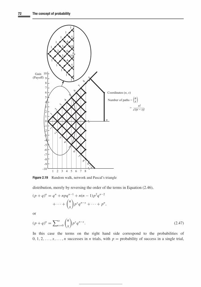
72 The concept of probability
n − x
n − x
Figure 2.19 Random walk, network and Pascal’s triangle
distribution, merely by reversing the order of the terms in Equation (2.46),
(p + q)n = qn + npqn−1 + n(n − 1)p2qn−2
+ · · · +(
n
x
)px qn−x + · · · + pn,
or
(p + q)n =∑n
x=0
(n
x
)px qn−x . (2.47)
In this case the terms on the right hand side correspond to the probabilities of0, 1, 2, . . . , x, . . . , n successes in n trials, with p = probability of success in a single trial,

73 2.6 Combinatorial analysis
Table 2.1 Pascal’s triangle
2n possiblen The binomial coefficients outcomes
0 1 11 1 1 22 1 2 1 43 1 3 3 1 84 1 4 6 4 1 165 1 5 10 10 5 1 326 1 6 15 20 15 6 1 647 1 7 21 35 35 21 7 1 1288 1 8 28 56 70 56 28 8 1 256
and q = 1 − p = p. For the use of this formula the trials must be stochastically independent.The binomial distribution is considered further in Chapter 3.
Although the appearance of the factor(n
x
)in Equation (2.47) may now be obvious, the
following serves to confirm the result. Consider each term in the expansion of (p + q)n to benumbered. Thus
(p + q)n = (p + q) (p + q) (p + q) . . . (p + q)Number 1 2 3 n
Each ‘p’ in px is chosen from x of these n factors and each ‘q’ in qn−x is chosen from theremaining (n − x). There are
(nx
)ways of putting the n factors in two piles of size x and (n − x)
respectively.In exchangeable sequences, order is not important so that all paths are equally likely. For
any node (n, x) where n = number of trials and x = number of successes, exchangeabilitywould dictate that
ωx,n = (number of paths) · px,n (2.48)
where ωx,n = probability of getting to the node in question by all paths, and px,n = probabilityof getting to the node in question by a single specified path. The evaluation of px,n could, forexample, follow from the content of the urn: the number of red and pink balls and the strategyfor replacement after a draw. The number of paths is given by Equation (2.44); here x replaces r .
The use of Pascal’s triangle goes back to the early history of probability theory (Bernstein,1996), and, indeed, was known to a Chinese mathematician in the fourteenth century (Chu’sprecious mirror). An early application was to the fair odds in an unfinished game – balla –discussed by Paccioli. We shall apply it to the finals in the National Hockey League or theWorld Series, in both of which the ‘best of seven’ wins. Figure 2.20 shows the possible resultsin such a series, and we can work out the probability that our team will win if it has lost the firstgame. It is assumed that the teams are evenly matched and that they have equal probabilities

74 The concept of probability
Figure 2.20 Possible results in a ‘best of seven’ series. The broken line shows the possible results ifour team has lost the first game. The probability then of winning is (1 + 6 + 15)/26 � 1/3
(50%) of winning each game. To use this method, one assumes all games are played; forexample, if a team has won four games and wins the series, it nevertheless goes on to completethe remaining three games. The resulting odds are correct since all permutations of results ofthe unplayed games are included.
2.6.2 Further combinatorial results
We use our random walk diagram to prove an important result. Figure 2.21 shows a sequenceof two random walks, the first from A to B with m trials and r successes, and the secondfrom B to C with n trials and (t − r ) successes. If one went from A to C through any path,there would be (m + n) trials with t successes. The number of paths from A to B is
(mr
). One

75 2.6 Combinatorial analysis
Figure 2.21 Random walk from A to C considered as random walks from A to B and then from B toC . All paths are covered if B takes all the dotted positions shown, from F to G
then starts at B and finishes at C ; the number of paths to C through B are(m
r
) · ( nt−r
)by the
multiplication principle, and since the path from B to C involves (t − r ) successes in n trials.In order to arrive at C by any path, it is necessary then to consider all the possible positionsfor B. Thus,(
m + n
t
)=
∑t
r=0
(m
r
)(n
t − r
). (2.49)
This result is the addition theorem for binomial coefficients.There are many more paths from A to C in Figure 2.21 when B is near the centre of the
rectangle ADC E than when it is near the corners D or E . We shall see later that winninglotteries corresponds to taking one particular extreme path, for example AEC , when all thepaths through the random ‘maze’ are equally likely (see Chapter 3 under ‘hypergeometricdistribution’ for a probabilistic solution).

76 The concept of probability
Several special results may be derived from Equation (2.49), including the following, ob-tained if we put m = 1:(
n + 1
t
)=
(n
t
)+
(n
t − 1
). (2.50)
To verify this result, sketch Figure 2.21 with m = 1. Expression (2.50) can be used to go fromnode to node in the random walk diagram, confirming previous results. Try this, starting atnode 0 (n = 0), at which the number of paths is set equal to zero. Remember that 0! = (n)0 = 1by definition and that
(nr
)and (n)r are 0 if r > n. Also
(nr
)(defined as (n)r /r !) is equal to 0 if
r is negative. See Feller (1968) for generalization of the binomial coefficients.
2.6.3 Occupancy problems; Bose–Einstein statistics
Occupancy problems have many practical applications, and are also important in statisticalmechanics; see Feller (1968). He considered problems of placing both distinguishable andindistinguishable objects into cells. Let there be r objects and n cells. For n = r = 3, Tables2.2 and 2.3 show the different arrangements. Feller makes the connection with particle physics,in which the distinguishable particles are the subject of classical mechanics, and the indistin-guishable ones those of Bose–Einstein statistics. Each distribution among cells corresponds toa ‘point in phase space’ and the cells to energy levels (e.g. Margenau and Murphy, 1956). For
Table 2.2 Arrangement of three distinguishable objects {0, 1, 2} into three cells
1. 0, 1, 2 – – 10. 0 1, 2 – 19. – 0 1, 22. – 0, 1, 2 – 11. 1 0, 2 – 20. – 1 0, 23. – – 0, 1, 2 12. 2 0, 1 – 21. – 2 0, 14. 0, 1 2 – 13. 0 – 1, 2 22. 0 1 25. 0, 2 1 – 14. 1 – 0, 2 23. 0 2 16. 1, 2 0 – 15. 2 – 0, 1 24. 1 0 27. 0, 1 – 2 16. – 0, 1 2 25. 1 2 08. 0, 2 – 1 17. – 0, 2 1 26. 2 0 19. 1, 2 – 0 18. – 1, 2 0 27. 2 1 0
Table 2.3 Arrangement of three indistinguishableobjects {0, 0, 0} into three cells
1. 000 – – 6. 0 00 –2. – 000 – 7. 0 – 003. – – 000 8. – 00 04. 00 0 – 9. – 0 005. 00 – 0 10. 0 0 0

77 2.6 Combinatorial analysis
some time, probabilities were assigned on the assumption that the 27 different possibilities ofTable 2.2 were equally likely, giving the basis for Maxwell–Boltzmann statistics (‘statistic’ isthe word used for this kind of inference by physicists).
It was later accepted that some of the possibilities could not in fact be distinguished, forexample arrangements 4, 5, and 6 in Table 2.2 collapse into arrangement 4 in Table 2.3, asa result of failure on our part to recognize an underlying reality. The question then arises:should one assign a probability of 3/27 = 1/9 to the arrangement just discussed (Table 2.2),or 1/10 (Table 2.3)? Bose and Einstein showed that, for some particles, the second assignmentis appropriate. This problem will be discussed in more depth in Chapter 6. It will be seen thaturn models can be used to obtain the distributions used in particle physics.
The number of arrangements of indistinguishable objects (e.g. Table 2.3) will now be derived.Let us take n = 10, and r = 8 (r objects and n cells). A typical arrangement would be of thefollowing kind: |00||0|0||||000|0|| in which the vertical lines | delineate the boundaries of thecells. If we omit the first and last of these barriers we are left with (n − 1) barriers. Combiningthese with the objects, we have (n + r − 1) entities which can be divided into two groups (| or0). The number of arrangements corresponds to the number of ways that two distinguishablegroups of indistinguishable objects can be arranged in a line (see Equation (2.44) and the textpreceding it). Therefore, the number of arrangements in the present case is
ar,n = n+r−1Cn−1 =(
n + r − 1
n − 1
)=
(n + r − 1
r
). (2.51)
If no cell is to remain empty, we consider the spaces between the r objects. There are (r − 1)of these spaces. There are again (n − 1) barriers omitting the first and last ones. If (n − 1) ofthe (r − 1) spaces are occupied by barriers then no two barriers can be adjacent to each other.(Note that r ≥ n.) There are
r−1Cn−1 =(
r − 1
n − 1
)
ways to choose the (n − 1) spaces from the (r − 1) ones available, and this is therefore thenumber of arrangements leaving no space empty. Try the arrangements with, for example,n = 3, r = 5.
Replacement of objectsWe have seen that replacement of objects taken from a pile, or urn, has implications with regardto the probability for the next draw. If we have coloured balls (say red and pink) in an urn, thesame probability will apply in two successive draws if we replace the ball after the first drawand then mix the balls up. The same applies in the case of a deck of cards: if we replace a cardand shuffle the deck, we judge that it has the same probability of reappearing.
Replacement also has an effect on the number of ways a group of distinguishable objectscan be arranged. Consider a group of n such objects, from which r are sampled. If there is noreplacement, the number of distinct samples is (n)r , following the usual rule for permutations.

78 The concept of probability
If the objects are replaced after each sample is taken, then there are n · n · n · . . . · n (r terms)= nr different samples. In this case, there can be repetitions of the same object in the sample;without replacement, each object can appear only once. Both calculations count differentorderings. Given replacement after each draw, the probability of no repetition in the sample is
(n)r
nr(2.52)
If n balls are placed at random in n cells, the probability that each cell is occupied is n!/nn.
For n = 6, this equals 0.0154. . . ; it is thus rather unlikely that in six throws of a die, all facesappear. The famous birthday problem is also solved by the same methods. As in all the casesconsidered here, in evaluating probabilities it is assumed that all distributions are equally likely.
2.6.4 The birthday problem
In a group of r people, what is the probability that at least two have the same birthday?The results have been found to be counter-intuitive and indeed, they may be for some. Let uscalculate, in particular, the number r for which the probability of at least two common birthdaysis greater than 1/2. Let us first work out the probability of no common birthdays, then theprobability of at least one shared birthday is 1 − Pr(none). We assume in the following that aperson has the same probability (1/365) of having a birthday on any particular day.
The total number of ways that the birthdays can be arranged is 365r ; 365 days for the firstperson, similarly for the second, and so on, assuming of course that we don’t have a leap year!If there are to be no shared birthdays, the first person still has the choice of 365 days, but thesecond is constrained to 364 to avoid whichever day is the birthday of the first, the third has363 possibilities and so on. Therefore, the number of ways of avoiding any shared birthdays is
365 × 364 × 363 × (365 − r + 1) = 365!/(365 − r )! = (365)r ,
and the probability of no shared birthdays is thus a special case of Equation (2.52):
p = (365)r
365r, (2.53)
and the probability of at least two shared birthdays is
p = 1 − p = 1 − (365)r
365r. (2.54)
Evaluation of Equation (2.53) involves rather large numbers: for expedient solutionsStirling’s approximation (Section 6.4) is often used. For present purposes, we rather firstnote that Equation (2.53) can be written as
p =(
1 − 1
365
) (1 − 2
365
)· · ·
(1 − r − 1
365
). (2.55)

79 2.6 Combinatorial analysis
Table 2.4 Results for birthday problem
Approximate: Equation (2.56) Exact: Equation (2.55)
r p p p p
5 0.973 0.027 0.973 0.02710 0.877 0.123 0.883 0.11715 0.712 0.288 0.747 0.25320 0.479 0.521 0.589 0.41125 0.178 0.822 0.431 0.56930 – – 0.294 0.706
A first approximation can be made by assuming that r is small, i.e. r � 365. Then all crossproducts in the formula can be neglected; thus
p � 1 − 1 + 2 + · · · + (r − 1)
365
and p � 1 + 2 + · · · + (r − 1)
365(2.56)
The results from this calculation are given in Table 2.4, together with accurate resultscalculated by Equation (2.55). Equation (2.56) can be solved mentally (at least as a fraction)but is only accurate up to about r = 10. The accurate results show that a surprisingly smallnumber of people are required for p = (probability of at least two birthdays) to exceed 0.5.This happens between r = 22 ( p = 0.476) and r = 23 ( p = 0.507).
The problem can be used nicely in a classroom with, say, 30 students. A piece of paper ispassed around upon which the students enter their birthdays. While this happens, the problemis solved. With a bit of luck (there is a 70% probability for r = 30), there will be at least twocommon birthdays. See Feller (1968, Vol. 1) for another approximate solution.
2.6.5 Urns with balls of many colours; Polya’s urn: relation to occupancy
We complete our study of combinatorial analysis using now urns with b balls, of k differentcolours. The number of balls initially is
g1 of colour 1,
g2 of colour 2,...
gi of colour i,...
gk of colour k,
b in total. (2.57)

80 The concept of probability
There are various strategies for drawing balls from the urn. We consider the following basicones.
(a) No replacement; eventually all of the balls will be used up. This leads to the hypergeometricdistribution (Sections 3.2 and 3.4.1).
(b) Replacement followed by mixing of the balls; the composition then stays the same. Thisleads to the binomial or multinomial distributions (Sections 3.2 and 3.4.1).
(c) Double replacement, with both balls being of the same colour as that just drawn, followedby mixing of the balls; this is Polya’s urn model.
We draw n balls in the experiment and find that there are
x1 of colour 1,
x2 of colour 2,...
xi of colour i,...
xk of colour k,
n in total. (2.58)
For any of the above sampling strategies, the order of results is not of significance in prob-abilistic analysis – exchangeability applies. An example will illustrate this. We take Polya’surn as the example. Let k = 3, so that there are three colours. Let g1 = 2, g2 = 3 and g3 = 5;consequently, b = 10. If we draw six balls and obtain two of colour 1, one of colour 2 andthree of colour 3, let us say in the order 3-1-1-2-3-3, then the probability is
5
10· 2
11· 3
12· 3
13· 6
14· 7
15.
Any other order of results corresponds to a permutation of the terms in the numerator with nochange in the denominator. For example, the order 1-1-2-3-3-3 results in the probability
2
10· 3
11· 3
12· 5
13· 6
14· 7
15,
which is the same as the previous result. It will be found generally that the probability ofobtaining a particular set of balls (2.58) drawn from the Polya urn model (2.57), given aparticular order, is the same as for any other order. The reader might wish to check thatthis is also the case for the other cases introduced above, with no replacement or singlereplacement.
We shall pursue the general case for the Polya urn, since this is relevant to the occupancyproblem, and to statistical mechanics: see Chapter 3 for more on the basic distributions, Chapter6 for more on statistical mechanics, and Chapter 8 for the use of the distributions, particularlythe hypergeometric, in exchangeability theory. We have seen that the same probability isobtained for any order of drawing. We may then assume that we draw all balls of colour 1 first,

81 2.6 Combinatorial analysis
then those of colour 2, and so on, and that the result will be the same for any other order. Theprobability for this order is then
(g1)
(b)· (g1 + 1)
(b + 1)· . . . · (g1 + x1 − 1)
(b + x1 − 1)· (g2)
(b + x1)· . . . · (g2 + x2 − 1)
(b + x1 + x2 − 1)· . . .
· (gk)
(b + x1 + x2 + · · · + xk−1)· . . . · (gk + xk − 1)
(b + n − 1). (2.59)
In the denominator of the last term, n = ∑xi . The equation (2.59) can be expressed as
∏ki=1 gi (gi + 1)(gi + 2) · · · (gi + xi − 1)
b(b + 1)(b + 2) · · · (b + n − 1),
or
∏ki=1(gi + xi − 1)xi
(b + n − 1)n. (2.60)
This probability corresponds to a single path in a (multidimensional) random walk from theorigin to node (x1, x2, . . . , xk). There are
n!
x1!x2! · · · xk!= n!∏k
i=1 xi !(2.61)
paths to the node in question. Therefore the probability of getting to node (x1, x2, . . . , xk) byany path is the product of Equations (2.60) and (2.61). This can also be written as
∏ki=1
(gi +xi −1xi
)(b+n−1
n
) . (2.62)
In this equation we have just solved our first multidimensional probability distribution; theset of random quantities {X1, X2, . . . , Xk} with particular values {x1, x2, . . . , xk} constitutes amultidimensional set. The formal methods for representing probability distributions are givenin Chapter 3.
It is interesting to note that the model for the number of ways of distributing r balls amongn cells in Equation (2.51) is in fact identical to an urn model. The term(
gi + xi − 1
xi
)(2.63)
represents the number of ways of distributing xi indistinguishable objects amongst gi cells;this is clear by reference to Equation (2.51). This is used in statistical mechanics. Indeed, theprincipal distributions for fundamental particles are derived in Chapter 6 by a demon whoplays various games using roulette wheels and urns. The values xi and gi represent the numberof particles and degeneracy associated with state i.
82 The concept of probability
We note in concluding that in the case where all the gi are equal to unity, i.e. gi = 1, fori = 1, . . . , k, then each term in the product term of the numerator of Equation (2.62) is equalto [xi !/(xi !0!)] = 1, and the resulting probability is
1(b+n−1n
) . (2.64)
This is an urn with single balls of the various colours. Polya’s urn is also discussed in de Finetti(1974), Feller (1968) and Blom et al. (1994).
2.7 Exercises
Basic exercises are included to revise odds, set theory and counting.
2.1 An engineer states that the odds of a beam surviving a load of 3 MN for 25 years is ‘5 to 1 on’. Whatis the engineer’s probability for this event? Draw a decision tree as in Figure 2.1(a) to illustrate theassignment of probability.
2.2 The odds of a prototype microchip surviving a current of 3µA for 2 hours are estimated as 4 to 3against. What is the estimated probability of this event? Draw a decision tree as in Figure 2.1(a) toillustrate the estimator’s assignment of probability.
2.3 The event E = (the score on a roll of a fair die is a composite number; that is, a non-prime numbergreater than 1). Calculate the odds on E , expressed as a ratio reduced to its lowest terms.
2.4 Odds vs. bookie’s odds. In a five-horse race, a bookmaker sets a stake of $240. The bookie quotesodds of r1 = 5 to 3 on, r2 = 2 to 1 against, r3 = 5 to 1 against, r4 = 19 to 1 against and r5 = 19 to1 against.7 Calculate ‘probabilities’ qi (i = 1, 2, . . . , 5) based on these odds. You may place a betof $(240 · qi ) on any of the five horses and if event Ei (= horse i wins) occurs, then you win thebookie’s stake of $240.
(a) From your point of view, do these odds constitute fair bets? Are the qi acceptable as probabilities?Justify your answer by determining whether or not the probabilities associated with these oddsare coherent.
(b) What is the bookie’s guaranteed profit if you place one bet on each of all five horses?
2.5 Fair vs. unfair odds. Six teams are competing in a design competition. An engineer offers a stakeof $100 to be won by a colleague who guesses the winner. He offers odds of 19 to 1 against teamA, 9 to 1 against team B, 9 to 1 against C, 3 to 1 on team D, 4 to 1 against E, and 7 to 3 againstF. Calculate ‘probabilities’ based on these odds. Are they coherent? If a person bets on each team,what is the engineer’s guaranteed profit? Assume that the odds reflect well the relative likelihood ofeach team winning, so that for example teams B and C are considered equally likely to win. Rescalethe probabilities and odds so that the bets become fair bets and the probabilities become coherent.
7 Usually odds in horse racing are expressed as ‘against’.

83 2.7 Exercises
2.6 Derive the condition of coherence for a bookmaker by using Equation (2.7) without making theassumption that s1 = s2 = · · · = sn = s (de Finetti, 1937).
2.7 Verify the following logical relationships. Set relationships are similar with S replacing 1 and ∅replacing 0.
1. A ∧ A = A = A ∨ A.2. ∼ (
A) = A.
3. A ∧ B = B ∧ A; A ∨ B = B ∨ A (Commutative rules).4. (A ∧ B) ∧ C = A ∧ (B ∧ C); similarly for ∨ (Associative rules).5. A ∧ (B ∨ C) = (A ∧ B) ∨ (A ∧ C); A ∨ (B ∧ C) = (A ∨ B) ∧ (A ∨ C) (Distributive rules).6. A ∧ 1 = A; A ∨ 0 = A.7. A ∧ A = 0; A ∨ A = 1.
8. A ∧ 0 = 0.
9. 0 = 1.
10. ∼ (A ∨ B) = A ∧ B (De Morgan’s theorem).11. ∼ (A ∧ B) = A ∨ B (De Morgan’s theorem).12. A ∧ (A ∨ B) = A.
13. A ∧ ( A ∨ B) = A ∧ B.
2.8 The union and intersection of a finite collection of sets Ai (i = 1, 2, . . . , n) are written as ∪i Ai and∩i Ai respectively. Verify for, say, i = 3 the following relationships.
1. ∼ (∪i Ai ) = ∩i ( Ai ) (general version of De Morgan’s theorem).2. ∼ (∩i Ai ) = ∪i
(Ai
)(general version of De Morgan’s theorem).
3. A ∪ (∩i Bi ) = ∩i (A ∪ Bi ).4. A ∩ (∩i Bi ) = ∩i (A ∩ Bi ).5. A ⊂ ∩i Bi ↔ A ⊂ Bi for every i .
2.9 Demonstrate the associative, commutative and distributive rules for sets using Venn diagrams.
2.10 Verify the following relationships.
1. A ⊂ A; ∅ ⊂ A ⊂ S.
2. A = B ↔ A ⊂ B and B ⊂ A.3. A ⊂ B ↔ A ∩ B = ∅.
4. A ⊂ B ↔ A = A ∩ B.
2.11 Verify the following duality relationship in a few cases. If we interchange
⊂ and ⊃∅ and S
∪ and ∩then the new relationship also holds.
2.12 Expand Equation (2.17) for n = 3. Write the corresponding probabilistic equation using the principlein Equations (2.11) and (2.12).

84 The concept of probability
2.13 For the sample space S which consists of the first ten natural numbers {1, 2, . . . , 10}, events A, B, Care defined as: A = {even numbers in S}, B = {prime numbers in S}, and C = {3, 5}.(a) Represent these sets in a Venn diagram.(b) Express the set D = {even prime numbers in S} as a set function of the above sets. How many
elements are in this set?(c) Simplify the expression B ∩ C .(d) Simplify the expression B ∪ C .(e) Simplify the expression A ∪ C .(f) What are the elements in the set A ∩ B ∩ C?
2.14 There are three possible causes for failure of a computer system. One or more of the causes maybe associated with a failure. Let Ai = {cause i is associated with a failure}, for i = 1, 2, 3 and sup-pose that Pr (A1) = 0.30, Pr(A2) = 0.39, Pr (A3) = 0.32, Pr (A1 ∧ A2) = 0.16, Pr (A2 ∧ A3) =0.12, Pr (A3 ∧ A1) = 0.12, and Pr (A1 ∧ A2 ∧ A3) = 0.02. Draw a Venn diagram that representsthis situation. Calculate the probability of each of the following events:
(a) A1 ∨ A2
(b) A1 ∧ A2
(c) A1 ∨ A2 ∨ A3
(d) A1 ∧ A2 ∧ A3
(e) A1 ∧ A2 ∧ A3.
2.15 The quality of mass-produced ceramic components for an electricity supply system is checkedby an inspection system. The products are unacceptable if they are fractured, oversize or warped.From past experience, the probability that a component is warped is 0.0015, the probability that it isfractured is 0.0020, the probability that it is oversize is 0.0014, the probability that it is either warpedor fractured or both is 0.0028, the probability that it is either fractured or oversize or both is 0.0029,the probability that it is either oversize or warped or both is 0.0025 and finally the probability thatit has at least one of these imperfections is 0.0034.
(a) What is the probability that a component is free of all imperfections?(b) What is the probability that a component is oversize but is free of other imperfections?(c) What is the probability that a component has all of the specified imperfections?
2.16 In a component failure, there are three possible causes Ei , i = 1, 2, 3. At failure, a reliability analysisindicates that
E1 + 2E1 E2 + E3 = 1.
What can be said regarding the values Pr(Ei )?
2.17 The six faces of a cube of side 10 cm have been painted purple. The cube is then cut into 1000smaller cubes, each of side 1 cm, and these smaller cubes are placed in an urn. One of these cubes isselected at random from the urn. What is the probability that this cube will have two painted faces?
2.18 Consider Raiffa’s urns of Figure 2.10. An urn is chosen at random from a room containing 800 oftype θ1 and 200 of type θ2. Two balls are sampled without replacement. What are the probabilities

85 2.7 Exercises
that the urn chosen is a θ1 or θ2 urn if the sampled balls are
(a) both red;(b) both pink; and(c) red and pink?
2.19 Everyday life 1.
(a) What kind of bets for the future are manifested in ‘puts and calls’ in security trading? Otherbets, on sporting events or in insurance might be pondered.
(b) A Canadian automobile insurance company threatens to double the insurance rate for a clientif she puts in a claim after a minor accident. But they will leave the rate the same if the claimis not entered even though they know about the accident. Bayes’ theorem applies equally wellas regards the probability of a future accident whether the claim is entered or not since thecompany knows of the accident. The client’s future risk is the same in either case. Could itbe that the insurance company is attempting to force the client to pay for her repairs herself?Comment on this quite common practice.
2.20 Everyday life 2. An elderly public figure is accused by several women of his age of having committedserious improprieties in his youth involving them individually. The women do not know each otherand appear reluctant to give evidence. They are ordinary people with no apparent motive falsely toaccuse the public figure. Comment on the probability of guilt.
2.21 Everyday life 3. Three door problem. This problem was a common topic of discussion some yearsago. The host in a television show has a set with three doors. Behind one is a prize, say a certificateentitling the contestant to a brand new Maserati. The contestant may choose one door at random,giving a one-in-three chance of winning the prize. He selects a door. At this point the host intervenesand offers to open one of the two remaining doors. She does so, and then offers the contestant theoption of changing his selection to the remaining closed door. Should he do so? It may be assumedthat the host will not open a door that contains the prize.
2.22 Warning light 1. Warning lights and devices are used in many applications, for example fire alarms,lights for oil level in an automobile and devices for methane gas detection in coal mines. In auto-mobile dashboards, warning lights are used rather than the more expensive gauges. Consider forexample, a device to indicate event T = ‘oil level below a specified level’. A warning light comeson – event L – to indicate that T might have occurred. Tests can be conducted to obtain Pr(L|T )and Pr
(L|T )
. Let these values be denoted p and q respectively, and let Pr(T ) = t. Find Pr(T |L),Pr(T |L), Pr(T |L) and Pr(T |L) in terms of p, q and t.
2.23 Warning light 2. The devices in Problem 2.22 are designed to indicate the occurrence of a rare event.This can pose difficulties in the design of the system. Consider the following problem. A warningdevice on an aircraft includes a light that is ‘on’ when the landing gear is correctly positioned. Itaccurately reflects the landing gear correctly in position 99.9% of the time. The remaining 0.1%corresponds to failure of the lighting system in the device, incorrectly indicating failure of thelanding gear to position itself. Given that failure of the landing gear occurs on average once in106 landings, what is the probability that the landing gear is incorrectly positioned if the light

86 The concept of probability
indicates ‘failure’? Assume that the warning device works perfectly when the landing gear has failed.Comment.
This problem might be analysed with a real-world application in mind; see Aviation Weekly andSpace Technology, July 30 and August 6, 1973. A Lockheed L-1011 aircraft crashed with manyfatalities after there was doubt whether the front landing gear was in the down position. The bulbsin the system indicating the position of the landing gear were found after the crash to have burnedout, and the probable cause of the accident was preoccupation of the crew regarding the landinggear position, resulting in distraction from the instruments and altitude of the aircraft.
2.24 An electronic company ‘A’ manufactures microprocessors. An important competitor, ‘B’, has in-troduced a new product which is selling well. Company A has to decide whether to introduce acompeting microprocessor. There are concerns regarding the response of company B, which couldexpand production, keep it at the same level, or reduce. From past experience, the chances of thethree actions are respectively 60%, 30%, and 10%. One source of information to company A is tostudy B’s advertising campaign. From past experience, they have assigned probabilities to the rivalreducing, maintaining, and increasing their advertising given that it is their intention to cut, keep atsame level, or expand production as in the table below.
Advertising is
decreased maintained increasedcut back 0.60 0.30 0.10
Company B is going to keep same level 0.30 0.50 0.20expand 0.10 0.30 0.60
It is then observed that advertising is in fact increased. What are the revised probabilities for therival’s course of action?
2.25 In an industrial plant, a flow meter is used to measure the direction of flow in a pipe, with an electricalsignal being sent back to the control room. Under ideal conditions, a positive signal should arrivewhen the flow is in one direction – positive flow – with a negative signal level when the flow is inthe opposite, or negative, direction. In reality, a positive signal level can be observed even if the flowis negative and vice versa, as a result of turbulence and system noise. The possible received signallevels X are −2, −1, 0, +1, +2. The probabilities of the value of X conditional on the direction ofthe flow are as follows.
x Pr(X = x | positive flow) Pr(X = x | negative flow)
+2 0.40 0.00+1 0.30 0.15
0 0.20 0.15−1 0.05 0.30−2 0.05 0.40
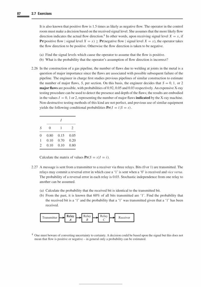
87 2.7 Exercises
It is also known that positive flow is 1.5 times as likely as negative flow. The operator in the controlroom must make a decision based on the received signal level. She assumes that the more likely flowdirection indicates the actual flow direction.8 In other words, upon receiving signal level X = x , ifPr(positive flow | signal level X = x) ≥ Pr(negative flow | signal level X = x), the operator takesthe flow direction to be positive. Otherwise the flow direction is taken to be negative.
(a) Find the signal levels which cause the operator to assume that the flow is positive.(b) What is the probability that the operator’s assumption of flow direction is incorrect?
2.26 In the construction of a gas pipeline, the number of flaws due to welding at joints in the metal is aquestion of major importance since the flaws are associated with possible subsequent failure of thepipeline. The engineer in charge first studies previous pipelines of similar construction to estimatethe number of major flaws, S, per section. On this basis, the engineer decides that S = 0, 1, or 2major flaws are possible, with probabilities of 0.92, 0.05 and 0.03 respectively. An expensive X-raytesting procedure can be used to detect the presence and depth of the flaws; the results are embodiedin the values I = 0, 1 or 2, representing the number of major flaws indicated by the X-ray machine.Non-destructive testing methods of this kind are not perfect, and previous use of similar equipmentyields the following conditional probabilities Pr(I = i |S = s) .
I
S 0 1 2
0 0.80 0.15 0.051 0.10 0.70 0.202 0.10 0.10 0.80
Calculate the matrix of values Pr(S = s|I = i).
2.27 A message is sent from a transmitter to a receiver via three relays. Bits (0 or 1) are transmitted. Therelays may commit a reversal error in which case a ‘1’ is sent when a ‘0’ is received and vice versa.The probability of a reversal error in each relay is 0.03. Stochastic independence from one relay toanother can be assumed.
(a) Calculate the probability that the received bit is identical to the transmitted bit.(b) From the past, it is known that 60% of all bits transmitted are ‘1’. Find the probability that
the received bit is a ‘1’ and the probability that a ‘1’ was transmitted given that a ‘1’ has beenreceived.
8 One must beware of converting uncertainty to certainty. A decision could be based upon the signal but this does notmean that flow is positive or negative – in general only a probability can be estimated.

88 The concept of probability
2.28 In the two systems below, the components have a reliability of 98%. This means that the probabilityof failure is 0.02. Find the system reliability in each case. Stochastic independence should beassumed. The systems are operational if there is a working path from A to B.
2.29 Describe an example of dependence that is conditional on our state of knowledge.
2.30 A batch of ten cables contains three defective cables. A random sample of four cables is taken fromthis batch and tested. Find
(a) the number of ways there can be exactly two defective cables in the sample, and(b) the number of ways there can be at least two defective cables in the sample.
2.31 A water diviner claims that he can locate hidden sources of water using a carved whalebone. A testis conducted by asking him to separate ten covered cans into two groups of five, one consisting ofcans containing water. It is arranged beforehand that five cans contain water. What is the probabilitythat the diviner correctly puts at least three cans into the ‘water group’, entirely by chance?
2.32 At the ‘Group of Eight’ meetings in 2002, what is the probability that George Bush and Tony Blairstand next to each other at the photo-op, purely by chance? How many ways can the eight personsbe seated around a circular table?
2.33 An urn contains seven red balls and three green balls. A second urn contains four red balls and sixgreen balls. A ball is chosen randomly from the first urn and placed in the second urn. Then a ballis chosen randomly from the second urn and placed in the first urn.
(a) What is the probability that a red ball is selected both from the first urn and then from the secondurn?
(b) What is the probability that a red ball is selected from the second urn?(c) At the conclusion of the selection process, what is the probability that the numbers of red and
green balls in each urn are identical to the initial numbers?

89 2.7 Exercises
Now consider the generalization to the case where there are n(> 1) balls initially in each urn, witha (such that 0 < a < n) red balls in urn 1 and b (with 0 < b < n) red balls in urn 2 initially.
(d) Show that the probability that a red ball is selected from the second urn during this process is,in general, different from the probability of drawing a red ball directly from the second urn,without transferring a ball from the first urn.
(e) Find a necessary and sufficient condition on the values of a and b for the two probabilities inpart (d) above to be equal.
2.34 Find a proof of Equation (2.49) based on the expansion of Newton’s formula for (p + q)m+n .
2.35 Two age-old problems.
(a) Find the number of distinct ways of arranging the letters in the word ‘STATISTICS’.(b) A hand of five cards is dealt from a standard deck of 52 cards. What are the odds against the
event that all five cards are of the same suit?
2.36 Hat problem; also an old problem.
‘I’m a decent man I am I am and I don’t want to shout, but I had a hat when I came in and I’ll have a hatwhen I go out!’ (Old Newfoundland song)
At a club for men on a wet and windy night all are wearing hats which they check in upon arrival.The person checking the hats becomes confused and returns them at random. What is the probabilitythat no man receives his hat? Consider n men and the change in value of probability as n increases.
2.37 General model of drawing from urn. In an urn with balls of two colours, g1 are of colour 1, and g2 ofcolour 2. A ball is drawn, and then replaced. Then h1 of the colour drawn and h2 of the other colourare added to the urn and mixed. A ball is now drawn from the urn, which contains g1 + g2 + h1 + h2
balls. The values h1 and h2 are arbitrary and could be negative. See Feller (1968). We consider nowthe case h2 = 0 and h1 > 0, which constitutes a general Polya urn. Show that the probability ofdrawing a ball of colour 2 at any drawing is g2/ (g1 + g2) .
2.38 Eight passengers share a compartment in a train which stops at eleven stations. What is the probabilitythat no two passengers leave at the same station?

3 Probability distributions, expectationand prevision
Bring out number, weight and measure in a year of dearth.William Blake, Proverbs of Hell
3.1 Probability distributions
We are now in the following situation. We have a probability mass of unity, and we wish todistribute this over the possible outcomes of events and quantities of interest. We also wish tomanipulate the results to assist in decision-making. We have so far considered mainly randomevents, which may take the value 0 or 1. A common idealized example that we have given isthat of red and pink balls in an urn, which we have labelled 1 and 0, respectively. Thus, thestatement E = ‘the ball drawn from the urn is red’ becomes E = 0 or E = 1, depending onwhether we draw a pink or red ball. The event E either happens or it does not, and there areonly two possible outcomes. Random quantities can have more than two outcomes. For thecase of drawings from an urn, the random quantity could be the number of red balls in ten(or any other number) of drawings, for example from Raiffa’s urns of Figure 2.10. A furtherexample is the throwing of a die which can result in six possible outcomes; the drawing of acard from a deck can result in 52 possible outcomes, and so on.
The possible outcomes often take discrete values, as in the examples just given; in the caseof a die these are {1, 2, 3, 4, 5, 6}. Or in the case of the tests on the concrete cylinder of the lastchapter (Section 2.1), we might assign (arbitrarily if we wish) the values 1, 2, 3, . . . , to intervalsof strength, e.g. 0–20 MPa, 20–40 MPa, and so on. The number of vehicles that can queue inthe turning lane at a traffic light takes a discrete set of possible values. We have in all of thesecases a discrete random quantity. This should be contrasted with a continuous one, whichcan take on any value in a range, for instance any strength in the interval 0–100 MPa. Suchcontinuous random quantities will have their mass of probability spread out or distributedover an interval.
A random quantity will always be indicated by an upper case letter, for example X, Y, A.
The event E above is random; an event is a special quantity with only two possible outcomes.It becomes tedious to insist that entities represented by an upper case letter are always random.
90

91 3.2 Discrete probability distributions
Often we have a deterministic quantity which we wish to denote with an upper case letter.Consequently an upper case letter does not necessarily indicate that a quantity is random buta random quantity will always have an upper case. Probability distributions are defined overthe possible values of a random quantity. We shall introduce some common distributions inthis chapter; Appendix 1 contains a listing of probability distributions and their properties, foreasy reference.
The possible outcomes that are being considered might be limited to a finite discrete setsuch as the results of die-tossing or drawing from an urn with specified numbers of ‘tri-als’. If the space in the turning lane is limited so that the maximum number of vehicles isfixed, then again we may set an upper limit to the number of vehicles, which may then bemodelled as random and finite. Or there may be a set that we might wish to regard as un-bounded. For example, if we are considering the distribution of ages of human beings ina certain population, we might consider the possible values as corresponding to the count-ably infinite set {1, 2, 3, . . .}. No doubt, we could devise an upper bound. But this is oftenunnecessary, provided that the distribution fitted to the ‘tail’ assigns negligible probabilitiesto very great ages. For example, if the probability of a person being greater than, say, 140years is very small, there might be no consequence to the analysis by including an infiniteset.
Another example might be the set of extreme wave heights in considering the design ofan offshore structure. There are no doubt physical bounds that could be set on the possiblewave heights. One has then to assess whether there is any advantage to such a procedure. Theprobability distribution fitted to the extreme wave heights might well have negligible probabilitymass corresponding to ‘unrealistically high’ values of wave height. This can always be checkedafter the analysis is complete to see whether the design situation is realistic. There is a danger ofbounding a parameter at an inappropriate value and excluding valid events of small probabilityfrom consideration.
3.2 Discrete probability distributions; cumulative distribution functions
The probability distribution of the random quantity X is the set of values of probability asso-ciated with the possible outcomes. This is written pX (x) for the discrete case. For the randomquantity Y the distribution is denoted pY (y), and so on for other quantities. The advantageof this notation is that we can see immediately from say pW (·) that we are referring to theprobability distribution of W. The lower case value of the random quantity indicates that therandom quantity is taking on a particular value. For example, for the case of a fair die, withX = outcome of throw,
pX (x) = Pr(X = x) = 1
6, for x = 1, 2, . . . , 6.

92 Distributions and expectation
A further example might be
pY (y) = Pr(Y = y) = y2
14, for x = 1, 2, or 3.
In these cases we may also write
pX (5) = 1
6; pY (3) = 9
14.
Probability distributions are defined over a partition, so that by Equation (2.9), we must havethat∑
XpX (x) = 1 and
∑Y
pY (y) = 1. (3.1)
3.2.1 Repeated trials
A common case of practical importance is that of ‘repeated trials of the same phenomenon’.Examples are repeated tosses of a coin, or drawings of a ball from an urn. These are thebasis for a set of distributions such as the binomial one, to be explained in the following.Instead of coins or coloured balls, consider the following events, which have a more practicalflavour.
1. ‘The strength of the steel sample is greater than 400 MPa.’2. ‘The component failed under the given voltage.’3. ‘This item is defective.’
Each of these events has a complement and can be considered as having outcomes of 0 or 1.Repeated trials correspond to a series of steel specimens, to a set of components, or to a seriesof tests to tell whether a manufactured item is defective or not.
3.2.2 Bernoulli and binomial distributions
When we consider the probability of success (E = 1 for event E) to be constant and known foreach trial we have the binomial case. A single trial is termed a Bernoulli trial and the series isa binomial process. In case 1 above, if we have substantial data from samples of similar steel,the probability might reasonably be considered constant and known; this might also be true inthe other cases. In the idealized example of the urn, the case of constant and known probabilitycorresponds to the case where the composition is known and the ball is replaced after drawing,with the balls subsequently mixed up by shaking before the next draw. Alternatively we mayconsider an urn with a very large number of balls with the proportion of red to pink known.Then if the number of balls is much greater than the number of draws, the probability of a red orpink in a draw is approximately constant. Each draw is a Bernoulli trial: the probability remainsthe same on each draw. The judgement of stochastic independence of the trials is required for

93 3.2 Discrete probability distributions
the probability to remain the same. This situation prevails in coin-tossing, die-throwing or indrawing cards from a deck if the cards are returned and the deck reshuffled.
If the Bernoulli trial is repeated n times, the binomial process results. Let X be the totalnumber of successes in these n trials;
X =∑n
i=1Ei , (3.2)
where Ei denotes the i th Bernoulli (0:1) trial. The probability distribution of X is the binomialdistribution, i.e.
Pr(X = x) = pX (x) =(n
x
)px (1 − p)n−x =
(n
x
)px qn−x , (3.3)
where Pr(Ei ) = p and q = 1 − p = p for each trial i . We can model the process as a specialcase of Figure 2.19, in which we take successive trials as being independent with constantprobability p. For a particular path in Figure 2.19, the probability of x successes is px and(n − x) failures is (1 − p)n−x . The binomial coefficient
( nx
)adds up all the paths to the node
(n, x) in this random walk diagram, counting all the orders of successes and failures. Thebinomial distribution of Equation (3.3) is often abbreviated to b(x, n, p).
There are∑
x
( nx
) = 2n possible paths to all nodes for given n; see Table 2.1. We can verifythis using Equation (2.46) by substituting p = q = 1 (note that these cannot be probabilities!).If all of the paths are equally likely, Equation (3.3) becomes
( nx
)/2n . This corresponds to
Bernoulli trials with a probability of 1/2 at each trial. The binomial distribution is symmetricalif p = 1/2. We see also that Equation (3.3) corresponds to terms of Newton’s expansion(p + p)n; see Equation (2.47).
Probability distributions for discrete random quantities represent masses of probabilityattached to the various possible outcomes, and are denoted probability mass functions (pmf s).
Example 3.1 Examples of Bernoulli (n = 1) and binomial (n = 5) distributions are given inthe upper of the pairs of the diagrams of Figure 3.1, showing the pmfs for p = 0.5 and p = 0.8.
The results could correspond to the probability of success in one or five trials on devices withknown reliability of 0.5 and 0.8. In five trials, the number of successes could be any value from0 to 5. The individual probability values are calculated using Equation (3.3).
Cumulative distribution functions (cdfs)We now introduce the cumulative distribution function or cdf, FX (x). This is defined as
Pr (X ≤ x) = FX (x) =∑
X≤xpX (x). (3.4)
Examples are shown in Figure 3.1 and other figures in the following. It is seen that one simplyaccumulates the probability as the value of the quantity increases. The value of FX (x) jumpsin value as each new probability is encountered as x increases. Finally the cdf is equal to unity.

94 Distributions and expectation
Figure 3.1 Bernoulli and binomial distributions
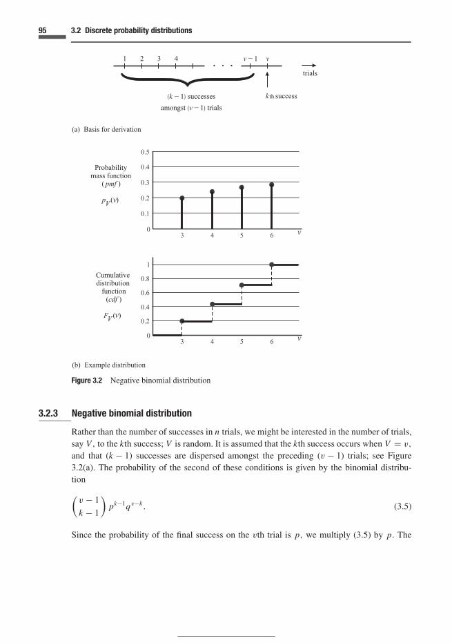
95 3.2 Discrete probability distributions
V
V
Figure 3.2 Negative binomial distribution
3.2.3 Negative binomial distribution
Rather than the number of successes in n trials, we might be interested in the number of trials,say V, to the kth success; V is random. It is assumed that the kth success occurs when V = v,
and that (k − 1) successes are dispersed amongst the preceding (v − 1) trials; see Figure3.2(a). The probability of the second of these conditions is given by the binomial distribu-tion
(v − 1
k − 1
)pk−1qv−k . (3.5)
Since the probability of the final success on the vth trial is p, we multiply (3.5) by p. The

96 Distributions and expectation
negative binomial distribution is then
Pr (V = v) = pV (v) =(
v − 1
k − 1
)pkqv−k, (3.6)
for v = k, k + 1, k + 2, . . . This is also known as the Pascal distribution.
Example 3.2 We are sampling for defectives in a batch in which the probability of a defectiveis 0.2, and we are interested in the number of trials (samples tested) until the third defectiveis found. Figure 3.2(b) shows the pmf and cdf for the case where p = 0.2, k = 3, calculatedusing Equation (3.6).
3.2.4 Geometric distribution
A special case of the negative binomial distribution is the geometric distribution, where weconsider the number of trials to the first success, rather than the general kth value. Thus k = 1in the negative binomial distribution. For example, we might be interested in the number ofyears to the first occurrence of an extreme flood. Let us consider a flood level with a probabilityof exceedance p per year. A typical practical situation would be the level with a 1% proba-bility of exceedance in a given year. Then the probability of v − 1 years without the extremeflood is
(1 − p)v−1,
assuming, as before, stochastic independence. If the first extreme flood occurs in the vth year,then
Pr (V = v) = pV (v) = (1 − p)v−1 p = pqv−1, for v = 1, 2, . . . , (3.7)
since the extreme event is preceded by (v − 1) years without an extreme occurrence (there isonly one path to this result in Figure 2.19). Equation (3.7) represents the geometric distribu-tion.
Example 3.3 We wish to obtain the probability of 100-year design storm being first exceededin a specified year. Then p = 0.01. The probability varies from 0.01 for year 1 (v = 1) to0.0083 for year 20 (v = 20), to 0.0037 for year 100 (v = 100) .
3.2.5 Hypergeometric distribution
This can be introduced using an urn of known composition. It contains b balls, g of whichare red and (b − g) pink. Drawing is carried out without replacement. The probability ofobtaining X ‘successes’ (red balls) in n trials (drawing of balls from the urn) is given by the

97 3.2 Discrete probability distributions
hypergeometric distribution. Writing the result for this in full:
Pr(X = x |b, n, g) =g!
x!(g − x)!· (b − g)!
(n − x)!(b − g − n + x)!b!
n!(b − n)!
=
(g
x
) (b − g
n − x
)(
b
n
) , (3.8)
for x = 0, 1, 2, . . . , up to the lesser of g, n. Equation (3.8) gives the number of ways, orcombinations, of choosing x red balls from g and (n − x) pink balls from (b − g), divided bythe number of ways of choosing n from b. All of these choices are without regard to order: seeEquation (2.44).
The right hand side of Equation (3.8) may be written as
n!
x!(n − x)!· (g)x (b − g)n−x
(b)n. (3.9)
The expression( n
x
) = n!/[x!(n − x)!] isolated on the left hand side of expression (3.9) is againthe number of ways of getting to the node (n, x) in our random walk diagrams (Figure 2.19).Since all paths are equally likely, the probability of a single path is simply
(g)x (b − g)n−x
(b)n. (3.10)
This can be understood as an application of the multiplication principle (Section 2.6): there are(g)x ways (permutations) of choosing the x red balls, (b − g)n−x ways of choosing the (n − x)pink balls and (b)n ways of choosing the n balls regardless of colour. Therefore Equation(3.10) gives the probability of getting to node (n, x) by a particular path since the order isspecified. Note that if b, g → ∞ with g/b constant and equal to p, then Equation (3.10)tends to px (1 − p)n−x , the probability of a single path in the binomial distribution. Also, ifn = b, x = g, Equation (3.9) is equal to unity since we have sampled every ball in the urn.
Equation (3.10) is then equal to the inverse of(
bg
), the number of paths to the endpoint. Each
is equally likely.It should be noted the probability of red (success) in each trial is constant unless one has the
results of the preceding trials: see Exercise 2.37 and Example 3.5 below.There are four forms of the hypergeometric distribution that give different insights; see
Exercise 3.6.
Example 3.4 Typical probability distributions for the Raiffa urn problem of Figure 2.10 areshown in Figure 3.3.

98 Distributions and expectation
Figure 3.3 Hypergeometric solutions with three trials to Raiffa’s urns of Figure 2.10; θ1 urn left, θ2 urnright
Example 3.5 Consider Raiffa’s θ1 urn (Figure 2.10). The probability of drawing red on thefirst draw is 4/10. On the second, without knowledge of the first result, the probability is
4
10· 3
9+ 6
10· 4
9= 36
9 · 10= 4
10.
Example 3.6 Consider the game Lotto 6–49, most popular in Canada in recent years. Onebuys a ticket in the lottery for a small sum and enters six different numbers from the set of49 consecutive numbers {1, 2, 3, . . . , 47, 48, 49}. The lottery organization also chooses six,presumably at random, and if our six numbers match theirs, regardless of order, then we winfirst prize – on occasions, millions of dollars.
We may regard the six winning numbers as ‘special’ and the remaining 43 numbers as‘ordinary’. The probabilistic solution to the problem is the standard hypergeometric distri-bution, in which we choose six numbers, which may be of two kinds, special or ordinary.The probability of drawing x special numbers (specified by the lottery organization) in sixtrials, each trial being our choice of a number in entering the lottery, is as follows, fromEquation (3.8):
Pr(X = x) =
(6
x
) (43
6 − x
)(
49
6
) , x = 0, 1, 2, . . . , 6.

99 3.2 Discrete probability distributions
Figure 3.4 Lotto 6–49: winning is the single path OAQ through the maze!
For x = 6, we deduce the probability of winning as 1:13 983 816. The result is shown graph-ically in Figure 3.4; in the figure, if x = 4, the result given by the equation above can also beseen as
(No. of paths from O to P) × (No. of paths P to Q)
No. of paths from O to Q
The winning result (x = 6) corresponds to the single path OAQ divided by the number of pathsfrom O to Q. The end point, Q in Figure 3.4, represents always the composition of the urn.
The hypergeometric distribution is of fundamental importance in studying exchangeabilityand has many other practical as well as theoretical applications. The successive trials are not

100 Distributions and expectation
independent, although exchangeability does apply (order is not important). The number oforders, or paths to a node, is
( nx
), as shown above. We have mentioned the more general case
where the parameter p or the urn composition is not ‘known’. In these cases, exchangeabilitymight still be judged appropriate. This subject is taken up further in Chapter 8.
3.2.6 Poisson distribution
The Poisson process is a limiting case of the binomial distribution. It is of extremely wideapplicability and has been used to study the number of Prussian cavalrymen kicked to deathby a horse in a certain army corps, and the distribution of yeast particles in beer. Arrivals oftelephone calls, computer messages, traffic, ships, aircraft, icebergs at an offshore installation,radioactive decay, occurrence of storms and floods, of cracks, flaws and particles in a material –all of these can be studied using the Poisson distribution. In each case, there is a parameterrepresenting the ‘exposure’. This could be time if the arrivals considered occur in time –telephone calls or storms – or distance or volume where the arrivals occur in a certain dis-tance or volume – particles or flaws in a material. In the Poisson distribution, we considera fixed value of the exposure parameter: a fixed time, distance or volume in the examplesgiven.
We shall introduce the distribution using an everyday example. Suppose we are study-ing arrivals of aircraft at an airport. The time interval would be fixed, say three hours.We denote this interval as t , and divide this interval into n subintervals of length �t suchthat
t = n�t.
Within each subinterval, an arrival of an aircraft is a ‘success ’, and non-arrival a ‘failure’.We judge that the number of successes occurring in any one time subinterval is independentof the number of successes in any other subinterval. Now consider n to be large, and �tto be small, such that the probability of more than one event occurring during any �t isnegligible. Let the rate of events – number per unit time – be λ, on average. For example,extensive records of past arrivals of aircraft might indicate that λ = 5.6 aircraft per hour arriveon average during the interval of three hours under consideration. Then, for each small �t, theprobability of an event is p = λ�t. We consider λ to be constant for the time period t. For anysubinterval
p = λ�t = λt
n= ν
n, (3.11)
where ν = λt is the expected (mean) number of successes during the time period t. The processthat we are describing is a binomial one: a series of n independent trials with a probability ofsuccess equal to p on each trial.

101 3.2 Discrete probability distributions
If X is the number of successes in the n trials, then
Pr(X = x) = pX (x) =(n
x
)px (1 − p)n−x
= n!
x! (n − x)!
(ν
n
)x (1 − ν
n
)n−x
= νx
x!
(1 − ν
n
)n
x terms︷ ︸︸ ︷n (n − 1) (n − 2) · · · (n − x + 1)[
n(1 − ν
n
)]x
, (3.12)
in which we have rearranged the terms. We now let n → ∞ and �t → 0, while keeping tconstant. As a result, ν = λt is also constant since λ is as well. The ratio of the x terms inthe numerator and the corresponding ones in the denominator within the braces {} of Equation(3.12) tends to unity, while
(1 − ν
n
)n= 1 − n
(ν
n
)+ n!
2! (n − 2)!
(ν
n
)2− n!
3! (n − 3)!
(ν
n
)3+ · · ·
→ 1 − ν + ν2
2!− ν3
3!+ · · ·
= exp (−ν) .
Then
Pr (X = x) = pX (x) = p (x, ν) = exp (−ν) νx
x!(3.13)
for x = 0, 1, 2, 3, . . . .
This is the Poisson distribution often associated with a stochastic process (Section 3.6).
Example 3.7 Long distance calls at a particular exchange arrive on average at a rate of oneevery four minutes. This rate can be considered to be constant for the time periods underconsideration. Suggest probability distributions for the number of calls in (a) five minutesand (b) an hour. In case (b), what is the probability that the number of calls exceeds 15? 20?30? An appropriate distribution is the Poisson distribution with (a) ν = 5 · 1
4 = 1.25 and (b)ν = 60 · 1
4 = 15 calls. The distributions are plotted in Figure 3.5. In case (b), if X is the numberof calls,
Pr (X > 15) = 1 − FX (15) = 1 − 0.5681 = 0.4319,
Pr (X > 20) = 1 − FX (20) = 1 − 0.9170 = 0.0830,
Pr (X > 30) = 1 − FX (30) = 1 − 0.9998 = 0.0002.
The values of FX for the calculations can be obtained from standard computer software,from statistical tables or they can be computed from first principles.

102 Distributions and expectation
x
x
x
x
Probabilitymass
function( pmf )
pX (x)
Probabilitymass
function( pmf )
Cumulativedistribution
function(cdf )
Cumulativedistribution
function(cdf )
pX (x)
Figure 3.5 Poisson distribution with different values of ν

103 3.3 Continuous random quantities
In the derivation above and in the examples, λ was taken as a constant. The main result,Equation (3.13), can be used if λ is not constant provided that one uses the correct expectedvalue. In this case
ν =∫ t
0λ (τ ) dτ (3.14)
where λ varies over the interval from 0 to t. One can think of ‘pseudotime’ if one wishes suchthat the rate is constant with respect to this parameter rather than ordinary time (or distance,volume, and so on).
3.3 Continuous random quantities; probability density; distribution functions for thecombined discrete and continuous case
In the previous section, ‘weights’ of probability were assigned to the discrete points corre-sponding to the possible outcomes of the random quantity. In some limiting distributions, wemight be interested in a countably infinite set of discrete outcomes, for example in the Poissondistribution just discussed. The random quantity can then take any value in the infinite sequence{0, 1, 2, 3, . . .}. The approach is the same as for a finite set of results: the sum of the ‘weights’of probability must approach unity as the number of outcomes tends to infinity.
An entirely different case, but one which also involves infinite sets, arises when we have aquantity which is continuous over some range. For instance, a voltage across a circuit couldtake any value in a range, say 0 to 5 Volts. For such a continuous random quantity, we ‘smear’out the probability into a density, much as we smear out a body’s mass when considering itsdensity, or as we smear out a load in considering a distributed load. In the present case, wesmear out our degree of belief over a continuous range.
An amusing initial example will illustrate the approach. This is Lewis Carroll’s ‘equallyfrangible rod’.1 By this is meant a rod, or let us say a specimen of steel of uniform crosssection, which is subjected to a tensile stress in a test machine. The probability of failure at anypoint along the length of the rod is assumed to be equal to that at any other point. In reality,there may be an increased probability of failure near the grips which attach the specimen tothe test machine, as a result of stress concentrations. But let us accept the idealization of equalprobability for the present illustration.
Figure 3.6(a) shows Lewis Carroll’s rod. The length is ‘a’, and the distance from the lefthand end to the breaking point is x . Since the value of x is not known, we denote it in generalas a random quantity X . We denote the probability density of X as fX (x) and this is definedsuch that
Pr(x ≤ X ≤ x + dx) = fX (x) dx . (3.15)
1 Lewis Carroll (Charles Dodgson) Pillow Problems. Reprinted by Dover, 1976.

104 Distributions and expectation
dx
dx
Figure 3.6 (a) Lewis Carroll’s ‘equally frangible rod’. The pdf is a uniform function of x and the cdfincreases linearly with distance x
The density is illustrated in Figure 3.6(a) for the equally frangible rod and in Figure 3.6(b)for a density where the probability is not uniformly distributed: certain values of X aremore likely than others. The probabilities of all the possible values of X must normalize sothat∫
all XfX (x) dx = 1. (3.16)
In the case of the rod with uniformly distributed probability of the breaking point,
fX (x) = 1
a, 0 ≤ x ≤ a
= 0 otherwise. (3.17)
This probability density normalizes in accordance with our desire for coherence expressed inEquation (3.16) above. Equation (3.17) is our first example of a probability density function.

105 3.3 Continuous random quantities
Figure 3.6 (b) Schematic illustration of a pdf whose density varies non-uniformly, with its associatedcdf
We shall abbreviate this term to ‘pdf ’. Figure 3.6(a) shows the pdf for the breaking point, and(b) shows that for a more general non-uniform distribution.
The cumulative distribution function (cdf ) is defined for a continuous random quantity as
FX (x) = Pr(X ≤ x)
=∫ x
−∞fX (u) du, (3.18)
in which u is a dummy variable. This is analogous to the summation in Equation (3.4). In thecase of the breaking point, (3.18) becomes
FX (x) =∫ x
−∞fX (u) du =
∫ x
0
1
adu = x
afor 0 ≤ x ≤ a. (3.19)
For example, the probability of the rod breaking in the first third of its length is 1/3 corre-sponding to 0 ≤ x ≤ a/3. We might at this point raise Lewis Carroll’s original question: ‘Ifan infinite number of rods be broken: find the chance that one at least is broken in the middle’.His answer is 0.632 12 . . . , and the method is given in Appendix 2. But there are certainimplications of his method as discussed there.

106 Distributions and expectation
From Equations (3.15) and (3.18), we can also see that
Pr(x1 < X ≤ x2) =∫ x2
x1
fX (x) dx
= FX (x2) − FX (x1). (3.20)
This is illustrated in Figure 3.6(b), for a non-uniform density.From Equation (3.18) we have the useful relationship
fX (x) = dFX (x)
dx. (3.21)
For example, if FX (x) = 1 − e−λx , fX (x) = λe−λx . This is the exponential distribution, whichwe shall now derive for a particular application.
3.3.1 Summary of notation
We have adopted the following shorthand notation:
pmf = probability mass function, for discrete quantities,
pdf = probability density function, for continuous quantities,
cdf = cumulative distribution functions, for discrete or continuous quantities.
3.3.2 Exponential distribution
We introduced probability density functions by means of a simple uniform density on LewisCarroll’s rod, and illustrated a non-uniform density in Figure 3.6(b). We now consider a specificexample of a non-uniform density. This is the waiting time to an event. The event could bethe failure of a component, for example an electrical or mechanical component in an assemblyor the warning lights in Exercises 2.22 and 2.23, or the arrival of a packet of information ina computer network, or a vehicle in a traffic problem, or a customer in a financial enterprise.Let T be the (random) time to the first event; there could be several failures, arrivals, events,and we are interested in the time to the first. We make the assumption that the probability ofan event occurring in the time interval �t is (λ�t) where λ, the rate of arrival per unit time,is a constant. This is the assumption in the Poisson distribution of Section 3.2.6 above.
Since λ is constant, the probability (λ�t) is the same for any interval �t in T . The interval�t is small enough that the probability of more than one event in any �t is negligible. Letn�t = t. Then the probability of no events in the first n intervals is (1 − λ�t)n. This followsfrom the binomial distribution, using independence. If this period of time t = n�t with noevent is followed directly by an event, then
Pr(t < T ≤ t + �t) = fT (t)�t
= (1 − λ�t)nλ�t, (3.22)

107 3.3 Continuous random quantities
Figure 3.7 Distribution of waiting times and exponential ‘tail’
where fT (t) is the probability density function of T . As noted, we have used in the abovethe binomial process with n failures followed by one success – a single-path route to the firstsuccess (Figure 2.19). Now Equation (3.22) can be written as
fT (t) = λ(1 − λ�t)n
= λ(1 − λt
n)n.
In the limit of large n,
fT (t) = λ exp (−λt) , t ≥ 0
= 0 for t < 0. (3.23)
This is the exponential distribution of waiting times, an example of which is given inFigure 3.7.
The cdf for the exponential distribution is as follows, by Equation (3.18), for t ≥ 0.
Pr(T ≤ t) = FT (t) = 1 − exp (−λt) . (3.24)
Figure 3.7 illustrates the exponential distribution and also the fact that the ‘tail’ area is givenby the simple exponential function exp (−λt). We shall encounter such ‘exponential tails’ lateron in extremal analysis.

108 Distributions and expectation
If we require the probability of the time to the first arrival being in the interval t1 to t2seconds, this is given by
Pr(t1 < T ≤ t2) = FT (t2) − FT (t1)
= exp (−λt1) − exp (−λt2) .
When probabilities are specified by a density, the probability of a particular value, e.g. X = x1
or T = t2, is zero by Equation (3.15); we have written Equations (3.18) and (3.24) above in aform equivalent to Equation (3.4) in the case of discrete random quantities, with the equalityincluded in Pr(X ≤ x) so as to maintain consistency. This is important in the unification ofdiscrete and continuous distributions, given below.
3.3.3 Normal (Gaussian) distribution
This is a common distribution, especially where the process is one of summing or averaging anumber of random quantities. The number of phone calls in a period of time might be averaged;the deflection of a structural member might be considered to be the sum of the deflections ofa number of elements; we might find the average of a set of data points measuring distance,mass or any quantity of interest. Many observations have been found naturally to follow thedistribution, including early ones on heights of human beings and other measurements, forexample chest size (Bernstein, 1996). These measurements are doubtless the result of manyadditive random factors including genetic ones. The process of summing and averaging isstudied in detail in Chapter 7, where the normal distribution is found as a limiting distributionto these processes. The normal distribution also appears naturally as that which maximizesentropy subject to the constraints that the mean and standard deviation are fixed (Chapter 6). Atthe same time, it must be emphasized that many quantities of engineering interest, for exampleextreme loads, are generally not normal distributed. In Chapter 9 we see that such processestend to the different class of extremal distributions. The conclusion is to choose distributionscarefully in applications.
The normal distribution takes the following form:
fX (x) = 1√2πσ
exp
[−1
2
(x − µ
σ
)2]
, (3.25)
where µ = mean and σ = standard deviation (see Section 3.5). It is the familiar bell-shapedcurve shown in Figure 3.8(a). The cdf cannot be obtained in closed form integration, butthe standard form (see below) is widely tabulated and available in computer programs. It isillustrated in Figure 3.8(b).
Changing µ has the effect of moving the distribution to a new location while σ dictatesthe spread, with small σ resulting in peaked distributions and large σ more flat ones; seeFigure 3.8(c). As a result µ and σ are known as location and scale parameters. We shall adoptthe shorthand notation N
(µ, σ 2
)for the distribution (3.25). The normal distribution has the

109 3.3 Continuous random quantities
Figure 3.8 Normal distributions
following properties.
1. It is symmetrical about its mode at x = µ.2. Points of inflexion occur at x = µ ± σ.
3. The curve approaches the x-axis asymptotically as x → ±∞.
4. As with all coherent pdfs, the area under the curve is unity. The mean is µ and the varianceis σ 2 (Section 3.5).
It is most convenient to consider a linear transformation of the random quantity X , bychanging the location and scale. We use the relationship
Z = X − µ
σ. (3.26)
Then we ensure that
fZ (z) dz = fX (x) dx ;

110 Distributions and expectation
d
d
Figure 3.9 Use of standard normal distribution
noting that
dz = dx
σ
we obtain the result
fZ (z) = 1√2π
exp
(− z2
2
). (3.27)
The quantity Z is the standardized normal random quantity and the distribution (3.27) is thestandard normal distribution. Comparison of Equations (3.25) and (3.27) shows that Z has amean of zero and standard deviation of unity. (The transformation of random quantities mustbe done according to proper mathematical rules, as outlined in Chapter 7.)
Equation (3.27) is most useful in calculating areas under the normal curve. ConsiderFigure 3.9; the area under the normal curve between x1 and x2 is
Pr (x1 < X ≤ x2) =∫ x2
x1
1√2πσ
exp
[−1
2
(x − µ
σ
)2]
dx
= FX (x2) − FX (x1) .

111 3.3 Continuous random quantities
The areas under this curve can be obtained from the standard normal distribution by makingthe substitution (3.26) and noting that dz = dx/σ, with the result that
Pr (x1 < X ≤ x2) =∫ z2
z1
1√2π
exp
(− z2
2
)dz
= Pr (z1 < Z ≤ z2) = FZ (z2) − FZ (z1). (3.28)
The transformation (mapping) from Z to X is shown in Figure 3.9 with z1 and z2 correspondingto x1 and x2. The standard normal distribution is the same for any problem so that areas underthe curve can be tabulated and used in any problem under consideration. Also areas underthe normal distribution are widely available in computer software programs, for exampleMATLAB r©. Use of the method is shown in the following examples.
Example 3.8 The strength of masonry for a project can be reasonably approximated using anormal distribution with mean of 18 MPa and standard deviation of 2.5 MPa. Find
(a) Pr(X ≤ 15) MPa,(b) k such that Pr(X ≤ k) = 0.2578,
(c) Pr(17 < X ≤ 21) , and(d) k such that Pr(X > k) = 0.1539.
In case (a),
Pr (X ≤ 15) = Pr(
Z ≤ 15 − µ
σ
)
= Pr(
Z ≤ 15 − 18
2.5
)
= Pr (Z ≤ −1.20) = 0.1151.
In case (b), the z-value corresponding to k = 0.2578 is z = −0.65 (e.g. from tables). Then,using
x = µ + σ z
from (3.26),
k = 18 + (2.5) (−0.65) = 16.38.
For case (c),
z1 = 17 − 18
2.5= −0.40 and z2 = 21 − 18
2.5= 1.2;
consequently
Pr (17 < X ≤ 21) = Pr (−0.40 < Z ≤ 1.20) = 0.5403.
The z-value in (d) corresponding to an area of (1 − 0.1539) = 0.8461 is z = 1.02. Then
k = 18 + (2.5) (1.02) = 20.55.

112 Distributions and expectation
3.3.4 Summary of properties of pmf s, pdf s, and cdf s
The following summarizes the properties of pmf s and pdf s.pmf pdf
1. 0 ≤ pX (x) ≤ 1 fX (x) ≥ 0,but not necessarily ≤ 1
2.∑
all x pX (x) = 1∫ ∞−∞ fX (x) dx = 1
3. Pr(X = x) = pX (x) Pr(x1 < x ≤ x2) = ∫ x2
x1fX (x) dx
It is interesting to note that, in the case of both pmfs and pdfs, we can write the propertiesof the cdf in a common manner, as follows.
1. FX (x) = Pr(X ≤ x).2. 0 ≤ FX (x) ≤ 1 since FX (x) is a probability.3. FX (−∞) = 0.
4. FX (∞) = 1.
5. If a jump in value occurs, FX (x) always takes the upper value, as in cdfs for discrete randomquantities.
6. Pr(x1 < X ≤ x2) = FX (x2) − FX (x1).
3.3.5 Unification of notation
Some unification arises from this, but it would be a step forward if we could treat the summationover probability mass functions and the integration over the density from a common stand-point. The expressions that we have encountered so far are as follows, for mass and densityrespectively.
FX (x) =∑
xi ≤xpX (xi )
FX (x) =∫
u≤xfX (u) du. (3.29)
We shall soon encounter summations and integrals of the kind∑
xig(xi )pX (xi ),∫
g(x) fX (x) dx . (3.30)
when we calculate expected values.It would be advantageous to unify these pairs of integrals since they occur frequently, and
since they contain the same concept, that is weighting outcomes either by point masses, or bydensity (smeared probability), in both cases over the possible values of the random quantity.There are two ways of achieving the required unification. One is by the use of Stieltjes integrals

113 3.3 Continuous random quantities
Figure 3.10 Random quantity X with combined discrete and continuous distribution
and the second is by the use of Dirac delta and Heaviside step functions. In both cases theintegration includes the jumps over masses as well as the gradual variation associated withdistributed masses: see Appendix 2. In the case of Stieltjes integrals, we note the main result,the inclusion within the same integral of both concentrated and distributed masses using oneexpression. This is given in the right hand side of the following (corresponding to sets ofEquations (3.29) and (3.30) above).
FX (x) = ∑xi
pX (xi )
FX (x) = ∫fX (u)du
}→ FX (x) =
∫dFX (x) (3.31)
∑xi
g(xi )pX (xi )∫g(x) fX (x)dx
}→
∫g(x) dFX (x). (3.32)
The term dFX (x) in the expressions above should be interpreted either as a sum over a step or asmooth integration over a continuous function. This is the Stieltjes integral. The mathematicalbackground is briefly outlined for the interested reader in Appendix 2.
3.3.6 Mixed discrete and continuous distributions
Occasionally mixed discrete and continuous distributions are needed; for instance, the strengthX of small units of a heterogeneous body may be modelled by a continuous distribution togetherwith a ‘spike’ at x = 0, the latter corresponding to the possibility of a flaw traversing the smallpart. Another instance is the maximum loading X in a year caused by a rare event, such asan earthquake. The spike at x = 0 corresponds to the case where the event does not occurwithin the time period, giving a discrete probability mass at x = 0. A diffuse spread of opinionregarding the earthquake severity and consequent load for the case where the value is not zerois shown by the density function adjacent to the spike at zero. In order to be coherent, the sumof the discrete mass and the area under the curve must be unity (see Figure 3.10).
3.3.7 Truncation and renormalization
Occasionally we encounter the case where the random quantity of interest is limited to therange (0, ∞) but we wish nevertheless to model it using a distribution such as the normal, which

114 Distributions and expectation
ranges from −∞ to +∞. First, one should consider the probability mass in the distribution,denoted fX (x) , with the chosen parameters, that occurs in the range −∞ to 0:
FX (0) =∫ 0
−∞fX (x) dx .
If this quantity is deemed to be negligible, then nothing further needs to be done. If not, oneway to deal with the problem is to truncate and renormalize. One uses the distribution fX (x)only in the range 0 to ∞ and in the renormalized form as follows:
f ∗X (x) = fX (x)
1 − FX (0).
Whether this is appropriate or not is a question of probabilistic judgement.
3.4 Problems involving two or more dimensions
Many, if not most, problems require consideration of more than one random quantity. In a studyof the response of a structure, we might be considering wind, wave and earthquake loadingon the structure, all of which are random quantities. In an economic study, we might have toconsider future interest rates as well as the rate of inflation. These might both be considered asuncertain. In both of these studies, we must consider not only the various random quantitiesnoted, but also their possible dependence, in the stochastic sense, upon each other. Knowingthe history of interest rates, we might be able to reduce our uncertainty about the rate ofinflation, or vice versa. Similarly, knowledge of the wind speed would enable us to estimate,with reduced uncertainty, the wave field.
We shall consider a straightforward example to introduce the approach. This is a model forthe movement of people, goods, money, packets of information, or other quantity of interestfrom one defined area of a city or region to another. The subject will be taken up again inChapter 6 (Section 6.10) which deals with the subject of entropy maximization. Figure 3.11illustrates a region divided into n geographical subregions. As an example, we shall focus ourdiscussion onto the movement of people: in particular, we wish to estimate the probability ofa person residing in region x working in region y. This could be important in a transportationstudy. The random quantity X denotes the origin and Y the destination of the person in question(let us say chosen randomly from amongst the population). We are therefore interested in theevent [(X = x)(Y = y)]. Note that this is a logical product, that is, the event that both (X = x)and (Y = y) occur. As is the case for any event, it takes the values 1 or 0 depending on its truthor falsity.
Example 3.9 The result of the probability assignment can be expressed in terms of a two-dimensional probability mass function pX,Y (x, y), shown in tabular and graphical form inTable 3.1 and Figure 3.12 respectively. The actual assignment in a particular case would bebased on past statistics combined with modelling such as the gravity model (Chapter 6).

115 3.4 Two or more dimensions
Table 3.1 Values of pX,Y (x, y)
X = xY = y 1 2 3 4
1 0.15 0.10 0.05 0.02 0.10 0.20 0.10 0.03 0.05 0.05 0.15 0.05
Figure 3.11 Geographical region for transportation study
Figure 3.12 Two-dimensional discrete probability distribution corresponding to Table 3.1

116 Distributions and expectation
3.4.1 Multinomial and hypergeometric distributions
The previous derivation of the binomial and hypergeometric distributions generalizes quitenaturally into several dimensions. In the multinomial process, rather than two possible out-comes of each trial, there are k in number. We might consider an urn with balls of k differentcolours; again if we replace the balls, the probability of drawing each colour remains the sameon each draw. Tossing a die several times, taking cards from a deck, again with replacement,sampling from a distribution with known parameters (for example the normal with known µ
and σ 2) and putting the results into ‘bins’, are examples of multinomial processes. As in thecase of the binomial process, we sample n times.
If the possible outcomes
{E1, E2, . . . , Ei , . . . , Ek}
occur
{X1 = x1, X2 = x2, . . . , Xi = xi , . . . , Xk = xk}
times with probabilities
{p1, p2, . . . , pi , . . . , pk} ,
then
Pr (X1 = x1, X2 = x2, . . . , Xi = xi , . . . , Xk = xk)
= pX1,X2,...,Xi ,...,Xk (x1, x2, . . . , xi , . . . , xk)
= n!
x1!x2! · · · xi ! · · · xk!px1
1 px22 · · · pxi
i · · · pxkk . (3.33)
We can also extend the binomial notation using
(n
x1x2 · · · xi · · · xk
)= n!
x1!x2! · · · xi ! · · · xk!, (3.34)
and (3.33) becomes
pX1,...,Xi ,...,Xk (x1, . . . , xi , . . . , xk) =(
n
x1 · · · xi · · · xk
)px1
1 · · · pxii · · · pxk
k . (3.35)
With regard to the hypergeometric distribution, we again consider an urn but now samplewithout replacement. It contains b balls, g1 of colour 1, g2 of colour 2,. . . , gi of colour i,. . . ,and gk of colour k. The probability of obtaining
{X1 = x1, X2 = x2, . . . , Xi = xi , . . . , Xk = xk}

117 3.4 Two or more dimensions
of colours 1,2, . . . , i, . . . , n respectively in n drawings without replacement is the hypergeo-metric distribution:
Pr {X1 = x1, X2 = x2, . . . , Xi = xi , . . . , Xk = xk}= pX1,X2,...,Xi ,...,Xk (x1, x2, . . . , xi , . . . , xk)
=g1!
x1!(g1 − x1)!· g2!
x2!(g2 − x2)!· . . . · gi !
xi !(gi − xi )!· . . . · gk!
xk!(gk − xk)!b!
n!(b − n)!
. (3.36)
There are four forms of the multidimensional hypergeometric distribution, as was the case inSection 3.2.5. See also Exercise 3.6.
3.4.2 Continuous random quantities
Instead of a density fX (x) on a single random quantity, we consider a density in more than onedimension. We start with two dimensions, the random quantities being X and Y, say. Figure3.13 illustrates the idea. The probability of the logical product
(x ≤ X ≤ x + dx)(y ≤ Y ≤ y + dy)
is given by the volume
Pr [x ≤ X ≤ x + dx)(y ≤ Y ≤ y + dy)] = fX,Y (x, y) dxdy. (3.37)
Therefore the probability of the random quantities X and Y being in the interval noted isthe appropriate volume under the two-dimensional density fX,Y (x, y). Figure 3.13 illustratesEquation (3.37).
To illustrate, we can extend the exponential distribution of (3.23), which has been used asa distribution of waiting times in Section 3.2. These could be the lifetime of devices, whetherthey be light bulbs or electronic components. Equation (3.38) below could then represent thejoint distribution of lifetimes {X, Y } of two such components of an assembly, or the waitingtimes for two transportation modes.
fX,Y (x, y) = ab exp [−(ax + by)] for x, y ≥ 0 (3.38)
= 0 elsewhere.
3.4.3 Coherence and cdf s
In order to be coherent (Section 2.2) we have to ensure that our probabilities add up to unity.This must also be the case for two- or n-dimensional random quantities. It is easy to check thatthe ‘spikes’ of probability in Figure 3.12 normalize so that this is a coherent evaluation. Thecondition can be written as∑
all xi
∑all yi
pX,Y (xi , yi ) = 1. (3.39)

118 Distributions and expectation
Figure 3.13 Two-dimensional continuous random quantity {X ,Y}

119 3.4 Two or more dimensions
Table 3.2 Values of FX,Y (x, y)
X = xY = y 1 2 3 4
1 0.15 0.25 0.30 0.302 0.25 0.55 0.70 0.703 0.30 0.65 0.95 1.00
For continuous random quantities,∫ ∞
−∞
∫ ∞
−∞fX,Y (x, y) dx dy = 1. (3.40)
This can be confirmed for Equation (3.38):∫ ∞
0
∫ ∞
0ab exp [−(ax + by)] dxdy = 1.
The cumulative distribution function (cdf ) is defined by
FX,Y (x, y) = Pr[(X ≤ x)(Y ≤ y)]
=∑
xi ≤x
∑yi ≤y
pX,Y (xi , yi ) (3.41)
for the discrete case, and by
FX,Y (x, y) = Pr[(X ≤ x)(Y ≤ y)]
=∫ y
−∞
∫ x
−∞fX,Y (u, v) du dv (3.42)
for the continuous case.
Example 3.10 The cdf FX,Y (x, y) for the distribution of Figure 3.12 is given in Table 3.2.
We can use the cdfs to deduce that
Pr[(x1 < x ≤ x2)(y1 < Y ≤ y2)]
=∑
x1<xi ≤x2
∑y1<yi ≤y2
pX,Y (xi , yi ) for discrete random quantities, and
=∫ y2
y1
∫ x2
x1
fX,Y (u, v)dudv for continuous random quantities. (3.43)
Example 3.11 Referring to Figure 3.12, Pr[(1 < X ≤ 3)(Y = 2)] = 0.30.
Example 3.12 Consider the continuous probability distribution fX,Y (x, y):
fX,Y (x, y) = x exp [−x(y + 1)] for 0 ≤ x ≤ ∞, 0 ≤ y ≤ ∞= 0 otherwise.
}(3.44)

120 Distributions and expectation
First, it is to be noted that∫ ∞
0
∫ ∞
0x exp [−x(y + 1)] dydx =
∫ ∞
0
[− exp (−x(y + 1))]∞
0 dx
=∫ ∞
0exp (−x) dx = [− exp (−x)
]∞0 = 1.
Also
Pr[(0 < X ≤ 1)(0 < Y ≤ 2)] =∫ 1
0
∫ 2
1x exp [−x(y + 1)] dydx
=∫ 1
0
[− exp (−3x) + exp (−2x)]
dx
=[
exp (−3x)
3− exp (−2x)
2
]1
0
= exp (−3)
3− exp (−2)
2− 1
3+ 1
2= 0.116,
and
FX,Y (x, y) =∫ x
0
∫ y
0u exp [−u(v + 1)] dvdu
=∫ x
0{− exp [−u(y + 1)] + exp (−u)} du
= 1 − exp (−x) + 1
y + 1{exp [−x(y + 1)] − 1} .
Summary of propertiesThe following summarizes the properties of two-dimensional distributions.
1. 0 ≤ pX,Y (x, y) ≤ 1 for all x, y 1. fX,Y (x, y) ≥ 0 for all x, y2.
∑all x
∑all y pX,Y (x, y) = 1 2.
∫ ∞−∞
∫ ∞−∞ fX,Y (x, y) dxdy = 1
3. Pr[(X, Y ) ∈ A] 3. Pr[(X, Y ) ∈ A]= ∑ ∑
A pX,Y (x, y) = ∫ ∫A fX,Y (x, y) dxdy
for any region A in the xy plane. for any region A in the xy plane.
4. fX,Y (x, y) = ∂2
∂x∂yFX,Y (x, y).
The discrete and continuous cases can be combined for conditions 2 and 3 using Stieltjesintegrals as discussed in Section 3.3.5 above.
3.4.4 Marginal distributions
It is possible to obtain from the joint distribution of X and Y the individual distributions of Xand Y . This is done simply by ‘summing’ over the other quantity. For instance, if the distributionof Y is required, we sum over X . The ‘summing’ is a summation or integration depending

121 3.4 Two or more dimensions
Figure 3.14 Discrete marginal distributions
on whether we are dealing with discrete or continuous random quantities, respectively. Themarginal distributions pX (x) and pY (y) in the discrete case are given by
pX (x) =∑all y
pX,Y (x, y)
and pY (y) =∑all x
pX,Y (x, y). (3.45)
In the case of continuous distributions,
fX (x) =∫ ∞
−∞fX,Y (x, y) dy
fY (y) =∫ ∞
−∞fX,Y (x, y) dx . (3.46)
Example 3.13 Consider the example of a discrete distribution given earlier in Figure 3.12; themarginal distributions, obtained using Equations (3.45), are shown in Figure 3.14.
Example 3.14 In Example 3.12 given for the continuous case, using the first of Equations(3.46), we have
fX (x) =∫ ∞
0x exp [−x(y + 1)] dy
= exp (−x) ,

122 Distributions and expectation
Figure 3.15 Discrete conditional probability distribution pY |X = 2
and using the second,
fY (y) =∫ ∞
0x exp [−x(y + 1)] dx = 1
(y + 1)2.
Example 3.15 The probability of Y occurring in any range, e.g. Pr(5 < Y ≤ 10), can beobtained in the usual way:
Pr(5 < Y ≤ 10) =∫ 10
5
1
(y + 1)2dy = −
[1
y + 1
]10
5
= 1
6− 1
11= 0.0758.
3.4.5 Conditional probability distributions
The conditional probability distributions are defined as follows, for the discrete case:
pY |X (x, y) = pX,Y (x, y)
pX (x)
pX |Y (x, y) = pX,Y (x, y)
pY (y). (3.47)
The meaning of these equations is best understood by considering a typical application usingthe discrete illustration used previously (Table 3.1). Consider for example pY |X=2(2, y) = g(y),say; this is given in Figure 3.15. The process of obtaining the conditional probability amountsto normalizing those probabilities corresponding to X = 2, by ensuring that the sum of theprobabilities is unity. The same reasoning applies for any given value of X (or for any Y in thecase of pX |Y ).
Example 3.16 The complete set of conditional probabilities in our discrete example are givenbelow in Tables 3.3.

123 3.4 Two or more dimensions
Table 3.3(a) Conditional discreteprobabilities pY |X (x, y)
X = xY = y 1 2 3 4
1 1/2 2/7 1/6 02 1/3 4/7 1/3 03 1/6 1/7 1/2 1∑
1 1 1 1
Table 3.3(b) Conditional discreteprobabilities pX |Y (x, y)
X = xY = y 1 2 3 4
∑1 1/2 1/3 1/6 0 12 1/4 1/2 1/4 0 13 1/6 1/6 1/2 1/6 1
In the case of continuous distributions, conditional probability densities are defined in asimilar manner to Equations (3.47):
fY |X (x, y) = fX,Y (x, y)
fX (x)
fX |Y (x, y) = fX,Y (x, y)
fY (y). (3.48)
Example 3.17 In Example 3.12 considered previously we have
fY |X (x, y) = x exp [−x(y + 1)]
exp (−x)= x exp (−xy) for x, y > 0.
fX |Y (x, y) = x exp [−x(y + 1)]
1/(y + 1)2
= (y + 1)2x exp [−x(y + 1)] for x, y > 0.
These may be interpreted in a similar way as in the discrete case; the functions representedby Equations (3.48) may be viewed as fX,Y with X or Y considered fixed (respectively) andnormalized by division by fX and fY respectively. In the example taken, let us consider fY |X=0.5,that is 0.5 exp (−0.5y). This function, and the parent distribution
fX=0.5,Y = 0.5 exp [−0.5 (y + 1)]
= [0.5 exp (−0.5)
]exp (−0.5y)

124 Distributions and expectation
0 2 4 6 8 100
0.1
0.2
0.3
0.4
0.5
y
Prob
abili
ty d
ensi
ty
fY|X = 0.5
f0.5,Y
Figure 3.16 Continuous conditional probability distribution
are plotted in Figure 3.16. The ratio between the ordinates, for any given value of y, is aconstant:fY |X=0.5
f0.5,Y= exp (0.5) = 1.649,
so that the distribution fY |X=0.5 is simply scaled from the parent f0.5,Y .
Conditional probability distributions can be manipulated in the same manner as ordinaryprobability distributions, for example
Pr[(a < x ≤ b)|Y = y] =∫ b
afX |Y (x, y)dx .
Other conditional distributions can also be derived using the same principles as those above,for example fY |(X≥5), pX |(Y≥y), and so on.
Example 3.18 Consider the lifetime T of a component, introduced in Section 3.3.2, given by
fT (t) = λ exp (−λt), t ≥ 0.
We wish to find the probability density for the lifetime, given that failure has not occurred inthe interval [0, t1] . The probability of failure in the interval [0, t1] is∫ t1
0λ exp (−λt) dt = 1 − exp (−λt1) ,
and the probability that the lifetime exceeds t1 is exp (−λt1) . The required density is then
fT |t>t1 (t) = λ exp (−λt)
exp (−λt1)= λ exp [−λ (t − t1)] ,
for t > t1.

125 3.4 Two or more dimensions
If we write τ = (t − t1) , we see that the new density is λ exp (−λτ ) , which is identical inform to the original density (termed the memoryless property of the exponential distribution).
3.4.6 Independent random quantities
In Section 2.5, we defined stochastic independence: events E and H are stochastically inde-pendent if we judge that
Pr(E |H ) = Pr(E).
We also showed that, as a consequence,
Pr(H |E) = Pr(H ),
subject to the trivial condition that Pr(E) �= 0. The idea is readily extended to random quan-tities. The random quantities X and Y are stochastically independent if
Pr(X = x |Y = y) = Pr(X = x) (3.49)
and
Pr(Y = y|X = x) = Pr(Y = y). (3.50)
In the case of discrete random quantities, these equations become
pX |Y (x, y) = pX (x) (3.51)
and
pY |X (x, y) = pY (y). (3.52)
Now pX,Y (x, y) = pX |Y (x, y)pY (y) from the second of Equations (3.47) and therefore
pX,Y (x, y) = pX (x)pY (y). (3.53)
In the continuous case, it can correspondingly be shown that
fX,Y (x, y) = fX (x) fY (y) (3.54)
by considering the small intervals dx and dy (Figure 3.13). Two random quantities X and Yare stochastically independent if Equations (3.53) or (3.54) hold for all x and y.
Example 3.19 In the discrete case, Figure 3.17 shows an example of independent X and Y,
for which (3.53) is satisfied.
Example 3.20 In the continuous case, Equation (3.38),
fX,Y (x, y) = ab exp [−(ax + by)] for x, y ≥ 0,

126 Distributions and expectation
Figure 3.17 Discrete independent random quantities
models independent random quantities X and Y since
fX (x) = ab∫ ∞
0exp [−(ax + by)] dy = a exp (−ax) ,
fY (y) = ab∫ ∞
0exp [−(ax + by)] dx = b exp (−by) .
As a consequence Equation (3.54) is satisfied and X and Y are stochastically independent. Forexamples where X and Y are not independent, see Figure 3.12 (discrete case) and Equation(3.44) (continuous case).
3.4.7 More than two random quantities
In this case the joint pmfs or pdfs would be of the kind
pX1,X2,...,Xn (x1, x2, . . . , xn) or fX1,X2,...,Xn (x1, x2, . . . , xn)
for random quantities X1, X2, . . . , Xn. Examples have been given already in the case of themultinomial and hypergeometric distributions (Section 3.4.1). The cumulative, marginal andconditional distributions are defined in a manner similar to those for two random quantities;thus
FX1,X2,...,Xn (x1, x2, . . . , xn) = Pr[(X1 ≤ x1)(X2 ≤ x2) · · · (Xn ≤ xn)].
In the discrete case,
FX1,X2,...,Xn (x1, x2, . . . , xn)
=∑
u1≤x1
∑u2≤x2
. . .∑
un≤xnpX1,X2,...,Xn (u1, u2, . . . , un), (3.55)
with an integral replacing the summation for the continuous case. A typical joint marginaldistribution for the continuous case would be
FX1,X2 (x1, x2) =∫ ∞
−∞
∫ ∞
−∞· · ·
∫ ∞
−∞fX1,X2,...,Xn (x1, x2, . . . , xn) dx3dx4 . . . dxn (3.56)

127 3.5 Means and moments
and a typical conditional distribution for the discrete case is
pX2,X3|X1,X4,X5,...,Xn (x1, x2, . . . , xn) = pX1,X2,...,Xn (x1, x2, . . . , xn)
pX1,X4,X5,...,Xn (x1, x4, x5, . . . , xn), (3.57)
where pX1,X4,X5,...,Xn (x1, x4, x5, . . . , xn) is the joint marginal distribution, given by
pX1,X4,X5,...,Xn (x1, x4, x5, . . . , xn)
=∑
all x2
∑all x3
pX1 X2,X3,X4,...,Xn (x1, x2, x3, x4, . . . , xn). (3.58)
3.5 Means, expected values, prevision, centres of mass, and moments
The most natural way for engineers to introduce the subject of this section is to considerthe probability as a ‘mass’ of unity which we distribute over the possible outcomes. In thisinterpretation, the mass represents our degree of belief regarding the random quantity underconsideration. Then the mean or ‘expected value’ is nothing but the centre of gravity of themass, as was discussed also in Section 1.6. This implies the imposition of a gravity field toproduce a force, acting at right angles to the quantity under consideration.
The product of a force and a distance gives a first moment, or simply, a moment. If a bodyis suspended in a gravitational field, the point at which there is a zero resultant moment is thecentre of gravity. This can be seen in a simple experiment by attaching a length of cord tothe body, for example a plate in the gravitational field; if the weight is attached at its centreof gravity, it will balance without tilting. The balancing of a scale and its use in measuringweights works on this principle. Thinking of probability as a set of ‘weights’ attached toparticular values, and the balance as our ‘balance of judgement’, we arrive at the expectedvalue of the random quantity as the point at which the weights balance, the centre of gravity.We now derive the appropriate equations.
3.5.1 Mean (expected value)
Let us take the example of waiting times. These could be for the arrival of a bus, or of datain a network, or of a customer in business. Figure 3.18 shows schematically the probabilitydistribution of waiting times, T : this represents our distribution of ‘degree of belief’ regardingthe various waiting times. The mean or ‘expected value’ of the distribution is the ‘centre ofmass’ of the distribution, given by
〈T 〉 = E(T ) = µT =∫
all tt fT (t)dt. (3.59)
Here, we have used the notations 〈·〉 and E(·) interchangeably; the first will be our standardversion while the second stands for ‘expected value’.2 The third notation (µ) is the Greek ‘m’
2 De Finetti uses P(·) denoting ‘prevision’; if we consider 0:1 random quantities (events), this becomes Pr(·) orprobability. Thus probability can be seen as a special prevision (expected value) for events.

128 Distributions and expectation
Mean(centre of mass)
Mode
Time, t
fT(t)
mT
T
Greatest ordinate (most likely value)
m
Figure 3.18 Waiting time distribution
for mean. We discussed in Chapter 1 (Section 1.6) the use of the word ‘prevision’, suggestedby de Finetti; we shall use this occasionally as an equivalent to ‘mean’ or ‘expected value’.
The physical interpretation of the mean as the centre of mass is most appropriate andaccurate; the (smeared) weights of probability in Figure 3.18 indicate the relative degree towhich each value is ‘expected’; no particular one is actually expected to the exclusion of theothers. In this sense, the term ‘expected value’ is not appropriate and even misleading. Oneinterpretation for which ‘expected value’ does make sense would be what is expected in thelong run. It is common to talk about ‘life expectation’: this is only expected on average. In aseries of bets, with say 50% chance of winning $10 and 50% chance of no money changinghands, the expected value, or mean, is $5. This would be the expected average gain in a longseries of bets but not in a single bet. If one had to take the average of many waiting times,one would expect this to be close to the mean of the distribution. The word ‘mean’ is neutralin regard to what is expected in a single trial and will often be used in the sequel. ‘Expectedvalue’ will also be used in conformance with usual usage. But the comments just made shouldbe borne in mind. The mode, the value with the greatest ordinate (mT in Figure 3.18), isthe most likely or the most probable. (But we do not ‘expect’ it to occur in a single trial,either.)
In the case of discrete random quantities, we consider the probability masses as beingconcentrated at discrete points xi , and the definition of mean for the random quantity Xbecomes
〈X〉 = E(X ) = µX =∑
all xixi pX (xi ). (3.60)
As we pointed out in Section 3.3.5, integrals involving discrete and continuous random

129 3.5 Means and moments
quantities can be written as Stieltjes integrals. The definition of mean for discrete or con-tinuous random quantities X can then be expressed as
〈X〉 = E(X ) = µX =∫
all xxdFX (x). (3.61)
Some examples will now be given.
Example 3.21 If we toss an honest coin three times, the mean number of heads is 1.5; thiscan be obtained by symmetry but can be checked by using Equation (3.60) or (3.61) above.
Example 3.22 Find the mean of the general binomial distribution of Equation (3.3). Applying(3.60), the mean is
〈X〉 = µX =∑n
x=0x ·
(n
x
).px (1 − p)n−x
=∑n
x=1
n!
(x − 1)! (n − x)!px (1 − p)n−x
= (np)∑n
x=1
(n − 1)!
(x − 1)! (n − x)!px−1(1 − p)n−x
= (np)∑m
y=0
m!
y! (m − y)!py(1 − p)m−y with y = x − 1, m = n − 1; then
〈X〉 = np,
noting that the summation in the second last line is merely the sum of all members b(y, m, p)of a binomial distribution with m trials. The value np makes sense since one would expect onaverage this number of successes in n trials. For example, one would expect on average onesuccess in ten trials with probability of success per trial equal to 0.1. (But one would not expectone success in every set of ten trials.)
Example 3.23 For the exponential distribution fX (x) = λ exp (−λx) for x ≥ 0, and fX (x) =0 for x < 0,
〈X〉 =∫ ∞
−∞x · fX (x) dx
=∫ ∞
0xλ exp (−λx) dx .
Integrating by parts, with x = u, λ exp (−λx) dx = dv,
〈X〉 = [x(− exp (−λx))
]∞0 −
∫ ∞
0exp (−λx) dx .
Noting that limx→∞[x exp (−λx)
] = 0, by L’Hopital’s rule,
〈X〉 = 1
λ. (3.62)

130 Distributions and expectation
3.5.2 Expected values and decisions
We shall see in the next chapter that the expected value of utility is the fundamental basis ofdecision-making. A special case of this is ‘expected monetary value’, abbreviated to EMV. Weintroduce this with an example. In Raiffa’s urns, we pose the following problem from Raiffa(1968). The urns are as in Figure 2.10.
Example 3.24 An urn is chosen at random from a room containing 800 of type θ1 and 200 oftype θ2. Two contracts are offered to you at no cost:
α1 : You receive $40 if the urn is of type θ1 and pay me $20 if it is of type θ2.
α2 : You pay $5 if it is of type θ1 and receive $100 if it is of type θ2.
You wish to investigate the merits of these two decisions; the first favours the outcome beinga θ1 urn whereas the second favours θ2. A first method might be to weight the outcomes bytheir probabilities. Let V be the (random) payoff in the contracts. The choice is illustrated inthe decision tree of Figure 3.19(a). Then
〈V |α1〉 = (0.8) (40) + (0.2) (−20) = $28, and
〈V |α2〉 = (0.8) (−5) + (0.2) (100) = $16.
The quantity 〈V |αi 〉 is the ‘expected monetary value’ (EMV) for each contract. These are theamounts that one would expect ‘in the long run’. There is no guarantee of gain in a single trial.But since the amounts are both positive, the contracts are attractive since they potentially havevalue for the person accepting the contract. With larger amounts of money, aversion to the riskof losing will become more important, as explained in Chapter 4.
The expected values are shown in Figure 3.19(a). Of the two choices α1 is the one with thehighest EMV, so that this choice is made. The decision crossed out (�=) in Figure 3.19(a) is thechoice not taken.
Example 3.25 Bayesian expected value. We now offer the same two contracts specified in thepreceding example, but include the option of sampling a ball from the urn, at a cost of $8. Thiswill allow us to change our probabilities of the urn being θ1 and θ2. The new decision tree isshown in Figure 3.19(b). The initial choice is between conducting the experiment – samplinga ball – in which the choice is labelled e1 and not conducting an experiment, labelled e0. Theresult of experiment is either a red ball (R) or a pink one (P). The main decision (α1 versusα2) is based on the result of the experiment – a very natural procedure. The endpoints in thedecision tree reflect the cost of the experiment (−$8), for example, $32 = $40 − $8.
We saw in Section 2.4.1 how to update the probabilities of θ1|R, θ1|P, θ2|R and θ2|P. Thesewere done using the number of balls in Section 2.4.1. A typical formal calculation using Bayes’
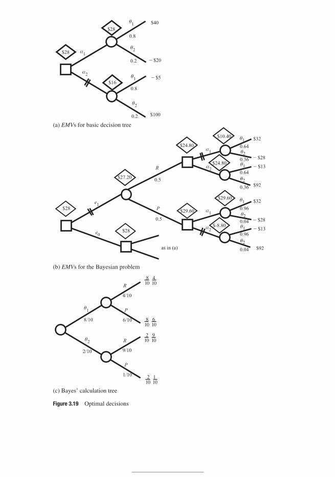
(a) EMVs for basic decision tree
(b) EMVs for the Bayesian problem
(c) Bayes’ calculation tree
Figure 3.19 Optimal decisions

132 Distributions and expectation
theorem is
Pr(θ2|P) = Pr(P|θ2)Pr(θ2)
Pr(P|θ2)Pr(θ2) + Pr(P|θ1)Pr(θ1)
=1
10 · 210
110 · 2
10 + 610 · 8
10
= 1
25= 0.04.
The Bayes’ tree is shown in Figure 3.19(c).The Raiffa problem presents an analogue of many real problems, and in particular the
fundamental choice between conducting an experiment or not. As noted before, the type ofurn (θ1 or θ2) represents the uncertain state of nature (traffic in a network, number of flaws ina weld, . . . ). One uses an experiment involving measurements to improve one’s probabilisticestimate of the state of nature.
3.5.3 Variance
The variance of a probability distribution is analogous to the moment of inertia of a bodytaken about the mean (or centre of mass). The variance σ 2
X for a random quantity X with meanµX is defined as
σ 2X = ⟨
(X − µX )2⟩ =
∑all x
(x − µX )2 pX (x) (3.63)
for a discrete random quantity, and
σ 2X = ⟨
(X − µX )2⟩ =
∫all x
(x − µX )2 fX (x) dx (3.64)
for a continuous one. The total (probability) mass is unity; Equations (3.63) and (3.64) arethe same as those for the moment of inertia of a body of unit mass. For either a discreteor continuous distribution with the cdf FX (x) specifying the distribution of mass (Stieltjesconvention), we have
σ 2X = ⟨
(X − µX )2⟩ =
∫all x
(x − µX )2dFX (x). (3.65)
The square root of the variance is the standard deviation, σX ; this corresponds to the radiusof gyration in mechanics. The ratio between the standard deviation and mean
γ ≡ σX
µX(3.66)
is known as the coefficient of variation, and is a useful parameter. For example, if we considerthe various loadings on a structure, it is important from the point of view of safety to knowhow much variation there is about the mean; the more there is, the higher the chance of anextreme loading.

133 3.5 Means and moments
Example 3.26 An example of the calculation of variance for the discrete distribution of Figure3.14 (top), using Equation (3.63). First
µX = 2.1, then
σ 2X = (1 − 2.1)2(0.3) + (2 − 2.1)2(0.35) + (3 − 2.1)2(0.3) + (4 − 2.1)2(0.05)
= 0.79 and σX = 0.8888, and
γ = 42% (coefficient of variation).
Example 3.27 For the exponential distribution, fX (x) = λ exp (−λx), for x ≥ 0, we recallthat the mean is 1/λ from Equation (3.62). Then using Equation (3.64):
σ 2X =
∫ ∞
0
(x − 1
λ
)2
λ exp (−λx) dx,
which may be evaluated by parts, giving
σ 2X = 1
λ2or σX = 1
λ.
The ratio between the standard deviation and mean, the coefficient of variation γ = σX/µX ,is then unity.
The interpretation above – as a moment of inertia – leads to some interesting conclusions. Werecall first the statement in the second paragraph of this section, that the probability ‘balances’at the centre of mass of the distribution: this is equivalent to saying that the first moment ofmass is zero about the centre of mass. The variance is the second moment of mass about thecentre of mass, and we can show by the ‘parallel axis’ theorem, well known in mechanics, thatthe variance is a minimum about the axis through the centre of mass.
Minimum variance: analogy to mechanics Consider the body shown in the illustration; wecalculate the moment of inertia about an axis B–B as∫
(r − d)2 dFR(r ), (3.67)
where r is the distance from the axis A–A through the centre of mass G to a particle of massdFR(r ), and d is the distance between the axis B–B and the parallel axis A–A through thecentre of mass. All distances are perpendicular to the parallel axes. Equation (3.67) can bewritten as∫
r2dFR(r ) − 2d∫
rdFR(r ) + d2. (3.68)
(Recall that the total mass in the case of probability is unity by coherence.) Since the first

134 Distributions and expectation
BA
AB
Body of unit mass with parallel axes
moment about the centre of mass is zero by definition,∫rdFR(r ) = 0,
Equation (3.68) becomes
σ 2G + d2, (3.69)
where σ 2G is the moment of inertia about the centre of mass.
Equation (3.69) is at a minimum when d = 0, so that the minimum moment of inertia(variance) σ 2
G occurs when the axis is through G. Equation (3.69) can also be used to deducethe following. The variance of Equation (3.63) or (3.64) was defined as the second momentabout the mean (or centre of gravity). Let the origin of coordinates be on the axis B–B. If thedistances are measured in the x-direction, we can apply (3.69), and we see that the secondmoment about the origin,
⟨X2
⟩, is given by⟨
X2⟩ = σ 2
X + µ2X , or
σ 2X = ⟨
X2⟩ − µ2
X . (3.70)
Equation (3.70) gives a useful ‘shortcut’ formula for the variance. This equation is introducedin more detail below; see Equation (3.87).
To conclude the analogy and to summarize, there are two interesting things about the centreof mass: the first moment of mass about this point is zero, and the moment of inertia is at aminimum. The first of these is identical to the condition we used to define probability, as a

135 3.5 Means and moments
‘price’ that we would pay for a bet on an outcome with a reward of unity if the outcome happens(Section 2.2). We can associate the prices with the distributed masses above. Consequently wesee that the mean is at the centre of mass of these prices. In the case of events there are onlytwo outcomes: the definition of the mean then coincides with the definition of probability. (Seethe Guide for Life on page 25.) For an event F,
〈F〉 = E(F) = P(F) ≡ Pr(F);
see also de Finetti (1974). The second interesting point, that the moment of inertia is a min-imum at the centre of mass, leads to the following. In order to define the centre of mass,or prevision-point – or the probability in the case of events – assume that a quadratic lossis incurred, corresponding to the term d2 in Equation (3.69), if we make an estimate awayfrom the centre of mass of our belief. This would ensure that we place our expected value(prevision), or probability, at the centre of mass to minimize this loss. Again see de Finetti(1974).
3.5.4 Mathematical manipulation of mean values
The mean or expected value of a function, g(X ), of a random quantity X is defined in a manneranalogous to the above:
〈g(X )〉 =∑
all xig(xi )pX (xi ), for discrete X (3.71)
or
〈g(X )〉 =∫ ∞
−∞g(x) fX (x) dx, for continuousX. (3.72)
Example 3.28 Take g(X ) = X2, and use the pmf of Figure 3.14 (top). Then
⟨X2
⟩ = (1)(0.3) + (4)(0.35) + (9)(0.3) + (16)(0.05)
= 5.20.
Example 3.29 Take g(X ) = exp (−X ) and fX (x) = λ exp (−λx) , x ≥ 0, i.e. the exponentialdistribution used previously. Then
〈exp (−X )〉 =∫ ∞
0exp (−x) λ exp (−λx) dx =
∫ ∞
0λ exp [−(λ + 1)x] dx
= λ
λ + 1.
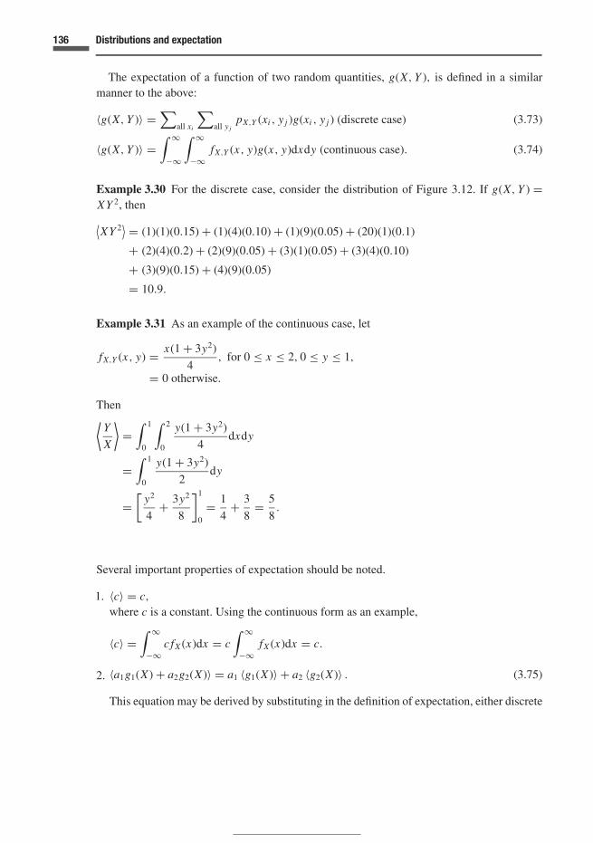
136 Distributions and expectation
The expectation of a function of two random quantities, g(X, Y ), is defined in a similarmanner to the above:
〈g(X, Y )〉 =∑
all xi
∑all y j
pX,Y (xi , y j )g(xi , y j ) (discrete case) (3.73)
〈g(X, Y )〉 =∫ ∞
−∞
∫ ∞
−∞fX,Y (x, y)g(x, y)dxdy (continuous case). (3.74)
Example 3.30 For the discrete case, consider the distribution of Figure 3.12. If g(X, Y ) =XY 2, then
⟨XY 2
⟩ = (1)(1)(0.15) + (1)(4)(0.10) + (1)(9)(0.05) + (20)(1)(0.1)
+ (2)(4)(0.2) + (2)(9)(0.05) + (3)(1)(0.05) + (3)(4)(0.10)
+ (3)(9)(0.15) + (4)(9)(0.05)
= 10.9.
Example 3.31 As an example of the continuous case, let
fX,Y (x, y) = x(1 + 3y2)
4, for 0 ≤ x ≤ 2, 0 ≤ y ≤ 1,
= 0 otherwise.
Then⟨Y
X
⟩=
∫ 1
0
∫ 2
0
y(1 + 3y2)
4dxdy
=∫ 1
0
y(1 + 3y2)
2dy
=[
y2
4+ 3y2
8
]1
0
= 1
4+ 3
8= 5
8.
Several important properties of expectation should be noted.
1. 〈c〉 = c,where c is a constant. Using the continuous form as an example,
〈c〉 =∫ ∞
−∞c fX (x)dx = c
∫ ∞
−∞fX (x)dx = c.
2. 〈a1g1(X ) + a2g2(X )〉 = a1 〈g1(X )〉 + a2 〈g2(X )〉 . (3.75)
This equation may be derived by substituting in the definition of expectation, either discrete

137 3.5 Means and moments
or continuous. A special case of Equation (3.75) is
〈a + bX〉 = a + b 〈X〉 . (3.76)
3. 〈a1g1(X, Y ) + a2g2(X, Y )〉 = a1 〈g1(X, Y )〉 + a2 〈g2(X, Y )〉 . (3.77)
This again may be proved by substituting in the definition, for example in the discrete case,
〈a1g1(X, Y ) + a2g2(X, Y )〉=
∑xi
∑y j
[a1g1(xi , y j ) + a2g2(xi , y j )]pX,Y (xi , y j )
= a1
∑xi
∑y j
[g1(xi , y j )pX,Y (xi , y j )
] + a2
∑xi
∑y j
[g2(xi , y j )pX,Y (xi , y j )
]= a1 〈g1(X, Y )〉 + a2 〈g2(X, Y )〉 .
A useful special case is obtained if g1(X, Y ) = X and g2(X, Y ) = Y ; then
〈X + Y 〉 = 〈X〉 + 〈Y 〉 . (3.78)
From Equations (3.75) and (3.77) it is seen that the operation of obtaining an expected valueis a linear operation.
2. For two independent random quantities,
〈XY 〉 = 〈X〉 〈Y 〉 , (3.79)
since (taking the continuous case as an example) fX,Y (x, y) = fX (x) fY (y) and therefore
〈XY 〉 =∫ ∞
−∞
∫ ∞
−∞xy fX (x) fY (y)dxdy
=∫ ∞
−∞x fX (x)dx
∫ ∞
−∞y fY (y)dy
= 〈X〉 〈Y 〉 .
Example 3.32 The last point may be verified in the case of the distribution in Figure 3.17:
〈XY 〉 = (10)(0.1) + (20)(0.15) + (20)(0.3) + (40)(0.45)
= 28,
and
〈X〉 = (10)(0.25) + (20)(0.75) = 17.5
〈Y 〉 = (1)(0.4) + (2)(0.6) = 1.6
Therefore 〈X〉 〈Y 〉 = 28 = 〈XY 〉. This would be expected because of the independence of Xand Y .

138 Distributions and expectation
3.5.5 Conditional expectation
Since conditional probability distributions such as fY |X , pX |Y>y, . . . , are valid normalizedprobability distributions, they may be used to calculate conditional expectations. For example,
〈X |Y 〉 =∫ ∞
−∞x fX |Y (x, y)dx (3.80)
for a continuous distribution and
〈Y |X〉 =∑
all y jypY |X (xi , y j ) (3.81)
for a discrete distribution.
3.5.6 Moments
We consider first a single random quantity X . To define moments, we let the function g(X ) = Xk
in Equations (3.71) and (3.72), where k is a constant. Then the expectations are⟨Xk
⟩ = µ(k)X =
∑all xi
xki pX (xi ), for discrete X, and (3.82)
⟨Xk
⟩ = µ(k)X =
∫ ∞
−∞xk fX (x) dx, for continuous X. (3.83)
These expectations define the kth moments about the origin. In particular, for k = 1, 〈X〉 =µ
(1)X = µX , the mean of the random quantity. The analogy to moments in mechanics is com-
plete. In the discrete case, the probabilities of the pmf at values x1, x2, . . . , are treated asconcentrated masses, and in the continuous case, the pdf is treated as a distributed mass, forexample a thin uniform plate bounded by the pdf and the x-axis, in both cases with totalmass = 1.
The moments about the mean, or central moments, are defined by letting g(X ) = (X −µX )k . Then 〈g(X )〉 is the kth moment about the mean, which we write as m(k)
X ; thus
m(k)X =
∑all x
(x − µX )k pX (x), for discrete X, and (3.84)
m(k)X =
∫ ∞
−∞(x − µX )k fX (x) dx, for continuous X. (3.85)
Note that the first central moment m(1)X is equal to zero. A particular case of great practical
importance is m(2)X , the variance σ 2
X , as described earlier:
m(2)X = σ 2
X = ⟨(X − µX )2
⟩; (3.86)
σX is the standard deviation. Both σ 2X and σX are, as noted earlier, measures of spread of the

139 3.5 Means and moments
Skewed to the right
g1 > 0
(b) Skewness
Symmetrical
g1 = 0
Skewed to the left
g1 < 0
Large X
2
x
(a) Measures of spread
Small X
2
x
pdf pdf pdf1 > 0
1 = 0
1 < 0
s s
Figure 3.20 Practical interpretation of moments
distribution. The following result is useful:
⟨(X − µX )2
⟩ = ⟨X2 − 2µX X + µ2
X
⟩= ⟨
X2⟩ − 2µX 〈X〉 + µ2
X
i.e.⟨(X − µX )2
⟩ = ⟨X2
⟩ − µ2X since 〈X〉 = µX
or σ 2X = ⟨
X2⟩ − µ2
X . (3.87)
This is the ‘shortcut’ formula noted before in Equation (3.70). Examples of the calculation ofthe variance have been given in Section 3.5.3.
The interpretation of m(2)X as a measure of spread is illustrated in Figure 3.20(a). If k = 3,
the third central moment, m(3)X , is obtained. The quantity
γ1 = m(3)X
σ 3X
(3.88)
is the coefficient of skewness and varies in value with the skewness of the distribution, asindicated in Figure 3.20(b). Note that if γ1 = 0, the distribution is not necessarily symmetrical,but if the distribution is symmetrical, then γ1 = 0. For k = 4, the fourth central moment can

140 Distributions and expectation
be used to obtain the coefficient of kurtosis (flatness):
γ2 = m(4)X
σ 4X
= m(4)X(
m(2)X
)2 . (3.89)
The parameter γ2 is equal to 3 for a normal distribution. As a result, the coefficient of kurtosisis often defined as
γ ′2 = γ2 − 3. (3.90)
The kurtosis is also associated with tail heaviness; the more probability mass in the tailsof the distribution, the greater the kurtosis. The normal distribution is the standard, termedmesokurtic with γ2 = 3, as noted. Then γ ′
2 = 0. Distributions with positive values of γ ′2 are
termed leptokurtic (more peaked); those with negative values are platykurtic (flat, or lesspeaked). See also Example 7.23.
3.5.7 Covariance and correlation
For functions of two random quantities, if g(X, Y ) = XkY �, then⟨XkY �
⟩is the moment of
order k + � of the random quantities X and Y . Similarly, if g(X, Y ) = (X − µX )k(Y − µY )�,then
⟨(X − µX )k(Y − µY )�
⟩is the central moment of order k + � of the random quantities X
and Y . Note that σ 2X is obtained if k = 2 and � = 0; similarly σ 2
Y is obtained if k = 0 and � = 2.If k = � = 1, the covariance σX,Y is obtained:
σX,Y = 〈(X − µX )(Y − µY )〉=
∑all xi
∑all y j
(xi − µX )(y j − µY )pX,Y (xi , y j ) (3.91)
in the discrete case, and
σX,Y = 〈(X − µX )(Y − µY )〉 =∫ ∞
−∞
∫ ∞
−∞(x − µX )(y − µY ) fX,Y (x, y)dxdy (3.92)
in the continuous case.The correlation coefficient ρXY is defined by
ρX,Y = σX,Y
σXσY(3.93)
and it should be noted that −1 ≤ ρX,Y ≤ 1, always. (See Exercise 3.25.) The covariance andin particular the correlation coefficient measure the extent of the linear relation between Xand Y . Thus a value of ρX,Y close to +1 would be associated with probabilities in the X–Yplane being concentrated along a line with positive slope (in the X–Y plane); a value closeto −1 with probabilities along a negative slope. See Figure 3.21 for examples in the discretecase.
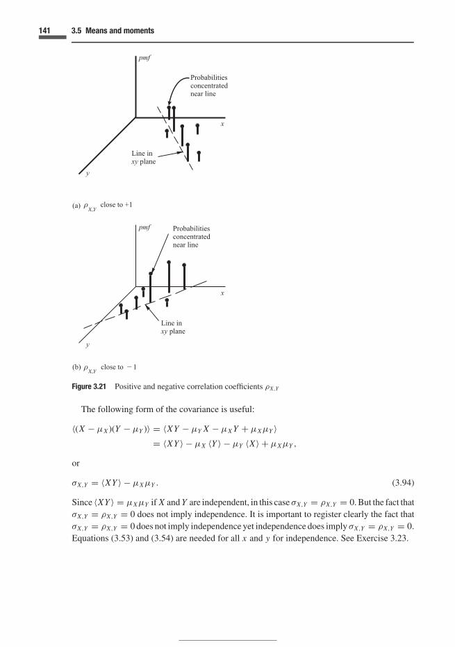
141 3.5 Means and moments
X,Y
X,Y
Figure 3.21 Positive and negative correlation coefficients ρX,Y
The following form of the covariance is useful:
〈(X − µX )(Y − µY )〉 = 〈XY − µY X − µX Y + µXµY 〉= 〈XY 〉 − µX 〈Y 〉 − µY 〈X〉 + µXµY ,
or
σX,Y = 〈XY 〉 − µXµY . (3.94)
Since 〈XY 〉 = µXµY if X and Y are independent, in this case σX,Y = ρX,Y = 0. But the fact thatσX,Y = ρX,Y = 0 does not imply independence. It is important to register clearly the fact thatσX,Y = ρX,Y = 0 does not imply independence yet independence does imply σX,Y = ρX,Y = 0.
Equations (3.53) and (3.54) are needed for all x and y for independence. See Exercise 3.23.

142 Distributions and expectation
Example 3.33 The calculation of covariance, using the pmf of Figure 3.12, is
µX = 2.1, µY = 2.0, 〈XY 〉 = 4.5
and therefore
σX,Y = 0.3.
Also⟨X2
⟩ = 5.20,⟨Y 2
⟩ = 4.60, σ 2X = 0.79, σ 2
Y = 0.60, and
ρX,Y = 0.44.
Example 3.34 The two-dimensional form of the normal distribution for two random quantitiesX and Y is
fX,Y (x, y) = 1
2πσXσY
√1 − ρ2
X,Y
exp −{
1
2(1 − ρ2
X,Y
)
×[
(x − µX )2
σ 2X
− 2ρX,Y (x − µX ) (y − µY )
σXσY+ (y − µY )2
σ 2Y
] }, (3.95)
whereρX,Y is the correlation coefficient between X and Y . IfρX,Y = 0, the distribution becomesthe (separable) product of two normal distributions
(µX , σ 2
X
)and
(µY , σ 2
Y
), in accordance with
(3.54). It is not generally the case that ρ = 0 results in independance; see end of precedingpage and Example 7.9.
3.5.8 Linear functions of random quantities
Let us now consider a linear function of the random quantity X ,
U = aX + b;
U must also be a random quantity. It has already been shown in Equation (3.75) and sequelthat
µU = aµX + b. (3.96)
In addition,
σ 2U = ⟨
(U − µU )2⟩
= ⟨(aX + b − aµX − b)2
⟩= ⟨
a2(X − µX )2⟩ = a2
⟨(X − µX )2
⟩. (3.97)
In short
σ 2U = a2σ 2
X . (3.98)

143 3.5 Means and moments
If U = a X + bY , where X, Y have a joint probability distribution, discrete or continuous,then
µU = aµX + bµY , (3.99)
which is also a consequence of Equation (3.75). The variance is
σ 2U = ⟨
(aX + bY − aµX − bµY )2⟩
= ⟨a2(X − µX )2 + b2(Y − µY )2 + 2ab(X − µX )(Y − µY )
⟩= a2
⟨(X − µX )2
⟩ + b2⟨(Y − µY )2
⟩+ 2ab 〈(X − µX )(Y − µY )〉 , (3.100)
or
σ 2U = a2σ 2
X + b2σ 2Y + 2abσX,Y . (3.101)
For independent random quantities σX,Y = 0 and in this case
σ 2U = a2σ 2
X + b2σ 2Y . (3.102)
If
Y = X1 + X2 + · · · + Xi + · · · + Xn,
where the Xi are mutually independent quantities, with variances
σ1, . . . , σi , . . . , σn,
then
σ 2Y =
∑n
i=1σ 2
i . (3.103)
Since σ 2U = a2σ 2
X , where U = aX, if
Y = X1 + X2 + · · · + Xi + · · · + Xn
n, (3.104)
the average of the Xs, then
σ 2Y = 1
n2
∑n
i=1σ 2
i . (3.105)
This is the case of independent random quantities; if the σ 2i are the same for each Xi ,and equal
to σ 2, then
σ 2Y = nσ 2
n2= σ 2
n. (3.106)
This would be true for iid (independent and identically distributed) random quantities. Butrandom quantities need not be identical to have the same σ 2
i , and they could still be independent

144 Distributions and expectation
so that Equation (3.106) has wider application than the iid case. Also, by extending (3.75) wefind for the relationship (3.104) that
µY = µX (3.107)
if the µX s are the same.
3.6 Random processes
We shall introduce briefly the subject of processes. We have already alluded to one: the Poissonprocess. This was introduced by means of examples of occurrences in time, for example arrivalsof computer messages or vehicular traffic. Usually these occur in time, but there are processes,as indicated earlier, which might involve distance or volume, for example. As a first illustration,consider a series of trials such as the random walk in the diagram of Figure 2.19. The processcould be modelled as the gain X (h) = 2Eh − 1 per trial h, where the gain is +1 for a successand −1 for a failure. Or the total gain Y (n) = ∑n
h=1 Xh could be considered. Examples ofthese are shown in Figure 3.22(a). If the events happen regularly in time, this could replace nas the abscissa and we would consider X (t) and Y (t) . We shall use time in the following forconvenience, but as noted other characterizations are possible.
Random processes are also termed stochastic processes. They can be continuous in time, asin Brownian motion where microscopic particles collide with molecules of a fluid. A furtherexample is given in Figure 3.22(b), which shows some regular and some random features.These random quantities – Brownian motion and Figure 3.22(b) – are continuous in time. Inaddition to considerations of time, the random quantity itself can be discrete or continuous –four combinations of possible kinds of processes. See Exercise 3.33. Processes that are discretein time generally have outcomes corresponding to times at the integers, as in Figure 3.22(a).They can be thought of as sequences of random quantities.
Papoulis (1965) and Ochi (1990) provide good introductions to the subject from an engi-neering standpoint. De Finetti (1974) provides excellent insights into the basis and meaningof different processes.
3.6.1 Processes with independent increments
In Figure 3.22(a) we introduced a process which could, for example, consist of successivetosses of a coin leading to Eh = heads and Eh = tails. These events would be judged to beindependent. We consider first such processes in discrete time. The process under considerationconsists of increments Xh in Y (n) = ∑n
h=1 Xh as described in the preceding section. These‘jumps’ then occur at the discrete points corresponding to the tosses of a coin. The tosses couldbe conducted at discrete times indexed h = 1, 2, 3, . . . , and then time could be used as theparameter of the process. This would then be described as in the lower part of Figure 3.22(a).
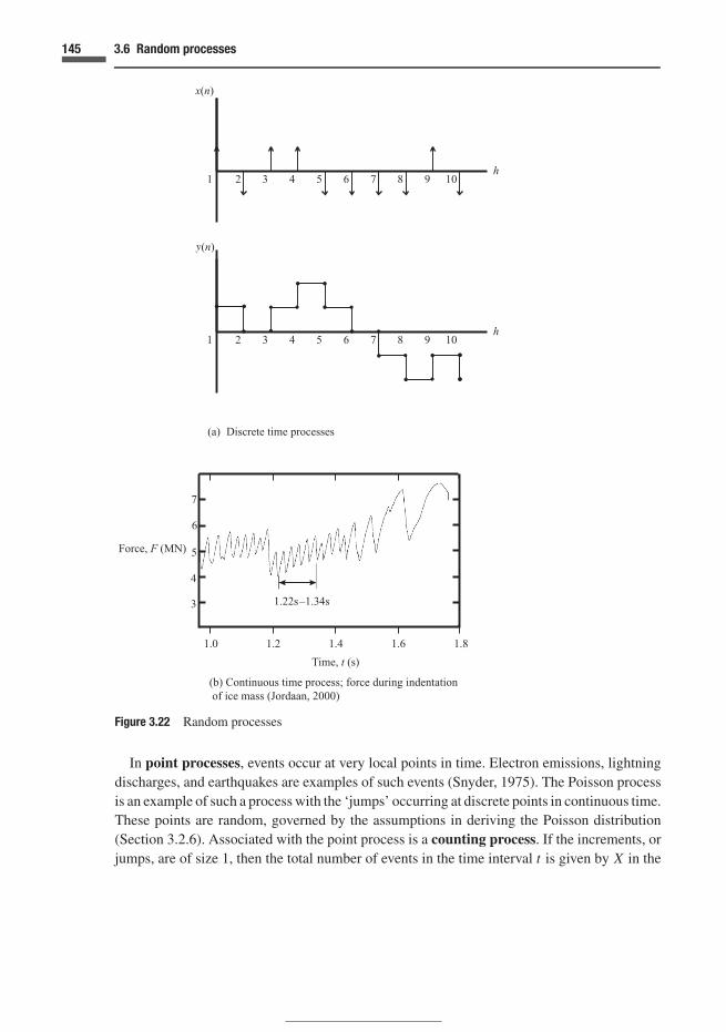
145 3.6 Random processes
y
1.22s–1.34s
(b) Continuous time process; force during indentation of ice mass (Jordaan, 2000)
Figure 3.22 Random processes
In point processes, events occur at very local points in time. Electron emissions, lightningdischarges, and earthquakes are examples of such events (Snyder, 1975). The Poisson processis an example of such a process with the ‘jumps’ occurring at discrete points in continuous time.These points are random, governed by the assumptions in deriving the Poisson distribution(Section 3.2.6). Associated with the point process is a counting process. If the increments, orjumps, are of size 1, then the total number of events in the time interval t is given by X in the

146 Distributions and expectation
Figure 3.23 Point process (top) and related counting process
Poisson distribution of Equation (3.13):
Pr (X = x) = pX (x) = exp (−ν) νx
x!= exp (−λt) (λt)x
x!, for x = 0, 1, 2, 3, . . . ,
where ν = λt and λ is the rate or intensity of the process. Processes of this kind in whichwe count the number of events are called counting processes. An illustration of point andcounting processes is given in Figure 3.23. The time between events was modelled by theexponential distribution as introduced in Section 3.3.2. See also Exercise 3.34 for the relatedErlang distribution, which models the time to the first, second or nth arrival.
The case where λ is constant leads to stationary increments. We pointed out in Section 3.2.6that the idea behind the Poisson distribution is readily extended to the situation where the rateλ varies with time, i.e. λ = λ (t) . In Equation (3.14) we noted that the expected number ofarrivals is given by
ν =∫ t
0λ (τ ) dτ,
and (3.13) applies. But the interarrival times are no longer modelled by the exponential orErlang distributions.
In the preceding the increments have been discrete and of unit size. The increments could bediscrete or continuous random quantities such that the increments over disjoint time intervals areindependent. The process is termed homogeneous if the increments over disjoint time intervalsof the same length have the same distribution. In the compound Poisson process, the increments(jumps) in time follow the Poisson point process but the quantity is modelled by a furtherrandom quantity. For instance, a series of telephone calls might follow the Poisson processand the length of the calls might follow an exponential distribution. We might be interestedin the total length of the telephone calls in a certain time interval. The auxiliary random

147 3.6 Random processes
quantity (length of calls) is sometimes called a ‘mark’ (Snyder, 1975). If the increments occurin continuous time, not at discrete points, we can divide the time period under considerationinto small intervals, and we can think of small increments occurring in these intervals. Theresult is a very large number of small independent increments. These follow the central limittheorem and the result is that the distribution is normal. This is the Wiener–Levy process. Ingeneral the decomposition of continuous processes requires the property of infinite divisibility,discussed briefly in Section 7.4.4.
3.6.2 Markov processes
We might consider that the probability of rain tomorrow depends on whether it is rainingtoday but not on the weather yesterday. This idea of dependence of one step in a process onthe preceding but not on events further in the past embodies the idea of a Markov process.Sometimes this is summarized in the statement:
‘Knowledge of the present makes the future independent of the past.’
We shall consider the discrete case in which there is again a sequence of values
X1, X2, X3, . . . , Xn, . . . , (3.108)
corresponding to states i, j taking the values 0,1,2,3, . . . In other words, the Xs will take thesediscrete values. The probabilities
Pr (Xn = i |Xn−1 = j) = pi | j (n) = pi j (n) (3.109)
are the (one-step) transition probabilities from j to i in moving from one step to another intime.
In the homogeneous case the transition probabilities are independent of time and we writepi j (n) = pi j :
pi j =
p00 p01 p02 · · ·p10 p11 p12 · · ·p20 p21 p22 · · ·...
......
. . .
. (3.110)
The sums of the columns must normalize for coherence:∑
ipi j = 1 for each j. (3.111)
Let the column vector qi (n) represent the probability of state i at step (time) n. The proba-bilities of states 0,1,2,3,. . . at time 1 are derived from the preceding set by means of
qi (1) = [pi j (1)
]q j (0) . (3.112)

148 Distributions and expectation
The two-step change is given by
qi (2) = [pi j (2)
] [pi j (1)
]q j (0) , (3.113)
and generally for n steps
qi (n) = [pi j (n)
] · · · [pi j (2)] [
pi j (1)]
q j (0) . (3.114)
For homogeneous chains,
qi (n) = [pi j
]nq j (0) . (3.115)
If at any stage in the process pi j = 1 for i = j and 0 for i �= j, then the state j is a trappingor absorbing state: transitions are possible into the state but not out of it.
Example 3.35 Counting processes are a special case of the Markov process. Consider thetotal number of heads in a sequence of tosses with an honest coin. Each step is dependent onthe preceding since any increment is added to it. This is a rather trivial example but helps inunderstanding the procedure. The one-step transition matrix is below. There are no zeros abovethe diagonal since the process cannot go back to a state once it has been left.
pi j =
0.5 0 0 · · ·0.5 0.5 0 · · ·0 0.5 0.5 · · ·...
......
. . .
. (3.116)
The initial state is
qi (0) =
100...
. (3.117)
One can implement Equations (3.112) to (3.115) to obtain the probabilities of states 0, 1, 2,3, . . . , at times 1, 2, 3, . . . The reader might wish to attempt this.
Example 3.36 We wish to model a queue – people, packets of data, aircraft. We make the rulethat a step is defined by an arrival in or a departure from the queue. Further, we assume thatthe process is homogeneous, with p = probability of a departure and 1 − p = probability ofan arrival. The state is the number in the queue. Then

149 3.6 Random processes
pi j =
0 p 0 0 · · ·1 0 p 0 · · ·0 1 − p 0 p · · ·0 0 1 − p 0 · · ·...
......
.... . .
, (3.118)
and the first four qi (t) are
10000...
,
01000...
,
p0
1 − p00...
and
02p − p2
0(1 − p)2
0...
. (3.119)
Ergodic chainsIn some cases a Markov chain evolves to a steady state, independent of the initial state. Thisis termed an ergodic chain. We can analyse this situation by supposing that q∗
i is the steadystate. Then, if this exists,
qi (n + 1) = qi (n) = q∗i .
For homogeneous chains
qi (n + 1) = [pi j
]q j (n) = [
pi j]
q∗j ,
and consequently
q∗i = [
pi j]
q∗j , (3.120)
or
[pi j − δi j
]q∗
j = 0. (3.121)
The term[δi j
]is the identity matrix; δi j = 1 if i = j, δi j = 0 otherwise.
The solution of (3.121) can be carried out as in the example below, or with further insightsusing eigenvalues and eigenvectors. If the chain is in a steady state, it is said to possessstationarity.
Example 3.37 In a queuing problem, three states are considered: 0 = no customers, 1 =number of customers ≤ n0 (specified number) and 2 = number of customers > n0. The

150 Distributions and expectation
homogeneous system is modelled by the transition matrix
[pi j
] = 0.8 0.2 0.6
0.1 0.6 00.1 0.2 0.4
. (3.122)
For a steady state (3.120) and (3.111) apply. Then
−0.2q∗0 +0.2q∗
1 +0.6q∗2 = 0
0.1q∗0 −0.4q∗
1 = 00.1q∗
0 +0.2q∗1 −0.6q∗
2 = 0q∗
0 +q∗1 +q∗
2 = 1 . (3.123)
Note that the third of these equations can be obtained from the first two (add and change sign)so that we need the fourth to solve. Then we find
q∗0 = 2
3, q∗
1 = 1
6, and q∗
2 = 1
6. (3.124)
3.6.3 Distributions and moments
Some authors consider ‘ensembles’ of outcomes as representing the random quantity, andthen model the behaviour of these as vectors. Each ensemble would constitute a different timeseries measure of the process – a different realization. It is simpler and more natural to considermerely the random quantity under consideration, which is our approach. The realizations aredata. For illustration, we shall concentrate on continuous random quantities; discrete randomquantities can be treated in a similar manner. As with other random quantities, those in astochastic process are modelled using a probability density. Here it is a function of time:
fX,t (x, t) .
This will have an associated cdf
FX,t (x, t) .
These distributions can be conceived of as a multidimensional distribution, with differ-ent times corresponding to different random quantities. For example, we could think of thesequence of values {X1, X2, X3, . . .} corresponding to times {1, 2, 3, . . .} as having a pdffX1,X2,X3,... (x1, x2, x3, . . .) . To make progress we must search for simplifications. The calcu-lation of moments assists in capturing essential features of a process.
The mean of X (t) is defined in a manner similar to (3.59) and in Section 3.5.6:
µX (t) = 〈X (t)〉 =∫ ∞
−∞x fX,t (x, t) dx . (3.125)
In order to study the behaviour of the process in time, we consider times t1 and t2 and the
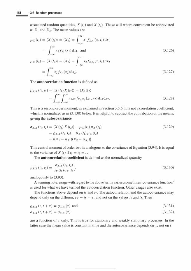
151 3.6 Random processes
associated random quantities, X (t1) and X (t2) . These will where convenient be abbreviatedas X1 and X2. The mean values are
µX (t1) = 〈X (t1)〉 = 〈X1〉 =∫ ∞
−∞x1 fX,t1 (x, t1) dx1
=∫ ∞
−∞x1 fX1 (x1) dx1, and (3.126)
µX (t2) = 〈X (t2)〉 = 〈X2〉 =∫ ∞
−∞x2 fX,t2 (x, t2) dx2
=∫ ∞
−∞x2 fX2 (x2) dx2. (3.127)
The autocorrelation function is defined as
�X,X (t1, t2) = 〈X (t1) X (t2)〉 = 〈X1 X2〉=
∫ ∞
−∞
∫ ∞
−∞x1x2 fX1,X2 (x1, x2) dx1dx2. (3.128)
This is a second order moment, as explained in Section 3.5.6. It is not a correlation coefficient,which is normalized as in (3.130) below. It is helpful to subtract the contribution of the means,giving the autocovariance
σX,X (t1, t2) = 〈X (t1) X (t2)〉 − µX (t1) µX (t2) (3.129)
= �X,X (t1, t2) − µX (t1) µX (t2)
= ⟨(X1 − µX1 )(X2 − µX2 )
⟩.
This central moment of order two is analogous to the covariance of Equation (3.94). It is equalto the variance of X (t) if t1 = t2 = t.
The autocorrelation coefficient is defined as the normalized quantity
ρX,X (t1, t2) = σX,X (t1, t2)
σX (t1) σX (t2), (3.130)
analogously to (3.93).A warning note: usage with regard to the above terms varies; sometimes ‘covariance function’
is used for what we have termed the autocorrelation function. Other usages also exist.The functions above depend on t1 and t2. The autocorrelation and the autocovariance may
depend only on the difference t1− t2 = τ, and not on the values t1 and t2. Then
�X,X (t, t + τ ) = �X,X (τ ) and (3.131)
σX,X (t, t + τ ) = σX,X (τ ) (3.132)
are a function of τ only. This is true for stationary and weakly stationary processes. In thelatter case the mean value is constant in time and the autocovariance depends on τ, not on t.

152 Distributions and expectation
sXX(t)
sXX(t)
t
t
Figure 3.24 Narrow and wide band processes
Example 3.38 Consider the process given by
X (t) = a cos (ωt + �) , (3.133)
in which a and ω are constants and � is random with a uniform distribution in [−π, π ] . Then
〈X (t)〉 =∫ π
−π
a cos (ωt + ξ )1
2πdξ = 0

153 3.6 Random processes
3.5−5
−4
−3
−2
−1
0
1
2x 10⁻³
4 4.5 5 5.5 6
Force, F (MN)
(dF
/dt)
/fre
quen
cy
Figure 3.25 Phase-plane diagram for segment 1.22–1.34s of Figure 3.22(b). See Jordaan (2000)
and
σX,X (τ ) = ⟨(X1 − µX1 )(X2 − µX2 )
⟩= a2
∫ π
−π
{cos (ωt + ξ ) cos [ω (t + τ ) + ξ ]} 1
2πdξ
= a2
4π
∫ π
−π
[cos (2ωt + ωτ + 2ξ ) + cos (ωτ )] dξ
= a2
2cos (ωτ ) , with (3.134)
ρX,X (τ ) = cos (ωτ ) . (3.135)
Example 3.39 Narrow and wide band processes. In narrow band processes, the frequency ofthe process is concentrated in a band near some frequency. We deal with spectral densities inChapter 7; see Figure 7.11. Figure 3.24 illustrates the nature of the processes in terms of timeseries and autocovariance functions. Figure 3.25 shows a phase-plane diagram, based on thedata from Figure 3.22(b). This represents a useful way of interpreting narrow band processes;see also Ochi (1990).
As noted above, ensembles represent particular sets of results of a time series, with eachmember of the ensemble representing a particular set of values in time; in effect, data. Thequestion arises in analysing and interpreting data: should one calculate expected values overtime or at a particular time over different ensembles? Ergodicity is a property that is often usedas a basis. We alluded to this for Markov chains. The ergodic property requires stationarity of

154 Distributions and expectation
the time series. The implication in statistics is that time averages for ergodic processes from asample are identical to averages over ensembles. It is often convenient to work out means andother moments from a particular time series rather than from a set of such time series. Figure3.22(b) shows an example of a time series. There are methods for removing the variation ofthe mean during a process and time-scaling could possibly be used to ensure stationarity ofthe process. But the process might well be non-stationary in nature. Figure 3.22(b) is of thiskind. The physical process does not suggest or support stationarity. The question is in realityone of modelling and inference. De Finetti (1974) points out that ergodicity is a property thatmay or may not apply but is not some kind of ‘autonomous principle’.
3.7 Exercises
It is a good idea to develop the habit of making plots and sketches of pdfs and cdfs of all probabilitydistributions encountered.
3.1 A random quantity X is modelled using the probability mass function
pX (x) = k (4 − x) , for x = 0, 1, 2, 3, and
= 0, otherwise.
(a) Find the constant k and the pmf. Sketch the distribution.(b) Find and sketch the cdf.(c) Find Pr(X < 2) .
3.2 For the following probability densities, determine the constant k, sketch the density, and find andsketch the cdf.
fX (x) = k(1 − x2
)for 0 < x < 1,
= 0, elsewhere.
fX (x) = exp (−k |x |) for all real x .
fX (x) = k sin (kx) for 0 < x <π
4,
= 0, elsewhere.
For the first pdf, find the Pr(X > 0.5) , for the second find Pr(X > 1) and for the third, findPr
(X > π
6
).
For an application of the second distribution, see Example 7.7.
3.3 A random quantity is modelled with a cdf
FT (t) =
0, for t < 1t2 − 2t − 1, for 1 ≤ t ≤ 2
1, for t > 2.
Determine the pdf fT (t) , and Pr(T ≤ 1.5) .

155 3.7 Exercises
3.4 In planning the use of a route for emergency vehicles in a city, there are ten signalized intersections.At each one, the traffic light is green for 40 seconds, yellow (amber) for 5 and red for 30 seconds.The emergency vehicle will stop at an intersection only if it is red. The signalling system is notcoordinated. What probability distribution models the number of stops? Determine the probabilitythat the emergency vehicle will have to stop at
(a) the first intersection;(b) none of the intersections;(c) the first four intersections;(d) the second, fourth, . . . , (even numbered) intersections but not at the others;(e) more than five intersections.(f) It is desired to reduce the probability in (e) to 0.02 seconds. What should the ‘red’ time be so
that this is obtained, keeping the amber and total cycle times constant?
3.5 A lot of 1000 transistors contains 900 that pass an acceptance test. The transistors are used ingroups of five to construct a component. It is decided to mix the failed transistors with those thathave passed the test and to select five randomly from the lot. The number of failed transistors in thegroup of five is of interest, denoted X.
(a) What is the distribution of X? Can the binomial distribution be used as an approximation?(b) Find the probability that not all the transistors have passed the test, using an exact method and
a binomial approximation.(c) What is the probability that more than two transistors in the component have failed the test?(d) What are the mean and the standard deviation? Use the approximate and exact distributions.
3.6 Summarize the four forms of the hypergeometric distribution as described and emphasized by deFinetti (1974).
3.7 In a telephone system, long distance telephone calls from a certain origin arrive at a rate of 12 perfive minutes. This rate can be considered as constant for the times under consideration.
(a) What models should be used to describe the time T between successive calls and for the numberof calls X in a minute?
(b) If a time τ elapses after a call, during which time no call is received, what is the distribution tothe next call?
(c) What is the probability that two calls arrive less than 30 seconds apart? What is the probabilitythat the next call will arrive after a minute elapses?
(d) Find the probability that two successive calls are separated by an interval that is within twostandard deviations of the mean? Sketch the pdf showing the calculation.
3.8 The number of flaws X per square metre of the surface of a plate is a random quantity. It is modelledusing a Poisson distribution with parameter λ = 1.67 per square metre.
(a) What are the mean and standard deviation of X?(b) What is the probability that a square metre of plate has no flaws?
If a square metre of plate has no flaws on its surface, it fails at a pressure of 5.6 kPa. If there are oneor more flaws, it fails at 2.8 kPa.(c) Find the mean pressure at which a square metre of plate fails.

156 Distributions and expectation
(d) Show that the standard deviation in kPa of the pressure for the square metre of plate is
2.8 exp (−1.67)√
exp (1.67 − 1).
3.9 Given that an earthquake has occurred, the magnitude R on a Richter scale is modelled as theexponential distribution
fR (r ) = 2.35 exp (−2.35r ) for r > 0,
= 0, otherwise.
Find the cdf and the probability that the next earthquake will have a magnitude greater than 6.0.
3.10 The pressure X acting on a ship’s hull during a collision is modelled by an exponential distributionwith a mean of 2 MPa. The number of impacts per year is modelled by a Poisson distribution witha mean equal to 10. Consider now only those impacts with X > x MPa.
(a) What model would you use for the number of these impacts (X > x) per year? Find the prob-ability that in a year the number of such impacts is equal to zero for the case x = 6 MPa.
(b) Consider now the maximum pressure in a year, written as Z . Using the result just obtained,derive the cdf FZ (z) .
(c) If the rate of impacts varies with time, with the same expected value, would the results derivedstill apply?
3.11 The concentration X of pollutant in a lake has been modelled using a normal distribution basedon past measurements, with a mean of 2.21 and a standard deviation of 0.46, in parts per million(ppm). Find the following.
(a) Pr(X < 1.5) .
(b) Pr(1.5 < X < 2.5) .
(c) Pr(X > 2.5) .
(d) The probability that in six samples, (a) occurs three times, (b) twice and (c) once.
3.12 Two rebars used in the construction of a gravity-based concrete offshore structure are connectedby a coupling. The strength of each rebar under the cyclic loading expected is normally distributedwith a mean of 300 MPa and a standard deviation of 30 MPa.
(a) Let X denote the strength of a rebar. What is the value of strength X = x f corresponding toFX (x) = 0.025?
(b) It is judged that the strengths of the two rebars are stochastically independent. What is theprobability that exactly one of the two rebars will fail at a strength less than x f ?
(c) An assembly of two rebars is to be tested. Denote the strength of the assembly as Y. What isthe value of FY
(x f
)given that FX
(x f
)is 0.025?
3.13 Find the mean, variance and standard deviation for Problem 3.1 and the first of 3.2.
It is a good idea to work through the derivations of the means and variances of commonly encountereddistributions (Appendix 1).
3.14 The Cauchy pdf with parameter a,
fX (x) = k
x2 + a2, for − ∞ < x < ∞, (3.136)

157 3.7 Exercises
is a bell-shaped curve resembling in a general way the normal distribution. But it has much thickertails.
(a) Find the value of k so that the pdf is well defined.(b) Find the cdf FX (x) .
(c) Find the inter-quartile range, the difference in x between FX (xL ) = 1/4 and FX (xU ) = 3/4.
(d) Find the mean and standard deviation.
3.15 The Pareto pdf is given by
fX (x) = ktk
xk+1, for x ≥ t (3.137)
= 0, for x < t.
(a) Find necessary conditions on k to ensure that 〈Xn〉 is finite.(b) Find the range of values for which the variance is finite. Find an expression for this variance.
3.16 An object (possibly an iceberg) is drifting on the ocean surface with a speed X that is random andmodelled by a gamma distribution:
fX (x) = xα−1 exp (−x/β)
βα� (α).
This distribution is based on a survey of all objects in a large area. Consider now the event thatthe object collides with an offshore installation. The probability of this event is proportional to thespeed X. Derive an updated velocity distribution using Bayes’ theorem given the event and usingthe pdf noted as a prior distribution. Show that this updated distribution is a gamma distribution withshape parameter changed from α to α + 1. Plot the prior and updated distributions for α = 2.5, andwith β taking the two values 0.11 and 0.38 ms−1.
3.17 An interesting example arises in arctic engineering. The area of an ice floe (assuming it to be circularof area A and radius R, approximately) is given by A = π R2. If R is random, then so is A. Whatis the mean area?
3.18 Geometric probability 1. A space probe is planned to land at a point P on the surface of a planet. Alocal coordinate system is constructed in the tangent to the surface at P. The probability of landingoutside a circle of radius 5 km with P as centre is considered to be zero, and the probability withinis judged to be uniformly distributed over the circular area with the density proportional to the area.Find the probability that the space probe will land
(a) within 2 km of P,(b) between 2 and 3 km from P,(c) north of the aiming point,(d) south of the aiming point and more than 2 km from P, and(e) exactly due north of P.
3.19 Geometric probability 2. Two signals are sent to a receiver, and arrive within the time interval t.The instants at which the signals arrive are denoted X1 and X2. If the signals arrive within the smallinterval τ of each other, interference and deterioration of the signals result. Find the probability of

158 Distributions and expectation
this event, on the assumption that X1 and X2 are independent and equally likely at any point in theinterval [0, t] .
3.20 Geometric probability 3.
(a) Two ships berth at the same quay in a harbour. The arrival times for the ships are independentand uniformly distributed (equally probable) during any 24 hour period. If, during the timewi (needed for mooring, loading and unloading) between arrival and departure of either ship,the other ship arrives, then the other ship has to wait to use the berth. For the first ship thiswaiting time is w1 = 1 hour. For the second ship the waiting time is w2 = 2 hours. Estimatethe probability that one of the ships will have to wait to use the berth during the next 24 hourperiod.
(b) A ferry carries freight continually from one bank of a river to another. This takes one hour. Aship moving along the river at right angles to the direction of travel of the ferry can be seenfrom the ferry if it passes the trajectory of the ferry less than 20 minutes away from its position.All times and places of intersection are judged to be equally likely. What is the probability thatthe ship will be seen from the ferry?
3.21 Geometric probability 4. On the surface of the earth the area bounded by two degrees of longitudeand by the line of latitude θ to θ + 1 degrees is to a good approximation, a rectangle of sides 111.12km (north–south) and 111.12 cos (θ + 0.5) km (east–west). A ship of beam (width) b is crossingthe degree-rectangle on a path of total length d. A stationary iceberg (or other object) of width w isplaced at a random position in the degree-rectangle.
(a) Find the probability that the ship will collide with the object during the crossing of the degree-rectangle and evaluate the probability given θ = 41◦, b = 28 m, w = 110 m and d = 83.2 km(these are plausible values for the RMS Titanic in 1912), or using some other values of interest.
(b) Using the values obtained in (a) find the probability that there are no collisions after 100crossings, and the number of crossings above which the probability of a collision just exceeds0.50.
3.22 Find the skewness of the exponential distribution
fX (x) = 1
βexp (−βx) for x ≥ 0
= 0 otherwise.
3.23 The joint probability distribution pX,Y (x, y) of the random quantities X and Y is as follows.
x0 1 2 3
1 227 0 0 1
27
y 2 627
627
627 0
3 0 627 0 0

159 3.7 Exercises
(a) Check for coherence and determine the marginal distributions pX (x) and pY (y) .
(b) Determine pX |Y (x, y) , pY |X (x, y) and pY |X=0 (y) .
(c) Find the means µX , µY , the standard deviations σX , σY as well as 〈XY 〉.(d) Determine the covariance σX,Y .
(e) Are X and Y independent?
3.24 Given the pdf
fX,Y (x, y) = 2 exp (−x − y) , for 0 ≤ x ≤ y and 0 ≤ y < ∞= 0 otherwise,
find the marginal distributions and check for independence.
3.25 Prove that the correlation coefficient ρXY is such that
−1 ≤ ρX,Y ≤ 1,
always. Comment on the meaning of ρXY = 0.
3.26 Raiffa decision problem. Consider an additional choice in Examples 3.24 and 3.25 of Section 3.5.2.You are offered the option of sampling two balls for a fee of $12 rather than the single ball at $8 inExample 3.25. The contracts offered remain the same as before. Note that the updated probabilitiesare the subject of Exercise 2.18. Is the new option an attractive one based on EMV compared to theothers?
3.27 A long distance telephone company is planning to increase the capacity of its networking system.A team set up to study the future demand is unable to reach a firm decision and concludes thatthe annual growth rate will be 1, 2, or 3 per cent with equal probability. Three capacities will beadequate for these three growth rates for the design period. The respective capacities are 5, 10 and15, in arbitrary units. Economics of scale given by the equation
cost = k (capacity)0.6
can be applied to the cost of the three capacity units. Draw a decision tree for this problem andindicate what decision you would recommend on the basis of maximum expected monetary value.Complete the calculation in terms of present monetary units, i.e. ignore interest on money and theeffects of inflation.
3.28 Aggregates for a highway pavement are extracted from a gravel pit. Based on experience with thematerial from this area, it is estimated that the probabilities are Pr(G) = Pr(good-quality aggregate)= 0.70, and Pr(G) = Pr(poor-quality aggregate) = 0.30. In order to improve this prior information,the engineer considers a testing program to be conducted on a sample of the aggregate. The testmethod is not perfectly reliable – the probability that a perfectly good-quality aggregate will passthe test is 80%, whereas the probability of a poor-quality aggregate passing the test is 10%.
(a) Draw both Bayes’ calculation and decision trees for the problem. The decision tree shouldinclude the options ‘do not implement test programme’ and ‘implement test programme’, as

160 Distributions and expectation
well as ‘accept the aggregate’ and ‘reject the aggregate’. Determine the optimal decisionon the basis of minimum-expected-cost, given the following monetary values (on a nominalscale). Accept, good aggregate, 15 units; accept, poor aggregate, −8 units; reject, good or pooraggregate, 5 units; cost of testing, 2 units.
(b) If a sample is tested, and if it passes, what is the probability of good-quality aggregate?(c) If a second test is performed, and the sample again passes, what is the probability of good-quality
aggregate? One can use the result of part (b) as a prior probability in this case.
3.29 In the design of a dam for flood control, the height of the dam depends on two factors. Thefirst is the level of water in the dam, denoted X, and the second is the increase caused by floodwaters coming into the reservoir, denoted Y . The level X takes the values {30, 40, 50 metres} withprobabilities {0.2, 0.5, 0.3} respectively, while Y takes values {10, 20, 30 metres} with probabilities{0.3, 0.4, 0.3} respectively. It is decided to use a decision analysis to determine the dam height. Twovalues are under consideration, 65 and 75 m, with costs of 12 and 15 units respectively. Theconsequences of overtopping are flooding downstream with costs of 15 units. (All costs can betreated as additive.) A hydrological study is under consideration in order to obtain a better estimateof the probabilities of the flood levels noted. For the purposes of the present analysis, the resultsof the study can be summarized by the values of R = 1 (low), R = 2 (medium) and R = 3 (high).The method has the reliabilities indicated in the following table.
Pr(R|Y )
R = 1 R = 2 R = 3
Y = 10 0.70 0.20 0.10Y = 20 0.10 0.80 0.10Y = 30 0.05 0.05 0.90
Update the probabilities of Y, i.e. determine the values Pr(Y |R) . Complete a decision analy-sis with tree, including the option: (complete study, do not complete study) and theoption (dam height= 65 m, dam height = 75 m). The cost of the study is 2 units.
3.30 Referring to Exercise 2.26, the engineer has to decide whether or not to close down a section ofthe pipeline to conduct major repairs. The following values of utility are assigned. Subtract 2 unitsas a ‘cost’ if tests are undertaken. Draw a decision tree and determine the optimal course of actionbased on the criterion of maximum expected utility. The symbol R denotes ‘repairs undertaken’.
S Given R Given R
0 7 101 6 52 5 0
3.31 The speeds of vehicles on a highway are modelled by a normal distribution with a mean of 60 kmh−1
and a standard deviation of 15. Determine the pdf of the relative speed of two vehicles moving in

161 3.7 Exercises
opposite directions. Assume now that the drivers, having seen a police car in the area, obey a speedlimit of 75 kmh−1; those exceeding the limit now drive at the limit, with the other speeds remainingunchanged. Sketch and describe the new distribution of speeds (in one direction).
3.32 Consider a sequence of four waves in a storm. The wave heights are {X1, X2, X3, X4} . Thesequantities are judged to be exchangeable, so that all 24 permutations such as {X1, X3, X2, X4} or{X4, X2, X3, X1} are considered equivalent. For quantities that are not exchangeable there are fourvalues 〈Xh〉 , six 〈Xh Xi 〉 for (h < i), and four
⟨Xh Xi X j
⟩for (h < i < j) . What can be said of these
in the case of exchangeable random quantities?
3.33 Sketch random processes that illustrate the four combinations of discrete or continuous in time anddiscrete or continuous random quantities.
3.34 In a Poisson process with constant intensity λ, show that the time T to the kth event is modelled bythe Erlang distribution
fT (t) = λ (λt)k−1 exp (−λt)
(k − 1)!, for t > 0, k ≥ 1. (3.138)
Verify that this is a special case of the gamma distribution.If accidents occur at the rate of 0.2 per month on a highway, describe the distribution of the time inmonths to the third accident.
3.35 Aircraft are serviced at a loading bay. An engineer is studying the waiting times and usage of spaceand decides to model the situation by dividing time into a discrete set of small time intervals duringwhich one arrival is expected. During one such time step, the crew at the loading bay can service{0, 1, 2} aircraft with probabilities {3/8, 1/2, 1/8} . The following strategy is adopted. One aircraftis allowed to wait to enter the bay if one is being serviced there. Consequently, when the bay haszero or one aircraft being serviced, an additional aircraft is then permitted to enter or to wait. In thecase where one is being serviced, and one is waiting, any arriving aircraft are routed elsewhere. Thestates under consideration are {0, 1, 2} , corresponding to the number of aircraft at the bay (waitingor being serviced) at the end of each time step. The end of a time step is defined such that anycompleted aircraft have moved on and before a new one is accepted.
(a) Derive the one-step transition matrix.(b) Find the long-run stationary state, if there is one.(c) If the bay starts out the day empty, so that an aircraft is admitted at the beginning of the next
step, write down the first three probability vectors qi .
3.36 Find the autocovariance of
(a) X (t) = A cos (ωt + �) ,
where A and � are independent random quantities, the latter uniformly distributed in the interval[−π, π ] .
(b) X (t) = ∑ni=1 [Ai cos (ωi t) + Bi sin (ωi t)] ,
where all of the Ai and the Bi are independent random quantities with 〈Ai 〉 = 〈Bi 〉 = 0 andσ 2
Ai= σ 2
Bi= σ 2
i .

4 The concept of utility
‘Your act was unwise,’ I cried, ‘as you seeBy the outcome.’ He calmly eyed me:‘When choosing the course of my action,’ said he,‘I had not the outcome to guide me.’
Ambrose Bierce
4.1 Consequences and attributes; introductory ideas
We have shown that two ingredients are combined in our decision-making: probability andutility. But utility has not been well defined. Up to this point, we have given detail of theprobabilistic part of the reasoning. We now present the basic theory with regard to utility.Probabilities represent our opinions on the relative likelihood of what is possible, but notcertain; utilities encode our feelings regarding the relative desirability of the various conse-quences of our decisions. Examples of where utilities fit into the decision-making processwere given in Section 1.2. A special case is expected monetary value (EMV), dealt with inSection 3.5.2.
There can be various components of utility, depending on the application. These com-ponents will be referred to as ‘attributes’. For example, in a study of airport developmentfor Mexico City, de Neufville and Keeney (1972) considered attributes of the followingkind.
� cost� airport capacity� safety� access time� noise� displacement of people.
There will usually be a set of such attributes, which depends on the problem at hand. Attributesmay have
162

163 4.1 Introductory ideas
� increasing value, for example money, profit, volume of sales, time saved in travelling, andwilderness areas available for enjoyment
� decreasing value, for example size of an oil spill, level of noise pollution, and deaths andinjuries in an accident.
Cost and safety are common attributes in engineering, and there are often tradeoffs betweenthe two. It is relatively easy to design a structure that is safe enough by excessive size of itsmembers; it is the art of engineering to provide a structure that is adequately safe (and hopefullyelegant) with appropriate economy.
The essence of utility is to transform the attributes into a single scale which measures thedesirability of the outcome. We shall introduce the concept by summarizing the transformationof a single attribute, money. The basic idea is contained in the following analysis that was givenby Daniel Bernoulli in the eighteenth century. He considered the utility u corresponding tomoney, x . If a person possesses a sum x , Bernoulli reasoned that a small change in the person’sutility, du, is proportional to a change dx in their capital, and also inversely proportional to theirworking capital x . For example, $5 will be of higher utility to a man under poverty-strickencircumstances than under relative affluence.1 Thus, du = (k1/x)dx where k1 is a constant, and
u = (k1 ln x + k2), (4.1)
where k2 is a constant of integration.The logarithmic relationship of (4.1) is an example of the non-linearity of utility with an
attribute, money. Figure 4.1 illustrates such a relationship. As a ‘summary’ value we oftenuse a mean value; the mean of two amounts of money A and B are shown as x in the figure.This would be our expected value corresponding to a bet with even odds on A and B. Imagineprobabilistic weights of 0.50 attached to the points A and B. Their centre of gravity is at point Gand the mean utility is u. Utility theory tells us to use x, the x-coordinate value correspondingto u, obtained from the nonlinear relationship, instead of x in decision-making. The germ ofthe concept of utility is ‘curving it’! If all of this seems too complicated, it is explained inmuch more detail in the following. We hope merely to whet your appetite.
In using utility theory we begin with an attribute measured on some scale, a prominent exam-ple being money as in the preceding example. Many decisions concern attributes which mightat best be ordered. For example, flooding of an area in dam construction and consequent effecton wildlife might be difficult to measure on a scale. This is not to say that these consequencesare not important: many would rank them as being amongst the highest in importance. Thepoint is that placing these consequences on a numerical scale might present difficulties sincemeasurement of the attributes might not be possible. The final decision would then have to bemade on the basis of a qualitative assessment of all the consequences with numerical supportwhere possible. Exercise 4.1 is intended to alert the reader to these difficulties.
1 We shall see that utility is a measure of an individual’s preferences: to speak of a beggar and a rich man is not quitewhat we mean. Rather, this applies for the same person under the two different circumstances.

164 The concept of utility
Attribute, x
Utility, u
u_
x x_
A
B
G
Figure 4.1 Utility and money: ‘weights’ of probability act upwards at A and B with their equilibratingunit weight acting downwards at G
The primary focus of this chapter is the quantitative analysis of attributes. This should becarried out where possible in important decisions and serves to assist in understanding riskaversion and in dealing with qualitative measures which should be given their proper weightin the decision. A further area of concern is that of the use of benefit–cost ratios. These canprovide a reasonable basis for certain comparisons but contain arbitrary elements, for examplein dealing with attributes measured in a qualitative manner. Risk aversion is not included and,furthermore, when considering the time value of money, the choice of interest rates can havea decisive effect on the results. The latter aspect applies to all methods unless the economicaspects are carefully modelled – and they need to include uncertainty. Exercise 4.2 points inthis direction using very simple models.
An excellent introduction to utility is the simple yet logically convincing treatment by Raiffa(1968) which is much recommended. More detail is given in Raiffa and Schlaifer (1961) and inKeeney and Raiffa (1976, reprinted 1993). The latter is a tremendously useful book, motivatedvery much by practice. Much of the development of utility theory has taken place during thetwentieth century, a prominent example being the work by von Neumann and Morgenstern(1947).
4.2 Psychological issues; farmer’s dilemma
The attributes in any particular problem have to be carefully considered and ‘massaged’ beforethey can be considered as utilities. How do we weigh our feelings in making decisions? The

165 4.2 Farmer’s dilemma
Table 4.1 Payoff matrix vi j
θ1 : perfect θ2 : fair θ3 : bad
α1 : crop A 11 1 −3α2 : crop B 7 5 0α3 : crop C 2 2 2
need for a unique method of ranking decisions will be introduced by the ‘farmer’s dilemma’(Rubinstein, 1975). This concerns a farmer who has to choose between three crops at thebeginning of the planting season. The three crops will behave differently in different weather.For simplicity, we consider only three possible weather conditions: perfect, fair and bad. Theseare literally our states of nature, and the farmer is unsure as to which will prevail. The possiblecrops are designated A, B and C. Crop A is potentially bountiful and a good money-maker,but will do well only if the weather is very good. If not, it will likely fail. Crop B is morehardy, but will not have the same potential in good weather. Crop C is most hardy, and is littleaffected by the weather, within the limits of the region.
Table 4.1 shows the potential payoffs to the farmer for the set of planting strategies, combinedwith the states of nature. The payoffs can be considered to represent money to some arbitraryscale. We shall use the notation αi to represent the possible actions (or strategies) available tothe farmer, and θ j to represent the states of nature. For some combination of these two, thepayoff is vi j . The farmer’s problem can also be viewed in the form of a decision tree, as inFigure 4.2.
Lest it be thought that the farmer’s dilemma does not encapsulate a real problem in theengineering or economic world, Table 4.2 illustrates the dilemma facing the regulatory au-thority in Canada when a major new bridge was being designed for harsh environmentalloadings. There is often considerable uncertainty in loadings under such circumstances, and,indeed, differences of opinion amongst experts, with load estimates ranging from high (ex-tremely conservative) to low (less conservative, but possibly realistic). Table 4.2 illustratesthe payoff matrix that might be in the regulator’s mind when attempting to decide upon adecision amongst the αi . As in all decisions, it might appear as a risky choice versus a safeone.
4.2.1 Pessimist’s solution: maximin
The first possible solution to the dilemma is to make the assumption that ‘the worst willhappen’. The farmer inspects the payoffs for each strategy, and chooses the minimum. Thisamounts to taking a minimum for each row, as shown in Table 4.3. The farmer then makes thebest of the situation by choosing the ‘best of the worst’, the maximum of the minima. Thiswould result in the choice of crop C in Table 4.3 (action α3). This is termed the ‘maximin’solution. There are three possible interpretations of the farmer’s behaviour.
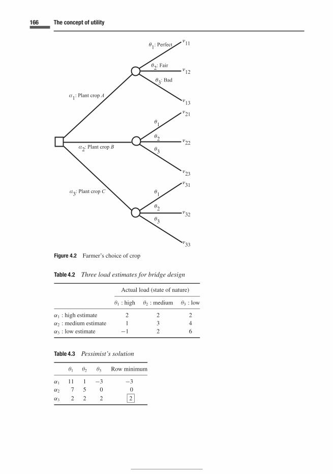
166 The concept of utility
Figure 4.2 Farmer’s choice of crop
Table 4.2 Three load estimates for bridge design
Actual load (state of nature)
θ1 : high θ2 : medium θ3 : low
α1 : high estimate 2 2 2α2 : medium estimate 1 3 4α3 : low estimate −1 2 6
Table 4.3 Pessimist’s solution
θ1 θ2 θ3 Row minimum
α1 11 1 −3 −3α2 7 5 0 0
α3 2 2 2 2

167 4.2 Farmer’s dilemma
Table 4.4 Optimist’s solution
θ1 θ2 θ3 Row maximum
α1 11 1 −3 11α2 7 5 0 7α3 2 2 2 2
1. He or she considers the probability of bad weather to be unity, in other words a certainty.This may be justified, but in general is unlikely to be a realistic judgement.
2. The farmer is very averse to taking risks and chooses a safe solution which is assured. Thismay well be related to the farmer’s present working capital.
3. If the farmer considers the ‘opponent’ – nature in this case – to be out to ‘get’ the farmer,the reaction is a reasonable one. We shall see in Chapter 5 that this attitude is a natural onein situations of conflict; in the present case, it may indicate poor judgement.
4.2.2 Optimist’s solution: maximax
The optimist assumes that the best always happens. Table 4.4 shows this solution. For eachpossible action, the maximum value of the payoff is identified as the value to choose. The‘best of the best’, the maximum of the maxima is then chosen, with the result that the optimistchooses action α1, crop A. There are three interpretations of the optimist’s behaviour, mirroringthe interpretations of the pessimist above. The probability of perfect weather could in fact bejudged to be unity, or the decision-maker is willing to take a risk, or the judgement of thedecision-maker could be faulty, indicating an unrealistically optimistic attitude.
4.2.3 The ‘in-betweenist’
The optimist and the pessimist represent extreme points of view which many of us would wishto avoid, by taking a compromise between them. This criterion (due to Hurwicz) attemptsto find common ground between the optimist and the pessimist. A weight β is placed onthe pessimist’s solution, with the weight (1 − β) on the optimist’s. The value β, such that0 ≤ β ≤ 1, is used as follows, using the above solutions for the optimist and the pessimist. Weassume that β = 0.6.
Action α1 : weighted value = (0.6)(−3) + (0.4)(11) = 2.6Action α2 : weighted value = (0.6)(0) + (0.4)(7) = 2.8Action α3 : weighted value = (0.6)(2) + (0.4)(2) = 2.
The in-betweenist would choose action α2, crop B, since this gives the greatest of the weightedvalues. The ‘index of pessimism’ β is chosen subjectively, with β = 1 indicating completepessimism, and β = 0 complete optimism.
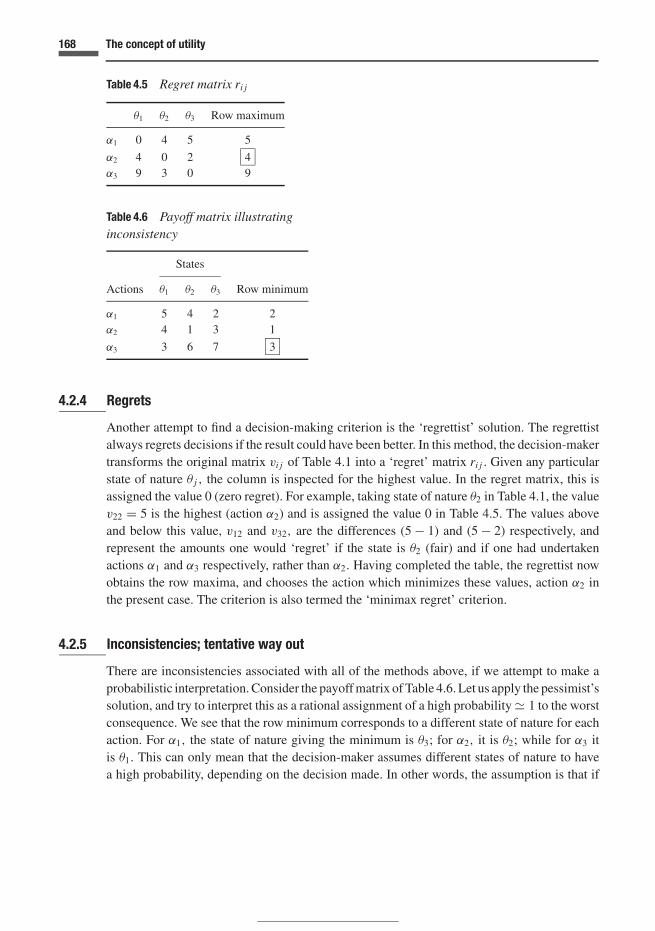
168 The concept of utility
Table 4.5 Regret matrix ri j
θ1 θ2 θ3 Row maximum
α1 0 4 5 5
α2 4 0 2 4α3 9 3 0 9
Table 4.6 Payoff matrix illustratinginconsistency
States
Actions θ1 θ2 θ3 Row minimum
α1 5 4 2 2α2 4 1 3 1
α3 3 6 7 3
4.2.4 Regrets
Another attempt to find a decision-making criterion is the ‘regrettist’ solution. The regrettistalways regrets decisions if the result could have been better. In this method, the decision-makertransforms the original matrix vi j of Table 4.1 into a ‘regret’ matrix ri j . Given any particularstate of nature θ j , the column is inspected for the highest value. In the regret matrix, this isassigned the value 0 (zero regret). For example, taking state of nature θ2 in Table 4.1, the valuev22 = 5 is the highest (action α2) and is assigned the value 0 in Table 4.5. The values aboveand below this value, v12 and v32, are the differences (5 − 1) and (5 − 2) respectively, andrepresent the amounts one would ‘regret’ if the state is θ2 (fair) and if one had undertakenactions α1 and α3 respectively, rather than α2. Having completed the table, the regrettist nowobtains the row maxima, and chooses the action which minimizes these values, action α2 inthe present case. The criterion is also termed the ‘minimax regret’ criterion.
4.2.5 Inconsistencies; tentative way out
There are inconsistencies associated with all of the methods above, if we attempt to make aprobabilistic interpretation. Consider the payoff matrix of Table 4.6. Let us apply the pessimist’ssolution, and try to interpret this as a rational assignment of a high probability � 1 to the worstconsequence. We see that the row minimum corresponds to a different state of nature for eachaction. For α1, the state of nature giving the minimum is θ3; for α2, it is θ2; while for α3 itis θ1. This can only mean that the decision-maker assumes different states of nature to havea high probability, depending on the decision made. In other words, the assumption is that if

169 4.2 Farmer’s dilemma
one plants crop A, it will hail, if crop B, snow will appear, and crop C will somehow causefrost. Nature does not generally behave in this way. The only reasonable interpretation is totalinconsistency, perhaps with an element of paranoia! The one situation where the reaction ofthe decision-maker might reasonably follow this pattern is where there is a genuine situationof conflict. This would not constitute a ‘game against nature’ but rather a game against anintelligent opponent, who is out to win. This situation will be dealt with in Chapter 5.
The other methods above also suffer from the problem of inconsistency outlined in thepreceding paragraph. Further, the regrettist solution suffers from a further drawback. Additionof a new alternative, which we would in any event not choose on the regrettist’s criterion, canalter our original choice (Hall, 1962).
Farmer’s tentative way outAlthough the in-betweenist has attempted to make a compromise between the pessimist andthe optimist, probabilities have not been properly introduced into the problem. There needs tobe a clear separation of the probabilities and the consequences in the decision-making process.The farmer realizes this, and consults a friend who knows probability theory, and who happensalso to be a meteorologist. They work together on the problem, addressing Table 4.1 and comeup with the following probabilities.
Pr(θ1) = 0.1,
Pr(θ2) = 0.5, and
Pr(θ3) = 0.4.
The farmer decides to weight the monetary values in Table 4.1 by the corresponding probabil-ities, conditional on the action taken. Remembering that vi j represents the payoff, we denoteit Vi j to emphasize that it is random.
⟨V1 j |α1
⟩ = (0.1)(11) + (0.5)(1) + (0.4)(−3) = 0.4,⟨V2 j |α2
⟩ = (0.1)(7) + (0.5)(5) + (0.4)(0) = 3.2, and⟨V3 j |α3
⟩ = (0.1)(2) + (0.5)(2) + (0.4)(2) = 2.0.
These are termed the farmer’s expected monetary values (EMVs), as introduced in Section3.5.2. We now consider the following criterion.
Tentative criterion: choose that action which maximizes the expected monetary value.
Accordingly, the farmer decides to follow action α2, plant crop B. At the same time, a farmerwho has a lot of money in the bank might wonder whether crop A might not have been a betterchoice whereas a farmer struggling financially might consider crop C a better option, sincethe prospect of a gain of zero (crop B) or a loss of (−3) in the case of crop A if the weather ispoor are not very attractive alternatives (imagine the amounts to be in $1000 000).

170 The concept of utility
4.3 Expected monetary value (EMV )
In this section we shall continue to deal with that universal attribute, money, and explore theusefulness of expected monetary value (EMV). We shall therefore explore further the conceptof EMV, but first introduce an interesting set of problems that will be of use in this chapter andelsewhere.
Brief digression: games with two dice Problems concerning two dice occur frequentlyin probability theory. One of the early problems in probability theory considered by Pascalwas posed to him by de Mere; this is used to introduce extremes in Chapter 9. We use two-diceproblems twice in this chapter, once in this section, and also in discussing transitivity of choices(Section 4.6). If we toss two dice, the possible results can be shown in a matrix {i, j} in whichi denotes the number on the first die, and j the number on the second. All results are equallylikely, with probability 1/36.
11 12 13 14 15 1621 22 23 24 25 2631 32 33 34 35 3641 42 43 44 45 4651 52 53 54 55 5661 62 63 64 65 66
In the game of craps, two dice are thrown and the sum of the two scores is the decidingfactor, so that calculation of the probabilities of (i + j), the total of the values on the two dice,is needed. There are 11 possible results, from 2 to 12, with probabilities corresponding to thediagonal values in the matrix. The probabilities increase in equal steps of 1/36, from 1/36 for

171 4.3 Expected monetary value (EMV )
a result of 2, to 6/36 for 7, and then decrease in the same way to 1/36 for 12. In craps, a firstthrow of seven or eleven wins, with a probability of 8/36 = 2/9. A first throw of two, threeor twelve loses. This has a probability of 4/36 = 1/9. Any other first throw, to win, must berepeated before a seven is thrown in the game.
For the amusement of the reader, we pose the following problem: two dice are thrown. Wehappen to observe that one of them shows a five. What is the probability that the other showsa four? (Answer: 2/11. Why?)
Back to EMV A decision-maker is considering whether to join in a simplified version ofthe game of craps. We shall consider small stakes, to assist in making our point that EMVis acceptable in this case. In our simplified game, two dice are thrown, and three states ofnature, as above, are of interest, but we terminate the game after one throw. The states areθ1 = ‘the total is 7 or 11’, θ2 = ‘the total is 2, 3 or 12’ and θ3 = ‘any other result’. In aparticular throw of the dice, we gain $9.00 in the case that θ1 happens, lose $9.00 if θ2 happens,with no exchange of money if θ3 happens. We judge the dice to be ‘fair’ and therefore assignPr(θ1) = 2/9, Pr(θ2) = 1/9 and Pr(θ3) = 2/3.
To find the EMV associated with a throw of the dice we weigh the various monetary valuesby the corresponding probabilities. The expected monetary value is
(9)(2/9) + (−9)(1/9) + (0)(2/3) = $1.00.
This would be the amount that we would expect ‘on average’ in a long series of throws; in asingle throw we would expect +9, −9 or 0 with the probabilities noted.
We are pondering an invitation to join the game just described. We have a few hundreddollars in our pocket, and since the amounts involved in the game are trivial compared withthe amount in our pocket, and since the EMV is positive, we expect to gain ‘in the long run’,and agree to play the game. Were the EMV negative, we should decline to join. We concludethat the EMV criterion is acceptable in this case as a guide in decision-making. But manyinteresting problems in life consist of single trials with large consequences which we do nothave the opportunity to repeat.
Such a stark contrast is provided if we return to the problem of the oil wildcatter of Section1.2. Monetary values for the wildcatter’s problem are shown in Figure 4.3. Suppose thatthe wildcatter has consulted a geologist and that she subsequently assigns the probabilitiesPr(θ1) = 0.15 and Pr(θ2) = 0.85. To implement the tentative criterion, we need to calculatethe EMV for each decision:
〈V |α1〉 = (0.15)(10 000 000) + (0.85)(−1 500 000) = $225 000
whereas 〈V |α2〉=$1 000 000, where V stands for monetary value.On the basis of our tentative criterion of maximizing expected monetary value, the wildcatter
should make the decision not to drill for oil. This seems reasonable. But the upper and lowerdecision branches of Figure 4.3 become equivalent in terms of expected monetary value whenPr(θ1) � 0.22, as can be easily verified. This means that the wildcatter, on the EMV criterion,

172 The concept of utility
Figure 4.3 Monetary values for oil wildcatter’s decision
would decide to drill if the probability of success was 25%. Is it worth risking $1000 000 forsure, as against a 25% chance at a gain of ten million dollars with a 75% chance at losing$1500 000? Shouldn’t the wildcatter’s decision depend on her working capital? This is thesubject of the following section.
4.4 Is money everything? Utility of an attribute
We shall demonstrate in this section that maximizing our expected monetary value constitutes areasonable decision criterion only as a special case of the more general criterion of maximizingour expected utility. Again, we should emphasize that we are using money as an example of anattribute, and that we could just as well be discussing some other attribute, such as the numberof injuries in an explosion, or the level of noise pollution.
Consider the following two alternative choices, α1 and α2, involving chance, which I offerto you. In order to have reasonable agreement on the assignment of probabilities, I present youwith a die. We wish to assign probabilities of 5/6 (say faces 1 to 5) and 1/6 (say face 6) toevents which we shall specify. Let us assume that you have satisfied yourself as to the honestyof the die. Now to describe the two ‘gambles’. In the first (α1), there is a 5/6 chance of gaining$2000 and a 1/6 chance of losing $4000, whereas in the second (α2) there is a 5/6 chance ofno exchange of money, the status quo, and a 1/6 chance of gaining $6000. Imagine that I amoffering them both to you, and you have to choose only one of them. In other words, you mustchoose between α1 and α2 in Figure 4.4.
Most people would consider α2 to be ‘safer’ than α1; to be sure, in accepting α2 yourprobability of obtaining no reward is 5/6 but the probability of losing money is zero. On theother hand, α1 involves a high probability of ‘winning’ but there is a clear risk, a probabilityof 1/6, of being ‘in the red’ to the tune of $4000. It is likely that you prefer α2; this is termed

173 4.4 Utility of an attribute
Figure 4.4 Choose a gamble: α1 or α2?
risk averseness. If you prefer α1, the reason might be that you are attracted to the 5/6 chanceof a gain of $2000 and you might have enough money at hand to cover the 1/6 contingency oflosing $4000. If this is the case, let us try again by multiplying each value in Figure 4.4 by 100,and consider sums of $200 000, $400 000, $0, $600 000 instead of $2000, $4000, $0, $6000respectively. If you still do not prefer α2, it is probable that you are not risk averse (or you havea large amount of money at your disposal). We could multiply the amounts by a further factor,say 10; then these would become $2 million, $4 million, $0, and $6 million respectively. It isunlikely that you still prefer α1; if you do, this could imply that you are risk prone, that you areattracted by risk, essentially the characteristic of a chronic gambler! In any event, it is rare thata person will find the two gambles in Figure 4.4 equally attractive. We assume risk-aversenessin the following.
Let us try the expected-monetary-value criterion using the values in Figure 4.4. It is readilychecked that the EMVs are the same in the two cases:
〈V |α1〉 = 〈V |α2〉 = $1000
(again V stands for monetary value). The EMV fails dismally as a criterion for discriminatingbetween α1 and α2. How can we express our preference for α2?
Possible measure using mean and standard deviation One approach that has beenproposed in the past is to determine a ‘measure of spread’ of the outcomes, in addition tothe mean. If the possible outcomes are widely dispersed, then high and low values would beexpected to be more likely to occur, the lower values in our case of monetary value involvinggreater ‘loss’ and therefore more risk. If the distribution is such that the probabilities areclustered together, there is less chance of an unexpected big loss. Measures based on the use

174 The concept of utility
pmf
pmf
Figure 4.5 Probability mass functions for gambles α1 and α2
of both mean and standard deviation have been proposed. For example, Raiffa (1968) notes acommon suggestion that one can use a single value to represent the lottery. This is equal to themean less a constant times the standard deviation. The measure would comprise
µV − kσV , (4.2)
where µV is the mean 〈V 〉 , σV is the standard deviation of V, and k is a constant dependingon our degree of risk-aversion. The value of expression (4.2) would be calculated separatelyfor each action, α1 and α2.
The distributions for the present case are shown in Figure 4.5 for the two cases underconsideration. The variance σ 2
Z is, as we have noted in Section 3.5, the moment of inertia of theprobability masses about the mean ($1000). In both cases α1 and α2 of Figure 4.5 these must byinspection be the same, and equal to the moment of inertia of two probability masses of (5/6)and (1/6) at ‘distances’ 1000 and 5000 (dollars) respectively from the centre of mass (1000in both cases). The variance is calculated as 5 × 10⁶ (dollar)2. The square root, the standarddeviation (or radius of gyration as explained in Section 3.5) is $2236 in both cases. The criterionexpressed by (4.2) simply does not work since µV and σV are the same for each action. Themean and standard deviation are not adequate descriptions: we cannot choose between α1 andα2 on the basis of these parameters since they are identical. Yet we prefer α2. The answer tothe problem is to elicit our utilities for the various outcomes. To do this we use BRLTs, whichwill be taken up in the next section.

175 4.4 Utility of an attribute
The idea contained in expression (4.2) has also been used in safety studies. In brief outline,first a random quantity representing risk is derived. This is the safety margin, given by theresistance minus the load such that a negative value indicates failure. If this quantity is denotedM , the parameter
β = mean of M
standard deviation of M= µM
σM(4.3)
is often used to describe safety levels; β is denoted the reliability index. As just demonstrated,cases can be found where the use of mean and standard deviation together fail to serve as anadequate criterion for choices under uncertainty. The question of safety is taken up in moredetail in Chapter 10, Section 10.3.1.
4.4.1 Basic reference lottery tickets (BRLTs)
This device was suggested by Raiffa (1968). One first isolates the best, or most desirableconsequence (B) and the worst, or least desirable, consequence (W ). In the example of theprevious section (Figure 4.4), these are B = $6000, W = −$4000. One constructs the basicreference lottery ticket (B RLT ) as shown in Figure 4.6. The value of π in Figure 4.6 representsthe probability of obtaining B and (1 − π ) is the probability of obtaining W . Since π = 1implies receiving B with probability one and W with probability zero, it is equivalent to B.
Similarly, π = 0 (or (1 − π ) = π = 1) is equivalent to W .Let us work again on the assumption that YOU are the subject performing the utility analy-
sis. Then you have to study the lottery of Figure 4.6 carefully and try to find values of π
corresponding to various values of the attribute in the interval between B and W , such thatyou are indifferent between any given value of the attribute and the B RLT . Let us list theattributes, as follows, which are in the interval [$6000, −$4000]. It can be seen that two of theπ values are already assigned.
$6000(B) π = 1
$2000$0
}π to be determined
−$4000(W ) π = 0.
Figure 4.6 Basic reference lottery ticket (BRLT) for decision of Figure 4.4

176 The concept of utility
(Certaintyequivalent)
Figure 4.7 Deciding on utility for $2000, with trial value of π = 0.8
Consider for example the value of $2000. You must reflect carefully and suggest a value of π
such that, for you, the situation in Figure 4.7(a) is true. In other words, you must be indifferentbetween the two alternatives on either side of the ≈ sign, where ≈ indicates indifference,as indicated before in Sections 1.4 and 2.1. The amount of $2000 used in this example istermed the certainty equivalent, and is denoted x . It is the amount on the left hand side ofthe indifference expression of Figure 4.7(a). The right hand side expresses the lottery in whichthere is an uncertain outcome with some element of risk. We now ponder our assignment of π.
Let us consider for a moment the relation between the value $2000 and the expected monetaryvalue (E MV ) of the B RLT . If π = 0.6, then the EMV would be equal to $2000. If you choosethis π -value, you would be saying that the lottery was equivalent, for you, to the possessionof $2000 for sure. The clear implication of this is that the ‘risk element’ inherent in the lotteryis of no consequence to you. This indicates a neutral attitude to risk. If you choose π > 0.6,

177 4.4 Utility of an attribute
you would then be risk averse, since you would be prepared to exchange $2000 for the lotteryonly if the E MV of the lottery is greater than $2000.
Suppose that you decide that π = 0.8 is acceptable to you. Then the expected value of thelottery is (0.8)(6000) + (0.2)(−4000) = 4000 (>2000). The difference between the expectedvalue of the lottery (since we are using money, this is the E MV = $4000) and the certaintyequivalent (x = $2000) is termed the risk premium. This is $2000 in the present instance.The risk premium is the amount that would have to be added to the certainty equivalent as anincentive, in units of monetary value in the present case, to induce you to take the risk involvedin the lottery. We have also introduced an abbreviated notation 〈B, π, W 〉 for the B RLT asshown in Figure 4.7(a). Your value of π is such that you are indifferent between the exchange of$2000 for 〈$6000, π, −$4000〉 or vice versa. The notation 〈B, π, W 〉 is similar to our notationfor expected value, except that there are three entities inside the brackets. The π -value will beshown actually to represent a prevision so that there is in fact common ground.
We can view the procedure with new insights by means of Figure 4.7(b). The attribute –money, in this case – is shown as the abscissa, with the π -value – the utility, as it turnsout – as the ordinate. The B RLT can be idealized using the straight line in Figure 4.7(b),which represents the ‘balance of probability’. Initially the E MV corresponds to the casewhere ‘weights’ are placed at B and W equal to 0.6 and 0.4 respectively: consider a weightof unity at the point E MV balanced by the ‘reaction points’ of 0.6 and 0.4 at B and W inequilibrium. The certainty equivalent x is also shown on the abscissa of Figure 4.7(b). Riskaversion can be visualized using analogies in mechanics in which we think of the probabilitiesas masses in a gravitational field perpendicular to the plane of the paper. The two steps are asfollows.
� We move our unit mass from point E MV to point R A. This results in an increase in thereaction (probability) from 0.6 (E MV ) to 0.8 (R A) on point B and a reduction of the reactionfrom 0.4 to 0.2 on point W. The higher probability of B expresses our risk aversion. Themean x = $4000 is obtained by taking moments of the masses about the utility axis.
� Two lines join points B and W, a straight one and a curved one as shown in Figure 4.7(b).The curve represents the utility (equal to π as we shall soon see). The point of intersection ofthe coordinates x and π = 0.8 define the point P on the utility curve. One can think of twosteps: first, moving the unit mass from E MV to point R A (as just discussed) and second,moving it from R A to point P. Then we can take moments about either the utility axis, withthe unit mass at RA, to give x = $4000 as above, or about the attribute axis, with the massat R A or P , to give the mean value of π = π = 0.8 (recall that there is a mass of 0.8 atπ = 1.0 and a mass of 0.2 at π = 0). The value π = 0.8 is also the utility of x = $2000;this is obtained from the curve of utility (π ) versus x .
To return to our original problem of Figure 4.4, we continue by repeating the processdescribed above for various certainty equivalents, in the range of interest. In the case of anyof the values of interest ($0 and $2000 have to be considered in this example), it might help

178 The concept of utility
Table 4.7 Author’s π -values
Certainty equivalent π -value of lottery (mine!)
−$4000 0.00−$2000 0.55
0 0.80$2000 0.92$4000 0.97$6000 1.00
to imagine that you have an IOU for this amount, and expect to receive a lottery in return.One has next to reflect on the B RLT , assigning different π -values until one is satisfied thatthe certainty amount of the IOU is indeed equivalent to the lottery. It is very useful initiallyin the case of each attribute to calculate the π -value such that the E MV of the lottery is equal tothe certainty equivalent; for the certainty equivalents of $0 and $2000 the values are π = 0.40and 0.60. In each case the lottery is the same, 〈$6000, π, −$4000〉. One can express one’s riskaversion by adjusting one’s value of π ; a higher value of π would indicate more risk aversionthan a lower value.
In Table 4.7 I have entered my own π -values as an illustration, using additional certaintyequivalents to complete the curve. As already noted, two of the π -values are immediatelyobtainable and will be shared by all, corresponding to B ($6000) and W (−$4000), thatis, π = 1 and π = 0 respectively. The values of π for the intermediate values are assessedsubjectively. My values of π in Table 4.7 attest to my risk-averseness; the value for a certaintyequivalent of $2000 is given as π = 0.92 (higher than the value of 0.8 used above as a discussionpoint). The key point is that the π values represent our utility and permit us to make the choicebetween α1 and α2 in Figure 4.4. This is explained in the next section. The values given in Table4.7 are plotted in Figure 4.8. In the case where utility increases with the attribute value, riskaverse behaviour corresponds to a concave utility function, as in this figure. Sharper curveswould indicate more risk-averseness, flatter curves less, and straight lines none.
4.5 Why do the π-values represent our utility? Expected utility
Our original motivation was to find a criterion that enables us to express a preference for one ofthe choicesα1 andα2 in the gamble of Figure 4.4. The next step is merely to replace the monetaryamounts in Figure 4.4 with the corresponding π -B RLT , i.e. the B RLT that is equivalent –for you or for me, depending on who is doing the analysis! – to the amount in question. Usingas an example the values in Table 4.7 and Figure 4.8 (my π -values), the amount $2000 isreplaced by 〈$6000, 0.92, −$4000〉, and so on. The problem of Figure 4.4 is therefore entirelyequivalent (for me) to that shown in Figure 4.9(a), since the monetary values of Figure 4.4have all been replaced by their π -B RLT s, which I have by definition agreed are equivalent.

179 4.5 Expected utility
Figure 4.8 The author’s utility for illustrative problem. Points × denotes centres of mass and arrowstheir certainty equivalents. The actions α1 and α2 are indicated by lines joining the possible outcomes
The next step is to infer the tree shown in Figure 4.9(b); the important point to note isthat the π -values are treated as probabilities conditional upon the events associated withthe probabilities 5/6 or 1/6. Thus the values 0.767 and 0.067 in Figure 4.9(b), for example,are equal to (5/6 × 0.92) and (5/6 × 0.08) respectively, and the values 0.000 and 0.167 areequal to (1/6 × 0.00) and (1/6 × 1.00) respectively. The other values are obtained in a similarmanner. The values in Figure 4.9(c) are found by collecting together the ‘B’ and the ‘W ’values of probability; for instance, the value of 0.77 is (0.767 + 0.000), rounded, whereas 0.23is (0.067 + 0.167), also rounded. This is clearly permissible since the ‘B’ and ‘W ’ events foreach decision branch are mutually exclusive (incompatible).
Having arrived at Figure 4.9(c), one finally has a basis on which to make a decision; onechooses that decision with the higher probability of ‘B’. Actually, I should say ‘I have a basisfor making a decision’ since the π -values are mine; you should enter yours in order to determineyour optimal course of action. It is evident that, for me, decision α2 is optimal since in thiscase the probability of B (i.e. 0.83) is greater than the probability of B were I to follow actionα1 (i.e. 0.77).

180 The concept of utility
Figure 4.9 Three decision trees which are essentially equivalent
The result may be simplified by treating the π -values for B as utilities; see Figure 4.10, inwhich the utilities are denoted by U . It is then immediately apparent that the probabilities ofB in Figure 4.9(c) are formally identical to the expected utilities in Figure 4.10; the higherthe expected utility, the higher the probability of B. Therefore, the following rule becomes ourbasic decision criterion:
CHOOSE THAT ACTION αi WHICH MAXIMIZESOUR EXPECTED UTILITY

181 4.5 Expected utility
0.00
Figure 4.10 Expected utility makes sense as a criterion for optimal decisions
The results above are readily generalized (Raiffa, 1968) to the following basic theorem. Thedecision-maker is indifferent between the following set of lotteries:
〈B, π1, W 〉 with probability p1
〈B, π2, W 〉 with probability p2...
......
......
〈B, π j , W 〉 with probability p j...
......
......
〈B, πn, W 〉 with probability pn
such that∑n
j=1 p j = 1
and the single lottery 〈B, π, W 〉, where
π = p1π1 + . . . + pnπn =∑n
j=1p jπ j . (4.4)
The steps in the logic involved in deriving this expression are the same as before, and areillustrated in Figure 4.11. The value π = ∑
p jπ j represents the prevision, or expectation, ofour utility U (or π ). Hence, we may write π as U and
〈U 〉 = π =∑n
j=1p jπ j . (4.5)
We shall use U , rather than π , in the sequel, and also emphasize the convention that the upper

182 The concept of utility
Figure 4.11 The expected-π -value theorem
case letter U represents utility, in general, since it is random, with a lower case, u, indicatinga particular value. The notation is the same as that used for random quantities in general.
4.5.1 Positive linear transformations
Having defined utility by means of the B RLT , we will have values in the range 0 to 1. Utility,unlike probability, does not have to be confined to this range. Consider the decision tree ofFigure 4.12. The problem is to choose one action from the set α = {α1, α2, . . . , αm}, each witha discrete set of outcomes � = {θ1, θ2, . . . , θn}. Each of the pairs (αi , θ j ) has a consequence.

183 4.5 Expected utility
Figure 4.12 Actions αi and states of nature θ j with consequences expressed as utilities u(αi , θ j )
Imagine that initially all of the utilities u(ai , θ j ) are obtained by means of B RLT s and aretherefore in the range [0, 1].
If we transform all of the values linearly by means of the following equation:
u′ = a + bu, b > 0, (4.6)
where u′ is the transformed utility, the ranking of the expected utilities⟨U ′⟩ = a + b 〈U 〉 (4.7)
is the same whether we use U or U ′. The optimal decision is therefore unaffected by the lineartransformation (4.6), which is therefore permissible provided that the transformation is positive(b > 0). This is often expressed as follows.
Utility is determined up to a positive linear transformation.
Two sets of utilities, one of which is a positive linear transformation of the other, are ‘strate-gically equivalent’, that is, they will give exactly the same ranking of decisions in terms ofoptimality.
We shall therefore omit the primes in Equations (4.6) and (4.7) in future consideration ofutility, and our fundamental criterion
CHOOSE THAT ACTION αi WHICH MAXIMIZESOUR EXPECTED UTILITY 〈U 〉

184 The concept of utility
¥
Figure 4.13 Utility function for Bill Beard, adapted from Grayson (1960)
will be taken to refer to utility U on any scale that is a positive linear transformation of anyother valid scale, including the BRLT π -scale.
There are many examples of the elicitation of utilities in practical situations; a classical caseis the work of Grayson (1960) on decisions by oil and gas operators. Figure 4.13 shows theutility function for Bill Beard, its concavity exhibiting a risk-averse behaviour. The units ofutility are sometimes termed ‘utiles’, which is generally a transformation of the π -scale. Alogarithmic relationship was found to fit Grayson’s data points by Kaufman (1963).
4.6 Attributes and measurement; transitivity
The purpose of decision theory is to construct a rational criterion for the choice of a particularaction under conditions of uncertainty. We pointed out in Section 4.1 that an outcome couldbe described by a set of attributes. In the intervening examples we have used money as theattribute for illustrative purposes, since money is well understood by all. We now considera wider set of attributes and define rules for their measurement. There is a great variety ofattributes, some of which are easier to measure than others. It is easy to measure money inmost circumstances, but what of the enjoyment of a wilderness area? Measurement may be

185 4.6 Attributes and measurement; transitivity
defined as the act of assigning a number to the attribute under consideration with a set of rulesto guide us. We might rank the level of pleasure associated with enjoyment of nature but it isdifficult to define a precise scale. In using probabilistic methods, we need to know the ‘rulesof the game’.
There are four main scales of measurement:
� Nominal� Ordinal� Interval� Ratio.
One rule concerns transitivity. This is required for ordinal, interval and ratio scales, so weshall define it at the outset. The property of transitivity requires the following, in which weuse preference relations; the same definition applies for numerical relations >, <, = insteadof preferences �, ≺, ≈.
1. a2 � a1, a1 � a3 → a2 � a3.
2. a2 ≈ a1, a1 ≈ a3 → a2 ≈ a3.
3. a2 � a1, a1 ≈ a3 → a2 � a3.
In this, the ai are the consequences (entities) under consideration, and the symbol ‘→’ shouldbe understood as ‘implies’. Many real-world events are not transitive; soccer team X mightbeat team Y, which might beat Z, yet Z beats X. An interesting example of an intransitivechoice is given at the end of the present section, using special dice.
In the nominal scale, a number is used only as a classification. For instance, in a factory,bolts (or widgets) may be classified into types 1, 2, 3, . . . In the nominal scale the numberdoes not indicate size or some other property on an increasing or decreasing scale; it merelydistinguishes types, for example, it could indicate the factory to which the widgets are to besent, or the colour that they are painted for purposes of variety in marketing. We can constructhistograms, for instance of the number of the types 1, 2, 3, . . . in stock. We can also obtain themode of the histogram, giving the classification with the most number in stock.
In the ordinal scale, we start with a classification, as in the nominal scale, but use a commonattribute of the entities under consideration such as cost, weight, or indeed our preferences,to rank them. For example, we might rank the grades of concrete that we are manufacturing,such that grade 3 is stronger than grade 2, which in turn is stronger than grade 1, and so on.In the ordinal scale, grade 2 is not twice as strong as grade 1, merely stronger. The earlytemperature measurements, an extreme case of which is the use of touch, resulted in a rankingsuch as ‘object A is hotter than object B’. These temperatures could be denoted 2 and 1respectively, but object A is not necessarily twice as hot as object B. Earthquake severity hasoften been measured on an ordinal scale by means of an interpretation of resulting damage tobuildings (modified Mercalli scale). Rock hardness is also measured on an ordinal scale. Inenvironmental studies, where we might rank consequences into categories of most preferable,acceptable, not preferable, for example, ordinal scales are of great usefulness. Ordinal scales

186 The concept of utility
can be subjected to a positive monotone transformation and still preserve the order; the newscale is then equivalent to the old one. The transformation could be non-linear (an essentialdifference from the interval and ratio scales).
With regard to statistical analysis, care must be taken when using ordinal scales. We mayuse histograms, obtain the mode (most common occurrence), as for nominal scales. Mediansand fractiles can be added to the list of useful statistics; we can for example state that 60% oforders of computers are for grade 5 and higher. An example will be given after dealing withthe next two categories, of the possible misuse of an ordinal scale.
An interval scale is an ordered set of numbers, but with the additional condition that equaldifferences at different points on the scale stand for the same difference in the attribute beingmeasured. A good example is the temperature scale, once thermometry had been developed;expansion of fluids as against gases gave the required result. Thus the Fahrenheit and Cel-sius scales are interval scales; differences of 0 to 5 degrees and 40 to 45 degrees representthe same differences in temperature. Additivity can be invoked if a zero is agreed upon byconvention; examples are the temperature scales just noted, or altitude if this is done withreference to sea level (for example). But the zero in the interval scale is arbitrary. All theusual statistics can be used, including the mean, standard deviation, skewness, and so on.The only reservation is that the mean and therefore the coefficient of variation (equal to thestandard deviation divided by the mean) are arbitrary since the zero point is agreed only byconvention. A positive linear transformation is permissible, for example from Fahrenheit toCelsius scales, but non-linear transformation will destroy the hard-won properties of the intervalscales.
In ratio scales, an absolute, or natural, zero is added to the interval scale. The most compellingexample is again temperature and the development of the Kelvin scale. Quantities such asmass, length and electrical resistance have natural zeros. Additivity applies and the scale canbe modified by multiplication by a positive constant, but not by a change in the zero. Allstatistical measures, including the coefficient of variation, can be used and have meaning.Ratio scales are common in physics and engineering, but less so in the social sciences. Wemay recall in this context Bridgman’s definition of a concept, which is identified with the setof operations which are used in making a measurement of the concept, mentioned at the endof Section 1.3.
Transitivity is required for ordinal scales, and must also apply to interval and ratio scales.This property is required in all our methods; for the use of utility theory, we require further thatattributes be measured using interval or ratio scales. These are needed for correct calculationof expected utility or expected value of any kind. This may be a reasonably clear requirement,but the point is emphasized in the following examples.
Example 4.1 Preferences under certainty. In this case we can use the transitive property ofordinal, interval or ratio scales to express preferences. If we consider two choices α1 and α2 withsingle-attribute consequences on an ordinal scale that indicate increasing value, the optimal

187 4.6 Attributes and measurement; transitivity
Table 4.8 Ordinal ranking and monetary values
θ1 – money θ1 – ordinal scale θ2 – money θ2 – ordinal scale
α1 $1000 000 3 $0 0α2 $500 000 2 $250 000 1
choice would correspond to the highest ordinal value. Any positive monotonic transformationof the ordinal ranking could also be used to make choices. Interval or ratio scales can be usedin a similar manner.
Example 4.2 Preferences under uncertainty: misuse of ordinal scales. Consider Table 4.8describing payoffs for two actions α1 and α2. The consequences are presented in terms ofmonetary value, and also on an ordinal scale. The probabilities of occurrence of θ1 and θ2 areboth 0.50. The nominal ranking in the table accords with the monetary values; θ1|α1 � θ1|α2 �θ2|α2 � θ2|α1. Let V denote the monetary value and W the ordinal value. It can be verifiedthat 〈V |α1〉 = $500 000, and 〈V |α2〉 = $375 000. Yet 〈W |α1〉 = 〈W |α2〉 = 1.5, and the clearpreference of α1 (on the basis of EMV) over α2 is lost. It is easy to construct an ordinal scalethat reverses the preference indicated by expected monetary value, for example by making theordinal value for θ2|α1 equal to −1.
Although the ordinal scale represents well the individual preferences, it is arbitrary in natureand should not be used with statistical measures such as the mean. It is easy to invent examplesthat show the same thing in comparisons of expected ordinal measures with maximum expectedutility.
Special dice: example of intransitive real-life choice There are many common situa-tions in life that are intransitive (such as the sporting events noted), but Bradley Efron (Paulos,1988) has introduced a set of dice that can lead to intransitive choices. This is presented asan interesting example of real-life intransitivity. Now to consider the dice: they are played inpairs by two individuals, with one die tossed by each player. The highest number wins. Withnormal dice, there would be no reason to choose one die over the other (unless one consideredone of them to be weighted, which we exclude in this example). Efron’s dice do not have theusual numbering. There are four of them, labelled A, B, C and D. The numbering system isas follows.
Die A Number 4 on four faces, and 0 on two faces,Die B Number 3 on all six faces,Die C Number 2 on four faces, and 6 on two faces,Die D Number 5 on three faces, and 1 on three faces.

188 The concept of utility
Now it can be shown that
� A beats B two-thirds of the time� B beats C two-thirds of the time� C beats D two-thirds of the time
yet
� D beats A two-thirds of the time!
This can be shown by means of the two-dice arrays introduced in Section 4.3. Taking thedice C and D for example, the following array represents the possible results, each with equalprobability. As before, the possibilities for the first die are represented in the rows, and for thesecond in columns.
25 25 25 21 21 2125 25 25 21 21 2125 25 25 21 21 2125 25 25 21 21 2165 65 65 61 61 6165 65 65 61 61 61
Given a choice of die to play in a game, the following preferences apply
A � B � C � D � A � . . . ,
an intransitive situation. A possible scam is evident: suppose that we make a set of dice asabove, and colour them red, blue and so on. We memorize the preference system, and go toour local pub. We offer a friend the choice of a die, and then choose one (obviously, one thatwill win two-thirds of the time). We then make bets and of course we are successful, unlessour opponent sensibly declines first choice.
4.7 Utility of increasing and decreasing attributes; risk proneness
Let us first review the main result achieved so far. Figure 4.14(a) shows an attribute X withincreasing value, and a risk-averse utility function. Taking two values of the attribute, x1 andx2, with x1 > x2 as shown, consider the lottery
〈x1, π = 0.5, x2〉 .
This special lottery, with a π -value of 0.5, is written compactly as
〈x1, x2〉 . (4.8)
Risk aversion implies that we will exchange the certainty equivalent x for this lottery,

189 4.7 Risk, attributes and utilities
Figure 4.14 The essential concavity of utility versus attribute given risk-averseness
that is,
x ≈ 〈x1, x2〉 , (4.9)
such that
x < x = x1 + x2
2. (4.10)

190 The concept of utility
The difference (x − x) is the risk premium, which we are prepared to ‘sacrifice’ so as to avoidrisk. We now consider the utilities of x1, x2 and x . First,
x1 ≈ u (x1) and x2 ≈ u (x2) .
This should be clear since x1 ≈ 〈B, π (x1) , W 〉 and x2 ≈ 〈B, π (x2) , W 〉 , as shown in Figure4.14(b). These π -values can then be transformed by any positive linear transformation to thescale u (·) . The utility represents the ‘value’ to us of the attribute under consideration, and thequantities x and u(x) can therefore be exchanged when considering preferences. Now
u (x) ≈ 〈u (x1) , u (x2)〉 , (4.11)
from the indifference relation (4.9). Thus
u (x) = u (x1) + u (x2)
2, (4.12)
since the relationship (4.11) represents a bet with probabilities of 0.50 on each outcome. Thisis shown in terms of BRLTs in Figure 4.14(b). Since x < x, and in view of Equations (4.10)and (4.12), the curve in Figure 4.14(a) must be concave.
A person who is risk-prone, that is, attracted to risk, will pay to enter into a situation involvingrisk. Consider for simplicity a 50–50 bet 〈0, x〉 as illustrated in Figure 4.15 for an attributewith increasing value – money is the usual quantity of interest to the gambler, although risksto life are also an occasional attraction. The risk-prone person would pay the amount (x − x)to enter into the bet for the attribute of increasing value, resulting in a convex utility function.A common situation is the use of slot machines offering lotteries, common in pubs. Even inthe knowledge that the machine is programmed to take money from the participant, there arestill large numbers of risk-prone players of these games.
Figure 4.15 Risk proneness represented by a convex curve. Risk neutrality is represented by a straightline; if money is the attribute, this amounts to the EMV criterion

191 4.7 Risk, attributes and utilities
uu
Figure 4.16 Increasing and decreasing utility functions expressing risk aversion
We mentioned in Section 4.1 that attributes may either be of increasing or decreasing valueas the size of the attribute increases. Money, profit and the size of wilderness areas are examplesof attributes with increasing value. We shall denote attributes with decreasing value by Y. Wegive some examples: the number of deaths and injuries in an accident, or the volume of oilspilled in a collision at sea. Or imagine that we are subject to a lawsuit that we believe wemay lose, say $y, with 50% probability, but we believe that we may possibly suffer no loss,also with 50% probability. Now assume that y = $50 000. We might be prepared to settleout of court for $30 000, i.e. y = $30 000, so as to avoid the risk of losing $50 000. Thusy > y expresses risk aversion in this case, the converse of the case x < x for the attributeX with increasing utility. This situation corresponded to a lottery 〈0, $50 000〉 . But y > ywill express risk aversion in any lottery 〈y1, y2〉, or 〈y1, π, y2〉 (except for the special casesπ = 0, 1).
The contrast between an attribute Y with decreasing utility and an attribute X with increasingutility is illustrated in Figure 4.16, the right hand side showing the case of decreasing value.Risk aversion is characterized by y > y; for example, we might accept an oil spill of 120 000m3 for sure to avoid a 50–50 lottery
⟨0, 200 000 m3
⟩.
The risk-averse utility function is concave, as in the case for attributes of increasing value.We have considered, in the above, attributes for which the utility is monotonically increasing
or decreasing with the attribute value. This is a useful property, which we shall assume in therest of this work. But many attributes are not of this kind. For example, consider your utilitywith regard to ambient temperature. For most of us, utility will increase with temperatureuntil some optimal value, and then decline. This non-monotonic behaviour can also occur withattributes such as blood sugar level, which has an optimal value of highest utility. This situationcan result in non-unique values of the certainty equivalent (see Keeney and Raiffa, 1976), andrequires special consideration.

192 The concept of utility
4.7.1 Deaths and injuries
An attribute that has to be considered in safety studies is the number of deaths and injuries.We shall assume in this discussion that the injuries are a constant proportion of deaths, andonly consider the latter, denoted W. Certainly our utility declines with W ; we do not considerthe bizarre situation of the military commander who, one assumes, is supposed to consider theenemy’s deaths a good thing. Various unusual results do appear in the literature, as reviewedby Nessim (1983). For example, a monotonically decreasing risk-prone utility function hasbeen proposed by some workers. The reasoning is based on the decision-maker’s preferencefor a lottery with relatively high probability of some deaths and with no deaths associated withthe complementary probability, as against a situation with even one certain death. As a specificexample, a 50–50 lottery between 0 and 60 deaths was preferred to 10 certain deaths. While thedesire to avoid deaths is commendable, this actually expresses risk proneness. A risk-aversedecision-maker would accept more than the mean of the lottery, that is, more that 30 deaths,to avoid the 50% probability of 60 deaths. The risk-prone attitude in the 50–50 lottery is anexample of faulty reasoning spurred by a misplaced desire to avoid deaths.
We have emphasized the fact that risk aversion is related to the question of the size of thequantity risked. For example, we would not wish to risk $10 000 in a 50–50 bet if our presentcapital was only (say) $11 000. The aversion to risk in this case occurs when we are faced witha ‘one-off’ bet – given the amounts and our present working capital, we would be unlikelyto wish to enter into a long-run series of bets. On the other hand, given the same amount ofcapital, we might be quite content to risk $10 in a series of bets, perhaps for our amusement.There is nothing amusing about death, but a similar situation prevails. In considering repeatedincidents involving deaths, the carnage of the roads might be mentioned. Over 40 000 deathsa year occur from this cause in the United States, mostly singly or in small numbers. If weexchanged 10 certain deaths so as to obtain instead a 50–50 lottery between 0 and 60 deaths,and if this were repeated in the long run, many unnecessary deaths would result. Our attitudeshould be closer to risk neutrality, but it may well be a good idea to include risk aversioninto a decision-making strategy where we might be able to bias the actions so as to avoidlarge accidents and thereby reduce overall risks. Such a risk-averse curve is illustrated inFigure 4.17.
4.8 Geometric representation of expected utility
We shall deal with risk-averse utility functions for an attribute X. (Risk proneness is handledeasily as a variation of the present treatment.) We are concerned with decision-making underuncertainty and consequently the attribute X is random. The decision tree is illustrated inFigure 4.12; we use X as the random quantity representing the state of nature rather than �
in the present discussion. And since the utility is derived from X, it is also random, denotedU. There will often be a function relating these two quantities, for example U = ln X. If we

193 4.8 Geometric representation of expected utility
Figure 4.17 Risk-averse utility with regard to large accidents
Figure 4.18 Schematic illustration of possible outcomes for a decision αi of Figure 4.12 indicated bydots with circles. Masses of probability are attached to these points. The expected result is shown by across
have the probability distribution of X, the distribution for U can be derived from it; methodsfor analysing functions of random quantities are given in Chapter 7.
Figure 4.18 shows utility U as a function of the attribute X ; the particular values shown bypoints might correspond to one of the branches of the decision tree of Figure 4.12. The criterionfor optimal decision-making is to maximize our expected utility, as in (4.5) or the equivalenttransformation (4.7). Imagine that the probabilities of various outcomes are indicated by thedots enclosed by small circles, and treat these as small masses. If the probability masses areplaced on these ‘consequence points’, the point (〈X〉 , 〈U 〉) is at the centre of mass – imagine

194 The concept of utility
a gravitational field applied at right angles to the plane of the paper. The centre of the massesis indicated by the cross in the figure. The expected value of the attribute and of the utility arealso indicated in the figure.
In the case of a continuous set of possible outcomes on the curve of Figure 4.18, with theprobabilistic mass spread out along the curve, the same arguments can be used. The centre ofmass would be determined by an integral rather than a sum – or, in both cases by the Stieltjesintegral
〈U 〉 =∫
udFU (u). (4.13)
The criterion for ranking the decisions is shown for the particular decision illustrated in Figure4.18 by 〈U 〉. The value of 〈X〉 is also shown for completeness. We can define the certaintyequivalent x in a similar way to that previously used for simple lotteries, as illustrated in thefigure. If u (·) denotes the function transforming X into U, then
u (x) = 〈u (X )〉 = 〈U 〉 (4.14)
or
x = u−1 [〈u (X )〉] . (4.15)
4.9 Some rules for utility
It is important to delineate the utility function u (·) carefully. We have already made someprogress. Given that we have determined point D between the ‘best’ and ‘worst’ points xB and
W
Figure 4.19 Region for concave utility function given points A, D and B

195 4.9 Some rules for utility
x
Figure 4.20 Risk premium x2 < x1, indicating a decreasingly risk-averse utility function
xW respectively, the shaded area in Figure 4.19 shows the possible region in which a concaveutility function can be placed. But we need to develop further rules to guide us. The first step isto enquire: how risk-averse are we, and how does this vary over the range of attributes? Figure4.20 illustrates a utility function that is decreasingly risk-averse. In this, two points x1 andx2 are contrasted, using two 50–50 lotteries 〈x1 − , x1 + 〉 and 〈x2 − , x2 + 〉 . Theseare lotteries centred on x1 and x2 respectively, with the same range 2. The risk premium isdenoted x and is defined by
x = x − x .
We have decreasing risk aversion if x decreases with the attribute x ; for example, in Figure4.20 the two values x1 and x2 have risk premiums x1 and x2 such that x1 > x2. Therefore agood measure of the characteristic of decreasing risk aversion for a given utility curve is thebehaviour of x . The fact that the slope of the curve of u versus x decreases as in Figure 4.20results in a decreasing x ; if the slope eventually becomes constant, then we have risk neutralityin that region, with x = 0. This might suggest that the second derivative
u′′ = d2u
dx2
be a measure of risk aversion. But this contains pitfalls. We know that we can transform autility curve linearly and obtain the same ranking of decisions, that is, strategically equivalentsolutions. The risk premiums are therefore the same but the values of u′′ differ by the constantof proportionality. This may be verified by the following example.

196 The concept of utility
Example 4.3 Consider the utility function
u (x) = a[1 − b exp (−cx)
]; (4.16)
then
u′ = du
dx= abc exp (−cx)
and
u′′ = d2u
dx2= −abc2 exp (−cx) .
If we transformed the scale of u (x) by means of a constant d > 0, with
u1 (x) = ad[1 − b exp (−cx)
],
then
u′′1 = du′′
so that the measure of risk aversion alters even though the function expresses the same utility.
To generalize this idea, we have to normalize u′′, and a useful measure was suggested byKeeney and Raiffa. We shall denote the local risk aversion measure as γ (x) , and this isdefined as
γ (x) ≡ −u′′
u′ . (4.17)
It can be shown that γ > 0 implies concavity and risk averseness, γ = 0 implies risk neutrality,and γ < 0 risk proneness. A constant γ (> 0) implies constant risk aversion. This means that a50–50 lottery 〈x − , x + 〉 will have the same risk premium for any x . This characteristicis exemplified by exponential utility functions.
Example 4.4 Using the function of Example 4.3, it can be verified that γ is a constant:
γ (x) = c.
The essential part of Equation (4.16) is the following linear transformation:
u (x) = − exp (−cx) . (4.18)
Example 4.5 We now explore the behaviour of the risk premium x = x − x for the exponentialrelationship of Equation (4.18). For the 50–50 lottery 〈x − , x + 〉 , x = x, and
E (U ) = 〈U 〉 = −1
2{exp [−c (x − )] + exp [−c (x + )]} .

197 4.10 Multidimensional utility
Figure 4.21 Constant risk aversion requires the values in the boxes to have the same difference fromtheir respective means (50 and 150, left and right)
Then using Equation (4.14), that u (x) = 〈U 〉 , we have
exp (−cx) = exp (−cx)
{1
2
[exp (c) + exp (−c)
]}
and
x = x − 1
cln
{1
2
[exp (c) + exp (−c)
]}.
Therefore x = (x − x) = (x − x) is a function only of (and c) and we have constant riskaversion, as indicated in Example 4.4. For an attribute in the range of 0 to 200, consider thelotteries of Figure 4.21. If one entered 65 in the box on the left (for a decreasing attribute),then constant risk aversion would require that one would have to enter 165 in the box on theright. The risk premium is the same (15) in each case. Decreasing and increasing risk aversionwould imply a reduction or increase in the risk premiums, respectively.
We have introduced several ways of assessing our utility. The various mathematical functionshave implications with regard to our attitude to risk. The exponential function representsconstant risk aversion (or proneness, depending on the sign of the constant in the exponent).This is a useful base case, and other functions can be assessed using the methods introduced.For example, when we introduced the idea of utility in Section 4.1, a logarithmic relationshipwas used. This arose from the thinking of Daniel Bernoulli, and can be shown to lead todecreasing risk aversion; this can be checked by calculating the value of γ. See Exercise 4.8.
4.10 Multidimensional utility
When we derived probability distributions in more than one dimension, we considered twoor more random quantities, say X and Y (taking as an example the case of two dimensions).In considering utility, the situation is similar, and we wish to obtain a function u X,Y (x, y)which expresses our preferences regarding two attributes, X and Y . The same fundamentalrule applies in terms of maximizing one’s expected utility; this now becomes
〈U 〉 =∫∫
all x,yfX,Y (x, y) u X,Y (x, y)dxdy (4.19)

198 The concept of utility
in the case of two dimensions, taking a continuous quantity for example. Extension to higherdimensions is straightforward. For attributes
X1, X2, . . . , Xi , . . . , Xn,
〈U 〉 =∫
· · ·∫
all xi
fX1,...,Xn (x1, . . . , xn) u X1,...,Xn (x1, . . . , xn)dx1 · · · dxn. (4.20)
The theory of multidimensional utility is analogous in a striking way to the theory formultidimensional probability: probability and utility are dual random quantities in their vectorspaces. We deal here with an introduction to preferences with several attributes so as to give aflavour of the theory. Before dealing with utility of several attributes, it is useful to considerpreferences under certainty and the use of value functions.
4.10.1 Preferences under certainty
In Example 4.1 we pointed out that any increasing scale expressing value can be used toindicate preferences under certainty. Ordinal scales can be used as well as interval or ratioscales, or positive monotonic transformations thereof. Instead of a single attribute, we are nowfaced with a set of attributes expressed as the vector
x = x1, x2, . . . , xi , . . . , xn. (4.21)
Dominance might be used to eliminate some possible choices. We consider here attributesthat are increasing in value. (It is easy to convert an attribute with decreasing value to one withincreasing value by altering the sign.) If we are considering two decisions α1 and α2 it mighthappen that the sets of consequences, represented by the vectors x(1) and x(2) respectively – ofthe kind (4.21) – are related in the following way:
x (1)h ≥ x (2)
h for all h, and
x (1)h > x (2)
h for some h. (4.22)
Then we must prefer α1 to α2 and we say that x(1) dominates x(2). This rule might serve toeliminate some possible decisions.
We might in some cases be able to construct a value function of the form2
vX (x) = vX1,X2,...,Xi ,...,Xn (x1, x2, . . . , xi , . . . , xn) (4.23)
which indicates preferences; the higher the value of v, the greater the desirability of the choice.Some attributes could be based on interval or ratio scales, with others on a subjective rankingscale, say in the range 0–10. It is convenient often to use the additive form
vX (x) =∑n
i=1wivXi (xi ) , (4.24)
2 We use upper case subscripts in this subsection, anticipating the random attributes of subsection 4.10.2.

199 4.10 Multidimensional utility
and in particular the linear form with appropriate weights
vX (x) =∑n
i=1wi xi = w1x1 + w2x2 + · · · + wi xi + · · · + wn xn. (4.25)
The weights in (4.24) and (4.25) reflect the relative importance of the attributes xi .
The use of such simplifications can be used in a heuristic manner – seeking to understandthe structure and to develop a set of important attributes. In some studies, a large number ofattributes are initially considered. For example, in a study of the cleanup of waste in subsurfacedisposal (Parnell et al., 2001), 21 evaluation measures were considered. It is often necessaryand appropriate to reduce the number of attributes so as to study the important ones in moredetail. We outline in the following the approach that can be used to justify on a rigorous basisthe use of simplified forms (4.24) and (4.25).
Indifference surfaces and rate of substitutionOften decisions will be concerned with attributes which involve a tradeoff, with an improvementin one attainable only through a sacrifice in the other. A common tradeoff in engineering occursbetween cost and safety. We continue to discuss attributes with increasing value so that wewould consider negative cost, in other words, monetary value. We can use the value functionv introduced above in (4.23) to construct indifference surfaces which are surfaces of equalvalue of v. Then
vX1,...,Xi ,...,Xn (x1, . . . , xi , . . . , xn) = v1, (4.26)
a constant, would describe such a surface. The higher the value of v, the higher the ‘value’to the decision-maker. Figure 4.22 shows a set of indifference curves for the two-dimensionalcase using attributes x and y, with v1 < v2 < v3. The consequences of three decisions α1, α2
and α3 are shown as points on the curves. Inspection of their location leads to the conclusion
Figure 4.22 Indifference curves v(x, y) = constant
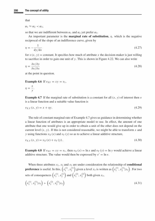
200 The concept of utility
that
α1 ≈ α2 ≺ α3,
so that we are indifferent between α1 and α2 yet prefer α3.
An important parameter is the marginal rate of substitution, η, which is the negativereciprocal of the slope of an indifference curve, given by
η = − 1
dy/dx(4.27)
for v (x, y) = constant. It specifies how much of attribute x the decision-maker is just willingto sacrifice in order to gain one unit of y. This is shown in Figure 4.22. We can also write
η = ∂v/∂y
∂v/∂x(4.28)
at the point in question.
Example 4.6 If vXY = xy = v1,
η = x
y.
Example 4.7 If the marginal rate of substitution is a constant for all (x, y) of interest then v
is a linear function and a suitable value function is
vX,Y (x, y) = x + ηy. (4.29)
The rule of constant marginal rate of Example 4.7 gives us guidance in determining whethera linear function of attributes is an appropriate model to use. In effect, the amount of oneattribute that one would give up in order to obtain a unit of the other does not depend on thecurrent level (x, y) . If this is not considered reasonable, we might be able to transform x andy using functions vX (x) and vY (y) so as to achieve a linear additive structure,
vX,Y (x, y) = vX (x) + vY (y) . (4.30)
Example 4.8 If vXY = xy = v1, then vX (x) = ln x and vY (y) = ln y would achieve a linearadditive structure. The value would then be expressed by v′ = ln v.
When three attributes x1, x2 and x3 are under consideration the relationship of conditional
preference is useful. In this,(
x (1)1 , x (1)
2
)given a level x3 is written as
(x (1)
1 , x (1)2 |x3
). For two
sets of consequences(
x (1)1 , x (1)
2
)and
(x (2)
1 , x (2)2
)both given x3,
(x (1)
1 , x (1)2 |x3
)�
(x (2)
1 , x (2)2 |x3
)(4.31)

201 4.10 Multidimensional utility
implies conditional preference (given x3). If the preferences
(x1, x2|x3)
for all (x1, x2) do not depend on x3 for all x3, there exists preferential independence. Thisimplies that the indifference curves for (x1, x2) are independent of x3.
If each pair of attributes in (x1, x2, x3) is preferentially independent of the remaining attribute,then we have pairwise preferential independence. This can be used to justify the additivefunction
vX,Y (x, y) = vX1 (x1) + vX2 (x2) + vX3 (x3) , (4.32)
and extended into higher dimensions if mutual preferential dependence between the attributesis judged appropriate; see Keeney and Raiffa (1976).
4.10.2 Preferences under uncertainty
For decision-making under uncertainty, we need to use utility, for all the reasons given inthis chapter, and principally to account for aversion to risk. We now have a vector x of nattributes (x1, . . . , xi , . . . , xn) . This set of attributes might be used to construct the entire utilityfunction
uX (x) = u X1,...,Xi ,...,Xn (x1, . . . , xi , . . . , xn) (4.33)
over all values (x1, . . . , xi , . . . , xn) of interest, perhaps using π -BRLTs together with the rulesfor utility outlined above. Structuring of a such a multiattribute utility function might beassisted by using a value function v (x1, . . . , xn) = vX (x) . It might be possible to enumerateuX [vX (x)] over all points of interest. This could be a lengthy process. It is emphasized thatin the final decision analysis X and UX (x) will be random and we need to weight U as in(4.19) and (4.20). We might wish to pay more attention to those areas of the space with greaterprobability.
Understanding the structure of the utility function can lead to better appreciation and analy-sis of the problem. The various functional forms have conceptual meaning, much as the mul-tidimensional forms in probability do. Let us start with two attributes X and Y. Under whatconditions is the additive function
u X,Y (x, y) = kX u X (x) + kY uY (y) , (4.34)
where the ks are constants, reasonable? This kind of simplification can be achieved by consid-ering forms of independence that are strikingly similar to those found in studying probabilitieswhere it was termed stochastic independence. This, we have noted, is conditional on ourinformation when making the judgement. Here we begin by defining utility independence.
The attribute X is utility independent of attribute Y if preferences regarding lotteries concerning valuesof X given Y = y are judged not to depend on the level Y = y.

202 The concept of utility
Figure 4.23 Inferences regarding independence of attributes in utility functions
This is illustrated by means of Figure 4.23(a) which shows a 50–50 lottery between two valuesof X, x1 and x2, given that Y = y. We would exchange the lottery for the certainty equivalent(x |Y = y), and utility independence implies that x does not depend on the value Y = y. Inother words, if we are satisfied with a particular certainty equivalent x for Y = y, we wouldnot wish to change this if we changed y.
Given utility independence, we can deduce that the utility function u X,Y (x, y) must be apositive linear transformation of the utility u X,Y (x, y1) based on Equation (4.6):
u X,Y (x, y) = a (y) + b (y) u X,Y (x, y1) , (4.35)
where b (y) > 0. The parameters a and b are now functions of y. Positive linear transformationsensure strategic equivalence of the utilities. See Exercise 4.10.
A further simplification results if we invoke additive independence. This applies if weare indifferent between the two lotteries shown in Figure 4.23(b) for all (x, y) and arbitrary(x1, y1). This condition can be written as
〈(x, y) , (x1, y1)〉 ≈ 〈(x, y1) , (x1, y)〉 . (4.36)

203 4.11 Analysis in normal form
As a consequence
1
2u X,Y (x, y) + 1
2u X,Y (x1, y1) = 1
2u X,Y (x, y1) + 1
2u X,Y (x1, y). (4.37)
We then set u X,Y (x1, y1) = 0, treating (x1, y1) as an arbitrary reference point. Then
u X,Y (x, y) = u X,Y (x, y1) + u X,Y (x1, y),
from (4.37). We can write
u X,Y (x, y1) = kX u X (x) ,
since x is the only quantity that is changing its value, and similarly
u X,Y (x1, y) = kY uY (y).
We then have the principal result of additive independence, that
u X,Y (x, y) = kX u X (x) + kY uY (y). (4.38)
Mutual utility independence occurs if X is utility independent of Y and if Y is utilityindependent of X. Under these conditions, it can be shown that the utility function can berepresented in the following bilinear form:
u X,Y (x, y) = kX u X (x) + kY uY (y) + kXY u X (x) uY (y), (4.39)
where the ks are scaling constants. The proof is based on two equations of the kind (4.35),one for each kind of utility independence in the mutual relationship. For details see Keeneyand Raiffa (1976). The form (4.38) can be obtained also by mutual utility independence andcondition (4.36), the latter at only one set of values (x, y, x1, y1).
We have given a flavour of the theory of multidimensional utility. It is important in manyprojects to have a rational basis for dealing with and combining consequences of various kinds.Multidimensional utility theory gives us guidance in this respect. There are many analogiesto the theory of multidimensional probability. An example is the relationship between crosssectional shapes of functions for independent quantities representing probabilities or utilities –in both cases there is a scaling relationship. There is considerable scope for improving ourunderstanding and ability to analyse by studying and applying the rules for structuring multi-dimensional utility functions. Keeney and Raiffa (1976) is the important reference in this area.
4.11 Whether to experiment or not; Bayesian approach; normal form of analysis
Very often the question is asked: do we need to undertake tests or experimentation in order toassist our decision-making? We know that we can incorporate the results of experiments in ourprobabilistic assessments by means of Bayes’ theorem. But we wish to make an assessment

204 The concept of utility
of the value of experimentation before we have the results. There is a formal way of doingthis which fits neatly into our decision-making procedure. This is sometimes rather clumsilytermed ‘preposterior’ analysis. The ‘normal’ form of analysis also follows, and this is a goodintroduction to our next subject, the question of game theory, dealt with in Chapter 5.
I shall introduce the present subject by means of an example. This concerns a buildingextension. In fact I had experience in practice of a very similar case soon after my graduation,so that this example had real appeal. A structural engineer is considering whether to extend anexisting building or to build instead on a separate site. The second option is more expensive,but there is uncertainty regarding the strength of the concrete in the ground floor columns ofthe existing building. The uncertainty is increased by the fact that the existing building wasconstructed some fifty years ago, and that records of the strength of the concrete are rathermeagre. Remedial action on the existing columns could be considered, but for the presentillustration, the simple choice will be made between the two decisions
α1 = ‘extend existing building’,
and
α2 = ‘build on separate site’.
Similarly, we shall simplify the states of nature into
E = ‘the strength of the concrete in the columns is ≥ 30 MPa’
and
E = ‘the strength of the concrete in the columns is < 30 MPa’.
The engineer is considering whether to obtain additional information by means of an experi-ment on the existing column, for example ultrasonic pulse tests, or the use of impact (hammer)devices, or the taking of small core samples by drilling and testing these. After some research,it is decided to consider taking core samples. But the engineer wishes to estimate the efficacyof the procedure a priori, before proceeding with the tests. Therefore two additional decisionsare added into the analysis,
e0 = ‘do not experiment’
and
e1 = ‘take core samples’;
we consider the core sample tests as a single result for simplicity. Two possible results of thecore tests are included, as follows.
T = ‘successful core tests’
and
T = ‘unsuccessful core tests’,
where T and T are based on the strength results of the core tests.

205 4.11 Analysis in normal form
Since the core tests (of diameter 1.5 cm) will not give a perfect indication of the strength ofthe existing columns, the engineer studies the literature for records of the frequency distributionof core strengths, given the strength of the larger specimens, and uses these values to assess theprobability of core strengths given column strength. A further study of methods of constructionleads to an assignment of probabilities of column strength. For the purposes of the presentanalysis, the following results are pertinent.
Pr (E) = 0.7, Pr(E) = 0.3,
and
Pr (T |E) = 0.95, Pr(T |E) = 0.05,
Pr(T |E) = 0.90, Pr(T |E) = 0.10.
The decision tree for the problem is illustrated in Figure 4.24. The set of outcomes is differentfor the two different actions. As we see, this minor complication can be dealt with quite simplyand naturally. The problem is an example of probabilistic inference, dealt with in more detail
Figure 4.24 Solution of problem involving building extensions

206 The concept of utility
in Chapter 8. The solution is also shown in Figure 4.24. Utilities have been assigned as shown,including a ‘cost’ of 0.5 units for the core tests.3
The decision tree of Figure 4.24 shows a chance fork after the decision e1, indicating thepossible results of the experiment. These results are not known at this stage; it is often mostimportant to conduct an analysis of the potential usefulness of the ‘experiment’, which couldbe a major undertaking. For example, it might be considered important to conduct a majorfield study on the wave regime to determine the loads on an offshore structure. This could be avery costly experiment, and careful consideration must be given to the potential benefits to begained. The structuring of the problem suggested in Figure 4.24 is aimed at a general approachto such a consideration. The idea is to consider the usefulness of an experiment (in the mostgeneral sense) before conducting it.
In deriving the solution, we proceed from the right hand side to the left in the tree of Figure4.24. The expected values of the upper (e0) branch are derived from the probabilities of E andof E, as stated above. The reader should verify the values. For the lower (e1) branch, Bayes’theorem is applied. For example, the values of probability of E given the result T are obtainedfrom
Pr (E |T ) = (0.95) (0.7)
(0.95) (0.7) + (0.1) (0.3)= 0.665
0.695= 0.957.
This shows how the probability of the existing columns being strong enough increases uponobtaining good test results. Further, the denominator gives the probability of T ; this value,as well as that of T , is needed in obtaining the final expected value, of e1, equal to 1.41.Again, the reader should verify the values. It is seen that the optimal decision is to conductthe experiment, and to extend the existing building if favourable test results are obtained, butto build on the separate site if the tests are unsuccessful. In short, we may write the result as{e1; α1 if T, α2 if T }.
4.11.1 Normal form of analysis
We now repeat the above analysis, but in normal form. This approach is different from theone just given in procedure but gives the identical result. It provides many additional insights,and paves the way for consideration of game theory. It also permits the analyst to postponethe assessment of the prior probabilities of E and E, and to test the sensitivity of the results tothis assessment. The first step is to list the strategies σi , as follows.
σ1 : e0; α1
σ2 : e0; α2
σ3 : e1; α1 if the result is T, α1 if the result is T
3 If the cost of the core tests is constant in monetary units, and if utility is non-linear with money, the same cost will bereflected by different amounts of utility depending on the position on the utility curve. The present case of constant‘cost’ in utility units is valid if the non-linearity is small or negligible.

207 4.11 Analysis in normal form
Figure 4.25 Strategies σ1 (left) and σ4 (right) in normal form
σ4 : e1; α1 if the result is T, α2 if the result is Tσ5 : e1; α2 if the result is T, α1 if the result is Tσ6 : e1; α2 if the result is T, α2 if the result is T .
Some of these strategies, for example σ5, are not very logical and could have been omitted.But it is instructive in this first example to consider all possible actions. Now consider eachstrategy in turn, and calculate the expected utility of the strategy given each state of nature.For example
u (σ1|E) = 0,
u(σ1|E) = −10,
and
u (σ4|E) = (−0.5) Pr(T |E) + (−2.5) Pr(T |E) = −0.6,
u(σ4|E) = (−10.5) Pr(T |E) + (−0.5) Pr(T |E) = −3.3.
These calculations are illustrated in Figure 4.25.The resulting values may be put in tabular form, as in Table 4.9, and also illustrated in the
graphical presentation of Figure 4.26. In general, the states of nature could have any dimension,rather than the two in this illustration. But the two-dimensional case of Figure 4.26 is a goodaid to understanding. In the figure, the further we are in the ‘northeast’ direction, the greaterthe utility. The lines joining σ2 and σ4, and σ1 and σ4, are termed the ‘efficient’ set or the‘admissible’ set, since they correspond to possible optimal decisions. The optimal decision σi
corresponds to the maximization of
〈U 〉 = p1u(σi |E) + p2u(σi |E), (4.40)

208 The concept of utility
Table 4.9 Utilities given statesof nature
Strategy σi u(σi |E) u(σi |E)
σ1 0 −10σ2 −2 −2σ3 −0.5 −10.5σ4 −0.6 −3.3σ5 −2.4 −9.7σ6 −2.5 −2.5
2
1
Figure 4.26 Utilities for all strategies, given states of nature
where p1 = Pr(E) and p2 = Pr(E). This corresponds to a straight line in the space ofFigure 4.26, the slope of which is dictated by the prior probabilities p1 and p2. To illustrate,we use the abbreviated notation
u(σi |E) ≡ u1, u(σi |E) ≡ u2.
Then (4.40) becomes
〈U 〉 = p1u1 + p2u2 = c, say. (4.41)
For any value of c, this is the line illustrated in the upper part of Figure 4.27. Its slope is
− p1
p2= − p1
p1= − p
p,

209 4.11 Analysis in normal form
Figure 4.27 Prior probability vector and line representing expected utility with prior odds
writing p1 simply as p. The slope of the normal to the line is then p/p (recall that the product ofthe slopes of two perpendicular straight lines in two-dimensional space in cartesian coordinatesis equal to −1).
The vector normal to the line of expected utility is shown as p in Figure 4.27. The ratio p/ prepresents the odds on the event under consideration as in Equation (2.5), and p/p the oddsagainst. For example if p = 3/7 with p = 4/7, then the slope of the line is (−3/4) and thenormal vector p has components (3/7, 4/7) as in the lower part of Figure 4.27. The odds onthe event are then 3:4. Note that p is not a unit vector; the scalar sum of the components add tounity so that its length is less than unity except where p = 0 or p = 1. The vector (3/7, 4/7)has length 5/7. It is advisable to work through one or two examples. See Exercises 4.12, 4.14and 4.15.
The optimal point is the one which maximizes expected utility. One can then imagine a linewith the slope of Equation (4.40) – or its equivalent (4.41) – but free to move in the space ofFigure 4.26 while keeping the same slope. This effectively changes 〈U 〉 – or its equivalent c –which is the quantity that we wish to maximize. The further we move in the northeast direction,the larger is 〈U 〉. In our building-extension problem, the furthest point in Figure 4.26 is thatcorresponding to σ4. The line corresponding to the assigned prior probability p = 0.70 withslope (−p/ p) is shown, together with the optimal point (σ4) and value of expected utility (1.41).
We can also deduce the values in Table 4.10. In producing this table, we suppose that we haveno knowledge of the prior probabilities, and imagine that the line corresponding to Equation(4.41) can have any slope. The question arises: under what conditions are the different strategies

210 The concept of utility
Table 4.10 Optimal strategies
p = Pr(E) Optimal strategy
0.00 to 0.48 σ2
0.48 to 0.92 σ4
0.92 to 1.00 σ1
of the efficient set optimal? The members of this set are σ1, σ2 and σ4. No other strategies canbe optimal. Let us begin with σ1. First imagine the expected-utility line of Equation (4.41) isvertical in Figure 4.26. This means that p = 1; the line approaches from the east and the firstpoint that it touches is σ1. We now increase p from zero slowly in small steps and move theresulting line each time from the northeast towards the efficient set. It will continue contactingσ1 first until its slope is the same as the line joining σ1 to σ4 in Figure 4.26, at which stageboth σ1 and σ4 are optimal. Increasing the slope further will result in σ4 being optimal untilthe slope of the line coincides with σ4–σ2. Finally the line is horizontal (p = 0, p = 1) andapproaches from the north.
To obtain the values of Table 4.10, we need the slopes of σ1–σ4 and σ4–σ2. Since we havethe coordinates in Table 4.9 above, these can easily be calculated. Then to get the values ofprobability in Table 4.10, we use the fact that the normal vector p is at right angles to theslope of the lines just noted (σ1–σ4 and σ4–σ2). We exploit the simple rule that the productof these slopes is −1. The direction of the vector p gives also the prior odds on E . It is wellworth working through the exercise of obtaining the values in Table 4.10; further examples aregiven in Exercises 4.12, 4.14 and 4.15. Exercise 4.16 deals with the extension to more thantwo dimensions.
We also note that the strategies can be used to reduce the problem to a decision tree suchas that of Figure 4.12, with all the possible actions stated at the start. The ideas above canbe readily generalized into several dimensions. This is illustrated in the general decision treesof Figure 4.28. Continuous random quantities can be dealt with using integration rather thansummation.
4.12 Concluding remarks
Probability and utility form natural components in a coherent theory of decision. That both ofthese attach to a person is a natural outcome of the nature of decision and of opinion. Utilityis then a personal concept: we cannot specify preferences, especially risk aversion, for others.This is as it should be, since one’s attitude to risk, and to the relative desirability of a set ofattributes is very much a personal affair. The personalistic aspect should then be seen as anatural outcome of proper modelling of the decision-maker’s dilemma.
The theory presents a powerful guide to the decision-maker, for structuring decisions andthinking about risk aversion. It must be adapted to the situation where we wish to developpolicies for a company, regulatory body or other organization. We might guide the client to

211 4.12 Concluding remarks
a
a
a
Figure 4.28 General decision tree and condensed tree
policies that reflect a reasonable level of risk aversion. An example might be a design code, oradvice to a company on operating policy for a manufacturing process, in which it is desiredto achieve a certain level of safety. In these cases, close consultation with the client or thegroup involved in the decision-making, with the objective of reaching a consensus, is needed.There is the responsibility to ensure that risks to human life are not excessive. Chapter 10 givesguidance on risk levels in society and on target levels.
The quotation by Ambrose Bierce given at the beginning of the chapter underlies a funda-mental truth. We might optimize our decision but when reality dawns, the unlikely state ofnature might well turn out to be true. The columns in the building might turn out not to beof adequate strength, the desired states of nature might not happen. We can arrange things so

212 The concept of utility
that the chance of undesirable outcomes is acceptably small. Yet decision-making under un-certainty holds no guarantee that everything will turn out as we might wish, while probabilityand utility nevertheless represent the best way to proceed in the circumstances.
4.12.1 Duality
Probability and utility are dual quantities in decision theory, much like force and displacementin mechanics. The structure of the theory in both cases revolves around a scalar product –maximum expected utility in one case and work in the other. Mathematical relationships ofduality abound. We saw in Chapter 2 the duality between sets of operations; in particular inExercise 2.11. In Section 5.4.3 below we have dual linear-programming solutions in linearspaces. Duality is found in projective geometry, whereby points and lines are dual elements;intersection of two lines gives a point and joining two points gives a line. These are dual oper-ations. Courant and Robbins (1941) show, for example, the theorems of Pascal and Brianchonto be dual statements. Desargues’ theorem has a dual version. In the principle of duality, onereplaces each element in a theorem by its dual, thus obtaining another theorem.
Duality in vector spaces is connected to the scalar product (see for example Greub, 1975).Courant and Robbins (1941) describe a straight line given by
ax1 + bx2 + cx3 = 0.
In a particular realization, for example
4 · 1 + 2 · 6 − 8 · 2 = 0,
it is impossible to distinguish between the interpretation that the point {x1 = 1, x2 = 6, x3 = 2}lies on the line
4x1 + 2x2 − 8x3 = 0,
written in short as {4, 2, −8} , and the interpretation that the point {4, 2, −8} lies on theline {1, 6, 2} . This symmetry provides the basis for the duality between point and line. Anyrelationship between line and point can be reinterpreted as a relation between point and lineby interchanging the coordinates.
We can characterize the maximization of expected utility as the scalar product
〈U 〉 = p · u =∑
ipi ui , (4.42)
in which pi is the probability of event Ei , and ui is the utility (payoff) associated with itsoccurrence. If one considers a set of random events Ei , with associated utilities ui , then
U =∑
iui Ei (4.43)
represents the gain that one would achieve, given the results Ei = 1 or 0 depending on theoccurrence or non-occurrence of Ei (respectively). Equation (4.42) can be derived from (4.43)by taking the expected values of both sides. Both Equations (4.42) and (4.43) can be taken to

213 4.12 Concluding remarks
Figure 4.29 Probability and utility
represent a scalar product of two vector quantities in dual vector spaces. This does not changeif integrals rather than sums are considered; generally
〈U 〉 =∫
udF.
One should expect then for there to be a dual relationship between probability and utility.Consider the fundamental lottery shown in Figure 4.29(a). This shows a chance fork in whichone obtains maximum utility (u = 1) with probability p or π, and minimum utility (u = 0)with the complementary value (1 − p) or (1 − π ). To define probability and utility one canproceed as follows. See Figure 4.29(b) and (c).
Probability p of E. Take a unit of utility and divide it into two parts (µ, 1 − µ) such that the certainreward µ is equivalent to uncertain E with unit of utility as reward if E occurs. Then p ≡ µ.Utility u of E. Take a unit of probability and divide it into two parts (π, 1 − π ) such that the certain eventE = 1 is equivalent to the uncertain reward of a unit of utility, with probability π . Then u ≡ π .
The separation of probability and utility is more than a matter of convenience. It is quite naturalto want to separate questions of impartial judgement regarding the occurrence of a future event,

214 The concept of utility
that is, assignments of probability, and questions of advantage, or gain given that the eventoccurs, that is, assignment of utility.
It is awkward, as in the above definition, to involve both probability and utility, so in definingprobability, we generally start with small amounts of money with no risk aversion and proceedin an iterative manner. A person in the street, if asked to express her opinion in terms of a fairbet, would be forced to an honest and optimal expression of opinion. The role of the bet ismuch the same as the operations in the operational definition of a concept due to Bridgman.In this, the concept is associated with the operations that one performs in the measurement ofthe concept, for example length is identified with the physical operations which are used inmeasuring it, laying a measuring rod with one end coincident with a particular mark, noting themark, taking the reading at the other end, and so on. In subjective probability theory, the bet isthe method for making a measurement of uncertainty; small amounts of money are used so thatfactors such as risk aversion do not enter into the picture since they are in the domain of utility.
4.13 Exercises
There are wide areas of application for utility theory. Projects can be constructed around subjects ofinterest in particular disciplines.
4.1 Benefit–cost ratio and qualitative measures. An authority is considering dam construction to supplyclean water to the region. Two alternatives, 1 and 2 below, are being considered for water supplyand flood control. The following table shows costs and benefits associated with the two alternativestogether with other consequences. The costs and benefits are annual values.
Alternative Water supply Flood control
1: one large dam Costs $20.2 ×10⁶ $8.0 ×10⁶
Benefits $23.2 ×10⁶ $8.3 ×10⁶
2: two small dams Costs $28.0 ×10⁶ $9.1 ×10⁶
Benefits $24.5 ×10⁶ $10.0 ×10⁶
Alternative Other consequences
1: one large dam Costs Flooding of 50 km2 of natural woodland and habitatRelocation of people, reduction in wild life
Benefits Improved human health for local populationRecreational facilities for 100 000 persons per year
2: two small dams Costs Flooding of 23 km2 of natural woodland and habitatRelocation of people, reduction in wild life
Benefits Improved human health for local populationRecreational facilities for 200 000 persons per year

215 4.13 Exercises
(a) Which project has the better benefit–cost ratio? Use stated dollar amounts.(b) Suggest ways to assist the authority to make a decision taking into account the other qualitatively
measured consequences listed above.(c) Comment on the merits of benefit–cost ratios in decision-making in particular in the above.
4.2 Time value of money. Commodity prices can be very volatile, and the problem is posed in arbitraryunits. An oil company has to make a decision on whether to invest in offshore production froma marginal oil field, the size of which is estimated at 200 MB (million barrels). The developmentrequires capital expenditure of 150 million per year for five years at which point production wouldcommence at the rate of 10 MB per year for 20 years. The production period would also incuroperating and maintenance costs of 75 million per year. The costs noted so far are in real (constant-worth) monetary units, with constant purchasing power with regard to year 1 of the project. Ina preliminary analysis of the problem, an engineer considers two scenarios as described in thetable below. These represent two possible developments of the world economy in average terms,the second corresponding to a period of conflict in the Middle East (rather alarmist but useful forcontrast). The values are in actual (inflated) monetary units.Calculate the net present worth for the two scenarios. For real monetary units, use a real interestrate calculated from the figures in the table. Calculate the EMV based on a probability of 0.80 forscenario 1 as against 0.2 for scenario 2.
Scenario 1 – stable Scenario 2 – volatile
Oil price Interest rate Inflation rate Oil price Interest rate Inflation Rate
15 per bbl 8% per year 4% per year 25 per bbl 15% per year 12% per yearincreasing at over 20 year over 20 year increasing at over 20 year over 20 year5% per year period period 10% per year period period
4.3 Consider the following payoff matrix for a fisher, who has to decide which species to fish onin a season. The states of nature are uncertain. Solve the problem using the maximin, maximax,Hurwicz (α = 0.5) and minimax regret criteria. Comment on the strategies. What is meant by utilitydominance? Give an example.
State of nature
θ1 θ2 θ3
Species A 1 1 1Species B 1 3 0Species C 0 4 0Species D 1 2 0
4.4 Imagine that you are a member of the Board of Directors of a small company, with assets of about$50 000. The table below shows a choice to be made by the board between three contracts (α1, α2

216 The concept of utility
and α3). The entries show the consequences with associated probabilities in brackets. Draw thedecision tree. Infer utility values for each outcome using π -basic-reference lottery tickets. Plot theresulting values of utility against money. Iterate if necessary. Complete the decision analysis usingexpected monetary value and expected utility criteria.
Consequences in $ (probability)
α1 −80 000 (0.2) 50 000 (0.8)α2 20 000 (0.6) 4000 (0.4)α3 100 000 (0.2) 0 (0.8)
4.5 Consider the statement: ‘A decision-maker is risk-averse if she or he prefers the expected conse-quences of a lottery to the lottery itself.’ Take two examples:
(i) an attribute with increasing preferences, e.g., money,(ii) an attribute with decreasing preferences, e.g. size of an oil spill.
Illustrate the statement above with regard to these two cases and sketch the utility functions. Assumethat the utilities range between 0 and 1. Use lotteries with 50–50% probabilities.
4.6 An engineer is working with a client in formulating a response to a potential oil spill in an offshoreregion. The volumes of spill under consideration are in the range 0–50 000 m3. Sketch a utilityfunction expressing risk aversion. Prove that the shape shown must express risk aversion by usingthe certainty equivalent of 〈0, 50 000〉. Consider the function
u (v) = b[c − exp (av)
],
where v = volume of spill, and a, b and c are constants. Discuss whether this might be used as autility function. Let u (0) = 1, and u (50 000) = 0. Show how the certainty equivalent noted can beused with this information in evaluating the constants a, b and c.
4.7 Study the problem of noise, for example in reduction of noise pollution in siting an airport. Whatwould constitute a good attribute in attempting to formulate utility? Consider intensity (energy perunit area per unit time – Wm−2). For utility, would decibels serve? (Note that doubling the decibellevel ‘buys’ intensity on a log scale.)
4.8 Contrast the exponential form of Example 4.3 and the logarithmic form
u (x) = ln [a (x + b)]
for expressing risk aversion. Obtain the local risk aversion measure γ (x) of Equation (4.17). Useexamples from your experience (cost, money, time saved in construction or manufacturing, delays,quality of product, . . .).

217 4.13 Exercises
4.9 Find the local risk aversion measure γ (x) for the quadratic utility function
u (x) = −ax2 + bx + c
with a, b > 0, and x < b/2a, so that u is increasing. Comment.
4.10 Strategic equivalence of two utility functions is defined such that the same preferences are impliedfor any lotteries with the same consequences. Show that the relationship between the two utilityfunctions u A and uB of the kind given in Equation (4.6), i.e. uB = a + bu A, b > 0 results in strategicequivalence. Use Equation (4.15) to assist in solution. Show also that strategic equivalence resultsin the positive linear transformation noted.
4.11 Consider a problem of your choice that involves multidimensional utility. Examples are cost andsafety, travel distance and noise (siting of airport or similar facility) and service rate providedfor incoming data and the queuing delay (in data transmission). Explore the relation between theattributes for utility and additive independence and speculate on the various forms of the utilityfunction, for example those given by Equations (4.38) and (4.39).
4.12 Solve the problem of Example 3.25 in normal form, listing all the strategies and plotting a graphsimilar to that in Figure 4.26. Find the optimal solution and the range of probabilities for whichvarious strategies are optimal, using the method given for Table 4.10.
4.13 An engineer is advising a city administration on the question of whether or not to recommend thata public transportation system (for example light rail transit) be built in the medium sized NorthAmerican city. The population of the area that would benefit from the service is well defined at420 000. The key to the success of the project is the proportion M of the population who will usethe facility. This is treated as a random quantity. In the preliminary study being undertaken, threevalues of M are considered. These are M = 0.2, 0.4 and 0.6. Initial best estimates of the probabilityof these events are
Pr (M = 0.2) = 0.5; Pr (M = 0.4) = 0.4; Pr (M = 0.6) = 0.1.
The following table gives the utility associated with various outcomes.
Action State Utility (0–100)
Build system M = 0.2 30M = 0.4 60M = 0.6 90
Do not build 60
The engineer realizes that a survey as to intentions might help, but that the results are unlikely tomatch subsequent behaviour. A person might indicate aversion to using the system yet subsequentlyfind it a useful form of transport, and vice versa. Let Y designate the proportion of the population

218 The concept of utility
who indicate that they will use the system; this is also discretized into three possible values, 0.2, 0.4and 0.6. Psychologists and previous literature are consulted and the following table is the result. Itgives values of Pr(Y |M) , the probability of the three values of Y (indications of use of the system),given the three subsequent levels of usage (the values in the table are for illustrative purposes).
Y
0.2 0.4 0.6
0.2 0.50 0.30 0.2M 0.4 0.10 0.60 0.3
0.6 0.15 0.15 0.70
Assume now that a survey has been carried out with the result that Y = 0.6. To account for the costof the survey, subtract two units of utility. What decision maximizes expected utility?
4.14 Reconsider the problem posed in Exercise 4.13.
(a) Analyze the problem in normal form, assuming that the survey has not been conducted. Includethe option whether to experiment (survey), at cost of 2 units, or not in the analysis. List theten strategies and obtain the utilities of the strategies given the states of nature. List these ina table for the three states of nature. Obtain the optimal decision using the given values ofPr(M = 0.2, 0.4, 0.6) .
(b) Obtain optimal strategies for the table of (a) using maximin, maximax, Hurwicz (α = 0.4), andminimax regret criteria.
(c) Use again the table of utilities of (a) but ignore the results for M = 0.4. Plot a graph ofU (σi |M = 0.2) versus U (σi |M = 0.6) and find the ranges of probability for which the variousσi are optimal, considering that only the two states of nature M = 0.2, 0.6 are possible.
(d) Discuss consequences with regard to the environment of building the system, and possible socialmeasures to affect and change public opinion regarding use of public transportation over time,for example to raise gasoline prices.
4.15 A company manufacturing microprocessors purchases batches of microchips by contract. To eval-uate the quality of the chips a test is conducted. The results are P (pass) or P (fail). It is found thatthe test method is not perfect and an analysis of performance of microchips purchased in the pastindicates the following, where S = satisfactory performance and S = unsatisfactory performance.The values in the table were obtained by conducting tests on microchips found to have either sat-isfactory or unsatisfactory performance. The utility associated with satisfactory performance is 15units and that associated with unsatisfactory performance −50 units, while that associated withrejecting a batch is 0 units.
Pr(P or P|S or S
)Test indication S S
P 0.85 0.30P 0.15 0.70

219 4.13 Exercises
(a) Draw a decision tree for the problem of deciding whether or not to accept or reject a batch ofmicrochips, conditional on the results of the test.
(b) A contractor with a good track record – 98% of her batches of microchips in the past has beensatisfactory – provides a batch for which the test shows the result P. Which decision, accept orreject, maximizes expected utility?
(c) Repeat part (b) in the case of a contractor with no track record; assume then that Pr(S) =Pr
(S) = 0.50.
(d) Conduct an analysis in normal form, listing all the strategies and plotting a graph similar tothat in Figure 4.26. Find the optimal solution and the range of probabilities for which variousstrategies are optimal, using the method given for Table 4.10.
4.16 Find a method to evaluate the ranges of probabilities for which various decisions are optimal in the‘normal form’ analysis, similar to the method for Table 4.10, but consider the case where there aremore than two dimensions.
4.17 Unfinished games and utility. In the early days of mathematical probability theory, one area ofendeavour related to utility was that of fair odds in an unfinished game; see Figure 2.20 and therelated discussion. This was applied to the finals in the National Hockey League or the World Series,in both of which the ‘best of seven’ wins. We now introduce a more general problem. Three playersA, B and C are engaged in a game of chance taking turns in this order. The winner will receive theentire pot of S dollars. When it is A’s turn, his probability of winning is pA. If A does not win itbecomes B’s turn, whose probability of winning is pB . If B does not win, it becomes C’s turn, andso on, returning to A if nobody has won, and continuing as before. The game is still in progress butsuddenly must be abandoned. It is A’s turn. Find the fairest way to divide the pot. Apply the resultto the following two cases.
(a) The winner obtains first ‘doubles’ in a throw with a pair of fair dice. The pot is $273.(b) An archery contest between three archers, in which the weakest (A) goes first. The first to hit
the bull’s eye receives the pot of $96. The following probabilities have been derived empiricallythrough observations of the performance of the archers:
pA = 0.2, pB = 0.5, pC = 0.9.

5 Games and optimization
Intelligence and war are games, perhaps the only meaningful games left.William Burroughs
We are survival machines – robot vehicles blindly programmed to preserve the selfish molecules knownas genes.
Richard Dawkins
A great truth is a truth whose opposite is also a great truth.Thomas Mann
5.1 Conflict
Up to now, we have considered decision-making in cases where we are the ‘protagonist’,and where the ‘antagonist’ is relatively benign, or more precisely, indifferent to our desires.In this case, we characterize the antagonist as ‘nature’ in which we have we considered na-ture to consist of those aspects such as weather that do not react to our everyday behaviour.We can then regard the activity of engineering design as a ‘game against nature’. In theexample of design of an offshore structure to resist wave loading, we might choose the de-sign wave height and ‘nature’ chooses the actual wave heights which the structure has toresist.
But nature includes creatures other than ourselves! In activities in which other humanbeings – or indeed, animals – are involved, we cannot rely on any kind of indifference. Ifwe set up a business, our competitors are out to do better than us, and this implies trying to takebusiness from us. Strategies will be worked out to achieve this objective. We can no longer relyon probabilistic estimates of our opponent’s strategies based on a study of ‘impartial’ nature,as we might do in studying a record of wave heights.
The situation where we face an antagonist who is out to beat us in some way or anotherhas strong links to animal behaviour in general. Dawkins (1989) in his book The Selfish Genepoints out the connections between strategies for survival of animals (or, more correctly,of genes) and game theory. We introduce this briefly, so as to bring into play an important
220

221 5.1 Conflict
and interesting line of thinking. Two animals in conflict could adopt strategies such as thefollowing.
� Fight always as hard as possible, retreating only if seriously injured.� Always retreat.� Attack and pursue an opponent that runs away but retreat if the opponent retaliates.� Fight back only when attacked.
Most of us know from personal experience that it is not sensible to fight to the finish in everyconfrontation, so that we might sometimes follow an aggressive approach and at other timesretreat, regardless of the stance of our opponent. This is a mixed strategy. The problem originallyapproached using mathematical methods by von Neumann was of the school playgroundvariety, but it has striking resemblances to conflict between animals as we shall describe. Thisgame was ‘match-penny’. Each of two players reveals the face of a coin at the same moment;if the faces are the same (both heads or both tails) one player wins. If they are unlike, the otherplayer wins. A variation of this is the rock–paper–scissors game, in which paper covers rock,scissors cut paper, and rock breaks scissors. The three objects are mimicked by the hands ofthe two antagonists, who each select one and reveal their selection simultaneously. The firstof the pairs in the preceding sentence wins.
A species of lizards shows similar behaviour.1 Three male types have evolved, distinguishedby the colour of their throats: orange, blue and yellow. Mating – and consequently contributionto the gene pool – is the objective of the game. Let us start with the moderate blue-throatedspecimens. They keep relatively small harems of three females, with small territories. Orange-throated lizards are much more aggressive, full of testosterone, and they easily take over fromthe blues. Their harems are large, up to seven females, with corresponding large territories,keeping the orange-throated lizards very busy indeed. The yellow-throated lizards infiltratethese large harems by simulating female behaviour and secretly mating with the femaleswithin. (The reviewer refers here to the movie Shampoo, in which a human follows the samestrategy.) Cycling by generation occurs, with the blue-throated lizards taking over from theyellows, the orange from the blues and so on. The ideas of game theory have been applied toproblems of biology notably by John Maynard Smith; see Dawkins (1989).
Our objective is to introduce the ideas of game theory so as to demonstrate another importantway of assigning probabilities. We wish to show that the allocation of probabilities followsdifferent rules under conditions of conflict, and that it is important to understand the influenceof this situation. Certainly we do not aim at an exhaustive treatment. We deal with two-personzero-sum games. The main concepts that we wish to convey are embodied in their solution,which can conveniently be carried out using linear programming. This is part of optimizationtheory, an important subject for engineers, so that this is also introduced. Lagrange multipliersare introduced as part of this subject; they are used extensively in Chapter 6.
1 See Scientific American of June, 1996.

222 Games and optimization
Table 5.1 Payoff matrix
B
τ1 τ2 τ3 τ4
σ1 12 3 9 8A σ2 5 4 6 5
σ3 −3 0 6 7
5.2 Definitions and ideas
At the outset, some basic definitions need to be given.2 There are two-person, three-person, orgenerally n-person games, depending on the number of participants. We shall consider onlytwo-person games. In previous chapters, we used the symbol α to denote actions in consideringdecisions in cases where there is no conflict. We now use σ and τ for the strategies in conflictsituations. These are the strategies open to the two people, A and B respectively. We introducethe payoff matrix of Table 5.1. After each play of the game, a
{σ j , τi
}pair is identified by
virtue of A having played σ j and player B τi . As a consequence, player B pays the amountentered at the
{σ j , τi
}intersection in Table 5.1 to player A. For example, if A plays σ2 and B
plays τ3, B pays A 6 units. We shall illustrate in Section 5.2.1 how games can be reduced toa matrix of the kind in Table 5.1. (In most real games the matrix is much larger.) The idea issimilar to the {α, θ} pairs used previously in Chapter 4 (for instance in Figure 4.12), the newelement being that of conflict.
It is a convention in game theory the amounts are paid by the column player (B here) to therow player (A); where the amounts are positive, A receives the amount. If there are negativeentries, as in {σ3, τ1} , the amount (3 units) is paid by A to B. Positive entries are negative for Bwho pays. The payoffs could be utilities; for the present with single payoffs for each
{σ j , τi
}pair, the relationship between utility and monetary value – or other attribute – would have tobe shared by both A and B. A further complication is that A’s positive values are negative forB, so that the sharing noted would have to be symmetrical about the origin. To avoid thesecomplications, we shall simply regard the amounts as relatively small monetary payoffs withno complications involving factors such as risk aversion.
If A plays σ2 and B plays τ3, then B pays A 6 units. Since the sum of the payoffs to each playerat each terminal state is zero (+6 for A and −6 for B in the case just noted), the game is termeda zero-sum game: what one player pays, the other receives. When interests are diametricallyopposed, as in the two-person zero-sum games under consideration, the games are games ofpure conflict or antagonistic games, again in the jargon of game theory. Further usage includes
2 The monumental work on games is the book by von Neumann and Morgenstern (1947); other excellent books suchas Jones (1980) and Luce and Raiffa (1957) may be consulted. Owen (1982) introduces games from a mathematicalpoint of view. Bernstein (1996) gives interesting historical perspectives.

223 5.2 Definitions and ideas
Table 5.2 Minimax solution
B
τ1 τ2 τ3 τ4
Rowminima
σ1 12 3 9 8 3
A σ2 5 4 6 5 4σ3 −3 0 6 7 −3
Column maxima 12 4 9 8
finite and infinite games, depending on the number of strategies. In the end-game in chess, it ispossible sometimes to formulate a set of moves which go on infinitely. This can be dealt withby stopping rules, for instance specifying a draw after a certain number of repetitions. Or onecan construct infinite coin-tossing games. We shall consider only finite games. Cooperativeand non-cooperative games correspond to instances where there is, or is not, cooperationbetween the players. We shall deal only with the non-cooperative variety. Moves can includechance elements, for instance in scrabble or poker, where there is uncertainty regarding thetokens or cards received. There will always be uncertainty regarding our opponent’s futuremoves.
Engineering design is sometimes thought of as a ‘game against nature’. In Section 4.2 wedealt with a real game against nature involving a farmer. Various approaches were consideredthat had different psychological implications: the optimist, the pessimist, and others. In thepresent case of games, we are up against an intelligent antagonist who is out to better us ina situation of conflict. The natural reaction to this situation is that of the pessimist assumingthat the worst will happen. This results in a ‘maximin’ solution, and will be the standardway of dealing with games. We now return to the problem of Table 5.1. Since the payoffsare to A, he selects the minimum in each row as shown in the last column of Table 5.2, andthen chooses the strategy that maximizes these minima. Therefore A chooses σ2. Player B,meanwhile, undergoes the same mental turmoil wondering what A is going to do. B has tomake the payoffs so they are negative to her. B therefore selects the column maxima – the worstthat can happen, the most that B might have to pay. Then the minimum of these is chosen,leading to the choice of τ2. It is to be noted that this minimax strategy is in fact identical to A’s,the difference – minimax versus maximin – arising from the fact that the payoffs are positivefor A, and negative for B.
The solution of the game is shown in Table 5.2, and is {σ2, τ2}. It turns out that the solutionleads to the saddle point shown, at which
Pure MAXIMIN = Pure MINIMAX. (5.1)
The value 4 at the saddle point is termed the value of the game. When this occurs, we havea solution in pure strategies. Both players are satisfied after the game that had they chosen

224 Games and optimization
Table 5.3 Match-penny
B
τ1 τ2
Rowminima
σ1 −1 1 −1σ2 1 −1 −1
A
Column maxima 1 1
Table 5.4 Game with no saddle point
B
τ1 τ2
Rowminima
σ1 3 6 3
σ2 5 4 4A
Column maxima 5 6
differently the result would have been worse. Neither regrets their decision once the otherplayer’s choice is known. A game in which the value is zero is a fair game; the present gameis not fair as its value is 4.
The question arises: is there always a saddle point? The answer is no. If there were always asaddle point, this would mean that, in the example in the introductory section ‘Conflict’ above,a single strategy such as ‘always attack’ or ‘always retreat’ would be the invariable solution.We shall explore the absence of saddle points by means of examples.
Example 5.1 Consider the game of match-penny: the original game studied by von Neumann.Player A chooses heads or tails on his coin, while B makes the same choice on hers. Neitherplayer knows the other’s choice. If the coins match, player B receives a payoff of unity fromA. If the coins don’t match, A receives a payoff of unity from B. In the matrix of Table 5.3, σ1
is the choice ‘heads’ for A, and σ2 ‘tails’; for B τ1 is ‘heads and τ2 is ‘tails’. The payoff matrixis shown in Table 5.3. There are no distinct maximin or minimax values, and no saddle point.
Example 5.2 A variation of this game is called ‘odds and evens’. The two players point eitherone or two fingers simultaneously. If the sum of the fingers is odd a designated player ‘odd’wins; if even, the designated player ‘even’ wins.
In the examples, there is neither a unique row maximin nor a column minimax. These canexist yet there may be no saddle point, as in the game in Table 5.4. In this game and othersimilar ones we have
Pure MAXIMIN ≤ Pure MINIMAX. (5.2)

225 5.2 Definitions and ideas
The solution to match-penny consists of a strategy of not demonstrating any pattern inshowing a particular face. For example, if one shows a head more often than a tail, or demon-strates any regularity of choice, our opponent will quickly realize this and adjust their actionsaccordingly and begin to gain. The essence of the solution is to show heads or tails randomly,without any pattern. One might have a subsidiary device such as a coin, a die, or roulettewheel, which permits us to choose heads or tails with a probability of 1/2 each time. This isan example of the use of a mixed strategy; in Table 5.3, within both pairs {σ1, σ2} and {τ1, τ2}the strategy would be chosen with a probability of 1/2. More details and proofs of this aregiven in Section 5.5.
5.2.1 Extensive form, normal form and reduction to matrix
We have introduced games using a payoff matrix with a set of strategies for each player. Howare real games reduced to this form? Example 5.1 showed how this is done for the game of‘match-penny’. We shall demonstrate further the method of reducing a game to a matrix, usingthe game of ‘Nim’, following Jones (1980). This gives a reasonably convincing idea of howany game can be reduced to a matrix game. In Nim, two distinct piles of matches are created.Two players alternately remove matches, one or more, from either of the two piles. They mustremove one or more matches from only one of the two piles at each turn. The game terminateswhen the last match is drawn, and the player who removes the last match loses the game. Thegame has been analysed in some detail by various persons; see Jones (1980) for specifics.Since both players know the full details at each step, it is a game of perfect information.
We can illustrate the extensive form of the game simply using 2–2 Nim. In this, there areonly two matches in each pile. Figure 5.1 shows the game in the form of a game tree, in whicheach possible state and play of the two players A and B is shown successively. At the start,on the left of the tree, it is A’s turn. A either removes one or two matches from a pile – this isshown for the lower of the two piles only; a symmetrical situation results with removal fromthe upper pile. Then it is B’s turn; depending on A’s move, all of B’s possible moves are shown.For example, given that A removed a single match as in the lower of the first choices opento him, B can remove both matches of the upper pile, a single one, or the single match in thelower pile left by A. These three choices are shown in the lower part of Figure 5.1, followingB’s turn. Then A plays, and so on to the end of the game. Again, if there is a symmetricalchoice, only one is shown in the figure. ‘Dumb moves’ have been included, where a playermakes a move that unnecessarily leads to their loss.
The game tree of Figure 5.1 is also known as the extensive form of the game, as it showsall the possible states – except for the symmetrically identical moves noted which have beenomitted so as to avoid unnecessary complication. (These can easily be added if wanted.) Nowwe have reduced the game to sets of strategies for each player and the corresponding endpoints.To illustrate, consider A’s possible strategies. These are shown in Figure 5.1 and summarizedin Table 5.5. Strategy σ1 consists of removal of both matches in a pile; thereafter A makesno further choices. To assist in following the strategies, the nodes in Figure 5.1 have been

226 Games and optimization
Table 5.5 Possible strategies for A
Strategy First turn Second turn
σ1 Remove two matches from a pile; node 1 − 2σ2 Remove one match from a pile; node 1 − 3 Remove two matches from the
remaining pile; node 8 − 12σ3 Remove one match from a pile; node 1 − 3 Remove one match from the
remaining pile; node 8 − 13
Figure 5.1 Extensive form of 2–2 Nim illustrated in a game tree. ‘X’ indicates that no matches remainin the pile
numbered from 1 to 15. Strategy σ1 corresponds to the choice 1 → 2. In strategies σ2 andσ3, A removes one match, and has to make a further choice if B removes the other from thesame pile; σ2 results if A removes both remaining matches and σ3 if a single match is removedon the second turn. These are paths 1 → 3 → 8 → 12 and 1 → 3 → 8 → 13 respectively inFigure 5.1. The strategies for B are listed in Table 5.6. B’s first choice will depend on A’s prior

227 5.2 Definitions and ideas
Table 5.6 Possible strategies for B
Strategy If at Move to Path
τ1 2 4 1 → 2 → 43 6 1 → 3 → 6
τ2 2 4 1 → 2 → 43 7 1 → 3 → 7
τ3 2 4 1 → 2 → 43 8 1 → 3 → 8
τ4 2 5 1 → 2 → 53 6 1 → 3 → 6
τ5 2 5 1 → 2 → 53 7 1 → 3 → 7
τ6 2 5 1 → 2 → 53 8 1 → 3 → 8
Table 5.7 Game of 2–2 Nim in normal form
B
τ1 τ2 τ3 τ4 τ5 τ6
σ1 4(A) 4(A) 4(A) 9(B) 9(B) 9(B)A σ2 10(B) 14(A) 12(B) 10(B) 14(A) 12(B)
σ3 10(B) 14(A) 15(A) 10(B) 14(A) 15(A)
Table 5.8 Game of 2–2 Nim in matrix form
B
τ1 τ2 τ3 τ4 τ5 τ6
σ1 1 1 1 −1 −1 −1A σ2 −1 1 −1 −1 1 −1
σ3 −1 1 1 −1 1 1
choice in the first play. She therefore starts at either node 2 or 3 in Figure 5.1. A completedescription of a strategy must take into account all possible states, and this is done by specifyinga course of action that depends on A’s first choice as in Table 5.6. All possible strategies arecovered in this set.
Now we can see how a specified course of action by A and B leads to a definite result. Forexample, if the set of actions {σ3, τ3} is decided upon, the result is node 15 in Figure 5.1, withA winning; this is handily deduced using Table 5.7. If A and B now agree that $1 is paid fromA to B if B wins, and vice versa, then the matrix of payoffs given in Table 5.8 is obtained. The

228 Games and optimization
game of 2–2 Nim has been reduced to a matrix game, similar in form to the payoff matrices ofthe preceding section. At this stage, A and B could sit in their favourite pub – this is after all apub game! – armed with Tables 5.7 and 5.8. They could then ignore their piles of matches, andsimply choose a pair of strategies
{σ j , τi
}independently, and look up the result in one of the
tables. Or if necessary pass their choices to an impartial referee to determine the payoff. Thisof course removes all the fun and interest from the game. But our purpose is to demonstratethat games can be reduced to a simple matrix of results corresponding to vectors of possiblestrategies and to the matrix form noted. This can be used to show, for example in Table 5.8,that strategy τ4 guarantees a win for B regardless of A’s choice.
In introducing the game of 2–2 Nim, player A started the play. In fact, player B could havestarted the game, or the starting player could have been decided by chance. For example, acoin could have been tossed to decide between players A and B. This is a simple example of achance move; note that there will (almost!) always be uncertainty as to our opponent’s potentialmoves. In a chance move, an external device such as the tossing of a coin or die, or the drawingof a card, or of letters in Scrabble, is introduced. We can think of such devices as extra playersif we wish, who play certain moves specified by the nature of the device. We can denote theseplayers as ‘nature’ if we wish, and the plays by nature would follow the rules of the device; forexample a die tossed will yield six possible outcomes, each with a probability of 1/6. Nature’splays would then correspond to mixed strategies, as mentioned at the end of the last section,and again in Section 5.5. The probabilities of nature’s strategies would be predetermined, andnot optimized as would those of the main players. The latter subject requires knowledge ofoptimization theory, to be introduced in the next sections.
Example 5.3 The game tree for match-penny, as introduced in Example 5.1 is shown inFigure 5.2. The payoff matrix has been given in Table 5.3.
In non-zero-sum games the sum of the payoffs is not zero. As an example, let us considerthe game of match-penny illustrated first in Table 5.3. Suppose now that if A loses, $2 is paid,
Figure 5.2 Game tree for match-penny with players A and B

229 5.3 Optimization
Table 5.9 Bimatrix for match-penny withnon-zero-sum payments
B
τ1 τ2
σ1 (−2, 1) (1, −2)A σ2 (1, −2) (−2, 1)
with $1 going to B, and the remaining $1 to the ‘banker’ running the game. Similarly, if Bloses, $2 is paid, but only $1 goes to A. The payoff matrix is then represented by the bimatrixof Table 5.9. Only zero-sum games are dealt with in this chapter, and the bimatrix is introducedonly to illustrate the more general situation.
5.3 Optimization
5.3.1 Importance in engineering
In engineering, in science and in economics, we often wish to obtain an optimal solutionwith regard to some quantity: minimum cost, minimum weight, maximum safety, shortesttransmission time for electronic data, maximum profit, shortest route or completion time. Weshall consider in this section and the next deterministic systems, which involve decisions underuncertainty, but not related to probability. The uncertainty arises as to the best optimal solution.Yet the methods can be applied to the solution of problems of probability as well. The coverageof the subject of optimization given here is introductory in nature; there are many texts whichgive a detailed treatment that can be consulted. Non-linear optimization is used in maximizingentropy, the subject of Chapter 6, and the solution to games with mixed strategies is carriedout using linear optimization in this chapter.
To introduce ideas, we consider the design of a bridge (Figure 5.3). We are interested indetermining the optimal span length x and number of piers n for a total bridge length �. Thusnx = � (see Figure 5.3). The bridge, apart from the abutments, is to be made of steel. The costof the abutments is a, in nominal units that we use for this problem. The cost of a pier is b,
and this may be taken for initial design purposes as constant, regardless of the span. The costper unit weight of steel is d, and m is the cost per unit length of the floor system, cross bracingand roadway. The main variable of interest is w, the weight of steel per unit length of span,which is taken to be a linear function of x :
w = kx, (5.3)
where k is a constant for the type of steel girder under consideration.This relationship can be seen to be approximately correct if we consider that bending moment
is proportional to the square of the span (∝ x2); section modulus s is proportional to the square

230 Games and optimization
Figure 5.3 Spacing of bridge piers
of girder depth h, (i.e. s ∝ h2) assuming constant width. Since section modulus is proportionalto bending moment, the span and girder depth – or weight – are linearly related (h ∝ x). Ifweight is proportional to h, we have the result in Equation (5.3). Then the total cost c is given by
c = a + (n − 1) b + dw� + m�;
this is to be minimized, and we write
Min
[c = a +
(�
x− 1
)b + dkx� + m�
]. (5.4)
In problems of optimization we use the notation ‘Min’ and ‘Max’ rather than ‘min’ and‘max’ to distinguish between the desire to obtain the maximum of a mathematical function –possibly subject to constraints – and the desire to study the maximum of a set of randomquantities, as we do in Chapter 9. The relationship (5.4) is the objective function in the jargonof optimization theory. The solution to the function (5.4) is
dc
dx= −b�
x2+ dk� = 0, or
x =√
b
dk, or
b = dkx2 = dwx . (5.5)
The last line may be interpreted as the rule ‘make the cost of one span � the cost of a pier’.This might form an approximate starting point in the spacing of piers and deciding the spanof the main girders in the design of the bridge.
We check the second derivative:
d2c
dx2= 2b�
x3> 0.
Therefore there is a minimum at x = √b/dk.
Real problems will tend to be more complex than this example. Often the introduction ofconstraints is important. We might want to make the depth of a girder a minimum subject to

231 5.3 Optimization
the condition that its deflection under working loads is not excessive. This might be achievedby specifying a maximum span-to-depth ratio, or by more detailed calculations.
Example 5.4 A product-mix problem: there are many examples of such problems, a famousone being the diet problem, to be dealt with later in Section 5.4.3. Suppose that we havewritten a contract to supply a mixture of two ores, which come from two sources, 1 and 2. Thefollowing have been determined by measurement.
� Ores 1 and 2 contain 5 kg/tonne and 10 kg/tonne of element A, respectively.� Ores 1 and 2 contain 4 kg/tonne and 5 kg/tonne of element B, respectively.� Ores 1 and 2 contain 4 kg/tonne and 1 kg/tonne of element C, respectively.
It is specified that the mixture must contain at least 8 kg of element A, at most 8 kg ofelement B, and at least 2 kg of element C. The costs of ores 1 and 2 are 2 and 1 units/tonnerespectively. Find the proportions that satisfy the conditions specified at minimum cost.
Let x1 and x2 be the number of tonnes of ores 1 and 2, respectively. Then we wish to find
Min (z = 2x1 + x2) (5.6)
subject to the constraints
5x1 + 10x2 ≥ 8,
4x1 + 5x2 ≤ 8 and
4x1 + x2 ≥ 2. (5.7)
Since the amount of material to be mined must be greater than or equal to zero, we havealso that x1 ≥ 0, x2 ≥ 0. If we treat all of the inequalities as equalities, we may obtain theboundaries and thereby plot the feasible space of solutions in this two-dimensional problemas in Figure 5.4. What is the optimal point and solution? This will be answered below inSection 5.4.
As just stated, we shall return to the solution of this problem; here it is to be noted thatthere are three inequality constraints. The problem is linear since the objective function andthe constraints are linear functions of the quantities x1 and x2.
Minimization versus maximizationOne important final point that should be made in this introduction is that maximization andminimization are essentially equivalent. To change Min to Max, one merely changes the signof the objective function. In the example above, the function (5.6) is equivalent to
Max(z′ = −z = −2x1 − x2
).
5.3.2 Lagrange multipliers
We consider a general optimization problem, in which the functions can be non-linear. Theprincipal application in the present work is the maximization of the entropy function, given in

232 Games and optimization
Figure 5.4 Feasible space for example in Section 5.3
the next chapter. We therefore deal with ‘Max’ rather than ‘Min’ in this subsection. As notedabove, it is an easy matter to convert a problem from Min to Max or vice versa. The purposehere is to maximize the objective function, that is, to find
Max[z′ = f
(x1, x2, . . . , x j , . . . , xn
) = f (x)]. (5.8)
This has to be done subject to the m constraints
h1(x1, x2, . . . , x j , . . . , xn
) = 0,
h2(x1, x2, . . . , x j , . . . , xn
) = 0,...
hi(x1, x2, . . . , x j , . . . , xn
) = 0,...
hm(x1, x2, . . . , x j , . . . , xn
) = 0. (5.9)

233 5.3 Optimization
These equations can be abbreviated to
hi (x) = 0, i = 1, . . . , m, or
h (x) = 0.
The boldface symbols indicate vectors.We consider equality constraints as in (5.9) initially. Generally m < n; if m = n then one
could (at least in principle) solve for the xs. The number (n − m) is termed the degrees offreedom; there are other kinds of degrees of freedom in probability theory; see for exampleChapters 8 and 11. To solve the optimization problem, we first form the Lagrangian, or com-posite function, denoted L . This is the objective function minus the constraints multiplied bythe ‘Lagrange multipliers’, λi :
L(x1, x2, . . . , x j , . . . , xn; λ1, λ2, . . . , λi , . . . , λm
) = f (x1, . . . , xn)−∑m
i=1λi hi (x1, . . . , xn) .
(5.10)
There is one Lagrange multiplier for each constraint equation. If the constraint equations (5.9)are satisfied, then Equation (5.10) reduces to (5.8), and we can, under these circumstances,maximize either of these two equations. In brief we can write (5.10) as
L (x,λ) = f (x) − λ · h.
The really elegant aspect of the Lagrangian L is that we can treat the multipliers λi asvariables, in addition to the x j . Then we determine the stationary points of L with respect tothe augmented list of variables, with the following result.
∂L
∂x j= ∂ f
∂x j−
∑m
i=1λi
∂hi
∂x j= 0, (5.11)
for j = 1, 2, . . . , n, and
∂L
∂λi= −hi (x1, x2, . . . , xn) = 0, (5.12)
for i = 1, 2, . . . , m. The neat thing is that Equations (5.12) are the constraint equations, sothat we have converted the original constrained problem of Equations (5.8) and (5.9) to theunconstrained one of finding the stationary point(s) of L , treating the λi as additional variables.
In effect, a stationary point of L at(x∗,λ∗) corresponds to the stationary point of f at x∗,
subject to the constraints of the problem, as originally stated. In considering the nature of astationary point using second derivatives, the original function f (·) should be differentiatedrather than the Lagrangian L (·) , which should not be expected to determine the character ofthe stationary point. See Exercise 5.5. The Lagrange multipliers are sometimes termed ‘un-determined’ multipliers but we shall see that they generally have meaning in physical problemsand are well worth determining. In the maximization of entropy, the first multiplier gives thepartition function while another gives the average energy kT, with k denoting Boltzmann’sconstant and T the temperature.

234 Games and optimization
Example 5.5 A numerical example will assist in describing the method. This is: find thestationary point of f (x1, x2) = 4x2
1 + 5x22 subject to h1 (x1, x2) = 2x1 + 3x2 − 28 = 0. The
solution is as follows:
L = 4x21 + 5x2
2 − λ (2x1 + 3x2 − 28) . (5.13)
(Here there is only one Lagrange multiplier.)
∂L
∂x1= 8x1 − 2λ1 = 0,
∂L
∂x2= 10x2 − 3λ2 = 0, and
∂L
∂λ= − (2x1 + 3x2 − 6) = 0 (5.14)
The first two of these equations yields x1 = λ/4, x2 = 3λ/10 and, using the third equation,x1 = 15/14, x2 = 9/7, λ = 30/7.
We can further illustrate the nature of the procedure described above by considering aproblem in three dimensions:
Max f (x1, x2, x3) (5.15)
subject to
h1 (x1, x2, x3) = 0 and
h2 (x1, x2, x3) = 0. (5.16)
The constraint equations can be represented by surfaces, as in Figure 5.5. Their intersectionrepresents the condition h1 = h2 = 0. The optimization procedure consists of moving along
Figure 5.5 Intersection of surfaces representing constraint equations

235 5.3 Optimization
this intersection line until a stationary value of f (·) is found. The solution{
x∗1 , x∗
2 , x∗3
}is
defined as the point at which f (x1, x2, x3) is a maximum. The nature of the stationary point,whether maximum, minimum or point of inflexion, must be investigated further, as discussedin the paragraph preceding Example 5.5.
We complete the discussion regarding the three-dimensional problem. At the stationarypoint, Equations (5.11) yield
∂ f
∂x1− λ1
∂h1
∂x1− λ2
∂h2
∂x1= 0,
∂ f
∂x2− λ1
∂h1
∂x2− λ2
∂h2
∂x2= 0 and
∂ f
∂x3− λ1
∂h1
∂x3− λ2
∂h2
∂x3= 0, (5.17)
all of which may be combined to give(∂ f
∂x1− λ1
∂h1
∂x1− λ2
∂h2
∂x1
)dx1 +
(∂ f
∂x2− λ1
∂h1
∂x2− λ2
∂h2
∂x2
)dx2
+(
∂ f
∂x3− λ1
∂h1
∂x3− λ2
∂h2
∂x3
)dx3 = 0. (5.18)
Rearranging,(∂ f
∂x1dx1 + ∂ f
∂x2dx2 + ∂ f
∂x3dx3
)− λ1
(∂h1
∂x1dx1 + ∂h1
∂x2dx2 + ∂h1
∂x3dx3
)
− λ2
(∂h2
∂x1dx1 + ∂h2
∂x2dx2 + ∂h2
∂x3dx3
)= 0, (5.19)
or
d f − λ1dh1 − λ2dh2 = 0. (5.20)
Therefore d f = dh1 = dh2 = 0; the last two conditions ensure that the point remains on theconstraint line.
The procedure outlined above yields stationary points of the constrained function; furtheranalysis must be conducted to determine their character, whether maximum, minimum, or pointof inflexion. Further, although the first derivatives of L with respect to the xi are equivalent tothe derivatives of f , it does not follow that the second derivatives of L and f are equivalent.These points are of concern in general, but in the case of maximizing entropy, we shall showthat the stationary point of H is a global maximum (Section 6.7). As a last point, it shouldbe noted that the technique described is in the field of the calculus of variations, and may betreated formally in that way.
The method just described will be used in Chapter 6 in maximizing the entropyfunction.

236 Games and optimization
5.3.3 Equality and inequality constraints; slack and excess variables
As noted above, the constraints in a problem can be equalities, =, or inequalities, either ‘greaterthan or equal to, ≥’, or ‘less than or equal to, ≤’, depending on the nature of the problem. In thecase of inequalities, a domain in the space under consideration can be delineated, giving theboundary and interior of the feasible region. This was shown for Example 5.4 in Figure 5.4. Fora general non-linear problem, the optimal solution might be on a boundary or in the interior ofthe feasible space, as illustrated in Figure 5.6. In this example, we consider the maximizationof z = f (x) , with x constrained to lie in the interval xa ≤ x ≤ xb. For linear problems, thesolution will be on one of the edges or vertices of a convex space.
In dealing with inequality constraints, it is convenient to eliminate them by adding slackand excess variables. For example, if we take the inequality
5x1 + 10x2 ≥ 8,
we can subtract an excess variable x3 to arrive at
5x1 + 10x2 − x3 = 8,
with x3 ≥ 0. This adds a new variable but converts the constraint to an equality. In Example 5.4the inequalities (5.7) can be written as
5x1 + 10x2 − x3 = 8,
4x1 + 5x2 + x4 = 8 and
4x1 + x2 − x5 = 2, (5.21)
where x3 and x5 are excess variables, and x4 is a slack variable. Excess variables reducethe ‘excess’ condition of the left hand side of ≥ to equality, while a slack variable providesthe slack in the left hand side of ≤ to ensure equality. On the boundaries of the feasible space of
Figure 5.6 Maxima on the interior and on the boundary of feasible space

237 5.4 Linear optimization
Figure 5.4, the appropriate slack and excess variables would equal zero, depending on theboundary under consideration.
We shall consider principally the linear problem, but slack and excess variables also have arole in non-linear analysis. Consider the following problem.
Example 5.6 This example is dealt with in detail in Beveridge and Schechter (1970). Find
Min(
z = 2x1 + x21 − x2
2
)(5.22)
subject to
x21 + x2
2 − 1 ≤ 0. (5.23)
The constraint confines the feasible region to the interior of the unit circle in x1 − x2 space.We can introduce a slack variable x3 such that
x21 + x2
2 − 1 + x23 = 0 (5.24)
where we have used the square of the slack variable to ensure that a positive quantity is added tothe left hand side of inequality (5.23). (We do not add squares in linear systems as the linearitywould then be destroyed.) We can now form the Lagrangian
L = −z − λ(x2
1 + x22 − 1 + x2
3
)= −2x1 − x2
1 + x22 − λ
(x2
1 + x22 − 1 + x2
3
). (5.25)
We differentiate this with respect to the four variables, resulting in the following equations:
1 + x1 + λx1 = 0
x2 − λx2 = 0
λx3 = 0
x21 + x2
2 + x23 − 1 = 0. (5.26)
These equations may be used to solve the problem; it is necessary to investigate the characterof the stationary points. This is dealt with in Exercise 5.5.
5.4 Linear optimization
In this case, the functions f (·) and h (·) introduced in the preceding section – in Equations (5.8)and (5.9) – are linear. This is the form that we are interested in when solving games, but themethods used, of ‘linear programming’, have wide application in other fields as well. As anaside, linear programming is a branch of ‘mathematical programming’; these terms do notrefer to computer programming but rather to a program of instructions to solve the problemusing mathematical methods (at the same time, computer programming does indeed assist inpractice). The constraint equations can involve ‘equality, =’, ‘greater than or equal to, ≥’, or‘less than or equal to, ≤’, depending on the problem under consideration. We wish to include in

238 Games and optimization
our analysis the possibility that any one of these relationships is allowed. The notation � isintroduced for this purpose. We pose the following problem, using minimization ‘Min’:
Min(
z = c1x1 + c2x2 + · · · + c j x j + · · · + cn xn =∑n
j=1c j x j
)(5.27)
subject to
a11x1 + a12x2 + · · · + a1 j x j + · · · + a1n xn � b1
a21x1 + a22x2 + · · · + a2 j x j + · · · + a2n xn � b2
...
ai1x1 + ai2x2 + · · · + ai j x j + · · · + ain xn � bi
...
am1x1 + am2x2 + · · · + amj x j + · · · + amn xn � bm . (5.28)
This may be written in matrix form:∑jai j x j = [
ai j]
x j � bi . (5.29)
(Vector notation can also be used if desired, for example Min (z = c · x), and so on.)In the jargon of mathematical programming, the c j are the cost coefficients, the bi the
stipulations, and the ai j the structural coefficients. The values of these quantities are known.The expression ‘linear programming’ is often abbreviated to ‘LP’. The methods of calculusintroduced in the preceding Section 5.3 lead to optimal solutions, but since the functions arenow linear, the derivatives are constant. Setting these equal to zero does not lead to a solution.It turns out that the optimal solutions are concentrated at the boundary corresponding to theconstraint equations – to the points or edges of the simplex, not the interior, as we shall see.
Example 5.7 Graphical solution to Example 5.4. In this example we introduced a linearoptimization problem of the kind just discussed. The constraints were plotted in Figure 5.4and formed a closed convex figure bounded by the linear constraint relationships. Referring tothis figure, let us now consider the objective function
z = 2x1 + x2,
which we wish to minimize. This is plotted on the figure for the case where z = 0. If wepreserve the slope and move the line in a northeast or southwest direction, we preserve therelationship between x1 and x2 but change the z-value. We have also plotted the objectivefunction for z = 0.5 on Figure 5.4. To minimize z, the further the line moves in the southwestdirection, the better.3 The solution to the problem is to move the line to the most southwestcorner of the convex region, to the intersection of the lines 5x1 + 10x2 = 8 and 4x1 + x2 = 2.
3 This is the reverse of the situation in Figure 4.26 since we are now minimizing rather than maximizing the objectivefunction.

239 5.4 Linear optimization
This is the point (see Figure 5.4) which gives the optimal set of values. The latter are alwaysindicated by an asterisk:
x∗1 = 12
35, x∗
2 = 22
35, with z∗ = 1
11
35. (5.30)
The salient aspect to be observed is that the solution corresponds to a vertex of the convexregion, on the boundary of the feasible space.
5.4.1 Geometric aspects
We now review some important definitions. For most purposes, we deal with Euclidean spaceRn and cartesian coordinates. Consider two points P (1)and P (2) in this n-dimensional space,with coordinates x (1)
j and x (2)j respectively, where j = 1, 2, . . . , n. The segment joining P (1)
and P (2) is the collection of points P (µ) whose coordinates are given by
x (µ)j = (1 − µ) x (1)
j + µx (2)j , for j = 1, 2, . . . , n, (5.31)
and µ is a number between 0 and 1, 0 ≤ µ ≤ 1. The coordinates of P (µ) for given µ representa linear combination of those of P (1)and P (2), with the point P (µ) ‘sliding’ on a straight linebetween P (1) where µ = 0 and P (2) where µ = 1. We can illustrate this definition well in twodimensions. First, we rewrite Equation (5.31) as follows:
x (µ)j = x (1)
j + µ(x (2)
j − x (1)j
), for j = 1, 2, . . . , n.
In two dimensions, n = 2, the situation is as illustrated in Figure 5.7. As noted, P (µ) can be atany point on the line joining P (1)and P (2), depending on the value of µ, at P (1) for µ = 0 andat P (2) for µ = 1.
A convex set is a set of points such that, if any P (1)and P (2) are members of the set, then thesegment joining them is also in the set. Some two-dimensional sets are illustrated in Figure 5.8;
−
−
Figure 5.7 Segment between P (1) and P (2)

240 Games and optimization
Figure 5.8 Convex and non-convex sets
(a), (b) and (c) are convex while (d), (e) and (f) are not. Figure 5.8(g) shows a three-dimensionalconvex set. A vertex or extreme point is a point in the convex set that does not lie on thesegment joining any other two points in the set. Figure 5.9 illustrates the idea. A convex hull ofa set of points is the smallest convex set containing the points. In two dimensions, Figure 5.10illustrates a convex hull: one can think of the points as a set of nails attached to the plane andof the convex hull as the convex set formed by wrapping a thread around the nails. The threadbecomes a plane or hyperplane in higher dimensions.
Simplexes are extensions of points, line segments, triangles, tetrahedra, into higher dimen-sions. For n ≥ 0, an n-simplex, or simplex of dimension n, is defined as the convex hull in anm-dimensional Euclidean space4 (Rm) of a set of points P (0), P (1), . . . , P (n), which constitutethe vertices. There are then (n + 1) of these points. The points must be ‘independent’; for
4 Simplexes are sometimes defined in affine space, in which the ability to measure length, distance and angles isrestricted. De Finetti emphasizes the importance of affine spaces in probability theory.

241 5.4 Linear optimization
Figure 5.9 Vertices of convex sets
Figure 5.10 Convex hull
example three points must not be collinear. Individual and two distinct points are independent;m + 1 points are dependent if they are in a hyperplane, and m + 2 or more points are alwaysdependent. Figure 5.11 shows the simplexes up to n = 3. Note that the tetrahedron containsfour simplexes of dimension 2, each of which contain three simplexes of dimension 1, each ofwhich contain two simplexes of dimension 0. Equilateral simplexes have sides of equal length.The word edge refers to the face of a convex hull or simplex.
5.4.2 Simplex method
We can think of the feasible space in any linear programming problem as a convex spacesuch as that in Figure 5.4. The objective function there is a straight line. Rather than this two-dimensional figure, one can imagine the outer edges (faces) of the feasible space to consistof planes and hyperplanes rather than lines. This feasible space can be thought of as a set ofsimplexes meeting with common faces (a set of triangles in Figure 5.4). The objective functioncan generally be thought of as a hyperplane; moving it in one direction increases its value z whilemoving it in the other decreases z. The solution will correspond to the intersection of the z-planewith a vertex of the feasible space – the vertex of the appropriate simplex. Multiple solutions can

242 Games and optimization
Figure 5.11 Simplexes
occur if the objective function is parallel to a face of the feasible space, and unbounded solutionscan occur if part of the feasible space is not closed. We leave aside these details for the present.
The simplex method was devised by Dantzig in 1947. It consists of investigating one vertexof a space such as that in Figure 5.4, and then improving the solution if not optimal until anoptimal solution can be recognized. We first need to convert our problem into the standardlinear programming form. This is as follows:
Min(
z = c1x1 + c2x2 + · · · + c j x j + · · · + cn xn)
(5.32)
subject to
a11x1 + a12x2 + · · · + a1 j x j + · · · + a1n xn = b1
a21x1 + a22x2 + · · · + a2 j x j + · · · + a2n xn = b2
...
ai1x1 + ai2x2 + · · · + ai j x j + · · · + ain xn = bi
...
am1x1 + am2x2 + · · · + amj x j + · · · + amn xn = bm, (5.33)
with
x j ≥ 0, j = 1, 2, . . . , n, andbi ≥ 0, i = 1, 2, . . . , m.
(5.34)
This form has been developed, with some variants, by convention. It is fundamental toimplementing a mathematical programming method, as will become evident. To convert aproblem that is not in standard form into the required form, the following are useful.
1. Any problem involving ‘Max’ can be converted to ‘Min’ by changing the sign of theobjective function. Min z and Max
(z′ = −z
)are equivalent.
2. If a negative sign appears on the right hand side of a constraint equation (negative stipulationbi ), simply multiply the equation through by (−1) .

243 5.4 Linear optimization
3. If a variable is unrestricted in sign (non-negativity is not satisfied: in the jargon of LP),replace it by the difference of two variables that are. For example, if xk is unrestricted insign, we write
xk = x+k − x−
k , (5.35)
where x+k and x−
k are two new variables and x+k , x−
k ≥ 0. Even though both of these arenon-negative, the difference of Equation (5.35) can be negative if x+
k < x−k . This step adds
one new variable to the problem for each unrestricted variable.4. If there are inequality constraints, we must convert these to equalities. As noted in Section
5.3.3 above, this is achieved by adding slack or excess variables. For example, the kthconstraint equation
ak1x1 + ak2x2 + · · · + akn xn ≤ bk
becomes
ak1x1 + ak2x2 + · · · + akn xn + xn+1 = bk,
where xn+1 is a slack variable, and
ak1x1 + ak2x2 + · · · + akn xn ≥ bk
becomes
ak1x1 + ak2x2 + · · · + akn xn − xn+1 = bk,
where xn+1 is an excess variable. In both cases xn+1 ≥ 0. We have used n as subscript forthe number of variables in Equations (5.33), but if there were h inequality constraints inthe original problem, this would increase to n + h.
First, we need to describe the simplex method. This consists of finding a vertex of the feasiblespace, for instance in Figure 5.4. This figure has been reproduced in Figure 5.12 to identifythe vertices where they have been numbered. Once a vertex has been identified, the solution isimproved until the objective function is minimized. Let us use Example 5.4 (also Figures 5.4and 5.12) to explore these ideas further. In standard form, we wish to
Min (z = 2x1 + x2)
subject to Equations (5.21):
5x1 + 10x2 − x3 = 8,
4x1 + 5x2 + x4 = 8 and
4x1 + x2 − x5 = 2. (5.21)
Note that the xi are all ≥ 0, and so are the stipulations. It is natural in this type of problemfor this to be the case since the physical quantities have to be positive. No doubt, this played
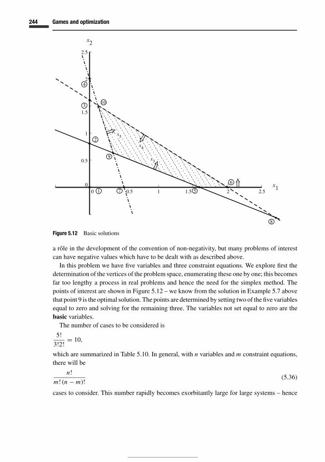
244 Games and optimization
2.5
2
1.5
1
0.5
00 1 1.5 2.520.5
Figure 5.12 Basic solutions
a role in the development of the convention of non-negativity, but many problems of interestcan have negative values which have to be dealt with as described above.
In this problem we have five variables and three constraint equations. We explore first thedetermination of the vertices of the problem space, enumerating these one by one; this becomesfar too lengthy a process in real problems and hence the need for the simplex method. Thepoints of interest are shown in Figure 5.12 – we know from the solution in Example 5.7 abovethat point 9 is the optimal solution. The points are determined by setting two of the five variablesequal to zero and solving for the remaining three. The variables not set equal to zero are thebasic variables.
The number of cases to be considered is
5!
3!2!= 10,
which are summarized in Table 5.10. In general, with n variables and m constraint equations,there will be
n!
m! (n − m)!(5.36)
cases to consider. This number rapidly becomes exorbitantly large for large systems – hence

245 5.4 Linear optimization
Table 5.10 Ten vertices in Example 5.4; points refer to Figure 5.12; f = feasible; nf = notfeasible; [0] indicates non-basic variable
Point→ 1 2 3 4 5 6 7 8 9 10
x1 [0] [0] [0] [0] 1.6 2 0.5 2.667 0.343 0.125x2 [0] 0.8 1.6 2 [0] [0] [0] −0.533 0.629 1.5x3 −8 [0] 8 12 [0] 2 −5.5 [0] [0] 7.625x4 8 4 [0] −2 1.6 [0] 6 [0] 3.486 [0]x5 −2 −1.2 −0.4 [0] 4.4 6 [0] 8.133 [0] [0]Nature nf nf nf nf f f nf nf f f
the need to shorten the procedure. Let us nevertheless complete the exercise for our example,as this assists greatly in explaining the simplex method. We take two examples, points 1 and6; the rest are summarized in Table 5.10. The shaded area only in Figure 5.12 is feasible sinceonly there are the constraints and non-negativity satisfied.
� Point 1, column 1 in Table 5.10. With x1 = x2 = 0, we can solve the three Equations(5.21) to find the values of the basic variables: x3 = −8, x4 = 8, x5 = −2. The conditionof non-negativity is violated which is confirmed by reference to Figure 5.12.
� Point 6, column 6 in Table 5.10. Here x2 = x4 = 0. The basis is {x1, x3, x5} . We substitutein Equations (5.21) to find
5x1 − x3 = 8,
4x1 = 8 and
4x1 − x5 = 2.
Then x1 = 2, x3 = 2 and x5 = 6. The point is therefore feasible since non-negativity issatisfied. This again can be checked by reference to Figure 5.12.
As indicated the basis is the collection of variables not set equal to zero in each case. Forpoint 6 the basis is, as noted, {x1, x3, x5} , and for case 10 it is {x1, x2, x3} . Each of the tensolutions in Table 5.10 is a basic solution. A feasible solution satisfies the constraint andnon-negativity conditions. Points in the shaded area of Figure 5.12 are feasible. Basic feasiblesolutions satisfy the constraint and non-negativity conditions in addition to being basic; theycorrespond to the vertices of the feasible space. Cases 5, 6, 9 and 10 are basic and feasible (weknow that 9 is optimal). It is convenient to deal with Phase II of the simplex method first –in this it is assumed that a basic feasible starting point is available. Phase I is concerned withfinding this starting point.
Phase II of simplex algorithmWe need, in accordance with the preceding two sentences, to have a basic feasible starting point.Let this be point 6 above, for which x2 = x4 = 0. Here, we deduce the required equations, butPhase I – to be introduced below – will do this for us automatically. The required equations are

246 Games and optimization
(5.37) below; these can be deduced from Equations (5.21), also reproduced as (i) to (iii) belowfor convenience. The basis is {x1, x3, x5} ; for ease of solution we like to have only one of thesevariables to appear in each equation. We therefore start with the second equation (ii) below.This is repeated, after division by 4, as the first line of Equation (5.37). It is the canonicalequation for x1; since x2 = x4 = 0, we can solve x1 = 2.
In the second line of Equation (5.37) we have started with equation (i), multiplied by (−1) ,
and then added equation (ii) after having multiplied this by 5/4. This eliminates x1 (we wantthe basic variables to appear in one equation only), and x3, another basic variable, appears witha coefficient of 1, as required. Noting again that x2 = x4 = 0, we can solve x3 = 2. The lastequation in (5.37) is deduced by taking equation (iii), subtracting equation (ii), and then multi-plying through by (−1) , to ensure a non-negative stipulation. This is again in canonical form,and with x2 = x4 = 0, we solve x5 = 6. All of this is in agreement with Table 5.10, point 6.
5x1 + 10x2 − x3 = 8 (i)
4x1 + 5x2 + x4 = 8 (ii)
4x1 + x2 − x5 = 2 (iii)
x1 +1.25x2 +0.25x4 = 2−3.75x2 +x3 +1.25x4 = 2
4x2 +x4 +x5 = 6 (5.37)
Note the structure of Equations (5.37). The basic variables appear only once, each in a singleequation, with a coefficient of unity.
The general canonical form is
x1 +a′1,m+1xm+1+ · · · +a′
1,n xn = b′1
x2 +a′2,m+1xm+1+ · · · +a′
2,n xn = b′2
. . ....
...xm +a′
m,m+1xm+1+ · · · +a′m,n xn = b′
m . (5.38)
Here, the basis is assumed to be {x1, . . . , xm} but it could be any set of m variables fromamongst the n. There are (n − m) non-basic variables. The primes in Equations (5.38) referto the fact that the original values in Equations (5.33) have been manipulated to eliminatevariables and to reduce the coefficients of the basis to unity, as we did in deducing Equations(5.37). The b′
i are termed the canonical stipulations.We now investigate this first basic feasible point – as given in (5.37) with x1 = 2, x3 =
2, x5 = 6, x2 = x4 = 0 – for optimality. (We actually know it isn’t since it corresponds topoint 6 in Figure 5.12, but we will not generally know this.) To do this we write the objectivefunction in terms of the non-basic variables:
z = 2x1 + x2 = 2 (2 − 1.25x2 − 0.25x4) + x2
= 4 − 1.5x2 − 0.5x4, or
z − 4 = −1.5x2 − 0.5x4. (5.39)

247 5.4 Linear optimization
In deducing this we have used the first of the set (5.37) to eliminate the basic variable x1.
Equation (5.39) represents the objective function in canonical form. The general form corre-sponding to Equation (5.39) is
z − z0 = c′m+1xm+1 + · · · + c′
n xn, (5.40)
written in terms of non-basic variables; z0 is a constant. The current solution is then z = z0;this has to be tested for optimality.
The solution of Equation (5.39) corresponding to the assumed basis {x1, x3, x5} is
z − 4 = 0, or z = 4, with z0 = 4 (5.41)
since x2 = x4 = 0. Now the key point is: would the act of increasing x2 or x4 from zero lead toa lower value of z? We look at Equation (5.39): both the coefficients of x2 and x4 are negative.Increasing either will reduce z. In the simplex method, we increase only one variable at a time.We choose x2 since it has the most negative coefficient (= −1.5) as compared to (−0.5) for x4.
How much can we increase x2? We can determine this by inspecting Equations (5.37). Wekeep x4 = 0 and therefore exclude it from the analysis. The first of Equations (5.37) can bewritten
x1 + 1.25x2 = 2 or x1 = −1.25x2 + 2. (5.42)
From this we can see that increasing x2 will reduce x1, and indeed whenx2 = (2/1.25) = 8/5 = 1.6, x1 will have been reduced to zero. Any further reduction willresult in x1 becoming negative, thus violating the non-negativity condition for all variables x j .
We repeat the process just followed for the second and third equations of (5.37), which are
−3.75x2 + x3 = 2 or x3 = 3.75x2 + 2, and (5.43)
4x2 + x5 = 6 or x5 = −4x2 + 6. (5.44)
In the first of these, (5.43), the fact that the coefficient a′22 = −3.75 is negative results in the
situation that x2 can be increased indefinitely without making x3 become negative. In the second,(5.44), the increase in x2 must be ≤ 6/4 = 1.5, at which point x5 becomes equal to zero.
Of the three conditions just investigated, the first states that x2 ≤ 1.6, the second that x2
can be increased without limit, and the third that x2 ≤ 1.5. The third governs; if implemented,all three conditions of non-negativity will be satisfied. Further, we increase x2 to the limit of1.5; then x5 = 0. Thus x5 leaves the basis and x2 enters it. The key in the procedure was tofind the minimum ratio of b′
i to a′ir provided a′
ir > 0. In the present example, this ratio wasb′
3/a′32 = 6/4. The index r equals the column number of the incoming basic variable.
The rule for changing the basis is summarized as follows.
Choose the most negative of the canonical cost coefficients, say c′r ;
then r denotes the column of the incoming basic variable;then choose the smallest b′
ia′
irprovided a′
ir > 0;
a′ir is then the pivotal element for bringing xr into the basis.

248 Games and optimization
We now investigate the second vertex of the feasible space. We have to rewrite Equa-tions (5.37) in canonical form corresponding to the new basis {x1, x2, x3} . The third equationof this set is ideal for the canonical form since it contains one basic variable (x2) , and the twonon-basic variables (x4 and x5) . We divide the equation by 4 to reduce the coefficient of x2 tounity. Then we use this equation to eliminate x2 from the first two. The coefficient a′
32 is thepivotal element in this case. We repeat for convenience below Equations (5.37) and underneaththem the new set of canonical equations (5.45) with the new basis {x1, x2, x3} .
x1 +1.25x2 +0.25x4 = 2−3.75x2 +x3 +1.25x4 = 2
4x2 +x4 +x5 = 6
x1 −0.0625x4 −0.3125x5 = 0.125+x3 +2.1825x4 +0.9375x5 = 7.625
x2 +0.25x4 +0.25x5 = 1.5. (5.45)
The objective function must also be written in canonical form:
z − 1.75 = −0.125x4 + 0.375x5. (5.46)
This is deduced by eliminating x2 from Equation (5.39) using the third equation containingthe pivotal element in the set (5.45).
We summarize the steps so far and complete the solution in the simplex tableau of Table 5.11.The second solution corresponds to point 10 in Figure 5.12 and Table 5.10, with x1 = 0.125,
x2 = 7.625 and x3 = 1.5. In the objective function, x2 has also been eliminated using thethird constraint equation. There is only one negative canonical cost coefficient, c′
4 = −0.125.
Hence r = 4, and inspecting the fourth column, we see that the smallest b′i/a′
i4 ratio is
Table 5.11 Simplex tableau; · denotes pivotal element
b x1 x2 x3 x4 x5 Basis
2 1 1.25 0.25 x1
2 −3.75 1 1.25 x3
6 4 1 1 x5
z − 4 −1.5 −0.5
0.125 1 −0.0625 −0.3125 x1
7.625 1 2.1875 0.9375 x3
1.5 1 0.25 0.25 x2
z − 1.75 −0.125 0.375
0.3429 1 0.0625 −0.2857 x1
3.4857 0.4571 1 0.4286 x4
0.6286 1 −0.1143 0.1429 x2
z − 1.3143 0.0571 0.4286
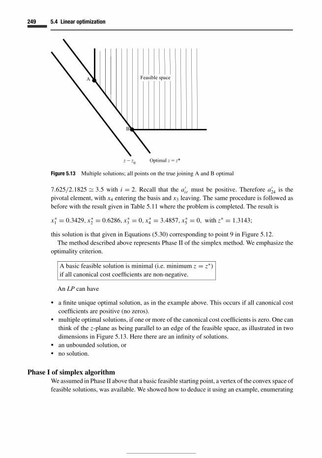
249 5.4 Linear optimization
0
Figure 5.13 Multiple solutions; all points on the true joining A and B optimal
7.625/2.1825 � 3.5 with i = 2. Recall that the a′ir must be positive. Therefore a′
24 is thepivotal element, with x4 entering the basis and x3 leaving. The same procedure is followed asbefore with the result given in Table 5.11 where the problem is completed. The result is
x∗1 = 0.3429, x∗
2 = 0.6286, x∗3 = 0, x∗
4 = 3.4857, x∗5 = 0, with z∗ = 1.3143;
this solution is that given in Equations (5.30) corresponding to point 9 in Figure 5.12.The method described above represents Phase II of the simplex method. We emphasize the
optimality criterion.
A basic feasible solution is minimal (i.e. minimum z = z∗)if all canonical cost coefficients are non-negative.
An LP can have
� a finite unique optimal solution, as in the example above. This occurs if all canonical costcoefficients are positive (no zeros).
� multiple optimal solutions, if one or more of the canonical cost coefficients is zero. One canthink of the z-plane as being parallel to an edge of the feasible space, as illustrated in twodimensions in Figure 5.13. Here there are an infinity of solutions.
� an unbounded solution, or� no solution.
Phase I of simplex algorithmWe assumed in Phase II above that a basic feasible starting point, a vertex of the convex space offeasible solutions, was available. We showed how to deduce it using an example, enumerating

250 Games and optimization
all the vertices and investigating them. In a large system of equations, this procedure becomesdifficult or impossible. It is convenient then to use Phase I, an ingenious method, to find abasic feasible starting point. We introduce this using a second extended example. This is thetransportation problem, a model of a system with multiple origins and destinations in themarketing of a product.
There are m centres of supply for a commodity and n markets. These can be thought of asorigins and destinations. The i th supply centre has in stock si units (amount) of the commodity(i = 1, 2, . . . , m) and the j th destination requires at least r j units ( j = 1, 2, . . . , n). Theamount of the commodity shipped from i to j is denoted xi j with cost ci j per unit. Thepurpose of the exercise is to minimize the total shipping cost∑
j
∑i
xi j ci j (5.47)
subject to the prescribed constraints∑j
xi j ≤ si ,∑i
xi j ≥ r j . (5.48)
We apply this model using the following data:
Table 5.12 Unit costs ci j
j1 2
1 5 3i 2 6 2
3 1 8
The following constants are to be used in the constraint equations:
s1 = 5, s2 = 7, s3 = 11 and
r1 = 12, r2 = 3.
The formulation of the problem using the data given is as follows.
Min (z = 5x11 + 3x12 + 6x21 + 2x22 + x31 + 8x32) (5.49)
subject to
x11 + x12 ≤ 5,
x21 + x22 ≤ 7,
x31 + x32 ≤ 11,
x11 + x21 + x31 ≥ 12 and
x12 + x22 + x32 ≥ 3. (5.50)
All xi j are ≥ 0.

251 5.4 Linear optimization
In standard form the constraints become
x11 +x12 +xs1 = 5,
x21 +x22 +xs2 = 7,
x31 +x32 +xs3 = 11,
x11 +x21 +x31 −xe1 = 12 andx12 +x22 +x32 −xe2 = 3. (5.51)
Slack variables are denoted xs1, xs2 and xs3 while excess ones are xe1 and xe2. Inspection of theseequations reveals that the slack variables provide a convenient initial basis; they automaticallyhave a coefficient of (+1), only one appears per equation, and they do not appear in theobjective function. Slack variables are a gift! But what do we do about the last two equations?Excess variables have a coefficient of (−1); multiplying the equation through by (−1) doesnot help since this would make the stipulation negative.
Rather than attempting elimination as we did to set up the Phase II example above, weintroduce the principal idea of Phase I. We simply add variables, called artificial variables,to the problem equations. Then the last two of the set (5.51) become
x11 +x21 +x31 −xe1 +xa1 = 12 andx12 +x22 +x32 −xe2 +xa2 = 3,
(5.52)
where xa1 and xa2 are the artificial variables, both ≥ 0. We have changed the original problemby adding these additional variables, and have enlarged the original convex space. Our purposenow is to eliminate them as soon as possible! If we do this and maintain feasibility, we hopesoon to end up on a basic feasible vertex of the original problem.
Our means of eliminating xa1 and xa2 is to introduce a temporary objective function asfollows:
w = xa1 + xa2. (5.53)
This can be written as
w = xa1 + xa2
= 15 − x11 − x12 − x21 − x22 − x31 − x32 + xe1 + xe2, (5.54)
using Equations (5.52). We wish to reduce w of Equation (5.53) to zero; then xa1 = xa2 = 0,
and we can return to the original objective function. In general the temporary objective functionmight be
w = xn+1 + xn+2 + · · · + xn+�, (5.55)
for � artificial variables.We now proceed as shown in Tables 5.13(a) and (b). The temporary objective function is
used in determining the incoming basic variable; it dictates the criterion for optimization untilit reaches zero. During this Phase I period, the original (z) objective function is adjusted toreflect the current basis, any incoming basic variables being eliminated from the objective

252 Games and optimization
Table 5.13(a) Solution to transportation problem; reduction of w to zero
b x11 x12 x21 x22 x31 x32 xs1 xs2 xs3 xe1 xe2 xa1 xa2 Basis
5 1 1 1 xs1
7 1 1 1 xs2
11 1 1 1 xs3
12 1 1 1 −1 1 xa1
3 1 1 1 −1 1 xa2
z − 0 5 3 6 2 1 8w − 15 −1 −1 −1 −1 −1 −1 1 1
5 1 1 1 xs1
7 1 1 1 xs2
8 −1 −1 1 1 1 −1 xs3
12 1 1 1 −1 1 xa1
3 1 1 1 −1 1 x32
z − 24 5 −5 6 −6 1 8 −8w − 12 −1 −1 −1 1 1
5 1 1 1 x11
7 1 1 1 xs2
8 −1 −1 1 1 1 −1 xs3
7 −1 1 1 −1 −1 1 xa1
3 1 1 1 −1 1 x32
z − 49 −10 6 −6 1 −5 8 −8w − 7 1 −1 −1 1 1 1
5 1 1 1 x11
7 1 1 1 xs2
1 −1 −1 1 1 1 1 −1 −1 xs3
7 −1 1 1 −1 −1 1 x31
3 1 1 1 −1 1 x32
z − 56 −9 5 −6 0 −4 1 8 −1 −8w − 0 0 0 0 0 0 1 1
function. But w is to be minimized until equal to zero, the purpose of which is solely to finda basic feasible starting point of the original problem. Then we focus on z. This process ofreducing w to zero endures for three cycles of the simplex operation as in Table 5.13(a). Atthe step when w = 0, one then immediately reverts to z; the temporary objective function w isno longer of any relevance; nor are the artificial variables. The completion of the problem andminimization of z is shown in Table 5.13(b). The tables (a) and (b) can be combined if desired.

253 5.4 Linear optimization
Table 5.13(b) Transportation problem continued; determination of optimal z
b x11 x12 x21 x22 x31 x32 xs1 xs2 xs3 xe1 xe2 Basis
2 1 −1 −1 1 1 x11
7 1 1 1 xs2
1 −1 −1 1 1 1 1 xs3
10 1 1 1 1 −1 −1 −1 x31
3 1 5 1 1 −1 x12
z − 29 3 9 −4 1 −1
1 1 1 −1 −1 −1 x11
7 1 1 1 xs2
1 −1 −1 1 1 1 1 xs1
11 1 1 1 x31
3 1 1 1 −1 x12
z − 25 1 −1 9 4 5 3
1 1 1 −1 −1 −1 x11
4 −1 1 −1 1 1 xs2
4 1 −1 1 1 1 1 xs1
11 1 1 1 x31
3 1 1 1 −1 x22
z − 22 1 1 10 4 5 2
Solution. x∗11 = 1 x∗
31 = 11 x∗22 = 3
x∗s1 = 4 x∗
s2 = 4 Other variables = 0.
z∗ = 22
We have introduced the simplex method by example – since it is a practical method for use.Formal theorems are available in works such as Karlin (1959) and Jones (1980), two excellentreferences in this area.
5.4.3 Dual linear programs
For each linear program, called the primal problem
Min(
z =∑n
j=1c j x j
)(5.56)
subject to∑n
j=1ai j x j = [
ai j]
x j ≥ bi , for i = 1, 2, . . . , m, (5.57)
x j ≥ 0, for j = 1, 2, . . . , n;

254 Games and optimization
there is a dual linear problem
Max(
w =∑m
i=1bi yi
)(5.58)
subject to∑m
i=1ai j yi = [
ai j]T
yi = [a ji
]yi ≤ c j for j = 1, 2, . . . , n, (5.59)
yi ≥ 0 for i = 1, 2, . . . , m.
In (5.59), [·]T indicates the transpose of the matrix. The striking relationship between thesetwo problems is typical of dual relationships. ‘Min’ in the primal becomes ‘Max’ in the dual.The variable x j is replaced by the dual yi ; cost coefficients and stipulations interchange;
[ai j
]is transposed. The dual of the dual problem is the primal; Exercise 5.12.
One of the problems that stimulated interest in LP is the diet problem (Jones, 1980). (Thisis a product-mix problem, similar to that in Example 5.4 and in Exercise 5.14.) In the primalproblem the x j are units of a particular type of food. The constraints specify the minimumamounts of nutrients – for example, vitamins – that must be supplied, governed by the bi ofEquations (5.57). The ai j denote the amount of each nutrient (i) contained in a unit of the foods( j) . The problem is to minimize the total cost as in Equation (5.56). This might be the approachtaken by a cost-conscious hospital board. The dual problem of Equations (5.58) and (5.59)represents that of a drug company that wishes to substitute synthetic mixtures of nutrientsthat satisfy the minimal requirements, thus containing bi units of nutrient i. The variable yi
now represents the price to be charged for a unit of nutrient i. The drug company wishes tomaximize the profit given by the function (5.58). The constraints of (5.59) indicate that thecost of any mixture of nutrients, equivalent to food j, should be less than the cost of the fooditself.
Now it turns out that the solutions to the primal and dual problems coincide! This means thatthe hospital board and the drug company can together satisfy minimum nutritional requirementsand maximum profit. An interpretation in terms of ‘shadow prices’ is given in Exercise 5.14.Jones (1980) and Chvatal (1980) provide good outlines of the theory of duality in linearprogramming.
The theory behind this begins with the following result:
z =∑n
j=1c j x j ≥ w =
∑m
i=1bi yi . (5.60)
This is shown by considering that
∑m
i=1bi yi ≤
∑m
i=1yi
(∑n
j=1ai j x j
)(5.61)
since∑n
j=1ai j x j ≥ bi ,

255 5.4 Linear optimization
by inequality (5.57). Now inequality (5.61) can be written as∑n
j=1x j
(∑m
i=1ai j yi
)≤
∑n
j=1c j x j
by inequality (5.59). Thus inequality (5.60) is proved.If we manage to find a primal feasible solution {x∗
1 , x∗2 , . . . , x∗
n } together with a dual feasiblesolution {y∗
1 , y∗2 , . . . , y∗
m} such that∑n
j=1c j x
∗j =
∑m
i=1bi y∗
i , or (5.62)
Min z = Max w, (5.63)
then the two solutions are optimal, since w ≤ z by inequality (5.60).The duality theorem turns this around. It states that, if we find an optimal solution
{x∗1 , x∗
2 , . . . , x∗n } of the primal problem, then the dual problem has a solution {y∗
1 , y∗2 , . . . , y∗
m}such that Equation (5.62) is satisfied. The solution to the primal LP gives the solution to thedual LP and vice versa; Min z =Max w.
Proof of duality theoremWe shall base the proof on the simplex method. It is then convenient to start with the duallinear program, since it is easy to deduce a canonical form from the dual constraints of Equation(5.59):∑m
i=1ai j yi = [
ai j]T
yi ≤ c j for j = 1, 2, . . . , n.
The useful thing to observe is that the inequalities (≤) in this relationship imply that slackvariables ym+ j will be used in the simplex method; thus
ym+ j = c j −∑m
i=1ai j yi , for j = 1, 2, . . . , n, (5.64)
and this gives an ideal basic feasible starting point. All of the slack variables enter the firstbasis. The other variables are non-basic and set equal to zero. The objective function containsonly non-basic variables:
Max(w =
∑m
i=1bi yi
).
(The motto ‘slacks are a gift’ presented earlier has real meaning!) To use the simplex methodas described above, we convert the objective function of (5.58) from ‘Max’ to ‘Min’ :
Min w′ = −w = −∑m
i=1bi yi =
∑m
i=1(−bi ) yi . (5.65)
We now consider the situation where we have completed the simplex operation, arriving atthe optimal solution w′∗:
w′ − w′∗ =∑m+n
h=1
(−bh)
yh . (5.66)
In this equation, we have written the last row of the simplex operation; h is an index that ranges

256 Games and optimization
over both i and j, over all (m + n) of the yh , including the slack variables (5.64). The negativesign in (−bh) in Equation (5.66) is included so as to be consistent with Equation (5.65). Nowwe know that, in Equation (5.66), (−bh) is 0 whenever yh is a basic variable and positive orzero when it is not, since w′ = w′∗ is optimal. The yh are zero when non-basic as demonstratedusing the simplex method above. Since all (−bh) are positive or zero they are non-negative,and consequently the bh are non-positive.
We know also that at optimality
w′∗ =∑m
i=1(−bi ) y∗
i or
w∗ =∑m
i=1bi y∗
i . (5.67)
The optimal x j in the primal problem are given by
x∗j = −bm+ j for j = 1, . . . , n. (5.68)
We shall show that {x∗1 , x∗
2 , . . . , x∗n }, thus defined, constitutes a primal feasible solution satis-
fying (5.62) and therefore optimal. First we write (5.66) as
w − w∗ =∑m+n
h=1bh yh ;
then substituting for w from (5.58):∑m
i=1bi yi − w∗ =
∑m+n
h=1bh yh =
∑m
h=1bh yh +
∑m+n
h=m+1bh yh .
We now substitute for the slack variables from Equations (5.64) and for bm+ j from (5.68):∑m
i=1bi yi − w∗ =
∑m
h=1bh yh +
∑n
j=1
(−x∗j
) (c j −
∑m
i=1ai j yi
).
Then we can write∑m
i=1bi yi =
(w∗ −
∑n
j=1c j x
∗j
)+
∑m
i=1
(bi +
∑n
j=1ai j x
∗j
)yi . (5.69)
Equation (5.69) has been derived from the definition of the objective function for w in termsof the yi in Equation (5.58), i.e. w = ∑m
i=1 bi yi , and from the definition of the slack variables,(5.64), thus eliminating any slack variables from the equation. Equation (5.69) therefore relatesgenerally the yi and is valid for any {y1, y2, . . . , ym} . We can choose all the yi to be zero; then
w∗ =∑n
j=1c j x
∗j . (5.70)
This, together with Equation (5.67), shows Equation (5.62) to be correct with the association(5.68).
If we choose now yi = 1, and all other yk to be zero (k = i) , then we find that
bi = bi +∑m
i=1ai j x
∗j .
Since the bi are non-positive, bi ≤ 0, therefore∑m
i=1ai j x
∗j ≥ bi , (5.71)
257 5.5 Back to games: mixed strategies
and with(
x∗j = −bm+ j
), Equation (5.68),
x∗j ≥ 0. (5.72)
These last two equations are the primal constraints.
5.4.4 Applications of linear programming
Linear programming has been applied in various optimization problems. These include product-mix problems, for example Exercise 5.14 and the diet problem discussed above in the secondparagraph of Section 5.4.3. The transportation problem introduced in Section 5.4.2 with PhaseI of the simplex method is another. Shortest and longest routes through a network can beobtained using linear programming, the latter of great use in scheduling and obtaining thecritical path in construction projects of various kinds. Warehouse storage and activity analysisare areas where linear methods can be used. Mathematical plasticity in structural theory can bedealt with using linear programming with elegant methodology introduced notably by Munro(see Cohn and Maier, 1979, for example). And of course there is the solution of problems ingame theory, the main focus here.
5.5 Back to games: mixed strategies
Games with saddle points have solutions with pure strategies. This was shown in the examplein Section 5.2 (Table 5.2). We now return to the ideas under the section ‘Conflict’, introducedat the beginning of the chapter. An animal might choose to fight or to retreat on a case by casebasis. The idea of a mixed strategy is to play the two strategies randomly, for example to fight50% of the time, and to retreat 50% of the time. This is a simplification of reality, since theindividual decisions are made depending on the protagonist’s state of mind and judgement ofthe strength of the antagonist. Von Neumann showed that, if mixed strategies are permitted,then equilibrium can be reached.
Each player’s problem in zero-sum games can be reduced to a linear program. Further, theplayers’ mixed strategies are dual solutions of each other’s. This is a beautiful result, and addsinsights into conflict and the difference between this situation and the ‘game against nature’ ofdecision theory. In the latter interpretation of a game against nature we face an impartial antag-onist, but in conflict our antagonist will choose strategies to outwit and defeat us. Estimationof the probabilities of our antagonist’s strategies is profoundly different where there is intelli-gent conflict.
Let us consider a typical zero-sum game without a saddle point, that illustrated in Table 5.4.We denote the payoff value in general as V, from B to A according to convention. The gameis repeated in Table 5.14, in which we have shown that A plays the strategies σ1 and σ2 withprobabilities p and (1 − p) respectively. At the same time, B plays τ1 and τ2 with probabilities

258 Games and optimization
Table 5.14 Game with mixed strategies
B
τ1 τ2
q 1 − q
σ1 p 3 6σ2 1 − p 5 4
A
Figure 5.14 Gain floor and loss ceiling
q and (1 − q) respectively. We first consider the situation from A’s point of view. He ponderswhat B will do. If she plays τ1, the mean (expected) payoff to A is
〈V 〉 = 3p + 5 (1 − p)
= 5 − 2p. (5.73)
If B on the other hand plays τ2, the mean is
〈V 〉 = 6p + 4 (1 − p)
= 4 + 2p. (5.74)
These are plotted in Figure 5.14(a). Player A can place a lower limit on his expected gains,shown as a gain floor in the figure. The greatest value of mean gain is at the intersection ofthe two lines, at
5 − 2p = 4 + 2p, or
p = 1
4. (5.75)
Player A therefore adopts the strategy of playing σ1 with probability 1/4, and σ2 with prob-ability 3/4, written {σ1, 1/4; σ2, 3/4} . This result is completely consistent with the maximinphilosophy in maximizing the gain floor.

259 5.5 Back to games: mixed strategies
Player B undergoes a similar reasoning process and calculates the following mean losses. IfA plays σ1, her mean loss is
〈V 〉 = 3q + 6 (1 − q)
= 6 − 3q. (5.76)
If A plays σ2, this becomes
〈V 〉 = 5q + 4 (1 − q)
= 4 + q. (5.77)
These are plotted in Figure 5.14(b). In this case B can construct a loss ceiling, shown in thefigure. To minimize the loss, B calculates
6 − 3q = 4 + q, or
q = 1
2; (5.78)
she adopts {τ1, 1/2; τ2, 1/2} . Again the philosophy is maximin, bearing in mind that B paysto A.
In the solution equilibrium has been reached; the value of the game is 4.5. This can becalculated from any of the four expected values above. The solution is based on mean values,averaged over many plays of the game, and constitutes a generalization of the saddle point ofEquation (5.1). It brings inequality (5.2) into equality.
5.5.1 Generalization and example
We now generalize the results on mixed strategies to show that player A and B’s solutions aredual linear programs. There is one point that must be introduced at the start so as to make thereasoning clear. We do this first with an example. Consider the payoff matrix (B to A):2 5 4
6 1 34 6 1
. (5.79)
As in the preceding section, player A evaluates the mean (expected) value of each strategy,assuming that B plays strategy τi . This must be evaluated using the transpose of matrix (5.79).In matrix (5.79), consider the case where A is considering the expected value given that Bplays τ2. The expected value is
(5) p1 + (1) p2 + (6) p3.
This can be seen to be given by the second member in the vector
2 6 4
5 1 64 3 1
p1
p2
p3
=
2 5 4
6 1 34 6 1
T
p1
p2
p3
. (5.80)

260 Games and optimization
The point of clarification is that we transpose the payoff matrix so as to write the theory ina manner that is compatible with our treatment of linear programming and duality above. Wethen define this transposed matrix as
[ai j
],
[ai j
] ≡ [payoff matrix
]T. (5.81)
As a result,[payoff matrix
] = [ai j
]T. (5.82)
In the example given above,
[ai j
] =2 6 4
5 1 64 3 1
.
In general, we write ai j as
[payoff matrix
]T = [ai j
] =
a11 a12 · · · a1 j · · · a1n
a21 a22 · · · a2 j · · · a2n...
......
...ai1 ai2 · · · ai j · · · ain...
......
...am1 am2 · · · amj · · · amn
(5.83)
and the payoff matrix is
[payoff matrix
] = [ai j
]T = [a ji
] =
a11 a21 · · · ai1 · · · am1
a12 a22 · · · ai2 · · · am2...
......
...a1 j a2 j · · · ai j · · · amj
......
......
a1n a2n · · · ain · · · amn
. (5.84)
This is the matrix given in a problem of game theory, by convention. For example, if A playsσ3 and B plays τ2, B pays a23 to A. We assume in the following that the values in the matrix ai j
are greater than or equal to zero. The reason for this is given below. To achieve this, one canadd the same positive constant to all the values in a payoff matrix without altering the strategicoutcome of the game.
Player A has n possible pure strategies,
σ1, σ2, . . . , σ j , . . . , σn.
Similarly B has m pure strategies
τ1, τ2, . . . , τi , . . . , τm .

261 5.5 Back to games: mixed strategies
Player A’s mixed strategies consist of
a p1 probability of strategy σ1,
a p2 probability of strategy σ2,...a p j probability of strategy σ j ,...and a pn probability of strategy σn.
We assume that both players are probabilistically coherent. Then for player A,∑n
j=1p j = 1. (5.85)
Player B’s mixed strategies are
a q1 probability of strategy τ1,
a q2 probability of strategy τ2,...a qi probability of strategy τi ,...and a qm probability of strategy τm,
again with coherence∑m
i=1qi = 1. (5.86)
As in the preceding section (Figure 5.14), player A evaluates the following values:
〈V 〉 = ai1 p1 + ai2 p2 + · · · + ai j p j + · · · + ain pn ≥ v, for i = 1, 2, . . . , m, (5.87)
where V, as before, represents a payoff from matrix (5.83). In this, v is the least of the setof the m sums given in (5.87); it corresponds to the gain floor of Figure 5.14(a). Rather thanconsisting of a series of straight lines, there will now be a set of hyperplanes in
{p j
}-space.
For any set of probabilities{
p j}, there will always be a minimum value (= v) amongst these
hyperplanes corresponding to the gain floor. Equations (5.87) may be written as∑n
j=1ai j p j = [
ai j]
p j ≥ v, (5.88)
Player A has now weighted the columns of matrix (5.84) – the rows of matrix (5.83) – by thep j , as required.
Now we introduce the new quantity x j given by
x j = p j
v, with j = 1, 2, . . . , n. (5.89)
Then the constraints (5.88) become∑n
j=1ai j x j = [
ai j]
x j ≥ 1 for i = 1, 2, . . . , m. (5.90)

262 Games and optimization
In deriving this equation, we have substituted p j = vx j and cancelled the factor v from bothsides of the result. Note that v has a fixed value for any set of values of
{p j
}. We see now
why the values ai j were made to be ≥ 0; this is to ensure that v > 0, and consequently x j ≥ 0,
required for the simplex method.We wish to find the set of probabilities at the maximum value of v, the highest point in the
gain floor. Substituting from Equation (5.89) into (5.85)
∑n
j=1x j = 1
v; (5.91)
then maximizing v implies
Min∑n
j=1x j . (5.92)
This equation, combined with the constraints (5.90), and the fact that all x j ≥ 0 (providedv > 0) shows that the determination of the optimal set {p j } can be achieved by the followingLP:
Min∑n
j=1 x j subject to∑nj=1 ai j x j = [ai j ]x j ≥ 1 for i = 1, 2, . . . , m and
x j ≥ 0, for j = 1, 2, . . . , n.
(5.93)
The striking similarity of relationships (5.93) and the pair (5.56) with (5.57) should be noted.To ensure v > 0 in the above, we make all ai j ≥ 0 in the matrix
[ai j
]. Then the inequalities
(5.88) ensure that v is positive since it is the smallest value calculated from them. To makethe entries ai j ≥ 0, one adds a constant value to each entry in the matrix
[ai j
]; doing so does
not alter the game strategically. Adding the same quantity to each payoff value results in allexpected values increasing by the same added amount. The relative values of these meanvalues are precisely the same. One could if one wishes, after the analysis, subtract the constantfrom the payoff values.
We now consider player B. He wishes to find the optimal set {qi } . The expected values forB are
〈V 〉 = a1 j q1 + a2 j q2 + · · · + ai j qi + · · · + amj qm ≤ t, for j = 1, 2, . . . , n, (5.94)
where t is the greatest of the sums – the loss ceiling of Figure 5.14. For example, using thepayoff matrix (5.79), the following equations result:2 5 4
6 1 34 6 1
q1
q2
q3
= [
payoff matrix]
q1
q2
q3
.
The payoff matrix is the transpose of[ai j
]. Thus the set of equations (5.94) is
∑m
i=1ai j qi = [
ai j]T
qi = [a ji
]qi ≤ t, for j = 1, 2, . . . , n. (5.95)

263 5.5 Back to games: mixed strategies
Again we consider a transformation
yi = qi
t, with i = 1, 2, . . . , m. (5.96)
Substituting into Equation (5.95) results in∑m
i=1ai j yi = [
a ji]
yi ≤ 1, for j = 1, 2, . . . , n,
and together with coherence,∑m
i=1 qi = 1, gives
∑m
i=1yi = 1
t.
Since we wish to minimize t, the equations just derived constitute the following linear program.
Max∑m
i=1 yi subject to∑mi=1 ai j yi = [
a ji]
yi ≤ 1, for j = 1, 2, . . . , n, and
yi ≥ 0, for i = 1, 2, . . . , m.
(5.97)
This is the dual LP to that given in Equations (5.93). Relationships (5.97) are similar in formto the pair (5.58) and (5.59).
We arrive at the interesting result that
Player B’s problem is the dual of player A’s.
Example 5.8 Match-penny. Player A chooses heads or tails on his coin, while B makes achoice on hers. Neither player knows the other’s choice. If the coins match, player B receivesa payoff of unity from A. If the coins do not match, A receives a payoff of unity from B.
The payoff matrix is
B
τ1 τ2
σ1 −1 1σ2 1 −1
A
First add unity to each entry:
B
τ1 τ2
σ1 0 2σ2 2 0
A

264 Games and optimization
Consider player B.
2q2 ≤ t
2q1 ≤ t.
Substitute yi = qi/t :
Max (y1 + y2)
subject to
2y2 ≤ 1
2y1 ≤ 1
with both yi ≥ 0. The solution is
q1 = q2 = 1
2;
the game is symmetrical so that p1 = p2 = 1/2.
Example 5.9 Find the solution to the matrix game−2 1 0
2 −3 −10 2 −3
. (5.98)
First, we make the entries positive by adding a positive constant, say 4, so as to ensure that thevalues of v and t are > 0. Then2 5 4
6 1 34 6 1
= [
a ji].
(This was used as an example in introducing the section above.) Then
ai j = [payoff matrix
]T =2 6 4
5 1 64 3 1
.
The mean values to be considered by A are
[ai j
]p j =
2 6 4
5 1 64 3 1
p1
p2
p3
≥ v.
Following the procedure given above, we then arrive at the following.
Min (x1 + x2 + x3) (5.99)

265 5.6 Discussion; design as a game against nature
subject to
2x1 +6x2 +4x3 ≥ 15x1 +x2 +6x3 ≥ 14x1 +3x2 +x3 ≥ 1,
with all x j > 0 (since v > 0).The dual LP (B’s solution) is
Max (y1 + y2 + y3) (5.100)
subject to
[a ji
]yi =
2y1 +5y2 +4y3 ≤ 16y1 +y2 +3y3 ≤ 14y1 +6y2 +y3 ≤ 1,
(5.101)
with all yi > 0.
The solution to the LPs yields the following optimal strategies:
A :
{σ1,
21
35; σ2,
13
35; σ3,
1
35
}and
B :
{τ1,
13
35; τ2,
12
35; τ3,
2
7
}, (5.102)
with a value of (124/35) .
5.6 Discussion; design as a game against nature
The key aspect introduced by game theory is the question of conflict. This gives an entirelydifferent complexion to the estimation of probabilities. We have considered two-person zero-sum games where the solution is based on maximin philosophy, on the assumption that one’sopponent is out to win at all costs. This represents a ruthless competitor and brings out theessential aspects of the solution to the assignment of probabilities under these conditions. Manyother solutions exist including those for n-person games, bimatrix games, cooperative gamesand bargaining models. One area of application of game theory is war, and in economics wherehuman behaviour is important. Another very interesting recent application is to the modellingof the behaviour of genes. Once again duality appeared – now in a different but related way tothat of the preceding chapter.
Various simplifications were introduced. Mean values were used when considering the valueof the various strategies. This is appropriate in repeated games where the consequences arenot large; see Chapter 4 on risk aversion. The analysis could be extended to consider utilities,and the utility functions could be different for the two players. In reality, the assessment ofprobabilities under conditions of conflict would involve a behavioural assessment of one’santagonist, and one’s own mental state at the point in time. There might be no similarity in

266 Games and optimization
the players’ behaviour assumed in the above; one player might be a lot stronger than the other.The idea of ‘mental roulette wheels’ in which decisions are made automatically according toa set of probabilities is clearly a simplification of reality (as are all models). Yet the importantideas of conflict are captured in the analysis. The difference from decision theory lies in theassessment of the opponent’s probabilities. This reflects the attitude taken in situations ofconflict. The central message to learn is that there is a different way to think about assessmentof probabilities in these situations.
We have posed questions of design as problems of decision. Another way to look at this isto consider design as a game against nature (Turkstra, 1970). In this approach, one considersa set of players, a set of moves, a set of outcomes (endpoints) and a set of values (utilities)attached to each outcome. The players here are the designer and nature; the designer choosesthe physical system and details (for instance structural form, dimensions, . . .) while naturechooses factors such as climate, loadings, good or bad workmanship, . . .; in the endpoints thesystem might function as intended or not, with associated utilities. This is the same modelas decision theory would indicate: one has to suppose the impartiality of nature. There isno room for maximin (pessimist) philosophies in this idealization. Yet, when we considerthat our interventions can change nature – large dams being a pertinent example – we seethe need to think about how these changing conditions should be modelled in our decisiontheory.
5.7 Exercises
5.1 Consider any game of your choice. Ponder the set of possible strategies for the players and thenormal form that arises as well as the corresponding payoff matrix.
5.2 Solve the following optimization problem, in which v represents the volume of a tank.
Max (v = x1x2x3)
subject to
x1 + x2 + 2x3 = b and
x1, x2, x3 ≥ 0.
5.3 A closed right cylindrical pressure vessel of volume v is to be constructed so as to have minimumsurface area a. Find the radius r and length � that achieve this. Discuss how one might investigatethe character of the stationary point found.
5.4 Solve the following optimization problem, in which H represents the entropy. There is a countableset of states xi , i = 0, 1, 2, . . . , of the random quantity X with associated probabilities pi .
Max(
H = −∑n
i=1pi ln pi
)

267 5.7 Exercises
subject to coherence∑∞i=0
pi = 1,
and∑∞i=0
pi xi = 〈X〉 = µ.
5.5 Sketch the feasible region and stationary points of Example 5.6. Investigate and determine theminima of Equation (5.22).
5.6 Solve by the simplex method and check the answer graphically:
Min z = −10x1 + 4x2
subject to 2x1 + x2 ≤ 9
x1 − 2x2 ≤ 2
−3x1 + 2x2 ≤ 1
x1, x2 ≥ 0.
5.7 Solve by the simplex method:
Max z′ = −3x1 − 6x2 + 3x3 − 3x4
subject to x1 − x2 + x3 ≤ 5
x1 + x2 + 2x4 ≤ 6
x2 − 2x3 + x4 ≤ 3
−x1 + 2x2 + x3 ≤ 2
x1, x4 ≥ 0
x2, x3 : unrestricted in sign.
5.8 Solve by the simplex method:
Max z′ = −2x1 + 4x2 − 2x3
subject to 3x1 − x2 + x3 ≤ 4
x1 − x2 + x3 ≤ 2
−2x1 + x2 − x3 ≤ 4
x1, x2, x3 ≥ 0.
5.9 Solve by the simplex method:
Min z = −x1 − x2 − 2x3
subject to 4 ≥ x1 ≥ 1
3x2 − 2x3 = 6
2 ≥ x3 ≥ −1
x2 ≥ 0.

268 Games and optimization
5.10 Check the answers to Problems 5.6 to 5.9 by using computer software.
5.11 Structural systems.
4
2 3
41
(a) An engineer is considering the structural system in Figure (a) on which the loads F1, F2 and F3
represent storage loads which will be imposed for a short duration. The objective is to maximizethe total storage subject to the capacity of the columns. These correspond to buckling loads of

269 5.7 Exercises
200 tonnes for column 1, 100 tonnes for columns 2 and 3, and 150 tonnes for column 4. Treatall beams as being simply supported at their ends.
(b) The structural system in Figure (b) is comprised of horizontal tension members (for examplewires) supported by vertical beams. The loads A, B and C are applied as shown in the figure,together with the capacities of the tension members. Assume that the beams can support theloads. What is the maximum load (A + B + C) that can be supported?
5.12 Show that the dual of the dual problem in LP is the primal problem.
5.13 Complementary slackness theorem. There is a natural relationship between the excess or slackvariables in either the primal or dual program and the decision variables in the other. Whenever anexcess or slack variable is not equal to zero (at optimality), the associated decision variable in thedual program is equal to zero. When a decision variable is greater than zero, the associated excessor slack variable is zero. The solution is such that∑n
j=1ai j x
∗j = bi or y∗
i = 0 or both, for i = 1, 2, . . . , m;∑m
i=1ai j y∗
i = c j or x∗j = 0 or both, for j = 1, 2, . . . , n.
Introduce the slack and excess variables
xn+i = −bi +∑n
j=1ai j x j , for i = 1, 2, . . . , m and
ym+ j = c j −∑m
i=1ai j yi , for j = 1, 2, . . . , n,
to show that
x∗n+i = 0 or y∗
i = 0 or both;
y∗m+ j = 0 or x∗
j = 0 or both.∑m
i=1ai j y∗
i = c j whenever x∗j > 0;
y∗i = 0 whenever
∑n
j=1ai j x
∗j > bi .
5.14 Consider the following product-mix problem. A company manufactures two products. Let x1 and x2
be the amounts of the products, say A and B, made. Various resources such as labour and differentkinds of raw materials are needed to make the products. In the present problem, there are threeresources required. The amounts available are bi = 5, 3, 4 units respectively for resources labelledi = 1, 2 and 3. The units just mentioned would typically be person-days, tonnes of steel, cubicmetres of fuel, and so on. Each unit of product A requires two units of the first resource (i = 1),while product B requires one unit. The corresponding values for the second resource (i = 2) areunity for both products while for resource 3 (i = 3) they are 0 and 2. The profit is 1.5 per unit of Aand 1 per unit of B produced. The profit is to be maximized subject to the availability of resources.
(a) Solve using the simplex method.(b) Find the dual of the linear program.(c) Use the complementary slackness theorem to deduce the solution of the dual problem.(d) Provide an interpretation of the dual problem in terms of ‘shadow prices’ (see for example
Monahan, 2000, or search the Web).

270 Games and optimization
5.15 A town produces a minimum of 200 000 tonnes of solid waste per year. There are two possible waysof disposing of the waste, first to dump the untreated waste in a landfill and second to incinerateit. Let x1 be the mass of untreated waste and x2 be the mass of untreated waste to be incinerated;use units of 1000 tonnes. The landfill will accept at most 160 000 tonnes of solid waste comprisinguntreated material, and 24 000 tonnes of ash from the incinerator. An 80% reduction of mass resultsduring incineration, leaving a mass equal to 20% of the untreated waste. The incinerator produces2500 units of energy per tonne of waste, which can be sold for $0.08 per unit. The table summarizesthe costs associated with shipping and treatment of the waste.
Cost per tonne
Landfill – untreated material $100Landfill – incinerator ash $200
Incinerator $60
(a) Formulate two objective functions, one that minimizes all costs (including sale of energy) andanother that minimizes the mass of material dumped in the landfill. Solve the problem for bothobjective functions.
(b) Reformulate the problem considering other objectives in waste disposal, for example pollutiondue to incineration, and recycling of fibre, plastics and metals.
5.16 Two software companies – A and B – are planning to market a product. Marketing strategistshave investigated four strategies open to B, and five open to A. They have prepared the followingtable, showing the payoffs for the various {σ, τ } pairs. The payoffs are from A’s perspective, with0 = failure of the product, 5 = satisfactory, 10 = maximum success. Use a maximin (game theory)approach to investigate whether there is a saddle point. Is there an optimal pure strategy or is amixed strategy appropriate? Under what conditions would you opt for a different approach fromthe maximin?
Company B
τ1 τ2 τ3 τ4
σ1 9 4 3 2σ2 3 1 3 8
Company A σ3 7 6 10 7σ4 4 4 5 3σ5 6 3 4 4
5.17 Solve the following two-person zero-sum game using mixed strategies if necessary. Plot the ex-pected values for each player to determine the gain floor and the loss ceiling as in Figure 5.14.

271 5.7 Exercises
τ1 τ2
σ1 1 −2σ2 −1 2
5.18 Solve the following two-person zero-sum game using mixed strategies if necessary. Player A playsthe rows and B plays the columns. We now denote the payoffs (from B to A, as per convention) as v.
Plot the values in a two-dimensional graph as pairs (vi |σ1) versus (vi |σ2) for all τi , i = 1, . . . , 5. Thepoints show the payoffs to A for the pure strategies open to B. Describe possible mixed strategiesopen to B. Interpret player B’s optimal strategy.
τ1 τ2 τ3 τ4 τ5
σ1 1 2 2 2 4σ2 3 1 4 3 3
5.19 For the game of rock-paper-scissors – mentioned in the introductory section in this chapter onConflict – construct the payoff matrix assuming payments of one unit. Is there a saddle point?Solve the game.
5.20 The following represents a payoff matrix, with A representing the row, and B the column, player.Payoffs are, according to convention, from B to A. Imagine that you are player B; the values in thetable can be interpreted as (negative) utilities for you.
(a) Consider the situation where A represents a non-antagonistic opponent, as in ‘design as a gameagainst nature’. Find B’s optimal strategy if it is estimated that Pr(σ1) = 0.2 and Pr(σ2) = 0.8.
Plot the values of the various strategies open to B in a two-dimensional graph with axes ‘valuegiven σ1’ and ‘value given σ2’. Find the ranges of probability of σ1 and σ2 for which variousstrategies open to B are optimal, and identify those that are never optimal.
(b) Analyze the problem as a two-person zero-sum game, considering player B’s game. Set up andsolve the linear program.
(c) Again consider the problem as a game. Plot the expected values of player B’s strategies againstPr(σ1) = p. Determine from this the optimal (mixed) strategy for A.
τ1 τ2 τ3 τ4
σ1 2 3 1 5σ2 4 1 6 0

6 Entropy
Chaos umpire sits,And by decision more embroils the frayBy which he reigns: next him high arbiterChance governs all.
John Milton, Paradise Lost, book ii, l. 907
6.1 Introductory comments
Entropy is a concept that is basic to the second law of thermodynamics. It has been usedextensively in deriving and studying probability distributions corresponding to maximum en-tropy. We know that it represents, in some way, disorder, and that the entropy of the universeincreases. Eddington called it ‘time’s arrow’. Its roots are in the erratic development of thelaws of thermodynamics over the last century and a half. Bridgman (1941) says of these lawsthat ‘they smell more of their human origin’ (as compared to the other laws of physics). Thisorigin encompasses such activities as the observation by Mayer of the colour of blood of hispatients in the tropics. During bleeding of these patients in Java, he noticed that the red colourof their venous blood was much brighter than that of his patients in Germany. This brightnessindicated that less oxygen had been used in the processing of body fuel than in Germany. Thehuman body, treated as a heat engine, needed less energy in the tropics since less energy wastaken out by the surroundings. Mayer concluded that work and heat are equivalent. The secondlaw is illuminated by the irreversible generation of heat during the boring of cannons usingteams of horses by Count Rumford.
As a result of the varying aspects of entropy it has been described as ‘a precious jewel withmany facets’. But what does entropy mean? We need a single clear definition. We need alsoto associate it with the words ‘disorder’ and ‘chaos’. We have used probability to reflect ourfeelings of uncertainty, but the relationship is not direct. We do not say that we are ‘moreuncertain’ as probability increases (rather the opposite). Uncertainty implies the absence ofcertainty, and we often say that we feel ‘more uncertain’ about an event if the probability of ithappening decreases for some reason or another. Using this sense of the word, some authorsassociate entropy with ‘uncertainty’ along with ‘disorder’.
272

273 6.2 Entropy and disorder
We give the following precise definition of the entropy of a quantity such as the energy levelof a particle whose value corresponds to one of a set of possible events.
Entropy is the smallest expected number of YES–NO questions to determine the true event.
The determination of this expected number must be made in the most efficient manner: theapproach to doing this is given in Section 6.2. The definition based on information theory,as also explained in the next two sections, derived from the work of Shannon (1948) andfurther advanced by Jaynes (1957, 2003), Khinchin (1957), Brillouin (1962), Tribus (1961,1969) and others. De Finetti (1974) briefly discussed entropy in terms of binary YES–NOquestions. Special mention should be made of Jaynes, who has made powerful contributionsto the study of entropy using information theory (see Rosenkrantz, 1983). This approachhas stimulated developments in areas other than classical thermodynamics, for example intransportation engineering and granular materials (configurational entropy). It will also behelpful in bringing a wider audience to thermodynamic thought.
6.2 Entropy and disorder
We often comment that our desk, or office, or other space, is in a state of disorder: ‘my roomis in chaos’, and so on. Imagine that we have 16 (= 24) piles of paper on our desk, and that amissing sheet is in one of them, but we don’t know which. The entropy is simply the power 4 inthe expression 24. To explain this further, we introduce the ‘entropy demon’, a close relative ofMaxwell’s demon.1 The entropy demon knows where your sheet of paper is, and will answerintelligently posed YES–NO (binary) questions. He insists that these be posed in such a waythat the expected number of questions is the least. This then measures the information contentof the state of disorder. Each question posed to the demon is answered by ‘yes’ or ‘no’, thuseliciting one bit of information. The term ‘bit’, or binary digit, comes from the binary (0–1)system, the unit of information in computing, and is our fundamental unit of disorder. Thedemon expects the questions to be framed so as to transfer the least expected number of bitsof information, as we shall now explain. Were we to ask in order, ‘is it in pile 1?’, ‘is it in pile2?’, . . . , and so on until we obtain the answer ‘yes’, the number of questions ranges from 1to 15 (if we know that the sheet is not in piles 1 to 15, it must be in pile 16). The numbersof questions and associated bits of information are all equally likely except for question 15 sothat the expected number of questions is
1
16(1 + 2 + · · · + 14) + 2
16(15) = 1
16(7 × 15) + 30
16= 8.4375.
1 Maxwell’s demon has very sharp faculties, so that, if a box is divided into two by a division with a small hole, hecan open and close the hole, purposely letting the faster molecules into one side, and the slower ones into the other.He thus raises the temperature of one side, and lowers that of the other, without expenditure of work. See Brillouin(1962), Chapter 13.

274 Entropy
The Entropy Demon
The entropy demon would be not at all pleased with this method. In a rare mood of cooper-ation, he advises the following. First, number the piles from 1 to 16. Then ask as follows (weassume in this demonstration that the number of the pile containing the missing number is 9).
1. You: ‘Is it > 8?’ Demon: ‘Yes’2. You: ‘Is it > 12?’ Demon: ‘No’3. You: ‘Is it > 10?’ Demon: ‘No’4. You: ‘Is it = 9?’ Demon: ‘Yes’.
By this procedure of halving the possibilities each time, and asking if the ‘true event’ is inone or other half, one arrives at the correct pile in four questions, regardless of which pile themissing sheet is in, thus freeing the demon to pursue his other interests.
For equally likely events, the entropy is defined by the number of bits of information requiredto determine the true event, and thereby to remove the disorder. The entropy associated with

275 6.2 Entropy and disorder
1/8
Figure 6.1 Probability distribution, initially (top), and then after the four successive questions
our original situation of the missing sheet is therefore 4 bits. The probability mass functions ofour state of uncertainty at various stages in the questioning of the entropy demon are shown inFigure 6.1. The game just described, involving the entropy demon, is a variation of the parlourgame of ‘twenty questions’, in which one tries within the limit of twenty questions to identifya person, or to guess an unknown occupation. The questions are generally of the kind that elicitone bit of information each time, and the objective is to obtain the correct answer with as fewbits as possible. We can also think of drawing an object from a hat containing a certain numberof distinct objects.
If there are n questions rather than four as in the example above, for events considered to beequally likely, there are 2n possible values, and the entropy is n. The entropy H is the logarithmto the base 2 of the number of possibilities. In the analysis above, only binary questions werepermitted. There is no reason why questions that permit three answers (ternary questions)should not be permitted, or in general, s-ary questions. In the latter case, the question mightbe ‘is the missing paper in group 1, 2, 3, . . . , s?’, where the available piles have been groupedinto s piles. Binary and s-ary questions are illustrated by the trees of Figure 6.2. In the case ofs-ary questions, and if the number of equally likely possibilities is sn , the entropy is again n if
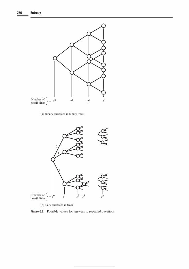
276 Entropy
Figure 6.2 Possible values for answers to repeated questions

277 6.3 Entropy and information: Shannon’s theorem
the base of the logarithm is s. We can therefore write
H (s)(sn) = logs(sn) = n, (6.1)
with a special case being the binary one, s = 2, already discussed. The superscript s in H (s)
indicates the number of possibilities in each question. We have used this as the base in measuringentropy; change of base will be dealt with in the next section.
6.3 Entropy and information: Shannon’s theorem
We again consider the situation in which we had lost an important piece of paper, en-tropy measuring the ‘missing information’ required to find it. The entropy demon is usuallyuncooperative so that the best we can do is to conduct a search. Yet the idea of measuringdisorder by means of missing information is very helpful. Entropy is often interpreted as ameasure of uncertainty; this is appropriate in the sense that the more questions that we have toask to find our missing object, the more uncertain are we.
In the previous section the entropy of sn possibilities was considered, using the base s forour logarithmic measure: the result was n. Let us consider the same number of possibilities, butwith the use of a different base, say b. First, we consider the set of sn equally likely possibilitiesin Figure 6.2(b). Let us denote the entropy of s possibilities to the base b as H (b)(s). Of course,we suspect that the result will be logb(s) but we must show this convincingly. An importantpoint is that we can always decompose the sn possibilities into a series with n nodes of spossibilities, each node of the series being identical in terms of information content (Figure6.2). Therefore the information content of the series is
H (b) (sn) = nH (b) (s) . (6.2)
This equation shows that the information content associated with the nodes in the tree ofFigure 6.2 are additive, each contributing H (b) (s), and resulting in nH (b)(s) in total. Each paththrough the tree constitutes a series of encounters with identical nodes, n in total.
In the following, we continue to consider the entropy to any base b, but for simplicity weomit the superscript and use the notation H (·). Consider now two sets of positive integers{r, m} and {s, n}. We wish to find the entropy of r and s (think of r and s as given and that wecan play with m and n). From Equation (6.2),
H(rm
) = m H (r ) and H(sn
) = nH (s) . (6.3)
We can choose an m, and find an integer n such that
sn ≤ rm < sn+1, (6.4)
where the pairs{sn, sn+1
}cover the range {1, s} ,
{s, s2
},{s2, s3
}, . . . , for n = 0, 1, 2, . . .
It is always possible to locate rm in one of these intervals (rm ≥ 1). We are going to make

278 Entropy
m arbitrarily large in the following, while keeping r and s unchanged; therefore n will alsobecome very large. First, we take logarithms of inequality (6.4):
n ln s ≤ m ln r < (n + 1) ln s,
and consequently
n
m≤ ln r
ln s<
n
m+ 1
m. (6.5)
Natural logarithms have been used in these equations, but any other base could have beenchosen and the results will be valid for any choice.
One of the basic requirements of Shannon’s theory is the very reasonable one that the entropyH (x) should increase monotonically with x . This requirement, combined with inequality (6.4),gives
H(sn
) ≤ H (rm) < H(sn+1
),
and using Equation (6.3),
nH (s) ≤ m H (r ) < (n + 1) H (s) .
It follows that
n
m≤ H (r )
H (s)<
n
m+ 1
m. (6.6)
Combining this inequality with (6.5),∣∣∣∣ H (r )
H (s)− ln r
ln s
∣∣∣∣ <1
m, (6.7)
which is independent of n.We now carry out our earlier suggestion, and make m arbitrarily large. Then Equation (6.7)
implies that
H (t) = k ln t, (6.8)
with k > 0 if H (t) is to increase with t , the number of possibilities. The derivation above wascarried out for integers, and t is therefore any integer. The base of the logarithms could havebeen any number; we used the natural base only for convenience. We can now measure theentropy of any integer to any base.
Example 6.1 If t = 7 and the base is 2,
H = log2 7 = 2.81 . . . bits. (6.9)
The constant k was taken as unity in (6.9) to be consistent with our previous definition ofthe bit. Equation (6.8) is identical to the Boltzmann definition, usually written as S = k log W ,notably on the monument to him in Vienna. We shall return to this definition later in this chapter.

279 6.3 Entropy and information: Shannon’s theorem
The units if one uses natural logarithms are sometimes termed ‘natural units’ or ‘nats’; weshall deal with thermodynamic units later. We can also interpret the value of 2.81 . . . bits –Equation (6.9) – in terms of binary questions using inequality (6.4) as shown in the followingexample.
Example 6.2 Considering the base 2, we can write H (7) = 0.1H(710
), from Equation (6.2),
and we note that 228 < 710 = (22.81...
)10 = 228.1... < 229. Therefore the number of binary ques-tions for 710 equally likely possibilities is between 28 and 29, and the entropy of 7 is boundedby a tenth of these values, i.e. it is between 2.8 and 2.9. We can approximate the entropy of 7in this way to any desired accuracy by considering 7100, 71000, and so on.
Example 6.3 The definition (6.8) is for a random quantity with equally likely possible values.What happens if the events are not equally likely? For example, consider the events {a, b, c, d}with probabilities {1/2, 1/4, 1/8, 1/8} respectively. If we wish to remove the maximum amountof uncertainty at each step, we should halve the probability with each question and answer.The questions that one would ask are: is it a?; if NO, is it b?; if NO, is it c? This is illustratedas a tree in Figure 6.3, in which the branches required to complete an ‘equally likely’ tree,similar to those already considered, are shown in dotted lines.
We now consider a finite partition of n possible events
{B1, B2, . . . , Bi , . . . , Bn}
Figure 6.3 Questions for possibilities {a, b, c, d} with probabilities { 12 , 1
4 , 18 , 1
8 }

280 Entropy
Figure 6.4 Finite partition of n events
with probabilities
{p1 = g1/b, p2 = g2/b, . . . , pi = gi/b, . . . , pn = gn/b}and with
∑ni=1 gi = b. This is shown in the form of a tree in Figure 6.4. The pi are therefore
represented by rational numbers, and indeed correspond to the probabilities of the drawing ofballs of colours 1, 2, . . . , i, . . . , n from an urn containing b balls, with g1 of colour 1, g2 ofcolour 2, . . . , gi of colour i, . . . , and gn of colour n. We shall now convert the tree of Figure 6.4to an equivalent case of equally likely possibilities. This is illustrated in Figure 6.5; in (a) thepossibilities {B1, B2, . . .} have been split into subsets of {g1, g2, . . .} possibilities, respectively.This results in the total set of b equally likely possibilities of Figure 6.5(b), the probability ofeach of which is 1/b. The situation now is different from the original one of Figure 6.4, butrelated. The entropy regarding the b possibilities of Figure 6.5(b) is found using (6.8):
H (b) = k ln b. (6.10)
But we wish to find the entropy corresponding to the partition
{B1, B2, . . . , Bn}of Figure 6.4. We denote this
H {p1, p2, . . . , pn} .
To find this value we note that the entropy associated with the gi possibilities given that Bi istrue is
H (gi ) = k ln gi ; (6.11)
imagine that we are surveying the gi possibilities while standing at Bi in Figure 6.5(a). Foridentifying the true Bi , we do not care which of the gi is true, only that one of these members of

281 6.3 Entropy and information: Shannon’s theorem
g
g
g
g
Figure 6.5 Tree showing conversion of partition {B1, B2, . . . , Bi , . . . , Bn} into equally likelypossibilities
the subset constituting Bi of Figure 6.5(a) is true. The entropy associated with Bi is thereforeEquation (6.10) minus (6.11):
k ln b − k ln gi = −k lngi
b= −k ln pi . (6.12)

282 Entropy
But this will be correct only if the particular Bi under consideration turns out to be the trueevent; the amount to be subtracted in Equation (6.12) depends more generally on which ofthe Bi is true. To deal with this we weight the amount to be subtracted by the correspondingprobability (pi = gi/b) of Bi and sum over all possible Bi . Then
H (p1, p2, . . . , pn) = k ln b − k∑n
i=1pi ln gi
= k∑n
i=1pi ln b − k
∑n
i=1pi ln gi . (6.13)
The final result is then
H (p1, p2, . . . , pn) = −k∑n
i=1pi ln pi , (6.14)
which may be interpreted as the expected value, or prevision, of the missing information thatwould be required to find the true Bi .
Equation (6.14) is equivalent to the formal definition of entropy given in the first section‘Introductory comments’ above except that we have used natural logarithms; this is no short-coming since we have above dealt with the conversion to any other base. The use of the naturalbase is a matter of convenience. We have explained in the preceding sections the sense inwhich Equation (6.14) represents ‘disorder’. The derivation above is based on Shannon’s work(1948); there are numerous references on the connection between entropy and informationtheory, for example Khinchin (1957), Brillouin (1962), Jaynes (1957, 2003) and Martin andEngland (1981).
The derivation given above has been constructed for rational numbers {p1, p2, . . . , pn};if it is postulated that H (p1, p2, . . . , pn) is continuous, then it is valid for any valuesof its arguments (Khinchin, 1957). In reality, only rational numbers are used in compu-tations, and the extension of the mathematical setting into Lebesgue spaces (Martin andEngland, 1981) might appeal to those interested in this subject. In this reference, entropyis defined as a lower bound to the expected number of YES–NO questions to determine thetrue event (as given above), and this is related to the ‘noiseless coding theorem’ of informationtheory.
We stated in the introductory section of this chapter that entropy can be considered as a‘precious jewel with many facets’. The approach based on information theory is the first mainfacet. The second main facet can be introduced by another game played by the demon.
6.4 The second facet: demon’s roulette
It is a scarcely guarded secret that the entropy demon enjoys gambling. He has devised agame to obtain the maximum-entropy solution to a problem. This turns out also to be the mostlikely solution, as we shall see. The germinal problem was the distribution of energy amongst‘identical’ particles, each of which can be in any of n energy (or quantum) states. To modelthis, the demon has constructed a roulette wheel with n divisions, giving n possible outcomes.

283 6.4 The second facet: demon’s roulette
He can set n to any finite value that he pleases. He labels these outcomes {E1, E2, . . . , En},which could be energy levels or any other application where the model makes sense. Thedemon has time on his hands and plays compulsively, N times, such that N � n. He countsthe number of times that the outcomes E1, E2, . . . , Ei , . . . , En occur, resulting in the numbersN1, N2, . . . , Ni , . . . , Nn, with
∑i Ni = N . Probabilities are assigned to the Ei on the basis
that
Pr(Ei ) ≡ pi ≡ Ni/N . (6.15)
The demon is not surprised that the numbers are reasonably close to each other – the resultingdistribution is uniform in this case. To make further progress, the results must be constrained,he explains. The mean, for example of energy, might be constrained to be equal to a certainvalue. We shall see that this changes the distribution from uniform to another shape.
A standard approximation to reality in many cases is that the energy content of a set ofparticles in a certain closed volume is constant. We can therefore state that the mean energy,averaged over all the particles, is fixed, but that the energy of the individual particles fluctuatesin some manner. We now pass this idea to our demon who fiendishly starts his game ofroulette over again. As an example problem, he takes n = 5. The events {E1, . . . , Ei , . . . , E5}are considered, corresponding to five equally spaced divisions of the roulette wheel. Thedemon assigns the values of the random quantity X, {x = 1, 2, 3, 4, 5} to the events Ei fori = 1, 2, . . . , 5, respectively. To test the idea of keeping the mean value constant, the demonagrees to specify that 〈X〉 = 2. The demon proposes to carry out the entire experiment, thatis, to spin the roulette wheel N times, and then to discard the result if the constraint is notsatisfied. For example, if N = 1000, the following result would be discarded:
N1 = 100, N2 = 200, N3 = 300, N4 = 400, N5 = 0, (6.16)
since the values of pi ,
p1 = 0.1, p2 = 0.2, p3 = 0.3, p4 = 0.4, p5 = 0.0, (6.17)
would not lead to the specified mean value of 2 since
(0.1) (1) + (0.2) (2) + (0.3) (3) + (0.4) (4) + (0.0) (5) = 3.0 (6.18)
On the other hand, the values of Ni given by {450, 300, 100, 100, 50} lead to a mean value of2.0, and therefore the imposed constraint is satisfied.
The demon poses the question: if I keep on repeating the experiment, discarding thoseassignments that do not agree with the constraint, what happens? The demon also agrees toincrease the value N to some very large number, say 100 000; each experiment gives him anassignment corresponding to the set {Ni }, with associated probabilities Pr(X = i). The demonhas been through all of this before, and is not surprised to find that certain results come upmuch more frequently than others: to obtain this conclusion he repeats the 100 000 spins of theroulette wheel many times, throwing away those results that do not conform to the imposed

284 Entropy
Figure 6.6 Schematic illustrating sharp peak at maximum entropy solution, becoming a Dirac spike
constraints, until he has many (ℵ) sets of results
{p1 = N1/N , p2 = N2/N , . . . , pi = Ni/N , . . . , pn = Nn/N } , (6.19)
all of which conform to the imposed constraint(s) (there could actually be several constraints).The demon constructs a graph to illustrate the point. The result is illustrated in Figure 6.6 for p1.A certain value of p1 = N1/N is much more likely than the others; this only becomes evidentif the number of repetitions (ℵ) of the entire experiment yielding results that are consistentwith the constraints becomes very large (ℵ � N � n). In the case n = 2, in the absence ofany constraints, the assignment N1 = N2 = N/2 is the most likely; this can be confirmed bynoting that there are many more paths through the ‘centre’ of the random walk diagram ofFigure 2.19, or near the centre of Pascal’s triangle (Table 2.1). A similar situation exists in thecase n > 2, as will be made clear in the following. In a sense the demon’s game represents amodel of nature.
The procedure followed by the demon in fact corresponds to the idea of an ‘ensemble’introduced by Gibbs. As noted, the germinal problem was the distribution of energy amongsta set of particles. A Gibbs ensemble is a set of N imagined copies of the real system underconsideration. The system could be a set of particles, for instance molecules in a gas, or in thecase of solids, the energy levels of an oscillator or the atomic vibrations at eigenfrequenciesof the solid (normal modes of vibration). In Aston and Fritz (1959),‘elements’ are elementaryparticles, atoms, molecules or modes of vibration (for example in crystals). A system containsmany elements, and a large number of systems is an ensemble. Fundamental particles will bedealt with further in Sections 6.8 and 6.9.
We can carry out a calculation that gives a result similar to the demon’s. This shows that thedemon is in fact maximizing the entropy of Equation (6.14). First, we write an expression forthe number of ways that the demon would obtain a particular result. We return to the case ofn outcomes and N spins of the wheel, with a result N1, N2, . . . that is in conformity with the

285 6.4 The second facet: demon’s roulette
imposed constraint(s). If the roulette wheel is perfectly balanced, as we have assumed in theforegoing, each of the possible ways w of obtaining the result is equally likely, and
w =(
N
N1 N2 · · · Ni · · · Nn
)= N !
N1!N2! · · · Ni ! · · · Nn!. (6.20)
For example with n = 2 and N = 6, and no constraints, there are 26 = 64 possible outcomeswith likelihoods of {1, 6, 15, 20, 15, 6, 1} for the outcomes N1 = {0, 1, 2, 3, 4, 5, 6} respec-tively (Pascal’s triangle). If the experiment (consisting of six trials) is repeated many times, theresult N1 = 3 occurs (on average) in the proportion (20/64) of the time, where the value 20 isobtained from Pascal’s triangle. For the maximum entropy solution, we wish to increase ℵ; wecould for example repeat the six trials a million times. But we also need to increase N . WhenN becomes very large there is a solution that is overwhelmingly likely. We shall demonstratethis in the following.
Returning to the general case, we wish to maximize Equation (6.20); this is a convenientrelative measure of the proportion of times a particular result will occur within the totalnumber of repetitions ℵ of the entire experiment, all of which yield results conforming to theconstraints. It is convenient in the present case to maximize (ln w) rather than w, since theyare monotonically related. Now
ln w = ln N ! −∑n
i=1ln Ni !. (6.21)
Next, we replace Ni with N · pi where pi is the probability assignment to the i th event Ei .Thus
ln w = ln N ! −∑n
i=1ln (N pi )!. (6.22)
We now use the Stirling approximation
N ! →√
2π N N N exp (−N ) (6.23)
as N → ∞. The proof of this formula is given in Feller (1968). Consequently,
ln N ! →(
N + 1
2
)ln N − N + 1
2(ln 2π ) (6.24)
as N → ∞. For large N , this tends to
(N ln N − N ). (6.25)
Substituting this into Equation (6.22), and noting that N − ∑i (N pi ) = 0,
ln w → N ln N −∑n
i=1[N pi ln N pi ]
= N ln N − N ln N∑n
i=1pi − N
∑n
i=1pi ln pi .
Therefore
ln w → −N∑n
i=1pi ln pi ; (6.26)

286 Entropy
apart from the coefficient N , this expression is identical to Equation (6.14). In fact, N iseventually replaced by k; this has no effect on the deliberations that follow since it is thesummation in the expression (6.26) that we wish to maximize. Later on, we will deal withthermodynamic units.
The spirit of the mathematical rendering of the entropy demon’s game leading to the expres-sion (6.26) was to find the probability distribution that occurs with greatest likelihood. Thecoefficient N in this expression represents the number of spins of the roulette wheel in onerealization of Equation (6.19), and the entire expression (6.26) represents the natural logarithmof the number of ways that a particular assignment {N1, N2, . . .} would be achieved. This isthen a convenient measure (to a logarithmic scale) of the proportion of times a particular resultwill occur if the whole procedure (spinning N times) were repeated many times (ℵ), all ofwhich yield results conforming to the constraints.
We wish then to choose the assignment that occurs with by far the greatest probability inthe demon’s game, and therefore we choose that distribution which maximizes
H = −∑n
i=1pi ln pi , (6.27)
in which we have omitted the factor N in expression (6.26). But the number of ways, w, isgiven by
w = exp (N H ) , (6.28)
and this becomes very large for large N and maximum H . See also Equation (6.85).
6.5 Maximizing entropy; Maxwell–Boltzmann distribution; Schrodinger’s nutshell
Methodology and introductory exampleWe saw in the preceding section that the probability distribution that maximises entropy is byfar the most likely distribution to occur in a random game such as that played by the demon,subject to the constraints of the problem. This suggests the idea of using mathematics to findthis distribution, resulting in the maximum-entropy method. The basic idea in the maximum-entropy method then is to maximize (6.27),
H = −∑n
i=1pi ln pi ,
subject to any constraints of the problem. This yields a probability distribution which hastwo main interpretations. In the first, the maximum-entropy distribution corresponds to thatfor which the maximum expected number of questions have to be asked to obtain the trueevent, as in Section 6.3 and Equation (6.14). There is a minimum amount of informationembodied in the probability distribution, other than what is contained in the constraints. Itis therefore ‘maximally non-committal with regard to missing information’, to use Jaynes’phrase. It is also the ‘flattest’ probability distribution consistent with the constraints. In the

287 6.5 Schrodinger’s nutshell
second interpretation, we obtain the probability distribution that is most likely in the demon’sroulette game, overwhelmingly, as in Section 6.4 and Equations (6.26) and (6.27).
In accordance with the prescription just given, we want to maximize Equation (6.27) subjectto any constraints in the problem for which we wish to derive a distribution of probability.This is best achieved by the use of Lagrange multipliers, which provide a useful and elegantway to proceed. The relevant theory was outlined in Section 5.3.2. It is helpful to introducethe procedure using an example; see also Jaynes (2003).
Example 6.4 An interesting and important problem to discuss so as to illustrate the develop-ment of the theory is the germinal one noted before, in which the outcomes represent energylevels X . We wish to find the maximum-entropy distribution, subject to the condition that themean value of X is fixed. To illustrate the method, let us assume that the random quantityhas three possible outcomes. X = 0, 1, 2 for i = 1, 2, 3 respectively. Let Pr(X = 0) = p1,
Pr(X = 1) = p2 and Pr(X = 2) = p3. The problem to be solved can be summarized asfollows.
Max(
H = −∑3
i=1pi ln pi
)(6.29)
subject to∑3
i=1pi = 1 (6.30)
and∑3
i=1xpi = 〈X〉 = µ,
which becomes
0 · p1 + 1 · p2 + 2 · p3 = 〈Xi 〉 = µ
or
p2 + 2p3 = µ. (6.31)
In the last three equations, µ stands for the mean value.The solution requires us to maximize the entropy, Equation (6.29), subject to the constraints
of (6.30) and (6.31). The Lagrangian is
L(p1, p2, p3; λ′
0, λ1) = −
∑3
i=1pi ln pi − λ′
0
(∑3
i=1pi − 1
)− λ1(p2 + 2p3 − µ) ; (6.32)
the reason for the use of the notation{λ′
0, λ1}
will become clear in the following. Differentiatingthe Lagrangian:
∂L
∂p1= (− ln p1 − 1) − λ′
0 = 0

288 Entropy
∂L
∂p2= (− ln p2 − 1) − λ′
0 − λ1 = 0
∂L
∂p3= (− ln p3 − 1) − λ′
0 − 2λ1 = 0
∂L
∂λ′0
= − (p1 + p2 + p3 − 1) = 0
∂L
∂λ1= − (p2 + 2p3 − µ) = 0. (6.33)
In differentiating H = − ∑i pi ln pi with respect to pi , we always obtain the term
(− ln pi − 1), as indicated above. It is most convenient to write
−λ0 = −λ′0 − 1, (6.34)
in which we have borrowed (−1) from the derivative of H ; this will always be done in thefollowing. From the first three derivatives of the Lagrangian, we can write
p1 = exp (−λ0) , p2 = exp (−λ0 − λ1) , p3 = exp (−λ0 − 2λ1) , (6.35)
and where we have used the first three derivatives of the Lagrangian L . The first of the tworemaining conditions, which is the constraint giving the normalization of probabilities, reducesto
exp (−λ0)[1 + exp (−λ1) + exp (−2λ1)
] = 1
or
exp λ0 = 1 + exp (−λ1) + exp (−2λ1) ; (6.36)
this is termed the partition function Z . This function and its important uses are described inmore detail below. In the present case,
Z (λ1) = exp λ0 =∑
jexp
(−λ1x j)
, j = 0, 1, 2.
The second constraint yields the following equation:
exp (−λ0)[exp (−λ1) + 2 exp (−2λ1)
] = µ. (6.37)
We can solve for the probabilities using Equations (6.35), (6.36) and (6.37). We assume firstthat µ = 1. Then Equations (6.35) and (6.36) can be combined to eliminate exp (−λ0) , givingexp (−2λ1) = 1, or λ1 = 0. Hence p1 = p2 = p3 = 1/3, as expected since the mean is at thecentre of the three values. For the case where µ = 0.5, and following the same procedure, itis found that
1.5 exp (−2λ1) + 0.5 exp (−λ1) − 0.5 = 0,
which may be solved as a quadratic equation to yield p1 = 0.616, p2 = 0.267, and p3 = 0.116(see Figure 6.7).

289 6.5 Schrodinger’s nutshell
Figure 6.7 Maximum entropy solution to problem with three possibilities
Canonical aspects and the nutshellThe derivation in Example 6.4 can be generalized to the result that is termed the ‘canonicalensemble’. Do not be put off by this rather forbidding expression. Of course the demon reallydislikes the canonical aspect! We are trying to obtain the distribution of energies amongstsystems that have a fixed number of particles. We can interpret for this example the system asa set of particles, or a macroscopic sample which the demon interrogates to find the energylevel of a particle in the sample. The energy is denoted as E and the possible energy states are{e0, e1, e2, . . . , ei , . . .}, a countably infinite set (we are now starting with e0 rather than e1 as itis convenient to do so; no following arguments are affected by the choice). The probability thatany system is in a state corresponding to energy ei is denoted pi . Imagine that we have a set ofN mental replicas of this system, and that the systems are placed in a heat bath at temperatureT , thermally insulated so that the total energy content is constant. This could be thought of asa ‘supersystem’ comprising the N replicas, with a convenient thermodynamic interpretation.
In Section 3.6.3, when discussing stochastic processes, it was pointed out that considerationof an ‘ensemble’ of outcomes was not necessary in modelling a random quantity in time; one hasonly to think of the random quantity. The same applies in the present case. The mental replicasof the preceding paragraph are similarly convenient ways of thinking about and representingthe situation to assist in developing a thought-experiment. A ‘mechanistic’ world of this kindcan be constructed following inductive reasoning and is useful in modelling and carrying outsimulations. But we could have merely stated that we are uncertain about the energy level ofparticle i and proceeded directly to Equations (6.40) to (6.42) below.
To continue with the thought-experiment: each replica corresponds to a spin of the demon’sroulette game, which is repeated N times. This leads to an assignment of probabilities
p0 = N0
N, p1 = N1
N, p2 = N2
N, · · · , Ni
N, · · · , and so on. (6.38)
As before, he then repeats the whole experiment (N trials) ℵ times to find the most likelydistribution. Probabilities are to be assigned subject to the only constraint that the total energyof the supersystem should be constant – since it is thermally insulated. If we average this

290 Entropy
energy over the systems, we find that the mean energy must be constant; therefore∑∞i=0
pi ei = 〈E〉 = µ, (6.39)
where µ denotes the mean energy. The problem of distributing the probabilities follows thedemon’s method; we play roulette subject to the constraints of the problem.
Mathematically, this is equivalent to
Max(
H = −∑∞
i=0pi ln pi
)(6.40)
subject to∑∞i=0
pi = 1 (6.41)
and∑∞i=0
pi ei = 〈E〉 = µ. (6.42)
We then form the Lagrangian
L = H − λ′0
(∑∞i=0
pi − 1)
− λ1
(∑∞i=0
pi ei − µ)
, (6.43)
and differentiate:
∂L
∂pi= − ln pi − λ0 − λ1ei = 0,
where λ0 = λ′0 + 1, as before in Equation (6.34). Hence
pi = exp (−λ0) exp (−λ1ei ) . (6.44)
Now the probabilities are coherent – Equation (6.41) – and therefore
exp λ0 =∑∞
i=0exp (−λ1ei ) (6.45)
which defines the partition function
Z ≡ exp λ0, (6.46)
as before. The normalization of probabilities appears in the Lagrangian as the first constraintmultiplied by the multiplier λ′
0; the second constraint fixes the mean. We write (6.44) as
pi = exp (−λ1ei )
Z (λ1). (6.47)
The partition function Z is termed the ‘Zustandssumme’ in German, or ‘sum-over-states’,which has led to the use of the symbol Z ; thus, from Equation (6.45),
Z (λ1) =∑
iexp (−λ1ei ) . (6.48)
A term of this kind appears as a normalizing constant in all maximum-entropy distributions. (Itarises from the condition of coherence
∑i pi = 1.) The following equations may be deduced

291 6.6 Maximum-entropy probability distributions
with relative ease; the first fixes the mean of the distribution.
µ = 〈E〉 = −∂ ln Z
∂λ1(6.49)
pi = − 1
λ1
∂ ln Z
∂ei. (6.50)
Schrodinger (1952) suggested that the second of these equations, (6.50), contains the wholeof thermodynamics ‘in a nutshell’. Indeed, it specifies the entire probability distribution ofenergy.
If we use Equation (6.14), i.e. H = −k∑
pi ln pi , and if there are w events which we judgeto be equiprobable (pi = 1/w for each i), the expression for entropy is
H = k ln w, (6.51)
which is Boltzmann’s formula. The constant k is Boltzmann’s constant, equal to 1.38 × 10⁻²³
Joules per degree K. We can write (6.47) as
pi = exp (−λ1ei )∑i exp (−λ1ei )
. (6.52)
For equally spaced small intervals de with ei in the i th interval, i = 0, 1, 2, . . . ,
pi = fE (e) de = exp (−λ1e) de∫ ∞e=0 exp (−λ1e) de
,
where fE (e) is now a density (see also Example 6.5 below). Carrying out the integration,
fE (e) = λ1 exp (−λ1e) , (6.53)
which may also be written as
fE (e) = exp (−e/kT )
kT, (6.54)
where λ1 = 1/kT . The term kT is the average energy of the oscillators (Eisberg and Resnick,1974). Thus (e/kT ) is dimensionless, as is appropriate.
6.6 Maximum-entropy probability distributions
We have just maximized entropy subject to the single constraint that the mean is fixed, resultingin the exponential distribution (6.52). The maximization of entropy can be carried out for thecase where there is a set of constraints. We consider, as before, a random quantity associatedwith the set of numbers {0, 1, 2, 3, . . . , i, . . .}. We denote this quantity as Xi with Pr(Xi =xi ) = pi . The set of constraints is associated with the functions g j (xi ). The problem is thenposed as follows:

292 Entropy
Max(
H = −∑
ipi ln pi
)
subject to∑i
pi = 1
and the following specified values of the mean ν j :∑i
g1 (xi ) pi = 〈g1 (X )〉 = ν1,∑i
g2 (xi ) pi = 〈g2 (X )〉 = ν2,
...∑i
g j (xi ) pi = 〈g j (X )〉 = ν j ,
...∑i
gm (xi ) pi = 〈gm (X )〉 = νm . (6.55)
Then the Lagrangian can be written as
L = −∑
ipi ln pi − λ′
0
(∑i
pi − 1)
−∑m
j=1λ j
[∑i
g j (xi ) pi − ν j
], (6.56)
where the constraints (6.55) have been condensed into a sum of terms, these having first beenmultiplied by the appropriate Lagrange multiplier. Following the same procedure as before,differentiating the Lagrangian and equating to zero, it is found that
pi = exp[−λ0 −
∑m
j=1λ j g j (xi )
]. (6.57)
From the condition of coherence (∑
pi = 1)∑
iexp
[−λ0 −
∑m
j=1λ j g j (xi )
]= 1,
which gives the partition function
Z (λ1, λ2, . . . , λm) = exp λ0 =∑
iexp
[−
∑m
j=1λ j g j (xi )
]. (6.58)
Hence
pi =exp
[− ∑m
j=1 λ j g j (xi )]
Z (λ1, λ2, . . . , λm). (6.59)
Also
λ0 = ln Z . (6.60)
There are several important applications of this distribution. First, in statistical mechanics,we may derive the Gibbs’ grand canonical ensemble. This is an even more forbidding title, andagain the demon takes exception to the canonical aspect. (Although he likes mathematics in

293 6.6 Maximum-entropy probability distributions
its most authoritative form.) The methodology outlined above follows a relatively straightfor-ward recipe; the ingredients are entropy, the constraints, the formation of the Lagrangian, andthe differentiation of the latter to obtain the desired distribution. The partition function thenprovides a summary of the whole result.
The following relationships are interesting and useful.
〈g j (X )〉 = ν j = −∂ ln Z
∂λ j. (6.61)
Hmax ≡ S = λ0 + λ1 〈g1 (X )〉 + · · · + λm 〈gm (X )〉= λ0 + λ1ν1 + · · · + λmνm . (6.62)
This defines the maximum entropy Hmax ≡ S, which is a function of λ0 = ln Z and the expectedvalues only. The variance of the distribution of g j (X ) is given by
σ 2G j
= ∂2λ0
∂λ2j
, (6.63)
and the covariance by
σG j ,Gk = ∂2λ0
∂λ jλk. (6.64)
See Exercise 6.4 for more details on these and related relationships.The exponential and normal distributions in their continuous form can also be seen as part
of the present theory, as illustrated in the following two examples.
Example 6.5 Exponential distribution. Consider Equation (6.59) in the following form:
pi =exp
[− ∑m
j=1 λ j g j (xi )]
∑k exp
[− ∑m
j=1 λ j g j (xk)] . (6.65)
We consider first the case where j = m = 1, and g1(xi ) = xi , and obtain essentially Equa-tion (6.47) again, but with X as the random quantity rather than E :
pi = exp (−λ1xi )∑k exp (λ1xk)
.
Now divide the x-axis into equally spaced intervals �x such that xi is contained in the i thinterval; i = 0, 1, 2, . . . , i, . . . Then
pi =[exp (−λ1xi )
] · �x∑k
[exp (−λ1xk)
] · �x.
In the limit as �x → 0,
pi = fX (x) dx = exp (−λ1x) dx∫ ∞x=0 exp (−λ1x) dx

294 Entropy
or, carrying out the integration,
fX (x) = λ1 exp (−λ1x) , (6.66)
which is the familiar exponential distribution with mean and standard deviation equal to 1/λ1;this was derived before as (6.53). If the constraint equation is written as
∑pi xi = µ, then
1/λ1 ≡ µ.
Example 6.6 Normal distribution. We consider now the case where g1 (xi ) is again equal toxi , with
∑pi xi = µ, and the second constraint is∑
pi (xi − µ) = σ 2. (6.67)
Equation (6.67) suggests that the variance (or equivalently the standard deviation) is fixed. Theconstraint may be written as∑
pi x2i = σ 2 + µ2, (6.68)
so that we take g2 (xi ) = x2i . Using Equation (6.65) and dividing the x-axis into equally spaced
intervals i = . . . ,−2, −1, 0, 1, 2, . . . , with xi contained in the i th interval, and following thesame procedure as before, it is found that
pi = fX (x) dx = exp(−λ1x − λ2x2
)dx∫ ∞
−∞ exp(−λ1x − λ2x2
)dx
. (6.69)
This can be written in the familiar form
fX (x) = 1√2πσ
exp
[−1
2
(x − µ
σ
)2]
, (6.70)
in which λ1 and λ2 have been solved for in terms of µ = ∫x fX (x) dx and σ 2 =∫
(x − µ)2 fX (x) dx . The distribution is dealt with in Sections 3.3.3 and 7.5. In the lattercase, the central limit theorem is used to derive the distribution as the ‘model of sums’. Themaximum-entropy derivation above is the simplest way to deduce this distribution from atheoretical standpoint, but all derivations give special insights.
In the case that all first and second moments are specified in the case of several randomquantities {X, Y, Z , . . .} the maximum-entropy distribution is the standard multidimensionalnormal distribution with the given moments. See Exercise 6.7.
Transition from discrete to continuous distributions Jaynes in his 1963 Brandeislectures (Jaynes 1963b; Rosenkrantz, 1983) discussed the question of the transition fromdiscrete to continuous probability distributions. In the expression for entropy derived in thepreceding,
H = −∑
pi ln pi , (6.71)
295 6.6 Maximum-entropy probability distributions
we can take
pi = Pr (xi ≤ X < xi+1) = fX (x) dx,
where fX (x) is the density corresponding to discrete probabilities pi and pi+1 at points xi
and xi+1 respectively. The difference (xi − xi+1) is equal to dx . The equivalence of pi andfX (x) dx seems natural in the probabilistic weighting pi of (ln pi ) in (6.71). But in the term(ln pi ), Jaynes argues for the inclusion of a function m (x) measuring the density of points inthe transition from the discrete to the continuous case (in units of proportion of points per unitlength). If there are h points in total over the range of x, then
1
dx= hm (x)
since there is one point added in the interval x to x + dx, or
dx = 1
hm (x).
Then
pi → fX (x)
hm (x)(6.72)
in the transition from discrete to continuous. The final result is
H = −∫
fX (x) ln
[fX (x)
m (x)
]dx (6.73)
from which an infinite term corresponding to (ln h) has been subtracted, leaving the terms ofinterest. This strategy hinges on the use of the function m (x) . It also deals with problemsof invariance in the continuous form of the expression for entropy. In the transition to thecontinuous distributions, Equations (6.66) and (6.70) above, we have taken m (x) as a constant.
6.6.1 Grand canonical ensemble
We now outline the grand canonical ensemble and the grand partition function. These arederived for the case where there is uncertainty regarding the number of particles in the system,in addition to that regarding the energy level or quantum state. We can think of our system asa ‘leaky box’, a device used by Tribus (1961) to explain the present situation. Other referencessuch as Gopal (1974), Eisberg and Resnick (1974) and Kapur and Kesavan (1992) might beconsulted. Previously, we considered that the number of particles in our system was fixed;this corresponded to the number n for which N trials (N � n) by the demon were conducted.Fundamental particles have a finite probability of penetrating a wall; photons are absorbedand emitted by the walls in a blackbody, with higher energy particles being converted into anumber of lower energy ones and vice versa, so that the number of particles is not fixed.
In Section 6.5, each trial corresponded to the demon ‘interrogating’ the system to find theenergy level of a particle in a spin of the roulette wheel. In the grand canonical ensemble, the
296 Entropy
systems (leaky boxes) are once again placed in a ‘supersystem’ containing N (leaky) boxessuch that the number of particles in this supersystem is fixed. The implication of this is that themean number of particles is fixed, but that the number varies from one realization to another,modelled as a random quantity in the demon’s game. The demon would be faced with having tosample a different number of particles from L (random) with particular values � = 0, 1, 2, . . . ,
each time he wishes to sample an energy level. For each of these combinations, he again playsN times, selecting only those results that conform to the constraints. For � particles, let there bek� energy levels corresponding to the quantum states. Let i denote all of the combinations of �
and k�. This can reasonably be modelled as being countably infinite. The whole experiment isrepeated ℵ times. The number of ways of obtaining the result is counted over all combinationsof � and k�, represented by i. We consider here only one type of particle; the analysis is easilyextended to more than one (see Tribus, 1961).
The problem reduces to that introduced above, that of finding
Max(
H = −∑
ipi ln pi
)
subject to∑i
pi = 1
with the following equations representing the constraints corresponding to Equations (6.55):∑i
pi ei = 〈E〉 (6.74)
∑i
pi�i = 〈L〉. (6.75)
The functions g1(xi ) and g2(xi ) in Equations (6.55) become ei and �i with xi = i. FollowingEquations (6.58) and (6.59) above, the solution is
pi = exp (−λ1ei − λ2�i )
Z (λ1, λ2), (6.76)
where
Z (λ1, λ2) = exp λ0 =∑
iexp (−λ1ei − λ2�i ) , (6.77)
and where there are two Lagrange multipliers, with m = 2 in Equation (6.55) above. The results(6.76) and (6.77) form the basis of Bose–Einstein and Fermi–Dirac statistics, to be discussedfurther in Sections 6.8 and 6.9 below. Equation (6.77) is usually written in the form
Z (µ, T ) =∑
iexp [(µ�i − ei ) /kT ] , (6.78)
where µ is the chemical potential. In the function Z of Equations (6.76) and (6.78) one canthink of i as ranging over all the values of �, and for each �, ranging over all the �-particlequantum states of the system.
Again, the use of ‘mental replicas’ in the reasoning above provides a mechanistic frame-work within which we can ask the demon to perform experiments provided the mood of the

297 6.7 Nature of the maximum: interpretations
moment takes him in that direction, or for us to perform Monte Carlo experiments of ourown. But the fundamental idea is merely to maximize the entropy function subject to specifiedconstraints.
6.7 Nature of the maximum: interpretations
We have mentioned that the entropy maximum is an absolute maximum, and that we donot have to worry about saddle points and the like. We shall give a proof of this statement,based on the presentation of Tribus (1969). First, we use the main result of the first part ofthe preceding section, with Hmax ≡ S, (6.62), and contrast this with another result that alsosatisfies the imposed constraints, but does not maximize entropy. We term these results A andB respectively. The probabilities assigned to the random quantity Xi are denoted pi and qi
respectively. Both assignments are coherent.We may now calculate
S − T = −∑
pi ln pi +∑
qi ln qi .
First, we add and subtract∑
qi ln pi , giving
S − T = −∑
(pi − qi ) ln pi +∑
qi ln
(qi
pi
). (6.79)
But we know that
ln pi = − ln Z −∑
jλ j g j (xi ) (6.80)
from (6.59), where ln Z ≡ λ0. Substituting for ln pi in the first term on the right hand side ofEquation (6.79),
S − T = λ0
∑i(pi − qi ) +
[∑i
pi
∑jλ j g j (xi ) −
∑iqi
∑jλ j g j (xi )
]
+∑
iqi ln
(qi
pi
).
Now the first term in this equation disappears as a result of coherence of both systems(Table 6.1). The terms in the square brackets add to zero since the first one is∑
ipi
∑jλ j g j (xi ) =
∑jλ j
∑i
pi g j (xi ) =∑
jλ jν j ,
with the same result for the second since they both satisfy the constraint equations (Table 6.1).As a consequence
S − T =∑
iqi ln
(qi
pi
). (6.81)

298 Entropy
Table 6.1 Comparison of systems, A satisfyingS ≡ Max(H = − ∑
pi ln pi ), and B with differentprobabilities qi
A B
S = − ∑pi ln pi T = − ∑
qi ln qi∑pi = 1
∑qi = 1∑
i g j (xi ) pi = ν j∑
i g j (xi ) qi = ν j
pi = 1Z exp
[− ∑
j λ j g j (xi )]
The qi differ from case A
To prove that this represents a positive quantity with a minimum at qi = pi , we make thefollowing change to Equation (6.81):
S − T =∑
i�Si =
∑i
[qi ln
(qi
pi
)− qi + pi
], (6.82)
where the notation �Si has been introduced, and the addition and subtraction of probabilitiesqi and pi make no difference to the quantity S − T, since both qi and pi normalize to unity.Taking each term �Si at a time we find
∂�Si
∂qi= ln qi − ln pi (6.83)
and
∂2�Si
∂2qi= 1
qi. (6.84)
The first derivative shows that there is a point of inflexion of each �Si at qi = pi , and thesecond, being always positive, shows that they reach a minimum at this point. The expression�Si = [qi ln (qi/pi ) − qi + pi ] is zero at qi = pi . Therefore the �Si and their sum, S − T, arealways positive, except when qi = pi . The maximum entropy value is then an unconditionalmaximum. Tribus (1969) ascribes the elegant last part of the proof to Gibbs.
We can now use Equation (6.26) to state that
w
w′ = exp [N (S − T )] , (6.85)
where w′ is the number of ways in which the solution corresponding to T can be realized,rather than S, for which there are w ways. This can be made as large as we like, so that forlarge enough N , the maximum-entropy solution has a likelihood corresponding to a probabilityspike of unit mass. (See also Figure 6.6 above.)
Bayesian thought experiment We could also consider the maximization of entropy as a‘thought experiment’ in which Bayesian updating is used, conditional on the thought experi-ment, with vague prior probabilities. The experiment is aimed at comparing various solutions

299 6.8 Blackbodies and Bose–Einstein distribution
such as the sets corresponding to pi and qi above. We can compare the ‘A’ and ‘B’ solutionsusing
Pr (solution|results of thought experiment) ∝ Pr (results|solution method)
∝ w, or w′, (6.86)
for solutions A and B respectively. The result is in accordance with (6.20) and the vague priorinformation being absorbed since it is essentially a constant and dominated by the likelihoodfunction. The maximum-entropy solution is much more likely than any other, consistent with(6.85).
6.8 Blackbodies and Bose–Einstein distribution
6.8.1 Blackbodies
The idea of the blackbody – seemingly vague – is indeed precise enough to have enabled MaxPlanck to discover the quantization of energy, first communicated in 1900. This is an elegantpiece of theory, yet there were serendipitous aspects to his discovery, as we shall describe.Segre (1980, 1984), in two historical works, gives an interesting account of the developmentof the theory, tracing the twists and turns of the experimental and theoretical reasoning. Hetermed it an ‘encompassing problem’. It is a common experience on a bright day that a roomwith an uncovered window will appear dark from the outside. The room acts as a trap forradiation which enters through the window. We know that black objects absorb radiation,and appear black for this reason. Examples are the room just mentioned, or the pupil of theeye. Conversely, white objects reflect light at all frequencies, and green objects absorb lightradiation at all frequencies except those corresponding to green, which are reflected.
All bodies emit thermal radiation as a result of their temperature and absorb radiationfrom their surroundings. The frequency of the radiation increases with temperature and hotbodies – including black ones – become visible at high temperatures even without any lightreflected from them. The porcelain maker Wedgwood observed and noted in 1792 that allbodies when heated become red at the same temperature. This can be confirmed in a roughway by observation of a campfire, grill, stones, and other objects in a fire turning red at thesame temperature. Kirchhoff considered the power emitted per unit surface area (emissivity e)for an interval of frequency, as well as the energy absorbed per unit time; these are in units ofpower per unit frequency per unit area. The surface is at temperature T and emits energy inthe frequency interval ν to ν + dν at the rate e (ν, T ) dν per unit area and per unit time. Thequantity e depends upon the nature of the surface. The fraction of power falling on the surfacethat is absorbed by it is a, where a is a number between 0 and 1.
The two opposing surfaces shown in Figure 6.8(a) are black and white. These are enclosedin a box such that there is no contact between the materials, and they can exchange heat onlyby radiation. The interior of the box is maintained at the same temperature T . For a blackbody

300 Entropy
Figure 6.8 Radiation and absorption between two surfaces

301 6.8 Blackbodies and Bose–Einstein distribution
a = 1, since all radiation is absorbed and none is reflected. The white surface reflects someradiation, but also absorbs and radiates the remainder. The surfaces are at constant temperatureand therefore there must be no net absorption of radiation by either. The flows in the twodirections in Figure 6.8(a) must then be the same, and this demonstrates that blackbodies mustbe the best radiators of energy. Good absorbers are therefore good radiators.
We now consider the situation in Figure 6.8(b), where two surfaces 1 and 2 are shown.These can be black or white, or any other colour or texture. The radiation from the surfaces isdenoted e1 and e2 respectively. The absorption is e2a1 and e1a2 respectively, with correspondingreflections of e2 (1 − a1) and e1 (1 − a2). For constant temperature of the left hand surface,
e1 + e2 (1 − a1) = e2a1 (6.87)
or
e1 + e2 = 2e2a1. (6.88)
Similarly, for the right hand surface,
e1 + e2 = 2e1a2. (6.89)
Therefore
e1a2 = e2a1 (6.90)
ore1 (ν, T )
a1 (ν, T )= e2 (ν, T )
a2 (ν, T )= u (ν, T ) , (6.91)
in which the function u is independent of the surface, and therefore a universal function, givingthe spectral density. The result is Kirchhoff’s law of heat exchange, showing that the ratio ofemissivity to absorption coefficient is independent of the nature of the body and a function offrequency and temperature only.
The use of a cavity with the interior walls maintained at constant temperature and whichcommunicates with the exterior through a small aperture provides a very good experimentalapproximation to a blackbody. This strategy results in radiation that is independent of thematerial. For a blackbody a = 1, since all radiation is absorbed and none is reflected. Blackradiation has the characteristic of perfect randomness, with propagation in all directions anda definite spectral distribution of energy. The apparatus employed in the early blackbodyexperiments is shown in Figure 6.9, together with some of the results. It should be noted thatat high temperatures, blackbodies will not appear black; stars and planets are modelled asblackbodies. In this way, the sun could be modelled as a blackbody at 6000 K.
6.8.2 Partition function, probabilities and solution
The derivation of the Bose–Einstein distribution provides the solution to the problem. Themethodology is embodied in Section 6.6, and the grand partition function. The particles in the

302 Entropy
Figure 6.9 Measurements of blackbody radiation. Based on H. Rubens and F. Karlbaum, Annalen derPhysik 4, 649 (1901)

303 6.8 Blackbodies and Bose–Einstein distribution
present case are bosons; more accurately, we shall eventually deal with a special case of this,photons. We repeat the main result previously obtained, Equation (6.77):
Z (λ1, λ2) = exp λ0 =∑
iexp (−λ1ei − λ2�i ) , (6.77)
with
pi = − 1
λ1
∂ ln Z (λ1, λ2)
∂ei= exp (−λ1ei − λ2�i )
Z (λ1, λ2). (6.92)
The usual form for Equation (6.77) was given in Equation (6.78):
Z (µ, T ) =∑
iexp [(µ�i − ei ) /kT ] . (6.78)
As we noted above, Schrodinger suggested that the results can be embodied in the logarithmof the partition function, containing everything in a nutshell. In the present case, (ln Z ) isknown as the grand potential, derivatives of which give the probabilities of various energylevels and the equations of state. Here we outline the theory to give the solution to the radiationproblem.
In the case of bosons, the energy of the system is the sum of the ‘private’ energies of theparticles. Each particle is therefore treated as being independent of the others. For � particleswith energy ε, the energy level in the expression for Z is
e = �ε (6.93)
for the quantum state considered. Equation (6.78) for Z can be shown to reduce to
Z =∏∞
i=1{1 − exp [(µ − εi ) /kT ]}−1 =
∏∞i=1
ξi , (6.94)
where εi is the particle energy and
ξi = {1 − exp [(µ − εi ) /kT ]}−1 . (6.95)
Equation (6.94) can be shown directly, and this is the subject of Exercise 6.8.We shall here demonstrate its character using a related method (Tribus, 1961). This first
requires us to recall that the summation in Equations (6.77) and (6.78) consists of i coveringall the values of �, and for each �, all the �-particle quantum states of the system. There istherefore a double summation implied. Now there is a neat and simple way to express thepartition function. First note that
ξi = 1
1 − exp [(µ − εi ) /kT ]= {1 − exp [(µ − εi ) /kT ]}−1
= 1 + exp [(µ − εi ) /kT ] + exp [(2µ − 2εi ) /kT ] + exp [(3µ − 3εi ) /kT ] + · · · (6.96)

304 Entropy
We shall demonstrate the idea by considering two states ε1 and ε2. Consider the product of thefollowing two terms taken from (6.94), using (6.96).
ξ1ξ2 = 1
1 − exp[(µ − ε1)/kT ]· 1
1 − exp[(µ − ε2)/kT ]= {1 + exp[(µ − ε1)/kT ] + exp[(2µ − 2ε1)/kT ]
+ exp[(3µ − 3ε1)/kT ] + · · ·}{1 + exp[(µ − ε2)/kT ]
+ exp[(2µ − 2ε2)/kT ] + exp[(3µ − 3ε2)/kT ] + · · ·}= 1
+ exp[(µ − ε1)/kT ] + exp[(µ − ε2)/kT ]
+ exp[(2µ − 2ε1)/kT ] + exp[(2µ − ε1 − ε2)/kT ] + exp[(2µ − 2ε2)/kT ]
+ exp[(3µ − 3ε1)/kT ] + exp[(3µ − 2ε1 − ε2)/kT ]
+ exp[(3µ − ε1 − 2ε2)/kT ] + exp[(3µ − 3ε1)/kT ] + · · · (6.97)
The series includes a term for no particles and consequently zero energy, represented by thevalue of unity at the beginning. Then two terms represent the likelihood of a single particlebeing in the two energy states ε1 and ε2 respectively. The next three terms (third line of (6.97)above) represent the likelihood of two particles being in the first state, one in the first and onein the second, or both in the second state, respectively. The states can be thought of as boxesin which the (indistinguishable) particles are arranged. This is illustrated in Figure 6.10. Thearrangements of three particles, and the corresponding terms in the fourth and fifth lines ofexpression (6.97) above are made clear in this figure. (Reference is also made to the occupancyproblems and the introduction to Bose–Einstein statistics given in Section 2.6.3 and Table 2.3.)The terms of expression (6.97) represent all of the possible arrangements of any number ofparticles between two states.
It can be checked that if all terms of the kind
ξi = 1
1 − exp [(µ − εi ) /kT ]
are multiplied into the products of kind in expression (6.97) above, the expansion of thisequation in a manner similar to (6.97) results in terms in which every possible number � ofparticles are arranged in all possible i quantum states. This results in
Z =∏∞
i=1{1 − exp [(µ − εi ) /kT ]}−1 , (6.98)
which is the first equality of (6.94). If we use (6.95), then
Z =∏
iξi . (6.99)

305 6.8 Blackbodies and Bose–Einstein distribution
one particle
two particles
three particles
e1 e2
Figure 6.10 Particles in boxes (occupancy)
For completeness, we provide a precis of the solution to the blackbody problem. The chemicalpotential µ for a photon gas is zero. We consider therefore the partition function
Z =∏
i
[1 − exp (−hνi/kT )
]−1, (6.100)
where we have made the substitution for the quantum of energy, εi = hνi , in which ν isfrequency and h is Planck’s constant. Then
ln Z = −∑
iln
[1 − exp (−hνi/kT )
]. (6.101)
The summation in Equation (6.101) can be replaced by an integral:
ln Z = −8πV
c3
∫ ∞
0ν2 ln
[1 − exp (−hν/kT )
]dν
where c is the speed of light and V is the volume of the blackbody enclosure. Now the internalenergy
〈E〉 = kT 2
(∂ ln Z
∂T
)V
. (6.102)

306 Entropy
Figure 6.11 Plot of energy density equation. Dotted lines show equations due to Rayleigh and Wien.See also Segre (1980)
The spectral density u (ν, T ) is defined by
〈E〉 = V∫ ∞
0u (ν, T ) dν (6.103)
and hence
u (ν, T ) = 8πν3
c3
h
exp (hν/kT ) − 1. (6.104)
This is Planck’s celebrated equation for the energy density as a function of frequency, whichwas found to agree with the experimental results.
The serendipitous nature of the discovery is famous; Planck originally divided the energy intosmall finite quantities for computational reasons, and expected that in the limit of infinitesmalintervals the calculations would be correct. It turned out that the relationship
ε = hν (6.105)
gave the best agreement, and he had then to develop a physical interpretation, which led to thequantization of energy, Equation (6.105) representing a quantum of energy.
Figure 6.11 gives a graph of the result (see also Figure 6.9) using
y = x3
exp x − 1,

307 6.9 Other facets; demon’s urns
where
x = hν
kT.
The material given above on the blackbody problem represents an outline, with the intentionof showing that it is quite accessible to a person with the introduction to entropy based onprobability given in this chapter.
6.9 Other facets; demon’s urns
We can feel, at this point, some satisfaction. We have derived, on different grounds, a simpleformula for entropy:
H = −∑
pi ln pi ,
and have applied it effectively to a number of physical situations. The demon detests this moodof self-satisfaction. He has come up with alternative explanations of the results, and differentsets of games. He suggests that we investigate the Bose–Einstein case a little further. Consider,he says, Equation (6.94) above:
Z =∏∞
i=1{1 − exp [(µ − εi ) /kT ]}−1 . (6.106)
Hence
ln Z = −∑
i{1 − exp [(µ − εi ) /kT ]} . (6.107)
It can be shown that the mean number of particles for the partition function of (6.94) isgiven by
〈L〉 =∑
i
1
{exp [(εi − µ) /kT ]} − 1,
and for state i by
〈Li 〉 = 1
{exp [(εi − µ) /kT ]} − 1. (6.108)
The derivation is dealt with in Exercise 6.11. The demon adds the question of degeneracy. Ifone can group several single-particle states gi in a group corresponding to the energy εi , or in asmall interval around εi , there is degeneracy gi for state i . There might be states with differentbehaviour that can be so grouped. Then, using Equation (6.108),
〈Li 〉 = gi[exp (εi − µ) /kT
] − 1. (6.109)

308 Entropy
Ah, says the demon, but I can get this result with a new game using an urn rather thana roulette wheel! Furthermore, you are yourself rather fond of urn models! Recall that, inPolya’s urn of Section 2.6.5, containing b balls of which we sample n, the probability of draw-ing {x1, x2, . . . , xi , . . . , xk} balls2 comprising {g1, g2, . . . , gi , . . . gk} of the various colours{1, 2, . . . , i, . . . , k} , is
1(b+n−1n
) ∏k
i=1
(gi + xi − 1
xi
). (2.62)
Let us consider a particular term in the product such as(
gi + xi − 1
xi
); (2.63)
this represents the number of ways that one can draw xi balls from gi of colour i, but it alsorepresents the number of ways that one can distribute xi indistinguishable objects (particles)amongst gi cells (states in energy level i). Reference is made to Section 2.6.5 and Equations
2 The symbols xi used for the remainder of this section are consistent with the urn models used in Chapter 2 andelsewhere, and not with the usage earlier in this chapter.

309 6.9 Other facets; demon’s urns
(2.62) and (2.63). Then the product
wB E =∏k
i=1
(gi + xi − 1
xi
)(6.110)
represents the number of ways that
n = x1 + x2 + · · · + xi + · · · + xk (6.111)
particles can be distributed amongst i energy levels with degeneracy
b = g1 + g2 + · · · + gi + · · · + gk . (6.112)
Now, says the demon, I sample n = ∑xi balls from an urn containing b = ∑
gi balls ofcolour i (i = 1, . . . , k) with double replacement, in accordance with Polya’s urn model. Asin the roulette game, I repeat the game repeatedly until I find the most probable distribution.Mathematically, this means that I maximize Equation (6.110); it must be obvious now that thesubscript ‘BE’ in this equation refers to ‘Bose–Einstein’. We can just as well maximize thelogarithm of Equation (6.110), that is, maximize
ln wB E =∑
iln (gi + xi − 1)! −
∑iln (xi )! −
∑iln (gi − 1)!. (6.113)
We know from Section 6.4 above that Stirling’s approximation reduces to ln N ! → N ln N −N . Using this in the expression for ln wB E , we have
ln wB E =∑
i[(gi + xi − 1) ln (gi + xi − 1) − xi ln xi − (gi − 1) ln (gi − 1)] . (6.114)
We can write the Lagrangian as
L = ln wB E − λ′0
(∑i
xi − n)
− λ1
(∑i
xiεi − n 〈ε〉)
, (6.115)
where we have included the appropriate constraint equations. Note that these are merelyvariations of the constraints that we considered before:
∑pi − 1 = 0 →
∑xi − n = 0 (6.116)∑
piεi − 〈ε〉 = 0 →∑
xiεi − n 〈ε〉 = 0. (6.117)
We can throw out as before those results that do not conform to the constraints, says the demon.The ‘fixing’ of the mean number of particles arises from the sampling itself. For given numberof balls n, the numbers gi are fixed. Note also that we have assumed xi , gi � 1 in making theStirling approximation, and therefore gi + xi − 1 � gi + xi . Differentiating the Lagrangianwith respect to xi , and using this excellent approximation, we have
xi = gi[exp (λ0 + λ1εi )
] − 1. (6.118)

310 Entropy
Table 6.2 Urn equivalents to thermodynamic models
Thermodynamics Urns
Particles, �i Balls drawn from urn, xi
Energy level, εi Colour iDegeneracy gi for level i Balls gi of colour iIndistinguishable, symmetrical, Double replacement:
Bose–Einstein∏k
i=1
(gi +xi −1xi
)Indistinguishable, antisymmetrical, Without replacement:
Fermi–Dirac∏k
i=1
(gixi
)Classical, Maxwell–Boltzmann, Single replacement:
distinguishable n!∏k
i=1g
nii
ni !
Classical, Maxwell–Boltzmann, Single replacement:
indistinguishable∏k
i=1g
nii
ni !
We compare this to Equation (6.109) above, with appropriate substitution of the constantsλ1 = 1/kT and λ0 = −µ/kT :
xi = gi[exp (εi − µ) /kT
] − 1. (6.119)
The equations are essentially the same, taking into account the use of the symbol xi in placeof 〈Li 〉 when using the urn model. The energy level for specifying 〈Li 〉 can be chosen to beappropriately small (Tolman, 1979) so we use �i in Table 6.2 and below.
Furthermore, says the demon, we can construct other probabilistic distributions byconsidering similar models. Consider Table 6.2. In general there is a correspondencebetween
� �i particles in energy level εi with degeneracy gi and� xi balls of colour i drawn from an urn containing gi balls of colour i,
where i ranges from 1 to k.
6.10 Applications outside thermodynamics
There have been many applications of the entropy concept outside the traditional ones inthermodynamics, and we will consider some of these in this section. We return in this sectionto the basic expression for entropy,
H = −∑
pi ln pi .
Jessop (1990) in problems of transport and Kapur and Kesavan (1992) in a variety of areas

311 6.10 Applications outside thermodynamics
Figure 6.12 Geographical zone
give overviews of the use of the principle. Jowitt (1979) used the principle to derive theGumbel distribution (see Chapter 9 for detail of this distribution) as a way of interpretingpdfs of maximum annual flood discharges, together with an interesting analysis of relatedparameter estimation. He also used the principle in a rainfall runoff model. This is summarizedin Jowitt (1999) together with an application; the catchment storage elements and the catchmentwater were described in probabilistic terms using in both cases the principle of maximumentropy.
A further application of the entropy concept lies in the area of granular media. Thiswas developed by Jowitt and Munro (1975), and was concerned with the use of meanporosity as a constraint in determining the microstucture distribution. It was found that themicrostructure was constrained to a number of feasible packing arrangements. An anal-ysis incorporating these constraints gives a theoretical interpretation of the critical voidratio.
Example 6.7 Detailed illustration in transport: origin to destination work trips. This ap-plication lies in the subject of transportation planning (Cohen, 1961; Wilson, 1970). Weconsider a region, that could be a city or an area including several urban centres. Weconsider origin-to-destination work trips within the region. The region is subdivided inton discrete zones {1, 2, 3, . . . , i, . . . , j, . . . , n}; see Figure 6.12; see also Section 3.4. Wewish, for planning purposes, to estimate the number of persons t k
i j commuting from i toj, using mode of transportation k (bus, car, rail transit and so on). The total number of

312 Entropy
trips
t =∑
i
∑j
∑k
tki j . (6.120)
We know the number of commuters ri residing in all zones as well as the number of workerss j in each zone. We can write
pki j = t k
i j/t ;
this is the probability of a worker commuting from i to j using mode of transport k.
One way to study this distribution is to pose the problem as follows, essentially to find the‘flattest’ distribution consistent with a set of constraints.
Max H = −∑
i
∑j
∑k
pki j ln pk
i j (6.121)
subject to∑i
∑j
∑k
pki j = 1 (6.122)
and∑j
∑k
pki j = ri/t, (6.123)
∑i
∑k
pki j = s j/t. (6.124)
One further constraint is added; it is supposed that the cost cki j for travel from i to j using k is
known, as well as the total spent on travel c. (These could represent some kind of generalizedcost, or impedance.) Then∑
i
∑j
∑k
pki j c
ki j = c/t = c. (6.125)
We follow the usual procedure of forming the Lagrangian
L = H − λ′0
(∑i
∑j
∑k
pki j − 1
)−
∑iλ
(1)i
(∑j
∑k
pki j − ri/t
)
−∑
jλ
(2)j
(∑i
∑k
pki j − s j/t
)− λ(3)
(∑i
∑j
∑k
pki j c
ki j − c
). (6.126)
In this equation, there are (2n − 2) Lagrange multipliers. Then differentiating and solving, itis found that
pki j = exp
(−λ0 − λ
(1)i − λ
(2)j − λ(3)ck
i j
). (6.127)
Substitution of the constraints leads to a version of the so-called gravity model, in whichthe ‘attraction’ between origin i and destination j decreases with cost ci j (and, by impli-cation, distance) for like modes of transport. In Newton’s gravity model, the force of at-traction between two bodies is governed by a distance deterrence function proportional to1/(distance)2. We shall not enter into a detailed discussion of the assumptions in the model

313 6.11 Concluding remarks
presented in this section, but note that the constraints can be modified to give a variety ofresults.
6.10.1 Prior probabilities
One of the perceived difficulties in inference – the subject of Chapter 8 – is the assignment ofprior probabilities to be used with Bayes’ theorem to determine posterior probabilities relatedto parameter estimation. There is a desire often to obtain a firm indisputable prior probabilitydistribution. Entropy methods offer a possible avenue in this direction. But it is rare that one’sprior knowledge corresponds to firm knowledge of moments. More usually it is a questionof background information and knowledge, often not easily put into a maximum-entropyformulation. An exception is the case when no moments are known, leading to a uniformdistribution. This is the case of prior ignorance.
6.11 Concluding remarks
The objective of the chapter was to introduce an important line of probabilistic thinking, usinga single unified definition of entropy from which all distributions of interest can be derived.The definition was given in the introduction to this chapter:
Entropy is the smallest expected number of YES–NO questions to determine the true event.
Many applications and interpretations rich in meaning have been seen to flow from this def-inition. These were termed ‘facets’ of the jewel, entropy. The interpretation of some thermo-dynamic results in terms of urn models (Section 6.9) can also be viewed as examples of theuse of the same fundamental definition.
The maximum-entropy method is based on the assumption that certain parameters givingexpected values (mean, variance, . . .) are fixed but that in any particular realization the randomquantity is free to take on any value provided that the expected values are maintained ‘onaverage’. This led to derivations of common probabilistic models such as the exponentialand normal distributions. These are derived elsewhere in the book on a different basis, forexample the normal distribution is derived in the next chapter on the basis of the centrallimit theorem. Insights are to be gained by seeing the different interpretations of a particulardistribution.
The fixing of moments works particularly well in the case of thermodynamic quanti-ties. The continual fluctuations of energy of particles with the total (or mean) energy re-maining constant is a vivid and satisfying idealization. But there have been many instanceswhere this idealization of a particular situation has to be reconsidered in the light of re-ality, and in particular of measurements. The best approach is that a discrepancy betweentheory and experience indicates the possibility of new constraints or a misapprehension

314 Entropy
regarding those already included. In this way, insights into the underlying mechanism may beobtained.
One has to take special care to avoid treating the concept as a sinecure, in the use of entropyto situations outside thermodynamics. It is tempting to say ‘the mean is known and nothingelse’. Problems in the world usually contain pieces of information that are not of this ‘clean’nature. In fact the situation is often murky, with vague knowledge of the mean and otherstatistical parameters. Further, there is not the vivid kind of interpretation described in theprevious paragraph. Maximum-entropy methods are beautiful because of their elegance anddepth of thought, but they do not provide a refuge for solution of the ‘murky’ problems of theworld. An example is the use of maximum-entropy prior probability distributions as a matterof dogma; this is simply not convincing.
6.12 Exercises
The chapter deals with a probabilistic definition and treatment of entropy. Applications in various areashave been introduced. The problems below can be supplemented with detailed analysis of informa-tion theory, probability theory, physics and thermodynamics as well as other applications outside ofthermodynamics. The maximum-entropy derivations provide additional insights into distributions de-rived in other ways elsewhere in the book.
6.1 Rare events, those events with a low probability p, are said to cause greater surprise when theyoccur and therefore contain greater information. The functions ‘surprisal’ and ‘information’ su
are defined as
su ∝ ln1
p= − ln p; (6.128)
see Tribus (1969) and Lathi (1998). Discuss this concept in terms of events such as
� aircraft crashes� suicidal aircraft crashes (Twin Towers)� frequent letters in the English language, e.g. t, e, a as against rare ones x, q, z (use of code
words)� events that cause surprise generally.
Discuss entropy as expected information
〈Su〉 =∑
pi (su)i (6.129)
and the relevance to source encoding (Lathi, 1998).
6.2 Consider an event E with probability p. Plot the entropy associated with this event (and itscomplement) against p. What would the maximum-entropy assignment of probability be, in theabsence of constraints other than coherence?Explain and contrast why the maximum-entropy solution becomes very likely, with a ‘sharp’distribution while the plot of H against p is quite smooth.

315 6.12 Exercises
6.3 Solve Example 6.4, obtaining the probabilities in terms of the mean µ. Plot the three pi againstµ, the latter ranging from 0 to 2.
6.4 Complete the proof of Equations (6.61) to (6.64). Also show that
λ j = ∂S
∂ν j, (6.130)
where S represents Hmax. Form the matrix of second order partial derivatives of λ0 with respect toλ1, . . . , λ j , . . . , λm (the Hessian matrix). Show that this is the variance–covariance matrix. Sincethis is positive definite, what conclusions can be reached?
6.5 Show that the maximum-entropy distribution subject to no constraints other than coherence is auniform distribution.
6.6 Find maximum-entropy solutions for the gamma and beta distributions.
6.7 Show that the maximum-entropy distribution in the case where the first and second moments(means, variances and covariances) of a set of random quantities X1, X2, . . . , Xi , . . . , Xn arefixed is the multidimensional normal distribution. Note that here we use the subscript i to de-note individual random quantities and not particular values of a single random quantity as in(6.55).
The treatment of ‘statistical physics’ in the various text books resembles somewhat the Towerof Babel, as would be expected for a subject rapidly developed. There is an opportunity to writeit all clearly and succinctly.
6.8 Show the equivalence (6.94) directly starting with Equations (6.77) and (6.78). Confirm in exam-ples that the occupancy corresponds to the information given in Section 2.6.3 and Table 2.3.
6.9 Again let Z = ∏i ξi . Obtain the function ξi in (6.99) for the Fermi–Dirac gas; the result is
ξi = 1 + exp [(µ − εi ) /kT ] ,
since not more than one particle can go to any energy state.
6.10 Derive the Bose–Einstein distribution using Jaynes’ widget method. It concerns a salespersonwho is in charge of a factory producing differently painted widgets. The question is which colourshould be produced each day. Constraints are concerned with the average number of widgetsordered each day and the average size of individual orders for the different colours. Details canbe found in Jaynes (1963a).
6.11 Show that the mean number of particles for the partition function of (6.94) is given by
〈L〉 = kT∂ ln Z
∂µ, (6.131)

316 Entropy
and in state i
〈Li 〉 = kT∂ξi
∂µ, (6.132)
and that this results in
〈L〉 =∑
i
exp [(µ − εi ) /kT ]
1 − exp [(µ − εi ) /kT ]
=∑
i
1
{exp [(εi − µ) /kT ]} − 1(6.133)
and
〈Li 〉 = 1
{exp [(εi − µ) /kT ]} − 1. (6.134)
Use the result ξi = {1 − exp [(µ − εi ) /kT ]}−1 .
6.12 Derive the Fermi–Dirac distribution using an urn model.
6.13 Derive the Maxwell–Boltzmann distribution using an urn model.
6.14 Review one or more areas of interest of application of the entropy expression outside thermody-namics.
6.15 Derive from first principles the expression for the rate of a spontaneous reaction using the theoryof activation energy,
ν exp(− εA
kT
),
where εA is the energy barrier and ν the number of runs per second at the barrier.

7 Characteristic functions, transformedand limiting distributions
Like the crest of a peacock, so is mathematics at the head of all knowledge.Old Indian saying
In mathematics, you don’t understand things. You just get used to them.John von Neumann
7.1 Functions of random quantities
Often we need to manipulate distributions and to consider functions of random quantities. Wedealt with an important example in Chapter 4, where utility U was a function of one or moreattributes, say X j . For optimal decision-making, we needed to calculate the expected utility〈U 〉 , that is, the first moment of U about the origin. The probability assignment had originallybeen made over the attributes, and we used the methods of Chapter 3 to obtain the expectedvalue 〈U 〉 of a function of these. But we might wish to derive the entire probability distributionof U in detail, given the distribution over the attributes X j , for instance in obtaining sensitivityto assumptions.
There are many other cases where we consider functions of random quantities. The voltageV across a resistor may be random with known probability density, and we might wish to findthe probability density associated with the power W:
W = V 2
r,
where r is the resistance. A further example is the calculation of the force F acting on a tubularmember in an offshore structure associated with a current velocity of magnitude V . This couldbe estimated using Morison’s equation
F = kV 2,
in which k is a constant. The problem to be addressed is: knowing the probability distributionof V, how does one find the probability distribution of F? Knowing the moments of V, howdoes one find the corresponding moments of F?
These questions will initially be addressed. Flowing from these ideas, characteristic func-tions and limit theorems provide further solutions, fundamental insights and background toprobability theory.
317

318 Mathematical aspects
7.2 Transformation of distributions
A most useful and general idealization has been introduced in Chapter 4, which will help usto conceptualize the present situation. This is, simply, to treat the probability distribution asrepresenting ‘masses’ of probability and to attach them to the curve giving the relationshipbetween the new random quantity, say Y, and the old one, X. Figure 7.1(a) represents a typicalrelationship. It doesn’t matter whether the distributions are discrete or continuous; in the firstcase the probability is treated as a set of ‘point masses’ on the curve, while in the second, themass is ‘smeared’ out as a distributed mass. This way of thinking about the problem will assistthroughout the following analyses. We showed in Chapter 4 that it is convenient to think ofthe probability masses as attached to the curve or relationship between U and the values of X ,and to take moments using U or X as ‘distance’ (see Figure 4.1).
u
Figure 7.1 Transformation of random quantities

319 7.2 Transformation of distributions
7.2.1 Single random quantities
We consider the case shown in Figure 7.1(a) where the quantity Y is a one-to-one increasingfunction of the quantity X ,
Y = g (X ) . (7.1)
This function could relate a set of points {xi } to {yi } , at which probability masses are attachedin the discrete case, or relate a continuous set of {x} values to the corresponding {y} in the caseof continuous quantities. We assume that we can invert the relationship to obtain
X = g−1 (Y ) . (7.2)
Then we can see from Figure 7.1(a) that if Y ≤ y then{
X = g−1 (Y )} ≤ {
x = g−1(y)}. (7.3)
Therefore, thinking of the probability as masses on the curve,
Pr (Y ≤ y) = Pr[X = g−1 (Y ) ≤ x = g−1(y)
].
In terms of cumulative distribution functions,
FY (y) = FX[g−1(y)
]. (7.4)
In general we can map regions or intervals of X to the corresponding regions of Y , given theone-to-one monotonic relationship between the two. Equation (7.4) is valid for both discreteand continuous random quantities.
Example 7.1 Given the standard logistic distribution
FX (x) = 1
1 + exp (−x)= exp x
1 + exp x, for − ∞ < x < ∞, (7.5)
find the distribution function of Y = exp X. The distribution (7.5) has been used for modelsof population growth (Gumbel, 1958). The transformation maps the random quantity X intothe space (0, ∞) . We have that the inverse relationship is
X = ln Y,
and using Equation (7.4),
FY (y) = y
1 + yfor y ≥ 0.
Example 7.2 Probability Integral Transform; Figure 7.1(b). Given a continuous random quan-tity X with cdf FX (x) , we consider the random quantity U defined by
U = FX (X ) . (7.6)

320 Mathematical aspects
In other words, U is defined by the cumulative distribution function itself, so that g ≡ FX
in Equation (7.1). What is the distribution of U? In fact, it is uniform on [0, 1] . Note that0 ≤ FX (x) ≤ 1, so that U is confined to this range. The inverse relationship corresponding toEquation (7.6) is
X = F−1X (U ) .
Also, by Equation (7.4),
FU (u) = FX[F−1
X (u)] = u for 0 ≤ u ≤ 1. (7.7)
The distribution of U is therefore uniform on [0, 1] . It is useful also to consider a continuousfunction FX that is strictly increasing (no flat regions); the reasoning can be extended toconclude that, if U has a continuous uniform distribution on [0, 1] , the random quantity Xdefined by
FX (X ) ≡ U
has a cdf FX (x) . U defines the probability integral transform.The results in this example are very useful. In Monte Carlo simulation, we often wish to
obtain a sample from a given distribution FX (x) . It is relatively easy to sample from a uniformdistribution. With the method just outlined, we can sample from a uniform distribution, anduse the relationship between u = FX (x) and x to find the value of x . This is shown in Figure7.1(b). An example of application is given in Exercise 7.2 and in Chapter 11.
For the case where the relationship (7.1) is negative, for example Y = −3X, the approach hasto be modified slightly. Then, for this example (Figure 7.2)
FY (y) = Pr (Y ≤ y) = Pr(
X ≥ x = − y
3
)
= 1 − FX
(x = − y
3
)(7.8)
for a continuous distribution. In the case of a discrete distribution, the probability mass (if any)at X = x must be added back into this equation since it has been subtracted out in the termFX (x) . In this case, Equation (7.8) becomes
FY (y) = Pr (Y ≤ y) = Pr(
X ≥ x = − y
3
)
= 1 − FX
(x = − y
3
)+ pX
(x = − y
3
). (7.9)
If the relationship between Y and X is not monotonic, one can map from one domain toanother in such a way as to obtain the required result. For example, in Figure 7.3, one mightobtain the cdf of Y in the case of a continuous random quantity as follows.
Pr (Y ≤ y) = FY (y) = FX (x1) + FX (x3) − FX (x2) ,

321 7.2 Transformation of distributions
Figure 7.2 y as a negative function of x
Figure 7.3 Non-monotonic relationship between y and x
where y = g (x1) = g (x2) = g (x3) . For the discrete case, this has to be modified so as toinclude any probability masses at these three points. One can again imagine that the probabilitymasses, discrete or continuous, are placed on the curve y = g (x) .
Returning to relationships that are one-to-one, the masses of probability for discrete randomquantities will simply be transferred to the corresponding y-value, as in
pY (y) = pX[g−1 (y)
]. (7.10)
Example 7.3 An honest coin is tossed twice. The probabilities of zero, one or two heads areas shown in Figure 7.4(a). Dollar rewards are given, equal to the number of heads raised to thepower three. The probability distribution of the dollar rewards is given in Figure 7.4(b).

322 Mathematical aspects
Y y
x
y
Figure 7.4 Example where y = x3
We consider now the case of continuous random quantities. Then for relationships that areone-to-one, continuous and differentiable,
Pr (y ≤ Y ≤ y + dy) = Pr (x ≤ X ≤ x + dx) ,
as shown in Figure 7.5, with two sets of values that are linked by the relationship y = g (x) .
Thus
fY (y) dy = fX (x) dx,
since this is the probability mass on the short segment ds (Figure 7.5). Consequently
fY (y) = fX (x)dx
dy
= fX[g−1 (y)
] dg−1 (y)
dy.
In this, it has been assumed that the function g(x) is increasing, and that it can be inverted.For a decreasing function (right hand illustration of Figure 7.5),
fY (y) dy = − fX (x) dx
and the result is the same as before, except for the presence of the minus sign. But the derivativedx/dy is also negative in this case, so that we obtain generally, for monotonic increasing or
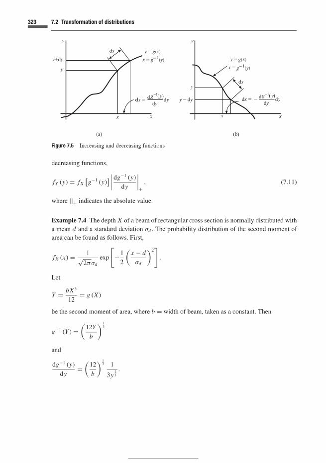
323 7.2 Transformation of distributions
ddd
d d dd
d
d
d
g
g−
g−g
−1
ddd
−1g g
Figure 7.5 Increasing and decreasing functions
decreasing functions,
fY (y) = fX[g−1 (y)
] ∣∣∣∣dg−1 (y)
dy
∣∣∣∣+
, (7.11)
where ||+ indicates the absolute value.
Example 7.4 The depth X of a beam of rectangular cross section is normally distributed witha mean d and a standard deviation σd . The probability distribution of the second moment ofarea can be found as follows. First,
fX (x) = 1√2πσd
exp
[−1
2
(x − d
σd
)2]
.
Let
Y = bX3
12= g (X )
be the second moment of area, where b = width of beam, taken as a constant. Then
g−1 (Y ) =(
12Y
b
) 13
and
dg−1 (y)
dy=
(12
b
) 13 1
3y23
.
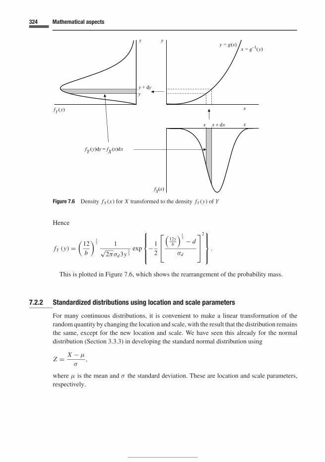
324 Mathematical aspects
−
Figure 7.6 Density fX (x) for X transformed to the density fY (y) of Y
Hence
fY (y) =(
12
b
) 13 1√
2πσd3y23
exp
−1
2
(12y
b
) 13 − d
σd
2
.
This is plotted in Figure 7.6, which shows the rearrangement of the probability mass.
7.2.2 Standardized distributions using location and scale parameters
For many continuous distributions, it is convenient to make a linear transformation of therandom quantity by changing the location and scale, with the result that the distribution remainsthe same, except for the new location and scale. We have seen this already for the normaldistribution (Section 3.3.3) in developing the standard normal distribution using
Z = X − µ
σ,
where µ is the mean and σ the standard deviation. These are location and scale parameters,respectively.

325 7.2 Transformation of distributions
In the exponential distribution
fX (x) = 1
βexp
(− x − α
β
)for x ≥ α, (7.12)
α represents a shift of the probability mass of the distribution (α is not the mean) and thestandard deviation is β. These two are the location and scale parameters in this case. For theGumbel distribution,
fZ (z) = 1
bexp
[− exp
(− z − a
b
)− z − a
b
], (7.13)
where a is the mode and b a measure of dispersion.In each case we can produce a standardized distribution by subtracting a location parameter
and dividing by a scale parameter. Denoting these in general by the symbols c and d, we canmake the substitution
Y = g (X ) = X − c
d(7.14)
so that
X = g−1 (Y ) = c + dY, (7.15)
dg−1 (y)
dy= d, (7.16)
fY (y) = d · fX (c + dy) , (7.17)
and
fX (x) = 1
dfY
(x − c
d
). (7.18)
In this, Y is the standardized random quantity.
Example 7.5 For the three cases discussed above (normal, exponential and Gumbel distribu-tions), the standardized distributions are
fY (y) = 1√2π
exp
(− y2
2
)for − ∞ < y < ∞, (7.19)
fY (y) = exp (−y) for 0 ≤ y < ∞, and (7.20)
fY (y) = exp[− exp (−y) − y
]for − ∞ < y < ∞. (7.21)
The density of the standardized distribution is always divided by d to get the distributionin terms of the non-standardized parameter. This ensures that the final probability ‘mass’ willbe measured in units of probability, without physical dimension. The three forms just givenare precisely the same regardless of the initial values of c and d. All distributions can be

326 Mathematical aspects
subjected to a linear transformation, but a standardized distribution does not necessarily result.The lognormal distribution, for example, can only be standardized in terms of the logarithmof the random quantity.
In some instances, the standardized distribution becomes a family of distributions that are afunction of a parameter or parameters, as in the following example.
Example 7.6 The gamma distribution
fX (x) = (x − a)α−1 exp [− (x − a) /β]
βα� (α), for x ≥ a with α > 0, β > 0 (7.22)
becomes, upon making the transformation y = (x − a) /β,
fY (y) = yα−1 exp (−y)
� (α), for y ≥ 0 with α > 0, β > 0. (7.23)
The constant α is the shape parameter of the standardized random quantity Y. Another exampleis the Weibull distribution (Exercise 7.3).
Interesting discussions of theoretical aspects in terms of stable distributions, a subclass ofthose that are infinitely divisible (see also Section 7.4.4 below) are given in de Finetti (1974)and Feller (1971).
7.2.3 Two random quantities
We consider now the transformation of two random quantities X1 and X2 with cdf FX1,X2 (x1, x2)into Y1 and Y2 using the one-to-one mapping
Y1 = g1 (X1, X2) and (7.24)
Y2 = g2 (X1, X2) . (7.25)
The use of cumulative distributions in one-to-one increasing relationships is similar to that givenfor single random quantities above in Equation (7.4). In this case, provided the relationshipscan be inverted as
X1 = g−11 (Y1, Y2) and (7.26)
X2 = g−12 (Y1, Y2) , (7.27)
then
FY1,Y2 (y1, y2) = FX1,X2
[g−1
1 (y1, y2), g−12 (y1, y2)
]. (7.28)
For the discrete case, given a one-to-one relationship not necessarily increasing, the proba-bility masses at the X coordinates transfer to the corresponding image points in Y coordinates,

327 7.2 Transformation of distributions
d
d
d
d
dd
d dJ
Figure 7.7 Mapping of (x1, x2) to (y1, y2) using inverse relationship
as in the one-dimensional case above of Equation (7.10). Thus
pY1,Y2 (y1, y2) = pX1,X2
[g−1
1 (y1, y2), g−12 (y1, y2)
]. (7.29)
For continuous random quantities, we again consider one-to-one relationships of the kindspecified in Equations (7.24) and (7.25), invertible, and which have continuous partial deriva-tives. Consider now the inverse mapping of Figure 7.7. This shows an element dy1dy2 in y1–y2
space that has been transformed into the element dx1dx2 in x1–x2 space. Our objective is onceagain to redistribute the probability masses; the mass that is placed on dx1dx2 must now beplaced on dy1dy2. In terms of the densities, written as fX1,X2 and fY1,Y2 , we have
fX1,X2 (x1, x2) dx1dx2 = fY1,Y2 (y1, y2) dy1dy2. (7.30)
We need to determine the relationship between the areas dx1dx2 and dy1dy2. Now
dx1 = ∂x1
∂y1dy1 + ∂x1
∂y2dy2 and
dx2 = ∂x2
∂y1dy1 + ∂x2
∂y2dy2, (7.31)
where x1 = g−11 (y1, y2) and x2 = g−1
2 (y1, y2) are the inverse relationships. The coefficients inthe relationships for dx1 and dx2, just given, form the Jacobian matrix:
∂x1
∂y1
∂x1
∂y2
∂x2
∂y1
∂x2
∂y2
. (7.32)
We can see that the two columns in this matrix are the coefficients just mentioned, andthese can be represented as vectors that are indicated by arrows in Figure 7.7. The area of theparallelogram of Figure 7.7 is given by the positive determinant |J | of the Jacobian matrix.

328 Mathematical aspects
This follows from the fact that the magnitude of the cross product of two vectors is equal tothe area of the parallelogram formed by using the two vectors as sides. The cross product oftwo vectors a and b in the x–y plane is equal to∣∣∣∣ax bx
ay by
∣∣∣∣ k,
where || is a determinant, ax and by are the components of a and b in the x and y directionsrespectively, and k is the unit vector at right angles to the x–y plane. The positive value ofthe determinant represents the area of the parallelogram, or the value of the cross product|ab sin θ |+ , where θ is the angle between a and b.
Thus
dx1dx2 =
∣∣∣∣∣∣∣∣
∂x1
∂y1
∂x1
∂y2
∂x2
∂y1
∂x2
∂y2
∣∣∣∣∣∣∣∣+
dy1dy2 = |J |+ dy1dy2 (7.33)
(where the + sign indicates the positive value of the determinant), and from Equation (7.21),
fY1,Y2 (y1, y2) dy1dy2 = fX1,X2 (x1, x2) dx1dx2
= fX1,X2
[g−1
1 (y1, y2), g−12 (y1, y2)
] |J |+ dy1dy2
or
fY1,Y2 (y1, y2) = fX1,X2
[g−1
1 (y1, y2), g−12 (y1, y2)
] |J |+ . (7.34)
The determinant had to be specified as being positive for the same reason as in the case ofsingle random quantities; the relationships between X and Y could involve negative gradientsand thus produce negative areas. We assign probability mass for positive increments of randomquantities only.
Example 7.7 The transformation
y1 = x1 − x2
y2 = x2
is useful, as will be seen. The inverse relationships are
x1 = y1 + y2
x2 = y2.
The positive value of the determinant of the Jacobian is
|J |+ =∣∣∣∣1 10 1
∣∣∣∣ = 1.

329 7.2 Transformation of distributions
From this we see that
fY1,Y2 (y1, y2) = fX1,X2 (y1 + y2, y2) . (7.35)
We can use this result in reliability theory, to be further considered in Chapter 10. Let X1 =R, the capacity (or resistance in the terminology of structural engineering) of a component,for example an electrical circuit, a transportation network or a structural component. If thecapacity is exceeded by demand, the system fails. Let X2 = Y2 = Z , the demand, for examplepeak voltage, traffic, or loading in the three examples cited. Then we write Y1 = M = R − Z ,
the ‘margin of safety’, the difference between capacity and demand. If M ≤ 0, we have failureof the system. From Equation (7.35)
fM,Z (m, z) = fR,Z (m + z, z) . (7.36)
We can evaluate probabilities related to various values of M by obtaining the marginal distri-bution
fM (m) =∫ ∞
−∞fR,Z (m + z, z) dz. (7.37)
If R and Z are independent of each other,
fM (m) =∫ ∞
−∞fR (m + z) fZ (z) dz. (7.38)
The function fM is termed a convolution of fR and fZ . (See Section 7.3 below.)To illustrate, we use exponential functions:
fR (r ) = λ1 exp (−λ1r ) and (7.39)
fZ (z) = λ2 exp (−λ2z) , (7.40)
for r, z ≥ 0, and 0 otherwise. Then, from Equation (7.37),
fM (m) = λ1λ2
∫ ∞
−mexp [−λ1 (m + z) − λ2z] dz for M ≤ 0 and
= λ1λ2
∫ ∞
0exp [−λ1 (m + z) − λ2z] dz for M ≥ 0.
The limits for these integrals are illustrated in Figure 7.8, and the following gives the results:
fM (m) = λ1λ2
λ1 + λ2exp (λ2m) for M ≤ 0 and (7.41)
fM (m) = λ1λ2
λ1 + λ2exp (−λ1m) for M ≥ 0. (7.42)

330 Mathematical aspects
Positive M
Negative M
Figure 7.8 Integration limits in reliability problems; broken line indicates m = 0
Failure corresponds to the event {M < 0} with probability
p f =∫ 0
−∞
λ1λ2
λ1 + λ2exp (λ2m) dm = λ1
λ1 + λ2. (7.43)
Models of choice. Another interpretation of the analysis of this example lies in models ofchoice. If R and Z represent two generalized costs for the choices A and B, the randomnessexpressing the uncertainty with regard to the perception of the next customer, then the events{M < 0} and {M > 0} might represent the choice of B and A respectively.
Example 7.8 Rayleigh distribution from Gaussian process. Voltage, sound, and the surfaceelevation of the sea can be modelled using a Gaussian process. The Rayleigh distribution canbe obtained from this process. We consider
X (t) = A (t) cos [ωt + (t)] , (7.44)
where ω is a constant; the amplitude A (t) and the phase (t) are random quantities such that0 ≤ A < ∞ and 0 ≤ ≤ 2π. On the assumption that these two random quantities vary slowlywith time, so that A and are negligible with respect to X , we obtain
X (t) � −ωA (t) sin [ωt + (t)] . (7.45)
If the joint distribution of X and X is such that they are independent and normal, N(0, σ 2
)and N
(0, ω2σ 2
)respectively,
fX,X (x, x) = 1
2πωσ 2exp
[− 1
2σ 2
(x2 + x2
ω2
)]. (7.46)
Then we can deduce the joint distribution of {A, } from this equation using Equation (7.34).

331 7.2 Transformation of distributions
Consequently,
f A, (a, ξ ) = 1
2πωσ 2exp
{− 1
2σ 2
[(a cos ωt + ξ
)2 +(−ωa sin ωt + ξ
)2
ω2
]}
×∣∣∣∣cos (ωt + ξ ) −a sin (ωt + ξ )−ω sin (ωt + ξ ) −ωa cos (ωt + ξ )
∣∣∣∣+
= a
2πσ 2exp
(− a2
2σ 2
), (7.47)
where we have written a (t) and ξ (t) simply as a and ξ. This equation shows that is uniformlydistributed from 0 to 2π. The distribution of A is then
f A (a) =∫ 2π
0f A, (a, ξ ) dξ
=∫ 2π
0
a
2πσ 2exp
(− a2
2σ 2
)dξ
= a
σ 2exp
(− a2
2σ 2
)for a ≥ 0. (7.48)
This is the Rayleigh distribution, discussed further in Chapter 9, Section 9.4.3.
7.2.4 Several random quantities
The need arises to consider several random quantities X1, X2, . . . , Xi , . . . , Xn which transforminto another set Y1, Y2, . . . , Yi , . . . , Yn. We shall use the vector notation illustrated by
X = (X1, X2, . . . , Xi , . . . , Xn) .
We also write
pX (x) = pX1,X2,...,Xi ,...,Xn (x1, x2, . . . , xi , . . . , xn)
and
fX (x) = fX1,X2,...,Xi ,...,Xn (x1, x2, . . . , xi , . . . , xn)
as the multidimensional probability distributions for the discrete and continuous cases, respec-tively. We wish to transform these to the distributions
pY (y) = pY1,Y2,...,Yi ,...,Yn (y1, y2, . . . , yi , . . . , yn)
and
fY (y) = fY1,Y2,...,Yi ,...,Yn (y1, y2, . . . , yi , . . . , yn) .

332 Mathematical aspects
The transformation using cumulative distribution functions and of discrete random quantitiesfollows the procedures outlined above; see, for example, Equations (7.28), (7.29) and (7.9).For example, the equation
pY (y) = pX[g−1 (y)
]
assigns probability masses from the X-space to the Y-space, in a similar way to that in Equation(7.29), provided that the relationships
g (x) = [g1 (x1, . . . , xn) , . . . , gn (x1, . . . , xn)] (7.49)
and their inverses
g−1 (y) = [g−1
1 (x1, . . . , xn) , . . . , g−1n (x1, . . . , xn)
](7.50)
are one-to-one.We shall now outline the generalization of the transformation of densities using Jacobians.
The results for the two-dimensional case generalize readily. Once again, we consider that theprobability mass is distributed over elementary volumes. For example, in the three-dimensionalcase a small cube in the y1–y2–y3 space transforms into a small parallelepiped in the x1–x2–x3
space, in a manner entirely analogous to the transformation depicted in Figure 7.7. The volumeof the parallelepiped formed by three vectors in a Euclidean space is given by the determinantformed by the components in three-dimensional cartesian coordinates. It is often introducedas the mixed triple product of the three vectors. This product is also the moment of a forceabout an axis in mechanics; see for instance Beer and Johnston (1981).
The components of our vectors are the values in the Jacobian; in three dimensions, thedeterminant of the Jacobian matrix (7.33) becomes
∣∣∣∣∣∣∣∣∣∣∣∣∣
∂x1
∂y1
∂x1
∂y2
∂x1
∂y3
∂x2
∂y1
∂x2
∂y2
∂x2
∂y3
∂x3
∂y1
∂x3
∂y2
∂x3
∂y3
∣∣∣∣∣∣∣∣∣∣∣∣∣
.
Then we have the transformation of volumes
dx1dx2dx3 =
∣∣∣∣∣∣∣∣∣∣∣∣∣
∂x1
∂y1
∂x1
∂y2
∂x1
∂y3
∂x2
∂y1
∂x2
∂y2
∂x2
∂y3
∂x3
∂y1
∂x3
∂y2
∂x3
∂y3
∣∣∣∣∣∣∣∣∣∣∣∣∣+
dy1dy2dy3 = |J |+ dy1dy2dy3, (7.51)

333 7.2 Transformation of distributions
and we find, analogously to Equation (7.34),
fY1,Y2,Y3 (y1, y2, y3)
= fX1,X2,X3
[g−1
1 (y1, y2, y3), g−12 (y1, y2, y3), g−1
3 (y1, y2, y3)] |J |+ , (7.52)
where |J |+ is now given in Equation (7.51).In n dimensions,
fY (y) = fX[g−1 (y)
] |J |+ , (7.53)
where
|J |+ =
∣∣∣∣∣∣∣∣∣∣∣∣∣∣∣∣∣∣∣∣∣∣∣∣
∂x1
∂y1
∂x1
∂y2· · · ∂x1
∂y j· · · ∂x1
∂yn
∂x2
∂y1
∂x2
∂y2· · · ∂x2
∂y j· · · ∂x2
∂yn...
......
...∂xi
∂y1
∂xi
∂y2· · · ∂xi
∂y j· · · ∂xi
∂yn...
......
...∂xn
∂y1
∂xn
∂y2· · · ∂xn
∂y j· · · ∂xn
∂yn
∣∣∣∣∣∣∣∣∣∣∣∣∣∣∣∣∣∣∣∣∣∣∣∣+
(7.54)
and the notation g−1 (y) is given in Equations (7.49) and (7.50) (which are valid for discreteor continuous quantities).
There is an elegant generalization of the visually perceived parallelepiped in three-dimensional space to that in a linear vector space of n-dimensions (Greub, 1975). If onehas n linearly independent vectors, they define an n-dimensional parallelepiped, and the vol-ume is defined analogously to the three-dimensional case. Spaces in which norms provide theabstraction of distance and inner products the abstraction of scalar products and consequentlyangles provide extensions of the applicability of the theory.
Example 7.9 Multidimensional normal distribution. For convenience we define here the vectorX as a column vector
X = (X1, X2, . . . , Xi , . . . , Xn)T . (7.55)
We continue to use the notation
fX (x) = fX1,X2,...,Xi ,...,Xn (x1, x2, . . . , xi , . . . , xn) . (7.56)
We start the example with the standardized multidimensional normal distribution with means

334 Mathematical aspects
of zero and standard deviations of unity,
fX (x) = 1
(2π )n/2 exp
(−1
2
∑n
i=1x2
i
)
= 1
(2π )n/2 exp
(−1
2XT · X
). (7.57)
Thus
〈X〉 = 0, (7.58)
where 0 is a column vector of zeros and the covariance matrix is
[D] = [I ] , (7.59)
the unit matrix. The Xs are therefore independent of each other with zero means and standarddeviations of unity. We noted in Section 3.5.7 that if covariances are zero the random quantitiesare not necessarily independent in general. The present case of normal distributions constitutesan exception to this rule.
Now we transform X into Y, where
Y = (Y1, Y2, . . . , Yi , . . . , Yn)T , (7.60)
using the linear transformation
Y = [A] X + µ, (7.61)
where
µ = (µ1, µ2, . . . , µn)T (7.62)
and [A] is the matrix
[A] = [ai j
] =
a11 a12 · · · a1 j · · · a1n
a21 a22 · · · a2 j · · · a2n...
......
...ai1 ai2 · · · ai j · · · ain...
......
...an1 an2 · · · anj · · · ann
. (7.63)
The inverse relationships (7.50)
g−1 (y) = [g−1
1 (x1, . . . , xn) , . . . , g−1n (x1, . . . , xn)
]are deduced from (7.61).
X = [A]−1 (Y − µ) (7.64)

335 7.2 Transformation of distributions
which appears as a column vector of linear relationships.We wish to obtain
fY (y) = fY1,...,Yi ,...,Yn (y1, . . . , yi , . . . , yn) (7.65)
by using Equation (7.53),
fY (y) = fX[g−1 (y)
] |J |+ .
Now
|J |+ =
∣∣∣∣∣∣∣∣∣∣∣∣∣∣∣∣∣∣
∂x1
∂y1· · · ∂x1
∂y j· · · ∂x1
∂yn...
......
∂xi
∂y1· · · ∂xi
∂y j· · · ∂xi
∂yn...
......
∂xn
∂y1· · · ∂xn
∂y j· · · ∂xn
∂yn
∣∣∣∣∣∣∣∣∣∣∣∣∣∣∣∣∣∣+
= 1
|A|+= |A|−1
+ . (7.66)
One gets
fY (y) = 1
(2π )n/2|A|−1
+ exp
[−1
2(y − µ)T
([A]−1
)T[A]−1 (y − µ)
],
where we have used the fact that ([C] [D])T = [D]T [C]T .
Now let
[�] = [A] [A]T ; (7.67)
� is then symmetric. Consequently
fY (y) = 1
(2π )n/2|�|−1/2 exp
[−1
2(y − µ)T [�]−1 (y − µ)
]. (7.68)
The matrix [�] is the covariance matrix
[�] =
σ 21 ρ12σ1σ2 · · · ρ1 jσ1σ j · · · ρ1nσ1σn
ρ21σ2σ1 σ 22 · · · ρ2 jσ2σ j · · · ρ2nσ2σn
......
......
ρi1σiσ1 ρi2σiσ2 · · · ρi jσiσ j · · · ρinσiσn...
......
...ρn1σnσ1 ρn2σnσ2 · · · ρnjσnσ j · · · σ 2
n ,
, (7.69)
where the σ s are the standard deviations and the ρs the correlation coefficients. See alsoExercise 6.4.

336 Mathematical aspects
In this example, we started with independent random quantities and ended with dependentones. In structural reliability theory the reverse is sometimes needed (Melchers, 1999).
7.3 Convolutions
We are often concerned with a linear combination of two random quantities; one case wasgiven in Example 7.7. Here we consider
Y = X1 + X2. (7.70)
This might be the total time for transmission of two packets of information, 1 and 2, or the totalwaiting time for two modes of transport, or the sum of two individual loadings. Consideringfirst the discrete case,
pY (y) =∑
y=x1+x2pX1,X2 (x1, x2) ,
where the summation is taken, as indicated, over all combinations of x1 and x2 that constitutea particular value y. For each fixed y we can write x1 (say) as (y − x2) , so that this expressioncan be written as
pY (y) =∑∞
x2=−∞ pX1,X2 (y − x2, x2) . (7.71)
(This could have been written in terms of x1 by substituting (y − x1) for x2.) In the case ofindependent random quantities X1 and X2,
pY (y) =∑∞
x2=−∞ pX1 (y − x2) pX2 (x2) or
pY (y) =∑∞
x1=−∞ pX1 (x1) pX2 (y − x1) . (7.72)
These equations are termed convolutions of pX1 and pX2 , and can be written succinctly as
pY = pX1 ∗ pX2 . (7.73)
For continuous random quantities, we consider again the sum in Equation (7.70). The methodused in Example 7.7 gives the result that follows, with a change of sign of x2 (since weconsidered there y1 = x1 − x2 rather than x1 + x2). For variety, we give a somewhat differentderivation. Referring to Figure 7.9, we integrate over the appropriate region (x1 + x2 ≤ y) tofind
FY (y) = Pr (X1 + X2 ≤ y) =∫ ∞
x2=−∞
∫ y−x2
x1=−∞fX1,X2 (x1, x2) dx1dx2. (7.74)
From this we obtain by differentiation with respect to y that
fY (y) =∫ ∞
−∞fX1,X2 (y − x2, x2) dx2. (7.75)
One can also derive this result directly from Figure 7.9.

337 7.3 Convolutions
Figure 7.9 Integration limits for convolutions
Again independence provides the further result that
fY (y) =∫ ∞
−∞fX1 (y − x2) fX2 (x2) dx2. (7.76)
The related result
fY (y) =∫ ∞
−∞fX1 (x1) fX2 (y − x1) dx1 (7.77)
may be found in a similar way to the above, for instance by reversing the order of integrationin Equation (7.74). Equations (7.76) and (7.77) are further examples of convolutions, writtenin a similar manner to the discrete version given in expression (7.73):
fY = fX1 ∗ fX2 . (7.78)
We can also express the convolutions in terms of cdfs. In this case
FY (y) =∫ ∞
−∞FX2 (y − x1) dFX1 (x1)
=∫ ∞
−∞FX2 (y − x1) fX1 (x1) dx1. (7.79)

338 Mathematical aspects
In the first line, we have used the Stieltjes notation (Appendix 2) which unifies the continuousand discrete cases. We write the convolutions as
FY = FX1 ∗ FX2 ; (7.80)
note that the integral (7.79) could have been written as
FY (y) =∫ ∞
−∞FX1 (y − x2) dFX2 (x2) . (7.81)
The two-fold convolutions discussed above can be extended to consideration of the sum ofseveral (say n) independent, random quantities, resulting in n-fold convolutions, written
fX1 ∗ fX2 ∗ · · · ∗ fXn−1 ∗ fXn and (7.82)
FX1 ∗ FX2 ∗ · · · ∗ FXn−1 ∗ FXn . (7.83)
Transforms, to be introduced after the next subsection, have the useful property of convertinga convolution integral into the product of two transforms, thus rendering analysis more easy.They are useful also in generating moments and defining an entire probability distribution.
Role of convolutions in engineering analysisConvolutions appear frequently in engineering problems, so that it is well worth the while spenton this subject. The use in probability theory has been introduced in the preceding paragraphs,and we use them to calculate failure probabilities in Chapter 10. But there are analogoususes in the various areas of circuit theory, mechanics, hydrology and mortality of persons orequipment, to name a few. These analyses are all based on linear superposition in time.
In the case of equipment mortality, let n0 be the number of pieces of new equipment inservice at time 0, the initial point of analysis. This decreases to
n0g (t)
at time t, such that g (0) = 1, with g (t) declining from unity eventually to zero. Now let thereplacement rate be f (t) per unit time at time t. Then the replacements during the time intervalfrom time τ to τ + dτ are f (τ ) dτ, and at time t – after an elapsed time (t − τ ) – the survivingreplacements are
f (τ ) g (t − τ ) dτ.
At time t, the total population is
n0g (t) +∫ t
0f (τ ) g (t − τ ) dτ, (7.84)
where it has been assumed as before that the n0 pieces of equipment are new.This can be extended to consideration of human populations by considering a mixture of
ages at the start of the analysis, and f (t) becomes the birth rate. The analysis is based onconstancy in time of the various rates and does not account for events such as plagues. There

339 7.3 Convolutions
I
FK
R
LQ
C
Figure 7.10 Electrical and mechanical systems
are ways to deal with such factors, beyond the present introduction. The second (convolution)term of Equation (7.84) could be used also to model the flow in a river, say, as a result of astorm of intensity f (t) in centimetres per hour (for example). In this case, g (t) is the ‘unithydrograph’, that is, the response of the system to a unit input at time 0. This again assumeslinearity of response of the system.
Figure 7.10 shows electrical and mechanical systems for which the equations are identical.Springs and capacitors act as storage units, dashpots and resistances cause dissipation andconsequent entropy increase, while the mass and the inductance provide inertial componentsto the equations. Two examples of the use of convolutions in these systems will be given. First,a linear spring–mass system subject to a forcing function f (t) constitutes an oscillator withone degree of freedom, with the response in terms of displacement x given by
x (t) = 1
ω
∫ t
0f (τ ) sin [ω (t − τ )] dτ, (7.85)
where ω is the natural frequency of the oscillator. Second, the response of a spring–dashpot orcapacitor–resistor system subjected to a force or potential follows equations similar in form to(7.84).
The main effect of the transforms of the following section is to convert the convolution to theproduct of two transformed quantities, thus providing a means of solution. The equations can

340 Mathematical aspects
often be expressed in terms of differential rather than integral equations, and the transformscan conveniently be applied to these too.
7.4 Transforms and characteristic functions
As a result of the widespread appearance of equations of the convolution kind – or equivalentforms as differential equations – it is common in engineering to use various transforms. Thetransforms are of several kinds, for example in the electrical circuit and viscoelastic theoryjust discussed, Laplace transforms are commonly used (Churchill, 1972), and in data analy-sis, signal processing and spectral analysis, Fourier transforms are central. The transformsconvert equations involving convolutions into simpler multiplicative forms, but there are otheradvantages. In probability theory, the transform can give all the moments of a distribution.Transforms can also be useful in calculating expected utilities (Keeney and Raiffa, 1976). Themain transforms used in probability theory are:
� the probability generating function,� the moment generating function, a close relative of the Laplace transform, and� the characteristic function, a close relative of the Fourier transform.
It is also of interest that the Laplace and Fourier transforms are in fact the same transform butwith a change of variable; see de Finetti (1974). We introduce the three main transforms justnoted, for completeness.
7.4.1 Probability generating functions ( pgf s)
We consider initially a discrete random quantity X, which takes values x = 0, 1, 2, . . . Thedefinition that follows is therefore confined to random quantities that take the possible valuesof 0 and the natural numbers. Typical examples are the binomial, Poisson and geometricdistributions. The probability generating function gX (t) is defined as the expected value
gX (t) = ⟨t X
⟩ =∑∞
x=0t x pX (x)
= pX (0) + tpX (1) + t2 pX (2) + t3 pX (3) + · · · (7.86)
One can see from the last line of this definition why gX (t) is termed a probability generatingfunction. If one can evaluate the series, the probability pX (n) is the coefficient of tn. The pgfsarise quite naturally as power series.
Example 7.10 Consider the geometric distribution of Equation (3.7)
Pr(X = x) = (1 − p)x−1 p,
x = 1, 2, . . .

341 7.4 Transforms and characteristic functions
Then
gX (t) = p∑∞
y=0t y (1 − p)y
= p∑∞
y=0[t (1 − p)]y
= p
1 − t (1 − p), (7.87)
in which y = x − 1. We see from these equations that
gX (t) = p + t [p (1 − p)] + t2[
p (1 − p)2] + t3
[p (1 − p)3
] + · · · (7.88)
The coefficients of tn give the probabilities of y = 0, 1, 2, . . . , or equivalently of x =1, 2, 3, . . .
Example 7.11 For the Poisson distribution of Equation (3.13),
pX (x) = νx exp (−ν)
x!, for x = 0, 1, 2, . . . ,
the pgf, from which the reader might wish to obtain probabilities, is
gX (t) = exp (−ν)∑∞
x=0
(νt)x
x!= exp (−ν) exp (νt) = exp − [ν (1 − t)] . (7.89)
The series (7.86) certainly converges for −1 ≤ t ≤ 1. Further discussion of this subject isgiven, for example, in Lloyd (1980), who also deals with the case where the values of therandom quantity do not correspond to the integers.
ConvolutionsWe discussed above in Section 7.3 the sum of independent random quantities X1 and X2, andthe resulting expressions were written as
pX1 ∗ pX2 .
The early motivation for the development of transform techniques arose out of the fact that,for two quantities X1 and X2,
t X1+X2 = t X1 t X2 , (7.90)
for any number t. Because of the result expressed in Equation (7.90), the present methodis intimately connected with the use of exponents. We have previously seen that for twoindependent random quantities X and Y , 〈XY 〉 = 〈X〉 〈Y 〉, as shown in Equation (3.79). In the

342 Mathematical aspects
present case,⟨t X1+X2
⟩ = ⟨t X1 t X2
⟩ =∑ ∑
t X1 t X2 pX1 (x1)pX2 (x2)
=∑
t X1 pX1 (x1)∑
t X2 pX2 (x2)
= ⟨t X1
⟩ ⟨t X2
⟩. (7.91)
We can therefore write
gX1+X2 (t) = ⟨t X1+X2
⟩ = gX1 (t) gX2 (t) ; (7.92)
the pgf of the sum of two independent random quantities is the product of the individual pgfs.This can be extended to the sum of three or more independent random quantities: the pgf ofthe sum of the independent random quantities is the product of the individual pgfs.
Example 7.12 The pgf of the sum of two independent Poisson random quantities X1 and X2
with expected values ν1 and ν2, respectively, is
gX1+X2 (t) = {exp − [ν1 (1 − t)]} · {exp − [ν2 (1 − t)]}= exp − [(ν1 + ν2) (1 − t)] , (7.93)
by Equation (7.92); see also Example 7.11. The resulting expression (7.93) is in fact thetransform of a Poisson random quantity with expected value (ν1 + ν2) . We see from thisresult that the sum of two Poisson random quantities is another Poisson random quantity withexpected value (ν1 + ν2) .
MomentsProbability generating functions can be used to calculate means, variances, and other moments.The derivative of gX (t) with respect to t is
g′X (t) = pX (1) + 2tpX (2) + 3t2 pX (3) + · · ·
=∑∞
x=1xpX (x) t x−1,
and therefore
g′X (t = 1) = 〈X〉 . (7.94)
Example 7.13 Applying this to the Poisson distribution using Equation (7.89), for example,we find that 〈X〉 = ν.
The second derivative
g′′X (t) = 2pX (2) + 3 · 2tpX (3) + 4 · 3t2 pX (4) + · · ·
=∑∞
x=2x (x − 1) pX (x) t x−2,

343 7.4 Transforms and characteristic functions
and therefore
g′′X (1) = 〈X (X − 1)〉 = ⟨
X2⟩ − 〈X〉 . (7.95)
We can use this expression to calculate the variance, which from Equation (3.87) is givenby
σ 2X = ⟨
X2⟩ − 〈X〉2 .
Example 7.14 For the Poisson distribution, using Equation (7.89),
g′′X (1) = ν2;
from Equation (7.95)⟨X2
⟩ = ν2 + ν
and therefore
σ 2X = ν.
7.4.2 Moment generating and characteristic functions (mgf s and cf s)
Both transforms to be described here will be seen to generate moments – rather than probabil-ities, as in the case of pgfs. We shall use the usually accepted terms, moment generating andcharacteristic functions (mgfs and cfs) although both generate moments. To extend the ideasof the previous section to continuous random quantities, and to those that take values otherthan integers, it is convenient to use the following functions, replacing t of the previous sectionwith
t = exp s, and (7.96)
u = exp (iu) (7.97)
in the case of mgfs and cfs respectively, where i = √−1. Then t X in Equation (7.86)becomes
exp (s X ) and (7.98)
exp (iu X ) , respectively. (7.99)
The two transforms are now defined.The moment generating function (mgf ) is given by
m X (s) = 〈exp (s X )〉 ={ ∑
all x exp (sx) pX (x) for discrete X,∫all x exp (sx) fX (x) dx for continuous X.
(7.100)
We see the essential role of the exponent, now formally as the power to the natural base ‘e’.

344 Mathematical aspects
Equations (7.100) may, as elsewhere, be combined into one using the Stieltjes form
m X (s) =∫
all xexp (sx) dFX (x) . (7.101)
We define the characteristic function (cf ) as
φX (u) = 〈exp (iu X )〉 ={ ∑
all x exp (iux) pX (x) for discrete X,∫all x exp (iux) fX (x) dx for continuous X.
(7.102)
These definitions may, as before, be combined in the Stieltjes integral:
φX (t) =∫
all xexp (iux) dFX (x) . (7.103)
The cf may also be written as
φX (u) = 〈cos ux + i sin ux〉=
∫all x
(cos ux) fX (x) dx + i∫
all x(sin ux) fX (x) dx, (7.104)
where we have used the integral as an example; the same equation may be rewritten withsummations.
The mgf does not necessarily converge. It may converge for only an interval around theorigin, especially when there is a lot of probability mass in the tails of the distribution. On theother hand, the cf exists for all real values of u. There is a one-to-one correspondence betweenan mgf (when it exists) or a cf and the corresponding probability distribution. The cf is moregeneral, and the one-to-one correspondence applies to all proper distributions. The importantresult is that knowledge of the cf is sufficient to determine the probability distribution. Seede Finetti (1974, vol. 1), Fraser (1976) and Lloyd (1980) for details. The inverse relation toEquation (7.102) in the continuous case is
fX (x) = 1
2π
∫ ∞
−∞exp (−iux) φX (u) du. (7.105)
Example 7.15 For the binomial distribution of Equation (3.3),
pX (x) =(
n
x
)px (1 − p)n−x ,
the mgf is
m X (s) =∑n
x=0exp (sx)
(n
x
)px qn−x =
∑n
x=0
(n
x
) [p exp (s)
]xqn−x
= [p exp (s) + q
]n, (7.106)
in which q = 1 − p.

345 7.4 Transforms and characteristic functions
In a similar way it can be shown that the cf is
φX (u) = [p exp (iu) + q
]n.
Example 7.16 For the Poisson distribution of Equation (3.13),
pX (x) = νx exp (−ν)
x!for x = 0, 1, 2, . . . ,
φX (u) = exp (−ν)∑∞
x=0
[ν exp (iu)
]x
x!= exp (−ν) exp
[ν exp (iu)
](7.107)
= exp{−ν
[1 − exp (iu)
]}.
The mgf is similarly obtained; we dealt with the pgf in Equation (7.89).
Example 7.17 For the standard normal distribution, fZ (z) =(
1/√
2π)
exp(−z2/2
),
m Z (s) = 1√2π
∫ ∞
−∞exp (sz) exp
(− z2
2
)dz
=(
exps2
2
)1√2π
∫ ∞
−∞exp
[− (z − s)2
2
]dz
= exp
(s2
2
). (7.108)
The cf may be shown to be given by
φZ (u) = exp
(−u2
2
). (7.109)
The proof for the cf requires contour integration in the complex plane; see Exercise 7.12.
Laplace and Fourier transformsThe mgf and the cf are closely related to the Laplace and Fourier transforms, respectively. TheLaplace transform is defined as the integral, usually from 0 to ∞, of the same argument asabove, except that the term exp (s X ) is replaced by exp (−s X ). In a similar way, φX (−u) isthe Fourier transform of fX (x) .
7.4.3 Linear transformations and convolutions
The mgf and cf of
Y = aX + b, (7.110)

346 Mathematical aspects
where a and b are constants, are, respectively,
mY (s) = 〈exp (sY )〉 = 〈exp [s (aX + b)]〉 = exp (sb) m X (as) and (7.111)
φY (u) = 〈exp (iuY )〉 = 〈exp [iu (aX + b)]〉 = exp (iub) φX (au) . (7.112)
Example 7.18 Transformation of the standard normal random quantity Z to the N(µ, σ 2
)distribution by the linear transformation Y = µ + σ Z . Using the cf, for example,
φY (u) = exp (iuµ) φZ (σu)
= exp(iuµ − σ 2u2/2
), (7.113)
using Equation (7.109). Similarly the mgf is
mY (s) = exp(sµ + σ 2s2/2
). (7.114)
The sum of independent random quantities X1 and X2 constitutes a convolution, as discussedabove in Section 7.3. Writing Y = X1 + X2, the distribution of Y is a convolution of those ofX1 and X2, written in summary form as
pY = pX1 ∗ pX2 and
fY = fX1 ∗ fX2
for discrete and continuous distributions, respectively. We use again the multiplicative propertyof the exponential function shown in Equation (7.90), that is, t X1+X2 = t X1 t X2 :
〈exp (sY )〉 = 〈exp [s (X1 + X2)]〉 = 〈exp (s X1)〉 · 〈exp (s X2)〉 and
〈exp (iuY )〉 = 〈exp [iu (X1 + X2)]〉 = 〈exp (iu X1)〉 · 〈exp (iu X2)〉.We can conclude that the mgf and cf of Y are
mY (s) = m X1 (s) · m X2 (s) and (7.115)
φY (u) = φX1 (u) · φX2 (u) , (7.116)
respectively. This can be extended to the sum of several, say n independent random quantities.If
Y =∑n
i=1Xi , (7.117)
where the Xi are independent, then
mY (s) =∏n
i=1m Xi (s)
= m X1 (s) · m X2 (s) · . . . · m Xi (s) · . . . · m Xn (s) and (7.118)
φY (u) =∏n
i=1φXi (u)
= φX1 (u) · φX2 (u) · . . . · φXi (u) · . . . · φXn (u). (7.119)

347 7.4 Transforms and characteristic functions
Addition of independent random quantities corresponds to multiplication of mgfs and cfs. Thisvery useful property will be exploited in several applications, not least in the Central LimitTheorem.
For the iid (independent and identically distributed) case, using cfs as an example,
φY (u) =∏n
i=1φXi (u) = φn
X (u) . (7.120)
Example 7.19 The sum of two independent random quantities X1 and X2, following thenormal distribution and with parameters
(µ1, σ
21
)and
(µ2, σ
22
)respectively, will have the
following cf, using Equations (7.113) and (7.116).
φY (u) = φX1 (u) · φX2 (u)
= exp(iuµ1 − σ 2
1 u2/2) · exp
(iuµ2 − σ 2
2 u2/2)
= exp[iu (µ1 + µ2) − (
σ 21 + σ 2
2
)u2/2
]. (7.121)
From this we see that the sum of the two independent normal random quantities is anotherwith a normal distribution having mean (µ1 + µ2) and variance
(σ 2
1 + σ 22
). Recall that there
is a one-to-one correspondence between a cf and the corresponding probability distribution.
Example 7.20 The convolution just discussed can be applied to a sum Y of n independentnormal random quantities X1, X2, X3, . . . , Xi , . . . Xn. The parameters are denoted as
(µi , σ
2i
)for the i th random quantity. One can apply the convolution of Example 7.19 initially to thefirst two of the random quantities, then to this result, and then to the third, and so on. Usingmgfs, based on Equation (7.114),
mY (s) = m X1 (s) · m X2 (s) · m X3 (s) · . . . · m Xi (s) · . . . · m Xn (s) ,
=∏
i=1exp
(sµi + σ 2
i s2/2)
= exp[s∑n
i=1µi +
(∑n
i=1σ 2
i
)s2/2
]. (7.122)
This is the mgf of a normal random quantity with parameters(∑n
i=1 µi ,∑n
i=1 σ 2i
). Addition
of normal random quantities results in another normal random quantity with these parameters.
Example 7.21 Gamma densities. The gamma distribution
fX (x) = xα−1 exp (−x/β)
βα� (α)(7.123)
has a cf as follows:
φX (u) = (1 − iuβ)−α . (7.124)
(See Exercise 7.18.) The sum Y of two random quantities with gamma distributions,X1 (parameters α1, β) and X2 (parameters α2, β) , that are independent results in another

348 Mathematical aspects
gamma density,
φY (u) = φX1 (u) · φX2 (u)
= (1 − iuβ)−α1 · (1 − iuβ)−α2
= (1 − iuβ)−(α1+α2) . (7.125)
This is a gamma density with parameters (α1 + α2, β) . The parameter β is the scale parameterwhile (α1 + α2) is the shape parameter resulting from the original two shape parameters α1
and α2. It is also said that the family of gamma distributions is ‘closed under convolution’,expressed by
f α1,β ∗ f α2,β = f α1+α2,β , (7.126)
where the meanings of the symbols are clear from the discussion above.
7.4.4 Infinite divisibility
The gamma and normal densities are examples of infinitely divisible distributions. The dis-tribution FY is denoted as infinitely divisible if it can be written as the sum of n independentrandom quantities with a common distribution FX , for every n. Thus
FY = FX ∗ FX ∗ · · · ∗ FX ∗ FX , with n terms in the convolution. (7.127)
The distribution function FY corresponds to the distribution of the sum of n independentand identically distributed (iid) random quantities, resulting in the n-fold convolution of thecommon distribution FX . In terms of cfs,
φY = φnX . (7.128)
Continuous stochastic processes with independent increments require infinite divisibility todecompose into the increments, as mentioned briefly at the end of Section 3.6.1.
Example 7.22 The exponential distribution
fY (x) = 1
βexp (−y/β)
has a cf as follows:
φY (u) = (1 − iuβ)−1 .
This can be written as
φY (u) =[(1 − iuβ)−
1n
]n, (7.129)
and (1 − iuβ)−1n is the cf of a random quantity with a gamma distribution
(parameters 1
n , β).
Therefore an exponentially distributed random quantity is the sum of n iid random quantitieswith gamma distributions as indicated, for every n.

349 7.4 Transforms and characteristic functions
For more details on infinitely divisible distributions, see de Finetti (1974) and Feller(1971).
7.4.5 Generation of moments
Both mgfs and cfs generate moments. As a reminder, the kth moment of a probability distributionabout the origin was defined in Equations (3.82) and (3.83) as
µ(k)X = ⟨
Xk⟩.
We make the following expansions. First, for the mgf,
m X (s) = 〈exp (s X )〉=
⟨1 + s X + 1
2!(s X )2 + 1
3!(s X )3 + · · · + 1
k!(s X )k + · · ·
⟩
= 1 + sµ(1)X + 1
2!s2µ
(2)X + 1
3!s3µ
(3)X + · · · + 1
k!skµ
(k)X + · · · (7.130)
The corresponding series for the cf is as follows:
φX (u) = 〈exp (iu X )〉=
⟨1 + iu X − 1
2!(u X )2 − 1
3!i (u X )3 + · · · + 1
k!(iu X )k + · · ·
⟩
= 1 + iuµ(1)X − 1
2!u2µ
(2)X − 1
3!iu3µ
(3)X + · · · + 1
k!(iu)k µ
(k)X + · · · (7.131)
One sees in both series a full set of moments for the probability distribution: the mgfs and cfsgenerate a series containing all the moments of the distribution of X. We now see why theexpression ‘moment generating function’ is used; in the usual usage, the term is reserved forthe mgf, as has been done in the above.
From Equations (7.130) and (7.131), it follows by differentiation and by setting s and uequal to zero that
dr m X (s)
dsr
∣∣∣∣s=0
= µ(r )X and (7.132)
drφX (u)
dur
∣∣∣∣u=0
= irµ(r )X . (7.133)
Central moments m(k)X = ⟨
(X − µX )k⟩
of a random quantity X, as defined in Equations (3.84)and (3.85), can also be generated. Taking cfs as an example, one can write[exp (−iuµX )
]φX (u) = [
exp (−iuµX )] 〈exp (iu X )〉 = 〈exp [iu (X − µX )]〉
= 1 + ium(1)X − 1
2!u2m(2)
X − 1
3!iu3m(3)
X + · · · + 1
k!(iu)k m(k)
X + · · ·(7.134)
350 Mathematical aspects
Example 7.23 A random quantity Y with a normal distribution(µ, σ 2
)has a cf as follows;
see Equation (7.113):
φY (u) = exp(iuµ − σ 2u2/2
).
This can be written as[exp (−iuµX )
]φX (u) = exp
(−σ 2u2/2)
= 1 − 1
2u2σ 2 + 1
2!u4
(1
2σ 2
)2
+ · · · (7.135)
From this we deduce that the variance m(2)X (second central moment) is σ 2, and that the fourth
central moment, m(4)X , the coefficient of u4/4!, is 3σ 4. This can be used to deduce the coefficient
of kurtosis given in Equations (3.89) and (3.90),
γ ′2 =
m(4)
X(m(2)
X
)2
− 3 = 0 (7.136)
in the present instance. The normal distribution is the standard, termed mesokurtic(γ ′
2 = 0).
Distributions with positive values are leptokurtic (more peaked); those with negative valuesare platykurtic (flat, or less peaked). See Figure 3.20.
7.4.6 Fourier transforms and spectral analysis
Laplace and Fourier transforms are related by a change of variable. Usage and convenience hasresulted in one or other of them being used in different applications. The transforms – as notedabove – are used to solve a variety of problems, many of them outside of probability theory.Tables of transform pairs (G and g below) are available for these applications. The questionof power spectra is generally dealt with using the Fourier transform. The Fourier transformG (ω) of the function g (t) is defined as follows:
G (ω) =∫ ∞
−∞g (t) exp (−iωt) dt. (7.137)
The inverse is
g (t) = 1
2π
∫ ∞
−∞G (ω) exp (iωt) dω. (7.138)
Note opposite signs in the exponent, as compared to characteristic functions in (7.102) and(7.105), but these are essentially the same transforms. The transform φ (−ω) from (7.102)gives the Fourier transform of (7.137).
The symmetry property relates the pairs of transforms and inverses; if
g (t) ⇐⇒ G (ω) (7.139)

351 7.4 Transforms and characteristic functions
then
G (t) ⇐⇒ 2πg (−ω) . (7.140)
(There are equivalent forms that avoid the 2π factor which mars the symmetry.) In this sub-section, the application which we wish to introduce is that of stationary random processes.The power spectrum or power spectral density (psd) s (ω) is the Fourier transform of theautocorrelation defined in (3.128) and (3.131); here we write �X,X (τ ) as � (τ ).
s (ω) =∫ ∞
−∞� (τ ) exp (−iωτ ) dτ, (7.141)
with the Fourier inversion formula yielding
� (τ ) = 1
2π
∫ ∞
−∞s (ω) exp (iωτ ) dω. (7.142)
For real processes, both the autocorrelation � (τ ) and the power spectrum s (ω) are real andeven functions. Note that the average power
⟨X2
⟩of the process is given by
� (0) = 〈X (t) X (t)〉 = ⟨X2
⟩. (7.143)
Transforms of the kind discussed here relate generally a process in time to its frequencycontent. In viscoelastic theory, for example, one is interested in the spectrum of retardationtimes in the compliance. In time series, there is generally a mixture of frequency componentswith the psd giving the relative power at the various frequencies. An interesting interpretationis given in de Finetti (1974, Vol. 1).
Physically we might apply a band pass filter with sharp cutoff giving the time history in afrequency range from ω to ω + �ω, for an observation time T . Then a realization of the psdis given by the average of the squared output of the filter:
limT →∞
[1
T
∫ T
0x2 (t, ω, �ω) dt
]. (7.144)
Example 7.24 Find the autocorrelation function and the spectral density for the process ofExample 3.38,
X (t) = a cos (ω1t + ) , (7.145)
in which a and ω1 are constants and is random with a uniform distribution in [−π, π ] . FromExample 3.38,
� (τ ) = a2
2cos (ω1τ ) (7.146)
since 〈X (t)〉 = 0. Note that since � is a function of τ only, this is a weakly stationary process.

352 Mathematical aspects
(a) Example 7.24
Figure 7.11 Power spectral densities
Using (7.146),
s (ω) = πa2
2[δ (ω + ω1) + δ (ω − ω1)] , (7.147)
where δ () is the Dirac delta function (see Appendix 2). This is plotted in Figure 7.11(a). TheFourier transforms are standard values which the reader might wish to check.
Example 7.25 Figure 7.11(b) shows power spectral densities for several processes whichrelate to Example 3.39 and Figure 3.24. These are given for positive values of ω. A process

353 7.4 Transforms and characteristic functions
v(ω)
w(ω)
eq(ω)
Figure 7.12 Power spectral densities for load processes
with a ‘peaked’ autocorrelogram declining rapidly to zero will indicate a wide band process,with white noise having an autocorrelogram corresponding to a Dirac spike at zero timedisplacement (τ = 0).
Example 7.26 Figure 7.12 shows power spectral densities for positive ω for several processesleading to loads on engineered structures (after Wen, 1990).
Example 7.27 The power spectral density for a blackbody was given in Equation(6.104):
u (ν, T ) = 8πν3
c3
h
exp (hν/kT ) − 1.

354 Mathematical aspects
7.4.7 Distributions in more than one dimension
The definitions for mgfs and cfs can readily be extended into two or more dimensions. Con-sidering an n-dimensional random quantity {X1, X2, . . . , Xn} , the functions are as follows:
m X1,X2,...,Xn (s1, s2, . . . , sn) = 〈exp (s1x1 + s2x2 + · · · + sn xn)〉
=
∑ · · · ∑ exp (s1x1 + s2x2 + · · · + sn xn) ·pX1,X2,...,Xn (x1, x2, . . . , xn)for discrete X and∫ ··· ∫ exp (s1x1 + s2x2 + · · · + sn xn) ·fX1,X2,...,Xn (x1, x2, . . . , xn) dx1 dx2 . . . dxn
for continuous X.
(7.148)
φX1,X2,...,Xn (u1, u2, . . . , un) = 〈exp (iu1x1 + iu2x2 + · · · + iun xn)〉
=
∑ · · · ∑ exp (iu1x1 + iu2x2 + · · · + iun xn) ·pX1,X2,...,Xn (x1, x2, . . . , xn)for discrete X, and∫ ··· ∫ exp (iu1x1 + iu2x2 + · · · + iun xn) ·fX1,X2,...,Xn (x1, x2, . . . , xn)dx1dx2 . . . dxn
for continuous X.
(7.149)
It is seen that the terms exp (sx) and exp (iux) in the one-dimensional case are replaced byexp
(∑s j x j
)and exp
(∑iu j x j
)in the multidimensional case. Each random quantity X j has
a companion quantity (s j or u j ) in the transformed space.Equations (7.118) and (7.119) are special cases of (7.148) and (7.149); for independent
random quantities {X1, X2, . . . , Xn}, the pmfs and pdfs can be written as products:
pX1,X2,...,Xn (x1, x2, . . . , xn) = pX1 (x1) · pX2 (x2) · . . . · pXn (xn) (7.150)
and
fX1,X2,...,Xn (x1, x2, . . . , xn) = fX1 (x1) · fX2 (x2) · . . . · fXn (xn). (7.151)
For their transforms, we find the product form previously obtained:
mY (s) =∏n
i=1m Xi (s) and
φY (u) =∏n
i=1φXi (u) ,
which are found by substituting Equations (7.150) and (7.151) into Equations (7.148) and(7.149), and then separating the summations or integrals into multiplicative terms, each in-volving only one random quantity and its companion transform parameter.
The joint moment generating or characteristic functions for two random quantities X1
and X2 are a special case of Equations (7.148) and (7.149). Taking in this case cfs as an

355 7.4 Transforms and characteristic functions
example,
φX1,X2 (u1, u2) = 〈exp (iu1x1 + iu2x2)〉
=
∑ ∑exp (iu1x1 + iu2x2) pX1,X2 (x1, x2)
for discrete X, and∫∫exp (iu1x1 + iu2x2) fX1,X2 (x1, x2) dx1dx2
for continuous X.
(7.152)
The joint moment⟨Xk
1 X �2
⟩of order k + � can be obtained as before by expanding the exponential
terms as series; thus
⟨Xk
1 X �2
⟩ = 1
ik+�
∂k+�φX1,X2 (u1, u2)
∂xk1∂x�
2
∣∣∣∣x1=0x2=0
. (7.153)
Special cases of this equation may be obtained as
〈X1〉 = 1
i
∂φX1,X2 (u1, u2)
∂u1
∣∣∣∣u1=0u2=0
, 〈X2〉 = 1
i
∂φX1,X2 (u1, u2)
∂u2
∣∣∣∣u1=0u2=0
,
⟨X2
1
⟩ = 1
i2∂2φX1,X2 (u1, u2)
∂u21
∣∣∣∣u1=0u2=0
,⟨X2
2
⟩ = 1
i2∂2φX1,X2 (u1, u2)
∂u22
∣∣∣∣u1=0u2=0
and
〈X1 X2〉 = 1
i2∂φX1,X2 (u1, u2)
∂u1∂u2
∣∣∣∣u1=0u2=0
.
(7.154)
These ideas may be extended into as many dimensions as we please.
Example 7.28 The random quantities X1 and X2 are modelled by the two-dimensional normalprobability distribution, given by the following joint probability density function. The meansare zero and the standard deviation is unity with a correlation coefficient ρ:
fX1,X2 (x1, x2) = 1
2π√
1 − ρ2exp
[− 1
2√
1 − ρ2
(x2
1 − 2ρx1x2 + x22
)](7.155)
for − ∞ < x1, x2 < ∞.
The joint characteristic function is, by definition, using Equation (7.152),
φX1,X2 (u1, u2) =∫∫
exp (iu1x1 + iu2x2)
× 1
2π√
1 − ρ2exp
[− 1
2√
1 − ρ2
(x2
1 − 2ρx1x2 + x22
)]dx1dx2
= exp
[−1
2
(u2
1 + 2ρu1u2 + u22
)]. (7.156)

356 Mathematical aspects
Equations (7.154) yield, for example,
〈X1 X2〉 = ρ, (7.157)
the correlation coefficient.
7.5 Central Limit Theorem – the model of sums
It can be stated quite generally that if one adds together or averages many random quantities,one obtains a random quantity that approaches the normal distribution. This certainly holdsfor independent and identically distributed (iid) random quantities with finite variances. It hasalso been proved for less demanding conditions, for instance where the random quantitiesare independent but not identically distributed, provided each one of these contributes only asmall amount to the sum. The theorem will also apply if there is some dependence betweenthe random quantities, provided that the correlation is very small except for that between onequantity and a limited number of others. In concise terms, the distribution of one randomquantity must not dominate the final result.
These statements introduce the Central Limit Theorem consciously in a rather loose fashion.But the theorem is most useful in making judgements regarding the distribution of a quantity thatcan be seen to be the sum or average of other random quantities which are largely independentof each other, in such a way that no one contributor dominates the result. We often average aset of readings to obtain estimates of the mean value. Examples where processes are additiveare packets of information that are the sum of many components, or a deformation which isthe sum of many individual deformations (for example the macroscopic creep experienced ina specimen may be the sum of a large number of individual thermally activated movements).A measured length may, in a survey, be the sum of many individual lengths.
All of these processes result in sums or averages and the Central Limit Theorem suggeststhat the final distributions should be close to the normal distribution. In one historic example,the use of the word ‘population’ arose from measurement of the height, weight and so on ofhuman and other populations. The resulting distributions have been found to fit the normaldistribution. Perhaps many independent genetic factors add together to result in the normality.The theorem can be characterized as the ‘model of sums’. We shall not prove it in its entiregenerality, but will introduce it by using an example, then give the transition from binomial tonormal distributions, and subsequently give a proof based on characteristic functions.
7.5.1 Illustration
The introductory example is concerned with iid random quantities Xi that are uniformlydistributed on the interval [0, 1] , that is
fXi (xi ) = 1 for 0 ≤ x ≤ 1
= 0 otherwise. (7.158)
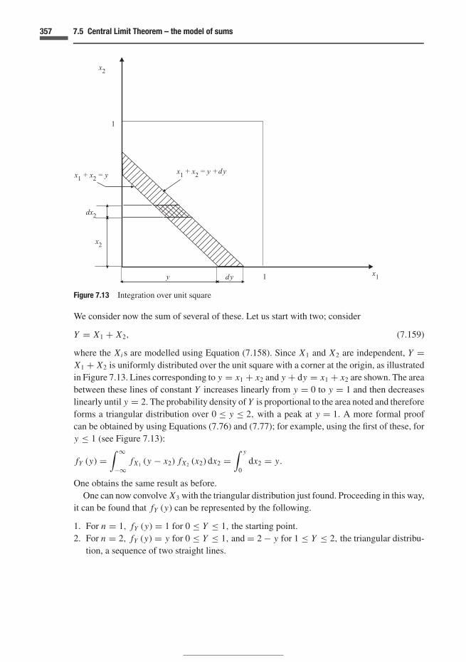
357 7.5 Central Limit Theorem – the model of sums
1
1 x1y dy
dy
x2
dx2
x2
x1 + x2 = y x1 + x2 = y +
Figure 7.13 Integration over unit square
We consider now the sum of several of these. Let us start with two; consider
Y = X1 + X2, (7.159)
where the Xi s are modelled using Equation (7.158). Since X1 and X2 are independent, Y =X1 + X2 is uniformly distributed over the unit square with a corner at the origin, as illustratedin Figure 7.13. Lines corresponding to y = x1 + x2 and y + dy = x1 + x2 are shown. The areabetween these lines of constant Y increases linearly from y = 0 to y = 1 and then decreaseslinearly until y = 2. The probability density of Y is proportional to the area noted and thereforeforms a triangular distribution over 0 ≤ y ≤ 2, with a peak at y = 1. A more formal proofcan be obtained by using Equations (7.76) and (7.77); for example, using the first of these, fory ≤ 1 (see Figure 7.13):
fY (y) =∫ ∞
−∞fX1 (y − x2) fX2 (x2) dx2 =
∫ y
0dx2 = y.
One obtains the same result as before.One can now convolve X3 with the triangular distribution just found. Proceeding in this way,
it can be found that fY (y) can be represented by the following.
1. For n = 1, fY (y) = 1 for 0 ≤ Y ≤ 1, the starting point.2. For n = 2, fY (y) = y for 0 ≤ Y ≤ 1, and = 2 − y for 1 ≤ Y ≤ 2, the triangular distribu-
tion, a sequence of two straight lines.

358 Mathematical aspects
3. For n = 3, fY (y) = 12 y2 for 0 ≤ Y ≤ 1, 1
2
[y2 − 3 (y − 1)2
]for 1 ≤ Y ≤ 2, and
12
[y2 − 3 (y − 1)2 + 3 (y − 2)2
], for 2 ≤ Y ≤ 3, giving a sequence of three para-
bolas.
In each case, there are n intervals, within each of which a curve of increasing order is found,first constant, then linear, then quadratic, then cubic, then quartic, and so on. The result maybe generalized by considering
Y = X1 + X2 + · · · + Xi + · · · + Xn. (7.160)
The resulting pdf is (see Exercises 7.25 and 7.26)
fY (y) = 1
(n − 1)![yn−1 −
(n
1
)(y − 1)n−1 +
(n
2
)(y − 2)n−1 −
· · · (−1)r
(n
r
)(y − r )n−1] (7.161)
for r ≤ y ≤ r + 1 and r = 0, 1, 2, . . . , n − 1.
Figure 7.14 shows several of these results, with a normal distribution plotted with the same meanand standard deviation as the distributions just obtained; to obtain the latter see Exercises 7.17and 7.25. The means and variances are µY = n/2 and σ 2
Y = n/12 respectively (Exercise 7.26).One can see the rapid convergence as n increases of the shape of the convoluted distributionsto that of the normal distribution. But it takes quite large n to ensure that the tails of thedistributions are reasonably similar.
Both the mean and standard deviation of Y tend to infinity as n → ∞. The standarddeviation is proportional to
√n, as shown in Exercise 7.26. Had we considered averages
Y = ∑Xi/n instead of sums, the mean would remain constant and the standard deviation
would decrease, in proportion to 1/√
n. To summarize, the convoluted distribution becomeswider and more spread out (sums), or shrinks, becoming narrower and more concentrated(averages). If we were to consider the random quantity
∑Xi/
√n, then we might expect the
distribution to be stable in lateral extent. This strategy will be considered in the followingsections.
7.5.2 Normal approximation to the binomial
In the special case where the Xi are Bernoulli random quantities that are independent, Y inEquation (7.160),
Y = X1 + X2 + · · · + Xi + · · · + Xn,
represents the binomial random quantity with mean np and variance σ 2 = npq, where q = p.
Although discrete, the binomial distribution can be approximated well for large n by the normaldistribution, provided the probability masses in the binomial distribution are approximated by

359 7.5 Central Limit Theorem – the model of sums
1
1 0.5 0 y
1
0.5 1 1.5 2 0
0.5 1 1.5 2 2.5 3 0
0.8
y
y
Figure 7.14 Addition of uniformly distributed random quantities (dotted line is normal distribution)
areas, for example by small rectangles – trapezoids are another possibility. Or the area underthe normal curve can be calculated from a value i − 1/2 to i + 1/2 when approximating theprobability at the integral value i. This is used in Exercise 7.27. Figure 7.15(a) shows thebinomial random quantity for p = 1/2 and n = 10. A good approximation is obtained evenfor this relatively small value of n; for p = 1/4, Figure 7.15(b) shows that for a larger value

360 Mathematical aspects
Figure 7.15 Normal approximation to binomial distribution
of n a good approximation can also be obtained. This approximation provides a useful tool forcalculation; see Exercise 7.27.
Transition from binomial to normal distributionsWe now consider more precisely the transition from the binomial to the normal distributions,based on de Finetti (1974). As noted at the end of Section 7.5.1, the mean and variance ofthe sum Y of n iid random quantities increases with n. The average of n binomial randomquantities is the frequency Y/n, the distribution of which becomes more and more peaked as

361 7.5 Central Limit Theorem – the model of sums
Figure 7.16 Normal and binomial distributions
n increases. A better behaved quantity is
W = 2Y − n√n
, (7.162)
which has a mean of√
n(2p − 1) and a standard deviation equal to 2√
pq. Figure 7.16(a) showsthe binomial probabilities distributed in this way. The usual binomial quantity Y (number ofsuccesses) takes values 0, 1, 2, . . . , n which are mapped onto W. One can also observe that

362 Mathematical aspects
the numerator of Equation (7.162) is the gain in n trials if a payment of ±1 unit is made for asuccess or failure, respectively. We consider the special case where p = 1/2, so that W has amean of zero and a variance of unity (2
√pq = 1).
We now spread out the probability masses at the various values of W = w (y) over the interval± (
1/√
n), resulting in a stepped probability density that is continuous. Figure 7.16(b) shows
two successive spread-out masses corresponding to y and y + 1. If one were to simulate apoint in this continuous distribution using random numbers, one would do this in two steps.First, one would simulate a point w on the distribution of W using the binomial distribution,and then a point in the interval w ± (
1/√
n)
using a uniform distribution for the second step.The first step involves the use of Equation (7.10), giving
pW (w) = Pr (Y = y) =(
n
y
) (1
2
)n
,
where y is given by Equation (7.162); y = (w
√n + n
)/2.
To denote the continuous random quantity spread over the interval ± (1/
√n), we could
change the letter W denoting the discrete random quantity used in the step leading to thecontinuous distribution; but for simplicity we shall retain W, as it will be clear when we areusing densities, as against concentrated masses of probability. The density is the probabilitymass ‘smeared out’ over the distance
(2/
√n):
fW (w) = Pr (Y = y) ÷(
2√n
)=
(n
y
) (1
2
)n
÷(
2√n
)
= 1
2
√n
(n
y
)/2n. (7.163)
As we increase n we wish to calculate the slope to determine whether we approach thenormal density. The slope between the midpoints w (y) and w (y + 1) of the stepped density –Figure 7.16(b) – is
f ′W (w) =
{[Pr (Y = y + 1) − Pr (Y = y)] ÷
(2√n
)}÷ 2√
n
= 1
4n [Pr (Y = y + 1) − Pr (Y = y)] . (7.164)
Now we know that
Pr (Y = y + 1)
Pr (Y = y)= n − x
x + 1· p
p. (See Exercise 7.22.)

363 7.5 Central Limit Theorem – the model of sums
We have that p = p = 1/2; substituting into Equation (7.164),
f ′W (w) = 1
4n Pr (Y = y)
(n − y
y + 1− 1
)
= 1
4n Pr (Y = y)
(n − 2y − 1
y + 1
). (7.165)
Substituting for Pr (Y = y) = fW (w) · 2/√
n from Equation (7.163), and y = (w
√n + n
)/2
from Equation (7.162),
f ′W (w) = 1
2
√n fW (w)
[−w
√n − 1(
w√
n + n)/2 + 1
]
= − fW (w)
(wn + √
n
w√
n + n + 2
)
= −w fW (w)
[1 + 1/
(w
√n)
1 + w/√
n + 2/n
]. (7.166)
We consider first non-zero values of w. In this case, Equation (7.166) can be written as
f ′W (w)
fW (w)= −w + terms that tend to zero as n → ∞. (7.167)
Therefore, in this limit,
f ′W (w)
fW (w)= d ln fW (w)
dw= −w. (7.168)
In the case where w = 0, we can write Equation (7.166) as
f ′W (w) = − fW (w)
[w + 1/
√n
1 + w/√
n + 2/n
]→ 0. (7.169)
This merely shows that the slope at w = 0 is zero, as would be expected for a distributionsymmetrical about the origin.
Equation (7.168) yields
ln fW (w) = −w2
2+ constant (7.170)
or
fW (w) = K exp
(−w2
2
), (7.171)
where K = 1/√
2π for coherence. Equation (7.171) is the standard normal distribution –recall that we arranged matters so that W had a mean of zero and a standard deviation of unity.

364 Mathematical aspects
Similar results can be obtained if the distribution is not standardized – a normal distributionis still arrived at, but with mean and standard deviation corresponding to the case underconsideration.
It is remarkable how the slopes across the stepped densities approach those of the normaldensity, matching this curve exactly in the limit of n = ∞. The derivation above is that ofa limiting distribution – seen also, for example in the derivation of the Poisson distributionfrom the binomial (Section 3.2.6). In these instances a sequence of distributions Fn or fn areconsidered; note that here the subscripts n do not refer to the random quantity but to the valueof n (deterministic number) in the sequence. The transition from the sequence to the limit isoften written as
Fn → F , or (7.172)
fn → f. (7.173)
7.5.3 Proof of the Central Limit Theorem
We consider now a more general situation, again using Equation (7.160), where the distributionof the Xi is not specified. Yet we retain the assumption that they are iid with common mean µ
and finite variance σ 2. Then
Y =∑n
i=1Xi
with mean µY = nµ and variance σ 2Y = nσ 2. We consider the standardized random quantity
W = Y − µY
σY= Y − nµ√
nσ. (7.174)
This quantity has a mean of zero and a standard deviation σW = 1. The distribution will notflatten or shrink, and W behaves in this respect similarly to Equation (7.162). Equation (7.174)can be written as
W =∑n
i=1 (Xi − µ)√nσ
=∑n
i=1 Vi√nσ
=∑n
i=1
Vi√nσ
=∑n
i=1Ti , (7.175)
where Vi = Xi − µ has a mean of zero and a standard deviation of σ . Note that Ti = Vi/√
nσ
must also have a mean equal to zero but a standard deviation of 1/√
n, resulting in the standarddeviation of unity for W .
The random quantity of Equation (7.175) has the characteristic function
φW (u) = φnT (u) = φn
V
(u√nσ
). (7.176)

365 7.5 Central Limit Theorem – the model of sums
where we have used Equations (7.120) and (7.112). Now
φV
(u√nσ
)=
∫ ∞
−∞exp
(iuv√nσ
)fV (v) dv
=∫ ∞
−∞
[1 + iuv√
nσ+ 1
2
(iuv√nσ
)2
+ · · ·]
fV (v) dv
= 1 + iu√nσ
〈V 〉 + 1
2
(iu√nσ
)2 ⟨V 2
⟩ + · · · (7.177)
We know that 〈V 〉 = 0; consequently⟨V 2
⟩ = σ 2 so that Equation (7.177) becomes
φV
(u√nσ
)= 1 − 1
2
u2
n+ terms involving n− 3
2 and smaller. (7.178)
Using Equation (7.176),
φW (u) =(
1 − 1
2
u2
n+ · · ·
)n
→ exp
(−u2
2
)as n → ∞. (7.179)
But this is the cf of the standard normal distribution; see Equation (7.109). This proves theCentral Limit Theorem for iid random quantities Xi . We normalized the random quantity Wso as to have a mean of zero and a standard deviation of one; we can reverse this by usingEquation (7.174) resulting in a very ‘flat’ distribution for Y, or a very ‘sharp’ one for Y/n, asdiscussed earlier. The key point in the derivation is the behaviour of φW (u) as n increases.
7.5.4 Second characteristic function and cumulants
This derivation can also be achieved by considering the second characteristic function whichis merely the logarithm of the characteristic function:
ψX (u) = ln φX (u) . (7.180)
Then
φX (u) = exp ψX (u) . (7.181)
Also the cumulants κs for s = 1, 2, 3, . . . of the second characteristic function are defined bythe power series
ψX (u) =∑∞
s=1κs
(iu)s
s!(7.182)
with
κs = isdsψX (u = 0)
dus. (7.183)
The cumulants κ1 and κ2 are the mean and variance of X ; the reader may wish to check.

366 Mathematical aspects
The following expansion results:
ψX (u) = κ1 (iu) + 1
2κ2 (iu)2 + 1
3!κ3 (iu)3 + · · · + 1
s!κs (iu)s + · · · (7.184)
Here it is convenient to consider small u, near the origin, and in the case where the mean iszero, as in the standardized distributions above, a parabolic approximation suffices:
ψX (u) � −1
2σ 2
X u2. (7.185)
Equation (7.176) becomes
ψW (u) = nψT (u) = nψV
(u√nσ
)(7.186)
= −n · 1
2
σ 2u2
nσ 2= −u2
2,
or
ψW (u) = ln φW (u) = −u2
2. (7.187)
This is the same result as that in Equation (7.179).
7.5.5 Non-identical independent random quantities
At the beginning of this section (7.5) we noted that the Central Limit Theorem also applies inmore general circumstances, for example where the distributions are not identical, or wherethere is some dependence; generally it is required that one of the Xi does not dominate theresult. An interesting review of extensions of the Central Limit Theorem is given by de Finetti(1974); we shall give a brief introduction to this. If we consider distributions of the Xi that aresimilar except for the variances, denoted σi , which vary from one quantity to another, then,instead of Equation (7.187) we have
−u2
2
[1 +
∑n
i=1
σ 2i
σ 2T
ε
(σi u
σT
)], (7.188)
where σ 2T = ∑n
i=1 σ 2i . Now we have the same expression as before, except for the summation
term, which can be thought of as a ‘correction’ to the previous result. If this term tends to zero,then the Central Limit Theorem remains valid. This can be shown to be true if the contributionof each term is small compared to the total of the preceding ones; also, the total variance σ 2
T
must diverge. A myriad of further extensions has been obtained, but for the purposes of thepresent work, the flavour of these given here is deemed sufficient.

367 7.6 Chebyshev inequality
7.6 Chebyshev inequality
We consider a random quantity X with finite mean µ and finite variance σ 2, and any distributionthat satisfies these conditions, continuous or discrete. The inequality is that
Pr (µ − cσ < X < µ + cσ ) ≥ 1 − 1
c2, (7.189)
in which a positive number c ≥ 2 is needed for useful results. The method for obtaining thisinequality is shown in Figure 7.17. This shows a continuous distribution, but the idea is equallyapplicable to discrete distributions. The method will be described in two steps.
Step 1 In the upper illustration of the figure, think of the variance as the second moment ofarea of the probability distribution about the centroid (mean) g (one can also thinkof the moment of inertia for unit distributed mass). If we remove the central area (orprobability mass), between the limits ±cσ, then the second moment is reduced.
Step 2 If we take the probability in the remaining areas (p1 and p2 in Figure 7.17) andconcentrate them as point masses on the edge of the central area, then the secondmoment is reduced even further.
Mathematically, these steps amount to the following.
Step 1 Since σ 2 = ⟨(X − µ)2
⟩,
σ 2 =∫
all x(x − µ)2dFX (x)
=∫
x≤µ−cσ(x − µ)2dFX (x) +
∫µ−cσ<x<µ+cσ
(x − µ)2dFX (x)
+∫
x≥µ−cσ(x − µ)2dFX (x)
≥∫
x≤µ−cσ(x − µ)2dFX (x) +
∫x≥µ−cσ
(x − µ)2dFX (x) .
Step 2 Now, for those regions over which these integrals are taken, provided c > 0,
(x − µ)2 ≥ (cσ )2,
so that
σ 2 ≥ c2σ 2
[∫x≤µ−cσ
dFX (x) +∫
x≥µ−cσdFX (x)
]. (7.190)
Therefore
1
c2≥ Pr [(X ≤ µ − cσ ) ∨ (X ≥ µ + cσ )] = p1 + p2

368 Mathematical aspects
Mass
Mass
cs cs
cs cs
cs cs
Figure 7.17 Probability masses for Chebyshev inequalities
or
Pr(µ − cσ < X < µ + cσ ) ≥ 1 − 1
c2.
This may also be written as
Pr (|X − µ| ≥ cσ ) ≤ 1
c2. (7.191)

369 7.6 Chebyshev inequality
Figure 7.18 Quadratic prevision example
The Chebyshev bound is rather crude if c is small (e.g. 2, 3 or 4) but is very useful in limittheorems. The method for deducing the bound is also valid for higher moments than the second.Also, we need not have commenced the analysis at the centroid. We could have started at anypoint, for example the origin.
Example 7.29 The ‘quadratic prevision’ PQ (X ) has been introduced by de Finetti (1974),where
PQ (X ) =√
P(X2) =√⟨
X2⟩.
Show that
1
c2≥ Pr
[|X | ≥ cPQ (X )]. (7.192)
This is an example where we commence the analysis at the origin rather than the centroid(Figure 7.18). We repeat steps 1 and 2. Thus
P2Q (X ) ≥ c2 P2
Q (X )
[∫x≤cPQ
dFX (x) +∫
x≥cPQ
dFX (x)
]
= c2 P2Q (X )
[Pr |X | ≥ cPQ (X )
],
corresponding to Equation (7.190). This leads directly to the required result.
The results of this section may be summarized in terms of standardized quantities as
Pr( |X − µ|
σ≥ c
)≤ 1
c2and (7.193)
Pr( |X |
PQ≥ c
)≤ 1
c2. (7.194)
The inequality will be applied in the following section.

370 Mathematical aspects
7.7 Laws of large numbers
We consider the mean Y of the sum of the iid set given in Equation (7.160); these Xi have afinite mean µ and finite variance σ 2. Since
Y = X1 + X2 + · · · + Xi + · · · + Xn,
we consider Y = Y/n. The weak law of large numbers states that for any given positive ε andθ, then for all n greater than n0 which we can find,
Pr(∣∣Y − µ
∣∣ > ε)
< θ. (7.195)
We know that⟨Y
⟩ = µ, and σ 2Y = σ 2/n. Applying the Chebyshev inequality of Equation
(7.191),
Pr(∣∣Y − µ
∣∣ ≥ cσ√n
)≤ 1
c2. (7.196)
If we associate θ with 1/c2, we can choose n0 using ε = cσ/√
n so that inequality (7.195) issatisfied. A further consequence of inequality (7.195) is that
Pr(∣∣Y − µ
∣∣ > ε) → 0 (7.197)
as n → ∞.
The result just obtained pertains to a particular n > n0 for which we can satisfy Equation(7.195). If we now consider several cases together, say for n = n0, n0 + 1, . . . , n0 + n1 (wheren1 is arbitrary), then the probability of at least one occurrence of the event
(∣∣Y − µ∣∣ > ε
)grows as n1 increases, and Equation (7.195) is no guarantee that this will not becomelarge.
The situation just discussed is in fact covered by the strong law of large numbers, whichensures that for any given positive numbers ε and θ, no matter how small, there is a numbern0 such that
Pr(maxn0≤n≤n0+n1
∣∣Y − µ∣∣ > ε
)< θ (7.198)
for arbitrary n1. This is the version emphasized by de Finetti (1974). It is also sometimes statedthat
(Y − µ
) → 0 with probability one. There are also more general proofs of the weak andstrong laws, for example for non-identical random quantities, or in the case that only the meanexists.
Probability and frequency; simulationThe theory just presented casts some light on the connection between probability and frequency.In the case where the Xi are Bernoulli (0:1) random quantities, Y is the frequency. In one view

371 7.8 Concluding remarks
of inference – which is not advocated here – the parameter of a distribution is a ‘fixed butunknown’ quantity. In the Bernoulli process, this would be the probability of success in thenext trial, used as a parameter in the binomial distribution. The value µ might be interpretedas the supposed probability; for example in the case of coin-tossing, Y would be frequency ofheads and the supposed probability of heads might be 1/2.
The laws of large numbers would then suggest that the frequency Y will be very close to the‘supposed probability’, with a high probability approaching unity. (See also Section 10.3.4 onprobability and frequency.) The results above might be used to justify an interpretation of proba-bility that is based only on frequency. As a definition of probability, this would be inappropriate,since we have used the concept of probability in deriving the laws above, and it is illogicalthen to use the theorem to justify the definition. It is much better to assess matters using theproper focus of our subjective judgement. In Chapter 8, a full analysis of inference and analy-sis of the parameters of a distribution is given in a manner consistent with the approach of thisbook.
With regard to bets ‘in the long run’, let us assume that we have a coin that we judge to beperfectly ‘honest’ with an exactly equal probability of heads and tails, and furthermore thatwe judge that independence will apply in a long series of tosses, that we judge the probabilityis 1/2 regardless of the results of the preceding tosses. In betting, say on heads in coin-tossing,‘in the long run’ variations tend to cancel each other out. Yet there is no guarantee that thiswill happen. If one is losing because of a series of tails, there is in fact no reason to supposethat a run of heads will subsequently occur to ‘cancel out’ the adverse series of tails. Indeed,at this stage – after the run of tails – the expected number of heads in a long series in thefuture is again 50%. One might place more faith in cycles in the stock market, for example, ifthere are interest rate changes aimed at retarding or stimulating growth. Here at least there isa mechanism that might have some favourable consequences.
SimulationOne area where the laws of large numbers do provide significant assistance is in simulationusing Monte Carlo methods (Chapter 11). In this method, one attempts to generate as closelyas possible a set of iid random quantities for computational purposes. Then the law of largenumbers can be used to estimate deviations from probabilistic estimates.
7.8 Concluding remarks
The manipulation of probabilities is an essential activity in probabilistic analysis. We learnmany interesting things from the theory presented in this chapter. The transformation of randomquantities with a known distribution function is frequently required in engineering analysis.Convolutions are regularly encountered. Transforms provide a powerful means of analysis. Theuse of convolutions and transforms shows a way to analyse sums of random quantities, withthe result that we find, for example, that the sum of independent normal distributions results in
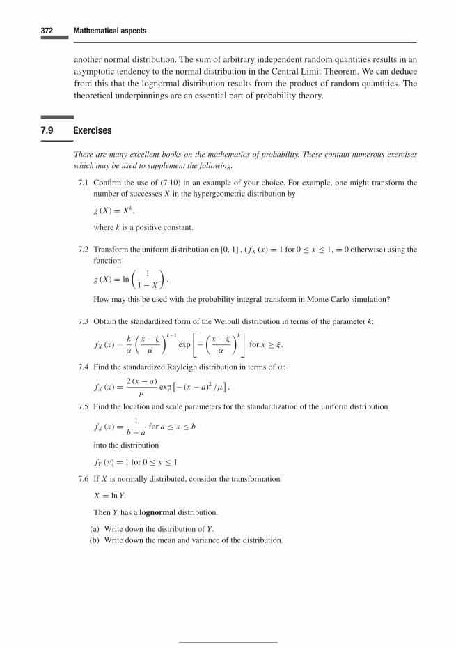
372 Mathematical aspects
another normal distribution. The sum of arbitrary independent random quantities results in anasymptotic tendency to the normal distribution in the Central Limit Theorem. We can deducefrom this that the lognormal distribution results from the product of random quantities. Thetheoretical underpinnings are an essential part of probability theory.
7.9 Exercises
There are many excellent books on the mathematics of probability. These contain numerous exerciseswhich may be used to supplement the following.
7.1 Confirm the use of (7.10) in an example of your choice. For example, one might transform thenumber of successes X in the hypergeometric distribution by
g (X ) = Xk,
where k is a positive constant.
7.2 Transform the uniform distribution on [0, 1] , ( fX (x) = 1 for 0 ≤ x ≤ 1, = 0 otherwise) using thefunction
g (X ) = ln
(1
1 − X
).
How may this be used with the probability integral transform in Monte Carlo simulation?
7.3 Obtain the standardized form of the Weibull distribution in terms of the parameter k:
fX (x) = k
α
(x − ξ
α
)k−1
exp
[−
(x − ξ
α
)k]
for x ≥ ξ.
7.4 Find the standardized Rayleigh distribution in terms of µ:
fX (x) = 2 (x − a)
µexp
[− (x − a)2 /µ].
7.5 Find the location and scale parameters for the standardization of the uniform distribution
fX (x) = 1
b − afor a ≤ x ≤ b
into the distribution
fY (y) = 1 for 0 ≤ y ≤ 1
7.6 If X is normally distributed, consider the transformation
X = ln Y.
Then Y has a lognormal distribution.
(a) Write down the distribution of Y.
(b) Write down the mean and variance of the distribution.

373 7.9 Exercises
(c) Show that 1/Y also has a lognormal distribution. Write down the mean and variance of thisdistribution.
(d) If Y1 and Y2 are two independent random quantities with lognormal distributions, show thatYP = Y1Y2 also has a lognormal distribution. Determine the parameters of YP in terms of theparameters of Y1 and Y2.
(e) Discuss the lognormal distribution as a ‘model of products’ in the light of the Central LimitTheorem as the ‘model of sums’.
7.7 Exponential growth. Let the size Z of a population be given by
Z = c exp (Xt)
for given time t ; c is a constant. If X is random with the density
fX (x) = d (1 − x)2 for 0 < x < 1,
and 0 otherwise, find fZ (z) .
7.8 Given that fX1,X2 (x1, x2) = 1 for 0 < x1 < 1 and 0 < x2 < 1, find fY1,Y2 (y1, y2) for the transfor-mation{
y1
y2
}=
[1 −12 1
] {x1
x2
}+
{21
}. (7.199)
Why is this transformation termed affine?
7.9 Consider Y = X1 + X2. Use Equations (7.76) and (7.77) to obtain fY (y) if X1 and X2 are iid withexponential distributions exp (−x) for x ≥ 0, = 0 otherwise.
7.10 Consider two iid random quantities X1 and X2 that are uniformly distributed on (0, 1) . Use thetransformations
y1 =√
−2 ln x1 cos (2πx2) and (7.200)
y2 =√
−2 ln x1 sin (2πx2) (7.201)
to show that Y1 and Y2 are independent random quantities with standard normal distributions.This algorithm can be used to generate normal random quantities from the uniform distribution(Chapter 11).
7.11 Two independent random quantities Z1 and Z2 are modelled using the standard normal distribution.The quantities R and � are polar coordinates related to Z1 and Z2 as follows for 0 ≤ R < ∞ and0 ≤ � ≤ 2π :
R = (Z 2
1 + Z 22
)1/2and (7.202)
� = arctan
(Z2
Z1
). (7.203)
Determine fR (r ) and f� (θ ) .

374 Mathematical aspects
7.12 Derive Equation (7.109).
7.13 Gamma and beta functions. It is a good idea to become familiar with the gamma function
� (s) =∫ ∞
0us−1 exp (−u) du. (7.204)
Show that
� (s) = (s − 1) � (s − 1) (7.205)
and that for positive integers s, � (s) = (s − 1)!. Also show that � (1/2) = √π, and that the beta
function
B (r, m − r ) =∫ 1
0ar−1 (1 − a)m−r−1 da (7.206)
used to normalize the beta distribution is given by
B (s, t − s) = � (s) � (t − s)
� (t). (7.207)
7.14 Human error. In a study of the effect of human error in design, Nessim used two independent gammadistributions with the same scale factor (β in Equation (7.210) below) to model the distributionsof undetected and detected errors (M and N respectively) (see Nessim and Jordaan, 1985). Showthat the probability of detecting an error,
P = N
M + N, (7.208)
is given by the beta distribution.Note that these distributions of error rates are consistent with the idea of gamma distributionsmodelling the uncertainty in rates and the errors themselves occurring as a Poisson process. Inthis context the gamma distributions are conjugate prior distributions for the rates of the Poissonprocess. This situation is modelled in Chapter 8. There are other applications using this idea;for example in arctic shipping, the two processes could correspond to successfully detected andavoided ice features on the one hand, and collisions with ice, on the other; see Jordaan et al.(1987).
7.15 For the binomial distribution of Equation (3.3),
pX (x) =(
n
x
)px (1 − p)n−x ,
(a) find the pgf;(b) use the result to show that the sum of two independent binomial random quantities X1
and X2, both with parameter p, but with n1 and n2 trials respectively, is another binomialdistribution.
375 7.9 Exercises
7.16 Use of transforms for expected utility. Keeney and Raiffa (1976) note that transforms can be used forexpected utility. Use (7.100), (7.102) or (7.137) to obtain the expected utility if the utility functionis given by (4.18):
u (x) = − exp (−cx) .
Obtain the equations of expected utility for various distributions such as the binomial and normal.
7.17 Show that the cf for a random quantity with a uniform distribution on [0, 1] is
φX (u) = exp(
iu2
)sin
(u2
)u2
= exp (iu) − 1
iu. (7.209)
7.18 Deduce from first principles the cf of the gamma density
fX (x) = xα−1 exp (−x/β)
βα� (α), x ≥ 0, α, β > 0, (7.210)
to give Equation (7.124),
φX (u) = (1 − iuβ)−α .
7.19 Find the cf of the bilateral exponential distribution:
fX (x) = exp (− |x |) for − ∞ < x < ∞. (7.211)
7.20 Find the characteristic function of the Cauchy distribution (introduced in Exercise 3.14),
fX (x) = a
π(x2 + a2
) , for − ∞ < x < ∞,
using the inversion formula. Show that the distribution is infinitely divisible and stable.
7.21 Ball bearing problem. The diameter X of a spherical ball bearing taken from a lot is normallydistributed with a mean of 10.0 mm and a standard deviation of 0.5 mm. The ball is supposed to fitinto a steel tube taken from another lot. The tube is circular in cross section, and the diameter Y isalso normally distributed but with a mean of 11.3 mm and a standard deviation of 1.2 mm. Use theresult of Example 7.19 to find the probability that a randomly chosen ball will fit into a randomlychosen tube. Five randomly chosen balls are paired off with five randomly chosen tubes. What isthe probability that all five balls will fit inside their tubes?
7.22 Show that, for the binomial random quantity X,
Pr (X = x + 1)
Pr (X = x)= n − x
x + 1· p
p.
7.23 It is a useful exercise to review transform pairs in an application. The use of Fourier transformsis well known to electrical engineers; Laplace transforms are used in the same discipline and inmechanics for viscoelastic theory and dynamics.

376 Mathematical aspects
7.24 Prove the relation between (7.139) and (7.140):
g (t) ⇐⇒ G (ω)
then
G (t) ⇐⇒ 2πg (−ω) .
Give an illustration of its use.
7.25 Deduce Equation (7.161) using convolution formulae and mathematical induction.
7.26 Using the result of Exercise 7.17 to show that the means and standard deviations of the distributionsof Equation (7.161) are given by
µY = n
2and σ 2
Y = n
12(7.212)
respectively.
7.27 Continuity correction. In approximating discrete distributions by continuous ones, as noted inSection 7.5.2, probability masses in the discrete distribution are approximated by areas, for ex-ample by small rectangles or trapezoids. The areas can be better approximated using the ‘con-tinuity correction’. In practice, this merely means approximating the probability of a particu-lar value i in the discrete distribution by the area under the continuous curve from i − 1/2 toi + 1/2.
The arrival of loaded carriers at a work station in a conveyor system occurs with probabilityp = 0.3, the remaining occurrences being unloaded (empty) carriers. The arrival of 20 carriersis being studied using the binomial distribution. Let X be the number of loaded carriers. Use thenormal approximation to the binomial distribution to calculate
(a) Pr(X = 5) and(b) Pr(2 ≤ X ≤ 10) .
Compare the results with the values from the binomial distribution.
7.28 For the multidimensional normal distribution of Example 7.9, determine the characteristic functionsof the forms given in Equations (7.57) and (7.68).
7.29 Sums of random numbers of random quantities. Very often we are interested in the sum
Y = X1 + X2 + · · · + Xi + · · · + X N ,
where the Xi and N are random. Assume that the Xi are iid.
(a) Give examples of practical interest of such a situation.(b) Find an expression for the mgf of Y in terms of the mgf of X and the probability distribution of
N .

377 7.9 Exercises
(c) A mathematical model of the travel of tourists is to be set up for a group of islands. The numberof tour groups per day, N , visiting a particular island is random with a Poisson distribution anda mean equal to µ. The size X of a tour group is also Poisson-distributed with a mean equal toν. Find the mgf of Y, the number of visitors per day at the specified island. Find the mean andvariance of Y .
7.30 There are 35 components in an assembly. Each component has a mean life of 5 years with astandard deviation of 2 years. Their lifetimes may be considered to be independent in the appli-cation considered. Find the probability that the mean life of all 35 components is greater than6 years.
7.31 The strong law of large numbers cannot be proved using the Chebyshev inequality. Find theproof.
7.32 Research the following concepts: convergence in the quadratic mean; weak convergence (conver-gence in probability); strong convergence (almost sure convergence). Which implies the others andwhy?
8 Exchangeability and inference
There is a history in all men’s lives,Figuring the nature of the times deceas’dThe which observed, a man may prophesy,With a near aim, of the chance of thingsAs yet not come to life, which in their seedsAnd weak beginnings lie entreasured.
William Shakespeare, King Henry IV, Part II
8.1 Introduction
We have described various probability distributions, on the assumption that the parametersare known. We have dealt with classical assignments of probability, in which events werejudged as being equally likely, and their close relation, the maximum-entropy distributions ofChapter 6. We have considered the Central Limit Theorem – the model of sums – and often thiscan be used to justify the use of the normal distribution. We might have an excellent candidatedistribution for a particular application. The next step in our analysis is to estimate the modelparameters, for example the mean µ and variance σ 2 for a normal distribution. We often wish touse measured data to estimate these parameters. The subject of the present chapter, ‘inference’,refers to the use of data to estimate the parameter(s) of a probability distribution. This is keyto the estimation of the probability of a future event or quantity of a similar kind.1 The fittingof distributions to data is outlined in Chapter 11.
References of interest for this chapter are de Finetti (1937, 1974), Raiffa and Schlaifer (1961),Lindley (1965, Part 2), Heath and Sudderth (1976), O’Hagan (1994) and Bernardo and Smith(1994). The book by Raiffa and Schlaifer remains a tremendous store of information – albeitwithout an index. Lindley pioneered the use of Bayesian methods in inference, particularlyin the context of classical methods. The other books are more recent and contain up-to-dateinformation on developments in the succeeding decades.
1 In some cases, we might estimate the probability of a past event – there is no real difference in approach, if theoutcome is unknown. For example, we might be uncertain as to who wrote a particular poetic work – WilliamShakespeare or the Earl of Oxford. An engineering example might be to estimate the strength of a member that hasalready failed.
378

379 8.1 Introduction
8.1.1 Frame of reference
In accordance with the preceding comments, there will always be consideration of a model ofsome kind, for the problems considered in this chapter.
Example 8.1 An example that encapsulates the key point is a binomial experiment, say thetossing of a coin. The parameter of interest in successive tosses of the coin is the probabilityp of heads in any of the trials, Equation (3.3):
pX (x) =(
n
x
)px (1 − p)n−x .
Let us assume that the coin is suspected to be biased; how do we estimate p? We mighttoss the coin, say, ten times and if we find three heads we might be tempted to estimate theprobability as 3/10. On the other hand, if we knew from previous experience that the coinwas unbiased (p = 1/2) and obtained the same result (three heads in ten tosses) we would beunlikely to change our probability assignment: we would put the result down to ‘chance’. Thesetwo extremes emphasize the role of prior information regarding the coin and our subjectivejudgement regarding this information.
Example 8.2 Consider again Example 2.7, the case of two boxes which are indistinguishablein appearance, one containing a two-headed coin, and the other an ‘honest’ coin. The modelhere is the binomial one in which the probability of heads is either 1/2 (honest coin) or certainty(two-headed coin). The coins were labelled E and E respectively. This is a special case ofExample 8.1, in which p = either 1/2 or 1.
Example 8.3 We wish to weigh an object and to estimate the uncertainty regarding the mea-surement. Savage used the example of a potato that we wish to weigh (Savage et al., 1962).We have some initial information on the weight of the object. We have a weighing device thathas been calibrated using known weights and repeated weighing of these. As a result we knowthat the readings given a known weight follow the normal distribution of Equation (3.25) withstandard deviation σ . This then represents the model of interest. We wish to weigh the newobject (potato, for example) and to estimate the uncertainty associated with this measurement.In order to do this, we need to study the parameters of the model; this might be the standarddeviation σ obtained from the calibration just mentioned.
Inference is concerned with the estimation of parameters, for example p or σ in the examplesabove, together with associated uncertainties. An example of this uncertainty would be thatassociated with small data sets, for example the ten tosses of the coin in Example 8.1 above.To deal with these problems correctly, Bayes’ theorem is used. This requires an estimate ofprior information to be combined with new information (generally measured data). As in allprobabilistic reasoning, there are subjective elements, here in the estimation of prior knowledge

380 Exchangeability and inference
and in the treatment of data. There is a desire sometimes to have some sort of ‘securityblanket’, for example a prior distribution that can be universally accepted. Sometimes this hasbeen proposed as the maximum-entropy distribution consistent with the state of knowledge.Unfortunately our knowledge is almost always not of the kind that leads to such assignments.The use of our prior knowledge based on subjective judgement should not be ducked; norshould our subjective assessment of data. Matthews (1998) points to the many problems thathave arisen in scientific inference regarding everyday problems in health and other areasthrough the attempt to avoid this subjective element.
A few words on the use of the term ‘population’, often used in inference. We often samplethe attributes of a real population. Bernstein (1996) gives an account of the history of thismeasurement. He describes the statistics collected by John Graunt on births and deaths inLondon in the seventeenth century, and the studies of population statistics by the BelgianQuetelet in the first half of the nineteenth century, the measurement of heights of adults and thesize of parent peas and their offspring by Galton later in the nineteenth century, together withthe accompanying growth of methodology, especially the use of the normal distribution. Theseexamples involve real human or other living populations, and this terminology has been carriedthrough to applications generally, for example a ‘population’ of steel specimens of which wewish to measure the strength. ‘Population parameter’ is an expression that is sometimes used,referring to the value that would be obtained if we sampled the entire ‘population’. We shallsimply use the term ‘parameter’ in the following.
8.1.2 Seeming simplicity: inference dominated by data
A question that might be posed is ‘why not use the ratio of successes to trials as the parameterin the binomial process, or estimate the mean and variance of a distribution from sufficientdata?’ The answer is that this is what one in effect does, given sufficient data. But there are twoextremes of knowledge, as noted above and previously in Section 2.3.2. The first correspondsto cases where the probability is well defined by past experience and by extensive data. A newdata point will have little influence on the result. The other extreme is where we have littleprevious knowledge. Consider an experimental device, for instance a rocket or space probe (asalso discussed below) for which there is little previous experience and only a small data set.The estimation of the parameter will inevitably contain uncertainties related to the small dataset. The Bayesian method given in this chapter includes the case where there are lots of data,and inference is then relatively straightforward, as a special case. But the Bayesian methodgives a rigorous and proper basis for the calculation, and uncertainty in the parameter is facedsquarely.
8.1.3 Inference and decisions
Decisions based on probabilistic inference can affect large numbers of people; for example,estimates of fish population parameters affect fishing policy, and whole communities can suffer

381 8.1 Introduction
Figure 8.1 Experimentation followed by main decision
if poor decisions are made (not least the one in Newfoundland, where the cod fishery wasoverfished almost to extinction). It is important that all problems of inference be visualizedas problems of decision. Figure 8.1(a) shows a typical decision tree for the following problem.We have a device or piece of machinery, and we have to decide whether to conduct a series oftests on similar pieces of equipment. The consequences of the various courses of action vary,

382 Exchangeability and inference
depending on the piece of equipment under consideration. For example, if the equipment isa space shuttle, the series of trials would be very expensive indeed, and the consequences offailure very serious. On the other hand, if the device is a can opener, a series of trials wouldnot be expensive, and obviously necessary if the device is to be commercially successful. Itis most important, in the use of probability theory, to draw decision trees and to visualize thenature of the inference being conducted, so as to avoid sterile statistical calculations that mighthave little relevance to the problem of decision-making under consideration.
Figure 8.1(b) shows a generalized decision tree for the present problem of inference. Theparameter under consideration is A. It can be seen that the present subject fits in very well indeedwith the decision-analysis approach. It is similar in structure to the Bayesian trees in Figures3.19(b), 4.24 and 4.28. The present analysis fits exactly into the structure of ‘preposterior’analysis. We shall, from time to time in this chapter, give examples of decision trees for problemsof inference. Often, inference will be concerned with scientific judgement. For example, is anew treatment for a disease or for crop production effective? Naturally, decisions are intimatelyinvolved with such questions (shall we mass-produce the new treatment for sale?), but we oftenwish also to give a fair opinion using available statistics as to the effectiveness of the treatment.This then becomes a question of judgement regarding a probability, and the decision treebecomes similar to those illustrated in Figures 2.1 and 2.2.
8.2 Series of events; exchangeability and urns
The usual format for data in problems of inference is a series of measured results, for exampleresults of coin tosses, a set of measurements of the strength of samples, a set of records ofsuccesses and failures of a device, accident records or measurements of heights of individuals.These will generally constitute our data set which involves repeated trials of the same phe-nomenon. The trials are similar, but nevertheless yield different results. We might select oursteel samples ‘at random’ and they yield different values when tested. In other words, we dealwith data sets in which we cannot favour one sample or test over another. Often the resultsare obtained in a controlled experiment. Repeated measurements are made under ‘identical’conditions, but there are factors beyond our control or knowledge which result in differencesfrom one trial to another. The judgement of exchangeability is simply that ‘the order of theresults is of no significance’.
Let us return to the problem discussed with regard to Figure 8.1(a). The series of eventsmight be simple coin-tossing, or testing of a set of steel samples or can openers. We contrastthese to tests on a new aircraft or a space shuttle or probe.2 The shuttle is a case where thereare serious consequences – seven people lost their lives in the Challenger accident and sevenmore on the Columbia. In such cases previous trials are seldom the same as later ones; design
2 With regard to the space shuttle Challenger, see Feynman (1986) and Dalal et al. (1989). Feynman states thatestimates of the probability of failure ranged from 1 in 100 to 1 in 100 000.

383 8.2 Series of events; exchangeability and urns
improvements will inevitably result from past experience so that the trials are not of the samephenomenon. We introduce this to show that in some cases, exchangeability is not appropriate:the order of the results can be important.
But order will not be important in the case of coin tossing or testing of a set of seeminglyidentical steel samples and in many practical problems. This is the traditional case that weshall analyse, that of ‘repeated trials of the same phenomenon’. These consist of n trials ofthe same device with no design changes along the way. The possible results of the trials areembodied in the series{E1 or E1, E2 or E2, . . . , Ei or Ei , . . . , En or En
}, (8.1)
consisting altogether of 2n possible events, or constituents, forming a partition. Equation (8.1)refers to the situation before the results are obtained, when the Ei are random. In any particularrealization, there will be n results, each corresponding to one or other of the pairs of possibleresults noted in (8.1). Let us denote this set of results (data) as D. There is no longer anyrandomness, since the results are a data chain. As an example, for n = 10, the following is atypical string of results, using the usual notation Ei = 1 (success) and Ei = 0 (failure):
D = {0, 1, 0, 0, 1, 1, 1, 1, 0, 1} . (8.2)
In this set of values, there are six successes (∑10
i=1 Ei ) and four failures. (Recall that the allo-cation ‘success and failure’ is arbitrary.) We might estimate from the results that the probabilityof success on the next trial is 0.60, based on the data D, or we might rely on extensive pastexperience with a similar device to estimate that (say) only 30% of the devices will succeed.But there is no seeming logic to the situation: what are the rules of the game?
The rule has already been given in Section 2.4. Bayes’ theorem tells us all we have to know:
Pr (En+1|D) = Pr (DEn+1)
Pr (D)= Pr (D|En+1) Pr (En+1)
Pr (D), (8.3)
where En+1 is the next event for which we wish to estimate the probability. We have noted thatthe new information D is now a set of data, and that there is no randomness associated withit. The terms Pr(D|En+1) and Pr(D) seem to involve probabilities of non-random data! Andwe go further to criticize the classical method for dealing with ‘random data’ when it is notrandom. In fact, there is no difficulty here; we are considering how likely D is, given the eventof interest En+1, compared to the likelihood of the same data given the other possible resultEn+1.
To see this, note that the term after the conditional sign, En+1, is in fact the quantity ofinterest in Pr(D|En+1); in this regard, we saw in Section 2.4, Equations (2.30) and (2.31), that
Pr (D) = Pr (D|En+1) Pr(En+1) + Pr(D|En+1)Pr(En+1). (8.4)
Then the right hand side of (8.3),
Pr (D|En+1) Pr (En+1)
Pr (D)= Pr (D|En+1) Pr (En+1)
Pr (D|En+1) Pr(En+1) + Pr(D|En+1)Pr(En+1)(8.5)

384 Exchangeability and inference
describes how likely the data is given the event of interest, En+1, compared to the otheralternatives (here En+1 only). There will be more on this aspect of inference in the followingsections.
8.2.1 Exchangeable sequences
The cornerstone of most probabilistic inference of the classical kind is the concept of ex-changeability, resulting in an edifice that is often poorly explored. It was delightfully andeffectively explored by de Finetti, resulting in clarification of the fundamental ideas.3 Theconcept may be summarized in the following judgement, referring again to the series of trialsof the ‘same phenomenon’, as discussed above:
The order of the results is of no significance.
In the example above, string (8.2), if we judge the results to be exchangeable, we judge that theorder of the 0s and 1s is of no significance. Therefore, all that is important is the fact that therewere six successes and four failures. These are termed sufficient statistics, in the sense thatthese numbers should be sufficient for us to make our inference (we shall soon show how!).But if we make design changes to our device during the testing period, the results will not beexchangeable.
There is an extremely simple interpretation of a finite set of exchangeable random events orquantities (let us assume that there are b of them). Since we consider that the order of obtainingthem is completely unimportant, we might just as well throw the results into a hat and drawthem at random. Of course we do not use hats in probability theory; the urn is our preferredtool. Therefore we have b balls in an urn. Since we are dealing with events, which take thevalues 0 and 1, these can be represented by pink and red balls respectively, as before in Section2.5.1. Often the assumption of independence is made at this point but we shall show that thisis not the appropriate assumption. What we have is exchangeability, not independence.
3 There is much to be gained from reading the early paper by de Finetti (1937).

385 8.2 Series of events; exchangeability and urns
The drawing of successive balls from an urn without replacement (Section 2.5.1) does notlead to independent trials, since the composition of the urn is changing with each draw – yetany order of results is considered as likely as any other. In other words they are exchangeable.The more important point is that we are using the data to change our probability assessments(this is what inference is all about), and any statement that the probability remains the sameafter knowledge of the results is obtained (independence) is incorrect.
Let us assume that there are g red balls in the urn. The string of results (8.2) above couldcorrespond to n = 10 drawings from the urn, as illustrated in Figure 8.2(a). A particularexample is where b = n = 10, and g = 6, in which case the number of drawings n and thenumber of balls b coincide. More generally below, we will make b > n. Raiffa’s urns are alsoidentified in the figure.
The parameter p in Example 8.1, the weight of the object and standard deviation σ inExample 8.3 are examples of parameters that we wish to estimate. We now introduce thekey step in our reasoning. We must treat the parameter – represented for now by the urncomposition – as being random. We model this situation by making the number of red ballsrandom, represented by the symbol G, and taking possible values 0, 1, 2, . . . , b. There arethen (b + 1) possible values of G. (We shall soon take the analogy from this discrete set tocontinuous sets of values.) Now we know that sampling from an urn with b balls correspondsto all of the possible paths through the ‘random walk’ diagrams of Chapter 2 (for example,Figures 2.9, 2.10, 2.18 and 2.19).
The composition of the urn is our analogue for our model or ‘population’ parameter which we wish toanalyse.
Example 8.4 Figure 8.2(a) illustrates the possible values of G for the case where b = 10.Raiffa’s urns form two of this set. The possible values of G are the 11 values {0, 1, 2, . . . , 10}.These correspond to the vertical axis in Figure 8.2(a), illustrated using arbitrarily a gain of +1for the drawing of a red ball or −1 for the drawing of a pink. The final set of possible gains is{−10, −8, . . . ,−2, 0, 2, . . . , 8, 10} . Recall Equation (2.48), Chapter 2, which states that
ωr,n =(
n
r
)pr,n,
as illustrated in Figure 8.2(b); p in this equation represents the probability corresponding to aparticular path with r successes, and ω to all paths.
The key aspect of the present demonstration is that the urn composition represents theparameter (or parameters) regarding which we wish to make inferences. Let the uncertaintyregarding the composition of the urn be denoted as follows:
Pr(G = g) = qg, with∑b
g=0qg = 1.
Suppose that we now sample n balls from the urn (n < b), and that r balls in the sample are

386 Exchangeability and inference
Figure 8.2 Exchangeable sequences

387 8.2 Series of events; exchangeability and urns
red. Since all orders of results – paths in Figure 8.2(b) – are exchangeable, their probabilitiesare equal. For the particular result R = r, we denote the probability as pr,n . Since the pathsare exchangeable, we might as well consider that all the 1s occur first, and then the 0s:
pr,n = Pr(E1 = 1, E2 = 1, . . . , Er = 1, Er+1 = 0, . . . , En = 0). (8.6)
For any particular path, including the one just introduced, and given the composition G = g,
pr,n = (g)r (b − g)n−r
(b)n. (8.7)
This corresponds to a single path in the hypergeometric distribution; see Section 3.2.5 andEquation (3.10). Then, for a random composition,
pr,n =∑b
g=0
(g)r (b − g)n−r
(b)nqg, (8.8)
where we have weighted the probabilities of Equation (8.7) by the corresponding qg. For anypath rather than a single path, we write, as before, the probability as ωr,n . Then
ωr,n =(
n
r
)pr,n =
(n
r
) ∑b
g=0
(g)r (b − g)n−r
(b)nqg. (8.9)
We are going to let the number, b, of members of our exchangeable set tend to infinity.Although our sample size n will be finite, we are trying to make inferences about a ‘population’that is very large. In effect, we are trying to find a rule for a ‘stable’ population, and we interpretthis as a very long string of results, of which we may have only a relatively small sample. Wecan write Equation (8.8) as follows:
pr,n =∫ 1
0
(θb)r [(1 − θ ) b]n−r
(b)ndF� (θ ) , (8.10)
where θ = (g/b), and F� (θ ) is a distribution function with jumps dF� (θ ) = qg at the corre-sponding values of (g/b) with 0 ≤ g/b ≤ 1. The representation of Equation (8.10) is essentiallythat of the Stieltjes integral (Section 3.3.5 and Appendix 2); one can think merely of an integralthat includes discontinuous jumps that correspond to a summation. We now permit the numberof balls b to increase indefinitely while keeping n and r constant. We then obtain that
pr,n =∫ 1
0θ r (1 − θ )n−r dF� (θ ) . (8.11)
From Equation (8.9),
ωr,n =(
n
r
) ∫ 1
0θ r (1 − θ )n−r dF� (θ ) . (8.12)
These are extremely important results. Equation (8.12) is essentially the result obtainedby Bayes, but he used a rather special distribution function F�; this will be discussed in the

388 Exchangeability and inference
following. Indeed, Equations (8.11) and (8.12) have the binomial form[θ r (1 − θ )n−r
]as part
of the result. This can be used regarding inferences for the binomial parameter (A, as discussedin the sequel) but represents a much more general situation, as given in the sections below,particularly 8.4 dealing with random quantities. The symbol � emphasizes this generality. If� is continuous, we can write Equation (8.11) as
pr,n =∫ 1
0θ r (1 − θ )n−r f�(θ )dθ, (8.13)
where f�(θ ) is the probability density of �.
The judgement of exchangeabilityA few words on the judgement of exchangeability. We know from personal experience thatcertain trials will not admit of this judgement. For example, our first few serves in a tennis matchmight have more 0s (failures) than 1s; this may change as the number of trials increases. In thecase of the space shuttle mentioned above, design improvements between trials could affect ourjudgement dramatically. Or the decision not to launch the shuttle in low temperatures (at whichthe O-ring seals in the booster rockets were prone to failure) would affect the exchangeabilityof the series of launches. A subset of the data might nevertheless be judged exchangeable. Inrepeated tests on the same machine, a phenomenon such as crack growth or fatigue might leadto failure, and the order of results could be rather significant; this would not apply if we testdifferent ‘identical’ devices. Fatigue, human or mechanical, using the same person or machine,would result in a judgement in which one might not accept exchangeability. In studies of safetyof advanced devices such as aircraft, one must be careful to note when technological changeshave resulted in improvements in performance as regards safety.
The judgement is basically a question of probabilistic – and therefore subjective – opinion inwhich we assume that there is no systematic variation of a relevant property with the progressionin the number of the test: 1, 2, 3, . . . , n. It should be recognized that exchangeability is thebasis of almost all common forms of inference, as outlined below. In dealing with samples fortesting it is generally reasonable. Altogether, it is a question of common sense.
8.2.2 Inference for exchangeable events
The quantity � represents the parameter space regarding which we wish to make inferences –the entire subject of inference revolves around this space. For the following, a single parameterwill be considered. We have some initial opinion regarding �, say expressed in terms ofthe probability density f (i)
� (θ ), where ‘i’ denotes ‘initial’. We wish to use the result of newinformation D, given by the string of data represented by (8.1), a typical example being (8.2)to arrive at a revised and updated density f (u)
� (θ ) using Bayes’ theorem:
f (u)� (θ ) ∝ Pr (D|θ ) f (i)
� (θ ) . (8.14)
Referring to Equation (8.11) or (8.13), we see that, given � = θ, the likelihood
� (θ ) ≡ Pr (D|θ ) (8.15)
389 8.3 Inference for binomial distribution
is given by
� (θ ) = θ r (1 − θ )n−r . (8.16)
The result amounts to ‘independence given the model parameter � = θ ’. The form of Equations(8.16), (8.11) and (8.13) is binomial in character; for this distribution,
pr,n|�=θ = � (θ ) = θ r (1 − θ )n−r (8.17)
(as always, for a particular path). We see from this equation how the ‘sufficient statistics’ {r, n}are used. These two values only are used from the data; other details are not important.
We shall now deal with binomial processes, but it is important to bear in mind (and will beshown) that the analysis above can be used generally for other processes; � stands generallyfor ‘hypothesis space’ or ‘parameter space’.
8.3 Inference using Bayes’ theorem; example: binomial distribution; Bayes’ postulate
We shall use the symbol A to represent the binomial parameter. We assume that the probabilityof x successes in n trials is given by the binomial distribution of Equation (3.3):
Pr(X = x |A = a, n) = pX |A(x, a) =(
n
x
)ax (1 − a)n−x , (8.18)
in which we have denoted the parameter as A, taking the particular value a. It is in the spirit ofthe Bayesian method that the quantity A is treated as being random; the contrast to the classicalmethod of making inferences is given in Sections 8.6 and 8.7 below. We wish to model ouruncertainty about A.
The relative importance of the data and previous experience (including previous data) isguided by Bayes’ theorem and the two terms on the right hand side of Equation (8.14). On theassumption of exchangeability, the final probability of x successes in n trials is given by
Pr(X = x |n) =(
n
x
) ∫ 1
0ax (1 − a)n−x dFA (a) . (8.19)
In this equation, FA(a) represents our current state of knowledge regarding the parameter ofthe binomial distribution. Let us assume that A is well represented by a density. Then
Pr(X = x |n) =(
n
x
) ∫ 1
0ax (1 − a)n−x f A(a)da. (8.20)
We suppose in the present example that our initial assessment of the uncertainty in A canadequately be represented by the beta distribution:
f (i)A (a) = ar0−1 (1 − a)n0−r0−1
B (r0, n0 − r0), 0 ≤ a ≤ 1. (8.21)

390 Exchangeability and inference
The parameters {r0, n0} characterize our prior opinion. In order that the probability densitynormalizes,
B (r0, n0 − r0) =∫ 1
0ar0−1 (1 − a)n0−r0−1 da. (8.22)
Here the beta function is given by
B (s, t − s) = � (s) � (t − s)
� (t), (8.23)
where the gamma function
� (s) =∫ ∞
0us−1 exp (−u) du. (8.24)
Note that for a positive integer s, � (s) = (s − 1)!. See Exercise 7.13 regarding gamma andbeta functions.
We assume now that we have conducted n1 tests with r successes, and that we deem theorder of obtaining the successes and failures not to be important. Applying Bayes’ theorem asin Equation (8.14) as well as the principle of exchangeability,
f (u)A (a) da ∝ ar (1 − a)n1−r · ar0−1 (1 − a)n0−r0−1 da
= ar+r0−1 (1 − a)n1+n0−r−r0−1 da,
and since the denominator in the following is the integral (sum) of the numerator over all valuesof the argument,
f (u)A (a) = ar+r0−1 (1 − a)n1+n0−r−r0−1
B (r + r0, n1 + n0 − r − r0). (8.25)
We see that the revised probability distribution is of the same form as the initial one, a betadensity, with parameters changed from {r0, n0} to {r + r0, n1 + n0} . We can write
r ′ = r + r0 and (8.26)
n′ = n1 + n0. (8.27)
Then (8.25) becomes
f (u)A (a) = ar ′−1 (1 − a)n′−r ′−1
B (r ′, n′ − r ′). (8.28)
Such distributions, which preserve their form during the application of Bayes’ theorem, aretermed conjugate families of distributions (more on this in Section 8.5 below).

391 8.3 Inference for binomial distribution
8.3.1 Applications of the binomial distribution; decisions
First, it is useful to explore Equation (8.28).
Example 8.5 Figure 8.3 illustrates Equation (8.25), using the notation r ′ = r + r0, n′ = n1 +n0, and s ′ = n′ − r ′. Then
〈A〉 = r ′
n′ , (8.29)
and each graph represents a situation with r ′ = number of successes, and s ′ = number offailures. Bayes’ postulate, to be introduced below, corresponds to one success and one failure,r ′ = s ′ = 1; this occupies the central position in the figure. The upper left quadrant showsvalues that correspond to information that is less informative than this postulate. As oneproceeds down and to the right, as n′ increases, the distributions become more peaked, withthe probability mass becoming more concentrated near the mean value, eventually in the limit,a Dirac spike. This shows the transition to the results based on data using Equation (8.29) with
Figure 8.3 Estimation of binomial parameter using the beta distribution

392 Exchangeability and inference
probability of success in the next trial given by
past successes
past trials.
The uncertainty associated with the estimation of the parameter is clearly shown and modelledin the distributions of Figure 8.3. Classical estimation does not face this aspect in a clearmanner; at the same time the uncertainty can be seen to be considerable. There is a richness tothe Bayesian approach that is not available in classical estimation.
Equations (8.19) and (8.20) give the probability of x future successes in n trials:
Pr(X = x |n) =(
n
x
) ∫ 1
0ax (1 − a)n−x f A(a)da. (8.30)
This equation, with f A(a) from (8.28) – on the basis of the conjugate analysis – will giveprobabilities taking into account uncertainty in the parameter A.
Example 8.6 Evaluate (8.20) using (8.28). We have
Pr(X = x |n) =(
n
x
) ∫ 1
0ax (1 − a)n−x · ar ′−1 (1 − a)n′−r ′−1
B (r ′, n′ − r ′)da
=(
n
x
)1
B (r ′, n′ − r ′)
∫ 1
0ax+r ′−1 (1 − a)n+n′−x−r ′−1 da. (8.31)
Using Equations (7.206) and (8.23),
Pr(X = x |n) =(
n
x
)B
(x + r ′, n + n′ − x − r ′)
B (r ′, n′ − r ′)
=(
n
x
)�
(n′)
� (r ′) � (n′ − r ′)· �
(x + r ′) �
(n + n′ − x − r ′)
� (n + n′). (8.32)
This is the beta-binomial distribution; see Appendix 1. This result should be contrasted withthe binomial distribution embodied in Equation (3.3) or (8.18),
Pr(X = x |A = a, n) = pX |A(x, a) =(
n
x
)ax (1 − a)n−x .
Equation (8.32) is a generalization of the binomial distribution, where parameter uncertaintyis modelled using the beta distribution. The standard binomial distribution of (3.3) can berecaptured for large r ′ and n′. Then the posterior distribution of the parameter becomes a Diracspike of unit probability mass on a = r ′/n′ (Exercise 8.2). This accords with (8.29) for largedata sets, showing the classical estimator to correspond to a large data set with certainty of theparameter. The classical situation is rescued from calamity by the use of confidence intervals;see below.

393 8.3 Inference for binomial distribution
DecisionsIn decision analysis, we need expected values to rank the various actions. These can often beobtained from the moments. For example, if the decision hinges on the utility
U = k · A,
where k is a constant, then
〈U 〉 ∝ 〈A〉 .
Second moments and higher,⟨A2
⟩,⟨A3
⟩, . . . , as well as transforms (see Exercise 7.16) can
also be used in expected-utility analysis. Raiffa and Schlaifer (1961) deal with the case oflinear loss – essentially the linear case just discussed.
Example 8.7 The mean value of A is given in (8.29):
〈A〉 = r ′
n′ or
〈A〉 = r + r0
n1 + n0. (8.33)
In the present interpretation, the prior distribution of Equation (8.21) is seen, by substitutingr = n1 = 0 in Equation (8.33), to be equivalent to having had r0 successes in n0 trials, withthe mean value of A represented by (r0/n0) .
Example 8.8 If r0 = n0 = 0, then the mean value of A is given by
〈A〉 = r
n1,
the frequency interpretation; note that this is a mean value. As we shall see in the followingExample 8.9, a somewhat different frequency is obtained if one starts with a uniform priordistribution, and then adds r successes in n1 trials.
Example 8.9 Assume that our initial information is consistent with the beta distribution, andin particular to the values r0 = 1, n0 = 2. Then our initial (prior) distribution is
f (i)A (a) = 1, 0 ≤ a ≤ 1, (8.34)
a uniform prior distribution. This is in fact Bayes’ postulate, which will be discussed furtherbelow. Suppose that we are investigating the testing strategy for a device, in which there will bea string of results such as in the expressions (8.1) or (8.2) above. Then the revised distributionfor A is given by (8.25) with r0 = 1, n0 = 2:
f (u)A (a) = ar (1 − a)n1−r
B (r + 1, n1 − r + 1). (8.35)

394 Exchangeability and inference
The mean of Equation (8.35), by reference to Equation (8.33), is
〈A〉 = r + 1
n1 + 2. (8.36)
This amounts to the use of Equation (8.33) with r0 = 1 and n0 = 2, i.e. the use of the observedfrequency, (r/n1) ,modified by the addition of two equivalent observations, one success and onefailure. The prior corresponding to r0 = 0 and n0 = 0, which gives the observed frequency asthe mean is discussed in Section 8.6. Equation (8.36) is Laplace’s ‘rule of succession’. Furtherinterpretations are given at the end of the present section, in terms of Bayes’ original analysis,and in terms of Polya’s urn model.
Example 8.10 In the case of the data string (8.2), using (8.35),
f (u)A (a) = a6 (1 − a)4
(6!4!/11!)= 2310 a6 (1 − a)4 ; (8.37)
the mean value of this distribution is
〈A〉 = 7
12. (8.38)
Example 8.11 A run of successes. We now consider further variations on the problem of testinga device. Let us suppose that the device is costly, for instance a space probe, as discussed above –but there are many less dramatic examples such as a new engine, the design of which we havejust completed, requiring the testing of several prototypes. We have so far conducted no testsbut we wish to investigate the decision as to how many tests to conduct to achieve a certainlevel of confidence in the device, as modelled in Figure 8.4(a). We can interpret the probabilityof success in the next trial as the reliability of the device (the complement of the probability offailure: see Chapter 10). This, in turn, is represented by the parameter A, which is random, andthe uncertainty in A should be taken into account. We now analyse the case where we have aseries of n1 successes, and no failures, so that r = n1. We judge that r0 = 1, n0 = 2 representsa reasonable prior, so that (8.35) represents our opinion. Substituting for r,
f (u)A (a) = (n1 + 1) an1 . (8.39)
This function is shown in Figure 8.4(b).A possible ‘estimator’, in other words a single value to represent the reliability, could be
given by the mean
〈A〉 =∫ 1
0(n1 + 1) an1 · a da
= n1 + 1
n1 + 2; (8.40)
but for small n1 there is a lot of uncertainty in this estimate. We might instead calculate the

395 8.3 Inference for binomial distribution
Figure 8.4 Tests on space probe
probability that a certain value of A = a1 is exceeded:
∫ 1
a1
(n1 + 1) an1 da = 1 − an1+11 . (8.41)
This is discussed in Lipson and Sheth (1973) in terms of the ‘success-run’ theorem (essentiallythe result just obtained).
Decision-making at this point should be subject to the fundamental methodology introducedthroughout this book; decision trees should be drawn, consequences evaluated, for exampleof success or failure as represented by A and (1 − A) , combined if required with the result(8.41).

396 Exchangeability and inference
8.3.2 Priors and security blankets
We have mentioned earlier the desire to have a universally accepted prior distribution. Thisarises from the belief that data are somehow objective, and that one should try to remove thesubjective element in the prior distribution. But the interpretation of data requires subjectivejudgement too. All probabilistic estimation requires an assessment of the information availableto the person involved (which may be shared with others). The present case illustrates thisattitude to priors. The prior distribution used above in Equation (8.34) is ‘Bayes’ postulate’(not to be confused with ‘Bayes’ theorem’). A certain degree of controversy surrounds theuse of the uniform prior distribution of � over [0, 1] . An interpretation that has been made isbased on the ‘principle of insufficient reason’; if we have no reason to prefer one value of θ
than any other, then � should be taken as uniformly distributed.This has been criticized by several well known authors, including Fisher and Pearson; an
interesting account is given by Stigler (1982). The grounds for the criticism are that, if we are‘completely ignorant’ regarding �, we must be completely ignorant regarding any monotonefunction of θ ; Stigler shows that treating the prior distribution over these functions as beinguniform gives quite different results regarding � when compared to the results using a uniformdistribution over � itself. All of this is related to the question of finding prior distributions thatexpress ‘complete indifference’; see also Section 8.6 below. From our point of view, a sinceresubjectivist should use their judgement as to which function of θ should be uniform, so thatthere is no reason to enter into the present difficulty. There is no justifiable security blanket.
Thomas Bayes
8.3.3 Historical note: Bayes’ postulate
To continue the discussion of ‘Bayes’ postulate’, Stigler argues that a careful reading of Bayes’paper shows his reasoning to have been sound. Bayes proposed an argument along the followinglines. A ball is rolled across a flat and levelled table; we can take the table as being square and of

397 8.3 Inference for binomial distribution
unit dimension (a kind of pool or billiard table). The final resting point of the ball is uniformlydistributed in the unit square. Let us measure the distance in one of the two directions from oneof the sides. This distance is a realization of the random quantity A(= a, say), the parameterin the binomial distribution. This is an experimental simulation of the uniform distribution,applied here to the parameter A. A second ball is now rolled n times across the table, andif the final position in any trial is within the distance a specified by the position of the firstball (say to the left of the first ball) then the trial is deemed a success. The whole procedureis repeated many times, the procedure representing precisely an analogue of the reasoningabove, leading to Equation (8.35). In fact, had Bayes possessed a modern computer, he mightwell have conducted a Monte Carlo simulation of this situation (see Chapter 11 and Exercise11.21).
Bayes added a ‘scholium’ to the argument. We give a brief summary here; full detail can befound in Stigler’s paper. In effect, Bayes showed that, if one started with his ‘uniform prior’,and no other information or result, then the probability of x successes in n trials is 1/(n + 1),for x = 0, 1, 2, . . . , n. (The result is for the case where the successes are achieved by any path;see Exercise 8.3.) For given n, this is a discrete uniform distribution; the probabilities of 0or 1 success in one trial are both equal to 1/2; the probabilities of 0, 1 or 2 successes in twotrials are all 1/3; and so on. Bayes then inferred that if our state of mind is such that we wouldassign this uniform discrete distribution, then the uniform distribution f (i)
A (a) = 1, 0 ≤ A ≤ 1is appropriate. This is much more cogent than the assertion that the principle of insufficientreason implies this distribution per se. Bayes’ reasoning also cleverly connects observables(X ) with unobservables (�). A further interpretation is given in terms of Polya’s urn model atthe end of the present section.
Stigler also discusses the possible motives for the poor interpretation of Bayes’ reasoningby eminent researchers. He concludes that much of the criticism arose from the desire to enlistBayes as a supporter of their probabilistic point of view.
Polya interpretationA further interpretation of the uniform prior distribution is Polya’s urn. Consider this modelin which there are initially one red and one pink ball. A ball is drawn, and this is replacedtogether with another of the same colour (double replacement; see also Section 2.6.5). Theprocedure is continued for n drawings. Given that there are r red balls drawn amongst these,we know that the composition is then r + 1 red balls in the total of n + 2. Then the probabilityof success (red ball) on the next draw is
r + 1
n + 2,
which is the same as the probability obtained from Equation (8.36).
Example 8.12 If there have been eight drawings, of which six are red, the probability of redon the next draw is 7/10.
398 Exchangeability and inference
Example 8.13 Given the following situation (de Finetti, 1974, vol. 2): there have been 100drawings from the urn, and we know only the result of eight drawings: numbers 1, 3, 8, 19,52, 53, 92, 100. These balls are red except for two (1 and 92), which are pink; what is theprobability (1) that the ball on the second drawing is red, (2) that the ball on the 95th drawingis red, and (3) given that the drawings continue to 1000 in total without any further resultsbecoming available, that the 1000th ball is red. The results of the 100 drawings are
{0, E2,1, E4, . . . , E7,1, E9, . . . , E18,1, E20, . . . , E51,1,1, E54, . . . , E91,0, E93, . . . , E99,1} .The data are exchangeable. The answers are: (1) not 1/3 (this would be correct if we had onlythe result of the first drawing), but 7/10; (2) and (3), also 7/10. The lesson of this example isthat probability is a function of information.
Another interpretation of Bayes’ scholium now is apparent (see also Blom et al., 1994).Consider the drawings from Polya’s urn. Let X denote the number of red balls in n trials. Ifwe obtain a sequence of reds, say n reds in n trials, then
Pr(X = n) = 1
2· 2
3· 3
4· . . . · n
n + 1= 1
n + 1. (8.42)
Also, since the series is exchangeable, then de Finetti’s result of Equations (8.13) and (8.20)apply; denoting the parameter again as A, then
Pr(X = r ) = ωr,n =(
n
r
) ∫ 1
0ar (1 − a)n−r f A(a)da; (8.43)
but r = n, so that
Pr(X = n) = ωn,n =∫ 1
0an f A(a)Pda. (8.44)
Equating (8.42) and (8.44),∫ 1
0an f A(a)da = 1
n + 1. (8.45)
But this equation represents the moments (n = 1, 2, . . .) about the origin of the distribution[ f A(a)] in question. Further, the values [1/(n + 1)] are the moments of the (continuous) uniformdistribution on [0, 1] . This is the only distribution with these moments, and therefore
f A(a) ≡ 1, 0 ≤ a ≤ 1.
This is Bayes’ postulate. Thus Polya’s urn is equivalent to Bayes’ postulate. Substitutionin Equation (8.43) gives the answer to the question posed with regard to Bayes’ scholium(Exercise 8.3 below), in which it is found that
ωx,n = 1
n + 1, (8.46)
for x = 1, 2, . . . , n. Thus X has a discrete uniform distribution, as in Bayes’ scholium.

399 8.4 Exchangeable random quantities
8.4 Exchangeable random quantities
Up to the present we have considered sequences of the kind{0, 1, 0, 0, 1, 1, 1, 1, 0, 1, E11 or E11, E12 or E12, . . .
}, (8.47)
where we have added uncertain (unknown) events to the string of 8.2. If, instead of events, weare considering quantities Xi , then we might have the sequence{
x1, x2, . . . , xn1 , Xn1+1, Xn1+2, . . . , Xn1+n}. (8.48)
The n1 lower case letters{
x1, . . . , xn1
}represent measurements, and there is nothing random
about these. They might consist of readings of the weight of Savage’s potato, or recordingsof ice thickness in an arctic field expedition, and they assist us in making inferences. Theupper case quantities Xi refer to random quantities, for example future values, or unknownvalues from the past. In the present idealization, both the data set and the random quantitiesare exchangeable. But they have different roles as we have seen above; data are used toimprove, change and update our probability distribution of the parameter, represented by �.
The remaining random quantities must then be based on this updated distribution, but wecannot improve our probabilistic situation without further information.
Let us consider a sequence of n exchangeable random quantities
{X1, X2, . . . , Xi , . . . , Xn} . (8.49)
Since the order is judged to be of no significance in making probabilistic statements, the n!permutations of (8.49) have the same n-dimensional probability distribution. Further, we maychoose any order by permuting the subscripts, for example
Xi1 , Xi2 , Xi3 , . . . , Xin ,
in which the subscripts i1, . . . , in have been chosen in any manner whatsoever. For example,we could put the original set 1, 2, . . . , n into a hat, and choose them at random, with the firstnumber drawn being i1, and so on. De Finetti (1974) states that:
. . . every condition concerning n of the Xh has the same probability, no matter how the Xh are chosen orlabelled.
We define the events Ei as follows:
Ei ≡ Xi ≤ x . (8.50)
Since the Xi are exchangeable, so are the Ei . We now make the following association:
Xi ≤ x → Ei , ‘success’, red ball in urn,
Xi > x → Ei , ‘failure’, pink ball in urn. (8.51)

400 Exchangeability and inference
--
Figure 8.5 Distribution of X , given parameters. The event Ei corresponds to Xi ≤ x .
Therefore, conditional on the value x , we have the same situation as before: a series of ex-changeable successes and failures in drawings from an urn.
In problems of inference we always consider a probabilistic model. The situation is illustratedin Figure 8.5. An example is the normal distribution in weighing an object. The quantities Xi
represent unknown results of (say, future) weighings. We have a direct analogy to the case ofevents through the associations (8.51) and consequently
Pr(Xi ≤ x) = FX (x) = Pr(Ei ). (8.52)
If our distribution parameters are known, we can calculate this probability directly as FX (x)from the distribution fX (x) with known parameters. This value will under these circumstancesbe fixed and known, corresponding to an urn of known composition.
But we wish to include uncertainty regarding the parameter value in our analysis, so weproceed as we did in Sections 8.2 and 8.3 above, and treat the parameter as being random, cor-responding to an urn with unknown composition. The symbol � now stands for the parameterof the distribution. Hence
Pr(Xi ≤ x |θ ) = FX |�=θ (x |θ ). (8.53)
Events were dealt with in Sections 8.2 and 8.3 above, and � = θ there stood for the probabilityof the event Ei . This probability is now represented by FX |�=θ (x |θ ). For convenience we repeatEquations (8.11) and (8.12) but using the density dF� (θ ) = f�(θ )dθ :
pr,n =∫ 1
0θ r (1 − θ )n−r f�(θ )dθ, (8.54)
and
ωr,n =(
n
r
) ∫ 1
0θ r (1 − θ )n−r f�(θ )dθ. (8.55)

401 8.4 Exchangeable random quantities
We can therefore write the two preceding equations for pr,n andωr,n replacing θ by FX |�=θ (x |θ ):
pr,n =∫ 1
0Fr
X |�(x |θ )[1 − FX |�(x |θ )
]n−rf�(θ )dθ, (8.56)
and
ωr,n =(
n
r
) ∫ 1
0Fr
X |�(x |θ )[1 − FX |�(x |θ )
]n−rf�(θ )dθ, (8.57)
respectively.We can think of � as corresponding to the parameter space such that Pr(� ≤ θ ) = F�(θ ).
This has been modelled by the contents of an urn. If there is more than one parameter involvedin the distribution of X, then (� ≤ θ ) represents the appropriate part of the parameter space,which contains several dimensions corresponding to the parameters required; the examples ofthe next section should make this clear. We know from the above that if the random quantitiesof interest
{X1, . . . , Xn}are exchangeable, then they have a common distribution function FX |�(x |θ ) for all Xi . Further,from the structure of Equations (8.56) and (8.57), which are valid for any choice of X = x,
we can see that the Xi are independent given the parameter � = θ . In raising FX |�(x |θ ) tothe power r in Equations (8.56) and (8.57), or raising its complement to the power (n − r ) ,
independence is clearly implied. And this is true for any X = x and for any � = θ. Therefore,given � = θ, the Xi are independent and identically distributed (iid).
8.4.1 Inference for exchangeable quantities
Let the parameter of interest be denoted A – this is intended as an example of a single-valuedparameter space. (A is really no different from � except that we reserve � for the generalidea of parameter or hypothesis space.) Therefore A could be the mean of the distribution forthe weight of our object or for a steel strength that is being measured. From the discussion inthe preceding paragraph, given the parameter A = a, the Xi are independent and identicallydistributed (iid) random quantities. In applying Bayes’ theorem, it is convenient to think ofintervals in the neighbourhood of the value of continuous random quantities considered, sincea continuous distribution gives a density. Let the data be
D = {x1, x2, . . . , xn} . (8.58)
The appropriate form of Bayes’ theorem then becomes
f (u)A (a) da =
[fX1,...,Xn (x1, . . . , xn|A = a) dx1 · · · dxn
] · f (i)A (a) da∫ [
fX1,...,Xn (x1, . . . , xn|A = a) dx1 · · · dxn] · f (i)
A (a) da, (8.59)
where the term in square brackets of the numerator is the likelihood � ≡ Pr (D|A = a) , forthe intervals stated. Now it always happens that the intervals ‘da’ cancel from the left and right

402 Exchangeability and inference
hand side of the Bayesian equation; the one on the denominator gets absorbed into the integral.Further, the intervals ‘dx1 · · · dxn’ cancel from the numerator and the denominator. So we canrewrite the equation as
f (u)A (a) =
[fX1,...,Xn (x1, . . . , xn|A = a)
] · f (i)A (a)∫ [
fX1,...,Xn (x1, . . . , xn|A = a)] · f (i)
A (a) da, (8.60)
dealing only with densities. In this case, the likelihood is
� = fX1,...,Xn (x1, . . . , xn|A = a) , (8.61)
omitting the intervals dxi , which are always omitted from Equation (8.60) in any event sincethey cancel.
Since the numerator of the right hand side of Equation (8.60) deals with iid quantities, wecan write it as
fX1,...,Xn (x1, . . . , xn|A = a) = fX |A=a (x1, a) · fX |A=a (x2, a) · . . . · fX |A=a (xn, a) ,
=∏n
i=1fX |A=a (xi , a) . (8.62)
Therefore
f (u)A (a) =
∏ni=1 fX |A=a (xi , a) · f (i)
A (a)∫ ∏ni=1 fX |A=a (xi , a) · f (i)
A (a) da, (8.63)
and
� =∏n
i=1fX |A=a (xi , a) . (8.64)
Examples of the application of this equation are given in the next section.As a final point of passing interest in this section, we note that in Equation (8.50), we
considered the events (Ei = Xi ≤ x) . We could equally well have considered the event Fi =(x ≤ Xi ≤ x + dx) .
8.5 Examples; conjugate families of distributions
We have already encountered an example of a conjugate family in making inferences regardingthe binomial distribution in Section 8.3. In the example given, the uncertainty regarding thebinomial parameter A was modelled using the beta distribution. We found that the reviseddistribution, after updating with Bayes’ theorem, was also of the beta family. Given this situ-ation, the term for the initial (prior) distribution that has been adopted in the literature is theconjugate prior distribution, and the families are termed conjugate families; the name andtechnique are due to Raiffa and Schlaifer (1961).
One should express one’s prior beliefs by means of any distribution that expresses one’sopinion correctly – it does not have to correspond to any family. The conjugate families

403 8.5 Examples; conjugate families of distributions
represent a convenient way to introduce the updating of beliefs about parameters, and, in thecases presented, have an interesting relationship to classical methods which are based entirelyon the data. But any distribution can be used, not necessarily of the conjugate family. Ingeneral, numerical computer-based techniques offer a flexible approach in cases where thereis no convenient mathematical ‘family’.
8.5.1 Unknown mean of normal distribution
We shall commence with an example from the theory of errors, for example an object weighedon a known and calibrated measuring device. Other than weighing, there are many othermeasurements in physics and astronomy which have been analysed in this way; a furtherexample is measuring distance between two points in a geodesic survey. For the present analysisit is assumed that the accuracy of the device has been ascertained from previous measurements;this is interpreted as the variance – or standard deviation – of the distribution being known.Readings have been observed to follow a normal distribution N
(µ, σ 2
).
We now undertake new measurements, for example of an unknown weight. As a result, wehave a number of new readings, represented by D = {x1, x2, . . . , xn} . The number n of datapoints may be small. Consequently the mean A is considered uncertain, and the data are to beused to make inferences about A. The readings are therefore modelled as N (A, σ 2), in whichA is random and σ 2 is the known variance. Thus
fX |A=a(x, a) = 1√2πσ
exp
[−1
2
(x − a
σ
)2]
= K1 exp
[−1
2(x − a)2 /σ 2
], (8.65)
in which the constant K1 = 1/(√
2πσ)
. We may now use Equation (8.63) to write
f (u)A (a) =
∏ni=1 fX |A=a (xi , a) · f (i)
A (a)
N1,
where we have written the denominator, which is nothing but a normalizing factor, as N1. Theproduct term of the numerator is the likelihood �, as defined in Equation (8.64) for densities.This term, in the case of the distribution (8.65), can be written as
�(a) = K n1 exp
[− 1
2σ 2
∑n
i=1(xi − a)2
]. (8.66)
Now∑n
i=1(xi − a)2 =
∑n
i=1x2
i − 2a∑n
i=1xi + na2;
noting that∑n
i=1 xi = nx, where x is the mean of the sample {x1, . . . , xn} , we may write that∑n
i=1(xi − a)2 =
∑n
i=1(xi − x)2 + n (x − a)2 . (8.67)

404 Exchangeability and inference
The two terms involving nx2 from the first (summation) term of Equation (8.67), and the onefrom the second term cancel (the reader might wish to check; these were included to completethe square). Now we see in this equation that the random quantity A = a appears only in thesecond term so that the first term can be included in the constant (this will not be the case whenwe deal with ‘unknown mean and variance’ below). Then
� (a) = K exp[− n
2σ 2(x − a)2
], (8.68)
where K = K n1 exp
[−(1/2σ 2)∑n
i=1 (xi − x)2]. The term does not involve a, so that (as noted)
it contributes only to the constant.Consequently,
f (u)A (a) = K exp
[− n2σ 2 (x − a)2
] · f (i)A (a)
N1
= exp[− n
2σ 2 (x − a)2] · f (i)
A (a)
N2, (8.69)
where we have absorbed all the constants into N2 = N1/K . It is emphasized that the densityf A (a), initial or updated, is a function only of a; everything else contributes merely to thenormalizing constant that ensures coherence. This fact is extremely useful in the updatingexercises of this chapter, and it is most helpful to exploit it. One concentrates on those termsthat are functions of the random quantity under consideration, and all the other multiplicativeterms become absorbed into the normalizing constant.
A few points should be made at this juncture. First, often a looser definition of likelihood �
is used, simply by the omission of the factor K in Equation (8.68); thus
� (a) = exp[− n
2σ 2(x − a)2
](8.70)
is often used. It is also seen that the likelihood function has the form of a normal distribution,with a standard deviation σ/
√n, in other words σ reduced by the factor
√n. It is useful to
introduce the terminology emphasized by de Finetti. For the distribution N (µ, σ 2), (1/σ ) istermed the ‘precision’, and (1/σ 2) = σ−2 is termed the ‘weight’ which we shall denote as w.The precision in the likelihood of Equation (8.70) is therefore increased from (1/σ ) by a factor√
n, and the weight by a factor of n:
w = nw1, (8.71)
where w1 = weight of one data point(1/σ 2
)and w = weight of data set.
Now we have set the stage for the use of a conjugate prior distribution. For the presentexample, this is another normal distribution. We therefore assume that our initial information

405 8.5 Examples; conjugate families of distributions
is reasonably consistent with a normal density; in other words
f (i)A (a) = 1√
2πσ0
exp
[−1
2
(a − µ0
σ0
)2]
(8.72)
= w1/20√
2πσ0
exp[−w0
2(a − µ0)2
]. (8.73)
In this equation, the distribution N (µ0, σ20 ) represents our prior belief regarding the parameter
µ represented by A. We use the notation σ−20 = w0. Substituting Equation (8.72) into (8.69),
we find
f (u)A (a) =
exp[− n
2σ 2 (x − a)2] · exp
[− 1
2σ 20
(a − µ0)2]
N2 · √2πσ0
. (8.74)
Again, we may absorb all constants into a single normalizing value; what matters is the functionof a. We combine the two exponential functions containing a as follows:
f (u)A (a) ∝ exp
(−1
2
{[(nσ−2) (x − a)2
] + [(σ−2
0 )(a − µ0)2]})
∝ exp[−1
2
(nσ−2 + σ−2
0
) ×(a2 − 2a
xnσ−2 + µ0σ−20
nσ−2 + σ−20
+ terms not involving a
)]. (8.75)
The last terms ‘not involving a’ are again constant, and we may adjust (8.75) to complete thesquare:
f (u)A (a) ∝ exp
−1
2
(nσ−2 + σ−2
0
) (a − xnσ−2 + µ0σ
−20
nσ−2 + σ−20
)2 .
We may conclude by writing the following (with a version where (1/σ 2) is written as theweight w):
f (u)A (a) = 1√
2πσ f
exp
[−1
2
(a − µ f
σ f
)2]
= w1/2f√2π
exp[−w f
2
(a − µ f
)2], (8.76)
where
µ f = xnσ−2 + µ0σ−20
nσ−2 + σ−20
,
= xnw1 + µ0w0
nw1 + w0, (8.77)

406 Exchangeability and inference
and
σ−2f = nσ−2 + σ−2
0 ,
w f = nw1 + w0. (8.78)
In these equations, w0 is the weight of the prior distribution, w = nw1 is the weight of thedata, in accordance with (8.71) and w f is the final weight.
As indicated earlier, the normal distribution represents the conjugate family for the param-eter A. The mean of the updated distribution is the weighted sum of the prior mean and themean of the likelihood, the weights being that of the prior distribution (1/σ 2
0 ) and that of thelikelihood (n/σ 2 = nσ−2). The posterior weight is the sum of the weights from the prior distri-bution and the likelihood. On the question of notation, had our prior information correspondedto a set of n0 readings, each with weight (1/σ 2
0 ), then the terms σ−20 in Equations (8.77) and
(8.78) above would be replaced by (n0σ−20 ) and w0 with n0w0.
Example 8.14 Bridge elevation 1. The elevation of a newly constructed bridge deck is mostimportant so as to give adequate clearance to a railway line below. A set of measurements witha particular measuring system showed the mean to be normally distributed with an averageof 20.70 m with a standard deviation of 0.150 m. Take these values as representing the priorknowledge.
Six new measurements of the elevation have been made using a new (improved) measuringdevice. The results are as follows (in metres). The device used is known to have a standarddeviation of 0.050.
20. 51, 20. 53, 20. 47, 20. 61, 20. 51, 20. 47,Mean: 20. 52, standard deviation: 0.0516.
The answer may be deduced as follows.Prior mean = 20.70.
Prior weight = 1/(0.150)2 = 44.4.
Data (likelihood) mean = 20.52.
Data (likelihood) weight = nσ−2 = 6/(0.05)2 = 2400.
Posterior mean = [(20.52)(2400) + (20.70)(44.4)] /(2400 + 44.4) = 20.52.
Posterior weight = 2444.4.
Posterior standard deviation = 0.0202 0.05/√
6.
Figure 8.6(a) shows the relevant distributions for this example.
Example 8.15 Bridge elevation 2. In this case, we have the following prior information:µ0 = 20.525 m; σ0 = 0.0221 m. The same data as in Example 8.14 are available, comprisingthe six measurements above. Then we obtain the following (using units of metres).
Prior mean = 20.525.
Prior weight = 1/(0.0221)2 = 2047.
Data (likelihood) mean = 20.52.

407 8.5 Examples; conjugate families of distributions
Figure 8.6 Change of opinion regarding bridge elevation
Data (likelihood) weight = nσ−2 = 6/(0.05)2 = 2400, as before.Posterior mean = [(20.52)(2400) + (20.525)(2047)] /(2400 + 2047) = 20.522.
Posterior weight = 4807.
Posterior standard deviation = 0.0150.
Figure 8.6(b) shows the relevant distributions for this example.
The two examples just completed show the influence of different prior distributions. In thefirst case the prior distribution is relatively diffuse with a low weight whereas in the secondcase the weight is similar to that of the data.
Future valuesRather than modelling the mean value, we might be interested in a future value. For example, wemight know the mean height of waves during a storm but might wish to address the uncertaintyin the next wave height. See Exercise 8.6.
408 Exchangeability and inference
8.5.2 Unknown variance of normal distribution
We now consider the case where the distribution is again normal N (µ, σ 2), but where the meanis known and we wish to study the variance σ 2 using available information which might notbe sufficient for a definitive value to be proposed. Then σ 2 is random, and we again followRaiffa and Schlaifer, and de Finetti, in modelling the ‘weight’ (1/σ 2), which we shall denoteas W, the upper case indicating the randomness of this parameter. An example is where weare calibrating our measuring device, for example that for determining the weight of an object.This we might do by making repeated measurements using an object the weight of which isaccurately known. Recall that this is an analogue for a much wider set of problems; also wediscussed calibration and Bayes’ theorem in Section 2.4.3.
Applying Bayes’ theorem in the present instance gives
f (u)W (w) =
∏ni=1 fX |W=w (xi , w) · f (i)
W (w)
N1, (8.79)
where
fX |W=w(x, w) = wn2√
2πexp
[−w
2
∑n
i=1(xi − µ)2
](8.80)
and N1 is a normalizing constant, as before. The likelihood is therefore as follows (omittingconstants):
� (w) = wn2 exp
[−w
2
∑n
i=1(xi − µ)2
]
= wn2 exp
[−w
2s2
d
], (8.81)
where s2d = ∑n
i=1(xi − µ)2. Now, � is of the same form as the gamma distribution; we shalluse this for the prior distribution of W, anticipating it as the appropriate conjugate family. Inparticular we shall use the chi-square distribution, which is a particular form of the gammadensity since this is commonly used in inferences regarding the variance.
The standard form of the gamma distribution is
fX (x) =xα−1 exp
(− x
β
)βα� (α)
. (8.82)
where α and β are positive constants, and � (·) is the gamma function. In studying variance, itis usual to write this as a chi-square distribution and we shall follow this convention. Formally,for a random quantity Y = 2X/β, the chi-square distribution with ν degrees of freedom is
fY (y) = yν2 −1 exp
(− y2
)2
ν2 �
(ν2
) , (8.83)
where α in (8.82) has been written as ν/2 and β = 2. The chi-square distribution can alsobe seen as a special case of the gamma distribution with shape parameter ν/2 and a scaleparameter of 2.

409 8.5 Examples; conjugate families of distributions
The prior distribution is written in terms of
W ′ = W
w0, (8.84)
where w0 is a normalizing constant (this allows us surreptitiously to change the scale parameterwhile keeping β = 2 as noted above). Using the form (8.83), we write
f (i)W ′
(w′) =
(w′) ν0
2 −1exp
(−w′
2
)
2ν02 �
(ν02
) , (8.85)
where (W ′ = W/w0) is chi-square, and where ν0 and w0 express our prior beliefs regardingthe parameter W . The ratio
W
W ′ = w0 (8.86)
is used to scale the parameter W ; note that⟨W
w0
⟩= ν0 (8.87)
so that
〈W 〉 = ν0w0. (8.88)
Also the standard deviation is 2√
ν0, and the mode (for ν0 > 2) is at (w/w0) = 2[(ν0/2) − 1].See also Exercise 8.8 (relates gamma and chi-square).
Substituting Equation (8.85) and the likelihood function into Equation (8.79) yields a dis-tribution of the same chi-square form as Equation (8.85):
f (u)W ′
(w′) =
(w′) ν f
2 −1exp
(−w′
2
)
2ν f2 �
( ν f
2
) , (8.89)
but with
W ′ = W
w f, (8.90)
where
ν f = ν0 + n (8.91)
and1
w f= 1
w0+ s2
d . (8.92)
The chi-square distribution of Equation (8.89) has a mean⟨W
w f
⟩= ν f ,
〈W 〉 = ν f w f , (8.93)
410 Exchangeability and inference
a standard deviation of 2√
ν f , and a mode (for ν f > 2) at (w/w f ) = 2[(ν f /2) − 1]. These areof assistance in obtaining a feeling for one’s degree of belief.
There are various versions of the distribution of Equation (8.89). Lindley (1965) considersthe variance σ 2 as the random quantity; prior knowledge is expressed via ν0, as above, and σ 2
0 ;the chi-square random quantities are (ν0σ
20 /σ 2) and (ν f σ
2f /σ
2), where
ν0σ20 = 1
w0, with
ν f σ2f = 1
w f= ν0σ
20 + s2
d . (8.94)
This is consistent with our formulation and is quite attractive since we can write s2d = νs2,
where s2 is the sample variance. Then
ν f σ2f = ν0σ
20 + νs2. (8.95)
Note that σ 20 and σ 2
f just discussed have a somewhat different meaning from that in Section8.5.1 since we are now modelling the variance as random, and these parameters now specifythe distribution of W ′.
Example 8.16 Referring to Example 8.14 above, we assume now that the measurements aretaken to a known height in order to estimate the variance. The measurements are as follows(in metres).
20. 51, 20. 53, 20. 47, 20. 61, 20. 51, 20. 47,Mean: 20. 52, standard deviation: 0.0516.Prior information on
(W = 1/σ 2
): w0 = 250; ν0 = 4; 〈W 〉 = 1000 = ν0w0, σ
20 = 0.001.
Prior standard deviation of W ′ = 2√
ν0 = 4.0.
The updated parameters are found to be w f = 61.07; ν f = 10, σ 2f = 1/610.7 = 0.00164;
The prior and posterior distributions of W are plotted in Figure 8.7.
Note: to obtain the distribution of W from that of W ′, see Exercise 8.8. For confidenceintervals, see Exercise 8.20.
8.5.3 Unknown mean and variance of normal distribution
It is often the case that neither the mean nor the variance are known before taking the measure-ment, yet we might know from past experience that the distribution is normal (and tests canbe conducted to verify this using the data; see Chapter 11). This is probably the most commonform of inference – we mentioned in the introduction to this chapter the measurements thathad been made historically, for example the heights (and other attributes) of human beings.
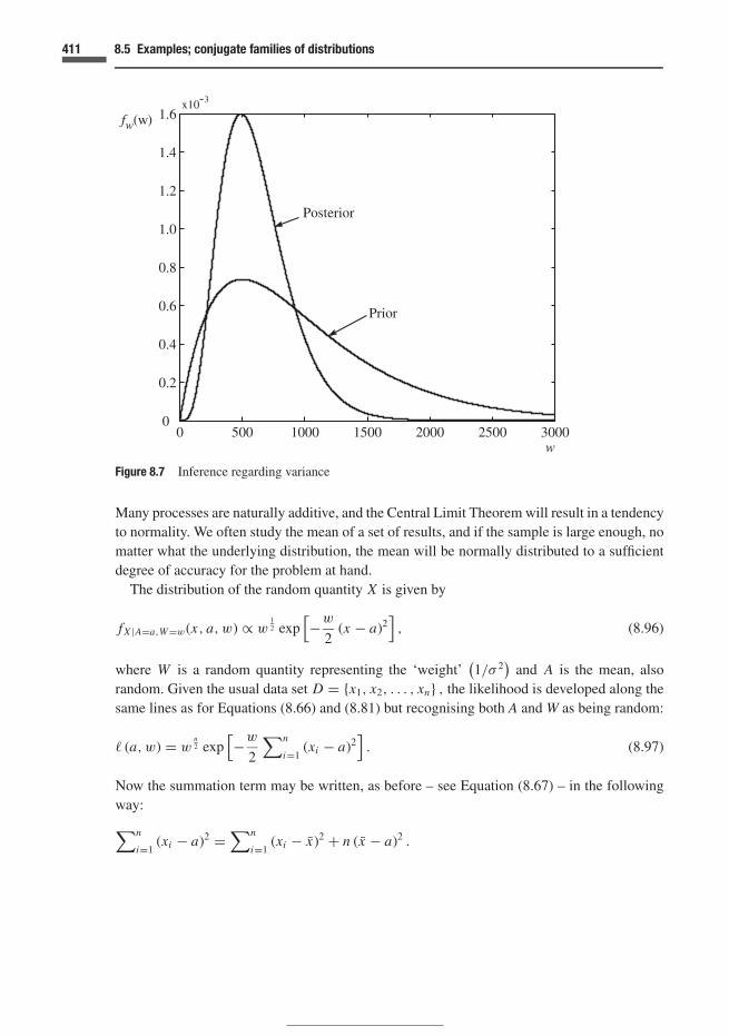
411 8.5 Examples; conjugate families of distributions
w
-
Figure 8.7 Inference regarding variance
Many processes are naturally additive, and the Central Limit Theorem will result in a tendencyto normality. We often study the mean of a set of results, and if the sample is large enough, nomatter what the underlying distribution, the mean will be normally distributed to a sufficientdegree of accuracy for the problem at hand.
The distribution of the random quantity X is given by
fX |A=a,W=w(x, a, w) ∝ w12 exp
[−w
2(x − a)2
], (8.96)
where W is a random quantity representing the ‘weight’(1/σ 2
)and A is the mean, also
random. Given the usual data set D = {x1, x2, . . . , xn} , the likelihood is developed along thesame lines as for Equations (8.66) and (8.81) but recognising both A and W as being random:
� (a, w) = wn2 exp
[−w
2
∑n
i=1(xi − a)2
]. (8.97)
Now the summation term may be written, as before – see Equation (8.67) – in the followingway:
∑n
i=1(xi − a)2 =
∑n
i=1(xi − x)2 + n (x − a)2 .

412 Exchangeability and inference
This may in turn be written as[νs2 + n (x − a)2
], (8.98)
where
s2 =∑n
i=1 (xi − x)2
ν(8.99)
is the sample variance (see also (11.5)) and
ν = n − 1. (8.100)
We cannot make the simplification carried out before, of including the term involving s2 of(8.98) in the constant part of the distribution, in the case of Equation (8.97), since it is in thepresent case multiplied by w, a random quantity in our investigation. We therefore write
� (a, w) = wn2 exp
{−w
2
[νs2 + n (x − a)2
]}. (8.101)
The conjugate family is the normal-gamma distribution, based on the ideas used in devel-oping Equations (8.72) and (8.85); this is written as follows for the initial (prior) distribution:
f (i)A,W (a, w|n0, µ0, ν0, σ0) ∝ w
ν02 − 1
2 exp{−w
2
[n0 (a − µ0)2 + ν0σ
20
]}. (8.102)
Note that ν0 and σ0 are used in a similar way to that in Section 8.5.2. The term
exp[−w
2ν0σ
20
]
is separable (as a multiplier) from the exponential term in Equation (8.102); it is attractive towrite w0 = 1/(ν0σ
20 ), as in Section 8.5.2. Combining the likelihood with this prior distribution,
the following is obtained:
f (u)A,W
(a, w|n f , µ f , ν f , σ f
) ∝ wν f2 − 1
2 exp{−w
2
[n f
(a − µ f
)2 + ν f σ2f
]}, (8.103)
where
n f = n0 + n, (8.104)
µ f = n0µ0 + nx
n0 + n, (8.105)
ν f = ν0 + n = ν0 + ν + 1 = n0 + n − 1 = n f − 1 (8.106)
and
ν f σ2f = ν0σ
20 + νs2 + n0n(x − µ0)2
n0 + n. (8.107)
There are interesting mechanical interpretations of these equations. Think of two masses,n0 and n, situated with their centres of mass at µ0 and x from the origin, respectively. Each

413 8.5 Examples; conjugate families of distributions
mass is distributed around these centres, with second moments of (ν0σ20 ) and (νs2) respectively
(sums of deviations squared; recall that νs2 = s2d ). The results can be viewed in an interesting
way, such that Equation (8.105) represents the distance from the origin to the centre of mass ofthe combined masses n0 and n, and that Equation (8.107) represents the second moment of thedistributed masses about the centre. See Exercise 8.10. We should keep in mind the constantsinvolved in the proportionalities; see Exercise 8.11.
We need to obtain the marginal distributions of A and W. We do this by integrating out therandom quantity not required. In the case where we wish to evaluate the distribution of A,
f (u)A (a) =
∫ ∞
0f (u)
A,W
(a, w|n f , µ f , ν f , σ f
)dw. (8.108)
This can be evaluated by substituting
z = w
2
[n f
(a − µ f
)2 + ν f σ2f
](8.109)
in expression (8.103). Then Equation (8.108) becomes
f (u)A (a) ∝
[n f
(a − µ f
)2 + ν f σ2f
]− 12 (ν f +1) ∫ ∞
0z
ν f2 − 1
2 exp (−z) dz. (8.110)
Now the integral in this expression is simply a gamma function equal to �( ν f
2 + 12 ). (Recall
the definition � (s) = ∫ ∞0 us−1 exp (−u) du.) Then
f (u)A (a) ∝
(1 + t2
ν f
)− 12 (ν f +1)
, (8.111)
where
t ≡ a − µ f
σ f /√
n f. (8.112)
The expression (8.111) is the student’s t-distribution with ν f degrees of freedom. Note thatwhen ν f σ f = νs2 with ν f = ν, n f = n and µ f = x, then
t = a − x
s/√
n.
This is the familiar data-based value of t. More on this in the next section (8.6).For inferences regarding W we wish to evaluate
f (u)W (w) =
∫ ∞
−∞f (u)
A,W
(a, w|n f , µ f , ν f , σ f
)da.
Now the quantity A = a appears only in the exponential term of expression (8.103), and wehave
f (u)W (w) ∝ w
ν f2 − 1
2 exp(−w
2ν f σ
2f
) ∫ ∞
−∞exp
{−w
2
[n f
(a − µ f
)2]}
da. (8.113)

414 Exchangeability and inference
The integral has the same form as that for the area under the normal distribution; recall that∫ ∞
−∞exp
[−1
2
(x − a
σ
)2]
dx =√
2πσ.
Consequently the integral in expression (8.113) is proportional to w− 12 , and substituting this
result into (8.113), we have
f (u)W (w) ∝ w
ν f2 −1 exp
(−w
2ν f σ
2f
). (8.114)
The random quantity (wν f σ2f ) therefore has a chi-square distribution with ν f degrees of
freedom. We can again write w f = 1/(ν f σ2f ); then
W ′ = W
w f
as in (8.90) is the chi-square random quantity with
f (u)W ′
(w′) =
(w′) ν f
2 −1exp
(−w′
2
)
2ν f2 �
( ν f
2
) , (8.115)
as in (8.89) but with the values of ν f , σ f , and w f calculated as in the present section.Note that Equation (8.102) is of the same form as (8.103) so that the same form of marginal
distributions apply for the prior distribution f (i)A,W as for f (u)
A,W with appropriate change of
parameters. The expression for f (i)W (w) is the same as (8.114) and (8.115), with ν0, σ0 and w0
replacing ν f , σ f and w f .
Example 8.17 We address again the bridge elevation of Examples 8.14 and 8.15. The meanand variance are unknown. The same data as in Example 8.14 are available, comprising the sixmeasurements given there. But we shall base the analysis on an entirely different set of priorinformation. This is as follows.
µ0 = 20.40 m; n0 = 4; then ν0 = 3; σ0 = 0.060 m.
w0 = 1
3 (0.060)2 = 92.6.
From the data, x = 20.52 m; s = 0.0516 m; n = 6.
Then we obtain the following (based on units of metres throughout).
n f = 10; ν = 5; ν f = 9,
µ f = 4 (20.4) + 6 (20.52)
10= 20.472 and
9σ 2f = 3 (0.060)2 + 5 (0.0516)2 + 4 · 6 (20.52 − 20.40)2
4 + 6, or
σ 2f = 0.0065192; σ f = 0.08074;
1
σ 2f
= 153.4; w f = 1
ν f σ2f
= 17.044.

415 8.5 Examples; conjugate families of distributions
Figure 8.8 Example problem with unknown mean and variance
The updated marginal distributions are a t-distribution for the mean and a chi-square distri-bution for the weight W. Figure 8.8 shows the prior and posterior distributions of the parameterA, the mean elevation.
8.5.4 Poisson distribution
As a final example of the use of conjugate prior distributions, we discuss a second distributionthat is not normal (we have already dealt with the binomial). We consider the distribution ofEquation (3.13):
Pr(X = x |ν) = exp(−ν)νx
x!. (8.116)
In the Bayesian analysis, we treat the parameter ν, the expected number of events in the specifiedperiod of time, as being random. We denote this as A with distribution f A(a). Consider a sample
{r1, r2, . . . , ri , . . . , rn} , (8.117)
where the values represent, for example, values of the total number of vehicles passing a pointin the specified period of time, with n time periods in total. The likelihood is
� (r1, r2, . . . , ri , . . . , rn|A = a) =[exp(−na)
]a
∑ni=1 ri∏n
i=1 ri !∝ [
exp (−na)]
anr , (8.118)
where r = ∑ri/n, the mean of the ri s. The number n corresponds to the number of periods
sampled, each corresponding to the time specified in defining ν. The conjugate prior distribution
416 Exchangeability and inference
is again the gamma distribution, and it can be verified that if the prior distribution is
f (i)A (a) = aαi −1 exp (−a/βi )
βαii � (αi )
, (8.119)
then the posterior distribution is also gamma with parameters α f and β f , where
α f = αi + nr and1
β f= 1
βi+ n. (8.120)
Example 8.18 In Exercise 7.14, we discussed the modelling of errors in design. The errors aremodelled as a Poisson process, based on the work of Nessim (1983); see Nessim and Jordaan(1985). The same idea has been applied to collisions in arctic shipping (Jordaan et al., 1987)and could be applied to other collisions, accidents and similar situations. In these models,the number of events N (errors, collisions, . . . ) in a time period t is modelled by the Poissondistribution
Pr(N = n|� = λ) =[exp(−λt)
](λt)n
n!(8.121)
based on Equation (8.116). The parameter ν is modelled in (8.121) as a random rate (�)multiplied by the time interval t. The conjugate family for � is the gamma density, here givenby
f� (λ) =[exp(−λtd )
](λtd )nd−1
� (nd )td . (8.122)
The distribution (8.122) is of the same form as (8.82), with α = nd and β−1 = td . One canthink of data as consisting of the observation of nd events in the time interval td . See alsoExample 8.19. Updating of (8.122) with new data consisting of nd1 events in time td1 results ina distribution of the same form as (8.122) but with new parameters nd + nd1 and td + td1 . Onecan integrate (8.121) over the possible values of � using (8.122) to find
pN (n) = � (n + nd )
� (n + 1) � (nd )· tntnd
d
(t + td )n+nd, n = 0, 1, 2, . . . (8.123)
Figure 8.9 shows the density f� (λ) with 〈�〉 = 0.50, and the event probabilities pN (n)from (8.123) for the various distributions of �. In Exercise 7.14, the probability of detectingan error is modelled by the beta distribution, based on distributions of the kind in (8.122).
In this example, the rate � is modelled as being constant in time (but random). The modelof Equations (8.116) to (8.120) uses the expected value as the parameter. In this case the ratedoes not have to be constant since one uses the expected value as theparameter of interest;

417 8.5 Examples; conjugate families of distributions
Number of collisions, n
25 50
42
21
(b) The effect of uncertainty regarding the rate of events
Figure 8.9 Poisson process including uncertainty regarding rate
recall Equation (3.14):
ν =∫ t
0λ (τ ) dτ .
A data-related interpretation of (8.120) is that 1/βi corresponds to the initial number of ob-servations (β → ∞ denoting a small number) and αi to the initial number of events observed.See Example 8.19.
8.5.5 Summarizing comments
We have dealt with the use of conjugate prior distributions, but emphasize that this has been amatter of convenience in introducing Bayesian methods. One’s prior beliefs can be expressed

418 Exchangeability and inference
by means of any coherent distribution. The use of numerical methods is a good way forward,and Monte Carlo sampling is an attractive alternative if one wishes to develop models that arenot confined to any particular family. The conjugate families arise from the exponential formof the distributions considered, in particular of fX |�; in each case, the likelihood consists ofa multiplication of exponential terms, resulting in additive terms in the exponent. Details ofthe exponential families and analysis can be found in Lindley (1965, vol. 2, p. 55) and in deFinetti (1974, vol. 2, p. 242). Other details of families of conjugate distributions can be foundin books such as Raiffa and Schlaifer (1961), Lindley (1965), O’Hagan (1994) and Bernardoand Smith (1994). These include treatments of the multidimensional normal distribution.
There is a strong need for generally available numerical schemes for updating distributionsusing Bayesian methods.
8.6 Basis for classical methods; reference prior distributions expressing ‘indifference’
Classical estimation corresponds to the case where the initial (prior) information is extremelyvague such that the result relies entirely on the new information D. The attitude may besummarized in the following comment in which the term ‘data’ refers to the one particulardata set that is to be analysed.
Let the set of data speak for itself.
This is an important case, and is the subject of most treatments of inference. It is thereforenecessary to make the link between the Bayesian case and the classical one, thus unifying thetheory. A certain set of prior distributions will give the classical results, and these are referredto as ‘reference’ prior distributions. For example, let us return to the example posed in Section8.3 above; we are testing a device and obtain the following results (8.2) in which success = 1,
and 0 = failure:
D = {0, 1, 0, 0, 1, 1, 1, 1, 0, 1} .
There are six successes in ten trials; if we relied entirely on the data, we would estimate theprobability of success in the next trial as the frequency 6/10, and this will be referred to as theclassical estimate. This is fine under conditions which we shall make clear in the following.We have also made clear in the preceding what to do if we have prior information, for examplein the form of other relevant tests. We also should be able to ascertain what uncertainty isassociated with our estimate, and how to deal with it. We know in the example just given thatthe uncertainty is more than in the case where there are 1000 tests with, say 606 successes,the probability estimate being 606/1000. But how much more, and how is this included indecision-making? These questions can be answered effectively within the present Bayesianformat.
We shall deal with the connection to the classical case first in several sections, then introduceand discuss various classical methods, some of which are closer to the spirit of the present

419 8.6 Basis for classical methods
Figure 8.10 Diffuse prior distribution; data dominates the inference (schematic)
analysis than others, and then present a set of examples of classical analysis in Section 8.7.6.As a result, we will be able to address problems using methods that coincide in terms of resultswith the classical ones, but that have a Bayesian structure, and then we can deal convincinglywith the questions raised in the preceding paragraph as well.
8.6.1 Unknown mean of normal distribution
In the case of ‘unknown mean’ discussed above, where the precision of the testing device isknown, the classical estimate of the mean µ of the distribution would be, simply, the samplemean, x, based on the data D = {x1, x2, . . . , xn}:µ x . (8.124)
This is a good example for a first illustration of the approach. Our generic example was theobject of unknown weight, which we are about to weigh. (We have noted that there are manyother applications in physics, engineering and astronomy.) The weighing device has a knownstandard deviation of, say, 1 g. Over a wide range of possible values, say from 100 to 200 g, wecan consider the prior distribution to be ‘diffuse’; Figure 8.10 illustrates the situation. Referringto Equation (8.69), inference regarding the mean was based on the equation
f (u)A (a) = exp
[− n2σ 2 (x − a)2
] · f (i)A (a)
N.
The situation in Figure 8.10 suggests that the prior distribution be taken as uniform in therange of interest, with
f (i)A (a) = constant.
The updated distribution is then dominated by the likelihood function, and is of the form
f (u)A (a) = 1√
2π(σ/
√n) exp
[− n
2σ 2(x − a)2
], (8.125)
420 Exchangeability and inference
which is normally distributed with a mean of x and a standard deviation of (σ/√
n). This isidentical to the classical result except that A is now a valid random quantity – see discussion ofconfidence intervals in Section 8.7.4 below. We may also achieve the same result as in Equation(8.125) by considering the conjugate prior distribution of Equation (8.72):
f (i)A (a) = 1√
2πσ0
exp
[−1
2
(a − µ0
σ0
)2]
.
If we make σ0 very large, then w0 = 0, and µ f = x (for finite µ0), and w f = n/σ 2, as foundin Equation (8.125).
8.6.2 Parameters of scale
When dealing, for example, with the standard deviation, we know that the parameter mustbe greater than zero, and that it scales the spread of the distribution. There are other scalingparameters that perform a similar function, for example the scaling parameter in the gammadistribution. As a result of this scaling the parameter covers the space from 0 to ∞. A uniformdistribution over (−∞, ∞) as in the case of the mean does not make sense. Let us denote thescale parameter as A. A good way to look at this problem is to follow similar logic to that givenin Chapter 4, in deriving utility functions using reasoning that originated with Daniel Bernoulli.Suppose that we have a small amount of probability dp to assign. We might reasonably decidethat equal amounts dp should be assigned to equal percentage (or proportional) changes in A.
In other words
dp ∝ da
a(8.126)
expresses this idea, which is fundamental to scaling.Our assignment of probability is then proportional to the change in a, i.e. to da, and inversely
proportional to the value of a. The form (8.126) is the characteristic form for parameters ofscale. We can then write
f (i)A (a) da ∝ da
aor
f (i)A (a) ∝ 1
a. (8.127)
Equation (8.127) is equivalent to that for the assignment of a uniform prior distribution to(ln A), since then
dp ∝ d (ln a) or (8.128)
dp ∝ da
a.
Example 8.19 In the Poisson distribution of (8.116), the expected value ν is a scale parameter.This was denoted A in Equation (8.119). The prior distribution expressing vagueness is of the

421 8.6 Basis for classical methods
form (8.127):
f (i)A (a) ∝ 1
a.
This corresponds to αi = 0 and very large βi in (8.119); the latter condition yielding 1/βi = 0in (8.120). The posterior distribution of A is then such that the parameters in (8.120) are
α f = nr and1
β f= n. (8.129)
This is the usual data-based interpretation. The mean of the distribution is α f β f = r , as wouldbe expected.
8.6.3 Coherence
The expression (1/a) cannot be integrated over the entire parameter space [0, ∞); an infiniteresult appears. Much the same is found in the case of the prior to the mean (uniform overthe space from −∞ to +∞). As a result, the reference prior distributions are often called‘improper’. Since we are attempting to specify ‘complete ignorance’ a priori – recall themantra ‘let the data set speak for itself’ – it is not surprising that the distributions do notnormalize. We become coherent only in the face of data! In reality, we will usually havesome information, and then it is not difficult to say that our opinion is diffuse in a certaindomain. This is why we prefer to term the prior distributions that give the data-based parametervalues ‘reference priors’. This does indeed represent a limiting case, and it is appropriate oftento investigate it, and, coupled with sensitivity analysis, we can obtain results adequate forour decision-making. The difficulties with ‘improper priors’, which do not normalize, maybe investigated; those who are mathematically minded may see, for example, the work ofJaynes.
But we can specify the prior distribution to be of the indifferent forms noted for the regionof interest only, and then they can be normalized. For example, the uniform prior might onlyapply in a range [a, b] that covers all values of interest. Or we might assume that the scaleparameter a ∝ (da/a) for values a1 ≤ a ≤ a2, where this interval is reasonably wide. Then wecan proceed with our analysis. The mathematical results for indifference are in reality limitingforms.
8.6.4 Unknown variance of normal distribution
If we specify the form (8.127) for the standard deviation, we can use it also for the varianceor for the weight W. (Use the method for transformation of distributions, Section 7.2; see‘Transformations to different powers’ just below. See also Exercise 8.16.) The prior distributionthat leads to the classical result, and it must be emphasized, in an improved and corrected form,

422 Exchangeability and inference
is a distribution that is, in the region of interest, of the following form:
f (i)W (w) ∝ 1
w. (8.130)
If we combine expression (8.130) with the likelihood for the unknown variance – Equation(8.81) – we obtain
fW (w) ∝ wn2 −1 exp
[−w
2s2
d
]. (8.131)
This is of the same form as (8.89), with
W ′ = W
w f,
as before in Equation (8.90). We have again that W ′ follows a chi-square distribution, withν f = n degrees of freedom; in our previous notation – compare Equations (8.89) to (8.92) –we can see that
(1/w f ) = s2d = ν f s2 = ns2. (8.132)
These results imply that ν0 → 0 in the prior distribution. This is a useful interpretation sincethe coefficient of variation of the chi-square distribution is
√2/ν, which tends to ∞ (becomes
very diffuse) if ν → 0.
Application of these results follows the same method as in Example 8.16; it is now completelybased on the new data summarized by s2 and n. Classical use is taken up further in Sections8.7.4 to 8.7.6 below.
Transformations to different powersHad we used σ 2 = �, say, as the parameter of interest, rather than W, we find that the priordistribution is again of the form
f� (θ ) ∝ 1
θ. (8.133)
This can be seen by making the transformation θ = 1/w;
f�(θ ) = fW (w) ·∣∣∣∣dw
dθ
∣∣∣∣ ∝ 1
w· 1
θ2= 1
θ. (8.134)
We may also consider the logarithmic form (8.128). By assigning a uniform density to ln w
(again, over the region of interest), the same prior is achieved, since
d (ln w) ∝ 1
wdw. (8.135)
Transformation from w to wk leads to a uniform distribution for the latter. One can see this byusing the quantities ln w and ln
(wk
), noting that ln
(wk
) = k ln w.

423 8.6 Basis for classical methods
8.6.5 Unknown mean and variance of normal distribution
We now consider the case where the mean and variance are unknown, as dealt with in Section8.5.3. Based on the above reasoning, we assign a joint prior density for the parameters {A, ln W }such that they are independent, and with a uniform distribution (in the regions of interest); thus
f (i)A,W (a, w) ∝ 1
w. (8.136)
This is combined with the likelihood function (8.101) to give
f (u)A,W (a, w) ∝ w
n2 −1 exp
{−w
2
[n (a − x)2 + νs2
]}. (8.137)
We can compare this equation with (8.103) from the preceding section, repeated here forconvenience:
f (u)A,W
(a, w|n f , µ f , ν f , σ f
) ∝ wν f2 − 1
2 exp{−w
2
[n f
(a − µ f
)2 + ν f σ2f
]}.
We can see that
ν f = ν = (n − 1) ; (8.138)
µ f = x, (8.139)
and also that the only term in the exponent that is part of (ν f σ2f ) is (νs2). The mechanical in-
terpretation of Section 8.5.3, given after Equation (8.107), is that the only mass being consideredis that due to the data. The moment of inertia referred to there is now (νs2).
To obtain the marginal distributions, Equation (8.137) is integrated over the (unwanted)random quantity, as in Section 8.5.3. Thus
f (u)A (a) ∝
(1 + t2
ν f
)− 12 (ν f +1)
, (8.140)
where
t = a − x
s/√
n, (8.141)
and the number of degrees of freedom is ν f = n − 1. The marginal distribution of W is
f (u)W (w) ∝ w
ν f2 −1 exp
(−w
2ν f s2
), (8.142)
where (to emphasize) ν f = n − 1. This again is of the same form as (8.89), with
W ′ = W
w f.
Then W ′ follows a chi-square distribution, with
ν f = n − 1 (8.143)

424 Exchangeability and inference
degrees of freedom; in our previous notation, we can see that
1
w f= ν f s2 = (n − 1) s2. (8.144)
In the case of unknown mean and variance, the degrees of freedom are (n − 1), as comparedto the case where the variance only is unknown (previous subsection), with n degrees offreedom. In both cases, the distribution of W a priori was ∝ (1/w), but in the case of meanand variance both unknown, the updating was carried out via the normal-gamma model, asdescribed above, and in Section 8.5.3. When integrating out the unwanted random quantity(the mean), in order to obtain the distribution of the variance, the integral was proportional tow− 1
2 ; this combined with the term wn2 −1 to produce w
n−12 −1, and we can see the reason for the
appearance of (n − 1) degrees of freedom.One can again think of a mechanical analogy; if there are n normal modes in a vibration
problem, these specify the configuration of the system. In the case of unknown variance, thecalculation of sample variance is carried out with respect to the fixed mean µ. The n units cantherefore vary independently, with n degrees of freedom, whereas in the case of the unknownmean and variance, the sample mean x = ∑
xi/n is used in the calculation of sample variance.This operates as a constraint, and the xi then have (n − 1) degrees of freedom.
8.6.6 Binomial parameter
In the binomial process, if we have r successes in n trials, the natural inference in the absenceof other information is that the frequency is (r/n). Uncertainty regarding this estimate willarise for small r and n. Referring to Equations (8.25) and (8.33), we see that this interpretationcan be made if r0 = n0 = 0. Substituting this in Equation (8.21), we find that
f (i)A (a) ∝ 1
a (1 − a). (8.145)
Applying Equation (8.145), we obtain
f (u)A (a) = ar−1 (1 − a)n−r−1
B (r, n − r ), (8.146)
with mean
〈A〉 = r
n. (8.147)
The proportionality (8.145) is the reference prior in the case of the binomial parameter. It isnot possible to normalize this density, as is the case of other reference priors. As before, itrepresents a limiting case and we can normalize it by assuming that it is valid over a range ofinterest within the [0, 1] space of A.
The transition from the reference prior of proportionality (8.145) to Bayes’ postulate of(8.34) and Section 8.3.3, i.e. f (i)
A (a) = 1 for 0 ≤ a ≤ 1, is quite interesting. By inspection ofEquation (8.146), we can see that this is achieved if r = 1 and n = 2, that is, one success and

425 8.6 Basis for classical methods
Probability a
Log-odds, u
Figure 8.11 Probability and log-odds
one failure. One can then justify the use of the uniform prior rather than the improper one(8.145) by the knowledge that success and failure are possible, and that we judge these to beequally likely. This shows that we can move quite quickly away from the state of ‘vagueness’implied by the reference prior.
Log-oddsAnother interesting way to look at the vague prior of proportionality (8.145) is to consider thetransformation into log-odds. Interpreting a as the probability of success on the next trial, then[a/(1 − a)] represents the odds, and
u = ln
(a
1 − a
)(8.148)
represents the log-odds. This function has a long history; see Tribus (1969). It has, for example,been used to denote the ‘evidence’ for a proposition. Figure 8.11 shows the function graphically.We now take A and consequently U as random and assign a uniform distribution to the log-odds:
fU (u) ∝ constant. (8.149)
Nowdu
da= 1
a (1 − a)(8.150)
from (8.148). As a result, transforming the distribution (8.149),
f A (a) ∝ 1
a (1 − a). (8.151)

426 Exchangeability and inference
Hence, a uniform distribution on the log-odds (or evidence) is equivalent to the proportionality(8.145). It is also worth noting that odds transform probability (0, 1 space) into a space from 0to +∞ (as in the case of scale parameters above) and that log-odds transform to a space from−∞ to +∞.
8.7 Classical estimation
8.7.1 Point estimation
Classical estimation is viewed and interpreted most effectively from a Bayesian perspective.The use of reference prior distributions then places this body of ideas at the disposal ofthe Bayesian, and we may then search for ways to make the theories compatible. The mainassumption in the classical approach is that the parameter of interest is a ‘constant but unknown’parameter, and that we have to use the data to obtain ‘estimates’, quite often ‘point’ estimates –single values – although sometimes supplemented by ‘interval’ estimates. We shall continueto use as an introductory example the case of a device of known precision, interpreted asmeaning that the standard deviation σ is known and that readings follow a normal distribution.The classical analysis would consist of the estimation of the mean µ as being approximatelyequal to the sample mean x , as noted in Section 8.6.1, Equation (8.124):
µ x .
We would be reasonably happy with this procedure if the data set (n) was very large. Otherwise,feelings of uncertainty arise from the ‘approximate’ part of this equation. To account for this,confidence intervals have been developed.
For the choice of a point estimate, a rule is needed. A Bayesian would look at the entireposterior distribution, and then make decisions following the methods of rational decision-making. In the classical approach, rules are set up often without any relation to the decisionbeing made; see comments in Section 8.7.3 below. The criterion might constitute the following.
� The mean value.� The most likely value.� A value that shows no bias.
Examples of mean values that might be used as point estimates are the posterior means inExamples 8.14 and 8.15. These would also be unbiased since they are at the mean of the dis-tributions representing the uncertainty regarding the parameter and therefore would constitutegood ‘average’ estimators.
8.7.2 Maximum likelihood
One method of estimation is that of the maximum likelihood, which we shall briefly introduce.This was developed without the use of Bayes’ theorem, mainly by R. A. Fisher, and therefore

427 8.7 Classical estimation
Figure 8.12 Most likely value
focusses on the information contained in the data. We repeat the definition (8.64) for thelikelihood:
� =∏n
i=1fX |A=a (xi , a) .
If we take the logarithm of the likelihood, we obtain a sum of terms rather than the product:
ln � =∑n
i=1ln fX |A=a (xi , a) . (8.152)
The idea is to obtain the estimator that leads to the maximum of the likelihood function, or ofthe equivalent for this purpose, the log-likelihood. Since it is based on data only, the methodhas strong application when there are large data sets and little prior information. In general,for a parameter A, the maximum likelihood function is shown schematically in Figure 8.12;this will approximate in shape the posterior density in cases where data dominates strongly.The mode of this distribution is the maximum likelihood estimator, as shown in Figure 8.12.This is denoted A.
Example 8.20 We shall show an example right away so that the principle may be understood.Consider the normal distribution; leaving out inessential constants, from Equation (8.101)above,
� (a, w) = wn2 exp
{−w
2
[νs2 + n (x − a)2
]}.
We shall maximize ln �. This is given by
ln � (a, w) = n
2ln w − w
2
[νs2 + n (x − a)2
]. (8.153)
In order to maximize ln �,
∂ ln �
∂a= nw (x − a) = 0,
or
a = x .

428 Exchangeability and inference
Thus
A = x . (8.154)
Also
∂ ln �
∂w= n
2w− 1
2
[νs2 + n (x − a)2
] = 0,
or
w = n[νs2 + n (x − a)2
] .
If we substitute the value of A = a = x,
W = n
νs2= n
(n − 1) s2. (8.155)
Since W corresponds to 1/σ 2, this estimate corresponds to
1
W= σ 2 = (n − 1) s2
n. (8.156)
The estimator A for the mean is the usual mean value but the estimator σ 2 differs from theusual value s2. For large n, (n − 1) /n 1. Lindley (1965, Part 2) has stressed the use of lawsof large numbers in obtaining a good basis for the theory.
8.7.3 Comments on point estimates
The purpose of inference is to assist in decision-making. Returning to the basic decisionproblem of Figure 8.1(b), we should first idealize our problem in terms of the overall objectives.Let us take an everyday example: we wish to estimate the length of string that we need to tieup a parcel. There is a natural tendency to overestimate since there is a distinct disutility inhaving a piece of string that is too short, especially if we are coming to the end of the ball.The estimate, then, is not in general a mean, if there is some purpose intended. The length ofstring depends on our utility function and the disutility of being short. The same idea appliesin ordering a length of pipe for a pipeline, to avoid penalty prices for re-ordering an additionallength later. Or if we are borrowing money for an investment, we might overestimate to avoidshort-term borrowing at a higher rate. Of course, we do not always want to overestimate – thepoint is simply that the utility also enters our thinking when we make an estimate. The generalsituation can result in bias in either direction away from the mean. See Exercise 8.25. Weshould not compose a rule in the void, without considering the specific context. The completemethodology has been explained in detail throughout this book.

429 8.7 Classical estimation
Estimates at the centre of massThe rationale for estimates that are as close to the mean value as possible is of interest. Supposethat we are considering the parameter A: this could be the mean value of a normal distribution,or the parameter of a binomial distribution. It is random, as we have insisted above. A goodrule that leads to the mean for estimating a single value of A, say A∗, is to choose the valuesuch that we lose an amount equal to a constant times (A∗ − a)2 , for any value of A = a. Thisis a quadratic loss function and in implementing it we have to account for the randomness in A.
We have dealt with this situation before in Section 3.5.3. We wish to minimize the quantity∫ (A∗ − a
)2dFA(a). (8.157)
This expression represents the second moment of the probability distribution about A∗. Itis well known in mechanics that the second moment is at a minimum when the axis aboutwhich moments are taken passes through the centre of mass: see Section 3.5.3. Therefore,expression (8.157) must be a minimum when A∗ is at the centre of mass, or, in other words,at the mean. Then the best estimate of A is the mean value 〈A〉. Under these conditions,we do wish to use the mean as an estimator. The ‘centre of mass’ of our degree of beliefexpressed by a distribution of masses of probability is a logical point at which to place our ‘bestestimate’.
In fact, de Finetti uses the minimization of the quadratic loss as an alternative way of definingprobability, and shows that it is equivalent to the ‘fair bet’ introduced in Section 2.1. For anevent, say E, then E∗ = 〈E〉 = Pr(E). He goes further to define ‘prevision’ in the same way.As a result, means, expected values and probability have essentially the same meaning, withthe latter being reserved for random events. The mean value of a parameter can therefore besaid to represent a ‘fair estimate’ of the parameter, in the sense just described. In general, thechoice of a particular value for some purpose depends on the situation at hand.
8.7.4 Confidence intervals; classical approach
As a result of the uncertainty in the parameter estimate that inevitably results when the database is small, confidence intervals were developed. This arose in the context of classical data-based analysis but this uncertainty is quite naturally addressed in the Bayesian formulation.But the idea of confidence intervals can be applied to the Bayesian case too. The easiest wayto bring out the points raised is to demonstrate them.
Example 8.21 In the analysis of the elevation of the bridge deck in Example 8.14, we foundthat the posterior mean elevation was 20.520 m with a standard deviation of 0.0202 m. We wishto express in a compact manner our uncertainty about the mean value. To do this, we constructthe confidence intervals on the mean. We shall soon see that in the classical viewpoint, the dataare treated as random but this runs into trouble once the (non-random) values are inserted. TheBayesian treats the data as non-random right from the start, and does not have to change thenature of the probabilistic statement.

430 Exchangeability and inference
−
Figure 8.13 Confidence intervals
The following would be the initial statement. We denote by ±zα/2 the points on the standardnormal distribution containing the probability α; see Figure 8.13(a). Based on Equation (8.76)we can state that
Pr
[−zα/2 ≤
(µ f − A
)σ f
≤ zα/2
]= 1 − α,

431 8.7 Classical estimation
where A is as before the quantity representing the (random and uncertain) mean. Thus
Pr[µ f − zα/2 · σ f ≤ A ≤ µ f + zα/2 · σ f
] = 1 − α (8.158)
is the natural consequence of this reasoning. Figure 8.13(b) shows the confidence intervals witha probability density, following the Bayesian viewpoint (the classicist is, strictly speaking,forbidden to draw the probability distribution – see below). We choose α = 0.05; then thevalues are
Pr [20.520 − 1.96 · 0.0202 ≤ A ≤ 20.520 + 1.96 · 0.0202] = 1 − α = 0.95 or
Pr [20.520 − 0.0396 ≤ A ≤ 20.520 + 0.0396] = 0.95 or
Pr [20.480 ≤ A ≤ 20.560] = 0.95, (8.159)
with the limits calculated to three decimal places. The values 20.480 and 20.560 in (8.159)enclose the 95% confidence interval.
In general we use (1 − α) 100% confidence intervals; α is arbitrary to a considerable degree.It is stated that the level of 95% (α = 0.05) had the attraction that it corresponded closely to±2 standard deviations of the normal distribution (a more precise value is 1.96, rather than 2).Under the assumption that prior information is vague, we might agree to use Equation (8.125)for a normal process with standard deviation σ . Then µ f x and σ f σ/
√n so that (8.158)
becomes
Pr[
x − zα/2 · σ√n
≤ A ≤ x + zα/2 · σ√n
]= 1 − α. (8.160)
The values
x ± zα/2 · σ√n
(8.161)
give the familiar classical confidence interval.
Classical approachThe classical method might present the following statement in connection with inferencesregarding the mean of a normal distribution, where the standard deviation σ is known.
Pr
[−zα/2 ≤
√n
(X − µ
)σ
≤ zα/2
]= 1 − α,
in which X based on data has been presented as random. Then
Pr[
X − zα/2 · σ√n
≤ µ ≤ X + zα/2 · σ√n
]= 1 − α.
We emphasize that the value of X continues to be considered as random in this equation.

432 Exchangeability and inference
Now we have pointed out that data can only be random when we don’t know the values. Theclassicist is forced to retreat to the following statement, upon obtaining the data, from whichx is calculated.
x − zα/2 · σ√n
≤ µ ≤ x + zα/2 · σ√n
(8.162)
with (1 − α)% confidence. The word ‘confidence’ replaces ‘probability’, since there are noprobabilities left in expression (8.162). It is identical in numerical values to (8.160).
VarianceAnother case was dealt with in some detail in Sections 8.5.2 and 8.6.4. This concerns the un-known variance. Here, we wish to develop the (1 − α) 100% confidence intervals for the vari-ance σ 2. The Bayesian can include prior information or judge that the intervals be data-based(Sections 8.5 and 8.6 respectively). Further, the Bayesian can, as before, write a probabilisticstatement based on Equation (8.89):
Pr[κ
21−α/2 ≤ W
w f≤ κ
2α/2
]= 1 − α, (8.163)
in which the random quantity W does not disappear. The symbol κ2 refers to values of the
chi-square distribution as illustrated in Figure 8.13(c). The analysis applies to the case wherethe mean is either known or unknown, with appropriate degrees of freedom ν f . If we take thecase of the reference prior expressing indifference for the case of unknown mean and variance,Equation (8.144), we find
Pr
[(n − 1) s2
κ2α/2
≤ σ 2 ≤ (n − 1) s2
κ21−α/2
], (8.164)
in which we have (informally as regards notation!) treated σ 2 as random.Figure 8.13(c) illustrates the posterior distribution in this case. In this we have shown the
interval with equal areas α/2 on either side; there are other ways to construct these limits; seeLindley (1965, Part 2).
Classical interpretation of chi-square distribution; biased or unbiased?In the case of unknown variance σ 2, the usual estimator based on data is
s2 =∑n
i=1 (xi − x)2
n − 1. (8.165)
We shall outline the background to the classical reasoning. It is common to refer to ‘randomdata’, a practice which (as previously indicated) I do not like since the data are not random onceobtained. Let the ‘population’ consist of the random quantities {X1, X2, . . . , Xi , . . . , Xn} ,
normally distributed, and with common parameters µ and σ 2, respectively. We assume thatthe random quantities are also independent and therefore they are iid.

433 8.7 Classical estimation
The chi-square distribution has been introduced previously. The name derives from the Greeksymbol used in its analysis
(χ2
). The distribution models sums of squares of deviations from
the mean of n random quantities taken from normally distributed parents. These might havedifferent means and standard deviations but are judged independent. We first normalize thesedeviations from the mean by dividing by the standard deviations, resulting in n independentrandom quantities following the standard normal N (0, 1) distribution. We then have
χ2 = Z21 + Z2
2 + · · · + Z2i + · · · + Z2
n, (8.166)
where the Zi are now iid.4 The square of a normally distributed random quantity is chi-square(Exercise 8.21). It can be shown – see Exercises 8.21 and 8.22 as well as Example 7.21 – thatχ2 in Equation (8.166) follows a chi-square distribution with n degrees of freedom. Further,S2 is now random:
S2 =∑n
i=1
(Xi − X
)2
n − 1, (8.167)
The quantity
χ2 = (n − 1) S2
σ 2(8.168)
has a chi-square distribution with ν = (n − 1) degrees of freedom. The number of degreesof freedom is in fact n if the known mean µ rather than X is used in Equation (8.167). SeeExercise 8.23 and, for example, DeGroot and Schervish (2002).
In the classical method, based on Equation (8.168), the statement would be made that
Pr[κ
21−α/2 ≤ (n − 1) S2
σ 2≤ κ
2α/2
]= 1 − α;
see Figure 8.13(c) for the definition of terms. This leads to
(n − 1) s2
κ2α/2
≤ σ 2 ≤ (n − 1) s2
κ21−α/2
, (8.169)
confidence intervals without a probability. The expression is the same as regards numericalvalues as (8.164). But we shall now investigate further; there are other differences.
Classical analysis of biasIt is noteworthy, first, that the mean of the distribution of (8.168) is ν = (n − 1), which corre-sponds to
⟨S2
⟩ = σ 2. We can also show this as follows. We know from Equations (3.107) and(3.106), regardless of the underlying distribution, that
µX = µ and
σ 2X = σ 2
n.
4 We have used a lower case letter χ in χ2 to denote a random quantity. This deviates from our usual practice of usingupper case letters for random quantities, and only to accord with established convention.

434 Exchangeability and inference
Using Equation (3.87) and these results, we can then conclude that
⟨S2
⟩ = 1
n − 1
⟨∑X2
i − n X2⟩
= 1
n − 1
(nσ 2 + nµ2 − σ 2 − nµ2
)= σ 2. (8.170)
Thus a measurement of S2 is, by this reasoning, an unbiased estimator of σ 2, and therefore agood estimator ‘on average’. For this reason, s2 from the sample is used with the divisor (n − 1)as in Equation (8.165) above. It does not follow from this that S is an unbiased estimator of σ,
so that this property is not of compelling attraction. For large n, the value of⟨S2
⟩tends to σ 2
and s will tend to σ also.Equation (8.168) seems at first glance to provide us with a connection to our analysis of
Sections 8.5 and 8.6 above, where we used chi-square distributions to model the prior andposterior distributions of W = σ−2. Glancing over our shoulder as we leave the subject, wenote that a chi-square distribution of W does not imply the same for σ 2, leading to Exercise8.24, which we term ‘Bayesian fly in the ointment’. The classical result is the ‘wrong wayaround’!
8.7.5 Classical method: hypothesis testing
Hypothesis testing is a formalized procedure that can be used as an aid to decision-making.There is a lot of common sense in the methodology but it has no real rigorous basis. Too oftenit is used in a spurious attempt to convert uncertainty to certainty, with conclusions of thekind ‘the claim is true’ or ‘the mean is equal to (stated value)’. The role of utility in decision-making varies depending on the problem. The two extremes correspond to cases first whereutility dominates the decision, whereas, in the second, we are trying to express a scientificopinion regarding probabilities. We have given an example of the first in the case of estimatingthe length of a piece of string to wrap a parcel; we overestimate to avoid being left short. Inproblems of safety, we use extreme values in estimates of load so as to reduce the probabilityand disutility of failure.
An example of a scientific judgement would be simply the best estimate of the strength ofsteel based on a set of tests. Or consider the question of a certain specified treatment on, say, thedevelopment of a seed to be used in agriculture. Tests are carried out, in which the crop fromthe new seed is compared to that from a traditionally used one. The scientist or engineer hasto express an opinion on whether the new seed is an improvement on the existing one. (Thereare many problems of this kind; new treatments for disease, new manufacturing processes,compositions of metals, and so on.) The concept of a fair estimate was discussed in Section8.7.3 ‘Comments on point estimates’ above.
The difference between the two extremes just discussed is sometimes small; it comes down tothe division between probability and utility, the question of judgement in terms of combining

435 8.7 Classical estimation
a ‘fair bet’ (probability) and what is desired (utility), a division which we have consideredin great detail throughout this work. It is strongly advocated that any particular problem beanalysed in a complete way using decision trees, so that the key elements in the problem can beclearly understood, as described in the earlier parts of this book. In my view, there is too muchemphasis on hypothesis testing in standard texts and teaching; it is an ‘ad hoc’ procedure, anapproximate form of decision-making, and should be taken with a pinch of salt.
MethodologyWe now outline the methodology of hypothesis testing. The first step is to propose a hypothesis,which we then examine with regard to its consistency with regard to the data. A hypothesis isassertion regarding the parameter or parameters of the probability distribution under consid-eration. The basis hypothesis under test is termed the null hypothesis. This is often denoted asH0, which is the notation that we shall use. As an example of a null hypothesis, we take thecase of the engineer on the road construction site. The asphalt content of the paving materialis measured by the normalized index A. It is desired that this index be 5. Let us assume furtherthat experience has shown that the index measurements follow a normal distribution with aknown standard deviation of 0.50.
Three samples are taken. The assertion made is that
Definition H0 : µ = 5.
In this, µ is the ‘population’ mean of the asphalt content in the batch being delivered. Supposethat the readings are
{4.81, 4.87, 5.15} .
It is usual also to make an alternative hypothesis. This could be as follows.
Definition H1 : µ �= 5.
From a Bayesian point of view, the mean µ will be a random quantity, say A. The probabilitythat A is equal to any specific value, for instance 5, is zero! What is meant in the present caseis rather the following.
Definition (loose but more appropriate) H0 : A is reasonably close to 5.
Blind adherence to the formalism of hypothesis testing could obscure the real questions at hand:is the asphalt delivered up to the required standard for the proper performance of the road? Isthe supplier trying to make a profit by reducing the asphalt content below specification?
The method of hypothesis testing usually follows the following six steps. They can beinterpreted with regard to Figure 8.14. The null hypothesis is accepted if the sample statistic

436 Exchangeability and inference
0
0
Figure 8.14 Hypothesis testing
falls within the central region of the probability distribution, which is drawn as if the nullhypothesis were indeed true. The parameter α is termed the level of significance of the test.
Step 1 H0 : A is reasonably close to 5 (= µ0).Step 2 H1 : A is not reasonably close to 5 (two-tailed),
or H1 : A is less than 5 (one-tailed).Step 3 Specify the level of significance; α = 0.1, α/2 = 0.05.
Step 4 Critical region for rejection of H0; z < −1.645, z > 1.645 (two-tailed), z < −1.282(one-tailed). We would be more likely to consider a one-tailed test in this examplesince we are most interested in the adverse situation where the asphalt content is toolow; a somewhat high value would not be of concern. Z is the standard normal randomquantity, and
z = x − µ0
σ/√
n,
where x is the sample mean, and n is the number of observations.Step 5 From the data, x = 4.94; z = 4.94−5.00
0.50/√
3= −0.196.
Step 6 Accept H0, reject H1.

437 8.7 Classical estimation
The last step follows from the rule that H0 is accepted if the sample value is in the cen-tral region of Figure 8.14. The practical decision is that the sample of road paving materialis accepted. The actual decision should depend on the consequences, for example possibledeterioration of the road and associated replacement costs if the material is substandard. Ifthe asphalt content is only marginally less than the specification, this may be acceptable ifthe consequences are insignificant with regard to potential deterioration of the road. But theformalized procedure should be thoroughly investigated to ensure that the confidence intervals,and the procedure itself, reflect the objectives of the decision-maker. It is natural to ask thequestion: if there is a difference between the data and H0, what is the probability that thedifference arose by pure chance? This is a useful perspective to use in hypothesis testing.
While judgement is applied in the choice of α – the values commonly used range from 0.01to 0.1 – some account of the consequences should be included in our thinking. The arbitrarinessof α-values is one of the drawbacks of the method.
Type 1 and 2 errorsAs noted, hypothesis tests could be one- or two-tailed. Figure 8.14(a) shows the two-tailedvariety whereas (b) shows the one-tailed variety. Within the methodology of hypothesis testing,type 1 and 2 errors are defined as follows.
Definition A type 1 error has been committed if the null hypothesis is rejected when it is true.
We note that, using the formal definition of the null hypothesis, the probability of the nullhypothesis being correct is zero! But we use the loose definition above, and we can then makeprogress at the expense of some precision in the definition.
Definition A type 2 error has been committed if the null hypothesis is accepted when it isfalse.
The same comments that are given after the definition of type 1 errors apply. To take this alittle further, we illustrate the Bayesian approach in Figure 8.15(a). In this the parameter A is
modelled as f A (a) with its mean at x = 4.94, and a standard deviation of(
0.50/√
3)
. The
regions of acceptance of H0 and H1 are indicated for the one-tailed test. This is contrastedwith the classical approach in (b), where the hypothesis H0 (mean is equal to 5.0) is supposedto be true. But to use this for decisions, we have to understand that µ µ0 really means ‘thebatch is acceptable’, with all of the implications associated with this statement. The spirit ofthe definitions of type 1 and 2 errors can best be illustrated by means of the decision tree ofFigure 8.16. A full decision analysis could be used to set the acceptance and rejection regions.With regard to decisions under uncertainty, we find the thoughts of Ambrose Bierce, recordedat the beginning of Chapter 4, to be apposite.

438 Exchangeability and inference
a
a
Figure 8.15 One-tailed hypothesis test: comparison of Bayesian and classical interpretation. Criticalinterval = (0.50/
√3) · (1.282) = 0.37
8.7.6 Common classical inference problems
The techniques developed in the classical approach give good solutions under a variety ofcircumstances. But they have neither the rigorous basis of Bayesian theory nor the clearconnection to decision theory stressed in this book. The development of a rational avenueto classical inference is largely associated with the work of de Finetti, who pointed out theassumptions that underly the classical approach. Fortunately the two approaches are consistentif one uses the reference prior distributions of the preceding section. This avenue permits theuser to assess in a powerful way the merits of a particular procedure. Classical methods arewidely used and disseminated; it is common in undergraduate education to introduce youngengineers and scientists to classical inference problems. They are often referred to and used inpractice and provide important common ground between the various viewpoints. The presentsection summarizes some applications of this kind. But the overriding need to place them in

439 8.7 Classical estimation
Figure 8.16 Illustration of hypothesis test as a decision problem. Consequences also enter the decision
a proper framework of decision-making is the task of the engineer or scientist using them. Thefollowing is a list of common inference procedures. Lindley (1965, Part 2), O’Hagan (1994),Bernardo and Smith (1994) and Lee (1997) give Bayesian interpretations of classical theoryand in particular hypothesis testing.
Many of the common techniques rely on the assumption that the underlying random quanti-ties (the Xi ) are normally distributed. There are instances where it is known from past experi-ence that a distribution is normal. In other cases, if the sample size is large enough, means andrelated random quantities will approximately follow the theory based on normal distributions.This follows from the Central Limit Theorem. A sample size of 30 or more for use of thenormal distribution in these cases is often quoted. We shall denote the unknown parameter asA, in each case, as was done above. This will always be the parameter being estimated in thefollowing.
The mean values below are generally interpreted as the ‘point estimate’ of classical theory.It is usually important to consider the distribution of A, not just 〈A〉, unless there is a largeamount of data. One case where a single value might suffice is the ‘most probable largest’value which appears in a very peaked distribution. See Chapter 9. The Bayesian interpretationof a confidence interval is that vague prior knowledge of the parameter leads to the probability(1 − α) of the parameter being in the interval.
1. Normal process or approximation. Estimate of µ ≡ A; σ 2 known.
� Using: x, σ 2.� Mean value: 〈A〉 = x .� Interval estimate with probability (1 − α): x ± zα/2σ/
√n.
� Remarks: σ must be known. Normal distribution required for n < 30 (approximately).For n ≥ 30, distribution of x need not be normal, also s σ .

440 Exchangeability and inference
2. Normal process or approximation. Estimate of µ ≡ A; σ 2 unknown.
� Using: x, s2.� Mean value: x .� Interval estimate with probability (1 − α): x ± tα/2s/
√n.
� Remarks: σ unknown, estimated by s. Normal distribution assumed. For n ≥ 30, tendsto case above with s σ . Parameter for t-distribution ν = (n − 1) degrees of freedom(d.f.).
3. Two normal processes or approximations. Estimate of µ1 − µ2 ≡ A; σ 21 and σ 2
2 known.
� Using: x1, x2.� Mean value: x1 − x2.
� Interval estimate with probability (1 − α): (x1 − x2) ± zα/2
√σ 2
1
n1+ σ 2
2
n2.
� Remarks: σ1, σ2 known. Normal distribution assumed for n1, n2 < 30. For n1, n2 ≥ 30,distribution need not be normal; also, then s1 σ1, s2 σ2.
4. Two normal processes or approximations. Estimate of µ1 − µ2 ≡ A; pooled estimate ofvariance.
� Using: x1, x2, s2p based on s2
1 , s22 .
� Mean value: x1 − x2.
� Interval estimate with probability (1 − α): (x1 − x2) ± tα/2sp
√1
n1+ 1
n2.
� s2p = (n1 − 1)s2
1 + (n2 − 1)s22
n1 + n2 − 2.
� Remarks: σ1, σ2 unknown, but it is judged that σ 21 σ 2
2 . For n1, n2 < 30, normal dis-tributions for both variables are assumed. tα/2 with ν = n1 + n2 − 2 d.f. sp = pooledestimate of variance.
5. Normal process or approximation. Estimate of µ1 − µ2 ≡ A; estimate of variance notpooled.
� Using: x1, x, s21 , s2
2 .� Mean value: x1 − x2.
� Interval estimate with probability (1 − α): (x1 − x2) ± tα/2
√s2
1
n1+ s2
2
n2.
ν = (s21/n1 + s2
2/n2)2
[(s21/n1)2/(n1 − 1)] + [(s2
2/n2)2/(n2 − 1)]degrees of freedom.
� Remarks: σ1, σ2 unknown. Cannot assume σ 21 = σ 2
2 – use hypothesis test and F distri-bution to check. Normality has to be assumed for n1, n2 < 30.
441 8.7 Classical estimation
6. Normal process or approximation for paired data (independence of pairs given meanand variance cannot be assumed; see comments below). Estimate of µD ≡ A, whereDi = X1i − X2i .
� Using: d, sd .� Mean value: d .� Interval estimate with probability (1 − α): d ± tα/2sd/
√n.
� Remarks: independence cannot be assumed: knowledge of one member of a pair causesus to change estimate of the other.
7. Estimate of σ 2 ≡ A; µ unknown.
� Using: x, s2.� Mean value: classically s2 but see Exercise 8.24.
� Interval estimate with probability (1 − α):(n − 1)s2
χ2α/2
< A <(n − 1)s2
χ21−α/2
.
� Remarks: normal distribution of Xs assumed. χ2 values from distribution with (n − 1)d.f.
8. Estimate of σ 21 /σ 2
2 ≡ A.
� Using: s21 , s2
2 .� Mean value: classically s2
1/s22 .
� Interval estimate with probability (1 − α):s2
1
s22
1
fα/2(ν1, ν2)< A <
s21
s22
fα/2(ν2, ν1).
� Remarks: normal distribution for both samples assumed, ν1 = n1 − 1, ν2 = n2 − 1 d.f.
9. Estimate of proportion p ≡ A, for large samples.
� Using: p = x/n.� Mean value: p.
� Interval estimate with probability (1 − α): p ± zα/2
√pq
n.
� Remarks: np, nq > 10.
10. Estimate of difference in proportion p1 − p2 ≡ A, for large samples.
� Using: p1 − p2 = x1/n1 − x2/n2.� Mean value: p1 − p2.
� Interval estimate with probability (1 − α): p1 − p2 ± zα/2
√p1q1
n1+ p2q2
n2.
� Remarks: np, nq > 10.
The list just given gives the commonly used tests but there are others.
Example 8.22 Suppose that an engineer is considering two kinds of cable for use in an offshoreoperation, say from manufacturers A and B. There is a suspicion that manufacturer B is using

442 Exchangeability and inference
an inferior grade of steel in the wires, and tests are conducted to determine whether this is areasonable conclusion. Strands of wire taken from cables from each manufacturer are removedand tested. The values given now are in MN. There are 16 tests in each group; previous testingindicated that the assumption of normal distribution of strength is reasonable. It is desired firstto test whether the variances are the same, and then to test the means.
A B
Mean (MN) 3456 3405Variance (MN)2 1190 3591
The tests will be conducted consecutively.
Step 1 H0 : σ 21 is reasonably close to σ 2
2 .Step 2 H1 : σ 2
1 is not reasonably close to σ 22 .
Step 3 Specify the level of significance; α = 0.1, α2 = 0.05 (two-tailed).
Step 4 Critical region for rejection of H0; F > 2.40, F < 1/2.40 = 0.417. F is the varianceratio; f = s2
1/s22 .
Step 5 f = 1190/3591 = 0.332.
Step 6 Reject H0, accept H1.
Variances should not be pooled; case 5 above. The test on the means will now be conducted.
Step 1 H0 : µ1 is reasonably close to µ2.Step 2 H1 : µ1 is not reasonably close to µ2.Step 3 Specify the level of significance; α = 0.05, α
2 = 0.025 (two-tailed).Step 4 Critical region for rejection of H0; T < −2.064, T > 2.064, where T is the student-t
random quantity, and the degrees of freedom are
ν =(
119016 + 3591
16
)2
115
[(119016
)2 + (359116
)2] = 23.96, say 24.
Step 5 t = 51.0−0√119016 + 3591
16
= 2.95.
Step 6 Reject H0, accept H1.
Of course, all the definite-sounding statements, ‘accept’, ‘reject’, and so on, cloak the factthat we are exercising judgment in the procedure above. It certainly appears unlikely that thetest results A and B are different by ‘pure chance’. In a scientific report, it is advisable to reportall the statistics and probabilistic reasoning, with conclusions. Scientific background such asthe chemical composition of the two steels is highly relevant. In the example above, we mightdecide to choose the ‘A’ cables but if the ‘B’ cables were a lot less expensive, and the strengthnevertheless satisfactory, we might opt for this solution.

443 8.8 Partial exchangeability
Paired observationsSometimes there will be measurements taken on the same object or person, before and after acertain treatment. For example, the competence of group of persons at a particular skill (wordprocessing, programming, playing squash, . . . ) might be tested before and after a trainingcourse. Or a set of engineered objects might be tested with and without a new treatment. Theappropriate way to study these problems is to consider the differences between the pairs ofreadings on the same person, object, . . . , as in case 6 in the list of common classical inferenceproblems above. In this way, the effect of the treatment is not masked by the variation fromone pair to another. For instance, an above-average performer will have higher-than-averagereadings compared to the rest of the group before and after the treatment. Contrast Exercises8.30 and 8.32 below.
Consideration of p-valuesOne way to get a better appreciation of the results of a hypothesis test is to work out the‘p-value’. For example, in the comparison of means in the second part of Example 8.22, wehad the experimental value of t equal to 2.95. The critical value of 2.064 corresponded toα/2 = 0.025 with T > 2.064 corresponding to rejection of H0. We can also work out thatT > 2.95 corresponds to p = 0.0035. This gives us a good idea of how unlikely is the result2.95 or greater.
Concluding commentThe set of common methods in this section is not exhaustive and has only been outlined. Furtherdetail can be found in many standard text books on the subject. See Exercise 8.27.
8.8 Partial exchangeability
We have discussed the use of exchangeability extensively in this chapter. This was implementedby means of Bayes’ theorem. But Bayes’ theorem by no means depends on this assumption.For example, consider Equations (8.76) to (8.78), in which we made inferences regarding themean of the normal distribution (variance known). The updated distribution of the mean A wasfound to be
f (u)A (a) = 1√
2πσ f
exp
[−1
2
(a − µ f
σ f
)2]
,
where
µ f = xnσ−2 + µ0σ−20
nσ−2 + σ−20
,
and
σ−2f = nσ−2 + σ−2
0 .

444 Exchangeability and inference
Let us assume that there was only one reading x (n = 1), and that the prior information hadcorresponded to a single reading, x0, on a device with standard deviation σ0. Then
µ f = xσ−2 + x0σ−20
σ−2 + σ−20
and
σ−2f = σ−2 + σ−2
0 .
The values {x0, x} are not exchangeable since they correspond to devices (say A and B) withdifferent variances (σ 2
0 and σ 2 respectively). We have partial exchangeability if any set ofreadings within each group (A or B) are exchangeable. If we have n0 and n1 readings in eachgroup respectively, then the weights in the above equations change from σ−2
0 and σ−2 to n0σ−20
and n1σ−2. We cannot exchange readings from one group to another since their variances are
different.In partial exchangeability, there are sets of circumstances which are perceived to be different,
and these form groups. Readings are then taken within the groups. For example, the age ofindividuals in a set of measurements of the response to a certain drug might be considered arelevant piece of information, as might be the water content of concretes in a set of readings,or the location in measuring wave heights. An interesting account is given in de Finetti (1972),and we shall give a very brief outline of the reasoning. We consider k groups, for example ageinterval, water–cement ratio of the concretes or location, in the examples just given. There aren readings in each of the k groups; for group j the set of readings are{
x1 j , x2 j , x3 j , . . . , xnj}.
We then have exchangeability within each group. These could be treated separately, as in theexample of readings with different standard deviations above, but there is the possibility ofmaking inferences from one exchangeable group to another. For example, we might know thestandard deviation of a certain steel, and be able to use the value to characterize the standarddeviation of another steel. Often this kind of inference is done quite naturally by engineers,but at the same time, the use of the formal structure of partial exchangeability is potentially ofgreat usefulness.
8.9 Concluding remarks
It is very common to have a set of measurements taken from an experiment, in which wejudge that the order of the results is not important. It is commonly stated that the resultsare ‘independent’. This is inappropriate if inferences are to be made using the data. Cer-tainly when it comes to parameter estimation, the parameter and consequently the prob-abilities that ensue are highly dependent on the data. The judgement that the order doesnot matter is much simpler and appropriate. This constitutes exchangeability. The use of the

445 8.9 Concluding remarks
concept of exchangeability then provides a sound basis for problems of inference. Bayesianmethods provide a coherent framework within which inferences regarding parameters can bemade.
Prior probabilities can often be represented by means of the conjugate families discussedin this chapter, but this is a particular choice that turns out to be convenient in terms ofmathematical tractability. The case of reference priors, expressing vague prior opinion, in thecommon cases investigated, turns out to be a special (limiting) case of the conjugate families.These form a useful connection with inference based principally on the data, which we termed‘classical’ inference. There is a desire amongst some analysts to achieve a Bayesian ‘holygrail’, in which all inferences follow automatically from a basic principle, including the choiceof prior distribution. This rather contradicts the spirit of the Bayesian attitude, in which properexpression of an individual’s opinion – based on available information – is a cornerstone ofthe approach. At the same time, there is no assurance that a conjugate prior distribution exists.It is most important that numerical methods for composing prior distributions and updatingthem are developed and become generally available.
The classical method, in which randomness regarding the parameter under investigation isnot directly confronted, results in the parameter often being modelled by a single value, butthe uncertainty surrounding this value is subsequently acknowledged by the use of ‘confidenceintervals’ and related devices. Rational decisions should be derived from the entire probabilitydistribution (see Chapter 4), which can be included in the Bayesian approach: then the devel-opment of simplified rules can be investigated from a better viewpoint. There may be caseswhere the posterior distribution is based on a large data set such that its distribution is a spikeat a certain value. In this case, the classical inference and the Bayesian are very close to eachother. Hypothesis testing must be approached with care.
We have dealt with only a few distributions in this chapter to illustrate the approach and toset a framework in which the various ‘estimators’ in the literature can be understood. Classicalestimators are generally satisfactory in cases with little or no prior information; when combinedwith confidence intervals, the analysis is close to the one advocated here. It is but a small step inthinking to consider the whole distribution rather than just the intervals. Once non-informativereference priors are understood, then it is acceptable to use the classical approach whereappropriate.
We take the approach that the probabilistic analyst has sufficient knowledge of the subjectunder consideration to assign a prior distribution, and that energy will not excessively beconsumed in debates as to whether a uniform distribution should be assigned to the parameterA or to A2, or to A3, and so on. In fact, if the data dominates, there are quite simple rulesto recapture the classical result, plus an infinity of others. At the same time there is a lotof interesting work on the subject of ‘non-informative priors’, invariance under parametertransformation, expression of complete ignorance and related subjects. The work of Jeffreysand Jaynes is particularly important. A further way to consider the reference priors is to consider‘data translation’ (Box and Tiao, 1973). In this method, it is shown that the likelihood, if plottedin the appropriate metric (e.g. ln A for a scale parameter), translates without change of shape.

446 Exchangeability and inference
But the search for a Bayesian ‘holy grail’ is likely to be a vain search. We should learn insteadto trust and use our judgement!
The parameters in a distribution give numerical expression to probabilities, and it couldbe argued that we are assessing ‘probabilities of probabilities’, or at least coming perilouslyclose to this. The most appropriate way to consider the various values of the parameter is ascorresponding to a set of ‘hypotheses’ or ‘scenarios’. The parameter value is conditional onthese scenarios, but we are uncertain regarding which scenario is true. In a simple piece ofanalysis, de Finetti (1977) showed that these hypotheses are arbitrary; in other words there aremany possible sets of hypotheses that can be used in any particular case. This is as it should be.
8.10 Exercises
8.1 In a problem involving the binomial distribution, the uniform distribution is judged an appropriatemeasure of prior knowledge, i.e. f (i)
A (a) = 1, 0 ≤ A ≤ 1. Ten observations of the process are madewith x successes. Plot the pdf of the posterior distribution for all possible results, i.e. with x =0, 1, . . . , 10 successes.
8.2 Show that (8.32) reduces to (8.18) for large r ′, n′.
8.3 Show that ωx,n in the case of Bayes’ scholium is equal to 1/(n + 1) by integrating (8.43) with auniform prior distribution. Also use (8.32) to verify this.
8.4 The voltage that can be carried by an integrated circuit is known to be normally distributed witha standard deviation of 0.10 volts. This is the ‘system capacity’ (see also Chapters 9 and 10). Themean capacity is to be studied in an application. Past measurements lead to the conclusion that themean capacity is normally distributed (µ0 = 5.50 volts, σ0 = 0.05 volts) . Six tests are undertakenon prototype circuits, with the results of the measurements giving that x = 5.80 volts.
(a) Update the distribution of the mean capacity using the prior information and the results of themeasurements.
(b) Find the 99% interval estimate based on the Bayesian distribution found in (a). (This is theso-called ‘Bayesian interval estimate’.)
(c) Contrast the result of (b) with the classical confidence intervals. Sketch all distributions.(d) How many measurements need to be taken to reduce the standard deviation of the mean to 0.01?
Use the result of (a) as the basis of calculation.
8.5 Assume now that the measurements on the prototype circuits in Exercise 8.4 have not been taken.It is being decided whether or not to take these measurements. Voltage surges occur in the circuitin practical applications. The maximum of these in a time period under consideration is termed the‘demand’, which is to be compared to the capacity of Exercise 8.4. If demand exceeds capacity,failure occurs.
The basic question to be decided is whether to include the circuits in a design to be marketed. Drawa decision tree that models the problem. Include the option ‘not to experiment’ versus ‘experiment

447 8.10 Exercises
with n prototype circuits’. Note on the decision tree the following consequences in units ofutility:
design accepted and survival: 10 units;design accepted and failure: −10 units;design rejected: −3 units;cost of testing: 0.5 units per circuit tested.
The failure probability can be worked out (in closed form for two normal or two lognormal distri-butions – see Chapter 10). This could be done with representative values of the parameters, and theproblem solved fully. In the calculation of failure probability, a future value of capacity is required(see Exercise 8.6).
8.6 Future values. In many problems, we are interested in a future value. For example, we might haveestimates of the parameters for a batch of steel specimens. Rather than the distribution of theparameter ‘mean’, we might wish to estimate the uncertainty in a future single value of strength,corresponding to a particular specimen. Describe how this might be accomplished.
8.7 Show how to obtain (8.89) from the prior distribution and the data.
8.8 Show that W in
fW ′(w′) =
(w′)νref
2 −1 exp(−w′
2
)
2νref
2 �(
νref2
) , (8.171)
where W ′ = W/wref has a gamma distribution of the form (8.82) with parameters α = ν/2, andβ = 2wref. The subscript ‘ref’ refers to the parameter of either the prior or posterior distribution(subscripts ‘0’ or ‘ f ’ respectively). The chi-square random quantities in Equations (8.85) and (8.89)are of the form (8.171) and the result shows how to model W using either the chi-square or gammaforms.
8.9 Study the meaning of ‘data-translated likelihood’ with regard to non-informative prior distributions.See for example Box and Tiao (1973, p. 26ff).
8.10 Geometric interpretations.
(a) Show that Equation (8.105) represents the distance from the origin to the centre of mass of thecombined masses n0 and n.
(b) Show that Equation (8.107) represents the second moment of the distributed masses about thecentre in (a). We have assumed, in writing ν0 = n0 − 1, that the prior information is in the formof, or analogous to, a set of data with n0 members. If this is not the case, one can think of theparameters n0 and (ν0σ
20 ) as the mass and moment of inertia of the prior information, without
there being necessarily any link between ν0 and n0.
8.11 Find the constant in the proportionality relationships (8.102) and (8.103).

448 Exchangeability and inference
8.12 It is very interesting to work through a problem with unknown mean and variance for a normallydistributed process, Sections 8.5.3 and 8.6.5, along the lines of Example 8.17. It is suggested thata problem be composed in the reader’s area of interest. It is instructive also to try various priordistributions including those that are non-informative. It is suggested to carry out the following.
(a) Use the mechanical analogy of Exercise 8.10.(b) Plot the prior and posterior distributions; compare these to the cases where the mean and variance
are known.(c) Study in particular the change in shape of posterior distributions given first, vague prior infor-
mation with ‘sharp’ data, and second, sharp prior information and vague data.
8.13 Plot the t-distribution for various degrees of freedom. Compare with the normal distribution.
8.14 Verify (8.120).
8.15 The occurrence of flaws in solid bodies can be modelled using the Poisson distribution, using length,area (see Exercise 3.8) or volume as the ‘exposure’ parameter. This can be used in failure analysis;for example the safety of steel pressure vessels in nuclear reactors, pipelines, ships, offshore rigs,and in aircraft.
(a) The occurrence of flaws in a welded joint is modelled as a Poisson process with a meanoccurrence rate of � flaws per metre of weld. Prior information has show that this parameterhas a mean of 0.5 flaws per metre with a coefficient of variation of 40%. Model this as a priordensity using the appropriate conjugate family. Update the distribution using measurements witha reliable device indicating five flaws in a weld of length 9.2 metres. Calculate the posteriormean, variance and coefficient of variation.
(b) Structure a decision problem – such as that in (a) – using the Poisson process involvinginitial information regarding the expected value or rate of the process, which might be updatedusing Bayesian methods. Show decision trees in which the decision ‘whether to experiment’ isincluded (preposterior analysis). The problem could be concerned with events other than flawsin a material; arrivals of messages or packets of information could be considered, or any of thenumerous uses of the Poisson process.
8.16 Show that the reference prior (8.127) for the scale parameter, applied to the standard deviation, alsoapplies to the variance and to the weight W .
8.17 What is the reference prior for Example 8.18? State how would you interpret the prior
f� (λ) = 1
λexp
(−λ
λ
). (8.172)
Is there a maximum-entropy interpretation of this prior distribution?
8.18 Linear loss problems. In problems of decision, there is often a linear loss associated with theparameter in the probability distribution. Raiffa and Schlaifer (1961) provide substantial backgroundto this problem. For example, these authors describe a manufacturing process in which objects aremass-produced in lots of size n. The proportion of defectives is a binomial process with parameter

449 8.10 Exercises
A. The lots can be sent directly for assembly, in which case the defective parts have to be replacedat a cost c1 each. Or the lots can be screened at cost c2 per lot and the defectives replaced at costc3 < c1.
(a) Write the utility functions in terms of cost for the two strategies, assuming utility to be linearwith money, in terms of the parameter A = a. Find the break-even point for a in terms of theconstants.
(b) How would you take into account randomness in A? Research the linear loss integrals, integratedover two parts of the parameter space, as presented by Raiffa and Schlaifer. How could they beapplied in case (a)?
(c) Sketch a Bayesian approach to the problem of determining the parameter A at minimum cost.(d) Suggest conditions under which the cost of testing and experimentation is additive to the utility
and independent of the current value of utility.(e) Propose an application of the theory above in an area of interest to you. Note that Raiffa and
Schlaifer have developed linear loss integrals for a variety of processes other than the binomialone.
8.19 Verify Equations (8.163) and (8.164).
8.20 Find 90% confidence intervals for the parameter W and for the corresponding standard deviationin Example 8.16.
8.21 Show that a random quantity that is the square of a standard normal distribution is chi-square withone degree of freedom.
8.22 We know (Example 7.21) that the gamma family is closed under convolution. Show that the distri-bution of χ2 as given by Equation (8.166) is chi-square with n degrees of freedom.
8.23 Why in the classical approach are there (n − 1) degrees of freedom in the chi-square distributionof (8.168) using (8.167)?
8.24 Fly in the ointment: inverted gamma distribution. Use the notation of Exercise 8.8. Make thetransformation
Y = 1
W, (8.173)
where Y models the variance, to show that the distribution of Y follows the ‘inverted gamma’ (or‘inverted chi-square’) distribution. Show that
〈Y 〉 = σ 2refνref
νref − 2, (8.174)
which differs from the ‘unbiased’ result of (8.170).
8.25 Write notes expressing your opinion on estimation from the point of view of decision-making,considering point estimates, centroids (mean values) and bias. We gave examples in Section 8.7.3of cases where bias in the estimate is a desirable property of the estimate, and in particular an

450 Exchangeability and inference
overestimate. Give further examples of this situation and give an example of the case where wemight wish to underestimate.
8.26 Write notes expressing your opinion of the best estimator for a binomial process. Consider caseswhere there is strong and weak prior information. In particular, discuss the values r0 and n0 in(8.33):
〈A〉 = r + r0
n1 + n0.
8.27 Research basis for members of the set of ‘common classical inference problems’, Section 8.7.6above.
The following consist of a set of classical inference problems. Numerous others can be found in the manytexts expounding classical methods, and these might be solved too. They contain a lot of useful thoughton decisions: it is important to ponder the relevance of the level of significance α and the consequencesof actions. It is suggested that decision trees be drawn in each case. Possible prior opinion should alsobe conjectured.
8.28 Classical inference 1. A manufacturer claims that the mean strength of a new type of strand forcable manufacture is more than 20 kN. The distribution of actual strengths is known to be normalto a good approximation, with a standard deviation of 1.4 kN. A random sample of five of the newcables has a mean of 22.5 kN.
(a) Is there sufficient evidence to support the claim?(b) Now suppose that the standard deviation σ is unknown and that the measured standard deviation
of the random sample is s = 1.4 kN. Is there sufficient evidence to support the claim?
8.29 Classical inference 2. Measurements of the output of power from a generator are known to benormally distributed with a standard deviation of σ = 2.89 kW. Find the smallest size of sampleneeded so that the mean of the ‘random sample’ lies within 0.10 kW of the unknown mean of thedistribution 95% of the time (treat the sample as future unknown values).
8.30 Classical inference 3. A boat manufacturer claims that a new type of hull increases the average speedof a speedboat by more than 2 km/h over that of a competitor’s hull design. Eleven speedboats, sixwith the new design and five with the old, are tested and their speeds (in km/h) are measured on atest course under identical environmental conditions.
New design (X A): 36 42 38 36 37 39.Old design (X B): 31 33 30 37 34.
Conduct an appropriate hypothesis test at a level of significance of 5%. Is there sufficient evidenceto accept the designer’s claim? What assumptions have you made?
8.31 Classical inference 4. Samples are drawn at random from two separate populations, with no membersin common, resulting in the following summary statistics:
X : n = 50, x = 643, sX = 26;Y : n = 90, y = 651, sY = 32.

451 8.10 Exercises
Are these data consistent with the hypothesis that the two population means are equal? Calculatethe p-value and comment.
8.32 Classical inference 5. Measurements of the torque output from an electric motor have been found tofollow the normal distribution. The output is governed by a controller, and a new controller is beingtested. Seven different motors are chosen at random and subjected to tests with the new and oldcontrollers giving the following results. Carry out a hypothesis test on the null hypothesis that thetorques using the new method are on average at least 2 units less for the new method, as comparedto the old.
Motor 1 2 3 4 5 6 7
New method 6.01 3.16 4.43 5.25 6.12 5.75 2.21Old method 8.88 6.22 7.46 7.83 8.83 8.19 5.64
See also Exercise 11.10 for the use of linear regression in this kind of analysis.
8.33 Classical inference 6. In the manufacture of a member carrying tension, two types of alloy are tested.It was found that 22 out of 40 specimens made of alloy A had strengths greater than a specifiedvalue, whereas 29 specimens out of 42 made with alloy B had strengths greater than the specifiedvalue. Do a test at the 5% level of significance to examine whether the difference between the twoproportions is significant.
8.34 An engineer is studying the fatigue life, Y, in cycles of stress, of a steel connector device. It isconvenient to consider the quantity
X = log Y.
Previous measurements have shown that X is a normally distributed random quantity with a standarddeviation of 0.20. The mean A of this distribution is the subject of study in the present investigation.Past experience has resulted in the assignment of a normal distribution to A with a mean of 5.80and a standard deviation of 0.10. The following ten measurements have subsequently been taken ofX :
5.61, 5.24, 5.12, 5.40, 5.14, 5.38, 5.40, 5.46, 5.41, 5.67.
Obtain the posterior distribution of A, and sketch the prior and posterior distributions. What is thename for the distribution of Y ?

9 Extremes
The longer you fish, the bigger the fish you catch.Old fisherperson’s saying
452

453 9.1 Objectives
9.1 Objectives
In the design of engineered systems, special account must be taken of the extreme conditionsto which the system is exposed during its use. We wish our structure to resist the greatestload applied to it during its lifetime; telephone and computer systems should be able to serveextreme demands; biological systems, to survive over time, must be able to cope with theextreme environmental conditions – including those induced by humans – to which theyare exposed; our manufacturing plant should, for maximum profit, be able to meet extremedemands at certain periods of its life. Other engineered systems include pipelines, transportationnetworks, the spillway on a dam, or a transmission line carrying electrical supply. Such systemswill generally have a demand and a capacity. For example, the flow of water over a spillway,the loading applied to a structure, or the number of customers or users of a system, constitutedemands on the system. Capacity represents the ability of the system to cope with the demand,for example the capacity of a spillway, resistance of the structural system, or the number ofusers that the system can serve.
Figure 9.1 shows schematically the demand and capacity, both being treated as random.The ‘overlap’ area is identified, in which there is a possibility of failure, in other words wheredemand can exceed capacity. The inability of the system to meet the demand is denoted assystem failure. The calculation of failure probability is dealt with in Chapter 10 on Risk,safety and reliability: it is not equal to the overlap area but requires a convolution integral.Here, we wish to concentrate on aspects of the probability distributions for demand and capacitythat require extremal analysis. In the case of capacity, we may wish to obtain the probabilitydistribution of the smallest value, for example the weakest link in a chain, or the shortest pathin a set of network links with random lengths of path, or the weakest cell in cancer research.In these examples, we are interested in smallest value of a set, rather than the largest, as is thecase when considering demand.
Figure 9.1 Possible exceedance of capacity by demand

454 Extremes
The key point in the preceding is that often we wish to consider the maximum or minimumof a set of values. For example, an offshore installation has to resist wave loads generated bystorms. For the period of time under consideration, we wish to obtain the distribution of themaximum of all the wave heights. Let the individual wave heights in a storm be representedby
{X1, X2, X3, . . . , Xi , . . . , Xn} ,
which are random (usually future) values. The number of waves in a storm is n. Then we wishto find the distribution of the extreme value Z :
Z = max (X1, X2, X3, . . . , Xi , . . . , Xn) ,
= maxn Xi . (9.1)
Since the Xi are random, so is Z . It is important to note that time enters Equation (9.1) viathe time period during which the storm lasts. The longer the time period, the greater is n, andas we shall see, this will affect the distribution of Z . We also need to consider the number ofstorms in our period of interest (for example, a year); see Example 9.13 in Section 9.8. Not allproblems of extremes involve time, but those involving safety of human life generally do, andit is important to understand the manner in which time enters the problem.
A more general notion that includes time as a special case is that of ‘exposure’. An examplewhere time is not involved is the ‘weakest link’ problem, mentioned above. In this, we have achain (for example, the anchor chain in an offshore installation) with n links. The number oflinks in the chain represent the exposure in this case. The strength of each link is random, and,for the n links, the individual values are denoted again as
{X1, X2, X3, . . . , Xi , . . . , Xn} , (9.2)
for each of the i = 1, . . . , n links of the chain. The chain fails when the weakest link fails. Wedenote this value as W. Thus
W = min (X1, X2, X3, . . . , Xi , . . . , Xn)
= minn Xi . (9.3)
This example shows that we may be interested in the extreme minimum as well as the extrememaximum in engineering problems. We might be interested in the shortest time to transmitinformation through a network. We will generally wish to purchase raw materials (or stocks!)at the minimum price.
It is noteworthy that, as in the deterministic optimization problems of Chapters 5 and 6,finding the extreme maximum is equivalent to a related problem of finding the extreme min-imum, and vice versa. One merely considers the negatives of the values initially given. Forexample, the minimization problem of Equation (9.3) can be converted to the following oneof maximization:
−W = max (−X1, −X2, . . . ,−Xi , . . . ,−Xn) . (9.4)

455 9.2 iid random quantities; de Mere’s problem
The definitive work on extremes was written by Gumbel (1958), which represents a mar-vellous store of information. Galambos (1978), David (1981) and Leadbetter, Lindgren andRootzen (1983) provide mathematical treatments while Castillo (1988) and Ochi (1990) focuson engineering applications. Maes (1985) is an excellent store of information for environmentalextremes.
9.2 Independent and identically distributed (iid ) random quantities; de Mere’s problem
An assumption that we have encountered many times is that of independent and identicallydistributed (iid) random quantities. This applies if we have a set of a random quantities as in(9.2),
{X1, X2, X3, . . . , Xi , . . . , Xn} ,
such that we judge the same distribution to apply to each Xi , which then have the same cdfFX (x). The random quantities are further judged to be stochastically independent – knowledgeof one value does not lead us to change the probability distribution of another. Then therandom quantities are iid, for example in die or coin tossing; the particles following the energydistributions of Chapter 6 were iid; this assumption formed the basis of the Central LimitTheorem in Chapter 7; it was a special case of exchangeability in Chapter 8. Using it, we candeduce particularly simple solutions.
Considering Equation (9.1), and the assumption that the random quantities Xi are iid,
FZ (z) = Pr (all Xi ≤ z) = FnX (z). (9.5)
Similarly, for iid random quantities, considering Equation (9.3),
FW (w) = 1 − Pr (all Xi > w) = 1 − [1 − FX (w)]n . (9.6)
For continuous random quantities, we can obtain the probability density functions correspond-ing to these two equations by differentiation; respectively,
fZ (z) = nFn−1X (z) fX (z) (9.7)
and
fW (w) = n [1 − FX (w)]n−1 fX (w) . (9.8)
Example 9.1 We now consider an introductory example. Various two-dice problems havebeen used to discuss probabilistic issues, for example in Sections 4.3 and 4.6. For the presentapplication, an interesting problem related to gambling was posed by the French nobleman,Antoine Gombauld, Chevalier de Mere. He consulted Pascal about it; Pascal wrote to Fermat,and the result was the famous Pascal–Fermat correspondence on the subject. The problemconcerned gambling with dice, which subject interested de Mere considerably. In tossing a

456 Extremes
die of six sides, the die must be tossed four times in order to achieve a six with a probabilitygreater than one half. In gambling with two dice, it seemed natural to extrapolate from thisresult; in order to obtain a double-six, multiply the result of four by the ratio of the numberof possible results (i.e. by 36/6). The answer, 24, is then supposed to indicate the number ofthrows required to achieve the double-six. De Mere found, probably by trial in gambling, thatthis logic did not work.
Let us solve the single-die problem first. The probability of obtaining no sixes in four throwsis (5/6)4 = 0.482 . . . (remember iid!). Thus the probability of obtaining at least one six is thecomplement of this, 0.518 . . . , which is greater than one half, and therefore a good long-runbet given even stakes. The corresponding probability of obtaining no double-sixes in 24 tossesis (35/36)24 = 0.508 . . . � 0.509. The probability of obtaining at least one double-six is thus0.491 . . . , and we can see why this is not a money-making proposition for bets with evenstakes. For the cases just discussed, we can give the flavour of extremal analysis by makingthe analogy that obtaining a six or a double-six could correspond to the event that the numberof telephone calls at an exchange exceeds a certain number, or that the flood level in a riverexceeds a specified value, with a probability of 1/6 or 1/36, respectively, on an annual basis.Then the probabilities of the number of telephone calls, or of floods exceeding the specifiedvalue at least once in four, and in 24, years is 0.518 and 0.491, respectively.
Formally, we may denote the outcome of the i th toss of a single die by the random quantityXi , where each Xi may be one of the numbers {1, 2, 3, 4, 5, 6} with equal probability. For twodice, we consider the sum of the two numbers, which can take the values {2, . . . , 12} . Thedouble-six corresponds to the value 12, and we denote the outcome again by the symbol Xi .
Then, following the notation of the preceding section, the possible values in four and 24 tossesare {X1, . . . , X4} and {X1, . . . , X24} respectively. In a single toss, for any Xi ,
FX (5) = Pr (X ≤ 5) = 5/6,

457 9.3 Ordered random quantities; order ‘statistics’
for the single die, and for the double-six,
FX (11) = Pr (X ≤ 11) = 35/36.
Let the maximum value in a set of tosses be Z ;
Z = max (X1, . . . , X4) , and
Z = max (X1, . . . , X24) ,
for the two cases respectively. For there to be no sixes or double-sixes, respectively, eachZ ≤ z = 5, and Z ≤ z = 11, and
FZ (z) = Pr (all Xi ≤ z) = FnX (z) =
(5
6
)4
, or
(35
36
)24
,
for the two cases, again respectively, from Equation (9.5). The solution then follows, as dis-cussed in Example 9.1 above.
9.3 Ordered random quantities; order ‘statistics’
As in the case of inference, we distinguish between data, which are not random, and randomquantities, which include future unmeasured values, the main subject of our uncertainty. Thedistinction can be represented as follows for the quantity X :
x1, x2, . . . , xn1 , Xn1+1, Xn1+2, . . . , Xn1+n2 .
The first n1 lower case values represent data or measurements, and the next n2 unknown(random) values, possibly in the future. We now concentrate attention on n of the second kindof quantities:
X1, X2, X3, . . . , Xi , . . . , Xn. (9.9)
These could be exchangeable or iid random quantities, or they could correspond to any otherstate of knowledge. We now imagine that the quantities are rearranged in order of increasingmagnitude
X (1), X (2), X (3), . . . , X (r ), . . . , X (n), (9.10)
such that
X (1) ≤ X (2) ≤ X (3) ≤ · · · ≤ X (r ) ≤ · · · ≤ X (n). (9.11)
The subscripts in parentheses (1) , (2) , (3) , . . . (r ) , . . . , (n) therefore represent the ‘orderstatistics’, which is the term often used to describe data which are ranked by size. We shall usethe term ‘ordered random quantities’ since we are not referring to data in the present context.We emphasize that we don’t know which subscript i in the string (9.9) corresponds to which(r ) in (9.10). The ordered random quantities are no longer exchangeable or iid; the position

458 Extremes
in the set matters. We now wish to obtain details of the distribution of these ordered randomquantities.
To do this, we assume first that the quantities under consideration in string (9.9) are judgedto be iid with cdf FX (x). Further, we choose a particular value X = x(r ), and we separatethe ordered Xs of (9.10) into two groups, those less than or equal to x(r ), r in number, andthose greater than x(r ), (n − r ) in number. We can at the same time construct an urn model,designating those less than or equal to x(r ) as being red (‘1’ balls), and those greater than x(r )
as being pink (‘0’ balls). Then the event Er = {X (r ) ≤ x(r )
}corresponds to the drawing of a
red ball. Since the distribution of the Xs is iid, drawing from the urn corresponds to a binomialprocess, with the probability of a red ball being FX
(x(r )
).
The drawings result in R = r red ‘1’ balls and n − r pink ‘0’ ones. Then for a particularorder of drawing, for example all red balls first, followed by all the pink ones,
Pr(R = r ) = pr,n = FrX
(x(r )
) [1 − FX
(x(r )
)]n−r, (9.12)
since we are dealing with a binomial process. Counting all orders,
Pr(R = r ) = ωr,n =(
n
r
)Fr
X
(x(r )
) [1 − FX
(x(r )
)]n−r; (9.13)
see Equations (2.48) and (3.3).

459 9.4 Introductory illustrations
We now wish to determine the probability that the r th ordered random quantity X (r ) is lessthan or equal to x(r ). This occurs if at least r of the n are less than or equal to x(r ). For example,if n = 10 and r = 8, we are interested in the eighth in order, or the third largest value, X (8). If,for a particular x(r ), there are eight, nine or ten values less or equal to than x(r ), then the eighthvalue X (8) must be ≤ x(r ). As noted, there is a one-to-one correspondence between the eventsEr = {
X (r ) ≤ x(r )}
and the occurrence of red balls. It is possible then to construct the cdfof the r th ordered random quantity X (r ):
FX (r )
(x(r )
) =∑n
t=r
(n
t
)Ft
X
(x(r )
) [1 − FX
(x(r )
)]n−t. (9.14)
We may differentiate Equation (9.14) to obtain
fX (r )
(x(r )
) = n!
(r − 1)! (n − r )!Fr−1
X
(x(r )
) [1 − FX
(x(r )
)]n−rfX
(x(r )
). (9.15)
(See Exercise 9.1). Equation (9.15) may also be derived by observing that, if the r th quantityis in the interval from x(r ) to x(r ) + dx(r ), there are (r − 1) values below x(r ) and (n − r ) abovex(r ). Then, Equation (9.15), multiplied on each side by dx(r ), represents the required probabilitythat the r th quantity is in the interval noted.
We now have the basis for analysing the probability distributions of the central value, orthe eighth out of ten, third largest, or other such quantities. This is useful in studying plottingpositions, as we shall see in Chapter 11 (Section 11.4). For the remainder of this chapter weconcentrate on the end points, with r = 1 or r = n, as was introduced in the preceding section,Equation (9.5) and in de Mere’s problem. The first success in the vth trial is illustrated inFigure 9.2. We focus on iid random quantities; exchangeable ones are addressed in Section9.9. Exercise 9.4 addresses the relationship between Equations (9.14) and (9.6).
Example 9.2 Equation (9.15) gives the distribution of the r th value from below out of n. Findthe expression for the distribution of (r ) X, the r th value from above. The answer is
f(r ) X(
(r )x) = n!
(r − 1)! (n − r )!
[1 − FX
((r )x
)]r−1Fn−r
X
((r )x
)fX
((r )x
). (9.16)
9.4 Introductory illustrations
Problems of extremes abound in engineering. Virtually all loadings – an exception beinghydrostatic loading with fixed water level – must be dealt with probabilistically. This includescommon situations, for instance surges in voltage which can cause failure of components, orloading on a floor in a building – although the background estimations for use in practice willlikely have been made in the second example by a group of researchers and practitioners (forexample a code committee) – as well as less common cases such as ice loading on a floating

460 Extremes
Figure 9.2 First success on the νth trial
structure that is operating in ice-covered waters. Floods are a common case involving extremes;spillway design and the design of systems to deal with electronic or vehicular traffic requireanalysis of extremes. We shall introduce some examples of maxima; minima can be treatedsimilarly.
9.4.1 Random ‘blows’
A stark situation is that of a structure that receives a certain number of randomly selected‘blows’ during a time period. Structures buffetted (for example) by the wind, by waves, orby any naturally occurring phenomenon fall into this category. We choose the example ofarctic shipping; this brings out the idea nicely but is quite general in principle. Here the vesselis buffetted by major interactions, termed ‘rams’, with heavy ice features. The methods ofextremal analysis provided us with the key to classification of ships for arctic operations.Figure 9.3(a) shows a histogram of values of bow force experienced by the MV Arctic, aninstrumented Canadian vessel that undertook a series of dedicated ice ramming trials (German

461 9.4 Introductory illustrations
Figure 9.3 Obtaining extremal distributions (c) for the random ‘blows’ of (a)

462 Extremes
0 10 20 30 40 50 600
0.2
0.4
0.6
0.8
1.2
z
FZ(z)
n = 1n = 10
n = 100
n = 1000
1.0
(c) Extremal distributions based on (a) and (b)
Figure 9.3 (Continued )
and Sukselainen, 1985). There were 139 rams, and a distribution has been fitted to these values,a gamma distribution as follows:
fX (x) = 1
(2.77)3.58 � (3.58)x2.58 exp
( −x
2.77
), (9.17)
where X represents force in MN.This distribution will be referred to as the parent probability distribution in the extremal
analysis. In Figure 9.3(a), there are some high values, some low values, and most cluster arounda central value which is more likely to occur that the high (or low) values. It turns out that thevarious arctic class vessels will be exposed to different numbers of ‘blows’ per unit time. Letus consider a time interval of one year (it is often convenient to study the greatest load in oneyear, and then to take into account the lifetime of the structure). The arctic classes might havethe following exposures (CAC denotes Canadian Arctic Class).
Highest class (CAC1) – thousands of rams per year.High class (CAC2) – hundreds of rams per year.

463 9.4 Introductory illustrations
Medium class (CAC3) – tens of rams per year.Lowest class (CAC4) – several rams per year.
We wish to determine the maximum force for each class. The extremal distribution por-trays the distribution of the maximum given the number of events. For ten events, we samplerandomly ten values from the ‘parent’ of Figure 9.3(a), and throw away all values except thelargest which is retained as a sample of the maximum value. We repeat this process manytimes, sampling ten at a time and keeping the maximum, throwing the rest away, and plot thenew distribution of the set of maxima, one from each sample. It is not surprising that eachvalue will tend to be higher than the average of the parent (although there is a small probabilityof being less than the average), and as a consequence the extremal distribution will be shiftedto the right, as shown in Figure 9.3(c). We find the new distribution by simulation or by usingEquations (9.5) and (9.17):
FZ (z) = FnX (z) .
If, instead of ten values, we sample 100 at a time, take the maximum, throw the others away,and repeat this process many times, it is not surprising that the resulting distribution shiftseven further to the right, as shown in Figure 9.3(c). This is again repeated for 1000 and 10 000repetitions. The distributions are seen to come closer together, and more ‘peaked’ as the number(log n) increases. Exercise 9.2 will assist in understanding the process of going to extremes.
From a modelling standpoint, aside from the probabilistic process, the extremal distributionmoves (as noted) to the right for a maximum, and eventually one might consider whetherphysical phenomena other than those characteristic of the parent distribution might come intoplay. For example, the higher forces that are given by the extremal distributions, particularlyfor CAC1, might lead to more large scale fracture processes in the ice, thereby alleviating theload.
9.4.2 Exponential parent distribution
As a second illustration we shall consider a phenomenon for which the parent follows theexponential distribution. This could be the waiting time for service in a computer applicationor communication network. We might be interested in the longest waiting time. Let X be therandom quantity of interest. The parent distribution is as follows
fX (x) = 1
βexp
(− x − α
β
), for x ≥ α, (9.18)
and 0 elsewhere; α and β are constants with β > 0.The cdf is as follows:
FX (x) = 1 − exp
(− x − α
β
)(9.19)
= 1 − exp (−ux ) , (9.20)

464 Extremes
where
Ux = X − α
β. (9.21)
Consequently the distribution of the maximum Z of n random quantities X is
FZ (z) =[
1 − exp
(− x − α
β
)]n
, (9.22)
or
FUz (uz) = [1 − exp (−uz)
]n, (9.23)
where
Uz = Z − α
β. (9.24)
The pdf for the two forms (9.22) and (9.23) is obtained through differentiation:
fZ (z) = n
βexp
(− z − α
β
) [1 − exp
(− z − α
β
)]n−1
(9.25)
and
fUz (uz) = n exp (−uz)[1 − exp (−uz)
]n−1. (9.26)
Figure 9.4 illustrates the results using Equation (9.25). A feature of the extremes derivingfrom the exponential distribution is that their distributions quickly become stable in shape, andhave even spacing for equal increments in (log n). This is dealt with further in Section 9.5, whereuseful descriptors of the extremes are introduced, and in the discussion of exponential-typedistributions in Section 9.6.2.
9.4.3 Waves
The third illustration is concerned with a Rayleigh distribution of the amplitude of a Gaussiannarrow band process. The distribution was first derived by Rayleigh in connection with soundwaves. Another application is voltage from an AC generator. It has also been used in connectionwith wave heights in the sea; Cartwright and Longuet-Higgins (1956) presented the main resultsin a famous paper. Ochi (1990) gives a detailed introduction to the theory; see also Sarpkayaand Isaacson (1981) for a useful summary from a practical standpoint. The assumption made isof a sea state with contributions from different regions, of the same frequency but with randomphase. This is essentially a Gaussian random process of surface elevation with a narrow bandspectrum (Section 3.6, Example 3.39); see also Example 7.8 in Chapter 7. It was shown therethat, under the assumptions noted, the probability distribution of the amplitude A of the process

465 9.4 Introductory illustrations
0 2 4 6 8 10 12 14 160
0.001
0.002
0.003
0.004
0.005
0.006
0.007
0.008
0.009
0.010
n = 1
n = 10 n = 100 n = 1000 n = 10000
x
Probability density
Figure 9.4 Extremes from exponential distribution
is given by
f A (a) = a
σ 2exp
(− a2
2σ 2
), for a ≥ 0, (9.27)
a Rayleigh distribution, where the parameter σ 2 is the variance of the narrow band Gaussianprocess describing the surface elevation; see Equation (7.48). This variance is also equal toboth the area under the spectral distribution and the time average of the energy of the randomprocess.
The expression for wave height in a storm is obtained by letting the crest-to-trough excursionH equal twice the amplitude A; since the determinant of the Jacobian = 1/2,
fH (h) = h
4σ 2exp
(− h2
8σ 2
), for h ≥ 0. (9.28)
For common spectral distributions such as the Bretschneider and Pierson–Moskowitz, theRayleigh distribution can be fitted using the significant wave height hs . This corresponds tovisual observation of wave height, but is formally defined as the mean of the highest one-thirdof the wave heights (hs = h1/3 in Figure 9.5). It can be shown that, with good approximation(see Ochi, 1990, p. 282), that
h2s � 16σ 2, (9.29)

466 Extremes
Figure 9.5 Significant wave height hs = h1/3, the mean of the highest 1/3 heights
and therefore we may write
fH (h) = 4h
h2s
exp
[(−2
h
hs
)2]
. (9.30)
The cdf of the random quantity H is
FH (h) = 1 − exp
[(−2
h
hs
)2]
. (9.31)
We are now in a position to compute the extremal distribution using Equation (9.5); thus thedistribution of the extreme wave Z in a storm with n waves is given by
FZ (z) = [FH (z)]n . (9.32)
If we assume that hs = 9 m, the Rayleigh individual wave height distribution, then
FZ (z) ={
1 − exp
[−2
( z
9.0
)2]}n
. (9.33)
The results are plotted in Figure 9.6 for n = 1,10,100,1000,10 000. Again the distributionsbecome more peaked and closer together.
A closed form solution is dealt with in Exercise 9.5.

467 9.4 Introductory illustrations
0 5 10 15 20 250
0.2
0.4
0.6
0.8
1.0
1.2
1.4
1.6
1.8
2.0
z, wave height (m)
n = 1
n = 10
n = 100
n = 1000
n = 10000
Probability density
Figure 9.6 Extremes from Rayleigh distribution
9.4.4 Lognormal parent distribution
A strong contrast to the behaviour of the preceding introductory illustrations is found if alognormal distribution is used as parent distribution. It has been used to model the luminosityof stars, the lifetime of electrical insulation (Castillo, 1988), the size distribution of particlesproduced upon the break-up of a solid, the daily discharges of a river, and various strengthphenomena, including that of ice. The extreme values of these quantities might be of interestin an application. Figure 9.7 shows typical results obtained in finding the maximum of theindicated numbers of lognormally distributed random quantities. It is seen that, in contrastto the preceding examples, the distributions tend to become more spread out, and the meansfurther apart, for equal increases in (log n). The lognormal distribution is not the only parentto exhibit this behaviour, and the generalization will be explored in the following subsection.The three types of behaviour are termed Class E1, Class E2 and Class E3 (Figure 9.8).
9.4.5 The three classes of extremes: E1, E2 and E3
We shall describe in Section 9.6 the fact that the distributions discussed above tend to anasymptotic distribution of the same mathematical form – the Gumbel distribution. This issometimes expressed by saying that the domain of attraction is the Gumbel type. We haveseen that the progression to the extreme distributions given in the illustrations shows differentbehaviour. In the first case – random blows – the extreme distributions become more and morepeaked,1 and the spacing between them decreases, as the number (log n) increases. This is
1 The gamma distribution behaves in this way if the shape parameter α = 3.58 in (9.17) is >1. See Table 9.1.

468 Extremes
0 20 40 60 80 1000
0.2
0.4
0.6
0.8
1.0
1.2
1.4
n = 1
n = 10
n = 100 n = 1000
Probability density
z
Figure 9.7 Extremes from lognormal distribution
E1
Rayleigh
Distribution
E2
Exponential
Distribution
E3
Lognormal
Distribution
Figure 9.8 Classes of extremes; except for exponential (E2), distributions are examples

469 9.5 Values of interest in extremal analysis
repeated in the case of waves, whereas the exponential parent results in stable behaviour. Thelognormal example, by contrast, shows increased spacing and dispersion.
Figure 9.8 illustrates the three behaviours, which are Classes E1, E2 and E3. The behaviourof the extremal distribution is of great importance in design. The type of parent dictates thesize of extreme; a lognormal parent may lead to much larger extremes than, say, a normal one.This emphasizes the importance of good modelling of the phenomenon under consideration.The convergence to the extremal distribution depends intimately upon the tail of the parentdistribution. The larger n is, the further into the tail of the parent do the members of the extremeset originate. We have seen that the exponential tail in the parent results in stable behaviour,2
and this is taken as the prototype of the parent distributions of the ‘exponential type’, and thedefining behaviour for Class E2. For the present we note that Classes E1, E2, E3 originate inparents whose extreme tails converge, as the exposure n → ∞, to the exponential type faster,the same as, or slower than, the exponential distribution. There is a general way to considerthis which will be given in Section 9.6.
When considering the minimum of a set of iid random quantities, unlimited to the left, theextremal distribution shifts to the left, following Equation (9.6). This is a mirror image ofresults obtained for maxima. See Exercise 9.6.
9.5 Values of interest in extremal analysis
There are four main descriptors that are commonly used in describing extreme values and ex-treme behaviour. They are return periods and associated characteristic extremes, most probablelargest (or smallest) values, and intensity functions.
9.5.1 Return period
We use the expression ‘return period’ frequently in considering design loads. For example the‘100-year flood’ or the ‘1000-year load’ may be discussed in design situations. The idea is agood one and assists in formulating rules for design. The quantities just noted will correspondto exceedance probabilities of the annual maximum of 1% and one-in-a-thousand respectively.As an example, we might consider the maximum load in a year, and whether it does or doesnot exceed a certain value Z = z. The event Ei that it does, in the i th year, occurs with theexceedance probability p such that
p = 1 − FZ (z). (9.34)
The distribution FZ (z) is that of annual extremes; the fact that it is the same for each periodderives generally from the iid assumptions, as in the derivation of Equation (9.5) or in the caseof Poisson arrivals, as in Section 9.8. The assumption of independent trials is reasonable since
2 There is a small decrease in the variance; see subsection 9.6.3 ‘Stability postulate’.

470 Extremes
knowledge of events from one year would not usually cause one to change the estimate ofprobability for the next. The return period tR is given by
tR = 1
p. (9.35)
Gumbel (1958, p. 23) states that ‘This result is self-evident: if an event has a probability p,
we have to make, on the average (1/p) trials in order that the event happen once.’ Gumbeldefines the return period as the average time to the first exceedance. We now explore the basisfor Equation (9.35).
In general, one considers a series of events: exceedance or non-exceedance of a specifiedvalue for maxima; falling short (negative exceedance) or not for minima. Each event possiblyoccurs in each of a series of exposures or time periods (often a year). In defining the events,the distribution of the maximum (or minimum) for each exposure period is used. We thereforedefine the event of interest as the possible exceedance of a specified maximum or falling shortof a minimum given the exposure; we shall use the word ‘exposure’, emphasizing the factthat we may be considering a variable other than time (for example, distance). The event ineach period of exposure or time (Ei ) will take values 1 or 0, a success or failure. Generally,independence between events and a constant probability of occurrence for each exposure is areasonable assumption. This is the basic assumption that is made in the binomial distribution,the negative binomial and geometric distributions (Section 3.2). It is the last two of thesedistributions that are of interest here.
From Chapter 3, Section 3.2.4, the probability distribution of the number of trials V untilthe first success is given by the geometric distribution:
Pr (V = v) = pV (v) = pqv−1, (9.36)
for v = 1, 2, 3, . . . This is illustrated in Figure 9.2. The return period is usually defined (fol-lowing Gumbel’s idea above) as the expected value of V given by Equation (9.36):
tR = 〈V 〉 =∑∞
v=1vpqv−1 = 1
p. (9.37)
Although Gumbel (and many of us) might feel that this result is intuitively justified, it is infact surprisingly difficult to prove given its simplicity. First we substitute V = U + 1; then
〈V 〉 =∑∞
u=0upqu +
∑∞u=0
pqu . (9.38)
In the first summation the first term corresponding to u = 0 is equal to zero. The remainingterms of this summation are∑∞
u=1upqu = q
∑∞u=1
upqu−1
= q 〈V 〉 , (9.39)
since the summation∑∞u=1
upqu−1

471 9.5 Values of interest in extremal analysis
is identical to the summation in Equation (9.37); it doesn’t matter whether the positive integers{1, 2, 3, . . .} are indexed as u or v. We may write the second term of Equation (9.38) as
q∑∞
u=0pqu−1;
the first term in the summation in this expression is (p/q) while the remaining termsare the probability masses in the geometric distribution, and sum to unity. Equation (9.38)may therefore be written as
〈V 〉 = q 〈V 〉 + q
(p
q+ 1
), and consequently
〈V 〉 = 1
p. (9.40)
Another proof of this relationship is asked for in Exercise 9.3.
Example 9.3 In the design of a spillway for a dam, the distribution of the annual maximumflood Z (in m3s−1) is given by the Gumbel distribution
FZ (z) = exp
[− exp
(− z − 35
8
)].
Find the return periods for discharges of 50 and 70 m3s−1. The return periods are
tR50 = 1
1 − FZ (50)= 7.0 (years), and
tR70 = 1
1 − FZ (70)= 79.9 (years).
The flood levels of 50 and 70 m3s−1 would be expected to occur, on average, every 7 and 80years, respectively.
Example 9.4 The distribution function of an extreme voltage Z during an interval is given by
FZ (z) = exp
[− exp
(− z − α
β
)]. (9.41)
Determine the event (value of Z ) with a return period of n intervals. Let zn be the requiredvalue. Put
1
n= 1 − FZ (zn)
= 1 − exp
[− exp
(− zn − α
β
)].
Solving for zn:
zn = α − β ln
[− ln
(1 − 1
n
)]. (9.42)

472 Extremes
Figure 9.9 Characteristic largest value of parent distribution; Ei corresponds to Xi > xn
This is an example of a characteristic value; see next subsection.
9.5.2 Characteristic values
The characteristic value is the value of the quantity corresponding to the return period. Fora return period tR = n we denote it as xn or zn for the random quantities X or Z ; thus then-year event is zn for the annual extreme Z . But the definition is often made so that it covers abroader range of applications than return periods; to this end we consider a set of n iid randomquantities X with cdf FX (x) . We use X as random quantity in this section since the n iidrandom quantities need not be annual maxima or minima (which we have denoted as Z andW ). They could fit other applications as well, for example a set of n readings of electricalresistance, of which we are interested in the largest or smallest value. Using the largest as anexample, we define Ei as the event that the i th of the set is greater than xn, where xn is a valuethat we choose, as described in the following (see Figure 9.9). The event Ei is defined as theevent that Xi > xn, and then Ei is such that Xi ≤ xn. Hence Pr(Ei ) = FX (xn) and
Pr (Ei ) = 1 − FX (xn) . (9.43)
Let
R =∑n
i=1Ei , (9.44)
the number of ‘successes’ occurring when Ei = 1.We define the characteristic largest value xn such that, in n trials,
〈R〉 = 1. (9.45)
We would expect on average one event in ten, one hundred, . . . , trials depending on the value

473 9.5 Values of interest in extremal analysis
of n. The process is again a binomial one, and the expected value of R is (np),
〈R〉 = np, (9.46)
where p ≡ Pr(Ei ) . Therefore, from Equation (9.45),
Pr (Ei ) = 1
n, (9.47)
and (as desired)
〈R〉 = n · 1
n= 1.
In these equations, for practical purposes n ≥ 2.
Consider now a series of intervals (such as a year), with one event (Ei or Ei ) per interval. Thereturn period is then n intervals. But the exposure period or time is not necessarily included inthe notion of characteristic value. From the above
FX (xn) = 1 − 1
n, (9.48)
and considering the maximum Z of the n values,
FZ (xn) = FnX (xn) =
(1 − 1
n
)n
→ 1
e(9.49)
as n → ∞. From this we see that (for example) the probability of the n-year event beingexceeded during n years tends toward (1 − 1/e) = 0.6321 as n increases. Thus there is a63% chance of the 100-year flood or wave being exceeded in a large number of (say 100)years.
The characteristic smallest value n x is defined such that the expected number of occurrencesof Bi (↔ Xi ≤ n x) is unity. In this case
FX (n x) = 1
n. (9.50)
Example 9.5 Find the characteristic extreme largest value for n iid quantities from an expo-nential distribution:
fX (x) = 1
βexp
(− x − α
β
), for x ≥ α. (9.51)
1
n= 1 − FX (xn) = exp
(− xn − α
β
); thus
xn = α + β ln n. (9.52)

474 Extremes
The characteristic extreme increases in proportion to ln n. The standardized random quantity
U = X − α
β(9.53)
has the characteristic extreme
un = ln n (9.54)
for the exponential distribution.
Example 9.6 Consider again the characteristic extreme of the Gumbel distribution (Example9.4). Compare this value with the location parameter in the distribution of the maximum of nvalues taken from the distribution (9.41),
FZ (z) = exp
[− exp
(− z − α
β
)].
The distribution of the maximum of the n values taken from this distribution is
[FZ (z)]n = exp
[− exp
(− z − α − β ln n
β
)]. (9.55)
The location parameter is
α + β ln n, (9.56)
which is also the mode (see details in the next section). The characteristic extreme value zn is,from Equation (9.42):
zn = α − β ln
[− ln
(1 − 1
n
)].
Since {ln [− ln (1 − 1/n)]} − ln n for large n, we see that the characteristic extreme ap-proaches the location parameter (α + β ln n) (mode) as n increases.
Example 9.7 Find the characteristic smallest value for the cdf
FX (x) = 1 − exp(−xk
), x ≥ 0, k > 0 (9.57)
(Weibull form), where X represents, for example, the time until the failure of a component ina series circuit, in which the failure of the first component is critical (these could also be thelinks in a chain). Equation (9.50) yields FX (n x) = 1/n, or
n x =[− ln
(1 − 1
n
)] 1k
. (9.58)
For k = 2, and n = 100, this yields n x = (0.010 . . .)1/2 = 0.100 . . .

475 9.5 Values of interest in extremal analysis
Figure 9.10 Class E1 extremal distribution; distributions become more peaked with (log n)
9.5.3 Most probable largest values
For Class E1 parent distributions, the extreme distribution becomes more and more ‘peaked’ formany repetitions (Figure 9.10). When the peak of the distribution is very sharp, we may think ofit increasingly as a spike of probability, and concentrate this near the mode of the distribution.This is the ‘most probable largest’ value, which is used in several codes3 to specify values to beused in design. For the random quantity Z we denote it z. It is a reasonable idea for the peakeddistributions noted, but loses its appeal for those with a large coefficient of variation. This isparticularly the case when rare events are considered, as discussed in Section 9.8 below.
The most probable largest value approximates closely the characteristic extreme if the num-ber of periods in the exposure equals the number n in the set of quantities of Section 9.5.2 above.The resulting situation is illustrated in Figure 9.11. This can be shown for exponential-type dis-tributions as follows. We start with a distribution of a random quantity Z that is, for example, anannual extreme. This is assumed to be exponential-type, not necessarily of Gumbel or other par-ticular form. Its cdf is FZ (z) . We then consider the maximum of n of these random quantities,which we denote Z�, with � denoting ‘largest’; the distribution of this is given by Equation (9.7):
fZ�(z�) = nFn−1
Z (z�) fZ (z�) . (9.59)
To obtain the mode of the extreme distribution, the derivative of (9.59) must be zero:
d
dz�
fZ�(z�) = 0. (9.60)
Substituting for fZ�(z�) from (9.59), differentiating and dividing through by n,
3 For example DnV Rules for the Design, Construction and Inspection of Offshore Structures, 1977, Appendix A,Environmental Conditions.

476 Extremes
Area = FZ(zn) = 1 − p
n
n
Figure 9.11 Most probable maximum; for example if p = 0.01, n = 100 (e.g. 100-year wave)
f ′Z (z�) Fn−1
Z (z�) + (n − 1) f 2Z (z�) Fn−2
Z (z�) = 0, (9.61)
where the prime denotes a derivative. The solution to this equation is the mode z� = z�; usingthis notation and dividing through by Fn−2
Z (z�) , one gets
− f ′Z (z�) FZ (z�) = (n − 1) f 2
Z (z�) . (9.62)
We write this in the abbreviated form
− f ′F = f 2 (n − 1) , (9.63)
or
f ′
f 2= n − 1
F. (9.64)
We apply L’Hopital’s rule for large values of the quantity z, as follows:4
f
1 − F − f ′
f. (9.65)
L’Hopital’s rule does not apply in all cases. Where it does, there are exponential-type parentdistributions, which lead to the Gumbel form in the extreme; see Section 9.6.4 below.
For these cases (where L’Hopital’s rule does apply), substituting Equation (9.64) into (9.65)yields
4 The left hand side of Equation (9.65) is the intensity function µ (see next subsection), and the ratio of the left andright hand sides is the ‘critical quotient’ introduced by Gumbel, further details of which are given in Section 9.6.4below.

477 9.5 Values of interest in extremal analysis
1
1 − F n − 1
F, (9.66)
or
F n − 1
n. (9.67)
Reverting to the full notation,
1
1 − FZ (z�) n (9.68)
for large n. We note that [1 − FZ (z�)] is the exceedance probability of the most probablelargest value z�, and 1/ [1 − FZ (z�)] the return period. We have therefore shown that
z� zn. (9.69)
The result is illustrated in Figure 9.11. There is an interesting congruence of return period,characteristic extreme, and most probable largest extreme value. As we have discussed above,the peaked form of the extreme distribution occurs in many applications, particularly in thearea of structural design for wind and waves, and therefore in naval applications. This makesit an attractive way to specify design values, for large n. An example is the application togusty wind; see for example Davenport (1964). The approach works well where the parentdistribution is Class E1. For other cases, it is not as useful, and for rare extreme events, thecongruence disappears, as noted in Section 9.8.
Example 9.8 Find the mode of the standardized distribution for the maximum of n exponen-tially distributed random quantities, Equation (9.26), reproduced here without the subscript‘z’:
fU (u) = n exp (−u)[1 − exp (−u)
]n−1. (9.70)
Differentiating and equating to zero, one finds that
u = ln n. (9.71)
The result just obtained is most important; the mode of the distribution of the maximum of nexponentially distributed random quantities is equal to (ln n) for the standardized case, whichis also the value of the characteristic extreme (see Example 9.5); thus
un = u = ln n. (9.72)
It might be remembered that the exponential distribution is the prototype of the convergenceof the Class E2 exponential-type distributions, which have equal spacing as they approach theextreme. Equation (9.69) is exact in this case, and for all n.
For a case where L’Hopital’s rule does not apply, see Exercise 9.11.

478 Extremes
m(t)
Time, t
Figure 9.12 Intensity and hazard
9.5.4 Intensity and hazard function
Given a continuous random quantity X , the probability that a value X = x is exceeded is[1 − FX (x)] . This probability of exceedance will decrease with increasing x, as will (ingeneral) the density fX (x) , at least for large X. This is shown in Figure 9.12(a). The ratiobetween the two has been termed the intensity µ(x) by Gumbel:
µ (x) = fX (x)
1 − FX (x). (9.73)
This quantity will be discussed further when dealing with the definition of the exponential typeof parent distributions (Section 9.6.4). It is intimately related to the dispersion of the extremaldistribution that is produced from a given parent X ; the greater the value of µ at an extremepoint of the parent, the smaller the deviation of the extremal distribution at that point, and viceversa.
The intensity has also another interpretation when dealing with the lifetime of systems, theircomponents, structures or people. Given that the age of the object or person is denoted T, withFT (t) being probability that the object (component) has failed, or that the person has died,

479 9.6 Asymptotic distributions
then
Pr (t < T < t + dt |T > t) = fT (t) dt
1 − FT (t)= µ (t) dt. (9.74)
The function µ (t) presents a typical ‘bathtub’ shape, as shown in Figure 9.12(b). For a person,this gives one’s mortality rate given that one has survived to the age T = t. One’s prospects atfirst improve, with the rate decreasing, and then inevitably deteriorate.
We saw that in the case of the Poisson process, one could model occurrences in distance,area or volume, or in some other dimension than time. The same is true in the case of hazardfunctions; one could, for example, model distance to the first accident in an automobile. Theintensity function µ (x) has, as noted a wider application, as will be explained in Section 9.6.4.It may increase, decrease or stay constant with increasing x . Gumbel (1958) has given anextended discussion of this quantity.
Example 9.9 Calculate the hazard function for the exponential distribution fT (t) =λ exp (−λt) :
µ (t) = λ exp (−λt)
exp (−λt)= λ. (9.75)
Therefore the hazard function is a constant for the exponential distribution. Examples ofapplication include physical phenomena such as large earthquakes or extreme winds. See alsoExercise 10.11.
9.6 Asymptotic distributions
9.6.1 Overview
In the introductory illustrations given in Section 9.4, all dealing with maxima, the cdf of theparent distribution was raised to the power n, expressing the number of repetitions of thephenomenon within the exposure period. It is sometimes inconvenient to raise the parent toa power; in fact we might not even have knowledge of the parent. Commonly used parentdistributions tend asymptotically as n increases to an extreme distribution of the same form,and this is a useful fact to exploit in analysis. We will focus again chiefly on maxima, but notethat minima have analogous results to those given below; these will be introduced from timeto time.
We have seen in Chapter 7 that, under quite wide circumstances, the distribution of the meanof a set of random quantities tends to a limiting distribution, the normal distribution, as n → ∞(Section 7.5). Further, the Central Limit Theorem deals with standardized random quantities inwhich a location parameter, the mean, is subtracted from the value of the random quantity, andthe resulting difference is divided by a measure of dispersion, the standard deviation (Section7.2.2). A striking analogy exists for the case of extremes. In this case, we consider iid random

480 Extremes
quantities Xi and their maximum
Z = maxn (Xi ) .
As n → ∞, the distribution of Y, given by
Y = Z − an
bn, (9.76)
tends to a limiting distribution. The normalizing values an and bn are location and scaleparameters.
For extremes, there are three limiting distributions, depending on the kind of parent distri-bution. In all of the cases used as introductory illustrations in Section 9.4, the parent tends tothe same type of extremal distribution, the Gumbel (type I) distribution. While this is certainlythe most important type, it is not the only one: there are, as noted, three, originating fromthree kinds of parent. These are the exponential type (type I), by far the most common; theCauchy type (type II); and parent distributions limited so as to be less than a certain specifiedvalue (type III). We use the names Gumbel, Frechet and Weibull to denote the three distri-butions, respectively. Frechet developed the type II distribution; the other names recognizethe extensive use by Gumbel and Weibull of the corresponding distributions in practice. Theresulting extreme distributions are now given, following the usual convention. As noted, all ofthe illustrations in Section 9.4 correspond to the first type.
1. Type I. Exponential type, leading to the Gumbel or double exponential distribution, asfollows:
FY (y) = exp[− exp (−y)
]for (9.77)
−∞ < y < ∞.
2. Type II. Cauchy type, leading to the Frechet distribution, as follows:
FY (y) = exp(−y−α
)with (9.78)
α > 0, for
−∞ < y < ∞.
3. Type III. Limited type, leading to the Weibull distribution, as follows:
FY (y) = exp[− (−y)α
]with (9.79)
α > 0, for
−∞ < y ≤ 0.
The three limiting distributions are related. Consider Equation (9.77), but in terms of thequantity Z rather than Y :
FZ (z) = exp
[− exp
(− z − an
bn
)]. (9.80)

481 9.6 Asymptotic distributions
If we substitute
Z = ln (V − γ ) (9.81)
and
an = ln (dn − γ ) , (9.82)
then
FV (v) = exp
[−
(v − γ
dn − γ
)−α]
, (9.83)
where α = 1/bn. This equation is of the same form as Equation (9.78). For other relationships,see Exercise 9.15. The logarithmic relationship (9.81) should be understood as a relationshipbetween extremes. It does not imply that a logarithmic relationship between the parent dis-tributions results in a similar relationship between the extremes. In fact both the normal andlognormal distributions as parents tend to the Gumbel (type I) distribution in the extreme. SeeTable 9.1 and also Hong (1994b).
The relationships may further be illustrated by the version, called the von Mises form(Castillo, 1988), which combines the three:
FZ (z) = exp
{−
[1 + c
(z − γ
δ
)]− 1c
}, (9.84)
with 0 ≤ 1 + c
(z − γ
δ
). (9.85)
We obtain the three extremal distributions with c > 0 (Frechet), c = 0 (Gumbel) and c < 0(Weibull). For c = 0, we must consider the limit c → 0. Equation (9.84) is also known asthe Generalized Extreme Value (GEV) distribution (Stedinger et al., 1993). For |c| < 0.3, theshape is similar to that of the Gumbel distribution. The GEV has the possibility to model aricher variety of tail shapes.
Both types I and II deal with quantities that are unlimited to the right for either the parent or theextreme, so that these tails will decline to zero. In dealing with maxima, the type I distributionis by far the most useful, since it is the natural extreme for most parent distributions. In the caseof the type II (Frechet) distribution, one is concerned with ‘pathological’ parent distributions,for example the Cauchy or Pareto distributions. These either do not possess moments or onlylower ones, as do the extremal distributions derived from them. For the Weibull distribution,one deals with the situation where there is a limitation on the maximum value that can beobtained. This is illustrated in Figure 9.13 (see left hand illustrations for maxima). This isnot to say that the latter two types do not have uses; on the contrary, they do. In particular,the Weibull distribution has strong applications in the analysis of droughts and weakest-linktheories (for example). See also Hong (1994a).
Yet in terms of maxima unlimited ‘to the right’, the Gumbel distribution has pride of place.Some writers have expressed concern that the distribution is unbounded to the left (when

482 Extremes
Figure 9.13 Weibull distributions
considering maxima). This is generally of little practical importance, given that the main massof the distribution is taken from the right hand side of the tail of the parent, and the probabilitymass to the left of the origin in the extremal distribution will be negligible. In some cases, onemight instead suppose a mass of probability at the origin corresponding to values less thanzero; this arises naturally in Poisson processes, Section 9.8 below. There might also be groundsfor truncating the distribution and renormalizing as described in Section 3.3.7 (Ochi, 1990).
We have introduced the theory in terms of maxima; a completely analogous theory can bederived for minima. Some aspects are summarized in Subsection 9.6.8 at the end of the presentsection, and in Section 9.7, Weakest link theories.
9.6.2 Gumbel distribution: type I
The Gumbel distribution has the well-known double-exponential form given in Equations(9.77) and (9.80). The distribution is illustrated in Figure 9.14 for the standardized form(9.77). We shall see it again in the discussion of Poisson processes, in Equation (9.160) below.For the standardized form of (9.77) the mode is at y = 0, the mean is equal to Euler’s constantγ = 0.5772 (to four places of decimals), the standard deviation is π/
√6 = 1.2825 (to four

483 9.6 Asymptotic distributions
Figure 9.14 Standardized Gumbel distribution
places) and it has a skewness of 1.1396 (again to four places). For the form given in Equation(9.80), dropping the subscripts n applied in this equation to a and b, the mode z = a, the meanis a + γ b, the variance (πb)2 /6, and the skewness has the value just quoted.
We may derive the distribution directly by considering a parent distribution of the exponentialform, with cdf
FX (x) = 1 − exp [−λ (x − x0)] . (9.86)
Since we are dealing with iid random quantities, the maximum of n of the Xs has the distribution
FZ (z) = {1 − exp [−λ (z − x0)]}n . (9.87)
We can write the probability of exceedance p of x in the parent distribution as
p = exp [−λ (x − x0)] , (9.88)
and let
np = η. (9.89)
Then Equation (9.87) becomes
FZ (z) =(
1 − η
n
)n. (9.90)
If n becomes large, while keeping η constant, with p becoming small, then a close approxi-mation is given by
FZ (z) = exp (−η) = exp (−np)
= exp {−n exp [−λ (z − x0)]}= exp {− exp [−λ (z − x0 − ln n)]} . (9.91)

484 Extremes
This is the Gumbel distribution. The probability mass for the parent distribution is distributedover the real axis for X ≥ x0. The distribution for Z covers the entire real axis, but it shouldbe noted that the mass is considerably shifted to the right since it is assumed that n → ∞.Any mass in the extremal distribution to the left of x0 would generally be negligible; see alsocomments at end of Section 9.6.2 above. A more general derivation shows that the maximumfor most common distributions tends to the Gumbel for n → ∞; see Section 9.6.5 below.
9.6.3 Stability postulate; logarithmic tendency of extremes
The stability postulate is used as a basis for deriving the extreme-value distributions; itrepresents a mathematical approach to the derivation of all three asymptotic distributions.It was first used by Frechet (1927) in deriving the distribution named after him above, andsubsequently by Fisher and Tippett (1928) in deriving all three distributions. Gnedenko (1941,1943) derived necessary and sufficient conditions for convergence to all three asymptoticdistributions. In these derivations it was postulated that the form of the extreme distributionstabilized as n → ∞. This form was taken as
FnZ (z) = FZ (gnz + hn) . (9.92)
In other words, the functional form of FZ raised to the power n could be obtained from FZ bya linear transformation of the argument of FZ itself.
We take the Gumbel distribution (9.80)
FZ (z) = exp
[− exp
(− z − an
bn
)]
as an example. In this case gn = 1, and we can see that
FnZ (z) =
{exp
[− exp
(− z − an
bn
)]}n
= exp
[− exp
(− z − an − bn ln n
bn
)]
= FZ (z − bn ln n) . (9.93)
This represents a shift of the mode of the distribution by (−hn) = bn ln n; the shape (andconsequently gn) remains constant. This is merely a demonstration; the original proofs resultingin the desired functional forms can be found in Gumbel (1958) and in other texts.
Equation (9.93) shows the logarithmic tendency of extremes; the mode increases in pro-portion to ln n. We draw attention in this context to the exponential distribution; we saw inExample 9.5 that the standardized random quantity U has the characteristic extreme un = ln nfor the exponential distribution. Further, the mode u is also equal to ln n, as shown in Example9.8.
The standardized exponential and Gumbel distributions are shown in Figure 9.15, togetherwith extremes taken from these parents. It is seen that the exponential distribution rapidly

485 9.6 Asymptotic distributions
Figure 9.15 Extremal distributions from exponential and double exponential distributions
converges to the Gumbel form; the shape of the latter remains the same, as explained above.Gumbel (1958, p. 116) notes that the extremes of the exponential distribution exhibit a variancethat, for n = 100, is only 0.6% less than the asymptotic value. We have seen in Section 9.4.5above that parent distributions tend to the extreme distribution in different ways from thosejust discussed. Some become more sharply peaked and closer together, others more diffuseand widely spaced, as n increases.
9.6.4 Exponential type; critical quotient and classes E1, E2 and E35
The prototype of the Class E2 convergence is the exponential distribution. For the standardizedversion, we have seen that the mode and the characteristic extreme are both exactly equal to(ln n), and the shape of the distribution of extremes converges quickly to the Gumbel type(Figure 9.15). The convergence and spacing of other distributions is therefore studied withreference to this distribution. The key aspect is how the tail of the parent behaves with regardto the prototype. Only those of the exponential type will converge to the Gumbel distribution.These are parent distributions whose tails approach the exponential form increasingly closelyas n → ∞. (We again consider the upper tails.)
The point of departure in our analysis is the intensity function µ (x) given in Equation (9.73)above. This was defined as
µ (x) = fX (x)
1 − FX (x).
It was found in Example 9.9 to be λ for the distribution λ exp (−λx), and it therefore takes the
5 The material in this subsection is not essential for the sequel.

486 Extremes
value µ = 1 for the standardized exponential distribution[exp (−x)
]with λ = 1, for any value
of the random quantity X . As we go further into the tail the numerator and denominator of theexpression for µ become smaller, and indeed, approach zero. Hence µ becomes indeterminate.We can study this behaviour asymptotically by applying L’Hopital’s rule. Thus
limx→∞
fX (x)
1 − FX (x)= − f ′
X (x)
fX (x), (9.94)
and this will be approximately true for large x, the more so the larger. For our standardizedexponential distribution, this ratio is again unity, and equal to λ for the pdf
[λ exp (−λx)
].
We can calculate µ (x) for any parent distribution of interest, which includes for presentpurposes only distributions unlimited to the right. This will indicate the closeness to an ex-ponential form for a given value of x . If µ is nearly constant, then one can deduce that it isapproximately exponential. The right hand side of Equation (9.94) will indicate the tendencyin the extreme for large x . Gumbel defines the critical quotient Q (x) as the ratio of these twoquantities:
Q (x) = µ (x)
− f ′ (x) / f (x)= − f 2 (x)
f ′ (x) [1 − F (x)]. (9.95)
This function will tend to unity for distributions of the exponential type, as shown in Figure 9.16.Whether it approaches from the top, giving ‘peaked’ convergence to exponential type, Class E1;or is equal to unity, Class E2; or approaches from the bottom, giving ‘diffuse’ convergence withwide spacing, Class E3; is dictated by the form of the parent. The three kinds of convergenceare summarized in the following behaviours of Q:
Q (x) =
1 + ε (x)11 − ε (x) ,
(9.96)
1.0
Q(x)
x
E1
E2
E3
Figure 9.16 Critical quotient Q(x)

487 9.6 Asymptotic distributions
where ε (x) is a small positive quantity that tends to zero as n → ∞. Equation (9.96) definesClass E1 (upper expression), Class E2 (middle expression) and Class E3 (lower expression).
In Exercise 9.12 it is asked to calculate and plot various intensity functions and criticalquotients.
Example 9.10 Consider the cdf
FX (x) = 1 − exp(−xk
), x ≥ 0, k > 0. (9.97)
Find the intensity, critical quotient, and class as a function of k. Note that k > 0. First wededuce that
fX (x) = kxk−1 exp(−xk
)and
f ′X (x) = kxk−1 exp
(−xk) [−kxk−1 + (k − 1) x−1
].
Substitution into Equation (9.73) gives
µ (x) = kxk−1, (9.98)
and into Equation (9.95):
Q (x) = kxk−1
kxk−1 − (k − 1) x−1
= 1
1 − (1 − 1
k
)1xk
.
We note that, for large x, 1/xk is small, so that we can write
Q (x) 1 +(
1 − 1
k
)1
xk. (9.99)
We see that Q (x) → 1 for large x ; the quantity ε in Equation (9.96) takes a positive sign fork > 1, is zero for k = 1, and takes a negative sign for k < 1, leading to Class E1, E2 andE3 behaviour in the three cases, respectively. Equation (9.97) is the Weibull distribution forminima; see Table 9.1 and Section 9.6.8 below.
9.6.5 General derivation of the Gumbel distribution
We obtained the Gumbel distribution from the exponential parent in Section 9.6.2. In Section9.8 below, we obtain it again using the Poisson process. We shall now derive the distributionin a general way that focusses attention on the characteristic extreme as well. Gumbel’s book(1958) contains a detailed treatment of the different derivations; he attributes the following toCramer and von Mises. One considers a cdf that can be expressed as follows:
FX (x) = 1 − exp [−g (x)] , (9.100)

488 Extremes
where g (x) is a monotonically increasing function of x, without limit. It is most important tocapture this behaviour in the upper tail, as we are considering again maxima. The characteristicextreme xn is given by
1 − FX (xn) = exp [−g (xn)] = 1
n. (9.101)
Therefore
exp [g (xn)] = n (9.102)
and
FX (x) = 1 − exp {− [g (x) − g (xn)]}n
. (9.103)
We take as before
Z = maxn Xi ,
and then
FZ (z) = limn→∞
(1 − exp {− [g (z) − g (xn)]}
n
)n
= exp (− exp {− [g (z) − g (xn)]}) . (9.104)
We now use the Taylor expansion of g (z) in the neighbourhood of xn. This is
g (z) = g (xn) + g′ (xn) (z − xn) + g′′ (xn)(z − xn)2
2!+ · · · , or
g (z) − g (xn) = g′ (xn) (z − xn) + · · · (9.105)
For small differences (z − xn) , we substitute only the first term of the right hand side of thisexpression into Equation (9.104) and obtain approximately
FZ (z) = exp(− exp
{− [g′ (xn) (z − xn)
]}). (9.106)
Compare this to Equation (9.80), reproduced here:
FZ (z) = exp
[− exp
(− z − an
bn
)].
We see that the characteristic extreme of the parent, xn, becomes – in the limit – the mode an
of the extreme distribution at that point, as previously found in Section 9.5.3. We can also seefrom Equation (9.100) that
g′ (xn) = fX (xn)
1 − FX (xn)= n fX (xn) = µ (xn) . (9.107)

489 9.6 Asymptotic distributions
This provides a more complete interpretation of the intensity; it provides a measure of thedispersion of the extremal distribution; comparing again to Equation (9.80),
g′ (xn) = µ (xn) = 1
bn. (9.108)
9.6.6 Common distributions of exponential type
The various parent distributions with tails of the exponential type, leading to the Gumbeldistribution, approach the limit at various speeds. Our criterion for this convergence has beenthe ‘prototype’, the exponential distribution; we saw in Example 9.5 that the standardizedrandom quantity has the characteristic extreme and the mode equal to (ln n). Furthermore, theClass E2, defined by the middle expression of Equation (9.96), is the exponential distribution.At the same time, the shape of this distribution changes and converges to the Gumbel formquite rapidly, as we saw in Figure 9.15 above. The Gumbel distribution does not change shapebut, as seen in Example 9.4, the characteristic extreme is given by
zn = α − β ln [− ln (1 − 1/n)] ,
which tends to
α + β ln n
as n → ∞. This is shown in Figure 9.17, in which
dn = − ln [− ln (1 − 1/n)] , (9.109)
so that zn = α + βdn. The tail of the Gumbel distribution converges to the exponential formquite quickly. It is actually of Class E1 in the classification above. Some distributions, likethe normal distribution, are very slow to converge; others, like the Gumbel (for characteristicextreme) and exponential (for shape) are very fast.
To set the scene for Table 9.1 below, we study this question using the characteristic extremean given by
1 − FX (an) = 1
nor
n = 1
1 − FX (an), (9.110)
and the dispersion bn given as
bn = 1
µ (an)= 1 − FX (an)
fX (an)= 1
n fX (an),
using Equations (9.108) and (9.110).
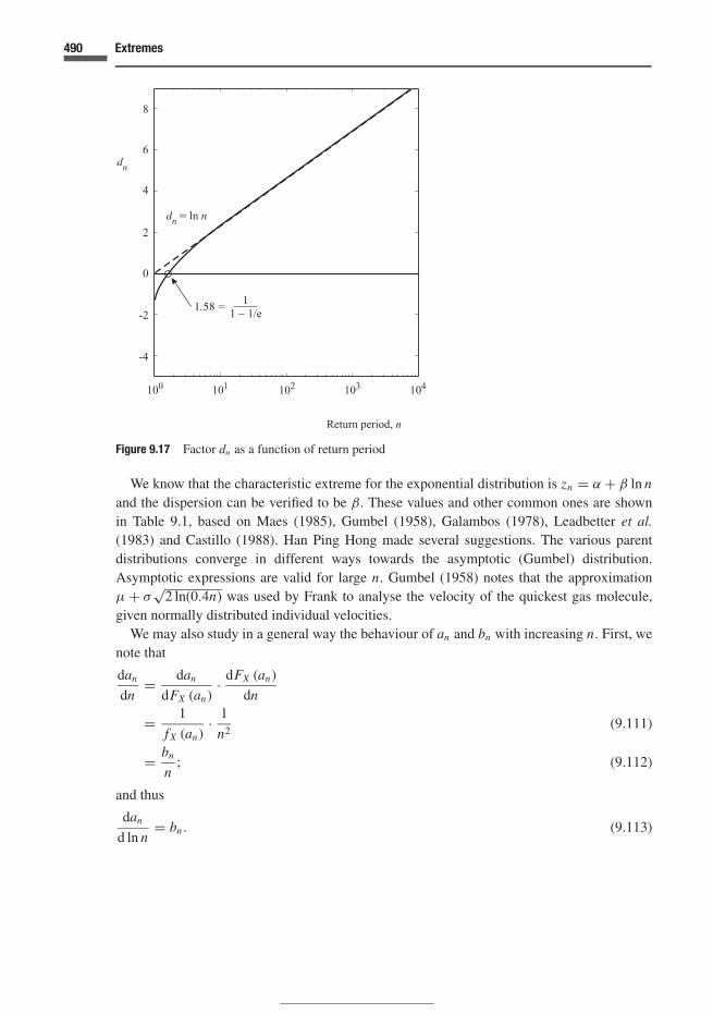
490 Extremes
1 − 1/e
Figure 9.17 Factor dn as a function of return period
We know that the characteristic extreme for the exponential distribution is zn = α + β ln nand the dispersion can be verified to be β. These values and other common ones are shownin Table 9.1, based on Maes (1985), Gumbel (1958), Galambos (1978), Leadbetter et al.(1983) and Castillo (1988). Han Ping Hong made several suggestions. The various parentdistributions converge in different ways towards the asymptotic (Gumbel) distribution.Asymptotic expressions are valid for large n. Gumbel (1958) notes that the approximationµ + σ
√2 ln(0.4n) was used by Frank to analyse the velocity of the quickest gas molecule,
given normally distributed individual velocities.We may also study in a general way the behaviour of an and bn with increasing n. First, we
note that
dan
dn= dan
dFX (an)· dFX (an)
dn
= 1
fX (an)· 1
n2(9.111)
= bn
n; (9.112)
and thus
dan
d ln n= bn. (9.113)

491 9.6 Asymptotic distributions
Table 9.1 Common probability distributions with Gumbel domain of attraction
Parent; Characteristic extreme an ; Classcdf FX (x) Dispersion factor bn E1, E2 or E3
Exponential; α + β ln n; E2
1 − exp(− x−α
β
)β
Logistic; ln(n − 1); E11/
[1 + exp (−x)
]n
n−1
Gumbel; α + β ln n; E1
exp{− exp
[−
(x−α
β
)]}β
Gamma β ln
[n
�(α)
]or
α > 1 : E1α = 1 : E2α < 1 : E3
(1)β{
ln n�(α) + (α − 1) ln
[ln n
�(α)
]};∫ x
0
uα−1 exp (−u/β) du
�(α)βαβ
[ln n
�(α)
]1−α
for n > 10, or
(1) an
an/β + 1 − α
Normal µ + σ
[(2 ln n)
12 − (ln ln n + ln 4π )
2 (2 ln n)12
]; E1
N (µ, σ 2); 1√2πσ
∫ x
−∞exp
[−
(u − µ
σ
)2]
du σ (2 ln n)−12
Lognormal; see Appendix 1 exp
{µ + σ
[(2 ln n)
12 − (ln ln n + ln 4π )
2 (2 ln n)12
]}; E3
1√2πσ
∫ y
0
1
wexp
[− (ln w − µ)2
2σ 2
]dw anσ (2 ln n)−
12
Rayleigh σ√
2 ln n; E1
1 − exp(− x2
2σ 2
)σ/
√2 ln n
2 parameter Weibull β(ln n)1/α;
α > 1 : E1α = 1 : E2α < 1 : E3
1 − exp[−
(xβ
)α]β
α(ln n)
1−αα
Asymptotic expressions are approximate, valid for large n.(1): relationship kindly suggested by Han Ping Hong.

492 Extremes
If we know the variation of bn with n, we can determine the behaviour of an. We explore this.
dbn
dn= d
dn
(1
n fX (an)
)= − 1
n2 fX (an)− f ′
X (an)
n f 2X (an)
dan
dn
= − 1
n2 fX (an)− f ′
X (an)
n f 2X (an)
1
fX (an)· 1
n2,
using Equation (9.111). Then
dbn
dn= 1
n2 fX (an)
[1
Q (an)− 1
], (9.114)
using Equation (9.95). The term before the square brackets is a positive quantity, while thatwithin is negative for Class E1, zero for Class E2, and positive for E3. The result is plottedschematically in Figure 9.18(a). From Equation (9.113), the behaviour of an with increasingvalues of (ln n) is sketched in Figure 9.18(b), based on 9.18(a).
9.6.7 Frechet distribution: type II
The main result for the type II distribution was given in Equation (9.78) in terms of thestandardized quantity Y. For the random quantity (Z − an) /bn, this can be written as
FZ (z) = exp
[−
(z − an
bn
)−α]
, (9.115)
for α > 0 and −∞ < z < ∞.Unlike the Gumbel distribution, the shape will depend on the parameter α. The distributionhas limited moments and, as stated earlier, distributions such as the Cauchy and Pareto fallinto the Frechet domain of attraction. The tail of the distribution is rather fat, compared to theGumbel. This has implications with regard to calculation of failure probability. The mean andstandard deviation are given in Appendix 1. The distribution has been used, for example, inanalysis of extreme wind speeds and floods.
9.6.8 Weibull distribution: type III; minima
The Weibull distribution of Equation (9.79) is readily converted to the linearly transformedrandom quantity (Z − an) /bn:
FZ (z) = exp
[−
(− z − an
bn
)α](9.116)
for α > 0 and − ∞ < z ≤ an.
As in the preceding subsection, the parameter α dictates the shape of the distribution (seeAppendix 1, also for mean and standard deviation). The distribution is based on parent distri-butions that are limited in value, to the right for maxima; see Figure 9.13. Often we consider thatthere is a physical maximum, yet its definition is vague and difficult to define, for example the

493 9.6 Asymptotic distributions
Figure 9.18 Dispersion factor and characteristic extreme as functions of n
maximum wave height that is physically possible. It is generally better in such instances to treatthe quantity as being unlimited, and to check that probabilities generated, for example with theGumbel distribution, are acceptably small in the regions where a physical limit is consideredpossible. See also Feller (1968, Chapter 1). A physical limit may be set in an engineered systemby devices such as fuses for maximum current, or weak links that fail under specified conditions.
So far in this subsection we have concentrated on maxima. We now transform Equation(9.79) to the case of a minimum. We might be considering droughts, the shortest time totransmit electronic information, or failure of the weakest link in a set of connected links underuniaxial tension. From Equation (9.3)
W = minn
Xi .
Then, from Equation (9.4),
−W = maxn
(−Xi ) . (9.117)

494 Extremes
We use the normalized Equation (9.79), knowing that we have to transform Y using V (say) =−Y. Then, using Equation (7.8),
FV (v) = 1 − exp (−vα) (9.118)
with 0 ≤ v < ∞.
This is a normalized random quantity, with a minimum of zero. We often wish to considerthe transformed quantity W, in
V = W − a
bn.
Equation (9.118) then becomes
FW (w) = 1 − exp
[−
(w − a
bn
)α](9.119)
with a ≤ w < ∞.
In these equations, we use a rather than an since this indicates a physical limit; see Figure 9.13.This is the factor associated with the Weibull domain of attraction.
9.7 Weakest link theories
The strength of materials – even carefully made laboratory specimens – is generally severalorders of magnitude less than the theoretical strength based on the separation of atoms inthe crystal lattice. Solids consist of a large quantity of elements, for example grains in poly-crystalline materials. The size, orientation and shape of these may differ from one to another,together with the morphology of the grain boundaries. The presence of dislocations will resultin movements under stress which will lower the stresses at failure. Heterogeneities and stressconcentrations cause failures locally in the material. Defects and flaws in the material willintervene to cause fracture at lower stresses than the theoretical values. These comments areespecially relevant to geophysical materials forming under natural conditions, since the flawstructure will be quite significant (Jordaan, 2000).
We now consider an initial model of the ‘weakest-link’ variety (Weibull, 1951; Bolotin,1969; Maes, 1985). This is the chain – or, more generally, a structure that may be consideredas a series of n elements such that the structure fails when one of the elements fail. If Ti isthe strength of the i th element or link, and the strengths of the elements are considered tobe iid with distribution function FT (t), the strength of the assembly, R = minn Ti , and fromEquation (9.6),
FR(r ) = 1 − [1 − FT (r )]n .
This can be written
FR(r ) = 1 − exp {n ln [1 − FT (r )]} . (9.120)

495 9.7 Weakest link theories
In the case where the structure may be considered to be composed of elements that are eachof volume v0, with the total volume v = nv0, then
FR(r ) = 1 − exp
{v
v0ln [1 − FT (r )]
}. (9.121)
The assumption that continues to be made is that the structure fails when the weakest elementfails.
Weibull suggested the use of a material function m (r ) to represent the expression{− ln [1 − FT (r )]} within Equation (9.121), and in particular the power-law equation
m (r ) =(
r − r0
r1
)α
, (9.122)
where α, r0 and r1 are constants with r0 representing a lower limit on strength. Substitutingthis into Equation (9.121), it is found that
FR(r ) = 1 − exp
[− v
v0
(r − r0
r1
)α]. (9.123)
We compare this with the type III extreme value distribution, given in Equation (9.119),reproduced here:
FW (w) = 1 − exp
[−
(w − an
bn
)α].
The equations are in fact identical in form, with
R ≡ W, (9.124)
r0 ≡ an and (9.125)(v0
v
) 1α
r1 ≡ bn. (9.126)
There is thus considerable basis for Weibull’s theory: we can interpret it as the asymptoticdistribution of the minimum of a set of random strengths with a lower minimum value r0.
Often it is reasonable to set r0 = 0 in Equation (9.123):
FR(r ) = 1 − exp
[− v
v0
(r
r1
)α]. (9.127)
9.7.1 Inhomogeneous stress states
Where the state of stress is inhomogeneous, it is still supposed that failure can take place inany link or element. The failure probability of each element is a function of the stress state, andin order to make the analysis tractable, we attempt to write a failure criterion that is a simplefunction of this stress state.

496 Extremes
Figure 9.19 Three elements in series
Example 9.11 As an introductory example, consider the situation illustrated in Figure 9.19.This shows three elements in series subjected to uniform tension, the cross sectional area ofthe elements being a, 2a and a, for the elements 1, 2 and 3 respectively. Uniform tensile stressin each element is assumed, stress concentrations being ignored. These stresses are then r, r/2and r respectively for the three elements. We assume that the material fails according to thesame distribution function as above, written here as FT (t) , where Ti is the stress in the i thelement, i = 1, 2, 3, implying that the same assumption as before, that the Ti are iid, is made.The failure stress is random since the Ti are, and the common value is denoted R (as before).This value has to be associated with one of the stresses, and we choose the stress in element 1,i.e. we use r (recall that the stresses in elements 1, 2 and 3 are r, r/2 and r respectively); thusr is the value of R at which failure of the assembly takes place. The failure of the assembly isthen given by
R = min (T1, T2, T3) , (9.128)
and
FR (r ) = 1 − [1 − FT (r )]2 [1 − FT (r/2)] . (9.129)
The consequence of the inhomogeneity is reflected in the inclusion of the different stress valuesin the three elements.
For more general states of stress, for instance a varying three-dimensional stress in a contin-uum given by the stress tensor σi j , Weibull proposed that one consider a homogeneous stressstate in a small volume �v around a point with cartesian coordinates x. In order that the stressσi j at this point be represented by a single scalar value, say s, it is supposed that one can write
s = rR · φ (x) , (9.130)

497 9.7 Weakest link theories
where φ (x) is a function of position only, and rR represents a reference value, for instance themaximum value in the body. See Exercise 9.18 for application of this to Example 9.11.
A more general example is given by the failure criterion represented by the maximum elasticstrain (Bolotin, 1969):
ε = 1
E[σ1 − µ (σ2 + σ3)] , (9.131)
where E = Young’s modulus and µ = Poisson’s ratio. This strain can be written as a functionof position, expressed by a non-dimensional function φ (x) as
ε ≡ s = rRφ (x) = rφ (x) . (9.132)
The value rR = r is, as noted, a reference value, for example the maximum strain at a certainpoint in the body. The strength Ti of the i th element is then described by the distributionfunction
FT (s) = FT [rφ (x)] . (9.133)
The function FT (t) is the same as that used previously, for example in Equation (9.121);in effect s replaces t , with φ representing a deterministic variation in stress. Randomness isembodied in FT (·) , taking particular values rφ. The reduction of a stress state to a single value,as just described, can also be used with the maximum-principal-stress or the Coulomb–Mohrfailure criteria, or others. See also Exercise 9.19.
The volume v0 of the body is divided into k small elements �vm, m = 1, . . . , k. The suppo-sition is made that the elements are small enough to ensure a homogeneous stress state, and yetthe assumption of independence of strength between elements is maintained (exchangeabilitywould often make a more natural assumption; see Section 9.9). Again we study (min Ti ). Therandomness is (as noted above) represented in FT (·) , which takes an independent value foreach element. Equation (9.121),
FR(r ) = 1 − exp
{v
v0ln [1 − FT (r )]
},
becomes
FR(r ) = 1 −∏k
m=1exp
(�vm
v0ln {1 − FT [rφm (x)]}
). (9.134)
This is a generalization of Equation (9.129). The value v0 should be interpreted as a referencevolume; it has been described, for example, as the volume of a standard test specimen (e.g.Bolotin, 1969). The function φm (x) applies to the small volume �vm . Equation (9.134) iswritten as
FR(r ) = 1 − exp
[1
v0
∑k
m=1(�vm ln {1 − FT [rφm (x)]})
]. (9.135)
498 Extremes
Replacing the sum in Equation (9.135) with an integral,
FR(r ) = 1 − exp
{1
v0
∫v
ln {1 − FT [rφ (x)]} dv
}. (9.136)
Now a similar simplification as before is made, writing the material function m (r ) as
m (r ) = − ln {1 − FT [rφ (x)]} =(
rφ (x) − r0
r1
)α
, (9.137)
so that
FR(r ) = 1 − exp
{− 1
v0
∫v
(rφ (x) − r0
r1
)α
dv
}. (9.138)
A simplification can be made if we let r0 = 0:
FR(r ) = 1 − exp
{− 1
v0
(r
r1
)α ∫v
φα (x) dv
}. (9.139)
The integral in this equation defines a ‘reduced volume’
v∗ =∫
v
φα (x) dv, (9.140)
so that
FR(r ) = 1 − exp
[−v∗
v0
(r
r1
)α]. (9.141)
Comparing this with Equation (9.127), we see that the equations are identical if the reducedvolume v∗ replaces the volume v of the body under homogeneous stress.
Example 9.12 Consider a beam of span l, with a rectangular cross section (depth h and widthb), subjected to pure bending moment m. The material is brittle and can be modelled usingWeibull’s theory with a maximum-tensile-stress criterion. Find the reduced volume v∗. Let ybe the distance from the neutral axis. We need to consider stresses only in the tensile half ofthe cross section. The maximum stress is taken as the reference value of stress, i.e.
rR = r = 6m
bh2. (9.142)
Then the stress varies only with y and is equal to
r · 2y
h(9.143)
and
φ (y) = 2y
h. (9.144)

499 9.7 Weakest link theories
The reduced volume is
v∗ = bl∫ h
2
0
(2y
h
)α
dy
= blh
2 (α + 1). (9.145)
This is the entire volume divided by 2 (α + 1) .
In Exercise 9.20, other loading cases are considered. We should note the simplifying aspectsinvolved in this analysis. The shearing stress is zero in Example 9.12, and shear is neglectedin the exercises involving bending. It might be reasonable to neglect shear in slender beams,but its presence is of considerable importance in many instances, particularly in reinforced andprestressed concrete beams. Shear is important in many other cases too; the spalling activityin compressive failure in ice-structure interaction, leading to mitigation of load severity, mayoften be associated with shear acting across weak grain boundaries.
9.7.2 Scale effects
The mean and variance of the distribution (9.123) are
〈R〉 = r0 + r1
(v
v0
)− 1α
�
(1 + 1
α
)(9.146)
and
σ 2R = r2
1
(v
v0
)− 2α[�
(1 + 2
α
)− �2
(1 + 1
α
)]. (9.147)
From the mean value, when r0 = 0, we may compare the strength of two volumes v1 and v2:
〈R〉1
〈R〉2=
(v2
v1
) 1α
; (9.148)
this may also be used with reduced volumes.The standard deviation of R is
σR = r1
(v
v0
)− 1α[�
(1 + 2
α
)− �2
(1 + 1
α
)] 12
, (9.149)
and the coefficient of variation γ is given by
γ =r1
(vv0
)− 1α [
�(1 + 2
α
) − �2(1 + 1
α
)] 12
r0 + r1
(vv0
)− 1α
�(1 + 1
α
) . (9.150)

500 Extremes
0 5 10 15 20 25 300
0.5
1
1.5
2
2.5
α
g
Figure 9.20 Coefficient of variation γ as a function of α
For r0 = 0, this becomes
γ =[�
(1 + 2
α
) − �2(1 + 1
α
)] 12
�(1 + 1
α
)
=[
�(1 + 2
α
)�2
(1 + 1
α
) − 1
] 12
, (9.151)
a function of α only. This equation can also be derived from Equation (9.141) using reducedvolume v∗. Figure 9.20 shows a plot of γ versus α. It is seen that the coefficient of variationdecreases considerably for large α.
9.7.3 Applications and discussion
First, we consider the geometry of the solid. If the cross-sectional area is constant, for instancein a bar under tension, volume in Equation (9.123) can be replaced by length. In other cases,the stressed volume of a solid might be proportional to a linear dimension cubed. For instance,the ‘bulb’ of stressed material in a semi-infinite solid with contact area proportional to thesquare of a linear dimension l will have a stressed volume proportional to l3. Figure 9.21shows the results from tensile tests by Griffith (1920) on glass threads, while Figure 9.22(a)shows values for tensile (flexural) tests (Jordaan and Pond, 2001). Certainly scale effects arein evidence, and lower values of α, in evidence for ice, support also the high variability, assuggested by Figure 9.20. Figure 9.22(b) shows a collection of results from ice compressive

501 9.8 Poisson processes: rare extreme events
–4 –3.5 –3 –2.5 –21
1.5
2
2.5
3
ln v
ln (
stre
ngth
)Adapted from Griffith (1920)
Figure 9.21 Griffith’s results for scale effect
failure. In the latter case, the stressed volume is proportional to l3, and area to l2. The observeddecrease, on average, of strength with (area)−1/2 is supported by measured values of α � 3 inEquations (9.127) and (9.141); see Sanderson (1988).
The methods above have been applied to ‘bundles’. Freudenthal (1968) introduces thisconcept, which originated in the work of Daniels in 1945. In this analysis, instability of thedominant flaw no longer leads to failure of the entire specimen or structure under consideration.The bundle consists of a large number of parallel threads or fibres with the same length andcross-sectional area. Failure first takes place in the weakest fibre, and the load is then distributedamongst the remaining ones, but does not necessarily lead to failure of the assembly. Anotherimportant area of research lies in the attempt to link the failure process to the flaw structure in thematerial, taking into account the state of stress at the point under consideration. The approachesof Hunt and McCartney (1979) and Maes (1992) represent examples of this important directionof research.
9.8 Poisson processes: rare extreme events
A model of arrivals of events that is often a good abstraction is the Poisson distribution(Sections 3.2.6 and 3.6.1). It is especially useful for cases of rare events, but can be usedmore widely. Arrivals of electronic communications, packets of data, telephone calls, errors,accidents, floods, earthquakes, and exceedance of wind speeds during typhoons, all of thesesubjects can be analysed as Poisson processes. There are cases where the ‘arrival rate’ for theextreme events is quite small, for example where the events are bolts of lightning, accidents,

502 Extremes
10–1
100
101
102
103
104
10–1
100
101
102
Hobsonís Choiceo Pond Inlet Molikpaq. + Hans Islandx Kigoriak
M.V. Arctic
Nominal Area (m2)
Mea
n N
omin
al P
ress
ure
(MPa
)
–3 –2.5 –2 –1.5 –1 –0.5 0–1
–0.5
0
0.5
1
log10
(Volume) (m2)
log 10
(Str
engt
h) (
MPa
)
10 100
101
102
103
104
10
100
101
102
Hobson’s Choiceo Pond Inlet Molikpaq. + Hans Islandx Kigoriak
M.V. Arctic
Nominal Area (m2)
Mea
n N
omin
al P
ress
ure
(MPa
)
0
0.5
1
log10
(Volume) (m2)
log 10
(Str
engt
h) (
MPa
)Cantilever (Frankenstein, 1959)Simple (Frankenstein, 1959)Cantilever (Frankenstein, 1961)Cantilever (Gow, 1988)Simple (Gow, 1988)
(a) Ice flexural strength
(b) Ice compressive strength as a function of nominal area
3A –0.5
3.33A–0.43
Standard deviation
Figure 9.22 Scale effect for ice. Details of the data can be found in Jordaan and Pond (2001)
hurricanes, earthquakes or collisions of icebergs with structures at certain offshore locations.Figure 9.23 illustrates the situation, which we shall explain in detail in the following.
We denote the events under consideration (messages, accidents, floods, typhoons, . . . ) bythe symbol Ei , i = 1, 2, 3, . . . It should be recalled (Section 3.2.6) that, for many applications,the arrival rate does not have to be constant. For our analysis we need the expected number ofarrivals ν during the period of interest t (often a year):
ν =∫ t
0λ (τ ) dτ,
where the rate λ(·) can vary with (for example) season; if λ is constant, then ν = λt . Weconsider again the case where the parent distribution of the random quantity of interest, X, isFX (x) . The magnitude Xi is associated with each event Ei , and again we make the assumptionthat the events are independent and identically distributed (iid).

503 9.8 Poisson processes: rare extreme events
Figure 9.23 Rare and frequent processes
Within the Poisson process, we consider those occurrences with a magnitude X greater thana specified value Z = z. These events are denoted as Fi , a subset of the Ei , such that {Xi > z} .
The quantity Z denotes, as before, the extreme value of interest during the period of interest.The number of events Ei during the period is a random quantity, denoted N , and this can bemodelled by the Poisson distribution:
pN (n) = exp (−ν) νn
n!, for n = 0, 1, 2, . . . (9.152)
Now the events Fi correspond to those events within the group Ei that exceed in magnitudeZ = z, so that the expected number of events Fi is
ν ′ = ν [1 − FX (z)] . (9.153)
The Fi therefore constitute another Poisson process, with the amended parameter ν ′. Thearrivals in this case number N ′ such that
Pr(N ′ = n′) = exp
(−ν ′) (ν ′)n′
n′!. (9.154)

504 Extremes
0.1
0.2
0.3
0 5 10 15 20 25 30z
Figure 9.24 Annual maximum wave height
For extremal analysis, we are interested in the case where Z = z is the maximum value ofthe Xi in the time interval under consideration. Then all ‘arrivals’ of the amended process musthave a magnitude Z ≤ z. This implies that n′ = 0 in (9.154) and then
Pr(N ′ = 0
) = exp(−ν ′) . (9.155)
This corresponds to the case that Z ≤ z so that (9.155) is equal to
Pr (Z ≤ z) = FZ (z) = exp {−ν [1 − FX (z)]} . (9.156)
This gives us the probability distribution of the extreme value Z .
Example 9.13 We may apply this idea to the problem introduced in Section 9.4.3, where weconsidered a number of waves per storm to obtain the distribution of the extreme wave duringthe storm (Equations (9.32) and (9.33) and Figure 9.6). If there are ν = 5 storms per year thenthe distribution of the annual maximum, on the assumption of a Poisson distribution of thenumber of storms per year, is
FZ (z) = exp
[−5
(1 −
{1 − exp
[−2
( z
9.0
)2]}n)]
. (9.157)
This is shown in Figure 9.24 for five storms per year and n = 1000 waves per storm.
If the distribution of X is exponential, let us say the shifted kind
fX (x) = 1
βexp
(− x − α
β
), x ≥ α (9.158)

505 9.8 Poisson processes: rare extreme events
Figure 9.25 Simple scaling
(and zero elsewhere), then
FX (x) = 1 − exp
(− x − α
β
). (9.159)
Equation (9.156) now takes the double exponential form
FZ (z) = exp
{−ν
[exp
(− z − α
β
)]}
= exp −{
exp
[−
(z − α − β ln ν
β
)]}. (9.160)
The contrast between rare and frequent events is illustrated in Figure 9.23. In the case whereν is sufficiently small, Equation (9.156) becomes
FZ (z) � 1 − ν [1 − FX (z)] = 1 − νp, (9.161)
where p is the probability that X exceeds the value z. This distribution for rare events isshown in Figure 9.25, taking the exponential form of Equations (9.158) and (9.160) as anexample. This case of ‘simple scaling’ has been used for the specification of design loads forrare environmental processes, such as earthquake and some ice loading events (Jordaan andMaes, 1991), and in studies of spills of hazardous materials by the author.
506 Extremes
The Poisson process will automatically give a spike of probability at the lower bound (whereit exists) of the quantity X. Suppose that FX (z) = 0 at x = z = α in Equation (9.156) – anexample of such a lower bound below which there is no probability mass is given in Equation(9.158). Then Equations (9.156) and (9.160) tell us that FZ (z = α) is exp (−ν) at this point.This has to consist of a probability mass at z = α, corresponding to the Poisson probabilityof N = 0 in Equation (9.152). It is approximately equal to (1 − ν) in the case of Equation(9.161). There is therefore no need to be concerned about the occurrence of quantities that areless than α in Equation (9.158) for the case of Poisson arrivals.
The methodology described in this section has been applied in studies of floods, wave heightsand extreme wind speeds during typhoons. It is described in the literature in these areas asthe ‘peak over threshold’ (POT) model. These applications are concerned with the analysisof environmental events which exceed a certain threshold, modelled as Z = z in Equation(9.155).
9.9 Inference, exchangeability, mixtures and interannual variability
9.9.1 Exchangeable random quantities
In Chapter 8, we pointed out that making inferences about the distribution of a random quantityusing data invariably leads to changing one’s assessment of probabilities. The same situationexists with regard to extremes: the use of data will lead to inferences regarding parameters ofthe distributions under consideration, in this case an extremal distribution. The consequence isthat probabilities will change, and independence will no longer apply. Then our iid assumptionused so far in this chapter is no longer valid. The simplest and most natural way out ofthis quandary is to consider again exchangeable random quantities. Then independence willagain be embedded in the structure of the analysis as part of exchangeability (conditional onthe parameter value). The analysis is then aimed at modelling the uncertainty regarding theparameter(s) of the extremal distribution.
Under the hypothesis of exchangeability, if we consider a set of values, possibly observa-tions, we might make the judgement that the order of the values in the set is of no consequence,as discussed in Chapter 8. The subject of study might be the time between arrival of packets ofdata in a network during a peak transmission period, or the heights of individual waves duringa storm. We may again avail ourselves of an urn model, as in Chapter 8 and in Section 9.3above. Suppose again that it contains R = r red ‘1’ balls and n − r pink ‘0’ ones. But the urnmodel will be of random composition, reflecting the fact that we are uncertain about the value ofthe parameter(s) of our distribution, exactly as we were in Section 8.2. We denote the parame-ter(s) by the �, taking particular values λ. To focus thinking, � might represent the parametersan and bn in the extremal distribution of wave heights in the design of an offshore rig.
We now develop an equation analogous to (9.12). Instead of a known composition of theurn we suppose that the proportion of red balls represents the cdf F� (λ) of the parameter.

507 9.9 Exchangeability and mixtures
Then we write FX,� (x |λ) as the probability that X ≤ x given that � = λ. The probability ofa particular composition being in the interval λ < � < λ + dλ is then
dF� (λ) = f� (λ) dλ
for a continuous distribution f� (λ) . For any particular order of drawing, for example all redballs first, followed by all the pink ones,
Pr(R = r ) = pr,n =∫ ∞
−∞Fr
X,� (z|λ)[1 − FX,� (z|λ)
]n−rdF� (λ) . (9.162)
Counting all orders,
Pr(R = r ) = ωr,n =(
n
r
) ∫ ∞
−∞Fr
X,� (z|λ)[1 − FX,� (z|λ)
]n−rdF� (λ) . (9.163)
Using the same arguments as we developed leading up to Equation (9.14), the cdf of the r thordered random quantity X (r ) is:
FX (r ) (z) =∑n
t=r
(n
t
) ∫ ∞
−∞Ft
X,� (z|λ)[1 − FX,� (z|λ)
]n−tdF� (λ) . (9.164)
The theory can be further developed into consideration of order statistics, but we shall con-centrate on the case where r = n or r = 1, that is
FZ (z) =∫ ∞
−∞Fn
X,� (z|λ) dF� (λ) (9.165)
for a maximum, and
FW (w) = 1 −∫ ∞
−∞
[1 − FX,� (w|λ)
]ndF� (λ) (9.166)
for a minimum. Compare the corresponding iid equations, (9.5) and (9.6). The pdf of themaximum (for example) is
fZ (z) = n∫ ∞
−∞Fn−1
X,� (z|λ) fX,� (z|λ) dF� (λ) , (9.167)
corresponding to Equation (9.7).We see that, in order to implement exchangeability, we may, as in Chapter 8, treat the random
quantity as being iid, conditional on the parameter value, that � = λ. One then integrates overthe possible parameter values to obtain the required distribution. It is always important to takeinto account uncertainty in parameter values in probabilistic analysis, and this can be veryimportant in estimating extreme values in design.
Example 9.14 We consider a random quantity X (0 ≤ X ≤ 1) representing the proportion ofdevices that successfully fulfil their function during the lifetime of an assembly. The uncertainty
508 Extremes
is modelled using the power-law relationship
fX,� (x |λ) = (λ + 1) xλ, (9.168)
with uncertainty in the parameter � expressed by
f� (λ) = 1
βexp −
(λ
β
), (9.169)
where β is a constant.From Equation (9.168),
FX,� (x |λ) = xλ+1,
and the distribution of the maximum of n of the Xs is, by Equation (9.165),
FZ (z) =∫ ∞
0
(zλ+1
)n 1
βexp −
(λ
β
)dλ
= zn
β
∫ ∞
0exp
[(n ln z − 1
β
)λ
]dλ
= zn
1 − βn ln z. (9.170)
Conjugate priorsGenerally, the extremal distributions do not possess conjugate prior distributions, as wereintroduced in Chapter 8; see Exercise 9.23. Both classical and Bayesian inference presentdifficulties. There are approximate techniques to deal with this, for example Evans and Nigm(1980) dealt with the Weibull distribution. Maes (1985) developed a special distribution (theexchangeable-extremal distribution) that does have sufficient statistics and a conjugate prior.Numerical techniques are also of importance; Monte Carlo techniques are also of great use-fulness; see Chapter 11. It is noteworthy that the parameter of the Poisson distribution may bemodelled using conjugate prior distributions of the gamma family (Section 8.5.4). This can beused with the Poisson distribution in the extremal processes of Section 9.8. This interpretationoffers one way forward.
9.9.2 Parameter uncertainty; fixed- and variable-in-time; return periods;inter-period variation
Uncertainty in the parameter of an extreme distribution will generally result when estimatingfrom a data set; there will be more or less uncertainty depending on the size of the data base.Inference proceeds via prior information combined with data (likelihood). We now discusssome aspects that relate to the source of uncertainty. In Nessim et al. (1995) a classification wasproposed for environmental loads, that was designed to be as simple as possible. This includedthe distinction between uncertainties that are fixed-in-time and variable-in-time. Some relatedaspects are briefly discussed.

509 9.9 Exchangeability and mixtures
One might find that, as data comes in, the parameter for extreme loading is at the upper endof the supposed range. There may be physical reasons why a parameter takes a high value ata certain physical location, for instance as a result of exposure to wind, or because of otherconstruction nearby a structure might become exposed to above-average wind loading. In thesecases, knowledge of the parameter leads to higher estimates of loading. We have advocatedthe use of Equation (9.165) for the extremal distribution FZ (z). In calculating return periods,Equation (9.35),
tR = 1
1 − FZ (z),
the uncertainty associated with the parameter must be taken into account. It is fixed-in-timeunder the circumstances just discussed, and will correctly lead to longer return periods.
If we assume that the final uncertainty represents a mixture, with different parametervalues for different structures, but that the different structures are exchangeable, there willbe different but unknown safety levels for the different structures. The inclusion of parameteruncertainty in the estimate of return period in this case will result in an overall estimate, averagedover the distribution of the parameter, and the resulting reliability will not be uniform. Thismight be of minor significance if the parameter uncertainty between structures is relativelysmall, but is a valid subject of study.
A second distinct situation occurs when there is variability between exposure periods. Themodelling of a wave or wind regime does not usually acknowledge explicitly the differentconditions from year to year. Higher-than-average seismic activity might result during periodswhen rock masses are in a highly stressed state – but this might be unknown to the analyst.One is forced to acknowledge this in considering the severity of threat from icebergs; there areyears on the Grand Banks when no icebergs appear so that the probability of collision is zero.In other years the areal density is considerable, up to 50 per degree-rectangle, and then thereis a probability of collision greater than zero. Similarly, ice thickness in temperate zones orthe arctic can vary from year to year depending on the accumulated freezing degree-days forthe year in question. Biological systems also have to contend with changes from year to yearthat are detectable and measurable. Drought and the presence or absence of ice are examples.Demand in data transmission (for example) will vary from one period to another for a varietyof reasons. These examples are variable-in-time.
In this second situation, the use of the expression for tR above needs special attention. Let uscontinue with the question of iceberg populations as an example. To simplify the discussion,let us assume that in our area of concern, two kinds of iceberg ‘years’ occur. In the kind‘A’, there are no icebergs in the area, so that the probability of collision is zero. In the kind‘B’, the iceberg population is such that the probability of collision is 0.2. The return periodcorresponding to the condition A is tR = 1/p = ∞, and for B it is tR = 1/p = 5 years. If wenow say that the return period is the expected value of these possibilities, both of which occurwith a probability of 1/2, we obtain a result equal to infinity. This is clearly unreasonable. Abetter result is obtained if one judged the yearly conditions to be exchangeable between years.

510 Extremes
The probability of collision for a given year for which we have no information as to conditionswould be the weighted probability of collision given the two possible scenarios. This is
p = 0.5 (0) + 0.5 (0.2) = 0.1.
The return period is then
1
p= 10 years.
This makes sense in terms of the usual understanding of the expression ‘return period’, andthe result corresponds to the expression tR = 1/ [1 − FZ (z)] with the weighted probability.
We see that the definition of return period as the expected number of years to the first eventdoes not work if we make explicit analysis of the changing probabilities from year to year. Ifwe use the ‘average’ probability, things work out when there is inter-period variability. Theoverall analysis might be viewed as corresponding to the Raiffa urn problem, as discussed inChapter 2 (Figure 2.10) in the context of Bayes’ theorem. If the parameter value corresponds tothe composition of one urn only (of the two), but we don’t know which, we have the situationat the beginning of the present subsection (fixed-in-time). If we have a mixture of urns, witha (randomly) different urn each period, we have the situation just discussed, with differenticeberg concentrations corresponding to different urns in different years. Exchangeabilityimplies that we have no means of distinguishing a priori between the periods, and detailsof the ‘composition’ would be hidden. The reader might wish to construct the Raiffa urncorresponding to this situation.
9.9.3 Mixtures
One might wish to model explicitly the inter-period variability. Thus the value of FX (x) couldbe given by a mixture
FX (x) =∫
FX |A(x |a) f A (a) da. (9.171)
As a mixture, the distribution f A (a) does not converge to a ‘spike’ with accumulated data as inthe case of exchangeability but expresses an unchanging reality – for example a reflection ofnature, with some interannual variation such as mean temperature, or accumulated rainfall orfreezing degree-days. To use this as a model, some additional information has to be includedin the idealization, a parameter that characterizes the physics such as those just mentioned. Itcould then be used for updating probabilities in a particular year (or other period).
9.10 Concluding remarks
Analysis of extremes has an important role in the design of engineering systems. The applicationusually follows one of two approaches. The first is evaluation of the parent distribution, and

511 9.11 Exercises
subsequent generation of the extremal distribution. One of the difficulties that might presentitself is that of extrapolation for large n. Do the same physical phenomena carry over into highervalues of the quantity under consideration? The other approach involves direct estimate of theextremal distribution based on data. In either case, understanding of the generation of extreme-value distributions is essential, as this will guide us in our modelling of physical systems.
9.11 Exercises
9.1 Verify that Equation (9.15) follows from Equation (9.14).
9.2 Basic exercise in extremes to become familiar with the process.
(a) Carry out Monte Carlo simulations (Chapter 11) to reproduce the extremal distributions ob-tained in Section 9.4. The Monte Carlo procedure should follow the procedure outlined under‘Random blows’. Histograms and fitted distributions should be produced.
(b) Repeat (a) by using the relationship FZ (z) = FnX (z) based on the parent cdf, thereby obtaining
graphical representations of extremal distributions as in Section 9.4.
9.3 Find a second proof of the return period relationship 1/p.
9.4 Show that Equation (9.14) reduces to the same form as (9.6) for the lowest endpoint (r = 1) .
9.5 Find a closed form solution for pdf of the extreme wave (Section 9.4.3) given a Rayleigh parent.Plot behaviour with respect to log n.
9.6 Repeat Exercise 9.2 but using the minimum of a set of random quantities, first using Monte Carlomethods and second by implementing Equation (9.6). Consider parent distributions both unlimitedand limited to the left.
9.7 Repeat Exercise 9.2 but considering now a situation based on Equation (9.15), for instance studythe distribution of the fifth out of eight for a given parent distribution such as the exponential.
9.8 An event (rams of an arctic vessel, voltage surges of a certain magnitude) occurs 20 times in a year.The distribution of its magnitude X is exponential, λ exp (−λx). Find the magnitude in terms ofthe mean 1/λ such that the return period is 100 years. Assume iid.
9.9 An approximation that is often useful for very small p (� 1/n) is
(1 − p)n � 1 − np. (9.172)
(a) Apply this in Exercise 9.8.(b) Equation (9.49) states that
FZ (xn) = FnX (xn) =
(1 − 1
n
)n
→ 1
e,

512 Extremes
in other words the n-year load on a structure has a 63% chance of being exceeded in n years forlarge n. A designer wishes therefore to choose a more conservative value. He then considers avalue z with a small probability of exceedance of the n-year load pne such that
pne = 1 − FZ (z) (9.173)
rather than the mode. Then if X is the parent,
[FX (z)]n = 1 − pne, or (9.174)
FX (z) = (1 − pne)1/n � 1 − pne
n, (9.175)
using a variation of the rule (9.172). Obtain pne in terms of an, bn and α for a Weibull parentdistribution based on Equation (9.116), with X replacing Z :
FX (x) = exp
[−
(− x − an
bn
)α]. (9.176)
An engineer in offshore practice would realize that a load factor is usually applied to the100-year load, giving a result that approaches the situation described.
9.10 Find the mode of the Rayleigh distribution
fX (x) = 2x
σ 2exp
(− x2
σ 2
).
9.11 Consider the following form of the Pareto distribution:
FX (x) = 1 − xk,
x ≥ 1, k > 0,
which has been used, for example, to model relative income distributions. Show that L’Hopital’srule does not apply, and that the critical quotient is equal to
k
k + 1.
9.12 Compute and plot the intensity function and critical quotient for the following distributions: normal,logistic and lognormal. Compare to that of the exponential distribution.
9.13 Show that the mode of the Gumbel distribution
fZ (z) = 1
βexp
[− exp
(− z − α
β
)− z − α
β
]
is z = α. Show also that this is approximately equal to the characteristic extreme zn .
9.14 Compare the results of using Table 9.1 with distributions obtained from the parent using Equation(9.5).
9.15 Derive the type III (Weibull) distribution from type I and type II. Explain which parameters dependon n.

513 9.11 Exercises
9.16 Calculate the hazard function for the distribution FX (x) = 1 − exp(−xk
), where k is a constant.
9.17 Plot Equation (9.114),
dbn
dn= 1
n2 fX (an)
[1
Q (an)− 1
],
for the distribution in Example 9.10, and discuss the behaviour of bn with an .
9.18 Consider Example 9.11. Let the vector
x =
123
represent the position of the three elements. We took rR as r (the stress in element 1). Find a matrixφ that transforms this into
r
112
1
,
giving the relative values of s in each element.
9.19 Consider the failure criterion
s =(
σ11
σ0
)d
+(
σ22
σ0
)d
+(
σ33
σ0
)d
,
where σ11, σ22 and σ33 are principal stresses, and d and σ0 are constants. Show how this can beused in Weibull’s strength distribution using an equation of the kind (9.122).
9.20 Find the reduced volume v∗, as in Example 9.12 for a cylindrical bar under torsion; for a prismaticbeam simply supported under point load; and for a prismatic beam, simply supported, loadedsymmetrically by two point loads. Treat the reduced stress as the greatest principal stress.
9.21 Consider the following non-homogeneous failure condition. A bar is stressed under uniform tension.Two aspects are to be considered. The first relates to a population of surface flaws, and the secondto flaws within the volume of the material. How would you approach this problem?
9.22 Show that the extremal distributions do not possess conjugate prior distributions or sufficientstatistics.
9.23 Analyse how you would take into account parameter uncertainty in Equation (9.148) for the scaleeffect, and in (9.151) for the variance.
9.24 Consider an extremal process that is modelled as a Poisson process. Treat the arrival rate as beingrandom. Develop a ‘peak over threshold’ (POT) model that includes parameter uncertainty in thearrival rate and an application of the model.

10 Risk, safety and reliability
The R-101 is as safe as a house, except for the millionth chance.Lord Thomson, Secretary of State for Air, shortly before boarding the airship headed to India on its first flight,
October 4, 1930
If you risk nothing, then you risk everything.Geena Davis
10.1 What is risk? Its analysis as decision theory
It is commonplace to make statements such as ‘life involves risk’, or ‘one cannot exist withoutfacing risk’, or ‘even if one stays in bed, there is still some risk – for example, a meteorite couldfall on one, or one could fall out and sustain a fatal injury’, 1 and so on. The Oxford dictionarydefines risk as a ‘hazard, chance of . . . bad consequences, loss, . . . ’ ; Webster’s definition issimilar: ‘the chance of injury, damage or loss’ or ‘a dangerous chance’. Two aspects thrustthemselves forward: first, chance, and second, the unwanted consequences involved in risk.We have taken pains to emphasize that decision-making involves two aspects: probabilities(chance), and utilities (consequences). Protection of human life, property, and the environmentare fundamental objectives in engineering projects. This involves the reduction of risk to anacceptable level. The word ‘safety’ conveys this overall objective.
In Chapter 4, aversion to risk was analysed in some detail. The fundamental idea wasincorporated in the utility function. We prompt recollection of the concept by using an anecdotebased on a suggestion of a colleague. A person is abducted by a doctor who is also a fanaticaldecision-theorist. He offers the person the following two options before release from captivity.First, removal of one kidney, then release. Second, toss an honest coin: if heads, release of thecaptive (with both kidneys intact); if tails, removal of both kidneys, followed by release. Ourattribute, to use the notation of Chapter 4, would be ‘number of kidneys lost’. The expectedloss for each option is the same; one kidney. We would be inclined to choose the first optionto avoid the possible dire consequences of the second. The utility would then be a concave
1 or, less commonplace, in the last instance: ‘one could suffer the fate of Howard Hughes!’
514

515 10.1 What is risk?
Figure 10.1 Risk analysis as a branch of decision analysis dealing with undesired consequences
decreasing function of the attribute (kidneys lost) with the loss of two corresponding to thelowest utility (death). It is most important that the non-linearity of utility with attributes in thecase of risk aversion be borne in mind when reading this chapter.
The direct relationship between the structure of rational decision-making and the conceptsembodied in the definition of risk implies that we can conduct risk analysis with the toolsalready developed in all of the preceding chapters. There is one condition that must applyto risk analysis: the consequences are unwanted, that is, of low utility. This is emphasized inFigure 10.1, which summarizes the relationship with decision theory. Some decision trees withimplications for risks of various kinds are given in Figure 10.2. The risks are classified broadlyinto those associated with natural phenomena, societal issues, and technological aspects. Butsome risks do not fall clearly into one of these; for example taking risks on the stock marketmight involve all three aspects.
The subjects covered by the term ‘risk analysis’ are extensive, and it would be futile toattempt to review them all. Our purpose is to expose those general principles that might beapplied in idealizing and solving problems in any area. The material reviewed in this chapterwill serve the purpose of illustration and no claim is made to comprehensiveness.
10.1.1 Safety Index (SI )
We may summarize the concepts in Figure 10.3, which illustrates both the probabilities andconsequences of actions. Taking a scale of utility from 0 (least desirable) to 1 (most desirable),the figure shows the area of interest in risk analysis. It is convenient for many purposes touse probabilities calculated on an annual basis, so that, for example, the annual risk to anindividual is assessed. Often it is useful to express this probability on a logarithmic scale(lower part of Figure 10.3). Usually the range under consideration is from about 10−2 to 10−7,giving a range on the (negative) log scale of 2 to 7. This logarithm to the base 10 will be

516 Risk, safety and reliability
Figure 10.2 Decisions involving risk
termed the ‘Safety Index’ (SI) which we abbreviate to SI (see Jordaan, 1988, and also Paulos,1988)2.
The consequence scale in Figure 10.3 in general deals with events that might include single,several or many deaths and injuries, minor or major damage to the environment (for example,
2 This is not the Safety Index of structural reliability theory, which we have termed the ‘Reliability Index’ (RI): seeSection 10.5.

517 10.1 What is risk?
Figure 10.3 Domain of risk analysis
small or large oil spills), or combinations of these. If the set of two consequences {loss of life,survival} for a single person is considered, this may be modelled by the two points {0, 1}. Oneis considering the risks to an individual which can be expressed as a probability per unit time,generally a year. This is a very useful measure of safety and can be a good guide to acceptablerisks. Section 10.4 deals with this question. Further discussion of the basis for the logarithmicmeasure is given in Jordaan (1988).
10.1.2 Small probabilities
The values quoted in the preceding paragraph show that it is necessary to deal with smallprobabilities. This is true also of extreme values used in design (Chapter 9) as well as prob-abilities of failure of engineering systems – the risk of failure. Common target values for the

518 Risk, safety and reliability
probability of failure are 10−3, 10−4, 10−5, 10−6 per annum; the annual probability of death ina road accident is one in ten thousand, and the probability of a person suffering a fatality on anaircraft of one of the major carriers per flight departure (see Section 10.2.3 below) is less thanone in a million. It is useful to attempt to develop a ‘feeling’ for these small values. We knowthat one chance in 10 000 corresponds to an SI of 4. This may be interpreted by means of foursuccessive ‘trials’ in each of which we have a one-in-ten chance of succumbing, and for eachof these, a further one-in-ten chance, and so on four times in total, assuming independence.
Paulos (1988) suggests using everyday objects to develop such a feeling. For example, onemight walk past a certain brick wall every day. One could count the number of bricks verticallyand horizontally, multiply the two numbers, and estimate thereby the number of bricks in thewall. If there are 1000 bricks the probability of 10−3 corresponds to a random hit on a particularbrick if a pebble is tossed (in such a way that each brick is equally likely to be hit). Othercommonplace objects might serve a similar purpose. As a further aid to obtaining a feeling forthe small numbers, consider the tossing of a coin. The probability of
� no heads in 10 successive tosses = 2−10 = 1/1024, or approximately one in a thousand;� no heads in 20 successive tosses = 2−20 = 1/1048 756, or approximately one in a million.
A further interpretation of small probabilities in terms of Good’s (1950) ‘device of imaginaryobservations’ is given in Jordaan (1988).
10.2 Risks to the individual
Risks to an individual can, as suggested above, be expressed as a probability per year. Thevalues depend very strongly on such factors as the wealth of the society in which the individuallives, their occupation and the socio-economic group to which the individual belongs. This is anunfortunate fact of life, and it is a matter of common observation that in certain societies, ‘lifeis cheap’ for some individuals. We note below the high rate of traffic fatalities in developingcountries. Rowe (1977) and Bulatao in Gribble and Preston (1993), for example, present dataon risks to persons in the developing world as against those in industrial countries. In the latterreference, it is found that the age-adjusted rates of death in developing countries are doublethose in industrial ones. Some extreme happenings can be noted. For example, Melchers (1993)mentions the risks in the Indian nuclear industry, whereby low-caste workers are employedat attractive daily rates to perform maintenance work under conditions of high exposure toradiation.
We shall present data mainly from the perspective of a Canadian, but similar risks would beapplicable to other countries with similar GDP per capita and social structure. To set the scene,we first present data from Statistics Canada, in Table 10.1. The values of annual risk (AR) per10 000 persons is a useful number and it is a good idea to remember several key values. Table10.1 shows that the annual risk of death for a Canadian (‘other things being equal’ ) is about0.7%. The SI is a little more than 2, an average value for all ages, both sexes, and for all reasons.

519 10.2 Risks to the individual
Table 10.1 Risks for Canadians based on data from Statistics Canada
Annual risk (AR) Safety Index (SI)per 10 000 persons [log10(AR/10 000)]
Cause or activity Male Female Male Female
All causes 66 2.2
All causes (male and female) 84 52 2.1 2.3
All causesAge 20–24 10 3 3.0 3.5
40–44 22 13 2.7 2.960–64 137 77 1.9 2.1
Heart disease 23 13.0 2.6 2.9Cancer (all types) 23 14.9 2.6 2.8Lung cancer 8.1 4.5 3.1 3.4HIV 0.4 0.1 4.4 5.3
All accidents 4.2 3.4Motor vehicle 1.0 4.0
Suicide 2.0 0.5 3.7 4.3Homicide 0.2 4.7
The table shows that risk is a lot less for younger people and that females are far less proneto accidents than males. As a person ages, the cause of death is likely to be associated morewith disease, but again women are less liable to succumb. This is manifested in the greaterlife expectancy of women. Disease is a significant cause of death, particularly as noted withageing. Accidents take their toll, especially on the road. It pays to be careful to avoid falls.The average citizen, especially if male, is more likely to succumb to suicide than to murder.Figure 10.4 summarizes various risks covering a range of values of the Safety Index.
Another risk measure that is useful when the activity under consideration is the fatalityaccident rate (FAR), which is the risk of death per 108 person-hours that the person is occupiedin the activity under consideration. Table 10.2 gives a set of values of FAR, several of whichhave been taken from Hambly and Hambly (1994). Recall that there are 8760 hours per year; incases where the risk is given as, say 1/1000 per year at work, this annual risk is divided by thenumber of hours at work, taken as 50 weeks × 40 hours = 2000 hours to give a FAR of 50 ×10−8. Vinnem (1998) shows how a risk profile for a worker in the offshore industry can beconstructed, including variations of the risk level during a working day.
10.2.1 Smoking
Smoking is a voluntary activity or, more properly, an addiction that is very destructive ofhuman life. In Canada, and in many countries, it is the leading cause of preventable deaths.

520 Risk, safety and reliability
Figure 10.4 Risks of death to an individual
The percentage of the population who smoke has declined from about 50% in the 1960s to thepresent rate of less than 30%; yet in 1996, over 45 000 Canadians died from smoking-relateddiseases. This translates into an annual risk (AR) per smoker of more than 5 × 10⁻³, givinga Safety Index of 2.3. These values were used to deduce the average FAR in Table 10.2. Thisrate would be higher for heavier smokers.
10.2.2 Traffic accidents
According to an article in the Guardian Weekly (July 5, 1998), accidents associated with motorvehicles have claimed 30 million lives since the first death in 1898. During the 1990s, the annualtotal rose to 500 000 deaths, most occurring in developing countries such as India. This humanhazard is projected to overtake war, tuberculosis and HIV as one of the world’s biggest killersby 2020. At the same time the death rate has been improving in most developed countries.Increased emphasis on the hazards of drinking and driving, road and car safety, use of seatbelts – all of these have assisted in reducing the death rate. In France, the number of deaths has

521 10.2 Risks to the individual
Table 10.2 Fatality accident rate (FAR)
Cause, activity of condition: risks are given for timewhile activities are undertaken
Risk of death per 108 personhours (FAR)
1. Plague in London in 1665 15 0002. Rock climbing while on rock face 40003. Travel by helicopter 5004. Travel by motorcycle and moped 3005. Average man in 60s (all causes) 1606. Average woman in 60s (all causes) 907. Construction, high-rise erectors 708. Smoking (average; see Section 10.2.1) 609. Gold mining (Witwatersrand, South Africa) 55
10. 1 in 1000 per year at work 5011. Motor vehicle accidents 2312. Average man in 20s (all causes) 1113. Travel by air 1014. 1 in 10 000 per year at work 515. All accidents 516. Offshore oil and gas extraction (mobile units) 517. Travel by train 518. Construction worker, average 519. Average woman in 20s (all causes) 420. Metal manufacturing 421. Travel by bus 122. 1 in 10 000 per year living near major hazard 123. 1 in 100 000 per year at work 0.524. Radon gas natural gas radiation, UK average 0.125. 1 in 100 000 per year living near nuclear plant 0.126. Buildings falling down 0.002
been reduced from about 17 000 in 1972 to 8000 in 1997. This remains a high figure. Similarhigh figures are found in other countries. There were about 3400 road deaths in Great Britainin 1998, with a population of about 58 million.
In the USA, over 41 000 people were killed on the road in 1999 at which time the populationwas about 273 000 000. The totals in the late 1960s and early 1970s exceeded 50 000 per year.During this period, the Vietnam war raged with the main US involvement from 1965 to 1973.The total number of Americans killed in the war was 58 209, according to a website devoted tothis subject. It might be a good thing if the attention devoted to road deaths were commensuratewith the risks, yet society is content to accept a callous attitude regarding the number of deathsthat occur at present. In Canada the number of deaths per year in the late 1990s was about3000, about 1 per 10 000 persons (risk of 10−4 per person per year). This rate has been halved

522 Risk, safety and reliability
during the last twenty years. The rate for Great Britain (based on the figures above) is about0.6 × 10−4; differences in distance travelled and vehicle ownership (number per capita) makedetailed comparisons difficult.
A better figure for broad comparison of road safety is the annual death rate per vehicle;the Guardian article referred to above reports that in many ‘developed’ countries the rate isless than five per 10 000 vehicles and as low as two in Japan and Australia. In India, theannual rate is 40 per 10 000 vehicles; 77 in Bangladesh; 111 in Ghana, and 192 in Ethiopia. Ageneral conclusion is that the driving of automobiles involves high risks, in countries that areconsidered developed or not.
The Twin Towers

523 10.2 Risks to the individual
10.2.3 Aircraft safety
The following was written in the period just before September 11, 2001. ‘I know of two caseswhere it is reasonable to conclude that a pilot of an important airline took the entire aircraft,including passengers and other crew to their death in a suicide mission. This is a minor ifalarming possibility, minor given the number of aircraft taking off each day.’ The element ofalarm has increased since September 11, but the main conclusion is still valid. The number ofsuch incidents is still proportionately small.
The risk of death in aircraft accidents has diminished considerably over the last decades(Lancaster, 1996). Most of the risk during normal flying occurs during takeoff, climb, descentand landing (Boeing, 2000). While statistics per hour in the activity are useful (given for airtravel in Table 10.2), it is most interesting to consider the risk per flight, since this would beapproximately constant if most of the risk occurs on landing and takeoff. It is also of interestfor travellers to know the risk of death if they choose a flight at random. Some years ago, acolleague and I estimated the probability of death per flight on major Canadian air carriers tobe less than one in a million (Wirasinghe and Jordaan, 1985). This is a considerably better ratethan the average for all aircraft. The answer appears to lie in the type of air carrier considered.Barnett and Wang (2000) analysed the risk of death per passenger per flight on various airlinesfor the years 1987–96. For US domestic airlines with scheduled routes (trunklines) the riskaveraged at 1 in 6.5 million for jet carriers. For domestic flights in ‘advanced-world’ scheduledjet operations, the risk was estimated at 1 in 11 million, whereas in the developing world therisk rose to 1 in 500 000. Slightly higher risks were found for international flights for eithercategory of development. It would seem appropriate to choose one of the ‘advanced-world’carriers if at all possible, yet the risks are still low for either category, ‘advanced-world’ ordeveloping. A final point is of interest: the majority of accidents are associated with human error(Lancaster, 1996; Stewart and Melchers, 1997). Smaller aircraft, microlights and helicopterspose significantly increased risks.
10.2.4 Risks at work
Risks at work vary considerably from country to country and from industry to industry. Someoccupations are particularly hazardous, for example flying helicopters, deep-sea diving andfishing, and mining. Fatality rates at work vary from less than 10−6 per year to 10−5 in vehiclemanufacturing to 10−4 in construction to 10−3 in some occupations (see also Table 10.2).Miners face high risks. Wilson (1979) notes annual death rates in the 1970s of 1.6 · 10−3
for coal miners. There is the additional hazard of lung disease. Fatality rates in the range 1to 1.25 · 10−3 are found in the South African gold mines (Webber, 1996), many associatedwith rockbursts. Often it is useful to collect data for a particular system. Risks in the offshoreindustry are often quoted as being 10−3 per annum. The following example illustrates theusefulness of searching for data.

524 Risk, safety and reliability
Figure 10.5 Annual risk for 1000 workers on mobile offshore units (WOAD)
Example 10.1 Offshore oil and gas industry. An engineer is investigating the safety of mobileunits for production in the offshore industry so as to formulate safety provisions for futureapplications. The engineer considers that current estimates of the order of 10−3 per year forthe risk to life of worker are too high. The main source of data consulted is WOAD, theWorldwide Offshore Accident Databank of Det norske Veritas. For mobile offshore units, therecord for the years 1970 to 1979 indicates an annual risk of death to the worker of close to 10−3.This includes exploration structures, for example jackups, drill ships and semisubmessibles.Many accidents are associated with drilling operations, and more than half of fatalities wereassociated with this activity in the WOAD database for the years 1980–1995.
An analysis of recent trends, from 1980 to 1996, yields the results in Figure 10.5. Theresults were obtained by dividing the number of deaths per year by the corresponding numberof personnel-years. It can be seen that the average level of risk is again close to 1 · 10−3, ofthe order of 0.8 · 10−3. But it is noteworthy that this value includes several large occurrences,such as the Alexander Kielland and the Ocean Ranger incidents. If these are omitted from thedata base, the remaining risk level is in fact close to 1 · 10−4. It is certain that serious lessonswere learned from these incidents: it is generally the case, for example in the airline industry,that lessons from failures are learned, and that the subsequent safety record is improved.It is therefore reasonable to assume that, with careful design, a target of 10−4 or better isobtainable. It is emphasized that the data upon which Figure 10.5 is based are derived for allkinds of offshore mobile units. An inspection of the data shows that most of the accidentsoccur in drilling, as noted, and none were recorded in WOAD in the category ‘production’for the years 1980–1995. The Petrobras P-36 accident of March 2001 involved 11 deaths inproduction using a semisubmersible.
As noted above, the values in this example have been calculated by dividing the numberof deaths per year by the personnel-years for the year in question. The latter is based on thenumber of rigs and the cabin capacities. The resulting risk level then covers personnel at risk

525 10.2 Risks to the individual
24 hours per day, as is usual for offshore work. The risk for a particular individual is less thanthis since the person will work only on certain shifts.
10.2.5 Perception of risk
We often read in the newspapers about aircraft accidents, but seldom do we read about trafficaccidents unless there are a large number of people involved. Yet far more lives are lost on theroads than in accidents associated with air travel. Large accidents attract the most attention,mainly as a result of media coverage, which quite naturally focusses on such happenings. Thecrash of an aircraft, resulting in over a hundred lives lost, is a tragic occurrence. There willinevitably be a large amount of time and space in the media devoted to such events. There isnothing wrong with this, yet we know that in Canada, the death toll on the roads each year isof the order of 3000, and of 40 000 in the United States. The tally of 3000 deaths correspondsto 20 major airline crashes, each involving 150 people; Canadians would be horrified by suchan annual occurrence. If there were 40 000/150 = 267 major crashes in the USA in a year,almost one per day, there would certainly be a major reaction!
In the UK and elsewhere, a large amount of media space and attention has been devotedto BSE – bovine spongiform encephalopathy, or mad cow disease. This is linked to CJD,Creutzfeldt–Jakob disease, or a variant, vCJD. The rate of occurrence of CJD worldwide isabout one in a million people; for the period 1996 to 2000, there were 87 cases of vCJD in theUnited Kingdom, resulting in death. These deaths are tragic, particularly in young children,and the cause should be addressed. The point being made here is there are far more roaddeaths, equally tragic in their circumstances, which do not receive proportionate attention inthe media. We noted above that far more Americans were killed on the road during the periodof the Vietnam war than in the war itself. The attention given by the media results to a largeextent from the size of the incidents, but there is certainly an element related to the novelty, asin the case of new diseases such as BSE and HIV.
There are other instances where humans will accept risks which can be seen to be quite high.There is the question of proneness to risk – the exhilaration which some people might feelwhen exposed to danger. Yet a person who is not especially risk-prone might fly microlightaircraft. A vessel navigating on the Labrador coast might not reduce speed in foggy conditions,even though the chance of encounter with an iceberg is relatively high. People smoke whileknowing of the risks; here an addiction is involved. Why do we accept high risks on the road?The answer seems to lie partly in the convenience of automobile use, but also the experiencesof the person involved and the consequent perception of risk. Even though we might consideran annual risk of 10−4 on the road to be high given the number of people killed, the returnperiod in years to the death of an individual, given present conditions is 10 000. One hearsremarks such as ‘it is the number of years to the next ice age’, which gives the misleadingimpression of a very low risk.
We do not often encounter cases of persons close to us who are killed on the road. Thecaptain of the vessel on the Labrador coast might have had no experience or report of interaction

526 Risk, safety and reliability
Figure 10.6 Circles of risk perception for an individualA = close family and friendsB = distant family and acquaintancesC = persons known: friends of friends, movie stars, sports heros
between ships and icebergs, since the density of shipping is very low. In terms of personalperception, Figure 10.6 illustrates a possible interpretation of an individual in society. Thefigure shows ‘circles of perception’, in which there are first (A) a number of people close tothe person: close family and friends, say 20 in total. Then there are (B) more distant relatives,and casual acquaintances, say 500 in total. Finally, there are (C) people known to the person:friends of friends, celebrities, movie stars, leaders in the community, say 5000 in total.
Given the annual probability of 10−4, the chance of a person in the ‘inner circle’ being killedin a year is (20/10 000) or one in five hundred. The majority of people will not experiencethis kind of tragedy personally. It becomes increasingly probable that an individual knowssomebody in circles B and C who has experienced a tragedy involving death on the road. Theanalysis using risk circles corresponds to a person’s experience. More empathy with regard tothe plight of others needs to be developed before we can solve the problem of road deaths. Ofcourse this might never happen.
10.3 Estimation of probabilities of system or component failure
The failure of structural components and systems is of central interest to engineers. This wasintroduced in Chapter 9, Section 9.1 and Figure 9.1. We shall first deal with demand possiblyexceeding capacity. The term system usually refers to an entire collection of objects andcomponents, such as an assemblage of mechanical or electronic components or the structuralelements – beams, columns, slabs perhaps – which make up an entire structure. Demand andcapacity might refer to the entire system; for instance a gravity-based structure offshore mightbe analysed for possible sliding or rotation under the action of wave loading. Failure wouldimply system failure. The problem could be approached using a single demand and capacity.In other cases, this is not possible, and the analysis might then be applied to a component ofthe system, for example a particular structural component such as a beam or a single electricalcomponent. Failure of the component might not lead to failure of the system, only to localfailure. The failure modes for the entire system might be rather complex and high in number,involving various component failures.

527 10.3 System or component failure
Failure rates for many standard industrial components and pieces of equipment are givenin data banks; Wells (1996) gives typical values for various items of equipment. Stewart andMelchers (1997) review various data bases. There are also proprietary data sets compiled byvarious organizations. Applications are many and varied, and the engineer must search for thebest data in any particular application.
In the next subsection, we give methodology for estimating the failure probability givenprobability distributions for demand and capacity. This approach is common in civil andstructural engineering, where the failure rates are rather low because of the implications offailure for human life. Often in these disciplines it is possible – as discussed above – to modelonly the failure of a component of a system, supplemented by approximate techniques andjudgement when dealing with the entire system. The failure of the entire system might bedifficult or impossible to model accurately; structural redundancy is an important example.Bounds or approximations might be the best that one can achieve. The term ‘system’ shouldbe interpreted rather loosely in the following subsection; the subsequent Section 10.3.2 givesmore detail of the relation between components and systems.
10.3.1 Demand and capacity
We now add flesh to the bones of the introduction of Section 9.1. Figure 10.7(a) shows detailof the ‘overlap’ area between demand and capacity, introduced in Figure 9.1. The demand(load on a structure, number of users of a transportation network, . . . ) is denoted as S, andthe capacity (structural resistance, capacity of the transportation network, . . . ) as T . As alwaysin the use of probability theory, the possible states must be clearly defined. Failure could bemodelled as collapse of a system or component, but it could also if desired be defined as somestate of damage or malfunction other than total collapse or failure.
We assume that S and T are modelled as continuous random quantities, and that they arestochastically independent. This follows the usual definition: one judges that knowledge of theload does not affect one’s probabilistic estimate of resistance or vice versa. We are consideringthe case where the calculation is made separately from any actual application of the demandor load, so we do not have evidence of the system response. This may be contrasted withthe case of proof loading of a system. If we actually load the system to a certain level andobserve its response, for instance in the proof loading or testing of a component, the probabilitydistribution of capacity or resistance must be updated to reflect this new information. If thesystem does not fail under a certain load, we know that its resistance is greater than this value;see Exercise 10.2.
There are other cases where load and resistance might be correlated for some physicalreason. For example, a certain temperature might be applied to a structural component causingstresses in the component. The loading corresponds to the temperature yet the response orresistance of the material might be temperature-dependent. Such correlations must be takeninto account. The present analysis is concerned with independent events.
To focus ideas we shall use the expressions ‘load’ for S and ‘resistance’ for T . Generallythe quantity S will be an extreme value, for instance the annual maximum load or demand

528 Risk, safety and reliability
( )
m
Figure 10.7 Calculation of probability of failure
during a given period of time. This is how time enters into the problem. The distribution ofextreme values has been dealt with extensively in Chapter 9. In Figure 10.7(a) we considerthe overlap area between load and resistance. Failure, a random event F, is defined as ‘loadexceeds resistance’ ; then F = 1 in the Boolean notation of Section 2.2. Its probability Pr(F)is denoted p f . No failure, or survival corresponds to F = 0. The survival of the structure iswritten as R; in Boolean notation
R = F = 1 − F. (10.1)
The probability Pr(F) can be written in several ways:
p f = Pr(T ≤ S)
= Pr(T − S ≤ 0)
= Pr(T
S≤ 1)
= Pr[(ln T − ln S) ≤ 0]. (10.2)

529 10.3 System or component failure
In structural engineering these are often written generally as
p f = Pr [g (S, T ) ≤ 0] , (10.3)
where g (·) is termed a limit state function. The probability of survival is written as
Pr (R) = r = 1 − p f , (10.4)
and is called the reliability.We now consider ways of evaluating p f from the distributions of S and T . Referring to
Figure 10.7(a), load and resistance are considered as being in the same units (e.g. MN, V, . . . ),with probability densities fS (s) and fT (t) . The common value of s and t is denoted x . Thena small increment in p f corresponds to the event (logical product)
(T ≤ x) (x ≤ S ≤ x + dx) ,
or
dp f = FT (x) · fS (x) dx .
Therefore
p f =∫ ∞
−∞FT (x) fS (x) dx . (10.5)
This can also be formulated as (see Exercise 10.3):
p f =∫ ∞
−∞fT (x) [1 − FS (x)] dx . (10.6)
A special case of this result can be obtained if the resistance shows little randomness, as inFigure 10.7(b) with mean µT . The probability of failure is then
p f = 1 − FS (µT ) . (10.7)
Similarly, if we can neglect the randomness in S,
p f = FT (µS) , (10.8)
where µS is the mean (deterministic) value of S.
Another way to calculate p f is to consider the margin of safety M (see Figure 10.8) fromEquation (10.2), a special case of the limit state function g (·) ,
g (T, S) = M = T − S. (10.9)
If M is negative, failure occurs and F = 1. If the margin of safety is positive, F = 0. Then
p f = Pr (F) = Pr (M ≤ 0) . (10.10)
We attempt to derive the distribution of M from the distributions of T and S. Then we cansolve for the probability of failure using (10.10).

530 Risk, safety and reliability
fM(m)
m
m
m
Figure 10.8 Margin of safety
Closed form solutions for p f are available only for a limited number of distributions, andthe calculation of failure probability is commonly carried out using numerical integration; seeMelchers (1999). We now give two examples: where R and S are exponentially and normallydistributed. Lognormal distributions are also commonly used: see Exercises 10.4 to 10.7. Apractice that should be avoided is that of using distributions to model load and resistance that areconvenient only for computational purposes. Computer packages that perform the numericalintegration for a variety of distributions are useful in this regard.
Example 10.2 The case of exponentially distributed random quantities was used in Exam-ple 7.7 to illustrate the transformation of distributions. This is a convenient illustration, butreal-world problems involve distributions such as the Gumbel. The following forms are thenused for illustration:
fT (t) = λ1 exp (−λ1t) and
fS (s) = λ2 exp (−λ2s) , (10.11)
for s, t ≥ 0, and 0 otherwise. The resulting distribution of M is
fM (m) = λ1λ2
λ1 + λ2exp (λ2m) for M ≤ 0, and
fM (m) = λ1λ2
λ1 + λ2exp (−λ1m) for M ≥ 0, (10.12)
with failure probability
p f =∫ 0
−∞
λ1λ2
λ1 + λ2exp (λ2m) dm = λ1
λ1 + λ2. (10.13)

531 10.3 System or component failure
Example 10.3 If S and T are normally distributed and independent with parameters(µS, σ
2S
)and
(µT , σ 2
T
)respectively, then M is also normally distributed with parameters(
µT − µS, σ2T + σ 2
S
). Then
p f = Pr (M ≤ 0) = Pr(
Z ≤ 0 − µM
σM
)
= FZ
(−µM
σM
)= FZ (−β) , (10.14)
where Z is the standard normal random quantity, and
β = µM
σM
is the Reliability Index discussed below (Section 10.5).
Extreme values usually follow non-normal distributions, as discussed in the preceding chap-ter. These are generally appropriate for the random quantity S. The failure probability is verysensitive to the distributions used in modelling. This illustrates the need for careful modellingand, in particular, attention to the appropriate tails of the distributions of T and S.
GeneralizationThe theory developed in the preceding subsection works well under the conditions of indepen-dence of demand and capacity for failure that arises from a single action (demand) exceedinga corresponding capacity. Rather than single actions T and S, we might need to consider setsof these:
T1, T2, T3, . . . and S1, S2, S3, . . . , (10.15)
related through the joint density function
fS1,S2,S3,...,T1,T2,T3,... (s1, s2, s3, . . . , t1, t2, t3, . . .) ≡ fSi ,Ti (si , ti ) .
Then the failure probability for failure mode j can be considered to be the integration oversome domain d j of the space occupied by the random quantities under consideration, for whichthe limit state function, g j (si , ti ) < 0; the latter is a generalization of (10.9). This is illustratedin two dimensions in Figure 10.9. The failure probability can then be written as
p f =∫
Si ,Ti ∈d j
fSi ,Ti (si , ti ) ds1ds2 . . . dt1dt2 . . . ; (10.16)
see Melchers (1999). Evaluation of Equation (10.16) would generally be carried out by someform of numerical integration; there are several commercially available software packagesavailable for this purpose. See Melchers (1999) and Madsen et al. (1986), for examples.

532 Risk, safety and reliability
(.)
(.)
Figure 10.9 Failure domain
10.3.2 Systems of components; redundancy
There is often a need to combine results for various components into system failure or reliability.For many components, data bases exist; see the introductory comments to Section 10.3 andExercise 10.1. Alternatively, the probability of failure of various components can be estimatedby the methods of the preceding subsection. We shall introduce the analysis of systems ofcomponents in this subsection; see McCormick (1981) and Billinton and Allan (1992), forexample, for further detail. The most common systems are series and parallel ones (Figure10.10). We assume in the following that the units (components) act independently of eachother. Recall from Equation (10.1) that R = 1 − F. We shall use F, R, ps and rs for eventsand probabilities pertaining to the system, and Fi , Ri , pi and ri for events and probabilitiespertaining to the units (i = 1, 2, . . . , n) . The ps denote failure probability and the rs theprobability of survival. From Equation (10.4),
ps + rs = 1 and (10.17)
pi + ri = 1 for i = 1, 2, . . . , n. (10.18)

533 10.3 System or component failure
Figure 10.10 Series and parallel systems
For the series system of Figure 10.10(a) failure occurs if any one – or more – of the unitsfails. Then
F = F1 ∨ F2 ∨ · · · ∨ Fi ∨ · · · ∨ Fn
= 1 −∏n
i=1(1 − Fi ) (10.19)
= 1 −∏n
i=1Ri , (10.20)
using the Boolean notation; see Equation (2.17). We can also write
R =∏n
i=1Ri ; (10.21)
the system operates if all components operate. From Equation (10.21) and using also Equation(2.40) based on independence,
rs =∏n
i=1ri . (10.22)
If the component failures are iid,
rs = rn, (10.23)
where ri = r is now common to all components. This is the ‘weakest link’ model; see Sections9.1 and 9.2 and Equation (9.6). Note that ps = 1 − rs . If one wishes to calculate ps using thepi s, (10.22) becomes
ps = 1 −∏n
i=1(1 − pi ) . (10.24)

534 Risk, safety and reliability
One may also use the method described in Chapter 2 using Equation (10.19). For instance,in the case of two units (n = 2) in series, Equation (2.16) yields the following (based also onindependence):
Pr(F1 ∨ F2) = Pr(F1) + Pr(F2) − Pr(F1)Pr (F2) or
ps = p1 + p2 − p1 p2. (10.25)
This may be extended to more than two units by expanding the right hand side of Equa-tion (10.19) and using the resulting linear form. Equation (10.22) does provide the easiestsolution.
Dealing now with the parallel system of Figure 10.10(b), the system fails if all componentsfail:
F = F1 F2 · · · Fi · · · Fn
=∏n
i=1Fi . (10.26)
Alternatively, one can write
R = 1 −∏n
i=1Fi
= 1 −∏n
i=1(1 − Ri ) . (10.27)
The failure probability of the system is
ps =∏n
i=1pi (10.28)
and
rs = 1 −∏n
i=1(1 − ri ) . (10.29)
Again in the iid case,
ps = pn, (10.30)
where pi = p is common to all units. This might also be thought of as the failure of theweakest link in a parallel system. One can use an equation analogous to (10.25) with theensuing sentence to develop equations for rs .
The term ‘active-parallel’ is often used to describe this situation; it means that no unit is heldon standby until other units fail; see Figure 10.10(c). Billinton and Allan (1992) discuss thisissue in some detail. Figure 10.11 shows the effect of increasing the number of componentsin series and parallel systems. As would be expected, the parallel systems show increasingreliability since more and more units must fail to effect system failure. The converse is truefor series systems. The question of redundancy is important in many engineering systems andcan be most beneficial.
Example 10.4 In the design of a system, it is required that the system reliability should be atleast 0.99. It comprises ten identical units in series. What should be the minimum reliability

535 10.3 System or component failure
Figure 10.11 Reliability of series and parallel systems
of each component? From Equation (10.23),
0.99 = r10,
or
ri = r = (0.99)110 = 0.9990,
assuming independence.
Example 10.5 A system comprises three units in parallel, with reliabilities of 0.98, 0.99 and0.97. Find the system reliability. Assuming independence and using Equation (10.28), we findthat ps = (0.02) (0.01) (0.03) = 6 · 10−6 and therefore rs = 1 − 6 · 10−6 = 0.999 994.
Example 10.6 Figure 10.12(a) shows a system of identical series and parallel units. Deducethe reliability of the system. The system in (a) can be reduced to that in (b), where
r11 = r12 = r5i ,
and consequently
rs = 1 − (1 − r11) (1 − r12)
= 1 − (1 − r5
i
) (1 − r5
i
)= 1 − (
1 − r5i
)2.

536 Risk, safety and reliability
Figure 10.12 Units in Example 10.6
Example 10.7 Figure 10.13(a) shows a system of series and parallel units. Deduce the reli-ability of the system. The system in (a) can be reduced to that in (b) as an intermediate steptowards a solution. Then
r8 = r1r2,
r9 = 1 − (1 − r3) (1 − r4) (1 − r5) and
r10 = 1 − (1 − r6) (1 − r7) .
The system reliability is then
rs = r10 [1 − (1 − r8) (1 − r9)] .
10.3.3 Human factors
We have noted that most accidents to aircraft result from human error. In structural systems,the role of human error is also dominant; Palmer (1996) analysed pipeline failures and con-cluded that most result from human errors. He, as well as Nessim and Jordaan (1985), Madsenet al. (1986) and Melchers (1999), reviewed literature on failures in structural engineering;all reached the same conclusion that human error is the principal cause of failure. Williamson(1997) lists incidents resulting from human error related to software. These include problemswith air traffic control systems, ambulance dispatching and in nuclear power systems. Finnieand Johnston (1990) list uncontrolled inflight closure of throttles on Boeing 747-400s, mal-function of linear accelerators leading to death during hospital treatment, flood gates openingin Norway during maintenance, and people killed by robots in Japan. Stewart and Melchers

537 10.3 System or component failure
Figure 10.13 Units in Example 10.7
(1997) survey the significant effect of human error in the offshore industry, in shipping and inpower plants. In particular areas of human activity there are studies of rates of error occurrenceand their cause, for example on human performance in inspection and quality control; thesemay be searched and reviewed (if available) in any particular application.
Bea (1998) studied actual failures in the offshore industry and concluded that most accidents(80%) are associated with human and organization factors. ‘Human error’ and ‘operator error’are simplifications insofar as the causes of the incidents might be related to organization,communication and regulation in a complex manner. The Piper Alpha accident is a case inpoint. The subsequent Cullen report (1990) spurred the move towards the ‘safety case’, in effectobjective-based regulation rather than prescriptive regulation. A healthy balance between thetwo is needed. Perrow (1999) notes that 60–80% of accidents are related to ‘operator error’ butthat the situation is much complicated by unexpected and complicated interactions amongstfailures.
Since human error is a significant contributor to failure of systems, the calculation of prob-ability of failure based only on the previous two subsections, in which errors are ignored, may
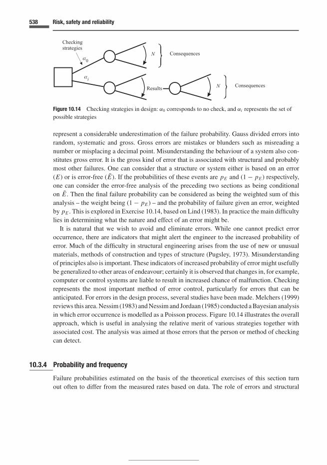
538 Risk, safety and reliability
Figure 10.14 Checking strategies in design: α0 corresponds to no check, and αi represents the set ofpossible strategies
represent a considerable underestimation of the failure probability. Gauss divided errors intorandom, systematic and gross. Gross errors are mistakes or blunders such as misreading anumber or misplacing a decimal point. Misunderstanding the behaviour of a system also con-stitutes gross error. It is the gross kind of error that is associated with structural and probablymost other failures. One can consider that a structure or system either is based on an error(E) or is error-free (E). If the probabilities of these events are pE and (1 − pE ) respectively,one can consider the error-free analysis of the preceding two sections as being conditionalon E . Then the final failure probability can be considered as being the weighted sum of thisanalysis – the weight being (1 − pE ) – and the probability of failure given an error, weightedby pE . This is explored in Exercise 10.14, based on Lind (1983). In practice the main difficultylies in determining what the nature and effect of an error might be.
It is natural that we wish to avoid and eliminate errors. While one cannot predict erroroccurrence, there are indicators that might alert the engineer to the increased probability oferror. Much of the difficulty in structural engineering arises from the use of new or unusualmaterials, methods of construction and types of structure (Pugsley, 1973). Misunderstandingof principles also is important. These indicators of increased probability of error might usefullybe generalized to other areas of endeavour; certainly it is observed that changes in, for example,computer or control systems are liable to result in increased chance of malfunction. Checkingrepresents the most important method of error control, particularly for errors that can beanticipated. For errors in the design process, several studies have been made. Melchers (1999)reviews this area. Nessim (1983) and Nessim and Jordaan (1985) conducted a Bayesian analysisin which error occurrence is modelled as a Poisson process. Figure 10.14 illustrates the overallapproach, which is useful in analysing the relative merit of various strategies together withassociated cost. The analysis was aimed at those errors that the person or method of checkingcan detect.
10.3.4 Probability and frequency
Failure probabilities estimated on the basis of the theoretical exercises of this section turnout often to differ from the measured rates based on data. The role of errors and structural

539 10.3 System or component failure
redundancy in making estimates difficult has been noted. Some authors advocate the use of‘nominal’ probabilities of failure. A better approach is to acknowledge those factors that arenot included in the calculations, such as errors and redundancy, and to improve modelling so asto close the gap. Probabilities are always conditional on certain events or assumptions, and thismight be a good way to interpret ‘nominal’ values. We have advocated a subjective conceptionof probability different from that of frequency. This should not be interpreted to mean that theprobabilities are somehow less ‘accurate’ than those based only on frequencies or that one canthen accept discrepancies with regard to data.
We have often used frequencies and data to estimate probabilities. The idea is to ‘massage’frequencies where necessary, to estimate probabilities. For example, in estimating the prob-ability of death in a scheduled flight on a major airline, we would look to accident recordsfor similar aircraft. In cases where the aircraft were different or were subjected to differentmaintenance procedures, we might adjust the data. Certain classes or ages of aircraft might beeliminated from our data base. This is a question of our probabilistic judgement. We cannotuse the excuse that our probabilities are subjective and therefore somehow they need not be inaccordance with measured data or that we can ignore the question of measurement.
The relationship between probability and frequency has been studied by de Finetti (1937).Let the events {R1, R2, . . . , Ri , . . . , Rn} represent survival in a given time period, say a year,of the objects of interest, for example a set of n electronic components or a set of n offshorerigs. We consider a future year so that these values are not known. The Ri can, as usual, takethe values 0 or 1. The probabilities associated with these events are
{r1,r2, . . . , ri , . . . , rn
}so
that they represent reliabilities. Then
ri = 〈Ri 〉
and∑n
i=1 Ri represents the number of ‘successes’ in n trials. Now we let{ω0, ω1, ω2, . . . , ω j , . . . , ωm
}represent the probabilities that {0, 1, 2, . . . , j, . . . , n} of the
events occur.We can write the expected number of survivals in two ways:
⟨∑i
Ri
⟩=
∑i〈Ri 〉 = r1 + r2 + · · · + ri + · · · + rn (10.31)
= (0) (ω0) + (1) (ω1) + (2) (ω2) + · · · + ( j)(ω j
) + · · · + (n) (ωn) ; (10.32)
these two ways must agree in order that the assignments {ri } and{ω j
}be consistent. Equations
(10.31) and (10.32) represent, in different ways, the expected number of events, for example,the expected number of components or rigs that survive. Equation (10.32) may be divided byn, giving∑n
i=1 ri
n= r =
(0
n
)(ω0) +
(1
n
)(ω1) + · · · +
(j
n
) (ω j
) + · · ·(n
n
)(ωn) . (10.33)
Now ( j/n) , with j = 0, 1, 2, . . . , n, represents the frequency of occurrence of the events.

540 Risk, safety and reliability
Since this is unknown in the present analysis, because we are considering the events in a futureyear, it is a random quantity. Let us denote the frequency as G, taking possible values j/n.
Then by Equation (10.33)
r = 〈G〉 ; (10.34)
the expected frequency equals the average probability of occurrence of the events Ri . Thisreasoning must apply both to reliability and probability of failure.
Some particular cases are of use in dealing with risk. They deal with the use of frequencyin assisting us to estimate probabilities. Two situations will be discussed.
(1) If the events {R1, . . . , Ri , . . . , Rn} are considered to be equiprobable, and if the frequencyis well defined by past records, then the probabilities ri = r = r must be consistent withthe frequencies.
(2) There are cases where the frequency is known, but not the individual probabilities. De Finettigives the example of the case where a ballot is taken with n voters. There are r favourablevotes in support of a certain candidate, or proposition. We do not know how any of the indi-viduals voted; we may express our uncertainty probabilistically as {r1, r2, . . . , ri , . . . , rn},where these express our probabilities that individuals {1, 2, . . . , i, . . . , n} voted in favourof the candidate or proposition. Yet we know the frequency in this case since we knowthe total number ( j) who voted for the proposition, and the total number of voters (n) . Byvirtue of Equation (10.34) our assignment must be constrained by the condition r = j/n.
In assigning the ri we would use any knowledge we might have regarding the propensitiesof the individuals concerned.
Let us now apply these ideas to engineering components and systems. Often we find thattheoretical estimates of failure probability do not accord with observed failure rates, as wasnoted above. The most constructive approach to this situation is to take the view that it pointsout deficiencies in our analysis. For example, calculations of failure probabilities of structuralsystems may not account completely for structural indeterminacy and redundancy or for errors.Instead, a judgemental allowance may be made for such factors. We should, at the same time,strive to improve our estimates of failure probability so that they match reality and that theycapture the essential points. The key point is that the probabilities and frequencies must beconsistent. The use of conditional probabilities, for example for a limit state at first yield, mayrepresent a temporary way out, but the long term objective should be consistency.
If the failure rates for the system or component are judged equiprobable, then these shouldbe similar to observed frequencies, possibly suitably ‘massaged’. In this, we might make thejudgement that the present systems are similar to those used in the past, or that there havebeen changes affecting the failure rates. For example, there are observable improvements inaircraft safety records over time. It is of course never true that the future is the same as the past.Yet we may make this judgement as being sufficiently accurate. For example, in estimatingwave heights or iceberg populations, we use statistical parameters (means, variances, . . . ) toestimate future conditions. We know that climate changes with time, but we might ignore this
541 10.4 Risk analysis and management
for a period of short duration so as to make a reasonable approximation for the commercial lifeof (say) an oil production facility. For other purposes, involving the longer term, we might wantto include models of climate change, greenhouse effects, and so on. Common sense shouldguide us: a new dam constructed affects conditions downstream, and we would adjust our floodestimates accordingly.
We might judge that failure rates are not equiprobable; components from two different man-ufacturers might have different failure rates. The safety record for fixed and mobile offshoreunits is different. For a given proportion of the two kinds of objects, our assignment of prob-ability must be consistent with the overall average. Often, in practice, a set of data has beencollected, yet, as a result of proprietary ownership, the results are not freely available. How tan-talizing such a set of data might appear to us! We might, at the same time, have some knowledgeof the average values collected, and our assignment of individual values must be consistentwith averages known. For example, we might know that, in a certain city or region, 42% ofthe population use a particular transportation mode or use a certain product. We might nothave data for each socio-economic group. Assignment of probabilities for these groups mustalso be constrained by p = 0.42. If the city contained three groups ‘low income’, ‘mediumincome’, and ‘high income’, each with the same number of members, we might validly assignp1 = 0.60, p2 = 0.40, p3 = 0.26, with a mean of 0.42, for the probabilities that an individualfrom each of the three groups uses a certain transit mode.
10.4 Risk analysis and management
Risk analysis is a branch of decision theory; all of the background developed in this bookis therefore of use in risk analysis. This provides an intellectual structure on which to basethe analysis. Often approximate methods are used, for example the use of target levels ofprobability for safety as a ‘cutoff’, as described in Section 10.4.2. In cases where decisionsare clearcut, these approximate methods might be sufficient. In other situations, more de-tailed decision analysis is needed, and factors such as risk aversion need to be addressed.Even in extended works on risk analysis, fundamental aspects such as risk aversion, aspresented in Chapter 4, are frequently neglected if the connection to decision theory is notappreciated.
Many engineering problems are concerned with the analysis and mitigation of risk. Thesiting of industrial facilities such as those involved in natural gas processing, or nuclear powerstations, transportation of hazardous goods, avoidance of computer system error or failureof control systems – these represent typical areas of application. Management of risk is animportant activity. Periodic inspection and maintenance are necessary to the safety of manyengineering systems. Common engineered objects where safety is an important aspect areaircraft, offshore rigs, ships, vehicles used in road transport, and pipelines. Inspection in thesecases will include, for example, the checking of the appearance and growth of cracks. (We havenoted in Chapter 2 the importance of cracks in the fracture and possible failure of structural

542 Risk, safety and reliability
systems.) In industrial systems generally, inspection and quality control are important parts ofthe production process. The best way to formulate a strategy for maintenance or inspection isby means of decision theory. Financial risk can also be analysed: uncertainty in interest rates,inflation, the price of oil, stock and bond prices – these can all be modelled using probabilitytheory.
Engineers will naturally attempt to answer questions posed by clients in industry or govern-ment. Most problems will be concerned with specific areas of interest, examples of which havebeen given in the preceding paragraph. A commendable case study in which multiattribute util-ity has been combined with probability is the siting of the Mexico City airport (de Neufville andKeeney, 1972; Keeney and Raiffa, 1976). The utility functions included attributes concernedwith cost, safety, access and noise pollution.
Full use of probabilistic decision theory is not always necessary; sometimes cost is usedas a ‘surrogate’, as, for example in a study of flood control and reservoir dam gates (Putchaand Patev, 2000), or individual outcomes such as possible fatalities and oil spill size (Tveitet al., 1980) can be considered in designing offshore production platforms for oil and gas. Insome cases, analysis reveals that the probabilities of undesired consequences are small, andfurther analysis is unnecessary. In others, the consequences turn out to be unimportant, andagain further analysis is not necessary. Often we develop approximate rules, especially forsmall repetitive problems. Cost–benefit approaches are frequently used.
In all of these instances, decision theory as developed in this book provides the necessaryguidance in understanding the nature of the problem and associated risks, and in making appro-priate approximations. Occasionally we deal with those having large potential consequences;the design of nuclear power stations or air traffic control systems are examples. Certainlydesign rules and codes of practice for structures are of this kind. The result is generally thatthe probability of undesirable events such as major adverse consequences to human life or theenvironment is reduced to a very small value.
Risk mitigation can often be assisted by analysis of risks prior to initiation of the project.This can be achieved by probability-reducing or consequence-reducing means. To take thequestion of transport of hazardous goods as an example, the probability of an accident near apopulated area can be reduced by re-routing the transportation system; consequences can bereduced – say in the case of rail transport of hazardous goods – by the design of special railcars that prevent the release of their contents.
10.4.1 Tools: event and fault trees
We have used decision trees extensively in this book. If we consider a series of chance forks, thisis often referred to as an event tree. The probabilities of the various events should be estimatedand added in an analysis. If these are conditional upon each other, or are independent, they canbe multiplied to obtain the final event probability. Event trees should be viewed as a naturalpart of the decision process and of the broader use of decision trees that include decision forksas well.

543 10.4 Risk analysis and management
Figure 10.15 Event tree for release of hazardous goods from a railroad car for Example 10.8
Example 10.8 Figure 10.15 illustrates the case of transportation of hazardous goods by rail.Notional values of probability in the figure are added as an example. If we assume that theprobability that a car contains chlorine is independent of the event of a derailment, and that theprobability of penetration of the containment is conditional on the car containing chlorine –for example if the car is specially designed for the purpose – and that the probability of asignificant release is conditional upon penetration, then the final probability of a significantrelease is
(10−4
) · (10−2
) · (0.3) · (0.1) = 3 · 10−8.
Fault trees were developed in the aerospace industry in the early 1960s (Barlow and Lambertin Barlow, Fussell and Singpurwalla, 1975). Their use is now widespread, for instance inanalysis of chemical plants (Wells, 1996) and nuclear plants (McCormick, 1981). Fault treescan be used as a design tool or in diagnostic analysis of existing systems and failures. Ineffect, they identify the Boolean and–or situations – the series and parallel system attributesanalysed in Section 10.3.2 above. There are two types of symbols, those describing eventsas in Figure 10.16(a) and logic gates as in 10.16(b). The events include rectangles denotingfailure that results from the logic gates. The focus of fault tree analysis is the ‘top event’,invariably an undesirable event, usually system failure. This will be explained by means of anexample.
Example 10.9 Figure 10.17 shows an electrical circuit. The top event is ‘motor does notoperate’. This is shown in Figure 10.18(a), together with primary faults contributing to failureand the use of an ‘or’ gate. Figure 10.18(b) shows a fault tree which incorporates an ‘and’gate.

544 Risk, safety and reliability
Figure 10.16 (a) Event symbols (b) Symbols for logic gates
Figure 10.17 Electric circuit
There exist other event and gate symbols; further, the failure of a system can always beanalysed in more depth if desired. The literature is rich in examples. See, for example, Barlow,Fussell and Singpurwalla (1975), McCormick (1981), Wells (1996), Billinton and Allan (1992).
Example 10.10 Boolean analysis. Figure 10.19 shows the relation of fault tree analysis to thereliability of components as expressed in a reliability block diagram. Boolean analysis can beapplied; for example in Figure 10.19(a)
F = F1 F2 F3 F4, (10.35)

545 10.4 Risk analysis and management
Figure 10.18 (a) Example of OR gate development (b) Example of AND gate development
whereas in Figure 10.19(b)
F = 1 − (1 − F1) (1 − F2) (1 − F3) . (10.36)
10.4.2 Safety and target probabilities: as low as reasonably practicable (ALARP)
In many cases, for instance in the design of nuclear power plants, and the siting of facilitiesdealing with explosive materials such as liquefied natural gas, a detailed decision analysismight be considered necessary. In many other cases, the safety is addressed by specifying‘target probabilities’, for instance, of failure of a system. These will be set at a sufficiently lowlevel to ensure a desired level of safety. We shall discuss this issue mainly from the point of

546 Risk, safety and reliability
Figure 10.19 Reliability block diagrams
view of a person at risk. In some applications attempts have been made to set safety levels byusing a cost–benefit approach, setting a monetary equivalent for loss of life. Baker (1977) andFlint and Baker (1976) review some applications in the offshore industry, and a calculation isgiven in Jordaan and Maes (1991). The conclusion is that this calculation is quite arbitrary andthat often exceedingly high and unrealistic risks to humans are indicated. There is confusionover the perspective: the owner might have an entirely different point of view from the workeron the installation.
It is the conviction of the writer that the person at risk should be the predominant factor inone’s thinking. An analysis by Nessim and Stephens (1995) illustrates the point. In consideringa tradeoff between safety and economy, Figure 10.20 illustrates various solutions to a designproblem, based on economic analysis, exemplified by curves A, B and C. A minimum safetylevel has been specified corresponding to a Safety Index of 4 (10−4 per year). The situationwhere the point corresponding to an optimal solution from the economic standpoint violates the

547 10.4 Risk analysis and management
Figure 10.20 Tradeoff between optimal cost and safety: SI = −log10 p f
minimum safety requirement is shown in the case of curve A. It is considered very reasonablethen to set a ‘cutoff’ corresponding to minimum safety.
In setting targets, there will often be a range of values that need to be considered; someoccupations, even within a given industry, are more hazardous than others. One might wantto express a target which one wishes over time to achieve. The ALARP (as low as reasonablypracticable) principle has been formulated and used in the UK in considering risks from nuclearpower stations (Wells, 1996; Melchers, 1993). This is illustrated in Figure 10.21. One can thinkof the diagram as representing an arrow pointing in the direction in which one wishes thingsto improve. This idea can be related to target values, as in Figure 10.22. In this figure, a targetof 10−5 is proposed, yet values of 10−4 are countenanced. See Moan (2004) for a discussionof offshore floating platforms.
Basic riskThe idea of basic risk is useful in deriving target risks in industrial projects. An individual insociety will face the following risks. (See Chapter 9 in Lind, 1972; also Starr, 1969.)
� Basic risk r0, defined as the risk that is impossible to avoid in living in society.� Voluntary risk rv, under the person’s control, that the person is prepared to accept.� Liability risk r�, where blame or liability attaches to a third party.
An estimate of basic risk is often taken as a proportion (about one-third) of the risks due to allaccidents. Taking the value from Table 10.1, it is found that r0 1.4 · 10−4 per annum. This issomewhat more than the value for motor vehicle accidents. The level of 10−4 is often given asa desired maximum risk per year in industrial activities. This is taken here to be a reasonablevalue for this purpose.
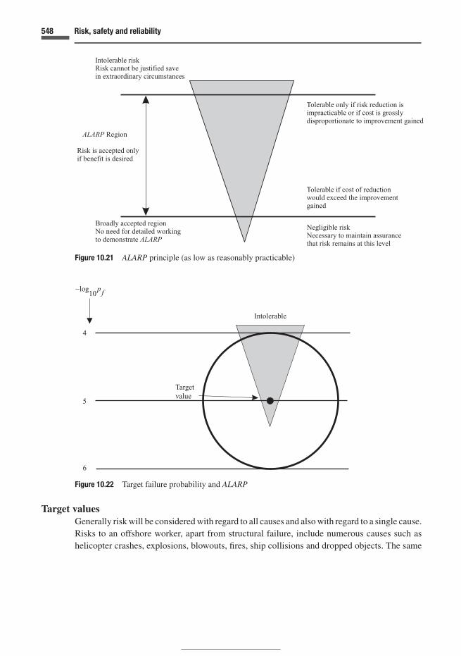
548 Risk, safety and reliability
Figure 10.21 ALARP principle (as low as reasonably practicable)
Intolerable
Targetvalue
4
5
6
−log10
pf
Figure 10.22 Target failure probability and ALARP
Target valuesGenerally risk will be considered with regard to all causes and also with regard to a single cause.Risks to an offshore worker, apart from structural failure, include numerous causes such ashelicopter crashes, explosions, blowouts, fires, ship collisions and dropped objects. The same

549 10.4 Risk analysis and management
Table 10.3 Some target values of tolerable risk to the individual
Target risk per year Safety Index
At work/all causes 10−4 4Specific causes 10−5 5At home/all causes 10−5 5Specific causes 10−6 6
is true of other industries. One then has to think of ‘all causes’ as against ‘specific causes’. Inthe calibration of offshore standards (Jordaan and Maes, 1991) we considered this aspect andarrived at values of 10−4 and 10−5 per annum for the two cases, respectively, the latter valuepertaining to structural safety. Wells (1996) proposed similar values from the perspective ofthe designer of process plants, particularly in the chemical industry. Table 10.3 suggests somevalues of tolerable risk. The values for those at work correspond to occupations where there isabove-average risk. Values for society (at home) are based on Wells (1996).
A final point can be made. If the target value of failure probability is pt , we may supposethat this should be comfortably lower than the basic risk r0 (Jordaan, 1988):
pt = r0 · �, (10.37)
where is a multiplier. Taking logarithms,
(− log10 pt ) = (− log10 r0) + (− log10 �). (10.38)
Arguments are presented Jordaan (1998), that suggest that the logarithm of failure probabilityis a reasonable utility measure. If this is accepted, one can illustrate the situation as in Figure10.23 where the change in utility associated with � is shown. A reasonable value for an offshorestructure is of the order of pt = 10−5 per annum where human life or significant damage tothe environment is involved. One can also use another factor, �1 say, in (10.37) to account forthe effect on human safety of (for example) evacuation of a rig in advance of a hurricane.
10.4.3 Acronyms: PPHA, HAZOP, FMEA and FMECA
The activities described under these names summarize methods that have been of use in prac-tice. Our approach has been to stress the approach and methods that one would use fromfirst principles, but for completeness we summarize the meaning of the acronyms; see Wells(1996) and Stewart and Melchers (1997) for further details. Preliminary process hazard analy-sis (PPHA) is used at the preliminary design stage, and is aimed at identifying the majorhazards, their cause and consequences. The method has been used in the analysis of processplants. Hazard and operability (HAZOP) studies were developed in the chemical and pro-cess industries. It was originally oriented towards flow lines in process plants, together withassociated equipment, and aims at a systematic analysis of hazards and other potential prob-lems. Wells (1996) gives excellent case studies. Failure modes and effects analysis (FMEA),

550 Risk, safety and reliability
Target value
Utility
∆1.00.50.1
u0
u0 + u1
u0 + 2u1
Figure 10.23 Variation of utility with �, a multipilier of basic risk R0. Utility is in relative units
developed originally for aerospace applications, and failure mode, effect and criticality analysis(FMECA) aims at systematic and extensive identification of failure modes in systems. Stewartand Melchers (1997) review literature and summarize some applications.
10.5 Structural systems
The use of limit states is natural for structural engineers. A structure may collapse, an oil storagefacility may be breached, a high-rise building may suffer excessive deflections to the discomfortof its occupants, vibrations may make the use of machinery difficult or impossible. The differentlimit states that make the structure unfit for purpose are a natural focus in design. In the contextof the present analysis, if a limit state is reached, this is termed ‘failure’. As can be seen in thelist of examples just given, the consequences of this failure vary considerably. Palmer (1996)discusses the development of structural engineering, and points to the thinking that must havegone behind the construction of arches in Roman times. These stone structures would be proneto failure due to instability resulting from external loads. The arch geometry might result in theformation of a mechanism. Similar arguments apply in the case of early cathedrals and archbridges. Pugsley (1951) refers to the failure as one of loss of ‘block stability’. This limit statewould not involve failure of the stone. Dead weight of the structure was the main concern;wind and the movement of people on the structures were considered relatively unimportant.As Pugsley points out the Achilles heel of this construction was foundation settlement. Limitstates corresponding to this failure mode were not considered in masonry construction.

551 10.5 Structural systems
Wood had been extensively used in construction, and particularly in railway bridges. Strengthwas an issue, and the variability led to the introduction of load factors that were greater than,say, those for wrought iron (Pugsley, 1966). In bridge construction, wood was superseded bycast iron during the expansion of railways in the nineteenth century. Again, material responseplayed an important role because of cast iron’s brittleness and vulnerability to fatigue. Manyfailures of iron bridges occurred, including famous examples such as the Tay bridge. Its failureduring a storm alerted engineers to the importance of wind loads, and subsequent designsincluded allowance for lateral loads due to wind.
Because of the failure of the material, testing of beams and columns was initiated. Thisled to the introduction of a factor of safety as the ratio of the load required to break thegirder or component to the load that it would be expected to carry. The possible presenceof large flaws in castings led to the use of large safety factors (4 to 6; Pugsley, 1951). Thedevelopment of steels then permitted the use of its ductility in design. The understanding ofbeam theory allowed the introduction of stress and the definition of factor of safety as theratio of the stress at failure to maximum working stress. In aeronautical engineering the useof histograms of peak acceleration, and in building design the plotting of histograms for floorloading represent examples of the introduction of probabilistic ideas and risk from the pointof view of determination of loadings. This, when combined with uncertainty in strength, ledto the early determination of probability of failure. Pugsley in the UK and Freudenthal in theUSA (Freudenthal et al., 1966 for example) were leaders in these developments.
One can see the step-by-step process of learning by experience. A facet of this experiencewas the need to deal with uncertainty, for example in allowing larger factors of safety whenthere was uncertainty in strength. The format used in current limit-states design is
γ l∗ ≤ φr∗, (10.39)
where l∗ is the specified load with load factor γ , and r∗ is the specified resistance with resistancefactor φ. This has been generalized to state that ‘the effect of the factored loads does not exceedthe factored resistance’ (for example, Canadian Standards Association, 1992).
Specifications of load for design purposes reflect the seriousness of consequences; the moreserious, the smaller the exceedance probability – and the longer the return period – on thedesign loading event. In particular, there may be implications of failure for human life. Insuch cases where the consequences of failure are serious and can be anticipated, we effectively‘engineer out’ the unwanted events by using loads and resistance that ensure that the probabilityof exceedance of load over capacity becomes very small. An example of the introduction ofconsequences into the design setting is the use of safety classes which govern the selectionof target levels of safety. An example is given in the Canadian Standards Association (1992)3
for fixed offshore structures in which two safety classes are defined for the verification of thesafety of the structure or any of its structural elements:
3 The 2004 edition is now available.

552 Risk, safety and reliability
Figure 10.24 Structural systems
(a) Safety Class 1 – failure would result in great risk to life or a high potential for environmentaldamage, for the loading condition under consideration;
(b) Safety Class 2 – failure would result in small risk to life and a low potential for environ-mental damage, for the loading condition under consideration.
The target annual probabilities of failure are given in the standard as 10−5 and 10−3 respectively.As noted in the above (Section 10.3.3) in reality most structural failures result from errors
and human factors. An opposite tendency to that of errors is that of redundancy and reservecapacity in structural systems. Redundancy is often not included in the methodology of struc-tural engineering. Figure 10.24 illustrates simple structural systems that correspond to theassumptions of series and parallel behaviour, as introduced in Section 10.3.2. In the case ofparallel systems, the usual mode of plastic collapse is illustrated. It is required that sufficientductility be provided so that the postulated modes of failure can occur. Analysis of systemductility is often complex and not fully calculated in design, it being possible only to modelthe failure of a component of a system, supplemented by approximate techniques involvingreserve strength ratios or judgement when dealing with the entire system. An additional levelof safety against collapse results. The calculation of failure probability, or estimates based oncode calibrations or comparisons, are then only approximate.
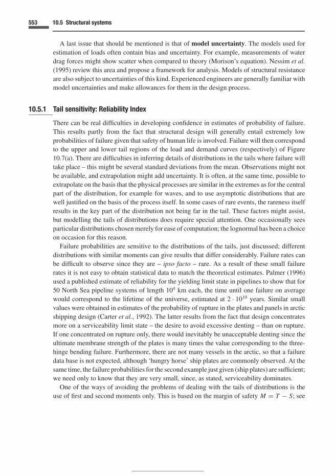
553 10.5 Structural systems
A last issue that should be mentioned is that of model uncertainty. The models used forestimation of loads often contain bias and uncertainty. For example, measurements of waterdrag forces might show scatter when compared to theory (Morison’s equation). Nessim et al.(1995) review this area and propose a framework for analysis. Models of structural resistanceare also subject to uncertainties of this kind. Experienced engineers are generally familiar withmodel uncertainties and make allowances for them in the design process.
10.5.1 Tail sensitivity: Reliability Index
There can be real difficulties in developing confidence in estimates of probability of failure.This results partly from the fact that structural design will generally entail extremely lowprobabilities of failure given that safety of human life is involved. Failure will then correspondto the upper and lower tail regions of the load and demand curves (respectively) of Figure10.7(a). There are difficulties in inferring details of distributions in the tails where failure willtake place – this might be several standard deviations from the mean. Observations might notbe available, and extrapolation might add uncertainty. It is often, at the same time, possible toextrapolate on the basis that the physical processes are similar in the extremes as for the centralpart of the distribution, for example for waves, and to use asymptotic distributions that arewell justified on the basis of the process itself. In some cases of rare events, the rareness itselfresults in the key part of the distribution not being far in the tail. These factors might assist,but modelling the tails of distributions does require special attention. One occasionally seesparticular distributions chosen merely for ease of computation; the lognormal has been a choiceon occasion for this reason.
Failure probabilities are sensitive to the distributions of the tails, just discussed; differentdistributions with similar moments can give results that differ considerably. Failure rates canbe difficult to observe since they are – ipso facto – rare. As a result of these small failurerates it is not easy to obtain statistical data to match the theoretical estimates. Palmer (1996)used a published estimate of reliability for the yielding limit state in pipelines to show that for50 North Sea pipeline systems of length 104 km each, the time until one failure on averagewould correspond to the lifetime of the universe, estimated at 2 · 1010 years. Similar smallvalues were obtained in estimates of the probability of rupture in the plates and panels in arcticshipping design (Carter et al., 1992). The latter results from the fact that design concentratesmore on a serviceability limit state – the desire to avoid excessive denting – than on rupture.If one concentrated on rupture only, there would inevitably be unacceptable denting since theultimate membrane strength of the plates is many times the value corresponding to the three-hinge bending failure. Furthermore, there are not many vessels in the arctic, so that a failuredata base is not expected, although ‘hungry horse’ ship plates are commonly observed. At thesame time, the failure probabilities for the second example just given (ship plates) are sufficient;we need only to know that they are very small, since, as stated, serviceability dominates.
One of the ways of avoiding the problems of dealing with the tails of distributions is theuse of first and second moments only. This is based on the margin of safety M = T − S; see

554 Risk, safety and reliability
Equation (10.9) and Cornell (1969). From this, a measure of structural safety has been derived:the ‘β-factor’, or Reliability Index defined as
β = µM
σM, (10.40)
where µM and σM are the mean and standard deviation of the margin of safety M (Section10.3.1). The motivation is that one would wish the mean value of M, µM , (the average mar-gin of safety) to be greater if there is more uncertainty, which occurs in the case of greaterσM . Keeping β constant then keeps the ratio between the safety margin and the level ofuncertainty, as measured by the standard deviation, constant. If one judges that the uncer-tainty can be modelled using normal distributions, the probability of failure is as given inEquation (10.14):
p f = FZ (−β) . (10.41)
The simplicity of dealing only with first and second moments in reliability theory is appealingand is important in many applications.
It should be borne in mind that this is indeed only an approximation, and was so intendedby the originator. Recall that in Section 4.4, in Equation (4.2), we discussed the use of suchapproximations in making decisions. The idea was to use a single value to represent the lottery.This was taken as being equal to the mean less a constant times the standard deviation; usingthe notation of the present section,
µM − βσM , (10.42)
where β is a constant depending on our degree of risk-averseness. We showed in Section 4.4using Equation (4.2) – essentially the same as (10.42) – that there are cases where we cannotdiscriminate between two actions since µM and σM are the same for each action, yet we havea clear preference for one of the two actions. Figure 10.25, which mimics Figure 4.5, shows
5/6
1/6
60
5/6
pmf
m
m
pmf
1
2
1/6
-4 0 2
Figure 10.25 Probability mass functions for strategies α1 and α2. The first choice leads to possiblecollapse (negative M) whereas the second one does not

555 10.5 Structural systems
Safety Indexand
ReliabilityIndex
Index
Index
Figure 10.26 Safety Index and Reliability Index
two simple probability distributions resulting from two actions α1 and α2. The use of (10.42)does not permit one to discriminate between α1 and α2. A utility function was needed to dothis.
But the β-factor was always intended as an approximation to take into account the veryinsufficiency of information in estimating probabilities and should therefore not be used forcalculating p f if this is the case. For unidimensional S and T, there is a simple relationshipbetween β and p f ; see Equation (10.14) or Exercise 10.8. Figure 10.26 shows the relationshipbetween our Safety Index
(− log10 p f)
and the Reliability Index β. It is seen that this isessentially linear over the range of interest. We have proposed the Safety Index as a utilityfunction for safety (Jordaan, 1988). The index β, being a linear transformation, could servethe same purpose. But the calculation of probability of failure from normal distributions ofload and resistance, implied in β, might not be accurate.
If one has detailed information on the probability distributions involved, and if one wishesto make correspondingly more detailed evaluations of risk, it would be better to proceed todetailed probabilistic design. Over the last decades the development, indeed redefinition ofβ so as to make a better estimate of p f , has been a central part of structural reliability (seeMadsen et al., 1986). In this approach, the definition of β has been amended so that randomquantities representing load and resistance are transformed into normal distributions. Then β
for the transformed system gives accurate values of p f . This development has been good inthe sense of providing consistency with the past.

556 Risk, safety and reliability
Figure 10.27 Code-writing decisions
10.5.2 Codes of practice
Codes of practice are formulated with the intention of setting minimum levels of safety. Thedecisions facing a designer are illustrated in Figure 10.27(a). There is no way that a code-writer can, or should, account for all the economic decisions in designing a structure; these arethe domain of the owner, designer and operator. See, for example, Rosenblueth (1987). Theinterested parties are
(i) the owner and operator (who might be the same);(ii) government and regulatory bodies responsible for safety;

557 10.6 Broad issues
(iii) the designers and contractors;(iv) not least, the future personnel who will work on the facility.
The purpose of the code is to ensure adequate safety and performance of the structure. Thecode-writer therefore attempts to make a judgement on behalf of society, to set a safety levelas a constraint on the design process. It therefore should focus on the interests of the fourthof the interested parties above. The role of the code as a constraint on design is shown inFigure 10.27(b). The responsibility of protecting persons at risk was emphasized in Sect-ion 10.4.2.
The code may include rules of thumb that assist the designer in obtaining quick and reliablesolutions. Fully probabilistic design is not a necessary or reasonable objective; the code shouldrelieve the designer of having to perform intricate probabilistic calculations. What is neededis a judicious use of probability theory (Palmer, 1996), with intense effort for large projectsinvolving possible loss of life or damage to the environment.
10.6 Broad issues
Attempts have been made to develop methods to deal with broad issues facing humankindas a whole. Our response to risks and dangers in society is often irrational; several exampleshave been given in the section on ‘Risks to the individual’, above. A more rational allocationof resources could certainly result in less suffering and in greater human happiness. A goodexample of this kind of analysis has been presented by Lind, Nathwani and Siddall (1991).Their analysis weighs the benefits against the costs of various possible actions. They drawattention to what they term ‘misallocation of resources’. Blind reduction of risk is not a goodthing; resources should be allocated where they can do the most good. They give the examplefrom the nuclear industry, where the expenditure on the saving of a life by installing hydrogenrecombiners to prevent explosions amounts to about $7 billion. At the same time, it is estimatedthat detection and reduction of radon in homes is 1000 to 100 000 times more cost-efficient.They discuss the lack of consistency in safety standards whereby pollutants in the outdoorsfrom industrial sources are controlled yet the risk from a variety of organic chemicals indoorsis 100 times greater. On the other hand, some of us would wish to aim at air in the outdoorsthat is clean as possible, for all sectors of society!
In formulating attributes to use in studying human happiness, careful thought must be paidto the parameters proposed to measure the attribute in question. These should reflect theattribute that is desired. As an example where an attribute might be misleading, consider theuse of Gross National Product (GNP) as a measure of the happiness of individuals in a nation.Goldsmith (1994) argues that, despite the quadrupling and trebling of the GNPs, in real terms,of the USA and UK respectively, in the last fifty years, both nations are ‘profoundly troubled’.GNP measures the extent of economic activity, and calculations based on it do not include, for

558 Risk, safety and reliability
example, the contribution of mothers or fathers who spend their time looking after their familieswithout pay, thus not contributing to the official economy. Policies such as globalization, whichlead to an increase in GNP, do not necessarily lead to increased happiness. Billions of peoplefrom countries with high unemployment – for instance India or Vietnam – have entered theworld economy, and they are able to work at a rate of pay approximately one-fiftieth thatof a person in the developed economies. Enterprises naturally move those factories requiringextensive labour to the developing countries where 50 people can be employed for the priceof one in the developed world. The result is the high level of unemployment and associatedmisery found in the developed country despite strides in the level of GNP.
Lind et al. (1991) discuss other indices, for example ones that include life expectancy, literacyand purchasing power based on GDP per capita. This is the human development index (HDI)developed by the United Nations Development Programme (UNDP). The main message in thestudy is the need for frameworks at the national level to make rational decisions regarding theallocation of national revenue and the development of resources so as to maximize benefits andthe avoidance of inefficient risk-reduction schemes. These efforts at analysis are worthwhile,yet whether they will succeed in the long run remains to be seen. There is a considerableelement of irrationality in attempts by humankind to come to terms with national, and moreso, international planning. For the foreseeable future, we can expect to see the desecration ofthe environment and the disregard for social issues as well as the disrespect and contempt forother animals and species to continue.
10.7 Exercises
There are many reference case studies in the area of risk analysis. It is a useful educational exercise tosearch for and consult those in your area of interest.
10.1 It is a useful exercise to conduct a search on data bases available in your area of interest.
10.2 Consider the case where proof loading is applied to a system. Describe how this may affect thedistribution of resistance fT (t) . Consider cases where the proof loading does and does not causesigns of distress in the system (for example cracking in a structure).
10.3 Prove Equation (10.6).
10.4 Derive p f for the case where T and S are uniformly distributed.
10.5 A component has random resistance that is modelled by a symmetrical triangular distribution inthe interval (10, 15) in arbitrary units. The loading is uniform in the interval (4, 12) using thesame units. Calculate the probability of failure.

559 10.7 Exercises
10.6 Derive p f for the case where T and S are modelled by chi-square distributions.
10.7 For lognormally distributed load and resistance, show that
p f = FZ
−ln
[µT
µS
(1 + v2
S
1 + vT
) 12]
{ln
[(1 + v2
T
) (1 + v2
S
)]} 12
, (10.43)
where µT and µS are the means of T and S whereas vT and vS are the coefficients of variation.Also show that the following approximations are reasonable.
p f FZ
−
ln
[µT
µS
]
(v2
T + v2S
) 12
(10.44)
for vT , vS < 0.3. Also
µT
µS exp
[β
(v2
T + v2S
) 12]. (10.45)
10.8 Show that p f for the case of normal distributions can be written as
Pr (−β) =1 − erf
(β√2
)
2. (10.46)
Use this or (10.14) to verify Figure 10.26.
10.9 Verify Equations (10.19), (10.21), (10.26) and (10.27) by substituting 1s and 0s using 1 = TRUE,0 = FALSE in the Fi and Ri .
10.10 Extend Equation (10.25) to find ps for three units in series, using Equation (2.17).
10.11 The failure rate generally follows the analysis of the intensity function of Section 9.5.4 and Figure9.12(b). For the special case of a constant intensity as in Example 9.9, show that the reliabilitycan be written as
R (t) = exp (−λt) ,
where t is time and λ is a parameter representing the failure rate. Use this to develop the mean-time-to-failure (MTTF) for series and parallel systems.
10.12 Find the reliability of the system in the figure, given a component reliability of 0.9.

560 Risk, safety and reliability
10.13 The error rate in a design/programming process has been found to be one per 100 calculations orprogramming statements.
(a) Given a total of 1000 statements, find the probability that the number of errors exceeds 20.(b) Given a checking process in which one in ten errors is detected, calculate the probability that
the number of errors exceeds 20 after checking.(c) Formulate a model in which the error and detection rate are treated as random. See Figure
10.14 and Nessim and Jordaan (1985).
10.14 Research the effect of human error on the capacity T of a system. In particular, consider the modelof human error due to Lind (1983).
10.15 Give examples of practical probability- and consequence-reducing measures in risk analysis inyour area of interest.

11 Data and simulation
‘I checked it very thoroughly,’ said the computer, ‘and that quite definitely is the answer. I think theproblem, to be quite honest with you, is that you’ve never actually known what the question is.’
Douglas Adams, The Hitchhiker’s Guide to the Galaxy
Entities should not be multiplied unnecessarily.Occam’s Razor
11.1 Introduction
Engineers continually face the necessity to analyse data and records from the past. These mightconsist of measurements of material strength, flood records, electronic signals, wave heightsin a certain location, or numbers per unit area of icebergs. The intention is to use these recordsof the past to assess our uncertainty regarding future events. The overall aim is, as always,to make decisions for design at an acceptable level of risk. Apart from good analysis, dataprovide the most significant means of decreasing uncertainty and improving our probabilisticestimates. Data are obtained from experiments. These always represent an available strategy,although money and effort are required to carry them out. It is the author’s experience that incases where there is considerable uncertainty regarding a physical process, one real experimentis worth a thousand theories.
In the use of probabilistic models two aspects present themselves: the choice of the modelitself, and the estimation of model parameters. We showed in Chapter 8 how to use datato estimate parameters of known distributions. The framework described in Section 8.1.1involved the knowledge of a distribution or process. In the present chapter, we describethe use of data to fit and compare distributions. The choice of a particular model can bemade by an analysis and understanding of the underlying process involved, or on an em-pirical analysis of data, or some combination of the two. The quantity under investigationmight be the sum of many other quantities leading to the use of the normal distribution.Or it might be multiplicative in character – bacteria multiply, and possibly fracture pro-cesses might show this characteristic, leading to the lognormal distribution. Or the strengthof an element might be the smallest of elements in its composition, leading to the Weibull
561

562 Data and simulation
distribution. The occurrence of accidents in time might be random, leading to the Poissondistribution.
Alternatively, the data might be compared empirically to various distributions and a choicemade on that basis. A combination of knowledge of the process and empiricism might be used.In some cases, one might use a set of empirical data itself as a model, in which case theremight not be any need to estimate model parameters. We summarize the approach noted witha Bayesian relationship, to be considered as a pragmatic guide in one’s thinking:
Pr (C |data) ∝ Pr (data|C) · Pr (C) , (11.1)
where C indicates the choice of a particular distribution. A common-sense result is that withdiffuse prior knowledge, the closer the data are to the fitted distribution, the higher the chancethat the fitted distribution is the best hypothesis. The importance of prior knowledge is alsoapparent. The equation is introduced to show that Bayesian thinking can guide the work of thepresent chapter. But the work does relate to real world data, which often do not fit the idealtheoretical model.
The present chapter also deals with simulation. Often convenient closed-form mathematicalmodels are not available, necessitating the use of numerical methods. Often data are notavailable or are found for certain parameters that are of indirect relevance to the problem athand. In these cases, Monte Carlo simulation is employed to generate results in a manner thatis in some ways analogous to an experiment, and certainly to a ‘thought-experiment’. Thisforms the second related subject of the chapter.
11.2 Data reduction and curve fitting
We shall introduce the ideas using an extended example. This concerns a problem of measure-ment. An engineer is using a survey instrument to measure the difference in elevation froma reference point of known elevation to the underside of a bridge deck. This problem wasintroduced in the context of inference in an example at the end of Section 8.5.1. It could bean important one for determining clearance under the bridge, for instance for a rail systemthat passes underneath. In order to assess the accuracy of the measuring system, the engineertakes 100 repeated measurements. These are given in Table 11.1. The problem is to determinethe distribution that best fits the data. The engineer suspects that the data follows the normaldistribution. This distribution of ‘errors’ in measurement was used extensively by Gauss instudies of astronomy and geodesy.
Calculations have traditionally been done manually. Now, computer-based methods providean effective and powerful means of dealing with data. For a beginner, it is useful for completeunderstanding to do some of the calculations by hand at least once. We shall lead the waythrough the analysis of the data set. The first thing to do is to obtain representative statistics.It should be noted that the treatment of the data set is based on the concept that ‘order doesn’tmatter’ thus being consistent with the assumption of exchangeability.

563 11.2 Data reduction and curve fitting
Table 11.1 Measurements of bridge elevation in metresfrom reference point
27.893 27.832 27.959 27.927 27.92927.914 27.925 27.929 27.988 27.83027.960 27.859 27.887 28.001 27.76327.799 27.826 27.898 27.883 27.92427.958 27.883 27.859 28.000 27.85427.882 27.882 27.853 27.892 27.94027.900 27.847 27.916 27.868 27.97127.939 27.850 27.940 27.925 27.85527.926 27.913 27.957 27.897 27.94527.827 27.814 27.894 27.952 27.90727.873 27.888 27.866 27.975 27.88427.970 27.838 27.819 27.905 27.87227.876 27.842 27.920 27.929 27.88127.955 27.859 27.926 27.993 27.83627.971 27.926 27.938 27.884 27.91027.805 27.982 27.888 27.932 27.90928.032 27.960 27.881 27.913 27.86727.961 27.877 27.890 27.861 27.93427.947 27.802 27.892 27.785 27.82627.865 27.910 27.909 27.792 27.852
11.2.1 Sample descriptive measures
We are given a set of measured values
x1, x2, x3, . . . , xi , . . . , xn. (11.2)
Note that these values cannot be random – they correspond to actual deterministic values suchas those in Table 11.1 above. A first task is to obtain minimum, maximum and the range,defined as the maximum minus the minimum. It is also useful for several purposes to rank thedata; this is usually done in ascending order and represents a task that is much better done bya computer than by hand.
Example 11.1 For the data set of Table 11.1, the ranked data is shown in Table 11.2. Theminimum and maximum are 27.763 and 28.032 m respectively, with a range of 0.269 m.
Central tendencyMoments are generated for data in a manner analogous to those for distributions. One canimagine, in a general way, that each data point has a probabilistic ‘weight’ of 1/n. But we willsee that for variance and standard deviation, usage suggests 1/ (n − 1). The most common and

564 Data and simulation
Table 11.2 Data of Table 11.1 ranked in ascending order
27.763 27.854 27.884 27.913 27.94527.785 27.855 27.884 27.914 27.94727.792 27.859 27.887 27.916 27.95227.799 27.859 27.888 27.920 27.95527.802 27.859 27.888 27.924 27.95727.805 27.861 27.890 27.925 27.95827.814 27.865 27.892 27.925 27.95927.819 27.866 27.892 27.926 27.96027.826 27.867 27.893 27.926 27.96027.826 27.868 27.894 27.926 27.96127.827 27.872 27.897 27.927 27.97027.830 27.873 27.898 27.929 27.97127.832 27.876 27.900 27.929 27.97127.836 27.877 27.905 27.929 27.97527.838 27.881 27.907 27.932 27.98227.842 27.881 27.909 27.934 27.98827.847 27.882 27.909 27.938 27.99327.850 27.882 27.910 27.939 28.00027.852 27.883 27.910 27.940 28.00127.853 27.883 27.913 27.940 28.032
useful measure of central tendency is that of the sample mean (commonly referred to as anaverage):
x =∑n
i=1 xi
n. (11.3)
Thus∑n
i=1(xi − x) = 0. (11.4)
Example 11.2 The mean of the data set of Table 11.1 is found to be 27.898 m.
Strictly, the mean presented in Equation (11.3) is the arithmetic mean. Weighted means applydifferent weights to particular data points (in which case order might matter). Geometric andharmonic means can also be calculated in particular instances, as in the following example.
Example 11.3 The geometric mean of n observations is the nth root of their product. Forexample, if a stock in a particular exchange increases by 5%, 10% and 12% in three successiveyears, we would be interested in the geometric mean
3√
1.05 · 1.10 · 1.12 = 1.0896 (to four decimal places).

565 11.2 Data reduction and curve fitting
The geometric mean is always less than the arithmetic one and gives better results whenmultiplicative compounding is the issue, as in the present example.
Measures of central tendency include the mode and the median. The mode correspondsto the most frequently occurring value, while the median represents the value in the middleof the ranked data set. For a data set with an odd number of observations, the median is the[(n + 1) /2]th value, for example the fifth if n = 9. If the number of data points is even, thenone averages the (n/2)th and the [(n + 2) /2]th values.
Example 11.4 In our data set of Table 11.2, several values occur twice (for instance 27.826,27.881, 27.909 and 27.913; see Table 11.2). Three values occur three times (27.859, 27.926 and27.929). There are too few repetitions of values to obtain a good estimate of central tendency.The use of the mode works better for grouped data, using the peak value in the frequencydistribution; see Subsection 11.2.2 below.
Example 11.5 The median of the data set of Table 11.2 is the mean of the 50th and the 51stranked data points, i.e. 27.8955 m.
DispersionThe first measure of dispersion of the data is the range, given above as 0.269 m for the dataof Tables 11.1 and 11.2. By far the most common measure of spread is the sample variance(s2
)and sample standard deviation (s). These values are given by
s2 =∑n
i=1 (xi − x)2
n − 1(11.5)
and
s =√∑n
i=1 (xi − x)2
n − 1(11.6)
respectively. The use of (n − 1) rather than n in Equations (11.5) and (11.6) is common andis sometimes termed ‘Bessel’s correction’. We have adopted this definition because of itscommon usage.
But the reason for this choice is more historic than compelling. It appeared naturally whenconsidering some inferences using the normal distribution where the mean and variance werebeing studied, for example in Equations (8.99), (8.100) and (8.143), in Section 8.6.5, andthere the factor (n − 1) was termed the ‘degrees of freedom’, ν. The use of ν = n appeared inSections 8.5.2 and 8.6.4 where inferences regarding the variance only are being made. Hencethere does not seem to be a strong reason to choose (n − 1) rather than n, except that theproblems of inference involving (n − 1) are more common. It is also stated in the literaturethat the estimator s2 is ‘unbiased’ but there are good reasons to question this, as described in
566 Data and simulation
Section 8.7.4 and in Exercise 8.24 (‘fly in the ointment’). Discussion of degrees of freedom isgiven in Section 11.3.2 below.
The sample coefficient of variation is defined in a manner analogous to that for probabilitydistributions, as given in Equation (3.66):s
x· 100, in per cent. (11.7)
Example 11.6 The standard deviation of the sample of Table 11.1 is found to be 0.0535 mand the coefficient of variation is0.0535
27.898· 100 = 0.19% (two significant figures).
The mean elevation is measured on an interval rather than a ratio scale (Section 4.7) so thatthere is a certain arbitrariness in the coefficient of variation.
Note that
s2 =∑n
i=1 (xi − x)2
n − 1
=∑n
i=1 x2i − 2x
∑ni=1 xi + nx2
n − 1
=∑n
i=1 x2i − nx2
n − 1, or
s2 = n∑n
i=1 x2i − (∑n
i=1 xi)2
n (n − 1). (11.8)
The last form is useful for computation.A measure of dispersion can be based on quantiles (quartiles, percentiles, deciles, . . . ).
These can be defined for an ordered data set in a similar way to that used for the median above.The basic idea is to find values such that a specified probability lies below the value in question.Data do not of themselves represent probabilities; one would likely want to smooth the databy fitting a distribution and to consider uncertainties in the parameters of the distribution(Chapter 8). The transition from data to probability is one that requires some introspection,and one should not automatically make the association that data represent probability (Section11.2.3 below).
We shall now give the rules for obtaining quantiles based only on the data (in other wordsbefore the ‘transition to probability’). The method is much the same as for medians above.Suppose that one wishes to obtain the point corresponding to the first quartile. We then calculate(n/4) . If this value is not an integer, round up to the next integer and take the correspondingordered value of the data as the quartile. If the value is an integer, calculate the mean ofthe corresponding ordered value of the data and the next highest. For third fractiles we use(3n/4) with a similar calculation procedure. For the (i/r )th fractile, we use (i/r ) · n and either

567 11.2 Data reduction and curve fitting
choose a value or average as just described. When a non-integer is found, one chooses the nextinteger as the division point giving the quantile, thus dividing the data set into two groups ofsize (i/r ) · (n − 1) and [(r − i) /r ] · (n − 1) . When an integer is found, the division point ishalfway between this integer and the next, thus dividing the data set into two groups of size(i/r ) · n and [(r − i) /r ] · n. Rather than taking the midpoint, linear interpolation could be used.
Example 11.7 Suppose the data set has n = 75 values. We wish to find the first quartile sothat r = 4 and i = 1. Then n/4 = 18.75 and we take the 19th value as the quartile. For thethird quartile i = 3 and 3n/4 = 56.25 so that we use the 57th value.
Example 11.8 For the data set of Table 11.1, (n/4) = 25, so that the first quartile is halfwaybetween the 25th and the 26th values in the ranked data. This gives (27.859 + 27.861)/2, or27.860. Similarly, the third quartile is 27.933.
The method just described is based only on the data; a better method might be required basedon the fitted probability distribution. See Subsection 11.2.3 (transition to probability) below.
Skewness and kurtosisWe give the usual classical definitions, which are useful for assessing skewness and flatnessof distributions. The coefficient of skewness is defined as
g1 =1n
∑ni=1 (xi − x)3
s3. (11.9)
The value will be positive for distributions skewed to the right and negative for distributionsskewed to the left (see also Figure 3.20).
Example 11.9 For the data of Table 11.1, the skewness is g1 = −0.0742. This low valueindicates a symmetric distribution.
The coefficient of kurtosis is given by
g2 =1n
∑ni=1 (xi − x)4
s4. (11.10)
This value is often compared to g2 = 3, which is the value for a normal distribution. Thekurtosis is a measure of ‘flatness’ and tail heaviness of distributions.
Example 11.10 For the data of Table 11.1, we find g2 = 2.69, which is close to the value 3for a normal distribution.
The definitions given in Equations (11.9) and (11.10) should be used with large samples.For small samples, the estimates will become unreliable, and a small bias will become evident;

568 Data and simulation
see Exercise 11.2 There are also other ways to define skewness and kurtosis, for example usingthe values
√g1 and (g2 − 3) . In using computer packages, it should be checked which version
of the definitions is used.
11.2.2 Grouped data and histograms
Histograms represent an excellent means of judging the form of the probability distribution.We shall focus on the data of Table 11.1. Figure 11.1 shows the result; the shape of thedistribution is bell-shaped and a good appreciation of the distribution of the measurementsis obtained. The first step in producing this display is to develop a tally chart, as shown inTable 11.3. Computer programs compute these automatically, but it is useful to complete atleast one by hand. Most programs will have a default number of class intervals and these areoften unsatisfactory; it is better oneself to specify the class boundaries. Too few intervals maylead to loss of information regarding the shape of the distribution and too many lead to erraticshaped results, hard to interpret. It is worth experimenting with the number of intervals – usinga computer package! – so as to get a feeling for these effects.
A useful approximate rule that has been found by experience for the number of intervals is
1 + 3.3 log10 n. (11.11)
For n = 100, this gives 7.6 intervals. The following was decided upon: start at 27.761 m andend at 28.033 m, with eight intervals of size 0.034 m. The tally chart is shown in Table 11.3.The ‘cut points’ are the class boundaries whereas ‘class marks’ indicate the midpoints of each
Figure 11.1 Histogram of elevation data

569 11.2 Data reduction and curve fitting
Table 11.3 Tally chart for data of Tables 11.1 and 11.2
Cut points Midpoints Tally Relative(class boundaries) (class marks, x j ) (frequency) frequency, g j
27.761–27.795 27.778 3 0.0327.795–27.829 27.812 8 0.0827.829–27.863 27.846 15 0.1527.863–27.897 27.880 25 0.2527.897–27.931 27.914 23 0.2327.931–27.965 27.948 16 0.1627.965–27.999 27.982 7 0.0727.999–28.033 28.016 3 0.03
interval. The usual assumption is that if a value coincides with the upper class boundary it istaken as being in that class, not the next. The intervals are often simply referred to as ‘bins’.
The tally from Table 11.3 is plotted as the frequency in Figure 11.1. The relative frequency,which is the frequency divided by the number n of data points, is given in the last column ofTable 11.3, and is shown on the right hand ordinate of Figure 11.1. The most likely value, themode, can now successfully be calculated; it corresponds to the class mark 27.880 in Table 11.3and in Figure 11.1.
One can calculate the mean, standard deviation and other statistics from a set of groupeddata. By using grouped data, one does lose some accuracy as compared to the use of the originaldata set. The method is analogous to that above. For a set of grouped data with class marks
x1, x2, x3, . . . , x j , . . . , xk (11.12)
and associated frequencies
g1, g2, g3, . . . , g j , . . . , gk, (11.13)
the sample mean and variance are
x =∑k
j=1 g j x j
n(11.14)
and
s2 =∑k
j=1 g j(x j − x
)2
n − 1(11.15)
=n
∑kj=1 g j x2
j −(∑k
j=1 g j x j
)2
n (n − 1), (11.16)
respectively.

570 Data and simulation
11.2.3 Cumulative frequency plots, fitting distributions and the transition to probability
We consider initially the grouped data of Table 11.3. In Table 11.4, these values are used togenerate cumulative frequency and cumulative relative frequency (cr f ) values; these are thesum of frequencies and relative frequencies respectively for those intervals (or bins) belowthe value (boundary) in question. The data can be used to plot the ogive given in Figure 11.2.Usually these curves are S-shaped as in the figure.
Table 11.4 Data for ogive and probability plot
Less than Cumulative relative Normalor equal to Cumulative frequency frequency = cr f z = F−1
Z (cr f )
27.761 0 0 −∞27.795 3 0.03 −1.88127.829 11 0.11 −1.22727.863 26 0.26 −0.64327.897 51 0.51 0.02527.931 74 0.74 0.64327.965 90 0.90 1.28227.999 97 0.97 1.88128.033 100 1.0 ∞
Figure 11.2 Frequency ogive for data of Table 11.4

571 11.2 Data reduction and curve fitting
Figure 11.3 Probability plot of binned data of Table 11.4
To check for normality of a distribution, ‘arithmetic probability paper’ has traditionally beenused. This has in the past been done by hand and again it is useful for a beginner to completeone or two plots by hand. The plots are now done very effectively by computer for a variety ofdistributions. The idea is to produce a graph, which if linear, would suggest that the distributionunder consideration is the appropriate one for use. The ‘arithmetic probability paper’ couldin the past be purchased at stationers but can be produced as follows. We shall complete thecalculation for the normal distribution, but the method can be applied to any distribution whichcan be normalized using location and scale parameters. The method for those that cannot isgiven below.
The cumulative relative frequencies range from 0 to 1, so that it is natural to use these as‘first estimates’ of cumulative probabilities. Since we are considering the normal distribution,for convenience the comparison is made with the standard normal distribution; see Equations(3.26) and (3.27), the cumulative distribution of which is denoted FZ . We calculate the inversevalues, F−1
Z , as in the last column of Table 11.4. A straight line in a plot of data againstthese values supports the assumption of a normal distribution. Figure 11.3 shows the result inthe present case. One can see that the data follows approximately a straight line, suggestingnormality. It should be noted that the first and last points with relative frequencies of 0 and 1correspond to −∞ and +∞ on the inverse cumulative axis for all distributions that range from−∞ to +∞.
In the example, the standard normal distribution has been used, but the analysis can be donefor other chosen distributions; see Figures 11.6 and 11.8 and related text below.

572 Data and simulation
Table 11.5 Ranked data for probability plot
r Value r/n (r − 1) /n(r − 1
2
)/n F−1
Z
(r− 1
2n
)
1 27.763 0.01 0 0.005 −2.5762 27.785 0.02 0.01 0.015 −2.1703 27.792 0.03 0.03 0.025 −1.960...
......
......
......
......
......
...50 27.894 0.5 0.49 0.495 −0.0125...
......
......
......
......
......
...98 28.000 0.98 0.97 0.975 1.96099 28.001 0.99 0.98 0.985 2.170100 28.032 1 0.99 0.995 2.576
Probability plots using entire data setWe now use the ranked data of Table 11.2 rather than the grouped data. This is again shown inTable 11.5, with r denoting the position in the ordered data set, giving a realization
x(1), x(2), x(3), . . . , x(r ), . . . , x(n)
of the set of ordered random quantities
X (1), X (2), X (3), . . . , X (r ), . . . , X (n); (9.10)
see also Chapter 9 and Equation (9.10). We now wish to associate a value with each entrythat gives a good idea of the associated probability of the random quantity being less thanthe value in question – equivalent to the cumulative relative frequency of Table 11.4. For thispurpose, three columns are shown in Table 11.5. The first gives (r/n) which gives valuesranging from (1/100) for the first (r = 1) to (50/100) = 0.5 for r = 50 to (100/100) = 1 forthe last (r = 100) . At first glance this seems reasonable, but we note that the last point shouldbe plotted at F−1
Z (1) = ∞ in the case of distributions unlimited to the right. The next columnshowing [(r − 1) /n] corresponds to the case where the data are ranked in decreasing order, saywith indices
{1, 2, 3, . . . , r ′, . . . , n
}. Then the frequency of exceedance of a value is
(r ′/n
)and, that of non-exceedance is
1 − r ′
n= r − 1
n
since r + r ′ = n + 1. This has the disadvantage that the first point has to be plotted at −∞.

573 11.2 Data reduction and curve fitting
Figure 11.4 Probability plot using entire data set of Table 11.5
Hazen suggested a compromise plotting position between (r/n) and[(r − 1) /n] :
r − 12
n. (11.17)
This allows the first and last points to be plotted. It is the default plotting position in MATLAB r©,and has been used in Figure 11.4; see Section 11.4 below for further discussion. The verticalaxes in the figure show
F−1Z
(r − 1
2
n
)(11.18)
and the corresponding value of FZ .
It is a matter of judgement to move from data to probabilities. The straight line in Figure 11.4is convincing and one might accept that a normal distribution is an acceptable probabilisticmodel in the present case. It is useful also to present the final result of the analysis in theform of the histogram together with the proposed probability distribution. Figure 11.5 showsthe result. The fitted normal curve was plotted using the sample mean and variance noted inExamples 11.2 and 11.6 above. The illustration shows Francis Galton’s apparatus for generatingbell-shaped distributions. Balls, beads or particles are inserted into the receptacle at the topand fall through the maze of spikes, bouncing off them, with the resulting distribution at thebottom.

574 Data and simulation
Francis Galton’s apparatus
Distributions not normalized by location and scale parametersFigure 11.6 shows data from dedicated rams of the vessel MV Arctic into multiyear ice,discussed in Section 9.4.1 above, with Table 11.6 giving the cumulative frequency data. Figure11.7 shows the ogive. The data is unsymmetrical, and after some experimentation with differentdistributions, it is decided to fit a gamma distribution. There is no generally convenient wayto normalize distributions that do not have location and scale parameters. The mean andvariance from the histogram are found to be 9.85 and 28.33 respectively, giving α = 3.4266and β = 2.8753 in the gamma distribution:
fX (x) = xα−1 exp (−x/β)
βα� (α);
see Appendix 1 for details of distributions.

575 11.2 Data reduction and curve fitting
Figure 11.5 Fitted normal curve for bridge elevation
Probabilitydensity
Figure 11.6 Gamma distribution fitted to MV Arctic data; relative frequencies as shown on histogram

576 Data and simulation
Table 11.6 Data for MV Arctic ogive
Less than Cumulative relative Gammaor equal to Cumulative frequency frequency = cr f x = F−1
X (cr f )
0 0 0 03 4 0.0288 2.456 37 0.2662 6.149 74 0.5324 9.3312 98 0.7050 11.9015 116 0.8345 14.7318 126 0.9065 17.2821 134 0.9640 21.2524 137 0.9856 24.8327 138 0.9928 27.4430 139 1.0 ∞
Figure 11.7 Ogive for MV Arctic data
The fourth column in Table 11.6 shows values of the inverse gamma distribution, usingthe parameter values just noted and using the cumulative probability values given in the thirdcolumn. For example, the value in the third row (6.14) is the inverse gamma value for the cdfequal to 0.2662 and with the parameters (α, β) noted. The resulting probability plot is given inFigure 11.8 and a reasonable fit is obtained. Figure 11.6 shows the histogram and fitted curve.(Note that the parameters used in Chapter 8 – Equation (9.17) – were slightly different as theywere based on slightly different data.)

577 11.2 Data reduction and curve fitting
Figure 11.8 Probability plot for gamma distribution (from Table 11.6)
In order to find the values of F−1X , parameters (α, β in the present case) had to be estimated
to deduce the value of the random quantity; the curve fitted was not a ‘standard ’ curve in thesense of the standard normal which is universally the same. But the procedure is very similar.In the present case, some iteration on the parameter values might be undertaken to find thebest fit. Since the product of analysis is a straight line (Figures 11.3, 11.4 and 11.8), the toolsof linear regression are often used to find the least-square fit (Section 11.3).
Transition to probabilityData when presented in histograms, ogives or probability plots will show ‘humps and bumps’,variations with regard to the postulated distributions. This is to be expected, as data sets willshow scatter. The fitted distribution might represent much better one’s judgement regardingprobability since the irregularities will have been ironed out. The assignment of probabilityusing data is a matter of the analyst’s best judgement. Generally, if a probabilistic model isappropriate with regard to the process and if the data show a good fit, then the fitted curve willbe used to estimate the probabilities.
Quantiles can also be deduced from the fitted distribution rather than from the data them-selves. Then the quantiles give probability- rather than the data-based values given in Section11.2.1 above. Uncertainty in parameters is also important in giving final estimates of prob-ability, as outlined in Chapter 8. Once the distribution is decided upon that represents one’sprobabilities, one can read off from the cdf the various quantiles that give one’s best esti-mate of probabilities less than or greater than a specified value or of values with a specifiedvalue of probability above or below. This is in distinction to the quantiles obtained earlier thatrepresented percentages of data points less than or greater than a specified value.

578 Data and simulation
11.2.4 Goodness-of-fit tests
Our approach in this section is pragmatic, aiming at finding the best-fit distributions given adata set. The curve-fitting procedure above can be carried out for a variety of distributionsand the best result chosen. This might be done using a least-squares technique; see Section11.3 below. At the same time we should be guided by prior knowledge, for example that aparticular distribution is appropriate for theoretical reasons or based on past experience offitting. We have discussed the shortcomings of hypothesis tests as decision-making tools inChapter 8 (Section 8.9). Yet they can be useful to gauge the quality of a particular fit, and theprocedure will be outlined for the chi-square test. The chi-square distribution was introducedin Chapter 8, see in particular Section 8.7.4, and the Subsection ‘Classical interpretation ofchi-square distribution’.
Chi-square testAssume first that we have a candidate model that we wish to test. There are as before, n datapoints. For example, this could be the normal distribution fitted to the data of Table 11.1. Touse the method, we consider grouped data, as in Table 11.3 and as shown in Figure 11.3. Wecompare with the model class marks (11.12) the observed frequencies (11.13),
g1, g2, g3, . . . , g j , . . . , gk, (11.13)
used in constructing the histogram, an example being the last column of Table 11.3. We assumethat the model yields probabilities
p1, p2, p3, . . . , p j , . . . , pk, (11.19)
corresponding to these values. The p j can be calculated by taking the value of the probabilitydistribution at the class mark and multiplying this value by the class interval or by integratingover the class interval. In effect we consider a partition and compare the measurements withthe fitted curve. The same procedure is followed for any type of distribution that we are fitting.
The chi-square test is based on the quantity
∑k
j=1
(g j − np j
)2
np j, (11.20)
which for large n is approximately chi-square with (k − 1) degrees of freedom. We mayinterpret Equation (11.20) as representing
∑ (observed frequency minus expected frequency)2
(expected frequency). (11.21)
The probability of the result (11.13) follows the multinomial distribution
n!
g1!g2! · · · g j ! · · · gk!pg1
1 pg22 · · · p
g j
j · · · pgk
k . (11.22)

579 11.2 Data reduction and curve fitting
The trend to a limiting chi-square distribution can be proved in two ways. These correspond tothe inductive and classical approaches. First, a Bayesian might start by considering Equation(11.1) with the prior term Pr(D) as being uniform. In other words we have vague opinionsa priori regarding the choice of distribution. Then the term Pr(D|data) is proportional to thelikelihood
pg11 pg2
2 · · · pgk
k (11.23)
with the p j random. In the classical approach, the g j are considered to be random. We canwrite (11.20) as
∑k
j=1
(g j − np j
)2
np j=
∑k
j=1
g2j
np j− n. (11.24)
If the number of data points n from which frequencies are calculated is large then the distributionof (11.20) becomes chi-square with (k − 1) degrees of freedom. In rough outline, the proofsresult in the distribution of (11.20) or (11.21) as being the integration of squares of normallydistributed random quantities over the volume of the annulus of a shell in (k − 1) dimensions.For example, the g j might be considered as binomial or multinomial random quantities whichtend to be normally distributed as n increases. The proofs are considered in more detail inExercise 11.7.
If the distribution is discrete, the class marks coincide with the possible values of therandom quantity, and it becomes a question of taking the value of the pmf at the point underconsideration – see Exercise 11.6. We noted that, in the case of continuous distributions, onecalculates the integral of the probability density over the bin between the class boundaries(approximately the density at the class mark multiplied by the class width).
If the data are used to estimate parameters of the distribution, note that there is a reductionin the degrees of freedom. If r parameters are estimated from the data, there are
k − r − 1 (11.25)
degrees of freedom; see Example 11.11 for an application.
Example 11.11 We use the data of Table 11.3 above, and the fitted normal distribution withx = 27.898 m and s = 0.0535 m. The data in the first and last two bins have been combinedto be consistent with the practical rule: use five or more bins with at least five samples in eachbin. The number of degrees of freedom is then six (number of bins) minus one minus two (forthe two parameters estimated with the data), resulting in three degrees of freedom.
The 95% range of the chi-square distribution is from 0.216 to 9.35. The observed value of0.32 is within this range but near the lower end, indicating a better-than-average fit.
One can obtain curious results if one does not have reasonably well-populated bins; hencethe rule quoted in this example. It is important to put goodness-of-fit tests into perspective. Forexample, the test just conducted says very little about the tails of the distribution. All of the

580 Data and simulation
Table 11.7 Chi-square goodness-of-fit test
Frequency Relative Estimated Normal EquationCut points (tally) frequency normal probability frequency (11.21)
< 27.829 11 0.11 0.0986 9.86 0.132427.829–27.863 15 0.15 0.1579 15.79 0.039727.863–27.897 25 0.25 0.2361 23.61 0.082427.897–27.931 23 0.23 0.2388 23.88 0.032327.931–27.965 16 0.16 0.1635 16.35 0.0073
> 27.965 10 0.10 0.1052 10.52 0.0259Totals 100 1.00 1.0001 100.01 0.3200
displays and results discussed in the preceding should be used in making judgements aboutprobabilistic models.
Other goodness-of-fit testsThere are numerous goodness-of-fit tests which are readily available in the standard literatureand which appear in computer packages. These can be researched for individual applications;the overall idea has been conveyed in the previous section of the chi-square test. See alsoD’Agostino and Stephens (1986).
11.2.5 Estimating model parameters
In Chapter 8, we dealt with the problem of parameter estimation. The Bayesian prescriptionwas advocated as the most rational approach. The literature and computer packages abound indifferent methods, without guidance as to which is appropriate. For example, point estimatescan be based on the method of moments (calculating moments from the data), best-fit linesin probability plots, or maximum likelihood methods. The methods can be assessed using theBayesian approach. If there are many data points, there will not be a large difference betweenclassical methods and the Bayesian approach.
In the final analysis, it not so much the estimates of position and spread of a distribution thatmatter as incorporating all of the uncertainty – the entire probability distribution including itsparameters – in decision-making. But there are also many cases where the parameter uncertaintyis minor, or where the decision only depends in a general way on the probabilities, and then alarge amount of detail is not necessary.
11.3 Linear regression and least squares
Engineers often have to deal with relationships between two quantities, for example temperatureand reaction rate, pressure and volume, load and deflection, voltage and current, fatigue life

581 11.3 Linear regression and least squares
and load range. The term ‘regression’ arose from early measurements by Francis Galton ofthe size of sweet peas – as suggested to him by Charles Darwin – and then of human beings.The studies focussed on the relationship between the size of parents and that of their offspring.In both cases – peas and humans – small parents lead to offspring that are below average insize while large parents lead to offspring that are above average in size. Yet he found thatthe smaller-than-average offspring of small parents were closer to the mean than were theirparents; likewise the larger-than-average offspring of large parents were also closer to the meanthan were their parents. There is a tendency to inherit small or large characteristics but alsoa tendency to ‘regress to the mean’. This led to the use of the term ‘regression’ in studyingrelationships between two quantities. It has also found application in other areas. In investments(Bernstein, 1996) overvalued stocks certainly have a tendency to regress, as any investor intechnology in the first part of this century will have come to realize. Galton also found that thedata on sizes of offspring fitted the normal distribution, an assumption that is usually made inregression studies.
In present-day usage, the term ‘regression’ in statistical analysis does not refer necessarily toactual regression to the mean. It is used in a general way to describe the study of the relationshipbetween two or more quantities. The term linear regression refers to the study of linearrelationships; Figure 11.9 shows a typical subject of study in which there are indications of alinear relationship with scatter about the mean line. We commence our analysis by consideringtwo quantities, y and x . Let x be interpreted as the ‘independent variable’ and y the dependentone. It is natural to consider y|x or ‘y given x’. Figure 11.10 shows the line with the variationaround it indicated with a distribution at xi . For example, x could represent the height ofparents in the example given in the preceding paragraph. The offspring would not all have thesame height; there would be scatter as in Figure 11.9. Let us assume that there are sufficientoffspring to model the distribution about the line. At point xi in Figure 11.10 we indicate anormal distribution of values with the line (α + βx) as the mean. It is then quite natural to model
Figure 11.9 Typical linear regression

582 Data and simulation
Table 11.8 Regression analysis data pairs
Independent quantity x1 x2 x3 · · · xi · · · xn
Dependent quantity y1 y2 y3 · · · yi · · · yn
Figure 11.10 Modelling of regression
the random quantity Y |x as being normally distributed. Often we can take the variance σ 2 aboutthe line as being constant, not a function of x . (This is sometimes termed homoscedastic; if σ 2
varies with x, heteroscedastic. Rather awkward terms!)In summary, we assume a normal distribution about a straight line with constant variance
for all the x of interest. A measured value of y, say yi given by
yi = α + βxi + εi , (11.26)
will depart from the line by the amount εi which is sampled from a normal distribution withvariance σ 2. These are the usual assumptions in linear regression analysis which can and shouldbe checked against available data, or assessed with regard to their importance.
We always commence with a set of data, in which the x and y values occur in pairs as inTable 11.8. Before we proceed to probabilistic analysis, we need to estimate the parameters ofthe line (α + βx) . The values, α and β, correspond to the ‘constant but unknown’ parametersthat were discussed in Chapter 8, and to the case where we have a very large amount ofdata, enough to remove any uncertainty regarding the position of the line. As described in

583 11.3 Linear regression and least squares
Figure 11.11 Relation of data to regression lines
Chapter 8, we can never determine them; we can only estimate them and account for associateduncertainties. We write the estimated line as
y = a + bx . (11.27)
The situation is illustrated in Figure 11.11. A particular data point will deviate a distance ei
from the estimated line (a + bx):
yi = a + bxi + ei . (11.28)
11.3.1 Obtaining the regression line: method of least squares
How do we estimate the regression line? (Recall that ‘regression’ no longer refers to ‘regressionto the mean’ as discovered by Galton.) The method generally used is to minimize the squaresof the deviations from the mean. If we regard the data points as entities with equal mass, thiswill give the line with minimum variance about it – see also Section 3.5.3. We can see thatthere is uncertainty in a and b, since the database is a sample limited in size. We will denotethese as A and B, which are then random. We shall obtain two estimators for a and b, whichwe denote a and b respectively. Following this strategy, we wish to minimize the ‘sums of thesquares of the errors’, or SSE, equal to
∑ni=1 e2
i , that is to find
Min(
SSE =∑n
i=1e2
i
)= Min
(∑n
i=1[yi − (a + bxi )]
2)
. (11.29)

584 Data and simulation
The solution is found by differentiation, noting that a and b are being estimated, resultingin two equations for the two unknowns:
∂ (SSE)
∂a=
∑n
i=1−2 (yi − a − bxi ) = 0 and (11.30)
∂ (SSE)
∂b=
∑n
i=1[−2xi (yi − a − bxi )] = 0. (11.31)
These are termed the normal equations. They can be solved to give the estimators a and b:
na + b∑n
i=1xi =
∑n
i=1yi (11.32)
and
a∑n
i=1xi + b
∑n
i=1x2
i =∑n
i=1xi yi . (11.33)
Eliminating a and solving for b using Equations (11.32) and (11.33):
b = n∑n
i=1 xi yi − (∑ni=1 xi
) (∑ni=1 yi
)n
∑ni=1 x2
i − (∑ni=1 xi
)2 . (11.34)
Equation (11.32) can be written as
na + bnx = n y, or
y = a + bx . (11.35)
Therefore
a = y − bx . (11.36)
We can see from this equation that the least-squares line passes through the centroid of thedata points (x, y) .
In conducting regression analysis, the following notation is useful.
sxx =∑n
i=1(xi − x)2 =
∑n
i=1x2
i −(∑n
i=1 xi)2
n, (11.37)
syy =∑n
i=1(yi − y)2 =
∑n
i=1y2
i −(∑n
i=1 yi)2
n, (11.38)
sxy =∑n
i=1(xi − x) (yi − y) =
∑n
i=1xi yi −
(∑ni=1 xi
) (∑ni=1 yi
)n
. (11.39)
These equations can result in small differences in two large numbers corresponding to the twoterms on the right hand side. Care must therefore be taken in completing the calculations. Onecan treat each data pair as a ‘point mass’ and then consider any of the Equations (11.37) to(11.39) as representing the moment of the masses about the centre-of-mass (left hand side).

585 11.3 Linear regression and least squares
This is equal to the moment about the origin of the masses (first term on the right) minusthe moment of the sum of the masses applied at the centroid about the origin (second term;note that these are equal to nx2, n y2 and nx y). This results from the parallel axis theoremin mechanics; the conclusion from a computational point of view is that the closer the originof computation is to the centroid, the smaller the problem resulting from calculating smalldifferences between large quantities. In the next subsection, the origin is taken at the mean ofthe xi ; calculating with the centroid as origin is a good computational strategy.
Comparison of Equation (11.34) with Equations (11.37) and (11.39) results in
b = sxy
sxx. (11.40)
We may also show that
SSE = syy − bsxy (11.41)
as follows. Since
SSE =∑n
i=1(yi − yi )
2 ,
where
yi = a + bxi , (11.42)
SSE =∑n
i=1
(yi − a − bxi
)2
=∑n
i=1
[(yi − y) − b (xi − x)
]2, using y = a + bx, and consequently
SSE =∑n
i=1(yi − y)2 − 2b
∑n
i=1(yi − y) (xi − x) + b2
∑n
i=1(xi − x)2
= syy − 2bsxy + b2sxx
= syy − bsxy, using Equation (11.39).
Example 11.12 Fatigue data are often studied using the methods of regression analysis. Thedata generally result from cyclic testing to failure of specimens loaded to a specified stresslevel s, with the number nc of cycles to failure being counted. Various stress levels are used;the higher the stress level, the smaller the number of cycles to failure. Table 11.9 shows sometypical results. Experience has shown that s–nc curves are non-linear, so that log-scales areused. We shall use
x = log s, and
y = log nc.
This is one way of dealing with non-linearities – to transform the original quantities by meansof non-linear functions.

586 Data and simulation
Table 11.9 Data for regression analysis
Stress, s Cycles x = log s y = log nc
MPa nc (3 dp) (3 dp)
160 301 740 2.204 5.480160 200 400 2.204 5.302160 425 210 2.204 5.629200 58 890 2.301 4.770200 82 020 2.301 4.914200 81 810 2.301 4.913300 38 070 2.477 4.581300 28 840 2.477 4.460300 39 931 2.477 4.601300 37 270 2.477 4.571300 24 520 2.477 4.390300 31 790 2.477 4.502300 68 360 2.477 4.835400 13 150 2.602 4.119400 8 830 2.602 3.946400 22 370 2.602 4.350400 15 920 2.602 4.202400 16 930 2.602 4.229400 21 970 2.602 4.342400 15 440 2.602 4.189
The results of the regression analysis are as follows.sxx = 0.4147, syy = 3.9284, sxy = −1.1981, b = −2.8891, a = 11.7044, x = 2.453,
y = 4.6161, SSE = 0.4669, σ = 0.1611, n = 20.
The data and the fitted line are shown in Figure 11.12.
11.3.2 Uncertainty in model parameters, mean and future values
All of the parameters and quantities in this section are modelled as being random, and theknowledge that we use is the data set of Table 11.8 (Table 11.9 is an example). In otherwords, we do not include prior knowledge regarding the parameter values so that the analysiscorresponds to the prior distributions expressing ‘indifference’ of Chapter 8. Exercises 11.16and 11.17 deal with conjugate-prior analysis. The only knowledge then is the set of data ofTable 11.8. Further, the assumption of exchangeability will be made, such that the order of then data pairs of Table 11.8 is not deemed important. There is a fair bit of mathematical detail inthe following; the theory is very similar in structure to that regarding the normal distributionin Chapter 8. We have stressed particularly in Chapter 8 that all important uncertainties should

587 11.3 Linear regression and least squares
Figure 11.12 Example regression plot
be taken into account. While the uncertainty of a future value with regard to the regressionline will be taken into account by analysing the scatter about the line, the parameters of theregression line will themselves include uncertainties. As in Chapter 8 it is inherent in thepresent approach to treat these parameters as being random. We have just demonstrated howa and b in the regression equation can be estimated by the method of least squares yieldingthe values a and b. For convenience, we consider the quantity a′ rather than a as the constantof the regression line. This is depicted in Figure 11.13; a′ is the intercept at the value x = xrather than the value a at x = 0 and then
a′ = y (11.43)
from Equation (11.36).The parameters a′ and b of the regression are now modelled as random quantities A′ and B
respectively. We assume further that the scatter about the regression line is normally distributedwith variance σ 2 (to be estimated). We follow the strategy adopted in Chapter 8 and associatew with
(1/σ 2
)as the ‘weight’ representing the (inverse) spread of the distribution. In our
Bayesian analysis, W is a random quantity. The distribution of Yi is then normal:
fY
(y|a′, b, w = 1
σ 2, x
)= 1√
2πσexp
{− 1
2σ 2
[y − a′ − b (x − x)
]2}
∝ w12 exp
{−w
2
[y − a′ − b (x − x)
]2}
. (11.44)

588 Data and simulation
Figure 11.13 Definition of a′
Also from this⟨Y |a′, b, w, x
⟩ = a′ + b (x − x) . (11.45)
Our basic assumption is that the prior distributions of A′, B and ln W are independent anduniform expressing little prior knowledge. Then
f (i)A′,B,W
(a′, b, w
) ∝ 1
w. (11.46)
The independence often makes sense from a judgement of the problem, and the uniformdistributions express initial ‘indifference’ regarding the values concerned (see also Section8.6). Given this initial vagueness, we should not be surprised that the assumptions result inequations similar to the classical data-based analysis. But the structure and interpretation aremore rational. Conjugate prior analysis can also be undertaken; see Exercise 11.16.
We consider now the likelihood of the data set, which is considered as an exchangeable setof n data pairs. The likelihood of the yi given the xi is
(a′, b, w
) ∝∏n
i=1w
12 exp
{−w
2
[yi − a′ − b (xi − x)
]2}
= wn2 exp
{−w
2
∑n
i=1
[yi − a′ − b (xi − x)
]2}
. (11.47)
Now∑n
i=1
[yi − a′ − b (xi − x)
]2 = n(y − a′)2 +
∑n
i=1[(yi − y) − b (xi − x)]2
= n(a′ − y
)2 + syy − 2bsxy + b2sxx
= n(a′ − a′)2 + sxx
(b − b
)2 + SSE, (11.48)

589 11.3 Linear regression and least squares
using (11.37) to (11.39), (11.43), (11.40) and (11.41). It is noteworthy that a′ and b enternaturally into Equation (11.48) and we can see that a′ = a′ and b = b minimize Equation(11.48), the left hand side of which is the same as (11.29). Since Equation (11.48) is minimized,the parameter estimates just noted constitute the maximum of the likelihood of (11.47).
The posterior distribution is obtained by multiplying the prior, Equation (11.46) by thelikelihood, Equation (11.47) into which Equation (11.48) has been substituted:
f (u)A′,B,W
(a′, b, w
) ∝ wn2 −1 exp
{−w
2
[n
(a′ − a′)2 + sxx
(b − b
)2 + SSE]}
. (11.49)
We now determine the marginal distributions of A′, B and W by integration.
Uncertainty in WIntegration of Equation (11.49) with respect to a′ yields
f (u)B,W (b, w) ∝ w
n2 −1 exp
{−w
2
[sxx
(b − b
)2 + SSE]}
×∫ ∞
−∞exp
{−w
2
[n
(a′ − a′)2
]}da′,
in which the integral has the form of the normal distribution; see also Section 8.5.3 and Equation(8.113). It is proportional to w−1/2, and consequently
f (u)B,W (b, w) ∝ w
n2 − 3
2 exp{−w
2
[sxx
(b − b
)2 + SSE]}
. (11.50)
We obtain the integral of Equation (11.50) with respect to b; again it is of normal form,proportional to w−1/2, and we find that
f (u)W (w) ∝ w
n2 −2 exp
[−w
2(SSE)
]. (11.51)
Thus [W · (SSE)] follows a chi-square distribution with (n − 2) degrees of freedom; see Equa-tion (8.83). The mean is
〈W · (SSE)〉 = n − 2, or
1
〈W 〉 = SSE
n − 2= s2 =
∑ni=1 e2
i
n − 2. (11.52)
This does not imply that the mean of the probability distribution of variance, i.e. the mean of(1/W ) is s2; see Section 8.7.4, and in particular Exercise 8.24 and Equation (8.174). In fact,⟨
1
W
⟩= SSE · ν
ν (ν − 2)= SSE
n − 4(11.53)
since ν = n − 2.
Degrees of freedomThe term ‘degrees of freedom’ used in statistics is similar to the usage in mechanics. In thepresent instance, we have (n − 2) degrees of freedom. In estimating the variance from a data set,

590 Data and simulation
with mean and variance unknown – see the discussion after Equation (8.142) – the number ofdegrees of freedom in the distribution of the variance was (n − 1) . We can think of the numberof independent elements in the sample used in the calculation of the parameter of interest: oneequation constraining the sample values has been used in calculating the mean, resulting in(n − 1) degrees of freedom remaining. In the case above there are n data pairs but two equationsconstraining them have been used in calculating the parameters a and b, resulting in (n − 2)degrees of freedom remaining. In mechanics, the number of normal modes of vibration dictatesthe degrees of freedom, the number of variables needed to specify completely the configurationof the system.
Uncertainty in BWe now wish to find the distribution of B. We therefore integrate (11.50) with respect to w.
We follow the strategy given in Section 8.5.3 by making the substitution, as in (8.109),
z = w
2
[sxx
(b − b
)2 + SSE]
(11.54)
in Equation (11.50). Then
f (u)B (b) ∝
[sxx
(b − b
)2 + SSE]− 1
2 (n−1)∫ ∞
0z
n2 − 3
2 exp (−z) dz
= �
(n
2− 1
2
) [sxx
(b − b
)2 + SSE]− 1
2 (n−1). (11.55)
We now make the substitution
t =(b − b
)s/
√sxx
(11.56)
and find that
f (u)T (t) ∝
[1 + t2
n − 2
]− 12 (n−1)
(11.57)
since the Jacobian is a constant. We conclude that the posterior distribution of
B − b
sB(11.58)
with
s2B = s2
sxx= SSE/ (n − 2)
sxx(11.59)
is a t-distribution with (n − 2) degrees of freedom. If we have a very large amount of data,B will model the idea of a ‘population’ parameter β which has little uncertainty associatedwith it.

591 11.3 Linear regression and least squares
Uncertainty in A′
In order to estimate this uncertainty we must integrate Equation (11.49) first with respect to band then with respect to w. Then
f (u)A,W (a, w) ∝ w
n2 −1 exp
{−w
2
[n
(a′ − a′)2 + SSE
]} ∫ ∞
−∞exp
{−w
2
[sxx
(b − b
)2]}
db.
Again the integral is of the form of the normal distribution and is proportional to w−1/2; then
f (u)A,W (a, w) ∝ w
n2 − 3
2 exp{−w
2
[n
(a′ − a′)2 + SSE
]}. (11.60)
Following the method used for B, we make the substitution
z = w
2
[n
(a′ − a′)2 + SSE
]
in Equation (11.60). Then
f (u)A (a) ∝
[n
(a′ − a′)2 + SSE
]− 12 (n−1)
∫ ∞
0z
n2 − 3
2 exp (−z) dz
= �
(n
2− 1
2
) [n
(a′ − a′)2 + SSE
]− 12 (n−1)
. (11.61)
Following the method as before, we substitute
t =(a′ − a′)s/
√n
(11.62)
and find the same result as in (11.57),
f (u)T (t) ∝
[1 + t2
n − 2
]− 12 (n−1)
,
since the Jacobian is a constant. The posterior distribution of
A′ − a′
sA′(11.63)
with
s2A′ = s2
n= SSE/ (n − 2)
n(11.64)
is a t-distribution with (n − 2) degrees of freedom.Again, for a very large amount of data, the uncertainty in A becomes negligible, thus
modelling the idea of a ‘population parameter’ α, as does B model β.
Uncertainty in mean responseWe have now modelled A′ and B as random quantities. This means that there is uncertaintyin both the position of the line
(A′) and its slope (B). Figure 11.14 illustrates the fact that the
uncertainty regarding these parameters results in a spread of the range about the mean response

592 Data and simulation
Figure 11.14 Illustration of confidence intervals in regression; narrowest intervals are at x
that widens as the x-value moves away from the mean x . We shall now demonstrate this fact.First, we consider W = w = (
1/σ 2)
as a constant in Equation (11.49); then
f (u)A′,B
(a′, b|w = 1
σ 2
)∝ exp
{− 1
2σ 2
[n
(a′ − a′)2 + sxx
(b − b
)2]}
= exp −[
n(a′ − a′)2
2σ 2
]exp −
[sxx
(b − b
)2
2σ 2
].
(11.65)
We see from this that given σ 2, A′ and B are independent and N(a′, σ 2/n
)and N (b, σ 2/sxx )
respectively. This independence occurs at the centroid of the data – see Figure 11.14. It is alsoone of the reasons for using a′ (at the centroid) rather than a in our uncertainty analysis.
We now consider the mean value, Equation (11.45), at a particular value x = x0:
⟨Y |a′, b, w, x0
⟩ = a′ + b (x0 − x) . (11.66)
We denote the random quantity 〈Y 〉 as M.Since A′ and B are random, independent and normallydistributed (given σ 2) and since
(M |σ 2
)is a linear function of a′ and b as in Equation (11.66),
consequently it is
N
{a′ + b (x0 − x) , σ 2
[1
n+ (x0 − x)2
sxx
]}. (11.67)
We see why the bands of uncertainty of Figure 11.14 enlarge as x0 moves away from x ; thevariance in (11.67) increases with a term proportional to (x0 − x)2 .

593 11.3 Linear regression and least squares
We now have to take into account uncertainty in σ 2. We know that W is distributed as inEquation (11.51):
f (u)W (w) ∝ w
n2 −2 exp
[−w
2(SSE)
],
and therefore we can write
fM (m) = fM |W=w (m, w) f (u)W (w)
and integrate over w. Following the same procedure as before (see Exercise 11.12), we findthat
T = M − [a′ + b (x0 − x)
]s√
1n + (x0−x)2
sxx
(11.68)
follows a t-distribution with (n − 2) degrees of freedom.
Uncertainty regarding future responseAlthough it is often necessary to have information regarding uncertainty of the mean line, itis also common in engineering to consider a future value. In our example of the fatigue ofa specimen, we would very likely wish to use the data to estimate the fatigue behaviour ofa specimen included in the actual structure. In effect, we consider now the random quantityY rather than the mean 〈Y 〉 , and expect more uncertainty in this particular value than in themean. The proof follows similar lines as in the case of 〈Y 〉 .
From Equation (11.44), we know that by assumption fY(y|a′, b, w = 1
σ 2 , x)
is a normaldistribution. We consider the value of Y at a particular value x = x0. Then
(Y |a′, b, w, x0
), is
N[a′ + b (x0 − x) , σ 2
]. We know that
(A′|b, w, x0
)is N
(a′, σ 2/n
)from Equation (11.65).
Since
fY,A′(y, a′|b, w, x0
) = fY(y|a′, b, w, x0
) · f A′(a′|b, w, x0
), (11.69)
we can deduce that (Y |b, w, x0) is
N[a′ + b (x0 − x) , σ 2 + σ 2/n
]; (11.70)
see Exercise 11.17(c). Again using the same method, and the fact that (B|w, x0) isN
(b, σ 2/sxx
), one can show that (Y |w, x0) is
N
[a′ + b (x0 − x) , σ 2 + σ 2
n+ σ 2 (x0 − x)2
sxx
].
Finally, taking into account the uncertainty in W, standing for(1/σ 2
), using the same method
as before, we find that
T = Y − [a′ + b (x0 − x)
]s√
1 + 1n + (x0−x)2
sxx
(11.71)
follows a t-distribution with (n − 2) degrees of freedom.

594 Data and simulation
Confidence intervalsThe calculation of confidence intervals assists in making judgements in regression analysis. Itis useful to plot them on the graphs showing the regression analysis so as to obtain an immediatefeeling for the uncertainty. The uncertainty is consistent with all of the models for decision-making presented in previous chapters, and this presents the most rigorous approach. We shallwrite down below the confidence intervals which can be derived in the manner described inChapter 8.
Hypothesis testing is also commonly applied in regression analysis. For example, we mightwant to make a judgement regarding the slope of the regression line; is it significantly greaterthan zero? We have discussed before the limitations of hypothesis testing and the attempt toconvert uncertainty into certainty. We advise the calculation of confidence intervals and theuse of judgement from that point onwards.
Confidence intervals for A′
Using Equations (11.63) and (11.64) we find that
Pr[a′ − tα/2 · sA′ ≤ A′ ≤ a′ + tα/2 · sA′
] = 1 − α, (11.72)
where the t-distribution has (n − 2) degrees of freedom and
s2A′ = s2
n= SSE/ (n − 2)
n. (11.73)
The intervals can be expressed simply as
a′ ± tα/2 · sA′ . (11.74)
If one wishes to obtain confidence intervals for A rather than A′, then we use
s2A = s2
∑x2
i
nsxx(11.75)
rather than (11.73); see Exercise 11.14.
Confidence intervals for BEquations (11.58) and (11.59) are used to show that
Pr[b − tα/2 · sB ≤ B ≤ b + tα/2 · sB
] = 1 − α, (11.76)
where the t-distribution has (n − 2) degrees of freedom and
s2B = s2
sxx= SSE/ (n − 2)
sxx. (11.77)
Again we can write the intervals as
b ± tα/2 · sB . (11.78)

595 11.3 Linear regression and least squares
1.9 2 2.1 2.2 2.3 2.4 2.5 2.6 2.7 2.80
1
2
3
4
5
6
7
8
x
y
Figure 11.15 Regression line and 95% confidence intervals for mean and future response inExample 11.12
Mean response M at x = x0
The confidence intervals can be derived as before using Equation (11.68):
[a′ + b (x0 − x)
] ± tα/2 · s
√1
n+ (x0 − x)2
sxx. (11.79)
Future response Y at x = x0
Again proceeding as before based on Equation (11.71), the intervals are
[a′ + b (x0 − x)
] ± tα/2 · s
√1 + 1
n+ (x0 − x)2
sxx. (11.80)
In regression analysis, confidence intervals for the variance are not usually done; see Exercise11.14.
Example 11.13 The results discussed have been applied to Example 11.12. Figure 11.15 showsthe widening of the intervals as one moves away from the mean x .

596 Data and simulation
Table 11.10 ANOVA Results for example problem
Source Sum of squares Degrees of Mean square Ffreedom
Due to regression SSR = 3.461 1 SSR = 3.461SSR
SSE/(n − 2)= 133.4
Residual (SSE) SSE = 0.467 n − 2 = 18SSE
n − 2= 0.02594 –
Total SST = 3.928 n − 1 = 19 – –
11.3.3 Analysis-of-variance (ANOVA) approach
The calculations can also be written in an analysis-of-variance (ANOVA) table. From Equation(11.41)
syy = bsxy + SSE.
This may be written as
Total sum of squares = Sum of squares due to regression + Residual (SSE), or (11.81)
SST = SSR + SSE.
To see this we write the left hand side of (11.81) as∑n
i=1(yi − y)2 =
∑n
i=1(yi − y)2 +
∑n
i=1(yi − y)2 + 2
∑n
i=1(yi − yi ) (yi − y)
=∑n
i=1(yi − y)2 +
∑n
i=1(yi − yi )
2 , (11.82)
which is the same as (11.81). To prove (11.82) we write
(yi − y) = (yi − yi ) + (yi − y)
and note that∑n
i=1(yi − yi ) (yi − y) =
∑n
i=1
(yi − a − bxi
) (a + bxi − y
)= a
∑n
i=1
(yi − a − bxi
) + b∑n
i=1xi
(yi − a − bxi
)− y
∑n
i=1
(yi − a − bxi
).
These last three terms are all equal to zero by the normal equations, (11.30) and (11.31).Equation (11.81) gives expression to (11.82); the results are summarized in Table 11.10 for
Example 11.12. We note that
SST = syy, and
SSR = bsxy .

597 11.3 Linear regression and least squares
Other values in the table include mean squares (sums of squares divided by degrees of freedom)and the F-value, the ratio of the mean squares, as noted in the table. This value assists inassessing whether the sum of squares due to regression is a significant component of thetotal. The 5% exceedance value for F with 1 and 18 degrees of freedom is 4.41. This isconsiderably below the value of 133.4 which must then correspond to a very small exceedanceprobability (actually of the order of 10−9). One can conclude that the regression is very strong.For background on the F-tests, see exercise 11.13.
11.3.4 Correlation
The correlation coefficient ρXY was introduced for two-dimensional probability distributionsin Chapter 3, defined in Equation (3.93) by
ρX,Y = σX,Y
σXσY,
where −1 ≤ ρX,Y ≤ 1, always. It measures the extent of linear relationship between X and Y .Corresponding to this, the sample correlation coefficient is defined as
r = sxy√sxx syy
. (11.83)
Another expression for this is
r = b√
sxx
syy. (11.84)
A related quantity is r2, the sample coefficient of determination:
r2 = s2xy
sxx syy; (11.85)
this can also be calculated using the square of (11.84); other forms can be deduced. Aninteresting version is
r2 = SSR
SST= 1 − SSE
SST, (11.86)
which expresses the proportion of the variation in Y that is explained by the regression line. Wethen know that r2 indicates in a better way the effectiveness of the regression in terms of the‘sums of squares’, or variance in Y. If r = 0.90, then r2 = 0.81, a less impressive number; thisdisparity is more evident when r = 0.70, seemingly a good correlation yet only r2 = 0.49 –less than half – is the proportion of variance explained by the regression.
For a two-dimensional normal distribution given by Equation (A1.140): in Appendix 1, ananalysis using Bayesian methods treats ρ, a parameter in the distribution, as a random quantity(Lindley, 1965). Prior information is taken as uninformative. Let us denote this random quantityas R. Then the result is that � = tanh−1 R is approximately (n → ∞) normal with mean equal

598 Data and simulation
to tanh−1 r and variance (1/n) . This approach is particularly useful when we are consideringthe relationship between two quantities in cases where there is no preference for (y on x) asagainst (x on y). We might be interested, for example, in the relationship between tensile andcompressive strengths of a material without wanting to consider either as the independent ordependent quantity. (But see the next section for a case where the reverse is wanted.) Or wemight be considering the relationship between wind speeds at two locations or between thefoot size and arm length of individuals, with no asymmetry suggesting (y on x) rather than (xon y). Jaynes (1976) discusses a strategy for determining regression coefficients that wouldnot reflect this asymmetry. This avenue is promising and would be useful to complete. Whereone quantity is used as an indicator, the asymmetry returns, as is discussed in the followingsection.
11.3.5 Uncertainty in X : Bayesian approach
We now consider the case where knowledge of one quantity, say Y, is used to improve theestimate of the other. We mentioned in the preceding paragraph the case where pairs of mea-surements are made without any preference for one or the other as the independent quantity.An example was given concerning the pairs of tensile and compressive strengths of a material.This set of pairs of measurements can provide background information for another analysis.We might subsequently be given one value, say Y = y, and wish to infer the distribution of Xgiven this information together with a prior distribution fX (x) . It is quite common in buildingprojects to measure only compressive strengths of concrete – denoted Y – and we might beinterested during a design to obtain estimates of tensile strength, say X, for example if crackopening could present a problem, such as in storing fluids.
Then we can write
fX |Y=y (x, y) ∝ fY |X=x (x, y) · fX (x) , (11.87)
using Bayes’ theorem. The term fY |X=x (x, y) is obtained from regression in the present analy-sis. We also see in this equation why we took Y = y as given rather than X = x ; the conditionaldistribution on the right hand side is reversed, as is always the case in Bayes’ theorem. In theexample of determining tensile from compressive strength, we would perform a regression ofcompressive strength (Y ) on tensile strength (X ) .
We take as an example the case where the assumption of a normal distribution applies inthe regression analysis as well as in the prior distribution fX (x) . We assume further that theparameters of the distributions are known, on the basis of sufficient prior evidence and data,so that there are no parameter uncertainties to be taken into account. Then Y |x is
N(α + βx, σ 2
)(11.88)
based on a linear regression analysis. As noted, we assume further that fX (x) is
N(µX , σ 2
X
). (11.89)

599 11.4 Plotting positions
The method of Exercise 11.17 can be used; the result is that X |y is
N
[µX + (y − µY )
ρσX
σY, σ 2
X
(1 − ρ2
)], (11.90)
where µY = α + βµX , σ 2Y = σ 2 + β2σ 2
X and ρ = βσX/σY is the correlation coefficient. Theanalysis results in a two-dimensional normal distribution fX,Y (x, y) with the conditional dis-tribution (11.90), consistent with the assumptions of linear regression since the mean valueof X |y is a linear function of y. In applications, the parameters α, β, σ 2 and ρ are estimatedfrom the regression data of Y on X. In general, we would wish to use the variance of a futureresponse from (11.80) in modelling the uncertainty in Y given X. In the present case, we haveassumed that parameters are well known so that σ 2 ∼= s2 is used in the analysis.
Example 11.14 Maddock and Jordaan (1982) used the approach described in an analysis ofdecisions in structural engineering.
11.3.6 Regression in several dimensions; non-linear regression
For background to analysis in several dimensions, see Raiffa and Schlaifer (1961), Box andTiao (1973), or O’Hagan (1994) for example. Problems are often non-linear in character; wedealt with this in Example 11.12 by transforming the quantities under consideration. Non-linearproblems are dealt with in many texts, including the one by Box and Tiao just quoted.
11.4 Plotting positions
In obtaining empirical fits to data, we showed in Section 11.2 above how the appropriateuse of a transformed ordinate, for example in Figures 11.4 and 11.8, leads to a straight linerepresentation, indicating that the chosen distribution provides a reasonable fit to data. Havingnow dealt with least squares and linear regression, we can also use these techniques to assist infitting a straight line. In this section we return to the question of plotting positions, on whichthere appear to be almost as many opinions as there are statisticians. We shall adopt a pragmaticapproach, and rely principally on Cunnane (1978) who has brought clarity to the issue, with acertain amount of character. In many cases, particularly where the data set is large, the choiceof plotting position has little effect on the results.
We discussed in Section 11.2 briefly the choice of value for the plotting position, and used
r − 12
n(11.17)
as a compromise position between (r/n) and [(r − 1) /n]. These two had the disadvantagethat either the last or the first points in the data cannot be plotted in the case of unlimited

600 Data and simulation
( )
Figure 11.16 Ogive and separation into r and (n − r) points. Note linear ordinate scale.
distributions since they are unity or zero and correspond in plots such as Figure 11.4 to +∞or −∞. Weibull (1939) suggested
r
n + 1; (11.91)
see Cunnane (1978) for a brief history. The expression (11.91) has endpoints that are not 0or 1.
For most purposes where there is a fair amount of data, Equation (11.17) is a reasonablechoice. For small data sets, further care is appropriate. Cunnane (1978) has developed severalrules to deal with this situation. To study the question further, we divide the problem into twostages.
Stage 1In the first stage, we consider the construction of the ogive, without yet considering the questionof fitting a particular distribution. We therefore analyse the random quantity (X ) and its cdfFX (x) as in Figure 11.16. This constitutes then an analysis of the quantity under considerationbefore obtaining data. In stage 2 we will study the question of linear presentations which are atransformation of the ordinate, as in the ordinate of Figure 11.4. We consider the data rankedin ascending order, as above and in Section 9.3. There, we derived the distribution of the r thordered random quantity X (r ) in terms of the parent fX (x) in Equation (9.15):
fX (r )
(x(r )
) = n!
(r − 1)! (n − r )!Fr−1
X
(x(r )
) [1 − FX
(x(r )
)]n−rfX
(x(r )
)
= r
(n
r
)Fr−1
X
(x(r )
) [1 − FX
(x(r )
)]n−rfX
(x(r )
). (11.92)
One can see that
r
(n
r
)Fr−1
X
(x(r )
) [1 − FX
(x(r )
)]n−r(11.93)

601 11.4 Plotting positions
constitutes a beta-distribution of the random quantity FX with parameters r and (n − r + 1) .
Blom (1958) generalized this as the transformed β-quantity.One approach that appears in the literature is as follows. Noting that
dFX(x(r )
)dx(r )
= fX(x(r )
), (11.94)
we may substitute into Equation (11.92) or (9.15) to obtain
fX (r )
(x(r )
)dx(r ) = r
(n
r
)Fr−1
X
(x(r )
) [1 − FX
(x(r )
)]n−rdFX
(x(r )
). (11.95)
But we can weight the cdf FX by fX (r ) to get a mean position on the FX axis. We do this bymultiplying each side of (11.95) by FX
(x(r )
)and integrating,
∫ ∞
−∞FX
(x(r )
)fX (r )
(x(r )
)dx(r ) =
∫ 1
0r
(n
r
)Fr
X
(x(r )
) [1 − FX
(x(r )
)]n−rdFX
(x(r )
)
= r
n + 1. (11.96)
In other words
⟨FX
(x(r )
)⟩ = r
n + 1. (11.97)
This is a distribution-free result but is in fact hard to interpret. It has been used to lendsupport to the use of (11.91) as a plotting position, the argument being that the ‘average’position of x(r ) on the FX axis will be correct, as given by (11.97). But the vertical axisthat we use in our fitting is not a linear FX scale (or FZ scale in the case of the standardnormal distribution) – it is a transformed non-linear scale as in Figure 11.4 (see FZ valueson vertical scale). Again, in Figure 11.8, the vertical scale is linear in F−1
X ; the correspondingFX -values are distinctly non-linear. A uniform distribution of fX in (11.94) only will result ina uniform F scale in curve fitting. Equation (11.91) might then be expected to work well forogives.
Stage 2The intention in data reduction is often, as outlined above, to determine empirically the best-fit distribution or to confirm or deny a distributional assumption. These presentations willgenerally be carried out using transformations of the ordinate in Figure 11.16, examples ofwhich were just discussed, using the ordinates of Figures 11.4 and 11.8 above. A linear fit inplots such as Figures 11.4 or 11.8 will be of the form
Y = X − c
d, (11.98)

602 Data and simulation
where X models the data and Y stands for the transformed quantity, termed F−1X and F−1
Z inthe examples above. This kind of transformation was introduced in Chapter 7, Equation (7.14).
We can then deduce that
〈Y 〉 = 〈X〉 − c
d(11.99)
and
⟨Y(r )
⟩ =⟨X (r )
⟩ − c
d. (11.100)
The second of these two equations means that, if we can obtain⟨X (r )
⟩, we can estimate
⟨Y(r )
⟩.
Rather than concentrate on the mean value of FX(x(r )
), as in Equation (11.97) we consider
instead X (r ), the random quantity under question, knowing that the transformation (11.100)will result in an appropriate mean value since the linearity ensures an equivalence. UsingEquation (9.15), repeated as (11.92) above, the analysis suggests that
⟨X (r )
⟩ =∫ ∞
−∞x(r ) fX (r )
(x(r )
)dx(r )
= r
(n
r
) ∫ ∞
−∞x(r ) F
r−1X
(x(r )
) [1 − FX
(x(r )
)]n−rfX
(x(r )
)dx(r ) (11.101)
be solved.There is no convenient and universal solution to Equation (11.101). We know that Equations
(11.96) and (11.97) are solutions in the case where the possible points on the Y axis areuniformly distributed, as would be the case for a uniform pdf. Approximate numerical solutionsto (11.101) have been obtained (Cunnane, 1978). These involve the generalization of (11.17)and (11.91) to
r − α
n + 1 − α − β(11.102)
and
r − α
n + 1 − 2α, (11.103)
where the equations have to be solved for α and β. Table 11.11 summarizes the results of theseendeavours. As noted, for cases with a reasonable amount of data, the Hazen result works welland in Cunnane’s paper has a good overall performance.
Recommendations vary: the Associate Committee on Hydrology of the National ResearchCouncil of Canada (1989) recommends the Cunnane compromise position below. In my view,the Hazen or Cunnane (compromise) positions represent simple and effective all-purpose rules,with further investigation needed in cases of small data sets.

603 11.5 Monte Carlo simulation
Table 11.11 Main results for plotting positions
Source Formula α, β in (11.102) Comments
Increasing rankr
nα = 0, β = 1
Decreasing rankr − 1
nα = 1, β = 0
Hazenr − 1
2
nα = 1
2 , β = 12 Works well in many cases
Weibullr
n + 1α = β = 0 Uniform or ogive
Blomr − 3
8
n + 14
α = β = 38 Developed for normal
Gringortenr − 0.44
n + 0.12α = β = 0.44 Developed for Gumbel
Cunnaner − 2
5
n + 15
α = β = 0.40 Compromise
11.5 Monte Carlo simulation
In analysis of engineering problems more often than not it is difficult to find the requiredsolution in closed form. A powerful way to solve problems numerically is the Monte Carlomethod, which is very flexible and has been widely used in industry. It offers a way out ofintractable problems. At the same time it is good advice to keep any closed form solutions aspart of the algorithm developed. This can reduce considerably the complexity of the programand the computer time required, and at the same time increase the elegance of the solution.Hammersley and Handscomb (1964) state that ‘Each random number is a potential source ofadded uncertainty in the final result, and it will usually pay to scrutinize each part of a MonteCarlo experiment to see whether that part cannot be replaced by exact theoretical analysiscontributing no uncertainty.’
11.5.1 Basis of method and historical comments
Monte Carlo simulation is essentially a method of integration (Hammersley and Handscomb,1964; Kalos and Whitlock, 1986). Our applications will be principally in the use of randomnumbers in problems of decision and probability, but let us commence with the problem ofdetermining areas such as those in Figure 11.17. In the Old Testament it was observed that thegirth of the columns of King Solomon’s temple were about three times as great as the diameter.If we do not know the value of π we might wish to determine the area of the circle in Figure11.17(a) by means of an experiment. In our case let us set up such an experiment. We canconstruct a model such as that in Figure 11.17(a) on a larger scale, with a circle inscribed in asquare. Assume that we know how to calculate the area of the square; to find the area of thecircle, we conduct a random experiment. Let us drop an object with a sharp point such as adart in such a manner that it is equally likely to penetrate at any point in the square with length

604 Data and simulation
Figure 11.17 Areas for hit-and-miss
of side d. If we repeat this many times we can count the number of times that the dart arrivesin the circle and divide this by the number of times it penetrates the square. This ratio willapproximate the ratio of the area of the circle and the area of the square, or
πd2/4
d2= π
4.
This experiment enables us to determine an approximation to the value of π. Example 11.15below shows how this experiment can be carried out in MATLAB.
One interpretation of the problem is in terms of ‘geometric probabilities’, outlined in Sections2.3.1 and 2.3.3, used also in the Titanic illustration of Chapter 2. In Example 11.15 below,the probability of an object arriving randomly within the circle is (π/4) . The solution alsoapproximates the integral
∫ 1
−1
∫ √1−y2
−√
1−y2dxdy.
It should be noted that other techniques of integration, for instance based on quadrature, mightprove more effective than Monte Carlo with better convergence. But we are interested in MonteCarlo because of its flexibility in solving complex problems possibly with many dimensions.
Another way of obtaining an approximation to π is the problem in Exercise 11.20 introducedby the Comte de Buffon in the eighteenth century. In this, a needle of length d is dropped atrandom onto a horizontal surface ruled with straight lines a distance s apart. It can be shown –see Exercise 11.20 – that the probability that the needle touches one of the lines is (2d/πs) .
Laplace later suggested that this might constitute a way to determine an approximation to π byrepeated throws of the needle. It might be worth noting that the scour of an ice feature on theseabed forms fairly straight lines which might intersect pipelines causing damage and possiblyoil spills. This problem has been treated in a number of applications.
Drawing coloured or numbered balls from urns might be viewed as Monte Carlo experiments.It is recorded that Kelvin in 1901 used advanced Monte Carlo techniques. Student (W. S. Gosset)early in the twentieth century used random sampling in his studies of distributions. The use ofMonte Carlo techniques achieved impetus by von Neumann and Ulam in the development of

605 11.5 Monte Carlo simulation
the atomic bomb during the second World War. These two together with Fermi and Metropoliscontinued this usage after the war. During the intervening years, the method has become anestablished part of engineering analysis.
11.5.2 Random numbers
Random numbers may be generated by physical processes such as coin- or die-tossing, drawingobjects from jars or urns, or drawing lotto chips. The name ‘Monte Carlo’ conjures roulettewheels and other gambling devices. A few decades ago it was common to publish tables ofrandom numbers derived on the basis of physical experiments. Copies of these tables canstill be found. The most common practice today is to use computer-generated sequences. Inthe sense that the sequences can be reproduced exactly by repeating the same algorithm ona computer, these sequences are not strictly random and are therefore termed pseudorandomnumbers (prns). Provided the method works well, the result is a string of iid numbers. We canthen obtain support for the methods from other theory involving iid quantities, and in particularthat of Chapter 7 including the Central Limit Theorem and the laws of large numbers.
The most common method of generating prns is the congruential method with the numbersgenerated by a relation such as
xi+1 ≡ axi + c (mod m) , (11.104)
in which xi is the current number, xi+1 the next in the recurrence relation and a, c and m are

606 Data and simulation
constants. The expression ‘mod’ or ‘modulo’ is used in the context of ‘congruence modulom’ relationships. The relationship could involve differences between numbers; then xi+1 and(axi + c) would differ by a multiple of the chosen natural number m. In random numbergeneration it relates to the remainder term. Specifically, the relationship (11.104) indicatesthat xi+1 is the remainder when (axi + c) is divided by m. The value a is the multiplier, c theincrement and m the modulus. For example, let a = 3, c = 3, m = 16, and x1 = 2. Then therelationship (11.104) results in the sequence
2, 9, 14, 13, 10, 1, 6, 5, 2, 9, . . .
After reaching again the initial value or ‘seed’, 2 in the present case, the sequence repeatsitself. This is always the case; eventually the initial seed recurs. In the example, the period is9. The maximum period would be m. The objective is to obtain a period as close as possibleto the maximum by judicious choice of a, c and m. In reality we use much larger values ofa, c and m than those used in the example above; typically m = 231 − 1, a = 75, c = 0 (dueto Park and Miller in Press et al., 1992). Kalos and Whitlock (1986) state that the choice ofc, if not zero, has little influence on the quality of the generator, a being most important. Butthe example emphasizes that the period is finite and the choice of constants important in apseudorandom number generator. The objective should be to achieve a period equal to m. Ifthis is achieved, the choice of seed does not matter since the sequence includes all possibleintegers, from 0 to (m − 1) if c �= 0. In the case where c = 0 in (11.104) the seed must neverequal zero or it simply perpetuates itself. If we divide the random numbers by m, the result isa set of prns in the range [0,1); to obtain numbers in the range [0,1], we divide by m − 1.
We mention that quasirandom numbers are sometimes used. These fill out the space ofintegration according to a pattern filling the volume of integration in a predetermined fashion.This is an example of a variance-reduction technique (see below and Press et al., 1992).
Lagged Fibonacci generatorsThese generators have become increasingly used in recent years. The name derives from theFibonacci sequence which is as follows:
1, 1, 2, 3, 5, 8, 13, 21, . . .
Each number apart from the first two is the sum of the two preceding numbers. This may bewritten as
xn = xn−1 + xn−2.
The first two numbers are given. In the case of lagged Fibonacci generators (lfgs)
xn = xn− + xn−k ; (11.105)
k and are the ‘lags’. The current value of x is determined by the value of x at k and placesago. Equation (11.105) is used with a modulo relationship in the algorithm. It is claimed thatperiods greater than 21000 can be obtained.

607 11.5 Monte Carlo simulation
Statistical testsPress et al. (1992) give a detailed analysis of prn generators, including algorithms other thanthe linear congruential method above. They detail the shortcomings of many system-suppliedgenerators. My suggestion is to check your algorithm against this good advice. There are manystatistical tests for prns (see for example Kalos and Whitlock, 1986). The simplest one is thechi-square test of Equation (11.21); one can use this
∑ (observed frequency minus expected frequency)2
(expected frequency)
to test for uniformity or against any desired distribution; see for example Exercise 11.19. Onecan also test for correlations between successive values, runs-up and runs-down, as well asother aspects. It is a good idea to do appropriate tests on your prn generator.
11.5.3 Hit-or-miss versus expected value methods
Rubinstein (1981) made the division suggested in the title to this subsection. We start with ahit-and-miss example.
Example 11.15 We can write a computer program in MATLAB to simulate the dropping ofdarts in a circle inscribed in a square. One solution is as follows. Only Pythagoras’ theorem isused.
x=unifrnd(-1,1,1,100000);y=unifrnd(-1,1,1,100000);z=(x.ˆ2)+(y.ˆ2);(Pythagoras)w=(z<=1);v=sum(w);4*v/100000
Estimates of π can be made with accuracy that we can calculate, increasing with n, thenumber of simulations. The process is close to a binomial set of trials, n in number with aprobability of success of (π/4) in each trial. The expected value is np = (nπ/4) with a standarddeviation of σ = √
npq � 0.411√
n. The coefficient of variation is then
√npq
np=
√q√
np.
This gives a value of 0.00 165 for n = 100 000, easily confirmed by the simulations.Given the large n, the normal distribution approximates very well the spread of values.
The standard deviation and 95% confidence intervals for n = 100 000 are then 130 and±1.96 · 130 � ±250 (in round numbers) respectively. The confidence intervals represent(250/78 500) = 0.32% of the mean. The mean will in general have a standard deviation that

608 Data and simulation
is proportional to√
npq
n=
√pq√n
∝ 1√n. (11.106)
Example 11.16 The use of expected or mean value is simpler. One is attempting to solve theintegral∫ 1
0
√1 − x2 dx, (11.107)
which we know has the value π/4. (See also Example 11.18 below.) This can be simulated as
x=rand(1,100000);y=sqrt(1-x.ˆ2);4*mean(y)
The variance σ 2 of this method can be assessed as in Section 11.5.5 below. For n simulations,it is σ 2/n, resulting in a coefficient of variation of√
0.05
100 000/ (0.785) = 9 × 10⁻⁴.
This decreases according to 1/√
n as above, but is less than the value 0.00 165 obtained forthe ‘hit-and-miss’ method. This shows that the variance depends on the Monte Carlo methodchosen for computation. This has important implications in design methods; a wise choice ofmethodology can lead to results that do contain the minimum variance. See Section 11.5.5below.
11.5.4 Sampling from distributions
To focus the discussion, we observe that (xi+1/m) in the use of (11.104) results in a uniformdistribution in the range from 0 to 1. Most prn generators will produce such a distribution (notethat some algorithms may exclude one or both endpoints). Now we introduce a most usefulresult.
All cdfs are uniformly distributed.
This statement can be understood by considering the cdf FX (x) of any random quantity X.
Since the cdf represents probability on a uniform scale from zero to unity, equal increments ofany size along the vertical axis represent equal increments of probability. Therefore all pointsare equally likely. To amplify, taking a continuous distribution as an example,
dFX (x) = fX (x) dx,
and we see that the shaded areas in Figure 11.18 are equal for equal increments in dFX (x) .
Similar arguments can be used for discrete distributions. The result just described was contained

609 11.5 Monte Carlo simulation
Figure 11.18 Equal increments dF of probability
in the probability integral transform given in Chapter 7 in Example 7.2 and in Figure 7.1(b).These statements are also consistent with our conclusion above in Section 11.4 regardingplotting positions, that there is an even spacing of points in the ordinate for ogives, but not forthe linearized plots in which the scale has been transformed.
Most computer packages will give random numbers tailored to particular distributions. Forexample, one can automatically generate random numbers to simulate Poisson or normaldistributions with given parameters. But it is useful to outline methods for carrying out thesesimulations. The use of cdfs is the most common. Suppose that we wish to sample randomvalues of the quantity X from a distribution of which we know the cdf FX (x) . We first samplefrom a uniform distribution of the random quantity U on the interval from 0 to 1. Denotethis value u. But u represents a possible realization of any point of U = FX (x) . We nowcalculate the inverse value x = F−1
X (x) , as shown in Figure 11.19. This can be repeated

610 Data and simulation
Figure 11.19 Sampling using uniform distribution
for any required size of sample of the Xs. We term this the inverse transform technique.One can use empirical data in simulations but one should be careful to ensure that one doesnot exclude any possibilities. Continuous distributions can be sampled as in the followingexample.
Example 11.17 Consider the Gumbel (double exponential) distribution
FZ (z) = exp
[− exp
(− z − a
b
)].
We can solve
z = F−1Z (z) = a − b ln (− ln FZ (z)) , (11.108)
sample FZ (z) , and calculate z.
Bayesian parameterIf the random generator is performing well, the values obtained should be iid. If we have aBayesian situation and know the distribution of the uncertain parameter we can sample a valueof the parameter first, then make the usual iid assumption given the parameter value, and weightover the distribution of the parameter.

611 11.5 Monte Carlo simulation
11.5.5 Variance reduction
We saw above that the ‘hit-and-miss’ and expected value methods resulted in different vari-ances. It is generally the case that the variance will depend on the simulation method. Theexpected value method can be seen as a numerical approximation of
µG = 〈g (X )〉 =∫
fX (x) g (x) dx, (11.109)
where fX (x) is a pdf. We take a random simulation
x1, x2, . . . , xi , . . . , xn (11.110)
in a similar way to the sample (11.2). Then we calculate
g (x1) , g (x2) , . . . , g (xi ) , . . . , g (xn) (11.111)
and use
〈g (X )〉 �∑n
i=1 g (xi )
n(11.112)
to approximate (11.109). The standard deviation associated with this calculation is
σ√n, (11.113)
where
σ 2 =∫
g2 (x) fX (x) dx − 〈g (X )〉2 . (11.114)
If this cannot be calculated (as is usual) one can use s2 computed from the simulation, as indealing with other data.
Example 11.18 For the simulation of (11.107) above,
g (x) =√
1 − x2, (11.115)
with fX (x) = 1, 0 ≤ X ≤ 1. From (11.114),
σ 2 =∫ (
1 − x2)
dx −(π
4
)2= 0.0498. (11.116)
(We happen to know the mean and we can complete the integration for the standard deviation,but these can always be simulated.)
Importance samplingWe noted that the variance of a method depends on the way a problem is set up. There are severalways to reduce the variance; see for example Kalos and Whitlock (1986). Importance samplinghas become an important part of engineering analysis. The idea is to focus the sampling ofthe most important part of the distribution. For example, there might be areas where g (x) in

612 Data and simulation
(11.109) is zero and sampling will only produce a string of zeros. The idea of importance sam-pling is to model using a pdf that is different from fX (x) , say f1 (x) . Then (11.109) is written
µG = 〈g (X )〉 =∫
fX (x) g (x)
f1 (x)f1 (x) dx . (11.117)
The function f1 (x) has to be chosen carefully.
Example 11.19 We use again Equation (11.115):
g (x) =√
1 − x2 = 1 − 1
2x2 + · · · . (11.118)
we take
f1 (x) = 6
5
(1 − 1
2x2
); (11.119)
where the factor 6/5 normalizes the distribution. The variance is reduced from 0.05 calculatedabove in Equation (11.116) to 0.011. By using
f1 (x) = 1 − αx2
1 − 13α
(11.120)
with α = 0.74, this can be further reduced to 0.0029; see Kalos and Whitlock (1986).
This introduction to importance sampling is intended to give a flavour of the method. Ithas been used extensively in virtually all areas of simulation. For application in reliabilitycalculations, see for example Melchers (1999).
11.5.6 Conclusion
Monte Carlo simulation presents a powerful and flexible method for solving engineeringproblems. It is one of the most important members of the engineer’s toolkit in the solutionof practical problems. There is a need for new packages to assist in Bayesian updating usingnumerical methods.
11.6 Exercises
11.1 Become familiar with ‘stem-and-leaf’ and ‘box-and-whiskers’ plots using one of the data setsbelow.
11.2 Show that in classical analysis the unbiased estimates of skewness and kurtosis are
g′1 = n
(n − 1) (n − 2) s3
∑n
i=1(xi − x)3
= n2
(n − 1) (n − 2)g1, and (11.121)

613 11.6 Exercises
g′2 = n (n + 1)
(n − 1) (n − 2) (n − 3) s4
∑n
i=1(xi − x)4 − 3 (n − 1)2
(n − 2) (n − 3)+ 3
= n2 (n + 1)
(n − 1) (n − 2) (n − 3)g2 − 3
[(n − 1)2
(n − 2) (n − 3)− 1
](11.122)
respectively. (Reference: Cramer, 1951.)
11.3 For the following data, which represent readings of three-day mortar compressive strength (nor-malized scale with no units) from a cement plant, follow all the steps in Section 11.2 above,including the fitting of a distribution.
2930 2820 2730 2780 25803040 2500 2680 2790 27302880 2660 2790 2730 27803060 3000 2660 2910 27203060 2960 2820 2820 30502820 3020 2890 3140 29202700 3060 3050 2790 28102880 2750 2530 2900 29402770 2820 3030 2700 29602890 2810 2760 2770 2850
11.4 For the following data, which represent readings of 10 minute average windspeed in the east–westdirection at the location of a building project, follow all the steps in Section 11.2 above, includingthe fitting of a distribution.
−8.93 − 2.52 0.54 0.04 5.14−5.19 1.58 5.68 0.65 0.76−4.83 −11.05 3.71 −8.61 2.03
2.73 − 4.21 −4.72 −9.95 −6.74−5.37 5.36 2.56 −5.85 1.38
4.90 7.03 8.25 −2.04 −2.7812.42 0.23 −4.24 −1.66 −4.73
1.93 − 3.87 3.67 2.86 −9.22−7.80 0.19 −3.44 0.81 −4.29−1.53 6.71 −8.37 −7.49 −2.26−0.73 2.28 −8.29 −3.52 4.42−1.83 −11.28 −4.31 −7.00 −0.12
11.5 For the following data, which represent readings of wave hindcast data, follow all the stepsin Section 11.2 above, including the fitting of a distribution. Give particular attention to thedouble exponential (Gumbel) distribution. The data represent estimates of the maximum annual

614 Data and simulation
significant wave height in metres, and were supplied by Val Swail and discussed in Swail et al.(1998).
9.212 10.484 11.441 10.511 13.122 10.625 10.72610.499 11.105 12.382 11.428 13.390 10.956 11.64410.438 13.637 11.356 10.349 9.583 11.500 9.68811.638 13.427 10.360 9.652 12.854 13.600 10.2209.823 11.005 10.694 11.138 10.793 12.152 10.19010.711 7.474 9.046 10.189 10.800 12.652 9.652%
11.6 The following data are from the work of von Bortkiewicz; see Jeffreys (1961). This concerns thenumber of men kicked to death by horses in a Prussian cavalry unit during a year. Fit a Poissondistribution and carry out a chi-square goodness-of-fit test.
Number of deaths Number of occurrences (frequency)0 1441 912 323 114 2
5 or more 0
11.7 Prove the result that (11.20) or (11.21) tends to a chi-square distribution as n → ∞ using aninductive approach. (See Lindley, 1965, Section 7.4.) Also prove the result that (11.20) or (11.21)tends to a chi-square distribution as n → ∞ using a mechanistic approach. (See Cramer, 1951,Chapter 30.)
11.8 Sketch how ‘regression to the mean’ in Galton’s experiments would be manifested in the best fitline.
11.9 Show that in regression analysis,
a =∑n
i=1 yi − b∑n
i=1 xi
n, where (11.123)
b =∑n
i=1 (xi − x) (yi − y)∑ni=1 (xi − x)2 . (11.124)
11.10 Carry out a regression analysis of the results in Exercise 8.32 (paired test) and comment onassumptions made there.
11.11 In a study of activation energy of creep movements in a viscoelastic material, the followingrelationship has been used:
e = Aexp
(−Q
RT
), (11.125)

615 11.6 Exercises
p = 15 MPa p = 35 MPa p = 55 MPa p = 65 MPa p = 70 MPa1T (K−1) ln e 1
T (K−1) ln e 1T (K−1) ln e 1
T (K−1) ln e 1T (K−1) ln e
0.003798 −7.30 0.003822 −7.24 0.003797 −6.90 0.003902 −8.10 0.003922 −8.250.004060 −9.36 0.003974 −8.38 0.004026 −9.15 0.003956 −8.80 0.004016 −8.450.003755 −6.54 0.003881 −8.80 0.003726 −6.10 0.003791 −5.40 0.003953 −8.900.003964 −8.50 0.003736 −6.65 0.003900 −8.25 0.003828 −8.15 0.004032 −9.450.003812 −7.35 0.004022 −9.60 0.003826 −7.68 0.004036 −9.40 0.003781 −5.350.003887 −8.00 0.003962 −8.60 0.003880 −8.00 0.003792 −5.150.003738 −5.90 0.003855 −8.35 0.00402 −8.80 0.003861 −7.65
0.003811 −8.45 0.003925 −9.10
where e is the strain rate, Q is the activation energy, T is the temperature (degrees Kelvin),R is the universal constant (R = k N0, where k is Boltzmann’s constant and N0 is Avogadro’snumber) and A is a constant.
(a) Take the logarithm of Equation (11.125) and determine the slope of regression lines, ln e versus(1/T ), obtained for each of the five values of p (hydrostatic pressure) below. Determineconfidence intervals for each of the slopes. From the slopes, determine the correspondingvalues of Q with associated variance and confidence intervals.
(b) It is supposed that Q will increase as p increases, due to the effect of pressure melting ingrain boundaries. Plot Q versus p, and comment. Pool those results that are similar, includingpooled values for the variance of Q, describing how you make these judgements. Pool allthe values, including the variance, on the hypothesis that there is no difference in Q for thevarious p. Comment on the result.
(c) Comment on the role of scientific knowledge in making inferences.
11.12 Complete the proof of Equation (11.68).
11.13 Research the background for the F-test in regression analysis (Table 11.10).
11.14 Use the analysis of uncertainty in the mean response to derive equation (11.75). Let V represent(1/W ) or variance. Find confidence intervals for V .
11.15 Circular regression. In placing a gravity based offshore structure (GBS) on the seabed, a least-squares fit is required to place the structure on pegs located on the seabed. Formulate an algorithmfor least squares around a circle to find the best fit centre location and radius for the GBS, giventhe location of a number of pegs.
11.16 Bayesian regression.
(a) Research methods of conjugate prior analysis for the parameters in regression analysis; seefor example Raiffa and Schlaifer (1961) or Box and Tiao (1973); develop an analogy to thenormal-gamma processes of Chapter 8.
(b) Research methods for multidimensional analysis using Bayesian methods; use the referencesin (a) as a starting point.

616 Data and simulation
11.17 Assume that Y |x is N(α + βx, σ 2
)(in other words, assume that there are sufficient data to
estimate a and b with little uncertainty), and that X is N(µX , σ 2
X
). Find the distribution of Y.
Note that
fX,Y (x, y) = fY |X=x (x, y) fX (x) .
(a) Show that this is a two-dimensional normal distribution of the kind in Equation (A1.140)(Appendix 1) with
µY = α + βµX ,
σ 2Y = σ 2 + β2σ 2
X and
ρ = βσX
σY.
(b) Show that the distribution of Y |x can also be written as
N
[µY + (x − µX )
ρσY
σX, σ 2
Y
(1 − ρ2
)]
and that of X |y as
N
[µX + (y − µY )
ρσX
σY, σ 2
X
(1 − ρ2
)].
(c) Show (11.70) using the results of this exercise.
11.18 In Cunnane’s 1978 paper, he discusses Hazen’s plotting position. Gumbel objected to this becausethe largest value is plotted at F = 1 − 1/2n, which corresponds to a return perion of 2n. ReviewGumbel’s and Cunnane’s response (in the 1978 paper).
Monte Carlo methods are rich in variety and can be formulated in any area of interest. They can beused to assist in the solution of important engineering problems. The following are introductory,and it is suggested that you compose problems in your area of expertise.
11.19 Use Monte Carlo simulation to generate 100 000 values uniformly distributed in the interval from0 to 1. Do a chi-square analysis to test that the results conform to a uniform distribution.
11.20 Buffon needle problem. A needle of length d is dropped at random onto a horizontal surface ruledwith straight lines a distance s apart. Show that the probability that the needle touches or intersectsone of the lines is
(2dπs
). Formulate a Monte Carlo simulation program to estimate π using this
principle. It should be noted that the problem is identical to that of finding the probability that ascouring iceberg or ridge keel interacts with a pipeline on the seabed.
11.21 Simulate Thomas Bayes’ billiard table experiment of Section 8.3.3 and compare the results with(8.35).
11.22 Use Monte Carlo simulation to replicate the demon’s maximum entropy experiments ofChapter 6.

617 11.6 Exercises
11.23 Use Monte Carlo simulation to model the Central Limit Theorem.
11.24 De Mere’s problem (Section 8.2). The problem concerns gambling with dice, which subjectinterested de Mere considerably. In tossing a die of six sides, the die must be tossed four times inorder to achieve a six with a probability greater than one half. In gambling with two dice, it seemednatural to extrapolate from this result; in order to obtain a double-six, multiply the result of fourby the ratio of the number of possible results (i.e. by 36/6). The answer, 24, is then supposed toindicate the number of throws required to achieve the double-six. De Mere found, probably bytrial in gambling, that this logic did not work. Simulate both the one- and two-dice problems andcompare the results to exact solutions. In this case the problem also simulates (for example) thenumber of years to exceed the capacity of a spillway if the probability of this happening in a yearis 1/6 or 1/24.
11.25 Simulation of extremal distributions; see Exercises 9.2, 9.6 and 9.7.
11.26 In the design of a dam for flood control, the height of the dam depends on two factors. The firstis the current level of water in the dam, and the second is the increase caused by flood waterscoming into the reservoir. The first can be modelled using the following discrete distribution, andthe second with a uniform distribution in the range 0 to 30 m.For a height of the dam of 60 m, what is the probability that it will be overtopped?
Water level, m 20 25 30 35 40 45Probability 0.20 0.30 0.30 0.10 0.06 0.04
11.27 The cumulative distribution function of annual maximum wave height Z in a study aimed atdetermining the design wave height is given by
FZ (z) = exp
[− exp
(− z − α
β
)]
with α = 10.4 m (mode) and β = 1.04 m (= s.d.×√6/π ). Simulate this distribution using a
uniform distribution on the interval (0, 1) using the integral transform theorem.
(a) Plot a histogram and compare this to the distribution given.(b) Estimate the 100-year wave height.
Note: These are significant wave heights. The maximum wave height will the largest in a stormwith given significant wave height (Chapter 8).
11.28 Use the method in Exercise 7.10 using two uniform distributions to simulate two normal distri-butions.
11.29 A method for inference that has been receiving a lot of attention is the Markov Chain Monte Carlo(MCMC); see for example Wilks et al. (1996). Consider applications in your area of research.

12 Conclusion
Sir, I have found you an argument. I am not obliged to find you an understanding.J. Boswell, The Life of Samuel Johnson
Uncertainty accompanies our lives. Coherent modelling of uncertainties for decision-makingis essential in engineering and related disciplines. The important tools have been outlined. It isneither possible nor desirable to attempt to give a recipe that can be used for specific problems.The fun of engineering is to use the tools so as to create a methodology that can be used for aparticular problem. Probability is seen as the measure of uncertainty. Decisions are based onan analysis of uncertainties using probability and of desires and aversion using utility. Thesefactors guide our thinking in approaching problems.
In estimating probabilities, the beacon that guides us is the definition of probability as a fairbet. Frequencies can be used only to assist in evaluating probabilities but do not constitute adefinition of probability. It is important to address all uncertainties without taking a problem outof reasonable practical proportion. If done in a blind manner without judgement, this can leadto gross overestimation of the uncertainty regarding our quantity of interest. Our estimates ofmean values, including variances and other moments, should accord with our judgement, andwe should beware of compounding uncertainties that might result in unrealistic engineeringjudgements.
Flowing from the definition of probability as a fair bet, Bayesian thought should guide ourmodelling. The inductive world treats any object regarding which we are uncertain as beingrandom.
Pr (hypothesis | information) ∝ Pr (information | hypothesis)
Pr (information)· Pr (hypothesis) . (12.1)
This can be applied quite generally. Although we have shown often mechanistic models equiv-alent to inductive ones, inductive reasoning is infinitely richer since it can guide our stepsfrom first hypothesis to solution of a problem. It can assist in guiding our thinking. Bayesianthinking results in a much wider purview than the formal solutions to problems of parameterestimation. At the same time in problems of inference, the Bayesian approach corrects manyaspects of classical estimation. It is time to make the transition from the classical methods to
618

619 Conclusion
a proper Bayesian formulation, especially in education. This presents a challenge but bringsforward the methods of decision theory to the engineer in a clear and appropriate manner.
One important tool in practical situations is the analysis of sensitivity. Often when facedwith an uncertainty, this can assist considerably in aiding one’s judgement. For example, onemight have a Monte Carlo simulation of a process and be concerned regarding uncertaintyin a parameter or other aspect of the model. A few sensitivity runs might assist enormouslyin identifying the importance of the feeling of uncertainty as regards the final estimate of adesign parameter. It is a question of being a good ‘detective’, in which Bayesian thought isfundamental.

Appendix 1 Common probabilitydistributions
Introduction
In this appendix we summarize the properties and uses of some common probability distributions. Thetreatment is brief, concentrating on the main distributions. Generally one-dimensional distributions aregiven so as to illustrate the character of the form, but the multidimensional normal distribution is addedfor reference purposes. There are texts such as Johnson et al. (1993, 1994) which contain large amounts ofdetail on distributions, including their history. Feller (1968, 1971) represents a great store of information.Patel et al. (1976) summarize properties of many distributions.
The shapes of the distributions are illustrated in Figures A1.1 and A1.2.
A1.1 Discrete distributions
A1.1.1 Uniform distribution
This describes a set of n equally likely outcomes.
pmf pX (x) = 1
n, for n possible outcomes. (A1.1)
cdf Stepped function with jumps of 1/n at the possible outcome points.
Mean and variance For a unit probability mass at x = a:
µ = a, (A1.2)
σ 2 = 0. (A1.3)
The moments for any uniform distribution can be obtained as those for a set of equal point masses atxi , i = 1, . . . , n:
µX = 1
n
∑n
i=1xi (A1.4)
σX = 1
n
∑n
i=1(xi − µx )2 (A1.5)
Characteristic function For a unit probability mass at x = a:
exp(iua). (A1.6)
620

621 A1.1 Discrete distributions
Uniform distribution
Binomial distribution Negative binomial distribution
Hypergeometric distribution Poisson distribution
Bernoulli distribution
Figure A1.1 Discrete distributions
For a set of n equal point masses at xi , i = 1, . . . , n, this becomes
φX (u) = 1
n
n∑i=1
exp(iuxi ). (A1.7)
Uses and remarks We often have a situation where the outcomes are equally likely. Tossing ofcoins, throwing of dice, and appearance of cards in games are examples. A set of target points wherearrivals at each is considered equally likely: asteroids entering the earth’s atmosphere, missiles arrivingin a region, positions of icebergs within equal areas of a degree-rectangle, and so on. In the Monte Carlomethod we choose equally likely points within a certain range.
A1.1.2 Bernoulli distribution
This was introduced in Section 3.2.2. The process consists of a single trial with probability p of success.

622 Appendix 1 Common probability distributions
Uniform distribution Beta distribution Gamma distribution
Exponential distribution Chi square distribution Rayleigh distribution
Normal distribution Lognormal distribution t distribution
Gumbel distribution Two dimensional normal distribution
-
-
,
Figure A1.2 Continuous distributions
pmf For x = 0, 1:
pX (x) = 1 − p = q, for x = 0,
= p, for x = 1. (A1.8)
Mean and variance
µX = p, (A1.9)
σ 2X = p (1 − p) = pq. (A1.10)
Characteristic function
φX (u) = q + p exp(iu). (A1.11)
Uses and remarks The distribution is the fundamental building block for various processes, notablythe binomial one. It corresponds to a single shot at a target with known probability giving a hit or miss,

623 A1.1 Discrete distributions
a toss of a coin, drawing of a ball from an urn with balls of two colours, or any single trial with twooutcomes.
A1.1.3 Binomial distribution
The distribution was introduced in Section 3.2.2, Equation (3.3).
pmf pX (x) =(
n
x
)px (1 − p)n−x
=(
n
x
)px qn−x , (A1.12)
where q = 1 − p.
Mean and variance
µX = np, (A1.13)
σ 2X = np (1 − p) = npq. (A1.14)
Characteristic function
φX (U ) = [q + p exp(it)
]n. (A1.15)
Uses and remarks Sum of n Bernoulli trials; classical model of a series of independent trials, witha probability of success p in each trial. Hits and misses in various processes, defective or not, above orbelow a certain value, all in independent trials with known probability.
A1.1.4 Negative binomial and geometric distributions
Introduced in Sections 3.3 and 3.4; stated in Equations (3.6) and (3.7).
pmf For the negative binomial distribution
pV (v) = Pr (V = vk, p) =(
v − 1
k − 1
)pkqv−k, (A1.16)
for v = k, k + 1, k + 2, . . .
For the geometric distribution
pV (v) = Pr (V = v|p) = (1 − p)v−1 p (A1.17)
= pqv−1
for v = 0, 1, 2, . . .
Mean and variance For the negative binomial distribution
µV = kq
p, (A1.18)
σ 2V = k
q
p2. (A1.19)

624 Appendix 1 Common probability distributions
For the geometric distribution, put k = 1.
Characteristic function For the negative binomial distribution
φX (u) =(
1 − q exp it
p
)−k
. (A1.20)
For the geometric distribution
φX (u) =(
1 − q exp it
p
)−1
. (A1.21)
Uses and remarks This distribution represents trials to the kth success in binomial process, forexample the number of defectives sampled until a good sample is found. Useful in design, particu-larly with regard to the number of trials (years) to the first extreme event; and a basis of return periodanalysis.
A1.1.5 Beta-binomial distribution
Introduced in Section 8.3.1 and Equation (8.32).
pmf pX (x) = Pr(X = x |n)
=(
n
x
)B(x + r ′, n + n′ − x − r ′)
B(r ′, n′ − r ′)(A1.22)
=(
n
x
)�(n′)
�(r ′)�(n′ − r ′)· �(x + r ′)�(n + n′ − x − r ′)
�(n + n′)(A1.23)
Mean and variance
µX = n · r ′
n′ , (A1.24)
σ 2X = n · r ′(n′ − r ′)(n′ + n)
(n′)2(n′ + 1). (A1.25)
Uses and remarks Used in decisions in binomial process with parameter modelled by the betadistribution (mixtures of the binomial process). See Bernardo and Smith (1994).
A1.1.6 Hypergeometric distribution
Introduced in Section 3.2.5; see Equation (3.8). Note the four forms of this distribution; see Exercise 3.6.
pmf pX (x) = Pr(X = x |b, n, g) =g!
x!(g−x)! · (b−g)!(n−x)!(b−g−n+x)!
b!n!(b−n)!
=(g
x
)(b−gn−x
)(b
n
) . (A1.26)

625 A1.1 Discrete distributions
Mean and variance
µX = ng
b, (A1.27)
σ 2X = n
g
b
(1 − g
b
) b − n
b − 1. (A1.28)
Characteristic function
φX (u) =(b−g
n
)(g
x
) F[−n, −g; b − g − n + 1; exp(iu)], (A1.29)
which
F(α, β; γ ; z) = 1 + αβ
γ+ α(α + 1)
γ (γ + 1)
z2
2!+ α(α + 1)(α + 2)
γ (γ + 1)(γ + 2)
z3
3!+ · · · (A1.30)
Uses and remarks Classically, drawing of balls from urns. This also models drawings of defectivesfrom a lot. Also used in discussion of exchangeability; trials without replacement are not independentbut are exchangeable.
A1.1.7 Poisson distribution
Introduced in Section 3.2.6 and in Equations (3.13) and (3.14).
pmf Pr (X = x) = pX (x) = p (x, ν) = exp (−ν) νx
x!(A1.31)
for x = 0, 1, 2, 3, . . . ,
with
ν = λt (A1.32)
for a process with constant rate; or
ν =∫ t
0λ (τ ) dτ (A1.33)
without.
Mean and variance
µX = ν, (A1.34)
σ 2X = ν. (A1.35)
Characteristic function Equation (7.107):
φX (u) = exp{−ν
[1 − exp (iu)
]}. (A1.36)
Uses and remarks A very large number of uses; see Section 3.2.6, such as the distribution ofparticles or flaws in a fluid or solid; arrivals of telephone calls, computer message, traffic, ships, aircraft,accidents, icebergs at a given position; radioactive decay; errors and misprints; failures; occurrence ofstorms and floods.

626 Appendix 1 Common probability distributions
A1.2 Continuous distributions
A1.2.1 Uniform distribution
Introduced in Section 3.3; Equation (3.17) considers the ‘equally frangible rod’.
pdf fX (x) = 1
a, 0 ≤ x ≤ a. (A1.37)
fX (x) = 1, 0 ≤ x ≤ 1, (A1.38)
fX (x) = 1
b − a, a ≤ x ≤ b, (A1.39)
fX (x) = 1
2, −1 ≤ x ≤ 1. (A1.40)
cdf FX (x) = x
a, (A1.41)
FX (x) = x, (A1.42)
FX (x) = x − a
b − a, (A1.43)
FX (x) = x + 1
2for the above four cases, respectively. (A1.44)
Mean and variance For the four cases, respectively,
µX = a
2,
1
2,
a + b
2, 0, (A1.45)
σ 2X = a2
12,
1
12,
(b − a)2
12,
1
3. (A1.46)
Characteristic function For the four cases, respectively,
φX (u) = exp(iua) − 1
aiu, (A1.47)
φX (u) = exp(iu) − 1
iu
(= exp
(iu2
)sin
(u2
)u2
), (A1.48)
φX (u) = exp(iub) − exp(iua)
(b − a)iu, (A1.49)
φX (u) = exp(iu) − exp(−iu)
2iu. (A1.50)
Exercise 7.17 posed the question of showing that the cf for a random quantity with a uniform distributionon [0, 1] is given by (7.209), repeated as (A1.48).
Uses and remarks The measure X could be over distance, area or volume. The collisions of objectson earth, missiles, meteorites from space; many situations require a uniform distribution spatially. Insimulation, uniform distributions can be used to generate random values, and subsequently transformedusing the integral transform theorem: see Example 7.2 and Chapter 11, Section 11.5.4.

627 A1.2 Continuous distributions
A1.2.2 Triangular distribution
In the shape of a triangle, commencing at a, peaking at c, and diminishing to zero at b.
pdf fX (x) = 2(x − a)
(c − a)(b − a)for a ≤ x ≤ c,
= 2(b − x)
(b − c)(b − a)for c ≤ x ≤ b. (A1.51)
Mean and variance
µX = a + b + c
3, (A1.52)
σ 2X = a2 + b2 + c2 − ab − ac − bc
18. (A1.53)
Characteristic function For a distribution symmetrical about the origin where it peaks, in therange [−a, a];
φX (u) = 2[1 − cos(au)]
a2u2. (A1.54)
Uses and remarks This is the sum of two independent uniformly distributed random quantities;see Section 7.5.1. It is a rough-and-ready distribution with a peak at the centre; used in PERT.
A1.2.3 Beta distribution
This distribution usually covers the [0, 1] space but can be transformed to cover [a, b] .
pdf fX (x) = xr−1 (1 − x)n−r−1
B (r, n − r ), 0 ≤ x ≤ 1, (A1.55)
where
B(r, n − r ) = �(r )�(n − r )
�(n), where r, n > 0. (A1.56)
Mean and variance For the shifted version
µX = r
n, (A1.57)
σ 2X = r (n − r )
n2(n + 1). (A1.58)
Characteristic function
φX (u) = M(r ; n; iu), (A1.59)
where M(α; β; z) is the confluent hypergeometric function
M(α; β; z) = 1 + αβ
γ
z
1!+ α(α + 1)
γ (γ + 1)
x2
2!+ α(α + 1)(α + 2)
γ (γ + 1)(γ + 2)
z3
3!+ · · · (A1.60)

628 Appendix 1 Common probability distributions
Uses and remarks Used in several places in Chapter 8; see (8.21) for example. The uniformdistribution is a special case, as is the arcsine distribution. The beta distribution serves as the conjugateprior distribution for certainty in the parameter of the binomial distribution. Used in various studiesrequiring a distribution over [a, b]. PERT is one such application.
A1.2.4 Exponential distribution
Introduced in Section 3.3.2; see Equation (3.23); also (7.12).
pdf fT (t) = λ exp (−λt) , t ≥ 0, (A1.61)
= 0 for t < 0.
Shifted version fX (x) = 1
βexp
(− x − α
β
)for x ≥ α. (A1.62)
cdf FX (x) = 1 − exp (−λt) . (A1.63)
Mean and variance
µX = α + β, (A1.64)
σ 2X = β2. (A1.65)
Characteristic function For
fX (x) = 1
βexp (−x/β) (A1.66)
the cf is as follows:
φX (u) = (1 − iuβ)−1. (A1.67)
Uses and remarks There are numerous uses; time between events in Poisson process (special caseof Erlang distribution). The exponential distribution forms the basis of extremal analysis; tails of mostdistributions tend to exponential form, some rather slowly.
A1.2.5 Laplace (double-exponential) distribution
It should be noted that the Gumbel distribution of extremes is sometimes also referred to as the double-exponential distribution, for quite different reasons. In engineering, the Gumbel distribution usually hasthis designation.
pdf fX (x) = 1
2βexp
(−|x − α|
β
)for − ∞ < x < ∞, −∞ < α < ∞, β > 0. (A1.68)
Mean and variance
µX = α, (A1.69)
σ 2X = 2β2. (A1.70)

629 A1.2 Continuous distributions
Characteristic function
φX (u) = exp(iuα)
1 + β2u2. (A1.71)
Uses and remarks Like the exponential distribution, only spread out symmetrically, on both sidesabout the mean, ranging to +∞ and −∞. See Example 7.7 in which failure probability is discussed,giving a variation of this distribution.
A1.2.6 Gamma distribution
Used in Chapters 7 and 8. See Example 7.20 and Equation (7.123).
pdf fX (x) = xα−1 exp(−x/β)
βα�(α), for x ≥ 0, α, β > 0. (A1.72)
Mean and variance
µX = αβ, (A1.73)
σ 2X = β2α. (A1.74)
Characteristic function
φX (u) = (1 − iuβ)−α. (A1.75)
Uses and remarks This distribution models a random quantity in the space [0, ∞), but can beshifted to start at x = a; see Equation (7.22). Conjugate prior for scale parameter; see Sections 8.5.3 and8.6.2. The sum Y of two gamma random quantities X1 (parameters: α1, β) and X2 (parameters: α2, β)that are independent is another gamma density with parameters (α1 + α2, β). The parameter β is the scaleparameter, while (α1 + α2) is the shape parameter resulting from the original two shape parameters α1
and α2. It is also said that the family of gamma distributions is ‘closed under convolution’. The Erlangdistribution is a special case; see Exercise 3.34.
A1.2.7 Chi-square distribution
The chi-square distribution is a special case of the gamma distribution with shape parameter ν/2 and ascale parameter of 2.
pdf The chi-square distribution with ν degrees of freedom is written as
fY (y) = yν2 −1 exp
(− u2
)2
ν2 �
(ν
2
) , for y ≥ 0; ν represents the degrees of freedom. (A1.76)
Mean and variance
µY = ν, (A1.77)
σ 2Y = 2ν. (A1.78)

630 Appendix 1 Common probability distributions
Characteristic function
(1 − 2iu)ν2 . (A1.79)
Uses and remarks This distribution is used extensively in inference regarding the variance andother scale parameters; see Sections 8.5.3 and 8.6.2. The sums of squares of independent normal randomquantities is chi-square. For the sum of three of these squares, the square of the speed of particles can befound, from which the distribution of the speed itself can be deduced, see Feller (1971, p. 48).
A1.2.8 Rayleigh distribution
Introduced in Equation (7.48).
pdf fX (x) = x
σ 2exp
(− x2
2σ 2
)for x ≥ 0, σ > 0. (A1.80)
cdf FX (x) = 1 − exp
(− x3
2σ 2
). (A1.81)
Mean and variance
µX = σ
√π
2, (A1.82)
σ 2X = σ 2
(2 − π
2
). (A1.83)
The mode is at σ. (A1.84)
Uses and remarks This gives the amplitude in a Gaussian process; also a wave height distribution.It is a special case of the Weibull distribution.
A1.2.9 Inverted gamma distribution
If Y has a gamma distribution, then (1/Y ) has an inverted gamma distribution. The symbol α belowcorresponds to that in the gamma distribution, with θ corresponding to 1/β there.
pdf fX (x) = θα
�(α)x−(α+1) exp
(− θ
x
)for x > 0. (A1.85)
Mean and variance
µX = θ
α − 1, α > 1, (A1.86)
σ 2X = θ2
(α − 1)2(α − 2), α > 2. (A1.87)
The mode is atθ
α + 1. (A1.88)
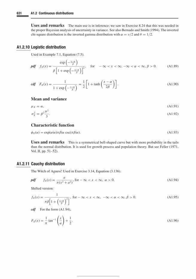
631 A1.2 Continuous distributions
Uses and remarks The main use is in inference; we saw in Exercise 8.24 that this was needed inthe proper Bayesian analysis of uncertainty in variance. See also Bernado and Smith (1994). The invertedchi-square distribution is the inverted gamma distribution with α = ν/2 and θ = 1/2.
A1.2.10 Logistic distribution
Used in Example 7.1, Equation (7.5).
pdf fX (x) =exp
(− x−α
β
)
β[1 + exp
(− x−α
β
)]2 , for − ∞ < x < ∞, −∞ < α < ∞, β > 0. (A1.89)
cdf FX (x) = 1
1 + exp(− x−α
β
) = 1
2
[1 + tanh
(x − α
2β
)]. (A1.90)
Mean and variance
µX = α, (A1.91)
σ 2X = β2 π2
3. (A1.92)
Characteristic function
φX (u) = exp(αiu)πβiu csc(πβiu). (A1.93)
Uses and remarks This is a symmetrical bell-shaped curve but with more probability in the tailsthan the normal distribution. It is used for growth process and population theory. But see Feller (1971,Vol. II, pp. 51–52).
A1.2.11 Cauchy distribution
The Witch of Agnesi! Used in Exercise 3.14, Equation (3.136).
pdf fX (x) = a
π (x2 + a2), for − ∞ < x < ∞, α > 0. (A1.94)
Shifted version:
fX (x) = 1
πβ[1 +
(x−α
β
)2] , for − ∞ < x < ∞, −∞ < α < ∞, β > 0. (A1.95)
cdf For the form (A1.94),
FX (x) = 1
πtan−1
(x
a
)+ 1
2. (A1.96)

632 Appendix 1 Common probability distributions
Mean and variance Moments do not exist. By symmetry, µX = α for form (A1.95). Integrationshows σX = ∞ (Exercise 3.14).
The mode and median are α. (A1.97)
Characteristic function
For form (A1.95), φX (u) = exp(iuα − | u | β). (A1.98)
Uses and remarks This distribution can be derived by transformation of a random quantity.Consider a light ray projected on a wall. If the angle describing the direction of the ray is uniform in(−π/2, π/2), the position where the ray intersects the wall is given by a Cauchy distribution; see Feller(1971) and Tribus (1969). It is a symmetrical bell-shaped distribution with fat tails, as compared tothe normal distribution. It has rather pathological aspects, such as infinite variance. It is closed underconvolution; the sum of n iid Cauchy random quantities has the same distribution as any of the members!See Feller (1971, p. 51). Also found by putting v = 1 in student’s t-distribution.
A1.2.12 Pareto distribution
See also Exercise 3.15 and Equation (3.137).
pdf fX (x) = ktk
xk+1for x ≥ t ; = 0 for x < t, k > 0. (A1.99)
cdf FX (x) = 1 −(
t
x
)k
. (A1.100)
Mean and variance
µX = kt
k − 1, k > 1, (A1.101)
σ 2X = kt2
(k − 1)2(k − 2), k > 2. (A1.102)
The mode is at t . (A1.103)
The median is t(2)1k . (A1.104)
Uses and remarks Has been used for distribution of incomes above a threshhold. It has rather fattails.
A1.2.13 Normal distribution
Introduced in Section 3.3.3; see Equation (3.25). Also in Chapter 6 as maximum entropy distribution,and in Chapter 7 in the Central Limit Theorem.
pdf fX (x) = 1√2πσ
exp −1
2
(x − µ
σ
)2
, σ > 0. (A1.105)

633 A1.2 Continuous distributions
Mean and variance
µX = µ, (A1.106)
σ 2X = σ 2. (A1.107)
Characteristic function For the standard form
fZ (z) = (1/√
2π ) exp(−z2/2), (A1.108)
the c f is given by (7.109)
φZ (u) = exp
(−u2
2
). (A1.109)
Uses and remarks This is widely used in many applications. The ‘model of sums’, in modellingerrors of measurements, and other quantities that are the sum of many others.
A1.2.14 Lognormal distribution
If a random quantity X = ln Y is normally distributed (µ, σ 2), then Y is said to be lognormally distributed(µ, σ 2).
pdf fY (y) = 1
σ√
2πy−1 exp
[− (lny − µ)2
2σ 2
], for y > 0. (A1.110)
Mean and variance Let a = exp µ, b = exp(σ 2):
µ = a√
b = exp
(µ + σ 2
2
), (A1.111)
σ 2Y = a2b(b − 1) = exp(2µ + σ 2)[exp(σ 2) − 1]. (A1.112)
The mode is at
exp(µ − σ 2). (A1.113)
The median is at
exp µ. (A1.114)
Uses and remarks Model of products, analogously to the normal distribution as the model ofsums. Often used for resistance of structural components.
A1.2.15 Student’s t-distribution
Used in the expression (8.111) and in similar situations.
pdf fX (x) =�
(v+1
2
)
�(
v
2
)√vπ
(1 + x2
v
)− 12 (v+1)
(A1.115)
= 1√
vB(
12 , v
2
)(
1 + x2
v
)− 12 (v+1)
. (A1.116)

634 Appendix 1 Common probability distributions
The parameter v is termed the degress of freedom.
Mean and variance
µX = 0 for v > 1, (A1.117)
σ 2X = v
v − 2. (A1.118)
Uses and remarks This is widely used in inference regarding means where the variance is alsouncertain.
A1.2.16 F-distribution
Used in Section 8.7.6 under ‘Common classical inference problems’; also Section 11.3.3 and Exercise11.13.
pdf fX (x) =(
v1v2
) v12
x (v1−2)
B(
v12 ,
v22
)(
1 + v1
v2x
)(v1+v2)/2
for B > 0, v1, v2 = 1, 2, . . . (A1.119)
The parameters v1 and v2 are the degress of freedom for the numerator and denominator respectively.
Mean and variance
µX = v2
v2 − 2, v2 > 2, (A1.120)
σ 2X = 2v2
2(v1 + v2 − 2)
v1(v2 − 2)2(v2 − 4), v2 > 4. (A1.121)
A1.2.17 Extremal – Gumbel
Also known as the extreme value type I, or the double-exponential distribution. (Note that the Laplacedistribution also has this name.) For maxima, see Equation (7.13) and Chapter 9. The following is formaxima.
pdf fZ (z) = 1
bexp
[− exp
(− z − a
b
)− z − a
b
]for −∞ < z < +∞, b > 0. (A1.122)
cdf FZ (z) = exp
[− exp
(− z − a
b
)]. (A1.123)
Mean and variance
µZ = a + bγ, where γ is the Euler constant = 0.5772 . . . , (A1.124)
σ 2Z = π 2b2
6. (A1.125)
The mode is at a. (A1.126)
The median is at a − b ln(ln 2). (A1.127)

635 A1.2 Continuous distributions
Characteristic function
exp(iau)�(1 − ibu). (A1.128)
Uses and remarks This is used extensively in extremal analysis, and is the most fundamental ofthe limiting extremal distributions. See the limit theorem in Chapter 9.
A1.2.18 Extremal – Frechet
Also known as the extreme value type II distribution. See Equations (9.78) and (9.115). The following isfor maxima.
pdf fZ (z) = α
bn
(z − an
bn
)−α−1
exp
[−
(z − an
bn
)−α], for α > 0 and − ∞ < z < ∞. (A1.129)
cdf FZ (z) = exp
[−
(z − an
bn
)−α], for α > 0 and − ∞ < z < ∞. (A1.130)
Mean and variance
µZ = an + bn�
(1 − 1
α
)for α > 1, (A1.131)
σ 2Z = b2
n
[�
(1 − 2
α
)− �2
(1 − 1
α
)]for α > 2. (A1.132)
The median is an + bn(ln 2)−1α . (A1.133)
Uses and remarks This is used in analysis of extremes. It is derived from pathological parentsand has fat tails.
A1.2.19 Extremal – Weibull
Introduced in Equation (9.79) and used in Section 9.7 for weakest-link theories. See also (9.119). Thisis given here for minima; the maximum is given in Equation (9.116).
pdf fW (w) = α
bn
(w − a
bn
)α−1
exp
[−
(w − a
bn
)α]for a ≤ w < ∞, α > 0, bn > 0. (A1.134)
Generally a is a physical limit.
cdf FW (w) = 1 − exp
[−
(w − a
bn
)α], for a ≤ w < ∞. (A1.135)
Mean and variance
µW = a + bn�
(1 + 1
α
), (A1.136)
σ 2W = b2
n
[�
(1 + 2
α
)− �2
(1 + 1
α
)]. (A1.137)

636 Appendix 1 Common probability distributions
Mode a + bn
(α − 1
α
) 1α
for α > 1. (A1.138)
Median an + bn(ln 2)1α . (A1.139)
Uses and remarks Used extensively in extremal analysis where there is a natural maximum orminimum value, for example a minimum strength.
A1.2.20 Two-dimensional normal distribution
pdf fX,Y (x, y) = 1
2πσ1σ2
√1 − ρ2
exp −{
1
2(1 − ρ2)
×[
(x − µX )2
σ 2X
− 2ρ(x − µX )(y − µY )
σXσY+ (y − µY )2
σ 2Y
]}. (A1.140)
Uses and remarks Basic form with two random quantities. See also Example 7.9 and (7.69).
A1.2.21 Multidimensional normal distribution
See Example 7.9, Equations (7.68) and (7.69).
fY(y) = 1
(2π )(n/2)| |−1/2 exp
[−1
2(y − µ)T [ ]−1(y − µ)
]. (A1.141)
The matrix [ ] is the covariance matrix
[ ] =
σ 21 ρ12σ1σ2 · · · ρ1 jσ1σ j · · · ρ1nσ1σn
ρ21σ2σ1 σ 22 · · · ρ2 jσ2σ j · · · ρ2nσ2σn
......
......
ρi1σiσ1 ρi2σiσ2 · · · ρi jσiσ j · · · ρinσiσn
......
......
ρn1σnσ1 ρn2σnσ2 · · · ρnjσnσ j · · · σ 2n
, (A1.142)
where the σ s are the standard deviations and the ρs are the correlation coefficients.

Appendix 2 Mathematical aspects
A2.1 Stieltjes integrals
These integrals provide a neat way to consider integrations and sums under a single umbrella.
We consider generally integrals of the kind∫ b
ag(x) fX (x)dx . We write this as
∫h(x)dx for
the time being, with h(x) = g(x) fX (x). The definition of the Riemann integral,
∫ b
ah(x)dx, (A2.1)
will be given for a bounded function h(·), in the range a ≤ x ≤ b, say. This range is dividedinto a set of division points
a = x0 < x1 < x2 < x3 < · · · < xn = b. (A2.2)
Two bounds on the integral are formed. These are named after the French mathematician GastonDarboux. For every interval [xi−1, xi ] let Mi and mi denote the maximum and minimum valueof h(·) in the interval. Then the following two (upper and lower) Darboux sums constitute anupper and lower bound to the integral:∑n
i=1Mi (xi − xi−1),
∑n
i=1mi (xi − xi−1). (A2.3)
The length of the largest subinterval is denoted δ; when this becomes smaller, the number ofsubintervals becomes larger. The upper Darboux sum will decrease or stay unchanged in value;conversely the lower sum will increase or stay the same. The function h(x) has a Riemannintegral if the two sums converge to the same value.
In order to include ‘jumps’ in the function h(x) = g(x) fX (x), corresponding in the presentcase to the ‘spikes’ in a pmf, a weight function in the Darboux sums is included. This is simplythe cdf FX (x), so that the function [FX (xi ) − FX (xi−1)] is considered in each Darboux sum asfollows:∑n
i=1M ′
i [FX (xi ) − FX (xi−1)],∑n
i=1m ′
i [FX (xi ) − FX (xi−1)], (A2.4)
where M ′i and m ′
i are the maximum and minimum, respectively, of g(x) in the interval [xi−1, xi ].
637

638 Appendix 2 Mathematical aspects
In the limit when the largest subinterval δ tends to zero, the integral is written as∫ b
ag(x)dFX (x). (A2.5)
This integral is termed the Stieltjes integral and includes ‘jumps’ in FX (x) because ofthe manner in which the Darboux sums are derived. It therefore combines summations andintegrals into one expression. It should be noted that if FX (x) is differentiable, and sincefX (x) = dFX (x)/dx , then Equation (A2.5) becomes∫
g(x) fX (x)dx .
The Riemann integral is therefore a special case of the Stieltjes integral.An example of the use of Stieltjes integrals, which is very close to the present application,
is the calculation of the moments of a group of particles, or ‘point masses’. Considering themoment of inertia of n particles,
I =∑n
i=1µi x
2i ; (A2.6)
where µi is the i th mass and xi is the distance from axis under consideration. If the particlesare small and numerous, we may wish to use expressions of the kind
I =∫
ρ(x)x2dx, (A2.7)
where ρ(x) is the mass per unit distance x . Expressions (A2.6) and (A2.7) can be combinedin the Stieltjes integral
I =∫
x2dµ(x), (A2.8)
where dµ(x) = ρ(x)dx in the continuous case and corresponds to the jumps µi for concentratedmasses. Stieltjes integrals have widespread application in engineering and contain a convenientshorthand notation, as illustrated above.
A2.1.1 Dirac delta and Heaviside step functions
These are commonly used in electrical circuit analysis, viscoelastic theory, and in other areasof engineering and physics, and provide an alternative way of considering ‘jumps’ in functions.The unit step function is defined by the two equations:
�(x) = 0 for x < 0,
�(x) = 1 for x ≥ 0. (A2.9)
This function is illustrated in Figure A2.1(a), in which a small interval τ is shown to the left of

639 A2.1 Stieltjes integrals
dd
∆t
Figure A2.1 Jumps and spikes
the origin t = 0. The definition of Equations (A2.9) can be conceived as a limit of the functionof Figure A2.1(a) with τ → 0.
The derivative of the unit step function is a highly singular function called the Dirac deltafunction, defined by the following conditions:
δ(t) = 0 for t �= 0δ(t) = ∞ for t = 0∫ ∞
−∞δ(t)dt =
∫ 0+
0−δ(t)dt = 1.
(A2.10)
This function is illustrated in Figure A2.1(b); in the limit as τ → 0 the Dirac function becomesa ‘spike’ of mass unity at the origin. (As pointed out by Butkov (1968), a more correct formfor the definition of δ(t) should be based on delta sequences which give the same shiftingproperty.)
Probability distributions such as the one illustrated in Figure 3.10 can be written as
fX (x) = (1 − p)δ(x) + gX (x) (A2.11)

640 Appendix 2 Mathematical aspects
in the case where X = random quantity, p = probability mass at x = 0, and gX (x) = distri-
bution of probability for x > 0, with∫
x>0gX (x)dx = 1 − p, for coherence.
We could denote a set of probability masses p1, p2, p3, . . . at x = x1, x = x2, x = x3, . . .
by means of the function
fX (x) = p1δ(x − x1) + p2δ(x − x2) + p3δ(x − x3) + · · · , (A2.12)
with cumulative distribution function
FX (x) = p1�(x − x1) + p2�(x − x2) + p3�(x − x3) + · · · (A2.13)
The insertion of (x − xi ) as the argument in δ(·) and �(·) shifts the ‘spike’ or ‘jump’respectively to x = xi . We see that Equations (A2.12) and (A2.13) can be used to include‘spikes’ and ‘jumps’.
A2.2 Integration
The engineer, scientist or economist working on a practical problem will not be concernedwith special sets such as Cantor’s, or the cardinality of the continuum (although he might,as in the case of the writer, be interested in these subjects). We take the approach here thatmathematics should conform itself to the needs of the practical problem at hand; de Finetti(1972) has made detailed studies of the mathematical implications of various assumptions.His analysis goes much further than our needs here. In short, there is a question of the kindof integral to be used in dealing with certain kinds of situations. For example, if we define adensity on the space [0, 1] such that it takes certain values on the rational numbers, a countablyinfinite set, with other values on the irrationals, which have the cardinality of the continuum,special techniques have to be used for the integration of such a function. Feller (1971, p. 34)shows (as one would expect) that the set of all rationals have a probability of zero, if theprobability is distributed over all numbers. The way around the problem of ‘different valueson the rationals and the irrationals’ is the use of Borel sets and Lebesgue integration. Thusthe probability associated with a set A is associated with the Lebesgue measure of the set A.
This requires the acceptance of complete (or σ -) additivity, i.e. one allows a countably infinitenumber of intersections and unions of sets, rather than a finite number. This point has causedsome controversy amongst mathematicians, with de Finetti opposing σ -additivity as an axiom.For example, he cites the case of an infinite number of possibilities, such as the set of integers.One is chosen ‘at random’, say X , and therefore Pr(X = 1, 2, 3, . . . or any other integer) = 0.
The sum of these values is also zero, yet the probability of the union, the certain event that oneof the numbers occur, is unity. In this case, σ -additivity does not hold. Details of the argumentscan be found in de Finetti (1972, and 1974, Vol. II – especially the appendix in the latter,Section 18).

641 A2.3 Lewis Carroll’s problem
The view is taken here that in studying practical problems requiring integration, one neverencounters ‘pathological’ cases such as the one where a density is defined differently on therationals and on the irrational numbers. We therefore consider Lebesgue integration to beinteresting but by no means necessary for the study of probability theory. Indeed, de Finetti,while excluding σ -additivity as an axiom, states (de Finetti, 1972, p. 105) that one mightnevertheless ‘be interested in studying those particular distributions which happen to be com-pletely additive on some domain’. This is quite enough for our purposes, and we can thereforestudy distributions that include an infinite number of possibilities, a simple example being thePoisson distribution.
We have dealt with Stieltjes integrals above as they have the attractive possibility of unifyingthe treatment of discrete and continuous random quantities.
A2.3 Solution to Lewis Carroll’s problem and discussion
The answer to the problem as given by Charles Dodgson goes along the following lines. Therod is divided into (n + 1) parts, where n is odd. These n points are considered to be the onlypossible division points, that is, the division points are the only points at which the rod willbreak. If n = 5, then there are six intervals, and we are considering the probability that therod will break at the central one of these. The probability in five trials of breaks at the outer
points, other than the centre, is (4/5)5; and at the centre the probability is then[1 − (
45
)5]. It
is assumed in this that the number of rods tested is equal to n, the number of possible divisionpoints. The probability of a central break is
pc = 1 −(
1 − 1
n
)n
, (A2.14)
which tends to (1 − 1/e) = 0.6321 . . . as n tends to infinity. (We have assumed inde-pendence with regard to the probabilities of successive breaks in the outer and centralregions.)
The first point of discussion is the linking of the number of rods to the number of di-vision points. Had we tested 2n, 3n, . . . rods each with n division points, we would haveobtained(
1 − 1
e2
),
(1 − 1
e3
), . . . (A2.15)
If we understand the question to mean that we wish to find the probability of one of the infinityof rods failing at exactly x = 1/2, we should first decide on what we mean by ‘infinity’. Letus continue to assume that it means a countably infinite number of rods, that is, correspondingto the integers {1, 2, 3, . . .} . If the possible locations of a break correspond to all the numbers,rational and irrational, then the probability of a break at x = 1/2 reduces to zero. In reality,

642 Appendix 2 Mathematical aspects
a break, however clean, will correspond to a certain interval. A proper definition of ‘whatis possible’ should be made at the outset in any study. This would likely lead to a finiteset corresponding to certain defined intervals; if there are m possible points, for our ‘equallyfrangible rod’ the probability of a break in a particular one of these is 1/m, similar to Dodgson’sassumption.

Appendix 3 Answers and commentson exercises
Chapter 2
2.1 5/6.2.2 3/7.2.3 1:2 on.2.4 Sum of qs is 49/40 – incoherent.2.5 Sum = 1.50 – incoherent; $50; 29:1, 14:1, 1:1, 13:2, all against.2.6 See de Finetti (1937).2.12 E1 ∨ E2 ∨ E3 = E1 + E2 + E3 − E1 E2 − E1 E3 − E2 E3 + E1 E2 E3.2.13 (b) A ∩ B, 1. (c) B ∩ C = C . (d) B ∪ C = B. (e) A ∩ C = ∅. (f) A ∩ B ∩ C = {1, 9}.Note that ‘1’ is not prime because it does not have exactly two factors.2.14 (a) 0.53. (b) 0.47. (c) 0.63. (d) 0.37. (e) 0.10.2.15 (a) 0.9966. (b) 0.0006. (c) 0.0001.2.16 Pr(E1) + 2Pr(E1 E2) + Pr(E3) = 1.2.17 0.096.2.18 (a) 2/5 for θ1. (b) 1. (c) 32/35.2.20 Probability of guilt is very high since the evidence comprises an independent series ofallegations.2.21 Yes, odds change to 2:1 on the other closed door (Bayes).2.22 Pr(T |L) = (pt)/(pt + q t), etc.2.23 Probability of correctly positioned landing gear given light off is 1/1001.001 � 0.001.
Poor system.2.24 36/43, 6/43, 1/43.2.25 (a) +2, +1, 0. (b) 9/50.2.26 Pr(S|I = 0) = 0.989, 0.007, 0.004; Pr(S|I = 1) = 0.784, 0.199, 0.017, etc.2.27 (a) 92%. (b) 0.583, 0.942.2.28 0.9604, 0.9996.2.29 An offshore rig has failed due to two possible causes: earthquake or hurricane. A seismicstation nearby indicates earthquake unlikely. Then the probability of a hurricane increases.2.30 (a) 63. (b) 70.2.31 1/2.
643

644 Answers and comments on exercises
2.32 1/4, 5040.2.33 (a) 0.3182. (b) 0.4273. (c) 0.5091. (e) a = b.2.35 (a) 50 400. (b) 16 627:33 � 504:1.2.36 See Feller (1968) and Blom et al. (1994).2.38 0.031 03 . . .
Chapter 3
3.1 (a) k = 1/10. (c) 0.7.3.2 k = 3/2, 2, 2; probabilities = 0.3125, 0.0677 (4 dp), 1/2.3.3 fT (t) = 2 (t − 1) , 1 ≤ t ≤ 2; 0.25.3.4 (a) 0.40. (b) 0.006 046 . . . (c) 0.0256. (d) 0.000 796 . . . (e) 0.1663. (f) 17.5 s.3.5 (a) Hypergeometric, can be approximated by binomial. (b) 0.4095 . . . , 0.4042 . . . (exact).(c) 0.008 56. (d) Approximate 0.45, exact 0.4459 (4 dp).3.6 See de Finetti (1974).3.7 (a) Exponential. (b) Same exponential, shifted by τ . (c) 0.699, 0.0907 (3 sf). (d) 0.950(3 sf).3.8 (a) 1.67, 1.292 (3 dp). (b) 0.188 (3 dp). (c) 3.327 (3 dp).3.9 7.52 ×10⁻⁷ (odds of less than one in a million).3.10 Model as a Poisson process with rate 10 exp(−x/2), 0.6077 (4 dp).3.11 (a) 0.0618. (b) 0.6739. (c) 0.2643. (d) Assume independence, use multinomial, 0.00170.3.12 (a) 241.2. (b) 0.04875. (c) 0.049375 � 5%.3.13 1, 1, 1; 3/8, 19/320, 0.2437.3.14 a/π, 1
πtan−1
(xa
) + 12 , 2a, 0, ∞.
3.15 (a) k > n. (b) k > 2,(kt2
)/[(k − 1)2 (k − 2)
].
3.17 π(µ2
R + σ 2R
).
3.18 (a) 4/25. (b) 1/5. (c) 1/2. (d) 21/50. (e) 0.3.19 1 − (1 − τ/t)2.3.20 (a) 69.5/242 = 0.1207 (4 dp). (b) 5/9.3.21 (a) 0.00124 (3 sf). (b) 88%, 558.3.22 2.3.23 (a) pX (x): 8/27, 4/9, 2/9, 1/27, pY (y): 1/9, 2/3, 2/9. (b) pX |Y (x, y) for y = 1: 2/3, 0,
0, 1/3, y = 2: 1/3, 1/3, 1/3, 0, y = 3: 0, 1, 0, 0; pY |X (x, y) for x = 0: 1/4, 3/4, 0, x = 1: 0,
1/2, 1/2, x = 2: 0, 1, 0, x = 3: 1, 0, 0; pY |X=0 (y): 1/4, 3/4, 0. (c) 19/9,√
2/3,√
234/27 �0.567, 19/9. (d) σX,Y = 0. (e) No. In addition to σX,Y = 0 we need pX,Y (x, y) = pX (x) ·pY (y) . This is found not to be true.3.24 By integration, fX (x) = 2 exp (−2x) ; fY (y) = 2 exp (−y)
[1 − exp (−y)
]; fX,Y (x, y)
�= fX (x) · fY (y) ; X, Y are not independent.3.25 Proof in standard texts; ρXY = 0 implies absence of a linear relationship.3.26 EMV for proposed option is 30.40 – greater than the others and therefore optimal.

645 Appendix 3
3.27 5 units is optimal (1% growth) on assumption that 5 or 10 units are added if necessary;EMVs are −4.83, −4.86 and −5.08.3.28 (a) It is optimal to test, accept if result is positive, reject if negative. EMV = 8.22.3.29 Pr(Y |R) = 0.792, 0.151, 0.057, for R = 1; 0.152, 0.810, 0.038, for R = 2; 0.088,0.118,
0.794, for R = 3. Optimal decision {e0, 75 m}.3.30 {e0, R} is optimal; EMVs 6.89 vs. 7.45.3.31 There will be a spike of probability equal to 0.1587 at 75 kmh−1.
3.32 There will only be one value of each expected value, e.g. the 〈Xh Xi 〉 will be the same foreach h and i.3.34 fT (t) = 0.004 t2 exp (−0.2t).3.35 (a) First row: 5/8, 1/8, 1/8; second row: 3/8, 1/2, 1/2; third row: 0, 3/8, 3/8. (b) 1/4,15/32, 9/32. (c) 1, 0, 0; 5/8, 3/8, 0; 7/16, 27/64, 9/64.3.36 (a) 1
2
⟨A2
⟩cos (ωt). (b)
∑σ 2
h cos (ωht) .
Chapter 4
4.1 Alternative 1, benefits: 31.5 × 10⁶, costs: 28.2 × 10⁶, ratio: 1.12. Alternative 2, benefits:34.5 × 10⁶, costs: 37.1 × 10⁶, ratio: 0.93. (b) Use of subjective judgement, reduction to equiv-alent dollar values, ordinal scales plus judgement, interval/ratio scales and utility. (c) Veryarbitrary. No risk aversion. Interest rates used can be arbitrary and give a variety of solutions.4.2 Scenario 1, NPW = 130, scenario 2, NPW = 7 (in millions), EMV = 105.4.4.3 Maximin, A; maximax, C; Hurwicz, C; Regret, B or C. Utility dominance occurs if all theutilities are greater than or equal to those for another, e.g. B ≥ D (strict dominance use > not≥).4.4 EMV of α1 is optimal ($24 000).4.6 If 35 000 m3 is accepted as certainty equivalent of 〈0, 50 000〉, one obtains a = 0.036, b =0.198, c = 6.05.4.7 Decibel scale is risk-prone.4.8 γ (x) = 1/ (x + b) might be more appropriate for money than constant aversion in expo-nential function.4.9 γ (x) = 2a/ (−2ax + b); increasing risk aversion.4.10 See Keeney and Raiffa (1976).4.12 σ1 = {e0, α1}, σ2 = {e0, α2}, σ3 = {e1, α1 if R, α1 if P} , σ4 = {e1, α1 if R, α2 if P} ,
σ5 = {e1, α2 if R, α1 if P}, σ6 = {e2, α1 if R, α2 if P} ; σ1 optimal if Pr(θ2) is in the range0 to 0.49, σ5 if in 0.49 to 0.65, σ1 if in 0.65 to 1.00.4.13 {e0, do not build}.4.14 (a) σ1 = {e0, α1} , σ2 = {e0, α2} , σ3 = {e1, α1 if Y = 0.2, α1 if Y = 0.4, α1 if Y = 0.6} ,
σ4 = {e1, α2 if Y = 0.2, α1 if Y = 0.4, α1 if Y = 0.6} , σ5 = {e1, α1 · · · , α2 · · · , α1 · · ·} ,
σ6 = {e1, α1 · · · , α1 · · · , α2 · · ·}, σ7 = {e1, α2 · · · , α2 · · · , α1 · · ·},σ8 = {e1, α2 · · · , α1 · · · , α2 · · ·}, σ9 = {e1, α1 · · · , α2 · · · , α2 · · ·},

646 Answers and comments on exercises
σ10 = {e1, α2 · · · , α2 · · · , α2 · · ·} ; σ2 is optimal. (b) σ2, σ1, σ7, σ7. (c) σ1 optimal if Pr(M = 0.2)is in the range 0 to 0.33, σ7 if in 0.33 to 0.70, σ2 if in 0.70 to 1.00.4.15 (b) accept, 〈U 〉 = 9.35. (c) reject, 〈U 〉 = −38.6. (d) σ1 = {
P–accept,P–accept}, σ2 ={
P–accept,P–reject}, σ3 = {
P–reject,P–accept}, σ4 = {
P–reject,P–reject}
; σ1 is optimalfor Pr(S) > 0.94, σ2 for 0.54–0.94, σ4 for < 0.54.4.16 For example, a plane through three points in 3D can be written in determinantal form,and then expanded in terms of the three variables, say in the first row. The direction cosinesare given by the coefficients of these variables divided by the square root of the sums of thecoefficients squared.4.17 The probability that A wins is pA/ [1 − (1 − pA) (1 − pB) (1 − pC )] . The fairest way ispA : (1 − pA) · pB : (1 − pA) · (1 − pB) · pC . (a) A: $108, B: $90, C: $75 (b) A: $20, B: $40,C: $36.
Chapter 5
5.2 x1 = b/3 = x2, x3 = b/6, V = b3/54.5.3 r = 3
√v/2π, = 2 3
√v/2π .
5.4 See Chapter 6.5.5 There are four stationary points: x1 = 1.00, x2 = x3 = 0, z = 3.00 (max); x1 = −1.00,x2 = x3 = 0, z = −1.00 (saddle point); x1 = −0.50, x2 = 0.87, x3 = 0, z = −1.50 (min);x1 = −0.50, x2 = −0.87, x3 = 0, z = −1.50 (min).5.6 x1 = 4, x2 = 1, x3 = x4 = 0, x5 = 11, z∗ = −36.5.7 x1 = 0, x2 = −13, x3 = −8, x4 = 0, x5 = 0, x6 = 19, x7 = 0, x8 = 36,
(z′)∗ = 54, z∗ =
−54.5.8 Solution is unbounded.5.9 x1 = 4, x2 = 10/3, x3 = 2, z∗ = −34/3.5.11 (a) F1 = 60, F2 = 200, F3 = 90,
(z′)∗ = 350. (b) A = 720 N, B = 300 N, C = 0 N;
another optimal solution: A = 620, B = 250, C = 150.5.14 (a) x1 = 2, x2 = 1, x3 = x4 = 0, x5 = 2,
(z′)∗ = 4. (b) Min (5y1 + 3y2 + 4y3) s.t. 2y1 +
y2 ≥ 1.5; y1 + y2 + 2y3 ≥ 1.0. (c) y3 = 0, y1 = 0.5, y2 = 0.5, w∗ = 4.5.15 (a) Min cost: Min (100x1 − 100x2); Min mass: Min (x1 + 0.20x2) s.t. x1 + x2 = 200, x1 ≤160, x2 ≤ 120; compatible objectives at x1 = 80, x2 = 120, z∗
1 = −$4000, z∗2 = 56 tonnes.
5.16 Saddle point at {σ3, τ2} ; value = 6.5.17 No saddle point. Strategy for A: {σ1, 1/2; σ2, 1/2} ; for B: {τ1, 2/3; τ2, 1/3} ; value = 0.5.18 No saddle point. Strategy for A: {σ1, 2/3; σ2, 1/3} ;for B: {τ1, 1/3; τ2, 2/3; τ3, 0; τ4, 0; τ5, 0} ; value = 5/3.5.19 No saddle point; solution {1/3, 1/3, 1/3} for each player.5.20 (a) Pr(σ1): 1 to 5/7, τ3 is optimal; 5/7 to 1/3, τ2; 1/3 to 0, τ4; τ1 never optimal. (c){5/7, 2/7} ; value = 17/7.

647 Appendix 3
Chapter 6
6.2 p = 1/2. Max entropy solution corresponds to Equation (6.85) which has a very sharppeak for large N .6.3 Combine Equations (6.31), (6.35) and (6.36) to obtain a quadratic in exp (−λ1). Solve forvarious µ and plot.6.4 See Jaynes (2003) and Kapur and Kesavan (1992). Positive definiteness implies convexity.6.5 pi = exp λ0; λ0 = ln n, where n = number of possibilities.6.6 Fix 〈X〉 , 〈ln X〉 for gamma. Fix 〈ln X〉 , 〈ln (1 − X )〉 for beta. See Tribus (1969) and Kapurand Kesavan (1992).6.7 See Kapur and Kesavan (1992).6.10 See Jaynes (1963a).6.12, 6.13 Follow procedure in Section 6.9.6.15 Derive the Maxwell–Boltzmann (classical) distribution of energies. Then calculate theprobability of surmounting an energy barrier of magnitude εA.
Chapter 7
7.2 y = g (x) = exp (−y) ; use to generate realizations of the exponential distribution.7.3 fY (y) = kyk−1 exp
(−yk).
7.4 fY (y) = 2yµ
exp(− y2
µ
).
7.5 y = x−ab−a .
7.7 fZ (z) = 3[1 − 1
t ln(
zc
)]2for c < z < c exp t .
7.8 fY (y) = 13 on transformed parallelogram. Affine because parallelism is preserved.
7.9 fY (y) = y exp (−y) , y > 0.
7.11 fR (r ) = r exp(− r2
2
), f� (θ ) = 1
2π.
7.12 See Feller (1971).7.14 fP (p) = [
pα1−1 (1 − p)α2−1]/B (α1, α2).
7.15 (a) [pt + (1 − p)]n . (b) [r t + (1 − p)]n1+n2 .7.18 See Feller (1971).7.19 1/
(1 + u2
).
7.20 exp (−a |u|).7.21 0.8413 . . . , 0.4214 . . .7.25 See Johnson et al. (1994); Feller (1971).7.27 (a) 0.1715, binomial 0.1789. (b) 0.9722, binomial 0.9753.7.28 exp
{− 12 uT [ ] u + iuT µ
}.
7.29 (a) Total time in telephone calls or electronic messages – number and length of each israndom. (c)
∑∞n=0
exp(−µ)µn
n! · exp[νn (exp t − 1)
]; 〈Y 〉 = µν; σ 2
Y = µν (1 + ν).

648 Answers and comments on exercises
7.30 0.0015 (4 dp).7.31 See de Finetti (1974, vol. 2), Feller (1971).7.32 See de Finetti (1974, vol. 1), Papoulis (1965).
Chapter 8
8.1 Then result is the beta distribution; see Section 8.3.8.4 (a) µ f = 5.68, σ f = 0.0316 . . . (b) 5.60 < A < 5.76 with 99% probability (2 dp). (c)5.69 < A < 5.91 with 99% probability (2 dp). (d) 96.8.6 We have to consider both σ and σ f .
8.10 (a) Take the first moment. (b) Use the parallel axis theorem.
8.11 2−( ν2 + 1
2 )√ nπ
(νσ 2
) ν2 1
�( ν2 ) .
8.15 (a) Posterior mean = 0.518, variance = 0.0239, s.d. = 0.155.8.17 f� (λ) ∝ 1/λ; one observation in specified period; maximum entropy subject to mean λ
known.8.18 (a) c2/ [(c1 − c3) n]. (d) If the utility is linear with money over the range considered.8.20 0.030, 0.064 (2 sf).8.24 See Lindley (1965, vol. 2), Box and Tiao (1973), Bernardo and Smith (1994).8.28 (a) Yes. z = 3.99 . . . , z0.05 = 1.645. (b) t = 3.99, t0.05(4 sf) = 2.132.8.29 3209.8.30 Yes. Comparison of means with pooled sample variance. t = 1.986, t0.05,9 = 1.833.8.31 Test for equality of variances – OK. Compare means with pooled variance. z = −1.603,p-value (two-sided) = 0.110. Accept equal population means.8.32 Paired two-sample t-test. t = −6.92, t0.05,6 = 1.943. Accept difference.8.33 No. Test for difference in proportions.8.34 µ f = 5.50, σ f = 0.05345 . . . Distribution of Y is lognormal.
Chapter 9
9.8 7.596 (3 dp).
9.9 (a) 7.60. (b) z = an + bn[ln
( pne
n
)] 1α .
9.10 x = σ√2.
9.16 µ (x) = kxk−1.9.18 1, 0, 0; 0, 1/4, 0; 0, 0, 1/3.9.19 See Freudenthal (1968).
9.20 Torsion of cylindrical specimen: v∗v
=[
2α+1π (α+2)
]α(α+1); rectangular beam under point load:
v∗v
= 12(α+1)2 .
9.21 See Madsen et al. (1986).

649 Appendix 3
Chapter 10
10.2 The distribution of capacity should be updated.10.4 Let fT and fS be uniform in [a, b] , [c, d] . Then p f = [(b − c) (b + c − a)] /
[2 (b − a) (d − c)] .
10.5 0.027.10.6 The ratio of two chi-square distributions (divided by their d.f.) is an F-distribution. Usethe third of (10.2) to obtain the result.10.10 See Exercise 2.12.10.11 For n identical units, (nλ)−1 (series), and
∑(nλ)−1 (parallel).
10.12 0.9802 (4 dp).10.13 Use Poisson processes.
Chapter 11
11.3 x = 2841, s = 145.11.4 x = −1.515, s = 5.24.11.5 x = 11.00, s = 1.34, mode = 10.40.11.6 y = 3.751 + 0.8136x .11.8 Slope will be less than 1 : 1.11.10 y = 1.204x − 4.419.
11.11 For p = 15 Mpa, y = −9623.1x + 29.574; for p = 35 Mpa, y = −9432.9x +28.531; for p = 55 Mpa, y = −8839.5x + 26.209; for p = 65 Mpa, y = −11600x +37.223, for p = 70 Mpa, y = −15648x + 53.554.11.15 Given a number of ‘pegs’ as data points (xi , yc), the best-fit centre (xc, yc) andradius r can be found for the GBS. The error for each data point can be expressed asei =
√(xi − xc)2 + (yi − yc)2. Use partial derivatives and minimize ∂δe
∂xc, ∂δe
∂yc, and ∂δe
∂r , where
δe is the sum of the squares of errors,∑n
i=1 e2i .
11.26 0.057 (2 sf).

References
Aston, J. G. and Fritz, J. J. 1959. Thermodynamics and Statistical Thermodynamics. Wiley.Baker, M. J. 1977. Rationalisation of Safety and Serviceability Factors in Structural Codes. CIRIA
(Construction Industry Research and Information Association), Report 63, London, England.Barlow, R. E., Fussell, J. B. and Singpurwalla, N. D. (eds.) 1975. Reliability and Fault Tree Analysis.
Society for Industrial and Applied Mathematics.Barnett, A. and Wang, A. 2000. Passenger-mortality risk estimates provide perspectives about airline
safety. Flight Safety Digest, 19, No. 4, April.Bayes, T. 1763. An essay towards solving a problem in the doctrine of chances. Phil. Trans. Royal Society
London. Series A53. Reproduced with biographical note by G. Barnard in Biometrika, 45 (1958).Bea, R. 1998. Human and organization factors in the safety of offshore structures. In Risk and Reliability
in Marine Technology, ed. C. Guedes Soares. Balkema, pp. 71–91.Benjamin, J. R. and Cornell, A. 1970. Probability, Statistics and Decision for Civil Engineers. McGraw-
Hill.Beer, F. P. and Johnston, E. R. 1981. Vector Mechanics for Engineers: Statics and Dynamics. McGraw-
Hill Ryerson.Bernardo, J. M., and Smith, A. F. M. 1994. Bayesian Theory. Wiley.Bernstein, P. L. 1996. Against the Gods: The Remarkable Story of Risk. Wiley.Beveridge, G. S. and Schechter, R. S. 1970. Optimization: Theory and Practice. McGraw-Hill.Billinton, R. and Allan, R. N. 1992. Reliability Evaluation of Engineering Systems, second edn. Plenum
Press.Blom, Gunnar 1958. Statistical Estimates and Transformed Beta-Variables. John Wiley and Almqvist
and Wiksell.Blom, Gunnar, Holst, Lars, and Sandell, Dennis 1994. Problems and Snapshots from the World of
Probability. Springer-Verlag.Boeing Commercial Airplanes Group 2000. Statistical Summary of Commercial Jet Airplane Accidents,
1959–1999. www.boeing.com/news/techissuesBolotin, V. V. 1969. Statistical Methods in Structural Mechanics. Holden-Day. (Translated from the
Russian by Samuel Aroni.)Box, G. E. P. and Tiao, G. C. 1973. Bayesian Inference in Statistical Analysis. Addison-Wesley.Bridgman, P. W. 1941. The Nature of Thermodynamics. Harvard University Press.— 1958. The Logic of Modern Physics. (First published 1927) Macmillan.Brillouin, L. 1962. Science and Information Theory. Academic Press.Butkov, E. 1968. Mathematical Physics. Addison-Wesley.Canadian Standards Association 1992. Reissued in revised form 2004. General Requirements, Design Cri-
teria, the Environment, and Loads. Standard CAN/CSA-S471-92. Part of Code for Offshore Structures.Carter, J. E., Frederking, R. M. W., Jordaan, I. J., Milne, W. J., Nessim, M. A. and Brown, P. W.
1992. Review and Verification of Proposals for the Arctic Shipping Pollution Prevention Regulations.
650

651 References
Memorial University of Newfoundland, Ocean Engineering Research Centre. Report prepared forCanadian Coast Guard, Arctic Ship Safety, Transport Canada Publication TP 11366E.
Cartwright, D. E. and Longuet-Higgins, M. S. 1956. The statistical distribution of the maxima of a randomfunction, Proc. Royal Society, A, 237.
Castillo, E. 1988. Extreme Value Theory in Engineering. Academic Press.Churchill, R. V. 1972. Operational Mathematics. McGraw-Hill.Chvatal, V. 1980. Linear Programming. W. H. Freeman.Cohen, M. H. 1961. The relative distribution of households and places of work – a discussion of the
paper by F. G. Wardrop. Proceedings of the Symposium on the Theory of Traffic Flow, ed. R. Herman.Elsevier, pp. 79–84.
Cohn, M. Z. and Maier, G. 1979 (eds.). Engineering Plasticity by Mathematical Programming. Proceed-ings of the NATO Advanced Study Institute, University of Waterloo, Canada, 1977. Pergamon.
Cornell, C. A. 1969a. Bayesian statistical decision theory and reliability-based structural design. Pro-ceedings, International Conference on Structural Safety and Reliability, Washington D.C.
— 1969b. A probability-based structural code. Journal of the American Concrete Institute. 66(12): 974–985.
Courant, R. and Robbins, H. 1941. What is Mathematics? (tenth printing, 1960) Oxford University Press.Cramer, H. 1951. Mathematical Methods of Statistics. Princeton University Press.Cullen, Hon. Lord 1990. The Public Inquiry into the Piper Alpha Disaster, The Department of Energy
(UK).Cunnane, C. 1978. Unbiased plotting positions – a review. Journal of Hydrology, 37, 205–222.D’Agostino, R. B. and Stephens, M. A. (eds.) 1986. Goodness-of-fit Techniques. Marcel Dekker.Dalal, S. R., Fowlkes, E. B. and Hoadley, B. 1989. Risk analysis of the space shuttle: pre-Challenger
prediction of failure. Journal of the American Statistical Association, 84(408): 945–957.Davenport, A. G. 1964. Note on the distribution of the largest value of a random function with application
to gust loading. Proceedings of the Institution of Civil Engineers, 28, 187–196.David, H. A. 1981. Order Statistics, second edition. Wiley.Dawkins, R. 1989. The Selfish Gene. Oxford.de Finetti, B. 1937. La prevision: ses lois logiques, ses sources subjectives. Annales de l’Institut Henri
Poincare, 7, 1–68. Translated in Kyberg, H. E. and Smokler, H. E. (eds.) 1964. Studies in SubjectiveProbability. Wiley.
— 1972. Probability, Induction and Statistics. Wiley.— 1974. Theory of Probability. Vols. 1 and 2, translated from Italian by Machi, A., and Smith, A. Wiley.— 1977. Probabilities of probabilities: a real problem or a misunderstanding? New Developments in the
Applications of Bayesian Methods, eds. A. Aykac and C. Brumat. North-Holland, pp. 1–10.DeGroot, M. H. 1970. Optimal Statistical Decisions. McGraw-Hill.DeGroot, M. H. and Schervish, M. J. 2002. Probability and Statistics, third edn. Addison Wesley.de Neufville, R. 1990. Applied Systems Analysis. McGraw-Hill.de Neufville, R. and Keeney, R. L. 1972. Use of decision analysis in airport development for Mexico
City. Analysis of Public Systems, eds. A. W. Drake, R. L. Keeney and P. M. Morse. MIT Press.Eatwell, J., Milgate, M. and Newman, P. 1990. The New Palgrave: Utility and Probability. MacMillan
Press, pp. 227–239.Eisberg, R. and Resnick, R. 1974. Quantum Physics of Atoms, Molecules, Solids, Nuclei, and Particles.
Wiley.Evans, I. G. and Nigm, A. M. 1980. Bayesian prediction for two-parameter Weibull lifetime models.
Communications in Statistics – Theory and Methods, A9(6), 649–658.Feller, W. 1968. An Introduction to Probability Theory and its Applications. I, third edn. Wiley.— 1971. An Introduction to Probability Theory and its Applications. II, second edn. Wiley.

652 References
Feynman, R. P. 1986. Personal observations on reliability of shuttle. Report to the President by thePresidential Commission on the Space Shuttle Challenger Accident, 2, Appendix F.
Finnie, B. W. and Johnston, I. H. A. 1990. The acceptance of software quality as a contributor to safety.In Safety and Reliability in the 90s. Proceedings of the Safety and Reliability Symposium, Elsevier,pp. 279–289.
Fisher, R. A. and Tippett, L. H. C. 1928. Limiting forms of the frequency distributions of the largest orsmallest member of a sample. Proc. Cambridge Philos. Soc. 24, 180–190.
Flint, A. R. and Baker, M. J. 1976. Risk analysis for offshore structures – the aims and methods. Designand Construction of Offshore Structures, Proceedings of the Conference. The Institution of CivilEngineers, London, 1977.
Frankenstein, G. E. 1959. Strength data on lake ice. CRREL Technical Report 59.— 1961. Strength data on lake ice. CRREL Technical Report 80.Fraser, D. A. S. 1976. Probability and Statistics: Theory and Applications. Duxbury Press (Wadsworth
Publishing).Frechet, M. 1927. Sur la loi de probabilite de l’ecart maximum. Ann. de la Societe Polonaise de
Mathematique. Cracow, 6:93.Freudenthal, A. M. 1968. Statistical approach to brittle fracture. In Fracture, ed. H. Liebowitz, vol. II,
pp. 591–619.Freudenthal, A. M., Garrelts, J. M. and Shinozuka, M. 1966. The analysis of structural safety. Journal of
the Structural Division, Proceedings of the American Society of Civil Engineers, 92(ST1): 267–325.Galambos, J. 1978. The Asymptotic Theory of Extreme Order Statistics. Wiley.German, J. G. and Sukselainen, J. 1985. M.V. Arctic Test Results and Analysis. Transport Canada Report
No. TP 6727E. Prepared for Coast Guard Northern, by German and Milne Inc., Ottawa, and TechnicalResearch Center of Finland, Helsinki.
Gnedenko, B. V. 1941. Limit theorems of the maximal term of a variational series. Comptes Rendus del’Academie des Sciences de l’URSS, 32, 7–9.
— 1943 Sur la distribution limite du terme maximum d’une serie aleatorie. Ann. Math. 44, 423–453.Goldsmith, James 1994. The Trap. Carroll and Graf.Good, I. J. 1950. Probability and the Weighing of Evidence. Hafner.— 1965. The Estimation of Probabilities. Research Monograph No. 30, MIT Press.Gopal, E. S. R. 1974. Statistical Mechanics and Properties of Matter. Ellis Horwood.Gow, A. J., Udea, H. T., Govoni, J. W. and Kalafut, J., 1988. Temperature and structure dependence of
the flexural strength and modulus of freshwater model ice. CRREL Report 88–6.Grayson, C. J. 1960. Decisions Under Uncertainty: Drilling Decisions by Oil and Gas Operators.
Harvard.Greub, W. 1975. Linear Algebra. Springer-Verlag.Gribble, J. N. and Preston, S. H. (eds.) 1993. The Epidemiological Transition: Policy and Planning
Implications for the Developing Countries. National Academy Press.Griffith, A. A. 1920. The phenomenon of rupture and flow in solids. Philosophical Transactions of the
Royal Society, A221, pp. 163–168.Gringorten, I. I. 1963. A plotting rule for extreme probability paper. Journal of Geophysical Research,
68, 3, 813–814.Gumbel, E. J. 1958. Statistics of Extremes. Columbia University Press.Hall, A. D. 1962. A Methodology for Systems Engineering. Van Nostrand.Hambly, E. C. and Hambly, E. A. 1994. Risk evaluation and realism. Proceedings, Institution of Civil
Engineers, Civil Engineering, 102, May: 64–71.Hammersley, J. M. and Handscomb, D. C. 1964. Monte Carlo Methods. Methuen.Heath, D. and Sudderth, W. 1976. De Finetti’s theorem on exchangeable variables. American Statistician,
30, No. 4, 188–189.

653 References
Hong, Han Ping. 1994a. A note on extremal analysis. Structural Safety. 13: 227–233.— 1994b. Estimate of extremal wind and wave loading and safety level of offshore structures. Risk An-
alysis, Proceedings of a Symposium, ed. A. S. Nowak. University of Michigan, Ann Arbor, Michigan.Hunt, R. A. and McCartney, L. N. 1979. A new approach to Weibull’s statistical theory of brittle fracture.
International Journal of Fracture, 15, 365–375.Jaynes, E. T. 1957. Information theory and statistical mechanics. Physics Review. 106, 620–630 and 108,
171–190.— 1963a. New engineering applications of information theory. Proceedings of the First Symposium on
Engineering Applications of Random Function Theory and Probability. Wiley.— 1963b. Information theory and statistical mechanics. In Statistical Physics, ed. K. W. Ford, W. A.
Benjamin. pp. 182–218.— 1976. Confidence intervals vs. Bayesian intervals. In Foundations of Probability Theory, Statistical
Inference, and Statistical Theories of Science, eds. W. L. Harper and C. A. Hooker. D. Reidel PublishingCompany. Also in Rosenkrantz (1983).
— 2003. Probability Theory: the Logic of Science, ed. G. Larry Bretthorst. Cambridge University Press.Jeffreys, H. 1961. Theory of Probability, third edn. Clarendon Press.Jensen, F. V. 1996. An Introduction to Bayesian Networks. UCL Press (also distributed by Springer).Jessop, A. 1990. Decision and Forecasting Models with Transport Applications. Ellis Horwood.Johnson, N. L., Kotz, S. and Kemp, A. W. 1993. Univariate Discrete Distributions. Wiley.Johnson, N. L., Kotz, S. and Balakrishnan, N. 1994. Continuous Univariate Distributions. Wiley.Jones, A. J. 1980. Game Theory: Mathematical Models of Conflict. Ellis Horwood.Jordaan, I. J. 1988. Safety levels and target probabilities implied in codes of practice. Civil Engineering
Systems, 5, No. 1, March 1988, 3–7.— 2000. Mechanics of ice-structure interaction. Engineering Fracture Mechanics, 2001; 68: 1923–1960.Jordaan, I. J. and Maes, M. A. 1984. Probability, exchangeability and extremes: with discussion of iceberg
loading. Civil Engineering Systems, 1, 234–241.— 1991. Rationale for load specifications and load factors in the new CSA code for fixed offshore
structures, Canadian Journal of Civil Engineering, 18, No. 3, 404–464.Jordaan, I. J. and Pond, J. 2001. Scale effects and randomness in the estimation of compressive ice loads.
Proceedings IUTAM Symposium on Scaling Laws in Ice Mechanics and Dynamics, eds. Dempsey, J.P. and Shen, H. H. Kluwer, pp. 43–54.
Jordaan, I. J., Nessim, M. A., Ghoneim, G. A. and Murray, A. M. l987. A rational approach to thedevelopment of probabilistic design criteria for Arctic shipping. Proceedings, Sixth OMAE (OffshoreMechanics and Arctic Engineering) Symposium, Houston, IV, pp. 401–406.
Jowitt, P. W. 1979. The extreme value type 1 distribution and the principle of maximum entropy. Journalof Hydrology, 42: 23–38. Discussion, 47: 385–390.
— 1999. A conceptual systems model of rainfall-runoff on the Haast River. Journal of Hydrology (NZ),38(1): 121–144.
Jowitt, P. W. and Munro, J. 1975. The influence of void distribution and entropy on the engineeringproperties of granular media. Proceedings of 2nd International Conference on Applications of Statisticsand Probability in Soil and Structural Engineering. Aachen.
Kalos, M. H. and Whitlock, P. A. 1986. Monte Carlo Methods. Wiley.Kapur, J. N. and Kesavan, H. K. 1992. Entropy Optimization Principles with Applications. Academic
Press.Karlin, S. 1959. Mathematical Methods and Theory in Games, Programming and Economics.
Vol. 1, Matrix Games, Programming and Mathematical Economics. (Vol. II deals with infinite games.)Addison-Wesley.
Kaufman, G. M. 1963. Statistical Decision and Related Techniques in Oil and Gas Exploration. Prentice-Hall.

654 References
Keeney, R. L. and Raiffa, H. 1976. Decisions with Multiple Objectives. John Wiley and Sons. ReprintedCambridge University Press, 1993.
Khinchin, A. I. 1957. Mathematical Foundations of Information Theory. Dover.Lancaster, J. 1996. Engineering Catastrophes. Abington Publishing.Laplace, P. S. de 1812. Theorie Analytique des Probabilites. (first edn. 1812 and subsequent edns.)
Courcier.— 1914. Essai Philosophique sur les Probabilites. (first edn., 1814 and subsequent edns.) Courcier.
English translation – A philosophical essay on probabilities. Wiley 1917, reprinted by Dover 1952.Lathi, B. P. 1998. Modern Digital and Analog Communication Systems. Oxford University Press.Leadbetter, M. R., Lindgren, G. and Rootzen, H. 1983. Extremes and Related Properties of Random
Sequences. Springer-Verlag.Lee, P. M. 1997. Bayesian Statistics. Arnold.Lind, N. C. 1972. Theory of Codified Structural Design. Notes pertaining to Invited Lectures to Academy
of Sciences of Poland.— 1983. Models of human error in structural reliability. Structural Safety, 1: 167–175.Lind, N. C., Nathwani, J. S. and Siddall, E. 1991. Managing Risks in the Public Interest. Institute for
Risk Research, University of Waterloo, Waterloo, Ontario, Canada.Lindley, D. V. 1965. Introduction to Probability and Statistics from a Bayesian Viewpoint. Part 1, Prob-
ability, Part 2, Inference. Cambridge University Press.— 1987. The probability approach to the treatment of uncertainty in artificial intelligence and expert
systems. Statistical Science 2, No. 1, 17–24.Lipson, Charles and Sheth, Narendra J. 1973. Statistical Design and Analysis of Engineering Experiments.
McGraw-Hill.Lloyd, Emlyn 1980. Handbook of Applicable Mathematics. Vol. II, Probability. Wiley.Luce, D. and Raiffa, H. 1957. Games and Decisions. John Wiley and Sons.Maddock, W. P. and Jordaan, I. J. 1982. Decision analysis applied to structural code formulation. Canadian
Journal of Civil Engineering, 9, No. 4, December: 663–673.Madsen, H. O., Krenk, S. and Lind, N. C. 1986. Methods of Structural Safety. Prentice-Hall.Maes, M. A. 1985. Extremal Analysis of Environmental Loads on Offshore Structures. Ph.D. Thesis.
University of Calgary, Canada.— 1992. Probabilistic behavior of a Poisson field of flaws in ice subjected to indentation. Procs. 11th
IAHR Int. Symposium on Ice, Vol. 2, pp. 871–882.Margenau, H. and Murphy, G. M. 1956. The Mathematics of Physics and Chemistry, second edn. Van
Nostrand, p. 604.Markham, W. E. 1980. Sea Atlas – Eastern Canadian Seaboard. Environment Canada.Martin, N. F. G. and England, J. W. 1981. Mathematical Theory of Entropy. Vol. 12 of Encyclopedia of
Mathematics and its Applications, ed. Gian-Carlo Rota. Addison-Wesley.Matthews, R. A. J. 1998. Fact versus factions: the use and abuse of subjectivity in scientific research.
ESEF (The European Science and Environment Forum). Working paper.McCormick, N. J. 1981. Reliability and Risk Analysis. Academic Press.Melchers, R. E. 1993. Society, tolerable risk and the ALARP principle. In Probabilistic Risk and Hazard
Assessment, eds. Melchers, R. E. and Stewart, M. G. Balkema, pp. 243–252.— 1999. Structural Reliability Analysis and Prediction, second edn. Wiley.Monahan, G. E. 2000. Management Decision Making. Cambridge University Press.Moan, T. 2004. Safety of floating offshore structures. Proceedings of the PRADS Conference, Sept 12–18,
Lubeck-Travemunde, Germany.National Research Council of Canada. 1989. Hydrology of Floods in Canada: A Guide to Planning and
Design. Associate Committee on Hydrology.Nessim, M. A. 1983. Decision-making and Analysis of Errors in Structural Reliability. Ph.D. thesis,
University of Calgary, Calgary, Alberta, Canada.

655 References
Nessim, M. A. and Jordaan, I. J. 1985. Models for human error in structural reliability. Journal ofStructural Engineering, ASCE, 111(6): 1358–1376.
Nessim, M. A. and Stephens, M. J. 1995. Risk-based optimization of pipeline integrity maintenance.Proceedings, OMAE.
Nessim, M. A., Hong, H. P. and Jordaan, I. J. 1995. Environmental load uncertainties for offshorestructures. Journal of Offshore Mechanics and Arctic Engineering, 117: 245–251.
Ochi, M. K. 1990. Applied Probability and Stochastic Processes. Wiley.O’Hagan, Anthony 1994. Kendall’s Advanced Theory of Statistics. Vol. 2B, Bayesian Inference. Edward
Arnold.Owen, G. 1982. Game Theory, second edn.Palmer, A. 1996. The limits of reliability theory and the reliability of limit state theory applied to pipelines.
Proceedings, Offshore Technology Conference, pp. 619–626.Papoulis, A. 1965. Probability, Random Variables, and Stochastic Processes. McGraw-Hill.Parnell, G. S., Frimpon, M., Barnes, J., Kloeber, J. M., Deckro, R. F. and Jackson, J. A. 2001. Safety risk
analysis of an innovative environmental technology. Risk Analysis, 21(1): 143–155.Patel, J. K., Kapadia, C. H. and Owen, D. B. 1976. Handbook of Statistical Distributions. Vol. 20 in
Statistics series, ed. D. B. Owen. Marcel Dekker.Paulos, John Allen 1990. Innumeracy: Mathematical Illiteracy and its Consequences. Vintage.Perrow, C. 1999. Normal Accidents. Princeton University Press.Press, W. H., Teukolsky, S. A., Vetterling, W. T. and Flannery, B. P. 1992. Numerical Recipes in C: the
Art of Scientific Computing, second edn. Cambridge University Press.Pugsley, A. G. 1951. Concepts of safety in structural engineering. Proceedings, Institution of Civil
Engineers, London, pp. 5–51 (including discussion).— 1966. The Safety of Structures. Edward Arnold.— 1973. The prediction of proneness to structural accidents. The Structural Engineer, 51, No. 6, 195–196.Putcha, C. S. and Patev, R. C. 2000. Risk assessment methodology for flood control and reservoir dam
gates. Proceedings, Third Annual Conference, Canadian Dam Association, Regina, Saskatchewan,pp. 18–25.
Raiffa, H. 1968. Decision Analysis: Introductory Lectures on Choices Under Uncertainty. Addison-Wesley (reprinted 1970).
Raiffa, H. and Schlaifer, R. 1961. Applied Statistical Decision Theory. Harvard University Press.Reprinted by M.I.T. Press, 1968.
Rosenblueth, E. 1987. What should we do with structural reliabilities? Reliability and Risk Analysis inCivil Engineering, Proceedings of ICASP 5 (International Conference on Applications of Statisticsand Probability in Soil and Structural Engineering), Vancouver, Vol. 1, pp. 24–34.
Rosenkrantz, R. D. (ed.) 1983. E. T. Jaynes: Papers on Probability, Statistics and Statistical Physics.D. Reidel Publishing Company.
Rowe, W. D. 1977. An Anatomy of Risk. Wiley.Rubinstein, M. F. 1975. Patterns of Problem Solving. Prentice-Hall.Rubinstein, R. Y. 1981. Simulation and the Monte Carlo Method. Wiley.Sanderson, T. J. O. 1988. Ice Mechanics: Risks to Offshore Structures. Graham and Trotman.Sarpkaya, T. and Isaacson, M. 1981. Mechanics of Wave Forces on Offshore Structures. Van Nostrand
Reinhold.Savage, L. J. 1954. The Foundations of Statistics. Wiley. Reprinted by Dover, 1972.— 1962. Bayesian statistics. In Recent Developments in Decision and Information Processes, eds. Machol,
R. E. and Gray, P. MacMillan Company, pp. 161–194.Schlaifer, R. 1959. Probability and Statistics for Business Decisions. McGraw-Hill Book Company.— 1961. Introduction to Statistics for Business Decisions. McGraw-Hill Book Company.Schrodinger, Erwin 1952. Statistical Thermodynamics, second edn. Cambridge University Press,
reprinted Dover Publications, 1989.

656 References
Segre, E. 1980. From X-Rays to Quarks. Freeman.— 1984. From Falling Bodies to Radio Waves. Freeman.Shannon, C. E. 1948. The mathematical theory of communications. Bell Systems Technical Journal, July
and October.Snyder, D. L. 1975. Random Point Processes. Wiley.Starr, C. 1969. Social benefit versus technological risk. Science, 165: 1232–1283.Stedinger, J. R., Vogel, R. M. and Foufoula-Georgiou, E. 1993. Frequency analysis of extreme events. In
Handbook of Hydrology, ed. D. R. Maidment. McGraw-Hill.Stewart, M. G. and Melchers, R. E. 1997. Probabilistic Risk Assessment of Engineering Systems. Chapman
& Hall.Stigler, S. M. 1982. Thomas Bayes’ Bayesian inference. Journal of the Royal Statistical Association.
145, Part 2, 250–258.— 1986. The History of Statistics. Harvard University Press.Swail, V. R., Cardone, V. J. and Cox, A. T. 1998. A long term North Atlantic wave hindcast. In Proceedings
of the 5th International Workshop on Wave Hindcasting and Forecasting, Melbourne, FL, January26–30, 1998.
Tolman, R. C. 1979. The Principles of Statistical Mechanics. Dover, reprinted from original versionpublished by Oxford University Press in 1938.
Tribus, M. 1961. Thermostatics and Thermodynamics. Van Nostrand.— 1969. Rational Descriptions, Decisions and Designs. Pergamon.Turkstra, C. J. 1970. Theory of Structural Design Decisions. Study No. 2, Solid Mechanics Division,
University of Waterloo.Venn, J. 1888. The Logic of Chance. Macmillan.Vinnem, J. E. 1998. Introduction to risk analysis. In Risk and Reliability in Marine Technology, ed. C.
Guedes Soares. Balkema, pp. 3–17.von Mises, R. 1957. Probability, Statistics and Truth, second revised English edn. Macmillan. (Original
German edn., 1928.)von Neumann, J. and Morgenstern, O. 1947. Theory of Games and Economic Behaviour, second edn.
Princeton University Press (first published 1944).Webber, S. J. 1996. Rockburst risk assessment on South African gold mines: an expert system approach.
Proceedings Eurock 96. Prediction and Performance in Rock Mechanics and Rock Engineering, ed.G. Barla. Balkema.
Weibull, W. 1939. A statistical theory of the strength of materials. Proceedings of the Ingeniorsveten-skapsakademin, Handlingar Nr 151, Stockholm.
— 1951. A statistical distribution function of wide applicability. Journal of Applied Mechanics, 18.Wells, Geoff. 1996. Hazard Identification and Risk Assessment. Institution of Chemical Engineers, Rugby.Wen, Yi-Kwei 1990. Structural Load Modeling and Combination for Performance and Safety Evaluation.
Elsevier.Wilks, W. R., Richardson, S. and Spiegelhalter, D. J. (eds.) 1996. Markov Chain Monte Carlo in Practice.
Chapman and Hall.Williamson, G. F. 1997. Software safety and reliability. IEEE Potentials, October/November, pp. 32–36.Wilson, A. G. 1970. Entropy in Urban and Regional Modelling. Pion.Wilson, R. 1979. Analyzing the daily risks of life. Technological Review, 81(4): 41–46.Wirashinghe, S. C. and Jordaan, I. J. 1985. Common risk and risk associated with air travel in Canada.
Transportation Forum, 1–4, 52–56.WOAD Statistical Report 1996. Worldwide Offshore Accident Databank. Veritas Offshore Technology
& Services, 1996, Høvik, Norway.

Index
Numbers in italics indicate tables or figures without text on that pageNumber followed by ‘ap’ are in the appendices
additive independence, utility 202–3Aids example, Bayes’ theorem 62aircraft arrival example, Poisson distribution 100aircraft safety 523
indicator lights 61risk per flight 523
ALARP (as low as reasonably practicable) principle 547,548
analysis-of-variance (ANOVA) approach, regressionanalysis 596–7
arctic shipping examplesconjugate prior distribution 416–17random ‘blows’ 460–3
‘arrival rates’, rare extreme events 501–2, 504artificial variables 251as low as reasonably practicable (ALARP) principle 547,
548asymptotic distributions
about asymptotic distributions 479–82convergence classes E1, E2 and E3 485–7Generalized Extreme Value (GEV) distribution
481relationships between types 480–3stability postulate 484–5type I, exponential type leading to Gumbel
distribution 480, 481–2type II, Cauchy type leading to Frechet distribution
480, 481type III, limited type leading to Weibull distribution
480von Mises form combining version 481see also Frechet distribution: type II; Gumbel
(double exponential) distribution: type I;Weibull distribution: type III
attributesabout attributes 162–4cost and safety 163deaths and injuries 192
increasing and decreasing 188–91value of 163
measurement 184–8interval scale 186nominal scale 185ordinal scale 185–6ratio scale 186
money/utility as an attribute 172–8preferences under certainty example 186–7preferences under uncertainty example 187quantitative analysis of 164special dice, intransitive real-life choice example
187–8transitivity 185–6see also basic reference lottery tickets (BRLTs);
farmer’s dilemma (utilities/attributes example);utility/utility theory
autocorrelation coefficient 151autocorrelation function 151, 351–2autocovariance 151, 152automatic profit, and insurance 28
‘Bald Soprano’ example, conditional probability 45basic reference lottery tickets (BRLTs)
basic construction 175certainty equivalent 176expected monetary value (EMV) 176–7and expected utilities 178, 180, 182and π -values 178–82risk premium 177utility analysis 175–6
basic risk 547bathtub curve (hazard function) 478, 479Bayes’ postulate
added ‘scholium’ 397, 398and the beta distribution 393–4historical note 396–7and prior distributions 396, 398
657
http://ebooks.cambridge.org/ebook.jsf?bid=CBO9780511804861

658 Index
Bayes’ theorem 48–63about Bayes’ theorem using urns 48–9Aids example 62Bayes’ calculation tree 51, 58, 59calibration and common sense 62coins, two headed/honest example 58communication system example 56–8and degree of belief 60and everyday life 58–61and exchangeability 383–4and exchangeable random quantities 401–2experimentation 203–6formal introduction 49–51and imperfect testing 61and inductive reasoning 63and inference 379–80, 389–90and mind changing/updating 56murder suspects example 58–61and rare disease testing 61Venn diagram for 50, 55welding flaws example 49–55
Bayesian approachand the binomial distribution 391–2and classical estimation methods 418–19frequency and probability 12–13see also inference
Bayesian expected value, EMV example 130, 131Bayesian parameter and monte carlo
methods 610Bayesian thought experiment, entropy 298–9Bernoulli, D., on utility 163Bernoulli distribution, property summary 621–3apBernoulli trials, and binomial distributions 92–3,
94Bernstein, P. L., on uncertainty 14Bessel’s correction 565best fit determination 601–3beta function/distribution 389–90
and Bayes’ postulate 393for estimating the binomial parameter 391, 392properties summary 622ap, 627–8ap
beta-binomial distribution, properties summary 624apbetting
and coherence/incoherence 29, 52, 53, 54see also fair bet concept
Beveridge and Schechter constraints example 237bias analysis, classical method and Bayesian fly in the
ointment 433–4bimatrix payoff representation 229binomial distribution
and Bernoulli trial 92–3, 94binomial random quantity 358–60estimation using the beta distribution 391, 392
negative binomial distribution 95–6property summary 621ap, 623ap
transition from binomial to normal distributions360–4
see also Poisson distributionbinomial formula, and Pascal’s triangle 71–3binomial parameter 389–398
and reference prior 424bins 569birthday problem 78–9blackbodies/blackbody radiation 299–301
emission curves 302blue-eyed/brown-eyed people example 44–6Bolotin, V. V., maximum elastic strain failure criterion
497–8Boltzmann’s formula/constant, entropy 291bookie operations 29
Dutch books 29Boolean analysis/operations 31–2
for risk analysis and management 544–5and set theory 36
Bose–Einstein distribution/statistics 76–7, 301–10bosons 303bridge design example, optimization 229–31bridge elevation examples
unknown mean of normal distribution 406–7unknown mean and variance of normal distribution
414bridge in Canada engineering, analogy to farmer’s
dilemma 165, 166Bridgman, P. W.
on concepts 9–10operational definition of a concept 214
BRLTs see basic reference lottery ticketsBSE, risk to the individual 525building extension example
experimentation considerations (Bayes’ theorem)204–6
normal form of analysis 206–10bundles concept for weakest link problems
(Freudenthal) 501
Calgary weather, and decision making 3–4calibration of instruments, and Bayes’ theorem 62Canadian Standards Association safety classes
551–2canonical aspects, entropy 289–91canonical equations/form/stipulations, simplex method
246–8capacity and demand 453Cauchy distribution, properties summary 631–2apcdf see cumulative distribution functions (cdf), for
discrete or continuous quantities
http://ebooks.cambridge.org/ebook.jsf?bid=CBO9780511804861

659 Index
Central Limit Theorem (model of sums)about Central Limit Theorem 356illustration 356–8non-identical independent random quantities 366normal approximation to the binomial 358–64proof 364–5second characteristic function and cumulants 365–6transition from binomial to normal distribution 360–4and unknown mean and variance of normal
distribution 411centre of mass 134–5
classical estimation methods 429certainty equivalent, BRLTs 176cfs see characteristic functions (of cfs)chain, weakest link example 454characteristic (extreme/largest) values 472–4characteristic functions (cfs) 343–5, 620–36ap
binomial distribution example 344–5gamma density example 347–8moment generation 349–50Poisson distribution example 345standard normal distribution example 345in two or more dimensions 354–6
Chebyshev inequalities 367–9and laws of large numbers 370probability masses for 368‘quadratic prevision’ example 369
chi-square distribution 408, 414classical estimation method 432–3properties summary 622ap, 629–30ap
chi-square goodness-of-fit test 578–80CJD/vCJD, risk to the individual 525classical estimation methods
about classical methods 418–19, 444–6and Bayesian format/structure 418–19bias analysis and fly in the ointment 433–4binomial parameter 424–5centre of mass 429chi-square distribution 432–3confidence intervals and shortcomings 429–34and inference 418maximum likelihood 426–8parameters of scale 420–1point estimates 426, 428–9reference priors expressing indifference 418–26transformations to different powers 422unknown mean of normal distribution 419–20unknown mean and variance of normal distribution
423unknown variance of normal distribution 421–2variance 432see also classical inference problems; hypothesis
testing
classical inference problems 438–43about classical methods 438–9common procedures 439–41offshore cable example 441–2p-value 443paired observations 443
codes of practice 556–7coefficient of kurtosis 140, 350, 567coefficient of skewness 139–40, 567coefficient of variation 132coherence/incoherence
and assignment of probabilities 30–1and betting 29, 52, 53and conditional probability 52, 53definition 26–7, 28probabilistic incoherence 28
coinsbiased example 66–7two headed/honest example, Bayes’ theorem 58
combinatorial analysis 67–71binomial distribution 71–4birthday problem 78–9Bose–Einstein statistics 76–7and distinguishable/indistinguishable objects 68–9occupancy problems 76–7poker example 71Polya’s urn 80–2random walk diagram 74–6replacement of objects 77–8urn model example 69–71see also Pascal’s triangle
compound Poisson process 146concavity of utility versus attribute given
risk-averseness 189concrete acceptability decisions example 5–6, 7concrete specimen example, probability 21conditional expectation 138conditional preferences, utility/utility theory 200–1conditional probability 43–8
‘Bald Soprano’ example 45blue-eyed/brown-eyed people example 44–6and coherence/incoherence 52, 53and information 45and stochastic dependence 46urn model examples 46–7, 47–8wave height example 45–6see also Bayes’ theorem
conditional probability distributions, multi-dimensionalproblems 122–5
confidence intervalsclassical estimation method and shortcomings
429–34linear regression 594–5
http://ebooks.cambridge.org/ebook.jsf?bid=CBO9780511804861

660 Index
conflict 220–1animals in conflict 221games against nature 220–1‘match-penny’ game 221
congruential generating method for random numbers605–6
conjugate families of distributionsabout conjugate families 390and gamma distribution 412likelihood function 404unknown mean of normal distribution 403–7
bridge elevation examples 406–7unknown mean and variance of normal distribution
410–15unknown variance of normal distribution
408–10conjugate prior distribution
about conjugate prior distribution 402–3,417–18
and exchangeable random quantities 508Poisson distribution 415–17
arctic shipping example 416–17consequences, and decisions 4constituents, for finding partitions 32–3constraints
Beveridge and Schechter example 237equality/inequality 236
continuous distributions 113properties summary 626–36ap
continuous random quantities, multi-dimensionalproblems 117–20
conventions 15–16convergence classes E1, E2 and E3 485–7convex/non-convex sets, linear optimization 239–41convolutions 336–40
electrical and mechanical systems 339in engineering analysis 338–40and linear transformations 345–8and probability generating functions (pgfs) 341–2Stieltjes notation 338in terms of cdfs 337
correlationcorrelation coefficient 140–1, 597and covariance 140–2positive and negative 64positive and negative coefficients 141
cost coefficients, linear optimization 238cost/safety tradeoff 5, 546–7Coulomb–Mohr failure criteria 497counting processes 144–5covariance 140–3
and correlation 140–2critical quotient 486
cumulative distribution functions (cdf) 620–36apcontinuous case 105discrete case 93characteristic (extreme/largest) values example
474and coherence 117–20and convolutions 337notation 106properties summary 112and sampling from distributions 608–9
dam spillway example of return period 471Darboux sums 637apdata reduction and curve fitting
about collection and use of data 561, 562, 563Bessel’s correction 565bridge elevation example 563, 564chi-square goodness-of-fit test 578–80data not normalised by location and scale parameters
574–7degrees of freedom 565–6dispersion 565–8estimating model parameters 580from data to probabilities 573, 577geometric mean 564–5goodness-of-fit tests 578–80grouped data 568–9histograms 568–9kurtosis/coefficient of kurtosis 567mean (average/arithmetic mean) 563–4median 565mode 565ogives 570, 574, 576probability plots 570–4quantiles 566range 565sample coefficient of variation 566sample variance 565skewness/coefficient of skewness 567standard deviation 565tally charts 568–9weighted mean 564
data transmission service decision example5, 6
de Finetti, B.and coherence 30–1on exchangeability 384and integration 640apand notation 15–16and probability definition 429
de Mere’s die tossing problem 455–7deaths and injuries, as attributes 192decision analysis 2, 383–5
http://ebooks.cambridge.org/ebook.jsf?bid=CBO9780511804861

661 Index
decision theorydecision trees 7and risk management 542and writing standards and rules 2
decisionsabout decisions and uncertainty 1–3and Bayes’ analysis and postulate 393–5Calgary weather example 3–4concrete acceptability example 5–6, 7and consequences 4data transmission service example 5, 6design standards example 6–7economic decision making 8and inference 380–2medical decision making 8–9nature of a decision 3–9oil wildcatter example 4–5and prevision 4and probabilities 4rail route relocation example 5, 6space probe example 394, 395trees 3–8, 166, 172–3, 180–1, 183, 205, 228, 381,
395, 439, 516, 556and utilities 4
degrees of freedom 233, 565–6, 589–90demand and capacity 453demon’s roulette, entropy 282–6dependence see stochastic dependence/independencedesign, and decision making 2design standards decisions 6–7, 556dice games
de Mere’s two dice problem 170–1, 455–7special dice, intransitive real-life choice example of
attributes 187–8Dirac delta functions 113, 638–40ap
Dirac spike 353, 639apdiscrete distributions, properties summary 620–5apdisjoint events 37disorder, and entropy 273–7dispersion 565–8
degrees of freedom 565–6quantiles 566sample coefficient of variation 566sample variance 565standard deviation 565
distinguishable/indistinguishable objects, andcombinatorial analysis 68–9
distributionsinfinitely divisible distributions 348and moments 150–4in more than one dimension 354see also probability distributions; transformation of
distributions and random quantities
domain of attraction, Gumbel type 467–9dominance, utility/utility theory 198double exponential distribution, class E2 468, 469duality (probability and utility) 212–14
dual linear problems/programs 253–7duality theorem proof 255–7primal problem 253–4sets 83
Dutch books 29
emission curves 302EMV see expected monetary valueengineering analysis, convolutions in 338–40engineering design as a game against nature 223entropy
about entropy, disorder, chaos, certainty anduncertainty 272–3, 313–14
applications outside thermodynamics 310–13Bayesian thought experiment 298–9Boltzmann’s formula/constant 291canonical aspects 289–91definition 273demon’s roulette 282–6demon’s urns 307–10and disorder 273–7Gibbs’ ensemble of imagined copies 284–6Gibbs’ grand canonical ensemble 292–3grand canonical ensemble 295–7granular media example 311and information 277–82and Lagrangian/Lagrange multipliers 287–8, 292maximizing with the entropy demon 274maximizing leading to the Maxwell–Boltzmann
distribution 286–91maximum is absolute, proof 297–8maximum-entropy probability distributions 291–7
exponential distribution example 293–4normal distribution example 294transition from discrete to continuous distributions
294–5partition function 288, 290, 293and Pascal’s triangle 284and prior probabilities 313Schrodinger’s nutshell 291Shannon’s theory 278–82‘sum-over-states’ (partition function) 290–1transport example of entropy 311–13Tribus presentation on entropy maximum 297–8using Stirling’s approximation 285
equality/inequality constraints 236‘equally frangible rod’, Lewis Carroll 103–6, 641–2apergodic chains/processes, Markov processes 149–50,
153–4
http://ebooks.cambridge.org/ebook.jsf?bid=CBO9780511804861

662 Index
estimation see classical estimation methods; failureprobabilities estimation for systems and/orcomponents
estimation of failure see failure probabilities estimationfor systems and/or components
event trees, for risk analysis and management 542–3events
equally likely 38incompatible, mutually exclusive and disjoint 37
excess variables and slack 236–7exchangeability
about exchangeability 384–8, 444–5and Bayes’ theorem 383–4exchangeable random quantities 399–402, 506–8
and iid assumptions 506–7inference for 401–2
exchangeable sequences 384–8and the hypergeometric distribution 99–100,
387and independence 66–7inference for exchangeable events 388–9judgement of 388and order of results 382–3, 384partial exchangeability 443–4and probability 38–9and random/non-random data 383and repeated trials 382‘sufficient statistics’ concept 384, 389urn examples 385, 386see also inference
exhaustive outcomes 28expectation, properties of 136–7expected monetary value (EMV) 130, 131, 170–2
basic reference lottery tickets (BRLTs) 176–7and Bayesian expected value example 130,
131dice game example 170–1money/utility as an attribute 172–8oil wildcatter example 171–2
expected utilities 180–3geometric representation 192–4
expected valuesand decisions 130–2see also mean (expected value)
exponential distribution 106–8, 348–9, 628apof waiting times 107
exponential parent distribution example 463–4exposure, to extremes 454extending the conversation (Myron Tribus) 55extremal-Frechet type distribution, properties summary
635apextremal-Gumbel type distribution properties summary
634–5ap
extremal-Weibull type properties summary 635–6apextreme voltage example of return period 471extremes
about extremes and uncertainty 2, 453–5, 510–11characteristic (extreme/largest) values 472–4
Gumbel distribution example 474classes of parent
E1 Rayleigh distribution example 468, 469E2 exponential distribution 468, 469E3 lognormal distribution example 468, 469
and conjugate priors 508demand and capacity 453exchangeable random quantities 506–8exponential parent distribution example 463–4exposure considerations 454exposure period variability 509intensity and hazard function 478–9and inter-period variation 509, 510
as a mixture 510lognormal parent distribution 467and maximum and minimum values 454most probable largest values 475–7parent probability distribution 462–3random ‘blows’ arctic shipping example 460–3return period of design loads 469–71
dam spillway example 471extreme voltage example 471
stability postulate 484–5system failure 453time aspects 454and uncertainty 508–9waves example with a Rayleigh distribution of the
amplitude of a Gaussian narrow band process464–7
see also asymptotic distributions; Poisson processes:rare extreme events; weakest link theories
F-distribution, properties summary 634apfactors of safety 551failure probabilities estimation for systems and/or
componentsabout failure estimation 526–7demand and capacity 527–32failure domain 532failure rate/probabilities calculations 528–30, 539–41failure rates 527frequency of occurrences 538–41generalization 531human error 536–8
checking strategies 538limit state function 529margin of safety 529, 530parallel systems 534–6, 537
http://ebooks.cambridge.org/ebook.jsf?bid=CBO9780511804861

663 Index
probability and frequency 538–41reliability 529series (weakest link) systems 533–6, 537systems of components 532–6
fair bet concept 20–1, 26, 66–7, 618historical note 17–18
FAR (fatality accident rate) 519, 521farmer’s dilemma (utilities/attributes example)
about the farmer’s dilemma 164–5choice of crop 165, 166in-betweenist solution 167–8inconsistency problem 168–9optimist’s solution (maximax) 167payoff matrix 165, 168pessimist’s solution (maximin) 165–7regret matrix 168regrettist’s solution 168tentative criterion/way out 169
fatality accident rate (FAR) 519, 521fatigue study example, linear regression 585–6, 587fault trees, for risk analysis and management 543–4feasible space plot 232Feller, W., on occupancy with particle physics 76FMEA (failure modes and effects analysis) 549–50FMECA (failure mode, effect and criticality analysis)
550Fourier transforms
definition 350and Laplace transforms 345and spectral analysis 350–3
Frechet distribution: type II 480, 481, 492properties summary 635ap
frequency, and probability 12–15, 538–41, 568–70and law of large numbers 370–1
Freudenthal, A. M., on bundle concept 501
gain floor and loss ceiling, games 258–9Galton, Francis, apparatus for bell-shaped distributions
573, 574games
antagonistic games 222bimatrix payoff representation 229and conflict 220–1cooperative/non-cooperative games 223definitions 222–5engineering design as a game against nature 223extensive/normal/matrix form 225–7fair games 224finite/infinite games 223gain floor and loss ceiling 258–9games against nature 220–1, 223
design 265–6intelligent conflict 257–9
‘match-penny’ game example 224–5, 228–9matrix of payoffs 227–8minimax solution 223mixed strategies 225, 257–63
generalization 259–63‘Nim’ game example 225–8‘odds and evens’ game example 224payoff matrix 222perfect information games 225pure conflict games 222pure strategies 223–4saddle points 224value of a game 223zero-sum games 222–3see also linear optimization; optimization
gamma distributioncharacteristic function example 347–8and conjugate family 412inverted, properties summary 630–1apMV Arctic ice ramming trials 574–7properties summary 622ap, 629apstandardized distribution example 326
gamma function 374, 390Gaussian error curve 62Gaussian (normal) distribution see normal (Gaussian)
distributionsGeneralized Extreme Value (GEV) distribution 481geometric distribution 96
properties summary 623–4apgeometric mean 564–5Gibbs’ ensemble of imagined copies 284–6Gibbs’ grand canonical ensemble, entropy 292–3goodness-of-fit tests 578–80grand canonical ensemble, entropy 295–7granular media example, entropy 311Gross National Product (GNP), risk and happiness
issues 557–8Gumbel (double exponential) distribution: type I
about Gumbel distribution 467–9, 480, 481–2, 482–4characteristic extreme value example 474critical quotient 486domain of attraction of Gumbel type 467–9general derivation of 487–9and the stability postulate 484–5standardized Gumbel distributions 482, 483
hazard functionbathtub curve 478, 479and intensity 478–9
hazardous occupations 523–4HAZOP (hazard and operability) studies 549Heaviside step functions 113, 638–40aphistograms 568–9
http://ebooks.cambridge.org/ebook.jsf?bid=CBO9780511804861

664 Index
historical note 16–19Holmes’ lawn example, stochastic
dependence/independence 64homogeneous processes 146, 150human error 536–8
checking strategies 538human happiness and risk issues 557–8hypergeometric distribution 96–100, 116–17
and exchangeability 99–100, 387Lotto example 98–9properties summary 621ap, 624–5apurn examples 97–8
hypothesis testing, classical methodabout hypothesis testing 434–5methodology 435–7, 439type 1 and 2 errors 437–8
ice under compression example, weakest link theories500–1, 502
icebergspopulations example of extremes 509–10and the Titanic 40–4
iid see independent and identically distributed (iid)random quantities
imperfect testing, and Bayes’ theorem 61importance sampling 611–12incoherence see coherence/incoherenceincompatible events 37incompatible outcomes 28independence
additive utility independence 202–3and exchangeability 66–7logical independence 65–6stochastic 46, 63–6mutual utility independence 203utility independence 201–3see also stochastic dependence/independence
independent and identically distributed (iid) randomquantities 143, 455
and the Central Limit Theorem 356–8, 455de Mere’s die tossing problem 455–7and ordered random quantities 457–9
independent random quantities 125–6indifference 11–12indifference surfaces, utility/utility theory 199inductive reasoning, and Bayes’ theorem 63inference
about inference 378–82and Bayes’ theorem 379–80, 389–90, 401–2and classical estimation methods 418decision trees 381and decisions 380–2for exchangeable events 388–9
for exchangeable random quantities 399–402with plenty/shortage of data 380and ‘population’ 380and ‘preposterior’ analysis 382probabilistic inference 205and probability theory 382and variance 411see also classical inference problems; conjugate
families of distributions; exchangeabilityinferred probabilities 38infinitely divisible distributions 348information, and entropy 277–82inhomogeneous stress states 495–9
see also weakest link theoriesinjuries and deaths, as attributes 192insufficient reason principle 38insurance 27–8
and automatic profit 28integration for engineers/scientists/economists 640–1apintelligent conflict, games 257–9intensity, and hazard function 478–9inverse transform technique in Monte Carlo simulation
610inverted gamma distribution, properties summary
630–1ap
Jacobian matrix 327–9for transformation of distributions 332–3
judgement of probability 10–11
Kirchhoff’s law of heat exchange 301emission curves 302
kurtosis (flatness), coefficient of kurtosis 140, 350, 567
lagged Fibonacci generators (lfgs) 606Lagrange multipliers 231–5
degrees of freedom 233with entropy 287–8numerical example 234–5stationary points of the constrained function 235
Laplace (double-exponential) distribution, propertiessummary 628–9ap
Laplace transforms 345large numbers, laws of 370–1
probability and frequency aspects 370–1and simulation 371strong law 370weak law 370
least squares method see method of least squaresLebesgue integration 640–1apLewis Carroll’s ‘equally frangible rod’ 103–6, 641–2apliability risk 547lie detection 61
http://ebooks.cambridge.org/ebook.jsf?bid=CBO9780511804861

665 Index
likelihood/likelihood function 404definition 56
limit stateslimit state function 529structures 550
Lindley, D. V., on unknown variances of normaldistributions 410
linear optimization/linear programmingabout linear optimization 237–9applications of linear programming 257convex hull 240convex/non-convex sets 239–41cost coefficients 238dual linear problems/programs 253–7duality theorem proof 255–7geometric aspects 239–41graphical solution example 238–9primal problem 253–4segments 239simplexes 240–1stipulations 238structural coefficients 238vertex/extreme point 240see also games; simplex method, linear programming
linear regressionabout linear regression 580–93analysis-of-variance (ANOVA) approach 596–7confidence intervals 594–5correlation coefficient 597data pairs 582degrees of freedom 589–90fatigue study example 585–6, 587future response 595–6mean response 595method of least squares 583–6regression line estimation 583–6sample coefficient of determination 597sample correlation coefficient 597uncertainty in mean response 591–3uncertainty in model parameters 586–91uncertainty regarding future response 593uncertainty in X: Bayesian approach 598–9see also regression
log-odds 425–6logic gate symbols 544logical independence 65–6logistic distribution 319
properties summary 631aplognormal distribution
class E3 468, 469properties summary 622ap, 633ap
lognormal parent distribution, extremes/extremeconditions 467, 468
loss ceiling and gain floor, games 258–9lottery 11, 12
and BRLTs 175–8Lotto example, hypergeometric distribution 98–9
management of risk see risk analysis and managementmargin of safety 175, 529, 530
see also failure probabilities estimation for systemsand/or components
marginal distributions, multi-dimensional problems120–2
marginal rate of substitution, utility/utility theory200
Markov processes 147–50counting processes example 148ergodic chains/processes 149–50, 153–4queue examples 148–9, 149–50and stationarity 149
‘match-penny’ game example 221, 224–5, 228–9mixed strategy games 263–5
MATLAB computer program example 607–8maximization and minimization 231maximum likelihood classical estimation method
426–8Maxwell–Boltzmann statistics/distribution 77,
286–91mean (data)
average/arithmetic mean 563–4geometric mean 564–5weighted mean 564
mean (expected value) 127–9conditional expectation 138mathematical manipulation 135–7and properties of expectation 136–7urn and decisions 130–2waiting times example 127–8
median 565medical decision making 8–9method of least squares 583–6
‘normal equations’ 584‘sums of the squares of the errors’ (SSE) 583–5
mgfs see moment generating functionsmind changing/updating 56minimization and maximization 231mixed discrete and continuous distributions 113mixed strategies, games
about mixed strategies 225, 257–9generalization 259–63‘match-penny’ example 263–5
mode 128, 427, 565model uncertainty, structural systems 553models, about choice of probabilistic models
561–2
http://ebooks.cambridge.org/ebook.jsf?bid=CBO9780511804861

666 Index
moment generating functions (mgfs) 343–4binomial distribution example 344–5convolution example 347moment generation 349–50Poisson distribution example 345standard normal distribution example 345in two or more dimensions 354–6
moments 138–40central moments 138coefficient of skewness and kurtosis 139–40, 350, 567moments about the origin 138practical interpretation 139and moment generating functions (mgfs) and
characteristic functions (cfs) 349–50and probability generating functions (pgfs) 342–3
Monte Carlo simulationabout Monte Carlo simulation 320, 603, 612basis of method 603–4Bayesian parameter 610historical comments 603–5hit-or-miss versus expected value methods 607–8importance sampling 611–12inverse transform technique 610MATLAB computer program example 607–8random numbers 605–7sampling from distributions 608–10variance reduction 611–12see also random numbers
Morison’s equation 317most probable largest values, extremes/extreme
conditions 475–7multidimensional problems see two or more
dimensional problemsmultidimensional normal distribution 636apmultinomial distributions 116–17multiplication principle 67–8, 97
permutations of objects 67–8and random walk concept 75–6
murder suspects example, Bayes’ theorem 58–61mutual utility independence 203mutually exclusive events 28, 37MV Arctic dedicated ice ramming trials 460–3
gamma distribution for data 574–7ogive for data 574, 576
National Hockey League example, unfinished gamesand Pascal’s triangle 73–4
negation 11–12negative binomial distribution 95–6, 621ap
geometric distribution 96property summary 621ap, 623–4ap
Nessim et al., on uncertainty 508–9‘Nim’ game example 225–8
non-linear regression and regression in severaldimensions 599
‘normal equations’, method of least squares 584normal form of analysis 206–11
strategies listing 206–8normal (Gaussian) distributions 108–11
cumulative density function 108, 109probability density function 108, 109properties summary 109, 622ap, 632–3apstandard normal distribution 110–11strength of masonry example 111unknown mean 403–7, 419–20unknown mean and variance 410–15, 423–4unknown variance 408–10
classical estimation method 421–2normalization of probabilities 29notations
convolutions, Stieltjes 338cumulative distribution function (cdf) 106integrals, Stieltjes 112–13prevision 16probability density function (pdf) 106probability mass function (pmf) 106random quantities 16vector random quantities 331
null events 37
objective function 230objectivity 9occupancy problems 76–7odds, and probability 24–5‘odds and evens’ game example 224offshore cable example, classical inference problem
441–2offshore industry
human factors and safety 537WOAD (Worldwide Offshore Accident Databank)
524work hazards 524
ogives 570, 574, 576, 600oil wildcatter example, expected monetary value (EMV)
171–2oil wildcatters’ dilemma 4–5optimal strategies 209–10optimization
bridge design example 229–31constraints 230–1degrees of freedom 233engineering applications 229–31entropy 286–7equality/inequality constraints 236Lagrange multipliers 231–5minimization and maximization 231
http://ebooks.cambridge.org/ebook.jsf?bid=CBO9780511804861

667 Index
objective function 230product mix example 231, 232slack and excess variables 236–7transportation problem 250–3see also games; linear optimization/linear
programmingorder relations 11ordered random quantities, and iid 457–9ordering of set of objects 67–8, 70
p-value, inference problems 443paired observations, inference problem 443pairwise preferential independence, utility theory 201parallel and series systems, failure probabilities 533–4parameters of scale, estimation methods 420–1parent probability distribution 462–3
exponential parent distribution example 463–4Pareto distribution, properties summary 632appartial exchangeability 443–4partitions 28
finding using constituents 32–3partition function, entropy 288, 290, 293
Pascal distribution 96Pascal’s triangle 71–4
and the binomial formula 71–3and entropy 284exchangeable sequences 73National Hockey League unfinished game example
73–4and random walks 71, 72
Paulos, J. A., on rare disease testing 61payoff matrix 222, 260–3
farmer’s dilemma example 165, 168pdf see probability density function (pdf), for
continuous quantitiespeak over threshold (POT) model 506perception of risk 525–6
circles of perception of risk 526permutations of objects 67–8
complete permutations 68pgfs see probability generating functions (pgfs)phase-plane diagrams 153photons 303π -values 178–83
and BRLTs 178–82Planck’s constant/equation 305, 306plotting positions 599–603
best fit determination 601–3construction of the ogive 600–1plotting position types summary 603
pmf see probability mass function (pmf), for discretequantities
point estimates, classical methods 426, 428–9
point processes 145, 146Poisson distribution 100–3, 621ap
aircraft arrival example 100communication examples 101–3conjugate prior distribution for 415–17and process 145–6properties summary 621ap, 625ap
Poisson process 145–6Poisson processes: rare extreme events 501–6
arrival rates 501–2, 504simple scaling 505waves in storms example 504
Polya’s interpretation/urn, and prior distributions397–8
Polya’s urn 80–2‘population’, and inference 380positive linear transformations, utilities 183–4‘posterior’ assessment 51POT (peak over threshold) model 506potential behaviour, historical note 17power spectral density (psd) 351–3PPHA (preliminary process hazard analysis) 549preferences 11–12, 162–202
conditional preferences 200–1under certainty 186–7, 198–201under uncertainty 187, 201–3
preferential independence, utility theory 201‘preposterior’ analysis 204
and inference 382prevision
and decisions 4notation explained 16‘quadratic prevision’ example of Chebyshev
inequalities 369prior distributions 383, 389, 396–8, 401–18
and Bayes’ postulate 396and conjugate families 445Fisher and Pearson criticism 396Polya’s interpretation/urn 397–8reference priors expressing indifference
418–26prior of proportionality
and the binomial parameter 424–5and log-odds 425–6
prns (pseudorandom numbers) 605–6, 607, 608probabilistic analysis, and regression 582–3probabilistic inference 205, 378–446probabilities of failure see failure probabilitiesprobability density function (pdf), for continuous
quantities 103–5more than two random quantities 126–7notation 106properties summary 112
http://ebooks.cambridge.org/ebook.jsf?bid=CBO9780511804861

668 Index
probability distributionsabout probability distributions 90–1, 318,
371–2Bernoulli trials 92–3, 94binomial distribution 92–3, 94conditional probability distributions 122–5continuous distributions 113
properties summary 626–36apcumulative distribution functions (cdfs) 93discrete distributions, 91–2
properties summary 620–5apexponential distribution 106–8geometric distribution 96hypergeometric distribution 96–100, 116–17mixed discrete and continuous distributions
113multinomial distributions 116negative binomial distribution 95–6normal (Gaussian) distribution 108–11renormalization 113–14truncation 113–14uniform distribution 103–106variance of 132–5see also asymptotic distributions; Poisson
distribution; transformation of distributions; twoor more dimensional problems
probability and frequency, and law of large numbers370–1
probability generating functions (pgfs) 340–3and convolutions 341–2and moments 342–3Poisson distribution examples 341, 342–3
probability integral transform 319–20, 609probability mass function (pmf), for discrete quantities
93, 620apmore than two random quantities 126–7notation 106properties summary 112
probability/probability analysis 9–10about probability and uncertainty 618–19about probability and utility (duality) 210–14assessment of 37–43assigning probabilities 20–5, 37–8, 39, 59behavioural view 15birthday problem 78–9classical assignments 37–8compound events 33–5and decisions 4definition 21–4, 26–7evaluation 14, 22–3exchangeability 38–9, 66–7fair bet concept 20–1, 26, 66–7, 618and frequency 12–15, 538–41geometric 37–8, 157–8
historical note 16–19judgement of 10, 44as a linear operation 27measurement of 24necessary assignments 37–8normalization of probabilities 29occupancy problems 76–7and odds 24–5Polya’s urn 79–82‘posterior’ assessment 51probabilistic incoherence 28probability plots 570–4rate of inflation example 14and relative frequencies 38–9rule for life 25subjective nature of 1, 9, 20–31theorem of total probabilities 29urn example 23see also Bayes’ theorem; coherence/incoherence;
combinatorial analysis; conditional probability;Pascal’s triangle; set theory; stochasticdependence/independence
processescounting processes 144–5discrete and continuous 144–5homogeneous processes 146, 150with independent increments 144–7intensity of 146Markov processes 147–50point processes 145, 146Poisson process 145Wiener–Levy process 147see also random processes
product mix example, optimization 231, 232proportionality, and the binomial parameter 424psd (power spectral density) 351–3pseudorandom numbers (prns) 605–6, 607, 608
‘quadratic prevision’ example of Chebyshev inequalities369
quantiles 566quasirandom numbers 606
Raiffa, H.on expected utilities 181on utility, and mean and standard deviation 174
Raiffa’s urns see urn model examplesrail route relocation decisions 5, 6random ‘blows’ arctic shipping example 460–3random events 21random numbers 605–7
congruential generating method 605–6lagged Fibonacci generators (lfgs) 606pseudorandom numbers (prns) 605–6, 607, 608
http://ebooks.cambridge.org/ebook.jsf?bid=CBO9780511804861

669 Index
quasirandom numbers 606statistical tests for 607see also Monte Carlo simulation
random processes (stochastic processes)about random processes 144discrete and continuous 144, 145see also distributions; Markov processes;
processesrandom quantities
about random quantities 21, 90continuous random quantities 90, 103discrete random quantities 90functions of 317iid (independent and identically distributed) 143–4,
455linear functions of 142–4notation explained 16
random walk concept 71, 72, 74–6range 565ranked data 572rare disease testing, and Bayes’ theorem 61rare extreme events see Poisson processes: rare
extreme eventsrate of inflation probability example 14Rayleigh distribution
class E1 468, 469from Gaussian process 330–1properties summary 622ap, 630ap
Rayleigh distribution of the amplitude of a Gaussiannarrow band process, wave example 464–7
reference prior distributions 418–26regression
about regression and linear regression 580–3modelling regression 581–2origin of usage 581and probabilistic analysis 582–3see also linear regression
regression analysis see linear regressionrelative frequencies 38–9, 568–70
see frequencyreliability
definition 529see also failure probabilities estimation for systems
and/or componentsreliability index 175
structural systems 554–5reliability theory 526–36, 553–7renormalization and truncation 113–14repeated trials, for probability distributions 92replacement of objects 77–8return period of design loads 469–71
dam spillway example 471extreme voltage example 471
Riemann integral 637–8ap
riskabout risk 1, 514–15, 516about risk and engineering 2aversion 162–9codes of practice 556–7decisions involving 516economic issues 557–8risk mitigation 542risk premium, BRLTs 177risk-prone problem 173, 190risk-averse utility functions 192–4risk-averseness, structural systems 554risk-aversion 173, 188–92
measures of 195–7small probabilities 517–18and uncertainty 13–14see also failure probabilities estimation for systems
and/or components; structural systems, risk andsafety
risk analysis and management 515, 541–50ALARP (as low as reasonably practicable) principle
547, 548basic risk 547and decision theory 514–15, 542domain of 517event symbols 544with event trees 542–3with fault trees 543–4liability risk 547reliability block diagrams 546and risk mitigation 542safety levels/target probabilities 545–7safety/economy tradeoff 546–7target risk values 548–9voluntary risk 547see also failure probabilities estimation for systems
and/or components; structural systems, risk andsafety
risk to the individualabout risk to the individual 518–19aircraft safety 523BSE 525for Canadians as an example 518–19circles of perception 526CJD/vCJD 525fatality accident rate (FAR) 519, 521human happiness issues 557–8perception of risk 525–6probability per year 518risk at work 523–5smoking 519–20traffic/road accidents 518, 520–2
annual death rate per vehicle 522road accidents see traffic accidents
http://ebooks.cambridge.org/ebook.jsf?bid=CBO9780511804861

670 Index
saddle points, games 224safety
about safety and engineering 2aircraft safety 523Canadian Standards Association safety classes
551–2cost/safety tradeoff 5factors of safety 551and hazardous occupations 523–4margin of safety/safety margin 175, 529, 530safety index (SI) 515–17, 555safety levels/target probabilities 545–7safety/economy tradeoff 546–7see also risk to the individual; structural systems, risk
and safety; work hazardssample coefficient of determination 597sample coefficient of variation 566sample correlation coefficient 597sample points, and set theory 35–6sample space, and set theory 35–6scale effects, weakest link theories 499–500scaling, simple scaling, rare extreme events 505Schrodinger’s nutshell, entropy 291security blanket 380segments, linear optimization 239sensitivity analysis 619series and parallel systems, failure probabilities 533–4set theory 35–7
and Boolean notation 36and sample space, sample points and possibilities
35Shannon’s theory, entropy 278–82SI (safety index) 515–17, 555simple scaling, Poisson processes: rare extreme events
505simplex method, linear programming
about the simplex method 241–2artificial variables 251basic solutions 244basic variables 244canonical equations/form/stipulations 246–8feasible solutions 245method description 243–5multiple solutions 249non-negativity 244Phase I of simplex algorithm 249–53Phase II of simplex algorithm 245–9simplex tableau 248–9standard linear programming form 242–3transportation problem 250–3
simulationabout simulation 562and law of large numbers 371
skewness/coefficient of skewness 567slack and excess variables 236–7smoking, risk to the individual 519–20space probe example, decisions 394, 395spectral analysis, and Fourier transforms 350–3SSE (sums of the squares of the errors) 583stability postulate 484–5standard deviation 132, 403, 565standard normal distribution 110–11standardized distributions 324–6
example 325stationarity, and Markov processes 149Stieltjes integral 112–13, 637–8ap
and mean 129Stieltjes notation, convolutions 338Stigler, S. M., on Bayes’ postulate 397stipulations, linear optimization 238Stirling’s approximation
with entropy 285stochastic dependence/independence 63–7
Holmes’ lawn example 64and judgement regarding probability 63–4and positive/negative correlation 64–5and truth (certainty) 63
stochastic processessee processes; random processes
strategiesfor conflict 220–1pure strategies 223–4
structural coefficients, linear optimization 238structural systems, risk and safety 550–7
Canadian Standards Association safety classes551–2
factors of safety 551iron bridges 551limit states 550model uncertainty 553reliability index 554–5and risk-averseness 554stone arches 550tail regions of load and demand curves 553use of first and second moments only 553–4with wood 551
student’s t-distribution, properties summary 622ap,633–4ap
subjectivity 9‘sufficient statistics’, and exchangeability 384,
389‘sum-over-states’ (partition function), entropy
290–1‘sums of the squares of the errors’ (SSE) 583–5symmetry property 350system failure 453
http://ebooks.cambridge.org/ebook.jsf?bid=CBO9780511804861

671 Index
tally charts 568–9terminology 15
see also notationstheorem of total probabilities 29theory of errors, and unknown mean of normal
distribution 403thermodynamic models and urn equivalents 310time, and extreme values 454Titanic, collision probability 31–2, 39–43, 44traffic accidents 518, 520–2
annual death rate per vehicle 522and perception of risk 525–6
transformation of distributions and randomquantities
about transformation of random quantities 318,371–2
about transforming distributions 318Jacobian matrix 327–9linear transformations 345–8Rayleigh distribution from Gaussian process example
330–1and reliability theory 329–30several random quantities 331–6
multidimensional normal distribution example333–6
using Jacobians 332–3vector notation 331
single random quantities 319–24coin tossing example 322continuous distributions 320cumulative distribution functions 319increasing and decreasing quantities 323non-monotonic relationships 321probability integral transform example 319–20rectangular beam example 323–4standard logistic distribution example 319
standardized distributions using location and scaleparameters 324–6
gamma distribution example 326for normal, exponential and Gumbel distributions
examples 325two random quantities 326–31see also characteristic functions (cfs); moment
generating functions (mgfs); probabilitygenerating functions (pgfs); single randomquantities
transition to probability 577transitivity, attributes 185–6transport example of entropy 311–13transportation problem 250–3triangular distribution, properties summary 627apTribus presentation on entropy maximum 297–8truncation and renormalization 113–14
two or more dimensional problems 114–27about multidimensional problems 114, 115coherence and cdfs 117–20conditional probability distributions 122–5continuous random quantities 117–20discrete random quantities 114–117hypergeometric distributions 116–17independent random quantities 125–6marginal distributions 120–2more than two random quantities 126–7multinomial distributions 116–17multidimensional normal distribution 294, 315, 333,
636approperties summary, two dimensional distributions
120two or more dimensions, distributions in 354–6two-dimensional normal distribution, properties
summary 622ap, 636ap
uncertaintyabout uncertainty and decision making 1–9about uncertainty and probability 9, 14, 16, 20–5,
272, 618–19and extreme conditions 508–9from one-off events 13from repetitive experiment 12–13preferences under 201–3and risk 13–14
uncertainty, with linear regressionBayesian approach 598–9in mean response 591–3in model parameters 586–96regarding future response 593
undetermined multipliers 233uniform distribution, properties summary
continuous 622ap, 626apdiscrete 620–1ap
unit step function 638–40apupdating probabilities/updating factor 56urn model examples
with balls of many colours 79–80Bayes’ theorem introduction 48–9betting 52, 53, 54combinatorial analysis 69–71conditional probability 46–8exchangeability 385, 386hypergeometric distribution 97–8mean (expected value) 132Pascal’s triangle 71–2Polya’s urn 80–2probability 10–11, 23Raiffa’s urns 47–9, 84–5, 130–2replacement of objects 77–8
http://ebooks.cambridge.org/ebook.jsf?bid=CBO9780511804861

672 Index
utility/utility theoryabout utility and attributes 162–4about utility and probability (duality) 210–14additive independence 202–3concavity of utility versus attribute given
risk-averseness 189conditional preferences 200–1and decisions 4dominance 198expected utilities 180–3
geometric representation 192–4experimentation considerations 203–6historical note 17increasing and decreasing attributes 188–91indifference surfaces 199marginal rate of substitution 200mean and standard deviation as measure
173–4money/utility as an attribute 172–8multidimensional utility 197–203mutual utility independence 203non-linearity of 163–4pairwise preferential independence 201positive linear transformations 183–4preferences under certainty 198–201preferences under uncertainty 201–3preferential independence 201ranking of utilities 183subjective nature of 1, 210utility function and risk aversion 194–7utility independence 201–3and value function 198see also attributes; basic reference lottery tickets
(BRLTs); expected monetary value (EMV);farmer’s dilemma (utilities/attributes example);risk
value function, and utility/utility theory 198variance of a probability distribution 132–5
and centre of mass 134–5coefficient of variation 132and inference 411minimum variance: analogy to mechanics 133–4and standard deviation 132
variance reduction 611–12Venn diagrams 34
with Bayes’ theorem 54, 55
and probability of compound events 33–5with welding flaws 50
voluntary risk 547von Mises form distributions 481von Neumann, J., on fair bets with biased coins 66–7
waiting times example, mean 127–8waves
example with a Rayleigh distribution of the amplitudeof a Gaussian narrow band process 464–7
height example, conditional probability 45–6waves in storms example, Poisson processes: rare
extreme events 504weakest link theories
about weakest links 494–5applications 500–1beam under bending moment example 498–9bundles concept (Freudenthal) 501chain example 454, 494–5Coulomb–Mohr failure criteria 497ice under compression example 500–1, 502inhomogeneous stress states 495–9
elements in series example 496maximum elastic strain failure criterion (Bolotin)
497–8scale effects 499–500and Weibull’s theory 495, 496–7see also failure probabilities estimation for systems
and/or componentsWeibull distribution: type III 480, 492–4
extremal-Weibull distribution, properties summary635ap
Weibull’s theory, and weakest link theories 495,496–7
weighted mean 564weights of probability 25welding flaws example, Bayes’ theorem 49–55Wiener–Levy process 147WOAD (Worldwide Offshore Accident Databank)
524work hazards
hazardous occupations 523–4lung disease 523offshore industry 524risk at work 523–5
zero-sum games 222–3
http://ebooks.cambridge.org/ebook.jsf?bid=CBO9780511804861