Computational solution of capacity planning models under uncertainty

Computational solution of capacity planningmodels under uncertainty

S.A. MirHassani, C. Lucas, G. Mitra *, E. Messina, C.A. Poojari

Department of Mathematics and Statistics, Brunel University, Uxbridge, Middelesex UB8 3PH, UK

Received 20 July 1998; received in revised form 2 October 1999

Abstract

The traditional supply chain network planning problem is stated as a multi-period resource

allocation model involving 0±1 discrete strategic decision variables. The MIP structure of this

problem makes it fairly intractable for practical applications, which involve multiple products,

factories, warehouses and distribution centres (DCs). The same problem formulated and

studied under uncertainty makes it even more intractable. In this paper we consider two re-

lated modelling approaches and solution techniques addressing this issue. The ®rst involves

scenario analysis of solutions to ``wait and see'' models and the second involves a two-stage

integer stochastic programming (ISP) representation and solution of the same problem. We

show how the results from the former can be used in the solution of the latter model. We also

give some computational results based on serial and parallel implementations of the algo-

rithms. Ó 2000 Elsevier Science B.V. All rights reserved.

Keywords: Benders decomposition; Scenario analysis; Strategic planning; Two-stage stochastic program-

ming; Parallel algorithm

1. Introduction

The planning and utilisation of production capacity is a major strategic decisionin manufacturing. The strategic decisions of a company are concerned with acquiringthe resources needed to survive and prosper over the long term. Such decisions haveto be made in the face of uncertainty, which arise in the future realisations ofdemand, price and technology data. When evaluating alternative decisions the

www.elsevier.com/locate/parco

Parallel Computing 26 (2000) 511±538

* Corresponding author. Tel.: +44-1895-203304; fax: +44-1895-203303.

E-mail address: [email protected] (G. Mitra).

0167-8191/00/$ - see front matter Ó 2000 Elsevier Science B.V. All rights reserved.

PII: S 0 1 6 7 - 8 1 9 1 ( 9 9 ) 0 0 1 1 8 - 0

potential bene®ts of new resources in conjunction with the existing ones must beconsidered. All these challenging aspects of manufacturing capacity planning havelong attracted the attention of economists as well as operational researchers andmanagement scientists. In recent years the supply chain planning problem has beengaining importance due to the increasing competitiveness introduced by the marketglobalisation (for a review see [53]). Firms are obliged to maintain high customerservice levels while at the same time they are forced to reduce cost and maintainpro®t margins. Strategic supply chain decisions are particularly important in thecontext of the corporate plan. Set against the requirement of reducing the inventorycosts, a high quality customer service can be guaranteed only by adopting ¯exiblecon®gurations, which allow a prompt reaction to highly volatile customer demand.

Traditionally this class of planning problems has been formulated as large mixedinteger programs, which are di�cult to solve (e.g., [8,10,25]). The solutions naturallydepend on the data used to instantiate the model. Many aspects of this data are quitevolatile and subject to wide variations, typically, national and global economic factors[29] which a�ect selling price and demand for goods as well as reliability (down time)of the production units. Some uncertainty is due to economic factors while othersarise as a consequence of the introduction of new technologies. Thus, very large in-vestment decisions are made on the basis of relatively unreliable forecasted data.

This has prompted researchers to investigate ways of building planning modelswhich can take into account wide variations in the data values which instantiate themodel parameters. By taking such an approach, a robust optimisation model can bedeveloped whose solution can provide decisions, which are near optimal for manyrealisations of model parameters.

Stochastic programming with recourse models are ideally suited for analysingresource acquisition planning problems from two perspectives. They combine de-terministic mathematical programming models for allocating resources optimallywith decision analysis models that provide hedging strategies in an uncertain envi-ronment. Stochastic programs (SPs) which explicitly consider randomness are muchmore versatile and provide more information than a deterministic representation ofthe strategic plans and tactical operations. SP models have been successfully appliedto strategic planning problems. In particular, two-stage stochastic programmingmodels have been developed in a number of applications, e.g., electricity utilityplanning [5], goods distribution [9], capacity planning [18,44,54], communicationnetwork planning [21], transportation planning and vehicle routing [20,34].

The success of this modelling technique is due to its ability to combine ``here andnow'' decisions with ``wait and see'' decisions. Indeed, in a co-ordinated supply chainnetwork, decisions are made over time at an increasing level of detail. Strategicdecisions such as production capacity levels are taken over a long planning horizonwhile operational decisions such as contingent production and distribution plans canbe taken over a shorter time horizon. Furthermore, at the time when strategic de-cisions are made there is no detailed knowledge of many decision parameters such asfuture product demands and prices. At the time of making operational decisions,however, more information is available and this can be used to optimise the pro-duction plans with respect to contingent information. A detailed description of how

512 S.A. MirHassani et al. / Parallel Computing 26 (2000) 511±538

the hierarchical structure of planning systems can be exploited for building multi-stage stochastic decision models can be found in [7,13,14,51].

This hierarchical structure is well exploited by decomposition solution methods.Among decomposition methods, Benders decomposition [52], scenario aggregation,progressive hedging algorithms [46] and stochastic decomposition [28] have beensuccessfully applied to solving a number of stochastic problems.

An important class of stochastic models is the two-stage stochastic linear programwith recourse. In the two-stage stochastic linear program with recourse, a ®rst-stagedecision is made which minimises the cost of the ®rst-stage decisions (variables) aswell as the expected cost of the second-stage decisions (variables) as a consequence ofmaking the ®rst-stage decisions. This expected second-stage cost is referred to as therecourse function.

Consider the deterministic optimisation problem P1. Let x 2 Rm1 and y 2 Rm2

represent the ®rst and second-stage decision variables and let k1 and k2 denote thenumber of ®rst- and second-stage constraints.

P1 : min Z � cx� fy �1:1�s:t: Ax � b; �1:2�

ÿ Bx� Dy � d; �1:3�x; y P 0;

where

c; x 2 Rm1 ; f ; y 2 Rm2 ; b 2 Rk1 ; d 2 Rk2 ; A 2 Rk1�m1 ; B 2 Rk2�m1 ;

D 2 Rk2�m2 :

In the deterministic case the vectors and matrices c, f, A, b, B, D and d are knownwith certainty to the planner. In the stochastic case, the values of the second-stageparameters fs, Bs, Ds and ds are alternative realisations of the uncertain values of theparameters f, B, D and d of the model. Uncertainty may be included in the model inmany ways. One such way is to represent the uncertain quantities as random vari-ables, so that the ®rst-stage decisions are made while the second-stage parameters areknown only by their probability distributions. Actual outcomes will be known later,at the time of taking the second-stage decisions. In this investigation we focus only onthe case where the probability distributions are discrete. We denote a particularoutcome of these random variables by a scenario s with corresponding probability ps,s 2 Sc, where Sc is the set of indices representing all possible outcomes and S � jScj.

The general formulation of a two-stage stochastic linear program with recourse isas follows:

P2 : min Z � cx� E�f sys� �1:4�s:t: Ax � b; �1:5�

ÿ Bsx� Dsys � ds 8s; �1:6�x; ys P 0; s 2 Sc:

Extensions of deterministic models to incorporate uncertainty in other ways havealso been developed. Wagner and Berman [54] discuss di�erent ways of taking un-certainty into account.

S.A. MirHassani et al. / Parallel Computing 26 (2000) 511±538 513

In the strategic planning problem that we consider in this paper, uncertaintyoccurs in the right-hand side vector d and it is an example of a ``®xed recourse''problem where the technological matrix D remains unchanged (deterministic) foreach scenario s. Problem (P2) can be interpreted as follows. A decision-maker mustselect the activity levels for x before the actual values of the random vectors areknown. After the values of the random vectors are known, the activity levels of y arechosen. Hence, the ®rst-stage activities are chosen so as to minimise the total cost ofthe ®rst stage and the expected cost of the second stage.

The main drawback of SP formulations of capacity planning problems is thatthey are computationally demanding, in particular when discrete (integer) restric-tions are imposed on some of the ®rst-stage and/or second-stage variables. Whenthe second-stage variables y are restricted to be integer the SP problem loses somedesirable properties such as convexity and continuity of the second-stage costfunction, see [48,49]. Creating and investigating large-scale stochastic programmingproblems require developing tools for modelling and solving SP models [40,31].Solution methods that are successful for stochastic linear programming cannot besimply adapted to the stochastic problem with integer second-stage variables. Anumber of approximation algorithms have been proposed in the literature, e.g.,[13,14,51]. Exact optimisation algorithms have also been developed and in the casewhen the stochastic parameters follow a discrete distribution Lenstra et al. [33]proposed an algorithm based on dynamic programming. For a survey of thesesolution techniques see [50]. In a number of applications, such as ours, only the®rst-stage variables are restricted to be integer. These problems often arise incapital investment, capacity planning, transportation, agricultural planning andplant location applications where decisions correspond to an investment policy andconsequently can be represented as 0±1 variables. The second-stage problem statedin continuous variables retains its convexity property of the recourse function and``conventional'' methods can still be applied that are successful in dealing with theconvex second-stage costs. In our particular case only the right-hand side values arestochastic in the second stage. Special purpose algorithms exist for solving LPproblems with multiple right-hand side values, see [23]. Although this provides atheoretical framework for solving the problem, the computational complexity stillremains the major di�culty.

Decomposition methods are the most widely applied solution techniques forsolving these problems because they can simultaneously exploit the stochastic pro-gramming and mixed integer programming model structures. Wollmer [55] proposeda cutting plane algorithm for the solution of the integer stochastic programming(ISP) problem where second-stage variables are continuous and the random vari-ables are discrete. Multi-stage programs have been addressed by Louveaux [37] andBienstock and Shapiro [5] that exploit their special structure to formulate and solvean equivalent two-stage problem with integer variables in the ®rst stage only.However, these approaches are well suited only when the resulting master problem(®rst-stage model) is tractable and when there are a limited number of realisations ofthe random variables, i.e., only a small manageable number of scenarios are con-sidered. Moreover, Laporte and Louveaux [35] provide an algorithm for problems


with ®rst-stage binary decision variables where the random vectors and the second-stage decisions variables may be discrete or continuous.

In particular, decomposition methods lend themselves to creating parallel com-putational algorithms. This aspect has been substantially explored by a number ofworkers, e.g., [6,15,45]. Parallel versions of progressive hedging algorithms have alsobeen developed in [2,3,27,41,42]. In respect of useful applicable models of reasonablesize not much computational work has been undertaken.

One important aspect of parallelising solution algorithms for these problems isthat it increases the reach to the user community involved in practical decision-making under uncertainty. The structure of these problems can be exploited for de-signing specialised solution procedures based on decomposition methods (e.g., [5,35]).

Decomposition methods when applied to ISP problems are often supported andguided by heuristic procedures in order to speed up the convergence. When a largenumber of scenarios are to be considered or when the subproblems are di�cult tosolve, then heuristic procedures may be applied to reduce the number of subprob-lems solved at each iteration of the decomposition algorithm [5]. When the com-putational di�culty arises in the solution of the master problem, as in our case, aheuristic must be designed in order to speed up the convergence and reduce thenumber of passes through the two stages. In order to design e�ective heuristics anaccurate analysis of the speci®c problem must be carried out. The ®rst step to gaininsight into the problem is the solution of the deterministic ``wait and see'' model foreach scenario. By analysing the optimal solutions obtained against all availablescenarios one can understand the behaviour of the model under di�erent realisationsof the stochastic parameters. The complete probability distribution of the optimalsolution value to the stochastic programming problem could also be computed. Adiscussion on the importance of the distribution problem and its related solutionmethod in the case of 0±1 problems can be found in [56].

We use the compact notation a/b/c adopted by Laporte and Louveaux [35] inorder to summarise some of the computational work that has taken place in recentyears, where:

a describes the ®rst-stage variables and is either C (continuous), B (binary) orM (mixed);

b describes the second-stage variables and is either C, B or M;c describes the probability distribution of the unknown parameters and is

either Dd (discrete distribution ) or Cd (continuous distribution).

Refs. ISP Scale Parallel

[5] M/M/Dd Small No[6] C/C/Dd Large Yes[30] C/C/Dd Large Yes[15] C/C/Dd Large Yes[19] C/C/Dd Large Yes[18] C/C/Dd Large No


The structure of this paper is as follows. In Section 2, we describe a capacityplanning model whose ®rst stage contains integer decision variables with the secondstage containing stochastic continuous variables. An analysis of the ``wait and see''models is presented in Section 3. The results of this analysis are later incorporatedinto the stochastic representation of the model. BenderÕs decomposition methodwhich has gained considerable acceptance as a solution technique for two-stage SPsis introduced in Section 4. The customisation of this method to solve two-stage in-teger SPs is also discussed in this section. In Section 5, two alternative decomposi-tions of the problem are introduced and the computational results of solving theprototype problem on a serial computer are presented. In Section 6, the paralleladaptation of the solution algorithms and the corresponding computational resultsare set out. Finally, our conclusions are reported in Section 7.

2. The network model structure

The model under consideration is formulated so as to represent the entire man-ufacturing chain, from the acquisition of raw material to the delivery of ®nalproducts. The four major stages of the manufacturing process are production andpacking at plants (sites), and transportation through (DCs), to customer zones(CZs). (see Fig. 1).

The ®rst-stage strategic decisions are concerned with the opening and closing ofsites and DCs and setting their capacity levels, in terms of how many and of what

[22] C/C/Dd Large No[28] C/C/Cd Large No[33] B/C/Dd Small No[35] B/C/Cd Small No[36] M/B/Dd Large No[41] C/C/Dd Large Yes[43] M/C/Dd Large Yes[47] C/C/Dd Large Yes[55] B/C/Dd Small No

Fig. 1.


type of line technology to have operating both in sites and DCs. All these strategicdecisions are represented by discrete variables. The second-stage operational deci-sions, such as production quantities, packing quantities and transportation amountsare represented as continuous variables. These account for the vast majority ofvariables in the model.

The model itself is made up of logical and operational constraints. The logicalconstraints ensure that lines can only exist on sites that are open and ensure physicalcapacity limitations at sites are obeyed. The operational constraints representing thevast bulk of the model maintain material balances and measure the shortage ofdemand. A full algebraic description of the model can be found in [38]. The onlyuncertain component in this problem is represented by the demand for products. Theproblem owner (decision-maker) has considered a reasonable number (100) of dif-ferent demand scenarios.

The resulting deterministic model even with one scenario is very large and con-tains many integer variables. Because of the size of the problem and the number ofinteger variables it is impossible to solve the deterministic equivalent model to op-timality or even verify optimality of the decomposition method. It is also very dif-®cult to solve a single occurrence of one scenario of demand.

In order to investigate the performance of di�erent solution techniques we con-sider a simpli®ed model hereafter referred to as the prototype model, which main-tains the same model structure. The statistics of the fully detailed planning modeland the reduced prototype model are given in Table 1.

Table 1

Network dimensions Prototype model Planning model

The number of sites, I 2 8

The types of packing line technology, YC 1 4

The types of production line technology, YR 1 2

The number of distribution centres, J 3 15

The types of DC line technology types, YD 1 2

The number of customer zones, H 4 30

The number of products, P 2 13

The number of time periods, T 6 6

Model statistics

Logical constraints: sites, DCs opening and closing,

limit on number of sites, DCs, and lines

268 1460

Continuous constraints: production, packing, ordering,

transportation, balance, demand, and also production

and packing capacities

155 4520

Discrete decision variables: sites, DCs, production lines,

packing lines, DC lines

197 1195

Continuous variables: production, packing, ordering,

transportation, and shortage quantities

218 44 021

Non-zeros 2265 118 884

Density 1.3% 0.044%

Scenarios 50 100


If we ignore the last row of Table 1, the rest of the table summarises a singlescenario deterministic mixed integer linear programming model presented as aprototype model in an aggregated form or as a detailed planning model of muchlarger dimension. These two models may be considered as a single scenario two-stage SP in which discrete variables specify the ®rst-stage decisions and the logicalconstraints the ®rst-stage model restrictions. The deterministic mixed integer linearprogram is initially used to validate logical relationships and usefulness of themodel. Subsequently repeated solutions of the model for all scenario realisationsprovide some insight into the robustness of the planning decisions and the distri-butions of the optimum solution values in respect of the stochastic demand pat-tern. The computation of an exact optimum solution for a two-stage integer SP ofthe size of the detailed planning model is pretty much intractable. Hence, we havedeveloped heuristic procedures which take the results of the ``wait and see'' modeland use these results to provide acceptable near-optimal solutions to the two-stageinteger SPs.

3. Investigation of ``wait and see'' models

The stochastic version of the prototype model set out in Table 1 is still very largewhen we consider the number of scenarios that can be generated. In order to analysea large-scale stochastic programming problem it is opportune to solve the ``wait andsee'' problems for di�erent scenarios. This analysis may be used to achieve areduction in the features of the deterministic (one scenario) model making thestochastic model more tractable.

When performing this scenario analysis we ®rst ®nd the discrete solution �xs of theMIP model for one particular scenario s, that will be referred to as ``con®guration''.Hence, a con®guration is a solution to the ®rst-stage discrete variables, x. Since wedo not prove optimality of this solution, it is necessary to carry out evaluation ofcon®gurations against all the scenarios in order to assess their performance. Themean and the variance of the LP optimal values of each con®guration for all thescenarios can be taken as performance indices. The expected value of the objectivefunction obtained for each con®guration represents a lower bound on the stochasticoptimal objective function, e.g., [54].

3.1. A strategy for scenario analysis

Let PMIP(s) denote a MIP problem for the data instance of scenario s and �xs the(sub)optimal integer solution. Therefore, for each s � 1; . . . ; S we de®ne:

PMIP�s� : min Z � cx� fy �3:1�s:t: Ax � b; �3:2�

ÿ Bx� Dy � ds; �3:3�x 2 f0; 1g; y P 0:


Let PLPR(s) denote the LP relaxation of the problem PMIP(s). Let PLP�s; j� denotethe LP problem when the ®rst-stage variables, x, are ®xed to �xs under scenario j.

Hence, for s � 1; . . . ; S; j � 1; . . . ; S we de®ne:

PLP�s; j� : min Z � c�xs � fy �3:4�s:t: Dy � dj � B�xs; �3:5�

y P 0:

It is easy to see that the problems set out in (3.1)±(3.5) lead to S, PMIP problems andS � �S ÿ 1�; PLP problems.

The major steps for scenario analysis are called phases. These phases are outlinedbelow:

Phase 1. Finding an integer solution for each scenario (computing a con®gura-tion).Phase 2. Evaluating the con®gurations.Phase 3. Carrying out solution matching and integer ®xing.The overall structure of the algorithm is given in Pseudo-code 1. The optimum

value of the LP model solved for scenario j and con®guration s represents thee�ect that con®guration s would have if scenario j occurred. The results of the

Fig. 2.


computations carried out in phase 1 and phase 2 create a vector of S con®gurationsand a pay-o� table of S � S objective function values, respectively, as shown in Fig.2. The pay-o� table illustrates for each scenario j the consequence of implementingcon®guration s. This is an important analysis since many of the con®gurations foundin phase 1 are suboptimal. Thus, in this analysis we determine the Min PLP�s; j� 8j.This identi®es the con®guration s that leads to the best solution for scenario j. IfPMIP(j) could be solved to optimality then Min PLP�s; j� 8j would equal PLP�j; j�.Then for every con®guration s, s � 1; . . . ; S, we determine the number, ns, of timesthis con®guration leads to the best solution for scenario j; j � 1; . . . ; S.


In general, we use scenario analysis to:· assess the performance of a con®guration taking into consideration the extreme

scenarios (low demand and high demand);· identify di�erent scenarios which lead to similar solutions;· identify good con®gurations which are then used to carry out variable ®xing;· compute the expected value and the variance of the pro®t for each con®guration.

3.2. Solution matching and integer ®xing

The scenario analysis leads to a subset of ``good'' con®gurations, Sgc, which havea positive value of nj (j � 1; . . . ; S) (con®guration with nj� 0 is no longer consid-ered). We next analyse the solution values of this subset of con®gurations estab-lishing which variables, if any, have the same solution value for all thesecon®gurations. These variables are then ®xed to this matching value and areremoved from the problem in further investigations.

Thus, given the subset of ``good'' con®gurations �xs, with s 2 Sgc � fs1; s2; s3; . . .g� Sc and a solution vector of the ®rst-stage variables, v, for the realisation of sce-nario s1 2 Sgc, we analyse individual components of the solution values and if �xk

s arethe same for all s1 2 Sgc, we then ®x �xk

s to this value. The steps of the solutionmatching and integer ®xing algorithms are set out in Fig. 3, where �xk

s denotes the kthcomponent of the con®guration for scenario s.

3.3. Summary of computational results

Computational tests were carried out in serial on one processor of a 12 processorPARSYTEC CC12 computer, in which each distributed unit is a power PC-604,

Fig. 3.


133 MHz and has 64 MB of local memory. We also used the optimisation solverFortMP [16] developed by our group. The three phases of scenario analysis have beencarried out on both the prototype model and the real planning model with 50 and 100scenarios, respectively. In the ®rst phase we identify a set of (sub)optimal con®gu-rations. In the second phase we evaluate the performance of the con®gurationsagainst scenarios. Other analyses can also be carried out on the results. For example,computing the average value of a con®guration for all scenarios.

The results of analysing the planning model are shown in Fig. 4, which shows ahistogram of nj that is the frequency distribution of the best con®guration.

The expected best and worst optimum values for all con®gurations are shown in Fig.5. The processing times for all these phases of scenario analysis are displayed in Table 2.

Fig. 4.

Fig. 5.

Table 2

Models Phases Time (s)

Prototype Phase 1 (IP) 710.21

Phase 2 (LP) and phase 3 169.7

Planning Phase 1 (IP) 92549.6

Phase 2 (LP) and phase3 115540.7


4. Benders decomposition

4.1. De®nition of master and subproblems

Our main interest is to solve the two-stage ISP problem. We naturally start withBenders decomposition since this has become a widely accepted method of solving two-stage stochastic LP problems. This decomposition method was originally introduced[4] to solve mixed integer programming problems. Since that time it has been extendedto process stochastic programming problems and we ®nd it a natural approach to solvethe integer stochastic problem at hand. We reformulate the problem P2 as P3:

P3 : min Z � cx� Q�x� �4:1�s:t: Ax � b; x P 0; �4:2�

where Q(x) is called the ``recourse function'' and is de®ned as

Q�x� � E min fys� � j Dysf � ds � Bx; ys P 0; s 2 Scg: �4:3�Benders decomposition method is applied to solve problem P3. This involves

solving a ®rst-stage master problem in tandem with a sequence of second-stagesubproblems P5. The master problem is set out in (P4):

P4 : min Z � cx� h �4:4�s:t: Ax � b; x P 0; �4:5�

hPXs2Sc

psPs � �ds � Bx�; �4:6�

Ps � �ds � Bx�6 0; s 2 Sc; �4:7�where the restrictions (4.6) or (4.7) are introduced only after solving the second-stageproblems. There are s � 1; . . . ; S second-stage subproblems P5 which are de®nedusing the optimum solution values x � �x of the ®rst-stage problem. In (4.6) Ps is thevector of dual variables of a typical second-stage problem (P5) and ps is the corre-sponding probability for scenario s:

P5 : min Zs � fys �4:8�s:t: Dys � ds � B�x; ys P 0: �4:9�

After solving the second-stage subproblems, if subproblem (P5) has no feasiblesolution (i.e., its dual is unbounded), then a feasibility cut (4.7) is added to the masterproblem. If all subproblems are feasible or optimal (dual bounded), then an opti-mality cut (4.6) is added. A recourse function that is ®nite (P5 is feasible) for anychoice of x is said to be complete. Therefore, after each pass either an optimality cut(4.6) or a feasibility cut (4.7) is introduced into the master problem.

Let ubl be the upper bound, and lbl be the lower bound in the lth pass. These arecalculated as follows:

lbl � C �x� �� h�; �4:10�

ubl � min ublÿ1;C �x� �n� Z �x

� �o; �4:11�


where Z��x� �Ps2Sc psZs and ��x; h�� is the solution of the master problem in the lthpass. When the relative gap, i.e., �ubl ÿ lbl�=�jlblj � 1�, between the upper boundand the lower bound falls within a given tolerance then the problem is said to besolved with su�cient accuracy.

4.2. Algorithmic framework

In the formulation of the planning problem we have introduced appropriateshortage variables, as a result all second-stage subproblems are feasible for non-negative demand quantities. The Pseudo-code 2 describes a simpli®ed Benders de-composition algorithm that does not take into account feasibility cuts and onlygenerates optimality cuts.

Throughout our work in solving subproblems in serial, we utilise the fact that theonly stochastic parameters are presented by demand levels, which are the right-handside values. Thus, after solving an initial subproblem the subsequent subproblemsare ``warm started'' by specifying their starting basis to be the optimal basis of theprevious subproblem.


5. Alternative decompositions

5.1. The standard representation

We ®rst apply Benders decomposition as described in Section 4 to a standardrepresentation of the two-stage problem. We observe that the algorithm starts by®nding a poor initial solution to the master problem and converges slowly to anoptimal solution. At each pass in this process an extra row is introduced to themaster problem which usually makes it more di�cult to solve. When dealing withinteger variables normally much more computational time is required to obtain anoptimal or at least a good suboptimal solution. In many cases it is impractical tosearch for an optimal solution in a reasonable time. Therefore, it is important to ®ndways to decrease the total number of passes as well as the computational time for themaster problem and subproblems.

We next apply Benders decomposition algorithm to our problem while ®xing theappropriate strategic decision variables to the values found from the scenarioanalysis and integer matching procedure discussed in Section 3.2. The results arereported in Table 3. This table illustrates that by using the results of the solutionanalysis and integer matching leads to an e�ective decrease in the computationaltime while not a�ecting the solution quality.

5.2. The expanded representation

In order to reduce the number of total passes that are needed to obtain anoptimal solution, it is desirable to have a good initial solution to the masterproblem. Usually a ``good'' solution is one that is not in con¯ict with the sub-problems. This means the master problem should be more representative of thesubproblems.

By including a scenario, say k, in the master problem we obtain the followingexpanded representation (the problem of choosing the most e�ective scenario k isdiscussed later):

min �Z � �C �X �Xs 6�k

psfys �5:1�

s:t: �A �X � �b; �5:2�ÿ �B �X � Dys � ds; �5:3��X ; ys P 0; s 2 Sc0 � Sc n fkg;

Table 3

Standard master and subproblems

Models LP IP Time (s) No. passes

Equ. deterministic 7.0849E + 7 7.0865E + 7 3708.24 ±

Standard ± 7.0865E + 7 5910.7 146

Standard and ®x ± 7.0865E + 7 273.35 74


where

�X � x yk� �T

; �B � B 0� �; �C � c; pkf� �

; �b �b

dk

" #and

�A �A 0

ÿB D

" #8s 2 Sc0

Therefore, the master problem is:

min �Z � �C �X �5:4�s:t: �A �X � �b; �5:5�

�X P 0

and a typical subproblem for s 2 Sc n fkg is:

min �Z � fys �5:6�s:t: Dys � ds � �B �X ; �5:7�

ys P 0; s 2 Sc0 � Sc n fkg:This formulation changes the master problem from an IP to a larger MIP problem

while reducing the number of subproblems by one, without any change in thestructure of the LP subproblem. By including a scenario we change the masterproblem to re¯ect a weighted realisation of a typical scenario. This makes the masterproblem more re¯ective of each subproblem and the initial master strategic decisionsnow take into account information about future observations of the environment.We call this the expanded master problem. The selection of which scenario to use inthe expanded master problem is an outcome of our investigations on all the sce-narios. Fig. 6 shows the structure of the standard master and subproblems versus theexpanded master problem and subproblems.

Fig. 6.


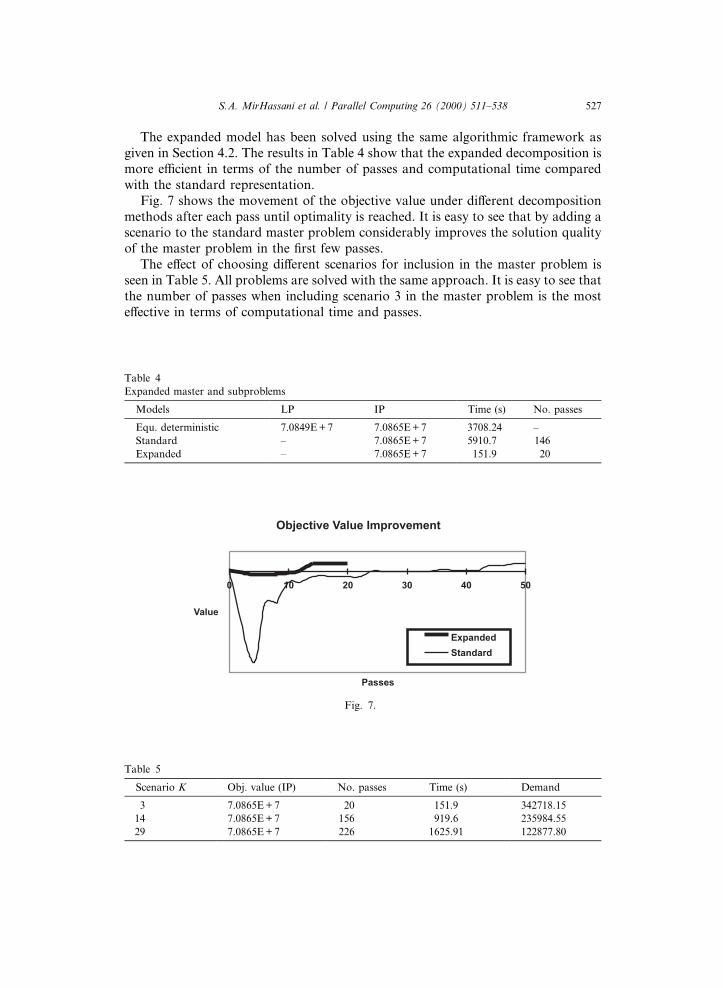
The expanded model has been solved using the same algorithmic framework asgiven in Section 4.2. The results in Table 4 show that the expanded decomposition ismore e�cient in terms of the number of passes and computational time comparedwith the standard representation.

Fig. 7 shows the movement of the objective value under di�erent decompositionmethods after each pass until optimality is reached. It is easy to see that by adding ascenario to the standard master problem considerably improves the solution qualityof the master problem in the ®rst few passes.

The e�ect of choosing di�erent scenarios for inclusion in the master problem isseen in Table 5. All problems are solved with the same approach. It is easy to see thatthe number of passes when including scenario 3 in the master problem is the moste�ective in terms of computational time and passes.

Table 4

Expanded master and subproblems



Standard ± 7.0865E + 7 5910.7 146

Expanded ± 7.0865E + 7 151.9 20

Fig. 7.

Table 5

Scenario K Obj. value (IP) No. passes Time (s) Demand

3 7.0865E + 7 20 151.9 342718.15

14 7.0865E + 7 156 919.6 235984.55

29 7.0865E + 7 226 1625.91 122877.80


Since the only uncertain component in this problem is represented by the de-mand for products, the total demand for each scenario can be considered as aparameter to explain di�erent passes for di�erent scenario choices in the masterproblem. Scenario 3 represents the biggest demand in our model. The resultsshown in Table 5 highlight how the total demand e�ects the total number of passesneeded to reach the solution.

5.3. The weighted representation

After considering the results in Table 5 we conclude that a strategy with highdemand, which calls for large amounts of capacity, provides a good initial solutionto the master problem in the Benders decomposition solution process. We thereforeinvestigated another decomposition in which the direction of optimisation for themaster problem is reversed. Thus, in the ®rst-stage the master problem is changed toa maximisation problem. This is achieved by introducing a strictly negative weight ato multiply the objective cx, of the master problem. Therefore, we rewrite problem(P2) as follows:

min Z � �ÿacx� � �1f � a�cx� E fys� �g �5:8�

s:t: Ax � b; �5:9�

ÿ Bx� Dys � ds 8s; �5:10�

x; ys P 0; s 2 Sc; 0 < a6 1:

The objective of the weighted master problem becomes min�ÿacx� h�, orequivalently max�acxÿ h�. Thus, the master problem is stated as a maximisationproblem:

max Z 0 � acxÿ h �5:11�

s:t: Ax � b; �5:12�

hPXs2Sc

psPs � �ds � Bx�; �5:13�

Ps � �ds � Bx�6 0 8s 2 Sc; �5:14�

x P 0;


where 0 < a6 1. A typical subproblem for s 2 Sc is:

min Z � �1� a�c�x� fys �5:15�

s:t: Dys � ds � B�x; �5:16�

ys P 0:

Fig. 8 shows the structure for the standard master and subproblems versus theweighted master and subproblems.

We have solved the weighted model using the algorithmic framework outlined inSection 4.1. The results of solving the weighted master problem and subproblems arereported in Table 6. In the weighted master approach the number of passes to

Fig. 8.

Table 6

Weighted master and subproblems



Standard ± 7.0865E + 7 5910.7 146

Weighted ± 7.0865E + 7 21.99 5

Table 7

Weight (a) IP Time (s) No. passes

0.2 7.0865E + 7 21.99 5

0.4 7.0865E + 7 85.3 11

0.8 7.0865E + 7 32.1 5

1.0 7.0865E + 7 52.7 6


achieve the optimum solution as well as the computational time decrease in com-parison with the standard method. This is because the master problem is much easierto solve at each pass. The number of passes are reduced since ``maximisation'' ®nds agood initial solution for the master.

By varying the weight over a range of values we have investigated the e�ect on thenumber of passes required by the Benders decomposition algorithm. The results setout in Table 7 illustrate that for the given prototype model, in¯uence of the weightparameter is limited and the number of passes range between 5 and 11.

5.4. Computational results

The results set out in Table 8 illustrate the importance of ®nding a gooddecomposition representation.

Clearly, the expanded method compared to the standard method leads to areduction in the number of passes but there is more computational time in each pass.The weighted approach is better on both counts. It has a fairly fast computationaltime in each pass while its convergence to the solution is quicker than the expandedapproach. This is particularly important in solving the real life application where it iscrucial to have as small a master problem as possible. In Fig. 9 we have described ina ``schematic form'' the nature and behaviour of the three alternative decomposi-tions. The standard decomposition has an initial master solution, which starts with aminimum amount of strategic resources (sites, DCs, and lines serving the supplychain) and with proposing cuts arrives at the optimum resource allocation. The

Fig. 9.

Table 8



Standard ± 7.0865E + 7 5910.7 146

Expanded ± 7.0865E + 7 151.9 20

Weighted ± 7.0865E + 7 21.99 5


expanded model due to the inclusion of a representative scenario in the master givesan initial strategic resource solution, which is near to the optimum allocation. Theweighted model on the other hand starts with a maximum (``greedy'') allocation ofstrategic resources but then rapidly reduces these resources through the decompo-sition process.

6. Investigation of parallel algorithms

6.1. Scope of parallel computing

Multi-processor computational platforms and parallel algorithms have beendeployed to address a number of intractable problems, which would otherwiserequire substantial numerical processing time even on a fast serial computer.Essentially the motivation for using parallel processing is to:

I. obtain a good speed up of execution time [1];II. scale up the data instances of a given problem class [26].Both these aspects have the common objective of achieving solutions of

acceptable instances of practical applications in a reasonable time. Dantzig [12]has long been a proponent of applying parallel algorithms to SP problems andover the last 10 years a number of researchers [15,30,32,42,45,47] have presentedparallelization of SP solution Algorithms. Our approach is to not only parallelisethe solution algorithm, but also to achieve performance gains on most readilyavailable hardware and software platforms. Thus, we have used both specialpurpose parallel computers PARSYTEC CC-12 (discussed in Section 3.3) andhave also adapted:

(a) a collection of high speed PCs;(b) these are connected by a 100 MB hub;(c) and PVM [24] is used as the message passing interface to achieve parallel pro-cessing.Each of the ®ve PC stations is a 333 MHz Pentium II, 128 MB RAM, VIGLEN

computer and the operating system is windows NT4. The cluster is con®gured as asingle program multiple data (SPMD) distributed processing environment. In thealgorithms presented in this section we have used a master/slave tree topologyparallel programming model. Another aspect of our approach is to present thesesolution algorithms essentially as black boxes which may be used as a scalableoptimisation server. Using client/server [11] software tools our aim is to scale upfrom a prototype model to realistic applications with very little additional e�orts bythe end users and modelling experts.

In scenario analysis, of the two main solver tasks, phase 1 requires an independentcollection of similar models to be solved; therefore each scenario is solved on oneslave processor. Whereas in phase 2 each slave processor evaluates one con®gurationagainst all scenarios.

The two-stage SP also displays substantial subproblem independence where thesolver is con®gured for a two-stage Benders decomposition algorithm.


6.2. Scenario analysis in parallel

The natural independence of problems in scenario analysis suggests that much ofthe computational e�ort of the scenario analysis algorithm can run in parallel. Let Nbe the number of available processors, which are made up of 1 master processor andN ÿ 1 slave processors.


As before (see Section 3) we apply a three-phase algorithm which is shown inPseudo-code 3. It is obvious from the computational times shown in Section 3.1 thatit is not worth confusing the algorithm logic by parallelizing phase 3.

In Table 9 we have shown the processing times for the prototype as well as the fullplanning problem.

Note:(a) In phases 1 and 2 it was observed that a static distribution of the scenario-based problem led to uneven loads and poor speed up. Hence, an ``on the ¯y'' dy-namic load distribution was implemented which gave better load balancing andnear linear speed up. See Table 9.(b) Starting with the prototype model, scenario analysis can be scaled up for theplanning model.

6.3. Benders decomposition in a parallel framework

To solve the ISP problem in a parallel environment we modify our previous al-gorithm. We consider the following parallel implementation for a master/slavestrategy for solving the problem. An outcome of our investigations into solvingsubproblems in serial, was that by using the previous basis as the initial basis for thenext subproblem led to the creation of deep cuts in the master problem. When wecarry out this task in a parallel environment we solve unique groups of subproblemson each processor. Initially the scenarios were chosen in a random fashion and thesubproblems were spread over the master and slave processors. The resulting cutswere less deep and hence less e�ective than those created in the serial approach. Thisapproach led to many more passes in the Benders decomposition when comparedwith the number of passes required in the serial algorithm. As a result of the analysisof the pay-o� table from phase 2 we are able to identify an important scenario (highdemand scenario) and solve this on the master processor in serial. In order to restorethe bene®cial performance of the serial approach, we broadcast the basis of the ®rstsubproblem from the master processor to all slave processors. Hence, each slaveprocessor warm starts from the same basis and works on its own unique group ofsubproblems.

Table 9

Models Phase Serial time (s) Parallel time (s)

Prototype Phase 1 (IP) 710.21 317.60

Prototype Phase 2 (LP) and phase3 169.7 38.81

Planning Phase 1 (IP) 92549.6 19435.4

Planning Phase 2 (LP) and phase 3 115540.7 23570.3


6.4. Computational results

A parallel implementation of the Benders decomposition is shown in Pseudo-code4. The master problem is solved on the master processor using a serial algorithm. Allexperiments were carried out on a PARCYTEC CC12 computer (see Section 3.3)

Table 10

Models IP, Obj. Serial Parallel

Time (s) No. passes Time (s) No. passes

Standard 7.0865E + 7 5910.7 146 5119.4 173

Expanded 7.0865E + 7 151.9 20 112.6 18

Weighted 7.0865E + 7 21.99 5 7.18 5


using the prototype model. Table 10 illustrates the time taken in solving the two-stage problem in serial and parallel.

7. Conclusions

Supply chain planning in the face of future uncertainties is an important as wellas a computationally challenging decision problem. The problem can be well an-alysed applying scenario analysis [17] as well as two-stage SP. However, practicalinstances of such problems for a multinational with a global sourcing requirement(D. Gregg, private communication) lead to instances of models which are intrac-table as SPs with todayÕs solver technologies. In this paper we have shown howscenario analysis can be easily scaled up for practical problems and be used toprovide what-if answers to sensitivities which an end user (decision-maker) maywish to investigate. Although two-stage SP can be parallelised with considerablesimplicity it may not converge as well as the serial Benders approach. We haveshown how a parallel Benders algorithm can be modi®ed to achieve a convergencerate comparable with the serial Benders approach. For the given problem we haveinvestigated alternative decomposition representations which take into consider-ation the nature of the master problem. We have shown that by reversing the senseof the master problem from minimisation to maximisation we can speed up thesolution process.

Finally, we have identi®ed a number of ways in which we might be able to im-prove the computational performance of the two-stage SP solution algorithm. Webelieve that the introduction of a Lagrangean method for solving the master problemmay improve the solution time since the master is a di�cult discrete optimisationproblem. We can also apply parallel branch and bound [39] to solve the masterproblem which is currently solved in serial. These are topics of our future investi-gations.

Acknowledgements

The research reported in this paper was supported by EPSRC ROPA grantawarded number GR/K92443. Also Mr. MirHassani has been supported by theIranian government. The work of Dr. A. Nagar in carrying out computational testsis gratefully acknowledged.

References

[1] G.M. Amdahl, Validity of the single processor approach to achieving large-scale computing

capabilities, AFIPS Conference Proceedings 30 (1967) 483±485.


[2] K.A. Ariyawansa, D.D. Hudson, Performance of a benchmark parallel implementation of the Van

Slyke and Wets algorithm for two-stage stochastic programs on the sequent/balance, Concurrency

Practice and Experience 3 (1991) 109±128.

[3] N.J. Berland, K.K. Haugen, Mixing stochastic dynamic programming and scenario aggregation,

Annals of Operation Research 64 (1996) 1±19.

[4] J.F. Benders, Partitioning procedures for solving mixed variables programming problems, Number

Math 4 (1962) 238±252.

[5] D. Bienstock, J.F. Shapiro, Optimising resource acquisition decisions by stochastic programming,

Management Science 34 (2) (1984).

[6] J.R. Birge, C.J. Donohue, D.F. Holmes, O.G. Svintsiski, A parallel implementation of the nested

decomposition algorithm for multi-stage stochastic linear programs, Mathematical Programming 75

(2) (1996) 327±352.

[7] G.R. Bitran, D. Tirupati, Hierarchical production planning, in: S.C. Graves, A.H.G. Rinnoy Kan,

P.H. Zipkin (Eds.), Handbook on Operations Research and Management Science, vol. 4, North-

Holland, Amsterdam, 1993, pp. 523±568.

[8] G.G. Brown, G.W. Graves, M.D. Honczarenko, Design and operation of a multi-commodity

production/distribution system using primal goal decomposition, Management Science 33 (11) (1987)

1469±1480.

[9] R.K.M. Cheung, W.B. Powell, Models and algorithms for distribution problems with uncertain

demands, Transportation science 30 (1) (1996) 43±59.

[10] M.A. Cohen, H.L. Lee, Strategic analysis of integrated production±distribution systems: models and

methods, Operations Research 36 (2) (1988) 216±228.

[11] J. Cruise, G. Mitra, D. Hague, Client/Server integration tools for mathematical programming

systems, Presented at Informs National Meeting, San Diego, 4±7 May, 1997.

[12] G.B. Dantzig, Planning under uncertainty using parallel computing, in: R.R. Meyer, S.A. Zenios

(Eds.), Parallel Optimization on Novel Computer Architectures (special issue), Annals of Operations

Research 14 (1988).

[13] M.A.H. Dempster, M.L. Fisher, L. Jansen, B.J. Lageweg, J.K. Lenstra, A.H.G. Rinnoy Kan,

Analytical evaluation of hierarchical planning systems, Operations Research 29 (4) (1981) 707±716.

[14] M.A.H. Dempster, M.L. Fisher, L. Jansen, B.J. Lageweg, J.K. Lenstra, A.H.G. Rinnoy Kan,

Analysis of heuristics for stochastic programming: results for hierarchical scheduling problems,

Operations Research (1984).

[15] M.A.H. Dempster, R. Thompson, EVPI-based importance sampling solution procedures for

multistage stochastic linear programmes on parallel MIMD architecture, Annals of OR 90 (1999)

161±184.

[16] E.F.D Ellison, M. Hajian, R. Levkovitz, I. Maros, G. Mitra, D. Sayers, FortMP manual, Brunel

University, West London and NAG Ltd, 1996.

[17] G.D. Eppen, R.K. Martin, L. Schrage, A scenario approach to capacity planning, Operations

Research 37 (4) (1989) 517±525.

[18] L.F. Escudero, P.V. Kamesam, A.J. King, R.J.B. Wets, Production planning via scenario modelling,

Annals of Operations Research 43 (1993) 311±335.

[19] L.F. Escudero, J.L. de la Fuente, C. Garcia, F.J. Prieto, Hydropower generation management under

uncertainty via scenario analysis and parallel computation, IEEE Transaction on Power Systems 11

(2) (1996) 683±689.

[20] A. Fefergruen, P. Zipkin, A combined vehicle routing and inventory allocation problem, Operations

Research 32 (5) (1984) 1019±1037.

[21] F. Fantauzzi, A. Gaivornski, E. Messina, Decomposition methods for network optimisation

problems in the presence of uncertainty, in: P.M. Pardalos, D.W. Hearn, W. Hager (Eds), Lecture

Notes on Economics and Mathematical Systems: Network Optimization, vol. 450, Gainesville, FL,

USA, 1996, pp. 234±248.

[22] H.I. Gassmann, MSLIP: a computer code for the multi-stage stochastic linear programming problem,

Mathematical Programming 47 (1990) 407±423.

[23] H.I. Gassman, S.W. Wallace, Solving linear programs with multiple right-hand sides: pricing and

ordering schemes, Annals of Operations Research 64 (1996) 237±259.


[24] Al. Geist, A. Begulin, J. Dongarra, W. Jiang, R. Mancheck, V. Sunderam, PVM 3 UserÕs guide and

reference manual, 1994.

[25] A.M. Geo�rion, G.W. Graves, Multi-commodity distribution system design by Benders decompo-

sition, Management Science 20 (5) (1974) 822±844.

[26] J.L. Gustafson, Re-evaluating AmdahlÕs law, Communications of the Association for Computimg

Machinery 31 (5) (1988) 532±533.

[27] T. Helgason, S.W. Wallace, Approximate scenario solutions in the progressive hedging algorithm,

Annals of Operations Research 31 (1991) 425±445 1991.

[28] J.L. Higle, S. Sen, Stochastic Decomposition: A Statistical Method for Large-scale Stochastic Linear

Programming, Kluwer Academic Publisher, Dordrecht, 1996.

[29] A. Huchzermeier, M.A. Cohen, Valuing operational ¯exibility under exchange rate risk, Operations

Research 44 (1) (1996).

[30] G. Infanger, Planning under Uncertainty: solving large scale stochastic linear program, Boyd and

Fraser, Danvers, MA, 1994.

[31] P. Kall, J. Mayer, SLP-IOR: an interactive model management system for stochastic linear programs,

Mathematical Programming 75 (1996) 221±240.

[32] A. King, SP/OSL version 1.0. Stochastic programming interface library: userÕs guide, Research Report

RC, 19757 (87525) 9/26/94 Mathematics, T.J Watson Research Center, Yorktown Heights, NY.

[33] B.G. Lageweg, J.K. Lenstra, A.H.G. Rinnooy Kan, L. Stougie, Stochastic integer programming by

dynamic programming, Statistica Neerlandica 39 (2) (1985).

[34] G. Laporte, F.V. Louveaux, H. Mercure, The vehicle routing problem with stochastic travel times,

Transportation Science 26 (1992) 161±170.

[35] G. Laporte, F.V. Louveaux, The integer L-shape method for stochastic integer programs with

complete recourse, Operation Research Letters 13 (1993) 133±142.

[36] C.M.A. Leopoldino, M.V.F. Pereira, L.M.V. Pinto, C.C. Riberio, A constraint generation scheme to

probabilistic linear problems with an application to power system expansion, Annals of operations

research 50 (1994) 367±385.

[37] F.V. Louveaux, Multi-stage stochastic programs with block-separable recourse, Mathematical

Programming Studies 28 (1986) 48±62.

[38] C. Lucas, E. Messina, G. Mitra, Risk and return analysis of a multi-period strategic planning

problem, in: L. Thomas, A. Christers (Eds.), Stochastic Modelling in Innovative Manufacturing,

Springer, Berlin, 1996.

[39] G. Mitra, I. Hai, M.T. Hajian, A distributed processing algorithm for solving integer programs using

a cluster of workstations, Parallel Computing 23 (1997) 733±753.

[40] E. Messina, G. Mitra, Modelling and analysis of multi-stage stochastic programming problems: a

software environment, European Journal of Operational Research 101 (1997) 343±359.

[41] J.M. Mulvey, A. Ruszczynski, A new scenario decomposition method for large-scale stochastic

optimization, Operations Research 43 (3) (1995) 477±490.

[42] J.M. Mulvey, H. Vladimirou, Evaluation of a parallel heading algorithm for stochastic network

programming, in: R. Sharda, B. Golden, E. Wasil, O. Balci, W. Stewart (Eds.), Impacts of recent

computer advances on operations research, Elsevier, Amsterdam, 1989.

[43] J.M. Mulvey, H. Vladimirou, Parallel and distributed computing for stochastic network program-

ming, Technical Report SOR-90-11, Department of Civil Engineering and Operations Research,

Princeton University, Princeton, NJ, 1990.

[44] E.M. Modiano, Derived demand and capacity planning under uncertainty, Operations Research 35

(2) (1987) 185±197.

[45] S.S. Nielsen, S.A. Zenios, Solving multi-stage stochastic network programs on massively parallel

computers, Mathematical Programming 73 (3) (1996) 227±250.

[46] R.T. Rockafellar, R.J.B. Wets, Scenario and policy aggregation in optimization under uncertainty,

Mathematics of Operations Research 16 (1991) 119±147.

[47] A. Ruszczynski, Parallel decomposition of multi-stage stochastic programming problems, Mathe-

matical Programming 58A (2) (1993) 201±228.

[48] R. Schultz, Continuity and stability in two-stage stochastic integer programming, in: K. Marti (Ed.),

Lecture Notes in Economics and Mathematical Systems, vol. 379, Springer, Berlin, 1992, pp. 81±92.


[49] R. Schultz, Continuity properties of expectation functions in stochastic integer programming,

Mathematics of Operations Research 18 (1993) 578±589.

[50] R.L. Schultz Stougie, M.H. Van der Vlerk, Two-stage stochastic integer programming: a survey,

Statistica Neederlandica 50 (3) (1996) 404±416.

[51] R. Stougie, Design and analysis of algorithms for stochastic integer programming, CWI Tract, vol.

37, Centrum voor Wiskunde en Informatica, Amsterdam, 1987.

[52] van Slyke, R.J.-B. Wets, L-shaped linear programs with application to optimal control and stochastic

programming, SIAM Journal on Applied Mathematics 17 (1969) 638±663.

[53] D.J. Thomas, P.M. Gri�n, Coordinated supply chain management, European Journal of Operational

Research 94 (1996) 1±15.

[54] J.M. Wagner, O. Berman, Models for planning capacity expansion of convenience stores under

uncertain demand and the value of information, Annals of Operations Research 59 (1995) 19±44.

[55] R.D. Wollmer, Two-stage linear programming under uncertainty with 0±1 integer ®rst-stage

variables, Mathematical programming 19 (1980) 279±288.

[56] M.A. Zimmermann, M.A. Pollatschek, The probability distribution function of the optimum of a

linear program with randomly distributed coe�cients of the objective function and the right-hand

side, Operations Research 23 (1) (1975) 137±149.


Computational solution of capacity planning models under uncertainty

Documents

Transcript of Computational solution of capacity planning models under uncertainty