
MODEL UNCERTAINTY
79
MODEL UNCERTAINTY Massimo Marinacci Department of Decision Sciences and IGIER, Universit` a Bocconi Abstract We study decision problems in which consequences of the various alternative actions depend on states determined by a generative mechanism representing some natural or social phenomenon. Model uncertainty arises because decision makers may not know this mechanism. Two types of uncertainty result, a state uncertainty within models and a model uncertainty across them. We discuss some two-stage static decision criteria proposed in the literature that address state uncertainty in the first stage and model uncertainty in the second (by considering subjective probabilities over models). We consider two approaches to the Ellsberg-type phenomena characteristic of such decision problems: a Bayesian approach based on the distinction between subjective attitudes toward the two kinds of uncertainty; and a non-Bayesian approach that permits multiple subjective probabilities. Several applications are used to illustrate concepts as they are introduced. (JEL: D81) Kirk: Do you think Harry Mudd is down there, Spock? Spock: The probability of his presence on Motherlode is 81% ˙ 0:53. 1. Introduction In this section we briefly discuss several important notions—in particular, uncertainty (including model uncertainty), probabilities, and decisions. We then outline how the paper proceeds before making a few remarks on methodology. The editor in charge of this paper was Juuso Valimaki. Acknowledgments: This paper was delivered as the Schumpeter lecture at the 29th Congress of the European Economic Association in Toulouse in August 2014. It is dedicated, with admiration and affection, to David Schmeidler on the occasion of his 75th birthday. I thank Pierpaolo Battigalli, Loic Berger, Emanuele Borgonovo, Veronica Cappelli, Simone Cerreia-Vioglio, Fabio Maccheroni, Nicola Rosaia, Elia Sartori, and Juuso Valimaki as well as an anonymous referee for many comments and suggestions on preliminary versions of the paper. The material is based on extensive collaboration with Pierpaolo Battigalli, Simone Cerreia-Vioglio, Fabio Maccheroni, and Luigi Montrucchio; it is supported by the AXA Research Fund and the European Research Council (advanced grant BRSCDP-TEA). E-mail: [email protected] Journal of the European Economic Association December 2015 13(6):998–1076 c 2015 by the European Economic Association DOI: 10.1111/jeea.12164
-
Upload
khangminh22 -
Category
Documents
-
view
0 -
download
0
Transcript of MODEL UNCERTAINTY

MODEL UNCERTAINTY
Massimo MarinacciDepartment of Decision Sciencesand IGIER, Universita Bocconi
AbstractWe study decision problems in which consequences of the various alternative actions depend on statesdetermined by a generative mechanism representing some natural or social phenomenon. Modeluncertainty arises because decision makers may not know this mechanism. Two types of uncertaintyresult, a state uncertainty within models and a model uncertainty across them. We discuss sometwo-stage static decision criteria proposed in the literature that address state uncertainty in the firststage and model uncertainty in the second (by considering subjective probabilities over models). Weconsider two approaches to the Ellsberg-type phenomena characteristic of such decision problems:a Bayesian approach based on the distinction between subjective attitudes toward the two kindsof uncertainty; and a non-Bayesian approach that permits multiple subjective probabilities. Severalapplications are used to illustrate concepts as they are introduced. (JEL: D81)
Kirk: Do you think Harry Mudd is down there, Spock?Spock: The probability of his presence on Motherlode is 81% ˙ 0:53.
1. Introduction
In this section we briefly discuss several important notions—in particular, uncertainty(including model uncertainty), probabilities, and decisions. We then outline how thepaper proceeds before making a few remarks on methodology.
The editor in charge of this paper was Juuso Valimaki.
Acknowledgments: This paper was delivered as the Schumpeter lecture at the 29th Congress of the EuropeanEconomic Association in Toulouse in August 2014. It is dedicated, with admiration and affection, to DavidSchmeidler on the occasion of his 75th birthday. I thank Pierpaolo Battigalli, Loic Berger, EmanueleBorgonovo, Veronica Cappelli, Simone Cerreia-Vioglio, Fabio Maccheroni, Nicola Rosaia, Elia Sartori,and Juuso Valimaki as well as an anonymous referee for many comments and suggestions on preliminaryversions of the paper. The material is based on extensive collaboration with Pierpaolo Battigalli, SimoneCerreia-Vioglio, Fabio Maccheroni, and Luigi Montrucchio; it is supported by the AXA Research Fundand the European Research Council (advanced grant BRSCDP-TEA).
E-mail: [email protected]
Journal of the European Economic Association December 2015 13(6):998–1076c� 2015 by the European Economic Association DOI: 10.1111/jeea.12164
Marinacci Model Uncertainty 999
Uncertainty. Uncertainty has increasingly taken center stage in academic and publicdebates, and there is a growing awareness and concern about its role in human domainssuch as environmental uncertainty (climate change, natural hazards), demographicuncertainty (longevity and mortality risk), economic uncertainty (economic andfinancial crises), risk management (operational risks, Basel accords), and technologicaluncertainty (Fukushima).
Uncertainty affects decision making directly by making contingent the payoffs of acourse of action (e.g., harvest and weather), as well as indirectly by generating privateinformation. The latter point is key in strategic interactions, where uncertainty andprivate information are essentially two sides of the same coin: uncertainty generatesprivate information when different agents have access to different information about theuncertain phenomenon; vice versa, private information per se can generate uncertaintyif agents are contemplating it (moral hazard and adverse selection issues).
In the real world, uncertainty is a primary source of competitive advantage (and soof business opportunities that may favor entrepreneurship). In the theoretical world,uncertainty makes the study of agents’ decisions and strategic interactions a beautifuland intellectually sophisticated exercise (altogether different from the study of physicalparticles’ actions and interactions). In both worlds, uncertainty plays a major role.
Probabilities. Uncertainty and private information are thus twin notions. Uncertaintyis indeed a form of partial knowledge (information) about the possible realizations ofsome contingencies that are relevant for agents’ decisions (e.g., betting on a die: Whatface will come up?). As such, the nature of uncertainty is epistemic.1 Intuitively, agentsdeal with uncertain contingencies by forming beliefs (expectations) about them. Yethow can the problem be properly framed? The notion of probability was the first keybreakthrough: you can assign numbers to contingencies that quantify their relativelikelihoods (and then manipulate those numbers according to the rules of probabilitycalculus). Probability and its calculus emerged in the 16th and 17th centuries with theworks of Cardano, Huygens, and Pascal, with a consolidation phase in the 18th and19th centuries with the works of the Bernoullis, Gauss, and Laplace. In particular, theLaplace (1812) canon emerged, based on equally likely cases (alternatives): that theprobability of an event is equal to the number of “favorable” cases divided by theirtotal number.
Departing from the original epistemic stance of Laplace, over time the “equallylikely” notion came to be viewed as a purely objective or physical feature (faces of adie, sides of a fair coin). Probability was no longer studied within decision problems,such as the games of chance that originally motivated its first studies in 16th and17th centuries, but rather as a physical notion unrelated to decisions and thereforeindependent of any subjective information and beliefs. All this changed in the 1920swhen de Finetti and Ramsey freed probability of physics,2 put its study back in decision
1. From the Greek word for knowledge, episteme ("�������). In the paper we use the terms“information” and “knowledge” interchangeably.
2. See Ramsey (1926) and de Finetti (1931, 1937).

1000 Journal of the European Economic Association
problems (probability “is a measurement of belief qua basis for action”, in Ramsey’swords), and rendered “equally likely” an epistemic—and thus subjective—evaluation.They did so by identifying the probability that agents attach to some (decision relevant)event with their willingness to bet on it, which is a measurable quantity. As Ramseyremarked, the “old-established way of measuring a person’s belief is to propose a bet,and see what are the lowest odds which he will accept”.
Epistemic probabilities a la de Finetti–Ramsey (often called subjective) quantifydecision makers’ degree of belief and can be ascribed to any event, repeatable or not,such as “tomorrow it will rain” or “left-wing parties will increase their votes in thenext elections”. In this way, all uncertainty can be probabilized; this is the main tenetof Bayesianism.
Model Uncertainty. In this paper we consider decision makers (DMs) who areevaluating courses of actions the consequences of which depend on states of theenvironment that—such as rates of inflation, peak ground accelerations, and drawsfrom urns—can be seen as realizations of underlying random variables that are partof a generative (or data generating) mechanism that represents some natural or socialphenomenon.
Each such mechanism induces a probability model (or law) over states thatdescribes the regular features of their variability. The uncertainty about the outcomesof the mechanism, and so about the inherent randomness of the phenomenon itrepresents, is called physical. Probability models thus quantify this kind of uncertainty,using analogies with canonical mechanisms (dice, urns, roulette wheels, and the like)that serve as benchmarks.3 As any kind of uncertainty that DMs deem relevant fortheir decision problems, physical uncertainty is relative to their ex-ante (i.e., prior tothe decision) information and its subjective elaboration—for instance, the analogyjudgment just mentioned. Thus physical uncertainty (often referred to as risk inthe literature) is an epistemic notion that accounts for DMs’ views on the inherentrandomness of phenomena. To paraphrase Protagoras: in decision problems, DMs are“the measure of all things”.
Probability models describe such DMs’ views by combining a structuralcomponent, which is based on theoretical knowledge (e.g., economic, physical), witha random component which accounts for measurement issues and for minor (and soomitted) explanatory variables.4 We assume that DMs’ ex-ante information allowsthem to posit a set of possible generative mechanisms, and so of possible probabilitymodels over states. Following a key tenet of classical statistics, we take such set as adatum of the decision problem. This set is generally nonsingleton (and so probabilities
3. In the words of Schmeidler (1989, p. 572), “the concept of objective probability is considered hereas a physical concept like acceleration, momentum or temperature; to construct a lottery with givenobjective probabilities (a roulette lottery) is a technical problem conceptually not different from buildinga thermometer.”
4. As Marschak (1953, p. 12) writes, they are “separately insignificant variables that we are unable andunwilling to specify”. Similar remarks can be found in Koopmans (1947, p. 169); for a discussion, seePratt and Schlaifer (1984, p. 12).
Marinacci Model Uncertainty 1001
are “unknown”) because the ex-ante information is not enough to pin down a singlemechanism. Model uncertainty (or model ambiguity) therefore emerges since DMs areuncertain about the true mechanism.5
The often-made modeling assumption that a true generative mechanism exists isunverifiable in general and so of a metaphysical nature. It amounts to assuming that,among all probability models that DMs conceive, the model that best describes thevariability in the states is the one that actually generates (and so causes/explains) themprobabilistically. In any event, the assumption underlies a fruitful causal approach thatfacilitates the integration of empirical and theoretical methods—required for a genuinescientific understanding.6
Priors and Decisions. We assume that the DMs’ ex-ante information also enablesthem to address model uncertainty through a subjective prior probability over models;in this we follow a key tenet of the Bayesian paradigm. Prior probabilities quantifyDMs’ beliefs by using analogies with betting behavior (Section 3.1).
The result is two layers of analysis: a first, classical layer featuring probabilitymodels on states that quantify physical uncertainty; and a second, Bayesian layercharacterized by a prior probability on models that quantifies model uncertainty. As iswell known, both layers involve nontrivial methodological aspects. The second layeris ignored by classical statistics; the first layer is indirectly considered within theBayesian paradigm through arguments of de Finetti representation theorem type.7
However, our motivation is pragmatic: we expect that the uncertainty characterizingmany decision problems that arise in applications can be fruitfully analyzed bydistinguishing physical and model uncertainty within DMs’ ex-ante information.8
5. See Wald (1950), Fisher (1957), Neyman (1957), and Haavelmo (1944, pp. 48–49). We will use “modeluncertainty” throughout even though “model ambiguity” is a more specific and hence more informativeterminology (see Hansen 2014). In any case, at the level of generality of our analysis, model uncertaintyis an all-encompassing notion. We abstract from any finer distinction, say between nonparametric (model)and parametric (estimation) uncertainty—that is, between models that differ either in substance (e.g.,Keynesian or New Classical specifications in monetary economics) or in detail (e.g., different coefficientvalues within a theoretical model). See Hansen (2014, p. 974) and Hansen and Sargent (2014, p. 1) for arelated point. For finer distinctions, see for example Draper et al. (1987), Draper (1995), the referencestherein (these authors call predictive uncertainty a notion similar to physical uncertainty), as well as Brock,Durlauf, and West (2003).
6. For a critique of this approach, with a purely descriptive, acausal, interpretation of models, see Akaike(1985), Breiman (2001), and Rissanen (2007) as well as Barron, Rissanen, and Yu (1998), Hansen andYu (2001), and Konoshi and Kitagawa (2008). Descriptive approaches now play an important role ininformation technology thanks to the large data sources currently available, the so-called big data (see,e.g., Halevy, Norvig, and Pereira 2009).
7. Cerreia-Vioglio et al. (2013a) provide a decision-theoretic derivation of the two layers within a deFinetti perspective. However, such asymptotic perspective (based on exchangeability and related large-sample properties) may be a straightjacket when DMs have enough information to directly specify a setof probability models. It is typical in these cases for models to be identified by parameters that have someconcrete meaning beyond their role as indices (urns’ compositions being a prototypical example). SeeSection 3.2.
8. As Winkler (1996) notes, this distinction can be seen as an instance of the “divide et impera” precept,a most pragmatic principle. A related point is eloquently made by Ekeland (1993, pp. 139–146). It is
1002 Journal of the European Economic Association
The two layers of analysis motivated by such a distinction naturally lead totwo-stage decision criteria: actions are first evaluated with respect to each possibleprobability model, and then such evaluations are combined by means of the priordistribution. In other words, in this hierarchical approach we first assess actions interms of physical uncertainty and then in terms of epistemic uncertainty.9
Outline. Our paper is an overview of both traditional and more recent elaborationsof this basic insight. In fact, the failure to distinguish these two kinds of uncertainty—in particular, the specific role of model uncertainty—may have significant economicconsequences. Both behavioral paradoxes (of which Ellsberg’s is the most well known)and empirical puzzles (e.g., in asset pricing) can be seen as the outcome of a toolimited account of uncertainty in standard economic modeling. To emphasize theirrelevance, we will illustrate concepts with several applications; these include structuralreliability (Section 4.5), monetary policy (Section 4.9), asset pricing (Section 4.10), andpublic policy (Section 4.11).10 We begin in Section 2 by presenting classical decisionproblems, the two-stage static decision framework of the paper; a few examples fromdifferent fields are given to illustrate its scope. In Section 3 we introduce a two-stageexpected utility criterion that reduces epistemic uncertainty to physical uncertainty(“uncertainty to risk” as it is often put), and so ignores the distinction. Yet given thatexperimental and empirical evidence indicate that this distinction is relevant and mayaffect valuation, in Sections 4 and 5 the criterion is modified in two different ways,Bayesian (Section 4) and not (Section 5), in order to deal more properly with modeluncertainty. In these sections we discuss how optimal behavior is affected by modeluncertainty as well as the extent to which such behavior reflects a desire for robustnessthat, in turn, may favor action diversification, lead to no trade results, and result inmarket prices for assets that—by incorporating premia for model uncertainty—mayexplain some empirical puzzles (Sections 4.9–4.11 and 5.3).
A final important remark: although some important results have already beenestablished for dynamic choice models under ambiguity, we consider only static choicemodels.11
Methodological Post Scriptum. In a philosophy of probability perspective, the twolayers of our analysis rely on different meanings of the notion of probability. In
interesting that de Finetti (1971, p. 89) acknowledge that “ . . . it may be convenient to use the ‘probabilityof a law (or theory)’ as a useful mental intermediary to evaluate the probability of some fact of interest”(emphasis in the original).
9. With all the relevant caveats, for brevity we will often refer to model uncertainty as epistemicuncertainty, which is short for “epistemic uncertainty about models” (and where by models we meanprobability distributions over states).
10. Though our focus is economics, we discuss applications in other disciplines to place concepts inperspective.
11. We refer to Miao (2014) for a recent textbook exposition; for different perspectives on the topic andon the literature (see Hanany and Klibanoff 2009; Siniscalchi 2011; Strzalecki 2013).

Marinacci Model Uncertainty 1003
particular, a distinction is often made, mostly after Carnap (1945, 1950),12 betweenepistemic and physical uncertainties, which are quantified (respectively) by epistemicand physical probabilities.13 In this dual view, model uncertainty is regarded as a mainexample of epistemic uncertainty, with prior probabilities representing DMs’ degreesof beliefs about models.14 Yet for decision problems this distinction is questionable atan ontological level because, as mentioned previously, all uncertainty that is relevantto decision problems is, ultimately, epistemic (i.e., relative to the state of DMs’information). In this paper we regard physical probability as the DMs modeling ofthe variability in the states of the environment, which they can carry out throughanalogies—“as if” arguments—with canonical mechanisms (e.g., states may be viewedto obtain as if they were colors drawn from urns).15 For our probabilistic understandingis shaped, nolens volens, by such mechanisms, and it was their role in games ofchance that actually gave rise to probability in the 16th and 17th centuries.16 In turn,probabilities in canonical mechanisms—and then, by analogy, in general settings—canbe interpreted as physical concepts in potential terms (dispositions, say a la Popper
12. See Good (1959, 1965), Hacking (1975), Shafer (1978), von Plato (1994), and Cox (2006) fordiscussions on this distinction. More applied perspectives can be found in Apostolakis (1990), Pate-Cornell (1996), Walker et al. (2003), Ang and Tang (2007), Der Kiureghian and Ditlevsen (2009), andMarzocchi, Newhall, and Woo (2012) as well as in the 2009 report of the National Research Council. Thisdistinction between the two notions of probability traces back to Cournot and Poisson, around the year1840 (see, e.g., Zabell 2011); Keynes (1921, p. 312) credits Hume for an early dual view of probability.LeRoy and Singell (1987) discuss a related distinction made in Knight (1921).
13. Terminology varies: in place of “physical” the terms aleatory and objective are often used, asare the terms phenomenological (Cox 2006) and statistical (Carnap 1945); in place of “epistemic” theterm subjective is often used, as is (though less frequently) personal (Savage 1954). Finally, physicalprobabilities are sometimes called chances, with the term probability being reserved for epistemicprobabilities (Anscombe and Aumann 1963; Singpurwalla 2006; Lindley 2013).
14. In the logical approaches of Carnap and Keynes, they actually represent degrees of confirmation (see,e.g., Carnap 1945, p. 517). The subjectivist approach, most forcefully proposed by de Finetti, is today morewidely adopted.
15. Le Cam (1977, p. 154) writes “ . . . most models or theories of nature which are encountered instatistical practice are probabilistic or stochastic. The probability measures entering in these modelsare . . . used to indicate a certain structure which can, in final analysis, be reduced to this ‘Everything is asif one were drawing balls from a well-mixed bag.’” Much earlier, Borel (1909, p. 167) had written “wecan now for formulate the general problem of mathematical statistics as follows: determine a system ofdrawing made of urns having a fixed composition, so that the results of a series of drawings, interpretedwith the aid of coefficients conveniently selected, lead with a great likelihood to a table which is identicalwith the table of observations” (p. 138 of the 1965 English translation). More recently, Gilboa, Lieberman,and Schmeidler (2010) propose a view of probability based on a formal notion of similarity.
16. Hacking (1975) is a well-known account of early probability thinking (for a discussion, see Gilboaand Marinacci 2013). On infants and urns, see Xu and Garcia (2008) and Xu and Kushnir (2013); possibleneurological bases of probabilistic reasoning are discussed by Kording (2007), and its importance, as a partof unconscious cognitive abilities, is discussed by Tenenbaum et al. (2011). They contrast conscious andunconscious manipulations of probabilities and explain the former’s problems by noting that numericalprobabilities are “a recent cultural invention that few people become fluent with, and only then aftersophisticated training”. These remarks are reminiscent of the expert billiard player example famously usedby Friedman and Savage (1948) and Friedman (1953) to illustrate the “as if” methodology—which, asthey write on p. 298, “ . . . does not assert that individuals explicitly or consciously calculate and compareexpected utilities . . . but behave as if they . . . [did] . . . ” (emphasis in the original).

1004 Journal of the European Economic Association
1959) or in actual terms (frequencies, say a la von Mises 1939).17 That being said,in stationary environments these two interpretations can be reconciled via ergodicarguments.18
2. Setup
2.1. Notation and Terminology
Probability Measures. Let .S; †/ be a measurable space, where † is an algebra ofevents of S (events are always understood to be in †). For instance, † could be thepower set 2S of S—that is, the collection of all subsets of S . In particular, when S isfinite we assume that † D 2S unless otherwise stated.
Let �.S/ be the collection of all (countably additive) probability measuresm W † ! Œ0; 1�. If S is a finite set with n elements and † is the power set of S ,then �.S/ can be identified with the simplex �n�1 D fx 2 R
nC W PniD1 xi D 1g of
Rn.
We will consider probability measures � defined on the power set of �.S/; forsimplicity, we assume that they have finite nonempty support. In other words, weassume that there exists a finite subset of �.S/, denoted by supp �, such that �.m/ > 0
if and only if m 2 supp �. Given any subset M � �.S/, we denote by �.M / thecollection of all probability measures � with supp � � M .
Integrals and Sums. Given a measurable space .X;X /, we often use the shorthandnotation Epf to denote the (Lebesgue) integral
RX f .x/dp.x/ of a X -measurable
function f W X ! R with respect to a probability measure p W X !Œ0; 1�. In particular,if the space X itself is finite, thenZ
X
f .x/dp.x/ DXx2X
f .x/p.x/
17. Popper (1959, p. 37) mentions these Aristotelian categories, though he claims that“propensities . . . cannot . . . be inherent in the die, or in the penny, but in something a little more abstract,even though physically real: they are relations properties of the experimental arrangement—of theconditions we intend to keep constant during repetition.” Earlier in the paper, on p. 34, he writes that“The frequency interpretation always takes probability as relative to a sequence . . . is a property of somegiven sequence. But with our modification, the sequence in its turn is defined by its set of generatingconditions; and in such a way that probability may now be said to be a property of the generatingconditions” (emphasis in the original).
18. In the terminology of Section 3.2, let p be a probability on †. Given any event Bk
� �kiD1
Z, definethe empirical measure by Op
T.B
k/.s/ D .1=T /
PT
iD11
..Qzi;:::;Qz
iCk/2B
k/.s/. If process fQz
tg is stationary
and ergodic, a well-known consequence of the individual ergodic theorem is that, p-almost everywhere,lim
TOp
T.B
k/ D p.B
k/. So in this case the probability p can be interpreted as the limit empirical frequency
with which states occur. Von Plato (1988, 1989) emphasize this “time average” view of frequentism, whichcan be reconciled with propensities when p.B
k/ is interpreted as a propensity (a similar remark is made
in an i.i.d. setting by Giere 1975, p. 219).
Marinacci Model Uncertainty 1005
that is, integrals reduce to sums. Throughout the paper, the reader can always assumethat spaces are finite and so integrals can be interpreted as sums (an exception arethe examples that involve normal distributions, which require infinite spaces). In thisregard, note that sums actually arise even in infinite spaces when the support of theprobability is finite (and measurable)—that is, supp p D fx 2 X W p.x/ > 0g. In thiscase,
RX f .x/dp.x/ D P
x2supp p f .x/p.x/.
Differentiability. The presentation will require us to consider differentiability on setsthat are not necessarily open. To ease matters, throughout the paper we say that a(convex) function f W C � R
n ! R is differentiable on a (convex) set C if it can beextended to a (convex) differentiable function on some open (convex) set containingC . If the set C is open, such set is C itself.
Equivalent and Orthogonal Measures. Two probability measures m and Qm in � areorthogonal, written m ? Qm, if there exists E 2 † such that m.E/ D 0 D Qm.Ec/;here Ec denotes the complement of E. In words, two orthogonal probabilitiesassign zero probability to complementary events. A finite collection of measuresM D fm1; : : : ; mng � � is (pairwise) orthogonal if all its elements are pairwiseorthogonal, that is, there exists a measurable partition fEign
iD1 of events such that, foreach i , mi .Ei / D 1 and mi .Ej / D 0 if j ¤ i .
We say that m is absolutely continuous with respect to Qm, written m � Qm, ifQm.E/ D 0 implies m.E/ D 0 for all events E. The two measures are equivalent if
they are mutually absolutely continuous, that is, if they assign zero probability to thesame events.
2.2. Decision Form
Following Wald (1950), a decision problem under uncertainty consists of a decisionmaker (DM) who must choose among a set of alternative actions whose consequencesdepend on uncertain factors that are beyond his control. Formally, there is a set A
of available actions a that can result in different material consequences c, within aset C , depending on which state of the environment s obtains in a state space S . Asdiscussed in the Introduction, states are viewed as realizations of some underlyingrandom variables. Often we consider monetary consequences; in such cases, C isassumed to be an interval of the real line.
The dependence of consequences on actions and states is described by aconsequence function � W A � S ! C that details the consequence
c D �.a; s/ (1)
of action a in state s. The quartet .A; S; C; �/ is a decision form under uncertainty.It is a static problem that consists of an ex-ante stage (up to the time of decision)and an ex-post stage (after the decision). Ex ante, DMs know all elements of thequartet .A; S; C; �/ and, ex post, they will observe the consequence �.a; s/ that results.
1006 Journal of the European Economic Association
However, we do not assume that DMs will necessarily observe the state that, ex post,obtains.19
We illustrate decision forms with a few examples from different fields. Some ofthem will also be used later in the paper to illustrate various concepts as they areintroduced.
Betting. Gamblers have to decide which bets to make on the colors of balls drawnfrom a given urn. The consequence function is �.a; s/ D w.s; a/ � c.a/, where w.a; s/
is the amount of money that bet a pays if color s is drawn and c.a/ is the price of thebet. States (i.e., balls’ colors) are observed ex post.
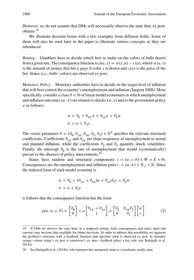
Monetary Policy. Monetary authorities have to decide on the target level of inflationthat will best control the economy’s unemployment and inflation (Sargent 2008). Morespecifically, consider a class � 2 ‚ of linear model economies in which unemploymentand inflation outcomes .u; �/ are related to shocks .w; "/ and to the government policya as follows:
u D �0 C �1�� C �1aa C �2w
� D a C �3":
The vector parameter � D .�0; �1� ; �1a; �2; �3/ 2 R5 specifies the relevant structural
coefficients. Coefficients �1� and �1a are slope responses of unemployment to actualand planned inflation, while the coefficients �2 and �3 quantify shock volatilities.Finally, the intercept �0 is the rate of unemployment that would (systematically)prevail in the absence of policy interventions.20
States have random and structural components s D .w; "; �/ 2 W � E � ‚.Consequences are the unemployment and inflation pairs c D .u; �/ 2 RC � R. Sincethe reduced form of each model economy is
u D �0 C .�1� C �1a/a C �1��3" C �2w
� D a C �3"
it follows that the consequence function has the form
�.a; w; "; �/ D��0
0
�C a
��1� C �1a
1
�C��2 �1��3
0 �3
� �w
"
�: (2)
19. If DMs do observe the state then, in a temporal setting, both consequences and states (past andcurrent) may become data available for future decisions. In order to address that possibility we augmentthe problem’s structure with a feedback function that specifies what is observed ex post. In dynamicsetups—where today’s ex post is tomorrow’s ex ante—feedback plays a key role (see Battigalli et al.2015a).
20. See Battigalli et al. (2015b), who interpret this atemporal setup as a stochastic steady state.

Marinacci Model Uncertainty 1007
The policy multiplier is �1� C �1a. For instance, a zero multiplier (i.e., �1a D ��1� )characterizes a Lucas–Sargent model economy in which monetary policies areineffective, whereas �1a D 0 characterizes a Samuelson–Solow model economy inwhich such policies may be effective.
Finally, states—that is, shocks’ realizations and the true model economy—are notnecessarily observed ex post.
Production. Firms have to decide on the level of production for some output evenwhen they are uncertain about the price that will prevail. The consequence function isthe profit �.a; s/ D r.s; a/ � c.a/, where r.s; a/ is the revenue generated by a unitsof output under price s and c.a/ is the cost of producing a units of output. In this case,states—that is, the price of output—are observed ex post.
Inventory. Retailers have to decide which quantity of some product to buy wholesale,while uncertain about how much they can sell.21 A retailer can buy any quantity a ofthe product at a cost c.a/. An unknown quantity s of the product will be demanded at aunit price p. Here the consequence function is the profit �.a; s/ D p minfa; sg � c.a/,where minfa; sg is the amount that retailers will actually be able to sell. States—thedemand for the product—are observed ex post.
Financial Investments. Investors have to decide how to allocate their wealth amongsome financial assets traded in a frictionless financial market. Suppose there are n
such assets at the time of the decision, each featuring an uncertain gross return ri afterone period. Denote by a 2 �n�1 the vector of portfolio weights, where ai indicatesthe fraction of wealth invested in asset i D 1; : : : ; n. Given an initial wealth w, theconsequence function �.a; s/ D .a � s/w is the end-of-period wealth determined by achoice a when the vector s D .r1; : : : ; rn/ 2 R
n of returns obtains. States—here, thereturns on assets—are again observed ex post.
Climate Change Mitigation. Environmental policy makers have to decide on theabatement level of gas emissions in attempting to mitigate climate change (see, e.g.,Gollier 2013; Millner, Dietz, and Heal 2013; Berger, Emmerling, and Tavoni 2014).The state space S consists of the possible climate states, which may consist of structuraland random components about the cause–effect chains from emissions to temperatures(Meinshausen et al. 2009). For instance, states may be represented by (equilibrium)climate sensitivity, a quantity that measures the equilibrium global average surfacewarming that follows a doubling of atmospheric carbon dioxide (CO2) concentrations(Solomon et al. 2007).
The action space A consists of all possible abatement level policies. Theconsequence function �.a; s/ D d.s; a/ � c.a/ describes the overall monetaryconsequence of abatement policy a when s is the climate state, as determined bythe monetary damage d.s; a/ and by the abatement cost c.a/.
21. This decision problem is often called the newsvendor problem (see, e.g., Porteus 2002).
1008 Journal of the European Economic Association
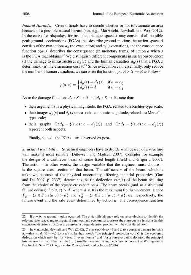
Natural Hazards. Civic officials have to decide whether or not to evacuate an areabecause of a possible natural hazard (see, e.g., Marzocchi, Newhall, and Woo 2012).In the case of earthquakes, for instance, the state space S may consist of all possiblepeak ground accelerations (PGAs) that describe ground motion; the action space A
consists of the two actions a0 (no evacuation) and a1 (evacuation), and the consequencefunction �.a; s/ describes the consequence (in monetary terms) of action a when s
is the PGA that obtains.22 We distinguish different components in such consequence:(i) the damage to infrastructures db.s/ and the human casualties dh.s/ that a PGA s
determines, (ii) the evacuation cost ı.23 Since evacuation can, essentially, only reducethe number of human casualties, we can write the function � W A � S ! R as follows:
�.a; s/ D�
db.s/ C dh.s/ if a D a0;
db.s/ C ı if a D a1:
As to the damage functions db W S ! R and dh W S ! R, note that:
� their argument s is a physical magnitude, the PGA, related to a Richter-type scale;
� their images db.s/ and dh.s/ are a socio-economic magnitude, related to a Mercalli-type scale;
� their graphs Gr db D f.s; c/ W c D db.s/g and Gr dh D f.s; c/ W c D dh.s/grepresent both aspects.
Finally, states—the PGAs—are observed ex post.
Structural Reliability. Structural engineers have to decide what design of a structurewill make it most reliable (Ditlevsen and Madsen 2007). Consider for examplethe design of a cantilever beam of some fixed length (Field and Grigoriu 2007).The action—in other words, the design variable that the engineer must choose—is the square cross-section of that beam. The stiffness s of the beam, which isunknown because of the physical uncertainty affecting material properties (Guoand Du 2007, p. 2337), determines the tip deflection �.a; s/ of the beam resultingfrom the choice of the square cross-section a. The beam breaks (and so a structuralfailure occurs) if �.a; s/ > d , where d � 0 is the maximum tip displacement. HenceFa D fs 2 S W �.a; s/ > dg and F c
a D fs 2 S W �.a; s/ dg are, respectively, thefailure event and the safe event determined by action a. The consequence function
22. If s D 0, no ground motion occurred. The civic officials may rely on seismologists to identify therelevant state space, and to structural engineers and economists to assess the consequence function (in thisevacuation decision structures are a given; a design decision problem will be considered next).
23. In Marzocchi, Newhall, and Woo (2012), C corresponds to �ı and L to a constant damage functiond
h—that is, d
h.s/ D �L for each s. In their words “the principal protection cost C is the economic
dislocation which may last for weeks or even months” and “for a non-evacuation decision, the principalloss incurred is that of human life [ . . . ] usually measured using the economic concept of Willingness toPay for Life Saved”. On d
h, see also Porter, Shoaf, and Seligson (2006).

Marinacci Model Uncertainty 1009
is given by
�.a; s/ D�
ı C c.a/ if s 2 Fa;
c.a/ else;
where ı is the damage cost of failure and c.a/ is the cost of the square cross-sectiona. States—the beam’s stiffness—might not be observed ex post.
Quality Control. Managers have to decide whether to accept or reject the shipmentof some parts from a supplier—say, integrated circuits from an electrical company(see, e.g., Raiffa and Schlaifer 1961; Berger 1993). The state space S consists of theproportion s of defective circuits in the shipment. Only the whole shipment can berejected, not individual parts. Thus the action space A consists of the two actions,a0 (reject the shipment) and a1 (accept the shipment). The consequence function isgiven by �.a0; s/ D 0 and �.a1; s/ D r.s/ � c.s/ � p; here r.s/ is the revenue fromthe sales of the output produced when s is the proportion of defective circuits, c.s/
is the cost they entail when entering the production line (Deming 1986, Chap. 15),and p is the price of the shipment once accepted. In other words: if the shipmentis rejected, then there is no output and so no revenues; if the shipment is accepted,the consequence depends on its cost and on the revenues and costs that it determinesgiven the proportion of defective circuits that it features. States—here, the proportionof defective circuits—are observed ex post unless defects are latent (Deming 1986,p. 409).
Public Policy. Public officials have to decide which treatment—for example,which type of vaccination—should be administered to individuals who belong to aheterogeneous population that, for policy purposes, is classified in terms of someobservable characteristic (covariate), such as age or gender.
Let X and T be, respectively, the (finite) collections of covariates and of possiblealternative treatments. If only aggregate (and not individual) outcomes matter forpolicy making, then we can regard actions as functions a W X ! �.T / that associateprobability distributions over treatments with covariates.24 Here a.x/.t/ 2 Œ0; 1� isthe fraction of the population with covariate x that has been assigned treatmentt .25 Treatment actions are fractional if they do not assign the same treatment toall individuals with the same covariate (see Manski 2009).
When state s obtains, cx.t; s/ denotes the (scalar) outcome for individuals withcovariate x who have been assigned treatment t .26 If public officials care about the
24. This simple distributional formulation abstract from the individual choice problems that may affecttreatment effects, which is a key issue in actual policy analysis (see Heckman 2008, p. 7).
25. The treatment allocation can be implemented through an anonymous random mechanism (a form ofthe “equal treatment of equals” ethical principle; see Manski 2009). If the population is large, then understandard assumptions a.x/.t/ can be regarded as the fraction of the population with covariate x undertreatment t and also as the probability with which the random mechanism assigns the treatment to everyindividual with that covariate.
26. The outcome can be material (say, monetary) or, from a utilitarian perspective, can be stated interms of welfare (say, in utils). Our specification presumes that the relevant policy information is about

1010 Journal of the European Economic Association
average of such individual outcomes, then the consequence function is �.a; s/ DPx.P
t2T cx.t; s/a.x/.t//p.x/, where p.x/ is the fraction of the population withcovariate x. The existence of various states explains why individuals with the samecovariate may respond differently to the same treatment.
Epistemology. Scientists have to decide whether to adopt a new theory or retain anold one. We can follow Giere (1985, pp. 351–352) and consider Earth scientists whoin the 1960s were faced with deciding whether to accept the new drift hypothesesor retain the old static ones. Abstracting from peer concerns, there are two relevantstates: “the tectonic structure of the world is more similar to drift models than to staticmodels” and the reverse, as well as two actions, “adopt drift models” and “retain staticmodels”. As Giere argues, status quo biases determine the consequence function thatcharacterizes the decision problem, which can be described by the following table:
Drift models approximately correct Static models approximately correct
Adopt Satisfactory Terrible
Retain Bad Excellent
Interactive Situations. Players have to decide which actions to play in a staticinteractive situation. For instance, in the previous production example suppose thereis a set I D f1; : : : ; ng of firms (an oligopoly) and that the price depends on theiraggregate production
Pi2I ai according to a (commonly known) inverse demand
function D�1.P
i2I ai /. In the decision problem of each firm i , the state is no longerthe price but rather the production profile a�i D .aj /j ¤i of the other firms; that is, S DA�i �j ¤iAj . In fact, for firm i that profile determines the monetary consequence�i .ai ; a�i / D ri .ai ; D�1.
Pi2I ai // � ci .ai /. The firm’s decision problem is thus
.Ai ; A�i ; Ci ; �i /, where Ci � R.In general, a static game form G D .I; .Ci /i2I ; .Ai /i2I ; .gi /i2I / among selfish
players27 consists of a set I D f1; : : : ; ng of players and, for each player i , a set Ci ofconsequences, a set Ai of actions, and an outcome function gi W A1 � � � � � An ! Ci
that associates the material outcome gi .a1; : : : ; an/ with action profile .a1; : : : ; an/.When player i 2 I evaluates action ai , the relevant states s are the action profiles
a�i of his opponents. As a result, the state space S D A�i is the collection of allaction profiles of his opponents and the consequence function is his individual outcomefunction gi W Ai � A�i ! Ci . The decision form for player i is thus .Ai ; A�i ; Ci ; gi /.States (i.e., opponents’ actions) may be observed ex post.
individuals with given covariates (say, the effect of vaccination on elderly white males) and not aboutparticular individuals.
27. That is to say, players who (like the firms just described) care only about their own material outcomes.In this paper we do not consider other regarding preferences (for a generalization of standard preferencesto such case, see Maccheroni, Marinacci, and Rustichini 2012).
Marinacci Model Uncertainty 1011
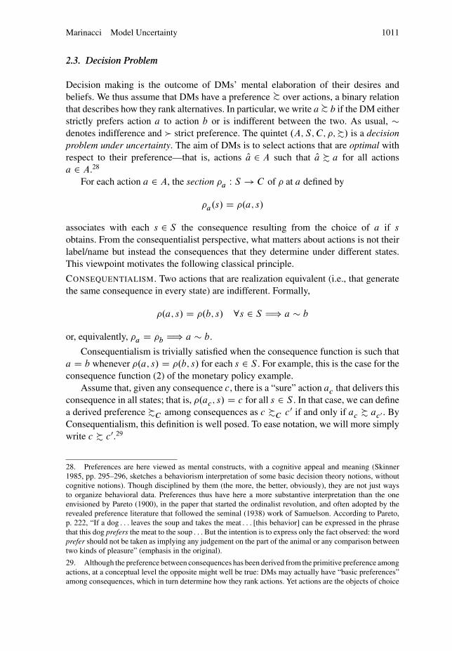
2.3. Decision Problem
Decision making is the outcome of DMs’ mental elaboration of their desires andbeliefs. We thus assume that DMs have a preference � over actions, a binary relationthat describes how they rank alternatives. In particular, we write a � b if the DM eitherstrictly prefers action a to action b or is indifferent between the two. As usual, �denotes indifference and � strict preference. The quintet .A; S; C; �; %/ is a decisionproblem under uncertainty. The aim of DMs is to select actions that are optimal withrespect to their preference—that is, actions Oa 2 A such that Oa % a for all actionsa 2 A.28
For each action a 2 A, the section �a W S ! C of � at a defined by
�a.s/ D �.a; s/
associates with each s 2 S the consequence resulting from the choice of a if s
obtains. From the consequentialist perspective, what matters about actions is not theirlabel/name but instead the consequences that they determine under different states.This viewpoint motivates the following classical principle.
CONSEQUENTIALISM. Two actions that are realization equivalent (i.e., that generatethe same consequence in every state) are indifferent. Formally,
�.a; s/ D �.b; s/ 8s 2 S H) a � b
or, equivalently, �a D �b H) a � b.
Consequentialism is trivially satisfied when the consequence function is such thata D b whenever �.a; s/ D �.b; s/ for each s 2 S . For example, this is the case for theconsequence function (2) of the monetary policy example.
Assume that, given any consequence c, there is a “sure” action ac that delivers thisconsequence in all states; that is, �.ac ; s/ D c for all s 2 S . In that case, we can definea derived preference %C among consequences as c %C c0 if and only if ac % ac0 . ByConsequentialism, this definition is well posed. To ease notation, we will more simplywrite c % c0.29
28. Preferences are here viewed as mental constructs, with a cognitive appeal and meaning (Skinner1985, pp. 295–296, sketches a behaviorism interpretation of some basic decision theory notions, withoutcognitive notions). Though disciplined by them (the more, the better, obviously), they are not just waysto organize behavioral data. Preferences thus have here a more substantive interpretation than the oneenvisioned by Pareto (1900), in the paper that started the ordinalist revolution, and often adopted by therevealed preference literature that followed the seminal (1938) work of Samuelson. According to Pareto,p. 222, “If a dog . . . leaves the soup and takes the meat . . . [this behavior] can be expressed in the phrasethat this dog prefers the meat to the soup . . . But the intention is to express only the fact observed: the wordprefer should not be taken as implying any judgement on the part of the animal or any comparison betweentwo kinds of pleasure” (emphasis in the original).
29. Although the preference between consequences has been derived from the primitive preference amongactions, at a conceptual level the opposite might well be true: DMs may actually have “basic preferences”among consequences, which in turn determine how they rank actions. Yet actions are the objects of choice
1012 Journal of the European Economic Association
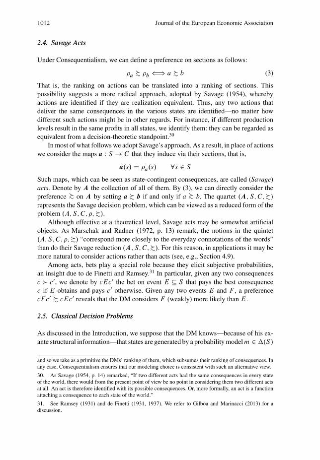
2.4. Savage Acts
Under Consequentialism, we can define a preference on sections as follows:
�a % �b () a % b (3)
That is, the ranking on actions can be translated into a ranking of sections. Thispossibility suggests a more radical approach, adopted by Savage (1954), wherebyactions are identified if they are realization equivalent. Thus, any two actions thatdeliver the same consequences in the various states are identified—no matter howdifferent such actions might be in other regards. For instance, if different productionlevels result in the same profits in all states, we identify them: they can be regarded asequivalent from a decision-theoretic standpoint.30
In most of what follows we adopt Savage’s approach. As a result, in place of actionswe consider the maps a W S ! C that they induce via their sections, that is,
a.s/ D �a.s/ 8s 2 S
Such maps, which can be seen as state-contingent consequences, are called (Savage)acts. Denote by A the collection of all of them. By (3), we can directly consider thepreference � on A by setting a % b if and only if a � b. The quartet .A; S; C; %/
represents the Savage decision problem, which can be viewed as a reduced form of theproblem .A; S; C; �; %/.
Although effective at a theoretical level, Savage acts may be somewhat artificialobjects. As Marschak and Radner (1972, p. 13) remark, the notions in the quintet.A; S; C; �; %/ “correspond more closely to the everyday connotations of the words”than do their Savage reduction .A; S; C; %/. For this reason, in applications it may bemore natural to consider actions rather than acts (see, e.g., Section 4.9).
Among acts, bets play a special role because they elicit subjective probabilities,an insight due to de Finetti and Ramsey.31 In particular, given any two consequencesc � c0, we denote by cEc0 the bet on event E � S that pays the best consequencec if E obtains and pays c0 otherwise. Given any two events E and F , a preferencecF c0 % cEc0 reveals that the DM considers F (weakly) more likely than E.
2.5. Classical Decision Problems
As discussed in the Introduction, we suppose that the DM knows—because of his ex-ante structural information—that states are generated by a probability model m 2 �.S/
and so we take as a primitive the DMs’ ranking of them, which subsumes their ranking of consequences. Inany case, Consequentialism ensures that our modeling choice is consistent with such an alternative view.
30. As Savage (1954, p. 14) remarked, “If two different acts had the same consequences in every stateof the world, there would from the present point of view be no point in considering them two different actsat all. An act is therefore identified with its possible consequences. Or, more formally, an act is a functionattaching a consequence to each state of the world.”
31. See Ramsey (1931) and de Finetti (1931, 1937). We refer to Gilboa and Marinacci (2013) for adiscussion.
Marinacci Model Uncertainty 1013
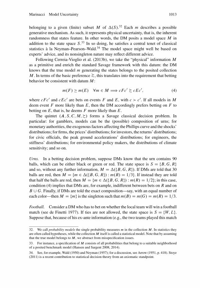
belonging to a given (finite) subset M of �.S/.32 Each m describes a possiblegenerative mechanism. As such, it represents physical uncertainty, that is, the inherentrandomness that states feature. In other words, the DM posits a model space M inaddition to the state space S .33 In so doing, he satisfies a central tenet of classicalstatistics a la Neyman–Pearson–Wald.34 The model space might well be based onexperts’ advice, and its nonsingleton nature may reflect different advice.
Following Cerreia-Vioglio et al. (2013b), we take the “physical” information M
as a primitive and enrich the standard Savage framework with this datum: the DMknows that the true model m generating the states belongs to the posited collectionM . In terms of the basic preference �, this translates into the requirement that bettingbehavior be consistent with datum M :
m.F / � m.E/ 8m 2 M H) cF c0 % cEc0; (4)
where cF c0 and cEc0 are bets on events F and E, with c � c0. If all models in M
deem event F more likely than E, then the DM accordingly prefers betting on F tobetting on E, that is, he deems F more likely than E.
The quintet .A; S; C; M; %/ forms a Savage classical decision problem. Inparticular: for gamblers, models can be the (possible) composition of urns; formonetary authorities, the exogenous factors affecting the Phillips curve and the shocks’distributions; for firms, the prices’ distributions; for investors, the returns’ distributions;for civic officials, the peak ground accelerations’ distributions; for engineers, thestiffness’ distributions; for environmental policy makers, the distributions of climatesensitivity; and so on.
Urns. In a betting decision problem, suppose DMs know that the urn contains 90
balls, which can be either black or green or red. The state space is S D fB; G; Rgand so, without any further information, M D �.fB; G; Rg/. If DMs are told that 30
balls are red, then M D fm 2 �.fB; G; Rg/ W m.R/ D 1=3g. If instead they are toldthat half the balls are red, then M D fm 2 �.fB; G; Rg/ W m.R/ D 1=2g; in this case,condition (4) implies that DMs are, for example, indifferent between bets on R and onB [ G. Finally, if DMs are told the exact composition—say, with an equal number ofeach color—then M D fmg is the singleton such that m.B/ D m.G/ D m.R/ D 1=3.
Football. Consider a DM who has to bet on whether the local team will win a footballmatch (see de Finetti 1977). If ties are not allowed, the state space is S D fW; Lg.Suppose that, because of his ex-ante information (e.g., the two teams played this match
32. We call probability models the single probability measures m in the collection M . In statistics theyare often called hypotheses, while the collection M itself is called a statistical model. Note that by assumingthat the true model belongs to M , we abstract from misspecification issues.
33. For instance, a specification of M consists of all probabilities that belong to a suitable neighborhoodof a posited benchmark model (Hansen and Sargent 2008, 2014).
34. See, for example, Wald (1950) and Neyman (1957); for a discussion, see Arrow (1951, p. 418). Stoye(2011) is a recent contribution to statistical decision theory from an axiomatic standpoint.
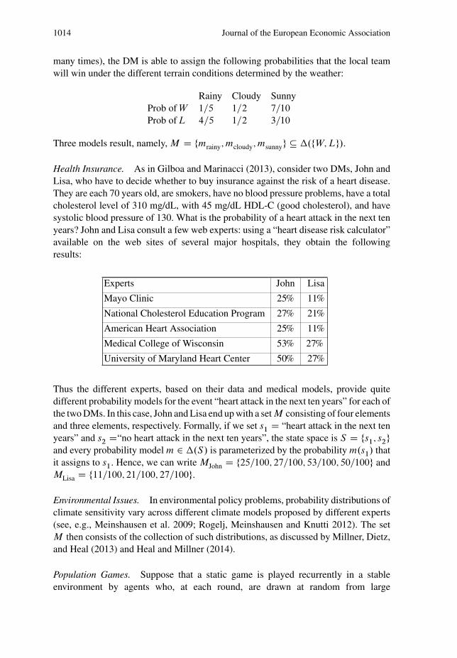
1014 Journal of the European Economic Association
many times), the DM is able to assign the following probabilities that the local teamwill win under the different terrain conditions determined by the weather:
Rainy Cloudy SunnyProb of W 1=5 1=2 7=10
Prob of L 4=5 1=2 3=10
Three models result, namely, M D fmrainy; mcloudy; msunnyg � �.fW; Lg/.
Health Insurance. As in Gilboa and Marinacci (2013), consider two DMs, John andLisa, who have to decide whether to buy insurance against the risk of a heart disease.They are each 70 years old, are smokers, have no blood pressure problems, have a totalcholesterol level of 310 mg/dL, with 45 mg/dL HDL-C (good cholesterol), and havesystolic blood pressure of 130. What is the probability of a heart attack in the next tenyears? John and Lisa consult a few web experts: using a “heart disease risk calculator”available on the web sites of several major hospitals, they obtain the followingresults:
Experts John Lisa
Mayo Clinic 25% 11%
National Cholesterol Education Program 27% 21%
American Heart Association 25% 11%
Medical College of Wisconsin 53% 27%
University of Maryland Heart Center 50% 27%
Thus the different experts, based on their data and medical models, provide quitedifferent probability models for the event “heart attack in the next ten years” for each ofthe two DMs. In this case, John and Lisa end up with a set M consisting of four elementsand three elements, respectively. Formally, if we set s1 D “heart attack in the next tenyears” and s2 D“no heart attack in the next ten years”, the state space is S D fs1; s2gand every probability model m 2 �.S/ is parameterized by the probability m.s1/ thatit assigns to s1. Hence, we can write MJohn D f25=100; 27=100; 53=100; 50=100g andMLisa D f11=100; 21=100; 27=100g.
Environmental Issues. In environmental policy problems, probability distributions ofclimate sensitivity vary across different climate models proposed by different experts(see, e.g., Meinshausen et al. 2009; Rogelj, Meinshausen and Knutti 2012). The setM then consists of the collection of such distributions, as discussed by Millner, Dietz,and Heal (2013) and Heal and Millner (2014).
Population Games. Suppose that a static game is played recurrently in a stableenvironment by agents who, at each round, are drawn at random from large
Marinacci Model Uncertainty 1015
populations, with one population for each player role (Weibull 1996). In the gameform G D .I; .Ci /i2I ; .Ai /i2I ; .gi /i2I / the symbol I now denotes the set of playerroles and i 2 I is the role of the agent drawn from population i . In that role the agentselects an action ai 2 Ai which yields consequence ci D g.ai ; a�i / provided the otheragents (the opponents) select actions a�i in their roles.
For agents in role i the probability ˛�i 2 �.A�i / describes a possible distributionof opponents’ actions, with ˛�i .a�i / being the fraction of opponents who select profilea�i when drawn. The set Mi � �.A�i / is the collection of all these distributions thatagents in role i posit.
Mixed Strategies. In an interactive situation among players who can commit to playactions selected by random devices, the probability ˛�i 2 �.A�i / can be interpreted asa mixed strategy of the opponents of player i . If so, ˛�i .a�i / becomes the probabilitythat opponents’ random devices select profile a�i (in general, such devices are assumedto be independent across players). Here Mi � �.A�i / can be interpreted as the set ofopponents’ mixed strategies that player i considers.
3. Classical Subjective Expected Utility
3.1. Representation
Consider a Savage decision problem .A; S; C; M; %/. Cerreia-Vioglio et al. (2013b)show that a preference � satisfying Savage’s axioms35 and the consistency condition(4) is represented by the criterion V W A ! R given by
V.a/ DZ
M
�ZS
u.a.s//dm.s/
�d�.m/: (5)
That is, the acts a and b are ranked as follows:
a % b () V.a/ � V.b/:
Here u W C ! R is a von Neumann–Morgenstern utility function36 that captures riskattitudes (i.e., attitudes toward physical uncertainty) and � W 2M ! Œ0; 1� is a subjectiveprior probability that quantifies the epistemic uncertainty about models, with supportincluded in M . The subjective prior � reflects some personal information on modelsthat DMs may have, in addition to the structural information that allowed them toposit the collection M .37 In particular, when that collection is based on the advice of
35. See, for example, Gilboa (2009, pp. 97–105).
36. That is, c % c0 if and only if u.c/ � u.c0/.
37. Here we do not adopt the evidentialist view, known in economics as the Harsanyi doctrine (see, e.g.,Aumann 1987; Morris 1995), that subjects with the same information should have the same subjectiveprobabilities (for discussions, see Jaynes 2003, Chap. 12; Kelly 2008).
1016 Journal of the European Economic Association
different experts, the prior may reflect the different weight (reliability) that DMs attachto each of them.
The quintet .A; S; C; M; %/ can therefore be represented in the form.A; S; C; M; u/. Representation (5) may be called classical subjective expected utilitybecause of the classical statistics tenet on which it relies. If we set
U.a; m/ DZ
S
u.a.s//dm.s/
we can then write the criterion as
V.a/ DZ
M
U.a; m/d�.m/;
In words, the criterion considers the expected utility U.a; m/ of each possiblegenerative mechanism m and then averages them according to the prior �. In someapplications it is useful to write V.a; �/ to emphasize the role of beliefs in an action’svalue.
This two-stage criterion can be seen as a decision-theoretic form of hierarchicalBayesian modeling.38 As emphasized in the Introduction, all its probabilisticcomponents are, ultimately, epistemic (and hence subjective) because they dependon some unmodeled background information known to DMs. If we denote suchinformation by I , we can informally account for this key feature by writing criterion(5) in the following heuristic form:
V.a j I / DZ
M
�ZS
u.a.s//dm.sjI /
�d�.m j I /:
Although we omit them for brevity, similar “information augmented” versions holdfor the other criteria studied in this paper.39
Optimal acts solve the optimization problem maxa2A V.a/. They thus depend onthe preference � via the utility function u and the prior �. To facilitate the presentation,hereafter we assume that optimal acts, if they exist, are unique (because, say, of suitablestrict concavity assumptions on the objective function). We denote by Oa the optimalact; to ease notation, we do not mark its dependence on u and � (or on the set A ofavailable acts).
Each prior � induces a predictive probability N� 2 �.S/ through reduction:
N�.E/ DZ
M
m.E/d�.m/ 8E 2 †: (6)
38. See, for example, Bernardo and Smith (1994) and Berger (1993). For, m and s can be seen asrealizations of two random variables—say, m and s—with m.s/ a realization of the distribution of s
conditional on m (see Picci 1977).
39. In these heuristic versions, conditioning on I is purely suggestive, without any formal meaning (togive useful content to I can be, indeed, a quite elusive problem) and without adopting, as just remarked,any evidentialist view.
Marinacci Model Uncertainty 1017
In turn, the predictive probability allows us to rewrite the representation (5) as
V.a/ D U.a; N�/ DZ
S
u.a.s//d N�.s/: (7)
This reduced form of V is the original Savage subjective expected utility (SEU)representation.40
The predictive N� is Savage’s subjective probability, elicitable a la de Finetti–Ramsey via betting behavior on events. For, let c; c0 2 C be any two consequences,with c � c0. Without loss of generality, we can normalize u so that u.c0/ D 0 andu.c/ D 1. If so, cF c0 % cEc0 if and only if N�.F / � N�.E/. Building on this simpleremark allows one to show that the probability N� may, in principle, be elicited (see,e.g., Gilboa 2009).
We remark that in the reduction operation that generates predictive probabilities,some important probabilistic features may disappear. For instance, in a binary statespace S D fs1; s2g consider the two collections M D f.0; 1/; .1; 0/g and M 0 Df.1=2 � ı; 1=2 C ı/ W 0 ı "g, where 0 < " < 1=2 is an arbitrarily small quantity.Taking a uniform prior on each collection yields, in each case, the uniform predictiveprobability on S that assigns probability 1=2 to each state. However, the collectionM consists of two very different models whereas the collection M 0 consists of manyalmost identical models. Thus very different probabilistic scenarios are reduced to thesame predictive probability.
Some special cases are important.
(i) If the support of � is a singleton fmg (i.e., � D ım), then DMs believe, perhapswrongly, that m is the true model. In this case the predictive probability triviallycoincides with m and so criterion (5) reduces to the Savage expected utilitycriterion U.a; m/. As a predictive probability, m is here a subjective probability(albeit a dogmatic one).
(ii) If M is a singleton fmg, then DMs have a maximal structural information and,consequently, know that m is the true model. There is no epistemic uncertainty,but only physical uncertainty (quantified by m).41 Criterion (5) again reducesto the expected utility representation U.a; m/, but now interpreted as a vonNeumann–Morgenstern criterion since, absent epistemic uncertainty, subjectiveprobabilities have no role to play. When combined with (7), this shows thatclassical SEU encompasses both the Savage and the von Neumann–Morgensternrepresentations.42
40. A further reduction, equation (20), will be discussed in Section 4.1. Note that probability measuresin �.S/ can play two different roles: predictive probabilities and probability models.
41. Knowledge of the true model (“known” probabilities) is a basic tenet of the rationalexpectations literature. Lucas (1977, p. 15) writes that “Muth (1961) . . . [identifies] . . . agents subjectiveprobabilities . . . with ‘true’ probabilities, calling the assumed coincidence of subjective and ‘true’probabilities rational expectations” (emphasis in the original).
42. Though the expected utility criterion was first proposed by Bernoulli (1738), the von Neumann andMorgenstern (1947) representation theorem marks the beginning of modern decision theory owing to its
1018 Journal of the European Economic Association
(iii) If M � fıs W s 2 Sg, then there is no physical uncertainty but only epistemicuncertainty (quantified by �). We can identify prior and predictive probabilities:with a slight abuse of notation, we write � 2 �.S/ so that criterion (5) takes theform
V.a/ DZ
S
u.a.s//d�.s/: (8)
This is the form of the criterion that is relevant for decision problems withoutphysical uncertainty.
(iv) If an act a is such that U.a; m/ D U.a; m0/ for all m; m0 2 supp �, we say that a iscrisp (Ghirardato, Maccheroni, and Marinacci 2004). It is intuitive that crisp actsare not sensitive to epistemic uncertainty and that they feature the same physicaluncertainty with respect to all models; hence, crisp acts can be regarded as purelyrisky acts.
Urns. In the previous urn example, suppose DMs are told that 30 balls are red, and soM D fm 2 �.fB; G; Rg/ W m.R/ D 1=3g. This is the three-color problem of Ellsberg(1961). In order to parameterize M with the possible number � 2 ‚ D f0; : : : ; 60gof green balls, we denote by m the element of M such that m .G/ D �=90. LetA D faB ; aG ; aRg be the 1 euro bets on the different colors. Suppose the prior �
is uniform—say, because DMs possess symmetric information about all possiblecompositions. If we normalize the utility function u by setting u.1/ D 1 and u.0/ D 0,then the following equalities hold:
V.aR/ D60X
D0
m .R/�.�/ D N�.R/ D 1
3
V.aG/ D60X
D0
m .G/�.�/ D N�.G/ D 1
61
60XD0
�
90D 1
3
V.aB/ D60X
D0
m .B/�.�/ D N�.B/ D 1 � N�.R [ G/ D 1
3:
Therefore, aR � aB � aG . DMs are indifferent among the bets.Now suppose that the DMs are instead given full information about the composition
of the urn—say, that the colors are in equal proportion. Then M D fmg is the singletonsuch that m.G/ D m.R/ D m.B/ D 1=3 and we are back to the von Neumann–Morgenstern expected utility. Since V.aR/ D V.aG/ D V.aB/ D 1=3, DMs are againindifferent among the bets. Despite the great difference in the quality of information,classical SEU leads to a similar preference pattern. In Section 4.4 we cast some doubtson the plausibility of this conclusion.
reliance on behavioral and so, in principle, testable axioms. But, there were some important earlier resultson means and utilities (see Muliere and Parmigiani 1993).

Marinacci Model Uncertainty 1019
Football. In the previous football example, let a and b be the 1 euro bets on thevictory of, respectively, the local and guest teams. If we normalize the utility functionu by setting u.1/ D 1 and u.0/ D 0, then
U.a; mrainy/ D mrainy.W /u.a.W // C mrainy.L/u.a.L// D 1
5u.1/ C 4
5u.0/ D 1
5
U.a; mcloudy/ D mcloudy.W /u.a.W // C mcloudy.L/u.a.L// D 1
2u.1/ C 1
2u.0/ D 1
2
U.a; msunny/ D msunny.W /u.a.W // C msunny.L/u.a.L//
D 7
10u.1/ C 3
10u.0/ D 7
10:
Consequently,
V.a/ D 1
5�.rainy/ C 1
2�.cloudy/ C 7
10�.sunny/
V .b/ D 4
5�.rainy/ C 1
2�.cloudy/ C 3
10�.sunny/:
Hence a % b if and only if �.rainy/ .2=3/�.sunny/.
Monetary Policy. In the monetary policy decision problem, within a state s D.w; "; �/ the pair .w; "/ represents random shocks and � parameterizes a modeleconomy. As in Battigalli et al. (2015a), we factor the probability models m 2 M ��.W � E � ‚/ as follows:
m.w; "; �/ D q.w; "/ � ı N .�/; (9)
where q 2 �.W � E/ is a shock distribution and ı N 2 �.‚/ is a (Dirac) probabilitymeasure concentrated on a given economic model N� 2 ‚. Each model m thuscorresponds to a shock distribution q and to a model economy � .
Suppose that the distribution q of shocks is known, a common assumption in therational expectations literature, so that there is epistemic uncertainty only about thestructural component � . In view of the factorization (9), we can then regard M as asubset of ‚ and therefore define the prior � directly on � .43 As a result, criterion (5)here becomes
V.a/ DZ
M
�ZW �E�‚
u.a.w; "; �//dq.w; "/ � ı N .�/
�d�. N�/
DZ
M
�ZW �E
u.a.w; "; �//dq.w; "/
�d�.�/:
43. Otherwise, � should be defined on pairs .q; /; that is, � 2 �.�.W � E/ � ‚/.
1020 Journal of the European Economic Association
The inner and outer integrals take care of, respectively, shocks’ physical uncertaintyand model economies’ epistemic uncertainty.
Natural Hazards. In the natural hazard evacuation decision problem, suppose thatofficials posit M based on the advice of experts—say, seismologists’ assessments of thePGA distribution (see, e.g., Baker 2008). If experts have different but dogmatic views,then M � fıs W s 2 Sg: experts disagree but each of them has no doubts about thePGA caused by the upcoming earthquake. In this case there is no physical uncertainty,but only epistemic uncertainty.
Population Games. As we have remarked, in some applications it is morenatural to consider actions rather than acts—that is, to consider the originaldecision problem .A; S; C; �; %/. If so, criterion (5) takes the form V.a/ DR
M .R
S u.�.a; s//dm.s//d�.m/. For instance, if in a population game we denote by�i the prior on Mi � �.A�i / held by agents in player role i , then we can write
V.ai / DZ
Mi
ZA
�i
u.gi .ai ; a�i //d˛�i .a�i /
!d�.˛�i /
for each action ai 2 Ai (Battigalli et al. 2015a). Here the special case (iii) discussedpreviously becomes Mi � fıa
�iW a�i 2 A�ig; that is, the distributions of opponents’
actions are degenerate. Agents drawn from a population then play the same action,so the population behaves as a single player. We are thus back to an interactivesituation among standard players, in which the mass action interpretation is actuallynot relevant (e.g., an oligopoly problem). In this case we can write V.ai / DR
A�i
u.gi .ai ; a�i //d�.a�i /.
Financial Investment. The financial investment (or portfolio) decision problem is
maxa2�
n�1
ZM
�ZS
u.a � s/dm.s/
�d�.m/
if, to ease notation, we assume w D 1.44 Its predictive form is
maxa2�
n�1
ZS
u.a � s/d N�.s/:
Suppose that there are two assets, a risk-free one with certain return rf and a risky onewith uncertain return r . In this case, the state space is the set R of all possible returnsof the risky asset. If we denote by a 2 Œ0; 1� the fraction of wealth invested in the riskyasset, then the problem becomes maxa2Œ0;1
RM .R
R u..1 � a/rf C ar/dm.r//d�.m/.
44. Versions of this problem have been studied by, for example, Bawa, Brown, and Klein (1979), Kandeland Stambaugh (1996), Barberis (2000), and Pastor (2000).
Marinacci Model Uncertainty 1021
Suppose r � rf D ˇx C .1 � ˇ/", with ˇ 2 Œ0; 1�. The scalar x can be interpretedas a predictor for the excess return, while " is a random shock with distributionq. The higher is ˇ, the more predictable is the excess return. Now, the state iss D ."; ˇ/, where " and ˇ are, respectively, its random and structural components.We assume, as in the previous monetary example, that m."; ˇ/ D q."/ � ı N .ˇ/, thatis, M � �.�.E/ � Œ0; 1�/. Each model thus corresponds to a shock distribution andto a predictability structure. If the shock distribution q is known, the only unknownelement is the predictability coefficient ˇ: the investor is only uncertain about thepredictability of the risky asset. The investment problem becomes
maxa2Œ0;1
ZŒ0;1
�ZE
u.rf C a.ˇx C .1 � ˇ/"//dq."/
�d�.ˇ/: (10)
In contrast, if the shock distribution and the predictability coefficient are both unknown,the problem is
maxa2Œ0;1
Z�.E/�Œ0;1
�ZE
u.rf C a.ˇx C .1 � ˇ/"//dq."/
�d�.q; ˇ/: (11)
In the terminology of Barberis (2000), problem (10) features only predictabilityuncertainty, while in problem (11) we have both parametric and predictabilityuncertainty.
A final remark. Models are often parameterized via a set ‚ and a one-to-one map � 7�! m , so that we can write M D fm W � 2 ‚g and V.a/ DR
‚.R
S u.a.s//dm .s//d�.�/. The need for analytical tractability often leadsresearchers to use parameterizations that depend on specifying only a few coefficients(e.g., two for normal distributions). Yet some collections M of models admit a naturalparameterization in which parameters have a concrete meaning, possibly in termsof (at least in principle) observables. So in the urn example we parameterized M
with the possible number of green balls (i.e., ‚ D f0; : : : ; 60g), and in the footballexample with the weather conditions (i.e., ‚ D fcloudy; rainy; sunnyg). In these cases,model uncertainty can be seen as uncertainty about such parameters, which in turncan be regarded as the (mutually exclusive and jointly exhaustive) contingencies thatdetermine the variability of states (see de Finetti 1977; Pearl 1988, pp. 357–372).Different models in M thus account for different ways in which contingencies mayaffect this variability.45
3.2. Uniqueness
The support of the prior � consists of probability models that are, in general,unobservable. For this reason, � can be elicited only through hypothetical bettingbehavior (an “assisted form of introspection” according to Le Cam 1977). However,
45. The link between parameters and states can be formalized via conditioning if we introduce randomvariables that have s and as realizations (see footnote 38).
1022 Journal of the European Economic Association
when in equation (5) the prior � is unique, it can be elicited from the predictive N�that it induces, which in turn is elicitable through bets on events. These considerationsmotivate our study in this section of � uniqueness.
Linear Independence. The linear independence of M —not just its affineindependence—underlies the desired uniqueness property. In particular, assume forsimplicity that M and S are finite sets, with M D fm1; : : : ; mng; linear independencemeans that, given any collection of scalars f˛ign
iD1,
nXiD1
˛imi .s/ D 0 8s 2 S H) ˛1 D � � � D ˛n D 0.
This is a condition of linear independence of the n vectors .m.s/ W s 2 S/ 2 RjS j.
Cerreia-Vioglio et al. (2013b) elaborate on Teicher (1963) to show that � is uniqueif M is linear independent. Hence, the reduction map � 7! N� which through equation(6) relates predictive probabilities on the sample space to prior probabilities on spaceof models, is invertible on �.M /. That is, distinct predictive probabilities N� and N�0correspond to distinct prior probabilities � and �0 and since the Savagean predictiveprobability N� can be elicited from betting behavior on events, it follows that any outsideobserver who is aware of M would then be able to infer the prior �.
Orthogonality. Orthogonality is a simple but important sufficient condition for linearindependence. Recall from Section 2.1 that, for a finite collection M D fm1; : : : ; mng,this condition amounts to requiring the existence of a measurable partition fEign
iD1
of events such that, for each i , mi .Ei / D 1 and mi .Ej / D 0 if j ¤ i . In words: foreach model mi , there is an element of the partition Ei that has probability 1 under thatmodel and probability 0 under every other model.
In an intertemporal setup, this condition is satisfied by some fundamental classesof time series. Specifically, consider an intertemporal decision problem in whichenvironment states are generated by a sequence of random variables fQztg defined onsome (possibly unverifiable, except by Laplace’s demon) underlying space and takingvalues on spaces Zt that, for ease of exposition, we assume to be finite. For example,the sequence fQztg can model subsequent draws of balls from a sequence of (possiblyidentical) urns; here Zt would consist of the possible colors of the balls that can bedrawn from urn t .
Suppose, for convenience, that all spaces Zt are finite and identical—each denotedby Z and endowed with the -algebra B D 2Z—and that the relevant state space S
for the decision problem is the overall space Z1 D �1tD1Zt D �1
tD1Z. Its pointss D .z1; : : : ; zt ; : : :/ are the possible paths generated by the sequence fQztg. Withoutloss of generality, we identify fQztg with the coordinate process such that Qzt .s/ D zt .
Endow Z1 with the product -algebra B1 generated by the elementary cylinderssets defined by zt D fs 2 Z1 W s1 D z1; : : : ; st D ztg. The elementary cylinder setsare the basic events in this intertemporal setting. In particular, the sequence fBtg, called
Marinacci Model Uncertainty 1023
filtration—where B0 fS; ;g and Bt is the algebra generated by the cylinders zt —records the building up of environment states. Clearly, B1 is the -algebra generatedby the filtration fBtg.
In this intertemporal setup, then, the pair .S; †/ is given by .Z1;B1/. The setM of generative models consists of probability measures m W B1 ! Œ0; 1�. Acts areadapted outcome processes a D fatg W Z1 ! C , often called plans. The consequencespace C also has a product structure C D C1, where C is a common instant outcomespace. More specifically, at .s/ 2 C is the consequence at time t if state s obtains.
Criterion (5) here takes the form
V.a/ DZ
M
�ZZ1
u.a.s// dm.s/
�d�.m/: (12)
Under standard conditions, the intertemporal utility function u W C1 ! R has a classicdiscounted form u.c1; : : : ; ct ; : : :/ D P1
�D1 ˇ��1.c� /, with subjective discountfactor ˇ 2 Œ0; 1� and (bounded) instantaneous utility function W C ! R.
As is well known (see, e.g., Billingsley 1965, p. 39), models are orthogonal in thestationary and ergodic case, which includes the standard independent and identicallydistributed (i.i.d.) setup as a special case. Formally, we have the following proposition.
PROPOSITION 1. A finite collection M of models that make the process fQztg stationaryand ergodic is orthogonal.
So in this fundamental case, (12) features a cardinally unique utility function u
and a unique prior �, with supp� � M . Since a version of Proposition 1 holds alsofor collections of homogeneous Markov chains, we can conclude that time seriesmodels widely used in applications satisfy the orthogonality conditions that ensure theuniqueness of prior �. Classical SEU thus provides a framework for empirical workthat relies on such time series (as is often the case in the finance and macroeconomicsliteratures).
Finally, note that the Savage reduced form V.a/ D RZ1 u.a.s// d N�.s/ of the
representation (12) features a predictive probability N� that makes the processfQztg stationary when, as in the previous result, models are stationary and ergodic(exchangeable, in the special i.i.d. case). The ergodic theorem (and the de Finettirepresentation theorem) can be seen as providing conditions when a converse holds.
Asymptotic Contingencies. In the asymptotic setting of this section, parameters maybe given a concrete interpretation, in the spirit of the discussion at the end of theprevious section. For, given a collection of models M D fmg2‚ in parametricform, under some probabilistic invariance conditions on the process fQztg (see, e.g.,Diaconis and Freedman 1987) there exists a sequence of Bt -measurable functions't W Z1 ! ‚ such that m .E / D 1 for every � , where E D f.z1; : : : ; zt ; : : :/ 2Z1 W limt!C1 't .z
t / D �g. For instance, if models make exchangeable a processfQztg of 0s and 1s, then m .zt / D Qt
�D1 �z� .1 � �/.1�z
�/ and 'n.zt / D Pt
�D1 z�=t .The events E are the contingencies that determine the models m in terms of the
1024 Journal of the European Economic Association
asymptotic behavior of the functions 't . Model uncertainty is thus uncertainty aboutthe events E —that is, about the asymptotic behavior of the functions 't .
46 Thisinterpretation of parameters in terms of “asymptotic” contingencies is sometimescalled predictive because it originates with the de Finetti representation theorem andthe predictive approach it pioneered (see Cifarelli and Regazzini 1996).
3.3. Stochastic Consequences
In some applications, actions are assumed to deliver consequences that are stochasticand not (as we have assumed so far) deterministic.47 Lotteries on consequences, ratherthan “pure” consequences, thus become the outcomes of actions when states obtain.
To see how to accommodate stochastic consequences in our setting, we musttemporarily abandon the Savage setting and consider an action based classical decisionproblem .A; S; C; �; M; %/. Assume that the state space has the Cartesian structureS D S1 � S2 and that all posited models m 2 M can be factored as
m.s1; s2/ D Qm.s1/�.s2/; (13)
where � 2 �.S2/ is a distribution on S2 that is known to the DM and so is commonacross all posited models. The stochastic consequence function Q� W A � S1 ! �.C /
defined byQ�.a; s1/.c/ D �.s2 W �.a; s1; s2/ D c/ (14)
associates a lottery Q�.a; s1/ 2 �.C / on consequences with each pair .a; s1/. By asimple change of variable, for each action a we have
V.a/ DZ
M
�ZS
u.�.a; s//dm.s/
�d�.m/
DZ
M
ZS
1
ZS
2
u.�.a; s1; s2//d�.s2/
!d Qm.s1/
!d�. Qm/
DZ
M
ZS
1
�ZC
u.c/ Q�.a; s1/.c/
�d Qm.s1/
!d�. Qm/;
whereR
C u.c/ Q�.a; s1/.c/ is the expected utility of lottery Q�.a; s1/ 2 �.C /. Hence,under the factorization (13) we can equivalently rank actions through either thedeterministic consequence function � on the full state space S or the stochasticconsequence function Q� on the partially specified state space S1, where models differ.
46. Since m�
.E�
/ D 1 for every , the existence of the functions f'tg requires that models fm
�g
�2‚
be orthogonal (the relations between these functions and orthogonal models are studied by Mauldin et al.1983). In turn (paraphrasing Ornstein and Weiss 1990) this ensures that with probability 1 a single samplingof process fQz
tg suffices to determine the process exactly (of course, such a sampling is an idealized notion
that involves an actual infinity of observations).
47. This section was written in collaboration with Pierpaolo Battigalli.
Marinacci Model Uncertainty 1025
The previous argument provides a simple foundation in our setting for classicaldecision problems .A; QS; �.C /; Q�; QM ; %/ featuring stochastic consequence functionsQ� and partially specified state spaces QS that do not exhaust all payoff-relevantuncertainty.48 Yet because the specification of an exhaustive state space is oftendifficult, it may be convenient in some applications to work directly with stochasticconsequence functions, viewing them as a purely distributional modeling of theresidual uncertainty not accounted for in the state space at hand. If so, a converseof the previous derivation shows that there is an underlying augmented state space,with the same Cartesian structure, on which an equivalent deterministic consequencefunction can be defined. Specifically, set S1 D QS , S2 D C A�S (i.e., S2 is the collectionof all maps s2 W A � S ! C ), and �.a; s1; s2/ D s2.a; s1/. Finally, if we define�.s2/ D �.a;s/2A�S Q�.a; s/.s2.a; s//, then M is the collection of all m on S1 � S2
defined via equation (13). Condition (14) is easily seen to hold and so actions can beequivalently ranked through either Q� or �.49 However, this augmented state space isjust a formal construction. Stochastic consequence functions are a more parsimoniousand direct modeling tool.
Under a stochastic version of Consequentialism, stochastic consequence functionsQ� induce maps a W S ! �.C / from states to lotteries defined by a.s/ D Q�a.s/, whichare called Anscombe–Aumann acts. Given any consequence set C , the set �.C / isalways convex. So, unlike Savage acts, Anscombe–Aumann acts have a natural convexstructure—an analytical feature most useful in establishing axiomatic foundations ofdecision criteria (see Gilboa and Marinacci 2013).
That said, in what follows we continue to study deterministic consequencefunctions. Our analysis does still apply also to stochastic consequence function, butwe omit details for brevity.
4. Within the Bayesian Paradigm: Smooth Ambiguity
4.1. Representation
Monetary Case. Suppose that acts are monetary, that is, the consequence space C isan interval of the real line.50 Representation (5) can then be equivalently written as51
V.a/ DZ
M
.u ı u�1/.U.a; m//d�.m/ DZ
M
u.c.a; m//d�.m/; (15)
48. See Fishburn (1981). Machina (2004) introduces a state space in the real line that, by building onsome insights of Poincare, makes it possible to define almost-objective events. Mutatis mutandis, alongwith the Lebesgue measure they provide a counterpart of the common � measure.
49. We can regard Q�, s2
2 C A�S , and � as, respectively, the behavioral, pure, and mixed strategies of achance player that plays after observing .a; s/. Then, the construction of the augmented state space is anapplication of the realization equivalence theorem of Kuhn (1953).
50. In what follows, whenever we consider monetary acts we tacitly assume that C is an interval of thereal line and that u W C ! R is strictly increasing and continuous.
51. Note that Im u is an interval in the real line because u is strictly increasing and continuous.
1026 Journal of the European Economic Association
where c.a; m/ is the certainty equivalent
c.a; m/ D u�1.U.a; m// (16)
of act a under model m. The profile fc.a; m/ W m 2 supp �g represents the scope ofmodel uncertainty, that is, the epistemic uncertainty that the DM experiences whendealing with alternative possible probabilistic models m that may generate states. Inparticular,
V.a/ DZ
M
u.c.a; m//d�.m/
is the decision criterion that the DM uses to address that epistemic uncertainty, while
U.a; m/ DZ
S
u.a.s//dm.s/
is how the DM addresses the physical uncertainty that each model m features.Implicitly, the representation (5) thus assumes identical attitudes toward physical
and epistemic uncertainty, both modeled by the same function u. But, there is no reasonto expect that this is generally the case; for instance, DMs might well be more averseto epistemic than to physical uncertainty. In the next section, the celebrated Ellsbergparadox will starkly illustrate this issue.
It is therefore important to generalize the classical SEU representation (5) bydistinguishing such attitudes. Toward that end, we adapt the smooth ambiguity modelof Klibanoff, Marinacci, and Mukerji (2005, hereafter KMM) to the present setup.52
Specifically, acts are ranked according to the criterion
V.a/ DZ
M
.v ı u�1/.U.a; m//d�.m/ (17)
DZ
M
v.c.a; m//d�.m/: (18)
Here c.a; m/ is the certainty equivalent (16) of act a under model m, and both u and� are interpreted as in the classical SEU representation. Moreover, in light of (18),the strictly increasing and continuous function v W C ! R represents attitudes towardmodel uncertainty—that is, toward the epistemic uncertainty that DMs experiencewhen dealing with alternative possible probabilistic models m that may generate states.A negative attitude toward model uncertainty is modeled by a concave v, which canbe interpreted as aversion to (mean preserving) spreads in the certainty equivalentsc.a; m/. Note that u and v share the same monetary domain C:
52. Related, yet distinct, models have been proposed by Segal (1987), Davis and Pate-Cornell (1994),Nau (2006), Ergin and Gul (2009), and Seo (2009).
Marinacci Model Uncertainty 1027
General Case. Set � D v ı u�1 W Im u � R ! R,53 so that we can rewrite (17) as
V.a/ DZ
M
�.U.a; m//d�.m/ (19)
or, in shorthand notation,V.a/ D E��.Emu.a//:
This is the original formulation of KMM, who show that a notion of ambiguity aversionis captured by the concavity of � (KMM, p. 1862). Because the domain Im u of � isdenominated in utils, such concavity can be interpreted as aversion to (mean preserving)spreads in expected utilities (KMM, p. 1851). By standard results in risk theory, theconcavity of � amounts to v being more concave than u—that is, to the existence ofa strictly increasing and concave function g such that v D g ı u. Hence ambiguityaversion in the present two-stage setup amounts to a higher degree of aversion towardepistemic than toward physical uncertainty.
Ambiguity neutrality corresponds to a linear �—that is, to equal attitudes towardphysical and epistemic uncertainty. If so, u D v and we return to the classical SEUrepresentation (5).
We close with an important observation: representation (19) continues to hold evenwhen C is not an interval of the real line, but just any set. Hence, equation (19) can beseen as the extension of the certainty equivalent representation (17) to general settings.
Portability. Representation (19) is “portable” across decision problems because itparameterizes personality traits: risk attitudes given by the function u and ambiguityattitudes given by the function �. Such traits can be assumed to be constant acrossdecision problems (with monetary consequences); in contrast, state spaces and beliefschange according to the situation. Therefore, once u and � are elicited or calibrated(say, in the laboratory), the representation can be used for different problems. As intraditional expected utility analysis, u can be elicited through lotteries; � can be elicitedthrough uncertain prospects based on some canonical mechanism (such as urns) thatsimulates model uncertainty.
Sources Matter. At a methodological level, the smooth ambiguity model drops abasic feature of Savage’s original approach, a feature that is often described by sayingthat his approach was able “to reduce uncertainty to risk”. To see why this is the case,assume for simplicity that the consequence space C is finite. Then the SEU criterion(7) can be equivalently written as
V.a/ DXc2C
u.c/ N�a.c/; (20)
53. See KMM (p. 1859). Since u is strictly increasing, the inverse u�1 exists; since u is continuous, theimage Im u D fu.c/ W c 2 C g is an interval of the real line. Note that inherits from u and v the propertiesof being continuous and strictly increasing.
1028 Journal of the European Economic Association
where N�a, the probability that act a induces on consequences, is defined by
N�a.c/ D N�.s 2 S W s 2 a�1.c// 8c 2 C:
The expected utility representation (20) is a “risk reduction” of the SEU criterion(7), that is often used in applications. The probability N�a is a lottery in the jargonof risk theory, and (20) shows that SEU relies, in the final analysis, on the lotteriesinduced by acts. These lotteries are evaluated per se, a la von Neumann–Morgenstern,independently of acts and of their underlying state spaces and subjective probabilities.In fact, consider acts a W S ! C and a0 W S 0 ! C defined on different state spaces: aslong as the subjective probabilities N� and N�0 on such spaces induce the same lottery (i.e.,N�a D N�0
a0), the SEU criterion (7) treats the two acts identically despite the altogetherdifferent kind of uncertainty that they might feature. This invariance across decisionproblems featuring different sources of uncertainty is a remarkable property of SEU.
The smooth representation partly abandons this property. We distinguished twosources of uncertainty, physical and epistemic. The former is featured by each modelm 2 M , each of which induces a lottery on consequences defined by ma.c/ D m.s 2S W s 2 a�1.c//. The latter is characterized by a prior � on M that induces a lotteryon consequences defined by �a.c/ D �.m 2 M W c.a; m/ D c/. Risk reductionismwould require these lotteries to be treated per se, a la von Neumann–Morgenstern,independently of their underlying sources of uncertainty. Accordingly, if u is therelevant von Neumann–Morgenstern utility, then we should use it for all these lotteriesand consider the expected utilities
Pc2C u.c/ma.c/ and
Pc2C u.c/�a.c/. This
is, indeed, what the SEU criterion (15) does. In contrast, the smooth ambiguitycriterion (17) permits different attitudes toward the two uncertainty sources via theirrespective von Neumann–Morgenstern utility functions u and v and expected utilitiesP
c2C u.c/ma.c/ andP
c2C v.c/�a.c/. In this sense, (17) is a source dependentcriterion. Within each source, however, it keeps the invariance principle of SEU (interalia, this helps make the criterion analytically tractable and portable, as remarkedpreviously).
Thus, in this setup we maintain a Bayesian approach by using a single probabilitymeasure to quantify probabilistic judgments within each source of uncertainty.However, different confidence in such judgments (whatever feature of a source causesit) translate as different degrees of aversion to uncertainty across sources, and so indifferent von Neumann–Morgenstern utility functions.54 The next example illustratesthis key point.
A Coin Illustration. Betting on coins is, intuitively, greatly affected by whether or notthe coins are well tested. Heads and tails are judged to be equally likely when bettingon a well-tested coin that has been flipped a number of times with approximately equal
54. See Chew and Sagi (2008), Abdellaoui et al. (2011), and Gul and Pesendorfer (2015) for recentdecision models that explicitly consider sources of uncertainty. Smith (1969) is an early paper that dropssource independence and considers different uncertainty attitudes for different sources of uncertainty.
Marinacci Model Uncertainty 1029
instances of heads and tails. There is only physical uncertainty, no model uncertainty.When dealing with an untested coin, however, we have both physical and modeluncertainty; here the different models correspond to different possible biases of thecoin. Suppose that DMs consider (if only for symmetry) a uniform prior over suchmodels; then once again heads and tails are judged to be equally likely by the resultingpredictive probability, as will be seen momentarily. Yet the evidence behind suchjudgments—and thus the confidence in them—is dramatically different. Hence, DMsmay well prefer, ceteris paribus, betting on tested coins rather than betting on untestedones.55
This preference naturally emerges in our setting by taking into account the negativeattitude of DMs toward model uncertainty. Specifically, call I the tested coin and II theuntested one. Actions aI and aII are, respectively, bets of 1 euro on coin I and on coinII. The state space is
S D fH; T g � fH; T g D fHH; HT; TH; T T g:
Here state HH obtains when both coins land heads, state HT obtains when coin Ilands heads and coin II lands tails, and so forth. The consequence function is
�.aI; s/ D�
1 if s 2 HH [ HT
0 if s 2 TH [ T TI �.aII; s/ D
�1 if s 2 HH [ TH
0 if s 2 HT [ T T:
The following table summarizes the decision problem in terms of acts:
HH HT TH T T
aI 1 1 0 0
aII 1 0 1 0
Given the available information, it is natural to set
M D�
m 2 �.s/ W m.HH [ HT / D m.TH [ T T / D 1
2
�:
In words, M consists of all models that assign probability 1=2 to either outcome forthe tested coin I. No specific probability is, instead, assigned to the outcome of theuntested coin. As a result, act aI is unaffected by model uncertainty, while aII is heavilyaffected.
If we normalize the utility function by setting u.1/ D 1 and u.0/ D 0, then
V.aI/ DZ
M
�.m.HH [ HT //d�.m/ D �
�1
2
�
55. In the jargon of epistemology, the evidence has the same balance but different weight (see Kelly2008; it is well known that the “weight of evidence” notion traces back to Keynes 1921). Gilboa (2009)discusses the importance of this coin example in the genesis of David Schmeidler’s approach to ambiguity(see Section 5). An insightful discussion can be found in Jaynes (1959, pp. 184–185).
1030 Journal of the European Economic Association
and
V.aII/ DZ
M
�.m.HH [ TH//d�.m/:
Because the prior � is unaffected by model uncertainty, it turns out to be irrelevantfor the value of act aI. It matters, instead, for act aII. Suppose � is uniform, so thatall models are equally weighted. If so, the value of act aII is given by the Riemannintegral V.aII/ D R 1
0 �.x/dx. If � is strictly concave, then it follows from the Jenseninequality that
V.aII/ DZ 1
0
�.x/dx < �
�Z 1
0
xdx
�D �
�1
2
�D V.aI/:
This ranking captures the desired preference for betting on the tested coin. It emergesthrough the explicit modeling of model uncertainty (and its aversion) that the smoothcriterion permits.
We close by observing that for the predictive probability we have N�.HH [ HT / DN�.TH [ T T / D 1=2 as well as
N�.HH [ TH/ DZ
M
m.HH [ TH/d�.m/ DZ 1
0
xdx D 1=2
N�.HH [ TH/ DZ
M
m.HH [ TH/d�.m/ DZ 1
0
.1 � x/dx D 1=2:
The predictive probabilities are thus not able to distinguish the different weights thatcharacterize the evidence about the two coins. This result confirms our remark inSection 3.1: in the reduction operation that generates predictive probabilities, someimportant information may be lost.
A Final Twist. For decision problems in which physical uncertainty is not relevant,M � fıs W s 2 Sg and so supp � � fıs W s 2 Sg. Representation (17) then takes theform V.a/ D R
S v.a.s//d�.s/. When v D u (identical attitudes toward physical andepistemic uncertainty), we are back in the situation of equation (8). Otherwise, whenv ¤ u (attitudes differ), it is the function v that matters.56
4.2. Analytical Examples
The two-stage representations that we have seen are very general. Some standardspecifications of its components would be helpful if we seek to compare findings
56. If we consider stochastic consequences (Section 3.3) with Anscombe–Aumann acts a W S ! �.C /,the special case
RS
.u.a.s///d�.s/ of representation (19) when supp � � fıs
W s 2 Sg is sometimes calledsecond-order (or recursive) expected utility (see Neilson 2010).
Marinacci Model Uncertainty 1031
across different applications. Hence we next consider a few specifications of utilityfunctions.57
(i) Suppose that both utility functions u and v are CARA,58 with u.x/ D �e�˛x
and v.x/ D �e�ˇx for all x 2 R. Then � W .�1; 0/ ! R is given by �.y/ D.v ı u�1/.y/ D �.�y/ˇ=˛ for each y < 0, and so, in shorthand notation,
V.a/ D �E�
�Eme�˛a
ˇ=˛:
In particular, � is concave provided that ˛ ˇ. If ˛ D ˇ, we return to the SEUcriterion V.a/ D �E N�e�˛a. If u.x/ D x (i.e., if u is risk neutral), then � D v and so
V.a/ D �E�e�ˇEm
a: (21)
(ii) Suppose that both utility functions u and v are CRRA,59 with u.x/ D x˛ andv.x/ D xˇ for all x > 0. Then � W .0; C1/ ! R is given by �.y/ D .v ı u�1/.y/ Dyˇ=˛ for each y > 0, so
V.a/ D E�
�Ema˛
ˇ=˛:
In particular, � is concave provided that ˛ � ˇ (in which case � as well is CRRA). If˛ D ˇ, we return to the SEU criterion V.a/ D E N�a˛ . If v.x/ D log x, then � D ˛�1v
and so V.a/ D ˛�1E� log.Ema˛/.
(iii) A CARA �, say �.x/ D �e��x , exhibits constant absolute ambiguity aversion(see KMM p. 1866). In this case,
V.a/ D �E�e��Em
u.a/: (22)
Since v D � ı u, we have v.x/ D �e��u.x/; that is, the function v is “CARA in utils”as opposed to the previous “CARA in money” case v.x/ D �e�ˇx . In the risk-neutralcase u.x/ D x, the two notions coincide; in particular, (21) and (22) are equal.
As KMM (p. 1886) argues, a constant Arrow–Pratt index ��00=�0 captures a formof constant (absolute) ambiguity aversion (CAAA), characterized by an exponential �.In a similar vein, the notions of DAAA and IAAA can be introduced. Finally, a power� can be viewed as capturing a form of CRAA.60
57. As to probabilities, normality is often assumed on models (though there is an increasing emphasison non-normal models); priors can be standardized through objective Bayesian methods, which often relyon noninformative priors (see, e.g., Kass and Wasserman 1996; Berger 2006).
58. A utility function u is CARA (constant absolute risk aversion) if, for all x 2 R, either u.x/ D x oru.x/ D �e�˛x for some ˛ > 0.
59. A utility function u is CRRA (constant relative risk aversion) if, for all x > 0, either u.x/ D log x oru.x/ D x˛ for some 0 < ˛ < 1.
60. Grant and Polak (2013) discuss constant ambiguity attitudes in terms of the weak certaintyindependence axiom of Maccheroni, Marinacci, and Rustichini (2006). Their analysis has been extendedto DAAA by Xue (2012), who suitably weakens that independence axiom and axiomatizes a constantsuperadditive DAAA version of variational preferences. Relative attitudes are instead related to the
1032 Journal of the European Economic Association
4.3. Certainty Equivalents
In the smooth ambiguity model, monetary acts a have two certainty equivalents:
c.a; �/ D v�1
�ZM
.v ı u�1/.U.a; m//d�.m/
�
and
c.a; �/ D ��1
�ZM
�.U.a; m//d�.m/
�:
The former expression is measured in money but the latter uses utils—the only kind ofcertainty equivalent that is well defined for general (i.e., not only monetary) acts. Sincec.a; �/ D u.c.a; �//, it follows that the two expressions are related by a simple changeof scale. In any case, it is the monetary certainty equivalent c.a; �/ that corresponds tothe standard notion of certainty equivalent and that generalizes the certainty equivalentc.a; m/. It features some noteworthy properties.
PROPOSITION 2. For each monetary act a and each prior �, the following statementshold: 61
(i) c.k; �/ D k for each k 2 R;
(ii) c.a C k; �/ D c.a; �/ C k for each k 2 R, provided u and v are CARA;
(iii) c.˛a; �/ D ˛c.a; �/ for each ˛ 2 Œ0; 1�, provided u and v are CRRA;
(iv) c.�; �/ is concave provided � is concave and u and v are either both CARA orboth CRRA.
Since c.a; N�/ D u�1.U.a; N�//, the Jensen inequality implies that for each acta and each prior � the inequality c.a; N�/ � c.a; �/ holds provided � is concave.Ambiguity aversion thus lowers the value of acts (in Section 4.9 we discuss whetherthis results in a more cautious choice behavior).
We close the section by computing the certainty equivalents for the examples givenin the previous section.
EXAMPLE 1. (i) In the CARA example of Section 4.2(i), we have v�1.x/ D�.1=ˇ/ log.�x/ and ��1.x/ D �.�x/˛=ˇ . Hence, in shorthand notation,
c.a; �/ D � 1
ˇlog E�
�Eme�˛a
ˇ=˛and c.a; �/ D �
E�
�Eme�˛a
ˇ=˛�˛=ˇ
:
multiplicative version of the weak certainty independence axiom studied by Chateauneuf and Faro(2009).
61. With a slight abuse of notation, k denotes both a scalar and a constant act (e.g., .a C k/.s/ D a.s/ C k
for each s 2 S).
Marinacci Model Uncertainty 1033
Under risk neutrality,
c.a; �/ D c.a; �/ D � 1
ˇlog E�e�ˇE
ma: (23)
(ii) In the CRRA example of Section 4.2(ii), we have v�1.x/ D x1=ˇ and��1.x/ D x˛=ˇ . Hence
c.a; �/ D
E�
�Ema˛
ˇ=˛�1=ˇ
and c.a; �/ D
E�
�Ema˛
ˇ=˛�˛=ˇ
:
(iii) In the CARA � example of Section 4.2(iii), we have v�1.x/ Du�1.�.1= / log.�x// and ��1.x/ D �.1= / log.�x/. Therefore,
c.a; �/ D u�1
�� 1
log E�e��E
mu.a/
�and c.a; �/ D � 1
log E�e��E
mu.a/:
�
The last utility certainty equivalent c.a; �/ can be seen as a version of the multiplierpreferences of Hansen and Sargent (2001, 2008); under risk neutrality, it coincides withequation (23). We will return to this important case in Section 5.2.
4.4. Illustration: Ellsberg Paradoxes
The classic paradoxes presented by Ellsberg (1961) starkly illustrate the importance ofdistinguishing between attitudes toward physical and epistemic uncertainty. The firstparadox involves two colors in two urns, the second paradox (which we have alreadyencountered) involves three colors in one urn.
Two Urns. Consider two urns, I and II, with 100 balls in each.
1. The DM is told that:(i) in both urns, balls are either white or black;
(ii) in urn I, there are 50 black and 50 white balls.
2. The DM is given no information on the proportion of white and black balls in urnII.
Thus urn I features only physical uncertainty whereas urn II features both physical andepistemic uncertainties. The DM must choose from the following 1 euro bets on thecolors of a ball drawn from each urn:
1. bets aI and bI, which pay 1 euro if the ball drawn from urn I is, respectively, blackor white;
2. bets aII and bII, which pay 1 euro if the ball drawn from urn II is, respectively,black or white.
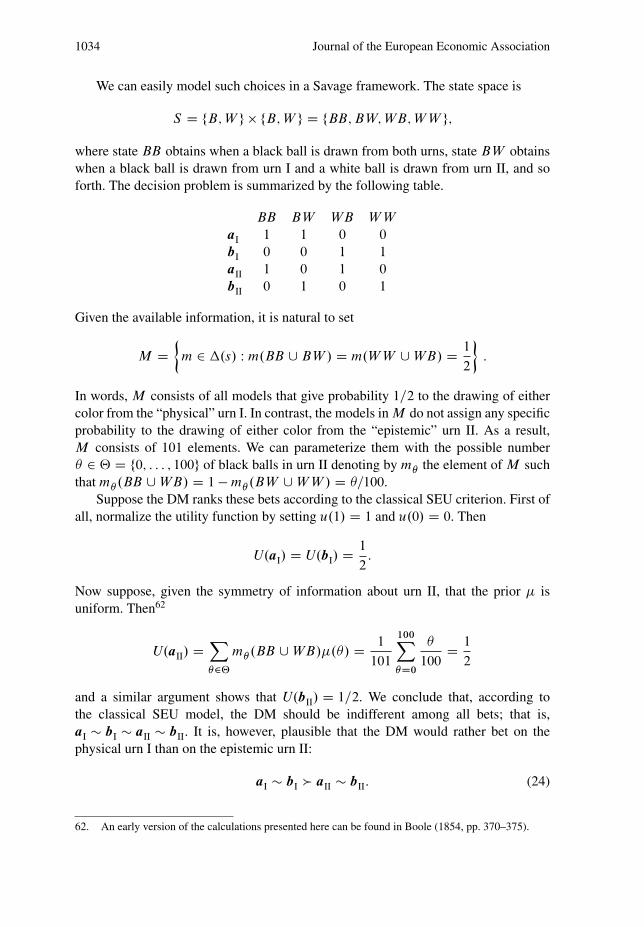
1034 Journal of the European Economic Association
We can easily model such choices in a Savage framework. The state space is
S D fB; W g � fB; W g D fBB; BW; WB; W W g;
where state BB obtains when a black ball is drawn from both urns, state BW obtainswhen a black ball is drawn from urn I and a white ball is drawn from urn II, and soforth. The decision problem is summarized by the following table.
BB BW WB W W
aI 1 1 0 0
bI 0 0 1 1
aII 1 0 1 0
bII 0 1 0 1
Given the available information, it is natural to set
M D�
m 2 �.s/ W m.BB [ BW / D m.W W [ WB/ D 1
2
�:
In words, M consists of all models that give probability 1=2 to the drawing of eithercolor from the “physical” urn I. In contrast, the models in M do not assign any specificprobability to the drawing of either color from the “epistemic” urn II. As a result,M consists of 101 elements. We can parameterize them with the possible number� 2 ‚ D f0; : : : ; 100g of black balls in urn II denoting by m the element of M suchthat m .BB [ WB/ D 1 � m .BW [ W W / D �=100.
Suppose the DM ranks these bets according to the classical SEU criterion. First ofall, normalize the utility function by setting u.1/ D 1 and u.0/ D 0. Then
U.aI/ D U.bI/ D 1
2:
Now suppose, given the symmetry of information about urn II, that the prior � isuniform. Then62
U.aII/ DX2‚
m .BB [ WB/�.�/ D 1
101
100XD0
�
100D 1
2
and a similar argument shows that U.bII/ D 1=2. We conclude that, according tothe classical SEU model, the DM should be indifferent among all bets; that is,aI � bI � aII � bII. It is, however, plausible that the DM would rather bet on thephysical urn I than on the epistemic urn II:
aI � bI � aII � bII: (24)
62. An early version of the calculations presented here can be found in Boole (1854, pp. 370–375).

Marinacci Model Uncertainty 1035
Besides introspection, overwhelming experimental evidence confirms this preferencepattern. Remarkably, the pattern emerges as soon as we distinguish—via the smoothambiguity model—between attitudes toward physical and epistemic uncertainty. Tothis end, we normalize also the utility function v by setting v.1/ D 1 and v.0/ D 0,and we assume that � D v ı u�1 is strictly concave, so that the DM is strictly ambiguityaverse (i.e., he is strictly more averse to epistemic than to physical uncertainty). Westill have V.aI/ D V.bI/ D 1=2, but now
V.aII/ DX2‚
�.m .BB [ WB//�.�/ D 1
101
100XD0
�
��
100
�
< �
1
101
100XD0
�
100
!D �
�1
2
�:
A similar argument shows that V.bII/ D V.aII/. Hence the Ellsberg pattern (24)emerges as soon as we distinguish the different attitudes by considering a higheraversion to epistemic than to physical uncertainty.
Three Colors. We return now to Section 3.1’s urn example in which DMs were toldthat 30 balls are red, so that M D fm 2 �.fB; G; Rg/ W m.R/ D 1=3g. We observedthat classical SEU implies that aR � aB � aG—that is, the DMs are indifferent amongbetting on any of the three colors—when a uniform prior � is assumed. Such a priorresults from the symmetric information about all possible compositions of green andblue balls.
Given the available information, it is plausible that DMs prefer betting on red tobetting on either green or blue; that is,
aR � aB � aG : (25)
In fact, all posited models agree on the probability of R, but they differ substantiallyon that of the other two colors.
We adopt the normalizations of the two urns paradox, that is, u.1/ D v.1/ D 1 andu.0/ D v.0/ D 0. Under the uniform prior of Section 3.1, we have V.aR/ D �.1=3/
and
V.aG/ D60X
D0
�.m .G//�.�/ D 1
61
60XD0
�
��
90
�< �
1
61
60XD0
�
90
!D �
�1
3
�:
A similar argument shows that V.aG/ D V.aB/. Hence pattern (25) is easily justifiedonce we account for differences in attitudes.
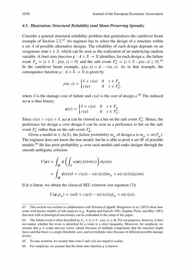
1036 Journal of the European Economic Association
4.5. Illustration: Structural Reliability (and Mean-Preserving Spreads)
Consider a general structural reliability problem that generalizes the cantilever beamexample of Section 2.2.63 An engineer has to select the design of a structure withina set A of possible alternative designs. The reliability of each design depends on anexogenous state s 2 S , which can be seen as the realization of an underlying randomvariable. A limit state function g W A � S ! R identifies, for each design a, the failureevent Fa D fs 2 S W g.a; s/ < 0g and the safe event F c
a D fs 2 S W g.a; s/ � 0g.64
In the cantilever beam example, g.a; s/ D d � �.a; s/. As in that example, theconsequence function � W A � S ! R is given by
�.a; s/ D�
ı C c.a/ if s 2 Fa
c.a/ if s 2 F ca ;
where ı is the damage cost of failure and c.a/ is the cost of design a.65 The inducedact a is thus binary:
a.s/ D�
ı C c.a/ if s 2 Fa
c.a/ if s 2 F ca :
Since c.a/ > c.a/ C ı, act a can be viewed as a bet on the safe event F ca . Hence, the
preference for design a over design b can be seen as a preference to bet on the safeevent F c
a rather than on the safe event F cb
.Given a model m 2 �.S/, the failure probability ma of design a is ma D m.Fa/.
The engineer does not know the true model, but he is able to posit a set M of possiblemodels.66 He has prior probability � over such models and ranks designs through thesmooth ambiguity criterion
V.a/ DZ
M
�
�ZS
u.a.s//dm.s/
�d�.m/
DZ
M
�..u.ı C c.a// � u.c.a///ma C u.c.a///d�.m/:
If � is linear, we obtain the classical SEU criterion (see equation (7))
U.a; N�a/ D .u.ı C c.a// � u.c.a/// N�a C u.c.a//;
63. This section was written in collaboration with Veronica Cappelli. Borgonovo et al. (2015) show howsome well-known models of risk analysis (e.g., Kaplan and Garrick 1981; Kaplan, Perla, and Bley 1983)that deal with technological uncertainty can be embedded in the setup of this paper.
64. The failure event is often described as Fa
D fs 2 S W g.a; s/ � 0g. For our purposes, however, it doesnot matter whether the event is identified by a weak or a strict inequality. Moreover, for simplicity weassume that g is scalar and not vector valued (because of multiple components that the structure mighthave) and that there is a single threshold, zero, and not multiple ones (because of different possible damagelevels).
65. To ease notation, we assume that costs ı and c.a/ are negative scalars.
66. For simplicity, we assume that the limit state function g is known.
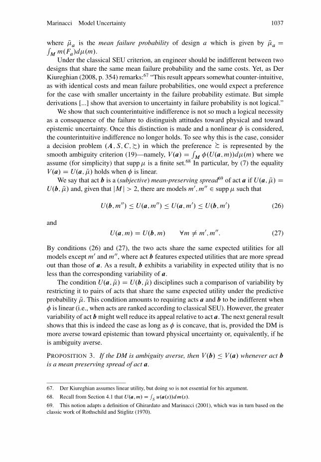
Marinacci Model Uncertainty 1037
where N�a is the mean failure probability of design a which is given by N�a DRM m.Fa/d�.m/.
Under the classical SEU criterion, an engineer should be indifferent between twodesigns that share the same mean failure probability and the same costs. Yet, as DerKiureghian (2008, p. 354) remarks:67 “This result appears somewhat counter-intuitive,as with identical costs and mean failure probabilities, one would expect a preferencefor the case with smaller uncertainty in the failure probability estimate. But simplederivations [...] show that aversion to uncertainty in failure probability is not logical.”
We show that such counterintuitive indifference is not so much a logical necessityas a consequence of the failure to distinguish attitudes toward physical and towardepistemic uncertainty. Once this distinction is made and a nonlinear � is considered,the counterintuitive indifference no longer holds. To see why this is the case, considera decision problem .A; S; C; %/ in which the preference � is represented by thesmooth ambiguity criterion (19)—namely, V.a/ D R
M �.U.a; m//d�.m/ where weassume (for simplicity) that supp � is a finite set.68 In particular, by (7) the equalityV.a/ D U.a; N�/ holds when � is linear.
We say that act b is a (subjective) mean-preserving spread69 of act a if U.a; N�/ DU.b; N�/ and, given that jM j > 2, there are models m0; m00 2 supp � such that
U.b; m00/ U.a; m00/ U.a; m0/ U.b; m0/ (26)
and
U.a; m/ D U.b; m/ 8m ¤ m0; m00: (27)
By conditions (26) and (27), the two acts share the same expected utilities for allmodels except m0 and m00, where act b features expected utilities that are more spreadout than those of a. As a result, b exhibits a variability in expected utility that is noless than the corresponding variability of a.
The condition U.a; N�/ D U.b; N�/ disciplines such a comparison of variability byrestricting it to pairs of acts that share the same expected utility under the predictiveprobability N�. This condition amounts to requiring acts a and b to be indifferent when� is linear (i.e., when acts are ranked according to classical SEU). However, the greatervariability of act b might well reduce its appeal relative to act a. The next general resultshows that this is indeed the case as long as � is concave, that is, provided the DM ismore averse toward epistemic than toward physical uncertainty or, equivalently, if heis ambiguity averse.
PROPOSITION 3. If the DM is ambiguity averse, then V.b/ V.a/ whenever act b
is a mean preserving spread of act a.
67. Der Kiureghian assumes linear utility, but doing so is not essential for his argument.
68. Recall from Section 4.1 that U.a; m/ D RS
u.a.s//dm.s/.
69. This notion adapts a definition of Ghirardato and Marinacci (2001), which was in turn based on theclassic work of Rothschild and Stiglitz (1970).

1038 Journal of the European Economic Association
In short, the indifference prescribed by classical SEU between acts a and b failsto hold as soon as the distinction between the attitudes toward epistemic and towardphysical uncertainty is made.70
Returning now to the design choice, consider two designs a and b that sharethe same costs. Since U.a; m/ D .u.ı C c.a// � u.c.a///ma C u.c.a//, it easilyfollows that b is a mean-preserving spread of a if and only if N�a D N�b and thereare m0; m00 2 supp � such that
m00b m00
a m0a m0
b
and ma D mb for all m ¤ m0; m00. By Proposition 3, ambiguity-averse engineers preferdesign a over design b even though the two designs share the same mean failureprobability and the same costs. In other words, engineers who are more averse towardepistemic than toward physical uncertainty exhibit the “preference for the case withsmaller uncertainty in the failure probability estimate” that Der Kiureghian (2008),previously quoted, claims is intuitive.
4.6. Extreme Ambiguity Aversion: Maxmin
Wald. Under extreme ambiguity aversion—that is, when ambiguity aversion “goesto infinity”—the smooth ambiguity criterion (17) reduces in the limit (under finitenessof M ) to the classic Wald (1950) maxmin criterion71
V.a/ D minm2M
ZS
u.a.s//dm.s/: (28)
Under this very cautious criterion, the DM “maxminimizes” over all possibleprobability models in M . Prior probabilities do not play any role.
We illustrate this limit result in an important special case. Mathematically,increasing ambiguity aversion corresponds to increasing concavity of the function� W Im u ! R. When this function is twice differentiable, its Arrow–Pratt index ofconcavity is D ��00=�0. In the CARA case ��.x/ D �e��x , for instance, theparameter > 0 is the constant Arrow–Pratt index, and so �� features constantabsolute ambiguity aversion (Section 4.2(iii)). Consider the utility certainty equivalent(Example 1)
c�.a; �/ D � 1
log
ZM
e��R
Su.a.s//dm.s/d�.m/ (29)
with > 0. Here ambiguity aversion goes to infinity or to zero provided that ! C1or ! 0, respectively. In particular, since v� D �� ı u, it is the aversion to epistemicuncertainty that underlies these limit cases.
70. We will refrain (for the sake of brevity) from further analysis, but all these considerations holdalso for the case of acts that—though not directly comparable through a mean-preserving spread—canbe connected via a finite sequence of intermediate acts that are, instead, comparable in that sense (seeRothschild and Stiglitz 1970, p. 231).
71. See KMM (p. 1867). This section was written in collaboration with Simone Cerreia-Vioglio.
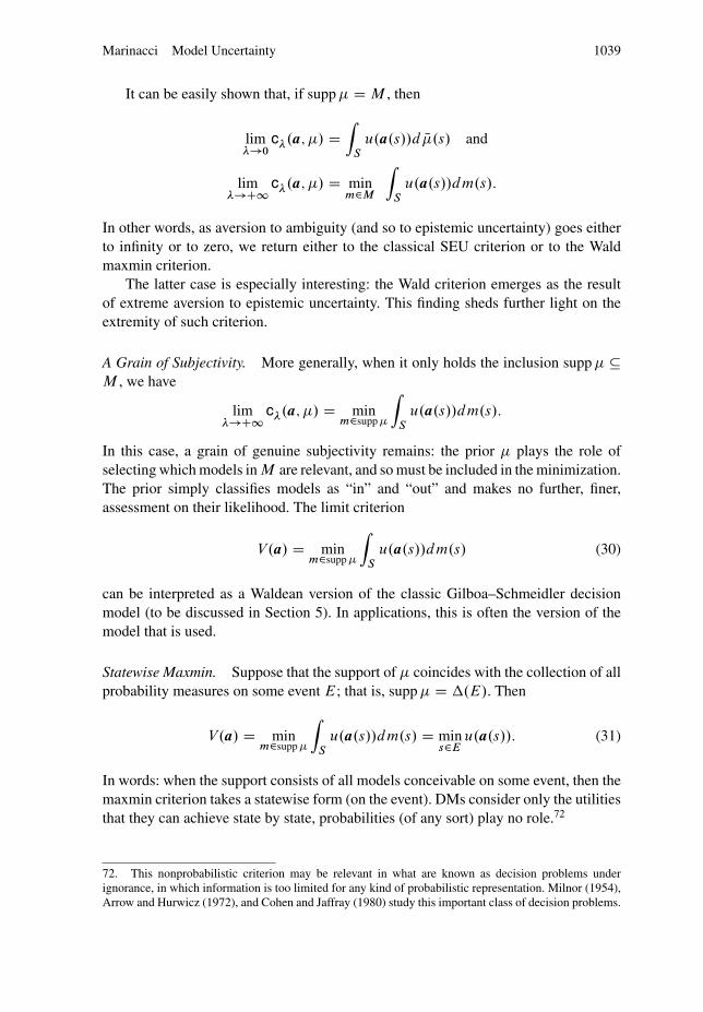
Marinacci Model Uncertainty 1039
It can be easily shown that, if supp � D M , then
lim�!0
c�.a; �/ DZ
S
u.a.s//d N�.s/ and
lim�!C1
c�.a; �/ D minm2M
ZS
u.a.s//dm.s/:
In other words, as aversion to ambiguity (and so to epistemic uncertainty) goes eitherto infinity or to zero, we return either to the classical SEU criterion or to the Waldmaxmin criterion.
The latter case is especially interesting: the Wald criterion emerges as the resultof extreme aversion to epistemic uncertainty. This finding sheds further light on theextremity of such criterion.
A Grain of Subjectivity. More generally, when it only holds the inclusion supp � �M , we have
lim�!C1
c�.a; �/ D minm2supp �
ZS
u.a.s//dm.s/:
In this case, a grain of genuine subjectivity remains: the prior � plays the role ofselecting which models in M are relevant, and so must be included in the minimization.The prior simply classifies models as “in” and “out” and makes no further, finer,assessment on their likelihood. The limit criterion
V.a/ D minm2supp �
ZS
u.a.s//dm.s/ (30)
can be interpreted as a Waldean version of the classic Gilboa–Schmeidler decisionmodel (to be discussed in Section 5). In applications, this is often the version of themodel that is used.
Statewise Maxmin. Suppose that the support of � coincides with the collection of allprobability measures on some event E; that is, supp � D �.E/. Then
V.a/ D minm2supp �
ZS
u.a.s//dm.s/ D mins2E
u.a.s//: (31)
In words: when the support consists of all models conceivable on some event, then themaxmin criterion takes a statewise form (on the event). DMs consider only the utilitiesthat they can achieve state by state, probabilities (of any sort) play no role.72
72. This nonprobabilistic criterion may be relevant in what are known as decision problems underignorance, in which information is too limited for any kind of probabilistic representation. Milnor (1954),Arrow and Hurwicz (1972), and Cohen and Jaffray (1980) study this important class of decision problems.
1040 Journal of the European Economic Association
A No-Trade Illustration. In a frictionless financial market, consider a primary assety W S ! R that pays out y.s/ if state s 2 S obtains. The market price of each unit ofthe asset is p. Investors have to decide how many units x 2 R of the asset to trade. Ifx > 0, investors buy the asset; if x < 0, they sell it; if x D 0, there is no trade.
In any case, a portfolio with x units of the asset has a, state contingent, payoffyx � px.73 The associated act x W S ! R is given by x.s/ D y.s/x � px. There isno trade on asset y when V.x/ < V.0/ for all x ¤ 0, that is, when investors do notbenefit from either buying or from selling the asset. Assume risk neutrality. The nextresult, which adapts to the present setup a classic result of Dow and Werlang (1992),shows that with maxmin behavior there might be no trade (unless the asset is crisp74).
PROPOSITION 4. Under maxmin behavior (29), there is no trade in asset y if andonly if its price satisfies
minm2supp �
Em.y/ < p < maxm2supp �
Em.y/: (32)
Condition (32) requires supp � to be nonsingleton; thus model uncertainty isessential for the result. In particular: the larger is the support of � (and so the perceivedmodel uncertainty), the larger the inequality and hence the set of prices that result inno trade.
Extreme ambiguity aversion may thus freeze market transactions—an importantinsight that has been often discussed in the literature.75 This suggests that sufficientlyhigh ambiguity aversion may arbitrarily reduce trade volumes. To see why this is thecase, suppose investors rank these acts through the utility certainty equivalent (29).Under risk neutrality, we then have, in shorthand notation,
c�.x; �/ D � 1
log E�e��E
mx: (33)
The next simple property will be useful.
LEMMA 1. c�.x; �/ c��.x; �/ for all x 2 R, with equality if x is crisp.
We say that there is at most "-trade volume on asset y if c�.x; �/ < 0 for allx … .�"; "/; in words, investors may benefit only from transactions involving quantitiessmaller than ". Next we show that sufficiently high ambiguity aversion can explain anyarbitrarily low trade volume (unless the asset is crisp).
PROPOSITION 5. Let " > 0. There is at most "-trade volume in asset y if
c"�.y; �/ < p < c�"�.y; �/: (34)
73. We abstract from any intertemporal issue (see Section 4.10).
74. That is, Em
x DEm0 x for all m; m0 2 supp �.
75. See, for example, Guidolin and Rinaldi (2013).

Marinacci Model Uncertainty 1041
In particular, the inequality holds when " is large enough (something that requiresa higher if " is smaller) provided the previous no-trade inequality (32) holds.76 Sowhenever the price of an asset precludes its being traded under maxmin behavior,a higher ambiguity aversion corresponds to lower trade volume on the asset undercriterion (33).
Extreme Risk Aversion. So far we have regarded maxmin behavior as the result ofextreme ambiguity aversion—that is, of a much higher aversion to model uncertaintythan to risk. Formally, however, the outcome statewise maxmin criterion a la LeontiefV.a/ D mins2S a.s/ can be seen as a limit version of the classic SEU criterion (5)as risk aversion becomes increasingly larger (see Laffont 1989). In other words, theLeontief criterion can correspond either to extreme risk aversion or to risk neutralitywith extreme model uncertainty aversion. The latter interpretation is consistent withpresuming that DMs are more averse to model uncertainty than to risk. Nonetheless,variations of the previous no trade (resp., low trade) results hold under extreme (resp.,high enough) levels of risk aversion. It remains an empirical and experimental issueto determine which is the more plausible behavioral hypothesis: high risk aversion ornormal risk aversion and high model uncertainty aversion.
4.7. Quadratic Approximation: Mean-Variance
For monetary acts, the smooth ambiguity criterion admits a simple quadraticapproximation that generalizes the well-known quadratic approximation of expectedutility. To show this we take a consequence w and an act b,77 and we consider thecertainty equivalent
c.w C b; �/ D v�1.E�v.c.w C b; m/// v�1
�ZM
v.c.w C b; m//d�.m/
�:
Maccheroni, Marinacci, and Ruffino (2013) show that, under standard differentiabilityassumptions on the functions u and v, the quadratic approximation of this certaintyequivalent is given by78
c.w C b; �/ w C E N�b � 1
2 u.w/2N�.b/ � 1
2. v.w/ � u.w//2
�.E.b//; (35)
76. Since lim˛!C1
c˛
.y; �/ D minm2supp �
Em
.y/ and lim˛!C1
c�˛
.y; �/ D maxm2supp �
Em
.y/.
77. With a slight abuse of notation, we denote by w the consequence and also the constant act equalto w in all states. In the financial applications that originally motivated quadratic approximations, w isinterpreted as initial wealth and Qb as an investment.
78. In (35) and thereafter, �u
D �u00=u0 and �v
D �v00=v0 are the classic Arrow–Pratt coefficients ofrisk aversion.
1042 Journal of the European Economic Association
where E.b/ W M ! R is the random variable
m 7! Emb Z
S
b.s/dm.s/
that associates the expected value of act b under each possible model m, and 2�.E.b//
is its variance. The quadratic approximation (35) extends the classic Arrow–Prattversion
c.w C b; �/ w C E N�b � 1
2 u.w/2N�.b/ (36)
of the SEU criterion (7). Relative to the Arrow–Pratt approximation, (35) features thenovel term
1
2. v.w/ � u.w//2
�.E.b//:
This term is an ambiguity premium jointly determined by the variance 2�.E.b//, an
information trait that captures the scope of model uncertainty that the DM perceives,and by the difference v.w/ � u.w/, a taste trait that captures the DM’s differencesin attitudes toward physical and toward epistemic uncertainty.79 In this regard, notethat v � u when v is more concave than u, that is, when the DM is more averse toepistemic than to physical uncertainty.
The approximation (35) leads to a natural generalization of the classic mean-variance model in which DMs rank acts a in terms of the robust mean-variancefunctional given by
E N�a �
22N�.a/ � �
22
�.E.a//; (37)
where and � are positive coefficients. This criterion is determined by the threeparameters , � , and �. In particular, when � D 0 we return to the usual mean-variance functional. In light of equation (35), criterion (37) can be viewed as a localquadratic approximation of a smooth ambiguity criterion at a constant w such that D u.w/ and � D v.w/ � u.w/. Thus, the taste parameters and � model theDM’s attitudes toward physical and epistemic uncertainty, respectively. Higher valuesof these parameters correspond to stronger negative attitudes.
The information parameter � determines the variances 2N�.a/ and 2�.E.a// that
measure, respectively, the physical and epistemic uncertainties that the DM perceiveswhen evaluating act a. Higher values of these variances correspond to a DM’s poorerinformation regarding such uncertainties.
Since the variance 2N�.b/ can be decomposed by the law of total variance,80 theapproximation (35) can be rearranged according to the Arrow–Pratt coefficients of u
and v:
c.w C b; �/ w C E N�b � u.w/
2E�2.b/ � v.w/
22
�.E.b//: (38)
79. See Jewitt and Mukerji (2011) and Lang (2015) for related notions of ambiguity premium.
80. That is, �2N�.b/ D E
�.�2.b// C �2
�.E.b//.

Marinacci Model Uncertainty 1043
This formulation suggests the conditions under which such an approximation is exact.It is well known that, if u is CARA and b has a normal distribution with mean k andvariance 2, then the Arrow–Pratt approximation (36) takes the following exact form:
c.w C b; �/ D w C k � 1
2 u.w/2:
This result easily generalizes to the quadratic approximation (38): if both u and v areCARA utility functions with respective constant Arrow–Pratt coefficients ˛ and ˇ, andif b has a normal distribution with unknown mean k and known variance 2, then (38)takes the exact form
c.w C b; �/ D w C Nk � 1
2˛2 � 1
2ˇ2
� (39)
as long as the prior on the unknown mean k is given by a normal distribution withparameters Nk and 2
�.81
Finally, the quadratic approximation may be part of an exact series expansionof the certainty equivalent. For example, consider the risk-neutral case c.a; �/ D�ˇ�1 log E�e�ˇE
ma in which u.x/ D x and v.x/ D �e�ˇx (Example 1). Its quadratic
approximation (35) is c.w C b; �/ w C E N�b � .ˇ=2/2�.E.b//. At the same time,
under standard regularity conditions we have, for ˇ ¤ 0 small enough, the expansion(see the Appendix)
c.w C b; �/ D w C E N�b � 1
2ˇ2
�.E.b// C1X
nD3
.�1/nC1
nŠˇn�1cn.E.b//: (40)
Here cn.E.b// is the nth cumulant of the random variable E.b/ W M ! R, which canbe expressed in terms of higher moments (with the third and fourth cumulants relatedto skewness and kurtosis, respectively; see, for example, Kendall 1946, Chap. 3).
When the prior is such that the random variable E.b/ has a normal distribution withparameters k and 2
�, the cumulants n � 3 are zero and so the expansion (40) takes thequadratic form (39); that is, c.w C b; �/ D w C k � .ˇ=2/2
�. However, unlike (39)this quadratic expansion does not rely on any normality assumption on b itself.
4.8. Behavioral Foundation
The smooth ambiguity representation admits a simple behavioral foundation in aclassical decision problem .A; S; C; M; %/ when M is a finite orthogonal set and actsare monetary (Section 3.2).82
81. The normality of the prior implies that Nk is the mean of the unknown means k and that �2�
is theirvariance.
82. This section was written in collaboration with Fabio Maccheroni. For a related axiomatization, in anintertemporal setting, see Cerreia-Vioglio et al. (2013a).

1044 Journal of the European Economic Association
Specifically, denote by E D fEmgm2M the event partition such that m.Em/ D 1
and m.Em0/ D 0 if m0 ¤ m (Section 3.2). We make a few assumptions, most of whichrely on that partition. We begin with a basic requirement on the preference.
ASSUMPTION 1. The preference � is both complete and transitive.
Next we assume that subjective expected utility applies to acts that are E-measurable.
ASSUMPTION 2. There exists a continuous and strictly increasing function v W R ! R
and a probability measure P on E such that a � v�1.R
S v.a.s//dP.s// for each E-measurable act a 2 A.
Next we assume a famous Savage axiom, but on a restricted class of acts. Givenany two acts a; b 2 A and any event E, set
aEb D�
a.s/ if s 2 E
b.s/ if s … E:
In words, aEb is the act that “mixes” acts a and b via event E.
ASSUMPTION 3 (Conditional Sure Thing Principle). If a; b; c; d 2 A and E 2 E ,then
aEc % bEc () aEd % bEd :
According to this separability requirement, the ranking of acts is independent ofcommon parts that depend on events, such as Ec , belonging to the algebra generatedby E . This assumption allows us to define, for each E 2 E , the conditional preference%E by
a %E b () aEc % bEc 8c 2 A:
Next we assume that each such conditional preference has an expected utilityrepresentation.
ASSUMPTION 4. There exists a continuous and strictly increasing function u W R ! R
such that, for each m 2 M , we have a �Em
u�1.R
S u.a.s//dm.s// for all a 2 A.
We can now establish the desired behavioral foundation for smooth ambiguity.83
PROPOSITION 6. A preference � on A satisfies Assumptions 1–4 if and only if thereexists a probability measure � on M such that representation (17) holds, that is,V.a/ D v�1.
RM v.U.a; m//d�.m//. In particular, N� D P on E .
The probability P in Assumption 2 is nothing but the restriction on the partition Eof the predictive probability N�.
83. Unlike Assumption 2, Assumptions 1 and 3 are not in behavioral terms; it is, however, a routineexercise to translate them into such terms through existing behavioral foundations of subjective expectedutility in finite and infinite state spaces.
Marinacci Model Uncertainty 1045
To understand this result, note that orthogonality entails that each model m
identifies a single atom Em of the partition E . In fact, conditional on event Em,only the physical risk described by m matters, that is, N�.EjEm/ D m.EjEm/. Therelative likelihood of different models thus corresponds to the relative likelihood ofthe different atoms. In other words, model uncertainty reduces to uncertainty overthese atoms. Assumption 2 thus amounts to assuming expected utility for this kindof uncertainty. Given any atom, physical uncertainty emerges through the conditionalpreference %E
m; as a result, Assumption 4 assumes expected utility also for this other
kind of uncertainty. The proof of Proposition 6 (see the Appendix) shows how tocombine the two separate expected utility assumptions into the representation (17).
4.9. Optima
Here we consider optimization problems of the form maxa2A V.a/, which play a keyrole in applications.
Back to Actions. Until now we have considered a few decision criteria within Savage’sframework .A; S; C; %/, with acts rather than actions as the objects of choice. Althoughthis framework is the one best suited for theoretical analysis, in applications it is oftenmore convenient to deal with actions than with acts, and so to consider the action-basedclassical decision problem .A; S; C; �; M; %/. Actions can be easier to interpret, asremarked in Section 2.4, and can be represented as vectors; hence they can be easierto handle analytically than acts, which are functions.
Be that as it may, we refer to r D u ı � W A � S ! R as the payoff (or reward)function. The expected payoff R.a; m/ D R
S r.a; s/dm.s/ of action a is simply theexpected utility U.a; m/ of the associated act a. The smooth criterion can then bewritten, in shorthand notation, as V.a/ D E��.R.a; m// R
M �.R.a; m//d�.m/.
Optima. We are now in a position to deal with the previous optimization problem,which can be written in terms of actions as
maxa2A
V.a/ D maxa2A
E��.R.a; m//: (41)
The following proposition, which extends a portfolio result of Taboga (2005) andGollier (2011), shows how this problem is equivalent to an expected utility problemwhen the original prior � is replaced by a tilted version O�, whose form depends on allelements of the decision problem at hand, including ambiguity attitudes.
PROPOSITION 7. Suppose that � W Im R ! R is twice differentiable, with �0 > 0
and �00 < 0. For each s 2 S , let r.�; s/ W A � Rn ! R be continuously differentiable
and strictly concave on the convex set A. Then there exists a probability measureO� 2 �.M /, equivalent to �, such that problems
maxa2A
E��.R.a; m// and maxa2A
E O�R.a; m/ (42)
1046 Journal of the European Economic Association
share the same solution Oa. In particular, O�.m/ D �.m/�.m/ where � W M ! R is theRadon–Nikodym function
�.m/ D �0.R. Oa; m//
E��0.R. Oa; m//: (43)
Since �0 is decreasing, the tilted prior O� alters, through �, the original prior � byshifting weight to models m with a lower expected utility R. Oa; m/, thus magnifyingtheir relative importance. Formally,
�.m0/ < �.m/ () R. Oa; m/ < R. Oa; m0/:
In sum, action Oa solves problem maxa2A E O�R.a; m/ even though O� handicaps Oaby overweighting its cons—at the expense of its pros—relative to the original prior�. In this sense, Oa is a robust solution when compared to the solution of the expectedutility problem maxa2A E�R.a; m/. Ambiguity aversion can thus be seen as a desirefor robustness on the problem solutions.84
EXAMPLE 2. In the CARA case �.x/ D �e��x , we have the exponential tilt�.m/ / e��R. Oa;m/. In the CRRA case �.x/ D x�, we have the power tilt �.m/ /R. Oa; m/��1. �
An action a 2 A is crisp for a smooth preference � if R.a; m/ D R.a; m0/ for allm; m0 2 supp � (see Section 3.1). Crisp actions are not sensitive to model uncertaintyand so for them � D 1; this equality implies the following corollary.
COROLLARY 1. Under the hypotheses of Proposition 7, the two problems in (41)share the same solution if it is crisp.
In short, ambiguity attitudes may matter only for decision problems that do nothave crisp solutions.
We close by observing that the tilted prior can be also regarded as a mixture, withweight determined by �, of the original prior and of another prior. Tilting can be thusseen as a convexification of priors.
LEMMA 2. There exist ˛ 2 .0; 1� and � 2 �.M / such that O� D ˛� C .1 � ˛/� ifand only if ˛ minm2supp � �.m/.85
Monetary Policy Illustration. To illustrate the previous result, we continue our studyof the monetary policy problem (Section 3.1). For that purpose we define a bivariate
84. For instance, in environmental policy making this feature of ambiguity aversion can provide arationale for some forms of the precautionary principle (Stern 2007). The more stringent the principle, thehigher the underlying ambiguity aversion (until the limit maxmin criteria of Section 4.6).
85. When M is not finite, the lemma requires the (almost everywhere) boundedness of � .
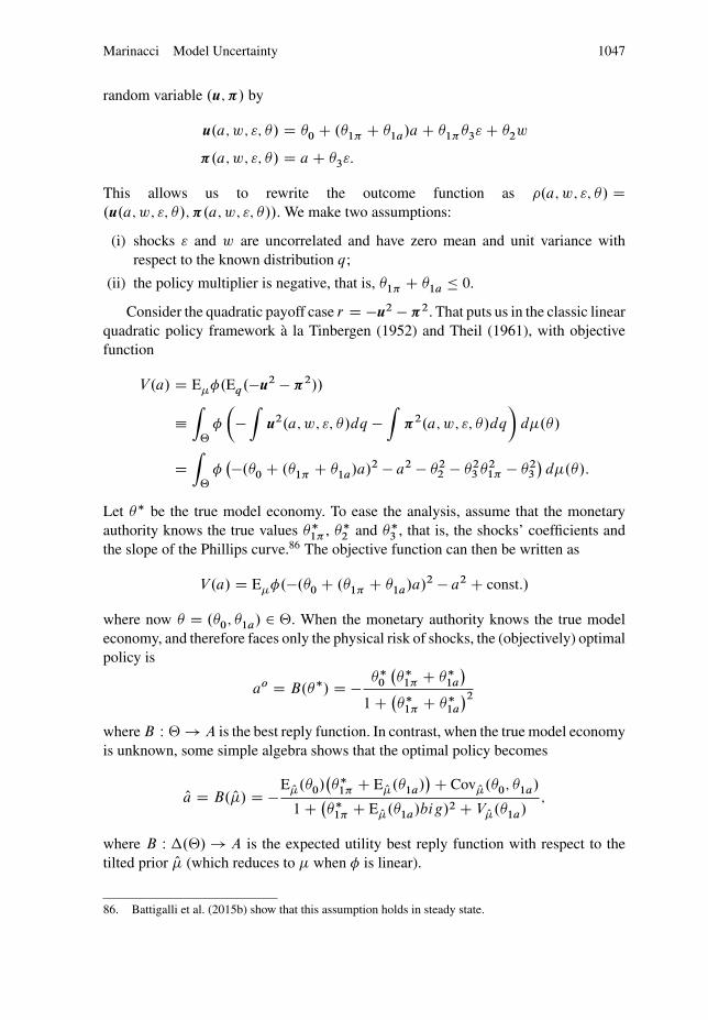
Marinacci Model Uncertainty 1047
random variable .u; �/ by
u.a; w; "; �/ D �0 C .�1� C �1a/a C �1��3" C �2w
�.a; w; "; �/ D a C �3":
This allows us to rewrite the outcome function as �.a; w; "; �/ D.u.a; w; "; �/; �.a; w; "; �//. We make two assumptions:
(i) shocks " and w are uncorrelated and have zero mean and unit variance withrespect to the known distribution q;
(ii) the policy multiplier is negative, that is, �1� C �1a 0.
Consider the quadratic payoff case r D �u2 � �2. That puts us in the classic linearquadratic policy framework a la Tinbergen (1952) and Theil (1961), with objectivefunction
V.a/ D E��.Eq.�u2 � �2//
Z
‚
�
��Z
u2.a; w; "; �/dq �Z
�2.a; w; "; �/dq
�d�.�/
DZ
‚
���.�0 C .�1� C �1a/a/2 � a2 � �2
2 � �23 �2
1� � �23
d�.�/:
Let �� be the true model economy. To ease the analysis, assume that the monetaryauthority knows the true values ��
1� , ��2 and ��
3 , that is, the shocks’ coefficients andthe slope of the Phillips curve.86 The objective function can then be written as
V.a/ D E��.�.�0 C .�1� C �1a/a/2 � a2 C const:/
where now � D .�0; �1a/ 2 ‚. When the monetary authority knows the true modeleconomy, and therefore faces only the physical risk of shocks, the (objectively) optimalpolicy is
ao D B.��/ D � ��0
���
1� C ��1a
1 C �
��1� C ��
1a
2where B W ‚ ! A is the best reply function. In contrast, when the true model economyis unknown, some simple algebra shows that the optimal policy becomes
Oa D B. O�/ D �E O�.�0/���
1� C E O�.�1a/C Cov O�.�0; �1a/
1 C ���
1� C E O�.�1a/big/2 C V O�.�1a/;
where B W �.‚/ ! A is the expected utility best reply function with respect to thetilted prior O� (which reduces to � when � is linear).
86. Battigalli et al. (2015b) show that this assumption holds in steady state.
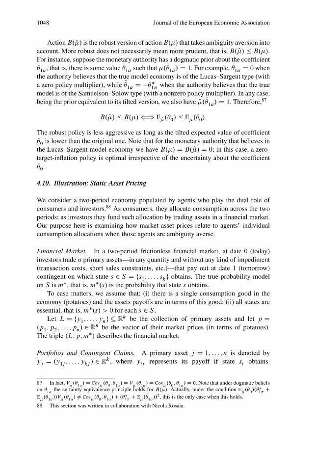
1048 Journal of the European Economic Association
Action B. O�/ is the robust version of action B.�/ that takes ambiguity aversion intoaccount. More robust does not necessarily mean more prudent, that is, B. O�/ B.�/.For instance, suppose the monetary authority has a dogmatic prior about the coefficient�1a, that is, there is some value N�1a such that �. N�1a/ D 1. For example, N�1a D 0 whenthe authority believes that the true model economy is of the Lucas–Sargent type (witha zero policy multiplier), while N�1a D ���
1� when the authority believes that the truemodel is of the Samuelson–Solow type (with a nonzero policy multiplier). In any case,being the prior equivalent to its tilted version, we also have O�. N�1a/ D 1. Therefore,87
B. O�/ B.�/ () E O�.�0/ E�.�0/:
The robust policy is less aggressive as long as the tilted expected value of coefficient�0 is lower than the original one. Note that for the monetary authority that believes inthe Lucas–Sargent model economy we have B.�/ D B. O�/ D 0; in this case, a zero-target-inflation policy is optimal irrespective of the uncertainty about the coefficient�0.
4.10. Illustration: Static Asset Pricing
We consider a two-period economy populated by agents who play the dual role ofconsumers and investors.88 As consumers, they allocate consumption across the twoperiods; as investors they fund such allocation by trading assets in a financial market.Our purpose here is examining how market asset prices relate to agents’ individualconsumption allocations when those agents are ambiguity averse.
Financial Market. In a two-period frictionless financial market, at date 0 (today)investors trade n primary assets—in any quantity and without any kind of impediment(transaction costs, short sales constraints, etc.)—that pay out at date 1 (tomorrow)contingent on which state s 2 S D fs1; : : : ; skg obtains. The true probability modelon S is m�, that is, m�.s/ is the probability that state s obtains.
To ease matters, we assume that: (i) there is a single consumption good in theeconomy (potatoes) and the assets payoffs are in terms of this good; (ii) all states areessential, that is, m�.s/ > 0 for each s 2 S .
Let L D fy1; : : : ; yng � Rk be the collection of primary assets and let p D
.p1; p2; : : : ; pn/ 2 Rn be the vector of their market prices (in terms of potatoes).
The triple .L; p; m�/ describes the financial market.
Portfolios and Contingent Claims. A primary asset j D 1; : : : ; n is denoted byyj D .y1j ; : : : ; ykj / 2 R
k , where yij represents its payoff if state si obtains.
87. In fact, V�
.1a
/ D Cov�
.0;
1a/ D V
O�.
1a/ D Cov
O�.
0;
1a/ D 0. Note that under dogmatic beliefs
on 1a
the certainty equivalence principle holds for B.�/. Actually, under the condition E�
.0/.�
1�C
E�
.1a
//V�
.1a
/ ¤ Cov�
.0;
1a/ C .�
1�C E
�.
1a//2, this is the only case when this holds.
88. This section was written in collaboration with Nicola Rosaia.
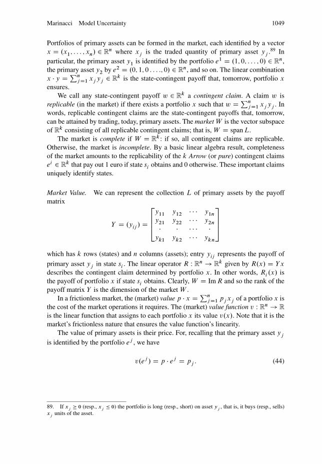
Marinacci Model Uncertainty 1049
Portfolios of primary assets can be formed in the market, each identified by a vectorx D .x1; : : : ; xn/ 2 R
n where xj is the traded quantity of primary asset yj .89 Inparticular, the primary asset y1 is identified by the portfolio e1 D .1; 0; : : : ; 0/ 2 R
n,the primary asset y2 by e2 D .0; 1; 0 : : : :; 0/ 2 R
n, and so on. The linear combinationx � y D Pn
j D1 xj yj 2 Rk is the state-contingent payoff that, tomorrow, portfolio x
ensures.We call any state-contingent payoff w 2 R
k a contingent claim. A claim w isreplicable (in the market) if there exists a portfolio x such that w D Pn
j D1 xj yj . Inwords, replicable contingent claims are the state-contingent payoffs that, tomorrow,can be attained by trading, today, primary assets. The market W is the vector subspaceof R
k consisting of all replicable contingent claims; that is, W D span L.The market is complete if W D R
k : if so, all contingent claims are replicable.Otherwise, the market is incomplete. By a basic linear algebra result, completenessof the market amounts to the replicability of the k Arrow (or pure) contingent claimsei 2 R
k that pay out 1 euro if state si obtains and 0 otherwise. These important claimsuniquely identify states.
Market Value. We can represent the collection L of primary assets by the payoffmatrix
Y D .yij / D
2664
y11 y12 � � � y1n
y21 y22 � � � y2n
� � � � � �yk1 yk2 � � � ykn
3775
which has k rows (states) and n columns (assets); entry yij represents the payoff of
primary asset yj in state si . The linear operator R W Rn ! R
k given by R.x/ D Y x
describes the contingent claim determined by portfolio x. In other words, Ri .x/ isthe payoff of portfolio x if state si obtains. Clearly, W D Im R and so the rank of thepayoff matrix Y is the dimension of the market W .
In a frictionless market, the (market) value p � x D Pnj D1 pj xj of a portfolio x is
the cost of the market operations it requires. The (market) value function v W Rn ! R
is the linear function that assigns to each portfolio x its value v.x/. Note that it is themarket’s frictionless nature that ensures the value function’s linearity.
The value of primary assets is their price. For, recalling that the primary asset yj
is identified by the portfolio ej , we have
v.ej / D p � ej D pj : (44)
89. If xj
� 0 (resp., xj
� 0) the portfolio is long (resp., short) on asset yj
, that is, it buys (resp., sells)x
junits of the asset.
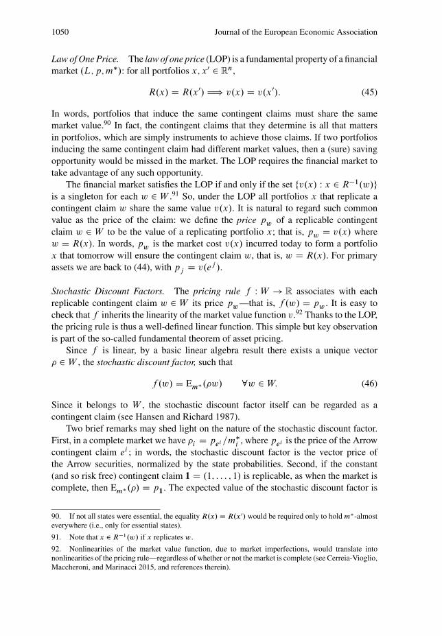
1050 Journal of the European Economic Association
Law of One Price. The law of one price (LOP) is a fundamental property of a financialmarket .L; p; m�/: for all portfolios x; x0 2 R
n,
R.x/ D R.x0/ H) v.x/ D v.x0/: (45)
In words, portfolios that induce the same contingent claims must share the samemarket value.90 In fact, the contingent claims that they determine is all that mattersin portfolios, which are simply instruments to achieve those claims. If two portfoliosinducing the same contingent claim had different market values, then a (sure) savingopportunity would be missed in the market. The LOP requires the financial market totake advantage of any such opportunity.
The financial market satisfies the LOP if and only if the set fv.x/ W x 2 R�1.w/gis a singleton for each w 2 W .91 So, under the LOP all portfolios x that replicate acontingent claim w share the same value v.x/. It is natural to regard such commonvalue as the price of the claim: we define the price pw of a replicable contingentclaim w 2 W to be the value of a replicating portfolio x; that is, pw D v.x/ wherew D R.x/. In words, pw is the market cost v.x/ incurred today to form a portfoliox that tomorrow will ensure the contingent claim w, that is, w D R.x/. For primaryassets we are back to (44), with pj D v.ej /.
Stochastic Discount Factors. The pricing rule f W W ! R associates with eachreplicable contingent claim w 2 W its price pw—that is, f .w/ D pw . It is easy tocheck that f inherits the linearity of the market value function v.92 Thanks to the LOP,the pricing rule is thus a well-defined linear function. This simple but key observationis part of the so-called fundamental theorem of asset pricing.
Since f is linear, by a basic linear algebra result there exists a unique vector� 2 W , the stochastic discount factor, such that
f .w/ D Em�.�w/ 8w 2 W: (46)
Since it belongs to W , the stochastic discount factor itself can be regarded as acontingent claim (see Hansen and Richard 1987).
Two brief remarks may shed light on the nature of the stochastic discount factor.First, in a complete market we have �i D pei =m�
i , where pei is the price of the Arrowcontingent claim ei ; in words, the stochastic discount factor is the vector price ofthe Arrow securities, normalized by the state probabilities. Second, if the constant(and so risk free) contingent claim 1 D .1; : : : ; 1/ is replicable, as when the market iscomplete, then Em�.�/ D p1. The expected value of the stochastic discount factor is
90. If not all states were essential, the equality R.x/ D R.x0/ would be required only to hold m�-almosteverywhere (i.e., only for essential states).
91. Note that x 2 R�1.w/ if x replicates w.
92. Nonlinearities of the market value function, due to market imperfections, would translate intononlinearities of the pricing rule—regardless of whether or not the market is complete (see Cerreia-Vioglio,Maccheroni, and Marinacci 2015, and references therein).
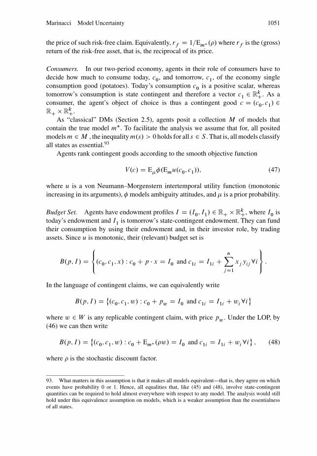
Marinacci Model Uncertainty 1051
the price of such risk-free claim. Equivalently, rf D 1=Em�.�/ where rf is the (gross)return of the risk-free asset, that is, the reciprocal of its price.
Consumers. In our two-period economy, agents in their role of consumers have todecide how much to consume today, c0, and tomorrow, c1, of the economy singleconsumption good (potatoes). Today’s consumption c0 is a positive scalar, whereastomorrow’s consumption is state contingent and therefore a vector c1 2 R
kC. As aconsumer, the agent’s object of choice is thus a contingent good c D .c0; c1/ 2RC � R
kC.As “classical” DMs (Section 2.5), agents posit a collection M of models that
contain the true model m�. To facilitate the analysis we assume that for, all positedmodels m 2 M , the inequality m.s/ > 0 holds for all s 2 S . That is, all models classifyall states as essential.93
Agents rank contingent goods according to the smooth objective function
V.c/ D E��.Emu.c0; c1//; (47)
where u is a von Neumann–Morgenstern intertemporal utility function (monotonicincreasing in its arguments), � models ambiguity attitudes, and � is a prior probability.
Budget Set. Agents have endowment profiles I D .I0; I1/ 2 RC � RkC, where I0 is
today’s endowment and I1 is tomorrow’s state-contingent endowment. They can fundtheir consumption by using their endowment and, in their investor role, by tradingassets. Since u is monotonic, their (relevant) budget set is
B.p; I / D8<:.c0; c1; x/ W c0 C p � x D I0 and c1i D I1i C
nXj D1
xj yij 8i
9=; :
In the language of contingent claims, we can equivalently write
B.p; I / D ˚.c0; c1; w/ W c0 C pw D I0 and c1i D I1i C wi8i
�where w 2 W is any replicable contingent claim, with price pw . Under the LOP, by(46) we can then write
B.p; I / D ˚.c0; c1; w/ W c0 C Em�.�w/ D I0 and c1i D I1i C wi8i
�; (48)
where � is the stochastic discount factor.
93. What matters in this assumption is that it makes all models equivalent—that is, they agree on whichevents have probability 0 or 1. Hence, all equalities that, like (45) and (48), involve state-contingentquantities can be required to hold almost everywhere with respect to any model. The analysis would stillhold under this equivalence assumption on models, which is a weaker assumption than the essentialnessof all states.
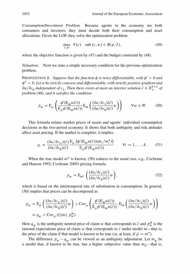
1052 Journal of the European Economic Association
Consumption/Investment Problem. Because agents in the economy are bothconsumers and investors, they must decide both their consumption and assetallocations. Given the LOP, they solve the optimization problem
maxc;w
V.c/ sub .c; w/ 2 B.p; I /; (49)
where the objective function is given by (47) and the budget constraint by (48).
Valuation. Next we state a simple necessary condition for the previous optimizationproblem.
PROPOSITION 8. Suppose that the function � is twice differentiable, with �0 > 0 and�00 < 0. Let u be strictly concave and differentiable, with strictly positive gradient and@u=@c0 independent of c1. Then there exists at most an interior solution Oc 2 R
kC1C of
problem (48), and it satisfies the condition
pw D E�
�0.Emu. Oc//
E��0.Emu. Oc//Em
�.@u=@c1/. Oc/
.@u=@c0/. Oc/w
�!8w 2 W: (50)
This formula relates market prices of assets and agents’ individual consumptiondecisions in the two-period economy. It shows that both ambiguity and risk attitudesaffect asset pricing. If the market is complete, it implies
�i D .@u=@c1i /. Oc/
.@u=@c0/. Oc/
E�
��0.Emu. Oc//.mi=m�
i /
E��0.Emu. Oc//8i D 1; : : : ; k: (51)
When the true model m� is known, (50) reduces to the usual (see, e.g., Cochraneand Hansen 1992; Cochrane 2005) pricing formula
pw D Em�
�.@u=@c1/. Oc/
.@u=@c0/. Oc/w
�; (52)
which is based on the intertemporal rate of substitution in consumption. In general,(50) implies that prices can be decomposed as
pw D E N��
.@u=@c1i /. Oc/
.@u=@c0/. Oc/w
�C Cov�
�0.Emu. Oc//
E��0.Emu. Oc//; Em
�.@u=@c1/. Oc/
.@u=@c0/. Oc/w
�!
qw C Cov� .�.m/; pmw / :
Here qw is the ambiguity neutral price of claim w that corresponds to Oc and pmw is the
rational expectations price of claim w that corresponds to Oc under model m—that is,the price of the claim if that model is known to be true (or, at least, if N� D m�).
The difference pw � qw can be viewed as an ambiguity adjustment. Let mg bea model that, if known to be true, has a higher subjective value than mb—that is,
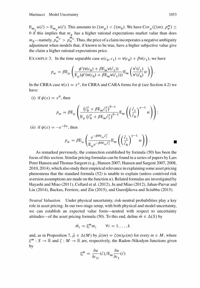
Marinacci Model Uncertainty 1053
Emgu. Oc/ > Em
bu. Oc/. This amounts to �.mg/ < �.mb/. We have Cov�.�.m/; pm
w / 0 if this implies that mg has a higher rational expectations market value than does
mb—namely, pm
g
w > pm
bw . Thus, the price of a claim incorporates a negative ambiguity
adjustment when models that, if known to be true, have a higher subjective value givethe claim a higher rational expectations price.
EXAMPLE 3. In the time separable case u.c0; c1/ D v.c0/ C ˇv.c1/, we have
pw D ˇE�
�0.v.c0/ C ˇEmv. Oc1//
E�.�0.v.c0/ C ˇEmv. Oc1///Em
�v0. Oc1/
v0. Oc0/w
�!:
In the CRRA case v.x/ D x� , for CRRA and CARA forms for � (see Section 4.2) wehave:
(i) if �.x/ D x , then
pw D ˇE�
0@ � Oc�
0 C ˇEm Oc�1
�1
E�
� Oc�0 C ˇEm Oc�
1
�1Em
� Oc1
Oc0
���1
w
!1A I
(ii) if �.x/ D �e�x , then
pw D ˇE�
e�ˇE
mOc�1
E�e�ˇEm
Oc�1
Em
� Oc1
Oc0
���1
w
!!: �
As remarked previously, the connection established by formula (50) has been thefocus of this section. Similar pricing formulas can be found in a series of papers by LarsPeter Hansen and Thomas Sargent (e.g., Hansen 2007; Hansen and Sargent 2007, 2008,2010, 2014), which also study their empirical relevance in explaining some asset pricingphenomena that the standard formula (52) is unable to explain (unless contrived riskaversion assumptions are made on the function u). Related formulas are investigated byHayashi and Miao (2011), Collard et al. (2012), Ju and Miao (2012), Jahan-Parvar andLiu (2014), Backus, Ferriere, and Zin (2015), and Guerdjikova and Sciubba (2015).
Neutral Valuation. Under physical uncertainty, risk-neutral probabilities play a keyrole in asset pricing. In our two-stage setup, with both physical and model uncertainty,we can establish an expected value form—neutral with respect to uncertaintyattitudes—of the asset pricing formula (50). To this end, define Om 2 �.S/ by
Omi D �mi mi 8i D 1; : : : ; k
and, as in Proposition 7, O� 2 �.M / by O�.m/ D �.m/�.m/ for every m 2 M , where�m W S ! R and � W M ! R are, respectively, the Radon–Nikodym functions givenby
�mi D @u
@c1i
. Oc/=Em
@u
@c1
. Oc/

1054 Journal of the European Economic Association
and
�.m/ D �0.Emu. Oc//=E��0.Emu. Oc//:94
The tilted model Om is the (equivalent) risk-neutral version of the model m, and thetilted prior O� is the (equivalent) ambiguity neutral version of the prior �. In particular,Om D m under risk neutrality (u linear) and O� D � under ambiguity neutrality (�
linear). Next, define Q� 2 �.M / by
Q�.m/ D �.m/ O�.m/ 8m 2 M;
where � W M ! R is the Radon–Nikodym function given by
�.m/ D Em
@u
@c1
. Oc/=E O�Em
@u
@c1
. Oc/:
In particular, Q� D O� if � is crisp: �.m/ D �.m0/ for all m; m0 2 supp �, that is, theexpected marginal utility of tomorrow consumption
Em
@u
@c1
. Oc/
is unaffected by model uncertainty.95 Under ambiguity neutrality we may well haveQ� ¤ O� D � if � is not crisp, that is, if model uncertainty matters.
PROPOSITION 9. Suppose the risk-free claim 1 is replicable. Under the hypotheses ofProposition 8,
pw D 1
rf
E Q�.E Omw/ 8w 2 W: (53)
The pricing formula (53) is the expected value version of (50). The tilted predictiveprobability Q� 2 �.S/ given by Q� D E Q� Om allows us to write it more compactly as
pw D 1
rf
E Q�.w/: (54)
We can thus regard Q� as the uncertainty neutral measure that asset pricing with modeluncertainty features. When the true model m� is known, (54) reduces to the usual (see,e.g., Ross 2005, p. 8) risk-neutral valuation pw D E Om�.w/=rf .
94. Vectors in Rk can be equivalently seen as real valued functions on S ; hence, we interchangeably use
(according to convenience) the vector and function notations �m 2 Rk and �m W S ! R.
95. Consumption data can be used to estimate � , �, and �m (if agents are assumed to act optimally; seeCochrane and Hansen 1992).

Marinacci Model Uncertainty 1055
4.11. Diversification
Preference for action diversification is a basic economic principle. In choice undercertainty, it reflects DMs’ desire for variety. In choice under uncertainty, it reflectstheir desire to hedge against uncertainty in order “not to put all eggs in one basket”.Ambiguity aversion, with its desire for robustness, magnifies such preference.
To illustrate this important issue in the present two-stage setting, we considerthe policy problem of public officials needing to decide which treatment should beadministered to a population (Section 2.2). Owing to the treatment diversificationthat they permit, fractional treatment actions may be a relevant option because, understate uncertainty, individuals with the same covariate may respond differently to thesame treatment. As emphasized by Manski (2009), standard expected utility is unableto give fractional treatments the relevance that, intuitively, they seem to deserve.For this reason, he replaced expected utility with maxmin regret, a criterion due toSavage (1951) that, however, violates the independence of irrelevant alternatives, abasic rationality tenet.96 A proper account of model uncertainty may, however, justifyfractional treatment without having to invoke a departure from expected utility asradical as maxmin regret.
To see why this is the case, for simplicity we assume that the population ishomogeneous (with all individuals sharing the same covariate). In this case, a treatmentaction is a probability distribution a 2 A D �.T / over the finite collection T ofalternative treatments, where a.t/ is the fraction of the population that has beenassigned treatment t . The consequence function is �.a; s/ D P
t2T c.t; s/a.t/. Denoteby Ncm.t/ D P
s2S c.t; s/m.s/ the expected outcome of treatment t under model m.Then criterion (19) takes the form
V.a/ DX
m2M
�
Xs2S
�.a; s/m.s/
!d�.m/ D
Xm2M
�
Xt2T
Ncm.t/a.t/
!d�.m/:
This expression is a utilitarian social welfare criterion when c.t; s/ is interpreted inwelfare terms; when c.t; s/ is interpreted in material terms, it assumes that publicofficials are risk neutral.
Consider binary treatment problems T D ft0; t1g, so that we can identify actionswith points of the unit interval—that is, a 2 Œ0; 1�. In particular, a is the fraction of thepopulation under treatment t1. A treatment action is fractional when a 2 .0; 1/—thatis, when it does not assign the same treatment to all individuals. The policy problemis maxa V.a/ D maxa E��..1 � a/ Ncm.t0/ C a Ncm.t1//. When � is linear, fractionaltreatment is not optimal unless Nc N�.t0/ D Nc N�.t1/. In fact, if Nc N�.t1/ ¤ Nc N�.t0/, then allindividuals are assigned to the treatment with the highest Nc N� value.97 As a result, in
96. See Chernoff (1954, pp. 425–426). Klibanoff (2013) presents a treatment choice example thatillustrates such a failure.
97. When NcN�.t
0/ D Nc
N�.t
1/, all actions (fractional or not) are optimal.

1056 Journal of the European Economic Association
general there is no treatment diversification when � is linear; this is the counterintuitivefeature of standard expected utility just discussed.
LEMMA 3. Suppose that � is concave. Fractional treatment is suboptimal if and onlyif V is strictly monotonic on Œ0; 1�.
Fractional treatment is thus suboptimal only if V is either steadily increasing orsteadily decreasing in a, as when � is linear and Nc N�.t1/ ¤ Nc N�.t0/. The next exampleshows that, in our setting, fractional treatment may be optimal.
EXAMPLE 4. Suppose that the outcome of interest is c.t; s/ D o.t; s/ � maxs o.t; s/,where o.t; s/ is an underlying outcome that enters the objective function via theanticipated ex-post regret caused by treatment t . Since c 0, we can consider aquadratic �.x/ D �x2. Let dm D Ncm.t0/ � Ncm.t1/. Simple algebra shows that
Oa D E�Em Ncm.t0/dm
E�d2m
:
Thus fractional treatment is optimal—that is, Oa 2 .0; 1/—if and only if jV.0/ �V.1/j < E�d2
m. �
In sum, fractional treatment may emerge under ambiguity aversion, as alreadyremarked by Klibanoff (2013) with a related example. In general, under ambiguityaversion (� concave), hedging against model uncertainty provides a further motif foraction diversification, on top of the standard hedging motif against state uncertaintythat risk aversion (u concave) features. In fact, suppose that A is a convex subset ofsome vector space.98 To see in its purest form the diversification effect of ambiguityaversion, assume that r is linear and � concave. Consider the preference � on A
represented by the criterion V.a/ D Pm �.R.a; m//�.m/. This criterion is clearly
concave on A (strictly concave if � is) and so, for each ˛ 2 .0; 1/, we have
a � b H) ˛a C .1 � ˛/b % a (55)
with strict preference when � is strictly concave. In words, if the DM is indifferentbetween two actions a and b, he prefers to diversify through actions that combinethem. Ambiguity aversion thus features a preference for hedging, as first remarked bySchmeidler (1989), who referred to this property as uncertainty aversion.
Note that the abstract notion of diversification may take different meanings indifferent applications. For instance, consider convex sets of the form A D �.X/. Insome applications, X is a collection of “pure” actions and a.x/ is the probabilitywith which a random device selects the pure action x; diversification thus amountsto randomization. In other applications, X is a collection of basic alternatives (assets,contingent goods, treatments, etc.) and a.x/ is the proportion of alternative x that
98. For instance, A may be a convex subset of Rn or it may have the form �.X/ for some set X . In
the latter case, X is embedded in A by identifying each x 2 X with the degenerate Dirac probabilityı
x2 �.X/.

Marinacci Model Uncertainty 1057
action a features; here diversification amounts to fractional allocation (i.e., allocationexpressed in proportional terms).
5. Beyond the Bayesian Paradigm: Multiple Priors
5.1. Representation
The smooth ambiguity model drops the source independence assumption of SEUand builds on the distinction between physical and epistemic uncertainties within aBayesian framework, in which both kinds of uncertainties are modeled via standardprobability measures. But different degrees of aversion to such uncertainties arepermitted, and so tastes take care of the distinction. A different, belief-based, approachthat departs from the Bayesian framework originates in the seminal work of Gilboa andSchmeidler (1989) and Schmeidler (1989). Here we focus on the celebrated multiplepriors model axiomatized by Gilboa and Schmeidler (1989).99
In the two-stage setup of our paper, the multiple priors model relaxes the Bayesiantenet that the DM’s information about epistemic uncertainty must be quantified bya single probability measure � and allows, instead, that it may be quantified by aset C of probability measures. Specifically, in our statistical decision theory setupbased on datum M , we consider a compact set C � �.M / of prior probabilities� W 2M ! Œ0; 1�; this set is possibly nonsingleton because the DM may not haveenough information to specify a single prior, a factor that becomes especially relevantwhen subjective probabilities’ domains (M for � and S for N�) are complex. The DMuses the criterion
W.a/ D min�2C
ZM
�ZS
u.a.s//dm.s/
�d�.m/ (56)
D min�2C
ZS
u.a.s//d N�.s/; (57)
where he cautiously considers the least among all the classical SEU functionalsdetermined by each prior � in C. The predictive form (57) is the original versionproposed by Gilboa and Schmeidler (1989), whereas (56) is the version studied byCerreia-Vioglio et al. (2013a); both have been adapted to our setup. Behaviorally, therepresentation is based on a complete, transitive, and statewise monotonic preference �that satisfies the uncertainty aversion property (55) and a weak form of independence,as discussed in Gilboa and Marinacci (2013). In particular, the cautious attitude of this
99. This important strand of research, pioneered by David Schmeidler, is recently discussed in detailby Gilboa and Marinacci (2013). For this reason, here we just outline its basic features (for a differentbut closely related literature, see Wakker 2010). The relevant version of the multiple priors model forthe two-stage setup that we employ is discussed by Marinacci (2002) and developed and axiomatized byCerreia-Vioglio et al. (2013a), who relate it to robust Bayesian analysis (see Berger 1990, 1993). Othertwo-stage perspectives have been offered by Amarante (2009) and Giraud (2014).
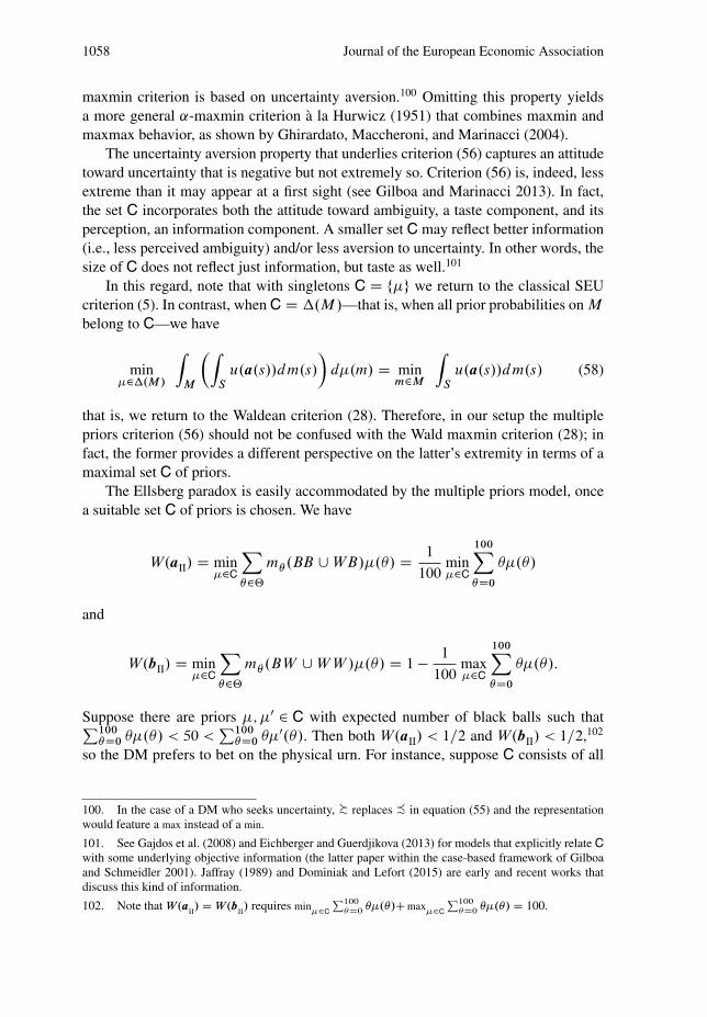
1058 Journal of the European Economic Association
maxmin criterion is based on uncertainty aversion.100 Omitting this property yieldsa more general ˛-maxmin criterion a la Hurwicz (1951) that combines maxmin andmaxmax behavior, as shown by Ghirardato, Maccheroni, and Marinacci (2004).
The uncertainty aversion property that underlies criterion (56) captures an attitudetoward uncertainty that is negative but not extremely so. Criterion (56) is, indeed, lessextreme than it may appear at a first sight (see Gilboa and Marinacci 2013). In fact,the set C incorporates both the attitude toward ambiguity, a taste component, and itsperception, an information component. A smaller set C may reflect better information(i.e., less perceived ambiguity) and/or less aversion to uncertainty. In other words, thesize of C does not reflect just information, but taste as well.101
In this regard, note that with singletons C D f�g we return to the classical SEUcriterion (5). In contrast, when C D �.M /—that is, when all prior probabilities on M
belong to C—we have
min�2�.M/
ZM
�ZS
u.a.s//dm.s/
�d�.m/ D min
m2M
ZS
u.a.s//dm.s/ (58)
that is, we return to the Waldean criterion (28). Therefore, in our setup the multiplepriors criterion (56) should not be confused with the Wald maxmin criterion (28); infact, the former provides a different perspective on the latter’s extremity in terms of amaximal set C of priors.
The Ellsberg paradox is easily accommodated by the multiple priors model, oncea suitable set C of priors is chosen. We have
W.aII/ D min�2C
X2‚
m .BB [ WB/�.�/ D 1
100min�2C
100XD0
��.�/
and
W.bII/ D min�2C
X2‚
m .BW [ W W /�.�/ D 1 � 1
100max�2C
100XD0
��.�/:
Suppose there are priors �; �0 2 C with expected number of black balls such thatP100D0 ��.�/ < 50 <
P100D0 ��0.�/. Then both W.aII/ < 1=2 and W.bII/ < 1=2,102
so the DM prefers to bet on the physical urn. For instance, suppose C consists of all
100. In the case of a DM who seeks uncertainty, � replaces � in equation (55) and the representationwould feature a max instead of a min.
101. See Gajdos et al. (2008) and Eichberger and Guerdjikova (2013) for models that explicitly relate Cwith some underlying objective information (the latter paper within the case-based framework of Gilboaand Schmeidler 2001). Jaffray (1989) and Dominiak and Lefort (2015) are early and recent works thatdiscuss this kind of information.
102. Note that W.aII/ D W.b
II/ requires min
�2C
P100
�D0�./C max
�2C
P100
�D0�./ D 100.
Marinacci Model Uncertainty 1059
possible priors; that is, let C D �.M /. By (58), we have
W.aII/ D min2‚
m .BB [ WB/ D 0 D min2‚
m .BW [ W W / D W.bII/
and so in this case we actually obtain the classical Ellsberg pattern (24).
5.2. Two-Stage Multiplier and Variational Preferences
We observed in Section 4.3 that, when �.x/ D �e��x , we have
c�.a; �/ D � 1
log
ZM
e��U.a;m/d�.m/
which is a form of the multiplier preferences of Hansen and Sargent (2001, 2008).103
As is well known (e.g., Cerreia-Vioglio et al. 2011),
� 1
log
ZM
e��U.a;m/d�.m/ D inf��
Xm2M
U.a; m/�.m/ C ˛R.�jj�/
!; (59)
where R is the relative entropy. At the same time, we can write the maxmin criterion(56) as
W.a/ D min�2C
ZM
U.a; m/d�.m/
D inf�2�.M/
�ZM
U.a; m/d�.m/ C ıC.�/
�;
where ıC W �.M / ! Œ0; C1/ is the indicator function of C in the sense of convexanalysis, that is,
ıC.�/ D�
0 if � 2 CC1 else:
(60)
This observation suggests that we consider the general two-stage representation
W.a/ D inf�2�.M/
�ZM
U.a; m/d�.m/ C c.�/
�;
where c W �.M / ! Œ0; C1/ is any convex function with inf�2M c.�/ D 0.Maccheroni, Marinacci, and Rustichini (2006) call variational the preferences thatadmit such a representation. Variational preferences extend both the maxmin and themultiplier preferences; the latter turn out to be the intersection of smooth and variationalpreferences (see Cerreia-Vioglio et al. 2011).
Maccheroni, Marinacci, and Rustichini (2006) axiomatize variational preferencesand show how the function c captures ambiguity attitudes in a simple way: a variational
103. Recall from Section 4.1 that U.a; m/ D RS
u.a.s//dm.s/.
1060 Journal of the European Economic Association
preference �1 is more ambiguity averse (in the sense of Ghirardato and Marinacci2002) than a variational preference �2 if c1.�/ c2.�/for every � 2 �.M /.104
Heuristically, the index c can be also viewed as a confidence weight on priors,where c.�/ > c.�0/ means that the DM gives prior �0 a higher weight than �. Inthe dichotomic case (60) that characterizes the maxmin criterion only two weights canbe given.
Finally, Strzalecki (2011) shows which axioms characterize multiplier preferenceswithin the class of variational preferences, and Cerreia-Vioglio et al. (2013a)axiomatize the two-stage version of variational preferences that we present here.
5.3. No Trade
The no-trade result of Dow and Werlang (1992) holds for the multiple priors criterion.Assume risk neutrality. The no-trade condition (32) becomes
min�2C
E N�.y/ < p < max�2C
E N�.y/ (61)
The larger the set C (and so the higher the perceived model uncertainty or the aversionto it), the larger the set of prices that result in no trade. It is important to observe that—since (as previously discussed) the multiple priors criterion (56) need not exhibitextreme attitudes—it follows that the scope of the multiple priors no-trade resultis actually much broader than for its Waldean counterpart (28), which does exhibitextreme attitudes.
In the present non-Bayesian setup, a low trade result holds more generally forvariational preferences. In reading this result, note that for the variational criterion wehave W."y/ �W.�"y/, with equality if y is crisp.
PROPOSITION 10. Let " > 0. There is at most "-trade volume in asset y if
W."y/
"< p < �W.�"y/
": (62)
When W is the multiple priors criterion, for each " > 0 the condition (62) reducesto equation (61). In fact,
min�2C
E N�.y/ D W.y/ < p < �W.�y/ D max�2C
E N�.y/:
Hence, there is no trade whatsoever and we are back to the Dow and Werlang (1992)result. The Dow and Werlang insight has been developed in many papers, starting withEpstein and Wang (1994) (see Guidolin and Rinaldi 2013).
104. We refer to Gilboa and Marinacci (2013) for a detailed discussion of comparative ambiguityattitudes.

Marinacci Model Uncertainty 1061
Appendix: Proofs and Related Analysis
A.1. Proof of Proposition 2
Points (i)–(iii) are easily checked. As to point (iv), observe that if � and u are concave,then c.�; �/, and so c.�; �/, is quasi-concave. Under either translation invariance(which, by (ii), holds in the CARA case) or positive homogeneity (which, by (iii),holds in the CRRA case), then c.�; �/ is concave.
A.2. Proof of Proposition 3
To prove Proposition 3, we need a preliminary lemma, due to Hardy, Littlewood andPolya 1934 (p. 94).
LEMMA A.1. Let x1 x2 x3 x4 and let � W Œx1; x4� �! R be concave. Then,
�.x4/ � �.x3/
x4 � x3
�.x2/ � �.x1/
x2 � x1
:
Now let U.b; m00/ U.a; m00/ U.a; m0/ U.b; m0/. Since for all m ¤ m0; m00,U.a; m/ D U.b; m/, we have that
U.a; m0/�.m0/ C U.a; m00/�.m00/ D U.b; m0/�.m0/ C U.b; m00/�.m00/:
We want to show that
�.m0/.�.U.b; m0// � �.U.a; m0/// C �.m00/.�.U.a; m00// � �.U.b; m00/// � 0:
Assume �.m0/; �.m00/ � 0. The preceding equality implies
�.m0/.U.b; m0/ � U.a; m0// D �.m00/.U.a; m00/ � U.b; m00//
so that we can rewrite the preceding inequality as
�.m00/ .� .U .a; m00// � � .U.b; m00///�.m00/ .U .a; m00/ � U.b; m00//
� �.m0/ .�.U.b; m0// � � .U.a; m0///�.m0/.U.b; m0/ � U.a; m0//
or equivalently
�.U.b; m0// � �.U.a; m0//U.b; m0/ � U.a; m0/ �.U.a; m00// � �.U.b; m00//
U.a; m00/ � U.b; m00/ :
Now let us check the following cases.
1. If U.b; m00/ U.a; m00/ U.a; m0/ D U.b; m0/, then the problem becomes oneof verifying whether �.m00/.�.U.a; m00// � �.U.b; m00/// � 0, which holds bythe concavity of �.
1062 Journal of the European Economic Association
2. If U.b; m00/ D U.a; m00/ U.a; m0/ U.b; m0/, then the problem is to verify
�.m0/.�.U.b; m0// � �.U.a; m0/// � 0:
However, this is true because U.b; m00/ D U.a; m00/ implies that U.a; m0/ DU.b; m0/.
3. If U.b; m00/ U.a; m00/ D U.a; m0/ U.b; m0/ , then we have
�.U.b; m0// � �.U.a; m0//U.b; m0/ � U.a; m0/ �.U.a; m0// � � .U.b; m00//
U.a; m0/ � U.b; m00/
(see Hardy, Littlewood and Polya 1934, p. 93).
4. If �.m0/ D 0, then again we must verify �.m00/.�.U.a; m00// � �.U.b; m00/// �0, which holds by the concavity of � .
5. If �.m00/ D 0, then again we must verify �.m0/.�.U.b; m0// � �.U.a; m0/// � 0.Yet this holds because �.m00/ D 0 implies that U.a; m0/ D U.b; m0/.
6. If �.m0/ D �.m00/ D 0, then the inequality trivially holds as an equality to zero.
A.3. Proof of Proposition 4
If x > 0, then
minm2supp �
Em.y/ < p () V.x/ D minm2supp �
Em.yx � px/ < 0:
If x < 0, then
V.x/ D minm2supp �
Em.yx � xp/ D � maxm2supp �
Em..�x/.y � p//
D x maxm2supp �
Em.y � p/ (A.1)
and so maxm2supp � Em.y/ > p if and only if V.x/ < 0. We conclude that equation (32)holds if and only if V.x/ < 0 if x ¤ 0.
A.4. Proof of Lemma 1
Since c�.�; �/ is concave, it follows that c�.x; �/ �c�.�x; �/ D c��.x; �/ for allx 2 R. If x is crisp, then c�.x; �/ D Emx D � c �.�x; �/.
A.5. Proof of Proposition 5
By Proposition 2(iv), c� is subhomogeneous. Fix any x 2 R. If x � " > 0, there is ak � 1 such that x D k"; hence
c�.x; �/ D c�.x.y � p/; �/ D c�.k".y � p/; �/ kc�.".y � p/; �/:
Marinacci Model Uncertainty 1063
Because
c�.".y � p/; �/ D c�."y; �/ � "p < 0 () c"�.y; �/ D c�."y; �/
"< p
we have that c"�.y; �/ < p implies c�.x; �/ < 0 when x � ".If x �" < 0, then there is a k � 1 such that x D k.�"/, so
c�.x; �/ D c�.x.y � p/; �/ D c�.k.�"/.y � p/; �/
D c�.k".p � y/; �/ kc�.".p � y/; �/:
We have
c�.".p � y/; �/ D "p C c�.".�y/; �/ < 0 () p < �c�.".�y/; �/
"D c�"�.y; �/:
Hence, p < c�"�.y; �/ implies c�.x; �/ < 0 when x �". We conclude that (34)implies c�.x; �/ < 0 for all x … .�"; "/.
A.6. Proof of Proposition 6
LEMMA A.2. If a �Em
bm for all m 2 M , then a � Pm2M bm1E
m.
Proof. Note that, a �Em
bm if and only if, for every c 2 A,
266666666664
c.s/ if s 2 E1:::
:::
c.s/ if s 2 Em�1
a.s/ if s 2 Em
c.s/ if s 2 EmC1:::
:::
c.s/ if s 2 En
377777777775
�
266666666664
c.s/ if s 2 E1:::
:::
c.s/ if s 2 Em�1
bm.s/ if s 2 Em
c.s/ if s 2 EmC1:::
:::
c.s/ if s 2 En
377777777775
where M D fmigniD1. If we omit (for brevity) the second column in the representation
of acts above, repeated application of Assumption 3 delivers
266666664
a.s/
a.s/
a.s/:::
a.s/
a.s/
377777775
�
266666664
b1.s/
a.s/
a.s/:::
a.s/
a.s/
377777775
�
266666664
b1.s/
b2.s/
a.s/:::
a.s/
a.s/
377777775
� � � � �
266666664
b1.s/
b2.s/
b3.s/:::
bM�1.s/
a.s/
377777775
�
266666664
b1.s/
b2.s/
b3.s/:::
bM�1.s/
bM .s/
377777775
The transitivity of � now implies the result. �

1064 Journal of the European Economic Association
Now we proceed with the proof of Proposition 6. By Assumption4, a �E
mu�1.
RS u.a.s//dm/ for all a 2 A and m 2 M . By the previous
lemma, a � Pm2M Œu�1.
RS u.a.s//dm.s//�1E
m. By Assumption 2, sinceP
m2M Œu�1.R
S u.a/dm/�1Em
is E measurable, we have
a �X
m2M
�u�1
�ZS
u.a/dm
��1E
m� v�1
Xm2M
v
�u�1
�ZS
u.a/dm
��P.Em/
!:
Setting �.m/ D P.Em/, we conclude that
a � v�1
�ZM
v
�u�1
�ZS
u.a.s//dm
���.m/
�
as desired.
A.7. Proof of Proposition 7
By standard arguments, there exists a unique solution Oa 2 A for the problemmaxa2A
RM �.R.a; m//d�.m/. It satisfies the variational inequality (see, e.g.,
Kinderlehrer and Stampacchia 1980, Chap. 1)105
rV. Oa/ � .a � Oa/ DnX
iD1
.ai � Oai /
ZM
�0.R. Oa; m//@R
@ai
. Oa; m/d�.m/ 0 8a 2 A:
Thus, since �0 > 0, we have
nXiD1
.ai � Oai /
ZM
�0.R. Oa; m//RM �0.R. Oa; m//d�.m/
@R
@ai
. Oa; m/d�.m/ 0 8a 2 A:
Consider the function � given by (43). Since �0 > 0, it holds �.m/ > 0 for each m 2M ; moreover,
Pm2M �.m/�.m/ D 1. Define O� 2 �.M / by O�.m/ D �.m/�.m/.
Since � > 0, O� and � are equivalent. We have rV. Oa/ � .a � Oa/ 0 if and only if
nXiD1
.ai � Oai /
ZM
@R
@ai
. Oa; m/d O�.m/ 0 8a 2 A: (A.2)
Yet because R is strictly concave, there is a unique solution Na 2 A for the problem
maxa2A
ZM
R.a; m/d O�.m/ (A.3)
105. If Oa is an interior point, condition rV. Oa/ .a � Oa/ � 0 reduces to rV. Oa/ D 0.

Marinacci Model Uncertainty 1065
and it is the unique action (Kinderlehrer and Stampacchia 1980, Chap. 1) that satisfiesthe variational inequality
nXiD1
.ai � Nai /
ZM
@R
@ai
. Na; m/d O�.m/ 0:
In view of (A.2), we conclude that Oa D Na and so Oa also solves problem (A.3).
A.8. Proof of Lemma 2
If O� D �, we have ˛ D minm2supp � �.m/ D 1. Suppose O� ¤ � and let 0 < N minm2supp � �.m/. We have �.m/ N O�.m/ and so N < 1 because O� ¤ �. Setting� D .1=.1 � N // O� � . N=.1 � N //� 2 �.M /, we can write O� D N� C .1 � N /�. Asfor the converse, let ˛ 2 .0; 1� and � 2 �.M / be such that O� D ˛� C .1 � ˛/�. Then�.m/�.m/ D O�.m/ � ˛�.m/ for all m 2 M , and so ˛ minm2supp � �.m/.
A.9. Proof of Proposition 8
From the constraints c0 D I0 � EP .�w/ and c1i D I1i C wi , it follows that
c0 � 0 () EP .�w/ I0 and ci1 � 0 () wi � �I1i8i;
that is, pw I0 and w � �I . Setting A D fw 2 Rk W EP .�w/ I0 and w � �I1g,
we can define the function g W A � Rk ! R as
g.w/ DXm
�
0@ kX
iD1
u�I0 � Em�.�w/; I1i C wi
mi
1A�.m/:
We can thus solve the optimization problem maxw2A g.w/. Since g is strictly concave,there is at most a solution Ow. Suppose it is an interior point of A (so that thecorresponding Oc is interior). The function g is differentiable at Ow. Denote by g0. OwI �/ WW ! R the directional derivative g0. OwI w/ D limt#0.g. Ow C tw/ � g. Ow//=t . SinceOw is interior, g0. OwI w/ D 0 for every w 2 W . By the chain rule,
0 D g0. OwI w/ D �E�.�0.Em.u. Oc////@u
@c0
. Oc/Em�.�w/
C E�
��0.Em.u. Oc///Em
�@u
@c1
. Oc/w
��:
By equation (46), pw D Em�.�w/, and so equation (50) follows.
1066 Journal of the European Economic Association
A.10. Proof of Proposition 9
Define � 2 �.S/ by
�i D E O�
Em.@u=@c1/. Oc/
E O�Em.@u=@c1/. Oc/Omi
!8i D 1; : : : ; k:
We have
�i D E O�� Omi Em.@u=@c1/. Oc/
E O�Em.@u=@c1/. Oc/
DXm
Em.@u=@c1/.c/
E�
��.m/Em.@u=@c1/.c/
Omi O�.m/
DXm
Em.@u=@c1/.c/E�.�0.Emu. Oc///
E�
��0.Emu. Oc//Em.@u=@c1/.c/
Omi O�.m/
DXm
Em.@u=@c1/. Oc/E�.�0.Emu. Oc///
E�
��0.Emu. Oc//Em.@u=@c1/. Oc/
.@u=@c1i /. Oc/
Em.@u=@c1/. Oc/mi O�.m/
DXm
.@u=@c1i /. Oc/E�.�0.Emu. Oc///
E�
��0.Emu. Oc//Em.@u=@c1/.c/
mi O�.m/
DXm
.@u=@c1i
/. Oc/
.@u=@c0/. Oc/
E�.�0.Emu. Oc///
E�
�0.Emu. Oc//Em
.@u=@c1/.c/
.@u=@c0/. Oc/
�mi O�.m/
DXm
.@u=@c1i
/. Oc/
.@u=@c0/. Oc/
E�
�.m/Em
.@u=@c0/. Oc/
�mi O�.m/
DXm
.@u=@c1i
/. Oc/
.@u=@c0/. Oc/
E O�Em
.@u=@c1/.c/
.@u=@c0/. Oc/
mi O�.m/ D 1
Em��
Xm
.@u=@c1i /. Oc/
.@u/.@c0/. Oc/mi O�.m/
D 1
Em��E O�
.@u=@c1i /. Oc/
.@u=@c0/. Oc/mi :
Note that E O�Em..@u=@c1/.c/=.@u=@c0/. Oc// D Em�� D 1=rf because the risk-freeclaim 1 is replicable. Since
�i DXm
Em.@u=@c1/. Oc/
E O�Em.@u=@c1/. Oc/Omi O�.m/ D
Xm
Omi Q�.m/
Marinacci Model Uncertainty 1067
we can write
Em�.�/E Q�.E Omw/ D Em�.�/E�w D Em�.�/
kXiD1
E O�
Em.@u=@c1/. Oc/
E O�Em.@u=@c1/. Oc/Omi
!wi
DkX
iD1
E O�.@u=@c1i /. Oc/
.@u=@c0/. Oc/miwi D E O�
kXiD1
.@u=@c1i /. Oc/
.@u=@c0/. Oc/miwi
D E O�Em
�.@u=@c1/. Oc/
.@u=@c0/. Oc/w
�D pw
where the last equality follows from equation (50).
A.11. Proof of Lemma 3
The if part is obvious. As to the converse, suppose that fractional treatment is notoptimal. We first remark that the concavity of V is easy to check. Hence V.0/ ¤ V.1/
because otherwise V.a/ � V.0/ D V.1/ for all a 2 .0; 1/. Suppose V.0/ < V.1/,so that the optimal decision is Oa D 1—that is, V.1/ > V.a/ for every a 2 Œ0; 1/.By concavity, V.a/ � aV.1/ C .1 � a/V .0/ � V.0/ for every a 2 Œ0; 1�, and soV.0/ D mina2Œ0;1 V.a/. Set �.a/ D V.a/ � V.0/=.V .1/ � V.0//. Then, �.0/ D 0
and �.1/ D 1. Since V , and so �, is concave, given any Na 2 .0; 1/, we have �.a/ �. Na/ C �0C. Na/.a � Na/ for all a 2 Œ0; 1�. Hence, 1 D �.1/ �. Na/ C �0. Na/.1 � Na/,which implies V 0C. Na/ D �0C. Na/ > 0 since �. Na/ < �.1/ D 1. We conclude that V
is strictly increasing. If V.0/ > V.1/, a similar argument shows that V is strictlydecreasing.
A.12. Proof of Proposition 10
For brevity we omit the proof. It is similar to the proof of Proposition 5 but with W inplace of c�.
A.13. Miscellanea
Equation (30). This is a special case of equation (58) with M D fıs W s 2 Eg.
1068 Journal of the European Economic Association
Equation (39). Assume that a is finitely valued. For ˇ ¤ 0 small enough, we have(see, e.g., Billingsley 1995, p. 148)
cˇ .a; �/ D � 1
ˇlog E�eˇE
m.�a/ D � 1
ˇ
1XnD1
ˇn
nŠcn.E.�a//
D �1X
nD1
.�1/nˇn�1
nŠcn.E.a// D
1XnD1
.�1/nC1ˇn�1
nŠcn.E.a//
D E N�a � 1
2˛2
�.E.a// C1X
nD3
.�1/nC1ˇn�1
nŠcn.E.a//:
In turn, this implies equation (40).
Equation (50). We have
pw D E�
�0.Em.u. Oc///
E�.�0.Em.u. Oc////Em
�.@u=@c1/. Oc/
.@u=@c0/. Oc/w
�!
D E�
Em
�0.Em.u. Oc///.@u=@c1/. Oc/
E�.�0.Em.u. Oc////.@u=@c0/. Oc/w
!!
D E�
Em�
�0.Em.u. Oc///.@u=@c1/. Oc/
E�.�0.Em.u. Oc////.@u=@c0/. Oc/
m
m� w
!!
D Em�
E�
��0.Em.u. Oc///.m=m�/
E�.�0.Em.u. Oc////
.@u=@c1/. Oc/
.@u=@c0/. Oc/w
!:
Since the market is complete, by considering Arrow contingent claims we getequation (51).
Example 4. We have Oa 2 .0; 1/ if and only if E� Ncm.t0/ Ncm.t1/ <
minfE� Nc2m.t0/; E� Nc2
m.t1/g. Since for all a; b 2 R it holds that 2 minfa; bg D.a C b/ � ja � bj, this inequality holds if and only if
2E� Ncm.t0/ Ncm.t1/ < E� Nc2m.t0/ C E� Nc2
m.t1/ � ˇE� Nc2
m.t0/ � E� Nc2m.t1/
ˇ:
That is, jV.a/ � V.b/ˇ D jE� Nc2
m.t0/ � E� Nc2m.t1/
ˇ< E�d2
m as desired.
Equation (57). Since fım W m 2 M g � �.M /, the inequality follows.However,
RS u.a.s//dm � minm2M
RS u.a.s//dm for all m 2 M , and soR
M .R
S u.a.s//dm/d�.m/ � minm2M
RS u.a.s//dm for all � 2 �.M /. Hence, also
the inequality � holds.
Marinacci Model Uncertainty 1069
References
Abdellaoui, Mohammed, Aurelien Baillon, Laetitia Placido, and Peter P. Wakker (2011). “The RichDomain of Uncertainty: Source Functions and Their Experimental Implementation.” AmericanEconomic Review, 101(2), 695–723.
Akaike, Hirotugu (1985). “Prediction and Entropy.” In A Celebration of Statistics, edited by AnthonyC. Atkinson and Stephen E. Fienberg. Springer.
Amarante, Massimiliano (2009). “Foundations of Neo-Bayesian Statistics.” Journal of EconomicTheory, 144, 2146–2173.
Ang, Alfredo H. S. and Wilson H. Tang (2007). Probability Concepts in Engineering, 2nd ed. Wiley.Anscombe, Francis J. and Robert J. Aumann (1963). “A Definition of Subjective Probability.” Annals
of Mathematics and Statistics, 34, 199–205.Apostolakis, George (1990). “The Concept of Probability in Safety Assessments of Technological
Systems.” Science, 250, 1359–1364.Arrow, Kenneth J. (1951). “Alternative Approaches to the Theory of Choice in Risk-Taking
Situations.” Econometrica, 19, 404–437.Arrow, Kenneth J. and Leonid Hurwicz (1972). “An Optimality Criterion for Decision-Making under
Ignorance.” In Uncertainty and Expectations in Economics, edited by C. F. Carter and J. L. Ford.Basil Blackwell.
Aumann, Robert J. (1987). “Correlated Equilibrium as an Expression of Bayesian Rationality.”Econometrica, 55, 1–18.
Backus, David, Axelle Ferriere, and Stanley Zin (2015). “Risk and Ambiguity in Models of BusinessCycles.” Journal of Monetary Economics, 69, 42–63.
Baker, Jack W. (2008). “An Introduction to Probabilistic Seismic Hazard Analysis (PSHA).” Workingpaper, Stanford University.
Barberis, Nicholas (2000). “Investing for the Long Run When Returns are Predictable.” Journal ofFinance, 55, 225–264.
Barron, Andrew, Jorma Rissanen, and Bin Yu (1998). “The Minimum Description Length Principlein Coding and Modeling.” IEEE Transactions on Information Theory, 44, 2743–2760.
Battigalli, Pierpaolo, Simone Cerreia-Vioglio, Fabio Maccheroni, and Massimo Marinacci (2015a).“Selfconfirming Equilibrium and Model Uncertainty.” American Economic Review, 105(2), 646–677.
Battigalli, Pierpaolo, Simone Cerreia-Vioglio, Fabio Maccheroni, Massimo Marinacci, and ThomasSargent (2015b). “Monetary Policies in Self-confirming Equilibria with Uncertain Models.”Working paper, Bocconi University.
Bawa, Vijay S., Stephen J. Brown, and Roger W. Klein (1979). Estimation Risk and Optimal PortfolioChoice. North-Holland.
Berger, James O. (1990). “Robust Bayesian Analysis: Sensitivity to the Prior.” Journal of StatisticalPlanning and Inference, 25, 303–328.
Berger, James O. (1993). Statistical Decision Theory and Bayesian Analysis, 2nd ed. Springer.Berger, James O. (2006). “The Case for Objective Bayesian Analysis.” Bayesian Analysis, 1, 385–
402.Berger, Loıc, Johannes Emmerling, and Massimo Tavoni (2014). “Managing Catastrophic Climate
Risks under Model Uncertainty Aversion.” Working paper, Fondazione Eni Enrico Mattei (FEEM)and Euro-Mediterranean Center on Climate Change.
Bernardo, Jose M. and Adrian Smith (1994). Bayesian Theory. Wiley.Bernoulli, Daniel (1954). “Specimen theoriae novae de mensura sortis.” Commentarii Academiae
Scientiarum Imperialis Petropolitanae, 1738 (translated in Econometrica, 22, 23–36).Billingsley, Patrick (1965). Ergodic Theory and Information. Wiley.Billingsley, Patrick (1995). Probability and Measure, 3rd ed. Wiley.Boole, George (1854). An Investigation in the Laws of Thought. Walton and Maberley, London.Borel, Emile (1909). Elements de la theorie des probabilites. Hermann, Paris.
1070 Journal of the European Economic Association
Borgonovo, Emanuele, Veronica Cappelli, Fabio Maccheroni, and Massimo Marinacci (2015). “RiskAnalysis and Decision Theory.” Working paper 556, IGIER, Bocconi University.
Breiman, Leo (2001). “Statistical Modeling: The Two Cultures.” Statistical Science, 16, 199–231.Brock, William A., Steven N. Durlauf, and Kenneth D. West (2003). “Policy Evaluation in Uncertain
Economic Environments.” Brookings Papers on Economic Activity, 1, 235–322.Carnap, Rudolf (1945). “The Two Concepts of Probability.” Philosophy and Phenomenological
Research, 5, 513–532.Carnap, Rudolf (1950). Logical Foundations of Probability. University of Chicago Press.Cerreia-Vioglio, Simone, Fabio Maccheroni, and Massimo Marinacci (2015). Put-Call Parity and
Market Frictions.” Journal of Economic Theory, 157, 730–762.Cerreia-Vioglio, Simone, Fabio Maccheroni, Massimo Marinacci, and Luigi Montrucchio (2011).
“Uncertainty Averse Preferences.” Journal of Economic Theory, 146, 1275–1330.Cerreia-Vioglio, Simone, Fabio Maccheroni, Massimo Marinacci, and Luigi Montrucchio 2013a.
“Ambiguity and Robust Statistics.” Journal of Economic Theory, 148, 974–1049.Cerreia-Vioglio, Simone, Fabio Maccheroni, Massimo Marinacci, and Luigi Montrucchio 2013b.
“Classical Subjective Expected Utility.” Proceedings of the National Academy of Sciences, 110,6754–6759.
Chateauneuf, Alain and Jose H. Faro (2009). “Ambiguity through Confidence Functions.” Journalof Mathematical Economics, 45, 535–558.
Chernoff, Herman (1954). “Rational Selection of Decision Functions.” Econometrica, 22, 422–443.Chew, Soo Hong and Jacob Sagi (2008). “Small Worlds: Modeling Attitudes toward Sources of
Uncertainty.” Journal of Economic Theory, 139, 1–24.Cifarelli, Donato M. and Eugenio Regazzini (1996). “de Finetti’s Contribution to Probability and
Statistics.” Statistical Science, 11, 253–282.Cochrane, John H. (2005). Asset Pricing. Princeton University Press.Cochrane, John H. and Lars P. Hansen (1992). “Asset Pricing Explorations for Macroeconomics.”
NBER Macroeconomics Annual, 7, 115–182.Cohen, Michele and Jean-Yves Jaffray (1980). “Rational Behavior under Complete Ignorance.”
Econometrica, 48, 1281–1299.Collard, Fabrice, Sujoy Mukerji, Kevin Sheppard, and Jean-Marc Tallon (2012). “Ambiguity and
the Historical Equity Premium.” Working paper 500, Department of Economics, University ofOxford.
Cox, David R. (2006). Principles of Statistical Inference. Cambridge University Press.Davis, Donald B. and M.-Elisabeth Pate-Cornell (1994). “A Challenge to the Compound Lottery
Axiom: A Two-Stage Normative Structure and Comparison to Other Theories.” Theory andDecision, 37, 267–309.
de Finetti, Bruno (1931). “Sul significato soggettivo della probabilita.” Fundamenta Mathematicae,17, 298–329.
de Finetti, Bruno (1937). “La prevision: ses lois logiques, ses sources subjectives.” Annales del’Institut Henri Poincare, 7, 1–68.
de Finetti, Bruno (1971). “Probabilita di una teoria e probabilita dei fatti.” In Studi in onore di G.Pompilj. Oderisi Editore, Gubbio.
de Finetti, Bruno (1977). Probabilities of Probabilities: A Real Problem or a Misunderstanding? InNew Developments in the Applications of Bayesian Methods, edited by A. Aykac and C. Brumat.North-Holland.
Deming, William E. (1986). Out of the Crisis: Quality, Productivity and Competitive Position.Cambridge University Press.
Der Kiureghian, Armen (2008). “Analysis of Structural Reliability under Parameter Uncertainty.”Probabilistic Engineering Mechanics, 23, 351–358.
Der Kiureghian, Armen and Ove Ditlevsen (2009). “Aleatory or Epistemic? Does It Matter?”Structural Safety, 31, 105–112.
Diaconis, Persi and David Freedman (1987). “A Dozen de Finetti-Style Results in Search of aTheory.” Annales de l’IHP Probabilites et Statistiques, 23, 397–423.
Ditlevsen, Ove and Henrik O. Madsen (2007). Structural Reliability Methods. Wiley.

Marinacci Model Uncertainty 1071
Dominiak, Adam and Jean-Philippe Lefort (2015). “Ambiguity and Probabilistic Information.”Working paper.
Dow, James and Sergio R. C. Werlang (1992). “Uncertainty Aversion, Risk Aversion, and the OptimalChoice of Portfolio.” Econometrica, 60, 197–204.
Draper, David (1995). “Assessment and Propagation of Model Uncertainty.” Journal of the RoyalStatistical Society, Series B, 45–97.
Draper, David, James S. Hodges, Edward E. Leamer, Carl N. Morris, and Donald B. Rubin (1987).A Research Agenda for Assessment and Propagation of Model Uncertainty. RAND CorporationNote.
Eichberger, Jurgen and Ani Guerdjikova (2013). “Ambiguity, Data and Preferences for Information—A Case-Based Approach.” Journal of Economic Theory, 148, 1433–1462.
Ekeland, Ivar (1993). The Broken Dice. University of Chicago Press.Ellsberg, Daniel (1961). “Risk, Ambiguity, and the Savage Axioms.” Quarterly Journal of Economics,
75, 643–669.Epstein, Larry and Tan Wang (1994). “Intertemporal Asset Pricing under Knightian Uncertainty.”
Econometrica, 62, 283–322.Ergin, Haluk and Faruk Gul (2009). “A Theory of Subjective Compound Lotteries.” Journal of
Economic Theory, 144, 899–929.Field, Richard V. and Mircea Grigoriu (2007). “Model Selection in Applied Science and Engineering:
A Decision-Theoretic Approach.” Journal of Engineering Mechanics, 133, 780–791.Fishburn, Peter C. (1981). “Subjective Expected Utility: A Review of Normative Theories.” Theory
and Decision, 13, 139–199.Fisher, Ronald A. (1957). “The Underworld of Probability.” Sankhya, 18, 201–210.Friedman, Milton (1953). “The Methodology of Positive Economics.” In Essays in Positive
Economics. University of Chicago Press.Friedman, Milton and Leonard J. Savage (1948). “The Utility Analysis of Choices Involving Risk.”
Journal of Political Economy, 16, 279–304.Gajdos, Thibaut, Takashi Hayashi, Jean-Marc Tallon, and Jean-Christophe Vergnaud (2008).
“Attitude Toward Imprecise Information.” Journal of Economic Theory, 140, 27–65.Ghirardato, Paolo, Fabio Maccheroni, and Massimo Marinacci (2004). “Differentiating Ambiguity
and Ambiguity Attitude.” Journal of Economic Theory, 118, 133–173.Ghirardato, Paolo and Massimo Marinacci (2001). “Risk, Ambiguity, and the Separation of Utility
and Beliefs.” Mathematics of Operations Research, 4, 864–89.Ghirardato, Paolo and Massimo Marinacci (2002). “Ambiguity Made Precise: A Comparative
Foundation.” Journal of Economic Theory, 102, 251–289.Giere, Ronald N. (1975). “Epistemological Roots of Scientific Knowledge.” In Induction, Probability,
and Confirmation, edited by G,. Maxwell and R. M. Anderson, Jr. University of Minnesota Press.Giere, Ronald N. (1985). “Philosophy of Science Naturalized.” Philosophy of Science, 52,
331–356.Gilboa, Itzhak (2009). Theory of Decision under Uncertainty. Cambridge University Press.Gilboa, Itzhak, Offer Lieberman, and David Schmeidler (2010). “On the Definition of Objective
Probabilities by Empirical Similarity.” Synthese, 172, 79–95.Gilboa, Itzhak and Massimo Marinacci (2013). “Ambiguity and the Bayesian Paradigm.” In Advances
in Economics and Econometrics: Theory and Applications, edited by D. Acemoglu, M. Arellano,and E. Dekel. Cambridge University Press.
Gilboa, Itzhak and David Schmeidler (1989). “Maxmin Expected Utility with a Non-unique Prior.”Journal of Mathematical Economics, 18, 141–153.
Gilboa, Itzhak and David Schmeidler (2001). A Theory of Case-Based Decisions. CambridgeUniversity Press.
Giraud, Raphael (2014). “Second Order Beliefs Models of Choice under Imprecise Risk: NonadditiveSecond Order Beliefs versus Nonlinear Second Order Utility.” Theoretical Economics, 9, 779–816.
Gollier, Christian (2011). “Portfolio Choices and Asset Prices: The Comparative Statics of AmbiguityAversion.” Review of Economic Studies, 78, 1329–1344.
1072 Journal of the European Economic Association
Gollier, Christian (2013). Pricing the Planet’s Future: The Economics of Discounting in an UncertainWorld. Princeton University Press.
Good, Irving J. (1959). “Kinds of Probability.” Science, 129, 443–450.Good, Irving J. (1965). The Estimation of Probabilities: An Essay on Modern Bayesian Methods.
MIT Press.Grant, Simon and Ben Polak (2013). “Mean-Dispersion Preferences and Constant Absolute
Uncertainty Aversion.” Journal of Economic Theory, 148, 1361–1398.Guerdjikova, Ani and Emanuela Sciubba (2015). “Survival with Ambiguity.” Journal of Economic
Theory, 155, 50–94.Guidolin, Massimo and Francesca Rinaldi (2013). “Ambiguity in Asset Pricing and Portfolio Choice:
A Review of the Literature.” Theory and Decision, 74, 183–217.Gul, Faruk and Wolfgang Pesendorfer, (2015) “Hurwicz Expected Utility and Subjective Sources.”
Journal of Economic Theory, 159, 465–488Guo, Jia and Xiaoping Du (2007). “Sensitivity Analysis with Mixture of Epistemic and Aleatory
Uncertainties.” Journal of the American Institute of Aeronautics and Astronautics, 45, 2337–2349.Haavelmo, Trygve (1944). “The Probability Approach in Econometrics.” Econometrica, 12,
Supplement.Hacking, Ian (1975). The Emergence of Probability. Cambridge University Press.Halevy, Alon, Peter Norvig, and Fernando Pereira (2009). “The Unreasonable Effectiveness of Data.”
IEEE Intelligent Systems, 24, 8–12.Hanany, Eran and Peter Klibanoff (2009). “Updating Ambiguity Averse Preferences.” BE Journal of
Theoretical Economics, 9, November.Hansen, Lars P. (2007). “Beliefs, Doubts and Learning: Valuing Macroeconomic Risk.” American
Economic Review, 97(2), 1–30.Hansen, Lars P. (2014). “Uncertainty Outside and Inside Economic Models.” Journal of Political
Economy 122, 945–987.Hansen, Lars P. and Scott F. Richard (1987). “The Role of Conditioning Information in Deducing
Testable Restrictions Implied by Dynamic Asset Pricing Models.” Econometrica, 55, 587–613.Hansen, Lars P. and Thomas J. Sargent (2001). “Robust Control and Model Uncertainty.” American
Economic Review, 91, 60–66.Hansen, Lars P. and Thomas J. Sargent (2007). “Recursive Robust Estimation and Control without
Commitment.” Journal of Economic Theory, 136, 1–27.Hansen, Lars P. and Thomas J. Sargent (2008). Robustness. Princeton University Press.Hansen, Lars P. and Thomas J. Sargent (2010). “Fragile Beliefs and the Price of Uncertainty.”
Quantitative Economics, 1, 129–162.Hansen, Lars P. and Thomas J. Sargent (2014). Uncertainty Within Economic Models. World
Scientific.Hansen, Mark H. and Bin Yu (2001). “Model Selection and the Principle of Minimum Description
Length.” Journal of the American Statistical Association, 96, 746–774.Hardy, Godfrey H., John E. Littlewood, and George Polya (1934). Inequalities. Cambridge University
Press.Hayashi, Takashi and Jianjun Miao (2011). “Intertemporal Substitution and Recursive Smooth
Ambiguity Preferences.” Theoretical Economics, 6, 423–472.Heal, Geoffrey and Antony Millner (2014). “Uncertainty and Decision Making in Climate Change
Economics.” Review of Environmental Economics and Policy, 8, 120–137.Heckman, James J. (2008). “Econometric Causality.” International Statistical Review, 76, 1–27.Hurwicz, Leonid (1951). “Some Specification Problems and Application to Econometric Models.”
Econometrica, 19, 343–344.Jaffray, Jean-Yves. (1989). “Linear Utility Theory for Belief Functions.” Operations Research
Letters, 8, 107–112.Jahan-Parvar, Mohammad R. and Hening Liu (2014). “Ambiguity Aversion and Asset Prices in
Production Economies.” Review of Financial Studies, 27, 3060–3097.Jaynes, Edwin T. (1959). Probability Theory in Science and Engineering. Mobil Oil Co., Dallas, TX.Jaynes, Edwin T. (2003). Probability Theory: The Logic of Science. Cambridge University Press.
Marinacci Model Uncertainty 1073
Jewitt, Ian and Sujoy Mukerji (2011). “Ordering Ambiguous Acts.” Working paper, Department ofEconomics, University of Oxford.
Ju, Nengjiu and Jianjun Miao (2012). “Ambiguity, Learning, and Asset Returns.” Econometrica, 80,559–591.
Kandel, Shmuel and Robert F. Stambaugh (1996). “On the Predictability of Stock Returns: AnAsset-Allocation Perspective.” Journal of Finance, 51, 385–424.
Kaplan, Stanley and B. John Garrick (1981). “On the Quantitative Definition of Risk.” Risk Analysis,1, 1–28.
Kaplan, Stan, Harold F. Perla, and Dennis C. Bley (1983). “A Methodology for Seismic Risk Analysisof Nuclear Power Plants.” Risk Analysis, 3, 169–180.
Kass, Robert E. and Larry Wasserman (1996). “The Selection of Prior Distributions by FormalRules.” Journal of the American Statistical Association, 91, 1343–1370.
Kelly, Thomas (2008). “Evidence: Fundamental Concepts and the Phenomenal Conception.”Philosophy Compass, 3, 933–955.
Kendall, Maurice G. (1946). The Advanced Theory of Statistics, 2nd ed. Griffin, London.Keynes, John M. (1921). A Treatise on Probability. Macmillan.Kinderlehrer, David and Guido Stampacchia (1980). An Introduction to Variational Inequalities and
Their Applications. Academic.Klibanoff, Peter (2013). “Thoughts on Policy Choice Under Ambiguity.” Journal of Institutional
and Theoretical Economics, 169, 134–138.Klibanoff, Peter, Massimo Marinacci, and Sujoy Mukerji (2005). “A Smooth Model of Decision
Making Under Ambiguity.” Econometrica, 73, 1849–1892.Knight, Frank H. (1921). Risk, Uncertainty and Profit. Houghton Mifflin.Konishi, Sadanori and Genshiro Kitagawa (2008). Information Criteria and Statistical Modeling.
Springer.Koopmans, Tjalling C. (1947). “Measurement Without Theory.” Review of Economic Statistics, 29,
161–172.Kording, Konrad (2007). “Decision Theory: What ‘Should’ the Nervous System Do?” Science, 318,
606–610.Kuhn, Harold (1953). “Extensive Games and the Problem of Information.” In Contributions to the
Theory of Games, edited by H. Kuhn and A. Tucker. Princeton University Press.Laffont, Jean-Jacques (1989). The Economics of Uncertainty and Information. MIT Press.Lang, Matthias (2015). “First-Order and Second-Order Ambiguity Aversion.” Working paper.Laplace, Pierre-Simon (1812). Theorie analytique des probabilites. Courcier, Paris.Le Cam, Lucien (1977). “A Note on Metastatistics or ‘An Essay Toward Stating a Problem in the
Doctrine of Chances’.” Synthese, 36, 133–160.LeRoy, Stephen F., and Larry D. Singell (1987). “Knight on Risk and Uncertainty.” Journal of
Political Economy, 95, 394–406.Lindley, Dennis V. (2013). Understanding Uncertainty, 2nd ed. Wiley.Lucas, Robert E., Jr (1977). “Understanding Business Cycles.” In Stabilization of the Domestic and
International Economy, edited by K. Brunner and A. H. Meltzer. North-Holland.Maccheroni, Fabio, Massimo Marinacci, and Doriana Ruffino (2013). “Alpha as Ambiguity: Robust
Mean-Variance Portfolio Analysis.” Econometrica, 81, 1075–1113.Maccheroni, Fabio, Massimo Marinacci, and Aldo Rustichini (2006). “Ambiguity Aversion,
Robustness, and the Variational Representation of Preferences.” Econometrica, 74, 1447–1498.Maccheroni, Fabio, Massimo Marinacci, and Aldo Rustichini (2012). “Social Decision Theory:
Choosing Within and Between Groups.” Review of Economic Studies, 79, 1591–1636.Machina, Mark J. (2004). “Almost-Objective Uncertainty.” Economic Theory, 24, 1–54.Manski, Charles F. (2009). “Diversified Treatment Under Ambiguity.” International Economic
Review, 50, 1013–1041.Marinacci, Massimo (2002). “Learning from Ambiguous Urns.” Statistical Papers, 43, 143–151.Marschak, Jacob (1953). “Economic Measurements for Policy and Prediction.” In Studies in
Econometric Method, edited by W. Hood and T. J. Koopmans. Wiley.Marschak, Jacob and Roy Radner (1972). Economic Theory of Teams. Yale University Press.
1074 Journal of the European Economic Association
Marzocchi, Warner, Christopher Newhall, and Gordon Woo (2012). “The Scientific Management ofVolcanic Crises.” Journal of Volcanology and Geothermal Research, 247/248, 181–189.
Mauldin, R. Daniel, David Preiss, and Heinrich von Weizsacker (1983). “Orthogonal TransitionKernels.” Annals of Probability, 11, 970–988.
Meinshausen, Malte, Nicolai Meinshausen, William Hare, Sarah C. B. Raper, Katja Frieler, RetoKnutti, David J. Frame, and Myles R. Allen (2009). “Greenhouse-Gas Emission Targets forLimiting Global Warming to 2ıC.” Nature, 458, 1158–1162.
Miao, Jianjun (2014). Economic Dynamics in Discrete Time. MIT Press.Millner, Antony, Simon Dietz, and Geoffrey Heal (2013). “Scientific Ambiguity and Climate Policy.”
Environmental and Resource Economics, 55, 21–46.Milnor, John (1954). “Games Against Nature.” In Decision Processes, edited by R. M. Thrall, C. H.
Coombs, and R. L. Davis. Wiley.Morris, Stephen (1995). “The Common Prior Assumption in Economic Theory.” Economics and
Philosophy, 11, 227–253.Muliere, Pietro and Giovanni Parmigiani (1993). “Utility and Means in the 1930s.” Statistical Science,
8, 421–432.Muth, John F. (1961). “Rational Expectations and the Theory of Price Movements.” Econometrica,
29, 315–335.National Research Council (2009). “Science and Decisions: Advancing Risk Assessment.” National
Academies Press, Washington, DC.Nau, Robert F. (2006). “Uncertainty Aversion with Second-Order Utilities and Probabilities.”
Management Science, 52, 136–145 (see also Proceedings of ISIPTA 2001).Neilson, William S. (2010). “A Simplified Axiomatic Approach to Ambiguity Aversion.” Journal of
Risk and Uncertainty, 41, 113–124.Neyman, Jerzy (1957). “Inductive Behavior as a Basic Concept of Philosophy of Science.” Review
of the International Statistical Institute, 25, 7–22.Ornstein, Donald S. and Benjamin Weiss (1990). “How Sampling Reveals a Process.” Annals of
Probability, 18, 905–930.Pareto, Vilfredo (1900). “Sunto di alcuni capitoli di un nuovo trattato di economia pura.” Giornale
degli Economisti, 20, 216–235 (translated in Giornale degli Economisti, 67, 453–504, 2008).Pastor, Lubos (2000). “Portfolio Selection and Asset Pricing Models.” Journal of Finance, 55,
179–223.Pate-Cornell, M.-Elisabeth, (1996). “Uncertainties in Risk Analysis: Six Levels of Treatment.”
Reliability Engineering and System Safety, 54, 95–111.Pearl, Judea (1988). “Probabilistic Reasoning in Intelligent Systems: Networks of Plausible
Inference.” Morgan Kaufmann.Picci, Giorgio (1977). “Some Connections Between the Theory of Sufficient Statistics and the
Identifiability Problem.” SIAM Journal on Applied Mathematics, 33, 383–398.Popper, Karl R. (1959). “The Propensity Interpretation of Probability.” British Journal for the
Philosophy of Science, 10, 25–42.Porter, Keith, Kim Shoaf, and Hope Seligson (2006). “Value of Injuries in the Northridge Earthquake.”
Earthquake Spectra, 22, 555–563.Porteus, Evan L. (2002). “Foundations of Stochastic Inventory Theory.” Stanford University Press.Pratt, John W. and Robert Schlaifer (1984). “On the Nature and Discovery of Structure.” Journal of
the American Statistical Association, 79, 9–21.Raiffa, Howard and Robert Schlaifer (1961). Applied Statistical Decision Theory. Harvard Graduate
School of Business Administration.Ramsey, Frank P. (1931). “Truth and Probability (1926).” In The Foundations of Mathematics and
Other Logical Essays, edited by R. Braithwaite. Routledge and Kegan Paul.Rissanen, Jorma (2007). Information and Complexity in Statistical Modeling. Springer.Rogelj, Joeri, Malte Meinshausen, and Reto Knutti (2012). “Global Warming under Old and New
Scenarios Using IPCC Climate Sensitivity Range Estimates.” Nature Climate Change, 2, 248–253.
Ross, Stephen A. (2005). Neoclassical Finance. Princeton University Press.
Marinacci Model Uncertainty 1075
Rothschild, Michael J. and Joseph Stiglitz (1970). “Increasing Risk I: A Definition.” Journal ofEconomic Theory, 2, 225–243.
Samuelson, Paul A. (1938). “A Note on the Pure Theory of Consumer’s Behaviour.” Economica, 5,61–71.
Sargent, Thomas J. (2008). “Evolution and Intelligent Design.” American Economic Review, 98(1),3–37.
Savage, Leonard J. (1951). “The Theory of Statistical Decision.” Journal of the American StatisticalAssociation, 46, 55–67.
Savage, Leonard J. (1954). The Foundations of Statistics. Wiley.Schmeidler, David (1989). “Subjective Probability and Expected Utility Without Additivity.”
Econometrica, 57, 571–587.Segal, Uzi (1987). “The Ellsberg Paradox and Risk Aversion: An Anticipated Utility Approach.”
International Economic Review, 28, 175–202.Seo, Kyoungwon (2009). “Ambiguity and Second-Order Belief.” Econometrica, 77, 1575–1605.Shafer, Glenn (1978). “Non-additive Probabilities in the Work of Bernoulli and Lambert.” Archive
for History of Exact Sciences, 19, 309–370.Singpurwalla, Nozer D. (2006). Reliability and Risk: A Bayesian Perspective. Wiley.Siniscalchi, Marciano (2011). “Dynamic Choice Under Ambiguity.” Theoretical Economics, 6, 379–
421.Skinner, Burrhus Frederic (1985). “Cognitive Science and Behaviourism.” British Journal of
Psychology, 76, 291–301.Smith, Vernon L. (1969). “Measuring Nonmonetary Utilities in Uncertain Choices: The Ellsberg
Urn.” Quarterly Journal of Economics, 83, 324–329.Solomon, Susan et al. (2007). IPCC Climate Change 2007: The Physical Science Basis. Cambridge
University Press.Stern, Nicholas (2007). The Economics of Climate Change. Cambridge University Press.Stoye, Jorg (2011). “Statistical Decisions Under Ambiguity.” Theory and Decision, 70, 129–148.Strzalecki, Tomasz (2011). “Axiomatic Foundations of Multiplier Preferences.” Econometrica, 79,
47–73.Strzalecki, Tomasz (2013). “Temporal Resolution of Uncertainty and Recursive Models of Ambiguity
Aversion.” Econometrica, 81, 1039–1074.Taboga, Marco (2005). “Portfolio Selection with Two-Stage Preferences.” Finance Research Letters,
2, 152–164.Teicher, Henry (1963). “Identifiability of Finite Mixtures.” Annals of Mathematical Statistics, 34,
244–248.Tenenbaum, Joshua B., Charles Kemp, Thomas L. Griffiths, and Noah D. Goodman (2011). “How
to Grow a Mind: Statistics, Structure, and Abstraction.” Science, 331, 1279–1285.Theil, Henri (1961). Economic Forecasts and Policy. North-Holland.Tinbergen, Jan (1952). On the Theory of Economic Policy. North-Holland.von Mises, Richard (1939). Probability, Statistics, and Truth. Macmillan.von Neumann, John and Oskar Morgenstern (1947). Theory of Games and Economic Behavior, 2nd
ed. Princeton University Press.von Plato, Jan (1988). “Ergodic Theory and the Foundations of Probability.” In Causation, Chance,
and Credence, edited by B. Skyrms and W. L. Harper. Kluwer.von Plato, Jan, (1989). “Probability in Dynamical Systems.” In Logic, Methodology and Philosophy
of Science VIII, edited by J,. E. Fenstad, I. T. Frolov, and R. Hilpinen. North-Holland.von Plato, Jan (1994). Creating Modern Probability: Its Mathematics, Physics, and Philosophy in
Historical Perspective. Cambridge University Press.Wakker, Peter P. (2010). Prospect Theory. Cambridge University Press.Wald, Abraham (1950). Statistical Decision Functions. Wiley.Walker, Warren E., Poul Harremoes, Jan Rotmans, Jan P. van der Sluijs, Marjolein Asselt, Peter
Janssen, and Martin Krayer von Krauss (2003). “Defining Uncertainty: A Conceptual Basis forUncertainty Management in Model-Based Decision Support.” Integrated Assessment, 4, 5–17.

1076 Journal of the European Economic Association
Weibull, Jorgen W. (1996). “The Mass Action Interpretation.” Research Institute of IndustrialEconomics Working Paper No. 427. In The Work of John Nash in Game Theory, edited byHarold Kuhn et al. Journal of Economic Theory, 69, 153–185.
Winkler, Robert L. (1996). “Uncertainty in Probabilistic Risk Assessment.” Reliability Engineeringand System Safety, 54, 127–132.
Xu, Fei and Vashti Garcia (2008). “Intuitive Statistics by 8-Month-Old Infants.” Proceedings of theNational Academy of Sciences, 105, 5012–5015.
Xu, Fei and Tamar Kushnir (2013). “Infants are Rational Constructivist Learners.” Current Directionsin Psychological Science, 22, 28–32.
Xue, Jingyi (2012). “Three Representations of Preferences with Decreasing Absolute UncertaintyAversion.” Working paper, Rice University.
Zabell, Sandy L. (2011). “The Subjective and the Objective.” Handbook of the Philosophy of Science,Vol. 7, edited by Prasanta S. Bandyopadyay and Malcolm R. Forster. Elsevier, pp. 1149–1174.