Introducing model uncertainty by movingblocks bootstrap

Andres M. Alonso1,2, Daniel Pena2, Juan Romo2

1 Departamento de Matematicas, Universidad Autonoma de Madrid, 28049 Madrid,Spain. e-mail: andres.alonso@uam.es

2 Departamento de Estadıstica, Universidad Carlos III de Madrid, 28903 Getafe,Spain. e-mail: {amalonso,dpena,romo}@est-econ.uc3m.es

It is common in parametric bootstrap to select the model from the data,

and then treat as if it were the true model. Chatfield (1993, 1996) has shown

that ignoring the model uncertainty may seriously undermine the coverage

accuracy of prediction intervals. In this paper, we propose a method based

on moving block bootstrap for introducing the model selection step in the

resampling algorithm. We present a Monte Carlo study comparing the finite

sample properties of the proposed method with those of alternative methods

in the case of prediction intervals.

AMS (2000): 62M10, 62F40.

Key words: sieve bootstrap, blockwise bootstrap, prediction, time series,

model uncertainty.

1 Introduction

When studying a time series, one of the main goals is the estimation

of forecast intervals based on an observed sample path of the process. The

traditional approach to finding prediction intervals assumes that the series

{Xt}t∈Z follows a linear finite dimensional model with a known errors distri-

bution, e.g. a Gaussian autoregressive-moving average ARMA(p, q) model

as in Box et al. (1994). In such a case, if the orders p and q are known, a

maximum likelihood procedure could be employed for estimating the param-

eters and then, plug in those estimates in the linear predictors. In addition,

some bootstrap approaches have been proposed in order to avoid the use

of a specified errors distribution, see e.g. Stine (1987) and Thombs and

Schucany (1990) for AR(p) models, Pascual et al. (2001) for ARMA(p, q)

models, and Alonso et al. (2002) for linear processes that admit a one-sided

infinite-order moving average representation

Xt − µX =+∞∑j=0

ψjεt−j , ψ0 = 1, t ∈ Z, (1)

where {εt}t∈Z is a sequence of uncorrelated random variables with E [εt] = 0,

E[ε2t

]= σ2 and with at most a polynomial decay of the coefficients {ψj}+∞j=0.

But, those bootstrap proposals assume that p and q are known or, in the

case of Alonso et al. (2002), it selects an approximating autoregressive model

AR(p) from the data, and then use the selected order, p, as if it were the

true order. Then, those approaches ignore the variability involved in model

selection, which can be a considerable part of the overall uncertainty (e.g.

Chatfield 1993, 1996). In practice, having observed a sample of size n, the

model, and particularly p and q are invariably unknown. Thus, we should

select a model from the data. Many model selection procedures have been

proposed, e.g. the final prediction error (FPE) of Akaike (1969), the Akaike

(1973) information criterion (AIC) or its bias-corrected version (AICC) of

Hurvich and Tsai (1989) and the Bayesian information criterion of Schwarz

(1978), see Bhansali (1993) for a review.

For finite autoregressive models, Masarotto (1990) and Grigoletto (1998),

propose to take into account model uncertainty as follows: first, to obtain

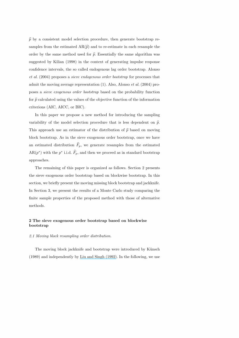
p by a consistent model selection procedure, then generate bootstrap re-

samples from the estimated AR(p) and to re-estimate in each resample the

order by the same method used for p. Essentially the same algorithm was

suggested by Kilian (1998) in the context of generating impulse response

confidence intervals, the so called endogenous lag order bootstrap. Alonso

et al. (2004) proposes a sieve endogenous order bootstrap for processes that

admit the moving average representation (1). Also, Alonso et al. (2004) pro-

poses a sieve exogenous order bootstrap based on the probability function

for p calculated using the values of the objective function of the information

criterions (AIC, AICC, or BIC).

In this paper we propose a new method for introducing the sampling

variability of the model selection procedure that is less dependent on p.

This approach use an estimator of the distribution of p based on moving

block bootstrap. As in the sieve exogenous order bootstrap, once we have

an estimated distribution Fp, we generate resamples from the estimated

AR(p∗) with the p∗ i.i.d. Fp, and then we proceed as in standard bootstrap

approaches.

The remaining of this paper is organized as follows. Section 2 presents

the sieve exogenous order bootstrap based on blockwise bootstrap. In this

section, we briefly present the moving missing block bootstrap and jackknife.

In Section 3, we present the results of a Monte Carlo study comparing the

finite sample properties of the proposed method with those of alternative

methods.

2 The sieve exogenous order bootstrap based on blockwisebootstrap

2.1 Moving block resampling order distribution.

The moving block jackknife and bootstrap were introduced by Kunsch

(1989) and independently by Liu and Singh (1992). In the following, we use

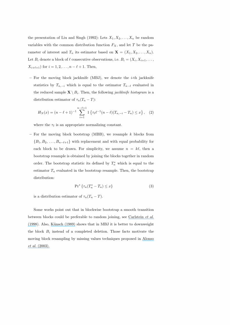
the presentation of Liu and Singh (1992): Lets X1, X2, . . . , Xn be random

variables with the common distribution function FX , and let T be the pa-

rameter of interest and Tn its estimator based on X = (X1, X2, . . . , Xn).

Let Bi denote a block of ` consecutive observations, i.e. Bi = (Xi, Xi+1, . . . ,

Xi+`+1) for i = 1, 2, . . . , n− `+ 1. Then,

– For the moving block jackknife (MBJ), we denote the i-th jackknife

statistics by Tn,−i which is equal to the estimator Tn−` evaluated in

the reduced sample X \Bi. Then, the following jackknife histogram is a

distribution estimator of τn(Tn − T ):

HN (x) = (n− `+ 1)−1n−`+1∑

i=1

1{τ``

−1(n− `)(Tn,−i − Tn) ≤ x}, (2)

where the τ` is an appropriate normalizing constant.

– For the moving block bootstrap (MBB), we resample k blocks from

{B1, B2, . . . , Bn−`+1} with replacement and with equal probability for

each block to be drawn. For simplicity, we assume n = k`, then a

bootstrap resample is obtained by joining the blocks together in random

order. The bootstrap statistic its defined by T ∗n which is equal to the

estimator Tn evaluated in the bootstrap resample. Then, the bootstrap

distribution:

Pr∗ {τn(T ∗n − Tn) ≤ x} (3)

is a distribution estimator of τn(Tn − T ).

Some works point out that in blockwise bootstrap a smooth transition

between blocks could be preferable to random joining, see Carlstein et al.

(1998). Also, Kunsch (1989) shows that in MBJ it is better to downweight

the block Bi instead of a completed deletion. Those facts motivate the

moving block resampling by missing values techniques proposed in Alonso

et al. (2003).

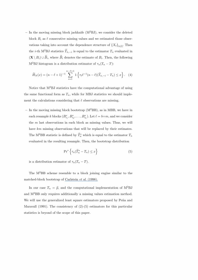
– In the moving missing block jackknife (M2BJ), we consider the deleted

block Bi as ` consecutive missing values and we estimated those obser-

vations taking into account the dependence structure of {Xt}t∈Z. Then

the i-th M2BJ statistics Tn,−i is equal to the estimator Tn evaluated in

(X \Bi)∪ Bi, where Bi denotes the estimate of Bi. Then, the following

M2BJ histogram is a distribution estimator of τn(Tn − T ):

HN (x) = (n− `+ 1)−1n−`+1∑

i=1

1{τ``

−1(n− `)(Tn,−i − Tn) ≤ x}. (4)

Notice that M2BJ statistics have the computational advantage of using

the same functional form as Tn, while for MBJ statistics we should imple-

ment the calculations considering that ` observations are missing.

– In the moving missing block bootstrap (M2BB), as in MBB, we have in

each resample k blocks (B∗i1, B∗

i2, . . . , B∗

ik). Let ` = b+m, and we consider

the m last observations in each block as missing values. Thus, we will

have km missing observations that will be replaced by their estimates.

The M2BB statistic is defined by T ∗n which is equal to the estimator Tn

evaluated in the resulting resample. Then, the bootstrap distribution

Pr∗{τn(T ∗n − Tn) ≤ x

}(5)

is a distribution estimator of τn(Tn − T ).

The M2BB scheme resemble to a block joining engine similar to the

matched-block bootstrap of Carlstein et al. (1998).

In our case Tn = p, and the computational implementation of M2BJ

and M2BB only requires additionally a missing values estimation method.

We will use the generalized least square estimators proposed by Pena and

Maravall (1991). The consistency of (2)-(5) estimators for this particular

statistics is beyond of the scope of this paper.

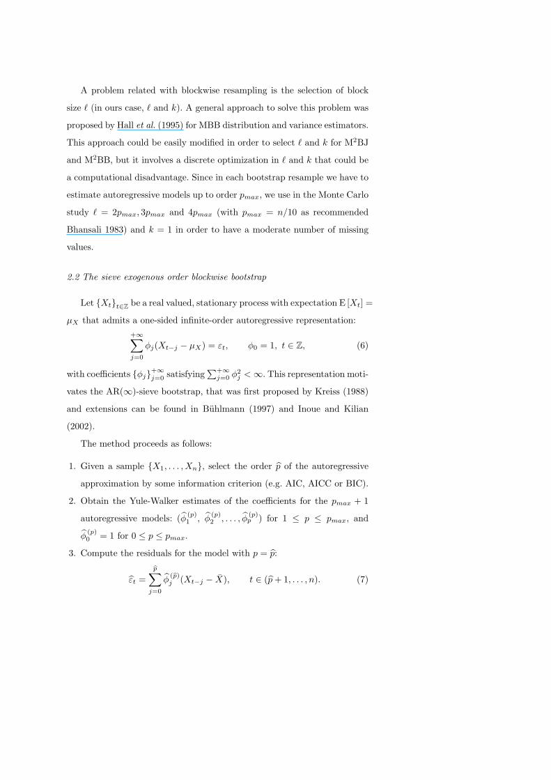
A problem related with blockwise resampling is the selection of block

size ` (in ours case, ` and k). A general approach to solve this problem was

proposed by Hall et al. (1995) for MBB distribution and variance estimators.

This approach could be easily modified in order to select ` and k for M2BJ

and M2BB, but it involves a discrete optimization in ` and k that could be

a computational disadvantage. Since in each bootstrap resample we have to

estimate autoregressive models up to order pmax, we use in the Monte Carlo

study ` = 2pmax, 3pmax and 4pmax (with pmax = n/10 as recommended

Bhansali 1983) and k = 1 in order to have a moderate number of missing

values.

2.2 The sieve exogenous order blockwise bootstrap

Let {Xt}t∈Z be a real valued, stationary process with expectation E [Xt] =

µX that admits a one-sided infinite-order autoregressive representation:+∞∑j=0

φj(Xt−j − µX) = εt, φ0 = 1, t ∈ Z, (6)

with coefficients {φj}+∞j=0 satisfying∑+∞

j=0 φ2j <∞. This representation moti-

vates the AR(∞)-sieve bootstrap, that was first proposed by Kreiss (1988)

and extensions can be found in Buhlmann (1997) and Inoue and Kilian

(2002).

The method proceeds as follows:

1. Given a sample {X1, . . . , Xn}, select the order p of the autoregressive

approximation by some information criterion (e.g. AIC, AICC or BIC).

2. Obtain the Yule-Walker estimates of the coefficients for the pmax + 1

autoregressive models: (φ (p)1 , φ (p)

2 , . . . , φ(p)p ) for 1 ≤ p ≤ pmax, and

φ(p)0 = 1 for 0 ≤ p ≤ pmax.

3. Compute the residuals for the model with p = p:

εt =p∑

j=0

φ(p)j (Xt−j − X), t ∈ (p+ 1, . . . , n). (7)

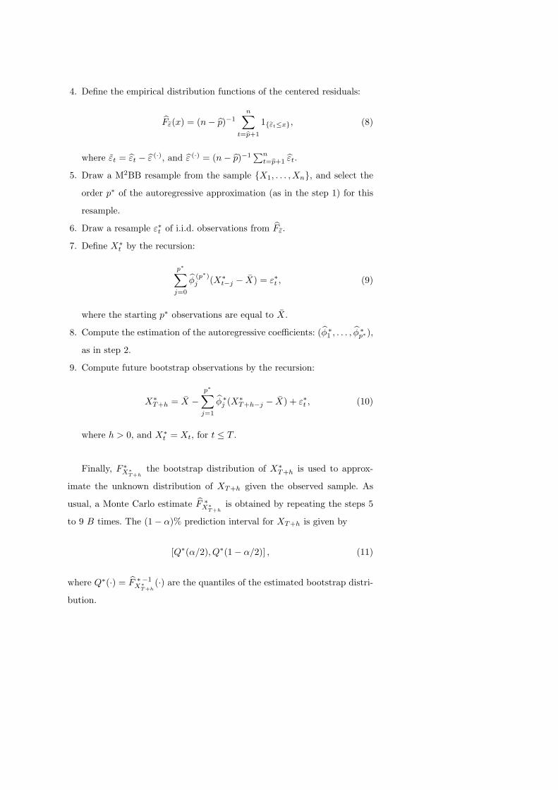
4. Define the empirical distribution functions of the centered residuals:

Fε(x) = (n− p)−1n∑

t=p+1

1{εt≤x}, (8)

where εt = εt − ε (·), and ε (·) = (n− p)−1∑n

t=p+1 εt.

5. Draw a M2BB resample from the sample {X1, . . . , Xn}, and select the

order p∗ of the autoregressive approximation (as in the step 1) for this

resample.

6. Draw a resample ε∗t of i.i.d. observations from Fε.

7. Define X∗t by the recursion:

p∗∑j=0

φ(p∗)j (X∗

t−j − X) = ε∗t , (9)

where the starting p∗ observations are equal to X.

8. Compute the estimation of the autoregressive coefficients: (φ ∗1 , . . . , φ∗p∗),

as in step 2.

9. Compute future bootstrap observations by the recursion:

X∗T+h = X −

p∗∑j=1

φ ∗j (X∗T+h−j − X) + ε∗t , (10)

where h > 0, and X∗t = Xt, for t ≤ T .

Finally, F ∗X∗T+h

the bootstrap distribution of X∗T+h is used to approx-

imate the unknown distribution of XT+h given the observed sample. As

usual, a Monte Carlo estimate F ∗X∗

T+his obtained by repeating the steps 5

to 9 B times. The (1− α)% prediction interval for XT+h is given by

[Q∗(α/2), Q∗(1− α/2)] , (11)

where Q∗(·) = F ∗−1X∗

T+h(·) are the quantiles of the estimated bootstrap distri-

bution.

3 Simulations results

We compare the different sieve bootstrap approaches for the following

models:

Model 1: (1− 0.75B + 0.5B2)Xt = εt

Model 2: Xt = (1− 0.3B + 0.7B2)εt.

Model 3: (1 + 0.7B − 0.2B2)Xt = εt

Model 4: Xt = (1 + 0.7B − 0.2B2)εt.

Model 1 was considered by Cao et al. (1997) and Model 2 by Pascual et

al. (2001). Model 3 and 4 were considered by Alonso et al. (2004). As in those

papers we used the following error distributions Fε: the standard normal, a

shifted exponential distribution with zero mean and scale parameter equal

to one, and a contaminated distribution 0.9 F1 + 0.1 F2 with F1 ∼ N (−1, 1)

and F2 ∼ N (9, 1). But, for sake of brevety, we only present the results for

the standard normal. We take sample sizes n = 50, and 100, leads h = 1 to

h = 5, and nominal coverage 1− α = 0.95.

To compare the different prediction intervals, we use their mean coverage

(CM ) and length (LM ), and the proportions of observations lying out to the

left and to the right of the interval.

The different sieve bootstrap are denoted by:

S corresponds to the sieve bootstrap without introducing model uncer-

tainty, i.e. the algorithm of Section 2 but omitting the step 5 and using

p∗ = p in steps 7 - 9.

EnS the endogenous sieve bootstrap using p obtained by AICC (see section

2.1 of Alonso et al., 2004).

ExS1 the exogenous sieve bootstrap using the moving missing block bootstrap.

ExS2 the exogenous sieve bootstrap using the AICC information criterion

(see section 2.2 of Alonso et al., 2004).

Notice that the difference between S and the other sieve bootstrap pro-

cedures corresponds to the variability associated to model uncertainty. A

Fortran implementation of procedure S can be found in Alonso (2004).

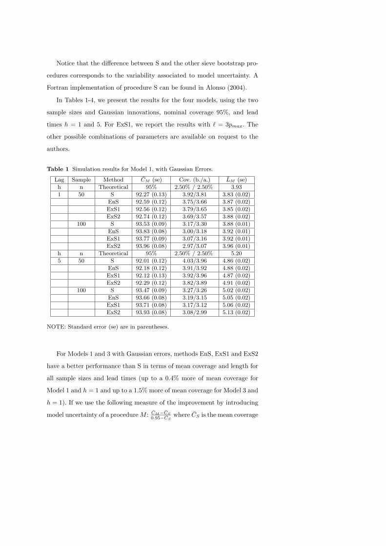
In Tables 1-4, we present the results for the four models, using the two

sample sizes and Gaussian innovations, nominal coverage 95%, and lead

times h = 1 and 5. For ExS1, we report the results with ` = 3pmax. The

other possible combinations of parameters are available on request to the

authors.

Table 1 Simulation results for Model 1, with Gaussian Errors.

Lag Sample Method CM (se) Cov. (b./a.) LM (se)

h n Theoretical 95% 2.50% / 2.50% 3.93

1 50 S 92.27 (0.13) 3.92/3.81 3.83 (0.02)

EnS 92.59 (0.12) 3.75/3.66 3.87 (0.02)

ExS1 92.56 (0.12) 3.79/3.65 3.85 (0.02)

ExS2 92.74 (0.12) 3.69/3.57 3.88 (0.02)

100 S 93.53 (0.09) 3.17/3.30 3.88 (0.01)

EnS 93.83 (0.08) 3.00/3.18 3.92 (0.01)

ExS1 93.77 (0.09) 3.07/3.16 3.92 (0.01)

ExS2 93.96 (0.08) 2.97/3.07 3.96 (0.01)

h n Theoretical 95% 2.50% / 2.50% 5.20

5 50 S 92.01 (0.12) 4.03/3.96 4.86 (0.02)

EnS 92.18 (0.12) 3.91/3.92 4.88 (0.02)

ExS1 92.12 (0.13) 3.92/3.96 4.87 (0.02)

ExS2 92.29 (0.12) 3.82/3.89 4.91 (0.02)

100 S 93.47 (0.09) 3.27/3.26 5.02 (0.02)

EnS 93.66 (0.08) 3.19/3.15 5.05 (0.02)

ExS1 93.71 (0.08) 3.17/3.12 5.06 (0.02)

ExS2 93.93 (0.08) 3.08/2.99 5.13 (0.02)

NOTE: Standard error (se) are in parentheses.

For Models 1 and 3 with Gaussian errors, methods EnS, ExS1 and ExS2

have a better performance than S in terms of mean coverage and length for

all sample sizes and lead times (up to a 0.4% more of mean coverage for

Model 1 and h = 1 and up to a 1.5% more of mean coverage for Model 3 and

h = 1). If we use the following measure of the improvement by introducing

model uncertainty of a procedureM : CM−CS

0.95−CSwhere CS is the mean coverage

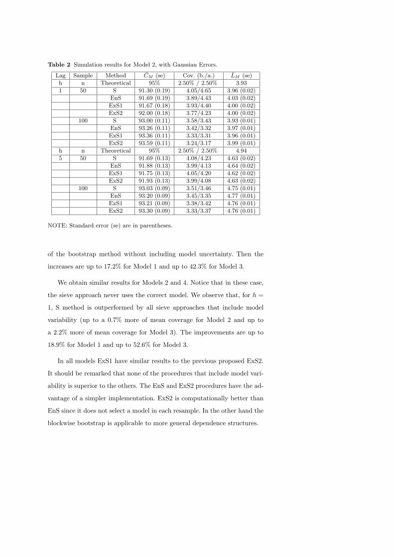
Table 2 Simulation results for Model 2, with Gaussian Errors.

Lag Sample Method CM (se) Cov. (b./a.) LM (se)

h n Theoretical 95% 2.50% / 2.50% 3.93

1 50 S 91.30 (0.19) 4.05/4.65 3.96 (0.02)

EnS 91.69 (0.19) 3.89/4.43 4.03 (0.02)

ExS1 91.67 (0.18) 3.93/4.40 4.00 (0.02)

ExS2 92.00 (0.18) 3.77/4.23 4.00 (0.02)

100 S 93.00 (0.11) 3.58/3.43 3.93 (0.01)

EnS 93.26 (0.11) 3.42/3.32 3.97 (0.01)

ExS1 93.36 (0.11) 3.33/3.31 3.96 (0.01)

ExS2 93.59 (0.11) 3.24/3.17 3.99 (0.01)

h n Theoretical 95% 2.50% / 2.50% 4.94

5 50 S 91.69 (0.13) 4.08/4.23 4.63 (0.02)

EnS 91.88 (0.13) 3.99/4.13 4.64 (0.02)

ExS1 91.75 (0.13) 4.05/4.20 4.62 (0.02)

ExS2 91.93 (0.13) 3.99/4.08 4.63 (0.02)

100 S 93.03 (0.09) 3.51/3.46 4.75 (0.01)

EnS 93.20 (0.09) 3.45/3.35 4.77 (0.01)

ExS1 93.21 (0.09) 3.38/3.42 4.76 (0.01)

ExS2 93.30 (0.09) 3.33/3.37 4.76 (0.01)

NOTE: Standard error (se) are in parentheses.

of the bootstrap method without including model uncertainty. Then the

increases are up to 17.2% for Model 1 and up to 42.3% for Model 3.

We obtain similar results for Models 2 and 4. Notice that in these case,

the sieve approach never uses the correct model. We observe that, for h =

1, S method is outperformed by all sieve approaches that include model

variability (up to a 0.7% more of mean coverage for Model 2 and up to

a 2.2% more of mean coverage for Model 3). The improvements are up to

18.9% for Model 1 and up to 52.6% for Model 3.

In all models ExS1 have similar results to the previous proposed ExS2.

It should be remarked that none of the procedures that include model vari-

ability is superior to the others. The EnS and ExS2 procedures have the ad-

vantage of a simpler implementation. ExS2 is computationally better than

EnS since it does not select a model in each resample. In the other hand the

blockwise bootstrap is applicable to more general dependence structures.

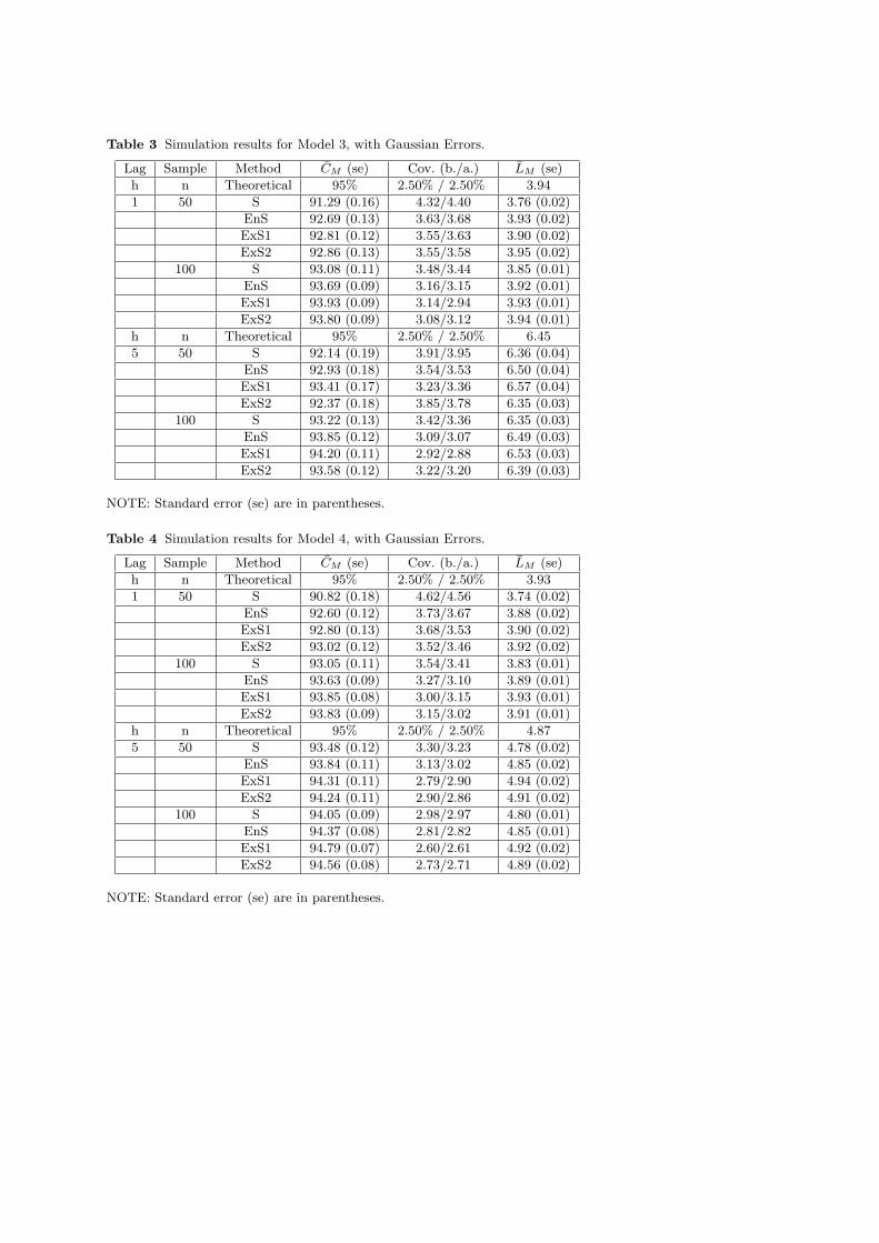
Table 3 Simulation results for Model 3, with Gaussian Errors.

Lag Sample Method CM (se) Cov. (b./a.) LM (se)

h n Theoretical 95% 2.50% / 2.50% 3.94

1 50 S 91.29 (0.16) 4.32/4.40 3.76 (0.02)

EnS 92.69 (0.13) 3.63/3.68 3.93 (0.02)

ExS1 92.81 (0.12) 3.55/3.63 3.90 (0.02)

ExS2 92.86 (0.13) 3.55/3.58 3.95 (0.02)

100 S 93.08 (0.11) 3.48/3.44 3.85 (0.01)

EnS 93.69 (0.09) 3.16/3.15 3.92 (0.01)

ExS1 93.93 (0.09) 3.14/2.94 3.93 (0.01)

ExS2 93.80 (0.09) 3.08/3.12 3.94 (0.01)

h n Theoretical 95% 2.50% / 2.50% 6.45

5 50 S 92.14 (0.19) 3.91/3.95 6.36 (0.04)

EnS 92.93 (0.18) 3.54/3.53 6.50 (0.04)

ExS1 93.41 (0.17) 3.23/3.36 6.57 (0.04)

ExS2 92.37 (0.18) 3.85/3.78 6.35 (0.03)

100 S 93.22 (0.13) 3.42/3.36 6.35 (0.03)

EnS 93.85 (0.12) 3.09/3.07 6.49 (0.03)

ExS1 94.20 (0.11) 2.92/2.88 6.53 (0.03)

ExS2 93.58 (0.12) 3.22/3.20 6.39 (0.03)

NOTE: Standard error (se) are in parentheses.

Table 4 Simulation results for Model 4, with Gaussian Errors.

Lag Sample Method CM (se) Cov. (b./a.) LM (se)

h n Theoretical 95% 2.50% / 2.50% 3.93

1 50 S 90.82 (0.18) 4.62/4.56 3.74 (0.02)

EnS 92.60 (0.12) 3.73/3.67 3.88 (0.02)

ExS1 92.80 (0.13) 3.68/3.53 3.90 (0.02)

ExS2 93.02 (0.12) 3.52/3.46 3.92 (0.02)

100 S 93.05 (0.11) 3.54/3.41 3.83 (0.01)

EnS 93.63 (0.09) 3.27/3.10 3.89 (0.01)

ExS1 93.85 (0.08) 3.00/3.15 3.93 (0.01)

ExS2 93.83 (0.09) 3.15/3.02 3.91 (0.01)

h n Theoretical 95% 2.50% / 2.50% 4.87

5 50 S 93.48 (0.12) 3.30/3.23 4.78 (0.02)

EnS 93.84 (0.11) 3.13/3.02 4.85 (0.02)

ExS1 94.31 (0.11) 2.79/2.90 4.94 (0.02)

ExS2 94.24 (0.11) 2.90/2.86 4.91 (0.02)

100 S 94.05 (0.09) 2.98/2.97 4.80 (0.01)

EnS 94.37 (0.08) 2.81/2.82 4.85 (0.01)

ExS1 94.79 (0.07) 2.60/2.61 4.92 (0.02)

ExS2 94.56 (0.08) 2.73/2.71 4.89 (0.02)

NOTE: Standard error (se) are in parentheses.

4 Conclusion

It has been shown by Masarotto (1990) and Grigoletto (1998) that if the

order of the AR is unknown, but finite, it can obtained prediction intervals

by bootstrap incorporating the sampling variability of p with better cov-

erage probabilities than those produced by standard bootstrap procedures.

Their approaches could be affected by the selected order p. In Alonso et

al. (2004) a sieve endogenous (and exogenous) order bootstrap have been

proposed and a simulation experiment have shown that both procedures

improve the standard sieve bootstrap. In this paper we have proposed an

alternative method based on moving blocks bootstrap for introducing the

model selection variability in the prediction intervals. Monte Carlo simula-

tions show that the proposed procedure provide comparable coverage results

than previous methods in general cases meanwhile its less dependent on the

initial selected order.

Acknowledgements This research was partially supported by the Plan NacionalI+D+I project BEC 2002-2054 and by the Fundacion BBVA.

References

1. Akaike, H. (1969) Fitting autoregressive models for prediction, Ann. Inst.Statist. Math., 21, 243-247.

2. Akaike, H. (1973) Information theory and an extension of the maximum like-lihood principle, 2nd International Symposium on Information Theory, B.N.Petrov, and F. Csaki, Eds., Akademiai Kiado, Budapest, 267-281.

3. Alonso, A.M. (2004) A Fortran routine for sieve bootstrap prediction intervals,J. Modern Appl. Statist. Methods, 3, 239-249.

4. Alonso, A.M., Pena, D. and Romo, J. (2002) Forecasting time series with sievebootstrap, J. Statist. Plann. Inference, 100, 1-11.

5. Alonso, A.M., Pena, D. and Romo, J. (2003) Resampling time series usingmissing values techniques, Ann. Inst. Statist. Math., 55, 765-796.

6. Alonso, A.M., Pena, D. and Romo, J. (2004) Introducing model uncertaintyin time series bootstrap, Statist. Sinica, 14, 155-174.

7. Bhansali, R.J. (1983) A simulation study of autoregressive and window esti-mators of the inverse autocorrelation function, Appl. Statist., 32 141-149.

8. Bhansali, R.J. (1993) Order selection for linear time series models: A review.In: Developments in Time Series Analysis, T. Subba Rao, ed., Chapman andHall, London, 50-66.

9. Box, G.E.P, Jenkins, G.M. and Reinsel, G.C. (1994) Time Series Analysis:Forecasting and Control, Prentice Hall. Englewood.

10. Buhlmann, P. (1997) Sieve bootstrap for time series, Bernoulli, 8, 123-148.11. Cao, R., Febrero-Bande, M., Gonzalez-Manteiga, W., Prada-Sanchez, J.M.

and Garcıa-Jurado, I. (1997) Saving computer time in constructing consistentbootstrap prediction intervals for autoregressive processes, Comm. Statist.Simulation Comput., 26, 961-978.

12. Carlstein, E., Do, K., Hall, P., Hesterberg, T. and Kunsch, H. R. (1998)Matched-block bootstrap for dependent data, Bernoulli, 4, 305-328.

13. Chatfield, C. (1993) Calculating interval forecasts, J. Bus. Econom. Statist.,11, 121-135.

14. Chatfield, C. (1996) Model uncertainty and forecast accuracy, J. Forecasting,15, 495-508.

15. Grigoletto, M. (1998) Bootstrap prediction intervals for autoregresions: somealternatives, Intern. J. Forecasting, 14, 447-456.

16. Hall, P., Horowitz, J.L. and Jing, B.Y. (1995) On blocking rules for thebootstrap with dependent data, Biometrika, 82, 561-574.

17. Hurvich, C.M. and Tsai, C.L. (1989) Regression and time series model selec-tion in small samples, Biometrika, 76, 297-307.

18. Inoue, A. and Kilian, L. (2002). Bootstrapping smooth functions of slopeparameters and innovations variance in VAR(∞) models. Internat. Econom.Rev. 43, 309-331.

19. Kilian, L. (1998) Accounting for lag uncertainty in autoregressions: The en-dogenous lag order bootstrap algorithhm, J. Time Ser. Anal., 19, 531-548.

20. Kreiss, J.-P. (1988) Asymptotical Inference of Stochastic Processes, Habilita-tionsschrift, Universitat Hamburg.

21. Kunsch, H.R. (1989) The jackknife and the bootstrap for general stationaryobservations, Ann. Statist., 17, 1217-1241.

22. Liu, R.Y. and Singh, K. (1992) Moving blocks jackknife and bootstrap captureweek dependence, In: Exploring the Limits of Bootstrap, R. Lepage and L.Billard eds., 225-248, Wiley, New York.

23. Masarotto, G. (1990) Bootstrap prediction intervals for autoregressions, In-tern. J. Forecasting, 6, 229-239.

24. Pascual, L., Romo, J. and Ruiz, E. (2001) Effects of parameter estimation onprediction densities: a bootstrap approach. Intern. J. Forecasting 17, 83-103.

25. Pena, D. and Maravall, A. (1991) Interpolation, outliers, and inverse autocor-relations, Comm. Statist. Theory Methods, 20, 3175-3186.

26. Stine, R.A. (1987) Estimating properties of autoregressive forecasts, J. Amer.Statist. Assoc., 82, 1072-1078.

27. Thombs, L.A. and Schucany, W.R. (1990) Bootstrap prediction intervals forautoregression, J. Amer. Statist. Assoc., 85, 486-492.

28. Schwarz, G. (1978) Estimating the dimension of a model, Ann. Statist., 6,461-464.