arX

iv:1

201.

2953

v2 [

mat

h.P

R]

23 J

an 2

012

Bootstrap Percolation on Random Geometric Graphs

Milan Bradonjic and Iraj Saniee

Mathematics of Networks and CommunicationsBell Laboratories, Alcatel-Lucent

600 Mountain Avenue, Murray Hill, NJ 07974, USA{milan,iis}@research.bell-labs.com

Abstract

Bootstrap percolation has been used effectively to model phenomena as di-verse as emergence of magnetism in materials, spread of infection, diffusion ofsoftware viruses in computer networks, adoption of new technologies, and emer-gence of collective action and cultural fads in human societies. It is defined onan (arbitrary) network of interacting agents whose state isdetermined by the stateof their neighbors according to a threshold rule. In a typical setting, bootstrappercolation starts by random and independent “activation”of nodes with a fixedprobabilityp, followed by a deterministic process for additional activations basedon the density of active nodes in each neighborhood (θ activated nodes). Here,we study bootstrap percolation on random geometric graphs in the regime whenthe latter are (almost surely) connected. Random geometricgraphs provide anappropriate model in settings where the neighborhood structure of each node isdetermined by geographical distance, as in wirelessad hocand sensor networksas well as in contagion. We derive tight bounds on the critical threshold,pc(θ),such that for allp > pc(θ) full percolation takes place, whereas forp < pc(θ) itdoes not. We conclude with simulations that compare numerical thresholds withthose obtained analytically.

1 Introduction

Some crystals or lattices studied in physics and chemistry can be modeled as consist-ing of atoms occupying sites with specified probabilities. The lattice as a whole wouldthen exhibit certain macroscopic properties, such as (ferro)magnetism, only when asufficient number of neighboring sites of each atom are also similarly occupied. Incomputer memory arrays each functional memory unit can be considered as an occu-pied site, and a minimum percentage of functioning units areneeded in the vicinity of

1

each memory unit in order to maintain the array with proper functioning. In adoptionof new technology or emergence of cultural fads, an individual is positively influencedwhen a sufficient number of its close friends have also done so.

All three examples cited above may be modeled via a formal process called “boot-strap percolation” which is a dynamic process that evolves similar to a cellular automa-ton. Unlike cellular automata, however, this process can bedefined on arbitrary graphsand starts with random initial conditions. Nodes are eitheractive or inactive. Onceactivated, a node remains active forever. Each node is initially active with a (given)probabilityp. Subsequently and at each discrete time step, a node becomesactive if θof its nearest neighbors are active, for a fixed value ofθ = 1, 2, 3, . . . . As time evolves,a fractionΦ of all the nodes are activated. The emergence of macroscopicpropertiesof interest typically involveΦ to be at or close to 1.

Gersho and Mitra [11] studied a similar model for adoption ofnew communica-tion services using a random regular graph and obtained (implicit) critical thresholdsfor widespread adoption. Chalupaet al [8] were the first to introduce bootstrap per-colation formally to explain ferromagnetism. Their analysis is carried out on regulartrees (Bethe lattices) and a fundamental recursion is derived for computation of thecritical threshold that has since been used extensively. Inthe more recent past, resultsfor non-regular (infinite) trees have also been derived by Balogh et al [5]. Aizenmanand Lebowitz [1] studied metastability of bootstrap percolation on thed-dimensionalEuclidean latticeZd which has now been thoroughly investigated in two and three di-mensions, see [7, 16]. The existence of a sharp metastability threshold for bootstrappercolation in two-dimensional lattices was proved by Holroyd [16] and recently gen-eralized tod-dimensional lattices by Baloghet al [4]. Even more recently, bootstrappercolation has been studied on random graphsG(n, p) by Luczaket al [18]. In [24]Watts proposed a model of formation of opinions in social networks in which the per-colation threshold is a certain fraction of the size of each neighborhood rather thana fixed value, a departure from the standard model that is usedby Amini in [2] forrandom graphs with a given degree sequence.

Many diffusion processes of interest have aphysical contactelement. A link inan ad hocwireless network, a sensor network, or an epidemiological graph connotesphysical proximity within a certain locality. Study of diffusion of virus spread inadhoc wireless, sensor or epidemiological graphs requires this notion of neighborhoodfor accurate estimation of likelihood of full percolation.This is in contrast to modelswith long-range reach where physical proximity plays little, if any, role. The naturalrandom model for such phenomena is the random geometric graph. In this work, wefocus on bootstrap percolation on random geometric graphs,a topic that has not beeninvestigated, to the best of our knowledge, and obtain tightbounds on their criticalthresholds for full percolation.

2

2 Random Geometric Graph Model

One of the transitions from the random graph modelG(n, p) of Erdos and Renyi [9, 10]and Gilbert [12] to models that may describe processes constrained by geometric dis-tances among the nodes is the model of random geometric graphs (RGGs) by Gilbert[13]. The RGG model has been used in many disciplines: for modeling of wirelesssensor networks [22], cluster analysis, statistical physics, hypothesis testing, spreadof computer viruses in wired networks, processes involvingphysical contact amongindividuals, as well as other related disciplines, see [21]for more details. For exam-ple, a wireless sensor network typically contains a large number of randomly deployednodes with links determined by geometric proximity enabledby (a small) radio rangeamong the nodes that is sufficient to enable successful signal transmission across thenetwork. A further application of RGG is in representingd-attribute data where numer-ical attributes are used as coordinates inR

d and two nodes are considered connected ifthey are within a threshold (Euclidean) distancer of each other. The metric distanceimposed on such a RGG captures the similarity between data elements.

Consider an RGG in two dimensions that is constructed by drawing n nodes uni-formly at random within[0, 1]2 and connecting every pair of nodes at Euclidean dis-tance at mostr. Let us denote this process by RGG(n, r). A summary of basic struc-tural properties of RGG(n, r) is as follows.

(i) RGG(n, r) is a ‘homogeneous’ geometrical model where the distribution of thenumber of nodes within a distancer from a given node follows the same bino-mial distributionBin(n−1, r2π) (with appropriate correction when the center iswithin a distancer of the boundary). The average degreeD = E(deg) of a nodeis r2π in the limit.

(ii) There is acritical valueλc such that forr >√

λc/n there exists agiant com-ponent, i.e., the largest connected component of orderΘ(n) nodes contained inRGG(n, r) whp1, [21]. We denote the critical threshold for existence of a giantcomponent byrc :=

√

λc/n.

(iii) In this regime, the second largest component is of order O(ln2 n).

(iv) The exact theoretical value of the constantλc is not known. It is experimen-tally established thatλc ≈ 1.44 for the dimensiond = 2 [23], while theoreticalboundsλc ∈ [0.696, 3.372] are given in [19]. There has been a recent improve-ment of the lower boundλc > 4/(3

√3) ≈ 0.7698 [17].

1Whp or “with high probability”, means with probability one as n, the number of nodes, tends toinfinity.

3

(v) RGG(n, r) is connected whp forr >√

lnn/πn, [15, 20]. We denote the criticalthreshold for connectedness byrt :=

√

lnn/πn.

(vi) Every monotone property in a RGG(n, r) (e.g., existence of a giant componentand connectedness) exhibits a sharp threshold [14].

In order to simplify our analysis on RGGs, we now introduceGn,r which is asymp-totically isomorphic to RGG(n, rn−1/2). LetX be a Poisson point process of intensity1 onR

2. Consider points ofX contained in[0,√n]2 representing the nodes of a graph

denotedGn,r. Two nodes ofGn,r are connected if their Euclidean distance is at mostr. Our analysis from here on will be based upon the fact that an instance ofGn,r isisomorphic to an instance of RGG(n, rn−1/2) whp [21].

We parameterizer =√π−1a lnn by introducing a new parametera which mea-

sures how denserGn,r is compared to an instanceGn,rt at the threshold for connected-nessrt. The conditiona > 1 enables us to deal with an asymptotically connectedGn,r [15, 21]. Notice that for sufficiently largen the expected degree is concen-trated around its meana lnn, which can be easily derived from the Chernoff and unionbounds.

For n = 1000, the critical thresholds for the existence of a giant component andconnectedness inGn,r satisfy rc ≈ 0.0316 and rt ≈ 0.0469, respectively. In Fig-ure 1 and Figure 2, we presentGn,r for four different regimes whenr takes values:0.020, 0.035, 0.045, 0.050, respectively. The values0.020 and 0.035 correspond to‘ultra’-sparse regime and emergence of a giant component, Figure 1. The values0.045and0.050 correspond to ‘almost’-connected and connected regimes, Figure 2.

Figure 1: ‘Ultra’-sparse regime and the emergence of the giant component.

4

Figure 2: ‘Almost’-connected and connected regimes.

3 Bootstrap Percolation

Bootstrap percolation (BP) is a cellular automaton defined on an underlying graphG =(V,E) with state space{0, 1}V whose initial configuration is chosen by a Bernoulliproduct measure. In other words, every node is in one of two different states0 or 1(inactive or active respectively), and a node becomes active with probabilityp inde-pendently of other nodes within the initial configuration.

After drawing an initial configuration at timet = 0, a discrete time deterministicprocess updates the configuration according to a local rule:an inactive node becomesactive at timet+1 if the number of its active neighbors att (not necessarily the nearestones) is greater than some definedthresholdθ. Once an inactive node becomes activeit remains active forever. A configuration that does not change at the next time step isastableconfiguration. A configuration isfully activeif all its nodes of are active.

An interesting phenomenon to study is metastability near a first-order phase transi-tion. Do there existp′c andp′′c such that:

(

∀p < p′c)

limt→∞

Pp (V becomes fully active) = 0 ,

and(

∀p > p′′c)

limt→∞

Pp (V becomes fully active) = 1 ?

A study of BP on a regular infinite tree first appeared in [8]. Subsequently, the relationsbetween the branching number of an infinite (non-regular) tree, threshold value, andpnecessary to fully percolate the tree were studied in [5].

5

An example of BP is ad-dimensional latticeZd equipped with Bernoulli productmeasure withθ = d [1]. ForZd andV = [0, L−1]d the existence of a unique thresholdpc was shown in [1]. Concretely forZ2 andV = [0, L − 1]2 the exact threshold valueis pc = π2/(18 lnL) [16]. Furthermore the sharp threshold for bootstrap percolationin Z

d in all dimensions was provided in [4].Additionally to BP on trees and lattices, there has been recent work of BP on ran-

dom regular graphs [6], Erdos-Renyi random graphs [18], as well as random graphswith a given degree sequence where the threshold depends upon node degree [2].

3.1 Bootstrap Percolation on Connected RGGs

The structure ofGn,r is conducted by random positions of its nodes and radiusr =r(n); so it is more ‘irregular’ than the structure of a tree or a lattice. In this work weare interested in BP onGn,r which for brevity we denote byBP (Gn,r, p, θ). In thisprocess a node becomes active with probabilityp independently of other nodes in theinitial configuration and an inactive node becomes active atthe following time step ifat leastθ = γD of its neighbors are active, whereγ = γ(n) andD(n) = E(deg) =r2π = a lnn is the expected node degree.

We derive critical thresholdsp′c(θ) andp′′c (θ) in BP (Gn,r, p, θ) such that a con-nectedGn,r does not become fully active forp < p′c whp, and conversely, becomesfully active for p > p′′c whp. These bounds are schematically presented in Figure 3.One of the key contributions of this work is that we showp′c = p′′c .

p′

cp′′

c

pc

0 1

γ

Figure 3: Critical bounds.

The main ideas of the proofs are as follows. We obtain the distribution of the num-ber of active neighbors for each node at the initial configuration. Forp < pc we use thePoisson tail bound and the union bound (see (12) in Appendix)to show that an initialconfiguration is stable whp. Forp > pc we use the Bahadur-Rao theorem to lowerbound the number of active neighbors for each node. Then we develop a geometricargument to show that a stable, fully active, configuration is reached withinO(n/r)steps whp. This geometric argument leverages the followingsimple observation aboutBP inZ

2 with θ = 1.

Lemma 1 Consider BP inZ2 with the thresholdθ = 1 and the initial probabilityp.For anyN and p = ω(1/

√N), a square[0, N ]2 becomes fully active withinO(N)

6

steps whp.

We now provide bounds on the critical threshold onp in Theorem 2 and Theorem 3.

Theorem 2 Consider bootstrap percolationBP (Gn,r, p, θ) wherer =√π−1a ln n

and θ = γa lnn, for a > 1. For anyγ > 0 and p < p′c(θ) := pc = γ/J−1(1/aγ)whereJ(x) = lnx+ x−1 − 1 for x > 1, Gn,r does not become fully active whp.

Proof We show that for the conditions of the assertion, an initial configuration isstable. The number of active nodes in the initial configuration follows Poisson distri-butionPo(pn). The degree distribution of a node isPo(r2π) − 1, and the expecteddegreeD = r2π = a lnn. By the thinning theorem [21] the number of active neigh-bors in the initial configuration followsPo(pD) − 1. Consider the definition of thedynamics inBP (Gn,r, p, θ). The probability that a node becomes active at the nexttime step given that it is inactive initially is

P (Po(pD)− 1 > γD) 6 P (Po(pD) > γD) . (1)

Let us now consider (1). Forp > γ, given thatpD → ∞, the tail bound on a Pois-son random variable (12) implies for any nodeP (Po(pD)− 1 > γD) → 1, hencefor sufficiently largen an initial configuration becomes fully active whp. Thereforewe consider the casep < γ and seek a maximalp′c < γ (see Figure 3) such thatBP (Gn,r, p

′c, γ) does not become fully active whp. From (12) it follows

P (Po(pD) 6 γD) 6 exp(−pDH(γ/p+D−1)) , (2)

whereH(x) = x lnx − x + 1 for x > 0. Moreover, the same inequality (12) yieldsthat the number of nodesPo(n) within the square[0,

√n]2 is concentrated around its

meann whp. Hence the union bound over all nodes yields

Pp (the initial configuration is stable) > 1−exp(

(1 + ǫ) lnn− pDH(γ/p +D−1))

.(3)

It follows thatPp (the initial configuration is stable) → 1 for (1+ǫ) ln n−pDH(γ/p+D−1) → −∞, or equivalently1 + ǫ < apH(γ/p + D−1). The functionH(x) isincreasing and for anyǫ > 0 and sufficiently largen we have1 + ǫ < apH(γ/p) <apH(γ/p+D−1). Hence the following condition1− paH(γ/p) < 0 suffices that theinitial configuration is stable whp.

Consider now the functionx−1H(x) = lnx + x−1 − 1 defined on(0,∞), whichis monotonically decreasing on(0, 1), monotonically increasing on(1,∞) and attainsits minimum0 at x = 1. Hence for any positiveγ < ∞ there are two solutions ofx−1H(x) = 1/aγ, which we callx1 < 1 < x2. This yieldsp > γ/x1 > γ orp < γ/x2 < γ. The acceptable solutions isp < γ/x2, sincep < γ.

7

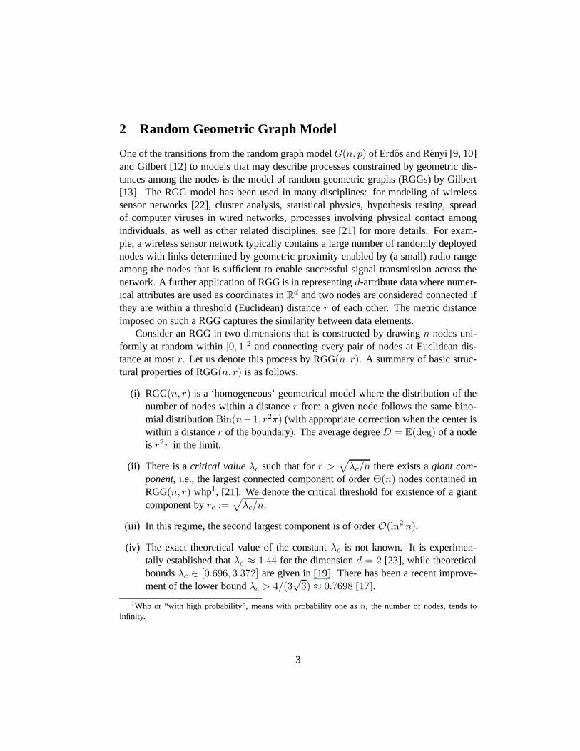
The functionJ(x) = x−1H(x) for x > 1, plotted in Figure 4, is continuous andstrictly increasing with the inverseJ−1 : [0,∞) → [1,∞). ForJ(γ/p) > 1/aγ theprobability given in (3) tends to1 asn tends to infinity. Finally, a bound onp is givenby

p <γ

J−1(1/aγ),

which concludes the proof. �

2 3 4 5 6 7

0.2

0.4

0.6

0.8

1.0

Figure 4: FunctionJ(x).

Let us denote the valuepc(a, γ) := γ/J−1(1/aγ). Herepc is also used to denotepc(a, γ). We now derivep′′c (θ) such that a connectedGn,r becomes fully active forp > p′′c whp. Observe thatpc = p′c(θ) = p′′c (θ).

Theorem 3 Consider bootstrap percolationBP (Gn,r, p, θ) wherer =√π−1a ln n

andθ = γa lnn. For anyγ ∈ (0, 1/5π), a > 5π/H(5πγ), andp > p′′c (θ) := p′′c =γ/J−1(1/aγ) whereJ(x) = lnx + x−1 − 1 for x > 1, Gn,r becomes fully activewithin O(n/r) steps whp.

The proof consists of two parts. We tile the square[0,√n]2 into cellsr/

√5×r/

√5

and show that in the initial configuration: (i) Whenγ < 1/5π anda > 5π/H(5πγ)every cell contains at leastγD nodes whp, (ii) Whenp > p′′c at least one cell containsγD or more active nodes. By Lemma 1 it follows that fora, γ, p in the specified rangesGn,r becomes fully active withinO(n/r) steps whp.Proof Tile the square[0,

√n]2 into cellsr/

√5× r/

√5, see Figure 5. Call two cells

neighboring if they share one side. Notice every pair of nodes within the same cell orwithin two neighboring cells are adjacent by the choice of the size of a cell. DefineG′

n,r

8

on the set of nodes ofGn,r as follows. The set of edges ofG′n,r consists of the subset of

edges ofGn,r whose terminal nodes belong to the same cell or two neighboring cells.By the monotonicity argument (Lemma 5 in Appendix)

Pp

(

G′n,r becomes fully active

)

6 Pp (Gn,r becomes fully active) . (4)

Therefore it is sufficient to show that whpG′n,r becomes fully active whenp > pc (10).

√

n

√

n

r/√

5

r/√

5

Figure 5: Tiling the square[0,√n]2.

Part (i) (To show that every cell contains at leastγD nodes whp.) We first boundthe probability an arbitrary cell contains at leastγD nodes. The number of nodes ina cell followsPo(r2/5), i.e.,Po(a lnn/5π). Moreover, the numbers of nodes in cellsare independent random variables (given the Poisson point processX ). Forγ < 1/5π,from (12) we obtain

P (a cell contains at mostγD nodes) = P

(

Po

(

a lnn

5π

)

< γa ln

)

6 exp

(

−a lnn

5πH(5πγ)

)

= n− a

5πH(5πγ) .

9

The total number of cells in[0,√n]2 is 5n/r2 = 5πn/(a ln n) = o(n). The union

bound taken over all cells yields

P (every cell contains at leastγD nodes) > 1− o(

n1− a

5πH(5πγ)

)

. (5)

Finally, for a > 5π/H(5πγ), from (5) it follows that every cell contains at leastγDnodes whp.

Part (ii). (To show that at least one cell containsγD or more active nodes.) We nowderive conditions such that at least one cell contains at least θ = γD active nodes inthe initial configuration. In order to guarantee that whp there is at least one cell among5n/r2 = Θ(n/ lnn), which contains at leastθ active nodes in the initial configuration,it suffices to findp such that

P (Po(pD) > γD + 1) = ω

(

lnn

n

)

, (6)

sincelimn→∞

1− (1− ω(lnn/n))Θ(n/ lnn) = 1 .

Defineα := (γ − p)/p, then by rewriting (6) we needp such that

P

(

Po(pD)− pD

pD> α+

1

pD

)

= ω

(

lnn

n

)

. (7)

By the Bahadur-Rao tail bound [3], asn → ∞, i.e.,pD = Θ(p lnn) → ∞, the shiftedPoisson random variablePo(pD)− pD satisfies

P

(

Po(pD)− pD

pD> α

)

≈√1 + α

α√2π

1√pD

exp (−pDI(α)) ,

where therate functionis defined by

I(α) = sups∈R

{sα− es + s+ 1} = (1 + α) ln(1 + α)− α . (8)

Therefore for (7) to be satisfied we require

n

lnn

√1 + α

α√2π

1√pD

exp {−pDI(α)} = ω(1) . (9)

The left hand side of (9) equals

exp{

ln

√1 + α

α√2π

− paI(α) ln n− ln(pa lnn) + lnn− ln lnn}

= exp{

(1− apI(α)) lnn− ln(pa)− 2 ln lnn+ ln

√1 + α

α√2π

}

,

10

which isω(1) if 1 > apI(α).From (8) andα = (γ − p)/p, the condition1 > apI(α) is equivalent to1/aγ >

J(γ/p), and moreover to

p >γ

J−1(1/aγ)= pc . (10)

To complete the proof notice that once anyγD nodes within a cell become active,all nodes within that cell become active at the next time stepas would all nodes withinits neighboring cells. This resulting process which jointly activates all nodes within onecell is equivalent to activating a site inZ2. The resulting BP inZ2 has the thresholdθ = 1 by construction, see Figure 5. ThusBP (G′

n,r, p, θ) becomes fully active whenp > pc by Lemma 1. Now the proof follows from (4). �

3.2 Analysis of the Critical Threshold

The critical thresholdpc = γ/J−1(1/aγ) can be rewritten as

ln pc = − ln a− ln(

(1/aγ)J−1(1/aγ))

. (11)

The function− ln(

xJ−1(x))

is monotonically decreasing inx, hencepc is mono-tonically increasing ina and monotonically decreasing inγ. As an example we nu-merically compute and tabulatepc for γ = 1/20 and different values ofa in Table 1.In Figure 6,pc is plotted as a function ina with precision10−6 for different values ofγ ∈ {1/70, 1/60, 1/50, 1/40, 1/30, 1/20}.

a pc

3 0.0000234197577164 0.0001242459668225 0.0003391906301616 0.0006649716344097 0.001079469303118 0.001557646750199 0.0020779022443210 0.0026234548777925 0.010118849802150 0.0174952120548

a pc

100 0.0246619916484200 0.0308408415894300 0.0338938242715400 0.035809469627500 0.0371585449017600 0.0381763433375700 0.0389805098623800 0.0396369961599900 0.0401864313551000 0.0406552556763

Table 1: Critical thresholdpc for different values ofa andγ = 1/20.

The experiments are performed onGn,r with n = 15000 nodes andr =√

a lnn/πfor a ∈ {10, 25, 50} andγ = 1/20. On these instances of graphs, for each chosen value

11

100 101 102 103a

10-1310-1210-1110-1010-910-810-710-610-510-410-310-210-1

p_c

Figure 6: Critical thresholdpc for γ ∈ {1/70, 1/60, 1/50, 1/40, 1/30, 1/20}.

of p in (0, 1) we simulate BP100 times. More precisely, within each experiment wegenerate a random initial configuration with the probability p and perform BP with thethresholdθ = γD where the expected degreeD is calculated for a given inputGn,r.

Our experimental results are presented such that abscissa corresponds to the initialprobability p, while ordinate corresponds to the percentage of fully active stable con-figurations attained for a givenp. The casesa = 10, 25, 50 are presented in Figure 7,Figure 8, Figure 9, respectively. A theoretical upper boundon the critical thresholdpcmatches with the performed experiments, i.e., the instanceof BP (Gn,r, p, θ) do notbecome fully active forp < pc(θ). On the other hand instances ofBP (Gn,r, p, θ) areexpected to become fully active whenp > pc(θ). This, however, does not happen inour simulations whenp is only slightly abovepc(θ). This is due to the finite size ofn = 15000 in our simulations and for sufficiently largen we can verify every value ofpstrictly above the theoretical thresholdpc(θ). We do not know whether the analyticallyderived threshold is sharp and plan to examine this further.

Acknowledgements

This work was funded by NIST Grant No. 60NANB10D128.

12

0.002 0.003 0.004 0.005 0.006 0.007 0.008 0.009 0.010p

0

20

40

60

80

100

percen

tage

Figure 7: Percentage of fully percolated configurations in100 simulations ofBP (Gn,r, p, θ) whenn = 15000, r =

√

10 ln n/πn ≈ 0.0452, D = 10 ln n ≈ 96.16andθ = ⌈20−1

E(deg)⌉ = ⌈4.81⌉ = 5.

0.000 0.005 0.010 0.015 0.020 0.025 0.030p

0

20

40

60

80

100

percen

tage

Figure 8: Percentage of fully percolated configurations in100 simulations ofBP (Gn,r, p, θ) whenn = 15000, r =

√

25 ln n/πn ≈ 0.0714, D = 25 ln n ≈ 240.40andθ = ⌈20−1

E(deg)⌉ = ⌈12.02⌉ = 13.

References

[1] A IZENMAN , M., AND LEBOWITZ, J. L. Metastability effects in bootstrap per-

13

0.016 0.018 0.020 0.022 0.024 0.026 0.028 0.030 0.032p

0

20

40

60

80

100

percen

tage

Figure 9: Percentage of fully percolated configurations in100 simulations ofBP (Gn,r, p, θ) whenn = 15000, r =

√

50 ln n/πn ≈ 0.1010, D = 50 ln n ≈ 480.79andθ = ⌈20−1

E(deg)⌉ = ⌈24.04⌉ = 25.

colation. Journal of Physics A: Mathematical and General 21, 19 (1988), 3801–3813.

[2] A MINI , H. Bootstrap percolation and diffusion in random graphs with givenvertex degrees.Electronic Journal of Combinatorics 17, #R25 (2010).

[3] BAHADUR , R. R., AND RAO, R. R. On deviations of the sample mean.Ann.Math. Statist. 31, 4 (1960), 1015–1027.

[4] BALOGH, J., BOLLOBAS, B., DUMINIL -COPIN, H., AND MORRIS, R. Thesharp threshold for bootstrap percolation in all dimensions. In preparation.

[5] BALOGH, J., PERES, Y., AND PETE, G. Bootstrap percolation on infinitetrees and non-amenable groups.Combinatorics, Probability & Computing 15,5 (2006), 715–730.

[6] BALOGH, J., AND PITTEL, B. Bootstrap percolation on the random regulargraph.Random Structures & Algorithms 30, 1-2 (2007), 257–286.

[7] CERF, R., AND CIRILLO , E. N. M. Finite size scaling in three-dimensionalbootstrap percolation.Ann. Prob 27(1998).

14

[8] CHALUPA , J., LEATH, P. L., AND REICH, G. R. Bootstrap percolation on aBethe lattice.J. Phys. C 12, L31 (1979).

[9] ERDOS, P.,AND RENYI , A. On random graphs.Publ. Math. Inst. Hungar. Acad.Sci.(1959).

[10] ERDOS, P., AND RENYI , A. On the evolution of random graphs.Publ. Math.Inst. Hungar. Acad. Sci.(1960).

[11] GERSHO, A., AND M ITRA , D. A simple growth model for the diffusion of newcommuinication services.IEEE Trans. on Systems, Man, and Cybernetics SMC-5,2 (March 1975), 209–216.

[12] GILBERT, E. N. Random graphs.Ann. Math. Statist. 30, 4 (1959), 1141–1144.

[13] GILBERT, E. N. Random plane networks.Soc. Ind. Appl. Math. 9, 4 (1961),533–543.

[14] GOEL, A., RAI , S.,AND KRISHNAMACHARI , B. Sharp thresholds for monotoneproperties in random geometric graphs. InSTOC ’04: Proceedings of the thirty-sixth annual ACM symposium on Theory of computing(New York, NY, USA,2004), ACM Press, pp. 580–586.

[15] GUPTA, P., AND KUMAR , P. R. Critical power for asymptotic connectivity. InProceedings of the 37th IEEE Conference on Decision and Control (1998), vol. 1,pp. 1106–1110.

[16] HOLROYD, A. E. Sharp metastability threshold for two-dimensional bootstrappercolation.Probability Theory and Related Fields 125(2003), 195–224.

[17] KONG, Z., AND YEH, E. M. Analytical lower bounds on the critical densityin continuum percolation. InProceedings of the Workshop on Spatial StochasticModels in Wireless Networks (SpaSWiN)(Limassol, Cyprus, April 16, 2007.).

[18] LUCZAK , T., JANSON, S., TUROVA, T., AND VALLIER , T. Bootstrap percola-tion on the random graphGn,p. Ann. of Appl. Probab. To appear.

[19] MEESTER, R., AND ROY, R. Continuum percolation. Cambridge UniversityPress, 1996.

[20] PENROSE, M. D. The longest edge of the random minimal spanning tree.TheAnnals of Applied Probability 7, 2 (1997), 340–361.

[21] PENROSE, M. D. Random Geometric Graphs. Oxford University Press, 2003.

15

[22] POTTIE, G. J.,AND KAISER, W. J. Wireless integrated network sensors.Com-mun. ACM 43, 5 (2000), 51–58.

[23] RINTOUL, M. D., AND TORQUATO, S. Precise determination of the criticalthreshold and exponents in a three-dimensional continuum percolation model.Journal of Physics A. Mathematical and General 30, 16 (1997), L585–L592.

[24] WATTS, D. J. A simple model of global cascades in random networks.Proceed-ings of the National Academy of Sciences 99(2002), 5766–5771.

Appendix

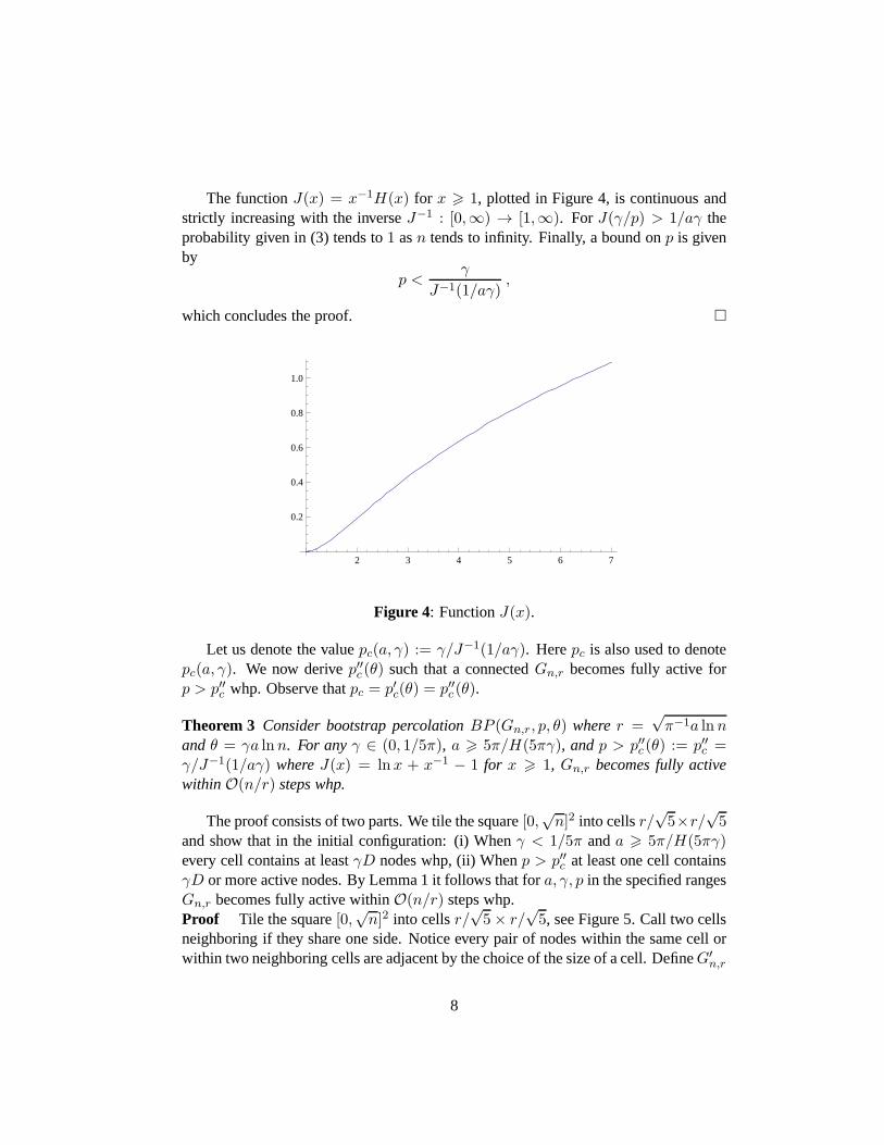
Lemma 4 (Concentration on a Poisson random variable, see [21]). A Poisson randomvariablePo(λ) (with λ > 0) satisfies:

P (Po(λ) > k) 6 exp (−λH(k/λ)) , for k > λ , (12)

P (Po(λ) < k) 6 exp (−λH(k/λ)) , for k < λ , (13)

whereH(x) = lnx+ x−1 + 1 for x > 0.

Lemma 5 For any two graphsG′ = (V,E′) andG = (V,E) on the same set of nodesV such that sets of edges satisfyE′ ⊆ E we have

Pp

(

G′ becomes fully active)

6 Pp (G becomes fully active) .

Proof We prove the assertion by induction int. LetXv (respectivelyYv) be the firsttime when a nodev becomes active inG′ (respectively inG). For everyv ∈ V we havePp (Xv = 0) = Pp (Yv = 0) = p. Let us assumePp (Xv = τ) = Pp (Yv = τ) for anyτ 6 t and anyv ∈ V . Then

Pp (Xv = t+ 1) = Pp (Xv = t) + (1− Pp (Xv = t)) ΠXv(t) , (14)

where

ΠXv(t) =

|NG(v)|∑

ℓ=θ

∑

I⊆V :|I|=ℓ

∏

i∈I

Pp (Xv = t)∏

i/∈I

(1− Pp (Xv = t)) .

Analogously we write the equation forPp (Xv = t+ 1) and defineΠY (t)

Pp (Yv = t+ 1) = Pp (Yv = t) + (1− Pp (Yv = t))ΠYv(t) , (15)

16

where

ΠYv(t) =

|NG(v)|∑

ℓ=θ

∑

I⊆V :|I|=ℓ

∏

i∈I

Pp (Yv = t)∏

i/∈I

(1− Pp (Yv = t)) .

It is not hard to see that the inductive hypothesisPp (Xv = t) 6 Pp (Yv = t) foranyv andNG′(v) ⊆ NG(v) yields

ΠXv(t) 6 Π(t) . (16)

Now (14), (15), and (16) givePp (Xv = t+ 1) 6 Pp (Yv = t+ 1) for any v. Fi-nally the initial configurations (att = 0) satisfyPp ({Xv}v∈V ) = Pp ({Yv}v∈V ) for{Xv}v∈V = {Yv}v∈V , which concludes the proof. �

17