Bootstrap methods
10
Applied Mathematical Sciences, Vol. 8, 2014, no. 96, 4783 - 4792 HIKARI Ltd, www.m-hikari.com http://dx.doi.org/10.12988/ams.2014.46498 On the Test and Estimation of Fractional Parameter in ARFIMA Model: Bootstrap Approach T. O. Olatayo and A. F. Adedotun Department of Mathematical Sciences Olabisi Onabanjo University, Ago-Iwoye Ogun State, Nigeria Copyright © 2014 T. O. Olatayo and A. F. Adedotun. This is an open access article distributed under the Creative Commons Attribution License, which permits unrestricted use, distribution, and reproduction in any medium, provided the original work is properly cited. Abstract One of the most important problems concerning Autoregressive Fractional Integrated Moving Average (AFRIMA) time series model is the estimation of the fractional parameter . This research work was aimed to show efficiency of the different methods used to test and estimate fractional parameter in the fractionally integrated autoregressive moving-average (AFRIMA) model. In this study, estimates were obtained by smoothed spectral regression method and truncated geometric bootstrap method which aid in the test and estimation of fractional parameter by obtaining estimates through regression estimation method. The results indicate that the semi-parametric methods outperformed the parametric method when elements of AR or MA components are involved. Performance of one of the semi-parametric method (Robinson estimator) usually is not as good as the other semi- parametric method: it has large bias, standard deviation and mean square error. The use of smoothed periodogram in this method improves the estimate; however, they are still not as good as the usual semi-parametric methods. In the long run, having compared the result of the two estimates, it was discovered that the bootstrap approach that is, the stimulation obtained using the truncated geometric bootstrap method produced a set of
-
Upload
olabisionabanjouniversity -
Category
Documents
-
view
3 -
download
0
Transcript of Bootstrap methods
Applied Mathematical Sciences, Vol. 8, 2014, no. 96, 4783 - 4792
HIKARI Ltd, www.m-hikari.com
http://dx.doi.org/10.12988/ams.2014.46498
On the Test and Estimation of Fractional Parameter
in ARFIMA Model: Bootstrap Approach
T. O. Olatayo and A. F. Adedotun
Department of Mathematical Sciences
Olabisi Onabanjo University, Ago-Iwoye
Ogun State, Nigeria
Copyright © 2014 T. O. Olatayo and A. F. Adedotun. This is an open access article distributed under
the Creative Commons Attribution License, which permits unrestricted use, distribution, and
reproduction in any medium, provided the original work is properly cited.
Abstract
One of the most important problems concerning Autoregressive
Fractional Integrated Moving Average (AFRIMA) time series model is
the estimation of the fractional parameter . This research work was
aimed to show efficiency of the different methods used to test and
estimate fractional parameter in the fractionally integrated
autoregressive moving-average (AFRIMA) model.
In this study, estimates were obtained by smoothed spectral regression
method and truncated geometric bootstrap method which aid in the test
and estimation of fractional parameter by obtaining estimates
through regression estimation method.
The results indicate that the semi-parametric methods outperformed the
parametric method when elements of AR or MA components are
involved. Performance of one of the semi-parametric method
(Robinson estimator) usually is not as good as the other semi-
parametric method: it has large bias, standard deviation and mean
square error. The use of smoothed periodogram in this method
improves the estimate; however, they are still not as good as the usual
semi-parametric methods.
In the long run, having compared the result of the two estimates, it was
discovered that the bootstrap approach that is, the stimulation obtained
using the truncated geometric bootstrap method produced a set of

4784 T. O. Olatayo and A. F. Adedotun
fractional parameter of the estimates of the parameters of ARFIMA
models that behave better and has reasonably good power.
Keywords: AFRIMA Model, Periodogram Regression, Truncated
Geometric Bootstrap, Parametric, Semi-parametric, Fractional
Parameter
1. Introduction
A time series is a realization or sample function from a certain stochastic process.
It is an ordered sequence of observation (a collection of observation made sequentially
in time). Although, the ordering is usually through equally spaced time interval, the
ordering may also be taken through other dimensions such as space.
Time series occurs in many fields such as agriculture, engineering, business and
economics, geophysics, medical sciences, meteorology, quality control, social
sciences, etc. Examples of time series are the total annual production of steel over a
number of years, the early temperature announced by the weather bureau and the total
monthly sale receipt in a departmental store etc.
Mathematically, a time series is defined by the values of a variable
(temperature, total sales, total production, etc) at times Thus is a function of
t; this is symbolized by .
Naturally, if we are working into future there are certain assumptions that we have to
make. The most important of which the behaviour pattern that we have found in the
past will continue. When looking into the future, there are certain pattern that we
assume will continue and this is to help in determination of those patterns that will
undertake the analysis of time series.
The Autoregressive Fractional Integrated Moving Average (ARFIMA)(p, d, q) process
was first introduced by [6] and [5]. The most useful feature for this process is the long
memory. This property is reflected by the hyperbolic decay of the autocorrelation
function or by the unboundedness of the spectral density function of the process.
While in an Autoregressive Moving Average (ARMA) structure, the dependency
between observations decays at a geometric rate.
The primary aim of the research is to show that the bootstrap ARFIMA model will
performs better in the estimation long memory phenomenon. To achieve the aim, the
following objectives are sought: Applying bootstrapping to the data to obtain the
fractional parameter using different methods, Estimation of fractional parameter, d,
using different methods, Proposition of ARFIMA models and distribution properties,
Estimation of parameters of the ARFIMA model and Identification of optimal models
in the ARFIMA models.
On the test and estimation of fractional parameter 4785
To overcome the difficulties of moving block scheme and geometric stationary
scheme in determining both b and p respectively we introduce another method called a
truncated geometric bootstrap scheme, [10].
2. Literature Review
Most of the author, [8],carried out a study in which she constructed a test for the
difference parameter d in the fractionally integrated autoregressive moving average
(ARFIMA) model. Estimates were obtained using smoothed spectral regression
estimation method. Also, moving block bootstrap method was used to construct the
test for d.
Also, [12], used performance of the Geweke-Porter-Hudak (GPH) test, the modified
rescaled range (MRR) test and two Lagrange multiplier (LM) type tests for fractional
integration in small samples with Monte Carlo methods Both the GPH and MRR
tests are found to be robust to moderate autoregressive moving-average components,
autoregressive conditional heteroskedasticity effects and shifts in the variance.
However, these two tests are sensitive to large autoregressive moving-average
components and shifts in the mean. It is also found that the LM tests are sensitive to
deviations from the null hypothesis. As an illustration, the GPH test is applied to two
economic data series.
From the literatures relating to the subject matter such as that of [8],there were
remarkable discoveries. He used the smoothed spectral regression estimation method
to estimate difference parameter, d, in the fractionally integrated autoregressive
moving average (ARFIMA) model. Moving blocks bootstrap method was used to test
the obtained, d. The study is limited in that for the Monte Carlo simulations, the test is
generally valid for certain blocks only and not all the blocks. For the valid blocks, the
test has reasonably good power.
Furthermore [3], applied Jacknife and Bootstrap for the estimation of fractional
parameter via the ARFIMA model. From the simulations, the estimation with moving
blocks gave smaller values of relative bias. There was no theoretical argument as to
what is the correlation between the number of terms of the series and the number of
cycles which appear in the block in order to get the optimal results from the
estimation.
It is in the light of the above researcher that we apply a different concept yet similar
method of boottrap. In this paper, the truncated geometric bootstrap method proposed
by [12] for stationary time series process was used to simulate the time series data.
The fractional difference, d, is estimated using regression estimation method. This
method is thought to produce a set of fractional parameter, d, of the estimates of
ARFIMA model that behave better and has reasonably good powers.
4786 T. O. Olatayo and A. F. Adedotun
3. Fractional ARIMA Processes
We consider the asymptotic and finite-sample properties of AFRIMA parameter
estimates obtained using ant of the various preliminary autoregressive estimators.
Maximum likelihood produces asymptotically normal estimates of ARFIMA
parameters which converge at the usual rate for stationary Guassian processes . The
Quasi-MLE has this property as well for a range of assumptions on the error process.
The MLE of Tieslau et al. converges at the standard rate to an asymptotic normal
distribution for ; at , convergence is to the normal distribution at rate
, and for convergence is at rate and the limiting distribution is
non-normal. The fractional differencing parameter can therefore be obtained by:
[7] obtained the peridogram estimation of d
Algorithm for Fitting Fractional Autoregressive Integrated Moving Average
Models
We fit full autoregressive integrated moving average models of various orders and
choose that model for which Akaike Information Criterion (AIC) is minimum. Let the
order of this full autoregressive integrated moving average model be p+d+q and let
the model be , denoted
by ARIMA (p.d,q) respectively.
Let the mean sum of squares of the residuals be and its Akaike Information
Criterion (AIC) be equal to AIC(1). The estimation of models is done by using
Malquardt algorithm and Newton-Raphson iterative method. Having fitted the full
model, we can now fit the best subset models by considering the subsets using
the fitted models with minimum AIC, [4] and [9].
Let the best subset autoregressive integrated moving average model be
,
where are subsets of the integers (1,2,…,p+d+q). Let the
mean sum of squares of the residuals be and AIC value be AIC(2);
. This is our final subset autoregressive integrated moving average
models.
On the test and estimation of fractional parameter 4787
Estimation Method of ARFIMA Models
Numerous methods of estimating ARFIMA models have been proposed in the
literature, see [1] and [2]. The majority of them can be divided into three groups:
Least squares method
One-step methods: Maximum Likelihood methods.
EML: Exact Maximum Likelihood.
MPL: Modified Profile Likelihood
CSS: Conditional sum of squares
Two-step methods: Log-periodogram regressions
Identification and Estimation of an AFRIMA Model
For the use of the regression technique several steps are necessary to obtain on
AFRIMA model for a set of time series data and these are given below.
Let be the process as defined earlier. Then is an ARMA
process and is an ARFIMA process.
Model Building Steps:
1. Estimate d in the ARIMA model; the estimate by
2. Calculate .
3. Using Box-Jenkins modeling procedure (or the AIC criterion) identify and
estimate and parameters in the ARMA process
4. Calculate
5. Estimate d in the ARFIMA model . The value of
obtained in this step is now estimate of d.
6. Repeat steps 2 to 5, until the estimates of the parameters converage.
In this algorithm, to estimates d we use the regression methods described in section. It
should be noted that usually only one iteration with steps 1-3 is used to obtain a
model. Related to step 3, it has widely been discussed that the bias in the estimator of
d can lead to the problem of identifying the short-memory parameters.
4. Results
The data was bootstrapped using truncated geometric bootstrapping method,[11] was
analysed with the use of a statistical software called OxMetrics. A two dimemsional
grid values of (p,q) was set up with maximum values (p,q)= (10,10) and a search over
all the constituent models was undertaken using the AIC to select the best fitting
model.
4788 T. O. Olatayo and A. F. Adedotun
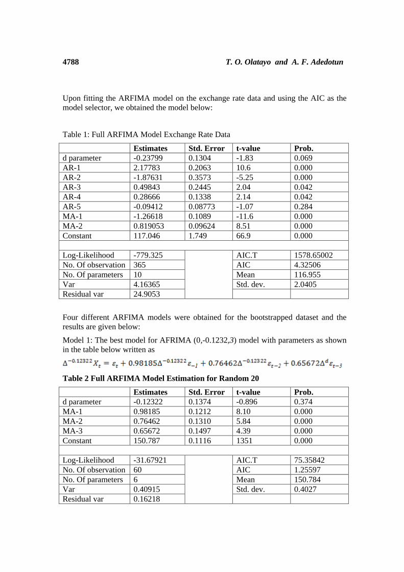
Upon fitting the ARFIMA model on the exchange rate data and using the AIC as the
model selector, we obtained the model below:
Table 1: Full ARFIMA Model Exchange Rate Data
Estimates Std. Error t-value Prob.
d parameter -0.23799 0.1304 -1.83 0.069
AR-1 2.17783 0.2063 10.6 0.000
AR-2 -1.87631 0.3573 -5.25 0.000
AR-3 0.49843 0.2445 2.04 0.042
AR-4 0.28666 0.1338 2.14 0.042
AR-5 -0.09412 0.08773 -1.07 0.284
MA-1 -1.26618 0.1089 -11.6 0.000
MA-2 0.819053 0.09624 8.51 0.000
Constant 117.046 1.749 66.9 0.000
Log-Likelihood -779.325 AIC.T 1578.65002
No. Of observation 365 AIC 4.32506
No. Of parameters 10 Mean 116.955
Var 4.16365 Std. dev. 2.0405
Residual var 24.9053
Four different ARFIMA models were obtained for the bootstrapped dataset and the
results are given below:
Model 1: The best model for AFRIMA (0,-0.1232,3) model with parameters as shown
in the table below written as
Table 2 Full ARFIMA Model Estimation for Random 20
Estimates Std. Error t-value Prob.
d parameter -0.12322 0.1374 -0.896 0.374
MA-1 0.98185 0.1212 8.10 0.000
MA-2 0.76462 0.1310 5.84 0.000
MA-3 0.65672 0.1497 4.39 0.000
Constant 150.787 0.1116 1351 0.000
Log-Likelihood -31.67921 AIC.T 75.35842
No. Of observation 60 AIC 1.25597
No. Of parameters 6 Mean 150.784
Var 0.40915 Std. dev. 0.4027
Residual var 0.16218
On the test and estimation of fractional parameter 4789
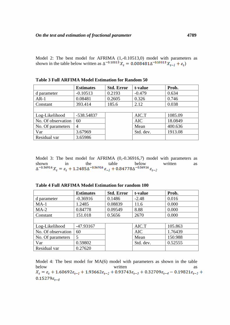
Model 2: The best model for AFRIMA (1,-0.10513,0) model with parameters as
shown in the table below written as )
Table 3 Full ARFIMA Model Estimation for Random 50
Estimates Std. Error t-value Prob.
d parameter -0.10513 0.2193 -0.479 0.634
AR-1 0.08481 0.2605 0.326 0.746
Constant 393.414 185.6 2.12 0.038
Log-Likelihood -538.54837 AIC.T 1085.09
No. Of observation 60 AIC 18.0849
No. Of parameters 4 Mean 400.636
Var 3.67969 Std. dev. 1913.08
Residual var 3.65986
Model 3: The best model for AFRIMA (0,-0.36916,7) model with parameters as
shown in the table below written as
Table 4 Full ARFIMA Model Estimation for random 100
Estimates Std. Error t-value Prob.
d parameter -0.36916 0.1486 -2.48 0.016
MA-1 1.2485 0.08839 11.6 0.000
MA-2 0.84778 0.09549 8.88 0.000
Constant 151.018 0.5656 2670 0.000
Log-Likelihood -47.93167 AIC.T 105.863
No. Of observation 60 AIC 1.76439
No. Of parameters 5 Mean 150.988
Var 0.59802 Std. dev. 0.52555
Residual var 0.27620
Model 4: The best model for MA(6) model with parameters as shown in the table
below written as
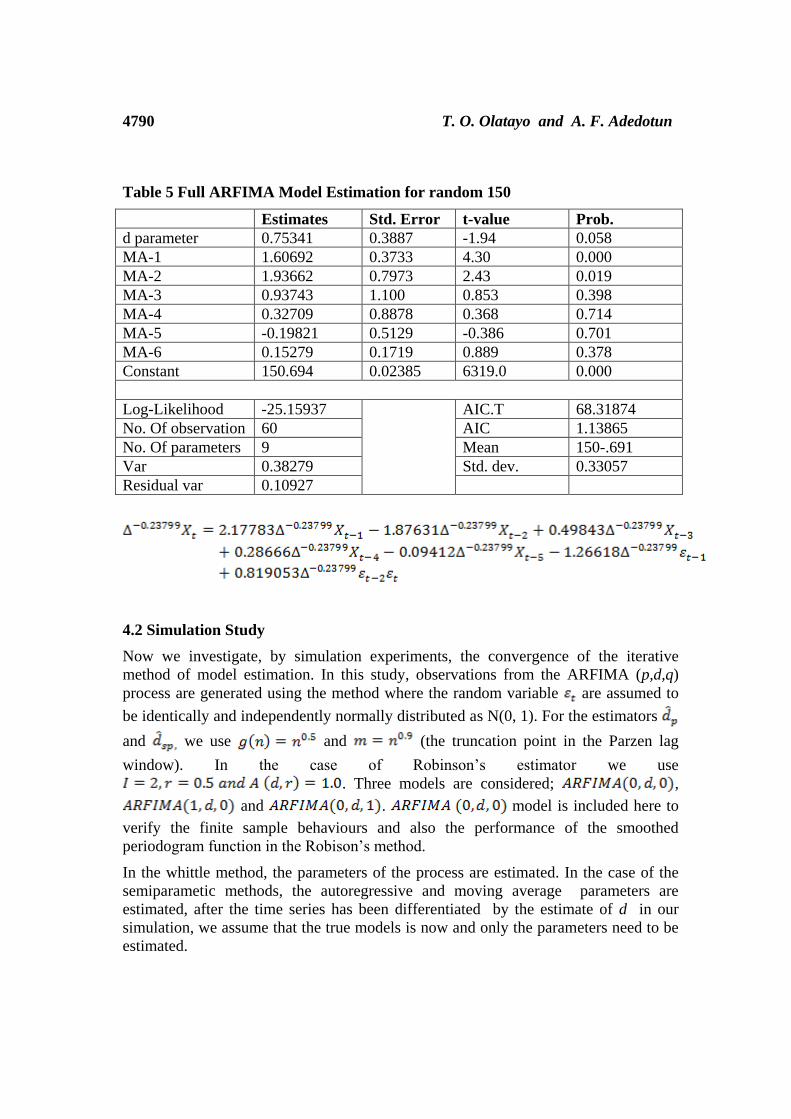
4790 T. O. Olatayo and A. F. Adedotun
Table 5 Full ARFIMA Model Estimation for random 150
Estimates Std. Error t-value Prob.
d parameter 0.75341 0.3887 -1.94 0.058
MA-1 1.60692 0.3733 4.30 0.000
MA-2 1.93662 0.7973 2.43 0.019
MA-3 0.93743 1.100 0.853 0.398
MA-4 0.32709 0.8878 0.368 0.714
MA-5 -0.19821 0.5129 -0.386 0.701
MA-6 0.15279 0.1719 0.889 0.378
Constant 150.694 0.02385 6319.0 0.000
Log-Likelihood -25.15937 AIC.T 68.31874
No. Of observation 60 AIC 1.13865
No. Of parameters 9 Mean 150-.691
Var 0.38279 Std. dev. 0.33057
Residual var 0.10927
4.2 Simulation Study
Now we investigate, by simulation experiments, the convergence of the iterative
method of model estimation. In this study, observations from the ARFIMA (p,d,q)
process are generated using the method where the random variable are assumed to
be identically and independently normally distributed as N(0, 1). For the estimators
and we use and (the truncation point in the Parzen lag
window). In the case of Robinson’s estimator we use
. Three models are considered; ,
and . model is included here to
verify the finite sample behaviours and also the performance of the smoothed
periodogram function in the Robison’s method.
In the whittle method, the parameters of the process are estimated. In the case of the
semiparametic methods, the autoregressive and moving average parameters are
estimated, after the time series has been differentiated by the estimate of d in our
simulation, we assume that the true models is now and only the parameters need to be
estimated.
On the test and estimation of fractional parameter 4791
5. Conclusion
In this study we considered a simulation study to evaluate the procedures for
estimating the parametric and semiparametric methods and also used the smoothed
periodogram function in the modified regression estimator. The results indicate that
the regression methods outperform the parametric Whittle’s method when AR or MA
components are involved. Performance of the Robinson estimator usually is not as
good as the other semiparametric methods; it has large bias, standard deviation, and
mean squared error. The use of the smoothed periodogram in Robinson’s method
improves the estimates; however, the results are still not as good as the usual
regression methods.
The simulation results showed clearly that the bootstrap is a very good alternative for
the estimation of time series data, in particular for the estimation of fractional
parameter via the Autoregressive Fractional Integrated Moving Average (ARFIMA)
model.
It is important to stress clearly that the units of samples have been geometrically
constructed in such a way that they preserve the structure and dependence between
terms of the time series.
From the tables in section four above, it is quite clear that the ARFIMA model from
simulated data did performed better as the units increased to 150. This is indicated by
the values of the AIC for all the models.
In comparing the result of the two estimates, it was discovered that the bootstrap
approach that is, the simulation obtained using the truncated geometric bootstrap
method produced a set of fractional parameter of the estimates of the parameters of
ARFIMA models that shows a behavior that is reasonably better and the power is
good.
References
[1] Baillie, R.T.,. Long memory processes and fractional integration in econometrics-
J. Econometrics, 73: (1996), 5-59.
[2] Beran, J., Y. Statistics for Long Memory Processes. Chapman and Hall, New
York.(1994)..
[3] Ekonomi, L and Butka .. Jacknife and bootstrap with cycling blocks for the
estimation of fractional parameter in ARFIMA model. Turk J. Math. 35, (2011),
151-158..
[4] Hagan, V. and Oyetunji, O.B. On the Selection of Subset Autoregressive Time
Series Models.UMIST Technical Report, (1980).No. 124 (Dept. of Mathematics).
4792 T. O. Olatayo and A. F. Adedotun
[5] Hosking, J.R.M. Fractional Differencing.Biometrika 68(1), . (1981), 165-176.
[6] Granger, C.and Joyeux R, An Introduction to Long-Memory Time Series Models
and Fractional Differencing. Journal of Time Series Analysis, 1. (1980).15-30..
[7] Geweke, J., S.and Porter-Hudak,. The estimation and application of long-memory
time series models. Journal of Time Series Analysis, 4: (1983), 221-238.
[8] Maharaj, E.A. A Test for the Difference Parameter of the ARFIMA model using
Blocks Bootstrap. Monash Econometric and Business Statistics Working Paper
11/99. (1999)..
[9] Ojo, J.F. On the Estimation and Performance of Subset Autoregressive Moving
Average Models. European Journal of Scientific Research, Vol 18, 14: (2007) ;
700-706.
[10] Olatayo, T.O., Amahia, G.N. & Obilade T.O. Boostrap Method for Dependent
Data Structure and Measure of Statistical Precision. Journal of Mathematics and
Statistics. 6(2): (2010). 84-88.
[11] Olatayo T.O. On the application of Bootstrap method to Stationary Time
Series Process. American Journal of Computational Mathematics, 2013, 3,
(2013), 61-65
doi:10.4236/ajcm.2013.31010 Published Online March 2013
(http://www.scirp.org/journal/ajcm)
[12] Yin-Wong Cheung. Test for Fractional Integration: A Monte Carlo Investigation
Journal of Time Series Analysis. Vol. 14, 4. (2008); 331-345.
Received: June 3, 2014