Effects of parameter estimation on prediction densities:a bootstrap approach

*Lorenzo Pascual, Juan Romo, Esther RuizDepartamento de Estadı stica y Econometrı a, Universidad Carlos III de Madrid, C /Madrid, 126, 28903 Getafe, Madrid, Spain

Abstract

We use a bootstrap procedure to study the impact of parameter estimation on prediction densities, focusing on seasonalARIMA processes with possibly non normal innovations. We compare prediction densities obtained using the Box andJenkins approach with bootstrap densities which may be constructed either taking into account parameter estimationvariability or using parameter estimates as if they were known parameters. By means of Monte Carlo experiments, we showthat the average coverage of the intervals is closer to the nominal value when intervals are constructed incorporatingparameter uncertainty. The effects of parameter estimation are particularly important for small sample sizes and when theerror distribution is not Gaussian. We also analyze the effect of the estimation method on the shape of prediction densitiescomparing prediction densities constructed when the parameters are estimated by Ordinary Least Squares (OLS) and byLeast Absolute Deviations (LAD). We show how, when the error distribution is not Gaussian, the average coverage andlength of intervals based on LAD estimates are closer to nominal values than those based on OLS estimates. Finally, theperformance of the bootstrap intervals is illustrated with two empirical examples. 2001 International Institute ofForecasters. Published by Elsevier Science B.V. All rights reserved.

Keywords: Forecasting; Least absolute deviations; Non normal distributions; Ordinary least squares

1. Introduction has been stressed by Chatfiel (1993). In thestandard approach to construct prediction inter-

Our main goal in this paper is to study the vals, based on Box and Jenkins (1976), predic-impact of parameter estimation on prediction tion errors are assumed to be Gaussian anddensities and we use the bootstrap as a device to intervals are obtained with center at the pointasses its relevance. The interest of building linear predictor and conditioning on parameterprediction intervals which are able to incorpo- estimates. Consequently, Box and Jenkins (BJ)rate the uncertainty due to parameter estimation intervals do not take into account the variability

due to parameter estimation and may havecoverage which is different from the nominal*Corresponding author. Tel.: 134-916-249-851; fax:one when the errors are not Gaussian. Alter-134-916-249-849.

E-mail address: ortega@est-econ.uc3m.es (E. Ruiz). natively, prediction intervals can be built using

bootstrap procedures. Bootstrap intervals can shapes closer to the corresponding empiricalincorporate the variability due to parameter prediction densities. As a second goal of thisestimation without assuming any particular dis- paper, we show how the bootstrap proceduretribution for the errors. We analyze the effect of proposed by Pascual et al. (1998) can beparameter estimation on the shape of prediction extended to construct prediction intervals indensities using the bootstrap procedure pro- multiplicative seasonal ARIMA models.posed by Pascual, Romo and Ruiz (1998) for The paper is organized as follows. First, inARIMA( p, d, q) models. Section 2 we describe the bootstrap procedureFirst, estimating the parameters by condition- proposed by Pascual et al. (1998) to construct

al Quasi-Maximum Likelihood (QML), we prediction intervals. Then, Section 3 containscompare bootstrap intervals (PRR) constructed the Monte Carlo results on the effects oftaking into account parameter variability with parameter variability on the shape of predictionintervals obtained by using parameter estimates densities when seasonal ARIMA models areas if they were the true parameters. The latter estimated by conditional QML by maximizingapproach will be referred to as conditional the conditional Gaussian likelihood function.bootstrap (CB). We compare average coverage Also, we carry out experiments to assess theand length of BJ, CB and PRR intervals. The effects of the method used to estimate the modeldifference between BJ and CB intervals could parameters on prediction intervals. In Section 4,be assignable to the deviation of the innovation we apply the bootstrap PRR procedure to obtaindistribution from the Gaussian assumption. The prediction densities for two real time series:difference between CB and PRR intervals could monthly observations of the Italian Industrialbe due to parameter estimation uncertainty. Production Index and levels of a luteinizingConsequently, we can distinguish between the hormone measured on a healthy woman. Final-two sources which could affect the precision of ly, Section 5 contains the conclusions and someprediction intervals when the model is known. suggestions for further research.As expected, given that the conditional QMLestimator is consistent, the variability due toparameter estimation should be taken into ac- 2. Bootstrap prediction intervalscount in the construction of prediction intervals

We now describe the bootstrap procedurewhen the series sample size is not large enough.proposed in Pascual et al. (1998) to constructIn this case, intervals obtained by conditioningprediction intervals for future values of serieson parameter estimates have average coveragegenerated by ARIMA ( p, d, q) processes givenlower than the nominal value. As the samplebysize increases, the effect of parameter estimation

is less important. d d d= y 5 f 1 f = y 1 ? ? ? 1 f = yt 0 1 t21 p t2pWe also study the effect of the estimation

method on the shape of prediction densities. In 1 a 1u a 1 ? ? ? 1u a , (1)t 1 t21 q t2qparticular, we consider the prediction of futurevalues of ARI( p, d) processes and compare where a is a white noise process, = is thetprediction intervals obtained when estimating difference operator such that =y 5 y 2 y andt t t21by Ordinary Least Squares (OLS) and by Least f , f , . . . , f , u , . . . , u are unknowns d0 1 p 1 qAbsolute Deviations (LAD). When the error parameters. From an observed series hy ,1distribution is not Gaussian, prediction densities y , . . . , y j, the parameters can be estimated by2 Tbased on the LAD estimator have, in general, a consistent estimator, for example conditional

ˆ ˆ ˆ ˆ ˆQML. Given (f , f , . . . ,f , u , . . . ,u ), the Once the parameters of model (5) have been0 1 p 1 qˆ * ˆ *residuals are calculated by the following recur- estimated and the bootstrap draws a , . . . , a2 T

sion are available, a bootstrap replicate of the seriesis constructed byd dˆ ˆa 5= y 2 f 2 f = y 2 ? ? ?t t 0 1 t21 ˆ ˆ ˆ* * * ˆ * ˆ *y 5 (11 f ) y 2 fy 1 a 1 ua ,d t t21 t22 t t21ˆ ˆ ˆˆ ˆ2 f = y 2 u a 2 ? ? ? 2 u a ,p t2p 1 t21 q t2q t5 3, . . . , T, (6)

t5 p1 d1 1, . . . , T, (2)* *where y 5 y and y 5 y . Then, bootstrap1 1 2 2

where the residuals corresponding to periods of ˆ ˆestimates f* and u* are obtained for thetime t5 0,2 1,2 2, . . . are set equal to zero. bootstrap series and bootstrap replicates of

ˆDenote by F the empirical distribution functiona future values of the series are generated byof the centered residuals. Given a set of p1 d ˆ ˆ*y 5 (11 f*)y 2 f*yT11 T T21initial values of the variable y , say hy , . . . ,t 1y j, a bootstrap replicate of the series ˆˆ * ˆ1 a 1 u*a ,p1d T11 T

* *hy , . . . , y j is constructed by the following1 Tequation ˆ ˆ* *y 5 (11 f*)y 2 f*yT12 T11 T

p q ˆˆ * ˆ *1 a 1 u*a , (7)d d T12 T11ˆ ˆ ˆ* * ˆ * ˆ *= y 5 f 1Of = y 1Ou a 1 a ,t 0 j t2j j t2j tj51 j51

ˆ ˆ* * *y 5 (11 f*)y 2 f*yT13 T12 T11t5 p1 d1 1, . . . , T, (3)ˆˆ * ˆ *1 a 1 u*a , . . .T13 T12*where y 5 y t5 1, . . . , p1 d andt t,

ˆ ˆˆ * ˆ * Notice that in the recursions above a is kepta , . . . , a are random draws from F . T11p1d2q T a*fixe in the different bootstrap replicates of yOnce the parameters of this bootstrap series are T11

ˆ ˆ ˆ ˆ ˆ* * * * * ˆ *while a changes from one to another repli-estimated, say (f , f , . . . , f , u , . . . , u ), T110 1 p 1 qcate.the bootstrap forecast k steps ahead is obtainedThis procedure is repeated B times to obtain aas follows,

(1) (B )* *set of B bootstrap replicates hy , . . . , y j.p T1k T1kd d Finally, the prediction limits are define as theˆ ˆ* ** *= y 5 f 1Of = yT1k 0 j T1k2j

j51 quantiles of the bootstrap distribution functionq * *of y , i.e., if G*(h)5Pr(y # h) is theT1k T1kˆ * ˆ * ˆ *1Ou a 1 a , *distribution function of y and its Montej T1k2j T1k T1kj51 (b)* *Carlo estimate is G (h)5 [(y # h) /B, aB T1k

k5 1,2, . . . (4) *100a% prediction interval for Y is given byT1k

* ˆ *where y 5 y , j> k, and a 5 12 a 11 aT1k2j T1k2j T1k2j * * F *S]]D *S]]DG[L ,U ]5 Q , Q (8)B B B Ba , j> k, i.e., the last p1 d observations of 2 2T1k2jthe series and the last q residuals are fixe in 21* *where Q 5G .B Border to obtain the prediction density condition-

Notice that in the procedure just described,al on the observed data. Finally, in expressionthe last p1 d observations of the series and theˆˆ *(4), a , j, k are random draws from F .T1k2j a fina q residuals are fixe in all bootstrapAs an illustration, we consider anreplicates of future values so we can obtain theARIMA(1,1,1) model without constant termprediction density conditional on the observed

=y 5 f=y 1 a 1ua . (5) sample. However, with the exception of the first t21 t t21

p1 d initial values, we do not fi any observa- Thombs and Schucany (1990) procedure totion when generating bootstrap replicates of the models with such representation excluding, forseries used to obtain bootstrap estimates of the example, generalized autoregressive conditionalparameters of the model. heteroscedasticity (GARCH) models. Therefore,In the bootstrap procedure proposed by the main advantage of the method just described

Thombs and Schucany (1990) for AR( p) pro- over the technique in Thombs and Schucanycesses, they fi the last p observed values of y (1990) is that the computational burden associ-tto obtain bootstrap replicates of the series and, ated with resampling through the backwardconsequently, they need to use the backward representation is avoided. Consequently, therepresentation of the AR( p) process. In the PRR bootstrap procedure can be easily appliedbackward representation, the process y is ex- to models with moving average componentstpressed as a linear combination of future values while the procedure proposed by Thombs andplus an error term. For example, for an AR( p) Schucany (1990) can only be directly applied toprocess the backward representation is given by autoregressive models. In Pascual et al. (1998)

can be seen a proof of the asymptotic validity ofy 5 f 1 f y 1 ? ? ? 1 f y 1 e . (9)t 0 1 t11 p t1p t this bootstrap resampling and a Monte Carlocomparison between both proposals.The errors of the backward representation can Alternatively, the bootstrap procedure justbe estimated by described could be also applied to construct

ˆ ˆ ˆ prediction intervals conditional on the parametere 5 y 2 f 2 f y 2 ? ? ? 2 f y ,t t 0 1 t11 p t1pestimates (CB). In this case, the parameters are

t5 1, . . . , T2 p. (10) estimated once and these estimates are used ind *the calculation of all bootstrap forecasts = y .T1kThen, bootstrap replicates of the series, Therefore, it is not necessary to generate boot-

* *hy , . . . , y j, generated to obtain bootstrap1 T strap replicates of the series as in (3) and theestimates of the parameters can be generated bootstrap forecast k steps ahead depends only

*with the same last p values by choosing y 5T2j on the resampled residuals and is given byy , j5 0,1,..., p2 1 and generating the re-T2j

p*mainder values of y by the following recur-T2j d dˆ ˆ* *= y 5 f 1Of = ysion T1k 0 j T1k2jj51

pqˆ ˆ* * ˆ *y 5 f 1Of y 1 e ,t 0 j t1j t ˆ ˆ * ˆ *1Ou a 1 a ,j51 j T1k2j T1kj51

t5 T2 p, . . . , 1, (11)k5 1, 2, . . . , (12)

ˆˆ *where e are random draws from F , thet e* ˆ *where y and a are define as in (4).empirical distribution of the centered and re- T1k2j T1k2j

Since the parameter estimates are kept fixe inscaled backward residuals; see Thombs andall bootstrap replicates of future values, the CBSchucany (1990) and for the rescaling see Stineprediction intervals do not incorporate the un-(1987). One problem of the backward repre-certainty due to parameter estimation. In thesentation when the forward errors are non-Gaus-case of AR( p) processes, the conditional boot-sian, is that even if they are independent, thestrap was proposed by Cao et al. (1997).backward residuals are not independent, merelyFinally, it is important to mention that for theuncorrelated. Furthermore, the need to use the

bootstrap procedures previously described, PRRbackward representation restricts the use of the

and CB, there are alternative methods to build al period. First, we will consider a stationaryARMA(1,1) process. Then, prediction densitiesprediction intervals to the one proposed in (8).will be constructed for a model with unit roots.In particular, Hall (1992) describes, amongFinally, we will analyze the properties of bothothers, two alternative intervals. The firs one,bootstrap procedures in models with seasonalcalled the percentile interval, is given bycomponents. For each model considered, we

a aˆ ˆ2y 2 t *, 2y 2 t * (13)F ] ] GT1k 12 T1k generate artificia series with several choices of2 2error distributions, in particular, Gaussian,

ˆwhere y is the point linear predictor of yT1k T1k Student-t with 3 degrees of freedom, Chi-and t* is a percentile of G*(h). Secondly, squared with four degrees of freedom andprediction intervals can be built by the percen- exponential errors. In all cases, we have cen-tile-t method as follows tered and rescaled the errors to have zero mean

† † and unit variance. All the models are estimateda aˆ ˆ ˆ ˆy 2 s t , y 2 s t (14)F G] ]T1k T1k 12 T1k T1k2 2 by conditional QML that coincides with OLSwhen the model lacks of a moving averageˆwhere s is the usual estimate of the standardT1k component. All computations have been carrieddeviation of the k-steps ahead prediction errorsout in a HP-UX C360 workstation, using For-ˆ ˆbased on the estimated parameters (f , f , . . . ,0 1 tran 77 and the corresponding subroutines ofˆ ˆ ˆf , u , . . . , u ) and the residual standard devia-p 1 q

† Numerical Recipes by Press, Flannery,tion and t is a percentile of the distribution ofTeukolsky and Veterling (1986). In particular,* ˆ ˆ * ˆ *(y 2 y ) /s where s is the boot-T1k T1k T1k T1k Gaussian, Student-t and Chi-squared errors areˆstrap counterpart of s . Hall (1992) pointsT1k generated using the subroutine ‘‘gasdev’’ andout that intervals (13) and (14) are not able tothe corresponding transformations in each case.deal with skewness of the prediction errorExponential errors are generated using uniformdistribution and can be improved by appropriaterandom numbers generated by subroutinetransformations. However, he stresses that the‘‘ran2 ’’ and transforming them as appropriate.interval in (8) is transformation-respecting andThe numerical optimization of the Gaussian log-consequently, is not affected by asymmetry oflikelihood function has been carried out usingthe error distribution.the subroutine ‘‘amoeba’’ with the maximumallowed function evaluations set equal to 5000and the fractional convergence tolerance set3. Effects of estimation on prediction

26equal to 10 . Finally, the subroutine used todensitiesobtain the LAD estimates of the parameters is‘‘medfi ’’ with the convergence tolerance setIn this section, several Monte Carlo experi-

27equal to 10 .ments are carried out to study the effect ofparameter estimation variability on the shape of

3.1. ARMA processesestimated prediction densities. Prediction den-sities are constructed by the bootstrap procedure

To illustrate the effect of parameter vari-described in the previous section, either con-ability on estimated prediction densities ofditioning on parameter estimates (CB) or intro-stationary ARMA processes, we generated 1000ducing the variability due to parameter estima-time series with the following ARMA(1,1)tion (PRR). The focus is on prediction of futureprocessvalues of multiplicative seasonal ARIMA( p, d,y 5 0.7y 1 a 2 0.3a , (15)q)3 (P, D, Q) processes, where s is the season- t t21 t t21s

where a is Gaussian. For each series, we age are reported in Table 1 for predictions onetcompute the empirical prediction density by and three steps ahead and T5 25, 50 and 100.generating future values of y conditional on For the Gaussian innovation distribution in thisT1khy , y , . . . , y j. We also calculate the bootstrap table, CB intervals have lower average coverage1 2 Tprediction densities obtained conditioning on than PRR intervals, the latter having averagethe parameter estimates (CB) and by using the coverage closer to the nominal value. Note thatPRR technique described in the previous sec- the average length of CB intervals is alsotion. Both densities are based on 999 bootstrap shorter than the empirical length. This effect isreplicates. Finally, we constructed prediction more evident for small sample sizes. Conse-intervals based on the Box and Jenkins pro- quently, it seems that for relatively small samplecedure (BJ). Notice that the difference between sizes, it is important to include the uncertaintyBJ and CB intervals could be associated with due to parameter estimation in prediction inter-departures of the innovation distribution from vals in order to obtain coverages closer to theGaussianity. On the other hand, the differences nominal values. As expected, since the con-between CB and PRR intervals are assignable to ditional QML estimator is consistent, CB andthe uncertainty in the estimation of the parame- PRR intervals get closer in terms of coverageters. The average coverage, the average cover- and length as the sample size increases. Theage for each tail and the average length of results are similar for predictions made one andintervals constructed with a 95% nominal cover- three steps ahead. Comparing BJ and PRR

Table 1aMonte Carlo results for model y 5 0.7y 1 a 2 0.3a with Gaussian errorst t21 t t21

Lead Sample Method Average Coverage Averagetime Size coverage(se) below/above length

1 n Empirical 95% 2.5%/2.5% 3.92

25 BJ 92.74(0.05) 3.8 /3.4 3.90(0.57)CB 90.68(0.07) 4.87/4.44 3.84(0.70)PRR 92.70(0.05) 3.7 /3.6 3.99(0.70)

50 BJ 94.04(0.03) 3.1 /2.8 3.92(0.39)CB 92.12(0.04) 4.04/3.84 3.79(0.52)PRR 93.46(0.03) 3.3 /3.2 3.93(0.51)

100 BJ 94.49(0.02) 2.7 /2.7 3.92(0.29)CB 93.66(0.03) 3.06/3.28 3.87(0.39)PRR 94.04(0.02) 2.91/3.05 3.91(0.37)

3 n Empirical 95% 2.5%/2.5% 4.35

25 BJ 93.59(0.05) 3.4 /3.0 4.48(0.79)CB 90.79(0.07) 4.81/4.40 4.18(0.74)PRR 93.14(0.04) 3.4 /3.4 4.38(0.77)

50 BJ 94.39(0.03) 2.9 /2.8 4.44(0.54)CB 92.97(0.04) 3.67/3.36 4.26(0.55)PRR 93.84(0.03) 3.1 /3.1 4.36(0.55)

100 BJ 94.78(0.02) 2.6 /2.6 4.42(0.39)CB 93.95(0.25) 2.93/3.12 4.30(0.40)PRR 94.27(0.02) 2.8 /2.9 4.34(0.41)

a Quantities in parentheses are standard deviations.

intervals, it is surprising to observe that, under that this distortion does not disappear when theGaussian innovations, although BJ intervals do sample size increases. The results are similar fornot incorporate estimation uncertainty, their one and three steps ahead predictions. Conse-properties are similar to the PRR intervals even quently, as pointed out by Pascual et al. (1998),for small sample sizes. BJ intervals are clearly distorted when the errorTable 2 reports the Monte Carlo results for distribution is not Gaussian.

80% prediction intervals for series generated by Table 3 reports the Monte Carlo results formodel (15) with innovations generated by a the same model but with innovations generatedStudent-t distribution with 3 degrees of freedom by an exponential distribution centered to haverescaled to have unit variance. It can be seen zero mean. Once more, differences between CBthat prediction intervals are improved when they and PRR intervals are larger than for Gaussianinclude the variability due to parameter estima- innovations. Therefore, when the innovationstion. Differences between CB and PRR intervals are not normal and estimation is carried out byare larger than for Gaussian errors. As expected, conditional QML, it seems important to includethese differences are smaller, the bigger the the variability due to parameter estimation insample size. Table 2 also includes the results of prediction intervals. For the sake of comparison,BJ intervals. The average coverage of BJ inter- Table 3 also includes the results of BJ intervalsvals is over nominal values and the average which are not able to deal with the asymmetrylength is also over the empirical length. Notice, of the error distribution. As an illustration, Fig.

Table 2aMonte Carlo results for model y 5 0.7y 1 a 2 0.3a with Student-t errorst t21 t t21

Lead Sample Method Average Coverage Averagetime size coverage(se) below/above length

1 n Empirical 80% 10%/10% 1.90

25 BJ 82.04(0.10) 8.70/9.26 2.43(1.19)CB 74.14(0.12) 12.82/13.04 1.91(0.51)PRR 78.78(0.10) 10.31/10.91 2.09(0.57)

50 BJ 84.37(0.07) 7.78/7.85 2.42(0.79)CB 77.21(0.08) 11.30/11.49 1.92(0.35)PRR 79.51(0.07) 10.15/10.34 2.00(0.35)

100 BJ 86.11(0.05) 6.98/6.90 2.47(0.67)CB 78.77(0.05) 10.64/10.59 1.91(0.25)PRR 79.60(0.04) 10.19/10.21 1.94(0.24)

3 n Empirical 80% 10%/10% 2.25

25 BJ 81.67(0.10) 9.22/9.11 2.79(1.36)CB 75.69(0.11) 12.24/12.07 2.32(0.81)PRR 79.20(0.09) 10.36/10.44 2.44(0.78)

50 BJ 83.42(0.07) 8.31/8.27 2.74(0.89)CB 77.51(0.08) 11.16/11.34 2.27(0.42)PRR 79.12(0.06) 10.39/10.49 2.32(0.43)

100 BJ 85.00(0.05) 7.62/7.38 2.79(0.77)CB 78.68(0.05) 10.75/10.57 2.25(0.30)PRR 79.34(0.05) 10.39/10.27 2.28(0.31)

a Quantities in parenthesis are standard deviations.

Table 3aMonte Carlo results for model y 5 0.7y 1 a 2 0.3a with exponential errorst t21 t t21

Lead Sample Method Average Coverage Averagetime size coverage(se) below/above length

1 n Empirical 95% 2.5%/2.5% 3.64

25 BJ 92.97(0.06) 0.58/6.44 3.83(1.02)CB 89.52(0.12) 6.34/4.14 3.86(1.30)PRR 93.28(0.08) 2.8 /3.9 4.05(1.39)

50 BJ 94.09(0.03) 0.01/5.81 3.88(0.79)CB 90.92(0.09) 5.22/3.86 3.64(0.96)PRR 94.27(0.06) 2.2 /3.5 3.86(1.04)

100 BJ 94.44(0.02) 0.0 /5.56 3.89(0.55)CB 93.14(0.06) 3.64/3.21 3.65(0.64)PRR 94.91(0.05) 1.97/3.12 3.74(0.66)

3 n Empirical 95% 2.5%/2.5% 4.20

25 BJ 93.64(0.04) 0.39/5.96 4.40(1.25)CB 89.40(0.10) 6.0 /4.59 4.14(1.29)PRR 93.25(0.06) 2.7 /4.07 4.39(1.39)

50 BJ 94.28(0.03) 0.02/5.53 4.38(0.91)CB 91.32(0.07) 5.0 /3.68 4.18(1.00)PRR 93.48(0.05) 3.08/3.4 4.30(1.01)

100 BJ 94.83(0.02) 0.003/5.14 4.38(0.64)CB 93.06(0.05) 3.81/3.12 4.17(0.67)PRR 93.94(0.04) 2.98/3.08 4.22(0.69)

a Quantities in parenthesis are standard deviations.

1 represents the empirical, BJ, CB and PRR have very similar properties when the innova-densities obtained for one step ahead predictions tions distribution is symmetric. However, if theof one of the series generated by model (15) distribution is Chi-squared or exponential, thewith exponential innovations and T5 100. This intervals built by (13) are not able to capture thefigur shows that the density constructed by asymmetry in the prediction errors. The percen-taking into account the variability due to param- tile-t intervals have the same problem for non-eter estimation is much closer to the empirical symmetric distributions although when the dis-density than when parameter estimates are tribution is symmetric and for small sampleconsidered as fixed Furthermore, it can be seen sizes, the average coverage can be slightlythat BJ density is clearly distorted. closer to nominal values. However, notice thatFinally, Table 4 reports the results obtained the percentile-t intervals have average length

for one-step ahead 95% prediction intervals for larger than for intervals built by (8) which aremodel (15) with Gaussian innovations, built closer to nominal. Since both the percentile andusing the PRR procedure by the expression in percentile-t intervals in (13) and (14) are cen-(8) and by the two alternative methods de- tered at the linear predictor, it may happen thatscribed by Hall (1992), the percentile interval in when the innovation distribution is not symmet-(13) and the percentile-t interval in (14). The ric, the intervals are not adequately centered andresults in Table 4 show that the prediction they might be improved by not centering theintervals built by (13) and the intervals in (8) interval at a particular value as in (8). In any

Fig. 1. Densities of one-step ahead predictions of one series of size 100 generated by model y 5 0.7y 1 a 2 0.3at t21 t t21

with exponential innovations.

2 2case, the differences in coverage between the = y 5 0.5= y 1 a (16)t t21 tintervals in (8) and the percentile-t intervalsonly appear for symmetric distributions and with exponential innovations. The results forvery small sample sizes (T525). When the 95% prediction intervals are reported in Table 5sample size is moderate (T5100), both intervals where it can be observed that the one-step aheadhave similar coverage for symmetric distribu- intervals have similar behavior to that previous-tions with the intervals in (8) having shorter ly commented, i.e. BJ intervals are not able tolength. On the other hand, the intervals in (8) capture the asymmetry present in the data andare clearly superior for asymmetric distributions the average coverage of the intervals builtfor any sample size. On top of that, the compu- conditional on parameter estimates is generallytations needed to construct the intervals in (8) under nominal coverage. Also, notice that CBare simpler than for the percentile-t intervals. intervals are not able to correctly capture theTherefore, we recommend to use in practice the asymmetry of the error distribution. Finally,intervals in (8) unless the sample size is very PRR intervals have average coverage close tosmall and there is evidence that the error the nominal value and they capture properly thedistribution is symmetric. Consequently, we will error prediction asymmetry. Notice that whenobtain prediction intervals by expression (8) for predictions are made three steps ahead, theall the simulations and the empirical application. average coverage of BJ intervals is over the

nominal value, implying more uncertainty aboutthe future than they should. Table 6 reports the3.2. Unit root processesresults obtained when the nominal coverage is

To analyze how the presence of unit roots 80%. In this case, the behavior of BJ intervals ismay affect the previous conclusions, we gener- even worse than before. For example, theated 1000 series from the ARI(2,1) process average coverage of BJ intervals for three steps

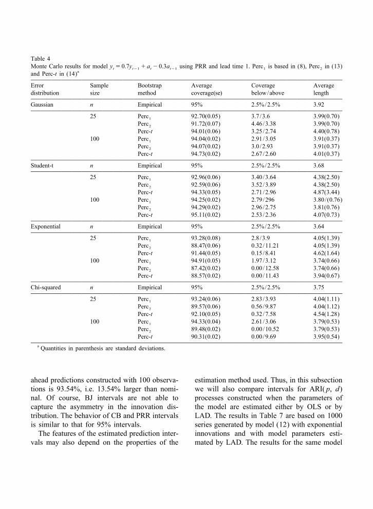
Table 4Monte Carlo results for model y 5 0.7y 1 a 2 0.3a using PRR and lead time 1. Perc is based in (8), Perc in (13)t t21 t t21 1 2

aand Perc-t in (14)

Error Sample Bootstrap Average Coverage Averagedistribution size method coverage(se) below/above length

Gaussian n Empirical 95% 2.5%/2.5% 3.92

25 Perc 92.70(0.05) 3.7 /3.6 3.99(0.70)1

Perc 91.72(0.07) 4.46/3.38 3.99(0.70)2

Perc-t 94.01(0.06) 3.25/2.74 4.40(0.78)100 Perc 94.04(0.02) 2.91/3.05 3.91(0.37)1

Perc 94.07(0.02) 3.0 /2.93 3.91(0.37)2

Perc-t 94.73(0.02) 2.67/2.60 4.01(0.37)

Student-t n Empirical 95% 2.5%/2.5% 3.68

25 Perc 92.96(0.06) 3.40/3.64 4.38(2.50)1

Perc 92.59(0.06) 3.52/3.89 4.38(2.50)2

Perc-t 94.33(0.05) 2.71/2.96 4.87(3.44)100 Perc 94.25(0.02) 2.79/296 3.80/(0.76)1

Perc 94.29(0.02) 2.96/2.75 3.81(0.76)2

Perc-t 95.11(0.02) 2.53/2.36 4.07(0.73)

Exponential n Empirical 95% 2.5%/2.5% 3.64

25 Perc 93.28(0.08) 2.8 /3.9 4.05(1.39)1

Perc 88.47(0.06) 0.32/11.21 4.05(1.39)2

Perc-t 91.44(0.05) 0.15/8.41 4.62(1.64)100 Perc 94.91(0.05) 1.97/3.12 3.74(0.66)1

Perc 87.42(0.02) 0.00/12.58 3.74(0.66)2

Perc-t 88.57(0.02) 0.00/11.43 3.94(0.67)

Chi-squared n Empirical 95% 2.5%/2.5% 3.75

25 Perc 93.24(0.06) 2.83/3.93 4.04(1.11)1

Perc 89.57(0.06) 0.56/9.87 4.04(1.12)2

Perc-t 92.10(0.05) 0.32/7.58 4.54(1.28)100 Perc 94.33(0.04) 2.61/3.06 3.79(0.53)1

Perc 89.48(0.02) 0.00/10.52 3.79(0.53)2

Perc-t 90.31(0.02) 0.00/9.69 3.95(0.54)a Quantities in parenthesis are standard deviations.

ahead predictions constructed with 100 observa- estimation method used. Thus, in this subsectiontions is 93.54%, i.e. 13.54% larger than nomi- we will also compare intervals for ARI( p, d)nal. Of course, BJ intervals are not able to processes constructed when the parameters ofcapture the asymmetry in the innovation dis- the model are estimated either by OLS or bytribution. The behavior of CB and PRR intervals LAD. The results in Table 7 are based on 1000is similar to that for 95% intervals. series generated by model (12) with exponentialThe features of the estimated prediction inter- innovations and with model parameters esti-

vals may also depend on the properties of the mated by LAD. The results for the same model

Table 52 aMonte Carlo results for model (12B) (12 0.5B)y 5 a with exponential errorst t

Lead Sample Method Average Coverage Averagetime size coverage(se) below/above length

1 n Empirical 95% 2.5%/2.5% 3.65

25 BJ 93.33(0.04) 0.14/6.5 3.77(1.04)CB 88.01(0.12) 7.6 /4.4 3.62(1.23)PRR 91.02(0.09) 4.7 /4.3 3.72(1.26)

50 BJ 94.03(0.03) 0.11/5.9 3.84(0.72)CB 90.15(0.09) 6.07/3.77 3.60(0.94)PRR 92.65(0.07) 3.8 /3.5 3.70(0.89)

100 BJ 94.44(0.02) 0.0 /5.56 3.87(0.53)CB 91.85(0.07) 5.04/3.11 3.65(0.66)PRR 93.45(0.06) 3.5 /3.05 3.72(0.68)

3 n Empirical 95% 2.5%/2.5% 19.05

25 BJ 96.48(0.03) 0.18/3.34 26.09(7.82)CB 88.07(0.10) 6.61/5.31 17.34(5.39)PRR 90.46(0.08) 4.4 /5.1 18.01(5.72)

50 BJ 97.41(0.02) 0.1 /2.6 26.96(5.37)CB 91.60(0.07) 4.79/3.61 18.62(3.99)PRR 92.75(0.06) 3.7 /3.6 18.85(3.90)

100 BJ 97.75(0.01) 0.0 /2.25 27.35(4.02)CB 92.96(0.05) 3.91/3.13 18.75(2.90)PRR 93.55(0.04) 3.3 /3.13 18.89(2.96)

a Quantities in parentheses are standard deviations.

estimated by OLS were reported in Table 5. the BJ intervals behavior is quite similar whenComparing Tables 5 and 7, we observe that estimating either by OLS or by LAD.when parameters are estimated by LAD, the

3.3. Seasonal modelsaverage coverage of CB and PRR intervals iscloser to the nominal value of 95%. For exam-

The focus in this section is on predictionple, with a sample size of 100 and intervalsdensities of series generated by multiplicativeconstructed for one-step ahead predictions, theseasonal ARIMA( p, d, q)3 (P, D, Q) pro-saverage coverage when OLS is used is 93.45cesses, where s is the seasonal period. Forand when the parameters are estimated by LAD,example, for monthly data, we consider thethe average coverage is 94.79. The same holdsmodelfor three-steps ahead predictions. The bootstrap

12 d D 12intervals based on LAD estimates are closer to s d s df L F L = = Y 5u L Q L a , (17)s d s dp P 12 t q Q tnominal intervals due perhaps to the betterwhere L is the backshift operator such thatproperties of such estimators under non-k D 12 Ds dsymmetric distributions. If the parameter es- L y 5 y and = 5 12L , and the auto-t t2k 12

timator has better properties it is expected that regressive and moving average polynomialsp 12s dthe predictions will also be better. Notice that f L 5 (12 f L2 ? ? ? 2 f L ), F L 5s dp 1 p P

Table 62 aMonte Carlo results for model (12B) (12 0.5B)y 5 a with exponential errorst t

Lead Sample Method Average Coverage Averagetime size coverage(se) below/above length

1 n Empirical 80% 10%/10% 2.19

25 BJ 84.60(0.10) 3.70/11.7 2.46(0.68)CB 73.13(0.15) 14.81/12.05 2.11(0.60)PRR 76.06(0.10) 12.72/11.21 2.23(0.61)

50 BJ 87.44(0.07) 1.6 /10.98 2.51(0.47)CB 76.68(0.12) 12.30/11.02 2.16(0.43)PRR 77.96(0.11) 11.25/10.97 2.20(0.42)

100 BJ 88.86(0.03) 0.52/10.62 2.53(0.35)CB 77.96(0.10) 11.56/10.48 2.18(0.31)PRR 78.62(0.09) 10.99/10.4 2.19(0.31)

3 n Empirical 80% 10%/10% 2.25

25 BJ 81.67(0.10) 9.22/9.11 2.79(1.36)CB 75.69(0.11) 12.24/12.07 2.32(0.81)PRR 79.20(0.09) 10.36/10.44 2.44(0.78)

50 BJ 83.42(0.07) 8.31/8.27 2.74(0.89)CB 77.51(0.08) 11.16/11.34 2.27(0.42)PRR 79.12(0.06) 10.39/10.49 2.32(0.43)

100 BJ 85.00(0.05) 7.62/7.38 2.79(0.77)CB 78.68(0.05) 10.75/10.57 2.25(0.30)PRR 79.34(0.05) 10.39/10.27 2.28(0.31)

a Quantities in parentheses are standard deviations.

12 12P1 2 F L 2 ? ? ? 2 F L , u L 5 (11 consequently, they are not reported. The intents ds d1 P qq 12 12 of this Monte Carlo experiment is to show hows du L 1 ? ? ? 1 u L ), Q L 5 (11 Q L1 q Q 1

12Q the PRR procedure can be extended to seasonal1 ? ? ? 1 Q L ) have all their roots out ofQmodels with good results. As an illustration, thethe unit circle to ensure stationarity and inver-empirical, BJ, CB and PRR densities of one-tibility. In particular, we generate 1000 seriesstep ahead predictions for a particular series ofwith the following ARIMA(0,1,1)3 (0,1,1)12size 240 generated by model (18) appear in Fig.model, usually known as airline model:2 where it can be seen that all densities are very

12 12 similar.== y 5 (12 0.33L)(12 0.82L )a , (18)t t

where a is a Gaussian innovation. Table 8treports the results obtained for sample sizes 120 4. Real data applicationsand 240. For Gaussian errors and sample sizes

In this section, we study the implementationrather large, the properties of the predictionof the PRR bootstrap procedure to the predic-densities constructed by the three methodstion of future values of two real time series,considered in this paper are rather similar. Themonthly observations of the Italian Industrialresults for different innovation distributions andProduction Index (IPI) and observations of thesample sizes are similar to the ones previouslylevels of a luteinizing hormone from Efron andcommented for models (15) and (16) and,

Table 712 12 aMonte Carlo results for model (12B)(12B )y 5 (12 0.33B)(12 0.82B )a with Gaussian errorst t

Lead Sample Method Average Coverage Averagetime size coverage(se) below/above length

1 n Empirical 95% 2.5%/2.5% 3.92

120 BJ 95.95(0.02) 2.06/1.99 4.25(0.31)CB 95.14(0.03) 2.44/2.42 4.20(0.42)PRR 95.26(0.03) 2.39/2.34 4.23(0.41)

240 BJ 95.66(0.01) 2.20/2.15 4.10(0.20)CB 95.15(0.02) 2.38/2.47 4.07(0.03)PRR 95.19(0.02) 2.34/2.46 4.08(0.28)

3 n Empirical 95% 2.5%/2.5% 5.40

120 BJ 95.89(0.02) 2.09/2.02 5.87(0.58)CB 95.18(0.03) 2.42/2.40 5.77(0.60)PRR 95.41(0.03) 2.29/2.31 5.87(0.61)

240 BJ 95.61(0.02) 2.19/2.20 5.65(0.38)CB 95.20(0.02) 2.35/2.45 5.60(0.42)PRR 95.27(0.02) 2.29.2.43 5.65(0.43)

12 n Empirical 95% 2.5%/2.5% 9.54

120 BJ 95.53(0.03) 2.26/2.20 10.38(1.45)CB 94.06(0.04) 2.96/2.97 10.22(1.44)PRR 94.55(0.04) 2.70/2.71 10.43(1.45)

240 BJ 95.42(0.02) 2.26/2.32 9.99(0.95)CB 94.59(0.03) 2.63/2.77 9.90(1.01)PRR 94.82(0.03) 2.49/2.68 10.01(0.99)

24 n Empirical 95% 2.5%/2.5% 14.42

120 BJ 96.35(0.03) 1.85/1.80 16.72(2.61)CB 94.59(0.05) 2.71/2.70 16.50(2.64)PRR 95.77(0.04) 2.11/2.12 17.50(2.64)

240 BJ 95.97(0.02) 1.99/2.04 15.64(1.67)CB 94.92(0.03) 2.47/2.61 15.52(1.73)PRR 95.66(0.020 2.09/2.25 16.12(1.73)

a Quantities in parentheses are standard deviations.

Tibshirani (1993), previously analyzed by Dig- to assess the predictive performance of theBox–Jenkins and bootstrap prediction intervals.gle (1990). The Italian IPI observed monthlyBefore estimating the model, the effects offrom January 1983 to September 1998 can be

several outliers have been removed from theseen in Fig. 3 and it presents a strong seasonaloriginal series using the program TRAMO; seecomponent and a stochastic trend. The firs 165´Gomez and Maravall (1996). The model esti-observations of the series, corresponding to the

mated by conditional QML from the seriesperiod up to September 1996, are used towithout outliers is given byestimate the ARIMA( p, d, q)3 (P, D, Q)12

12model which describes the dynamic behavior of== y 5 (120.59L)(120.57L )a . (19)12 t t(0 07) (0 07)the Italian IPI. The last 24 observations are used

Table 82 aMonte Carlo results for model (12B) (12 0.5B)y 5 a with exponential errors and LAD estimationt t

Lead Sample Method Average Coverage Averagetime size coverage(se) below/above length

1 n Empirical 95% 2.5%/2.5% 3.65

25 BJ 93.11(0.05) 0.38/6.51 3.83(1.04)CB 89.91(0.11) 5.72/4.37 3.75(1.23)PRR 93.17(0.08) 2.62/4.21 3.89(1.26)

50 BJ 93.90(0.04) 0.24/5.87 3.88(0.72)CB 91.13(0.10) 5.10/3.77 3.68(0.94)PRR 94.01(0.07) 2.51/3.48 3.81(0.88)

100 BJ 94.41(0.02) 0.03/5.56 3.89(0.53)CB 92.74(0.07) 4.17/3.10 3.70(0.64)PRR 94.79(0.05) 2.21/3.00 3.80(0.68)

3 n Empirical 95% 2.5%/2.5% 19.05

25 BJ 96.55(0.04) 0.30/3.15 27.11(7.91)CB 89.25(0.10) 5.66/5.09 18.25(5.61)PRR 92.42(0.08) 2.98/4.60 19.77(6.23)

50 BJ 97.51(0.02) 0.03/2.45 27.64(5.37)CB 92.01(0.08) 4.50/3.49 19.21(3.99)PRR 93.96(0.06) 2.72/3.32 19.99(4.10)

100 BJ 97.83(0.01) 0.00/2.16 27.76(3.85)CB 93.47(0.05) 3.48/3.04 19.09(2.80)PRR 94.70(0.04) 2.36/2.95 19.64(2.99)

a Quantities in parentheses are standard deviations.

Fig. 2. One-step ahead prediction densities of one series of size 240 generated by model (13) with Gaussian innovations.

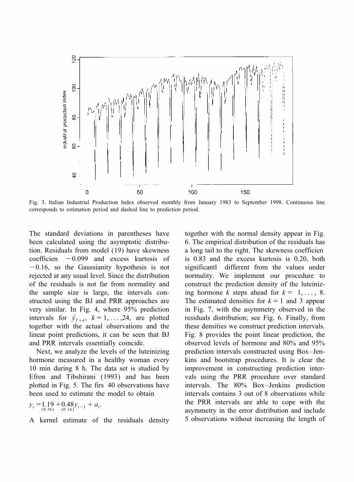
Fig. 3. Italian Industrial Production Index observed monthly from January 1983 to September 1998. Continuous linecorresponds to estimation period and dashed line to prediction period.

The standard deviations in parentheses have together with the normal density appear in Fig.been calculated using the asymptotic distribu- 6. The empirical distribution of the residuals hastion. Residuals from model (19) have skewness a long tail to the right. The skewness coefficiencoefficien 20.099 and excess kurtosis of is 0.83 and the excess kurtosis is 0.20, both20.16, so the Gaussianity hypothesis is not significantl different from the values underrejected at any usual level. Since the distribution normality. We implement our procedure toof the residuals is not far from normality and construct the prediction density of the luteiniz-the sample size is large, the intervals con- ing hormone k steps ahead for k5 1, . . . , 8.structed using the BJ and PRR approaches are The estimated densities for k5 1 and 3 appearvery similar. In Fig. 4, where 95% prediction in Fig. 7, with the asymmetry observed in the

ˆintervals for y , k5 1, . . . ,24, are plotted residuals distribution; see Fig. 6. Finally, fromT1ktogether with the actual observations and the these densities we construct prediction intervals.linear point predictions, it can be seen that BJ Fig. 8 provides the point linear prediction, theand PRR intervals essentially coincide. observed levels of hormone and 80% and 95%Next, we analyze the levels of the luteinizing prediction intervals constructed using Box–Jen-

hormone measured in a healthy woman every kins and bootstrap procedures. It is clear the10 min during 8 h. The data set is studied by improvement in constructing prediction inter-Efron and Tibshirani (1993) and has been vals using the PRR procedure over standardplotted in Fig. 5. The firs 40 observations have intervals. The 80% Box–Jenkins predictionbeen used to estimate the model to obtain intervals contains 3 out of 8 observations while

the PRR intervals are able to cope with they 51.19 10.48y 1 a .t t21 t(0 36) (0 16) asymmetry in the error distribution and include5 observations without increasing the length ofA kernel estimate of the residuals density

Fig. 4. Real observations of IPI (d) together with point linear predictions (s). 95% prediction intervals constructed byBox–Jenkins and bootstrap procedures.

Fig. 5. Observations of the luteinizing hormone measured in a healthy woman every minute during 8 h. Continuous linecorresponds to estimation period and dashed line to prediction period.

Fig. 6. Estimated density of residuals from AR(1) model for the luteinizing hormone and normal density.

Fig. 7. Densities of one and three steps ahead predictions of the luteinizing hormone constructed by BJ and PRR procedures.

Fig. 8. Observations of luteinizing hormone (d) and point linear predictions (s). 80% and 95% intervals constructed by BJand PRR procedures.

the intervals. Even when looking at the 95% OLS autoregressive parameter estimates withprediction intervals, BJ intervals leave out 2 observations centered at the sample mean andobservations while PRR intervals do not leave using all 48 observations; the bootstrap standard

ˆout any observation. We have also computed error for f based on 200 bootstrap replicates isˆbootstrap prediction intervals conditional on 0.12. The standard deviation of f is rather

parameter estimates (CB). However, although small with respect to the standard deviation ofthe sample size is small, CB intervals are hardly the errors (0.43) and this could explain why thedistinguishable from PRR intervals and, conse- parameter variability does not affect the shapequently, we have not plotted them in Fig. 8. of prediction intervals. This example shows howTherefore, it seems that for the values of the for small sample sizes and non-normal innova-luteinizing hormone analyzed in this paper, the tion distributions it could be worth consideringdifference between BJ and PRR intervals is due bootstrap prediction intervals in order to im-to non-normality of the errors and not to prove the prediction performance of ARIMAparameter estimation. Efron and Tibshirani models.(1993) give the bootstrap distribution of the Since the error distribution of the luteinizing

hormone is not Gaussian, we have also esti- LAD estimator the prediction MSE is reducedmated the parameters of the AR(1) model by to 0.38. Fig. 9 also represents the PRR 80% andLAD with the following results: 95% bootstrap intervals constructed using the

OLS and LAD estimators. The LAD intervalsy 50.73 10.68y 1 a .t t21 t adapt better to the asymmetry of the error(0 37) (0 17)

distribution than the OLS intervals. RememberThe standard deviations in parentheses have that the 80% PRR intervals constructed with

been calculated using the suggestion by Bassett OLS estimates leave out 3 observations whenand Koenker (1976). The point linear predic- they were supposed to leave approximately onetions of the luteinizing hormone provided by the out. When PRR intervals are constructed usingOLS and LAD estimators have been plotted in LAD estimates, they leave out only one ob-Fig. 9. It can be seen that LAD predictions are servation. Consequently, it seems, as expected,systematically larger than OLS predictions and that using parameter estimators more appro-usually closer to the observed values. The MSE priate to the innovations distribution improvesof the OLS predictions is 0.51 while for the the performance of PRR prediction intervals.

Fig. 9. Observations of luteinizing hormone (d) and point linear predictions obtained using OLS (s) and LAD (1). 80%and 95% intervals constructed using OLS and LAD.

5. Conclusions monthly series of the Italian IPI. Since thesample size is rather big (165 observations) and

This paper focuses on the effects of parame- the innovation distribution is not far fromter estimation on the shape of prediction den- normality, the prediction intervals obtained bysities for seasonal ARIMA models. Prediction BJ and PRR procedures are very similar. How-intervals can be obtained using bootstrap pro- ever, BJ and PRR prediction intervals con-cedures which do not assume any distribution structed for the levels of a luteinizing hormonefor the errors and can incorporate the variability differ significantlydue to parameter estimation. In particular, we Several questions remain open for furtherconsider the bootstrap technique proposed by research using resampling techniques; for exam-Pascual et al. (1998) for ARIMA models ex- ple, the effect of the uncertainty on the spe-tending it to models with seasonal components. cificatio of the model over prediction densities.By means of Monte Carlo experiments, we have This question has been addressed for autoreg-firs studied how coverage and length of predic- ressions and using a different bootstrap strategytion intervals are affected by not taking into by Masarotto (1990) and Grigoletto (1998).account the variability due to parameter estima- However, they center the prediction intervals attion. We show that the average coverage of the a linear combination of past observations andintervals is closer to the nominal value when this strategy may not be adequate when theintervals are constructed incorporating parame- distribution of the innovations is not Gaussian.ter uncertainty. As expected, since we areconsidering consistent estimators, the effects ofparameter estimation are particularly important

Acknowledgementsfor small sample sizes. Furthermore, these ef-fects are more important when the error dis- The authors are very grateful to the refereestribution is not Gaussian. We also analyze the for comments that helped to improve the paper.effect of the estimation method on the shape of Also, we are grateful to Lory A. Thombs for herprediction densities. In particular, we compare comments, to Eva Senra for providing theprediction densities constructed when the pa- Italian IPI data and to Regina Kaiser for helpingrameters of ARI( p, d) models are estimated by us to clean the series of outliers. FinancialOLS and by LAD. We show how, when the support was provided by the European Unionerror distribution is not Gaussian, the average project ERBCHRXCT 940514 and by projectscoverage and length of intervals based on LAD CICYT PB95-0299, DGICYT PB96-0111 fromestimates are closer to nominal values than ´the Spanish Government and Catedra dethose based on OLS estimates. Since both Calidad BBV.estimates are consistent, this effect is lessevident as the sample size grows. It is remark-able how bootstrap prediction intervals adapt to

Referencesthe asymmetry of the problem providingasymmetric prediction intervals improving on

Bassett, G., & Koenker, R. (1976). Asymptotic theory ofthe necessarily symmetric BJ prediction inter-least absolute error regression. Journal of the Americanvals (see, e.g., Fig. 8).Statistical Association 73, 618–622.Finally, the performance of the PRR tech- Box, G. E. P., & Jenkins, G. M. (1976). Time Series

nique is illustrated with two empirical examples. Analysis: Forecasting and Control, Holden-Day, SanFirst, we estimate prediction densities for a Francisco.

Cao, R., Febrero-Bande, M., Gonzalez-Manteiga, W., Press, W. H., Flannery, B. P., Teukolsky, S. A., &Prada-Sanchez, J. M., & Garcia-Jurado, I. (1997). Vetterling, W. T. (1986). Numerical Recipes, CambridgeSaving computer time in constructing consistent boot- University Press, Cambridge.strap prediction intervals for autoregressive processes. Stine, R. A. (1987). Estimating properties of autoregres-Communications in Statistics, Simulation and Computa- sive forecasts. Journal of the American Statisticaltion 26, 961–978. Association 82, 1072–1078.

Chatfield C. (1993). Calculating interval forecasts. Jour- Thombs, L. A., & Schucany, W. R. (1990). Bootstrapnal of Business and Economic Statistics 11, 121–135. prediction intervals for autoregression. Journal of the

Diggle, P. (1990). Time Series. A Biostatistical Intro- American Statistical Association 85, 486–492.duction, Clarendon Press, Oxford.

Efron, B., & Tibshirani, R. (1993). An Introduction to the Biographies: Lorenzo PASCUAL is Ph.D. student at theBootstrap, Chapman and Hall, New York. ´ ´Departamento de Estadı stica y Econometrı a of Univer-´Gomez,V., & Maravall, A., (1996). Programs TRAMO and sidad Carlos III de Madrid. He works on bootstrapSEATS: Instructions for the user. Documento de Traba- methods for prediction in time series models.

˜jo no. 9628, Banco de Espana (Spain).Grigoletto, M. (1998). Bootstrap prediction intervals for Juan ROMO received his Ph.D. in Mathematics fromautoregressions: some alternatives. International Jour- Texas A&M University. He has been Associate Professornal of Forecasting 14, 447–456. both in Universidad Complutense and Universidad Carlos

Hall, P. (1992). The Bootstrap and Edgeworth Expansion, III de Madrid, where he is Professor of Statistics andSpringer-Verlag, New York. Operations Research since 1996.

Masarotto, G. (1990). Bootstrap prediction intervals forautoregressions. International Journal of Forecasting 6, Esther RUIZ received her Ph.D. in Statistics from the229–239. London School of Economics in 1992. She is Associate

Pascual, L., Romo, J., & Ruiz, E. (1998). Bootstrap Professor of Economics at Universidad Carlos III depredictive inference for ARIMA processes. Working Madrid since 1995.Paper 98-86, Universidad Carlos III de Madrid.