RESPIRATORY PARAMETER ESTIMATION USING FORCED ...

76-24,700TSAI, Ming-Jer, 1948- RESPIRATORY PARAMETER ESTIMATION USING FORCED OSCILLATORY IMPEDANCE DATA.

The Ohio State University, Ph.D., 1976 Engineering, biomedical

Xerox University Microfilms, Ann Arbor, Michigan 48io6

RESPIRATORY PARAMETER ESTIMATION USING FORCED OSCILLATORY IMPEDANCE DATA

DISSERTATION

Presented in Partial Fulfillment of the Requirements for the Degree Doctor of Philosophy in the Graduate

School of The Ohio State University

byMing-Jer Tsai, B.S., M.S.

* * * * *

The Ohio State University

1976

Reading Committee:

Prof. R. L. Pimmel

Prof. R. B. McGhee

Prof. R. L. Hamlin

Approved by

AdvisorDepartment of Electrical Engineering

RESPIRATORY PARAMETER ESTIMATION USING

FORCED OSCILLATORY IMPEDANCE DATA

By

Mlng-Jer Tsai, Ph.D.

The Ohio State University, 1976 Professors R. B. McGhee and R. L. Pimmel, Advisors

Traditionally, the respiratory mechanical system has been

modeled and analyzed using linear electric circuit. The impedance of

such a model can be measured using the forced oscillation technique.

Based on the measured impedance data and analytical expression forimpedance of the circuit model, the respiratory mechanical parameters

can be determined with certain parameter estimation technique. Such anapproach for determining respiratory parameters was studied in this

dissertation. In this study, an extended forced oscillation technique

which employs a specially designed device known as "impedance analyzer"

and a least-square parameter estimation algorithm which combines several

gradient methods and a uniform random search routine were utilized.

Using noise-free and noisy artificial data it was found that the basicrespiratory parameters in normal human beings, i.e., total resistance,inertance, and compliance of a series R-I-C model, can be accurately

estimated from impedance data at 20 frequencies in the range 1 - 10 Hz

even with measurement errors as high as 10%. This frequency range is1

r

inadequate for estimating parameters from more complicated models, however, by extending the frequency range to 50 Hz and limiting the

measurement errors within 5%, it may be possible to obtain reliable

values for the parameters. The impedance data of supine, apneic dogs

in control state and under various experimental conditions including the use of added external resistance, lighter gas, abdominal weighing,

and pharmacological broncho-constriction and dilatation were actually collected at 26 frequencies in the range 1 to 16 Hz. From this data

the total respiratory resistance, inertance, and compliance were deter

mined. Our control parameter values were comparable to previously

reported values. With those interventions, the alterations in parameters

were consistent with predicted effects. The total resistance and com

pliance were also measured with the more conventional tidal breathing

technique. Both parameters showed higher values than those determined

by using the new approach proposed in this dissertation although the correlations were relatively high. The discrepancies may be attributed

to differences in flow rates, tidal volumes, and operating frequencies

used in these two techniques.

2

ACKNOWLEDGEMENTS

The author gratefully acknowledges the advice provided to him

by the members of his Guidance Committee. Particular thanks are due

to Professor R. L. Pimmel for his constant guidance and motivation

throughout this study. Thanks are also due to Professor R. B. McGhee

for his support and advice on part of computer study in this disserta

tion. Professor R. L. Hamlin is also to be thanked for his help in

arranging experiments for this study.This research was supported in part by the NIH grant nos. HL-

17585 and HL-19118. It was also supported by Ohio State University grant no. EE 28. Extensive computer time has been contributed by IRCC

of the Ohio State University. These assistances made it possible for

this research in this dissertation to be conducted and are responsible

to a considerable extent for its completion.The author also wishes to express his thanks to his parents and

other members of his family for their encouragement and support through

out this years of graduate study.Finally the author is indebted to E. J. Stiff and D. J. Robinson

for their assistances in conducting the experiments and to Misses Julie

Kauper and Anne-Marie Tjon for their help in typing this manuscript.

22 ill

VITA

Jan. 16, 1948 ....................... Born - Taiwan, China

1969 ............................... B.S., Control Engineering,National Chiao-Tung University, Hsinchu, Taiwan

1969-1970 ....... . Second Lieutenant,Chinese Air Force,Hsinchu, Taiwan

1970-1971 ........ ...................Junior Electrical Engineer,General Instrument Taiwan Co., Taipei, Taiwan

1971-1973 ........................... Graduate Research Assistant,Electrical Engineering, University of Cincinnati, Cincinnati, Ohio

1973 ............. ...................M.S., Electrical Engineering,University of Cincinnati, Cincinnati, Ohio

1973-1976 .... ....................Graduate Research Associate,Electrical Engineering,The Ohio State University, Columbus, Ohio

- *

PUBLICATIONS

Gross, D.R., M.J. Tsai, R.L. Hamlin and R.L. Pimmel, Input Impedance Measurements in the Left Common Coronary Artery of Horses, 27th' ACEMB, p. 207, 1974.Gross, D.R., R.L. Pimmel, M.J, Tsai, and. R.L. Hamlin, Input Impedance of the Renal Artery from Isolated Perfused Kidneys of Dogs, 1st Midwest Biomedical Engineering Conference, P. 2.4, 1975.

iv

Tsai, M.J., R.B. McGhee, R.L. Pimmel, and P.A. Bromberg, Critical Analysis of Optimization Techniques for Recovering Ventilation Perfusion Distribution, 1st. Midwest Biomedical Engineering Conference, P. 1.3, 1975.

Tsai, M.J. and R.L. Pimmel, Computer Estimation of Respiratory Parameters from Forced Oscillatory Data, 28th ACEMB, P. 338, 1975.

Tsai, M.J., R.B. McGhee, R.L. Pimmel, and P.A. Bromberg, An Evaluation of a Numerical Technique for Recovering Ventilation- Perfusion Ratios, 28th ACEMB, P. 492, 1975.

FIELDS OF STUDY

Major Field: Electrical Engineering

Studies in Control Engineering: Professors R.E. Fenton, R.H. Raible(University of Cincinnati), and K.W. Han (Chiao-Tung University)

Studies in Biomedical Engineering: Professors R.M. Campbell,H.R. Weed, and R.L. Pimmel

Studies in Computer Systems: Professors K.W. Olson, W.G. Wee(University of Cincinnati)

Studies in Statistics: Professor P.R. Archambault

Studies in Physiology: Professor R.K. Smith

v

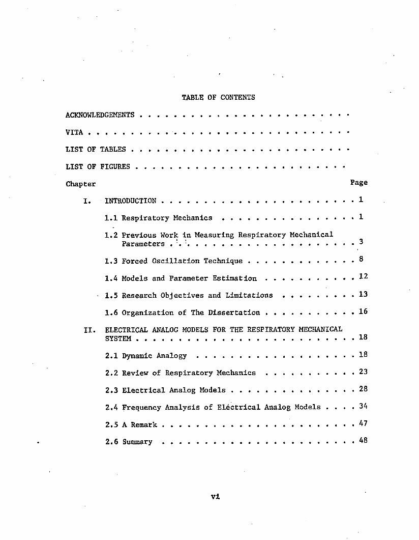
TABLE OF CONTENTS

ACKNOWLEDGEMENTS .................................................

V I T A .................. ..........................................LIST OF TABLES ...................................................

LIST OF FIGURES .................................................Chapter Page

I. INTRODUCTION....................................... . 11.1 Respiratory Mechanics ............................... 11.2 Previous Work in Measuring Respiratory Mechanical

Parameters . . :.................. .. ............... . 3

1.3 Forced Oscillation Technique ................. . . . . 81.4 Models and Parameter Estimation................... . 12

• 1.5 Research Objectives and Limitations . . . . . . . . . 13

1.6 Organization of The Dissertation................ 16II. ELECTRICAL ANALOG MODELS FOR THE RESPIRATORY MECHANICAL

SYSTEM.................................................... 18

2.1 Dynamic A n a l o g y ................................ 182.2 Review of Respiratory Mechanics................ 23

2.3 Electrical Analog Models ............................ 282.4 Frequency Analysis of Electrical Analog Models . . . . 34

2.5 A Remark........................................ 472.6 S u m m a r y ........................................ 48

vl

TABLE OF CONTENTS (Continued)

Chapter PageIII. PARAMETER ESTIMATION BY NONLINEAR REGRESSION ANALYSIS . .49

3.1 Parameter Estimate Problem ........................ 49

3.2 Numerical Methods for Parameter Estimation........ 54

3.2.1 Regression Analysis Method .................. 54

3.2.2 Gradient Methods . . . . . . . .............. 583.2.3 An Algorithm for Constrained Parameter

Estimation.................................. 65

3.2.4 Uniform Random Search M e t h o d ................ 693.2.5 A Complete Algorithm for Constrained Parameter

Estimation.................................. 703.3 Application in Estimating Respiratory Parameters from

Artificial Impedance D a t a .......................... 72

3.3.1 Formulation of the P r o b l e m .................. 72

3.3.2 Estimations Based on Artificial Noisy Data . . 77

3.4 Summary............................................ 88IV. PROCEDURES AND M E T H O D S ..................................90

4.1 Overall S y s t e m .................................... 904.2 System Calibration .......................... 94

4.3 Experimental Procedures ............................ 103

4.4 Data Analysis........................................106

vii

TABLE OF CONTENTS (Continued)

Chapter Page

V. RESULTS AND DISCUSSIONS.................................. 1105.1 Frequency Response of Respiratory Impedance in Dogs . n o

5.2 Estimated Values for R , I , and C from, _ . rs rs rsImpedance D a t a ......................................1225.3 A Comparison of Forced Oscillation and Other

Conventional Techniques for Measuring R and C . . 132ITS ITS

5.4 Correlations with Works of Others.................... 138

5.5 Discussions on Experimental Conditions ............. 141

5.6 Summary............................................ 144VI. SUMMARY AND SUGGESTIONS.................................. 145

6.1 Summary and Conclusion............................. 1456.2 Applications...................... 147

6.3 Extensions and Suggestions.... ...................... 148

APPENDIX

A. COMPUTER PROGRAMS................ ...................... 151

B. EXPERIMENTAL D A T A ........................................ 161LIST OF REFERENCES................................................171

viii

LIST OF TABLES

Table Page1. Analogies between three second-order dynamic systems . . . 20

2. Summary of parameter estimate for the R-I-C modelbased on artificial d a t a ............................... 80

3. Summary of parameter estimate for the airway andlung-chest model based on artificial data .............. 84

4. Correspondence between readings from water manometerand chart recorder in calibrating pressure measurement . . 95

5. Correspondence between readings from chart recorderand impedance analyzer in calibrating pressure measurement........................................... 96

6. Correspondence between readings from chart recorder andimpedance analyzer in calibrating flow measurement . . . . 98

7. Errors in phase measurement ............................. 998. Typical frequency response of the respiratory impedance

in an anesthetized and paralyzed normal d o g .......... Ill9. Estimated values for R , I , and C for all 10 dogsrs rs rsused in the studies of effects of three mechanical

interventions...................................... 12310. Corrected values for R , I , and C in 6 normal dogs . 126rs rs rs11. Variations in &rs> ^rs* an^ ^rs ^ue to m3iS3 loading of

the a b d o m e n .............. 12812. Variations in R,.s, Irs, and Crs due to an external

resistor ............................................. 12813. Variations in Rrs, Irs, and Crs due to breathing He-O^

gas m i x t u r e ................ 12814. Estimated values for Rrs, Irg, and Crs for 6 normal

dogs used in the drug s t u d y .......................... 131

ix

LIST OF TABLES (Continued)

Table Page

15. Static respiratory compliance measured in 5 dogs . . . . 138

16. Values for Crg reported in the literature...............140

17. Measured values for mouth pressure, flow, and volume during forced oscillations ............................ 143

x

LIST OF FIGURESFigure Page

1. Three analog second-order systems: (A) mechanical rectilinear system, (B) pressure-volume system, and(C) electrical circuit system...................... .. • 21

2. Variations in pressure and volume during a normal respiration cycle ......................... . . . . . . . 24

3. Static volume-pressure curve of the total respiratory system during relaxation in the upright posture . . . . *27

4. Equation and graph of alveolar pressure and air flow . . 27

5. An electrical analog of the total respiratory system during spontaneous breathing . . . ......................29

6. An electrical analog of the total respiratory system in an anesthetized and paralyzed subject under forced oscillations....................... • • • • 29

7. Series R-I-C circuit representing the total respiratory mechanical system ...................................... 29

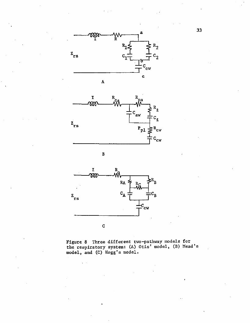
8. Three different two-pathway models for the respiratory system: (A) Otis' model, (B) Mead's model, and (C)Hogg's m o d e l ...................... ................ • • 33

9. Frequency response of a R-I-C model with nominal parameter v a l u e s ........................ 39

10. Relative contribution of inertance and compliance reactance to the total respiratory reactance in normal adult human .................................................. 38

11. Frequency response of the input impedance of the modelas shown in Fig. 6 with nominal values for the parameters 39

12. Total effective compliance and resistance in Mead'smodel in four different conditions..................... 44

13. Magnitude and phase of the total respiratory impedancein various conditions ........................ . . . . . 4 5

xi

LIST OF' FIGURES (.Continued)

Figure Page

14. Pole and zero configurations of the input impedance in Mead's model with four different conditions ............ 46

15. A dynamic system with multiple inputs and one output . . 51

16. A parameter identification system ................ .. . 5317. Flow chart for a minimization algorithm............ .. . 67

18. Flow chart for a complete algorithm for constrained parameter estimation...................................... 71

19. A scheme for estimating respiratory parameters from Impedance d a t a ........................................ 74

20. Block diagram for the overall experimental system . . . . 91

21. Block diagram for the impedance analyzer.............. 92

22. Set-up for pressure calibration ......... . 95

23. Impedance of endotracheal tube in a i r .................. 101

24. Impedance of endotracheal tube in ^-0^ mixture..........10225. Transthoracic pressure tracing during lung deflation . . 108

26. Pressure, flow, and volume recordings during artificial ventilation in an anesthetized and paralyzed dog . . . . 108

27. Reproducibility of impedance data obtained in a singledog (Dog # 1) during one experiment......................114

28. Typical frequency response of the respiratory impedanceof a paralyzed apneic dog (Dog # 1) ....................115

29. Frequency responses of magnitudes (A), phase angles (B), real parts (C), and imaginary parts (D) of the respiratory impedances in 6 normal dogs In control states . . . H O

30. An example of variation in respiratory impedance due to mass loading in the abdominal region of a paralyzed dog . 117

xil

LIST OF FIGURES (Continued)

Figure Page

31. An example of variation in respiratory impedance due toan added external resistor .............................. 118

32. An example of variation in respiratory impedance due to breathing a He - gas m i x t u r e ..........................119

33. Variations in the respiratory impedance of Dog # 12 due to a bronchoconstrictor, physostigmine, and a bronchodilator, at r o p i n e .......... 120

34. Frequency responses in magnitudes (A), phase angles (B), real parts (C), and imaginary parts (D) of the respiratory impedances in the dog with narrowed trachea ('2 ') , the dog with obstructive small airways (11') and 6 normal dogs in average (solid lines)..........................121

35. An example of agreement between experimental and theoretical (R-I-C model) impedances . . . . . . . . . ........ 124

36. Relative contributions of compliance reactance (Xc) andinertance reactance (X ) to the total reactance (X) andtotal impedance (|Z|) Sased on the mean values for R ,I , and C given in Table 10..................... r? . . 126rs rs

37. Comparison of the forced oscillation technique (fo)with the tidal breathing method (dyn) in measuringR (A) and C ( B ) ........................................ 135rs rs

38. Static deflation pressure-volume curves in 5 paralyzed apneic d o g s .............................................. 136

• 39. Hysteresis phenomena in p-v curves ..................137

xili

CHAPTER I

INTRODUCTION

1»1 Respiratory MechanicsThe breathing mechanism can be characterized as a reciprocating

bellows pump. The chest wall acts as the outer layer of the bellows

and it is effectively coupled to the muscles which provide the source

of energy. The lungs are intimately attached to this outer layer, and are specialized to disperse the gas over the gas-exchange surface. The

bellows is made up of the respiratory bronchioles, alveolar ducts, alveolar sacs and the 300 million alveoli. It is connected to the atmosphere

through the tracheobronchial tree and the upper airway.

The lungs are viscoelastic structures. Their elastic properties are mainly caused by the surface tension of the surfactant, a surface-

active fluid lining the alveoli, and by the elastic fibers throughout

the lung tissues. Likewise, the thorax has elastic properties which come

from the natural elasticity of the muscles, tendons, and connective

tissues of the chest. A significant part of muscular effort during brea

thing is simply to stretch the elastic structures of the lungs and thorax. The elasticity of the lungs is characterized by its compliance which is

the ratio of lung volume to transpulmonary pressure. The static compli

ance Is the ratio of total lung volume to total transpulmonary pressure

while dynamic compliance relates an incremental volume change, for example,

tidal volume, to the corresponding change in pressure. The compliance

1

2of the thorax can be described in a similar way.

Another part of the respiratory muscular effort is utilized in

overcoming frictional resistance in the airways and tissues of the lungs

and thoracic cage. Airway resistance in a simplistic sense is similar to that of a fluid flowing in a tube, and it is governed by the length

and diameter of the tube and by the density and viscosity of the fluid.

Tissue resistance, which is similar to the frictional resistance in a

solid, results from the slipping of various microscopic elements past

each other as they are rearranged to accommodate the dimensional changes

of the chest during ventilation.In addition to resistance and compliance, a third mechanical

factor, the inertance, is used in characterizing respiratory dynamics.

This last factor accounts for Inertial properties and describes the

relationship between volume acceleration and its corresponding pressure.

Only a very small amount of respiratory work is spent for overcoming the

inertial force in normal breathing.

In view of the complex nature of the distribution of pressures and motions in the breathing mechanism, it is conceivable that the

respiratory mechanical system is extremely nonlinear. In fact, this

nonlinear nature has been pointed out in reports [27,49,58,59,60], •For instances, the lung compliance is highly variable and depends in a

complex way on the conditions existing when the volume changes are

produced [58];under almost all conditions, the pressure-volume curve

is sigmoid-shaped and shows hysteresis; values for compliance even depend

on the posture of the subject; the flow resistance is also variable and depends on flow rates which produce different flow patterns in the

tracheo-bronchial tree [59]; airways resistance is approximately linearly

related to the degree of Inflation of the lungs [60]; either pulmonary

or respiratory resistance exhibits a hyperbolic relationship with lung volumes [49,27]; hysteresis may also appear in the volume history of

pulmonary [49].Many investigators[12,23,24,34] have developed quite a few

techniques to quantitatively determine the mechanical behavior of the

respiratory system by regarding it as a linear system despite its .

nonlinear nature. This approach has been possible because in many

situations, the respiratory system is restricted to operate in a very

small region (e.g., 0*5 & of tidal volume and less than 0.5 1/s of flow rate) within its physically allowable capacity (e.g., 5 H of vital capacity and 5 Jt/s of maximum flow rate), so that the nonlinear phenomena

such as hysteresis is not prominent and the nonlinear properties such as

volume-dependent compliance and volume- and flow-dependent resistance can

be approximated with constant linear elements without causing significant

discrepancies.

1.2 Previous Work in Measuring Respiratory Mechanical Parameters

Rohrer [1], one of the earliest investigators in measuring airway

resistance, anatomically measured the trachea and bronchial tree of a

human lung post mortem and calculated the cumulative resistance of the

entire system using Poiseuille’s law and turbulence theory. Neergaard and Wirz [2] who conducted the first important in vivo experimental study

of pulmonary resistance on humans in 1927, measured the intrapleural pressure through a large-bore needle with a good optical recording system

and recorded the respiratory flow simultaneously with a pneumotachograph.

They were able to obtain values for pulmonary resistance by analytically

separating the intrapleural pressure into two major components, the

pressure to overcome the viscous resistance associated with flow and the

pressure to overcome the elasticity associated with the change in lung

volume.The nonelastic pulmonary resistance is composed of airway resis

tance and lung tissue resistance. A number of studies [3,4,5,6,7] were

devoted to separate these two quantities. Bayliss and Robertson [3]

reasoned that airway resistance but not tissue resistance would vary with

viscosity,. By assuming that the gas flow was entirely laminar, they estimated the fraction of nonelastic pulmonary resistance attributable

to airway resistance in cats by comparing the pressure-flow relationship

obtained with air to those obtained with hydrogen. Fry et al. [4], com

paring the pressure-flow relationships obtained in subjects breathing

two different gases, air and an argon-oxygen mixture, demonstrated that

tissue friction was negligible both in normal and emphysematous subjects.

Mcllroy et al.[5], who argued that the gas combinations which have equal

kinematic viscosities should be selected, found that the tissue viscous

resistance was about 30% - 40% of the pulmonary resistance. The results

using this approach in separating tissue resistance from airway resistance

have been inconsistent and inconclusive.

Von Neergaard and Wirz [8] first employed the airway interruption

technique to measure the airway resistance of the respiratory tract with the belief that mouth pressure immediately after interruption of airflow

equaled alveolar pressure. However, later studies [9,10,11] indicated that the interrupter technique overestimated alveolar pressure, and thus

airway resistance, by approximately 20% in normal subjects. Mead and

Whittenberger [II] suggested that the reason is because during the time

necessary for equilibration of pressure, the rate of change of lung volume becomes zero and the magnitude of change of alveolar pressure

during this period is equal to the lung tissue resistive pressure that

existed prior to interruption. They thus postulated that resistance

determined by the interrupter technique is composed of airway resistance

and lung tissue resistance. Marshall and DuBois [51] even suggested that the interrupter resistance is actually a measure of the total flow

resistance throughout the entire respiratory system, i.e., the sum of

airway, lung tissue and chest wall tissue resistances. Recently,

Jackson et al.[52] recognizing the transient response of mouth pressure

to rapid interruption is characterized by a curve composed of two

distinctly different slopes, improved the correlation between resis

tances determined by the interrupter technique and those found by the plethysmograph in normal subjects by performing a curvilinear extra

polation back to the time of interrupt to estimate alveolar pressure

just prior to the interruption.DuBois et al. [12] first successfully used the plethysmographic

method for measuring airway resistance. This method is based on Boyle's law and uses a large airtight body box. Measurements are made

in two steps: first, the subject sits and pants through a pneumotacho- - graph while box pressure and mouth flow are monitored, and then against

a closed mouthpiece while monitoring box pressure and mouth pressure,

which is assumed equal to alveolar pressure. Data from the former

configuretion provides a calibration between box pressure and alveolar

pressure which is then used with data from the first configuration to

calculate the ratio of mouth flow to alveolar pressure, which is the

airway resistance. In practice, airway resistance can be measured very

simply and quickly using.an oscilloscope and a special attachment to

the scope face [38], Although thermal effects and other features such as inhomogeneities of the lung [12-16] may introduce measurement error

and variability, the plethysmographic method of measuring airway resistance has been widely employed as a research tool. Clinically its use

is limited because the equipment is expensive and complicated and

because confinement in the box produces problems with many subjects.

Mead [39,40] modified the plethysmographic method so that it is more versatile and easier to construct, however it is still considered use

ful only in research and in special clinical studies.The clinical measurement of pulmonary mechanics has been con

siderably facilitated since intra-esophageal pressure has been adopted

as a measure of intrapleural pressure. The most commonly used method

for measuring esophageal pressure employs air-containing latex balloons

sealed over catheters which trasmit balloon pressure to an external pressure transducer [17,18] . Previous studies have shown that volume-

pressure curves for lungs based on esophageal pressure vary with the

position of the balloon within the esophagus [17,19], with body posture [20,21] , and with balloon volume [22]. Nevertheless, Milic-Emili et al.

[22,41] suggested that esophageal pressure measured with a balloon which

contains a small volume (0.5 ml) and is placed in the middle third of the esophagus closely reflects local pleural pressure variations. Most

comparisons of esophageal with pleural pressure have indicated a good

agreement between changes in the two pressures measured in seated sub

jects, inspiring moderate volumes of air from the resting volume [41,

53]. The relationship between absolute pleural and esophageal pressure

is not as precise.From continuous records of esophageal pressure, airflow and

volume signals, many methods have been developed for calculating pul

monary resistance and dynamic compliance, and all are based on the original work of Neergaard-Wirz [8]. In most of the methods, pulmonary

compliance is first calculated by dividing tidal volume by the pleural

pressure change between points of zero flow. By dividing the respira

tory volume by this compliance, the elastic pressure is obtained. The nonelastic pressure can then be obtained by subtracting the elastic

pressure from the total pleural pressure at a given flow rate. From

the ratio of nonelastic pressure to flow, the pulmonary resistance is calculated.

Pulmonary resistance can also be measured directly on a catho

de ray oscilloscope using the subtraction method [23], in which an appropriate amount of signal proportional to the lung volume is sub

tracted from the total esophageal pressure so that the pressure flow loop displayed on the oscilloscope is "closed." The slope of the

resulting straight line is the pulmonary resistance. Another alterna

tive for determining the pulmonary resistance from pressure-flow-volume recording is the method of isovolume[24],where difference in both

pleural pressure (Ap) and airflow (Av) is measured between two instants

in a steady respiratory cycle when respiratory volume is identical. Since volume is equal at these two instants, the elastic pressure is

also equal. Therefore, the measured pressure difference is attributed

to flow resistance. Pulmonary resistance is calculated as Ap/Av, and a device for automatically performing these manipulations has been described [42,43].

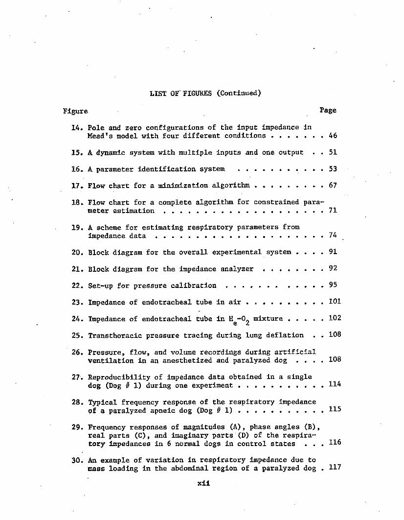
Hilberman et al. [34] has developed a technique for automated

computation of the parameters of the respiratory mechanics using digi

tal computers. This technique assumes that the respiratory mechanical

system is a second-order system and uses Fourier series analysis and phasor method of computation to determine, for the first harmonic which

contains about 80% of the total energy, the magnitude of impedance, phase angle, compliance and resistance of the respiratory system. They

found that this so-called phase method provided results for various

groups of subjects, which did-not differ significantly from the conven

tional method [24]. Based upon the same theory, Ostrander et al.[54] used hardware narrow band filters to extract fundamental Fourier compo

nents of esophageal and plethysmographic pressure, and flow of gas at the mouth during spontaneous breathing to determine the airway resis

tance, pulmonary resistance and dynamic compliance. It was found that compliance values thus obtained were statistically equivalent to conven

tional dynamic compliance and resistance values showed no linear trends

with breathing frequency over the range of 1.2 - 3.2 Hz.

1.3 Forced Oscillation TechniqueDuBois et al.[25] first employed the technique of forced osci

llation for the study of respiratory mechanics. They applied sinusoidal pressure waves generated by an oscillating air pump at the mouth or

around the thorax. From recording of pressure and flow they calculated

the overall impedance of the chest (Z ) over the frequency range fromIT S

2 to 15 Hz. They demonstrated that the respiratory system behaved like a second-order system similar to a resistance-inductance-capacitance

(RLC) series circuit. The flow impedance of such a system is heavily dependent on total respiratory compliance (C , analog of capacitance)IT S

at low frequencies, heavily dependent on total respiratory inertance

(I , analog of inductance) at high frequencies, and can be completely rsattributed to total resistance (R , analog of electrical resistance)rsat a certain intermediate frequency. Impedance reaches a minimum at

this frequency (resonant frequency) and the phase angle between

pressure and flow is 0°. They also found that the resonance in normal

subjects was at a frequency of approximately 5.8 Hz and the total

respiratory resistance was 4-6 cm ^O/fc/s at a flow rate of 0.29 l/s which was not greatly different from resistance calculated from the data

of Otis et al. [55], 3.9 cm ^O/Jl/s at normal breathing frequency. They

claimed that there was no evidence for any basic difference between

resistance measurement at this forced rapid frequency and resistance

measured at ordinary breathing frequency.Hull at al. [50] in 1961 applied similar forced oscillation

technique to the anesthetized, apneic dogs in a body respirator to determine their respiratory mechanics. Using an oscilloscope and the Lissa-

jous pattern displayed by the simultaneous recording of driving pressure

and flow, they could find the resonant frequency (fQ) and total respiratory resistance (R ). From the resonant frequency and independentlyrsmeasured total compliance (crs)» they also determined the total respira

tory inertance (I ) as 1/(4tt f^ C ) by analogy with a RLC second-order 3 rs o rs

system.

10Mead’s group [26] showed that the Impedance measurement could

be made during spontaneous breathing by superimposing the forced oscilla

tions on the normal respiratory patterns. This greatly facilitated the

use of forced oscillation technique for measuring total respiratory

resistance in conscious subjects. By tuning the frequency of forced oscillation to achieve zero phase angle between pressure and flow,

Fisher et al. [27] measured total respiratory resistance and showed that

it agreed well with measurements by other methods. Grimby et ai. [28]

simulated resonance to measure the total resistance at frequencies

(3-9 Hz) other than the resonant frequency, by adding to the pressure

signal ones proportional either to instantaneous volume or to volume

acceleration. Total respiratory resistance in their patients with

chronic obstructive diseases (COPD) was found to decrease as the frequ

ency of oscillation was increased. In normal subjects, such frequency

dependent behavior was essentially absent.

Goldman et al.[29] further simplified the forced oscillation

technique by measuring the total resistance as the ratio of pressure

difference to flow difference at two specific instants in the induced

cycle where the components of the supplied pressure difference due to

elastic and inertial impedances are both equal to zero (i.e., instants

of two consecutive extremes in the observed oscillatory flow signal).

This is similar to the isovolume technique described previously for

tidal breathing and eliminates the need to electrically simulate resonance.

The forced oscillation technique was commonly employed to

measure total respiratory resistance. But Vincent et al. [49] alternatively used this technique to determine the pulmonary resistance at

11various lung volumes by utilizing esophageal pressure instead of trans-

thoracic pressure. The most satisfactory procedure they adopted was

that in which the subject breathed very shallowly and moderately fast

(approximately 50/min) while forced oscillations at 4 Hz were applied at the mouth. Shallow breathing moved too small a volume to interfere

with volume history effect, yet apparently kept the glottis wide open.

They found that total pulmonary resistance and lung volume was in a

hyperbolic relationship.Using a body plethysmograph with an airtight neck seal, Peslin

et al. [48] measured total respiratory impedance at FRC in normal

subjects over a frequency range of 3-70 Hz, by simultaneously monitoring sinusoidal perithoracic pressure and flow at the mouth. This impe

dance, known as "transfer impedance" [61], is different from the input

impedance which is obtained by utilizing pressure and flow both measured at the mouth. According to their data, it was suggested that the

respiratory system is characterized by a fourth-order system.Recently, Michaelson eit al. [30] obtained the total respiratory

impedance (Z ) from 3 to 45 Hz rapidly by employing a modification ofITS

the forced oscillation technique in which a random noise pressure

containing all frequencies of interest was imposed on the respiratory

system at the mouth and compared to the induced random flow using

Fourier and spectral analysis. They found that Zrg in COPD deviated

from second-order behavior that was observed in normals in that the

phase of Z^s remained more negative at all frequencies and the

magnitude of ^lzrs! was clu -te at low frequencies and decreasedto a minimum at a much higher frequency.

12

Another extension of the forced oscillation technique has

recently been made in this laboratory [31,32]. The so-called "impedance

analyzer" can generates necessary sinusoidal oscillations and electro

nically process pressure and induced flow signals to provide direct

readouts of the magnitude and phase angle of the respiratory impedance at

a certain selected frequency in the range of 1-100 Hz. With this

instrument, the frequency response of the respiratory impedance in the

essential frequency range can be obtained rapidly and accurately.

1.4 Models and Parameter EstimatePhysiological systems have been studied extensively and understood

better by creating appropriate models for them. A large number of

models have been built up in terms of electrical system because there

is a well developed theory describing this system and because the elec

trical models are easily constructed and manipulated. Such models have been traditionally used to simulate the mechanical aspects of the res

piratory system and they have provided the theoretical basis for inter

preting various experimental data obtained for the study of the respi

ratory mechanics [44].Earlier investigators [15,27,28,33] assumed a series arrangement

of RIC elements and showed that it provided an acceptable model for

many clinical and research purposes. Because the total inertance

(I) has negligible effect at ordinary breathing rate (e.g., < I Hz) an RC circuit is usually adequate for the study of mechanics with sponte-

neous and even panting breathing. Many techniques [8,23,24,34] for measuring resistance and compliance are essentially based upon this

13simple model. However, studies in patients with lung diseases have

strongly suggested that more complex models which include series as well

as parallel elements are necessary in order to explain the frequency

dependence of compliance and resistance [28,45,46,47].

Although mechanical behavior of the respiratory system over a

certain range of variations is basically cletermined by the frequency

response of the forced oscillatory impedance, it is also desirable to

relate this data to models with more direct physiological significances.

There have been attempts to empirically manipulate parameter values in

such a model to obtain the best subjective match between the model response and the experimental data [30,48], However, there have been

no attempts to apply more objective mathematical techniques for parameter

estimation except the most recent work by Peslin et_al. [113]. The match

between an assumed realistic model for the respiratory system and the

respiratory impedance data obtained experimentally by the forced osci-O 1

llation technique is essentially a ''parameter estimation" problem which has received a great deal of interest from system engineers and econo

mists. Although most parameter identification techniques were developed

to deal with linear dynamic systems in time-domain, they are extendible

to solve this particular problem (estimation of respiratory mechanical

parameters from the impedance data) in which frequency is the independent

variable [35,36,56,57].

1.5 Research Objectives and LimitationsThis dissertation formulates the determination of mechanical

parameters in the respiratory system as a parameter estimate problem by

constructing a realistic electrical model for the system. Numerical

14values for these parameters will be extracted from the frequency dependence of the forced oscillatory impedance by using a parameter estimation

numerical method. This approach has its advantages in that the important

respiratory mechanical parameters could be determined noninvasively,

simultaneously, accurately and sensitively.

Certain specific aims are pursued in this dissertation. They

are the following:1. Develop realistic electrical circuit models for the respiratory

system, which may explain the impedance data obtained experiment

ally by using the forced oscillation technique.2. Develop a numerical algorithm which can identify the parameters

in an analog model constructed for the respiratory system, based

upon the oscillatory impedance data.3. Justify the proposed approach for determining respiratory para

meters by comparing its results with those obtained by more con

ventional methods.4. Validate the model by imposing known mechanical perturbations on

the respiratory system and then determine whether they are

reflected in the changes of values for the model parameters as

predicted.Electrical circuit models used to represent the respiratory

system are usually composed of lumped, linear constant elements such as

resistor, capacitor and inductor. However, the corresponding physical

elements in the respiratory system are actually distributed, nonlinear,

and possibly time-varying due to the phenomena such as turbulent flow,

hysteresis, multi-dimensional movement of respiratory muscles, etc.

15Any lumped linear electrical circuit can only approximate the compli

cated respiratory mechanical system to certain limited degree. It

should be realized that any conclusion about the respiratory mechanics

drawn from an approximate linear model only pertains to the range of

variations used in developing the model.

Theoretically, the impedance of an electrical circuit is com

pletely defined only when its frequency response characteristics are known for frequencies from 0 to However, for the purpose of iden

tifying an electrical system from its impedance measurement it is usually not necessary to know the entire impedance spectrum. In many

cases, It Is only essential to measure the impedance in a certain

limited frequency range which characterizes the important behavior of the electrical system. Because of the limited frequency response of

the transducers used to obtain the experimental data for the study of

this dissertation, the respiratory impedance was measured without dis

tortion at frequencies ranging from 0.9 to 16 Hz. It is believed that

impedance in this frequency range is adequate to characterize the respi

ratory system in normal subjects, which can be represented with a second

order system. Many Investigations have shown that this simple second order system is inadequate to explain the physical measurements obtained in abnormal subjects [45,30,48]. There Is some indication that the range of 0.6 - 16 Hz may be insufficient to characterize the resispira-

tory system in certain diseases. If this is true, then any attempt to model such a system from Its impedance measurement over the limited

spectrum used in this dissertation would encounter difficulty.

1.6 Organization of the DissertationChapter L is an introduction to the dissertation.. It presents

a brief review of various techniques which have been used to determine

the mechanical parameters of the respiratory system with special attention paid to the forced oscillation technique, which serves as a basis

for the research reported in this dissertation. The problem to be

investigated, and the scopes and objectives of the research are then

defined. Finally, a summary of the contents of each chapter is given.

In Chapter II, realistic electrical circuit models for the

respiratory mechanical system are developed and the physiological signi

ficance associated with parameters in the models are discussed. The fre-j j

quency response characteristics of these models in terms of pole-zero

configurations, Bode diagrams and Nyquist plots are then analyzed.These models are useful in Chapter V for estimating the respiratory

parameters from the measured respiratory impedance data.

A brief discussion of the basic ideas and features of several

numerical methods applicable for the parameter estimation problems are first discussed in Chapter III. Next, a universal parameter estimation

algorithm which combines random searching with gradient methods to

handle the particular identification problem in this dissertation is

described. The results of studies to verify the correctness of the

program and the usefulness of this algorithm are then summarized.In the next chapter, the configuration of the overall experi

mental system, the calibration of various devices including the specially designed impedance analyzer, the experimental procedures in collecting

respiratory impedance data in different conditions, and the correction

17of this data for the impedance of the endotracheal tube are described.

Basically, the whole chapter is an extended and detailed description

of the forced oscillation technique which provides the necessary data

for the estimation of respiratory mechanical parameters as will be

discussed in Chapter V.In Chapter V, Respiratory impedance data obtained by using the

forced oscillation technique in normal dogs, dogs under pharmacological

and mechanical interventions, and dogs with respiratory deseases is first

presented. In the next section, the total respiratory resistance, com

pliance and inertance (parameters in the series R-I-C model)are estimated

from the impedance data obtained in various experimental conditions by

using the parameter estimate algorithm developed in Chapter III. The

resulting values for the total resistance and compliance are compared

respectively with those reported by other investigators and with those

obtained in the same study by using more conventional methods. The

statistical significances of the variations in parameter values due to

different experimental conditions are tested and justified with pre

dicted results.Chapter VI summarizes the specific results, makes a conclusion,

Indicates certain problems, and suggests the possible improvements and

further works for the approach presented in this dissertation.

CHAPTER IIELECTRICAL ANALOG MODELS FOR THE RESPIRATORY MECHANICAL SYSTEM

2.1 Dynamic AnalogySince all physical systems must obey the laws of thermodynamics,

it is not surprising to find considerable similarities in the models and equations describing these systems. This natural analogy between

different systems facilitates the transfer of analytical techniques

and provides insights into the behavior of these systems. Analogies are particularly useful when comparing an unfamiliar system with one

that is better understood.Mathematical and structural analyses have been established

between many engineering systems such as electrical, mechanical,

acoustical, and magnetic systems[62], Understanding and analytical

techniques accumulated for one system have benefitted the study

of other systems. At the present time, linear electrical circuit

theory has been developed to a more sophisticated level than the

corresponding theory of other systems; it is common to apply this

knowledge in solving problems in other fields. The mechanical behavior

of the respiratory system is in nature a mechanical system and provides

an excellent example of where electrical analog models have been succe

ssfully applied.Generally speaking, the properties of a dynamic system can be

separated into ttto general categories, depending on whether they

dissipate or conserve energy. Resistive properties describe the loss

18

19

of energy while storage properties describe the conservation of energy and can be further separated into storage of potential energy and

kinetic energy. Both resistive and storage properties are always

present In real dynamic systems, although they may be more or less important in specific systems, The particular distribution of these

properties In a dynamic system is responsible for its inherent behavior.

Although the nature of the system property (resistve or storage)

is exactly the same in all dynamic systems, they may be defined by

different physical quantities in different fields. Nevertheless, a

general definition of these system properties that is independent of

a particular system can be given In terms of a pair of characterizing

variables: across Cor relative) variable and through Cor transfer)

variable. Voltage or pressure drop across an element are illustrations

of across or relative variables; voltage or pressure at one terminal

is measured relative to that at the other terminal. Electrical current

and fluid flow are obvious examples of through variables. In a less clear sense, force and velocity In the mechanical rectilinear system

may be conceived respectively as across and through variables. The

resistive property of a dynamic system can be defined by the ratio of

an across-variable to a through-variable; the potential storage pro

perty is defined by the ratio of the across-variable to the integral of a through-variable, and the kinetic storage property Is defined by the ratio of an across-variable to the derivative of a through variable.

These properties can also be defined by the reciprocal of the ratios

and this Is commonly done with the potential storage property. A more

20

generalized definition for these system properties can be found in the book by Blesser [633.

Table I lists comparative variables and parameters in three

different types of second-order dynamic systems as shown in Figure 1.

Note that the elements in each system are defined in the way described

above. The structures and describing equations for a system can be

obtained by simply interchanging each quantity of this system with its

counterpart in the analogous system.

Table 1 Analogies between three second-order dynamic systems

System

QuantityMechanical Pressure-Volume Electrical

AcrossQuantity

Force f Pressure p Voltage v

ThroughQuantity

Velocity x Flow v Current i

Integral Displacement X

Volume v Charge q

Derivative Acceleration X

Volume Acceleration V

Charge Acceleration i

ResistiveElement

FrictionB=f/*

Flow Resistance R=P/v

Ohm's Resistance R = v/i

PotentialStorageElement

Elasticity 1 x k “ f

Compliance C = v/p

Capacitance C = q/v

KineticStorageElement

Mass .. M = f/x

Inertance I = p/v

Inductance L = v/i

21

p(t)=p1(t)-p2(t)

A B C

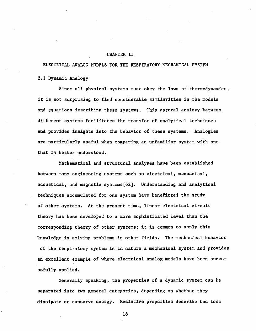
Figure 1 Three analog second-order systems: (A) Mechanical rectilinear system, (B) Pressure-volume system, and (C) electrical system.

Figure 1-A shows a mechanism consisting of an inertial element

(mass), a viscous element (dashpot), and an elastic element (spring).

Motion in this system is measured in terms of the distance x(t) that

the mass M moves relative to the point where M is in the equilibrium state with no force f(t) exerted from outside. If the three elements

are all linear, the equation of motion can be obtained from Newton's

laws and is shown in Eq.(2.1) in which B is the viscosity of the dashpot

and K is the elastic constant of the spring.

M x(t) + B x(t) + K x(t) = f(t) (2.1)

Figure 1-B shows a pressure-volume system, a rigid conducting tube

connected to an elastic balloon. In this case, motion is expressed as

volume v(t) and force as pressure p(t). Three properties are distri

buted throughout this system; however, for many purposes these distri

buted effects can be lumped into the compliance of the balloon (C), the

flow resistance in the tube (R) and the combined inertia of the fluid

and balloon (I). By analog to the mechanical system without actual

22derivation, the equation of motion of this pressure-volume system is

easily obtained and is given in Eq. (2.2).

I V(t) + R -fr(t) + v(t) - p(t) (2.2)Similarly, by analogy, the R-L-C in series circuit (Fig. 1-C) is de

scribed by Eq. (2.3a, b).

L q(t) + R q(t) + -i q(t) = v(t) (2.3a)

or

L i(t) + R i(t) +-/i(t) = v(t) (2.3b)CAs shown in Table 1, the system property is defined as the ratio

of two physical quantities. For instance, fluid resistance is defined

as the ratio of pressure to flow in the pressure-volume system. This ratio is known as the "static" value of the associated element. This

definition is only meaningful when the element is linear and its static value is constant, independent of particular values of the correspond

ing physical quantities. Frequently the relationship between the two physical quantities which define a system property is nonlinear, i.e.,

the characteristic curve of the concerned element cannot be represented with a straight line. In such instance, the static value of the element

changes from point to point on the nonlinear characteristic curve and

hence no single numerical value can be used to represent the nonlinear

property. Graphical techniques often offer the best way for describing

and analyzing the behavior of such nonlinear elements and the system containing them.

However, if relatively small signals are involved, then only a

small section of the nonlinear characteristic curve must be considered.

In this case, a single "dynamic" value can be used to approximate the property of the element without causing significant discrepancy. By

23doing so, nonlinear elements can be replaced with linear ones and a

dynamic system containing nonlinear elements can thus be linearized.

The dynamic value of a system element may be defined as the slope of the tangent line at a particular point of the associated characteristic curve. Once a nonlinear system is linearized, the system analysis

becomes much easier. Many well developed analytical methods for linear

systems can be employed to yield rather precise results. These results,

however, only pertain to the particular operating range in which the nonlinear system is actually linearized.

As will be seen later, the study in this dissertation does not

consider the static response of the respiratory mechanical system and only concerns itself with the dynamic behavior of this system in response

to a small externally applied sinusoidal pressure disturbance. The applied disturbance is so small that the system only operates in a

relatively small portion of the entire physical admissible region.

Therefore, the respiratory system under study can be well approximated

with a linear dynamic system in which each element is assigned a dynamic value at the actual operating point (e.g., FRC) regardless of the inher

ent nonlinearities of the system.

2.2 Review of Respiratory Mechanics

Before the electrical analog models for the respiratory mechanical system can be developed, it is desirable to review certain

aspects of respiratory mechanics. Detailed discussion on this subject

can be found in many texts [64,65,66].Figure 2 summarizes events which occur during normal respiration.

Just before the inspiration, the respiratory muscles are relaxed and no

24

in traalv eo la r p re ssu re

in trap leural p re ssu re in trap leu ra lp re ssu re

INSPIRATION EXPIRATION4 s e c

Figure 2 Variations in pressures and volume during a normal respiration cycle.

25air is flowing. The intrapleural pressure is subatmospheric and intra

alveolar pressure is exactly atmospheric. Inspiration is initiated by the contraction of intercostal muscles and the diaphragm. When the

diaphragm contracts, its dome moves downward into the abdomen, thus

enlarging the volume of the thoracic cage. Meanwhile the inspiratory

intercostal muscles contract, leading to an upward and outward movement

of the ribs and further increase in thoracic cage size. As the thoracic cage begins to expand, the intrapleural pressure decreases. This

increases the difference between the intra-alveolar and intrapleural

pressure, and the lungs are forced to enlarge. As the lungs enlarge, the air pressure within the alveoli drops to less than atmospheric

causing bulk flow of air from the atmosphere through the airways into

the alveoli until their pressure again equals atmospheric. The expan

sion of thorax and lungs produced during inspiration by active muscular

contraction stretches both lungs and thoracic wall elastic tissues.When inspiratory muscles begin relaxing, the stretched tissues recoil

to their original length since there is no force left to maintain their

expansion. The thorax and lungs return to their original sizes, alveolar air becomes temporarily compressed so that its pressure exceeds

atmosphere. Thus normal expiration appears to be completely passive,

depending only upon the cessation of inspiratory muscular activity and the relaxation of these muscles. In actuality, the inspiratory muscles

relax gradually to eliminate the large flows that would result with rapid relaxation. Under certain conditions, however, expiration can

be enhanced by the contraction of expiratory muscles including abdo

minal muscles, which actively decreases thoracic cage size. The abdo-

26minal muscles help by Increasing intra-abdominal pressure and passing

the diaphragm up higher into the thorax.The forces developed by various respiratory muscles are the energy

source that powers the pulmonary machine. The forces are opposed bythe sum of a number of different forces. These force components may bedivided into three general categories. The first is the force used to

overcome the elastic properties of the lung and chest wall. This repre

sents the potential energy of the system, since the work done on the

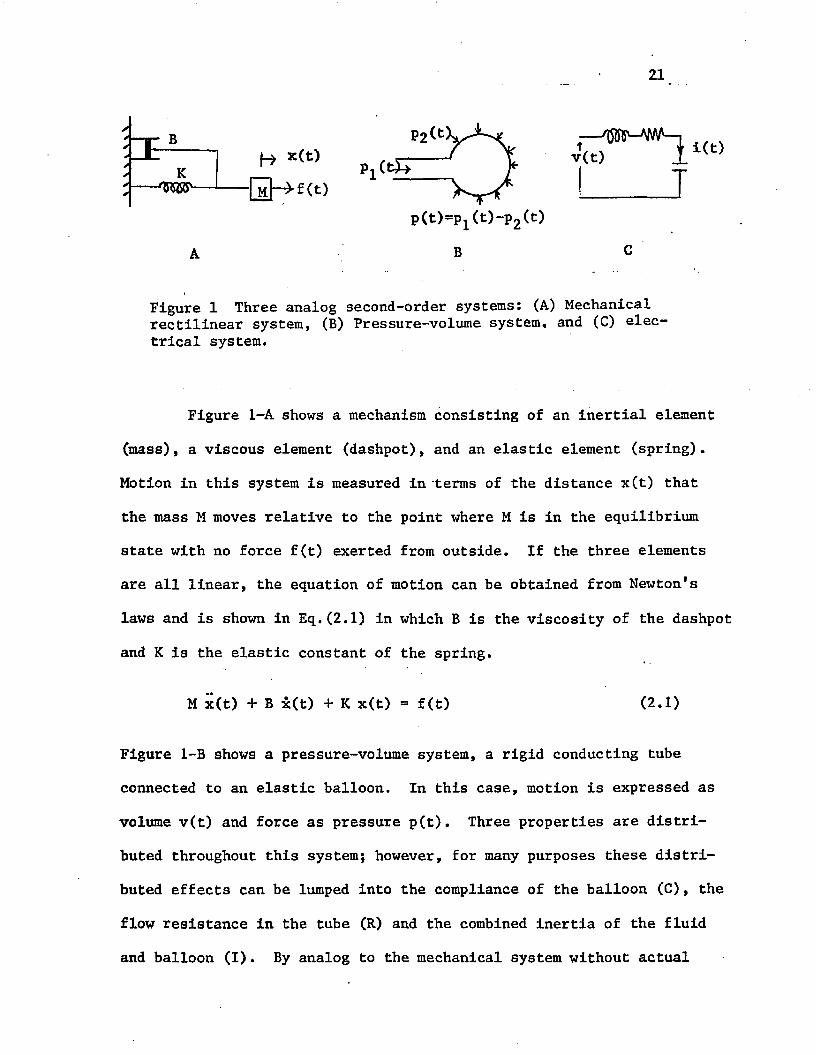
elastic elements during inspiration is returned during expiration. A

typical relationship between pressure and volume is shown in Figure 3,

and it can be seen that the relationship is nearly linear for small

volume variations around FRC.

The second component of the opposing force is that required to overcome the frictional resistance, which exists only when the system is in

motion; unlike the elastic force, resistive force includes two signifi

cant components: that due to gas flow through the trachealbronchialtree and that due to movement of the lung and thoracic tissues. In

considering flow resistance in the respiratory tree, three types of

fluid flow may be involved: laminar, transitional disturbed, or true

turbulent flow. When flow is laminar, the associated pressure is

proportional to the flow rate and depends on the viscosity of the gas.The pressure associated with turbulent flow is considerably greater than

laminar flow. For turbulent flow, the density of the gas becomes

important and viscosity unimportant, and the pressure is approximately

proportional to the square of the flow. For transitional flow, the\pressure-flow relationship lies somewhere between these two. Flow

changes from laminar to turbulent when the Reynolds number exceeds 2000.

100-* V C

•0

Pr*

40

ERV

RV-20 J I L-

-20-60 -40

Figure. 3 Static volume—pressure curve of the total respiratory system during relaxation in the upright posture. The volume at zero pressure corresponds to FRC.

(L /S E O

TURBULENTLAMINAR

1.0 (CM H20)

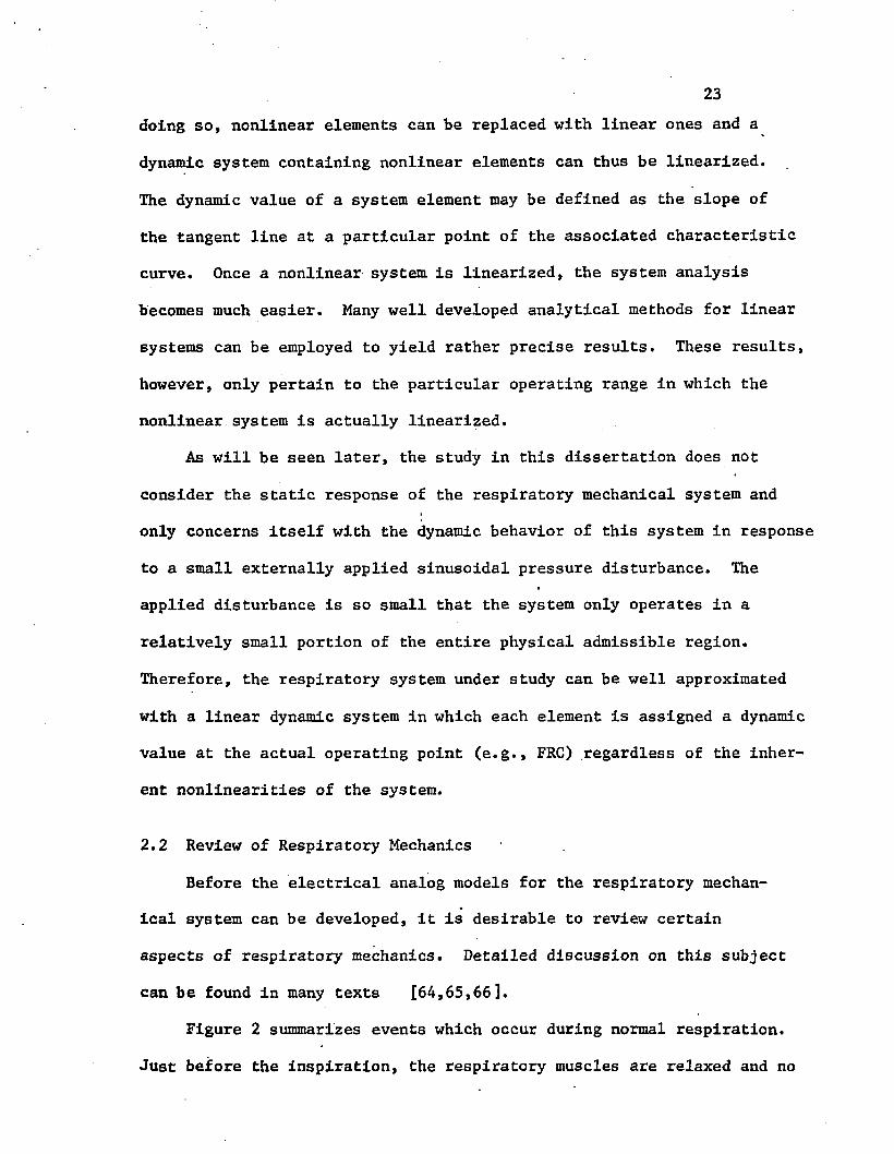
Figure 4 Equation and graph of alveolar pressure and air flow.

28(This is a dimensionless number equal to (density x velocity x diameter)

/viscosity). In smooth straight tubes, turbulent flow occurs at high velocity and in the respiratory system this essentially occurs only

in the larger airways, such as the main bronchi and trachea. The flow

rate in the smaller airways is very low. However, entrance region

effects are found at each branching of the tracheobronchial tree, and

the pressure required for the distrubed flow in these regions is difficult to determine. Figure 4 shows the relationship between flow and

the pressure due to the airway resistance, and it can be seen that this

relationship is approximately linear for flows below 0.5 i/s. The air

way resistance varies with lung volume but this effect is negligible for small volume changes (0.5&) around the FRC.

The third component is the force required to accelerate various

elements of the respiratory system including the mass of the lung and chest wall and the gas in the airways. This has been shown to be neg

ligible when compared to other force components at normal breathing rates, however, it does become the limiting factor at unphysiological

rates as with the application of forced oscillations. Relatively little

is known about the inertial effects but they are generally thought to

be constant for small variations around FRC.

2.3 Electrical Analog Models

Figure 5 shows a simplified analogous electrical network of the

total respiratory system [44]. The entire system is divided into three

major parts: airways, lungs and chest wall. The compliance of thecheeks, gas compressibility and small airway distensibility are repre

sented with shunt capacitors. The motion of the chest wall is concen-

n o s e

mouth.■Mt-nwJ

u u n g

29r- c h e s t w a l l

g a s

■yW—'£22'->—|- - - - vfiEJr-1 f—

jlung t i s s u e ^

- vW—Juuz -jI—, I rj5 c a g e—'MA~v222—j}— —

I- - vfiM/—| (~

H *~|-~| ” —£22,— | J—

r __________

+diaphragm

-VW’"vW4H I— [/V /{~

abc f om en

Figure 5 An electrical analog of the total respiratory system during spontaneous breathing.

Airway Lung Tissue Chest Wall

r— Pa0- p .iri r—ij/WWL—. 000 jli-lLwwv1

Pjlv ~ fpl"

* 4 t 3a w aw

**alv“

1ti— - F — r

|— ^ ppi -Pb;

. . - t -------r— tI, C , Pp, R cw *cw c w

Figure 6 An electrical analog of the total respiratory system in an anesthetized and paralyzed subject under forced oscillations,

Rrs Irs Crs

respiralory

Z rs —

Pds

Figure 7 Series R-I-C circuit representing the total respiratory mechanical system.

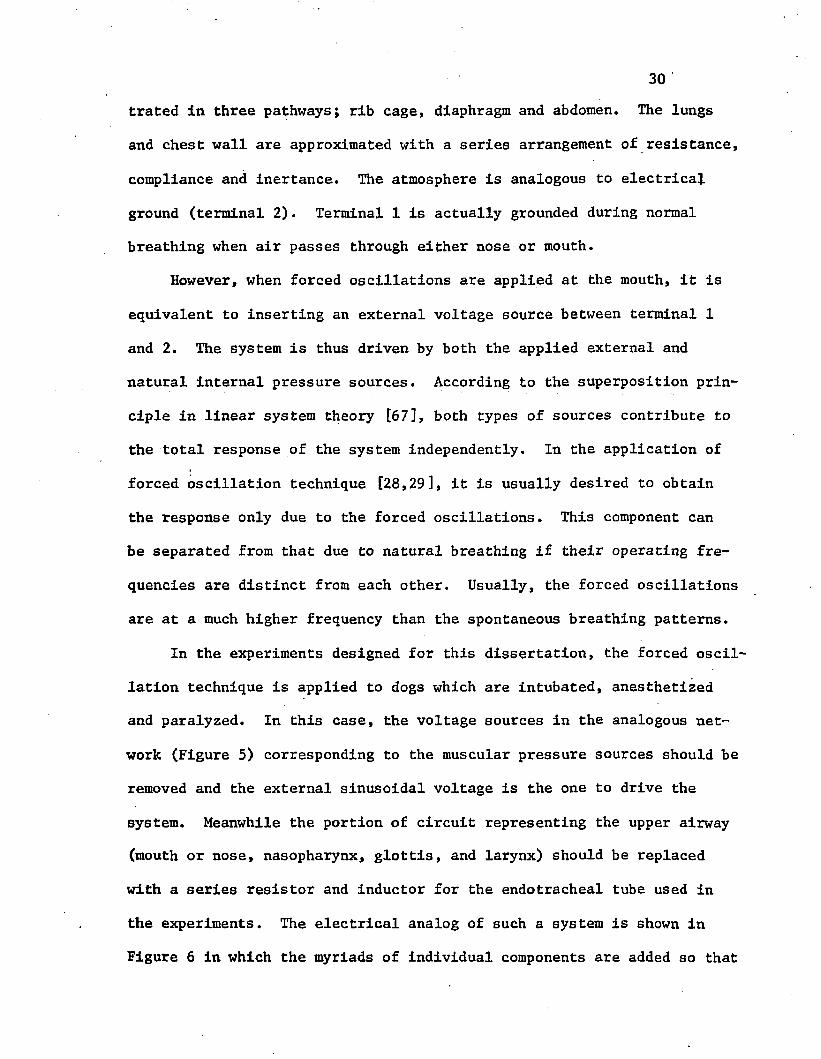
30trated in three pathways; rib cage, diaphragm and abdomen. The lungs

and chest wall are approximated with a series arrangement of resistance,

compliance and inertance. The atmosphere is analogous to electrical

ground (terminal 2). Terminal 1 is actually grounded during normal breathing when air passes through either nose or mouth.

However, when forced oscillations are applied at the mouth, it is

equivalent to inserting an external voltage source between terminal 1

and 2. The system is thus driven by both the applied external and

natural internal pressure sources. According to the superposition principle in linear system theory [67], both types of sources contribute to

the total response of the system independently. In the application of

forced oscillation technique [28,29], it is usually desired to obtain

the response only due to the forced oscillations. This component can be separated from that due to natural breathing if their operating fre

quencies are distinct from each other. Usually, the forced oscillations are at a much higher frequency than the spontaneous breathing patterns.

In the experiments designed for this dissertation, the forced oscil

lation technique is applied to dogs which are intubated, anesthetized and paralyzed. In this case, the voltage sources in the analogous net

work (Figure 5) corresponding to the muscular pressure sources should be

removed and the external sinusoidal voltage is the one to drive the

system. Meanwhile the portion of circuit representing the upper airway (mouth or nose, nasopharynx, glottis, and larynx) should be replaced with a series resistor and inductor for the endotracheal tube used in

the experiments. The electrical analog of such a system is shown in Figure 6 in which the myriads of individual components are added so that

31each major area is represented as having one resistance, one compliance, and one inertance. Various pressures at different sites in the system are noted. For example, the pressure in the airways is the difference

between alveolar pressure (Paiv) and pressure at the mouth (Pao) • pressure across the lung tissue is the difference between alveolar and pleural pressure (Pp^) and pleural pressure relative to the atmospheric

pressure equals pressure across the chest wall. Cg represents the

compressibility of air and thus is represented as connected to ground

since its degree depends on the difference between atmospheric and air

way pressure.A two-terminal linear network like that in Figure 6 made up of

basic passive elements (i.e., resistor, capacitor, and inductor) shows

a particular relationship between voltage and current as measured at

the two input terminals. When the input voltage is sinusoidal, this relationship is known as input impedance. In Figure 6, C is normallyOvery small compared to or Ccw so that when it is removed the input

impedance is not significantly altered. After moving C and then com-O

bining the same type of elements into a single one, the electrical analog

in Figure 6 is reduced into a series R-I-C circuit as shown in Figure 7. Although this is a greatly simplified model for the actual

respiratory system, it is adequate for interpreting much of the experimental data obtained in studying the respiratory mechanics in normal

subjects [25,30,44,50].In patients with chronic obstructive pulmonary disease (COPD),

many investigators [28,30,45,46,68] have recognized that the measured

pulmonary compliance and resistance are frequency-dependent. This

32observation is obviously inconsistent with the simple R-I-C model and

several alternate models have been proposed to explain this frequency-

dependent behavior. In the model of Otis et al. [45], the lungs are considered to be made up of a number of parallel air pathways, each

consisting of a resistance and a compliance (the inertance is ignored). According to their theory, the frequency-dependency of compliance or

resistance is caused by the discrepancies in time constant between separated pathways of the lungs. (Time constant of a pathway is the

product of its associated flow resistance and compliance . It is a con

venient expression for the speed of filling air into the pathway). This

model could be interpreted with an electrical analog circuit as shown in

Figure 8-A, where only two pathways are used to approximate the air passage in the lungs. These two pathways share the other three elements

C^, I (an approximate of total inertance), and R (sum of extrathoracic airway resistance and tissue resistance of chest wall).

Mead [46] considered the airways as a compliant structure in parallel with the air spaces, and using a two-compartment model, demonstrated

that time constant discrepancies between the airway and the parenchyma

could explain the decreasing of compliance and resistance with increase

of frequency. This frequency-dependence in normal subjects is too small

to be detected in the frequency range for practical measurements. As peripheral airway resistance is increased, the time-constant inequality

becomes greater, and can account for most of the frequency-dependent

behavior in patients with COPD. This model can be represented with the

electrical circuit as shown in Figure 8-B as suggested by pimmel [37 ].A feature of this representation is the separation of the airway resis-

rs

-AA/V-R

KlfI T

R„

□ ? J T 2

cw

aw

rs cw

B

rs

I R- w ------vSV :R,RA * ~Rr ^ " B

CA i i:C~ $ U -

J'Figure 8 Three different two-pathway models the respiratory system: (A) Otis1 model, (B) model, and (C) Hogg's model.

for Mead1

34tance into a central component (Rca) and a peripheral component (Rpa)by inserting an element (C av) standing for the airway compliance

between the junction of Rca and Rpa and the point corresponding to the

pleural pressure. The resistance of the airway compartment is so small

that it is practically omitted from the model. It should be noticedthat the circuit shown in Fig. 8-A will have the same input impedance

as the one shown in Fig. 8-B if R ° R__ + R.r . R-, =0, Cn = C andvd cw x x aw

R2 = R&*Another model proposed by Hogg et al. [68] c.onsiders the resistance

of channels for collateral ventilation to be too high (compared to resistance of normal ventilatory pathway) to result in frequency-dependent

behavior in normal lungs. But collateral channels become important for air ventilation with obstruction of peripheral airway, causing time-

constant difference between collateral and normal ventilated areas, accounting for frequency-dependent compliance in emphysematous lungs.

The appropriate electrical analogue of this situation is shown in Figure

8-C in which the resistor R^ accounts for the collateral channels. In severe emphysema, airway resistance in the obstructed area (e.g., the

pathway of Rg - Cg) is much greater than the collateral flow resistance and can be practically removed from the analog circuit. Two parallel

pathways, R , - Cg and C^, are thus formed and their time'constants will

be unequal. This electrical analog circuit can also be transformed

into the one as shown in Figure 8-A without altering the input impedance

by setting R = rd+r^» ri=0» ^i^A* R2~RC an(* ^2=CB*

2.4 Frequency Analysis of Electrical Analog Models

One of the major aims of this dissertation is to estimate the

35parameters of the respiratory system, which cannot be measured directly.

Mouth pressure and airflow are the only easily measurable physical quantities by using forced oscillations. Thus, the mechanical parameters

mudt be estimated from these measurements. When the system is represented

by any one of the models developed in the last section, estimating the

electrical parameters in the model can be done from the input voltage and current, which are analog to the mouth pressure and airflow in the

respiratory system subjected to forced oscillations. The input impedance

is a very convenient method for characterizing this relationship and it

is extremely useful in relating the measured quantities to the system

parameters. As will be seen in the next chapter, the conventional forced oscillation technique is extended to directly provide the input impe

dance of the respiratory system at a specific frequency by electronically processing the measured pressure and flow signals. The impedance

data thus obtained in a certain frequency range will be the basis upon which the respiratory mechanical parameters can be determined.

At any given frequency, the input impedance Z of a two-terminal

linear network is generally a complex quantity. Its absolute value or magnitude |z| is defined as the ratio of the amplitude of the input voltage to the amplitude of the input current and its argument or phase angle <p is defined as the phase shift between the current and the vol

tage with the current as a reference. The real part of the impedance is

referred to as its resistance R and the imaginary part as its reactance

X. The reciprocal of the impedance is called admittance. The impedances of the three passive two-terminal elements, resistor (R), capacitor (C), and Inductor (L), are respectively known as R, 1/jooC and jtoL or

R, l/(Cs), and Ls, where s = jo). The impedance of a series circuit

consisting of several circuit elements is the sum of the impedances of

the individual circuit elements. The impedance of a circuit made up of

parallel elements can be obtained by taking the reciprocal of the

corresponding admittance which is the sum of the admittances of the

individual elements.The input impedance of a two-terminal linear circuit is a function

of frequency except when the circuit contains only resistors, in which case the input impedance is a real number, and is independent of fre

quency. Many important characteristics of a two-terminal linear cir

cuit can be obtained by examining the frequency response of its input impedance. The frequency response of a system is generally presented in

certain standard graphical forms such as Nyquist and Bode diagrams. The latter is extensively employed in the following paragraphs. More de

tailed discussions of input impedance of a two-terminal linear network

are available in standard texts on linear circuit theory.[61,67,691.Applying these techniques to the electrical analog model shown in

Figure 7 leads to an expression for the input impedance of the circuit

as shown in Eq. (2.4) and (2.5).1

37If two new parameters, wn , the undamped natural frequency, and

£, the damping ratio, defined as ____2 _ 1 _ ^ s I Crsui « r— and £ = ---- I-n I crs 2 NJ IrBrs rs

are introduced, then Eq. (2.5) may be rewritten as shown below:S ,S » -£ w + (2.6)I d n _ n

The two zeros of Z (S„ and S_) are a complex conjugate pair if £ < 1,rs 1 d

two equal real numbers if £ = 1, and two unequal real numbers if £ >1.

Substitution of s = jw into Eq. (2.4a) yields the equation

Z_ = R + j(u I - JL-) = R_a + jX (2.7)18 rs rs coC rsrs

It is obvious that the real part Rrs of the impedance is independent offrequency but the imaginary part X^g is frequency-dependent. At low fre

quencies, X is dominated by the compliant component X = - —-— but rs c wCrsit is dominated by the inertial component Xjjj = at high frequency.When w « to = l. X and X_ cancel each other and X becomes zero.n j l C * m C rsrs rsConsequently, at this frequency, the phase angle 6 = 0 and the magnituders|Z is minimal. In general, this condition is called resonance, andI ITS '

is called the resonant frequency of the series R-I-C circuit.Typical values for the mechanical parameters in normal adult humans

are Rrfl = 2.7 cmHjO/l/s, Crs = 0.1 l/cml^O, and Irg = 0.01 cm E^O/l/s^

[44]. The corresponding respiratory impedance, from Eq. (2.4), is shown in Eq. (2.8).

Z * (JLLL) (ju + 3.765) (jrn + 266.24) (2.8)19

This system has a resonant frequency at w *= 31.62 rad/sec or f = 5 Hz.

One pole at origin and two zeros at -3.756 and -266.24. Its Bode dia

gram representation is given in Figure 9, in which the two corner fre-

38quencies are at w = 3.756 and 266.24 rad/sec or f = 0.6 and 42.37 Hz.

Note that at the resonant frequency phase angle crosses over zero

degree and the magnitude reaches a minimum. Figure 10 shows the rela

tive contribution of X_ and X_ to the total reactance X as functionsm rsof frequency.

rs

-1

-2 ter 25Figure 10 Relative contribution of inertance and compliance reactances (Xjn and Xc) to the total respiratory reactance (Xrs) in normal adult humans.

Applying this approach to the electrical analog model shown in Figure 6 results in the expression for the input impedance shown in

Eq. (2.9) in which = R* + Rc(j, = I* + 1 ^ and 1/Cfa) = 1/C*

+ 1/CW .

rsPCs)TOT (2.9a)

PCs) - 1 C C0 IoMS* + (R I. +1 R, J C c. saw g Aw aw Aw aw Aw g Aw1,

+ I*awcg Riwciu.+1aw(cg

Magnitude

- DB

Magn

itud

e

25

20

15

10

- 9(P5.5 1 50 100 200 500 rad/2 5 10 20Figure 9 Frequency response Of aRIC model with nominal parameter values

25 90'

Phase20

15 Q.

10

- 9(f50 100 200 500 rad/s

55 10 2025 1

Figure 11 Frequency response of the input impedance of the model as shown in Fig. 6 with nominal values for the parameters.

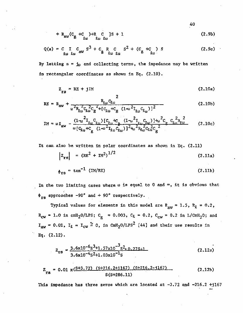
By letting s = jy and collecting terms, the impedance may be written

in rectangular coordinates as shown in Eq. (2.10).

Z » RE + jIM (2.10a)2

RE - Raw + " t A ------- (2.10b)“ V ‘*»C* +t<R»+08 V 1

IM - .1 - «& ■ (2.10c)“ [Cjiw+Cg

It can also be written in polar coordinates as shown in Eq. (2.11)

|Zrs| = (Re2 + im2)1/2 (2.11a)

$ra ° tan"1 (IM/RE) (2.11b)

In the two limiting cases where w is equal to 0 and 00, it is obvious that

4 approaches -90° and + 90° respectively, xsTypical values for elements in this model are Raw = 1.5, = 0.2,

R ^ = 1.0 in cmH20/LPS; Cg = 0.003, Cj, = 0.2, Ccw = 0.2 in L/Cml^O; and

Iaw =0.01, Iji = Icw = 0, in Cml^O/LPS^ [44] and their use results in Eq. (2.12).

z = 3.6xl0-6s3+1.57xl0~ S2+0.?7S4.1 (2.12a)TS 3.6xl0"4S2+1.03xl0_1S

Z =0.01 ^ S+3.72) (5+216.2+1167), .(S+216.2^161)_ (2#12b)ra S(S+286.11)

This impedance has three zeros which are located at -3.72 and -216.2 +.il67

41and two poles which are located at origin and -286.11. For the pair of

complex conjugate zeros, the damping ratio is equal to 1.57 and theundamped natural frequency is 137.7 Hz. The frequency response is shown

in Figure 11. A comparison between Figures 9 and 11 points out thatthe'frequency responses of the respiratory impedance in both cases are

almost identical except when angular frequency is greater than 100

rad/sec (or 16 Hz). This implies that the shunt capacitor C in Figure 6

has little effect on total respiratory impedance at frequencies less

than 16 Hz in normal subjects and consequently the respiratory mechan

ical system can be well represented by the simple RIC in series circuit.

Since the three different models described in the previous section for explaining the frequency-dependent behavior can be interpreted

within the framework of a single electrical analog circuit, although each element in this circuit has a different anatomical counterpart in

each of the three models, it is not necessary to treat them separatelyin order to analyze the frequency response of these models.

Using the model in Figure 8-A which also represents the other two

models since they can be transformed into it, the equations (13 and 14) of Otis at al. [45] can be adopted directly to ‘obtain the impedance

between points a and b. The results are shown in Eqs. (2.13) through

(2.15) in which T^ = and T2 <=* R2^2*

zab - Rab ~ i — <2-13’“Cab

Rab . A V ^ C r ^ c p - ^ c ^ c , )U)2(T2C1+T1C2)2+(C1+C2)2 (2.14)

42Cab - m2(Tlc?+?2cl) 2+<c.j*-£2l?--- (2.15)

w2(t 2c i+t 2c2)+(C1+C2)

The impedance can be combined with that of the shared complianceCC£i), to find the impedance between points a and c which is given by

Eq. (2.16) or(2.17).

ZQ = Z , + L _ (2.16)ac ab jwccm

Zac = Rab + (2‘17)aD U c . Cab cio

Zflc can also be represented by an equivalent circuit made up of a sin

gle frequency-dependent resistor R and capacitor C in series. These6 6can be found by comparing Eq. (2.17) with (2.18), and the results are

shown in Eqs. (2.19) and (2.20).Z = R - j JL (2.18)ac e u)Ce

Ke - Rab - ( 2 _ 1 9 )

or (T2 C-l+T^ )2+ ( Cj+C^ )1

Ce . . ^ C ^ C T i C y b T ^ ^ J C ^ C , , ) 2___________________Cab+CcO +

When the time constants of the two separate pathways are equal, i.e.,

Ti “ T2, these expressions can be simplified .as shown in Eqs. (2.21)

and (2.22). It is noteworthy that for this case (T^Tj) , the desired

parameters Re and Cfi are independent of frequency.

r = ^ (2.21)

Ce » Ccm(°l+C2) (2,22)Ci+C2+Cc(tf

43The total input impedance may be expressed as shown in Fig. (2.23)

in which total respiratory resistance (Rrs) is equal to R+Re and thetotal effective compliance Cr8 is equal to Ce.

Z__ = R + Re + j (oil - — ) (2.23)rs e wCe

Both R and C__ are frequently-dependent except when the time con- rs rsstants of the two parallel pathways are equal (Tj=T2).

In order to illustrate the frequency-dependent behavior, Mead's

model (Fig. 8-B) [46] and his parameter values for normal humans are employed. These parameters are:

R = 2.5; I = 0.01; C «* 0.2;U(l)Rx = 0; 0^0.0005; ^ = 0;

R2 55 0.5; C2 ■ 0.2; T2 = 0.01The effective respiratory compliance and resistance for this case

are shown in Figure 12, (curve A), together with those for increasing

peripheral airway resistance (curves B-C) and compliance as in COPD (curve D). The values of compliance and resistance in the two pathways

are identical to those used by Mead [46]. The corresponding total respiratory impedances for these four cases are shown in Figure 13.

It can be seen that no detectable changes in effective compliance and

resistance occur in the frequency range for practical measurements (0-1.5

Hz for compliance, 10 BPM - 10 Hz for resistance) in normal lungs.

However, when the peripheral airway resistance is raised, the frequency-dependency becomes more prominent. In COPD (curve D), drastic

decreases in both compliance and resistance with frequency are very obvious. The total dynamic compliance falls by 65% at 1 Hz and 80%

44

ooc<cClEOoo>o0)n-M-LU

15-, L/cmH20Curve

Cl .005 .005 .005 .005 C2 .2 .2 .4 .4

0 5 10 HZ

12 - 1

cc

Figure 12 Total effective compliance and resistance in Mead's model in four different conditions (see text).

iZrs!

12

10 -

6 “

2 -

HZ(a)

60-,

2(f_

in (f_

-29-

50Figure 13 Magnitude (a) and phase (b) of total respiratory impedance in Mead's model in various conditions (see text)

46at 2 Hz; total resistance falls by 45% at 5 Hz and 65% at 10 Hz.

Figure 14 shows the pole-zero configurations of the respiratory

Impedances In the four cases mentioned above. It is found that as the

peripheral airway resistance Increases both zeros and poles of the

respiratory impedance move toward the origin. This implies that the

respiratory impedance becomes more sensitive to the change of frequency

in the region near the origin as the peripheral airway resistance increases. In other words, a frequency change in the lower frequency

range can cause more prominent change in respiratory impedance if the peripheral airway resistance is raised.. This may explain whey the

frequency-dependence behavior of effective compliance and resistance in COPD is detectable in the practical, measurement frequency range which

is relatively low.

-1 -i -i ■poo

o*-

L00

->dt -toi =3?)s -loo ° T

rlOO

J-200

Figure 14 Pole (solid symbol) and zero (empty symbol) configurations of the input impedance in Mead's model with four different conditions: normal (o), increasing peripheral resistance (a), increasing peripheral resistance (□), and COPD (O).

2.5 A RemarkIn previous sections, all discussions about the analog linear

electrical models representing the respiratory mechanical system were

directed toward human subjects. However as will be noticed in Chapter 4, dogs were the experimental animals used for the study described in

this dissertation. One may wonder if those models for human lungs are

also applicable to dogs?

The anatomical studies reported by Tyler et al [75] indicated

significant structural differences in lungs of man and mammals commonly

used in experimental studies. For example, interlobular air drifts

are nearly nonexistent in cow and pig; occur more frequently in the horse and man; and are present to a relatively greater degree on a

segmental basis in the dog. Tyler also suggested that these specimens might be grouped into three distinct morphological groups with the cow

and pig designated as type 1, the dog as type 2, and the horse and man as type 3. Since anatomical features certainly have some influence on

function, lung mechanics in dog might be different from that in man.

Certain differences between dog and man have been shown in several comparative studies [76,77,78]. On the other hand, the same studies have

also established the basic mechanical behaviors in dog and man are identical.

Emilio et al [76] found that the relationships between dynamic respiratory pressure and flow in both dog and man follow Rohrer’s

equation and that the relaxation pressure-volume curves in both species

were nearly identical. Hull eral [50] suggested that the gross behav

ior of the respiratory system in dogs can be modeled by a constant series R-L-C circuit. The frequency-dependent behavior of compliance

48and resistance caused by inequality in the time constants of various pathways in the lungs was also demonstrated in dogs [79].

All these facts strongly suggest that the linear electrical cir

cuit models developed in previous sections to represent the respiratory

mechanical system for man also is appropriate for dogs.

2.6 SummaryAlthough the breathing mechanism is very complicated, its mech

anics are basically analogous to other dynamic systems such as mechanical and electrical circuit systems. The well developed theories

for electrical circuit systems can greatly facilitate studies of the

respiratory mechanical system by applying dynamic analogy between these

two systems. The use of two-terminal linear electrical circuits for

modeling the respiratory mechanical system in order to explain the impedance data obtained from forced oscillations is fully justified.

The mechanical behavior of a normal respiratory system can be represented by a simple second order R-I-C model. But, models containing two

pathways are necessary in accounting for the frequency-dependent behav

ior of compliance and resistance. The frequency analysis of the input Impedance of a particular model can provide valuable information on the

Inherent nature of the associated respiratory system. The discussions in this chapter have provided theoretical bases for those in the next _

chapter which deals with the estimation of respiratory parameters from

the impedance data.

CHAPTER III

PARAMETER ESTIMATE BY NONLINEAR REGRESSION ANALYSIS

3.1 Parameter Estimate ProblemIn the studies of various systems such as automatic control

systems, physiological systems, economic systems, etc., two types of problems are generally encountered. The first one is to find the response of a given system to specific inputs or excitations. The other

problem is to find a mathematical description (model) of an unknown

system based on a -certain set of inputs and corresponding outputs. This

type of problems is known as the modeling or identification problem [35].

Modeling problems can be separated into two broad categories,

depending on the degree of a priori knowledge of the system. If the nature of the system is completely unknown, the problem may be termed as

a "Black Box" identification problem. In many cases, a great deal of

knowledge concerning the basic equations describing the system, often

from a knowledge of its structure or from the available mathematical

models or similar system, may exist, but the specific values of the system parameters may be unknown. Some authors have termed this the "Grey Box" problem [35]. The problem addressed in this dissertation is essentially

a modeling problem, and belongs to the second category.

Modeling problems usually encompass four sub-problems: represen

tation, measurement, estimation, and validation [88]. The representation

49

problem deals with how a system should be modeled. It is necessary to

know whether the model should be static or dynamic, linear or nonlinear,

deterministic or random, continuous or discrete, and so on. In order

to verify a model, physical quantities must be measured, and the measure

ment problem consists of defining which physical quantities should be

measured and how they should be measured. Usually, a certain number of

non-measurable parameters are involved in the model, and the estimation

problem deals with the determination of these parameters from the measured quantities. After a model has been completely specified, through choice of an appropriate mathematical representation, measurement of

signals and estimation of parameters, the model must be verified. The

validation problem deals with demonstrating confidence1in the model and

this is often achieved by a statistical test involving confidence limits, and physical justification of the model. These four sub-problems as

applied to respiratory mechanics are considered in various chapters of

this dissertation: the representation, measurement and validation problems

are respectively dealt in Chapter II, IV, and V; the remaining problem,

parameter estimation, is discussed in this chapter.A general structure for considering this type of problem has been

discussed by Bekey [35]. In these discussions the system is represented

as shown in Figure 15. The k input variables to the system are designated

as x.) x0, ..., x. and the single output variable of the system is y .X L , K « O

If a priori knowledge can be used to develop a mathematical representationof the system that contains a certain number of unspecified parameters,

6 -,6 „, ..., 6 , then the system can be characterized by Eq. (3-la),oi op

51

> y.

Figure 15 A dynamic system with multiple inputs and single output

By defining two vectors,

andX — (x1> • • •,

0o = (9ol> •••’ eop) ’where the prime symbol represents' the transpose of a vector, then

Eq. (3.1a) can be rewritten as Eq. (3.1b).

y0 - f<x;0o) (3.1b)

Suppose n observations of the form; y , x, , ..., x ;ou lu kuu = l,2,...,n, are available by direct measurements of the input and

output variables. Regardless of how X^ = xiu » anc* ^orku ou

u = 1,2, ...,n are actually obtained, two distinct situations are possible.

These measurements can be without any error or there can be a certain

amount of random error in the measurement. In the first case, Eq.(3.1b) for the n observations can be written as shown in Eq.(3.2a) or in vector

form as in Eq.(3.2b).

u=l,2,...,n (3.2a)

(3.2b)

y f(X ;0_)ou u o/ \ / \

I—1 0

>. f(X1;0 ) 1 0Y 53 0

0s 09o f (x ;o )l°n/ n o **

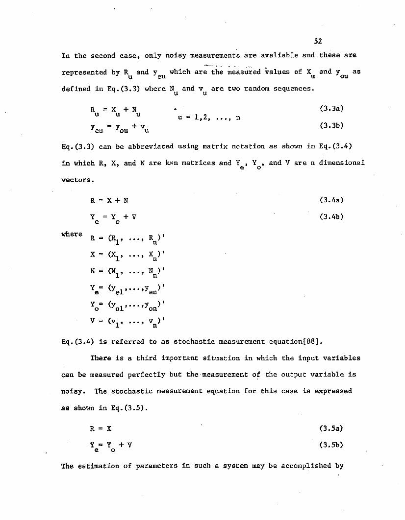
52In the second case, only noisy measurements are available and these are

represented by R and y which are the measured values of X and y as r u eu u oudefined in Eq.(3.3) where and v^ are two random sequences.

R = X + N u u uy = y + v 3eu 3ou u

(3.3a)

(3.3b)u = 1,2, ..., n

Eq.(3.3) can be abbreviated using matrix notation as shown in Eq.(3.4)

in which R, X, and N are kxn matrices and Y , Y , and V are n dimensional * * e ovectors.

R = X + N

Y = Y + V e o

(3.4a)

(3.4b)

where R = (R^> * *•> VX = (xx, .• VN = (Nr .. Hn)'

Y = e <yel’" *,yen>'Y = o <yol’“ •*yon>'V = (v^ .. V

Eq.(3.4) is referred to as stochastic measurement equation[88].There is a third important situation in which the input variables

can be measured perfectly but the measurement of the output variable is

noisy. The stochastic measurement equation for this case is expressed

as shown in Eq.(3.5).

R = X (3.5a)Y = Y + V (3.5b)e o

The estimation of parameters in such a system may be accomplished by

53following the scheme as shown in Figure 16 [88]. The measured output

variable, Y^, is approximated by Y^ as defined by Eq.(3.6).

(3.6)

Y is a structural model of Y , in which 0 = (6., ..., 0 )1 denotes an m o 1 Pestimated value of 0 . The stochastic error between the measured outputoY and model output Y is symbolized by Y and is defined in Eq.(3.7). e m

/ \ yml £(x1;0)

s* II ••

y mn \ /

•

f(x ;0)k n >

Y = Y - Y e m (3.7)

Vsystem

model

algorithm

Figure 16 A parameter identification system

54This error, Y, which is computable, is used along with the measurednoise-free input variables, X, to obtain an estimate for Qq from aparameter estimation algorithm. This algorithm is usually an iterative

process in which values for 0 and Y are changed iteratively until themfinal values for 0 and Y are obtained.m

The problems described in this dissertation as well as in many

other engineering problems fit into this third category. Many algorithms

have been developed for solving this type of problems [35,36], and the

more important ones are discussed briefly in the following sections.

3.2 Numerical Methods for Parameter Estimation

3.2.1 Regression Analysis MethodConsider the system as shown in Figure 15. Suppose the input

variables of the system can be measured without any errors, but the measurement of the output variable is noisy as expressed by Eq.(3.8) in which vu» u = 1,2, ..., n , is a random sequence.

y = f(X ;0 ) + v u=l,2,...,n (3.8)■'eu u o uThis is a system of n equations with p unknown parameters. If n<p, there

are fewer equations than unknowns. Such an underdetermined system of

equations does not lead to unique or meaningful values for 0o= (0Q^>••[83], If n=p, there are exactly as many equations as unknowns, and if

measurement errors are not present, 0 could be obtained exactly byosolving the set of equations although the solution may rot be unique.

In this case, nothing can be done about the measurement errors. The cha

racteristics of the errors will greatly affect the solution for 0Q. If

55n>p, there more equations than unknowns, and within this overdetermined

structure, the effect of measurement errors could be offset. This is.

the case of real interest in this dissertation, and in classical statis

tics, this type of problems is studied under the subject of "Regression

Analysis" [84].Generally speaking, the objective of regression analysis is to

Adetermine a vector 0 which serves as an estimate of the true parameter

vector 0 , by making use of the theoretical response function of the . osystem. This estimation may be accomplished by minimizing a specific

measure of the error Y (Eq. 3.7) and this measure is usually referred toAas criterion or error function. The estimate vector 0 is usually chosen

so as to minimize a weighted sum of squares of the components of Y, J, as

defined in Eq.(3.8a) or in matrix form in Eq.(3.8b), in which

J(0) = w-y 2 + w0y 2 + ... + w y 2 (3.8a)1 1 L l n nJ(0) = Y f W Y (3.8b)

the matrix W is given by Eq.(3.9)./ \ w.

W = (3.9)

In other words, the estimate vector 0 is determined according to Eq.(3.10).

mjn J(0) = J(0) (3.10)

A

This technique for choosing 0 is known as the generalized least

squares or weighted least squares method. When each component of Y is

weighted equally, the weighting matrix is reduced to as shown in Eq.(3.11)

56

in which I is the n*n identity matrix and w is a constant, and this

equation is referred to as the least squares method.

W = w I (3.11)

Linear Regression AnalysisWhen the theoretical response function f(Xu ;0) is a linear

function of the parameter vector 0, the minimization of the sum squares

is particularly simple. For this case, Eqs.(3.2b), (3.6), (3.5b), and

(3.7) can be expressed as Eqs.(3.12), (3.13), (3.14), and (3.15) respec

tively.

Y = H 0 (3.12)o oY = H 0 (3.13)IQY = H 0 + V (3.14)e , oY - H (0 - 0) + V (3.15)o

In these equations H is an nxp matrix whose components can be computed

from elements of the input matrix X. The criterion function J given by Eq.(3.8) may be written in a quadratic form in 0 as shown in Eq.(3.16).

J(0) = Y 1 W Y - 2 Y' W H +0' H ’ W H O (3.16)e e eIf W is a symmetrical and positive definitive matrix, the

criterion function J in Eq.(3.16) is also positive definitive and has aAminimum at 0=0 which may be found by equating to zero the gradient of J

Awith respect to 0. The resulting 0 is given implicitly by Eq.(3.17).

(H' W.H) 0 = H' W Ye (3.17)

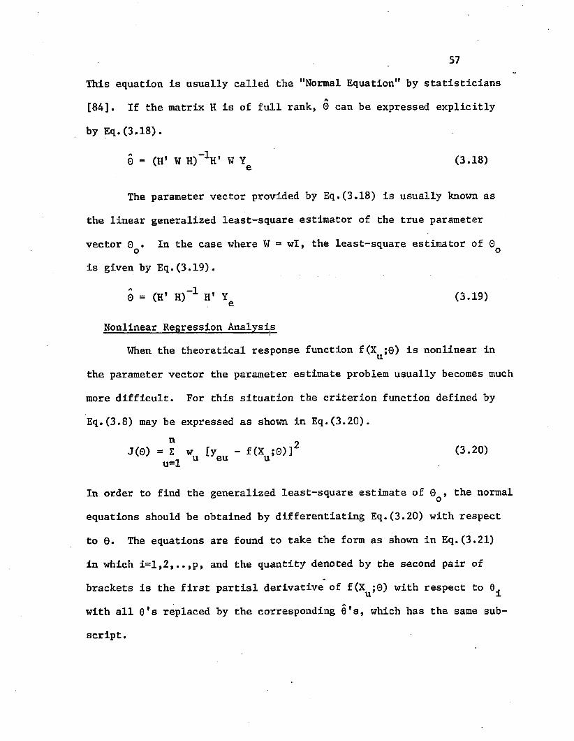
57This equation is usually called the "Normal Equation" by statisticians

A[84]. If the matrix H is of full rank, 0 can be expressed explicitly

by Eq.(3.18).

0 = (H* W H)”^ 1 W Y (3.18)&

The parameter vector provided by Eq.(3.18) is usually known as

the linear generalized least-square estimator of the true parameter

vector 0 . In the case where W = wl, the least-square estimator of 0 o ois given by Eq.(3.19).

0 = (H’ H)_1 H ’ Y£ (3.19)

Nonlinear Regression AnalysisWhen the theoretical response function f(X^;0) is nonlinear in

the parameter vector the parameter estimate problem usually becomes much

more difficult. For this situation the criterion function defined by

Eq.(3.8) may be expressed as shown in Eq.(3.20).n 2 J(0) = S w [y - f(X ;0)r (3-20)t u 'eu uu=l

In order to find the generalized least-square estimate of 0q, the normal

equations should be obtained by differentiating Eq.(3.20) with respect

to 0. The equations are found to take the form as shown in Eq.(3.21)

in which i=l,2,..,p, and the quantity denoted by the second pair of brackets is the first partial derivative of f(X^;0) with respect to 0.

with all 0*s replaced by the corresponding 0's, which has the same sub

script.

58n 3f(X ;0)2 w [y - f(X ;0)] [--- -— ] = 0 i=l,..,p (3.21)u=1 u eu u 3Q^ Q=Q

aEq.(3.21) must be solved for 0, and since no general formula can be

obtained each problem must be treated individually. Draper and Smith [84]

have pointed out that even with one unknown parameter and a relativelya ,simple nonlinear function, finding 0 by solving the normal equations is

not easy. When more parameters are involved and the nonlinear function

is more complicated, the solution of normal equations can be extremely difficult to obtain, and iterative methods must be employed in nearly

aall cases. The difficulties in obtaining 0 may be compounded by the

fact that multiple solutions may exist, corresponding to multiple sta

tionary values of the criterion function.AIn many nonlinear cases, since it is difficult to find 0 directly

from the normal equations, estimation of parameters is frequently achieved

by utilizing certain optimum seeking methods with the aid of high speed

digital computers. These computing techniques fall into two general

categories: gradient methods and search techniques [35], which are briefly

discussed in the following paragraphs.

3.2.2 Gradient Methods

Gradient methods are based on finding the values of 0 for which

the gradient vector of the criterion function, J, with respect to the

parameter vector equals zero, since the condition satisfies a necessarycondition for the existence of a local minimum of J. The corresponding

thcomputer algorithms are based upon computing the i+1— parameter estimate

using Eqs.(3.22) and (3.23).

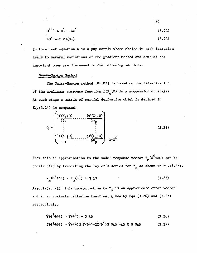
ei+1 = 01 + A01

A01 =-K VJ(01)

59(3.22)

(3.23)

In this last equation K is a pxp matrix whose choice in each iteration

leads to several variations of the gradient method and some of the

important ones are discussed in the following sections.

Gauss-Newton MethodThe Guass-Newton method [86,87] is based on the linearization

of the nonlinear response function f(X^;0) in a succession of stages

At each stage a matrix of partial derivative which is defined in

Eq.(3.24) is computed./ \3f(XijO) 3f(X1;0)-•••«••• ■ * i i ■

301 30d

3f(x ;0) af(x ;0)V“"W7...... ............. .....5T*—\ 1 P S

(3.24)

0=0

From this an approximation to the model response vector Ym (0 +A0) can be

constructed by truncating the Tayler’s series for Y^ as shown in EQ.(3.25)

Y (0*4*0) - Y (01) + Q A0 m m (3.25)

Associated with this approximation to Yffi is an approximate error vector

and an approximate criterion function, given by Eqs.(3.26) and (3.27)

respectively.

Y (0*4*0) = Y(0*) - Q A0J(01+A0) = Y(0±)W Y(Oi)-2Y(0±)W QAG'+AG'Q'W QA0

(3.26)

(3.27)

60The parameter change vector A0 can be obtained by minimizing

J(0*+A0). Since the expression in Eq.(3.27) is analog to that in Eq.(3.16), the minimizing value of A0 can be obtained by simply comparing

.to Eq.(3.18). It is given by Eq.(3.28).

A01 o (Q'w Q)"1 Q' W YC01) , (3.28)

This result can be written in a more meaningful form as shown in

Eq.(3.30) by using the relationship described by Eq.(3.29).

i 3J VJ(0 ) --0= 0130

3(Y' W Y)

0s©130

= -2 Q* W YC©1) (3.29)

A01 = (Q1 W Q)-1 VJ(0i) (3.30)

The value for A0 at the i— iteration provided by Eq.(3.30) is

then used to obtain a new value of 0 according to Eq.(3.22) for further

iteration. It is clear that the term, - --(Q'W Q) \ in Eq.(3.30)

corresponds to the K matrix in Eq.(3.23). This procedure, which is

called the Gauss-Newton method, has possible drawbacks in certain appli

cations since it may converge very slowly, oscillate widely, or even not

converge at all.

Steepest Descent Method

The steepest descent method is based on adjusting parameters along

a line parallel the local gradient vector, i.e., K in Eq.(3.23) is a

constant diagonal matrix. For this method, the parameter change vector

61given by Eq.(3.23) can be written as Eq.(3.31) in which k is a scalar

constant.

A01 = - k VJCG1) (3.31)

Since the gradient vector is normal to the corresponding- contour

lines, the movement of the parameter vector in each step is in a

direction perpendicular to the contour at the starting point. The scalar

constant k determines the step size of each movement. It can be chosen

in each step in such a way that it leads to the largest possible decrease

in J(0) along the gradient direction from the starting point. Since at

the minimum of the criterion function, VJ(0)=O, the step size becomes

very small near the minimum for any finite value of k. Consequently the

steepest descent method is expected to be inefficient at the terminal

iterations.

Newton-Raphson Method

The Newton-Raphson method [89] uses linear extrapolation of J(0)

to zero for obtaining the quantity K in Eq.(3.23), while J(0) is appro

ximated with the first two terms of its Taylor's series expansion. For

the scalar case, J(0) is expressed as Eq.(3.32).

J(0) * JC01) +-— J (0-01) (3.32)

i+1 iIf 0=0 is selected so that J(e)=0, then A0 is given by Eq.(3.33).

* J (e1)A0 r (3.33)

VJ (0 )

62For the vector case, the parameter change vector can be analogously

obtained as shown in Eq.(3.34).

A01 = - •no1)IvJCe1)! v j Cg 1)

= ~ k° VJC01) (3.34)

The K matrix in Eq.(3.23) is found by multiplying the identity matrix

by the term in brackets which is denoted as k°. The parameter change

vector, like the steepest descent method, is in the direction normal to

the contour of J(0) dt the starting point.

This method usually works successfully in early stages of theiterative process, but produces very large steps near the minimum where

|VJ|->- 0, unless J(0)-> 0. Since it is unreasonable to expect J(0)->- 0

when real physical data is involved, another way of obtaining the scale

factor k in terminal stages is necessary.

Gradient Searching Method

The steepest descent method may be inefficient near the minimum

because of very small step adjustments of the parameter vector. On the

other hand, the Newton-Raphson method may fail in accurately locating the minimum because of the large parameter changes near the minimum.

The gradient searching method [90] represents a compromise between these

two methods for obtaining the scale factor k. Since the criterion func

tion, J, is bounded from below by the value zero, it follows that in any

region where J is continuous, there exists at least one value for k in

each step, k , so that Eq.(3.35) is satisfied.

63

min JCO^k VJC©1)] = J ^ - k V l C © 1) ] (3.35)k>0

i+1 i i-KL i * iSo long as VJ=0, then J(0 )< J(0 ) where 0 = 0 -k VJ(0 ), and thusthe sequence of values for J converges. Ordinarily, the convergence is

toward a minimum of J and the sequence in J is accompanied by a related

convergent sequence of parameter vectors.*A particular searching routine for k can be obtained by starting

with the value of k° given by Eq.(3.34) and then halving it if

J(0i+^)>J(0^) or doubling it if J(0i+^)<J(0‘i'). This adjusting processis continued until three points between 0* and 0*+^ are found which

include a local minimum of J(0). A quadratic interpolation is then used *to find k which leads to this local minimum of J(0). Using this value

*of k , a parameter change vector and a new parameter vector can be

obtained and the iteration cycle may begin again.

Gradient Projection Method

In the estimation of parameters of a nonlinear system, it may quite often be possible that all feasible values of the parameter vector

lie within certain closed and bounded convex region in the parameter

space because of certain constraints imposed on the parameters. For this

case, the search for optimum parameters which minimize a specified

criterion function J can be carried out only in the admissible region.

A very general approach to these constrained parameter estimation prob

lems, called gradient projection method, was developed by Rosen [91-93]. In his scheme, the parameter vector is changed in the direction of

steepest descent with optimal step size until a minimum of J is found.

( It is essentially a gradient searching method. ) If moving in the

64direction of steepest descent causes any of the constraints to be

violated, the parameter vector is changed along the projection of the

negative gradient onto the boundary of the admissible region.The computation for the gradient projection involved in Rosen’s

approach is quite complicated because of its applicability to a broad

category of parameter constraints. If the constraints on parameters

take the form shown in Eq.(3.36), then the admissible region becomes a

hypercube and the projection of the gradient is greatly simplified [95].

a^ > > b_. j= 1,2, ... ,p (3.36)

This particular type of constraints, is frequently encountered in many

parameter estimation problems including the one encountered in this

dissertation. For this type of problem, the iteration procedure to

obtain a solution would be as follows:1. Calculate the gradient vector with the current parameter vector,

2. For each component of 0*, determine whether it is interior to

the admissible region or at the upper or lower extreme of the

region.3. For each of these components lying on the boundary, determine

whether or not its corresponding gradient component points into

the region. If it does, set that gradient component to zero.

Otherwise, leave the gradient component unchanged.

4. For those components interior to the admissible region, leave

their gradient components unaltered. The gradient vector thus

65 -iobtained, denoted as is the desired gradient projection.

5. Compute the maximum allowable step size k° which is the minimumP

positive value of found by evaluating Eq.(3.37).

0 - a,

3J/30..if 3J<e±) <0

8eJ j=l,2,...,p

3J(0±)i£ ------ >0 (3.37)

30j

6. Execute the gradient searching routine to find an optimumsfe Oconstrained step size k^, starting with k^ obtained in Step 5,

7. Set A0*=-k*VJp and 0^+^=0^+A0^, and return to Step 1 for another

iteration.

3.2.3 An Algorithm for Constrained Parameter Estimation

In the last sections, several different methods for nonlinear

regression analysis of parameter estimation problems have been briefly

discussed. Each method has certain advantages and drawbacks. Although one particular method might work best in one type of problem, it may be considerably inferior to the other methods with a different type of

problem. Actually, for each method there are problems which are ineffectively handled, and thus no method can be called "best" for all non

linear regression problems. Nevertheless, an algorithm which can effec

tively solve a large number of problems may be constructed by combining

the best features of various methods while avoiding their most serious

66limitations. For example, an excellent method developed by Marquardt

[94] represents a compromise between the Gauss-Newton method and the steepest descent method which almost always converges and does not "slow down" like the steepest descent method often does. McGhee [57]

also devised such an algorithm which is a combination of basic Gauss- Newton method, the optimum gradient searching method and the gradient

projection method. This algorithm is universally convergent for problems

with parameters subject to range constraints. The computational strategy

employed in this algorithm may be summarized as follows:

1. At i ^ iteration, compute A0^ according to Eq.(3.30) using the

basic Gauss-Newton method.i+12. If the resulting 0 from Step 1 satisfies the constraints and

reduces the value of J, use it for next iteration.i3. Otherwise, compute A0 by Newton-Raphson method (Eq.(3.34)). If

i+1the resulting 0 satisfies all constraints, find the optimum step and associated new parameter vector for next iteration, using

the gradient searching method.

4. If the constraints are not satisfied by the Newton-Raphson method,compute VJp and maximum allowable step size by gradient projection

method and then carry out a search for the optimum A0^ and asso- -f+1ciated 0 for further iteration.

Figure 17 presents a flow chart which implements the above stra

tegy. The programming of this flow chart has been implemented by McGhee [57] as a Fortran subroutine and given the title LOCMIN. After certain modifications, the routine is executable on the IBM 370/165 system. A

listing of the modified program in included in Appendix A. As shown in

enter subroutine

MLOOP - 0

MLOOP=MLQOP+l

call REGRES sub. compute J(01)t VJ AO; set PHI-PHID-J(en ______

ABSVC-1011

_ yesVJ <EGRAD ?no

0-01+A0 PHIT"J(0)

noyes

no(0)|<ZSTOP ? yes'T”

yes

nonoPHIT <PHI ?call GRPREX subyes

PHI - PHIT solution at jtertex of R

noyesHID-PHIcEPHI ? call GRASER sub.

compute AO; set 01«01-t-A0,PHI»J(01)

’HIDno

yesA0 < ECSVC yesno

no,OOP > NLOOP

yesexlt subroutine 01. PHI____

Fifure 17 Flow chart for a minimization algorithm

the flow chart, three subroutines, REGRES, GRPREX, and GRASER, are called in LOCMIN. They respectively implement the basic Gauss-Newton

method, gradient projection method and gradient searching method.

Although not shown in the flow chart, three another subroutines, SUMSQR,

MODEL, and MINV, are also called in this program. SUMSQR and MODEL are

two user's supplied subroutines which are used for computing the value

of the criterion function and the response of the mathematical model

respectively. MINV is a subroutine in the system library for matrixinversion. Since the criterion function and the model are dependent

on particular problems, subroutines MODEL and REGRES would have to be

modified if applied to different problems.As indicated in the flow chart, the program terminates when one

of the following criteria is satisfied:1. The change in J is less than a specified value (EPHI).2. The change in any parameter is less than a specified value.(EC).

3. The number of iterations is more than a specified value (NLOOP).4. fVJ| is less than a specified value (EGRAD).

5. The gradient projection attains a constrained minimum.

6. The absolute value of the model response is greater than a

specified value (ZSTOP).Since the nature of various parameter estimation problems is

different, the criteria for terminating the program in order to save

computation time or to achieve high accuracy will depend on the particular problem. The stop criteria provide the users more flexible control

over the iteration process and the most efficient use of this algorithm

may be obtained by selecting approprite stop criteria. The last three

69

criteria described above also help to avoid computational problems

arising from round-off and overflow of the arithmetic registers.

3.2.4 Uniform Random Search MethodAll methods described this far in the chapter are limited to the

determination of local minimums. They can be used for the location of global (or absolute) minimums only when the criterion function is uni-

modal over the constrained parameter space. Unfortunately, the sum

squared error function displays multiple minimums in many parameter estimation problems including the one presented in this dissertation.

In dealing with this situation, gradient methods must be combined with certain random search methods [97]. The pure random search method originally proposed by Brooks [95] and discussed by others [89,96] may

be used. The method consists of measuring the sum of squared errors, J(0), at N random points selected from a probability distribution uni

form over the entire admissible parameter space and taking the point

with the smallest value of J as an approximation for the minimum.

According to Korn [96], the probability of locating a point lying

within 10% of the optimum for each parameter in N trials is given by

Eq.(3.38) in which p is the number of parameters.

NP - 1 - (1 - 10_P) * N 10"P for 1GP» N (3.38)

Conversely, the number required to have a probability of 0.9 ofDlocating such a point is N - 2.3 x 10 [89]. When p is large, the

number of trials needed to insure a sufficiently high probability of obtaining a value near the true minimum may be extremely large.

70

Nevertheless, this method may be useful in chosing- a starting point for

the subsequent gradient methods in the absence of any information

regarding the location of the optimum.

3.2.5 A Complete Algorithm for Constrained Parameter Estimation

By combining gradient methods and random search methods, it is

possible to construct an algorithm for finding the global minimum of

the sum squared error function in most parameter estimation problems.

A flow chart for the combination described by McGhee [57J is shown in

Figure 18. The strategy is as follows:1. Start the estimation procedure by locating the minimum associated

with an initial guess for the parameter vector provided by the

human experimentor (LOCMIN subroutine).

2. Carry out-an uniform random search within the admissible parameter space and select the best parameter vector in a specified

number of trials (RANSER subroutine).3. Locate the minimum using the best parameter vector obtained in

Step 2 as the starting vector.4. Go to Step 2, repeat for a preset number of times (NTRIAL) and

choose a best estimation.

The RANSER routine which searches for a "promising" starting

vector provides that the overall algorithm will converge to the global

minimum of the criterion function with probability arbitrary close to

one. The LOCMIN subroutine efficiently refines the rough parameter estimate provided by random searching. By repeatedly exercising the

outermost loop, the algorithm can provide a specified number of

yes10 of trials

no

yeslower value for criterion functioj

noyes

< no of trials?no

stop

k+1

read input data

take current estimate as the best estimate

print out best estimate of parameter vector

call LOCMIN subroutine to obtain an estimate

call RANSER subroutine to provide a starting parameter vector_____

call LOCMIN subroutine to obtain an estimate; take this estimate as the best estimate____

read input parameters including initial guess lower and upper bounds, and program stop crite- rlons________________

. Figure 18 Flow chart for a complete algorithm for constrained parameter estimation

72independent estimates. In the situations where the human experimentor

can provides a promising initial .guess for the parameter vector, this loop may be not necessary. When the loop is essential, the specifica

tion of the optimum number of trials depends on the nature of the

special problems and usually requires an empirical judgement.

The whole algorithm was coded in Fortran [57] and the program

which is ready for running in IBM 370/165 system is attached in Appendix A. In addition to those subroutines mentioned previously,

this program uses two additional subroutines, RANDU and INPUT. RANDU

which is contained in the library and called by RANSER, is an uniformly

distributed random number generator. The subroutine INPUT is used to

read input data based on which the parameter estimation is conducted.As has been pointed out, several subroutines in the program

are problem-oriented. In Appendix A those subroutine are written for

the purpose of estimating respiratory mechanical parameters from impe

dance data. For other applications, these subroutines must be modified.

3.3 Application of the Algorithm in Estimating Respiratory Parameters from Artificial Impedance Data

It is clear from the discussions in Chapter II, that under certain conditions the respiratory mechanical system can be represented

by analog electrical circuits in which each element is associated with

certain physiological effects. A modification of the forced oscillation technique may serve as a relatively easy experimental means for

obtaining data for use in estimating the parameters in the model.This technique which has been described previously [18] and is reviewed

in detail in Chapter I, allows measurement of the respiratory input

73

impedance over a certain frequency range. Based upon this experimental

impedance data and an assumed theoretical electrical model, it is possi

ble to invoke the parameter estimation technique described above to

estimate the significant mechanical parameters of the respiratory system.

This particular parameter estimation problem can be clearly

described by using the configuration as shown in Figure 19 which is

actually identical to Figure 16 except the symbols used for various

variables have been changed. The input impedance of the electrical

model, z , may be expressed as a function of frequency and system para- mmeters as shown in Eq.(3.39) in which w is the angular frequency and

0= is an p-vector of unknown parameters, each representing

one element (resistance, capacitance, or iductance) in the model.

z = f(w;0) (3.39)mThe angular frequency is the only input variable which is assumed to be

measurable without any error. The output variable is the respiratory impedance and random noise is present in its measurement. The measured

noisy output, z^, is written in Eq.(3.40) in which v is a random vari

able and Zq is defined by Eq.(3.41) with 0q being the true parameter

vector.

z = z + v (3.40)e o

z = f(w;0 ) (3.41)o o

The measured impedance z is approximated by z , and the optimum esti-e mAmate 0 is obtained using the algorithm developed in the last section

with a) as the input variable and the error defined by Eq.(3.42).

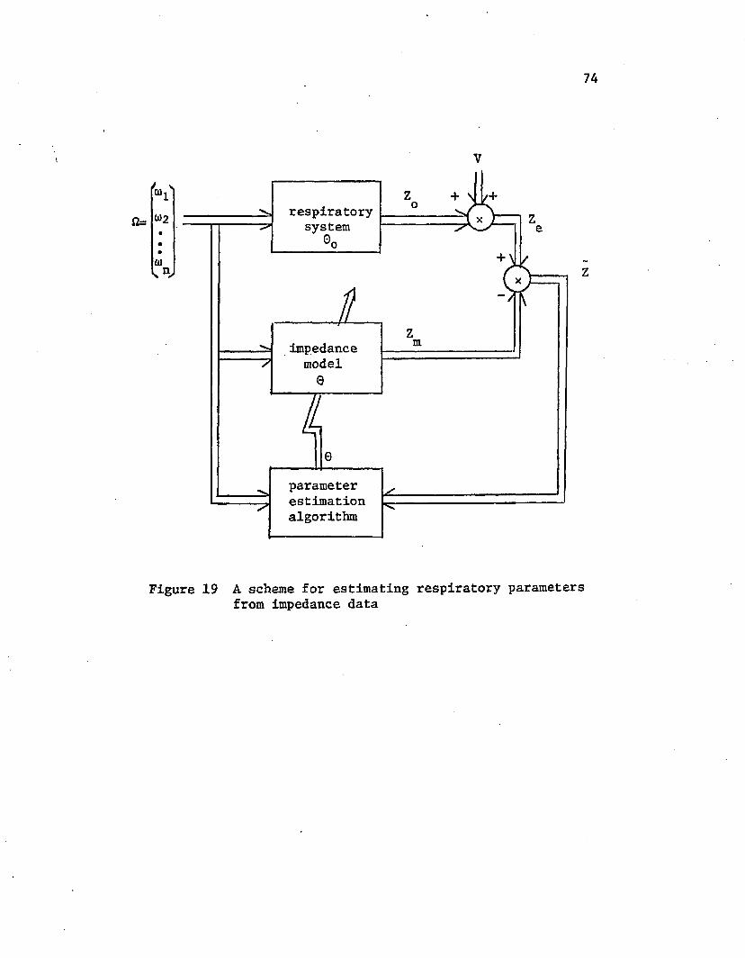
74

V

«= 012

0)

- /

respiratorysystem

parameterestimationalgorithm

impedancemodel

Figure 19 A scheme for estimating respiratory parameters from impedance data

Note that since impedance is a complex variable, z , z , z , and ze m oare all complex-valued.

Suppose (w, ,z ), (u)0,z ), (u> ,z O are n available1 ei ez n enobservations. A criterion function may be defined as shown in Eq.(3.43)

in which the subscript i denotes the sequence of observations, each

corresponding to a particular frequency,

n ~ ?J(0) = E | z | (3.43)

i=l 1

" K ± - Zmi!2

The complex impedances can be expressed in rectangular form as shown in

Eqs.(3.44) and (3.45) and Eq,(3.43) can be rewritten as Eq.(3.46).

zei 'Uei + 3 Vei

zmi “V + i \ i (3'W >

J<0) = [(uei - <Vl)2 + (Vei - V 2! <3‘46>1=1

Using the relationship expressed in Eqs.(3.47) and (3.48), the criterion

function J in Eq.(3.46) can be modified as shown in Eq.(3.49) where each

element in the summation is a real number.

r . . m . l<i<neiiv*1e(i-n) (n+l)<i<2n (3.47)

yml “ C "mi 1<1<n

Vm(i-n) (n+l)<i<2n (3.48)

76

J(0) = (yei - yml)2 (3.M)

It is known that the parameter estimation algorithm employed here

is an iteration process. At each iteration, the gradient of the cri

terion function with respect to the parameter vector, VJ(0), must be computed according to Eq.(3.29) with the weighting matrix W =>>,1 as shown

in Eq.(3.50).

J(0) = - 2 Q' Z (3.50)

For the particular criterion function given in Eq.(3.49), the error

vector Z is defined in Eq.(3.51) and the derivative matrix in Eq.(3.52).

ye r 7ml

ye2n“ ^m2n (3.51)

391• 30P•• ••

3Pm(“>n)m

90J 90P3vm (o>i)301 39p» •

•

3',m(“n)1 39i 36d .

(3.52)

773.3.2 Estimations Based on Artificial Noisy Impedance Data

In this section the application of the parameter estimation

algorithm developed in this chapter is tested with artificially

generated impedance data. A specific linear electrical circuit model

of the respiratory mechanical system is assumed and its input impedance

is computed at various frequencies over the range of interest. Elementsin a sequence of guassian random noise are added to the computed

Impedance values to simulate experimental errors. With either noisy or

noise-free data, the parameters in the model are estimated using thesame algorithm. The ability of this algorithm to accurately estimate

parameters in this particular problem is verified by comparing the

estimated parameter vector with the true one.To be more specific, the noisy impedance data, zeu> u=l,...,n,

is produced in the following way. A random sample of size m, X2»

..., v , from an uniform distribution is first generated by the computer, musing an appropriate subroutine. For each sample, the mean is equal to

1/2 and variance 1/12. According to the central limit theorem [85], the

statistic given in Eq.(3.53) approaches a standard normally distributed

variable with the distribution, n(0,l). Then, from n(0,l) a random sample of size 2n, S^, S^» •••» can be produced by the computer.

m n mS = — ( I Xj ) 0.53)

12 j=l 3 2

In practice, the.impedance at each frequency, zeu» measured in terms

of amplitude peu and phase <j>eu to which the random noise are actually introduced. Expressions for the polar forms of zgu and z (noise-free

impedance) are shown in Eqs.(3.54) and (3.55).

78ou

u = l)2j •■«j nz = p e (3.54)ou ou

j<f>z = p e eu (3.55)eu eu

Then the artificial impedance data are defined by Eqs.(3.56) and (3.57)

in which a. and a_ specify the level of noise on the measurement of theX Mamplitude and phase angle.

p = p + a. p S0 .. (3.56)eu ou 1 Hou 2u-lu * 1,2, ..., n

 S (3.57)Yeu Tou 2 Tou 2u

The Simple Series R-I-C ModelThe first model considered was the simple series R-I-C model as

shown in Figure 7. The input impedance of this model is given in

Eq.(2.7) and is repeated here as Eq.(3.58).

z - R + j (wl - l/(o)C)) (3.58)m

The artificial data was generated according to typical values as given

in the following [44]:

R = 2.7, I - 0.01, C = 0.1Let 0=s(0^, Q^t 0g)=(R> I» C). Then the elements in the criterion function

defined by Eq.(3.49) is now given by Eq.(3.59) for this model and the

2nxp derivative matrix Q in Eq.(3.52) is given by Eq.(3.60) in whicht i l(o_£, i=l,2,... ,n, is the i— angular frequency component. Values for

0_ , i=l,2,3, are constrained to be between 0 and ten times the nominal

value for each parameter.

79

mi

l<i<n

(n+1) <i< 2n (3.59)

100

1 00 00 0• •• •0 0

00

1/(0)103 )1/(to203 )

i/(w2e32)

■*- nth row (3.60)

The results of estimations in six separate cases are summarized

in Table 2. Artificial impedance data with no noise (cases 1 and 4),

5% noise, i.e., a =a =0.05, (cases 2 and 5), and 10% noise, i.e.,X ^al=a2~ (v3SeS an(* ^ were utilized. In the first three cases ten observations at frequencies, f = i, i=l,2, ..., 10 were used and in the

other three cases, twenty observations at frequencies f^ = i/2, i=l,2,

..., 20 were used. For all cases, the stop criterions used are as follows:

ZSTOP=1010, EPHI=10~16, EC=10~16, EGRAD=10_11, NLOOP=200

For each case, ten independent estimations were obtained with ten

different initial guesses each of which was provided by the RANSER

subroutine from 1000 random selections.In the ten independent trials for each of the six cases the

estimated values for the three parameters were identical to fifth

significant digit. In the two cases with no noise (cases 1 and 4), the

estimated parameter vectors were identical to the true one within the

Table 2 Summary of parameter estimate for the R-I-C model based onartificial impedance data.

case no. of ob freq. noise estimated valuesno servations range level 61 02 031 10 1-lOHz 0% .275E01 .1 E-l .1 E+0

(0%) (0%) (0%)2 10 1-10 5% .277E01 .108E-1 .940E-1

(0.8%) (0.1%) (-6%)3 10 1-10 10% .278E01 .115E-l .885E-1

(1.1%) (15%) (-12%)4 20 0*5-10 0% .275E01 .IE-1 .1 E+0

(0%) (0%) (0%)5 20 0.5-10 5% •276E01 .102E-1 .955E-1

(0.4%) (2%) (-4.5%)6 20 0.5-10 10% .277E01 .104E-1 .913E-1

(0.7%) (4.2%) (-8.7%)

true value 2.75 .01 .1upper bound 25. .1 1.lower bound 0. 0. 0.

1. Value in parentheses is the % difference of the estimated parameter from the true one.

81precision of the computer. When noise was present, the estimated para

meter vector was slightly different than the true one, and the deviation

was more prominent with higher level of noise. For example, in case 3

10% noise resulted in 1%, 15%, and 12% errors in the estimated values

for R, I, and C respectively. Comparing the % errors in case 2 to those

in case 5 (or case 3 to case 6), it seems that a larger number os obser

vations offset the effect of random noise.Based on this study it seems that the respiratory mechanical para

meters in normal humanbeings can be accurately estimated from the impe

dance data at 20 frequencies in the range from 1 to 10 Hz even with

measurement error as high as 10%.

The Airway and Lung-Chest ModelA second model which separates the airways and lung-chest’ combina

tion with a shunt compliance as shown in Figure 6 was then investigated.

The input impedance of this model has been given in Eq.(2.10). Let

0=0, »9o>6o>9/ ,0C,0,)=(R ,R. ,1 ,In ,C ,C„ ). The model response1 2 3 4 5 6 aw* Aw’ aw’ Aw’ g Awcan be expressed as shown in Eq.(3.61). The corresponding derivativematrix Q=(q^j) can be then computed according to Eq.(3.62).

The artificial impedance data was generated by using typical

values for parameters in normal adult humans as shown in the following:0 =1.5, 0 =1.2, 0 =0.01, 0 ,=0., 0 =0.003, 0 =0.1 .ol o2 o3 o4 o5 ob

The program stop criterions used in this case were the same as those usedfor the R-I-C model.

With ..., n and n= 20, 30, or 40, it was found that

there was considerable disagreement between independent estimates

^mi "\91 + kl/k2 l<i<n

(n+l)<i<2n

(1 j“l(k20g - o>2 02 05 0£)/kf j "20 j“3

2“i k ki 05 06/ k^ j**4

2 ^(-a)2 02 05 02 + 2 k kx)/ k* j"5

[2 k2 02 06 - 2^ ( 0) 02 0* 0fi + k k6)]/ k2 j=6

0 j=l2

2iiij ®2^5 0g(k4 + toj k3 05)/ k4 j“2

“i j“3[k4(-w^ k 0^- kjio 050$)~ 2o>£ k k3e506)]/k4 j=4

with ^ = 02 9g

[k4(c^ 02 0g + k2)+2k3(u>J 0^050g+Wik k5)]/k4 j=5

yik^C-to^ k04+ 2u)2 ®2®5®6 " ^5^ ) + 2k3(ii)£02030g+(u.|kk£ 2

(3.61)

l<i<n

(3.62)

(n+l)<i<2n

)]/k| j=6

83obtained with different starting vectors and that there were significant

discrepancies between these values and the true parameter values. This

probably results from the fact that the above frequency ranges are not adequate for defining the characteristics of the respiratory impedance

of this particular model.When n=50, i.e., 50 observations are obtained at frequencies,

1,2, ..., 50 Hz, the estimation becomes more accurate. The results of

11 independent successful estimations based on impedance data with no

noise, 1%, 3%, and 5% random measurement errors are listed in Table 3.For each estimation, the number of iterations required and the mean

residual sum squared errors, J^, are tabulated. Values for the true

parameters and their lower and upper bounds are also included in the

table. The initial parameter vector in each case was selected by the

RANSER subroutine from 3000 random trials. For all cases presented in

Table 3, the associated iteration processes were terminated by the

parameter change criterion. However, about 50% of other trials which

are not listed in the table, the program was terminated by the loop count criterion. In these situations, the estimations were terminated prematurely or were converging to local, non-global minimums. This seems

to suggest that if the estimation is terminated by the parameter change criterion, the estimated parameter values would more likely be reliable.

From Table 3, it can be seen that for each parameter, the discre

pancy between the estimated and true values and the mean residual sum of

squared errors become larger when the noise level is increased. It was

found that with measurement errors up to 5%, there were good agreements

between estimated and true values for 0O (I ) and 0. (C. ); the3 aw 6 S,u)

Table 3 Summary of parameter estimate for the airway and lung-chest model based on artificial data

-----------caseno

noise j level e 2 e 3 6** 05 0 6

no. of iterations

Jm

1.130E+1.150E+1

. 155E+1

. 120E+1. 954E-2 . lOOE-1

.507E-3

. 933E-5. 260E-2 . 301E-2

•766E-1.100E-1 56 .95E-12

2 0% . .155E+1.150E+1

. 918E+0

.120E+1.964E-2.100E-1

. 402E-3

. 643E-4.540E-2.305E-2

.87 0E-1

. 100E+0 10 •43E-10

3.177E+1.135E+1

. 743E+0

. 118E+1. 906E-2 . 999E-2

•860E-3•622E-3

.420E-2

.361E-2•836E-1.994E-1 12 .35E -8

4 •195E+1.163E+1

.102E+1

.109E+1. 923E-2 . 986E-2

. 540E-4

. 916E-3.531E-2.451E -2

• 991E-1 . 987E-1. 18 . ICE-2

5 1%.153E+1 . 163E+1

. 140E+1

.108E+1. 108E-1 . 979E-2

•807E-4.293E-3

.434E-2

.400E-2• 105E+0 . 989E-1 19 .10E -2

• 6 .189E+1.159E+1

. 939E+0

.113E+1•105E-1 . 991E-2

.442E-3

. 715E-3.611E-2.405E-2

• 121E+0 . 988E-1 30 •10E-2

7 . 212E+1 .174E+1

.254E+0

.986E+0.707E-2 . 962E-2

.862E-4

. 784E-3.196E-2 . 552E-2

.138E+0

. 978E-1 33 .92E-2

8 3% . 188E+1 . 168E+1

.915E+0

.103E+1. 961E-2 . 970E-2

.407E-3

.207E-3.568E-2.440E-2

.120E+0

. 990E-1 15 .91E -2

9 . 189E+1 .176E+1

.939E+0

. 961E+0. 105E-1 . 960E-2

.442E-3

. 999E-3.611E-2.593E-2

.121E+0

. 940E-1 194 • 93E-2

10

115%

.192E+1

.177E+1

.130E+1

.171E+1

. 964E+0

.972E+0

•155E+1.103E+1

. 906E-2

. 965E-2

. 954E-2

. 977E-2

•196E-3.573E-3

.507E-3

. 188E-3

.437E-2

.547E-2

. 260E-2

.450E-2

.103E+0

. 917E-1

.766E -1

. 941E-1

17

9

•24E-3

.24E -3

True parameter 1.5 1.2 .01 0 . .003 .1upper bound . .3 .3 .05 .001 .008 .2jlower bound 1°. 0. 0. 0 . 0 . 0 .

There are two rows of data in each case. The first row represents the initial parameter vector and the second row represents the final estimate of parameters.

85discrepancies for 9, (R ) and 9_ (R. ) were larger but in all cases they1 aw L xu)were within 20% of the true values; estimated values for 0^ were in

_3the order of 10 which was very close to its true value; estimates for

0 (C ) were not as good as those for the other parameters, but theJ Oestimated values still had the same order of magnitude as the true one.

The difficulties in estimating parameters for this model arise

mainly from the small value of the shunt compliance, C , whose effectSon the total respiratory impedance is shadowed by C at lower frequenciesand by I at higher frequencies. As a conquence, its precise determi- awnation from the impedance data over practical frequency range is quite

limited. Nevertheless, the estimation of parameters in this model can

still be accomplished if more data which contain less noise and spread

over a wider frequency range can be collected.

Since the element I„ included in this model has a value nearly£u)equal to zero, and shows little contribution to the total impedance

from which the six parameters are estimated, it is not necessary to include it in the model. Its inclusion may have compromised the model and caused some of the difficulties encountered in parameter estimation.

If I„ is removed from the model, these difficulties are expected to be£b)reduced.

The parallel Compartments ModelThe parallel compartment model shown in Figure 8A may be used to

represent the lungs' mechanics in patients with COPD. This model has

seven parameters in it, i.e., Q=(9^,02»02»0^»®5*®g»0y)= (^»^»^2, , i*^2*C ). According to Eqs.(2.19), (2.20), and (2.23) the theoretical model cw

86

ymi " 01+ k]/k2 l<i<n“l0A " k3 / k 4 (n+1)<i<2n (3.63)

n j-1{k2[u2(T1T20506+ kT2O5)+05l- 2k10)J k9g0g}/k2 J"2{k2 [«i|(T1T2e5 06+ kT1 %)+0^J- 2 ^ kO6 05 )/k2 j-3

l<i<n j=A

{k2 [aj2(T1T2+T1T202e6+kT202)+20295]-2k1 [(oJk(T2+0206)+05+06 ])/k 2 j»5

{k2[t1)J(T2Tj+T2T103e5+kT103)+20306]-2k1 [wJk(T1+0395)+e6+05 ]}/k| .1-6 0 j«7

q. ,=<° j"lI 2 3 2 (3 ‘6A)-[2 k /lcj1G5eg(T107+k)-2k3ui kSgOgGyJ/k^, j - 2

2 3 2 - l2 k 4(ji e605 (T207-fk)-2k3aj1 kOgOgflyl/k j - 3

(u. j“42 2 2 3 (n+l)<i<2n

-{k4[<d1O7(T2+2T1O206)+07+2tl)1k(T2+0206)+2(95+06)]-2k3t)l

O7k(T2+e206)+(o197(05+06)])/kJ

-{k4[tu307(T^+2T20305)+e7+2«2k(T1+0305)+2(06+O5)]-2k3[(iJ ^e^dj+OgOgj+uJiO^es+Og)]}/^

-{k4Ia>J(T20g+T30g)+0g+eg]- k3[ta k2+(1J1(05+06)2]}/kJ j-7

where _kl " V l T2k + <Ti e5+ T206>

k2- 4 k2 + <05+e6)2k3 " '07Iwi (T2 9S+ T1 96)+95+96 1+Ui k2+<65+66)2

k4= ai107[ai2 k2+(0g+06)2lk - T2e5+ Ti06

V 6205

T2" 0306

87response In this case is given as shown in Eq.(3.63). Meanwhile the 2n><7

derivative matrix Q is given in Eq.(3.64). Since the exact expression

for Q is rather complicated , it may be worthwhile to approximate the

first derivatives by finite differences as shown in Eq.(3.65).

3y y (0_,...,0 +A0,,.. •, )—y (0_,.•.,0.,•..,0 ). m | _ m 1______j j______ P m 1________ P<Ln"ij 3 0 ^ A0.j M (3.65) i

The choice of A0^ is a compromise between arithmetic round-off errors

and approximation accuracy. Usually A0^ can be chosen as small as

possible if the corresponding difference in y^ does not vanish due to

round-off error. If the derivative matrix is computed in this manner,

the subroutine REGRES incorporate in the complete program for parameter

estimation can be made independent of any particular problem.

A set of artificial data was generated at 50 frequencies, 1,2,

...,50 Hz, according to the following nominal values for the seven para

meters :R=2.5, R =0., R =0.2, 1=0.01, C =0.005, C =0.2, C =0.2 .

1 fa Am ^ W

From this set of impedance data, the seven parameters were in turn

estimated by using the parameter estimation algorithm. The program stop criterions used In this case were as those used for the previous

models. The lower bound was zero for each parameter and the upper bound

was 5 times the nominal value for each of the three resistors, 10 times

for the inductor, and 5 times for each the three capacitors. Each initial

guess was selected from 3000 trials.It was found that a relatively accurate estimation could be

obtained only when the resistive components of the initial parameter

vector, R, R^,and R£> were quite close to the true values. The

88parameter could not be Identified exactly but its estimated value, like the true value, was always smaller than those for C0 and C . The

£. W

parameter I, however, had a good recovery in most cases. As in the

airway and lung-chest model, the solutions were more reliable when the

program was terminated due to the satisfaction of the parameter change

criterion. When the data is noisy, the chance for an accurate estima

tion became much less. With 1% of random noise, only about 20% of

independent trials provided "good" estimates. This probably results

from the multiple extremums of the criterion surface and its distortion

due to measurement noise.

3.4 SummaryThis chapter shows that the parameter estimation problem can be

solved by using a nonlinear regression analysis technique. With this

technique, the effect of random measurement error on the parameter estimation can be offset since the problem is overspecified. Each

individual algorithm for nonlinear regression analysis has certain

advantages and disadvantages with regard to converging speed and

accuracy. A superior method may be obtained by combining several algorithms so that the best features of each can be utilized while

avoiding the drawbacks. A universally convergent algorithm which

is applicable in the situations where the parameters are subject to certain range constraints and the criterion function has multiple

minimums in the constrained parameter space,has been developed. It

combines the, Gauss-Newton, Newton-Raphson, gradient searching, gradient

projection and uniform random searching methods.

This algorithm is applied to the problem of estimating mechanical

parameters of the respiratory system from impedance data provided by the

forced oscillation technique. By using artificially generated impedance

data from certain assumed electrical circuit models of the respiratory

system, it is found that parameters in a series R-I-C model can be identified easily and accurately even with experimental random errors

as high as 10%. When the respiratory system is represented by other

more sophisticated models such as those shown in Figures 6 and 8, the

parameter estimation problem becomes more difficult. To accomplish an

accurate estimation with these models, it may be necessary to utilized

more impedance data over a wider frequency range with less experimental

error and more computer time to pick a more promising initial parameter

vector and to allow more convergence to a local minimum.

CHAPTER IV

PROCEDURES AND METHODS

The forced oscillation technique, which is used in this study

to obtain experimental data, is a modification of the approach first used by DuBols et al. [25]. In their study, the impedance of the

total respiratory system at frequencies from 2 to 15 Hz was determined.

Fisher et al. [27], Grimby et al. [28], and Goldman et al. [29] used the

same technique to measure the respiratory resistance in normal subjects and in subjects with lung diseases. Recently, Peslin et al. [48] mea

sured total respiratory impedance in normal subjects over a frequency

range of 3 - 70 Hz by applying perithoracic pressure oscillations.

Michaelson £t al. [30] used forced random noise to obtain the total

respiratory impedance from 3 to 45 Hz with the aid of computer in analyzing experimental data. For the same purpose, a relatively simple

and direct method was developed by Piramel et al.[32] and is essentially

employed for this dissertation.

4.1 Overall SystemA block diagram for the overall experimental system is shown

in Figure 20, in which the impedance analyzer is a specially designed

instrument [31]. This unit is mainly composed of five blocks of circuits (Figure 21): 1) an oscillator in the frequency range of 1 to 100Hz, which is used to drive an acoustic suspension speaker (AR 3-A,

Acoustic Research) to produce sinusoidal pressure waveforms which are

90

Pressure

Pre A m p Impedance

AnalyzerFlow

Pre A m pMouthPressureTransducer

Pneumotachograph . 'ressure Transducer

rilH

To Subject

— PneumotachographPressureGenerator(Speaker)Figure 20 Block diagram for the overall experimental system

92

•5* Filtered Pressure Signals

SampleandHold

Frequency Selector Switch ^

P ressurePanelMeter

rj I BandJ *4 P ass,1 L ^ I

TriggerCircuits

ZeroCrossingDefector

P ressu reInput

ClockPhaseDetector P hase

PanelMeter

Clock

s*- Filtered Flow Signal

SampleandHold

FlowPanelMeter

TriggerCircuits

BufferAmplifier

BendP assFilter

ZeroCrossingDetector

FlowInput

Clock

Frequency Clock-*- Detector ■>- Frequency

Panel MeterClock

VoltageControlledCurrentSource

BondPassFilter

osc.(3 6 0 f)

Figure 21 Block diagram for the Impedance Analyzer

93applied, to the airway of the subject; 2) two matched narrow bandpass

filters which are mechanically latched to the oscillator frequency con

trol; 3) two identical peak detectors, each of which samples the fil

tered signal (pressure or flow) and holds at its peak value for meter

display; 4) a phase detector for sensing the phase difference between the two sinusoidal signals; 5) a frequency detector for measuring the

frequency of preset oscillation.

In performing the experiments, a volume-controlled respirator (Model 607, Howard Apparatus) was connected to the endotracheal tube

of the paralyzed dog through a three-way valve whose the other opening was connected to the loudspeaker. A heated pneumotachograph (Model

3700, Hans Rudolph Co.) in conjunction with a high quality differential

pressure tranducer (Model MP-45, Valadyne) was used to monitor the flow

signal. An identical differential pressure tranducer was connected to

the mouth side of the pneumotachograph with the reference open to the

atmosphere, and it was used to measure mouth pressure. All connecting

tubes were matched in length and made as short as physically possible,

in order to minimize the artifactual phase lags introduced by these

tubes [71].

Pressure and flow signals from the transducer carrier-amplifiers

were processed by the impedance analyzer. Peak values for both signals,

the phase angle between them, and the frequency of the forced oscilla

tion were recorded from the panel of the impedance analyzer. A graphi

cal recording of the pressure and flow signals, both with forced oscillations and with tidal breathing can be displayed on a chart recorder

(Series 200, Brush Instrumentation). A respiratory integrator (Series

200, Brush Instrumentation) provided a volume signal.

4.2 System Calibration

Calibration of Pressure ChannelThe peak amplitude of the sinusoidal pressure signal at a

particular frequency is indicated by one of the two galvanometers on

the panel of the impedance analyzer. The magnitude of the meter

deflection depends on the gain of the pressure transducer and its

associated carrier-amplifier, and on the gain of the filter, peak

detector and galvanometer in the impedance analyzer. The calibration

of the entire channel using a water manometer as a standard must be performed in two steps since the impedance analyzer responds only to

relatively high frequency oscillation which is too rapid for the water

manometer to follow.In the first step, various intensities of static pressure were

measured by the water manometer and applied to the pressure trans

ducer and recorded with the span control of the carrier-amplifier set

to 0.1 and sensitivity of the DC amplifier set to 5 mv/div. The setup is as shown in Figure 22. The two sets of readings in the range of

Interest are listed in Table 4. This data indicates that the pressure

transducer plus its carrier-amplifier had a linear response to static

pressure up to 6 cm H2O and the conversion factor between pressure and

chart deflection is simply:

1 cm HoO 4 divisions of deflection(4.1)

or 1 division of deflection 'v. 0.25 cm H2O

A push button was mounted on the carrier-amplifier for the convenience

of daily calibration. Its output was found to correspond to 4.45 cm H2O

of pressure and would cause 21.8 divisions of deflection on the chart

95

recording if control settings were the same as mentioned before.

Pressu T ransd,

Carr i er Amp1 IfIe f

r eAmplifie i ■

Chart ^Record i ng

:er

To Atmosphere

Manomete r

Bal l o o n e y

Figure 22 Set-up for pressure calibration

Table 4 Correspondence between Readings from Water Manometerand Chart Recorder in Calibrating Pressure Measurements,

Pressure .cm H2O 0 1 2 3 4 5 5.45 6

Divisions of deflections 0 4 8 12 16 20 21.8 23.5

* output of the pressure calibration button

In the second step, the setup as shown in Figure 1 was modified

so that the subject end of the tubing was blocked and sinusoidal

pressures generated by the Impedance analyzer and speaker at various

intensities and frequencies were applied. Pressure variations were

recorded on the chart recorder and the values dislpayed on the pressure panel meter on the impedance analyzer were compared to the magnitudes

of the signal displayed by the chart recorder. Data are given in

96Table 5. Note that the strip chart recorder had a flat frequency

response from DC to at least 20 Hz. This means that the chart recorder

caused no distortion in measuring the sinusoidal pressures in the range

of interest.

Table 5 Correspondence between Readings from Chart Recorder and Impedance Analyzer in Calibrating Pressure Measurements.

Meter Reading Peak to Peak Deflection in Divisions 1 Hz 10.1 Hz 20.1 Hz

0 0 0 00.5 2.1 2.1 2.01.0 4.2 4.1 3.61.5 6.3 6.3 5.62.0 8.4 8.3 7.62.5 10.5 10.4 9.23.0 11.3 12.0 11.23.5 15.3 14.2 13.24.0 17.5 16.2 15.04.5 20.0 18.5 17.0

By applying linear regression analysis [72,75], a relationship between the observed deflections on the strip chart and the meter

readings at certain frequencies may be expressed as shown in Eq. 4.2

in which P,jef is the number of divisions of deflection from peak to

peak, Rp is the meter reading for pressure, and F is the frequency in

Hz.

Pdef = °*74 + 3*82 *4* " 0,06 F By incorporating the conversion factor as given in Eq. 4.1, the observed

deflection (Eq. 4.2) can be converted into actual physical quantity as expressed in Eq. 4.3 where P is the peak value of mouth pressure in

cm HjO.

P = 9.2 x 10“2 + 0.48 Rp - 7.7 x 10"3 F (4.3)

97

Calibration, of Flow Channel

The flow recording channel includes the pneumotachograph, its

associated pressure tranducer and carrier-amplifier, and the filter,

detector and panel meter in the impedance analyzer. The magnitude of

the flow signal is indicated by the other galvanometer on the front

panel of the analyzer. It can also be monitored and displayed on the

strip chart recorder. For calibration, the span control of the carrier- amplifier was set to 1.2 and the sensitivity of the DC amplifier was

set to 2 mv/div. The volume-controlled respirator which supplied the necessary flow was arranged so that the gas ( air or He-02 mixture) flowed in and out of the cylinder of the respirator through the pneumo

tachograph. The ratio control was set to 50%. An almost sinusoidal

flow waveform was recorded on the strip chart. The exact frequency was

obtained from the time-marker available on the chart.Suppose the stroke volume of the respirator was adjusted to

x cc.and the revolving speed y Hz. Peak value of the flow signal was

measured as z divisions of deflection. Then the conversion factor between the chart recording and the actual flow quantity was simply

1 division of deflection (-^7?. ) cc/s. (4.4)z

It was found that for any combination of x and y, the conversion factor

was almost identical. It was 33.3 cc/div for air and 29.8 cc/div for He-02 mixture. The flow recording system was slightly less sensitive

to He-02 mixture than to air. In addition, the calibration button for

flow was found to correspond to 380 cc/s and 340 cc/s for air and He-02

respectively.

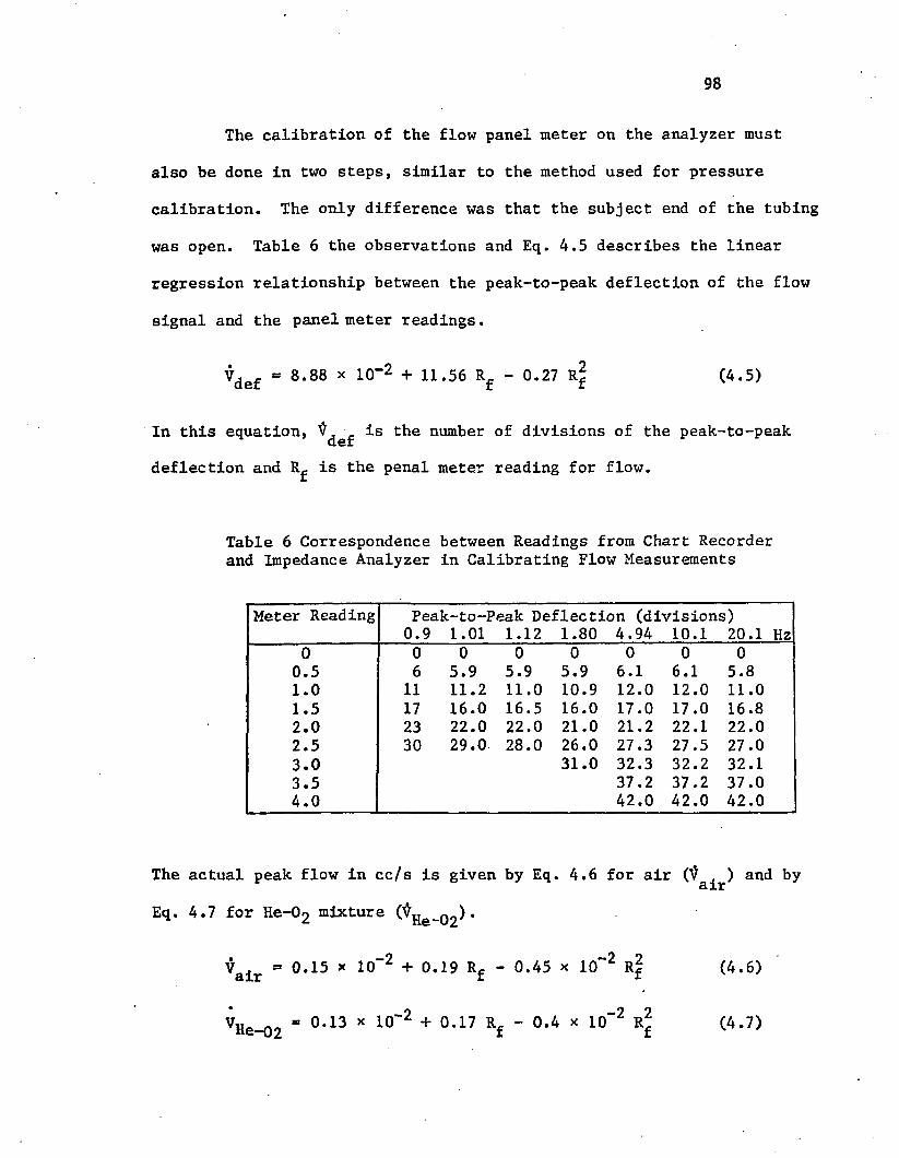
98

The calibration of the flow panel meter on the analyzer must

also be done in two steps, similar to the method used for pressure

calibration. The only difference was that the subject end of the tubing

was open. Table 6 the observations and Eq. 4.5 describes the linear regression relationship between the peak-to-peak deflection of the flow

signal and the panel meter readings.

Vdef = 8.88 x 1CT2 + 11.56 Rf - 0.27 R2 (4.5)

In this equation, ^ e£ *s the number of divisions of the peak-to-peak deflection and R^ is the penal meter reading for flow.

Table 6 Correspondence between Readings from Chart Recorderand Impedance Analyzer in Calibrating Flow Measurements

Meter Reading Peak-to-Peak Deflection (divisions)0.9 1.01 1.12 1.80 4.94 10.1 20.1 Hz

0 0 0 0 0 0 0 00.5 6 5.9 5.9 5.9 6.1 6.1 5.81.0 11 11.2 11.0 10.9 12.0 12.0 11.01.5 17 16.0 16.5 16.0 17.0 17.0 16.82.0 23 22.0 22.0 21.0 21.2 22.1 22.02.5 30 29.0- 28.0 26.0 27.3 27.5 27.03.0 31.0 32.3 32.2 32.13.5 37.2 37.2 37.04.0 42.0 42.0 42.0

The actual peak flow in cc/s is given by Eq. 4.6 for air ($ ) and byairEq. 4.7 for He-02 mixture C0jie_o2) •

Valr = 0.15 x 10“2 + 0.19 Rf - 0.45 x 10~2 r| (4.6)

vHe_o2 “ 0,13 x 10~2 + 0,17 Rf " 0,4 * 10"2 Rf (4*7)

99

In summary, the actual physical quantities of pressure and

flow can be obtained from the two galvanometer readings on the impedance

analyzer by employing Eqs. 4.3 and 4.6 or 4.7.

Correction of Phase Measurement

A five gallon glass bottle was connected to the subject end

of the system as shown in Fig. 20 [31] in order to test the phase

measurement. This element approximates a pure compliance which has an impedance of (1/jwc). Thus, the phase shift between pressure and

flow should be -90° at all frequencies. Table 7 shows the difference between the phase angles measured (by the impedance analyzer) and

theoretical values. This variation probably arises from the following

sources: 1) the differences in characteristics between pressure and

flow transducers, 2) the differences in phase lags of the two associated

Table 7 Errors in Phase Measurements

Freq.(Hz)

Phase Diff. (degree)

Freq.(Hz)

Phase Diff. (degree)

0.9 -5 4.0 01.01 -4 4.43 -21.12 -4 5.0 -11.27 -2 5.6 -11.42 -5 6.28 01.60 -4 7.15 -21.80 -2 8.0 -22.01 -2 9.0 -32.25 -2 10.1 -32.54 0 11.2 -32.83 0 12.7 -33.19 0 14.2 -43.58 0 16.0 -5

100

carrier-amplifiers, and 3) the distortion in waveforms. It was found

that in this particular loading condition, pressure and flow waveforms

deviate from pure sine-waves at frequencies below 1.8 Hz and at frequ" encies above 12.7 Hz. However, since the variations in the phase

measurements are within 5°, no phase corrections will be made in the

subsequent animal experiments.

Correction for the Impedance of the Endotracheal Tube

A cuffed tracheal tube (37 cm in length and 1.1 cm in diameter)

was always inserted into the trachea of the subject animals dring the experiments. The actual measured impedance should include the impedance

of the tube in addition to the respiratory impedance of the subject.

The latter can be obtained by simply subtracting the impedance of the

endotracheal tube from the measured impedance.

The impedance of the endotracheal tube was measured with the same equipment setup used in measuring the respiratory impedance except

that the tube was open to the atmosphere instead of being inserted into

the lower airway of the subject.Figure 23 is the Bode plot of the measured impedance of the

endotracheal tube at the flow rate of about 0.25 Jl/s, with air.Examining the Bode plot indicates that it can be approximated by a

transfer function with a single zero. This fact suggests that the

endotracheal tube can be represented by a series R-L electrical circuitwhich has a single zero at ai = R/L. Practically, the compliance effect

of the endotracheal tube can be neglected because of its rigidity. By using the parameter estimation algorithm (as described in the previous

chapter), the optimum parameters in the R-L circuit were found to be

101

20 t r t— i— i— i— r T----1---1--1--1-1 I I

18

16

n

12

co 10Q

8

6

If

2

0

• magnitude - DB

A phase - degree

• •• • •

■ i___ 1___I i— i 1— L _L J I I l__1—.1—I5 10 20 50 100

Figure 23 Impedance of endotracheal tube in air

9ff

7(P

TJ 3T 0) W5 &0

3(P

120 rad/^

102

cat,o

T---- 1--- 1---1— i— i— r— j----------- 1------ 1---- 1----j--1— i— i— i— f

• magn i tude - DB *■*

6 [•* a phase - degree •t

• * AM * » ‘

2 h °» • ' •

o r a

AA»

AAA

AA

AA A

A A * ‘

A

< » » i i I________________ I_________ i______ i____ i____i___I__ i__i__L

90°

70°

tt5(ff

3(P

l(f

5 10 20 50 100 120Figure 24 impedance Qf endotracheal tube In He+02

rad /s

103

R ** 1.11 cm Ô/Jl/s and L = 0.063 cm Ô/i/s^.

For the He-02 mixture, the same analysis can be applied. The Bode plot of the impedance of the endotracheal tube for this gas at a flow

rate of 0.3 *•/s Is given in Figure 24. The optimum parameters are

R = 1.0 cm Ô/Jl/s and L = 0.025 cm Ô/A/s^.

4.3 Experimental Procedures

At the beginning of each experiment, before the system was

activated, it was checked to insure that the transducers and amplifiers

were connected properly, that the pneumotachograph was clean, and that no leaks existed in the tubing. After the system was turned on, and

allowed to warm up, the control switches in various electronic units

were set to the normal operating positions. There are as follows:

1. Pneumotachograph heater was set to 105°F.

2. In pressure recording channel, span control of the carrier- amplifier was set to 0.1 and sensitivity of the DC amplifier

was set to 5 mv/div.3. In flow recording channel, span control of the carrier amplifier

was set to 1.2 and sensitivity of the DC amplifier was set to

2 mv/div.4^ Ventilation rate of the respirator was set to 20 BPM, duration

ratio 50% and stroke volume 350 cc.All dogs were weighed and apparent abnormalities such as ocular

and nasal discharge were observed and recorded. The dog was anesthetized with intravenous injections of fentanyl, 0.035 mg/kg, droperidol,

1.8 mg/kg, (Innovar, 0.05 cc/kg) and sodium pentobarbital, 6 mg/kg.

104

Intubation was accomplished while in a vertral supine recumbency and the

cuff of the endotracheal tube was inflated with 8-12 cc of air depending

on the size of the dog. After placing the dog in a dorsal supine recumbency, it was secured to insure uniformity of the pulmonary testing.

Succinyl choline, 1 mg/kg, was then used to effect respiratory arrest and respiration was maintained by using a volume-controlled respirator

at the rate of 20 BPM and a tidal volume of 8 cc/lb. After approximately

15 minutes of artificial ventilation, the experiment began. Maintenance

doses were used as necessary during the experiment.Data from two distinct sets of experiments were utilized in this

dissertation. One, collected by Robinson [74], involved the use of

bronchoconstrieting and dilating drugs. The second series of experiments

constitutes a part of this dissertation research and was concerned with the effects of various physical interventions on the measured and com

puted respiratory parameters. The procedures for the second set of expe

riments are described as follows.Ten mongrel dogs (20 - 25 kg in weight) were used and four

different experimental conditions were usually studied. These included a control study and while ventilating with an external resistor, abdo

minal weighting and He-02 mixture. In each experimental condition,

three kinds of data were obtained consistently on most of the dogs.Forced oscillations were applied intermittently at 26 logarith

mically-spaced frequencies in the range from 0.91 Hz to 16 Hz. At each frequency, the magnitudes of the mouth pressure and airflow and the

phase angle between them were recorded from the panel meters on the

impedance analyzer. Before each reading, the dog’s lungs were first

105

ventilated several times and then inflated to near total lung capacity

(TLC) three times to produce a constant lung history. The lungs were always assured to be at functional residual capacity (FRC) after inflations and while forced oscillations were applied. Peak oscillatory flow was maintained between 0.2 i/s and 0.5 i/s during all experiments.

Collecting of an entire set of impedance data took approximately 15

minutes.The second Set of data was obtained while the dog was ventilated

from a closed air circuit at about 20 cycles/min and a stroke volume of

8 cc/lb of body weight. This circuit was formed by connecting the air inlet and outlet of the respirator to the two openings of the associated

cylinder with two pieces of tubes. Mouth pressure, flow and volume were recorded on the strip chart for at least five consecutive respira

tory cycles. Volume was obtained by integrating flow with an electronic

integrator. An inflation to near TLC was performed just prior to obta

ining this data.Next, after inflating the lungs to near TLC three times, a gra

duated large plastic syringe was used to inflate the lungs with 1200 cc

of room air (or of the He-02 mixture) and then deflate them in 100 cc

increments back to FRC. At each point, a pause of 3-4 seconds was ade

quate to produce a plateau in the transthoracic (mouth) pressure tracing. The lungs were then re-inflated in 100 cc increments to the 1200 cc

maximum.These three sets of data requiring about 45 minutes were obtained

with each of four variations in experimental conditions. Between each

experimental variation, the dog was ventilated for 5 minuted or so.

106

After obtaining a set of control data, the abdominal region of the dog

was weighted using approximately 10 lbs and the three types of data were collected. In Dog #9, 20 lbs of weight was used. The third set of

data were obtained while an external resistor was connected in series

with the endotracheal tube. The resistor consisted of an orifice (18 mm

in length and 6 mm in ID) placed in the middle of two identical tubes

(65 mm in length and 125 mm in ID). The resistance was measured using a technique identical to that described for measuring the impedance of the

endotracheal tube and found to be 1.37 cm l^O/j/s. In the final experi

mental variation, a 80% He - 20% O2 gas mixture was used in ventilating

the lungs. To insure that all N2 was eliminated, a 5 minute washout of

the lungs before collecting data was performed. The experiment was

facilitated with the use of a 60 liter gas bag filled with the He-02

mixture.

4.4 Data AnalysisDuring forced oscillation, peak values for pressure and flow,

phase angle and frequency of oscillation were obtained directly from the

penal meters on the impedance analyzer. Meter readings for pressure and flow were converted into physical quantities using Eqs. 4.3, 4.6, and

4.7 and the magnitude of the impedance was calculated from these quanti

ties. This data described the frequency dependence of the complex flow

Impedance, and was used to estimate the mechanical parameters of the

respiratory system. Parameter estimation was accomplished by using the

estimation algorithm developed in Chapter 3, in which the criterion

function J was defined in Eq. 4.8 in which Zg represented the

107

experimental impedance data at various frequencies, and was the

theoretical impedance of an assumed electrical circuit model.

J = E IZm C^) - Ze C£±>|2 (A.8)i=l

In general, n was 26, however in some studies less data was collected.

This mothodology was applied with the simple R-I-C model and with the other more complicated models as developed in Chapter 2. The mean

residual sum of squared errors was used as an indicator of the goodness

of the agreement between the experimental data and the optimal model

response. All data were analyzed on the IBM 370/165 digital computer.

Figure 25 illustrates a mouth pressure tracing during the static deflations. During inflations, the tracing was similar except the change

of pressure was reversed. Data for pressure and volume were used to

construct the pressure-volume curves. Respiratory static compliance was

calculated from the pressure-volume curve at FRC in the range of tidal

volume.While using artificial ventilation in a closed air ciucuit, the

recorded pressure, flow and volume signals were almost sinusoidal. Figure

26 shows a segment of such recording from which respiratory resistance and dynamic compliance may be calculated. Total dynamic compliance was

calculated by dividing tidal volume by the total pressure change between

points of zero flow (e.g., a and b). The isovolume technique [24] was

employed in calculating total respiratory resistance. Two points (e.g.,

c and d) were selected on the volume curve where respiratory volume was identical and flow rate was approximately 0.4 2,/s. Difference in both

108spliei

Figure 25 Transthoracic pressure tracing during lung deflation

re3aure

— c:— rz. — — _ ::Figure 26 Pressure, flow, and volume recordings

during artificial ventilation in anesthetized and paralyzed dog

109

pressure and flow rate occured between these two points was measured.

Since volume was identical at these two points, elastic forces should also have been identical. Therefore, the entire pressure difference was

attributed to flow resistance which can be calculated from the ratio

Ap/Av. The resistance and dynamic compliance were defined as the average of the values computed from at least 5 consecutive breaths.

Total respiratory resistance and compliance obtained from the

forced oscillation technique were compared with values obtained by the

more conventional method and the correlation was obtained. In each

experimental condition, data was collected on at least four dogs. Diff

erences among mean values for total respiratory resistance, inertance, and compliance in various conditions were tested for statistical signi

ficance using the Student t-distribution [73].

CHAPTER V RESULTS AND DISCUSSIONS

As mentioned in Chapter VI, data from 18 dogs was included in

this study. Data for Dogs #1-10 were obtained by the author while the

data for Dogs #11-18 was obtained by others [71,74]. Among the first

10 dogs, six were considered to be in normal healthy conditions based

on a rather limited physical examination. Data obtained from these 6

dogs can be regarded as a representation for the class of normal dogs.

Among the second 8 dogs (Dogs #11-18), six were normal, one had a narrowed trachea, and the remaining one had "small airways disease" induced

by smoking cigarettes for 6 years. Both sets of dogs were studied under

the same experimental conditions except that different pneumotachographs

were used. It is believed that less distortions and thus less experi

mental errors were present in the data from Dogs #1-10.

5.1 Frequency Response of Respiratory Impedance in DogsFigure 27 is a Bode diagram, illustrating typical reproducibility

of impedance data when multiple sets of data were collected on a single

dog during one experiment. The flow rates for these three different

runs were 0.15, 0.22, and 0.28 i/s in average over all the frequency

components. Although there were some small variations at certain frequ

encies, no consistent differences in the overall responses were observed.

The mean value of these three sets of data, tabulated in Table 8 and

110

Illplotted In. Figure 28, represented a typical frequency response of the respiratory impedance in a normal dog. Impedance data from all dogs

are attached in Appendix B. The impedance data for each dog as listed in

the appendix include s the impedance of the endotracheal tube used in

the experiments in addition to the respiratory impedance of the dog.

Table 8 Typical frequency response of the respiratory impedance in a normal dog

Freq. Impedance Mag. Phase

0.90 6.67 -54.31.01 5.17 -51.01.12 4.96 -51.31.25 4.34 -49.31.41 4.06 -43.71.57 3.59 -40.01.80 3.16 -36.32.01 3.13 -32.02.24 2.84 -26.02.51 2.59 -22.72.82 2.39 -14.03.17 2.40 -5.73.54 2.36 1.73.97 2.28 10.04.42 2.28 23.04.96 2.56 34.35.58 2.75 42.06.24 2.97 46.77.14 3.33 57.07.95 3.81 59.3.9.03 4.17 64.010.10 4.87 68.311.17 5.30 70.012.60 5.89 72.314.13 6.51 75.315.90 7.68 77.3

112Figure 29 shows the frequency variations In the magnitudes (|Zrgj),

phases (<j> ), real parts (R ), and imaginary parts (X ) of the respi-ITS ITS IT Sratory impedances (Z ) of the six healthy dogs in the first group ofIT S

subjects (Dogs #1, 2, 4, 5, 6, 8). Each curve in the figure was drawn

by connecting consecutive points with a straight line. Some variations

among dogs can be seen in each of the four diagrams of the figure, but

these differences are quite small and reflect small individual varia

tions in the mechanical properties of the respiratory systems in diff

erent dogs.It can be seen from the magnitude and the phase curves of Figure

29 that the frequency response of the respiratory impedance in a normal

dog has a pattern consistent with a series R-I-C electrical circuit.

The resonance frequency of the system (fQ) identified by the frequency where the magnitude is a minimum and where the phase angle equals 0°

is about 3.5 Hz. If the measured impedance is corrected for the impe

dance of the endotracheal tube, the resonance frequency will be higher.

As shown in Fig. 29, R decreased with increasing frequencyITS

in the range 0.9 - 3.5 Hz and remained relatively constant at higher

frequencies, 3.5 - 16 Hz. This phenomenon suggests that the series R-I-C model is not adequate to explain the experimental impedance data

at frequencies below 3.5 Hz since R in the R-I-C model should be inde-ITSpendent of frequency. This higher frequency behavior of R in normalIT sdogs is consistent with the result obtained in healthy individuals by

Grimby et al. [28] which showed no significant change in R ar frequ-” ITS

encies from 3 to 9 Hz. As to the frequency-dependent R^g at frequencies

below 3.5 Hz, there are no similar data in the literature for comparison.

113

Figures 30* 31, and 32 Illustrate variations in respiratory impedances as three different mechanical interventions were introduced.

These included breathing with mass loading of the abdomen, an external

resistor, and a lighter gas mixture (80% He - 20% * With ten pounds

of abdominal weight the phase curve shifted downward (Fig. 30B) and the

lower frequency portion of the magnitude curve moved upward (Fig. 30A). The external resistor significantly increased the magnitude of the impedance at all frequencies (Fig. 31A). While breathing the gas

mixture, the phase curve shifted to the right (Fig. 32A) and the higher

frequency portion of the magnitude curve moved downward (Fig. 32B).

Figure 33 illustrates the effects of two drugs, physostigmine

and atropine, on the respiratory impedance of a single dog (Dog # 12).

Physostigmine, a powerful broncho-constrictor, raised the magnitude of

the impedance significantly at all frequencies (Fig. 33A) and atropine,

a broncho-dilator, which was administered 60 minutes after the first

drug, reversed the effect of physostigmine and brought the impedance

back to control values. No significant change in phase data was observed

with these two drugs (Fig. 33B).

Figure 34 shows |Z |, ({> , R and X of the respiratoryITS ITS ITS ITS

impedance of the two dogs with respiratory diseases and the averageresponse of the six normal dogs in the same study. When compared to

normals, the dog with narrowed trachea, Dog # 14 (denoted by f2'),

showed a large increase in |zrg| and no variations in <f>rs* The dog withobstructive disease, Dog # 13 (denoted by '1’) showed a smaller increase

in |zrsl and a small change in the phase curve. Both of the increasesin Z were associated with increases in R as indicated in Fig. 34C. rs rs

Magnitude

- DB

222018

16

II*12

10

8

6

l>2

11fununun

123- X

23

l1»

J1

t ►

!ii ?

1 9

?9fiM I

I 5 S i « f t 'f* i f 2"T

■ S s

10 20 50Angular Frequency

100

•JOiS

51?

ov 30"5c <

10

-It?

-30

-5 $

-7lT

200

ii i

FURti

n,-e 1

2- 1

? i r !

ii9 i

Uu II 3 3 t *i

ft- r

ft•

•

I 1t

9 M : ; i» 5 * * \

V I 1 ‘

Angular Frequency

Figure 27 Reproducibility of impedance data obtained in a single dog (Dog # 1) during one experiment.

114

Angular Frequency

Figure 28 Typical frequency response of the respiratory impedance of a paralyzed apneic dog (Dog # 1).

12

10

8

6

2

0

6 116

5

3

2

1

0

-3<r

-6(f

-9 tf16 HZ1280

12

8

0

816 HZ12840

Figure 29 Frequency responses' of the magnitudes (A), phases (B), real parts (C), and imaginary parts (D) of the respiratory impedances in 6 normal dogs (#1,2,4,5,6, and 8) in control states.

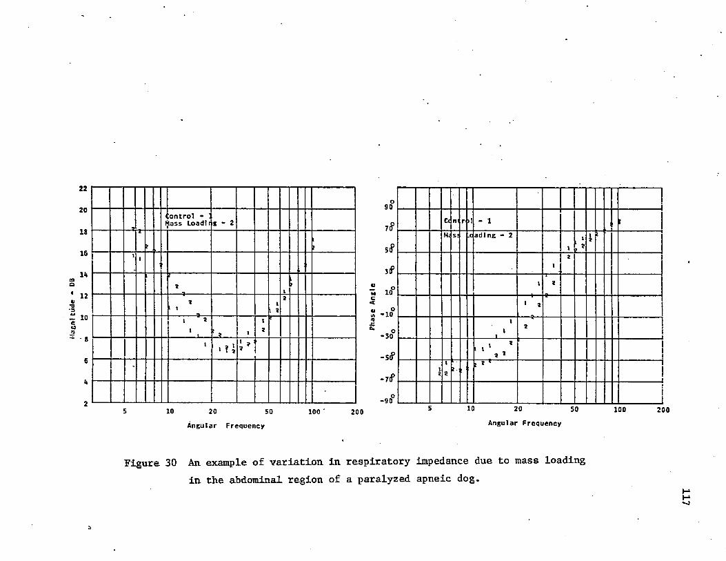
Mucftltude

- DB

22 20

18

16

Hi

12

10

• 8 6 I* 2

?

1C o n t r o l - : l a s s L o a d t i 1 - 2

tI>

1 I

!

*X

It

7t t

II 7

7

I * I

* i

t7

i

1

-

o90

if

sf

3(P■» o* 10 c <ei °X -io

o-5 0

-s<P-7(f

o-9 0

1j

Cc m r >1 - 1 r

Mi s ; X a d l n g - 2

XX

1 *I7

I

I7

1 7

1 7

iX

i7

7 2

I7 7

iI 2 1

10 20 50

Angular Frequency100 200 10 20 50

Angular Frequency100 200

Figure 30 An example of variation in respiratory impedance due to mass loading in the abdominal region of a paralyzed apneic dog. 117

2ro ■.8 ■

6 -,U '12 '10 ■8 '6 ‘U ■

2 '

Con ;rt I Trcttrna

i a

Heyt vtor

‘ i

* a

i i

10 20 50

Angular Frequency

o907 ffsff3lP

I ifatw o 2 *-10

o-30

100 200

-5 8

o■70

o-90

Co M O ifl.

1 *I

*

* !

3a * i

, ? 3 ?i i 1 II xI

1 \ 1


100 200

Figure 31 An example of variation in respiratory impedance due to an added external resistor.

118

Angular Frequency5 10 20 50

Angular Frequency

Figure 32 An example of variation in respiratory impedance due to breathing a He — O2 gas mixture.

Macn

ltud

e

222013

10.o■a 2.U

1210

&£

1tt

i8i2 Control -

Pl.ysostlgf1ilne -j 2 I

! *1 21I*

2I)

s3 i3 I

11

fI

. .

23 21

!1\

1 2 2 J1 )

2L> »

i l2 2> J

1 7 2 iI

f\1•

iIi

JI 1 > *

1! ii

”3 V t 1

9(f

7(f

30°

« 10° U* - 10° o «n>£ -30°

-50°

-70°


100 200-90"

|ControlPhysostI

- 1gmlne - 2 i 1

I ' ! ' i!1 j

I

1i

2 i

i i 3i»fcI

1l1

10 20 50 Angular Frequency •

100 200

Figure 33 Variations in the respiratory impedance of Dog if 12 due to a bronchocons trie tor , physostigmine, and a broiichodilator, atropine.

120

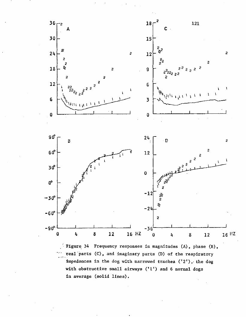
18 121

15

12

9

6

3

0

12 22

2h

6(f 12

3<f

-12

-6 CP

-3616 HZ0 128 0 8 12k

Figure 34 Frequency responses in magnitudes (A), phase (B), real parts (C), and Imaginary parts (D) of the respiratory impedances in the dog with narrowed trachea (* 2 *) ,■ the dog with obstructive small airways ('I') and 6 normal dogs in averdge (solid lines).

122Fig. 34D demonstrates that X^s for Dog // 14 was much different from

those for normal dogs. This fact implies that the inertial and elastic

properties of the lungs in this dog were greatly different than those in

normal dogs since X is determined by these energy storage properties.ITS

5.2 Estimated Values for R , I , and C from Impedance Datars* rs rsThe variations in impedances due to either mechanical or phar

macological interventions are resulted from changes in the mechanical properties of the respiratory systems. As mentioned in the previous chapter, the mechanism of the respiratory system can be studied using

electrical analog circuits whose elements have physiological signifi

cances. Therefore it is entirely possible to link induced variations in

impedance of the respiratory system to alterations in the values of

analogous elements in the corresponding electrical circuits.

Using the series R-I-C electrical circuit, values for these three

elements, the total resistance (Rrs) > inertance (*rg)> anc* compliance (C ) of the respiratory system, can be estimated from the measured freq-ITS

uency response of the respiratory impedance by employing the parameter

estimate technique described in Chapter III. The results for the ten

dogs (Dogs # 1-10) in various experimental conditions are summarized in

Table 9. Note that those values for R , I , and C includes thers rs rseffects of the endotracheal tube. Values for C thus obtained repre-rssent the dynamic total compliances at FRC.

Also included in Table 9 is the mean residual sum of squared

errors (J^) for each estimation, which is a gross indication of how good

the model is in explaining the experimental data. Figure 35 shows the

Table 9 Estimated values for Rj-g, Irg, and Crg for all 10 dogs used In the studies of eEfects of three mechanical interventions

Dog Wt. # kg ^rs

Control Irs Crs ^m

Mass Loading Rrs ^rs ^rs Jm

External *rs *ra

Resistor crs Jm

80% He- Rrs - rs

•20% 02Jra

1* 20 2.324 .076 3 .0325 .312* 20 2.578 .0739 .0276 .346 .2.407 .0293 .0292 .4233 20 3.042 .0786 .0229 .481 4.155 .0915 .0233 .6924* 20 2.460 o

4 .0319 .365 3.639 .0938 .0299 .396 2.151 .0325 .0298 .3155* 22 2.094 .0736 .0332 .154 3.778 .0975 .0304 .269 1.926 .0292 .0339 .2386* 25 2.792 .084 .0279 .419 2.874 .0799 .0212 .554 4.145 .0978 .0325 .527 2.673 .0375 .0315 .3197 20 2.943 .0871 .0274 .454 2.801 .0834 .0224 .481 3.935 .1033 .0319 .362 2.591 .0393 .0339 .1858* 23 2.201 .0686 .0317 .242 2.308 .0642 .0215 .354 3.411 .0866 .0355 .246 2.074 .0335 .0351 .1819 25 2.386 .0654 .0352 .219 2.67 .065 .018**.527 3.558 .0863 .0373 .238 2.173 .0304 .0359 .24210 20 3.057 .0768 .0261 .446 3.407 .0751 .0175 .75 4.385 .0976 .028 .354 3.04 .0393 .0291 .173

x 2.583 .0754 .0296 .344 2.848 .0766 .0207 .535 3.876 .0943 .0311 .386 2.379 .0339 .0323 .260

SE 0. 109 .0021 .0012 .035 0.225 .004 .0011 .083 0.119 .002 .0015 .063 0.131 .004 .0010 .031

x = mean; SE = standard error; Jm = mean residual sum of squared errors units: Rj.s, cm H-0/1/s; Irs, cm H20/l/s^; Crs, 1/cm H20 * denotes dogs with a normal (superficial) examination.** indicates that 20 lbs of weight was used in this particular dog.

123

Magnl tii'le

20!

1U ckc1cw>

II It -S(f

Otf35 5 10 20 50 1003 20010 20 50 1Q05

Angular Frequency Angular Frequency

Figure 35 An example of agreement between experimental and theoretical (R-I-C model) impedances.

124

125experimental measurements and the response with the optimum parameters

for Dog // 1 and indicates the typical agreement that was achieved in

these ten dogs. The mean residual error J is, in this case, equal to

0.3. This number represents the mean square of the distance in complex

plane between experimental and theoretical impedances at a particular frequency.

Control Measurement

Values for R , I , and C from control measurements obtained rs rs rsin six dogs which were judged to be normal are given in Table 10 after

correcting for resistance (1.11 cm 1^0/£/s) and inertance (0.063 cm 1^011 2/s ) of the endotracheal tube. Mean values ± SE for all six dogs were

R : 1.298 + 0.104 cm H„0/Jl/s; I : 0.0114 ± 0.0022 cm Ho0/£/s2; C : rs 2 rs 2 rs30.6 + 0.9 ml/ cm ^0; and FRC: 718.2 + 28 ml. FRC values were predicted

by using the formula for anesthetized, supine dogs as shown in Eq. (5.1) [98].

FRC (ml) = ( body weight in kg ) x 34

Using the analysis in Chapter II for the R-I-C circuit and the

mean parameter values from the six normal dogs, the respiratory system

is characterized by a pole at p = 0 and two zeros at z^ = -5.97 and z^ - -12.1; resonant frequency is 8.5 Hz; and the system is slightly overdamped with a damping ratio of 1.06. According to the same model and parameter values, Figure 36 illustrates the relative contribution

of compliance reactance and inertance reactance to total respiratory impedance.

126Table 10 Corrected values for R_,,, I__, and C In 6 normal dogsi. a rs ITS

Dog Body FRC Corrected Corrected Corrected Crs Crs/FRC# wt. ml Rrs *rs ml/cm HoO cm l^O-l

kg cm HpO/l/s cm H9O/I/S2 Abs. per k g1 20 663 1.214 0.0133 32.4 1.62 0.04892 20 663 1.468 0.0109 27.6 1.38 0.04164 20 663 1.35 0.007 31.9 1.6 . 0.04815 22 729 0.984 0.0106 33.2 1.51 0.04556 25 829 1.682 0.021 27.9 1.12 0.03378 23 762 1.091 0.0056 31.7 1.38 0.0416X 21.7 718 1.298 0.0114 30.6 ' 1.435 0.0432SE 0.84 28 0.104 0.0022 0.9 0.076 0.0056x: mean; iSE: standard error.

-3

251 2117139Frequency - HZ

Figure 36 Relative contributions of compliance reactance (X,,) and inertance reactance (X^) to the total reactance (X) and total impedance (|z|) based on the mean values for Rrs » Irs * and crs given in Table 10.

127

Effect of Loading In Abdomen

Five dogs (Dogs // 6,7,8,9,10) were used to study the effect of

mass loading of the abdomen. Values for R , I , and C for all five ° rs rs rs

dogs in this experimental condition can be found in Table 9. Table 11

shows the mean values of the control and mass loaded parameters for

four dogs (Dogs # 6, 7, 8, and 10) in which ten pounds of weight were

used. ( twenty pounds of weight were used in Dog #9. ) Student t-

value for comparing the two means for each parameter are also given in

the table.

No significant difference was detected in the value for R^g or

I . However, the abdominal loading produced a very significant deer-ITS

ease in compliance ( p < 0.01). Twenty pounds of abdominal weight (Dog

# 9) produced a change in compliance which was about twice that produced

by ten pounds.

Effect of External Resistor

Respiratory impedances in 8 dogs (Dogs # 3-10) were measured

with and without an additional external resistor connected in series to

the endotracheal tube. The external resistor was made of an orifice

(length 18 mm, diameter 6 mm), placed in the middle of two identical

short tubes (length 65 mm, diameter 12.5 mm). Its resistance was inde

pendently determined as 1.37 cm ^O/i/s at flow rates in the range used

for impedance measurements at various frequencies.Values for R , I , and C in the 8 dogs are given in Table 9.ITS ITS ITS

Mean values + SE for control parameters and for those obtained with external resistor are shown in Table 12. The t-values for comparing the

128

Table 11 Variations In R , I , and C due to mass loading of the abdomen.rs rs rs

Control MassLoading

t-value

R (cm HoO/A/s) rs ^ 2.748+0.19 2.848+0.225 0.34Irs(cm H20/£/s2) 0.079+0.004 0.076+0.004 0.59

C (ml/cm H„0) rs 2 28.27+1.2 20.65+1.08 4.71Values are means ± SE.

Table 12 Variations in R , 1 , and C due to an external resistorrs rs rsControl External

Resistort-value

Rrg(cm H20/il/s) 2.622+0.136 3.876+0.119 6.93Irg(cm H20/£/s2) 0.076+0.003 0.094+0.002 5.53C^g(ml/cm H20) 29.54+1.46 31.1+1.5 0.73Values are means ± SE.

Table 13 Variations in R , I , and C due to breathing He-02 mixture rs rs

Control He-02 t-valueRrg(cm H20/£/s) 2.564+0.122 2.37 9+0.131 1.03Irg(cm R20/£/s2) 0.075+0.003 0.034+0.004 13.46C (ml/cm. H„0) rs 2 29.7+1.4 32.3+0.97 1.51Values are means ± SE..

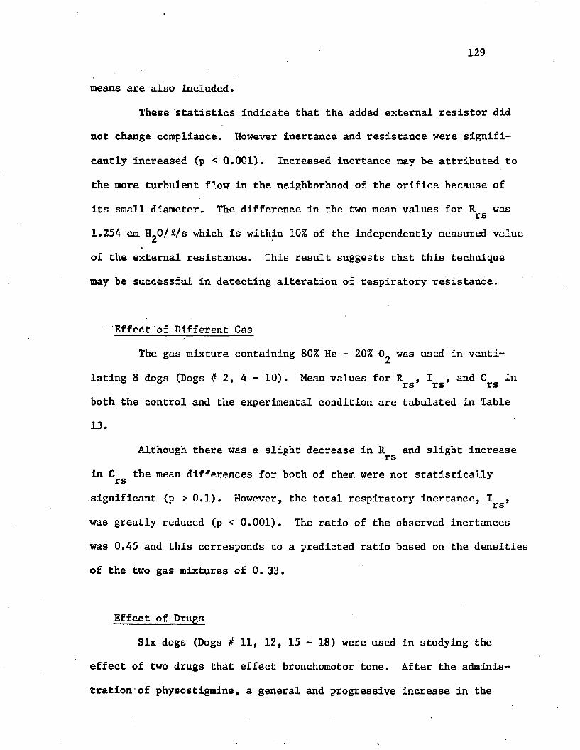
129

means are also included.

These ‘statistics indicate that the added external resistor did not change compliance. However inertance and resistance were signifi

cantly increased (p < 0.001). Increased inertance may be attributed to

the more turbulent flow in the neighborhood of the orifice because of

its small diameter. The difference in the two mean values for R wasrs1.254 cm O/fc/s which is within 10% of the independently measured value

of the external resistance. This result suggests that this technique

may be successful in detecting alteration of respiratory resistance.

Effect of Different Gas

The gas mixture containing 80% He - 20% 0^ was used in venti

lating 8 dogs (Dogs // 2, 4 - 10). Mean values for R , I , and C inITS ITS ITS

both the control and the experimental condition are tabulated in Table 13.

Although there was a slight decrease in R^g and slight increase

in Crs the mean differences for both of them were not statistically

significant (p > 0.1). However, the total respiratory inertance, I ,IT S

was greatly reduced (p < 0.001). The ratio of the observed inertances was 0.45 and this corresponds to a predicted ratio based on the densities

of the two gas mixtures of 0. 33.

Effect of Drugs

Six dogs (Dogs # 11, 12, 15 - 18) were used in studying the

effect of two drugs that effect bronchomotor tone. After the adminis

tration of physostigmine, a general and progressive increase in the

130

magnitude of the Impedance at every frequency was observed, and a

maximum effect was reached after 1 to 1.5 hours [74]. Atropine was administered intravenously one hour after physostigmine. Estimated

values for R , X , and C from impedance data for each dog in controlITS ITS ITS

state and under the influence of these two drugs are given in Table 14. Note that the impedance data for atropine was taken 45 minutes after its administration.

Rrs increased to 135% of control value after physostigmine and this increase was associated with a significant increase in I and a

slight decrease in C . In all but two dogs (Dogs // 16 and 18) , atropineITS

almost completely reversed the increases in R and I induced byrs rsphysostigmine. Physostigmine, a acetylcholinesterase inhibitor, can

cause bronchoconstriction by stimulation of the parasympathetic receptors

and atropine acts as a bronchodilator by inhibiting the bronchoconstric-

tive effects of parasympathetic mediators. One possible reason for the

failure of atropine in Dogs #16 and 18 is that during the period when

the impedance data was collected after the administration of atropine

the effect of atropine might not strong enough to counteract the physos

tigmine which might reach its maximum effect during that period.

Two Diseased Cases

Data from two diseased dogs (Dogs # 13 and 14) were also analyzed.

In the obstructed dog (Dog # 13), the respiratory resistance (3.7 cm 1^0/2A/s) and inertance (0.068 cm l^O/A/s ) were found to be higher than those

for normal dogs in the same study (Table 14) by 50% and 24% respectively

while the total compliance (0.019 A/cm H^O) was 24% lower. The value for

Table 14 Extimated. values for Rfg, lrs> ant* ^rs ôr t*ie 6 normal dogs used in the drug study

Dog0

Wt.kg “rs

ControlT c ^ s '■'rs ^m

Physostigmine ^rs ^rs ^rs Jm

Atropine ^rs *rs Crs Jm

11 17.3 1.93 .059 .028 .23 3.38 .075 .020 000• 2.48 .059 .023 1.1

12 17.3 2.03 .060 .023 .50 2.61 .076 .018 .67 2.01 .062 .023 .55

15 15 2.04 .060 .023 .49 2.58 .077 .019 .65 2.02 .063 .023 .59

17 22.7 3.16 .053 .018 1.8 3.64 .070 .014 2.2 3.15 .051 .018 1.8

16 21.8 2.75 .051 .030 • •O 00 3.96 .058 .028 .75 4.86 .051 .029 .86

18 17.3 2.81 .049 .029 .63 3.84 .055 .023 .43 5.27 .05 .027. .82

X 18.6 2.46 .055 .025 .69 3.33 .069 .020 .92 2.41* .059* .022* .95

SE .12 .21 .002 .002 .23 .25 .004 .002 .26 .27 .003 .001 .19

x = mean; SE = standard error; Jm = mean residual sum of squared errors

units: R -g, cm IÔ/l/s; Irs> cm IÔ/l/s^; Crs, 1/cm H2O

* Mean value is taken over the first four entries in the corresponding column.

131

132J was 0.6 which was comparable to those for normal dogs in this study, mThis relatively small value of J indicates that the respiratory system

of this dog can be also modeled with the second order R-I-C circuit.

This indication becomes more obvious when noting the similarities in the frequency dependence of impedance for this dog and for the normal dogs in

this study as shown in Figure 34. The same finding was also described by

Michaelson et al. [30] in the study of pulmonary mechanics by spectral analysis of forced random noise.

In Dog if 14 which had a congenitally narrowed trachea as diag

nosed by an X-ray, a greatly increased airway resistance would be expected.

Indeed, this dog was found to have R =9.78 cm H90/&/s which was fourrs ztimes the control value. The total inertance (0.21 cm H^O/Jl/s^) was also

greatly Increased. Value for J in this case, 7.0, was much higher thanmin other cases (Table 14”), and this implies that the simple R-I-C model

may be inadequate for representing the respiratory mechanical system in

this particular dog.

5.3 A Comparison of Forced Oscillation and Other Conventional Techniquesfor Measuring R and Crs rs

In Dogs # 6 - 10, total respiratory resistance, R , and compli-ITSance, C , were measured both by the forced oscillation and a tidal brea- rs 7thing method as described in Section 4.3. Values for R and C deter-rs rsmined by using these two methods are compared in Figures 37 A and B in

which the subscripts "dyn" and "fo" are used respectively to denote the results from tidal breathing and forced oscillation techniques.

As made clear in the last section, the forced oscillation tech

nique in combination with a parameter estimate algorithm is sensitive

133for detecting changes in mechanical parameters induced by various

mechanical interventions. It was found that these changes were also

detectable by using the tidal breathing method. From Fig. 37 it can be

seen that dogs with external resistor had the highest values for Rjjyn or

Rf0 and the same compliance measurements or Cf0) as in the control

state; Dogs with abdominal mass loading had the lowest values for C,jyn

or CfQ and a slightly increased Rdyn. or Rf0 ; Dogs breathing He-02 mixture showed no prominent differences in resistance and compliance from the

control measurements.Undoubtedly, values for Rrg and Crs obtained from these two

different techniques should be highly correlated. In fact, it was found

that the sample correlation coefficients were recpectively r=0.87 between

Rdyn and Rf0 and r=0.80 between Cdyn and Cf0. Furthermore a linear model

was found to be adequate in explaining the relationship between Rdyn anc* Rfo or between Cdyn and Cf0 gy the method of least squares, linear

regression lines for C^yn vs CfQ and R yn. vs Rfo are given in Ecls• 5.2 and 5.3.

cdyn = -3.2xl0"4 + 1.38 Cfo (5.2)

Rdyn = -8 .9X1CT3 + 1.44 Rf0 (5.3)The coefficients in these two equations are all highly significant.

There two possible reasons for explaining the discrepancy

between Rdyn an(* Rf0 • Airflow rates employed in the tidal breathing method were approximately 1.5 times higher than in the forced oscillation

technique, and these higher flow rates could produce an increase in

measured Rj-s* The operating frequencies employed in both methods were

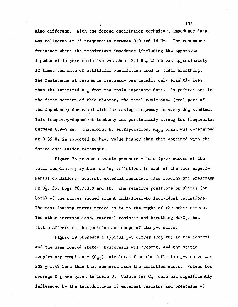
134also different. With the forced oscillation technique, impedance data

was collected at 26 frequencies between 0.9 and 16 Hz. The resonance

frequency where the respiratory impedance (including the apparatus impedance) is pure resistive was about 3.5 Hz, which was approximately

10 times the rate of artificial ventilation used in tidal breathing.

The resistance at resonance frequency was usually only slightly less than the estimated from the whole impedance data. As pointed out in

the first section of this chapter, the total resistance (real part of the impedance) decreased with increasing frequency in every dog studied.

This ftfequency-dependent tendancy was particularly strong for frequencies

between 0.9-4 Hz. Therefore, by extrapolation, R<jyn which was determined

at 0.35 Hz is expected to have value higher than that obtained with the

forced oscillation technique.Figure 38 presents static pressure-volume (p-v) curves of the

total respiratory systems during deflations in each of the four experi

mental conditions: control, external resistor, mass loading and breathing

He-02, f°r D°gs #6,7,8,9 and 10. The relative positions or shapes (or both) of the curves showed slight individual-to-individual variations.

The mass loading curves tended to be to the right of the other curves.The other interventions, external resistor and breathing He-02, had

little effects on the position and shape of the p-v curve.Figure 39 presents a typical p-v curves (Dog #8) in the control

and the mass loaded state. Hysteresis was present, and the static respiratory compliance (Cst) calculated from the inflation p-v curve was 20% + 1.4% less than that measured from the deflation curve. Values for

average Cst are given in Table 9. Values for Cst were not significantly influenced by the introductions of external resistor and breathing of

135

oCMX0CJ

e

7

6

S

4O CONTROL

□ LORD IN G

V ExtcrnM. dettiTftHce.O We- <?*.

3 00

e

6 % o cm H20/£/s

I

x

9

CONTROL

EtlSRHRL RctlMTDNtC.

.oz.

Cfo Jl/cm H2O02. 05 0<5

Figure 37 Comparison of the forced oscillation technique (fo) with the tidal breathing method (dyn) in measuring Rrs (A) and Crs (B)‘.

136

. controlo mass loading * external R. 0 A*0 He - 02 o .. a

0 a * a

O * * a

0 * * oO A a a

O A • a

O A • o

O A «a

o *0. Dog # 6O AO*

OM o 0 * 4 a

0 * A 0

0 * Aa

0*4O m a

* L - *— J-------L

Dog // 8

1.2|1.

.8

.6

.4

piPmQ>r &

. 0)

.20

A AO

A « O

A «3 a

A «0 0

* a

O>

NDI 0A0 •

U AO A

0 A O

1 I .. ■

Dog // 7

cm H2O

0440«A

O * A

0*4O *a a

Of A O

o 44 O0 AA 0

0 AAO

0 AQA

Dog # 9

-4 0 4 8 12 16 . 20Transthoracic pressure 1.2

Figure 38 Static deflation pressure-volume curves in 5 paralyzed apneic dogs.

1.

.8

.6

.4

.2

o-

FRC 0

a)>o,0cd0)HO>00§

A A OA AO

A 4 0

A O* °

AOA 0

AOA O

A 0 4 a

AOA O

A 0 4 0

. 0* 0 Dog // 10A 0 Ao

Oao

f_____« _ . t . ---1-----1— cm H2O

-4 0 4 8 12 16 20 24

lung

volume above

FRC

.137

1.2ol

1.0

.8

.6

.4

.2

FRC +0

0 Control o Mass loading

• •• • OD

• • m• • aa

• • 00 {

• • o o • • o o

• • o o

• • o o

• •0 0

© os o o*sa

Dog // 8

a*J------ L

cm ^ 0_i__________ 1___________1----------------1----------------1

-4 0 4 8 12 16 20 24Transthoracic pressure

Figure 39 Hysteresis phenomena in p-v curves.

138He-02» Mean values for Cst were 64+4 (control), 67+3 (external resistor),

and 65+3 (He-02) ml/cm 1^0. However with 10 lbs of abdomial loading,

mean values for Cst (44+3 ml/cm H£0) were significantly decreased. In

addition, the 20 lbs of weight placed on Dog #9 caused a more marked

decrease in Cst.A comparison of Cst with obviously showed that values for

Cgt greatly exceeded those for although their correlation was high ( r*=0.85). The author cannot explain this discrepancy. It is suspected

that certain systematic experimental error was introduced during collect

ing the static pressure and volume data.

Table 15 Static respiratory compliance measured in 5 dogs

Dogno.

Control ExternalResistor

MassLoading

He-02

6 74 67 ' 51 677 62 69 46 728 65 67 41 579 70 76 42 7110 48 55 38 56X 64 67 44 65SE 4 3 3 3

unit: ml/cm H2O10 lbs of weight was used for Dog #6,7,8 and 10, but 20 lbs for Dog #9.

5.4 Correlations with Works of OthersHull and Long [50] used the forced oscillation technique similar

to that described in this study except the oscillations were applied to

the body surface and the data analysis was based on a manually manipulated

electrical subtraction technique. They reported the following values for 7 normal, anesthetized, apneic (induced by hyperventilation) dogs:

139^•=4.3+0.9 cm H20/1/s , Crs=0.022+0.004 1/cm H20, Irs=0.041+0.008

2cm H20/l/s , fQ=5.4+0.5 Hz, and a damping ratio of 1.57+0.14.The author is unaware of any other studies using forced osci

llation technique in dogs, however there are considerable data on resistance and compliance as measured by other techniques. Dain and Gold [99] using an electrical subtraction technique (Mead and Wittenberger)

found that the average pulmonary resistance for three conscious, standing

dogs (wt. 19-22 kg) was 1.33 cm H20/l/s and the total respiratory resis

tance was 1.26+0.09 (SE) while they were anesthetized, supine and paralyzed, and artificially ventilated. These values agree reasonably with

our value for Rj.g obtained from the forced oscillation technique. Our

values for Rrg are also similar to those for pulmonary resistance reported by others in dogs anesthetized with various anesthetic agents fl00,101,/8]•

The values of Crs measured in this study compare favorably with values

reported in the literature as shown in Table 16. Absolute values for our

Crs were slightly higher than others, but this is attributed to the larger

sizes of our dogs. Mean values for specific compliance (CrS/FRC) or

compliance per kg of body weight in our dogs were slightly lower.

Sharp et £lL*[104] have reported that mass loading of the abdomen reduces the slope of the linear portion of the thoracic p-v curve both

in conscious subjects and in anesthetized paralyzed subjects. Ting tl05 1 reported the reduction in total respiratory compliance for thoracoabdominal

loading. These findings together with those of others Cl06,1071 are consistent with the changes in the total compliance that were observed

in this study.

140Table 16 Values for C__ reported in the literatureITS

110. of (logs

By.wt. kg

Anesthsia BodyPosition crsAbs. Per kg

Crs/FRC Paralyzed

Ref

15 12.6 Pentobarbital Supine 17.78 1.41 0.0415 No 7817 17.7 Thiopental Supine 30.1 1.7 0.05 Yes 1026 8-20.6 Pentobarbital Supine - 1.6 0.0471 Yes 1037 12 Diallylbarbituric Lateral 22 1.83 0.0538 Yes 50C,iu 21.7 Pentobarbital Supine 30.6 1.435 0.0432 Yes *

units: Crs,ml/cm H20, Crg/FRC, cm FRC is predicted value.* present study

The mixture of 80% He - 20% 02 (with a density of 1/3 and

viscosity 1.11 times those of air) was proposed as physiological therapy

for patients with obstructive lung diseases [ 108] . Barach [1091

reported that less respiratory effort was required for human-beings and

dogs breathing the He-O^ mixture. Mcllory et al.[5] and Maio et al.tllp]

reported large decreases in airway resistance during spontaneous breathing

of He-02 mixture in normal subjects and subjects with asthma.The flow rates used in the experiments of this study (approximately

0.3 1/s for air and o.4 1/s for He-02) were relatively low compared to those in other studies using He-02 mixtures. In fact, it is believed

that in most areas of the airways the flow pattern was nearly laminar

[ill] for both gases. For laminar flow,flow resistance does not depend on flow rate but instead, depends upon the viscosity of gas, which is

slightly higher for the He-02 mixture. This may explain the insignificant reduction in total respiratory resistance that was observed in this study

when the He-O^ mixture was used. An additional factor is the fact that

the airway resistance accounts for about 60% of the total respiratory

resistance [112] and thus small changes in airway resistance would have

141

an even smaller effect on the total resistance.

Most of the pressure associated with inertial effects is attri

buted to accelerating the lightest element in the respiratory system, the gas in the airways. This results since the gas must be accelerated

to high velocities whereas the low velocities associated with lung and

chest wall motion require little acceleration. The density of the gas is therefore the most important factor in determining the total respira

tory inertance. Consequently, the 55% reduction in inertance for the

He-O^ mixture (Table 13) is fairly consistent with the fact that this

mixture has a density which is one third that of air.

5.5 Discussions on the Experimental ConditionsDuring forced oscillations, the pressure and flow measurements at

a frequency around 1.2 Hz were not as stable as at other frequencies.

This was probably caused by cardiac pulsations and could be suppressed

by increasing the intensity of the forced oscillation at this particular

frequency. However it was sometimes necessary to repeat the same measu

rement several times at this frequency and use averaged readings.

While the dog was breathing the He-02 mixture from a close system,

CO2 concentration in the gas bag increased during the period of forced oscillations. However, since the maximum concentration of CO2 was about

5%, its effect on diluting the He-02 mixture was ignored.Since the slowest time constant of the respiratory system inclu

ding the endotracheal tube was on the order of one tenth of a second, a

couple of seconds was adequate to reach a steady state condition. In

practice, the impedance data at each frequency was obtained several

seconds after forced oscillations were initiated. Transient effect should

142not Interfere with obtaining the true frequency response of the respira

tory Impedance. During static lung inflation and deflation, a pause of

3-4 seconds at each step was definitely enough to obtain a steady trans-

thoracic pressure tracing.As mentioned in Section 3.1, the use of linear electrical circuit

model to represent the respiratory system is valid only when the system operates in a relatively small region around a particular operating point

so that the inherent nonlinearities of the system can be validly linearized. This constraint was satisfied during forced oscillations, since

forced oscillatory mouth pressure, flow, and volume were almost sinusoidal waveforms oscillating about the FRC of the paralyzed apneic dog. Table 17 gives an example of peak values of forced oscillatory mouth pressure

and flow and calculated values of volume obtained by dividing peak flow by the angular frequency. It is evident that the dynamic operating area

of the respiratory system during forced oscillations was so restricted

in comparison to the physically admissible region that linear approximate

to the nonlinear respiratory system was acceptable.As also shown in Table 17, the flow rates varied with the frequ

encies of the forced oscillations. This variation might result in different flow patterns and flow resistance in the tracheobronchial

tree at different frequencies. Actually this was probably not the case ,

since all flow rates were very small, laminar flow dominated in all

cases and hence the flow resistances at all frequencies were basically independent of the flow rates employed. Nevertheless, it is still

desirable to keep flow rates constant at all frequencies of interest.

This can be achieved by either adding certain feedback circuit in the present impedance analyzer [71] or increasing internal impedance of the

air pressure generator [281.

In obtaining the static pressure- volume curve, volume readings were taken directly from the graduations on the syringe. The pressure

and temperature differences between lungs and the syringe were not taken

into account. Actually the apparent readings for lung volume were

different from the true values. But, since in any state of-the inflation

and deflation process, this difference was very small so that no correction was necessary.

Table 17 Measured values for mouth pressure, flow and volume during forced oscillations

Frequency(Hz)

Pressure (cm H90)

flow(1/s)

volume(ml)

0.9 1.23 0.19 33.61.01 1.18 0.19 29.91.12 1.32 0.23 32.71.26 1.23 0.24 30.31.41 1.18 0.26 29.31.59 1.22 0.30 30.01.8 1.08 0.28 24.82.01 0.93 0.26 20.62.24 1.03 0.32 22.72.53 0.88 0.30 18.92.82 0.93 0.33 18.63.18 0.83 0.32 16.03.51 0.88 0.33 15.03.99 0.78 0.32 12.84.42 0.77 0.33 11.94.94 0.82 0.33 10.65.58 0.86 0.33 9.46.27 0.85 0.30 7.67.14 0.90 0.28 6.27.98 1.18 0.30 6.09.0 1.07 0.28 5.010.1 1.16 0.26 4.111.2 1.01 0.21 3.012.6 1.19 0.21 2.714.2 0.84 0.12 1.315.9 1.02 0.13 1.3

5.6 SummaryBy using the forced oscillation technique respiratory impedance

(Z__) at 26 frequencies between 0.9 and 16 Hz were determined in 18 dogs X sduring two separate periods. The 10 dogs (Dogs //1-10) used during the second period were subject to various mechanical interventions; on the

other hand, during the first period, 6 dogs were subject to pharmaco

logical interventions and the remaining two were diseased dogs. It was

found that alteration in respiratory mechanics due to these interventions

and abnormal conditions were significantly reflected in the response of Zrs to different frequencies.

By using a parameter estimation algorithm, the total respiratory

resistance (Rrs), inertance (Irs), and compliance (Crs) were estimated from the impedance data, based on a R-I-C second order model. For normal

dogs, Rrs=1.3±0.1(SE) cm H2O, Irg=0.0114±0.0022 cm ^O/l/s^, and Crs^l.435±0.076 ml/cm H2O per kg, which are all in the normal ranges for

these parameters. The variations of R^, lrSj and Crs from control values due to various interventions and respiratory diseases were consistent with the predicted effects and justified by works of other investi

gators .R^_ and C__ were also determined by using the tidal breathing its rs

technique. Although this more conventional method produced higher values

of Rrg and Crg than the forced oscillation technique, the discrepancies were not exceeding large and their correlation was very high.

In a word, the forced oscillation technique combined with the parameter estimation algorithm has been demonstrated to be sensitive in

detecting changes in respiratory mechanical parameters caused by a wide

scope of different situations.

CHAPTER VI SUMMARY AND SUGGESTIONS

6.1 Summary and ConclusionThe study of the respiratory mechanical system can be facilitated

by using its dynamic analogies. The analogous electrical circuits are

most convenient for this purpose because of the extensive theory that

has been developed for these systems.Many investigators have established that the respiratory compli

ance and resistance are almost independent of frequency in the practical

range of measurement in normal subjects, but they are frequency-dependent

in patients with chronic obstructive lung diseases. Also it is generally accepted that the respiratory mechanical system in normals can be repre

sented by a second order RLC circuit model, but more complex models

(e.g. two-compartment parallel models) are necessary to account for the

respiratory mechanics in patients with lung diseases.Respiratory impedance (Zrs) is a convenient method in characte

rizing the mechanical properties of the respiratory system. Any signi

ficant physiological alterations in the respiratory system should be

reflected by the changes in the frequency response of Zrg. The magnitude

and phase angle of Zrs at 26 frequencies between- 0.9 and 16 Hz were

obtained by employing the forced oscillation technique with the use of

a specially designed device, the "Impedance Analyzer". Under the experimental conditions in which the impedance data was collected, the

145

146physical signals (pressure, flow, and volume) were restricted to operate

in a sufficiently small portion of the physically admissible region so

that the inherently nonlinear respiratory mechanical system could be

approximated with a linear system.

The analogous electrical circuit model provides the theoretical

basis for interpreting the impedance data obtained from the forced

oscillation technique. Based on a realistic model, certain physio

logically significant parameters in the respiratory system were estimated

simultaneously from the impedance data by employing a parameter .estima

tion technique. The estimation algorithm used in this study is a combi

nation of several gradient methods and a random searching routine. It

is universally convergent and applicable in cases where the parameters

are subject to range constraints and the criterion surface contains

multiple minimums.This new approach was used to study the respiratory mechanics

in dogs. It was found that zrs in normal dogs behaved approximately

like a second order system. The following values of the respiratory

resistance (RrS), inertance (Irs) > anc compliance (Crs) were obtained in normal dogs: Rrs= 1.298+0.104 (SE) cm H20/l/s, Irs= 0.0114+0.0022

cm H^O/l/s^, and Crg= 30.6+0.9 ml/cm H2O, which are all in the normal

ranges for these parameters. The variations of R^* *rs’ anc* ^rs ^roni control values due to mechanical (mass loading in the abdominal region,

adding an external resistor, and breathing a He-02 mixture) and phar

macological (physostigmine and atropine) interventions were consistent

with the predicted effects. in a dog with narrowed trachea was

markedly increased. Rrs was also raised in dog with obstructive lung

147disease but to a less degree. Good correlation existed between values

for Rj-g or Crs obtained with forced oscillations and with tidal breathing.\All these findings have led to the conclusion that the appraoch

proposed in this dissertation provides an alternate technique for studying the mechanics of the respiratory system. This approach is

accurate in determining the respiratory mechanical parameters and it is sensitive to variations caused by a wide varieties of perturbations.

6.2 Applications

Since the parameter estimation algorithm used in this research is for the most part independent of the particulars of this problem,

only slight modifications are necessary to allow its application to other

parameter estimation problems in the fields of economics, engineering,

and biology. One of the most immediate applications of this algorithm

may be the fitting of data with a nonlinear algebraic equation with

certain unknown parameters. In addition to the respiratory parameter

estimation problem described in this dissertation, this algorithm has

also been used to study the recoverability of ventilation-perfusion

ratios from inert gas retention measurements 180] .Since the general methodology and techniques (circuit theory,

frequency response analysis, parameter optimization) used in developing

and evaluating the respiratory mechanical models have been successful,

it may provide an approach for studying other biological or physiological

problems. The extension to studies of the cariovascular system are apparent and additional promising areas include the study of muscle

mechanics and ion transport across cell membranes.

6.3 Extensions and Suggestions

The parameter estimation algorithm employed in this study is a combination of several gradient methods and a uniform random search

routine. The several gradient methods together are responsible for

locating the relative minimum of the criterion surface. Although this

algorithm has proved to be universally convergent, It may converge slowly

if the criterion surface exhibits narrow valleys [35]. In its application to the parameter estimation problems in this study, it was found

that the algorithm converged very slowly and showed difficulty in

reaching the minimum within a practical computing time when the model

used to represent the respiratory system contained two parallel pathways.

There are several techniques for improving the performance of gradient

methods. Among them are the "method of parallel tangent" due to Shah,

Buehler and Kempthorne [81] and the "deflected gradient" method of

Fletcher, Powell and Davldon [82]. It will be interesting to investigate whether these alternatives are more powerful in handling the same

estimation problems as dealt in this study, particularly when the models

become more complicated.

The impedance data available for the study of this dissertation

were taken at 26 frequency components logarithmically spaced between 0.9

and 16 Hz. This data was sufficient for determing the three parameters

in the second order R-I-C model by using the parameter estimation algorithm. However, as pointed out in Chapter 3, more impedance data over a

wider frequency range is necessary for successful estimation of para

meters which appear in a more complex model. This model may include

certain important parameters of the respiratory function which have

previously been difficult to assess. These includes the contribution

149of small airways to airways resistance and the compliance of airways at

various lung volume [37]. It is of considerable physiological interest

to identify those parameters using the approach employed in this study.

Therefore it is worthwhile to extend the experimental design to provide

more impedance data over a wider frequency range (e.g. 1 - 50 Hz).

In the present study, the mechanical properties of the respira

tory system in dogs were investigated by using a new approach which is

actually a combination of forcrd oscillation technique and parameter

estimation method. Using this approach, it is possible and valuable to

conduct similar investigations on other animals whose lungs according to

Tyler's classification belong to the other two types of mammalian lung

structure (Dog lungs belong to the second type) [75]. Since, within

certain limits, anatomy dictates function, it is expected to find differences in mechanical behavior between the three distinct subgross

lung types.Experiences accumulated on experimental design and data analysis

during animal studies can greatly facilitate a similar study in man. By

imposing forced oscillations on spontaneously breathing patterns, the

respiratory parameters in conscious subjects can be determined by using

the same approach. The possible subjects include normals, patients with

various lung's diseases, and cigarette smokers. The physiological

abnormalities in human respiratory system can be investigated by this

approach.In addition, the approach leads itself to rapid testing using

random oscillation which contains all frequencies of interest [30],

The respiratory impedance data over a wider frequency range can be made

available much more rapidly with random forced oscillations than by

150"deterministic approach" described in this dissertation and it would

be particularly valuable with children and with critically ill patients.

The one limitation of the random forced oscillation approach is the

increased complexity of the data analysis.

APPENDS A

COMPUTER PROGRAMS

This appendix is composed of a listing of the Fortran program

for the estimation of respiratory parameters from the forced oscillatory

impedance data. The complete program as listed applies only to the estimation of parameters in the series R-I-C model. However, it can

be used to estimate parameters in other models just by changing two

subroutines, MODEL and REGRES. This program can also be applied to

other parameter estimate problems after rewriting three problem-oriented

subroutines, INPUT, MODEL and REGRES.This program is directly executable in IBM 360/165 system. It

is also executable in other comparable computer systems without requiring any modifications except the possible changes of system library

subroutine names, which are called in the program.A brief description of this program is contained in the follow

ing paragraphs. Detailed discussions can be found in Chapter 3 of

this dissertation and in Reference 57 where the original version of

this program was developed.The main program is simply a proper collection of various sub

routines. It implements the flow chart shown in Figure 18 in Chapter 3.

The necessary parameters for the entire program are first set up. They

are as follows:

151

152

NP = number of parameters to be estimatedNPOINT = number of elements in the data vector, YO.

NTRIAL = total number of independent parameter determinations desired.

MRAND = number of independent parameter vectors to be generated in random search (RANSER subroutine)

NLOOP = maximum number of iterations in an independent parameter determination.

IRPAT = an odd integer less than 9 digits for RANDU subroutine used in random searching.

CE = initial guess for the unknown parameter vector provided by the human experimenter.

A = vector of lower limits for parameters.

B = vector of upper limits for parameters.

EBDRY = constant used in GRPREX subroutine to prevent division by zero.

ZSTOP, EPHI, EC, EGRAD 33 values for the stop criterions (see § 3.2.3)

The INPUT subroution accepts the experimental impedance data including magnitude and phase at each frequency and then set up two

arrays for the dependent variable (YO) and independent variable (FREQ).

Based on a given parameter vector (C) and the frequency sequence (FREQ),

the MODEL subroutine computes the model response (Y). The SUMSQR sub

routine simply computes the value of the criterion function (PHI) at a

given parameter vector (C).The REGRES subroutine provides the gradient vector (GRADP) of

the criterion function with respect to the parameter vector and the parameter change vector (BETA) of the basic Guass-Newton method from

a specified parameter vector (C). Note that the two dimensional array

X which contains the derivative matrix Q as defined in Eq. (3.24) is

153

the only variable to be changed in this subroutine if the entire program

is to be applied to the other models or problems.The LOCMIN subroutine implements the flow chart as shown In

Figure 17 in Chapter 3. It can determine a local minimum of the

criterion function by calling three subroutines, REGRES, GRASER, and

GRPREX, which respectively Implement the basic Guass'-Newton, Optimum

gradient searching and Gradient projection methods. The optimum para

meter vector is found with a given starting vector and within the range

specified by the lower and upper bounds of the parameters (A and B).

After computation the optimum parameter vector is returned in the array

Cl. The iteration process is terminated by one of the four stop crite-

rions (EPHI, EGRAD, EBDRY, and NLOOP). Intermediate results of the

estimation process can be selectively obtained by specifying the argu

ment INTRVL.The RANSER subroutine implements the uniform random search to

provide a starting parameter vector for the LOCMIN subroutine. This

vector, Cl, is selected within a specified number of independent trials

(MRAND). A library subroutine (RANDU) is called by this subroutine,

which is used to generate a sequence of uniformly distributed random

number.Finally, it should be noticed that in this program all arrays

except the one, S, used in the REGRES subroutine have sizes large enough to allow the problem to be used in any situation where the number of

parameters and number of data points are not greater than 20 and 100

respectively. The array S must have a dimension exactly equal to NP x NP. Additionally, it is worthwhile to know that most messenges

which are prohibited in this listed program because they are only

related to the execution process of the algorithm and do not effect

the final result can be made available by removing the first character

"C" in the statement which contains the "PRINT” instruction.

155

o.c.______________( \--------- c **+ykW+** . . .

DIMENSION YO(IOO) ,CFf?0),A(20),B( 20),C1 120),YE(100),FREQ!100)COMMON NPOINT,NP,ZSTOP,YO,FREQ1 FORMAT (5F10.)j _________ ____ ________________________________7 FORMAT (514,19)

9 FOB MA'DHFIO.?)2 FOSMAT(1H1,30X,•NONLINEAR SYSTEM PARAMETER ESTIMATION*)34 FORMAT(40X , 1 IN APPLICATION TO') __________"26’ FORMATtlSX,‘ESTIMATION OF RESPIRATORY MECHANICAL PARAMETERS FROM I♦ MPEOAMC E OAT A•/////)27 FORMAT!* PROGRAM STOP CRTTFRIONS:*/)6 FORMAT!PX,•ZSTOP1,10X,1E P H I M I X , 1 EC*,13X.1EGRAD1,10X» •E8DRYM ____4 F0RMATI5F15.4//)29 FORMAT! • PROGRAM CONTROL PARAMETERS:1/)II FORMAT IPX,•NPOINT1,<>X, 1NTRIAL1»10X »•NLOOP1«10X,•MRANO* »13Xi,NP*,10♦ X,'IR PAT1) _ ___________________________________■0--- FORMAT(110,5115)3 FORMAT!//1 r CE(I) A(I) B(I)1)5 FORMAT)IP,6X.E15.fl,2X,F15.8,?X,El5.8)20 FORMAT)1?CH INITIAL PARAMETFR ESTIMATES PRODUCE AN UNSTABLE RES PON *SS. DESCENT TO A MINIMUM WILL NOT BE CARRIED OUT. )30 FORMAT!5H PHI=,E15.R)15 FORMAT (50H I C U ) )23 FORMAT) Ilf),F15.7) „___14' FORMAT) 4SHI FINAL PARAMETER ESTIMATES ^ f / 7 7 / )16 F0RMAT(I10,E15.7)17 FORMAT!1H ///22H SUM-SOUAREO ERROR = E15.P)31 F0RMAT(//9X,•I1,4X,•OBSERVED Y*,4X,'ESTIMATED y*/) . _______________'25 FORMATII10.2E15.7)28 F0R.MAT(//14X,11 1 ,6X. *AMP. RES . 1 ,6X . *ANG. !RES. 1,BX, ‘FREQ1 /)24 FORMAT(115.3E15.6) READ(5.1)ZS70P,EPHI,EC,EGRA0,FBDRY....... ....... .....................

READ 15.7) NPniNT,NTRIAL,NLOOP,MRAND,NP.IRPAT RFAD(5,9 I ICEII),1=1,NP)READ!5,9) (All),1=1,NP)READ(5,9) (8(1),1 = 1,N P ) _____ _________________________________________PRINT 2 PRINT 34 PRINT 26 PRINT 27----- PRINT 6 'PRINT 4, ZSTOP,EPHI,EC,EGRAO.EBDRY PRINT 29

PRINT 11 . _______________"PRINT B,NPOINT,NTRIAL,NLOOP.MRAND,NP,IRPAT PRINT 3PRINT 5,1 I » C F11)«A(I),B(I),1=1,NP)CALL INPUT(FREQ,YO) ____________________

CALL SUMSQR(CE.PHI,KX)IF(KX)18,18,19 19 PRINT 20GO TO 33 ___ __________ _____________"18 PRINT 30,P H I ..... ..CALL LOCMINICE,PHI,A,B.EPHI,EC,EGRAD,EBDRY,NLOOP,NP,1)PRINT 15_ PRINT 23,(I ,CE( I) , I = 1 ,NP)________________________________

------IF(NTRIAL - 1)22,22,2121 DO 10 K = 2,NTHIALCALL RANSER)IRPAT,HRAND,A ,B,C1,NP )CALL LOCMIN(C1,TPHI,A,B,EPHI,EC,EGRAD,EBORY,NLOOP,NP,1)PRINT 15PRINT 23,CT,C1*11,1 = l.NPJ IF(PHI - TPMI110,10,12

0 .1:. 12 PHI = TPHI------------- DO 13 I = t.NP13 CE! I) = Cl ( I)

' 10 CONTINUE________________ 22 PRINT 14print 1 5 .... r ". PRINT 16. (I.CE! I ),I = l.NP)1 PRINT I 7,PHICALL MODEL(CE,FREQ,YE,NP,NPOINT)--------- ------ PRINT 31.• : PRINT 25, (I,YO(I)»YECI),1=1,NPOINT)(. I PRINT ?R

NH=NPniNT/ 2 ------------------ 00 3? I =1 ,NHAMPRF S=SQfl T1Y0(I)**7*Y0II*N)I)♦* ?)-SORT!Yf(I)**?*YFII+ NH)**?) ANGKFS=(ATAN2<Y0(1*MH),Y0(I ))—A TAN2IYF(I*NH),YF<I )))*100./3.1416

32 PRINT 24,(I,AMPRES,ANGRFS, FREQ!I))33 STOP END

(

i .

156

CC_ _ c£c

!1 11

1... - 10

1215

1413

CccC- c •c

10ccc

---------***INPUT***--------------------------------------------------SUBROUTINE INPUT!FREQ.YO)DIMENSION YOIIOO) .FREQI50),AMPI50|,ANG(50)__ _____________________' COMMON NPOINT,NP,ZSTOP PRINT 11FORMAT!//* ENTER INPUT SUBROUTINE.*/)NH=NP0TNT/2__________________________________________________________

' READ! 5,1) ( FREO (I) ,AMP 11)', ANG III-,I'sljNH)““FOR MAT(F7«2«F7.3»F7. 1 )DO 10 I = I , N HY0II>=AKPIT)*CnS(ANG(I)*3.1416/lfl0.) __________________YO!I*NH)=AHP(I)*SIN(ANGII)*3.1416/180.)PRTNT 12F0RMATI5X,'RESPIRATORY IMPEDANCE DATA:*)PRINT 15 .____________________________________~ FORMAT!/14X,*I*,7X,* AMP.•,11X,•ANG.•,10X,'REAL *,9X,•IMAGTT7ftX, ••FREO.*)PRTNT 14, (I,AMP!I),ANGII),YO(I),Y0(I+NH1,FRGO11),1 = 1.NH)FORMATII15<5E15,7)____________ _____________________________________PRINT 13FORMAT!/* EXIT INPUT SUBROUTINE. ')RETURNEND ___________________________________________________________

....•••MODEL**.*.. ___________________SUBROUTINE MODELIC,FREO,Y,NP,NPOINT) R-I-C MODELIMPLICIT COMPLEX(J,Z> ______DIMENSION Y1100),C(20),FREQ!50)J=I 0•,1•)NH=NP0INT/2DO 10 1=1,NH___________ _______________W=2.*3.14l<,*FRE0II) “ZC=1./IJ*W+CI3))ZL=J*W*CI2 1Z=C!1KZC+ZL . ________________________Y !I)=REALIZ )Y(I+NH)=AIMAGU)CONTINUERETURN ____________________________END

'•••REGRES***------------------------------------------C SUBROUTINE REGRES1C,GRAPP.OETA,PHI)DIMENSION El IPO) ,X (100,20) , St 3,3) ,GRADP(20) ,Cf20) ,Y(100) ,

*LM(20),KM(?0),Y0(100),BETA(?0),FREQI50)COMMON NPOINT,NP,ZSTOP,Y0,FREQ C PRTNT 1919 FORMAT I///5X» 24HENTER REGRES SUBROUTINE.)CALL M00EL1C,FREO,Y,NP,NPOINT) ...00 I 1=1,NPOINT 1 E d ) = VO! I) - Y!I)NH=NP0INT/2

on 21 1=1,NH XII,1 ) = 1.XII,2 )=0.X 11 ,3 ) =0.21 CONTINUE NH1=NH*100 22 J=NH1 .NPOINTH=2.*3.1416*FREQ!J-NH) _XIJ,1)=0.XIJ,2)=WXIJ.31 = 1./!W*CI 3)**2)22 CONTINUE . .00 6 J = I,NP00 & I = 1,NP6 SII.J) » O.00 7 I = 1,NP __ ___

" ' nn 7 j e i,np00 7 K = l,N°nlNT7 S(I,J)=S(I,J)tX(K,II*XCK,J)CALL MTNV IS.NP,D,LM,KM)DO 1« I = l.NP10 GRADP(I) = 0.

157

00 11 I = l.NP DO 11 J = 1,NPOINT

11 GRADPIT) = GRAD?(I ) - 2.*XIJ,I)*E1JL------ DO 14 1 = 1 .NPBETA(T) = 0. on IA K s 1,NP14 BET A ( I) = DETAII) - (1 ,/2 . »*! S! I ,K 1 *GR AOP (K ) L _____________________PHT s 0.

00 15 K = 1,NPOINT15 PHI = E(K)*EIK> ♦ PHI C PRTNT 17. PHI-•17" FORMAT!7X .' PHI = 'HElft.B)---------------------------------------------C PRINT 18

10 FORMAT! • EXIT REGRES SUBROUTINE.')RETURN— END---- --- ----- --------- --------------------CCc•C------------ ***SUMSQR***-----------------------------------------------------

SUBROUTINE SUMSQRIC,PHI.KX)DIMENSION Y0(100).C120),Y(100),El 100)’ COMMON NPOINT,MP,ZSTOP,YO,FREQPHI=0 .0 KX = 0

CALL MODELIC,FREQ.Y.NP,NPOINT)DO 1 T = I.NPOINT • :TFIABStY!I))—ZSTOP) 11,12,1212 KX=1 PRINT 13

13 ^F0RMAT(7X,'UNSTABLE SYSTEMi SUM-SQUARED ERROR HILL NOT EVALUATED!!"GO TO 1411 Ell) = Y O U ) - Y U )

1 PHI = PHI .♦ ElI)*E11) --------------------------- -14 RETURN END

C ***LOCMIN***C SUBROUTINE LCCNINICl,PHI,A ,B,FPHI,EC.EGRAP-EBDRY.NLnnP,NP.INTRVL) "

DIMENSION CI20),C I i201 ,GRAOP| 20 >, A f 20 ), B! 20 ) .DELTAC 120) .BETA 120) PRINT 1_ 1 F0RMATI////24H ENTER LOCMIN SUBROUTINE) _ ___ _______ND = 0 ' "■

NS = 0 MLOOP = 012 MLODP=MLOOP+l ■ call regresici,gradp,beta;phijphio = phi13 ABSVC = 0 .on 14 I = 1,NP ______________14 ABSVC = ABSVC ♦ C1II)*C1II)------- ----------------------SCALEF = 0.00 15 I = 1,NP

15 SCALEF = SCALEF ♦ GRAOPII)*GRADP!I) IF! SCALEF - EGRAD)26 ,43 ,43----------------------- '"*•-----------------26 CO'iTIMJEC PRINT 27,SCALEF27 FORMAT!61H GRADIENT CONDITION SATISFIED. GRADIENT MAGNITUDE SQUA*RE0 = E15.8)GO TO 9 43 DO 37 I = l.NP.. 37 CII) = C U D ♦ BETAI I)________ __________________________________________DO 3B I = l.NPIF IC11) - A(I))3,3,4040 IF1CII) - Oil)138,3,338 CnNTINUF_______________________________________________ ________

CALL SUMSQRIC.PHIT,KX,NSMSQ)IFI KX ) 39 , 39 ,2539 IF I PH IT - PIII)41 ,25, 2541 PHI = PHI T . _.. .......... .. ....... ..............DO 42 I = 1,NPc h i ) » c m42 OFLTACII) = BETAtI)GO TO )7

3 CONTINUE 'C PRINT 44 FORMAT 111<?H THE CAUSS-NEWTON PARAMFTFR CHANGE VFCTOIt VIOLATES 7H

*F. RANGE CONSTRAINTS. A NF.W TON-RAPHSON STEP HILL BE IKIED.) ____25 00 16 I = 1 ,NPDELTACtI) = -IPHID*GRADP11))/SCALEF

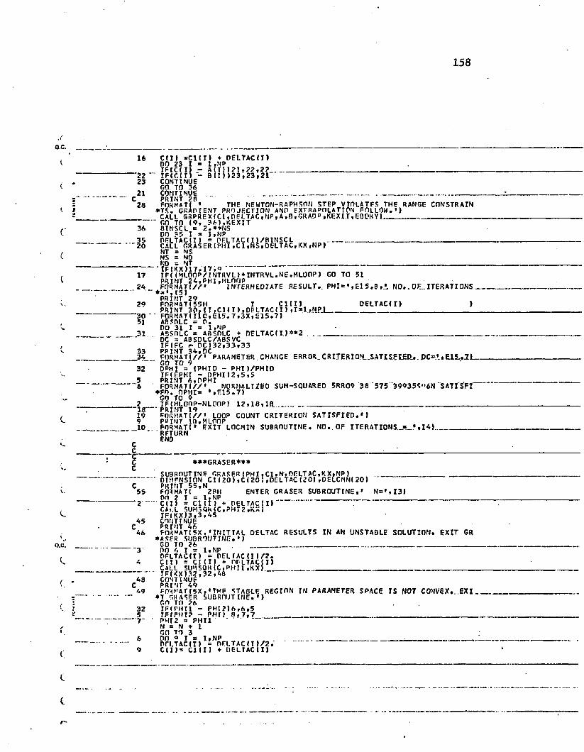
on

nn

o

16 CII) =C1(I) ♦ DELTAC(I)DO 23 I = 1 .NPXPICdl - A!I))2I,?2,2?_________________ _____ _________________________— 22 * IF c C111 - B (I) )23,23,21

23 CONTINUE GO TO 3621 CONTINUE ...______ ___ __________ __ -___ _________________ _____C PRINT 2828 FORMATC • THE NEWTON-RAPHSON STEP VIOLATES THE RANGE CONSTRAIN*TS. GRADIENT PROJECTION AND fXTRAPOLATIDN FOLLOW.')

CALL GRPREXICl.DELTAC.NP.A,B.GRADP.KEXIT.E0DRY1______________________GO TO 19, 36),KEXIT 36 BINSC L = 2.**MS Dn 35 I = > »NP35 DELTAC(I ) = DELTACm/BINSCL -----------------------------------"20 CALL GRASERIPHI,Cl,NS,DELTAC,KX.NP)NT = NS NS = NONO = NT__________________________________________________________________-------IF(KX)17.17,9 '17 IF((MLOOP/INTRVL >*INTRVL.NE.MLOOP) GO TO 51 PRINT 24.PHI .MLOfJP24 FORMAT!//' INTERMEDIATE RESULT., PHI» • ,El 5.B ,'_ NO.. 0E._ITERATIONS..

15)PRINT 2929 FORMAT!55M I C1CI) DELTAC!I) )PRINT 30,(1,CUI),DELTAC(I) »I=l,NP.l___________________________________~ 30 FORMAT (I10,E15.7,3X,E15.7)51 ABSOLC = 0.DO 31 I = l.NP31 ASSOLC = ABSOLC + DELTACJI) __________________________________

" DC = AB SDLC/ABS VCIF (EC DC)32,33,33ll FORMAT?/^ PARAMETER CHANGE ERROR. CRITERIOH .SATIS.EIEO.. 0C='., E1L.2L GO TO 932 DpHI = (PHID - PHIJ/PHID

IF(EPHI - DPHI)2,5,55 PRINT 6,DPHI . . .. ..... .■'6 FORMAU//' NORMALIZED SUM-SQUARED 5RR09 38 575 39935S*'6N SATISFI*FI>. DPHI= ',EI5.7)GO TO 92 IF(HLOOP—NLOOP) 12,18,18___________________________________________*18*— PRINT 19 19 FORMAT!//' LOOP COUNT CRITERION SATISFIED.')9 PUINT 10.MLOOP10 FORMAT! » EXIT LOCMIN SUBROUTINE. NO. OF ITERATIONS ,1 A).** ' RETURNEND

***GRASER***SUBROUTINE GRASER(PHI.Cl.N,DELTAC,KX,NP) _________________ ______------ DIMENSION CU20),C(20,,DELTAC(20) ,0ELCHN(20)

C PRINT 55,N55 FORMAT! 2BH ENTER GRASER SUBROUTINE,' N=',I3)DO 2 I a l.NP ________________________________________________~ 2 C(I) = C1(I) ♦ DELTAC (I)CAi.L SUHSQK(C,PHI2,KXj IF!KX)3,3,45

AS CONTINUEC PRINT A6A6 FORMAT!5X,'INITIAL DELTAC RESULTS IN AN UNSTABLE SOLUTION. EXIT GR

*ASER SUBROUTINE.')C-0 TO 26 ___________________________ _________________________" 3 DO A I = l.NPDFLTAC1I) = DEL TAC(I ) 22.A Cl I) = Cl ! I) ♦ OF LTAC(I)CALL SUMSOK(C,PHII,KX)__________________________________________________ .. IF(KX )32 ,32 ,A8A8 CONTINUE

C PRINT 4949 FORMAT15X » *THF STABLE REGION IN PARAMETER SPACE IS NOT CONVEX., EXI _.

AT GBASER SIJBRniJT INE. •)GO TO 26 32 IF(PH11 - PHI 2)6,6,55 IFIPtir? - PHI) 8,7,7 _______________________________________________

— j ~ - p M I 2 _ p H n

N = N ♦ I CD TO 36 DO o I = l.NP _________________________________________ _DFI.TACd ) = DELTAC IT )/2.

9 Cl I) = C U I ) ♦ DELTAC 11)

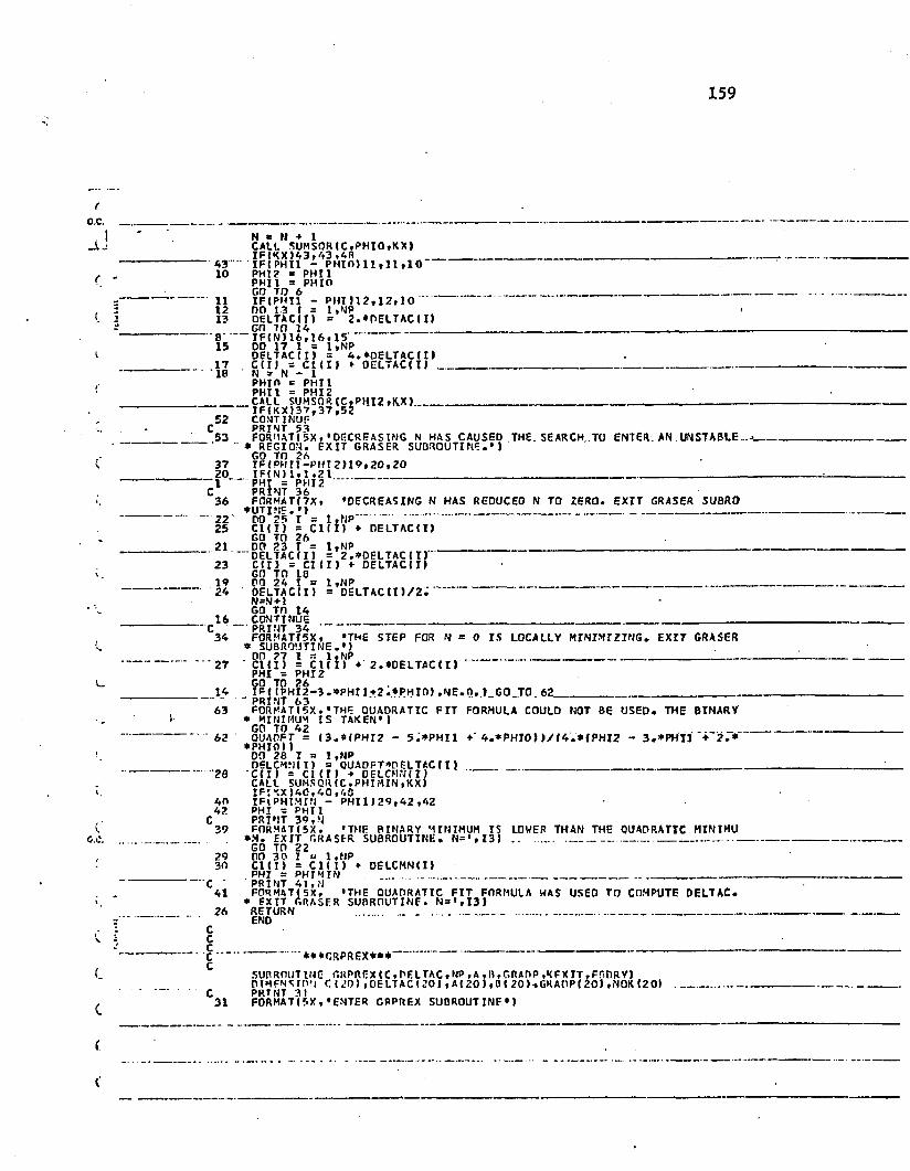
OUUoU

N « M + 1CALL SUMSORIC.PHIO.KX)IF!KXJ43,43,4R ________________________________________________ _

43 IF!PHII - PHIOJ11,11,1010 PHI? a PHI 1 PHI I = PHIO

GO TO 6 _____ _________ _________________________11 IF(PMT1 - PHI 11?,12,1012 DO 13 I = 1,NP13 DELTAC11) = 2.*PELTAC11)Gfl TO 14 _ ______________________________________________ _____— 8--- IF(N)16,16.1515 00 17 I = 1 »NP

DELTAC(11 = 4.*0ELTACII>17 CII) = Ct(IJ ► DCLTACII)______________________________________________'18 ' N s N - 1p h i o = p h i l PHI I = PHI 2

_______ CALL SUMSOft(C»PHI2,K.X)__________________________________________________------- IF(KX)37» 37,5252 CONTINUFC PRINT 5353 FORMAT!5X,•OECREASIMG N HAS CAUSED THE.SEARCH..TO ENTER.AN UNSTABLE.— ' * REGION. EXIT GRASER SUQROUTINE.* 1GO TO 26 37 IF < PH II —PHI 2)19,20,20

20 IF1N ) 1, 1,2 t__________ _____________________________ _____________________— I PHI = PHI2C PRINT 3636 FORMAT!7X, ♦DECREASING N HAS REDUCEO N TO ZERO. EXIT GRASER SUBRO♦UTINF.•) __________________________________________________“ 22' DO 25 I = l.NP25 Cl!I) = Cl(I) ♦ DELTAC(I)GO TO 2621 DO 23 I = 1,NP ________________________________________________ DELTAC(11 = 2.*DELTACI I)

23 CII) = Cl (I) DELTAC!!)GO TO 1819 DO 24 I = 1,NP ______________________________________________' 24 OELTACCI) = OELTACID/2. "N=N + 1 GO TO 141 6 CONTINUE_______________________________________________________________ _C34 FOR M ATI 5 X » ♦THE STEP FOR ft = 0 IS LOCALLY MINIMIZING. EXIT GRASER

f SUBROUTINE.’)0(1 ?7 1 a l.NP _______ __ ________________________________"'27 ' CHI) = CllI) ♦ 2.9DELTAC (I )PHI = PHI 2 GO TO 2614 IF((PHI2-3.9PHI1+2.9PHI0).NE.O.)_G0 TO 62_____________________________

... . PRINT 6363 FORMA T15X »1 THE OUADRATIC FIT FORMULA COULD NOT BE USED. THE BINARY * MINIMUM IS TAKEN’)GO TO 42 ________62 OUAPFT = I3.*(PHI2 - 5.9PHI1 4.9PHI0) )/14.*{PHI2 - 3.*PHI1 ♦ 2.*♦PHIO))DO 28 I a l.NP

OELCMN(I) = OUADFT>»DELTAC (IJ____________________________ _______________"■"20 'C(I) = Cl(I) + DELCMN(I)CALL SUMSQIUC.PHIHIN.KX)IF:XX>40,40,40 40 IFlPHIMIN - PHI1)29,42,42 42 PHI a PHI 1C PRINT 39,N39 F0RMATC5X, ’THE BINARY MINIMUM IS LOWER THAN THE QUADRATIC HINIMU*M. EXIT GRASER SUBROUTINE:. N=’,I3) ________ _________________ ________GO TO 2229 00 30 I - l.NP30 Cl II) = C1(I) * DELCMNU)PHI = PHIMIN . ___________ ___________________________________"C ' 'PRINT 41,N41 FORMAT!5X, ’THE QUADRATIC FIT FORMULA WAS USED TO COMPUTE DELTAC. * EXIT GRASER SUBROUTINE. N=*,I3)26 RETURN _______ _____ ________ ______ ___________________________END

***r,RPREX*** ..SUBROUTINE GRPREX IC .DELTAC , NP , A ,B ,GRAOP ,KFXIT .FfiORY) OIMFNSTO'I Cl 20) , OELT AC < 20) , AI 20 ), 0 I 20 >-,GRAPP ( 20) ,NOK (2 0) C PRTNT 3131 FORMAT15X,’ENTER GRPREX SUBROUTINE*)

160

NHAX = 00KO b 0.KEXIT = 2 _ __ on i r = i»np--------------NOKII) = ?.IFICU) - AID - EBDRY)3,3,23 IFIGRAPP1I)11,4,4 _'4 GRAOPCI) o 0. ...NMAX » NHAX + 1 NHX (I ) = I GO TO 1“ 7 IFICID - BIT)-+“ EBDRY>1,777----------------------------7 IFIGRAPPII) )4,4,1

1 CONTINUETFINMAX - NP)12,11,11 ________________________________________________"“11 CONTINUFC PRINT 1313 FORM4TI5X, 'THE SEARCH PROCEDURE HAS ATTAINED A CONSTRAINED HXNIH*UM. EXIT GRPREX SUBROUTINE.JU________________________________________ _----- KEXTT = I ..........

00 29 I = 1,NP29 DFLTACII) a 0.GO TO 1 4 __________________ ____ ___________ i ,____________“ 12 DO 15 I = 1?NP ----------------------NX a NOX I I )GO TO!15,16),NK16 IFIGRAOPIT)>17,15,18 _ ___________________________~ 1 T OKSTEP = (CII) - Bill)/GRADP(II------------ ---------------------------GO TO 221R OKSTEP = CCD) - All))/GRADPII>22 IFI OX 0)23,23,24 __________ ___________________________ ______

24 IFIOXSTEP - OKO)23,15»15 *23 QKO * OKSTEP 15 CONTINUEDO 26 I = 1 ,NP________________________ ______________________— 26"-DELTAC! I) ' = -QKO*GRADPIT )-------------------------C PRINT 3030 F0RHATI5X,'GRADIENT PROJECTION AND EXTRAPOLATION TO A ROUNDARY CON ♦PLETED. EXIT GRPREX SUBROUTINE.')_______________________ _____________14' RETURN ENDCC---------------C ***RANSER***C SUBROUTINE RANSFRIIRPAT.MRAHO,A,B.C 1,NPJ------ DIMENSION A)20),B(20),C1(2D),C(2 0 ),0120)PRINT 11 FORMAT 155H1ENTER RANSER SUBROUTINE. IDO 2 I a l.NP

" 2 ---D I D = Bill - ATI) -----------------------------------------------3 no 4 I B 1 ,NPCALL RANOUtIRPAT,IYEL,YEL)IRPATalYEL

4 Cl 11) = AIT) ♦ Dll )*YEL ------------------- --------------------CALL SUMSOKIC1,PHI,KX)IFIKX)5,5 , 35 PRINT 6“ 6-- FORMAT I * RANOOM SEARCHING HAS ESTABLISHED A" START TNG" VALUE TOR" PHI' "*.')DO 7 I b 7 ,MRAND

DO 8 J = I,NPCALL RANDUIIRPAT»IYEL.YEL)IRPAT =1YEL8 CIJ) = AIJ) + OIJ)*YELCALL JUMSORIC,PHIT ,KX) ________________ ;_____________________________...... IFIKX)9,°,79 IFJPHI - PH IT)7,7,1010 PHI = PHITDO 11 J = l.NP _______________ :__________________________________________

■ It CIIJ) = ClJ)7 CONTINUEPRINT 12,PHI12 FORMATI70M EXIT RANSER SUBROUTINE. SMALLEST VALUE FOUND FOR SUH-SQ ♦UAREP ERROR = E15.8 ///)PRINT 1616 FORMAT!50H MINIMIZING PARAMETER VALUES //IPRINT 13______________________ ____ ___________________________ _____-13-- FOR MAT 150H I ~ Cl I D " »PMINT14.II,CtlI).I b 1,NP)14 FORMAT III 0,F20.B)PRINT 15, IRPAT _ ___________ __ _______________15 FORMAT!/OH IRPAT b 1 12)

R FT URNEND

APPENDIX B EXPERIMENTAL DATA

All forced oscillatory impedance data used in this dissertation are listed in this appendix. Totally, 18 mongrel dogs were used

for collecting this data. In each of the first 10 dogs (# 1-10), data was collected in control condition and conditions in which part or all

of the three mechanical interventions (mass loading in the abdominal

region, inserting an external resistor, and breathing 80% He-20% 0^

gas mixture) were respectively introduced. Data for Dogs //11-18 were

collected by D.J. Robinson in this laboratory (see references 71 and 74).

Six of these eight dogs were subject to the perturbations of two drugs,

physostigmine and atropine, which can effect the bronchomotor tone.

One of the remaining two dogs, #14, had narrowed trachea and the other,

#13, had obstructive airways due to smoking cigarettes for six years.

Each set of data in the listing contains the impedances measured at 26 different frequencies between 0.9 and 16 Hz. The magnitude of

the impedance is in the unit of cm ^O/i/s and the phase angle is in

degree.

161

Dog 1 control #1 #2>.c. FREQ MAG. PHASE FREQ MAG.

0.90 6.9? -55.01.Cl 5.75 -*9.0-l.tT-- r.7<r--- ‘-sfvO----l.?’. 5.?r< -53.0. 1.51__ 6.27____-A6.0___1.5 6 3.53 -99.0l.PO 3.39 —90.03.01- 3.31---3? .0--?.?9 ?.«>i -2F.02.52 2.65 -79.0-?.??--2.3F----1? .0---2.15 7.9 6 -6.0’ r » .2 .3* - i . 0 ___2.95 10.0

2.?l ?9.03.59 - — 2 9 . 0 ---2 .7° 9 t.O3 .If 51.0T.-?6--- 59.0--

3 . 9 99.9?-9.095. if 6.33-7.19-7.of 3.7P 6?.0 «.00 .. 9.21___ 65.010.10 5.99 70.0n . r o 5.9? 71.0— 12.60-- 6.15---73.0--1 9 . 2 0 6.51 75.015. SC 6.19 77.0

0.901.C1

— 1.12-1.26 _ 1.91 1.59 l.PO- 7.01 2.23 2.62— 7.P2 ' 3. IF 3. 56 3. co

9.92— 9 .0 fl 6.65 6.73— 7. 19“ 7.°7 9.CO 10.10

1 1 . JO -12 . 6 0 15. 10 15.50

5.735.77- 6 . 7 f t -9.573.993.723.70 3.12 7.037.69

-7.95-7.5?2.93 7.23 2.22 ?• K6 7.797.93-3.39-3.935.715.70 5.61 5.76 6. RP 7.75

PHASE-55.0 -50.0 --S0.0- - 5 0 . 0 -55.0 -90.0 —3 5.0 -39.0 -2r .0 -2->.0 *—15.0"

- r .0 5.0 1C.023.0 ’6.097.097.0— 57.fl-OC.065.0 6P .071.073.076.0 70 .0

Dog 2 control He-02ERE Ci MAG. phase FRFQ MAG. PHASE

6.5 P -~Sr.0 -.... C.90 " '7.02' -56.0I.01 6.7 ’ -59.0 1.01 6.06 -6 5.0.... . 1.12 .. 5.E5 -55.0 ______ 1.12 5.65 -53.01.26 ‘.02 -52.0 1.26 5.2? -57.01.9] 9.55 -9ft. 0 1.92 5.65 -50.0........ 1.59 6. 1C- -59,0 1.59 5.33 -56.0l.on ?.,!5 -9? .0 l.PO 5.05 -9 6.0?.ri 3.56 -?p .0 7.01 3.9? -ft’.r.7.76 7.75 ■"-3 2.0 2.75 3.55 " -50.02.‘3 7.96 -29.0 2. r3 3.1? -77.0_ .. „ 2.62 2.7? .. -73.0 ___ 2.62 7.05 -33.03.IP 2.9? -19.0 3.1R 7.65 -70.03.51 7.62 -6.0 3.59 7.63 -2 3.0---------- B.59 - 2.96 — - -3 .0----- 3. PR 7.32 -21.05.5? 7.37 10.0 5.5? 7.10 -19.0

5.95 2.95 20.0 9.55 1 .96 -9.06. 5P — 2.67 ■ ?f. .11 6.55 1 . 95 —3 • 06.77 2.F6 3P.0 6 .75 7.01 17.0.. . . .... 7.15 3.19 — 59 .0 7.15 2.C1* 72.07.56 ?.r>5 55.0 7.01 2.IP ?ft.O9.00 3.P? 5P.0 5.10 7.31 3’.0----------10.10 5.91 63.0... lo. 10 7.95 90.011.70 5.P9 66.0 1 1 .20 2.33 52.012.60 5.71 65.0 17.60 7.63 95.019. 20 7 .2». 77.(t "T9. 20 1 2.69 55.0'15.90 7.62 75.0 15.eo 2.93 58.0

#3. - - averageFREQ MAG. PHASE FREQ MAG. PHASE0.90 5.81 -59.0 0.90 6.16 -56.31.0! 5.05 -59.0 1.01 5.17 -51.0

' 1.12 6.89 -59.0 - 1.12 6.96 -51.31.76 5.70 -96.0 1.25 6.36 -69.31.51 3.95 -91 .0 1.61 6.06 -63.71 .59 3.5? -36.0 1.57 3.59 -60.01 .po 2.9ft -39 .0 l.eo 3.16 -36.32.01 2.96 -30.0 2.01 3 .13 -32.02.25 2.79 -2 5.0 2.76 7.R6 —26 . 02.90 2.9R -21.0 2.51 2.59 -22.7

— "7 2.33 ---19.0 ---- — 2.B2 2.39 -15.0 -—3.IP 7.30 -6.0 3.17 2.60 -5.73 .56 2.32 9.0 3.56 2.36 1.73 ,9R 2.15 10.0 3.97 7.28 10.09.5? 2.-30 2 2.0 6.62 7.78 23.09.Oft 2.*0 ?3 .0 5 .9 ft 2.56 36.35.5P 2.72 60.0 5.58 2.75 62.06.77 7.PR 97.0 6.79 2.97 66.77.15- 3.23 --- 55.0 ---- 7.15 3.33 57.07.91 3.72 56.0 7.95 3.R1 59.3«.10 3.99 63.0 9.03 6.17 66.010.10 5.ft? 67.0 10.10 5.8 7 68.311 .20 5,07 6R.0 11.17 5.30 70.017.60 5.7? 71.0 12.60 5.89 72.319.10 6.13 75.0 16.13 6.51 75.315.90 7.60 77.0 15.90 7.68 77.3

162

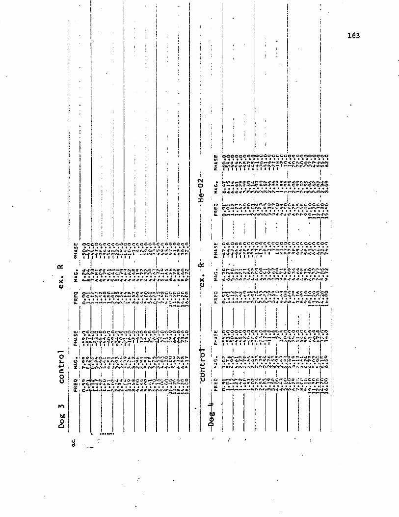
Dog

3 co

ntro

l

XCL)

b* O C C O C C C C C C C C C C C C C C C c c c o c c cc*r**u>f a: *ifvrsiO a»r ipo ir.r**■«<*.© cv'11 :t 7 i i • i i i i i I

• *t'4 tOf-trc Hî^jrrrgac <Mcv,CP-rv.3 tn<(Mu>crO r.rvf*a.of*'C*tcr'*<*C'«r**r-<rn‘*'Cr,*««c*>*r*a,«tfr-| 4 « • » • • • • • • • » • • • » • * « • • • • • • • »X *nu>*r*rnwof *C0=0*tL<i:cO O»-,04r*rvjCC*-H>A'lsya.r*,C' C',_4<tlr»a^COOOCC iL trC*->f'.C’<.wC.C(N.'»riu.»— knc«4’C-ci\ii-»3 c «-<*'< p-cmC a* » * • • • • • • • » • • • • • • • • • • « » • » • •

i lr>im IfH

c c f c o o o c c c c o c o o c c c c c c c c o o c oq r-t* mm** co 'ic «i piipip I I I I I I I 1 I Ir• «C<A»Nf rv,4r.«-* i i #Hf-»csr'rfr'f1*

o<X ,O rC ol-n/O/rviO'-c • •■ • • •• • ••f-a.fÔCOvW *xt.*w 4>*ou; ! !

VI h- PJ © -* 'I •* If o* aj c C • * OU2 c c c c © c ot, •-•-A C *4 O •£ p • C O -«C\f I*-<v* o| O.C INU i• • • • •© *4 JH*4l 4*4 P4 f\| f\| CM vf«»iiv*CNuvO’C«rvi 0

CMOI«JX

163

iin o o o o o c c o o c c c c c o o a c c c c o o c o o< CO-O «ts.a:r-ir'-'0 *-'»âc<vc<ccpjCcrp^^tfvM X •Cini lT lA*T*# 'f "-P P • P*1 fV Pm •— I C\. Ph | «\ P“l P\ sj »f \ ifV *0a i I I I i i ( I I I i I I I

NîfHinCM^ <*f,*C<\i<,'C0 cnpu,,**oty in m< fv.ru »* O* CLUwer.a eccc.c cr OirC'CCrtO• • • • • • • • • • • • • • • • • • • A * * * * * *r’lP'.r.r-fv. fNPM- r-ii-ir rNt rvrir.fv.mrMCO

i :Ur*wf*riCCHVfr.raÔircCffif.(tccccocUi C*-'<,Vi«^<nO<Mu CLf li'C ‘Ch P.P-MO

u. ©*np*r*»*«P"'*-*P»«,,'J<MCVf*»rW WA<T“hJC If*

Uj c c o c c c c c c c c c c c c o c c c t c o c c o cv/". » • • • • • • • • * * • • * • • • • • • • • * • • •< r-'Trs.w cup i r.r* r.a p'r *-** - c.a, 0s u. r - ^ - c c i - f x r s - t st * * t * <vp>p.*hpm i i *-»<M(\rrwipir.<*c*cr“f» a ,1 I I I I I I Ijl I | |

I • ■ i I !• ijf*©*—*-**~'4.P.CC*—O/P-oc -p o-*Jv*c:«r.©P>.P-uvcMc hr.r^cp• • • • • i i » i i

H H N N N C H H ^ i f i r t a a o r c c o < c c c c c c oV C.«-» 4.CC CuJ'c, vj CH.rN* 0 *-*<P,roojC-! • • • • • • • • » • • • • • • • • • • • ■ • • •'••

r c o o c c o o c o c c c c c c c o c o c o c ci i i i • • • * • tC O

tr»<ptCa.ui<MC-u.a •r p* *-»trv« c < / *-**/ o *■« .cp* KIl'iV'd* <| W l( ( ........ .I I I I I jl I I I ,

i [ i !-p-.Cvi irir.cîpitcp.p*.r*> •r

NK.iAi/MT <<<rv. -*irc p c «cr*p-'£ r*r*«i'h*v'-e -j a

r>*r«rg(Vi(NCM('Mi !

b or* «jfp-.c C I'm P-C O r-'VO

b e .:cccccc. c p*.cO'O-Mpjsj <*ier civ*u*kccû%o^ c cc ru^c.--•»-• p . r-N©

o6

Dog-

5 co

ntr-

ol

—ex.

-R -

He

-02

FRFQ

HAG.

PHASE

FREO

MAG.

PHASE

FREQ

HAG.

PHAS

E

164

lu O O O C C C O O O O C C C O O O O O O O O O O O O O(fl< viO'CfnrgfM raor-Oa I I I I I I I I I l l M I

esi ' IO 9 P“ lAttrr,® * ©rt©0» CM© *«CM 4). 43 rvraop.— c<>m«o * m* < m m «<■. r« <\ n oj n ca ca r* c* m pj m m r» pn m m

or o *N»r-r«c **p*ar,.'ra*aoro.~«ccajp»i©©ccc© UJ a . c c a r t e . ^ i o O < O c r n ^ 0 ^ ^ r k« r,B( ^ oOf • • • • • • t i t i i t t i t i t t t i i i c i i iu. '4->ir»’Cr-at'a o^ rT'OPfll (f1p4

IccoooocccooocccocccccccoccC P* N P\ C a «o < >< arr *■* -C **'tf* O <A cc pj a fn oc w* ** 4*Cir If IfMp «?*?*? «*«•"■.<*’.CM IA<*0• I I I I 1 I • I I I I I I

f frv.fr>f\jfvfst»-‘U>fnfVvtQrccrHa:OMC*co r-oo <COO <cC^hH<tir,HR4c>C(7Q.x cf-fi-ecoA-ifr.rr.i a:

. ! ! ! !•-«r-ir\.f«.<\;cc uw*j,0‘r-Circ\>rHO <cccccccOCHM4CCNV <LHIt>C>|C *4'f\.-CCAf\P-fS.O -

cz

Xa>

e c e o e c c o c c c o c o c o c c o c c c c c o o • • « • • • • • » • • • • • * • ■ • • * • • • • • ••-a'Crvf-rtcr-rso r*Q mcaicr\'C,fH(Aa:cwirfr*.irtsf rrfnfy.fN.rs*M*M J | *“»rar\jfc,fri.4I I I I I I I I I! i i !NO a mpg©cef",*'fi«Of**t'-0‘Sw'-ip-p-râ 'C<4‘Arf**#fr>wwr* *->«•<{« c P * * a r -<C <C tAtA 4". «* «4 At 4 •/ 4 >4 4 4 4MAIA «C «C f- OC 0* ae*-'f'wr*fs.e~c\.*f ~c o - c ^ c c c c ca c < a c.tsiV'cr u' c 4C «c r.^cc fN.f'-rvC • • « » « • • • • • « • • ■ * • • • • • • • • • • •inrv'Cf-ctc C*"*a«44>

I 5

• e c c c c c e c c o c c c c c e c c c c o e c c c c ;c t* *>. c-*~4 rr-.p-rc.trv44 4 I I a-mao. n,(T,fr.7intntf-.»c <r,‘r- •I I I I l I I I I

c c • •ac* tnn i I

o o c c c c c c c c c c c c c c o c o c c c• • • • ••C«C»"-C,f'-.£.CCf*Vrr*CCtf 4 & x.o fs.h1 rsf**© 44 4<«- |I I I I i i I i I I l

be • •*>*o

P.4C hC 4 r-.mo e ra a p»*.<-•*ccp-4 ***►*!o<4VtftCir<r«i7-to«i1* • i i i

•u-C . f-r-<«cr\tn44,44444444 -4 4444u>»O'0f»f*«r.ot •— an <cr»

f I ! 1C « ^ n o c ccciArvii-«c h o c c C c cg Cp»irw4 <cu.CrvMM. ch<*\C • • • • » • » # • • • • • • • » • • • • • • • « # •C »-•»-* ivcnaJS. I'. r.r«< fa>a.o>G>Mo.«i at

a) 5 .

< z o Wu’-Ajrt.aira a.a r^jf^rvr-a a rr.caf-r.'fno r tr.isica1 a c<n,-o: ^ c. u.(\un»-«r-Aa p-«>••*•••••< »n ia i r »cn rw f>j rv ra %r mT ^ «

‘ cccocccccocccccccccocccccc• ~ --- a't*O I intftru>*r •!*; t**rsrsi i i i i T i i i i

c*-*<Njf.cvc~4rvjarO'4>aocmHcc«o^cccocc • CC^4-iCC«'>/C.«fcO-/CiMCHH<Nr-(t,C j• • • • • • • • • • • • • • • • • • • • • A * • • • I

I ifs.mlj<rr*sjc c 4 <\«crio.#p-rvn cmraracr a ^ r \ j« r . a u . io v fnrv. »-<»-*r»*j ^ a f ^ o i r C . C ' C f ’j• •••••'••••••••.•a******rnA<r-MrrtC4ivrw(\r44 A.rN>r«rs.rMOiA.i ininii nCHiviN

i i i1 c«^Fr*ojccrg

I:rgiA^ Ircurcu (mhC 4 * - o u v C c wa C* Ki-j *cu.-wrv.ir.«.r.u s_ 4 c • •••••••••••••««•••••*••**, c^T4 »r-*prHcaA»r,afarn( i<4•4tAa'X.r'*u.</o<-»rM4u\pinHHH

ui e s o c e c e c o c c c c o c c c c c c c c o o b

Ov.+Jcoo

r-î'B'o r-L- l •j-i m c o [fI I I 1 I I I .1 1 1 1 |i | 1 1 Ia rva. a r.4 P A.frg<rva.clo*ca 4 iAsf<M4 f>c*/\iveuMi C »*.p a.C jppft'AHâ u. hP»c Csf • • • •••»•••••••••«•«••»•••L -C-AuW4 P.inP*i r\rwPaPiptmP1<4-4iA4..

:o • •r<ajp“

woa

• • I • Ia . r * 4 \ ^ p - u . a ‘ C ^ p -a

:o uO • •b-4

o6

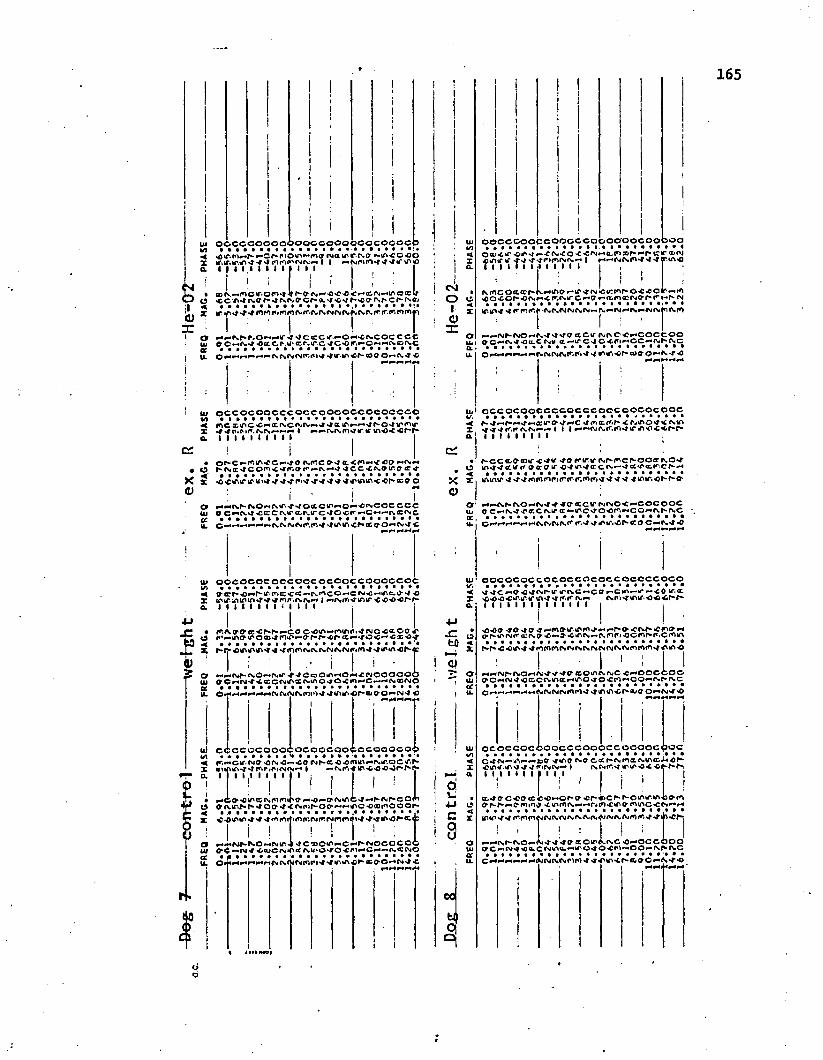
cont

rol

weig

ht

— ex.

R

'He^

lo cc cc o o cc io o c co o o d c cc o c cc fi• •••••••••••••I***********rÔ^n^-fno râ in rrso *-m>ca -co*oi<ip'cmc,v«-i l I #-«<sirMT'w«p>/tf‘mio 1 1 1 1 1 1 1 1 1 1 1 1 1I l ;

sI i

I I

I t

Oj , | , , ;, , M . j , j | T |

# p-GO'-Gir'Xismmf'O!

tooCl

cd is m c »r o m *f P“ 9 iv * * o ' G < * * < & ^ © ®<c c * * • * is c f* * is is O ’ o r- a. ■* <- ■* f- *o <?■ is f- c r- is » • ,•••• • • • • • • • • * # • * , # * • * ♦ * • * ! •tf*. o# -J 1*1 t*l f»# IS »**• IS IS *M Pm IS N IS IS I*:!»“• I** 101*1 fS f t .I S IT IT.**",m 1*110

o HiMNhr.oi-iHirsracccirô^p.cocccc ui & c-'^*^^«ccf>.u'a.p.«rc c*or. -o*M»-'Cs.cDf».cgf » *14, © «tlfVvih*COO "C

ui o ec o c o o cc co cc o o co c co co c c coV) • • » • • § « • • • • • • • ■ • • • • • • • • • * •■< me xific -£.*-« ccrvc is is**** r*-o-J trmirX •#<*t**rir*.isis<-n« I ** *isisfrwir.ir mo-c-cr-p- o. I I I » I I I I I I .

! I i• ©r-C C«-*PO rv.fr, CO'»ieL'CiOpM<oo*ô.*«4O r*o*a:*lCOfr'<'i,n‘.or *-'r.*-*sl'#CC'Ci'.oir.ca:v 4' • • • • » * • * • • • • • • • • • • • • • • • • • •X •CCtAiTtr - T ' t ' 4-4 *trm»fts;'©r-«o O

o H M ^ P t O m M T - t ' I O S C ^ O H ’f i ^ O e C C C uj o c**fs<tf«ce:Cfs»rcLi\irC'to<cr *hC*h*-o,cinco* • • • • • • » • • • • • • » • » • • • » • • • • • •14 Cp*» »> ii •HPIA<f*K<yO^P<ty CI

li> © o c o e o e e c c o o c o e o o c c o c o c c o c

x mir.imiw^^^fw.isfw*** J «-»is#<wifnf ’C««0’Gf-p“ A. I I I I I I I I i I I I I ;

irrt.aocc’Cr'-f- -CG o>oin«-PMnii«'*r<JO<a.oo it

pm |N*P- IS G •>* Pw IT ■# C ® O rfl G +4 •£ PJ © o O O O 69CHNt<C(CCNiPS(VillQ>|O<CinHC«-<HNe0NO • • • • # • • • • • • * • • • • • • • » • • • • * > . •© m m** *+ 0**4is rw04 iscni*w a in»o -pr- o< o* o ■■« is * <*>H H H M MJ

ui C C C C O C Q O G C O G O G C Q Q * i O C O O O C O Q • *•••••«•'• ••»•••» •*••*••••< r‘>MCtf>N9<orM <-"Cofvp-«'©'£<nin*<*isu\a>C‘iMS’X *f mr»c»<vis * | »*<Sf*,.'f-ir*C'0'0,Of,kP*i*“0. l l l l l l i a i l l o o o r- • , • • • • • • # • • • • • • • • • , • • • • * * • * ] •

| i ! T ! ! I ! : IH«*N|w^MMr.<l'fCOOiPMC^ÔCOCCOArU»o*xo<*k4C^"^(s>C(MO©• M«4HiMn{ o( Nr)ri'i'fir<tfv<ch8B O'4M4<c

CM01o

X

165

o e c c c o o c c o o c & c o o o o ' o o c o o b o a • ««•«••••••••••••••••••'•*«Ow<ciP4 iP*i^-cn<co< ctr a>oioyitnr <r >i •rririNN } r«i-N<sn,l'l«Hr.iAifl I I I I I I I .1 I I II II

is pi c O ct a p* K • * & o - tf' ■♦in *c tc cn f» G < O r - *G ^)O-COf->0lsr*<.r.lStr4 •••••••••••••••••••«•• •>• • •X ipiP'i'l rf'r'.r'iPisfv.iNjfvicsfs—i fv.fM .»Hisifsli<sri I ’^ a acu i\jivc<c «-«c o c c o oo c «cs>i<}a.CisiU' a i/>c>}G4ri^GC'*c«r NC • • • • • • « • • • • • » * « • • • * • • • • * * *

O^^F4lM«F-is.(sr4iN.r.r*'4’- nM'.<«r>'a3a-O'~is '0r+i-\f4t*r+

© C C O C O O C C C C O C C C O C C O C G O C O O C v. • • • • • • • • • • • » • • • * • • » « • • • » • *■< isu%x iv>N>"n i I i * *i\jisc*“.iTWirii,V'0«c*cp«p"I I I I I I I I I

P*CCclG ooit G !<*«•«• isr-r'GNOOfflSO'/O U>*fACM* C 9C9H -O'*UWarc cC‘C'ot<ctCP,»< **••••••••!•#•*♦*•••••••••x I mnumt 'i <*** miricr>i*jircriir.if>ri»j 'J•* u'*r.«0f*f,“O‘o ; •H cv.r-rsOi-is*i,*tecwp(NO«c»-cocooc Uj o C^(s^r>a:cisu'<r»-ii'C'tO'Or,«Mco^rsh>rsc tc i ••*•*•*••*••••••••••••••••14 *0

I

I— o cc o co cco co ccG co ccccceco co ^ ^ •c *G<c*>r<sr,*-ir*rcwC^CG^-CM\»-w‘ -<o u*.<tx wj«o*o»cu'U‘.u, i A ' * f s « <snwtrttf>'0 'G'GP»f,~ a. I I I I M I I l I l f I »i\ ■ •••»**••••••••••••*****••p* f** < o u' * »n in m is is rs cs is cnj *v< c*> <*» p"* •i' Gt t

^ rryr*'fvo«-«<S''p*/,*«yG «cOknr«.puc h o c c c o c * (p o * * rx <3 c& c in cc »h m o o <c n o o «-• is is c

I .*'*

© C O C C O C O O O C C O O O O C C O O O O C 1 JOC • »•••*••••*•*••••••*••••••\|«P9 N9 CC NIPfltHi ii i i i i p i i i | ; |i 1 I 1 I1cc ff c-oo cc c*o«or-o cr**«>cr*,p'OtP“riO'OGrV •C»l'Ct>ISp»*r<iP,)»Crf,tG rtlftG'Ch'-r*fCi<ntfsji'<isisisrwAi<vi<v/viSi*>iP.«P«f u>«C

I I 1nl.r 1^îsr-iso )<t<>t«f G x oinSisc o m o c c o o o 9 C IV y) X C Q - ^ ^ o p O O is is G***•*##*•*•••••••••••• •:• * •

Oo

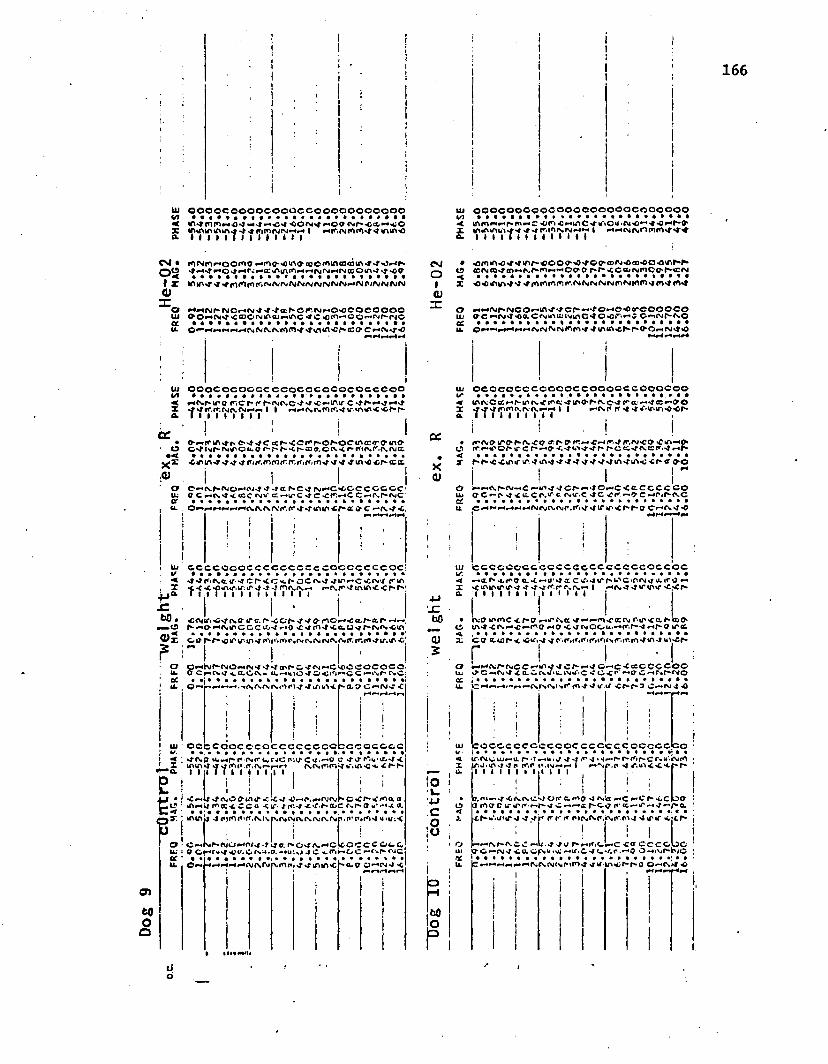
166

Ui O O O C C O O O O C O O O C C C O O O O O O O O O O

o- I I I I II I » I I I t I I

tu ooocoooooceeoeooooocoooooo to • • • • • # • • ♦ ► * • • • • • • • • • • • * • • •< lAmMPHfwrrtMC»0friO»-«u-iC4,M'*©U'f**o*",4«c^-lw0‘S i t i i T I » i • I I i I I

P*Ost"a*(‘w»’«CCU'linfl'>>M*4rMrM»*rMC0QtfW'r « ^ 0 w < *••••••«•*•*•»•«•••••••»••I X » rm < ^ ’T ^ ’r ic irn r* f^ ^ rv fw fv rg < \jp \jfv ir j# -* rv jr j/\< v j/v jrv jOo HHNhÔH(v*j*i*ta^6 ^NHO'fleoeoooo u j O' o ^ fM > 4 « cco orN ju tcu«»«u 'iG 4C a •«••••••••*•••••••»•»••«••

I

UJto<Xa

or■ o «<x*<voru.

!o o o c o c o o c c C C O C O C O C O C O C C C O O «•*••»•**•••*••••••«••»••*H N h it & ricr-c* cI I Mv»fnrwir*n«fi<d**h*• I I I I I I I

! ' ! Io-~ wN*tr*, ccr-^cn'r'-oôctncco'ocnoC *4 «m f- n *r © «. c *- f- f- < h- a 9. C s cv< r * 1*1 rs. r. <\ ru cc •*•••••«••••••»«••••*•••••’Cit'in-T«?»t*t1ittr,tCHntr.tr.tr,ft,fn* * 4 4u*v«c Cr*CCCL

i I i IC *-*I S . f - O J 4 4 4 a f* C -4 py •■«C *Gc c c o c o c • Q C i-*C\4 < ccc c\m* <S #-«ir C 4 C 4 lr.»-«C C *-KV.P-0gC• • • • • « ft • • t

<, X<Ma jC to.•.ca>£

o^^«x^*-<^4<\,o.OsO.'(f-.rr «r (Tto^r-a 4 C -<\4 'C,

t

C C C C O C O C C C C C C C S C C O C C C C C C O C*t«jr»«N.a.ir <*JCr“'CC*cr,« o c c w< <5**r-u'.ir 4 4 4 i\.rv.»-« nM<''tiA*n'£'ChhriTn I I i i I I I I I

«civu*. 'C4 cva it c. f- -ccf- 44 o- ©»-•*c <c#-a. r* • h--»o>*-«fvinCGC uw *-«0 <4r>4<.cl,04r-cv<'*«ou>

i * I "i » * * i iO f* it) lT IT tfW P'U1* f*» f** p*. <S OJ o* <Vi C*I If, <«W If. 0% *£> j! | ■ Ic*"<rMf**<o~«<N4 44cpr“ w'fiN c oc cococa.O Ch*CV4 <o,C(V.t> U.<-U)0<f £i«Ci,**“,cC»-,»Nf,*CNC:i • i « i

; uj 1 oeecoocococcocccccbccocccc; 4<vp u,^ r i\r w n c p'.r c m ••-•o c 4 4 f .u'uw <cnirw 4 sr<Oi«.fr.rw *»- r-» ^^ rr* liiM 6 'C 't< h N i i ;i i I i i i i i ;i i j

e ! [ i i

O *

I

O)tooa

!,4 <VOOtn4 d:*£4 >0— f tc ■£ Z c & < \f- f 4 44- coC f'.r- cy y* •*«.! a. •:• •••••.**•..•». • • •»•••••n.n'r»(<»'*i d<u.<r>rinr~«oo^4'ôo><siM4a>>ea4vnf>P* ecputn-f en*» f'n*-"'0 0 ‘(r r»r-<ca»Oii,iC«M~«i,J •••»«»*•••*••••••••••*••*•

•lH^l|>.lMcO'•K''f'ê^•^•ê>►ô■Olfeoooooo f-1 is, ry Py CM W f<V mu% < N I** O* O *-t fU ** 4)r n lpi» |> I

O C C C C C C C O O C O C C O C O O C C O Q O C O Oumv C cc h* m fv <■ r'c: «4 m 0* fv-o a-•-* *1 as O O » I 1-rv.r r 4I I I I I I I I I Ii i i Ir<'<V0 »/,,0>rfcA,<‘0 tfrf' jr,N< 0 sCkfv-«0cTf-toor-u* c f'«-,o <-*j,t**'sf4,rfcP-ctc.4‘.cc<<.4 «-»r- • • • • » ■ • • • • • • * « • • » • • • * • • • • •f*‘fs‘'C«ca>a- u‘ 4iLn4‘4’4'4'4 4'4-4tn*j,u%‘<;-cr-<r aci !

C£u.^wft,N(V^C»-^«J ^ ^ « > I C i - C < t C C C C C O rytr.C 4C C •xr P-PS.C4iru">< r-o c

tccccccccccccccccecccocccc *—ct r» c.-i#-oj<r a C 4trf*»w"«C’nrg u.«i‘0 *-•<ifMnru' »rv|-<r*.r‘r,fs.r-« | ry<T4tririir 'C<p*I I I I t l l I i I I I I 4

r « o m m c - c r - o *-^»rNcc r .i^< a ,f '» « D O -iA4'Cf *-* #-*rF'0 h o *c <NiOOui* n,.f «4»Hf«»o »r<cco outor* ’0u,i«4-srr .r.«».<,,»r»<ri<s<r..{O'4tf>4u\'Cr**r i

C C ^ ^ ' » C ^ » 4 0 H C < t c C C C C O O O1 C —.(\j4 {. 0. C. f\.*/»U.lMO*'C < O <•’ ***0 C * f*yt*OJO . • • • • • • • * • • • * » • * • • • • « » » • • « •C*»risJ4'0

C O C C C C C C C C C O C C C C C C C O C C C C C O• ••*»••••••«•••«»••*••■ «‘t«i r - fN ic u j^ -u r* - t «-<y > j* 4 4 •»j»~r“ P*{1 I I I

p.ni»-%f<(<s.o.<istOr>,e.H'0 4 N« *-<C3 COOC IT (T* r'1 r-r- >J C —•<-■* hC.C(r«t -c r-.cc Cl• •••«•

1 I 1 1 C. 4 4 U >ca C C C C U Coc**ru y:&cû.s);<Hi/.C'rc*CP.*-'0 0 - *v*r-hjc

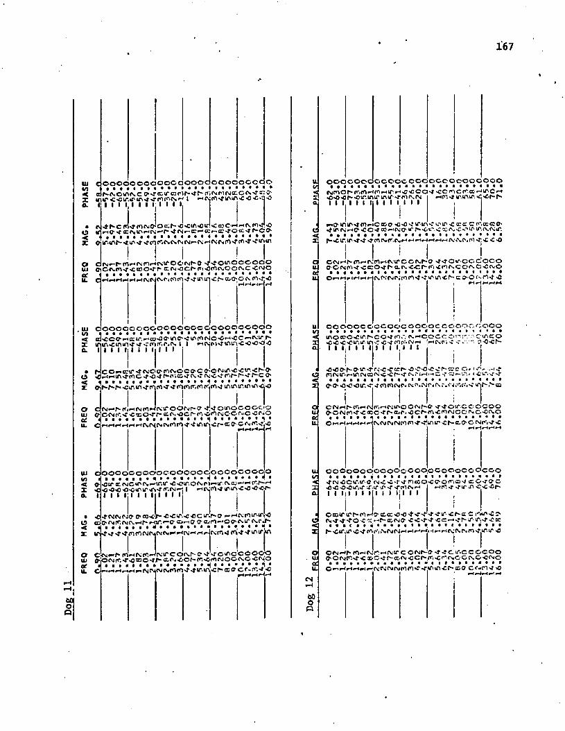
167

UJV)<Zo .

o

o<x

X O'

oUJGC

6000000000000000000000000* ♦ * # • • • « • • • • • * • < • • • * • • • • •

o ^ c o i r c o c n f ' - t f r ^ f f i f M f U M C c . o c w K C * i t < »c i r . i r n c ^ c N * - * i ^ * « c \,ro > fV '* iA 'C ,o ,c * 3 >o I I I I, I I I M I I I

•»t f* C sf cn <m oi o c; n <3 if. <6 ic »o <o c «h w cv. m»r £rn O' < OC <N IA *-» CM r* CM c? «-* oc ri CC O CO >f f-C O '

* • • • » • « • • • • « • • * « • • • • • # • • •i t r i f l e s * c \ r ^ (M r -c \r -< < \ ,r * p ’) N f c ^ '4 '^ 1r r | c

Jcsr-r i iHfMfn cM ooiNjr o o ôcccoo oiCcv.Pw ccO'fT' GCM cr'" «»i<oinc\iOqfc <ruo

, UJ i/i < X a

I

c v -c ^ c n mH H H f * H

o o o o o o c o o o o c o o c o o o o o o o o o o # • * « # # • • • • • • • * • « • • • • • * • • •

• ^ O ^ * H C C i r .* ^ C 0 '0 6 ‘ W,'C '^ ^ 0 f 0 < sJ O * 6 ,^ 'C C « -»A :ir ;?•*■ ir»<inu>r-*i'Cror<"'f>-fv I I Hjv.p iniri-C’O'O'O'O I I I lil I l lii I t |

{* C C « ^ C U ' 4 ^ 0 0 < r i < S iO C O iO •-< ** m tn c sf *o <* i cq sT c\<v fs. f*. ^ rn (<\ <f * ra en r. co

©UJ C£U . CJ

UJ cVI i< o-X a

u’M n i r . m u x i 'O

CM «-* f»* rr< m CM CO CM IT O O CM r-©cm r*. -6 ® orr- c cs c r* • « # « * • • • • • • • • *rn rH •-< r< »H CV CM (S CM Cl n-f *•

TI? 'T-f OK'OCOOt'CI (n-CifllVOOlvC'CfVO • a a a a a a a a q a

i r i i r i 'C r ^ c c f f 'H H H p - H

o o o o o o o o o c o o o o o c o o o o o o o d o «C ir cc cm C *o cm ir. u* «C ir. o cm cl #-• ir <s a; *■* ** ro h- *-«'0'0’0'040*r tf'vr»<n".CM*-i I u iac «0'0'CA-l I I I I I I I I I M I

srCMCMoJcO‘00< L C'CU‘!<jjcir!r-o -r cv.roir.ir(•O CDC< d. - - - - - - - - - - - - , ,y IT ^ ^C*1Cr)CM(\*<MCM*"l4*'<CM»,**r-C^“ CMn"&«4 ( f ^ lAU" »A

O C ^ K M n H M r . i - ' M C C O ^ e ' f - f C ^ c ' C O O O Odi (>.o <*v rf. "f >C —- O .f f— *3- f. UI' Of—cfi.OroivoocvO'C (VO u. c ) — n i v i v i v f v Mi f i •J' - t i f if<< l" ffi<7 c . r« r f . 'f 'C

o o o o o o d o c c o c o o d o c c o c o o o o o orvjriaf-f.fonmmr n.C'COcw <ccicr«^K'C'' OsO>or-'Oir.uMrifMf'‘4-niisrj nri >? it.vait< >Cf- f- I I I I I I I I I I I I I I

nffi/iuw mncioo •O'O'J ifin'fif ir«c ee cc-.««0- d .rirfvnc.cc'r ecncvo'if ■csKv-C'f ir-in<\.<vir.

V<Ia

<M

00oa

CPsii-af'fo-‘tvfn-<fu,ircc(v.r-& ôf-occocoo-c in m < cr o >j-f-o. r. >cc t*-! n is. c o c-c ru oOr<HriH>-irHf\.C‘i«\n'imiri<'ru'm'CO-eca-or'irt<# -O

4H—

OOOOOCOOCOOCOOOOCCCiOOCOOOO inooc-cif.hco>»m,'. HCOccc'i’:' - c t c o■c >o-e < it, it. m >c < m o', tv r I I I; I I I II I I I I I I I r u f v r ; v 'I"l•Off'h-O'if ru^^ter- <0'I,<3>oô*crc o*Piruir.—iir.rvaivvc-Cf—ris.-i—l.-'C v — ■-■'.» <• « * » • • « • • • • • • • * • • • • • • • • • • •

O-a- <3-00 if. <■ nificvr. tvr'.fjr.cN r.cj.nr.-, <■ uAf->co

civ nr-if. •-*i\

:u A f

p - i« - < c ; i f > o o < v r - c r v f ^ o i r c c o c o o o> C m ro »r oo c-r r-o. r. c r-m u: io i\j c c ru o iv o0MHrartHrlWUM\iniH'fs,‘UMI’ if-C.O' C IVfl»r >c

r-i r~ir-fr~*r-1

O O O o O O O O O O O c O O O p C O O O C O • ( • • • • • • • • < > a a > > > a < > i >.fCV'OCif.lf 0 <v^'C'r'flrl«0O,'C0'On'.«i'J ®^)^'0>cif;ir ir.ir tf'-T'Tfifvn |I I III I I I I I I Ijl I I

i

d c o oa • a •

o - r o cO 'C 'O f -

I

ocoif tf r-m»-iO' ctcc u3<i -f'T'T'T -ru" u: r-c c far^r rv «r <1--f o c •« — r-a ivo- c c <= n N» r-ir• if. umcI « I ( • • • ( « • • • • f i l l • • * • I • * • • •^ < *T, IT %C f‘‘j *Ni OJ ^ *H*H f'* i1 «% f I-, *%. rsi r j w #-* h

I I 1sJf*_4fvtr <*“ «<NJfwO©^g^fa. t^^CVr'r-irvir C © < M K O 'fs*CU*.CCa o fsir*. *r »• c r* co cm c c < r! cn. © o © c o o© 0 ( M ©

V

168

UJC/1<xa.

o-t

o c o o e o o o o c o o o o o ci c t l i i i j a c t l i c i c

eo < cr c f» <-> c >0 c . O C cn c s i<ir.cr.crcr«xonoirAriH I

z o

I I I I I I M l I I I I.

C o O o O O O O O■cr>:cvjiT>r inifl

o c c o c o o d c c c c o o o cN »C OC IT *- (\ •"-( <C » IT -C 4 CV. C- CM» n -o <s »c ^ c**» cn cn <n <n fv» f*"<C ^ •‘Tj n i r i f* * c

' ] r,«-ccv«0»»lc'iu'C<

o o o o o o c o o«o cc -o fv. r- ir. O' *-< c\jI • • I I I • I •

o c i< v ^ f“- COCv.r'-O'-Tuj cC<,[^a,fS'£C^rri'CeeU. Q«HrCHHr*fc('crgNcncfl'f*lirtf

cneoop

JCUIOCOCC'O («■, ri O © r- O <• CuO • •••••«■••o f~ © o-c <■>. <0'«-'Z 'O 'f <-*•*' C J . ' - C C ir G W i l t C C I f i f v O Kite* u*. cf.u~ cr^sf r.fiPiraM r-<Ct. n'l-'TI I I I I I M M I 1,11 I j

o o o c e c o o o o d c o c o o c o o o o c t - o »r>o>-i'f c c w ir x-.r.ircoC'~r- e o,nm.'*-- - - . i t i a i a l0 90 cr-i'ir-*’'! H H H H N

• • • • • I » t • (ir\cr c r .c r . ^ o - o c o 'C O 't o c c f -

-i r r©C\i»-*r* n*,f-,fvjn*.c Ofy^?'.,,'J*C'rOCc o 0»©<Nir* ac.©*tl»-x cr* p'.-fir.f-jco.NCO• - - - -

»r.ir • c r - a o - c n o« a « * •

O o

169

U J*n<Xa.

o<X

oUJcc.

o o o o o o c o o o o o d o o o d o o o o o o o o o• ( * • • • • • • ■ • • • • • • • • • • • • • • • * •corner-r-*«c«cco* 'OCf*‘»Cfrcc iro»-«•G'G'Ct* 'OirirMPir.ir c'.cv.f'j pHrn«sfir'mtr *cr*fSfcJ i 11 • 1111111 iji | |0-w.»r rvinuMrr- aoomcoo-o•oc< r-- •c<r."£ia3<'.>cr-u'u\(\ir,o

r-j-cir.ir mfvin

1 ICWO<MCOnO'c l-~o>c(\ico*->o<-mo-r'C m o H o j o o c c o o o 0'C'Nn«i‘-ccco-Jf'a -«-.oi' <m-oo-o<NO........................... • I l l i a a l i l t tfv.jv.rK'W ouvuN<l-cc,C'Ct\Mv|-'0

H H H f H

UJ CCOOOCC OCOOCOCCOOCOOOC ccoo ifl »|a»a»**t***»**aaa*aaa***fa< it 'o a jo c irr 'c c .'? x c<v-*-<co.—•c'vcvr', rr.ircuvczo X •A-O'C'CuMf'u'i ■C'C'j roirvi*-! f-icvfO-J >}■ ir.in -c •o-Cf'- CL III I I I I I I III I I 1,1

oUIa:

fv.jr*«o cr.o>ir-«f iviffO ^ o n s i m w irtn.ir.fHiftrftfy.cor-'i’OJi'iC'.a-'C.-i'o: -au\a-aaCir.<Y'frd l ■ • > a i i a a a a a a f t a i a a a a a a a a l a<>■O' *0 «o < it. •*■ mri cv.(\i m r>! Ci r> i msi im n r<w in h- r- ®

U- cIM o >0 IM c O •" O r-> X, O I- CIA "0 r-> © •! o c © o o o o OMCHvf-CXO-ff-ir "MU- c M*l-C, 'aCO‘-lO'C^O4aa»aaa«aaaaaaaa|aaaaaaaa|a_I_fH!-i»-i«-a{\(' <ir.ir."Cr'C00'OtMrtvj''O

UJ o c c o o o o o o o c o o o o o c o o o c c o o o o(/> a l a . i a a , a a a a i a a a a a a a a 1 a a a a a a a a ^ a< irtuC'flff-ortO'JcO'JiJ'OX <0«0"COU* UMJ'U' ItWvT t'1(\.f-a a-vP'.*? ■J1T.W"C,C'CI'-Xa 'O'COU'.UMJMT

I I I m i I III I I I I

■aC'0p;CC''O>"lfiffNOifi'C''b>fOOCOCO

> <0-0«'l’a-ao c’.o;f'Ciru'f-'J-u'.ir<r'o:of,'i'£-£0 o <\.tjfc<5x-'r'K.p»0''C'C'r'»''Ccc---Jr-u*if,"t•co'X cirir>c*«i“fO{ {v.Nfv-— iTiT

o cUJ o* et U. o

*osC'jh,XHiTOhr,ii£ • • • • • I t « > • • • • • • • •r* rH oM 4 *h fv r„ i\ c* m c*v< >i m »r

rtHCO O Cs#0 • • • • • t * l j •c r- ©O' c c* ?cHHH^H

cX

oUjccu.

vOblop

0000000000a a a a a a a a a aO'0NI<'iCCOCCU' »r r i n p"< n f. rv. tv. r.1 I I I I I I I I I

V J r

OCOCOOCOOOOOC'OOOa a a a a a t a a a a a a a a a

CC 6C 5 a-JPV -C a"* C PW 0" vl O'*! 00 ^ i r ~ i I | I j »-<»-i(\;<v,(\.c\c>W-T II I

r0f\,(\lr^OC 0'CO<M»- OC <■•*■ K I* P- PI O © -C • • • • • • • • • •r- r*r- r* o *c >o *o-*r f<*

ZO<r\jo-ir.fOtrVNimfOffON* 'co ir,n\ < r- <n iaip o; •-* *c r- v • •••«•••••«*•’•*m »* >f -c sr uvtr>u\< ■£ r*: ! ■ iMflj'CO' IT JT C <><**.« OC OOOO C0*-*lT.© i''<i"»0Cgp~0‘ OCC U* f\ O• •«••• » « # « « t t * l t l t l > l * ' f00>0*-<0'COP'.0'04Cf,-tfV<VVf.fCV.<cr *~t<C3| i |• I l‘l 1 II I I I I, I •h cv fv m <- ^ tf** -o

I It•M*-4©o*Nrs*£ir<*%#-<o 0 ‘O^»--C '‘ v?ir ' .vm cvr»>f ccr*u* h \ t * o o c '« j c ^ r . c r - j 0 '»^r*»-‘c -c va• • • • • • • • • • •Is- </ < m ir iA «*. < (f* n"* o* ro m r*i r*» <t*i m < * tr f~ ^

■ I I ! .0 « C i r ^ C C a<00(M3i(MrJ-'|0(Mr.cCCiCC '0'ON(ri'fJ:-'Os.''Cr..v9'f.rt<NHcr.tv.-.a a a a a a a a a . - a a a a a a a a a a t a a l a

QaJr-JrHJr-Ja-vtVJfViCM*VjtrmfOvl'U'iiA-C|v-r 3C(v*, l'ICI

OOCOOOCOOOCCOOC’C CCJOf OCCO;' a a a a a a a ' a a a a a a a a j a a a a ifHO"*a“aCC0'f<M<'a-H(a‘.U'.0'U'('«<VaX Cc.'Pi>fff I'.C-Ci-O•Otr.iruwmfr.jr,(*'l<<i:v.«-i l I l I i i; l i i i I I I 1,1i

~i■"■•ir

(cr-'CsJ'f.r-.X'Cr'-c-cu'u-irt' o.'TX-r-rir oc o o - f t '- 'f i> ro ar-9 -t~5 C-xtv.jv-^ I.*. ^

a a a a a a a , a a a a a a a t ' i a a a a a a a - a a aClT Vf v}- -J •! 1C (/' Ci

Oa“ClMViOO»"CO<vaO'CO'<J‘UVC'/ "otCCCOOO O OtVK*.»T <CO*Jf*C O r-r*.>C twaX C OC )r,(vO • • ♦ • • • • ! • • • • • • • * ! • • • • • < - * •*•irir. •Cf''.*- x c w^s* oI I 1

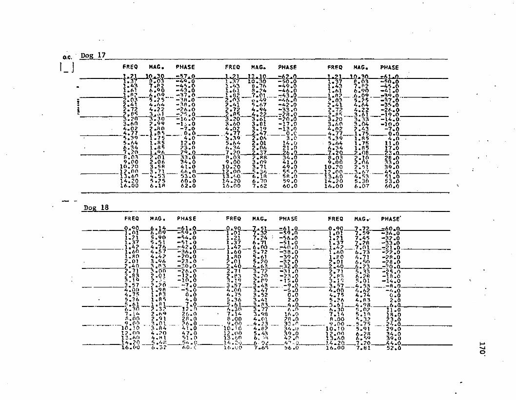
o.c.LJ

Dog 17FR EQ MAG. PH A SE FREO MAG. PHASE

h S M f c M7 . 8 21 . 4 36 . 9 06.09

2 . 4 1 4.662 . 7 2 4 . 2 2

2 . 9 93 . 6 04 . 0 2 7 . n o

6.391 . R 55 . 6 41 . 8 56 . 3 47,202 . 0 69 . 0 03 . 5 810.203 . 7 12.00 4.535 . 2 51 4 . 2 0

1 6 . 0 0 6 . 1 8

0 _ 1 . 2 1 1 2 . 1 0 - 6 2 . 00 1 . 3 7 1 0 . 3 0 - 5 0 . 00 1 . 4 3 8 . 7 6 - 4 9 . 00 1 . 6 1 8 . 7 4 - 4 6 . 00 1 . 0 2 7 . 0 1 . - 4 3 . 0 .0 2 . 0 3 o . 4 9 - 4 6 . 00 2 . 6 1 5 . 6 7 - 4 2 . 00 2 . 7 2 4 . 9 4 - 3 3 . 0

,0 2 . 8 5 4 . 2 2 r 2 8 . 0 _,0"" 3 . 2 0 3 . 6 1 - 2 0 . 00 3 . 6 0 3 . 8 1 - 1 7 . 0

,0 4 . 0 2 3 . 1 9 - 1 3 . 0, 0 . . 4 . 7 7 2 . 4 7 . . . 0 . 0 .,0 5 . 3 9 2 . 0 6 3 . 0,0 5 . 6 4 2 . 0 1 1 4 . 0,0 6 . 3 4 2 . 0 6 21 . 0

7 . 2 0 2 . 3 7 2 6 . 0,0 8 . 0 3 7 . B R 3 4 . 0.0 9 . 0 0 3 . 0 9 41 . 0,0 1 0 . 2 0 3 . 7 1 4 9 . 0. 0 ..... 1 2 . 0 0 —5 . 36 55 . 0.0 1 3 . 6 0 6 . in 5R . 0. 0 1 4 . 2 0 6 . 7 0 5 9 . 0.0 1 6 . 0 0 7 . 6 2 6 0 . 0

FREQ MAG. PHASE

1 .71 1 0 . 3 0 —61 . 01 . 3 7 e .03 - 5 0 . 01 . 4 3 7 . 8 2 - 4 5 . 01 . 6 1 6 . 9 0 - 4 1 . 01 . 8 2 . . 6 . 0 9 . - 3 9 - 02 . 0 3 5 . 7 5 - 3 7 . 02 . 4 1 4 . 6 4 - 3 5 . 02 . 7 2 4 . 2 2 - 2 6 . 02-8 5 3 . 6 1 _ - 1 9 . 03 . 2 0 3 . 3 3 - 1 4 . 0 .3 . 6 0 3 . 0 4 - 1 0 . 04 . 0 2 7 . 4 3 - 7 . 04 . 7 7 - 1 . 7 5 . . 0 . 05 . 3 9 1 . 8 5 4 . 05 . 6 4 1 . 7 5 11.06 . 3 4 1 . 8 5 1 7 . 07.70 __2 . 0 8 7 3 . 08 . 0 3 7 . 1 0 2 8 . 09 . 0 0 2 . 0 6 3 3 . 0

1 0 . 7 0 2.51 3 9 . 017.00 3.67.. 4 6 - 01 3 . 6 0 4 . 5 3 5 1 . 01 4 . 2 0 5 . 3 0 5 3 . 01 6 . 0 0 6.07 6 0 . 0

Dog 18FREQ MAG. PHASE FREQ MAG. PHASE0 . 9 0 6 . 1 4 - 6 1 . 0 0 . 9 0 7 . 5 1 - 6 1 . 01 . 0 1 6 . 0 9 - 5 9 . 0 1 . 0 1 7 . 3 2 - 5 9 . 01 . 2 1 5 . 9 0 - 5 4 . 0 1 . 2 1 7 . 2 4 ; - 5 6 . 01 . 3 7 5 . 5 1 - 5 1 . 0 1 . 3 7 6 . 7 1 - 5 1 . 01 . 4 ? 4 . 7 6 - 4 2 . 0 1.42. _ 6 . 0 0 - 4 0 . 0 .1 . 6 0 4 . 5 7 - 3 6 . 0 1 . 6 0 5 . 7 2 - 3 8 . 01 . 8 0 4 . 4 ? - 2 0 . 0 1 . 8 0 5 . 6 1 - 3 9 . 02 . 0 1 3 . 9 6 - 2 3 . 0 ' 2 . 0 1 5 . 7 0 - 3 2 . 02 . 4 0 3 . 8 3 - 7 0 . 0 2 . 4 0 4 . 6 3 - 3 2 . 02 . 7 1 3 . 0 0 - 2 6 . 0 2 . 7 1 3 . 7 ? - 3 1 . 02 . 9 3 2 . 0 1 - 1 2 . 0 2 . 8 3 3 . 2 0 - 2 3 . 03 . 1 0 •> - 1 0 . 0 3 . 1 9 2 . 8 9 - 1 5 . 03 . 5 7 . 7 . 2 0 - 7 . 0 3 . 5 7 . 3 . 4 3 - 9 . 04 . 0 0 I . 9 8 - 5 . 0 4 . 0 0 3 . 4 7 - 5 . 04 . 7 5 1 . P 3 0 . 0 4 . 7 5 3 . 5 2 0 . 05 . 3 6 1 . 8 6 4 . 0 5 . 3 6 3 . 4 1 2 . 06 . 6 1 1 . 8 1 . ...... 7 . 0 5 . 6 1 3 . 8 3 4 . 06 . 3 0 7 . 3 ? 1 2 . 0 6 . 3 0 3 . 7 7 6 . 07. -4 ? . 6 9 2 6 . 0 • 7 . 1 4 3 . 9 8 1 6 . 08 . 0 0 2 . 9 1 2 8 . 0 8 . 0 0 4 . 0 1 2 8 . 09 . 0 0 - . 3 . 0 1 . . 3 6 . 0 ... 9 .06 - 4 . 2 3 , . 3 3 . 0

1 0 . !0 3 . 8 4 4 1 . 0 1 0 . 1 0 4 . 8 ? 3 4 . t)1 2 . 0 0 4 . 2 0 4 7 . 0 1 2 . 0 0 5 . 4 3 3 9 . 01 2 . 6 0 4 . Hi 51 . 0 13 . 6 0 6 . "H 4 ? .01 4 . 2 0 4 . 4 8 54 . f: 1 4 . 2 0 6. 92 /,->. . i1 6 . 0 0 6 . 3 2 6 0- C 16.1 :0 7 . 6 8 5 6 . 0

FREQ MAG.- PHASE'0 . 9 0 7.72,. - 6 0 - 01 . 0 1 7 . 5 9 - 3 6 . 01 . 2 1 7 . 4 5 - 3 2 . 01 . 3 7 7 . 2 8 - 3 3 . 01 . 4 ? . . 7 . 0 1 . . - 2 1 - 0 . ..1 . 6 0 6 . 7 3 - 2 2 . 01 . 8 0 6 . 7 1 - 2 8 . 02 . 0 1 6 . 5 0 - 2 8 . 02 - 4 0 6 . 2 3 - ’ 0 . 02 . 7 1 5 . 3 3 - 2 5 . 02 . 8 3 6 . 2 8 - 1 8 . 03 . 1 5 5 . 0 1 - 1 4 . 03 . 5 7 , 4 . 5 3 . -8-04 . 0 0 4 . 6 2 - 4 . 04 . 7 5 4 . 7 4 0 . 05 . 3 6 4 . 8 3 2 . 0

i 5 - 6 1 -4 .98.. 6 - 06 . 3 0 5 . 0 ? 1 1 . 0

> 7 . 1 4 5 . 1 8 1 8 . 0> 8 . 0 0 5 . 3 2 2 3 . 09-00 - 5 . 7 5 24-01 1 0 . 1 0 5 . 9 1 2 9 . 01 1 2 . 0 0 6 . 2 8 3 4 . 0■ 1 3 . 6 0 6 . 5 9 3 9 . 014-20 - 7 . 2 0 4 4 - 0» 1 6 . 0 0 7 . 8 1 5 2 . 0

170

171

LIST OF REFERENCES

1. Rohrer,F., Der Stroraungswiderstand In den menschlichen Atemwegen und der Elnfluss der unregelmassigen Verzweigung des Bronchialsysterns auf den Atmungsverlauf in Verschiedenen Lungenbezirken. Arch. f.d. ges., 162: 225, 1915.

2. Neergaard, K. Von, and Wirz, K. Uber eine Methode Zur Messung derLungenelastizitat am lebenden Menschen, inbesondere beim Emphysem.Z. Klin. Med. 105: 35-50, 1927.

3. Bayliss, L.E., and G.W. Robertson. The visco-elastic properties ofthe luns. Quart. J. Exper. Physiol. 29: 27, 1939.

4. Fry, D.L., W.W. Stead, R.V. Ebert, and C.C. Brown. The mechanicsof pulmonary ventilation in normal subjects and in patients withemphysema. Am. J. Med. 16: 80, 1954.

5. Mcllory, M.B., J. Mead, N.J. Selverstone, E.P. Radford. Measurement of lung tissue viscous resistance using gases of equal kinematic viscosity. J. Appl. Physiol. 17: 485, 1955.

6. Dean, R.B. and M.B. Visscher. Kinetics of lung ventilation. Am. J. Physiol. 134: 450, 1941.

7. Mcllory, M.D. and R.V. Christie. Clin. Sc. 131: 147, 1954.

8. Von Neergaard, K. and K. Wirz. Die Messung der stromungswiderstandein den Atemwegen des Menschen inbesondere bei Asthma und Emphysema. Ztschr. F. Klin. Med. 105: 52, 1927.

9. Vuilleumier, P. Ztschr. f. Klin. Med. 143: 698, 1944.10. Otis, A.B. and D.F. Proctor. Measurement of alveolar pressure in

man. Am. J. Physiol. 152: 106,. 1948.

11. Mead, J. and J.L. Whittenberger. J. Appl. Physiol. 5: 779, 1953.

12. DuBois, A.B., S.Y. Botelho, and J.H. Comroe, Jr. A new method for measuring airway resistance in man using a body plethysmograph: values in normal subjects and in patients with respiratory disease. J. Clin. Invest. 35: 327, 1956.

17213. Varene, P. and C. Jacquemin, Plethysmographic measurement of the

Impedance of the gaseous ventilation system. Prog. Resp. Res. 4: 88-101, 1969.

14. Smidt, V., K. Mugsers, and W. Buchheim. Electronic compensation of differences in temperature and water vapour between in- and expired air and other signal handling in body plethysmography.Prog. Resp. Res. 4: 39-49, 1969.

15. Bargeton, D. and G. Barres. Time characteristics and frequency response of body plethysmograph. Prog. Resp. Res. 4: 2-23, 1969.

16. Chester, E.H., L.E. Ostrander, J.B.Franck, and D.E. Niewoehner. Influence of breathing rate on airway resistance and compliance measurements. Respiration Physiology 20: 337, 1974.

17. Mead, J., M.B. Mcllory, N.J. Selverstone, and B.C. Krieke. J. Appl. Physiol. 7: 491, 1955.

18. Petit, J.M., and J. Milic-Emili. Measurement of endoesophageal pressure. J. Appl. Physiol. 13: 481, 1958.

19. Frank, N.R., J. Mead, A.A. Siebens, and C.F. Storey. J. Appl. Physiol. 9: 38, 1956.

20. Knomles, J.H., S.K. Hong, and H. Rahn. Possible errors using esophageal balloon in determination of pressure-volume characteristics of the lung and thoracic cage. J. Appl. Physiol. 14:525, 1959.

21. Linderholm, H. Lung mechanics in sitting and horizontal postures studied by body plethysmographic methods. Am. J. Physiol. 204:85, 1963.

22. Milic-Emili, J., J. Mead, and J.M. Turner. Topography of esophageal pressure as a function of posture in man. J. Appl. Physiol. 19(2): 212-216, 1964.

23. Mead, J., and J.L. Whittenberger. Physical properties of human lungs measured during spontaneous respiration. J. Appl. Physiol.5: 779-796, 1953.

24. Marshall, R. Objective tests of respiratory mechanics. In: Handbook of Physiology. Respiration. Washington, D.C.: Am. Physiol. Soc., 1965, sect. 3, Vol. II, Chapt. 55, p. 1404-1405.

25. DuBois, A.B., A.W. Brody, D.H. , Lewis, and B.F. Burgess, Jr. Oscillation mechanics of lungs and chest in man. J. Appl. Physiol. 8: 587, 1956.

173

26. Mead, J. Control of respiratory frequency. J. Appl. Physiol. 15: 325, 1960.

27. Fisher, A.B., A.B. DuBois, and R.W. Hyde. Evaluation of the forced oscillation technique for the determination of resistance of breathing. J. Clin. Invest. 47: 2045, 1968.

28. Grimby, G., T. Takishima, W. Graham, P. Machlem, and J. Mead.Frequency dependence of flow resistance in patients with obstructive lung disease. J. Clin. Invest. 47: 1455, 1968.

29. Goldman, M., R.J. Knudson, J. Mead, N. Peterson, J.R. Schwaber, andM.E. Wohl. A simplified measurement of respiratory resistanceby forced oscillation. J. Appl. Physiol. 28(1): 113-116, 1970.

30. Michaelson, E.D., E.D. Grassman, and W.R. Peters. Pulmonary mechanics by spectral analysis of forced random noise. J. Clin. Invest. 56: 1210-1230, 1975.

31. Sunderland, R. A practical design of an instrument for measuring respiratory resistance by forced oscillation. M.S. Thesis, Ohio State University.

32. Pimmel et al. Proceeding of the 27th ACEMB, p. 18, 1974.

33. Brody, A.W., A.B. DuBois, 0.1. Nissel, and J. Engelberg. Natural frequency, damping factor, and inertance of the chest-lung system in cats. Am. J. Physiol. 186: 142-148, 1956.

34. Hilberman, M., R.W. Stacy, and R.M. Peters. A phase method of calculating respiratory mechanics using a digital computer. J. Appl. Physiol. 32(4): 535-541, 1972.

35. Bekey, G.A. System identification - an introduction and a survey. Simulation, pp. 151-166, Oct., 1971.

36. Astrom, K.J. and P. Eykhoff. System identification - A survey. Automatica 7: 123-162, 1971.

37. Pimmel, R.L. Impedance analysis of a respiratory model that includes airway compliance and central and peripheral airway resistance, submitted to IEEE Transaction on Biomedical Engineering.

38. Briscoe, W.B. and A.B. DuBois. The relationship between airway resistance, airway conduction and lung volume in subjects of different age and body size. J. Clin. Invest. 37: 1279-1285, 1958.

39. Mead, J. Volume displacement body plethymograph for respiratory measurements in human subjects. J. Appl. Physiol. 15: 736-740,1960.

174

40. Leith, D.E. and J. Mead. Principles of body plethysmograph. Report of the NHLI. Div. of Lung Disease. Nov., 1974.

41. Milic-Emili, J., J. Mead, J.M. Turner and E.M. Glauser. Improvedtechnique for estimating pleural pressure from esophageal pressure. J. Appl. Physiol. 19: 207-211, 1964.

42. Dennis, M.W., J.S. Douglas, J.U. Casby, J.A.J. stolwijk and A. Bouhuys. On-line analog computer for dynamic lung compliance and pulmonary resistance. J. Appl. Physiol. 26: 248-252, 1969.

43. Murphy, B.G., J. Dosman, F. Bode and P.T. Macklem. A dynamic compliance computer: comparison of on-line results with manual calculations in man. J. Appl. Physiol. 36: 629-633, 1974.

44. Mead, J. and J. Milli-Emili. Theory and methodology in respiratorymechanics with glossary of symbols. Handbook of Physiol. Sect.3, Vol. 1, p. 363, 1964.

45. Otis, A.B., Colin B. Mckerrow, Richard A. Bartlett, Jere Mead,M.B. Mcllroy, N.J. Selverstone and E.P. Radford. J. Appl. Physiol. 8: 427-443, 1956.

46. Mead, J. Contribution of compliance of airways to frequency- dependent behavior of lungs. J. Appl. Physiol. 26: 670-673, 1969.

47. Woolcock, A.J., N.J. Vincent and Peter T. Macklem. Frequency dependence of compliance as a test for obstruction in the small airways. J. Clin. Invest. 48: 1097, 1969.

48. Peslin, R., C. Durivier, and J.M. Lambert. Repouse en frequence du systeme mecanique ventilatoire total de 3 A 70 Hz. Bull. Physiol-Pathol. Respir. 8: 267-297, 1972.

49. Vincent, Norma J., R. Knudson, D.E. Leith, Peter T. Macklem, and J. Mead. Factors influencing pulmonary resistance. J. Appl. Physiol. 29: 236-243, 1970.

50. Hull, W.E. and E.C. Long. Respiratory impedance and volume flow at high frequency in dogs. J. Appl. Physiol. 16: 439-443, 1961.

51. Marshall, R., and A.B. DuBois. The measurement of viscous resistance of the lung tissues in normal man. Clin. Sci. 15: 161-170, 1956.

52. Jackson, A.C., H.T. Milhorn, Jr., and J.R. Norman. A re-evaluation of the interrupter technique for airway resistance measurement.J. Appl. Physiol. 36(2): 264-268, 1974.

175

53. Daly, W.J. and S Bonduraut. Direct measurement of respiratory pleural pressure changes in man. J. Appl. Physiol. 18: 513-518,1963.

54. Ostrander, Lee E., Edward II. Chester, and Jead-Bernard Franck. Fundamental frequency analysis of pulmonary mechanical resistance and compliance. J. Appl. Physiol. 35(4): 526-537, 1973.

55. Otis, A.B., W.O. Fenn and H. Rahn. J. Appl. Physiol. 2: 592, 1950.56. McGhee, R.B. Some parameter optimization techniques (chapter 48)

in Digital Computer User's Handbook, New York, McGraw-Hill, 1967.

57. McGhee, R.B. Identification of nonlinear dynamic systems byregression analysis methods. Ph.D. dissertation, University of Southern California, 1963.

58. Radford, E.P., Jr. Static mechanical properties of mammalianlungs. Handbook of Physiology, Sect. 3, Vol. 1, p. 429, 1964.

59. DuBois A.B. Resistance to breathing. Handbook of Physiology,Sect. 3, Vol. 1, p. 451, 1964.

60. Briscoe, W.A. and A.B. DuBois. The relationship between airwayresistance, airway conductance and lung volume in subjects of different age and body size. J. Clin. Invest. 37: 1279-1285, 1958.

61. Bose, A.G. and K.N. Stevens. Introductory Network Theory. NewYork, Harper & Row, 1965.

62. Olson, H.F. Dynamical Analogies. Princeton: D. Van Nostrand Co.,Inc., 1958.

63. Blesser, W.B. A Systems Approach to Biomedicine. McGraw-Hill,1969. pp. 82-85.

64. Vander, A.J., J.H. Sherman, and D.S. Luciano. Human Physiology.McGraw-Hill, 1970. Chapt. 11.

65. Peters, R.M. The Mechanical Basis of Respiration. Little andBrown, 1969. Chapt. 4.

66. Julius H. Comroe. Physiology of Respiration. Year Book MedicalPublisher, 1965.

67. Chan-Chan-Chan. Analysis of Linear Networks and Systems. Addison- Wesley, 1972.

68. Hogg, J.C., P.T. Macklem, and W.M. Thurlbeck. The resistance ofcollateral channels in exercised human lungs. J. Clin. Invest.48: 421r-431, 1969.

176

69. Takahashi, T. Mathematics of Automatic Control. English edition. Holt, Rinehart, and Winston, 1966.

70. P.-T. Machlem and J. Mead. Resistance of central and peripheral airways by a retrograde catheter. J. Appl. Physiol. 22 : 395-401, 1967.

71. Robinson, D.J., H.B. Williams, and R.L. Pimmel. Characterizing respiratory mechanics with the forced sinusoidal impedance, p. 403, 28th ACEMB, 1975.

72. Chamberlain, R.L., D. Jowett. The OMNITAB Programming System, A Guide for Users. Statistical Lab., Iowa State University.

73. Goldstein, A. Biostatistics: An Introductory Text. New York, Mac- Millian, 1964. pp. 59-61.

74. Robinson, D.J. Personal Communications. Biomedical Engineering Center, The Ohio State University.

75. Tyler, W.S. et al. Structural analogues of the respiratory system. Arch. Enviromental Health 14: 62, 1967.

76. Agostoni, E., F.F. Thimn and W.D. Fenn. Comparative features ofthe mechanics of breathing. J. Appl. Physiol. 14(5): 679-683, 1959.

77. Radford, E.P. Recent studies of mechanical properties in mammalian lungs. In tissue elasticity, pp. 177-189. American Physiology Society, 1957.

78. Crosfill, M.L. and J.G. Widdicombe. Physical characteristics ofthe chest and lungs and the work of breathing in different mammalianspecies. J. Physiol. 158: 1-14, 1961.

79. Brown, R. eit jal. Physiological effects of experimental airway obstruction with beads. J. Appl. Physiol. 27(3): 328-335, 1969.

80. Tsai, M.J., R.B. McGhee, R.L. Pimmel, and R.A. Bromberg. An evaluation of a numerical technique for recovering ventilation-perfusion ratios, p. 492, 28th ACEMB, 1975.

81. Shah, B.V., R.J. Buehler, and G. Kempthorne. Some algorithms forminimizing a function of several variables. J. Soc. Ind. Appl.Math. 12: 74-92, March 1964.

82. Fletcher, R., M.J. Powell. A rapidly converging descent method for minimization. Computer Journal 6: 163-168. 1963.

83. Rust, B.W. and W.R. Burrus. Mathematical Programming and the Numerical Solution of Linear Equations. Elsevier, 1972.

17784. Draper, N.R. and H. Smith. Applied Regression Analysis. John Wiley

and Sons, New York, 1966.85. Hogg, R.V. and A.T. Craig. Introduction to Mathematical Statistics.

McMillian, 1970.86. Hartley, H.O. The modified Guass-Newton method for fitting of

nonlinear regression functions by least squares. Technometrics 3(2): 269-280, May 1961.

87. Williams, E.J. Regression Analysis. John Wiley and Sons, Inc.,New York, 1959.

88. Mendel, J.M. Discrete Techniques of Parameter Estimation. Marcel Dekker, Inc., New York, 1973.

89. Spang, H.A. A review of minimization techniques for nonlinear functions. SIAM Review, vol. 4, no. 4, pp. 343-365, Oct. 1962.

90. Bromberg, N.S. Maximization and minimization of complicated multi- variable functions. AIEE transactions, Vol. 58, Part 1, pp. 725- 730, Jan. 1962.

91. Rosen, J.B. The gradient projection method for nonlinear programming, Part II, noplinear constraints. J. Soc. Indust. Appl. Math., Vol. 9, no. 4, pp. 514-532, Dec. 1961.

92. Rosen, J.B. The gradient projection method for nonlinear programming, Part I, linear constraints. J. Soc. Indust. Appl. Math.,Vol. 8, no. 1, pp. 181-217, March 1960.

93. Kirk, D.E. Optimal Control Theory. Printice-Hall Inc., New Jersey,1970.

94. Marquardt, D.W. An algorithm for least squares estimation of nonlinear parameters. J. Soc. Indust. Appl. Math., Vol. 2, pp. 431- 441, 1963.

95. Brooks, S.H. A discussion of random methods for seeking maxima. Computer Journal, Vol. 6, no. 2, 1958.

96. Korn, G.A. Random Process Simulation and Measurements. McGraw- Hill, New York, 1966.

97. White, R.C., Jr. A survey of random methods for parameters optimization. Simulation, pp. 197-205, Nov. 1971.

98. Gillespie, D.J., and R.E. Hyatt. Respiratory mechanics in the unanesthetized dog. J. Appl. Physiol. 36(1): 98-102, 1974.

178

99. Dain, D„ and W.M. Gold. Mechanical properties of the lungs and experimental asthma in conscious allergic dogs. J. Appl. Physiol. 38(1)° 96-100, 1975.

100. Hickey, R.F., P.D. Graf, J.A. Nadel, and C.P. Larson. The effects of halothane and cyclopropane on total pulmonary resistance in the dog. Anesthesiology 31: 334-343, 1969.

101. Woolcock, A.J., P.T. Macklem, J.C. Hogg, N.J. Wilson, J.A. Nadel,N.R. Frank, and J. Brain. Effect of vagal stimulation on central and peripheral airways in dogs. J. Appl. Physiol. 26: 806-813,1969.

102. Mead, J. and C. Collier. Relation of volume history of lungs to respiratory mechanics in anesthetized dogs. J. Appl. Physiol. 14 : 669-678, 1959.

103. Collier, C.R. and J. Mead. Pulmonary exchange as related to altered pulmonary mechanics in anesthetized dogs. J. Appl. Physiol. 19: 659-664, 1964.

104. Sharp, J.T., J.P. Henry, S.K. Sweany, W.R. Meadows, and R.J. Pietras. Effect of mass loading the respiratory system in man. J. Appl. Physiol. 19(5): 959-966, 1964.

105. Ting, E.Y. Ventilatory mechanics during thoracoabdominal compression. Federation Proc. 20: 420, 1961.

106. Watson, J.F., N.S. Cherniack, and F.W. Zechman. Respiratory mechanics during forward acceleration. J. Clin. Invest. 39: 1737-1743, 1960.

107. Hong, S.K., E.Y. Ting, and H. Rahn. Lung volume at different depths of submersion. J. Appl. Physiol. 15: 550-553, 1960.

108. Barach, A.L. Use of helium as a new therapeutic gas. Prov. Soc. Exper. Biol, and Med. 32: 462, 1934.

109. Barach, A.L. Effects of inhalation of helium mixed oxygen on the mechanics of respiration. J. Clin. Invest. 15: 47-61, 1936.

110. Maio, D.A. and L.I. Farhi. Effect of gas density on mechanics of breathing. J. Appl. Physiol. 23: 687-693, 1968.

111. Jaffrin, M.Y. and P. Kesic. Airway resistance: a fluid mechanical approach. J. Appl. Physiol. 36(3): 354-361, 1974.

112. Ferris, B.G., Jr., J. Mead, and L.H. Opie. Partitioning of respiratory flow resistance in man. J. Appl. Physiol. 19(4): 653-658,1964.

179

113. Peslin, R,, J. Papon, C. Duvivler, and J. Richalct. Frequencyresponse of the chestr modeling and parameter estimation. J. Appl. Physiol, 39(4): 523-534, 1975.

RESPIRATORY PARAMETER ESTIMATION USING FORCED ...

Documents

Transcript of RESPIRATORY PARAMETER ESTIMATION USING FORCED ...