A Parsimonious Bootstrap Method to Model Natural Inflow Energy Series

Research ArticleA Parsimonious Bootstrap Method to ModelNatural Inflow Energy Series

Fernando Luiz Cyrino Oliveira,1 Pedro Guilherme Costa Ferreira,2

and Reinaldo Castro Souza3

1 Department of Industrial Engineering, Pontifical Catholic University of Rio de Janeiro (PUC-Rio), Rua Marques de Sao Vicente 225,Gavea, 22451-900 Rio de Janeiro, RJ, Brazil

2 Brazilian Institute of Economics (IBRE-FGV), Rua Barao de Itambi 60, Botafogo, 22231-000 Rio de Janeiro, RJ, Brazil3 Department of Electrical Engineering and Postgraduate Metrology for Quality and Innovation Programme,Pontifical Catholic University of Rio de Janeiro (PUC-Rio), Rua Marques de Sao Vicente 225, Gavea,22451-900 Rio de Janeiro, RJ, Brazil

Correspondence should be addressed to Fernando Luiz Cyrino Oliveira; [email protected]

Received 19 June 2013; Revised 22 September 2013; Accepted 23 September 2013; Published 12 January 2014

Academic Editor: Youqing Wang

Copyright © 2014 Fernando Luiz Cyrino Oliveira et al. This is an open access article distributed under the Creative CommonsAttribution License, which permits unrestricted use, distribution, and reproduction in any medium, provided the original work isproperly cited.

The Brazilian energy generation and transmission system is quite peculiar in its dimension and characteristics. As such, it canbe considered unique in the world. It is a high dimension hydrothermal system with huge participation of hydro plants. Suchstrong dependency on hydrological regimes implies uncertainties related to the energetic planning, requiring adequate modelingof the hydrological time series. This is carried out via stochastic simulations of monthly inflow series using the family of PeriodicAutoregressivemodels, PAR(p), one for each period (month) of the year. In this paper it is shown the problems in fitting thesemodelsby the current system, particularly the identification of the autoregressive order “p” and the corresponding parameter estimation. Itis followed by a proposal of a new approach to set both themodel order and the parameters estimation of the PAR(p)models, using anonparametric computational technique, known as Bootstrap.This technique allows the estimation of reliable confidence intervalsfor the model parameters. The obtained results using the Parsimonious Bootstrap Method of Moments (PBMOM) produced notonly more parsimonious model orders but also adherent stochastic scenarios and, in the long range, lead to a better use of waterresources in the energy operation planning.

1. Introduction

The Brazilian electrical energy production and transmissionsystem is unique in the world, due to its continental dimen-sion and the strong participation of hydro plants (about 80%of the energy produced in the country comes from hydroplants with various owners). The national grid, also knownas National Interconnected System (NIS from now on)embodies generation utilities of the following geographicalregions: Southeast/Midwest, South, Northeast, and North.Only 3.4%of the generated energy in Brazil is outside the poolof the NIS; they are formed by isolated generators located,mainly, in the Amazonas region [1].

It is well known that generation systemswith strong hydroshare are highly dependent on the hydrological regimes.Therefore, the energy operational planning consists of deter-mining what would be the optimal amount of hydro andthermal generation for the planning horizon, that meets theprojected demand and takes into account the constraints ofthe generation plants as well as the electrical constraints ofthe system [2].

As a consequence of this strong hydrological dependence,the uncertainty associated with the energy planning in Brazilrequires the use of robust and reliable stochastic modeling ofthe hydrological time series. Hence, the need of generating

Hindawi Publishing CorporationMathematical Problems in EngineeringVolume 2014, Article ID 158689, 10 pageshttp://dx.doi.org/10.1155/2014/158689

http://dx.doi.org/10.1155/2014/158689

2 Mathematical Problems in Engineering

syntheticseries from such stochastic models is required inorder to produce the optimal operating costs and, at the sametime, to increase the reliability of the system as a whole [3].

The energy planning in Brazil is carried out via a chainof mathematical model sand corresponding computer pro-grams, aiming at producing the optimal operation and expan-sion programs [4].

The medium range operation computer program used inthe country is the so-calledNEWAVE.This software producesfor eachmonth of the planning horizon (thatmay vary from 5to 10 years, on amonthly basis) the optimal share of hydro andthermal resources that minimize the expected operationalcosts of the system. The hydro plants are represented in anaggregate manner and the estimation of the optimal opera-tional policy is carried out via a Stochastic Dynamic DualProgramming (SDDP from now on) [5].

To produce the optimal policy, NEWAVE considers arange of scenarios of energy inflows, all of them obtained bystochastic simulations having as the base models the PeriodicAutoregressive structure, PAR(𝑝) models, one for eachmonth of the year. The problem formulation is based onequivalent energy systems, that is, the four geographical sub-systems that constitute the NIS. In this approach, the hydrological series are transformed into Natural Inflow Energy(NIE, for short) [6].

This way, the stochastic models employed to generatehydrological scenarios to be used by NEWAVE should pre-serve, as close as possible, the main features of the historicalrecords, in order to guarantee that the produced optimalpolicy is reliable and satisfactory. In this paper, it is shownthat the current approach to set the order and the parametersestimates of the PAR(𝑝) structures is, somehow, limited andmay be improved. Indeed, the existing approach tends toidentify less parsimoniousAR structures and the correspond-ing parameters are estimated by the classical method ofmoments.Theproposed improvement described in this paperuses a nonparametric technique, known as Bootstrap, whichallows, among other facilities, the estimation of more reliableconfidence intervals for the model parameters. The datasetused in this paper corresponds to four monthly NIE timeseries related to the four regions of the country (subsystemsSoutheast/Midwest, South, Northeast, and North), coveringthe period ranging from January 1931 to December 2010.

The remaining part of the paper is organized as follows.Section 2 presents a short overview of the existing approachesto model NIE series, including the current approach used inthe Brazilian Electrical System (BES), which is, in a sense, themain criticism of the paper. It is then followed by Section 3where the proposed use of Bootstrap as an improvement toolto the existing model is thoroughly described. Finally, in thelast section, the main results are presented and discussed,followed by suggestions for future researches on the subject.

2. Modeling NIE Series: A Review includingthe Model in Current Use in Brazil

According to [7], the time series models applied to hydro-logical series are an important tool for the planning and

the operation of hydrothermal systems. There are a greatnumber of papers in the specialized literature dealing withthis problem for all possible types of time series observations,that is, yearly, monthly, weekly, daily, and so forth.

Among the models cited in the literature, the followingare the most used: (i) AutoregressiveMoving Average ARMA(𝑝, 𝑞); (ii) Pure Autoregressive AR(𝑝); (iii) MultivariateAutoregressive Moving AverageMARMA(𝑝, 𝑞); (iv) PeriodicARMA(𝑝, 𝑞), (v) Periodic Autoregressive PAR(𝑝); (vi)Autoregressive Fractional Integrated Moving AverageARFIMA(𝑝, 𝑑, 𝑞); (vii) Gamma Autoregressive GAR(𝑝);(viii) Periodic Additive Autoregressive Gamma PAGAR(𝑝);(ix) Periodic Multiplicative Autoregressive Gamma PMGAR(𝑝); (x) Periodic Autoregressive Gamma PGAR(𝑝).

Concerning the use of the Box & Jenkins family of mod-els, in particular the AR structures, they can be consideredas the pioneers to model hydrological series. Indeed [8] pro-posed an AR(1) tomodel inflows and [9] used a similar struc-ture to model monthly rainfall in Australian rivers coveringthe period from 1859 to 1952.

After these pioneer proposals, the following works on thearea were related to improvements in their applications tohydrology problems as, for instance, in the models identifica-tion structure and parameters estimations. Some importantpapers using AR(𝑝) and ARMA(𝑝, 𝑞) structures to modeldaily, monthly, and yearly hydrological series were published,such as [7, 10–16]. In the case of the two contributions byBeard mentioned above, it is addressed the question relatedto the inflow simulations for a particular inflow station andthe extension of this result to more than one inflow stationthat may have a correlation structure among them.

More recently, [17] uses the AR(𝑝) and ARMA(𝑝, 𝑞)structures to model the average monthly inflows of Goksuriver, located in the Southern region of Turkey. The inter-esting aspect dealt by the author is the use of three possibleways to arrive at the model structure identification: via theAutocorrelation Function, Minimum Residual Variance, andthe Akaike Information Criterion. Such analysis showed thatit should be considered more than one approach to select themodel order, differently of what is used in the BES that usesonly one structural identification method.

Concerning the periodic class of models, the emphasishas been put on the PAR(𝑝) and PARMA(𝑝, 𝑞) structures.The PAR(𝑝) structure fits a single AR(𝑝) to each period ofthe series and, similarly, a PARMA(𝑝, 𝑞) structure fits anARMA(𝑝, 𝑞) structure to each period of the series.

The extension fromPAR(𝑝) into PARMA(𝑝, 𝑞) structuresis not trivial, as pointed out by [18]. Besides, it is also men-tioned that the PAR(𝑝) structures have produced rather goodfit to hydrological series and this would not encourage the useof more elaborated structures, such as PARMA(𝑝, 𝑞). How-ever, one can find in the literature a considerable number ofpapers where the adopted structure was the more elaboratedPARMA(𝑝, 𝑞) as, for instance, the works by [16, 19–22]. Par-ticularly, in [22] the author presents two possible ways tomake the parameters estimation: via Method of Moments

Mathematical Problems in Engineering 3

(MOM) and via Maximum Likelihood (ML) and concludedthat the latter produces better results than the former. Onthe other hand, [19] proposes an alternative way to estimatethe model parameters of a PARMA(𝑝, 𝑞) model through amore parsimonious formulation and apply the approach to amonthly inflow series of Frazer river (British Columbia) andSalt river (Arizona).

In Brazil, the paper by [23] is themain reference concern-ing the production of weekly forecasts based on ARMA(𝑝, 𝑞)models, considering periodic and nonperiodic parameters.They use the software PREVIVAZ [24], developed by CEPEL(Brazilian Electrical Research Center) [25] and used by ONS,the BrazilianNational SystemOperator [1], on the nationwideoperation planning.

The model used in the BES to produce the NIE scenar-ios is the Periodic Autoregressive PAR(𝑝) structure. Thesescenarios are used in a SDDP, that produces the Cost toGo Functions [26, 27]. As a result of this approach adoptedofficially in Brazil, a large number of papers have beendevoted to the subject, discussing and proposing alternativesto improve this statistical procedure.

Although the use of PAR(𝑝) models has been widely usedin Brazil, it is important to bear in mind that they were firstproposed by [8] and have been discussed ever since in theinternational literature; see, for instance [28, 29], that havemade substantial contributions to the implementation of suchmodels. Also it is important to mention the contributions ofother authors on the discussion concerning the best way toestimate the model parameters (Method of Moment, Max-imum Likelihood, and Bayesian Inference Methods, amongothers) [16, 22, 30].

Therefore, this paper aims to propose methodologicaladvances in the PAR(𝑝) model regarding the structure iden-tification and the model parameters estimation.

2.1. The PAR(𝑝) Model. Assuming that a time series is com-posed of 𝑛 years and 𝑠 seasonal periods of observations (inthis work, 𝑠 = 12months) and that 𝑌

𝑟,𝑚is a realization of this

series in year 𝑟 and month 𝑚 (𝑟 = 1, 2, . . . 𝑛; 𝑚 = 1, 2, . . . , 𝑠),the Periodic Autoregressive model, PAR(𝑝), where 𝑝 is themodel order (𝑝 = 𝑝

1, 𝑝2, . . . , 𝑝

𝑚), obtained by assuming a

simple AR structure for each seasonal period. The analyticalexpression for the PAR(𝑝) model is given by

𝑌𝑚,𝑟

− 𝜇𝑚=

𝑝𝑚

∑

𝑖=1

𝜙𝑚

𝑖(𝑌𝑚−𝑖,𝑟

− 𝜇𝑚−𝑖

) + 𝑎𝑚. (1)

𝜇𝑚: expected mean for seasonal period𝑚.

𝜑𝑚

𝑖: 𝑖th autoregressive coefficient for seasonal period

𝑚.𝑎𝑚: independent noise series with zero mean and

variance 𝜎2𝑎𝑚

for seasonal period𝑚.

Denoting 𝜌𝑚𝑘as the correlation between 𝑌

𝑚,𝑟and 𝑌

𝑚−𝑘,𝑟,

and considering that (1) is an autoregressive model of the Box& Jenkins family, the parametric estimation can be conducted

by solving the Yule-Walker system [31]. For any period𝑚 wehave

[[[[[[[[[

[

1 𝜌𝑚−1

1𝜌𝑚−1

2⋅ ⋅ ⋅ 𝜌𝑚−1

𝑝𝑚−1

𝜌𝑚−1

11 𝜌

𝑚−2

1⋅ ⋅ ⋅ 𝜌𝑚−2

𝑝𝑚−2

𝜌𝑚−1

2𝜌𝑚−2

11 ⋅ ⋅ ⋅ 𝜌

𝑚−3

𝑝𝑚−3

......

... ⋅ ⋅ ⋅...

𝜌𝑚−1

𝑝𝑚−1

𝜌𝑚−2

𝑝𝑚−2

𝜌𝑚−3

𝑝𝑚−3

⋅ ⋅ ⋅ 1

]]]]]]]]]

]

[[[[[[[[[

[

𝜙𝑚

1

𝜙𝑚

2

𝜙𝑚

3

...𝜙𝑚

𝑝𝑚

]]]]]]]]]

]

=

[[[[[[[[[

[

𝜌𝑚

1

𝜌𝑚

2

𝜌𝑚

3

...𝜌𝑚

𝑝𝑚

]]]]]]]]]

]

. (2)

Denoting by 𝜙𝑚𝑘𝑗

the 𝑗th autoregressive parameter of aprocess of order 𝑘, 𝜙𝑚

𝑘𝑗is the last parameter in this process.

The Yule-Walker equations to each period𝑚 can be rewrittenas follows:

[[[[[[[

[

1 𝜌𝑚−1

1𝜌𝑚−1

2⋅ ⋅ ⋅ 𝜌𝑚−1

𝑘−1

𝜌𝑚−1

11 𝜌

𝑚−2

1⋅ ⋅ ⋅ 𝜌𝑚−2

𝑘−2

𝜌𝑚−1

2𝜌𝑚−2

11 ⋅ ⋅ ⋅ 𝜌

𝑚−3

𝑘−3

......

... ⋅ ⋅ ⋅...

𝜌𝑚−1

𝑘−1𝜌𝑚−2

𝑘−2𝜌𝑚−3

𝑘−3⋅ ⋅ ⋅ 1

]]]]]]]

]

[[[[[[

[

𝜙𝑚

𝑘1

𝜙𝑚

𝑘2

𝜙𝑚

𝑘3

...𝜙𝑚

𝑘𝑘

]]]]]]

]

=

[[[[[[

[

𝜌𝑚

1

𝜌𝑚

𝑘2

𝜌𝑚

𝑘3

...𝜌𝑚

𝑘𝑘

]]]]]]

]

. (3)

If the model orders were previously known, the param-eters could be obtained directly by solving the equationsystem (3). However, as one has to first identify the orderof the model, the system (3) can be solved sequentially foreach value of 𝑝

𝑚, obtaining the values for the parameters

𝜙𝑚

𝑝𝑚,1⋅ ⋅ ⋅ 𝜙𝑚

𝑝𝑚,𝑝𝑚

for each model order 𝑝𝑚.

At this stage, it is important to discuss some questionsregarding the model identification and parameters estima-tion. Concerning the identification of the model order, it isusually used the 95% confidence interval for 𝜙𝑚

𝑘,𝑘given by the

asymptotic result 1.96/𝑁, where𝑁 is the number of years ofthe time series. Such asymptotic interval was proposed by [32,33]. In [34], the authors defined a Quasi White Noise processfor series with this asymptotic approximation. This studywas further developed by [35] for Periodic Autoregressivestructures.

In practical terms, there are various ways to identify theBox & Jenkins model structure. One possible way consists ofincrementing the value of 𝑝

𝑚, starting from 1 until a value

“𝑘+1,” for which the parameter𝜙𝑚𝑘+1,𝑘+1

is nomore significant.In this case, the last value of 𝑝

𝑚for which 𝜙𝑚

𝑝𝑚,𝑝𝑚

is significantwill be the model order; that is, 𝑝

𝑚= 𝑘. The model

parameters become 𝜙𝑚𝑘,1⋅ ⋅ ⋅ 𝜙𝑚

𝑘,𝑘.This criterion will be referred

to here as “left to right” identification procedure (LR fromnow on).

The second possibility, that is, “right to left” identificationprocedure (RL from now on), as opposed to what happenswith the LR procedure is such that the order of the modelis defined as the value 𝑘∗ such that, for all 𝑘 > 𝑘

∗, 𝜙𝑚𝑘𝑘

isnot significant. As an example, if the Partial AutocorrelationFunction (PACF) shows that the lag 6 is significant and forall lags greater than 6 is not significant, the identified orderwill be 6, even if intermediate values for the parameters 𝜙𝑚

𝑘𝑘

are nonsignificant. In actual fact, this is the way the modelorders are identified in the current BES implemented in theNEWAVE computer system.


Table 1: Methods tested.

Method Structural identification Parameters estimation

MOM-RLPAFC asymptotic confidence interval.Criterion: for a period𝑚, the procedure looks for the largest order 𝑖 so that all 𝜙𝑚

𝑘𝑘

estimations for 𝑘 > 𝑖 are not significant.

MOM(point estimates)

BMOM-RL PACF Bootstrap confidence interval for each lag.Criterion: the same as that of MOM-RL.


MOM-LRPAFC asymptotic confidence interval.Criterion: for a periodm, the procedure looks for the largest order i so that all 𝜙𝑚

𝑘𝑘

estimations for 𝑘 < 𝑖 are significant. This criterion does not admit nonsignificantintermediary lags.


PBMOM PACF Bootstrap confidence interval for each lag.Criterion: the same as that of MOM-LR.

MOM(Bootstrap confidence intervals)

A third way to identify the PAR(𝑝) model order wasproposed recently by [35]. The authors use the resamplingtechnique known as Bootstrap to arrive at the model orderidentification. It was observed that the proposed Bootstrapbased approach produces results very close to that of the LRmethod.

Another possibility, mentioned in the appropriate litera-ture, is theminimization of some information criteria to iden-tify the model order. The most cited criteria are the AkaikeInformation Criterion [36] and Schwarrz Criterion [37]. Theadvantage of this approach is the equilibrium between thefitted model and the model parameter parsimony. In the spe-cific case of using these criteria for time series, the estimatedparameters of any model will not be used if they do not con-tribute to the good fitting of the model to the series. Accord-ing to the recent literature, this is themost adequate structuralidentification procedure of the Box & Jenkins models; see[38]. In [39], it is emphasized the importance of this proce-dure for periodic models.

Finally, with respect to the parameters estimation, it isworth mentioning that the technique proposed in this paperis somehow similar to the one adopted in the BES; that is, itused the Method of Moments (MOM), where the samplingmoments are equated to the theoretical moments obtaineddirectly from the model analytical specification.

Once the model structure has been identified, the nextstep consists of obtaining estimates for themodel parameters.The recommended approach to obtain these estimates is theMaximum Likelihood (ML) method. In the case of pureAR structures, like PAR(𝑝), one can also use the Method ofMoment estimate procedure, as it produces similar results toML estimation, [29].

Having the model identified and the parameters esti-mated, the next step consists of the application of a set ofgoodness of fit tests to check if the model has produced resid-uals that resemble a white noise process, as well as check onpossible underfitting or overfitting of the model structure.

As mentioned in the introductory section, the goal of thispaper is to propose improvements in the current stochasticapproach used in BES, regarding the identification andestimation phases of the PAR(𝑝) model. This way, it will bepossible not only to estimate parsimonious models, as theLR identification does [39, 40], but also to fit the confidence

intervals to the model parameters. As a result of that, onlysignificant parameterswill be estimated by themodels.There-fore, the main objective here is to raise the discussion aboutthis subject and propose a new way to produce confidenceintervals for the parameters of the PAR(𝑝) models, as well asimprove on the structural identification.

Finally, four models were tested in order to evaluate theperformance of the proposed approach. For each one of them,it was carried out both parameters estimates and structuralorder identification using different schemes, as shown inTable 1. The last one, called Parsimonious Bootstrap Methodof Moments (PBMOM), is the main contribution of thispaper.

3. The Bootstrap Technique

Bootstrap is a computationally intensive statistical techniquethat allows the evaluation of the variability of estimatorsbased on a unique sample. The technique is recommendedfor problems where the conventional statistical proceduresare not straight forwardly implemented. It is recommendedfor situations with small and/or large samples, provided theresults obtained are close to those obtained via the usualasymptotic analysis in large samples.

Operationally, the technique consists of drawing withreplacement the elements of a finite random sample, produc-ing the so-called Bootstrap sample of the same size of theoriginal sample. This way one can obtain a set of Bootstrapsamples, enough to generate the Bootstrap distribution of thestatistics of interest. Thus, the set of Bootstrap observationscorresponds to an estimate of the true sampling distributionof the statistics of interest. As shown in [41], as the originalsample size tends to infinity the Bootstrap distribution of thestatistics converges to the true distribution of these statistics.

Let𝑋 = (𝑥1, 𝑥2, . . . , 𝑥

𝑛−1, 𝑥𝑛) be the original finite sample

of size 𝑛 obtained from an unknown probability modeldescribed by its distribution function 𝐹 and 𝜃 = 𝑆(𝑋)

particular statistics of interest. Denote 𝑋∗𝑖, 𝑖 = 1, 2, . . . , 𝐵, as

the 𝑖th Bootstrap sample of size 𝑛 obtained from the originalsample𝑋 bymeans of a drawingwith replacement procedure.For each sample one can obtain the corresponding Bootstrapestimate of the statistics of interest: 𝜃∗

𝑖= 𝑆(𝑋

∗

𝑖).


The mean, variance, and standard error of the Bootstrapestimator of 𝜃 is defined by

𝜃∗

=∑𝐵

𝑖=1𝜃∗

𝑖

𝐵,

Var (𝜃∗𝑖) =

∑𝐵

𝑖=1(𝜃∗

𝑖− 𝜃∗

)2

𝐵 − 1,

SEboot = √Var (𝜃∗𝑖).

(4)

As shown in [41],

Var (SEboot) ≅𝐶1

𝑛2+𝐶2

𝑛𝐵, (5)

where𝐶1and𝐶

2are constants that depend on the population

distribution 𝐹, but do not depend on 𝑛 and 𝐵. The resultshown in (5) illustrates that the uncertainty of the Bootstrapestimators depends, mainly, on the original sample size, nomatter how big is the number of Bootstrap samples one takes(i.e., the value of 𝐵). In fact, in the present application, it wasnot necessary to estimate explicitly this expression.

Some of the publishedmethods to build confidence inter-vals using Bootstrap are Nonstudentized Pivotal, Bootstrap-t, Percentile, Bias Corrected Percentile, Bias Corrected andAccelerated Percentile, Test-Inversion, and Studentized Test-Inversion. For details, see [41–43]. In this paper, it will be usedthePercentilemethod, which is based on the percentiles of theestimated Bootstrap distribution and is adequate for paramet-ric and nonparametric simulations, according to [42].

Denoting by 𝐺 the distribution function of 𝜃∗, then the(1−2𝛼) percentile confidence interval is defined by the 𝛼 andthe (1 − 𝛼) percentiles of 𝐺. Hence, the lower bound value ofthe interval is given by 𝐺−1(𝛼) while the upper bound valueis 𝐺−1(1 − 𝛼). By considering 𝐺−1(𝛼) = 𝜃∗(𝛼), then the confi-dence interval of the Bootstrap distribution can be written as

[𝜃%,inf , 𝜃%,sup] = [𝜃∗(𝛼)

, 𝜃∗(1−𝛼)

] . (6)

It is important to emphasize that this result is theoreticaland it refers to the case where the number of samples isinfinite. According to [44], on theBootstrap case, this numberis finite and is given by (𝑛 being the original sample size)

(2𝑛 − 1

𝑛) . (7)

Therefore, according to the previous equation, for asample size equal to 10, it would be possible to obtain 𝐵 =

92378 Bootstrap samples. In real terms, 𝐵 should be bigenough to allow the calculation of the statistics of interest.On the other hand, the Bootstrap sample size 𝐵 does notnecessarily need to be obtained as a result of (7). This wasthe case in the present application.These statistics are orderedin ascending order and, as such, the percentiles of interestsare estimated. Let 𝜃∗(𝛼)

𝐵and 𝜃∗(1−𝛼)

𝐵be the [𝛼 ∗ 100%] and

[1 − 𝛼 ∗ 100%] percentiles (lower and upper bound, resp.)of the ascending ordered list of the 𝐵 statistics coming from

Table 2: Comparison between the parameters estimated: BMOM-RL and MOM-RL—subsystem Southeast/Midwest.

Period Lag BMOM-RL MOM-RL Dif %Lowerlimit Parameter Upper

limit Parameter

1

1 0,329 0,630 0,976 0,588 7,142 −0,529 −0,025 0,474 −0,020 26,953 −0,673 −0,074 0,453 −0,061 20,784 −1,056 −0,208 0,362 −0,153 36,235 −0,205 0,300 1,006 0,245 22,64

2

1 0,323 0,636 0,919 0,631 0,832 −0,736 −0,260 0,184 −0,229 13,583 −0,065 0,270 0,673 0,226 19,674 −0,654 −0,224 0,254 −0,186 20,235 −1,130 −0,368 0,046 −0,280 31,456 0,007 0,456 1,173 0,357 27,93

3 1 0,458 0,628 0,767 0,638 −1,68

4 1 0,470 0,627 0,771 0,631 −0,622 0,030 0,218 0,402 0,222 −1,91

51 0,462 0,623 0,787 0,606 2,792 −0,263 −0,037 0,198 −0,023 59,953 0,155 0,319 0,472 0,325 −2,07

6 1 0,740 0,830 0,901 0,813 2,11

71 0,547 0,703 0,843 0,681 3,162 −0,211 0,015 0,233 0,047 −68,233 0,079 0,261 0,424 0,253 3,19

8 1 0,717 0,826 0,910 0,822 0,539 1 0,692 0,815 0,900 0,812 0,26

101 0,055 0,366 0,654 0,366 −0,122 −0,255 0,111 0,599 0,096 15,213 −0,073 0,289 0,613 0,316 −8,55

11 1 0,536 0,721 0,851 0,720 0,23

12

1 0,430 0,651 0,849 0,643 1,362 −0,365 −0,106 0,206 −0,104 2,153 −0,212 0,020 0,270 0,021 −5,254 −0,039 0,253 0,522 0,254 −0,32

the Bootstrap samples. For instance, in the case of 𝐵 = 10.000and 𝛼 = 0.025, then lower bound value is the point in theposition 250 and the upper bound value is the point in theposition 9750. According to [34], this sample size is largeenough to guarantee the minimum variance estimators, asshown in (5).

Hence, the approximate (1 − 2𝛼) interval is given by

[𝜃%,inf , 𝜃%,sup] ≈ [𝜃∗(𝛼)

𝐵, 𝜃∗(1−𝛼)

𝐵] . (8)

The percentiles are computed from the empirical dis-tribution using the Bootstrap samples. Notwithstanding,according to [42], supported by the Central Limit Theorem,considering very large Bootstrap samples (𝐵 → ∞),


Table 3: Comparison between the parameters estimated: PBMOMand MOM-LR—subsystem Southeast/Midwest.

Period Lag PBMOM MOM-LR Dif %Lowerlimit Parameter Upper

limit Parameter

1

1 0,445 0,596 0,722 0,591 0,782 — — — — —3 — — — — —4 — — — — —5 — — — — —

2

1 0,385 0,587 0,740 0,581 1,082 — — — — —3 — — — — —4 — — — — —5 — — — — —6 — — — — —

3 1 0,460 0,626 0,769 0,638 −1,90

4 1 0,472 0,627 0,770 0,632 −0,682 0,027 0,216 0,398 0,222 −2,68

51 0,689 0,789 0,870 0,791 −0,232 — — — — —3 — — — — —

6 1 0,740 0,829 0,901 0,813 2,00

71 0,741 0,881 1,038 0,882 −0,062 — — — — —3 — — — — —

8 1 0,716 0,826 0,909 0,822 0,509 1 0,693 0,814 0,903 0,812 0,19

101 0,440 0,658 0,837 0,668 −1,472 — — — — —3 — — — — —

11 1 0,538 0,720 0,852 0,720 0,07

12

1 0,565 0,699 0,811 0,696 0,522 — — — — —3 — — — — —4 — — — — —

the Bootstrap histogram resembles a Gaussian distribution,justifying (8).

With these two intervals estimated, one can check theirsignificance in the following way: if the zero value is withinthe interval [𝜃%,inf , 𝜃%,sup], then this parameter is nonsignif-icant and its value is zero. Otherwise, the parameter is stati-cally different from zero.

4. Results

Before presenting the results, it is important to call theattention of the reader to the correct understanding of thetables and figures containing the results of the analysis. InTables 2, 4, 6, and 8 are shown the estimated parameters and

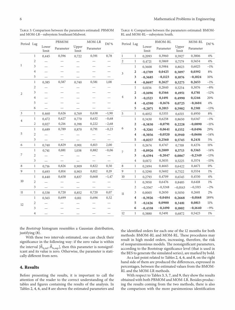
Table 4: Comparison between the parameters estimated: BMOM-RL and MOM-RL—subsystem South.


limit Parameter

1 1 0,2093 0,3960 0,5927 0,3806 4%2 1 0,4721 0,5869 0,7179 0,5654 4%

3

1 0,3608 0,5984 0,8023 0,6025 −1%2 −0,1709 0,0425 0,3097 0,0392 8%3 −0,3685 −0,1123 0,1076 −0,1024 10%4 −0,0697 0,2627 0,5275 0,2653 −1%

4

1 0,0156 0,2840 0,5254 0,3076 −8%2 −0,1696 0,1566 0,4951 0,1781 −12%3 −0,1523 0,1491 0,4990 0,1246 20%4 −0,4590 −0,1676 0,0725 −0,1604 4%5 −0,2071 0,2013 0,5982 0,2301 −13%

5 1 0,4052 0,5355 0,6515 0,4950 8%

6

1 0,3430 0,6258 0,8650 0,6347 −1%2 −0,3830 −0,0791 0,2228 −0,0890 −11%3 −0,3261 −0,0641 0,1552 −0,0496 29%4 −0,3056 −0,0520 0,1940 −0,0606 −14%5 −0,0257 0,2560 0,5745 0,2431 5%

7

1 0,2674 0,4747 0,7318 0,4276 11%2 −0,0926 0,2889 0,5713 0,3365 −14%3 −0,4394 −0,2047 0,0867 −0,2349 −13%4 0,0172 0,3035 0,5225 0,3574 −15%

8 1 0,2494 0,4665 0,6422 0,4671 0%9 1 0,3290 0,5602 0,7522 0,5534 1%10 1 0,2793 0,4709 0,6545 0,4530 4%

11

1 0,3950 0,6476 0,8485 0,6418 1%2 −0,5567 −0,3248 −0,0143 −0,3315 −2%3 0,0005 0,2650 0,5050 0,2601 2%4 −0,3926 −0,0484 0,2668 −0,0168 189%5 −0,1426 0,0900 0,3481 0,0813 11%6 −0,4338 −0,1490 0,1802 −0,1640 −9%

12 1 0,3880 0,5491 0,6872 0,5423 1%

the identified orders for each one of the 12 months for bothmethods: BMOM-RL and MOM-RL. These procedures mayresult in high model orders, increasing, therefore, the riskof nonparsimonious models. The nonsignificant parameters,according to the Bootstrap significance level (that is used inthe BES to generate the simulated series), aremarked by bold.

As a last point related to Tables 2, 4, 6, and 8, on the righthand side of them are produced the differences, expressed inpercentages, between the estimated values from the BMOM-RL and the MOM-LR methods.

With respect to Tables 3, 5, 7, and 9, they show the resultsobtained with both PBMOM andMOM-LR. Besides produc-ing the results coming from the two methods, there is alsothe comparison with the more parsimonious identification


Table 5: Comparison between the parameters estimated: PBMOMand MOM-LR—subsystem South.


limit Parameter

1 1 0,2068 0,3950 0,5896 0,3806 4%2 1 0,4713 0,5859 0,7133 0,5654 4%

3

1 0,4563 0,6484 0,8042 0,6483 0%2 — — — — —3 — — — — —4 — — — — —

4

1 0,2573 0,5004 0,7046 0,5187 −4%2 — — — — —3 — — — — —4 — — — — —5 — — — — —

5 1 0,4074 0,5355 0,6509 0,4949 8%

6

1 0,4301 0,6192 0,7740 0,6223 0%2 — — — — —3 — — — — —4 — — — — —5 — — — — —

7

1 0,5106 0,6374 0,7574 0,6126 4%2 — — — — —3 — — — — —4 — — — — —

8 1 0,2442 0,4669 0,6434 0,4670 0%9 1 0,3271 0,5573 0,7477 0,5534 1%10 1 0,2802 0,4704 0,6523 0,4531 4%

11

1 0,4105 0,6506 0,8380 0,6467 1%2 −0,5619 −0,3303 −0,0245 −0,3378 −2%3 0,0112 0,2284 0,4185 0,2328 −2%4 — — — — —5 — — — — —6 — — — — —

12 1 0,3905 0,5514 0,6894 0,5422 2%

method (MOM-LR) to show the importance of the reductionof the autoregressive order of the PAR(𝑝) models, speciallyconcerning the convergence of the estimated parametersfrom the methods PBMOM and MOM-LR. This result, in asense, points out the robustness of the PBMOMmethod.

In building the results for the BMOM-RL and PBMOMapproaches, 𝐵 = 10, 000 Bootstrap samples were generated.In this way, once the model order is obtained following theprocedure described above, the lower and upper boundspercentiles were calculated, as well as the Bootstrap averagesfor each one of the lags corresponding to the autoregressiveorders of the models.

Moving now to the presentation of the results by sub-systems, one can see from Table 2 that, in general, when

Table 6: Comparison between the parameters estimated: BMOM-RL and MOM-RL—subsystem Northeast.


limit Parameter

1 1 0,5168 0,6610 0,7736 0,6533 1%

2

1 0,5249 0,7543 1,0334 0,6966 8%2 −0,9783 −0,3862 0,0291 −0,3207 20%3 −0,6571 −0,2027 0,2788 −0,1894 7%4 0,0564 0,4116 0,8673 0,3731 10%

3 1 0,6551 0,7804 0,8718 0,7684 2%4 1 0,5611 0,6934 0,8021 0,6781 2%5 1 0,7546 0,8306 0,9083 0,8118 2%6 1 0,9003 0,9421 0,9724 0,7923 19%7 1 0,9511 0,9670 0,9843 0,9515 2%8 1 0,9639 0,9776 0,9867 0,9661 1%9 1 0,9101 0,9441 0,9661 0,9334 1%

101 0,4355 0,8286 1,2539 0,7836 6%2 −0,3083 0,5061 1,1934 0,3618 40%3 −1,0720 −0,4971 0,0937 −0,3109 60%

11 1 0,6861 0,9887 1,2919 0,9366 6%2 −0,6892 −0,3469 −0,0115 −0,2954 17%

12

1 0,4884 0,7050 0,9160 0,6801 4%2 −0,5076 −0,0912 0,2891 −0,0469 94%3 −0,6113 −0,0034 0,5330 −0,0652 −95%4 −1,4567 −0,5329 0,4884 −0,3389 57%5 −0,3229 0,5589 1,4244 0,3773 48%

the identification is not carried out by themost parsimoniousprocedure, the difference between the estimated parametersby the two approaches was around 20% superior in average.Besides that, when one looks at the parameters estimated bythe BMOM-RL, that allows for the estimation of confidenceintervals, it can be noticed that the significant parametersobtained by the MOM-RL method (the one used in the BES)should have been classified as nonsignificant, once the valuezero lies within the confidence interval. Such limitation couldonly be observed by the use of the Bootstrap estimationprocedure.

As a counterpart to the identification criterion shown inTable 2, in Table 3 are presented the results obtainedwhen theidentification and the estimation of the parameters are carriedout using the PBMOM technique. The average differencebetween the estimated parameters from the PBMOM and theMOM-LR methods is less than 1%; a clear cut indication ofthe consistency of the method. Moreover, the recommendedmethod, if adopted, makes the estimation of nonsignificantparameters in the models impossible.

Considering that the PBMOM produced more parsimo-nious formulations, such models were fitted and used to gen-erate scenarios, which, in a sense, reproduced the historicaldata for all subsystems. Mean, variance, distributional form,correlation, and negative sequence tests were performed [45].


Table 7: Comparison between the parameters estimated: PBMOMand MOM-LR—subsystem Northeast.


limit Parameter

1 1 0,5156 0,6589 0,7739 0,6532 1%

2

1 0,3713 0,5390 0,7163 0,5390 0%2 — — — — —3 — — — — —4

3 1 0,6569 0,7813 0,8744 0,7683 2%4 1 0,5608 0,6934 0,8001 0,6781 2%5 1 0,7533 0,8301 0,9066 0,8117 2%6 1 0,9018 0,9425 0,9720 0,9333 1%7 1 0,9512 0,9669 0,9842 0,9514 2%8 1 0,9642 0,9776 0,9867 0,9660 1%9 1 0,9087 0,9439 0,9659 0,9333 1%

101 0,7769 0,8497 0,9031 0,8392 1%2 — — — — —3 — — — — —

11 1 0,6880 0,9856 1,2873 0,9365 5%2 −0,6905 −0,3433 −0,0151 −0,2953 16%

12

1 0,4832 0,6371 0,7657 0,6233 2%2 — — — — —3 — — — — —4 — — — — —5 — — — — —

In all of them the null hypothesis of similarity with the his-torical observationswas accepted at 95% level. As an example,Figure 1 shows that, for the Southeast/Midwest subsystem, theaverage of the generated scenarios and the historical seriesaverage almost coincide.

Based on the scenarios obtained by using the proposedmodel, the performance of these series was compared withthe corresponding historical ones using Stochastic DynamicProgramming, as shown in [26].The total expected operatingcosts for both sets of series were compared.This expected cost(for thewhole system) is shown in Table 10. It can be observedthat the use of synthetic series (generated by PBMOM) allowsfor a cost nearly 7% lower than the one obtained with thehistorical series. Thus, one can state that, using this approachto produce synthetic series, it is possible to obtain moreeconomical operation policies.

5. Final Remarks

Thispaper presents a new approach for the stages of structuralidentification and parametric estimation in order to simulatesynthetic scenarios of NIE via PAR(𝑝) using the Bootstrap

Table 8: Comparison between the parameters estimated: BMOM-RL and MOM-RL—subsystem North.


limit Parameter

1 1 0,5978 0,7411 0,8462 0,7354 1%

2

1 0,6114 0,9273 1,4539 0,8181 13%2 −1,4504 −0,5984 −0,1584 −0,4375 37%3 −0,4379 0,0397 0,6213 −0,0026 −1653%4 −0,0638 0,3084 0,8751 0,2724 13%

3 1 0,6938 0,7849 0,8519 0,7680 2%4 1 0,6559 0,7476 0,8178 0,7430 1%

5 1 0.8797 1,0329 1,1811 0,9861 5%2 −0.4568 −0.25964 −0.06875 −0,2370 10%

6 1 0,8288 0,8858 0,9304 0,8722 2%

71 1,0195 1,1718 1,3459 1,0682 10%2 −0,8053 −0,5534 −0,3192 −0,4725 17%3 0,1460 0,3022 0,4573 0,3171 −5%

8 1 0,9430 0,9647 0,9791 0,9544 1%

9

1 0,9828 1,3402 1,7124 0,9812 37%2 −1,3616 −0,7776 −0,2557 −0,3311 135%3 −0,3152 0,1203 0,5692 0,0068 1675%4 −0,2789 −0,0230 0,2378 −0,0223 3%5 0,1167 0,2850 0,4742 0,3029 −6%

10 1 0,2745 0,5498 0,8781 0,5185 6%2 −0,0496 0,2880 0,5498 0,3112 −7%

11

1 0,3651 0,6852 1,0426 0,6490 6%2 −0,8519 −0,3182 0,1440 −0,2118 50%3 0,0010 0,7420 1,5594 0,4971 49%4 −1,0684 −0,2595 0,4426 −0,0135 1818%5 −0,5886 −0,1752 0,2013 −0,2352 −26%

12 1 0,5382 0,7097 0,8356 0,6936 2%

technique. In particular, the Bootstrap technique was essen-tial in the estimation of the confidence interval for the PACFcoefficients, leading to models far more parsimonious thanthe traditional asymptotic approach to set such intervals usedpreviously. Besides this, synthetic scenarios were producedand these series were generated using the available monthlydata for the four Brazilian subsystems to fit the PAR(𝑝)PBMOM structures. The obtained results using the PBMOMproduced not only more parsimonious model orders butalso adherent stochastic scenarios and, in average terms, leadto a better use of water resources in the energy operationplanning.

As a consequence of these findings, one could state thatthe proposed approach in this paper is quite promising, spe-cially taking into account that it has been used for the highlycomplex Brazilian hydrothermal energy system. Therefore,the method could also be recommended to be used for anyother large scale hydrothermal energy system.


Table 9: Comparison between the parameters estimated: PBMOM-and MOM-LR—subsystem North.


limit Parameter

1 1 0,5975 0,7403 0,8452 0,7354 1%

2

1 0,6730 0,8739 1,0839 0,8405 4%2 −0,5967 −0,3656 −0,1490 −0,3317 10%3 — — — — —4 — — — — —

3 1 0,6953 0,7853 0,8530 0,7680 2%4 1 0,6575 0,7481 0,8174 0,7430 1%

5 1 0,8797 1,0329 1,1811 0,9861 5%2 −0,4568 −0,2596 −0,0688 −0,2370 10%

6 1 0,8313 0,8858 0,9286 0,8722 2%

71 1,0195 1,1718 1,3459 1,0680 10%2 −0,8053 −0,5534 −0,3192 −0,4725 17%3 0,1460 0,3022 0,4573 0,3171 −5%

8 1 0,9430 0,9647 0,9791 0,9544 1%

9

1 0,9721 1,3444 1,6998 1,1816 14%2 −0,8561 −0,4723 −0,0695 −0,4080 16%3 — — — — —4 — — — — —5 — — — — —

10 1 0,5242 0,7933 1,1201 0,7933 0%2 — — — — —

11

1 0,5203 0,7075 0,8431 0,7080 0%2 — — — — —3 — — — — —4 — — — — —5 — — — — —

12 1 0,5326 0,7085 0,8351 0,6936 2%

Table 10: Expected total operating cost (R$) for the NIS.

Current model 2.1279 × 107

Proposed model: PBMOM 1.9780 × 107

Conflict of Interests

The two types of software mentioned in the paper (NEWAVEand PREVIVAZ) were developed by the Brazilian ElectricalResearch Center (CEPEL) to be used by the National Oper-ation System (ONS) to set the optimal dispatch of thehydrothermal Brazilian energy system.They are not commer-cial types of software and are only used by ONS and electricalenergy agents. Therefore, there is no conflict of interests byany of the three authors of this paper; that is, the authorsdo not have direct financial relation with the commercialidentities mentioned that might lead to a conflict of interests.

0 10 20 30 40 50 60Period

MW

med

0

2

4

6

8

10

12

14×10

4

Original historic series averageAverage of the scenarios generatedScenarios

Figure 1: Average of the scenarios (red line) and historic average(blue line) for the Southeast/Midwest subsystem.

Acknowledgments

The authors would like to thank the R&D program of theBrazilian Electricity Regulatory Agency (ANEEL) for thefinancial support.

References

[1] ONS, 2012, http://www.ons.org.br/home/.[2] M. V. F. Pereira, “Optimal stochastic operations scheduling of

large hydroelectric systems,” International Journal of ElectricPower and Energy Systems, vol. 11, no. 3, pp. 161–169, 1989.

[3] M. V. F. Pereira, N. Campodonico, and R. Kelman, “Long-termhydro scheduling based on sthocastic models,” in InternationalConference on Electrical Power Systems Operation and Manage-ment, (EPSOM’1998), 1998.

[4] P. G. C. Ferreira, A estocasticidade associada ao setor eletricobrasileiro e umanova abordagempara a geracao de afluencias viamodelos periodicos gama [Tese de Doutorado], PUC-Rio, 2013.

[5] A. L. M. Marcato, Representacao hıbrida de sistemas equiva-lentes e individualizados para o planejamento da operacao amedio prazo de sistemas de potencia de grande porte [Tese deDoutorado], PUC-Rio, 2013.

[6] L. A. Terry, M. V. F. Pereira, T. A. A. Neto, L. F. C. A. Silva,and P. R. H. Sales, “Coordinating the energy generation of theBrazilian national hydrothermal electrical generating system,”Interfaces, vol. 16, article 1, pp. 16–38, 1986.

[7] J. D. Salas and J. T. B. Obeysekera, “ARMAmodel identificationof hydrologic time series,”Water Resources Research, vol. 18, no.4, pp. 1011–1021, 1982.

[8] H. A. Thomas and M. B. Fiering, “Mathematical synthesis ofstreamflow sequences for the analysis of river basins by simula-tion,” Design of Water Resource Systems, pp. 459–463, 1962.

[9] E. J. Hannan, “A test for singularities in Sydney rainfall,” Aus-tralian Journal of Physics, pp. 289–297, 1955.


[10] L. R. Beard, “Use of interrelated records to simulate streamflow,”Journal of Hydrology, vol. 104, pp. 13–22, 1965.

[11] L. R. Beard, “Hydrologic Simulation in water yield analysis,”Hydrology Engineering Center. US Army Corps of Engineers,1967.

[12] J. R. Stedinger and M. R. Taylor, “Synthetic streamflow gen-eration: model verification and validation,” Water ResourceResearch, vol. 18, no. 4, pp. 909–918, 1982.

[13] J. R. Stedinger, D. P. Lettenmaier, and R. M. Vogel, “MultisiteARMA(1, 1) and disaggregation models for annual streamflowgeneration,” Water Resources Research, vol. 21, no. 4, pp. 497–509, 1985.

[14] N. C. Matalas, “Mathematical assessment of synthetic hydrol-ogy,”Water Resource Research, vol. 3, no. 4, pp. 937–947, 1967.

[15] R. Srikanthan and T. A.Mcmahon, “A review of lag-oneMarkovmodels for generation of annual flows,” Journal of Hydrology,vol. 37, no. 1-2, pp. 1–12, 1978.

[16] J. D. Salas, D. C. Boes, and R. A. Smith, “Estimation of ARMAmodels with seasonal parameters,” Water Resources Research,vol. 18, no. 4, pp. 1006–1010, 1982.

[17] U. G. Bacanli, “Stochastic modeling of monthly Streamflowdata,” in Proceeding of the 5th International Scientific ConferenceonWater, Climate and Environment (BALWOIS), Ohrid, Repub-lic of Macedonia, 2012.

[18] P. F. Rasmussen, D. S. Jose, F. Laura, R. Jean-Claude, andB. Bernard, “Estimation and validation of contemporaneousPARMA models for streaflow simulation,” Water ResourcesResearch, vol. 32, no. 10, pp. 3151–3160.

[19] Y. G. Tesfaye, Seasonal time series models and their application tothe modelling of river flows [Ph.D. thesis], University of Nevada,2005.

[20] Q. Shao and R. Lund, “Computation and characterizationof autocorrelations and partial autocorrelations in periodicARMA models,” Journal of Time Series Analysis, vol. 25, no. 3,pp. 359–372, 2004.

[21] A. V. Vecchia, “Maximum likelihood estimation for periodicautorregressivemoving averagemodels,”Techmometrics, vol. 27,article 4, pp. 375–384, 1985.

[22] A. V. Vecchia, “Periodic autoregressive moving avarege(PARMA) modeling with application to water resources,”Water Resources Bulletin, vol. 21, no. 5, pp. 721–730, 1985.

[23] M. E. P. Maceira, J. M. Damazio, A. O. Ghirardi, and H. M.Dantas, “Periodic ARMAmodels applied to weekly streamflowferecasts,” in Proceeding of the International Conference onElectric Power Engineering (PowerTech ’99), Budapest, Hungary,1999.

[24] Previvaz,Manual de Previsao de Vazoes Semanais, 2000.[25] CEPEL, “Centro de pesquisas de energia eletrica,” 2011, http://

www.cepel.br/.[26] R. C. Souza, A. L. M. Marcato, B. H. Dias, and F. L. C. Oliveira,

“Optimal operation of hydrothermal systems with hydrologicalscenario generaton through bootstrap and periodic autorre-gressive models,” European Journal of Operational Research, vol.222, no. 3, pp. 606–615, 2012.

[27] M. E. P. Maceira, D. D. J. Penna, and J. M. Damazio, “Geracaode cenarios sinteticos de energia e vazao para o planejamentoda operacao energetica,” in 16 Simposio Brasileiro de RecursosHıdricos, November, 2005.

[28] R. H. Jones and W. M. Brelsford, “Time series with periodicstructure,” Biometrika, vol. 54, pp. 403–408, 1967.

[29] K. W. Hipel and A. I. McLeod, Time Series Modelling of WaterResources and Environmental Systems, Elsevier, Amsterdam,The Netherlands, 1994.

[30] M. Pagano, “On periodic and multiple autoregressions,” TheAnnals of Statistics, vol. 6, no. 6, pp. 1310–1317, 1978.

[31] G. E. P. Box, G.M. Jenkins, andG. C. Reinsel,Time Series Analy-sis: Forecasting and control, Prentice Hall, Englewood Cliffs, NJ,USA, 3rd edition, 1994.

[32] M. S. Bartlett, “On the theoretical specification and samplingproperties of autocorrelated time-series,” Journal of the RoyalStatistical Society, vol. 8, pp. 27–41, 1946.

[33] M. H. Quenouille, “The joint distribution of serial correlationcoefficients,” Annals of Mathematical Statistics, vol. 20, pp. 561–571, 1949.

[34] A. C. Neto and R. C. Souza, “A bootstrap simulation study inARMA (p, q) structures,” Journal of Forecasting, vol. 15, no. 4,pp. 343–353, 1996.

[35] F. L. C. Oliveira and R. C. Souza, “A new approach to identifythe structural order of par (p)models,” Pesquisa Opracional, vol.31, no. 3, pp. 487–498, 2011.

[36] H. Akaike, “Factor analysis andAIC,” Psychometrika, vol. 52, no.3, pp. 317–332, 1987.

[37] G. Schwarz, “Estimating the dimension of a model,”TheAnnalsof Statistics, vol. 6, no. 2, pp. 461–464, 1978.

[38] H. Lutkepohl, Introduction to Multiple time Series Analysis,Springer, Berlin, Germany, 1991.

[39] R. Lund, Q. Shao, and I. Basawa, “Parsimonious periodic timeseriesmodeling,”Australian&NewZealand Journal of Statistics,vol. 48, no. 1, pp. 33–47, 2006.

[40] F. L. C. Oliveira, Nova abordagem para geracao de cenarios deafluencias no planejamento da operacao energetica de medioprazo [Dissertacao de Mestrado], PUC-Rio, 2010.

[41] B. Efron and R. J. Tibshirani, An Introduction to the Bootstrap,vol. 57 of Monographs on Statistics and Applied Probability,Chapman and Hall, New York, NY, USA, 1993.

[42] J. Carpenter and J. Bithell, “Bootstrap confidence intervals:when, which, what? A practical guide for medical statisticians,”Statistics in Medicine, vol. 19, pp. 1141–1164, 2000.

[43] D. N. Silva,Ometodo bootstrap e aplicacoes a regressao multipla[Dissertacao de Mestrado], IMEEC, UNICAMP, 1995.

[44] T. E. Unny and K. Cover, “Application of computer intensivestatistics to parameters uncertainy in streamflow synthesis,” inProceeding of the Symposia on Statistics in Honours of ProfessorV. W. Josni’s 70th Birthdat, 1985.

[45] F. L. C. Oliveira, Modelo de series temporais para construcaode arvores de cenarios aplicadas a otimizacao estocastica [Ph.D.thesis], Pontifical Catholic University of Rio de Janeiro, Rio deJaneiro, Brazil, 2013.

Impact Factor 1.73028 Days Fast Track Peer ReviewAll Subject Areas of ScienceSubmit at http://www.tswj.com

Hindawi Publishing Corporation http://www.hindawi.com Volume 2013Hindawi Publishing Corporation http://www.hindawi.com Volume 2013

The Scientific World Journal

A Parsimonious Bootstrap Method to Model Natural Inflow Energy Series

Documents

Transcript of A Parsimonious Bootstrap Method to Model Natural Inflow Energy Series