SPE 124041

New Inflow Performance Relationship for Solution-Gas Drive Oil Reservoirs Mohamed Elias, SPE, H. Ahmed El-Banbi, SPE, K.A. Fattah, and El-Sayed Ahmed Mohamed El-Tayeb, SPE, Cairo University

Copyright 2009, Society of Petroleum Engineers This paper was prepared for presentation at the 2009 SPE Annual Technical Conference and Exhibition held in New Orleans, Louisiana, USA, 4–7 October 2009. This paper was selected for presentation by an SPE program committee following review of information contained in an abstract submitted by the author(s). Contents of the paper have not been reviewed by the Society of Petroleum Engineers and are subject to correction by the author(s). The material does not necessarily reflect any position of the Society of Petroleum Engineers, its officers, or members. Electronic reproduction, distribution, or storage of any part of this paper without the written consent of the Society of Petroleum Engineers is prohibited. Permission to reproduce in print is restricted to an abstract of not more than 300 words; illustrations may not be copied. The abstract must contain conspicuous acknowledgment of SPE copyright.

Abstract The Inflow Performance Relationship (IPR) describes the behavior of the well’s flowing pressure and production rate, which is an important tool in understanding the reservoir/well behavior and quantifying the production rate. The IPR is often required for designing well completion, optimizing well production, nodal analysis calculations, and designing artificial lift. Different IPR correlations exist today in the petroleum industry with the most commonly used models are that of Vogel’s and Fetkovitch’s. In addition to few analytical correlations, that usually suffers from limited applicability. In this work, a new model to predict the IPR curve was developed, using a new correlation that accurately describes the behavior the oil mobility as a function of the average reservoir pressure. This new correlation was obtained using 47 actual field cases in addition to several simulated tests. After the development of the new model, its validity was tested by comparing its accuracy with that of the most common IPR models such as Vogel, Fetkovitch, Wiggins, and Sukarno models. Twelve field cases were used for this comparison. The results of this comparison showed that: the new developed model gave the best accuracy with an average absolute error of 6.6 %, while the other common models are ranked, according to their accuracy in the following order to be Fetkovich, Sukarno, Vogel, and Wiggins, with average absolute errors of 7 %, 12.1 %, 13.7 %, and 15.7 respectively. The new developed IPR model is simple in application, covers wide range of reservoir parameters, and requires only one test point. Therefore, it provides a considerable advantage compared to the multipoint test method of Fetkovich. Moreover, due to its acuuracy and simplicity, the new IPR provides a considerable advantage compared to the widely used method of Vogel. Introduction For slightly compressible fluids, the productivity index is given by:

⎥⎦

⎤⎢⎣

⎡+−

⋅=oBo

rokSwrer

khJμ75.)/ln(

00708.0 ……………….......................... (1)

Therefore, the variables that affecting the productivity index and in turn the inflow performance are essentially those that are pressure dependent parameters (µo, Bo, and kro). Fig.1 schematically illustrates the behavior of those variables as a function of reservoir pressure. Above the bubble-point pressure, kro equals unity and the term (kro/µoBo) is almost constant. As the pressure declines below pb, the gas is released from solution which can cause a large decrease in both kro and (kro/µoBo). Assuming that the well’s productivity index is constant, the oil flow rate can be calculated as follows:

( )wfprpJoq −= .…………………………………………… (2) Eq.2 suggests that the inflow into a well is directly proportional to the pressure drawdown. Evinger and Muskat2 (1949) observed that when the pressure drops below the bubble-point pressure, the inflow performance curves deviates from that of the simple straight-line relationship as shown in Fig.2, therefore, the above relationship is not valid for two-phase flow or in case of solution gas drive reservoires.

2 SPE 124041

Fig.1- Effect of pr on Bo, µo, and kro (After Ahmed, T.1)

Many IPR correlations addressed the curvature in Fig.2 of the inflow performance curves in case of solution gas drive oil reservoirs in which the bubble point pressure is the initial reservoir pressure. Based on the literature survey, the most known IPR correlations can be subdivided into empirically derived and analytically derived correlations. Some of the most known empirical derived correlations are Vogel3 (1968), Fetkovich4 (1973), Kilns and Majcher5 (1992), Wiggins6 (1993), and Sukarno et al.7 (1995). Some of the most known analytical derived correlations are Wiggins et al.8, 9 (1991, 1992), and Del Castillo, Yanil et al.10, 11 (2003).

Fig.2- The inflow performance curve below the bubble- point pressure (After Ahmed, T.1) The Empirical derived Correlations Vogel's Method In 1968, Vogel3 used a computer program based on Weller’s12 assumptions in 1966 for solution gas drive reservoirs to predict inflow performance curves. Vogel used twenty-one reservoir data sets to develop the following IPR:

28.02.01

max,⎥⎦

⎤⎢⎣

⎡⎥⎦

⎤⎢⎣

⎡−−=

rpwfp

rpwfp

oqoq

…................................ (3)

Vogel’s correlation gave a good match with the actual well inflow performance at early stages of production but deviates at later stages of the reservoir life. Therefore, this will affect the prediction of inflow performance curves in case of solution gas drive reservoirs, because at later stages of production the amount of the free gas that comes out of the oil will be greater than the amount at the early stages of production. Fetkovich's Method In 1973, Fetkovich4 developed an IPR based on the data from multi-rate tests “forty different oil wells from six fields.” In addition, the general treatment of the inflow performance for the solution gas drive provided by Raghavan13 under pseudo-steady state conditions was used. The following relation gives the oil flow rate as introduced by Raghavan13:

dprp

wfp oBooSrok

Joq ∫=μ

)(………………………………... (5)

Where: So is the oil saturation, and J the modified productivity index for this case, and is defined by:

SPE 124041 3

SwrerkhJ

+−=

75.)/ln(2.1411

……………………................ (6)

The form given by Eq.5 is not useful in a practical sense- the integral must be reduced to a simple function of pressure. The approach suggested by Fetkovich4 in the pursuit of Eq.5, is that he assumed the oil mobility function is a "simple" function of pressure. For example, Fetkovich4 proposed the following relationship between the oil mobility function and pr:

rpxoBo

oSrok⋅=

μ)(

.…........................................................... (7)

Where, x is simply constant. Fetkovich4 concluded that Eq.7 is too simplistic to model all of the changes of the pressure and saturation-dependent properties during depletion. Finally, the "Fetkovich form" of the IPR equation is given as the "backpressure" modification form, which is written as:

n

rp

wfp

oqoq

⎥⎥

⎦

⎤

⎢⎢

⎣

⎡−= 2

21

max,………………………………. (8)

This model requires a multi-rate test to determine the value of the backpressure exponent (n). As indicated, the main parameter that has the great effect on the Fetkovich's model is the oil mobility as a function of the average reservoir pressure, which assumed to be a linear relationship as illustrated in Fig.3.

Fig.3- Mobility-pressure behavior for a solution gas drive reservoir (After Fetkovich4) Klins and Majcher's Method In 1992 based on Vogel’s work, Klins and Majcher5 developed the following IPR correlation that takes into account the change in bubble-point pressure and reservoir pressure due to the depletion in solution gas drive reservoirs.

⎥⎥

⎦

⎤

⎢⎢

⎣

⎡

⎟⎟⎠

⎞⎜⎜⎝

⎛⎟⎟⎠

⎞⎜⎜⎝

⎛−−=

=

1705.0295.00.1

0max,

N

rpwfp

rpwfp

Soqoq ………... (8)

Where, N1 is defined by the following equation:

( )bpbprp

N 001.0235.1*72.028.01 ++= ⎟⎟⎠

⎞⎜⎜⎝

⎛ …………………….. (9)

Wiggins's Method (1993) In 1993, Wiggins6 developed a generalized empirical three phase IPR similar to Vogel3 correlation to overcome the problem of applying his developed analytical model in 1991. This correlation is:

2481092.0519167.01

max, ⎟⎟⎠

⎞⎜⎜⎝

⎛⎟⎟⎠

⎞⎜⎜⎝

⎛−−=

rpwfp

rpwfp

oqoq ………… (10)

4 SPE 124041

Sukarno and Wisnogroho's Method In 1995, Sukarno and Wisnogroho7 developed the following IPR equation based on simulation results that attempts to account for the flow-efficiency variation caused by rate-dependent skin:

⎥⎦

⎤⎢⎣

⎡⎟⎠⎞⎜

⎝⎛⎟

⎠⎞⎜

⎝⎛ −−−=

=

34093.0

24416.01489.01

0max, rpwfp

rpwfp

rpwfp

FESoq

oq... (11)

Where:

3

3

2

21 ⎟⎟⎠

⎞⎜⎜⎝

⎛⎟⎟⎠

⎞⎜⎜⎝

⎛⎟⎟⎠

⎞⎜⎜⎝

⎛+++=

rpwfp

arp

wfpa

rpwfp

aoaFE ............................ (12)

33

221 SibSibSiboibia ⋅+⋅+⋅+= ………….. (13)

In Eq.13, S is the skin factor, and ao, a1, a2, a3, boi, b1i, b2i, and b3i are the fitting coefficients that are shown in Table 2.1.

Table 1- Constants for Sukarno and Wisnogroho boi b1i b2i b3i

ao a1 a2 a3

1.0394 0.01668 -0.0858 0.00952

0.12657 -0.00385 0.00201 -0.00391

0.0135 0.00217 -0.00456 0.0019

-0.00062 -0.0001 0.0002 -0.00001

The Analytical Derived Correlations Wiggins's Method (1991) In 1991, Wiggins, Russell, and Jennings8,9 studied the three-phase inflow performance for oil wells producing oil, water, and gas in a homogeneous, bounded reservoir. They started from the basic principle of mass balance with the pseudo-steady state solution to develop the following analytically IPR correlation:

44

33

2211

max, ⎟⎟⎠

⎞⎜⎜⎝

⎛⎟⎟⎠

⎞⎜⎜⎝

⎛⎟⎟⎠

⎞⎜⎜⎝

⎛⎟⎟⎠

⎞⎜⎜⎝

⎛++++=

rpwfp

DC

rpwfp

DC

rpwfp

DC

rpwfp

DC

oqoq

….. (14)

Where, C1, C2, C3…Cn, and D coefficients are determined based on the oil mobility function and its derivatives taken at the average reservoir pressure (pr) as given by:

⎪⎭

⎪⎬⎫

⎪⎩

⎪⎨⎧

⎟⎠⎞⎜

⎝⎛⎟

⎠⎞⎜

⎝⎛⎟

⎠⎞⎜

⎝⎛⎟

⎠⎞⎜

⎝⎛

=+

=+

=+

=−=

\\\

061

\\

021

\

001

DpoBorok

DpoBorok

DpoBorok

DpoBorokC

μμμμ…. (15)

⎪⎭

⎪⎬⎫

⎪⎩

⎪⎨⎧

⎟⎠⎞⎜

⎝⎛⎟

⎠⎞⎜

⎝⎛⎟

⎠⎞⎜

⎝⎛

=+

=+

==

\\\

041

\\

021

\

021

2DpoBo

rok

DpoBorok

DpoBorokC

μμμ…. (16)

⎪⎭

⎪⎬⎫

⎪⎩

⎪⎨⎧

⎟⎠⎞⎜

⎝⎛⎟

⎠⎞⎜

⎝⎛

=+

=−=

\\\

061

\\

061

3DpoBo

rok

DpoBorokC

μμ………………... (17)

⎪⎭

⎪⎬⎫

⎪⎩

⎪⎨⎧

⎟⎠⎞⎜

⎝⎛

==

\\\

0241

4DpoBo

rokCμ

……………………………… (18)

\\\

0241

\\

061

\

021

0 =+

=+

=+

== ⎟

⎠⎞⎜

⎝⎛⎟

⎠⎞⎜

⎝⎛⎟

⎠⎞⎜

⎝⎛⎟

⎠⎞⎜

⎝⎛

DpoBorok

DpoBorok

DpoBorok

DpoBorokD

μμμμ….. (19)

Wiggins, et al.8, 9 found that the main reservoir parameters that play a major role in the inflow performance curve are relative permeability and fluid properties (i.e., the oil mobility function). The major problem in applying the Wiggins's analytical IPR is its requirement for the mobility derivatives as a function of average reservoir pressure, which is very difficult in practice. Therefore, in 1993 Wiggins6 developed the empirical IPR equations that previously presented (i.e., Eq.10) from this analytical IPR model by assuming a third degree polynomial relationship between the oil mobility function and the average reservoir pressure. Wiggins, et al.8,

9 also presented plots of the oil mobility as a function of the average reservoir pressure taken at various flow rates to establish the "stability" of the oil mobility profile for a given depletion level. An example to the oil mobility-pressure profile that is presented by Wiggins, et al.8 is shown in Fig.4.

SPE 124041 5

Fig.4- The oil mobility profiles as a function of pressure- various flow rates (Case 2, after Wiggins, et al.8) Del Castillo, Yanil's Method In 2003, another theoretical attempt to relate the IPR behavior with the fundamental flow theories is developed by Del Castillo, Yanil et al.10, 11. In this model, a second-degree polynomial IPR is obtained with a variable coefficient (v), or the oil IPR parameter that may in fact be a strong function of pressure and saturation. The starting point for this development is the pseudo-pressure formulation for the oil phase, which is given as:

∫= ⎥⎦

⎤⎢⎣

⎡ p

basepdp

oBorok

nprokoBop

oppμ

μ)( …………………… (20)

In that work, Del Castillo, Yanil et al.16, 17 presumed that the oil mobility function has a linear relationship with the average reservoir pressure as given below:

rpderpfrpoBo

rok⋅+== 2)(

μ……………………………. (21)

Where e, and d are constants established from the presumed behavior of the oil mobility profile. Fig.3 refers to the physical interpretation of Eq.21. Substituting with Eq.21 in Eq.20 and manipulating, the following equation could be presented:

( )2

11max,

⎥⎦

⎤⎢⎣

⎡⎥⎦

⎤⎢⎣

⎡−−−=

rpwfp

vrp

wfpv

oqoq

…………………………. (22)

Specifically, the ν-parameter is given as:

⎟⎠⎞⎜

⎝⎛ +

=

rped

v1

1 ……………………………………………… (23)

Wiggins, et al.8, 9 and Del Castillo and Yanil et al.10, 11 relationships can only be applied indirectly or inferred, by estimating the oil mobility as a function of the average reservoir pressure to construct the IPR curve. Future Inflow Performance Relationship In the absence of saturation data as a function of reservoir pressure, three simple methods can be used to predict future inflow performance curves. First Method (Vogel's Method) This method was provided by Vogel3 and provides a rough approximation of the future maximum oil flow rate (qo, max) f at the specified future average reservoir pressure (pr) f from the following equation:

) ) ))

)) ⎥⎥⎦

⎤

⎢⎢⎣

⎡

⎥⎥⎦

⎤

⎢⎢⎣

⎡+=

prpfrp

prpfrp

poqfoq 8.02.0max,max, ……………… (24)

6 SPE 124041

Second Method (Fetkovich's Method)

A simple approximation for estimating future (qo, max) f at (pr) f was proposed by Fetkovich4. The relationship has the following mathematical form:

) ) ))

0.3

max,max,⎥⎥⎦

⎤

⎢⎢⎣

⎡=

prpfrp

poqfoq ………………..………… (25)

Third Method (Wiggins's Method) Wiggins6 extended the application of Eq.14 to predict future performance by providing the following relationship:

) ) ))

))

⎥⎥⎥

⎦

⎤

⎢⎢⎢

⎣

⎡

⎟⎟⎠

⎞⎜⎜⎝

⎛+=

284.015.0max,max, prp

frp

prpfrp

poqfoq ……………... (26)

Summary of Literature Survey As indicated, the empirical correlations suffer from the limitation of their application range as they depend largely on the data used in their generation, and its lack of accuracy. In addition, they are not explicitly function of reservoir rock and fluid data, which are different from one reservoir to another. On the other hand, the analytical correlations suffer from their difficulty to be applied due to its requirement to the oil mobility profiles and its derivatives in addition to the assumptions used in their development. As discussed, the main parameter that affects the productivity index and in turn the inflow performance curves is the oil mobility function (kro/µoBo) and its relation to the average reservoir pressure. Therefore, the relationship between the oil mobility function and the average reservoir pressure should be accurately determined. In addition, the most common equation that represents a basic start point for the development of any IPR equation, in case of solution gas drive reservoirs is Eq.20,which mainly a fuction of the oil mobility (kro/µoBo). Most of the perviously empirical derived IPR equations did not take into their consideration the whole effect of the oil mobility function, this in turn largely reduce the accuracy, power, and utility of these equations. Even though the models that took into their consideration the effect of this function, such as the models of Fetkovich4 and Wiggins6, assumed the relationships between this function and pr, as the linear form and the third polynomial form for Fetkovich and Wiggins, respectively. In fact, these linear and polynomial forms do not accurately describe the general behavior of the oil mobility function with the average reservoir pressure with an accurate manner. On the other hand, some of analytical derived IPR equations did not considered the effect of this function, except the models of Wiggins, et al.8, 9 Del Castillo, Yanil et al.10, 11. Wiggins’s model is so complicated because it requires the oil mobility represented in its derivates as a function of the average reservoir pressure, this is greatly difficult in application. Del Castillo, Yanil’s model is not accurate, this is because Del Castillo, Yanil assumed a liner relationship between the oil mobility function and pr, which in turn reduce the accuracy of this model. Another parameter should be considered in the selecting of the IPR method, is the aspect of conducting the flow tests. It is evident that test costs have to be taken into consideration. Finally, the range of applicability will also influence the selecting of the IPR methods to predict the well performance. Accordingly based on the literature survey in this work, it is necessary to: Develop a new, more general, simple, and consistent method to correlate inflow performance trends for solution gas drive oil

reservoirs. This new method takes into consideration the behavior of the oil mobility function with the average reservoir pressure without the direct knowledge of this behavior.

Determine the applicability and accuracy of the proposed new model by applying it on different field cases with a comparison with some of the most known and used IPR equations, considering a wide range of fluid, rock, and reservoir characteristics.

Test some of the available IPR methods on field data. Address the prediction of future performance from current test information.

The New Developed IPR Model In this work, a single well 3D radial reservoir model using MORE14 reservoir simulator was built. The reservoir simulation was used to investigate the shape and in turn the relationship between the oil mobility function and the average reservoir pressure. Then, a new IPR equation was derived based on the resulted oil mobility-pressure profile; this new IPR is mainly a function of the relationship between the oil mobility and the average reservoir pressure. Then, forty-seven field cases (published cases) were used to develop an empirical relationship between the oil mobility and average reservoir pressure. Thus, obtaining a new IPR model that is explicitly function of the oil mobility that is highly affect the IPR model.

SPE 124041 7

0

0.5

1

1.5

2

2.5

3

3.5

4

0 400 800 1200 1600 2000 2400The Avergae Reservoir Pressure, Psia

The

Oil

Mob

ility

Fun

ctio

n

3000 STB/day5000 STB/day10000 STB/day50000 STB/day100000 STB/day353820 STB/day

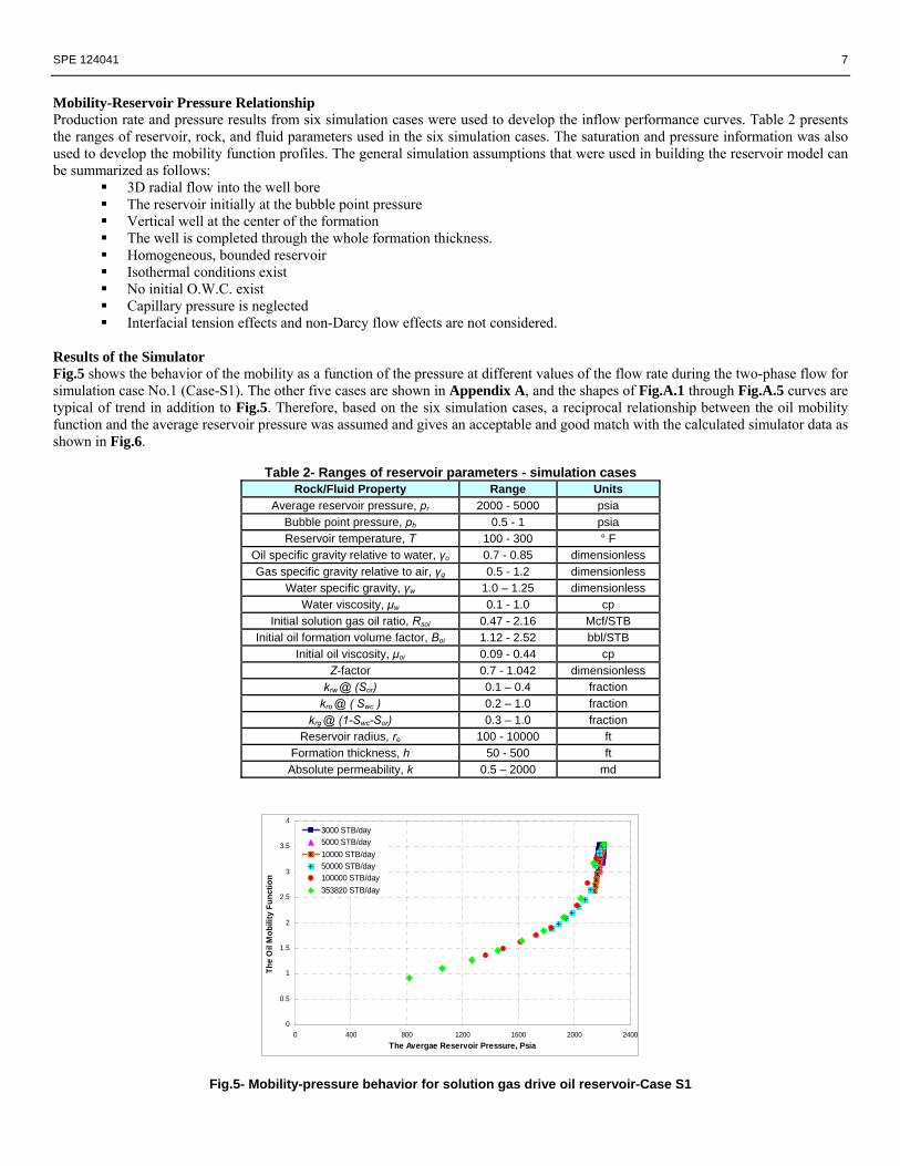
Mobility-Reservoir Pressure Relationship Production rate and pressure results from six simulation cases were used to develop the inflow performance curves. Table 2 presents the ranges of reservoir, rock, and fluid parameters used in the six simulation cases. The saturation and pressure information was also used to develop the mobility function profiles. The general simulation assumptions that were used in building the reservoir model can be summarized as follows:

3D radial flow into the well bore The reservoir initially at the bubble point pressure Vertical well at the center of the formation The well is completed through the whole formation thickness. Homogeneous, bounded reservoir Isothermal conditions exist No initial O.W.C. exist Capillary pressure is neglected Interfacial tension effects and non-Darcy flow effects are not considered.

Results of the Simulator Fig.5 shows the behavior of the mobility as a function of the pressure at different values of the flow rate during the two-phase flow for simulation case No.1 (Case-S1). The other five cases are shown in Appendix A, and the shapes of Fig.A.1 through Fig.A.5 curves are typical of trend in addition to Fig.5. Therefore, based on the six simulation cases, a reciprocal relationship between the oil mobility function and the average reservoir pressure was assumed and gives an acceptable and good match with the calculated simulator data as shown in Fig.6.

Table 2- Ranges of reservoir parameters - simulation cases

Rock/Fluid Property Range Units Average reservoir pressure, pr 2000 - 5000 psia

Bubble point pressure, pb 0.5 - 1 psia Reservoir temperature, T 100 - 300 ° F

Oil specific gravity relative to water, γo 0.7 - 0.85 dimensionless Gas specific gravity relative to air, γg 0.5 - 1.2 dimensionless

Water specific gravity, γw 1.0 – 1.25 dimensionless Water viscosity, μw 0.1 - 1.0 cp

Initial solution gas oil ratio, Rsoi 0.47 - 2.16 Mcf/STB Initial oil formation volume factor, Boi 1.12 - 2.52 bbl/STB

Initial oil viscosity, μoi 0.09 - 0.44 cp Z-factor 0.7 - 1.042 dimensionless

krw @ (Sor) 0.1 – 0.4 fraction kro @ ( Swc ) 0.2 – 1.0 fraction

krg @ (1-Swc-Sor) 0.3 – 1.0 fraction Reservoir radius, re 100 - 10000 ft

Formation thickness, h 50 - 500 ft Absolute permeability, k 0.5 – 2000 md

Fig.5- Mobility-pressure behavior for solution gas drive oil reservoir-Case S1

8 SPE 124041

S = 0.28313816r = 0.91659146

The Avearge Reservoir Pressure, psia

The

Oil

Mob

ility

0 400 800 1200 1600 2000 24000.0

0.5

1.0

1.5

2.0

2.5

3.0

3.5

4.0

Standard Deviation, Relative Error,

Fig.6- Reciprocal model- Case S1

Derivation of the new IPR Equation The starting point for the derivation is the definition of the oil-phase pseudopressure for a single well in a solution gas drive reservoir and the pseudo-steady state flow equation for the oil-phase. In this work, a new form for the oil mobility function at different values of the average reservoir pressure (i.e., the reciprocal relationship) is obtained from the simulation study that performed on MORE simulator using the six simulation cases. This reciprocal relationship was used as:

brparpoBo

rok+⋅

=⎥⎦

⎤⎢⎣

⎡ 1μ

………………………………............ (27)

Where, a and b are constants established from the presumed behavior of the mobility profile. Substituting Eq.27 in Eq.20 and manipulating (the details are provided in Appendix B), the following new IPR equation will be introduced:

)1ln(

)1ln(1

max, +⋅

+⋅−=

rpwfp

oqoq

αα

………………………………….. (28)

Where: α is the oil IPR parameter for the new IPR model. The productivity index can be numerically calculated from the following developed equation:

⎥⎦

⎤⎢⎣

⎡+⋅+−

⋅=1

175.0)/ln(

00708.0

rpSwrerkhPI

αα ………………................ (29)

Eq.28 is the proposed new IPR equation. As recognized, the α-parameter is not "constant," therefore, forty-seven field cases (published cases) were used to develop the following two empirical relationships between the variable coefficient α which represent the oil mobility function and average reservoir pressure: When the average reservoir pressure-range is less than or equal to 1600 psia the following relationship was developed:

brpa +=

.1α …………………………………………….. (30)

Where: a= -0.981, and b= -152.585.

When the average reservoir pressure-range is greater than or equal to 1600 psia the following relationship was developed:

5.4.3.2.. rphrpgrpfrperpdc +++++=α ………………. (31)

SPE 124041 9

52185.241748.631369.520941.20698.40043065.0 rprprprprp ×−Ε+×−Ε−×−Ε+×−Ε−×−Ε+−=α

-0.0012

-0.0011

-0.001

-0.0009

-0.0008

-0.0007

-0.0006

-0.0005

-0.0004

-0.0003

-0.0002

-0.0001

0

0 1000 2000 3000 4000 5000 6000 7000The Average Reservoir Pressure, psia

The

Varia

ble

Coe

ffiec

int, α

Table 3 shows the constants of Eq.31. Table 3- Constants of Eq.31

Constant Value c = -0.0043065

d = 4.98E-06 e = -2.41E-09

f = 5.69E-13 g = -6.48E-17 h= 2.85E-21

Eq.30 and Eq.31 were developed based on the following developed chart between the α-parameter and the average reservoir pressure (i.e. Fig.7) that was generated from the forty-seven field cases. Table 4 introduces the ranges of data used in the development of these two equations. Finally, Eq.28, Eq.30, and Eq.31 represent the new developed IPR model.

Fig.7- The variable coefficient α and the average reservoir pressure chart Methodology to use the New IPR Model Step1. If the average reservoir pressure is less than or equal to 1600 psia, therefore, the oil IPR parameter (α) is calculated using Eq.30 as follows:

585.152981.01

−×−=

rpα

If the average reservoir pressure is greater than or equal to 1600 psia, therefore, the oil IPR parameter (α) is calculated using Eq.31 as follows: Step2. Calculate qo, max using Eq.28 and any given test point:

])1ln(

)1)(ln(1/[)(max, +×−

+×−−=

rptestwfp

testoqoqα

α STB/day

Step3. Assume several values for pwf and calculate the corresponding qo using Eq.28:

])1ln(

)1ln(1[max, +×−

+×−×=

rpwfp

oqoqα

α STB/day

Step4. For future IPR, calculate αf using the future value of pr) f using Eq.30 or Eq.31 according to the value of pr) f: Step5. Solve for qo, max, at future conditions using Fetkovich’s equation (i.e., Eq.25) as follows:

10 SPE 124041

) ) ))

0.3

max,max, ⎥⎥

⎦

⎤

⎢⎢

⎣

⎡×=

prpfrp

poqfoq STB/day

Step6. Generate the future inflow performance-curve by applying Eq.28 as follows:

])1)ln(

)1ln(1[)max, +×

+×−×=

frpf

wfpffoqoq

α

α STB/day

Table 4- Ranges of data used in the development α-pr relationship

Properties Data range

1. Fluid properties data: Gas specific gravity 0.60 - 0.8

API gravity of oil 20- 50 Water specific gravity 1.04 -1.074

Initial oil formation volume factor (bbl/STB) 1.3 - 1.94 Initial oil viscosity ( cp) 0.27- 0.99

Initial solution gas oil ratio,( Mscf/STB) 0.132 - 4.607 Bubble point pressure (psia) Up to 7000

2. Rock properties data: Porosity 0.1 - 0.35

Absolute permeability (md) 2.5 - 2469 Irreducible water saturation 0.1 - 0.32

Residual oil saturation ( W/O) 0.08 - 0.17 Residual oil saturation (G/O) 0.07 - 0.14

Critical gas saturation 0.02- 0.17 Total compressibility ( psi-1) 0.33 x 10-3 – 30 x 10-6

Oil relative permeability @ 0.02 and 0.1 Sgc 0.444 – 0.52 3. Reservoir and well dimension: Average reservoir pressure (psia) Up to 7000

Drainage area (acres) 20 - 80 Formation thickness (feet) 10 - 182

Reservoir radius ( feet) 250 - 1053 Well bore radius (feet) 0.33 - 0. 35

Reservoir temperature (deg. F) 156 - 238 Validation of the New IPR Model To verify and validate the new developed IPR model, information from twelve field cases were collected and analyzed to get the present inflow performance, and two-field cases were collected and used to predict the future IPR curve. The ranges of fluid properties, rock properties, and reservoir data of these cases are included in Table 4. Each field case uses actual field data which representing different producing conditions. In order to test the accuracy and reliability of the new developed IPR model, which is single point method, it will be compared to some of the other two-phase IPR methods currently available in the industry. These methods are those of Vogel3 (single point method), Fetkovich4 (multi-point method), Wiggins6 (single point method), and Sukarno7 (single point method) for the present inflow performance. And, Vogel3, Fetkovich4, Wiggins6 for the future inflow performance Elias, Mohamed15, presents the complete details of the comparison analysis while the cases analyzed for present and future performances are summarized in Table 5 and Table 6, respectively. Field Case No.1: Carry City Well Frederic Gallice and Michael L. Wiggins16 presented multirate-test data for a well producing from the Hunton Lime in the Carry City Field, Oklahoma. The test was conducted in approximately 2 weeks during the well, which was producing at random rates, rather than in an increasing or decreasing rate sequence. The average reservoir pressure was 1600 psia, with an estimated bubble-point pressure of 2530 psia and an assumed skin value of zero. The multi-rate test of this well is summarized in Table 7. Table 8 presents the predictions of the well’s performance for the test information at a flowing bottomhole pressure of 1194 psia, which representing a 25 % of the pressure drawdown. As can be observed, the maximum well deliverability varies from 2550 to 4265 STB/D. The largest flow rate was calculated with Wiggins’s IPR, while the smallest rate was obtained using Fetkovich model. Fig.8 shows the resultant IPR curves for the different methods of calculations such as Vogel, Fetkovich, Wiggins, and Sukarno in comparison with the actual field data and the new developed IPR model. It is clear from this figure that the method of the new

SPE 124041 11

developed IPR model is succeed to estimate the actual well performance . In addition, it can be clearly concluded from this figure that the methods of the new developed IPR model and Fetkovich’s model are nearly estimate the maximum oil flow rate for this well more accurately than the other models, and as indicated, the other methods overestimate the actual performance.

Table 5- Validation field cases analyzed for the present performance Case Case Name Case Type pr, psia

1 Carry City Well 29 Vertical Well 1600

2 Case X1B 22 Vertical Well 2580

3 Well 4 26 Vertical Well, Layered Reservoir 5801

4 Well 8, West Texas 30 Vertical Well, Low Pressure 640

5 Well 1, Gulf of Suez, Egypt 13 Vertical Well 2020

6 Well M110-1979 31 Vertical Well 2320

7 Well M200 31 Vertical Well 3263

8 Well 3-Field C 8 Vertical Well 3926

9 Well E, Keokuk Field 28 Vertical Well 1710

10 Well A, Keokuk Field 30 Vertical Well 1734

11 Well TMT-27 30 Vertical Well, Low Pressure 868

12 Well A 30 Vertical Well 1785

Table 6- Validation field cases analyzed for the future performance Case Test

Chronology Case Name Reference pr,

psia 1 Present Well M110-1979 17 2321

1 Future Well M110-1987 17 2067

2 Present Well A, Keokuk Field-1934

22 1734

2 Future Well A, Keokuk Field-1935

22 1609

Table 7- Test data- Field Case No.1

Test Data pwf, psia qo, STB/D

1600 0

1558 235

1497 565

1476 610

1470 720

1342 1045

1267 1260

1194 1470

1066 1625

996 1765

867 1895

787 1965

534 2260

351 2353

183 2435

166 2450

12 SPE 124041

0

200

400

600

800

1000

1200

1400

1600

1800

0 1000 2000 3000 4000 5000Flow Rate, STB/day

Bot

tom

Hol

e Fl

owin

g Pr

essu

re, p

sia

SukarnoWigginsFetkovichVogelThe new IPRField

Test Point

Table 8- Prediction of the performance of Case No.1 at 25 % of the pressure drawdown Field Data The new IPR method Vogel method Fetkovich method Wiggins method Sukarno method

pwf, psia qo, STB/D qo, STB/D qo, STB/D qo, STB/D qo, STB/D qo, STB/D 1600 0 0 0 0 0 0 1558 235 297 169 213 164 177 1497 565 614 408 444 398 423 1476 610 703 489 516 477 505 1470 720 728 511 536 499 528 1342 1045 1140 977 920 965 995 1267 1260 1321 1233 1115 1225 1244 1194 1470 1470 1470 1288 1470 1470 1066 1625 1688 1856 1559 1879 1828 996 1765 1790 2051 1690 2091 2003 867 1895 1954 2382 1905 2462 2290 787 1965 2044 2569 2021 2679 2445 534 2260 2284 3062 2309 3297 2830 351 2353 2428 3329 2447 3680 3018 183 2435 2544 3507 2522 3985 3133 166 2450 2555 3521 2527 4013 3142

0 2657 3627 2550 4265 3205 The average absolute errors percent between the actual flow-rate data and the calculated rate for the five IPR methods that used in this study are shown in Fig.9 for the comparison. It is clear from this figure that the new developed IPR model has the lowest average absolute error percent that is 6.47 %, while the average absolute error percent for Fetkovich’s method is 8.56 %. The other single-point methods have average absolute errors percent ranging from 20.1 to 32.3 % for Sukarno and Wiggins, respectively. In summary, the new model provided the best estimates of well performance for this case’s entire range of interest. The multipoint method of Fetkovich tends to do a better job of predicting well performance than the other three single-point methods. Overall, the single-point methods of Vogel, Wiggins, and Sukarno provided similar great average differences in this case. As indicated in this work, the more important relationship to evaluate well performance is the relationship between the oil mobility function and the average reservoir pressure, and this was clearly demonstrated from the value of the average absolute error percent that resulted from using the new developed IPR model.

Fig.8- The predicted inflow curves by the different used methods in comparison to the actual field data for Case No.1

SPE 124041 13

The new IPR 6.47

Vogel 26

Fetkovich 8.56

Wiggins 32.3

Sukarno 20.1

0

5

10

15

20

25

30

35

Ave

rage

Err

ors

%

Models

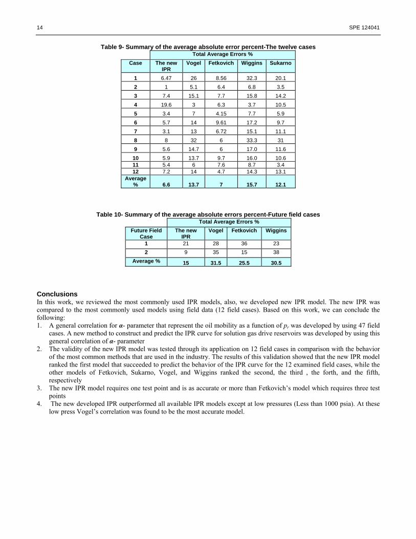
Fig.5.2- The average absolute errors percent at 25 % drawdown for Case No.1 Field Cases Summary for the Present Inflow Performance The additional cases and their analysis are presented in detail in Ref. 10. Table 9 presents a summary of the average absolute errors percent that was obtained for each method in each one of the twelve case studies that were examined. As indicated, the method of the new developed IPR model always provided the most reliable estimates of the actual well data analyzed. It has the lowest value of the total average absolute error percent, which is 6.6 % in comparison with that of Fetkovich's method, which has a reasonable average absolute error percent of 7 % but is still higher than the method of the new developed IPR model. The other methods always provided less accurate values for the pressure-rate estimates of the actual well data that used in this analysis. The method of the new developed IPR model tends to do a better job of predicting well performance than the other methods, and this it may be due to assume an accurate relationship between the oil mobility function and the average reservoir pressure (i.e., the Reciprocal Relationship). Overall, the single-point methods of Vogel, Wiggins, and Sukarno provided great average absolute errors percent in the cases examined- 12.1 to 15.7 %. However, the following comment should be introduced based on the above table Case No.4, the Vogel's model provided the best estimates of well performance for this case. The single point method of Wiggins tends to do a good job of predicting well performance in this case. Finally, it can be concluded from this case that the new IPR model has some limitations in case of low-pressure reservoirs, which have a reservoir pressure less than 1000 psia. This is because there were no sufficient data below 1000 psia in case of development the new IPR model, therefore it is recommended in this case to use Vogel’s model. Field Case Summary for the Future Performance The analyses of the two future field cases are presented in detail in Ref. 15. Table 10 presents a summary of the average absolute errors percent that was obtained for each method in each one of the two future case studies that were examined. As indicated, the method of the new developed IPR model always provided the most reliable estimates of the actual well data analyzed. It has the lowest value of the total average absolute error percent, which is 15 %. The other methods always provided less accurate values for the pressure-rate estimates of the actual future well data that used in this analysis. Overall, the other methods of Fetkovich, Vogel, and Wiggins provided great average absolute errors percent in the cases examined range from 25.5 % and 31.5 % for Fetkovich and Vogel, respectively. However, general comment can be presented based on Table 10 and the future cases analyzed in this work, the average absolute error percent is almost as great for the Fetkovich's method as compared to the method of the new developed IPR model - 25.5 % compared to 15 %. As indicated, the main reasons for that are:

1) Fetkovich considered the relationship between the mobility function and the average reservoir pressure is linear relationship (see Fig.3), but the new IPR model considered this relation is reciprocal relationship (see Fig.5 and Fig.6) which cover the entire range of interest more accurately.

2) The backpressure equation parameter (n) of Fetkovich IPR equation (Eq.8) does not take into consideration the change in the average reservoir pressure.

3) The new model IPR parameter (α) of Eq.28 takes into consideration the change in the average reservoir pressure (see Eq.30 and Eq.31).

14 SPE 124041

Table 9- Summary of the average absolute error percent-The twelve cases Total Average Errors %

Case The new IPR

Vogel Fetkovich Wiggins Sukarno

1 6.47 26 8.56 32.3 20.1 2 1 5.1 6.4 6.8 3.5 3 7.4 15.1 7.7 15.8 14.2 4 19.6 3 6.3 3.7 10.5 5 3.4 7 4.15 7.7 5.9 6 5.7 14 9.61 17.2 9.7 7 3.1 13 6.72 15.1 11.1 8 8 32 6 33.3 31 9 5.6 14.7 6 17.0 11.6

10 5.9 13.7 9.7 16.0 10.6 11 5.4 6 7.6 8.7 3.4 12 7.2 14 4.7 14.3 13.1

Average % 6.6 13.7 7 15.7 12.1

Table 10- Summary of the average absolute errors percent-Future field cases

Total Average Errors % Future Field

Case The new

IPR Vogel Fetkovich Wiggins

1 21 28 36 23 2 9 35 15 38

Average % 15 31.5 25.5 30.5 Conclusions In this work, we reviewed the most commonly used IPR models, also, we developed new IPR model. The new IPR was compared to the most commonly used models using field data (12 field cases). Based on this work, we can conclude the following: 1. A general correlation for α- parameter that represent the oil mobility as a function of pr was developed by using 47 field

cases. A new method to construct and predict the IPR curve for solution gas drive reservoirs was developed by using this general correlation of α- parameter

2. The validity of the new IPR model was tested through its application on 12 field cases in comparison with the behavior of the most common methods that are used in the industry. The results of this validation showed that the new IPR model ranked the first model that succeeded to predict the behavior of the IPR curve for the 12 examined field cases, while the other models of Fetkovich, Sukarno, Vogel, and Wiggins ranked the second, the third , the forth, and the fifth, respectively

3. The new IPR model requires one test point and is as accurate or more than Fetkovich’s model which requires three test points

4. The new developed IPR outperformed all available IPR models except at low pressures (Less than 1000 psia). At these low press Vogel’s correlation was found to be the most accurate model.

SPE 124041 15

Nomenclature

A Drainage area of well, sq ft

a Reciprocal model constant, dimensionless

a0,a1,a2,a3 Constants for Sukarno and Wisnogroho, dimensionless

API stock tank oil liquid gravity in ,O API

b Reciprocal model constant, dimensionless

b0,b1,b2,b3 Constants for Sukarno and Wisnogroho, dimensionless

Bo Oil formation volume factor, bbl/STB

Bg Gas formation volume factor, bbl/SCF

CA Shape constant or factor, dimensionless

C1,C2,C3,C4, D Wiggins's constants, dimensionless

d, e Del Castillo, Yanil's constants, dimensionless

h Formation thickness, ft

J Productivity index of the reservoir (PI), STB/psi

n deliverability exponent for Fetkovich, dimensionless

N1 Oil IPR parameter for Klins's equation, dimensionless

pb Bubble Point Pressure, psia

pD Dimensionless pressure

pe Pressure at the outer boundary, psia

PIα Productivity index from the new IPR model, STB/psi

pr Average reservoir pressure, psia

pwf Bottom hole flowing pressure, psia

qo Oil flow rate, STB/D

qo, max Maximum oil flow rate, STB/D

re Drainage Radius, ft

Rs Solution gas-oil ratio, scf/STB

rw Well Radius, ft

S Radial flow skin factor, dimensionless

So Oil saturation, fraction

T Reservoir temperature, οF

0=⎟⎠⎞

⎜⎝⎛

DpooroKβμ

Mobility ratio at zero dimensionless pressure

\

0=⎟⎠⎞

⎜⎝⎛

DpooroKβμ

Mobility ratio first derivative at zero dimensionless

pressure

\\

0=⎟⎠⎞

⎜⎝⎛

DpooroKβμ

Mobility ratio second derivative at zero dimensionless

pressure

\\\

0=⎟⎠⎞

⎜⎝⎛

DpooroKβμ

Mobility ratio third derivative at zero dimensionless

pressure

α Oil IPR parameter for the new IPR model, dimensionless

γ Euler's constant (0.577216 )

γg Gas gravity, fraction

γo Oil gravity, fraction

μo Oil Viscosity, cp

Δp Pressure drawdown, psi

16 SPE 124041

References 1. Ahmed, T., and D. McKinney, P.: Advanced Reservoir Engineering, Page 342-361, Gulf Professional Publishing -

Elsevier Inc., Oxford, UK (2005). 2. Evinger, H.H. and Muskat, M.: “Calculation of Theoretical Productivity Factors,” Trans., AIME (1942) 126-146. 3. Vogel J.V.: “Inflow Performance Relationships for Solution Gas Drive Wells,” JPT, Jan 1968 (SPE 1476). 4. Fetkovich: “The Isochronal Testing of Oil Wells,” Paper SPE 4529 presented at the 1973 SPE Annual Meeting, Las

Vegas, NV, Sep. 30-Oct. 3. 5. Klins, M.A., and Majher, M.W.: “Inflow Performance Relationships for Damaged or Improved Wells Producing Under

Solution-Gas Drive,” (Paper SPE 19852) JPT, Dec. 1992, p. 1357-1363. 6. Wiggins, M.L., “Generalized Inflow Performance Relationship for Three-Phase flow” Paper SPE 25458, Production

Operations Symposium, Oklahoma City, OK, March 21-23 (1993). 7. Sukarno, P. and Wisnogroho, A.: “Generalized Two-Phase IPR Curve Equation under Influence of Non-linear Flow

Efficiency,” Proc., Soc of Indonesian Petroleum Engineers Production Optimization Intl. Symposium, Bandung, Indonesia (1995) 31–43.

8. Wiggins, M.L.: Inflow Performance of Oil Wells Producing Water, PhD dissertation, Texas A&M University, TX (1991). 9. Wiggins, M.L, Russel, J.L., and Jennings, J.W.: “Analytical Inflow Performance Relationships for Three Phase Flow,”

Paper SPE 24055, presented at 1992 Western Regional Meeting, California, April, 273-282. 10. Del Castillo, Y.: New Inflow Performance Relationships for Gas Condensate Reservoirs, M.S. Thesis Texas A& M

University, May 2003, College Station. 11. Archer, R.A., Del Castillo, Y., and Blasingame, T.A.: "New Perspectives on Vogel Type IPR Models for Gas Condensate

and Solution-Gas Drive Systems," Paper SPE 80907 presented at the 2003 SPE Production Operations Symposium, Oklahoma, OK, 23 –25 March.

12. Weller, W. T.: “Reservoir performance during two-phase flow”, Journal Pet. Tech. (1966) 240 – 246. 13. Raghavan, R., Well Test Analysis, Page 513-514, Prentice Hall Petroleum Engineering Series, Englewood Cliffs, New

Jersey (1993). 14. MORE Manual, Version 6.3, ROXAR (2006). 15. Elias, Mohamed: New Inflow Performance Relationship for Solution Gas Drive Reservoirs, MS thesis, U. of Cairo, Giza,

Egypt (2009). 16. Gallice, Frederic and Wiggins, M. L.:"A Comparison of Two-Phase Inflow Performance Relationships" Paper SPE

88445, the 1999 SPE Mid-Continent Operations Symposium, Oklahoma City, Oklahoma, March 28–31 (1999). 17. Ribó, M. O.: “Análisis de pruebas de presión en pozos de Cerro Prieto,” Proceedings symposium in the field of

geothermal energy, Agreement CFEDOE (Comisión Federal de Electricidad de México-Department of Energy of USA), San Diego California, USA, 123-129 (1989).

18. Wiggins, M.L., Wang, H.-S.: “A Two-Phase IPR for Horizontal Oil Wells” Paper SPE 94302, Production Operations Symposium, Oklahoma City, OK, April 17-19 (2005).

19. Abdel Salam, M.: Inflow Performance Relationship Correlation for Solution Gas Drive Reservoirs Using Non-Parametric Regression Technique, MS thesis, U. of Cairo, Giza, Egypt (2008).

20. Kabir, C. S. and Kiog, G. R.:" Estimation of AOFP and Average Reservoir Pressure from Transient Flow-After-Flow Test Data: A Reservoir Management Practice" Paper SPE 29583, Rocky Mountain Regional/ Low-Permeability Reservoirs Symposium, Denver, CO, March 20-22 (1995).

21. Haider, M.L.: “Productivity Index,” Paper SPE 937112, Fort Worth Meeting (1936). 22. Gallice, F.: A Comparison of Two-Phase Inflow Performance Relationships, MS thesis, U. of Oklahoma, Norman,

Oklahoma (1997).

SPE 124041 17

0

0.5

1

1.5

2

2.5

3

3.5

4

4.5

0 400 800 1200 1600 2000 2400 2800 3200 3600 4000

The Average Reservoir Pressure, psia

The

Oil

Mob

ility

Fun

ctio

n

248166 STB/day100000 STB/day10000 STB/day1000 STB/day

0

1

2

3

4

5

6

7

8

0 400 800 1200 1600 2000 2400 2800 3200 3600The Average Reservoir Pressure, psia

The

Oil

Mob

ility

Fun

ctio

n

85600 STB/day

50000 STB/day

10000 STB/day

0

0.3

0.6

0.9

1.2

1.5

1.8

2.1

0 500 1000 1500 2000 2500 3000 3500 4000 4500 5000 5500 6000

The Average Reservoir Pressure, psia

The

Oil

Mob

ility

Fun

ctio

n 61400 STB/day

10000 STB/day

1000 STB/day

Appendix A

Fig.A.1- Mobility-pressure behavior for solution gas drive oil reservoir-Case S2

Fig.A.2- Mobility-pressure behavior for solution gas drive oil reservoir-Case S3

Fig.A.3- Mobility-pressure behavior for solution gas drive oil reservoir-Case S4

18 SPE 124041

0

0.5

1

1.5

2

2.5

0 500 1000 1500 2000 2500 3000 3500

The Average Reservoir Pressure, psia

The

Oil

Mob

ility

Fun

ctio

n

26550 STB/day

10000 STB/day

3000 STB/day

0

1

2

3

4

5

6

7

8

0 500 1000 1500 2000 2500 3000 3500

The Average Reservoir Pressure, psia

The

Oil

Mob

ility

Fun

ctio

n

213013 STB/day

100000 STB/day

10000 STB/day

Fig.A.4- Mobility-pressure behavior for solution gas drive oil reservoir-Case S5

Fig.A.5- Mobility-pressure behavior for solution gas drive oil reservoir-Case S6 Appendix B In this Appendix, the derivation of the new IPR equation is based on the pseudo-steady state flow equation for a single well in a solution gas drive reservoir systems (pseudopressure formulation). In addition the relation between the mobility of the oil phase and the average reservoir pressure (i.e., Reciprocal relationship – Mo = 1.0 / (a. pr+ b) is used. The definition of the oil-phase pseudopressure for a single well in a solution gas drive reservoir is given as: :

∫= ⎥⎦

⎤⎢⎣

⎡ p

basepdp

oBorok

nprokoBop

oppμ

μ)( …………………... (B.1)

The pseudo-steady state flow equation for the oil-phase in a solution gas drive reservoir is given by:

ssboqwfpopprp

opp ⋅+= )()( ………………………….. (B.2)

Where:

⎥⎦

⎤⎢⎣

⎡+−= )

43)(ln(12.141 S

wrer

hnprok

oBossb

μ………………….. (B.3)

SPE 124041 19

In this work, a new form for the oil mobility function at different values of the average reservoir pressure (i.e., the reciprocal relationship) is obtained from the result of the simulation study that performed on MORE simulator using the six simulation cases as follows:

brparpoBo

rok+⋅

=⎥⎦

⎤⎢⎣

⎡ 1μ

……………………………………... (B.4)

Where, a and b are constants established from the presumed behavior of the mobility profile. Solving Eq.B.2 for the oil rate, qo, the following equation for the oil flow rate can be presented:

⎥⎦⎤

⎢⎣⎡ −= )()(1

wfpo

pprpopp

ssboq …………………………… (B.5)

Solving Eq.B.5 for the maximum oil rate, qo, max (i.e., at pwf = zero, or ppo (pwf) = 0):

⎥⎦⎤

⎢⎣⎡ =−= )0()(1

max, wfpopprp

opp

ssboq ………………… (B.6)

Dividing Eq.B.5 by Eq.B.6 gives the "IPR" form (i.e., qo/qo, max) in terms of the pseudopressure functions, which yields:

)0()(

)()(

max, =−

−=

wfpopprp

oppwfp

opprpopp

oqoq ………………………... (B.7)

At this point, it should be noted that, it is not the goal to proceed with the development of an IPR model in terms of the pseudopressure functions, ppo (p)-rather, the goal is to develop a simplified IPR model using Eq.B.4 and Eq.B.7 as the base relations. Substituting Eq.B.4 into Eq.B.1, this yields:

[ ]pbasepbpa

anprok

oBop

basepdp

bpanprok

oBopo

pp ).ln(1]1[)( +=∫ +⋅= ⎥

⎦

⎤⎢⎣

⎡⎥⎦

⎤⎢⎣

⎡ μμ

Or,

)]ln()[ln(1)( bbasepabpaa

nprokoBop

opp +⋅−+⋅= ⎥⎦

⎤⎢⎣

⎡μ……….. (B.8)

Substituting Eq.B.8 into Eq.B.7, this gives:

)]ln()[ln()]ln()[ln(

)]ln()[ln()]ln()[ln(

max, bbasepabbbasepabrpa

bbasepabwfpabbasepabrpa

oqoq

+⋅−−+⋅−+⋅

+⋅−+⋅−+⋅−+⋅=

Or,

)ln()ln(

)ln()ln(

max, bbrpa

bwfpabrpa

oqoq

−+⋅

+⋅−+⋅= ……………………….. (B.9)

Rearranging Eq.B.9 gives the following form:

)ln()ln(

)ln(

)ln()ln()ln(

max, bbrpa

bwfpa

bbrpabrpa

oqoq

−+⋅

+⋅−

−+⋅+⋅

= ………………. (B.10)

Or,

)ln(

)ln(

)ln(

)ln(

max,b

brpabwfpa

bbrpabrpa

oqoq

+⋅+⋅

−+⋅+⋅

= ……………….. (B.11)

20 SPE 124041

Dividing the right term through Eq.B.11 by the term b gives the following form:

)1ln(

)1ln(

)1ln(

)1ln(

max, +

+−

+

+=

rpba

wfpba

rpba

rpba

oqoq

………………… (B.12)

Defining α = a/b and substituting this definition into Eq.B.12, this yields the following IPR form:

)1ln(

)1ln(1

max, +⋅

+⋅−=

rpwfp

oqoq

αα

……………………………… (B.13)

Where: α is the oil IPR parameter for the new IPR model. It is suggested that Eq.B.13 serves as an equation of the proposed new IPR model. The productivity index can be numerically calculated by recognizing that J must be defined in terms of pseudo-steady state flow conditions. For slightly compressible fluids, the oil flow rate is given by:

( )( )SwreroBo

wfprphokoq

+−

−⋅=

75.0)/ln(

00708.0

μ…………………………... (B.14)

The productivity index is defined as the ratio of the total liquid flow rate to the pressure drawdown. For a water-free oil production, the productivity index was developed from Darcy’s law for steady state radial flow of a single incompressible fluid and is given by:

poq

wfprpoq

JΔ

=−

= ……………………………………….. (B.15)

The above equation is combined with Eq.B.14 to give:

( )SwreroBo

hokJ

+−⋅

=75.0)/ln(

00708.0μ

…………………………… (B.16)

The oil relative permeability concept can be conveniently introduced into Eq.B.16 to give:

⎥⎦

⎤⎢⎣

⎡+−

⋅=oBo

rokSwrer

khJμ75.0)/ln(

00708.0 …………………………... (B.17)

Eq.B.4 can be rewritten as a function of the oil IPR parameter (α) as given below:

11

+⋅=⎥

⎦

⎤⎢⎣

⎡

rprpoBo

rokαμ

…………………………………… (B.18)

Substituting with Eq.B.18 to Eq.4.17, the following expression for the productivity index can be presented:

⎥⎦

⎤⎢⎣

⎡+⋅+−

⋅=1

175.0)/ln(

00708.0

rpSwrerkhPI

αα ……………………… (B.19)

Eq.4.19 determines the productivity index of the well.