Carnegie Mellon UniversityResearch Showcase @ CMU

Department of Social and Decision Sciences Dietrich College of Humanities and Social Sciences

7-2007

Slope of Inflow Impacts Dynamic Decision MakingVarun DuttCarnegie Mellon University

Cleotilde GonzalezCarnegie Mellon University, conzalez@andrew.cmu.edu

Follow this and additional works at: http://repository.cmu.edu/sds

This Conference Proceeding is brought to you for free and open access by the Dietrich College of Humanities and Social Sciences at ResearchShowcase @ CMU. It has been accepted for inclusion in Department of Social and Decision Sciences by an authorized administrator of ResearchShowcase @ CMU. For more information, please contact research-showcase@andrew.cmu.edu.

1

Slope of Inflow Impacts Dynamic Decision Making Varun Dutt and Cleotilde Gonzalez Dynamic Decision Making Laboratory

Carnegie Mellon University 5000 Forbes Avenue, 208 Porter Hall

Pittsburgh, PA 15213 (412) 268-6242 (phone) / (412) 268-6938 (fax)

varundutt@cmu.edu / coty@cmu.edu

ABSTRACT

In this paper, we show how participants learn to control a simple dynamic stocks and flows task with repeated inflow and outflow decisions. We present the effect that environmental inflow functions of different slopes (positive and negative) have on our ability to control the simple dynamic system. We investigate this slope effect in two experiments with two kinds of functions (linear and non-linear), and we formalize the decision-making process through a System Dynamics model. A process of human and model data fitting common in the Cognitive Sciences helped explain the reasons for the differences found in a system in which the slope of the inflow function is positive in contrast to one in which the slope inflow function is negative (although the total system net flow is the same).

Keywords: Dynamic Decision Making, Learning, Linear and Log functions, Positive and Negative slopes, Stocks and Flows

INTRODUCTION

An understanding of the building blocks of dynamic systems, such as stocks, flows and feedback, is essential for dealing with realistic dynamic problems, such as global warming (Sterman and Sweeney 2002), factory production, demands and prices of goods (Forrester 1961), and extinction of natural resources (Moxnes 2003). Unfortunately, there is strong and increasing evidence of poor human understanding of basic concepts of dynamic systems. For example, Sweeney and Sterman (Sweeney and Sterman 2000) experimented to find human capabilities for understanding the relationships between stocks and flows by asking participants to draw the quantity in the stock and how it varied over time, given the rates of flow into and out of the stock. In this experiment, they presented MIT graduate students with a paper problem concerning a bathtub and asked them to sketch the path for the quantity of water in the bathtub over time, given the patterns for inflow and outflow of water. Despite the apparent simplicity of this task (due to the presence of linearity in the inflow and outflow), they found that only 36% of the students answered correctly.

More recently, researchers have found that this misunderstanding of the concepts of flow

and accumulation is more fundamental, a phenomenon that has been termed stock-flow failure (Cronin and Gonzalez in press; Cronin, Gonzalez, and Sterman under review). Poor performance in the interpretation of very simple stock and flow problems cannot be attributed to an inability to interpret graphs, contextual knowledge, motivation, or cognitive capacity (Cronin et al., under

2

review). Rather, stock-flow failure is a robust phenomenon that appears to be difficult to overcome.

Motivated by these initial studies of human judgment of system dynamics, we have

searched for many ways to investigate further the robustness of the stock-flow failure and present a cure and vaccine for the problem. Guided by the tradition of research in Dynamic Decision Making (DDM), we constructed a tool, “Dynamic Stock and Flows” (DSF) (Gonzalez and Dutt under review). DSF is a generic dynamic tool that represents the simplest possible dynamic system containing its most essential elements: a single stock; inflows, which increase the level of the stock; and outflows, which decrease the level of the stock (see description below). Computer learning tools have long been used in the study of DDM, (also called microworlds, Gonzalez, Vanyukov, and Martin 2005), and many more specialized tools have been created to help managers obtain practice and training in organizational control, (also called Management Flight Simulators, Paich and Sterman 1993; Sterman n.d.).

In this paper, we report one of the initial studies investigating DDM with DSF, aimed at

determining the effect of slope of an inflow on DDM. Our main interest is to determine human processing of cause-effect relationships. Specifically, we examine human processing of inflows, when the inflow, either increases (positive slope) or decreases (negative slope) over time.

In DDM, it has been observed that people may detect linear, positive correlations given

enough trials with outcome or feedback. However, people have difficulty when there is random error or non-linearity and negative correlations (Brehmer 1980). Given that the relationship between an inflow and a stock is by definition positive, one would expect the same human performance when the inflow increases or decreases over time (if the total net flow of the system is the same and if outflow does not interact in any way). This is the main hypothesis we test in this study.

We first introduce DSF; then, we present two experiments intended to investigate the

effect of positive and negative slopes of inflow on dynamic decision making; and finally, we present a simple System Dynamics model that helps explain the structure of the decision-making process. We validate the model by a process of fitting the model’s data to the human data.

A GENERIC DYNAMIC STOCKS AND FLOWS TASK

The experiment described in this paper was carried out using a Dynamic Stocks and Flows (DSF) task. The capabilities of the tool and its potential for Management Science research and education are described in a different publication (Gonzalez and Dutt under review). Thus, we will only describe here those characteristics of the task relevant to the current research.

DSF is the simplest possible dynamic system containing the most essential elements of

every dynamic system: a single stock that represents accumulation (i.e., water) over time; inflows, which increase the level of stock, and outflows, which decrease the level of stock. The participant’s goal in this task is to maintain the stock at a particular level or at least within an acceptable range. Participants do not control the stock level directly; rather, the stock is influenced by exogenous environmental flows (Environment Inflow and Outflow) and by endogenous user flows (User Inflow and Outflow). The environment inflow and outflow increase

3

or decrease the level of stock, both of which are outside the control of decision makers. Stock levels are also influenced by user’s inflow and outflow, which increase or decrease the level of the stock and are controlled by the decision maker.

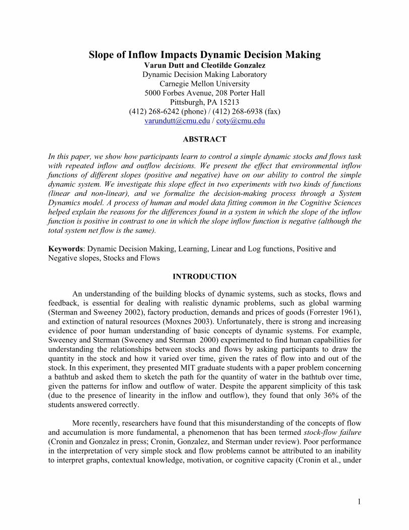
Figure 1 presents the graphical user interface of DSF. In this version, the stock represents

continuous units of the stock as water in a tank. The markings on the left-hand side of the tank represent the water level in the tank at any instance of time. There are 4 pipes connecting the tank, 2 labeled User Inflow and Environment Inflow, which increase the level of stock in the tank, and 2 pipes labeled User Outflow and Environment Outflow, which decrease the level of stock in the tank.

Figure 1. Dynamic Stocks and Flows task

The participant must set the inflow and outflow rates at each instance of time in the respective text boxes labeled Enter the Inflow(Gallons/Time Period) and Enter the Outflow(Gallons/Time Period), typically to compensate for environmental inflow and outflow that push the stock away from its desired level. The environmental inflow and outflow are exogenous functions that can be defined by the experimenter or instructor. The target level of stock is shown with a red horizontal line with a label Goal on the right and also in the Goal (Gallons) information box, as shown in the information section next to the Amount in Tank (Gallons) box.

The information panel informs a user of the User Inflow (Gallons/Time Period) and User

Outflow (Gallons/Time Period), i.e. inflow and outflow decisions made by the participant in the last time period, the Environment Inflow (Gallons/Time Period) and Environment Outflow (Gallons/Time Period), i.e. inflow and outflow caused by the environment in the last time period

4

(which were outside the participant’s own decision making and control), and the actual Amount in Tank (in Gallons) and the Goal amount (also in Gallons) to be maintained in the tank in each time period. In clicking the Submit button, after entering the values of inflow and outflow in the two text boxes, the system will apply the environment and participant flows to the tank and move forward to the next time period.

EXPERIMENT 1

Methods Experimental Design

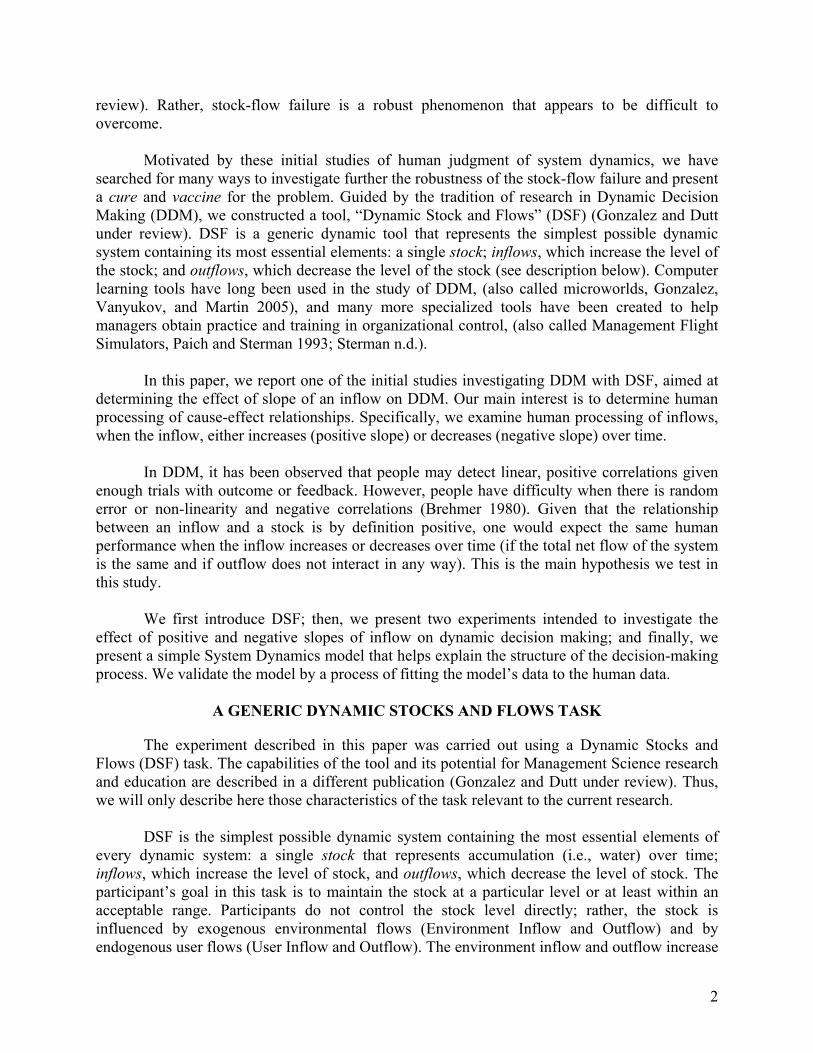
In this experiment, we controlled for the Environment Inflow curve slope (positive, negative) and ask participants to attempt to control the system over the course of 100 time periods. The goal was to maintain the level of water in the tank to 4 Gallons or within +/- 0.1 Gallons from the goal during all the 100 time periods. The Environment Inflow function slopes were either positive or negative. Figure 2 shows the two Environment Inflows as function of time periods. The Environment Outflow was constant and set at 0 Gallons/Time Period during100 time periods. Hence, Environment net flow was equal to Environment Inflow. The initial water level in the tank was fixed in both positive and negative conditions at 2 Gallons. Environment Inflow increased or decreased over the course of 100 time periods within a range of 2.08 Gallons/Time Period and 10 Gallons/Time Period. We defined the Environment Inflow in such a way that the values in each time period would not correlate directly with the time period, using the following formulas: 0.08 * (TimePeriod) + 2 for the increasing linear Environment Inflow function and (-7.92/99) * (TimePeriod-1) + 10 for the decreasing linear Environment Inflow function. Both functions caused an equal amount of water to flow into the tank over the course of 100 time periods (= 604 Gallons).

0

2

4

6

8

10

12

1 6 11 16 21 26 31 36 41 46 51 56 61 66 71 76 81 86 91 96

Time Periods

Envi

ronm

ent

Inflo

w

Positive Negative Figure 2. Two curve slopes for Environment Inflow as a function 100 time periods

5

We used the User’s Inflow and Outflow decisions and the stock level per trial as dependent variables. We expected individuals to decrease their use of the Inflow and to switch to controlling the system only by matching their Outflow to the Inflow caused by the environmental function. Thus, we also expected the User’s Outflow function to match the Environment’s Inflow function in long term: increasing for the positive linear Environment Inflow curve and decreasing in the negative linear Environment Inflow curve over 100 time periods. Finally, we expected that users would reduce the discrepancy between the goal and the stock with task practice. However, reducing discrepancy over the negative linear environment’s Inflow was expected to be more difficult than reducing discrepancy in the positive linear environment’s Inflow. Participants

Thirty-two graduate and undergraduate students from diverse fields of study participated

in this experiment. 15 were females, and 17 were males. Ages ranged from 18 years to 46 years with an average age of 23 years. All participants received a base pay of $5 and an additional bonus according to their performance in the task. Current bonus for the time period is (see Figure 1) displayed the bonus earned in the last time period and Total money earned (see Figure 1) displayed the total cumulative bonus earned up to the current time period. All participants started with a bonus amount of $5 (the base pay). Each time a participant came 0.1 Gallons above or below the goal of 4 Gallons in the water tank (i.e. their water level lay between 3.9 Gallons and 4.1 Gallons for the experiment), the participant earned a performance bonus in the experiment. Procedure

Participants were randomly assigned to one of the two conditions (i.e. positive or

negative Environment Inflow linear curves), and they were given instructions on the computer before starting the dynamic stocks and flows task. Participants were encouraged to ask questions after reading the instructions and were handed a paper copy of instructions. Participants were not given any information concerning the nature of Environment Inflows and Outflows and were told that these environmental flows were outside their own decision making and control over the entire course of the DSF task. They were then asked to play the DSF task for 100 time periods, where participants sat in front of a computer screen and were presented with DSF displayed in the center of the screen. (The current time period of the total 100 time periods was shown on the top left corner of the simulation screen; see Figure 1.) We made use of Windows XP-based desktop computer terminals with plasma screens, which had a resolution of 1024 x 1080; the desktop computers ran on a Pentium 4 processor base. Results

Data were analyzed with a 2 x 99 repeated measures ANOVA. (We dropped the first time

period on the analyses, since individuals did not have a system’s response when they made the first decision.) An alpha level = .05 was used. The results for the User Inflow, Outflow, and Stock levels are shown in Table 1.

6

Table 1. Analysis of Variance (repeated measures) in the Experiment 1 for User Inflow, User Outflow, and Stock

Source Df F P Measure: User Inflow, between participants

Curve Slope (CS) 1 2.858 (.101)

Error 31

Measure: User Inflow, within participants

Time Period (TP) 1- 99 98 1.356 .012

TP x CS 98 1.009 (.458) Error (TP) 3038

Measure: User Outflow, between participants

Curve Slope (CS) 1 2.951 (.096)

Error 31

Measure: User Outflow, within participants

Time Period (TP) 1- 99 98 1.740 .000

TP x CS 98 15.867 .000

Error (TP) 3038

Measure: Stock, between participants

Curve Slope (CS) 1 12.718 .001

Error 31

Measure: Stock, within participants

Time Period (TP) 1- 99 98 9.894 .000

TP x CS 98 7.031 .000

Error (TP) 3038

Note: Values enclosed in parentheses represent interactions that were insignificant. The CS is either positive sloped or negative sloped Environment Inflow, p < .05.

The results indicate that on average, the Stock differed between the positive and negative

Environmental Inflow curves. The stock was higher for the negative (M = 5.909, SE = .205) than the positive condition (M = 4.297, SE = .027). The analyses also indicated that the User Inflow,

7

Outflow, and Stock diminished significantly over time in both conditions. Further, the decrease of the User Outflow and Stock interacted with the slope of the Environmental Inflow function. These interactions between the slope of the Environment Inflow function and the time periods are shown in Figure 3 for the User Outflow and in Figure 4 for the Stock.

0

2

4

6

8

10

12

14

16

18

201 4 7 10 13 16 19 22 25 28 31 34 37 40 43 46 49 52 55 58 61 64 67 70 73 76 79 82 85 88 91 94 97 100

Time Periods

Use

r Out

flow

Positive Negative Figure 3. The nature of User Outflow for positive and negative linear Environment Inflow curve slopes over 100 time periods

0

5

10

15

20

25

30

1 5 9 13 17 21 25 29 33 37 41 45 49 53 57 61 65 69 73 77 81 85 89 93 97

Time Periods

Stoc

k le

vel

Positive Negative Figure 4. The nature of Stock for positive and negative linear Environment Inflow curve slopes over 100 time periods

Figure 3 indicates that the User Outflows follow the Environment Inflow functions quite

closely. Also, as shown in Figures 3 and 4, most variability occurs in the negative linear condition and during the first half of the trials. Thus, we performed a second set of analyses involving the Inflow, Outflow, and Stock during the first 50 trials. These results indicate that during the first 50 time periods the User’s Outflow in the negative conditions was higher (M = 8.793, SE = .289) than in the positive one (M = 4.312, SE = .052) (F(1,31) = 310.974, p<.001). Also, the stock was on average higher in the negative (M = 7.625, SE = .398) than in the positive condition (M = 4.419, SE = .046) (F(1,31) = 191.842, p<.001). Once again, the decrease of the

8

User Outflow and Stock interacted with the slope of the Environmental Inflow function (complete statistical results are not shown to save space.) Discussion

Our results demonstrate that in learning to control a dynamic system from outcomes,

individuals learn more quickly when the system follows a positive linear function than a negative linear one. These results support our hypothesis and findings from studies on probability learning and human judgment (Brehmer, 1980; Sterman, 1994): that positive linear causality is the basic schema used by people to control a dynamic task.

Individuals seem better able to comprehend positively correlated quantities than their

negatively correlated counter parts (Dörner, 1980; Sterman, 1994). In this experiment, individuals had more difficulty controlling the system when the system responded with a decrease in Environmental Inflow rather than an increase. This outcome was demonstrated by variability in the User’s Outflow decisions during the first half of the learning experience. (See Figure 3 for Environment Inflow negative slope during the first 50 time periods.) Thus, despite the equal amount of Net Flow into this system, the decreasing rate of inflow represented more cognitive difficulties in this very simple dynamic system.

While fast and highly accurate learning in the positive linear environment may be helpful

in some situations, we understand that most relationships in real-world situations are non-linear (e.g., production – stagnation cycles for products in markets, emission of green house gases, etc). Thus, it is important to determine if this slope effect in favor of the positive versus the negative slopes for linear Environment Inflow curves also occurs when the relationships are non-linear. This is the goal of Experiment 2.

EXPERIMENT 2

Methods Experimental Design

In this experiment, we again controlled for the Environment Inflow curve slope (positive,

negative) and asked participants to attempt to control the system over the course of 100 time periods. In this case, however, the environmental curves were non-linear (logarithmic). We used the positive log function, 5*LOG (TimePeriod), and the negative log function, 5*LOG (101- TimePeriod), for the Environment Inflow over a range of 100 time periods. These functions are shown in Figure 5. Both conditions had a total Environment net flow of 831 Gallons over the course of 100 time periods. All other conditions for the experiment were identical to those in Experiment 1.

As the non-linear decreasing curve has an initial close-to-zero slope and then decreases at

a rapid pace in the last few time periods, while the increasing curve has an initial, fast-increasing slope and then stabilizes in a close-to-zero slope, we expected that higher variability would occur

9

in the first few time periods for the increasing function and the last few time periods for the decreasing function.

0

2

4

6

8

10

12

1 5 9 13 17 21 25 29 33 37 41 45 49 53 57 61 65 69 73 77 81 85 89 93 97

Time Periods

Envi

ronm

ent I

nflo

w

Positive Negative Figure 5. Two curve slopes for non-linear (Log) Environment Inflow as a function of 100 time periods Participants

Thirty graduate and undergraduate students from diverse fields of study participated in

this experiment. 16 were females, and 14 were males. Ages ranged from 18 years to 56 years, with an average age of 25 years. All participants received a base pay of $5 and an additional bonus according to their performance in the task. Procedure

Participants were randomly assigned to one of two conditions (positive or negative

nonlinear curves). All other procedures were identical to those in Experiment 1. Results

Data for all 30 participants were analyzed with a 2 x 99 repeated measures ANOVA at an

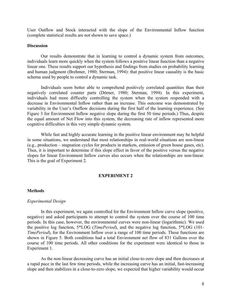
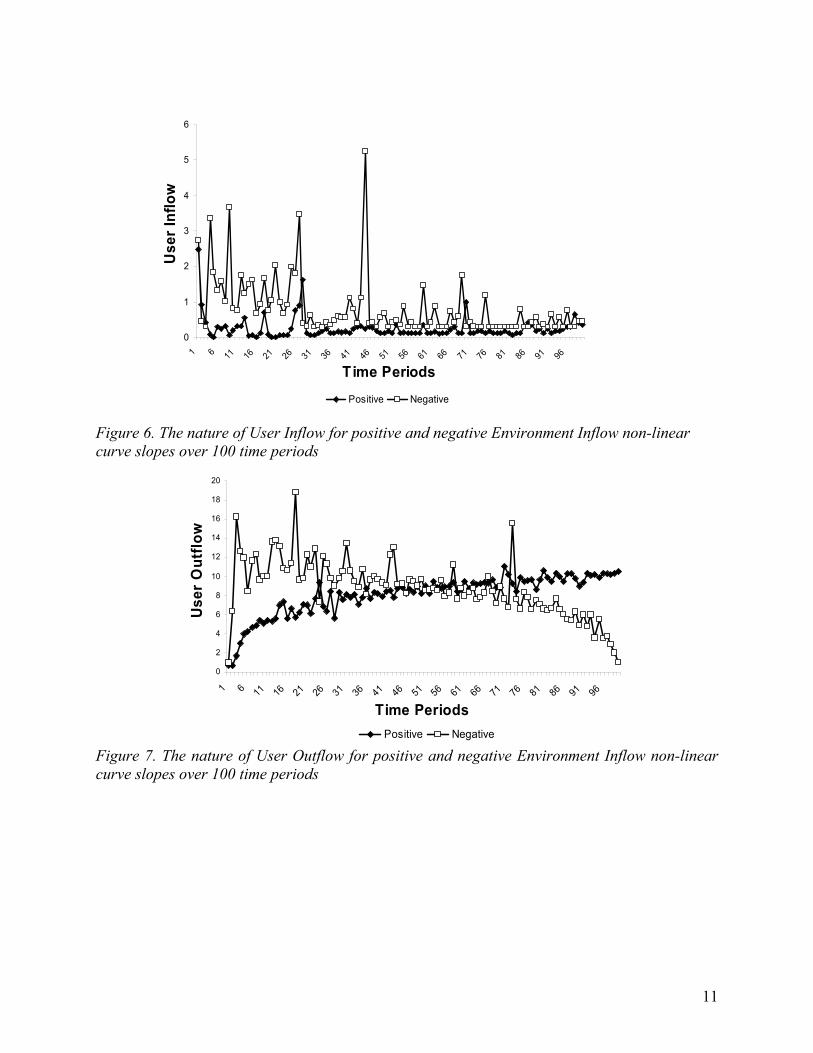
alpha level = .05. The results for the User Inflow, Outflow, and Stock levels are shown in Table 2. The results indicated that the User Inflow, Outflow, and Stock changed significantly over time in both positive and negative conditions (time period effect) and that the change over time interacted with the slope of the Environmental Inflow function. The interaction between the slope of the Environment Inflow function and the time period for the User Inflow is shown in Figure 6. This interaction for the User Outflow function is shown in Figure 7, and the interaction for Stock is shown in Figure 8.

10

Table 2. Analysis of Variance (repeated measures) in the Experiment 2 for User Inflow, User Outflow, and Stock

Source Df F P

Measure: User Inflow, between participants

Curve Slope (CS) 1 9.851 .004

Error 29

Measure: User Inflow, within participants

Time Period (TP) 1- 99 98 1.323 .020

TP x CS 98 1.590 .000 Error (TP) 2842

Measure: User Outflow, between participants

Curve Slope (CS) 1 2.025 (.165)

Error 29

Measure: User Outflow, within participants

Time Period (TP) 1- 99 98 1.990 .000

TP x CS 98 10.567 .000

Error (TP) 2842

Measure: Stock, between participants

Curve Slope (CS) 1 1.001 (.325)

Error 29

Measure: Stock, within participants

Time Period (TP) 1- 99 98 4.227 .000

TP x CS 98 2.516 .000

Error (TP) 2842

Note.: Values enclosed in parentheses represent interactions that were insignificant. The CS is either positive sloped or negative sloped Environment Inflow, p < .05.

11

0

1

2

3

4

5

6

1 6 11 16 21 26 31 36 41 46 51 56 61 66 71 76 81 86 91 96

Time Periods

Use

r Inf

low

Positive Negative

Figure 6. The nature of User Inflow for positive and negative Environment Inflow non-linear curve slopes over 100 time periods

0

2

4

6

8

10

12

14

16

18

20

1 6 11 16 21 26 31 36 41 46 51 56 61 66 71 76 81 86 91 96

Time Periods

Use

r O

utflo

w

Positive Negative Figure 7. The nature of User Outflow for positive and negative Environment Inflow non-linear curve slopes over 100 time periods

12

0

2

4

6

8

10

12

14

16

18

20

1 6 11 16 21 26 31 36 41 46 51 56 61 66 71 76 81 86 91 96

Time Periods

Stoc

k Le

vel

Positive Negative Figure 8. The nature of Stock for positive and negative Environment Inflow non-linear curve slopes over 100 time periods

As Experiment 1, this experiment also illustrates that User Outflows follow the

Environment Inflow functions quite closely. However, the User Inflow and Stock again indicate that most variability occur during the first half of the trials, where the negative slope functions result in higher Inflow and higher Stock levels than the positive slope function. No difference between the positive and negative slope functions was observed for the last 50 trials of the experiment in the User Inflow and Stock results. An analysis of the first 50 trials indicated that, on average, the User Inflow in the negative conditions was higher (M = 1.098, SE = .152) than in the positive condition (M = .245, SE = .038) (F(1,30) = 4.27, p<.05); the user’s outflow in the negative conditions was also higher (M =10.677, SE = .290) than in the positive ones (M = .6.851, SE = .126) (F(1,30) = 80.35, p<.001); the stock was higher on average in the negative (M = 7.938, SE = .419) than in the positive conditions (M = 4.757, SE = .143) (F(1,30) = 6.49, p<.05). The same analysis for the last 50 trials of the experiment did not show a difference between the positive and negative slopes for Inflow and Stock variables. A significant difference was found only for the User Outflow (F(1,31) = 85.334, p<.001), where the Outflow was higher for the positive (M = 9.543, SE = .081) than the negative (M =7.067, SE = .195) slope function. Once again, the decrease of User Outflow and Stock interacted with the slope of the Environmental Inflow function. Discussion

The results from this experiment replicate the results from Experiment 1, where learning

occurs faster in a positive function than a negative one. The results form Experiments 1 and 2 together suggest the effect of the slope of the environmental function is robust and perhaps independent from the linearity of the function.

The results do not support our initial expectations that a higher discrepancy would be

found for the increasing (rather than the decreasing) function during the first few time periods and that an opposite effect would be found in the second half of the experiment. Rather, no

13

difference was found in the Inflow and Stock values for the second half of the experiment, and a difference was found during the first half of the experiment, where the negative slope curve presented higher values of Inflow and Stock, reproducing the results of Experiment 1.

MODELING THE DYNAMIC DECISION MAKING PROCESS

To investigate the slope effect reported for the previous experiments, we built a system dynamics model. This model represents the human processes by which a decision maker goes about keeping control of DSF under positive and negative slopes. Here we follow an approach that is tradition in cognitive modeling, which involves a “matching process” between model and human data, helping to fine-tune the model with human behavior as shown in data collected from experiments (Schunn and Wallach 2001). This process is also encouraged and followed in many cases in system dynamics models (Oliva, 2003).

The closeness of our model to the actual observed phenomena was calculated with a

statistical measure on trend (Pearson Correlation Coefficient, r) and a statistical measure on deviation from actual observed phenomena (Root Mean Squared Standard Deviation (RMSD)) (Schunn and Wallach 2001).

In the following section, we present the underlying structure of the model that reproduces

the slope effect found in our previous two experiments. Then, we present a discussion of the model fit to human data by giving statistical measures for trend and value deviation. DSF Model Structure

We developed a System Dynamics model using Vensim® software from Ventana

Systems. To help develop this model, we drew upon our observations from verbal protocols collected from four participants (Ericsson and Simon 1993). We collected one protocol from each of four different groups described in the 2 experiments (linear-positive slope, linear-negative slope, non-linear-positive slope, and non-linear-negative slope). We also made use of the analyses of inflow and outflow human decisions data and their resulting stock, the averages of participants’ decisions for each of the conditions, and comparisons of the participants’ inflow and outflow decisions to the stock and environmental flow values.

The resulting model structure from this research is shown in Figure 9. We explain next

the process we followed to determine the model’s variables and parameters. The structure of the system is simply represented by the stock, the inflows (User and

Environment), and the outflows (User and Environment). The Environment Inflow is either a linear or logarithmic function, as defined in our experiments, and the Environment Outflow is zero in all groups.

14

Figure 9. The System Dynamics Model of Human Dynamic Decision Making The information sources reveal that participants clearly understood their task to reduce

the discrepancy between the observed level of stock and the goal level (represented by the Discrepancy variable in the model). This discrepancy, however, seemed to be only one of the many variables individuals used to make their inflow and outflow decisions.

The information sources also reveal that within the first few time periods participants

recognized that the unknown environment’s outflow did not change from the zero value in the experiment, and hence there was only a change in the environment’s inflow in each time period, which was added water in the tank. For example, a participant in the collected verbal protocol for the non-linear, positive-environment inflow condition was making User Inflow and Outflow decisions for the seventh time period and had 4.9 Gallons of water in the tank. She clearly indicated that “…as the Environment has only added water to the tank in the previous time periods, this time it will again and I expect the amount the Environment will add will be around 3.9 Gallons.” The participant removed 5 Gallons from the tank by using the Outflow decision

15

only and keeping 0 Gallons/Time Period in the Inflow decision. It seemed clear that participants cared about the net flow into the system more than their own individual inflow and outflow decisions. Also the participants were trying to perceive the net flow of Environment into the tank. This Perceived Environment Net flow is used to forecast the behavior of the Environment net flow (represented by the Forecast of Net flow variable). The nature of the zero Environment Outflow and the function-based Environment Inflow was represented in our model by what we have termed User Correction Weight to Inflow-Outflow or W parameter.

Thus, according to our information sources, individuals’ decisions appear to be

determined directly by the Forecast of Net flow and the Discrepancy. According to the verbal protocols, it seems that individuals attempt to correct for an observed discrepancy over the course of a number of time periods rather than instantaneously. Verbal protocols indicate that participants were amazed by the variability of the unknown environment’s net inflow and could not correctly estimate the exact amount of water the environment was going to add in the next time period (reflected in both Perceived Environment Net flow and the Forecast of Net flow). The participant in the collected verbal protocol for the preceding non-linear, positive-environment inflow condition decreased the water level to 3.8 Gallons at the beginning of the eighth time period; she further reduced the water level to 4.0 Gallons in the ninth time period, anticipating correctly this time that the Environment would add 4.2 Gallons in the present time period. The same participant took 9 time periods from the beginning to make the water level in the tank meet the goal for the first time. Hence, participants corrected for the discrepancy by balancing their forecast for Environment Inflow and system discrepancy over the course of many time periods.

Although for the specified participant this course of correction took 9 time periods, it is

clear from the collected data that it was only around the seventh time period that participant began to make a real attempt in correcting the discrepancy and understanding the mechanics of the DSF task. The time from the seventh time period to the ninth time period, i.e. 2 time periods, is the Perceived Time for Correction in our model that participants take to meet the discrepancy. From the verbal protocols, it is evident that during these 9 time periods the same participant had a memory of discrepancy for only the last one or two time periods (i.e., the participant mentions that in the last time period the discrepancy was 0.2 Gallons and it had now become 0.0 Gallons). The Memory of Discrepancy and Forecast Horizon are parameters that account for participants’ memory of previously seen discrepancy values and Environment net flow values. The Forecast of Net flow as well as the User Net Flow correction, where participants may adopt an approach over the course of many time periods, can be explained by the smoothing affect in system dynamics with the memory parameters of Memory of Discrepancy and Forecast Horizon, as described above. This smoothing effect of time averages to represent expectations is indeed similar to blending parameters used in learning models of dynamic decision making under the cognitive modeling approach (Gonzalez, Lerch, and Lebiere 2003).

The heart of the model consists of a balancing loop to determine the User Net Flow for

the system in each time period. The Environment Inflow into the stock in the absence of Environment Outflow causes the stock to move away from the Goal in every time period. This causes an increase in discrepancy. The increase in discrepancy beyond the acceptable range (which was set as 0.1 Gallons from the Goal at 4 Gallons for both Experiment 1 and Experiment 2) causes a User Net Flow Correction to account for the increase in discrepancy over the

16

Perceived Time for Correction (PTC) smoothened over the Memory of Discrepancy (MD). At this point the User Net Flow Correction is also affected by the Forecast of flow, where the Forecast of flow comes from the memory of Perceived Environment Net flow value (which in our model is the Forecast Horizon (FH)). The Perceived Environment Net flow is directly affected by the Environments Inflows and Outflows and its value is determined by the Environment’s Perception (EP). Part of the User Net Flow Correction determines the User Inflow, and the other part determines the User Outflow, where both the parts are weighted by the User correction weight to Inflow and Outflow (W). The resultant value of the User Inflow and User Outflow causes the stock to decrease, and hence User Inflow and User Outflows move the stock in a direction opposite to that caused by the Environment Inflow, brining the stock closer to the goal. The code for Vensim® model equations can be found in Appendix of this paper. Model and Human Data fits

According to the information sources for the construction of the preceding model, we

expected that the parameters of the model, the Environment Perception (EP), the Forecast Horizon (FH), the Perceived Time for Correction (PTC), the Memory for Discrepancy (MD), and the Correction for Inflow-Outflow (W), would be different for the positive and the negative slope conditions.

Guided by these expectations, we proceeded with parameter tuning while measuring the

fit of the model’s data to the humans’ average and median values over the course of 100 trials, using the r and RMSD statistics. The resulting parameter values and data fit statistics for data from Experiments 1 and 2 are summarized in Table 3. The same model depicted in Figure 9 was used to fit the data of the 4 different data groups from Experiments 1 and 2. The value of the parameters summarized in Table 3 help provide a coherent explanation for the different human behavior found between the positive and negative slopes. Figure 10 presents a graphical example of the fitting of the Stock data for linear, positive, and negative slopes functions.

17

Figure 10. The Model fit to Stock for linear positive and linear negative Environment Inflow

Table 3. Model measures for Stock, User Inflow, and User Outflow in Experiments 1 and Experiment 2 for different Environment Inflow conditions

Condition Parameters Fit Measures

EP FH MD PTC W Median Mean R RMSD r RMSD

Stock Linear Positive 1.03 1 1.1 2.5 1 .82 1.94 .79 2.34

18

Linear Negative 1.0 1.5 1.0 4.3 1 .91 3.9 .88 4.15 Non-Linear Positive

1.03 1 1 2.0 1 .95 1.85 .51 2.62

Non-Linear Negative

1.07 1.5 1 4.5 1 .91 7.54 .63 8.00

User Inflow Linear Positive 1.03 1 1.1 2.5 1 1.00 .91 .86 1.70 Linear Negative 1.0 1.5 1.0 4.3 1 .95 1.27 .20 1.67 Non-Linear Positive

1.03 1 1 2.0 1 .89 .97 .69 1.68

Non-Linear Negative

1.07 1.5 1 4.5 1 .92 .86 .23 1.84

User Outflow Linear Positive 1.03 1 1.1 2.5 1 .99 1.61 .99 1.53 Linear Negative 1.0 1.5 1.0 4.3 1 .87 2.15 .84 2.27 Non-Linear Positive

1.03 1 1 2.0 1 .98 1.86 0.95 1.96

Non-Linear Negative

1.07 1.5 1 4.5 1 .94 .86 .81 1.40

Note: p<.05 and z=1.96 The reason for higher Stock, User Inflow, and User Outflow values for the negative-

sloped Environment Inflow cases when compared with their positive-sloped counterparts in Experiments 1 and 2 becomes clear after observing the PTC and FH parameter values resulting from the model. Table 3 shows that the value of PTC and FH are higher for the negative-sloped cases for both Linear and Non-Linear Environment Inflow when compared with their positive- sloped counter parts. For example, in the case of Stock, the values are FH=1, PTC=2.5 for the linear, positive-sloped Environment Inflow, and values are FH=1.5, PTC=4.3 for the linear, negative-sloped Environment Inflow. The same is the trend in User Inflow and User Outflow across all linear and non-linear positive and negative cases for Environment Inflow. Greater FH value means that the participant takes more time to forecast the Environment Inflow value, and this extra time causes the stock to increase due to the Environment Inflow, which drives the stock away in each time period. Similarly, greater PTC value means that the participants take more time to perceive the discrepancy happening in the tank and hence also takes more time to correct the discrepancy; this extra time causes the stock to rise again due to Environment Inflow into the stock with each elapsing time period. To meet the higher stocks, participants order higher user inflows and outflows, causing User Inflow and User Outflow values to rise as well. When we fit our model to the negative-sloped Environment Inflow cases, we see that increasing FH and PTC generates a good fit for the human data. This increase in FH and PTC in our model causes the Stock to rise higher (due to the Environment Inflow action and slower corrective action), causing the discrepancy to increase further, and hence, the User Net Flow correction to increase further. The User Net Flow correction is further increased by the Forecast for net flow, which now happens over a larger time period range (due to FH increase, where there are increased Environment Inflows over this larger time range). The increase in User Net Flow correction as described above causes higher User Inflow and User Outflow in our models, where

19

the User Inflow and User Outflow are derived from the User Net Flow correction and weighted by the User Correction Weight to Inflows and Outflows (W).

CONCLUSIONS

Many of the complex dynamic effects found in the real world can be better understood with simple tasks, such as DSF. Here we present a new research process by which to understand the basic building blocks of dynamic systems. The focus of this paper is on a simple effect, that of the slope of the inflow on a system. Two systems with equal opportunity for balance, with equal net flow, but with positive and negative inflow slopes, were found to generate different human decision-making behaviors. The construction of a System Dynamics model in combination with behavioral data collection and verbal protocol techniques have provided a rich, cognitive explanation of why a system with a negative slope of inflow function may take longer to control. It appears that individuals take more time to forecast the inflow value and to perceive the discrepancy from the goal. This outcome supports previous findings indicating that positive linear causality is the basic schema used by people to control a dynamic task (Brehmer, 1980; Sterman, 1994).

ACKNOWLEDGMENTS

This research was partially supported by the National Science Foundation (Human and Social Dynamics: Decision, Risk, and Uncertainty, Award number: 0624228) and by the Army Research Laboratory (DAAD19-01-2-0009) awards to Cleotilde Gonzalez.

20

References

Brehmer, Berndt. 1980. In one word: Not from experience. Acta Psychologica, 45, 223-241. Cronin, Matthew A., and Cleotilde Gonzalez. In press. Understanding the building blocks of

system dynamics. System Dynamics Review. Cronin, Matthew A., Cleotilde Gonzalez, and John D. Sterman. Under review. Why don't well-

educated adults understand accumulation? A challenge to researchers, educators and citizens. Organizational Behavior and Human Decision Processes

Dörner, Dietrich. 1980. On the difficulties people have in dealing with complexity. Simulation and Games, 11(1), 87-106.

Ericsson, K. Anders, and Herbert A. Simon. 1993. Protocol analysis: Verbal reports as data. Cambridge, MA: MIT Press.

Forrester, Jay W. 1961. Industrial dynamics. Waltham, MA: Pegasus Communications. Gonzalez, Cleotilde, and Varun Dutt. Under review. A generic dynamic control system for

management education. Academy of Management Learning & Education. Gonzalez, Cleotilde, J. F. Lerch, and C. Lebiere. 2003. Instance-based learning in dynamic

decision making. Cognitive Science, 27(4), 591-635. Gonzalez, Cleotilde, P. Vanyukov, and M. K. Martin. 2005. The use of microworlds to study

dynamic decision making. Computers in Human Behavior, 21(2), 273-286. Moxnes, E. 2003. Misperceptions of basic dynamics: The case of renewable resource

management. System Dynamics Review, 20, 139-162. Oliva, Rogelio. 2003. Model calibration as a testing strategy for system dynamics models.

European Journal of Operational Research, 151, 552-568. Paich, M., and John D. Sterman. 1993. Boom, bust and failures to learn in experimental markets.

Management Science, 39(12), 1439-1458. Schunn, C. D., and D. Wallach. 2001. Evaluating goodness-of-fit in comparison of models to

data. University of Pittsburgh. Sterman, John D. 1994. Learning in and about complex systems. System Dynamics Review, 10,

291-330. Sterman, John D. N.d. Teaching takes off, flight simulators for management education: "The

Beer Game". Flight Simulators for Management Education Retrieved February 18, 2007, from http://web.mit.edu/jsterman/www/SDG/beergame.html

Sterman, John D., and L. B. Sweeney. 2002. Cloudy skies: Assessing public understanding of global warming. System Dynamics Review, 18(2), 207-240.

Sweeney, L. B., and John D. Sterman. 2000. Bathtub dynamics: initial results of a systems thinking inventory. System Dynamics Review, 16(4), 249-286.

21

Appendix Vensim® Equations for System Dynamics Model

(01) Discrepancy= Goal - Stock Units: Gallons (02) Env Inflow= 8*(RAMP( 1 , 0 , 100 ))/100+2 (For Linear Positive) 10-(7.92/99)*(RAMP( 1 , 0 , 100 )-1) (For Linear Negative) 5* LOG(RAMP( 1 , 0, 100 ),10) (For Non Linear Positive) 5*LOG(101-RAMP( 1 , 0 , 100 ),10) (For Non Linear Negative) Units: Gallons/Second (03) Env Ouflow= 0 Units: Gallons/Second (04) "Environment's Perception (EP)"= 1 Units: Dmnl [0,50,0.01] (05) FINAL TIME = 100 Units: Second The final time for the simulation. (06) "Forecast Horizon(FH)"= 1 Units: Dmnl [1,50,0.01] (07) Forecast of flow= SMOOTH(Perceived Environment Net flow, "Forecast Horizon(FH)") Units: Gallons/Second (08) Goal= 4 Units: Gallons (09) INITIAL TIME = 1 Units: Second The initial time for the simulation. (10) "Memory of Discrepancy(MD)"= 1 Units: Second [1,50,0.01] (11) Perceived Environment Net flow= DELAY FIXED("Environment's Perception (EP)"*(Env Inflow-Env Ouflow), 1, K)

K: 0 (For Linear Positive), -2 (For Linear Positive), 0 (For Non Linear Positive), 0 (For Non Linear Negative)

Units: Gallons/Second (12) "Perceived Time for Correction(PTC)"= 1 Units: Second [0,50,0.01]

22

(13) SAVEPER = TIME STEP

Units: Second [0,?] The frequency with which output is stored. (14) Stock= INTEG (Env Inflow+User Inflow-Env Ouflow-User Outflow, 2) Units: Gallons (15) TIME STEP = 1 Units: Second [0,?] The time step for the simulation. (16) "User correction weight to Inflow and Outflow(W)"= 1 Units: Dmnl [0,1,0.01] (17) User Inflow= (1-"User correction weight to Inflow and Outflow(W)")*User Net flow Correction Units: Gallons/Second (18) User Net flow Correction= IF THEN ELSE((Discrepancy>0.1 :OR: Discrepancy <-0.1), SMOOTH(-1 * Discrepancy /"Perceived Time for Correction(PTC)" , "Memory of Discrepancy(MD)") ,0) + Forecast of flow Units: Gallons/Second (19) User Outflow= "User correction weight to Inflow and Outflow(W)"*User Net flow Correction

Units: Gallons/Second