A DESIGN STUDY OF RADIALINFLOW TURBINES

IN THREE-DIMENSIONAL FLOWby

Yi-Lung Yang

B.S., National Taiwan University (1983)M. S., Massachusetts Institute of Technology (1986)

SUBMITTED IN PARTIAL FULFILLMENT OF THEREQUIREMENTS FOR THE DEGREE OF

DOCTOR OF PHILOSOPHYin

Aeronautics and Astronauticsat the

Massachusetts Institute of Technology

June, 1991

(O)Massachusetts Institute of Technology 1991

Signature of AuthorF

Department of Aeronautics and AstronauticsMarch 29,1991

Certified byDr. Choon S. Tall

Chairman of Thesis Committee

Prof. James E. McCuneThesis Committee Member

Prof. Mark DrelaThesis Committee Member

.w · ,

Professor Harold Y. WachmanChairman, Departmental Graduate Committee

MASSACUS ' S INSTI1 UTEOF TS u "^' 1'99

11r L 1991

LIBRARIES

Certified by

Certified by

Accepted byU

A DESIGN STUDY OF RADIAL INFLOW TURBINESIN THREE-DIMENSIONAL FLOW

byYi-Lung Yang

submitted to the department ofAeronautics and Astronautics

in partial fulfillment of the requirementfor the degree of Doctor of Philosophy

ABSTRACTThe development and the application of a computational tool based on an analytical

theory for the design of turbomachinery blading in three-dimensional, inviscid flow arepresented. In the design problem, the enthalpy or swirl distribution to be added/removedby a blade row is prescribed, and one then proceeds to determine the blade geometry; thisis in contrast to the direct problem in which one proceeds to determine the performanceof a blade row for a specified geometry. In the computational method, discretizationof the governing equations in the theory is implemented via the use of finite-elementmethod on the meridional plane and Fourier collocation technique in the circumferentialdirection. The three-dimensional design method is used to compute the blade shape inradial inflow turbine wheels in subsonic flow. This requires the following specifications:swirl distribution, number of blades, hub and shroud geometrical contour, location of bladeleading and trailing edges, configuration of stacking axis, blockage distribution, wheel speedand mass flow rate. A technique of generating a smooth swirl distribution within theblade region from a specification of swirl and its derivative with respect to the meridionaldistance along the hub and shroud is proposed. Excellent agreements have been obtainedbetween the computed results from the present design technique and those from directinviscid computations based on Euler solver; this demonstrates the correspondence andconsistency between the two techniques. The design method is then used to examinethe influence of the following parameters on the design of a radial inflow turbine wheelproposed for helicopter powerplant application: (i) the swirl distribution within the bladeregion for a fixed power output; (ii) the stacking axis; (iii) the hub and shroud profiles; (iv)the number of blades; and (v) the thickness distribution. Two parameters are proposedas a measure of the goodness of a design; they are the pressure gradient on the boundingsurfaces of the blade region and the wake number. The wake number has been developed togive a measure of the extent of secondary flow formation within the blade passage. Resultsfrom this design study suggest that the proposed technique of prescribing swirl distributionis a useful one and that a good design requires the specification of a swirl distribution thathas its location of maximum loading near the leading edge. The computed results alsodemonstrate the sensitivity of the pressure distribution to a lean in the stacking axis and aminor alteration in the hub/shroud profiles. In most of these design calculations an inviscidregion of reversed flow on the pressure surface of the blade has been observed. However,when a Navier-Stokes solver is used to analyze the flow through the designed wheel, nobreakdown of flow within the blade passage has been observed. Furthermore, the computedvalues of swirl distribution and reduced static pressure distribution from the Navier-Stokescalculation agree fairly well with those from the present design calculation, implying thatthe flow in the designed turbine rotor closely approximates that of an inviscid flow. Thepresent work illustrates the synergistic use of a design tool coupled to an analysis toolfor implementing design; such an approach allows one to concentrate on the aerodynamicquantities of interest rather than on the choices of blade geometry.

Thesis Supervisor: Dr. Choon S. TanTitle: Principal Research Engineer,

Department of Aeronautics and Astronautics.

2

Acknowledgements

I would first like to thank my supervisor, Dr. Choon S. Tan, for being a constant

source of inspiration and encouragement during the course of this project. The advice and

guidance he offered were greatly appreciated. Particular thanks are due to Professor Sir

William Hawthorne for his invaluable insight and encouragement. The time and effort he

spent throughout this research were deeply appreciated.

My thanks also go to Professor James E. McCune for his help and support. I am

indebted to him for having given generously of his time. The contributions of Professor

Mark Drela to the viscous flow aspects of the research were also invaluable.

I am also grateful to Dr. John J. Adamczyk of NASA-LEWIS Research Center who

provided both the Euler and viscous codes. I am also indebted to James D. Heidmann of

NASA-LEWIS Research Center for his assistance in the Euler and viscous calculations.

My friend and Post-doctoral Fellow at the Gas Turbine Laboratory, Dr. Andrew Wo,

deserves special mention for the hours of discussions and for reviewing my results.

I would also like to acknowledge some of my GTL collegues: Earl Renaud, for his

help with the computer facilities; Lou Catterfaster; Charlie Haldmann; Reza Shokrollah-

Abhari; Gwo-Tung Chen; Quin Yuan; Dan Gysling; Pete Silkowski; Tonghuo Shang; Eric

Strang; Seung Jin Song; who all made my stay at MIT a memorable one.

This project was sponored by the NASA Army Propulsion Directorate Grant NAG3-

772, under the supervision of Mr. Pete Meitner. This support is gratefully acknowleged.

Finally, I would like to thank my family for their love and support which made this

research possible.

3

Table of Contents

Abstract ..... . ....................................................................2

Acknowledgements ................................................................ 3

Table of Contents ........ 4

Nomenclature ................... 8...............................................

List of Figures .................................................................. 10

Chapter 1 Introduction ........................ 17

1.1 Radial Inflow turbines ................. ................................. 17

1.2 Design Specifications ............................................... 18

1.3 Scope and Objectives of the Present Research ........ .................. 20

Chapter 2 Literature Survey of Inverse Design Methods ....... .................... 22

2.1 Blade to Blade Design Methods ........................................ 22

2.1.1 Singularity Methods ......... .. ......... ........... 232.1.2 Conformal Transformation Methods ............................ 24

2.1.3 Hodograph Methods ........................................... 25

2.1.4 Stream Function/Potential Plane Methods ..................... 25

2.1.5 Taylor Series Expansion Methods .............................. 26

2.1.6 Potential/Stream Function Methods .................... .... 26

2.1.7 Time-Marching Methods ....................................... 27

2.1.8 Other Methods .................. ................ 28

2.2 Hub-to-Shroud Design Methods ........................................ 28

2.3 Quasi-Three-Dimensional Design Methods ....... ................. 29

2.4 Three-Dimensional Design Methods .................................... 29

2.5 The Present Approach to Three-Dimensional Design .................... 31

Chapter 3 Inverse Design Theory ................... ........................... 33

4

3.1 Governing Equations ........ .. .................................. 3

3.2 Theoretical Formulation .......................................... 34

3.2.1 The Clebsch Approach ......................................... 35

3.2.2 Mean Flow Equations ......................................... 37

3.2.3 Periodic Flow Equation ........................................ 38

3.2.4 Blade Boundary Condition ..................................... 39

3.3 The Boundary Conditions .............................................. 40

3.3.1 Stream Function ............................................... 40

3.3.2 Velocity Potential ........ ............. ....... 41

3.4 The Initial Conditions .................................................. 41

3.4.1 Artificial Density .............................................. 41

3.4.2 Blade Shape ... ..... ............................. 42

3.5 The Kutta-Joukowski condition ........................................ 42

3.6 Blockage Effects ........................................................ 43

3.7 Summary ...................................... ................. 45

Chapter 4 The Mean Swirl Schedule ........................................... 46

4.1 Kinematic Constraints ................................................. 46

4.2 Biharmonic Equation ....... . ........ ................ 484.3 Method of Specifying rVe along the Hub & the Shroud ........ .... 49

4.4 Summary ................................. ................... 50

Chapter 5 The Numerical Technique ............. ..... ............ 52

5.1 Grid Generation .................................................. 52

5.1.1 Algebraic Method ............................................. 52

5.1.2 Elliptic Method ............................................... 53

5.2 The Elliptic Solver .................................................. 54

5

5.3 The Convective Equation Solver ........................... 56

5.4 The Biharmomic Solver ................................................ 57

5.5 The Computational Scheme ............................................ 59

Chapter 6 Parametric Study of Inverse Designs ................................... 62

6.0 Two Parameters Used to Characterize a Design ......................... 63

6.1 Mean Swirl Schedule .............................................. 68

6.1.1 Effect of the Maximum Loading Position ....................... 69

6.1.2 Effect of Regions of Vanishing rve ....... 71

6.1.3 Effect of the Maximum Loading ()a ................... 73

6.2 Stacking Position ...................................................... 76

6.3 Lean in Stacking Line.................................................. 78

6.4 Slip Factor ............................................................. 79

6.5 Blockage Effects ........................................................ 80

6.6 Number of Blades ..................................................... 81

6.7 Exit Swirl ............................... 83

6.8 Modified Hub and Shroud Profiles ...................................... 84

6.9 Summary ............................. 85

Chapter 7

7.1

7.2

7.3

7.4

7.5

Flow Analysis by Solving Euler and Navier-Stokes Equations ........... 88

Euler and Navier-Stokes Codes Descripttion ...................... 88

Comparison between Design and Euler Results ......................... 90

Comparison between Design and Viscous Results ....................... 91

Effect of the Tip Clearance ............................................. 95

Summary .............................................................. 98

Chapter 8 Conclusions and Suggestions for Future Work ......................... 100

6

I I

8.1 Summary and Conclusions ............................................ 100

8.2 Suggestions for Future Work .......................................... 101

References .................................................................... 103

Table I: Turbine Design Conditions ........................................... 107

Figures .......................................................................... 108

Appendix

Appendix

Appendix

Appendix

Appendix

Appendix

A: An Expression for Velocity Jump Across the Blade ................. 184

B: Mass-Average of the Continuity Equation with the Effect of

Tangential Blockage, b ............................................ 185

C : A Multigrid Method for the Poisson Equation ..................... 187

D: The Relationship between Number of Grid Points and Number of

Harmonic Modes ..................................... ............ 191

E: Nondimensional Form of Variables ................................. 192

F: The Derivation of the Wake Number ............................... 192

7

__

Nomenclature

Roman Letters

B

b

fH

N

P

S

S(a)

T

tn

to

V

W

number of blades

blockage, Eq.(3.33)

blade shape, Eq.(3.5)

enthalpy

shape function, Eq.(5.5)

pressure

entropy

sawtooth function, Eq.(3.14)

temperature

blade normal thickness, Eq.(3.35)

blade tangential thickness, Eq.(3.34)

absolute velocity

relative velocity

Greek Letters

a

'pe

6p(a)

Pa

0

blade surface, Eq.(3.5)

ratio of specific heats

shed vorticities, Eq.(4.1)

periodic delta function, Eq.(3.6)

density

artificial density, Eq.(3.20)

Stokes stream function, Eq.(3.22)

8

lean angle of blade camber (see Fig. 6.16)

impeller rotational speed

blade circulation

periodic potential function, Eq. (3.17)

harmonic mode of periodic potential function, Eq. (3.25)

vorticity

Subscripts

bl

r,0, z

LE

TE

Superscripts

+/-

Others

()

[1()

" at " the balde

the r-,0-,z- component

blades leading edge

blades trailing edge

total, stagnation

the blade pressure/suction surface

rotary

vector quantity

tangential mean, Eq.(3.8)

periodic part

column matrix

matrix

9

w

r

I

List of Figures

Chapter 3

Fig. 3.1 Right-handed cylindrical coordinate system and nomenclature

Chapter 4

Fig. 4.1 An illustration of Prandtl wing theorem

Fig. 4.2 Schematic plot of rVe distribution along the hub and shroud

Chapter 5

Fig. 5.1 The 4-node element

Chapter 6

Fig. 6.1 Velocity triangle at leading edge

Fig. 6.2 Grid used for calculation

Fig. 6.3a The blade camber at mid-span for two different grid sizes

Fig. 6.3b The distribution of Pred. at mid-span for two different grid sizes

Fig. 6.4a The meridional velocity on the suction surface for Wake number = 1.86

meridional velocity on

distribution of rVe, W,

distribution of rVe, r,

distribution of r 7 , ,

distribution of rVe, ,

distribution of rV, ,

distribution of rVe, -,

distribution of rV0, - ,

the suction surface

and o.tV along the

and a_ along the

and a_~ along the

and a ralong the

and a_-& along the

and along the

and -r? along the68

for Wake number =

hub and shroud for

hub and shroud for

hub and shroud for

hub and shroud for

hub and shroud for

hub and shroud for

hub and shroud for

10

Fig.

Fig.

Fig.

Fig.

Fig.

Fig.

Fig.

Fig.

6.4b

6.5a

6.5b

6.5c

6.5d

6.5e

6.5f

6.5g

The

The

The

The

The

The

The

The

3.61

case a

case b

case c

case d

case e

case f

case g

The distribution of

distribution

distribution

distribution

distribution

distribution

distribution

distribution

distribution

distribution

distribution

distribution

Mrct. on the

Mre,. on the

distribution

Mrt. on the

Mr,e. on the

distribution

Mre. on the

M,re. on the

of

rVo,W and aV

rV o, and rV

along the hub and shroud for case h

along the hub and shroud for case i

of rV for case a

of rV8 for case b

of rV for case c

of rVe for case d

of rg 9 for case e

of rVe for case f

of rVe for case g

of rte for case h

of rV9 for case i

of Pred. for case a

suction side for case a

pressure side for case a

of Pred. for case f

suction side for case f

pressure side for case f

of Pred. for case g

suction side for case g

pressure side for case g

The maximum adverse pressure gradient vs the region of Ov = 0

The Wake number verse the region of vp = 0On

The distribution of Pred. for case h

The M,,t. on the suction side for case h

The M,,i. on the pressure side for case h

The distribution of Pred. for case i

The Mr,,. on the suction side for case i

11

The

The

The

The

The

The

The

The

The

The

The

The

The

The

The

The

The

The

The

Fig. 6.5h

Fig. 6.5i

Fig. 6.6a

Fig. 6.6b

Fig. 6.6c

Fig. 6.6d

Fig. 6.6e

Fig. 6.6f

Fig. 6.6g

Fig. 6.6h

Fig. 6.6i

Fig. 6.7a

Fig. 6.7b

Fig. 6.7c

Fig. 6.8a

Fig. 6.8b

Fig. 6.8c

Fig. 6.9a

Fig. 6.9b

Fig. 6.9c

Fig. 6.10a

Fig. 6.10b

Fig. 6.11a

Fig. 6.11b

Fig. 6.11c

Fig. 6.12a

Fig. 6.12b

The Mre,. on the pressure side for case i

The maximum adverse pressure gradient verse the maximum loading - )

The Wake number verse the maximum loading - r tmwa

The position of ( )maz vs stacking position for axisymmetric calculation

The position of (~),, vs stacking position for three-dimensional calcula-

Fig. 6.15a

Fig. 6.15b

Fig. 6.16

Fig. 6.17a

Fig. 6.17b

Fig. 6.17c

Fig. 6.18a

Fig. 6.18b

Fig. 6.18c

FIG. 6.19a

Fig. 6.19b

Fig. 6.19c

Fig. 6.20a

Fig. 6.20b

tion

The

The

The

The

The

The

The

The

The

The

The

The

The

The

maximum adverse pressure gradient verse the stacking position

Wake number verse the stacking position

definition of the lean ange, p

blade shape for lean angle, p = -6.65 °

blade shape for lean angle, p = 0.00°

blade shape for lean angle, p = +6.65°

distribution of Prcd. with lean angle Vo = -6.65 °

Mrct. on the suction side with lean angle p = -6.65 °

Mre. on the pressure side with lean angle o = -6.65 °

distribution of Pred. with lean angle p = 6.65°

Mr,. on the suction side with lean angle yo = 6.65°

MrCe. on the pressure side with lean angle po = 6.65°

maximum adverse pressure gradient verse the lean angle

Wake number verse the lean angle

Velocity triangle

Velocity triangle

The distribution

The Mr,e. on the

The M, 1. on the

The distribution

The Mrc. on the

The Mr,I. on the

at leading edge, slip factor = 0.95

at leading edge, slip factor = 0.86

of Pred. for slip factor = 0.95

suction side for slip factor = 0.95

pressure side for slip factor = 0.95

of Pred. for slip factor = 0.86

suction side for slip factor = 0.86

pressure side for slip factor = 0.86

12

Fig. 6.12c

Fig. 6.13a

Fig. 6.13b

Fig. 6.14a

Fig. 6.14b

Fig.

Fig.

Fig.

Fig.

Fig.

Fig.

Fig.

Fig.

6.21a

6.21b

6.22a

6.22b

6.22c

6.23a

6.23b

6.23c

Fig. 6.24a

Fig. 6.24b

Fig. 6.25a

Fig. 6.25b

Fig. 6.26a

Fig. 6.26b

Fig. 6.26c

Fig. 6.27a

Fig. 6.27b

Fig. 6.27c

Fig. 6.28a

Fig. 6.28b

Fig. 6.29a

Fig. 6.29b

Fig. 6.30a

Fig. 6.30b

Fig. 6.30c

Fig. 6.31a

Fig. 6.31b

Fig. 6.32a

Fig. 6.32b

Fig. 6.32c

Fig. 6.33a

Fig. 6.33b

The maximum adverse pressure gradient verse the slip factor

The Wake number verse the slip factor

The normal thickness, t,, for the input

The tangential thickness, to, from the output

The distribution of Pred. for case g, with blockage effects

The M7r,. on the suction side with blockage effects

The Mr,I. on the pressure side with blockage effects

The distribution of Pred. for number of blades B=21

The M,r. on the suction side for number of blades B=21

The M,el. on the pressure side for number of blades B=21

The maximum adverse pressure gradient verse the number of blades B

The Wake number verse number of blades B

The distribution of rVe, g and-9- along the hub and shroud with 30% ofswirl left after trailing edge

The distribution of rVe with 30% of swirl left after the trailing edge

The distribution of Prc,. with 30% of swirl left

The Al,,l on the suction side with 30% of swirl left

The MrCa. on the pressure side with 30% of swirl left

The distribution of rVo, !~ , and-r along the hub and shroud

The distribution of ro

The distribution of Pred., stacking at leading edge

The M,,tI on the suction side, stacking at leading edge

The Mr,1. on the pressure side, stacking at leading edge

The blade camber vs the meridional distance of the original and modifiedhub & shroud profiles

Radial distribution of blade camber along constant z-section for the originaland modified hub & shroud profiles

Chapter 7

13

Fig. 7.1 The mesh used for calculation

Fig. 7.2a The specified rVe for design calculation

Fig. 7.2b The blade shape from the design calculation, number of blade B = 14

distribution

distribution

distribution

distribution

distribution

difference in

distribution

distribution

distribution

distribution

of Pred on the suction surface from the design calculation

of Pred on the pressure surface from the design calculation

of Pred on the hub surface from the design calculation

of Pred on the shroud surface from the design calculation

of rVq from the Euler calculation

L rVe between design specification and Euler calculation

of Pred on the suction surface from the Euler calculation

of Pred on the pressure surface from the Euler calculation

of Pred on the hub surface from the Euler calculation

of Pred on the shroud surface from the Euler calculation

distribution of rVe from the viscous calculation

difference in rVe between design specification and viscous calculation

distribution of Prod on the suction surface from the viscous calculation

distribution of Pred on the pressure surface from the viscous calculation

distribution of P,,d on the hub surface from the viscous calculation

distribution of Pr,d on the shroud surface from the viscous calculation

distribution of relative Mach number M,, 1 from the design calculation

distribution of relative Mach number M,j from the viscous calculation

meridional velocity on the surface 1-point above the S.S

meridional velocity on the surface 1-point below the P.S.

distribution of entropy S at the leading edge

distribution of entropy S at the { chord

distribution of entropy S at the 1 chord

distribution of entropy S at the Q chord

distribution of entropy S at the trailing edgedistribution of entropy S at the trailing edge

14

Fig.

Fig.

Fig.

Fig.

Fig.

Fig.

Fig.

Fig.

Fig.

Fig.

Fig.

Fig.

Fig.

Fig.

Fig.

Fig.

Fig.

Fig.

Fig.

Fig.

Fig.

Fig.

Fig.

Fig.

Fig.

7.3a

7.3b

7.3c

7.3d

7.4a

7.4b

7.5a

7.5b

7.5c

7.5d

7.6a

7.6b

7.7a

7.7b

7.7c

7.7d

7.8a

7.8b

7.9a

7.9b

7.10a

7.10b

7.10c

7.10d

7.10e

The

The

The

The

The

The

The

The

The

The

The

The

The

The

The

The

The

The

The

The

The

The

The

The

The

The distribution of streamwise vorticity l, at the leading edge

The

The

The

The

The

The

The

The

The

4distribution of streamwise vorticity fl at the chord

distribution of streamwise vorticity Q at the 2 chord

distribution

distribution

distribution

distribution

distribution

distribution

distribution

The distributionblades B = 21

The distributionB = 21

of streamwise vorticity Qf at the 4 chord

of streamwise vorticity lz at the trailing edge

of entropy S at the leading edge, number of blades B = 21

of entropy S at the 4 chord, number of blades B = 21

of entropy S at the chord, number of blades B =21

of entropy S at the i chord, number of blades B = 21

of entropy S at the trailing edge, number of blades B = 21

of streamwise vorticity 0 r at the leading edge, number of

of streamwise vorticity nf at the chord, number of blades4

Fig. 7.13c

Fig. 7.13d

Fig. 7.13e

Fig.

Fig.

7.14a

7.14b

Fig. 7.15a

Fig. 7.15b

Fig. 7.15c

Fig. 7.15d

Fig. 7.16a

The distribution of streamwise vorticity l at the chord, number of bladesB = 21

B = 21The distribution of streamwise vorticity 0z at the trailing edge, number ofblades B = 21

The distribution of rVe from the viscous calculation with 3% of tip clearance

The difference in rVe between design specification and viscous calculationwith 3% of tip clearance (only the blade region)

The distribution of Pred. on the suction surface from the viscous calculationwith 3% of tip clearance

The distribution of Pred. on the pressure surface from the viscous calculationwith 3% of tip clearance

The distribution of Ped. on the hub surface from the viscous calculation with3% of tip clearance

The distribution of Pred. on the shroud surface from the viscous calculationwith 3% of tip clearance

The meridional velocity on the surface 1-point above the S.S. with 3% of tipclearance

15

Fig.

Fig.

Fig.

Fig.

Fig.

Fig.

Fig.

Fig.

Fig.

7.11b

7.11c

7.11d

7.11e

7.12a

7.12b

7.12c

7.12d

7.12e

Fig. 7.13a

Fig. 7.13b

Fig. 7.11a

The meridional velocity on the surface 1-point below the P.S. with 3% of tipclearance

The distribution

The distribution

The distribution

The distribution

The distribution

The distributiontip clearance

The distributionclearance

The distributionclearance

The distributionclearance

The distributiontip clearance

of entropy S at the leading edge with 3% of tip clearance

of entropy S at the 4 chord with 3% of tip clearance

of entropy S at the 2 chord with 3% of tip clearance

of entropy S at the 3 chord with 3% of tip clearance

of entropy S at the trailing edge with 3% of tip clearance

of streamwise vorticity f at the leading edge with 3% of

of streamwise vorticity f1 at the chord with 3% of tip

of streamwise vorticity Qf at the 2 chord with 3% of tip

of streamwise vorticity [1 at the 3 chord with 3% of tip

of streamwise vorticity 0z at the trailing edge with 3% of

Appendix B

Fig. B.1 Control volume for an axisymmetric flow

Appendix C

Test grid for

Log(residue)

Test grid for

Log (residue)

Test grid for

Log(residue)

multigrid study, uniform mesh

verse unit of work for mesh-a

multigrid study, with distortion in Z direction

vs unit of work for mesh-b

multigrid study, with distortion in both R and Z directions

vs unit of work for mesh-c

16

Fig.

Fig.

Fig.

Fig.

Fig.

Fig.

7.17a

7.17b

7.17c

7.17d

7.17e

7.18a

Fig. 7.18b

Fig. 7.18c

Fig. 7.18d

Fig. 7.18e

Fig.

Fig.

Fig.

Fig.

Fig.

Fig.

C.la

C.lb

C.2a

C.2b

C.3a

C.3b

Fig. 7.16b

Chapter 1

Introduction

There are two problems of interest to designers of turbomachinery. One is the "inverse"

problem in which the enthalpy or swirl distribution to be added/removed by a blade row

is prescribed, and one then proceeds to determine the blade geometry. The other is the

"direct" problem in which one proceeds to determine the performance of a blade row for

a specified geometry. The direct problem has been solved in both two-dimensional and

three-dimensional flows. The inverse problem has also been addressed and solved within

the two-dimensional limit; not much work has been done, however, in developing a truly

inverse design method in three-dimensional flow.

One can of course use the direct solution to solve the design problem of turbomachinery

iteratively. One starts by guessing a blade shape, then calculates the flow field by using

analysis programs, and compares the solution with the desired flow conditions. If these do

not match, the blade geometry is altered. The whole process is repeated until the required

conditions are achieved. In this case, the designer's experience and talents are vital in

reducing the number of trials.

In the two papers on the "Theory of Blade Design for Large Deflections" published in

1984 (Ref. 1, 2), a new technique was presented for designing the shape of turbomachinery

blades in three-dimensional flow. In this work, further development of the method and its

application to a design study of radial inflow turbines are presented.

1.1 Radial Inflow Turbines

Small radial inflow turbines are suitable for a variety of applications; e.g. in tur-

bochargers, space vehicles, and other systems where compact power sources are required.

17

Turbines of this type have a number of desirable characteristics, such as high efficiency,

ease of manufacture, and sturdy construction. However, peak design-point efficiencies of

the conventional radial inflow turbines seldom approach those of the most highly developed

axial machines. The lower efficiencies of radial inflow turbines might have been a result of

the economics of the historical market. Primarily the flow inside the rotors is very complex

with strong three-dimensionality, hence an optimal design may be difficult to achieve.

A good example of the effect of the lack of knowledge of optimum blade shape is the

use of radial filament blades for radial inflow turbines. This geometric restriction has no

aerodynamic justification. These radial filament blades are used because they reduce the

centrifugal bending forces and are easy to describe and manufacture. As a result, most of

the radial inflow turbines used in industry have similar blade shapes and a similar overall

performance. A rational design method is desirable for making a substantial improvement

in the aerodynamic performance of radial inflow turbines.

1.2 Design Specifications

A number of inverse design methods are available for two-dimensional flow. It is conve-

nient to prescribe a velocity or pressure distribution on the pressure and suction surfaces,

so that the profile losses can be minimized. However, this type of design specification gives

no independent control over the blade thickness and could result in problems associated

with the closing of blade profiles. As an alternative, the velocity or pressure on the suction

side and the thickness distribution are prescribed. In any case, none of the two-dimensional

inverse design methods available seem to be applicable to the three-dimensional design of

radial turbines.

In three dimensions the specification of the velocity (or pressure) distribution on the

blade surfaces can not be easily implemented. This is not only due to the complication

resulting from the necessity to prescribe the velocity (or pressure) as a function of two

18

independent variables, but also because additional constraints on the velocity distribution

have to be satisfied in three-dimensional flow. For example, in the limit of the incompress-

ible flow, the conservation of mass requires the velocities to be divergence free. As a result,

it is not possible to specify the velocities on the blade surface arbitrarily.

A design specification that has been applied to the inverse design of blades in three

dimensional flow is the distribution of the circumferentially averaged swirl velocity rV9

defined by:

rVe (r, z) = | re (r, 0, z) dO

where B is the number of blades. At first sight the specification of Ve seems to be quite

arbitrary and without any important influence on the behavior of the flow field. However,

on closer inspection we can see that for an uniform upstream flow the bound circulation

r on the blade is given by:

rB = 27rrVe

It will be shown later on that rVe is directly related to the blade loading and therefore

the pressure distribution (see Eq.(3.31)). At the same time, the specification of the rVe

distribution for three dimensinal problems has other advantages over the more conventional

velocity or pressure distribution used in two-dimensional design methods. For example, it

is fairly easy to obtain constant work along the span for a blade row which results in a

zero spanwise variation of circulation and hence no shed vorticities. Thus, the exit kinetic

energy loss can be reduced.

The important role played by rVe has been recognized by several previous workers (see

Chapter 2). For example, in the case of aircraft propellers, one can specify an optimum

circulation distribution similar to that suggested by Theodorsen (Ref. 3) and hence reduce

the induced losses (Smith Ref. 4). The distribution of circulation is also widely used in the

design of marine propellers (Kerwin Ref. 5) in which the control of the loading can avoid

cavitation and noise problems.

19

1.3 Scope and Objectives of the Present Research

In the present study, the three-dimensional design problem of a radial inflow turbine

is addressed. The turbine is composed of a vaneless volute and one impeller rotating at a

fixed speed. For simplicity, the flow is assumed to be steady and irrotational, and the fluid

is inviscid and non-heat conducting. The blades are assumed to be thin and set at zero

local angle of incidence. The impeller hub and shroud profiles are given and the mean swirl

schedule is prescribed. The blade shape is determined iteratively from the requirement of

no flow normal to the blades.

The objectives of the research are: (1) to develop a computational technique for im-

plementing the inverse design of radial inflow turbines in three-dimensional flow; (2) to

characterize rVe distribution by parameters related to fluid mechanics; and (3) to develop

guidelines for an rVp distribution that would result in a good design. Two parameters are

proposed as a measure of the goodness of a design; they are the pressure gradient on the

bounding surfaces of the blade region and the wake number (see chapter 6). The resulting

flow through the designed turbine wheel can be analyzed using a three-dimensional viscous

code to assess the goodness of a particular design. If the viscous flow analysis indicates the

presence of flow separation, strong secondary flow and high losses, then new parameters

can be redefined and then use to generate a different rVe distribution while maintaining

the overall change in rVe across the blade row constant. The whole process can be re-

peated until good flow conditions are achieved. It is hoped that the above process can

help designers toward a more rational way of blading design in three-dimensional flow; it

should be noted that in such a procedure, attention is focused on the flow quantities of

interest rather than on the blade geometry.

The thesis will be organized as follows:

The literature relevant to the present work will be reviewed in chapter 2. We will see

that very few three-dimensional design methods are reported in the published domain and

20

the convenience of using an rVe specification will be pointed out.

In chapter 3, we will describe the theoretical background for the method and derive the

relevant governing equations. It will be deduced from the theory that the mean swirl sched-

ule rVe is the natural flow quantity to specify in a design procedure for turbomachinery

blading in three-dimensional flow.

In chapter 4, we will discuss the kinematic constraints on the mean swirl schedule rVe

and present an analytical method to control and interpolate the rVe distribution within

the blade region.

The numerical technique used to solve the relevant governing equations will be described

in chapter 5.

A parametric study of radial inflow turbine design will be presented in chapter 6. The

configuration is one that has been proposed for a helicopter power plant application. This

design study consists of exploring the effect of the design parameters (namely the mean

swirl schedule, stacking position, lean in stacking angle, slip factor, number of blades and

modified hub & shroud profile) on boundary layer and secondary flow development within

the blade passage. Some guidelines for an optimal rVe distribution are then suggested.

In chapter 7, results from the present design code is compared to those from a direct

Euler calculations. Three-dimensional viscous code has also been used to analyze the

flow through the designed turbine wheel in terms of boundary layer and secondary flow

development.

The conclusions from this study and some suggestions for further work are presented

in chapter 8.

21

Chapter 2

Literature Survey of Inverse Design Methods

In this chapter, some of the previous inverse design methods used in turbomachinery

are reviewed. Different approaches to the problem are discussed. Since the flow through a

real turbomachine is three-dimensional, unsteady and viscous, an inverse design procedure

under these conditions would be difficult to implement if not impossible. For this reason,

approximations are made to simplify the governing equations into a form that would make

the design problem solvable. Two approximations commonly used in all of the methods

are that the flow is steady and inviscid.

Two-dimensional methods in the blade to blade plane will be reviewed first, followed

by schemes in a plane normal to blade to blade plane, called the meridional plane. Then

some quasi-three-dimensional methods are reviewed. Then fully three-dimensional design

methods are introduced and described. Finally, the theory used in this thesis will be

commented upon.

2.1 Blade to Blade Design Methods

The flow through an axial machine with a high hub-to-tip ratio can be considered as

two-dimensional because the fluid is constrained to move on a nearly cylindrical surface

of revolution. In these cases, we can take the flow at mid-span as being representative of

the velocity field. When we unwrap the cylindrical surface of revolution, we have a row of

airfoils which is called a cascade.

An inverse design method in a blade-to-blade plane is attractive because the velocity or

pressure distribution can be prescribed along the airfoil, which allows a good control over

the boundary layers. There are several schemes for solving the blade-to-blade problem.

We will present only a few examples of each scheme.

22

2.1.1 Singularity methods

In this approach, the flow field and the blade shape are represented by a distribution

of vortices and/or sources and sinks. The strength of these singularities determines the

flow field. The blade shape can be determined from the boundary condition, i.e., the flow

tangency to the airfoil surface.

One of the most popular and well known direct methods is Martensen's surface vortic-

ity technique (Ref. 6). Wilkinson (Ref. 7) adopted this direct method to solve the inverse

problem. In this method, the suction surface velocity and the blade thickness are pre-

scribed. Then the Martensen's method is used to solve the actual velocity distribution on

an initial blade shape. The difference between the desired and calculated velocity distri-

bution is then assumed to be due to a vortex distribution on the mean camber line. The

mean camber line is then adjusted to make it a streamline, and the thickness distribution

is added symmetrically. The process is repeated until convergence is reached. A similar

approach has been used by Murugesan & Railly (Ref. 8) who specified the velocity distri-

bution on both suction and pressure sides. A distribution of vorticity around the blade

surface is used to correct the difference between the calculated and the prescribed surface

velocities. Schwering (Ref. 9) formulated the velocity in terms of the stream function. He

prescribed the velocity on the airfoil surface which is the same as the strength of bound

vorticity and obtained the airfoil geometry by locating the stagnation streamline. Recently,

Lewis (Ref. 10) produced another inverse design procedure. In this method, the airfoil is

discretized into panels and the direction of the panels is parallel to the local velocity. He

allows for a variety of specifications, e.g., in the specification of the velocity on both sides

of blade, or only of the velocity on suction surface together with a blade thickness.

Betz & Fliigge-Lotz (Ref. 11) proposed a method for the design of thin radial cascade

in the (r, ) plane. They use vortices to account for the jump in the tangential velocity

across the blade and source/sink distribution to account for the stream tube height vari-

23

ations. The vorticity is represented by a periodic delta function, i.e., all the vorticity is

concentrated on the blades and the flow is irrotational everywhere else. In this method,

the circulation is specified along the radius and the blade shape is calculated iteratively.

Another study was reported by Hawthorne et al. (Ref. 1) of the design of thin blades

in cascades. The mean tangential velocity is specified as an input. Hawthorne et al.

(Ref. 1) presented two different approaches to solve the problem, one using the Biot-Savart

approach which is a classical aerodynamic representation of incompressible potential flow

and the other using Clebsch's formulation. The Clebsch approach is used here because it

can be readily extended to three-dimensional flow.

Dang & McCune (Ref. 12) extended the Clebsch approach for the design of cascades

with appreciable thickness. The thickness is modelled by considering a distribution of

sources and sinks on the mean camber line. Since the velocity is discontinuous across

the mean camber line, the accuracy and efficiency will be low. A "smoothing" expansion

technique described in McCune & Dang (Ref. 13) was used to determine the highly non-

linear nature of the flow field.

2.1.2 Conformal Transformation Methods

By means of the conformal transformation of a cascade of airfoils into a circle, the

shape of the airfoils can be determined from a prescribed distribution of velocity given on

the circle. Lighthill (Ref. 14) uses the transformation Z = e to transform a cascade of

blades into a single blade, and this single blade is then transformed into a circle on which

the desired velocity is specified as a function of circle angle. The argument of the blade

surface velocity can be calculated from a Poisson integral. A simple integration of this

argument gives the blade shape.

Gostelow (Ref. 15) has extended the conformal technique to compressible subsonic

flow using the assumption that the pressure-volume relation is linear. In a later report,

24

Gostelow et al. (Ref. 16), gave a detailed computational procedure.

2.1.3 Hodograph Methods

Hodograph Methods change the independent variables from (x, y) to (u, v) where x, y

are physical coordinates and u, v are two components of velocity. In the hodograph plane,

the full potential flow equations are linear; nevertheless, the boundary conditions in the

hodograph plane are complicated. For example, the far field flow maps into a logarithmic

singularity. These complications require careful treatment.

An early application is given by Cantrell & Fowler (Ref. 17) for incompressible flow. In

their work, the surface velocity can be controlled precisely. It has been extended to subsonic

flow by Uenishi (Ref. 18) and has been applied to transonic flow by Hobson (Ref. 1).

Another example of the use of the hodograph plane in design problem for a single airfoil is

given by Bauer et al. (Ref. 20). It was later applied to a cascade by Garabedian & Korn

(Ref. 21) and Lorn (Ref. 22). They show that the system of equations is always hyperbolic

if the variables x, y, u and v are assumed to be complex. The flow field is calculated by the

method of characteristics in finite difference form. Further improvements in the method

were introduced by Sanz (Ref. 23) and Sanz et al. (Ref. 24).

2.1.4 Stream Function/Potential Plane Methods

This method was first proposed by Stanitz (Ref. 25) to solve the channel flows. The

methods change the independent variables from (x,y) to (, O) where x,y are physical

coordinates and 0I is the stream function and is the potential. The solid surfaces cor-

respond to lines of constant ~p and hence it is easy to impose the boundary conditions

there. The desired velocity is specified for the input as a function of arc-length in the

physical plane. Stanitz & Sheldrake (Ref. 26) have extended the method from channel

flows to cascade. However, the blades need to have cusped leading and trailing edges to

25

avoid stagnation points as they are singular points of the transformed equations. Later,

Schmidt (Ref. 27) introduced an implicit upwind difference scheme to allow for transonic

shockless flow design.

2.1.5 Taylor Series Expansion Methods

These methods solve the equations of motion by using a pitchwise expansion of the

flow variables in a Taylor series around the mean streamline. This approach is suitable for

high solidity cascade design in shockless flow.

Wu & Brown (Ref. 28) have applied this approach for cascade design in compressible

flow. The inlet and exit flow angles, a desired mean streamline shape and thickness distri-

bution are specified. First, the flow along the mean streamline is calculated and then it is

extended in the pitch direction by the use of Taylor Series. The blade shape is determined

by the given mass flow.

A similar approach has been used by Novak & Haymann-Haber (Ref. 29) for cascades

with a large radius change. The pressure difference across the blade and circumferen-

tial thickness is specified. A fourth order Taylor Series is then used to approximate the

tangential flow field.

2.1.6 Potential/Stream Function Methods

If the flow is irrotational, a velocity potential can be defined and the governing equations

reduced to a single scalar equation. The velocity is obtained from the gradient of velocity

potential. Similarly, one can use the stream function instead of the potential.

An early work was carried out by Sator (Ref. 30) who solved the linearized potential

equation. He used a finite difference scheme suggested by Murman & Cole (Ref. 31). In the

subsonic region, a central difference operator is used. In the supersonic region, a backward

difference operator is used. The leading edge shape is given along with pressure distribution

26

on the remainder of the airfoil. After convergence, an integral boundary layer calculation

is used to determine the displacement thickness and to correct the profile coordinates.

A full potential equation was solved with a finite difference technique by Beauchamp

& Seebass (Ref. 32). The computational method was used for designing shock-free turbo-

machinery blades. Cedar & Stow (Ref. 33) used a finite element technique for the design

of turbomachinery blades.

Wang (Ref. 34) reported an inverse design method based on stream function equation.

This method used the non-orthogonal curvilinear coordinates and the technique of artificial

compressibility. The surface velocity is used as an input.

2.1.7 Time-Marching Methods

A technique which is widely used for the computation of transonic flow is the so-called

"time-marching" technique. In this technique, the unsteady Euler equations are integrated

forward in time until a steady state solution is reached. If the numerical scheme takes

the conservative form, it can be used in both subsonic and supersonic or mixed subsonic/

supersonic regions. Since there is no assumption that the flow is irrotational, this technique

can be used with strong shock waves.

One of the first applications of this method for inverse design was given by Thompkins

& Tong (Ref. 35) and Tong & Thompkins (Ref. 36). They specify the blade surface

pressure for the input plus geometric constraints, such as a closed trailing edge. At the

same time, Meauze (Ref. 37) provided another inverse design method. He prescribed a

desired velocity distribution and the closure condition of the profile which was ensured by

an iterative process on the solidity of the cascade. His second version of the design method

allowed the blade thickness to be prescribed and the velocity on the suction side to be

assigned. Later Meauze & Lesain (Ref. 38) extended this method to the design of cascades

with a large variation of radius.

27

Finally, Singh (Ref. 39) reported another inverse design method based on Denton's

(Ref. 40) time-marching scheme. His approach is similar to Meauze's. In his calculation,

the initial guess of blade shape is provided with zero thickness.

2.1.8 Other Methods

Recently Giles et al. (Ref. 41) used a finite volume approach to solve the steady Euler

equations on an intrinsic mesh. In this method, the boundary layer is modelled by its

displacement thickness and is solved in a global Newton iteration implicitly. The scheme

allows for analysis or design mode with a thin finite wake. In the design mode, the surface

pressure is used for the input. For the closure of the leading edge and trailing edge two

shape functions are introduced for a closed profile.

2.2 Hub-to-Shroud Design Methods

In this section, we will describe a design method in the hub-to-shroud plane, or merid-

ional plane. The streamline curvature method has been widely used to solve the through

flow problem. In this technique, the problem is usually solved numerically and iteratively

on the streamlines. An integration of velocity gradient along a quasi-orthogonal grid de-

termines the flow properties from hub to shroud. The method can be run in both analysis

and inverse modes.

One of the earlier examples is that of Smith & Hamrick (Ref. 42). They prescribed the

hub geometry and the velocity along the hub. The shroud profile in the meridional plane

can be determined from the given mass flow.

Different design specifications were used by Wright & Novak (Ref. 43). A mass average

of swirl schedule was used for the input of the design. Given the hub and shroud profile, a

linear variation of velocity in the circumferential direction was assumed, and this scheme

then gave the blade velocity distribution. A similar approach has also been reported by

28

Novak (Ref. 44) and later by Katsanis (Ref. 45). Not much work has been done in the

inverse design in the meridional plane. In most cases, this technique is coupled with

blade-to-blade flow field to form a quasi-three-dimensional problem as will be seen later

on.

2.3 Quasi-Three-Dimensional Design Methods

In this approach, a three-dimensional flow is split into two two-dimensional problems.

One is the hub-to-shroud through flow problem and the other is the blade-to-blade cas-

cade problem. Ideally, the iteration of the solutions between these two planes can account

for some three-dimensional effects. Typically, this process has been used for axial tur-

bomachines where the three-dimensional effect is not too significant, e.g., the use of the

radial-equilibrium theory in connection with a blade-to-blade program.

Kashiwabara (Ref. 46) applied the technique to axial, mixed, and radial blading design.

In the design he prescribed the velocity distribution along the blade surfaces. The singu-

larity method is used in the blade-to-blade calculation. The blade forces in the spanwise

direction are neglected in the radial equlibrium.

Jennions & Stow (Ref. 47, 48) reported a quasi-three-dimensional design procedure.

The effect of blade forces and blade-to-blade variations have been taken into account in

the radial equilibrium equation. The scheme allows several choices of blade-to-blade inverse

design.

2.4 Three-Dimensional Design Methods

An early three-dimensional inverse design method has been presented by Okurounmu

& McCune (Ref. 49, 50) for subsonic and transonic flow in an axial machine of constant

hub and tip radius. They assumed the blade rows to introduce small disturbances so that

linearized lifting surface theory could be applied. The blades were assumed to have zero

29

thickness and were modelled by a prescribed bound vorticity. If the circulation was not

uniform in the spanwise direction, the wakes could also be modelled by sheets of vorticity.

Using the Clebsch formulation to prescribe the flow field, Tan et al. (Ref. 2) presented

a new way to design highly loaded blades. The mean swirl schedule rVe is specified for the

design. For an annular duct of constant hub and tip radius, the flow equations are solved

by spectral methods where the velocity is expanded in a Fourier Series in the tangential

direction and in a Bessel Series radially. The wrap angle, f, is represented by an axial

Chebyshev Series and a Cosine Series in the radial direction. Borges (Ref. 51) applied

this technique for a radial inflow turbine using a finite difference multi-grid scheme. He

constructed and investigated the performance of two different impellers. The blades for

the first impeller were designed by a conventional method, those for the second impeller

were designed using his program to a swirl schedule which he formulated. This work

showed that the second impeller gave a definite improvement in efficiency over a wide

range of operation. Using a numerical scheme based on finite element method, Ghaly

(Ref. 52) applied this method to a radial inflow turbine blades for subsonic flow. The

parametric study given by him (Ref. 53) showed the important role of rVe in this inverse

design method. Zangeneh (Ref. 54, 55) extended the finite difference multi-grid method

developed by Borges to subsonic flow and designed a small high speed radial inflow turbine.

He showed that the specified swirl schedule agreed very well with the results from Euler

calculation. The measurement of secondary flow is confirmed by viscous solutions.

Dang & McCune (Ref. 56) extended the above technique to the case of rotational flow

but only considered a three-dimensional linear cascade with zero thickness. Due to the

rotationality of the flow, it was necessary to keep track of the Bernoulli and drift surfaces.

This introduced a further complication in the process. A numerical example was given for

a linear blade row design with an incoming shear flow.

A numerical method was presented by Soulis (Ref. 57) for the design of thin turboma-

chinery blades with specified swirl across the blade span as suggested by W. R. Hawthorne.

30

- - - - - - -. - -I I I.. - .. . r . .. . · . . . .1- e. -

The numerical scheme involves iterations between the direct solution of a finite-volume

method and a design solution. Due to an approximation inherent to his program, this

method cannot be applied to the design of rotating cascades or blade rows with strong

shock.

A completely different approach has been published by Zhao et al. (Ref. 58) who used

a Taylor Series expansion in the circumferential direction. This was an extention of the

theory by Wu & Brown (Ref. 28). In this method, the rVe distribution on the mean hub-

to-shroud stream surface and blade circumferential thickness were specified. Assuming

the flow to be irrotational and isentropic, the blade shape was determined by the hub-to-

shroud stream surfaces that passed the design mass flow. They found that in order to have

no velocity normal to the hub and shroud surfaces, the rVO needs to be modified near the

end wall. This condition, they call the annular constraint.

Recently, Turner (Ref. 59) has applied the double stream function formulation for

three-dimensional Euler equations. Correct shock capturing was permitted by using a

conservative form of discrete equations along with a pressure upwind scheme. The discrete

equation system was solved by Newton's method. The code can be used for analysis as

well as design purpose. The pressure jump across the blade and its thickness are specified

for the inverse design. However, this method can only handle a small amount of stream

surface wrapping. Therefore, the method is restricted to flow with little or no streamwise

vorticity.

From the above description, it can be seen that relatively little work is done in the

inverse problem of the three-dimensional flow. Except for Turner's method, the assumption

of irrotationality is used.

2.5 The Present Approach to Three-Dimensional Design

The most important stage in the design of radial inflow turbines is the design of the

31

meridional profile and the blade shape of the rotor. Conventionally, the hub and shroud

profiles are prescribed by elliptical arcs and the blade shape is radial. Using some of the

available analysis codes, the hub and shroud profiles and blade shape are modified itera-

tively. Because the flow inside a radial inflow rotor is highly three-dimensional, the above

optimal process is expensive and time consuming, even with today's powerful comput-

ers. Only recently, have three-dimensional inverse design methods become available. It is

then feasible to assess design in terms of fluid mechanics instead of iterating on changes

in geometry. As a result, an improvement in the performance of radial turbines become

possible.

The theory upon which the current approach depend has been published in Ref. 1 &

2. Several previous workers, (namely, W. Ghaly, J. Borges and M. Zangeneh) have applied

this theory to the design study of radial inflow turbines. They have demonstrated that this

inverse design theory can improve the performance of radial inflow turbines over a wide

range of operation. In particular, W. Ghaly has noted the sensitivity of the blade shape

and the pressure field to minor alteration in the specified mean swirl schedule. Thus, it is

suggested that one might, through the specification of a suitable swirl distribution, be able

to control the resulting reduced static pressure distribution and hence the development

of boundary layer and secondary flow in the blade passage. The present work has been

undertaken to examine this aspect of the design procedure.

32

Chapter 3

Inverse Design Theory

In this chapter, the basic theory of the inverse design method will be presented. This

inverse theory, developed by Tan et al. (Ref. 2), is based on the Clebsch's transformation.

Further development of the method to compressible flow is made by Ghaly (Ref. 52). The

correct treatment of blockage will be given in the section 3.6.

The basic idea is to represent the blades by sheets of bound vorticity as in classical

aerodynamics. It will be shown in the following that the strength of this bound vorticity

is related to the mean swirl schedule rVo and the blade shape (i.e. the location of the

bound vortex sheet representing the blades). In the direct problem, one would specify

the blade geometry (or shape) and proceed to compute the required distribution of bound

vorticity on the blade surface so that the associated flow field is one that satisfies the

condition of zero normal velocity on the blade surface. By contrast, in the design problem,

we would specify the distribution of bound vorticity (i.e. the mean swirl rVe) and proceed

to determine the blade surface geometry (i.e. location of bound vortex sheet on which the

normal velocity vanishes).

3.1 Governing Equations

The problem under consideration is that of a steady irrotational flow of an inviscid

non-heat conducting ideal gas or liquid in a radial impeller of arbitary hub and shroud

profiles, rotating at a constant speed w. With these assumptions, the only vorticity in the

flow field is that bound to the solid surfaces. This also implies that any swirl induced by

the presence of blades/impeller will be of the free vortex type. The impeller blades are

assumed to have zero thickness so that each blade is represented by a vortex sheet. The

33

blades are set at zero angle of incidence to avoid the occurrence of infinite velocity at the

leading edge. This is not a limitation of the technique for one can readily account for this

leading edge singularity as is done so in classical thin airfoil theory.

With the above assumptions, the flow is both homenthalpic and homentropic, i.e., the

rothalpy (H, see Eq.(3.3)) and the entropy (S), are constant everywhere in the flow field.

The governing equations are reduced to the following form:

V '(pW) = 0 (3.1)

W x - 0 (3.2)

H= H + W2 122 = H* + W2 = H + V2 wrV = constant (3.3)2 2 2 2(4*) = (4k)' = (kP)' (3.4)

PT PT TT

where p, p, T are the fluid pressure, density and temperature. V is the absolute velocity,

and W is the relative velocity, i.e., the velocity vector relative to the rotating frame (W =

V - rwe). H, H*, H are the rothalpy (rotary total enthalpy), rotary static enthalpy

and static enthalpy. '7 is the ratio of specific heats. Note that away from the blade the

momentum equation is identically satisfied by the irrotationality condition.

3.2 Theoretical Formulation

Without any loss of generality, blade surfaces in a cylindrical coordinate system (see

Fig. 3.1) may be represented by

ca(r, , z) =0- f(r,z) B (3.5)B

where (r, , z) is the right-handed coordinate system, f is the angular coordinate of a

point on the blade surface (Some manufacturers of radial inflow turbines call f the wrap

angle), B is the number of blades, and n is zero or an integer. Thus the blade surface are

at = f (r, z) ± '" or a = 2 for n = 0,1, 2, 3,...B.

34

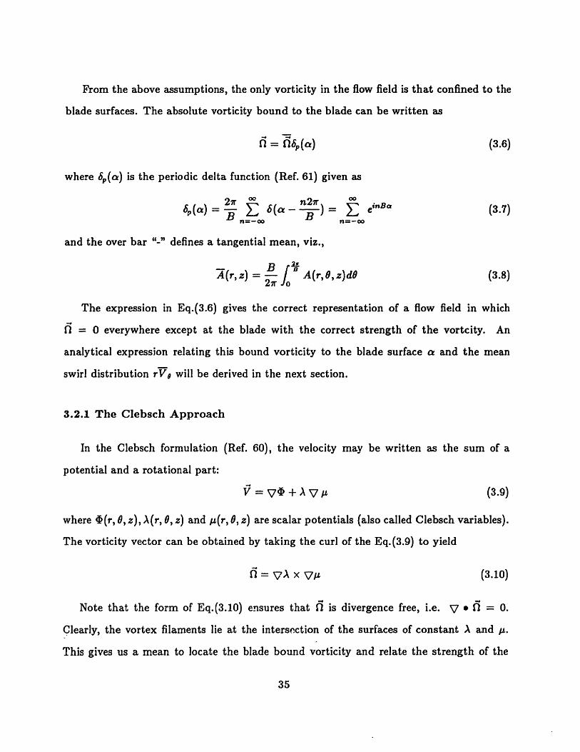
From the above assumptions, the only vorticity in the flow field is that confined to the

blade surfaces. The absolute vorticity bound to the blade can be written as

nf = nS (a) (3.6)

where p(a) is the periodic delta function (Ref. 61) given as

6 21r E- 6(a- n27r =Z i (3.7)___=__ n rll' = -oOn=-oo n=-oo

and the over bar "-" defines a tangential mean, viz.,

(r,z) = 2 A(r, , z)dO (3.8)

The expression in Eq.(3.6) gives the correct representation of a flow field in which

O = 0 everywhere except at the blade with the correct strength of the vortcity. An

analytical expression relating this bound vorticity to the blade surface a and the mean

swirl distribution rVe will be derived in the next section.

3.2.1 The Clebsch Approach

In the Clebsch formulation (Ref. 60), the velocity may be written as the sum of a

potential and a rotational part:

V= V + AV (3.9)

where (r, 0, z), A(r, 0, z) and p(r, 0, z) are scalar potentials (also called Clebsch variables).

The vorticity vector can be obtained by taking the curl of the Eq.(3.9) to yield

= VA x V (3.10)

Note that the form of Eq.(3.10) ensures that Ql is divergence free, i.e. V * Q = 0.

Clearly, the vortex filaments lie at the intersection of the surfaces of constant A and A.

This gives us a mean to locate the blade bound vorticity and relate the strength of the

35

blade bound vorticity to the physical quantities. For other applications of this physical

interpretation, readers may refer to the works of Dang & McCune (Ref. 56), Hawthorne

et al. (Ref. 62), Tan (Ref. 63) and Hawthorne & Tan (Ref. 90).

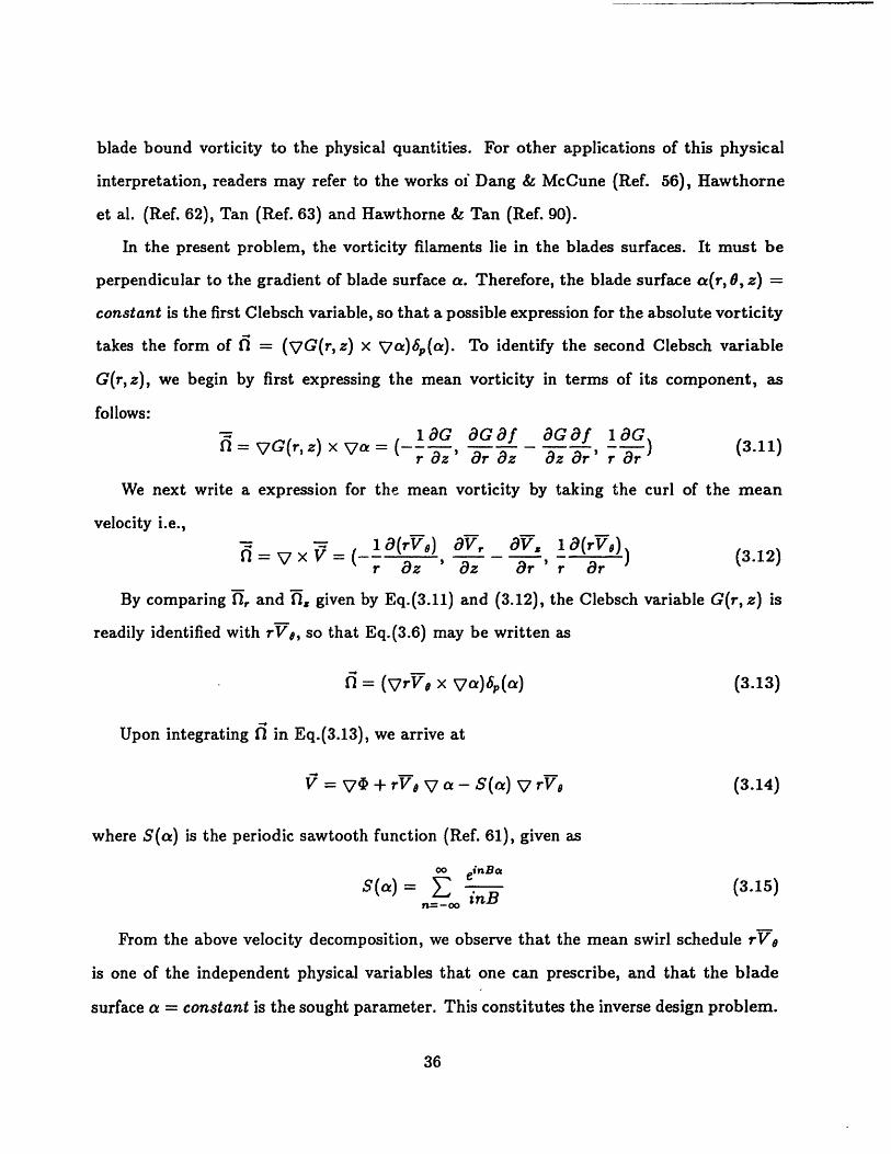
In the present problem, the vorticity filaments lie in the blades surfaces. It must be

perpendicular to the gradient of blade surface a. Therefore, the blade surface a(r, 0, z) =

constant is the first Clebsch variable, so that a possible expression for the absolute vorticity

takes the form of = (G(r,z) x Vac)6p(a). To identify the second Clebsch variable

G(r,z), we begin by first expressing the mean vorticity in terms of its component, as

follows:'= laG aGaf OG a f lOG

= G(r,z) x Va = (- a a a (3.11)r odz' r doz z r' ,r r .)

We next write a expression for the mean vorticity by taking the curl of the mean

velocity i.e.,

la(rV,) V, 8V, 1 (rVe)n=vxv= ( a' a - a, ' , ar ) (3.12)r az ' rr ' r arBy comparing f,. and i, given by Eq.(3.11) and (3.12), the Clebsch variable G(r, z) is

readily identified with rVO, so that Eq.(3.6) may be written as

i = (vrVe x Va)6p(a) (3.13)

Upon integrating fl in Eq.(3.13), we arrive at

VV = 4 + rVe V a- S(a) V rV, (3.14)

where S(a) is the periodic sawtooth function (Ref. 61), given as

oo einBa

S(a)= inB (3.15)

From the above velocity decomposition, we observe that the mean swirl schedule rVe

is one of the independent physical variables that one can prescribe, and that the blade

surface a = constant is the sought parameter. This constitutes the inverse design problem.

36

-

Alternatively, one can also specify ac from which the swirl schedule rVO can be determined.

This constitutes the direct problem.

It is convient to express the velocity in terms of a sum of a mean part V and a periodic

part V, as

V = V7 + rVe V a (3.16)

V = V - S(a) V rVO (3.17)

Since in the upstream and downstream regions the flow field are irrotational, the last term

on the right hand side (RHS) of Eq.(3.16) and Eq.(3.17) vanishes in those regions of the

flow field. The theoretical formulation has made use of a Fourier series to represent the

6-dependence of the flow variables. As such, the mean flow can be regarded as the zeroth

mode of this Fourier series representation.

3.2.2 Mean Flow Equations

The continuity equation, Eq.(3.1), may be also written as

V *W = -We VIn p (3.18)

By taking the pitch average of equation (3.18), we have the mean flow as

V W = -W · V lnp (3.19)

The non-linear term on the RHS of Eq.(3.19) couples the periodic flow to the mean flow;

this is to be expected as the equation of continuity for a compressible fluid is nonlinear.

To solve the mean flow numerically, it is convenient to introduce an artificial density

pa(r,z) to account for compressiblity effects (Ghaly, see Ref. 52). The artificial density

pa(r,z) is defined as

V .paW = 0 (3.20)

37

Comparing Eq.(3.19) with Eq.(3.20) we obtain the governing equation for p as

W · Vlnp = W · lnp (3.21)

with an appropriate initial condition. We see that the artificial density has a physical

meaning in the limit of B -, oo (This is referred to the Bladed Actuator Duct, Tan et al.,

Ref. 2). In the Bladed Actuator Duct limit, the effect of individual blades on the flow field

is smeared out in the tangential direction so that the periodic part of the flow vanishes,

hence W = 0,P = Pa-

The mean velocity may either be formulated using the Clebsch expression in Eq.(3.16)

or in terms of the more familiar Stokes stream function which has often found application in

throughflow and actuator disc calculations. Here, for historical reasons, we will adopt the

use of Stokes stream function, , for the description of the mean flow. Thus, an alternative

expression for the mean velocity which satisfies the definition of artificial density Pa in

Eq.(3.20) is

PaWr --- lar az

We -rV W (3.22)r

r dr

The governing equation for 4p is obtained by equating the definition of la = av, _ avaz 6r

(see Eq.(3.12)) in terms of ,p from the above definition, and therefore we have

82 1 a 2 (lnPa) a _ (ln pa) a = rparVe af arVe of (3.23r2 rr ar z2 r r az a a az za[ z ar ar az

Eq.(3.23) is elliptic when the flow is subsonic and hyperbolic when the flow become

supersonic. Note that the right hand side vanishes outside the blade region as the flow is

irrotational there.

3.2.3 Periodic Flow Equation

38

The continuity equation for the periodic part of the flow is obtained by subtracting

the pitch-averaged continuity equation in equation (3.19) from the continuity equation in

equation (3.18), yielding

V V = -W * V lnp +W * lnp (3.24)

As the flow is spatially periodic from blade passage to blade passage, it is convenient

to express the periodic velocity potential $ in the form of the Fourier Series in the circum-

ferential direction, and we have

+00

Z- E -(r, z)einBO (3.25)n=-oo,00

Substituting Eq.(3.17) and Eq.(3.25) into Eq.(3.24), we get

e-inB V2 f rVe 8f drV V~ ;2 r " = rein f( ) + [-W · v In p + W · V In P]T(n)inB or ar az aF

(3.26)

where V2D = r + 2- n2B, and FT(n) denotes the Fourier coefficients of the nthr r r az2 r2

mode. Note that the RHS of Eq.(3.26) vanishes when n = 0 so that 0o 0, as it should,

since W - 0 by definition. Since it is assumed that the specified rVe distribution is such

that no trailing vorticity appears downstream of the blade row, and that the upstream flow

is irrotational, the first two terms on the RHS of Eq.(3.26) vanish identically upstream and

downstream of the blade row.

3.2.4 Blade Boundary Condition

The procedure for determining the blade shape is an iterative one. A first guess for the

blade shape is used to compute the velocities from Pa, i, and bn. Then, the blade shape

is updated by using the blade boundary condition which means that there is no velocity

normal to the blade surface. This can be written in the form:

Wb * VCa = 0 (3.27)

39

where Wb W = ( = + + -) is the velocity at the blade (+/- represents the blade pres-

sure/suction surface). We may expand the above equation in the following:

Of Of trVaWrar + WzL = - + (V)bl V (3.28)

Eq.(3.28) may appropriately be integrated to obtain the blade shape f(r,z) with an ini-

tial condition. This specification of an integration constant for f is called the "stacking

condition" (Tan et al., Ref. 2), as will be discussed later.

3.3 The Boundary Conditions

Poisson's equation requires a specification of either the Dirichlet or the Neumann

boundary conditions in order to have an unique solution mathematically. This corresponds

to the specification of the inflow/outflow boundary conditions and the requirement of no

flow through the solid wall. Here, the boundary conditions for Eq.(3.23) and Eq.(3.26)

will be discussed separately.

3.3.1 Stream Function

First we will discuss the boundary conditions for the stream function, Eq.(3.23), which

is obtained from the definition of the mean tangential vorticity. We have:

* along the inflow section, b is given (based on an uniform flow)

The upstream flow may be considered to be uniform if the upstream boundary is far

enough from the leading edge.

* along the outflow section, = (parallel flow)

Because the influence of the blade row decreases exponetially and there is no pressure

jump at the trailing edge, the downstream flow may be considered to be parallel at

a distance far enough from the trailing edge.

40

* along the hub and shroud, ?b is constant (no flow normal to the wall)

3.3.2 Velocity Potential

The requirement of the conservation of mass for periodic flow is contained in Eq.(3.26).

The corresponding boundary conditions for Eq.(3.26) are:

* along the inflow section, - = 0

The upstream flow may be considered to be parallel if the upstream boundary is far

enough from the leading edge.

· along the outflow section, except q, = 0 at hub (to have an unique solution), = 0

Because the influence of the blade row decreases exponetially, the downstream flow

may be considered to be parallel at a distance far enough from the trailing edge.

* along the hub and shroud, an = orv e-nB' (no flow normal to the wall)

3.4 The Initial Conditions

The mean continuity equation in Eq.(3.21) and the blade boundary condition in Eq.(3.28)

are two first order convective equations. Each of these equations requires the specification

of an initial condition on a line extending from the hub to the shroud (not coinciding with

any streamlines). The specification of the initial condition for these two equations will be

discussed next.

3.4.1 Artificial Density

We assume that the flow is steady and that far upstream the approaching flow is axisym-

metric, irrotational and reversible. The initial condition for the artificial density Eq.(3.21),

can be given from the mean flow far upstream (referred to as the Bladed Actuator Duct),

i.e.,

41

* along the inflow section, p0 = p is specified.

3.4.2 Blade Shape

The initial condition for the blade shape is referred to as the blade stacking condition.

This specification of the stacking condition is similar to the design of a three-dimensional

blade shape using the strip theory. In the strip theory, two-dimensional blades are designed

by blade-to-blade method and we need to specify an axis from the hub to shroud along

which all the designed two-dimensional blade sections are to be stacked. Here, the initial

condtion for the Eq.(3.28) is

o f = ft(rt, z.t); f must be a line from hub to shroud (not coinciding with any of

the streamlines)

3.5 The Kutta-Joukowski Condition

The Kutta condition ensures smooth flow at a sharp trailing edge. This translates

to the fact that, in subsonic flow, the pressure must be continuous at the trailing edge.

Accordingly, the swirl schedule should be such as to satisfy this condition. The homentropic

assumption implies that all the thermodynamic properties will be continuous if either p or p

or T is. Here, the way to impose the Kutta-Joukowski condition is by specifying H+ = H-

explicitly in our inverse design method (where +/- represents the blade pressure/suction

side respectively). As the rothalpy is uniform (see Eq.(3.3)), we have

H -He=I 1 1 ( - + '+ ) x (W-- +) = -bI ·)W (3.29)2 2 2

However, the velocity jump AW across the blade (from the definition of the bound

vorticity) can be written in the form (Ref. 2, see Appendix A) of

27r flx a 2r Vca ·- rV B AvwI 1 B ( 7 aV Va-VrV) (3.30)B 1,7ei 12B1,7ei 12

42

Substituting the above expression into Eq.(3.29), and using the fact that IWbl lies on

the blade surface, i.e., Wbl * Va = 0, we obtain

H+-- = 2 IWbe * vrVeJ (3.31)

so that the Kutta-Joukowski condition can be satisfied by setting the right hand side of

the above equation to zero, i.e.,

Wbl * vrVe = 0 (3.32)

It is worthy to note that as the incidence angle at the blade leading edge is assumed

to be zero, the pressure there should be continuous in a way similar to that at the trailing

edge. Therefore the condition of zero incidence at the blade leading edge implies that rVg

should satisfy Eq.(3.32) at the leading edge as well.

For a free vortex design, rVa is constant along the leading edge and the trailing edge

(no shed vorticity), so that there is no trailing vorticity downstream of the blade row. If

we impose ov = 0 at the leading edge and the trailing edge where s is the meridional

distance along the quasi-streamline coordinate, then Eq.(3.32) is identically satisfied.

3.6 Blockage Effects

In general, the thickness along the shroud is very small, so the assumption of zero

thickness would be a good approximation. However, in the hub region, due to the stress

considerations, the blades are designed with a relatively thick section compared to the

shroud region. To partially account for this effect, we introduce the blockage, b(r,z), on

the mean flow, and neglect the periodic variation of flow quantities caused by the thickness

(see Ref. 64, 65). For the mean flow, we have

V bpW = (3.33)

where

b = 1 2 (3.34)('B'r)

43

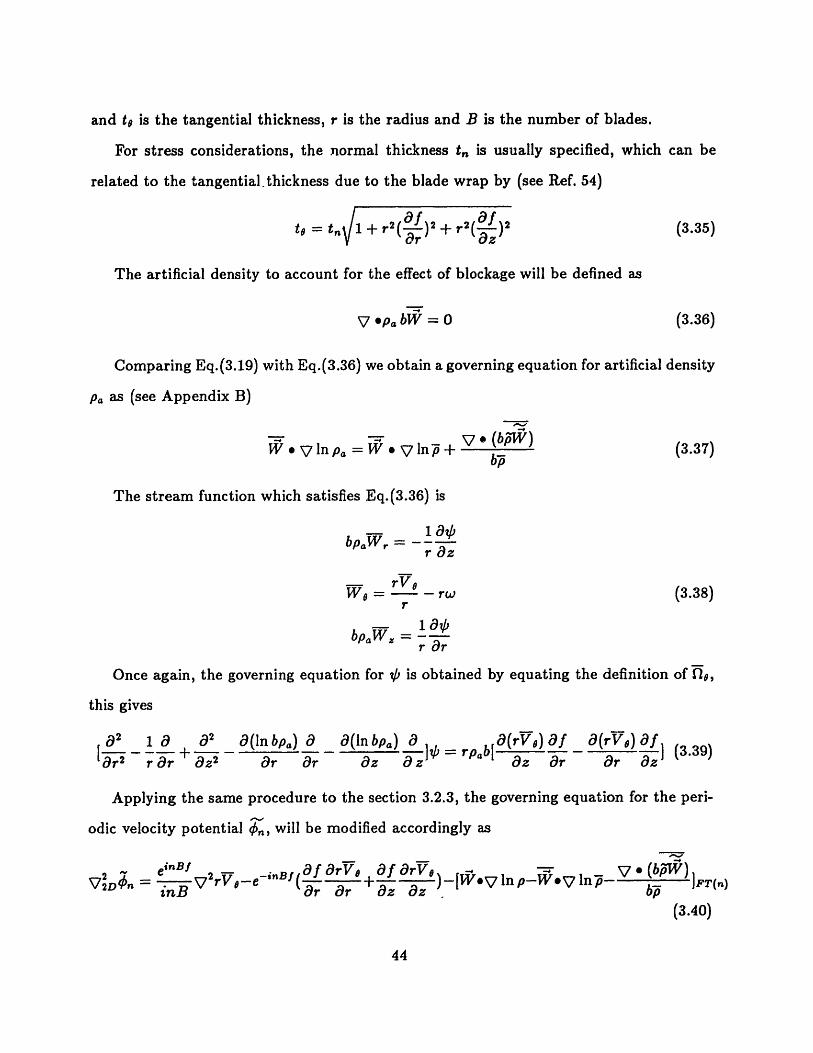
and t is the tangential thickness, r is the radius and B is the number of blades.

For stress considerations, the normal thickness t, is usually specified, which can be

related to the tangential.thickness due to the blade wrap by (see Ref. 54)

to = t l1 + r2 ()2 + 2( )209Z

(3.35)

The artificial density to account for the effect of blockage will be defined as

V P bW = 0 (3.36)

Comparing Eq.(3.19) with Eq.(3.36) we obtain a governing equation for artificial density

Pa as (see Appendix B)

W . v lnpa = W · In + V o (bpyW)(3.37)

The stream function which satisfies Eq.(3.36) is

bpaWr ar az

rVeWe = -- - rr (3.38)

bpaWz -r r

Once again, the governing equation for is obtained by equating the definition of Ie,

this gives

a2 (lIn bpa) aoz2 ar ar

a(lnbpa) a faz az

P a(rVe) af- rpbt z r8z ar

Applying the same procedure to the section 3.2.3, the governing equation for the peri-

odic velocity potential O,, will be modified accordingly as

V2D4n - einBf - if (afOrVomB2D rV Or ar

Of Or )_lWrvlnpW.vlnpV (bP~I)]a ~-[W* In p-W~ In-]3.4T(n)(3.40)

44

a2

[r21 ar ar

9(rVo) dfOr oz (3.39)

We see that the blockage b has no influence on the periodic flow onS from the last term

on the RHS. When there is no blockage, i.e., b = 1, Eq.(3.37), Eq.(3.39) and Eq.(3.40)

become identical to their original forms in Eq.(3.21), Eq.(3.23) and Eq.(3.26) respectively.

The corresponding boundary conditions for Eq.(3.37), Eq.(3.39) and Eq.(3.40) are the

same as before.

3.7 Summary

Given the mean swirl schedule, the hub and shroud profile, number of blades and

stacking condition, the current method can give us the detailed three-dimensional blade

shape and the entire flow field. The governing equations in terms of the stream function

4' (Eq.(3.23), artificial density Pa (Eq.(3.21)), velocity potential o' (Eq.(3.26)) and blade

shape f (Eq.(3.28)), need to be solved simultaneously. As they are nonlinear, the solution

scheme is an iterative one.

The analysis shows that the mean swirl schedule is the only velocity component that

may be specified as an input. Moreover, this schedule is proportional to the circulation

around the blades from Kelvin theorem, i.e.,

r = (irV)LE. - tV(7, z)J (3.41)

It is also related to the work done across the blade row from the Euler's turbine equation.

HT2 - HT1 = w[(r V) 2 - (rV)i] (3.42)

The enthalpy jump across the blade (or pressure jump when the fluid is incompressible)

is related to the rate of change uf the mean swirl schedule (see Eq.(3.31)). However, there

could be many rVe distributions within the blade region to give a same overall change in

rV across the blade row. It is conjectured that there could be an optimum rVo distribution

that results in a flow field with minimum loss, be it of viscous origin or due to the resulting

secondary flow and boundary layer development.

45

Chapter 4

The Mean Swirl Schedule

From the previous chapter, we have seen the important role played by the mean swirl

schedule in this three-dimensional design method. In this chapter, we will first discuss the

kinematic constraints on the mean swirl schedule. Then, we will describe a method to

generate the mean swirl schedule within the blade region. The specification of the mean

swirl schedule can be shown to reduce to a boundary value problem. Finally, we propose

a procedure for controlling the distribution of the mean swirl schedule along the hub and

the shroud.

4.1 Kinematic Constraints

The previous analytical studies assume the flow to be irrotational and inviscid; there-

fore, if we take a closed circuit C and allow it to wrap around a blade, we arrive at

rc =O= dl = f.d u dl= u· dl-- uidl+rw-rl =yn+-rw-ric, BCD AB DC

where r,, r and rl are the circulation at upstream, blade circulation at the wall and

blade circulation near the wall (see Fig. 4.1). The y, and An are the shed vorticity from

the blade and the distance from station 1 to the wall. In the limit of An -- 0, we get

ar (4.1)

where n is the distance normal to the hub and shroud surfaces. This is the so-called

"Prandtl Wing Theorem". The strength of the vortex sheet shed by a wing is equal to the

spanwise gradient in the circulation along the wing. Now the circulation on the blade can

be related to the mean swirl schedule by Kelvin Theorem (see Eq.(3.41)), i.e.

rB = [(rV)L.E. - (rVe)] (4.2)

46

By combining Eq.(4.2) with Eq.(4.1) and noting that (rV)L.E. is a constant, we arrive

at

I(r) = (4.3)dn

We see that there are shed vorticities from the blade due to a non-vanishing normal

gradient of the mean swirl at the wall. The vanishing of the normal gradient of the mean

swirl schedule along the hub and the shroud is dictated by the need to satisfy the boundary

condition of no normal flow along the hub and the shroud. This point has been noted by

Smith (Ref. 66), Tan (Ref. 64, 67), Falcao (Ref. 68) and Tan et al. (Ref. 2), thus

=0 (4.4)an

at the hub and shroud.

This implication results in an additional constraint on the blade shape f at the hub

and shroud. As the velocity is tangent to the walls, i.e.

I + .n = 0 and WI-n=O (4.5)

By taking the difference between these two, we have

A W * n = 0 (4.6)

Substituting for AW from Eq.(3.30) and simplifying, we obtain

Va VrVe af +rVe+ =0 (4.7)IV"7 12 an an

We have noted from Eq.(4.4) that o__ = 0 along the hub and the shroud; furthermore

the dot product Va o VrVe is in general not equal to zero, therefore

af= 0 (4.8)

On

at the intersection of the blade with the walls, i.e., the dihedral angle needs to be zero,

which has been shown by Smith (Ref. 69) and Brebner & Wyatt (Ref. 70).

47

It is also interesting to note that when -vA is zero at the endwalls, the boundary

condition for the periodic velocity potential (see section 3.3.2) is reduced to

= 0 (4.9)an

along the hub and shroud.

4.2 Biharmonic Equation

The boundary conditions that need to be imposed on the mean swirl schedule can be

summarized as follows:

* at the leading edge: rV9 is a constant which is given; the condition of zero incidence

requires that aVO = 0.as

* along the hub and shround : rVe is prescribed as a mean to control the loading

distribution; the rVe distribution must also satisfy the kinematic constraint that

arV = 0.an

* at the trailing edge : rVe is a constant which is specified; the Kutta-Joukowski

condition requires that rV = 0.as

Obviously, along each boundary defining the blade region, two boundary conditions

are specified. This means we need at least a fourth order partial differential equation

to generate the rVe distribution for the specification. Here, the biharmonic equation is

adopted to generate the distribution of rVe, i.e., we solve

V4 (rV e) = R(r, z) (4.10)

where2 1 a 2': +4 - )2

48

to obtain a smooth continuous distribution of rVe within the blade region. The source

term R(r,z) can be used as a mean to control/tailor the rVe distribution in a desirable

way. Here, R(r,z) is set to zero for simplicity in the present study. The present study

concentrates on the effect of prescribing rVO distribution along the hub and the shroud

only.

4.3 Method of Specifying rVg along the Hub and the Shroud

As we alluded to in the previous section, the proposed method for controlling/tailoring

the distribution of rV9 is to prescribe the rVe distribution along the hub and shroud. The

specification of rVs(r, z) is thus reduced from the need of specifying on a two-dimensional

domain to one on a one-dimensional domain, i.e., along the boundaries of the blade region.

Since the design and the biharmnonic codes require the evaluation of V 2rVe (see Eq.(3.26)

& Eq.(4.10)), a continuity of the second derivative of rVO along the hub and shroud is sug-

gested. This implies that the flow field and hence the pressure field will be smooth. As

we have seen from Eq.(3.31), pressure jump is closely related to the first derivative of rVe.

It suggests that a specification of (Var ' could be helpful. Moreover, the shape of the

loading is mainly controlled by the second derivative of rVg, so it is useful to choose the

magnitude of a, along the hub and shroud. Because of the requirement of zero incidence

at the leading edge and the need to satisfy Kutta-Joukowski condition at the trailing edge,

two transition curves are needed at both ends to have ve = 0. This gives us the currentas

choice. Namely, we separate the meridional distance along the hub and shroud into three

sections. This corresponds to Section 1 : from the leading edge to position A, Section 2 :

from position A to position B, and Section 3 : from position B to the trailing edge. (see

Fig. 4.2). The boundary conditions for each section are listed below:

* Section 1 : rVe(s) is quartic in s

49

specify rVe = (rVi)L.E., (re)' = O, (rVe)' = 0 at L.E.

specify (rV')' = (rV-) (rVe) = (rV)AB at A

* Section 2: rVe(s) is quadratic in s

obtain from section 1, re = (rVe)A, (rV)' = (rVe)A, (rV)" = (rVe)A at A

a Section 3: rVe(s) is quintic in s

obtain from section 2, rVo = (rVO)B, (Vo)' = (rVe), (rVe)" = (rVe)B at B

specify rV = (rVe)T.E., (rVe)' = 0, (a)" = 0 at T.E.

These specifications are applied both at the hub and the shroud with the additional note

that the condition of (rVe) = 0 at the leading edge and the trailing edge is not required

by the constraints, but numerical continuity of V2rVe at the leading edge and the trailing

edge is preferred. By altering the location of position A (the maximum loading position)

and position B (the extent of the finite loading), the value of the maximum derivative of

rVe at position A, and the slope of the loading from postion A to position B, a variety of

distributions of rVo can be obtained.

4.4 Summary

The kinematic constraints on the mean swirl schedule require 0 -= 0 along the hub

and the shroud. This results in an additional constraint on f along the hub and shroud.

Failure to satisfy Eq.(4.4) and Eq.(4.8) will not produce infinitely large induced velocities

due to %- along the hub and shroud numerically. However, Eq.(4.5) will not be satisfied in

general, i.e., the velocity jump across the blade will not be tangent to the wall.

The biharmonic equation gives us a possible way to interpolate the distribution of rVe.

If one uses only Poisson's equation to generate the rVe distribution, then the Dirichlet

and Neumann boundary conditions cannot be satisfied simultaneously. One may use some

50

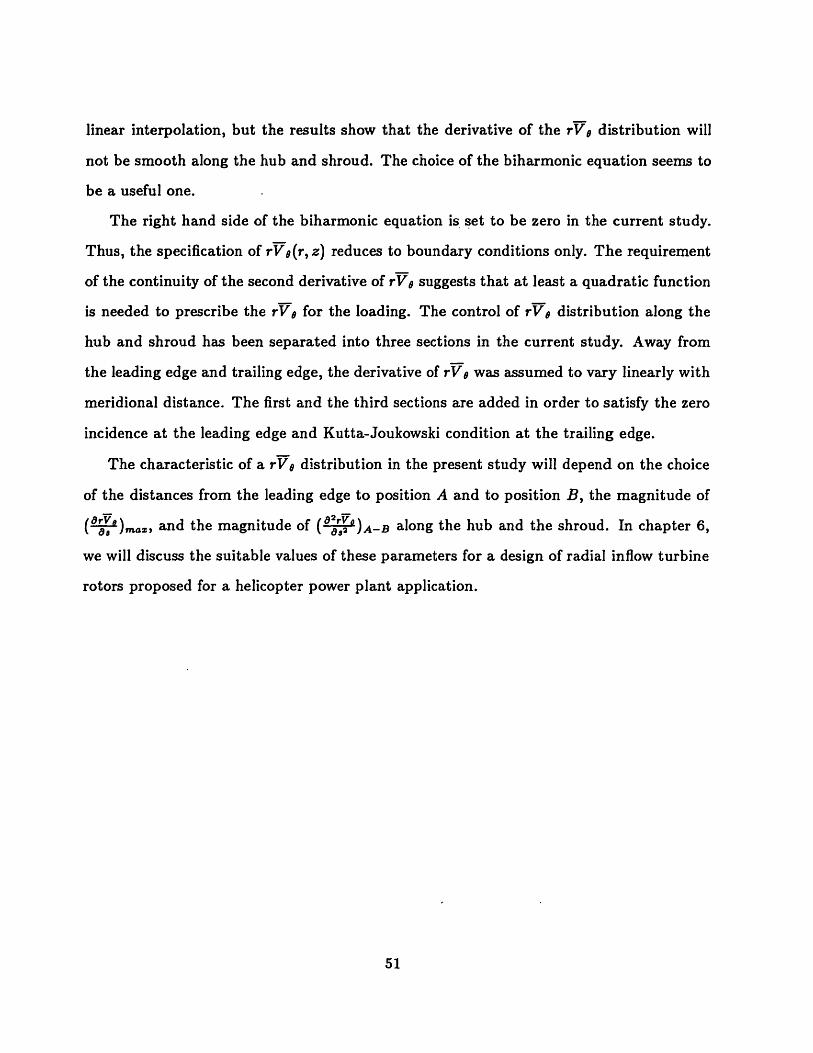
linear interpolation, but the results show that the derivative of the rVe distribution will

not be smooth along the hub and shroud. The choice of the biharmonic equation seems to

be a useful one.

The right hand side of the biharmonic equation is set to be zero in the current study.

Thus, the specification of rVe(r, z) reduces to boundary conditions only. The requirement

of the continuity of the second derivative of rVa suggests that at least a quadratic function

is needed to prescribe the rVe for the loading. The control of rV, distribution along the

hub and shroud has been separated into three sections in the current study. Away from

the leading edge and trailing edge, the derivative of rVe was assumed to vary linearly with

meridional distance. The first and the third sections are added in order to satisfy the zero

incidence at the leading edge and Kutta-Joukowski condition at the trailing edge.

The characteristic of a rVo distribution in the present study will depend on the choice

of the distances from the leading edge to position A and to position B, the magnitude of

(ua0v)maz, and the magnitude of (a 2 2)A-B along the hub and the shroud. In chapter 6,

we will discuss the suitable values of these parameters for a design of radial inflow turbine

rotors proposed for a helicopter power plant application.

51

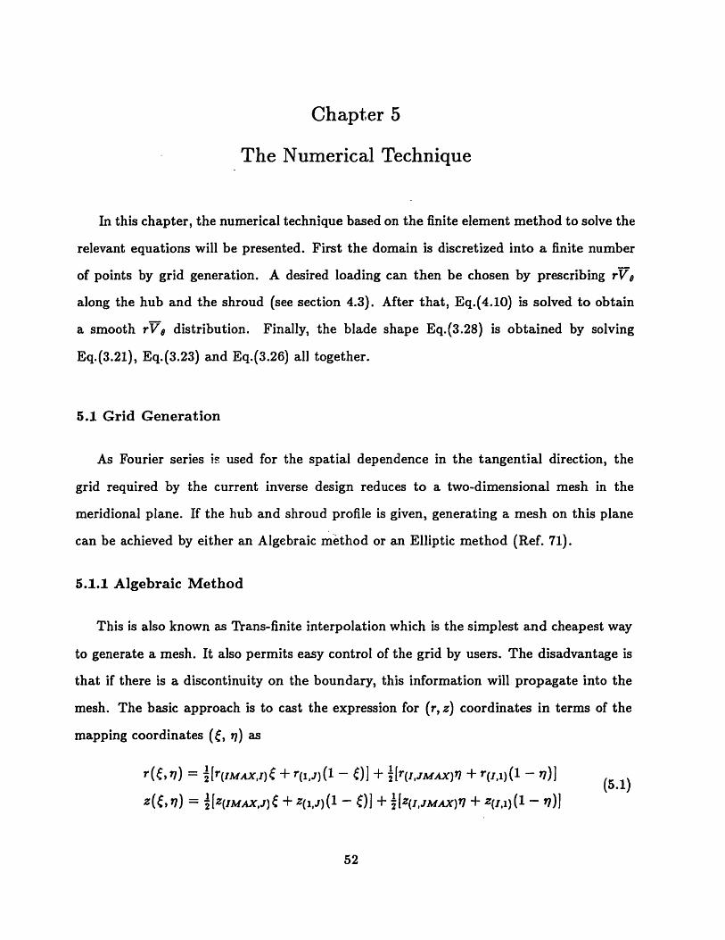
Chapter 5

The Numerical Technique

In this chapter, the numerical technique based on the finite element method to solve the

relevant equations will be presented. First the domain is discretized into a finite number

of points by grid generation. A desired loading can then be chosen by prescribing rVo

along the hub and the shroud (see section 4.3). After that, Eq.(4.10) is solved to obtain

a smooth rV distribution. Finally, the blade shape Eq.(3.28) is obtained by solving

Eq.(3.21), Eq.(3.23) and Eq.(3.26) all together.

5.1 Grid Generation

As Fourier series i used for the spatial dependence in the tangential direction, the

grid required by the current inverse design reduces to a two-dimensional mesh in the

meridional plane. If the hub and shroud profile is given, generating a mesh on this plane

can be achieved by either an Algebraic method or an Elliptic method (Ref. 71).

5.1.1 Algebraic Method

This is also known as Trans-finite interpolation which is the simplest and cheapest way

to generate a mesh. It also permits easy control of the grid by users. The disadvantage is

that if there is a discontinuity on the boundary, this information will propagate into the

mesh. The basic approach is to cast the expression for (r, z) coordinates in terms of the

mapping coordinates (, ) as

r(C i7) = '[r(IMAxj) + r(lij)( (- )J + [r(i.jMAX) + r(I, l)( (-t (5.1)

Z(, 7 = 2Z(IMAXJ) + Z(1 J)(1 -e)I + [Z(I,JMAX)7 + Z(j) I,(1 )

52

where the algebraic mapping is given by

= IMAX-1 (5.2)J-1

' JMAX-1

We see that the trans-finite interpolation uses a direct form, and no numerical itera-

tion is needed. Other forms of transfomation are possible; however, a certain amount of

ingenuity is required.

5.1.2 Elliptic Method

One of the most highly developed techniques for generating grids is the elliptic method.

It is based on the fact that the stream function b and potential function X for incompress-

ible flow form an orthogonal body fitted computational mesh. Instead of solving ib and ,

we solve two elliptic equations for mapping coordinates and r7. The advantage of this

method is that it produces a smooth grid and can be controlled by a variety of modifica-

tions. However, the resulting equations are usually solved iteratively. Here, the two elliptic

equations are

er,, + z = P(,) (5.3)

7rr + zz = Q(6 7)

where P and Q are terms which control the point spacing on the interior of the domain.

Equations (5.3) are then transformed into physical coordinates by interchanging the roles

of the independent and dependent variables. This yields a system of two elliptic equations

of the form

aree - 2r + 'yrq = - I J 12 (Pre + Qr) (5.4)

azf - 2ze + yz,, = - I J 12 (Pz + Qz)

where

=r +z2

= rr + ZZ

] = rr + z2

53

I J = (,) = rEz, - rze

This system of equations is solved on an uniform-spaced grid in the computational

plane (d, ra). This provides the (r, z) coordinates of each point in the physical space.

5.2 The Elliptic Solver

Eq.(3.23) for the Stokes' stream function and Eq.(3.26) for the velocity potential are

two second order Elliptic equations (for subsonic flow). The Finite Element Method is

used to solve for these two equations. The nonlinear part of the differential operator in

Eq.(3.23) and Eq.(3.26) is moved to the right hand side (RHS). As the solution procedure

is iterative, the RHS is assumed to be given from the previous iteration or from an initial

guess, so that the equations may be treated as linear equations.

Here, we use a 4-node isoparametric element to interpolate the variables (see Fig. 5.1).

The coordinates r and z are expressed in terms of the coordinates of the four corner nodes

by

{ = (1 + i)(1 + 77{ ) = N{ (5.5)i=1Zi Zi

where NT is the transpose of the shape function vector. The Jacobian can be in terms of

the coordinates of ri and zi byBr az

IJ]=ar w-e (5.6)8O BO

Then the derivative of variables in the physical plane can be expressed in terms of those

in the computational plane, by using

{Or } [ _- 1 I [ 11 12 ] { a (5.7)

_ a' 121 I22 a7

54

If we use the Galerkin method, the variational form of equation (3.23) becomes

I 1 r T 1T )( N )+ 1 ( Nr)(BN) ]?dA + I If TN qdA (5.8)

= _ T[k]j + T q

Where _q is the nodal value of l l 0, + + P ar ara f

of [k] and q is done by Gaussian Quadrature. For stationary value of I, i.e., r = 0, we

obtain the Euler equation

[k]+ = -q (5.9)

with the corresponding boundary conditions. This is done locally from element to element.

To assemble the contribution from each element, we apply the direct stiffness technique to

obtain the global matrix over the whole domain as

[KJL = -Q (5.10)

The same procedure applies to the periodic velocity potential in Eq.(3.26). The system

of equations (5.10) can be solved directly by LU decomposition or iteratively, such as via

the conjugate gradient method. Here we use the latter procedure. Because these equations

are nonlinear and coupled, there is no need for an exact solution of 4I or qb, before the

blade camber, f (Eq.(3.28)) or artificial density, Pa (Eq.(3.21)) have converged during the

intermediate iterations.

The multigrid scheme (Ref. 72, 73, 74) is useful for saving computational time for

Eq.(3.23) and Eq.(3.26). In Appendix C, we will demonstrate the performance of the

multigrid coupled with the conjugate gradient method. For a test problem with a fixed

RHS, the multigrid scheme can save about half of the computational time. However, when

this scheme is coupled with our inverse design code, the benefit is not so obvious. This

is because for each global iteration, after the new blade camber is obtained, it typically

requires ten sweeps of the conjugate gradient method to update b and 0,n on the finest level.

Improved accuracy in b or , does not improve the overall convergence rate. Therefore,

55

the design code combined with the multigrid scheme is not as efficient as one would have

expected.

5.3 The Convective Equation Solver

Eq.(3.21) for the artificial density and Eq.(3.28) for the blade camber are two first

order hyperbolic equations. One way to solve these equations is by the method of char-

acteristics. Here, one tries to locate the streamlines from the blade velocity and integrate

the information along each streamline. An alternative way to do this is to use a direct

numerical differentiation and integration, based on the Finite Element Method that evalu-

ates its derivative. The RHS of Eq.(3.21) and Eq.(3.28) may be considered given from an

initial guess or the previous iteration. The operator W,a + Wza can be separated into

two parts; one part that consists of the unknown nodal points will be kept on the LHS

and the other part that consists of the given initial nodal points will be moved to the RHS

together with the original RHS values. For example, Eq.(3.28) can be written as

&f -- cgfW. a zaaf - q (5.11)

where q equals [r2 - w + Vbl *a].

Now consider one element where fi and f4 are given (see Fig. 5.1). The unknowns

f2 and f will be determined by satisfying Eq.(5.11) at nodes 1 and 4 (alternatively, two

Gaussian points could give a better weighted accuracy), so from Eq.(5.7) we have

J[W,(IiNi,efi + Il2Ni,qf,) + W4 (21N,,Vfi + I22Nfi)=,f= | q4J (5.12)

[wr (INifi + I12Ni,fi) + w ( 2lNifi + I22Ni$VIfi)] i Jwhere Ni,x means oi and the free index i represents the sum from 1 to 4. Now the known

values f and f4 can be moved to the RHS, and Eq.(5.12) can be rewritten as

[k] f2 (5.13)[]{f2 =

56

Eq.(5.13) can be used to determine the unknowns f2 and fs on each element. Between

the two adjacent elements, the average value will be used for f. After all the unknowns f

have been evaluated along the span, this procedure will march to the next streamwise loca-

tion using the previous solutions as the new initial conditions. This procedure allows one

to integrate forward or backward depending on the position of the stacking line. Likewise,

the solution for p0 from Eq.(3.21) can be implemented through the same procedure.

As we mentioned in section 4.1, there is an additional constraint on the blade shape

f at the hub and shroud, i.e., ~a = 0. Because the value of ~a is influenced by every f

along the boundary, the boundary condition = 0 is imposed explicitly, i.e., the value

of f along the hub and shroud is altered after the blade camber is determined. The same

technique used in the above is adopted. Here, Wr and W, are replaced by - cos V and

sin v, where v is the angle normal to the boundary side 1-4, and q is set to be zero. Given

the values of fi and f4, f 2 and f are obtained by satisfying af = 0.

5.4 The Biharmonic Solver

To obtain the mean swirl schedule, the biharmonic equation, Eq.(4.10), is used to

interpolate the distribution. The biharmonic equation can be solved by the Finite Element

Method as in structural mechanics. A simple triangular element developed by Bazeley et

al. (Ref. 75) is used. The element (BCIZ) makes use of the area coordinate for the shape

function with rVe, (rVe),, and (rVo),, as the nodal variables. The element is compatible

in r, but the adjacent normal gradient (rVO),n is not. Following the same procedure as

in Sec.5.2, the resulting system equations for each element are:

[k]rV = +q (5.14)

where

[k]= f f( T MT )( + N) + ia )(a)dA+r2 ar2 dr 2 r ozr + r

57

and

q = rrTR(r, z)dA

Now if we assemble the local nodal variables, we get the global system matrix. To

solve this system matrix requires double precision accuracy since rVp and its gradients are

used at the same time; thus the amount of memory size will be six times the total number

of nodes. Furthermore, we have found this method to be rather inefficient in terms of

practical implementation.

An alternate approach, which we eventually adopt, is based on the idea of reducing

the biharmonic equation into two coupled Poisson equations (Ref. 76, 77, 78, 79). Since

each of the Poisson equations is well-posed, the system equations may be solved through

an iterative means as described in the following.

7 rV( ) = w(k l) in G

rV = rVspecified on aG

rVOk) = ( - )rVa1) + ErV(k) (5.15)

Vw(k) = R in G

(k) = vr () -c - g] on G0 a n

W(k) = (1 - 6)(k-l1) + 6(k)

where G is the domain of the blade region, aG is the boundary of the blade region, c is

an arbitrary nonzero constant, and are two relaxation constants and g is set to be

zero for vanishing normal gradient of rVe. These two Poisson equations can be solved by

the same approach as that described in Sec.5.2. Solution procedure only requires single

precision accuracy; thus the memory size will be two times the total number of nodes.

Thus, this is a more suitable method than the previous one. Since under-relaxation is

used, small numbers of conjugate gradient iterations (usually 10 - 15) are needed on each

local iteration. The CPU time will be dependent on c, E and 6. Typically, the solution

requires k = 250 global iterations to achieve machine accuracy with c = 1, = 5 = 0.15.

58

5.5 The Computational Scheme

Computer programs have been written to implement the numerical procedures de-

scribed in this chapter. The whole procedure is summarized in the following:

Step 1. Grid Generation

Given the hub and shroud profiles, grid generation is used to generate an appropriate

two-dimensional mesh. The required resolution of mesh depends on the number of the

periodic harmonic modes used to represent the spatial dependence in the tangential di-

rection. In order to resolve the information of the highest frequency, a minimum number

of mesh points is needed (see Appendix D). From the Appendix D, the minimum number

of mesh points required is also related to the change in the blade shape. Thus, a prior

idea about the distribution of :l (see Eq.(3.28)) helps in determining the clustering of

mesh. For the far upstream and downstream boundaries, the flow can be approximated

to be parallel at a distance far enough from the leading and the trailing edge. At present,

the numerical upstream and downstream boundaries are set at a distance of quarter chord

(averaged meridional distance between the hub and the shroud) from the leading and the

trailing edge.

Step 2. Mean Swirl Schedule

The distances from the leading edge to position A and to position B, the magnitude

of (0V,)maz and )A-B, are the parameters used to control rVa distribution along

the hub and the shroud. The distance from the leading edge to position A will affect

the blade shape significantly. The distance from the leading edge to position B sets the

region of finite loading (see chapter 4). The magnitude of ( a), m is closely related to the

pressure jump across the blades. The magnitude of (d,2 )A-B controls the shape of the

loading. More details on these parameters will be discussed further in the next chapter.

59

After the values of rVe and its normal gradient (to be zero) along the hub and the shroud

are specified, the biharmonic solver is used to interpolate the rVo distribution within the

blade region.

Step 3. Inverse Design

In the inverse design program, the flow variables are nondimensionalized by the radius

of blade tip, meridional velocity and rotary stagnation quantities at the leading edge (see

Appendix E). Here, the values used for the input are:

- Velocity triangle and Mach number at the leading edge

- Ratio of specific heats, 7-

- Stacking condition

- Mean swirl schedule, rVa (r, z)

- Normal thickness distribution of blade, t(r, z)

The design scheme starts with an initial guess of the blade camber, then it solves for

the stream function b Eq.(3.23) and Sn, for each n from Eq.(3.26). Then, the velocity

field is calculated to update the blade camber f Eq.(3.28), artificial density Pa Eq.(3.21)

and density field. If the difference in the blade camber between the current iteration

and the previous one is large, then the stream fuction and potential harmonic modes will

be calculated again. The whole scheme is considered to achieve convergence when the

maximum change in blade camber is less than a small number (10- 5 radian typically).

The outputs from the design program are:

- Blade shape f

- Velocity field (except Va which has been specified), pressure field and etc.

60

Since there is a jump across the blade in the density, its gradient will behave like a

periodic delta function. The method to evaluate the gradients of the density (or Inp)

is to take a Fourier Transformation (FT) and then evaluate the gradients in the Fourier

space. The inverse Fourier Transformation (IFT) is used to obtain the physical values

from Fourier coefficients. A fast Fourier Transform (Ref. 80) has been used to evaluate the

FT and IFT of W and In p. Lanczos smoothing (Ref. 81) has also been used to suppress

the Gibbs phenomenon due to the sawtooth behavior.

61

Chapter 6

Parametric Study of Inverse Designs

In this chapter, the computational tool that has been developed based on the analytical

theory in chapter 3 is applied to the design study of a radial inflow turbine proposed for

a helicopter power plant application. For turbines, the pressure field would tend to have

a favorable distribution throughout so that the real flow could be predicted based on

an inviscid assumption. By examining the simplest case, the radial inflow turbine, some

guidelines can be obtained for an optimal rVO distribution in terms of "parameters" related

to fluid mechanics.

Not much is known today about the optimization of the efficiency of radial turbines.

Probably the most useful correlations and studies are those carried out by NASA and

summarized in Reference 82, Chapter 10, by Rohlik, which gives a good guide to the state

of the art of high-performance radial inflow turbines. However, the design of blade shapes

in this three-dimensional flow field is still in an elementary stage. It has been shown by

Borges (Ref. 51) and Zangeneh (Ref. 54) that the use of the present inverse design method

for designing a radial turbine rotor can lead to an improvement in its overall efficiency by

not only reducing the losses in the rotor, but also minimizing the exit kinetic energy by

prescribing the mean swirl value to be zero at the trailing edge.

We will choose a turbine rotor (Ref. 83) proposed for application in a helicopter power

plant for our case study. The design conditions are summarized in Table I. The velocity

triangle at the leading edge of the rotor is shown in Fig. 6.1; the absolute flow angle at the

leading edge is about 75° and the corresponding absolute Mach number was computed to

be about 0.98. The impeller wheel will be designed to yield a blade camber distribution

that will result in the complete removal of swirl at the trailing edge. Thus, the flow will

leave the turbine wheel axially at the exit. The hub profile, the shroud profile and the

62

associated finite element mesh on the meridional plane are shown in Fig. 6.2. There

are 97 uniformly-spaced grid points in the streamwise direction, and 33 grid points in the

spanwise direction. The number of blades was taken to be 14. To save computational time,

4 complex harmonic modes are used for the periodic flow which corresponds to 9 Fourier

collocation points between adjacent blade camber lines. When the solution of the current

grid resolution is compared with a solution of grid resolution of 145 x 49 x 33 (see chapter

7), the maximum difference in blade shape at the mid-span is no more than 0.01 radians

(see Fig. 6.3.a). The maximum difference in reduced static pressure along the mid-span

(which is at the maximum loading position on the suction surface) is no more than 7%

of its maximum pressure jump (see Fig. 6.3b). Based on this results, a grid resolution of

97 x 33 x 9 yields results of adequate accuracy that can be used for a design study.

The parameters that a designer can choose in this design method are the mean swirl

schedule, stacking position, lean in stacking line, slip factor, number of blades and hub &

shroud profile. We will present the influence of each parameter on the resulting design.

Before we begin our study, we wish to propose two parameters that we can use to assess

the goodness of a particular design. These two parameters will provide a quantitative

measurement of the resulting design.

6.0 Two Parameters Used to Characterize a Design

The goodness of a design depends on the response of the boundary layer and secondary

flow to the inviscid reduced static pressure field. In other words, a design based on the

assumption of inviscid flow is "good" only if the viscous influence can be kept to be

"minimal" e.g. a design with minimal aerodynamic loss. Therefore, the designer would

like to pick a pressure field (if possible) that would minimize undesirable viscous effects

such as flow separation from the walls with accompanying increased losses and blockage.

When the wall boundary layers are thin and well behaved, the inviscid flow field would

63

be a fairly good approximation to that of the actual flow. Hence, a good control of the

inviscid pressure gradients would help in developing an "optimal" design. Here, in a first

attempt, two parameters are proposed to characterize a design.

The behavior of a viscous flow through the impeller (i.e. the development of secondary

flow and boundary layer) is dictated by the reduced static pressure field. Therefore, the

reduced static pressure gradient is the first quantity that we want to examine. Clearly, the

larger the maximum adverse reduced static pressure gradient, the tendency of boundary

layer to separate is higher; so (ata)maz is the first parameter that we would like to

minimize in an inviscid design.

In general, the adverse reduced static pressure gradient on the suction surface is higher

than the one on the pressure surface. As we will see later on that the reduced static

pressure distribution on the pressure surface does not vary significantly in all cases; this is

due to the fact that the velocities remain relatively close to zero on the pressure surface.

Because the variation in the reduced static pressure from the pressure side to the suction

side is close to a sawtooth function (see chapter 3), it may be sufficient to examine the

maximum value of the adverse reduced static pressure gradient on the suction surface

within the blade passage. In particular, only the maximum values of the adverse reduced

static pressure gradients on the suction surface along the hub (ap0-)h, the mid-span

(aoP d)m and the shroud (Pa-.-), are pointed out to characterize a particular design.

The second parameter to be developed pertains to the development of secondary flow.

The low momentum fluid within the blade passage will be driven by the secondary flow

to the location of minimum reduced static pressure. Thus, the secondary flow would

determine the position of the wake at outlet and can then have an influence on separation.

It was suggested by W.R. Hawthorne that one can describe the movement of a fluid particle

in the spanwise direction in terms of the Wake number (see Appendix F). However, an

alternative derivation for the Wake number is given here. The distance (do) that a fluid

particle travels in the spanwise direction from the leading edge to the trailing edge along

64

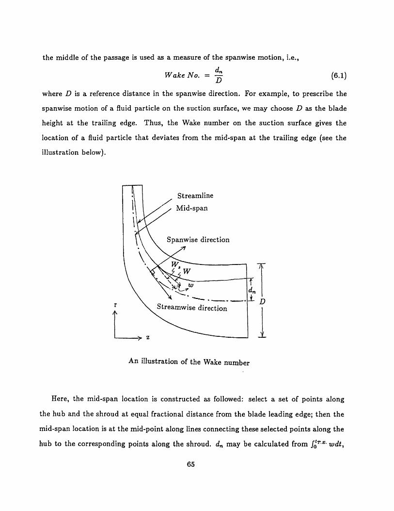
the middle of the passage is used as a measure of the spanwise motion, i.e.,

dWWake No. =D (6.1)

where D is a reference distance in the spanwise direction. For example, to prescribe the

spanwise motion of a fluid particle on the suction surface, we may choose D as the blade

height at the trailing edge. Thus, the Wake number on the suction surface gives the

location of a fluid particle that deviates from the mid-span at the trailing edge (see the

illustration below).

D

IAn illustration of the Wake number

Here, the mid-span location is constructed as followed: select a set of points along

the hub and the shroud at equal fractional distance from the blade leading edge; then the

mid-span location is at the mid-point along lines connecting these selected points along the

hub to the corresponding points along the shroud. d may be calculated from froTC wdt,

65

where w is the velocity in the spanwise direction and tT.E. is the time that a fluid particle

travels through the blade passage. The Wake number can thus be written as

1 [tT.Er.Wake No. = D wdt

orI T. WdWake No. = D.. -WdsD AL W.

where W, is the relative velocity along the mid-span on the suction surface and ds is the

distance along the mid-span on the suction surface. If W > w and W ~ W,, then

1 T.E. Wake No. D .. W ds (6.2)

where W is the relative velocity along the streamline on the suction surface. For low speed

flow, the rotary total pressure is constant everywhere in the flow field (see Eq.(3.3)), i.e.,

P 1 1 Pred 1w2 12r2 Pd + W2 = constant (6.3)P 2 2 p 2

Upon differentiating Eq.(6.3) in the spanwise direction (or quasi-orthogonal), we have

Pred + p8WAn F cn

oraw 1 aPred aWaAn pW an n(6.4)

In general, the first term in the RHS of Eq.(6.4) is positive and the second term is negative

(i.e. the streamwise velocity on the hub is lower, -w is negative). To obtain an upper

bound of the spanwise motion of a fluid particle, we may neglect the second term in the

RHS of Eq.(6.4), thus

w = f| adn + constant I I l apd dn + constant (6.5)dn + pW an

To determine the integration constant in Eq.(6.5), we may apply the boundary condition

at the hub or the shroud where w equals to zero. Thus, the spanwise velocity at mid-span

66

can be obtained by either setting

mid-span 1 aredW dn

JHub pW an

orr Shroud 1 aPred

Jmid-span pW anHere, an average value of the above two expressions is used, i.e.,

AI Shroud 1 ared 1 aPred xD

w WY - I dn = -( ) x Dn(6.6)2 Hub PW an 2 pW an

where (- 2 -p,- )A is the spanwise average of - apecd and Dn is a spanwise characteristicPW ar B an

distance. The value (-p a8PId) can be approximated further by - w ( n) where pW

is taken to be the value at mid-span. Since -D is of the order of unity, the Wake number

can finally be written as

A

Wake No. = n l ds (6.7)L.E. pW

We have now derived an approximate expression for the Wake number; it is an integral from

the leading edge to the trailing edge of the spanwise gradient of pressure coefficient along

the mid-span. For compressible flow, in particular when the Mach number is not close to

unity, the variation in density is less than that in pressure (from isentropic relationship),

and a mass average of the value of °p-d along the span is used in the calculation of the

Wake number, so that the above expression of the Wake number can still be used to predict

the appropriate trend of the spanwise motion of a fluid particle. The expression of the

Wake number derived in Appendix F is different from the one derived here. However, both

Wake numbers do give the same trend in the results to be presented here.

To illustrate the usefulness of the Wake number, an example of two different Wake

numbers on the suction surface is shown in Fig. 6.4a and 6.4b, where the Wake numbers

are 1.86 and 3.61 respectively. Here, Fig. 6.4a and 6.4b show the meridional velocity

67

on the suction surface with maximum loading near the leading edge (see section 6.1.1).

Hence, there is not much difference between these two cases close to the trailing edge.

We see that with a Wake number of 1.86, the velocity near the inlet is higher along the

hub than along the shroud; the spanwise movement of a fluid particle is from the shroud

toward the hub. For the case of a Wake number of 3.61, the fluid particle will be driven

from the hub toward the shroud. Thus, in a real flow, we can expect that the location of

the wake at the outlet will be lower for the Wake number 1.86 than the one with a Wake

number 3.61. Similarly, the definition of the Wake number can be applied on the hub and

the shroud surfaces to indicate the movement of low momentum fluid from the pressure

side toward the suction side. In general, the spanwise gradient of reduced static pressure

is significant on the suction , the hub and the shroud surfaces. Thus, we will examine the

Wake numbers on these three surfaces only and try to minimize these Wake numbers in

an inviscid design.

6.1 Mean Swirl Schedule

The mean swirl schedule is the only flow quantity that a designer can control in this

theory. As the derivative of rVe is related to the pressure jump across the blade (see

Eq.(3.31)), and I - w is related to the blade wrap (see Eq.(3.28)), we see the important

role played by the distribution of rVe in this inverse design method. Establishing the

general effect of the mean swirl schedule on pressure distribution will be the first step of

the present work.

There could be many choices of the rVe distributions that will accomplish the same

amount of work across the blade row. As we have discussed in Chapter 4, one way to

generate the distribution of rVe is by specifying the rVg along the hub and the shroud

and then interpolates by the biharmonic equation with its RHS equals zero. The way to

control the distribution of rVa along the hub and the shroud is by specifying the location

68

of the maximum loading (position A), region of finite loading (between position A and

position B), the maximum loading (value of (_v )maz) and the slope of the loading (value

of (as )A-B). In the next three sections, the important characteristics of the r distri-

bution that will be examined are: (i) the maximum loading position A; (ii) the regions of

vanishing spanwise gradient of rVe; and (iii) the maximum loading (8a)ma.

6.1.1 Effect of the Maximum Loading Position

The maximum loading position could be located at any point from the leading edge

toward the trailing edge. In this section, we will attempt to assess the influence of the

location of maximum loading on the reduced static pressure field. For consistent assess-

ment, the values of (_),maz and (B2Ve)A-B for rVo distribution along the hub and the

shroud will be kept constant, and the influence of varying the maximum loading position

A on the design will be investigated.

As the slip factor is 1 at the leading edge and the flow leaves the trailing edge axialy,

the overall change in rVO across the blade row is -1 (normalized by the rtw). The distance

along the hub is 0.5 and 0.338 along the shroud (normalized by the tip diameter). The

minimal value of the maximum loading ()' is constrained by the distance of the

shroud and it is -1.5. There could be no upper limit of the maximum loading. However,

if the maximum loading is too large (-2.5 in this case), there is reversed loading along the

hub which is not desirable. Thus, an average value of the maximum loading (i ")mz = -282 r

is used in this study. The value of ()a is set to be 0 so that the maximum loading

can be kept to be -2 along the shroud.

Here, we will vary the maximum loading position A from near the leading edge to near

the trailing edge. The choice of the distance from the leading edge to position BHub, is the

same as AHUb along the hub, i.e., the second section of the loading is omitted. However,

along the shroud this cannot be done easily because the meridional distance is shorter

than that along the hub, hence the portion from position AShroud to position BShroud will

69

maintain the same maximum loading. Five different maximum loading positions have been

examined. Fig. 6.5a, 6.5b, 6.5c, 6.5d, and 6.5e show the distributions of rVe, a~, and e

along the hub and shroud for each case. The contour plots of rV$ from the biharmonic

interpolation are shown in Fig. 6.6a, 6.6b, 6.6c, 6.6d, and 6.6e. The control parameters

are listed in Table 6.1.1.

Table 6.1.1 Control Parameters forFive Different Locations of Maximum Loading

Case AHub = BHu AShroud BShroud

a 0.025 0.025 0.150

b 0.125 0.025 0.144

c 0.250 0.085 0.253

d 0.375 0.194 0.313

e 0.475 0.188 0.313

These five cases correspond to the maximum loading at location near the leading edge, at

4chord, at chord, at 4 chord and at location near the trailing edge for the hub (the chord

is mearsured by the meridional distance along the hub and the shroud). Also, there is a

significant difference in the distribution of w, especially along the hub where the radius

is small. As the blade shape is directly related to the value of E, case "a" will provide

the smallest wrap angle. As the position of maximum loading is moved toward the trailing

edge, the blade camber will need more and more wrap/turning in the exducer. Clearly,

case "e" will give the largest blade wrap/turning f (see Fig. 6.5e).

From chapter 3, the strength of tangential component of the bound vorticity is related

to the means swirl and blade wrap by fie = rV - rv# A. Thus, the induced velocityBr a Br

in the meridional plane by the bound tangential vorticity is proportional to the derivative

of f and rVO. In these five cases the gradient of the mean swirl schedule is about the same

(no more than -2), so that the larger the blade turning the stronger will be the induced

meridional velocity. The effect of the induced flow due to the bound tangential vorticity

70

ne (negative in these cases) will result in flow reversal (along the hub). Numerical results

show that case "a" is the only one in which there is no reversed Wbl (see section 6.2).

Hence, strong adverse streamwise pressure and spanwise pressure gradients are expected

if the maximum loading position is at location near the trailing edge. It suggests that by

locating the maximum loading position near the leading edge would tend to reduce the

blade wrap and avoid flow reversal on the hub.

6.1.2 Effect of Regions of Vanishing OrVeOn

In the previous section, we have set the maximum loading ([a/. )a,_ and its location to

be the same for both the hub and the shroud near the inlet (case "a"). This is becasue the

inlet section is almost straight for this particular rotor (see Fig.6.2). By maintaining the

same value of rVe from the hub to the shroud (i.e., a = 0 near the inlet), the spanwise

variation of pressure, velocities, etc. on both the pressure and suction surfaces near the

inlet (i.e., P-Iz = 0, ?= 0, etc) may be kept to the minimum. Thus, it might be useful

to examine the influence of the regions of relatively small spanwise gradient of rVe on the

design; this can be achieved by altering the distance from the leading edge to position B,

i.e., the loading for the first and second sections along the hub is kept the same as the one

along the shroud.

Without any loss of generality, we can again insist on the same value of (a = -22a2 ,j

(the average) and ( A-D = 0 (i.e. the maximum loading along the shroud remains

-2) for the hub and shroud. From the results in the previous section, the position of

maximum loading should be chosen to be near the leading edge; thus it is appropriate to

choose a distance of 0.025 from the leading edge to position A for both the hub and the

shroud. Besides, the portion of constant loading (-2) will extend from Ashrod = 0.025

to BShroud = 0.15 along the shroud (case "a"). By keeping the loading on the shroud the

same, three cases of rVp with different position of BHUb along the hub will be examined.

71

Clearly, the longer the distance from the leading edge to position BjHub, the regions of

srVA = 0 are larger. The specified values of BHUb are given in the Table 6.1.2a.an

Table 6.1.2a Control Parameters for Three DifferentLengths for Regions with Vanishing Ova

case BHub

a 0.025

f 0.064

g 0.100

Further increase in the distance from the leading edge to position BHub beyond the

value of 0.01 will result in a negative value of rVo near the trailing edge. Hence, the

location of BHub is set at 0.100 as its upper limit. With these inputs, the distributions

of rVe, Ov and W' along the hub and shroud are plotted in Fig. 6.5a, 6.5f, and 6.5g.

Fig. 6.6a, 6.6f, and 6.6g give the contour plot of the rVa distribution from the biharmonic

interpolation.

With these three different mean swirl distributions, the reduced static pressure distri-

butions and relative Mach number contours from the design calculation are shown in Fig.

6.7, 6.8, 6.9 respectively. In these three cases the flow is reversed (i.e., negative meridional

velocity) on the pressure surface from few percent of the chord to about middle of the

chord (Fig. 6.7c, 6.8c, 6.9c). Hence, the velocities remain relatively close to zero on the

pressure surface. The reduced static pressure distribution on the pressure surface is seen

to be approximately the same among these three cases (see Fig. 6.7a, 6.8a, 6.9a). Under

these circumstances, the pressure on the suction surface is essentially determined by the

loading distribution, i.e., the specified 9v@.

Fig. 6.10a and 6.10b show the effect of regions of vanishing spanwise gradient of the

mean swirl on the maximum adverse pressure gradient and the Wake number. These

results are summarized in the Table 6.1.2b.

72

Table 6.1.2b Effect of Different Lengths for Regions with Vanishing von the Maximum Adverse Pressure Gradient and Wake Number

case (2 d -)h (pt)m (2aL ), (Wake no)h (Wake no),... (Wake no),

a 0.816 0.800 1.209 6.309 3.261 4.652

f 0.917 0.937 1.226 5.726 2.965 4.813

9 1.065 1.133 1.267 5.269 2.677 4.887

where (a)h, (a )m,, and (Pred. ), are the maximum adverse reduced static pressure

gradients along the hub, the mid-span and the shroud quasi-streamlines on the suction

surface and (Wake no)h, (Wake no),.,,, and (Wake no), are the Wake numbers on the

hub, the suction and the shroud surfaces.

Since the loading along the shroud is kept the same, the maximum adverse pressure

gradient at the shroud is about the same. As case a" has the smallest slope of arV' from

position B to the trailing edge, so will the ape along the hub and mid-span (see Fig.

6.10a). Case "g" has the largest regions of vanishing spanwise gradient of the mean swirl

hence the regions of the vanishing spanwise pressure gradient is increased (see Fig. 6.7a,

6.8a, 6.9a). Thus, the flow is more uniform in the spanwise direction in case "g" than

the one in case "a", and the resulting velocities on the hub surface are increased and the

velocities on the shroud surface are reduced relatively when we compare the results of case

"g" with the results of case "a". Therefore, the Wake numbers are reduced on the suction

and the hub surfaces and increased on the shroud surface when we increase the regions of

vanishing Ee'a (see Fig. 6.10b).

6.1.3 Effect of the Maximum Loading (a-)ma:

In the previous two sections, we have obtained the following conclusions: (i) the maxi-

mum loading position should be located near the leading edge and (ii) the rVO distribution

along the hub and the shroud needs to be the same in order to reduce the spanwise varia-

tion of the flow field. Here, we will attemp to answer what value of the maximum loading

73

should be used in a design. In other words, whether a loading distribution with a smaller

maximum loading over a region (_ less than -2) or a loading distribution with a

larger concentrated maximum loading (( greater than -2) is better.

From the theory we know the pressure jump across the blade is related to the streamwise

derivative of re. Here, three different values of (' a)moz are examined. For the first case,

the maximum loading is the smallest one among these three cases, where )" = -1.75

and the shape of the loading will have a larger region of plateau as shown in Fig. 6.5h.

The second case is case g" where the magnitude of the (~" is -2 which is higher

than case h". For the last case, the magnitude of ( L)m^' is set at -2.25 resulting in

a loading distribution that is triangular in appearance (see Fig. 6.5i). The value of the

()2 )A-B is the same for these three cases which is chosen to be zero. The control points

AHUb and AShroud are set at 0.025 as before to reduce the blade wrap and to avoid flow

reversal at the blade. Clearly, the distance from the leading edge to position BShroud is

the largest for a loading with a large regions of plateau, and the smallest for a triangular

shape of loading. The distance from the leading edge to position BHub is set by maximizing

regions of 0 = 0 as long as there is no negative value of rVe near the trailing edge along

the hub. Fig. 6.6g, 6.6h, and 6.6i give the contour plots of the rVe distributions from

the biharmonic interpolation. The characteristic parameters for these rVe distribution are

indicated in the Table 6.1.3a.

Table 6.1.3a Control Parameters forThree Different Maximum Loading Distributions (a),ma

case (m) BHub BShroud

h -1.75 0.150 0.250

9 -2.00 0.100 0.150

i -2.25 0.050 0.075

The pressure distribution and Mach number contour from design code are plotted in

Fig 6.9, 6.11 and Fig. 6.12 separately. Clearly, we see that regions of reversed flow on

74

the pressure surface are the smallest for case i" (compare Fig. 6.9c, 6.11c, and 6.12c).

However the magnitude of reversed flow is the largest for case "i". For case "h", a flat

loading along the shroud extends toward the trailing edge and so the blade camber is highly

wrap near the exducer. The resulting pressure field have the largest spanwise variation

among these three cases (see Fig. 6.9, 6.11, 6.12).

Fig. 6.13a and 6.13b show the effect of the maximum loading (a)maz on the maxi-

mum adverse pressure gradient and Wake number respectively. The results are also sum-

marized in the Table 6.1.3b.

Table 6.1.3b Effect of Different Maximum Loading Distributions (°84),,on the Maximum Adverse Pressure Gradient and Wake Number

case (d)h ( -)m (aptL). (Wake no)h (Wake no)... (Wake no),

h 0.806 1.436 1.629 6.001 2.869 4.322

9 1.065 1.133 1.267 5.269 2.677 4.887

i 1.236 0.974 1.163 4.874 3.046 4.210

Once again, we see that to reduce the maximum adverse pressure gradient on the

suction surface, one should reduce the slope of --VO from postion B to the trailing edge.as

As the slope of rv. is the smallest for a triangular shape of loading (case "i") along the

shroud, the maximum adverse pressure gradient is the smallest along the mid-span and

the shroud (see Fig. 6.13a). However, along the hub, the meridional distance is the longest

one and the increase of (tarV),ma will increase the slope of _rVI from BHub to the trailing

edge. Thus, to reduce the maximum adverse pressure gradient along the hub, one should

decrease the value of (rv),a.; to reduce the maximum adverse pressure gradient along

the shroud, one should increase the distance from BShroud to the trailing edge.

The pressure jump at the blade near the inlet is the largest for a loading of triangular

shape (case "i" ) . Because the area of passage reduces from the leading edge to mid-chord,

the dynamic head is increased near the inlet. Therefore, the increase in Wake number due

to a higher pressure jump at the blade near the inlet is compensated. As the pressure

75

jump reduces in magnitude from mid-chord to the trailing edge in case "i", it results in

a decrease of the Wake number. Thus, the Wake numbers on the hub and the shroud

surfaces is the smallest for case i" (see Fig. 6.13b). In so far as the Wake number on the

suction surface is concerned, there is not much difference among these three cases. The

effect of the mean swirl schedule on the Wake number on the suction surface has been

assessed in section 6.1.2. It suggests that a loading distribution with a triangular shape

will result in design with a reduced blade wrap as well as a reduction in the streamwise

and the spanwise pressure gradients.

6.2 Stacking Position

The blade boundary Equation Eq.(3.28), requires the specification of an initial con-

dition (see section 3.4.2). This is referred to as the specification of a stacking position

(r,t, Z,t) as well as its stacking angle f = ft(rot,zt). As the strength of the bound vortic-

ity in the r and z directions is determined solely by the rV$ distribution, the change in the

stacking condition will affect the bound tangential vorticity distribution only. Therefore,

we can expect a change in the meridional velocity due to an alteration in stacking condi-

tion. In this section, we will simply choose the stacking angle fZt(rt, zt) to be zero along

the stacking axis. The effects of different stacking positions will be studied first.

Five different rVe distributions that we have referred to as case "a" to case "e" will be

examined here. Several stacking positions will be chosen at (rt, Zt) between the leading

edge and the trailing edge. The calculations have first been done for the Bladed Actuator

Duct flow model. Design calculation based on this model is computationally efficient when

it is compared to that based on three-dimensional model. Fig 6.14a shows the stacking

positions vs the position of maximum loading along the hub. We see that the loading of case

"e" results in negative value of Wbl so that solution fails to obtain a converged blade shape.

The loading in case "d" indicates that there are transonic regions due the higher loading

76

near the trailing edge and hence the higher turning of the blade shape over there. The

loadings in case "a", b", and Uc" does not result in negative value of Wbt if stacking position

is chosen to be at the maximum loading position or slightly downstream of it. The reason

is that if the stacking position is near the maximum loading position, then the resulting

tangential bound vorticity fe is small or even zero near the maximum loading position (if

the stacking of the blade is straight, i.e., a = 0 and there is no spanwise variation of the

mean swirl in the inducer, then = 2v t _ rv, .f # rV x 0- 0 X -. 0). Hence,Br Baz Bz Br BrO

the induced meridional velocity is reduced and a negative value of Wbi can be avoided.

For three-dimensional flow (Number of blades is 14), the results for different stacking

positions is shown in Fig 6.14b. It is seen that only with the loading distribution of case

"a" that there exist no negative Wb for stacking positions at the leading edge, the 8 chord,

and the chord. These results are consistent with results based on actuator duct model.

Fig. 6.15a and 6.15b show the effect of different stacking postions on the maximum adverse

pressure gradient and Wake number respectively. The results are also summarized in the

Table 6.2.

St,

Lead

18

14

Table 6.2 Effect of Different Stacking Positionson the Maximum Adverse Pressure Gradient and Wake Number

acking (Ps-.)h (as)m 7 (), ) (Wakeno)h (Wake no),.,. (Wake

ting edge 0.816 0.800 1.209 6.309 3.261 4.65

chord 0.789 0.826 1.088 6.319 3.040 4.9E

chord 0.717 0.843 1.060 6.692 3.386 4.75

no),

52

I2

10

For the loading distribution of case "a", there is no significant spanwise variation of

the mean swirl near the inlet. If we stack the blade straight (i.e., ft = 0) at the leading

edge or chord, the strength of the bound tangential vorticity nf is small or zero within

the region from the leading edge to chord. As a result, the flow field will be very similar

for these three stacking positions (see Fig. 6.15).

77

6.3 Lean in Stacking Line

As we have mentioned in the previous section, the initial condition along the stacking

line doest not need to be straight, i.e., ft # 0. The value could be arbitrary. For simplicity,

we shall choose the stacking value to be a straight line, but allowed it to lean in two different

directions while maintaining the same amount of work done. (see the definition in Fig.

6.16). The results from these design calculations would allow us to assess the influence of

the lean on the flow behavior.

We shall use the rVg distribution of case g" for the study here, and choose the stacking

position at the leading edge. Three different lean angles are examined, i.e., p = -6.65° , 0. °,

and 6.65°. The maximum allowable lean angle p is obtained whenever there is a negative

value of Wbl. This is not known apriori.

Fig. 6.17a, 6.17b, and 6.17c give the blade shapes for these three different lean angles.

We see that these blade shapes have significant difference only near the leading edge. Near

the leading edge, the non-vanished value of ~a (i.e., the lean angle) can alter the sign and

arV - BTVAstrength of ie (i.e., fr ° _ Bv ~af) on the blade surface. This will alter the value of

Wb and hence the reduced static pressure distribution. Computed solutions from design

calculation are shown in Fig. 6.18 for the case with p = -6.65 ° and in Fig. 6.19 for the

case with p = +6.65°. Comparing Fig. 6.9a with Fig. 6.18a and 6.19a, we see a non-zero

lean angle results in a large spanwise gradient in the pressure.

Fig. 6.20a and 6.20b show the effect of different lean angles on the maximum adverse

pressure gradient and Wake number respectively (see Table 6.3).

Table 6.3 Effect of Different Lean Angles pon the Maximum Adverse Pressure Gradient and Wake Number

Lean angle (ped. )h (ape- )m (P2 .), (Wake no)h (Wake no),,. (Wake no),

-6.65 ° 0.976 1.163 1.674 5.833 3.612 4.050

0° 1.065 1.133 1.267 5.269 2.677 4.887

6.650 1.101 1.179 1.110 4.815 1.855 5.814

78

Clearly, the adverse streamwise pressure gradient on the shroud can be reduced by

using a positive lean angle. The streamwise pressure gradient ap-d along the mid-span

is not affected by the lean angle Vo. This is similar to what we have seen in the previous

section where different positions with fat = 0 do not alter the pressure field significantly.

Nevertheless, aP.. as well as the Wake number changes dramatically. It suggests that a

positive lean angle o can reduce the loading along the shroud and increase the loading

along the hub (see Fig. 6.20b). As a result, the velocity is increased along the hub and

decreased along the shroud. Hence, the Wake number is reduced on the suction and the

hub surfaces but increased on the shroud surface.

6.4 Slip Factor

The slip factor, ratio of the tangential velocity over the blade rotating speed, is fixed

(1 in our case) at the design point. Here, we neglect the constraints on the mechanical

strength such that the rotational speed can be altered for a study of slip factor. In each

case, the mass flow and the work done are kept the same for different slip factors. Two

additional velocity triangles from the design point will be examined, i.e., one with a slip

factor 0.95 and the other 0.86 (see Fig. 6.21). The reaction of the turbine wheel is increased

from 0.5 to 0.53 and 0.57 respectively. However, the circulation on the blade is decreased to

97% and 93% of its design point respectively. Thus, the loading on each blade is decreased.

We can expect the blade profile loss to be decreased by using a smaller slip factor. On

the other hand, the windage loss would be increased due to a higher blade speed. The

same normalized rVe distribution (case "g") and stacking at the leading edge with ft = 0

are used for the present study. The data for the study and results are summarized in the

Table 6.4.

79

Table 6.4 Effect of Different Slip Factorson the Maximum Adverse Pressure Gradient and Wake Number

slip w(rmp) ( )h (P)m ,(ae ))h (Wake no)h (Wake no),.,. (Wake no),

1 64,000 1.065 1.133 1.267 5.269 2.677 4.887

0.95 65,700 0.988 0.979 0.946 4.784 2.700 4.239

0.86 69,000 0.882 0.742 0.731 3.730 2.758 3.122

The results from design calculations are plotted in Fig. 6.22 and 6.23 for slip factors

0.95 and 0.86 separately. Comparing the results with Fig. 6.9, 6.22, and 6.23, for different

slip factors, we see that the loading on each blade has been decreased due to an increase

in the reaction for a smaller slip factor, hence, the streamwise pressure gradient apr.L, the

spanwise pressure gradient a-t and regions of reversed flow reduce significantly.

Fig. 6.24a and 6.24b show the effect of different slip factors on the maximum adverse

pressure gradient and Wake number respectively. The case of slip factor 0.86 gives the

smallest Wake number on the shroud and the hub surfaces among these three cases. How-

ever, the Wake number on the suction surface incresaes slightly due to the reduction of

the dynamic head on the suction surface (smaller loading). It suggests that a reduction in

the slip factor can help the aerodynamic performance.

6.5 Blockage Effects

The thickness of blade is accounted for partially through the specification of blockage

distribution (see section 3.6). Here, the normal thickness t, of the blade is specified. Fig.

6.25a shows the distribution of the normal thickness t, (normalized by the diameter) and

the output of the tangential thickness t from design calculation is shown in Fig. 6.25b. It

is seen that the influence of the blade thickness appears to be more significant along the

hub and the maximum effect is about a 40% decrease of the cross section area. Fig. 6.26

gives the reduced static pressure and Mach number contour from the design calculation

80

with blockage effects. In contrast to the situation with no bloackage (Fig 6.9), the Mach

number on the suction side reaches a value as high as 0.9 (see Fig. 6.26b). In addition,

regions of the reversed flow on the pressure side are reduced (see Fig. 6.26c). As one might

have expected that the inclusion of blockage increases the mean level of velocity.

6.6 Number of Blades

The design technique allows one to specify the number of blades. From the original

design conditions, we choose a number of blades to be 14. It is observed that there exists

a large region of reverse flow on the pressure side. To reduce regions of the reversed flow,

increasing the number of blades is one of the solutions. From the analysis of relative

eddy on a radial filament blade, we can arrive at the number of blades needed to avoid

reversed flow on the pressure surface. The flow field associated with a relative eddy at the

mid-passage is 2wj (see the illustration below).

relative eddy

Blade Tip

pressure suctionside sideside

V

2irr

An illustration of the relative eddy on the meridional velocity

81

1-rn-IT

1

The incoming flow is V, so that the resulting velocity field can be approximated by the

superposition of these two flow. For the velocity on the pressure surface to attain a value

of near zero7rr

2W = V,B

i.e.2wrr

B= V, (6.8)Vr

By using the above analysis, the number of blades needed to avoid the reversed flow on

the pressure side is B = 2, = 27r tan a ~ 23.Vr

Computed results for a design calculation using the loading distribution of case "g"

with a blade number of 21 is shown in Fig. 6.27. One can see that there is no region of

reversed flow on the pressure side (see Fig. 6.27c). The loading on each blade is reduced

by virtue of an increase in blade number.

Fig. 6.28a and 6.28b show the effect of number of blades on the maximum adverse

pressure gradient and Wake number respectively (see Table 6.6).

Table 6.6 Effect of Different Numbers of Blades Bon the Maximum Adverse Pressure Gradient and Wake Number

No. of blades (BP'd )h (L)m ('P") (Wake no)h (Wake no),.,. (Wake no),

14 1.065 1.133 1.267 5.269 2.677 4.887

21 0.693 0.581 0.495 5.207 3.026 4.128

Clearly, the streamwise and spanwise pressure gradient drop significantly by using more

blades. As the distance along the shroud is shorter than the one along the hub, hence,

the decrease of the maximum adverse pressure gradient is more significant at the shroud

than at the hub (see Fig. 6.28a) The Wake numbers on the hub and the shroud surfaces

are reduced for the 21-blade design as well. Nevertheless, the Wake number on the suction

side increases (see Fig. 6.28b). This is due to the fact that the dynamic head reduces from

a 14-blade design to a 21-blade design. Comparing the sum of the Wake numbers on the

82

hub, the suction and the shroud surfaces between a 14-blade design and a 21-blade design,

we can expect that the low momentum fluid driven by the secondary flow will be higher

for the 14-blade design.

6.7 Exit Swirl

The influence of exit swirl on the design is examined. As we have seen previously

reversed flow appears on the pressure side for a 14-blade design. Here, we allow some

residual swirl to remain at the trailing edge so as to alleviate the loading on each blade.

The penalty is that the total work done by the rotor is reduced. From previous study, the

number of blades has to increase to 21 to avoid reversed flow. Hence, if one uses 14-blade

design, the loading should decrease by about 33% of its value at the leading edge in order

to avoid reversed flow on the pressure surface. Based on this estimation, we specify a

swirl deduction that has a residual swirl at the trailing edge plane equal to 30% of that

at the leading edge. Fig. 29 shows the specified rVo distribution with a residual swirl

equal to 30% of that at the leading edge which is similar to case "g" loading except that

the maximum gradient of the mean swirl schedule 8,. is reduced from -2 to -1.4rtw

(30% off). We see that the W changes dramatically at the hub (see Fig. 6.29a). The

corresponding mean swirl schedule from the biharmonic interpolation is shown in Fig.

6.29b. To prevent WVb1 from becoming negative, the stacking position is set at chord to

reduce the blade wrap near the trailing edge. The design calculation is shown in Fig. 6.30

and summaried in the Table 6.7 for the 30% of residual swirl at the exit.

Table 6.7 Effect of Different Exit Swirlon the Maximum Adverse Pressure Gradient and Wake Number

rVe left (aP)h (apl)m (aP), (Wake no)h (Wake no),.,,. (Wake no),

0% 1.065 1.133 1.267 5.269 2.677 4.887

30% 0.395 0.340 0.632 2.901 1.061 4.332

83

The results show that the streamwise and spanwise gradients of pressure are reduced

significantly by allowing some portion of the swirl left the trailing edge as expected. Also,

there is no region of reversed flow on the pressure side (see Fig. 6.30c).

6.8 Modified Hub & Shroud Profile

The flow through turbine wheel with the original hub & shroud profile have been

studied by Civinskas et al. (Ref. 83) and the resulting losses have been evaluated by a

quasi-three-dimensional viscous analysis program. In their work, a region of reversed flow

on the hub surface has been predicted. Also, the flow on the suction surface near the inlet

region becomes transonic. Therefore, a modified hub & shroud profile has been suggested

by them. In this section, we will examine the effect of altering the hub & shroud profiles

on the pressure distribution within the blade passage.

The modified hub & shroud profile (see Fig. 6.31b) has a larger cross section for the

inducer and a smaller cross section after mid-chord to the trailing edge. In order to obtain

a meaningful comparison with the results obtained with the original hub & shroud profile

(see Fig. 6.2). We assume the same stacking position and, as nearly as possible, the same

rVe distribution (case "g"). Fig. 6.31a shows the distribution of rV along the hub and

shroud, and Fig. 6.31b shows the corresponding rVe distribution from the biharmonic

interpolation. The number of blade was also 14 and stacking specification is ft = 0 at

the leading edge. Fig. 6.32 gives the results from the design calculations. The results are

summarized in the Table 6.8.

Table 6.8 Effect of Different Hub and Shroud Profileson the Maximum Adverse Pressure Gradient and Wake Number

Profile ('-Pr)h ()m (2"PL), (Wake )h (Wakeno),., (. (Wake no),Original 1.065 1.133 1.267 5.269 2.677 4.887

Modified 1.178 0.976 1.096 5.167 2.868 3.886

As the specified rVe is similar along the hub and shroud, one might expect that the

pressure distribution along the hub and the shroud is also similar between the original

84

and the modified profile (see Fig. 6.9a and Fig. 6.32a). However, near the inlet, the area

of cross section increases, hence the velocities decrease (i.e. WbL decreases). Because the

pressure difference across the blade is directly related to the product of the rate of change

of rVO along the mean streamline at the blade and mean velocity at the blade (Wbl), this

results in a different loading along mid-span. We see that the maximum adverse pressure

gradient along the mid-span is decreased along the mid-span, and also the Wake number

is increased on the suction surface for the modified hub & shroud profile.

We have seen that the pressure gradient from pressure side to suction side on the hub

and shroud surfaces is about the same for both the original and the modified profiles. Due

to the fact that the area of passage decreases in the exducer, the flow is more uniform

for the modified profile design than that for the original profile design. Hence, the Wake

numbers on the hub and the shroud surfaces decrease for the modified profile. From these

results, the sensitivity of the blade geometry and the pressure distribution to a variation

in hub & shroud profiles is apparent.

The change in the blade camber distribution according to the modification in the hub

and shroud profile is shown in Fig. 6.33. We see there is a significant reduction in the

blade turning by using a smaller cross section area of the exducer.

Figure 6.33b shows a very large lean in the blade near the trailing edge which would

yield prohibitive centrifugal bending stresses in practice. Modification of the rVe distribu-

tion to materially reduce the lean would probably envolve the relaxation of the requirement

that the maximum derivative of rVg with respect to meridional distance must be the same

on the hub and the shroud. It remains clear, however, that the aerodynamic features of

the conventional radial filament designs are unlikely to be optimum.

6.9 Summary

A parametric study of the inverse design method is presented. The efforts concentrates

on exploring the range of parameters which will affect the pressure field. Two parameters,

85

the maximum adverse reduced static pressure gradient and the Wake number, have been

used to characterize a design. Some design guidelines have been proposed for radial inflow

turbines. These design guidelines are summarized in the following.

The location of the maximum loading should be chosen to be as near to the leading

edge as possible. The smaller the distance from the leading edge to position A, the smaller

the blade wrap and the strength of fiB; this can prevent the formation of region of reversed

flow in the hub.

Increased regions of vanishing spanwise gradient in rV# (i.e., a' = 0 near the inlet)

can reduce the spanwise gradient of flow and pressure fields, and hence reduce the Wake

number on the suction surface. However, the slope of .. VA from position B to the trailing

edge will increase which will result in a higher adverse pressure gradient in the streamwise

direction.

The choice of a triangular loading with its maximum gradient near the leading edge

will result in a larger pressure jump at the leading edge compared to a flat loading so that

the magnitude of reversed flow on the pressure side will be expected to increase. However,

the resulting strength of bound tangential vorticity flo is smaller due to a smaller blade

wrap, hence regions of reversed flow on the pressure surface is reduced. The secondary

flow measured by the Wake number is reduced on the hub and the shroud surfaces for a

rV distribution with a triangular shape. Also, the adverse streamwise pressure gradient

is reduced because of a smaller slope in arVe from B to the trailing edge. This suggest

that a triangular type of loading is desirable (see Fig. 6.12).

The study shows that in order to avoid reversed flow on the blade, the stacking position

should be set near the position of the maximum loading or slightly downstream of it such

that the strength of the bound tangential vorticity ne1 is samll or zero. Hence, excessive

induced meridional velocity (negative) due to flo can be avoided. The choice of stacking

position (with ft = 0) does not alter significantly the pressure distribution along the mid-

span but the pressure distribution changes along the hub and the shroud (see Fig 6.15a).

86

This effect becomes even more significant when we lean the stacking line. The results show

that the spanwise pressure gradient (or the Wake number) can be controlled through the

choice of lean angle p. A positive lean angle p increases the loading along the hub and

reduces the loading along the shroud (see Fig. 6.20a). This can reduce the maximum

adverse pressure gradient along the shroud and the Wake number on the suction and the

shroud surfaces significantly.

The study of slip factor shows that a smaller slip factor can reduce the aerodynamic

loading on each blade, but the reaction of turbine wheel needs to be increased. There

should be a trade off between Ve and rw for an optimal slip factor.

The thickness of blades is partially accounted for in our blockage formulation. The

results show considerably large effects on the hub because of a larger normal thickness

and turning. We have found that the Mach number becomes as high as 0.9 on the suction

surface. A correct treatment of blade thickness effect is important for a high Mach number

flow.

To avoid the reversed flow on the pressure side of the blade, we increase the number of

blades from 14 to 21 (instead of 23 from the analysis of relative eddy). The results show

that the pressure gradient on each blade is reduced significantly.

An alternative way to reduce the loading on the blade is to allow some portion of the

residual swirl after the trailing edge. But this would lead to a reduction in turbine work

output. The study shows that the reversed flow on the pressure side disappears if we retain

a residual swirl at the exit equal to 30% of that at the leading edge.

From the results of a modified hub & shroud profile, the sensitivity of the meridional

profile on the pressure distribution is apparent. A larger region of reverse flow on the

pressure side and the spanwise variation in the tip section of the impeller is due to the

increase of cross section. However, reducing the cross section near the exducer reduces the

spanwise gradient of pressure considerably.

87

Chapter 7

Flow Analysis by Solving Euler

and Navier-Stokes Equations

In this chapter, we will demonstrate the consistency and correspondence of the inverse

design procedure and the direct procedure. This is accomplished by comparing the results

from the design calculation to the corresponding results from direct calculation based on

an Euler solver. Then, solutions of the Navier-Stokes equations are obtained by using

"average passage" code (see section 7.1). This permits an assessment of the performance

of the designed rotor blades based on the losses generated in the passage, including the

behavior of the boundary layers and their subsequent migration under the action of the

reduced static pressure field. Finally, the interaction between the tip clearance flow and

secondary flow is examined. The effect of tip clearance on the current design is also

included.

7.1 Euler and .Navier-Stokes Codes Description

The programs used to analyze the radial inflow turbine is a three-dimensional in-

viscid/viscous "average passage" codes developed by J. J. Adamczyk at NASA Lewis

(Ref. 85, 86, 87). The codes use three averaging processes to obtain the average passage

equations from the full Navier-Stokes equations. These are ensemble average, time aver-

aging, and passage-to-passage average. Ensemble averaging yields the familiar Reynolds-

averaged Navioer-Stokes equations. This averaging process removes the random fluctuations

from the flow field. Time averaging further simplifies the flow equations by removing the

deterministic unsteady flow component which occurs because of the relative movement

of different blade rows. Finally, the equations are passage-to-passage averaged, which

88

removes the effect of different blade count of stator and/or rotor blade rows. In this pro-

cedure, the flow is assumed to be spatially periodic from blade passage to blade passage.

For multistage turbomachinery, with stator blade rows and/or rotor blade rows having

different numbers of blades, this will not generally be true. The average passage equations

obtained by the three averaging processes are discretized using a control volume approach

in a cylindrical coordinate system. Using this control volume approach, all flow quantities

are cell-centered. To obtain values of flow variables at cell surfaces, an averaging process

is used which results in second-order accuracy. In the viscous solutions, a Baldwin-Lomax

turbulence model is employed (Ref. 88).

The discretized average passage equations obtained by the control volume approach are

solved using a four-stage Runge-Kutta time-stepping scheme. Second and fourth difference

smoothing operators are used to avoid alternate point decoupling in the solution. The

Riemann invariants C+ and C- are used to calculate the radial velocity component at

the upstream boundary. Constant entropy is assumed from an upstream state to the inlet

boundary, and this is used to determine the inflow temperature, pressure and density. At

the downstream boundary, the static pressure at the hub is specified. All other downstream

flow quantities are extrapolated from the interior of the flow domain. At the hub and

shroud surfaces, an extrapolated normal pressure gradient boundary condition is employed

in conjunction with an adiabatic wall. In the viscous solutions, the computational cells

which lie in the stationary regions on the hub surface employ a zero velocity boundary

condition. All other hub cells use the rotor speed as the velocity boundary condition.

The shroud is stationary in the absolute frame of reference and is so modeled. For the

inviscid solution, the flow is tangent to the hub, pressure and suction surfaces in the

relative frame of reference and to the shroud surface in the absolute frame of reference.

The mesh boundaries extending from the blade leading and trailing edges to the inflow and

outflow boundaries, respectively, are periodic boundaries. At these boundaries, periodicity

is enforced by setting the flow variables in the computational cell outside the computational

89

domain equal to those at the corresponding periodic location.

The codes contain a one-dimensional inviscid flow model for the clearance gap flow.

This model conserves mass, momentum, and total eithalpy across the clearance gap. As a

result, the pressure difference across the gap is zero. This is a rather simplied representation

of the flow in the clearance region, but it does result in a flow across the clearance gap

which serves to reduce the loading in the tip region. This model is simply implemented by

enforcing the previously stated periodic boundary conditions. This model for the flow in

the clearance gap was applied to the entire blade tip.

7.2 Comparison between Design and Euler Results

The design conditions are the same as in Chapter 6. In the computation, a finer mesh

is used as shown in Fig. 7.1. The finer mesh consists of 145 grid points in the streamwise

direction and 49 grid points in the spanwise direction. We also use 16 complex harmonic

modes for the periodic flow calculation instead of the 4 used in chapter 6. This corresponds

to 33 grid points in the tangential direction. For a direct calculation, the spacing of the grid

is clustered closer to the blade surfaces in the blade to blade plane (see Fig. 7.1) which

is different from the design calculation. Fig. 7.2a shows the specified rVO distribution

which is the loading distribution of case "g" in chapter 6 (see Fig. 6.5g). The resulting

blade shape is shown in Fig. 7.2b with 14 blades and stacking f, = 0 at chord of

the impeller. The distributions of the reduced static pressure on the suction surface, the

pressure surface, the hub surface and the shroud surface are plotted in Fig. 7.3a, 7.3b,

7.3c, and 7.3d respectively. These computed results will be referred to in the comparison

with those from Euler calculation and Navier-Stokes calculation as well.

An Euler code based on Jameson's scheme developed by Adamczyk (see section 7.1) has

been applied to compute the flow through the designed wheel at design conditions. From

this computed flow field, the circumferential mean of the tangential velocity (and hence the

90

mean swirl schedule rVe) can be determined to compare with the specified rVO distribution

for the design calculation. (This provides a check of the inverse design procedure whereby

one proceeds to determine the blade shape for a particular specification of the mean swirl

schedule, rV.) Fig. 7.4a. shows the rV- distribution obtained from the Euler calculation.

When this is compared to the specified rV* distribution of Fig. 7.2a used for the inverse

design calculation, the maximum difference between the two was found to amount to no

more than two percent of the design value of r-V at the blade leading edge (see Fig. 7.4b).

Results in Fig. 7.5a, 7.5b, 7.5c and 7.5d show the computed reduced static pressure

distributions on the blade suction surface, the blade pressure surface, the hub surface, and

the shroud surface. Comparing these results with those in Fig. 7.3 shows the excellent

agreement between the computed results from the inverse design code and the direct in-

viscid code. In addition, similar results have been obtained for the use of 21 blades. The

agreement in rV distribution is even better for it falls within one percent of the design

value at the blade leading edge.

7.3 Comparison between Design and Viscous Results

A Navier-Stokes code developed by Adamczyk (see section 7.1) is used to analyze the

flow through the designed radial inflow turbine rotor. In the viscous solutions, a Baldwin-

Lomax turbulence model is employed. The transition from laminar flow to turbulent flow

is achieved by specifying a point transition (2% of chord is used here). The Reynolds

number based on radial velocity, density and radius at rotor tip is 8.51 x 10. The Prandtl

number is assumed to be constant and is equal to 0.739, and the turbulent Prandtl number

is assumed to be 0.9.

Using the same blade shape shown in Fig. 7.2b for the viscous code, the resulting

rV, distribution is shown in Fig. 7.6a. The maximum difference between the design

specification and viscous prediction was found to be within five percent of the value of rVA

at the blade leading edge.

91

The prediction of reduced static pressure from the viscous calculation is plotted in Fig.

7.7. It is seen that there is a big difference in pressure distribution on the suction surface

near the inlet section (compare Fig.7.3a and Fig. 7.7a). This is probably associated with

the development of the incoming boundary layers on the hub and the shroud surfaces

well before the leading edge. The reduced static pressure field could have resulted in the

migration of viscous layers on the hub and the shroud surfaces onto the suction surface

in the blade region (we will see next). This leads to the formation of two regions of low

momentum fluid on the suction surface (one from the hub and the other from the shroud);

the resulting flow field can be seen clearly in Fig. 7.9a. These two regions of low momentum

fluid alter the flow field on the suction surface in the inducer (see Fig. 7.9a). We note that

there is reversed flow on the pressure surface from inviscid calculation. Comparing Fig.

7.3b and 7.7b, the agreement of the pressure distribution on the pressure surface between

the design and viscous solutions is good. No dramatic separation of the boundary layer has

been observed on the pressure surface. Actually, when we compare the inviscid and viscous

results at mid-span (see Fig. 7.8a and Fig. 7.8b), the major difference occurs only on the

suction surface where viscous effect is expected to be significant. Here, the Mach number

has been given a negative sign if the meridional velocity is reversed in Fig. 7.8. Comparing

Fig. 7.3c & 7.3d with Fig. 7.7c & 7.7d, the agreement of the pressure distribution on the

hub and the shroud surfaces is very good between the design and viscous solutions. From

these results, there is no drastic breakdown of the boundary layers on the bounding walls

for this designed impeller.

The evolution of entropy from the leading edge to the trailing edge is given in Fig. 7.10.

From these plots, we see that the movements of low momentum fluid are from the pressure

side toward the suction side on the hub and the shroud surfaces. The resulting secondary

flow drives the low momentum fluid onto the suction surface. The absolute streamwise

vorticity is shown in Fig. 7.11. The strength of the streamwise vorticity indicates the

trend of the secondary flow. Toward the s chord, the overall low momentum fluid on the4

92

hub and the shroud surfaces have been moved to the suction surface together with the

blade boundary layer fluid (see Fig. 7.10d). At the trailing edge, the low momentum fluid

is pushed into the free stream (see Fig. 7.10e) by the two concentrated counter-rotating

streamwise vortices on the suction surface (see Fig. 7.11e).

As we mentioned in chapter 6, in order to avoid reversed flow on the pressure surface,

the number of blades should increase from 14 to 21. As noted previously, the same rV#

distribution shown in Fig. 7.2a is used for the 21-blade design. The reulting blade shape

has been used for viscous analysis. In Fig. 7.12 and Fig. 7.13, we show the evolution of

entropy and absolute streamwise vorticity from the leading edge to the trailing edge for the

21-blade design. The movements of low momentum fluid are from the pressure side toward

the suction side on the hub and the shroud surfaces which is very similar to the results of

14-blade design. At the trailing edge, the resulting low momentum fluid is concentrated

at about mid-span on the suction surface. The strength of the secondary movement is

smaller than the one in 14-blade design as expected (see section 6.6).

The sources of the losses in the turbomachinery can consist of (1) bounding wall profile

loss; (2) dissipation loss associated with the vorticity field; and (3) kinetic energy loss

associated with the secondary motion. In the following analysis, a mass average of the

total temperature and the total pressure is used to assess the performance of the turbine

which includes only the first two sources of the losses. Here, Table 7.3a and Table 7.3b

summarize the mass average of the total temperature and the total pressure for the 14-

blade and 21-blade design respectively.

Table 7.3a Mass Average of the

Total Temperature at Different Stations

No. of Blades Tgo sTl Tt2 Tts

14 1.00000 1.00008 0.77644 0.77672

21 1.00000 1.00054 0.77714 0.77729

93

Table 7.3b Mass Average of the

Total Pressure at Different Stations

No. of Blades Pto Ptl Pt2 Pts

14 1.00000 0.98936 0.31122 0.31050

21 1.00000 0.98812 0.31001 0.30919

where stations 0, 1,2, and 3 represent the far upstream, the blade leading edge, the blade

trailing edge, and far downstream. The turbine efficiency can be defined as

actual work for a given pressure ratio (7.1)- ideal work f or a given pressure ratio

If the flow is adiabatic, then this definition is equivalent to

1 (= To (7.2)

Using Eq.(7.2), we see that the efficiency of 14-blade design is 0.968 where the efficiency

for 21-blade design is 0.964. The performance is very similar for the same rVO specification

with a different number of blades, however, the performance of 14-blade design is slightly

better. The mass average of entropy production can be computed in accordance with the

following equation

_ = 7 Iln(T )- _ n(f ) (7.3)

Here, the computed mass average of entropy production is summarized in the Table

7.3c.

Table 7.3c Mass Average of the

Entropy Production between Different Stations.

No. of Blades ()0-1 ()1-2 ()2-3

14 0.01106 0.03967 0.00390

21 0.01432 0.04509 0.00344

94

--� - --- .- ----. . - - .. .--.; .. ;'... ...... -

From these calculation, the main losses (not including loss due to the kinetic energy

associated with the secondary motion) occur within the blade passage, i.e., the losses in

the upstream and downstream flows are relatively small. The viscous losses of the 14-

blade design are smaller than those of the 21-blade design. It seems that reducing the

adverse pressure gradient and the Wake number (see section 6.6) in 21-blade design does

not improve the performance. The 50% increase of the blade surface and hence the skin

friction losses evidently overwhelms any improvement due to these presumably favorable

effects.

7.4 Effect of the Tip Clearance

The viscous average passage computer code described in the section 7.1 is used to study

the effect of tip clearance on the current design. The same fine mesh is used (see Fig. 7.1)

except that the shroud is moved axially as well as radially to account for the tip clearance.

A typical three percent of the span is used for the tip clearance at the leading and the

trailing edges. The actual tip clearance varies linearly between these two points (see the

illustration below). In the computations, three additional grid points are added to account

for the clearance flow.

rD, 3% D,

of the tip clearance

D,

Meridional distance

along the shroud

An illustration of the tip clearance along the shroud

95

Using the designed blade shape shown in Fig. 7.2b, the resulting rV* distribution

with 3% of the tip clearance is shown in Fig. 7.14a. The maximum difference between

the design specification and viscous prediction was found to be within seven percent of

the design value of rV- at the blade leading edge (see Fig. 7.14b). The effect of the tip

clearance on the computed mean swirl is the greatest at the blade tip in the exducer.

The prediction of the reduced static pressure from the viscous calculation with 3% tip

clearance is plotted in Fig. 7.15. As we have seen in the previous section, two regions of

low momentum fluid are formed on the suction surface (see Fig.7.15a). Fig. 7.16 shows the

meridional velocity near the suction and the pressure surfaces. Comparing Fig.7.9a and

Fig.7.16a, we see that the incoming velocity is decreased at the mid-span for the case of 3%

of the tip clearance. This is due to a 3% increase of area, some mass flow going through the

tip clearance region (see Fig. 7.16a) and also the blockage caused by the boundary layers.

The agreement of the pressure distribution between the design and viscous solutions is

good for the pressure and the hub surfaces. However, on the shroud surface a tip leakage

vortex occurs from the leading to the trailing edge (see Fig. 7.15d). This leakage vortex

starts on the suction side of the blade and reaches the pressure side of the blade toward

the trailing edge. This high loss region can be examined further in the sequence of entropy

plots shown in Fig. 7.17.

The evolution of entropy from the leading edge to the trailing edge is given in Fig.

7.17 and the absolute streamwise vorticity is plotted in Fig. 7.18. Clearly, the incoming

boundary layer on the shroud surface becomes thicker than the one without tip clearance

(compare Fig. 7.10a and Fig. 7.17a). This is due to a 3% increase of area. At the

mid-chord, two concentrated counter-rotating streamwise vorticities (one is due to the

secondary flow on the shroud surface and the other is due to the tip leakage flow) are

observed on the shroud surface near the suction side corner (see Fig.7.18c). Comparing

Fig.7.10c and Fig. 7.17c, further low momentum fluid is driven into the free stream from

the shroud surface possibly due to the interaction of the tip leakage flow and the secondary

96

flow. Toward the trailing edge, the movements of low momentum fluid are mainly driven

by the tip leakage vortex (negative sign) and is from the suction side toward the pressure

side on the shroud surface (see Fig. 7.17d). At the trailing edge, the tip leakage vortex has

moved onto the pressure surface. The region of high losses is near the shroud surface and,

in particular, concentrates at the core of the tip leakage vortex on the pressure surface (see

Fig. 7.17e and 7.18e). Only one strong streamwise vorticity is observed after the trailing

edge which is different from that without tip clearance. From the interaction of the tip

clearance flow and the secondary flow on the shroud surface, this suggests that a reduction

in the Wake number on the shroud surface from a design can reduce the tip clearance

losses.

To assess the performance of the turbine, a mass average of the total temperature and

the total pressure for the 0% and 3% of tip clearance is summarized in the Table 7.4a and

Table 7.4b.

Table 7.4a Mass Average of the

Total Temperature at Different Stations

Tip Clearance Tto Tt, Tt2 Tts

0% 1.00000 1.00008 0.77644 0.77672

3% 1.00000 1.00097 0.78227 0.78222

Table 7.4b Mass Average of the

Total Pressure at Different Stations

Tip Clearance PPt P 2 P6s

0% 1.00000 0.98936 0.31122 0.31050

3% 1.00000 0.97711 0.30671 0.30559

Using Eq.(7.2), we see that the efficiency of 0% of tip clearance is reduced from 0.968

to 0.944 for 3% of tip clearance. We see that there are 2.4% drop of efficiency due a 3% of

tip clearance. The mass average of entropy production is summarized in the Table 7.4c.

97

Table 7.4c Mass Average of the

Entropy Production between Different StationsTip Clearance (a)o- (S)1-2 ( )2-3

0% 0.01106 0.03967 0.00390

3% 0.02742 0.07007 0.00341

The computed results seem to indicate that the presence of tip leakage flow introduces

further losses in the upstream as well as in the blade passage. After the trailing edge, there

is no significant difference in losses between the situation with and the situation without tip

clearance. However, the loss due to kinetic energy associated with the secondary motion

has not been included in the present analysis on loss. For a consistent comparison, we

should also include this as well.

7.5 Summary

The numerical results show that there is consistency and direct correspondence between

the current design method and the three-dimensional Euler code. The error between the

prescribed ro and the calculated rVo by Euler calculation is no more than two percent

of the incoming swirl.

The agreement of the pressure distribution between the design and viscous calculations

implies that there is no drastic flow breakdown. The reversed flow on the pressure side

does not cause any flow breakdown as one might have thought.

Two counter-rotating streamwise vorticity regions are observed which are probably

driven by the reduced static pressure field. This may have resulted in the migration of the

low momentum fluid onto the suction surface. At the trailing edge, low momentum fluid

was driven into the free stream region located on the suction side, at three quarters of

the span (measured from the hub) where the two counter-rotating streamwise vorticities

are observed. The usefulness of the Wake number on the secondary flow is confirmed

98

by comparing the location and the strength of the streamwise vorticity in the viscous

solutions between the 14-blade and 21-blade designs. Similar conclusions on the generation

of secondary flow and its movement are given by Zangeneh-Kazemi & Hawthorne in Ref. 89.

The mass average of the entropy production shows that the major losses occur in the

blade passage (this does not include the loss due to kinetic energy associated with the

secondary motion). The performance of 14-blade and 21-blade designs is similar by using

the same specified mean swirl for the design.

Tip leakage flow introduces further losses in the blade passage. At the trailing edge,

only one strong streamwise vorticity is observed, and the low momentum fluid become con-

centrated near the shroud surface which is different from the results without tip clearance.

The mass average of entropy production shows that the losses in the blade passage are

increased significantly. A decrease of 2.4% efficiency of the rotor is observed with the 3%

of tip clearance used in the calculation. This value could have been higher if we include

the loss due to the kinetic energy associated with the tip clearance vortex.

99

Chapter 8

Conclusions and Suggestions for Future Work

8.1 Summary and Conclusions

In the present investigation, we have shown how the new approach for inverse design can

be used to design turbomachinery blading in three-dimensional flow. The computed results

in chapter 6 illustrate the use of the technique to implement design studies in which one

can isolate the influence of each design parameter, such as loading distribution, stacking

position, lean in stacking angle, slip factor, number of the blades and hub & shroud profile

geometry on the flow field while keeping the mass flow and the power the same. Some

guidelines for choosing a good rVe distribution based on reducing the adverse pressure

gradient and the Wake number have been proposed. Furthermore, excellent agreement was

obtained between the prescribed rVe distribution and that obtained from a direct Euler

calculation of the flow through the designed rotor. These results show the consistency and

correspondence of the design code and a direct calculation. Finally, a three-dimensional

viscous analysis program has been used to analyze the flow in the designed rotor from a

given choice of rVe distribution; this allows one to assess the extent of the viscous effects

(such as the boundary layer behavior and formation of secondary flow). The agreement

on the pressure distribution between the inviscid and viscous solutions suggests that the

inviscid flow gives a good approximation of the real fow. Based on the current design

procedure, it appears that it is possible to control the boundary layers based on the inviscid

pressure field.

We shall attempt to summarize the important contributions of this study on the design

of radial inflow turbines in the following:

(1) A way to specify the rVq distribution has been proposed. This involves specification of

rVe along the hub and the shroud boundaries and interpolation of rVe for the interior

100

domain in the blade region from a biharmonic equation. The distribution of rVe along

the hub and the shroud was separated into three sections which is generated through

a polynomial fit.

(2) Some suggested design guidelines for radial inflow- turbines are:

- The location of maximum loading should be near the leading edge in order to reduce

the blade wrap and avoid reversed flow on the hub.

- A triangular shape of loading distribution reduces the maximum adverse pressure

gradient on the suction surface and Wake numbers on the hub and the shroud

surfaces.

- An increase in the regions of vanishing spanwise gradient of the mean swirl reduces

Wake number on the suction surface.

- A positive lean angle reduces the loading along the shroud and increases the loading

along the hub.

- The stacking position should be near the location of maximum loading or slightly

downstream of it in order to reduce inviscid regions of flow reversal on the hub

surface.

(3) The use of Wake number can give a measure of the formation of secondary flow.

(4) The consistency and the correspondence between the current inverse procedure and

the direct problem have been established.

(5) The use of the design tool developed here and the viscous analysis tool allows one to

concentrate on the aerodynamic quantities of interest rather than on the choices of

blade geometry.

8.2 Suggestions for Future Work

101

As for future work, the following suggestions are made:

(1) During the course of this research, we have only considered a restricted class of rVe

distribution; in particular, the maximum streamwise gradients of rV along the hub

and the shroud are chosen to be the same and the maximum loading position is set near

the leading edge. These restrictions are based solely on aerodynamic considerations.

However, the designed blade shapes have a highly lean angle at the trailing edge. From

the structure point of view, such a blade shape may lead to very high centrifugal

stresses. Consequently, investigations are needed to identify classes of rVe distribution

that would yield a compromise between aerodynamics and structure. Alternatively, the

current procedure could be modified to allow for imposition of structural constraints.

This might entail the specification of rVa over part of the blade region and the blade

camber distribution over remaining portion of the blade region.

(2) The design study should further be carried out to assess the fluid dynamic influence of

the followings:

- A non-free vortex blading; this may require a proper treatment of the presence of

trailing vorticity.

- Rotational incoming flow.

- Inclusion of splitter blades.

- Effects of blockage due to the presence of boundary layer and tip clearance flow.

(3) Development of an optimization scheme to couple the design and viscous calculations

that allow the inclusion of aerodynamic as well as structural contraints.

(4) Experimental investigation should be undertaken to assess the adequacy of the ideas

and concepts in these various studies. It is expected that the resulting experimental

work will also lead to further improvements in the theory.

102

Reference

Ref. 1 Hawthorne, W.R.; Wang, C.; Tan, C.S. and McCune, J.E.: "Theory of Blade Design forLarge Deflections : Part I - Two-Dimensional Cascades" Trans. ASME, J.Eng. for GasTurbines and Power. Vol. 106 No 2, pp.346-353, 1984

Ref. 2 Tan, C.S.; Hawthorne, W.R.; McCune, J.E. and Wang, C.: Theory of Blade Design forLarge Deflections: Part II - Annular Cascades" Trans. ASME, J.Eng. for Gas Turbines andPower Vol. 106, pp.354-365, 1984

Ref. 3 Theodorsen, T.: "Theory of Propellers" McGraw Hill, New York, 1948Ref. 4 Smith, L.H.: Unducted Fan Aerodynamic Design" Trans. ASME, J. of Turbomachinery,

Vol. 109, July 1987Ref. 5 Kerwin, J.E.: Marine Propellers" Annual Review of Fluid Mechanics, Vol. 18, pp.367-403,

1986Ref. 6 Martensen, E.: "The Calculation of the Pressure Distribution on a Cascade of Thick Airfoils

by Means of Fredholm Integral Equations of the Second Kind", NASA TT-F-702, 1959Ref. 7 Wilkinson, D.H.: "A Numerical Solution of the Analysis and Design Problems for the Flow

Past One or More Aerofoils in Cascades" ARC R & M 3545, 1967Ref. 8 Murugesan, K. and Railly, J.M.: Pure Design Method for Aerofoils in Cascade" J. Mech.

Eng. Sci., Vol. 11 No 5, pp.454-467, 1969Ref. 9 Schwering, W.: "Design of Cascades for Incompressible Plane Potential Flows with Pre-

scribed Velocity Distribution" Trans. ASME, J. of Eng. Power, pp.321-332, 1971Ref.10 Lewis, R.I.: "A Method for Inverse Aerofoil and Cascade Design by Surface Vorticity" ASME

paper 82-GT-154, 1982Ref.11 Betz, A. and Fliigge - Lotz I.: Design of Centrifugal Impeller Blades" NACA-TM-No.902,

1939Ref.12 Dang, T.Q. and McCune, J.E.: "Design Method for Highly-Loaded Blades with Blockage

in Cascade" Proceedings. ASME Conference 'Computation of Internal Flows: Methods andApplications', pp. 129-136, 1984

Ref.13 McCune, J.E. and Dang, T.Q.: Periodic Internal Flows" Proceeding ASME Conference'Computation of Internal Flows : Methods and Application', pp.123-128, 1984

Ref.14 Lighthill, M.J.: "A Mathematical Method of Cascade Design" ARC Rep. & Mem. 2104,1945

Ref.15 Gostelow, G.R.: "Method of Designing Cascade Blades with Prescribed Velocity distributionin Compressible Potential Flows" NACA Rep. 978, 1950

Ref.16 Costello, G.R.; Cummings, R.L. and Sinnette J.T.: "Detailed Computational Procedure forDesign of Cascade Blades with Prescribed Velocity Distributions in Compressible PotentialFlows" NACA Rep. 1060, 1952

Ref.17 Cantrell, H.H. and Fowler, J.E. : "The Aerodynamic Design of Two-dimensional TurbineCascades for Imcompressible Flow with a High-Speed Computer" Trans. ASME, J. of BasicEng. Vol. 81 No 3, pp.349, 1959

Ref.18 Uenishi, A.: "A Design Method and the Performance of Two-Dimensional Turbine Cascadesfor High Subsonic Flows" ASME paper 71-GT-34, 1971

Ref.19 Hobson, D.E. : "Shock-free Transonic Flow in Turbomachinery Cascades" Ph.D. Thesis,Cambridge Univ., 1974

Ref.20 Bauer, F.; Garabedian, P. and Korn, D.: "Supercritical Wing Sections I", lecture notes inEconomics and Mathematical systems, Vol. 66, Springer-Verlag, New York, 1972

Ref.21 Garabedian, P. and Korn, D.: "A Systematic Method for Computer Design of SupercriticalAirfoils in Cascades" Comm. Appl. Math., Vol. 29, pp.369-382, 1976

Ref.22 Korn, D.: "Numerical Design of Transonic Cascades" J. of Computational Physics, Vol. 29,pp.20-34, 1978

Ref.23 Sanz, J.M.: Design of Supercritical Cascades with High Solidity" AIAA J. Vol. 21 No.9,1983

103

Ref.24 Sanz, J.M.; McFarland, E.R.; Sanger, N.L.; Gelder, T.F. and Cavicchi, R.H.: "Design andPerformance of a Fixed, Non-accelerating Guide Vane Cascade that Operate Over an InletFlow Angle Range of 60 Degree" ASME paper 84-GT-75, 1984

Ref.25 Stanitz, J.D.: Design of Two-Dimensional Channels with Prescribed Velocity DistributionsAlong the Channle Walls" NACA Rep. 1115, 1951

Ref.26 Stanitz, J.D. and Sheldrake, L.J.: "Application of a Channel Design Method to High-SolidityCascades and Tests of an Impulse Cascade with 900 of Turning" NACA Rep. 1116, 1951

Ref.27 Schmidt, E.: "Computation of Supercritical Compressor and Turbine Cascade with a DesignMethod for Transonic Flows" Trans. ASME J. Eng. for Power, Vol. 102 No.1, pp.68-74, 1980

Ref.28 Wu, C. and Brown, C.A.: "A Theory of the Direct and Inverse Problems of a CompressibleFlow Past Cascades of Arbitrary Airfoils" J. of the Aero. Science, No. 19, pp.183-196, 1952

Ref.29 Novak, A.R. and Haymann-Haber, G.: "A Mixed Flow Cascade Passage Design Based on aPower Series Expansion" ASME paper 82-GT-121, 1982

Ref.30 Sator, F.G.: "Inverse Computation of Profile Shapes for Given Transonic Flow-Configurationswith and without Detached Bow-Shock in Two-Dimensional Turbomachinery Cascades" Trans.ASME J. Eng. for Power, Vol. 99 No.4, pp.601-607, 1977

Ref.31 Murman, E.M. and Cole, J.D. : "Calculation of Plane Steady Transonic Flows" AIAA J.Vol.23 No.2, pp.114-121, 1971

Ref.32 Beauchamp, P.P. and Seebass, A.R.: "Shock-free Turbomachinery Blade Design" AIAAVol.23 No.2, pp.249-253, 1985

Ref.33 Cedar, R.D. and Stow, P.: A Compatible Mixed Design and Analysis Finite Element Methodfor the Design of Turboinachinery Blades" Int. J. for Num. Methods in Fluids, Vol.5, pp.331-345, 1985

Ref.34 Wang, Zhengming : "Inverse Design Calculations for Transonic Cascades" ASME paper 85-GT-6, 1985

Ref.35 Thompkins, W.T. and Tong, Siu A,,,ng: Inverse or Design Calculations for Non-potentialFlow in Turbomachinery Blade Passages" Trans. ASME. J. Eng. for Power, Vol. 104,pp.281-285, 1982

Ref.36 Tong, Siu shing and Thompkins, W.T.: "A Design Calculation Procedure for Shock-free orstrong Passage Shock Turbomachinery Cascades" ASME paper 82-GT-220, 1982

Ref.37 Meauze', G.: "An Inverse Time Marching Method for the Definition of Cascade Geometry"Trans. ASMW. J. Eng. for Power, Vol.104, pp.650-656, 1984

Ref.38 Meauze', G. and Lesain, A.: "Use of an Inverse Method for the Design of High EfficiencyCompressor and Turbine Blades with Large Change in Radius" ASME paper 84-GT-206,1984

Ref.39 Singh, U.K.: "A Design Time Marching Method for the Generation of Blades in a Cascade"ASME paper 6-GT-167, 1986

Ref.40 Denton, J.D.: "An Improved Time Marching Method for Turbomachinery Flow Calculation"Trans. ASME. J. Eng. for Power, Vol.105, pp.514-524, 1982

Ref.41 Giles, M.; Drela, M. and Tompkins, W.T.: "Newton Solution of Direct and Inverse TransonicEuler Equations" AIAA paper 85-1530, 1985

Ref.42 Smith, K.J. and Hamrick, J.T.: "A Rapid Approximate Method for the Design of HubShroud Profile of Centrifugal Impellers of Given Blade Shape" NACA TN 3399, 1954

Ref.43 Wright, L.C. and Novak, R.A. : "Aerodynamic Design and Development of the Generalelectric CF805-23 Aft Fan Component" ASME paper 60-WA-270, 1960

Ref.44 Novak, R.A.: "Streamline Curvature Computing Procedures for Fluid-Flow Problems" Trans.ASME. J. Eng. for Power, Vol.89, pp.478-490, 1967

Ref.45 Katsanis, T.: "Fortran Program for Calculating Transonic Velocities on a Blade-to-BladeStream Surface of a Turbomachine" NASA TND-5427, 1969

Ref.46 Kashiwabara, Y.: "Theory on Blades of Axial, Mixed and Radial Turbomachines by InverseMethod" Bulletin of the JSME, Vol.16, No.92, pp.272-281, 1973

104

Ref.47 Jennions, I.K. and Stow, P.: A Quasi-Three-Dimensional Turbomachinery Blade DesignSystem: Part I - Through Flow Analysis" ASME paper 84-GT-26, 1984

Ref.48 Jennions, I.K. and Stow, P.: "A Quasi-Three-Dimensional Turbomachinery Blade DesignSystem: Part II - Computerized System" ASME paper 84-GT-27, 1984

Ref.49 Okurounmu, 0. and McCune, J.E.: "Lifting Surface Theory of Axial Compressor BladeRows : Part I - Subsonic Comprssor" AIAA J. Vol.12, No.10, pp.1363-1372, 1974

Ref.50 Okurounmu, 0. and McCune, J.E.: "Lifting Surface Theory of Axial compressor Blade Rows: Part II - Transonic Compressor" AIAA J. Vol.12, No.10, pp.1372-1380, 1974

Ref.51 Borges, J.E.: "Three-Dimensional Design of Turbomachinery" Ph.D. Dissertation, engineer-ing Department, Cambuidge Univ., Sept. 1986

Ref.52 Ghaly, W.S.: "A Study and Design of Radial Turbomachinery Blading in Three-DimensionalFlow" Ph.D. Thesis, Department of Aeronautics and Astronautics, MIT, Sept. 1986

Ref.53 Ghaly, W.S. : "A Parametric Study of Radial Turbomachinery Blade Design in Three-Dimensional Subsonic Flow" Trans. of the ASME, Journal of Turbomachinery, Vo1.112,pp.338-345, July 1990

Ref.54 Zangeneh-Kazemi, M.: "Three-Dimensional Design of Radial-Inflow Turbines" PhD Thesis,Cambridge University Engineering Department, 1988

Ref.55 Zangeneh, M. and Hawthrone, W.R. : "A Fully Compressible Three Dimensional InverseDesign Method Applicable to Radial and Mixed Flow Turbomachines" ASME paper 90-GT-198, 1990

Ref.56 Dang, T.Q. and McCune, J.E.: "A Three-Dimensional Blade Design Method in RotationalFlow" Proceedings International Conference on Inverse Design Concepts in Engineering Sci-ences (ICIDES) G.S. Dulikravich, ed. Univ. of Texas, Austin, 1984

Ref.57 Soulis, J.V.: "Thin Turbomachinery Blade Design Using FinSe Volume Method" Inte. J.for Numerical Methods in Eng. Vol.21, pp.19-36, 1985

Ref.58 Zhao, Xiao-Lu; Sun, Chun-Lin and Wu, Chung-Hua: "A Simple Method for Solving Three-Dimensional Inverse Problem of Turbomachinery Flow and the Annular Constraint condition"Trans. ASME. J. of Eng. for Gas Turbines and Power, Vol.107, pp.293-300, 1985

Ref.59 Turner, M.G. : "Design and Analysis of Internal Flow Fields Usig a Two Stream functionFormulation" MIT GTL Report NO.201, 1990

Ref.60 Lamb, Sir Horace : "Hydrodynamics" 6th ed. Dover Publications, New York, pp.248-249,1932

Ref.61 Lighthill, M.J.: "Fourier Analysis and Generalized Functions" Cambridge, University Press,1959

Ref.62 Hawthorne, W. R.; McCune, J. E.; Mitchell, N. A. and Tan, C.S.: "Non-Axi-SymmetricFlow Through an Annular Actuator Disc: Inlet Distortion Problem" Trans. ASME. J. ofEng. for Power, Vol.100, pp.604, 1978

Ref.63 Tan, C.S. : "Vorticity Modelling of Blade Wakes Behind Isolated Annular Blade-Rows:induced Disturbances in Swirling Flows" Trans. ASME. J. of Eng. for Power, Vol.103,pp.279-287, 1981

Ref.64 Hirsch, CH. and Warzee, G.: "A Finite-Element Method for Through Flow Calculations inTurbomachines" Trans. ASME. J. of Fluids Engineering, vol.98, pp.403-421, 1976

Ref.65 Hirsch, CH. and WArzee, G.: "An Integrated Quasi-Three-Dimensional Finite-Element Cal-culation Program for Turbomachinery Flows" ASME paper 78-GT-56, 1978

Ref.66 Smith, L.H.: "Secondary Flow in Axial-Flow Turbomachinery" Transactions ASME, pp.1065-1076, 1955

Ref.67 Tan, C.S.: "Three-Dimensional Incompressible and Compressible Beltrami Flow Through aHighly Loaded Isolated Rotor" MIT GT & PDL Report 147, 1980

Ref.68 Falcao, A.: "Three-Dimensional Flow Analysis in Axial Turbomachines" Ph.D. thesis, Cam-bridge University, 1970

Ref.69 Smith, L.H. and Yeh, Hsuan: "Sweep and Dihedral Effects in Axial-Flow Turbomachinery"Trans. ASME. J. of Basic Engineering, pp.401-416, Sep. 1963

105

Ref.70 Brebner, G.G. and Wyatt, L.A.: The Velocities Induced by Distributions of Infinite KinkedSource and Vortex Lines Representing Wings with Sweep and Dihedral in IncompressibleFlow" ARC Rep. & Mem. 3667, 1970

Ref.71 Anderson, D.A.; Tannehill, J.C. ad Pletcher, R.H,: Computational Fluic Mechanics andHeat Transfer" McGraw-Hill Book Company, pp.521-532, 1976

Ref.72 Gozani, J.; Nachshon, A. and Turkel, E.: "Conjugate Gradient Coupled with Multigrid foran Indefinite Problem" NASA Contractor Report 172379, June 1984

Ref.73 Deconinck, J. and Hirsch, C.: A Multigrid Method for the Transonic Full Potential Equa-tion Discretized with Finite Elements on an Arbitrary Body Fitted Mesh" Vrije UniversiteitBrussel, Department of Fluid Mechanics

Ref.74 Pitkiiranta J. and Sararinen, T.: "A Multigrid Version of a Simple Finite Element Methodfor the Stokes Problem" Math. of Computation, Vol.45, No.171, pp.1-14, 1985

Ref.75 Bazeley, G.P.; Cheung, Y.K.; Irons, B.M. and Zienkiewicz, O.C.: "Triangular Elements inPlate Bending - Conforming and Non-conforming Solutions" Proc. 1st Conf. Matrix Methodsin Structural Mechanics, pp.547-576, AFFDL-TR-CC-80, Wright-Patterson A.F. Base, Ohio,1966

Ref.76 Smith, J.: "The Coupled Equation Approach to the Numerical Solution of the BiharmonicEquation by Finite Differences I" SIAM, J. Numer. Anal. Vol.5, No.2, pp.323-339, June 1968

Ref.77 Smith, J.: "The Coupled Equation Approach to the Numerical Solution of the BiharmonicEquation by Finite Differences II" SIAM, J. Numer. Anal. Vol.7, No.1, pp.104-111, March1970

Ref.78 Ehrlich, L.W.: "Solving the Biharmonic Equation as Coupled Finite Difference Equations"SIAM, J. Numer. Anal. Vol.8, No.2, pp.278-287, June 1971

Ref.79 Mclaurin, J.W.: "A General Coupled Equation Approach for Solving the Biharmonic Bound-ary Value Problem" SIAM, J. Numer. Anal. Vol.11, NO.1, pp.14-33, March 1974

Ref.80 Cooley, J.W. and Tukey, J.W.: "An Algorithm for the Machine Calculation of ComplexFourier Series" Math. Compt., 1965

Ref.81 Acton, F.S.: "Numerical Methods that usually work" Harper & Row Publishers, 1970Ref.82 Rohlik, H.E.: "Radical Inflow Turbines" Ch.10 of Turbine Design and Application" Vol.3,

A. J. Glassman, ed., NASA SP-290, pp.31-58, 1975Ref.83 Civinskas, K.C. and Povinelli, L.A. : Application of a Quasi-Three-Dimensional Inviscid

Flow and Boundary Layer Analysis to the Hub-Shroud Contouring of a Radial Turbine"NASA TM 83669, 1984

Ref.84 Adamczyk, J.J. : "Model Equation for Simulating Flows in Multistage Turbomachinery"ASME, paper 85-GT-226 and NASA TM-86869, 1985

Ref.85 Adamczyk, J.J.; Mulac, R.A. and Celestina, M.L.: "A Model for Closing the Inviscid Formof the Average-Passage Equation System" J. of Turbomachinery, Vo.108, No.4, pp.180-186,1986

Ref.86 Celestina, M.L.; Mulac, R.A. and Adamczyk, J.J.: "A Numerical Simulation of the InviscidFlow Through a Counter Rotating Propeller" J. of Turbomachinery, Vol.108, No.4, pp.187-193, 1986

Ref.87 Heidmann, J.D. and Beach, T.A.: "An Analysis of the Viscous Flow Through a CompactRadial Turbine by the Average Passage Approach" NASA TM 102471, 1990

Ref.88 Baldwin, B.S. and Lomax, H.: "Thin Layer Approximation and Algebraic Model for Seper-ated Turbulent Flows" AIAA paper 78-257, Huntsville, Alabama 1978

Ref.89 Zangench-Kazemi, M; Dawes, W. N. and Hawthorne, W. R.: "Three-Dimensional Flow inRadial Inflow Turbines" ASME paper No. 88-GT-103, 1988

Ref.90 Hawthorne, W. R. and Tan, C. S.: "Design of Turbomachinery Blading in Three-DimensionalFlow by the Circulation Method: A Progress Report" Proceedings International Conferenceon Inverse Design Concepts in Engineering Sciences (ICIDES) G.S. Dulikravich, ed. PennState University, PA, 1987

106

Table I Turbine Design Conditions

Inlet Total Temperature, °K

Inlet Total Pressure, N/m2

Specific Work, Jig

Work Factor ( Slip )

Rotor Tip Speed, m/s

Rotor Tip Diameter, m

Rotative Speed, rpm

Mass Flow Rate, kg/sec

Power, Kw

Specific Ratio, y

Number of Blades, B

1607

1.637 x 106

466.2

1

682.8

0.2038

64,000

2.370

1,105

1.294

14

107

4,v.

r,V,

G,v 9

Fig. 3.1 Right-handed cylindrical coordinate systemand nomenclature

///////// wr

C

_-- D,

I~~~~

II

II

__

A

TbD

- 1

1

Fig. 4.1 An illustration of Prandtl wing theorem

108

I ·

I

I

2.

1.

0.

-1.

-2.

0.0

Fig. 4.2

0.1 0.2 0.3 0.4 0.5 0.6

Chord

Schematic plot of tVr distribution along the hub andshroud

R

(Z2,

(Z3

(z 4 , r4 )

r/

(-1,1)

z

(-1,-1) 3

1)

4 (1,-1)

Fig. 5.1 The 4-node element

109

W = V

rw = Ve

Fig. 6.1 Velocity triangle at leading edge

MESH 97X33

Upstream

_ Leading edge

Shroud

aailing edgeI

Downstream

Hub

0.0 0.1 0.2

z

0.3 0.4

Fig. 6.2 Grid used for calculation

110

a = 74.710

0.7-

0.6 -

0.5-

R 0.4-

0.3-

0.2-

n ll

-0.1 0.5- --- i

'.

BLADE SHAPE (AT MID-SPAN

Radian

Fig. 6.3a

Pr.

0.0 0.1 0.2 0.3 0.4 0.5

Chord

The blade camber at mid-span for two different grid sizesREDUCED STATIC PRESSURE AT MID-SPAN

[] MESH 97X33X9

(C MESH 145X49X33

0.1 0.2 0.3 0.4

Chord

The distribution of P,,d at mid-span for two different grid sizes

111

0.0

Fig. 6.3a

0.5

^ ^^

(

I

MERIDIONAL VELOCITYu.a)

0.4-

R 0.3-

0.2-

n/i-0.1

Fig. 6.4a

0.0

The meridional velocityber = 1.86

0.1 0.2 0.3

zon the suction surface for Wake num-

MERIDIONAL VELOCITY

u.5

0.4 -

R 0.3-

0.2

-0.1

Fig. 6.4b

0.0

The meridional velocityber = 3.61

0.1

Z

0.2 0.3

on the suction surface for Wake num-

112

- -1· v..

A_

IIIulr I -

2.

1.

0.

-1.

-2.

-3.0

Fig. 6.5a

I

.U.7

0.6

0.5

R 0.4

0.3

0.2

0.1

Chord

The distribution of rVo, ', and-, along the hub andr 9tshroud for case a

NORMALIZED MEAN SWIRL SCHEDULE

INC= 0.05.00oo0 0

.2000

0.3000

>.4000

.5000

0.6000

%.7000

Zo.8000

o.oo000

-0.1 0.0 0.1 0.2 0.3 0.4 0.5

Z

Fig. 6.6a The distribution of rVe for case a

113

3.

3.

2.

1.

0.

-1.

-2.

-3.0.0 0.1 0.2 0.3 0.4 0.5 0.6

Chord

Fig. 6.5b The distribution of rfe, , anda9"3 alongshroud for case b

the hub and

NORMALIZED MEAN SWIRL SCHEDULE

INC= 0.05

.2000

+0.3000

>6.4000

<.5000

0.6000

.7000

;.8000

Yo.9000

0.0 0.1 0.2 0.3 0.4 0.5

Z

Fig. 6.6b The distribution of rVe for case b

114

0.7

0.6

0.5

R 0.4

0.3

0.2-

0.1-0.1

A --I

%.000ooo

0.1 0.2 0.3 0.4 0.5 0.6

Chord

e distribution of r'o, - , andsr9- along the hub andr ) *

U. '

0.6

0.5

R 0.4

0.3

0.2-

0.1-0.1

Fig. 6 6c

shroud for case c

NORMALIZED MEAN SWIRL SCHEDULE

INC= 0.05[;.oooo

%. 1 0 0 0

-'.2000

+0.3000

>0.4000

6.5000

0.6000

.7000

0.8000

Y'.9000

0.0 0.1 0.2 0.3 0.4 0.5

z

The distribution of rVe for case c115

3.

2.

1.

0.

-1.

-2.

-3.0.0

Fig. 6.5c

I

Th

0.1 0.2 0.3 0.4 0.5 0.6

Chord

i The distribution of rVe, , and-' along the hub andr asshroud for case d

NORMALIZED MEAN SWIRL SCHEDULE

INC= 0.05

-. 2000

+0.3000

'6.4000

%.5000

.600ooo

S.7000

.80ooo0

0.9soo

0.0 0.1 Q.2 0.3 0.4 0.5

Z

Fig. 6.6d The distribution of rho for case d

116

2.

1.

0.

-1.

-2.

-3.0.0

Fig. 6.5c

0.7

0.6

0.5

R 0.4

0.3-

0.2-

-0.1

3.

A --

IIIU& . -

3.

2.

1.

0.

-1.

-2.

-3

Fig. 6.5e

U.i

0.6

0.5

R 0.4

0.3

0.2

0.1

0.0 0.1 0.2 0.3 0.4 0.5 0.6

Chord

The distribution of rV, -, and along the hub andshroud for case e

NORMALIZED MEAN SWIRL SCHEDULE

.00ooo

%.1000

O.2000

+0.3000

'6.4000

%.5000

0.6000

0.7000

70.8000

Yo.9ooo

-0.1 0.0 0.1 0.2 0.3 0

z

.6.6e The distribution of rVe for case e117

.4 0.5

I I J i --A

I I / \I

I I .I I

-Va Ia a a' a a rlK / ' ' ' \a a - * , - - - - -_ - - - - - II I

I ICI~ / ~I '

---- --- Ir ----:I II 11 I , I

I I a I~I

I I -I ,--1 49\3 I

I h II I / \ I, , a , I, , a a

I I I I I

a a a a a _

Fig

- -

J. _ _ , _ _~~~~~~~~~~~~~~~~~~~~~~~~~~

,\ �

0.0 0.1 0.2 0.3 0.4 0.5 0.6

Chord

6.5f The distribution of r, - , and-I along the /hPb andshroud for case f

NORMALIZED MEAN SWIRL SCHEDULE

-0.1

Fig. 6.6f

0.0 0.1 0.2 0.3 0.4 0.5

Z

The distribution of rVe for case f118

3.

2.

1.

0.

-1.

-2.

-3.

Fig.

U. I

0.6

0.5

R 0.4

0.3

0.2

0.1

I

3.

2.

1.

0.

-1.

-2.

-3.0.0

Fig. 6.5g

IX

0.7

0.6

0.5'

R 0.4

0.3

0.2

0.1-0.1

Fig. 6.6g

0.1 0.2 0.3 0.4 0.5 0.6

Chord

The distribution of re, , and--' along the hub andr S

shroud for case g

NORMALIZED MEAN SWIRL SCHEDULE

INC= 0.05[.0000

'.2000

+0.3000

>6.4000

%'.5000

.600oo

O.7000

Z0.8000

Y.9000

0.0 0.1 0.2 - 0.3 0.4 0.5

z

The distribution of rVe for case g

119

3.

2.

1.

0.

-1.

-2.

-3.

I

I

I

I

I

I

I! .

I II II II II II I*·II I

-1- I

I II I

---- I------L----

I I II I III

. _ _ _ _ _ _ _ _ _ _ _ _ _ _

III.

----r

I I II I II I II I II I I

I I II I II I II I II I II II

0.0 0.1 0.2 0.3 0.4 0.5 0.6

Chord

Fig. 6.5h The distribution of r, , and' alongshroud for case h

the hub and

NORMALIZED MEAN SWIRL SCHEDULE0.7

0.6

0.5-

'L 0.4-

0.3-

0.2

U.I

INC= 0.05

0.2000

0.3000

>.4000

%.5000

0.6000

.7000

o0.80oo

Y. 9 0 0 0

-0.1 0.0 0.1 0.2 0.3 0.4 0.5

Z

Fig. 6.6h The distribution of rIV for case h

120

L · ·

I

II

II

. - - - -_-J

/

a-,vI.-a.,"

3.

2.

1.

0.

-1.

-2.

-3.0.0 0.1 0.2 0.3 0.4 0.5 0.6

Chord

Fig. 6.5i The distribution of rVe,- , anda-~ along the hub andshroud for case i

NORMALIZED MEAN SWIRL SCHEDULE0.7

0.6

0.5

R 0.4

0.3

0.2

0.1-0.1

Fig. 6.6i

INC= 0.05

0.0 0.1 0.2 0.3 0

Z

The distribution of rVe for case i121

,I.0000

%.10 0 0

.2000

+0.3000

.4000

%.5000

0.6000

.7000

;.8000

Y.9000

0.5

-

).4

REDUCED STATIC PRESSURE

Pr.l.

0.0 0.1 0.2

Fig. 6.7a The distribution of

U.i)

0.4

R 0.3

0.2-

0.1*-0.1

0.3 0.4 0.5 0.6

Chord

Pred. for case a

~.0000

.2000ooo

t.3000

>6.4000

b.5000

t.6000

.7000

20.8000

\'.9000

0.0 0.1 0.2 0.3 0.4 0.5

z

Fig. 6.7b The M,,l. on the suction side for case a

0.5'

0.4

R 0.3-

0.2

0.1

rregion

-0.1

c'oooo

(.1000

b.2000

-b.3000

>6.4000

b.5000

'.6000

3.7000

7.8000

't.9000

0.0 0.1 0.2 0.3 0.4 0.5

z

Fig. 6.7c The M,,.1 on the pressure side for case a

122

~ P

-

-

REDUCED STATIC PRESSURE

P,.L

0.0 0.1 0.2

Fig. 6.8a The distribution of

0.5

0.4

R 0.3

0.2 -

-0.1

0.3 0.4 0.5 0.6

Chord

Pred. for case f

.0000

%.1ooo

$.2000

b.3000

>6.4000

b.5000

b.6000

70.7000

1.8000

't.9000

0.0 0.1 0.2 0.3 0.4 0.5

Z

Fig. 6.8b The M,,t. on the suction side for case f

u.5

0.4

R 0.3

0.2-

0.1

r region

-0.1

Fig. 6.8c The M,,l. on

q.0000

%. 1000

'b.2000

'b.3000

>6.4000

b.sooo

'b.6000

-e.7000

.8000

'6.9000

0.0 0.1 0.2 0.3 0.4 0.5

z

the pressure123

side for case f

_Il.oI

A e.

_

REDUCED STATIC PRESSURE

Pr..

0.0 0.1 0.2

Fig. 6.9a The distribution of

U.0

0.4

R 0.3'

0.2

0.1-0.1

0.3 0.4 0.5 0.6

Chord

Pred. for case g

.0000oooo

(7.1000

9'.2000

t).3000

>.4000

%.5000

t.6000

.700

.8ooo

't.9000

0.0 0.1 0.2 0.3 0.4 0.5

z

Fig. 6.9b The M,r,. on the suction side for case g

u.D

0.4

R 0.3

0.2-

0.1*-0.1

r region

I.0000~.oooo

0.2000

>6.4000

b.5000

t.6000.7000

4.8000

't.9000

0.0 0.1 0.2 0.3 0.4 ' 0.5

Z

Fig. 6.9c The M,,. on the pressure side for case g

124

_

,,

L

~ W

- along the shroud

(_ along the mid-span

ig- along the hub

0i

Fig. 6.10a

0.00 0.04 0.08 0.12 0.16

Distance of vanishing normal gradient of the mean swirl

The maximum adverse pressure gradient vs the region ofarV = 0an

6.0-

WAKE NO 4.5-

3.0-

1.5-

m

OO

on the hub surface

_ on the shroud surface

(_ on the suction surface

(

I I I

Fig. 6.10b

0.00 0.04 0.08 0.12 0.1

Distance of vanishing normal gradient of the mean swirl

The Wake number vs the region of aV 0 = 0an

125

1.IU

1.45 -

(' a. ).. 1.20-

0.95-

0.70

6

on

I I I

7 CI.0 I

REDUCED STATIC PRESSURE

Pa.d.

0.0 0.1 0.2

Fig. 6.11a The distribution

0.5

0.4

R 0.3

0.2'

0.1-0.1 0.0 0.1

0.3 0.4 0.5 0.6

Chord

of Pred. for case h

4.0000

q.1000

.2000

t.3000

>6.4000

'b.5000

t.600070.7000

:6.8000

'6.9000

0.2 0.3 0.4 0.5

z

Fig. 6.llb The MC. on the suction side for case h

0.5

0.4'

R 0.3

0.2

0.1-0.1

w region

{.0000

(~.1000

xe.2000

t.3000)

>6.4000

b.5o00

'b.6000

.7000

6,8000

't.9000

0.0 0.1 0.2 0.3 0.4 0.5

z

Fig. 6.11c The M,,r. on the pressure side for case h

126

^ ^^

--

_

--

_

REDUCED STATIC PRESSURE

Prod.

0.0 0.1 0.2

Fig. 6.12a The distribution

0.5

0.4

R 0.3

0.2

0.1-0.1

0.3 0.4 0.5 0.6

Chord

of P,,d. for case i

I5.0000

%.100oo

.2ooo'.2000

0.3000

>6.4000

<b.5000

'b.6000

.7000

:.8000

'.9000

0.0 0.1 0.2 0.3 0.4 0.5

z

Fig. 6.12b The Mr,, on the suction side for case i

u.0

0.4

R 0.3

0.2-

-0.1

Fig. 6.12c The M,,. on

w regionq. 1ooo

'b.2000

t.3000>6.4000

b.5000

.6oo000

.7000

4:.8000

'6.9000

0.0 0.1 0.2 0.3 0.4 0.5

z

the pressure side for case i

127

A ~

_IIX,

.

A.._. _

-

A- along the shroud

ce- along the mid-span

3- along the hub

Fig. 6.13a

1.7 1.9 2_1 2.3 2.5

( t i).

The maximum adverse pressure gradient verse the maximumloading (' " )ma

9rW

6.0O

WAKE NO 4.5-

3.0-

1.5'

A-- on the hub surface

_ on the shroud surface

- on the suction surface

LA

C)

mA A

A

(

1.7

--Fig. 6.13b The Wake

_ _ _

1.9 21 2.3

rtJ

number verse the maximum

2.5

arvNloading ( a B, rw

128

O1.45-

(a ),...0 1.295-

0.95

0.70-

[I..

(D

I0

(D

- -11.70

1 I ( ,

--7.5

,.,,--,

CD

X

Without reversed flow on thle blade

With reversed flow on the blade

With region of transonic flow

a Case b Case c Case d Case e

Fig. 6.14a The position of (b)mazisymmetric calculation

T.E.

7/8 Chord

3/4 Chord

5/8 Chord

1/2 Chord

3/8 Chord

1/4 Chord

1/8 Chord

L.E.

vs stacking position for ax-

CD

x

Without reversed flow on the blade

With reversed flow on the blade

Case a Case b Case c Case d Case e

Fig. 6.14b The position of ()ma: vs stacking position for three-dimensional calculation

129

T.E.

7/8 Chord

3/4 Chord

5/8 Chord

1/2 Chord

3/8 Chord

1/4 Chord

1/8 Chord

L.E.

Case

X X X A X

-XX 0 A X

-X 0 C X X

-X 0 X X X

-O X X X X

-0 X X X X

-0 x x x xv1 1 1

-X X X X X

-X X X X X

-X X X X X

-X X X X X-X X X X X

-0 X X X X-m X X X X

_I _ If ic

- --

V '_ - 'f

- --- i x i

I _

v

1.iU

1.45

(Ba.E )maz 1.20

0.95

0.70

shroud

mid-span

hub

A

A

Fig. 6.15a

-0.02 0.03 0.08 0.13

Stacking distance from the leading edge

The maximum adverse pressure gradientposition

0.18

verse the stacking

7.5

6.0-

WAKE NO 4.5

3.0

1.5 -

A-m 9-m

A

O

on the hub surface

on the shroud surface

on the suction surface

A

0

Fig. 6.15b

-0.02 0.03 0.08 0.13 0.18

Stacking distance from the leading edge

The Wake number verse the stacking position

130

en

-

`----I-`--

--- ` �---`- -- �--

I I I

Fig. 6.16 The definition of the lean angle, p

131

BLADE SHAPE

0.25

Radians -0.50

-1.25

-2.000.0

Fig. 6.17a

0.1 0.2 0.3 * 0.4 0.5

Chord

The blade shape for lean angle, p = -6.65°

BLADE SHAPE

Radians

Fig. 6

0.0 0.1 0.2 - 0.3 0.4 0.5

Chord

.17b The. blade shape for lean angle, p = 0.000BLADE SHAPE

0.25

Radians -0.50

-1.25

-2.000.0

Fig. 6.17c

132

0.6

0.6

0.1 0.2 0.3 0.4 0.5

Chord

The blade shape for lean angle, p = 6.650

0.6

_ _

A --

REDUCED STATIC PRESSURE

0.3

0.3

p,,.. 0.2

0.1

0.10.0 0.1 0.2 0.3

Chord

Fig. 6.18a The distribution of

A -

Pred.

0.4 0.5 0.6

with lean angle p = -6.65°

0.1

%.oooo

'b.2000

t.3000

>6.4000

b.5o000

.6ooo

70.7000-M ----4).8000

'6.9000

-0.1 0.0 0.1 0.2 0.3 0.4 0.5

z

Fig. 6.18b The Mr,,. on the suction side with lean angle p = -6.55°

0.4'

R 0.3

0.2

0.1

v region

-0.1

[.0000.oooo.100ooo

'b.2000

t.3000

>6.4000

b.5o000

"b.6000

:%.7000

.8000

't.9000

0.0 0.1 0.2 0.3 0.4 0.5

z

Fig. 6.18c The Mr.,. on the pressure side with lean angle Vo = -6.65°

133

0.5

0.4'

R 0.3

0.2

^ "

A~

_

0.

0.

Pr.d. O.

0.

0.

REDUCED STATIC PRESSURE

0.0 0.1 0.2 0.3 0.4

Chord

Fig. 6.19a The distribution of p,,d. with lean

u.D

0.4

R 0.3

0.2-

0.1-0.1

0.5 0.6

angle p = 6.650

%.oooo

L'.2000

t.3000

>6.4000

<b.5000

b.6000

.7000

:;.8oo00

\'.9000

0.0 0.1 0.2 0.3 0.4 0.5

z

Fig. 6.19b The M,,e. on the suction side with lean angle p = 6.65°

0.5

0.4

R 0.3

0.2

0.1

w region

-0.1

[.0000

. looo

'b.2000

t.3000-'.4000b.5000

'b.6000

.7000

* .8000

'6.9000

0.0 0.1 0.2 0.3 0.4 0.5

z

Fig. 6.19c The M,,. on the pressure side with lean angle p = 6.65°

134

_ _

. . W

-

--

1.0

1.55 -

(aZA)a. 1.30

1.05-

0.80-

A

along the shroud

&. along the mid-span

Eg- along the hub

O []ID

0

El

I I

Fig. 6.20a

-8. -2. 4. 10. 16.

Lean angle p

The maximum adverse pressure gradient verse the lean angle

7.5

6.0-

WAKE NO 4.5-

3.0-

1.5

[

EA

A

~,. on the hub surface

C on the shroud surface

Cg on the suction surface

ID

A

CD

O

-8

Fig. 6.20b The W

-2. 4. 10. 16

Lean angle o

ake number verse the lean angle

135

I.I

W V-

I V9

= 74.680= 11.240

TW

Fig. 6.21a Velocity triangle at leading edge, slip factor = 0.95

a = 74.5706 = 30.400

rw

Fig. 6.21b Velocity triangle at leading edge, slip factor = 0.86

136

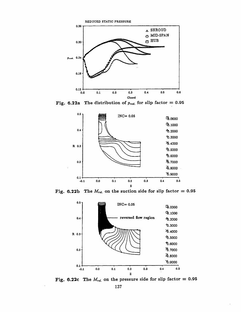
REDUCED STATIC PRESSURE

0.36

0.30

Piro. 0.24

0.18

0.120.0 0.1 0.2

Fig. 6.22a The distribution

0.4

R 0.3'

0.2'

0.1

0.3 0.4 0.5 0.6

Chord

of Pred. for slip factor = 0.95

.0000

'.2000

b.3000

>6.4000

b.5000

t.60oo

.7000'.8000

'.9000ooo

-0.) 0.0 0.1 0.2 0.3 0.4 0.5

z

Fig. 6.22b The M,.,. on the suction side for slip factor = 0.95

v region

0.0 0.1 0.2 0.3 0.4

z

Fig. 6.22c The M,,L. on the pressure side for slip factor = 0.95137

0.5

0.4

R 0.3-

0.2

A

-0.1

%.0000

%C. 1000

'b.2000

-t.3000

>6.4000

b.5000

.6000

7.7000

i.8000

'6.9000

0.5

_ _· ·

l

A r

0.5I

.

Ual

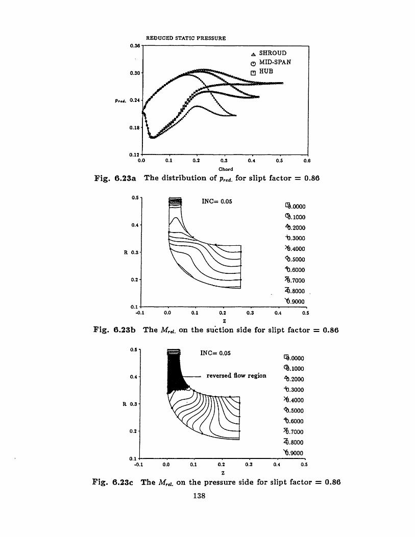
REDUCED STATIC PRESSURE

P,.d.

0.0 0.1 0.2

Fig. 6.23a The distribution of

u.D

0.4

R 0.3-

0.2-

-0.1

O.3 0.4 0.5 0.6

Chord

Pr,,d. for slipt factor = 0.86

[.0000

.100ooo

.2000

t.3000

>6.4000

%.5000

tb.6000

.7000

2;.8000

'6.9000

0.0 0.1 0.2 0.3 0.4 0.5

z

Fig. 6.23b The M,,l. on the suction side for slipt factor = 0.86

0.5

0.4

R 0.3-

0.2-

. 1

-0.1

w region

0.0 0.1 0.2 0.3

q.0000(. 1000

b.2000

-. 3000

>6.4000

'b.5000

1'.6000

1.7000

).8000

>6.9000

0.4 0.5

z

Fig. 6.23c The M,,l. on the pressure side for slipt factor = 0.86

138

-

A .--

n c

IIal |A.._ . _

I_..

zd- along the shroud

- along the mid-span

- along the hub

OIT!

[D

Fig. 6.24a

0.8 0.9 1.0 1.1 1.2

Slip factor

The maximum adverse pressure gradient verse the slip factor

7.5.

e.0 -

WAKE NO 4.5-

3.0 -

1.5-

0.

Fig. 6.24b The W

b on the hub surface

q on the shroud surface

[g on the suction surface

OmA

A(D

ID

A

O O

8 0.9 1.0 1.1 1.

Slip factor

take number verse the slip factor

2

139

I. IU

1.45-

( a. ), 0.9520-

0.95 -

n 7n l1 I ·

n ·~

Vl

I I I

u.'

0.6

0.5

R 0.4

0.3

0.2-

n

NORMAL THICKNESS

INC= 0.005

. 0 . 0.3-0.1 0.0 0.1 0.2 0.3

6.25a The normal thickness, t,, for

TANGENTIAL THICKNESS

0.6

0.5

R 0.4

0.S3

0.2

INC= 0.005

.0000

%.0100

4'.0200

+0.0300

'6.0400

.0500

0.0600

%.0700

.0800

Y.0900

0.4 0.5

the input

.0000oo

%.0100

'.0200

+0.0300

>.0400

%.0500

0'.0600

J.0700

.0800

Y0.0900

-0.1

Fig. 6.25b

0.0 0.1 0.2 0.3

z -

The tangential thickness, t,

140

0.4 0.5

from the output

Fig.

,J,

l._

0.7

dR .IIB.UO.

REDUCED STATIC PRESSURE

0.30

0.30

Pa. 0.24

0.18

0.120.0 0.1 0.2

Fig. 6.26a The distribution of

0.3 0.4 0.5 0.6

Chord

Pred. for case g, with bloc:kage effects

.0000

%.1000

t.ooo'b.2000t.3000

>.4000

.5sooo

b.60oo

.7000

7.8ooo

't.90oo

0.0 0.1 0.2 0.3 0.4 0.5

z

Fig. 6.26b The M,,. on the suction side with blockage effects

0.0 0.1 0.2 0.3 0.4 0.5

z

Fig. 6.26c The Mr,,. on the pressure side with blockage effects

141

0.5

0.4

R 0.3-

n l

-0.1

0.5

0.4

R 0.3

0.2

0.1-0.1

- - | - - - - f X |_,

^ ^ _

v.s

REDUCED STATIC PRESSURE

U.JO

0.30

pod. 0.24

0.18

0.120.0 0.1 0.2

Fig. 6.27a The distribution of

0.5.

0.4

R 0.3-

0.2-

0.1-

0.3 0.4 0.5 0.6

Chord

Pred. for number of blade

5.0000

Q(.1 000

'.2000

t.3000

>6.4000

.500ooo

'b.600

.7000

~.8000

'6.9000

-0.1 0.0 0.1 0.2 0.3 0.4 0.5

Fig. 6.27b The Mr,,. on the suction side for number of blades B = 21

R 0.3-

0.2

0.1

4.0000%.10oo00

'b.2000

t.3000

)6.4000

'.5000

b.6000

.7000

:;.8ooo

\'.9000

-0.1 0.0 0.1 0.2 0.3 0.4 0.5

z

Fig. 6.27c The M. on the pressure side for number of blades B = .21

142

as B = 21

-

, *

n e _

A .U.5

1

1.4U

1.15

( Do.)mar 0.90

0.65-

0.40-

Fig. 6.28a

AA- along the shroud

C. along the mid-span

[.g along the hubOm

O

A

12. 17. 22. 27. 32.

Number of blades

The maximum adverse pressure gradient verse the numberof blades

ib surface

lroud surface

Lction surface

m

A

0O

Fig. 6.28b

12. 17. 22. 27. 32.

Number of blades

The Wake number verse the number of blades

143

WAKE NO

* art

I I I

c

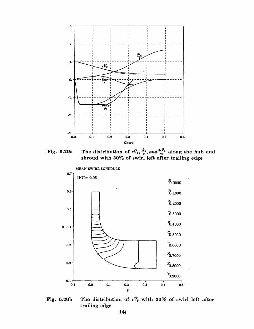
J.

2.

1.

0.

-1.

-2.

-3.0.0

Fig. 6.29a

]

0.7

0.6'

0.5.

R 0.4

0.3-

0.2

0.1 0.2 0.3 0.4 0.5 0.6

Chord

The distribution of rV, O, and9a- along the hub andshroud with 30% of swirl left after trailing edge

MEAN SWIRL SCHEDULE

INC= 0.05LI~oooo

0.2000

+0.3000

&6.4000

'.5000

.6000

%.7000

0.8000

Yo.soo

0.0 0.1 0.2 0.3

z0.4 0.5

Fig. 6.29b The distribution of re with 30% of swirl left aftertrailing edge

144

-0.1

n

A 1II

V. -

REDUCED STATIC PRESSURE

0.36

0.30'

Prad. 0.24

0.18

0.0

Fig. 6.30a

0.1 0.2 0.3

Chord

The distribution of P,,d.

0.4 0.5 0.6

with 30% of swirl left

R

-. 1 0.0 0.1 0.2 0.3 0.4 0.5

z

Fig. 6.30b

0.5'

0.4

R 0.3

0.2

0.1-0.1

Fig. 6.30c

The Mr,,. on the suction side with 30% of swirl left

.000oooo

%.10ooo

1.2000

t.3000

>6.4000

O.sooo

'.6000

7.7000£* ----

'6.9000'~.sooo

0.0 0.1 0.2 0.3 0.4 0.5

z

The M,,l. on the pressure side with 30% of swirl left

145

A SHROUD

C) MID-SPAN

ED HUB

Wl BU s ·

I

0.

2.

1.

0.

-1.

-2.

-3.0.0 0.1 0.2 0.3 0.4 0.5 0.6

Chord

Fig. 6.31a The distribution of rV, , and°.-V' along the hub andshroud

NORMALIZED MEAN SWIRL SCHEDULE

0.7

0.6

0.5

R 0.4

0.3'

0.2

INC= 0.05

%.1000

.2000

+0.3000

)'.4000

!0.5000

'0.6000

%.7000

20.8000

Yo.9000

0.0 0.1 0.2 - 0.3

Z

0.4 0.5

Fig. 6.31b the distribution of rV,146

0.1-0.i

e

L.

REDUCED STATIC PRESSURE, modifed profile

Pvrd.

Fig. 6.32a

0.0 0.1 0.2 0.3 0.4

Chord

The distribution of Pr,,d., stacking at

0.5 0.6

leading edge

INC= 0.05.oooo0000

.2000

t.3000

>6.4000

b.5000

b.6000

i.7000

:a.8000

'6.9000

0.1 0.2 0.3 0.4 0.5

Fig. 6.32bz

The M,,a. on the suction side, stacking at leading edge

0.5

0.4

R 0.3s

0.2-

n -0.1

v region

[.0000C%.1 0 0 0

'.2000

-b.3000

>6.4000

b.5000

'b.6000

7.7000

.8000

'6.9000

0.0 0.1 0.2 0.3 0.4 0.5

z

Fig. 6.32c The M,.t. on the pressure side, stacking at leading edge

147

0.5

0.4

R 0.3

0.2-

0.1-0.1 0.0

.

_ .

V.^

_

U~JL

BLADE SHAPEOriginal

O

0.

Radian -0.

-1.

-1.

.2.'

Fig. 6.33a Theand

0.0 0.1 0.2 0.3 0.4 0.5 0.6 -

Meridional Distance

blade camber vs the meridional distance of the originalmodified hub & shroud profiles

BLADE SHAPEOriginal Modinea

0.7 0.4

0.6 0.3

Radius 0.5 0.2

0.4 0.1

0.3 0.0

0.2 -0.1-

0.1 .0.2

C3 Z = O.OSZr.E.0 Z = 0.25Z.E., Z = O.50Zr..+ Z = 0.75Zr..

Z = Z.E.

. _:ex

(Modified)

(Origisal)

-2.0 -1.6 -1.2 -0.8

Radiuu

-0.4 0.0 0.4

Fig. 6.33b Radial distribution of blade camber along constant z-sectionfor the original and modified hub & shroud profiles

148

I 1 · · ·

i

I- J-n!

�

eCl

X^Y-Y-*X

GRID 33X49 (Plotted at the trailing edge)

-0.2 -0.1

Shroud

0.0

Trailing edge

Downstream

0.1 0.2

-0.3

Fig. 7.1 The mesh used for calculation

149

0.25

0.15

SPAN 0.05

-0.05-

-0.15-0.4

Shro

Suction

-0.3

GRID 145X49

Upstream

0.7-

0.6-

0.5-

R 0.4-

0.3S

0.2 -

0.1-0.1

Hut

0.0 0.4 0.5

..

1 -

- __

i.

ub

-

NORMALIZED MEAN SWIRL SCHEDULE

R

Fig. 7.2a

-0.1 0.0 0.1 0.2 0.3

Z

The specified rVO for design calculation

0.4 0.5

-0.1 0.0 0.1 0.2 0.3 0.4

z

Fig. 7.2b The blade shape from design calculation, number of bladesB = 14

150

0.4

0.3

0.2

r 0.1

0.0

-0.1

-0.2-0.2

U0.

INC= 0.005

0.6

0.5

R 0.4

0.3

0.2

0.1

[.1200

(.1400

"'.1600

0.1800

'>.2000

*.2200

.2400

%.2600

70.2800

Y'.3000

-0.1 0.0 0.1 0.2 0.3 0.4 0.5

z

The distribution of Pred. on the suction side from the designcalculation

U.-

0.6

0.5

R 0.4

0.3-

0.2-

0.1

Fig. 7.3b

INC= O.G05%.1200

(.1400

'.1600

+0.1800

>).2000

%8.2200

'.2400

:%.2600

0.2800

YO.3000

-0.1

The distril

0.0 0.1 0.2 0.3 0.4 0.5

z

bution of Prcd. on the pressure side from the designcalculation

151

Fig. 7.3a

· r I ·

rA

A,.p

0.15 C= INC= 0.005

0.05

-0.05

Theta -0.15

-0.25

-0.35

-0.450.000 0.133 0.267 0.400 0.533 0.667 0.800

Chord

The distribution of Pred. on the hub surface from the designcalculation

0.15

0.05

-0.05

Theta -0.15

-0.25

-0.35

Fig. 7.3d

-0.45

INC= 0.005[.1200

.1400

.1600

+0. 1800

'.2000

%.2200

0.2400

%.2600

70.2800

Y.3000

0.000 0.133 0.267 0.400 0.533 0.667 0.800

Chord

The distribution of Ped. on the shroud surface from the de-sign calculation

152

Fig. 7.3c

0.7'

0.6

0.5

R 0.4-

0.3 -

0.2

n

NORMALIZED MEAN SWIRL SCHEDULE

INC= 0.05

-0.1 0.0 0.1 0.2 0.3

Z

The distribution of r from the EulerTHE DIFFERENCE IN ri.

%.0000

%.1000

0.2000

+0.3000

'&4000

'%.5000

40.6000

%.7000

0.8000

0.9000

0.4 0.5

calculation

U.'

0.6

0.5'

R 0.4

0.3.

0.2-

Fig. 7.4b

0.1

INC= 0.50%:3.00%

-2.50%

-2.00%

-1.50%

X1.00%

o.00%

.50%

%.00%

Y1.50%

-0.1 0.0 0.1 0.2 0.3 0.4 0.5

z

The difference in ro between design specificationcalculation

and Euler

153

Fig. 7.4a

.IX

--

lA.

R

INC= 0.005%.1200

(%.1400

+.1600

+0.1800

)i.2000

'.2200

0.2400

%.2600

70.2800

'O.3000

-0.1 0.0 0.1 0.2 0.3 0.4 0.5

z

Fig. 7.5a The distribution of Pred. on the suction side from the Eulercalculation

0.7'

0.6

0.5

R 0.4

0.3

0.2-

0.1

INC= 0.005[.1200

.1400

.1600

+0.1800

'6.2000

'.2200

0.2400

0.2600

7i.2800

Y.3000

-0.1 0.0 0.1

Fig. 7.5b The distribution of p,,d.calculation

0.2 0.3 0.4 0.5

z

on the pressure side from the Euler

154

_ · I ·

rAl

--

--

.

0.15 TNC = nnnr

0.05

-0.05

Theta -0.15

-0.25

-0.35

-0.450.000 0.133 0.267 0.400 0.533 0.667 0.800

Chord

The distribution of Pred. on the hub surface from the Eulercalculation

0.15

0.05

-0.05

Theta -0.15

-0.25

-0.35

-0.45

Fig. 7.5d

0.000

INC= 0.005[.1200

.1400

$.1600

+0.1800

>6.2000

.2200

0.2400

1.2600

0.2800

YO.3000

0.133 0.267 0.400 0.533 0.667 0.800

Chord

ibution of p.,, on the shroud surface from the EulerThe distrcalculation

155

Fig. 7.5c

U. 7

0.6I

0.5

R 0.4

0.3 -

0.2

/n1

Fig. 7.6a

NORMALIZE MEAN SWIRL SCHEDULE

INC= 0.05

-0.1 0.0 0.1 0.2 0.3

Z

The distribution of re from the ViscoiTHE DIFFERENCE IN rVo

0.7

0.6

0.5

R 0.4

0.3

0.2-

0.1

lINC= 1.0%

.o0000

%.1000

0.2000

+0.3000

)'.4000

'.5000

0.6000

%.7000

i.8000

0.9000

0.4 0.5

is calculation

5.0%

-4.0%

-3.0%

+2.0%

-1.0%

%o%1.0%4.0%B~os

4io%

Z~o~a

'~osa

-0.1 0.0 0.1 0.2 0.3 0.4 0.5

Z

Fig. 7.6b The difference in rV$ between design specification and Vis-cous calculation

156

I

A m

A., _

_ · g

0.7INC= 0.005

0.6

0.5

R 0.4

0.3

0.2-

0.1

%.1200

.1400

.1600

+0.1800

)O.2000

('.2200

'.2400

b.2600

70.2800

Yo.3000

-0.1 0.0 0.1 0.2 0.3 0.4 0.5

z

The distribution of Pr,d. on the suction side from the viscouscalculation

0.7

0.6

0.5

R 0.4

0.3

0.2

0.1

Fig. 7.7b

INC= 0.005

-0.1

The distril

.1200

.1400

J.1600

+0.1800

)6.2000

(6.2200

'.2400

%.2600

0.2800

0Y.3000

0.0 0.1 0.2 0.3 0.4 0.5

Z

bution of P,,d. on the pressure side from the viscouscalculation

157

Fig. 7.7a

.

A m

Am-

1

U.lb

0.05

-0.05

Theta -0.15

-0.25

-0.35

-0.450.000 0.133 0.267 0.400 0.533 0.667 0.800

Chord

The distribution of P,,d. on the hub surface from the viscouscalculation

U.1

0.05

-0.05

Theta -0.15

-0.25

-0.35

-0.45

Fig. 7.7d

INC= 0.005q.1200

%.1400

0.1600

0.1800

'>.2000

<.2200

.2400

%.2600

70.2800

Y.3000

0.000

The distr

0.133 0.267 0.400 0.533 0.667 0.800

Chord

ibution of Pr. on the shroud surface from the vis-cous calculation

158

Fig. 7.7c

A.._

I

J~ sac4

RELATIVE MACH NUMBER AT MID-SPAN0.15

0.05

-0.05

Theta -0.15

-0.25

-0.35'

-0.450.000 0.133 0.267 0.400 0.533

Chord

The distribution of relative Mach:sign calculation

I RELATIVE MACH NUMBER AT MID-SPAN

0.667 0.800

number Mc,, from the de-

0.15

0.05

-0.05

Theta -0.15

-0.25

-0.35'

Fig. 7.8b

-0.450.000 0.133 0.267 0.400 0.533 0.667 0.800

Chord

The distribution of relative Mach number Mre, from the vis-cous calculation

159

Fig. 7.8a

MERIDIONAL VELOCITY

0.000

Il6iIIIililIIIII Mt1111 11 S11iiIIiS

{ll lllllllllllllll llill4i

UIsIIIIIIIIIIIIIIIIIIIII I IIII

JI 111iiI 1iiIIIiIII IIiMiI 816iIU{{asabllllllllliliigli lgillili#

J ,aaasallilll s a,*lll llll l l l-

M ii} 1J l &l 1 1 M - -

I .. . Ml, llallh -

, a

0.025 0.050

Leading Edge

z

z

Fig. 7.9a The meridional velocity on the surface 1-point above the S.S.

MERIDIONAL VELOCITY

0.075 0.100 0.125

sallillllllllsllllsIllllllllllllllsIIi

wu alllalllllla llllllll slllillllllll las

UUaaIIIIIIIaIIla alI{IIsia1 lIII IU{..U....aIIIaII. a .i. , i.i.4|$$$|&g&UEases 51 ala 5|$|&s&8|lU

I~llN88$4&&Maaasaaggaa

,.......·

_....--···

..v

, '---_----'---

,...-'--...---

*-------

Leading Edge

. . . ..

-0.025

Fig. 7.9b

0.000 0.025 0.050

z0.075 0.100 0.125

The meridional velocity on the surface 1-point below the P.S.

160

0.5251

0.500

R 0.475

0.450-

0.425-0.025

U. b*

0.500*

R 0.475-

0.450-

0.425- I 1 ·

"'

A P~

I

Shroud

0.00 T P.S.S.S. 1H

Hub

0.0 0.1

Fig. 7.10a The distribution of entropy S at the leading edge

STREAMWISE VORTICITY AT L.E.

INC= 2.00

Shroud

P.S.S.S.

Hub

[4.0000

-(.0000

-4.0000

-2.0000

).0000

.0000

.000oooo

7. 000 0

Z10.0000

-0.2 -0.1 0.0 0.1 0.2 0.3 0.4

Fig. 7.11a The distribution of streamwise vorticity fl, at the leadingedge

161

ENTROPY AT L.E.

INC= 0.01

0.7-

SPAN 0.6-

0.5

0.4

-0.2

.o0 000

(.0100

z'.0200

.0300

>6.0400

"<.0500

.0600

.0700

4.0800

'.0900

-0.1 0.2 0.3 0.4

0.s8

0.7-

SPAN 0.6-

0.5-

0.4

^ A

I I I -,

ENTROPY AT 1 CHORD4

0.71

0.6-

SPAN 0.5-

0.4

0.3-0.2

Fig. 7.10b

INC= 0.01

Shroud

S.S. P.S.

Hub

-0.1 0.0 0.1

a

0.2 0.3

The distribution of entropy S at the chord

STREAMWISE VORTICITY AT CHORD

0.7

0.6

SPAN 0.5-

0.4-

0.3-

-0.2

Fig. 7.111

INC= 2.00

Shroud

S.S.

-[3.0000

-.0000

-4.0000

-2.0000

>4.0000

<.0000

4.00ooo00

5.0000

4.0000

Y10.0000

P.S.

Hub

0.3 0.4

fl at the . chord4

162

[. 0000

Q.0100

'.0200

-. 0300

>6.0400

<'.0500

.0600

%.0700

.0800

Y.o9oo

0.4

-0.1 ' 0.0 0.1 0.2

The distribution of streamwise vorticity

1 r · · · _

·

--

At

E

u.oI

0.5-

SPAN 0.4-

0.3-

0.2

-0.2

Fig. 7.10c

U.OI

0.5-

SPAN 0.4-

0.3-

0.2

-0.:

Fig. 7.1]

2

lc

!NTROPY AT CHORD

INC= 0.01

Shroud

-0.1 0.0 0.1 0.2 0.3

The distribution of entropy S at the chord

STREAMWISE VORTICITY AT CHORD

INC= 2.00

Shroud

163

.0000oo

(.0100

.0200

'.0300

>6.0400

`.0500

'.0600

0.0700

.0800

"0.0900

0.4

.oooo0 0 0 0

"-4.0000

-- 2.0000

9.0000

4.0000

Y•0.0000

-0.1 0.0 0.1 0.2 0.3 0.4

The distribution of streamwise vorticity fl at the chord2

_

A a

S.41.

n 2

El

I

NTROPY AT CHORD

INC= 0.01

S

S.S.

P.S.

Hub

1 -0.2 -0.1 0.0 0.1 0.2

id The distribution of entropy S at the chord

STREAMWISE VORTICITY AT CHORD

INC= 2.00

S

S.S.

Hub

d

164

.oooo0 0 0 0

(. 0 1 0 0

'.0200

-. 0300

>6.0400

B.0500

.0600

%.0700

.0800

Y0.0900

U.4'

0.3-

SPAN 0.2-

0.1 -

nn

Fig .7.10,Fig. 7.11

0.3

SPAN 0.2-

0.1 -

0.0 -0.3

Fig. 7.11

0.3

C. 00 o0

-4.0000

4.0000

- 2.0 0 0 0

4.0000

4.0000

Yb.0 0 0 04.0000

-0.2 -0.1 0.0 0.1 0.2 0.3

The distribution of streamwise vorticity f at the chord

n a_

V.V

_

U.25

0.15-

SPAN 0.05-

-0.05-

-0.15-0.4

Fig. 7.1C

U.'OI

0.15 -

SPAN 0.05-

-0.05 -

ENTROPY AT T.E.

INC= 0.01

P.S.

[.0000

q.0100

4 .0200

+.0300

>6.0400

.0500

0.0600

.0700

4.0800

Y'.0900

S.S.

[ub

-0.3 -0.2 -0.1 0.0 0.1

a

le The distribution of entropy S at the trailing edge

STREAMWISE VORTICITY AT T.E.

INC= 2.00

Shro

P.S.

-i.0000

z-4.0000

±2.0000

6. ooo0+4.0000

4.0000

.0000

Y. 0oo0 0 0~.0000Y10.0000

S.S.

ub

-0.4

Fig. 7.11e

-0.3 -0.2 -0.1 0.0 0.1 0.2

B

The distribution of streamwise vorticity flz at the trailingedge

165

0.2

_ ·

"

-u ,

I Ri

Shroud

S.S. P.S.

Hub

-0.1

Fig. 7.12a

u.O.

0.7-

SPAN 0.6-

0.5-

0.4-

2 -0.1 0.0 0.1 0.2 0.3 0.4

The distribution of entropy S at the leading edge, number ofblades B = 21

STREAMWISE VORTICITY AT L.E.

INC= 2.00 ,4L. 0 000

-{6.0000

-4.0000

-±2.0000

>4.0000

:.0000

76.0000

Y10.0000

Shroud

S.S. '-~ ~ P.S.Hub

-0.2

Fig. 7.13a

-0.1 0.0 0.1

a

0.2 0.3 0.4

The distribution of streamwise vorticity fi, at the leadingedge, number of blades B = 21

166

ENTROPY AT L.E.

INC= 0.01U.8I

0.7

SPAN 0.6-

0.5-

[. 0000

.0100

z.0200

-t.0 30 0

>6.0400

<.0500

t).0600

5.0700

4.0800

Y0.0900

· · _· ·

O

-

.-

_

ENTROPY AT CHORD4

INC= 0.01

Shroud

S.S.

Hub

-0.2

Fig. 7.12b

U.' I

0.6-

SPAN 0.5-

0.4-

-0.1 0.0 0.1

eThe distribution of entrojblades B = 21

STREAMWISE VORTICITY AT CHORD

INC= 2.00

Shroud

S.S. P.S.

0.2 0.3 0.4

py S at the chord, number of4

4.0000

4-2.0 0 0 0-2.0000

>6.0000

.0000

';4.0000

N.0000

4.0000

Y•0.0000

-0.2

Fig. 7.13b

-0.1 0.0 0.1

8

0.2

The distribution of streamwise vorticity lnumber of blades B = 21

0.3 0.4

at the chord,4

167

0.7I

0.6 -

SPAN 0.5-

0.4-

0.3

P.S.

[.0000

Q.0100

Z.0200

-. 0300

>6.0400

J.0500

.0600

%.0700

4.0800

Yo.0900_ · ·

A m

I

n J_I

n e . __.. 11} YV.)

ENTROPY AT CHORD

INC= 0.01

S.

Fig. -0.12

Fig. 7.12c

U.bI

0.5-

SPAN 0.4-

0.3

n

2 -0.1 0.0 0.1 0.2 0.3 0.4

The distribution of entropy S at the 2 chord, number ofblades B = 21

STREAMWISE VORTICITY AT CHORD

INC= 2.00 ,

Shroud

L6.0000

-4.0000

>4.0000±2.0000

<~.0000

q.0000

~.0000

4.oooo

Y•o.oooo

-0.1 0.0 0.1 0.2 0.3

The distribution of streamwise vorticity atnumber of blades B = 21

0.4

the 2 chord,

168

Shroud

0.5

SPAN 0.4'

0.3-

0.2-

[~. 0 0 0 0

(.0100

'.0200

+0.0300

>6.0400

'.0500

.0600

5.0700

4.0800

Y'.o900

-0.2

Fig. 7.13c

II - -

-

.*I

ENTROPY AT A CHORD

INC= 0.01

S.S.

-0.2

Fig. 7.12d

0.4 -

0.3 -

SPAN 0.2-

0.1-

0.0-

-0.3

Fig. 7.13d

-0.2 -0.1 0.0 0.1 0.2 0.3

The distribution of entropy S at the chord, number ofblades B = 21

STREAMWISE VORTICITY AT CHORD

INC= 2.00

Sh

SS.

1-.0000

6.oooo

4.0000

±-2.0000

~.0000>6.oooo

9.0000

'4.0000

•.0000YO.0000

-0.2 -0.1 0.0 0.1 0.2 0.3

The distribution of streamwise vorticity at the chord,number of blades B = 21

169

U..'

0.3

SPAN 0.2-

0.1-

0.0

I.0000

!.0100

.0200

-.0300

>6.0400

.0500

to.0600

5.0700

4.0800

'6.0900_

I,

-

ENTROPY AT T.E.

INC= 0.01

Shro

P.S.

SS.

[.0000

.0100

>.0200

'~.0300

Y.0400

`.0500

.0600

0.0700

.0800

Y.0900

[ub

-0.4

Fig. 7.12e

-0.3 -0.2

The distribution ofblades B = 21

STREAMWISE VORTICITY AT'

INC= 2.00

-0.1

e

0.0 0.1 0.2

entropy S at the trailing edge, number of

T.?.

[.0000

(6.00 0 0

-4.0000

±2.0000

.0000

.0000

u4.0000

.0000

Yo.00 0 0

-0.4

Fig. 7.13e

-0.3 -0.2 -0.1 0.0 0.1 0.2

The distribution of streamwise vorticity f, at the trailingedge, number of blades B = 21

170

U.AD

0.15

SPAN 0.05-

-0.05-

.n 15

Shroi

P.S.

S.S.

0.25

0.15-

SPAN 0.05-

-0.05 -

-0.15-

· · · · ·

· ,e

V.ely

NORMALIZED MEAN SWIRL SCHEDULE

0.7

0.6

0.5'

R 0.4

0.3

0.2-

-0.1

Fig. 7.14a The disti

INC= 0.05.00

.2000

+0.3000

'.4000

'.5000

0o.6000

7.8o00

Yo.9000

0.0 0.1 0.2

Z

ribution of rVe from

0.3 0.4 0.5

the viscous calculation with3% of tip clearance

U.-r

0.6.

0.5-

R 0.4-

0.3-

0.2

0.1

Fig. 7.14b

THE DIFFERENCE IN rV9

INC= 1.%

8.%

-4.%

x2.%

2.%

Y8.%- ·

-0.1

The diffecous calcuregion)

0.0 0.1 0.2 0.3 0.4 0.5

Z

srence in rVe between design specification and vis-ilation with 3% of tip clearance (only the blade

171

A _

II !.J

I

0.7INC= 0.005

0.6

0.5

R 0.4

0.3'

0.2-

n1

Fig. 7.15a

-0.1 0.0 0.1 0.2 0.3 0.4 0.5

z

The distribution of Pred. on the suction surface from the vis-cous calculation with 3% of tip clearance

U.,

0.6

0.5

R 0.4'

0.3-

0.2-

Fig. 7.15b

0.1

INC= 0.005%.1200

.1400

.16oo00

+0.1800

O.2000

.2200

0.2400

%.2600

7.2800

Y.3000,I

-0.1 0.0 0.1 0.2 0.3 0.4 0.5

z

The distribution of Pred. on the pressure surface from the vis-cous calculation with 3% of tip clearance

172

%.1200

.1400

.1600

+0.1800

0.2000

.2200

'0.2400

%.2600

.2800

YO.3000·I _ __

A m

l 4V._ .

,,

R

0,

Fig. 7.15c

.0 0.1 0.2 0.3 0.4 0.5 0.6

z

The distribution of Prd. on the hub surfac-calculation with 3% of tip clearance

0.7 0.8

from the viscous

INC= 0.005

Tip Leakage vortex

0.0

Fig. 7.15d

0.1 0.2 0.3 0.4

z

The distribution of Pred. on thecous calculation with 3% of tip

173

0.5 0.6 0.7 0.8

shroud surface from the vis-clearance

R

'.1200

%.1400

.1600

+0.1800

Y.2000

.2200

40.2400

%.2600

0.2800

0.3000

A . S

MERIDIONAL VELOCITY NIEXT TO THE S.S.

li I.lllll Illll"".. lllllll. u

UUIIa.IIII s.tII*''" jIIIIIIUaI.llllllllll*u'."'a,,lllllll

lIIIIIIIIII."'"" IIII XJIeuI

gill~ jjjjjjj~ill{ Il/J{

jSltL {{

Leading Edge

-0.025

Fig. 7.16a

0.000 0.025 0.050

z

0.075 0.100 0.125

The meridional velocity on the surface 1-point above the S.S.with 3% of tip clearance

MERIDIONAL VELOCITY NEXT TO THE P.S.

UUIIIIIIIIIIli i , ,.,,, , IIII li{UIIIII111 IIt","'" I IIII{II8 UJ

U8Ii Is .."'.. ,,I I1ll11lllll

a........ ......... .............. --.m ..........

....... *** . .... ao .. .....

........::::::: ..... '--'_... ......

Leading Edge

-0.025 0.000 0.025 0.050

z0.075 0.100 0.125

Fig. 7.16b The meridional velocity on the surface 1-point below the P.S.with 3% of tip clearance

174

U.DZD '

0.500-

R 0.475 -

0.450

0.425

U.DZD

0.500-

R 0.475-

0.450 -

0.425- · ·

f e

A eee

ENTROPY AT L.E.

INC= 0.01

Shroud

0.00 fP.S.S.S.ub

-0.2

Fig. 7.17a

0. -

0.7

SPAN 0.6-

0.5

0.4-0.2

Fig. 7.18a

-0.1 0.0 0.1

a0.2 0.3 0.4

The distribution of entropy S at the leading edge with 3% oftip clearance

STREAMWISE VORTICITY AT L.E.

INC= 2.00 ,LUJS.0000

t4.0000

-4.0000

+. 00 0 0

zt4.000046.0000

,4.0000

Y0.0000

Shroud

S.S. .. ~ P.S.S.S.

-0.1 0.0 0.1 0.2 0.3 0.4

a

The distribution of streamwise vorticity f, at the leadingedge with 3% of tip clearance

175

U.'

0.7-

SPAN 0.6

0.5 -

nd

[q.00 00

(.0100

'~.0200

".0300

>6.0400

<.0500

'.0600

;.0700

4.0800

'~.0900

A

_.

ENTROPY AT CHORD

INC= 0.01

Shroud

S.S.

flub

-0.2

Fig. 7.17b

u.'-I

0.6

SPAN 0.5

0.4 -

0.3 --0.2

Fig. 7.18b

-0.1 0.0

The distribution ofclearance

STREAMWISE VORTICITY AT -

INC= 2.00

Shroud

S.S.

Hub

0.1 0.2 0.3 0.4

entropy S at the chord with 3% of tip

L CHORD

[.0000

t4. 000 0

>-2.0000

).0000

.0000

P.S. t.0000

,6.0000

Y4.0 0 0 0

-0.1 0.0 0.1 0.2 0.3 0.4

The distribution of streamwise vorticity at the chord with3% of tip clearance

176

U. '

0.6'

SPAN 0.5-

0.4 -

0-.

C'.0000

.0100

1.0200

+0.0300

1b.0400

.0500

0.0600

'.0700

OI.0800

'o.09oo

P.S.

, . ·

, J

-

ENTROPY AT CHORD

INC= 0.01

Shroud

-0.1 0.0

.Fig. 7.17c

U0.6

0.5-

SPAN 0.4-

0.3-

n9-0.2

0

The distribution of entropy S at the chord with 3% of tipclearance

STREAMWISE VORTICITY AT 1 CHORD

INC= 2.00 ,

Shroud

S..

-0.1 0.0 0.1 0.2

Lk .0000

A.0000

-4.0000

t 2.0 00 0

>6.0000

.0000

Y.0000

0.3 0.4

Fig. 7.18c The distribution of streamwise vorticity fl at the 2 chord with3% of tip clearance

177

0,6 _

0.5

SPAN 0.4

0.3-

0.2

-0.2

.f000oo

!.0100

L'.0200

.0300

6.0400

'(.0500

'.0600

;.0700

.0800

"0.0900

0.1 0.2 0.3 0.4

_ __

- _ · · I ·

A -

I

vow

ENTROPY AT CHORD

U.4

0.3

SPAN 0.2

0.1

0.0-0.3

Fig. 7.17d

0.4

0.3-

SPAN 0.2-

0.1 -

nonIN

-0.3

INC= 0.01

C

P.S.

[.0000

9.0100

'.0200

-.0300

.0400

<.0500

t. 0600

.0700

4.0800

Y'.0900

Hub

-0.2 -0.1 0.0 0.1 0.2 0.3

The distribution of entropy S at the chord with 3% of tipclearance

STREAMWISE VORTICITY AT q CHORD

INC= 2.00

S]

P.S.S

Hub

-0.2 -0.1 0.0 0.1

Uz. 0000

(4.0000

-4.0000

-2.0000

).0000

4 .0000

4.0000

Y0o.0 0 0 0

0.2 0.3

Fig. 7.18d The distribution of streamwise vorticity at the chord with3% of tip clearance

178

I · __

A ·

S.'

._

ENTROPY AT T.E.

SPAN

P.S.

[.0000

9.0100

~.0200

'.0300

)6.0400

<.0500

'.0600

%.0700

4.0800

Y.0900

S.S.

Hub

-0.4 -0.3 -0.2

Fig. 7.17e

0.25

0.16

SPAN 0.05

-0.05

.f 1R

-0.1

9~

0.0 0.1 0.2

The distribution of entropy S at the trailing edge with 3% oftip clearance

STREAMWISE VORTICITY AT T.E.

INC= 2.00 ,

Shrou,

P.S.

S.S.

:ub

IZ)8.0000

)6.0000

-4.0000

7.0000.0000Y0.0000

Yb.0 0 0 0

-0.4

Fig. 7.18e

-0.3 -0.2 -0.1

i

0.0 0.1 0.2

The distribution of streamwise vorticity nf at the trailingedge with 3% of tip clearance

179

· I · · ·

.

V -

R

Z

IdzI

Fig. B.1 Control volume for an axisymmetric flow

180

00o

f..0

00-oci'

In

-0.50

Fig. C.la

-0.25 0.00 0.25 0.50

Z

0.75 1.00

Test grid for multigrid study, uniform mesh

0. 50. 100. 150. 200. 250. 300. 350.

Fig. C.lb Log(residue) verse unit of work for mesh-a

181

1.25 1.50

400.

..................... ........................................................................

e _ · · · ·

V))n

04

-

To

UnC'

U,V.._

0

In

u,

Fig.

-0.5 -0.2 0. 02 05 07 10.5.-0.50 -0.25 0.00 0.25 0.50 0.75 1.00 1.25 1.50

C.2a Test grid for multigrid study, with distortion in Z direction

0. 50. 100. 150. 200. 250. 300. 350. 400.

Fig. C.2b Log(residue) verse unit of work for mesh-b

182

. 4

................----------------....... I .....................H H HH

... . .... 11"i ............ .II.............................

I

i1I

I

II

I

-0.25 0.00 0.25 0.50 0.75

z1.00 1.25 1.50

Fig. C.3a Test griddirection

for multigrid study, with distortion in both R and Z

0. 50. 100. 150. 200. 250. 300. 350.

Fig. C.3b Log(residue) verse unit of work for mesh-c

183

nCY

o

0J

Inu-I

-0.50

400.

.

-o

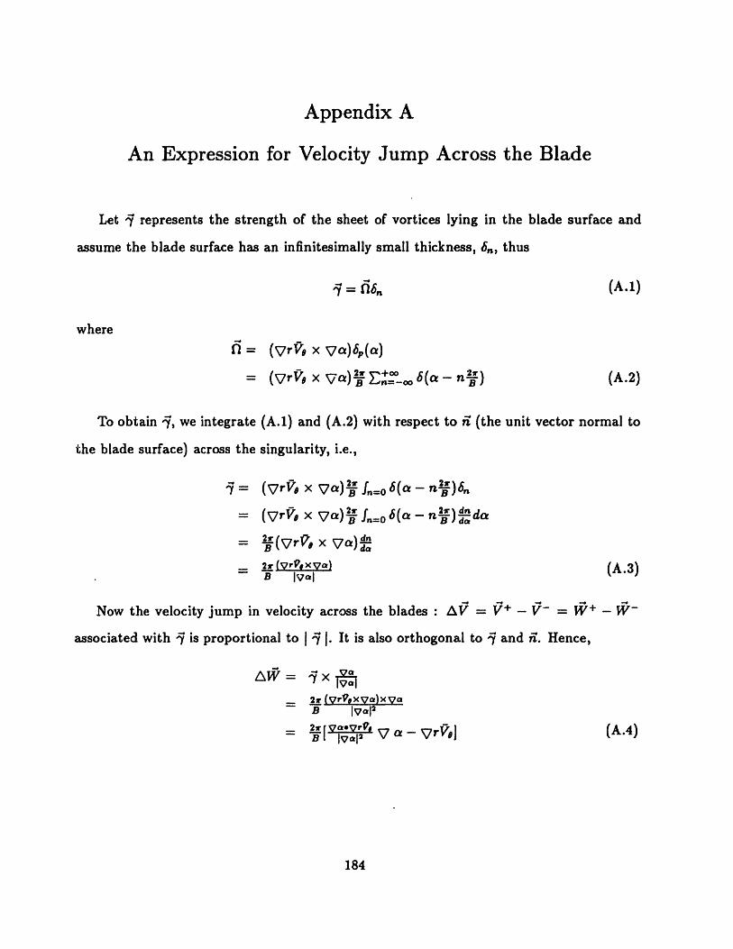
Appendix A

An Expression for Velocity Jump Across the Blade

Let represents the strength of the sheet of vortices lying in the blade surface and

assume the blade surface has an infinitesimally small thickness, 6,, thus

7 = is2, (A.1)

where

n = (vr0 x )bp(a)

= (vrV x ) E+' 6(a - n ) (A.2)

To obtain ', we integrate (A.1) and (A.2) with respect to in (the unit vector normal to

the blade surface) across the singularity, i.e.,

' = (vrQe x Vt) r n=o (a - n ) n(V r T x V a) ' n=O 6(c - ) daTr 7Cn) doB (VrV, x )d

2 (y r xyVa) (A.3)B Ivol

Now the velocity jump in velocity across the blades : AV + -= V++ -- W-

associated with ' is proportional to j [. It is also orthogonal to and n. Hence,

AW= 7xT72 (tex Va)x aB Ival 2

= -2S[VV' vVr (A.4)ffIv- V ca- V]

184

Appendix B

Mass-Average of the Continuity Equation

with the Effect of Tangential Blockage, b

The introduction of the blockage distribution b(r, z) has been used to account for blade

thickness in axisymmetric flow (Ref. 64, 65). In this appendix, we will derive the governing

equation for the artifial density p(r, z) (see chapter 3) with the effect of blockage. If we

take a control volume as shown in Fig B.1 and do a mass balance, then we have

bpW, (2irrdz) - (b + k dr)( pW, + 2adr)j2r(r + dr)dzl

+bpWr[7r(r + dr)2 - rr2j - (b + fdz)(pW, + aW--dz)[7r(r + dr) 2 - 7rr2 = 0

i.e.,

== V bpW = (B.1)

since pW = pW + pW + pW + pW, Eq. (B.1) can be rewritten as

V bW = - *bpW

or

V7W = -We V. bpatWVlnb -

define the artificial density Pa as

V bpaW = 0

or

W = -W V in bp.

185

(B.2)

(B.3)

introducing the Stokes stream function & to satisfy Eq.(B.3), i.e.,

1 a

bp r az

W.= 1 labpa r ar

Now combine Eq. (B.2) and Eq.(B.3), we have

W * Vln p = W * Ini+ -e (B.4)

which is the Eq.(3.37) with blockage effect. It is interesting to check the consistency

for the equation (B.4) when there is no blockage. i.e., b = 1.

W * Vlnp = W 7Vln + W *· Vn(l + )

= W v7np +W[-(e)P

= W ln

= W * vlnp

- w.vaLn- W vln

= WV7 ln

=W * lnp= W·Vln~ro

+

+

+

+ p(V* A# p+e IpW - eP VpW)+ .(e pW)

+p

We see the expression of Eq. (B.4) is identical to the area-average form in Eq. (3.21)

when b = 1.

186

I'+(A) 0

0 - -;(~ · vO- qw · v~)

(V · ~ - v 0W)P pv-r--/

--

+ ()2 ( + .] ' ()

Appendix C

A Multigrid Method for the Poisson Equation

The multigrid version of a finite element method is presented.

algorithm considers

V2 = S

= g8n 9

The basic multigrid

in G

on GI

on G2(C.1)

where G is the domain and 8G is the boundary of the domain.

We approximate (C.1) on the finest grid by

Lm Om = Fm

B m = Gm

in Gm

on a Gm(C.2)

The superscript m denotes an approximation on a grid with mesh hm. We also use

auxiliary grids G1, G2... Gm-l, with + = 1

The multigrid cycle begins with a "fine-to-coarse" process which starts with one relax-

ation sweep on the finest grid. We then have an approximate solution. We then transfer

the residual

(C.3)R = Fm _ Lm m

to the next coarser grid using

R m - = Tm-I Rm

on the grid Gm-l, we solve

Lt- l Atm-1 = Rm-i

where A Em-' is an approximation to the fine grid error

A OM = , - '

(C.4)

(C.5)

(C.6)

187

This process is repeated to grid Gk until we get to the coarsest grid. On the coarsest

grid we use I relaxation sweeps rather than one relaxation sweep used on the finer grids.

To return to the finer grid we begin by using I relaxation sweeps on the coarsest grid. The

"coarse-to-fine" process starts by calculating O which is a new approximation to 2 by, new

n= rold + I AO,1 (C.7)

This improved approximation is the correction to the next finer grid. This process is

continued until we reach the finest grid Gm. This process consists of one cycle of multigrid.

When used as an iteration process, this cycle is repeated until convergence is reached.

As distinct from finite difference approaches the interpolation operators, I_ l and

Tm -l, are not arbitrary but based on the finite element interpolation spaces (G' and

Gm-l). They are considered in some detail next.

Let us first consider the coarse to fine grid interpolation operator Im_l. The only

natural choice for the interpolation of a coarse mesh function Ob- to a fine mesh location

(xzi, yi,) is to use the value of Obm in the location (, yi) given by the finite element

approximation in space Gm - .

" ." - Om- Y, ") " m-"

[II -1]ij = %,m (, y) -= Z rk ct, (C.8)k.

where the matrix I, is given by

= N 1 (, yij) (C.9)

On an arbitrary mesh, this results in non-uniform interpolation coefficients 41 and for

an uniform mesh bilinear elements. This can be written in a simple formula:

[Ir m1 = 1 1 + 4 + 4 + 4b-I) for the center node4 4 (C.10)

[I -1,m-lm - (4?m-l1 + m--1) for the mid side nodes (C.10)

[Ir_l -lli, = Om- for the corner nodes (identity)188

Next we consider the fine to coarse grid interpolation operator T-'. As distinct from

the finite difference case the residual is an integral quantity which is scaled differently on

different grids. A consistent representation of R - by means of fine grid quantities is

found by approximating the coarse mesh functions in the integral form with fine mesh

interpolations in the space G', namely.

[TL-' Rm 'Jj = E l j f l N-(xs,y) R'ds (C.11)

on an uniformly subdivided coarse mesh, Eq. (C.11) can be reduced to

[IT-' R'i = Skl It Rl

=gn' + (Ri+l + +Rm l Ji ~+ Ij)+Ri, + + R-j+ + Ri+ j + Ri (C.12)

The convergence of the computation is measured by the evaluation of the L2-norm

residual on the finest grid in terms of the work count which is defined in units representing

the work needed for one conjugate gradient on the finest mesh. For instance, the work

count for one complete multigrid cycle with four-level grids and for the present strategy is

given by

10 + 20 + + 00 = 17.8125 units.

The additional work for the residual weighting and other intepolations are not included.

All computations are carried out using a fine mesh with 97 x 33 mesh points and successive

coarser meshes of 49 x 17, 25 x 9, 13 x 5 mesh points.

The test case that we choose to assess the algrith is to apply it to the solution of

V2 = 2rs + 6rz2 with the Dirichelet boundary condition on four sides. The multigrid

grid scheme will turn on after 50 units of work on the finest grid. Three different grids are

used (Fig. C.la, C.2a, C.3a). For mesh in Fig. C.la which is an uniform grid, the three-

level of multigrid scheme results in maximum saving in computational time (Fig. C.lb). It

189

shows that only 4 cycles of multigrid scheme are needed for the solutions to reach machine

accuracy. For the distorted mesh, in Fig. C.2a and Fig. C.3a, the two-level of multigrid

scheme results in maximum saving in computational time (Fig. C.2b and Fig. C.3b). For

mesh in Fig.C.3a, using four-level of multigrid scheme leads to solution divergence (Fig.

C.3b). This may be due to the interpolation errors on the distorted mesh. Thus, the use

of a low level of multigrid scheme is more suitable than a high level of multigrid scheme

for a distorted mesh.

190

Appendix D

The Relationship between Number of Grid Points and

Number of Harmonic Modes

The periodic potential equations is a Poisson equation with a high frequency in the

RHS, i.e., V2 k = S(r,z)einBf(r 'z) (see Eq.(3.26)). In order to resolve the information due

to the high frequency, a suitable mesh size is needed. A one-dimensional model problem

is used to examine the requirement of the mesh size.

a 2 jXa z 2 COS 27r (D.1)

The study shows that regardless the boundary condition and using two-node or three-

node elements, the minimum number of elements, M, in order to avoid the solution diver-

gence is given by the relation

M=j (D.2)

This is the so-called "Nyquist criteria". Thus, the minimum number of elements in the

streamwise or spanwise direction for the design code depends on the change in blade wrap,

number of harmonic modes, and number of blades. It can be written as

nBAf2r (D.3)

191

Appendix E

Nondimensional Form of Variables

There are two different ways of nondimensionalization of the variables. One is normal-

ized by the quantities in the relative frame, such as the data used in the design program.

The other is normalized by the quantities in the absolute frame, such as the data presented

in the thesis. We will state the reference quantities for each case separately.

I. Normalized Form of Variables in the Design Code.

Since the flow is steady in the relative frame, it is convenient to normalize the variables

in terms of the quantities in the relative frame. In the design calculation, the tip radius is

used to normalize the length. The radial velocity at the leading edge is used as the reference

velocity. The thermodynamic quantities are normalized by the rotary total quantities at

the leading edge. These normalized variables are shown below:

Lrc = rtip

VrC = W,

T,, = T;

Pref = PT

Prt = P;

II. Normalized Form of Variables in the Output

In general, the far upstream quantities are specified as inputs for a design. It would

be suitable to present the variables which are normalized by these upstream quantities.

Here, the upstream total pressure, total temperature, diameter are used to normalize the

variables. These variables are shown below:

192

L,, = Diameter

T,,/ = TT

Pref = pT

Prf = PT

For example, from the above normalization, the reduced static prssure is nondimen-

sionalized by Pre,, i.e.,

P - pw2r2PTPT

P 1 pw2r 2

PT 2 T(VP )2

193

Pred

Ped = _ (r)22

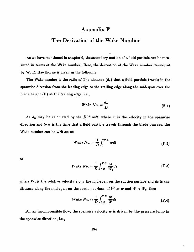
Appendix F

The Derivation of the Wake Number

As we have mentioned in chapter 6, the secondary motion of a fluid paritcle can be mea-

sured in terms of the Wake number. Here, the derivation of the Wake number developed

by W. R. Hawthorne is given in the following.

The Wake number is the ratio of The distance (d,) that a fluid particle travels in the

spanwise direction from the leading edge to the trailing edge along the mid-span over the

blade height (D) at the trailing edge, i.e.,

Wake No. =D (F.)

As d may be calculated by the fo T.. wdt, where w is the velocity in the spanwise

direction and tT.E. is the time that a fluid particle travels through the blade passage, the

Wake number can be written as

Wake No. = j wdt (F.2)

or

Wake No. = .E. w ds (F.3)

where W, is the relative velocity along the mid-span on the suction surface and ds is the

distance along the mid-span on the suction surface. If W > w and W - W., then

Wake No. ds (F.4)

For an incompressible flow, the spanwise velocity w is driven by the pressure jump in

the spanwise direction, i.e.,

194

Apred = Ipw 2

W =red W2h d_-

Thus, the Wake number can be expressed as

Wake No. .. Whrud - Hbd

For a compressible flow, the W in the above expression is replac

number, i.e.,fT.E. Mhfo d -M 2

Wake No. , Td .. M5 JL.E. M

(F.7)

:ed by the relative Mach

(F.8)

Even though the expression of the Wake number used in chapter 6 is different from the

one derived here. However, both Wake numbers do give the same trend summarized in

chapter 6.

195

or

(F.5)

(F.6)