MITLibraries - DSpace@MIT
103
MITLibraries Document Services Room 14-0551 77 Massachusetts Avenue Cambridge, MA 02139 Ph: 617.253.5668 Fax: 617.253.1690 Email: docsmit.edu http://Iibraries.mit.edu/docs DISCLAIMER OF QUALITY Due to the condition of the original material, there are unavoidable flaws in this reproduction. We have made every effort possible to provide you with the best copy available. If you are dissatisfied with this product and find it unusable, please contact Document Services as soon as possible. Thank you. Some pages in the original document contain color pictures or graphics that will not scan or reproduce well.
-
Upload
khangminh22 -
Category
Documents
-
view
0 -
download
0
Transcript of MITLibraries - DSpace@MIT

MITLibrariesDocument Services
Room 14-055177 Massachusetts AvenueCambridge, MA 02139Ph: 617.253.5668 Fax: 617.253.1690Email: docs�mit.eduhttp://Iibraries.mit.edu/docs
DISCLAIMER OF QUALITY
Due to the condition of the original material, there are unavoidableflaws in this reproduction. We have made every effort possible toprovide you with the best copy available. If you are dissatisfied withthis product and find it unusable, please contact Document Services assoon as possible.
Thank you.
Some pages in the original document contain colorpictures or graphics that will not scan or reproduce well.
Estimation of Car-following Safety:Application to the Design of Intelligent Cruise Control
by
SHIH-KEN CHEN
B.S. in Agricultural Machinery EngineeringNational Taiwan University
(1985)
M.S. in Mechanical EngineeringUniversity of Wisconsin-Madison
(1990)
Submitted to the Department of Mechanical Engineering
in partial fulfillment of the requirements for the degree of
DOCTOR OF PHILOSOPHY IN MECHANICAL ENGINEERING
at the
MASSACHUSETTS INSTITUTE OF TECHNOLOGY
February 1996
� Massachusetts Institute of Technology 1996. AR rights reserved.
Author ............. -..............................................................Department of Mechanical Engineering
November 30, 1996
Certified by ...... /...............r.......................................
Thomas B. Sheridan
Thesis Supervisor
Accepted by .......... ...................................................&,-& Ain A. SoninrjQ- Chairman, Departmental Committee
41ASSACHUSETTS INS]"ITUTEOF TECUIN 111-V eGy
MAR- 1 9 1996
LIBRARIES

Estimation of Car-following Safety:
Application to the Design of Intelligent Cruise Control
by
SHIH-KEN CHEN
Submitted to the Department of Mechanical Engineering
on November 30, 1996, in partial fulfillment of therequirements for the degree of
DOCTOR OF PHILOSOPHY IN MECHANICAL ENGINEERING
Abstract
In designing an intelligent cruise controller (ICC) for an automobile, one would like toknow the risk of collision based on all the information provided by on-board sensorsand computers as well as vehicle, highway and driver conditions. Based on thisinformation, the ICC can determine whether to take actions and what kind of actions.Most current ICC's use radar to detect speed and distance of the two vehicles anddetermine the control action 'based on a theoretical safe-following model withouttaking into account other factors such as the individual driver's driving behavior. Asa result , these ICC's, when they are put in the market, may not be acceptable for alldrivers.
The purpose of this thesis was to investigate differences in car-following behaviorunder different conditions, to develop a framework for modelling car-following safetybased on these real data, and finally to demonstrate the usefulness of this model inthe design of intelligent cruise control.
Two approaches were used to measure car-following behavior: field measurementsand simulator experiments. The field measurements provided realistic but uncon-trolled data for a large and varied population under different environmental condi-tions. The simulator experiments, on the other hand, provided data among differentgroups of drivers in a planned, controlled environment. The results show that envi-ronmental effects on car-following were mostly minimum, while driver characteristicshave a great influence on car-following behavior.
A preliminary analysis of the kinematics of car-following safety was presented.The analysis showed that an analytical solution for this safety model might not beobtainable due to the fact that the empirical car-following data could not be expressedin a convenient analytical form. We proposed an alternative solution to this problemby using the Monte-Carlo simulation to determine the probabilities of a crash occuringgiven certain specified conditions. A fuzzy-logic intelligent cruise controller was thendeveloped based on the crash analysis results from the model. Simulation resultsshowed that such an ICC has potential of reflecting individual driver's driving habitsand, at the same time, maintaining safety.
2

Thesis Committee: Professor Thomas B. Sheridan (Chairman)Professor Moshe E. Ben-AkivaProfessor Louis L. Bucciarelli, Jr.
3

I would like to express my deepest gratitude to my thesis advisor, Professor
Thomas B. Sheridan for his constant support and encouragement throughout my
doctoral study at MIT. His patient guidance and inspiring advice help me through
many difficult moments. I would also like to thank my thesis committee members,
Professor Moshe E. Ben-Akiva and Professor Louis L. Bucciarelli, Jr., for their in-
valuable help and interest in my work.
The companionship and technical support I received while working in the Human-
Machine Systems Laboratory are most enjoyable and precious experience. I am espe-
cially grateful to Dr. Jie Ren for sharing his experience and technical expertise when
I needed them, to Nicholas Patrick for his help in statistical analysis, to Jienjuen Hu
and Shiet Sheng Chen for their inputs to the building of HMSL driving simulator, to
the three UROP students, Steven Ahn, Miltos Kambourides and Mithran Mathew,
for their efforts in collecting highway data for the project, and to Jackie Anapole
and Walter Milne for recruiting many subjects for the experiernents. Many thanks
to all the HMSL members for their lasting friendship and support: Dave Schloerb,
Shumei Askey, Suyeong Kim, James Thomas, Mark Ottensmeyer, Mike Kilaras. Sin-
cere thanks also extend to former members of the lab: Chi-Cheng Cheng, Kan-Ping
Chin, Mike Massimino and Jong Park. I would also like to thank all the subjects for
their participation in this research.
The financial support of the Toyota Motor Corporation is deeply appreciated. I
would like to thank Mr. Norio Komoda and Hideki Kusunoki for the insight discussion
about this sponsored project.
My parents, Shih-Man Chen and Jie-Jien Chen have given me endless love, support
and confidence throughout the long doctoral work. I will always be grateful for their
unequivocal love and for accepting the long separation.
Last but not, least, I would like to- express my heartfelt thanks to my wife, Y-
Mei Wang, for her continuous love and encouragement when I was down and for the
sacrifice and understanding during very difficult times.
4
Acknowledgments

1 INTRODUCTION
1.1 Problem Description ....
1.2 Car-following Research . . .
1.3 Intelligent Cruise Control
1.4 Summary of this Thesis
1.4.1 Objectives . . . . . .
1.4.2 Thesis Contributions
1.4.3 Thesis Overview
12
12
14
15
16
16
17
18
20
20
22
23
24
25
30
35
..............................................
.......................
.......................
.......................
.......................
.......................2 Field Measurements on Car Following
2.1 Location . . . . . . . . . . . . . . . . . . . . .
2.2 Variables . . . . . . . . . . . . . . . . . . . . .
2.3 Data Collection and Analysis . . . . . . . . .
2.4 R esults . . . . . . . . . . . . . . . . . . . . . .
2.4.1 Baseline Results . . . . . . . . . . . . .
2.4.2 Effect of Environmental Conditions
2.5 Summary . . . . . . . . . . . . . . . . . . . .
3 Simulator Tests
3.1 Human-Machine Systems Laboratory (HMSL)
3.2 Experimental Tasks . . . . . . . . . . . . . . .
3.3 Subjects . . . . . . . . . . . . . . . . . . . . .
3.4 R esults . . . . . . . . . . . . . . . . . . . . . .
..........................
.............
.............
.............
.............
.............37
37
38
40
41
Driving Simulator
...........
...........
...........5
Contents

3.5 Summary . . . . . . . . . . . . . . . . . . . . . . . . . . . . . 46
4 An Integrated Method for Evaluating Car-following Safety
4.1 Framework of the Model . . . . . . . . . . . . . . . . . . . . .
47
47
4.2 The CARMASS Model ............
4.2.1 Scenario . ... . . .. .. .. .. ..
4.2.2 Assumptions . . . . . . . . . . . . . .
4.2.3 Structure . . . . . . . . . . . . . . .
4.3 Simulation Results . . . . . . . . . . . . . .
4.3.1 Manual Control . . . . . . . . . . . .
4.3.2 Engine Control . . . . . . . . . . . .
4.3.3 Limited Automatic Braking Control
4.3.4 Full Automatic Braking Control
4.4 Correction Factors . . . . . . . . . . . . . .
4.5 Summ ary . . . . . . . . . . . . . . . . . . .
. . . . . . . . . . . 50
. . . . . . . . . . . 5 1
. . . . . . . . . . . 5 1
. . . . . . . . . . . 53
. . . . . . . . . . . 5 3
. . . . . . . . . . . 54
. . . . . . . . . . . 55
. . . . . . . . . . . 5 7
. . . . . . . . . . . 5 7
. . . . . . . . . . . 58
. . . . . . . . . . . 5 9
5 Demonstration of Intelligent Cruise Control
5.1 Overview of Proposed ICC System . . . . . .
. 52 Fuzzy-logic ICC . . . . . . . . . . . . . . . . .
5.2.1 Fuzzy Set Application . . . . . . . . .
5.2.2 Safe Distance Control . . . . . . . . . .
5.2.3 On-line Learning of Driver Skill . . . .
5.2.4 Design of Fuzzy-logic ICC . . . . . . .
5.3 Simulation Results . . . . . . . . . . . . . . .
5.4 Summ ary . . . . . . . . . . . . . . . . . . . .
61
. . . . . . . . . . . 6 2
. . . . . . . . . . . 6 3
. . . . . . . . . . . 6 3
. . . . . . . . . . . 64
. . . . . . . . . . . 6 5
. . . . . . . . . . . 6 6
. . . . . . . . . . . 68
. . . . . . . . . . . 7 1
6 Conclusions and Recommendations
6.1 Conclusions .... ............................
6.2 Direction for Future Research ......................
A HMSL Driving Simulator
A. I Overview . . . . . . . . . . . . . . . . . . . . . . . . . . . . . . . . . .
72
72
74
76
76
6

A.2 Functional Components . . . . . . . . . . .
A.2.1 Visual Display . . . . . . . . . . . . .
A.2.2 Control Feel . . . . . . . . . . . . . .
A.2.3 Dynamics Computations . . . . . . .
A.2.4 Auditory Display . . . . . . . . . . .
B Analytical Basis of the Car-following Model
. B.1 Kinematics of the Crash Scenario . . . . . .
B.2 Possible Analytical Solution . . . . . . . . .
77
77
79
80
83
84
84
87
90
90
91
92
95
95
97
98
98
101
............................
..............
..............
..............
..............
..............C Fuzzy Set Theory
C . Fuzzy Set . . . . . . . . . . . . . . . . . . . . . . . . . . . . . . . . .
C.2 Notation, Terminology and Basic Operation . . . . . . . . . . . . . .
C.3 Fuzzy-Logic Controller . . . . . . . . . . . . . . . . . . . . . . . . . .
D Fuzzy-Logic Intelligent Cruise Control
D.1 Control Schem e . . . . . . . . . . . . . . . . . . . . . . . . . . . . . .
D.2 Input Fuzzification . . . . . . . . . . . . . . . . . . . . . . . . . . . .
D .3 Fuzzy Rules . . . . . . . . . . . . . . . . . . . . . . . . . . . . . . . .
DA Output Defuzzification . . . . . . . . . . . . . . . . . . . . . . . . . .
Bibliography
7

List of Figures
1-1 Intelligent Cruise Control Operating Concept . . . . . . . . . . . . . 15
2-1 Typical View of the Traffic on 193 . . . . . . . . . . . . . . . . . . . 21
2-2 Typical Example of Box Plot . . . . . . . . . . . . . . . . . . . . . . 25
2-3 Raw Data . . . . . . . . . . . . . . . . . . . . . . . . . . . . . . . . . 26
2-4 Raw Data in Percentile ... . . . . . . . . . . . . . . . . . . . . . . . . 29
2-5 Histogram of Daytime Headway . . . . . . . . . . . . . . . . . . . . . 30
2-6 Comparison of Following Distance under Dry and Wet Road Surface . 31
2-7 Comparison of Following Distance during Day and Night . . . . . . . 32
2-8 Comparison of Following Distance during Rush and Non-rush Hour . 34
2-9 Comparison of Following Distance for Different Locations . . . . . . 35
3-1 Configuration of HMSL Driving Simulator . . . . . . . . . . . . . . . 39
3-2 Comparison of Following Distance for Senior and Young Drivers . . . 43
3-3 Comparison of Following Distance for Young Experienced and Inexpe-
rienced D rivers . . . . . . . . . . . . . . . . . . . . . . . . . . . . . . 44
3-4 Comparison of Following Distance for Young Female and Male Drivers 44
3-5 Comparison of Following Distance with Passing and No-passing 44
3-6 Braking Reaction Time for Young Drivers . . . . . . . . . . . . . . . 45
3-7 Braking Reaction Time for Senior Drivers . . . . . . . . . . . . . . . 45
4-1 Block diagram of the car-following evaluation algorithm . . . . . . . . 48
4-2 Cumulative frequency distributions for car-following distance . . . . . 54
8

4-3 Hypothetical distribution of the safety margin with lead vehicle emer-
gency braking, without any braking control and with a "surprise" re-
action tim e . . . . . . . . . . . . . . . . . . . . . . . . . . . . . . . .
4-4 Hypothetical distribution of the safety margin with lead vehicle emer-
gency braking, without any braking control and with alert reaction
tim e . . . . . . . . . . . . . . . . . . . . . . . . . . . . . . . . . . . .
4-5 Hypothetical distribution of the safety margin with lead vehicle emer-
gency braking and with automatic engine braking control . . . . . . .
4-6 Hypothetical distribution of the safety margin with lead vehicle emer-
gency braking and with limited automatic braking control . . . . . .
4-7 Hypothetical distribution of the safety margin with lead vehicle emer-
gency braking and with full automatic braking control . . . . . . . .
4-8 Hypothetical shift of distribution of the safety margin for dry and wet
road surface . . . . . . . . . . . . . . . . . . . . . . . . . . . . . . . .
55
55
56
57
58
59
Vehicle System with ICC . . . . . . . . . . . . . . . . . . .
Margin to Collision for Limited Braking Control . . . . . .
Safe Following Distance for the ICC . . . . . . . . . . . . .
Safe Following Distance for the ICC after On-line Learning
Example of Car-following with Lead Car Slow down . . . .
Example of Car-following with Lead Car Speed up . . . . .
Example of Car-following with Lead Car Emergency Stop
5-1
5-2
5-3
5-4
5-5
5-6
5-7
. . . . . . 63
. . . . . . 66
. . . . . . 67
. . . . . . 68
. . . . . . 69
. . . . . . 70
. . . . . . 70
A-1 Configuration of HMSL Driving Simulator . . . . . . . . . .
A-2 Typical View from HMSL simulator . . . . . . . . . . . . . .
A-3 Setup for the Gas and Brake Pedals and the Steering Wheel
A-4 Configuration of HMSL Driving Simulator Vehicle Model
C-1 Configuration of Fuzzy-Logic Controller . . . . . . . . . . . .
D-1 Block Diagram for Car-following Controller . . . . . . . . . .
D-2 Input Membership Functions for Car-following Controller
77
78
80
82
93
97
97
9

D-3 Fuzzy Rules for Braking Controller . . . . . . . . . . . . . . . . . . . 99
10

2.1
2.2
2.3
2.4
2.5
3.1
3.2
3.3
Regression Analysis for Following Distance vs. Speed
ANOVA of Effect of Road Surface Conditions . . . .
ANOVA of Effect of Lighting Conditions . . . . . . .
ANOVA of Effect of Rush Hour . . . . . . . . . . . .
ANOVA of Effect of Location . . . . . . . . . . . . .
. . . . . . . . 27
. . . . . . . . 31
. . . . . . . . 33
. . . . . . . . 33
. . . . . . . . 34
ANOVA of Effect of Driver Experience . . . .
ANOVA of Effect of Driver Gender . . . . . .
ANOVA of Effect of Driver Intention to Pass
41
42
42
11
List of Tables

Chapter
INTRODUCTION
1.1 Problem Description
Rear-end collision is one of the most common types of crashes involving two or more
vehicles. The National Safety Council (NSC) reported [1] that there were approx-
imately 11.5 million automobile crashes in 1990, of which 22 million were front-to-
rear-end, about 19.1% of the total. These crashes accounted for 24% of all collisions
involving two or more vehicles. The NSC further reported, in the same year, on 800
fatalities (in front-to-rear-end crashes) or 44% of the fatalities occurring in all mo-
tor vehicle cashes. Front-to-rear-end collisions accounted for 11.4% of all fatalities
involving two or more vehicles in crashes 2.
There is plenty of evidence that these front-to-rear-end accidents result primarily
from drivers keeping inadequate headway for the speed of travel and, therefore, not
being able to stop or slow down sufficiently when the lead vehicle unexpectedly de-
12

celerates or stops rapidly due to the late timing of a maneuver, an obstacle, or some
other emergency situation. The NSC [1] reported that 8.7% of all collisions or nearly
one-half of front-to-rear-end crashes are due to drivers following too closely. Various
warning systems and intelligent cruise controllers are being designed to help the inat-
tentive, inexperienced or risk-prone driver keep an adequate following distance and
react when unexpected situations occur. To be acceptable to the driver, those devices
should be actuated by a "smart" algorithm which activates either or both warning
and deceleration 7 depending on the circumstances. Unfortunately, what drivers be-
lieve to be an acceptable following distance is not easy to deal with for many reasons.
The individual driver has his/her own intuitive and heuristic internal model of the
car following situation. The driver may also decide to engage in active risk-taking
behavior when planning and carrying out driving maneuvers. The driver's sensory
and perceptual limits for detecting speed and distance may change according to age
and gender. These and many other factors are not mutually exclusive, which makes
the defining of a safe following distance very complex.
The current research on "car-following" focuses on fitting overall highway data
to some theoretical model. This approach usually includes data for every car in
a traffic stream, some of which are not really car-following. In order to realize a
validlcar-following model, an experimental data for steady car-following needs to be
established, and for this a method to evaluate the car-following safety needs to be
developed.
13

Considerable research has been directed to drivers' car-following behavior or headway
distribution. Tolle 3 compared different models of headway distribution using real
highway data. He tested three different statistical distributions, composite exponen-
tial, Pearson Type III and log-normal and concluded that log-normal was the best
fit of the three. Koshi 4 suggested possible dual-mode car-following behavior. He
analyzed highway data and found the possible discontinuity between low speed and
high speed region. Chishaki [5] formulated a headway distribution model based on
the distinction between leaders and followers. He developed a very complex math-
ematical model to describe an overall headway distribution as a function of traffic
flow.
Several researchers also tried to define a so-called "safe" following distance (or
headway). Dull 6 defined the safe distance as a function of vehicle braking capabil-
ity and of driver reaction time. He employed this theoretical safe stopping distance
as a safe following distance in his design of collision warning system. Colbourn [8]
investigated the effects of traveling speed, driving experience and instructed probabil-
ity of the leading vehicle's stopping on driver car-following behavior. He found that
the effects were minimum, and that drivers adopt headways of approximately two
seconds. Fenton 9 proposed a headway safety policy for automated highway oper-
ations by analyzing all the possible parameters that affect the theoretical stopping
distance. loannou 71 et al. sed the California rule for safe car-following distance, a
vehicle length for every 10 m.p.h, for their intelligent cruise control design.
14
1.2 Car-following Research

These mathematical models, though easy to implement in simulation, can hardly
reflect the real driver judgments of the safe following distances, since they all try to
define what is a safe following distance instead of what following distances drivers
believe to be safe and/or actually employ.
1.3 Intelligent Cruise Control
An Intelligent Cruise Control (ICC) system is an assisting system that controls rel-
ative speed and distance between two vehicles in the same lane. The system has
great potential for enhancing the safety, comfort and convenience of highway driving
by sensing and appropriately responding to forward traffic scenarios. A schematic
diagram for the ICC system is shown in figure 1-1.
AL
Figure 1-1: Intelligent Cruise Control Operating Concept
Highway driving safety is potentially improved by responding to slower leading
vehicles with high closure rates and vehicles that cut into the lane of the intelligent
cruise control vehicle. High closure rate traffic scenarios detected by the system alert
the driver and automatically initiate braking. The degree of braking depends on the
15

relative distance, own vehicle speed, and the closing rate.
Many automobile companies and research institutes have undertaken research and
development of intelligent cruise control for the last few decades. Early research used
warning devices to passively warn drivers of potential danger, instead of the active
braking device that will automatically slow the vehicle in the presence of danger 6]
[10]. The application of advanced technology sensors, processors and software has
pushed forward to include braking control as part of the intelligent cruise control
[11] 12] 13] 14].
1.4 Summary of this Thesis
1.4.1 Objectives
The objectives of this research are to develop a measurement method and experimen-
tal data for car-following, to evaluate car-following safety with a proposed simulation
model, and to use such model to help design intelligent cruise control. For this pur-
pose, the following issues are investigated:
1. Car-following behavior of Boston drivers.
2. Braking reaction time measured in a laboratory setting.
3. Safety model of car-following based on car-following behavior and braking re-
action time.
16

4. Possible application to the design of intelligent cruise control.
This research first investigated constant velocity car following behavior as a func-
tion of absolute speed, weather, illumination, traffic density, driver intention, experi-
ence and gender. Two approaches were used to measure the car-following behavior:
field measurements and actual-driver-in-the-loop simulator tests. The field measure-
ments provided realistic but uncontrolled data for a large and varied population under
different environmental conditions. The simulator tests, on the other hand, provided
data distinguishing among different groups of drivers in a planned, controlled en-
vironment. Those data were then used in combination to develop and validate an
evaluation model of car-following safety. Finally, with this knowledge of car-following
safety, an example of intelligent cruise control is demonstrated.
1.4.2 Thesis Contributions
This thesis makes the following major contribution:
1 A data base for steady car-following was acquired. This data base
provides analyzed steady car-following data instead of commonly seen raw data
that includes much non-following information.
2 A driving simulator was developed for investigation of driver behav-
ior. The low-cost, fixed-base driving simulator developed for this research pro-
vides a useful tool for further driver related research.
17

3 A dynamic braking reaction time distribution was obtained. Using
the driving simulator to test driver braking reaction time proved to be safe,
efficient and, we believe, reasonably accurate. With the control environment,
both surprise and alert reaction time was investigated.
4 A model for estimating car-following safety was implemented. This
thesis proposes the implementation of a Monte-Carlo model for evaluating car-
following safety. The simulation demonstration shows its effectiveness in inves-
tigating safety under different conditions.
5. A fuzzy intelligent cruise controller was developed using the safety
simulation results. It is first such design to take into account real driver
car-following behavior. It improves the acceptability of this type of driver aid
device.
1.4.3 Thesis Overview
This thesis is arranged as follows:
Chapter 2 presents the method used to collect and analyze highway data. The
implication of environmental effects on car-following behavior are also discussed. In
chapter 3 design of the Human-Machine Systems Laboratory (HMSL) Driving Sim-
ulator is first discussed. Experimental tasks for car-following and braking reaction
measurement are then described. Cha' ter 4 discusses the model for evaluating car-
following safety with some examples. Chapter demonstrates the use of safety results
in the development of a fuzzy intelligent cruise controller. Chapter 6 states the con-
18

clusions and suggests some directions for future research.
19

Chapter 2
Field 1\4easurements on Car
Following
Real highway data are important for evaluating the safety of driver car-following
behavior and the effectiveness of intelligent cruise control. This chapter summarizes
the locations chosen for highway measurements, describes the method used to obtain
data from the measurements, and finally discusses the measurement results which
imply environmental effects on car-following behavior, including effects of weather,
illumination, traffic density and locations.
2.1 Location
The considerations for choosing the lo-cations includes: being within convenient dis-
tance from MIT, high traffic density to measure steady car-following behavior, and
availability of a high-rise building nearby for videotaping the traffic.
20

Most measurements were carried out on Interstate 193 near Boston area. This
section of 193 is a dual three-lane freeway going north and south. The location has
the merit of having steady traffic flow during the rush hour and even during the non-
rush hour. Only data from the inner two lanes were taken. A high elevated parking
lot along the highway was chosen to place a video camera so that we could have a
clear view of the whole highway and thus were able to distinguish between vehicles
on adjacent lanes. Figure 21 shows a typical view of the traffic on this section of
highway.
I �: " -,
Figure 21: Typical View of the Traffic on 193
Another location, the Massachusetts Turnpike 1-90), was ainly used to collect
additional high speed data and to show the effect of a different location. This section
of 1-90 is a dual four-lane toll'highway going east and west. Again, only the inner
21

two lanes were considered.
Both highways are well maintained and have good surface quality. The average
throughput ranges from 1500 to 2000 vehicles per hour per lane during rush hour and
approximately 1000 to 1600 vehicles per hour per lane during non-rush hour.
2.2 Variables
Clearly car-following spacing is a function of driver, environment and vehicle. In this
thesis, however, only environmental conditions were considered for the field measure-
ments since the other two variables are not readily measured from the method used
to collect the traffic data. Instead, they will be considered in the simulator tests
and safety evaluation sections. The environmental variables of interest for this thesis
include:
1. Surface conditions - dry or wet,
2. Lighting conditions - daylight or night,
3. Traffic density - rush hour or non-rush hour, and
4. Location - near downtown area 1-93) or away from downtown (I-90).
Surface condition coincides with weather in that wet surface was considered only
when there was light rain, the road surface was wet and the visibility was not much
worst than that under dry surface. Daylight was considered to be normal light, with
22

no cars having their headlights on. Night was when all cars had their headlights on,
and the sun had completely set. We defined the rush hour as to 7 in the evening.
The two locations were used to show whether drivers followed cars differently near
downtown areas. These variables were chosen because they were easily observed and
distinguished.
2.3 Data Collection and Analysis
A Sony Hi-8 Handycam video camcorder was used for measurement. It had a 0:1
zoom lens with I lux light sensitivity. The camera was adjusted so that about three
cars following one another could be seen in one video frame. This ensured proper
car-following action but did not sacrifice accuracy. The traffic data collected from the
highways were analyzed using the stop-frame method on a VCR (distance measured
by a scale on the screen). The VCR had a slow-frame speed of 160 second per frame,
and this was used to calculate a velocity for the vehicles.
Since this study only considered car-following under a steady traffic stream, cars
with observable acceleration/deceleration were discarded. To achieve this goal with-
out measuring the acceleration rate, we employed the data only when there were at
least three cars following each other at approximately the same speed. Two station-
ary marks, 55 feet apart on the highway, were used to calibrate between the distance
that appears on the TV display (TV-screen-inches) and the distance on location (real
distance). In order to avoid errors caused by image distortion from the camera, we
measured the distance from the center of the screen where the markers were observed.
23

Each cited instance of car-following was classified by the speed at which both cars
were traveling and the distance the cars were measured to be apart from one another.
It was assumed and afterward checked that both cars were traveling at the same
speed. It was also assumed that the velocity was constant for the specified distance
between the two marks. A collection of about 50-100 of these data points constituted
one data set for each video session. There were 60 video sessions from 1-93 and 5
sessions from I90, or roughly 5600 data points in all.
2.4 Results
The results of the field measurements are discussed in this section. Analysis of vari-
ance was used to evaluate the difference in car-following distances under different
environmental conditions and so-called box plots provided graphical presentation of
the comparisons and showed the general distributions. Figure 22 shows a typical
example of a box plot. A box plot has several graphic elements. The lower and upper
lines of each "box" are the 25th and 75th percentiles of the distribution. The line in
the middle of the box is the median value of the sample. The lines extending above
and below the box show the total range of data in the sample, except that any sample
value that is. more than 1.5 times the box range is shown as individual point above
or below the box.
24

30 -
25 -
20 -(na)
1 -co
10
-
0
............................................................................................................................... .
. ...............................................................................................................................
............................................................. T ................................. ..........................
-----------------------
. .............................................. ......
............................................................ .
............................................................................................................................... .
Column number
Figure 22: Typical Example of Box Plot
2.4.1 Baseline Results
Figure 23 shows the raw data under seven different conditions. Note that figure
2-3(a) to (e) are the raw data taken from I-93 while figure 2-3(f) and (g) ar6 from
1-90. Also note that only one non-rush hour data set, figure 2-3(b), is presented for
comparison.
By observation, all the data sets seem to indicate that there is poor correlation
between following distance and speed. A two-variable regression analysis was used to
test this observation. The equation to be estimated under the analysis is
(f ollowing dstance = A B (speed) (2.1)
where A and are two coefficients to be estimated.
The results of the regression analysis are shown in Table 21. Since the sample
25

(a) 193, Daytime. Dry, Rush hour
30-�
25 . . ........ I.......... .................... .........
20 - -- -------- .......... .......... ......... ....................n 1413
1 5 .......... .........7
1 0 ......... ....... ......... .
5 ...... . ..... ...............................
4-00 2 40 60 8 0 1 00 20
Velocty(km/h)
(c 193, Dusk, Dry, Rush hour30
25 . ........ ......................I............................... .n = 508:
20 ........ ........... ................................I.........
1 5 ... .. .................... .
10 . ........ ................ 7-
5 ------ ........
(d) 1-93, Nighttime, Dry, Rush hour
St ........ ............................... ............. ---------
n!= 630.. ......... I............ .. . ............
.............. ........
.......... ........7
0 2 4 6 8 0 1 00 12(Spo.d (k,,,Ih)
................... L ..........
1060.......... :L
........ - -
........ - -
--------- I
I :,vt ........
.. ..........
i
........ - -
........ - -
I
- . I I I I I I
2 ........ ........... ............................
20 --------- -------- .600.:
1 5 .......... .... ... .......
I . ........ .......... ..........
5- --------- ...................... ..........
0
3
2 . 201Sa 1 513:�2 1 0I..
5
0
(g) 190, Nighttime, Dry, Rush hour
..................... . ...... .i ..........n:= 850
..........-7 .....................
. . ....................---------- -------- 7-
. . .................... ..........
.......... .................... ... ........
(b) 193, Daytime, Dry, Non Rush hour
IIL.a
Ii2
If1
III
aIi.211
c 20 40 60 80Velo.,ty(km/h)
1 00 20
3
2
2(
1 !
1
I
c
'9II.412
Ii26�1.
IIL.C
Ii.2'5�1.
0 20 40 60 80 1 00 120V.l.ity (kmlh,)
(e) 193, Daytime, Wet, Rush hour (f) 190, Daytime, Dry, Rush hour30
2
20
1 S
1
IIL
a
IE�2
'9
I42
0
G11-6u-
du luu lzu
Velo.ity (km/h,)0 20 40 60 80 100 120
Vel.ity (krVh)
0 2 0 40 60 80 100V.1o.ity (krNh)
120
Figure 23: Raw Data
26
30-�
2 - - -------- .......... ---------- .......... ...........n = 577:
2 --- --------- ............ .............
15-7 ............
10-L
5 - ------------------ -----------
........ --
.........
........ --
........ --
........ --
I

Coef ficients
Conditions Intercept, A Slope, B R 2 Numberof PointsI93, daytime, dry, rushhour 5.18 0.15 0.11 1413 1193, daytime, dry, nonrushhour 8.01 0.06 0.11 577193, dusk, dry, rushhour 8.28 0.046 0.069 508193, nighttime, dry, rushhour 6.28 0.14 0.35 610I93, daytime, wet, rushhour 5.77 0.15 0.31 1060190, daytime, dry, rushhour 11.95 0.04 0.006 1600190, nghttime, dry, rushhour 10.19 0.06 0.015 850
size is large enough, the Student's t test was used to determine whether A or were
significantly different from zero. This hypothesis could be rejected in both cases at
the 95 percentile. The small R' values < 04) show that there is little correlation
within each data set.
Table 2.1: Regression Analysis for Following Distance vs. Speed
A "dual-mode" assumption is widely used in the analysis of traffic flow. It seemed
to the author that car-following behavior might show a similar characteristic. A
dual model is clearly evident in figure 2-3(c) and (e). The high speed region (or
free-flow region) has a steeper slope than the low speed region (or congested region).
The critical speed is at around 50 km/hr for both cases. Our interpretation of this
phenomenon is that in the congested condition drivers do not really follow the cars
ahead as closely as they would in a free-flow condition, because they know that they
are not really in a steady flow and they will be forced to brake sooner or later. The
non-rush hour data, on the other hand, do not show the "dual mode" characteristic
and reveal only very slight variation within the whole speed range. The data also
show a great variation among drivers in keeping a steady car-following distance. For
27

example, the following distance for the speeds of 40-50 km/hr ranges from to 20
meters during daytime and from to 25 meters during nighttime.
Figure 24 presents the raw data from Figure I in cumulative probability functions.
From these graphs it is easy to see that people are more sensitive to speed during rush
hour than during non rush hour. For example, under daylight and during rush hour,
the average increase of following distance per speed increase of 10 km/hr was about
one meter, while during non rush hour the average increase was only 06 meter. Notice
the extremely narrow range for the non-rush hour data. This shows that drivers paid
little attention to the their speeds when following the lead car under light traffic. It
also appears that people were less sensitive to speed in car following when driving on
I-90 than on I-93.
Another common way of dealing with car-following behavior is to look at the time
headway distribution. A time headway is time needed for the following car to reach
the current position of the lead car. In another word, the time headway is product
of current relative distance between two cars and the inverse of following car current
speed. A common recommendation from the government regarding highway safety is
to follow a car with two seconds time headway. Figure 25 shows the histogram of time
headway distribution for the daytime data. It is evident that majority of people we
observed followed cars at much smaller time headway. In fact, most people seemed
to keep one second headway. The overall distribution fits to a general log-normal
distribution as sggested by many researchers 3 15].
28

Figure 24: Raw Data in Percentile
29

11 I I I I 11 I I I I 1 I I 11 I I 1 I I I I 11 I 11 I I I
I- I-
120
1 00
80>10aa)Ma 602U.
40
20
0
I.............................................................. .
.....................................................
&� .......................................... .
I I ...........................1 125 1.5 175 2 225 25 275 3
Time Headway (sec)
Figure 25: Histogram of Daytime Headway
2.4.2 Effect of Environmental Conditions
Based on the collected data, the car-following distance was found to vary greatly in
each speed range.
Effect of Road Surface Conditions and Weather
Figure 26 compares driving on a dry surface in clear weather with driving on a wet
surface in rainy weather. Generally speaking, people claim to take more caution
while driving under adverse weather conditions than under normal conditions. (The
effect of the road surface was considered to coincide with that of the weather since
we did not collect other wet-pavement data such as icy road or snowy weather.) In
our experiments, however, the average following distance was not significantly greater
on rainy days than under clear weather for some of the speed ranges. An Analysis
of Variance (ANOVA) showed that there were no statistically significant differences
30
..............................
.....................
................ -
............
...........
0 025 0.5 075
101;�"n_

SpeedRange(km/h) F dj P10 - 20 112.2 1,40 < 000120 - 30 9.2 1,681 = 0002530 - 40 9.1 1,849 = 0002640 - 50 0.005 17 275 = 0945 - 60 0.025 1,105 = 0874
between means for different conditions for the speed ranges from 40 to 60 km/hr,
while the effect was significant for the ranges from 10 to 40 km/hr. Table 22 shows
the detailed analysis. The results suggest that people may not be so sensitive to speed
if the traffic flow is close to steady even though the pavement is wet. Note that also
shown in figure 26 are the one-second and two-second headway lines. It is evident
that most people keep well below the recommended two seconds headway, and many,
especially at high speeds, are even below one second headway.2 seconds headway
30
-25E
0) 200CV'n 155cmC.§10-20U- 5
0
15 25 35 45 55Speed (km/hr)
Figure 26: Comparison of Following Distance under Dry and Wet Road Surface
Table 22: ANOVA of Effect of Road Surface Conditions
31

Effect of Lighting Conditions
Figure 27 shows the effects of ambient lighting conditions on the car-following dis-
tance distribution. Due to the lack of high speed data for daytime on 193, only those
data under congested flow were compared. To examine the effect at higher speed,
data from I90 were used. This is justified since the effect of location is minimum as
will be shown later. We would normally expect that low visibility will greatly increase
the following distance. An ANOVA was again computed and the results are shown
in Table 23. The car-following differences between daytime and nighttime were sig-
nificant for the low speed region while there is no significant difference for the high
speed region. Overall, the car-following distance during nighttime was approximately
14 percent greater than that during daytime.
Ea)0CV(n00)C.3:�20U_
15 25 35 45 55 65 75
Speed (Km/hr)
Figure 27: Comparison of Following Distance
85 95 105 115
during Day and Night
32

SpeedRange(km/h) F dj P10 - 20 4.98 1,53 = 00320 - 30 4.74 1, 736 = 0.0330 - 40 3.32 1, 783 = 0.0740 - 50 18.65 1, 290 < 0.00150 - 60 36-86 11171 < 0.00170 - 0 2.4 11108 = 0128 - 90 0.05 11405 = 08290 100 2.4 1, 642 = 0.12100 110 0.3 1,244 = 0.58
SpeedRange(km/h) F dj P30 - 40 0.57 1,709 = 04540 - 50 6.24 11222 = 0013
1 5 - 60 0.12 1,89 = 073
Table 23: ANOVA of Effect of Lighting Conditions
Effect of Traffic Conditions
Rush hour usually means heavy traffic, especially for areas near downtown. Therefore,
the effect of the rush hour on car-following behavior was investigated. The results
are shown in Figure 28. It seems that except for the speed range 40-50 km/hr,
there was no significant difference in the following distance under these two different
conditions. An ANOVA was computed on the cell means. Table 24 shows the results
and confirms this observation. It appears that rush hour has little effect on drivers
car-following behavior.
Table 2 ANOVA of Effect of Rush Hour
33

SpeedRange(km/h) dj P70 - 0 16-33 11156 < 0.001
-80 - 90 - 16.23 17 334 < 0.00190 100 1. 1,341 = 032
E00Cco00cmC
-20U_
35 45 55
Speed (km/hr)
Figure 28: Comparison of Following Distance during Rush and Non-rush Hour
Effect of Location
Figure 29 compares the nighttime data from the two different locations. Overall, the
average nighttime following distance on 193 was approximately 15 percent greater
than that on I90. The ANOVA in Table 25 shows that the difference was significant
at ranges from 70 to 90 km/hr but not at the range 90 to 100 km/hr. The cause of
this difference may be the fact that there are 4 lanes on 10 while only three lanes
on 193. Also, the existence of a downstream exit on 193 from where we took the
data, compared to no exit for about 2 miles on that 190 section, may also contribute
to the difference.
Table 25: ANOVA of Effect of Location
34

30
- 25E0)0 20CVCD5 15MC.§10.20
LL 5
0
35 45 55
Speed (km/hr)
Figure 29: Comparison of Following Distance for Different Locations
Overall, the environmental effect of pavement wetness and illumination on driver
car-following behavior seems to be minimal when the traffic is in free flow, while the
effect appears to increase when the traffic becomes congested. As for traffic density,
no obvious effect is shown for the collected data.
2.5 S ummary
The video camera together with the stop-frame method provides a simple, yet ac-
curate, way to measure car-following distance on the highway. The findings of the
environmental effects on car-following behavior show some interesting results:
1. The speed-spacing relationship seems to be comprised of two separate regions,
a "dual mode" behavior. The boundary of these two regions lies around a speed
of 40-50 km/hr.
2. There is great variation among drivers in car-following behavior.
35

3. There is greater variation of following distance between drivers within a speed
range than there is of means between speed ranges.
4. The environmental effect of pavement wetness and illumination on driver car-
following behavior seems to be inimal when the traffic is in free flow, while
the effect appears to increase when the traffic becomes congested. As for traffic
density, no obvious effect is shown for the collected data.
5. Drivers in this study seem to keep the following distance well below the recom-
mended 2 seconds headway.
36

Chapter 3
Simulator Tests
In most cases, the rationale for developing a driving simulator is to provide a safe and
economical means for presenting an operational scenario in a controlled environment
with readily available measures of system performance. Many examples of the accep-
tance and utilization of driving research simulators now exist throughout the United
States, Europe and Japan. 16] 17] [18] 19]
3.1 Human-Machine Systems Laboratory (HMSL)
Driving Simulator
The driving simulator developed in the Human-Machine Systems Laboratory provides
a variety of possible parameter variations. Figure 31 shows the configuration of the
simulator. The fixed-base car cabin allows the driver to control the vehicle through
the existing gas pedal, brake, and steering wheel. Two audio speakers are used to
37

generate the sound environment. Steering wheel torque feedback is generated by a
computer-controlled DC motor on the steering shaft. The motion of the vehicle is fed
back to the driver mainly by the visual cues from the projection screen and secondarily
by the feel of the steering wheel and the auditory cues which include engine noise (a
function of speed) and a car-passing sound (change in loudness and pitch according
to the closing speed and distance relative to on-coming cars). The road scene consists
of a two-lane highway with vehicles in each lane. The subject's vehicle can pass or be
passed by other vehicles. The detailed description of this simulator is in Appendix A.
Generally speaking, skilled drivers were able to sense the lateral acceleration
through visual cues and steering wheel torque. This simulator has been tested and
performance on it compared to results from actual road test with regard to longitu-
dinal distance to objects (there is tendency to keep a slightly larger distance in the
simulator), oversteer on sharp curves (one tends to oversteer in the simulator because
acceleration cues are issing), and other variables.
3.2 Experimental Tasks
The simulator was used to test the effect of driver experience, gender and intention to
pass on car-following behavior, and to test the driver's braking reaction time under
different conditions, such as lead car applying full brake and a suddenly appearing
obstacle. In other words, car-following distance distribution and reaction time distri-
bution under different driving conditions and under different speeds were measured
using the HMSL simulator.
38

ProjectionScreen
Figure 31: Configuration of HMSL Driving Simulator
The subjects were first given oral and written instruction describing the task
and the procedure of the experiment. They were then given practice driving the
simulator for as long as necessary in order to easily handle the vehicle and be familiar
with a variety of presented scenarios that would appear in later experiments (usually
15 minutes). Inu-nediately following the practice, two different experiments were
conducted with about 12 minutes for each experiment and a 5-minute break between
them. In the first experiment, the subjects were instructed to follow the lead car
and to change speed or to brake as they would in normal driving according to the
lead car conditions. The lead car changed speed randomly and occasionally braked
to stop. For the second experiment, the subjects were asked to drive at their normal
speeds and were allowed to pass whenever possible without collision. There were "no
passing" zones and on-coming cars to limit the passing frequency. Following distances
at different speeds were continuously recorded in the computer, and braking reaction
39

times were measured whenever the lead car applied its brake. This reaction time
was measured from the onset of the lead car braking until the onset of the subject's
applying maximum braking.
3.3 Subjects
The 35 drivers tested in the simulator were all holders of a current U.S. driver license.
None of the drivers was professional. The subjects had been selected on the basis of
their driving experience, age, and gender. The 11 senior subjects, with a mean age of
72, were all experienced drivers with more than 40 years of driving experience. The
24 young subjects included:
(1) Inexperienced drivers, with a mean of 13 years of driving (O- = 0.5 year), and
a mean age of 27.2 (o = 22).
(2) Experienced drivers, with a mean of 63 years of driving (a = .8 years), and a
mean age of 29.7 (o = 5.5).
(3) Female drivers, with a mean of 38 years of driving (o = 24 years and a mean
age of 29 (o, =5.2).
(4) Male drivers, with a mean of 40 years of driving (o = 31 years) and mean age
of 28.3 (o = 41).
Categorization into two experience levels was made on the basis of statistical risk
of accident, assuming drivers with up to 2 years experience have a higher risk of
accident.
40

QeedRange(km/h) F d.f�'Jj 1
40 - 0 50-37 111000 < 0.0150 - 60 17-38 111623 < 0.0160 - 70 0.8 17 2221 = 03470 - 0 309.57 17 2324 < 0.0180 - 90 136.13 112230 < 0.0190 100 14.43 112499 < 0.01100 110 12.45 17 1780 < 0.0111 - 120 7.68 17 1050 < 001
All subjects were volunteers and were not paid for their services during the period
of approximately I hour required for testing.
3.4 Results
The log-normal distribution was assumed to compare the mean following distance for
each experimental condition.
The main effect of driver experience on following distance was statistically signifi-
cant (P<0.05) for all speed ranges except for the range of 60-70 krn/h (P=0.34). The
detailed ANOVA analysis is shown in table 31. Overall, the inexperienced drivers
kept larger following distance than experienced drivers did.
Table 31: ANOVA of Effect of Driver Experience
Table 32 shows the ANOVA for different genders of drivers. Except for speed
ranges of 40-50 and 100-110 krn/hr, differences in the following behavior for male and
female drivers were statistically significant. The average following distance for female
drivers was larger than that for male drivers.
41

SpeedRange(km1h) F dj P40 - 0 2.08 111000 = 0.1550 - 60 16.66 1,1623 < 0.00160 - 70 31-05 112222 < 0.00170 - 0 14.92 17 2324 < 0.00180 - 90 12.60 112230 < 0.00190 100 19.61 1) 2136 < 0.001100 110 1.08 1,1780 0.3011 - 120 96.72 111050 < 0001
SpeedRange(km/h) F dj P40 - 0 58.97 1,1000 < 0.0150 - 60 1.36 I 1623 = 02460 - 70 36.01 112222 < 0.0170 - 0 9.52 112324 < 0.0180 90 217.87 17 2230 < 0.0190 100 382.63 112136 < 0.01100 110 --382.74 111780 < 001
I 110 - 120 40.43 111050 < 01-1
Table 32: ANOVA of Effect of Driver Gender
The driver intention to pass had great effect on following distance as shown in
table 33. The data seemed to suggest that before passing, drivers slightly increased
following distances.
Table 3.3: ANOVA of Effect of Driver Intention to Pass
42

The effect of age on car-following behavior is easily seen from the box plot. Fig-
ure 32 shows the detailed result. The effect was obviously statistically significant
(P<0.01) for all speed ranges. The mean following distance for the senior drivers is
almost twice that for the younger drivers.
35 -
- 30'E�(D 25'0C-5 20 -In0"' 1 -C.3:-2 1 -0U_
-
0
i Ii i i i i : I . .
. I ........ . ........ I.........I........ ......... :.........!........ . ....... . ......... 1� ........ ! . .....-
........ ... :........ ........ ....... I ........ L. .......
.... .. .... ..... ... ......
... .... .
. ...... . ........................................................ ......... . ................. . ...... --------
.......
---------
.........
I---------
1.........
T- - - -- - - -
. . . .. . . .
I--------
I........
---------
.........
--------- �:� -- ---------- ------------------- y ------ -
........ ..... SaWbr-Oduer-. .
Youjg- DIverI I i I
45 55 65 75 85 95
Speed (Km/hr)
Figure 32: Comparison of Following Distance for Senior and Young Drivers
Figure 33 34 and 35 show the box plots for following distances for different
experience, gender and intention to pass. Using the same recommended following
headway, i.e., 2 seconds, we can see that the following distances from the simulator
test were well below the recommended distances.
Figure 36 shows the cumulative frequency function for braking reaction time for
the young drivers. The mean reaction time for the lead car applying its emergency
brake is 125 seconds, while that for sudden appearance of an obstacle is 1.10 seconds.
Both reaction times include perception time and foot movement time. These results
are very close to those from Olson's experiment under surprise conditions 23]. For
the senior drivers, the distribution is shown in figure 37. The average reaction times
43

E�(1)0aC13(1)a0)C.3:20
LL
45 55 65 75 85 95 105 115Speed (km/hr)
Figure 33: Comparison of Following Distance for Young Experienced and Inexperi-enced Drivers
'9'0)0C:coCna0)C.3.120
LL
45 55 65 75 85 95 105 115
Speed (km/hr)
Figure 34: Comparison of Following Distance for Young Female and Male Drivers
E1�0C2.Ln00)C.3:20
LL
45 55 65 75 85 95 105 115
Speed (km/hr)
Figure 35: Comparison of Following Distance with Passing and No-passing
44

---1 ----- --------------- ;---- - -------------------------------------- ;---------- - ---
-. 4 .....i...4 .... ....i.... . -; ....i.....i.....;....i....4.... ....i.....;....a....
.... .... . ....
Lead car emergency braking
Sudden obstacle
I.............. I............................... ............ 2 ..........................
I.............
............................r ........ ..........................
................................................Z ................r.....................................................'r I---
...................... ........ I. Lead car emergency braKingSudden Obstacle4/1.. � I - - . 0 . . . . -
for emergency braking and sudden obstacle are 1.5 and 13 seconds, respectively. It
is obvious that the reaction time increases with age. The difference lies in the longer
perception time for the senior drivers than for the younger drivers.
100
90
80
70
- 60a02 500a. 40
30
20
1 0
0
I 1.5Time (sec)
20.5 2.5
36:
.............
Figure
100
90
80
70
16 0E0950aa. 40
JU
20
1 0
0
Braking Reaction Time for Young Drivers
I- ----------------- ---e,
I--------- -- -- -7 ..............................................
...................... .......................................... ........................... ......................... .
...................................... ........... ......................... .
. ...................................... ...................................................... .
./
1 1.5
Time (sec)20.5 2.5
Figure 37: Braking Reaction Time for Senior Drivers
45
... .... ....
..................... . .... ........................... ...........
.......... .... ...........

The HMSL driving simulator proved to be eective in the research of driver car-
following behavior and braking reaction. The effects of driver characteristics on car-
following behavior are statistically significant in'terms of driver experience, gender,
intention to pass and age. These results provide a guideline for designing a collision
avoidance system that is intended to suit individual needs. The braking reaction time
distribution is reasonable compared to other research, and thus will be used for the
modeling purpose of the next chapter.
46
3.5 Summary

Chapter 4
An Integrated 1\4ethod for
Evaluating Car-following Safety
The car-following data discussed in the previous two chapters clearly shows that
there might not be a simple mathematical form to represent car-following distance in
a general way. Even if a more complex form can be found, it could be too complex
for the car-following safety analysis. This chapter discusses a model developed to
estimate safety. The model is called CARMASS which stands for CAR-following
Model And Safety Simulation.
4.1 Framework of the Model
Figure 41 diagrams the framework for evaluating the safety of car-following. The car-
following distance distribution is acquired using the data from highway measurements.
The distribution of driver reaction time, on the other hand, comes from the results of
47

the simulator test only. The vehicle braking characteristics are dependent on vehicle
type, vehicle speed, and road surface conditions. The discrete following distance and
stopping distance are sampled separately using the Monte Carlo method, assuming
these conditions are independent of one another. The difference between these two
distances then forms the distribution of safety margin under that particular condition.
The status of the interaction, collision or not, is then determined.
speed,
weather,
pavement,
driver
characteristic
driver
characteristic
speed,
pavement
Figure 41: Block diagram of the car-following evaluation algorithm
The kinematics in determining the safety of car-following are straightforward if
all the factors to be considered are available. The factors to be considered include
variables from driver, environment and vehicle. A collision scenario means that a
driver keeps too short a distance to react soon enough to stop his/her own vehicle
48

before reaching the lead car stopping position. Therefore, the car-following safety
model compares the car-following distance (Df) and the safe relative distance (D..)
between the two cars. If the difference is positive, there is no collision. Otherwise,
there is a collision. Equation 41 shows this simple relation.
A = Df - D, (4.1)
where A margin to collision, Df = car-following distance, D, = safe relative dis-
tance.
The car-following distance is obtained from the highway data while the safe rela-
tive distance makes use of the following equation:
i V2 V2D, + ['f VI (4.2)
2 af al
where
Ds the stopping distance required to avoid collision,
f the speed of following car,
T, the driver braking reaction time,
VI = the speed of lead car,
al = the deceleration of lead car,
af = the deceleration of following car.
The parameters af and al are dependent upon the assumed vehicle braking char-
acteristics while T, varies according to the probability distribution derived in chapter
3. For the extreme case of a sudden-stopped obstacle or vehicle moving perpendicu-
49

lar to own vehicle path, the effective a, is infinity and the required stopping distance
would be the largest.
The probability distribution of collision is obtained through the Monte-Carlo in-
tegration of the two distance distributions
P(A < ) P(DS = X)P(Df > + x)dx (4-3)
where
P (A < ) the probability of margin to collision less than ,
P (D = x) = the probability of car-following distance equaling to x,
P(Df > + x) = the probability for safe relative distance larger than x.
When = the result represents the probability of collision. For detailed discus-
sion of the analytical model, see Appendix B.
4.2 The CARMASS Model
CARMASS is a quasi Monte-Carlo simulation which uses car-following data recorded
from the real highway as a source of realistic information on vehicle speeds and
following distances in traffic. The simulation also incorporates routines to represent
the effect of the driver's reaction time and hence the potential for -collisions. The
objective is to develop a tool that can be used to (1) investigate the sensitivity of
rear-end collisions to various kinematic parameters and assumptions, 2) provide some
insight into the effectiveness and limit of potential intelligent cruise control.
50

4.2.1 Scenario
The model simulates the scenario for a lead vehicle and a following vehicle traveling
in the same lane. At time To, the lead car applies emergency braking and slows to
a stop. After some human response time delay, the driver of the following vehicle
begins to brake if no automatic braking control is available, or the automatic braking
control begins to brake after some sensor time delay. The parameters that determine
whether or not a rear-end collision occurs are:
1. the lead vehicle's speed,
2. the following vehicle's speed,
3. the following distance,
4. the two vehicles' deceleration,
5. the reaction time of the following vehicle's driver to the onset of lead car braking,
and
6. the reaction time of potential intelligent cruise controllers.
Following sections discuss the basis for specifying each of the these parameters.
4.2.2 Assumptions
Several assumptions were made to simplify the analysis process or to make the sim-
ulation more realistic.
51

Braking Reaction Time
Random values for the braking reaction time are obtained from the distribution de-
scribed in chapter 3 As discussed before, this distribution was based on the surprise
reaction time data with the following speed at around 55 km/hr. However, drivers
may be more alert when keeping shorter following distances as suggested by Farber
et al. 20]. Accordingly, the reaction time for alert drivers should be shorter than for
non alert drivers. Based on Johansson et al. study 21], the correction factor for
surprise and alert reaction time is about 13. This will be adopted in this thesis as
an assumption in order to make the simulation more realistic.
Lead Car Deceleration Level
For an emergency situation, it is assumed that the driver of the lead vehicle will brake
at or near the limit of tire-pavement friction. Hence the braking level for the lead car
under investigation is fixed at 0.7g or 6.86m 2/8 , a level achievable on dry pavement by
vehicles capable of meeting FMVSS 105, the Federal Motor Vehicle Safety Standard
for braking. Since about 80% of rear-end crashes occur during dry weather, only dry
weather is under consideration for this model 2].
Following Car Deceleration Level
It is again assumed that, in an emergency, the following driver will apply full brake as
described for the lead car braking limit. For an automatic braking-control vehicle, the
52

deceleration level is set to the desired level for the controller. To maintain deceleration
at a comfortable level, the braking is limited to 2.5m 2/ .
4.2.3 Structure
As noted above, CARMASS is a quasi Monte-Carlo simulation. Vehicle speed and
following distance and driver's braking reaction time are random variables, sampled
from appropriate distributions discussed in previous two chapters. The lead vehi-
cle's braking level is set at emergency braking. The following vehicle's braking level
depends on whether or not an automatic braking control is used.
In each single iteration of the model, the following speed and distance of a vehicle
are read from the traffic data file. Random values are drawn from the following
driver's braking reaction time for manual control. CARMASS then calculates, given
these initial conditions, the margin to collision based on the kinematics explained in
the previous sections.
4.3 Simulation Results
To illustrate the procedure, consider the following four examples for different control
actions. The distribution of the car-following distance under daylight and dry pave-
ment acquired from the highway data, -as shown in Figure 42, are used for all the
examples.
53

100
90
80
:F 70
C 60a)2a) 50CL
40
30
20
10
0
0 5 10 15 20 25Following Distance (m)
Figure 42: Cumulative frequency distributions for car-following distance
4.3.1 Manual Control
The first example considers the driver response when the lead car suddenly brakes
fully to stop and there is no automatic braking control. The distribution of the
brake reaction time is described in figure 36 for this special case. The stopping
distance for this special case was derived by using equation 42. Using the Monte
Carlo sampling method, the safety margin is a distribution as shown in figure 43.
From this hypothetical result one can see that under this special condition, most of
the population will have a collision for all the speed ranges. Note that in this example,
the braking reaction time is based on a "surprise" reaction time. Figure 44 shows
the result when the following drivers are in an alert condition and thus the braking
reaction time is reduced by a factor of 135. There is slight improvement in terms of
margin-to-collision; however, the majority of the drivers still have a collision.
54

''. '' 1 I I
'E 20
C00.T
750.2 -20(D0C2 -40CO0
4 100
Figure 43: Hypothetical distribution of the safety margin with lead vehicle emergencybraking, without any braking control and with a "surprise" reaction time
4.3.2 Engine Control
The second example involves the case when the lead car applies full braking, and
automatic engine braking control is applied to the following vehicle. In this case,
the driver reaction time is replaced by the sensor/actuator delay time, assumed to
be 03 second. The engine braking characteristics varies for different vehicles. An
E�C0.LAZ0.2(D0C:VIna
100
Oput:u kru[1/11F)
Figure 44: Hypothetical distribution of the safety margin with lead vehicle emergencybraking, without any braking control and with alert reaction time
55

approximate equation has a first order response
Deceleration(t = A (I _ B) (4.4)
where A and are two constants.
Due to lack of detailed data for engine braking, we ignore the fact that the deceleration
rate should change according to the gear ratio and the vehicle speed and assume
the rate to be constant. Figure 45 shows the hypothetical result. It is clear that
with automatic engine braking the outcome is worse than for manual braking since
the deceleration rate is very small for engine braking compared to that for regular
braking. Therefore, it is reasonable to conclude that engine braking can only be used
to slow the vehicle under normal conditions rather than to stop the vehicle in an
emergency situation like the one assumed in this example.
-i� 0
C.2 -100.La-d0 -200.20)0 -300CVInc -400
4 100
Speed (km/hr) r"Ito"llum k/O)
Figure 4: Hypothetical distribution of the safety margin with lead vehicle emergencybraking and with automatic engine braking control
56

4.3.3 Lmited Automatic Braking Control
The third example shows the case where the lead car applies emergency braking
and an automatic braking control is activated. However, in order for the vehicle to
be operated at a comfortable maneuvering level, the deceleration rate is limited to
2.5m/s'. The sensor/actuator delay is again assumed to be 03 second. Figure 46
shows the simulation results. One can see that with this limited braking, collision
can only be avoided for a very small population and only for low speed conditions.
20E�
0.2W -= 20'50 -40.200) -60Cco -V5 80�i
4 100
Speed (km/hr) rercermle k/O)
Figure 46: Hypothetical distribution of the safety margin with lead vehicle emergencybraking and with limited automatic braking control
4.3.4 Full Automatic Braking Control
For the last example, assume maximum deceleration is allowed for the automatic
braking control. Obviously, the result will be much better than that for limited
braking. Figure 47 shows that most of the population will avoid collision under this
condition.
57

- 20FE
a 150.W= 10000 5a)0a 0.5-(n -50
4 100
Oijutlu kN111/1111
Figure 47: Hypothetical distribution of the safety margin with lead vehicle emergencybraking and with full atomatic braking control
4.4 Correction Factors
The procedure can be modified with some correction factors for different assumed
conditions but using similar statistical distributions. For example, data from the
highway measurements show there is 09 meter greater average following distance
under wet road surface for speed range 30-40 km/h. The safety margin might then
be estimated by simply shifting the distribution of safety margin to the right by 09
meter. In this case the collision probability would be 94% instead of 96% as in the dry
surface condition (assuming the reaction time remains the same). Figure 48 shows
this hypothetical shift,
The procedure can be further refined to include correlation at the stage of Monte
Carlo sampling between reaction times and following distances (a young man with
faster -reaction times follows more closely) and of course can be improved upon with
better data as it becomes available.
58

10 0 ................... ..................D ry surface ................... ............. ....................
....................... ......... ...............................................8 0 . . ...................... ........................ ... ............
........................ ........................
........................ ....................... ......................... ..................... ........................
....................... ........................ ........................................... .........ED 6 0 ....................... ......... ............................. ........................
W ....... ....................... .......CL ................ ........................ .......... ............................ ...... ...........
4 0 . .......... :::: ......... .............. ......... ............................................... .............. ...... .................. .................................... ...... ......................
... ...........:111111111111111111111111:1111 ...........2 0 . . ...................... .................................. ........................ ...................................... ............. ............. ........................ ........................................... ........................ ........................ ........................
0 �� I i
-20 -1 5 -10 -5 0 5
Distance to Collision (m)
Figure 48: Hypothetical shift of distribution of the safety margin for dry and wet roadsurface
4.5 Summary
Although CARMASS incorporates many simplifying and idealizing assumptions, it
provides a simple way to estimate car-following safety. It is important to keep in mind
that the findings reflect these assumptions and only provide "potential" collision. The
high frequency of collision resulting from long braking reaction time seems unrealistic
and of course our examples are based on the most extreme and worst-case assump-
tion of lead-car behavior. However, even with moderate reaction times, drivers still
are driving in a risky situation. This can be seen from the very short headway that
drivers keep when they are following a lead car. Though significant rear-end collisions
are a rare event for a given driver, it is the designer's responsibility to understand
any potential risks and design a device that can help drivers avoid these rare events.
Simulation results from CARMASS can provide a guideline for designing and evalu-
ating such a device. It is shown that engine braking control may not be used for the
59

purpose of avoiding collision. Such limited braking can avoid collision only if drivers
are willing to give up short following distance. Full braking is the only option if the
driver's desire of following closely is to be satisfied.
60

Chapter
Demonstration of Intelligent
Cruise Control
The results from chapter 4 indicate potential collisions in car-following if the emer-
gency scenario does occur. Many reports have indicated that the major contributing
causes of the discussed accident scenario are driver inattention (long reaction time)
and following too closely (small headway) 24] 25]. Since we may not be able to
change driving habits, it is evident that the only way to help drivers avoid collisions
in emergency is to reduce driver reaction time. This can be done either by using a
warning system which will arouse the driver's attention or by employing intelligent
cruise control which will detect an emergency situation and respond with a delay
which only a fraction of the driver reaction time
Intelligent cruise control is a system designed to control relative speed and distance
between two consecutive vehicles in the same lane. An ICC system can be consid-
61

ered as an extension of the traditional cruise control. Over the past few decades,
ICC researchers have been focusing on developing more reliable sensors and image
processing technology 6 10] [13]. Some important, non-technical issues that will
affect the success of ICC are yet to be resolved. Among them, how to make a proper
trade-off among comfort, convenience and safety is a question frequently asked by
human factors researchers. In another words , whether ICC can provide support to
suit each individual need is our main concern. A successful ICC needs not only to deal
with the complex driving task in the presence of hard disturbances such as appear-
ance of obstacles, but it also must have the capability of imitating driver car-following
behavior. This chapter describes the design of a fuzzy-logic based CC which utilizes
the car- following model derived in the previous chapter and provides on-line learning
process to mimic the driving behavior without much sacrificing safety and comfort.
5.1 Overview of Proposed ICC System
The overall vehicle system equipped with the proposed ICC is shown in figure 5-1.
There are three blocks or modules in this diagram. The fuzzy control block is the
main part of the ICC and will be discussed in more detail in the next section. The
vehicle block denotes the vehicle's equipment and its interaction with the ICC and
the environment. The speed control block stands for the traditional cruise control
that is usually included as a part of the ICC.
62

, driver
Figure 5-1: Vehicle System with ICC
5.2 Fuzzy-logic ICC
5.2.1 Fuzzy Set Application
Generally speaking, a good control theoretic design must be based on thorough knowl-
edge of the system to be controlled, the environmental influences, and the relevant
task elements. In many situation however, the structure of the system is unknown,
parameter variation is unpredictable, or goals and constraints are not readily quantifi-
able by a single number. Fuzzy set theory, introduced by L.A. Zadeh thirty years ago
[26], may be invoked to deal with such control problems. In fact, fuzzy set theory en-
ables the conversion of linguistic control strategy, based on expert knowledge, into an
automatic control strategy. The resulting algorithm usually preserves, or is marked
by, the expert's subjective, inaccurate, incomplete, and maybe even contradictory
63

behavior.
Fuzzy set theory has a short yet remarkably rich history in process control and
decision making 27]. For control of a number of ill-defined processes in particular,
fuzzy-logic controllers have proven to be the most satisfying substitute for a skilled
human operator. One of the first, and most striking, examples of fuzzy logic control is
the control of a cement kiln by Holmblad and Ostergaard 28]. A brief introduction
to fuzzy set theory is given in Appendix C.
Intelligent cruise control systems are based on the availability of fairly accurate
measurements whereas most aspects of driver car-following behavior are much more
inexact by nature. The non linearity of the vehicle dynamics and the uncertainty
surrounding the environment and the driver further remove the classical linear control
from consideration. In dealing with non-linearity and uncertainty, fuzzy set theory has
been demonstrated to have design advantages over other non-linear control theories
[29]. Thus, the proposed ICC system employs the fuzzy-logic technique in solving
this complex control problem.
5.2.2 Safe Distance Control
As shown in figure 5-1, safe distance control is one of the major control elements
of the IM The purpose of this module is to create a car-following criterion for the
controller based on the results of the safety evaluation described in chapter 4 For
example, if the control objective is to maintain a safe distance in all instances, and the
control constraint limits the braking level to 2.5m/s 2(these two elements are adopted
64

by virtually all the ICC's currently been developed), the margin to collision from the
simulation shown in figure 46 will be used to calculate safe following distances. Figure
5-2 shows the same graph in a 2-D form. If the overall ICC goal is to avoid collisions
in an emergency, this goal can not be achieved without sacrificing the driver's desire
of keeping a close following distance. Instead, the safe following distance for this
special case would approximately increase to the distribution shown in figure 53 at a
95% level. The large increase of following distance is due to the use of limited braking
for the sake of comfort. Again, this is a result of trading driver desire of following
closely for the safety and comfort of driving. However, if the maximum braking
capacity is allowed, the safe following distance will substantially decrease, perhaps
to what the driver originally desires. Notice that this only provides the initial safe
following distance distribution used for the ICC. Subsequently, the control module
will modify the following criterion according to on-line learning of individual driver
following behavior. This on-line learning is discussed in more detail in the following
section.
5.2.3 On-line Learning of Driver Skill
One advantage of using fuzzy-logic for control design is to mimic the operator control
action. In addition to incorporating the real-world driver following behavior into the
design process, it is easy to implement the on-line learning of each individual driv-
ing habit. As shown in the previous section, the ICC trades the individual desire
of -following closely with overall safety and comfort. Unfortunately, this design may
not appeal to some drivers who are either risk-prone or are willing to sacrifice some
65

100
.. ...............8 0 . ................... ................... .................. ........
-35 km/hr
-45 km/hr................... ................... ................... ........ 44 .......60 55 krn/hr
------ 65 km/hr
4 0 . ................... ................ f.4 .................. ...... ........ 75 km /hr' -1 ...!.... ..... . ...a. J85 krn/hr
2 0 . ............ ................... t- ........... ......
0
-1 00 -80 -60 .40 -2 0 20Margin to Collision (m)
Figure 52: Margin to Collision for Limited Braking Control
comfort. The ICC can learn from observing driving action under different conditions
while the ICC is disabled. For instance, the ICC could detect that the driver fre-
quently brakes near maximum braking capacity. It then modifies the safe following
control module to adopt a different safe following policy. Figure 54 shows the ex-
ample when full braking is allowed. Note that the safe following distance is close to
the observed driver following distance. This implies that if the observed following
distance distribution reflects what drivers really like to maintain, the ICC must use
full braking when emergency occurs in order to maintain safety.
5.2.4 Design of Fuzzy-loglic ICC
For this application, the original form given by Mamdani is used for design of the
fuzzy-logic ICC 30]. Mamdani's fuzzy control method can be characterized by a
66

100
80
60
40
20
E�
a)0aV.T0cmC.3.20U_
0
30 40 50 60 70Speed (km/hr)
80 90 100
Figure 53: Safe FoHowing Distance for the ICC
crisp relation and a context depending on the fuzzy equality. Vague rules are used to
described characteristics of the system and commonly have the following form:
IFAND
THEN
absolute speed IS fast
lead car IS opening
mcrease engzne power slightly.
AND distance IS large
(5.1)
Now the problem is to generate all the proper control rules in the if-then-else form
for the overall controller. For demonstration purpose, the author simply tried out
different possible driving rules based on some common sense. If the system involved
becomes very large and complex, other procedures have to be taken to acquire the
rules.
The detailed description of this fuzzy-logic controller is in Appendix D.
67

100
Observed car-following distance- Safe following distance (braking=0.3g)
E� 80 Safe following distance (braking=0.7g)
6 0 . . ..... ........... ................ ................ .............. - -
CD.C3: 4 0 . . ..... ........... ................ ....... ................ ................. ..............
co 2 0 . . .............. .............. .... ................. ............... .
0
30 40 50 60 70 80 90 100Speed (krn/hr)
Figure 54: Safe Following Distance for the ICC after On-line Learning
5.3 Simulation Results
Three separate simulations were carried out to validate the controller design. For all
2three examples, the braking was limited to comfortable level of 2.5m/s
The first simulation, as shown in figure 5-5, involved the scenario that an ICC-
equiped car was traveling at 80 km/hr and wished to maintain this speed. A slower
car appeared at far distance and was approaching fast. When the distance reduced to
near the safety limit, the ICC began to act by reducing engine output and eventually
by applying the brake to slow down the car. Finally, the speed reduced to the same
speed as the lead car and followed the lead car at constant distance. Note that the
final following distance was maintained at about 20 meters, which represented the
necessary condition for this particular ICC that was operating with limited braking.
68

100 Following distance (m)
Lead car speed (km/hr)
Following car speed (km/hr).............80 :Braking torque(x2O)
.......................... ......................... ............................ . ...........................UV
40
20
0
0 5 1 0 1 5 20Time (sec)
Figure 5-5: Example of Car-following with Lead Car Slow down
The second example simulated the case where sometime after the first scenario,
the lead car sped up quickly to 90 km/hr. The ICC car reacted by increasing the
speed back to 80 km/hr as set by the driver and maintained at that speed thereafter.
The result is shown in figure 56. Note that in this case, the braking was never used
and the following distance kept growing since there was a 0 km/hr positive relative
velocity between the two vehicles.
The final example involved the scenario that after traveling at 80km/hr for some
time, a slower car (traveling at 70 km/hr) appeared. At time t=4 second, the lead car
applied emergency braking. The ICC reacted by applying maximum braking allowed,
i. e. 25 m2, to stop the car to avoid collision. Note that the final distance between the
two stopping cars was about 3 meters. Therefore, a potential collision was avoided.
These three simulation results show that the fuzzy controller can perform both
69

-------------------------------------- ..............-............................ .........................-
. ..............
0
Following distance (m)
Lead car speed (km/hr)
................. - Following car speed (km/hr)
Braking torque(x2O) (N-M)
. . ..................... ...............................................................................
. . .......................... .............................................................................
. . ................................ .................................................................
1 00
8 -
60 -
40 -
20 -
0
.__I .
..............................V ..../ ...............
I
- -Following distance (m)
- Lead car speed (km/hr)
- - Following car speed (km/hr)
Braking torque(x2O) (N-m)
.
I
1 0
Time (sec)1 200 5
Figure 56: Example of Car-following with Lead Car Speed up
1 00
80
60
40
20
0
2 6 200 4 8Time (sec)
Figure 57: Example of Car-following with Lead Car Emergency Stop
70
............. ...........
..... .........;
.-I

speed and distance control under different conditions. Note that a low-pass filter
was added to the fuzzy-logic controller to smooth out the control output for all three
cases.
5.4 Summary
The design process for a fuzzy-logic intelligent cruise controller based on the results
from the CARMASS was demonstrated in this chapter. Using fuzzy-logic evidently
helps realize the complete control system in a very short period of time and avoids
complicated mathematical analysis.
The ICC can assist drivers, with observed car-following behavior, in avoiding
collisions in an emergency only when the ICC is using full braking capacity. In the
case that comfort is the main concern, the ICC must increase the safe distance to an
extent that some drivers may not like to have the ICC. The trade-off problem may
be resolved through on-line learning.
Some simulation examples were shown to validate the ICC. The results showed
that the ICC successfully performed safe car-following and collision avoidance.
71

Chapter 6
Conclusions and
Recommendations
6.1 Conclusions
A driving simulator was first designed for the purpose of carrying out car-following
research in the laboratory. This simulator provides most of the necessary elements to
achieve realistic driving, including sound environment, force feedback on the driving
apparatus and realistic visual environment. Numerous experiments carried out on
this simulator proved its adequacy and effectiveness.
Understanding Driver car-following behavior is important in the design of any
driver aid. While a lot of research has been focused on a mathematical model of
car-following in overall traffic flow, very little has been done regarding individual
car-following behavior in a steady traffic stream. This thesis investigates the driver's
72

car-following behavior in a steady traffic stream on both actual highways and in a
simulator creates a data base that can provide for future research in related areas.
The study of car-following behavior reveals following important information:
1. The speed-spacing relationship seems to be comprised of two separate regions,
a "dual mode" behavior. The boundary of these two regions lies around speed
of 50 km/hr.
2. There is great variation among drivers in car-following behavior, and no simple
function relating following distances to vehicle speed as appropriate.
3. There is greater variation of following distance between drivers within a speed
range than there is between speed ranges.
4. The environmental effect of pavement wetness and illumination on driver car-
following behavior seems to be minimal when the traffic is in free flow, while
the effect appears to increase when the traffic turns into congested flow. As for
traffic density, no obvious effect is shown for the collected data.
5. Drivers in Boston area seem to keep the following headway well below the 2
seconds recommendation value.
6. The effects of driver characteristics on car-following behavior are significant.
General speaking, male drivers keep smaller distance than female drivers ex-
perienced drivers keep smaller dist ance than inexperienced drivers, and younger
drivers keep smaller distance than older drivers. smaller distance.
73

This thesis also investigates driver braking reaction time in a simulator under
different assumptions. The results show that while older drivers do have longer reac-
tion times, experience and gender seem to have little effect on overall reaction time.
The mean values vary from 1.1 seconds to 1.5 seconds for response to lead car using
emergency braking.
Using the experimental data of car-following and braking reaction time, a numeri-
cal model for estimating car-following safety is proposed and some examples are given
to demonstrate its feasibility. The simulation results show potential car-following
safety problems when drivers are responsible for unexpected emergency traffic con-
ditions. On the other hand, intelligent cruise control system shows its potential in
helping drivers by reducing reaction time.
Based on the CARMASS simulation results of safety, a simple fuzzy-logic intelli-
gent cruise controller is developed. The controller can perform basic speed control as
well as more sophisticated safe distance control. It also has an ability to learn indi-
vidual driver's habits provided they are within the preset safety limit. A simulation
result shows the effectiveness of this controller.
6.2 Direction for Future Research
While a data base for steady car-following has been established, it is never a com-
plete work. More data must be taken and analyzed to really understand the inter-
dependency of all the environmental factors. A multiple regression model is worthy
74

of exploring when additional data become available.
Although the comparison of car-following behavior as a function of driver char-
acteristics has been made with the HMSL driving simulator, the following data still
are not comparable to real highway data. A more detailed calibration of the HMSL
driving simulator is necessary to generalize measured behavior on the control highway.
The CARMASS model presented here assumes that the deceleration levels for both
the lead car and the following car are identical for the simulation. Consideration of
the difference between these two needs to be explored. This approach will lead to a
more general car-following model.
The intelligent cruise control designed in this thesis provides a simple example of
utilizing the safety margin as a basis for design. The controller has been shown to be
effective in performing classical speed and safe distance control tasks. However, the
adaptiveness, or the learning ability, of the controller needs validation.
75

Appendix A
HI\4SL Driving Simulator
A. I Overview
The objective of the HMSL simulator is to provide a basic tool for driver-related
research with acceptable simulator fidelity. The general block diagram for the HMSL
driving simulator is illustrated in figure 31 and is redrawed here in figure A-1. The
whole simulator is under control of the host PC-486 computer, which directs the
scenario or event sequence encountered by the driver. An instrumented cab is tied in
with this host computer and another PC-486 computer and some subsidiary electronic
equipment are arranged to provide interactive steering and speed control for the
driver. Control signals. from the cab are processed by the host computer using vehicle
equations of motion to yield vehicle motion commands for the main visual display
system, instrument drive signals (speedometer), auditory display (engine and road
noise, tire squeal, crashing, wind, etc.), and other subsidiary visual display (rearview
76

scenes).
ProjectionScreen
Figure A-1: Configuration of HMSL Driving Simulator
A-2 Functional Components
A-2.1 Visual Dsplay
Visual inputs provide the predominant cues for driving. The delineated path to be
followed must be perceived visually, along with other vehicles or obstacles that must
be avoided. The resolution of these cues is not usually critical to steering and speed
control tasks but is crucial to distance control. The driver controls the vehicle's path
through combined perception of heading angle and lateral position relative to the
commanded path, and the local curvature of the commanded path 31]. Smooth
motion of the commanded path display is an important factor because image textural
77

streaming"' across the retinal field is an important cue for vehicular control 321.
With these design requirements, a good visual display generator is needed even
for a low-cost, fixed- base simulator such as the one designed here. A SiliconGraph-
ics Indigo-11 Extreme is used to generate high- resolution graphics and a Barco-800
projector is used to project the image on a large projection screen sized 12'xS'. The
screen refresh rate is about 20 frames/sec which is at the lower limit of smooth mo-
tion. This updated rate. however, is slightly lower than the recommended 004 econd
computation delay [33].
A general scene seen by the, driver from the cab is shown in figure A-2
Figure A-2: Typical View from HMSL simulator
78

The control force or "feel" characteristics of steering and pedals can be an important
aspect of simulator realism and impressions of the vehicle's handling and braking
qualities can have small effects on driver performance. The primary concern in a car
simulator is with the steering dynamics. The driver's hands and arms combined with
the steering system should form a fairly complicated dynamic system with equiva-
lent inertia, damping and compliance properties to those in real driving 34]. The
driver controls the position of the steering wheel and receives proprioceptive feedback
information on joint position and force exerted via pressure and stretch receptors.
The driver's neuromuscular system also contains feedback loops or reflex arcs which
operate with very small loop time delays of approximately 25 msec 35].
Due to current predominance of power-assisted steering, passive steering feel char-
acteristics (i.e., spring, viscous damping, and friction) can offer a plausible steering
feel. However, to correctly simulate the restoring torque reflected back by rolling tires
on the road or the dynamics of power steering is more difficult. The HMSL simulator
simulates the conventional steering system with motor-generated force feedback as a
function of steering wheel position and vehicle speed. The control feel is controlled
by a computer-driven fuzzy-logic controller.
Figure A-3 shows the setup of the springs for the gas and brake pedals and the
motor for the ste.ering wheel.
79
A.2.2 Control Feel
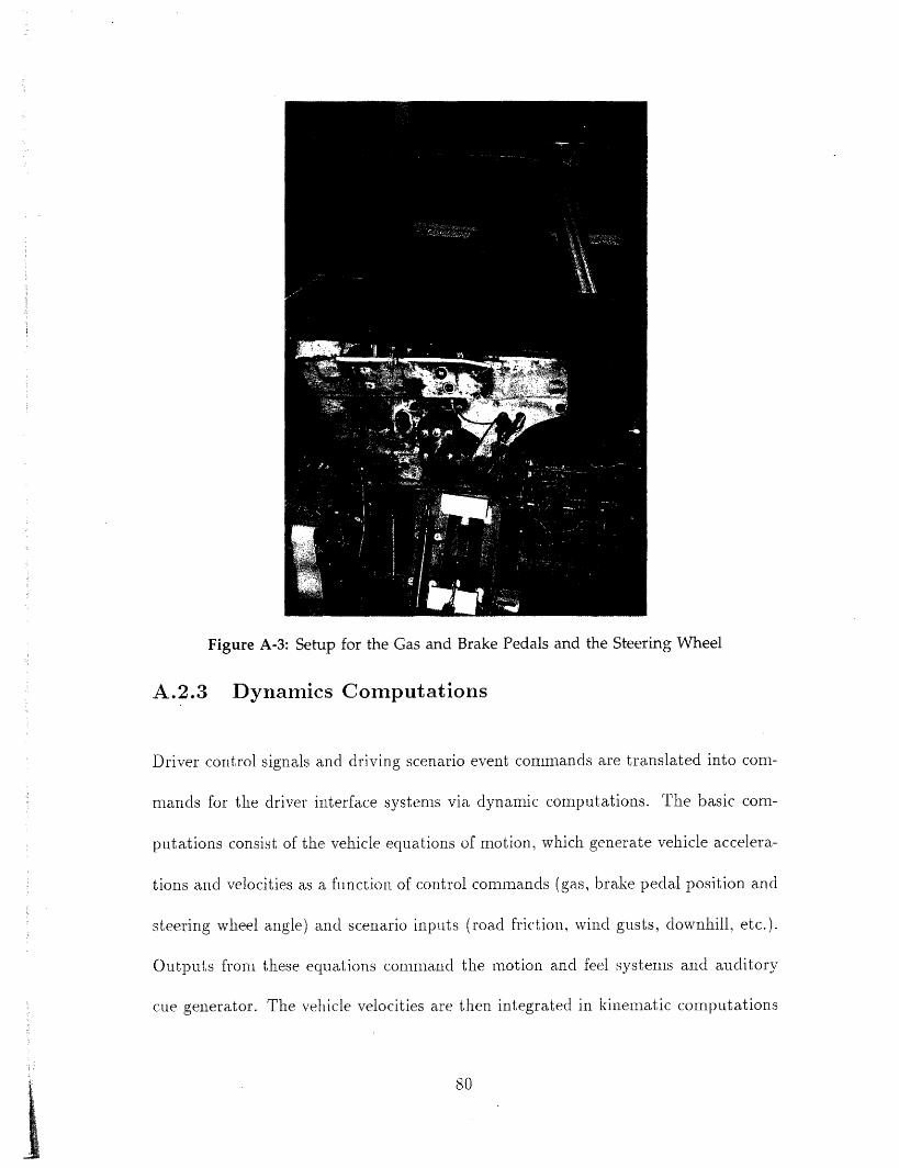
Figure A-3: Setup for the Gas and Brake Pedals and the Steering Wheel
A.2.3 Dynamics Computations
Driver control signal,-, and driving scenario event commands a-re translated into com-
mands for the driver interface systems via dynamic computations. The basic com-
putations consist-, of the vehicle equations of motion, which generate vehicle accelera-
tions ad velocities as a fnction of control commands (gas, brake pedal position and
steering wheel angle ad scenario iputs (road friction, wind gusts, downhill, etc.).
Outputs -from these equations command the motion and feel systems and auditory
Cue generator. The vehicte velocities are then integrated i kematic computations
so

to yield vehicle state variables (e.g., distance, heading and lane position) which form
commands to the display generator.
The equations of motion include force and moment expressions which in general
would result in six-degree-of-freedom motions. Simplifications are usually applied
here, however, as appropriate to a given situation, in order to minimize the devel-
opment effort, improve reliability, and reduce cost. Computational delay is another
concern in determining the degree of complexity of the equations of motion. At best,
significant computational delay will reduce simulator realism. At worst, it will seri-
ously destabilize the driver's closed-loop control behavior and invalidate experimental
results.
The HMSL simulator uses Dugoff's vehicle model for the equations of vehicle mo-
tion 36]. Figure A-4 shows the overall model developed for this simulator. Dynamics
of both the vehicle body and tires are taken into account in this model.
The equations of motion based on above model is described as follows. For the
dynamic equations:
m(,� - rv = (A. 1)
m(� - ru) = Fv (A.2)
1 = T (A-3)
T + ,,7.i(R - ,j - F�jX�,j - C.iw.i (A.4)
Fr Frl + F.2 + -,3 + - D (A-5)
F = Fyl + y2 + y3 + Fy4 (A-6)
81

FRONT
wi and Ti2
Fh
Uwi
Fxwi
(A.7)
(A.8)
(A-9)
(A.10)
b
-0- -- --Y body axis
axis
REAR
I I-It I IIj - �zi
Vehicle Geometry Tire Model
Figure A-4: Configuration of HMSL Driving Simulator Vehicle Model
T = t(F.,71 -F.2 - Fr3 + Fr4) + a(Fy, + y2 - b(Fy3 + y4)
F.j F..j cos(6j - y.j sin(6i)
Fqj F..j sin(bi) + F,.i cos(bi)
1 2
FD = -CDpADU2
For the tire kinematics:
u, = u + tr
U = U - tr
U = u - tr
U = u + tr
(A.11)
(A.12)
(A.13)
(A.14)
(A. 15)
v = v + ar
V = v + ar
V3 = br
V = v - br
Uw = Ui cos(6j) + vi sin(6j)
82

1+ (A. 16)UWi
iviai = tan- 6i (A 17)
Ui
A.2.4 Auditory Dsplay
Auditory cues can be important feedback in certain control situations, such as tire
squeal during cornering and braking, and in holding constant speed. In the real world
these effects contain combined auditory and motion cues, which can be simulated to
a large degree with auditory cues from a good sound system. Auditory cues can also
add to driving realism through sounds associated with the engine, tires, wind, body
resonance due to road texture, etc.
Auditory cues can be displayed with reasonable cost high-fidelity systems, and
generated with a variety of sound generator electronics currently produced for video
games. The more difficult job is to correctly generate the appropriate amplitude and
frequency commands for realistic sound cues.
The HMSL simulator uses a PC-based SoundBlaster-Pro sound board to simulate
all the sound effects for the simulator. FM sound is used to generate the engine
noise as a function of engine speed. Digitized sound, on the other hand, is used to
generate special sound effects such as tire squeal, car crash and car-passing sounds
as a function of relative distance and speed. Generally speaking, these simple sound
effects have been found to be satisfactory for the purpose of this research.
83

84
Appendix
Analytical Basis of the
Car-following 1\4odel
B-1 ]Kinematics of the Crash Scenario
The model considered in this thesis consists of two vehicles, lead vehicle A and follow-
ing vehicle B, with the condition that the driver of the lead vehicle suddenly applies
his/her vehicle's brakes. The driver of the following vehicle reacts to this situation
and applies his/her own vehicle's brakes. There are several possible outcomes of these
actions:
1. Vehicle strikes moving vehicle A after vehicle applies the brakes.
2. Vehicle strikes stationed vehicle A after vehicle applies the brakes.
3. Vehicle strikes moving vehicle A prior to the time vehicle applies the brakes.

4. Vehicle strikes stationed vehicle A prior to the time vehicle applies the
brakes.
5. Vehicle does not strike vehicle A.
Time equaling zero is assigned to the time at which the driver of vehicle A begins
to apply his/her brakes. By applying the laws of motion it is possible to determine
which of the above outcomes has occurred.
For vehicle A:
TAS = VA/aA, (B. )
SA = VATAS IaA (TAS)' (B.2)2
where
TAs time in seconds required for vehicle A to stop given that it is not struck by
vehicle B,
VA = initial velocity of vehicle A in meters per second (mps),
aA = brake deceleration in meters per second square (we have adopted the conven-
tion of assigning deceleration a positive sign, thus expressing it as a variable operating
counter to velocity
SA distance in meters covered by vehicle A during the time required to stop.
For vehicle B:
TBS = BICeB, (B.3)
S = VBTBS - 1aB (TB S)2 (B.4)2
85

where TBS, VB, aB and SB are corresponding variables for vehicle B.
The following distance between the two vehicles at time zero is Df.
The instantaneous distance between vehicles can be determined from the following
relations:
D(ti) SA(ti) + Df - SB(ti), (B.5)
I 2 1 TD(ti) VAti - -aA(ti) + Df - VBti - -OB(ti - r)2, (B-6)2 2
where
ti instantaneous time in seconds measured from time zero,
D(ti) = distance in meters between the two vehicles at time = zero,
T, braking reaction time in seconds for driver of vehicle B.
If D(ti) is less than or equal to zero, a crash has occurred The time (tc) at which
a crash occurs can be determined by setting D(t, = and solving for t,.
2tc I-Vr [V + 4aDr] 211 (B.7)2a, r
where
V VB + TraB - VA,
1ar 2 (Ce-l - fA),
Dr Df + (CfBT2)-,2
The solution is the smallest positive value of tc. An imaginary solution for tc
would imply that vehicles do not crash (i.e., the relative distance between does reach
86

zero). Thus the condition for a non crash is
V2 + 4aD < 0. (B.8)
If this condition is not met, then a crash has occurred. Note that equation 6) applies
only when both vehicles are in motion and both have started to decelerate. Therefore,
if t, is less than T a crash occurred before vehicle began to decelerate. In this
case, equation 6) becomes:
D(ti) = VAti - -CeA(ti) + Df - VBtj. (B.9)2
Again a crash occurs when D(ti = 0. Equation 9) can be used to solved for the
time (4)
Note that the condition in which the following vehicle stops before striking
vehicle A was eliminated by an imaginary solution to equation 7). From the above
results, the distance to crash point could also be computed.
B.2 Possible Analytical Solution
If it is desired to determine the probability of a crash analytically, one could begin
with equation (8). Define a new variable:
0 = V2 + 4aD,, (B. I 0)
87

and compute its probability density function. Then,
0probability of a crash = I - pr(Ol 0) f (01) d0j. (B. I )
00
One can conceptually obtain the density function0f Or by a convolution of the distri-
bution of the input variables 37]. The variables in (10) can be expressed in terms
of the input variables as follows:
Vr = VB + IrCeB - VA,
a, = (aB - A), (B. 1 2)2
Dr = D + (aBTr2)-2
Therefore,
0 = g(Df) T, aA� aB, VA, VB)i (B. 13)
where g contains six independent random variables (ideal condition). These random
variables are distributed as follows:
g (Df , Tr, aA, CeB, VA, VB = f (Df ) f (Tr) f (CiA) f (CeB) f (VA) f (VB) (B. 14)
Five new random variables can be defined as:
O = f (Df , Tr, aA, Cf B, VA, VB) -(i = 2 3, - -, 6) (B. 1 5)
88

The original variables can be transformed to functions of the j's by using equation
Df = Df (01, 02, 06),
T, = T, (01, 02, 06), (B. 16)
VB VB (01, 02, 06),
Using these variables we can write:
h (01, 02, 06) f [Df (01, 02, 06), T, (01, 02, 106), VB(01,02,' - ',06) I ii
(B. 17)
where I J I is the absolute value of the Jacobian of the transformation. The distribution
of 01 can be obtained by integration of 17).
h (01, 02, 06) dO2dO3 dO6 (B. 18)00h(01 = f
If the distributions of the input variables in equations 14) can be expressed in con-
venient analytic form, it might be possible to perform the integration in equation
(18). However, for this thesis, they are expressed as discrete distributions obtained
empirically. At this point, the difficulties of obtaining an analytical solution should
become evident. In addition, if one wishes to obtain a probability distribution of crash
margin, as is done using the simulation model CARMASS, the problems become even
greater. Therefore, the Monte Carlo simulation was chosen for this thesis.
89

Appendix C
Fuzzy Set Theory
CA Fuzzy Set
Traditionally, mathematics dictate that an object be only a full member of a given
set, or not a member at all. There is nothing in between. What distinguishes fuzzy
sets from conventional crisp sets is the fact that fuzzy set theory allows degrees of
membership, varying from (non-member) to I (full member). Fuzzy sets provide an
elegant mechanism to describe and handle all sorts of so-called linguistic variables,
the variable "speed" for instance. A linguistic variable is characterized by a series
of terms, such, as "low", "moderate" or "high", each term representing a fuzzy set
(e.g. the fuzzy set "high speed", of which a speed of 80 km/hr may be a member
to a degree of only 03). The function that associates a grade of membership of a
fuzzy set with every object that to some extent could be in that set, is called the
membership function. The most commonly used membership function is that of a
90

trapezium. Other examples are triangle, square, exponential, etc. When smoothness
of the membership functions is considered essential, exponential relationships are
employed.
C.2 Notation, Terminology and Basic Operation
A fuzzy set A of a universe of disclosure U is characterized by a membership function
PA -- + [0, 1], which associates with each element y of U a number PA (Y) in the interval
[0,1], which represents the grade of membership of y in A. The support of A is the
set of points in U at which YA(Y > 0. A fuzzy singleton is a fuzzy set whose support
is a single point in U. In particular, A is called a non fuzzy singleton if the grade of
the only element is .
Let A and be two fuzzy sets in U with membership functions A and IiB,
respectively. The set theoretic operations of union and intersection for fuzzy sets are
defined as follows. The membership function PAUB of the union A U is pointwise
defined for all u E U by
YAUB (u = max (PA (U), YB (U)) (C. )
The membership function PAnB of the intersection AnB is pointwise defined for all
u E U by
ItAnB (u) =- min(FA (U), YB (U)) (C.2)
For a detailed discussion of fuzzy sets and operations on fuzzy sets, refer to Zadeh
91

[38].
C.3 Fuzzy-Logic Controller
A comprehensive survey of fuzzy-logic controller (FLC) design has been made by Lee
[39]. In the following section, the author will review the most common type of FLC.
It was employed by Holmblad and Osterggard 28].
As shown in figure C-1, an FLC consists of the following major units. Fuzzy rea-
soning is performed by the inference engine, the kernel of the FLC. The fuzzification
inference converts real numbers into fuzzy sets, to be supplied as an input to the
decision making logic. The knowledge base of an FLC comprises two components,
namely, a data base and a fuzzy control rule base. The data base provides the in-
ference engine with the membership functions of fuzzy sets used in the rule base.
The rule base holds the control rules. The defuzzification inference transforms fuzzy
control actions into non fuzzy, crisp controls. Fuzzification is performed by interpret-
ing an input xo as a non fuzzy singleton A, that i PA(XO) is equal to zero, except
at the point xO, at which PA(xo) equals one. The antecedent part of a control rule
consists of a number of conditions, each of them relating an input to a term which is
represented by a fuzzy set "speed is high" for example). Analogously, the antecedent
consists of one or more conclusions. Control rules, just as the contents of the data
base, are usually-formulated by consulting experts. The so-called self-organizing con-
troller 40], however, is an exception to this rule. For a self-organizing controller, it
is not necessary to have an exhaustive set of rules as the starting point. By applying
92

Fuzzy-Logic Contoller
..- .- __.Y
Figure C-1: Configuration of Fuzzy-Logic Controfler
a performance criterion, the algorithm is capable of conceiving additional rules, and
of deleting redundant or contra-productive rules.
In order to illustrate the operation of the inference mechanism, consider the fol-
lowing dual-inputs-single-output mechanism of n fuzzy control rules:
input x Z's A' and y is '
rules if x Z's Ai and y is Bi then C (C.3)
output Z Z's C,
where x, y and z are linguistic variables representing the process state variables and
the control variables, respectively. Ai, Bi and C, on the other hand, are linguistic
values (or terms) of the linguistic variables x, y and z in the universe of disclosure U,
V and W, respectively, with i = 1 2 ... I n. The inference process starts with assessing
for every rule the weighting factors ai that express the significance of that rule. Since
93

non fuzzy singletons are assumed for a defuzzification strategy (i.e., the fuzzy inputs
A' and are equal to the non fuzzy input xo and yo, respectively), this may simply
be performed as:
a = A, xO A AB (YO) (C.4)
with i = 1 2 ... In, and where PAi(xo) and YBj(YO) play the role of the degrees of
partial match (per condition) between the controller input and the corresponding
i1h 1hterm in the e rule. The contribution of the rule to the fuzzy controller output
is then calculated as:
PC, W = ai P Ci M (C.5)i
As a result, the membership function C, which is the union of the individual control
decisions C.5 isn
PC (W) U ailACi (W) (C.6)i=1
Deducing a crisp control value zo from C' is achieved by performing one of two de-
fuzzification strategies. The first method, "center of area" or "zero-order moment"
method, calculates the abscissa value that divides the area under the output member-
ship function in two equal parts. The other method, "center of gravity" or first-order
moment" method, yields the center of gravity of the output membership function.
94

95
Appendix D
Fuzzy-Logic Intelligent Cruise
Control
The fuzzy-logic intelligent cruise controller was designed by referring to the human
operator's experience and to control engineering knowledge. The design procedure for
the fuzzy-logic braking controller will be described in detail in the following sections.
D.1 Control Scheme
For the car-following controller, the following variables were used as input information.
D relative distance between own car and lead car
absolute keed of own car
R relative speed between own car and lead car

We assumed that we have perfect sensors and actuators, i.e., the dynamics of
them were ignored. Based on this information and the knowledge extracted from a
hypothetical expert driver, the controller determines appropriate control action.
B braking torque
T engine torque
The following are some possible rules we could expect from an expert:
1. If absolute speed is fast and distance is large and lead car is opening then increase engine
power slightly;
2. If absolute speed is fast and distance is large and lead car is closing then decrease engine
power slightly;
3. If absolute speed is medium and distance is small and lead car is closing then apply medium
braking;
4. ...
Note that only one output can be used each time. Therefore additional rules are
needed to avoid any conflicts. For example, we added "if there is braking then exert
no engine torque output."
Figure (D-1) shows the block diagram of this controller.
96

Distance to obstacle (m)NoteA o is stopping distnace at 1 0 km/h.
Partition of absolute speedA very Slow medium fast very1 slow fast
4 5
B..I0 15 35 55 75 95
Speed (km/h)
Partition of relative speed
gropening fast opening A closing closing fast
R2_ 2
-20 -10 1 0 20
Absolute speed (U)
Relative speed (Ur) - Braking torque (B)
Distance (D) Fuzzffy U"Ur',D' Rules B',T1 Defuzzify Engin Torque (T)ON- - _4110- No-
I I
Figure D-1: Block Diagram for Car-following Controller
D.2 Input Fuzzification
Figure (D-2) shows one example of the partition of the input spaces. Note that the
6 is the desired car-following distance derived from the safe car-following distance
distribution which is adjustable.
Partition of distanceIld e very4 " zmnll maHhim lorria
9v
Speed (km/h)
Figure D-2: Input Membership Functions for Car-following Controller
97

Since there are three inputs for this controller, there is no way to express all the
fuzzy rules in a simple matrix form such as that for the braking controller. In this
preliminary design, we use five partitions for for each input. This results in 125
rules for the whole controller, which is somewhat complex to derive immediately and
required numerous iterations to get to the final rule base.
D.4 Output Defuzzification
Figure (D-3) shows the combination of the output membership functions. The range
of the braking torque is - 00 Nm while the increase/decrease of engine torque is
limited to 200 Nm. Note that the two outputs are mutually exclusive, i.e., if braking
is used, the engine power must be cut off, and vice versa.
The final crisp output was determined using the center of gravity method. For
instance, for the braking output, the output torque would be:
3
T,(yj B)Output torque = (D. )
3
i=O
98
D.3 Fuzzy Rules

Partition of braking torque output
iking torque (Nrn)
Partition of changed engine torque output9t,
medium smalldecrease decrease i
no small mediumchange increase increase
T2
b..
100 200 Changed engine torque (Nm)-200 -100
Figure D-3: Fuzzy Rules for Braking Controller
99

Bibliography
[1] Accident Facts. National Safety Council, Itasca, IL, 1992.
[21 McGehee, D.V., Dingus T.A. and Horowitz A.D. The potential value of a front-to-rear- end collision warning system based on factors of driver Behavior, visualperception and brake reaction. In Proc. of the Human Factors Society 36th AnnualMeeting, Atlanta, 1003-1005, 1992.
[3] Tolle, J. E. Vehicular headway distribution: testing and results. In TransportationResearch Record, 456, 56-64, 1976.
[4] Koshi, M., Iwasaki M. and Ohkura 1. Some findings and an overview on vehicularflow characteristics. In Proc. of the 8th International Symposium on Transportation andTraffic Flow Theory, 1981 (edited by Hurdle V.F., Hauer E. and Stewart G.N.)University of Toronto Press, Toronto, Ontario, 403-426, 1983.
[5] Chishaki T and Tamura Y. Headway distribution model based on the distinctionbetween leaders and followers. In Transportation and Traffic Theory, 43-63, 1984
[6] Dull, E.H. and Peters H.J. Collision avoidance system for automobiles. SAEpaper 780163, 1978.
[71 Ioannou, P.A., Chien C.C. and Hause J. Autonomous intelligent cruise control.In Proc. of the IVHS America 1992 Annual Meeting, Newport Beach, California, ,97-105, 1992.
[8] Colbourn, C.J., Brown I.V. and Copernan A.K. Drivers' judgements of safedistances in vehicle following. In Human Factors, 20(l), 1-11, 1978.
[9] Fenton, R.E. A headway safety policy for automated highway operations. InIEEE Transaction on Vehicular Technology, VT-28, 1, 22-28, 1979.
[10] Minami, K.1 Yasuma, T. and Okabayashi, S. A collision-avoidance warningsystem using laser radar. SAE pa- er 881859, 1988.
[11] Morita, T. An approach to intelligent vehicle. In Proc. of the Intelligent Vehicles,1993.
100

[12] loannou, P., Xu, Z., Eckert, S., Clemons, D. and Sieja, T. Intelligent cruisecontrol: theory and experiemnt. In Proceeding of 32 CDC, San Antonio, TX,1885-1890, 1993.
[13] Kakinami T., Sato J., Saiki, M. and Soshi K. Autonomous vehicle control systemusing an image processing sensor. SAE paper 950470, 1995.
[14] Gortan, L., Borodani, P. and Carrea P. Fuzzy-logic employed in an autonomousICC vehicle. SAE paper 950472, 1995.
[15] Wasielewski, P. Car-following headways on highways interpreted by semi-Poissonheadwav distribution model. In Transportation Science, Vol-13, No.1, February1979.
[16] Schwartz, S. H., Allen, R. W., Hogge, J. R. and Stein, A. C. A simulator studyof driver reaction to metric speed sign. In International Symposium on Traffic ControlSystem, Berkeley, 1979.
[17] Yoshimoto, K. An analysis of the man-automobile system with a driving simula-tor. In Proceeding of IFAC Conf. on Man-Machine Systems, Baden-Baden, Germany,1982.
[18] Malaterre, G. and Lechner, D. Emergency manoeuvres at junctions using adriving simulator. In M. Koshi (Ed.) Transportation and Traffic Theory, North-Holland: Elsevier Science Publishing Co., Inc., 1990.
[19] Kappler, W. Using a driving simulator to investigate vehicle handling proper-ties. In H.P. Willumeit (Ed.) Human Decision Making and Manual Control, North-Holland: Elsevier Science Publishing Co., Inc., 1986.
[20] Farber, E. and Paley, M. Using freeway data to estimate the effectiveness ofrear-end collision countermeasures. In Proceeding of IVHS America 1993 AnnualMeeting, Washington D.C., 1993.
[21] Johansson, G. and Rumar, K. Drivers' brake reaction time. In Human Factors,13(l), 23-27, 1971.
[22] National Highway Traffic Safety Administration Rear-end crashes: problem sizeassessment and statistical description(DRAFT), Office of Crash Avoidance Re-search, NHTSA, December 21992.
[23] Olson, P.L. and Sivak, M. Perception-response time to unexpected roadwayhazard. In Human Factors, 28(l), 91-96, 1986.
[24] Clarke, R.M., Goodman, M.J., et al. Driver performance and IVHS collisionsavoidance systems: a search for design-relevant measurement protocols. In Pro-ceeding of IVHS America 1993 Annual Meeting, Washington D.C., 1993.
[25] Knipling, R.R., Hendricks, D.L., et al. A front-end analysis of rear-end crashes.In Proceeding of IVHS America 1992 Annual Meeting, Newport Beach, Calif., 1992.
101

[26] Zadeh LA. Fuzzy algorithm. In Information and Control, V8, p338-353, 1965.
[27] Kosko, B. Neural Networks and Fuzzy Systems. Prentice-Hall, New Jesey, 991.
[28] Holmblad, L.P. and Ostergaard, J.J. Control of a cement kiln by fuzzy logic. InM.M. Gupta and E Sanchez (Eds.) Fuzzy Information and Decision Process, p389-399, Elsvier, Amsterdam, 1982.
[29] Ren, J. and Sheridan, T.B. Optimization with fuzzy linear programming andfuzzy knowledge base. In Proc. of IEEE World Congress on Computational Intelligence,Orlando, Florida, 1994.
[30] Mamdani, E.H. Application of fuzzy logic to approximate reasoning using lin-guistic systems. In IEEE Trans. Comput., nr.26, p1182-1191, 1977.
[31] Donges, E. A two-level model of driver steering behavior. In Human Factors, Vol.20, No. 6 p691-707, December 1978.
[32] Gordon, D.A. Perceptual basis of vehicular guidance. In Public Roads, Vol. 34,No. 3 p53-68, 1966.
[33] McRuer, D.T. and Klein, R.H. Comparison of human driver dynamics in simula-tors with complex and simple visual displays and in an automobile on the road.In Eleventh Annual Conference on Manual Control, NASA TMX-62, 464,p684-692,1975.
[341 Jex, H.R. and Magdaleno, R.E. Biomechanical models for vibration feedthroughto hands and head for a sernisupine pilot. Presented at Symposium on BiodynamicModels and Their Applications, February 1977.
[35] Gualtierotti, T., Spinelli, D and Margaria, R. Effect of stress on lower neuroractivity. In Experimental Medicine and Surgery, Vol. 26, Nos. 23, 1958.
[36] Dugoff, H., Fancher, P.S., and Segel, L. An analysis of tire traction propertiesand their influence on vehicle dynamic performance. SAE paper 700377, 1970.
[371 Hogg, R.V. and Craig, A.T. Introduction to Mathematical Statistics. 3rd Edition,The acmillan Co., Toronto, 1970.
[38] Zadeh, L.A. Outline of a new approach to the analysis of complex systems anddecision processes. In IEEE Trans. Systems, Man and Cybernetics, SMC-3, p28-44,1973.
[39] Lee, C.C. Fuzzy logic in control system: fuzzy logic controller - part I II. InIEEE Trans. Systems, an and Cybernetics, SMC-20, p4O4-435, 1990.
[40] Procyk, T.J. and Mamdani, E.H. A linguistic self-organizing process controller.In Automatica, 15, p15-30, 1979.
102