CHAPTER 1 - DSpace@MIT
190
OPERATIONAL AND POLICY IMPLICATIONS OF MANAGING UNCERTAINTY IN QUALITY AND EMISSIONS OF MULTI-FEEDSTOCK BIODIESEL SYSTEMS by Ece Gülşen B.S., Materials Science and Engineering Sabancı University, 2009 Submitted to the Department of Materials Science and Engineering and the Engineering Systems Division in Partial Fulfillment of the Requirements for the Degrees of Master of Science in Materials Science and Engineering and Master of Science in Technology and Policy at the Massachusetts Institute of Technology June 2012 © 2012 Massachusetts Institute of Technology. All rights reserved. Signature of Author Department of Materials Science and Engineering Technology and Policy Program, Engineering Systems Division Submitted on May 11, 2012; Presented on May 21, 2012 Certified by Randolph Kirchain Principal Research Scientist, Engineering Systems Division Thesis Supervisor Certified by Elsa Olivetti Research Scientist, Engineering Systems Division Thesis Supervisor Accepted by Joel P. Clark Professor of Materials Systems and Engineering Systems Acting Director, Technology & Policy Program Thesis Reader Accepted by Gerbrand Ceder R. P. Simmons Professor of Materials Science and Engineering Chair, Departmental Committee on Graduate Students
-
Upload
khangminh22 -
Category
Documents
-
view
2 -
download
0
Transcript of CHAPTER 1 - DSpace@MIT

OPERATIONAL AND POLICY IMPLICATIONS OF MANAGING UNCERTAINTY IN
QUALITY AND EMISSIONS OF MULTI-FEEDSTOCK BIODIESEL SYSTEMS
by
Ece Gülşen
B.S., Materials Science and Engineering Sabancı University, 2009
Submitted to the Department of Materials Science and Engineering and the Engineering Systems Division in Partial Fulfillment of the Requirements for the Degrees
of
Master of Science in Materials Science and Engineering and Master of Science in Technology and Policy
at the Massachusetts Institute of Technology
June 2012
© 2012 Massachusetts Institute of Technology. All rights reserved.
Signature of Author
Department of Materials Science and Engineering Technology and Policy Program, Engineering Systems Division
Submitted on May 11, 2012; Presented on May 21, 2012 Certified by
Randolph Kirchain Principal Research Scientist, Engineering Systems Division
Thesis Supervisor
Certified by
Elsa Olivetti Research Scientist, Engineering Systems Division
Thesis Supervisor
Accepted by
Joel P. Clark Professor of Materials Systems and Engineering Systems
Acting Director, Technology & Policy Program Thesis Reader
Accepted by
Gerbrand Ceder R. P. Simmons Professor of Materials Science and Engineering
Chair, Departmental Committee on Graduate Students

i
This page is intentionally left blank.

ii
OPERATIONAL AND POLICY IMPLICATIONS OF MANAGING UNCERTAINTY IN
QUALITY AND EMISSIONS OF MULTI-FEEDSTOCK BIODIESEL SYSTEMS
by
Ece Gülşen
Submitted to the Department of Materials Science and Engineering and the Engineering Systems Division on May 11, 2012 and presented on May 21, 2012 in Partial
Fulfillment of the Requirements for the Degrees of Master of Science in Materials Science and Engineering and Master of Science in Technology and Policy
ABSTRACT
As an alternative transportation fuel to petrodiesel, biodiesel has been widely promoted within
national energy portfolio targets across the world. Early estimations of low lifecycle greenhouse gas
(GHG) emissions of biodiesel were one of the main drivers behind extensive government support in
the form of financial incentives for the industry. However, several recent studies have reported a
high degree of uncertainty and variation (U&V) in these emissions, raising questions concerning the
carbon benefits of biodiesel compared to petrodiesel. A smaller degree of U&V in physical
feedstock characteristics emerging from compositional variation was already known to producers.
Although feedstock blending has been broadly practiced by the industry to meet multiple fuel
quality standards and to control costs, its implications on these U&V characteristics of biodiesel
have not been explicitly addressed by researchers or policymakers. This work investigates the
impact of feedstock blending on the U&V characteristics of biodiesel by using a chance-constrained
(CC) blend optimization method. The objective of the optimization is minimization of feedstock
costs subject to fuel standards and the decision variables are feedstock proportions. Two sets of
prediction models are developed to represent the physical properties and lifecycle emissions of
feedstocks within the CC model. The results indicate that blending can be used to manage U&V
characteristics of biodiesel, and to achieve cost reductions through feedstock diversification. Monte
Carlo simulations suggest that emission control policies which restrict the use of certain feedstocks
based on their GHG estimates, overlook blending practices and benefits, lowering the quality and
increasing the cost of biodiesel. In contrast, emission control policies which recognize the multi-
feedstock nature of biodiesel, provides producers with feedstock selection flexibility, and enables
them to manage their blend portfolios cost effectively without compromising fuel quality or
emissions reductions.
Thesis Supervisors: Randolph Kirchain, Principal Research Scientist, Engineering Systems Division
Elsa Olivetti, Research Scientist, Engineering Systems Division
Thesis Reader: Joel P. Clark, Professor of Materials Systems and Engineering Systems

iii
This page is intentionally left blank.

iv
ACKNOWLEDGMENTS
During my three years at MIT, I have had the privilege to work with and get inspired from many great people, only a proportion of which I have space to acknowledge here. First and foremost, my deepest gratitude goes to my advisor, Randolph Kirchain, whose nurturing mentorship and invaluable support have made this work become a reality. His kindness, care for others and sense of humor made this experience quite unique and memorable. I am also deeply thankful to Elsa Olivetti for spending countless hours with me and patiently guiding me through various obstacles I encountered. Her constantly positive attitude has taught me to see those obstacles smaller than they really were, and helped me find the light at the end of the tunnel. I would also like to thank Fausto Freire, João Malça, Érica Castanheira and Luis Dias from the University of Coimbra, for their collaboration and for making our research trip to Portugal a valuable experience.
Materials Systems Laboratory (MSL) has been a second home to me. I owe a great deal to Joel Clark for giving me an opportunity to continue my thesis work at MSL, to Frank Field for his challenging and enlightening questions, to Elisa Alonso for sharing her comments after each presentation, to Jeremy Gregory for patiently listening to my weekly updates in the subgroup meetings, to Rich Roth for constantly radiating his energy to MSL, and to Terra Cholfin for generously helping me whenever I needed a hand. I was also very lucky to be surrounded by friends who were fun, hardworking and caring. Melissa Zgola for her pleasant presence by my cubicle and sincere friendship, Tracey Brommer and Jiyoun Chang for being great listeners and giving me courage at challenging times, Thomas Rand-Nash for sharing his wise comments and freshly brewed coffee. Hadi Zaklouta, Nathan Fleming, Boma Brown-West, Trisha Montalbo, Siamrut Patanavanich, Natalia Ciceri, Reed Miller, Nathalie Rivest, Lynn Reis, Suzanne Greene and others at MSL, for making MSL a place to be remembered with fond memories.
Technology and Policy Program (TPP) ‘11 friends, you were dearly missed during my last year. Learning together with you was an amazing experience that I will never forget. I would also like to thank Sydney Miller for her devotedness to helping any student who stepped into her office any time of the day. Her words were always a great relief to me. Likewise, I wish to thank Ed Ballo and Krista Featherstone, for everything they have done to make life easier for us during our studies.
I do not know what I would do without the hours full of laughter, good food and music spent with Arzum Akkaş, Güneş Bozkurt and many other Turkish friends. Another heartfelt “thank you” goes to my friends from Boston Rueda and Sidney-Pacific, Iman Soltani, Chieh Wu, Cristian de Figueroa, Dan Rodman, Leebong Lee, Jean-Philippe Coutu and many more that I cannot name here. Time spent dancing and working with them on various projects made my life more colorful and meaningful.
It is impossible to express how grateful I am for Cleva Ow-Yang. She has been one of the most influential people in my life, continuing to support me during her Boston visits from Istanbul. She is not only an incredible coach; she is truly an incredible person. I still have a lot to learn from her generosity and hard work. I also wish to thank Özge Akbulut who has been a great mentor before and after joining MIT.
I have been grateful for the presence of Sheraz Choudhary and Kaustuv DeBiswas in my life. They have always been there whenever I needed someone wise to talk to, and I know that they will always be.
Lastly, I cannot imagine how I would survive without one caring man, Caleb Joseph Waugh. He has brought love, beauty and joy into my life with his kind and patient soul.
I dedicate this thesis to my parents and brother, Şerif, Yıldız and Kaan, who have always loved me endlessly, put my dreams in front of theirs and given me strength during the most difficult times of our lives. Their perseverance has been my inspiration without which I would not be able to carry on.

v
Table of Contents
CHAPTER 1: INTRODUCTION ........................................................................................................... 1
1.a) Background and Motivation ........................................................................................................ 1
1.b) Research Questions and Related Work ...................................................................................... 7
1.c) Thesis Outline .............................................................................................................................. 9
CHAPTER 2: PREDICTION OF PHYSICAL PROPERTIES OF BIODIESEL BASED ON CHEMICAL
COMPOSITION ............................................................................................................................... 11
2.a) Purpose and Scope .................................................................................................................... 11
2.b) Chemical Compositions of Biodiesel Feedstocks ...................................................................... 14
2.c) Prediction of Physical Characteristics Subject to Technical Standards ..................................... 16
2.c.1) Iodine Value (IV) ........................................................................................................................ 17
2.c.2) Oxidative Stability (OS) ............................................................................................................. 19
2.c.3) Cetane Number (CN) ................................................................................................................. 31
2.c.4) Cold Filter Plugging Point (CFPP) ............................................................................................... 33
2.d) Summary of Physical Characteristics ........................................................................................ 34
2.e) Summary and Conclusion .......................................................................................................... 35
CHAPTER 3: CHANCE-CONSTRAINED BLEND OPTIMIZATION ....................................................... 37
3.a) Motivation and Background ...................................................................................................... 37
3.b) Chance-Constrained (CC) Optimization Model Formulation .................................................... 40
3.c) Chance-Constrained Optimization Applied to Biodiesel Feedstock Blending ........................... 41
3.d) Summary and Discussion .......................................................................................................... 46
CHAPTER 4: IMPACT OF FEEDSTOCK DIVERSIFICATION ON THE COST OF BIODIESEL ................. 48
4.a) Motivation and Scope ............................................................................................................... 48
4.b) Analysis of Historical Feedstock Prices ..................................................................................... 52
4.c) Biodiesel Specifications ............................................................................................................. 55
4.c.1) Iodine Value (IV) – maximum 120 ............................................................................................. 55
4.c.2) Oxidative Stability (OS) - minimum 4.5 hours ........................................................................... 56
4.c.3) Cetane Number (CN) – minimum 47 ......................................................................................... 57
4.c.4) Cold Filter Plugging Point (CFPP) – minimum -1˚C .................................................................... 58
4.c.5) GHG Emissions Threshold – maximum 65% of petrodiesel emissions ...................................... 59
4.d) Choice of Confidence Levels ..................................................................................................... 61
4.e) Chance-Constrained (CC) Optimization Formulation................................................................ 62

vi
4.f) Model Scenarios ........................................................................................................................ 66
4.g) CC Optimization Model Applied to Single Period Price Data .................................................... 67
4.g.1) Sensitivity Analysis on the CFPP Constraint Level .................................................................... 67
4.g.2) Sensitivity Analysis on Blend Diversification............................................................................. 70
4.h) CC Optimization Model Applied to Multiple Period Price Data ................................................ 74
4.h.1) Sensitivity Analysis on Constraint Levels .................................................................................. 74
4.h.2) Sensitivity Analysis on Blend Diversification ............................................................................ 79
4.h.3) Analysis of Feedstock Cost of Biodiesel .................................................................................... 81
4.i) Summary and Conclusion ........................................................................................................... 90
CHAPTER 5: ANALYSIS OF BIODIESEL LIFECYCLE GHG EMISSIONS ............................................... 92
5.a) Introduction .............................................................................................................................. 92
5.b) Emission Control Policy (ECP) Frameworks for Lifecycle GHG Emissions ................................. 97
5.c) Estimation of Lifecycle GHG Emissions ..................................................................................... 99
5.c.1) General Emission Estimation Methodology ............................................................................ 100
5.c.2) Estimation Methodology for LUC Emissions ........................................................................... 102
5.d) Feedstock-specific LUC GHG Emissions: ................................................................................. 106
5.d.1) Geographical Mapping for Soil-Climate Combinations .......................................................... 107
5.d.2) Accounting for Scenarios Influenced by Man-Made Decisions (FLU, FMG, FI) .......................... 114
5.d.3) Accounting for the Crop Productivity and Co-Product Energy Allocation Factors ................. 120
5.e) Results and Summary of Feedstock-Specific Lifecycle GHG Emissions Estimations ............... 123
5.f) Feedstock Cost Analysis of Biodiesel Blends subject to Technical and GHG Emission
Constraints ..................................................................................................................................... 127
5.f.1) Single Period Price Data Analysis on the Maximum Number of Feedstocks in Blend, Ω ........ 128
5.f.2) Single Period Price Data Analysis on Blend and Feedstock GHG Emissions Thresholds, E and
.......................................................................................................................................................... 138
5.f.3) Multiple Period Price Data Analysis ........................................................................................ 149
5.g) Feedstock Include/Exclude Decision Space ............................................................................ 158
5.h) Summary and Conclusion ....................................................................................................... 161
CHAPTER 6: CONCLUSIONS AND FUTURE WORK ....................................................................... 164
REFERENCES ................................................................................................................................ 169
APPENDICES ................................................................................................................................ 179
Appendix-A: Soil-Climate Combinations ........................................................................................ 179
Appendix-B: Lifecycle GHG Emissions Details of 75 Feedstock Scenarios ..................................... 181

vii
List of Abbreviations
APE Allylic Position Equivalent
BAPE Bis-Allylic Position Equivalent
CAN Canola Oil
CC Chance-Constrained
CFPP Cold Filter Plugging Point
CN Cetane Number
EC European Commission
EISA Energy and Independence Security Act
EPA Environmental Protection Agency
EU European Union
FA Fatty Acid
FAME Fatty Acid Methyl Ester
FAO Food and Agriculture Organization of the United Nations
GHG Greenhouse Gas
HACS High Activity Clay Soils
IV Iodine Value
LACS Low Activity Clay Soils
OECD Organization of Economic Co-operation and Development
OS Oxidative Stability
ORG Organic Soils
PLM Palm Oil
POD Spodic Soils
RED Renewable Energy Directive
SAN Sandy Soils
SNF Sunflower Oil
SYB Soybean Oil
T Tocopherol
TT Tocotrienol
U&V Uncertainty and Variation
VOL Volcanic Soils
WET Wetland Soils

1
CHAPTER 1:
INTRODUCTION
1.a) Background and Motivation
Access to clean, economic and secure energy resources plays a major role in shaping the
policies of nations. It is an essential tool for economies to grow and societies to prosper, and
therefore accelerating economic growth worldwide has recently triggered an ever-increasing
demand for energy. As a result, the world has witnessed the emergence of a number of
alternative, renewable energy resources.
Among the sectors of economic activity, the transportation of persons and goods is one that
depends heavily on energy. In fact, transport accounts for about 19% of global energy use and
23% of energy-related carbon dioxide emissions [1]. Given current trends, those figures are
projected to increase by nearly 50% by 2030 and more than 80% by 2050 [1]. Therefore,
alternative and renewable fuels will play a major role in planning a sustainable roadmap for
future transport challenges. Although much effort is being expended to electrifying the vehicle
fleet, that transition will take decades and may never result in a complete departure from
conventional sources of propulsion. As such, for years to come, one of the fundamental
requirements for a transport fuel is that it needs to be a liquid. Because the liquefaction
processes of other fuels such as natural gas or coal are not sufficiently efficient yet, there is a
significant gap between the demand and supply for alternatives to petroleum. Biofuels,
particularly bioethanol and biodiesel, will be part of the solution to fill in this gap. Despite
controversies around their lifecycle greenhouse gas (GHG) emissions and potential contribution
to increased food prices [2], biofuels have already been included in mandated national energy
portfolio targets across the world. According to OECD-FAO data, global production was 92.9
billion tons for bioethanol and 17.2 billion tons for biodiesel in 2009. These figures are
projected to reach 155 and 42 billion tons by 2020, respectively [3]. Unfortunately, this
commitment to biofuels comes at a cost. Currently, the production of biofuels is more costly

CHAPTER 1 INTRODUCTION
2
than production of petroleum fuels and must be subsidized, mandated, or otherwise regulated
to be marketable. This governmental policy intervention occurs in many forms across the globe.
Legislations such as Renewable Fuels Standard (RFS) in the US or the Renewable Energy
Directive (RED) 2009/28/EC in the EU incentivize more use of biodiesel, particularly on the
grounds of GHG reductions and set national targets of biodiesel shares in the transport sector.
Similar programs exist in other large economies like Brazil, China and India [4].
Considering the sheer volume of expected production in the upcoming years, these issues point
to clear and pressing questions: How can biofuels be produced cost effectively while still
providing net social benefit (i.e., with lower contribution to climate change and without undue
stress on food supplies)? How can governmental policies be constructed that foster cost
effective biofuel production? There are clearly many opportunities that could be employed to
realize cost effective biofuels, ranging from agricultural improvements on the farm to
technological improvements at the refinery. One set of opportunities that has been little
explored are operational decisions, specifically the selection and blending of feedstocks, made
by the biofuels producer. This thesis characterizes such opportunities and explores how biofuels
policies can be constructed to foster or preclude the potential benefits from effective
operational decision making.
Biodiesel Production Challenges
Global biofuels production is dominated by bioethanol and biodiesel. Because production
technology and feedstocks required for these fuels are quite different from each other, the
challenges concerning their development are not necessarily the same. In order to focus the
scope of interest, this work considers only first generation biodiesel which is made from
vegetable oils. However, there are some common issues with bioethanol regarding the
sustainability performance of the fuel, and part of the results obtained can be extended to
bioethanol.
Biodiesel has a large and growing global market. In the US, diesel accounts for about one
quarter of on and off-road transport, and biodiesel can be blended into diesel up to 20% in
volume without engine modification [5]. Between 2000 and 2008, the US domestic production

CHAPTER 1 INTRODUCTION
3
rose from 2 million gallons to 780 million gallons [4]. The EU is another region where biodiesel
production volumes have increased substantially over recent years. Particularly because of the
widespread use of diesel powered cars in the member countries, the market opportunity for
biodiesel is promising. In 2007, diesel powered cars accounted for 53.3% of total new car
registrations [6] and biodiesel constituted about 80% of the biofuels market on energy basis in
2010 [7].
Increased use of biodiesel is heavily dependent on its performance compared to petrodiesel.
There are multiple performance criteria that concern not only the technical quality or the cost
of fuel, but also the sustainability measure of the final product. A number of ways to improve
these performance criteria can be attributed to different stages in the whole biodiesel chain,
from feedstock cultivation to transport of feedstocks, and to biodiesel production at the
facilities. Operation level decision making at these facilities, particularly at the feedstock
selection process, offers a significant opportunity to improve biodiesel performance. In the
following, we outline five critical challenges related to feedstock selection decisions at the
producer level. Understanding these challenges is a fundamental step to identifying real
opportunities to reduce costs while still meeting performance requirements and, to identifying
policy solutions that allow these opportunities to realize.
1. COMPLIANCE WITH TECHNICAL STANDARDS. The physical characteristics of the feedstocks
typically used in a biodiesel batch differ from one another and these differences are reflected in
the quality of the final fuel. Therefore, although the production technology of biodiesel is based
on well-known chemical reactions, producing a fuel that meets multiple technical specifications
simultaneously is a major challenge. There might be more than 20 different technical
constraints specified in a standard depending on the market region. The most common ones
among these standards are ASTM D67511 enforced in the US and EN 142142 enforced in the EU.
In general, a single feedstock is not able to meet all the constraints specified within a standard
1 Can be found at http://enterprise.astm.org/filtrexx40.cgi?+REDLINE_PAGES/D6751.htm.
2 Can be found at http://ec.europa.eu/enterprise/policies/european-standards/index_en.htm.
CHAPTER 1 INTRODUCTION
4
for the production of the final fuel. This motivates blending, but the complexity of the feedstock
selection decision causes producers to use a limited, experience-based set of recipes.
2. COMPLIANCE WITH SUSTAINABILITY STANDARD. On top of the technical standards, biodiesel
production is now subject to strict lifecycle GHG emissions standards imposed by governmental
bodies worldwide. Although GHG emissions reporting protocols and lifecycle estimation models
are still under progress, regulatory mandates to ensure GHG reductions compared to fossil fuel
are already in place. According to the EU biodiesel policies, starting from 2013, producers must
demonstrate that the lifecycle GHG emissions of their fuel are at least 35% less than that of
petrodiesel. The reduction requirement will be increased to 50% in 2017, and fuels produced at
new facilities after 2017 will be subject to a 60% reduction. In the US, reduction thresholds vary
between 20% and 50% depending on the classification of biodiesel in consideration. These new
GHG standards create another performance criterion which producers must take into account
as they seek out raw materials.
3. FLUCTUATION IN FEEDSTOCK PRICES. Because feedstock cost is estimated to be about 85% of
the final cost for biodiesel production [8-10], cost reduction opportunities are strongly
dependent on the feedstock prices. Today, soybean, canola (low eruric acid rapeseed), palm
and to some extent sunflower are the most common feedstocks used globally. Figure 1 shows
the distribution of (a) major vegetable oils produced worldwide in 2010/2011 [11], and (b)
vegetable oils used for global biodiesel production in 2007 [12]. Due to the fact that vegetable
oil is used as raw material in many other industries, particularly in the food industry, only about
10% of the produced vegetable oil goes toward biodiesel production [11, 12].

CHAPTER 1 INTRODUCTION
5
Figure 1 – Vegetable oil global production data (a) overall production, (b) production for biodiesel use.
Prices among feedstocks do not only differ from each other, but also fluctuate to a significant
extent over time. Figure 2 shows the nominal prices of some of the major vegetable oils
between 1981 and 2011. When the relative prices among feedstocks shift based on the market
conditions, a producer might need to modify the feedstock proportions used in the biodiesel
batch to remain profitable. Therefore, the ability to quickly adjust the feedstock blend portfolio
in response to dynamics such as price fluctuations and availability in the market could bring
substantial value to biodiesel producers.
Figure 2 - Nominal vegetable oil prices between June 1981 and June 2011. Data is taken from [13].
4. INCREASED MARKET COMPETITION. The market for biodiesel has been increasingly
competitive due to recent policies setting national production volume targets and providing
financial incentives to producers in the form of subsidies and/or tax credits. In the US,
timetables were published by the Energy Independence and Security Act (EISA) in 2007 which
requires the production of at least 1.28 billion gallons of biodiesel out of 16.55 billion gallons of

CHAPTER 1 INTRODUCTION
6
biofuels by 2013. This level of production corresponds to more than 7% of the total renewable
biofuel production target. The EU policies promoting renewable energy are also likely to
increase biodiesel production volumes dramatically. For example, the so-called “20/20/20”
mandatory goals for 2020 set a target of 20% share for renewable energy in the total EU energy
mix. 10% of this renewable share belongs to renewable energy in the transportation sector, and
because of the dominance of diesel powered cars in the EU, biodiesel is likely to be the main
renewable fuel in achieving this target. These market opportunities create new dynamics, lower
barriers to entry for newcomers and result in increased competition among producers. This
competition is likely to affect the level of access to fuel-grade and economic feedstocks in the
market.
5. DEGREE OF UNCERTAINTY & VARIATION (U&V). In addition to the presence of multiple
biodiesel specifications and feedstock price fluctuations, both the physical characteristics and
GHG emission estimates of feedstocks suffer from U&V which leads to challenges in controlling
the degree of compliance with standards. U&V in physical characteristics arise mostly from the
specific genetics of a crop that determines the chemical composition, from environmental
conditions during crop growth, and from handling and storage conditions along the supply
chain. On the other hand, U&V in lifecycle GHG emissions could arise from a substantially wider
range of factors such as soil type, fertilizer amount and type, climate conditions, crop yield,
agricultural technology, processing technology, transportation in addition to land use change
(LUC) and indirect LUC (iLUC) effects [14-19]. Consequently, the degree of U&V in lifecycle GHG
emissions is much higher than that of physical characteristics of feedstocks. Early emission
control policies have traditionally ignored U&V, but the challenge has been increasingly
recognized by policymakers in the US and EU. As an example, after extensive efforts and
multiple revisions, the US Environmental Protection Agency (EPA) has published emissions
distributions as opposed to just the point estimates for the most commonly used feedstocks,
such as canola and palm oil [20, 21]. Similarly, there are current policy debates within the
European Commission (EC) focused on the uncertainty of GHG emissions, particularly iLUC
emissions, and the executive Commission is considering to exclude some or all of biodiesel use
from the EU’s climate targets [22].
CHAPTER 1 INTRODUCTION
7
The challenges regarding feedstock selection process including compliance with standards,
fluctuation in feedstock prices, increased market competition and overall U&V inherent in the
system point to a need for a capability to blend multiple feedstocks. This capability would allow
producers to modify the batch composition over time towards cost effective biodiesel
production that can compete with petrodiesel. This, in turn, requires a flexible and responsive
feedstock selection process that can also incorporate the system U&V into decision making. In
practice, feedstock blending has been a common strategy to take advantage of the different
physical characteristics unique to each vegetable oil, drive overall costs down, lower exposure
to price fluctuations, and to some extent, to manage the risk of non-compliance emerging from
U&V [5]. While a total of more than 350 different oil seed species have been identified for
potential use in biodiesel, typical blending practices heavily rely on a few experience-based
recipes [14]. Therefore, there might be significant opportunity for cost reductions and/or
superior fuel quality by increasing feedstock selection flexibility for producers with analytical
decision making tools.
1.b) Research Questions and Related Work
Although feedstock blending practices are prevalent within the biodiesel industry, an analytical
approach to finding optimal feedstock portfolios has not been studied extensively. Therefore
there is a need for an optimal feedstock selection model that could assist in minimizing the cost
for producers. Because of feedstock price fluctuations, evolving policies, and dynamic feedstock
availability, the optimal blending strategy is not always intuitive and relying solely on the
previous experience of producers may not be sufficient. Particularly important is the lack of a
critical approach to characterize U&V in physical properties and the lifecycle GHG emissions,
when several feedstocks are blended at production facilities. Considering the prevalence of
blending practices within the industry, overlooking its impact on the U&V characteristics of the
final fuel might lead to suboptimal decisions, both at the producer and the policymaker level.
Understanding the impact of feedstock blending on the U&V characteristics of biodiesel has
been our primary motivation in conducting this research study, and to that end, we ask the
following questions: Can feedstock blending be used as a tool to explicitly manage U&V in

CHAPTER 1 INTRODUCTION
8
physical and emissions characteristics of the final fuel? Can explicit consideration of U&V in
blending decisions provide economic benefit to biodiesel producers? How does this economic
benefit affect the technical and environmental performance of the fuel? What characteristics of
the production context amplify or mute that economic benefit? Given the active role of policy
in the biodiesel system, what policy formulations maximize or minimize the benefits accrued
through blending?
Several bodies of literature have contributed to answering questions related to technical
biodiesel properties, U&V in biodiesel GHG emissions, and the use of blend optimization
models in industries other than biodiesel. Each of them forms a basis from which this work is
built. A brief summary of these studies is given in the following paragraphs. A more detailed
literature review related to these research questions is provided at the beginning of
corresponding chapters in the remainder of the thesis.
As early as the 1980s, some studies investigated the relationship between feedstock properties
and the final fuel characteristics [23]. With developments in chemical characterization
techniques, numerous works have contributed to understanding the main drivers behind fuel
properties. An extensive review can be found in The Biodiesel Handbook by Knothe, Krahl and
Gerpen [24]. Despite a large number of works published in this field, an explicit investigation of
the impact of blending feedstocks on different fuel properties has been limited to a few
experimental studies such as [9].
In more recent years, increasing number of papers and reports on the estimation of biodiesel
lifecycle GHG emissions have been published, such as [17], [25] or [26]. In addition, the EC has
published directives, guidelines and emission calculations tools such as BIOGRACE [27] to
provide a transparent platform for the development of emissions estimation methods. The US
EPA has taken similar steps, and published several biodiesel pathway emissions based on
complex models developed by the Argonne National Laboratory, Food and Agricultural
Research Institute (FAPRI), etc. [20, 21]. Yet, so far there has been no major study on exploring
how lifecycle GHG emissions estimations of biodiesel are affected by feedstock blending.
CHAPTER 1 INTRODUCTION
9
Another set of related work can be found in the area of optimization under uncertainty
methods. The fundamentals of these methods, particularly the chance-constrained
optimization, were established in the 1950s [28]. In the later years, several studies developed
models using the same principles to solve challenging blending problems governed by U&V [29-
33]. However, optimal feedstock selection for biodiesel under uncertainty has not been
addressed so far. More broadly, no blend optimization models have been developed, where
each performance characteristics of the blend is modeled explicitly rather than proxy indicators
such as composition.
Absence of research on U&V characteristics in optimal biodiesel production seems to be a
particularly important gap because previous studies in recycling or paper industry have shown
that the degree of U&V could actually be controlled by using probabilistic blend optimization
methods [32, 34, 35]. Following a similar methodology, we have filled this gap by developing
models to understand the impact of blending feedstocks on the underlying uncertainty of final
fuel characteristics. Our results show that blending enables producers to control uncertainty in
fuel characteristics, mitigate temporal feedstock cost variation and achieve significant cost
savings that are on the order of 20%.
1.c) Thesis Outline
Chapter 2 summarizes the most critical constraints that biodiesel is subject to, and develops
physical property prediction models to estimate fuel characteristics based on chemical
composition of feedstocks. Despite fairly abundant data in the literature, we decided to derive
these characteristics from the building blocks of fuel chemistry. Because most of these fuel
characteristics are related to each other, overlooking these relations by assigning arbitrary
values from reported ranges would not reflect a realistic feedstock system. In addition, using a
bottom-up approach enables us to incorporate U&V into the prediction model based on the
primary compositional factors, and properly propagate it through feedstock blending.
Chapter 3 briefly summarizes the chance-constrained optimization methodology we have used
for optimal blending, and provides the model formulation.

CHAPTER 1 INTRODUCTION
10
Chapter 4 provides analysis related to the impact of feedstock diversification on the final cost of
biodiesel by using historical price data. Note that GHG emissions are primarily excluded from
the analyses presented in this chapter.
Chapter 5 introduces general emission control policy frameworks, details a feedstock-specific
GHG estimation model that incorporates LUC emissions, and presents an analysis on how the
feedstock cost of biodiesel changes under different emission control policies.
Chapter 6 summarizes the model results and concludes with a discussion of future work.
11
CHAPTER 2:
PREDICTION OF PHYSICAL PROPERTIES OF BIODIESEL BASED ON
CHEMICAL COMPOSITION
2.a) Purpose and Scope
Biodiesel can be obtained from using several types of vegetable oils, animal fats and waste
cooking oil which mainly contain triacylglycerols in their composition. At the end of a chemical
reaction called transesterification, these triacylglycerols can be converted to esters of fatty
acids (FAs) that determine the final fuel properties. Therefore, the quality of biodiesel is directly
related to the chemical content of feedstocks used. There are about 25-30 technical quality
standards that the producer needs to meet to be able to sell 100% biodiesel in the market.
Some of these standards are more related to handling, storage and processing conditions which
will be specific to business operations. For example, water content (max. 500 mg/kg) or metals
such as Cu, Na, Ca, Mg (max. 5 mg/kg) can be characterized under this category. On the other
hand, other standards such as iodine value (IV), cetane number (CN), cold filter plugging point
(CFPP), oxidative stability (OS), etc. can be mostly attributed to the chemical characteristics of
the feedstocks composing the fuel.3 In general, technical specifications are harmonized across
different countries, yet a few exceptions exist. For example, the US ASTM D67514 does not have
a constraint on IV, whereas EU EN 142145 limits the maximum IV to 120. Similarly, CN
requirements are slightly different, with minimum 47 for the US, and 51 for the EU countries.
OS is another standard that differs, with 3 hours in ASTM D6751 and 6 hours in EN 14214. As
will be explained later, we have found that these exceptions potentially favor domestic
feedstocks over imported ones.
3 Note that in practice handling, storage and processing conditions will have an impact on most fuel properties. For
simplicity, we assume no such impact in the analysis.
4 Can be found at http://enterprise.astm.org/filtrexx40.cgi?+REDLINE_PAGES/D6751.htm.
5 Can be found at http://ec.europa.eu/enterprise/policies/european-standards/index_en.htm.

CHAPTER 2 PREDICTION OF PHYSICAL PROPERTIES OF BIODIESEL
12
Because the chemical content of each feedstock is slightly different, the quality of biodiesel
might vary depending on its feedstock composition. The producer needs to ensure that the final
product is qualified with respect to each technical specification. At the same time, to lower
cost, the producer might compromise the end product quality to some extent by including
inferior feedstocks in the blend. For these reasons, being able to predict the properties of the
end product based on its constituent feedstocks may help the producer realize cost reduction
opportunities. Not surprisingly, there are already some commercial software products that
specialize in predicting the fuel properties based on the chemical information provided in terms
of molecular content [36]. Similarly, there are numerous research studies that (1) investigate
the relationship between the feedstock properties and the final fuel characteristics, and (2)
how blending can be used to engineer the final fuel quality. To highlight the most relevant
studies among them, this section provides a brief literature review.6
In 1985, Harrington reported the chemical and physical characteristics of fuels derived from
vegetable oils and established some relationships between the two [23]. In 1999, Allen et al.
presented an experimental method for predicting the viscosities of biofuels from the
knowledge of their fatty acid compositions and found that viscosity reduces considerably with
increase in unsaturation [37]. In a study by Ghosh and Jaffe in 2006, a detailed composition-
based model for predicting the cetane number of biodiesel was developed by using a database
of 203 diesel fuels and regressing the measured cetane numbers on their chemical composition
parameters [38]. This model suggests that when feedstock chemical compositions are known,
the resulting cetane number of the fuel can be predicted. A similar experimental study by
Knothe et al. determined the most significant factors affecting the cetane number of biodiesel
as unsaturation and branching in the fatty acid ester [39]. In 2010, Chuck et al. discussed
spectroscopic sensor techniques that help gain further information on the fatty acid profile of
the biodiesel in the blend [40]. Some of the other composition-based prediction models or
6 Note that we did not attempt to cover the whole range of related studies in a chronological order. However, we
mention the dates of these publications to provide a sense of historical development in this research field.
CHAPTER 2 PREDICTION OF PHYSICAL PROPERTIES OF BIODIESEL
13
studies investigating the relationship between the chemical and physical characteristics for
biodiesel can be found in [12, 41-50].
Both the necessity to blend different oils due to availability and cost of raw materials, and the
effects of legislation or market preference on product composition were discussed by Young as
early as 1985 [51]. Young emphasized the importance of interchangeability of fats and oils to
produce the required triglyceride composition meeting the specified standards for the final
product. Recently in 2008, Moser investigated the influence of blending canola, palm, soybean
and sunflower oil methyl esters on biodiesel characteristics, and reported relationships
between several properties and their dependence on chemical structure such as saturation
level [9]. In the same year, Knothe examined neat fatty acids existing in biodiesel and compared
their technical performances in an attempt to optimize the fatty ester composition to improve
fuel properties [52]. He suggested that genetic modification of the fatty acid profile offers the
best possibility of addressing several fuel property issues simultaneously; emphasizing that the
fatty acids giving optimized fuel properties occur less commonly in vegetable oils. Nonetheless,
because genetic modification of an edible product is a complicated issue having significant
implications on factors such as economics, nutritional value or mouthfeel; optimizing the fatty
ester composition through optimal blending of feedstocks seems to be a more viable tool for
biodiesel producers.
As outlined above, research efforts so far have focused on understanding the relationship
between the chemical and physical properties of biodiesel. Investigating the impact of blending
feedstocks on different fuel properties has been limited to a few experimental studies. Because
blending remains to be a core practice in biodiesel production, and feedstock options are
expanding every passing year, we have developed a model that predicts the most critical,
chemical composition-related properties of the final fuel based on the proportions of the
feedstocks used. In addition, recognizing the inherent uncertainty and variation within the
composition of each feedstock, we have designed the prediction models with the capability of
incorporating the compositional uncertainty. Consequently, the property values are predicted
as distributions rather than point estimates. By combining these uncertainty-aware prediction

CHAPTER 2 PREDICTION OF PHYSICAL PROPERTIES OF BIODIESEL
14
model results with the probabilistic optimization model we will explain in Chapter 3, we have
developed a powerful tool to be used in optimum feedstock selection for biodiesel production.
2.b) Chemical Compositions of Biodiesel Feedstocks
The primary feedstock for biodiesel is vegetable oils7. Chemical composition of the most
common vegetable oils is extensively surveyed in the literature [24 and references therein].
Some studies have shown that chemistry of biodiesel is far less complicated than petrodiesel
[53], owing to the basic chemical structure of vegetable oils. The constituent components are
mainly triglycerides—esters of glycerol and fatty acids (FAs).
Researchers and producers have developed various methods of producing biodiesel from
multiple vegetable oils and a review of these methods can be found in [14]. The most common
production method has been transesterification. During transesterification, triglycerides react
with methanol8, and methyl esters of FAs (FAMEs) are obtained as the final fuel. Glycerol is a
byproduct of the reaction. A schematic of this process is depicted in Figure 1.
Figure 1 – A schematic representation of transesterification. Each R represents the specific FA of the ester.
Assuming that there is no contamination during transesterification, and the byproducts and
catalysts are completely removed from the system, physical characteristics of biodiesel are
directly related to the inherent FAs within vegetable oils. A number of structural manifestations
of these FAs have direct or indirect impact on biodiesel characteristics. These manifestations
include, but not limited to;
7 Feedstock and vegetable oil will be used interchangeably for the rest of the paper.
8 Other alcohol derivatives can be used, however methanol is commonly preferred due to cost and processing considerations.
Triglyceride
Methanol
FAME Glycerol
CHAPTER 2 PREDICTION OF PHYSICAL PROPERTIES OF BIODIESEL
15
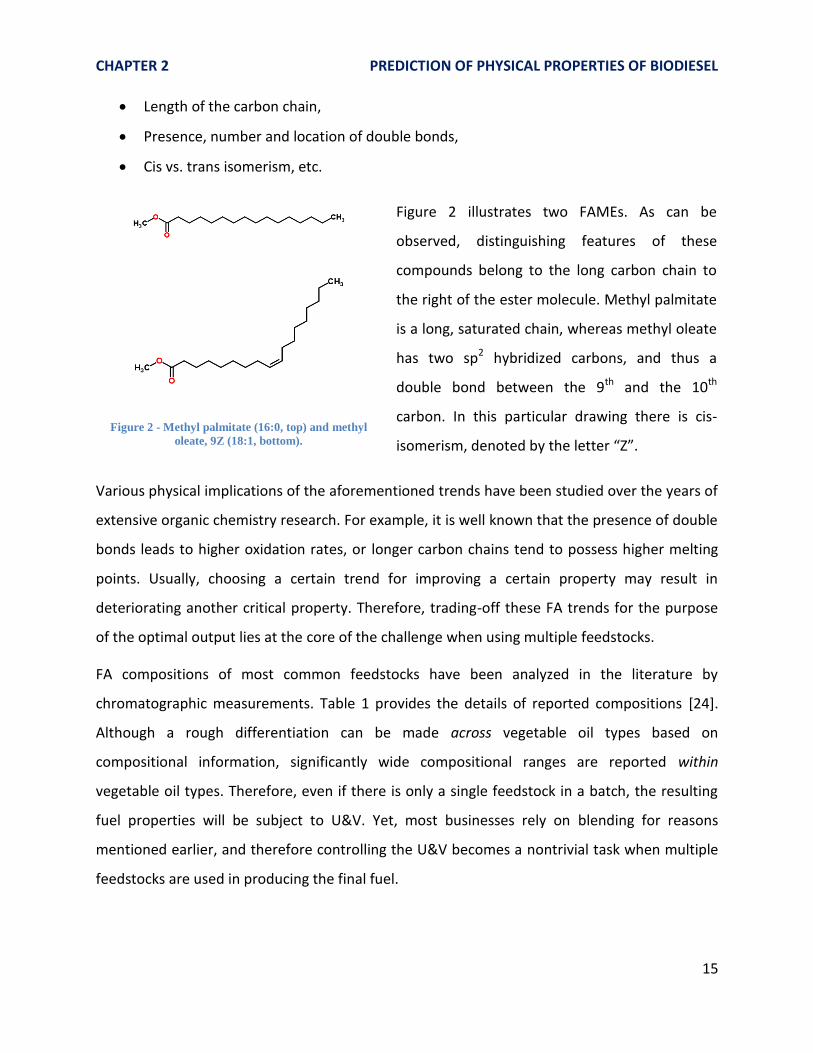
Length of the carbon chain,
Presence, number and location of double bonds,
Cis vs. trans isomerism, etc.
Figure 2 illustrates two FAMEs. As can be
observed, distinguishing features of these
compounds belong to the long carbon chain to
the right of the ester molecule. Methyl palmitate
is a long, saturated chain, whereas methyl oleate
has two sp2 hybridized carbons, and thus a
double bond between the 9th and the 10th
carbon. In this particular drawing there is cis-
isomerism, denoted by the letter “Z”.
Figure 2 - Methyl palmitate (16:0, top) and methyl
oleate, 9Z (18:1, bottom).
Various physical implications of the aforementioned trends have been studied over the years of
extensive organic chemistry research. For example, it is well known that the presence of double
bonds leads to higher oxidation rates, or longer carbon chains tend to possess higher melting
points. Usually, choosing a certain trend for improving a certain property may result in
deteriorating another critical property. Therefore, trading-off these FA trends for the purpose
of the optimal output lies at the core of the challenge when using multiple feedstocks.
FA compositions of most common feedstocks have been analyzed in the literature by
chromatographic measurements. Table 1 provides the details of reported compositions [24].
Although a rough differentiation can be made across vegetable oil types based on
compositional information, significantly wide compositional ranges are reported within
vegetable oil types. Therefore, even if there is only a single feedstock in a batch, the resulting
fuel properties will be subject to U&V. Yet, most businesses rely on blending for reasons
mentioned earlier, and therefore controlling the U&V becomes a nontrivial task when multiple
feedstocks are used in producing the final fuel.
CHAPTER 2 PREDICTION OF PHYSICAL PROPERTIES OF BIODIESEL
16
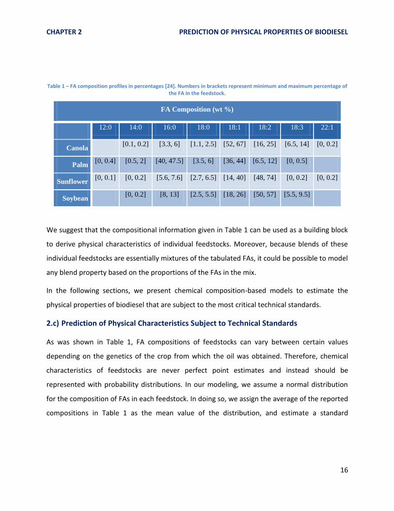
Table 1 – FA composition profiles in percentages [24]. Numbers in brackets represent minimum and maximum percentage of the FA in the feedstock.
FA Composition (wt %)
12:0 14:0 16:0 18:0 18:1 18:2 18:3 22:1
Canola [0.1, 0.2] [3.3, 6] [1.1, 2.5] [52, 67] [16, 25] [6.5, 14] [0, 0.2]
Palm [0, 0.4] [0.5, 2] [40, 47.5] [3.5, 6] [36, 44] [6.5, 12] [0, 0.5]
Sunflower [0, 0.1] [0, 0.2] [5.6, 7.6] [2.7, 6.5] [14, 40] [48, 74] [0, 0.2] [0, 0.2]
Soybean [0, 0.2] [8, 13] [2.5, 5.5] [18, 26] [50, 57] [5.5, 9.5]
We suggest that the compositional information given in Table 1 can be used as a building block
to derive physical characteristics of individual feedstocks. Moreover, because blends of these
individual feedstocks are essentially mixtures of the tabulated FAs, it could be possible to model
any blend property based on the proportions of the FAs in the mix.
In the following sections, we present chemical composition-based models to estimate the
physical properties of biodiesel that are subject to the most critical technical standards.
2.c) Prediction of Physical Characteristics Subject to Technical Standards
As was shown in Table 1, FA compositions of feedstocks can vary between certain values
depending on the genetics of the crop from which the oil was obtained. Therefore, chemical
characteristics of feedstocks are never perfect point estimates and instead should be
represented with probability distributions. In our modeling, we assume a normal distribution
for the composition of FAs in each feedstock. In doing so, we assign the average of the reported
compositions in Table 1 as the mean value of the distribution, and estimate a standard

CHAPTER 2 PREDICTION OF PHYSICAL PROPERTIES OF BIODIESEL
17
deviation assuming that the reported ranges cover 6 standard deviations of the whole
distribution9.
Figure 3 shows the information given in Table 1 graphically with the addition of the error bars
representing compositional standard deviations.
Figure 3 - Compositions of FAs in each feedstock. In the x-axis, the first number represents the number of carbon atoms and
the second number represents the number of double bonds.
2.c.1) Iodine Value (IV)
Iodine value is the mass of iodine in grams consumed by 100 grams of vegetable oil or FAME. It
is a direct indication of the degree of unsaturation in the carbon chain, because iodine is
extremely reactive with sp2 and sp hybridized carbons. A high degree of unsaturation is known
to result in polymerization reactions in diesel engines under combustion conditions, and
therefore is not desired. In addition to this, oxidation of the fuel is also highly correlated with
unsaturation.
Iodine value of a neat FAME can be calculated as in Eqn 2.1:
(2.1)
9 Approximately 99% of all the possible values of a normally distributed random variable fall within the 6 standard
deviations range.

CHAPTER 2 PREDICTION OF PHYSICAL PROPERTIES OF BIODIESEL
18
where 253.81 g/mol is the molecular weight of an iodine molecule, I2, #db is the number of
double bonds and MWFAME is the molecular weight of the FAME. Table 2 shows calculated IVs of
various neat FAMEs.
Table 2 – IVs of various neat FAMEs.
12:0 14:0 16:0 18:0 18:1 18:2 18:3 22:1
IV 0 0 0 0 81.74 164.55 248.45 69.23
Based on the IV of constituent FAMEs present, IV of a FAME mix can be calculated as in Eqn 2.2:
∑
(2.2)
where is the volume proportion of FAMEi in the mix.
However there has been some criticism against the effectiveness of IV as a technical standard,
mostly due to the following reasons [54]:
1- IV does not provide information about the nature of unsaturation. For example, the
relative oxidation rates are 1 for oleates (18:1), 41 for linoleates (18:2) and 98 for
linolenates (18:3) and IV estimation does not capture the relative magnitude of these
rates [55].
2- IV of a fatty compound depends on its molecular weight, leading to lower IV for longer
carbon chains.
3- IV of two or more dissimilar compounds may be the same, hiding the underlying
structural differences that affect oxidation stability directly.
Nevertheless, IV is still enforced as a technical constraint under EN 14214, with maximum
allowed value being 120. This constraint particularly limits the amount of soybean and
sunflower oil used in biodiesel, due to their higher linoleic and linolenic content.

CHAPTER 2 PREDICTION OF PHYSICAL PROPERTIES OF BIODIESEL
19
We modeled IVs of canola, palm, soybean and sunflower based on the compositional
information shown in Figure 3 and the principles outlined in Eqns 2.1 and 2.2. Then, we ran
Monte Carlo simulations to reflect the potential IV range for each feedstock.
Table 3 compares the literature reported IV ranges with the ranges predicted by the model. The
model and the reported values are in good agreement with each other.
Table 3 – Comparison of 5th
and 95th
percentile IV values predicted by the model and the ranges reported in the literature.
Model IV Prediction Reported IV in Literature
Canola [101, 116] [94, 120]
Palm [45, 52] [50, 55]
Sunflower [110, 136] [110, 143]
Soybean [120, 129] [120, 143]
Later in Chapter 4, model results will show that IV does not become a binding constraint most
of the time, because the optimal blend is never primarily composed of soybean and/or
sunflower. Both canola and palm, having lower IVs, can offset their impact in the final fuel.
2.c.2) Oxidative Stability (OS)
OS of biodiesel has been studied extensively due to its direct impact on fuel degradation over
time. Biodiesel might be transported over long distances and/or stored for significant durations,
and therefore fuel degradation due to oxidation is a major concern in the industry. The most
common method to determine OS is the so-called Rancimat test that is specified both under
ASTM D6751 and EN 14214. In the test procedure, 3 grams of biodiesel sample is placed into a
tube which is heated to 110˚C, and then air is swept through the tube. This action creates
volatile compounds that form upon oxidation. When these compounds meet deionized water
kept in another vessel connected to the sample tube, conductivity of water changes. The time
elapsed until the maximum rate of change in the conductivity of water is reached, in other
words the induction period, is defined as the OS in the biodiesel standards. In Europe, the
CHAPTER 2 PREDICTION OF PHYSICAL PROPERTIES OF BIODIESEL
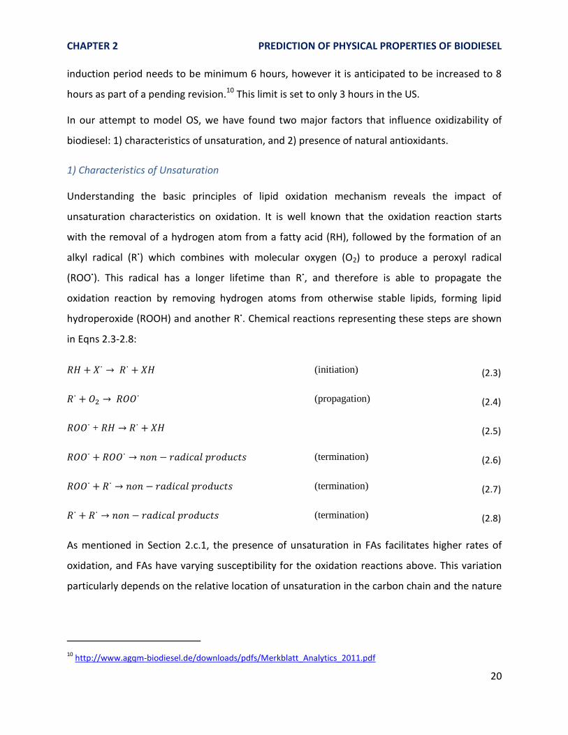
20
induction period needs to be minimum 6 hours, however it is anticipated to be increased to 8
hours as part of a pending revision.10 This limit is set to only 3 hours in the US.
In our attempt to model OS, we have found two major factors that influence oxidizability of
biodiesel: 1) characteristics of unsaturation, and 2) presence of natural antioxidants.
1) Characteristics of Unsaturation
Understanding the basic principles of lipid oxidation mechanism reveals the impact of
unsaturation characteristics on oxidation. It is well known that the oxidation reaction starts
with the removal of a hydrogen atom from a fatty acid (RH), followed by the formation of an
alkyl radical (R˙) which combines with molecular oxygen (O2) to produce a peroxyl radical
(ROO˙). This radical has a longer lifetime than R˙, and therefore is able to propagate the
oxidation reaction by removing hydrogen atoms from otherwise stable lipids, forming lipid
hydroperoxide (ROOH) and another R˙. Chemical reactions representing these steps are shown
in Eqns 2.3-2.8:
(initiation) (2.3)
(propagation) (2.4)
+ (2.5)
(termination) (2.6)
(termination) (2.7)
(termination) (2.8)
As mentioned in Section 2.c.1, the presence of unsaturation in FAs facilitates higher rates of
oxidation, and FAs have varying susceptibility for the oxidation reactions above. This variation
particularly depends on the relative location of unsaturation in the carbon chain and the nature
10
http://www.agqm-biodiesel.de/downloads/pdfs/Merkblatt_Analytics_2011.pdf

CHAPTER 2 PREDICTION OF PHYSICAL PROPERTIES OF BIODIESEL
21
of unsaturation, such as hybridization of carbon atoms [43, 55]. Consider the representative
carbon chain in Figure 4 and observe the positions of carbons relative to the double bonds:
Figure 4 – Allylic and bis-allylic positions in a carbon chain
Due to the delocalization of the double bonds adjacent to the allylic and bis-allylic carbon
atoms, C-H bonds in the allylic and bis-allylic positions are weaker and easier to break. As a
result, these atoms are highly prone to oxidation, with bis-allylic position possessing even a
higher reactivation rate. Knothe defines two indices, allylic position equivalent (APE) and bis-
allylic position equivalent (BAPE), in order to represent these positions in a carbon chain; and
shows that compounds having very similar IVs might have distinctively different APE and BAPE
indices [54]. One APE is the equivalent of one allylic position contained in a fatty compound of
concentration 1% in a mixture. Similarly, one BAPE is the equivalent of one bis-allylic position
contained in a fatty compound of concentration 1% in a mixture. APE and BAPE of most
commonly found FAs can be calculated as in Eqns 2.9-2.10:
( ) (2.9)
(2.10)
where A is the amount of each FA in percentage.
Table 4 lists the calculated APE and BAPE indices for some neat FAMEs.

CHAPTER 2 PREDICTION OF PHYSICAL PROPERTIES OF BIODIESEL
22
Table 4 – Calculated APE and BAPE indicess of FAMEs commonly found in biodiesel.
FAME APE BAPE
Methyl Oleate 18:1 200 0
Methyl Linoleate 18:2 200 100
Methyl Linoleneate 18:3 200 200
Methyl Erucate 22:1 200 0
2) Presence of Natural Antioxidants in the Vegetable Oil
The presence of antioxidants inhibits oxidation according to the simplified model outlined in
Eqns 2.11-2.12:
(2.11)
(2.12)
One major advantage of antioxidants is their phenolic nature that possesses a resonance
structure leading to radical stabilization. Therefore, even if a hydrogen atom is removed from
an antioxidant, the resonance structure can accommodate the electronic imbalance and keep
the molecule less reactive, preventing propagation of oxidation.
We surveyed several papers reporting data and various aspects regarding antioxidants in
vegetable oils [9, 12, 24, 44-46, 49, 56-61]. However, deriving a quantitative relationship that
can explain the variation in OS among biodiesel samples proved to be difficult in the absence of
systematically collected data. It is well known that most unrefined vegetable oils contain
natural antioxidants such as tocopherols or tocotrienols, yet these naturally-occurring
constituents are usually removed or deactivated by refining, distillation or transesterification
processes [57, 58, 61]. It is not always possible to track all the post-extraction steps of the
samples reported in the literature. Sometimes the samples are purchased from chemical supply
companies or donated by biodiesel producers [44]. In the first case, the degree of refining is
expected to be higher compared to regular biodiesel feedstocks, and in the latter case
purchased biodiesel might contain artificial antioxidants [45]. During the discussions with the
Portuguese biodiesel producers, we were informed that artificial antioxidants are not used in

CHAPTER 2 PREDICTION OF PHYSICAL PROPERTIES OF BIODIESEL
23
the European market unless the customer specifically asks for it. Therefore all antioxidants in
the final fuel are expected to be natural. Figure 5 shows the structure of the two most common
antioxidants and Table 5 tabulates the distribution of them in the major feedstocks.
Figure 5 – Structure of tocopherols and tocotrienols found in most vegetable oils, taken from [43].
Table 5 – Tocopherol and tocotrienol values found in the literature (ppm).
α-T* β-T γ-T δ-T α-TT** β-TT γ-TT δ-TT
Canola
179a
202b 314c
180d
65b
18c 409a
490b
420c
340d
9b
14c - - - -
Palm 89b
122c
377d
7c
1d
18b
39c
4d
6c 128b
52d -
4d 323b 72b
Soybean
93a
100b
62c
116d
11a
8b
11c
17d
1046a
1021b
537c
578d
374a
421b
147c
263d
- - - -
Sunflower
981a
670b
497c
671d
27b
21c
23d
11b
118c
4d
1b
19c - - - -
*Tocopherol ;
** Tocotrienol
a Averages of reported values in [56];
b Taken from [62];
c Taken from [9];
d Taken from [43].
As can be seen in Table 5, although each feedstock has more or less of a characteristic
distribution of antioxidants, absolute tocopherol or tocotrienol levels could be quite different
CHAPTER 2 PREDICTION OF PHYSICAL PROPERTIES OF BIODIESEL
24
across different samples of the same feedstock type. Certainly, one of the major factors that
contribute to these differences is the variation in post-extraction steps for each sample. In fact,
even if there were no post-extraction processing differences across samples, several other
factors such as planting location, breeding line, temperature and climate during growth,
variation in gene pools of the seeds can result in differences in natural antioxidant levels
manifested in the harvested crop [56]. More interestingly, stabilizing effect of the same
antioxidant type has been found to vary when it is artificially added to different feedstocks
which suggests complex chemical interactions depending on the species involved [57]. This last
point poses a challenge from a modeling perspective where the stabilizing impact of each
antioxidant is aimed to be predicted irrespective of the host feedstock.
It should be reiterated that on top of all the complexities listed, the possible variation in the
storage time of the samples might introduce another degree of bias to the collected data as
antioxidants tend to degrade over time. Even more, the vessel that transports the vegetable oil
might have an impact on the resulting oxidative stability of the biodiesel, because it is shown
that the presence of copper, iron and nickel reduces OS as a result of catalytic effect [42].
Despite all these factors, controlled experiments have shown that natural antioxidants stabilize
methyl esters by reducing the rate of peroxide formation considerably [57]. Therefore, we
attempted to capture the impact of naturally occurring antioxidants in our model. With few
data points regarding the tocopherol and tocotrienol levels, we decided to represent the
antioxidant levels with dummy variables; 0 representing absence, and 1 representing presence
of the antioxidant in consideration. Furthermore, we considered only γ-tocopherol and
tocotrienols, because α-tocopherols are found to be the least effective stabilizers [57, 63], and
β- and δ-tocopherols are found in very small amounts in all the seed oils. Table 6 summarizes
the dummy variable selection for the model. Note that sunflower oil possesses no major natural
antioxidant in our model.

CHAPTER 2 PREDICTION OF PHYSICAL PROPERTIES OF BIODIESEL
25
Table 6 – Selected dummy variables for γ tocopherol and tocotrienol levels in feedstocks.
γ-T TT (α + β + γ + δ)
Canola 1 0
Palm 0 1
Soybean 1 0
Sunflower 0 0
Lastly, we assumed a linear blending model for the dummy variables when feedstocks are
mixed with each other.
Multiple Regression Analysis on Unsaturation and Natural Antioxidants
Given the strong dependence of OS on unsaturation and natural antioxidant levels, we
performed a multiple regression analysis of induction period on these two factors. Table 7
tabulates the induction period data used. Some measurements are based on blends of
feedstocks and the blend ratios are indicated in the table. Total number of samples is 69.

CHAPTER 2 PREDICTION OF PHYSICAL PROPERTIES OF BIODIESEL
26
Table 7 - Reported induction periods of several feedstocks and their blends. Rancimat method was used in all experiments. Total number of samples is 69.
FEEDSTOCKS Blend Ratio
Induction Period (h)
FEEDSTOCKS Blend Ratio
Induction Period (h)
CAN - 6.4a CAN/SNF 1:1 6.5
a
- 6.9
b 1:3 6.8
a
- 6.9g 3:1 6.2
a
- 9.1
h PLM/SYB 1:1 6.2
a
- 7.8i 1:3 5.5
a
PLM - 10.3a 3:1 7.7
a
- 11.0b 1:9 5.2
a
- 14.2
c 1:4 5.4
a; 4.2
b
- 11.1d 3:7 5.6
a
- 15.4
i 2:3 5.9
a
- 13.4f 3:2 6.9
a
SYB - 5.0a 7:3 7.4
a
- 3.9b 4:1 8.2
a; 7.4
b
- 3.9
c 9:1 9.2
a
- 3.5d 2:3 5.0
b
- 6.6
e 3:2 6.2
b
- 3.8f PLM/SNF 1:1 8.1
a
SNF - 6.2a,*
1:3 7.1a
- 1.8c 3:1 9.2
a
- 3.4
h SYB/SNF 1:1 5.8
a
- 1.7f 1:03 6.4
a
CAN/PLM 1:1 7.6a 3:1 5.4
a
1:3 9.6a CAN/PLM/SYB 1:1:1 5.4
a
3:1 6.5
a 1:1:3 5.0
b
4:1 7.8b 2:1:2 5.7
b
3:2 9.3
b 3:1:1 6.6
b
2:3 10.6b 1:2:2 6.3
b
CAN/SYB 1:1 5.3a 2:2:1 7.7
b
1:3 5.1a 1:3:1 8.0
b
3:1 5.9
a CAN/PLM/SNF 1:1:1 7.8
a
4:1 4.2b CAN/SYB/SNF 1:1:1 5.0
a
2:3 4.7
b SYB/SNF/PLM 1:1:1 6.7
a
3:2 5.2b CAN/PLM/SYB/SNF 1:1:1:1 5.7
a
4:1 5.9
b
a [9]; b [44]; c [58]; d [45]; e [12]; f [49]; g [46]; h [63]; i [57]

CHAPTER 2 PREDICTION OF PHYSICAL PROPERTIES OF BIODIESEL
27
Table 8 details the antioxidant levels, chemical compositions and the resultant APE and BAPE
indices corresponding to the samples listed in Table 7:
Table 8 – Antioxidant levels (dummy variables), chemical composition (%) and resulting APE and BAPE indices of several feedstocks and their blends. The data is taken from the same resources as in Table 7. Total number of samples is 69.
*High oleic sunflower.
FEEDSTOCKBlend
Ratioγ-T TT 12:0 14:0 16:0 16:1 18:0 18:1 18:2 18:3 20:0 20:1 22:0 22:1 APE BAPE
Canola - 1 - - - 4.6 0.2 2.1 64.3 20.2 7.6 0.7 - 0.3 - 184.6 35.4
Canola - 1 - - 0.1 4.4 - 1.7 62.4 19.7 9.5 0.6 1.3 - - 185.76 38.67
Canola - 1 - - - 4.8 - 1.4 66.8 19.7 7.2 - - - - 187.4 34.1
Canola - 1 - - - 6.0 - 2.1 60.3 20.9 8.2 0.6 1.3 0.3 0.2 181.64 37.17
Canola - 1 - - - 4.0 - - 60.5 20.3 9.4 - - - - 180.4 39.1
Palm - 0 1 0.3 1.1 41.9 0.2 4.6 41.2 10.3 0.1 0.3 - - - 103.6 10.5
Palm - 0 1 - 1.0 40.1 - 4.1 43.0 11.0 0.2 0.3 - - - 108.52 11.44
Palm - 0 1 - - 41.3 - 3.5 43.1 12.1 - - - - - 110.4 12.1
Palm - 0 1 - 0.6 47.2 - 3 40.8 8.2 0.2 - - - - 98.4 8.6
Palm - 0 1 - - 43.3 - - 40.5 9.6 0.3 - - - - 100.8 10.2
Palm - 0 1 - - 40.3 - 3.1 43.4 13.2 - - - - - 113.2 13.2
Soybean - 1 - - 0.1 11.0 - 4.3 23.1 53.3 6.8 0.3 - - - 166.32 66.81
Soybean - 1 - - 0.1 10.8 - 4 23.4 53.9 7.8 - - - - 170.2 69.5
Soybean - 1 - - - 14.1 0.7 5.2 25.3 48.7 6.1 - - - - 161.6 60.9
Soybean - 1 - - - 10.5 - 4.1 24.1 53.6 7.7 - - - - 170.8 69
Soybean - 1 - - 0.1 11.0 0.1 4 23.4 53.2 7.8 0.3 - 0.1 - 169 68.8
Sunflower* - - - - - 4.5 - 4 82.0 8.0 0.2 0.3 - 1.0 - 180.4 8.4
Sunflower - - - - 0.2 5.3 - 5.7 20.6 67.4 0.8 - - - - 177.6 69
Sunflower - - - - - 6.0 - 4.7 24.0 63.7 - 0.3 0.2 0.8 - 175.84 63.74
Sunflower - - - 0.5 0.2 4.8 0.8 5.7 20.6 66.2 0.8 0.3 - - - 176.8 67.8
Canola/Palm 3:1 0.75 0.25 0.1 0.3 13.9 0.2 2.7 58.5 17.7 5.7 0.6 - 0.2 - 164.35 29.18
Canola/Palm 1:3 0.25 0.75 0.2 0.8 32.6 0.2 4.0 47.0 12.8 2.0 0.4 - 0.1 - 123.85 16.73
Canola/Palm 1:1 0.5 0.5 0.2 0.6 23.3 0.2 3.4 52.8 15.3 3.9 0.5 - 0.2 - 144.1 22.95
Canola/Palm 2:3 0.4 0.6 - 0.6 25.8 - 3.1 50.8 14.5 3.9 0.4 0.5 - - 139.42 22.33
Canola/Palm 3:2 0.6 0.4 - 0.4 18.7 - 2.6 54.6 16.3 5.8 0.5 0.8 - - 154.86 27.78
Canola/Palm 4:1 0.8 0.2 - 0.2 11.6 - 2.2 58.5 18.0 7.6 0.5 1.0 - - 170.31 33.22
Canola/Soybean 4:1 1 - - 0.1 5.7 - 2.2 54.5 26.4 8.9 0.5 1.0 - - 181.87 44.3
Canola/Soybean 3:2 1 - - 0.1 7.0 - 2.7 46.7 33.1 8.4 0.4 0.8 - - 177.98 49.93
Canola/Soybean 2:3 1 - - 0.1 8.3 - 3.3 38.8 39.9 7.9 0.4 0.5 - - 174.1 55.55
Canola/Soybean 1:4 1 - - 0.1 9.6 - 3.8 31.0 46.6 7.3 0.3 0.3 - - 170.21 61.18
Canola/Soybean 1:3 1 - - - 9.0 0.1 3.6 34.2 45.3 7.7 0.2 - 0.1 - 174.25 60.6
Canola/Soybean 3:1 1 - - - 6.1 0.2 2.6 54.3 28.6 7.6 0.5 - 0.2 - 181.15 43.8
Canola/Soybean 1:1 1 - - - 7.6 0.1 3.1 44.2 36.9 7.7 0.4 - 0.2 - 177.7 52.2
Canola/Sunflower* 3:1 0.5 - - - 4.6 0.2 2.6 68.7 17.2 5.8 0.6 - 0.5 - 183.55 28.65
Canola/Sunflower* 1:3 0.75 - - - 4.5 0.1 3.5 77.6 11.1 2.1 0.4 - 0.8 - 181.45 15.15
Canola/Sunflower* 1:1 0.5 - - - 4.6 0.1 3.1 73.2 14.1 3.9 0.5 - 0.7 - 182.5 21.9

CHAPTER 2 PREDICTION OF PHYSICAL PROPERTIES OF BIODIESEL
28
(Table 8 continued.)
*High oleic sunflower.
Because regression analysis assumes that there exists a linear relationship between the
dependent and the explanatory variables, it is necessary to investigate if there are any
nonlinear relationships11. As can be seen in Figure 6, scatter plots of induction periods vs. BAPE
and APE indices demonstrate a significant degree of linearity, with R2 values of 0.6085 and
11
If they exist, nonlinear to linear transformations might still enable regression analysis.
FEEDSTOCKBlend
Ratioγ-T TT 12:0 14:0 16:0 16:1 18:0 18:1 18:2 18:3 20:0 20:1 22:0 22:1 APE BAPE
Palm/Soybean 9:1 0.1 0.9 0.3 1.0 38.8 0.2 4.6 39.5 14.6 0.9 0.3 - - - 110.32 16.35
Palm/Soybean 4:1 0.2 0.8 - 0.8 34.3 - 4.1 39.0 19.5 1.5 0.3 - - - 120.08 22.51
Palm/Soybean 4:1 0.2 0.8 0.2 0.9 35.6 0.2 4.5 37.8 19.0 1.6 0.2 - - - 117.04 22.2
Palm/Soybean 7:3 0.3 0.7 0.2 0.8 32.5 0.1 4.5 36.1 23.3 2.4 0.2 - - - 123.76 28.05
Palm/Soybean 3:2 0.4 0.6 - 0.6 28.4 - 4.2 35.1 27.9 2.8 0.3 - - - 131.64 33.59
Palm/Soybean 3:2 0.4 0.6 0.2 0.7 29.3 0.1 4.4 34.4 27.6 3.1 0.2 - - - 130.48 33.9
Palm/Soybean 1:1 0.5 0.5 0.2 0.6 26.2 0.1 4.4 32.7 32.0 3.9 0.2 - - - 137.2 39.75
Palm/Soybean 2:3 0.6 0.4 - 0.4 22.6 - 4.2 31.1 36.4 4.1 0.3 - - - 143.2 44.66
Palm/Soybean 2:3 0.6 0.4 0.1 0.4 23.1 0.1 4.3 30.9 36.3 4.7 0.1 - - - 143.92 45.6
Palm/Soybean 3:7 0.7 0.3 0.1 0.3 19.9 0.1 4.3 29.2 40.6 5.4 0.1 - - - 150.64 51.45
Palm/Soybean 1:4 0.8 0.2 - 0.3 16.8 - 4.3 27.1 44.8 5.5 0.3 - - - 154.76 55.74
Palm/Soybean 1:4 0.8 0.2 0.1 0.2 16.8 0.0 4.2 27.5 44.9 6.2 0.1 - - - 157.36 57.3
Palm/Soybean 1:9 0.9 0.1 0.0 0.1 13.6 0.0 4.2 25.8 49.3 6.9 0.0 - - - 164.08 63.15
Palm/Soybean 1:3 0.75 0.25 0.1 0.3 18.4 0.1 4.2 28.4 42.8 5.8 0.1 - - - 154 54.38
Palm/Soybean 3:1 0.25 0.75 0.2 0.8 34.1 0.2 4.5 36.9 21.1 2.0 0.2 - - - 120.4 25.13
Palm/Soybean 1:1 0.5 0.5 0.2 0.6 26.2 0.1 4.4 32.7 32.0 3.9 0.2 - - - 137.2 39.75
Palm/Sunflower* 3:1 - 0.75 0.2 0.8 32.6 0.2 4.5 51.4 9.7 0.1 0.3 - 0.3 - 122.8 9.975
Palm/Sunflower* 1:3 - 0.25 0.1 0.3 13.9 0.1 4.2 71.8 8.6 0.2 0.3 - 0.8 - 161.2 8.925
Palm/Sunflower* 1:1 - 0.5 0.2 0.6 23.2 0.1 4.3 61.6 9.2 0.2 0.3 - 0.5 - 142 9.45
Soybean/Sunflower* 3:1 0.75 - - - 9.0 - 4.1 38.6 42.2 5.8 0.1 - 0.3 - 173.2 53.85
Soybean/Sunflower* 1:3 0.25 - - - 6.0 - 4.0 67.5 19.4 2.1 0.2 - 0.8 - 178 23.55
Soybean/Sunflower* 1:1 0.5 - - - 7.5 - 4.1 53.1 30.8 4.0 0.2 - 0.5 - 175.6 38.7
Palm/Canola/Soybean 1:1:1 0.666 0.333 0.1 0.4 18.8 0.1 3.6 42.8 27.8 5.1 0.3 - 0.1 - 151.47 37.92
Palm/Canola/Soybean 3:1:1 0.4 0.6 - 0.6 27.1 - 3.7 42.9 21.2 3.4 0.4 0.3 - - 135.53 27.96
Palm/Canola/Soybean 2:2:1 0.6 0.4 - 0.4 20.0 - 3.2 46.8 23.0 5.2 0.4 0.5 - - 150.98 33.41
Palm/Canola/Soybean 2:1:2 0.6 0.4 - 0.4 21.3 - 3.7 38.9 29.7 4.7 0.3 0.3 - - 147.09 39.03
Palm/Canola/Soybean 1:3:1 0.8 0.2 - 0.2 12.9 - 2.7 50.7 24.7 7.1 0.5 0.8 - - 166.42 38.85
Palm/Canola/Soybean 1:2:2 0.8 0.2 - 0.2 12.9 - 2.7 50.7 24.7 7.1 0.5 0.8 - - 166.42 38.85
Palm/Canola/Soybean 1:1:3 0.8 0.2 - 0.3 15.5 - 3.7 35.0 38.1 6.0 0.3 0.3 - - 158.65 50.11
Canola/Palm/Sunflower* 1:1:1 0.333 0.333 0.1 0.4 16.8 0.1 3.5 61.9 12.7 2.6 0.4 - 0.4 - 154.64 17.92
Soybean/Canola/Sunflower* 1:1:1 0.666 - - - 6.5 0.1 3.4 56.2 27.0 5.1 0.3 - 0.4 - 176.81 37.22
Soybean/Sunflower*/Palm 1:1:1 0.333 0.3 0.1 0.4 18.8 0.1 4.2 48.6 23.7 2.6 0.2 - 0.3 - 150.08 29.01
Soybean/Canola/
Palm/Sunflower* 1:1:1:1 0.5 0.25 0.1 0.3 15.4 0.1 3.7 52.9 23.0 3.9 0.3 - 0.3 - 159.85 30.83

CHAPTER 2 PREDICTION OF PHYSICAL PROPERTIES OF BIODIESEL
29
0.4582 respectively12. As expected, FAMEs with higher BAPE and APE values have shorter
induction periods.
Figure 6 – Scatter plots of induction period vs. BAPE and APE indices of the FAMEs in Table 8.
Prior to running the multiple regression, we randomly selected 35 out of the 69 available data
points as the training set, and used the remaining 34 points as the validation set later on.
Multiple regression analysis on the training set resulted in R2 =0.84, with BAPE, γ-tocopherol
and tocotrienol as the explanatory variables. These variables are statistically significant at the
95% confidence level. Detailed parameters of the regression analysis are listed in Table 9:
Table 9 – Multiple regression analysis results for OS.
Term Estimate Std Error t Ratio Prob >|t| Lower 95% Upper 95%
Intercept 7.41 0.702 10.54 <0.0001 5.98 8.84
BAPE -0.092 0.014 -6.40 <0.0001 -0.12 -0.06
γ-T 2.76 0.732 3.78 0.0007 1.27 4.25
TT 4.12 0.738 5.59 <0.0001 2.62 5.63
Thus, the regression equation for the induction period can be expressed as in Eqn 2.13:
(2.13)
12
Because we represent the γ-tocopherol and tocotrienol levels with dummy variables in the model, scatter plots for those variables are not included in this part.

CHAPTER 2 PREDICTION OF PHYSICAL PROPERTIES OF BIODIESEL
30
The model was validated on the validation set, and a reasonable fit was found with a root-
mean-square error of 1.23. Figure 7 compares the induction periods predicted by the model
and measured in the experiments for all of the 69 samples.
Figure 7 – Comparison of the oxidative stability regression model predictions with the experimental data.
Having found a regression equation, we performed Monte Carlo simulations to demonstrate
potential range of induction periods for each feedstock. The results are listed in Table 10. The
numbers in bracket represent 5th and 95th percentile estimates. Modeled induction period
ranges follow the general trend reported in the literature with palm oil having the highest OS
among others. However, the upper bounds of measured values are considerably higher than
the model prediction. We think that those values are outliers, and therefore are not captured
by the regression equation. It is also possible that those outlier samples contained some sort of
antioxidant additives in their composition.
Table 10 – Monte Carlo simulation results of induction periods (IPs) predicted by the regression model. The numbers in bracket represent the 5
th and 95
th percentile estimates.
FAME Model IP Estimate (h) Measured IP in Literature (h)
Canola [6.0, 6.8] [6.4, 9.1]
Soybean [3.6, 4.1] [3.5, 6.6]
Sunflower [1.1, 2.4] [1.8, 3.4]
Palm [10.5, 10.8] [10.3, 15.4]

CHAPTER 2 PREDICTION OF PHYSICAL PROPERTIES OF BIODIESEL
31
2.c.3) Cetane Number (CN)
CN of biodiesel is equivalent to the octane rating in gasoline and is an indication of ignition
quality. Similar to octane rating, it is a dimensionless descriptor. CN is determined based on the
ignition performance of the fuel relative to a straight chain hydrocarbon, hexadecane (C16H34)
and a highly branched hydrocarbon, 2,2,4,4,6,8,8-heptamethylnoane (C16H34). Both substances
are considered to be the primary reference fuels and assigned CNs of 100 and 15 respectively.
Minimum CN requirement is 51 under EN 14214, and 47 under ASTM D6751. An Ignition Quality
Tester (IQT) or a cetane engine can be used to determine the CN of biodiesel. However the
equipment are quite expensive, and therefore biodiesel producers usually do not conduct CN
tests in their facilities. Because CN is generally not a concern for biodiesel, currently there is no
immediate need for prediction models in making blending decisions. Yet, with the potential of
increased feedstock diversification over the coming years, inclusion of new species such as corn
and babassu might make this constraint binding. This has been the main motivation in
incorporating CN prediction in our blending model.
It is known that saturated and unbranched hydrocarbons increase the CN of a blend whereas
unsaturated and highly branched compounds lower it [39]. Other than a few exceptions,
biodiesel tend to have higher CN compared to petrodiesel and this is seen as one of the
advantages of biodiesel. Nevertheless, it is not trivial to predict the CN of a hydrocarbon blend.
Both gasoline and diesel industry have historically relied on empirical studies and experience to
assess octane rating or CN of blends [38, 39, 64-66]. One of the most comprehensive and
relevant works we have come across belongs to the ExxonMobile Process Research
Laboratories in which a detailed composition-based model for predicting the CN of diesel fuels
in general was developed [67]. Because petrodiesel has a more complex chemical structure
than biodiesel, including various hydrocarbons such as normal paraffins, mono-branched and
multi-branched i-paraffins, naphthalenes, etc., this work used the experimental data of a total
of 203 diesel fuels and defined different molecular lumps to model the CN for each category.
There is also an extensive compendium of experimental CN data, published by the US National
Renewable Energy Laboratory (NREL) to support low emission fuel research [68].

CHAPTER 2 PREDICTION OF PHYSICAL PROPERTIES OF BIODIESEL
32
We have found that a linear CN blending rule based on the proportions of different feedstocks
(canola, soybean, etc.) leads to predictions with great error. However, an earlier study found a
promising result when a simple linear blending rule was used based on the proportions of the
neat FAs that constitute the biodiesel [69]. Thus, owing to the relatively simple chemical
composition of vegetable oils, it is possible to predict the CN of biodiesel using Eqn 2.14:
∑
(2.14)
Table 11 lists measured CN of various FAMEs that we have used in our model as inputs for Eqn
2.14. Note that it is possible to find slightly different CN data concerning these FAMEs in the
literature. We believe the differences in measurements emerge from several factors pertaining
to the complications in measurement procedures. The reader might refer to [24] for further
details regarding these procedures.
Table 11 – CNs of various neat FAMEs.
12:0 14:0 16:0 18:0 18:1 18:2 18:3 22:1
CN 61.4
a 66.2
a 74.5
a 86.9
a 59.3
b 38.2
b 22.7
a 74.2
a,*
a Taken from [24];
b Taken from [41];
c Taken from [39];
* Ethyl ester
Similar to IV and OS, we performed Monte Carlo simulations to find the 5th and 95th percentile
CN estimates for each feedstock. As listed in Table 12, agreement between the modeled CNs
and literature reported values is very promising. This, in turn, means that CN of any blend can
be predicted based on the blend’s FA profile.
Table 12- Comparison of 5th
and 95th
percentile model estimates and literature reported values of CN.
FAME Model CN Estimate CN Reported [24]
Canola [48.6, 54.1] 47.9a, 56
a
Palm [62.8, 67.2] 62b
Sunflower [43.3, 53.6] 54a, 58
a
Soybean [44.6, 48.5] 49.6a, 55.9
a
a Taken from [24];
b Taken from [9].

CHAPTER 2 PREDICTION OF PHYSICAL PROPERTIES OF BIODIESEL
33
2.c.4) Cold Filter Plugging Point (CFPP)
Cold flow properties of biodiesel are of central concern, especially if the final fuel will be used in
colder climates. There is evidence that FAMEs derived from soybean develop performance
issues when ambient temperature falls down [24]. Palm oil derivatives have even worse cold
weather performance. In fact, cold flow performance is one of the reasons to blend various
types of vegetable oils for commercial applications.
There are a few different standards that constrain the cold flow quality of biodiesel. These are
cloud point (CP), freezing point (FP), low-temperature flow test (LTFT), pour point (PP) and cold
filter plugging point (CFPP), but none of these standards are enforced by ASTM D6751 or EN
14214. Instead, certain flow quality is demanded by customers based on climate conditions. As
an example, biodiesel regulations in Germany require 0˚C, 10˚C and -20˚C CFPPs for the
summer, spring/autumn and winter months respectively.
Methods to measure the aforementioned standards might suffer from lack of repeatability and
reproducibility because some measurements are based on subjective observation. For example,
CP is defined as the temperature at which crystals become visible. Similarly, PP refers to the
lowest temperature where fluid motion is detected. In an effort to automate the measurement
process, CFPP emerged as an alternative bench-scale test method. In the CFPP test method, the
sample is cooled at 1˚C intervals and then drawn through a wire mesh under vacuum. The
lowest temperature at which 20 mL of oil passes through the filter in 60 seconds is defined as
CFPP. Our model analyzes CFPP only, as a representative parameter for all the other cold flow
parameters.
In general, presence of saturation leads to undesired cold flow properties, because saturated
hydrocarbons tend to form wax crystals at lower temperatures, and the presence of wax may
lead to start-up and operability problems. A thermodynamic modeling study found that the
amount of saturation was the main determinant for CP of biodiesel regardless of composition
of unsaturated esters [70]. Likewise, a recent study [9] concluded that CFPP is linearly related to
the proportion of saturated fats in the compound, and this relation can be expressed as in Eqn
2.15 (R2=0.86):

CHAPTER 2 PREDICTION OF PHYSICAL PROPERTIES OF BIODIESEL
34
[ ] (2.15)
where [Sats] is the percentage of saturated compounds in the fuel.
Using Eqn 2.15 we modeled CFPP values of the most common biodiesel feedstocks based on
their FA composition, and performed Monte Carlo analysis to explore potential ranges. Table 13
compares our model results with the literature reported values, which are in close agreement
with each other.
Table 13 – Comparison of 5th
and 95th
percentile model predictions and the literature reported values for CFPP.
FAME Model CFPP Estimate, ºC Literature CFPP Reported*, ºC
Canola [-6.4, -5.7] [-7,-4]
Palm [11.9, 13.8] [10, 16]
Sunflower [-4.5, -3.5] [-4,-1]
Soybean [-3.2, -1.9] [-5,-2]
* Data taken from [24].
Note that the model does not consider the presence of any minor constituents present
naturally or artificially in the feedstock. For example, it is known that vegetable oils naturally
contain steryl glucosides (StG) which turn into free StG (FStG) upon transesterification. FStG are
known to possess very high melting points (~240 ºC) that could have a considerable effect on
cold flow properties [24]. Similarly, trace amounts of monoacylglycerol (MAG), diacylglycerol
(DAG) and triacylglycerol (TAG) that may remain after partial transesterification are known to
negatively impact the low temperature operability performance. Consideration of these other
factors requires more specific data along with more detailed models.
2.d) Summary of Physical Characteristics
A careful look at Section 2.c1-2.c.4 revealS competing features of hydrocarbon chains, and that
they need to be traded-off in order to meet all the technical standards simultaneously. Table 14
summarizes these features:

CHAPTER 2 PREDICTION OF PHYSICAL PROPERTIES OF BIODIESEL
35
Table 14 – Competing features of hydrocarbon chains, undesired features are in red.
Long, Saturated Chains Short, Unsaturated Chains
Low IV High IV
High OS Low OS
High CN Low CN
High CFPP Low CFPP
In practice, use of additives such as antioxidants, cetane enhancers, cold-flow improvers could
ameliorate some of these properties. However, it has been reported that these additives may
react differently with each feedstock and use of more than one additive may lead to
compatibility issues. To give an example, it was reported that some cold flow improving
additives negatively affect the oxidative stability of biodiesel [71]. Therefore, leveraging from
the distinct advantages of individual feedstocks and blending them accordingly seems to be a
part of the solution to meet multiple technical standards concurrently.
Additionally, the discussion so far has made it clear that even if using one type of vegetable oil
was possible to meet all the technical standards, feedstock price differences are already a
strong motive to use multiple feedstocks in a single batch. In Chapter 4, we will incorporate the
feedstock prices into blending decisions and will provide a more detailed analysis of feedstock
property distributions.
2.e) Summary and Conclusion
Physical characteristics of biodiesel feedstocks, namely vegetable oils13, play a crucial role in
determining the final fuel quality. These characteristics are dependent on the FAs that
constitute the vegetable oil, and are subject to U&V due to the compositional variation of FAs
found in each vegetable oil.
In addition to U&V within the physical characteristics of each feedstock, the requirements of
current technical standards necessitate the use of multiple feedstocks that have competing
advantages. Along with producers’ cost minimizing goals, this leads to prevalence of feedstock
blending practices in the biodiesel industry. As a result, predicting the final fuel performance
13
Vegetable oil and feedstock will be used interchangeably for the remaining of the document.

CHAPTER 2 PREDICTION OF PHYSICAL PROPERTIES OF BIODIESEL
36
that is subject to multiple standards becomes a challenging task. FA composition-based physical
prediction models can create great value for the biodiesel producers in their operations.
Finally, because the prediction models we have developed are mostly based on FA
compositions and are irrespective of the crop species, they can be applied to new feedstocks
becoming available in the upcoming years. In other words, the presence of such prediction
models will enable the producers to expand their feedstock portfolio in a faster and low-risk
way, leading to more feedstock diversification in the biodiesel market. The advantages of
feedstock diversification will be detailed in Chapter 4.
On top of the technical standards outlined in this chapter, biodiesel is now subject to a
greenhouse gas (GHG) emissions standard to ensure a certain level of sustainability
performance over its lifecycle. Because the GHG emissions do not depend on the composition
characteristics of a feedstock, their prediction models are completely different and are not
included in this chapter. This will be the main focus of Chapter 5.
Our goal is to show how the predicted physical properties and GHG emissions along with their
U&V characteristics change in a biodiesel blend compared to that of individual feedstocks.
Recognizing U&V as a critical theme to the blending formulation, we will apply a probabilistic
optimization technique, generally referred to as “chance-constrained optimization” to calculate
optimal blend portfolios. The details of this optimization technique will be discussed in the next
chapter, Chapter 3.

37
CHAPTER 3:
CHANCE-CONSTRAINED BLEND OPTIMIZATION
3.a) Motivation and Background
In almost every industry, cost reduction is critical to profitability. For first generation biodiesel,
there are two main factors that contribute to the total fuel cost: feedstock costs and feedstock-
to-fuel conversion costs. Controlling feedstock costs offer the greatest opportunity to drive
down costs, because published process models in addition to industry reports estimate
feedstock costs to be between 77%-88% of the total [8-10, 72, 73]. One study that modeled the
technological learning and cost reductions over time for biofuels concluded that by 2030,
despite expected crop yield increases and advances in conversion technologies, feedstock costs
will still be the major part of the total cost [74]. Therefore, being able to use cheaper feedstocks
available in the market provides a great competitive advantage to the producer. Nevertheless,
as Chapter 2 outlined, there are multiple technical industry constraints in addition to the
recently introduced GHG emission thresholds that producers are required to comply with, and
these limit the feedstock options. A prevalent practice to meet the standards with lower costs is
feedstock blending, and so far blending decisions have been based on fixed recipes derived
from experience. This is because predicting the physical characteristics of a blend is a nontrivial
task, and thus exploring recipe variations in search for cheaper portfolios presents a risky
endeavor for biodiesel companies. In contrast, there has been a great amount of effort in
developing blending models for petroleum-based fuels, particularly for gasoline, where a
number of feedstocks are combined to make a mixture meeting certain quality specifications
[64, 75-77]. Although some studies such as [9] and [44] have explored the resulting physical
properties of blending biodiesel feedstocks, there has not been an explicit model that
incorporates the unique chemical composition characteristics in each feedstock and then use
them as decision variables in an optimal blend formulation.

CHAPTER 3 CHANCE-CONSTRAINED OPTIMIZATION MODEL
38
The most common blending models apply linear programming techniques to identify the
lowest-cost mix of raw materials subject to certain specifications. Some of the earlier examples
from the industry can be found in [78-80]. These models treat raw material quality as
deterministic. Undoubtedly, inherent U&V within the chemical composition of each biodiesel
feedstock impedes development of optimal blend formulations. In fact, compositional U&V is
not a unique challenge to the biodiesel industry and has been the focus of research in many
other materials-based industries including inorganics recycling [81-83], paper production [35,
84-87] and rubber manufacturing [88-91]. This challenge led to an improvement on
deterministic linear programming techniques, enabling the incorporation of feedstock quality
variation into optimization problems [92-98]. The details of these methods will not be discussed
in the scope of this work.
Within the industry, a conventional way to account for U&V and thereby reduce the risk of
noncompliant batches is to add a margin of safety around compositional specifications by
narrowing the original window of constraints. Gaustad et al. discusses this method for recycled
materials and shows that it results in over-conservative solutions [32]. Similarly, Wendt et al.
surveys the methods for process optimization under uncertainty, and states that the
conventional way to deal with uncertainties results in an overdesign of the process equipment,
leading to an operating point defined by an overestimation of uncertainties [29]. Singh et al.
discusses a very similar phenomenon in gasoline blending in terms of product quality giveaway,
in which gasoline is made with more expensive feedstock, when in fact, a lower cost feedstock
might have sufficed. Quality giveaway leads to a blend that exceeds the minimum requirement
(or fall below the maximum allowed). In their paper titled The Price of Robustness, Bertsimas
and Sim also express concerns regarding the over-conservative nature of conventional models,
and propose an approach that adjusts the level of conservatism in terms of probabilistic bounds
of constraint violations [99]. In short, conventional ways that attempt to incorporate U&V
information into an optimal blending problem are known to result in overestimation of
uncertainty, and therefore can lead to lower profitability.
Fortunately, researchers have come up with methods that explicitly consider U&V and properly
integrate it into complex optimization problems. The details of these different methods will not

CHAPTER 3 CHANCE-CONSTRAINED OPTIMIZATION MODEL
39
be discussed within the scope of this work, but a relatively recent review of them can be found
in [31]. One such method is chance-constrained (CC) optimization. We will introduce this
method and show that it can be applied to manage quality U&V in making optimal blend
decisions for multi-feedstock biodiesel systems.
Variants of CC optimization were first formulated by Charnes and Cooper [28]. Applications can
be found in feed mixing [100], materials production [32, 101, 102] and coal blending [30]. In a
recent paper, Olivetti et al. analytically characterized the benefit of using CC formulation as
compared to one with a linearized constraint [33].
The problem of optimal feedstock blending for biodiesel offers an interesting case for the CC
methodology, because there are multiple feedstocks with probabilistic distributions subject to
multiple constraints. Currently, there are only four main feedstocks, namely canola oil, soybean
oil, sunflower oil and palm oil14, used by the biodiesel markets. But in fact, more than 350
chemically different oil-bearing crops, including jatropha, camelina and corn, have been
identified for potential use in biodiesel production [14]. On top of this, ways to use waste
cooking oil or animal waste as alternative feedstocks due their desirable price and low
environmental footprint have been studied in recent years [50, 103-106]. All of these
developments point to a need for an analytical solution approach where optimal blending
decisions can be made with minimal dependence on fixed recipes.
As previously mentioned in Chapter 2, we assume that each fatty acid (FA) type is normally
distributed in each feedstock. Because iodine value (IV), oxidation stability (OS), cetane number
(CN) and cold filter plugging point (CFPP) are all related to FA composition profiles, our goal is
to build a compositional CC optimization model that uses the FA-based property predictions
developed in Chapter 2. In addition to the technical specifications, we treat the GHG emissions
as one of the constraints in the model; and later in Chapter 5, we analyze the impact of
blending on the resulting biodiesel GHG distribution using the CC optimization technique.
14
We will call these feedstocks as “canola, soybean, sunflower and palm” for ease of reading hereafter.

CHAPTER 3 CHANCE-CONSTRAINED OPTIMIZATION MODEL
40
3.b) Chance-Constrained (CC) Optimization Model Formulation
We begin by describing the theory behind CC optimization. Let Xi be a normally distributed
random variable with mean and standard deviation ; Ai a corresponding weighing
coefficient; and Y and Z constants representing deterministic constraints. We define α and β as
confidence levels of meeting the specified constraint. Thus, the probability of meeting the
constraint can be expressed as in Eqns 3.1-3.2:
{∑
} (3.1)
{∑
} (3.2)
Because we assume Gaussian distributions for the random variables in this model, we can
transform Eqns 3.1 and 3.2 to obtain the standard normal distribution with mean µ=0, and
variance σ2=1, and then use standard test coefficients corresponding to the chosen confidence
levels. The test coefficient for Gaussian distribution is usually denoted by z-value. At the limit of
meeting the constraint, ∑ approaches to Y or Z. Thus:
∑
∑
(3.3)
∑
∑
(3.4)
where refers to the pooled standard deviation of the mix and can be calculated as in Eqn
3.5:
√∑∑
(3.5)

CHAPTER 3 CHANCE-CONSTRAINED OPTIMIZATION MODEL
41
where is the correlation coefficient between and . By definition when .
Because we assume no correlation between feedstocks, when . In other words,
all feedstock scenarios considered in the model are regarded to be statistically independent
from each other, whether or not they belong to the same crop species. Each feedstock scenario
defines a certain set of conditions, such as soil type and climate region of cultivation or
different agricultural practices that lead to a large number of factors and contribute to
statistical independence across scenarios.
Figure 1 illustrates a property distribution of a blend which meets the constraint (a)
conservatively, (b) with high confidence level, (c) with low confidence level. Note that the
constraint level is defined by the user based on risk preferences and can be controlled by the
choice of the test coefficient, z-value.
Figure 1 – Illustration of a blend that meets the specified constraint level (a) conservatively, (b) with high confidence level,
(c) with low confidence level.
3.c) Chance-Constrained Optimization Applied to Biodiesel Feedstock Blending
CC optimization for the biodiesel blending problem can be formulated as in Eqns 3.6-3.13. The
objective is to minimize the total feedstock cost.
∑
(3.6)
∑
(3.7)
∑
(3.8)
(3.9)

CHAPTER 3 CHANCE-CONSTRAINED OPTIMIZATION MODEL
42
(3.10)
(3.11)
(3.12)
(3.13)
where;
: unit price of feedstock i
: volume proportion of feedstock i in the blend
: total demand
: supply of feedstock i
test coefficient for normal distribution, one-tailed
: mean iodine value of the blend
: iodine value constraint
: standard deviation of iodine value in the blend
: mean oxidation stability of the blend
: oxidation stability constraint
: standard deviation of oxidation stability in the blend
: mean cetane number of the blend
: cetane number constraint
standard deviation of cetane number in the blend
: mean cold filter plugging point of the blend
: cold filter plugging point constraint

CHAPTER 3 CHANCE-CONSTRAINED OPTIMIZATION MODEL
43
: standard deviation of cold filter plugging point in the blend
: mean GHG of the blend
: GHG constraint
: standard deviation of GHG in the blend
The amounts of each feedstock to be blended, namely Ai, constitute the decision variables of
the optimization problem. Choosing a set of Ai values determines the amount of each FA, aj, in
the blend. Because FAs are the building blocks that define all the physical parameters, we can
derive IV, CN, OS and CFPP based on the FA profile of the blend. The following equations
outline how this derivation is performed.
Mean physical parameter values are derived as in Eqns 3.14-3-20:
∑
(3.14)
∑
(3.15)
(∑
)
(∑
)
(3.16)
(3.17)
∑
(3.18)
(∑
) (3.19)

CHAPTER 3 CHANCE-CONSTRAINED OPTIMIZATION MODEL
44
∑
(3.20)
where;
: mean composition of FA j in the blend
: mean composition of FA j in feedstock i
: iodine value of FA j
: mean BAPE of the blend
: intercept in the oxidation stability regression equation
: coefficient of BAPE in the oxidation stability regression equation
coefficient of γ-tocopherol in the oxidation stability regression equation
amount of γ-tocopherol in the blend
coefficient of tocotrienol in the oxidation stability regression equation
amount of tocotrienol in the blend
: cetane number of FA j
: cold filter plugging point of FA j
: intercept in the cold filter plugging point regression equation
: coefficient of total saturation in the cold filter plugging point regression
equation
: mean GHG of feedstock i
Standard deviations are derived as in Eqns 3.21-3.26 based on the principle indicated in Eqn
3.5:
√∑
(3.21)

CHAPTER 3 CHANCE-CONSTRAINED OPTIMIZATION MODEL
45
√∑
(3.22)
√∑
(3.23)
√ ( ∑
∑
) (3.24)
√
∑
(3.25)
√∑
(3.26)
where;
: standard deviation of composition of FA j in the blend
: standard deviation of composition of FA j in feedstock i
: standard deviation of GHG emissions of feedstock i
Finally, it must be noted that there is another layer of U&V factor for the predicted properties
OS and CFPP. This U&V stems from the standard errors in their prediction coefficients, and
should be propagated similar to the compositional U&V. Yet, because the prediction
coefficients are multiplied by the relevant FA compositions, estimating the variance of the
product becomes nontrivial. The exact variance of a product of two random variables was
derived by Goodman in 1960 [107]. In Eqn 3.27 we refer to an approximation to estimate the
variance of two random variables that are independent from each other:
( ) ( ) ( ) ( ) ( ) (3.27)

CHAPTER 3 CHANCE-CONSTRAINED OPTIMIZATION MODEL
46
In Eqns 3.28-3.29, we outline the set of statements that would be used if the standard error in
the BAPE coefficient for OS prediction, and the standard error in the total saturation coefficient
for CFPP were taken into account.15 However, note that these complex estimates have not been
used to obtain the results reported in the subsequent chapters.
[ ( ∑
∑
)
( ∑
∑
) ]
(3.28)
[ ∑
∑
]
(3.29)
where;
: standard deviation of BAPE coefficient in the OS regression equation
standard deviation of CFPP coefficient in the CFPP regression equation
3.d) Summary and Discussion
CC optimization offers a way to explicitly consider U&V and properly incorporate it into a
blending model. In that respect, it can be an effective tool to manage feedstock quality
variation for biodiesel applications, providing a potential advantage over deterministic models,
which do not account for uncertainty, or over conventional risk control models that
15
In fact, OS prediction has two more coefficients, g-tocopherol and tocotrienol coefficients, that possess standard errors. For simplicity of illustration, we did not include them here.

CHAPTER 3 CHANCE-CONSTRAINED OPTIMIZATION MODEL
47
overestimate uncertainty. In Chapter 4, we will explore the main advantages of CC optimization
that are manifested by increased feedstock diversification of the optimal blend. In order to fully
comprehend this mechanism, it is particularly important to understand the implications of Eqn
3.5 that estimates the standard deviation of a mix based on the proportions of its constituents
and their standard deviations. If looked carefully, one can realize that Eqn 3.5 leads to lower
standard deviation for the mix compared to all or some of its constituents under certain
conditions. Although we assume complete statistical independence of feedstock scenarios in
the model, similar results would be obtained even if there was a limited degree of correlation
among feedstocks, leading to values greater than 0, but smaller than 1.

48
CHAPTER 4:
IMPACT OF FEEDSTOCK DIVERSIFICATION ON THE COST OF BIODIESEL
4.a) Motivation and Scope
Consumption of biodiesel increased tremendously over recent years as a result of national
energy policies worldwide. For example, domestic production and use of biodiesel in the US
rose from 2 million gallons in 2000 to 780 million in 2008 [5]. Similarly, biodiesel consumption
in the EU increased from 4,145 ktoe16 in 2006 to 10,019 ktoe in 2010. As the market has grown,
cost has become a key parameter for biodiesel to compete with similar transportation fuels.
Various policy incentives such as tax credits and subsidies are already in place by governments
to provide fiscal support for biodiesel producers. Typically the short-term goal of these policies
is to meet the national renewable energy portfolio targets, and the long-term expectation is
that the biodiesel production industry will eventually mature and emerge as a cost-competitive
alternative to petrodiesel [108].
As mentioned in Chapter 3, feedstock costs have been estimated to be between 77%-88% of
the final fuel cost in biodiesel industry [8-10, 72, 73]. Comparison of historical vegetable oil and
petrodiesel prices in Figure 1 demonstrates the significance of feedstock costs, and clarifies the
reason for current biodiesel subsidies in place: even before the capital investment, processing
inputs and operating costs, just the vegetable oil prices tend to be too high for biodiesel to
compete with petrodiesel. The spread among the feedstock prices as well as price fluctuations
are additional challenges threatening the long-term stability of the biodiesel industry.
16
Kilo ton oil equivalent.

CHAPTER 4 IMPACT OF FEEDSTOCK DIVERSIFICATION ON THE COST OF BIODIESEL
49
Figure 1 – Comparison of historical petrodiesel and biodiesel feedstock prices. Raw data is taken from [13].
In an effort to control financial risks emerging from fluctuations in feedstock commodity prices,
producers have moved to convert their facilities to multi-feedstock use systems in the US,
especially after the price of soybean oil rose faster than diesel prices between 2007 and 2008
[5]. At the same time, the US Department of Agriculture started to fund research on feedstock
diversification. As a result, the proportion of soybean oil use in the national biodiesel market
fell from 85% in 2007 down to 50% in 2008. In a way, feedstock diversification has become a
strategy to control biodiesel costs [5].
In fact, researchers have identified more than 350 oil-bearing crops for potential use in
biodiesel production [14]. Clearly, as more options become available for blending decisions,
selection of a feasible and cost effective feedstock portfolio will be crucial to biodiesel
producers to maximize profits. Yet, even if there was no supply constraint for any feedstock and
the producers were able to switch between different suppliers on a short term basis, finding
the optimal blend portfolio is not a trivial task. The main reason for this challenge can be
characterized as U&V which manifests as twofold:
1) Compositional U&V in Feedstock Characteristics:
As discussed previously, biodiesel is subject to a number of physical property constraints. Yet,
feedstocks constituting the final fuel never have point estimates concerning these limits, and
therefore producers have to account for poorly characterized variations in their feedstock

CHAPTER 4 IMPACT OF FEEDSTOCK DIVERSIFICATION ON THE COST OF BIODIESEL
50
parameters. As a result, they tend to make conservative feedstock choices with regard to the
constraints they face, and this in turn might increase the unit cost of biodiesel.
2) Temporal U&V in Feedstock Prices
In a hypothetical world where there is perfect information about the properties of each
vegetable oil, and where vegetable oils are traded only for biodiesel production purposes, we
would see a correlation between the price and quality. This correlation would enable us to
predict feedstock prices over time. Nonetheless, the fact that vegetable oil is used as a
commodity in many other industries, food industry being the primary, makes any global price
prediction model extremely complex and inaccurate. A significant degree of price fluctuation
exists for each of these feedstocks. In fact, even if there was no other market for the vegetable
oil industry, because there are multiple properties that matter for biodiesel, ranking the market
value of vegetable oils would be quite challenging. It is very common to observe competing
performance characteristics of hydrocarbons that need to be traded-off. OS and CFPP are very
good examples for this observation. If OS is good for a specific vegetable oil, CFPP may not be
good enough and vice versa. As explained in Chapter 2, the underlying reasons for these
opposing behaviors are explained by the basic principles of organic chemistry. These
complexities coupled with the commodity price volatility in the global vegetable oil market
introduce a challenge for the biodiesel producers. The market value of a feedstock does not
necessarily capture the value for the producer. At times, higher quality feedstocks might be
more expensive as one would expect, however at other times an inferior feedstock might be
the most expensive vegetable oil. Clearly, a fixed blend recipe cannot be the most cost effective
solution at all times; and instead, producers need to adapt to the market conditions by
changing their blend compositions to maximize profits.
From the blender’s perspective, the two U&V challenges introduced by uncertain physical
characteristics and feedstock price fluctuations make blending decisions nonobvious. In
principle, although profits can be increased by making adjustments to the blend portfolio based
on market prices, the lack of U&V characterization lead to conservative choices where only
certain blend portfolios, in other words experience-based recipes, are being used.

CHAPTER 4 IMPACT OF FEEDSTOCK DIVERSIFICATION ON THE COST OF BIODIESEL
51
For the reasons explained above, there seems to be a need for optimal blending models that
incorporate U&V to assist the feedstock selection process. In Chapter 1 we had asked whether
or not feedstock blending could be used as a tool to manage U&V in biodiesel characteristics,
and if so, whether or not it provides economic benefits to the producer. This chapter will
answer these questions by implementing a CC optimization blending algorithm which favors
feedstock diversification for the optimal biodiesel blend. The main focus of the analyses will be
impact of blending on physical characteristics rather than lifecycle GHG emissions. Later in
Chapter 5, we will address the relationship between blending and emissions estimates in more
detail.
Implications of Increased Feedstock Diversification
The CC model minimizes the total biodiesel feedstock cost while incorporating U&V in
feedstock properties. One of the most significant outcomes of the model is increased
diversification of the blend portfolio. Increased diversification has a two-fold impact on the
blend:
1. Addition of feedstocks that have inferior properties can help reduce cost while still
meeting the standards until the respective constraints become binding at a specified
level of confidence.
2. Blending multiple distributions may result in reduced U&V characteristics under certain
conditions. This in turn, has a positive feedback on the first impact. Because with
reduced U&V overall, the average value of any property does not need to be as
conservative with respect to the constraint. Therefore, more of the inferior feedstocks
can be used while still meeting the standards with the same level of confidence, until
the respective constraints become binding.
The first impact is a relatively better understood and widely accepted optimization concept.
Yet, misconceptions about the second impact disincentivize producers, and prevent them from
realizing the benefits of diversification.

CHAPTER 4 IMPACT OF FEEDSTOCK DIVERSIFICATION ON THE COST OF BIODIESEL
52
In the following, we will demonstrate the diversification impact of the CC model and how it
changes the ultimate characteristics of biodiesel. We begin with analyzing historical feedstock
prices in Section 4.b.
4.b) Analysis of Historical Feedstock Prices
Figure 2 shows the variation in the four main vegetable oil nominal prices starting from June
198117. Except for a few months, palm oil has been the cheapest vegetable oil in the global
market. Origin of cultivation (primarily Indonesia and Malaysia) and high yields are possible
factors explaining the consistently low prices.
Figure 2 – Nominal vegetable oil prices between June 1981 and June 2011. Data is taken from [13].
For our analyses, we focus on the more recent data that spans from January 2003 until June
2011, which was the latest available date in the database at the time of our inquiry. We also
wanted to eliminate the impact of inflation on prices that the producers face in the market, and
thus used the FAO vegetable oil price index to convert nominal prices to deflated prices. These
deflated prices of the period of interest are shown in Figure 3:
17
The data is monthly and in nominal US dollars. Available at http://www.indexmundi.com/.
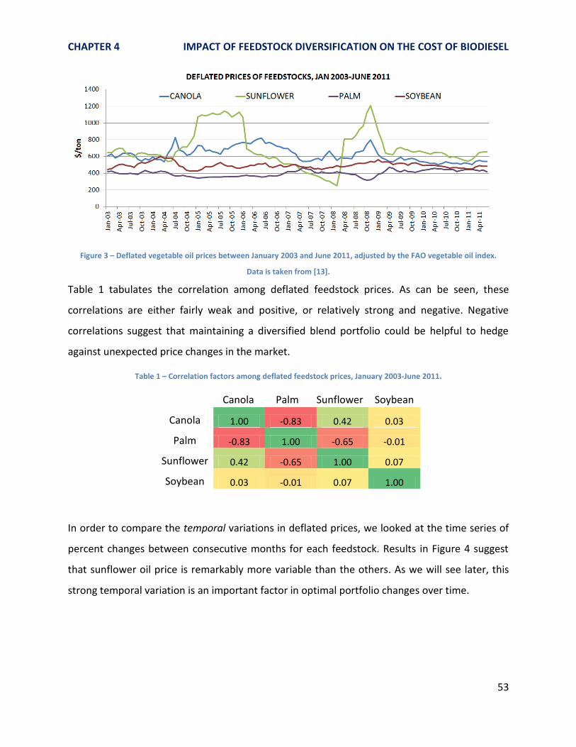
CHAPTER 4 IMPACT OF FEEDSTOCK DIVERSIFICATION ON THE COST OF BIODIESEL
53
Figure 3 – Deflated vegetable oil prices between January 2003 and June 2011, adjusted by the FAO vegetable oil index.
Data is taken from [13].
Table 1 tabulates the correlation among deflated feedstock prices. As can be seen, these
correlations are either fairly weak and positive, or relatively strong and negative. Negative
correlations suggest that maintaining a diversified blend portfolio could be helpful to hedge
against unexpected price changes in the market.
Table 1 – Correlation factors among deflated feedstock prices, January 2003-June 2011.
Canola Palm Sunflower Soybean
Canola 1.00 -0.83 0.42 0.03
Palm -0.83 1.00 -0.65 -0.01
Sunflower 0.42 -0.65 1.00 0.07
Soybean 0.03 -0.01 0.07 1.00
In order to compare the temporal variations in deflated prices, we looked at the time series of
percent changes between consecutive months for each feedstock. Results in Figure 4 suggest
that sunflower oil price is remarkably more variable than the others. As we will see later, this
strong temporal variation is an important factor in optimal portfolio changes over time.

CHAPTER 4 IMPACT OF FEEDSTOCK DIVERSIFICATION ON THE COST OF BIODIESEL
54
Figure 4 – Percent changes between consecutive months in deflated feedstock prices.
The price data presented so far shows that although nominal biodiesel feedstock prices have
increased over time, there is no obvious trend of increase for deflated prices. In addition, Figure
3 suggests that the order of deflated prices did not change that much, mostly maintaining the
relationship pricepalm<pricesoybean<pricecanola<pricesunflower. Yet, the reported negative
correlations between price variations shown in Table 1 signal historical instances where
changes in prices were in opposite directions for different feedstocks. This observation suggests
that adjusting the optimal blend portfolio over time might lead to cost reductions for the final
fuel.
In the following sections, we will show that varying and diversifying the blend portfolio when
there are opportunities to use low-cost feedstocks might lead to significant cost reductions. In
analyzing these opportunities, we will apply the CC optimization model on the deflated price
data of the four main vegetable oils. Unless otherwise indicated, GHG emissions constraint is
not included in the analyses shown in this chapter.
In section 4.c, we continue with defining the set of specifications that the final fuel product is
required to meet.

CHAPTER 4 IMPACT OF FEEDSTOCK DIVERSIFICATION ON THE COST OF BIODIESEL
55
4.c) Biodiesel Specifications
The following subsections detail the biodiesel specifications we have chosen to represent in the
CC optimization model. For the remainder of this thesis, the constraint levels specified below
are used unless indicated otherwise.
4.c.1) Iodine Value (IV) – maximum 120
EN 14214 limits the IV of biodiesel by 120 maximum. Although this limit creates a very strong
bias against soybean, we have set the maximum IV limit to 120 in the model to represent the
EU biodiesel markets. Figure 5 illustrates the Monte Carlo simulations of the IV estimates for
biodiesel made from each feedstock. The non-compliant parts of the distributions are indicated
in red. While canola and palm meet the specification by almost 100%, both soybean and
sunflower distributions indicate a high degree of non-compliance.
Figure 5 – Monte Carlo simulations of IV estimates for biodiesel made from each feedstock. Non-compliant parts of the
distributions are shown in red.

CHAPTER 4 IMPACT OF FEEDSTOCK DIVERSIFICATION ON THE COST OF BIODIESEL
56
4.c.2) Oxidative Stability (OS) - minimum 4.5 hours
OS is determined by the Rancimat method where induction period is measured as a direct
indication of oxidation quality. ASTM D6751 and EN 14214 limit the induction period by
minimum 3 hours and 6 hours, respectively. Differences in the standards point toward
regionalism favoring domestic feedstocks over imported ones.18 Due to generally lower prices
of soybean compared to canola, when the OS limit is set to 3 hours, soybean is favored by the
model in the blend. On the other hand, if the OS limit is set to 6 hours, canola becomes the
dominant feedstock despite its higher price.
We use the average induction period constraint of the two standards, namely 4.5 hours. In
doing so, we aim to incorporate OS as a technical constraint without biasing the model results
by the national policies in place.
Figure 6 shows the Monte Carlo simulations of OS estimates predicted by the model. Again,
canola and palm distributions indicate a high degree of compliance in complete contrast to the
100% non-compliance rate of soybean and sunflower. Notice the particularly superior OS values
for palm.
18
Soybean, which is the main biodiesel feedstock in the US, has relatively low OS compared to canola, which is the main biodiesel feedstock in the EU.
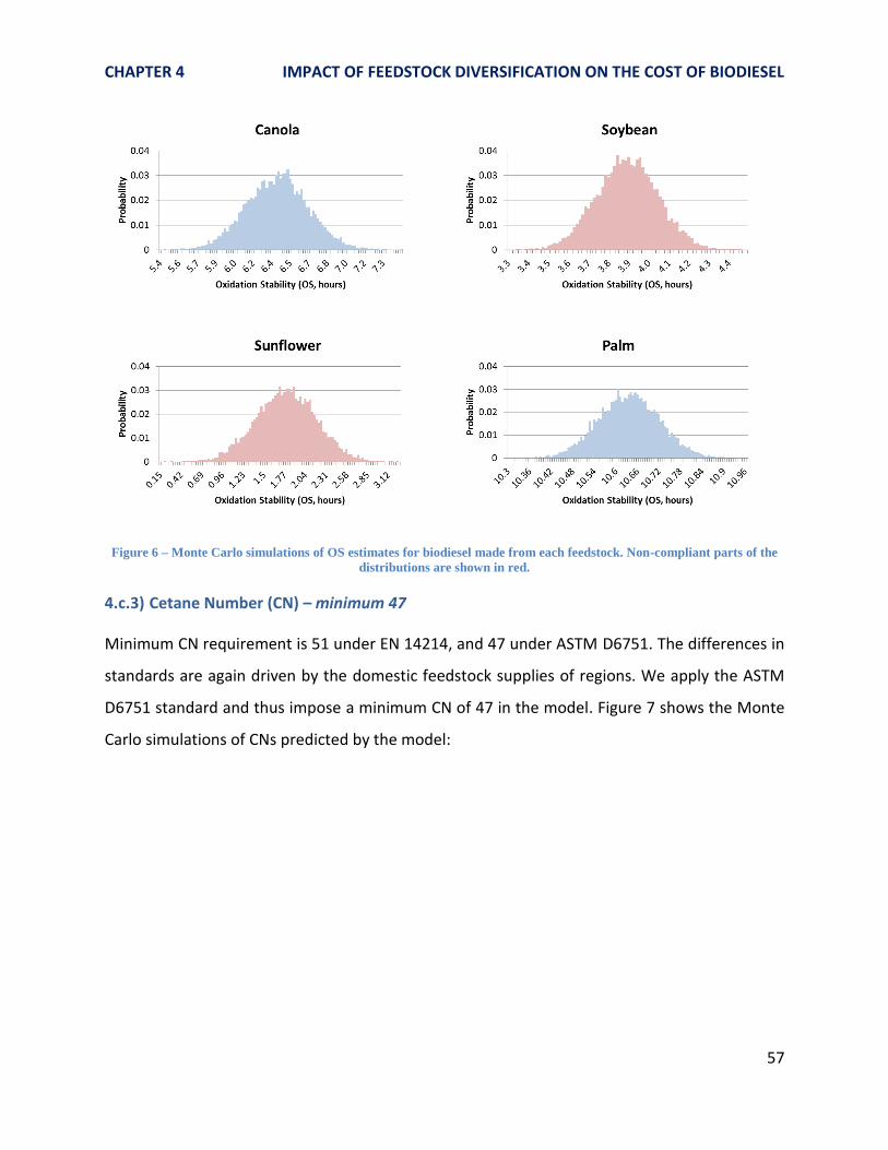
CHAPTER 4 IMPACT OF FEEDSTOCK DIVERSIFICATION ON THE COST OF BIODIESEL
57
Figure 6 – Monte Carlo simulations of OS estimates for biodiesel made from each feedstock. Non-compliant parts of the
distributions are shown in red.
4.c.3) Cetane Number (CN) – minimum 47
Minimum CN requirement is 51 under EN 14214, and 47 under ASTM D6751. The differences in
standards are again driven by the domestic feedstock supplies of regions. We apply the ASTM
D6751 standard and thus impose a minimum CN of 47 in the model. Figure 7 shows the Monte
Carlo simulations of CNs predicted by the model:

CHAPTER 4 IMPACT OF FEEDSTOCK DIVERSIFICATION ON THE COST OF BIODIESEL
58
Figure 7 – Monte Carlo simulations of CN estimates for biodiesel made from each feedstock. Non-compliant parts of the
distributions are shown in red.
4.c.4) Cold Filter Plugging Point (CFPP) – minimum -1˚C
Neither ASTM D6751 nor EN 14214 enforces a limit for CFPP, yet biodiesel producers are still
obliged to meet a certain level, either because of regional regulations or their customers’
demands. Note that CFPP requirement also changes according to the season as the warmer
months of the year might not necessitate a cold flow capability of the fuel.
The model uses -1˚C as the minimum CFPP limit. Although this constraint might be insufficient
for cold climates, it is a reasonable constraint for warmer regions where the winter months are
mild.
Figure 8 shows the Monte Carlo simulations of CFPPs predicted by the model. Palm has a
particularly inferior CFPP performance whereas all the other feedstocks meet the constraint by
100% probability.

CHAPTER 4 IMPACT OF FEEDSTOCK DIVERSIFICATION ON THE COST OF BIODIESEL
59
Figure 8 – Monte Carlo simulations of CFPP estimates for biodiesel made from each feedstock. Non-compliant parts of
the distributions are shown in red.
4.c.5) GHG Emissions Threshold – maximum 65% of petrodiesel emissions
According to the EU biofuel policies, starting from 2013, producers must demonstrate that the
lifecycle GHG emissions of their biodiesel is at least 35% less than the baseline fossil fuel. The
reduction requirement will be increased to 50% in 2017, and new installations after 2017 will
be subject to a 60% reduction. Thresholds in the US vary between 20% and 50% depending on
the category of biodiesel19.
For the baseline analysis we apply the current EU GHG emissions threshold which is 35%
reduction with respect to the fossil fuel reference. The fossil fuel reference is petrodiesel and its
lifecycle emissions are estimated to be 83.8 gCO2-eq/MJ [109]. For the GHG emissions
estimates, we refer to the reported mean values in BIOGRACE [27]. Yet, because the BIOGRACE
19
There are 5 biofuel categories defined under Renewable Fuel Standard program. These categories are called D3=cellulosic biofuel, D4=biomass-based biodiesel, D5=Advanced biofuel, D6=Renewable Fuel, D7=Cellulosic diesel. The GHG thresholds determined for each category are 60%, 50%, 50%, 20% and 60% respectively.
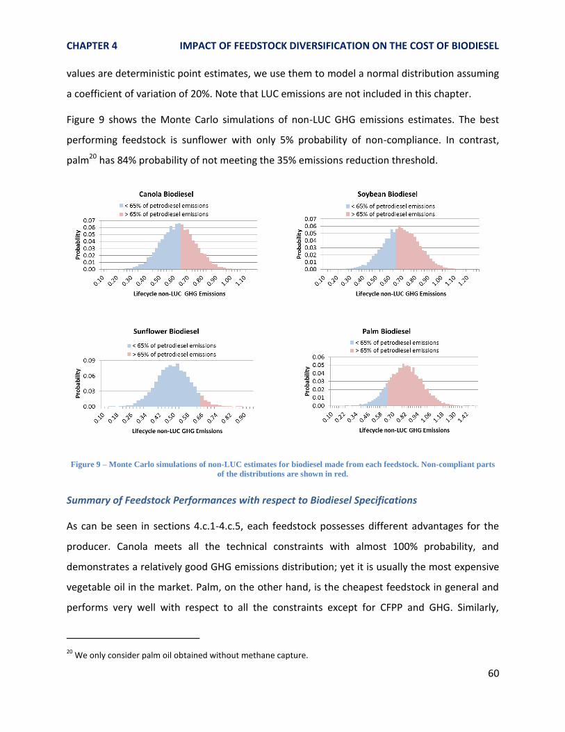
CHAPTER 4 IMPACT OF FEEDSTOCK DIVERSIFICATION ON THE COST OF BIODIESEL
60
values are deterministic point estimates, we use them to model a normal distribution assuming
a coefficient of variation of 20%. Note that LUC emissions are not included in this chapter.
Figure 9 shows the Monte Carlo simulations of non-LUC GHG emissions estimates. The best
performing feedstock is sunflower with only 5% probability of non-compliance. In contrast,
palm20 has 84% probability of not meeting the 35% emissions reduction threshold.
Figure 9 – Monte Carlo simulations of non-LUC estimates for biodiesel made from each feedstock. Non-compliant parts
of the distributions are shown in red.
Summary of Feedstock Performances with respect to Biodiesel Specifications
As can be seen in sections 4.c.1-4.c.5, each feedstock possesses different advantages for the
producer. Canola meets all the technical constraints with almost 100% probability, and
demonstrates a relatively good GHG emissions distribution; yet it is usually the most expensive
vegetable oil in the market. Palm, on the other hand, is the cheapest feedstock in general and
performs very well with respect to all the constraints except for CFPP and GHG. Similarly,
20
We only consider palm oil obtained without methane capture.

CHAPTER 4 IMPACT OF FEEDSTOCK DIVERSIFICATION ON THE COST OF BIODIESEL
61
sunflower and soybean oil are superior with respect to some properties but inferior with
respect to others. The producer’s goal is to obtain a biodiesel blend that costs as low as possible
while meeting all the constraints at a specified confidence level.
Table 2 summarizes the performance of each feedstock with respect to the specifications
described above:
Table 2 – Summary of individual feedstock performances with respect to biodiesel specifications. Percentages represent the compliance rate of the property distribution.
IV OS CN CFPP GHG
Canola (++)
99%
(++)
100%
(++)
100%
(++)
100%
(+)
59%
Soybean (--)
4%
(--)
0%
(-)
35%
(++)
100%
(-)
40%
Sunflower (-)
37%
(--)
0%
(+)
67%
(++)
100%
(++)
95%
Palm (++)
100%
(++)
100%
(++)
100%
(--)
0%
(--)
16%
(++) highly superior; (+) superior; (-) inferior; (--) highly inferior
4.d) Choice of Confidence Levels
As mentioned in Chapter 3, one of the strengths of the CC model is being able to specify the
confidence levels prior to solving a probabilistic optimization problem. In other words, the
model provides the user with the capability of incorporating preferred risk levels into the
feedstock selection process. Where properties are characterized by normal distributions, the
parameter that determines the risk level for each constraint is the test coefficient for the
Gaussian distribution, known as the z-value.

CHAPTER 4 IMPACT OF FEEDSTOCK DIVERSIFICATION ON THE COST OF BIODIESEL
62
In our model, for all the physical property constraints, we used the test coefficient of a one-
tailed21 Gaussian distribution z-value that corresponds to 95% confidence level. On the other
hand, realizing that in practice compliance with the GHG reduction threshold cannot be as strict
as the technical properties22, we relaxed the z-value down to 80% confidence level for the GHG
emissions constraint only. This means that every blend portfolio meets the GHG threshold by at
least 80% probability.
4.e) Chance-Constrained (CC) Optimization Formulation
The objective of the optimization is to minimize the feedstock cost of the blend subject to the
constraints described in Section 4.c. The general problem formulation was outlined in Chapter 3
in Eqns 3.6-3.26. A more detailed formulation that specifies the chosen confidence level for
each constraint is provided in Eqns 4.1-4.21.
The objective and biodiesel constraints are indicated in Eqns 4.1-4.8:
∑
(4.1)
Demand ∑
(4.2)
Supply ∑
(4.3)
Iodine Value (4.4)
Oxidation Stability (4.5)
21
Note that constraints we consider in the model are one-sided. In other words, each constraint has either a minimum or maximum requirement. This is the reason for choosing a one-tailed distribution test coefficient.
22 The level of monitoring the estimated lifecycle GHG emissions of each biodiesel batch is currently not clear in
the EU. In fact, according to the legislation language, the producers will not be able to use any feedstocks of which GHG emissions do not meet the 35% reduction criterion. Debates are continuing and the details of monitoring each batch belonging to each producer is not clarified. This is why we think choosing a lower confidence level is appropriate in the model.

CHAPTER 4 IMPACT OF FEEDSTOCK DIVERSIFICATION ON THE COST OF BIODIESEL
63
Cetane Number (4.6)
Cold Filter
Plugging Point
(4.7)
Greenhouse Gas
Emissions
(4.8)
where;
: unit price of feedstock i
: volume proportion of feedstock i in the blend
: total demand23
: supply of feedstock i
: test coefficient for normal distribution, 95% confidence level, one-tailed
: test coefficient for normal distribution, 80% confidence level, one-tailed
: mean IV of the blend
: IV constraint, maximum 120
: standard deviation of IV in the blend
: mean OS of the blend
: OS constraint, minimum 4.5 hours
: standard deviation of OS in the blend
: mean CN of the blend
: CN constraint, minimum 47
standard deviation of CN in the blend
: mean CFPP of the blend
: CFPP constraint, minimum -1 ˚C
: standard deviation of CFPP in the blend
23
Because we are interested in the proportions of feedstocks in the blend rather than the exact amounts, we represent the total demand with 1 in the model.
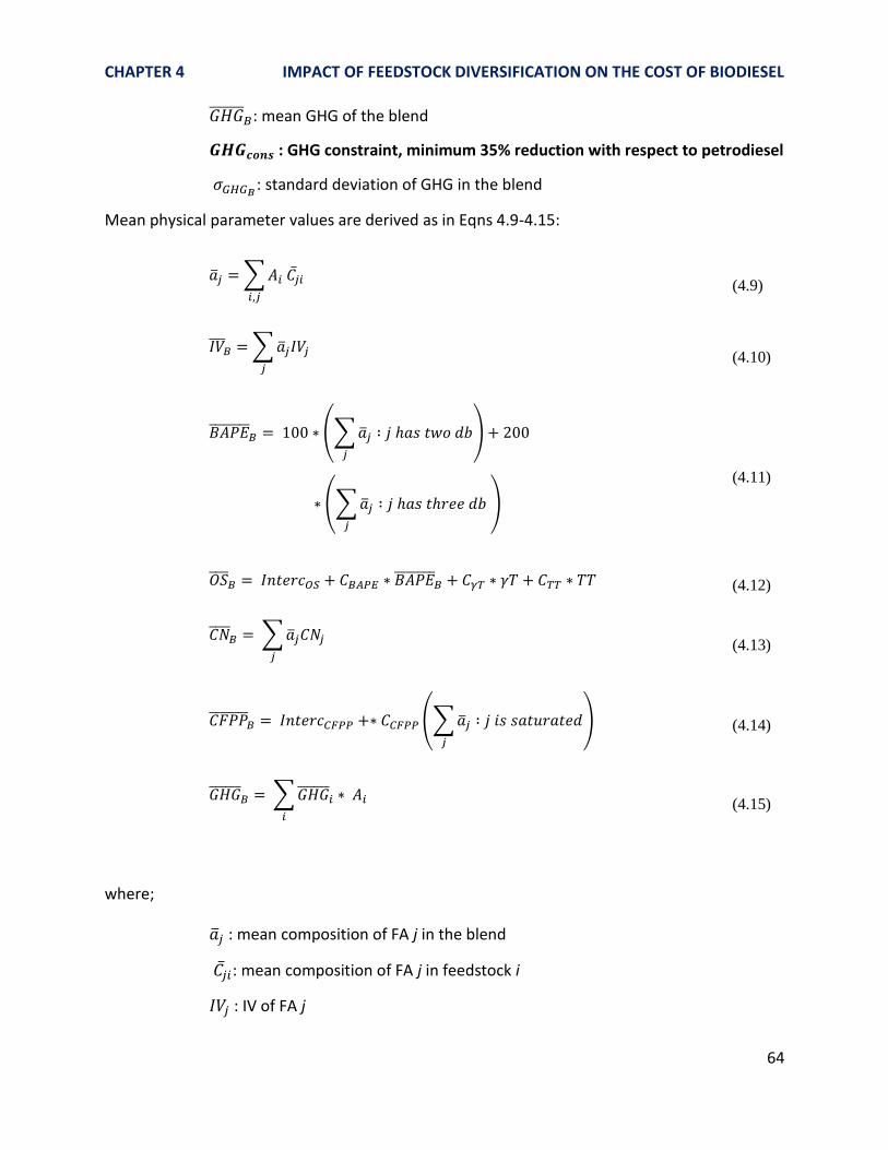
CHAPTER 4 IMPACT OF FEEDSTOCK DIVERSIFICATION ON THE COST OF BIODIESEL
64
: mean GHG of the blend
: GHG constraint, minimum 35% reduction with respect to petrodiesel
: standard deviation of GHG in the blend
Mean physical parameter values are derived as in Eqns 4.9-4.15:
∑
(4.9)
∑
(4.10)
(∑
)
(∑
)
(4.11)
(4.12)
∑
(4.13)
(∑
) (4.14)
∑
(4.15)
where;
: mean composition of FA j in the blend
: mean composition of FA j in feedstock i
: IV of FA j

CHAPTER 4 IMPACT OF FEEDSTOCK DIVERSIFICATION ON THE COST OF BIODIESEL
65
: mean BAPE of the blend
: Intercept in the OS regression equation
: Coefficient of BAPE in the OS regression equation
coefficient of γ-T in the oxidation stability regression equation
amount of γ-tocopherol in the blend
coefficient of TT in the oxidation stability regression equation
amount of tocotrienol in the blend
: CN of FA j
: CFPP of FA j
: Intercept in the CFPP regression equation
: Coefficient of total saturation in the CFPP regression equation
: mean GHG of feedstock i
Standard deviations are derived as in Eqns 4.16-21:
√∑
(4.16)
√∑
(4.17)
√∑
(4.18)
√ ( ∑
∑
) (4.19)
√
∑
(4.20)

CHAPTER 4 IMPACT OF FEEDSTOCK DIVERSIFICATION ON THE COST OF BIODIESEL
66
√∑
(4.21)
where;
: standard deviation of composition of FA j in the blend
: standard deviation of composition of FA j in feedstock i
: standard deviation of GHG emission of feedstock i
Finally, note that our model does not consider the following aspects in order to maintain the
generality of the results:
Supply constraints that the producers might face at any point in time.
Binding bilateral contracts between the suppliers and the producers.
Delays in between orders and delivery24.
Impact of demand-supply quantities on the market clearing price25.
4.f) Model Scenarios
We analyzed a series of scenarios which included different sets of feedstocks available to the
user at the commodity price prior to making a blend decision. As expected, because of the
existing constraints, not every combination of feedstocks results in a feasible set. Table 3 shows
the feasibility of each possible blend set. The first column shows the feasibility results without
any GHG emissions constraint, whereas the second column also include the 35% GHG emissions
reduction threshold.
24
Portuguese producers have indicated a duration of one month between the purchase and delivery.
25 This is a reasonable assumption because the market for biodiesel is much smaller than other markets that trade
vegetable oils. Therefore changes in supply and demand quantities due to the economic activity in the biodiesel industry would not be enough to shift market clearing prices.

CHAPTER 4 IMPACT OF FEEDSTOCK DIVERSIFICATION ON THE COST OF BIODIESEL
67
Table 3 – Feasibility table for each possible blend set.
Feasibility without 35% GHG Reduction
Feasibility with 35% GHG Reduction
1 Feedstock CANa F* NF**
SYBb NF NF SNFc NF NF PLMd NF NF
2 Feedstocks CAN-PLM F NF
CAN-SYB F NF CAN-SNF F NF SYB-SNF NF NF SYB-PLM NF NF
SNF-PLM NF NF
3 Feedstocks CAN-SYB-PLM F NF
CAN-SNF-PLM F F CAN-SYB-SNF F NF SYB-SNF-PLM NF NF
4 Feedstocks CAN-SYB-SNF-PLM F F
a Canola;
b Soybean;
c Sunflower,
d Palm;
* Feasible;
** Not feasible
4.g) CC Optimization Model Applied to Single Period Price Data
4.g.1) Sensitivity Analysis on the CFPP Constraint Level
To illustrate the model behavior with respect to changes in the industry standards, we
performed a set of sensitivities on the CFPP constraint26. In performing these sensitivities, we
used the deflated feedstock prices observed in April 2007. These prices were $567, $485, $457
and $438 per ton of canola, soybean, sunflower and palm oil, respectively.
Figure 10 shows how the feedstock cost of biodiesel changes with respect to the CFPP
constraint. Note that although the other technical constraints are present, we have excluded
the GHG constraint from this analysis.
When the constraint is more restrictive, relaxing the maximum allowable CFPP limit results in
cost reductions of the blend in a linear fashion. When the constraint becomes less binding, the
26
CFPP is chosen arbitrarily among the other binding constraints.

CHAPTER 4 IMPACT OF FEEDSTOCK DIVERSIFICATION ON THE COST OF BIODIESEL
68
rate of cost reduction starts to fall down because other constraints in the system continue to be
binding the optimal solution.
Figure 10 – Sensitivity of feedstock cost of biodiesel with respect to CFPP constraint.
This sensitivity analysis illustrates that the model is capable of estimating the marginal cost of
changing the CFPP standards. And this capability can be quite useful for the producer. For
example, if the producer sells the product to a cold-climate market and therefore needs to
meet a stringent -4˚C standard, the feedstock costs will be about $43/ton higher than if the
constraint was 0˚C, and about $70/ton higher than if the constraint was 4˚C. Depending on the
market price of biodiesel in different climate regions, the producer can strategically position the
product and engineer its properties accordingly. Marginal cost estimation capability can also
serve as an analytical tool in guiding the industry standards that would be technically
acceptable but also economically feasible for the biodiesel industry to survive and compete
with conventional fuels.
It is important to realize that this analysis is performed under a system where four different
feedstocks are available. Thus, the producer has an extensive decision space in which the
optimal solution is obtained after evaluating every possible combination of the four feedstocks.
Figure 11 illustrates the resulting optimal blend portfolios with respect to changes in the CFPP
limit. Notice the reduction in canola use as the constraint becomes less binding, and the
increase in sunflower and palm which are cheaper and inferior to canola in terms of the CFPP
characteristics (revisit Figure 8).

CHAPTER 4 IMPACT OF FEEDSTOCK DIVERSIFICATION ON THE COST OF BIODIESEL
69
Figure 11 – Optimal blend portfolios under varying CFPP constraints.
It is also important to remember that the resulting property values are distributions rather than
point estimates, and each optimal solution is expected to have a maximum of 5% non-
compliance rate, i.e. the probability of violating the constraint. By performing Monte Carlo
analyses on the optimal blend portfolios, we simulated 10,000 CFPP estimations for each blend
in Figure 11. Out of the 10,000 simulation results, we determined the ones that possessed a
higher CFPP than the maximum allowable limit. In Figure 12, histograms of three blend
simulations are shown. Corresponding maximum CFPP limits are -4 ˚C, 0˚C and 4 ˚C. The red
parts of the distributions indicate the probability of violating the CFPP limit, and are 4.65%,
4.45% and 4.61%, respectively. These non-compliance rates, which are all less than 5%, confirm
the reliability of the CC optimization algorithm outlined earlier that had a 95% confidence level
as part of the constraint set. This analysis shows that the performance of the model does not
deteriorate as the level of a binding constraint changes, and that the model is capable of
maintaining the compliance rate at various constraint levels for the optimal solution.

CHAPTER 4 IMPACT OF FEEDSTOCK DIVERSIFICATION ON THE COST OF BIODIESEL
70
Figure 12 – Monte Carlo simulations of optimal blend CFPP distributions under different CFPP limits.
4.g.2) Sensitivity Analysis on Blend Diversification
Blend Portfolios and Feedstock Costs
In this section, we analyze the changes in feedstock cost of biodiesel by changing the degree of
blend diversification while keeping the constraints constant as described in Section 4.c,
excluding the GHG emissions constraint. Again, we use the deflated feedstock prices of April
2007.
Figure 13 illustrates the increase in feedstock cost when the number of available feedstocks to
the producer is reduced. The x-axis indicates which feedstocks are present in each blend set.
Remember from Table 2 that the only feedstock that is feasible when used 100% is canola.
Therefore, even though the other feedstocks are usually cheaper than canola, they cannot be
used alone and meet all the technical constraints simultaneously.

CHAPTER 4 IMPACT OF FEEDSTOCK DIVERSIFICATION ON THE COST OF BIODIESEL
71
Figure 13 – Feedstock costs and optimal blend portfolios with respect to blend diversification. April 2007 deflated feedstock
prices are used.
Not surprisingly, the cost does not demonstrate a smooth increase when we move from 4-
feedstock, to 3-feedstock, or from 3-feedstock to 2-feedstock blends. Because the feedstock
property and the constraint space is relatively discrete, when the optimal solution moves from
one corner to another, the change in cost, i.e. the objective of the optimization formulation,
does not necessarily increase monotonically. In fact, the presence or absence of a critical
feedstock can abruptly change the results regardless of the degree of diversification. In the
model, canola is the critical feedstock that exists in all feasible combinations and taking it out to
observe the change in biodiesel cost is not even possible, due to resulting infeasibilities.
Nevertheless, a general increasing trend in costs is apparent in Figure 13 as fewer feedstocks
become available to the producer.
Figure 13 also shows the resulting optimal feedstock proportions under each blend set. When
all the four feedstocks are available, the producer is able to diversify the portfolio using all of
them. Comparing CAN-SYB-SNF-PLM (4-feedstock blend) with CAN-SYB-SNF (3-feedstock-blend)
highlights the advantage of diversification. There is a subtle but significant difference between
the blend use distributions of these two optimal portfolios. In the former, the use of each
feedstock is relatively comparable, whereas when palm is excluded in the latter, canola has to

CHAPTER 4 IMPACT OF FEEDSTOCK DIVERSIFICATION ON THE COST OF BIODIESEL
72
be included in a much larger proportion. In fact, the proportions of soybean and sunflower are
reduced in the absence of palm, and consequently this shift results in a substantial cost
increase for biodiesel. As can be observed, the feedstock cost of the former blend is $485/ton
whereas it is $527/ton for the latter one. This is a 9% increase in the total feedstock cost of
biodiesel.
Monte Carlo Simulations
Another important comparison metric is the performance of the biodiesel blend with respect to
each quality constraint. Therefore, we compare the resulting IV, OS, CN and CFPP distributions
of CAN-SYB-SNF-PLM with CAN in Figure 14. The x-axes of the distributions have identical scales
for ease of comparison. Notice that CAN has wider distributions in general and over-performs
with respect to the constraints at the specified confidence level. In other words, none of the
constraints ever become binding for 100% canola biodiesel. In contrast, the 4-feedstock blend,
CAN-SYB-SNF-PLM, has tighter distributions, particularly when the constraint becomes binding
for OS and CFPP. From the perspective of the producer whose goal is to meet every constraint
with at least 95% confidence level, both blends are good enough to sell in the market. Yet, as
we have seen in Figure 13, CAN costs 9% more than CAN-SYB-SNF-PLM.
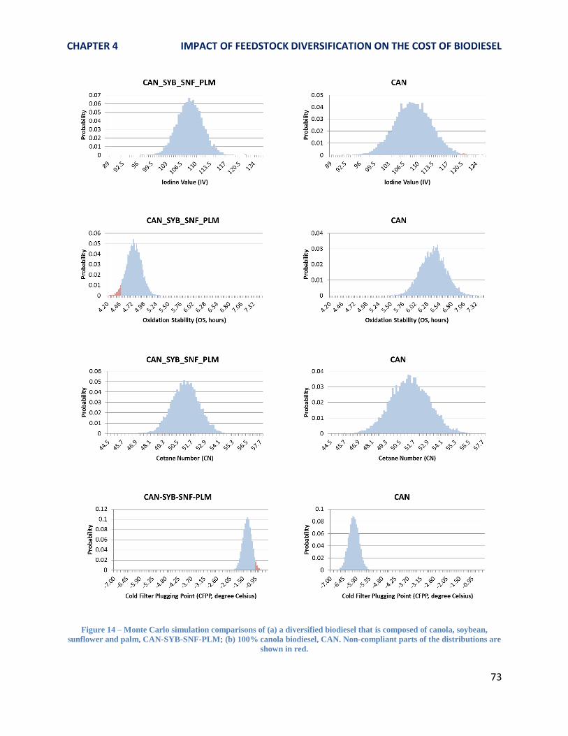
CHAPTER 4 IMPACT OF FEEDSTOCK DIVERSIFICATION ON THE COST OF BIODIESEL
73
Figure 14 – Monte Carlo simulation comparisons of (a) a diversified biodiesel that is composed of canola, soybean,
sunflower and palm, CAN-SYB-SNF-PLM; (b) 100% canola biodiesel, CAN. Non-compliant parts of the distributions are
shown in red.

CHAPTER 4 IMPACT OF FEEDSTOCK DIVERSIFICATION ON THE COST OF BIODIESEL
74
4.h) CC Optimization Model Applied to Multiple Period Price Data
4.h.1) Sensitivity Analysis on Constraint Levels
In order to observe how the historical blend portfolios and costs would differ with respect to
changing constraint levels in CFPP, OS and GHG, we ran the CC optimization model on the
monthly data between January 2003 and June 2011. Because CN and IV rarely become binding,
we excluded them from the analyses in this section.
Sensitivity on the CFPP Constraint
Figure 15 shows how the historical optimal portfolios change when the maximum CFPP limit is
(a) -2˚C, (b) -1˚C and (c) 0˚C. Note that although the other technical constraints are present, we
did not include the GHG constraint in the optimization formulation for this analysis.
Similar to the single period price data observation presented in Section 4.g, we see a reduction
in the overall use of canola and an increase in palm and sunflower as the constraint is relaxed.
Figure 15 – Historical optimal blend portfolios when the CFPP constraint is (a) -2 ˚C, (b) -1˚C and (c) 0˚C.

CHAPTER 4 IMPACT OF FEEDSTOCK DIVERSIFICATION ON THE COST OF BIODIESEL
75
Figure 16 shows the resulting feedstock cost of biodiesel over time. The differences between
the curves reflect the marginal cost of tightening the constraint from 0˚C to -1˚C, and from -1˚C
to -2 ˚C. Depending on the relative prices of feedstocks, some months demonstrate a relatively
high cost difference, whereas in other months, feedstock cost of biodiesel almost converges to
a single point.
Figure 16 – Feedstock cost of biodiesel subject to different CFPP limits.
Sensitivity on the OS Constraint
Figure 17 shows how the historical optimal portfolios change when the minimum OS limit is (a)
6 hours, (b) 4.5 hours, and (c) 3 hours. Again, although all the other technical constraints are
present, we did not include the GHG emissions constraint in the optimization formulation for
this analysis.
A reduction in the overall use of canola and an increase in soybean are observed as the
constraint is relaxed from 6 hours to 3 hours. The particular increase in the use of soybean
explains why the US industry standard for OS is only 3 hours. Soybean is the most common
domestic biodiesel feedstock in the US and can be a very attractive option for the producer
when the OS limit is low.
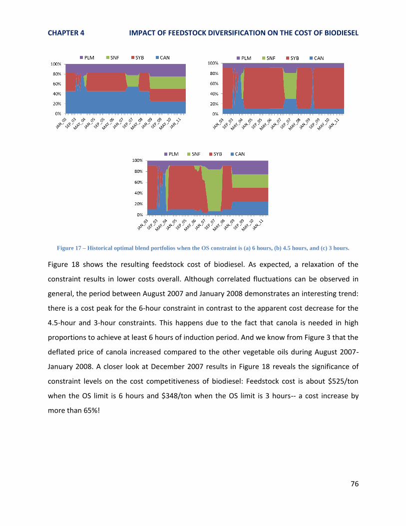
CHAPTER 4 IMPACT OF FEEDSTOCK DIVERSIFICATION ON THE COST OF BIODIESEL
76
Figure 17 – Historical optimal blend portfolios when the OS constraint is (a) 6 hours, (b) 4.5 hours, and (c) 3 hours.
Figure 18 shows the resulting feedstock cost of biodiesel. As expected, a relaxation of the
constraint results in lower costs overall. Although correlated fluctuations can be observed in
general, the period between August 2007 and January 2008 demonstrates an interesting trend:
there is a cost peak for the 6-hour constraint in contrast to the apparent cost decrease for the
4.5-hour and 3-hour constraints. This happens due to the fact that canola is needed in high
proportions to achieve at least 6 hours of induction period. And we know from Figure 3 that the
deflated price of canola increased compared to the other vegetable oils during August 2007-
January 2008. A closer look at December 2007 results in Figure 18 reveals the significance of
constraint levels on the cost competitiveness of biodiesel: Feedstock cost is about $525/ton
when the OS limit is 6 hours and $348/ton when the OS limit is 3 hours-- a cost increase by
more than 65%!

CHAPTER 4 IMPACT OF FEEDSTOCK DIVERSIFICATION ON THE COST OF BIODIESEL
77
Figure 18 - Feedstock cost of biodiesel subject to different OS limits.
Sensitivity on the GHG Emissions Constraint
In this section, we keep all the technical constraints, namely CFPP, OSI, IV and CN, and add the
GHG emissions constraint to the optimization formulation. Note there is no consideration of
LUC emissions in this chapter. A detailed emissions analysis that includes LUC will be presented
in Chapter 5.
Figure 19 shows how the historical optimal portfolios change when the maximum GHG
emissions limit is (a) 65%, (b) 67.5%, and (c) 70% of petrodiesel emissions. As the constraint is
relaxed, a decrease in the use of sunflower and a considerable increase in the use of soybean
are observed. In fact, this result is expected based on the feedstock prices shown in Figure 3
and GHG emissions distributions shown in Figure 9. In general, soybean oil is the second
cheapest feedstock among the four, but its GHG emissions estimates are high, making it an
attractive candidate only when the GHG limit is not too tight.

CHAPTER 4 IMPACT OF FEEDSTOCK DIVERSIFICATION ON THE COST OF BIODIESEL
78
Figure 19 – Historical optimal blend portfolios when the GHG constraint is (a) 65%, (b) 67.5%, and (c) 70% of
petrodiesel emissions.
Figure 20 shows the resulting feedstock cost of biodiesel. As expected, a relaxation on the
constraint results in lower costs overall. However, depending on the relative prices of
feedstocks, the cost might be insensitive to the small variations in the GHG emissions
constraint. This effect can be observed particularly between March 2007 and March 2008.
Figure 20 – Feedstock cost of biodiesel subject to different GHG limits.

CHAPTER 4 IMPACT OF FEEDSTOCK DIVERSIFICATION ON THE COST OF BIODIESEL
79
4.h.2) Sensitivity Analysis on Blend Diversification
By implementing the CC optimization formulation outlined in Section 4.e on the deflated
monthly price data between January 2003 and June 2011, we obtained the historical optimal
portfolios for each blend subset described in Table 3.
Figure 21 demonstrates the distribution of each feedstock in the optimal blends. No GHG
emissions constraint is included, and all the other technical constraints are met by at least 95%
confidence level at each point in time.
As can be observed, inclusion of more feedstock options into the system enables the producer
to be flexible and vary the portfolio according to the market prices to minimize the feedstock
cost. A detailed cost analysis will be presented in Section 4.h.3, but comparing the changes in
blend portfolios here provides crucial insight about the model. For example, comparing CAN-
PLM and CAN-SYB-SNF-PLM portfolios in Figure 21 clearly shows that because the producer is
restricted to canola and palm only in the 2-feedstock blend, the portfolio does not change
between 2003 and 2011. On the other hand, because the producer is allowed to mix sunflower
and soybean in the latter blend, the portfolio demonstrates interesting patterns of different
feedstock proportions over time. Another interesting observation is the consistent inclusion of
sunflower in the blend sets (when it is allowed) for certain time intervals between 2003 and
2011. The feedstock prices in Figure 3 support the model decision to include sunflower at those
time intervals, because sunflower prices plummeted between January 2006 and February 2008.

CHAPTER 4 IMPACT OF FEEDSTOCK DIVERSIFICATION ON THE COST OF BIODIESEL
80
Figure 21 - Historical optimal blend portfolios for the model scenarios described in Section 4.f. No GHG emissions
constraint is included. CFPP, CN, IV and OS constraints are met by at least 95% confidence level.

CHAPTER 4 IMPACT OF FEEDSTOCK DIVERSIFICATION ON THE COST OF BIODIESEL
81
In order to illustrate how the portfolios might change when a new constraint is added, we have
also plotted the historical optimal portfolios with the GHG emissions constraint at 35%
reduction threshold in Figure 22. Remember from Table 3 that the only blend sets that are
feasible with a GHG limit were CAN-SNF-PLM and CAN-SNF-SYB-PLM. Comparing these blends
in Figure 22 with their equivalents in Figure 21 shows that a GHG limit might change the
producers’ blend portfolio to a significant extent. Obviously, addition of the GHG limit comes at
a cost for the producer which will be examined in Section 4.h.3, and later in more detail in
Chapter 5.
Figure 22 - Historical optimal blend portfolios for the model scenarios described in Section 4.e. 35% GHG reduction threshold is included at 80% confidence level. CFPP, CN, IV and OS constraints are met by at least 95% confidence level.
4.h.3) Analysis of Feedstock Cost of Biodiesel
In the following sub-sections, we report the changes in biodiesel feedstock costs under various
blend sets.
Time Series of Optimal Blend Costs
Figure 23 shows the feedstock cost of biodiesel over years assuming that only the specified
feedstocks were available to the producer. The blend is optimized subject to the constraints
outlined in Section 4.c, but does not include the GHG threshold. As expected, increasing
diversification in the portfolio leads to lower unit costs for biodiesel. Cost reduction in January
2005 is the largest among the other months, and using the 4-feedstock blend over 100% canola
results in 38% savings.
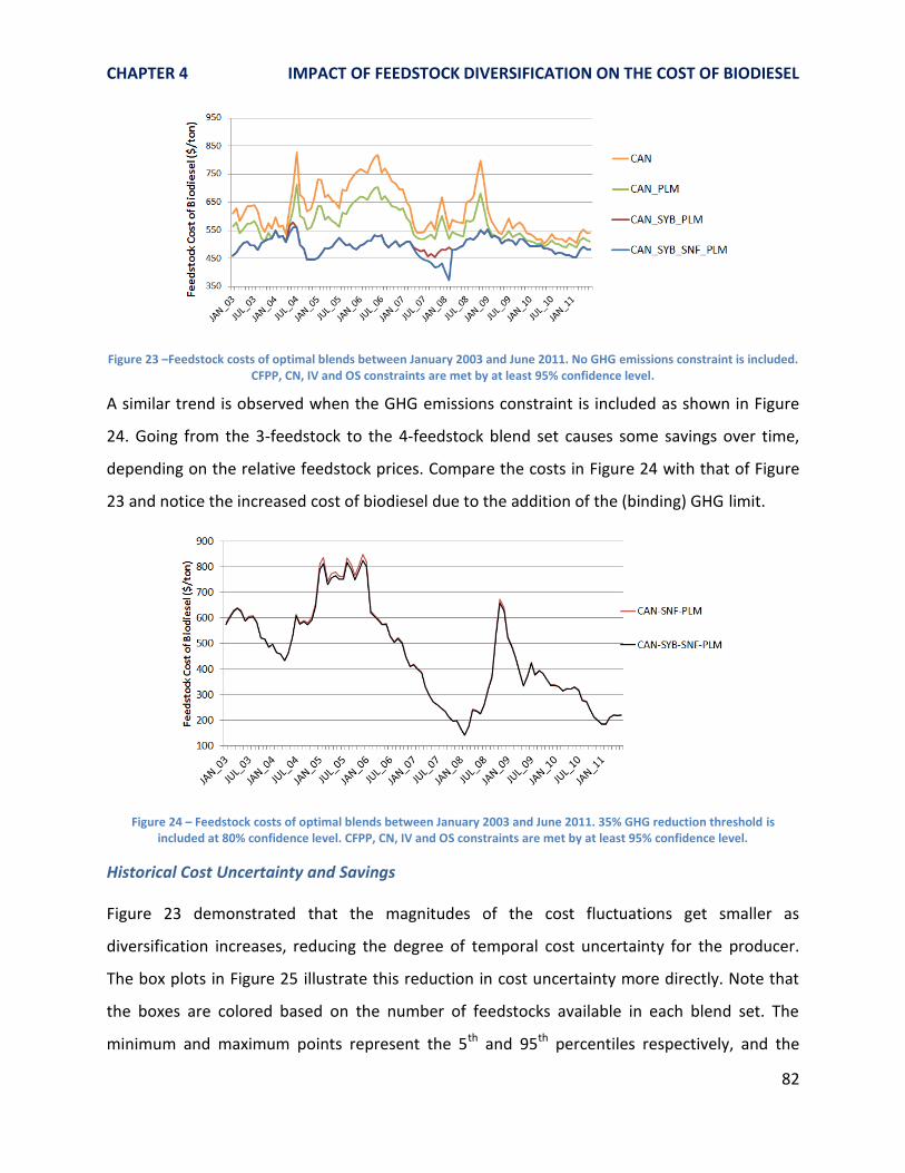
CHAPTER 4 IMPACT OF FEEDSTOCK DIVERSIFICATION ON THE COST OF BIODIESEL
82
Figure 23 –Feedstock costs of optimal blends between January 2003 and June 2011. No GHG emissions constraint is included.
CFPP, CN, IV and OS constraints are met by at least 95% confidence level.
A similar trend is observed when the GHG emissions constraint is included as shown in Figure
24. Going from the 3-feedstock to the 4-feedstock blend set causes some savings over time,
depending on the relative feedstock prices. Compare the costs in Figure 24 with that of Figure
23 and notice the increased cost of biodiesel due to the addition of the (binding) GHG limit.
Figure 24 – Feedstock costs of optimal blends between January 2003 and June 2011. 35% GHG reduction threshold is included at 80% confidence level. CFPP, CN, IV and OS constraints are met by at least 95% confidence level.
Historical Cost Uncertainty and Savings
Figure 23 demonstrated that the magnitudes of the cost fluctuations get smaller as
diversification increases, reducing the degree of temporal cost uncertainty for the producer.
The box plots in Figure 25 illustrate this reduction in cost uncertainty more directly. Note that
the boxes are colored based on the number of feedstocks available in each blend set. The
minimum and maximum points represent the 5th and 95th percentiles respectively, and the

CHAPTER 4 IMPACT OF FEEDSTOCK DIVERSIFICATION ON THE COST OF BIODIESEL
83
black dots represent the median. In fact, analyzing the cost uncertainty based on historical cost
ranges is tricky because the range might be high due to cost reductions taking place at certain
points in time. Consider the most diversified blend, CAN-SYB-SNF-PLM, and observe that it
demonstrates a small degree of variation over time, but not the smallest among all the blend
sets. For example, CAN-SYB-PLM has a smaller cost range, hence smaller degree of cost
uncertainty associated with it. However, the increased uncertainty in the former blend emerges
from the presence of sunflower and the resulting feedstock cost reduction opportunities
manifested at certain points in time, particularly between January 2006 and February 2008. In
other words, the cost uncertainty might be a little bit higher in the former blend, but it does not
mean that this is an undesired outcome for the biodiesel producer.
Figure 25 - Box plots of feedstock costs of biodiesel blends optimized monthly between January 2003 and June 2011. No
GHG emissions constraint is included. The lowest and highest points for each blend set represent the 5th
and 95th
percentile and the black dots represent the medians. Boxes are colored based on the number of feedstocks included in the blend set.
As we move towards less diversified blends, not only the difference between the 1st and 3rd
quartiles gets larger, but also the minimum cost that can be achieved gets higher. This means
that producers are exposed to cost fluctuations under higher costs to a significant extent when
they limit their operations to 1 or 2 feedstocks only.

CHAPTER 4 IMPACT OF FEEDSTOCK DIVERSIFICATION ON THE COST OF BIODIESEL
84
Cost histograms in Figure 26 are included to have a closer look at the population characteristics
of the box plots in Figure 25, and to understand what drives the cost uncertainty. The blend
sets that include sunflower stand out with low cost subpopulations that can be characterized as
outliers. As discussed before, these occurrences are a result of low sunflower prices observed in
certain time periods between 2003 and 2011. Similarly, an apparent dispersion in the
distribution can be observed for the blend sets that have either 2 feedstocks or 1 feedstock
only. This dispersion indicates a high degree of exposure to feedstock price volatility.

CHAPTER 4 IMPACT OF FEEDSTOCK DIVERSIFICATION ON THE COST OF BIODIESEL
85
Figure 26 – Histograms of historical optimal blend costs for each blend subset.
Another critical cost performance metric is the average cost for each blend set observed over
2003-2011. In Figure 27, we plotted this metric normalized by the least diversified blend,
namely 100% canola biodiesel. As can be seen, the most diversified blend leads to more than
20% savings on average compared to 100% canola.
Figure 27 – Average unit cost of biodiesel, normalized by the cost of the least diversified blend.
Comparison of Cumulative Savings under Different Cost Reduction Strategies
It is important to note that all the analyses above were concerned about the cost of producing
one unit, namely 1 metric ton of biodiesel. An average biodiesel production facility can produce
up to 100,000 tons annually. As Figure 27 suggested, considerably lower feedstock costs can be
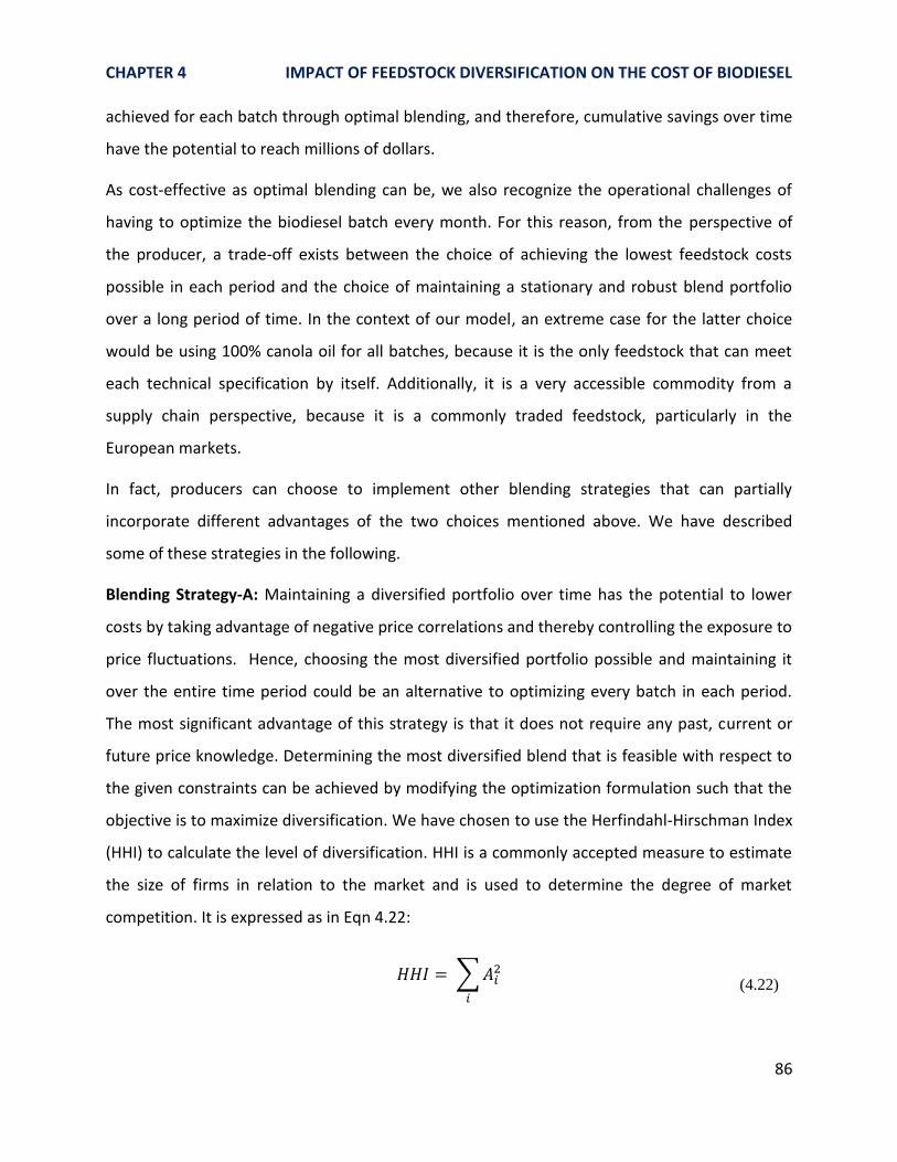
CHAPTER 4 IMPACT OF FEEDSTOCK DIVERSIFICATION ON THE COST OF BIODIESEL
86
achieved for each batch through optimal blending, and therefore, cumulative savings over time
have the potential to reach millions of dollars.
As cost-effective as optimal blending can be, we also recognize the operational challenges of
having to optimize the biodiesel batch every month. For this reason, from the perspective of
the producer, a trade-off exists between the choice of achieving the lowest feedstock costs
possible in each period and the choice of maintaining a stationary and robust blend portfolio
over a long period of time. In the context of our model, an extreme case for the latter choice
would be using 100% canola oil for all batches, because it is the only feedstock that can meet
each technical specification by itself. Additionally, it is a very accessible commodity from a
supply chain perspective, because it is a commonly traded feedstock, particularly in the
European markets.
In fact, producers can choose to implement other blending strategies that can partially
incorporate different advantages of the two choices mentioned above. We have described
some of these strategies in the following.
Blending Strategy-A: Maintaining a diversified portfolio over time has the potential to lower
costs by taking advantage of negative price correlations and thereby controlling the exposure to
price fluctuations. Hence, choosing the most diversified portfolio possible and maintaining it
over the entire time period could be an alternative to optimizing every batch in each period.
The most significant advantage of this strategy is that it does not require any past, current or
future price knowledge. Determining the most diversified blend that is feasible with respect to
the given constraints can be achieved by modifying the optimization formulation such that the
objective is to maximize diversification. We have chosen to use the Herfindahl-Hirschman Index
(HHI) to calculate the level of diversification. HHI is a commonly accepted measure to estimate
the size of firms in relation to the market and is used to determine the degree of market
competition. It is expressed as in Eqn 4.22:
∑
(4.22)

CHAPTER 4 IMPACT OF FEEDSTOCK DIVERSIFICATION ON THE COST OF BIODIESEL
87
where is the proportion of each component in the system, i.e. the market share of Firm-A, or
the volume proportion of feedstock-X in the blend, etc.
Diversification in a system is maximized when HHI is minimized. Therefore, we changed the
objective of the CC optimization as in Eqn 4.23. Note that all the other constraints remain the
same.
∑
(4.23)
Blending Strategy-B: Consider a hypothetical situation in which a producer wants to set a single
stationary blending rule to be used throughout the entire period of interest and has complete
information about the future prices ex ante. Then, the optimal stationary portfolio would be
the one that minimizes the total costs integrated over time. All the constraints remaining the
same, the objective of the optimization can be formulated as in Eqn 4.24:
∑
(4.24)
where is deflated price of feedstock i in time period t, and is the volume proportion of
feedstock i in the blend in time period t. Note that we use deflated prices to find the optimal
portfolio. Otherwise, because the nominal prices are larger in magnitude in the more recent
years due to inflation, the optimal blend portfolio would be biased by the latest prices observed
in the market.
Blending Strategy-C: Blending Strategy-B required the precise knowledge of future prices.
Recognizing the impossibility of such a scenario in real world, we introduce a semi-stationary
blending rule that uses the blend portfolio which minimizes the previous year’s total feedstock
costs. Optimization is performed on an annual basis under this strategy. Because consecutive
years’ prices are expected to be similar, adjusting the blend on an annual basis might provide a
limited degree of cost certainty to the producer.

CHAPTER 4 IMPACT OF FEEDSTOCK DIVERSIFICATION ON THE COST OF BIODIESEL
88
Figure 28 shows the stationary blend portfolios corresponding to the blending strategies
described above. Observe the high degree of diversification for Blending Strategy-A, but notice
that there is a slight divergence from the theoretical maximum degree of diversification, which
is achieved when all the components in a mix are in equal proportions. The underlying reason is
the existence of technical constraints that the final product is subject to. In Blending Strategy-B,
the blend is primarily composed of soybean due to desired technical properties along with
relatively low costs over 2003-2011. The annually optimized blend portfolios in Blending
Strategy-C are very similar to that of Blending Strategy-B, except for the year 2008. This
significant change in 2008 takes place due to very low sunflower prices observed in 2007.
Figure 28 – Stationary blend portfolios optimized under different blending strategies.
Figure 29 shows cumulative savings of implementing a variety of blending scenarios, including
the three strategies described above, compared to the baseline of using 100% canola oil only.
The blue bars on the left represent cost savings of the monthly optimized blend sets, and the
available feedstocks to the producer are indicated on the x-axis. The bars on the right represent
the savings of the three stationary blending strategies. The numbers reported on the y-axis are
in nominal dollars.
Monthly optimization of the blend using 4 feedstocks has the greatest cost advantage and leads
to more than $150 million savings over 2003-2011. Even using 2 feedstocks lowers the
feedstock costs substantially, leading to savings between $23 million and $63 million depending
on the specific blend set.
Stationary blend strategies lead to cost savings of $63 million, $142 million and $111 million
corresponding to Blending Strategy A, B and C respectively. Because Blending Strategy-B can be

CHAPTER 4 IMPACT OF FEEDSTOCK DIVERSIFICATION ON THE COST OF BIODIESEL
89
applied only under hypothetical conditions, it can be regarded as the lower bound of a
stationary blend rule. Comparison of Blending Strategy-A and Blending Strategy-C with the
monthly optimization scenarios indicates that a well-designed stationary blending rule can
approximately achieve the cost performance equivalent to that of 2 or 3-feedstock blend sets
over time.
Figure 29 – Cumulative cost savings compared to using 100% canola oil only. Figures are in nominal dollars.
Finally, we also report the time series of cumulative savings in Figure 30. Note that because
nominal costs are reported here, there is a potential bias in magnitudes of the savings that
belong to later years.27 Notice the decline in the cumulative savings for Blending Strategy-C.
This indicates that using the portfolio which minimizes the total costs of 2007 in 2008 leads to a
higher cost than just using 100% canola. If the historical prices are examined carefully, one
would observe a significant decline in sunflower oil prices in 2007, followed by a significant
increase in 2008. Because this semi-stationary blend is using 2007 price data to optimize the
batches in 2008, it is agnostic to the abrupt price increase of sunflower oil in 2008. We conclude
that although it is common sense and practically feasible to use previous year’s price data to set
a stationary blending rule for the upcoming year, the resulting feedstock costs could be
undesirable due to unexpected price fluctuations in vegetable oil markets.
27
The FAO vegetable oil price index was 102 in January 2003, and 259 in June 2011.

CHAPTER 4 IMPACT OF FEEDSTOCK DIVERSIFICATION ON THE COST OF BIODIESEL
90
Figure 30 – Time series of cumulative savings of different blending strategies, 2003-2011.
4.i) Summary and Conclusion
Controlling the total feedstock cost through optimal blending plays a major role in the cost
effectiveness of biodiesel. Yet, compositional U&V in feedstock characteristics and temporal
U&V in feedstock prices make blending decisions nontrivial for the producers. Results
presented in this chapter show that the CC model is able to incorporate the compositional U&V
into the optimization formulation, leading to diversified blends with lower costs. Feedstock
diversification at the industry level has already been recognized as a way to control biodiesel
costs, and therefore the CC model can be used as a very effective analytical tool to guide the
efforts towards diversification.
Finally, it is worth mentioning that feedstock diversification at the producer level has other
significant implications for the procurement strategy of a firm. Despite the fact that effective
supply contracts might help producers in reducing costs and ensuring adequate supply of
components, it is also known that there is a risk in committing to a contract in advance. This
commitment might result in not being able to take advantage of low spot prices in the market
[110]. In the biodiesel industry, continuous use of experience-based recipes poses a similar risk
where the producers are likely to sign long-term contracts with the suppliers providing the
recipe components. In the next chapter, we will see that even though the number of different
crop species remains the same in the blend, there is an advantage in diversifying the number of
different suppliers due to variations in GHG emissions estimates. This advantage is particularly
important for ensuring a high probability of compliance with the GHG thresholds, and is
CHAPTER 4 IMPACT OF FEEDSTOCK DIVERSIFICATION ON THE COST OF BIODIESEL
91
manifested by being able to pool different feedstock samples from statistically independent
suppliers. Therefore, the CC optimization model can also offer an analytical tool for developing
supply chain management strategies for the biodiesel producers.
92
CHAPTER 5:
ANALYSIS OF BIODIESEL LIFECYCLE GHG EMISSIONS
5.a) Introduction
According to the European Commission Directive 2009/30/EC [109], lifecycle GHG emissions
means “all net emissions of CO2, CH4, and N2O that can be assigned to the fuel (or any blended
components) or energy supplied. This includes all relevant stages from extraction to cultivation,
including land use changes, transport and distribution, processing and combustion, irrespective
of where those emissions occur.”
Promotion of biodiesel has been supported by governments to reduce dependence on finite
petroleum fuels, achieve national energy independence, and cut down tailpipe emissions. In
more recent years, biodiesel has become more desirable due to the expanding sustainability
agenda of developed countries. However, some life cycle assessment (LCA) studies indicate a
high degree of uncertainty and variation (U&V) in biodiesel greenhouse gas (GHG) emissions
[15-18, 25, 26, 111-118] that contribute to global warming. Because of this U&V, whether or
not biodiesel has GHG emission benefits with respect to its conventional equivalent, namely
petrodiesel, is not certain. Similar concerns exist for other biofuels too [19, 119-122]. The topic
has been heavily discussed in the media and several magazine articles have been published
highlighting the controversy on GHG benefits of biofuels. The headlines of these articles such as
Questioning Europe’s Math on Biofuels [123], ‘Serious’ Error Found in Carbon Savings of Biofuels
[124], For Greening Aviation, Are Biofuels the Right Stuff [125], Biodiesel Could Reduce
Greenhouse Gas Emissions [126], Corn Ethanol will not Cut Greenhouse Gas Emissions [127],
Biofuels Emissions may be ‘Worse than Petrol’ [128], indicate the level of controversy and
uncertainty on the topic.
LCA studies have demonstrated that the cultivation of biodiesel feedstocks and particularly the
land use change (LUC) associated with the conversion from reference land to cultivated land
dominate the biodiesel lifecycle emissions. In some cases, the overall emission estimates for
CHAPTER 5 ANALYSIS OF BIODIESEL LIFECYCLE EMISSIONS
93
biodiesel exceed those of conventional petrodiesel by a wide margin. For example, Lange et al.
reports an emission scenario as high as 700% that of petrodiesel on a per energy basis for
biodiesel obtained from soybean cultivated in Brazil [25]. This is in contrast to another emission
estimate reported by the same author, which is approximately -150% that of petrodiesel for
biodiesel obtained from palm cultivated in Southeast Asia. Other studies such as [16], [26],
[129] or [17] report less extreme lifecycle emissions around 10% to 200% that of petrodiesel. It
must be noted that these estimation results tend to be quite sensitive to the assumptions, data,
and scope of the study under consideration.28 In that respect, comparing two LCA reports of the
same feedstock might be inappropriate because of the disparate underlying conditions of the
assessments.
Malca et al. identifies scenario uncertainty and parameter uncertainty as key issues affecting
the emission results [17]. With respect to the scenario uncertainty, different LCA methods such
as co-product allocation or substitution, as well as varying practices within a method such as
mass-based or energy-based co-product allocation might result in distinct outcomes. Parameter
uncertainty manifests through each lifecycle stage in the form of variable agricultural and
production inputs, particularly for cultivation, or in the form of emissions that are not well
known, such as emissions due to the quantitative changes in soil carbon stock [117]. Collection
of more data points and specifying the exact conditions for the lifecycle of a feedstock might
reduce the parameter uncertainty emerging from variable inputs. Yet, this might require an
incredible amount of effort and the results obtained might not necessarily apply to the same
type of feedstock cultivated and processed somewhere else. Looking at the categories of
cultivation inputs more closely might clarify the challenges associated with the precision of
emission estimations. Soimakallio et al. categorizes the various cultivation inputs under
electricity, fossil fuels, fertilizers, limestone and pesticides and soil carbon balances [117]. The
electricity emission input is dependent on the grid mix of the region. Fossil fuels that are
required in machinery and equipment of biodiesel production might emit more or less GHGs
28
Because the main purpose of this work is to incorporate U&V information into blending models rather than characterizing the U&V itself, the details of these studies will not be covered.

CHAPTER 5 ANALYSIS OF BIODIESEL LIFECYCLE EMISSIONS
94
based on their combustion technology. Fertilizer emissions depend fundamentally on the
nitrogen content, however some nitrous oxide emissions are also generated due to nitrification
and denitrification processes by micro-organism activity in soil. The amount of these emissions
is uncertain but may be significant. For instance, Crutzen et al. concludes that for biodiesel
derived from rapeseed, nitrous oxide emissions are on average about 1.0-1.7 times than the
saved carbon dioxide emissions due to the avoidance of the use fossil fuels [130]. Limestone is
used to control the acidity of the agricultural soil and it reacts with the soil content, releasing
carbon dioxide to the atmosphere. The amount of these emissions varies with respect to the
soil characteristics. For pesticides, the emissions due to production vary significantly in the
literature, but usually are much lower than other input factors. U&V in soil carbon balances can
emerge from variable inputs but also due to the lack of scientific understanding regarding the
mechanism of soil emissions over long years. A diverse set of approaches to discount future
emissions bring another layer of uncertainty29. McKone et al. also mentions U&V as one of the
grand challenges for LCA of biofuels and adds that having a large number of potential
feedstocks with different characteristics in a system of distributed decision-making presents
substantial challenges for current LCA approaches because of the vast scope of information
needed to address so many alternatives [131].
The risk of increasing GHG emissions due to increased biodiesel production has alerted
governments to take precautionary actions. Regulatory and scientific work towards more
accurate and comprehensive estimations and efficient ways to enforce proposed rules are
under progress globally. According to the EU biofuels policies, starting from 2013, producers
must demonstrate that the lifecycle GHG emission of their fuel is at least 35% less than the
baseline fossil fuel. The reduction requirement will be increased to 50% in 2017, and new
installations after 2017 will be subject to a 60% reduction. In the US, GHG thresholds change
29
US EPA suggests two options for dealing with long term GHG emissions: one with a 30-year time period with no discounting and one with a 100-year time period with a discount rate of 2%. The resulting GHG emissions differ across two accounting approaches.

CHAPTER 5 ANALYSIS OF BIODIESEL LIFECYCLE EMISSIONS
95
based on the specific category of biodiesel30. Depending on the type of feedstock used and the
production conditions, biodiesel might fall under 50% or 20% reduction requirement. The EU
has published directives, guidelines and open access resources such as BIOGRACE [27, 109, 132]
that assist the estimation of biodiesel GHG emissions; and implemented incentive systems such
as tax credits for blending biodiesel in petrodiesel. The US has taken similar steps, and the
Environmental Protection Agency (EPA) has published several biodiesel pathway emissions
based on complex models developed by the Argonne National Laboratory, Food and
Agricultural Research Institute (FAPRI), etc. [20, 21]. The agency has also implemented the
Renewable Fuel Standards (RFS2) program to incentivize low GHG emission feedstocks through
governmental credits, in addition to developing an emission reduction trading system where
assigned Renewable Identification Numbers (RINs) are traded among blenders and refineries
[133, 134]. It is important to note that these governmental credits can be received if the
emission performance criteria are met by the industry. More importantly, these criteria are
based on the mean emissions estimations of feedstocks, carrying the risk of overlooking wide
ranges of inherent U&V. Although the specific details of these regulatory aspects will not be
covered within the scope of this work, we will represent their significant aspects through the
emission control policy frameworks that will be introduced in Section 5-b.
Given the increasing global nature of feedstock supplies, where there is a wide range of
cultivation practices, climate conditions, soil type, agro-technologies etc., it is infeasible to
verify that a specific biodiesel batch conforms to the assumptions and scenarios described in
one of the thousands of LCA reports published in the literature. Part of the challenge is the
absence of an intergovernmental enforcement mechanism that would require the reporting of
the feedstock origins and their detailed cultivation and processing conditions relevant to GHG
estimations. This may change in the future as increased legislation in the EU may mandate
increased tracking and transparency within the supply chain. Nevertheless for now, because
30
The nomenclature used in the US legislation for biofuels requires some explanation. There are 5 biofuel categories defined under Renewable Fuel Standard program. These categories are called D3=cellulosic biofuel, D4=biomass-based biodiesel, D5=Advanced biofuel, D6=Renewable Fuel, D7=Cellulosic diesel. The GHG thresholds determined for each category are 60%, 50%, 50%, 20% and 60% respectively.

CHAPTER 5 ANALYSIS OF BIODIESEL LIFECYCLE EMISSIONS
96
biodiesel feedstocks are also used for many other purposes, particularly in the food industry for
which lifecycle emissions are not a consideration, the biodiesel industry might be at a
disadvantage in requiring further information along the supply chain. Because transfer and
certification of information at each agent will come at a cost, potentially adding to the unit cost
of biodiesel production.
Regardless of the issues related to reporting systems, developing ways to deal with inherent
U&V in emission estimations remains a major challenge, both at the producer and at the local
or national policy level. Among the LCA studies mentioned earlier, some of them such as [111]
and [119] recognize this challenge and report probabilistic emission distributions (within a
chosen scenario) rather than deterministic estimates. In fact, some researchers such as
Venkatesh et al. have also addressed the U&V in the emission estimates of petroleum-based
fuels and represented them by probability distributions [135]. Representation of U&V with
probability distributions has been known as a strong analytical approach, particularly for risk
assessment of policy analysis [136].
Despite an increasing recognition of the existence of GHG U&V for individual feedstocks, to
date, there has been no particular attention to the prevalent feedstock blending practices in
these discussions and how blending might change the resulting U&V characteristics of the final
fuel. Because the policies usually focus on mean emission estimates and do not take the
distribution characteristics into account, mean emissions are recognized as the only and key
property of the resulting blend in the current policy frameworks. However, previous studies in
related materials processing systems, such as the recycling or paper industry, have shown that
the U&V characteristics of a blend can be substantially different than that of the constituent
components [32, 35]. The impact of blending on U&V characteristics is of particular significance
in the case of biodiesel emissions control policies, because as Mullins et al. has shown for
individual feedstocks, the probability of meeting the policy target is very sensitive to the
underlying distribution characteristics of these stochastic parameters [119].
In what follows, we first describe a methodology to estimate feedstock-specific lifecycle GHG
emissions, including the LUC impact. Then we incorporate the emissions results into the

CHAPTER 5 ANALYSIS OF BIODIESEL LIFECYCLE EMISSIONS
97
property prediction and optimization models developed in Chapter 2 and Chapter 3 in order to
obtain optimal blend portfolios. In doing so, we show that certain limitations imposed by
emissions control policies might lead to suboptimal conditions for the biodiesel industry.
Section 5-b introduces the general emission control policy frameworks, Section 5-c discusses
the GHG estimation methods as outlined by the EC, Section 5-d details the feedstock-specific
GHG estimation methodology we have developed based on the information we have gathered,
Section 5-e summarizes the feedstock-specific GHG estimates, Section 5-f presents a feedstock
cost analysis of biodiesel blends subject to technical and emission constraints, Section 5-g
summarizes feedstock decision space under different policy frameworks and finally Section 5-h
concludes.
5.b) Emission Control Policy (ECP) Frameworks for Lifecycle GHG Emissions
Given the efforts to mitigate climate change impacts worldwide, there have been a number of
emission control policies (ECPs) implemented to control the amount of lifecycle emissions
resulting from biodiesel. The enforcement mechanism for these ECPs has been provision of
financial support contingent upon compliance with emissions thresholds. In general, because
the production of biodiesel is not as cost effective as petrodiesel, financial support through
governmental programs has been a major stimulus for the industry. In the absence of such
programs, the industry does not have an incentive to produce biodiesel unless it becomes
economically attractive over petrodiesel.
Because the purpose of this study is not to analyze the details of these existing policies, here we
provide a very brief overview of the general aspects as they relate to our blend optimization
model.
ECP-A: Under this policy framework, certain feedstocks whose estimated mean emissions are
higher than a regulated threshold value are prohibited from the biodiesel market or and not
given governmental support in the form of subsidies and/or tax credits. Although policies are
currently being shaped, the EU is moving towards this policy option.
ECP-B: This framework requires the emissions distribution of each biodiesel batch, or the
emissions distributions of a certain number of batches in each production period, to meet the
CHAPTER 5 ANALYSIS OF BIODIESEL LIFECYCLE EMISSIONS
98
regulated threshold by a certain confidence level that is determined by the policymaker. The
level of non-compliance, i.e. non-compliant number of batches or insufficient statistical
confidence level, is fined, taxed or not given governmental support in the form of subsidies
and/or tax credits. Currently, neither the EU nor the US has policies that can be considered
under ECP-B. We have included this framework for a comprehensive analysis of potential policy
options.
ECP-B allows more flexibility than ECP-A, because the producers can utilize some economically
and/or technically attractive feedstocks that have higher emissions than the threshold limit by
blending them with low emissions feedstocks. At the same time, the emissions distribution of
the blend still conforms to the reduction standard with the specified confidence level.
ECP-C: In this framework, regulations assign a certain emissions reduction credit value to
biodiesel and require the industry to meet a minimum credit score at the end of a compliance
period31. The producers are then free to trade these credits among each other. If the number of
credits in the market is binding for the industry, trading can increase the value of low emissions
feedstock biodiesel, and thus the market might be driven toward lower emissions feedstocks32
[137]. With the enactment of Energy Independence and Security Act (EISA) of 2007, the US EPA
was given the authority to design the RFS2 program for biofuels, and administer an emissions
reduction credit trading model. The credits in this model are Renewable Identification Numbers
(RINs) and they are generated through production of renewable biofuels at the production
facilities. The key part that is relevant to our optimization model is that “RINs can only be
generated if it can be established that the feedstock from which the fuel was made meets
EISA’s definitions of renewable biomass”. This, in turn, imposes a 20% emissions reduction
threshold on the mean emissions of the feedstock, compared to the petrodiesel. In other
31
Note that this is slightly different than a cap-and-trade model where the total amount of emissions is capped and the pre-allocated emission permits are traded among agents. This allocation can be performed proportional to a baseline year’s production volumes. The regulators can also choose to auction the permits rather than allocating them freely, but then it becomes equivalent to an emissions tax instead of a cap-and-trade model.
32 As Schnepf and Yacobucci mentions in their CRS report, after the tax credit of $1.00 per gallon had expired at the
end of 2009 and the production volumes in 2010 dropped below the mandated levels by the government, biomass-based credits (RINs) were trading at dramatically higher levels in 2010 than the previous year. RINs were around $0.01-$0.02 at the end of 2009, whereas they were as high as $0.85-$0.90 in late 2010.

CHAPTER 5 ANALYSIS OF BIODIESEL LIFECYCLE EMISSIONS
99
words, any feedstock that does not demonstrate a minimum reduction of 20% cannot be
included in the batch that generates RINs. For this reason, although it gives more flexibility than
ECP-A through trading, it restricts the use of some feedstocks that might be of economic value
to the biodiesel producer.
Clearly, some ECP reduction criteria limit the feedstock choices of biodiesel producers and
potentially increase the cost of the final fuel. While it is important to consider unintended
climate change impacts of increased biodiesel production, it is crucial to realize that the existing
policies fall short of recognizing the U&V characteristics of GHG emissions estimates by solely
focusing on the mean values. Perhaps due to this perspective, understanding the impact of
blending on the U&V characteristics of the final fuel has never been studied extensively. In fact,
when U&V is a dominant factor in the emissions estimate of a biodiesel pathway, using the
mean value as a metric for emissions control might lead to significant risks of non-compliance
with the policy targets. At another extreme, if U&V is not a dominant factor but not
characterized well, then the emissions thresholds with uninformed safety factors for U&V might
be too conservative with respect to the policy targets.
Therefore we argue that proper consideration of biodiesel emissions U&V characteristics in
blending is needed to inform policy decisions. Implementing GHG U&V measures into an
optimal feedstock blending model might enable policymakers to set well-informed emissions
limits, by revealing the level at which policy targets are met and thereby avoiding the risks of
non-compliance or conservative decisions that might hamper the biodiesel industry.
5.c) Estimation of Lifecycle GHG Emissions
GHG emissions occur at various stages of the lifecycle of biodiesel. At a high level, these stages
can be categorized as cultivation, LUC and indirect land use change (iLUC), processing, transport
and distribution. LUC emissions take place when there is conversion of land use, and the carbon
stock levels in the soil and the vegetation change following the conversion. iLUC refers to the
land-use changes taking place elsewhere in the world due to a shift in a local region caused by
increased biodiesel feedstock production. There have been some recent early attempts to
estimate iLUC using worldwide general equilibrium models [121]. Our model does not include

CHAPTER 5 ANALYSIS OF BIODIESEL LIFECYCLE EMISSIONS
100
iLUC emission estimations due to lack of consensus in the scientific community and extremely
wide ranges published in the literature.
The main purpose of this work is to incorporate fairly representative U&V information into
blending models rather than accurately characterizing the U&V of individual feedstocks.
Therefore, as for the GHG emissions inputs to our model, we decided to choose a database that
is comprehensive and consistent with its estimation methodology. The European Commission’s
(EC) directives, guidelines and emission calculation tools such as BIOGRACE [27] provide
transparent33 and publicly available information through the EC publications.
In the following, we first outline the general estimation methodology used for GHG emissions
as described in the EC directives and guidelines. Next, we detail the LUC emissions modeling
and highlight its importance to our feedstock blending models. Finally, we introduce an
integrated geographical mapping approach for obtaining a fairly representative lifecycle GHG
emissions data, including the LUC emissions, for the biodiesel feedstocks considered in the
model.
It is important to note that the Commission has not published any data on the quantification of
U&V of their estimations. Recognizing this lack of U&V characterization, we also introduce
probability distributions to represent the uncertain and variable characteristics of biodiesel
lifecycle GHG emissions.
5.c.1) General Emission Estimation Methodology
Eqn 5.1 is taken from the Directive 2009/28/EC (Renewable Energy Directive, will be referred to
as RED in this document) [138], and describes how to estimate the total emissions from the use
of biodiesel34:
33
In contrast, the models used by the US are quite complex and the inputs and assumptions are not necessarily transparent to the user.
34 Although the RED finds the substitution method appropriate for the purposes of policy analysis, energy
allocation is indicated as the most appropriate method for the regulation of individual economic operators, because it is “easy to apply, predictable over time, minimizes counter-productive incentives and produces results that are generally comparable with those produced by the substitution method”. Therefore GHG emissions are
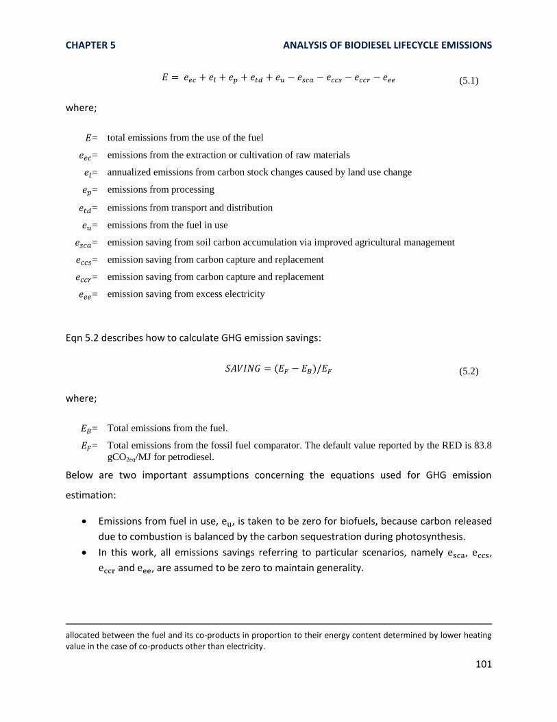
CHAPTER 5 ANALYSIS OF BIODIESEL LIFECYCLE EMISSIONS
101
(5.1)
where;
= total emissions from the use of the fuel
= emissions from the extraction or cultivation of raw materials
= annualized emissions from carbon stock changes caused by land use change
= emissions from processing
= emissions from transport and distribution
= emissions from the fuel in use
= emission saving from soil carbon accumulation via improved agricultural management
= emission saving from carbon capture and replacement
= emission saving from carbon capture and replacement
= emission saving from excess electricity
Eqn 5.2 describes how to calculate GHG emission savings:
( ) (5.2)
where;
= Total emissions from the fuel.
= Total emissions from the fossil fuel comparator. The default value reported by the RED is 83.8
gCO2eq/MJ for petrodiesel.
Below are two important assumptions concerning the equations used for GHG emission
estimation:
Emissions from fuel in use, , is taken to be zero for biofuels, because carbon released
due to combustion is balanced by the carbon sequestration during photosynthesis.
In this work, all emissions savings referring to particular scenarios, namely , ,
and , are assumed to be zero to maintain generality.
allocated between the fuel and its co-products in proportion to their energy content determined by lower heating value in the case of co-products other than electricity.

CHAPTER 5 ANALYSIS OF BIODIESEL LIFECYCLE EMISSIONS
102
5.c.2) Estimation Methodology for LUC Emissions
Various LUC scenarios for biodiesel feedstocks were determined and emissions were estimated
using the EC guidelines. More detailed information can be found in the RED [138] and
Commission Decision notified under document C(2010) 3751 (will be referred to as the
Commission Decision in this document) [132]. This section is intended to be a summary of the
methodology used in the model.
The definition of LUC emissions and the motivation for including them in lifecycle analysis is
explained as follows in the RED:
“If land with high stocks of carbon in its soil or vegetation is converted for the cultivation of raw
materials for biofuels, some of the stored carbon will generally be released into the atmosphere,
leading to the formation of carbon dioxide. The resulting negative greenhouse gas impact can
offset the positive greenhouse gas impact of the biofuels, in some cases by a wide margin. The
full carbon effects of such conversion should therefore be accounted for in calculating the
greenhouse gas emission saving of particular biofuels. This is necessary to ensure that the
greenhouse gas emission saving calculation takes into account the totality of the carbon effects
of the use of biofuels.”
The RED clearly states that the land use restrictions apply whether the biofuels are produced in
the European Community or imported. It also excludes the use of land that has high biodiversity
value, such as primary forests, areas designated for nature protection purposes, and highly
biodiverse grassland35. Similarly, land that has high carbon stock is also excluded. These include
wetlands; continuously forested areas with trees higher than 5 meters and a canopy cover of
more than 30%; land spanning more than one hectare with trees higher than five meters and a
canopy cover of between 10% and 30%, or trees able to reach those thresholds in situ.
As outlined in the RED, LUC emissions are estimated using Eqn 5.3:
35
More detailed descriptions of these land categories can be found in Article 17.
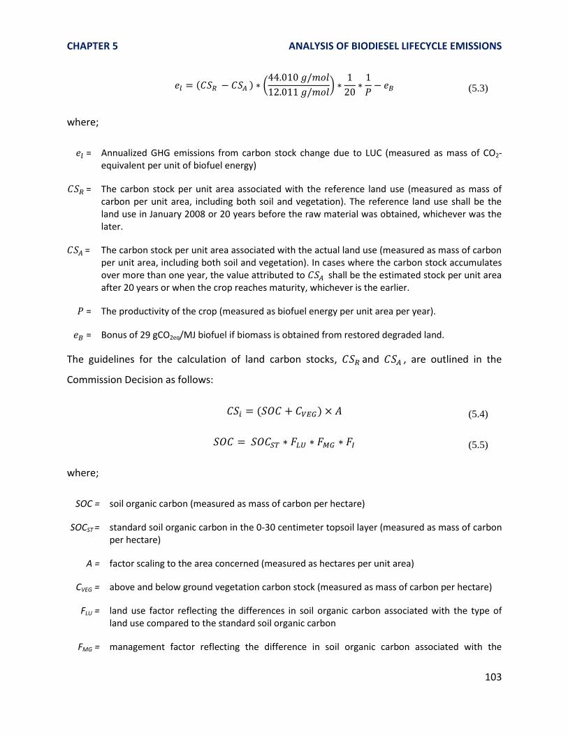
CHAPTER 5 ANALYSIS OF BIODIESEL LIFECYCLE EMISSIONS
103
( ) (
)
(5.3)
where;
= Annualized GHG emissions from carbon stock change due to LUC (measured as mass of CO2-equivalent per unit of biofuel energy)
= The carbon stock per unit area associated with the reference land use (measured as mass of carbon per unit area, including both soil and vegetation). The reference land use shall be the land use in January 2008 or 20 years before the raw material was obtained, whichever was the later.
= The carbon stock per unit area associated with the actual land use (measured as mass of carbon per unit area, including both soil and vegetation). In cases where the carbon stock accumulates over more than one year, the value attributed to shall be the estimated stock per unit area after 20 years or when the crop reaches maturity, whichever is the earlier.
= The productivity of the crop (measured as biofuel energy per unit area per year).
= Bonus of 29 gCO2eq/MJ biofuel if biomass is obtained from restored degraded land.
The guidelines for the calculation of land carbon stocks, and , are outlined in the
Commission Decision as follows:
( ) (5.4)
(5.5)
where;
SOC = soil organic carbon (measured as mass of carbon per hectare)
SOCST = standard soil organic carbon in the 0-30 centimeter topsoil layer (measured as mass of carbon per hectare)
A = factor scaling to the area concerned (measured as hectares per unit area)
CVEG = above and below ground vegetation carbon stock (measured as mass of carbon per hectare)
FLU = land use factor reflecting the differences in soil organic carbon associated with the type of land use compared to the standard soil organic carbon
FMG = management factor reflecting the difference in soil organic carbon associated with the

CHAPTER 5 ANALYSIS OF BIODIESEL LIFECYCLE EMISSIONS
104
principle management practice compared to the standard soil organic carbon
FI = input factor reflecting the difference in soil organic carbon associated with different levels of carbon input to soil compared to the standard organic carbon
The values of SOCST depend on the climate region and soil type of the land, and are listed in the
Commission Decision as shown in Table 1:
Table 1 – SOCST, standard soil organic carbon in the 0-30 centimeter topsoil layer, tC/ha.
Climate Region Soil Type
HACS LACS SAN POD VOL WET
Boreal, dry 68 - 10 117 20 146
Boreal, wet 68 - 10 117 20 146
Cold temperate, dry 50 33 34 - 20 87
Cold temperate, moist 95 85 71 115 130 87
Warm temperate, dry 38 24 19 - 70 88
Warm temperate, moist 88 63 34 - 80 88
Tropical, dry 38 35 31 - 50 86
Tropical, moist 65 47 39 - 70 86
Tropical, wet 44 60 66 - 130 86
Tropical, montane 88 63 34 - 80 86
CVEG values depend on the climate region and land cover, and are listed in the Commission
Decision as shown in Table 2. For forest land, the Commission Decision refers to more than 200
values of CVEG depending on domain, ecological zone and continent of the land. For the
purposes of our LUC modeling, having more than 200 scenarios representing the forest lands
would not be feasible. Moreover, some of those scenarios result in very similar numerical
values. Therefore, we identified the minimum and maximum CVEG values36 corresponding to
each climate type.
36
In some cases outliers were not included. For example temperate oceanic North America forests having more than 30% canopy have a CVEG value of 406 tC/ha which stands out as an outlier among the other forest CVEG numbers. Similarly, boreal tundra woodland that is younger than 20 years has 0 tC/ha. We think that these forest types are not representative of the forests that are likely to be converted to cropland, and therefore might bias the
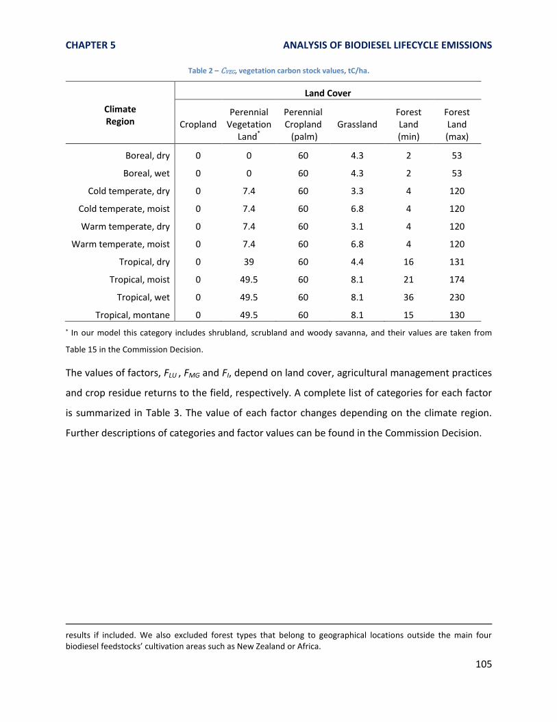
CHAPTER 5 ANALYSIS OF BIODIESEL LIFECYCLE EMISSIONS
105
Table 2 – CVEG, vegetation carbon stock values, tC/ha.
Climate Region
Land Cover
Cropland Perennial
Vegetation Land*
Perennial Cropland (palm)
Grassland Forest Land (min)
Forest Land (max)
Boreal, dry 0 0 60 4.3 2 53
Boreal, wet 0 0 60 4.3 2 53
Cold temperate, dry 0 7.4 60 3.3 4 120
Cold temperate, moist 0 7.4 60 6.8 4 120
Warm temperate, dry 0 7.4 60 3.1 4 120
Warm temperate, moist 0 7.4 60 6.8 4 120
Tropical, dry 0 39 60 4.4 16 131
Tropical, moist 0 49.5 60 8.1 21 174
Tropical, wet 0 49.5 60 8.1 36 230
Tropical, montane 0 49.5 60 8.1 15 130
* In our model this category includes shrubland, scrubland and woody savanna, and their values are taken from
Table 15 in the Commission Decision.
The values of factors, FLU , FMG and FI, depend on land cover, agricultural management practices
and crop residue returns to the field, respectively. A complete list of categories for each factor
is summarized in Table 3. The value of each factor changes depending on the climate region.
Further descriptions of categories and factor values can be found in the Commission Decision.
results if included. We also excluded forest types that belong to geographical locations outside the main four biodiesel feedstocks’ cultivation areas such as New Zealand or Africa.

CHAPTER 5 ANALYSIS OF BIODIESEL LIFECYCLE EMISSIONS
106
Table 3 – List of the factor categories.
FLU
cropland, cultivated
perennial cropland
grassland
native forest
managed forest
shifting cultivation-shortened fallow
shifting cultivation-matured fallow
FMG
cropland:
full-tillage
reduced-tillage
no till grassland:
improved
nominally managed
moderately degraded
severely degraded
FI
low
medium
high with manure
high without manure
Finally, it is worth noting that although the Commission guidelines briefly describe the methods
to calculate the soil organic carbon in organic soils, they do not contain values for determining
SOC for them. Because organic soils are geographically very limited, exclusion of them from this
work does not change the estimation results for major biodiesel feedstocks.
5.d) Feedstock-specific LUC GHG Emissions:
In the light of the EC guidelines outlined above, LUC emissions of a biodiesel feedstock can be
determined if the following are known:
1. climate region of cultivation
2. soil type of cultivated land
3. reference and actual land cover types
4. agricultural management practices and inputs
The first two factors are geographical and can be, to some extent, mapped if the country of
origin is known. This limits the LUC scenario space to certain soil-climate combinations for each
feedstock and these combinations can be determined by geographical mapping. On the other
CHAPTER 5 ANALYSIS OF BIODIESEL LIFECYCLE EMISSIONS
107
hand, the last two factors are mostly influenced by man-made decisions and are harder to
predict based on geographical information.
The next section will detail our methodology of using geographical mapping to determine the
most likely soil-climate combinations for each feedstock.
5.d.1) Geographical Mapping for Soil-Climate Combinations
Top Feedstock Producers
Because each crop37 needs certain soil and climate conditions to be harvested with high yields,
major biodiesel crops are likely to be cultivated in certain geographical locations. In order to
test this hypothesis, we have used publicly available FAOSTAT global crop production database
[139]. The FAOSTAT database enables to inquire;
i. area harvested
ii. yield
iii. production quantity
for various crops including canola, soybean, sunflower and palm at the country level. For each
crop, we have extracted the top countries that, when combined, contribute to at least 80% of
the annual global production. Although data as old as the year 1961 is available in this
database, we focused our efforts on 2005-2009 data38 to draw conclusions about the
distribution of crop production globally. Figure 1 summarizes the average production volume of
each crop by the top producers between 2005 and 2009:
37
Although the distinction between the words “crop” and “feedstock” is very subtle, we generally refer to the whole seed or plant with the word “crop”, whereas we refer to the obtained vegetable oil with the word “feedstock”.
38 The most recent 5-year period available at the time of our inquiry.

CHAPTER 5 ANALYSIS OF BIODIESEL LIFECYCLE EMISSIONS
108
Figure 1 – Global distribution of average feedstock production by major producers between 2005 and 2009.
Although the data we have gathered does not allow us to determine where exactly each crop is
cultivated within one specific country, we assume that because these countries are major
producers of these crops, their dominant climate and soil combinations reflect the conditions at
which cultivation takes place. This assumption is most likely to hold true for palm for which the
major producers are only Indonesia and Malaysia with very characteristic soil and climate types.
Rest of the
World: 19%
Indonesia 41%
Malaysia 40%
Palm Global Production
Rest of the World:
18%
China 22%
Canada 20%
India 13%
Germany 10%
France 9%
Poland 4%
United Kingdom
4%
Canola Global Production
Rest of the World:
19%
United States of America
38%
Brazil 25%
Argentina 18%
Soybean Global Production
Rest of the World:
18%
Russian Federation
21%
Ukraine 17%
Argentina 11%
China 6%
France 5%
United States of America
4%
India 4%
Hungary 4% Romania
4%
Bulgaria 3%
Turkey 3%
Sunflower Global Production

CHAPTER 5 ANALYSIS OF BIODIESEL LIFECYCLE EMISSIONS
109
On the other hand, a more detailed agricultural dataset is needed to determine the exact soil
and climate combinations for crops like canola or sunflower where cultivation is relatively
distributed across the globe, with a diverse set of soil and climate conditions.
Before moving on to soil-climate combination mapping, it might be useful for the reader to see
all the major feedstock producers included in our model on a global map as shown in Figure 2.
As can be expected, certain regions such as Africa, Greenland or Arabic Peninsula do not
contribute to global biodiesel feedstock production.
Figure 2 – Major biodiesel feedstock producer countries highlighted in blue.
Soil-Climate Combination Mapping
As discussed earlier, the Commission Decision refers to global soil type and climate region
classifications and presents the world maps created based on those classifications. These maps
are also publicly available through the online Transparency platform39 established by the RED.
However, because the format of the maps were not suitable for extracting information
regarding to a specific location in the world, i.e. country-level soil types and climate regions, we
first converted the raster images of the maps to vector files, then overlaid vector files of
39
http://eusoils.jrc.ec.europa.eu/projects/RenewableEnergy/

CHAPTER 5 ANALYSIS OF BIODIESEL LIFECYCLE EMISSIONS
110
country borders, and finally performed a spatial analysis40 on the flat projections of the globe to
obtain the areal climate and soil distribution of individual countries.
The climate regions are defined by a set of rules based on factors such as annual mean daily
temperature, total annual precipitation, total annual potential evapo-transpiration and
elevation, and are classified based on the IPCC guidelines [140]. Figure 3 shows the result of this
classification at the global scale:
Figure 3 – Climate regions defined based on the classification of IPCC, published by the European Commission, JRC.
Mineral soils are classified according to the World Reference Base (WRB) [141] and then
translated into IPCC Tier-I level classes [142]. The classification scheme is represented in Figure
4:
40
ARCGIS analysis tools were used to perform these analyses.

CHAPTER 5 ANALYSIS OF BIODIESEL LIFECYCLE EMISSIONS
111
Figure 4 – IPCC Tier-I Level scheme for grouping mineral soil types based on the WRB soil classification system [140].
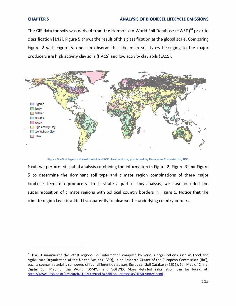
CHAPTER 5 ANALYSIS OF BIODIESEL LIFECYCLE EMISSIONS
112
The GIS data for soils was derived from the Harmonized World Soil Database (HWSD)41 prior to
classification [143]. Figure 5 shows the result of this classification at the global scale. Comparing
Figure 2 with Figure 5, one can observe that the main soil types belonging to the major
producers are high activity clay soils (HACS) and low activity clay soils (LACS).
Figure 5 – Soil types defined based on IPCC classification, published by European Commission, JRC.
Next, we performed spatial analysis combining the information in Figure 2, Figure 3 and Figure
5 to determine the dominant soil type and climate region combinations of these major
biodiesel feedstock producers. To illustrate a part of this analysis, we have included the
superimposition of climate regions with political country borders in Figure 6. Notice that the
climate region layer is added transparently to observe the underlying country borders:
41
HWSD summarizes the latest regional soil information compiled by various organizations such as Food and Agriculture Organization of the United Nations (FAO), Joint Research Center of the European Commission (JRC), etc. Its source material is composed of four different databases: European Soil Database (ESDB), Soil Map of China, Digital Soil Map of the World (DSMW) and SOTWIS. More detailed information can be found at: http://www.iiasa.ac.at/Research/LUC/External-World-soil-database/HTML/index.html

CHAPTER 5 ANALYSIS OF BIODIESEL LIFECYCLE EMISSIONS
113
Figure 6 – Global climate regions and political country borders overlapped.
In doing this spatial analysis, we followed an elimination rule where only the most dominant
soil types and climate regions were considered. This was necessary to obtain a feasible number
of LUC scenarios to be used in the optimization model, and to consider only the most likely
scenarios for each feedstock. The elimination criteria were based on the relative area of the soil
type and climate region of a country and the following rules were applied:
The dominant soil type and climate region of a country were determined based on the
largest aerial coverage, and named as soil-1 and climate-1 for each country in the
model.
If the dominant soil type and/or climate region was covering more than 80% of the
country in area, other soil type or climate regions were not considered.
If the dominant soil type and/or climate region was less than 80% of the country in area,
and the second largest soil type and/or climate region was larger than 20% of the
country, then the second soil type and/or climate region was also considered and
named as soil-2 and climate-2, respectively.
Finally, combinations of all resultant soil types and climate regions for each country
were listed to represent the most prevalent conditions in that country. For example, if
the rules above resulted in country-X having two climate regions and two soil types,
then that country was assumed to possess all the following soil-climate combinations:
o soil-1 with climate-1
o soil-1 with climate-2
o soil-2 with climate-1
o soil-2 with climate-2

CHAPTER 5 ANALYSIS OF BIODIESEL LIFECYCLE EMISSIONS
114
Based on the method above, the soil-climate combinations in Table 4 were obtained.
Combination ID refers to an internally generated index in the model where all possible soil-
climate combinations were numbered from 1 to 72 and can be found in Appendix A.
Table 4 – Prevalent climate-soil combinations for each feedstock.
SOIL-CLIMATE COMBINATION COMBINATION ID
Canola, Sunflower HACS + Boreal wet 2 Canola, Soybean, Sunflower HACS + Cold temperate dry 3
Canola, Sunflower HACS + Cold temperate moist 4 Soybean, Sunflower HACS + Warm temperate dry 5
Canola, Sunflower HACS + Warm temperate dry 6 Canola, Soybean, Sunflower HACS + Tropical dry 7
Canola, Sunflower HACS + Tropical moist 8 Palm HACS + Tropical wet 9
Canola, Sunflower LACS + Tropical dry 19 Canola LACS + Tropical moist 20
Soybean, Palm LACS + Tropical wet 21 Canola, Sunflower POD + Boreal wet 38
Canola POD + Cold temperate moist 40
5.d.2) Accounting for Scenarios Influenced by Man-Made Decisions (FLU, FMG, FI)
At the end of Section 5.b.2, we listed land cover types and agricultural management practices
as human factors adding to the U&V in the lifecycle GHG emissions of biodiesel. Recognizing
that there are relatively small numbers of distinct land cover types, we considered this U&V as
scenario uncertainty and created the most likely land conversion scenarios for each feedstock.
Likewise, different agricultural practices can be considered as scenarios in the lifecycle of
biodiesel. Nevertheless, due to the large number of steps in cultivation and the inherent
variations within each step, if we were to represent this U&V in terms of distinct scenarios, we
would have to create thousands of them. Instead, recognizing that agricultural practices can
span numerous factors that, when combined, contribute to the U&V in a more continuous way,
we chose to represent this U&V with a distribution.
In the following. we will discuss the scenario creation for land conversions followed by the
methodology used to represent agricultural practice variations as distributions.

CHAPTER 5 ANALYSIS OF BIODIESEL LIFECYCLE EMISSIONS
115
Land Conversion Scenarios (FLU)
As was shown in Table 2, the Commission considers land cover types under five main
categories: cropland, perennial vegetation land, perennial cropland, grassland and forestland.42
Therefore, when an arable land is intended to be used for crop cultivation, the following land
cover conversions might occur:
For canola, soybean and sunflower:
I. cropland-to-cropland (cc)
II. grassland-to-cropland (gc)
III. perennial vegetation land-to-cropland (pc)
IV. perennial cropland-to-cropland (pc’)
V. forestland-to-cropland (fc)
For palm:
VI. perennial vegetation land-to-perennial cropland (pp)
VII. perennial cropland-to-perennial cropland (pp’)
VIII. cropland-to-perennial cropland (cp)
IX. grassland-to-perennial cropland (gp)
X. forestland-to-perennial cropland (fp)
The RED assumes that cropland-to-cropland (cc) conversion does not lead to LUC emissions.43
Therefore, although crop rotations are common practices in agriculture, we did not consider
the cc scenario in our LUC modeling. Instead, we included a “no-LUC” scenario for each
feedstock later on and considered only the lifecycle GHG emissions regarding cultivation,
processing and transportation under that scenario. With a similar approach, we also excluded
perennial cropland-to-perennial cropland (pp’) conversions. Finally, we omitted cropland-to-
perennial cropland (cp) and perennial cropland-to-cropland (pc) conversions assuming that it
would be highly unlikely that an arable land would switch from any crop to palm (which is the
only perennial crop in our model) or from palm to any other crop.
42
The exact definitions of these land covers can be found in the references given in the RED.
43 In practice, because different crops would hold different amounts of carbon in soil, crop rotation can also lead to
some degree of GHG emissions. Yet, these emissions are probably much lower compared to other land cover conversions.

CHAPTER 5 ANALYSIS OF BIODIESEL LIFECYCLE EMISSIONS
116
These considerations left us with a total of 6 land conversion scenarios: gc, pc, fc for canola,
soybean and sunflower; and pp, gp and fp for palm.
Next, we wanted to further evaluate the likelihood of these scenarios for each feedstock given
the production and geographical information presented earlier. Because we know the major
producers of these crops, knowledge of the historical land conversion statistics for these
producers can be used as a proxy to eliminate unlikely scenarios. Certainly, another approach
would be estimating the total area of each land cover in each major producer, and then using
those estimates to predict potential land conversion scenarios for the future. Yet, we think that
the former approach is more valid, because past trends of land use changes are, to some
extent, also reflections of future land use policies of countries. To be more explicit, just because
a country possesses large areas of forestland, the next marginal land to be cleared for biodiesel
production does not have to be forestland. For example, Brazil has more than 60% of
forestland44 according to the FAO; however, as will be shown next, the forestland has been only
4% of total land converted to cropland between 2001 and 2004 in Brazil.
Tracking the historical LUC of countries is possible using satellite imagery. Figure 7 shows
results of the Winrock satellite data analysis for a selection of countries between 2001 and
2004, as published by the US EPA in the Federal Register in 2009 [144]. Except for the US,
Canada and Russia, all the other major biodiesel feedstock producers are included in this
analysis.45
Figure 7 – Types of land converted to cropland by country, values are in percent. Taken from [144].
44
http://www.indexmundi.com/facts/indicators/AG.LND.FRST.ZS
45 Note that the European countries are represented by the category “EU”.
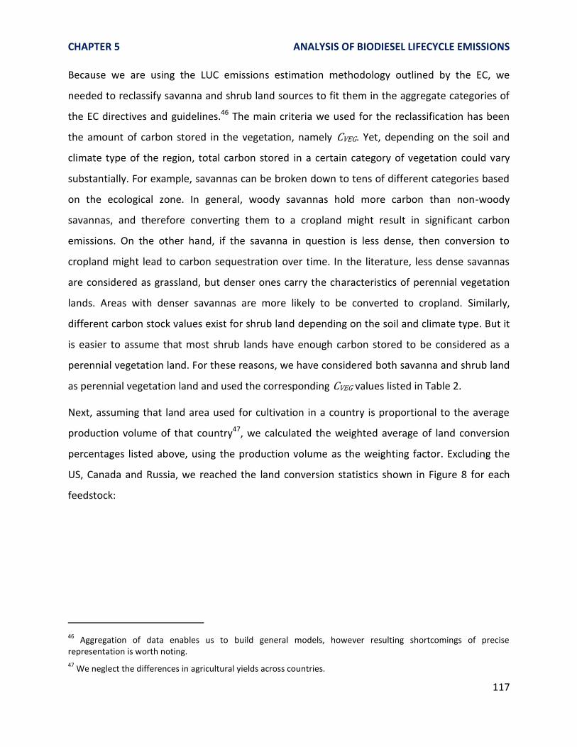
CHAPTER 5 ANALYSIS OF BIODIESEL LIFECYCLE EMISSIONS
117
Because we are using the LUC emissions estimation methodology outlined by the EC, we
needed to reclassify savanna and shrub land sources to fit them in the aggregate categories of
the EC directives and guidelines.46 The main criteria we used for the reclassification has been
the amount of carbon stored in the vegetation, namely CVEG. Yet, depending on the soil and
climate type of the region, total carbon stored in a certain category of vegetation could vary
substantially. For example, savannas can be broken down to tens of different categories based
on the ecological zone. In general, woody savannas hold more carbon than non-woody
savannas, and therefore converting them to a cropland might result in significant carbon
emissions. On the other hand, if the savanna in question is less dense, then conversion to
cropland might lead to carbon sequestration over time. In the literature, less dense savannas
are considered as grassland, but denser ones carry the characteristics of perennial vegetation
lands. Areas with denser savannas are more likely to be converted to cropland. Similarly,
different carbon stock values exist for shrub land depending on the soil and climate type. But it
is easier to assume that most shrub lands have enough carbon stored to be considered as a
perennial vegetation land. For these reasons, we have considered both savanna and shrub land
as perennial vegetation land and used the corresponding CVEG values listed in Table 2.
Next, assuming that land area used for cultivation in a country is proportional to the average
production volume of that country47, we calculated the weighted average of land conversion
percentages listed above, using the production volume as the weighting factor. Excluding the
US, Canada and Russia, we reached the land conversion statistics shown in Figure 8 for each
feedstock:
46
Aggregation of data enables us to build general models, however resulting shortcomings of precise representation is worth noting.
47 We neglect the differences in agricultural yields across countries.

CHAPTER 5 ANALYSIS OF BIODIESEL LIFECYCLE EMISSIONS
118
Figure 8 – Distribution of land conversions that took place in major producer countries between 2001 and 2004. The US, Canada and Russia are not included due to lack of data.
Based on the magnitudes of land conversions in Figure 8, we decided to exclude fc conversion
for soybean and gp conversion for palm. Elimination of these conversions leaves us with a
reasonable set of scenarios to be used as inputs in the optimization model. At the same time,
based on the distributions on Figure 8, we think that all three conversion types, namely fc, pc
and gc, occur significantly enough to be included in the model for canola and sunflower.
The analyses and assumptions described above leads to the land conversion scenarios
summarized in Table 5. Plus and minus signs refer to the presence and absence of land
conversions considered in the model, respectively.
Table 5 – Scenario matrix to be used in FLU determination.
gc pc fc gp pp fp
CANOLA + + + NA NA NA PALM NA NA NA - + +
SOYBEAN + + - NA NA NA SUNFLOWER + + + NA NA NA
NA:
Not applicable; (+): Included in the model; (-): Excluded from the model.
Agricultural Management Practices and Inputs (FMG, FI)
As summarized in Table 3 previously, the EC assigned certain factors, FMG and FI, to account for
variations in management practices and inputs left in the field following harvesting. On top of
the variations due to man-made decisions (such as using manure, full-tillage, no-tillage, etc.),
these values also change based on the climate region of the land. Furthermore, it is hard to say

CHAPTER 5 ANALYSIS OF BIODIESEL LIFECYCLE EMISSIONS
119
that these estimations are perfectly accurate, as reflected by the IPCC’s error estimations for
each individual factor48 [142], and therefore it is more appropriate to characterize them as
distributions rather than point estimates. Nonetheless, as will be shown next, the multitude of
factors spanning a wide range of agricultural management practices and inputs dominates the
IPCC U&V range of each individual factor, FMG and FI.
One major challenge in a global biodiesel supply chain is to know the factors that determine
FMG and FI of a purchased feedstock. In other words, it is usually not possible to determine if the
feedstock was cultivated in a field that was previously grassland or forestland, or if the
grassland was degraded, or if the input was low, medium, etc. Consequently, the lack of specific
information might result in disparate factor estimates for a single crop, even if the soil type and
the climate region is known. To give an example, for cropland in a warm temperate, dry climate
FMG is 1 if there is “full-tillage”, 1.02 if there is “reduced tillage” and 1.1 if there is “no-tillage”;
similarly FI is 0.95 if input is “low”, 1 if input is “medium”, 1.37 if input is “high with manure”
and 1.04 if input is “high without manure”. Therefore, FMG * FI varies between 0.95 and 1.51.
Given that the details of agricultural management and inputs are not known to every agent in
the supply chain, there seems to be a relatively wide range of factor values for cropland in a
warm temperate, dry climate. For illustration purposes, we present a portion of the factors in
Table 6 from the model, including FLU values that change with the climate region:
Table 6 - Illustration of minimum and maximum cropland factors used in the model.
48
± two standard deviations, expressed as a percent of the mean were defined as the “error” in IPCC 2006, and these errors are usually about 5-10% of the mean estimate. When sufficient studies were not available for a statistical analysis, the error is assumed 50% of the mean.
MIN MAXFLU FMG FI FLU FMG FI FLU*FMG*FI FLU*FMG*FI
Boreal, dry 0.8 1 0.95 0.8 1.1 1.37 0.76 1.21
Boreal, wet 0.69 1 0.92 0.69 1.15 1.44 0.63 1.14
Cold temperate, dry 0.8 1 0.95 0.8 1.1 1.37 0.76 1.21
Cold temperate, moist 0.69 1 0.92 0.69 1.15 1.44 0.63 1.14
Warm temperate, dry 0.8 1 0.95 0.8 1.1 1.37 0.76 1.21
Warm temperate, moist 0.69 1 0.92 0.69 1.15 1.44 0.63 1.14
Tropical, dry 0.58 1 0.95 0.58 1.17 1.37 0.55 0.93
Tropical, moist 0.48 1 0.92 0.48 1.22 1.44 0.44 0.84
Tropical, wet 0.48 1 0.92 0.48 1.22 1.44 0.44 0.84
Tropical, montane 0.64 1 0.94 0.64 1.16 1.41 0.60 1.05
MIN MAX
CR
OP
LAN
D

CHAPTER 5 ANALYSIS OF BIODIESEL LIFECYCLE EMISSIONS
120
In summary:
1. Because of imperfect estimations, each individual FMG and FI value should be
represented by an U&V distribution rather than a point estimate.
2. Yet, the multitude of factor values due to various management and input scenarios
worldwide dominates the U&V range of individual FMG and FI values.
3. Furthermore, in a global biodiesel supply chain, it is not possible to determine the
individual FMG and FI values, because it requires the knowledge of exact management
and input scenarios belonging to feedstocks purchased from different suppliers.
For the reasons summarized above, we chose to model the U&V in FMG and FI in a single normal
distribution for each climate region. In this model, the minimum and maximum values of FMG*FI
corresponding to each climate represent the ends of the normal distribution, spanning 8σ
(99.993666%) of the whole population. The mean FMG*FI value of each climate is determined as
the average of minimum and maximum FMG*FI. For FLU, we used the deterministic values as
given the EC guidelines. Figure 9 illustrates our U&V modeling for FLU*FMG*FI.
Figure 9 – Representation of the U&V of the factors in the model.
5.d.3) Accounting for the Crop Productivity and Co-Product Energy Allocation Factors
Crop Productivity, P
The productivity term introduced earlier in Eqn 5.3 converts the units of the emissions from
tCO2/ha to tCO2/MJ using the feedstock yields. In calculating the productivity, one should
consider:

CHAPTER 5 ANALYSIS OF BIODIESEL LIFECYCLE EMISSIONS
121
a. Crop yield, CY (kg/ha)
b. Oil extraction yield, EY: percent of the seed mass that is obtained as oil
c. Lower heating value (LHV) of the vegetable oil in consideration, LHV (MJ/kg)
This leads to Eqn 5.6 for the expression of productivity:
(5.6)
Crop Yield: It varies across countries, perhaps due to variations in climate and soil types as well
as agro-technology deployed. In order to use a yield value that would be most representative,
we took weighted averages of reported yields of the major producers included in the model,
where the total production volume was used as the weighting factor. As can be seen in Figure
10, palm has an exceptionally higher yield value, making it a very attractive feedstock in the
market.
Figure 10 – 2005-2009 average crop yields, weighted by the production volumes of major producers.
Oil Extraction Yield: It is a function of both the oil content of the seed and the technology used
to extract oil from the seed. Sunflower 44% [145], palm 22% [112], soybean 18% [114] and
canola possesses 40%49 oil extraction yield. Low extraction yield of soybean is not surprising,
because soybean is a crop that is highly valued for its high protein content which is commonly
used for animal meal.
49
Personal communication with Portuguese biodiesel producers.
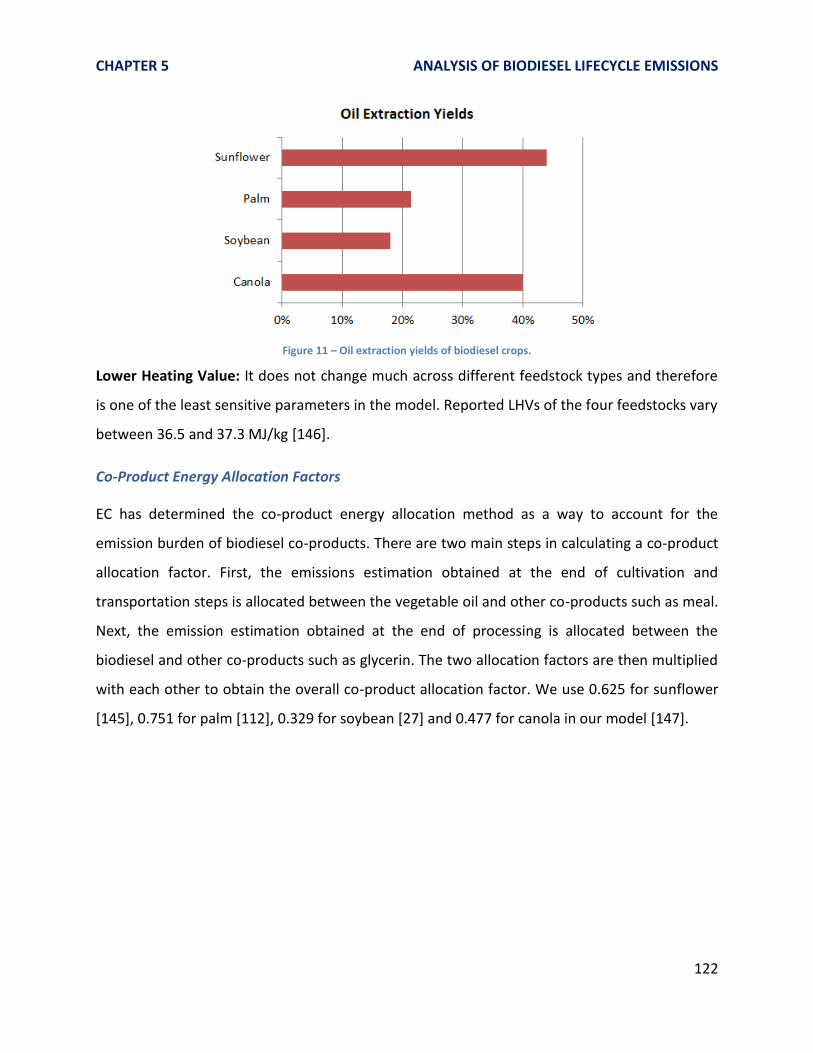
CHAPTER 5 ANALYSIS OF BIODIESEL LIFECYCLE EMISSIONS
122
Figure 11 – Oil extraction yields of biodiesel crops.
Lower Heating Value: It does not change much across different feedstock types and therefore
is one of the least sensitive parameters in the model. Reported LHVs of the four feedstocks vary
between 36.5 and 37.3 MJ/kg [146].
Co-Product Energy Allocation Factors
EC has determined the co-product energy allocation method as a way to account for the
emission burden of biodiesel co-products. There are two main steps in calculating a co-product
allocation factor. First, the emissions estimation obtained at the end of cultivation and
transportation steps is allocated between the vegetable oil and other co-products such as meal.
Next, the emission estimation obtained at the end of processing is allocated between the
biodiesel and other co-products such as glycerin. The two allocation factors are then multiplied
with each other to obtain the overall co-product allocation factor. We use 0.625 for sunflower
[145], 0.751 for palm [112], 0.329 for soybean [27] and 0.477 for canola in our model [147].

CHAPTER 5 ANALYSIS OF BIODIESEL LIFECYCLE EMISSIONS
123
Figure 12 – Co-product energy allocation factors for biodiesel crops.
5.e) Results and Summary of Feedstock-Specific Lifecycle GHG Emissions Estimations
The methodology described above resulted in a total of 75 different lifecycle scenarios for the
four feedstocks considered in the model. The details of each scenario can be found in
Appendix-B.
Out of the 75 scenarios, 4 of them refer to no-LUC emissions estimations published by
BIOGRACE [27] for canola, soybean, sunflower and palm biodiesel, and can be seen in Figure 13.
These estimates include cultivation without land use change, processing and transport; and co-
product energy allocation method is used as determined by the RED. The data source is a
database prepared by the JEC Consortium in 2008.
Figure 13 – Lifecycle GHG estimates as published by BIOGRACE [27]. LUC emissions are not included.
In order to represent the inherent GHG emissions U&V as discussed by several papers in the
literature [15-18, 25, 26, 111-118], we added a coefficient of variation (COV) factor of 20% to

CHAPTER 5 ANALYSIS OF BIODIESEL LIFECYCLE EMISSIONS
124
these deterministic, no-LUC emissions estimates and ran Monte Carlo simulations. Resulting
emission distributions are shown in Figure 14 where non-compliant parts are shown in red.
Note that the probability of compliance is quite sensitive to the level of chosen COV.
Figure 14 – Estimated emissions distributions of biodiesel obtained from canola, soybean, sunflower and palm. Distributions obtained by Monte Carlo simulations applied on the deterministic BIOGRACE data. 20% COV is assumed for each feedstock
esimatation. LUC emissions are not included.
We also note a further assumption made regarding the processing conditions for palm.
BIOGRACE reports two different palm scenarios; one with methane capture at the mill, where
bunches of fresh palm fruit are separated into palm kernels, empty fruit bunches and palm oil,
and one without methane capture. GHG emissions estimate is 69 gCO2-eq/MJ without methane
capture, and 37 gCO2-eq/MJ with methane capture. Because we are not imposing any supply
constraints or price differentials among the vegetable oils obtained from the same crop species,
palm biodiesel with lower GHG emissions leads to a strong bias in the optimization model,
where use of palm is strongly preferred. This bias is also driven by the lowest palm oil prices
observed historically compared to other biodiesel feedstocks. As a result, the feedstock cost of
biodiesel becomes almost insensitive to varying GHG thresholds. Nevertheless, we came to the

CHAPTER 5 ANALYSIS OF BIODIESEL LIFECYCLE EMISSIONS
125
conclusion that methane capture is not widely practiced by the current palm oil extraction
businesses, and therefore palm oil with 37 gCO2-eq/MJ emissions is not common. According to
the mandatory surveys conducted by the Malaysian Palm Oil board and the information
provided by the Indonesian Embassy, the EPA concluded that only 10% of the current palm oil
mills capture methane during the separation process50 [21]. Assuming that this specific
information in the processing conditions can be transferred along the supply chain in a
transparent way, one would expect methane-captured palm oil to possess a price premium in
the biodiesel feedstock market. Because we are not sure what the price premium of that is (or
will be), exclusion of methane-captured palm oil scenario seems to be a reasonable assumption
for our purposes. Therefore the palm scenarios in the model proposed here exclude those with
methane capture.
Out of the remaining 71 LUC scenarios; 30 belong to canola, 10 belong to soybean, 27 belong to
sunflower and 4 belong to palm oil. The multitude of scenarios is driven by the diversity of the
geographical conditions suitable for the cultivation of each feedstock, i.e. soil type and climate
region, and the prevalence of different types of land conversions as was shown in Figure 8.
Figure 15 summarizes the mean emissions of the 75 scenarios. The black bars refer to the no-
LUC emissions estimates. More details can be found in Appendix-B.
Figure 15 – Summary of 75 biodiesel lifecycle GHG emissions. Only mean emission estimates are shown. Black bars represent the lifecycle scenarios without LUC.
The histogram in Figure 16 provides an indication of where the majority of emissions scenarios
are clustered, and which are outliers. The ranges specified in the x-axis refer to the emissions
50
105 mills capture methane out of 1030 total mills in Indonesia and Malaysia.
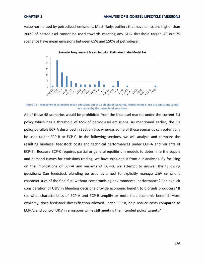
CHAPTER 5 ANALYSIS OF BIODIESEL LIFECYCLE EMISSIONS
126
value normalized by petrodiesel emissions. Most likely, outliers that have emissions higher than
200% of petrodiesel cannot be used towards meeting any GHG threshold target. 48 out 75
scenarios have mean emissions between 65% and 150% of petrodiesel.
Figure 16 – Frequency of estimated mean emissions out of 75 biodiesel scenarios. Figures in the x-axis are emissions values normalized by the petrodiesel emissions.
All of these 48 scenarios would be prohibited from the biodiesel market under the current EU
policy which has a threshold of 65% of petrodiesel emissions. As mentioned earlier, the EU
policy parallels ECP-A described in Section 5.b; whereas some of these scenarios can potentially
be used under ECP-B or ECP-C. In the following sections, we will analyze and compare the
resulting biodiesel feedstock costs and technical performances under ECP-A and variants of
ECP-B. Because ECP-C requires partial or general equilibrium models to determine the supply
and demand curves for emissions trading, we have excluded it from our analyses. By focusing
on the implications of ECP-A and variants of ECP-B, we attempt to answer the following
questions: Can feedstock blending be used as a tool to explicitly manage U&V emissions
characteristics of the final fuel without compromising environmental performance? Can explicit
consideration of U&V in blending decisions provide economic benefit to biofuels producers? If
so, what characteristics of ECP-A and ECP-B amplify or mute that economic benefit? More
explicitly, does feedstock diversification allowed under ECP-B, help reduce costs compared to
ECP-A, and control U&V in emissions while still meeting the intended policy targets?
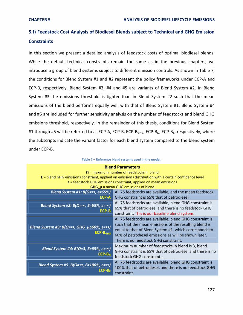
CHAPTER 5 ANALYSIS OF BIODIESEL LIFECYCLE EMISSIONS
127
5.f) Feedstock Cost Analysis of Biodiesel Blends subject to Technical and GHG Emission
Constraints
In this section we present a detailed analysis of feedstock costs of optimal biodiesel blends.
While the default technical constraints remain the same as in the previous chapters, we
introduce a group of blend systems subject to different emission controls. As shown in Table 7,
the conditions for Blend System #1 and #2 represent the policy frameworks under ECP-A and
ECP-B, respectively. Blend System #3, #4 and #5 are variants of Blend System #2. In Blend
System #3 the emissions threshold is tighter than in Blend System #2 such that the mean
emissions of the blend performs equally well with that of Blend System #1. Blend System #4
and #5 are included for further sensitivity analysis on the number of feedstocks and blend GHG
emissions threshold, respectively. In the remainder of this thesis, conditions for Blend System
#1 through #5 will be referred to as ECP-A, ECP-B, ECP-BGHG, ECP-BΩ, ECP-BE, respectively, where
the subscripts indicate the variant factor for each blend system compared to the blend system
under ECP-B.
Table 7 – Reference blend systems used in the model.
Blend Parameters Ω = maximum number of feedstocks in blend
E = blend GHG emissions constraint, applied on emissions distribution with a certain confidence level ε = feedstock GHG emissions constraint, applied on mean emissions
GHG_µ = mean GHG emissions of blend
Blend System #1: B(Ω=∞, ε=65%) ECP-A
All 75 feedstocks are available, and the mean feedstock GHG constraint is 65% that of petrodiesel.
Blend System #2: B(Ω=∞, E=65%, ε=∞) ECP-B
All 75 feedstocks are available, blend GHG constraint is 65% that of petrodiesel and there is no feedstock GHG constraint. This is our baseline blend system.
Blend System #3: B(Ω=∞, GHG_µ≤60%, ε=∞) ECP-BGHG
All 75 feedstocks are available, blend GHG constraint is such that the mean emissions of the resulting blend is equal to that of Blend System #1, which corresponds to 60% of petrodiesel emissions as will be shown later. There is no feedstock GHG constraint.
Blend System #4: B(Ω=3, E=65%, ε=∞) ECP-BΩ
Maximum number of feedstocks in blend is 3, blend GHG constraint is 65% that of petrodiesel and there is no feedstock GHG constraint.
Blend System #5: B(Ω=∞, E=100%, ε=∞) ECP-BE
All 75 feedstocks are available, blend GHG constraint is 100% that of petrodiesel, and there is no feedstock GHG constraint.

CHAPTER 5 ANALYSIS OF BIODIESEL LIFECYCLE EMISSIONS
128
Note that we regard Blend System #2 as our baseline blend and ECP-B as our baseline policy
control. In the remaining, when one or more of the three parameters are not specifically
indicated, it is assumed that the parameters of the baseline blend are present.
5.f.1) Single Period Price Data Analysis on the Maximum Number of Feedstocks in Blend, Ω
This section compares blend systems under ECP-B and ECP-BΩ where the maximum number of
feedstocks in the blend, Ω, is the focus of analysis.
When there is no restriction on Ω, the optimization model minimizes the cost subject to
technical and emissions standards by using different amounts of available feedstocks. As
expected, optimal blend portfolios change when the prices of individual feedstocks change over
time. For this reason, the total number of feedstocks used by the model, and thus the feedstock
diversification, varies based on the input prices51. This leads to a direct relationship between
the maximum degree of feedstock diversification that can be achieved in each period and the
feedstock prices pertaining to that period. In order to illustrate this relationship, we have
chosen two distinct monthly price sets that were observed between 2003 and 2011: April 2007
and January 2005. Our analyses showed that the prices observed in April 2007 enable the
greatest degree of diversification for the optimal model.52 In contrast, the prices observed in
January 2005 provide a limited degree of diversification. Figure 17 compares the prices
observed at these two points in time. Note that all the monetary figures in this chapter are the
market prices deflated by the FAO vegetable oil index as discussed in Chapter 4.
51
This effect was observed in Chapter-4 where the focus was on blending chemical property distributions and the distinction between different LUC scenarios was not made.
52 Although the details of this observation will not be discussed here, it suffices to note that the relative magnitude
of feedstock prices is one of the most important factors in enabling a diverse optimal portfolio.

CHAPTER 5 ANALYSIS OF BIODIESEL LIFECYCLE EMISSIONS
129
Figure 17 – Observed deflated prices in January 2005 and April 2007.
The optimization model has multiple input parameters to represent the chemical content of
each feedstock and the relevant technical constraints that the biodiesel is subject to. Table 8
summarizes these exogenous parameters and constraints used in the model for this analysis.
Table 8 – Summary of exogenous parameters and constraints used in Section 5.f.1
Price Input(s) April 2007, January 2005
Iodine Value (IV) max 120
Oxidation Stability (OS) min 4.5 hours
Cetane Number (CN) min 47
Cold Filter Plugging Point (CFPP) max -1 ˚C
Confidence Level for
Technical constraints
95%
(for one-tailed Gaussian dist.)
Lifecycle GHG Emission Threshold max 65% of petrodiesel
Confidence Level for
GHG Emission constraint
80%
(for one-tailed Gaussian dist.)
Maximum Number of Feedstocks Allowed in the Blend, Ω
variable
Note that the last row in Table 8 is a new constraint we added for the purposes of this analysis.
Therefore Eqn 5.7 was added to the optimization formulation:

CHAPTER 5 ANALYSIS OF BIODIESEL LIFECYCLE EMISSIONS
130
(5.7)
where;
: Number of feedstocks in the optimal blend
Ω: Maximum number of feedstocks allowed in the optimal blend
For the April 2007 price set, when the model is run without any restrictions on the number of
blend components, 23 out 75 feedstock scenarios are included at least at 0.5% by volume in the
optimal portfolio.53 By changing the maximum limit of number of feedstocks available, we ran
the model starting at Ω=20 all the way down to Ω=1. Note that for each point, all the previously
determined 23 feedstocks are actually available to the model, yet the feedstock number
limitation does not allow the use of each feedstock. Figure 18 shows the resulting blend
portfolios and the feedstock cost of biodiesel.
53
In fact a total of 24 different feedstocks are used, but 1 of them is used less than 0.5 % in the blend, and therefore we do not consider it in our analysis.

CHAPTER 5 ANALYSIS OF BIODIESEL LIFECYCLE EMISSIONS
131
Figure 18 – Optimal blend portfolios and costs, April 2007.
As expected, the optimal blend is highly diversified when the feedstock limit is high. In fact, the
number of feedstocks used in the blend follows the exact same pattern with the varying limit Ω,
except when the optimization problem becomes infeasible at Ω =2 feedstocks. Note that the
model evaluates all the 23 feedstocks at each iteration, rather than omitting the least favorable
one of the previous blend as the feedstock limit is reduced by 1. This dynamic character of the
model can be better understood by observing the use of 3_snf_gc54 in different blends. When Ω
is high, it comprises 5-8% of the total blend, but when the limit Ω=10 feedstocks; it is eliminated
from the portfolio by the model. Later, as the limit reaches Ω=6, 3_snf_gc is included again at
14% and increased up to 51% when Ω=3.
54
Sunflower cultivated on a cropland which was converted from grassland. The first number, 3, refers to the soil-climate combination which is high activity clay soils + cold temperate, dry climate.

CHAPTER 5 ANALYSIS OF BIODIESEL LIFECYCLE EMISSIONS
132
It is interesting to observe the total amount of canola, palm, sunflower and soybean used in the
blend. For example, soybean is not used in any of the blends in Figure 18. Although it is not the
most expensive feedstock, it has desirable technical properties and some soybean LUC
scenarios have acceptable GHG emissions estimates. The optimization approach we use enables
us to inquire about the opportunity costs of unused decision variables. The opportunity costs
belonging to unused soybean scenarios reveals that the real price of the lowest emission
soybean (syb_no_luc, µGHG=68% of petrodiesel) has to go down for about $1 to be included in
the most diversified optimal blend55. Surprisingly, as discussed in Chapter 4, when there were
only the main four, no-LUC feedstocks (can_no_luc, plm_no_luc, syb_no_luc and snf_no_luc)
available to the system, soybean comprised about 3.5% of the optimal blend. Furthermore, the
total feedstock cost of the blend was higher. Lower cost of B(Ω=20) despite the absence of
soybean seems to be an interesting aspect of scenario diversification. The underlying reason for
this cost reduction mechanism is the capability of risk pooling via diversification. In other
words, by including several scenarios of the same crop species, the producer is able to lower
the exposure to U&V, because the resulting property distributions get tighter for diverse
blends. With tighter property distributions, more of the cheaper and inferior feedstocks can be
included while meeting the standards with specified confidence levels, and as a result soybean
is excluded from the blend.
Figure 18 also shows the resulting cost of the blend on the secondary y-axis with respect to the
maximum number of feedstocks allowed. The cost nonlinearly increases from $479.8/ton to
$486.3/ton (1.4% increase in deflated dollars) as the limit on the number of feedstocks
tightens. This example illustrates that restricting the feedstock scenario options for the
producers might result in an increase in the cost of biodiesel. Note that the restriction applied
here does not take into account the technical properties or GHG emission estimates of
individual feedstocks, it is simply a limit on the number of blend components that can be mixed.
55
Because of the non-linear effects in the model, it is not possible to determine the exact reduced cost for a variable.

CHAPTER 5 ANALYSIS OF BIODIESEL LIFECYCLE EMISSIONS
133
This shows how a simple criterion, such as the maximum number of feedstock scenarios
allowed in a blend, can have a profound impact on the cost of biodiesel.
In fact, this impact can be higher if a set of prices belonging to another period, such as January
2005, were considered. Figure 19 shows the changing optimal portfolio and resulting costs
when Ω is reduced from 10 to 1 for January 2005. Because the prices demonstrate a high spread
among feedstocks in this period, the model uses maximum 7 feedstock scenarios out of 75. A
careful look at the secondary y-axis will show that cost difference between B(Ω=3) and B(Ω=7) is
more than $60/ton, which corresponds to an 8% reduction in the feedstock cost of biodiesel. It
is not surprising that the greatest cost differential (~$54/ton) between two consecutive steps
takes place when one of the crop species, namely soybean, is eliminated from the blend as the
number of feedstock limit reaches to 3. Nevertheless, there is still about $6/ton of cost
reduction between B(Ω=4) and B(Ω=7) which both include all the four, chemically different
crops. Hereafter, we will simply refer to the first type of cost reduction mechanism, where
addition of chemically different crop species is concerned, as inter-species diversification.
Likewise, we will refer to the second type of cost reduction mechanism, where addition of
different LUC scenarios for each crop is concerned while the number of chemically different
crop species remains constant, as intra-species diversification.

CHAPTER 5 ANALYSIS OF BIODIESEL LIFECYCLE EMISSIONS
134
Figure 19- Optimal blend portfolios and costs, January 2005.
But how exactly does diversification, particularly intra-species diversification, of the portfolio
help reduce cost? The model has only 4 distinct prices corresponding to canola, palm, soybean
and sunflower. Therefore, in order to obtain reduced costs, more diversified blends must use
more of the cheaper feedstocks compared to less diversified blends. Figure 20 demonstrates
this trend for April 2007 and January 2005 optimal portfolios. For April 2007, sunflower and
palm are the cheapest feedstocks and therefore are used more in the more diversified blends.
For January 2005, the results need further explanation; because although we observe smaller
proportions of canola as the diversification increases, we also observe a slight increase in
sunflower which is the most expensive feedstock. In addition, contrary to the expectation of
using more palm for more diversified blends, we observe a reduction in its total use. These
trends show that, due to the presence of multiple feedstocks and multiple constraints, the
model achieves cost minimization by adjusting the portfolio in a very intricate way. To be more

CHAPTER 5 ANALYSIS OF BIODIESEL LIFECYCLE EMISSIONS
135
explicit, the model alters the optimal solution for more diversified blends such that the possible
minimum cost is achieved at the expense of using more of the most premium feedstock.
Ultimately, technical property advantages gained through using premium feedstock lead to cost
reduction opportunities for the balance of the blend.
Figure 20 - Changes in use of feedstocks with respect to maximum number of feedstocks allowed in the blend.
The next question is what enables the more diversified blends to use more of the cheaper and
potentially inferior feedstocks overall and still perform at the same level with the less
diversified blends that are composed of premium feedstocks?
The cost reduction enabling mechanism can be understood by comparing the probabilistic
performance outcomes of the more and less diversified blends with respect to the binding
constraints. In order to do the performance comparison analysis, we ran 10,000 Monte Carlo
simulations for each blend calculated in April 200756 and observed the resulting distribution of
biodiesel properties. These simulations have also provided us with a way to validate the
property prediction model.57
Note that IV and CN constraints are not binding for any of the blends discussed above, and thus
are not critical for performance comparison analysis. On the other hand, performance with
respect to the binding OS, CFPP and GHG constraints are critical and will be discussed next.
56
For brevity, we do not report simulation results for January 2005. The results would be identical to the April 2007 set of simulations.
57 Calibration of our model with experimental data remains to be future work.

CHAPTER 5 ANALYSIS OF BIODIESEL LIFECYCLE EMISSIONS
136
Figure 21 compares the OS performance of (a) B(Ω=3) and (b) B(Ω=20). As the comparison
illustrates, the probability of meeting the minimum 4.5-hour induction period limit is greater
than 95% for both blends. Thus, the two blends perform equally well with respect to the given
constraint at the required confidence level. The differences between the blends are:
a) estimated mean OS values
b) spread of the OS distribution (note the same scale of the x axes and different scales for
the y axes)
The fact that B(Ω=20) has a slightly lower mean OS explains the lower biodiesel costs observed
earlier. In other words, inclusion of more of the cheaper and inferior58 feedstocks has resulted
in a cost reduction for biodiesel. Yet, because of the diversification impact, the overall spread of
the simulated OS outcomes has narrowed, leading to the same probabilistic performance level
at the constraint level for both blends. Higher probability densities observed in B(Ω=20) provide
a greater degree of confidence at each estimated point.
Figure 21 - Comparison of OS distributions for (a) B(Ω=3), (b) B(Ω=20).
Similarly, Figure 22 compares the CFPP performance of (a) B(Ω=3) with (b) B(Ω=20). Again, the
two blends perform equally well, with confidence levels higher than 95%. The mean CFPP value
for B(Ω=20) is slightly inferior, potentially enabling a lower biodiesel cost.
58
Inferior with respect to the OS quality.

CHAPTER 5 ANALYSIS OF BIODIESEL LIFECYCLE EMISSIONS
137
Figure 22 - Comparison of CFPP distributions for B(Ω=3) (top) and B(Ω=20) (bottom).
Finally, Figure 23 compares the GHG emission performances. Note that the emission values in
the x-axes are normalized by the petrodiesel emissions. As discussed earlier, we had chosen
80% confidence level for the GHG constraint. Monte Carlo simulations of the two blends, (a)
B(Ω=3) and (b) B(Ω=20), confirm that 65% emission reduction with respect to petrodiesel is met
with at least 80% probability. Similar to the OS and CFPP comparisons, the performances of the
two blends are equivalent at the given confidence level. Mean GHG estimation of B(Ω=20) is
slightly higher than B(Ω=3) estimation (63% vs. 60% of petrodiesel emissions), but the overall
distribution is tighter.
Figure 23 - Comparison of GHG distributions for (a) B(Ω=3), (b) B(Ω=20). The emission values in the x-axes are normalized by the petrodiesel emissions.
To emphasize the significance of the probability distribution characteristics, we also report the
cumulative probability distribution comparison for the GHG estimates. This is particularly
important in the context of the climate change policies where the focus is on the chance of
meeting or not meeting the specified targets over time. As Figure 24 suggests, when maximum
feedstock limit is 3 (a), the probability of meeting a reduction target falls below 100% much

CHAPTER 5 ANALYSIS OF BIODIESEL LIFECYCLE EMISSIONS
138
earlier than when the limit is 20 (b). In other words, the level of confidence to lower emissions
over time would be higher in a policy context where restrictions did not impede with the ability
to diversify.
Figure 24 - Comparison of cumulative GHG distributions for (a) B(Ω=3), (b) B(Ω=20). The emission values in the x-axes are normalized by the petrodiesel emissions.
Results reported in this section show that simply limiting the number of feedstocks that can be
used in a blend might lead to an increase in the biodiesel cost by a few percent which can be
significant over the total production volumes, while the performance of the blend remains the
same with respect to the biodiesel standards.
5.f.2) Single Period Price Data Analysis on Blend and Feedstock GHG Emissions Thresholds, E
and
This section is a comparison of blend systems under ECP-A, ECP-B, ECP-BGHG, ECP-BE where
different GHG emissions threshold criteria concerning the parameters ε, E and GHG_µ are the
focus of analyses.
This analysis focuses solely on the GHG emissions of the blend. For reasons explained earlier,
April 2007 and January 2005 deflated price data are used. Table 9 lists the exogenous
parameters and constraints used in the model for this section.

CHAPTER 5 ANALYSIS OF BIODIESEL LIFECYCLE EMISSIONS
139
Table 9 - Summary of exogenous parameters and constraints used in Section 5.f.2
Price Input April 2007, January 2005
Iodine Value (IV) max 120
Oxidation Stability (OS) min 4.5 hours
Cetane Number (CN) min 47
Cold Filter Plugging Point (CFPP) max -1 ˚C
Confidence Level for
Technical constraints
95%
(for one-tailed Gaussian dist.)
Lifecycle GHG Emission Threshold variable
Confidence Level for
GHG Emission constraint
80%
(for one-tailed Gaussian dist.)
We first look at the blend system under ECP-BE where all the 75 scenarios are available to the
model and the blend GHG emissions threshold is varied from 65% to 100% that of petrodiesel.
The resulting optimal blend portfolios are shown in Figure 25 and Figure 2659 for April 2007 and
January 2005, respectively. The fact that the optimal blend gets more diverse as the GHG
emissions threshold is relaxed hints the possibility of a cost advantage through diversification.
Otherwise, the model could simply increase the ratio of the less expensive and higher emission
feedstock scenarios and eliminate the more expensive ones, resulting in an equally or less
diversified blend.
59
Figure 25 and Figure 26 are not intended for detailed reading. It is included to illustrate the change in the diversification of the blend.

CHAPTER 5 ANALYSIS OF BIODIESEL LIFECYCLE EMISSIONS
140
Figure 25 – Optimal blend portfolios and costs of biodiesel with respect to varying blend GHG emissions threshold.
Figure 26 - Optimal blend portfolios and costs of biodiesel with respect to varying blend GHG emissions threshold.
Figure 25 and Figure 26 also demonstrate how the feedstock cost of biodiesel changes with
respect to varying blend GHG emissions thresholds. Because tighter GHG thresholds increase
the cost, we will refer to this concept as abatement cost, but note that it is the cost of abating
35% of petrodiesel emission per ton of biodiesel rather than cost of abating 1 ton of CO2. A
careful examination of Figure 25 reveals that the abatement cost for April 2007 is not very
high—low emissions blend costs only 0.3% more than the high emissions one. On the other
hand, the abatement cost for January 2005 in Figure 26 stands out as a substantial percentage

CHAPTER 5 ANALYSIS OF BIODIESEL LIFECYCLE EMISSIONS
141
of the total biodiesel cost. Low emissions blend costs about $703/ton whereas high emission
one costs only $433/ton—a 62% increase in the feedstock cost of biodiesel!
Notice the relationship between the maximum achievable degree of diversification and
maximum cost savings through diversification. For April 2007, despite the small degree of
change in cost, the number of feedstocks used in the blend more than doubles by going from
23 to 52 as the constraint is relaxed60. Whereas for January 2005, the high degree of change in
cost is accompanied by a small degree of diversification for which the number of feedstocks
changes from 7 to 12. The main reason behind the difference between April 2007 and January
2005 are the relative costs of feedstocks in this period. Because there is a high degree of
variation among the prices observed in January 2005, the potential for cost savings is greater.
At the same time, disparate prices in January 2005 create a strong preference for cheaper
feedstocks, and therefore the potential for diversification reduces.
The careful reader will notice that the set of conditions outlined so far fall under the context of
ECP-B where the GHG constraint is imposed on the blend rather than individual feedstocks.
Therefore the GHG constraint within the optimization formulation was set as in Eqn 5.861. Note
the 80% confidence level specified for the z-value.
ECP-B (5.8)
where;
: mean GHG emissions of the blend
: standard deviation of GHG emissions in the blend
: blend GHG constraint
In order to represent the set of conditions pertaining to ECP-A, we modified the GHG constraint
in the model such that certain feedstocks are eliminated based on their mean GHG emissions
compared to the threshold value, . The modified set of equations is shown in Eqn 5.9:
60
Only the feedstocks that are used at least 0.5% are counted.
61 There is a slight modification on the notation compared to Chapter 3 to make it easier for the purposes of this
chapter.
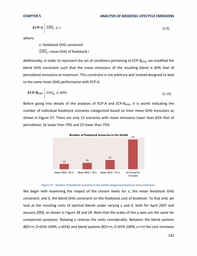
CHAPTER 5 ANALYSIS OF BIODIESEL LIFECYCLE EMISSIONS
142
ECP-A (5.9)
where;
ε: feedstock GHG constraint
: mean GHG of feedstock i
Additionally, in order to represent the set of conditions pertaining to ECP-BGHG, we modified the
blend GHG constraint such that the mean emissions of the resulting blend is 60% that of
petrodiesel emissions at maximum. This constraint is not arbitrary and instead designed to lead
to the same mean GHG performance with ECP-A.
ECP-BGHG (5.10)
Before going into details of the analyses of ECP-A and ECP-BGHG, it is worth indicating the
number of individual feedstock scenarios categorized based on their mean GHG emissions as
shown in Figure 27. There are only 13 scenarios with mean emissions lower than 65% that of
petrodiesel, 16 lower than 70% and 23 lower than 75%.
Figure 27 – Number of feedstock scenarios in the model categorized based on mean emissions.
We begin with examining the impact of the chosen levels for ε, the mean feedstock GHG
constraint; and E, the blend GHG constraint on the feedstock cost of biodiesel. To that end, we
look at the resulting costs of optimal blends under varying ε and E, both for April 2007 and
January 2005, as shown in Figure 28 and 29. Note that the scales of the y-axes are the same for
comparison purposes. Relaxing ε reduces the costs considerably. Between the blend systems
B(Ω=∞, E=65%-100%, ε=65%) and blend systems B(Ω=∞, E=65%-100%, ε=∞) the cost increases
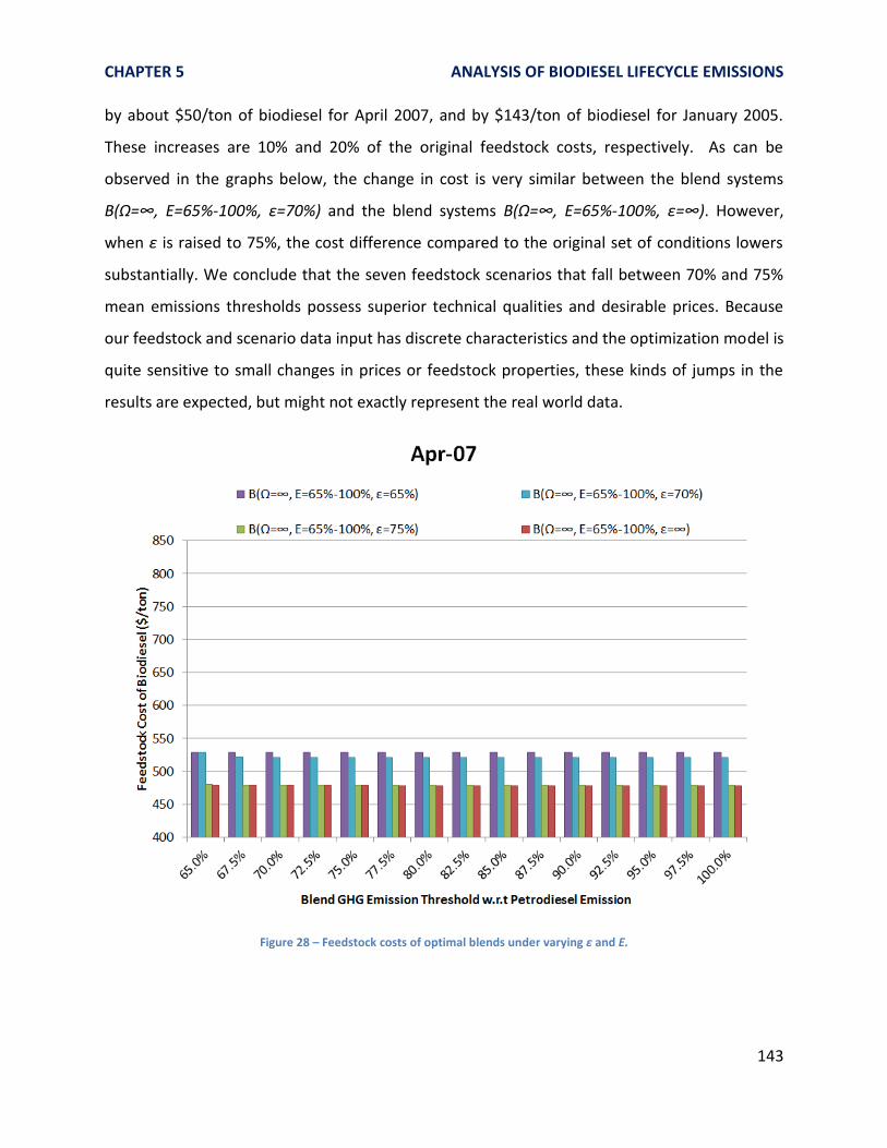
CHAPTER 5 ANALYSIS OF BIODIESEL LIFECYCLE EMISSIONS
143
by about $50/ton of biodiesel for April 2007, and by $143/ton of biodiesel for January 2005.
These increases are 10% and 20% of the original feedstock costs, respectively. As can be
observed in the graphs below, the change in cost is very similar between the blend systems
B(Ω=∞, E=65%-100%, ε=70%) and the blend systems B(Ω=∞, E=65%-100%, ε=∞). However,
when ε is raised to 75%, the cost difference compared to the original set of conditions lowers
substantially. We conclude that the seven feedstock scenarios that fall between 70% and 75%
mean emissions thresholds possess superior technical qualities and desirable prices. Because
our feedstock and scenario data input has discrete characteristics and the optimization model is
quite sensitive to small changes in prices or feedstock properties, these kinds of jumps in the
results are expected, but might not exactly represent the real world data.
Figure 28 – Feedstock costs of optimal blends under varying ε and E.
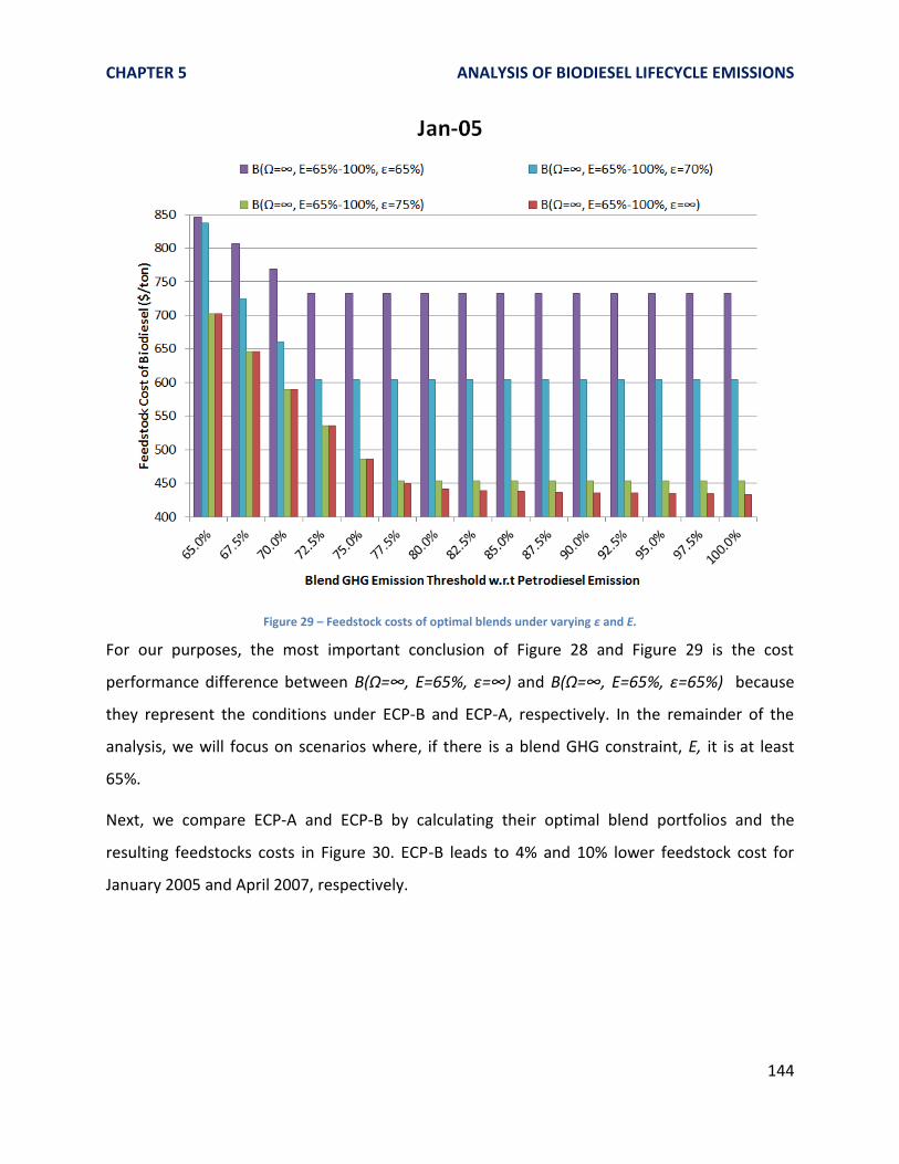
CHAPTER 5 ANALYSIS OF BIODIESEL LIFECYCLE EMISSIONS
144
Figure 29 – Feedstock costs of optimal blends under varying ε and E.
For our purposes, the most important conclusion of Figure 28 and Figure 29 is the cost
performance difference between B(Ω=∞, E=65%, ε=∞) and B(Ω=∞, E=65%, ε=65%) because
they represent the conditions under ECP-B and ECP-A, respectively. In the remainder of the
analysis, we will focus on scenarios where, if there is a blend GHG constraint, E, it is at least
65%.
Next, we compare ECP-A and ECP-B by calculating their optimal blend portfolios and the
resulting feedstocks costs in Figure 30. ECP-B leads to 4% and 10% lower feedstock cost for
January 2005 and April 2007, respectively.

CHAPTER 5 ANALYSIS OF BIODIESEL LIFECYCLE EMISSIONS
145
Figure 30 – Optimal blend portfolios and feedstock costs of ECP-A and ECP-B for (a) January 2005, (b) April 2007.
A primary interest of analysis is the emissions distribution comparison of the blends. Clearly, by
eliminating certain feedstock scenarios from the model based on their high GHG emissions, we
obtain a restricted blend that is composed of low GHG feedstocks only. And it is evident that
the mean emissions of this restricted blend will be lower than if it was not restricted.
Nevertheless, as discussed earlier, the distribution of resulting emissions matter in terms of the
chance of meeting or not meeting the emissions reduction targets over time. Therefore, we
next compare the emissions distribution of the blends under ECP-A and ECP-B. For brevity, we
limited this analysis to April 2007 only, because the results would be identical for any point in
time.
The first column in Figure 31 shows the emissions distributions of (a) B(Ω=∞, ε=65%) under
ECP-A, and (b) B(Ω=∞, E=65%, ε=∞) under ECP-B. We first look at the performance of the
blends with respect to the 65% petrodiesel emissions threshold. The distribution of B(Ω=∞,
ε=65%) shows that this constraint is met with only 69% probability, whereas B(Ω=∞, E=65%,
ε=∞) meets the constraint with 80% probability. Next, we look at the mean emissions and
notice that B(Ω=∞, ε=65%) has lower mean emissions (60%) than B(Ω=∞, E=65%, ε=∞) (63%).
This explains the lower cost of B(Ω=∞, E=65%, ε=∞) as was shown in Figure 30. The total
number of feedstocks used in the blend is also shown on the graphs in Figure 31. The degree of

CHAPTER 5 ANALYSIS OF BIODIESEL LIFECYCLE EMISSIONS
146
feedstock diversification in B(Ω=∞, ε=65%) is about half of B(Ω=∞, E=65%, ε=∞) with only 13
as opposed to 24 feedstocks.
The second column in Figure 31 shows the OS distributions to illustrate how a technical
property distribution of the two blends differs under ECP-A and ECP-B. Due to feedstock
diversification in B(Ω=∞, E=65%, ε=∞), we observe a tighter OS distribution, and therefore
more of the feedstocks with inferior OS characteristics can be added to the blend. This gives a
cost reduction advantage at the expense of decreasing the mean OS value from 4.80 hours to
4.62 hours.
Figure 31 – Comparison of GHG emission and OS distributions of (a) ECP-A, (b) ECP-B.
Higher mean emissions of ECP-B compared to ECP-A might be seen as a negative outcome from
the perspective of the policy maker. Because, as opposed to the technical biodiesel constraints
that need to be met by each batch, GHG emissions matter on average and the mean emissions
is the most relevant metric for assessing performance averaged over time. This consideration
led us to creating the blend system B(Ω=∞, GHG_µ≤60%, ε=∞) under ECP-BGHG. In this policy,
all the 75 scenarios are included but the blend GHG constraint is modified such that the mean

CHAPTER 5 ANALYSIS OF BIODIESEL LIFECYCLE EMISSIONS
147
emissions of the resulting portfolio is 60%. The choice of 60% is not arbitrary; it is in fact
identical to the mean emissions observed for B(Ω=∞, ε=65%) under ECP-A. In order to obtain a
blend portfolio with 60% mean emission for modeling B(Ω=∞, GHG_µ≤60%, ε=∞), we reduced
the constraint E from 65% to 63%62, and then ran a Monte Carlo simulation with 10,000
randomly sampled iterations on the optimal blend. The resulting GHG emissions distribution is
shown in Figure 32. Note that although B(Ω=∞, GHG_µ≤60%, ε=∞) has the same mean
emissions with B(Ω=∞, ε=65%), it demonstrates a tighter distribution. Total number of
feedstocks used is 17. In addition, the confidence level with respect to the 65% emissions
threshold is observed at 97%, which is an improvement over 80%.
Figure 32 – GHG emissions distribution of B(Ω=∞, GHG_µ≤60%, ε=∞) under ECP-BGHG.
The constituents and cost of blends are of great importance in illustrating the strength of the
CC optimization model. Figure 33 shows the comparison of blend portfolios. In B(Ω=∞,
GHG_µ≤60%, ε=∞) all the feedstocks that are in B(Ω=∞,ε=65%) are used in slightly different
proportions and 4 more feedstocks are added to the optimal portfolio63. These additional
feedstocks are denoted in different shades of red on the graph. Three of them are palm
scenarios with 70%, 70% and 81% emissions; and one of them is a sunflower scenario with 66%
emissions. Because all of these 4 feedstock had emissions higher than 65%, none of them were
allowed under ECP-A, and thus were not included in B(Ω=∞,ε=65%). Another interesting
62
E=63% was found by trial and error method.
63 Only the feedstocks used more than 0.5% are considered.

CHAPTER 5 ANALYSIS OF BIODIESEL LIFECYCLE EMISSIONS
148
observation is significantly lower overall use of canola in ECP-BGHG at 25% compared to 65% in
ECP-A; and higher overall use of sunflower in ECP-BGHG at 56% compared to 35% in ECP-A. It
must be remembered that price of feedstocks have a significant impact on the include/exclude
decisions made by the model, and for April 2007 the following trend holds:
pricecan>pricesyb>pricesnf>priceplm. Thus, the decrease in canola, the increase in sunflower and
the addition of palm explain how a significant cost reduction can be achieved under ECP-BGHG
by providing more feedstock options to the producer without compromising the mean emission
performance of biodiesel.
Figure 33 – Comparison of optimal blend portfolios and costs for modified ECP-A and ECP-BGHG, April 2007.
One can also argue that there might exist a domino effect in a multiple feedstock system
subject to multiple constraints such that including (or excluding) a feedstock into (or from) an
optimal portfolio might require a set of other include/exclude decisions, either to keep the
blend feasible or to reach to the optimal point with a new set of feedstocks. In the example
above, addition of palm might have enabled the use of more sunflower, and in turn, the
proportion of canola could be reduced. On top of this multiple feedstock-multiple constraint
complexity, there is a distribution tightening impact of diversification which was observed in
the Monte Carlo simulations shown in Figure 22, 23 and 31. Clearly, optimal solutions obtained

CHAPTER 5 ANALYSIS OF BIODIESEL LIFECYCLE EMISSIONS
149
by the CC model are extremely challenging to achieve by man-made decisions when all the
complexities are taken into account.
Results presented in this section demonstrated that the GHG emissions thresholds have might
significant implications on the cost of biodiesel, depending on the relative prices observed at a
given point in time. As expected, relaxing the GHG emissions constraint leads to more diversified
blends, particularly through intra-species diversification. Under ECP-A, we showed that the
resulting blend emissions distribution might indicate risks of non-compliance with the policy
targets. Under ECP-B, we observed that the feedstock cost might decrease by about 10%
compared to blends under ECP-A in April 2007, while the probabilistic performance of
compliance with respect to the GHG constraint is improved. Finally, by slightly modifying the
parameter E under ECP-B and thereby obtaining the conditions for ECP-BGHG, we showed that
the same mean emissions with the blends under ECP-A can be achieved, with significantly lower
costs and improved probabilistic performance of compliance via inter- and intra-species
diversification.
5.f.3) Multiple Period Price Data Analysis
This section is a multiple period comparison analysis of blend systems under ECP-A, ECP-BΩ, ECP-
BGHG, ECP-BE with the blend system under ECP-B. The main focuses of the analyses are the
feedstock cost of biodiesel and the degree of feedstock diversification.
In Section 5.f.2, we have seen how feedstock cost and fuel performance of biodiesel change
through inter- and intra-species diversification when optimized based on two different single
period price sets. In this section, our goal is to look at multiple periods and characterize the
resulting feedstock cost of blends subject to different sets of constraints, some of which
correspond to the policy frameworks introduced earlier. A total of 102 monthly price sets are
used in the model, covering the range between January 2003 and July 2011, which was the
latest available data point at the time of our inquiry.
We begin with comparing the baseline blend system B(Ω=∞, E=65%, ε=∞) under ECP-B and
B(Ω=3, E=65%, ε=∞) under ECP-BΩ, for which the only difference is the maximum number of
feedstocks in the blend. Figure 34 shows the resulting cost difference (the latter minus the

CHAPTER 5 ANALYSIS OF BIODIESEL LIFECYCLE EMISSIONS
150
baseline blend cost64) on the primary y-axis with a range of $1/ton to $61/ton, and the number
of feedstocks used in each blend on the secondary y-axis.
Figure 34 – Feedstock cost differences and number of feedstocks used in B(Ω=∞, E=65%, ε=∞) under ECP-B, and in B(Ω=3, E=65%, ε=∞) under ECP-BΩ.
The figure suggests that lower cost difference points usually correspond to higher number of
feedstock differences in the optimal blends, but note that this does not always hold true.
Similarly, the higher cost differences are generally observed when the number of feedstock
difference is lower. We will explain the drivers behind this observation through the end of this
section.
Secondly, we compare the feedstock costs of B(Ω=∞, E=65%, ε=∞) and B(Ω=∞, E=100%, ε=∞)
to observe the impact of relaxing the blend GHG constraint over the entire period between
January 2003 and July 2011. Figure 35 demonstrates a very similar pattern to Figure 34, except
that the cost difference is negative and it has a larger range, from -$1/ton to -$278/ton. Also
note the great degree of diversification for B(Ω=∞, E=100%, ε=∞) with optimal blends
composed of more than 50 feedstocks.
64
In all the subsequent graphs in this section, the feedstock cost difference is calculated where the baseline is subtracted from the other blend system in consideration.
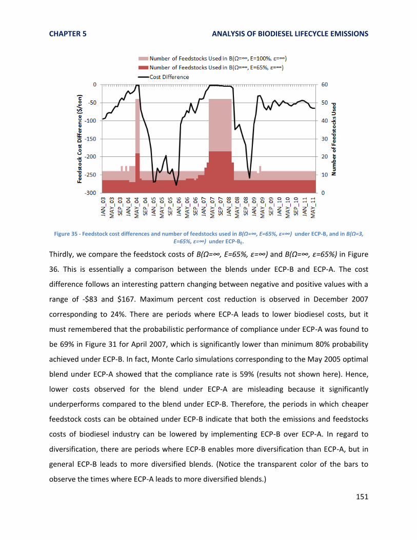
CHAPTER 5 ANALYSIS OF BIODIESEL LIFECYCLE EMISSIONS
151
Figure 35 - Feedstock cost differences and number of feedstocks used in B(Ω=∞, E=65%, ε=∞) under ECP-B, and in B(Ω=3, E=65%, ε=∞) under ECP-BE.
Thirdly, we compare the feedstock costs of B(Ω=∞, E=65%, ε=∞) and B(Ω=∞, ε=65%) in Figure
36. This is essentially a comparison between the blends under ECP-B and ECP-A. The cost
difference follows an interesting pattern changing between negative and positive values with a
range of -$83 and $167. Maximum percent cost reduction is observed in December 2007
corresponding to 24%. There are periods where ECP-A leads to lower biodiesel costs, but it
must remembered that the probabilistic performance of compliance under ECP-A was found to
be 69% in Figure 31 for April 2007, which is significantly lower than minimum 80% probability
achieved under ECP-B. In fact, Monte Carlo simulations corresponding to the May 2005 optimal
blend under ECP-A showed that the compliance rate is 59% (results not shown here). Hence,
lower costs observed for the blend under ECP-A are misleading because it significantly
underperforms compared to the blend under ECP-B. Therefore, the periods in which cheaper
feedstock costs can be obtained under ECP-B indicate that both the emissions and feedstocks
costs of biodiesel industry can be lowered by implementing ECP-B over ECP-A. In regard to
diversification, there are periods where ECP-B enables more diversification than ECP-A, but in
general ECP-B leads to more diversified blends. (Notice the transparent color of the bars to
observe the times where ECP-A leads to more diversified blends.)

CHAPTER 5 ANALYSIS OF BIODIESEL LIFECYCLE EMISSIONS
152
Figure 36 - Feedstock cost differences and number of feedstocks used in B(Ω=∞, E=65%, ε=∞) under ECP-B,
and in B(Ω=∞, ε=65%) under ECP-A.
Finally, we compare the feedstock costs of B(Ω=∞, E=65%, ε=∞) and B(Ω=∞, GHG_µ≤60%,
ε=∞). Obviously, because the blend GHG constraint (E=63%) was more strict for the latter blend
to obtain a mean emission of 60%, higher costs are expected. As can be observed in Figure 37,
the difference between the two can be as low as $2/ton or as high as $119/ton. The level of
diversification is the same except for when the prices are relatively similar across vegetable oils,
and thus diversification is highly favored.

CHAPTER 5 ANALYSIS OF BIODIESEL LIFECYCLE EMISSIONS
153
Figure 37 - Feedstock cost differences and number of feedstocks used in B(Ω=∞, E=65%, ε=∞) under ECP-B,
and in B(Ω=∞, GHG_µ≤60%, ε=∞) under ECP-BGHG.
The consistent trend between higher levels of diversification and lower levels of cost difference
between the blend systems is significant and provides valuable insight about the optimization
mechanism. To investigate this trend further, we decided to focus on the sub-period between
January 2004 and January 2005 during which some of the lowest and highest blend costs were
recorded, and we analyzed the deflated feedstock prices as shown in Figure 38.

CHAPTER 5 ANALYSIS OF BIODIESEL LIFECYCLE EMISSIONS
154
Figure 38 – Deflated feedstock prices observed between January 2004 and January 2005.
As the feedstock prices get closer to each other around April 2004, they also get lower
altogether, and hence a smaller cost difference is observed between the blends in Figures 34-
37. As the difference across feedstock prices widens after May 2004, we observe higher cost
differences along with lower levels of diversification in Figures 34-37. In order to measure this
widening effect in prices and to quantify the dispersion among the feedstock prices for each
month, we calculated the variance of monthly feedstock price sets. As a result, we found a close
relationship between lowest variance price sets and the minimum cost differences observed in
Figures 34-37. This result suggests that as the price differences among feedstocks get smaller,
the impact of various policy frameworks on the feedstock cost of biodiesel diminishes.
Focusing on the comparison of blend portfolios and costs in January 2005 as an illustration can
provide further insight into the trends observed in Figure 34-37. Figure 39 shows the total use
of chemically different crop species, neglecting the different LUC scenarios existing within the
use of each crop. The bars appear in the order of the analyses presented above, with the
baseline blend, B(Ω=∞, E=65%, ε=∞) under ECP-B, at the beginning.
Note the absence of soybean in B(Ω=3, E=65%, ε=∞) even though it is used more than
palm in B(Ω=∞, E=65%, ε=∞). Apparently, when there are only 3 feedstocks to choose
from, palm is preferred over soybean, perhaps due to some of its technical properties as
well as its low price and low emissions. The consequence of limiting the portfolio to
three feedstocks is higher feedstock cost due to increased use of canola and sunflower.

CHAPTER 5 ANALYSIS OF BIODIESEL LIFECYCLE EMISSIONS
155
Not surprisingly, B(Ω=∞, E=100%, ε=∞) stands out as the lowest cost blend due to the
lower GHG emissions threshold. Because soybean is the second cheapest feedstock of
January 2005 and has desirable technical properties, the blend is primarily composed of
soybean.
B(Ω=∞, ε=65%) is 100% canola and it meets all the technical constraints at the specified
confidence level. Yet, the previous analysis has shown its low probabilistic performance
with respect to the GHG constraint.
B(Ω=∞, GHG_µ≤60%, ε=∞) possesses the second highest cost among all the blend
systems, yet it must be remembered that it has performs significantly better than
B(Ω=∞, ε=65%) with respect to the GHG constraint.
Figure 39 – Optimal blend portfolios and feedstock costs of ECP-B, ECP-BΩ, ECP-BE, ECP-A, and ECP-BGHG in January 2005.
Figure 40 is a similar plot to Figure 39, except that it shows the average percent use of each
crop over 2003-2011. Interestingly, B(Ω=∞, E=65%, ε=∞) has a very diverse portfolio, indicating
that each single crop might be economically valuable for the producer over the period of
multiple years. This suggests that, in the absence of specific feedstock constraints, producers
should be prepared to include chemically different crops into their portfolios at any point in
time in order to take advantage of fluctuating feedstock prices in the market. Note that the
least amount of diversification is observed in B(Ω=∞, E=100%, ε=∞) because of the lower GHG
limit, biasing the portfolio toward soybean.65
65
In reading these results, it must be remembered that the set of technical constraints we have determined in Chapter 4 might not perfectly represent the real operation requirements. For example, we set minimum induction

CHAPTER 5 ANALYSIS OF BIODIESEL LIFECYCLE EMISSIONS
156
Figure 40 – Average optimal blend portfolios of ECP-B, ECP-BΩ, ECP-BE, ECP-A, and ECP-BGHG A over 2003 and 2011.
Figure 41 summarizes the multi period cost results by comparing Box-Whisker plots of blends
optimized under ECP-A, ECP-B and ECP-BGHG. Minimum and maximum points refer to the 5th
and 95th percentiles, and the rectangles represent the first and third quartiles. Observing the
differences in average costs represented by black dots reveals that implementing ECP-A instead
of ECP-B results in $35/ton higher feedstock costs over time, corresponding to a 6% increase.
Similarly, implementing ECP-A instead of ECP-BGHG results in $18/ton higher costs,
corresponding to a 3% increase. Given the high volumes of biodiesel production, these
differences add up to significant expenses for producers.
Also notice that imposing GHG limits on the feedstock level under ECP-A results in more
variable feedstock costs over time. As mentioned earlier, when ε=65%, the producer is only
allowed to use canola and sunflower, and this makes feedstock costs more exposed to price
fluctuations in the market. This is a significant result that illustrates the impact of emission
control policies on the potential cost of biodiesel in the market.
time as 4.5 hours rather than the US limit of 3 hours, or the EU limit of 6 hours. Similarly, CFPP was set to -1˚C, yet this limit might change depending on the local conditions.

CHAPTER 5 ANALYSIS OF BIODIESEL LIFECYCLE EMISSIONS
157
Figure 41 – Box plots of optimal blend costs corresponding to 102 monthly price data under ECP-A, ECP-B and ECP-BGHG.
Finally, we estimated cumulative cost savings for an average biodiesel producer that has an
annual production volume of 100,000 ton biodiesel66 and produces equal amounts each month.
Figure 42 shows these savings when the baseline blend, B(Ω=∞, E=65%, ε=∞), is used instead
of others. Note that the cost savings compared to the modified ECP-BGHG is expected, because
ECP-BGHG has a tighter blend GHG emissions threshold. One can interpret that figure as the cost
of abating mean emissions from 63% to 60% of petrodiesel per ton of biodiesel over the period
of 2003-2011 for an average biodiesel producer. More than $30 M savings compared to ECP-A
is a significant result, and shows that uninformed policy decisions might lead to significant costs
for the biodiesel industry as well as lower GHG performances overall. Finally, comparing ECP-A
and ECP-BGHG shows that more than $30 M savings ($63 M - $33 M) can be obtained by
implementing ECP-BGHG instead of ECP-A, while achieving GHG distributions with the same
mean emissions value and lower standard deviation.
66
We neglect the other constituents that might exist in the final fuel such as trace amounts of methanol, water as well as the loss of 3 H atoms for each mole of triglyceride reacting with methanol.

CHAPTER 5 ANALYSIS OF BIODIESEL LIFECYCLE EMISSIONS
158
Figure 42 – Cumulative cost savings of different ECPs compared to implementing ECP-A, accumulated over 2003-2011 for a
biodiesel producer producing 100,000 tons/year.
5.g) Feedstock Include/Exclude Decision Space
We had started with identifying a total of 75 different LUC GHG emissions scenarios at the
beginning of this chapter. In section 5.f, we analyzed several ECPs given that these 75 feedstock
scenarios are available to the producer subject to certain constraints. In this section, we
summarize the feedstock space based on include/exclude decisions made by the optimal model
under the frameworks of ECP-A, ECP-B and ECP-BGHG.
The matrix in Table 10 compares ECP-A and ECP-B in terms of the number of feedstocks that
are used at least once over the period 2003-2011. (+) sign represents inclusion and (-)
represents exclusion by the respective ECP. 49 out of 75 feedstocks are never used by either of
the ECPs. This is a significant conclusion indicating that some feedstock scenarios cannot be
used to meet certain GHG emissions performance of biodiesel. On the other hand, there are 13
feedstocks which are never used by ECP-A, but used at least once by ECP-B. As was shown in
Figure 42, this might lead to a feedstock cost difference on the order of $30 M in deflated
dollars for a medium-sized producer over the period of 2003-2011.

CHAPTER 5 ANALYSIS OF BIODIESEL LIFECYCLE EMISSIONS
159
Table 10 – Number of feedstocks used in the optimal blend at least once over the period 2003-2011. (+) refers to inclusion, (-) refers to exclusion by the respective ECP.
ECP-A (+) ECP-B (+) 13
ECP-A (-) ECP-B (+) 13
ECP-A (+) ECP-B (-) 0
ECP-A (-) ECP-B (-) 49
Figure 43 presents more detailed information by two Venn diagrams representing (a) the
feedstocks that are always included in the optimal blend under different ECPs over the period
2003-2011, and (b) the feedstocks that are included in the optimal blend at least once over the
period 2003-2011. Not surprisingly, ECP-A is a subset of ECP-BGHG, and ECP-BGHG is a subset of
ECP-B in both diagrams. Based on the model input parameters, canola biodiesel with no-LUC
(can_no_luc) is the most premium feedstock that is always used in the optimal blend under
every ECP. As shown in diagram (a), some scenarios of palm and sunflower, namely 3_snf_gc,
5_snf_gc, snf_no_luc, 21_plm_pp and 9_plm_pp, are always used by ECP-BGHG and ECP-B. On
the other hand, 2 of these feedstocks, 21_plm_pp and 9_plm_pp, are never used under ECP-A
due to the 65% emissions threshold for individual feedstocks. In fact, ECP-A can never use any
of the palm scenarios because of the emissions constraint even if the price of palm goes to
zero.

CHAPTER 5 ANALYSIS OF BIODIESEL LIFECYCLE EMISSIONS
160
Figure 43 – Venn diagrams representing the feedstock decision space within different ECPs.
Table 11 lists the 26 feedstocks that are used at least once between 2003 and 2011, with their
average deflated prices and average percent uses in the optimal blend under each ECP. The
listed is sorted in descending order based on the percent use under ECP-B. ECP-A is dominated
by canola use, whereas all chemically different crop species are well represented in the average
portfolio of ECP-B and ECP-BGHG.

CHAPTER 5 ANALYSIS OF BIODIESEL LIFECYCLE EMISSIONS
161
Table 11 – Feedstocks that are used at least once by any of the ECPs between 2003 and 2011. Percentages refer to average proportions used in the blend. The list is sorted in descending feedstock use order under ECP-B.
5.h) Summary and Conclusion
In this chapter we started with describing different ECPs aimed at GHG emissions reductions for
biodiesel compared to petrodiesel emissions. Next, we described a feedstock-specific lifecycle
GHG emissions estimation methodology that led to 75 distinct feedstock scenarios belonging to
canola, soybean, sunflower and palm. Results presented in Section 5.f and Section 5.g illustrate
that cost reduction opportunities exist when a policy does not pose restrictions on individual
feedstock choices, encourage feedstock diversification and set thresholds on the resulting
Average
Deflated Price
($/ton) ECP-A ECP-B ECP-BGHG
1 can_no_luc 622.4 89.5% 24.5% 23.1%
2 syb_no_luc 494.2 0.0% 19.5% 14.1%
3 5_snf_gc 690.3 0.9% 12.5% 16.7%
4 snf_no_luc 690.3 0.9% 11.2% 11.1%
5 9_plm_pp 400.1 0.0% 10.3% 10.8%
6 3_snf_gc 690.3 0.9% 7.4% 11.2%
7 21_plm_pp 400.1 0.0% 6.7% 6.9%
8 3_can_gc 622.4 0.0% 1.2% 1.0%
9 2_snf_gc 690.3 0.9% 0.7% 0.9%
10 19_snf_gc 690.3 0.9% 0.6% 0.7%
11 7_snf_gc 690.3 0.9% 0.6% 0.6%
12 plm_no_luc 400.1 0.0% 0.6% 0.3%
13 6_snf_gc 690.3 0.9% 0.5% 0.6%
14 38_snf_gc 690.3 0.9% 0.5% 0.5%
15 4_snf_gc 690.3 0.9% 0.5% 0.5%
16 5_snf_pc 690.3 0.9% 0.5% 0.5%
17 3_snf_pc 690.3 0.9% 0.4% 0.4%
18 2_snf_pc 690.3 0.9% 0.3% 0.1%
19 8_snf_gc 690.3 0.0% 0.3% 0.0%
20 5_syb_gc 494.2 0.0% 0.2% 0.0%
21 2_snf_fc 690.3 0.0% 0.2% 0.0%
22 2_can_gc 622.4 0.0% 0.2% 0.0%
23 38_snf_fc 690.3 0.0% 0.1% 0.0%
24 6_snf_pc 690.3 0.0% 0.1% 0.0%
25 3_syb_gc 494.2 0.0% 0.1% 0.0%
26 4_snf_pc 690.3 0.0% 0.1% 0.0%

CHAPTER 5 ANALYSIS OF BIODIESEL LIFECYCLE EMISSIONS
162
emissions of the biodiesel blend instead of individual feedstocks. Results also show that
emissions performance of the fuel is not compromised to achieve these cost reductions.
Indeed, with the use the CC optimization model, the producer can control the non-compliance
rate based on risk preference. Comparison of ECP-A and ECP-B suggests that the probabilistic
emissions performance of the fuel can be improved, leading to a higher chance of meeting the
emissions reduction target. Furthermore, comparison of ECP-A and ECP-BGHG shows that the
same level of mean biodiesel emissions can be achieved by implementing policies that allow
more extensive feedstock options. Both ECP-B and ECP-BGHG cost lower than ECP-A, on average
by 6% and 3%, respectively. These cost saving opportunities are promising in making biodiesel
cost competitive with petrodiesel while ensuring that the goals of emissions reductions are
achieved.
Although we have not discussed in the body of this chapter, the supply-chain literature
indicates that there might be additional financial risk control benefits for the producers who are
diversifying their raw material supplier portfolio. It has been suggested that there is a trade-off
for the manufacturer between signing a portfolio of long term contracts with its suppliers and
having access to a spot market [148]. The manufacturer incurs inventory risk when purchasing
too many contracts and spot price risk when buying too few. In the case of biodiesel
production, when ECPs restrict producers’ portfolio selection to a few feedstocks on the
grounds of emission control, the whole industry is exposed to spot prices of vegetable oils
coming from certain regions. Consequently, producers cannot implement financial hedging
strategies through diversification of suppliers corresponding to different feedstock scenarios in
our model.
Currently, ECPs in the US and EU can be characterized under ECP-A which limits the potential
for feedstock diversification. In addition, the biodiesel producers have been relying on
experience-based blending recipes instead of being able to fully capture the market
opportunities emerging from fluctuating feedstock prices. In order for biodiesel production to
become cost effective, the implications of current ECPs and industry practices with regards to
blending need to be further analyzed and understood. The analysis presented in Chapter 5

CHAPTER 5 ANALYSIS OF BIODIESEL LIFECYCLE EMISSIONS
163
provides valuable insight on the topic and can be extended for consideration of other
alternative emission control policies.

164
CHAPTER 6:
CONCLUSIONS AND FUTURE WORK
Biodiesel is a promising alternative fuel to petrodiesel, supported by governments to reduce
dependence on finite petroleum fuels, achieve national energy independence, and cut down
tail pipe emissions. In recent years, biodiesel has become more desirable due to the expanding
sustainability agenda of developed countries; however several lifecycle assessment studies
have reported a high degree of uncertainty and variation (U&V) in lifecycle greenhouse gas
(GHG) emissions, raising questions about the emissions benefits of biodiesel in comparison to
petrodiesel. As a response, regulatory bodies worldwide have either already implemented, or
are in the process of designing emission control policies (ECPs), imposing restrictions on the
types of feedstocks that can be used in producing a biodiesel batch. When these ECPs become
fully effective, they are likely to result in reduced feedstock diversification within the biodiesel
industry.
Total cost, fuel quality and lifecycle GHG emissions are crucial performance parameters for
biodiesel to be competitive with petrodiesel. Feedstock portfolio selection is central to
improving each of these parameters; because (1) feedstock cost is about 85% of the total cost,
(2) there are multiple technical specifications for the final fuel, and individual feedstocks have
varying degrees of compliance with respect to each specification, and (3) lifecycle emissions of
each feedstock are different, particularly due to the LUC impact.
Producers are faced with several challenges in making optimal feedstock portfolio decisions for
each biodiesel batch that they produce. First of all, there is a significant degree of U&V in
physical characteristics and particularly in GHG emissions estimates of feedstocks. Secondly,
feedstock prices fluctuate over time, and thus feedstock cost of the blend might vary depending
on the market conditions. So far canola, soybean, sunflower and palm oil have been the main
feedstocks, and producers have relied on a set of experience-based, fixed blend recipes using
these feedstocks to ensure fuel quality for their customers. On the other hand, there are other
CHAPTER 6 CONCLUSIONS AND FUTURE WORK
165
promising oil seeds such as camelina, jatropha and corn that might provide a wider feedstock
selection for producers, potentially leading to lower costs and improved quality for the final
fuel. Nevertheless, with the availability of new feedstock options, the complexity of the
decision space might necessitate the use of analytical decision making tools that minimize costs
while ensuring fuel quality and emissions reductions. So far, ECPs in the US and EU have been
designed in a way to exclude certain feedstocks, leading to a restricted feedstock selection
space for producers.
In this work, we created two sets of prediction models; one for physical fuel characteristics and
one for feedstock lifecycle GHG emissions. In the former set, we developed chemical
composition-based models for predicting a subset of critical fuel properties, namely iodine
value, oxidation stability, cetane number and cold filter plugging point. These prediction models
rely upon the fatty acid composition characteristics of vegetables oils, capture the inherent
compositional U&V and properly propagate it into the predicted fuel property. In the latter set,
we developed a feedstock-specific lifecycle GHG emissions distribution model based on the EU
directives, guidelines and data. This model incorporates the most likely LUC scenarios for
canola, soybean, sunflower and palm biodiesel based on a detailed analysis of the global
production statistics and geographical distribution of soil types and climate regions. In
calculating the optimal blend portfolios subject to the technical and sustainability standards, we
employed a chance-constrained (CC) optimization model in which the objective is to minimize
the total feedstock cost and the decision variables are the feedstock proportions in the blend.
The CC optimization model explicitly considers the U&V in decision variables and incorporates it
into the blending decision. Thus, the producer can manage feedstock quality variation and
select feedstocks based on non-compliance risk preference.
After formulating an optimization algorithm based on the prediction models we developed and
the CC methodology, we used monthly vegetable oil price data observed between 2003 and
2011 to investigate cost reduction opportunities for producers through optimal blending. The
results show that optimal blends tend to be diversified compared to experience-based blend
recipes, and that feedstock diversification always reduces costs. In some cases, this reduction is
as large as 38%, depending on the set of constraints and relative prices of vegetable oils.

CHAPTER 6 CONCLUSIONS AND FUTURE WORK
166
When there is no GHG emissions constraint on the system, average savings of more than 20%
can be achieved during the period between 2003 and 2011, by using the optimal blend
portfolios compared to using 100% canola. In addition, when the fuel is composed of a diverse
set of vegetable oils, the cost of the final fuel is less exposed to vegetable oil price fluctuations
in the market, and thus more stable biodiesel costs can be obtained. Recognizing the potential
operational challenges of using blend rules that change every month based on prices, we also
created three robust blend rules to be used over the entire period between 2003 and 2011.
Results show that each robust blend outperforms experienced-based recipes, but none can
achieve the cost performance of monthly optimized blends, and that the producer needs to
evaluate the trade-off between having to optimize biodiesel batches every month vs. using a
single blend rule over long periods of time.
When there is a GHG threshold in the system imposed by ECPs, optimal blend portfolios and
total feedstock costs vary depending on whether the threshold is applied upon the mean
emissions of individual feedstocks or on the final fuel emissions characteristics. Our analyses
show that ECPs that restrict the use of certain feedstocks based on their mean GHG emissions
do not necessarily lead to biodiesel blends with better GHG performance. In contrast, ECPs
imposing restrictions on the final fuel (i.e., the blend) emissions can achieve equivalent or
better emissions characteristics, by encouraging feedstock diversification for producers, and
enabling them to risk-pool from a larger feedstock population with a diverse set of emissions
distributions. As a result, lower and less variable feedstock costs can be achieved without
compromising the emissions reduction targets or the fuel quality with final fuel-based ECPs.
Cost reductions up to 24% can be obtained depending on the relative vegetable oil prices
observed in the period of interest between 2003 and 2011. Obviously, lowering production
costs lowers the amount of subsidy required to make the biodiesel system viable. Ultimately, it
seems difficult to find a case for not scrapping the currently implemented feedstock-based ECPs
in favor of the economic efficiency (and equivalent emissions performance) of final fuel-based
ECPs.
To summarize, we showed that feedstock blending can be used as a tool to explicitly manage
U&V in physical and emissions characteristics of the final fuel. Moreover, explicit consideration

CHAPTER 6 CONCLUSIONS AND FUTURE WORK
167
of U&V in blending decisions can provide economic benefit to biodiesel producers by enabling
them to control the rate of non-compliance based on risk preference. Our results indicate that a
strategic selection of feedstocks prior to production can amplify that economic benefit. We also
found that emission control policies which exclude certain feedstocks from the biodiesel market
minimize the economic benefits accrued through blending, and do not necessarily improve the
GHG benefits of the final fuel.
There are a number of related topics that can be studied building upon the results obtained
from this work. Calibration of the physical prediction model we developed based on the
literature reported values can be pursued with real production data from biodiesel producers.
These calibration efforts might increase the accuracy and precision of the model as well as
identifying compositional differences of the same crop species originating from different
suppliers around the world, leading to a more detailed decision making tool for producers. A
related study can be performed to find the optimal FA composition profile for a biodiesel
feedstock through genetic engineering techniques. Because current policies provide financial
incentives only if feedstocks with low emissions are used in a biodiesel batch, a study that
models future feedstock prices based on their GHG emissions estimates can provide useful
insights into the future of biodiesel feedstock market. Similarly, a more detailed study
investigating the implications of ECPs that can incorporate the methods and costs of emissions
monitoring might fill in the gap between emissions reduction targets of governments and
research efforts to precisely estimate lifecycle emissions of biodiesel. A related topic which we
have left out within the scope of this project is the characterization of the subtle difference
between uncertainty and variation in emissions data. The questions concerning whether or not
they can be separated from each other and if so, the implications of their relative magnitudes in
the context of ensuring emissions reduction targets remain to be answered. Because we
concluded that feedstock diversification is a major driver for achieving cost reductions and
managing cost uncertainty, an analytical investigation of the benefits of feedstock
diversification from the perspective of a supply-chain management strategy remains to be
future work as well. Finally, waste cooking oil presents a very interesting case for our model
due to its low cost, low emissions but an incredibly high U&V in physical characteristics.

CHAPTER 6 CONCLUSIONS AND FUTURE WORK
168
Therefore, future work could focus on identifying potential benefits and drawbacks of blending
waste cooking oil along with premium vegetable oils for production of cost effective and low
emissions biodiesel that can compete with petrodiesel.

169
REFERENCES
[1] IEA/OECD, "Transport, Energy and CO2: Moving Toward Sustainability," International Energy Agency2009.
[2] NPR. (2008) World Bank Chief: Biofuels Boosting Food Prices. NPR. Available: http://www.npr.org/templates/story/story.php?storyId=89545855
[3] OECD/FAO, "BIOFUEL - OECD-FAO Agricultural Outlook 2011-2020," OECD2010.
[4] (2011, May 2012). Strategic Energy Technologies Information System, Biofuels for the Transport Sector. Available: http://setis.ec.europa.eu/newsroom-items-folder/biofuels-for-the-transport-sector
[5] E. Carter and I. Ardjosoediro, "The U.S. Biodiesel Market, 2000 to 2010: Riding the Rollercoaster," FAS/USDA, Ed., ed: Office of Global Analysis, 2011.
[6] J. Smolinska, "EU Economic report," ACEA-European Automobile Manufacturers' Association, 2008.
[7] B. Flach, S. Lieberz, K. Bendz, B. Dahlbacka, and D. Achilles, "EU-27 Biofuels Annual-EU Annual Biofuel Report," ed: USDA Foreign Agricultural Service. The Hague, the Netherlands, 2011.
[8] S. Retka-Schill, "Walking a tightrope," Biodiesel Mag, vol. 5, pp. 64-70, 2008.
[9] B. R. Moser, "Influence of Blending Canola, Palm, Soybean, and Sunflower Oil Methyl Esters on Fuel Properties of Biodiesel†," Energy & Fuels, vol. 22, pp. 4301-4306, 2008.
[10] C. C. Group, "Soybeans and Biodiesel: Key Price Relationships," White Paper2009.
[11] USDA, "Oilseeds: World Markets and Trade," F. A. Service, Ed., ed, 2012.
[12] B. R. Moser, "Comparative oxidative stability of fatty acid alkyl esters by accelerated methods," Journal of the American Oil Chemists' Society, vol. 86, pp. 699-706, 2009.
[13] Index Mundi. Available: http://www.indexmundi.com/
[14] S. Basha, K. Gopal, and S. Jebaraj, "A review on biodiesel production, combustion, emissions and performance," Renewable and sustainable energy reviews, vol. 13, pp. 1628-1634, 2009.
[15] A. Pradhan, D. Shrestha, A. McAloon, W. Yee, M. Haas, J. Duffield, and H. Shapouri, "Energy life-cycle assessment of soybean biodiesel," Agricultural Economic Report, 2009.
[16] J. Malça and F. Freire, "Uncertainty Analysis in Biofuel Systems," Journal of Industrial Ecology, vol. 14, pp. 322-334, 2010.
[17] J. Malça and F. Freire, "Life-cycle studies of biodiesel in Europe: A review addressing the variability of results and modeling issues," Renewable and sustainable energy reviews, vol. 15, pp. 338-351, 2011.
[18] B. Schade, T. Wiesenthal, S. H. Gay, and G. Leduc, "Potential of Biofuels to Reduce Greenhouse Gas Emissions of the European Transport Sector," Transport Moving to Climate Intelligence, pp. 243-269, 2011.

170
[19] T. Searchinger, R. Heimlich, R. Houghton, F. Dong, A. Elobeid, J. Fabiosa, S. Tokgoz, D. Hayes, and T. Yu, "Use of US croplands for biofuels increases greenhouse gases through emissions from land-use change," Science, vol. 319, p. 1238, 2008.
[20] "Notice of Supplemental Determination for Renewable Fuels Produced Under the Final RFS2 Program from Canola Oil," vol. 75, ed. Federal Register, 2010, pp. 43522-43525.
[21] "Notice of Data Availability Concerning Renewable Fuels Produced From Palm Oil Under the RFS Program," vol. 77, ed. Federal Register, 2012, pp. 4300-4318.
[22] C. Dunmore. (2012) EU Officials to Decide the Fate of Biofuels. Euro News. Available: http://www.euronews.com/newswires/1502448-eu-officials-to-decide-fate-of-bio-fuels/
[23] K. J. Harrington, "Chemical and physical properties of vegetable oil esters and their effect on diesel fuel performance," Biomass, vol. 9, pp. 1-17, 1986.
[24] G. Knothe, J. Van Gerpen, J. Krahl, and C. Press, The Biodiesel Handbook, 2nd ed.: AOCS press Champaign, IL, 2010.
[25] M. Lange, "The GHG balance of biofuels taking into account land use change," Energy Policy, 2011.
[26] T. Thamsiriroj and J. Murphy, "Can Rape Seed Biodiesel Meet the European Union Sustainability Criteria for Biofuels?," Energy & Fuels, vol. 24, pp. 1720-1730, 2010.
[27] E. Commission. BIOGRACE [Online]. Available: http://www.biograce.net/
[28] A. Charnes and W. W. Cooper, "Chance-constrained programming," Management Science, pp. 73-79, 1959.
[29] M. Wendt, P. Li, and G. Wozny, "Nonlinear Chance-Constrained Process Optimization under Uncertainty," Industrial & Engineering Chemistry Research, vol. 41, pp. 3621-3629, 2002.
[30] J.-S. Shih and H. C. Frey, "Coal blending optimization under uncertainty," European Journal of Operational Research, vol. 83, pp. 452-465, 1995.
[31] N. V. Sahinidis, "Optimization under uncertainty: state-of-the-art and opportunities," Computers & Chemical Engineering, vol. 28, pp. 971-983, 2004.
[32] G. Gaustad, P. Li, and R. Kirchain, "Modeling methods for managing raw material compositional uncertainty in alloy production," Resources, Conservation and Recycling, vol. 52, pp. 180-207, 2007.
[33] E. A. Olivetti, G. G. Gaustad, F. R. Field, and R. E. Kirchain, "Increasing Secondary and Renewable Material Use: A Chance Constrained Modeling Approach To Manage Feedstock Quality Variation," Environmental Science & Technology, 2011.
[34] G. Gaustad, E. Olivetti, and R. Kirchain, "Design for Recycling," Journal of Industrial Ecology, vol. 14, pp. 286-308, 2010.
[35] E. Persson, P. Engstrand, L. Karlsson, F. Nilsson, and M. Wahlgren, "Utilization of the natural variation in wood properties–a comparison between pilot plant and mill scale trials," 2003, pp. 2-5.
[36] (2012, June 2011). Petroprogram. Available: http://www.petroprogram.com/BIOC_brochure.pdf
[37] C. Allen, K. Watts, R. Ackman, and M. Pegg, "Predicting the viscosity of biodiesel fuels from their fatty acid ester composition," Fuel, vol. 78, pp. 1319-1326, 1999.

171
[38] P. Ghosh and S. Jaffe, "Detailed composition-based model for predicting the cetane number of diesel fuels," Ind. Eng. Chem. Res, vol. 45, pp. 346-351, 2006.
[39] G. Knothe, A. C. Matheaus, and T. W. Ryan, "Cetane numbers of branched and straight-chain fatty esters determined in an ignition quality tester< sup>☆</sup>," Fuel, vol. 82, pp. 971-975, 2003.
[40] C. J. Chuck, C. D. Bannister, J. Gary Hawley, and M. G. Davidson, "Spectroscopic sensor techniques applicable to real-time biodiesel determination," Fuel, vol. 89, pp. 457-461, 2010.
[41] B. Freedman and M. Bagby, "Predicting cetane numbers of n-alcohols and methyl esters from their physical properties," Journal of the American Oil Chemists' Society, vol. 67, pp. 565-571, 1990.
[42] G. Knothe and R. O. Dunn, "Dependence of oil stability index of fatty compounds on their structure and concentration and presence of metals," Journal of the American Oil Chemists' Society, vol. 80, pp. 1021-1026, 2003.
[43] A. Kamal‐Eldin, "Effect of fatty acids and tocopherols on the oxidative stability of vegetable oils," European Journal of Lipid Science and Technology, vol. 108, pp. 1051-1061, 2006.
[44] J. Y. Park, D. K. Kim, J. P. Lee, S. C. Park, Y. J. Kim, and J. S. Lee, "Blending effects of biodiesels on oxidation stability and low temperature flow properties," Bioresource Technology, vol. 99, pp. 1196-1203, 2008.
[45] H. Tang, R. C. De Guzman, S. O. Salley, and S. K. Y. Ng, "The oxidative stability of biodiesel: Effects of FAME composition and antioxidant," Lipid Technology, vol. 20, pp. 249-252, 2008.
[46] J. Polavka, J. Paligová, J. Cvengroš, and P. Simon, "Oxidation stability of methyl esters studied by differential thermal analysis and Rancimat," Journal of the American Oil Chemists' Society, vol. 82, pp. 519-524, 2005.
[47] B. R. Moser, M. J. Haas, J. K. Winkler, M. A. Jackson, S. Z. Erhan, and G. R. List, "Evaluation of partially hydrogenated methyl esters of soybean oil as biodiesel," European Journal of Lipid Science and Technology, vol. 109, pp. 17-24, 2007.
[48] E. Alptekin and M. Canakci, "Characterization of the key fuel properties of methyl ester-diesel fuel blends," Fuel, vol. 88, pp. 75-80, 2009.
[49] R. Sarin, M. Sharma, S. Sinharay, and R. Malhotra, "Jatropha-palm biodiesel blends: an optimum mix for Asia," Fuel, vol. 86, pp. 1365-1371, 2007.
[50] M. Canakci and H. Sanli, "Biodiesel production from various feedstocks and their effects on the fuel properties," Journal of Industrial Microbiology and Biotechnology, vol. 35, pp. 431-441, 2008.
[51] F. V. K. Young, "Interchangeability of fats and oils," Journal of the American Oil Chemists' Society, vol. 62, pp. 372-376, 1985.
[52] G. Knothe, "“Designer” Biodiesel: Optimizing Fatty Ester Composition to Improve Fuel Properties†," Energy & Fuels, vol. 22, pp. 1358-1364, 2008.
[53] L. D. Clements, "Biending Rules for Formulating Biodiesel Fuel," 1996.
[54] G. Knothe, "Structure indices in FA chemistry. How relevant is the iodine value?," Journal of the American Oil Chemists' Society, vol. 79, pp. 847-854, 2002.
172
[55] E. N. Frankel, Lipid oxidation: Oily Press Dundee, Scotland, 1998.
[56] D. Dolde, C. Vlahakis, and J. Hazebroek, "Tocopherols in breeding lines and effects of planting location, fatty acid composition, and temperature during development," Journal of the American Oil Chemists' Society, vol. 76, pp. 349-355, 1999.
[57] A. Fröhlich and S. Schober, "The influence of tocopherols on the oxidation stability of methyl esters," Journal of the American Oil Chemists' Society, vol. 84, pp. 579-585, 2007.
[58] S. Jain and M. Sharma, "Stability of biodiesel and its blends: a review," Renewable and sustainable energy reviews, vol. 14, pp. 667-678, 2010.
[59] S. Jain and M. Sharma, "Measurement of the Oxidation Stability of Biodiesel Using a Modified Karl Fischer Apparatus," Journal of the American Oil Chemists' Society, pp. 1-7, 2011.
[60] Y. C. Liang, C. Y. May, C. S. Foon, M. A. Ngan, C. C. Hock, and Y. Basiron, "The effect of natural and synthetic antioxidants on the oxidative stability of palm diesel," Fuel, vol. 85, pp. 867-870, 2006.
[61] M. Mittelbach and S. Schober, "The influence of antioxidants on the oxidation stability of biodiesel," Journal of the American Oil Chemists' Society, vol. 80, pp. 817-823, 2003.
[62] W. W. Christie. (2012, January). The AOCS Lipid Library, Tocopherols and Tocotrienols. Available: http://lipidlibrary.aocs.org/lipids/tocol/index.htm
[63] S. Schober and M. Mittelbach, "Antioxidants In: Stability of Biodiesel–Used as a Fuel for Diesel Engines and Heating Systems. Presentation of the BIOSTAB Project Results: Proceedings, Graz July 3rd (2003), editor BLT Wieselburg, Austria," ISBN 3-902451-00-9.
[64] R. Snee, "Developing blending models for gasoline and other mixtures," Technometrics, vol. 23, pp. 119-130, 1981.
[65] W. Healy Jr, C. Maassen, and R. Peterson, "A NEW APPROACH TO BLENDING OCTANES f," 1959, p. 132.
[66] J. Kinast, "Production of biodiesels from multiple feedstocks and properties of biodiesels and biodiesel/diesel blends," Golden, Colorado: National Renewable Energy Laboratory, Gas Technology Institute, 2003.
[67] P. Ghosh and S. B. Jaffe, "Detailed composition-based model for predicting the cetane number of diesel fuels," Industrial & Engineering Chemistry Research, vol. 45, pp. 346-351, 2006.
[68] M. Murphy, J. Taylor, and R. McCormick, "Compendium of experimental cetane number data," Contract DE-AC36-99-GO10337. Golden CO: National Renewable Energy Laboratory, 2004.
[69] L. D. Clements, "Blending Kules for Formulating Biodiesel Fuel," 1996.
[70] H. Imahara, E. Minami, and S. Saka, "Thermodynamic study on cloud point of biodiesel with its fatty acid composition," Fuel, vol. 85, pp. 1666-1670, 2006.
[71] S. Schober and M. Mittelbach, "Influence of diesel particulate filter additives on biodiesel quality," European Journal of Lipid Science and Technology, vol. 107, pp. 268-271, 2005.
[72] M. Haas, A. McAloon, W. Yee, and T. Foglia, "A process model to estimate biodiesel production costs," Bioresource Technology, vol. 97, pp. 671-678, 2006.

173
[73] "A Technology Performance and Regulatory Review," American Biofuels Association & Information Resources, INC., Jefferson City, MO1994.
[74] M. de Wit, M. Junginger, S. Lensink, M. Londo, and A. Faaij, "Competition between biofuels: Modeling technological learning and cost reductions over time," Biomass and Bioenergy, vol. 34, pp. 203-217, 2010.
[75] C. W. DeWitt, L. S. Lasdon, A. D. Waren, D. A. Brenner, and S. A. Melhem, "OMEGA: An improved gasoline blending system for Texaco," Interfaces, pp. 85-101, 1989.
[76] A. Singh, J. F. Forbes, P. J. Vermeer, and S. S. Woo, "Model-based real-time optimization of automotive gasoline blending operations," Journal of Process Control, vol. 10, pp. 43-58, 2000.
[77] J. Li, I. Karimi, and R. Srinivasan, "Recipe determination and scheduling of gasoline blending operations," AIChE Journal, vol. 56, pp. 441-465, 2010.
[78] R. Metzger and R. Schwarzbek, "A linear programming application to cupola charging," J. Ind. Eng, vol. 12, pp. 87-93, 1961.
[79] R. F. Hutton and J. Allison, "A linear programming model for development of feed formulas under mill-operating conditions," Journal of Farm Economics, vol. 39, pp. 94-111, 1957.
[80] T. E. Baker and L. S. Lasdon, "Successive linear programming at Exxon," Management Science, pp. 264-274, 1985.
[81] J. Westbrook, "Problems with residual and additive elements and their control through specifications," Resource Recovery and Conservation, vol. 4, pp. 369-393, 1980.
[82] R. D. Peterson, "Scrap variability and its effects on producing alloys to specification," LIGHT MET(WARRENDALE PA), pp. 855-859, 1999.
[83] M. Reuter and A. van Schaik, "Thermodynamic metrics for measuring the “sustainability” of design for recycling," JOM Journal of the Minerals, Metals and Materials Society, vol. 60, pp. 39-46, 2008.
[84] S. M. Abubakr, G. M. Scott, and J. H. Klungness, "Fiber fractionation as a method of improving handsheet properties after repeated recycling," TAPPI Journal, vol. 78, pp. 123-126, 1995.
[85] E. Thode, "A model experiment in pulp blending," Pulp Pap. Mag. Can, vol. 62, pp. T195-T200, 1961.
[86] J. LEHTONEN and L. LEHTONEN, "Differentiation in pulp and paper business," Paperi ja puu, vol. 86, pp. 251-253, 2004.
[87] S. Lundqvist, F. Ekenstedt, T. Grahn, Ö. Hedenberg, L. Olsson, and L. Wilhelmsson, "Selective use of European resources of spruce fibers for improved pulp and paper quality," 2003, pp. 2-5.
[88] C. M. P. Bizi and N. R. Demarquette, "Effect of the processing conditions and the addition of trans‐polyoctenylene rubber on the properties of natural rubber/styrene–butadiene rubber blends," Journal of Applied Polymer Science, vol. 109, pp. 445-451, 2008.
[89] I. A. Hussein, R. A. Chaudhry, and B. F. Abu Sharkh, "Study of the miscibility and mechanical properties of NBR/HNBR blends," Polymer Engineering & Science, vol. 44, pp. 2346-2352, 2004.

174
[90] L. Nunes, "Mechanical characterization of hyperelastic polydimethylsiloxane by simple shear test," Materials Science and Engineering: A, vol. 528, pp. 1799-1804, 2011.
[91] O. Kramer and W. Good, "Correlating Mooney viscosity to average molecular weight," Journal of Applied Polymer Science, vol. 16, pp. 2677-2684, 1972.
[92] G. Tintner, "A note on stochastic linear programming," Econometrica: Journal of the Econometric Society, pp. 490-495, 1960.
[93] J. Dupacová and P. Popela, "Melt control: Charge optimization via stochastic programming," Applications of Stochastic Programming (SW Wallace and WT Ziemba, eds.), Philadelphia, SIAM and MPS, pp. 277-298, 2005.
[94] N. Bliss, "Advances in scrap charge optimization," 1997, pp. 27-30.
[95] A. Hartley, P. Eastburn, and N. Leece, "Steelworks control of residuals," Philosophical Transactions of the Royal Society of London. Series A, Mathematical and Physical Sciences, vol. 295, pp. 45-55, 1980.
[96] W. H. Evers, "A new model for stochastic linear programming," Management Science, pp. 680-693, 1967.
[97] U. S. Karmarkar and K. Rajaram, "Grade selection and blending to optimize cost and quality," Operations Research, pp. 271-280, 2001.
[98] D. Mihailidis and K. Chelst, "Optimal blending of out-of-specifications substances," Journal of the Operational Research Society, pp. 458-466, 1998.
[99] D. Bertsimas and M. Sim, "The price of robustness," Operations Research, pp. 35-53, 2004.
[100] C. Van de Panne and W. Popp, "Minimum-cost cattle feed under probabilistic protein constraints," Management Science, pp. 405-430, 1963.
[101] M. Kumral, "Application of chance-constrained programming based on multi-objective simulated annealing to solve a mineral blending problem," Engineering Optimization, vol. 35, pp. 661-673, 2003.
[102] A. Rong and R. Lahdelma, "Fuzzy chance constrained linear programming model for optimizing the scrap charge in steel production," European Journal of Operational Research, vol. 186, pp. 953-964, 2008.
[103] M. Cetinkaya and F. Karaosmano lu, "Optimization of base-catalyzed transesterification reaction of used cooking oil," Energy Fuels, vol. 18, pp. 1888-1895, 2004.
[104] C. Enweremadu and M. Mbarawa, "Technical aspects of production and analysis of biodiesel from used cooking oil--A review," Renewable and sustainable energy reviews, vol. 13, pp. 2205-2224, 2009.
[105] R. Howard-Hildige, A. P. O'Connell, and J. J. Leahy, "Demonstate the use of blends of waste cooking oil with biodiesels and mineral fuel for engines and heating the Country Council Offices at Mallow County Cork," Altener Project2002.
[106] A. Phan and T. Phan, "Biodiesel production from waste cooking oils," Fuel, vol. 87, pp. 3490-3496, 2008.
[107] L. A. Goodman, "On the exact variance of products," Journal of the American Statistical Association, pp. 708-713, 1960.
[108] A. Demirbaş, Biodiesel: a realistic fuel alternative for diesel engines: Springer Verlag, 2008.

175
[109] E. Commission, "Directive 2009/30/EC of the European Parliament " EEC, 2009.
[110] V. Martínez‐de‐Albéniz and D. Simchi‐Levi, "A portfolio approach to procurement contracts," Production and Operations Management, vol. 14, pp. 90-114, 2005.
[111] A. A. Acquaye, T. Wiedmann, K. Feng, R. H. Crawford, J. Barrett, J. Kuylenstierna, A. P. Duffy, S. C. L. Koh, and S. McQueen-Mason, "Identification of ‘Carbon Hot-Spots’ and Quantification of GHG Intensities in the Biodiesel Supply Chain Using Hybrid LCA and Structural Path Analysis," Environmental Science & Technology, 2011.
[112] E. G. Castanheira and F. M. Freire, "Environmental performance of palm oil biodiesel—A life-cycle perspective," 2011, pp. 1-6.
[113] M. Frondel and J. Peters, "Biodiesel: a new oildorado?," Energy Policy, vol. 35, pp. 1675-1684, 2007.
[114] H. Huo, M. Wang, C. Bloyd, and V. Putsche, "Life-cycle assessment of energy use and greenhouse gas emissions of soybean-derived biodiesel and renewable fuels," Environmental Science & Technology, vol. 43, pp. 750-756, 2008.
[115] R. J. Plevin, M. O’Hare, A. D. Jones, M. S. Torn, and H. K. Gibbs, "Greenhouse Gas Emissions from Biofuels’ Indirect Land Use Change Are Uncertain but May Be Much Greater than Previously Estimated," Environmental Science & Technology, vol. 44, pp. 8015-8021, 2010.
[116] L. Reijnders and M. Huijbregts, "Biogenic greenhouse gas emissions linked to the life cycles of biodiesel derived from European rapeseed and Brazilian soybeans," Journal of Cleaner Production, vol. 16, pp. 1943-1948, 2008.
[117] S. Soimakallio, T. Mäkinen, T. Ekholm, K. Pahkala, H. Mikkola, and T. Paappanen, "Greenhouse gas balances of transportation biofuels, electricity and heat generation in Finland--Dealing with the uncertainties," Energy Policy, vol. 37, pp. 80-90, 2009.
[118] T. Thamsiriroj and J. Murphy, "Is it better to import palm oil from Thailand to produce biodiesel in Ireland than to produce biodiesel from indigenous Irish rape seed?," Applied Energy, vol. 86, pp. 595-604, 2009.
[119] K. A. Mullins, W. M. Griffin, and H. S. Matthews, "Policy Implications of Uncertainty in Modeled Life-Cycle Greenhouse Gas Emissions of Biofuels⊥," Environmental Science & Technology, 2011.
[120] DOE and USDA, "DOE Actively Engaged in Investigating the Role of Biofuels in Greenhouse Gas Emissions from Indirect Land Use Change," ed, 2008.
[121] T. D. Searchinger, "Response to New Fuels Alliance and DOE Analysts Criticisms of Science Studies of Greenhouse Gases and Biofuels," ed.
[122] R. Righelato and D. V. Spracklen, "Carbon mitigation by biofuels or by saving and restoring forests?," Science Magazine, vol. 317, p. 902, 2007.
[123] J. Kanter, "Questioning Europe's Math on Biofuels," in The New York Times, ed. Green Column, 2011.
[124] J. Kanter, "'Serious' Error Found in Carbon Savings for Biofuels," in The New York Times, ed, 2011.
[125] D. Biello, "For Greening Aviation, Are Biofuels the Right Stuff?," Yale School of Forestry & Environment Studies2009.

176
[126] G. T. Beer T., Campbell P. K., "Biodiesel could reduce greenhouse gas emissions," CSIRO, Australia KS54C/1/F2.27, 2007.
[127] M. Cimitile. (2009, April 20, 2009) Corn Ethanol will not Cut Greenhouse Gas Emissions. Scientific American. Available: http://www.scientificamerican.com/article.cfm?id=ethanol-not-cut-emissions
[128] J. Giles. (2008, February 7, 2008) Biofuels Emissions may be 'worse than petrol'. New Scientist. Available: http://www.newscientist.com/article/dn13289-biofuels-emissions-may-be-worse-than-petrol.html
[129] J. Hill, E. Nelson, D. Tilman, S. Polasky, and D. Tiffany, "Environmental, economic, and energetic costs and benefits of biodiesel and ethanol biofuels," Proceedings of the National Academy of Sciences, vol. 103, p. 11206, 2006.
[130] P. J. Crutzen, A. R. Mosier, K. A. Smith, and W. Winiwarter, "N< sub> 2</sub> O release from agro-biofuel production negates global warming reduction by replacing fossil fuels," Atmospheric Chemistry and Physics, vol. 8, pp. 389-395, 2008.
[131] T. E. McKone, W. W. Nazaroff, P. Berck, M. Auffhammer, T. Lipman, M. S. Torn, E. Masanet, A. Lobscheid, N. Santero, U. Mishra, A. Barrett, M. Bomberg, K. Fingerman, C. Scown, B. Strogen, and A. Horvath, "Grand Challenges for Life-Cycle Assessment of Biofuels," Environmental Science & Technology, vol. 45, pp. 1751-1756, 2011.
[132] Comission Decision on the guidelines for the calculation of land carbon stocks for the purpose of Annex V to Directive 2009/28/EC, E. Commission, 2010.
[133] U. EPA, "Renewable Fuel Standard Program (RFS2) Regulatory Impact Analysis," ed: US Environmental Protection Agency Washington, DC, 2010.
[134] U. EPA, "Renewable Fuel Standard (RFS2) Delayed RIN Generation Guidance Document for Canola Oil," O. o. T. a. A. Quality, Ed., ed, 2010.
[135] A. Venkatesh, P. Jaramillo, W. M. Griffin, and H. S. Matthews, "Uncertainty analysis of life cycle greenhouse gas emissions from petroleum-based fuels and impacts on low carbon fuel policies," Environmental Science & Technology, 2011.
[136] M. G. Morgan and M. Henrion, Uncertainty: a guide to dealing with uncertainty in quantitative risk and policy analysis: Cambridge Univ Pr, 1992.
[137] R. Schnepf, Renewable fuel standard (RFS): Overview and Issues: DIANE Publishing, 2011.
[138] E. Commission, "Directive 2009/28/EC of the European Parliament and of the Council of 23 April 2009 on the promotion of the use of energy from renewable sources and amending and subsequently repealing Directives 2001/77/EC and 2003/30/EC," Official Journal of the European Union, pp. 16-61, 2009.
[139] U. Nations. FAOSTAT [Online]. Available: http://faostat.fao.org/default.aspx
[140] IPCC, "2006 IPCC Guidelines for National Greenhouse Gas Inventories," 2006.
[141] J. A. Deckers, F. Nachtergaele, and O. C. Spaargaren, World reference base for soil resources: Introduction vol. 1: Acco, 1998.
[142] IPCC, "Guidelines for National Greenhouse Gas Inventories," 2006.
177
[143] F. Nachtergaele, H. van Velthuizen, L. Verelst, N. Batjes, K. Dijkshoorn, V. van Engelen, G. Fischer, A. Jones, L. Montanarella, and M. Petri, "Harmonized World Soil Database," 2010, pp. 34-37.
[144] "Regulation of Fuels and Fuel Additives: Changes to Renewable Fuel Standard Program," vol. 74, ed. Federal Register, 2009, pp. 24904-25142.
[145] F. Figueiredo, D. F., "Biodiesel de girassol ou micralgas em Portugal: Uma avaliacao comparativa de ciclo vida," Departamento de Engenharia Mecanica, Universidade de Coimbra, 2011.
[146] P. S. Mehta and K. Anand, "Estimation of a Lower Heating Value of Vegetable Oil and Biodiesel Fuel," Energy & Fuels, vol. 23, pp. 3893-3898, 2009/08/20 2009.
[147] J. Malça, "Incorporating Uncertainty in the lifecycle modeling of biofuels: Energy renewability and GHG intensity of bioethanol and biodiesel, 2006," PhD, Mechanical Engineering, Universidade de Coimbra, Coimbra, 2011.
[148] V. Martínez‐de‐Albéniz and D. Simchi‐Levi, "Mean‐variance trade‐offs in supply contracts," Naval Research Logistics (NRL), vol. 53, pp. 603-616, 2006.

178
This page is intentionally left blank.

179
APPENDICES
Appendix-A: Soil-Climate Combinations
COMBINATION ID SOIL TYPE + CLIMATE REGION
1 High Activity Clay Soils + Boreal, dry
2 High Activity Clay Soils + Boreal, wet
3 High Activity Clay Soils + Cold temperate, dry
4 High Activity Clay Soils + Cold temperate, moist
5 High Activity Clay Soils + Warm temperate, dry
6 High Activity Clay Soils + Warm temperate, moist
7 High Activity Clay Soils + Tropical, dry
8 High Activity Clay Soils + Tropical, moist
9 High Activity Clay Soils + Tropical, wet
10 High Activity Clay Soils + Tropical, montane
NA High Activity Clay Soils + Polar, moist
NA High Activity Clay Soils + Polar, dry
NA Low Activity Clay Soils + Boreal, dry
NA Low Activity Clay Soils + Boreal, wet
15 Low Activity Clay Soils + Cold temperate, dry
16 Low Activity Clay Soils + Cold temperate, moist
17 Low Activity Clay Soils + Warm temperate, dry
18 Low Activity Clay Soils + Warm temperate, moist
19 Low Activity Clay Soils + Tropical, dry
20 Low Activity Clay Soils + Tropical, moist
21 Low Activity Clay Soils + Tropical, wet
22 Low Activity Clay Soils + Tropical, montane
NA Low Activity Clay Soils + Polar, moist
NA Low Activity Clay Soils + Polar, dry
25 Sandy Soils + Boreal, dry
26 Sandy Soils + Boreal, wet
27 Sandy Soils + Cold temperate, dry
28 Sandy Soils + Cold temperate, moist
29 Sandy Soils + Warm temperate, dry
30 Sandy Soils + Warm temperate, moist
31 Sandy Soils + Tropical, dry
32 Sandy Soils + Tropical, moist
33 Sandy Soils + Tropical, wet
34 Sandy Soils + Tropical, montane
NA Sandy Soils + Polar, moist
NA*: Combination not available in the model.

180
(continued from the previous page)
COMBINATION ID SOIL TYPE + CLIMATE REGION
NA Sandy Soils + Polar, dry
37 Spodic Soils + Boreal, dry
38 Spodic Soils + Boreal, wet
NA Spodic Soils + Cold temperate, dry
40 Spodic Soils + Cold temperate, moist
NA Spodic Soils + Warm temperate, dry
42 Spodic Soils + Warm temperate, moist
43 Spodic Soils + Tropical, dry
NA Spodic Soils + Tropical, moist
NA Spodic Soils + Tropical, wet
NA Spodic Soils + Tropical, montane
NA Spodic Soils + Polar, moist
NA Spodic Soils + Polar, dry
49 Volcanic Soils + Boreal, dry
50 Volcanic Soils + Boreal, wet
51 Volcanic Soils + Cold temperate, dry
52 Volcanic Soils + Cold temperate, moist
53 Volcanic Soils + Warm temperate, dry
54 Volcanic Soils + Warm temperate, moist
55 Volcanic Soils + Tropical, dry
56 Volcanic Soils + Tropical, moist
57 Volcanic Soils + Tropical, wet
58 Volcanic Soils + Tropical, montane
NA Volcanic Soils + Polar, moist
NA Volcanic Soils + Polar, dry
61 Wetland Soils + Boreal, dry
62 Wetland Soils + Boreal, wet
63 Wetland Soils + Cold temperate, dry
64 Wetland Soils + Cold temperate, moist
65 Wetland Soils + Warm temperate, dry
66 Wetland Soils + Warm temperate, moist
67 Wetland Soils + Tropical, dry
68 Wetland Soils + Tropical, moist
69 Wetland Soils + Tropical, wet
70 Wetland Soils + Tropical, montane
NA Wetland Soils + Polar, moist
NA Wetland Soils + Polar, dry
NA*: Combination not available in the model.

181
Appendix-B: Lifecycle GHG Emissions Details of 75 Feedstock Scenarios
Mean LUC GHG
Emissions w.r.t. to
Petrodiesel*
Mean Non-LUC GHG
Emissions w.r.t. to
Petrodiesel
Mean TOTAL GHG
emissions w.r.t. to
Petrodiesel
Stdev of GHG Emissions
w.r.t. to Petrodiesel
40_can_gc 55% 62% 117% 48%
38_can_gc 48% 62% 110% 49%
20_can_gc 78% 62% 140% 18%
19_can_gc 42% 62% 104% 13%
8_can_gc 98% 62% 160% 26%
7_can_gc 45% 62% 107% 15%
6_can_gc 47% 62% 109% 37%
4_can_gc 49% 62% 111% 40%
3_can_gc 10% 62% 72% 20%
2_can_gc 34% 62% 96% 29%
40_can_fc 235% 62% 297% 68%
38_can_fc 127% 62% 189% 43%
20_can_fc 317% 62% 379% 70%
19_can_fc 228% 62% 290% 53%
8_can_fc 322% 62% 384% 74%
7_can_fc 228% 62% 290% 53%
6_can_fc 225% 62% 287% 63%
4_can_fc 228% 62% 290% 64%
3_can_fc 197% 62% 259% 54%
2_can_fc 110% 62% 172% 34%
40_can_pc 167% 62% 229% 56%
38_can_pc 147% 62% 209% 57%
20_can_pc 258% 62% 320% 23%
19_can_pc 181% 62% 243% 14%
8_can_pc 530% 62% 592% 90%
7_can_pc 322% 62% 384% 49%
6_can_pc 301% 62% 363% 85%
4_can_pc 322% 62% 384% 91%
3_can_pc 139% 62% 201% 39%
2_can_pc 205% 62% 267% 63%
can_no_luc 0% 62% 62% 12%
21_syb_gc 117% 68% 185% 30%
20_syb_gc 99% 68% 167% 23%
7_syb_gc 56% 68% 125% 18%
5_syb_gc 12% 68% 81% 19%
3_syb_gc 13% 68% 81% 25%
21_syb_pc 361% 68% 430% 37%
20_syb_pc 326% 68% 394% 29%
7_syb_pc 235% 68% 303% 19%
5_syb_pc 66% 68% 135% 19%
3_syb_pc 78% 68% 146% 25%
syb_no_luc 0% 68% 68% 14%
*Petrodiesel=100%

182
(continued from the previous page)
Mean LUC GHG
Emissions w.r.t. to
Petrodiesel*
Mean Non-LUC GHG
Emissions w.r.t. to
Petrodiesel
Mean TOTAL GHG
emissions w.r.t. to
Petrodiesel
Stdev of GHG Emissions
w.r.t. to Petrodiesel
38_snf_gc 9% 49% 57% 9%
19_snf_gc 8% 49% 56% 2%
8_snf_gc 18% 49% 66% 5%
7_snf_gc 8% 49% 57% 3%
6_snf_gc 8% 49% 57% 7%
5_snf_gc 2% 49% 50% 3%
4_snf_gc 9% 49% 58% 7%
3_snf_gc 2% 49% 51% 4%
2_snf_gc 6% 49% 55% 5%
38_snf_fc 23% 49% 71% 8%
19_snf_fc 41% 49% 90% 9%
8_snf_fc 58% 49% 106% 13%
7_snf_fc 41% 49% 90% 10%
6_snf_fc 40% 49% 89% 11%
5_snf_fc 35% 49% 84% 9%
4_snf_fc 41% 49% 89% 12%
3_snf_fc 35% 49% 84% 10%
2_snf_fc 20% 49% 68% 6%
38_snf_pc 26% 49% 75% 10%
19_snf_pc 32% 49% 81% 3%
8_snf_pc 53% 49% 102% 6%
7_snf_pc 33% 49% 82% 3%
6_snf_pc 24% 49% 73% 8%
5_snf_pc 9% 49% 58% 3%
4_snf_pc 25% 49% 74% 8%
3_snf_pc 11% 49% 60% 4%
2_snf_pc 15% 49% 64% 6%
snf_no_luc 0% 49% 49% 10%
21_plm_fp 56% 81% 137% 32%
9_plm_fp 62% 81% 143% 31%
21_plm_pp -11% 81% 70% 13%
9_plm_pp -11% 81% 70% 10%
plm_no_luc 0% 81% 81% 16%
*Petrodiesel=100%