AN ESSAY ON EXTERNALITIES, PROPERTY VALUES

AND URBAN ZONING

by

William J. Stull

B.A,, Northwestern University(1966)

SUBMITTED IN PARTIAL FULFILLMENT

OF THE REQUIREMENT FOR THEDEGREE OF DOCTOR OF

PHILOSOPHY

at the

MASSACHUSETTS INSTITUTE OFTECHNOLOGY

October, 1971( L o.Teb.

Signature of AuthorDE

Certified by

Accepted by_

3ignature Redactedpartment of fconomics, October 8, 1971

Eignature Redacted(T \hesis Supervisor

Signature RedactedChairman, Departmental Committee

ArChIuei on Graduate StudentsSTF. %.E

MAR 21 1972

ABSTRACT

Title: An Essay on Externalities, Property Values andUrban Zoning

Author: William J. Stull

Submitted to the Department of Economics on October 8, 1971,in partial fulfillment of the requirement for the degree ofDoctor of Philosophy

This dissertation is concerned with a cluster of theo-retical and empirical problems in the economics of land-usecontrol. Chapter I sets the stage for the analysis of theseproblems by focusing attention on the importance of urbanland as a national resource. Chapter II reviews the economicliterature on zoning and neighborhood externalities and con-cludes that there are several important research problemswhich remain to be solved,

The first of these concerns the empirical significanceof neighborhood quality as a determinant of residential pro-perty values. This is taken up in Chapters III and IV.Modern economic research has failed heretofore to establishconclusively that adverse neighborhood environments affectthe market price of residential properties. In Chapter IIIa simple theory of household bidding behavior at a real es-tate auction is developed -- a theory which suggests (amongother things) that residential properties in undesirableneighborhoods will sell for less than those in desirableneighborhoods, ceteris paribus. In Chapter IV this theoryis tested econometrically using aggregate data for the single-family homes located in forty-six Boston suburbs. The re-sults of the estimations indicate that the price of a homedepends on its structure and lot characteristics, its acces-sibility to employment, and on the characteristics of itsneighborhood environment. Community public service and taxvariables are found to be insignificant.

The second research problem noted in the survey of theliterature is the paucity of theoretical models which can beused as tools for analyzing the economic aspects of land-usecontrol devices. Chapter V is a response to this deficiency;therein a mathematical model of the land-use control problemfaced by a new town developer is presented. The model is thenused to show how changes in zoning boundaries affect otherurban economic variables such as the size of the labor force,the urban wage rate, and the land value gradient. In addi-tion, the implications of the existence of neighborhood ex-ternalities for the behavior of the developer are worked outand some policy recommendations are made.

Thesis Supervisor: Jerome RothenbergTitle: Professor of Economics

ACKNOWLEDGEMENTS

This dissertation was essentially written in the year

between September, 1970 and September, 1971. The debts,

emotional and intellectual, which I incurred during this

period were not numerous. Yet they were of the most funda-

mental sort, and I am grateful to have the opportunity here

to acknowledge them.

First, let me say that I found the faculty of the

economics department at M.I.T. to be most helpful and sup-

portive. John Harris and Jerome Rothenberg were my advisors

and they guided my thinking and research from the very be-

ginning. Their contributions to this dissertation were fun-

damental and too numerous to mention here. My debt to Jerome

Rothenberg is particularly great because he was the one who

first encouraged me to pursue the line of research contained

in this work. In addition, he agreed to serve as my princi-

pal advisor. I would also like to thank Ronald Grieson and

Robert Solow who read the final manuscript in its entirety

and made many useful comments.

The contributions of my friends and fellow students at

M.I.T. are perhaps less tangible than those of my teachers

and advisors, but they are no less real. My contemporaries

at M.I.T. created an intimate and supportive social environ-

ment without which the writing of this dissertation would

have been much more painful than it was. Some of my friends

read and commented upon early drafts of various chapters in

4

this work. I would especially like to thank Larry Hirschhorn

and Bill Wolfson for their efforts in this respect.

More important, however, were the various subtle ways in

which these individuals renewed my enthusiasm for work by

taking my mind off economics for brief interludes, In this

regard, I would especially like to thank Richard Butler for

companionship and a patient ear. I also owe a great deal to

Larry Hirschhorn who constantly expanded my stodgy, bourgeosis

economist consciousness with his brilliant insights and apoc-

alyptic views of the world -- not all of which I had the wit

or sophistication to agree with, And above all I would like

to acknowledge an enormous personal debt to Andy and Marianne

Sum for cigars, good wine, modern jazz and many of the most

pleasant evenings imaginable, Others who made contributions --

mainly by being themselves when I was around -- were Mary

Gubbins, Bill Lebovich, Ellen Coin, John Gruenstein and Allen

MacDonnell.

The greatest debt of all I owe to my wife Judy who cheer-

fully supported me throughout this enterprise -- even while she

was carrying a baby and working on her own dissertation, In

addition to typing and proofreading, she made numerous styl-

istic and substantive suggestions which eventually found their

way into the final text. Perhaps her greatest contribution,

however, was the gentle spur which she applied whenever my

energy or will power seemed to flag. Without her, the disser-

tation would have taken much longer to complete than it did.

Finally, I wish to thank JoAnn Loeb for her expert

5

typing of a difficult manuscript. And last, but surely not

least, I must thank the National Science Foundation for the

financial support which it provided during my four years of

graduate study, As usual, the Old Testament tells it like it

is:

They prepare bread for laughter,and wine comforteth the living:but money answereth to all.

Ecclesiastes 10:19

TABLE OF CONTENTS

CHAPTER PAGE

I, SOME INTRODUCTORY REMARKS .o...... ,,. 7

A, Public Policy and Urban Land *...,.... 7B, The Role of the Economist . . . . . . . . . , , 17C, A Methodological Postscript . . . . . . . 25

II. NEIGHBORHOOD EXTERNALITIES AND URBAN LAND: ASURVEY OF THE LITERATURE , .,, , , 27

A, Introduction . . . . . . . . . . . . . . . . 27B, Some Economic Writings .. g.., .. ... 34C, The Shape of Things to Come.. . .0.0. 56

III. NEIGHBORHOOD QUALITY AND THE RESIDENTIAL SITECHOICE . , , , , , . , , , , . , , , 61

A. Quantifying Neighborhood Quality . . . . . . . 62B. Household Behavior at a Real Estate Auction . . 70C, Consumer Bids and Market Valuation . . , . 92

IV. AN EMPIRICAL STUDY OF RESIDENTIAL PROPERTY VALUESIN A SUBURBAN AREA . * , ,. . .. . , . . . . , 100

A, A General Specification . , . . . , . . 101B, Variables and Data Base . , , , , , , . , , . 105

Figures IV-1 and IV-2 . . . , . . . . . 120C, Some Estimations . . . . . . . o . . . . 132

Table IV-1 * . . . . . . e . . . . . . . 133Table IV-2 *. . . . . ,. . . . . . . . 150

D. Some Objections and Qualifications . . . ., 152E. Conclusions . . . . . . . . . , . . . 160

V. LAND-USE CONTROL IN A SIMPLE URBAN ECONOMY WITHEXTERNALITIES . . , . , . . . . , , , , , , 162

A. Introduction . . , . . . . . . . . . . 162B. A New Town Economy . , . e . . . . . .. 164

Figure V-1 * . . . . .0 . . . . . . . 179Figure V-2 . . . . . . . . . . . . . . 187Figure V-3 * . . . * . . ,. . . . . . . 191

C, Maximizing the Aggregate Value of Urban Land 197D. The Land-Use Control Problem Revisited . o . 203

Figure V-4 . . . . . , . . , . . , , . 204

EPILOGUE 0 0 , * * . . . . . . . . . . . . . . . . 217

TECHNICAL APPENDIX . 0 * . a * . . . . . 0 * 0 . 0 a 220

BIBLIOGRAPHY . . . . . . . a . . , . . . . . . , , a 243

BIOGRAPHICAL NOTE . . . . . . . 0 * , . .* . 0 2 5251

CHAPTER I

Some Introductory Remarks

A. Public Policy and Urban Iand

The declared purpose of the National Housing Act of 1949

was "the realization as soon as feasible of the goal of a

decent home and a suitable living environment for every

American family."I In the early 1950's, for reasons not at

all obscure, the first part of this objective tended to take

precedence over the second in the eyes of the public and its

politicians. The postwar housing shortage produced purchasers

(usually subsidized by the federal government) for virtually

every suburban, single-family home that the housing industry

was capable of supplying. The inevitable result was flimsy

construction, humdrum architecture and bleak landscapes. By

1960, however, the wind had begun to shift to a different

quarter. The supply of homes of all types had increased

dramatically over the previous decade, and households had

become correspondingly more fastidious about the housing

"packages" which they were being offered. Many came to appre-

ciate that "a decent home" was not enough and that "a suitable

living environment" was an important desideratum in its own

right.

1 U.S., Statutes at Large, 63, p.413.

8

The experience of Levitt and Sons during the 1950's

epitomizes some of the changes which took place. Levitt

built three large "Levittown" developments during this

period. The first, on Long Island, had gridiron streets

and identical small bungalows -- the famed $7990 Cape

Codders. Few concessions were made to neighborhood beauty,

Nonetheless, the development was very profitable, and it

set a precedent for numerous imitations throughout the country.

The second Levittown, only slightly less monotonous than the

first, was built near Philadelphia and was also extremely

lucrative. The third, by way of contrast, was a financial

disappointment -- even though it offered four distinct models

and some environmental amenities such as curvilinear streets.

By 1960 it seemed that the American home buyer was no longer

willing to be a "Levittowner" when other choices were avail-

able. What had been satisfactory, even desirable, in 1950

had thus become quite unacceptable one decade later.2

It is now apparent that this episode only adumbrated

further changes to come. If the supply of suburban land

were unlimited, the escalation of household expectations con-

cerning home and neighborhood which began during the 1950's

could always be met by further new construction at the urban-

rural fringe. Each new development would have larger homes,

2This brief history was culled from "The New Look ofMr. Levitt's Towns," sweek, September 13, 1965 and "NewAccent for Bill Levitt," Fortune, December, 1965. As thesetitles suggest, Levitt was able to change his style of opera-tion to satisfy the new breed of home buyer.

9

a more pleasing physical layout, and more open space and

greenery than the one which came before. To a certain

extent, of course, this was the pattern of suburban growth

through much of the postwar period. As new suburbs came

into being, the older ones were left behind by the upwardly

mobile middle class to be occupied by households further

down on the economic ladder.

In recent years, however, problems have arisen. In

particular, there is now evidence that this filtering

process has stalled. The supply of suitable undeveloped

land, a necessary ingredient for any Xanadu, is no longer

seen as unlimited in many metropolitan areas.3 Consequently,

its price has risen.4 Speaking somewhat loosely, the current

situation may be described as one in which a high demand is

3Kubla Khan, it will be recalled, required "twice fivemiles of fertile ground,"

A rude indication of this price increase may be foundin the Department of Housing and Urban Development's statis-tical profile of new homes purchased with FHA-insured mort-gages. These figures show that between 1960 and 1969, lotprices increased much more rapidly (by 74 percent) than didstructure prices (33 percent) or purchaser income (49 percent)."Typical FHA-Financed New Home cost $20,563 in 1969, up $995,"HUD News, May 1, 1970. It is possible, of course, that thislarge increase in average lot price is completely the productof increased average lot size rather than increased price perunit land. This seems doubtful, however.

10

pressing upon a continually shrinking supply. 5 This pressure

is particularly serious in its consequences because, as we

indicated above, the suburban experience during the 1950's

conditioned Americans to expect a continual improvement in

their home and its ambient environment. To make matters even

worse, it also reestablished the eventual acquisition of a

space-consuming, detached, single-family home as a credible

aspiration for all but the poorest citizens. The postwar

building boom thus put to rest most of the resignation which

was built up during the lean years between 1929 and 1945.

Once all this is understood, many current public controversies

become interpretable as specialized responses to a larger prob-

lem.

The social consequences of the declining availability of

suburban land have been twofold. First, class conflicts over

the use of the available supply of residential property have

been exacerbated, The home-owning middle class has stoutly

defended its turf against the incursions of the lower class

5The supply of vacant land suitable for residentialdevelopment in any given period depends upon the rate of pastdevelopment and upon changes in zoning practices, transporta-tion facilities, and the location of employment during theprevious period. In many of our larger metropolitan areasthis supply has been getting smaller year by year -- notbecause transportation and employment are not decentralizingas fast as they used to, but rather because zoning restric-tions in partially developed communities have tightened. Thesituation around New York City is particularly serious in thisregard. Richard Reeves, "Land is Prize in Battle for Controlof Suburbs," The New York Times, August 17, 1971, p. 1.

11

using minimuma-lot zoning and other devices.6 The upper

class, on the other hand, has taken the offensive and

attempted to reestablish its hegemony over the downtown

areas in many of our large central cities.7 The poor, as a

result, have been forced to fight a war on two fronts -- in

the central city to hold what they already have and in the

suburbs to acquire what they believe they are entitled to.

It does not take much imagination to see that a sudden

increase in the available supply of undeveloped suburban

real estate (conceivably through some innovation in transpor-

tation) would do a great deal to mitigate these conflicts.

The second consequence of the Closing of the suburban

frontier has been a renewed interest in city and regional

planning among those of our society's opinion-making elite

who reside in large metropolitan areas. Planning is seen as

a way of making the most equitable and efficient use of the

now scarce undeveloped urban land.8 The general consensus

6A useful survey of such practices in northeastern NewJersey may be found in Norman Williams, Jr. and Thomas Norman,"Exclusionary Land-Use Controls: The Case of Northeastern NewJersey," Land-Use Controls Quarterly, 4 (Fall, 1970).

7matt Edel documents this assault in his recent paper"Market, Planning, or Warfare?# Recent Land Use Conflicts inthe United States," Readings in Urban Boonomics, ed. 4.Rothenberg and M* Edel (New York# Macmillan and Company, 1972).

8 Throughout this study we shall use the word "urban" todenote institutions, objects, or phenomenon which are metro-politan in scope. Thus, "urban" land includes both centralcity and suburban land.

12

here is that this resource is too important to be left to the

capricious dictates of suburban governments and private

developers. Two of the most frequently discussed planning

innovations are new towns and metropolitan government. There

is hardly room in the present study for an extended analysis

of these proposals. Nonetheless, a few comments are appro-

priate to make clear the relationship between our work here

and the large (one is tempted to say excessively large) litera-

ture on these other two topics.

Let us consider metropolitan government first. This

reform has come to be thought of as a panacea by all right-

minded "urbanologists" in spite of the fact that there has

been very little careful empirical analysis of the specific

costs to be incurred and benefits to be received from consoli-

dation. Indeed there has been a paucity of writing on existing

metropolitan governments. As Roger Starr has observed in an

article on New York City politicss

Earnest citizens in America -- even in New York -- haveheld up the ideal of a regional government as a misty,glamorous objective; a Valhalla of good government.Many of these gentlemen have forgotten that New YorkCity has for seventy years now, offered a practicaldemonstration of the possibilities and difficulties ofa regional government... Instead of speculating as tohow regional government mightwork, one can see how NewYork does work -- or doesn't.

A careful accounting of the costs and benefits of metro-

politan government would do more than just delimit the net

welfare gains to be anticipated. It would also provide impor-

9 "Power and Powerlessness in a Regional City," The PublicInterest, 16 (Summer, 1969), p.4.

13tant evidence about the political feasibility of such

amalgamations. If there are some local government preroga-

tives which are so deep-seated and jealously guarded as to

be untransferable to a superior authority except at very high

political cost, it may be that full-blown metropolitan govern-

ments will continue to be impossible to establish except under

rather special conditions. The most that could then be

expected in the majority of urban areas would be a regional

authority with distinctly circumscribed powers.

These considerations are particularly important with

respect to the policy questions we have been discussing here --

namely, those concerned with the nature and extent of govern-

mental interference in the private market for urban property.

Traditionally, real estate has been regulated only at the

local level. This, of course, is true of many other govern-

ment activities as well. However, because the control of

municipal land is so closely associated with the class segre-

gation and small-town self-determination apparently sought

by so many suburbanites when they migrate from the central

city, it will be especially difficult to dislodge and vest in

a higher level of government.10 Nor, incidentally, is it

10Robert C. Wood documents the "stubborn conviction" ofmost suburbanites that they are entitled to small-town govern-ment and their willingness to go to great lengths to achieveit in his SUb bia: Its People and Their Polities (Boston:Houghton Mifflin Company, 195). Richard boock supplementsthese observations by noting that municipalities then usetheir jealously guarded political powers to exclude "outsiders"of all types, be they apartment dwellers, park visitors, motelguests, or customers of a local discount house. The ZoningGaze: Municipal Practices and Pol cies (Madison, Wisconsin:The University of Wisconsin Press, 1966), Chapter II.

14

entirely clear that this control should be so transferred.

The desire of ordinary citizens to live among their own kind

and to possess at least a modicum of control over their

destiny (henceforth to be known as the desire for home rule)

is frequently given virtually no weight by liberals promoting

metropolitan government.11 In spite of this, it may very well

be true that some vestiges of home rule should be preserved

within the interstices of even the most far-reaching metro-

politan political system. In any case, political considera-

tions will probably require it, and a likely field of operation

for this residual municipal power is some control over the

uses to which local land may be put.12

The burden of the previous few paragraphs may be succinctly

summarized by saying that one cannot safely dismiss modest

proposals to reform existing American land regulation insti-

tutions by simply waving hands and uttering the incantation

"metropolitan government." The hard realities are, first,

that metropolitan government may be a long time coming in

many areas and, second, even when it finally arrives its juris-

diction over land use is likely to be distinctly limited. Once

11A careful theoretical analysis of the optimal sizepolitical jurisdiction which does take into account home ruleconsiderations may be found in Jerome Rothenberg's "LocalDecentralization and the Theory of Optimal Government,"(Massachusetts Institute of Technology, Department of Economics,Working Paper No. 35, December, 1968).

12Baboook comes to this same conclusion. Q.cit.,Chapter X.

15

these facts are appreciated, it becomes obvious that local

control over land use is likely to be with us for some time.

This means in turn that the present techniques used by local

governments to regulate the urban land market and protect

residential neighborhoods (principally zoning) are not apt

to be superseded by more radical methods.

Similar kinds of remarks can be made about the plethora

of proposals to establish new towns. Such enterprises are

obviously the wish dreams of the planning profession. What

is in doubt is the extent to which these dreams are likely

to be fulfilled in the coming decades. The private market

thus far has shown little interest in new towns, principally

because of the large amounts of initial capital which they

require. 13 There i, furthermore, little evidence that the

public sector will be any more responsive to the presumed

"needs" of society in this area. William Alonso has argued

rather persuasively that most of the nonaesthetio arguments

for the publio provision of new towns turn out to be rather

insubstantial when subject to close scrutiny.14 Given that

even city planners are not united in their support, it is

difficult to imagine Congress or the various state legisla-

tures appropriating significant funds for such "socialistic"

13Anthony Downs, "Private Investment and the Public Weal,"Saturdar Review, LIV (May 15, 1971), p.25. This article isone of the few which carefully analyzes new towns from thepoint of view of the prospective private developer.

14 "The Mirage of New Towns," The Public Interest, 19(Spring, 1970).

16

enterprises. The only possible exception appears to be a

"demonstration" grant or two designed to raise the level of

public tastes. Perforce, the number of people directly

affected by such a program would be small.

What then are we left with? The principal message seems

to be that serious-minded citizens interested in improving

neighborhood environments, resolving the aforementioned land-

use conflicts, and generally instituting a more "rational"

utilization of scarce urban land in our large metropolitan

areas should set aside their passionate commitment to metro-

politan government and new towns. Such fancies only promote

woolgathering and a general unwillingness to consider less

dramatic but more practicable alternatives. The truth is

that the vast majority of American urban dwellers will for at

least the next decade or two be subject to a system of land

regulation and control which is not terribly different from

the one we have now. To be sure, the winds of controversy

which are currently buffeting this system will undoubtedly

produce some reforms. It seems highly unlikely, however, that

the resulting changes will be revolutionary in scope. Most

will probably be of the order of magnitude of the Massachusetts

"Anti-Snob Zoning" law which was passed several years ago.15

These observations suggest that it is not possible to

15It is worth remarking in this context that as of July,1971, not one dwelling unit has been built under the auspicesof the program set up by this statute. Anthony J. Yiddis,"Anti-Snob Zoning Batting Big .000," Boston Globe, July 11,1971, p.A-47.

17

justify scholarly indifference to zoning and other existing

forms of land regulation on the grounds that these devices

are "obsolete" and soon to be discarded. Instead, the argu-

ment cuts the other way. The probable permanence of these

institutions coupled with the likelihood of their reform in

the next few years makes them particularly interesting subjects

for scholarly investigation. Furthermore, if reforms are to

be made, it is essential that policymakers have sufficient

knowledge about the political feasibility and probable effective-

ness of the various alternatives to choose among them intelli-

gently. Since the only source of such knowledge at the moment

is our past and present experience with existing regulatory

devices, the challenge to academic researchers interested in

urban affairs seems rather well-defined.

B. The Role of the Economist

Up to now economists have paid scant attention to land-

use control devices and have consequently contributed little

to their evolution. One searches in vain through the copious

legal and planning literature on zoning, subdivision control,

land law and other related topics for any important idea or

technique which originated with a member of the economics

profession. A revealing example of the extent to which the

mainstream of economic thought has failed to influence publio

policy in this area occurred in the first twenty-five years

of this century. This was the gestation period for what was

later to become the most frequently used tool for regulating

urban land -- the comprehensive zoning ordinance. What is

18

significant is that this same period also saw the publication

(in several editions) of Pigou's Wealth and Welfare and The

Economics of Welfare, two volumes now thought to be the foun-

tainheads of all modern work on externalities.1 6 In these

works Pigou proposed the tax and subsidy solutions which have

now become part of the litany of economists, to be recited

whenever a hiatus between private and social costs or private

and social benefits is encountered. The interesting thing is

that the lawyers and urban reformers who confronted the

eminently practical problems of imposing some social disci-

pline on the private uses of urban land and of protecting

residential neighborhoods from the incursion of nuisance

industries never gave these particular solutions a moment's

thought. This is true even though the main impetus for public

land regulation at the time was obviously the desire to mini-

mize nonmarket interdependencies among economic activities --

the very kind of problem which Pigovian methods seemed designed

to handle. The point here is not that taxation would have

been a better solution than districting, but only that the

inevitable first thought of a modern economist on the whole

matter of the control of externalities was not even considered

by the policymakers of the day.

Returning to the main thread of the argument, we may ask

16A. C. Pigou, Wealth and Welfare (Londons Macmillan andCompany, 1st ed., 1912) and The Economics of Welfare (London:Macmillan and Company, 1st ed., 1920),e This is R. H. Coase'sassessment of Pigou's influence. "The Problem of Social Cost,"The Journal of law and Economics, III (October, 1960), p.28.

19

why it is that economists have not made more intellectual

contributions in this area. Part of the reason undoubtedly

is the professional myopia of the lawyer and the planner.

This perhaps explains why Pigovian thinking has not worked

its way further into the law and planning journals than it

has. Much more, however, is due to the economist's lack of

interest in all policy questions concerning the allocation

and regulation of urban land.1? There has been some academic

writing on these subjects, of course, but it is small in

amount when compared to the bountiful literature on such

important topics as the stability and uniqueness of the per-

fectly competitive equilibrium.

The origins of this indifference are complex. One

possible explanation is that land-use regulation has simply

not been thought of as a very important public policy area --

or at least not important enough to be worthy of the econ-

omist's attention. Perhaps it is true that many economists

think this however, the argument itself has little merit.

One may agree with Banfield that urban beauty (or any other

objective of land-use control) is not a matter of anyone's

essential welfare. 18 Nonetheless, it is obvious that the

17A very recent exception to this proposition is thespate of writing on urban renewal culminating in JeromeRothenberg's Economic Evaluati of Urban newal (Washington,D.C.t The Brookings Institution, 1967).

18Edward Banfield, The Uneavenly City (Boston: LittleBrown and Company, 1968), pp.7-8.

20

typical urban dweller regards policy issues concerning land

use in his neighborhood and community to be terribly impor-

tant. One need only attend a meeting of the local zoning

appeals board to ascertain this. The land-use conflicts

mentioned in the previous section are manifestly real and

frequently vituperative.

The ubiquity of zoning statutes in urban areas lends

further credence to this view. Allen Manvel in his report

to the National Commission on Urban Problems estimates that

in 1967 approximately 90 percent of the cities and towns in

the United States with a population over 5000 had some kind

of zoning statute.19 In addition, 51 of the 52 largest cities

possessed such ordinances.2 0 The one exception is Houston

which, as is well-known, has chosen to substitute an elabor-

ate system of publicly enforced restrictive covenants for

zoning.2 1 If one accepts the proposition that the legis-

lation passed by municipal governments bears some reasonable

relationship to the preferences of the electorate, one must

conclude from these statistics that land-use control has been

"revealed" to be "important." It is interesting to note

19Allen Manvel, Local Land and Building Regulation(Washington, D.C.# The National Commission on Urban Problems,Research Report No.6,,1968), p.31.

2OIbid., p.171.

2 1Bernard H. Siegan, "Non-Zoning in Houston," The Jour-nal of law and Econopgj XIII (April, 1970), pp.77-91.

21

that Manvel's figures seem to indicate that the number of

households subject to some kind of zoning is only slightly

smaller than the number subject directly or indirectly to

the property tax -- an institution which has inspired a

copious amount of economic writing over the past century.

All of this suggests that the real reason for the curious

unwillingness of economists to work in this area must lie

elsewhere. A useful tentative hypothesis is that the real-

ities of the urban land market were uncongenial to the con-

tinued evolution and refinement of the perfectly competitive

model. As a result, these realities were ignored. Part of

the problem obviously lay in incorporating the various

spatial concepts inherent to the study of urban land into the

perfectly competitive framework. As Isard and others have

reminded us, the traditional assumption underlying this frame-

work is that all of a nation's economic activities take place

at a point, thus allowing transportation costs to be ignored.22

It is not at all clear what the welfare properties of a "com-

petitive" model would be once this assumption is relaxed.

Is it significant, for example, that virtually all firms in

the retail sector of our economy are imperfect competitors

in the sense that they face downward-sloping demand curves?

This fact, due of course to transportation costs, is mani-

festly inconsistent with the traditional assumption that the

22Walter Isard, Location and Space-Economy (Cambridge,Massachusetts: The M.I.T.Pres, 1956), pp.24-27.

22

atomistic firm can sell all he wishes to sell at the current

market price.

A second awkward fact undoubtedly was the prevalence of

nonmarket interrelationships among economic agents in urban

areas. It is well-known that the presence of such external

effects destroys the efficiency properties of the perfectly

competitive model. The reasons for this are complex and we

shall not get into them here.23 The essential point is that

production and consumption externalities are much more char-

acteristic of life in a metropolis than of life in a rural

area or small town.24 Indeed, one suspects that the economy

which the perfectly competitive model most closely describes

is a self-sufficient agricultural district in which indepen-

dent yeoman farmers live on isolated family farms, leaving

only to exchange produce at some centrally located market.

In such an economy there would be virtually no externalities --

all would be "internalized" by the spatial extent of the

individual farms. In order for this bucolic vision to remain

credible, it was apparently necessary to ignore the urban

conditions under which most people lived. It was particularly

2 3A terse but illuminating discussion of this problemmay be found in Kenneth J. Arrow's "Political and EconomicEvaluation of Social Effects and Externalities," The Analysisof Public Output, ed. Julius Margolis (New York: NationalBureau of Economic Research, 1970), pp.13-16.

24Some modest evidence for this assertion may be foundin the differing urban and rural attitudes toward zoning.Babcock, op.cit., pp.20-25.

23

important to ignore the land and housing markets since it is

here that interdependence is most easily seen.

These contentions are perhaps overly harsh, but the

fact remains that until recent years academic economists

working in the mainstream of the profession have treated dis-

dainfully all economic problems associated with urbanization.

The field was left to the aforementioned city planners and

lawyers, aided by a handful of outcast land economists, regional

scientists, and some utopians. Since around 1960, however, a

sea change has occurred. Economists have responded to the

policy interests of the larger society and have begun to

analyze urban economies using the tools heretofore reserved

for more "important" problems. To be sure there has not been

(as we shall see) a great deal of work on the specific topics

which this dissertation is concerned with. On the other hand,

it is now perfectly clear that an economist can participate

in the solutions to the pressing planning and land-use prob-

lems of his day without condescension. As will hopefully be

brought out in subsequent chapters, many of the key issues

in planning, zoning, and modern property law are intimately

related to important topics in the burgeoning economic litera-

ture on externalities and public goods.

To get a feeling for this interpenetration, consider

the particular phenomenon which is the focus of the present

study -- namely, the dependence of a household's well-being

on the dominant characteristics of its surrounding residential

24

environment.25 As we observed above, most Americans now live

in fairly densely populated areas; hence, there is a good

deal of rubbing of shoulders and elbows. If the private mar-

ket in land were allowed to operate unfettered, a large

majority of these households would have to accept a local

environment which might at any moment change in a way which

affected them adversely. To the lawyer this interdependence

constitutes a fundamental challenge to the presumed inviola-

bility of private property, the cornerstone of Anglo-Saxon

law for a millenium. Lawyers, therefore, are very interested

in establishing new legal theories which may be used to

adjudicate these conflicts and resolve them in a rational

fashion. This is where the economist comes in. To him,

attractive neighborhoods and other sorts of urban beauty

are just another kind of consumption externality, another

way in which the decisions of some economic agent have a non-

market effect on the utility of one or more households.

Ideally, this general experience with external effects will

enable the economist to suggest legal decision rules which

are rational in the sense that they promote either a more

efficient utilization of resources or a more desirable distri-

bution of income, or perhaps both.26

2 5Henceforth, this dependence shall be known as a "neigh-borhood externality." It is an externality because individuallots are usually so small that one's "neighborhood" is con-trolled chiefly by others.

26 This is not a particularly new idea. Coase makes asimilar kind of proposal. Op.cit., pp.42-44.

25

C, A Methodological Postscript

This dissertation is a response to both the social

problems outlined in Section A and to the assertion in

Section B that economists have the capability to aid in

solving them. It will use the tools and perspective of the

professional economist to analyze some of the intellectual

and policy problems which arise when local governments

attempt to regulate the land within their boundaries in the

public interest, Since successful applications of the econ-

omic method usually involve the frequent use of statistical

and mathematical methods, we shall not shy away from these

here. Indeed, it is not an exaggeration to say that the

essential contribution of this study will be the application

of such tools to an area of government policy dominated by

the professional irrationalities of the lawyer and the city

planner.

This commitment to the economic toolbag is not without

its costs. Any proper application of econometric or theoret-

ical methods requires careful attention to details and under-

lying assumptions. This takes time and space which could

be devoted to other matters. Consequently, it will not be

possible to analyze in great depth the full range of intel-

lectual and policy questions which our topic is capable

of posing. Instead we shall have to be selective. Essentially,

the particular choices which have been made were determined

by the state of the economic art when this study was begun.

As we shall see in Chapter II, some gaps in the literature

26

seemed more serious than others and our priorities were

determined accordingly.

There has been some attempt made to ensure that the use

of mathematical and econometric methods will not distract

the reader from the many policy questions which underlie

and motivate this study. Since World War II there has been

a regrettable tendency among economic writers to eschew that

close contact with reality which in earlier periods was

thought to be essential to the good health of the discipline.

This contact has frequently been replaced by an arid formalism

productive only of isolated stands of prickly theorems. In

a sense it is the means of economic research rather than the

ends which have come to predominate. Fortunately, urban

economics has thus far avoided this drought. Most of the

current writing in the area is still characterized by a lively

interest in the affairs of men who participate in real world

urban economies.

This tradition has inspired the underlying institutional

emphases of the present dissertation. In the chapters which

follow we shall supplement the formal analysis of economic

models with frequent references to the legal and planning

literature on zoning and the governmental regulation of land

generally. The intent here is both to enrich our analytic

work and to promote that interdisciplinary perspective which

seems so necessary if economists are going to make useful

contributions in this area.

CHAPTER II

Neighborhood Externalities and Urban land Markets:A Survey of the Literature

A. Introduction

Let us now begin to scrutinize the specific terrain

which lies ahead. As indicated in the previous chapter, this

dissertation focuses upon a rather special urban phenomenon:

the neighborhood externality (or neighborhood effect). The

scarcity of land in urban areas forces households (through

the price mechanism) to economize on its use. The result

is small lot sizes and a good measure of nonmarket inter-

dependence among the consumers and firms who share the same

neighborhood. In a society which attaches a great deal of

importance to home ownership, this interdependence becomes

a rather serious matter.

Suppose, for example, that a mortuary moves in next door

to a single-family house. If the family living in this house

does not like to be reminded frequently of the finiteness of

human existence, its well-being will fall as a result of the

change in land use (assume a vacant lot occupied the site

before). Moreover, if this family's feelings about nearby

mortuaries are widely shared, the value of the property which

they own will fall as well. Thus they will not be able to

change their residential location without suffering a finan-

cial loss. To make matters worse (assuming our household is

a typical one), this house is virtually the only asset in

28

the family portfolio. Thus, it was not possible for the

household to protect itself in advance against such capital

losses through diversification.

This unhappy little scenario takes on public policy

significance once it is recognized that achieving a very

decentralized ownership of residential land has always been

an objective, frequently an explicit objective, of government

action in America. As John Delafons points out, many state

constitutions have taken it upon themselves to add the right

to possess property to the list of "inalienable rights"

affirmed by the Declaration of Independence. 1 Local govern-

ment officials, particularly those with an urban constituency,

thus found themselves in a quandary beginning around the turn

of the century. Two of their basic values suddenly came into

conflict with one another. On the one hand, these officials

wished to promote homeownership within their communities by

somehow reducing the risk (or at least the perceived risk)

associated with this particular asset vis-a-vis all other

assets. On the other hand, they recognized that the accom-

plishment of this objective would require some governmental

interference in the operation of the private land market, an

institution in whose beneficent qualities they were meta-

physically predisposed to have absolute faith.

A number of institutional arrangements were suggested

Land-Use Controls in America (Cambridge, Massachusetts:Harvard University Press, 1962), p. 18,

29

as solutions to the externality problem. The one which

eventually achieved the greatest acceptance was the com-

prehensive zoning ordinance. This device was based upon

the operational principle that "incompatible" land uses

should be strictly separated from one another by isolating

them in homogeneous districts or zones. To paraphrase

Justice Sutherland, the pigs were henceforth to be kept out

of the parlour by restricting them to the pigpen.2 The

appeal of districting is easily understood once it is realized

that many of the early architects of the zoning institution

were very impressed with the tendency of the land market to

generate a "natural" kind of districting or zoning completely

unaided by government action.3 This empirical fact (subse-

quently made famous by the sociologists at the University

of Chicago in their studies of "natural areas") made it easy

to rationalize zoning as a mere adjunct to basic market

forces, a device which would prevent these forces from making

"mistakes" by containing them within reasonable boundaries.

Such theories, coupled with the aforementioned universal

desire to promote home ownership (and some general interest

in city planning), were sufficient to persuade many of the

prominent lawyers, politicians, and reformers of the Progres-

2Village of Euclid v. Ambler Realty Company, 272 U.S.365 (1926).

3Seymour Toll, Zoned American (New York: Grossman Pub-lishers, 1969), p. 164.

30

sive era that zoning deserved their support.4 Eventually,

in 1926, even the Supreme Court was moved to speak in favor

of the institution.5 Once the experts pronounced it accep-

table, zoning spread rapidly throughout the United States.

It became particularly popular in newly--formed suburban

areas, first in the 1920's and later in the 1950's.

Naturally, as the years have gone by new regulatory and

control devices have appeared. Most, however, have merely

supplemented, rather than replaced, the web of restrictions

which zoning imposes on the land market. Subdivision regu-

lations now permit a certain amount of municipal control over

development on the rural-urban fringe,,an area where the legal

status of conventional zoning restrictions has always been

somewhat in doubt. 6 A second device, one which has received

much popular and scholarly attention in recent years, is urban

renewal, Putting things a bit loosely, urban renewal projects

4The first comprehensive zoning ordinance was passed inNew York City in 1916. The story behind this statute is aninteresting one. It is ably recounted in two recent books:Seymour Toll, op. cit., Chapters 3-6 and S. J. Makielski, ThePolities of Zoning (New York: Columbia University Press, 1976),Chapter 1. The second of these accounts is particularly inter-esting because it reveals that to a great extent the finaldecisions concerning the location of boundary lines took placeat the borough level or below. This would seem to be a pieceof historical evidence in favor of the proposition put forthin the previous chapter that metropolitan government need notnecessarily lead to a highly centralized system of land-usecontrol.

5Euclid v. Ambler, Op._cit.

6An early case which still poses some problems for muni-cipalities wishing to zone completely undeveloped areas isAverne Bay Construction Company v. Thatcher, 278 N.Y. 222,15 N.E. 2d 587 (1938).

31

are designed to eliminate configurations of land use which

are inefficient and outmoded and which are unlikely to be

improved upon by existing market forces. We shall have more

to say about the economics of urban renewal a bit later on.

The main point to be made here is that renewal in a sense

picks up where zoning leaves off. Under current law, zoning

is comparatively helpless to change patterns of land use

once development has in fact occurred. An important indicator

of this weakness is the great difficulty which municipalities

have had in eradicating nonconforming uses. Clearly an insti-

tution which cannot even be used to alter the economic activities

taking place on isolated parcels is not going to be very help-

ful in effecting the redevelopment of very large areas in the

blighted sections of our central cities. This, of course, is

where urban renewal comes in.7

There are now some planners who call for the elimination

of most or all zoning ordinances, but it is rather unclear

just what kinds of regulations, if any, they are to be replaced

with.8 In general, most American planners regard zoning as a

poor substitute for the kind of complete control over land

which their brethern in Europe enjoy. It is quite unlikely,

7The complementarity of zoning and urban renewal isrecognized in Martin Bailey's important paper "Notes on theEconomics of Residential Zoning and Urban Renewal," LandEconomics, 35 (August, 1959).

8See, for example, John Reps, "Requiem for Zoning,"Taming-Megalopolis, ed. H. Wentworth Eldredge (Garden City,New York: Doubleday and Company, Inc., 1967).

32

however, that in the foreseeable future either subdivision

regulations or urban renewal powers will be extended to give

American planners the kind of comprehensive control over the

land market which they covet, As we remarked in the previous

chapter, it seems highly probable that most urban dwellers

twenty years from now will be living under a land-use control

system which is little different from the one we presently

have, a system in which zoning ordinances and the districting

principle continue to play the major role in guiding market

forces.

These remarks about the probable durability of zoning

should not be taken to mean that the application of the device

in specific situations is not without its difficulties. In-

deed, the reverse is probably true. It is generally much

easier to get planners and local government officials to

agree on the districting principle than it is to get them to

agree on a specific partition of land for a particular city.

In practice what happens is that zoning districts are laid

out to conform more or less closely to the existing, market-

determined pattern of land use. Partly this is done for rea-

sons of expediency. The lines have to be drawn somewhere and

the least controversial solution is obviously to have them

follow the use boundaries which already exist. There may be

an element of calculation in this as well, however, We

remarked above that the existence of "natural areas" in large

cities made it easier for zoning experts to justify the dis-

tricting principle. If one believes that the market-deter-

33

mined allocation of urban land is very close to the optimal

one and that zoning ordinances are only needed to make minor

adjustments in that allocation, then it seems logical to

choose district boundaries which basically follow the use

boundaries determined by private market forces.

Whatever the specific explanations advanced for this

sort of behavior, it should be Clear that the method need not

give satisfactory results in all cases. One obvious point is

that you cannot rely on prior market allocations for guidance

in areas where these allocations have not occurred. It is

undoubtedly this complete absence of development which prompted

many early judges to be suspicious of zoning restrictions im-

posed on large tracts of vacant or agricultural land. How

was one to be sure that district lines drawn in such areas

were not completely arbitrary?

A more trenchant criticism of the practice of drawing

zoning districts so they match pre-existing natural areas is

that it is in fundamental conflict with the theoretical under-

pinnings of the districting principle. Either the laissez faire

market solution is optimal or it is not. If it is, then no

zoning ordinances are required. If it is not, then presumably

some restrictions must be imposed on the operation of market

forces. The task then becomes one of determining precisely

what kinds of restrictions these should be. Obviously, an

operating principle which just says "Follow the market" begs

the entire question. It gives no counsel as to when and to

what extent the market should not be followed -- the problems

34

which are in fact the critical ones.

It is at this juncture that economists would seem to

be able to make some contribution. What we shall call the

land-use problem -- that is, the determination of the proper

quantities and locations of all types of land use in an urban

area -- is not fundamentally different from the ordinary

kinds of optimization and allocation problems which econo-

mists are accustomed to deal with. It is hardly unusual to

pick up a scholarly journal and find an article proposing a

certain scheme of taxation on the grounds that it is "efficient"

or that it is "Pareto superior" to any other. It is not at all

clear why similar kinds of articles could not be written about

zoning restrictions. Thus far, however, only a few examples

have appeared in the economics literature.

B. Some Economic Writings

The professional economic literature on neighborhood

externalities and zoning is not copious. Some reasons for

the economist's indifference to these topics were suggested

in the previous chapter, There has been some writing in the

field, however, and in this section we will review it rather

carefully. Our conclusions with respect to this literature

will serve as points of departure for the excursions into

rather specialized areas which will occupy us in later

chapters.

Our story begins with Alfred Marshall. He devoted a

chapter of his Principles of Economics to the determination

35

of urban land values.9 This is really a quite sensible piece

of writing (as Alonso and others have pointed out), but one

which is only peripherally related to the specific topics we

are concerned with here, He was mainly interested in non-

residential land uses and the role which accessibility plays

in determining the site value for such uses, He did, however,

devote a paragraph to residential development in which he

recognized that at least a portion of the value of a residen-

tial site is due to its neighborhood environment.1 0

Pigou extended this observation by noting that such

neighborhood effects are really only special cases of a larger

class of economic phenomena. He observed in The Economics of

Welfare that a divergence between marginal private net product

and marginal social net product occurs "when the owner of a

site in a residential quarter of a city builds a factory there

and so destroys part of the amenities of the neighboring

sites."'1 Pigou did not make the further observation, as

Marshall surely would have, that this destruction of amenities

would in turn lead to a decline in residential property values.

He did, however, at least by implication, propose feasible

solutions to the inefficiencies which neighborhood external-

ities presumably bring about. As we remarked earlier, the

9Alfred Marshall, Principles of Economics (London: Mac-millan and Company, 8th ed., 1930), Chapter XI,

0 Ibid., p. 445.

11A, C, Pigou, op. cit., pp. 184-185.

36

compensation and tax-subsidy principles which Pigou proposed

to apply to all situations where marginal private and social

products differed are now well-known to all economists. 12

It is reasonable to assume that Pigou would have suggested

that one or both be used to repair the inefficiencies brought

about by neighborhood externalities, though he apparently

never explicitly made this suggestion.

Neither Marshall nor Pigou discussed zoning or any other

form of districting in his work. This is hardly surprising

since the institution had not yet appeared in either England

or the United States at the time these two men began writing.

Moreover, neither was particularly concerned with the govern-

ment regulation of urban land as a topic in itself. Marshall

was mainly interested in the basic operation of the real

estate market and how land values were determined. He might

have based a discussion of public land policy on his observa-

tion that neighborhood quality affects these values but he

chose not to. Pigou, on the other hand, was very much inter-

ested in the possibility of government intervention to improve

the efficiency of the private market economy. He was not,

however, very interested in the real estate market. As a

result, he concentrated his attention on the aforementioned

"general" solutions to the externality problem without ever

12R. H. Coase had observed, however, that Pigou'sthiniing on the applicability of these two principles toexternality problems was not always as clear as it might havebeen. Op. cit., pp. 28-39.

37

taking cognizance of the fact that economic activities take

place in a spatial context.

To obtain early economic discussion of zoning restric-

tions and other land-use control devices, it is necessary to

consider works coming out of a tradition very different from

that of the Cambridge economists. Unlike Pigou and Marshall,

the scholars in this tradition -- who have come to be known

as the Land Economists -- were concerned exclusively with the

nature and operation of real property markets and the effect

of government action upon them. A list of the major writers

in this school would include Richard Hurd, Robert Haig, Ernest

Fisher, Homer Hoyt, and Richard Ratcliff. It is quite beyond

the scope of this dissertation to survey all of the important

works which these men and their students have produced since

the beginning of this century. It suffices for our purposes

to observe that they usually recognized that neighborhood

externalities might produce important inefficiencies and in-

equities in the operation of urban land markets and that these

might be cured or at least mitigated by some form of zoning.13

Unfortunately, there was never any attempt made to link up

this insight with the conventional economic literature on

13see, for example, Robert Haig, "Toward an Understandingof the Metropoliss The Assignment of Activities to Areas inUrban Regions, " Quarterly Journal of Economics, 40 (May, 1926),pp. 431-434. Ernest Fisher, "Economic Aspects of Zoning,Blighted Areas, and Rehabilitation Laws," American EconomicReview, XXXII (Supplement, Part 2; March, 1942), pp. 332-333.Richard Batcliff, Urban Land Economics (New York: McGraw-HillBook Company, 1949), pp. 413-415.

38

externalities which began with Pigou. This is a task which

remains largely undone even today.

Modern interest in neighborhood externalities and the

public policy problems which they pose really began with a

spate of articles on the economics of urban renewal which

appeared in the early 1960's. For reasons which are not en-

tirely clear -- except perhaps that it was an instrumentality

which originated with the federal government -- urban renewal

captured the fancy of economists in a way which zoning never

did. As a result, there were quite a few good pieces on the

subject published within a comparatively short time.

A useful place to begin is with Otto Davis and Andrew

Whinston's "The Economics of Urban Renewal."1 5 This article

used a simple game-theoretic model to demonstrate that the

existence of neighborhood externalities may produce market

equilibria which are not Pareto optimal. The authors go on

to discuss alternative institutional arrangements which may

prevent such inefficient results from occurring and observe

that urban renewal laws may be helpful under certain condi-

tions. They concluded by proposing a criterion which can be

used to determine whether or not urban renewal activities

14 A few articles have attempted to bridge this gap.Some of these are discussed below.

15Urban Renewal: The Record and the Controversy, ed.James Q. Wilson (Cambridge, Massachusetts: The M.I.T. Press,1966). This article is an elaboration of an earlier pieceby Otto Davis alone. "A Pure Theory of Urban Renewal," IEconomics 36 (August, 1960).

39

should take place in particular neighborhoods.

This contribution was followed by a series of articles

which elaborated on its basic themes.16 The culmination of

this line of writings appeared, however, in book form. This

volume -- Economic Evaluation of Urban Renewal by Jerome

Rothenberg -- deepened Davis and Whinston's analysis sub-

stantially and integrated it into the conventional literature

on cost-benefit analysis.1 7

The importance of neighborhood externalities was

reiterated in this work and some further implications of the

phenomenon were pointed out. Rothenberg noted that neighbor-

hood externalities really enter into the cost-benefit analysis

of an urban renewal project in two ways. First, the usual

project is large enough in area to "internalize" many of these

effects, thus permitting a more efficient utilization of urban

land., This was the same point made by Davis and Whinston in

the article cited above. The resulting gain in efficiency,

typically measured by the increment in total land value brought

about by assembling many small parcels into a single large one,

is one of the principal benefits associated with urban renewal.

Second, urban renewal projects typically replace

"blighted" neighborhoods with ones which are substantially

16 See, for example, Otto Davis, "Urban Renewal: A Replyto Two Critics," Land Economics, 39 (February, 1963) and Hugh0. Nourse, "The Economics of Urban Renewal," Land Economics,42 (February, 1966).

1 7 (Washington, D. C.: The Brookings Institution, 1967),

40

newer, cleaner, and more spacious than their predecessors.

To the extent that this occurs, the neighborhood environment

of dwelling units located in areas adjoining the renewal site

is improved. The welfare gains attendant to this improvement

are real and should be included in any accounting of the bene-

fits of the project, The increase in residential land values

in such nearby areas (appropriately adjusted for demand and

locational shifts) is conventionally used as an aggregate

measure of these welfare changes.

Rothenberg's work thus firmly established the importance

of neighborhood externalities to any empirical or theoretical

analysis of urban renewal, This accomplished, one might have

expected economists to turn their attention to zoning, an

institution which is also concerned with externality-induced

inefficiencies in the private real estate market. Unfortun-

ately this has not occurred. The definitive work on the

economics of zoning has, in fact, yet to be written.

Davis and Whinston have managed to keep the topic before

academic readers with a series of articles commencing shortly

after their collaborative piece on urban renewal was published.

In "The Economics of Complex Systems: The Case of Municipal

Zoning" they developed programming and game-theoretic models

to show that if each household's well-being at a specific

location depends on who its neighbors are, then a completely

decentralized, unregulated market mechanism cannot be expected

to achieve a Pareto optimal equilibrium -- if indeed it achieves

41

an equilibrium at all.18 Some of the arguments employed in

this paper are obvious extensions of those used in their

analysis of urban renewal. They go on to observe that zoning

restrictions may be used to moderate locational interdepend-

encies and thus permit the market to perform more efficiently.

Their basic policy recommendations are straightforward:

First, birds of a feather should be encouraged to flock togeth-

er. The article can thus be interpreted as an endorsement

for the districting principle, though it is perhaps easier

to see it as a recommendation for racial, ethnic and class

segregation in housing, Second, special restrictions ought

to be imposed on land usage near the boundary lines separating

areas inhabited by different groups. Such restrictions should

be designed to mitigate externality "spillovers."

These are not revolutionary proposals; certainly they

are less far-reaching than what one would first expect from

so technical an article. We remarked earlier that the dis-

tricting principle goes back at least to the turn of the century

in this country. The notion that boundary areas should be

planned so as to minimize externalities is of similar vintage.19

In fact, however, the basic contribution of the article lies

not in the novelty of its policy recommendations, but rather

in the way in which it brought the conventional tools of economic

18Kyklos, 17 (Fasc. 3, 1964).

19Davis and Whinston's proposal here is just a generali-zation of the "greenbelt" principle first popularized byEbenezer Howard in his famous book Garden Cities of Tomorrow(London: Faber and Faber, 1902),

42

analysis to bear on a heretofore neglected problem. We noted

above that the land economists felt no compulsion to relate

their rather casual endorsement of zoning to the traditional

economic literature on welfare economics. Davis and Whinston

took it upon themselves to investigate in detail just what

this relationship might be.

The remarks in the previous paragraph should not be taken

to mean that Davis and Whinston's article is the last word on

the economics of zoning. Instead, it is more of a first step.

Its principal limitation is that it completely ignored what we

have earlier called the land-use control problem. Specifi-

cally, how does the practical zoning administrator decide how

much land to allocate to each of the homogeneous zones which

Davis and Whinston suggest that he set up?2 0 And does the

answer to this question depend in any way on the strength of

the neighborhood externalities present in the economy? These

questions were ignored by the Davis and Whinston article. If

many people have strong, common feelings about their residen-

tial environment and if 1&nd is scarce, it may not be possible

to partition an urban area and insulate boundary lines so that

2 00tto Davis, this time without Whinston's assistance,has discussed some of the political factors which enter intosuch decisions in "Economic Elements in Municipal ZoningDecisions," Land Economics, XXXIX (November, 1963).

43neighborhood effects are completely eliminated.2 1 If this

is indeed the case, our administrator will need more guidance

than Davis and Whinston are able to give him.

This criticism suggests that the logical next step for

the evolution of economic analysis in this area would be the

integration of the theory of externalities into the rapidly

growing body of empirical and theoretical work on the urban

land market. On the empirical front some progress has been

made -- as we shall see below, Theoretical articles bridging

the gap, however, are scarce. This point is brought home

rather forcefully by noting that Alonso's discussion of urban

zoning in his Location and Land Use (easily the most influential

theoretical treatment of the urban land market) completely

ignored neighborhood externalities even though these constitute

the institution's raison d'etre.2 2

2 1Note that boundary regulations impose costs as well asconfer benefits, Land which is subject to certain (binding)restrictions cannot be as productive (ignoring externalities)as land which is not so constrained. The critical questionthus becomes whether or not the direct efficiency loss imposedby the constraint is greater or less than the indirect gainbrought about by the reduction or elimination of externalities.This tradeoff is most clearly seen in the case of greenbelts.Here land along boundary lines is completely withdrawn from"productive" use. Obviously such a solution to the neighbor-hood externality problem will only be feasible in an urbanarea where land is not a very scarce commodity. It is worthnoting in this connection that Howard's greenbelt proposalswere coupled with a radical population decentralization schemewhich, had it been carried out, would have made urban landmuch more abundant in England.

2 2 (Cambridge, Massachusetts: Harvard University Press,1964), pp. 117-125.

44

One theoretical study of the urban land market which does

take into account neighborhood effects is Martin Bailey's 1959

note in Land Economics.23 This article could have perhaps been

included in our brief review of the urban renewal literature.

But since its focus seemed more general than the other works

discussed there, it was reserved for discussion here. Bailey's

basic contribution was the establishment of two (alternative)

criteria for determining whether or not there is a need for

zoning restrictions or redevelopment in any particular residen-

tial area. These criteria relate to the spatial pattern of

land values across the neighborhood in question. Bailey argued

that neighborhood externalities will cause land value reduc-

tions in any residential area which adjoins an "undesirable"

land use and that these price reductions will in turn cause

second-order locational adjustments along the boundary line

separating the two kinds of use. The end result is a sub-

optimal allocation of land between the two activities. Bailey

suggested that the extent of the resulting inefficiency varies

directly with the difference in land prices at the center of

the two areas and inversely with the difference in land prices

near their (common) boundary line.

The principal merit of Bailey's approach to neighborhood

externalities is that the quantity of land allocated to each

economic use in an urban area is allowed to be an endogenous

variable in the model. This contrasts, for example, with the

230p. cit.

45

Davis-Whinston approach which fixes both the number of (pre-

sumably identical) sites and the number of households to be

assigned to them. As soon as land quantities are variable,

it becomes possible to think of zoning ordinances (or urban

renewal projects) as embodying planners' decisions about how

much land should be allocated to each economic activity in an

urban area. Thus, Bailey's article directly confronts the

land-use control problem as we have defined it and presents

alternative methods for obtaining solutions in specific cases.

The only shortcoming of this analysis is that the model

Bailey used was, in fact, a rather restricted one. It only

pertained to land-use patterns in a small neighborhood rather

than to those in the city as a whole. Moreover, it did not

take into account accessibility linkages between different

land uses -- such as those between the home and the work

place or the home and the nearest shopping center. Once it

is recognized that many land uses which generate external

diseconomies also provide goods, services, and jobs, the prob-

lem of deciding on an optimal allocation of urban land be-

comes much more complicated. One wonders whether Bailey's

criteria will continue to apply in these more general cases.

In spite of such difficulties "Notes on the Economics of

Residential Zoning and Urban Renewal" is a pioneering work.

It is a pity that it has inspired so few attempts to general-

ize and deepen its basic findings.

Let us now consider some empirical studies of neighbor-

hood effects. All of the theoretical and policy studies

46

which we have thus far cited have assumed that neighborhood

externalities are in some sense "important." The empirical

literature which we are now going to discuss refuses to

accept this assumption. Instead, neighborhood externalities

are seen only as phenomena whose importance constitutes a

hypothesis to be tested. The usual argument is that if the

hypothesis is "true," then the effects of neighborhood

quality should show up in the prices which residential prop-

erties receive in the private market. This is a sensible

approach, though as we shall see in the next chapter, neither

the presence nor the absence of sucl. price effects is an

unambiguous indicator of what everyone thinks is a desirable

neighborhood.

In general, there are numerous factors which will help

determine the price at which a particular house and lot will

be sold when it is placed on the market. The neighborhood

surrounding the parcel is only one out of this multitude and

probably not the most important. It follows that the researcher

who is interested in isolating the influence of neighborhood

alone must develop a research strategy which will permit him

to control for the separate influences of all the other vari-

ables. Two general methods have been employed to do this.

The first is the "comparable neighborhood" or "comparable

property" approach. The basic strategy here is to obtain two

neighborhoods (or properties) which are identical in all ways

except one. Price differences can then be attributed solely

to the single variable which has not been held constant. Prob-

47

ably the most famous study ever to employ this methodology

was Luigi Laurenti's Property Values and Race.24 An exter-

nality study which uses the same procedure is Hugh Nourse's

"The Effect of Public Housing on Property Values in St.

Louis,"25 In both of these cases a major problem was choosing

"control" neighborhoods which were truly comparable to the

"experimental" neighborhoods in all ways but the crucial one,

Laurenti and Nourse apparently succeeded in doing this. Most

other researchers, however, have felt the task to be too dif-

ficult and turned instead to other approaches.

The second method for determining whether or not any

particular variable influences property values requires the

use of multiple regression techniques. Here market price is

regressed on the set of variables which the researcher feels

will most adequately "explain" why price differs from one

property to another. The advantage of this procedure is that

one need not worry about obtaining "control" properties or

neighborhoods. The principal disadvantage is that one must

have data on all variables which enter into the price deter-

mination process, The statistical properties of the multiple

regression technique are such that it is not acceptable (except

in rare cases) to carry out an estimation when it is known

24 (Berkeley, California: University of California Press,1960). Laurenti, of course, wished to determine whether Negrooccupancy had any effect on property values (ceteris paribus).

2 5Land Economics, 39 (November, 1963). Nourse found noevidence that public housing projects raise neighborhood prop-erty values -- hardly a surprising result,

48

that an independent variable is missing. Either a proxy for

this variable must be found or the research project must be

abandoned.

All of the empirical studies which remain to be discussed

use this "hedonic" regression technique. Many do not speci-

fically focus on the neighborhood externality hypothesis

described above. Because, however, neighborhood effects

must be controlled for in some way in any analysis of prop-

erty values, all these studies include some neighborhood

variables, or at least proxies for these variables, in their

regressions.

The standard place to begin any survey of the econometric

literature on the determinants of residential property values

is Eugene Brigham's 1965 paper on this topic.26 Brigham

sought to determine how land values varied along several rays

emanating from the center of Los Angeles. His main interest

was the role which accessibility to employment played in in-

fluencing these values. However, for the reasons mentioned

above, he also included several neighborhood variables as

well. The specific variables he chose -- average block in-

come, average block building value and the extent of over-

crowding on the block -- were only proxies for the more de-

tailed kinds of neighborhood characteristics which he was

26 "The Determinants of Residential Land Values," LandEconomics, 41 (November, 1965).

49

unable to obtain.2 7 In general, Brigham's results support

the neighborhood externality hypothesis, though perhaps not

as strongly as one would have expected. In each regression

at least one "amenity" variable was significant and had the

proper sign. The main problem is that different variables

were significant in different equations. Thus, Brigham's

results (at least those concerning neighborhood environment)

look a little like the product of a determined fishing expe-

dition. Nonetheless, his findings are highly suggestive, and

they clearly stimulated a good deal of further exploration in

the wilderness which he had pioneered.

Following Brigham there were several more articles of

the same type which used various proxies for neighborhood

quality more or less successfully in their regressions.28

Most of these studies were not specifically interested in

measuring the price effects of neighborhood quality. Thus,

the use of surrogate variables was not perhaps inappropriate.

It is difficult to know, however, whether their findings

really support the hypothesis that neighborhood externalities

27The single variable which might not be a pure proxywas the one measuring overcrowding. High population densitymight be a "bad" by itself, even without the dwelling unitand neighborhood deterioration which usually accompany it,

2 8R. N. S. Harris, G. S. Tolley and C. Harrel, "TheResidential Site Choice," The Review of Economics and Statis-tics, 50 (May, 1968): class character of surrounding neighbor-hood. Wallace Oates, "The Effects of Property Taxes and LocalPublic Spending on Property Values," Journal of PoliticalEconomy, 77 (November-December, 1969): median family incomein the community. Harold Brodsky, "Residential Land and Im-provement Values in a Central City," Land Economics, XLVI(August, 1970): median family income in census tract.

50

exert an important influence on the operation of residential

real estate markets.

To see why this is true note that the income class of

the neighborhood or community in which the sample properties

were located was the standard measure of environmental amenity

used by these studies. The problem with this particular proxy

is that it may give misleading results in certain cases. Con-

sider, for example, a real estate auction in which the parti-

cipants care only about the house and lot which they purchase

and not at all about its neighborhood. In this market neigh-

borhood externalities as we have defined them do not exist.

However, a researcher who felt that income was a suitable

proxy for neighborhood quality would come to the opposite

conclusion because he would note a positive correlation between

the price a property received on the market and the income of

its purchaser. This correlation would, of course, be due to

the fact that the "better" house-lot combinations will tend

both to fetch a high price and to be purchased by high-income

families. Clearly the way to avoid this erroneous result is

to regress parcel price on the income of the neighbors rather

than on the income of the purchaser. This is very difficult

to do, however, when the data being used describes geographical

aggregates rather than individual properties -- as was the

case with several of the studies mentioned above.

Difficulties like those referred to in the previous

paragraph are perhaps inevitable whenever the data one really

wants are not available and proxies must be used. Let us now

51

consider some studies where this data constraint does not

exist. One rather influential paper in this group is Ridker

and Henning's investigation into the effects of air pollution

on residential property values in St. Louis.29 They con-

cluded that air cleanliness, as measured by sulfation level,

had a small but significant effect on the market price of

single-family homes in the St. Louis area. This is a nice

result, but one which is not immediately relevant to our main

interest here since air pollution is not usually thought of

as a neighborhood externality as we have defined that term.

It is a kind of externality to be sure, but the affected popu-

lation is typically much larger than the one composed of only

those individuals living in the immediate vicinity of pollu-

tion-emitting devices.

The two studies which came closest to testing the neigh-

borhood externality hypothesis as we originally proposed it

are by Kain and Quigley and by Crecine, Davis, and Jackson.30

The first of these found that proximity to nonresidential land

uses generally lowered the market value of single-family homes.

2 9R. Ridker and J. J. Henning, "The Determinants ofResidential Property Values with Special Reference to AirPollution," The Review of Economics and Statistics, 49 (May,1967).

3 0John Kain and John Quigley, "Measuring the Quality andCost of Housing Services," (Harvard University Program onRegional and Urban Economics, Discussion Paper Number 54,1969). John Crecine, Otto Davis, and John Jackson, "UrbanProperty Markets: Some Empirical Results and Their Implica-tions for Municipal Zoning," The Journal of Law and Economics,X (October, 1967). The latter will occasionally be referredto as the "Crecine study."

52

The second, on the other hand, found that such proximity had

no effect on market value. As we shall now see, there are

various defects in both studies. It is impossible therefore

to decide which conclusion is the more nearly correct on the

basis of the published results.

The study by Kain and Quigley is based upon a sample of

residential properties in the St. Louis metropolitan area.

A task force of inspectors and interviewers gathered data on

a large number of qualitative and quantitative housing char-

acteristics for each of 1500 dwelling units. The qualitative

variables were then aggregated into a small number of quality

indices through the use of factor analysis. One of the re-

sulting indices (or factors) measured the amount of nonresi-

dential land use in the neighborhood. This index, along with

four additional quality indices and numerous other accessi-

bility, public service and quantitative housing variables, was

then used as an independent variable in a property value regres-

sion of the conventional sort. The results of this estimation

indicated that proximity to nonresidential land uses tended

to lower the market value of single-family homes (ceteris

paribus). This, of course, is direct affirmation of the

neighborhood externality hypothesis.

The principal difficulty with Kain and Quigley's result

is that it is ultimately contingent upon the factor-analytic

technique used to reduce the number of housing quality variables

down to a manageable size. This is hardly the place for a de-

tailed critique of this particular use of factor analysis.

53

However, the main objection may be briefly indicated. Basi-

cally the problem is that each of the five factors or indices

which were used in the price regression were linear combina-

tions of all the original housing quality variables. Thus

even though one of the factors is labeled "nonresidential

use," it is still really a composite variable subject to the

influence of many housing quality variables having nothing

to do with the dwelling unit's proximity to nonresidential

activities. The other four indices were similarly contamin-

ated by "irrelevant" variables -- numbering among them, of

course, the nonresidential use variable. The point, therefore,

is that the factor-analytic method is not particularly well-

adapted to the study of a specific housing quality variable

because it does not permit the researcher to isolate this

variable's separate influence from the influence of all other

quality variables. Kain and Quigley concede this point in a

sequel to the paper cited above. 3 1

The paper by Crecine, Davis, and Jackson avoids this

particular difficulty because it does not rely on factor

analysis to effect an a priori reduction in the number of

possible independent variables. There are other problems,

however -- as we shall now see.

The specific objective of the Crecine study was to

determine whether or not a single-family home's proximity

3 1John Kain and John Quigley, "Evaluating the Qualityof Residential Environment," (Harvard University, Program onRegional and Urban Economics, Discussion Paper Number 56,1969), p. 23.

54

to various types of land use affected its market value. Thus,

it was a study whose exclusive interest was the neighborhood

externality hypothesis that we have been discussing in the

past several pages. The data base consisted of observations

on individual properties grouped in several sets, each set

corresponding to a particular residential area in the city of

Pittsburgh. Market price, lot size, and neighborhood data

were obtained for each property, and then market price per

square foot of lot size was regressed on the neighborhood

variables. Accessibility to both employment and public ser-

vices was controlled for by restricting each regression to a

single residential area. The results of these estimations

did not support the neighborhood externality hypothesis. In-

stead, the authors found a random pattern of regression co-

efficients, indicating that there was no systematic relation-

ship between the price of a house and the characteristics of

its surrounding neighborhood. They concluded from this that

neighborhood externalities were probably not operationally

important features of urban land markets and that therefore

much modern zoning legislation was misguided.

These results, though provocative, are vitiated by

numerous defects in the design of the study and in the quality

of the data base. The first of these is related to the

authors' choice of dependent variable. The basic price

figure which they used covered both house and lot; yet no

structure characteristics (such as number of rooms, age or

condition) were included in the regression. It was argued

55

that these factors were completely controlled for by dividing

lot size into price and by restricting each regression to a

single neighborhood. These attempts to compensate for a basic

insufficiency in the data base seem inadequate, however, once

it is recognized that nearly all studies of residential prop-

erty values have found structure characteristics to be among

the most important determinants of the price of the structure-

lot package. 3 2

A second problem with the Crecine study is the definition

of neighborhood which it was forced to use. Because of the

way the census and land-use data were gathered, the "neighbor-

hood" of a particular parcel covered only the city block in

which the parcel was located. Activities directly across the

street were not included. Needless to say, this deficiency is

a serious one, and it necessarily calls into question all of

the study's findings.

Finally, one may question whether restricting each regres-

sion to a sample of properties all drawn from the same small

area permits a fair test of the neighborhood externality

hypothesis. If one accepts a somewhat broader definition of

"neighborhood" than the one Crecine et al. used, it could be

said that this research strategy actually controls (inadver-

tently) for the price effects of residential environment

32 See, for example, Kain and Quigley, "Measuring theQuality and Cost of Housing Services," oo. cit., pp. 12-14.The low R2 which Crecine et al. obtained for most of theirregressions is further evidence of the inadequacy of theircontrol techniques.

56

because all of the properties in a particular sample in fact

come from the same "neighborhood." A more reasonable

sampling procedure would involve selecting properties from

a diversity of environments (presumably from all over the

metropolitan area) -- thus introducing much greater neighbor-

hood variation into the sample than the Crecine study permitted.

The principal disadvantage of a geographically dispersed

sample is that it increases the overall data requirements of

the study. For example, specific employment accessibility

variables would then have to be included in the regression.

Such complications are, however, the price one usually has

to pay to obtain a study which is sufficiently well-designed

to discriminate among important economic hypotheses.

C. The Shape of Things to Come

Our survey of the economic literature on neighborhood

externalities is now complete. What have we learned from this

extended review of a dozen or so rather obscure journal articles?

The principal impression that this literature leaves is one of

fragmentation and incompleteness. There are scattered inter-

esting contributions, but there is no evidence that a cumula-

tive process of scientific investigation is underway, partic-

ularly one which will eventually lead to a synthesis of prior

work and the resolution of important issues.33 The main cause

of this rather desultory performance is, as was indicated

earlier, the general indifference of most economists to

33 The one possible exception to this statement is theliterature on urban renewal.

57

public policy problems concerning the regulation and control

of urban land. This dissertation does not pretend to close

all gaps and solve all problems. Instead, it will focus only

on a small number of particular problems which have not been

adequately resolved in the current literature. The ultimate

hope is that these modest contributions will prepare the way

for more mature works in the future.

Having said this, let us now indicate where these problem

areas are. Recall, first of all, the rather unsatisfactory

state of the empirical literature purporting to measure the

influence of neighborhood externalities on property values.

To be sure, many (but not all) of the authors cited in the

previous section found some evidence that neighborhood quality

affects these values. Unfortunately, however, the specific

variables which most of the studies used to quantify neighbor-

hood quality were deficient in important respects. Many were

only the crudest sort of proxies; others were composite vari-

ables which intermingled neighborhood effects with other com-

ponents of the housing package. In truth, there has really

only been one study -- that by Crecine, Davis, and Jackson --

which used a proper set of variables in its regression.34

34By this we mean that they used real neighborhood land-use data rather than proxies or composites. We have beenassuming throughout this chapter that land-use variables arethe "correct" ones to include in a property value regression(given that they are available). This is a rather naturalassumption to make because land use is what, in fact, zoningordinances regulate. There is an alternative, however, whichwe will discuss in the next chapter. Note finally, that ourremarks here about the Crecine study do not constitute anendorsement of the definition of neighborhood which they chose.

58

Ironically enough, however, this article was the only one

cited which came up with completely negative results.

There is clearly a need, therefore, for still another

careful study of the impact which neighborhood has on residen-

tial property values. If the existence of this influence

cannot be definitely ascertained by economists using sophis-

ticated econometric techniques, then perhaps it is time to

reconsider the rationality of the elaborate system of zoning

controls which has been set up in most large American commun-

ities over the past half century. This is the challenge

which the Crecine study poses.

In Chapter IV of this dissertation, we respond to this

challenge by reporting the results of an empirical investi-

gation into the determinants of single-family home property

values in the suburban Boston area. This study is unique in

that its data base includes both a large number of structure,

lot, and accessibility variables and a large number of neigh-

borhood land-use variables. The results of the estimations

indicate not only that neighborhood exerts a significant

influence on the market price of homes, but also that differ-

ent kinds of land uses have different kinds of price effects.

Thus, for example, we show that industrial uses lower home

values more than multiple-family uses do. In addition, com-

mercial uses are shown to have a nonlinear effect on price

due to the shopping convenience which they afford. Results

such as these last two have never before been obtained because

of the data inadequacies which have plagued earlier studies.

59

Having produced strong statistical support for the

hypothesis that neighborhood characteristics influence the

price of residential properties, we then go on to Chapter V

where we consider some theoretical consequences of this

finding. We noted in the previous section of the present

chapter that there have been few attempts thus far to integrate

the microeconomic theory of externalities into the rapidly

evolving body of theory dealing with the urban land market.

This has been the case in spite of the fact that such a

synthesis is probably prerequisite to any truly systematic

economic analysis of zoning and the other forms of government

land regulation. Chapter V attempts to remedy this deficiency.

In that chapter we shall construct a model of a new town

economy with certain unique features. The model will contain

both residential and nonresidential land uses. The latter

will impose external costs upon the former because households

will be assumed to dislike living in neighborhoods which are

not exclusively residential. To complicate things the non-

residential uses will also be the only source of local employ-

ment for the households. Thus, the developer in deciding how

much land to allocate to each of the two activities will

somehow have to balance these competing considerations. The

model is clearly a generalization of Martin Bailey's model

described earlier. The main innovation is the inclusion of

a labor market which links the two sectors of the economy.

Using this model, we shall demonstrate the importance

of land-use control devices to the developer. It will turn

60

out that the strength of the typical household's aversion

to nearby nonresidential uses (i.e., the importance of neigh-

borhood externalities) becomes a critical element in the

developer's decisions regarding land use and the employment

of control techniques, We will then attempt to generalize

these results a bit by considering their applicability to

urban economies in which land holdings are decentralized.

This in turn will produce a few insights into the strengths

and weaknesses of the typical urban zoning ordinance,

Chapter III contains a preliminary theoretical dis-

cussion of the theory of household choice in a real estate

market. The bidding model popularized by Alonso is general-

ized to cover a broader range of choice situations than his

originally allowed. Our findings here are of some interest

in themselves, but their principal importance in this dis-

sertation is as theoretical inputs into Chapters IV and V.

CHAPTER III

Neighborhood Quality and the Residential Site Choice

It is a commonplace that households choose among pro-

spective residential locations at least partially on the

basis of neighborhood. In the present chapter we shall

attempt to model this decision process. To do so it is

necessary to devote some analytical attention to the neigh-

borhood externality concept. We gave it a definition in

Chapter II which was both casual and intuitive, but which

served our purposes at the time. Here we must probe deeper.

In Section A we consider some preliminary methodological

issues which must be faced if the neighborhood quality con-

cept is to be made operational. Having settled these, we

will then in Section B develop a formal model of consumer

bidding behavior for an urban land market. This model will

be an attempt to bridge the gap between the theoretical and

empirical literature on property values. It is a partial

response to those critics who have found the modern theory

of urban land valuation to be a sterile enterprise without

significant empirical applicability. Finally, in Section C

we will attempt to translate our analytical conclusions

about consumer bids into empirical inferences about probable

price relationships in real-world property markets. Our

conclusions there will lead naturally into Chapter IV where

the results of an empirical study examining the influence of

62

neighborhood on residential property values will be pre-

sented.

A. Quantifying Neighborhood Quality

Consider a consumer whose well-being depends not only

on the goods and services which he himself purchases but also

on the way in which land is used in the neighborhood of his

residence. How might one usefully extend the classic theory

of consumer choice to permit this everyday situation to be

handled analytically? Since neighborhood externalities are

really nothing more than a matter of "taste," the appropriate

procedure would seem to involve the inclusion of some neigh-

borhood variables as arguments in our consumer's utility

function.1 This is simple enough in principle, but for an

empirical study we need to know more. Specifically, what

sorts of variables should they be?2

The traditional literature on zoning and city planning

has emphasized land-use variables. Naturally, the relevant

authors did not couch their discussions in terms anywhere

lThis is the conventional way of dealing with consump-tion externalities. Obviously, what we are calling a neigh-borhood externality is a special case within this broaderclass. For a good survey of scholarly writing on consump-tion (and production) externalities which discusses theanalytical treatment of these phenomena see E. J. Mishan,"The Post War Literature on Externalities: An InterpretativeEssay," Journal of Economic Literature, IX (March, 1971).

2As Kenneth Arrow reminds us, this is a "deep problem"in the analysis and interpretation of consumption external-ities of all types. "Political and Economic Evaluation ofSocial Effects and Externalities," in The Analysis of PublicOutput, ed. Julius Margolis (New York: National Bureau ofEconomic Research, 1970), p. 16.

63

near as arcane as "utility function" but the substance of

their thinking is clear enough. Put simply, they found it

very convenient to think and plan using a set of fairly stan-

dard land-use categories. Evidence of this predilection may

be found in practically all works on zoning or subdivision

controls, even the most modern, It is a natural extension of

this approach to land regulation to assume that land-use

variables are the appropriate neighborhood arguments to use

in a study of household residence choice. This is the assump-

tion we shall be making throughout this study.

Since this assumption is an important one, let us

scrutinize it a bit before pushing on to other matters. It

is appropriate to begin by examining what appears to be the

principal objection to land-use variables as indicators of

neighborhood quality. The argument goes something like this:

Households do not really object to factories in their neigh-

borhoods. What they object to are the characteristics of the

typical factory. The typical factory is noisy and ugly, pol-

lutes the air, and fills the neighborhood with traffic and

strangers twice a day. If, however, a quiet, nonpolluting,

fully automated, and beautiful factory (designed perhaps by

Mies or Saarinen) were built in a residential neighborhood,

homeowners there might not complain too vociferously.3 Per-

3Jane Jacobs would add the requirement that the struc-ture be small since large buildings are inimical to the"close-grained diversity" she finds so desirable. The Deathand Life of Great American Cities (New York: Random House,1961), p. 234.

64

haps they would even prefer it to the vacant lot which it

replaced. Moreover, what applies to factories applies to

other land uses as well. It is the consumer-relevant char-

acteristics of the use rather than the abstract nature of

the economic activity being conducted on the land which

matters. When comparing residential properties, for example,

perhaps it is differences in population density which are

really important, rather than differences in the number of

dwelling units in the structure.

An immediate corollary is that neighborhood land-use

variables are at best proxies for a more basic set of argu-

ments, and it is these which the researcher should ideally

include in his consumer's utility function. A partial list

of these arguments might include noise (measured in decibels),

pollution (measured in parts per million), traffic (measured

in vehicles per unit time), and crowding (measured in persons

per unit area).

How much ought one to make of this suggestion?4 One

point is fairly clear: From a practical, city-planning

point of view it seems quite useful. As was indicated above,

the early zoning ordinances (and most still in effect today)

were based on the principle that intrinsically "incompatible"

land uses should be rigidly segregated, with no provision for

4 Economists will note that the overall perspective beingsuggested here is very similar to the one appearing in thegoods-as-bundles-of-characteristics literature, See, forexample, Kelvin Lancaster, "A New Approach to Consumer Theory,"Journal of Political Economy, 74 (April, 1966).

65

exceptional treatment of those uses which were atypical of

their general class. It was (and is) a rather heavy-handed

method, but the framers of the early ordinances were pre-

occupied with zoning's constitutionality and were therefore

in no position to promote a more innovative approach. Many

modern statutes, however, have moved to a less restrictive

position on these matters by including a section on perfor-

mance standards for industrial uses and a section on bulk

standards for multiple-family uses. Firms meeting a variety

of conditions relating to noise, pollution, traffic, etc.

are given a wider range of site choices than those which do

not.5 Similar treatment is accorded multiple-family develop-

ments conforming to certain overall density or bulk stand-

ards.6 Authors in the zoning field who have promoted these

regulations have stressed both their underlying logic from

the point of view of nuisance law (using arguments identical

to the one in the previous paragraphs) and the increase in

planning flexibility which they will permit. Many planning

authorities are finding the overall approach attractive and

it seems to have a bright future.

These policy developments suggest that economists inter-

5A brief summary of the legal status of performancestandards may be found in Norman Williams, Jr., The Structureof Urban Zoning (New York: Buttenheim Publishing Corporation,1966), pp. 218-219, 222-223.

6For a case upholding the right of an appeals board touse bulk criteria in granting a zoning exception to a largeapartment complex see Appeal of Borden, 87 Atlantic (2d) 465(1952).

66

ested in the role which neighborhood externalities play in

the operation of the urban land market might find it useful

to think in "performance" rather than "land-use" terms. Un-

fortunately, however, the "performance" approach to neighbor-

hood externalities is difficult to implement in an empirical

study. For the most part "performance" data are simply un-

available.? In addition, the technical details associated

with the setting of standards and the measurement of the

relevant phenomena are usually quite complex and many have

yet to be worked out. 8 For these reasons the empirical por-

tion of the present study (in Chapter IV) had to rely upon

"land-use" rather than "performance" data. In order to pre-

serve some measure of consistency across chapters we decided

to employ land-use variables throughout the study -- even in

the theoretical sections where the conceptually more correct

"performance" variables could have been used. Thus the dis-

cussion in the pages which follow will be couched exclusively

in "land-use" terms. The reader should remain aware, however,

of the alternative conceptual framework which has been dis-

7The one prominent exception to this statement is dataon air pollution. For an excellent study of the effect ofair pollution on property values see R. Ridker and J. J.Henning, "The Determinants of Residential Property Valueswith Special Reference to Air Pollution," Review of Economicsand Statistics, 49 (May, 1967).

8The complexity of the standards and the inability ofthe laymen to understand them figured prominently in what isperhaps the earliest case on the subject. InternationalHarvester Co. v. Zoning Board of City of Chicago, 193 NorthEastern 856 (1963). In spite of these drawbacks, thecourt decided in favor of the regulations.

67

cussed here.

Now that we have settled on a general method of quanti-

fying neighborhood quality, let us return to our typical

consumer and imagine him to be searching for a home in some

metropolitan area. A useful way to begin thinking about this

process is to imagine that the typical household organizes

its perceptions of a neighborhood along two dimensions.9 The

first, of course, is land use. The household (implicitly)

chooses a set of q land-use categories which it finds rele-

vant. Presumably, these categories will be nonoverlapping

and exhaustive. The second dimension is spatial. The house-

hold partitions the physical space surrounding prospective

residential sites into two parts: the neighborhood and the

rest of the world.. 0 We shall assume that the physical

partition used by the household is identical for every prop-

erty. Consequently all of the neighborhoods which it examines

are of the same size. Land-use configurations within neigh-

borhoods are then noted but those outside are not.

When this partition is combined with a land-use classi-

fication system, the result for any residential location is

9 For a beautifully written (and scholarly) account ofhow urban dwellers perceive their cityscapes see Kevin Lynch,The Image of the City (Cambridge, Massachusetts: The M.I.T.Press, 1960). Lynch's ideas quite transcend the crude sortof analysis we are attempting here.

10A more complicated partition process is possible inwhich the neighborhood is further subdivided into (roughly)concentric rings. Because of data and time restrictions thisrefinement has not been incorporated in the present study.

68

a vector z describing the distribution of land uses in a

well-defined local area.

z = [z1 z2 Z3 '.. zq1G

For a particular residential location, zi is the amount of

land use i (in acres, for example) located in the neighbor-

hood. It should be clear that all q of z's elements must

appear as separate arguments in our consumer's utility func-

tion. We might note also that if the typical consumer is at

all discriminating, q could be quite large -- a possibility

which might be embarrassing for researchers with small sample

sizes. One tends to think, however, that the real-world tax-

onomies used by consumers are probably fairly coarse since

neighborhood evaluation with a very fine set of categories

would be quite time-consuming.

A more fundamental difficulty, however, concerns the

researcher's a priori knowledge of the land-use taxonomy

which defines the elements of z in the real world. Suppose

he has some land-use data for certain urban neighborhoods or

communities and he wishes to determine the relationship be-

tween property values and neighborhood amenities (to take a

nonrandom example). It is hardly enough to know that there

is some set of land-use categories which the typical consumer

uses. He must have a very good idea of in fact which set it

is. We will grapple with this problem in the context of a

specific estimation a bit later. What is to be stressed here

are the various methodological issues involved.

69

Two preliminary points are worth making. The first is

that the researcher can in no way be aided by an conventional

application of microeconomic theory since that theory has

nothing to say in general about what arguments ought to ap-

pear in utility functions (or production functions for that

matter). The second is that simple observation of human

market activity may not be much help either since external-

ities, by definition, are "goods" which are outside the con-

trol of the households which "consume" them. Therefore, the

revelation of preference which is prerequisite to the con-

sumption of ordinary commodities is missing.11

These observations are not, however, cause for total

despair. Man, after all, is a political animal as well as

a consumer (conventional economic theory notwithstanding).

Tastes not revealed in the marketplace often appear in the

city council chamber, This suggests that a solution to the

specification problem we are facing may be found by consult-

ing the political and legal literature on zoning and land-use

control -- a literature which deals at great length with the

problem of choosing useful sets of land-use categories. As

we shall see in the next chapter, this approach is a fruit-

ful one. There we will have much occasion to draw inspira-

tion from the zoning literature and from assorted zoning cases

and statutes.

1 1Consumption externalities bear an obvious kinship topublic goods in this regard, See Paul A. Samuelson, "ThePure Theory of Public Expenditure," Review of Economics andStatistics, XXXVI (November, 1954), p. 389.

70

B. Household Behavior at a Real Estate Auction

In this section we formalize the residential choice

problem by constructing a mathematical model of household

behavior at a real estate auction. We imagine that indi-

vidual consumers bid against business firms and other con-

sumers for the right to acquire desirable sites in the

metropolitan space economy. The sites themselves are then

occupied by the economic agent whose bid was the highest.

In this way the assignment of firms and households to the

available sites and the market valuation of those sites are

determined simultaneously.

This approach to the urban land market has a long

intellectual history.12 It has even been found useful by

writers outside the discipline of economics.13 Several

modern contributions have distilled the essence out of the

earlier, largely verbal, literature and presented it using

fairly sophisticated mathematical arguments.14 The model

12A succinct summary of this history may be found inWilliam Alonso, Location and Land Use (Cambridge, Massa-chusetts: Harvard University Press, 1964), Chapter 1.

13For example, when the human ecologists at the Uni-versity of Chicago spoke of competition, dominance, invasionand succession, they seemed to have a kind of auction modelin mind, though they probably would have been offended bythis prosaic suggestion. For a concise statement of theChicago School's theory of urban land use see R. D. McKenzie,"The Ecological Approach to the Study of Human Community,"The City, ed. Robert E. Park and Ernest W. Burgess (Chicago:The University of Chicago Press, 1925), pp. 73-79.

14Two good examples are Alonso, op. cit. and MartinBeckmann, "On the Distribution of Urban Rent and ResidentialDensity," Journal of Economic Theory, 1 (June, 1969).

71

to be presented below builds on this recent work. We shall

be attempting to modify the theoretical tools which others

have bequeathed us to make them suitable to our specific

needs. As Orr has observed, much of the theoretical work

on the urban land market is not of immediate value to the

empirical economist.1 5 Our modifications, therefore, will

always be aimed at making the various theoretical constructs

operational. Above all we want the results obtained by manip-

ulating our model to be useful inputs to the econometric study

which follows in the next chapter.

Let us begin by considering a household which is seeking

to purchase a single-family home in a metropolitan area. Since

much of the scholarly work on the residential site choice has

put great emphasis on the work trip as a key locational factor,

we shall suppose that the head of the household is already

employed.1 6 Thus the situation we have in mind is not one in

which job and residential location are being determined simul-

taneously. Because we are dealing with the single-family home

market, this is not a particularly restrictive assumption since

mortgage financing typically requires evidence of regular

employment.

15Larry L, Orr, Municipal Government Policy and theLocation of Population and Industry in a Metropolitan Area(unpublished Ph.D. dissertation, Department of Economics,Massachusetts Institute of Technology, 1967), p. 34.

16For a detailed study which confirms many of one'sintuitions about the nexus between the work trip and residen-tial location. John F. Kain, "The Journey-to-Work as aDeterminant of Residential Location," Papers and Proceedingsof the Regional Science Association, 9 (1962),

72

Our household wants more from the house it finally

chooses than just proximity to employment. Among other

things, its well-being depends on the structural character-

istics of the unit itself (its age, number of rooms, etc.),

the physical features of the lot (its size, topography,

etc.), the quality of local public services, and the "char-

acter" of the neighborhood in which the house is located.

We formalize these prosaic notions by writing the household's

utility function in the following way:

u = u(z, x, v, c, s), (3-1)

where

z = a vector of neighborhood land-use variables,

x = a vector of ordinary (nonhousing and nontrans-portation) commodities,

v = leisure time,

c = a vector of dwelling unit and lot character-istics,

s = a vector of public services.

The z vector is the same one that was referred to in

the previous section. To simplify the exposition which fol-

lows we partition it into four subvectors:

Z Z :** z* :z* * *z~~~~ =(*z*]=z z2 |1 2'

The land uses included in the z* subvector are those which

serve a local convenience function. Herein we find neighbor-

hood shopping centers, public schools, churches and local

73

professional buildings. These uses supply frequently pur-

chased private goods and services as well as the most commonly

used public and institutional services. Their presence in a

neighborhood thus reduces overall travel time and expendi-

ture for its inhabitants. The z** subvector, on the other

hand, includes those activities whose presence in a neigh-

borhood does not in general effect important travel time and

money savings for nearby residents. Some examples here might

be cemeteries, warehouses, nursing homes, power plants and

military installations.1 7 In the real world, of course,

convenience is a continuous variable. The distinction we

are trying to draw is therefore somewhat artificial, and it

may be difficult in practice to decide in which polar cate-

gory a particular use belongs. Nonetheless, the dichotomy

is a useful one.

Each of these categories is then further subdivided

into those uses which contribute to the overall "quality"

of the neighborhood or community in which they are located

(z* and z**) and those which detract from it (zl and z**).

"Quality" as it is used here refers to the aesthetic or

amenity characteristics of any local residential area. Is

it a "nice" place to live, pleasant in appearance, quiet and

sober? Some uses contribute to this sort of environment

170bviously, some of these uses may in fact be work-places for local residents. When we speak of "convenience"here, however, we are only concerned with the nonemploymentservices a use may provide. The accessibility of residen-tial land to employment will be accounted for elsewhere.

74

while others do not.18 Clearly, "quality" is a very sub-

jective concept and different households will generally have

different ideas about the meaning of the term. It is one of

the central hypotheses of the present study, however, that

this diversity of opinion is not so great as to render the

concept void of any empirical content, We will return to

this problem later on in the present chapter.

One immediate objection to the use of "high quality"

and "low quality" categories is that in all real-world situ-

ations the aesthetic contribution of any particular use to a

neighborhood will depend upon the nature of the activity

which it supplants. Thus, an apartment house will improve a

neighborhood if it replaces a junkyard, but it will do the

opposite if it replaces a single-family home. To handle this

problem we shall assume for the moment that we are privy to

18 "Quality" as it is defined here does not include thesocial characteristics of the neighborhood population. Thisis perhaps an important omission and we shall have some moreto say about it in the next chapter, The main thing to notehere is that the hypothetical auction we are setting up isone in which all homeowners are assumed to participate simul-taneously. Once this conceptual framework is adopted, itdoes not make much sense to say that the social character-istics of a neighborhood determine the size of the bids whichlocal properties receive since the social characteristics ofa neighborhood are not determined until after the auction iscomplete. Note the similarity between our institutional speci-fication and that of Alonso in this respect, The questionremains, however, as to whether or not a general auction modelrepresents a reasonable idealization of the quite complexmarket process which allocates households to sites in thereal world. This cannot be answered a priori. However, ourempirical results in Chapter IV suggest that this frameworkis a fairly sensible one, and that therefore it is not com-pletely unreasonable to ignore the social dimensions of neigh-borhood quality (as we have done) if this enables the researcherto achieve a notable simplification in his working model,

the inner workings of our consumer's utility function and

that it is therefore possible to classify land uses into

those which raise his utility and those which lower it.

Using the standard nomenclature, those uses which raise

utility generate positive externalities while those which

lower it generate negative externalities. Note that under

these definitions a use which generates positive external-

ities may still lower property values in a particular area

if it replaces one which has a stronger positive effect than

it has.

A typical element of z* might be a local park or church.

Both are used by local residents, and both on balance add to

a neighborhood's overall attractiveness. Typical elements

of z2 , on the other hand, might be uses like dry-cleaning

establishments, gas stations or grocery stores, Such activ-

ities are convenient to have in the neighborhood but they

do detract from its appearance and quietude. The difference

between z1* and z activities corresponds exactly to that

between z and z2 .

It is worth remarking that the distinction we have drawn

here between the convenience and aesthetic characteristics

of a land-use type is not one which derives its only sus-

tenance from the utility it affords this study. Rather, it

goes to the heart of a current controversy among city planners

concerning zoning strategy. Old-fashioned zoning laws empha-

sized the relative degree of objectionableness of the various

land uses; they were only concerned with what we have called

76

a use's aesthetic qualities. The more modern thinking on

the subject has stressed the interrelationships among land

uses. 19 What this seems to mean is that zoning districts

ought to be drawn up with at least some attention paid to

the input-output relationships among activities. Obviously,

our interest in the "convenience" characteristics of a non-

residential land use is consistent with this overall view.20

Returning now to (3-1), let us indicate the (assumed)

signs of the various partial derivatives. It will be conven-

ient to enumerate the various sets of arguments in the utility

function as follows:

1. z, (desirable, convenience uses)

2. z* (undesirable, convenience uses)

2*3. z2 (desirable, nonconvenience uses)

14. z2* (undesirable, nonconvenience uses)

5. x (ordinary commodities)

6. v (leisure)

7. c (structure and lot characteristics)

8. s (public services).

19See, for example, John Delafons, Land-Use Controls inAmerica (Cambridge, Massachusetts: The M.I.T. Press, 1962) p. 94.

2 0In his discussion of the evolution of zoning "theory,"Williams draws the distinction between "service" criteria and"nuisance" criteria, op, cit., p. 76. We have obviously usedboth to classify land uses.

77

The partial derivative of u with respect to a particular

argument will then be noted u. The i refers to a general

set of arguments and j to a specific element of that set.

Thus, for example, u1 is the partial derivative of the

utility function with respect to a small change in the

argument corresponding to the first enumerated use in the

overall set of desirable convenience uses. For those readers

who find this notation clumsy, apologies are in order. How-

ever, we wish to make notationally clear the difference

between the partial derivative of utility with respect to an

argument and the partial derivative of utility with respect

to a variable. For the former we use the ui notation; for

the latter the more conventional u/ notation.2 1 The dis-

tinction is important because in the analysis which follows

a variable change will occasionally induce multiple argument

changes.

The signs of the uj are as follows:

U > 0, (3-2.1)i

2< (3-2.2)

u > 0, (3-2.3)

4

u4 < 0, (3-2.4)

u > 0, (3-2.5)

2 1This notation is a variant of one proposed by R. C.Buck, Advanced Calculus (New York: McGraw-Hill Book Company,1956), p. 193.

78

u6 > 0, (3-2.6)

U > 0, (3-2.7)i

u > 0, (3-2.8)

The signs of ul and u3 are positive because they refer to

changes in aesthetically desirable land uses. The signs of

2 anu and ui are negative because the uses involved are undesir-

able, The additional utility afforded by the convenience uses

(1 and 2) is indirect in that it is a consequence of inter-

mediate changes in leisure and supernumerary income brought

about by the original land-use change. It is therefore not

part of the utility increment referred to in (3-2.1) and

(3-2.2). Obviously, the total differential of u with respect

to z is of indeterminate sign because the indirect (positive)

leisure and income effects may outweigh the (negative) exter-

nality effect. The signs of u5 u6 U and u are positiveit it ui an iaepstv

because we are assuming that all the relevant variables are

defined so that increases in them increase the household's

well-being.

The household's freedom of choice is subject to two kinds

of constraints; income and time, The former is the more con-

ventional so we shall consider it first. We write the budget

restraint of the household as follows:

y = LPixi + r + t + k(d, zi, z2 , x),

where

y = annual income,

Pi = price of ordinary commodity i,

xi = quantity of ordinary commodity i,

r = annual housing payment

t = annual local tax payment,

k = the transportation expenditure function,

d = length of the work trip.

The logic of this specification is comparatively straight-

forward. The consumer's annual income is exhausted by pay-

ments for ordinary goods, for housing, for local taxes, and

for transportation. 2 2

We shall assume that both the annual housing payment

and the annual local tax payment are proportional to the mar-

ket value (m) of the property in question. Thus,

t = bim and

r = b2m-

b2 is a kind of credit parameter; the tighter the market for

mortgage money is the larger it will be. b2 may also depend

on the specific characteristics of the house (age, etc.) but

we will ignore such refinements here. b1 is nothing more than

the equalized property tax rate (that is, the nominal tax rate

22 We assume that there are no savings or nonlocal taxes.

80

times the assessment-value ratio). 2 3 Both, of course, are

positive. Substituting, we obtain

y = EpiXi + m(b, + b2 ) + k(d, z1 , z2 , x). (3-3)

Our specification of the transportation expenditure

function deserves a comment or two. The inclusion of the

work trip length seems unexceptionable. Obviously,

k/ad > 0. (3-4)

The work trip, however, is by no means the only regular trip

taken by the household, John Kain cites a study which sug-

gests that thirty-five to forty percent of the trips origi-

nating in the dwelling unit are for shopping, school, or

social-recreational purposes.24 Obviously, the household's

total transportation expenditure will be lower if the desti-

nations of such trips are close by, Since z* describes the

amount of land in the neighborhood devoted to uses which com-

prise these destinations, it seems sensible to assume

k/24i < 0 and (3-5.1)

;k/7z2i < 0, (3-5.2)

23 The distinction between the two tax rates is importantbecause of the wide variation in assessment-value ratios bothwithin and across communities. See, for example, David Black,Ineaualities in Effective Property Tax Rates: A StatisticalStudy of the City of Boston (unpublished Ph.D. dissertation,Department of Economics, Massachusetts Institute of Technology,1967).

24 Kain, op. cit., p. 139. The specific source of thesefigures is R. E. Schmidt and M. E. Campbell, Highway TrafficEstimation (The Eno Foundation for Highway Traffic Control,1956), Table 11-4.

81

where z*j and2 are typical elements of z* and* respec-

tively. Presumably, the more land in the neighborhood de-

voted to, let us say, retail establishments, the more variety

and hence the fewer shopping trips to nonlocal stores. Fi-

nally, to be complete we also include the quantities of ordin-

ary commodities consumed (x) as arguments of k. In general

the more bread a household consumes, the more trips it makes

to the bakery. Hence,

k/)xi > 0. (3-6)

The second restriction on household behavior is one of

time. For purposes of this study we shall suppose that the

twenty-four hours of the day can be divided into three groups:

work, leisure, and transportation. Thus we may write

* *24 = w + v + h(d, z1 , z2 X x), (3-7)

where

w = number of hours devoted to work,

h = the transportation time function.

Were we specifying an absolutely general model of con-

sumer behavior, we might wish to make w an endogenous variable.

However, such a complication is of rather peripheral relevance

to the topic at hand, so we will eschew it and assume w con-

stant. This means that a household's leisure hours (v) are

determined as a residual as soon as its transportation hours

(h) are known. Note that the transportation time function

82

specified here has the same arguments as the transportation

cost function described above. The explanation for this is

obvious -- to produce a unit of transportation requires in

general both time and resource inputs. Reasoning as we did

in preceding paragraphs, we shall assume

;h/bd > 0,

)h/2Z)i < 0,

ah/)z2 < 0,

h/xi > 0.

It will be convenient to rewrite (3-7) in the following way:

* *v = 24 - w - h(d, zj, z2 , x) or

v = v(d, z , z*, x). (3-8)

From which it follows that

Bv/2d < 0, (3-9)

vbzi* > 0, (3-10.1)

BvB21 > ,(3-10.2)

av/ax < 0. (3-11)

Leisure is reduced by increases in commuting distance and

additional purchases of ordinary commodities. Leisure is in-

creased when goods and services are provided at more acces-

sible locations.

83

The reader who is familiar with recent innovations in

the theory of the consumer will no doubt feel that the treat-

ment of time presented here scarcely scratches the surface

of what is potentially a rather complex subject. The point

of this exercise, however, is not to promote the Gary Becker

view of the world,25 Instead, we are simply trying to come

to terms with a frequently observed real-world phenomenon.

Nearly all of the critics of urban form in America stress

the large amount of time the typical household devotes to

intrametropolitan transportation. Supplementing these obser-

vations, there is some scholarly work which suggests that it

is the time costs rather than monetary costs of commutation

which the household finds the most irksome.26 The ineluc-

table conclusion seems to be that the time constraint does

affect the location decision, and that therefore it should be

included in our model. This we have attempted to do, albeit

in a very simple way.

We now return to the auction process discussed above.

A useful way to begin our analysis is to select some arbi-

trary single-family home property and then ask the following

question: What is the maximum value our consumer will bid for

2 5The seminal paper on the household as a consumer oftime appears to be Gary Becker, "A Theory of the Allocationof Time," Economic Journal, 75 (September, 1965).

26See, for example, J. R. Meyer, J. F. Kain, and M. Wohl,The Urban Transportation Problem (Cambridge, Massachusetts:Harvard University Press, 1966), pp. 99-107.

84

the particular piece of real estate chosen? As Alonso re-

minds us, the answer to this question is indeterminate unless

one specifies in advance what the consumer's "target" level

of utility is likely to be.2 7 Consumers with restricted pros-

pects will bid more for a particular piece of property (in-

come being held constant) than will those who have a wide

menu of residential options (including, perhaps, some in dif-

ferent metropolitan areas). Let us choose, therefore, some

arbitrary utility level U.28

By rearranging (3-3) we obtain

m = [1/(b1 + bl2 [y - pii - k]. (3-12)

The problem of determining the consumer's maximum bid for any

piece of property then becomes one of maximizing (3-12) sub-

ject to the constraint

** ** **u = u~z1 , z2, z1 , , x, v, c, s). (3-13)

2 7Alonso, op. cit., p. 59. Much of the analysis whichfollows is a simple extension of Alonso's work. Alonso'smathematics, however, tend to be of the hammer and tongsvariety. We shall be using more economical methods.

28 The choice of S here is "arbitrary" only in the sensethat the mathematical results which follow below do not de-pend on the specific level chosen. In the real world a con-sumer's "target" level of utility is certainly not arbitrary.It will depend partly on the level of well-being enjoyed inthe previous period and partly on the level of well-beingwhich could be enjoyed in other cities. Obviously, this con-cept may be useful for an analysis of interurban migration.We shall discuss it in more detail in.Chapter V.

85Forming the appropriate Lagrangean expression, we obtain

L = [1/(b1 + b 2 )1[y - ZPixi - k]

*** **- X[I - u(z1, z2, z1 , z2 , x, v, c, s)], (3-14)

X, of course, is a Lagrangean undetermined multiplier. Since

the piece of property on which the bid is to be made has been

fixed a priori, the following variables are parametric to the

consumer's bidding decision: bl, d, z*, z**, c and s. They

vary only when the property is varied. The remaining param-

eters to the decision (those not associated with the prop-

erty) are b2 , y, p and U-. The decision variables then are

the xi's; these are under the control of the consumer and are

manipulated to maximize the bid,

The first-order (necessary) conditions for maximizing L

are the following:

3L/ xi = [1/(b, + b2 )](~ 1 - k/2)xi)

+ X[u 1 + u(v/xi)1 = 0; (3-15)

(* *-*6)

= - u(z1 , z2 , z1 z2 , x, v, c, s) (3-16)

= 0.

If there are n ordinary commodities, (3-15) and (3-16) together

comprise n+1 equations in n+1 unknowns -- X and the xi's. The

equilibrium value of leisure may then be found by substituting

the equilibrium xi's into (3-8).

Some insights into these conditions may be obtained by

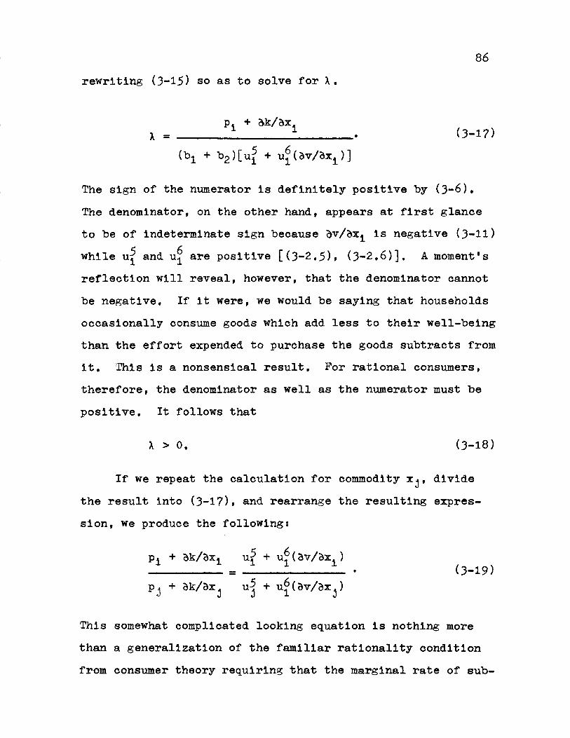
86

rewriting (3-15) so as to solve for X.

Pi + 6k/x 1 (3-17)

(b1 + b2 )[u5 + u6(av/xi)1

The sign of the numerator is definitely positive by (3-6).

The denominator, on the other hand, appears at first glance

to be of indeterminate sign because 5v/2Xi is negative (3-11)

while ui and u6 are positive [(3-2.5), (3-2.6)]. A moment's

reflection will reveal, however, that the denominator cannot

be negative. If it were, we would be saying that households

occasionally consume goods which add less to their well-being

than the effort expended to purchase the goods subtracts from

it. This is a nonsensical result. For rational consumers,

therefore, the denominator as well as the numerator must be

positive. It follows that

X > 0. (3-18)

If we repeat the calculation for commodity xj, divide

the result into (3-17), and rearrange the resulting expres-

sion, we produce the followings

Pi + Zk/bx1 u5 + u6(av/6x )- (3-19)

pj + k/3x u5 + u6(v/ax )

This somewhat complicated looking equation is nothing more

than a generalization of the familiar rationality condition

from consumer theory requiring that the marginal rate of sub-

87

stitution between any two commodities be equal to their price

ratio, The term on the left is the ratio of the marginal

costs of the two goods from the consumer's point of view,

"Cost" as it is used here includes both "price," as it is con-

ventionally defined, and the out-of-pocket transportation ex-

penditures required to purchase the last unit of the good,

The term on the right is a ratio of net marginal utilities.

The marginal utility obtained from directly consuming one

additional unit of each commodity is adjusted for the loss of

leisure attendant to the act of purchasing them, If (3-19)

did not hold for a real-world consumer, he would not be be-

having "rationally" in that his bid could be increased (for

the given utility level) by simply rearranging his purchases,

Let us return now to the maximum bid itself. To distin-

guish it from the actual amount which the household will pay

once the auction is complete, we shall denote this bid by M,

For every consumer there will be an M associated with each

property on which he bids, In the case above, M would be ob-

tained by substituting the equilibrium values of the xi's

into (3-12), The next question is a natural one. How would

M change if one or more of the property parameters changed?

To answer this question it is convenient to formalize the

relationship between M and the various parameters in the con-

sumer bidding problem by writing it as a general function,2 9

29 The reader familiar with Alonso's work will note that(3-20) is a generalization of his residential bid price curves.Op. cit,, Chapter IV.

88

Thus,

M = M(z , z2, z**, , d, c, s, bl, e). (3-20)

Some of the parameters listed earlier have not been included

as formal arguments in (3-20) since they play no interesting

role in the analysis which follows. One may think of them as

being embodied in the specific functional form of M.

What are the signs of the various partial derivatives of

(3-20)? An economical way of obtaining the necessary infor-

mation is to make use of the Envelope Theorem. In the context

of the problem at hand this theorem states that

M/,ca = BL/Ba, (3-21)

where a is any variable parametric to the bid-maximizing pro-

cess and L is the Lagrangean function defined in (3-14). An

interesting initial application of (3-21) is the following:

M/b= L/au = -X < 0. (3-22)

(3-22) informs us that an increase in the consumer's target

or expected well-being causes M to fall (other parameters held

constant). This conclusion is a generalization of Alonso's

result showing that lower residential bid price curves corre-

spond to higher levels of utility. 3 0

Repeated application of (3-21) produces a not unexpected

30Alonso, op. cit., p. 69.

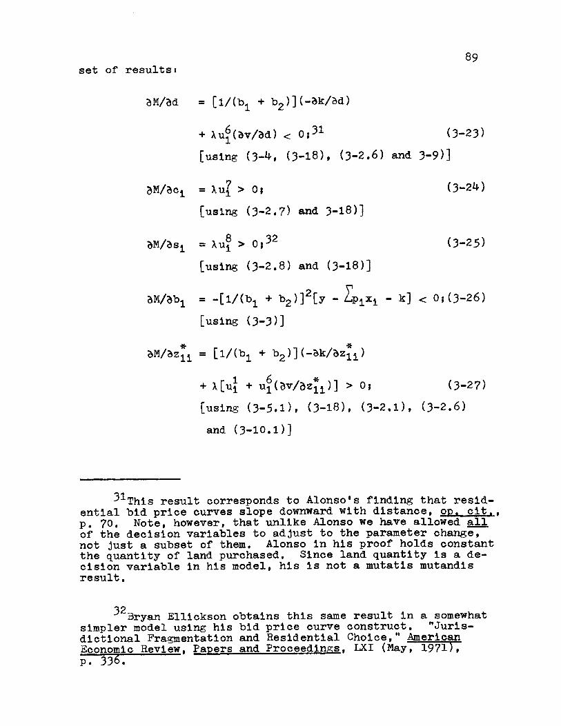
89set of results:

BM/ad [1/(b1 + b2)](-6k/6d)

+ Xu6(bv/Bd) < 0;31 (3-23)

[using (3-4, (3-18), (3-2.6) and 3-9)]

N/Aci = Xu, > 0; (3-24)

[using (3-2.7) and 3-18)]

W/as, =u > 032 (3-25)

[using (3-2.8) and (3-18)]

BM/3b1 = -[i/(b1 + b2)] 2 [y - zpixi - k] < 0;(3-26)

[using (3-3)]

zM/azii = [1/(b + b2 )](-ak/az*,)

+ X[uI + u (Ov/az*i)] > 0; (3-27)

[using (3-5.1), (3-18), (3-2.1), (3-2.6)

and (3-10.1)]

3 1This result corresponds to Alonso's finding that resid-ential bid price curves slope downward with distance, op. cit.,p. 70. Note, however, that unlike Alonso we have allowed allof the decision variables to adjust to the parameter change,not just a subset of them. Alonso in his proof holds constantthe quantity of land purchased. Since land quantity is a de-cision variable in his model, his is not a mutatis mutandisresult.

32 Bryan Ellickson obtains this same result in a somewhatsimpler model using his bid price curve construct. "Juris-dictional Fragmentation and Residential Choice," AmericanEconomic Review, Papers and Proceedings, LXI (May, 1971),p. 336.

90

)M/z* = [1/(bl + b2 )](-;k/kz2i)

+ X[u2 + U6( v/;z2i1 ? 0; (3-28)

[using (3-5.2), (3-18), (3-2.2),

(3-2.6) and (3-10.2)]

?M/ zii = Xui > 0; (3-29)

[using (3-18) and (3-2.3)]

M/z** = Xu, < 0; (3-30)

[using (3-18) and (3-2.4)]

In words (3-24), (3-25), (3-27) and (3-29) tell us that the

maximum bid a household will make on a particular piece of prop-

erty varies directly with the quality of the property itself,

the quality of the public services available in the community

where the property is located, and the proximity of the prop-

erty to land uses which enhance its immediate neighborhood.

(3-23), (3-26) and (3-30) tell us that the maximum bid varies

inversely with distance from the workplace, the local (equal-

ized) tax rate, and the proximity of the property to land uses

which neither add amenities to the neighborhood nor serve any

convenience function. Finally, (3-28) tells us that those

uses which are unattractive but which provide frequently used

goods and services have an indeterminate effect on the maximum

bid.

In order to apply (3-27) - (3-30) to any real-world situ-

ation it is important to recall that the following side condi-

tion holds:

91

A = Y z + z + 2 ~

where A is the area of the neighborhood. (3-31) is merely a

mathematical expression of our earlier assumption that the

land-use classification system used by our consumer is ex-

haustive and nonoverlapping, Since we have assumed that the

household rather mechanically selects a set of neighborhood

boundaries which are then applied to all prospective residen-

tial sites, A is constant across properties.

An important implication of (3-31) is that it makes no

sense to speak of the effect of a small increase in (say)

on the maximum bid of the consumer without at the same

time indicating the nature of the land use being replaced by

that increment. 33 A similar caveat applies to interproperty

comparisons. It follows that neighborhood-induced bid differ-

ences across properties at some point in time or across time

for some particular piece of property will be composites of

the partial effects given in (3-27) - (3-30). For example** **

if one (area) unit of zlj were converted to one unit of Z2i

in the neighborhood of some property, our consumer would

change his bid for this parcel by an amount equal to

M/Bz*i - AM/?z*. This result has some implications for

model specification and we shall return to it in the next

chapter.

33The reader will recall that a similar point was madeearlier when we discussed "desirable" and "undesirable" landuses,

92

C. Consumer Bids and Market Valuation

(3-23) through (3-30) constitute the essential results

of this chapter's mathematical analysis. We shall have much

occasion to use them in the following chapter -- both to guide

model specification and to interpret our empirical results.

As one might expect, it will be assumed that the results we

have obtained for the bidding behavior of a single consumer

can be used to predict the pattern of final valuations pro-

duced by the housing auction process. For example, we will

make the inference that houses with many rooms ought to sell

for more than those with few rooms. This seems reasonable

because we have shown that the typical household will bid

more for a house with many rooms than it will for a house

with few rooms (3-24).

On the surface this extension seems unexceptionable. In

fact, however, the precise way which the housing and land mar-

kets sort out the various individual bids to produce a final

valuation for all properties and a final assignment for all

bidders is something of a black box. Alonso struggled with

the problem in his seminal book and came up with a solution

which seemed fairly satisfactory for the simple consumer choice

model with which he was working.34 Unfortunately, the calculus

which he describes is not easily extended to the much richer

model we are using here. It would seem, however, that this

34 Alonso, op. cit., Chapter 5. Not everyone has beensatisfied with even this solution. For an impassioned dissentsee H. G, Berkman, "The Game Theor of Land Use Determination,"Land Economics, 41 (February, 1965).

93

extension is not really necessary to accomplish the objec-

tives of this study. Alonso was interested in explaining

the absolute value (or price) of land at every point in his

space economy. This study, on the other hand, because it

focuses on externalities, is only concerned with value or

price differences within that economy. Why does one property

or set of properties have a higher value than does another?

To answer this question we need not have a full-blown theory

of urban land valuation. Instead, simple inferences from the

theory of the household, like those described above, would

seem to suffice.

It is possible, however, to raise several a priori objec-

tions to even this modest proposition. Heretofore we have

been implicitly assuming that all consumers have identical

incomes and utility functions and that all face the same set

of residential location options. Suppose one or more of these

assumptions does not hold in the real world. What are the

likely empirical consequences? Let us consider some possi-

bilities.

Suppose first of all that consumers have the same

utility function and residential choice set but their incomes

differ. It follows that the competition for sites among the

members of a particular income class guarantees that in equilib-

rium all (local) members of that class will be at an iden-

tical level of utility. At the same time this competition

ensures that each member of the class is paying the maximum

value possible given the characteristics of his particular

94

piece of property and the common (class) equilibrium level

of well-being.

To see that each of these assertions is true consider a

price below this maximum for some piece of property. If a

household succeeded in purchasing at this low price, it would

subsequently enjoy a higher level of utility than the other

members of its class. However, if the auction market is

working properly, such a sale will never be consummated.

Additional members of the class (perhaps from other cities)

will enter the auction looking for a bargain, They will bid

on the property in question -- thereby raising its price

until the household which actually occupies the site is at

the same utility level as everyone else in its income class.

Moreover, if the households which participate in this compe-

tition are "rational" in the sense that at any point in time

one cannot rearrange their purchases so as to make them better

off, the equilibrium price paid will in fact be the maximum

possible price bid consistent with the common utility and in-

come level.

Our conclusion therefore is that taste homogeneity and

competition impose a certain discipline on the auction pro-

cess which ensures that the prices households actually pay

will be fairly close approximations to the maximum bids of

their income class for the properties which they occupy. If

we make the further (not unreasonable) assumption that each

household's "target" utility level is at least partially

determined by its previous levels of well-being, then one

95

would expect repeated land auctions of the type we have been

describing to induce each of the individual "target" utility

levels to converge gradually to one of the common achieved

class levels. 35 Given these assumptions it follows that the

model of consumer bidding behavior developed in this chapter

ought to be useful in explaining price differences among prop-

erties occupied by the same income class.

But what about price differences among properties

occupied by different income classes? There probably exist

special cases where one would expect income differences to be

of no consequence. In general, however, these differences

will be associated with further differences in marginal rates

of substitution among the various pairs of components in the

housing package. Thus one would ordinarily expect the marginal

value of an additional room to differ in equilibrium from one

income class to another. The precise extent of the divergence

will depend, of course, on the specific functional form of the

utility function in question and on the equilibrium level of well-

being achieved by the various income classes. The essential

point, however, is that a diversity of incomes with utility

functions the same would seem to be little different in its

consequences from a diversity of utility functions with in-

3 51f at the same time there is free migration into andout of the city, the common local achieved level of utilitywill gravitate toward some national figure which holds for allcities. A model in which this occurs is presented in ChapterV. Naturally the speed at which all these adjustments occurin the real world will depend on various institutional factors --such as information, transaction and moving costs and the degreeof geographic mobility.

96

comes the same. In both cases, different people can be ex-

pected to attach different valuations to the separate com-

ponents of the housing package. Where all households have

identical utility functions and incomes, on the other hand,

one expects these valuations to be identical as well. Ob-

viously, the model developed in the chapter will be more

useful in the latter case than in the former.

Let us explore this household diversity question in more

detail. Suppose for concreteness that all households have

the same incomes but that their tastes differ.36 What specif-

ic differences might this make? It is unlikely that differ-

ent households will have markedly different tastes about the

structure or lot characteristics of a property. For most

households more rooms will always be preferred to less, though,

of course, the intensity of the feeling will vary with family

size. It is quite possible, however, that there are major

taste differences with respect to neighborhood. Some house-

holds might violently object to living next door to an apart-

ment house while others would not give it a second thought.

36Note there are several different ways in which tastesmight differ from one consumer to another. For one thing,different consumers might use different neighborhood concepts.One household might be concerned about all that goes on withina one mile radius of its dwelling unit, while another mightworry only about what happens on its particular block. Alter-natively, consumers might differ in terms of the land-use taxon-omy which they find relevant. For the purposes of the dis-cussion which follows let us ignore these types of taste di-versities and just focus upon differences in marginal ratesof substitution across a common set of land-use categoriesapplied to a common neighborhood area.

97

To simplify our discussion of this problem consider a

single-family home one block away from a glue factory, and

two consumers, A and B, with identical incomes, 3 7 From the

point of view of consumer A the presence of this glue factory

is a major blight on the neighborhood which cannot be ignored.

Consumer B, on the other hand, is indifferent to this partic-

ular land use or perhaps even favorably disposed towards it. 3 8

As James Q, Wilson puts it, "One man's ugliness is another

man's home." 3 9 Obviously, if there are enough individuals

like B, the house in question might not sell at a significant

discount relative to other houses which are identical in every

way except for the proximity to the glue factory. It is

equally obvious that houses near glue factories will tend to

be occupied by consumers more like B than A, Should it come

to pass, therefore, that a researcher can find no significant

price difference between houses near glue factories and those

far away, it would not necessarily follow that everybody was

indifferent to glue factories. This would only be one possible

3 7 The glue factory has a long history of appearances indiscussions of this kind. The first writer to single out thisparticular villain appears to be Robert Haig in "Toward anUnderstanding of the Metropolis: The Assignment of Activitiesto Areas in Urban Regions," Quarterly Journal of Economics, 40(May, 1926), p. 433.

3 8 The existence of such individuals is not altogetherfanciful. Jane Jacobs rather likes glue factories, oP, cit.,p. 232.

3 9 "Urban Problems in Perspective, "The MetropolitanEnigma, ed. James Q. Wilson (Cambridge, Massachusetts: TheM.I.T. Press, 1968), p. 353.

98

explanation. Another would be that there are lots of con-

sumers around like Mr. B relative to the number of sites near

glue factories and that the relevant urban property markets

were efficient enough to ensure that individuals with such

tastes actually inhabited these sites,40 Note that this last

possibility does not seem to require large numbers of consumers

like B relative to the number of consumers like A. Thus there

could be a kind of consensus about the undesirability of glue

factories, and the researcher still might not find that houses

located near these uses sell at a discount.

Consider now the opposite case, Suppose the researcher

does find a significant price differential, What can he con-

clude then? Obviously, he cannot infer that everyone dislikes

glue factories. It is clear, nonetheless, that some people

dislike them. In order to make a guess about the ubiquity

of this sentiment it is necessary to have information about

the number of sites near glue factories relative to the number

of sites in the market as a whole. Since such data is apt to

be unavailable, our researcher is probably going to be left

somewhat in the dark about the true strength of the "consensus"

which he has stumbled upon.

What can we conclude from all of this? Admittedly, things

are rather untidy from a theoretical point of view. The essen-

tial point however seems to be that taste and income differ-

4 oThis was the conclusion reached by 0. Davis, J. Crecineand R. Jackson in "Urban Property Markets: Some EmpiricalResults and Their Implications for Municipal Zoning," Journalof Law and Economics, X (October, 1967).

99ences among consumers may be sufficiently great to obliterate

the presumed relationship between market price and neighbor-

hood (or even property) characteristics. If this is true,

then a heuristic application of this chapter's principal

results, (3-23) through (3-30), to real-world data will bear

no fruit. On the other hand, there is no necessity about

this. The consumer diversity objection to the use of our

bidding model to predict house price differences is really

only hypothetical. One can only judge its probable serious-

ness in the light of some actual estimations, This we shall

do in the next chapter.

CHAPTER IV

An Empirical Study of Residential PropertyValues in a Suburban Area

In Chapter II we noted that economists have enjoyed only

indifferent success in their attempts to quantify the impact

of neighborhood on residential property values. It was ap-

parent, however, from our discussion there that most of the

relevant studies suffered from rather serious methodological

flaws. The most ubiquitous shortcoming was the absence of

variables which quantified neighborhood "character" or

"quality" in a reasonable way. In most cases researchers

were forced to resort to proxies which could only capture

the impact of neighborhood in the crudest fashion.

In the present chapter we seek to improve on the perfor-

mance of our predecessors. Our specific objective will be to

reexamine the relationship between neighborhood quality and

residential property values by exploiting heretofore unused

data sources. As the reader will discover, the experiments

with these new variables were quite successful. Indeed, this

study comes up strongly in favor of the proposition that neigh-

borhood or community "aesthetics" are an important determinant

of residential property values. This conclusion then leads

us naturally into Chapter V where we will formally analyze

some of the public policy issues which neighborhood external-

ities raise in the real world.

101

A. A General Specification

We will be analyzing the market for suburban, single-

family homes in the Boston metropolitan area. As one might

surmise from the preceding chapter, we shall find it expedient

to think of the market process which allocates this partic-

ular type of housing unit to households as a kind of auction.

More concretely, we shall be supposing that in 1960 all of

the homes in the Boston suburban area were auctioned off to

prospective residents. The results of this event were, first,

a distribution of households among communities and residences

and, second, a set of market values for the various structure-

lot-neighborhood-community combinations available. This study

shall focus primarily on the latter set of outcomes.

A natural first question to ask is why the single-family-

home market was chosen. Partially the choice was a matter of

convenience; the available data for such dwelling units seemed

more respectable than the comparable figures for dwelling units

in multiple-unit structures. The principal reason for this

difference is that the Census of Housing includes a very heter-

ogeneous collection of dwelling unit types in its category

"renter-occupied units." Indeed, some of the units in this

category are single-family homes which happen not to be owner-

occupied. The Census category for which value data is avail-

able -- "owner-occupied dwelling units in single-unit struc-

tures" -- is, on the other hand, a fairly homogeneous one.'

1For additional discussion of this and related matterssee the Technical Appendix.

102

A more important reason for concentrating on the single-

family home market is that this is where one would expect the

impact of neighborhood externalities to be the strongest,

Renters are thought to have only an ephemeral attachment to

the dwelling unit and neighborhood in which they currently

live -- at least compared to owner-occupiers. Consequently,

it seems likely that undesirable neighborhood features will

influence rents less strongly than they will influence home

values. Although this is hardly a proven hypothesis, it has

apparently been found satisfactory as a working assumption by

several generations of zoning code authors. Nearly all such

laws are much more protective of homes than of apartments.2

In short, therefore, a priori evidence seems to suggest that

the single-family home market is the logical place to begin

an empirical study of neighborhood externalities,

Let us return to our real estate auction. A useful way

of summarizing the valuation outcomes of this auction is to

use a simple multiple regression technique in which market

value is regressed on the characteristics of the property

being sold. Using the notation of the previous chapter, we

may express this general relationship (in linear form) as

2 1n most zoning statutes the regulations governing con-ditional uses are stricter for single-family districts thanfor multiple-family districts. Newton, a suburb of Bostonand one of the communities in our sample, has a fairly typicalordinance in this regard. Its list of acceptable conditionaluses for a particular residential district type increasesmonotonically with the maximum number of dwelling units perstructure allowed in the district. City of Newton, The RevisedOrdinances of the City of Newton, Massachusetts Chapter 25(Newton: Published by the Board of Alderman, 1969).

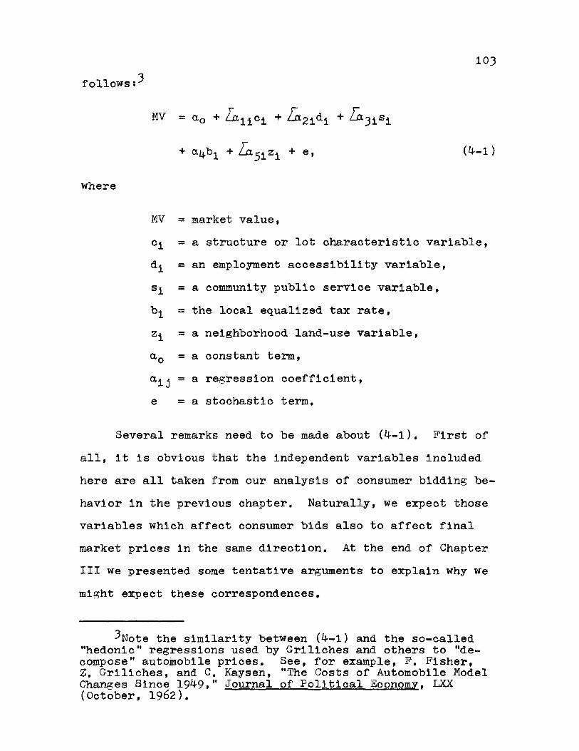
103

follows:3

MV =ao + Liici + fa21di + L3s

+ cgb1 + ZX51zi + e, (4-1)

where

MV = market value,

ci = a structure or lot characteristic variable,

di = an employment accessibility variable,

si = a community public service variable,

bi = the local equalized tax rate,

zi = a neighborhood land-use variable,

ao = a constant term,

aij = a regression coefficient,

e = a stochastic term.

Several remarks need to be made about (4-1). First of

all, it is obvious that the independent variables included

here are all taken from our analysis of consumer bidding be-

havior in the previous chapter. Naturally, we expect those

variables which affect consumer bids also to affect final

market prices in the same direction. At the end of Chapter

III we presented some tentative arguments to explain why we

might expect these correspondences.

3Note the similarity between (4-1) and the so-called"hedonic" regressions used by Griliches and others to "de-compose" automobile prices. See, for example, F. Fisher,Z. Griliches, and C. Kaysen, "The Costs of Automobile ModelChanges Since 1949," Journal of Political Economy, LXX(October, 1962).

104

A second point concerns the level of data aggregation

to which (4-1) could conceivably apply. Thus far we have

spoken of this relationship as if it applied only to individ-

ual properties. It would seem, however, that it could also

be used to analyze aggregate data in which each observation

corresponded to a separate geographic area. Under this alter-

native interpretation, the dependent and independent variables

in (4-1) become submarket averages. This generalization of

the relationship is very important for the current study be-

cause the only data available is on a community basis. This

means that in the present study we shall be estimating the

relationship between the "average" (actually the median)

value of homes in a "typical" Boston suburb and the "average"

structure, lot, accessibility, and neighborhood character-

istics of the same units.

Pursuing this matter a bit further, it is important to

be clear about the operational meaning to be attached to the

term "average neighborhood quality." Ideally, we would like

to have land-use data for the "typical" single-family home

neighborhood in each community, having defined "neighborhood"

in some reasonable geographic way a priori. Such data would

theoretically be obtained by averaging the neighborhood land-

use distributions for all single-family homes in a community --

thereby obtaining a composite distribution. Multiple obser-

vations would then be generated by repeating this calculation

for each community in the sample. Regrettably, figures this

refined do not exist. Moreover, the prerequisite data acqui-

105

sition seems too costly and time-consuming for a single re-

searcher to undertake. A task force would be necessary, and

one doubts whether research money allocated to such an effort

would be well-spent.

Fortunately, other data is available which is only

slightly inferior to this ideal -- namely, aggregate land-use

data for entire communities. The basic idea here is that the

percentage distribution of a community's total land among the

appropriate land-use categories ought to approximate roughly

the percentage distribution of neighborhood land among these

same categories for the "typical" single-family home in the

community. This does not seem to be a particularly unreason-

able assumption, though it is possible to quibble about the

implied treatment of properties located very close to community

boundary lines. One might also raise the objection that the

use of these aggregate distributions does not allow the re-

searcher to take into account proximity differences within

the separate communities. For example, two communities might

have identical overall land-use distributions with one having

homes adjoining factories and the other having homes adjoining

only parks, churches, and schools. Naturally, one would expect

rather different market valuations in the two cases. Our re-

sponse to these criticisms is simply that if they are really

serious they will significantly affect our results. The proof

of the pudding is in the eating.

B. Variables and Data Base

Our sample consisted of observations on 46 suburban cities

106

and towns in the Boston Standard Metropolitan Statistical

Area. These are listed in the Technical Appendix. Our choice

of suburbs was partially determined by the availability of

data. Many small towns were not used because the Census data

on them was incomplete. These omissions may have reduced the

generality of our results since small suburbs may differ sys-

tematically from larger ones. However, there was nothing

that could be done about this. In addition, all cities and

towns outside the Boston SMSA were excluded categorically. We

restricted our sample in this way because we wished to have

the residents of its component communities participate in the

same geographic labor market. Many of Boston's outer suburbs

are really more affiliated with the older industrial cities

which ring Boston than with Boston itself. These centers --

Lowell, Brockton, Lawrence and Haverhill -- now contain a

great deal of low-wage employment. In general, low wages

mean low residential property values, other things equal. To

control for this effect only those towns which were clearly

oriented towards the Boston economy were used.

In spite of these restrictions our sample is a very diverse

one. It contains the full range of suburban possibilities out-

lined by Wood and others.4 In addition to a number of middle-

class bedroom communities of the type celebrated in story and

song, our sample also includes manufacturing suburbs (Everett,

4 Robert C. Wood, Suburbia: Its People and Their Politics,(Boston: Houghton Mifflin Company, 1958), pp. 114-121. Doug-las E. Kneeland, "The Outer City: There is no Firm Stereotype,"New York Times, May 31, 1971, p. 1,

107

Cambridge), ethnic enclaves (Somerville, Watertown), univer-

sity towns (Wellesley, Waltham, Cambridge), and several older,

high-income suburbs (Newton, Brookline). This diversity, of

course, is absolutely essential for a study of neighborhood

externalities. If neighborhoods did not vary a great deal

across communities, one would expect their influence on price

to be swamped by other factors.

Let us now consider the specific variables to be used in

the estimation. For convenience we will organize our discus-

sion around the categories used earlier. The discussion of

each variable will be brief and fairly general. A more de-

tailed description of the variables used and their sources is

presented in the Technical Appendix. In all cases the vari-

ables to be discussed will refer to the single-family housing

stock of entire communities rather than to individual proper-

ties.

Structure and Lot Variables

In the previous chapter we demonstrated how the structure

and lot characteristics of a piece of property affect the

amount the typical consumer wishes to bid on it (3-24). Per-

haps the single most important element here is size. Our

model suggests that the larger are the structure and lot com-

ponents of the homes in a suburb the higher will be their

average market price. The two variables we used to capture

these effects are the average lot area and the average number

of rooms for single-family homes in the community. In addition

to size, one expects age to exert some independent (negative)

108

influence. Older housing is usually less desirable (holding

condition constant) because its interior and exterior features

are typically "old-fashioned." The variable we used to control

for this effect was the average age of owner-occupied dwelling

units.5 Finally, the condition of the houses in a community

and the frequency with which certain plumbing facilities are

absent ought to affect market price. We attempted to control

for these influences by including a proportion sound, with all

facilities variable (for owner-occupied dwelling units). If

all the owner-occupied dwelling units in a particular community

are "sound" (as defined by the Bureau of the Census) and all

have complete plumbing facilities (private toilet and bath,

hot and cold running water), then this variable will take on the

value "1." If not, it will take on some (nonnegative) value

less than one. This may seem to be a fairly crude way of cap-

turing what is potentially a multitude of effects. It turns

out, however, not to matter very much for this study because

the vast majority of the units in all communities (generally

well over 90 percent) are both in sound condition and possess

all the necessary plumbing. Hence the number of units having

some of these characteristics but not others is necessarily

small and it would seem that we need not worry about them.

Employment Accessibility

The distance from a piece of property to the workplace

5For a discussion of the difference between the set of"single-family homes" and the set of "owner-occupied dwellingunits" in a community see the Technical Appendix.

109

affects the maximum amount which the consumer feels he can

bid for the parcel. This we noted in the previous chapter.

In addition, if the distance is great enough, the household

may not bid on the property at all. These two effects to-

gether suggest that the closer a community is to employment

centers the higher its average residential market valuation

ought to be (other things equal, of course). Propinquity to

employment means both more bids and higher bids, each of

which will exert an independent positive influence on price.

We attempted to capture this accessibility effect by

introducing two different variables into our equation. The

first of these is road distance to the central business dis-

trict (CBD) from the geographic center of the community. In

one form or another the distance to the CBD has figured prom-

inently in urban land price determination studies for more

than thirty years.6 We have chosen the road distance variant

because it seemed reasonable and was comparatively easy to

obtain. Note that our analysis of consumer bidding behavior

in the previous chapter seems to suggest that a distance vari-

able is theoretically more appropriate than a time variable

(once a transportation mode has been selected) since the

former can capture the effect of both travel time and travel

expenditure simultaneously while the latter obviously cannot.

In practice, of course, distance, travel time and travel ex-

6An important early study which focused considerableattention on this variable is Homer Hoyt's One Hundred Yearsof Land Values in Chicago (Chicago: University of ChicagoLibraries, 1933).

110

penditure are usually so highly intercorrelated that any one

of them can serve as an acceptable proxy for any of the others.

The second employment accessibility variable used was the

following ratio:

total employment in the community-total single-family homes in the community

The purpose of this variable is to capture the influence of

proximity to local (as opposed to central city) employment.

This is an important factor in the present study because many

of the communities in our sample are substantial employment

centers in their own right. It seemed appropriate to "normal-

ize" the quantity of local employment to control for community

size. A thousand jobs in a residential community with many

homes will have a different effect on average housing price

than will the same thousand jobs in a community with very few

homes.

What sign do we expect for the local employment coeffi-

cient? One might at first suppose it to be indeterminate.

Accessibility to jobs should, of course, raise property values.

However, the existence of many jobs in a community also implies

a large concentration of commercial and industrial land uses

which in turn should lower property values through their neigh-

borhood externality effects. The resultant of these two forces

could, presumably, be either positive or negative. This argu-

ment would be valid were it not the case that the neighborhood

effects are being controlled for separately in our equation.

Our conclusion therefore is that an increase in (normalized)

111

local employment should raise property values, ceteris pari-

bus.

Land Use

In the previous chapter we found it advantageous to

analyze household bidding behavior using the following heur-

istic classification system:

1. desirable, convenience uses (zr)

2. undesirable, convenience uses (z)

**3. desirable, nonconvenience uses (z1 )

4. undesirable, nonconvenience uses (z2 *)

This taxonomy, though useful for us, is not the kind one

ordinarily encounters in the city planning or zoning litera-

ture. The typical zoning ordinance classifies activities by

industry, process, or structure. Most land-use data sources

(including the one to be used in the study) follow the same

procedure.

Given this situation, it seems important to attempt to

bridge the gap between the two types of taxonomy. By so doing,

we shall be able to use our formal model of consumer bidding

behavior to analyze land uses as the typical zoning ordinance

sees them. Our results, moreover, will be in terms of cate-

gories which are in some sense "natural" and thus easily

understood. The specific strategy we shall follow is to pre-

sent a simple set of zoning activity categories and then

112

attempt to fit each category into the desirability-convenience

framework outlined in 1 through 4 above,

A typical set of zoning district classes is the following:

A. Residential

Al. Single-Family

A2. Multiple-Family

B. Commercial (or Business)

B1. Local

B2. General

C. Industrial

Cl. Light (or Restricted)

C2. Heavy (or General)

In addition there are two other general categories of

land use which are controlled in one way or another by most

zoning ordinances but for which special districts are not

usually set up:

D, Institutional

E, Agricultural and Vacant land,

Naturally, A through E above do not correspond exactly

to the classifications used by every city, This set of cate-

gories does, however, constitute the framework of virtually

all zoning ordinances; cities will usually differ only in the

extent to which they flesh out this skeleton with additional

subcategories. A very common way of doing this is to break

down one or more of the classes given above into "bulk" sub-

113

categories which differ among themselves only in the strin-

gency of their building and lot size requirements. 7 Very

early zoning statutes did not contain these complexities but

recent years have seen their proliferation.8

In this study we shall ignore all such refinements --

primarily to keep the set of independent variables to a man-

ageable size. Since it seemed unlikely that the aggregated

data we were using would permit us to make very close dis-

tinctions among a large number of land-use categories anyway

this limitation did not seem to be a serious one.

We shall examine the land uses listed above one at a time.

Our objective will be to determine the probable strength and

direction of the effect of each on single-family home property

values. A through E constitutes an exhaustive classification;

hence, it is econometrically incorrect to include all types

of land use in the regression equation if at the same time you

include a constant term. 9 It did not seem reasonable to drop

the constant term on this account alone so it was retained

7 Boston, for example, has two single-family districtswhich differ only in that one permits a higher Floor-AreaRatio and a smaller minimum lot size than does the other.City of Boston, Boston Zoning Code and Enabling Act (Boston:City of Boston Printing Section, 1968), pp. 8, 50.

8 Charles M. Haar, "The Social Control of Urban Space,"Cities and Space, ed. Lowdon Wingo, Jr. (Baltimore: The JohnsHopkins Press, 1963), p. 185.

9This is the problem of perfect multicollinearity. SeeJ. Johnston, Econometric Methods (New York: McGraw-Hill BookCompany, 1963), pp. 201-202.

114

and one of the land-use variables was dropped instead.1 0 We

chose single-family homes to be the "numeraire" land use.

Operationally, this choice meant that in the present study

we tried to determine how average single-family property

values varied across a set of communities whose land-use dis-

tributions diverged in various ways from that of an "ideal"

community which consists of nothing but single-family homes.

Given this formulation, the coefficients of the included land

uses measure composite effects of the sort discussed when we

analyzed the influence of neighborhood changes on consumer

bids in the previous chapter (3-32). For example, the coef-

ficient of land use zi in (4-1) is a measure of the marginal

change in average community home values brought about by con-

verting one percent of a community's land from single-family

homes to zi. In the pages which follow we shall refer to this

price change as the "net effect" or "net influence" of the

land-use change.

Multiple-family land uses in our sample include two-

family homes, "three-deckers," and modern apartment complexes.

All would seem to fall naturally into class 4. They serve no

particular convenience function and they are usually thought

to be undesirable additions to single-family neighborhoods for

10This is a standard procedure for dealing with dummyvariables. A. Goldberger, Econometric Theory (New York: JohnWiley and Sons, Inc., 1964), p. 221.

11For a more complete listing of the components of allour land-use categories and a discussion of the classifica-tion procedure see the Technical Appendix.

115

both amenity and ethnocentric reasons.12 If one examines any

real-world zoning disputes in which homeowners are trying to

keep multiple-family structures out of their neighborhood or

community, it is fairly clear that class, ethnic, and racial

considerations play as big a role as the probable appearance

of the structures. In this study we shall not attempt to sort

out these two effects. Since both probably operate in the

same direction (there were few luxury, high-rise apartment

buildings in suburban Boston in 1960) and since the propor-

tion of Blacks (the most "undesirable" minority) is very small

in the Boston metropolitan area and in each of the sample com-

munities, our overall results should not be much affected by

this omission.

Another frequently-heard objection to the construction of

multiple-family structures in suburban areas is the burden they

will allegedly impose upon the local public sector, particu-

larly the school system. In this study we will attempt to

control for this influence by including public service and tax

variables in our pricing equation. We shall, however, defer

12 Judicial opinions abound in pejorative references toapartment houses. Some particularly choice invective may befound in Justice Sutherland's famous opinion in Village ofEuclid v. Ambler Realty Co., 272 U.S. 375 (1926). A somewhatmore positive (but minority) view may be found in Appeal ofBorden, 87 Atlantic (2d) 465 (1952). The opinion in this lastcase was obviously influenced by the postwar housing shortageand baby boom.

13 The legal status of such arguments is still in doubt.Norman Williams observes that there are many cases on bothsides of the question. The Structure of Urban Zoning (NewYork: Buttenheim Publishing Corporation, 1966), p. 51.

116

a detailed discussion of these variables until a bit later

in the chapter because the issues raised by their inclusion

are rather complex.

Our overall conclusion then is that multiple-family land

uses probably exert a negative net influence on price [using

(3-27) and (3-30)] due to the neighborhood externalities which

they generate.1k As indicated above, this conclusion abstracts

from all tax and expenditure questions.

Commercial land uses as they are conventionally defined

would seem to fall largely into class 2. One thinks immedi-

ately of "Ma and Pa" grocery stores. There is, however, some

ambiguity about this nomenclature; certain activities which

one could conceivably designate as "commercial" -- such as

wholesaling or warehousing -- rather clearly belong in class 4.

Finally, to complicate things even more there are many "com-

mercial" uses which fall midway between these two extremes.

Zoning codes confronting this diversity have tended to

respond in two ways. Those "commercial" uses which are land-

intensive, which generate common-law nuisances, and which serve

no local convenience function are frequently confined to in-

dustrial districts. 15 We shall follow this practice and de-

l4 Here and in the rest of the chapter we will assume thatsingle-family homes are in class 1 use. They enhance a neigh-borhood physically and they provide readily accessible socialrelationships.

1 5For example, Boston's zoning code tends to restrictwholesaling, storage, and transportation uses to industrialdistricts, op. cit., pp. 29-30, 32-33. Newton, on the otherhand, places many of these activities in various kinds of"Business" district, op. cit., p. 21.

117

fine wholesale, public utility, and transportation uses to be

"industrial." The uses which remain in our commercial cate-

gory are retail, service, or office activities. Most zoning

codes try to handle these by further dividing their commercial

classification into "local" and "general" subclassifications.

Ma and Pa grocery stores go in the former; automobile dealer-

ships, funeral homes, large office complexes, and animal hos-

pitals go in the latter, Unfortunately, our land-use data was

not refined enough to permit the inclusion of two distinct

commercial variables in our regression. As a result we had to

improvise.

It seemed likely that all communities would support some

local commercial establishments but that only a few of the

largest (and oldest) would contain significant amounts of gen-

eral commercial activity. This suggested that the mathematical

relationship between average market price and the proportion

of a community's land devoted to (nondifferentiated) commer-

cial activity might be nonlinear with a second derivative

which is everywhere negative. The two possible general forms

of such a relationship are shown graphically in Figures IV-1

and IV-2. Note that in both cases the price change induced

by a one unit increase in the proportion of commercial land

(brought about by a corresponding single-family reduction) is

lower algebraically than the one which preceded it. This would

be due both to a higher marginal proportion of general commer-

cial activity as total commercial activity increases (noted

above) and to diminishing marginal travel cost savings to

118

additional increments of local commercial activity.

But which of the two general functional forms is likely

to be the true one? This is a question which cannot be set-

tled theoretically. Recall that in the previous chapter we

discovered that class 2 land uses had an indeterminate effect

on household bids (3-28). Their influence on market price is

presumably the same. Thus, the initial slope of the price-

commercial land relationship [at (0,0) assuming the function

to be homogeneous] may be either positive or negative. Sub-

stituting the first few acres of local commercial activity

for single-family homes may raise property values in the com-

munity rather than lower them. Either result is theoretically

permissible.

There is, however, some empirical evidence which can be

brought to bear on this question. Casual inspection of the

"New Town" literature suggests that local commercial activity

is important enough to such enterprises to be included in them

in spite of adverse neighborhood effects. Columbia, Maryland,

for example, has a hierarchy of commercial services. Some are

located at the neighborhood level and are within walking dis-

tance of every house. Others are located at the village

level and still others are only to be found "downtown."t16

This careful attention to shopping accessibility by a profit-

maximizing entrepreneur (who was also counseled by emminent

16"Maryland's 'new town' may make it big," Business Week,March 9, 1968. J. W. Anderson, "A Brand New City for Maryland,"Harper's Magazine, November, 1964.

119

social scientists) suggests that a restricted amount of com-

mercial activity may well raise total community residential

property values even while lowering the value of those homes

immediately adjacent to it. Commercial and residential land

uses in Reston, America's other important "New Town," inter-

penetrate in a similar way and for similar reasons.' 7 All of

this evidence suggests that Figure IV-1 depicts the more prob-

able relationship.

Our research strategy will be to include both a linear

and a quadratic commercial term in (4-1). The arguments in

the previous two paragraphs suggest that the sign of the

squared term should be negative (producing a negative second

derivative) and the sign of the linear term should be positive

(producing a positive initial slope).

Industrial land obviously belongs in class 4, Included

here are all of the more obnoxious land uses: factories, ware-

houses, railroad yards, truck depots, quarries, power plants,

etc. Many zoning statutes distinguish between "light" and

"heavy" industrial activities on the basis of various nuisance

criteria. Unfortunately, our data did not enable us to separ-

ate these two types of use in our estimations. We were re-

duced perforce to a single industrial variable. This limita-

tion did not seem to be a particularly serious one since both

industrial subcategories operate on price in the same direc-

tion. It is only the strength of their effects which is

17Robert E. Simon, Jr., "Modern Zoning for Reston,"American County Government, May, 1967.

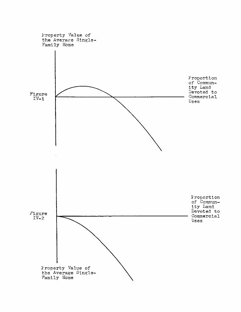
Property Value ofthe Average Single-Family Home

Proportionof Commun-ity LandDevoted. toCommercialUses

Proportionof Commun-ity Land

re Devoted to

2 CommercialUses

Property Value ofthe Average Single-Family Home

FigureIV-1

Fig uIV-

121

likely to differ. The situation is thus rather different

from the commercial specification problem we faced above.

There the two use subcategories could conceivably influence

price in different directions, a contingency which had to be

taken account of in the specification.

It is important to observe that our remarks concerning

the relationship between industrial land and community prop-

erty values refer only to the neighborhood externality

effects. The presumed positive relationship between manufac-

turing activity and property values which operates through

local tax rates is being held constant. Recall our discus-

sion of a similar problem with respect to multiple-family

uses.

We conclude than that converting land from single-family

to industrial use will lower average single-family home prop-

erty values [using (3-27) and (3-30)] if local employment

and taxes are held constant. The sign of the industrial land

coefficient should therefore be the same as the sign of the

multiple-family coefficient and for essentially the same

reasons. One expects, however, the industrial coefficient

to be greater in absolute value than the multiple-family coef-

ficient because industrial uses are obviously the more unde-

sirable.

Institutional land uses include churches, schools,

hospitals, museums, and public buildings. Virtually none

generate important nuisances and most are comparatively

122

attractive in appearance.18 In our schema they would seem to

belong in classes 1 and 3. We observed in (3-27) and (3-29)

that uses in these classes should have a generally favorable

effect on property values. However, the specific problem

which concerns us here is not whether institutional land uses

raise property values more than other uses but specifically

whether they raise them more than single-family uses do, If

so, then their net effect on price will be positive. If not,

it will be negative.

There can be no a priori answer to this question. Many

institutional land uses could very well have a positive net

influence on the community's single-family property values.

Universities may have this effect because of the status they

confer on a community and the cultural facilities which they

provide. Some local institutional uses such as churches and

schools probably have similar potency. Profit-maximizing

suburban developers have frequently been known to donate

school sites to the communities they were developing.1 9 In

18There have been occasional attempts on the part of com-munities to exclude these uses. The usual argument has beenthat institutional uses generate traffic. A typical case isRoman Catholic Welfare Corporation v. Piedmont, 289 Pacific(2d) 438, 1955. Here a small community attempted to preventthe construction of a Catholic school in a single-family neigh-borhood. The court found, in a typical holding, that thealleged nuisances were not important enough relative to othercountervailing considerations to enjoin the construction.

1 9Anthony Downs, "Private Investment and the Public Weal,"Saturday Review, May 15, 1971, p. 25. Levitt and Sons hasdonated church sites as well. Herbert Gans, The Levittowners(New York: Pantheon Books, 1967), p. 68.

123

order for this to be a rational policy it is necessary that

schools make the community a more desirable place to live in

the eyes of prospective purchasers.

On the other hand, many other institutional uses will

not be as highly regarded as single-family homes. Good

examples might be hospitals, nursing homes, or trade schools.

These uses are apt to have a slightly negative net influence

on values because they do not provide any convenience for

local residents to counterbalance the various minor nuisances

which they may create (traffic in particular).

What are the implications of all this for model speci-

fication? One initial point is that the nonlinear model

described above for commercial uses seems inappropriate.

The negative externalities generated by the "worst" insti-

tutional uses are for the most part much weaker than those

generated by the more obnoxious commercial uses, such as auto

dealerships, filling stations, and drive-in restaurants. More-

over, it is probably not true that communities with high pro-

portions of institutional land have a disproportionately

higher proportion of the less desirable institutional uses

than do those communities with a low proportion of institu-

tional land. Many of the "institutional" communities in our

data base, for example, are university towns.

Both of these considerations suggest that a simple linear

specification is the most appropriate. We cannot however,

specify in advance the sign of the coefficient. As our re-

marks above made clear, both a negative and positive sign

124

are theoretically possible. One does expect, however, that

the coefficient's algebraic value (be it positive or nega-

tive) will be greater than the corresponding values of the

industrial and multiple-family coefficients. This is to be

anticipated partly because the typical institutional use pro-

vides some local services and partly because these uses are

generally more attractive and less disruptive of single-

family neighborhoods than the other two.

Vacant Land and Agriculture is a kind of residual cate-

gory. It includes large parks, swamp and water, golf courses,

wildlife refuges, as well as agriculture and other undeveloped

private lands. Most of these uses would seem to fall in class

3. In general, they are not distinctly undesirable and most

do not provide important local services. Consequently, [using

(3-27) and (3-29)] the net effect of vacant land on property

values is theoretically indeterminate. However, as was the

case with institutional uses, some empirical intuition can be

brought to bear on the problem.

The critical fact is that vacant or underdeveloped land

is easily converted to some other use if market pressures so

dictate. This is generally true even in those communities

which make a concerted effort to preserve their open space

using zoning and other devices. One of the few things that

planning experts seem to agree upon is that a major weakness

of traditional zoning ordinances is their inability to disci-

125

pline development at the urban-rural fringe.2 0 The very pres-

ence of vacant land thus necessarily creates uncertainty about

the future development of the neighborhood or community in

which it is located. This suggests that the vacant land and

agriculture coefficient in our regression should be negative.

Vacant land will have a negative net effect on property values

because it may at any time be converted to uses which are

markedly less desirable than single-family homes.

One can argue further that this coefficient is apt to be

larger algebraically (less negative) than either the multiple-

family coefficient or the industrial coefficient but smaller

than the institutional coefficient. This ranking, of course,

is largely intuitive. It is certainly not unreasonable to

suppose that vacant land will have a weaker net effect on prop-

erty values than will factories or apartments. While it re-

mains vacant such land contributes "light and air" to the

community. Moreover, if it is ever developed, the worst that

can happen is that one of these latter uses will be built

upon it.

It is perhaps less clear that institutional uses should

rank higher than vacant land. The argument is essentially

that many institutional land uses supply important community

services while vacant land does not. In addition, the typical

20 Daniel Mandelker, "Delegation of Power and Functionin Zoning Administration," Washington University Law Quarterly(February, 1963), p. 64. John Delafons, Land-Use Controls inAmerica (Cambridge, Massachusetts: The M.I.T. Press, 1962),p. 83.

126

institution is surrounded by a certain amount of landscaped

greenery which contributes to community spaciousness just as

vacant land does.

Local Tax and Expenditure Variables

The last variables we will consider in this section

describe the tax and expenditure decisions of each community's

local government. We have reserved them until the end because

their presence in our price equation creates some special prob-

lems.

Charles Tiebout, in a now-celebrated paper, has argued

that the diversity of local governments in a metropolitan area

offers the typical household a "menu" of tax-expenditure com-

binations which enables him to choose the combination which

suits his tastes and income the best. 2 1 Tiebout's analysis

was essentially normative; he saw that forcing a household to

choose among a multiplicity of local governments was a way of

partially circumventing the public goods "revealed preference"

problem outlined by Samuelson.22 Many subsequent writers have

stressed the behavioral significance of Tiebout's work. Some

have developed complex game-theoretic models in which suburban

and central-city governments vie with one another for high-

21 Charles M. Tiebout, "A Pure Theory of Local Expendi-tures," Journal of Political Economy, 64 (October, 1956).

2 2Paul A, Samuelson, "The Pure Theory of Public Expen-ditures," Review of Economics and Statistics, XXXVI (Novem-ber, 1954), and "Diagrammatic Exposition of a Pure Theory ofPublic Expenditures," ibid., XXXVII (November, 1955).

127

income citizens and "clean" industry by manipulating the tax

and expenditure variables under their control.23 Others have

taken Tiebout's assertion that household's "shop around" among

alternative jurisdictions as a hypothesis which may or may not

be supported by close analysis of empirical data.24

In the present study we are not directly concerned with

this general phenomenon except to the extent that expenditure

and tax variables exert an independent influence on the value

of single-family homes. Unfortunately, Tiebout's article did

not mention property values at all, and the subsequent litera-

ture on the subject has been somewhat confused. Dick Netzer

comes to the following conclusion: "To the extent that the

Tiebout hypothesis holds, there is no a priori expectation of

a significant correlation between tax rates and per capita or

per pupil property values."25 Wallace Oates, on the other

hand, has taken the position (in effect) that the acid test

for the Tiebout hypothesis is precisely such a correlation,26

2 3Jerome Rothenberg, "Strategic Interaction and ResourceAllocation in Metropolitan Intergovernmental Relations," Ameri-can Economic Review, LIX (May, 1969).

24 See, for example, Larry Orr, Municipal GovernmentPolicy and the Location of Population and Industry in a Metro-Politan Area (unpublished Ph.D. dissertation, Department ofEconomics, Massachusetts Institute of Technology, 1967).

25 Dick Netzer, Economics of the Property Tax (Washington,D.C.: The Brookings Institution, 1966), p. 127.

26More correctly, a partial correlation. Wallace E.Oates, "The Effects of Property Taxes and Local Public Spend-ing on Property Values: An Empirical Study of Tax Capitaliza-tion and the Tiebout Hypothesis," Journal of Political Economy,77 (November - December, 1969).

128

Which of these views is the correct one? The answer

to this question may be obtained rather quickly if we observe

that in the real world there is a simultaneous relationship

between property values on the one hand and tax rates and

public expenditure variables on the other.2 7 In the previous

chapter we demonstrated that household bids for properties in

a community would rise, ceteris paribus, if public services

rose (3-25) or if the real property tax rate fell (3-26).

Since we have been assuming that bid changes lead to property

value changes in the same direction, it follows that the sign

of the public service coefficients in (4-1) should be positive

and the sign of property tax rate coefficient should be nega-

tive.28

It will not do, however, simply to regress property

values on these local government variables using ordinary

least squares. The values taken by tax and expenditure vari-

ables for any particular suburb are surely not exogenous to the

auction process we have been considering in this study, though

both Orr and Tiebout have in effect taken this position.29

Instead, they are the outcome of political decisions which

27Bryan Ellickson develops this idea much more fullythan we do here. Op. cit. and, Metropolitan ResidentialLocation and the Local Public Sector (unpublished Ph.D. dis-sertation, Department of Economics, M.I.T., 1970).

2 8The size of the tax coefficient is a measure of theextent to which property taxes are "capitalized" into the valueof land. It is here that our study intersects with much of thetraditional literature on the incidence of the property tax. Agood survey may be found in Netzer, op. cit., Chapter III.

29 Tiebout, op. cit., p. 418. Orr, op. cit,, pp. 94-96.

129

necessarily depend (inter alia) on both the character of the

households who have bid the highest for the residential sites

in the community and on the size of the winning bids. Since

the principal source of local government revenue in the United

States is the property tax, one expects the latter to be partic-

ularly important. Analytically, all of this suggests that

there are separate political decision-making relationships in

the real world which determine tax rate and public service

levels -- relationships which include property values among

their independent variables.

It would seem therefore that the Oates position is the

theoretically correct one provided one understands that (4-1)

is to be estimated with some technique such as two-stage least

squares which takes account of the interdependencies described

above. If indeed tax and public service variables are important

factors in the household location decision, one expects them

to be statistically significant in the estimated form of (4-1),

There is, of course, no necessity about this, It may be that

local government variables do not enter into household location

calculations at all. Alternatively, there may be a great

diversity of taste about the proper level and distribution of

local government tax and expenditure activity. Recall that the

main point of the Tiebout welfare argument was the accommodation

of just such diversity. We noted earlier that heterogeneous

tastes about neighborhood characteristics might attenuate the

statistical relationship between these variables and property

values. A similar argument can presumably be made with respect

130

to the characteristics of municipal governments. Hence,

Netzer's comment on Tiebout, while questionable as an a

priori deduction, may be quite accurate as an empirical state-

ment, particularly if many other factors influence consumer

choice besides the decisions of the local public sector.

The one practical conclusion we can draw from this brief

survey of the work of other economists is that it would be

irresponsible to ignore the local public sector completely in

any empirical study of community property values. Let us con-

sider, therefore, the specific variables to be included in

(4-1).

On the tax side the natural choice is the equalized tax

rate. Assessment-value ratios differ widely across communities

in most metropolitan areas so it is essential to adjust actual

tax rates to obtain annual property tax payments as a propor-

tion of market (not assessed) valuation. This is a standard

calculation in the empirical literature on the property tax.

Choosing appropriate public service variables is not

quite so simple. An important initial problem is the choice of

a reasonable public output measure. This is much discussed in

the literature on economics of scale in urban public services. 30

Because of space and time limitations, we shall not attempt to

break new ground on this subject. Instead, we will use the

standard escape hatch and choose appropriate input variables

30A good survey may be found in Richard V. Butler, CostFunctions for Urban Public Services (unpublished Master'sthesis, Department of Economics, Massachusetts Institute ofTechnology, 1968).

131

as proxies. But which variables should they be? Both casual

and scholarly examination of suburban political behavior sug-

gests that the most important service provided by these govern-

ments from the point of view of the citizenry is education.31

Many of the empirical studies of property values which preceded

the present one have followed this lead and included school in-

put variables (not always successfully) among their independent

variables.3 2 On the basis of these precedents it seemed fair

to conclude that if any public service variable was to affect

property values, it would most likely be a school quality index.

Several such indices were available to this study: total

expenditure per pupil, teacher-student ratio, average teacher

salary, and maximum salary for teachers with bachelor's degrees.

On the basis of prior reasoning total expenditure per pupil

appeared to be the most satisfactory single variable. It encom-

passes a teacher quality factor (presumably correlated with

3 1Robert C. Wood notes the preoccupation of suburbaniteswith their school system and the attendant special qualitiesof school politics, op. cit., pp. 186-194.

32A partial list would include Oates, op. cit., p. 962(expenditure per pupil); David M. Schroedl, Land as an Invest-ment (unpublished Master's thesis, Sloan School of Management,Massachusetts Institute of Technology, 1964), pp. 13-15 (tea-cher salary maximum and membership in regional educationassociation); John F. Kain and John M. Quigley, "Measuringthe Quality and Cost of Housing Services," (Program on Regionaland Urban Economics, Discussion Paper No. 54, Harvard Univer-sity, 1969), p. 10 (average eighth grade student achievementtest score); Ronald Ridker and John A. Henning, "The Deter-minants of Residential Property Values with Special Referenceto Air Pollution," Review of Economics and Statistics, 49(May, 1967), p. 257 (classification of schools by educatorsand real estate men as above average, average, below average);Orr, op. cit., p. 131 (education expenditure per pupil).

132

salaries paid) and a class size factor (presumably measured

by the teacher-student ratio). Of course, inclusion of both

salary and class size variables together also seemed to be

acceptable. The maximum salary variable was finally rejected

as a teacher quality index because no further evidence was

available on the stringency of the requirements which had to

be fulfilled to reach this maximum, Thus in the end we were

left with two alternative specifications: one which included

only total expenditure per pupil and the other which included

the teacher-student ratio and the average teacher salary.

C. Some Estimations

As mentioned earlier, our data base consisted of obser-

vations on all of the above variables for forty-six suburban

Boston communities in 1960. Our procedure was to regress the

median value of single-family homes for these communities (as

reported in the 1960 Census of Housing) on various combinations

of the independent variables we have discussed.3 3 The estima-

tion procedures used were ordinary least squares (OLSQ) and

two-stage least squares (TSLS). Table IV-1 presents the most

interesting and important results of these estimations.

3 3 More specifically, we used the median value of owner-occupied dwelling units in single-unit structures. The valueof these units covers both house and lot and is based uponappraisals by owners. This procedure undoubtedly producesserious errors in the valuation of individual properties.There is some evidence, however, that these errors "wash out"when the individual prices are aggregated into averages. L.

Kish and J. Lansing, "Response Errors in Estimating the Value

of Homes," American Statistical Association Journal, 49 (Sep-tember, 1954). Presumably these results also apply to the

median.

133Table IV-1

Alternative Estimates of a Valuation Equationfor One-Family Homes in Suburban Boston in 1960

Regression Coefficients (Absolute t Ratios in Parentheses)

Equation Number la 2a j a 4a 5a

Median Numberof Rooms

Average Age(in Years)*

Average LotSize (in Acres)

Road Distance toCBD (in Miles)

Proportion Sound,all Facilities*

Local EmploymentNumber of Homes

Proportion Land notto One-Family Homes

Proportion Land toMult. -Family Homes

ProportionCommercial

Land toUses

(Proportion Land toCommercial Uses)2

ProportionIndustrial

Land toUses

Proportion Land toInstitutional Uses

ProportionVacant

EqualizedTax Rate

Land

School Expenditureper Pupil

6223)b(9.59)h

-156( 3 . 4 6 )b

3861(1,71)0

-59(1.04)

13746(1.76)0

66(1.14)

4842(6.42) b

-125(2.93 )b

6002(2.75)b

-85d(1.62)d

12386

117(2.12)c

-8133(2.96)b

4483(6.07)b

-104(2.31)0

7121(2.96)b

-132(2.42

14761(2.10

(2322.48) b

-6385(1.28)

64035(1.86)0

-959410(2.75)b

-8412(1.89)c

6348(0.68)

-4830(1.94)0

5025(5.40)b

- 119(2.50)b

(73933.06 )b

-127(2.36

1(15621.44)d

349(2 .31 )c

-5549(1.17)

72604(2.01)c

-926160(2.50)b

-7312(1,61)d

4863(0.53)

-4006(1 .52)d

-45(1.75)0

-5(0.74)

5571(3.69) c

-128(2.08)d

7485(2.83)c

-138(2.35)c

12707(1.29)

478(2. 09)d

-5456(0.95)

91927)d(2.07)

-1267000(2.45)c

-9603(1.90)d

6485(0.63)

-4009(1 .35 )d

5(0.11)

-12(0.91)

134

Table IV-1

(Continued)

Equation Number 1 2 3 4 5

Constant -30600 -16190 -20620 -18550 -21860Term (3 .9 3 )b (1 .8 8 )d ( 2 . 3 0 )c (1.85)0 (1 .9 5 )d

Estimation OLSQ OLSQ OLSQ OLSQ TSLSMethod

R2 .880 .902 .933 .939 .923

q2 .861 .884 .909 .912 -

Degrees of Freedom 39 38 33 31 3(For t Tests)

aThe dependent variable is the median value ofowner-occupied dwelling units in single-unitstructures.

bSignificant at the .01 level (one-tailed test).

OSignificant at the .05 level (one-tailed test).

dSignificant at the .10 level (one-tailed test).

*For owner-occupied dwelling units rather thandwelling units in single-unit structures.

135

We shall discuss the results sequentially, starting with

the simpler models and then moving on to the more complex ones.

For the moment assume that the true model is one in which

government service variables and the local tax rate are not

included. It will turn out in the light of some further re-

sults that this is really a quite reasonable assumption. We

defer discussion of this matter until a bit later, however,

when we shall examine some "Tiebout" models which explicitly

take cognizance of the local public sector.

Models Exclusive of Local Government

Consider the first three equations in Table IV-1.

Equation 1 includes only a fairly conventional set of struc-

ture, lot, employment accessibility characteristics. Equa-

tion 2 includes all of the variables in equation 1 plus an

additional variable describing the proportion of community

land not occupied by single-family homes. Equation 3 repre-

sents our full-blown neighborhood model. It includes the

panoply of neighborhood variables described in the previous

section as well as the six structure, lot, and accessibility

variables included in equations 1 and 2. Obviously, the three

equations represent 3 distinct points along a continuum of

increasingly complex neighborhood specifications.

Note first of all that the R2 for all three estimations

is fairly high for a cross-section study. Note also that R2

rises as the number of neighborhood variables increases --

even when it is corrected for the decline in degrees of free-

136

dom (R2 ).34 Turning to the estimates themselves, one very

striking preliminary observation is the way that introducing

more complicated neighborhood specifications improves the

general performance of the structure, lot, and accessibility

variables. To be sure, in all three equations these variables

have coefficients whose signs are as predicted in the earlier

sections of this chapter. However, in equation 3 all six have

coefficients which are significant at least at the .05 level

(using a one-tailed test), while in equation 1 there are two

coefficients which are not even significant at the .10 level.3 5

Note in particular the much higher t ratios for lot size, dis-

tance and local employment. These results, of course, lend

some credence to our contention that neighborhood should not

be ignored when modeling the property valuation process.

The inclusion of neighborhood variables also has the

effect of weakening the influence of the structure variables

somewhat (smaller coefficients for age and rooms) while drama-

tically strengthening the employment accessibility effects

(larger coefficients for distance and normalized local employ-

ment). This latter result suggests that the employment acces-

sibility variables in equation 1 are doing double duty: They

are capturing both commutation cost and neighborhood exter-

34Goldberger, op. cit., p. 217.

35 0ne-tailed tests were used because it seemed reason-able to assume that most of the coefficient signs in TableIV-1 were known a priori. The choice was not a particularlysignificant one, however. Had two-tailed tests been applied,the interpretation of the results given in that table wouldhave been unaffected.

137

nality effects. Since these separate factors operate in

opposite directions on market price, the accessibility coef-

ficients are larger in equation 2 and much larger in equation

3, both of which control for neighborhood quality separately.

The general improvement of the CBD distance coefficient, both

in significance and in (absolute) size, is particularly grati-

fying because of the importance attached to this variable in

previous studies.

Let us now consider the neighborhood variables them-

selves. In equation 2 we have included a single neighborhood

variable -- the proportion of community land devoted to land

uses other than single-family homes. It is a simple general

measure of community "attractiveness" from the point of view

of the prospective home-owner. The reader will recall that in

the previous chapter we considered some land uses which might

in certain situations be preferred to homes, but it was fairly

obvious that they were special cases. Common sense suggests

that this variable should have a negative coefficient, and in-

deed in equation 2 it does. Note especially its high level of

statistical significance. What equation 2 says in effect is

that converting 10 percent of a community's land from single-

family homes to some other (unspecified) land use will lower

average home values in that community by around $810, ceteris

paribus.

We put no particular stock in the precise magnitude of

this coefficient since the "true" specification is probably

more like that of equation 3 than that of equation 2. None-

138

theless, equation 2 is suggestive. Its most important message

is that neighborhood effects are significant and that there is

some sort of "consensus" about them. Specifically, it seems

clear that homeowners in general prefer communities whose land

is exclusively occupied by single-family homes. This is di-

rectly contrary to the conclusions of Crecine et al, who have

argued that there is a strong possibility that "the urban prop-

erty market is not characterized by great interdependence and

that externalities do not abound in that market."36 We shall

have more to say about this position a bit later on.

In equation 3 we decomposed the gross non-single-family

effect discovered in equation 2. We did this by subdividing

non-single-family land into the five general land-use cate-

gories discussed in detail earlier. Each was then treated as

a separate variable for estimation purposes. Altogether, six

new variables were added to the original specification given in

equation 1 (commercial land enters through both linear and

squared terms). A natural first test of the reasonableness of

this decomposition is a Chow test of the null hypothesis that

all six neighborhood variables are jointly equal to zero

against the alternative that they are not. 3 7 This statistical

36J. Crecine, 0, Davis, and J. Jackson, "Urban PropertyMarkets: Some Empirical Results and Their Implications forMunicipal Zoning," Journal of Law and Economics, X (October,1967), pp. 93-94.

3 7The mechanics of the test are lucidly described inFranklin M. Fisher, "Tests of Equality Between Sets of Coef-ficients in Two Linear Regressions: An Expository Note,"Econometrica, 38 (March, 1970).

139

test will in effect tell us how improbable our estimated

results are on the assumption that the true neighborhood

coefficients are equal to zero and the rest of the specifi-

cation is "correct." The results of this test are gratifyingly

decisive. The value of the appropriate F statistic (with 6 and

33 d.o.f.) turned out to be 4,43, which is significant at the

.005 level. Thus it is highly unlikely that the "true" neigh-

borhood coefficients are jointly equal to zero.

Turning to the estimates themselves, note first of all

the relationship among the multiple-family, industrial, insti-

tutional, and vacant land coefficients. It is essentially as

predicted in the previous section. Both the industrial and

multiple-family coefficients are negative with the former being

larger than the latter -- exactly what one would expect on the

basis of neighborhood externality considerations. The vacant

land coefficient is also negative but smaller in absolute value

than the first two, again a not unsurprising result. Finally,

the institutional coefficient is positive, suggesting that over

some range it would be profitable for suburban homeowners to

promote institutional locations in their community (ceteris

paribus). What is most striking about all of this is that the

size ranking of these four coefficients conforms exactly to our

a priori expectations.

The t statistics of these four coefficients present a

somewhat mixed picture, The vacant and industrial coefficients

are significant at the .05 level and the multiple-family coef-

ficient just misses being significant at the .10 level. The

institutional coefficient, on the other hand, is clearly

insignificant. There are two possible explanations for this.

The first is that households really evaluate neighboring in-

stitutional uses in about the same way as they evaluate single-

family homes, so that in the true model the institutional co-

efficient is zero. The second possibility is that the low

institutional t statistic is simply the consequence of stochastic

influences peculiar to the specific body of data we have used.

Observe that there are twelve distinct regressors in equation 3,

six of them dealing with land use. Even if all were in fact

variables in the true model, there is a reasonable probability

that one or two will show up with low t statistics due to

"noise" in the valuation process.

There is really no way of deciding between these alter-

native hypotheses except by consulting an independent set of

data and repeating the estimation. Our predisposition, however,

is toward the second alternative. The order of magnitude of the

institutional coefficient is certainly consistent with that of

the others. Moreover, it seems unwise to conclude flatly that

institutional uses should be dropped from the regression on the

basis of a single experiment. One does not expect, after all,

that the two uses will have exactly the same effects. The

critical thing is that it is the institutional coefficient to

which this ambiguity attaches rather than any of the others.

ge remarked in the previous section that this coefficient could

reasonably be expected to be positive, negative, or zero. Ob-

viously, our estimation does not settle this question. 4hat

141

does seem to be important, however, is that the institutional

coefficient is greater (algebraically) than the multiple-family,

vacant and industrial coefficients. This result is worth

noting, particularly since changing the institutional coeffi-

cient to zero preserves this ranking.

Commercial land was accorded special treatment. In

Section B of this chapter we argued that there was a strong

possibility that the relationship between commercial activity

and single-family property values was nonlinear. Our estimation

results clearly vindicate this hypothesis. We included a linear

and a squared commercial term in our specification and both

were significant at least at the .05 level. The former is posi-

tive and the latter is negative, indicating that the functional

relationship being estimated has the shape of an inverted U.

These results strongly support our earlier contention that a

small amount of commercial activity in a community may very

well be preferred to additional single-family homes. Large

amounts, on the other hand, are undesirable, and this is the

source of the negative coefficient of the squared term.

By taking the first derivative of equation 3 with respect

to the proportion of commercial land and setting it equal to

zero, we may calculate the "optimal" proportion of community

land devoted to this use. By "optimal" we mean of course the

proportion which maximizes the average value of single-family

homes in the entire community (ceteris paribus). It turns out

that the coefficients in equation 3 imply an "optimal" figure

142

of 3.3 per cent, which seems reasonable.38 Approximately 60

per cent of the communities in our data base had proportions

which were lower than this and 40 per cent had proportions

which were higher.

Several remarks need to be made about this result. Note

first of all that the "optimal" amount of commercial activity

for the typical suburb is probably dependent upon the avail-

ability of alternative facilities in neighboring communities.

If all the cities and towns in our sample suddenly increased

significantly the amount of land devoted to shopping centers

within their boundaries, the "optimal" percentage calculated

above would probably decline. If, on the other hand, shopping

centers started closing down everywhere, this percentage would

probably rise.

Second, the fact that some particular percentage of a

community's land maximizes the average value of its single-

family homes (ceteris paribus) suggests that it may be worth-

while for homeowners to act collectively to change this percen-

tage if in fact it is not "optimal." Whether in the real world

they do this is difficult to say. There are many communities

in our sample with commercial percentages both far above and

far below the 3-4 per cent range calculated above. This is not

in itself evidence of the failure of collective action in the

separate suburbs, however. Property tax and public service

considerations, for example, may dictate an allocation of land

3 8The corresponding figures for equations 4 and 5 are3.8 and 3.6 per cent respectively.

143

to commercial activities which is very different from the

optimum calculated when only externality and accessibility

factors are taken into account. This is a point which many

authors have stressed, particularly with respect to office

activities. Moreover, if each community separately pursues

an optimizing strategy, the collective result may be chaos,

with "target" percentages shifting too rapidly for individual

equilibria ever to be attained.

Thus without additional data it is impossible to deter-

mine whether or not the homeowners in our specific sample of

communities actually regulate the amount of local commercial

activity with an eye toward increasing their own property values.

Some nonsystematic remarks on their probable capabilities in

this area can be made however. In general it appears that even

if the target percentage (as we have calculated it above) is

known and even if it stays constant over a long period, the

ability of the collectivity of homeowners in any community to

achieve their will in this matter is distinctly limited.

In the first place many communities (including several

in our sample) developed fully before they had any kind of

land-use controls. The zoning bodies of these municipalities

thus confronted a fait accompli when it came time to draw up

local land regulations. Frequently, the community contained

more commercial (or other) land than was thought to be desirable,

but the power of these bodies to eject any established economic

activity was (and in general still is) distinctly limited. For

example, local governments are just beginning to get judicial

144

authorization to "amortize" non-conforming uses.39 Thus it is

perfectly possible for a community to have too many commercial

uses and still be quite unable to do very much about it.

Those suburbs with too little commercial activity are

restricted in other ways. Here the essential problem is a

political one. Though homeowners as a body might benefit from

commercial expansion in these communities, there are other

interest groups who will be hurt and who can be expected to

show some opposition. In general, they will be the established

local merchants, who want to restrict competition as much as

possible, and those owners of residential property who will

end up next-door to any proposed development. The objections

of the latter group are typically vociferous and their arguments

frequently have some legal stature.40 In typical cases, there-

fore, the adversely affected parties will hold at least a

partial veto power over any expansion of nonresidential activity,

even if the homeowners in the community as a whole will benefit

from the change.

39 What this essentially means is that it is now possibleto restrict the life of a non-conforming use to some finitelength. The precise judicial safeguards which will protect prop-erty owners from confiscation have yet to be worked out, how-ever. Williams, op. cit., pp. 232-233.

4 0A typical conflict situation occurs when the city coun-cil amends the existing zoning map (spot zoning) or the zoningboard of adjustment grants a variance, and the change is opposedby the neighbors of the affected parcel. They may effectivelychallenge the power of the decision-making body either on EqualProtection or Delegation of Atthority grounds, Mandelker,op. cit., pp. 60-61.

145

Tiebout Models

Now we drop the assumption that local government tax and

expenditure decisions do not enter into the market's valuation

of single-family homes. Representative results from this phase

of our analysis are given in Table IV-1, equations 4 and 5.

Both of these equations include the community's equalized tax

rate and its educational expenditure per pupil in public

schools (kindergarten through high school) along with all the

other variables in equation 3. Equation 4 was estimated with

ordinary least squares (OLSQ), equation 5 with two-stage least

squares (TSLS). Many other regressions besides these were run

using slightly different tax and service variables in various

combinations. On the public service side, average teacher

salary and the teacher-student ratio were substituted for total

expenditure per pupil. On the tax side, the average property

tax bill for homeowners was substituted for the equalized prop-

erty tax rate. Equations 4 and 5 are perfectly representative

of the results obtained from this series of estimations so we

shall confine our discussion to them.

There are several points to be made about these equations.

Observe first of all that the coefficient estimates for the

structure, lot, accessibility and neighborhood variables in

equations 4 and 5 are not very different from those in equation

3. What is especially significant from the point of view of

this study is the similarity of the neighborhood coefficients

across the three equations. Not only does each separate land-

use coefficient have approximately the same value in each of

146

the three equations, but also the size ranking of the insti-

tutional, vacant land, multiple-family, and industrial coeffi-

cients is the same in each. The t ratios in equations 4 and 5

are generally (but not universally) lower than those in

equation 3,41 Nonetheless, five of the six structure and lot

variables and three of five neighborhood variables are signif-

icant at least at the .10 level.

More important are the generally poor performances of the

tax and school expenditure variables in the two equations,

particularly equation 5. In equation 4 these two variables

were simply added to the list of those already included in

equation 3. OLSQ was then used to estimate the augmented

model. The results of this estimation were mixed. The co-

efficient of the equalized tax rate was negative (as expected)

and significant at the .05 level; the coefficient of the school

expenditure per pupil variable was statistically insignificant

and of the wrong sign. If a joint test is performed, the null

hypothesis that both coefficients are equal to zero cannot be

rejected even at the .10 level since the value of the appro-

41The test statistic for the TSLS coefficients is not thesame as the one for the OLSQ coefficients, though both arebased ultimately on the t distribution. The degrees of freedomparameter for the TSLS statistic is the extent to which theequation under discussion is overidentified. Phoebus J. Dhrymes,Econometrics: Statistical Foundations and Applications (New York:Harper and Row, 1970), pp. 272-277. In the present case thereare 3 included endogenous variables and 5 excluded exogenousvariables so the degree of overidentification is 3 [5-(3-1)1.Goldberger, op_. cit., p. 314.

147

priate F statistic (with 2 and 31 d.o.f.) is only 1.54.4 2

Of course, these OLSQ results may not be very important

because, as we argued earlier, there is probably a simultaneous

relationship between median home values on the one hand and

local taxes and expenditures on the other. If this is the

case, our coefficient estimators in equation 4 will be biased

and inconsistent.4 3 To produce estimates of the coefficients

which were at least consistent, we reestimated using TSLS.

The result is equation 5.44 We have already commented on the

small changes in the structure, lot, accessibility, and neigh-

borhood coefficients which this reestimation brings about. The

changes in the tax and education coefficients are, however, much

more significant. Both coefficients shifted the "wrong" way.

4 2The value of the F statistic would have to be at least2.49 to reject the hypothesis of joint equality to zero at the.10 level.

4 3Johnston, op. cit., p. 233.

44 The method of TSLS involves "purging" the tax andschool expenditure variables of their correlation with theerror term. To do this each is separately regressed on theother independent variables in the equation and on some addi-tional exogenous variables not included in the equation. Thefitted values of the dependent variables from these two regres-sions were then used to reestimate equation 4. Goldberger,op. cit., pp. 329-336. The additional exogenous variables usedwere population, population density, the ratio of populationto the number of single-family homes, and the market value ofcommercial, industrial, and multiple-family property per capitaand per single-family home. Note that we have carefully avoidedany variables based on the characteristics of the community'spopulation. Our auction model implies that all of these areendogenous. Population is taken to be exogenous because it isessentially determined prior to the auction by the number ofdwelling units in the community and their size distribution.

148

The coefficient of the equalized tax rate changed from nega-

tive to positive while the coefficient of the expenditure

variable become more negative. Thus in equation 5 both vari-

ables end up with coefficients which have an incorrect sign.

These results are quite typical of all the TSLS estimations

with which we experimented. In every case the coefficients

either had the wrong sign or very low t ratios.

The message which comes through all of this is clear

enough: our study simply finds no evidence that either local

tax rates or local school systems are significant factors in

the residential site choice. If they were, they should have

exerted an independent influence on the market price of the

community's single-family homes, an effect which we were quite

unable to isolate. These results are perhaps not all that sur-

prising. The economics literature on the capitalization of

taxes and public services contains several studies on both

sides of the question.4 5 On the other hand, an important re-

cent paper by Wallace Oates, which was very similar to the

present study (except for the absence of direct measures of

neighborhood quality), came out with coefficient estimates for

4 5Netzer cites some (conflicting) early studies on thetax side, op. cit., pp. 34-35. Some representative resultson the expenditure side are: Ridker and Henning (school qual-ity weakly significant or not at all) op. cit., pp. 254-256;Kain and Quigley (school quality -- measured by average stu-dent test score -- weakly significant or not at all) op. cit.,p. 12; Orr (educational expenditure per pupil weakly signif-icant), op. cit., pp. 128, 131; Oates (educational expendi-ture per pupil and equalized property tax rate strongly signif-icant).

149

the equalized property tax rate and educational expenditures

per pupil which were of the right sign and highly significant.4 6

How then can the negative outcome of our study be explained?

A very plausible answer to this question may simply be

that the diversity of neighborhood environments in our sample

swamped the influence of public sector differences across com-

munities. Boston is different from many metropolitan areas

in that a significant number of its suburbs are older industrial

and commercial centers. Some of these communities are included

in our sample. Their residential environments are dramatically

different from those available in the primarily residential

communities located further from downtown Boston. The land-use

distributions of two sample communities, Newton and Somerville,

are shown in Table IV-2 below to illustrate the range of possi-

bilities covered by this study. The former is a large wealthy

suburb whose school system has a fine reputation; the latter

is an old-time industrial area developed in the 1880's and

1890's. The available indices of public school quality, on

the other hand, do not vary nearly as much as do the land-use

distributions. Several of these indices are also shown in that

table for the same two cities. The upshot is that the typical

household may not find public service differentials to be partic-

ularly important in choosing among cities and towns as hetero-

geneous as those in our sample. The fact that Oates' results

were for a sample of suburbs especially chosen to be "residen-

4 6 Ibid.

150

Table IV-2

Land Use and School Characteristics forNewton and Somerville, Massachusetts in 1960

Variable Newton Somerville

ProportionSingle-Family .50 .09

ProportionMultiple-Family .06 ,43

ProportionCommercial .03 .09

ProportionIndustrial .04 .23

ProportionInstitutional .07 .07

ProportionVacant .30 .09

Educat, Expend.Per Pupil $435 $362

Average TeacherSalary 6545 35978

Student-TeacherRatio 21.9 21.9

151

tial" supports this conclusion.4 7 By selecting his communities

in this way he carefully controlled for precisely those influ-

ences (i.e., neighborhood) which we are trying to assay in

this study.

An alternative explanation for our results is that the

school quality indices we have chosen do not really measure

"quality" as the typical homeowner sees it. One significant

possibility here is that the perceived "quality" of a school

system really varies only with the proportion of its students

who are poor or of undesirable racial background. The latter

consideration is not important for the present study because

the percentage of blacks in all of the sample communities is

quite small. The former, however, may very well be relevant.

It is obviously beyond the scope of this study to model behavior

of this kind, since it would require a detailed analysis of the

composition of each city's public school population and some

study of the public-parochial school choice.

What is worth noting, however, is that we probably have

at least partially controlled for this effect through our

multiple-family variable. ve suggested earlier that part of

the typical homeowner's antipathy toward multiple-family struc-

tures may be due to the expected class character of their occu-

pants rather than to their appearance. An important component

of this class consciousness could very well be the desire of

home-owning parents to have their sons and daughters go to

47Ibid-., p. 960.

152

schools where most or all of the students are of middle or

upper class background. To the extent that this is true one

expects the multiple-family parameter in equations 3, 4 and 5

to be negative even if the buildings themselves were beauti-

fully designed, In short, therefore, the negative multiple-

family coefficients in these equations are best interpreted

as composites, only one component of which is due to visual

undesirability or nuisances in the common law sense.

D. Some Objections and Qualifications

Let us now return to the research problem which motivated

this study in the first place -- namely, estimating the empir-

ical relationship between neighborhood character and property

values. Our conclusions concerning this relationship consti-

tute the heart of the present study's contribution to the urban

economic literature, Since these conclusions will surely not

go unchallenged, it seems appropriate to try to anticipate

probable objections and qualifications to them. This we shall

attempt to do in the present section.

The first such objection we shall consider is founded

upon the observation that the structure variables included in

our regressions (number of rooms, age, and a dichotomous con-

dition and plumbing variable) do not fully capture all impor-

tant dimensions of structure quality. This is certainly true.

There are clearly many other secondary characteristics -- such

as the type of building material, the quality of landscaping,

the number of repairable defects, the presence or absence of

153

fireplaces, garages and basements, etc. -- which influence

bidders' decisions but which do not appear in our equations.

The critical question, however, concerns the significance of

these omissions. The core of the argument being presented

here consists of the assertion that they are nontrivial. It

is argued that this is the case because the missing variables

are both important in their own right and probably highly corre-

lated with many of the included variables. Thus, it is likely

that the coefficient estimates presented in Table IV-1 are

the products of biased (and inconsistent) estimators.4 8 It

is further asserted that one particularly important source of

bias is the correlation between the omitted structure quality

variables and the character of the neighborhood in which the

structure is located. Everyone knows that low quality struc-

tures are usually located in low quality neighborhoods. Thus

the specific negative coefficients we obtained for the indus-

trial, commercial (squared), vacant, and multiple-family land-

use variables probably reflect the influence of both the neigh-

borhood and the omitted structure quality characteristics.

If all of this is true, then we have perhaps misrepre-

sented the conclusiveness of our findings. Unfortunately, it

was not possible to test the implied hypothesis explicitly

because additional structure quality variables were simply not

available. However, the allegations presented here are not

invulnerable to challenge on a priori grounds. In the first

place, it should be noted that the argument in the previous

4 8Goldberger, op. cit., pp. 196-197.

154

paragraph is ultimately dependent upon the existence of neigh-

borhood effects. If no one cared about neighborhood, there

would presumably be no systematic relationship between the

quality of the neighborhood and the quality of the structure.

Thus it is not possible to use this argument to discredit our

basic conclusions concerning- the existence of neighborhood

effects.

Second, it may further be the case that our coefficient

estimators are not in fact biased. Brodsky and others have

pointed out that there are alternative levels of aggregation

in land value analysis and that the variables which play an

important role at one level may be insignificant at another.4 9

Thus it is perfectly possible for a variable to influence price

at the block or parcel level, but not at the community level.

For example, it may be true that stone houses command a higher

price (ceteris paribus) than wood houses. However, if each

community in the sample has a similar proportion of stone

houses (which might incidentally be the case in our study) then

building material will not be an important factor in explaining

intercommunity price differences. The main point here is thus

that aggregation probably eliminates some variables, and the

secondary structure characteristics we have been discussing

seem particularly likely candidates.50

49Harold Brodsky, "Residential Land and ImprovementValues in a Central City," land Economics, XLVI (August, 1970),pp. 236-237.

50The high R2 we obtained for all our regressions is someadditional (though not conclusive) evidence that there were noimportant variables missing.

155

Another argument against the conclusions we have drawn

from our regression results is somewhat more intricate. It

may be stated as follows: Suppose that all households are

indifferent to neighborhood. Each is thus concerned only

with the characteristics of his particular house and lot and

its accessibility to employment. Suppose further that low

income households have more limited transportation options

than do high income households. Now imagine a real estate

auction (of the usual type) in which both income groups parti-

cipate. The results of this auction are predictable. First,

the poor will usually end up paying less for their homes than

do the rich. In addition, they will tend to purchase lower

quality homes (i.e., those with smaller lots and smaller and

older structures), and ones which are more accessible to em-

ployment and shopping centers. It follows that in equilibrium

there is likely to be a (simple) negative correlation between

the price a home receives on the market and its proximity to

nonresidential uses, This, it is contended, demonstrates that

there is no need to invoke neighborhood externalities to ex-

plain the low price of homes in neighborhoods containing many

nonresidential uses. Our regression results merely show that

the poor value shopping and employment accessibility more than

the rich do. This propensity, coupled with the fact that the

poor must pay less for housing than the rich, produces the

negative land-use coefficients exhibited in Table IV-1.

This argument, though blessed with a superficial plausi-

bility, is fallacious. Its basic error consists in confusing

156

the total price which a household pays for a composite commod-

ity with the implicit prices it pays for each of the separate

components of the composite, Thus, while it is generally true

that the poor pay a lower total price for housing than the

rich, it does not follow that houses possessing features partic-

ularly desired by the poor should be lower in price, other

things equal.

Let us consider an automotive example. Suppose again

that there are only two types of households, rich and poor.

Suppose further that there are only two types of autos, black

and yellow. Let the rich be indifferent to color while the poor

prefer yellow to black. If a fixed number of yellow and black

autos are auctioned off, it is clear that the poor will tend to

purchase the yellow ones and the rich the black. It does not

follow from this, however, that the yellow cars will sell for

less than the black ones. Indeed, if anything, the reverse is

true. The price of a yellow car can never fall below that of

a black one because the rich are willing to pay the same for

both. Whether the price of the yellow car will in fact be higher

depends on the proportion of yellow cars to black cars relative

to the proportion of rich to poor.

These results generalize to situations where automobiles

are differentiated along more dimensions that just that of

color. It will still be true that yellow cars will never re-

ceive a lower price than black cars, other things equal. The

implicit price of "yellowness" must always be positive or zero

with the pattern of tastes we have described. It follows,

157

using an identical argument, that the implicit prices of

shopping and employment accessibility must always be positive

or zero -- even in the extreme case where these qualities are

valued by the poor but not the rich. Thus, income distribu-

tional considerations alone are not sufficient (or even neces-

sary) to explain the various negative land-use coefficients we

display in Table IV-1. Neighborhood externalities must be

invoked.

A third possible objection to the specifications used in

this study focuses upon the failure to include average community

income among the independent variables. Surely, the argument

goes, the value of the homes in a particular community are in-

fluenced by the incomes of their purchasers; therefore, to leave

income out is to misspecify the price determination equation.

Now on the surface this objection seems reasonable enough --

however, it too is falacious. The truth is that the value of

a piece of property does not in fact depend in a causal sense

upon the income of its buyer. Instead, these two variables are

jointly determined by a third -- namely, the quality of the prop-

erty and its ambient neighborhood and community environment.

Thus, if a particular piece of property is of high quality, it

will tend both to command a high price and be purchased by a

person of high income. To suppose, however, that there must be

a direct causal linkage between price and owner income because

of the positive simple correlation between them is to commit

the so-called "fallacy of the lurking factor."

Thus far we have skirted over the probable generality of

158

our coefficient estimates. Before leaving the present section

it is appropriate to consider this matter, at least briefly.

The essential point is that the specific numerical estimates

we displayed in the previous section depend partially on the

overall distributions of housin7 and neighborhood character-

istics present in metropolitan Boston in the year 1960. These

estimates are not, in short, determined only by demand consider-

ations, even though our bidding model might at first suggest

this. Supply considerations are also involved. Suppose, for

example, that between 1960 and 1965 the average number of rooms

for single-family homes in the whole area increased while the

population and its demographic composition remained unchanged.

One would anticipate that this supply adjustment would cause

the implicit price of rooms to fall, other things equal. If we

reestimated our "hedonic" regression for the year 1965, it is

likely that the rooms coefficient would be smaller than it was

in 1960.

Why should we expect this result? Essentially there are

two elements involved. The first is the existence of taste

differences among the bidders with respect to interior space.

As more large homes come on the market, they will tend to be

occupied by households whose space preferences are less intense

than were the preferences of those who occupied such homes

earlier. Since the implicit price of any housing component is

presumably determined by the preferences of the marginal bidder,

one would expect the price of rooms to fall on this account.

The second element is simply the diminishing marginal utility

159

which each household receives from successive increases in the

number of rooms which it occupies. As it acquires more inter-

ior space, the additional amount the household wishes to bid

for further space increments declines. If enough households

improve their housing situation in this way, their bid reduc-

tions will eventually translate into market price reductions

for those units with large numbers of rooms. Note that this

effect is operative even if all households are identical in

every way.

These ideas are rather easily extended to the neighbor-

hood variables in our equation. We suggested earlier that an

increase in the number of desirable residential locations

relative to the number of undesirable locations (near glue

factories, for example) may cause neighborhood-induced price

differentials to shrink or disappear (holding constant demand

and the total number of units available). This is merely

another way of stating that the price of a nice neighborhood

declines as the supply of nice neighborhoods increases, other

things equal. As was the case with rooms, this downward shift

in price is the product of two separate effects. The first

is a taste diversity effect. As more homes in nice neighbor-

hoods become available, they are occupied by households who

are less concerned with neighborhood quality than were the

households previously occupying such homes. As a result, the

implicit price of neighborhood quality falls. The reader may

recall that we touched on this phenomenon in our glue factory

example in the previous chapter. The second effect, as before,

16o

is due to diminishing marginal utility. As all households

come to live in nicer environments, the incremental value of

additional improvements to these environments will tend to

fall.

The upshot is that the coefficients given in Table IV-1

are to a certain extent space and time specific. It is defin-

itely not legitimate to assume that they can be applied to

some metropolitan area other than Boston without careful con-

sideration of differences in the housing stock and average

neighborhood quality between the two cities,51 This caveat

also applies, as indicated above, to intertemporal comparisons

within the Boston SMSA itself. The land-use patterns and

housing facilities of a metropolitan area change over time and

the set of implicit prices for the components of the housing

package will change with them.

E. Conclusions

'4e have come some distance in this chapter. First of

all, we have demonstrated fairly conclusively that neighbor-

hood externalities played a significant role in determining

the price of single-family homes in a large American metro-

politan area in a particular year. This is not in itself a

particularly surprising result. As we mentioned in Chapter II,

there have been other empirical studies which have arrived at

similar conclusions (though for different cities and years).

5 1 There may of course be differences on the demand sideas well. 4e are abstracting from these here,

161

Our demonstration is especially compelling, however, because

we were not forced to use proxy variables to quantify neigh-

borhood character as so many earlier studies were.5 2 In

addition, we did not use complicated composite variables of

the type used by Kain and Quigley.5 3

We have done much more in this chapter, however, than

simply confirm the importance of neighborhood externalities.

We have made a first cut at classifying these effects and

ranking their separate strengths. Equation 3 is particularly

interesting in this regard and summarizes our main conclusions

rather nicely. The only other study which attempted to decom-

pose the general influence of neighborhood upon price was the

one done by Crecine, Davis, and Jackson. As we have already

had occasion to remark, these men obtained completely negative

results.54 Thus the present study appears to be the first ever

to have accomplished this decomposition.

Overall, our results would probably come as no surprise

to a real estate agent, a suburban developer, or a practicing

city planner. It is nice, however, to have some statistical

support for hypotheses which "everyone" believes to be true.

Occasionally, "everyone" is wrong. It is to be hoped that the

work done here will stimulate further explorations into the

economics of urban land. Perhaps future studies will produce

results which are not so commonplace.

5 2 See Chapter II, Section 3.

530p, cit., pp. 3-5.

54 The probable sources of error in this study are de-scribed at length in Chapter II, Section B.

CHAPTER V

Land-Use Control in a Simple UrbanEconomy with Externalities

A, Introduction

We noted in Chapter II that very few theoretical analyses

of land-use control devices have appeared in the professional

economics literature. In this chapter we shall attempt to re-

spond to this deficiency. Our first task will be to develop

a comparatively simple static, two-sector urban land model

which includes neighborhood externalities. This model will be

of a rather special type. Specifically, we shall assume that

we are analyzing the settlement of a new town which is owned

entirely by a private developer prior to its inhabitation. A

distinctive feature of this model will be the labor market

linkage between the residential and manufacturing areas of the

community. Unlike most other urban models, this one will try

to take account of the fact that the households and firms lo-

cated in any city are subject to the discipline of a labor mar-

ket in which both participate. 1

Having constructed this model, we will then use it to

explore the effect of land-use changes on various important

economic variables. Once these basic connections are established

'Another model which possesses this feature may be foundin Edwin S. Mills, "An Aggregative Model of Resource Alloca-tion in a Metropolitan Area," Pacers and Proceedings of theAmerican Economics Association, LVII (May, 1967).

163

and it is clear how the model operates, we will turn our

attention to the problem of determining and maintaining an

optimal allocation of urban land. One particular optimizing

strategy -- maximizing aggregate property values -- will be

considered in depth, and some implications of such a strategy

worked out. Alternative institutional arrangements for sus-

taining the optimal allocation will then be discussed and com-

pared. It is in this context that some of the practical short-

comings of the zoning tool will be described. We will conclude

this chapter with some policy recommendations.

To accomplish all of this it will be necessary to make

many simplifications in the basic model being presented. Not

the least of these is the new town framework outlined in the

previous paragraph. The assumption that some higher authority

supervises the initial settlement of the town is patently incon-

sistent with the history of most American communities. The

only exceptions have been a few company towns such as Pullman,

Illinois and Lowell, Massachusetts and some planning experi-

ments such as Radburn, New Jersey. Nonetheless, as will be

made clear in subsequent sections, the assumption of a carefully

regulated primordial auction greatly simplifies the analysis.

It enables us, in particular, to avoid the problem of deter-

mining what a completely laissez faire private market equilib-

rium would actually look like.

This would, of course, be an interesting area to explore.

However, the problems associated with the construction of a true

general equilibrium model of location and land values are very

164

difficult, and it cannot be said that they are presently very

near to being resolved. The Alonso market solution, for

example, is clearly inadequate because it does not take into

account the numerous interrelationships among the bid rent

curves of the economic agents who participate in the land

auction.2 The sources of this interdependence are, first, exter-

nalities and, second, the usual sort of labor and product mar-

ket interactions which economists are accustomed to deal with.

Once it is recognized that the amount of money any household

or firm is willing to bid for a particular parcel depends on

the number and location of all other households and firms, it

becomes impossible to form a unique queue based on the relative

steepness of bid rent curves. This result in turn makes the

market process which Alonso sets up to allocate households and

firms to sites seem rather unrealistic. This is especially

true if you interpret his model as a deterministic one, capable

of generating the same equilibrium solution in repeated trials.

Fortunately, however, our interests in this dissertation

do not require us to build the very sophisticated location

model which would be necessary to close these gaps in the

literature. It turns out that most of the insights we have to

offer can be brought out in a satisfactory way using simpler

tools.

B. A New Town Economy

Ue begin by assuming that our town sits on a line which

2 Alonso, op. cit., Chapter 5

165

extends indefinitely in two directions. Except for a (fixed)

center point, which we shall suppose represents a transpor-

tation node connecting our urban economy with the outside

world, the line is featureless. 3 We will further assume that

this line has been subdivided by a developer into small iden-

tical lots of length q* in advance of any property sales, In

this economy each of these small parcels can be devoted to

only one of two possible economic uses -- residential activities

or manufacturing activities. Any parcel not utilized for either

of these purposes is assumed to be vacant. Available urban

land is allocated to households and firms through a market

mechanism which is constrained in its operation by some kind

of land-use control instrument. This instrument partitions

the linear space economy into homogeneous districts, thus pro-

viding a framework of restrictions within which the private

market is allowed to operate. An example of such a partition

is exhibited below. It makes use of the assumption (to be

adhered to throughout this chapter) that the developer chooses

to allocate land near the center of the city to manufacturing

rather than using it for residential purposes.

3This is a standard assumption. See, for example,Alonso, op. cit., pp. 15-17. As used here and in Alonso,"featureless" means the permanent absence of both distinctivenatural features (topographical, geological, and climatic)and all man-made improvements (including structures).

166

t t C t tb tb taa

C is the center of the city. Manufacturing is restricted to

the interval (t*, ta) while residences are restricted to the

open-ended segments extending to the left from t* and to the

right from t*. The natural operation of the private market

for residential land produces two "housing" zones: (t1 , t*)

and (t*, t ). All parcels to the right of ta and to the left

of tb, the margins of civilization, remain vacant, Associated

with this partition there is a market price gradient (not

shown) indicating the equilibrium price paid at each location.

In addition to a land market this model possesses a labor

market whose freely fluctuating wage rate equilibrates factor

supply and demand. Labor will be demanded by the manufacturing

sector in accordance with the world price of the output which

it produces (appropriately adjusted for intercity transporta-

tion costs), the equilibrium urban wage rate, and the amount

of land allocated to manufacturing. Labor will be supplied by

the residential sector in accordance with the wage rate and the

extent to which "desirable" residential locations are available

in the economy. Fluctuations in the quantity of labor supplied

are ultimately brought about by migration into or out of the

urban area in response to changed conditions there or in the

rest of the world.

The way in which land-use problems enter the model may

now be easily seen. Prior to the primordial auction, the

167

developer must choose the appropriate locations for t* and t*

the manufacturing-residential boundary points. His choice

will be conditioned by the fact that there is a dual relation-

ship between these two sectors. The first is through the labor

market, a connection we have already discussed, The second

comes about because consumers do not like to live in commun-

ities which have extensive manufacturing activities in them

(other things equal).4 This of course is a neighborhood exter-

nality effect of the type we have discussed at length in earlier

chapters, Once the developer has weighed these two factors and

chosen a pair of boundary points which maximizes his welfare

function, he is faced with a second problem. W4hat institutional

arrangements should he set up to ensure that the particular

partition he has chosen will endure after he has sold all of

of the land?

Before we can discuss these policy matters intelligently,

it is necessary to go over the details of the basic model

rather carefully. This task will occupy us for the remainder

of Section B, First, the equilibrium in the residential por-

tion of the land market will be described on the assumption

that the urban wage rate and the location of the residential-

manufacturing boundary points are exogenous. The properties

of the (long-run) urban labor supply curve will follow natur-

ally from this analysis. Then we will repeat these calcula-

tions for the manufacturing sector (with the wage rate again

4some evidence supporting this proposition was presentedin the previous chapter.

168

taken to be exogenous). Here it will be the (long-run) labor

demand curve which will be generated. Finally, we will put

the two sides of the urban labor market together and allow

the wage rate to adjust so that in equilibrium the quantities

of labor supplied and demanded will be equal, Once this is

done it will become clear how changes in the initial land-use

decision (i.e., changes in t and tb) would affect the overall

equilibrium in both the land and labor markets,

Residential Land and Labor Supply

All consumers are assumed to have identical utility func-

tions of the following form: 5

u = u(x1 ,x2, x.'p Xn, q, t, t*, t**), (5-1)

where

xi = the quantity of ordinary (nonland and non-transportation) commodity i purchased,

q = the quantity of land owned,

t = the distance from the consumer's residenceto the urban center (C),

t* = the distance from one of the zoning boundariesto C,

t** = the distance from the consumer's residenceto the nearest zoning boundary.

The inclusion of the x's and q is quite standard and requires

5 The reader should note that the notation in this chapterdoes not correspond exactly to that in Chapter III. Recall alsothat there are no durable structures in this model. This ex-plains why land appears in the utility function and "housing"does not.

169

no commentary. t is included in (5-1) as a way of indirectly

capturing the loss of leisure brought about by the need to de-

vote some time to shopping and work trips. The basic thought

underlying this particular specification is that total travel

time will always be a positive monotonic function of the dis-

tance from the residence to the central city.

The last two arguments in (5-1) introduce neighborhood

externalities into the model. This specification takes two

kinds of external effects into account.6 The first is a land

quantity effect. Other things equal (including wages, land

prices, distance to C, and distance to t*), all of our house-

holds would prefer having only a little manufacturing land in

their community to having a lot. They might rationally have

such tastes, for example, if the overall level of local air

pollution or traffic congestion varied directly with the total

quantity of town land devoted to industrial purposes. If we

assume that our city will always be partitioned symmetrically,

then the length of the segment (t*, C) will be equal to the

length of the segment (C, t*), Denote the common length by

t*,7 Under this assumption, the total amount of land in the

community devoted to manufacturing is 2t*. Since 2t* is only

6 1n Chapters III and IV these two dimensions were reducedto one through use of the neighborhood concept,

?e shall also from time to time use t* as a symbol forthe boundary point itself. This should cause no difficulty ifone thinks of the line along which our city is stretched as anaxis with C at the zero point.

170

a positive linear transformation of t*, it is appropriate to

substitute the latter for the former in (5-1) provided it is

understood that the underlying mathematical form of the util-

ity function is different in the two cases.

The second externality argument embodies a distance

effect. Holding the total quantity of manufacturing land in

the community constant (and everything else), households will

prefer living far away from industrial zones to living near

them. This sentiment seems to be universal and needs no ex-

tended explanation. In (5-1) we denoted the distance from the

consumer's residence to the (nearest) zoning boundary by t**.

Since our space economy is one-dimensional, however, the follow-

ing side condition holds:

t** = t - t*. (5-2)

This means that the last three arguments in (5-1) are determined

as soon as the two distance variables t and t* are known. In

the analysis which follows we shall take advantage of this

redundancy by always substituting (5-2) directly into (5-1),

thereby reducing the number of variables in the system.

The assumed signs of the first-order partial derivatives

are the natural ones:

ui > 0 (i = 1, 2, ... , n), (5-3.1)

un+1 > O, (5-3.2)

Un+2 < O, (5-3.3)

un+3 < 0, (5-3.4)

%+4 > 0. (5-3.5)

171

Each consumer living in our new town is subject, as in

Chapter III, to a simple budget restraint.

y = rpixi + rq + h(t), (5-4)

where

y = the (annual) urban money wage rate,

pi = the price of ordinary commodity i,

xi = the quantity of ordinary commodity i,

r = the annual land payment per acre,

h = the transportation cost function [h'( ) > 0].

The household's income in this model is thus exhausted by pay-

ments for ordinary commodities, for residential land, and for

transportation. This specification assumes that the total

annual expenditure for the last of these is a function only of

the distance from household's residence to the center of the

city. This is a strong assumption, considerably more restric-

tive than the one we made in Chapter III. Ie are trying to

reduce the problem to the bare essentials, however, and this

specification seems a sensible way to do it. Essentially, (5-4)

is based on two assumptions: first, that all ordinary commodities

are only offered for sale at C (with prices determined by the

world market) and, second, that the length of the average (one-

way) work trip over the year is t. To justify the latter, it is

perhaps useful to suppose that the typical worker changes jobs

occasionally during the year and works for firms located on

both sides of the urban center.

172

The actual assignment of households to lots takes place

at the primordial auction. Recall first that the size of the

lot has been fixed in advance. Thus,

q = q* (5-5)

a constant at all locations. We make this assumption because

it greatly simplifies the subsequent analysis. Basically, it

reduces the dimensions of the site choice so that only location-

al factors need to be considered. This means in turn that the

distinction between the price paid per unit land and the total

price paid for the parcel is not particularly important here.

One is always a constant multiple of the other.

Once the land is subdivided, the developer chooses a

particular t* and auctions off the land in the industrial zone

to manufacturers and the land outside of this zone to house-

holds, For the moment we will focus only on the residential

zone, reserving discussion of the manufacturing sector for a

bit later on. When the auction is announced, consumers migrate

to the city from the rest of the world and bid on the parcels

available. We will suppose that existing credit arrangements

require that each household which takes title to a parcel must

pay back a constant proportion of the purchase price (m*) each

year for a long period. Thus for each household we have

rq* = bm.* = bmq*, (5-6)

where m is the purchase price per acre. As in Chapter III,

b is an exogenous real credit parameter. We assume this kind

173

of payment system because it is a simple way of dealing with a

capital asset (land) within the confines of a static model.

Returning to the auction itself, we shall suppose that

the new town is small with respect to the rest of the world

so that it is reasonable to assume that there is an infinitely

elastic supply of prospective residents at some particular

utility level.8 Note that we need not assume that all of the

people living in the rest of the world are at this level. All

that is necessary is that there be a large number of such

people relative to the number of residential sites available

in the new town. Note also that if there are two such large

groups of households in the world, both with identical skills,

but with one enjoying a higher level well-being than the other,

it will be members of the less well-off group who will capture

all of the sites in the community. At every possible local

wage rate they will be able to outbid the members of the more

well-off group and still end up no worse off than they were

before.

The reasoning in the previous paragraph, coupled with (5-5),

implies the following equilibrium condition for each purchas-

ing household once the auction is complete;

u = u(xi, x2 ***et Xn, q*, t, t*, t-t*). (5-7)

The a in (5-7) is of course the common level of well-being

8 Another way of putting this is that the world demandfor residential sites in the new town is perfectly elastic ata particular level of well-being.

174

alluded to above. It is determined exogenously by economic

conditions in the rest of the world The logic of (5-7) as an

equilibrium condition is easily seen. Suppose at some point in

the primordial auction the price of a particular parcel is quite

low relative to the local wage rate (held constant for the mo-

ment). Assume it is low enough so that if the property were

sold at this price the purchaser would achieve a welfare gain.

That is, he would subsequently be able to live at a level of

well-being higher than the one he enjoyed previously (presumably

u). If in fact the supply of households is perfectly elastic at

u, however, a sale will never be consummated at such a low price.

Other households will enter the auction and bid the price of

the parcel up until it is just high enough to make its ultimate

purchaser indifferent between living in the new town and living

elsewhere. Clearly the price cannot rise higher because that

would imply a welfare loss for the purchaser. He could do

better if he simply left the city. (We are ignoring the influ-

ence of intercity transport costs here.) Thus what (5-7) really

says is that migration equalizes utility levels across cities.

This in turn is a somewhat more general statement of the famil-

iar proposition that migration equalizes real wage rates.

We now have four functional restrictions on the behavior

of any household in our economy. First, it must always be on

its budget line (5-4). Second, the quantity of land purchased

is fixed in advance and constant at all locations (5-5). Third,

the price it can actually bid for a parcel is constrained by

the size of the annual payment it chooses to make (5-6). And

175

fourth, it must always be at a fixed utility level (5-7).

These four conditions, together with the assumption (discussed

in Chapter III) that households are "rational" in their bidding

behavior, are enough to determine a gradient showing how the

equilibrium price per acre of residential land varies with

distance. Because of the symmetry assumption, it is suffi-

cient to focus on only one side of this overall relationship,

a procedure we shall adhere to throughout our analysis of land

market operations.

We designate the right-hand land value gradient as follows:

m = m(t; y, t*). 9 (5-8)

A useful way to think about this relationship is as a curve in

price-distance space which sifts up or down in response to

changes in y or t*. The semicolon in (5-8) is used to rein-

force this thought.

By applying the envelope theorem procedure described in

Chapter III it is possible to determine the signs of the various

partial derivatives of (5-8). To do this choose some particular

residential location (thus fixing t) and assume that y, t*, 5,

pi(i = 1, 2, .. , n), b and h( ) are given. The equilibrium

market value for this location may then be determined by sub-

9Unlike the bidding function in Chapter III [M( )I, (5-8)may be estimated using real world price data. Indeed, theequations obtained in Chapter IV may be thought of as moregeneral forms of this same type of relationship. Note alsothat the other parameters to the problem, such as U, have beensubsumed in the functional form rather than being directly in-cluded in the argument list.

176

stituting (5-5) and (5-6) into (5-4), solving for m, and then

maximizing this expression subject to the utility equalization

constraint (5-7). The details of a similar calculation were

worked through rather carefully in Chapter III so we need not

repeat them here. Instead, let us turn directly to the results.

First, what is the slope of the price gradient? By

applying the envelope theorem we obtain the following:

M/ t = [1/(bq*)][-h'(t)] + X[un+2 + un+4]- (5-9)

The sign of this expression is indeterminate because one of the

terms in the third set of brackets is negative Iun+2, using

(5-3.3)] and the other is positive [un+4, using (5-3.5)], The

slope of the price gradient is not always negative (as is its

counterpart in Alonso's model) because of the externality dis-

tance effect.1 0 If households did not particularly care how

far they lived from factories, then un+4 would be equal to zero

and the sign of (5-9) would be unambiguously negative.1 1 This

result has some potential empirical importance because it sug-

gests that real world residential land value gradients need not

slope downward from the center of the city at every point. Con-

centrations of nuisance-creating industries around the central

business district might, for example, cause the price gradient

to slope upward rather than downward in nearby residential areas.

In order to simplify the subsequent analysis we shall

1 0 Alonso, op. cit,, p. 70.

11The sign of X is easily shown to be positive. SeeChapter III.

177

assume that m( ) intersects the horizontal (distance) axis

only once and that this intersection point is the urban-rural

margin.12 We know such a margin must exist because households

have limited budgets; there will always be some distance beyond

which no one can afford to live. In the present model the

actual urban-rural margin (labeled t ) will always be inside

this outer limit because travel is onerous as well as costly

and because of neighborhood externalities. The important thing,

however, is the necessary existence of such a point. Land

prices inside it will be positive (because of capitalized

accessibility) and land prices outside it will be zero (because

no one wishes to live there). 13

The assumption that there be no additional intersection

points is really a further restriction on the regularity of the

underlying utility and travel cost functions. W'Ie make it be-

cause multiple intersections (caused by a price gradient which

dips below the horizontal axis and then rises up again) would

complicate the forthcoming arguments in a nonessential way. In

addition, their existence seems empirically implausible.

In Figure V-1 an arbitrary residential price gradient

for one-half of the city is depicted. Note that we have drawn

the curve so it slopes upward in that section of the residen-

tial zone located close to the manufacturing sector. This fol-

lows a suggestion made two paragraphs earlier. There is no

12 Recall that m( ) describes land prices for the right-hand side of the city only.

134e are assuming no agricultural demand for land.

178

necessity about this particular shape, however; many others

are possible, even with the single intersection restriction.

A rather likely real world situation is one in which transport

costs are so high that they swamp the externality effects in

(5-9), causing the gradient to be negatively sloped everywhere.

Next, let us consider how the price of an arbitrary

residential parcel would change if the developer decided to

shift the manufacturing-residential boundaries out slightly

further. To answer this question we must calculate the partial

derivative of (5-8) with respect to t*. Using the same pro-

cedure as before we obtain

7m/Bt* = X(un+3 - un+4) < 0. (5-10)

The sign of (5-10) is determined by (5-3.4) and (5-3.5). This

result tells us that the larger the developer makes the manu-

facturing district prior to the primordial auction the lower

will be the price he receives for each residential parcel (other

things equal, including the wage rate). This comes about simply

because of externalities. If households did not care about

their neighborhoods, un+3 and un+4 would be equal to zero and

so would (5-10).14

In terms of Figure V-1, an increase in t* causes the

(prospective) value gradient to shift downward at every point.

14Note that employment accessibility considerations donot enter into (5-10) because we are assuming that the manu-facturing sector is expanded uniformly in both directions. Aslong as this occurs, the average accessibility of each parcelto employment remains unchanged.

Figure V-1

Residential Land Value Gradient

m

C t

m(t;y,t*)

180

This means in that diagram that t', the urban-rural margin,

will shift to the left, Because we have assumed that the

urban-rural margin is the only point at which m( ) intersects

the horizontal axis and because the function is necessarily

single-valued in distance, this last result is a general one.

Thus we have shown (informally) that

ZtI/ t* < 0. (5-11)

Recall that thus far in the analysis we have assumed, that

the (annual) urban wage rate received by all households in our

economy (y) is constant. If we now allow a small increase in

this variable, how will the land value gradient (5-8) shift?

Proceeding as above we can show the following:

?m/?y = 1/(bq*) > 0. (5-12)

Basically, (5-12) tells us that a one dollar increase in annual

income for all local households will lead to an increase of

1/(bq*) dollars in the price of all previously occupied parcels

in the community. That this means is that income increases are

completely capitalized into the value of land, with the exact

size of the capitalization effect being determined by b, the

credit parameter. This is a strong result, but it is a natural

consequence of our earlier assumptions about intercity migra-

tion and the equalization of utility levels. Obviously, local

income increases do not lead to long-run welfare increases in

this model.

Once again referring to Figure V-1, it is clear that an

181

increase in y causes the entire land value gradient to shift

uoward. It follows immediately, using an argument identical

to the one underlying (5-11), that

t/Py > 0. (5-13)

We are now in a position to say something about the

(long-run) supply curve of labor in this economy. Given t* and

y (and the other parameters), the working population of the

city is

Ls = 2(t' - t*)/q*, (5-14)

assuming a symmetrical city and one worker per household.

Applying (5-13) we obtain

oLs/ y = (2/q*)(ht'/y) > 0. (5-15)

This result tells us that an increase in the urban wage rate

prior to the primordial auction will induce a larger equilib-

rium urban population and labor force. Thus the new town

developer faces a labor supply curve which is -positively

sloped, This is true even though the supply of households at

a particular utility level (rather than at a particular wage

rate) is perfectly elastic. (5-15) is easily understood in

terms of Figure V-1. An increase in y causes m( ) to shift

upward, thereby increasing the quantity of inhabited land

(t'-t*). Since we have assumed population density constant,

this necessarily implies an increase in population and labor

force.

182

Manufacturing Land and Labor Demand

Now we turn to the manufacturing sector of our urban

economy. We assume first that all firms have identical pro-

duction functions

Z = F(L,Q), (5-16)

where

Z = the quantity of output produced,

L = the quantity of labor input,

Q = the quantity of land input. 1 5

We make the following (usual) assumptions about the partial

derivatives of F:

Fi > 0, i = 1,2, and (5-17.1)

F i < 0, i = 1,2. (5-17.2)

Each firm hires labor locally at the current urban wage

rate and sells its output to the rest of the world at the

(exogenous) world price. Before it can be sold, however, it

must be shipped from the point of manufacture to C, the inter-

urban transportation node. Because these local transportation

costs are absorbed by the seller, a site close to C is, other

things equal (including land price), more desirable than one

further out. Annual profit under these conditions is defined

15Recall our earlier assumption that there are no durablecapital assets in the economy.

183

as follows:

P = [W-k(t)]Z - yL - RQ, (5-18)

where

W = the world price of the output,

k = the intracity per unit output transport costfunction [k' ( 3 > 0],

t = the distance from the point of production toC,

R = the annual land payment per unit area,

As indicated earlier, we shall assume that the land to

be auctioned off for manufacturing has been subdivided in ad-

vance into identical lots, each the same size as the residential

parcels described above. Thus,

Q = q* (5-19)

at each location. The argument for making all manufacturing

lots identical is the same as the one used to justify the corre-

sponding restriction on the residential land market (5-5), The

further assumption that the sizes of the manufacturing and

residential parcels be equal to each other is not an extremely

important one, but it does simplify subsequent discussions of

the land succession process. We will then not have to worry

about lot size differences impeding the smooth adjustment of

the land market in effecting transitions from one land use to

another.

We shall further suppose that each firm purchases only a

184

single lot. This is in fact another restriction on the produc-

tion function (5-16). Diseconomies of scale set in so quickly

that no firm who has purchased one parcel can outbid a new firm

for the right to occupy either of the two parcels which adjoins

it. In this situation the assumption that firms are atomistic

profit maximizers translates into the following single first-

order condition:

;P/3L = [W - k(t)]F1 - y = 0. (5-20)

(5-20) says that for each firm the net marginal revenue product

must equal the wage rate. There is no condition corresponding

to (5-20) for land because the quantity of this factor is not

a decision variable in the present model.

At the primordial auction each parcel of land in the manu-

facturing sector is sold to the firm which bids the highest.

As was done in our analysis of the residential land market, we

will suppose that existing credit arrangements are such that

any firm actually acquiring a parcel is obligated to repay a

constant proportion of the purchase price (M1*) each year. Thus

for every such firm we have

Rq* = BM* = BMq*, (5-21)

where M is the purchase price per acre and B is an exogenous

real credit parameter.

Since entry into the auction is free and since we shall

assume that our new town faces an infinitely elastic supply of

firms willing to earn a "normal" zero profit, the following also

185

holds:

M = [W - k(t)][Z/(Bq*)] - y[L/(Bq*)]. (5-22)

To obtain this result, (5-21) and (5-19) were substituted into

(5-18) and P was set equal to zero,

Conditions (5-19), (5-20) and (5-22) taken together imply

the existence of an equilibrium price gradient and an equilib-

rium labor gradient in the manufacturing zone. The former shows

how the equilibrium price per unit land varies with distance

from C, For the right-hand side of our city we denote this

relationship as follows (with y taken as an exogenous parameter):

M = M(t;y),1 6 (5-23)

The labor gradient shows how the quantity of labor hired varies

with distance from C, We denote this relationship (again for

the right-hand side of the city) in an analogous way:

L = L(t;y). (5-24)

To see how these relationships are generated consider

some arbitrary firm which has purchased a site in the manufac-

turing zone, Presumably it is in equilibrium; therefore, (5-20)

and (5-22) hold. Because we have also assumed that each firm

takes q, W, y, and B as given, these two conditions together

with the production function (5-16) constitute a system of three

equations in three unknowns -- Z, L and M. If we knew their

16This is not to be confused with the bidding functionin Chapter III which is also denoted M( ),

186

functional forms, we could solve these equations for the spe-

cific values of the variables at the location in question.

By repeating this calculation for all of the industrial loca-

tions in the manufacturing zone, we could then trace out three

curves, each showing how one of the manufacturing variables

varied with distance from C. Two of these relationships are

given in (5-23) and (5-24); the third, the output gradient,

has been suppressed because it plays no interesting role in the

analysis which follows.

Proceeding as we did in our discussion of the residential

land market, we now inquire into the signs of the partial deriv-

atives of the labor and price gradients. By substituting the

production function into (5-22) and then differentiating the

latter and (5-20) partially with respect to t, we obtain the

following results:

M/Bt = [-kI(t)/(Bq*)]F(L,q*) < 0; (5-25.1)

L/ t = [k'(t)/(W - k(t))][Fj/Fjj) < 0. (5-25.2)

The first of these tells us that the price gradient is

everywhere negatively sloped in the manufacturing zone. It also

reveals that high (marginal) transportation costs produce a

function which is steeply sloped -- hardly a surprising result.

A typical curve is shown in Figure V-2.

The second inequality tells us that the manufacturing

labor gradient is negatively sloped everywhere. This conclu-

sion follows from (5-17.1), (5-17.2), and the recognition that

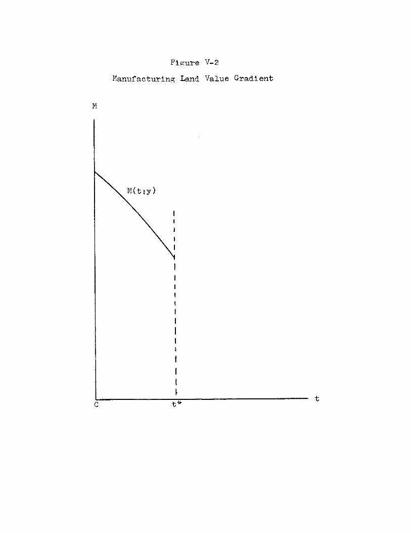
Figure V-2

Manufacturing Land Value Gradient

N

M(t;y)

I

tC t

188

the cost of transporting one unit of output from the firm's

location to C can never exceed the price this unit will re-

ceive once it reaches its destination.1 7 The basic result

given in (5-25.2) seems sensible and is roughly consistent with

reality. Both in the model and in the real world, accessible

land has more labor employed on it than does inaccessible land.

Thus far we have assumed that the urban wage rate is

fixed. It is appropriate now to ask how the labor and price

gradients would shift if we relaxed this assumption and allowed

an exogenous increase in y. Proceeding as above, we partially

differentiate (5-20) and (5-22) with respect to y to obtain the

following:

y= [L/(Bq*)] < 0; (5-26.1)

aL/ay= E1/F1 ][1/(W - k(t))] < 0. (5-26.2)

An increase in the urban wage rate causes both the market value

of each parcel and the amount of labor hired to work it to de-

cline. The first of these effects would appear in Figure V-2

as a downward shift in the M( ) curve.

Let us now consider the demand curve for labor in our new

town. Given the definition of L, the total quantity of labor

demanded by the manufacturing sector at some wage rate y and

17It is worth recalling here that (5-25) also dependsrather crucially on our assumption that the wage rate is takenas given by all firms and that it is the same at all locations.

189

for some particular boundary point t* is

Ld = (2/q*)J L(t;y) dt.0

(5-27)

We are assuming that the lot sizes are small enough so that

the labor density curve is a very close approximation to a con-

tinuous function and thus can be integrated. It follows immedi-

ately that

?'Ld/y = (2/q*)J (2L(t;y)/ 3y] dct. 1 8

0(5-28)

Hence, due to (5-26.2),

Ld/hy -< 0. (5-29)

Thus the demand curve for labor in our economy is negatively

sloped. An increase in the urban wage rate will lead each of

the firms in the manufacturing sector to hire less labor (other

things equal). The collective effect, of course, is to reduce

the overall quantity of labor demanded.

Market Equilibrium

Heretofore we have looked at the two

labor market quite independently, treating

18Here and elsewhere in the chapter,following relationship:

q

sides of the urban

y in both cases as

I make use of the

q

d/daT f(x,a) dx = f /Aa/[f/(x,a)I dxp p

+ f(q,a)(dq/da) - f(p,a)(dp/da).

190

an exogenous parameter. Now we shall close the system by re-

quiring that the equilibrium urban wage rate equalize the quan-

tities of labor supplied and demanded. In Figure V-3 the supply

and demand curves for labor are shown superimposed. Since we

have already demonstrated that the supply curve slopes upward

and the demand curve slopes downward, it is reasonable to assume

an equilibrium intersection point exists [(L*,y*) in Figure V-31.

The market clearance condition, Ls = Ld, implies, using

(5-14) and (5-27) that

t*

t-t* = L(t;y) dt, (5-30)0

a relationship which could in principle be solved to obtain the

equilibrium y. Associated with this y there are then particular

equilibrium price and labor gradients describing outcomes in the

land market. Equilibrium conditions such as (5-30) are, however,

of little interest in themselves. 19 What is important is how

the equilibrium values of the variables change in response to

parameter changes. Since this dissertation is ultimately con-

cerned with land-use policies, a natural first question to ask

is how the equilibria in both the labor and land markets will

be affected by a change in t*, the manufacturing-residential

boundary point. From the point of view of the developer, we

are asking how his decision about the location of t* prior to

the primordial auction will influence the outcomes of that auc-

tion.

19Paul A. Samuelson Foundations of Economic Analysis(New York: Atheneum, 19655, p. 7.

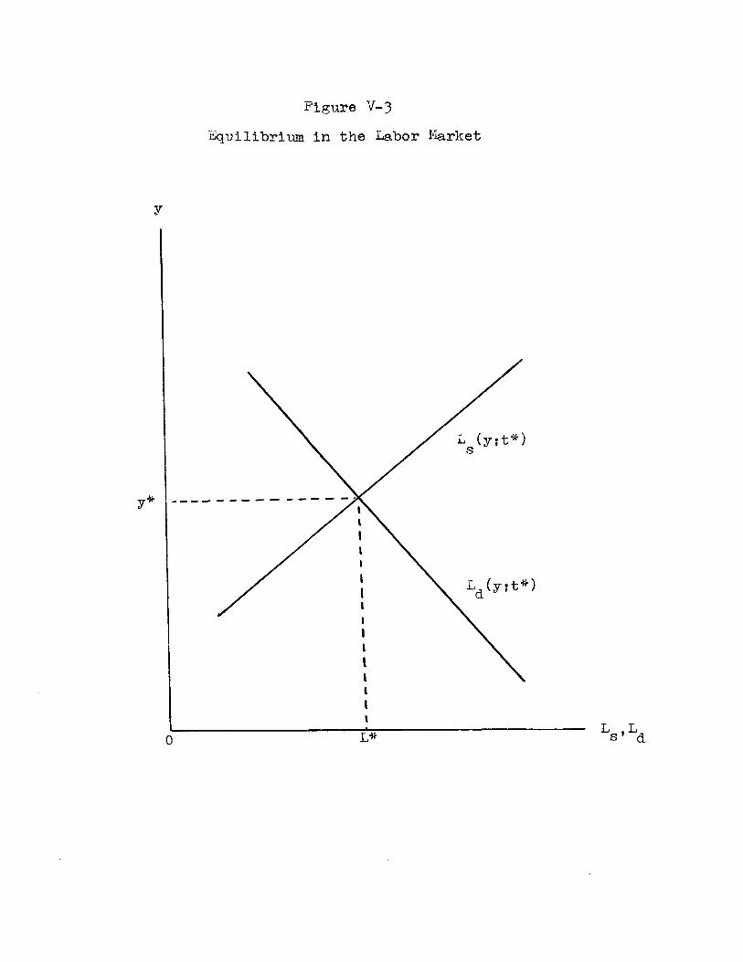
Figure V-3

Equilibrium in the Labor Market

y

Ls (y;t*)

II

Ld (y;t*)

I

t

L OL0 L* d

192

Let us consider the labor market first, How does a change

in t* affect the supply and demand for labor? On the supply

side we have from (5-11) and (5-14)

;Ls/t* = [2/q*][(0t'/ht*) - 1] < 0. (5-31)

Thus a small increase in t* causes the supply curve of labor to

shift upward and to the left. The logic behind this result is

comparatively straightforward. Basically, an increase in t*

(other things equal) makes our new town a less desirable place

to live for the typical citizen, Consequently, at each wage

rate fewer people will end up migrating to the city than would

have if the change had not occurred, This decrease in desir-

ability comes about for two reasons, First, the length of the

average work trip for the entire community is increased because

those residential properties closest to t* (and hence those

with the most accessibility) have been converted to manufactur-

ing uses, Second, the externality effects described earlier in-

crease with an increase in t*, thereby causing all sites re-

maining in residential use to become less attractive than pre-

viously. The combined effect can easily be seen by examining

Figure V-1. Increasing the amount of land devoted to manufac-

turing simultaneously moves t* to the right and tt to the left

(5-14), thus effecting a shrinkage in both the quantity of in-

habited residential land and the labor force, Note that if

there were no externalities in the economy, t' would not shift

to the left (because the price gradient would not shift down-

ward), Labor supply would then be less sensitive to land use

193

changes than it would be if externalities were present. The

analytical consequences of this last situation are that t'/t*

would equal zero in (5-31).

The demand for labor is given in (5-27). It follows

immediately that

Ld/Zt* = (2/q*)L(t*;y) > 0, (5-32)

because q* and L(t*;y), the quantity of labor hired by the firm

located immediately to the left of t*, are always positive.

Thus, an increase in t* causes the demand curve for labor to

shift upward and to the right. At each wage rate, more workers

than before are demanded by the manufacturing sector. This is

a sensible result because increasing t* allows more firms to

participate in the economy.

It should now be clear how a small increase in t* will

affect the city's wage rate and labor force. Both the demand

and supply curves for labor in Figure V-3 will shift upward.

Thus the developer will find that the more land he allocates

to manufacturing prior to the primordial auction the higher the

equilibrium money wage will be after the auction is complete.

That is,

dy/dt* > 0. (5-33)

The effect on the size of the equilibrium labor force and popu-

lation, on the other hand, will be indeterminate. As any intro-

ductory student knows, a simultaneous upward shift in both

supply and demand has a positive effect on price but an ambigu-

194

ous effect on quantity. Thus a new town with a large amount

of land devoted to manufacturing may have either a bigger or

smaller population (and labor force) than one with a lesser

amount of land devoted to this purpose.

The results in the previous paragraph have several inter-

esting implications. First of all, we have demonstrated that

there is a connection between the quantities of land allocated

to different activities and some other seemingly unrelated

economic and demographic variables. This suggests that zoning

and other land policies should not be implemented in isolation

but rather should be coordinated with existing economic planning

or development programs being carried out in other governmental

departments. This is hardly a new idea as far as very small

gqovernmental units are concerned. Very often they will regard

the local zoning ordinance as the only effective way of con-

trolling economic activity within their boundaries.20 Large

cities, on the other hand, typically have separate zoning and

economic development (or redevelopment) agencies which operate

quite independently of each other.21 Our analysis suggests that

this is not a sensible way to run a city.

20A typical small town situation is described in Shannonv. Building Inspector of 4oburn, 328 Mass. 633 (1952). Herethe rezoning of a district from residential to industrial wasupheld on the grounds that it would promote local economicdevelopment.

21Some evidence for this assertion in the case of Bostonmay be found in William W'eismantel, Collision of Urban Renewalwith Zoning: The Boston Experience, 1950-1967 (unpublishedPh.D. dissertation, Department of City and Regional Planning,Harvard University, 1968).

195

A second point concerns the positive relationship we

have established between the location of the residential-

manufacturing boundary point and the urban wage rate. This

result indicates that it may be possible to explain money wage

rate differences among certain communities at least partially

in terms of their differing land-use policies. Of course, the

magnitude of the real world effects here are probably fairly

weak so that to isolate them the researcher would have to con-

trol for the influence of other variables rather carefully.

Finally, note that our new town can be in equilibrium

with the rest of the world at any of an infinity of different

money wage rates (each associated with a different land-use

policy). This is a natural consequence of our assumption that

it is utility levels rather than wage rates which are equalized

between cities by interurban migration, The essential point

thus is that utility levels can be equalized between two cities

(thereby bringing them into migratory equilibrium with respect

to one another) even though their money wage rates are very

different. It is this characteristic of real world urban econ-

omies which induces social scientists studying migration pro-

cesses to deflate money wage rates with amenity and price level

indices.

Let us now trace the labor market adjustments described

above back through to the underlying land market changes. The

effect on the price gradients in the two zones of the economy

is mixed. Because of (5-33) and (5-26.2), an increase in t*

will cause the auction prices for land in the manufacturing

196

sector to be lower than they would have been in the absence

of the increase. In terms of Figure V-2, the change induces

a downward shift in the M( ) function. In the residential

sector, on the other hand, the price gradient does not neces-

sarily shift in either direction, To see this note that the

following relationship holds for any residential parcel:

dm/dt* = (Om/ y)(dy/dt*) + )m/Zt*. (5-34)

(5-34) is obtained by differentiating (5-8) fully with respect

to t*, The first term is positive [the induced income effect,

(5-12) and (5-33)], but the second is negative [the externality

effect, (5-10)]. The net effect is indeterminate. It is impos-

sible therefore to ascertain in advance how the price of any

particular residential parcel would change if the developer

decided prior to the auction to increase the quantity of manu-

facturing land available for sale. To answer such a question

more specific knowledge about the functional forms of m( ), M( )

and L( ) would be necessary.

Finally, we may ask what difference the neighborhood exter-

nality assumptions make to all of this analysis. In truth, they

do not play nearly as big a role here as they will in subsequent

sections when we consider the specific policy problems associated

with setting up and maintaining an optimal allocation of urban

land. Several comments can now be made, however, The basic

fact is that the existence of consumer tastes about the quan-

tity and location of manufacturing land in the space economy

causes the size of the urban population (and labor force) to

197

be more sensitive to land use changes than would otherwise be

the case. This we noted earlier in our discussion of the prop-

erties of the labor supply curve. As is clear from (5-31),

if there are no neighborhood externalities a marginal increase

in t* will induce a smaller upward shift in the labor supply

curve than would occur if externalities did exist. Thus both

the wage increase and the labor quantity decrease will be less

in the no externality case (other things equal) than they would

be in the externality case.

This result suggests in turn that cities in the real

world which are characterized by particularly offensive environ-

ments (due to smell, air pollution, ugliness, etc.) ought to

have higher prevailing money wage rates and smaller populations

(in equilibrium) than those cities which are not so character-

ized. Obviously, to test such a hypothesis the influence of

all variables -- including the industrial structure of the

economy -- must be controlled for. Such a task would not be

simple to do because there is usually a close relationship be-

tween the economic base of an urban area and its environmental

undesirability. Nonetheless, this seems like an interesting

area to explore.

C, Maximizing the Aggregate Value of Urban Land

Thus far in this chapter we have concerned ourselves with

the structural characteristics of a simple model of a new town

economy. Using this model we have demonstrated that a change

in land use has a diverse set of consequences which extend

throughout the entire economy. Nothing has been said, however,

198

about the developer. It is he who is in charge of planning

the new town and who in the end must make all land allocation

decisions. In the model economy which has been constructed in

the present chapter the scope for decision making has been re-

duced to the bare minimum. All the developer must do is de-

cide on the location of a single point: t*, the point which

separates the residential zone from the manufacturing zone.

How this choice is made is the subject of the present section.

We will assume that our developer wishes to maximize

profits. Once the developer has purchased and subdivided the

land (i.e., once the costs associated with these two activ-

ities are sunk), a strategy which maximizes profits is equi-

valent to one which maximizes land values. Thus we will assume

that our developer chooses the t* which maximizes the total re-

ceipts to be obtained from the primordial auction.2 2 We will

now try to indicate some of the implications of this choice.

The total of the receipts which the developer will obtain

by auctioning off all parcels on the right-hand side of the

city is equal to the sum of the following two integrals:

t* t'

V f M(t;y) dt + f m(t;yt*) dt. 23 (5-35)0 t*

22A more complex model would begin at an earlier stageand include the land purchase and subdivision decisions aswell. These aspects of the development problem were, however,peripheral to the main interest of this study. Consequently,we ignored them.

23Because we have assumed that our developer always laysout a symmetrical new town, we can focus (as before) on onlyone side of the urban land market.

199

The first term gives the total sales in the manufacturing zone,

the second total sales in the residential zone. We now wish

to maximize V with respect to t*, the land-use boundary param-

eter. Differentiating, we obtain

t*

dV/dt* = d/dt*{ M(t;y) dt0

to

+ d/dt*' m(t;y,t*) dt. (5-36)0

Butt* t*

d/dt*,r M(t;y) dt = /?t*f M(t;y) dt0 0

t*

+ [dy/dt*1[?)/?yf M(t;y) dt]. (5-37)

Hence, utilizing (5-26.1),

t*

d/dt*,f M(t;y) dt = M(t*;y)0

- [dy/dt*], [1/(Bq*)]L(t;y) dt. (5-38)

Moreover, we know from (5-27) that the integral in the second

term is nothing but a constant multiple of the quantity of

labor demanded at wage rate y. Hence

d/dt*J M(t;y) dt = M(t*;y)0

- [ciy/ct*] [1/(2B1) JLd#

Now let us look at the second term of

t I

d/dt*f m(t;yt*)t*

tI

dt = /bt*j m(t;y,t*)t*

dt

at].

The first term of (5-40) becomesI

3(t;y,t*)

t

at = Sm/)t*t*

- m(t*;y,t*).

The second term of (5-40) becomes

t'

[dy/dt*][/Zyf m(t;y,t*)]dtt*

t

= (dy/dt*),f ?m/By dt.t*

Both of these results are obtained by noting that m(t

Inserting (5-41) and (5-42)

200

(5-39)

(5-36).

t- t

+ [dy/dt*][()/ayf m(try,t*)t*

t

b/ t*lt*

(5-40)

dt

(5-41)

(5-42)

;y,t*) = 0.

into (5-40), we obtain

201

d/dt*4 m(ty,t*) dt = 7m/3t* dtt* t*

t

- m(t*;yt*) + (dy/dt*)f m/ay dt. (5-43)t*

Furthermore, utilizing (5-12) we see that

tI

5 m/6y dt = (t' - t*)/(bq*) = Ls/(2b). (5-44)t*

Finally, substituting (5-39), (5-43), and (5-44) into

(5-36) we obtaint

dV/dt* = M(t*;y) - m(t*;y,t*) + j Zm/6t* dtt*

+ [dy/dt*]L(1/b)(Ls/2) - (1/B)(Ld/2)]. (5-45)

If we now assume that b = B and that the labor market is always

in equilibrium (Ls = Ld), it follows that

dVdt*= M(t*;y) - m(t*;y,t*)

t'I

+ tm/*t* dt.24 (5-46)

24 The assumption that the two credit parameters are thesame is consistent with the static framework we have been usingthroughout this chapter. If we drop this assumption, theboundary condition described below (5-47) simply becomes morecomplex. Our basic arguments concerning the role of neighbor-hood externalities would remain unchanged, however.

202

Setting dV/dt* equal to zero, we then obtain

tI

M(t*;y) = m(t*;y,t*) - f 2m/Zt* dt. (5-47)t*

(5-47) is the first-order condition for the maximization

of V. What does it tell us? Essentially, (5-47) is a restric-

tion on the (per unit) land prices paid by the two uses at t*,

the boundary point. M(t*;y) is the price paid by the manufac-

turingr firm located immediately to the left of t*. And m(t*;yt*)

is the price paid by the corresponding household immediately to

the right.

Note, first of all, that if there are no externalities in

the economy the integral term on the right-hand side of (5-47)

is equal to zero due to (5-10). In this situation

M(t*;y) = m(t*;yt*). (5-48)

Thus, if there are no externalities, a necessary condition for

the maximization of aggregate land values is that the prices

paid by the two uses at the boundary point be the same.

If there are externalities in the economy, however, the

integral term in (5-47) is negative. In this case a necessary

condition is that the two prices be different. More specif-

ically, the condition (5-47) states that for a maximum the manu-

facturing price at t* must be greater than the residential price

at the same point, with the difference being equal to the total

decrease in residential land values which would come about if

the boundary point were moved out slightly and y were held con-

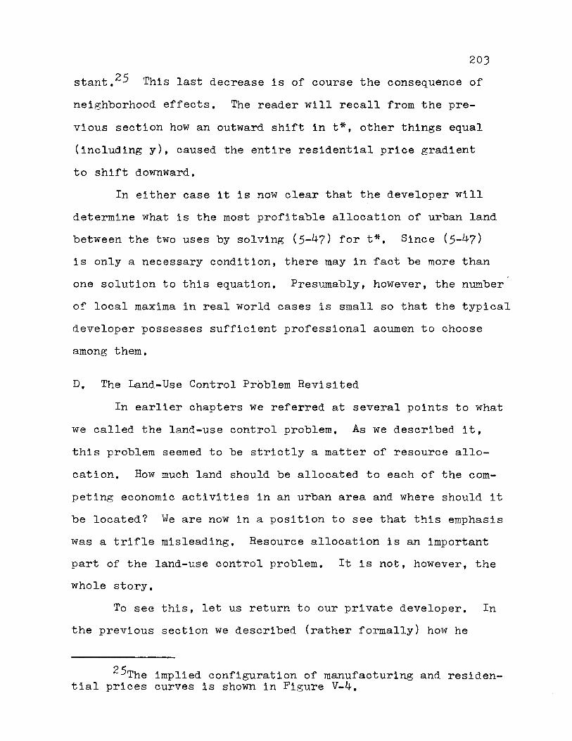
203

stant.2 5 This last decrease is of course the consequence of

neighborhood effects. The reader will recall from the pre-

vious section how an outward shift in t*, other things equal

(including y), caused the entire residential price gradient

to shift downward.

In either case it is now clear that the developer will

determine what is the most profitable allocation of urban land

between the two uses by solving (5-47) for t*. Since (5-47)

is only a necessary condition, there may in fact be more than

one solution to this equation. Presumably, however, the number

of local maxima in real world cases is small so that the typical

developer possesses sufficient professional acumen to choose

among them.

D, The Land-Use Control Problem Revisited

In earlier chapters we referred at several points to what

we called the land-use control problem. As we described it,

this problem seemed to be strictly a matter of resource allo-

cation. How much land should be allocated to each of the com-

peting economic activities in an urban area and where should it

be located? We are now in a position to see that this emphasis

was a trifle misleading. Resource allocation is an important

part of the land-use control problem. It is not, however, the

whole story.

To see this, let us return to our private developer. In

the previous section we described (rather formally) how he

2 5The implied configuration of manufacturing and residen-tial prices curves is shown in Figure V-4.

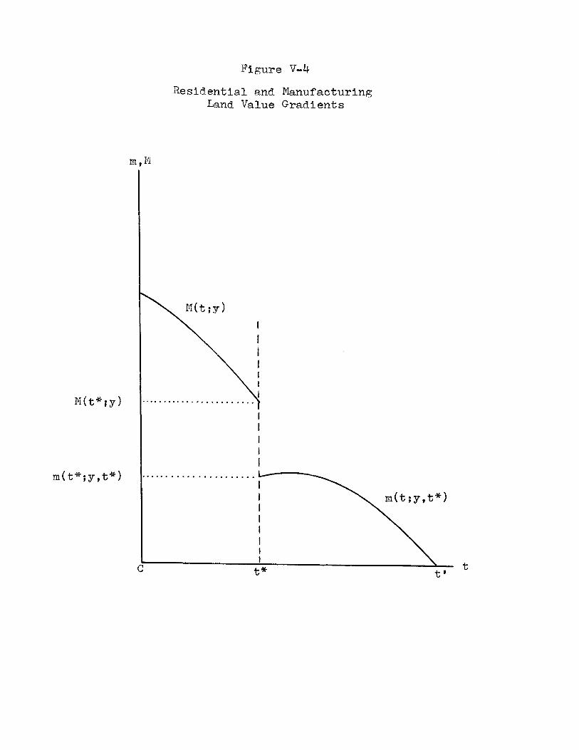
Figure V-4

Residential and ManufacturingLand Value Gradients

mm

M(t*;y)

m(t*;y,t*)

m (t; y)

m(t;y,t*)

C ttI

205

would go about choosing a t* which maximized the total market

value of his land holdings. Thus in this rather special case

we solved the allocation problem, strictly defined. If we

know the functional forms of the various curves and if we know

the developer is a profit maximizer, then we can easily deter-

mine the partition of the urban space economy he will choose.

If our developer wishes only to lease all of the lots in

the town, this partition is all he needs to know. Suppose,

however, he wishes to sell his holdings immediately (the assump-

tion we have been making throughout this chapter). This deci-

sion generates a new problem. How can the developer be sure

that the value-maximizing allocation will be preserved after

the land is sold? At first this might appear to be an irrele-

vant question. After all, why should the developer care about

what happens to his land after it has been sold? In fact, he

does not really care. He does, however, care about the expec-

tations which prospective purchasers have about the future

appearance of the community in which they are considering

buying a lot. If these purchasers do not expect the present

allocation of land (determined by the developer) to persist in

the future, this expectation will affect (probably adversely)

the price which they are willing to pay.

Thus the developer must really make two decisions. First,

he must decide upon a land-use partition which, if it is viewed

as immutable by all purchasers (firms as well as households),

will maximize his total sales revenue. This is the allocation

decision described above. Second, he must choose some insti-

206

tutional arrangement which will provide a credible guarantee

that in fact the chosen partition will persist into the future.

This distinction is a general one; it applies to land-

use decisions made by communities as well as those made by pri-

vate developers. In the community case, of course, the appro-

priate choice criteria are not nearly as clear-cut as they are

in the developer case, There is simply no single behavioral

assumption which commands wide agreement among experts in the

field of local government. In some cases it may be reasonable

to assume that communities strive to maximize total land values;

in other cases such an assumption is clearly inappropriate.

4hatever the criteria actually employed, however, it should be

clear that a community faces the same problem that a private

developer does. It must determine an "optimal" allocation of

the land within its boundaries among all alternative economic

activities. In addition it must set up one or more institu-

tional mechanisms for achieving this optimal arrangement and

preserving it once it has been achieved. Obviously, the developer

does not have to worry about achieving the initial optimal

arrangement since in the beginning he has complete control over

the land. Otherwise, however, the situations faced by the

developer and the community are very much the same.

It is worth remarking at this point that the distinction

we are drawing here between the allocational and the institu-

tional aspects of the land-use control problem corresponds

closely to the conceptual distinction drawn in the legal and

planning literature between a community's master plan and its

207

zoning statute.2 6 The standard planning view is that the master

plan is a document which contains the ultimate planning goals

of the community. A zoning statute, on the other hand, is re-

garded only as one of several alternative control or regulatory

devices which can be used to achieve these goals. Thus (in

theory) the master plan stands behind the zoning statute and

has an existence independent of it. From the point of view of

the present study it is useful to think of the master plan (or

at least the physical portion of it) as embodying the commun-

ity's land allocation objectives (derived presumably from some

social welfare function). It thus indicates what the community

regards as the optimal pattern of local land use. The zoning

ordinance then becomes only an institutional tool for bringing

this optimal pattern into existence and preserving it once it

has been achieved.

Unfortunately, few communities in the real world have

paid much attention to "proper" planning procedures. In nearly

all cases, municipalities passed their first zoning ordinance

long before they had a master plan, a sequence of events which

most city planners find preposterous. As Eaar has demonstrated

in the article cited above, the courts have had to employ some

rather far-fetched arguments to certify the constitutionality

of zoning in the absence of any "comprehensive" plan. Most

communities in fact end up treating their zoning map as if it

26The most famous piece of writing on this subject isCharles Haar's "In Accordance with a Comprehensive Plan,"Harvard Law Review, 68 (April, 1955).

208

were the same thing as a municipal plan, a practice which

leads to awkward moments when these same communities wish to

demonstrate in court that changes which they have made in their

map were dictated by "general welfare" considerations rather

than by the caprice of the zoning board of appeals.

One may ask at this point what the preceeding discussion

has to do with neighborhood externalities, the phenomenon with

which this chapter is ostensibly concerned. To see the rela-

tionship we must make use of the results obtained in the pre-

ceeding section. 4e have assumed that our developer wishes

to maximize the total value of his land holdings. It follows

(as demonstrated above) that a necessary condition for achieving

this maximum when neighborhood externalities are present is a

land price gradient which is discontinuous at the (optimal)

residential-nonresidential boundary. IWhen externalities are

not present, on the other hand, a necessary condition is that

the gradient be continuous at this location.

Ahat is the significance of these results? The critical

point concerns the relative stability of the value-maximizing

allocations in these two cases. In the no-externality case

the optimal allocation is stable because there will be no market

forces operating to alter the developer's original partition

(i.e., his choice of t*) once he has divested himself of all

of the land in the new town. 27

2 7The implicit assumption here is that the (absolute)slope of the manufacturing price gradient at t* exceeds the(absolute) slope of the residential price gradient at the samepoint. This will typically be the case because one expects thedeveloper to put the economic activity with the steepest bidprice curves closest to the urban center.

209

In the externality case, however, these forces do exist.

Suppose, for example, the developer makes all of the lots in

the new town subject to a restrictive covenant which requires

the boundary point separating the two types of land use to be

at a specific location. Suppose further that all the purchasers

regard this system of covenants as watertight. If in fact the

chosen t* was the optimal one, then the spatial pattern of

prices received by the developer for all of his lots will be

similar to the one shown in Figure V-4. That is, there will

be a discontinuity in the price gradient at t*, with the residen-

tial price lying below the manufacturing price at this point.

Now what will happen if subsequent to the primordial auction

the covenant system is found to be legally void? Clearly,

there will be conversions from residential to nonresidential

uses in the area immediately to the right of t*. The motiva-

tion behind these conversions will be the desire of households

to realize capital gains on the property which they purchased.

Such conversions will continue until prices are equalized at

the boundary. Once this occurs the system will have reached

an equilibrium and no more changes will take place.

In this particular example, of course, the developer was

unaffected by the legal errors which he committed when he

drafted the covenants. This is the kind of mistake, however,

which a developer cannot afford to make too often. If his prom-

ises to prospective purchasers in successive developments are

to remain credible, it is essential that the arrangements which

he sets up to perpetuate a certain pattern of land use be effec-

210

tive. Thus the presence of neighborhood externalities makes

the institutional aspects of land-use control rather impor-

tant to the profit-maximizing developer. If he cannot set up

his controls properly, he will probably end up getting less

than the maximum value for his land holdings because of the

attendant uncertainty.28

The device which developers typically use to ensure that

the land-use patterns which they set up will be sustained

through time is the restrictive covenant. 29 Since covenants

are a kind of private contract, the restrictions which they

can impose on land use are much greater than those which can

be imposed under police power regulations such as zoning. One

need only to look at the covenants used by Levitt and Sons

to affirm this.3 0 This is one of the reasons that developers

find the device very useful. Another reasons is that the typi-

cal set of covenants (or "building scheme") can be enforced by

2 8This result neet not obtain in all cases. It is quitepossible that in some instances a higher value will be obtainedbecause of a particular pattern of (mutually inconsistent) ex-pectations on the part of the purchasers. One does not expectsuch results generally, however. Most households do not buyreal estate for speculative purposes.

29A brief discussion of the legal aspects of covenantsmay be found in Williams, op. cit., pp. 18-22. This topic,incidently, would be an interesting area to explore using theeconomic theory of coalitions. Bargaining and the costs oforganization enter into the creation and. maintenance of coven-ant systems in obvious ways.

30Delafons, op. cit., pp. 76-79. Levitt's covenantseven go so far as to impose some restrictions on the hangingof laundry outdoors.

211

any one of the property owners who purchased subject to it.

This makes the restrictions much more difficult to alter be-

cause any changes require virtually one hundred per cent

agreement to be implemented.

Neighborhood externalities introduce similar kinds of

complications in the community case too. Municipalities, like

developers, typically wish to impose locational restrictions on

those land uses which generate strong neighborhood effects. One

suspects that they will want to do this even if they do not

choose to follow an explicit land value maximizing strategy.

These restrictions are likely in turn to lead to price discon-

tinuities of the type shown in Figure V-4. The problem which

the community must solve in this situation is then identical to

the one faced by the developer -- namely, what institutional

arrangements should be set up to preserve a particular status

quo. As in the developer case, there is an inherent source of

instability in the system. The more people there are who re-

gard some particular pattern of land use as permanent (due to

faith in a zoning statute) the more incentive there is for

particular individuals (speculators!) to try to undermine the

statute in order to achieve capital gains.3 1 These simple

dynamics account for much of the distrust which has come to

surround the zoning institution in the past half century.

A specific example will clarify these observations. Sup-

31Typical members of this last group are entrepreneurswho seek to build apartment buildings and shopping centers in

heretofore homogeneous single-family home neighborhoods.

212

pose that the point labeled t* in Figure V-4 is the community

optimum (on the basis of some social welfare function). Sup-

pose further that the community is able to bring about this

optimal partition through public action32 (perhaps urban re-

newal) and that it seeks to perpetuate its handiwork by passing

a zoning law. If every prospective purchaser in the town be-

lieves the location of t* to be permanent due to the invulner-

ability of the zoning ordinance, then the spatial pattern of

land values will be as indicated in Figure V-4.

The villain of the piece, a speculator, now appears. If

he believes, contrary to everyone else, that the zoning ordin-

ance is not immutable, he will purchase one or more of the

(residential) lots immediately to the right of t* at the low

price which prevails there. The price is low, of course, be-

cause of the proximity of manufacturing processes. He will

then endeavor to persuade the zoning board of appeals to grant

him a use variance. Alternatively, he will try to get the city

council to amend the zoning map in his favor ("spot zoning"),

If he succeeds in either of these endeavors, he will be able to

resell his holdings to one or more manufacturing firms and make

a capital gain of (roughly) M(t*;y) - m(t*;y,t*) dollars per

unit area.

What arguments will he use to persuade the relevant

government officials to grant him this windfall? For one thing

32 e remarked in Chapter IV and elsewhere that zoningitself is not well-designed for this purpose.

213

he may seek to persuade them that external circumstances have

changed (even though they have not), and that therefore a re-

zoning is necessary to return the statute to optimality.

Second, he may assert that the current zoning restrictions im-

pose unreasonable "hardship" on him and that therefore he is

entitled to a variance. 33 Third, he may attempt to challenge

the entire zoning ordinance on grounds of legal insufficiency.

Last, but certainly not least, he may attempt to bribe the

appropriate officials to obtain the adjustments desired.

This last method is worth a comment or two. "vie noted

above that a strategy of land value maximization in the presence

of externalities meant a discontinuous land price gradient. We

went on to observe that although communities might not always

want to pursue that particular strategy, it seemed likely that

they would still wish to restrict externality-generating land

uses in such a way that price discontinuities would result. If

these speculations are correct, one would expect corruption of

the type described in the previous paragraph to be a rather com-

mon characteristic of American zoning systems -- which indeed it

is. The simple truth is that government-imposed price discon-

tinuities, such as the one exhibited in Figure V-4, will always

331n fact, of course, the only "hardship" he endures isthe prospect of not achieving a lucrative capital gain if thezoning is not changed. On occasion even the courts fail toappreciate this point. See, for example, Vernon Park Realty.Inc, v. City of Mount Vernon, 307 N.Y. 493, 121 N.E. (2d)517 (1954). In this case a sharp developer bought a parkinglot subject to a zoning restriction and then persuaded thecourt to invalidate the restriction on due process grounds sohe could build a shopping center.

214

be standing invitations to bribery.

In real world situations at least one of the strategies

described in the previous paragraph will frequently work.34

Indeed, the ease with which variances and map changes are ob-

tained has generated widespread cynicism and anxiety among

zoning experts.35 The problem here is a real one. If there

is any merit at all to the view that the allocation of a com-

munity's land should be planned in some way rather than left

exclusively to market forces, then it is a problem worth

solving. Zoning can probably never be made into a positive

instrument for effecting major land use changes. Perhaps,

however, it can still be usefully employed as a holding device

for preserving worthwhile configurations of urban land which

already exist. The question to be asked then is the following:

What changes should be made in the zoning instrument and the

way in which it is typically administered to enable it to per-

form this particular task more effectively than it has in the

past?

This is hardly the place for an extended discussion of

34Some evidence for this proposition may be found in datarevealing that in most American cities a very high percentageof variance requests are granted by the local zoning board ofappeals. A few such statistics are presented in Stephen Sussna,"Zoning Boards: In Theory and In Practice," Land Economics, 37(February, 1961). Sussna argues that most of the requestsgranted by zoning boards are reasonable in the light of changedcircumstances. This is definitely a minority view,

35Sussna lists a number of representative sources. Ibid,,p. 82.

215

institutional reform in this area. Several suggestions, how-

ever, have been made which are worth mentioning. First of all,

some modern zoning enabling acts explicitly prohibit spot

zoning. In addition, many of the more recent zoning ordinances

orbid use variances.36 Obviously, if such restrictions become

universal, much of the problem of instability described above

will be solved. One difficulty with this solution, however, is

that it disallows legitimate marginal map changes in response

to changing conditions in the local economy.

Other reforms are less restrictive of planning initiative.

Delafons and Babcock separately propose that the procedure at

zoning board hearings be formalized.3 7 They feel that in most

municipalities these proceedings are so anarchic that a rational

weighing of the public and private interests in specific dis-

putes is completely impossible. This state of affairs encour-

ages both arbitrary and illegal decision making on the part of

local officials.

Finally, Haar and others argue that the way to protect a

zoning map from administrative or legislative incursion is to

found it upon a well-articulated, comprehensive, municipal

plan.38 This plan will presumably embody the social goals of

the community and. will thus be optimal according to at least

some (appropriately weighted) set of social indices. This set,

3 6 Delafons, o, cit., p. 59.

37Ibid,, 97 and Babcock, oD..cit., pp. 154159.

38H.daar, op. cit.

216

of course, may or may not contain the index which has been

given prominence in this study -- namely, aggregate community

land values. In any case, Haar's point is that the existence

of a plan will give the courts an additional check on official

irresPonsibility in zoning administration cases, Those vari-

ance or spot zoning decisions which are not in accordance with

the community plan can then be easily ascertained and rejected.

EP ILOGUE

We have now completed the limited range of tasks which

we set out for ourselves in Chapter II. Having come this far,

it is reasonable to ask about what lies ahead. The Ph.D. dis-

sertation by its very nature is an extremely restricted art

form -- one whose preeminent virtue is depth rather than breadth.

The main implication of this unwritten law for the present study

was that many interesting topics in the economics of neighbor-

hood externalities and land-use control systems were either in-

adequately treated or completely ignored in the main text.

Such exclusions were, of course, the price paid for the moder-

ately high level of mathematical and econometric detail which

characterized the last three chapters of this study. Now that

the main work of the dissertation is over, however, it seems

appropriate to make amends by indicating at least briefly what

some of these topics are and how they might be fruitfully

analyzed by future researchers,

Let us begin by considering the empirical work on neighbor-

hood externalities contained in Chapter IV. The reader will re-

call that our principal conclusion there was that neighborhood

environment appears to exert an empirically measurable (but

fairly complex) effect on the market values of single-family

homes. It is now a generally accepted canon of empirical re-

search that no study can ever be truly conclusive since there

is always the possibility that there are "lurking factors" oper-

218

ating unbeknownst behind the scenes. Nonetheless, the general

results given in Chapter IV seem, in retrospect, to be fairly

solid. Consequently, most of the empirical topics which imme-

diately spring to mind are basically refinements of the work

done in that chapter. This is not to say, however, that they

are not worth looking into.

Surely it would be interesting, for example, to determine

the precise generality of the results presented in Chapter IV.

To do this it will probably be necessary to repeat (at least

in broad outline) the empirical study described in that chapter

for assorted city and year combinations other than 1960 Boston.

It would perhaps also be useful if at least some of these sub-

sequent studies used less aggregated data than we were forced

to use here. Data on individual properties would be ideal, al-

though, as indicated in the text, it will probably be difficult

to obtain. Finally, it would be desirable for someone to con-

sider the impact of neighborhood externalities on the market

value of properties other than single-family homes. Solid

statistical evidence on this question would be of obvious

utility to city planners and local government officials.

Now let us turn to the theoretical results presented in

Chapter V. Jhat, if any, avenues for future research do they

open up? It seems fair to say that these results are much more

suggrestive than definitive. The main reason for this is that

the model developed in Chapter V is a fairly restricted one;

it does not have a great deal of utility outside of the specific

applications for which it was constructed. Indeed, as indicated,

219

in the text, a truly general theory of the urban land market

does not yet exist. Alonso's model and the one in Chapter V

are useful beginnings, but there are still a large number of

important real world complexities which remain to be incor-

porated into them. Plany of these were discussed in the main

text. The principal task ahead, therefore, for economists

wishing to extend the theoretical results appearing in this

study is quite well-defined -- namely, build a better model.

Once such a paradigm is available, it will be possible to in-

vestigate the economic aspects of land-use control devices in a

much more systematic way than was done here. Hopefully our

efforts in this dissertation will stimulate further research

along these lines.

The final set of research problems suggested by our study

concerns the impact which zoning ordinances and other land-use

control devices have had on real world urban space economies.

Surprisingly enough, very little is known about this in spite

of the fact that these policy tools have been in widespread use

for over fifty years. The principal difficulty here has been

the absence of any sound theoretical framework which could be

used to guide empirical investigations. We discussed this

general problem in the previous paragraph. Once a full-blown

theory of the urban land market is developed it will become

possible to make reasonable guesses about what would happen

to cities if zoning ordinances were abolished. And this, of

course, is what one has to know if he wishes to assay their

effectiveness.

Technical Appendix

A. Introduction

The purpose of this appendix is to explain the various

technical procedures used to prepare the data base for the

estimations presented in Chapter IV. Included here will be

a list of the Massachusetts cities and towns which made up

our sample. In addition, we will go through each one of the

variables introduced in Chapter IV and discuss its origin in

detail. Some of these variables were taken directly from

other sources; others were the product of special manipula-

tions. In the latter cases we shall show explicitly what

assumptions were introduced and how the calculations were

performed. As is true of all econometric studies, many

choices had to be made. Hopefully this appendix will make

clear what these choices were and why we resolved them the

way we did.

B. Cities and Towns

The forty-six Massachusetts cities and towns which made

up our sample are listed alphabetically in Table A-1. Note

that Boston is not included in this sample. This was done

deliberately because it is much larger in area and population

than any of its satellite communities. It has been suggested

elsewhere that the older industrial cities surrounding Boston

(such as Cambridge and Somerville) should also be excluded

from a study which purports to analyze "suburban" property

221

Table A-1

Forty-Six Massachusetts Cities and Towns

Arlington Needham

Belmont Newton

Beverly Norwood

Braintree Peabody

Brookline Quincy

Cambridge Randolph

Chelsea Reading

Cohasset Revere

Concord Salem

Danvers Saugus

Dedham Scituate

Everett Sharon

Framingham Somerville

Hull Stoneham

Lexington Swampscott

Lynn Wakefield

Malden Waltham

Marblehead Watertown

Medford Wellesley

Melrose Weymouth

Milton Winchester

Nahant Winthrop

Natick Woburn

222

values.1 This thought was rejected because we wished to have

a sample of communities which were highly diverse in their

residential environments.

C. Variables

Our procedure in this section will be to go through the

variables used in Chapter IV one by one. In each case we

will indicate the source of the data and what manipulations,

if any, were performed prior to its use in our regression

equations.

Median Value of Single-Family Homes

This series was taken from the 1960 Census of Housing.2

Technically, the figures used cover only "owner-occupied

dwelling units in single-unit structures." Hence, they do

not take account of single-family homes which were renter-

occupied rather than owner-occupied in 1960. Unfortunately

there was no way of obtaining any value data for renter-

occupied homes; consequently, no corrections were possible.

However, because the number of renter-occupied dwelling units

in single-family structures was probably small for most of

the sample communities, it is unlikely that such corrections

1J. D. Heinberg and W. E. Oates, "The Incidence ofDifferential Property Taxes on Urban Housing: A Comment andSome Further Evidence," National Tax Journal, XXIII (March,1970), p. 95.

2U.S. Bureau of the Census, U.S. Census of Housing,1960. Vol. I, States and Small Areas, Part 4: Iowa-Massachu-setts (Washington, D. C.: U.S. Government Printing Office,1963).

223

would have affected our results significantly.

In addition to the median value series, the Census also

provided data from which a series of average values could be

calculated. The principal difficulty here was that in order

to calculate these averages a representative number had to

be assigned to each of several value categories -- one of

which was open-ended -- for all communities. Since it seemed

wiser to avoid arbitrary choices whenever possible, we de-

cided to use the median. In addition, it was felt that the

median would be somewhat less sensitive to extreme response

errors than the average would be.

Unfortunately, it was not possible to use the same

measure of central tendency consistently throughout the

regressions. Some of the independent variable series are

made up of median values and others of average values. This

situation was caused by the diversity of data sources which

had to be brought together to control for all possible in-

fluences on housing price. It did not seem likely, however,

that this minor inconsistency had any substantive effect on

our general results.

Median Number of Rooms for Single-Family Homes

The basic source for this series was again the 1960

Census of Housing.3 This volume contained a figure for the

median number of rooms in owner-occupied dwelling units for

all of the larger cities and towns in Massachusetts. It

3 Ibid.

224

also usually contained additional data from which an average

could be calculated once a representative value was assigned

to the open-ended rooms category. As above, the arbitrariness

of any choice for this value suggested that the median was a

more satisfactory measure of central tendency. In addition,

there were a number of small towns in our data base for which

an average could not be calculated because of limitations in

Census coverage. Consequently, if we had wished to use the

average number of rooms instead of the median, it would have

been necessary to drop these observations from our already

too small sample. All factors, therefore, seemed to favor

the use here of the median instead of the average.

There are two kinds of corrections which could have been

made in the Census median room series to make it more suitable

for our purposes. First, it would have perhaps been desirable

to adjust the Census figures so that they would cover renter-

occupied dwelling units in single-unit structures as well as

all owner-occupied units. This is the same adjustment sug-

gested above for the value series. Again, however, the number

of units involved did not appear large enough to make it worth

the trouble.

A second possible correction seemed more imperative.

The owner-occupied room series included owner-occupied dwell-

ing units in multiple-unit structures. Since many of the

communities in the sample (such as W'altham, Watertown, and

Somerville) had a large number of such units, it did not seem

reasonable to ignore their presence in the Census data. In

225

general one would expect owner-occupied units in multiple-

unit structures to be smaller than owner-occupied units in

single-unit structures. Consequently, those communities

with a large number of units in the former category would

probably have an owner-occupied room figure which was signif-

icantly lower than the (unavailable) single-family home room

figure. For those communities with no owner-occupied dwelling

units in multiple-unit structures this difference would not

exist.

A fairly complex adjustment procedure was devised to

correct this difficulty. We defined the following variables:

MR = the median number of rooms in owner-occupieddwelling units.

MRS = the median number of rooms in owner-occupieddwelling units in single-unit structures.

MRM = the median number of rooms in owner-occupieddwelling units in multiple-unit structures.

NOO = the number of owner-occupied dwelling unitsin the community.

NOOS = the number of owner-occupied dwelling unitsin single-unit structures in the community.

NOOM = the number of owner-occupied dwelling unitsin multiple-unit structures in the community.

Given these definitions the following relationship was

then assumed to be approximately true:

ME = [(NOOM)(MIUrl) + (NOos)(MRS))/NOO. (A-1)

If in every case the median were equal to the average, (A-1)

would hold exactly. All the variables in this expression

226

were known from the Census except for MRM and MRS. The last

of these, of course, was the figure we were seeking.

We then supposed that MRM and MRS differed only by an

additive parameter which was the same in all communities.

That is, we assumed,

MRS = MRM +a. (A-2)

Obviously, in the real world a will not be constant across all

cities and towns. An assumption such as (A-2) was necessary,

however, if we were going to make any progress with the limited

data which was available.

The next task involved obtaining an estimate for a. To

do this we consulted the 1960 Census of Housing volume cover-

ing the Boston metropolitan area.4 This source cross-tabulated

number of rooms against ownership characteristics and structure

type for the city of Boston and its suburban ring. Using

these figures and some simple arithmetic it was possible to

obtain the value of a for the entire Boston suburban area.

This number turned out to be approximately 0.4. Thus in the

suburban portion of the Boston SMSA the median number of rooms

in owner-occupied dwelling units in single-unit structures

was about 0.4 greater than the corresponding figure for owner-

occupied units in multiple-unit structures.

4U.S. Bureau of the Census, U.S. Census of Housing, 1960.Vol. II, Metropolitan Housing, Part 2: Abilene-Corpus ChristiSISA (Washington, D.C.: U.S. Government Printing Office, 1963).

227

4e then substituted this figure into (A-2), substituted

this expression into (A-1) and solved for 1411S.

MIRS = MR + (0.4)(NOOM/NOO). (A-3)

All variables on the right-hand side were then known, thus

making it possible to obtain an estimate of MRS for each com-

munity. This was the series which we then used in our esti-

mations,

Average Age of Owner-Occu ied Dwelling Units

The 1960 Census of Housing provides no median age figure

for single-family homes or indeed for any other kind of dwell-

ing unit. All that was available were distributions of owner-

occupied dwelling units among the following age-of-construc-

tion categories: 5

1959 - 19601955 - 19581950 - 19541940 - 19441939 and earlier.

In order to calculate an average age of structure for

the owner-occupied units in each of our sample communities

it was necessary to assign a representative age to all of the

above birthday categories. For the closed categories the

midpoint was chosen. For the open-ended category a somewhat

more elaborate rrocedure was required. Before explaining it

Su.s. Bureau of the Census, U.S. Census of Housing,160. Vol. I, Part 4, op, cit.

228in detail, let us be clear about why it was necessary.

The simplest procedure here would have been to choose

a reasonable representative age for the owner-occupied

dwelling units built before 1940 and then apply it to all

communities in our sample. The main problem with this method

is that it frequently does not enable the researcher to dis-

criminate very effectively among communities with housing

stocks of different ages. Two cities might have an identical

distribution of units among the five construction-date cate-

gories mentioned above and yet still have housing stocks

whose average ages were very different. The problem is

particularly acute, of course, when a high proportion of the

total number of units in each of the communities is in the

open-ended category. This, it turns out, is the case for

the set of cities and towns in our sample.

Fortunately, supplementary figures were available which

enabled us to sharpen our average age estimates a good deal.

The basic data source used for this correction was the 1940

Census of Housing.6 In this volume dwelling units were dis-

tributed among the following ten construction-date categoriesa

1935 - 19401930 - 19341925 - 19291920 - 19241910 - 19191900 - 19091890 - 18991860 - 18891859 and earlier.

6U.S. Bureau of the Census, U.S. Census of Housing 1940.Vol. II, General Characteristics, Part 3: Iowa-Montana (Wash-ington, D. C.: U.S. Government Printing Office, 1943).

229

Regrettably, for most of the communities in our sample this

distribution was available only for all units and not for

owner-occupied and renter-occupied separately. There was

nothing we could do about this. As a result we were forced

to assume throughout that the separate 1940 distributions

for all units and for owner-occupied units were not very

different.7

Our procedure then was to calculate the median date of

construction for the 1940 stock of dwelling units in each of

the communities in our sample. The median was chosen over

the average for reasons previously described. The fact that

the median is less sensitive than the average to response

errors seemed particularly important in this context because

people living in older dwelling units typically have only a

poor idea of precisely when their structures were built.

Once we obtained this figure for each community, we

subtracted it from 1960 to obtain the median age (in 1960)

of dwelling units constructed before 1940 on the assumption

that none of the dwelling units available in 1940 were with-

drawn from the housing stock in the subsequent twenty years.

This, of course, is an unreasonable assumption. Dwelling

units are withdrawn from the housing stock over time, and

typically in any period it is the older units which disappear.

To control for this phenomenon (although in a very simple-

7More specifically, we assumed that the median valuesof the two age distributions were identical.

230

minded way) we subtracted five years from the age previously

calculated.

These adjusted median age figures, different for every

community, were then used as the representative values for

the open-ended category in our average age calculations.

The averages themselves were computed as simple weighted sums

of all the representative values (i.e., those assigned to

both the closed and open-ended categories) with the weights

being the proportion of units in each category. This calcu-

lation produced an average age figure for the owner-occupied

dwelling units in each community.

One may ask why we did not go on to make an adjustment

for the presence of owner-occupied dwelling units in multiple-

unit structures as was done in the case of the rooms variable.

Basically, there were two factors involved. First of all, it

was felt that such an adjustment was less important for age

because this variable is really only a rough proxy for a large

number of other factors which enter into the residential site

choice (condition, architecture, quality of kitchen and bath-

room facilities, etc.). Since the influence of age on housing

price is not particularly well-defined in the first place,

further improvements in the accuracy of our age data seemed

less important than corresponding improvements in the accuracy

of our rooms data.

Secondly, it was not completely clear which way the

bias should go. Do we expect that owner-occupied dwelling

units in single-unit structures will be on balance older or

231

younger than owner-occupied dwelling units in multiple-unit

structures? For some communities one might expect the former

to be older, for others the latter. Consider Table A-1,

covering those cities for which separate age data on owner-

occupied and renter-occupied dwelling units was available for

both 1940 and 1960. Clearly, if we wished to assume that on

the average owner-occupied dwelling units in multiple-unit

structures were the same age as renter-occupied units, we

could not go on to assert that the former are necessarily

older than owner-occupied dwelling units in single-unit struc-

tures. In Cambridge and Somerville this is manifestly not

the case. Moreover, one suspects that the owner-occupied

dwelling units in multiple-unit structures are probably a bit

newer on balance than renter-occupied units generally. This

suggests that there might be more than just two cities in

Table A-2 whose owner-occupied dwelling units in single-unit

structures are on the average older than their owner-occupied

dwelling units in multiple-unit structures.

The point of these speculations is to demonstrate that

the probable direction of the bias introduced into our age

series by ignoring owner-occupied dwelling units in multiple-

unit structures is more difficult to determine than it was

in the case of the rooms variable. This consideration,

coupled with the fact that age is basically only a proxy for

a multitude of other structure characteristics suggested that

the kind of adjustment we made in the rooms series was un-

necessary here.

232

Table A-2

Average Age (in Years) of the Housing Stockfor Selected Massachusetts Cities in 1960

City

Cambridge

Lynn

Malden

Medford

Newton

Quincy

Somerville

AverageAge

all units

55

50

48

38

37

37

52

AverageAge

0-0 units

59

45

47

36

36

36

54

AverageAge

R-0 units

54

54

49

40

38

38

51

% UnitsOwner-

Occupied

22

44

48

60

60

60

0-0 = Owner-OccupiedR-0 = Renter-Occupied

233

Proportion Owner-Occupied Dwelling Units Sound, With All

Plumbing Facilities

This series was essentially taken from the 1960 Census

of Housing.8 The only complication encountered was the

necessity of estimating for two communities (Nahant and Hull)

the proportion of vacant units which were sound and had all

plumbing facilities. This was done by calculating the cor-

responding percentage for a randomly selected group of small

towns for which the necessary data was available, This average

figure was then applied to the two communities in question.

Again no attempt was made to correct the Census owner-

occupied series for the presence of owner-occupied dwelling

units in multiple-unit structures. It was felt that there

would not be a significant difference between the two kinds

of owner-occupied units with respect to this condition and

plumbing variable.

The Ratio of Local Employment to the Number of Single-Family

Homes

The denominator of this fraction was taken from the 1960

Census of Housing.9 The specific figure used was the number

of owner-occupied dwelling units in single-unit structures.

No adjustment was made for renter-occupied units in single-

unit structures for reasons previously discussed.

8lbid

9 lbide

234

For the numerator, total local employment, we used

estimates provided by Wilbur Smith and Associates, a firm

which served as a consultant to the Boston Regional Planning

Project.1 0 These estimates covered every type of employment,

including all jobs in the public sector.

Road Distance to Downtown Boston

This series was obtained by measuring the road distance

from some major crossroads near the geographic center of each

community to the Massachusetts statehouse in downtown Boston.1'

The road distance was chosen over the linear distance because

the former was felt to be a much more accurate measure of the

typical suburbanite's accessibility to core employment (and

shopping). This refinement seemed especially important for

the present study because some of our communities (particularly

those along the south shore) were located in such a way that

a linear distance measure would seriously overestimate their

accessibility.

Average Lot Size for Single-Family Homes

Vogt, Ivers, and Associates, a Cleveland consulting firm,

performed a land-use survey in 1963 covering most of Eastern

Massachusetts. The basic tool employed in this survey was air

photography (though this technique was supplemented by on-the-

10The figures themselves were taken from David M.Schroedl, op. cit., Appendix. Schroedl apparently got thedata from Smith and Associates personally.

1 1Rand McNally Road Atlas (New York3 Rand McNally andCompany, 45th edition, 1969).

235

ground inspections in areas where economic activities were

highly concentrated), Two of the outputs of this inventory

for each community were the number of single-family homes

and the total amount of land devoted to single-family homes. 12

We took the ratio of the latter to the former to obtain an

estimate of average lot size for single-family homes in each

community.

Proportion of Community Land Not Devoted to Single-Family Homes

The source for this series was the Vogt, Ivers, and

Associates study mentioned above.13 We defined the following

variables:

TLAND = total land area of the community.

ROADS = total land area of community devoted toroads.

HOMES = total land area of community devoted tohomes.

The specific ratio used as an independent variable in the

estimations was then

TLAND - ROADS - HOMES.TLAND - ROADS

12Vogt, Ivers, and Associates, Comprehensive Land UseInventory Report (Boston: Metropolitan Area Planning Council,Department of Commerce and Development, 1965). Note thatthroughout this study we have implicitly assumed that land-use patterns in 1960 were essentially the same as those in1963.

1 3Ibid. All of the land-use variables in this studycome from Vogt, Ivers, and Associates. Consequently, we willnot continue footnoting this source.

236

Land devoted to roads and highways caused some classification

problems in this study because these uses did not fit natu-

rally into any of the zoning categories described in Chapter IV.

The simplest and most sensible procedure seemed to be to use

a total land figure in all our calculations which was net of

land devoted to roads and highways. This is why ROADS is sub-

tracted from the numerator and denominator of the above ratio.

This procedure seemed preferable to forming an additional roads

and highways cateogry because we wished to restrict the total

number of land-use categories to six. To be sure, one additional

category probably would not have made any great difference,

However, there were numerous other candidates for this seventh

position besides roads and highways, and there seemed to be no

good criteria for choosing among all the possibilities. The

line had to be drawn somewhere and we decided to confine our

attention to the six zoning categories previously described.

Prooortion of Community Land Devoted to Nultiole-Family Uses

The specific ratio used here was

MULFAM ,TLAND - ROADS

where MULFAM is the quantity of land devoted to multiple-

family uses. "Multiple-family" as it is defined here in-

cludes the following list of activities:

Two-family dwellings,

Multiple-family dwellings (apartments, boardinghouses, dormitories, trailer camps).

237

Proportion of Community Land Devoted to Commercial Uses

The specific ratio used here was

COMMER ,TLAND - ROADS

where COMMER is the quantity of land devoted to commercial

uses. "Commercial" as it is defined here covers the follow-

ing list of activities:

Retail (local and general),

Services (personal, professional, financial andoffice),

Hotels and Motels,

Indoor Recreation and Entertainment (bowlingalleys, skating rinks, lodges, movietheaters, YMCA's, etc.).

Proportion of Community Land Devoted to Industrial Uses

The specific ratio used here was

INDUST_,TLAND - ROADS

where INDUST is the quantity of land devoted to industrial

uses. "Industrial" as it is defined here covers the follow-

ing list of activities:

Manufacturing (heavy and light),

Transportation and Utilities (railroad yards andright-of-way, airports, bus and truck ter-minals, depots and garages, dock and portfacilities, large parking lots, power sta-tions, gas and power lines, sewerage treat-ment plants and other sanitary facilities,radio and TV stations, antennas, telephonefacilities),

238

Wholesaling, Warehousing, and Storage (indoorand outdoor),

Mining and Quarrying.

Proportion of Community Land Devoted to Institutional Uses

The specific ratio used here was

INSTIT ,TLAND - ROADS

where INSTIT is the quantity of land devoted to institutional

uses. "Institutional" as it is defined here covers the fol-

lowing list of activities:

Medical, Religious, and Cultural (hospitals,clinics, nursing homes, churches, museums,and assembly halls),

Schools and Public Buildings (all schools -- publicand private -- up to and including secondaryschools, post offices, city halls, fire andpolice stations),

Colleges and Universities.

Proportion of Community Land Vacant

The specific ratio used here was

VACANTTLAND - ROADS

where VACANT is the quantity of land in the community which

is either completely unused or devoted to activities which

involve the addition of only a minimal number of immobile

improvements to the land. This category is something of a

residual; it covers the following activities:

239

Forests,

Agriculture and Vacant Lots,

Swamps and Marshes,

Rivers, Lakes, and Ponds,

Construction Projects (residential and nonresiden-tial),

Military Installations,

Outdoor Amusement Facilities (golf courses, drivingranges, athletic fields, public beaches, fair-grounds and amusement parks, outdoor swimmingand wading pools, racetracks, drive-in theaters,major parks, botanical gardens and zoos).

Construction projects were included here because there seemed

to be no other place to put them. In general their influence

on the composite proportion was insignificant because the

amount of land under construction in 1963 in all of the sample

communities was very small. Military inbtallations were in-

cluded here because the large ones, really the only ones that

matter, are mostly vacant land.

Equalized Tax Rate

A community's equalized tax rate may be calculated by

multiplying its actual tax rate by an assessment ratio which

measures the extent to which properties in the community are

assessed at fair market value. The actual 1960 property tax

rate for the cities and towns in our sample was obtained from

the December, 1960, issue of TaxTalk, a publication of the

Massachusetts Federation of Taxpayers Associations.14

14"1960 Tax Rates for Massachusetts Cities and Towns,"TaxTalk, 28 (December, 1960), pp. 2-3.

240

The only assessment ratios available ultimately derived

from 1961 State Tax Commission data on the full market value

of property in all Massachusetts communities. We obtained

the ratios themselves indirectly using the actual and equal-

ized tax rates for 1962 as reported in later issues of Tax-

Talk 1 5

School Expenditure Per Pupil

This series was obtained from data provided in the 1960

Annual Report of the Massachusetts Department of Education.16

The actual variable used was the following ratiot

Total Expenditure for Support of Public Schools.Net Average Membership in Public Schools

The numerator does not include what is known as school

"outlay." This means that purchases of land, plant and equip-

ment were omitted from our total expenditure figures. It

should also be noted that these "support" figures covered

all public schools, including evening and vacation schools.

The amounts spent on these last two educational services,

however, were so trivial that it did not seem worthwhile to

subtract them out.

15"1962 'Actual,' 'Equalized,' and 'Per Capita Direct'Tax Rates," TaxTalk, 30 (October, 1962), pp. 2-3,

16 Commonwealth of Massachusetts, Department of Education,Annual Report, Part II, 1960. Two of the other educationvariables mentioned in the text, the teacher-student ratioand average teacher salary, were also calculated from dataavailable in this report.

241

The denominator of this fraction is a pupil ennumeration

measure used by the Massachusetts Department of Education.

It is always a bit less than the total number of pupils

enrolled and a bit more than the average daily attendance.

Population, Population Density, and the Ratio of Population

to Single-Family Homes

These three variables were used in the two-stage least

squares estimations, All entered as excluded exogeneous

variables. The first was obtained directly from the 1960

Census of Population.17 The second was calculated by dividing

the population figure by the Vogt, Ivers, and Associates total

area figure (net of the area covered by roads and highways).

The third, a crude measure of the relative political strength

of homeowners, was obtained by dividing population by the

number of owner-occupied dwelling units in single-unit struc-

tures,

Market Value of Non-Single-Family Home Property per Capita

and per Home

These two variables were also used only in the first

stage of the two-stage least squares procedure. The denomin-

ators of the two fractions (population and the number of

owner-occupied dwelling units in single-unit structures)

17U.S. Bureau of the Census, U.S. Census of Population,1960. Vol. I, Characteristics of the Population, Part A:Number of Inhabitants (Washington, D.C.: U.S. GovernmentPrinting Office, 1963).

242

are familiar and require no commentary. The numerator of

both -- the total market value of all land and buildings

devoted to uses other than single-family homes -- has not

yet been discussed in this Appendix. The way we obtained

this series will now be briefly discussed.

The Massachusetts Department of Commerce published data

for 1960 showing the total assessed value of the land and

buildings in all Massachusetts cities and towns.18 We took

this figure for each of our sample communities and converted

it to a total market value figure by multiplying it by the

reciprocal of the assessment-value ratio described above.

Next we obtained an estimate of the total market value of

single-family homes in each sample community by multiplying

the median value of these homes by the number of owner-

occupied dwelling units in single-unit structures. This

last figure was then subtracted from the total market value

of all land and buildings to obtain an estimate of the market

valuation of all real estate used for purposes other than

single-family homes. This difference was then used as the

numerator of the two ratios described here.

18Massachusetts Department of Commerce, Division ofPlanning and Research, Statistics of Massachusetts Citiesand Towns by Subregions, September, 1963.

BIBLIOGRAPHY

Books and Monographs

Alonso, William, Location and Land Use (Cambridge,Massachusetts: Harvard University Press, 1964).

Babcock, Richard, The Zoning Gape. Municipal Practices andPolicies (Madison, Wisconsin# The University of WisconsinPress, 1966).

Banfield, Edward, The Unheavenly City (Bostons Little, Brownand Company, 1968).

Black, David, Inequalities in Effective Property Tax Rates.A Statistical Study of the City of Boston (UnpublishedPh.D. dissertation, Department of Economics, MassachusettsInstitute of Technology, 1967).

Buck, R. C., Advanced Calculus (New Yorks McGraw-Hill BookCompany, 1956).

Butler, Richard V., Cost Functions for Urban Public Services,(Unpublished Master's thesis, Department of Economics,Massachusetts Institute of Technology, 1968).

City of Boston, Boston Zoning Code and Enabling Act (Boston.City of Boston Printing Section, 1968).

Commonwealth of Massachusetts, Department of Commerce,Division of Planning and Research, Statistics of Massa-chusetts and Towns by Subregions, September, 1963.

Commonwealth of Massachusetts, Department of Education,Annual Report, Part II, 1960.

Delafons, John, land-Use Contrbls in America (Cambridge,Massachusetts. Harvard University Press, 1962).

Dhrymes, Phoebus J., Econometrios. Statistical Foundationsand Applications (New Yorks Harper and Row, 1970).

Ellickson, Bryan, Metropolitan Residential Location and theLocal Public Sector (Unpublished Ph.D. dissertation,Department of Economies, Massachusetts Institute ofTechnology, 1970).

Gans, Herbert, The Levittowners (New Yorks Pantheon Books,1967).

244

Goldberger, A., Econometric Theory (New Yorks John Wileyand Sons, Inc., 1964).

Howard, Ebenezer, Garden Cities of Tomorrow (London: Faberand Faber , 1902) .

Hoyt, Homer, One Hundred Years of Land Values In Chicaso(Chicago: The University of Chicago Libraries, 1933).

Isard, Walter, Location and Space-Econosy (Cambridge,Massachusetts: The M.I.T. Press, 1956).

Jacobs, Jane, The Death and Life of Great American Cities(New York: Random House, 1961).

Johnston, J., Econometric Methods (New York: McGraw HillBook Company, 1963).

Laurenti, Luigi, Propertv Values and Race (Berkeley, Califor-nia: University of California Press, 1960).

Lynch, Kevin, The Image of the City (Cambridge, Massachusetts:The M.I.T. Press, 1960).

Makielski, S. J., The Politics of Zoning (New York: ColumbiaUniversity Press, 1966).

Manvel, Allen, Local Land and Building Repulation (Washington,D.C.: The National Commission on Urban Problems, ResearchReport No. 6, 1968).

Marshall, Alfred, Principles of Economics (London: Macmillanand Company, 8th ed., 1930).

Meyer, J. R., Kain, J. F., and Wohl, M., The Urban Transpor-tation Problem (Cambridge, Massachusetts: Harvard UniversityPress, 1966).

Netzer, Dick, Economics of the Property Tax (Washington, D.C.:The Brookings Institution, 1966).

Orr, Larry, Municipal Government Policy and the Location ofPopulation and Industry in a Metropolitan Area (UnpublishedPh.D. dissertation, Department of Economios, MassachusettsInstitute of Technology, 1967).

Pigou, A. C., The Economics of Welfare (London: Macmillan andand Company, 1st, ed., 1920).

Pigou, A. C., Wealth and Welfare (London: Macmillan andCompany, 1st. ed., 1912).

Rand McNally Road Atlas (New York: Rand McNally and Company, 1969).

245

Rateliff, Richard, Urban Land Economics (New Yorks McGraw..Hill Book Company, 1949).

Rothenberg, Jerome, Eoonomic Evaluation of Urban Renewal(Washington, D. C.: The Brookings Institution, 1967).

Samuelson, Paul A., Foundations of Economic Analysis (NewYork: Atheneum, 1965).

Schmidt, R. E., and Campbell, M. E., Highway Traffic Estima-tion (The Eno Foundation for Highway Traffic Control,195~6).

Schroedl, David M., Land As An Investment (UnpublishedMaster's Thesis, Sloan School of Management, Massachu-setts Institute of Technology, 1964).

Toll, Seymour, Zoned American (New York: Grossman Publishers1969).

U.S. Bureau of the Census, U.S. Census of Housing, 1940.Vol. II, GeneralCharaeteristiec, Part 3: Iowa-Montana(Washington, D. C.: U.S. Government Printing Office,1943).

U.S. Bureau of the Census, U.S. Census of Housing, 1960.Vol. II, Metropolitan Housing, Part 2: Abilene-CorpusCh~i-sti SMSA (Washington, D. C.: U.S. Government Printingoffice, 1963).

U.S. Bureau of the Census, U.S. Census of Housing, 1960.Vol. I, States and Small Areas, Part 4t Iowa-Massachu-setts (Washington, D. C.: U.S. Government Printing Office,1963).

U.S. Bureau of the Census, U.S. Census of Population. 1960.Vol. I, Characteristics of the Population, Part A:Number of Inhabitants (Washington, D. C.: U.S. GovernmentPrinting Office, 1963).

Vogt, Ivers, and Associates, Comprehensive Land Use InventoryReport (Boston: Metropolitan Area Planning Council,Department of Commerce and Development, 1965).

Weismantel, William, Collision of Urban. eRwal with Zoning:The Boston Eperience. 1950-1967 IUnpublished Ph.D.dissertation, Department of City and Regional Planning,Harvard University, 1968).

Williams, Norman, The Structure of Urban Zoning (New York:Buttenheim Publishing Corporation, 1966).

Wood, Robert C., Suburbia: Its People and Their Politics(Boston: Houghton Mifflin Company, 1958).

246

Articles and Periodicals

"1962 'Actual,' 'Equalized,' and 'Per Capita Direct' TaxRates," Tax Talk, 30, October, 1962.

Alonso, William, "The Mirage of New Towns," The PublioInterest, 19, Spring, 1970.

Anderson, J. W., "A Brand New City for Maryland," Harper'sMagazine, November, 1964.

Arrow, Kenneth J., "Political and Economic Evaluation ofSocial Effects and Eternalitieu," The Ana8ris of PublieOutput ed. Julius Margolis (New Yorks National Bureauof Economic Research, 1970).

Bailey, Martin, "Notes on the Economics of ResidentialZoning and Urban Renewal," Land Economics, 35, August,1959.

Becker, Gary, "A Theory of the Allocation of Time," EconomioJournal, 75, September, 1965.

Berkman, H. G., "The Game Theory of Land-Use Determination,"Land Economics, 41, February, 1965.

Beckman, Martin, "On the Distribution of Urban Rent andResidential Density," Journal of Egonomic Theory, 1,June, 1969.

Brigham, Eugene, "The Determinants of Residential Land Values,"Land Economics, 41, November, 1965.

Brodsky, Harold, "Residential Land and Improvement Values ina Central City," Land Econoemics, 46, August, 1970.

Coase, R. H., "The Problem of Social Cost," The Journal ofLaw and Economics, III, October, 1960.

Crecine, John, Davis, Otto, and Jackson, Robert, "UrbanProperty Markets: Some Empirical Results and Their Impli-cations for Municipal Zoning," The Journal of Law andEonomies, X, October, 1967.

Davis, Otto, "A Pure Theory of Urban Renewal," Land Economics.36, August, 1960.

Davis, Otto, "Economic Elements in Municipal Zoning Decisions,"land Economies, 39, November, 1963.

Davis, Otto, "Urban Renewal: A Reply to Two Critics," LandEgnomics, 39, February, 1963.

247

Davis, Otto and Whinston, Andrew, "The Economies of ComplexSystems: The Case of Municipal Zoning," Kyklos, 17,Faso. 3, 1964.

Davis, Otto and Whinston, Andrew, "The Economies of UrbanRenewal," Urban Renewal: The Record and the Controversy,ed. James Q. Wilson (Cambridge, Massachusetts: The M.I.T.Press, 1966).

Downs, Anthony, "Private Investment and the Public Weal,"Saturdaz Review, LIV, May 15, 1971.

Edel, Matthew, "Market Planning, or Warfare?: Recent LandUse Conflicts in the United States," in Readings inUrban Economics, eds. Jerome Rothenber and Matthew Edel(New York: Macmillan and Company, 1972).

Ellickson, Bryan, "Jurisdictional Fragmentation and Residen-tial Choice," American Economic Review, Papers and Pro-ceedings, LXI, May, 1971.

Fisher, Ernest, "Economic Aspects of Zoning, Blighted Areas,and Rehabilitation Laws," American Economic Review,XXXII, Supplement, Part 2, March, 1942.

Fisher, Franklin M., "Tests of Equality Between Sets ofCoefficients in Two Linear Regressions: An ExpositoryNote," Econometrica, 38, March, 1970.

Haar, Charles, "In Accordance with A Comprehensive Plan,"Harvard Law Review, 68, April, 1955.

Haar, Charles, "The Social Control of Urban Space," Citiesand Space, ed. Lowdon Wingo, Jr. (Baltimore, The JohnsHopkins Press, 1963).

Haig, Robert, "Toward an Understanding of the Metropolis:The Assignment of Activities to Areas in Urban Regions,"Quarterly Journal of Economics, 40, May, 1926.

Harris, R. N. S., Tolley, G. S., and Harrell, C., "TheResidential Site Choice," The Review of Economics andStatistics, 50, May, 1968.

Heinberg, J. D., and Oates, W. E., "The Incidence ofDifferential Property Taxes on Urban Housing: A Commentand Some Further Evidence," National Tax Journal, XXIII,March, 1970.

Kain, John, "The Journey-to-Work as a Determinant of Residen-tial Location," Papers and Proceedings of the RegionalScience Association, 9, 1962.

248

Kain, John and Quigley, John, "Evaluating the Quality ofResidential Environment," Harvard University, Programon Regional and Urban Economics, Discussion Paper No. 56,1969.

Kain, John and Quigley, John, "Measuring the Quality andCost of Housing Services," Program on Regional and UrbanEconomics, Discussion Paper No. 54, Harvard University,1969.

Kish, Leslie and Lansing, J., "Response Errors in Estimatingthe Value of Homes," American Statistical AssociationJournal, 49, September, 1954.

Kneeland, Douglas E., "The Outer City. There is no FirmStereotype," The New York Times, May 31, 1971, p. 1.

Lancaster, Kelvin, "A New Approach to Consumer Theory,"Journal of Political Economy, 74, April, 1966.

Mandelker, Daniel, "Delegation of Power and Function inZoning Administration," Washington University LawQuarterly, February, 1963.

"Maryland's 'New Town' may make it big," Business Week,Maroh,9, 1968.

McKenzie, R. D., "The Ecological Approach to the Study ofHuman Community," The City, eds. Robert Park and ErnestBurgess (Chicago: The University of Chicago Press, 1925).

Mills, Edwin S., "An Aggregate Model of Resource Allocationin a Metropolitan Area," Papers and Proceedings of theAmerican Economics Association, LVII, May, 1967.

Mishan, E. J., "The Postwar Literature on Externalities.An Interpretative Essay," Journal of Economic Literature,IX, March, 1971.

"New Accent for Bill Levitt," Fortune, December, 1965.

"The New Look of Mr. Levitt's Towns," Newsweek, September13, 1965.

Nourse, Hugh, "The Economics of Urban Renewal," Land Economics,42, February, 1966.

Nourse, Hugh, "The Effect of Public Housing on PropertyValues in St. Louis," Land Economics, 39, November, 1963.

Oates, Wallace E., "The Effects of Property Taxes and LocalPublic Spending on Property Values: An Empirical Studyof Tax Capitalization and the Tiebout Hypothesis,"Journal of Political Economy, 77, November-December, 1969.

249

Reeves, Richard, "Land is Prize in Battle for Control ofSuburbs," The New York Times, August 17, 1971, p. 1.

Reps, John, "Requiem for Zoning," Taming Megalopolis, ed.H. Wentworth Elderdge (Garden City, New York: Doubledayand Company, Inc., 1967).

Ridker, Ronald and Henning, John A., "The Determinants ofResidential Property Values with Special Reference toAir Pollution," Review of Economics and Statistics, 49,May, 1967.

Rothenberg, Jerome, "Local Decentralization and the Theoryof Optimal Government," Massachusetts Institute ofTechnology, Department of Economics Working Paper No. 35,December, 1968.

Rothenberg, Jerome, "Strategic Interaction and ResourceAllocation in Metropolitan Intergovernmental Relations,"American Economic Review, LIX, May, 1969.

Samuelson, Paul A., "Diagrammatic Exposition of a Pure Theoryof Public Expenditures," The Review of Economics andStatistics, 37, November, 1955.

Samuelson, Paul A., "The Pure Theory of Public Expenditures,"The Review of Economics and Statistics, 36, November, 1954.

Siegan, Bernard, "Non-Zoning 6n Houston," The Journal of Lawand Economics, XIII, April, 1970.

Simon, Robert E., Jr., "Modern Zoning for Reston," AmericanCounty Government, May, 1967.

Starr, Roger, "Power and Powerlessness in a Regional City,"The Public Interest, 16, September, 1969.

Sussna, Stephen, "Zoning Boards: In Theory and In Practice,"Land Economics, 37, February, 1961.

"1960 Tax Rates for Massachusetts Cities and Towns," Tax Talk,28, December, 1960.

Tiebout, Charles M., "A Pure Theory of Local ERxpenditures,"Journal of Political Economy, 64, October, 1956.

"Typical FHA-Financed New Home Cost $20,563 in 1969, up $995,"HUD News, May 1, 1970.

Williams, Norman Jr . and Norman, Thomas, "Exclusionary land-Use Controlsa The Case oof Northeastern New Jersey," LandUse Controls Quarterly, 4, Falli 1970.

250

Wilson, James Q., "Urban Problems in Perspective," TheMetropolitan Enigma, ed. James Q. Wilson (Cambridge,Massachusetts: The M.I.T. Press, 1968).

Yudis, Anthony J., "Anti-Snob Zoning Batting Big .000,"Boston Globe, July 11, 1971, p. A-47.

Cases and Statutes

Appeal of Borden, 87 Atlantic (2d) 465 (1952).

Averne Bay Construction Co. v. Thatcher, 278 New York 222,15 North Eastern (2d) 587 (1938).

International Harvester Co, v. Zoning Board of City of Chicago,193 North Eastern (2d) 856 (1963).

Roman Catholic Welfare Corporation v. Piedmont, 289 Pacific(2d) 438 (1955).

Shannon v. Building Inspector of Woburn, 328 Massachusetts63 (1952).

U.S., Statutes at Large, 63, p. 413.

Vernon Park Realty, Inc, v. City of Mount Vernon, 307 NewYork 493, 121 North Eastern (2d) 517 (1954).

Village of Euclid v. Ambler Realty Co., 272 U.S. 375 (1926).

BIOGRAPHICAL NOTE

4illiam J. StullNovember 22, 1944Chicago, Illinois

Arlington High SchoolArlington Heights, Illinois1962National Merit Scholar

Northwestern UniversityEvanston, Illinois1966B.A.Mathematics and EconomicsPhi Beta KappaPi Mu Epsilon

Judith C, StullJune 25, 1966

Harvard Law SchoolCambrid-re, Massachusetts1967D,.,

National Science Foundation FellowMassachusetts Institute of TechnologyDepartment of EconomicsCambridge, Massachusetts1972Ph,D.

Swarthmore CollegeSwarthmore, PennsylvaniaDepartment of EconomicsAssistant ProfessorSeptember, 1971

Deborah Louise StullSeptember 14, 19711:17 P.M.