redacted - MIT's DSpace - Massachusetts Institute of Technology

Computational Modeling of the Densification of

Silica Glass Under Shock Loading

by

Mohammad Shafaet Islam

B.S.E, University of Michigan (2015)

Submitted to the Department of Aeronautics and Astronauticsin partial fulfillment of the requirements for the degree of

Master of Science in Aeronautics and Astronautics

at the

MASSACHUSETTS INSTITUTE OF TECHNOLOGY

June 2018

Massachusetts Institute of Technology 2018. All rights reserved.

ASignature redactedA uthore......... ........Department of Aeronautics and Astronautics

Signature redacted May 24, 2018

Certified by...Ran'l Radovitzky

Professor of Aeronautics and AstronauticsThesis Supervisor

Accepted by .........MASSACHUSETTS INSTITUTE

OF TECHNOLOGY

JUN 28 2018

LIBRARIESARCHIVES

Signature redactedHamsa Balakrishnan

Associate Professor, Aeronautics and AstronauticsChair, Graduate Program Committee

Computational Modeling of the Densification of Silica Glass

Under Shock Loading

by

Mohammad Shafaet Islam

Submitted to the Department of Aeronautics and Astronauticson May 24, 2018, in partial fulfillment of the

requirements for the degree ofMaster of Science in Aeronautics and Astronautics

Abstract

Under extremely high pressures (greater than 10 GPa), glass undergoes a severe per-manent reduction in volume. The permanent densification of glass serves as a mech-anism for the material to absorb large amounts of energy under pressures potentiallyachievable during ballistic loading. This ability has recently garnered interest in glassas a candidate material for ballistic protection. The development of such glass-basedprotection systems can be aided by simulation tools. However, this requires an accu-rate constitutive model capturing material response under high pressure and shear.In this work, we develop three constitutive models for glass of varying complexitywhich account for its response to loading, including during densification. Our mostcomprehensive model combines an equation of state for glass with a plasticity modelwhose flow rule permits permanent volumetric reduction. The model shows a satis-factory match to experimental pressure-density data for a wide range of pressures,including those within the densification regime. To verify the model, we simulateshock conditions in an idealized piston using finite element simulation, and find thatthe Rankine-Hugoniot jump conditions are satisfied. Lastly, we use the model to aidthe design of high pressure experiments of glass capable of causing densification. Weperform finite element simulation of two experimental geometries. The first geom-etry uses laser induced surface acoustic waves to generate high pressures, while thesecond design uses shock waves that travel through the entire body of the sample.The first design illustrates a competition between densification and fracture. In par-ticular, highly tensile stresses causing fracture in experimental samples mitigate highcompressive stresses necessary for transformation. The second design is a convergingshock configuration which avoids this issue and therefore can be used to evaluatethe mechanical response of glass at high pressures. The computational frameworkpresented here can be used to design better experiments for glass testing as well asmeasure the ballistic protection performance of glass under extreme loads.

Thesis Supervisor: Rail Radovitzky

3

Title: Professor of Aeronautics and Astronautics

4

Acknowledgments

First and foremost, I would like to thank my advisor Ranil Radovitzky for his patience,

support, and guidance over the past three years. I am grateful for this opportunity

to conduct research as a part of the RRgroup, and to be a part of the collaborative

environment he has cultivated within the group.

I would also like to thank the past and present members of the RRgroup who have

helped me through this endeavor. Thank you to the postdoes in the group Aur6lie

Jean, Martin Hautefeuille, Adrian Rosolen, Yang Liu, Khai Pham, Panos Natsiavas,

Ryadh Haferssas, Bianca Giovanardi and Anwar Koshakji for always sharing your

knowledge and helping me out when research (and even life) got tough. I also want

to thank the fellow graduate students in the group including Brian Fagan, Tom Fronk,

Zhiyi Wang, Chris King, Michael Braun, Brad Walcher, and Adam Sliwiak for sharing

the academic experience with me and making it an enjoyable one.

Some of my favorite parts of graduate school involved teaching. For that, I would

like to thank Professors David Darmofal, Qiqi Wang and once again Ranil for giving

me the opportunity to serve as a TA in undergraduate courses in the AeroAstro

Department. I really enjoyed the opportunity to improve my teaching in Unified

Engineering and 16.90, and getting to know the undergraduate community at MIT.

As we do during House Meetings, I also want to give a shout-out to my Sidney-

Pacific (SP) family for providing me with a wonderful community at my home away

from home. Thank you to the Heads of House Julie Shah, Neel Shah, Alberto Ro-

driguez and Nuria Jane for being so supportive and for feeding me every week during

our SPEC+ meetings. Thank you to all of the friends I have made here. I will always

cherish the times I spent getting involved, and helping out with Coffee Hour and

Brunch (usually spent cutting pineapples). I am grateful for this community that has

so positively shaped my graduate school experience.

Last, but not least, a thank you to my actual family for their unconditional love

and support. Thank you to my four younger siblings Sharline, Saqib, Farhan and

Fahim, for making time spent back home so much fun. Thank you to my parents for

5

always being on my side and inspiring me to work hard and achieve my goals. I am

inspired by your work ethic and I hope I can do as much as you. Dad, I know you

are watching from above, so I hope this will make you proud.

6

Contents

1 Introduction

1.1 Background and Motivation . . . . . . . . . . . . . . . . . . . . . . .

1.2 Review of Experimental Characterization of Glass Densification . . .

1.3 Previous Efforts on Constitutive Modeling of Glass under Extreme

L oading . . . . . . . . . . . . . . . . . . . . . . . . . . . . . . . . . .

1.4 Thesis Contributions . . . . . . . . . . . . . . . . . . . . . . . . . . .

19

19

21

23

25

2 Computational Framework for Modeling Glass Densification 27

2.1 Finite Deformation Kinematics and Kinetics . . . . . . . . . . . . . . 27

2.2 Constitutive Models for Glass . . . . . . . . . . . . . . . . . . . . . . 28

2.2.1 Equation of State with Deviatoric Elastic Response . . . . . . 28

2.2.2 Introducing Inelasticity (a first attempt) . . . . . . . . . . . . 39

2.2.3 Inelastic Model for Glass Densification . . . . . . . . . . . . . 42

2.3 Numerical Implementation of Governing Field Equations . . . . . . . 54

2.3.1 Spatial Discretization . . . . . . . . . . . . . . . . . . . . . . . 56

2.3.2 Temporal Discretization . . . . . . . . . . . . . . . . . . . . . 56

2.4 Sum m ary . . . . . . . . . . . . . . . . . . . . . . . . . . . . . . . . . 57

3 Shock Physics in Glass

3.1 Unidimensional Shocks . . . . . . . . . . . . . . . . . . . . . . . . . .

3.1.1 Artificial Viscosity . . . . . . . . . . . . . . . . . . . . . . . .

3.2 Verifying the Rankine-Hugoniot Jump Conditions Under Elastic Con-

d ition s . . . . . . . . . . . . . . . . . . . . . . . . . . . . . . . . . . .

59

59

61

64

7

3.3 Verifying the Plastic Shock Structure Under Inelastic Conditions . . .

3.4 Sum m ary . . . . . . . . . . . . . . . . . . . . . . . . . . . . . . . . .

4 Exploring Transformations in Glass using Simulations

4.1 Surface Acoustic Wave Experiments . . . . . . . . . . . . . . . . . . .

4.2 Fracture in Surface Wave Experiments . . . . . . . . . . . . . . . . .

4.3 Exploring Converging Shock Waves . . . . . . . . . . . . . . . . . . .

4.4 Sum m ary . . . . . . . . . . . . . . . . . . . . . . . . . . . . . . . . .

5 Conclusion

5.1 Sum m ary . . . . . . . . . . . . . . . . . . . . . . . . . . . . . . . . .

5.2 Model Improvements . . . . . . . . . . . . . . . . . . . . . . . . . . .

A Derivation of Rankine-Hugoniot Jump Conditions

B Variational Formulation of Camclay Theory of Plasticity

B.1 Governing Equations . . . . . . . . . . . . . . . . . . . . . .

B.1.1 Update Algorithm . . . . . . . . . . . . . . . . . . .

B.1.2 Implementation based on logarithmic elastic strains .

B.1.3 Yield Criterion . . . . . . . . . . . . . . . . . . . . .

C Time Integration Procedure for Inelastic Model for Glass

C.1 Time-Integration Procedure . . . . . . . . . . . . . . . . . .

8

69

71

73

73

87

92

97

99

99

101

103

107

. . . . 107

. . . . 109

. . . . 110

. . . . 114

117

117

List of Figures

1-1 Volcanic glass, or obsidian which forms upon the rapid cooling of vol-

canic m agm a. . . . . . . . . . . . . . . . . . . . . . . . . . . . . . . . 19

1-2 A crystalline material (left) containing an orderly structure, and amor-

phous glass (right) containing randomly oriented silicon and oxygen ions. 20

1-3 Equation of State for Glass describing the volumetric behavior of low

density and high density (transformed) silica glass . . . . . . . . . . . 24

2-1 Equation of State (EoS) for glass describing the pressure-density be-

havior of glass in the low density regime (shown in green) and the high

density regime (shown in blue). . . . . . . . . . . . . . . . . . . . . . 29

2-2 Equation of State (EoS) for glass containing low density behavior, high

density behavior, and polynomial fit for phase transition regime. The

phase transition behavior shows a flattening in the pressure density

behavior which is indicative of the occurrence of a phase transformation. 35

2-3 Celerity corresponding to EoS for glass. The celerity is positive since

the EoS is a purely increasing function. There is a dip during the onset

of the phase transformation process in glass. . . . . . . . . . . . . . . 35

2-4 Shock Wave separating shocked and unshocked regions in a material.

There is a jump in the thermodynamic state variables across the shock,

which are related via the Rankine-Hugoniot Jump Conditions . . . . 36

9

2-5 Glass EoS expressed in the shock velocity-particle velocity (U. - UP)

space. The behavior is roughly linear in the low density and high den-

sity regimes. Additionally, there is a kink in the phase transformation

(blue) regime, indicative of material transformation in this range of

particle velocities. . . . . . . . . . . . . . . . . . . . . . . . . . . . . . 37

2-6 Unloading Path from an arbitrary density to the corresponding un-

loading density pp, denoted by PUnload in this figure. . . . . . . . . . . 40

2-7 Volumetric Behavior of Model under Cyclic Hydrostatic Loading and

Unloading. The model unloads to various densities based on the ini-

tially applied pressure, illustrating that the model may be used to

achieve various degrees of permanent densification. . . . . . . . . . . 41

2-8 Yield Surface for Camclay Model . . . . . . . . . . . . . . . . . . . . 44

2-9 Volumetric Behavior of inelastic model for glass obtained from hy-

drostatic loading and unloading. The model shows a good match to

experimental data available in the literature from Alexander [11, Sato

[28] and Marsh [201. Furthermore, it exhibits 77% relative densification

upon unloading from high pressures of approximately 80 GPa. .... 48

2-10 Volumetric behavior of inelastic model under cyclic loading. The model

allows for various degrees of permanent densification to be achieved,

based on the applied loading pressure. . . . . . . . . . . . . . . . . . 49

2-11 Relative densification (in %) observed upon unloading from hydrostatic

pressures between 0 and 80 GPa. Our model predicts a fairly linear

pressure-densification behavior, with densification beginning at a pres-

sure of 10 GPa (as observed in experiments) and ending close to 80

G P a. . . . . . . . . . . . . . . . . . . . . . . . . . . . . . . . . . . . . 50

2-12 Shear Stress vs. Shear Strain for constitutive test in which various

initial pressures are applied followed by a shear deformation which is

increased up to a value of y = 0.2. The results illustrate that higher

initial pressures result in higher shear stresses at a given shear strain. 51

10

2-13 Variation of effective shear modulus with initial pressure. The shear

modulus increases as the applied hydrostatic pressure increases. . . . 52

2-14 Pressure vs. Volumetric Compression Results for constitutive test in

which various initial shear strains are applied followed by pressure load-

ing to 50 GPa and unloading. The results illustrate no dependence of

the volumetric behavior predicted by the model on initially applied

shear strains. . . . . . . . . . . . . . . . . . . . . . . . . . . . . . . . 53

3-1 Boundary Value Problem (BVP) Setup for idealized piston. A piston

velocity is applied to the bar to initiate a shock wave. . . . . . . . . . 59

3-2 Finite element mesh used to represent bar in idealized piston. The

top figure illustrates the initial coarse mesh, while the bottom figure

illustrates the refined mesh obtained after 3 levels of refinement. . . . 60

3-3 Pressure Profiles along length of bar at time t = 0.1 ms for various

piston velocities. The results show significant amounts of oscillation,

which increase in magnitude with increasing piston velocity. . . . . . 61

3-4 Shock Waves along length of bar at time t = 0.1 ms for various pis-

ton velocities. The oscillations previously present have been mitigated

through the use of artificial viscosity. . . . . . . . . . . . . . . . . . . 64

3-5 Shock in Piston separating shocked and unshocked regions. The shock

has traveled halfway through the bar (left) causing a jump in the pres-

sure between the two regions (right). . . . . . . . . . . . . . . . . . . 65

3-6 Comparison of theoretically expected shock velocity, jacobian, and

pressure (shown as blue lines) to those found in the simulations (shown

as red dots). Theoretically obtained jacobian corresponds to the con-

servation of mass, while theoretically obtained pressure corresponds to

conservation of momentum. A good match is found in all three results,

illustrating that the jump conditions are satisfied. . . . . . . . . . . . 68

11

3-7 Shock Profiles Obtained from applying a piston velocity of U, = 2000 m/s

using the inelastic model for glass transformation under plastic and

elastic (the preconsolidation pressure pc is set to a very high value

to prevent yielding) conditions. We observe that the elastic shock is

much sharper than the plastic shock, and also travels much farther.

The inelastic shock lags behind. These characteristics agree with the

expectations of shock theory. . . . . . . . . . . . . . . . . . . . . . . . 70

4-1 Experimental setup and glass samples for surface acoustic wave exper-

iments. The experimental setup contained a conical prism and lens

used to focus a laser pulse on engraved gold rings deposited on the

samples, generating surface waves. Convergence of the surface waves

leads to high pressures in the samples. A reference mirror and high

speed camera allowed for imaging of the surface waves over time. . . . 74

4-2 Focusing and diverging surface acoustic waves (SAWs) resulting from

the ablation of the gold coating in glass samples. The red dashed circle

shows the region where the gold ring was ablated. The white lines are

fringe patterns which can be used to infer the surface displacement of

the sample at a given time. High pressures are achieved in the sample

when the focusing SAW converges to the center. . . . . . . . . . . . . 75

4-3 Interferometric images of propagating surface acoustic waves shown

at various times. The focusing shock wave converges at t = 31 ns,

leading to large pressures. The wave diverges thereafter, causing tensile

stresses in the sample leading to brittle fracture. Fringe Patterns in

the images can be used to infer surface displacements at the time of

im aging. . . . . . . . . . . . . . . . . . . . . . . . . . . . . . . . . . . 76

4-4 3D schematic of Glass Sample and surface shock wave setup. The laser

excitation ring is applied at the location of the gold ring on the sample,

generating focusing and diverging surface shock waves. . . . . . . . . 77

12

4-5 Profile of glass sample modeled using axisymmetric finite elements.

The laser excitation pulse is modeled as a Gaussian force distribution. 78

4-6 Comparison of numerical and experimental out-of-plane displacements

at various times during surface wave convergence, for a laser energy of

0.15 m J. . . . . . . . . . . . . . . . . . . . . . . . . . . . . . . . . . . 79



0.25 m J. . . . . . . . . . . . . . . . . . . . . . . . . . . . . . . . . . . 80



0.5 m J. . . . . . . . . . . . . . . . . . . . . . . . . . . . . . . . . . . . 80



0.75 n J . . . . . . . . . . . . . . . . . . . . . . . . . . . . . . . . . . . 81

4-10 Correlation obtained between applied laser energy and Gaussian am-

plitude. There is a roughly linear trend between the amplitude and

laser energy. However, this tapers off between 0.75 mJ and 1 mJ. . . 82

4-11 Snapshots of the pressure contours in the glass sample at various times

for 0.15 mJ case (A = 15 GPa). A P-wave and surface acoustic wave

are generated by the Gaussian force distribution. These waves travel

at different speeds and converge causing large tensile and compressive

pressures at the center. ... . . . . . . . . . . . . . . . . . . . . . . . 83

4-12 P-wave and Rayleigh wave speeds computed at each nanosecond in

the simulation. The theoretical speeds are also indicated as dashed

red lines. We observe that the simulations show reasonable match to

the theoretical value. . . . . . . . . . . . . . . . . . . . . . . . . . . . 85

13

4-13 Pressure Profile on surface of glass sample during convergence of Rayleigh

wave, shown for simulations corresponding to 0.25 mJ and 1.00 mJ

experiments. The peak pressure achieved are 6 GPa and 12 GPa re-

spectively, showing that the 1.00 mJ experiments have the potential to

cause transformation. Fracture effects will likely mitigate transformation. 86

4-14 Crater in glass sample observed in the 1.00 mJ experiments. The

dimensions are a diameter of 15-20 pm and depth of 5 1um. The crater

likely occurs due to high tensile stresses occurring upon convergence of

the Rayleigh waves. . . . . . . . . . . . . . . . . . . . . . . . . . . . . 87

4-15 Hoop and Radial stress profiles during Rayleigh wave convergence and

divergence. High tensile stresses are observed at the center of the glass

sample before the high compressive pressures necessary for transfor-

mation. Thus, we suspect fracture will occur and prevent pressures

necessary for transformation from being achieved. . . . . . . . . . . . 89

4-16 Fracture patterns in glass substrate caused by the convergence of a

surface acoustic wave generated by laser energy of = 0.25 mJ . . . . . 90

4-17 Fracture patterns in glass substrate caused by the convergence of a

surface acoustic wave generated by laser energy of = 1.00 mJ . . . . . 90

4-18 Pressure Profile on surface of glass sample during convergence of Rayleigh

wave, from 3D simulations with fracture and axisymmetric simulations

without fracture. The predicted peak pressure is not high enough to

cause transformation when fracture is accounted for. . . . . . . . . . 91

4-19 An axisymmetric view of the experimental setup for generating shock

waves through the bulk of the glass sample. A laser (depicted by

arrows in the figure) is applied to a polymer host, generating a shock

wave in the material. The wave propagates to the glass and eventually

converges, resulting in very high pressures at the center. . . . . . . . 92

4-20 Axisymmetric and 3D Setup for BVP representing converging shock

wave experim ent. . . . . . . . . . . . . . . . . . . . . . . . . . . . . . 93

14

4-21 Axisymmetric and 3D Views of Converging Shock Waves in Glass at

various times. The shock wave travels through the material and con-

verges at the center, resulting in the highest compressive pressures (in

red) experienced by the sample throughout the simulation (at approxi-

mately at 8 ns). The wave then diverges outwards at t = 10 ns causing

tensile stresses (in blue) in the sample. . . . . . . . . . . . . . . . . . 95

4-22 Pressure Profiles in Glass sample when pressure wave converges to the

center, for various applied piston velocities . . . . . . . . . . . . . . . 96

4-23 Density Profile of Glass sample, resulting from high pressures induced

in sample by applied piston velocity . . . . . . . . . . . . . . . . . . . 96

A-I Shock Wave separating shocked and unshocked regions. There is a

jump in the thermodynamic state variables across the shock, which

are related via the Rankine-Hugoniot Jump Conditions. . . . . . . . . 103

B-i Yield Surface of the Camclay Model . . . . . . . . . . . . . . . . . . . 115

15

List of Tables

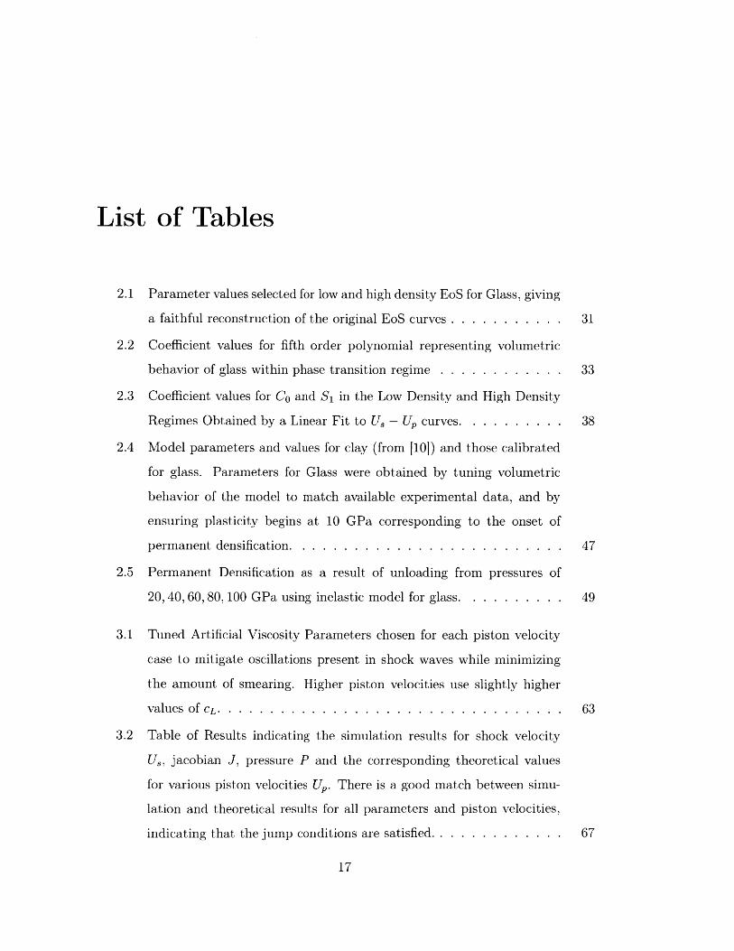
2.1 Parameter values selected for low and high density EoS for Glass, giving

a faithful reconstruction of the original EoS curves . . . . . . . . . . . 31

2.2 Coefficient values for fifth order polynomial representing volumetric

behavior of glass within phase transition regime . . . . . . . . . . . . 33

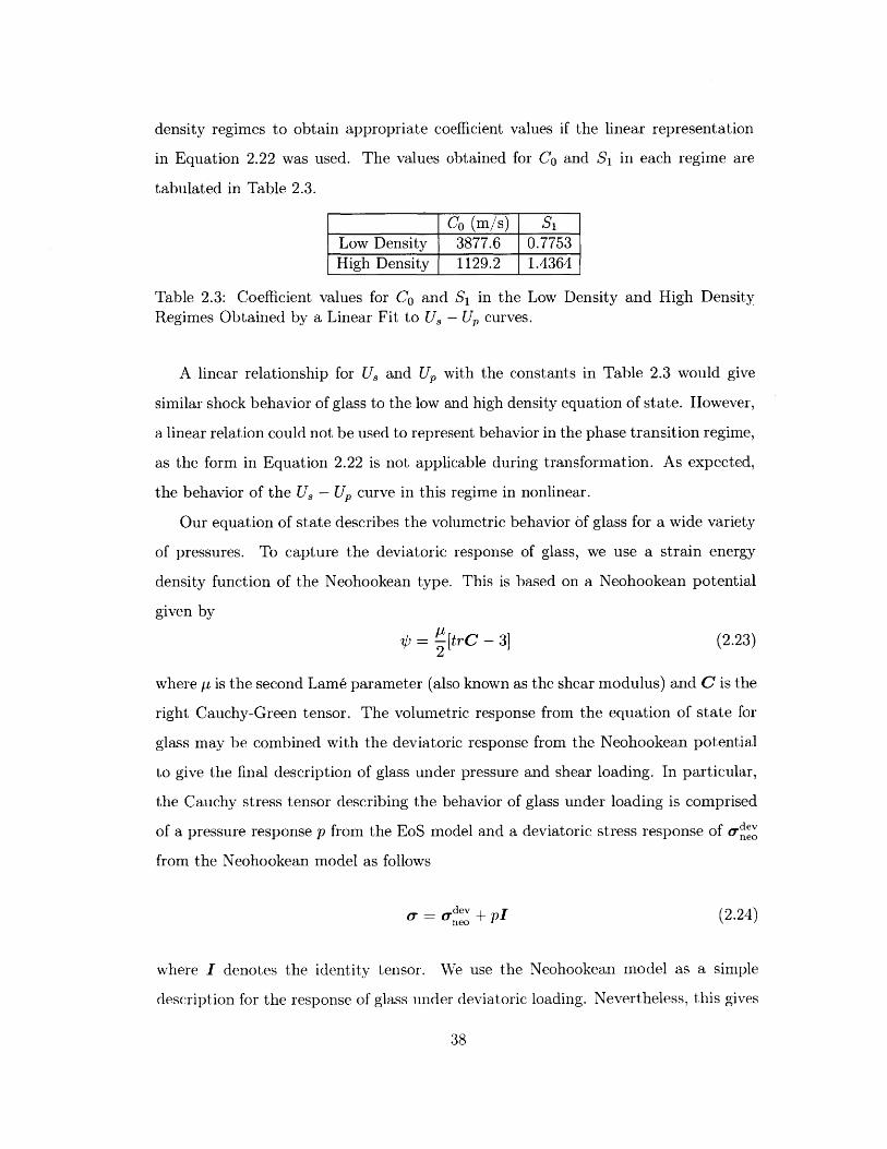
2.3 Coefficient values for Co and Si in the Low Density and High Density

Regimes Obtained by a Linear Fit to U, - Up curves. . . . . . . . . . 38

2.4 Model parameters and values for clay (from [10]) and those calibrated

for glass. Parameters for Glass were obtained by tuning volumetric

behavior of the model to match available experimental data, and by

ensuring plasticity begins at 10 GPa corresponding to the onset of

permanent densification. . . . . . . . . . . . . . . . . . . . . . . . . . 47

2.5 Permanent Densification as a result of unloading from pressures of

20, 40, 60, 80, 100 GPa using inelastic model for glass. . . . . . . . . . 49

3.1 Tuned Artificial Viscosity Parameters chosen for each piston velocity

case to mitigate oscillations present in shock waves while minimizing

the amount of smearing. Higher piston velocities use slightly higher

values of CL. . . . . . . . . . . . . . . . . . . . . . . . . . . . . .. . .63

3.2 Table of Results indicating the simulation results for shock velocity

Us, jacobian J, pressure P and the corresponding theoretical values

for various piston velocities U,. There is a good match between simu-

lation and theoretical results for all parameters and piston velocities,

indicating that the jump conditions are satisfied. . . . . . . . . . . . . 67

17

4.1 Material properties used for simulation of fracture . . . . . . . . . . . 90

18

Chapter 1

Introduction

1.1 Background and Motivation

Glass is a fascinating material that is nearly ubiquitous in everyday life, and also

readily available in nature. In the natural world, one may encounter glass in settings

such as volcanoes, where molten magma that cools rapidly and lacks time to crystallize

forms a glass known as obsidian (shown in Figure 1-1). Glass may be also be found

in sites of meteorite impact, where it forms under shock conditions typically present

during planetary impact.

Figure 1-1: Volcanic glass, or obsidian which forms upon the rapid cooling of volcanic

magma.

19

In more everyday settings, glass is found in household and commercial products

such as windows, cookware and chemical beakers. While these products comprise

some of the traditional uses of glass, the material has also recently attracted significant

attention for applications involving ballistic protection. Specific applications include

military applications such as windows for ground and aerial combat vehicles 111].

Such applications may appear to be strange for a material as brittle as glass, which

risks breaking very easily. However, the amorphous microstructure of glass, coupled

with its unique ability to undergo a severe amount of permanent compaction, allows

it to absorb large amounts of energy when subjected to extremely high pressures

present in ballistic applications.

The microstructure of glass is composed of silicon and oxygen ions bonded in a

4-coordinated structure [1], in which each silicon atom is covalently bonded to four

oxygen atoms. The bonds between the ions are randomly oriented giving rise to

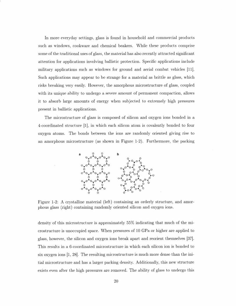
an amorphous microstructure (as shown in Figure 1-2). Furthermore, the packing

a ba

Figure 1-2: A crystalline material (left) containing an orderly structure, and amor-

phous glass (right) containing randomly oriented silicon and oxygen ions.

density of this microstructure is approximately 55% indicating that much of the mi-

crostructure is unoccupied space. When pressures of 10 GPa or higher are applied to

glass, however, the silicon and oxygen ions break apart and reorient themselves [37j.

This results in a 6-coordinated microstructure in which each silicon ion is bonded to

six oxygen ions [1, 28]. The resulting microstructure is much more dense than the ini-

tial microstructure and has a larger packing density. Additionally, this new structure

exists even after the high pressures are removed. The ability of glass to undergo this

20

transformation under high pressures is known as permanent densification, and pro-

vides glass with a way to absorb energy under extreme loading via severe compression.

This energy absorption mechanism in glass may potentially be exploited for ballistic

protection applications in which glass is subjected to extremely high pressures.

Understanding the behavior of glass and the potential of permanent densification

for ballistic applications requires extensive experimental testing and computational

analysis. In the following sections, we summarize previous experimental observations

of the densification of glass under high pressures, as well as computational efforts to

model this densification.

1.2 Review of Experimental Characterization of Glass

Densification

The densification of silica glass and its potential to transform under high pressures has

been the subject of extensive study. Initial evidence of the permanent densification of

silica glass was first observed by Bridgman and Simon [5] in the 1950s, who performed

compression tests on thin disks of silica glass and measured an 8% increase in density

after loading to 16 GPa. They also report that this densification process begins at a

threshold pressure of 10 GPa. Similar compression experiments were performed by

Christiansen [6], who observed densification at much lower pressures of 5 GPa, and

only 4% densification upon loading to 10 GPa. Roy and Cohen [8] observed initial

densification at even lower pressures around 2 GPa upon performing compression tests

on powdered samples of silica glass, and observed a larger 11% densification at 10

GPa. Experimental studies and analysis by Mackenzie [19] imply that such disparities

in densification measurements are due to differences in the amount of shear present

in each experimental setup, as high shear was also found to facilitate densification.

This provides an explanation for Roy and Cohen's observations of densification at

low pressures, as powdered samples generate large amounts of internal shear forces

upon compression, likely aiding the densification process of glass without the need

21

for a large pressure contribution. High temperatures were also found to facilitate

densification [19, 13].

Further testing at similar pressures was conducted by Susman and Zha in the

1990s. Susman [32] conducted compression tests on rods of silica glass to pressures

of 16 GPa at room temperature, and found a 20% increase in density at 16 GPa.

Zha performed compression tests using a diamond anvil cell (DAC) to apply large

hydrostatic pressures to glass, and performed measurements on the sound velocities

and refractive index of shocked samples to obtain densification values. They found a

19.6% increase in density upon loading to 16 GPa [38], in agreement with the results

reported by Susman. Polian and Grimsditch [26] also performed experiments utilizing

a DAC to even larger pressures, and found a 40% increase in density at 30 GPa, much

higher than previously observed.

In more recent years, shock experiments have been performed to higher pressures

of 50 GPa. Alexander [1] performed plate impact experiments using gas guns to

shock glass to high pressures. Although densification amounts were not detailed in

this study, he obtained pressure-density data describing the volumetric behavior of

glass up to 40 GPa. Sato [28] also performed testing at high pressures, conducting

compression tests on silica glass to 50 GPa and using x-ray diffraction for density mea-

surements. Sato's experiments give further pressure-density data for the volumetric

behavior of glass, and it is hypothesized from their results that silica glass transforms

to a high density amorphous polymorph with a density of p = 3.88 g/cm3 , suggesting

approximately 77% densification [4] in glass. Some researchers believe that this high

density material is actually stishovite, a crystalline polymorph of amorphous silica

glass [21]. However, there is still debate on whether the resulting material is truly

crystalline or another amorphous polymorph of glass [38].

Extensive testing has been conducted on glass to explore its densification behav-

ior, as described above. However, there is wide variability in the results obtained

by different researchers. Furthermore, most studies focus on the response of glass to

hydrostatic loading. Clifton et al. performed some experimental studies on the shear

response of glass [7, 31]. They conduct angled flyer plate experiments on glass, and ob-

22

served a loss of shear strength under large pressure-shear deformation. They attribute

this behavior to the rearrangement of bonds in the silicon and oxygen microstructure

[31], similar to that which occurs during permanent densification. However, the effect

of shear on permanent densification is still not completely established. Given these

limitations, it is clear that more effort should be devoted to the high pressure and

shear response of glass.

1.3 Previous Efforts on Constitutive Modeling of Glass

under Extreme Loading

There have been a number of previous efforts towards the computational and consti-

tutive modeling of glass. These efforts have attempted to capture the densification

behavior observed in the previously described experiments. The first effort on compu-

tational modeling of glass was carried out by Woodcock et al. [12, 38], who observed

densification in Molecular Dynamics (MD) simulations of silica glass [36]. Such MD

studies have been useful in the development of constitutive models for glass. Several

of these proposed constitutive models are reviewed here.

One constitutive model for glass was proposed by Lambropoulous [17] in 1991.

He used a plasticity model to describe the permanent densification of glass. In this

model, a yield criterion based on both pressure and deviatoric loading is developed,

as well as a volumetric flow rule that continues to increase the amount of perma-

nent densification in glass. While this model captures densification and the effect of

shear, it is based on a small-strain formulation that is not representative of the large

deformations of glass under the high pressures required for permanent densification.

Keryvin et al. [15] present a constitutive model based on large deformation kinemat-

ics. However, the model only applies under hydrostatic loading to a pressure of 25

GPa, and is unable to describe glass densification under higher pressures achieved in

recent experiments. The model also does not apply under combined pressure-shear

loading. The JH2 material model developed by Johnson and Holmquist [14] is a

23

failure model for ceramics that has been adapted for modeling glass. This model

utilizes an equation of state to describe the pressure-density behavior of glass, as well

as a strength and damage model for failure modeling. While their model accounts

for some permanent densification, the volumetric behavior present in the model is

not validated with experimental data, and may not be representative of the volu-

metric behavior of glass during the transformation process. Schill [29J performs MD

simulations of silica glass and observes densification which eventually saturates upon

sufficiently high pressure-shear deformation. Their MD results inspire a critical state

plasticity model for glass densification with a combined pressure-shear yield condi-

tion. Their model also incorporates a shear modulus based on elastic compression,

coupling pressure and shear response.

Becker developed an equation of state for glass [3] based on experimental data.

This equation of state describes the volumetric behavior of glass before and after

its transformation. Figure 1-3 shows the pressure-density relation for glass, where

the green solid curve represents the behavior of normal silica glass, and the blue

solid curve represents the behavior of the transformed silica polymorph. While the

75 40-5 Hugoniot data 400

65 - P-Lo density 350- P-H i density 0.

55 K-Lo density 300(C 45 . - -K-Hi density 250 U

35 2000

$ 25 - 150

CL 15 100

5 50 0

-5 2.0 3.0 4.0 5.0 0

Density (g/cm 3)

Figure 1-3: Equation of State for Glass describing the volumetric behavior of low

density and high density (transformed) silica glass

pressure-density relation, or volumetric behavior, of glass is known in the low density

and high density regimes, no description is provided in the intermediate densification

24

regime.

The references above show that there has been some effort to formulate a con-

stitutive model for glass. We seek to develop a constitutive model for glass which

captures its behavior under all pressures, and shows agreement with pressure-density

data available from experiments in the literature. Such a constitutive model should

also capture the densification of glass under high pressures.

1.4 Thesis Contributions

In summary, the development of ballistic protection systems based on glass requires

more high pressure studies and improved constitutive models. Our work focuses

on the development of numerical models for glass. Such models are used to design

potential high pressure experiments on glass.

In this work, we develop several plausible constitutive models for glass captur-

ing its deformation behavior under densification. Each model is tested under shock

conditions for verification purposes using finite element simulations. Afterwards, the

models are used to perform simulations of two experimental setups in order to study

their potential to cause transformation in glass.

This thesis is structured as follows. In Chapter 2, we present our proposed con-

stitutive models for glass deformation and densification developed in this study. In

Chapter 3, we present shock loading tests conducted using the constitutive models to

see if they give results in agreement with shock theory. In Chapter 4, we present sim-

ulations conducted to explore the capabilities of two experimental configurations to

generate high pressures in glass. Our goal here is to motivate the design of a new ex-

perimental geometry capable of generating very high pressures in glass. We conclude

with Chapter 5, discussing possible improvements to our constitutive models.

25

Chapter 2

Computational Framework for

Modeling Glass Densification

The computational framework for our work is provided in this chapter. Here we

describe the finite deformation kinematics, the constitutive models developed for glass

densification, and the the balance of linear momentum which we solve using the finite

element method. Emphasis is placed on the specific constitutive models we develop

for glass densification, which are the novel aspects of this work.

2.1 Finite Deformation Kinematics and Kinetics

Here we summarize the basics of finite deformation kinematics and kinetics which can

be found in any solid mechanics text. Consider a body initially occupying a reference

configuration BO. The motion of the body is described by the deformation mapping

X = a(X, t), X E BO (2.1)

Here, the coordinates X are the material coordinates of a particle in the body while x

are the spatial coordinates at time t. The local deformation of infinitesimal material

27

neighborhoods is described by the deformation gradient

F = dx = dp(Xt) (2.2)dX dX

The determinant of the deformation gradient tensor, defined by J, relates the volume

of a body in the reference configuration V to its volume in the current configuration

V

J = det (F) = - (2.3)VO

Stresses resulting from deformation may be expressed in the reference configuration

by the first Piola-Kirchoff stress tensor P as follows

P =JFT (2.4)

where a is the Cauchy stress tensor.

2.2 Constitutive Models for Glass

In this section we present the constitutive models developed in this thesis to model

the response of glass under high pressures. The three models are listed below, and

are ordered in level of sophistication:

" Model 1: Equation of State (EoS) with Neohookean Deviatoric Potential

" Model 2: Model 1 with inelastic effects (our first attempt to incorporate in-

elasticity)

" Model 3: Inelastic Model for Glass

A description of each constitutive model is outlined in the following subsections.

2.2.1 Equation of State with Deviatoric Elastic Response

The first constitutive model developed in this study was an equation of state (EoS)

for glass. An EoS is a constitutive equation relating the pressure and density of a ma-

28

terial, This EoS was coupled with a strain energy density function of the Neohookean

type to describe the deviatoric response of glass. This is a fairly generic elastic energy

typically used to describe rubber. However, the elastic constants in the model may be

tuned to capture the response of glass under shear. For volumetric loading, we adopt

an EoS developed by Becker [3, 111. The EoS was developed and validated through

comparison with experimental data available on glass. For low pressures, a volumet-

ric response was constructed which would agree with direct density measurements of

glass at pressures up to 10 GPa. For higher pressures at which densification occurs,

obtaining direct density measurements in experiments is challenging [111. Instead,

shock and particle velocity data (referred to as Hugoniot data in the shock literature)

from plate impact experiments on glass were converted to pressure-density data using

the Rankine-Hugoniot jump conditions (given in Equations 2.17-2.19). The pressure-

density data inferred from these shock experiments were used to develop the response

of glass under high pressures. The resulting equation of state is plotted in Figure 2-1.

75 __4__

7 Hugoniot data 40065 - P-Lo density 350 g

- P-Hi density 0.55 K-Lo density i 300 e

( 45 K-Hi density I 250 "M

S35 - 200 3

$ 25 150

0.15 100=

5 50

-2.0 3.0 4.0 5.0 0

Density (g/cm3)

Figure 2-1: Equation of State (EoS) for glass describing the pressure-density behavior

of glass in the low density regime (shown in green) and the high density regime (shown

in blue).

Figure 2-1 depicts the pressure-density behavior of silica glass in the low density

regime (shown in green) as well as its behavior in the high density regime (shown in

blue). The variation of the bulk modulus of glass with increasing density in each of

these regimes is also shown using dashed lines. Ultimately, the figure illustrates that

29

the volumetric behavior of glass has a complicated nonlinear response.

Two separate equations were developed to describe the nonlinear volumetric re-

sponse of glass in the low density and high density regimes. The equation of state for

glass in the low density regime is given by the following equation

Ka a _'"Ka [( P0 2kP - 1 - 1-tanh lnn - +FE (2.5)

ka Poa k' POa Po

Equation 2.5 contains a number of parameters. The parameter Ka represents the bulk

modulus of the initial silica glass, k' is its derivative with respect to pressure, and

POa is a reference density. Additionally, F is the Mie-Gruneisen parameter (a quantity

from statistical mechanics describing volume changes due to atomic vibrations [22])

and E is the internal energy. Furthermore, p and po refer to the current and initial

density of the glass material, respectively. Lastly, the factor x is a parameter which

captures the unusual decrease in bulk modulus which occurs in silica glass at low

pressures [3], a phenomenon known as pressure softening [38]. This softening can be

observed in Figure 2-1 by the slight dip in bulk modulus (represented by the green

dashed line) which occurs at low densities.

The equation of state in the high density regime (representing the behavior of the

transformed glass) is given by

P K= b 1 +FE (2.6)

in which the parameters Kb, k', F, and E have the same physical interpretations

described earlier for the low density equation of state (where the subscript b is now

used to represent the high density glass). The reference density Pob was given to be

3900 kg/m 3 [4].

While the equation of state provides a description of the volumetric behavior of

glass prior to and after the densification process, no description is provided for its

behavior during the densification process. Our goal was to introduce a description for

the volumetric response during densification, and effectively connect the low density

30

and high density regimes. This would provide a full constitutive description of the

behavior of glass under high pressures.

To achieve this goal, we began by reconstructing the equation of state for glass in

the low density and high density regimes. The parameters in Equations 2.5 and 2.6

(aside from po = 2.2 g/cm 3 and Pob = 3.9 g/cm 3 ) were not available, so we performed

a parameter fit to determine appropriate values which could faithfully reconstruct the

low and high density equation of state. The program xyscan was used to store data

points from the equation of state curve in Figure 2-1. The stored data points were

then plotted alongside the equation of state given by Equations 2.5 and 2.6, where

arbitrary parameter values were used. These parameter values were tuned so that

the resulting equation of state followed the trend of the data points. In other words,

a set of parameters was found to accurately reconstruct the original equation of state

curves in Figure 2-1. For simplicity, we set the internal energy E to zero.

The following set of parameters given in Table 2.1 was found to give a good

reconstruction of the low and high density equations of state.

Parameter Ka k POa X K kbValue 31 GPa 2.0 2150 kg/m3 0.5 60 GPa 7.0

Table 2.1: Parameter values selected for low and high density EoS for Glass, givinga faithful reconstruction of the original EoS curves

To describe the volumetric behavior of glass during the transformation process,

we assumed a polynomial representation for the equation of state in this regime. We

required the polynomial to be continuous and continuously differentiable at the points

where it connected to the low density and high density curves. This provided four

conditions on the polynomial. Additionally, an inflection point was specified at the

center of the phase transition regime, with a specified slope. This provided two more

conditions on the polynomial, which was now required to satisfy six conditions in

total. A fifth order polynomial representation was assumed in order to satisfy the six

conditions. This representation is shown in Equation 2.7, where the constants co to

31

c5 are unknown.

Ptransition = Co + Cip + C2P2 + C3 P3 + C4p4 + C5P5 (2.7)

Introducing the parameters Ponset, PFinal, and PInflection (representing the density cor-

responding to the initiation of glass densification, the end of transformation, and the

inflection respectively) as well as mlnflection (the slope at the inflection point) one may

write the six conditions as follows:

Ptransition(Ponset) = Plow(Ponset) (2.8)

Ptransition(Ponset) = Piow(Ponset) (2.9)

Ptransition(PFinal) = Phigh(PFinal) (2.10)

Ptransition(PFinal) P hgh(PFinal) (-1

Ptransition (PInflection) = mInflection (2.12)

Ptransition(Plnflection) = 0 (2.13)

In Equations 2.8 - 2.13, the prime denotes a derivative with respect to density, and

Plow and Phigh represent the low density and high density equations, respectively. If

we assume the form of Ptransition given by Equation 2.7, and denote plow(Ponset) and

Phigh(PFinal) simply as POnset and PFinal respectively, Equations 2.8-2.13 may be written

as the following linear system

1 Ponset Ponset nset POnset POnset CO Ponset

12 3 4 5 1PiaPFinal PFinal PFinal PFinal PFinal C1 PFinal

0 1 2 POnset 3 pOnset 4,pnset 5pdJnset C 2 POnset

0 1 2 PFinal 3 PFinal Final F5 pFinal C3 PFinal

0 1 2 Plnflection 3P nfiection 4PInfection 5PInflection C 4 mlnflection

0 0 2 6 plnflection 12P nflection 20pInfection c5 0

Solving the system for the constants co to c5 required specifying the parameters Ponset,

PFinal, PInflection and mlInection. The parameter Ponset was chosen so that POnset would

32

be approximately 10 GPa, as it has been observed experimentally that permanent

densification begins at this pressure [38]. Additionally PFinal was chosen so that PFinal

would be a sufficiently large pressure where transformation is known to end. Lastly,

Plnflection and m1 Inflection were chosen so that the material does not experience any

softening in the transformation regime.

Solving the above matrix system for the coefficients (co to c5 ) of the phase transi-

tion polynomial, with the values of POset = 2.8 g/cm 3 , PFinal = 5 g/cm 3 , PInflection =

3.9 g/cm 3 and MInflection Slope = 5 resulted in the coefficient values given in Table 2.2.

All densities were provided in units of grams per cubic centimeter (g/cm 3 ) to avoid

Polynomial Constant Value

CO -2969.8 GPac1 4029.0 m 2 /s2 x10 9

C2 -2182.6 m5 / (kg S2) x109

C3 592.0130 m8 /(kg 2 s2) x10 9

C4 -80.29 m1 /(kg 3 S2) x109

c5 4.3549 m /(kg4 s2) xlo9

Table 2.2: Coefficient values for fifth order polynomial representing volumetric be-havior of glass within phase transition regime

ill-conditioning of the system which contains large powers of density. Additionally,

Equation 2.7 gives pressure in units of GPa, so one should multiply the value obtained

from this equation by 109 to obtain the pressure in Pa.

The complete equation of state modeling the behavior of glass in the low density,

phase transition, and high density regimes is then

-- ] [ - tanh (Xn ()

P= cO + cIp + c 2p2 + c3p3 + c4P4 + c5p5

k'-1 +lE

if P < Ponset

if Ponset < P < PFinal

if P > PFinal

(2.14)

with the values of each constant summarized in Tables 2.1 and 2.2. The celerity, or

33

wave speed of the material, can be calculated based on the EoS as follows

c = (2.15)

Using Equation 2.15, the celerity in each of the three regimes is given by

k' -1 P)k'lKa ( )a -1- + 2(- -- " - 1 sech2 X In [I - tanh X In (L)

POa POa p k' POa PO PO

C =</c 1 2c2 p + 3c3 p2 + 4c4 p3 + 5c p4

Kb()k-1

(2.16)

A plot of the glass EoS for all three regimes is given in Figure 2-2, with the corre-

sponding celerity plotted in Figure 2-3. Note that since the EoS is a strictly increasing

function, the celerity (found from the EoS by Equation 2.15) is positive for all densi-

ties. We observe that the transformation occurs at a pressure of POnset = 10.224 GPa,

which is close to the 10 GPa value specified in the literature. From Figure 2-2, we

observe a decrease in the slope of the EoS within the phase transition (blue) regime

which is indicative of the phase transformation occurring in glass [2]. This flattening

of the EoS is also reflected in Figure 2-3 which shows a corresponding decrease in

celerity during the beginning of phase transformation. Ultimately, our EoS for glass

shows the expected characteristics in the presence of a phase transformation.

Equations of state may also be described in an alternative parameter space. For

example, the shock velocity-particle velocity (U, - Up) space is also generally used to

describe the behavior of a material under shock loading. This particular description

is often used in shock experiments such as plate impact tests. This is because the par-

ticle velocity (or the projectile velocity) is known, and the velocity of the shock wave

due to impact may also be measured 2-1. To convert an EoS from the pressure-density

description to the shock velocity-particle velocity description, the Rankine-Hugoniot

jump conditions must be applied. The three Rankine-Hugoniot jump conditions rep-

34

90

s0

70

~60s0

S40

14

V.30

20 -

10

Glass EOS

2000 2500 3000 3500 4000 4500 5000 5500

Figure 2-2: Equation of State (EoS) for glass containing low density behavior, highdensity behavior, and polynomial fit for phase transition regime. The phase transition

behavior shows a flattening in the pressure density behavior which is indicative of the

occurrence of a phase transformation.

Ti

12000-

11000

10000

9000

8000

7000

6000

5000

4000

3000

2000-2000

Celerity vs Density

-Low Density- Phase Transition- High Density

2500 3000 3500 4000 4500

DensLtyd) (kg/Td5000 5500

Figure 2-3: Celerity corresponding to EoS for glass. The celerity is positive since the

EoS is a purely increasing function. There is a dip during the onset of the phasetransformation process in glass.

35

___ -j

- Low DensityPhase TransitionHigh Density

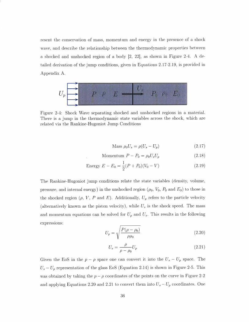
resent the conservation of mass, momentum and energy in the presence of a shock

wave, and describe the relationship between the thermodynamic properties between

a shocked and unshocked region of a body [2, 22], as shown in Figure 2-4. A de-

tailed derivation of the jump conditions, given in Equations 2.17-2.19, is provided in

Appendix A.

UP P P E P Po E

Figure 2-4: Shock Wave separating shocked and unshocked regions in a material.

There is a jump in the thermodynamic state variables across the shock, which are

related via the Rankine-Hugoniot Jump Conditions

Mass poU, = p(U, - Up) (2.17)

Momentum P - Po = poUUp (2.18)

1Energy E - E= -(P + Po)(Vo - V) (2.19)

2

The Rankine-Hugoniot jump conditions relate the state variables (density, volume,

pressure, and internal energy) in the unshocked region (po, V, P and Eo) to those in

the shocked region (p, V, P and E). Additionally, Up refers to the particle velocity

(alternatively known as the piston velocity), while U, is the shock speed. The mass

and momentum equations can be solved for Up and U,. This results in the following

expressions:

UP = P0 (2.20)

PPo

us = Up (2.21)P - po

Given the EoS in the p - p space one can convert it into the U, - Up space. The

U, - Up representation of the glass EoS (Equation 2.14) is shown in Figure 2-5. This

was obtained by taking the p - p coordinates of the points on the curve in Figure 2-2

and applying Equations 2.20 and 2.21 to convert them into U, - Up coordinates. One

36

-I

could also perform this transformation analytically by taking the EoS in Equation

2.14 and substituting it for P in Equations 2.20 to 2.21, but this was not done here

due to the complexity of the EoS.

8500-Low Density

Phase TransitionHigh Density

7500

E7000

6500U06000-

>5500-0 5000

4500

4000

35000 1000 2000 3000 4000 5000

Particle Velocity [m/si

Figure 2-5: Glass EoS expressed in the shock velocity-particle velocity (US - UP)space. The behavior is roughly linear in the low density and high density regimes.

Additionally, there is a kink in the phase transformation (blue) regime, indicative ofmaterial transformation in this range of particle velocities.

We observe that the shock velocity-particle velocity curve is approximately linear

in the low density and high density regimes. This agrees with experimental observa-

tions which suggest that the shock velocity is linearly related to the particle velocity

in materials not undergoing transformation. This linear relation is usually written as

Us = CO + S1Up (2.22)

where CO (the ambient pressure bulk sound velocity) and Si are tabulated in the lit-

erature for various materials [2, 221. This approximately linear relationship between

U, and Up in the low and high density regimes suggests that a Mie-Gruneisen equa-

tion of state could be used to model the pressure-density behavior of glass in these

regimes, rather than the low and high density equations in Equations 2.5 and 2.6.

This motivated us to perform a linear fit to the U, - U, curves in the low and high

37

density regimes to obtain appropriate coefficient values if the linear representation

in Equation 2.22 was used. The values obtained for Co and S1 in each regime are

tabulated in Table 2.3.

Co (m/s) SiLow Density 3877.6 0.7753High Density 1129.2 1.4364

Table 2.3: Coefficient values for Co and S in the Low Density and High Density

Regimes Obtained by a Linear Fit to U, - Up curves.

A linear relationship for U and Up with the constants in Table 2.3 would give

similar shock behavior of glass to the low and high density equation of state. However,

a linear relation could not be used to represent behavior in the phase transition regime,

as the form in Equation 2.22 is not applicable during transformation. As expected,

the behavior of the U, - Up curve in this regime in nonlinear.

Our equation of state describes the volumetric behavior of glass for a wide variety

of pressures. To capture the deviatoric response of glass, we use a strain energy

density function of the Neohookean type. This is based on a Neohookean potential

given by

)= [trC - 3] (2.23)2

where p is the second Lam6 parameter (also known as the shear modulus) and C is the

right Cauchy-Green tensor. The volumetric response from the equation of state for

glass may be combined with the deviatoric response from the Neohookean potential

to give the final description of glass under pressure and shear loading. In particular,

the Cauchy stress tensor describing the behavior of glass under loading is comprised

of a pressure response p from the EoS model and a deviatoric stress response of 0.dev

from the Neohookean model as follows

0 .=dev + pI (2.24)neo

where I denotes the identity tensor. We use the Neohookean model as a simple

description for the response of glass under deviatoric loading. Nevertheless, this gives

38

a complete description of glass behavior under multiaxial loading, accounting for its

transformation process. While the model describes the volumetric response of glass

during the transformation process, it is a purely elastic model and therefore unable to

capture any type of plastic effects. In particular, the model is forced to unload back

to the original density regardless of the loading pressure. Thus, it cannot capture any

permanent changes in density that occur as a result of permanent densification.

2.2.2 Introducing Inelasticity (a first attempt)

In order to address the limitations of our previous model, we introduce an internal

variable to capture permanent densification of glass. This internal variable, denoted

by , represents the degree of transformation of glass and is given by

P -Ponset (2.25)PFinal - POnset

In Equation 2.25, Ponset = 2800 kg/'m3 refers to the density at the onset of transfor-

mation in glass, PFinal = 5000 kg/m3 refers to the density at the end of transformation,

and p is the current density. If p < POnset, then = 0 indicating that no transforma-

tion has taken place yet. If p > PFinal, = 1 indicating that the glass has fully trans-

formed. Lastly, for densities within the phase transition regime (Ponset < P < PFinal),

( may take on any value between 0 and 1.

During the loading process, the maximum amount of densification achieved up

to the current step is stored. Given this value of and the current density p, the

unloading path is fully defined. This is done by defining the density after unloading

as pp (where the subscript P stands for permanent), given by

Po = po + (P -Po) (2.26)

which will be larger than po for positive amounts of transformation ( > 0). Given

p and pp, one may define a linear unloading path as shown in Figure 2-6. If = 0,

the unloading path will follow the low density EoS. If = 1, the unloading path will

39

Glass EOS

-Low DensityPhase Transition

50 - High Denssty

0. 40

0..30

:3

20

Unloading Path10

0 - ----------

2000 2500 3000 3500 4000 4500 5000 55

Density, p [kg/m3I

Figure 2-6: Unloading Path from an arbitrary density to the corresi

density pp, denoted by PUnload in this figure.ponding unloading

follow the high density EoS. Otherwise, a linear unloading path will be defined as

described above. In summary, the material will simply follow the behavior of the

EoS under loading conditions, but upon unloading will follow a new unloading path

dictated by the current density p and degree of transformation .

A quadrature point constitutive test involving cyclic hydrostatic compression load-

ing and unloading was conducted in order to exhibit the permanent densification

effects present in this model. During a constitutive test, a deformation gradient is

provided and the constitutive model is used to compute the resulting stress tensor.

In the case of hydrostatic compression, the deformation gradient is given by

A 0 0

F = 0 A 0 where A < 1

0 0 A

where a smaller value of A represents a larger amount of compression. During a

hydrostatic compression constitutive test, A is decreased over many time steps, and

the stresses are computed at each time step.

40

0

In this cyclic loading test, we apply hydrostatic pressure to a value within the

phase transformation regime, unloading completely, and subsequently reload to a

higher pressure. This procedure was repeated for a number of cycles. This cyclic test

resulted in the pressure-density behavior shown in Figure 2-7. We observe that the

model is capable of exhibiting different degrees of permanent densification based on

the applied pressure. Reloading of the densified glass in a given cycle also follows

the previous unloading path, exhibiting the model's ability to track history. Lastly,

the model exhibits 77% relative densification after unloading in the final cycle, in

agreement with measurements by Sato [28].

50

Pressure Vs Density

~30-

S20-

10-

02000 2500 3000 3500 4000 4500 5000 5500

Densty (kg/m1m

Figure 2-7: Volumetric Behavior of Model under Cyclic Hydrostatic Loading andUnloading. The model unloads to various densities based on the initially appliedpressure, illustrating that the model may be used to achieve various degrees of per-manent densification.

Our new model is able to capture the volumetric behavior of glass during den-

sification, as well as model permanent changes in density from loading to pressures

greater than 10 GPa. However, permanent densification is captured in an ad-hoc

manner through the introduction of an internal variable. In the next section, we

turn to a more comprehensive 3D tensorial plasticity model for capturing permanent

densification effects.

41

2.2.3 Inelastic Model for Glass Densification

Our final constitutive model for glass is based on the Camclay theory of granular

plasticity. Camclay is a volumetric plasticity model generally used to represent the

behavior of granular materials such as sand or clay. The deformation behavior of

these materials have some mechanisms in common with glass. For example, sand

and clay exhibit deformation behavior that is highly dependent on pressure, and

accompanied by a significant reduction in volume under pressure. This behavior is

similar to observations of glass densification under extreme pressures. It is this feature

of the model that makes it attractive for modeling glass densification.

A variational formulation of the Camclay model is presented by Ortiz and Pan-

dolfi in [25] (outlined in Appendix B). They also provide references for more classical

papers on the Camclay theory. For our model, we combine the densification un-

der pressure available through Camclay with the volumetric response of glass given

in Equation 2.14. For completeness, an overview of key aspects of the constitutive

model are provided below. The update algorithm for this constitutive model is pro-

vided in Appendix C.

Kinematics

A multiplicative decomposition of the deformation gradient into an elastic and plastic

part is assumed

F = FFP (2.27)

From the elastic part, one can compute the elastic right-Cauchy Green tensor

Ce = F eT Fe (2.28)

A logarithmic elastic strain measure based on the right Cauchy-Green tensor is used

in this finite deformation setting

Oe = - log(Ce) (2.29)2

42

Free energy

The constitutive model is based on a free energy W which we require to have the

following arguments

W (F, FP, T, q) (2.30)

where q represents a set of internal variables specialized to the constitutive model. The

free energy can be additively decomposed into an elastic free energy and a "plastic"

free energy with the following arguments

W(F, FP, T, q) = We (Ce, T) + WP(T, q, FP) (2.31)

where We must depend on the deformation via the right-Cauchy Green tensor Ce

due to the requirements of material frame-indifference. The elastic free energy may

be further decomposed into deviatoric and volumetric parts

We(Cc, T) = We'""'(Je, T) + We'dev(Ce'dev, T) (2.32)

where the elastic jacobian is given by

Je = det(Fe) (2.33)

Volumetric Elasticity (EoS)

The volumetric portion of the elastic energy is given by

Wevol(Je T) = f (J) + poCT I - log - (2.34)TO

where f(J') is defined such that the corresponding pressure is the equation of state

given in 2.14.

Deviatoric Elasticity

The deviatoric portion of the elastic energy is given by

We,dev (e IT) = t e 2 (2.35)

43

where e' is the deviatoric part of the logarithmic elastic strain

ee = e - -tr(Ce)I (2.36)3

and p is the shear modulus.

Stored Energy

To account for permanent compression effects, we introduce the volumetric plastic

strain

OP = log JP (2.37)

where the plastic Jacobian is defined as

JP = det FP (2.38)

The stored energy is based on the plastic Jacobian, the effective plastic strain, and

temperature

WP(T, e', OP) (2.39)

Yield Criterion

The model utilizes an elliptic yield surface to determine whether plasticity is occur-

ring. The yield surface is described in the pressure-shear space by the following yield

q

PC PO P

Figure 2-8: Yield Surface for Camclay Model

44

condition

f(p, q) = q2 + a2 (p - Po) -a2 (2.40)

where p and q are the effective pressure and shear stress corresponding to a stress

state and may be computed by

1 011 + 0-22 + 0-33 (2.41)3 3

q = V -i- = (0-11 + 0-22 + 0-33 + 20-12 + 20-13 + 20-23) (2.42)

where o-rj is the Cauchy stress tensor. Under conditions of pure elasticity, the Cauchy

stress tensor is

o- = 2pe' + pI (2.43)

where ee and p are defined in Equations 2.36 and 2.14 respectively.

Flow Rule

A flow rule of the form in Equation 2.44 is assumed to describe the evolution of the

plastic deformation gradient

P = DPFP-1 = (PM)FP- 1 , &P > 0 (2.44)

where M is a symmetric tensor defining the direction of plastic flow and satisfying

the kinematic constraint below,

12S(trM2 + pme j mdev = 1 (2.45)

ae 3

a is the internal friction parameter and MAde is the deviatoric part of M given by

1Mdev = M - -(trM)I (2.46)

3

45

Pressure Hardening Behavior

In the presence of densification, the volumetric response (i.e. pressure) transitions

smoothly from the low density EoS to the high density EoS. To achieve this objective,

we start by defining the relative densification

= PP - Po - -1 (2.47)Po Po

where po represents the original density of glass, and pp represents the final density

of glass after being subjected to a loading and unloading cycle involving densifica-

tion. Furthermore, the plastic jacobian physically represents the ratio of volumes or

densities

Jp - - 0 (2.48)

So the relative densification is related to plastic jacobian as follows

AP = - - 1 (2.49)JP

where we may simply compute JP as the determinant of our plastic deformation

gradient. Finally, the pressure can be computed as a weighted average of the low

and high EoS in order to account for transformation. The form in Equation 2.50

gives a good match to experimental data. We include the arguments of AP and the

equations of state to be explicit about the dependence of pressure on elastic and

plastic compression.

p = ( \1 - 2AP(JP)pi0o eos(J') + (1 - \1 - 2AP(JP))Phigh eos(J) (2.50)

One key difference between the standard Camclay model and our modified model

for glass is the predicted pressure response. The original Camclay model uses a loga-

rithmic equation of state (p = K log J) to describe pressure experienced by granular

materials. However, we use the low density equation of state (Equation 2.5) for glass

here (under elastic conditions). Under plasticity, our pressure response is also mod-

46

ified from the Camelay model. In our model, yielding represents the occurrence of

permanent densification in glass as this is an irreversible process. We calibrate our

model parameters so that yielding begins at the experimentally observed hydrostatic

pressure of 10 GPa (as described in Reference 138]).

Our constitutive model contains a number of parameters given in Table 2.4. These

parameters were adjusted to accurately reflect the behavior of glass. For example,

the elastic moduli for glass are given in the literature (E = 71 GPa, v = 0.17). In

our model, E and v are used to specify the shear response of glass (the correspond-

ing shear modulus is G = 30.1 GPa), while the volumetric response is given by the

equation of state. The remaining parameters were obtained by tuning the model so

that yielding would begin at 10 GPa (representing the onset of permanent densifica-

tion as described previously), and so that the pressure-density behavior would match

closely with pressure-density data available in the literature. Table 2.4 lists the ma-

terial parameter values which are representative for a granular material such as clay

(Reference [10]) and our modified parameters chosen to represent glass behavior.

Parameter Name Symbol Value for Clay Value for GlassDensity p 1529 kg/m 3 2200 kg/m 3

Young's Modulus E 750 71 GPaPoisson ratio v 0.4 0.17

Reference Pressure Pref 0.5 Pa 10 GPaReference Plastic Volumetric Strain OP 0.75 0.5

Preconsolidation Pressure Pc 1.0 MPa 20 GPaRate Sensitivity Parameter r/ 1.0 kPa-s 1.0 kPa-s

Friction Angle _ 100 23.20

Table 2.4: Model parameters and values for clay (from [10]) and those calibrated forglass. Parameters for Glass were obtained by tuning volumetric behavior of the modelto match available experimental data, and by ensuring plasticity begins at 10 GPacorresponding to the onset of permanent densification.

To illustrate the volumetric behavior of our new model, we first perform a cyclic

hydrostatic test to full densification on a single quadrature point. Loading was per-

formed to a pressure of 80 GPa, with unloading following subsequently. The model

parameters used for the test are shown in Table 2.4. The pressure-density plot re-

47

sulting from the test is shown in Figure 2-9, alongside experimental pressure-density

data for glass reproduced from the following sources: Alexander [1], Sato 128], Marsh

[20]. We observe a satisfactory match between volumetric behavior predicted by the

model and the provided pressure-density data. Furthermore, the model exhibits per-

manent densification upon unloading. In fact, we observe 77% relative densification

to a density of p = 3900 kg/m 3 as suggested by Sato in [28]. Our phenomenological

model accounts for the volumetric deformation behavior of glass and its ability to

demonstrate significant permanent densification.

90

80

70

60

so

40

20

10 -

200

0 Lhnawmids D.ataC, Marsh LASL Dataa Satm Data Pressure Vs Density

Se

2500 3000 3500 4000Denskty (kq'nS I

4500 5000 5500

Figure 2-9: Volumetric Behavior of inelastic model for glass obtained from hydrostatic

loading and unloading. The model shows a good match to experimental data availablein the literature from Alexander [11, Sato [28] and Marsh [20]. Furthermore, it exhibits77% relative densification upon unloading from high pressures of approximately 80GPa.

We perform an additional cyclic loading test to partial amounts of densification.

Hydrostatic loading was performed to a pressure of 20 GPa, after which unloading

occurred. This loading and unloading was repeated for a few cycles, with each sub-

sequent loading pressure being higher than the one before. Pressures of 20, 40, 60,

80 and 100 GPa were used for the test. The pressure density curve resulting from

this cyclic loading constitutive test are shown in Figure 2-10. Our model exhibits

48

0~

eoe

0

100

- Glass E7

~40-

02000 2500 3000 3500 4000 4500 5000 5500

Deinsity fkg,, I

Figure 2-10: Volumetric behavior of inelastic model under cyclic loading. The modelallows for various degrees of permanent densification to be achieved, based on theapplied loading pressure.

various degrees of permanent densification upon unloading from different pressures.

Table 2.5 summarizes the final densities obtained from unloading from the applied

pressures during the cyclic test. The relative densification saturates at 77%, at a

pressure between 80 GPa and 100 GPa. We also plot the amount of densification

Loading Pressure Final Density Upon Unloading Relative Densification (in %)20 GPa 2,230 kg/m3 1.3%40 GPa 2,670 kg/m3 21.3%60 GPa 3, 101 kg/m 3 41 %80 GPa 3,718 kg/M 3 69 %100 GPa 3,900 kg/m3 77.3%

Table 2.5: Permanent Densification as a result of unloading from pressures of20,40, 60,80, 100 GPa using inelastic model for glass.

due to unloading from pressures between 0 and 100 GPa in Figure 2-11. We observe

that for pressures below 10 GPa, the model predicts no densification, as expected.

At approximately 85 GPa; however, the relative densification saturates to a value

of 77%, indicating full transformation to the high density glass. For pressures in

49

between this range, the relative densification appears to grow fairly linearly. This

relationship between loading pressure and relative densification is predicted by our

phenomenological model, but not necessarily representative of the true densification

behavior of glass. Experimental data on this relationship is required so that we may

calibrate model parameters to more accurately capture the true behavior.

-0

cO0

d)

a)

QU

80

70

60-

50

40

30

20

10

0I0 ~-------------- --- i----- -----I--------- ---

0 20 40 60 80 100Loading Pressure [GPaI

Figure 2-11: Relative densification (in %) observed upon unloading from hydro-static pressures between 0 and 80 GPa. Our model predicts a fairly linear pressure-densification behavior, with densification beginning at a pressure of 10 GPa (as ob-

served in experiments) and ending close to 80 GPa.

The tests conducted so far give insights into the model behavior under volumetric

loading. The following constitutive tests explore the deviatoric behavior of this model

for glass, as well as its response to combined pressure-shear loading.

For our first study of the deviatoric response of the model, we apply hydrostatic

pressure followed by a simple shear deformation. The deformation gradient corre-

sponding to a shear deformation is given by (where -y is the shear strain)

01 0

F= 0 1 0

0 0 1

50

We perform this test to determine the effect of pressure on deviatoric response of

the model. Initially applied pressures of p = 0, 10, 20, 30,40, 50 GPa were used for

the test. For each applied pressure, the shear stress as a function of shear strain is

obtained, shown in Figure 2-12.

Shear Stress Vs Shear Strain Upon Initially Applied Pressure

- P= 0 GPa- P=IOGPa

6 - .P=20 GPa- P 30 GPa- P= 40 G:Pa

P= 50 GPa

02

0

0.00.05 010 0.15 0.20Shear Strain

Figure 2-12: Shear Stress vs. Shear Strain for constitutive test in which various initial

pressures are applied followed by a shear deformation which is increased up to a value

of 7 = 0.2. The results illustrate that higher initial pressures result in higher shear

stresses at a given shear strain.

To more thoroughly quantify the effect of pressure on initial shear stress, the test

was repeated with p = 0, 2, 4, 6, 8 GPa compressive and tensile pressures, and in every

case, a measure of the effective shear modulus was obtained by taking the ratio of

the shear stress and the shear strain in the initial linear regime

S= 2 (2.51)

The variation of the shear modulus with initial pressure is shown in Figure 2-13. Fig-

ures 2-12 and 2-13 suggest that the larger the initially applied pressure, the greater

the amount of shear stress predicted by the model for a given strain level. In other

words, the effective shear modulus is greater for larger initial pressures.This is a phys-

51

.. A

Shear Modulus Vs Pressure

34

36

34

32

30

28-10 0 15 20D 30 40 W0

Pressure [GPa]

Figure 2-13: Variation of effective shear modulus with initial pressure. The shear

modulus increases as the applied hydrostatic pressure increases.

ically meaningful description of the response of granular materials to pressure-shear

loading, as an initial pressure can cause grains to develop a large amount of inter-

nal friction, facilitating high shear stresses upon shear deformation. This behavior is

likely true for glass as well, as the pressure can cause atoms to come closer in contact

with each other. Thus, subsequent shear deformation will cause large internal shear

stresses between the atoms.

A similar pressure-shear loading test was conducting by Schill et al. in [291 in their

MD simulations of silica. They also obtain the shear modulus behavior as a function

of pressure. However, unlike our response which is purely increasing, they observe a

dip in shear modulus for pressures between 0 - 3 GPa. This drop in shear modulus at

low pressures has been experimentally observed in glass [38, 7]. To improve our model,

we may further calibrate our shear response to capture experimental observations of

deviatoric behavior of glass.

We performed another constitutive test combining pressure and shear. In this

test, we impose a shear strain, followed by an applied hydrostatic pressure. Shear

strains of -y = 0.1, 0.2,0.3, 0.4, 0.5 are initially applied. Then, we apply a hydrostatic

pressure of 50 GPa and then unload. The pressure response resulting from this test

52

was recorded for each value of -y, and is shown in Figure 2-14.

Pressure vs. Compression Upon Initially AppIlied Shear Strain

=B.

0 01 0.2 03 04 03 06 07 0.8Volumetric Strain

Figure 2-14: Pressure vs. Volumetric Compression Results for constitutive test inwhich various initial shear strains are applied followed by pressure loading to 50GPa and unloading. The results illustrate no dependence of the volumetric behavior

predicted by the model on initially applied shear strains.

Figure 2-14 illustrates that the pressure response predicted by the model is un-

affected by the initially applied shear strains. The amount of plasticity observed in

each case is also the same. In reality, we might expect glass to experience larger

densification with larger initial shear deformation (as Mackenzie explains that shear

can facilitate densification in [191).

In the preceding sections, we have presented three constitutive models on glass

transformation. Our final model takes advantage of Camclay's ability to represent

permanent volumetric reduction, and combines this model with the expected volu-

metric deformation behavior of glass. Various constitutive tests are performed to

illustrate the behavior of each model under different loading conditions. To conclude

our description of the computational framework, we introduce the governing equa-

tions and their spatial and temporal discretization using the finite element method

in the next section.

53

2.3 Numerical Implementation of Governing Field

Equations

In order to complete our description of the computational framework, we describe

the discretization used in the finite element method to solve the balance of linear

momentum. The strong form of the partial differential equation (PDE) corresponding

to the balance of linear momentum is given by

po = Vo - P + poBo E Bo (2.52)

In Equation 2.52, B0 is the region occupied by the body in its reference configuration,

po is the initial density of the body, ; is the acceleration of the body, and BO is an

applied body force. Boundary conditions are also present. These may be either

Dirichlet boundary conditions through which displacement is prescribed on the body,

or Neumann type boundary conditions where traction is prescribed. The Dirichlet

and Neumann conditions are given by Equations 2.53 and 2.54, respectively

= on aDB0 (2.53)

P-N =Ton aNBO (2.54)

where &DBO and aNBo represent the set of points on which Dirichlet and Neumann

boundary conditions are applied, respectively. The union of these points comprises

the entire body (as indicated in Equation 2.55) whereas the intersection of these

points is null (Equation 2.56), as no point has more than one boundary condition

specified.

&NBO U &DBO = 0BO (2.55)

aNBo n&DBo = 0 (2.56)

Equations 2.52-2.54 complete our description of the boundary value problem (BVP)

of elasticity. To solve the linear momentum balance equation using the finite element

54

method, the PDE must be recast in its weak form by multiplying by a test func-

tion and integrating over the domain. In the case of continuous Galerkin (CG), we

integrate over the entire body and obtain the following weak form

(P(3h- 'Wh + Ph: VO6Oh)dV = 5 pOB - 6 PhdV + j 6W'TdSe~~~~ Oe9 60Bnh

(2.57)

where Ph is a continuous polynomial approximation for the deformation map for each

element and 6 'h is a trial function. Equation 2.57 refers to the Continuous Galerkin

(CG) weak formulation of the linear momentum balance PDE. To incorporate frac-

ture, we utilize a weak formulation that is based on the discontinuous Galerkin (DG)

formulation coupled with a cohesive zone model (CZM). This leads to an alternative

weak formulation for the balance of linear momentum

f0h [P63h ' 6Ph + Ph : Vo0h] dV

+ Ji h [aT ([h) - [A. 1 + (1 - a) [6 4h] - K^) - N-] dS (2.58)

+ (1 - a) [oh & N- : - C) : [h1 ®9 N- dSa IQ0h hs

fOh Whd + j T_ SS6hdSOh 0,N

In 2.58, [e] and (.) represent the jump and average operators on the internal boundary

respectively, defined by [e [ - -] and (.) =[+ + e-]. Furthermore, 3 is

a stability parameter, h, is a characteristic element size, C = is the LagrangianaF

tangent moduli and a is a parameter equal to either 0 or 1 (a value of 1 indicates

that fracture is occurring). More details regarding the weak form in Equation 2.58

can be found in [27].

Lastly, numerical discretizations may be applied to Equations 2.57 and 2.58 to make

these weak forms solvable via the finite element method.

55

2.3.1 Spatial Discretization

A finite element approximation to the deformation map may be expressed as

nodes

.(Phi(X, t) = 1j Xia(t)Na(X) (2.59)a

where Xia (equal to >hi(Xa, t)) are the spatial nodal coordinates, Xa are the material

nodal coordinates, and Na represents the material shape functions. Applying this

finite element representation to the balance of linear momentum given by Equation

2.57 yields its semi-discrete form

Z Mia k -kb+fPt (X, fa(t) (2.60)b

where

Viakb Joj PO ikNaNbdQo (2.61)

fii t = P1 Nae,1 dQo (2.62)J e

e 0

denote the consistent mass matrix and internal force array, respectively. Additionally,

, and f ext represent the acceleration array, and external force array resulting from

surface tractions and applied body forces, respectively. The acceleration array may

be further discretized via temporal discretization.

2.3.2 Temporal Discretization

The lumped mass matrix Newmark method, expressed in Equations 2.63-2.65 was

applied for temporal discretization. The Newmark parameters 0 and -' in Equations

56

2.63-2.65 were set to 0 and 0.5, respectively, for our studies.

x+1 = x + Att + At 2 i~n + 0 1+ .][yi i i 1 (2.63)

.x 1 = x + At[(1 - _), mn 1] (2.64)

S+1 = mMl [fe - fintln+1 (2.65)

In the scheme above MLi is the lumped mass matrix, f ext and fi"t refer to the

external and internal forces, respectively, and At is the time step used. The nodal

displacements may be found using the Newmark scheme, which may then be applied

to update the nodal coordinates, velocities and accelerations.

2.4 Summary

In this Chapter, we have provided an overview of the computational framework for

our work. In particular, we present the basic kinematics, governing equations, and the

constitutive models developed in this work. Our first constitutive model for glass was

an equation of state for glass capturing its volumetric behavior in all pressure regimes

including the transformation regime, coupled with a Neohookean shear model. We

extended this elastic model to include plasticity for modeling permanent. densification

by introducing an internal variable representing the degree of transformation. This

internal variable allowed us to define an unloading path, so that upon unloading

from high pressures (greater than 10 GPa), the material would have a higher density

than before. Our final model for glass densification was inspired by the Camelay

volumetric plasticity model, which was a full tensorial plasticity model (as opposed

to our previous model which illustrate ID plasticity in pressure). We were able to tune

our constitutive model parameters to give a good match to experimental pressure-

density data, and also exhibit severe permanent densification (77% as hypothesized

by Sato). Our combined pressure-shear constitutive tests exhibited expected behavior

of glass, although the model could be improved by incorporating the effect of shear

on volumetric behavior (see Figure 2-14).

57

Chapter 3

Shock Physics in Glass

The transformation of glass occurs under extremely high pressures involving shock

loading conditions. As a result, it is essential to test our constitutive models under

such conditions, and ensure that they behave robustly and provide results consistent

with shock theory. In this chapter, we explain the steps taken to verify our models

under shock loading.

3.1 Unidimensional Shocks

An idealized piston problem was formulated in order to test the constitutive models

described in Chapter 2. The setup for the piston boundary value problem is given in

Figure 3-1.

Figure 3-1: Boundary Value

velocity is applied to the barProblem (BVP) Setup for idealized piston. A piston

to initiate a shock wave.

In this problem, a bar of length L = 1 m and width w = 0.2 m was subjected

to shock loading initiated by a piston velocity Up which was continuously applied to

59

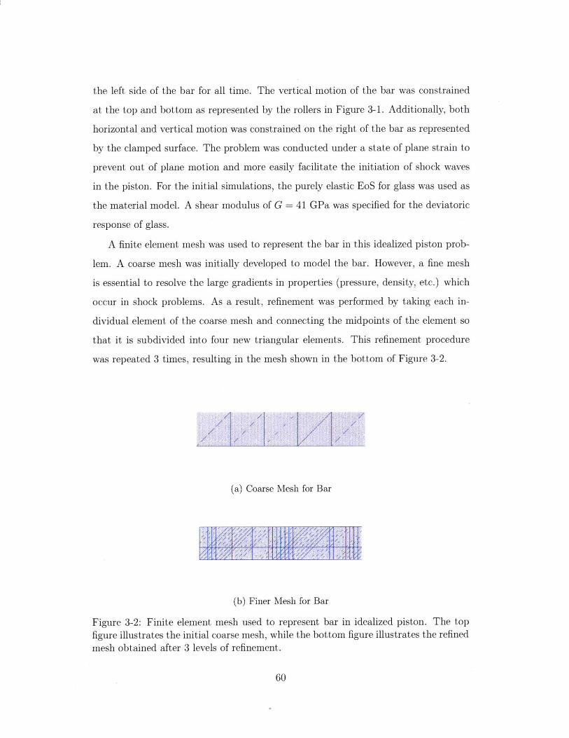
the left side of the bar for all time. The vertical motion of the bar was constrained

at the top and bottom as represented by the rollers in Figure 3-1. Additionally, both

horizontal and vertical motion was constrained on the right of the bar as represented

by the clamped surface. The problem was conducted under a state of plane strain to

prevent out of plane motion and more easily facilitate the initiation of shock waves

in the piston. For the initial simulations, the purely elastic EoS for glass was used as

the material model. A shear modulus of G = 41 GPa was specified for the deviatoric

response of glass.

A finite element mesh was used to represent the bar in this idealized piston prob-

lem. A coarse mesh was initially developed to model the bar. However, a fine mesh

is essential to resolve the large gradients in properties (pressure, density, etc.) which

occur in shock problems. As a result, refinement was performed by taking each in-

dividual element of the coarse mesh and connecting the midpoints of the element so

that it is subdivided into four new triangular elements. This refinement procedure

was repeated 3 times, resulting in the mesh shown in the bottom of Figure 3-2.

(a) Coarse Mesh for Bar

(b) Finer Mesh for Bar

Figure 3-2: Finite element mesh used to represent bar in idealized piston. The topfigure illustrates the initial coarse mesh, while the bottom figure illustrates the refinedmesh obtained after 3 levels of refinement.

60

-I

The idealized piston simulation was performed with several applied piston veloci-

ties of Up E [200,400, 600,800, 1000] m/s. The uniaxial stress (a-l) profile was plotted

over the midline of the bar at a time of t = 0.1 ms in the simulation. Here, we treat

ol as the pressure p to obey the conventions of shock theory [2]. Thus, pressure pro-

files were obtained for each of the different piston velocity cases, as shown in Figure

3-3.

Shock Profiles at time t=o. I.s for various piston velocities

- U, =40I0 M/l

- LIP =6We,.

00.0 0.2 0.4 0.6 08 1.0

Positon along Bar [m]

Figure 3-3: Pressure Profiles along length of bar at time t = 0.1 ms for various

piston velocities. The results show significant amounts of oscillation, which increase

in magnitude with increasing piston velocity.

FRom Figure 3-3, we observe that the pressure profiles, or shock waves, exhibit

severe amounts of oscillation, particularly for high piston velocities. These oscillations

are non-physical and are generally an artifact of the mesh discretization used in order

to solve the problem numerically. Furthermore, they illustrate the need for numerical

dissipation to dampen the oscillations present in the shock waves in Figure 3-3. This

dampening may be achieved through the use of artificial viscosity.

3.1.1 Artificial Viscosity

Artificial viscosity refers to the use of numerical dissipation in order to mitigate

spurious numerical oscillations occurring in problems involving shock waves. Here,

61

we discuss an artificial viscosity method formulated by Lew et al. in Reference [181

which we subsequently apply in our simulations to prevent oscillations resulting from

shock waves, while preventing smearing of these shocks.

We begin with the general framework for the treatment of constitutive equations,

which involves an additive decomposition of the first Piola-Kirchoff stress tensor into

an equilibrium part Pe and a viscous part Pv as follows

P = PC + Pv (3.1)

It is assumed that the equilibrium stress is of the form

PC(F, U) = -Jp(J, U)F- T (3.2)

where p(J, U) is the pressure given by the equation of state. Additionally, the viscous

stress is of the form

Pv(, F) = J-vF-T (3.3)

where

a-" = 2,q (sym (NF-') (3.4)

and n is the Newtonian viscosity coefficient. One may consider the addition of an

artificial viscosity A71 to the actual Newtonian viscosity n, so that the total viscosity

is given by

nh=7+A7 (3.5)

The artificial viscosity coefficient A17 may be computed as follows

{max(, - lp(cAU - cLa) - 7) Au < 0

In Equation 3.6, 1 is a measure of the element size, Au is a measure of the velocity

jump, and a is a characteristic sound speed of the material such as the celerity.

The artificial viscosity coefficient An is computed at every gauss point during finite

62

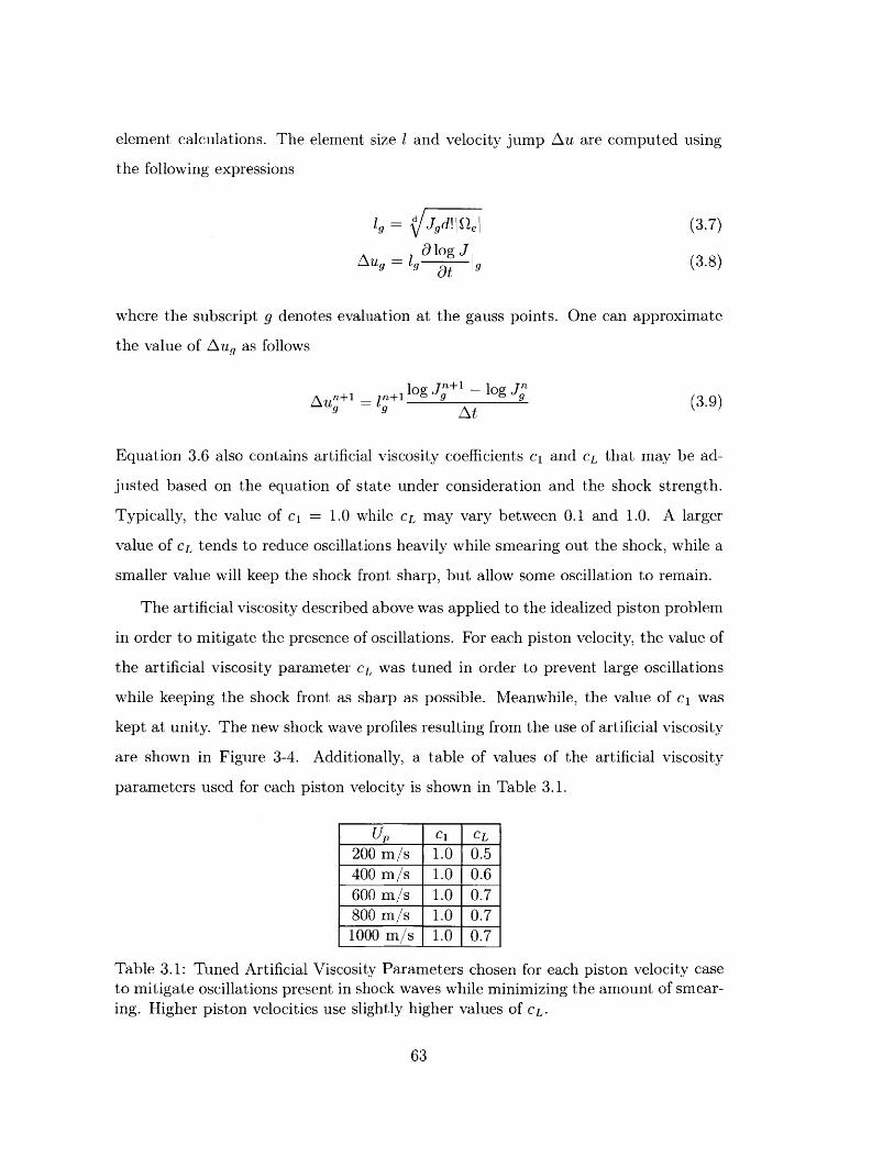
element calculations. The element size 1 and velocity jump Au are computed using

the following expressions

1g = Jgd! QeJ (3.7)

AUg = 1log J (3.8)

where the subscript g denotes evaluation at the gauss points. One can approximate

the value of Aug as follows

ln1 ogJ 1 -l og J (39)- At

Equation 3.6 also contains artificial viscosity coefficients ci and CL that may be ad-

justed based on the equation of state under consideration and the shock strength.

Typically, the value of c1 = 1.0 while CL may vary between 0.1 and 1.0. A larger

value of CL tends to reduce oscillations heavily while smearing out the shock, while a

smaller value will keep the shock front sharp, but allow some oscillation to remain.

The artificial viscosity described above was applied to the idealized piston problem

in order to mitigate the presence of oscillations. For each piston velocity, the value of

the artificial viscosity parameter CL was tuned in order to prevent large oscillations

while keeping the shock front as sharp as possible. Meanwhile, the value of ci was

kept at unity. The new shock wave profiles resulting from the use of artificial viscosity

are shown in Figure 3-4. Additionally, a table of values of the artificial viscosity

parameters used for each piston velocity is shown in Table 3.1.

UP C1 CL200 m/s 1.0 0.5400 m/s 1.0 0.6600 m/s 1.0 0.7800 m/s 1.0 0.71000 m/s 1.0 0.7

Table 3.1: Tuned Artificial Viscosity Parameters chosen for each piston velocity caseto mitigate oscillations present in shock waves while minimizing the amount of smear-

ing. Higher piston velocities use slightly higher values of CL.

63

Shock Profiles at f =DA ms for various piston velocities

0.4 0.6Position along Bar [m]

Figure 3-4: Shock Waves along length of bar at time t = 0.1 ms for various piston

velocities. The oscillations previously present have been mitigated through the use

of artificial viscosity.

The oscillations present in the initial shock wave results have been removed in

Figure 3-4. Additionally, although there is some smearing present, the shock waves

generally remain sharp. Ideal values of CL were larger for the higher piston velocity

cases which exhibited more serious amounts of oscillations. Overall, the introduction

of artificial viscosity eliminates the spurious oscillations which are present from the

numerical solution of shock problems. In the remainder of this chapter, we discuss

the verification studies conducted to ensure that the constitutive models obey shock

theory. Artificial viscosity was applied in these studies to mitigate oscillations.

3.2 Verifying the Rankine-Hugoniot Jump Conditions

Under Elastic Conditions

The Rankine-Hugoniot jump conditions, introduced earlier in Chapter 2 and repeated

below in Equations 3.10-3.12, represent conservation of mass, momentum and energy

in the presence of shock waves [2]. Furthermore, they relate thermodynamic properties

64

14

12

10

=2 ra'!

4 Xf r! s

00 =$I! s

C.8

6

4

2

N

N

010-I 0.2 0.8 1.0D

in the shocked and unshocked regions separated by a shock wave.

Mass poUs = p(Us - Up) (3.10)

Momentum P - Po = poUU, (3.11)

1Energy E - EO= -(P + Po)(V - V) (3.12)

2

In our idealized piston problem, the piston velocity UP creates a shock wave that

separates these shocked and unshocked regions. This is shown in Figure 3-5, where a

shock wave initiated by a piston velocity of Up = 1000 m/s has traveled to the center

of the bar, separating the two regions. The left portion of the bar (in blue) has been

shocked to a pressure of approximately 14 GPa, while the right portion (in red) is

unshocked, as may be observed on the right plot indicating pressure values.

Figure 3-5: Shock in Piston separating shocked and unshocked regions. The shock

has traveled halfway through the bar (left) causing a jump in the pressure between

the two regions (right).

To verify the Rankine-Hugoniot relations, one may measure the thermodynamic

properties in the shocked and unshocked regions and ensure that the values of these

properties satisfy the jump conditions. These conditions assume that the material

under consideration may be idealized as a fluid and has no strength in shear [22] [2].

65

Thus, in order to verify that the conditions hold, we must assume that the shear

modulus of our material G = 0.

In order to verify that the mass and momentum jump conditions were satisfied, pis-

ton simulations was conducted using the elastic EoS model for Up E [200, 400, 600, 800, 10001

m/s. Additionally, the artificial viscosity coefficients shown in Table 3.1 were used

for each case. However, the shear modulus was set to zero so that the bar could be

idealized as a fluid such that the Rankine-Hugoniot conditions could be verified.

Algebraic manipulations were performed on the mass jump condition to make it

easier to verify. Taking Equation 3.10 and solving for the jacobian J(= P) yieldsp

J - 1 - UP (3.13)p U

where J represents the ratio between the deformed and undeformed volumes. Addi-

tionally, the momentum jump condition is given by

P = pOU5 Up (3.14)

From the simulations, one may directly measure quantities such as J and P. Ad-

ditionally, given the relation between U, and Up as shown in Figure 2-5, one may

obtain the theoretical relationship between J and Up by applying the mass conser-

vation equation (Equation 3.13), as well as P and Up from the momentum equation

(Equation 3.11).

A table of results indicating shock speed, pressure, and jacobian for piston ve-

locities of Up E [200,400, 600, 800, 1000] m/s is shown in Table 3.2. The table shows

values obtained from the simulations, as well as theoretically expected values obtained

by applying the jump conditions for each piston velocity. The simulation shock speed

was estimated by extracting the time taken for the shock to travel halfway across

the bar, and dividing the length traveled (half of the bar, or 0.5 m) by this value.

Additionally, the pressure was directly measured by taking o in the shocked region,

and the jacobian was obtained by taking the determinant of the deformation gradi-

66

ent F in this region, using the postprocessing software. All quantities were obtained

independently. We observe a very close match between theoretical and simulation

shock speeds, pressures, and jacobians for all applied piston velocities.

Up Us Us,theoretical J Jtheoretical P Ptheoretical

200 m/s 4034 m/s 4033 m/s 0.95 0.95 1.79 GPa 1.77 GPa400 m/s 4205 m/s 4185 m/s 0.9045 0.9044 3.68 GPa 3.68 GPa600 m/s 4327 m/s 4340 m/s 0.862 0.862 5.72 GPa 5.73 GPa800 m/s 4513 m/s 4498 m/s 0.8224 0.8222 7.90 GPa 7.92 GPa1000 m/s 4625 m/s 4657 m/s 0.784 0.786 10.22 GPa 10.22 GPa

Table 3.2: Table of Results indicating the simulation results for shock velocity Us,jacobian J, pressure P and the corresponding theoretical values for various pistonvelocities Up. There is a good match between simulation and theoretical results forall parameters and piston velocities, indicating that the jump conditions are satisfied.

The simulation results presented in Table 3.2 are also plotted as data points along

with the theoretically expected shock velocity, jacobian and pressure as blue curves

in Figure 3-6, for piston velocities between 0 and 1000 m/s. The theoretical values

were obtained by taking the U, - Up representation of the EoS and applying the jump

conditions to transform it into the corresponding J - U and P - Up relations. Overall,

the data points line up with the theoretically predicted curves, indicating a good

match between results. There are some discrepancies between the theoretical and

simulation shock velocities since the shock velocities were estimated. However, the

good match between simulation and theoretical results for the jacobian and pressure,

representing conservation of mass and momentum respectively, illustrates that each

condition is verified.

The piston velocities applied here correspond to those in the low density regime,

before glass transformation occurs (one may refer to 2-5 to verify this). Since our

inelastic model for glass also obeys the low density EoS in this regime, this model

would give the same results (the Rankine-Hugoniot jump conditions would also be

satisfied using the inelastic model). In the next section, we study the shock phe-

nomenon predicted by the inelastic model under plastic conditions, and verify that

this behavior obeys expectations of shock theory.

67

4400k

43 -4200

4100

400D

If, [rn/si

(a) Shock versus Particle Velocity

1- Theareicalo Smabton

D.95

09

0.8

0.750 200 400 600 800 1000

UI m/s

(b) Jacobian versus Particle Velocity

12

0 Sm~abton10

0 200 400 600 WJO 1000

(c) Pressure versus Particle Velocity

Figure 3-6: Comparison of theoretically expected shock velocity, jacobian, and pres-sure (shown as blue lines) to those found in the simulations (shown as red dots).Theoretically obtained jacobian corresponds to the conservation of mass, while theo-retically obtained pressure corresponds to conservation of momentum. A good matchis found in all three results, illustrating that the jump conditions are satisfied.

68

3.3 Verifying the Plastic Shock Structure Under In-

elastic Conditions

The Rankine-Hugoniot jump conditions only hold under elastic conditions. Therefore,

we cannot expect the conditions to be satisfied at the high pressures where glass

densification takes place. However, we may expect plastic effects to alter the shocks

generated in the bar under such pressures. For example, it is known that elastic-

plastic shocks have a more complex structure than the typically sharp elastic shocks.

Additionally, shock speeds are typically lower under plastic conditions compared to

elastic conditions [22].

To confirm that our simulations also exhibit an elastic-plastic shock under plastic

conditions, the piston problem was run using our inelastic model for glass with a piston

velocity of Up = 2000 m/s, which is large enough to generate pressures necessary for

transformation to occur. For comparison, the problem was also performed using the

same model under purely elastic conditions (the preconsolidation pressure pc was set

to a very high value to prevent plasticity in the model). Shock profiles at time t

0.1 ms were obtained and plotted together for comparison in Figure 3-7.

Figure 3-7 shows the pressure profiles at a time of t 0.1 ns under elastic and

inelastic conditions. Artificial viscosity parameters of ci = CL = 1 were used to miti-

gate the large oscillations which would occur at this high piston velocity. We observe

that the shock pressures achieved under plasticity are lower than those under purely

elastic conditions, due to hardening behavior under plasticity. The plastic shock ob-

served is not as sharp as the elastic shock, due to inelastic effects which cause the

plastic shock to smear out. Furthermore, the plastic shock travels a shorter distance

than the elastic shock, confirming the lower speed of plastic shocks established in

shock theory. Our comparison shows that under inelastic conditions, our simulations

provide qualitative results consistent with the theory.

69

-~ 21

Shock Profiles at t =0.1 ms for Elastic and Inelastic Conditions

D 0.2 0.4 0.6Position Along Bar [m]

0.8

Figure 3-7: Shock Profiles Obtained from applying a piston velocity of U, = 2000 m/s

using the inelastic model for glass transformation under plastic and elastic (the pre-

consolidation pressure pc is set to a very high value to prevent yielding) conditions.

We observe that the elastic shock is much sharper than the plastic shock, and also

travels much farther. The inelastic shock lags behind. These characteristics agree

with the expectations of shock theory.

70

40

35 k-

30

25

- Elastlic-- Inelastic -

0~

0L.5

0~

20 -

15 -

10 -

5

0I0. 1.0

.. .. .. .... .. ... ..

3.4 Summary

In this Chapter, the constitutive models described in Chapter 2 were tested under

shock physics. An idealized piston problem was used to aid in this verification pro-

cess. A description of the artificial viscosity formulation used to mitigate oscillations

resulting from simulating shock problems was discussed. The Rankine-Hugoniot jump

conditions were then verified in the elastic regime by comparing theoretical and sim-

ulation shock velocity, jacobian, and pressure obtained for various piston velocities.

Lastly, the piston problem was performed using a high piston velocity to illustrate

the effects of plasticity. We find that the plastic shocks generated by our simulations

are wider and travel slower than elastic shocks, in agreement with theoretical expec-

tations. Thus, our constitutive models behave robustly and in agreement with theory

under shock loading conditions.

71

Chapter 4

Exploring Transformations in Glass

using Simulations

In this Chapter, we describe our efforts to guide the design of high pressure exper-

iments on glass using computational tools and constitutive models. Our goal is to

determine the adequacy of two experimental designs for generating high pressures for

glass transformation. In the first design, laser pulses are used to generate converging

surface acoustic waves (SAWs) which cause high pressures. The second experimental

design is a novel setup in which converging shock waves travel through the thickness

rather than the surface of glass. Our simulations show that there is a competi-

tion between transformation in glass due to highly compressive stresses which occur

upon wave convergence, and fracture due to tensile stresses which occur afterwards

(we model this fracture using 3D simulations). We believe that the design of high

pressure experiments on glass can ultimately lead to new high pressure applications

utilizing it (e.g. ballistics).

4.1 Surface Acoustic Wave Experiments

Here we study experiments on glass in which surface acoustic waves are generated

using concentrated laser pulses (detailed in References [33] and [34]). In these ex-

periments, a ring shaped laser pulse is applied to the surface of a cylindrical glass

73

Probe pulse M wror400 nm, 180 fs Seem

Camerae Left

Lens Reference Excitation pulseMinor focus Focusing SAW

Gold ring SAW

MotorizedLens

stage SwpLens

Excitation pulse Axc

800 nm, 300 ps Adinmr

(a) Optical setup for surface shocks (b) Glass samples used in experiments

Figure 4-1: Experimental setup and glass samples for surface acoustic wave experi-

ments. The experimental setup contained a conical prism and lens used to focus a

laser pulse on engraved gold rings deposited on the samples, generating surface waves.

Convergence of the surface waves leads to high pressures in the samples. A reference

mirror and high speed camera allowed for imaging of the surface waves over time.

sample in order to generate focusing and diverging stress waves in the material. The

convergence of the focusing stress waves results in large pressures at the center of the

sample. We simulate these experiments to determine if these large pressures are high

enough to cause transformation in glass. Multiple surface wave experiments were

conducted, each at a different laser excitation pulse energy (the applied laser pulse

energies were 0.15, 0.25, 0.5, 0.75 and 1.00 mJ).

The setup for this experiment is shown in Figure 4-la. Cylindrical glass samples of

radius and thickness 300 prm (shown in Figure 4-1b) were fabricated by the Xin Zhang

Group in Boston University, and contained deposited gold rings of radius 100 Am.

To generate surface acoustic waves in the glass sample, a laser excitation pulse was

focused into a ring using a conical prism and lens combination [33]. The ring shaped

laser pulse was applied to the region of the sample containing the engraved gold ring,

resulting in ablation of the gold and the formation of focusing and diverging surface

acoustic waves. These waves traveled through the surface of the sample, with the

focusing wave generating large amounts of pressure in the sample upon converging

to its center. Figure 4-2 shows a snapshot of the surface of the glass sample at a

time of t = 21.3 ns after the laser pulse was applied. Here we observe the focusing

74

-.

and diverging waves generated by ablation of the gold ring. The snapshot contains

fringe patterns (depicted by the distorted white lines), which may be used to infer

the surface displacement of the sample at the time of imaging.

A afion area

Figure 4-2: Focusing and diverging surface acoustic waves (SAWs) resulting from theablation of the gold coating in glass samples. The red dashed circle shows the regionwhere the gold ring was ablated. The white lines are fringe patterns which can beused to infer the surface displacement of the sample at a given time. High pressuresare achieved in the sample when the focusing SAW converges to the center.

Fringe patterns were captured at multiple times in a given experiment using a

high speed camera. Figure 4-3 illustrates fringe patterns captured at various times

in one such experiment. The first image shows the sample at t = 16 ns, and each

subsequent image is taken every 3 ns afterwards. We observe that the focusing wave

travels closer to the center over time, eventually converging at time t = 31 ns and

causing highly compressive pressures here. Afterwards, the surface wave begins to

diverge, resulting in tensile stresses at the center.

The schematic in Figure 4-4 captures the essential aspects of the experiment. It

shows the laser excitation ring of radius 100 prm which is applied to a glass sample

of thickness and radius 300 pm, generating diverging and focusing surface waves

through the sample. To model this experiment, one could perform a three dimensional

simulation of the boundary value problem (BVP) represented in Figure 4-4. However,

the sample has axial symmetry due to its cylindrical shape, enabling us to model a two

dimensional slice of the sample using axisymmetric finite elements (assuming no 3D

75

Figure 4-3: Interferometric images of propagating surface acoustic waves shown at

various times. The focusing shock wave converges at t = 31 ns, leading to large

pressures. The wave diverges thereafter, causing tensile stresses in the sample lead-

ing to brittle fracture. Fringe Patterns in the images can be used to infer surface

displacements at the time of imaging.

76

Focusing surface shock Laser excitation ring

Diverging surface shock

0 JlO 4 tl

Figure 4-4: 3D schematic of Glass Sample and surface shock wave setup. The laserexcitation ring is applied at the location of the gold ring on the sample, generatingfocusing and diverging surface shock waves.

effects such as fracture or anisotropy are present). The axisymmetric analysis results

in a 2D problem that is computationally less expensive than the full 3D problem. The

problem setup for the 2D axisymmetric model is shown in Figure 4-5. In this model,

the left side corresponds to the center of the actual sample. This side is constrained

from horizontal motion due to symmetry. The bottom and right side (corresponding

to the outer edge of the sample) are free to move. While our setup contains no vertical

constraints and permits vertical rigid body translations, this is not an issue as we are

only interested in the sample behavior at the very early stages of wave propagation

before notable rigid body translations can occur. Lastly, the top of the sample is

traction free except for the region where the laser excitation pulse is applied. The

laser pulse transduced onto the gold ring is assumed to have a Gaussian spatial profile

in the experiments. Accordingly, we model the load caused by the gold ablation due

to the laser as a Gaussian force distribution. This force distribution is represented by

Equation 4.1, and is applied for an short time of t = 300 ps in the experiments.

f(r) = A x exp d(r2 R) (4.1)

Equation 4.1 gives the downward pressure f(r) acting on a point at a distance r from

the center of the sample. In Equation 4.1, R = 100 pm and represents the location

77

T100y

R = 300 pm -

Figure 4-5: Profile of glass sample modeled using axisymmetric finite elements. Thelaser excitation pulse is modeled as a Gaussian force distribution.

of the center of the pulse, d = 5 pm and is a length scale defining its width, and A

represents the amplitude of the Gaussian force distribution. The amplitude of the

Gaussian is unknown in each experiment; only the applied laser energy is known.

Since the Gaussian amplitude is an input to our model (and not the laser energy),

we must infer a relationship between the two. To determine this relationship, we

calibrated our amplitude in the simulation to each experiment, ensuring that the

predicted wave behavior (amplitude, speed, shape) matched those in the experiments

(determined using fringe patterns).

The inelastic model for glass was used in our simulations. The material properties

of the glass used in the experiments were po = 2510 kg/m 3, K = 72 GPa and

G = 30.1 GPa, so these values were also used in our simulations. These were run

for a time span of T E [0,40] ns (so that the convergence and divergence behavior

of the surface waves was captured). Additionally, we employed artificial viscosity

in our simulations, as is customary with problems involving shocks. The artificial

viscosity parameters were adjusted to avoid oscillations, with parameters of ci =

78

1.0 and CL = 0.05 selected here. Third order axisymmetric finite elements were

used in the mesh to accurately capture wave propagation occurring in the sample.

Lastly, the Gaussian amplitude was tuned as described earlier, so that a good match

between experimental and simulation surface displacement profiles was obtained for

each laser energy. Comparisons of the surface displacements in the experiments and

the simulations (tuned to agree with experiments as closely as possible) are shown

below for the laser energies of 0.15, 0.25, 0.5, and 0.75 mJ.

T- 121- T- 'KaA

0 0 -I

Dfrtd. a,: fr,- (frm)

(a) t = 12.7 ns

0 0 20 'a a 20 30 .0 so0 W 0 M

(c) t = 21.3 ns

'GooDigt o [o (tm)

(e) t = 30.7 ns

II

Oittfom fom O~ (M)

(b) t 17.1 ns

W M0 W N .0 M 20 W 0 W 20 0 0 W 0 MWDistooo from (moo (tmn)

(d) t 26.2 nsT 3- 3 u

.. 1/

-, 0 N0 So 0 30 20 W a W N 0 JQ 4o YO oDi()t=m rom f.1 (m)

(f) t = 35.1 ns

0

-W To N M a W0 20 W0 0 20 M .0 M doDistance from fom (tom)

(g) t = 39.7 ns

Figure 4-6: Comparison of numerical and experimental out-of-plane displacements at

various times during surface wave convergence, for a laser energy of 0.15 mJ.

Figures 4-6 through 4-9 show the out-of-plane displacement of the surface of the

sample from the experiment and our simulations at several different times. Each set of

figures corresponds to a different laser energy. The simulation surface displacements

79

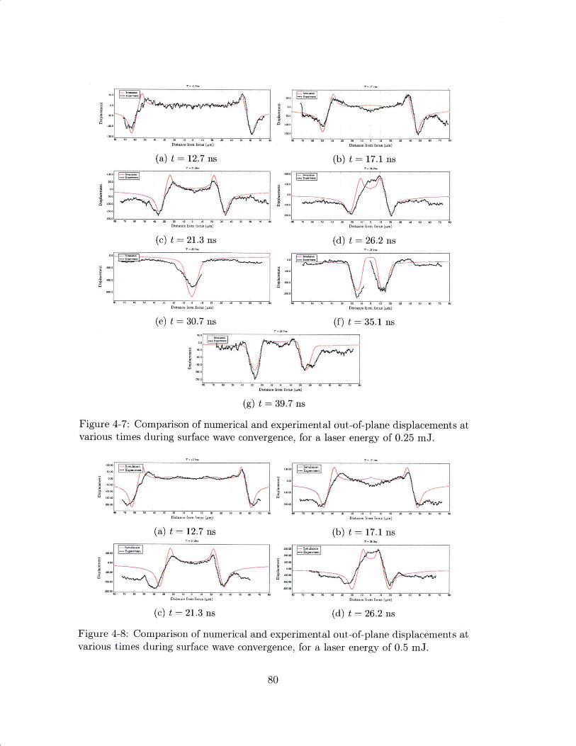
a -.ma loaDurfce fom. focus (tAm)

(a) t = 12.7 ns

N W .0 30 20 17 . 20 s NDistmnce from focus (mm)

(b) t = 17.1 ns

-o "I A.

I .

'V I -a,

X 0 a W - X .0 .m TO N

Distnce fzom focus (AM)

(c) t 21.3 ns

Wad

Dist( e &om focus (tM)

(e) t = 30.7 ns

Disto. fom. focus (m)

(d) t = 26.2 ns

.-aao en so a D, oo to ot to. (tot) o so to aDistn = om focus (pm)

(f) t = 35.1 ns

E,9

No

no-Distnce fomm ocus (pm)

(g) t = 39.7 ns

Figure 4-7: Comparison of numerical and experimental out-of-plane displacements atvarious times during surface wave convergence, for a laser energy of 0.25 mJ.

am am

'Wo

MO

(a) t = 12.7 ns

Dist..c. from focus (AM)

(b) t = 17.1 ns

Woo10100 .s2000_

N TO W W o a o. o tWto M)Dist-c from facus (jum)

(c) t = 21.3 ns

Disttco fhom focus (gm)

(d) t = 26.2 ns


80

"it-c from focus (JAM)

-

-

so 0 .0 N 4

(a)00 2 =127 () = 7.1<00 200 N 0

oLwm from f-0 (pmo) Di.~Diso 0 0 W a) ( 0002M)

(a) t =12.7 ns (b) t 17.1 ns

IN

DW~~0, &-oo f-oo (AI)

(c) t = 21.3 ns


at negative x-positions are obtained by reflecting the results about the x = 0 position.

We observe a satisfactory match between surface amplitudes for each laser energy,

justifying our correlation between experiment and simulation parameters.

From the calibration process, we determined that amplitudes of 15, 20, 32, 39

and 40 GPa could be correlated to laser energies of 0.15 mJ, 0.25 mJ, 0.5 mJ, 0.75

mJ and 1.00 mJ, respectively. We plot this relationship between laser energy and

the Gaussian amplitude, shown in Figure 4-10. We observe a roughly linear trend

between the amplitude and Gaussian pulse for lower laser energies. The amplitude

appears to saturate for higher laser energies. However, more data from higher energies

cases (1.25 mJ or 1.50 mJ) should be obtained to verify this behavior. In [91, Fabbro

et al. discuss an analytical method to determine this relationship between amplitude

and applied laser energy. This approach is based on the actual physical processes

occurring during laser irradiation. However, our tuning approach (comparing surface

displacements) is expected to give the same relationship between amplitude and laser

energy, so we are not interested in the finer details of the processes discussed in the

paper.

Overall, our inelastic model for glass is able to capture the surface displacements

observed in the experiments. Furthermore, we have established a correlation between

laser energy and Gaussian amplitude, allowing us to use our simulations to analyze

81

Correllation Between Gaussian Amplitude and Laser Energy

35

3D

E Z5.. ... .

20-

15101 0.2 0.3 0.4 0.5 0.5 0.7 0.8 0.9 1.0

Laser Ewergy (mj)

Figure 4-10: Correlation obtained between applied laser energy and Gaussian am-plitude. There is a roughly linear trend between the amplitude and laser energy.However, this tapers off between 0.75 mJ and 1 mJ.

the pressures experienced by the glass sample for given laser energies. As a repre-

sentative case, we perform a simulation with a Gaussian amplitude of A = 15 GPa

(corresponding to the lowest energy case of 0.15 mJ), and illustrate pressure contours

in the sample at several times, shown in Figure 4-11.

In Figure 4-11, we focus on the upper left of the sample to illustrate the behavior

of the waves generated by the Gaussian pulse. Pressure contours (computed as p =

-}(tr(a)) are shown, where the red contours correspond to compression and the blue

contours correspond to tension. We observe interesting wave propagation phenomena

from the simulations, most notably the formation of two waves (a primary wave and

a surface wave).

The sequence of events in the images depicted in Figure 4-11 is described below.

At time t = 1 ns, the laser excitation pulse has been applied to the surface of the

sample. This results in a single wave containing compressive, tensile, and compressive

components as shown at t = 5 ns. This wave then divides into a primary wave (known

as a P-wave) and a surface acoustic (or Rayleigh) wave. The two waves are visible at

t = 15 s. The P-wave travels through the entire depth of the sample and propagates

82

I

i

(a) t = 1 ns (b) t =5 ns

(c) t = 15 ns (d) t = 17 ns

j

(e) t = 20 ns

i

(f) t = 23 ns

i

(g) t = 30 ns (h) t = 32 ns

Figure 4-11: Snapshots of the pressure contours in the glass sample at various times

for 0.15 mJ case (A = 15 GPa). A P-wave and surface acoustic wave are generated bythe Gaussian force distribution. These waves travel at different speeds and convergecausing large tensile and compressive pressures at the center.

83

I

I

much faster than the Rayleigh wave, which travels only along the surface. The P-

wave converges to the center first, resulting in compressive pressures at the center at

t = 17 ns. The P-wave then diverges, becoming a tensile wave (shown at t = 20 ns)

which crosses the tensile component of the incoming Rayleigh wave, augmenting the

strength of this Rayleigh wave at t = 23 ns. The Rayleigh wave then converges to

the center, resulting in tensile followed by compressive pressures at the center (at

t = 30 ns and t = 32 ns respectively). Afterwards, tensile stresses occur at the center

once again as the surface wave diverges outward (not shown). We note that the

highest pressures are observed at the center of the sample when the Rayleigh wave

converges (approximately t = 32 ns).

To further validate our model, we compare the speed of the P-wave and Rayleigh

waves observed in the simulations to analytical results. The speed of P-waves and

Rayleigh waves in a material are both dependent on material constants. Expressions

for these speeds are given in Equations 4.2 and 4.3 [161.

VP= F-:G (4.2)po

G 0.7+112v

Vr _ (0.87= +-1 (4.3)p0 1+ V

In Equations 4.2 and 4.3, K, G, po and v represent the bulk modulus, shear modulus,

density and Poisson's ratio, respectively, of the material through which the wave is

traveling. For our glass, these material parameters were approximately K = 72 GPa,

G = 30.1 GPa, and po = 2510 kg/m 3 (v can be determined from K and G as roughly

0.317). Substituting these values into Equations 4.2 and 4.3 gives an expected P-wave

velocity of 6.68 km/sec and Rayleigh wave velocity of 3.22 km/s.

To estimate the P-wave and Rayleigh-wave velocities in our simulations, we first

determine the positions of the two waves at every nanosecond. This is done by finding

the locations on the surface where pressure changes sign (one location corresponds to

the P-wave, the other to the Rayleigh wave). Based on these locations, we determine

the distance traveled by the waves from one nanosecond to the next. Dividing distance

84

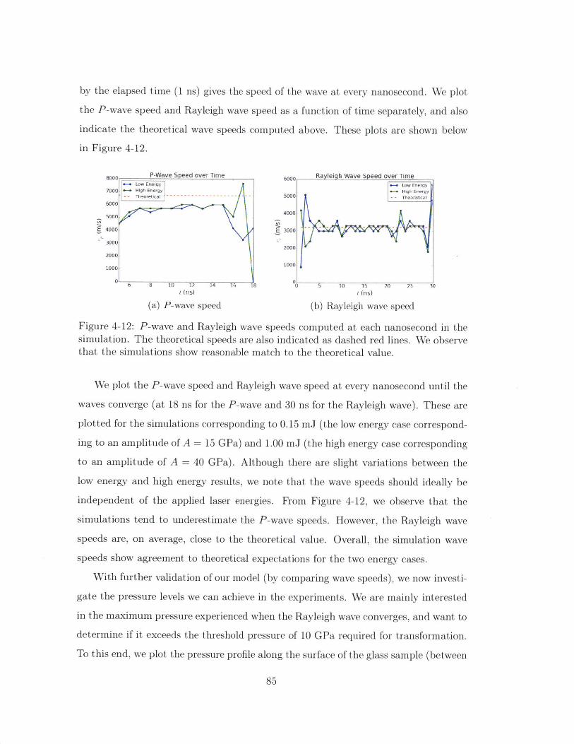
by the elapsed time (1 ns) gives the speed of the wave at every nanosecond. We plot

the P-wave speed and Rayleigh wave speed as a function of time separately, and also

indicate the theoretical wave speeds computed above. These plots are shown below

in Figure 4-12.

8000 P-Wave Speed over Time 6000 Rayleigh Wave Speed over Time

- LW Eer- Low Energy

7000 - gh'E.a y -------- -------------------- -- - 50006000

40005000

E4ooo E 3000

20002000

10001000

6 8 10 12 14 16 1 is 0 5 10 15 20 25 30Oi(s) t (ns)

(a) P-wave speed (b) Rayleigh wave speed

Figure 4-12: P-wave and Rayleigh wave speeds computed at each nanosecond in thesimulation. The theoretical speeds are also indicated as dashed red lines. We observethat the simulations show reasonable match to the theoretical value.

We plot the P-wave speed and Rayleigh wave speed at every nanosecond until the

waves converge (at 18 ns for the P-wave and 30 ns for the Rayleigh wave). These are

plotted for the simulations corresponding to 0.15 mJ (the low energy case correspond-

ing to an amplitude of A = 15 GPa) and 1.00 mJ (the high energy case corresponding

to an amplitude of A = 40 GPa). Although there are slight variations between the

low energy and high energy results, we note that the wave speeds should ideally be

independent of the applied laser energies. From Figure 4-12, we observe that the

simulations tend to underestimate the P-wave speeds. However, the Rayleigh wave

speeds are, on average, close to the theoretical value. Overall, the simulation wave

speeds show agreement to theoretical expectations for the two energy cases.

With further validation of our model (by comparing wave speeds), we now investi-

gate the pressure levels we can achieve in the experiments. We are mainly interested

in the maximum pressure experienced when the Rayleigh wave converges, and want to

determine if it exceeds the threshold pressure of 10 GPa required for transformation.

To this end, we plot the pressure profile along the surface of the glass sample (between

85

0-50 pm) when the Rayleigh wave converges. Figure 4-13 shows the pressure profile

for two laser energies of 0.25 mJ (A = 20 GPa) and 1.00 mJ (A = 40 GPa). We find

that the peak pressure achieved in the 0.25 mJ case is only 6 GPa, so applying this

laser energy will not induce any transformation in glass. However, the 1.00 mJ case

illustrates a peak pressure of approximately 12 GPa, so an experiment run with a

1.00 mJ laser energy has the potential to cause transformation in glass.

14 Pressure Profile during Surface Wave Convergence

12

10

CL

2-

0-

a-2

0 10 20 30 40 50Position from Center (pm)

Figure 4-13: Pressure Profile on surface of glass sample during convergence of Rayleighwave, shown for simulations corresponding to 0.25 mJ and 1.00 mJ experiments. Thepeak pressure achieved are 6 GPa and 12 GPa respectively, showing that the 1.00 mJexperiments have the potential to cause transformation. Fracture effects will likelymitigate transformation.

The high energy case has the potential to cause transformation in glass. However,

only a small portion of the glass sample close to the center experiences a pressure

above 10 GPa required for transformation. Furthermore, the convergence of the

Rayleigh wave actually causes high tensile pressures prior to the compressive pressures

which cause transformation. These tensile pressures have the capability to cause

fracture, which may mitigate the high pressures predicted by our simulations (which

do not incorporate fracture). We explore the role of fracture in the next section.

86

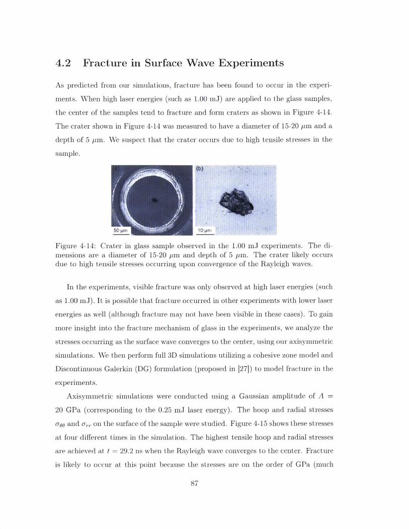
4.2 Fracture in Surface Wave Experiments

As predicted from our simulations, fracture has been found to occur in the experi-

ments. When high laser energies (such as 1.00 mJ) are applied to the glass samples,

the center of the samples tend to fracture and form craters as shown in Figure 4-14.

The crater shown in Figure 4-14 was measured to have a diameter of 15-20 Pm and a

depth of 5 pm. We suspect that the crater occurs due to high tensile stresses in the

sample.

50pr 10 PM

Figure 4-14: Crater in glass sample observed in the 1.00 mJ experiments. The di-mensions are a diameter of 15-20 pjm and depth of 5 pm. The crater likely occursdue to high tensile stresses occurring upon convergence of the Rayleigh waves.

In the experiments, visible fracture was only observed at high laser energies (such

as 1.00 mJ). It is possible that fracture occurred in other experiments with lower laser

energies as well (although fracture may not have been visible in these cases). To gain

more insight into the fracture mechanism of glass in the experiments, we analyze the

stresses occurring as the surface wave converges to the center, using our axisymmetric

simulations. We then perform full 3D simulations utilizing a cohesive zone model and

Discontinuous Galerkin (DG) formulation (proposed in [271) to model fracture in the

experiments.

Axisymmetric simulations were conducted using a Gaussian amplitude of A

20 GPa (corresponding to the 0.25 mJ laser energy). The hoop and radial stresses

a00 and o-,, on the surface of the sample were studied. Figure 4-15 shows these stresses

at four different times in the simulation. The highest tensile hoop and radial stresses

are achieved at t = 29.2 ns when the Rayleigh wave converges to the center. Fracture

is likely to occur at this point because the stresses are on the order of GPa (much

87

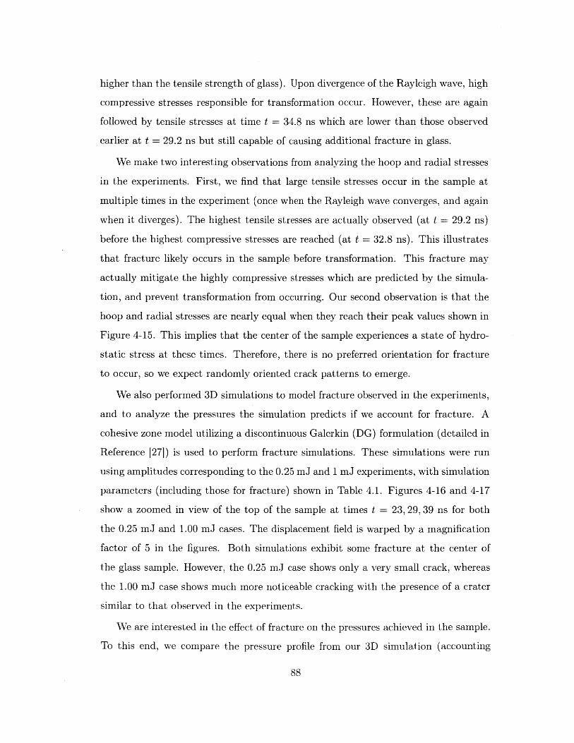
higher than the tensile strength of glass). Upon divergence of the Rayleigh wave, high

compressive stresses responsible for transformation occur. However, these are again

followed by tensile stresses at time t = 34.8 ns which are lower than those observed

earlier at t = 29.2 ns but still capable of causing additional fracture in glass.

We make two interesting observations from analyzing the hoop and radial stresses

in the experiments. First, we find that large tensile stresses occur in the sample at

multiple times in the experiment (once when the Rayleigh wave converges, and again

when it diverges). The highest tensile stresses are actually observed (at t = 29.2 ns)

before the highest compressive stresses are reached (at t = 32.8 ns). This illustrates

that fracture likely occurs in the sample before transformation. This fracture may

actually mitigate the highly compressive stresses which are predicted by the simula-

tion, and prevent transformation from occurring. Our second observation is that the

hoop and radial stresses are nearly equal when they reach their peak values shown in

Figure 4-15. This implies that the center of the sample experiences a state of hydro-

static stress at these times. Therefore, there is no preferred orientation for fracture

to occur, so we expect randomly oriented crack patterns to emerge.

We also performed 3D simulations to model fracture observed in the experiments,

and to analyze the pressures the simulation predicts if we account for fracture. A

cohesive zone model utilizing a discontinuous Galerkin (DG) formulation (detailed in

Reference [27]) is used to perform fracture simulations. These simulations were run

using amplitudes corresponding to the 0.25 mJ and 1 mJ experiments, with simulation

parameters (including those for fracture) shown in Table 4.1. Figures 4-16 and 4-17

show a zoomed in view of the top of the sample at times t = 23,29, 39 ns for both

the 0.25 mJ and 1.00 mJ cases. The displacement field is warped by a magnification

factor of 5 in the figures. Both simulations exhibit some fracture at the center of

the glass sample. However, the 0.25 mJ case shows only a very small crack, whereas

the 1.00 mJ case shows much more noticeable cracking with the presence of a crater

similar to that observed in the experiments.

We are interested in the effect of fracture on the pressures achieved in the sample.

To this end, we compare the pressure profile from our 3D simulation (accounting

88

SS

0 20 60 W0 so 10

(a) Radial/Hoop Stress contours att = 10.0 ns

2SS

Hopg and Maglal Stress rftUtes at t -29.2 te

-U'

(b) Radial/Hoop Stress contours att = 29.2 ns

i

S

10 Hoop and Sadial Stress Promes at t = 32 _ ns

0

-5 -

- 2 W W0 W

(c) Radial/Hoop Stress contours att = 32.8 ns

10 Hoop and Radial Stress Prolies at t = 34.8 ns

5

-S

0 ~ 4 28 V Wtistrce hor Radhn lam$

(d) Radial/Hoop Stress contours att = 34.8 ns

Figure 4-15: Hoop and Radial stress profiles during Rayleigh wave convergence anddivergence. High tensile stresses are observed at the center of the glass sample be-fore the high compressive pressures necessary for transformation. Thus, we suspectfracture will occur and prevent pressures necessary for transformation from beingachieved.

89

Hopandieafl Stmes Pvo~ks 0t t -0 we

A

-5

Table 4.1: Material properties used for simulation of fracture

(a) t 23 ns (b) t = 29 ns (c) t 39 ns

Figure 4-16: Fracture patterns in glass substrate caused by the convergence of asurface acoustic wave generated by laser energy of = 0.25 mJ

(a) t 23 ns (b) t 29 ns (c) t 39 ns

Figure 4-17: Fracture patterns in glass substrate caused by the convergence of asurface acoustic wave generated by laser energy of = 1.00 mJ

90

Properties ValuesDensity p = 2510 kg/m3

Bulk Modulus K = 72 GPaShear Modulus G = 30.1 GPaCohesive strength o-c = 1.OGPaFracture energy Ge = 200Tension/Shear weighting -y = 1.0DG stability parameter # = 1.0

for fracture) to that from the corresponding axisymmetric case for the 1.00 mJ case.

Figure 4-18 illustrates the peak pressures achieved from the axisymmetric simulation

which does not account for fracture (the pressure profile is reflected about x = 0 in

this case) and the 3D simulation with fracture. We observe that the predicted peak

1Comparison of Pressure Prufille with and without Fracture- Without Fracture- With Fracture

-40 -20 0 20 40Position from Center (pm)

Figure 4-18: Pressure Profile on surface of glass sample during convergence of Rayleighwave, from 3D simulations with fracture and axisymmetric simulations without frac-ture. The predicted peak pressure is not high enough to cause transformation whenfracture is accounted for.

pressure is much lower when fracture is modeled. In this case, the peak pressure is

only about 2 GPa, as opposed to the 12 GPa value predicted in the axisymmetric

case. Physically, fracture occurs in order alleviate the high tensile stresses experienced

in the glass sample. However, it also prevents the compressive pressures achieved

when the surface wave converges from being high enough for transformation. Thus,

we find that fracture wins out in this competition, and prevents us from achieving

transformation in glass.

We conclude that the surface acoustic wave experiments are not suitable for caus-

ing glass transformation. This is because the pressures achieved are generally not high

enough to exceed the threshold of 10 GPa required for transformation. Although the

1.00 mJ experiment did have the potential to induce glass transformation, fracture

91

actually occurs before these high pressures can be reached. Fracture reduces the peak

pressures we can achieve in the experiments, and mitigates transformation in the glass

samples.

In the next section, we explore a new experimental design which can more easily

generate large compressive stresses in glass.

4.3 Exploring Converging Shock Waves

In this section, we explore an alternative experimental configuration to generate high

pressures in glass. The idea of this new setup is to apply a laser pulse to the body of

a cylindrical glass sample, rather than to its surface, in order to generate shock waves

that will travel through the bulk of the sample. The convergence of these "bulk"

shock waves can generate pressures larger than those achieved with surface waves,

which tend to disperse and lose strength during propagation. A schematic for this

new configuration (shown in the axisymmetric view) is shown in Figure 4-19.

sapphire(~10OPm)

glass

sapphire -(-300pm) polymer

Figure 4-19: An axisymmetric view of the experimental setup for generating shockwaves through the bulk of the glass sample. A laser (depicted by arrows in the figure)is applied to a polymer host, generating a shock wave in the material. The wavepropagates to the glass and eventually converges, resulting in very high pressures atthe center.

In this setup, the glass sample is attached to a polymer host, and the polymer

glass substrate is glued in between two sapphire plates. A laser excitation pulse is

92

-A--____ ____

applied to the circumference of the polymer, resulting in a shock wave. This shock

wave transduces from the polymer into the glass sample, and eventually converges to

the center, resulting in high pressures here. Waves are generated through the entire

bulk of the sample, rather than just the surface as in the previous experiments, giving

the configuration the potential to provide higher pressures.

Our goal, as before, was to model the experiment in order to determine the pres-

sures achievable in this new experimental configuration. The BVP setup for perform-

ing finite element simulations of the converging shock wave experiment is shown in

Figure 4-20, depicted in both the axisymmetric (left) and three dimensional (right)

modes. Both schematics illustrate a glass sample of thickness t and radius R con-

strained from vertical motion on the top and bottom (representing the plates pre-

venting out of plane motion in the experiments). The polymer material itself was

not modeled in our finite element setup. Instead, we model only the glass sample

and the transduction of the shock wave from the polymer to the glass. This is mod-

eled as a uniform piston velocity applied on the outer edge of the sample (as shown

in. the schematic) for a very short time (this transduction time is unknown in the

experiments).

UtI t

(a) Axisymmetric Numerical Setup (b) 3D Numerical Setup

Figure 4-20: Axisymmetric and 3D Setup for BVP representing converging shock

wave experiment.

An axisymmetric and corresponding 3D simulation was performed to illustrate

93

-A

wave propagation behavior in this experiment. As a representative case, we choose an

arbitrary a piston velocity of Up = 1000 m/s applied for a short time of t = 1 ns. The

dimensions of the samples used for our simulations were t = 5QPm and R = 50Pm.

The inelastic model for glass is used for these simulations with the same material

parameters given in Table 2.4 (except that the friction angle was set to 4 = 71.50 -

this prevents yielding in shear).

Snapshots of the pressure contours in the glass sample, in the axisymmetric and

corresponding 3D views, are shown in Figure 4-21. A compressive shock wave is

generated at time t = 1 ns and begins to travel through the glass sample. The shock

converges to the center at t = 8 ns. At this point, the highest or peak pressure is

experienced by the sample. After convergence the wave diverges outward, causing

large tensile stresses. We are primarily interested in pressure achieved in the sample

when the shock wave converges to the center. This is because this converging pressure

is the largest pressure experienced by the sample, and the most likely to cause phase

transformation.

From the representative simulation, we observe that compressive pressure occurs

before tensile pressure (unlike in the previous experiment). Therefore, we expect that

the material will transform before fracture happens. Since we are mainly interested

in transformation behavior, there is no need to model fracture. For this reason, we

perform axisymmetric simulations in the remainder of our study.

We perform simulations to determine the adequacy of these experiments for gen-

erating high pressures. No experimental data was available for this configuration, so

we could not develop a correlation between applied laser energy and piston velocity.

As a result, we apply arbitrary piston velocities of Up = 500, 1000,1500, 2000 and ob-

serve the pressures achieved in these cases as a first step. The pressure profile when

the peak pressure is achieved at the center is shown for each piston velocity in Figure

4-22. We also plot the expected density profile along the radius of the glass sample

after the shock converges in Figure 4-23.

Figure 4-22 illustrates that extremely high peak pressures can be achieved using

this setup. A piston velocity of Up = 500 m/s results in a peak pressure of about. 10

94

(a) Axisymmetric View at t = 1 ns

(c) Axisymmetric View at t = 5 ns

(e) Axisymmetric View at t = 8 ns

(g) Axisymmetric View at t = 10 ns

(d) 3D View at t = 5 ns

(f) 3D View at t = 8 ns

(h) 3D View at t = 10 ns

Figure 4-21: Axisymmetric and 3D Views of Converging Shock Waves in Glass at

various times. The shock wave travels through the material and converges at the

center, resulting in the highest compressive pressures (in red) experienced by the

sample throughout the simulation (at approximately at 8 ns). The wave then diverges

outwards at t = 10 ns causing tensile stresses (in blue) in the sample.

95

(b) 3D View at t = 1 ns

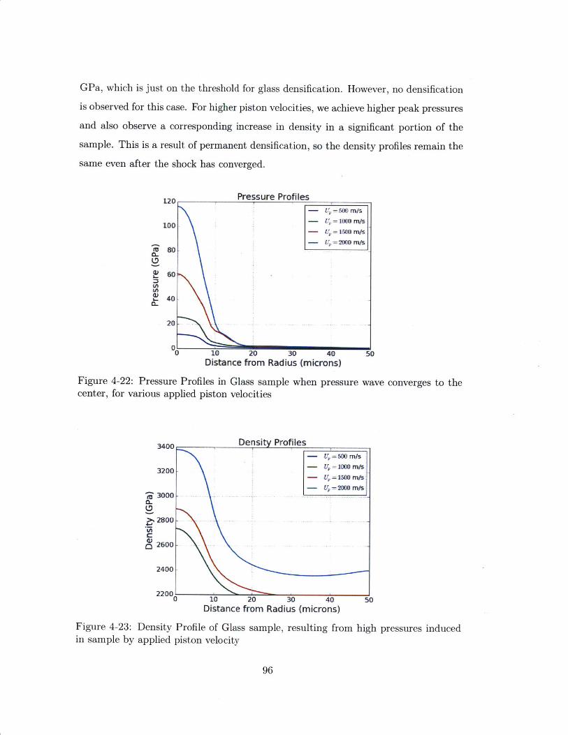
GPa, which is just on the threshold for glass densification. However, no densification

is observed for this case. For higher piston velocities, we achieve higher peak pressures

and also observe a corresponding increase in density in a significant portion of the

sample. This is a result of permanent densification, so the density profiles remain the

same even after the shock has converged.

120

'100

to0~I.,

U,U,

60

40

20

Pressure Profiles

0 10 20 30 40Distance from Radius (microns)

Figure 4-22: Pressure Profiles in Glass sample when pressurecenter, for various applied piston velocities

50

wave converges to the

Density Profiles

3200

3000

2800

S2600

2400

2200 10 20 30 40 50

Distance from Radius (microns)

Figure 4-23: Density Profile of Glass sample, resulting from high pressures inducedin sample by applied piston velocity

96

- U-=. MI

- u =loco nm/s2' = oMISU,=-" S

01

- T.5W m/s

- U.1500 m/s

- U = 2"3 m/s.. ....-. ...

"WL;

0

I

Overall, our initial simulations illustrate that this configuration has the potential

to cause transformation in glass. Furthermore, this experimental setup avoids the pre-

transformation fracture which occurs in the initially studied configuration. To more

accurately predict the pressures that we may achieve in this setup, we must develop

a correlation between laser energy and our applied piston velocity, which requires

experimental data from this setup. Nevertheless, this configuration is promising for

achieving glass transformation due to extreme loading.

4.4 Summary

In this Chapter, we explore two experimental configurations for initiating transforma-

tion in glass. We first study experiments where laser induced surface acoustic waves

are used to produce high pressures upon wave convergence. However, we observe

competing effects of transformation and fracture. High tensile stresses occur in the

samples prior to compressive stresses, causing the samples to break and preventing

significant compressive stresses necessary for transformation from occurring. In the

second configuration, shock waves are generated through the entire body of the sam-

ple rather than just the surface. This setup takes advantage of a converging setup,

which is found to provide very high pressures necessary for transformation. The

problem of fracture occurring prior to transformation is avoided here. As a next step,

one could determine correlations between experimental and simulation parameters,

and perform parameter studies with the intent of developing a design for maximizing

pressure. Such a design would allow for the study of glass under extreme conditions.

97

Chapter 5

Conclusion

5.1 Summary

The development of glass-based ballistic protection systems can be aided by simu-

lation tools utilizing accurate constitutive models. In this thesis, we have presented

several constitutive models developed to capture the high pressure response of glass

including during its densification process.

Our initial model was based on an equation of state for glass which gives its

volumetric response in the low density and high density regimes. A polynomial fit

connecting the low density and high density behavior was used to model the response

in the densification regime. This augmented equation of state was coupled with a

Neohookean model for shear to provide a full description of the stress tensor. How-

ever, at this point the model was purely elastic and unable to capture permanent

densification effects. Therefore, we introduced an internal variable known as the de-

gree of transformation to track densification progress. Given the current density and

degree of transformation, we could determine the unloading path and model increase

in density upon unloading from high pressures. This model introduced plasticity

in an ad-hoc manner and did not incorporate full 3D tensorial plasticity. Our final

model was an improvement which combined the volumetric behavior described by the

equation of state with important features of the Camclay volumetric plasticity model.

A yield condition based on pressure and shear and a flow rule permitting permanent

99

volumetric deformation were key ingredients which allowed us to model the effect of

shear and a severe degree of permanent densification. The model showed satisfactory

agreement to pressure-density data available in the literature and can represent up

to 77% relative densification as predicted by Sato [28] after high pressure loading.

For verification, we tested our constitutive models under shock conditions. We

performed finite element simulation of an idealized piston. Shock waves were gener-

ated in a constrained bar by applying a piston velocity at one end, and an artificial

viscosity formulation presented in f181 was employed to remove spurious oscillations

in the shock waves arising from the problem. The pressures and densities upstream

and downstream of the shock wave were measured for several piston velocities, and

found to agree to theoretically expected values obtained using the Rankine-Hugoniot

jump conditions.

Lastly, the constitutive models were used to study the efficacy of two experimental

configurations for generating high pressures, and ultimately transformation, in glass.

In the first configuration, surface acoustic waves were generated in cylindrical glass

samples via lasers. The convergence of these surface acoustic waves were hypothe-

sized to cause transformation in glass. To simulate these experiments, a correlation

was established between applied laser energy and the amplitude of the Gaussian force

distribution (an input to our simulations) resulting from laser application. Our simu-

lations illustrated propagation of two types of waves in the samples: a primary wave

(P-wave) and surface wave. We found that the P-waves traveled much faster than

the surface waves, and that divergence of the P-waves caused large tensile stresses

which would fracture experimental samples. Furthermore, the P-waves would diverge

before the surface waves could converge to the center and cause large compressive

pressures and transformation. Thus, we found that the fracture actually mitigated

the compressive pressures that could be achieved, and so this experimental setup was

inadequate for causing transformation.

In the second configuration, we conceived an experiment in which a laser is shined

on the outer surface of a cylindrical glass sample to generate uniaxial radial converging

waves through the thickness. The simulations illustrated that this configuration could

100

generate pressures required for glass transformation. Furthermore, any tensile stresses

capable of causing fracture would only occur after transformation had occurred. To

verify that this model is adequate for causing transformation, we need to obtain

experimental data to correlate the experiments to the simulations.

As a next step, we could improve the constitutive models developed in this work.

Some feasible improvements are given in the next section.

5.2 Model Improvements

Here we outline several improvements that can be made to our constitutive models.

" Effect of shear: Shear has been found to facilitate permanent densification in

glass [19j. To improve our model, we can develop a more accurate condition

for the onset of glass densification based on pressure and shear. Such a yield

criterion has been developed by Molnar et al. [23], who perform MD simulations

to determine combinations of pressure and shear which cause onset of glass

densification, and uses this data to construct a yield condition for densification.

They propose an elliptical yield surface (similar to that in our inelastic model)

which eventually evolves into a Drucker-Prager type surface as densification

progresses. We could adopt a similar yield criterion for our glass model, so that

the yield behavior incorporates data molecular dynamics. Experimental data

could also be incorporated to improve the description of yielding.

" Temperature: High temperature is also found to facilitate transformation in

glass [19, 13]. In this work, we neglect thermal effects. In the future, we may add

temperature as an input parameter which affects the volumetric deformation

behavior, as well as relative densification achieved in glass at a given pressure

loading. We may take advantage of the data collected in high temperature

studies on glass (such as in [13]) to aid our temperature modeling efforts.

" Densification: The model could be further refined by calibrating our pressure-

densification behavior (shown in Figure 2-11) to experimental data on relative

101

densification achieved from unloading at different pressures (as obtained by

Wakabayashi et al. in [35])

Incorporating the improvements listed above to our inelastic model for glass would

yield a more comprehensive glass model accounting for thermal and shear effects on

glass densification. Such a model can inspire new experimental configurations for

triggering phase transformation in glass, which in turn can provide experimental data

informing the constitutive models. This combined protocol in which simulations and

experiments guide each other can improve our understanding of glass densification

and lead to improved models. A better understanding of the behavior of glass under

extreme conditions, coupled with improved models which accurately describe this

behavior, can promote the design of effective glass-based protection systems.

102

Appendix A

Derivation of Rankine-Hugoniot

Jump Conditions

The Rankine-Hugoniot jump conditions are statements of the conservation of mass,

momentum and energy, in the presence of a shock wave as shown in Figure A-1. The

conservation of mass, momentum, and energy are given by

- Mass poU, = p(U, - Up)

- Momentum P - Po = pOUUp

- Energy E-EO = 1(P+Po)(Vo- V)

We prove these relations below, using the shock front in Figure A-1 as the center of

reference. The derivation presented here is based on [22].

UsPP E Po Po EO

Figure A-1: Shock Wave separating shocked and unshocked regions. There is a jumpin the thermodynamic state variables across the shock, which are related via theRankine-Hugoniot Jump Conditions.

103

Up

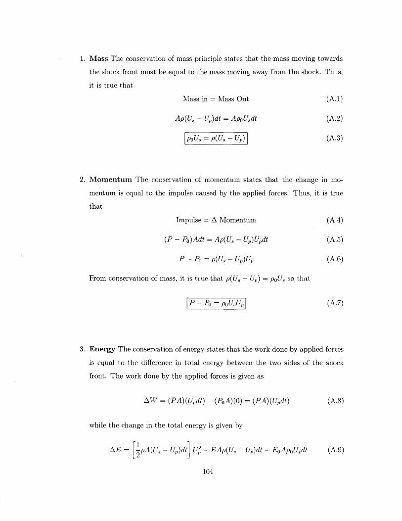
1. Mass The conservation of mass principle states that the mass moving towards

the shock front must be equal to the mass moving away from the shock. Thus,

it is true that

Mass in = Mass Out (A.1)

Ap(Us - Up)dt = Apo Usdt (A.2)

poU, = p(U -U) (A.3)

2. Momentum The conservation of momentum states that the change in mo-

mentum is equal to the impulse caused by the applied forces. Thus, it is true

that

Impulse = A Momentum (A.4)

(P - Po)Adt = Ap(U, - Up)Updt (A.5)

P - Po = p(U - up)up (A.6)

From conservation of mass, it is true that p(U, - Up) = poU, so that

P - P0 = poUsU, (A.7)

3. Energy The conservation of energy states that the work done by applied forces

is equal to the difference in total energy between the two sides of the shock

front. The work done by the applied forces is given as

AW = (PA)(Updt) - (P0 A)(0) = (PA)(Updt) (A.8)

while the change in the total energy is given by

AE = - pA(Us - Up)dt] U2 + EAp(U, - Up)dt - EoApoUndt (A.9)

104

Equating AW and AE, we obtain

AW = AE (A.10)

Pup [ p(Us - Up)1 U,2 - Eopo(U.) + Ep(U - Up) (A.11)

Applying conservation of mass stating that p(U, - Up) = poUs

= - Eo poUs + EpoUs (A.12)

PU, = Ipo UsU + po U,(E - Eo) (A.13)

Solving for E - EO gives

E - EO Pup 1 UsU (A.14)poUs 2 po Us

Applying conservation of momentum stating that Up = PO and substituting

for U,P(P-Po) 1 (P-Po)2E -Eo = P 0 8 2U202(A. 15)

p0 Us2 2 pgUs2

Combining conservation of mass and momentum

(PO - p)US = -pUp = - - PO) (A.16)Po U ,

1pOU -p(P - Po - ) (A.17)

Given that = V we have

P-P 0p2 Us = - (A.18)

VO - V

Substituting this into Equation A.15, we have

V 0 - V I (PPo) 2 pE - Eo = P(P - Po)- -0(2 -- V) (A.19)

P -PO 2 P- PO

105

or alternatively,

E - = (P + Po)(V - V) (A.20)2

106

Appendix B

Variational Formulation of Camclay

Theory of Plasticity

Here we present a variational formulation of the Camelay Theory for Granular Plas-

ticity developed by Ortiz and Pandolfi in [24] (more details can be found in the

reference). Our implementation of the inelastic model for glass is based heavily on

this formulation. For a more thorough review of the Camclay theory, one can refer

to [30].

B.1 Governing Equations

We begin by assuming a multiplicative decomposition of the deformation gradient F

into an elastic part F' and a plastic part FP as follows

F = FFp

The free energy is assumed to be of the form

A(F, FP, T, q) = We(Fe, T) + WP(T, q, FP)

107

where We is the elastic strain energy density, WP is the stored energy of cold work,

T is the temperature, and q represents a set of appropriate internal variables. Due to

material-frame indifference, We should only depend on F' by the elastic right-Cauchy

Green deformation tensor Ce

Ce = FeTFe = FP-TCFPl

so that the frame indifferent free energy has the appropriate arguments

A(F, FP, T, q) = We (Ce, T) + WP(T, q, FP) (B.1)

The elastic strain energy density We is assumed to be decoupled into volumetric and

deviatoric components We,"' and Wedev as follows:

we (Ce, T) = We'vol(Je, T) + We'dev(Ce'dev, T) (B.2)

where We,vol and Wedev are given by

K TT1we'Vol(Je, T) = -[log Je - 3a(T - T) 2 PoT -log T2 +PTO (

Wedev = [tee 2 (B.4)

In Equations B.3 and B.4, je is the Jacobian of the elastic deformation, K is the

isothermal bulk modulus, a is the thermal expansion coefficient, T and To the cur-

rent and reference absolute temperature respectively, po the mass density per unit

undeformed volume, Cv the specific heat per unit mass (constant volume), and [t the

shear modulus. The equation of state resulting from We,vol is

p = K(Oe - 3a(T - To)) (B.5)

108

and define the logarithmic elastic strain as

e 1E log(C )

2(B.6)

The stored energy WP is a function of the effective plastic strain JP and the volumetric

plastic strain OP = log JP so that

A(F, FP, T, EP) = We(Ce, T) + WP(T, EP, OP) (B.7)

The flow rule is assumed to be of the form

FPFP-' = eM, cP > 0 (B.8)

where iP is the effective plastic strain rate and M is the direction of plastic flow

satisfying the following kinematic constraint

1 ' .-+ (Mde- Mde=

a 3(B.9)

with Mdev being the deviatoric part of M and a defined as an internal friction coeffi-

cient. We assume linear rate-sensitivity and accordingly define a dual kinetic potential

as follows

* ( p)22

(B.10)

where j is a viscosity constant.

B.1.1 Update Algorithm

The flow rule given by Equation B.8 may be discretized in time as

FP+1 =exp(AePM)FP

0"1= ACP(trM)O%

(B.11)

(B.12)

109

The problem is solved incrementally by formulating the following incremental energy

function

fn(Fn+1, Tn+1; E-n+1, M) = We(Fe + 1, Tn+1 ) + WP(Tn+1, e6+i, 0+1) + At* (A /At)

(B.13)

and defining an effective work of deformation by minimizing fA with respect to En+1

and M

Wa (Fn+1 , Tn+)= min fn(Fn+1,Tn+1;+ 1 , M)c+1M

(B.14)

subject to the kinematic constraint in Equation B.9 and the plastic irreversibility

constraint

AEP = ePn+i - er > 0 (B.15)

One can show that Wn is a potential for the first Piola-Kirchoff stress tensor Pn+1

OWnPn+1 = 0Y+ (Fn+1, Tn+1) (B.16)

Furthermore, the consistent tangent moduli is given by

DPn+1 = 2 (Fn+l, Tn+l)o9Fn+1i9Fn+1

(B.17)

B.1.2 Implementation based on logarithmic elastic strains

The incremental work of deformation can be written in the form below if we ex-

press the strain energy density in terms of logarithmic elastic strain and consider the

discretized flow rule B.11

fn= W (log[exp(-Ae/M)C*('eP/'L )PM)], Tn+l}+WP(Tn+1, En+1 n+1)+Ato. (AE

(B.18)

the predictor elastic right Cauchy-Green tensor is defined as

Cn 'Pre = FP-T C+FP-1 (B.19)

110

We assume commutativity of plastic flow direction M with elastic predictor as follows

MCi =e C ,re M (B.20)

The following identity holds under these conditions

log[exp(-AePM)C e,re exp(-AEPM)] = log(C 'P'e) -pMrM (B.21)

From the kinematic constraint in Equation B.9 and the above definition we have

Ap = 12(AP)2 + 2AeP -AeP (B.22)

where the deviatoric part of the incremental plastic strain is

AeP = AEpdev - Ap - 1AGpj3

(B.23)

The incremental relations for plastic strains

E P+1 = E + AEO

OPn+ = OPn + AOP

(B.24)

(B.25)

may be inserted into the incremental work of deformation to give the following

fn(F.+1 , Tn+1 ; AcP) = e+1're - , Tn+1) + WP(Ta+1, 6+D+1) + Atn1*(AeP/At)

(B.26)

where the elastic predictor strain is given by

1Ce'pre = log(C''),n+1 -2 lo(C+1?

111

(B.27)

The incremental work of deformation may be optimized with respect to the incre-

mental plastic strain, resulting in the following Euler-Lagrange equations

-crn+l + [Uo(C+1, O1+) + 2*' (AP/At)][API + e]/A + Po(epn+ 1 , On+1)I = 0

(B.28)

where the critical uniaxial stress and pressure are given by

aWP

PWPPO = 00

and the conjugate stress tensor to the logarithmic elastic strain is given by

aWe17 K I + 2p-ee

ae,yre

The stress tensor un+1 is given by

Tn+l = K(Onlf - AOP)I + 2p(en',' AeP)

and can also be separated into its volumetric and deviatoric components

Pn+1 = K(Oe'pe - AOP) pn'r+1 KAOP

2pre - AeP) =rl- 2pAeP

(B.29)

(B.30)

(B.31)

(B.32)

(B.33)

(B.34)

(B.35)

where

dev 1s = adev = 0 - -(trM)I3

(B.36)

Decomposing the Euler-Lagrange Equation B.28 into volumetric and deviatoric com-

ponents results in

,/ I AOP-p'li + KAOP + PO,n+i + (0O7,n+i + )__ = 0

a_ 2 0~(B.37)

112

-spre 1 + 2pAeP + (uo,,+1 + 2* ) = 0n+ 3 AEP

Taking the norm of the deviatoric equation gives

pre 2 1 2 AeP - AePqn+)2 = (3pAEP + CO7,n+l + * 2 A Ep2

where

(qr+e)2 = 3pre . Sp+q~ sl2 +1 n7l~

Inserting Equations B.37 and B.39 into the constraint given in Equation B.22 results

in the following identity

( pre 2

n+1

3pdtEP + (-0,n+1 + ?P*'+ (Ky71 - P,n+1? 2

(a2KAEP + u-o,,+1 + ip*')

which is satisfied under the following conditions

+1pre - (3tAc + O-O,n+ + 0*') COS (B.42)

Ppe1 = PO,n+i + [aKAEP + (uo,n+1 + 0*')/a] sin # (B.43)

The system of equations B.43 can be solved using Newton-Raphson iteration. This

requires a linearization of the equations to the following form

dqp+71 = CjidEp 1 + C1 2d$

dP'+n1 = C21den+1 + C22 d4

(B.44)

(B.45)

113

(B.38)

(B.39)

(B.40)

= 1 (B.41)

where the constants C11, C12, C21 and C22 are given below

C1 = (3p + + HE,n+I + aHeo,n+1 sin # cos#

(B.46)

C12 = aHeo,n+ 1 AEP cos 2 # - (3pAEP + 0,n+i+ )*') sin 0

(B.47)

C21= HoE,n+1 + (aK + + cfHoo,n+laAt

1+ -He,n+I + HeO,n+i sin sin #

(B.48)

C22 = (aHoo,n+iAEP + Heo,n+1 AEP sin 0 + IaKAEP + +a(-0n1 + *)Cos

(B.49)

and the hardening moduli are defined as

Hoo9 09Po - a 2 Wp (OP, EP)

0Po - 2W OP P)&6 P 0OP19eP

Ho- 0 (OP EP)

0 P0P 'OO

00p0 02WP

H OE (OP, & O )P9o-o _ 2 W P, P

(B.50)

(B.51)

(B.52)

(B.53)

(B.54)

B.1.3 Yield Criterion

The yield criterion for the Camclay model is obtained by setting AcE equal to zero

in Equation B.41, giving

2 _ 2 02 (B.55)

The elliptical yield surface corresponding to Equation B.55 is shown below. The

internal friction parameter a is related to the friction angle # as follows.

6 tan 4a =

3 - tan5(B.56)

114

The internal friction parameter is also depicted in the yield surface in Figure B-1.

PC P P

Figure B-1: Yield Surface of the Camclay Model

We omit details regarding the consolidation and hardening behavior of soils in the

Camclay theory, but one can look to Reference [30] for more details on these aspects

of the model.

115

Appendix C

Time Integration Procedure for

Inelastic Model for Glass

An algorithm for the time-integration of the inelastic model for glass is given in this

Appendix.

C.1 Time-Integration Procedure

The time integration procedure for the glass model is as follows:

Given: FP and Fn+1

Calculate: O-n+1, Fp+,

Step 1 Calculate the predictor elastic deformation gradient

(C.1)

Step 2 Compute the right Cauchy-Green tensor and the predictor logarithmic strain

C epr= F efre Fi( e~n+1 n+1 n+1

Ce~pre = log (C e)

(C.2)

(C.3)

117

Fn+1 = n+1FK1

Step 3 Calculate the predictor deviatoric and volumetric components of the stress

tensor:

sn+1 = o+dev - 2,ep*

Ka

k1Ka p - K

kn+ p- - i]

(Po a

\POa)- ]1 [i - tanh X In ( )

\ Po

(C.4)

(C.5)

Step 4 Calculate the yield function or overstress (based on the current stress state)

as

f (p, q) = q2 + a2(pP) - .2 (C.6)

where

P = Pn+1

q = 'j s. where s = sn+12:

Po = PO,n+1 = -0En+1

19WPq0 = qo,n+i = -

wsn+1

where the incremental stored energy function is

(C.7)

(C.8)

(C.9)

(C.10)

1Wn+1 = Wnp + 2 [W(On+1 ) - Wcg(On)I -

(C.12)We(OP) = op pedOP = pref,,f coshJ ( ref

Step 5 Determine whether stress state corresponds to the elastic or plastic regime

1. If f < 0 -* Elastic

7n+1 sn+i + Pn+I and we are DONE

2. Else -+ Plastic Perform a Newton-Raphson iteration to solve Equations C.13

118

with

(C.11)-Wf'( n+1)AE-P

and C.14 for AcP and V/*' (and follow Steps 6-9)

q Pre (3pAEc + o-o,n+l + 0*') cos

Pf+7I = PO,n+1 + [aKAcP + (O-on+ 1 + l*')/a] sin #

(C.13)

(C.14)

Step 6 Update FP using the exponential map

FP = exp(AtD$+1)Fp (C.15)

where DPn+1 is the direction of plastic flow.

Step 7 Update the plastic jacobian and relative densification parameter

JP = det(Fn+1 ) (C.16)

(C.17)1)

Step 8 Compute final pressure in glass as a weighted average of the low and high

density glass EoS

Pn+I = (v/1 - 2AP)pilo eos + (1 - 2 AP)Phigh eos

Step 9 The .final Cauchy stress tensor is given by

I-~n+1= Sn+1 + Pn+1I

rb

119

(C.18)

(C.19)

AP = I-

Bibliography

[1] C.S. Alexander et al. "Changes to the shock response of fused quartz due to

glass modification". In: International Journal of Impact Engineering 35 (2008),

pp. 1376-1385. DOI: 10. 1016/j .ijimpeng.2008.07.019.

[2] J.R. Asay and M. Shahinpoor. High-Pressure Shock Compression of Solids. New

York: Springer-Verlag, 1993.

[31 B. Aydelotte and B. Shuster. "A Computational Study of the ARL Glass Model

and its Predictions of Ballistic Penetration and Fracture Conoid Development".

In: 28th International Symposium on Ballistics. Atlanta, Geogia, USA, Sept.

2014.

[4] R. Becker. Steps Toward Glass-Specific Models in Parallel Design Codes. Tech.

rep. Herndon, VA: ARL, May 2010.

[5] P.W. Bridgman and I. Simon. "Effects of Very High Pressures on Glass". In:

Journal of Applied Physics 24 (1953), pp. 405 -413. DOI: 10.1063/1.1721294.

[6] E.B. Christiansen, S.S. Kistler, and W.B. Gogarty. "Irreversible Compressibility

of Silica Glass as a Means of Determining the Distribution of Force in High-

Pressure Cells". In: Journal of the American Ceramic Society 45 (1962), pp. 172

-177. DOI: 10.1111/j.1151-2916.1962.tbllll5.x.

[7] R.J. Clifton, M. Mello, and N.S. Brar. "Effect of shear on failure waves in

soda lime glass". In: AIP Conference Proceedings 429 (1998), pp. 521-524. DOI:

10.1063/1.55558.

121

[8] H.M. Cohen and R. Roy. "Effects of Ultra high Pressures on Glass". In: Journal

of the American Ceramic Society 44 (1961), pp. 523 -524. DOI: 10. 1111/j .

1151-2916.1961.tb13717.x.

[9] R. Fabbro et al. "Physical study of laser-produced plasma in confined geometry".

In: Journal of Applied Physics 68.2 (1990), pp. 775-784. DOI: 10 . 1063/1 .

346783. eprint: https: //doi . org/10. 1063/1.346783. URL: https: //doi.

org/10.1063/1.346783.

[101 Thomas Fronk. "Accelerated computational modeling of ballistic helmet test

protocols". MA thesis. Massachusetts Institute of Technology, 2016. URL: http:

//hdl.handle.net/1721.1/108930.

[11] A.G. Gazonas et al. Multiscale Modeling of Non-crystalline Ceramics (Glass).

Technical Report 0765. US Army Research Laboratory, 201.

[12] M. Grujicic et al. "The effect of high-pressure densification on ballistic pen-

etration resistance of a soda-lime glass". In: Journal of Materials Design and

Applications Part L (2011), pp. 298-315. DOI: 10.1177/1464420711412849.

[13] M. Guerette et al. "Structure and Properties of Silica Glass Densified in Cold

Compression and Hot Compression". In: Scientific Reports 5 (2015), pp. 1-10.

DOI: 10. 1038/srep15343.

[141 T.J. Holmquist and G.R. Johnson. "A Computational Constitutive Model for

Glass Subjected to Large Strains, High Strain Rates, and High Pressures". In:

Journal of Applied Mechanics 78 (2011), pp. 1-9. DOI: 10.1115/1.4004326.

[15] V. Keryvin et al. "Constitutive modeling of the densification process in silica

glass under hydrostatic compression". In: Acta Materialia 62 (2014), pp. 250-

257. DOI: 10.1016/j .actamat.2013.07.067.

[16] H. Kolsky. Stress Waves in Solids. Dover Publications, 1963.

[17] J.C. Lambropoulos, S. Xu, and T. Fang. "Constitutive Law for the Densification

of Fused Silica, with Applications in Polishing and Microgrinding". In: Journal

122

of the American Ceramic Society 79 (1996), pp. 1441-1452. DOI: 10. 1111/j .

1151-2916.1996.tb08748.x.

[18] A. Lew, R. Radovitzky, and M. Ortiz. "An artificial-viscosity method for the

lagrangian analysis of shocks in solids with strength on unstructured, arbitrary-

order tetrahedral meshes". In: Journal of Computer-Aided Materials Design 8.2-

3 (2001), pp. 213-231. DOI: 10. 1023/A: 1020064403005.

[19] J.D. Mackenzie. "High-Pressure Effects on Oxide Glasses: I, Densification in

Rigid State". In: Journal of the American Ceramic Society 46 (1963), pp. 461

-470. DOI: 10.1111/j.1151-2916.1963.tb13776.x.

[20] S.P. Marsh. LASL Shock Hugoniot Data. University of California Press, 1980.

[21] R.G. McQueen, J.N. Fritz, and S.P. Marsh. "On the Equation of State of

Stishovite". In: Journal of Geophysical Research 68 (1963), pp. 2319-2322. DOI:

10.1029/JZ068i008p02319.

[22] M.A. Meyers. Dynamic behavior of materials. Wiley Interscience, 1994.

[23] G. Molnar et al. "Densification dependent yield criteria for sodium silicate

glasses - An atomistic simulation approach". In: Acta Materialia 111 (2016),

pp. 129-137. DOI: 10.1016/j.actamat.2016.03.053.

[24] M. Ortiz and A. Pandolfi. "A variational Cam-clay theory of plasticity". In:

Computer Methods in Applied Mechanics and Engineering 193 (2004), pp. 2645-

2666. DOI: 10 . 1016 / j . cma . 2003 . 08 . 008. URL: http : / / linkinghub .

elsevier.com/retrieve/pii/SO045782504000817.

[25] Ortiz, M. and Pandolfi, A. "A variational Cam-clay theory of plasticity". In:

Computer Methods in Applied Mechanics and Engineering 193 (2004), pp. 2645-

2666. DOI: 10. 1016/j . cma.2003.08.008. URL: file: ///tmp/literature/

2003-cmame-pandolfi.pdf.

[26] A. Polian and M. Grimsditch. "Room-temperature densification of a-SiO 2 versus

pressure". In: Physical Review B 41 (1990), pp. 6086-6089. DOI: 10 . 1103 /

PhysRevB.41.6086.

123

[27] R. Radovitzky et al. "A scalable 3D fracture and fragmentation algorithm based

on a hybrid, discontinuous Galerkin, Cohesive Element Method". In: Computer

Methods in Applied Mechanics and Engineering 200 (2011), pp. 326-344. DOI:

10. 1016/j .cma.2010.08.014.

[28] T. Sato and N. Funamori. "Sixfold-Coordinated Amorphous Polymorph of SiO 2

under High Pressure". In: Physical Review Letters 101 (2008), pp. 1-4. DOI:

10.1103/PhysRevLett.101.255502.

[29] W. Schill et al. "The anomalous yield behavior of fused silica glass". In: Journal

of the Mechanics and Physics of Solids 113 (2018), pp. 105-125. DOI: 10. 1016/

j .jmps.2018.01.004.

[30] A. Schofield and P. Wroth. Critical State Soil Mechanics. London: McGraw-Hill,

1968.

[311 S. Sundaram and R.J. Clifton. "Flow behavior of soda-lime glass at high pres-

sures and high shear rates". In: A IP Conference Proceedings 429 (1998), pp. 517-

520. DOI: 10.1063/1.55556.

[32] S. Susman et al. "Intermediate-range order in permanently densified vitreous

SiO 2 : A neutron-diffraction and molecular dynamics study". In: Journal of the

American Ceramic Society 46 (1963), pp. 461 -470. DOI: 10. 1103/PhysRevB.

43.1194.

[33] D. Veysset. "Real-Time Observations of Materials under Dynamic Loading Con-

ditions at the Micron Scale". PhD thesis. MIT, 2016. URL: http: //hdl. handle.

net/1721. 1/104573.

[34] D. Veysset et al. "Acoustical breakdown of materials by focusing of laser-

generated Rayleigh surface waves". In: Applied Physics Letters 111 (2017),

pp. 1-4. DOI: 10 . 1063/1.4993586.

[35] D. Wakabayashi. "Compression behavior of densified a-Si0 2 glass". In: Physical

Review B 84 (2011), pp. 1-6. DOI: 10.1063/1. 1777192.

124

[361 L.V. Woodcock, C.A. Angell, and P. Cheeseman. "Molecular dynamics studies of

the vitreous state: Simple ionic systems and silica". In: The Journal of Chemical

Physics 65 (1976), pp. 1565-1577. DOI: 10.1063/1.433213.

[37] A. Yokoyama et al. "Elastic wave velocities of silica glass at high temperatures

and high pressures". In: Journal of Applied Physics 107 (2010), pp. 1-5. DOI:

10.1063/1.3452382.

[38] C. Zha et al. "Acoustic velocities and refractive index of Si-0 2 glass to 57.5 GPa

by Brillouin scattering". In: Physical Review B Condensed Matter 50 (1994),

pp. 105-112. DOI: 10. 1103/PhysRevB. 50.13105.

125

redacted - MIT's DSpace - Massachusetts Institute of Technology

Documents

Transcript of redacted - MIT's DSpace - Massachusetts Institute of Technology