Nonlinear Vibration Energy Harvesting - MIT's DSpace

Nonlinear Vibration Energy Harvesting:fundamental limits, robustness issues, and practical

approaches

by

Ashkan Haji Hosseinloo

Submitted to the Department of Mechanical Engineeringin partial fulfillment of the requirements for the degree of

Doctor of Philosophy in Mechanical Engineering

at the

MASSACHUSETTS INSTITUTE OF TECHNOLOGY

June 2018

c Massachusetts Institute of Technology 2018. All rights reserved.

Author . . . . . . . . . . . . . . . . . . . . . . . . . . . . . . . . . . . . . . . . . . . . . . . . . . . . . . . . . . . . . . . .Department of Mechanical Engineering

May 15, 2018

Certified by. . . . . . . . . . . . . . . . . . . . . . . . . . . . . . . . . . . . . . . . . . . . . . . . . . . . . . . . . . . .Konstantin TuritsynAssociate Professor

Thesis Supervisor

Accepted by . . . . . . . . . . . . . . . . . . . . . . . . . . . . . . . . . . . . . . . . . . . . . . . . . . . . . . . . . . .Rohan Abeyaratne

Chairman, Department Committee on Graduate Theses

Nonlinear Vibration Energy Harvesting: fundamental limits,

robustness issues, and practical approaches

by

Ashkan Haji Hosseinloo

Submitted to the Department of Mechanical Engineeringon May 15, 2018, in partial fulfillment of the

requirements for the degree ofDoctor of Philosophy in Mechanical Engineering

Abstract

The problem of a scalable energy supply is one of the biggest issues in miniaturizingelectronic devices. Advances in technology have reduced the power consumption ofelectronic devices such as wireless sensors, data transmitters, and medical implants tothe point where harvesting ambient vibration, a universal and widely available sourceof energy, has become a viable alternative to costly and bulky traditional batteries.However, implementation of vibratory energy harvesters is currently impeded by threemain challenges: broadband harvesting, low-frequency harvesting at small (micro)scales, and robust energy harvesting at presence of parametric uncertainties.

This thesis investigates two main directions for effective vibration energy harvest-ing: (i) fundamental limits to nonlinear energy harvesting and techniques to approachthem, and (ii) robust energy harvesting under uncertainties. As well as being offundamental scientific interest, understanding maximal power limits is essential forassessment of the technology potential and it also provides a broader perspective onthe current harvesting mechanisms and guidance in their improvement. We beginby developing a general framework and model hierarchy for the derivation of fun-damental limits of the nonlinear energy harvesting rate based on Euler-Lagrangianvariational approach. The framework allows for an easy incorporation of almost anyconstraints and arbitrary forcing statistics and represents the maximal harvestingrate as a solution of either a set of DAEs or a standard nonlinear optimization prob-lem. Closed-form expressions are derived for two cases of damping-dominated anddisplacement-constrained motion.

Stemming from the study of fundamental limits, we present an almost-universalstrategy termed buy-low-sell-high (BLSH) to maximize the harvested energy for awide range of set-ups and excitation statistics. We further propose two techniques torealize the non-resonant BLSH strategy, namely latch-assisted harvester and adaptivebistable harvester. To validate the efficacy of the proposed strategy and practicaltechniques, we perform a simulation experiment by exposing the said harvesters toharmonic and experimental, random walking-motion excitations; it is shown thatthey outperform their linear and conventional bistable counterparts in a wide range

3

of harmonic excitation and random vibration.Furthermore, we propose to harvest energy by exploiting surface instability or in

general instability in layered composites which is, in part, motivated by the BLSHstrategy. Instabilities in soft matter and composite structures e.g. wrinkling allowlarge local strains to take place throughout the entire structure and at regular pat-terns. Unlike conventional harvesting techniques, this allows to harvest energy fromthe entire volume of the structure e.g. by attaching piezoelectric patches at large-strain locations throughout the structure. We show that this significantly improvesthe power to volume ratios of the harvesting devices. In addition, these structural in-stabilities are non-resonant that consequently enhances robustness of such harvesterswith respect to excitation characteristics. The high efficacy of energy harvesting viastructural instabilities, in part, is attributed to its ability to approximately follow theBLSH logic. Additionally, we put forth the idea of extending this idea to control theinstability; and hence, extend the application of the aforementioned idea from energyharvesting to a whole new level of tunable material/structures with a myriad of ap-plications from electromechanical sensors and amplifiers to fast-motion actuators insoft robotics.

And last but not least, to more specifically address the robustness issues of passiveharvesters, we propose a new modeling philosophy for optimization under uncertainty;optimization for the worst-case scenario (minimum power) rather than for the ensem-ble expectation of the power. The proposed optimization philosophy is practicallyvery useful when there is a minimum requirement on the harvested power. We for-mulate the problems of uncertainty propagation and optimization under uncertaintyin a generic and architecture-independent fashion. Furthermore, to resolve the ubiq-uitous problem of coexisting attractors in nonlinear energy harvesters, we proposea novel robust and adaptive sliding mode controller for active harvesters to movethe harvester to any desired attractor by a short entrainment on the desired attrac-tor. The proposed controller is robust to disturbances and unmodeled dynamics andadaptive to the system parameters.

Thesis Supervisor: Konstantin TuritsynTitle: Associate Professor

4

Acknowledgments

Firstly, I would like to express my sincere gratitude to my advisor Prof. Konstantin

(Kostya) Turitsyn for the continuous support of my Ph.D study and related research,

for his patience, motivation, and immense knowledge. I could not have imagined hav-

ing a better advisor and mentor for my Ph.D study. Besides my advisor, I would like

to thank the rest of my thesis committee: Prof. Steven Leeb and Prof. Themistoklis

Sapsis for serving as my committee members and for their insightful comments and

encouragement. I would also like to thank Prof. Jean-Jacques Slotine for introduc-

ing me to nonlinear control and for his enriching discussions on nonlinear control of

co-existing attractors in energy harvesters.

A very special thank you to Profs. Hover, Rodriguez, Youcef-Toumi, my advisor

Prof. Turitsyn, Dr. Chin, and Dr-to-be’s Xinchen Ni and Benjamin Charles Druecke

(with whom I TA’ed dynamics twice) for making my dynamics and controls teaching

experiences so enjoyable. Also, I sincerely appreciate the support, guidance and

advice of Leslie Regan, Joan Kravit and Una Sheehan.

A very sincere thank you to my fellow labmates for the stimulating discussions

and all the fun we have had in the last four years. I would also like to thank my

friends, Reyhaneh, Nima, Setareh, Sasan, Hussein, Safa, Mojtaba and all my other

friends at MIT and elsewhere, without whom this long journey would not have been

possible. Any acknowledgement in this thesis of my friends and the profound role

they have played in my life would fail to do true justice.

Last but most certainly not the least, I would like to thank my family: my parents

and my brother for supporting me spiritually throughout my Ph.D study and my life

in general.

5

Contents

1 Introduction 21

1.1 Challenges of vibratory energy harvesting . . . . . . . . . . . . . . . . 23

1.1.1 broadband and low-frequency energy harvesting . . . . . . . . 23

1.1.2 robust energy harvesting under uncertainty . . . . . . . . . . . 27

1.2 Thesis overview . . . . . . . . . . . . . . . . . . . . . . . . . . . . . . 28

2 Fundamental limits to nonlinear energy harvesting 31

2.1 A generic framework . . . . . . . . . . . . . . . . . . . . . . . . . . . 33

2.1.1 no constraints . . . . . . . . . . . . . . . . . . . . . . . . . . . 34

2.1.2 displacement constraints . . . . . . . . . . . . . . . . . . . . . 34

2.1.3 damping-constrained motion . . . . . . . . . . . . . . . . . . . 36

2.1.4 a general case . . . . . . . . . . . . . . . . . . . . . . . . . . . 37

2.2 Force constraints . . . . . . . . . . . . . . . . . . . . . . . . . . . . . 40

2.3 Non-resonant latch-assisted (LA) energy harvesting . . . . . . . . . . 42

2.4 Summary and conclusion . . . . . . . . . . . . . . . . . . . . . . . . . 46

3 Non-resonant energy harvesting via an adaptive bistable potential 49

3.1 Adaptive bistable harvester . . . . . . . . . . . . . . . . . . . . . . . 50

3.1.1 BLSH: adaptive bistability logic . . . . . . . . . . . . . . . . . 51

3.1.2 mathematical modeling . . . . . . . . . . . . . . . . . . . . . . 52

3.2 Results and discussion . . . . . . . . . . . . . . . . . . . . . . . . . . 56

3.2.1 harmonic excitation . . . . . . . . . . . . . . . . . . . . . . . . 56

3.2.2 random excitation: waking motion . . . . . . . . . . . . . . . 60

7


4 Energy harvesting from structural instabilities 65

4.1 Wrinkling instability . . . . . . . . . . . . . . . . . . . . . . . . . . . 67

4.1.1 general idea . . . . . . . . . . . . . . . . . . . . . . . . . . . . 67

4.1.2 mathematical modeling . . . . . . . . . . . . . . . . . . . . . . 68

4.2 Numerical results and discussion . . . . . . . . . . . . . . . . . . . . . 72

4.3 Conclusion and future directions . . . . . . . . . . . . . . . . . . . . . 75

5 Design of vibratory energy harvesters under stochastic parametric

uncertainty 77

5.1 Mathematical model . . . . . . . . . . . . . . . . . . . . . . . . . . . 80

5.2 Uncertainty propagation and optimization formulation . . . . . . . . 82

5.3 Numerical results and discussion . . . . . . . . . . . . . . . . . . . . . 84


6 Robust and adaptive control of coexisting attractors in nonlinear

vibratory energy harvesters 97

6.1 Mathematical modeling of an active nonlinear harvester . . . . . . . . 100

6.2 Robust and adaptive sliding mode control . . . . . . . . . . . . . . . 102

6.2.1 generic formulation . . . . . . . . . . . . . . . . . . . . . . . . 102

6.2.2 application to bistable harvester . . . . . . . . . . . . . . . . . 104

6.3 Results and discussion . . . . . . . . . . . . . . . . . . . . . . . . . . 106


7 Conclusion and contributions 115

A List of publications 119

8

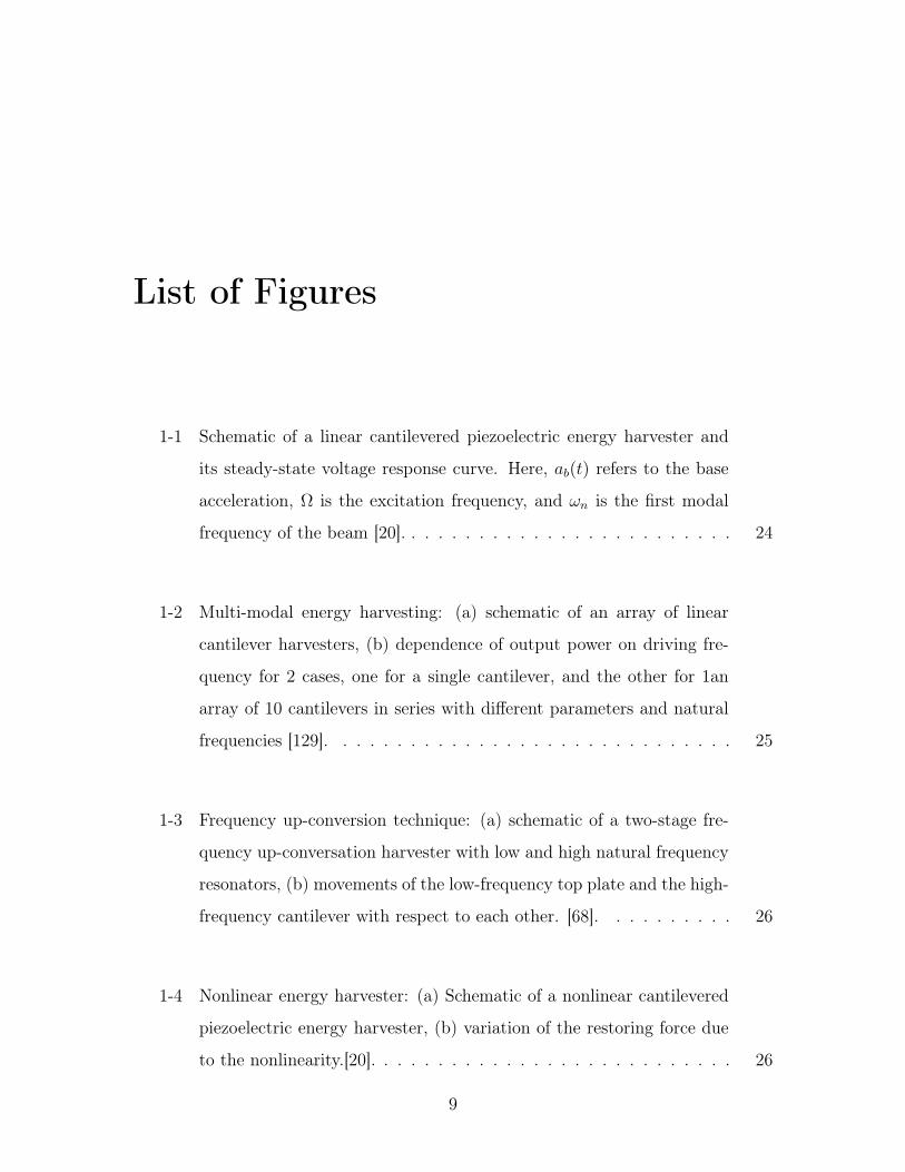
List of Figures

1-1 Schematic of a linear cantilevered piezoelectric energy harvester and

its steady-state voltage response curve. Here, 𝑎𝑏(𝑡) refers to the base

acceleration, Ω is the excitation frequency, and 𝜔𝑛 is the first modal

frequency of the beam [20]. . . . . . . . . . . . . . . . . . . . . . . . . 24

1-2 Multi-modal energy harvesting: (a) schematic of an array of linear

cantilever harvesters, (b) dependence of output power on driving fre-

quency for 2 cases, one for a single cantilever, and the other for 1an

array of 10 cantilevers in series with different parameters and natural

frequencies [129]. . . . . . . . . . . . . . . . . . . . . . . . . . . . . . 25

1-3 Frequency up-conversion technique: (a) schematic of a two-stage fre-

quency up-conversation harvester with low and high natural frequency

resonators, (b) movements of the low-frequency top plate and the high-

frequency cantilever with respect to each other. [68]. . . . . . . . . . 26

1-4 Nonlinear energy harvester: (a) Schematic of a nonlinear cantilevered

piezoelectric energy harvester, (b) variation of the restoring force due

to the nonlinearity.[20]. . . . . . . . . . . . . . . . . . . . . . . . . . . 26

9

2-1 Contour plot of optimal average harvested power with penalty coef-

ficient 𝑒 = 5 as a function of penalty coefficient 𝑑 and displacement

limit 𝑥max when subjected to harmonic excitation 𝐹 (𝑡) = 2 sin(0.1𝑡).

The numerical values of 𝑚 = 1 and 𝑐𝑚 = 1 are used. The dashed

red line shows the transition from the potentially harvestable regime

to the non-harvestable regime. The inset shows the optimal average

power in terms of 𝑑 for different values of 𝑒 for a fixed displacement

limit of 𝑥max = 1.5. . . . . . . . . . . . . . . . . . . . . . . . . . . . . 39

2-2 Power flow diagram of the VEH consisting of the main harvesting sys-

tem coupled with its harvesting controller. . . . . . . . . . . . . . . . 41

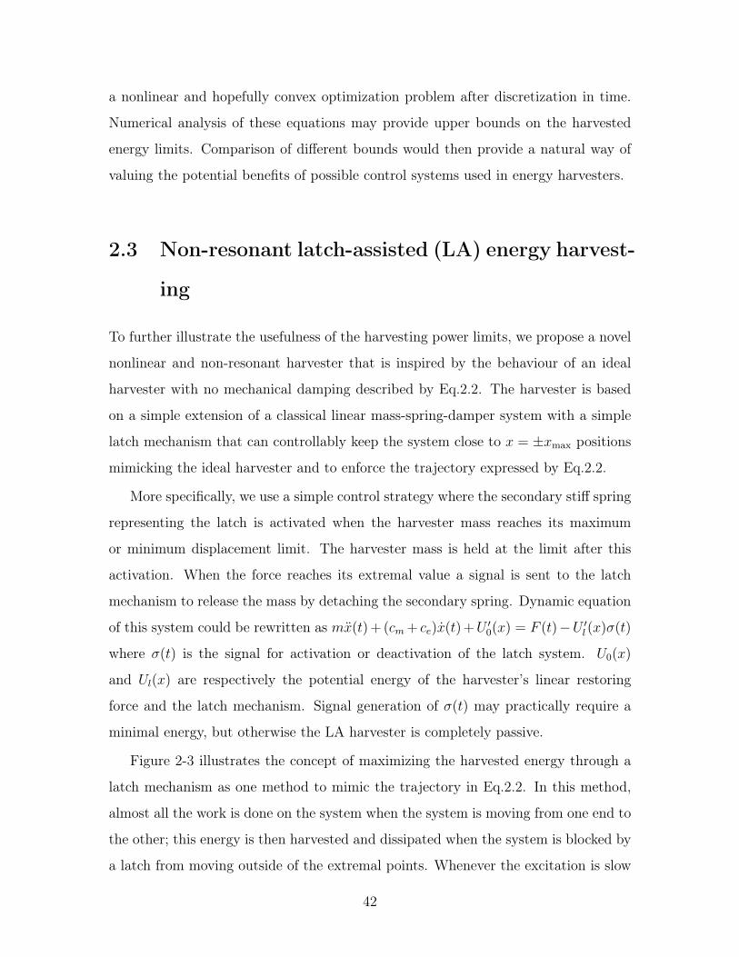
2-3 Latch-assisted harvester: here, an energy harvester with linear mechan-

ical and electrical damping, and linear stiffness is considered. Vibration

travel is constrained to 1.5 units i.e. |𝑥(𝑡)| ≤ 1.5. . . . . . . . . . . . 43

2-4 Displacement and energy time histories: (a) depicts the displacement

time history for the three linear, bistable, and latch-assisted harvesters.

Damping ratios of 𝜁𝑚 = 0.02 and 𝜁𝑒 = 0.1, and displacement limit of

1.5 units are used. The excitation is harmonic of the form 𝐹 (𝑡) =

2 sin(0.1𝑡) and its scaled waveform (scaled to unity in amplitude) is

plotted as dashed line, (b) depicts the corresponding energy time his-

tory for the three harvesters. . . . . . . . . . . . . . . . . . . . . . . . 44

2-5 Phase and force-displacement diagrams: (a) depicts the phase diagram

for the three linear, bistable, and latch-assisted systems. Damping

ratios of 𝜁𝑚 = 0.02 and 𝜁𝑒 = 0.1, and displacement limit of 1.5 units

are used. The excitation is harmonic of the form 𝐹 (𝑡) = 2 sin(0.1𝑡).

(b) depicts the force-displacement curves for the linear, bistable, latch-

assisted mechanism, and ideal harvester with no mechanical damping. 45

10

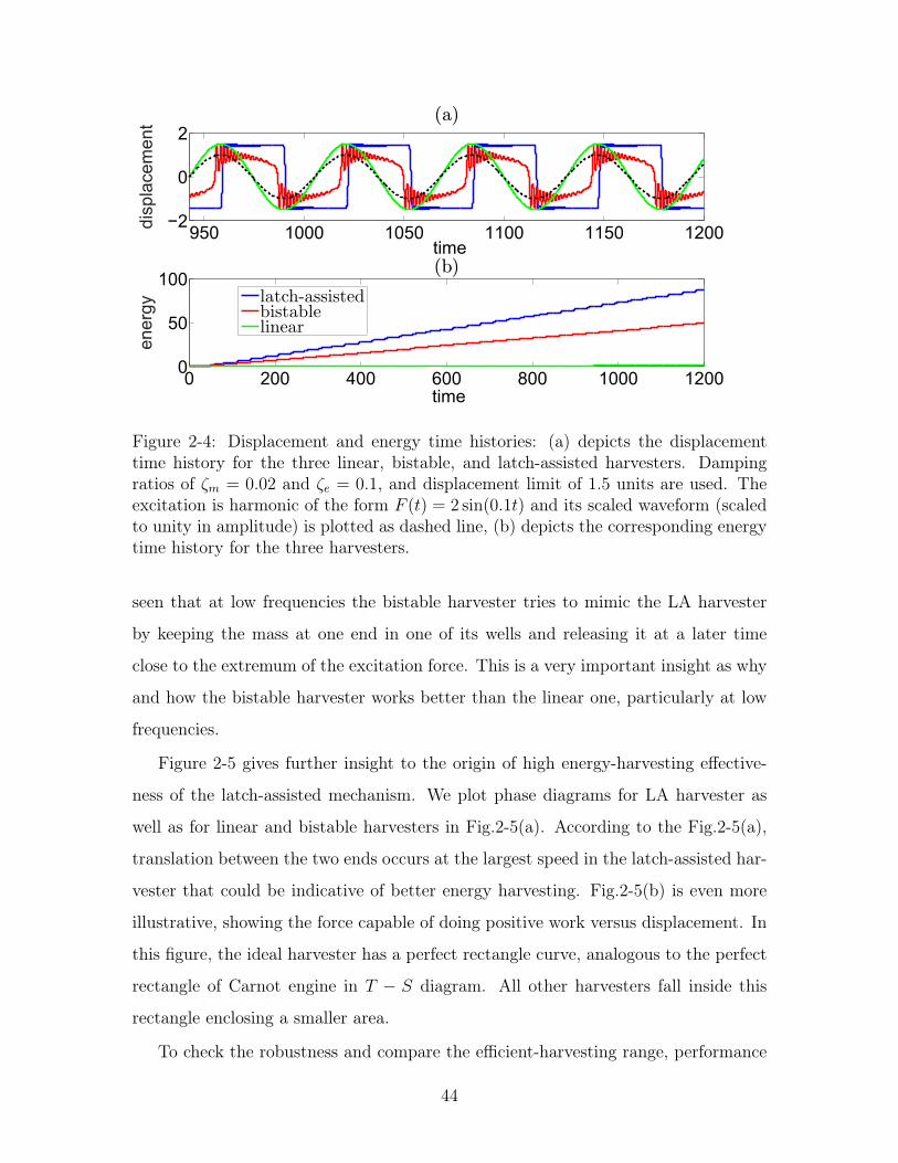
2-6 Normalized average harvested power contours: normalized average

power of the three harvesters for a wide range of harmonic base ex-

citation amplitude and frequency is plotted for a fixed displacement

limit of 2.5 units. The average power is normalized by the maximum

average power that could be harvested by an ideal harvester with no

mechanical damping. . . . . . . . . . . . . . . . . . . . . . . . . . . 46

2-7 Energy harvesting while walking: (a) time history and (b) velocity

spectrum of experimental acceleration recorded at the hip while walk-

ing [66]. (c) displacement time history of the nonlinear LA-VEH when

base-excited by walking motion. Displacement and time (frequency)

are scaled by 13𝜇m and 500 rad/s, respectively. The same damping

ratios and displacement limit of 1.5 units are used.(d) time history of

nondimensional harvested energy for the three systems. In addition to

the optimal bistbale harvester (𝑥𝑠 = 0.9 and 𝑎 = 2), performance of

two bistable harvesters with detuned parameter 𝑎 are also illustrated. 47

3-1 Passive BLSH strategy realized by an adaptive bistable potential for

an arbitrary excitation input. The transition from one displacement

limit to the other is highlighted by the background colour change in

the figure. . . . . . . . . . . . . . . . . . . . . . . . . . . . . . . . . . 52

3-2 Energy harvesting with adaptive bistability (a) schematics of a can-

tilever energy harvester with piezoelectric transduction mechanism equipped

with adaptive bistability (b) change in harvester’s potential function

to realize the BLSH logic and the sequence of the harvester mass tra-

jectory on admissible potential curves following the logic . . . . . . . 55

11

3-3 Energy harvesting with conventional bistable system. (a) and (b) show

surface and contour plots of average harvested power in terms of system

parameters 𝑎 and 𝑥𝑠. (c) and (d) show surface and contour plots of

harvester displacement amplitude in terms of system parameters 𝑎 and

𝑥𝑠. The other parameters are set as 𝐹0 = 10, 𝑤 = 0.05, 𝜁 = 0.01, 𝜅 = 5,

and 𝛼 = 1000. . . . . . . . . . . . . . . . . . . . . . . . . . . . . . . . 58

3-4 Average harvested power (on the left) and harvester displacement am-

plitude (on the right) of the conventional bistable energy harvester as

a function of the potential parameter 𝑎 for three different values of the

parameter 𝑥𝑠 = 2, 3, 4. The other simulation parameters are the same

as those in Fig. 3-3 . . . . . . . . . . . . . . . . . . . . . . . . . . . . 58

3-5 Displacement time histories of linear, conventional bistable, and adap-

tive bistable energy harvesters subjected to harmonic excitation with

excitation amplitude 𝐹0=10, and frequency 𝜔=0.05. The other simu-

lation parameters are as 𝜁 = 0.01, 𝜅 = 5, and 𝛼 = 1000. . . . . . . . . 59

3-6 Electrical-state (voltage or current depending on transduction mech-

anism) time histories of linear, conventional bistable, and adaptive

bistable energy harvesters subjected to harmonic excitation with exci-

tation amplitude 𝐹0=10, and frequency 𝜔=0.05. The other simulation

parameters are as 𝜁 = 0.01, 𝜅 = 5, and 𝛼 = 1000. . . . . . . . . . . . 60

3-7 Phase portrait (a), and displacement-force diagram (b) of the three

harvesters when subjected to harmonic excitation with excitation am-

plitude 𝐹0=10, and frequency 𝜔=0.05. The other simulation parame-

ters are as 𝜁 = 0.01, 𝜅 = 5, and 𝛼 = 1000. . . . . . . . . . . . . . . . 61

3-8 Time history of the harvested energy by the three harvesters when

subjected to harmonic excitation with excitation amplitude 𝐹0=10, and

frequency 𝜔=0.05. The other simulation parameters are as 𝜁 = 0.01,

𝜅 = 5, and 𝛼 = 1000. . . . . . . . . . . . . . . . . . . . . . . . . . . . 61

12

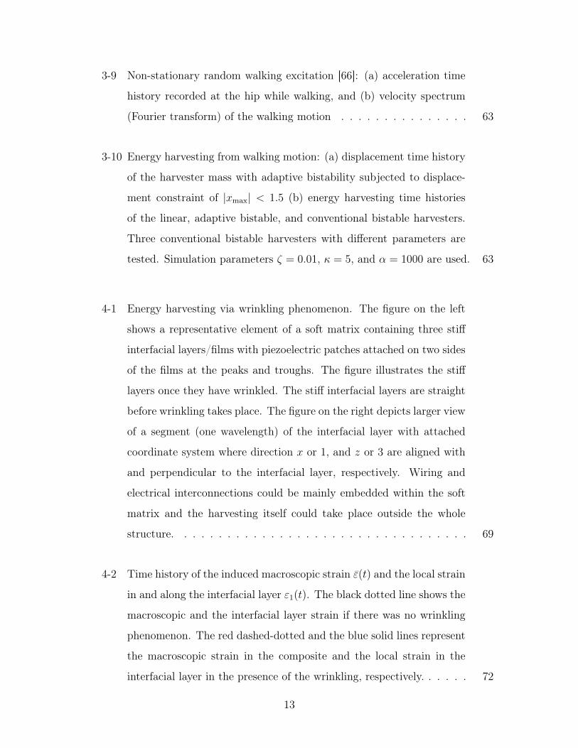
3-9 Non-stationary random walking excitation [66]: (a) acceleration time

history recorded at the hip while walking, and (b) velocity spectrum

(Fourier transform) of the walking motion . . . . . . . . . . . . . . . 63

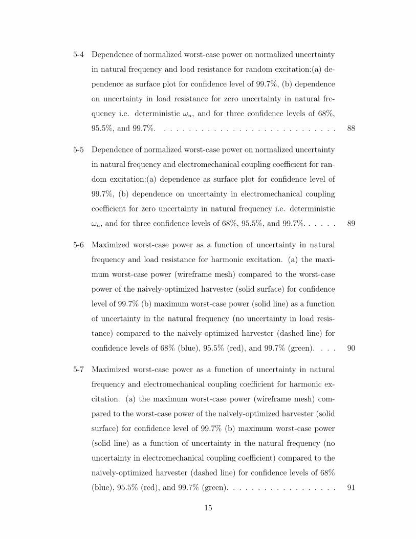
3-10 Energy harvesting from walking motion: (a) displacement time history

of the harvester mass with adaptive bistability subjected to displace-

ment constraint of |𝑥max| < 1.5 (b) energy harvesting time histories

of the linear, adaptive bistable, and conventional bistable harvesters.

Three conventional bistable harvesters with different parameters are

tested. Simulation parameters 𝜁 = 0.01, 𝜅 = 5, and 𝛼 = 1000 are used. 63

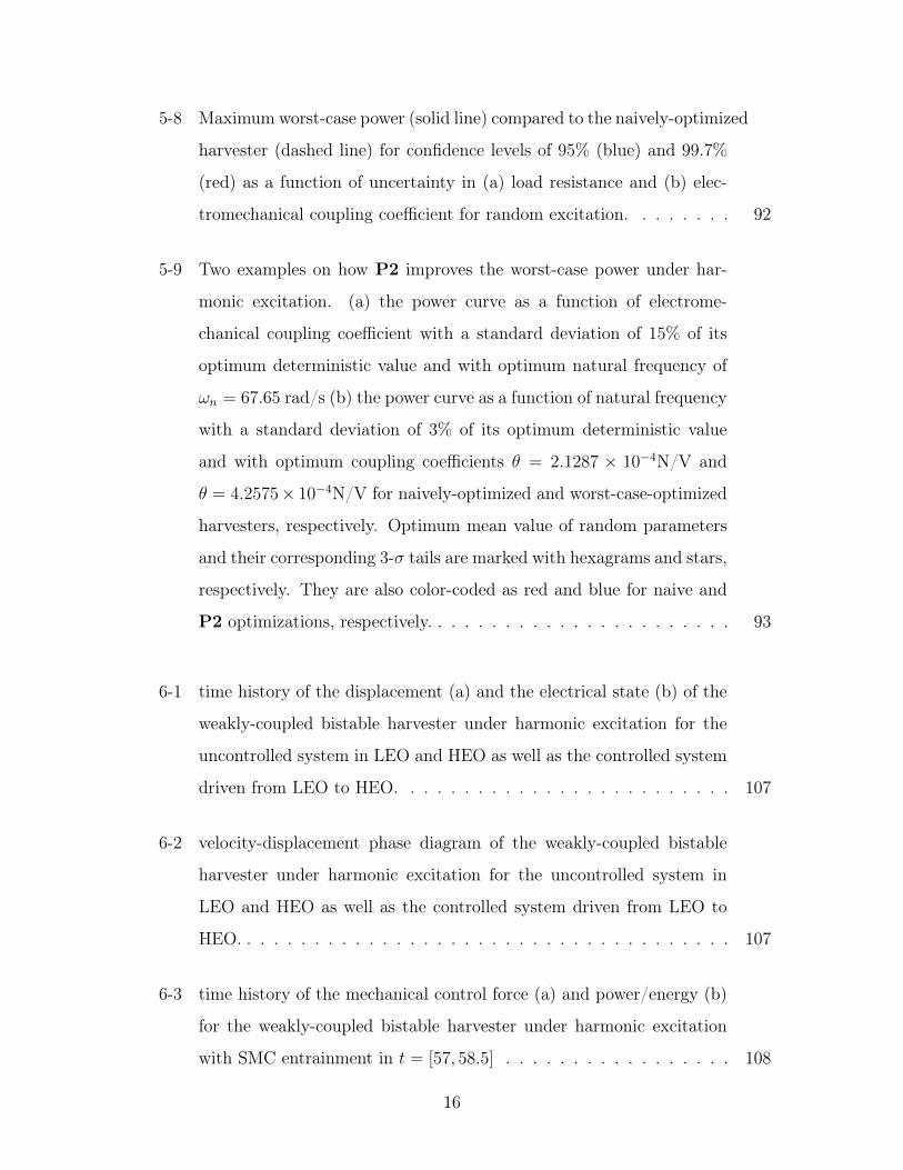
4-1 Energy harvesting via wrinkling phenomenon. The figure on the left

shows a representative element of a soft matrix containing three stiff

interfacial layers/films with piezoelectric patches attached on two sides

of the films at the peaks and troughs. The figure illustrates the stiff

layers once they have wrinkled. The stiff interfacial layers are straight

before wrinkling takes place. The figure on the right depicts larger view

of a segment (one wavelength) of the interfacial layer with attached

coordinate system where direction 𝑥 or 1, and 𝑧 or 3 are aligned with

and perpendicular to the interfacial layer, respectively. Wiring and

electrical interconnections could be mainly embedded within the soft

matrix and the harvesting itself could take place outside the whole

structure. . . . . . . . . . . . . . . . . . . . . . . . . . . . . . . . . . 69

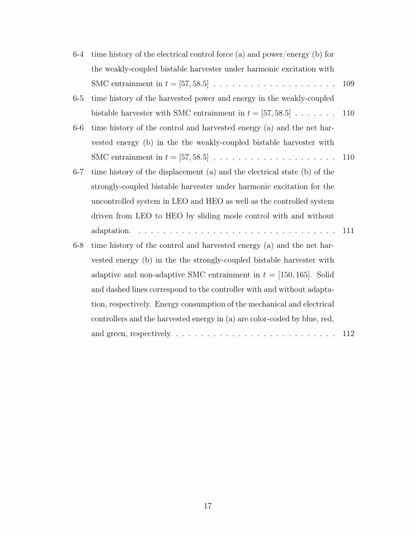
4-2 Time history of the induced macroscopic strain 𝜀(𝑡) and the local strain

in and along the interfacial layer 𝜀1(𝑡). The black dotted line shows the

macroscopic and the interfacial layer strain if there was no wrinkling

phenomenon. The red dashed-dotted and the blue solid lines represent

the macroscopic strain in the composite and the local strain in the

interfacial layer in the presence of the wrinkling, respectively. . . . . . 72

13

4-3 Dependence of the average harvested power on the external resistive

load 𝑅 with and without the wrinkling phenomenon. The optimal load

for maximal harvested power is illustrated by hexagrams on each curve.

The optimal loads 𝑅opt for the cases with and without the wrinkling

are 2.0 × 1011Ω, and 2.3 × 1011Ω, respectively. . . . . . . . . . . . . . 73

4-4 Time history of the induced voltage 𝑣(𝑡), and the harvested energy

across the external load per unit area of the piezo layer with (solid

line) and without (dashed line) the wrinkling phenomenon. . . . . . . 74

5-1 A base-excited PEH modeled as a sdof oscillator coupled with an elec-

tric circuit modeling a load resistance and the inherent capacitance of

the piezoelectric layer. . . . . . . . . . . . . . . . . . . . . . . . . . . 80

5-2 Dependence of normalized worst-case power on normalized uncertainty

in natural frequency and load resistance for harmonic excitation: (a)

dependence as surface plot for confidence level of 99.7%, (b) depen-

dence on uncertainty in natural frequency for two different normalized

uncertainty values in load resistance (𝜎𝑛𝑅 = 𝜎𝑅/𝑅

detopt%), and for three

confidence levels of 68%, 95.5%, and 99.7%. . . . . . . . . . . . . . . 85


in natural frequency and electromechanical coupling coefficient for har-

monic excitation: (a) dependence as surface plot for confidence level

of 99.7%, (b) dependence on uncertainty in electromechanical coupling

coefficient for two different normalized uncertainty values in natural

frequency of 0% (solid line) and 20% (dashed line), and for three con-

fidence levels of 68% (blue), 95.5% (red), and 99.7% (green). . . . . . 86

14


in natural frequency and load resistance for random excitation:(a) de-

pendence as surface plot for confidence level of 99.7%, (b) dependence

on uncertainty in load resistance for zero uncertainty in natural fre-

quency i.e. deterministic 𝜔𝑛, and for three confidence levels of 68%,

95.5%, and 99.7%. . . . . . . . . . . . . . . . . . . . . . . . . . . . . 88


in natural frequency and electromechanical coupling coefficient for ran-

dom excitation:(a) dependence as surface plot for confidence level of

99.7%, (b) dependence on uncertainty in electromechanical coupling

coefficient for zero uncertainty in natural frequency i.e. deterministic

𝜔𝑛, and for three confidence levels of 68%, 95.5%, and 99.7%. . . . . . 89

5-6 Maximized worst-case power as a function of uncertainty in natural

frequency and load resistance for harmonic excitation. (a) the maxi-

mum worst-case power (wireframe mesh) compared to the worst-case

power of the naively-optimized harvester (solid surface) for confidence

level of 99.7% (b) maximum worst-case power (solid line) as a function

of uncertainty in the natural frequency (no uncertainty in load resis-

tance) compared to the naively-optimized harvester (dashed line) for

confidence levels of 68% (blue), 95.5% (red), and 99.7% (green). . . . 90

5-7 Maximized worst-case power as a function of uncertainty in natural

frequency and electromechanical coupling coefficient for harmonic ex-

citation. (a) the maximum worst-case power (wireframe mesh) com-

pared to the worst-case power of the naively-optimized harvester (solid

surface) for confidence level of 99.7% (b) maximum worst-case power

(solid line) as a function of uncertainty in the natural frequency (no

uncertainty in electromechanical coupling coefficient) compared to the

naively-optimized harvester (dashed line) for confidence levels of 68%

(blue), 95.5% (red), and 99.7% (green). . . . . . . . . . . . . . . . . . 91

15

5-8 Maximum worst-case power (solid line) compared to the naively-optimized

harvester (dashed line) for confidence levels of 95% (blue) and 99.7%

(red) as a function of uncertainty in (a) load resistance and (b) elec-

tromechanical coupling coefficient for random excitation. . . . . . . . 92

5-9 Two examples on how P2 improves the worst-case power under har-

monic excitation. (a) the power curve as a function of electrome-

chanical coupling coefficient with a standard deviation of 15% of its

optimum deterministic value and with optimum natural frequency of

𝜔𝑛 = 67.65 rad/s (b) the power curve as a function of natural frequency

with a standard deviation of 3% of its optimum deterministic value

and with optimum coupling coefficients 𝜃 = 2.1287 × 10−4N/V and

𝜃 = 4.2575× 10−4N/V for naively-optimized and worst-case-optimized

harvesters, respectively. Optimum mean value of random parameters

and their corresponding 3-𝜎 tails are marked with hexagrams and stars,

respectively. They are also color-coded as red and blue for naive and

P2 optimizations, respectively. . . . . . . . . . . . . . . . . . . . . . . 93

6-1 time history of the displacement (a) and the electrical state (b) of the

weakly-coupled bistable harvester under harmonic excitation for the

uncontrolled system in LEO and HEO as well as the controlled system

driven from LEO to HEO. . . . . . . . . . . . . . . . . . . . . . . . . 107

6-2 velocity-displacement phase diagram of the weakly-coupled bistable

harvester under harmonic excitation for the uncontrolled system in

LEO and HEO as well as the controlled system driven from LEO to

HEO. . . . . . . . . . . . . . . . . . . . . . . . . . . . . . . . . . . . . 107

6-3 time history of the mechanical control force (a) and power/energy (b)

for the weakly-coupled bistable harvester under harmonic excitation

with SMC entrainment in 𝑡 = [57, 58.5] . . . . . . . . . . . . . . . . . 108

16

6-4 time history of the electrical control force (a) and power/energy (b) for

the weakly-coupled bistable harvester under harmonic excitation with

SMC entrainment in 𝑡 = [57, 58.5] . . . . . . . . . . . . . . . . . . . . 109

6-5 time history of the harvested power and energy in the weakly-coupled

bistable harvester with SMC entrainment in 𝑡 = [57, 58.5] . . . . . . . 110

6-6 time history of the control and harvested energy (a) and the net har-

vested energy (b) in the the weakly-coupled bistable harvester with

SMC entrainment in 𝑡 = [57, 58.5] . . . . . . . . . . . . . . . . . . . . 110

6-7 time history of the displacement (a) and the electrical state (b) of the

strongly-coupled bistable harvester under harmonic excitation for the

uncontrolled system in LEO and HEO as well as the controlled system

driven from LEO to HEO by sliding mode control with and without

adaptation. . . . . . . . . . . . . . . . . . . . . . . . . . . . . . . . . 111

6-8 time history of the control and harvested energy (a) and the net har-

vested energy (b) in the the strongly-coupled bistable harvester with

adaptive and non-adaptive SMC entrainment in 𝑡 = [150, 165]. Solid

and dashed lines correspond to the controller with and without adapta-

tion, respectively. Energy consumption of the mechanical and electrical

controllers and the harvested energy in (a) are color-coded by blue, red,

and green, respectively. . . . . . . . . . . . . . . . . . . . . . . . . . . 112

17

List of Tables

4.1 Material properties and geometric dimensions of the matrix, interfacial

layer, and the piezoelectric patches . . . . . . . . . . . . . . . . . . . 75

19

Chapter 1

Introduction

Harnessing environmental kinetic energy has played a big role in fulfilling our energy

needs over centuries: from waterwheels in ancient Egypt to modern water turbines in

the present time. Although we still rely on such technologies for harvesting energy in

large scales, our continuously changing technological trends necessitate adapting or

innovating new harvesting techniques. Sea-change advances in microfabrication and

electronics in the last two decades have led to development of small, low-power devices.

Unfortunately, implementation of such devices have been hindered by scalability or

maintenance issues of their traditional power sources. i.e. batteries. The considerable

reduction in power consumption of electronic devices such as wireless sensors, data

transmitters, and medical implants 1 has been to the point where ambient vibration,

a universal and widely available source of energy, has become a viable alternative to

costly traditional batteries. As a result, the concept of vibration energy harvesting

has gained much attention in the last decade.

In addition to scalability issues of conventional batteries, batteries must be reg-

ularly recharged or replaced, which can be very costly and cumbersome for systems

with large number of devices e.g. a large network of sensors, or for devices that are

remote or are hard to reach such as medical implants. In view of all such challenges,

and abundance of vibratory kinetic energy at small scales and across different fields,

1for example, electronic microchips for health monitoring that consist of a sensing unit and amicrocontroller have an average power consumption of approximately 50 𝜇𝑊 [8, 5].

21

vibratory energy harvesting has flourished as a major thrust among other energy

harvesting techniques. Vibratory energy harvesters (VEHs) exploit the ability of ac-

tive materials (e.g., piezoelectric, magnetostrictive, and ferroelectric) and electrome-

chanical coupling mechanisms (e.g., electrostatic and electromagnetic) to generate an

electric potential in response to mechanical stimuli and external vibrations [118, 103].

In view of advances in microfabrication and flexible electronics, vibratory energy

harvesting has found applications across different fields such as biomedical implants

and health monitoring of structures and machines. For medical implants, such as

pacemakers [106, 64], spinal stimulators [9], and electric pain relievers [102], the avail-

ability of reliable and noninvasive power supply is of utmost importance to eliminate

replacement of batteries, which has been shown to pose a significant risk of infec-

tion [20]. It has been reported that 1.2% of the 40,000 people who annually replace

batteries for pacemakers develop risky complications [59].

For structural health monitoring, vibratory energy harvesting is also envisioned

to play a critical role in further evolution of these technologies. During the last two

decades, more than 500 bridge failures have been reported in the United States [128]

resulting in millions of dollars in damage. One approach to avoid such disasters cen-

ters on an early warning system using structural health-monitoring sensor networks

[20]. As the sensor network hardware evolves, the possibility of embedding these

networks in all types of aerospace, civil, and mechanical infrastructure is becoming

both technically and economically feasible. However, the concept of embedded sens-

ing cannot be fully realized if the systems will require cables to access traditional

power sources or if batteries have to be periodically replaced [94]. Vibratory energy

harvesting could be a viable source of energy to make these embedded systems as

autonomous as possible since it has been recently demonstrated that the energy har-

vested from vibrations caused by the flow of traffic over bridges or the swaying of

a building due to wind loading provides a feasible approach to power such networks

[23, 30].

22

1.1 Challenges of vibratory energy harvesting

A typical vibratory energy harvester (VEH) consists of a vibrating host structure,

a transducer (e.g., electromagnetic, electrostatic, or piezoelectric), and a harvesting

circuitry (e.g., a simple electrical load). Most of the conventional VEHs exploit linear

resonance i.e. i.e. tuning the natural frequency of the host structure to the excita-

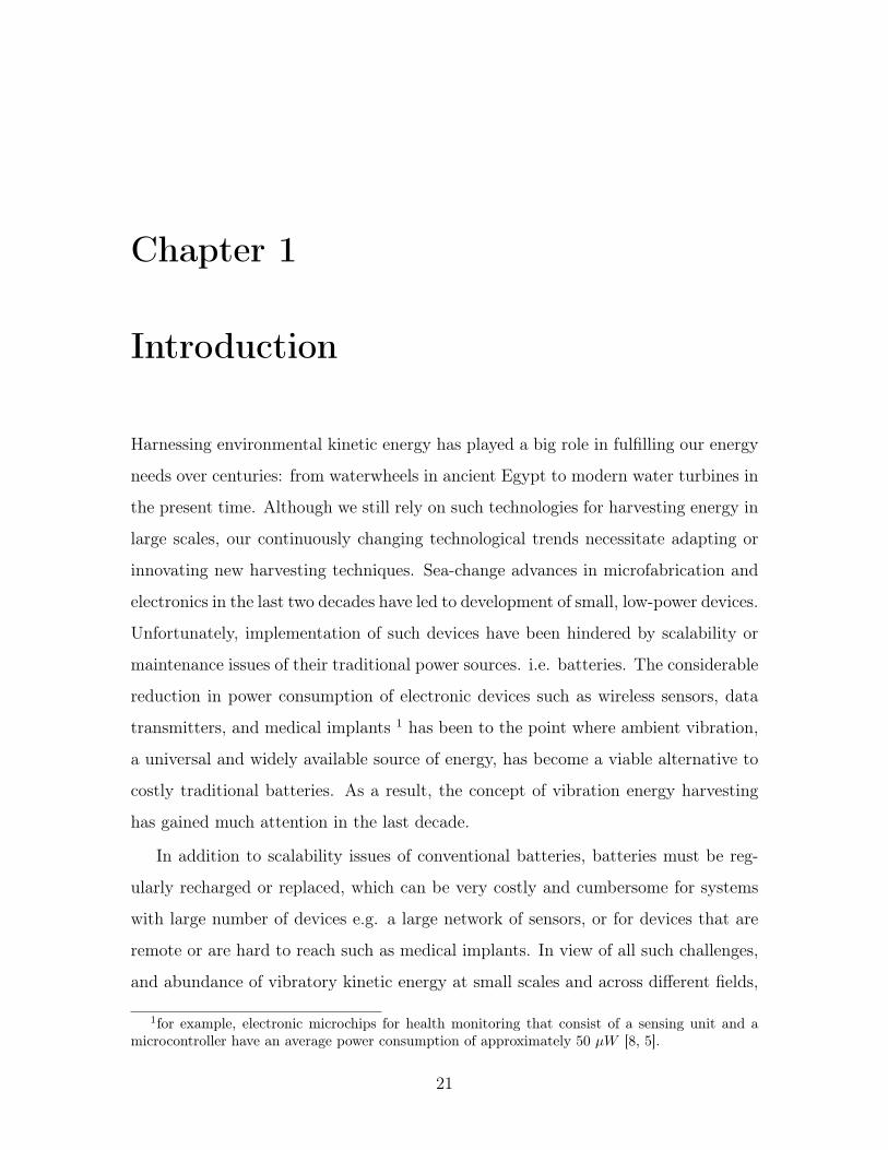
tion frequency, to maximize the harvested energy. Schematic of a linear cantilevered

piezoelectric energy harvester is illustrated in Fig.1-1. This approach has three ob-

vious downsides: first, most of the real-world excitation sources are wideband or

non-stationary [45, 52, 43, 55, 53], meaning that the excitation power is spread over

a range of frequencies or the dominant frequencies changes over time; hence, a linear

harvester with a fixed and narrow resonance (which is the case for passive and lightly-

damped structures) is very ineffective in such an excitation environment. Second, the

natural frequency of structures at small (micro-) scale is typically large (order of

hundreds of Hz to KHz) while excitation frequency of many real-world sources such

as walking and waves are typically much smaller (< 10 Hz). Consequently, this big

gap hinders realization of linear resonance at small scales for many practical appli-

cations. Third, The inherent narrow resonance makes the harvesting performance

very sensitive to system or excitation parameters i.e. a small change in the natural

frequency of the system or excitation frequency of the source results in drastic drop

in the output power of the harvester. To remedy these issues, techniques such as

resonance tuning, multi-modal energy harvesting, frequency up-conversion, and more

recently purposeful inclusion of nonlinearity have been investigated [123, 20].

1.1.1 broadband and low-frequency energy harvesting

Resonance tuning i.e. modifying and tuning the resonance frequency of the harvester

has been proposed in the literature to cope with non-stationary harmonic excitation.

This technique relies on modifying the effective stiffness of the harvester using different

methods such as adding auxiliary magnets[12, 11] or by applying axial force[73]. One

major shortcoming of these methods is that the tuning itself needs additional energy

23

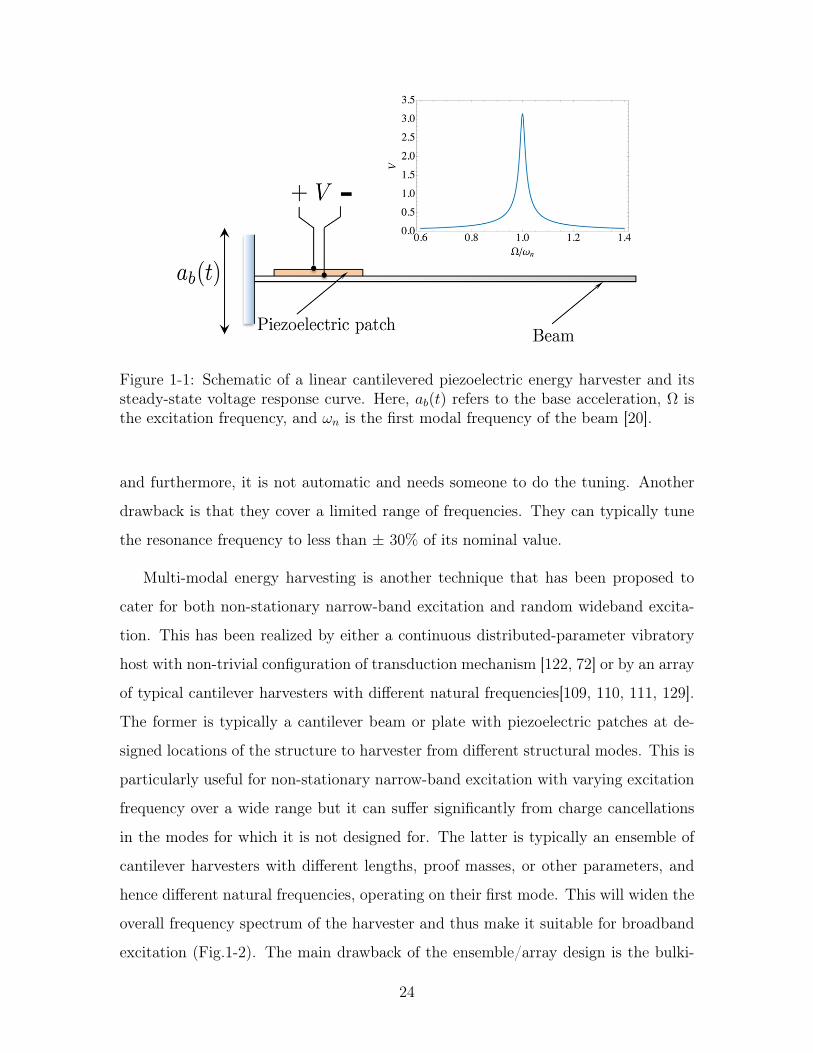
Figure 1-1: Schematic of a linear cantilevered piezoelectric energy harvester and itssteady-state voltage response curve. Here, 𝑎𝑏(𝑡) refers to the base acceleration, Ω isthe excitation frequency, and 𝜔𝑛 is the first modal frequency of the beam [20].

and furthermore, it is not automatic and needs someone to do the tuning. Another

drawback is that they cover a limited range of frequencies. They can typically tune

the resonance frequency to less than ± 30% of its nominal value.

Multi-modal energy harvesting is another technique that has been proposed to

cater for both non-stationary narrow-band excitation and random wideband excita-

tion. This has been realized by either a continuous distributed-parameter vibratory

host with non-trivial configuration of transduction mechanism [122, 72] or by an array

of typical cantilever harvesters with different natural frequencies[109, 110, 111, 129].

The former is typically a cantilever beam or plate with piezoelectric patches at de-

signed locations of the structure to harvester from different structural modes. This is

particularly useful for non-stationary narrow-band excitation with varying excitation

frequency over a wide range but it can suffer significantly from charge cancellations

in the modes for which it is not designed for. The latter is typically an ensemble of

cantilever harvesters with different lengths, proof masses, or other parameters, and

hence different natural frequencies, operating on their first mode. This will widen the

overall frequency spectrum of the harvester and thus make it suitable for broadband

excitation (Fig.1-2). The main drawback of the ensemble/array design is the bulki-

24

Figure 1-2: Multi-modal energy harvesting: (a) schematic of an array of linear can-tilever harvesters, (b) dependence of output power on driving frequency for 2 cases,one for a single cantilever, and the other for 1an array of 10 cantilevers in series withdifferent parameters and natural frequencies [129].

ness and low power density. Furthermore, mylti-modal energy harvesting in general

requires more sophisticated and complex harvesting circuitry[123].

The most prominent technique in the literature for addressing the issue of realiz-

ing linear resonance at small scales is frequency up-conversion. As mentioned earlier,

resonant frequency of harvesters at small scales are typically much higher than the

excitation frequency of many practical excitation sources such as walking or ocean

waves. To remedy this issue, frequency up-conversion converts the low-frequency ex-

citation of the source to vibration of the high-frequency harvesting device where it

can be harvested more effectively. Working principle of many of such devices is that a

slowly-vibrating primary system periodically excites a secondary high-frequency sys-

tem which then freely vibrates with its natural frequency until the next low-frequency

periodic excitation by the primary system. Energy is then harvested from the high-

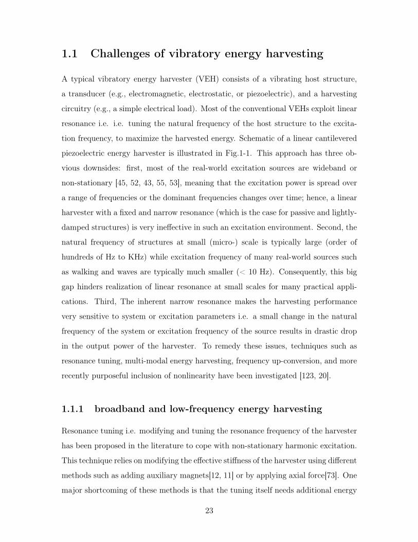
frequency free vibration of the secondary system[100, 71, 68, 63]. Figure 1-3 illustrates

a micro harvester with a frequency up-conversion technique.

To improve the efficacy of harvesting under broadband excitations, the intentional

introduction of nonlinearities into the design of VEHs has been a topic that has

received wide attention in the recent years.

The ability of nonlinearities to extend the frequency response spectrum of VEHs

has recently led many researchers to exploit them as a means to enhance the trans-

25

Figure 1-3: Frequency up-conversion technique: (a) schematic of a two-stage fre-quency up-conversation harvester with low and high natural frequency resonators,(b) movements of the low-frequency top plate and the high-frequency cantilever withrespect to each other. [68].

Figure 1-4: Nonlinear energy harvester: (a) Schematic of a nonlinear cantileveredpiezoelectric energy harvester, (b) variation of the restoring force due to thenonlinearity.[20].

duction of VEHs under broadband excitations. This is based on The ability of non-

linearities to extend the coupling between the excitation and a harmonic oscillator

to a wider range of frequencies [20]. The most common approach to the design of

such systems introduces a nonlinear restoring force using, for example, magnetic or

mechanical forces [80, 31, 83]. Figure 1-4 depicts schematics of a typical nonlinear

piezoelectric energy harvester with auxiliary magnets.

Over the last few years, research results have indicated that, when carefully in-

troduced, nonlinearity can be favorable for energy harvesting because it extends the

bandwidth of the harvester and, hence, allows for more efficient transduction under

26

the ambient random and non-stationary sources [20]. On the contrary, there are

studies which show that nonlinear VEHs do not always outperform their linear coun-

terparts. For instance, Daqaq [18] showed that for an inductive energy harvester with

negligible inductance, bistability (and in general any stiffness nonlinearity) does not

provide any improvement over a linear harvester when excited by white noise. In an-

other study, using real vibration measurements (of human walking motion and bridge

vibration) in simulations of idealized energy harvesters, Green et al. [35] showed that,

although the benefits of deliberately inducing dynamic nonlinearities into VEHs have

been shown for the case of Gaussian white noise excitations, the same benefits could

not be realized for real excitation conditions. It is also well-known that nonlinear

VEHs could generally suffer from one or more of the following: co-existing attractors,

sensitivity to initial conditions, and chaotic motion. These nonlinear phenomena are

generally undesired and weaken or complicate the harvesting process.

1.1.2 robust energy harvesting under uncertainty

Parametric uncertainty is inevitable with any physical device mainly due to man-

ufacturing tolerances, defects, and environmental effects such as temperature and

humidity. Hence, uncertainty propagation analysis and optimization under uncer-

tainty seem indispensable with any energy harvester design. Although researchers

have explored the topics of sensitivity analysis and optimization under uncertainty

in other fields like controls, finance, and production planning, they have not received

much attention in the field of energy harvesting.

Sensitivity of linear and even nonlinear VEHs to harvesting system and excitation

parameters on one hand, and inherent uncertainty and randomness in system param-

eters and vibratory excitations on the other hand, necessitate sensitivity propagation

analysis and optimization under uncertainty for effective harvesting. There are very

few studies in the context of energy harvesting that have studied sensitivity analysis

under uncertainty [90, 33, 81, 78] and even fewer studies on optimization of VEHs

under such uncertainties [2, 28].

Approaches to optimization under uncertainty have followed a variety of mod-

27

eling philosophies, including expectation minimization, minimization of deviations

from goals, minimization of maximum costs, and optimization over soft constraints

[104].The two optimization studies mentioned above are of the expectation-minimization

type (minimization of the negative of the ensemble average of the harvested power).

Although ensemble-expected power could be important in many applications, the

ensemble-minimum (worst-case scenario) power is often more important in the con-

text of energy harvesting where there is a minimum power requirement for every sin-

gle harvester so that the device to which the VEH supplies power, operates properly.

Hence, there is a need in the field to address the questions of uncertainty propagation

and optimization under uncertainty with respect to the worst-case scenario rather

than the ensemble expectation.

1.2 Thesis overview

Having provided an introduction to linear and nonlinear vibration energy harvesting

and the current challenges in the field, we now detail the focus of this thesis. This

thesis investigates fundamental problems in vibration energy harvesting, and pro-

vides mathematical tools and practical techniques to improve energy harvesting in

low-frequency and broadband excitations as well as harvesting under parametric and

environmental uncertainties. Specifically, we investigate fundamental power limits in

nonlinear VEHs and propose some techniques to approach these limits in practice.

We also study the robustness issues of the harvesters, and propose a new optimiza-

tion philosophy for passive harvesters and a novel sliding mode controller for active

variants.

We begin, in chapter 2, by putting forth a framework by which to assess maximal

power limit of a generic single-degree-of-freedom (sdof) nonlinear VEH subject to

exogenous excitation waveform and general constraints [47, 54]. We then derive the

fundamental limits on the output power of an ideal energy harvester for arbitrary

excitation waveforms and show that the optimal harvester maximizes the harvested

energy through a mechanical analog of a buy-low-sell-high (BLSH) strategy. We also

28

propose a non-resonant and passive latch-assisted harvester to realize this strategy. It

is shown that the proposed harvester harvests energy more effectively than its linear

and conventional bistable counterparts over a wider range of excitation frequencies

and amplitudes.

A novel non-resonant and adaptive bistable harvester is proposed in chapter 3

[48]. The potential barrier of the proposed harvester changes accordingly to mimic

the BLSH strategy developed in chapter 2. We discuss how the proposed harvester

can be realized by modifying the conventional bistable harvester. We show that

a harvester equipped with adaptive bistability following a BLSH logic significantly

outperforms its linear and conventional bistable counterparts under both harmonic

and experimental non-stationary random walking excitations. Also, the proposed

harvester does not suffer from the robustness issues that affect the linear and conven-

tional bistable systems when the system parameters are detuned.

Chapter 4 presents the idea of energy harvesting from structural instabilities [51,

38] that is in part motivated by the BLSH strategy discussed in chapter 2. In this

chapter we discuss how to exploit surface instability or in general instability in layered

composites for energy harvesting, where intriguing morphological patterns with large

strain are formed under compressive loads. We show that the induced large strains,

which are independent of the excitation frequency, could be used to give rise to large

strains in an attached piezoelectric layer to generate charge and, hence, energy. We

particularly focus on wrinkling of a stiff interfacial layer embedded within a soft

matrix. We derive the governing dynamical equation of thin piezoelectric patches

attached at the peaks and troughs of the wrinkles. Results show that wrinkling could

help to increase the harvested power by more than an order of magnitude.

Shifting gears to robust energy harvesting under uncertainty, chapters 5 and 6

focus on improving the harvesting process under parametric and environmental un-

certainties for passive and active harvesters, respectively. In chapter 5, we propose

a new modeling philosophy for optimization under uncertainty; optimization for the

worst-case scenario (minimum power) rather than for the ensemble expectation of the

power [49, 50]. The proposed optimization philosophy is practically very useful when

29

there is a minimum requirement on the harvested power. We formulate the prob-

lems of uncertainty propagation and optimization under uncertainty in a generic and

architecture-independent fashion, and then apply them to an sdof linear piezoelectric

VEH with uncertainty in its different parameters. The simulation results show that

there is a significant improvement in the worst-case power of the designed harvester

compared to that of a naively optimized (deterministically optimized) harvester.

Chapter 6 presents a novel robust and adaptive controller for nonlinear VEHs

to move them to desired high-energy attractors under uncertainty [37]. Nonlinear

systems driven by harmonic excitation often exhibit coexisting periodic or chaotic

attractors. For effective energy harvesting, it is always desired to operate on the

high-energy periodic orbits; therefore, it is crucial for the harvester to move to the

desired attractor once the system is trapped in any other coexisting attractor. In

this chapter we develop a robust and adaptive sliding mode controller to move the

nonlinear harvester to any desired attractor by a short entrainment on the desired

attractor. The proposed controller is robust to disturbances and unmodeled dynamics

and adaptive to the system parameters. The results show that the controller can

successfully move the harvester to the desired attractor, even when the parameters

are unknown, in a reasonable period of time, in less than 30 cycles of the excitation

force.

A summary of the contributions extended by this thesis is given in chapter 7. We

outline directions for future research and identify outstanding questions.

30

Chapter 2

Fundamental limits to nonlinear

energy harvesting

As discussed in the introduction, to overcome the limitations of linear harvesters,

researchers have recently tried to make use of purposeful introduction of nonlinearity

in VEH design. One of the key challenges in designing nonlinear harvesters is the

immense range of possible nonlinearities. Among different types of nonlinearity, bis-

ability has received more attention in the past few years [15, 24, 64, 41, 48]. However,

the question of fundamental limitations of nonlinear energy harvesting is still open.

Explicit identification of fundamental performance limits has played a crucial role

in many fields of science and engineering. In energy field, the classical Carnot cycle

efficiency was a guiding principle for development of thermal power plants, and com-

bustion engines. It has also inspired scientific debates that consequently led to the

formation of modern statistical physics. The Lanchester-Betz limit for wind harvest-

ing efficiency [6], and Shockley-Queisser limit for the efficiency of solar cells[113] are

commonly used for long-term assessment of sustainable energy policies. Shannon’s

limit of information capacity [112] has formed a foundation for the development of

modern communication systems. The Bode’s integral on sensitivity limits in feed-

back control theory [108] is a standard tool for analysis of design trade-offs in modern

control systems.

There have been very few but influential studies in the context of energy harvest-

31

ing that have addressed the question of maximal power limits for VEHs. The idea of

maximizing the the harvested energy was originated in the seminal studies by Mitch-

eson et al. [88, 89], and Ramlan et al. [99]. Mitcheson et al. [88] derived maximum

harvested power for a velocity-damped and coulomb-damped resonant generators as

well as for coulomb-force parametric generator (CFPG) with one mechanical degree of

freedom when subjected to harmonic excitation. They also estimated the maximum

possible harvested power for a general harvesting device excited by harmonic force

using proof mass traversal at the force extrema [89]. Ramlan et al. [99] took an en-

ergy approach and estimated the available power from a nonlinear VEH subjected to

harmonic excitation. They showed that with a displacement constraint, the nonlinear

harvester can harvest, in the limit, 4𝜋

times what a tuned linear VEH can harvest.

More recently, similar to [99] but in a more advanced fashion, Halvorsen et al. [39]

derived upper bound limits for a harvester with one mechanical degree of freedom and

linear damping. They considered two cases of arbitrary general excitation waveform

in the absence of displacement limits (damping-dominated motion) and periodic ex-

citation with displacement limits. The upper bound limit for a damping-dominated

motion was generalized to multiple sinusoid input by Heit and Roundy [42]. Also,

maximal power limits for nonlinear energy harvesters under white noise excitation

were explored in [40, 70, 62]. Although these studies address the same fundamental

question, the white noise approximation is rather restrictive and leads to overly con-

servative bounds. This assumption may not be applicable to many practical settings

where most of energy harvesting potential is associated with low frequencies.

Although the question of fundamental limits to energy conversion rate in the

context of vibration energy harvesting has received limited attention thus far, such

questions have been studied thoroughly in statistical physics. For example, the sem-

inal Jarzynski relation derived in [60] can be interpreted as the statistical constraint

on the possible efficiency of the work to free energy conversion process. More general

relations have been derived in [107, 14] for entropy production in stochastic systems.

The stochastic systems appearing in vibratory system analysis are specific examples

of the so-called non-equilibrium steady states (NESS) that were studied for example

32

in [13, 125]. Despite the immense effort in the statistical physics community, most

of the studies have focused on the systems where the stochastic fluctuations have

thermal nature and satisfy special fluctuation-dissipation relations. This is the case

in many practically relevant systems, such as molecular motors [4], or optical trap

experiments [1]. The main challenge with extension of these results to the vibrational

systems is the inherent non-equilibrium nature of the fluctuations that requires more

general approaches not relying on underlying microscopic statistical features of the

system. However, more general approaches relying on the techniques from control

and information theory [105] may eventually lead to convergence of these currently

separate fields.

The organization of the chapter is as follows. In section 2.1, we develop a generic

framework for deriving the energy harvesting limits, and generalize it to almost ar-

bitrary excitation waveforms. In addition, we provide insights as how to approach

these limits in practice, resulting in our almost-universal strategy termed buy-low-

sell-high (BLSH). To illustrate the approach, we build a hierarchy of increasingly

more constrained models of nonlinear harvesters, derive the closed-form solutions for

simplest models, and provide general formulations where the closed-form solutions

do not exist. Section 2.2 comments on some realistic constraints with regard to the

harvesting force applicable to both passive and active harvesters. Inspired by the

optimal solutions to the simple model, i.e. the BLSH strategy, in section 2.3, we

propose a conceptual design of non-resonant latch-assisted nonlinear harvesters and

show that they are significantly more effective than the traditional linear and nonlin-

ear harvesters in broadband low-frequency excitation. A summary of the work and

concluding thoughts are offered in section 2.4.

2.1 A generic framework

We consider a model of a single-degree-of-freedom ideal energy harvester characterized

by the mass 𝑚 and the displacement 𝑥(𝑡) that is subjected to the energy harvesting

force 𝑓(𝑡) and exogenous excitation force 𝐹 (𝑡). The dynamic equation of the system

33

is a Newton’s second law 𝑚(𝑡) = 𝐹 (𝑡) + 𝑓(𝑡). The fluxes of energy in the system

are given by the expressions 𝐹, −𝑓, and 𝑚22 representing respectively the external

input power to the system, harvested power, and instantaneous kinetic energy of the

system.

2.1.1 no constraints

We start our analysis by considering an idealized harvester with no constraints im-

posed on either the harvesting force, 𝑓(𝑡) or the displacement, 𝑥(𝑡). It is easy to

show that overall harvesting rate in this setting is unbounded. Indeed, the trajectory

defined by a simple relation (𝑡) = 𝜅𝐹 (𝑡) that can be realized with the harvesting

force 𝑓 = 𝑚𝜅 −𝐹 results in the harvesting rate of 𝜅𝐹 2 that can be made arbitrarily

large by increasing the mobility constant 𝜅. This trivial observation illustrates that

the question of fundamental limits is only well-posed for the model that incorporates

some technological or physical constraints. This is a general observation that ap-

plies to most of the known fundamental limits. For example, Carnot cycle limits the

efficiency of cycles with bounded working fluid temperature, and Shannon capacity

defines the limits for signals with bounded amplitudes and bandwidth.

2.1.2 displacement constraints

To derive the first nontrivial limits to the energy harvesting power limits we consider

the displacement amplitude and energy dissipation constraints that are common to

all energy harvesters. For the first constrained model we consider the displacement

constraint with the trajectory limited in a symmetric fashion, i.e. |𝑥(𝑡)| ≤ 𝑥max,

where 𝑥max is the displacement limit. In this model we assume there is no natural

dissipation of energy in the system, so in the steady state motion, the integral net

input of energy into the system equals the harvested energy. Thus, the maximum

harvested energy could be evaluated simply by maximizing the following expression

34

[39]:

𝐸max = max𝑥(𝑡)

∫d𝑡 𝐹 (𝑡)(𝑡). (2.1)

Here the optimization is carried over the set of all “reachable” trajectories, that can

be realized given the system constraints. As long as the harvesting force 𝑓 is not

subjected to any constraints, this set simply coincides with the set of bounded tra-

jectories defined by |𝑥(𝑡)| ≤ 𝑥max. The optimal trajectory is then easily found by

rewriting the integral in Eq.2.1 as −∫

d𝑡 (𝑡)𝑥(𝑡) . It is straightforward to check that

this expression is maximized by

𝑥*(𝑡) = −𝑥max sign[ (𝑡)

]. (2.2)

The interpretation of Eq.2.2 is straightforward and can be summarized as a buy-

low-sell-high (BLSH) harvesting strategy. The optimal harvester keeps the mass at

its lowest (highest) position until the force 𝐹 reaches its local maximum (minimum)

and then activates the force 𝑓 to move the mass by 2𝑥max upwards (downwards) as

fast as possible. In general, 𝑓 is not passive for all time, and this mechanism is in

fact non-resonant. Similar results were reported for time harmonic excitation in [39].

Also, the CFPG discussed in [88] follows a similar displacement trajectory as Eq.2.2

when the excitation is harmonic with relatively large force amplitude. However, if the

excitation is non-stationary or not harmonic the trajectories will be very different and

CFPG will not track the changes in direction of external forcing 𝐹 (𝑡) unlike BLSH

described by Eq.2.2.

The BLSH strategy is remarkably similar to the strategy employed by Carnot

cycle machine and can be also derived using similar geometric arguments. In the

𝐹 − 𝑥 parametric plane, the overall harvested energy is defined as the integral∮𝐹𝑑𝑥

representing the area of the contour produced by the cycle. For a local realization of

the force, both the values of the force and the values of displacement are bounded, so

the energy is maximized by the contour with rectangular shape. Similarly, the Carnot

cycle has a simple rectangular shape in temperature-entropy 𝑇 − 𝑆 diagram derived

35

by recognizing that the overall work given by∮𝑇𝑑𝑆 is the area of the contour that

is constrained by the temperature limits.

The net harvested energy in this model can be expressed as 𝐸max = 𝑥𝑚𝑎𝑥

∫| (𝑡)|𝑑𝑡.

For commonly used Gaussian models of the random external forces characterized by

the Fourier transform 𝐹𝜔 =∫

dt exp(𝑖𝜔𝑡)𝐹 (𝑡), and corresponding power spectral den-

sity |𝐹𝜔|2, the quantity (𝑡) is a Gaussian random variable with zero mean and the

variance given∫

𝑑𝜔2𝜋𝜔2|𝐹𝜔|2. Therefore, the maximal harvesting energy is given by the

following simple expression:

𝐸max = 𝑥max2

𝜋

√∫d𝜔

2𝜋𝜔2|𝐹𝜔|2 (2.3)

The strategy favours the high frequency harmonics which produce frequent extrema

of the external force each coming with the harvesting opportunity. In practice, har-

vesting energy at very high harmonics will not work because of the natural energy

dissipation in the system. So, in our next model, we consider the limits associated

with dissipation.

2.1.3 damping-constrained motion

To make the analysis tractable, we define a new model without the displacement con-

straints (so 𝑥max = ∞), but with additional damping force 𝐹𝑑 = −𝑐𝑚. Consequently,

the dynamic equation changes to 𝑚(𝑡)+𝑐𝑚(𝑡) = 𝐹 (𝑡)+𝑓(𝑡), and 𝑐𝑚2(𝑡) represents

the power dissipated in the mechanical damper. The harvested energy −∫

d𝑡 𝑓(𝑡)(𝑡)

is then equal to∫

d𝑡 [𝐹 (𝑡)(𝑡) − 𝑐𝑚2(𝑡)], assuming no accumulation of energy in the

system at steady state. This is a simple quadratic function in that is maximized

by = 𝐹/2𝑐𝑚 thus resulting in the following integral energy expression.

𝐸max = max

∫d𝑡

[𝐹 (𝑡)− 𝑐𝑚

2]

=

∫𝐹 2(𝑡)

4𝑐𝑚𝑑𝑡. (2.4)

As in the previous models, without any constraints on the harvesting force, the trajec-

tory is achievable with the input harvesting force of the form 𝑓(𝑡) = 𝑚*(𝑡)−𝐹 (𝑡)/2.

36

These results were also reported by Halvorsen et al.[39]. Furthermore, using Par-

seval’s theorem and the final result in Eq.2.4, the maximum energy in frequency

domain is equal to 𝐸max =∫

𝑑𝜔8𝜋𝑐𝑚

|𝐹𝜔|2. This simple frequency-domain representation

has an important property that with the optimal and ideal harvester force, energy

is harvested from all the frequency components of the excitation force equally pro-

portionate to the power spectrum of the forcing function. This is very advantageous

to low frequency and broadband vibration sources such as wave or walking motion

where efficient resonant harvesting is not possible.

2.1.4 a general case

In a similar fashion it is possible to construct more complicated limits that combine

multiple constraints. Although most of these models do not admit a closed-form

solution, the corresponding optimization problem can be transformed into a system

of differential-algebraic equations (DAEs) using the Lagrangian multiplier and slack

variable techniques. For example, incorporation of the displacement constraints into

a damped harvesting model can be accomplished by solving the following variational

problem:

𝐸max = max

∫𝑑𝑡

[𝐹− 𝑐𝑚

2 − 𝜇ℰ − 𝜆(ℐ − 𝛼2)]. (2.5)

Here, the unconstrained optimization is carried over 𝑥(𝑡), 𝑓(𝑡), the two Lagrangian

multiplier functions 𝜆(𝑡) and 𝜇(𝑡) and the so-called slack variable 𝛼(𝑡). The function

ℰ(𝑥, , , 𝑡) = 𝑚+𝑐𝑚−𝐹 −𝑓 represents the equality constraint associated with the

equations of motion, while the indicator function ℐ(𝑥) = 𝑥2𝑚𝑎𝑥−𝑥2 that is positive only

on admissible domain represents the inequality constraint for the displacement. Other

equality and inequality constraints on the displacement, velocity, or harvesting force

can be naturally incorporated in a similar way. Using the standard Euler-Lagrangian

variational approach the problem can be transformed into a system of DAEs that can

be solved for arbitrary forcing functions and thus provide universal benchmarks for

any practical harvesters.

It is worth noting that the general approach of studying the extremal behavior of

37

the physical systems using variational approach is by no means new. In its modern

form it originated in the quantum field theory [91] but has since been applied in

many fields most notably in one of the most difficult nonlinear problem of turbulent

dynamics [26]. Halvorsen et al. [39] also used similar variational approach to find the

maximal power bound for a VEH subjected to period excitation and displacement

limits.

The innocent-looking DAEs resulted from applying the variational approach to the

Lagrangian in Eq2.5 are not always easy to solve even computationally (particularly

if the DAEs have a high index). However, the time-discretized objective function

in Eq.2.4 can be maximized using standard nonlinear optimization approaches. In

particular, optimization of quadratic functionals like Eq.2.4 complemented by any

linear equality and inequality constraints like 𝑚 = 𝐹 + 𝑓 and |𝑥| < 𝑥max can be

easily performed using standard convex optimization techniques [7]. Discretization

of the system can be accomplished by using spectral representation of the force and

displacement signals.

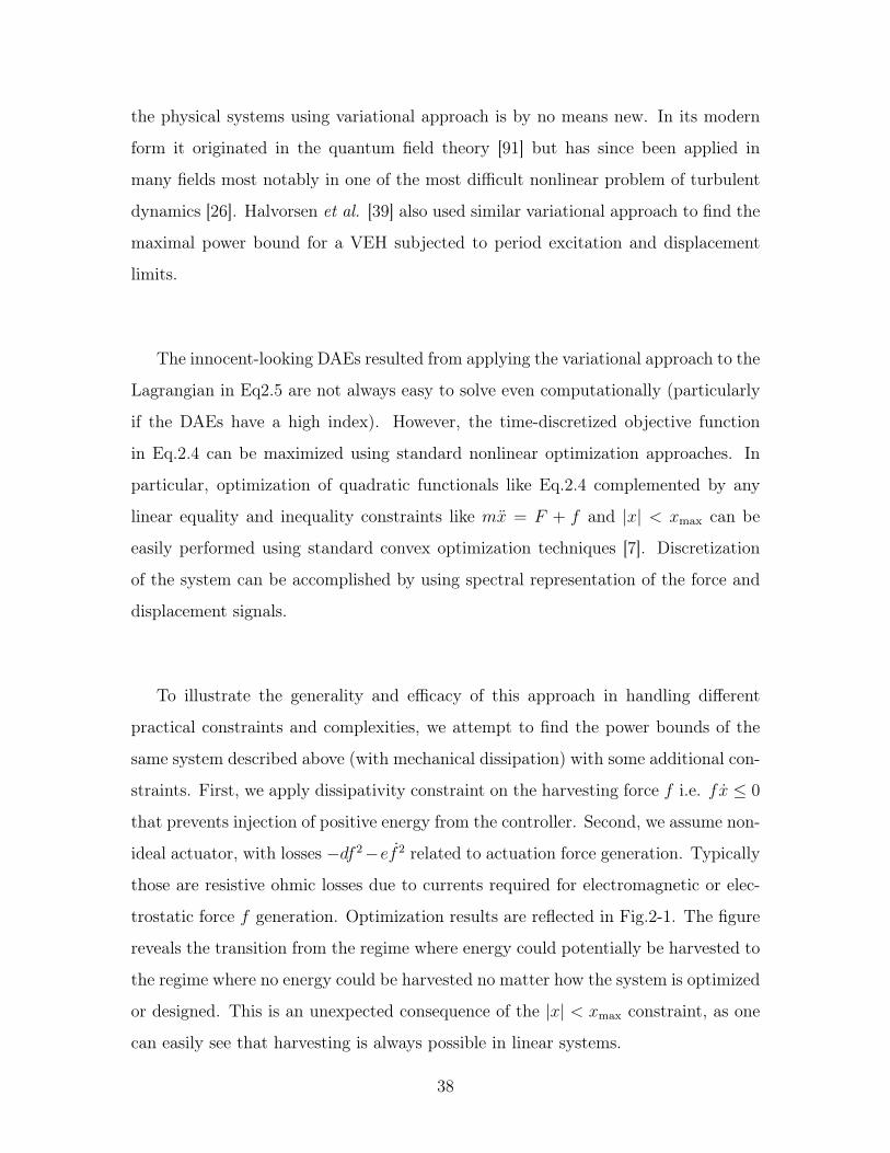
To illustrate the generality and efficacy of this approach in handling different

practical constraints and complexities, we attempt to find the power bounds of the

same system described above (with mechanical dissipation) with some additional con-

straints. First, we apply dissipativity constraint on the harvesting force 𝑓 i.e. 𝑓 ≤ 0

that prevents injection of positive energy from the controller. Second, we assume non-

ideal actuator, with losses −𝑑𝑓 2−𝑒𝑓 2 related to actuation force generation. Typically

those are resistive ohmic losses due to currents required for electromagnetic or elec-

trostatic force 𝑓 generation. Optimization results are reflected in Fig.2-1. The figure

reveals the transition from the regime where energy could potentially be harvested to

the regime where no energy could be harvested no matter how the system is optimized

or designed. This is an unexpected consequence of the |𝑥| < 𝑥max constraint, as one

can easily see that harvesting is always possible in linear systems.

38

d

0 0.02 0.04 0.06 0.08 0.1 0.12 0.14 0.16 0.18 0.2

max

imum

displacement(x

max)

0.5

1

1.5

2

2.5

3

3.5

4

4.5

5

5.5

6

-0.4

-0.3

-0.2

-0.1

0

0.1

0.2

0.3

d

0 0.05 0.1 0.15 0.2

averagepow

er

-0.4

-0.2

0

0.2

xmax = 1.5

e = 0e = 5e = 10ideal (d = e = 0)

Figure 2-1: Contour plot of optimal average harvested power with penalty coefficient𝑒 = 5 as a function of penalty coefficient 𝑑 and displacement limit 𝑥max when subjectedto harmonic excitation 𝐹 (𝑡) = 2 sin(0.1𝑡). The numerical values of 𝑚 = 1 and 𝑐𝑚 = 1are used. The dashed red line shows the transition from the potentially harvestableregime to the non-harvestable regime. The inset shows the optimal average power interms of 𝑑 for different values of 𝑒 for a fixed displacement limit of 𝑥max = 1.5.

39

2.2 Force constraints

A small scale harvester with ideal arbitrary harvesting force may not be easily re-

alizable with the current technology. More accurate power limits can be derived on

models incorporating additional constraints on the harvesting force 𝑓(𝑡). In a more

realistic representation of the system, the harvesting force 𝑓(𝑡) can be decomposed

into three parts. First, there is an inherent or intentionally introduced restoring force

from the potential energy 𝑈(𝑥) usually originating from the mechanical strain of a

deflected cantilever harvester or a magnetic field. Second, there is the linear har-

vesting energy force, 𝑐𝑒, that is typical to most of the traditional conversion mecha-

nisms, particularly to electromagnetic transduction mechanisms. Finally, controlled

harvesters may also utilize an additional control force 𝑢(𝑡) to enhance the energy

harvesting effectiveness. The control force can not be used for direct extraction of

energy from the system, however it can be used to change the dynamics of the system

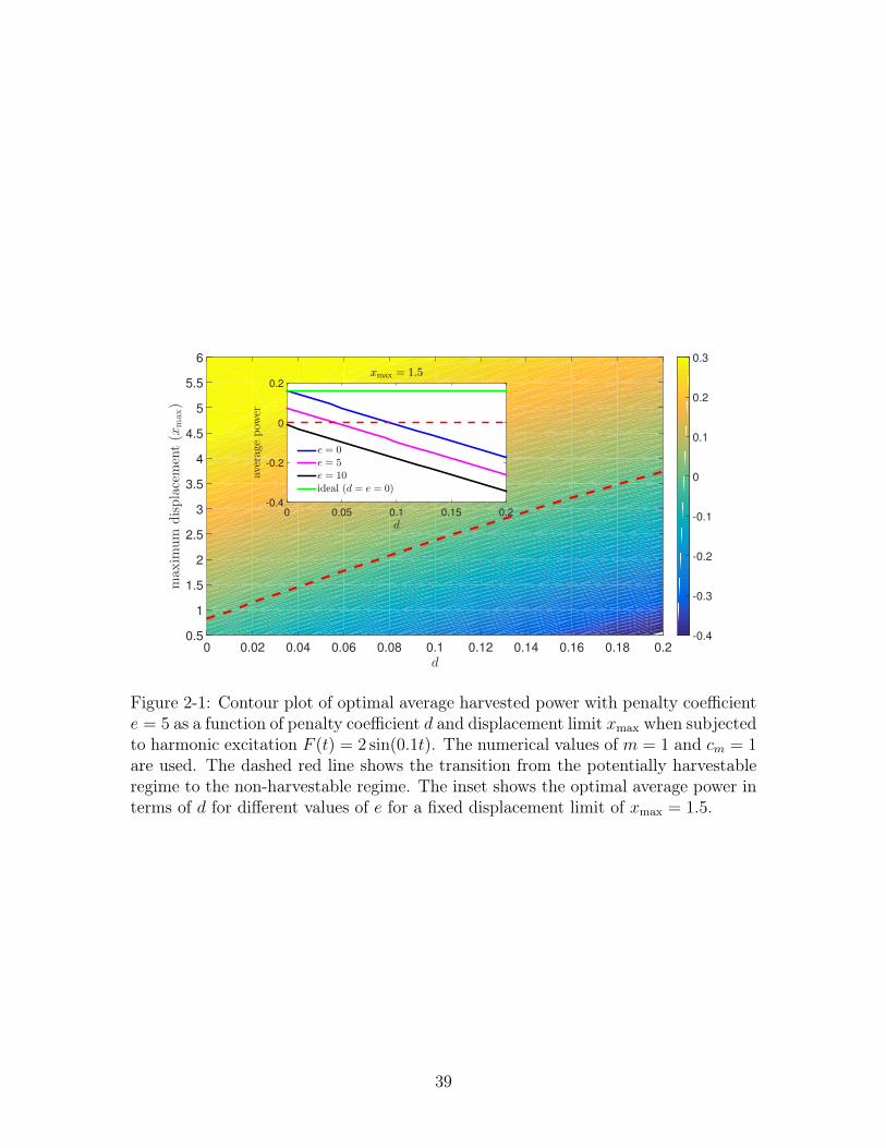
in a way that increases the overall conversion rate 𝑐𝑒2. More precisely, the overall

energy harvested from the system is given by∫𝑑𝑡[𝑐𝑒

2−𝑤(𝑡)], where 𝑤(𝑡) represents

the power necessary to produce the control force 𝑢(𝑡) and its corresponding power

𝑝(𝑡) = 𝑢(𝑡). The power flows in the system is illustrated schematically in Fig.2-2.

The corresponding optimization problem can be written as:

𝐸max = max

∫𝑑𝑡

[𝐹− 𝑐𝑚

2 − 𝑙(𝑡)]. (2.6)

Here the new function 𝑙(𝑡) = 𝑤(𝑡) − 𝑝(𝑡) represents the losses of power during the

control process. The specifics of the losses process depend on the details of the

system design and can be difficult to analyze in a general setting. However, it is easy

to incorporate a number of common natural and technological constraints on the loss

rate. First, the second law of thermodynamics implies that the losses are always

positive. If the control system cannot accumulate any energy, this constraint can

be represented simply as 𝑙(𝑡) ≥ 0. If energy accumulation is possible, only integral

constraint can be enforced:∫𝑙(𝑡)𝑑𝑡 ≥ 0. Obviously, if the former is the only constraint

imposed on the system, the optimal solution would correspond to zero losses 𝑙 = 0

40

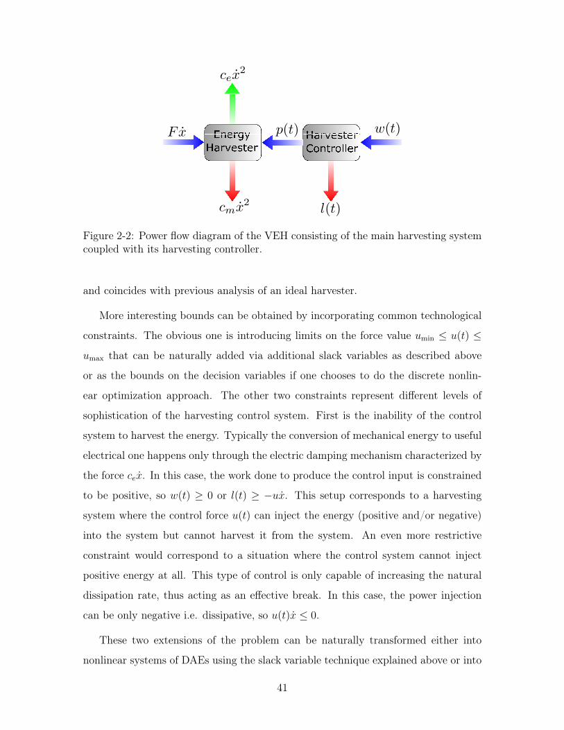
Figure 2-2: Power flow diagram of the VEH consisting of the main harvesting systemcoupled with its harvesting controller.

and coincides with previous analysis of an ideal harvester.

More interesting bounds can be obtained by incorporating common technological

constraints. The obvious one is introducing limits on the force value 𝑢min ≤ 𝑢(𝑡) ≤

𝑢max that can be naturally added via additional slack variables as described above

or as the bounds on the decision variables if one chooses to do the discrete nonlin-

ear optimization approach. The other two constraints represent different levels of

sophistication of the harvesting control system. First is the inability of the control

system to harvest the energy. Typically the conversion of mechanical energy to useful

electrical one happens only through the electric damping mechanism characterized by

the force 𝑐𝑒. In this case, the work done to produce the control input is constrained

to be positive, so 𝑤(𝑡) ≥ 0 or 𝑙(𝑡) ≥ −𝑢. This setup corresponds to a harvesting

system where the control force 𝑢(𝑡) can inject the energy (positive and/or negative)

into the system but cannot harvest it from the system. An even more restrictive

constraint would correspond to a situation where the control system cannot inject

positive energy at all. This type of control is only capable of increasing the natural

dissipation rate, thus acting as an effective break. In this case, the power injection

can be only negative i.e. dissipative, so 𝑢(𝑡) ≤ 0.

These two extensions of the problem can be naturally transformed either into

nonlinear systems of DAEs using the slack variable technique explained above or into

41

a nonlinear and hopefully convex optimization problem after discretization in time.

Numerical analysis of these equations may provide upper bounds on the harvested

energy limits. Comparison of different bounds would then provide a natural way of

valuing the potential benefits of possible control systems used in energy harvesters.

2.3 Non-resonant latch-assisted (LA) energy harvest-

ing

To further illustrate the usefulness of the harvesting power limits, we propose a novel

nonlinear and non-resonant harvester that is inspired by the behaviour of an ideal

harvester with no mechanical damping described by Eq.2.2. The harvester is based

on a simple extension of a classical linear mass-spring-damper system with a simple

latch mechanism that can controllably keep the system close to 𝑥 = ±𝑥max positions

mimicking the ideal harvester and to enforce the trajectory expressed by Eq.2.2.

More specifically, we use a simple control strategy where the secondary stiff spring

representing the latch is activated when the harvester mass reaches its maximum

or minimum displacement limit. The harvester mass is held at the limit after this

activation. When the force reaches its extremal value a signal is sent to the latch

mechanism to release the mass by detaching the secondary spring. Dynamic equation

of this system could be rewritten as 𝑚(𝑡) + (𝑐𝑚 + 𝑐𝑒)(𝑡) +𝑈 ′0(𝑥) = 𝐹 (𝑡)−𝑈 ′

𝑙 (𝑥)𝜎(𝑡)

where 𝜎(𝑡) is the signal for activation or deactivation of the latch system. 𝑈0(𝑥)

and 𝑈𝑙(𝑥) are respectively the potential energy of the harvester’s linear restoring

force and the latch mechanism. Signal generation of 𝜎(𝑡) may practically require a

minimal energy, but otherwise the LA harvester is completely passive.

Figure 2-3 illustrates the concept of maximizing the harvested energy through a

latch mechanism as one method to mimic the trajectory in Eq.2.2. In this method,

almost all the work is done on the system when the system is moving from one end to

the other; this energy is then harvested and dissipated when the system is blocked by

a latch from moving outside of the extremal points. Whenever the excitation is slow

42

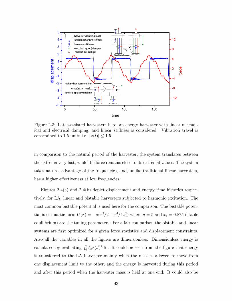
Figure 2-3: Latch-assisted harvester: here, an energy harvester with linear mechan-ical and electrical damping, and linear stiffness is considered. Vibration travel isconstrained to 1.5 units i.e. |𝑥(𝑡)| ≤ 1.5.

in comparison to the natural period of the harvester, the system translates between

the extrema very fast, while the force remains close to its extremal values. The system

takes natural advantage of the frequencies, and, unlike traditional linear harvesters,

has a higher effectiveness at low frequencies.

Figures 2-4(a) and 2-4(b) depict displacement and energy time histories respec-

tively, for LA, linear and bistable harvesters subjected to harmonic excitation. The

most common bistable potential is used here for the comparison. The bistable poten-

tial is of quartic form 𝑈(𝑥) = −𝑎(𝑥2/2− 𝑥4/4𝑥2𝑠) where 𝑎 = 5 and 𝑥𝑠 = 0.875 (stable

equilibrium) are the tuning parameters. For a fair comparison the bistable and linear

systems are first optimized for a given force statistics and displacement constraints.

Also all the variables in all the figures are dimensionless. Dimensionless energy is

calculated by evaluating∫ 𝑡

0𝜁𝑒(𝑡′)2d𝑡′. It could be seen from the figure that energy

is transferred to the LA harvester mainly when the mass is allowed to move from

one displacement limit to the other, and the energy is harvested during this period

and after this period when the harvester mass is held at one end. It could also be

43

time

time

Figure 2-4: Displacement and energy time histories: (a) depicts the displacementtime history for the three linear, bistable, and latch-assisted harvesters. Dampingratios of 𝜁𝑚 = 0.02 and 𝜁𝑒 = 0.1, and displacement limit of 1.5 units are used. Theexcitation is harmonic of the form 𝐹 (𝑡) = 2 sin(0.1𝑡) and its scaled waveform (scaledto unity in amplitude) is plotted as dashed line, (b) depicts the corresponding energytime history for the three harvesters.

seen that at low frequencies the bistable harvester tries to mimic the LA harvester

by keeping the mass at one end in one of its wells and releasing it at a later time

close to the extremum of the excitation force. This is a very important insight as why

and how the bistable harvester works better than the linear one, particularly at low

frequencies.

Figure 2-5 gives further insight to the origin of high energy-harvesting effective-

ness of the latch-assisted mechanism. We plot phase diagrams for LA harvester as

well as for linear and bistable harvesters in Fig.2-5(a). According to the Fig.2-5(a),

translation between the two ends occurs at the largest speed in the latch-assisted har-

vester that could be indicative of better energy harvesting. Fig.2-5(b) is even more

illustrative, showing the force capable of doing positive work versus displacement. In

this figure, the ideal harvester has a perfect rectangle curve, analogous to the perfect

rectangle of Carnot engine in 𝑇 − 𝑆 diagram. All other harvesters fall inside this

rectangle enclosing a smaller area.

To check the robustness and compare the efficient-harvesting range, performance

44

displacement-2 -1 0 1 2

velo

city

-3

-2

-1

0

1

2

3(a)

displacement-1 0 1

F(t)−2ζ

mx(t)

-2

-1.5

-1

-0.5

0

0.5

1

1.5

2

(b)

latch-assisted

bistable

linear

ideal

Figure 2-5: Phase and force-displacement diagrams: (a) depicts the phase diagramfor the three linear, bistable, and latch-assisted systems. Damping ratios of 𝜁𝑚 = 0.02and 𝜁𝑒 = 0.1, and displacement limit of 1.5 units are used. The excitation is harmonicof the form 𝐹 (𝑡) = 2 sin(0.1𝑡). (b) depicts the force-displacement curves for the linear,bistable, latch-assisted mechanism, and ideal harvester with no mechanical damping.

of the three harvesters over a wide range of base excitation frequencies and ampli-

tudes is illustrated in Fig. 2-6. In this experiment, fixed parameters are used for all

three harvesters for full range of excitation statistics (e.g. 𝑎 = 0.5 and 𝑥𝑠 = 1 for the

bistable system). To make sure that the harvesters are confined within the displace-

ment limit (2.5 units in this case), very stiff walls at ±𝑥max are implemented in the

simulations. The latch-assisted harvester has higher power over a wider range of ex-

citation frequencies and amplitudes. The LA harvester works best at low frequencies

and large amplitudes where it can mimic the ideal harvester best. Low effectiveness

of the LA harvester at low frequencies and small amplitudes is because the system

does not reach the displacement limits to latch, and hence works like a linear system

in this region.

It has been shown that the current nonlinear harvesters in particular, the bistable

harvesters are sensitive to the type of excitation, and may not be very effective when

subjected to real ambient vibration sources [35]. To analyze how robust and efficient

the LA harvester is when subjected to real-world vibration signals, we tested its

45

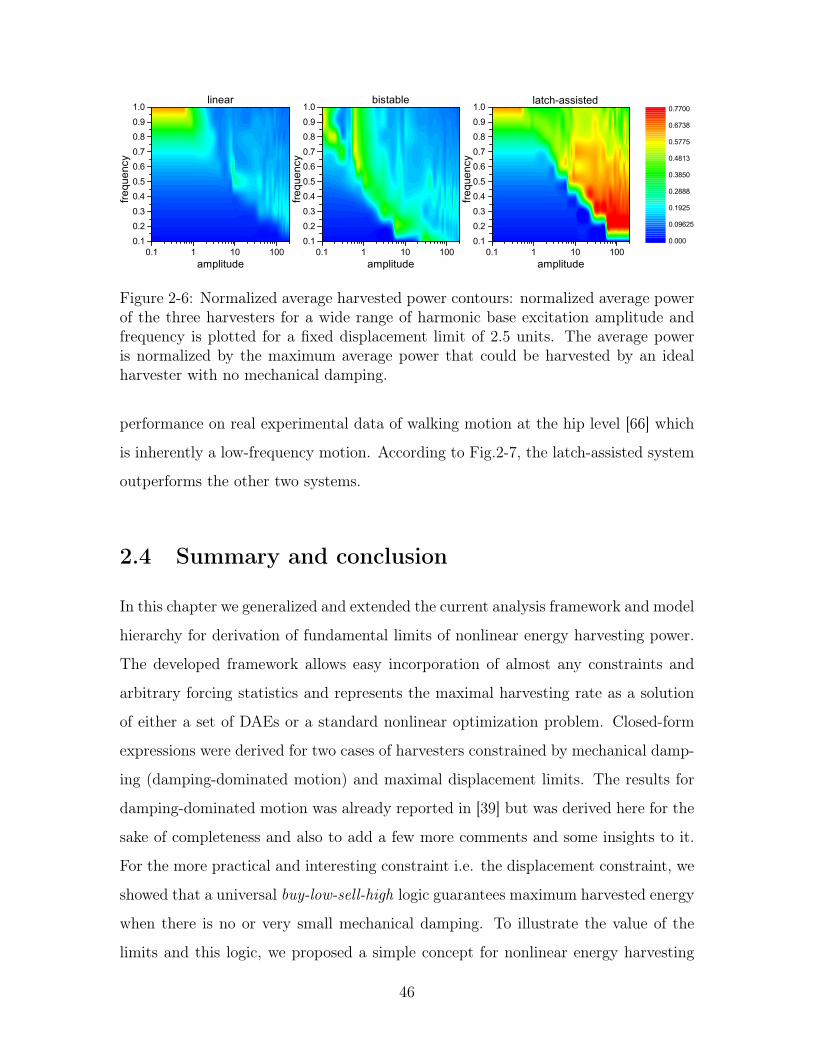
Figure 2-6: Normalized average harvested power contours: normalized average powerof the three harvesters for a wide range of harmonic base excitation amplitude andfrequency is plotted for a fixed displacement limit of 2.5 units. The average poweris normalized by the maximum average power that could be harvested by an idealharvester with no mechanical damping.

performance on real experimental data of walking motion at the hip level [66] which

is inherently a low-frequency motion. According to Fig.2-7, the latch-assisted system

outperforms the other two systems.

2.4 Summary and conclusion

In this chapter we generalized and extended the current analysis framework and model

hierarchy for derivation of fundamental limits of nonlinear energy harvesting power.

The developed framework allows easy incorporation of almost any constraints and

arbitrary forcing statistics and represents the maximal harvesting rate as a solution

of either a set of DAEs or a standard nonlinear optimization problem. Closed-form

expressions were derived for two cases of harvesters constrained by mechanical damp-

ing (damping-dominated motion) and maximal displacement limits. The results for

damping-dominated motion was already reported in [39] but was derived here for the

sake of completeness and also to add a few more comments and some insights to it.

For the more practical and interesting constraint i.e. the displacement constraint, we

showed that a universal buy-low-sell-high logic guarantees maximum harvested energy

when there is no or very small mechanical damping. To illustrate the value of the

limits and this logic, we proposed a simple concept for nonlinear energy harvesting

46

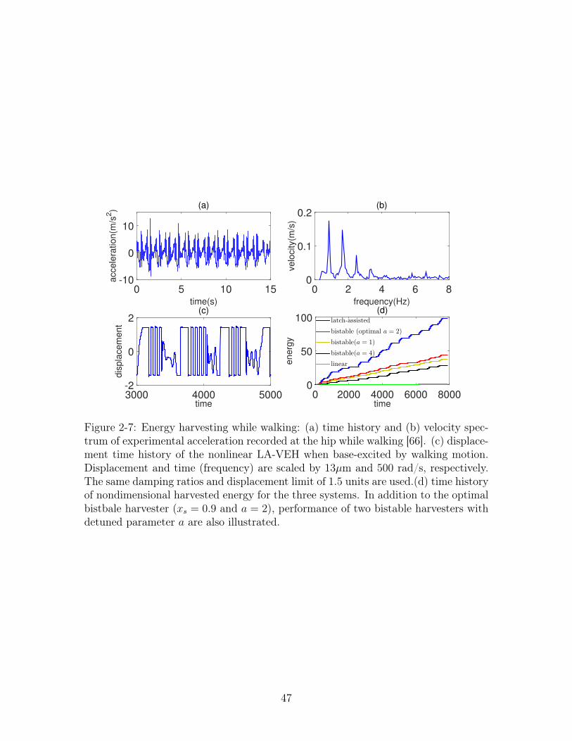
time(s)

0 5 10 15

accele

ration(m

/s2)

-10

0

10

(a)

frequency(Hz)

0 2 4 6 8velo

city(m

/s)

0

0.1

0.2(b)

time3000 4000 5000

dis

pla

cem

ent

-2

0

2(c)

time0 2000 4000 6000 8000

energ

y

0

50

100(d)

latch-assisted

bistable (optimal a = 2)

bistable(a = 1)

bistable(a = 4)

linear

Figure 2-7: Energy harvesting while walking: (a) time history and (b) velocity spec-trum of experimental acceleration recorded at the hip while walking [66]. (c) displace-ment time history of the nonlinear LA-VEH when base-excited by walking motion.Displacement and time (frequency) are scaled by 13𝜇m and 500 rad/s, respectively.The same damping ratios and displacement limit of 1.5 units are used.(d) time historyof nondimensional harvested energy for the three systems. In addition to the optimalbistbale harvester (𝑥𝑠 = 0.9 and 𝑎 = 2), performance of two bistable harvesters withdetuned parameter 𝑎 are also illustrated.

47

that mimics the performance of the optimal system using a passive and non-resonant

latch mechanism. The proposed mechanism outperforms both linear and bistable

harvesters in a wide range of parameters including the most interesting regime of

low-frequency large-amplitude excitation where the current harvesters fail to achieve

high performance. It was also shown that the conventional bistable harvester tries

to mimic the BLSH logic at low frequencies which provides a fundamental insight to

why and how the the bistable harvester performs well at low excitation frequencies.

48

Chapter 3

Non-resonant energy harvesting via

an adaptive bistable potential

Following the discussion in chapters 1 and 2, deliberate introduction of nonlinearity,

in particular bistable nonlinearity, have been the focus of a big body of research in

the field of vibration energy harvesting since 2009 [15, 25, 41]. However, recent stud-

ies have revealed that monostable and bistable nonlinear harvesters do not always

outperform their linear counterparts. One of the main issues with the bistable har-

vester when subjected to harmonic excitation is non-uniqueness of the solution and

co-existing low-energy and high-energy orbits at a given excitation frequency and am-

plitude [25, 79, 119, 24]. In fact, for a monostable nonlinear harvester the probability

of converging to the low-energy orbit is higher than that of the high-energy orbit

[98]. Also, Masana and Daqaq [84] showed that for a given excitation level, bistable

harvester’s performance is very sensitive to the potential shape (shallow versus deep

wells).

Performance of the bistable harvester is further diminished when it is subjected

to random excitation. Daqaq [18] showed that for an inductive energy harvester

with negligible inductance, bistability (in general any stiffness nonlinearity) does not

provide any improvement over the linear one when excited by white noise. Cottone et

al. [15] and Daqaq [19] showed that when driven by white noise, a necessary condition

for the bistable harvester to outperform its linear counterpart is to have a small

49

ratio of mechanical to electrical time constants. They along with other researchers

[76, 40, 132] showed that for a given noise intensity, the output power highly depends

on the shape of the bistable potential. Zhao and Erturk [132] showed that the bistable

harvester could outperform its linear counterpart only in a narrow region where noise

intensity is slightly above the threshold of interwell oscillations.

The bistable harvester becomes even less efficient and less robust when it is excited

by more realistic and real-world random vibrations (not white noise). Using real

vibration measurements (human walking motion and bridge vibration) in simulations

of idealized energy harvesters Green et al. [35] showed that, although the benefits of

deliberately inducing dynamic nonlinearities into such devices have been shown for

the case of Gaussian white noise excitations, the same benefits could not be realized

for the real excitation conditions.

We begin in section 3.1 by introducing adaptive bistability as a technique to realize

the BLSH strategy proposed in chapter 2, followed by mathematical formulation

of the problem. We then expose the proposed adaptive bistable harvester to both

harmonic and random walking excitation, and the results are presented in section

3.2. A summary of the chapter is provided in section 3.3.

3.1 Adaptive bistable harvester

In this chapter, we consider both capacitive and inductive harvesters (with single-

degree-of-freedom in the mechanical domain) with an adaptive bistable potential.

Here, the adaptive bistable potential refers to a potential where the potential shape,

in particular the potential barrier height could change according to a logic in an

adaptive fashion. Adaptive bistability could be realized in different ways that will

briefly be discussed later in the chapter. But first we want to find the logic accord-

ing to which the bistability should change adaptively so that its harvesting power

approaches the fundamental maximal power. The question of fundamental maximal

power was detailed in chapter 2 where we proposed an almost universal BLSH strat-

egy to maximize the harvested power. We employ this strategy here as the basis for

50

the adaptive bistability logic.

3.1.1 BLSH: adaptive bistability logic

It was found in chapter 2 that for a displacement-constrained scenario, an optimal

trajectory for an ideal harvester or a near-optimal trajectory for many practical har-

vesters is as follows:

𝑥*(𝑡) = −𝑥max sign[ (𝑡)

]. (3.1)

The interpretation of Eq.3.1 is as follows: when the excitation force 𝐹 (𝑡) is in-

creasing, 𝑥(𝑡), the harvester displacement, should be kept at its lowermost limit, and

vice versa, when 𝐹 (𝑡) is decreasing, 𝑥(𝑡) should be kept at its uppermost limit. Thus,

the transitions between displacement limits occur when sign of (𝑡) is changing i.e.

at extremums of 𝐹 (𝑡). In other words, in this logic, the harvester mass is kept at its

lowest position (−𝑥max) until the excitation force 𝐹 (𝑡) reaches its maximum when the

mass should then be pushed to its highest position (𝑥max) (either by the excitation

force, or by the harvesting force if the local maximum of the excitation force is still

negative or not big enough to push the mass to the highest position limit1). Simi-

lar dynamics occur in the reverse direction and this strategy continues in the same

fashion at every extremum of the excitation force 𝐹 (𝑡).

If the harvester is incapable of injecting energy to the system (passive-only har-

vester), the harvested mass should traverse between the limits (±𝑥max) by the exci-

tation force 𝐹 (𝑡) only. In this case, the logic is slightly modified; the harvester mass

should be kept at its lowest (highest) displacement limit till the largest maximum

(most-negative minimum) of the excitation force is reached. Only then, the harvester

mass is pushed from one displacement limit to the other. This logic is very similar to

the well-known buy-low-sell-high strategy in stock market; hence, we call this logic a

Buy-Low-Sell-High (BLSH) strategy hereafter.

1It should be noted even though the harvesting force is injecting energy to the system in thiscase during a short period, the net amount of harvested energy will be positive at the end. This isbecause injection of the energy by the harvesting force will pay off when the next excitation forceminimum is reached.

51

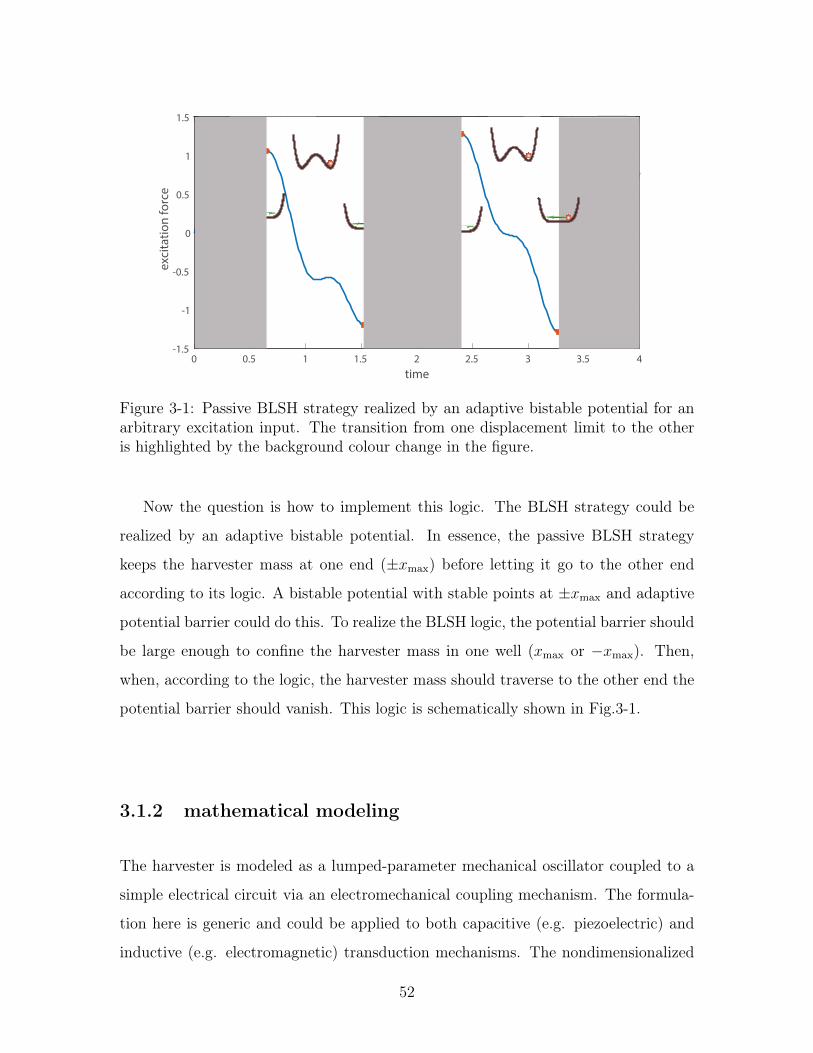
time0 0.5 1 1.5 2 2.5 3 3.5 4

exci

tatio

n fo

rce

-1.5

-1

-0.5

0

0.5

1

1.5

Figure 3-1: Passive BLSH strategy realized by an adaptive bistable potential for anarbitrary excitation input. The transition from one displacement limit to the otheris highlighted by the background colour change in the figure.

Now the question is how to implement this logic. The BLSH strategy could be

realized by an adaptive bistable potential. In essence, the passive BLSH strategy

keeps the harvester mass at one end (±𝑥max) before letting it go to the other end

according to its logic. A bistable potential with stable points at ±𝑥max and adaptive

potential barrier could do this. To realize the BLSH logic, the potential barrier should

be large enough to confine the harvester mass in one well (𝑥max or −𝑥max). Then,

when, according to the logic, the harvester mass should traverse to the other end the

potential barrier should vanish. This logic is schematically shown in Fig.3-1.

3.1.2 mathematical modeling

The harvester is modeled as a lumped-parameter mechanical oscillator coupled to a

simple electrical circuit via an electromechanical coupling mechanism. The formula-

tion here is generic and could be applied to both capacitive (e.g. piezoelectric) and

inductive (e.g. electromagnetic) transduction mechanisms. The nondimensionalized

52

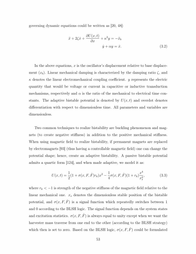
governing dynamic equations could be written as [20, 48]:

+ 2𝜁 +𝜕𝑈(𝑥, 𝑡)

𝜕𝑥+ 𝜅2𝑦 = −𝑏

+ 𝛼𝑦 = . (3.2)

In the above equations, 𝑥 is the oscillator’s displacement relative to base displace-

ment (𝑥𝑏). Linear mechanical damping is characterized by the damping ratio 𝜁, and

𝜅 denotes the linear electromechanical coupling coefficient. 𝑦 represents the electric

quantity that would be voltage or current in capacitive or inductive transduction

mechanisms, respectively and 𝛼 is the ratio of the mechanical to electrical time con-

stants. The adaptive bistable potential is denoted by 𝑈(𝑥, 𝑡) and overdot denotes

differentiation with respect to dimensionless time. All parameters and variables are

dimensionless.

Two common techniques to realize bistability are buckling phenomenon and mag-

nets (to create negative stiffness) in addition to the positive mechanical stiffness.

When using magnetic field to realize bistability, if permanent magnets are replaced

by electromagnets [93] (thus having a controllable magnetic field) one can change the

potential shape; hence, create an adaptive bistability. A passive bistable potential

admits a quartic form [124], and when made adaptive, we model it as:

𝑈(𝑥, 𝑡) =1

2(1 + 𝜎(𝑥, 𝐹, )𝑟𝑘)𝑥2 − 1

4𝜎(𝑥, 𝐹, )(1 + 𝑟𝑘)

𝑥4

𝑥2𝑠

, (3.3)

where 𝑟𝑘 < −1 is strength of the negative stiffness of the magnetic field relative to the

linear mechanical one. 𝑥𝑠 denotes the dimensionless stable position of the bistable

potential, and 𝜎(𝑥, 𝐹, ) is a signal function which repeatedly switches between 1

and 0 according to the BLSH logic. The signal function depends on the system states

and excitation statistics. 𝜎(𝑥, 𝐹, ) is always equal to unity except when we want the

harvester mass traverse from one end to the other (according to the BLSH strategy)

which then is set to zero. Based on the BLSH logic, 𝜎(𝑥, 𝐹, ) could be formulated

53

as follows:

𝜎(𝑥, 𝐹, ) =

⎧⎪⎨⎪⎩0; (𝑡) = 0 & 𝐹 (𝑡)𝑥(𝑡) < 0

1; |𝑥(𝑡)| ≈ 𝑥max & 𝐹 (𝑡)𝑥(𝑡) > 0

. (3.4)

In Eq.3.4, the signal function is set to unity when |𝑥(𝑡)| is approximately and not

exactly equal to 𝑥max. The reason is twofold: first, once the potential is activated the

mass still oscillates in that well even though by a small amount; hence, to make sure

it does not exceed the displacement limits, the potential is activated slightly before it

reaches ±𝑥max. Second, once the mass reaches one well, we want to keep it trapped

in that well until the condition for the release of the mass arises i.e. first condition in

Eq.3.4. However, before this condition has arisen, the mass oscillates slightly in that

well, so its displacement will be approximately and not exactly equal to ±𝑥max. In

simple words, the second condition in Eq.3.4 says that the mass should be trapped

and kept at one end once it reaches the displacement limits before the first conditions

arises and it is released. It is also worth mentioning that in the limit where the

potential barrier height goes to infinity the approximation changes to equality.

Figure3-2(a) depicts an energy harvester with piezoelectric (capacitive) transduc-

tion mechanism equipped with adaptive bistable potential. The adaptive bistability is

realized by an electromagnet and a permanent magnet (the proof mass). An On/Off

controller is used to implement the BLSH logic. The controller senses the excita-

tion and then according to the BLSH strategy sends a signal to the current supplier

to supply an appropriate current (𝜎(𝑡) = 1) or to shut down the current supply

(𝜎(𝑡) = 0).

It should be noted that using electro- and permanent magnets is not the only way

to realize adaptive bistability. Although this technique is easy to implement, care

should be taken to design the electromagnets with minimal losses. Since the harvester

mass is at the displacement limits for a substantial fraction of the time, ohmic losses

could be larger than the harvested energy if the electromagnets are poorly designed.

Another possible way to realize the adaptive bistability as mentioned earlier is via

adaptive buckling. Buckling as a means to create bistability in the context of energy

54

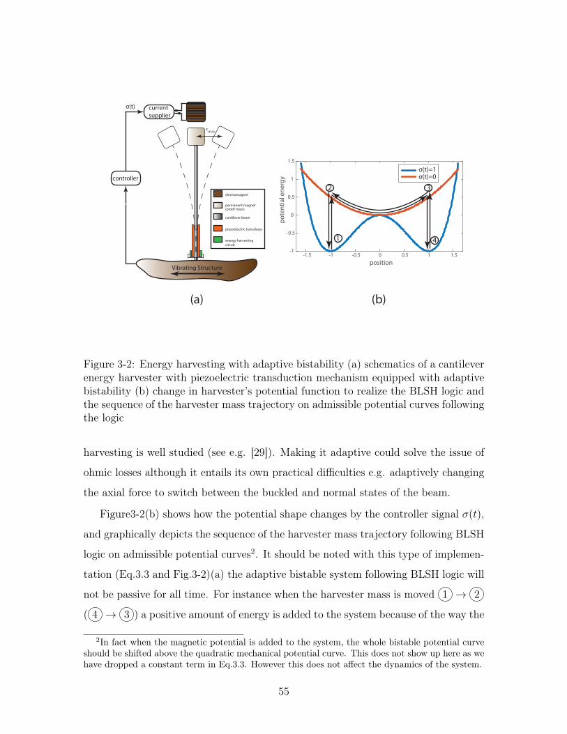
Vibrating Structure

controller

current supplier

xmax

electromagnet

permanent magnet (proof mass)

cantilever beam

piezoelectric transducer

energy harvestingcircuit

position-1.5 -1 -0.5 0 0.5 1 1.5

pote

ntia

l ene

rgy

-1

-0.5

0

0.5

1

1.5

σ(t)=0σ(t)=1

1

2 3

4

(a) (b)

σ(t)

Figure 3-2: Energy harvesting with adaptive bistability (a) schematics of a cantileverenergy harvester with piezoelectric transduction mechanism equipped with adaptivebistability (b) change in harvester’s potential function to realize the BLSH logic andthe sequence of the harvester mass trajectory on admissible potential curves followingthe logic

harvesting is well studied (see e.g. [29]). Making it adaptive could solve the issue of

ohmic losses although it entails its own practical difficulties e.g. adaptively changing

the axial force to switch between the buckled and normal states of the beam.

Figure3-2(b) shows how the potential shape changes by the controller signal 𝜎(𝑡),

and graphically depicts the sequence of the harvester mass trajectory following BLSH

logic on admissible potential curves2. It should be noted with this type of implemen-

tation (Eq.3.3 and Fig.3-2)(a) the adaptive bistable system following BLSH logic will

not be passive for all time. For instance when the harvester mass is moved 1 → 2

( 4 → 3 ) a positive amount of energy is added to the system because of the way the

2In fact when the magnetic potential is added to the system, the whole bistable potential curveshould be shifted above the quadratic mechanical potential curve. This does not show up here as wehave dropped a constant term in Eq.3.3. However this does not affect the dynamics of the system.

55

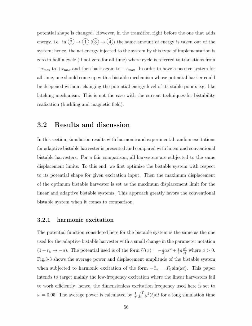
potential shape is changed. However, in the transition right before the one that adds

energy, i.e. in 2 → 1 ( 3 → 4 ) the same amount of energy is taken out of the

system; hence, the net energy injected to the system by this type of implementation is

zero in half a cycle (if not zero for all time) where cycle is referred to transitions from

−𝑥max to +𝑥max and then back again to −𝑥max. In order to have a passive system for

all time, one should come up with a bistable mechanism whose potential barrier could

be deepened without changing the potential energy level of its stable points e.g. like

latching mechanism. This is not the case with the current techniques for bistability

realization (buckling and magnetic field).

3.2 Results and discussion

In this section, simulation results with harmonic and experimental random excitations

for adaptive bistable harvester is presented and compared with linear and conventional

bistable harvesters. For a fair comparison, all harvesters are subjected to the same

displacement limits. To this end, we first optimize the bistable system with respect

to its potential shape for given excitation input. Then the maximum displacement

of the optimum bistable harvester is set as the maximum displacement limit for the

linear and adaptive bistable systems. This approach greatly favors the conventional

bistable system when it comes to comparison.

3.2.1 harmonic excitation

The potential function considered here for the bistable system is the same as the one

used for the adaptive bistable harvester with a small change in the parameter notation

(1 + 𝑟𝑘 → −𝑎). The potential used is of the form 𝑈(𝑥) = −12𝑎𝑥2 + 1

4𝑎𝑥4

𝑥2𝑠

where 𝑎 > 0.

Fig.3-3 shows the average power and displacement amplitude of the bistable system

when subjected to harmonic excitation of the form −𝑏 = 𝐹0 sin(𝜔𝑡). This paper

intends to target mainly the low-frequency excitation where the linear harvesters fail

to work efficiently; hence, the dimensionless excitation frequency used here is set to

𝜔 = 0.05. The average power is calculated by 1𝑇

∫ 𝑇

0𝑦2(𝑡)d𝑡 for a long simulation time

56

𝑇 . One should note that this expression gives the normalized dimensionless average

power. The dimensional instantaneous power is equal to (𝑚𝜔3𝑛𝑙

2𝑐)𝛼𝜅

2𝑦2 where 𝑚, 𝜔𝑛,

and 𝑙𝑐 are the harvester mass, time-scaling frequency, and length scale, respectively.

Hence, the average power used here is nondimensionalized by 𝑚𝜔3𝑛𝑙

2𝑐 , and further

normalized by (𝛼𝜅2)3.

It could be seen from Fig.3-3 that the average power increases monotonically with

𝑎 and 𝑥𝑠 up to a maximum and then drops sharply. This is where the interwell oscil-

lation turns into intrawell oscillation (potential barrier linearly increases with 𝑎 and

𝑥2𝑠). A drastic decrease in the amplitude of oscillation verifies this. It should be noted

that for values below the optimum value of 𝑎 (for a given 𝑥𝑠), the system is still in

interwell motion; however, the power monotonically decreases as 𝑎 is decreased from

its optimum value. This could be seen more clearly in Fig.3-4. This suggests the

robustness issues with the conventional bistable system, that is, the harvester works

efficiently only when the potential barrier is slightly below its critical value when it

triggers the interwell oscillation which agrees with Zhao and Etrurk’s claim [132].

Next, we compare the performance of the adaptive bistable harvester with that of

an optimized conventional bistable and linear harvesters when they are subjected to

harmonic excitation. To this end, we first optimize the parameters of the bistable

system for given excitation input and displacement limits. The same harmonic excita-

tion used for Figs. 3-3 and 3-4 is considered here (𝐹0 = 10 and 𝜔 = 0.05). According

to Figs.3-3 and 3-4 the optimal parameters corresponding to maximum displacement

of 3.4 are 𝑥𝑠 = 2 and 𝑎 = 12. For a fair comparison the parameters of the adaptive

bistable and linear harvesters are set such that their maximum displacements do not

exceed this value (𝑟𝑘 = −300 and 𝑥𝑠 = 2.8 for the adaptive bistable, and natural

frequency of√

3 for the linear harvester).

Figures 3-5 and 3-6 show time histories of the displacement and electrical-domain

state (voltage or current for capacitive or inductive transduction mechanisms, respec-

tively) for the three adaptive bistable, conventional bistable and linear harvesters.

3Since we are not optimizing the power with respect to 𝛼 and 𝜅 it is fine to normalize the powerby 𝛼𝜅2.

57

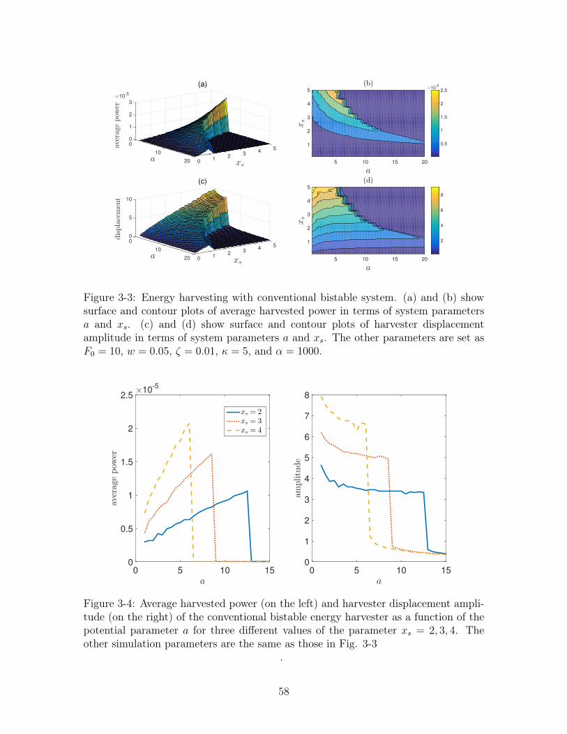
54

3

xs

21

(a)

020

10

a

0

1

3

2

0

×10-5

averagepow

er

(b)

a

5 10 15 20

xs

1

2

3

4

5×10

-5

0.5

1

1.5

2

2.5

54

3

xs

21

(c)

020

10

a

10

0

5

0

displacement

(d)

a

5 10 15 20

xs

1

2

3

4

5

2

4

6

8

Figure 3-3: Energy harvesting with conventional bistable system. (a) and (b) showsurface and contour plots of average harvested power in terms of system parameters𝑎 and 𝑥𝑠. (c) and (d) show surface and contour plots of harvester displacementamplitude in terms of system parameters 𝑎 and 𝑥𝑠. The other parameters are set as𝐹0 = 10, 𝑤 = 0.05, 𝜁 = 0.01, 𝜅 = 5, and 𝛼 = 1000.

a

0 5 10 15

averag

epow

er

×10-5

0

0.5

1

1.5

2

2.5

xs = 2xs = 3xs = 4

a

0 5 10 15

amplitude

0

1

2

3

4

5

6

7

8

Figure 3-4: Average harvested power (on the left) and harvester displacement ampli-tude (on the right) of the conventional bistable energy harvester as a function of thepotential parameter 𝑎 for three different values of the parameter 𝑥𝑠 = 2, 3, 4. Theother simulation parameters are the same as those in Fig. 3-3

.

58

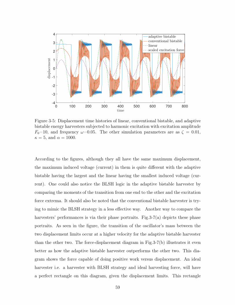
time0 100 200 300 400 500 600 700 800

displacement

-4

-3

-2

-1

0

1

2

3

4adaptive bistableconventional bistablelinearscaled excitation force

Figure 3-5: Displacement time histories of linear, conventional bistable, and adaptivebistable energy harvesters subjected to harmonic excitation with excitation amplitude𝐹0=10, and frequency 𝜔=0.05. The other simulation parameters are as 𝜁 = 0.01,𝜅 = 5, and 𝛼 = 1000.

According to the figures, although they all have the same maximum displacement,

the maximum induced voltage (current) in them is quite different with the adaptive

bistable having the largest and the linear having the smallest induced voltage (cur-

rent). One could also notice the BLSH logic in the adaptive bistable harvester by

comparing the moments of the transition from one end to the other and the excitation

force extrema. It should also be noted that the conventional bistable harvester is try-

ing to mimic the BLSH strategy in a less effective way. Another way to compare the

harvesters’ performances is via their phase portraits. Fig.3-7(a) depicts these phase

portraits. As seen in the figure, the transition of the oscillator’s mass between the

two displacement limits occur at a higher velocity for the adaptive bistable harvester

than the other two. The force-displacement diagram in Fig.3-7(b) illustrates it even

better as how the adaptive bistable harvester outperforms the other two. This dia-

gram shows the force capable of doing positive work versus displacement. An ideal

harvester i.e. a harvester with BLSH strategy and ideal harvesting force, will have

a perfect rectangle on this diagram, given the displacement limits. This rectangle

59

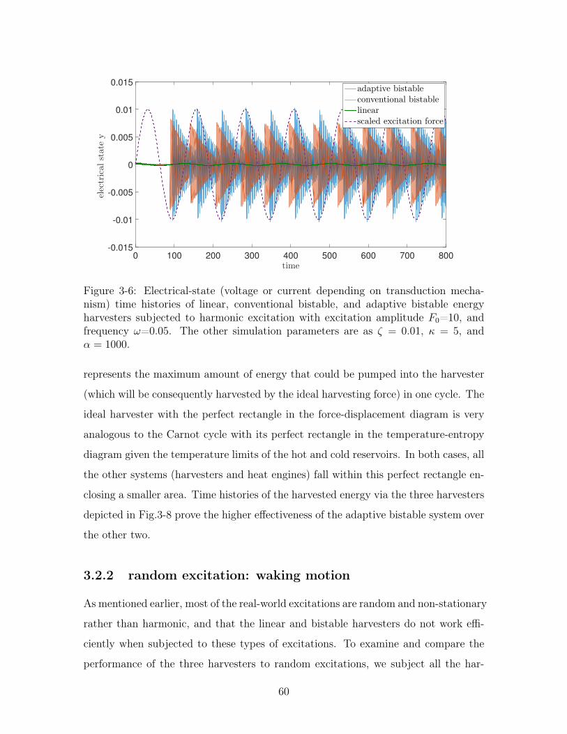
time0 100 200 300 400 500 600 700 800

electrical

statey

-0.015

-0.01

-0.005

0

0.005

0.01

0.015adaptive bistableconventional bistablelinearscaled excitation force

Figure 3-6: Electrical-state (voltage or current depending on transduction mecha-nism) time histories of linear, conventional bistable, and adaptive bistable energyharvesters subjected to harmonic excitation with excitation amplitude 𝐹0=10, andfrequency 𝜔=0.05. The other simulation parameters are as 𝜁 = 0.01, 𝜅 = 5, and𝛼 = 1000.

represents the maximum amount of energy that could be pumped into the harvester

(which will be consequently harvested by the ideal harvesting force) in one cycle. The

ideal harvester with the perfect rectangle in the force-displacement diagram is very

analogous to the Carnot cycle with its perfect rectangle in the temperature-entropy

diagram given the temperature limits of the hot and cold reservoirs. In both cases, all

the other systems (harvesters and heat engines) fall within this perfect rectangle en-

closing a smaller area. Time histories of the harvested energy via the three harvesters

depicted in Fig.3-8 prove the higher effectiveness of the adaptive bistable system over

the other two.

3.2.2 random excitation: waking motion

As mentioned earlier, most of the real-world excitations are random and non-stationary

rather than harmonic, and that the linear and bistable harvesters do not work effi-

ciently when subjected to these types of excitations. To examine and compare the

performance of the three harvesters to random excitations, we subject all the har-

60

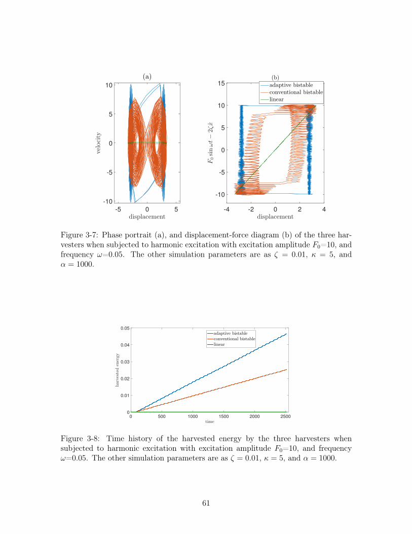
displacement-5 0 5

velocity

-10

-5

0

5

10

(a)

displacement-4 -2 0 2 4

F0sinωt−2ζx

-10

-5

0

5

10

15

(b)

adaptive bistableconventional bistablelinear

Figure 3-7: Phase portrait (a), and displacement-force diagram (b) of the three har-vesters when subjected to harmonic excitation with excitation amplitude 𝐹0=10, andfrequency 𝜔=0.05. The other simulation parameters are as 𝜁 = 0.01, 𝜅 = 5, and𝛼 = 1000.

time0 500 1000 1500 2000 2500

harvesteden

ergy

0

0.01

0.02

0.03

0.04

0.05

adaptive bistableconventional bistablelinear

Figure 3-8: Time history of the harvested energy by the three harvesters whensubjected to harmonic excitation with excitation amplitude 𝐹0=10, and frequency𝜔=0.05. The other simulation parameters are as 𝜁 = 0.01, 𝜅 = 5, and 𝛼 = 1000.

61

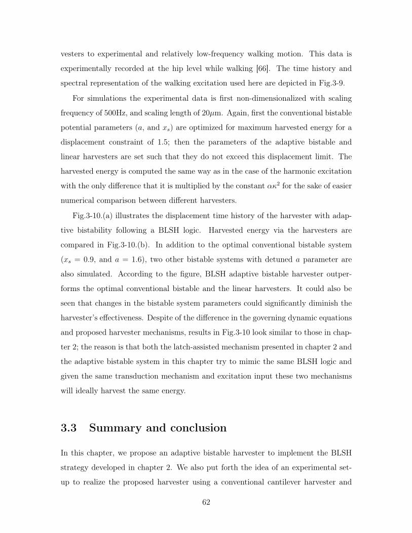
vesters to experimental and relatively low-frequency walking motion. This data is

experimentally recorded at the hip level while walking [66]. The time history and

spectral representation of the walking excitation used here are depicted in Fig.3-9.

For simulations the experimental data is first non-dimensionalized with scaling

frequency of 500Hz, and scaling length of 20𝜇m. Again, first the conventional bistable

potential parameters (𝑎, and 𝑥𝑠) are optimized for maximum harvested energy for a

displacement constraint of 1.5; then the parameters of the adaptive bistable and

linear harvesters are set such that they do not exceed this displacement limit. The

harvested energy is computed the same way as in the case of the harmonic excitation

with the only difference that it is multiplied by the constant 𝛼𝜅2 for the sake of easier

numerical comparison between different harvesters.

Fig.3-10.(a) illustrates the displacement time history of the harvester with adap-

tive bistability following a BLSH logic. Harvested energy via the harvesters are

compared in Fig.3-10.(b). In addition to the optimal conventional bistable system

(𝑥𝑠 = 0.9, and 𝑎 = 1.6), two other bistable systems with detuned 𝑎 parameter are

also simulated. According to the figure, BLSH adaptive bistable harvester outper-

forms the optimal conventional bistable and the linear harvesters. It could also be

seen that changes in the bistable system parameters could significantly diminish the

harvester’s effectiveness. Despite of the difference in the governing dynamic equations

and proposed harvester mechanisms, results in Fig.3-10 look similar to those in chap-

ter 2; the reason is that both the latch-assisted mechanism presented in chapter 2 and

the adaptive bistable system in this chapter try to mimic the same BLSH logic and

given the same transduction mechanism and excitation input these two mechanisms

will ideally harvest the same energy.


In this chapter, we propose an adaptive bistable harvester to implement the BLSH

strategy developed in chapter 2. We also put forth the idea of an experimental set-

up to realize the proposed harvester using a conventional cantilever harvester and

62

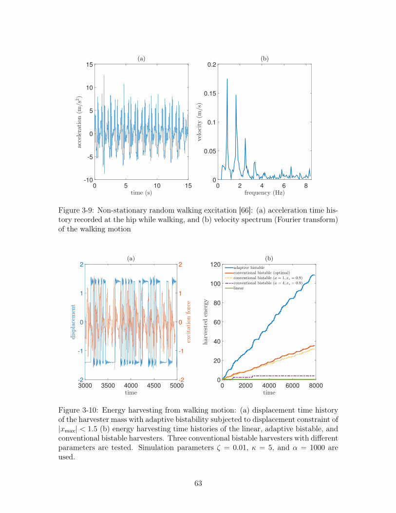
time (s)0 5 10 15

acceleration

(m/s2)

-10

-5

0

5

10

15

(a)

frequency (Hz)0 2 4 6 8

velocity

(m/s)

0

0.05

0.1

0.15

0.2

(b)

Figure 3-9: Non-stationary random walking excitation [66]: (a) acceleration time his-tory recorded at the hip while walking, and (b) velocity spectrum (Fourier transform)of the walking motion

time3000 3500 4000 4500 5000

displacement

-2

-1

0

1

2

(a)

excitation

force

-2

-1

0

1

2

time0 2000 4000 6000 8000

harvesteden

ergy

0

20

40

60

80

100

120

(b)

adaptive bistable

conventional bistable (optimal)

conventional bistable (a = 1, xs = 0.9)

conventional bistable (a = 4, xs = 0.9)

linear

Figure 3-10: Energy harvesting from walking motion: (a) displacement time historyof the harvester mass with adaptive bistability subjected to displacement constraint of|𝑥max| < 1.5 (b) energy harvesting time histories of the linear, adaptive bistable, andconventional bistable harvesters. Three conventional bistable harvesters with differentparameters are tested. Simulation parameters 𝜁 = 0.01, 𝜅 = 5, and 𝛼 = 1000 areused.

63

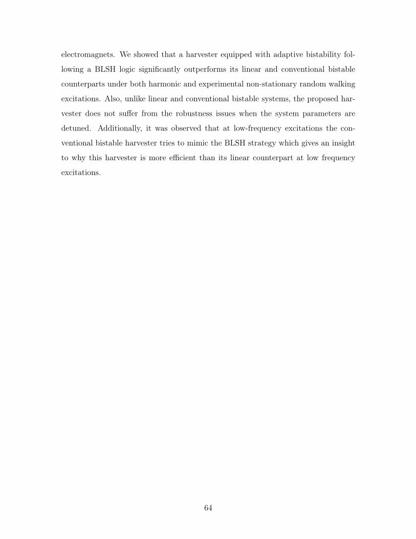
electromagnets. We showed that a harvester equipped with adaptive bistability fol-

lowing a BLSH logic significantly outperforms its linear and conventional bistable

counterparts under both harmonic and experimental non-stationary random walking

excitations. Also, unlike linear and conventional bistable systems, the proposed har-

vester does not suffer from the robustness issues when the system parameters are

detuned. Additionally, it was observed that at low-frequency excitations the con-

ventional bistable harvester tries to mimic the BLSH strategy which gives an insight

to why this harvester is more efficient than its linear counterpart at low frequency

excitations.

64

Chapter 4

Energy harvesting from structural

instabilities

In addition to their issues of narrow spectrum and lack of robustness, the existing

harvesting methods often rely on relatively large host structures to realize linear or

nonlinear resonance which usually results in low harvested power to volume ratios.

For instance, in linear or bistable harvesters, a cantilever beam is often used as the

host structure and piezoelectric patches for energy transduction are used only close

to the clamped end since high strains take place only at the clamped end and at the

beam’s bottom and top surfaces. This inherent mechanical behaviour consequently

results in low power to volume ratios.

In order to overcome the above-discussed issues of the VEHs, one needs to look

for a non-resonant mechanism for robust harvesting, that at same time can induce

large strains throughout its entire volume as opposed to a small area/volume, so

as to improve the harvesting power density. To this end, in this chapter, we pro-

pose to exploit instabilities in multi-layered composites or surface instabilities. Un-

like classical half-sine buckling of a beam-like structure, instabilities and buckling in

composite structures and soft material could take interesting morphological patterns

such as wrinkles, folds, and creases [74] that exhibit large strains at regular patterns

throughout the entire structure. Furthermore, we will discuss that high efficacy of

energy harvesting via structural instabilities, in part, is attributed to its ability to

65

approximately follow the BLSH logic introduced in chapter 2.

Intriguing morphologies and surface patterns in nature at different scales from

wrinkles on skins of mammalians, plants and fruits [10, 67, 131] to crumpled mem-

branes of blood cells[126] have inspired a big body of research in soft matter instabili-

ties. Recent studies in this field have found applications in other disciplines including

soft lithography, metrology, flexible electronics, and biomedical engineering[74]. Here,

we extend the application of soft matter instabilities to kinetic energy harvesting.

The induced instability results in large local strains that could be exploited for

energy harvesting which is the focus of this chapter. The unconventional instabilities

are common to structures that have both stiff and soft components such as a multi-

layer composite structure consisting of stiff layers embedded within a soft matrix or

a bi-layer structure of a stiff layer sitting on a soft foundation. The large local strain

as a result of instability in such structures is the result of two mechanisms: i) when

the stiff layers go unstable, they take almost no more load resulting in lower compos-

ite stiffness. This consequently leads to large macroscopic strain. ii) the nonlinear

geometric pattern of the stiff layer (e.g. sinusoid in wrinkling) locally amplifies the

strain. A key advantage of these types of instabilities is that they are independent of

the excitation (compressive force) frequency.

In this chapter, we focus on wrinkling as the most common instability pattern

in composite layers. We begin in section 4.1 by deriving the state/strain states in a

multi-layer composite of a soft matrix containing stiff layers that is subjected to peri-

odic compressive force. We then feed the calculated stresses to piezoelectric patches

attached on the troughs and peaks of wrinkling instabilities of the stiff layers and

derive the dynamic equation of the electrical domain when the piezoelectric patches

are connected to a simple external resistive load. In section 4.2 we present the results

of numerical simulations before we conclude the chapter by conclusions and future

research directions in section 4.3.

66

4.1 Wrinkling instability

4.1.1 general idea

Surface instabilities are grouped into five main categories: wrinkle, crease, fold,

period-double1, and ridge [127]. Based on the phase diagram developed by Wang

and Zhao[127], wrinkling is the most common surface instability if there is no de-

lamination in the layers; hence, we focus on the wrinkling instability in this chapter.

Based on the classic beam theory, a clamped beam buckles under axial compressive

force in its first mode (with a mode shape similar to a half sine) before any other

modes take place. In fact other modes never take place because they posses larger

potential energy than the first mode. However, if the beam is sitting on a softer elastic

foundation or embedded in an elastic softer matrix, the beam buckles in higher modes

which is usually referred to as wrinkling. The unconventional higher mode buckling

occurs simply because the system always seeks a configuration with the lowest poten-

tial energy; and above a critical stiffness of the foundation/matrix the higher modes

of buckling posses lower potential energy than the classic half-wavelength buckling

mode.

When compared to classical buckling, soft matter buckling such as wrinkling has

a major advantage of delayed instability. The soft foundation or matrix delays the

instability i.e. the structure buckles at a larger critical load. This greatly improves the

energy harvesting process by significantly increasing the power inflow to the system.

This is because the external force displacement as a result of instability occurs at a

larger value of the force; hence, more energy is pumped into the structure. This is in

accordance with the buy-low-sell-high strategy where displacement is allowed only at

the maximum excitation force magnitude (refer to chapter 2).

Figure 1-1 illustrates schematically how energy is harvested via wrinkling insta-

bility. Piezoelectric patches are attached at two sides of the interfacial layers at the

peaks and troughs of the wrinkles. Piezoelectric patches could be connected in series

or parallel to an external load or any other harvesting circuitry (not shown on the

1sometimes period-double or even period-quadruple are categorized under wrinkling, e.g. in [74]

67

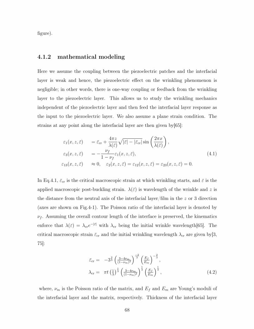
figure).

4.1.2 mathematical modeling

Here we assume the coupling between the piezoelectric patches and the interfacial

layer is weak and hence, the piezoelectric effect on the wrinkling phenomenon is

negligible; in other words, there is one-way coupling or feedback from the wrinkling

layer to the piezoelectric layer. This allows us to study the wrinkling mechanics

independent of the piezoelectric layer and then feed the interfacial layer response as

the input to the piezoelectric layer. We also assume a plane strain condition. The

strains at any point along the interfacial layer are then given by[65]:

𝜀1(𝑥, 𝑧, 𝜀) = 𝜀cr +4𝜋𝑧

𝜆(𝜀)

√|𝜀| − |𝜀cr| sin

(2𝜋𝑥

𝜆(𝜀)

),

𝜀3(𝑥, 𝑧, 𝜀) = − 𝜈𝑓1 − 𝜈𝑓

𝜀1(𝑥, 𝑧, 𝜀), (4.1)

𝜀13(𝑥, 𝑧, 𝜀) ≈ 0, 𝜀2(𝑥, 𝑧, 𝜀) = 𝜀12(𝑥, 𝑧, 𝜀) = 𝜀23(𝑥, 𝑧, 𝜀) = 0.

In Eq.4.1, 𝜀cr is the critical macroscopic strain at which wrinkling starts, and 𝜀 is the

applied macroscopic post-buckling strain. 𝜆(𝜀) is wavelength of the wrinkle and 𝑧 is

the distance from the neutral axis of the interfacial layer/film in the 𝑧 or 3 direction

(axes are shown on Fig.4-1). The Poisson ratio of the interfacial layer is denoted by

𝜈𝑓 . Assuming the overall contour length of the interface is preserved, the kinematics

enforce that 𝜆(𝜀) = 𝜆cr𝑒−|𝜀| with 𝜆cr being the initial wrinkle wavelength[65]. The

critical macroscopic strain 𝜀cr and the initial wrinkling wavelength 𝜆cr are given by[3,

75]:

𝜀cr = −323

(3−4𝜈𝑚(1−𝜈𝑚)2

)−23(

𝐸𝑓

𝐸𝑚

)− 23,

𝜆cr = 𝜋𝑡(13

) 13

(3−4𝜈𝑚(1−𝜈𝑚)2

) 13(

𝐸𝑓

𝐸𝑚

) 13, (4.2)

where, 𝜈𝑚 is the Poisson ratio of the matrix, and 𝐸𝑓 and 𝐸𝑚 are Young’s moduli of

the interfacial layer and the matrix, respectively. Thickness of the interfacial layer

68

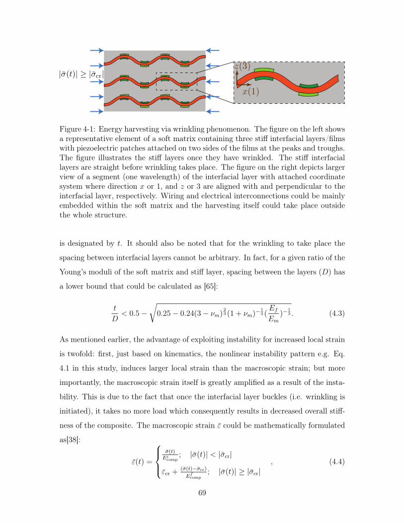
Figure 4-1: Energy harvesting via wrinkling phenomenon. The figure on the left showsa representative element of a soft matrix containing three stiff interfacial layers/filmswith piezoelectric patches attached on two sides of the films at the peaks and troughs.The figure illustrates the stiff layers once they have wrinkled. The stiff interfaciallayers are straight before wrinkling takes place. The figure on the right depicts largerview of a segment (one wavelength) of the interfacial layer with attached coordinatesystem where direction 𝑥 or 1, and 𝑧 or 3 are aligned with and perpendicular to theinterfacial layer, respectively. Wiring and electrical interconnections could be mainlyembedded within the soft matrix and the harvesting itself could take place outsidethe whole structure.

is designated by 𝑡. It should also be noted that for the wrinkling to take place the

spacing between interfacial layers cannot be arbitrary. In fact, for a given ratio of the

Young’s moduli of the soft matrix and stiff layer, spacing between the layers (𝐷) has

a lower bound that could be calculated as [65]:

𝑡

𝐷< 0.5 −

√0.25 − 0.24(3 − 𝜈𝑚)

23 (1 + 𝜈𝑚)−

13 (

𝐸𝑓

𝐸𝑚

)−13 . (4.3)

As mentioned earlier, the advantage of exploiting instability for increased local strain

is twofold: first, just based on kinematics, the nonlinear instability pattern e.g. Eq.

4.1 in this study, induces larger local strain than the macroscopic strain; but more

importantly, the macroscopic strain itself is greatly amplified as a result of the insta-

bility. This is due to the fact that once the interfacial layer buckles (i.e. wrinkling is

initiated), it takes no more load which consequently results in decreased overall stiff-

ness of the composite. The macroscopic strain 𝜀 could be mathematically formulated

as[38]:

𝜀(𝑡) =

⎧⎪⎨⎪⎩(𝑡)

𝐸𝑖comp

; |(𝑡)| < |cr|

𝜀cr + ((𝑡)−cr)

𝐸𝑓comp

; |(𝑡)| ≥ |cr|, (4.4)

69

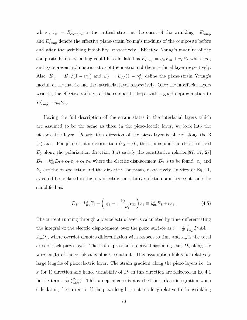
where, cr = 𝐸𝑖comp𝜀cr is the critical stress at the onset of the wrinkling. 𝐸𝑖

comp

and 𝐸𝑓comp denote the effective plane-strain Young’s modulus of the composite before

and after the wrinkling instability, respectively. Effective Young’s modulus of the

composite before wrinkling could be calculated as 𝐸𝑖comp = 𝜂𝑚𝑚 + 𝜂𝑓 𝑓 where, 𝜂𝑚

and 𝜂𝑓 represent volumetric ratios of the matrix and the interfacial layer respectively.

Also, 𝑚 = 𝐸𝑚/(1 − 𝜈2𝑚) and 𝑓 = 𝐸𝑓/(1 − 𝜈2

𝑓 ) define the plane-strain Young’s

moduli of the matrix and the interfacial layer respectively. Once the interfacial layers

wrinkle, the effective stiffness of the composite drops with a good approximation to

𝐸𝑓comp = 𝜂𝑚𝑚.

Having the full description of the strain states in the interfacial layers which

are assumed to be the same as those in the piezoelectric layer, we look into the

piezoelectric layer. Polarization direction of the piezo layer is placed along the 3

(𝑧) axis. For plane strain deformation (𝜀2 = 0), the strains and the electrical field

𝐸3 along the polarization direction 3(𝑧) satisfy the constitutive relation[87, 17, 27]

𝐷3 = 𝑘𝑠33𝐸3 +𝑒31𝜀1 +𝑒33𝜀3, where the electric displacement 𝐷3 is to be found. 𝑒𝑖𝑗 and

𝑘𝑖𝑗 are the piezoelectric and the dielectric constants, respectively. In view of Eq.4.1,

𝜀3 could be replaced in the piezoelectric constitutive relation, and hence, it could be

simplified as:

𝐷3 = 𝑘𝑠33𝐸3 +

(𝑒31 −

𝜈𝑓1 − 𝜈𝑓

𝑒33

)𝜀1 ≡ 𝑘𝑠

33𝐸3 + 𝑒𝜀1. (4.5)

The current running through a piezoelectric layer is calculated by time-differentiating

the integral of the electric displacement over the piezo surface as 𝑖 = 𝑑𝑑𝑡

∫𝐴𝑝

𝐷3𝑑𝐴 =

𝐴𝑝3, where overdot denotes differentiation with respect to time and 𝐴𝑝 is the total

area of each piezo layer. The last expression is derived assuming that 𝐷3 along the

wavelength of the wrinkles is almost constant. This assumption holds for relatively

large lengths of piezoelectric layer. The strain gradient along the piezo layers i.e. in

𝑥 (or 1) direction and hence variability of 𝐷3 in this direction are reflected in Eq.4.1

in the term: sin( 2𝜋𝑥𝜆(𝜀)

). This 𝑥 dependence is absorbed in surface integration when

calculating the current 𝑖. If the piezo length is not too long relative to the wrinkling

70

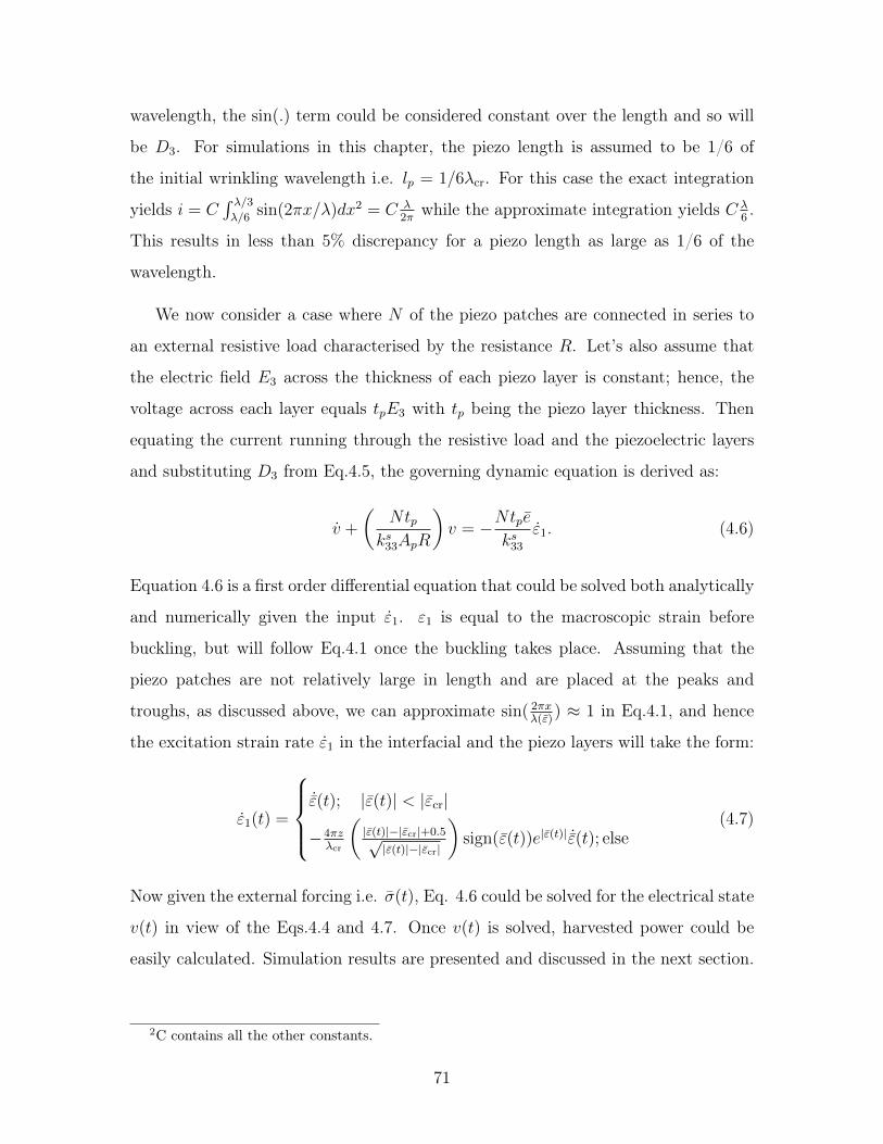
wavelength, the sin(.) term could be considered constant over the length and so will

be 𝐷3. For simulations in this chapter, the piezo length is assumed to be 1/6 of

the initial wrinkling wavelength i.e. 𝑙𝑝 = 1/6𝜆cr. For this case the exact integration

yields 𝑖 = 𝐶∫ 𝜆/3

𝜆/6sin(2𝜋𝑥/𝜆)𝑑𝑥2 = 𝐶 𝜆

2𝜋while the approximate integration yields 𝐶 𝜆

6.

This results in less than 5% discrepancy for a piezo length as large as 1/6 of the

wavelength.

We now consider a case where 𝑁 of the piezo patches are connected in series to

an external resistive load characterised by the resistance 𝑅. Let’s also assume that

the electric field 𝐸3 across the thickness of each piezo layer is constant; hence, the

voltage across each layer equals 𝑡𝑝𝐸3 with 𝑡𝑝 being the piezo layer thickness. Then

equating the current running through the resistive load and the piezoelectric layers

and substituting 𝐷3 from Eq.4.5, the governing dynamic equation is derived as:

+

(𝑁𝑡𝑝

𝑘𝑠33𝐴𝑝𝑅

)𝑣 = −𝑁𝑡𝑝𝑒

𝑘𝑠33

1. (4.6)

Equation 4.6 is a first order differential equation that could be solved both analytically

and numerically given the input 1. 𝜀1 is equal to the macroscopic strain before

buckling, but will follow Eq.4.1 once the buckling takes place. Assuming that the

piezo patches are not relatively large in length and are placed at the peaks and

troughs, as discussed above, we can approximate sin( 2𝜋𝑥𝜆(𝜀)

) ≈ 1 in Eq.4.1, and hence

the excitation strain rate 1 in the interfacial and the piezo layers will take the form:

1(𝑡) =

⎧⎪⎪⎨⎪⎪⎩˙𝜀(𝑡); |𝜀(𝑡)| < |𝜀cr|

−4𝜋𝑧𝜆cr

(|𝜀(𝑡)|−|𝜀cr|+0.5√

|𝜀(𝑡)|−|𝜀cr|

)sign(𝜀(𝑡))𝑒|𝜀(𝑡)| ˙𝜀(𝑡); else

(4.7)

Now given the external forcing i.e. (𝑡), Eq. 4.6 could be solved for the electrical state

𝑣(𝑡) in view of the Eqs.4.4 and 4.7. Once 𝑣(𝑡) is solved, harvested power could be

easily calculated. Simulation results are presented and discussed in the next section.

2C contains all the other constants.

71

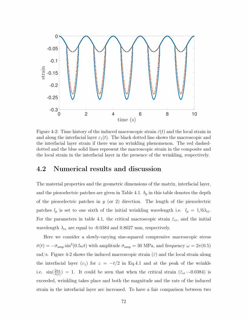
0 2 4 6 8 10

time (s)

-0.3

-0.25

-0.2

-0.15

-0.1

-0.05

0

strain

Figure 4-2: Time history of the induced macroscopic strain 𝜀(𝑡) and the local strain inand along the interfacial layer 𝜀1(𝑡). The black dotted line shows the macroscopic andthe interfacial layer strain if there was no wrinkling phenomenon. The red dashed-dotted and the blue solid lines represent the macroscopic strain in the composite andthe local strain in the interfacial layer in the presence of the wrinkling, respectively.

4.2 Numerical results and discussion

The material properties and the geometric dimensions of the matrix, interfacial layer,

and the piezoelectric patches are given in Table 4.1. 𝑏𝑝 in this table denotes the depth

of the piezoelectric patches in 𝑦 (or 2) direction. The length of the piezoelectric

patches 𝑙𝑝 is set to one sixth of the initial wrinkling wavelength i.e. 𝑙𝑝 = 1/6𝜆cr.

For the parameters in table 4.1, the critical macroscopic strain 𝜀cr, and the initial

wavelength 𝜆cr are equal to -0.0384 and 0.8027 mm, respectively.

Here we consider a slowly-varying sine-squared compressive macroscopic stress

(𝑡) = −amp sin2(0.5𝜔𝑡) with amplitude amp = 30 MPa, and frequency 𝜔 = 2𝜋(0.5)

rad/s. Figure 4-2 shows the induced macroscopic strain (𝜀) and the local strain along

the interfacial layer (𝜀1) for 𝑧 = −𝑡/2 in Eq.4.1 and at the peak of the wrinkle

i.e. sin( 2𝜋𝑥𝜆(𝜀)

) = 1. It could be seen that when the critical strain (𝜀cr=-0.0384) is

exceeded, wrinkling takes place and both the magnitude and the rate of the induced

strain in the interfacial layer are increased. To have a fair comparison between two

72

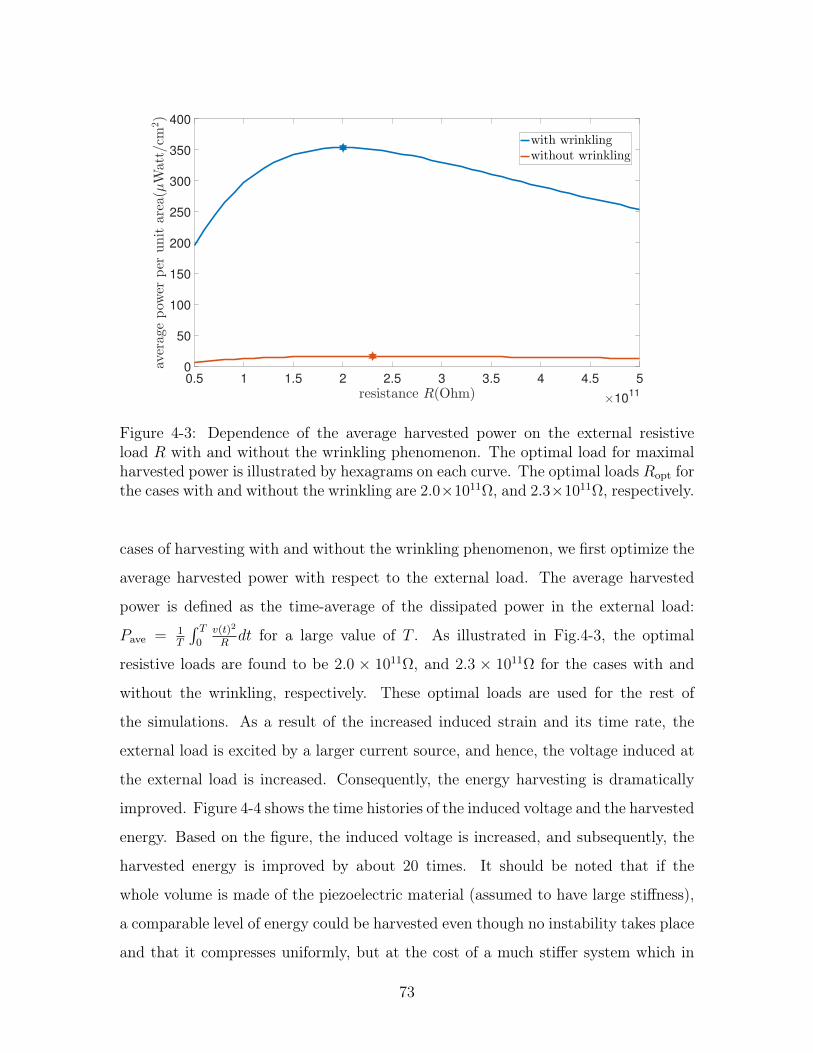
0.5 1 1.5 2 2.5 3 3.5 4 4.5 5

resistance R(Ohm)×10

11

0

50

100

150

200

250

300

350

400

averagepow

erper

unitarea(µWatt/cm

2)

with wrinklingwithout wrinkling

Figure 4-3: Dependence of the average harvested power on the external resistiveload 𝑅 with and without the wrinkling phenomenon. The optimal load for maximalharvested power is illustrated by hexagrams on each curve. The optimal loads 𝑅opt forthe cases with and without the wrinkling are 2.0×1011Ω, and 2.3×1011Ω, respectively.

cases of harvesting with and without the wrinkling phenomenon, we first optimize the

average harvested power with respect to the external load. The average harvested

power is defined as the time-average of the dissipated power in the external load:

𝑃ave = 1𝑇

∫ 𝑇

0𝑣(𝑡)2

𝑅𝑑𝑡 for a large value of 𝑇 . As illustrated in Fig.4-3, the optimal

resistive loads are found to be 2.0 × 1011Ω, and 2.3 × 1011Ω for the cases with and

without the wrinkling, respectively. These optimal loads are used for the rest of

the simulations. As a result of the increased induced strain and its time rate, the

external load is excited by a larger current source, and hence, the voltage induced at

the external load is increased. Consequently, the energy harvesting is dramatically

improved. Figure 4-4 shows the time histories of the induced voltage and the harvested

energy. Based on the figure, the induced voltage is increased, and subsequently, the

harvested energy is improved by about 20 times. It should be noted that if the

whole volume is made of the piezoelectric material (assumed to have large stiffness),

a comparable level of energy could be harvested even though no instability takes place

and that it compresses uniformly, but at the cost of a much stiffer system which in

73

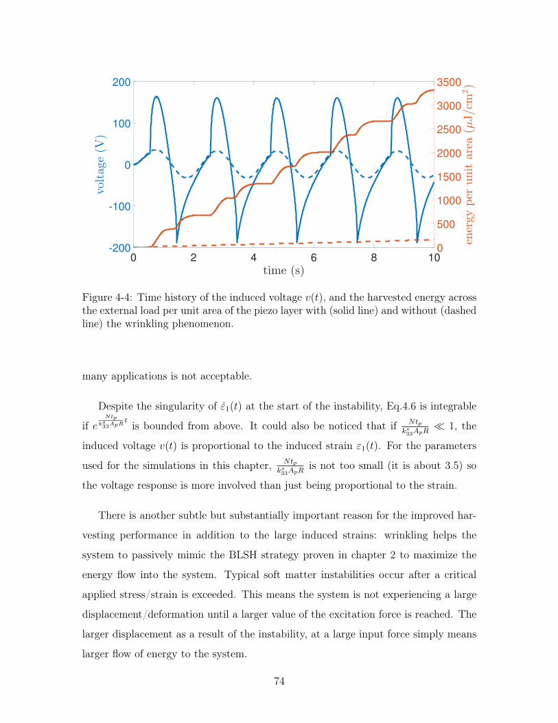
0 2 4 6 8 10

time (s)

-200

-100

0

100

200

voltage(V

)

0

500

1000

1500

2000

2500

3000

3500

energy

per

unitarea

(µJ/cm

2)

Figure 4-4: Time history of the induced voltage 𝑣(𝑡), and the harvested energy acrossthe external load per unit area of the piezo layer with (solid line) and without (dashedline) the wrinkling phenomenon.

many applications is not acceptable.

Despite the singularity of 1(𝑡) at the start of the instability, Eq.4.6 is integrable

if 𝑒𝑁𝑡𝑝

𝑘𝑠33𝐴𝑝𝑅𝑡 is bounded from above. It could also be noticed that if 𝑁𝑡𝑝

𝑘𝑠33𝐴𝑝𝑅≪ 1, the

induced voltage 𝑣(𝑡) is proportional to the induced strain 𝜀1(𝑡). For the parameters

used for the simulations in this chapter, 𝑁𝑡𝑝𝑘𝑠33𝐴𝑝𝑅

is not too small (it is about 3.5) so

the voltage response is more involved than just being proportional to the strain.

There is another subtle but substantially important reason for the improved har-

vesting performance in addition to the large induced strains: wrinkling helps the

system to passively mimic the BLSH strategy proven in chapter 2 to maximize the

energy flow into the system. Typical soft matter instabilities occur after a critical

applied stress/strain is exceeded. This means the system is not experiencing a large

displacement/deformation until a larger value of the excitation force is reached. The

larger displacement as a result of the instability, at a large input force simply means

larger flow of energy to the system.

74

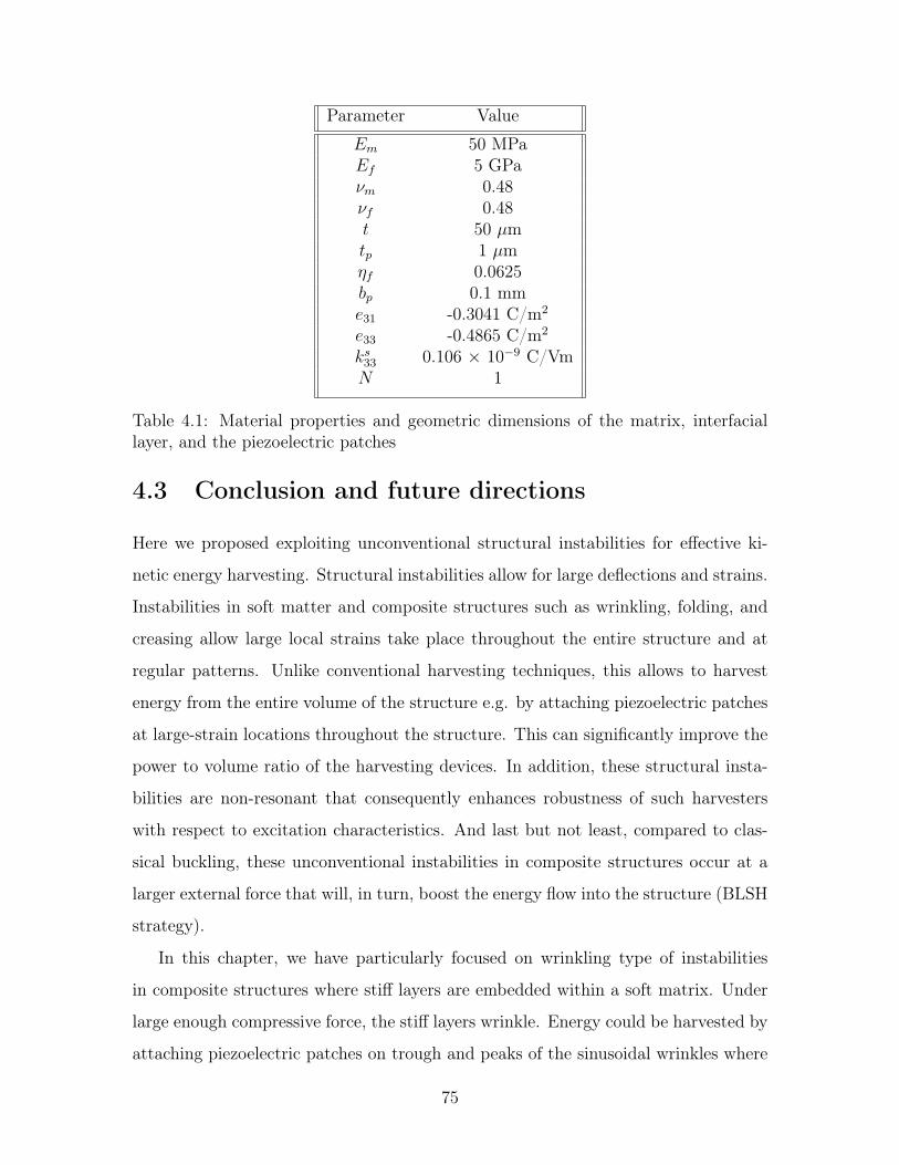
Parameter Value

𝐸𝑚 50 MPa𝐸𝑓 5 GPa𝜈𝑚 0.48𝜈𝑓 0.48𝑡 50 𝜇m𝑡𝑝 1 𝜇m𝜂𝑓 0.0625𝑏𝑝 0.1 mm𝑒31 -0.3041 C/m2

𝑒33 -0.4865 C/m2

𝑘𝑠33 0.106 × 10−9 C/Vm𝑁 1

Table 4.1: Material properties and geometric dimensions of the matrix, interfaciallayer, and the piezoelectric patches

4.3 Conclusion and future directions

Here we proposed exploiting unconventional structural instabilities for effective ki-

netic energy harvesting. Structural instabilities allow for large deflections and strains.

Instabilities in soft matter and composite structures such as wrinkling, folding, and

creasing allow large local strains take place throughout the entire structure and at

regular patterns. Unlike conventional harvesting techniques, this allows to harvest

energy from the entire volume of the structure e.g. by attaching piezoelectric patches

at large-strain locations throughout the structure. This can significantly improve the

power to volume ratio of the harvesting devices. In addition, these structural insta-

bilities are non-resonant that consequently enhances robustness of such harvesters

with respect to excitation characteristics. And last but not least, compared to clas-

sical buckling, these unconventional instabilities in composite structures occur at a

larger external force that will, in turn, boost the energy flow into the structure (BLSH

strategy).

In this chapter, we have particularly focused on wrinkling type of instabilities

in composite structures where stiff layers are embedded within a soft matrix. Under

large enough compressive force, the stiff layers wrinkle. Energy could be harvested by

attaching piezoelectric patches on trough and peaks of the sinusoidal wrinkles where

75

maximum strain is achieved. Here we have assumed one-way coupling between the

host structure and the piezoelectric patches i.e. the piezoelectricity does not affect the

wrinkling phenomenon. Since we are mainly targeting low-frequency excitation, we

assume static stress-strain analysis in the structure which we then feed as the input

to the piezoelectric patches. Under low-frequency compressive stress on the structure,

we derive the first-order dynamic equation of the electrical state of the system, and

consequently calculate the harvested power dissipated in a resistive load connected

to the piezoelectric patches. Theoretical and simulation results show that wrinkling

could help improve the harvested power by more than an order of magnitude. We be-

lieve the proposed approach opens the way to previously uncharted energy harvesting

paradigms, and in view of the recent advances in flexible electronics[17], introduces a

promising method to effectively harvest energy for a wide range of applications.

In this preliminary study we neglected, for the sake of simplicity, the feedback

from the transduction mechanism on the structure; however, we know that the trans-

duction mechanism adds a secondary mechanical and electrical/magnetic potential

energy to the system. This will in turn delay and could eventually prevent the insta-

bility if the feedback is too strong; this could be exploited to control the instability.

An even more efficient method to control the instability is to design the system such

that it is near the instability boundaries; then by a small perturbation of the sys-

tem, e.g. by applying a small voltage on the piezo-layers with the right polarity,

one can help the instability occur and even move across different modes of instabil-

ity. This way, we could control the instability, and hence, extend the application

of the aforementioned idea from energy harvesting to a whole new level of tunable

material/structures with a myriad of applications from electromechanical valves in

micro-fluidics to electromechanical amplifiers/transistors to soft robotics.

76

Chapter 5

Design of vibratory energy harvesters

under stochastic parametric

uncertainty

Vibratory energy harvesters as potential replacement of conventional batteries are not

as robust as conventional batteries. To efficiently harvest energy from the excitation

source, mechanical and electrical parameters of the harvester should be well optimized

and finely tuned. Finding exact or approximate optimal deterministic parameters

for electromagnetic[120] and piezoelectric[22, 114, 115, 116, 101] energy harvesters

has been comprehensively studied in the literature for the linear harvesters. For the

nonlinear energy harvesters, researchers have mainly studied the effects of mechanical

potential shape[76, 19, 40, 132] or the harvesting circuitry[36, 121, 21]. All these stud-

ies have assumed deterministic system parameters to optimize the harvested power;

however, manufacturing tolerances, wear and tear and material degradation, and hu-

midity, temperature and environmental conditions among others result in parametric

uncertainty in the system. Moreover, excitation statistics are also often random and

even non-stationary in real world. Uncertainty in the system usually necessitates two

types of analysis: uncertainty propagation and sensitivity analysis, and optimization

under uncertainty for robust design.

Although being well explored in other fields like controls, finance, and produc-

77

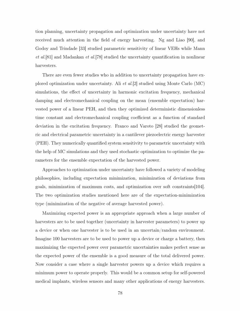
tion planning, uncertainty propagation and optimization under uncertainty have not

received much attention in the field of energy harvesting. Ng and Liao [90], and

Godoy and Trindade [33] studied parametric sensitivity of linear VEHs while Mann

et al.[81] and Madankan et al.[78] studied the uncertainty quantification in nonlinear

harvesters.

There are even fewer studies who in addition to uncertainty propagation have ex-

plored optimization under uncertainty. Ali et al.[2] studied using Monte Carlo (MC)

simulations, the effect of uncertainty in harmonic excitation frequency, mechanical

damping and electromechanical coupling on the mean (ensemble expectation) har-

vested power of a linear PEH, and then they optimized deterministic dimensionless

time constant and electromechanical coupling coefficient as a function of standard

deviation in the excitation frequency. Franco and Varoto [28] studied the geomet-

ric and electrical parametric uncertainty in a cantilever piezoelectric energy harvester

(PEH). They numerically quantified system sensitivity to parametric uncertainty with

the help of MC simulations and they used stochastic optimization to optimize the pa-

rameters for the ensemble expectation of the harvested power.

Approaches to optimization under uncertainty have followed a variety of modeling

philosophies, including expectation minimization, minimization of deviations from

goals, minimization of maximum costs, and optimization over soft constraints[104].

The two optimization studies mentioned here are of the expectation-minimization

type (minimization of the negative of average harvested power).

Maximizing expected power is an appropriate approach when a large number of

harvesters are to be used together (uncertainty in harvester parameters) to power up

a device or when one harvester is to be used in an uncertain/random environment.

Imagine 100 harvesters are to be used to power up a device or charge a battery, then

maximizing the expected power over parametric uncertainties makes perfect sense as

the expected power of the ensemble is a good measure of the total delivered power.

Now consider a case where a single harvester powers up a device which requires a

minimum power to operate properly. This would be a common setup for self-powered

medical implants, wireless sensors and many other applications of energy harvesters.

78

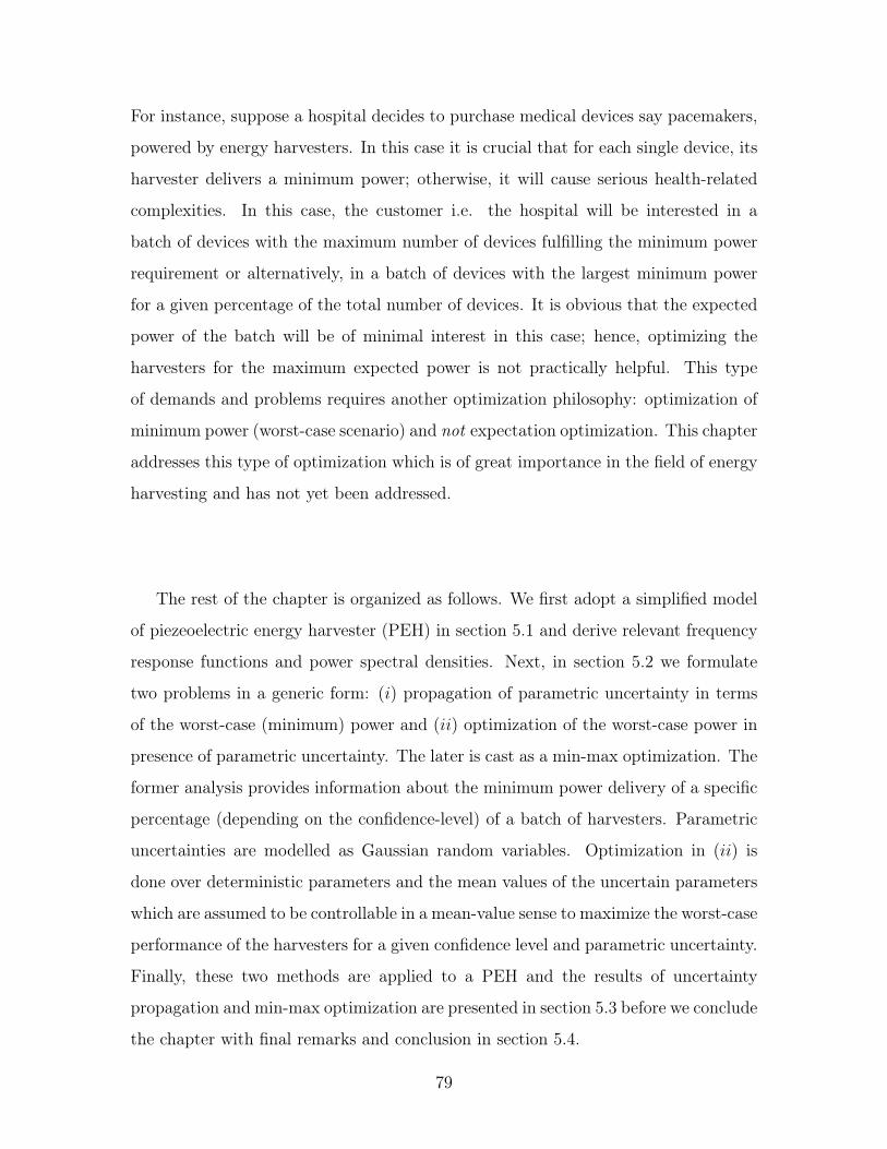
For instance, suppose a hospital decides to purchase medical devices say pacemakers,

powered by energy harvesters. In this case it is crucial that for each single device, its

harvester delivers a minimum power; otherwise, it will cause serious health-related

complexities. In this case, the customer i.e. the hospital will be interested in a

batch of devices with the maximum number of devices fulfilling the minimum power

requirement or alternatively, in a batch of devices with the largest minimum power

for a given percentage of the total number of devices. It is obvious that the expected

power of the batch will be of minimal interest in this case; hence, optimizing the

harvesters for the maximum expected power is not practically helpful. This type

of demands and problems requires another optimization philosophy: optimization of

minimum power (worst-case scenario) and not expectation optimization. This chapter

addresses this type of optimization which is of great importance in the field of energy

harvesting and has not yet been addressed.

The rest of the chapter is organized as follows. We first adopt a simplified model

of piezeoelectric energy harvester (PEH) in section 5.1 and derive relevant frequency

response functions and power spectral densities. Next, in section 5.2 we formulate

two problems in a generic form: (𝑖) propagation of parametric uncertainty in terms

of the worst-case (minimum) power and (𝑖𝑖) optimization of the worst-case power in

presence of parametric uncertainty. The later is cast as a min-max optimization. The

former analysis provides information about the minimum power delivery of a specific

percentage (depending on the confidence-level) of a batch of harvesters. Parametric

uncertainties are modelled as Gaussian random variables. Optimization in (𝑖𝑖) is

done over deterministic parameters and the mean values of the uncertain parameters

which are assumed to be controllable in a mean-value sense to maximize the worst-case

performance of the harvesters for a given confidence level and parametric uncertainty.

Finally, these two methods are applied to a PEH and the results of uncertainty

propagation and min-max optimization are presented in section 5.3 before we conclude

the chapter with final remarks and conclusion in section 5.4.

79

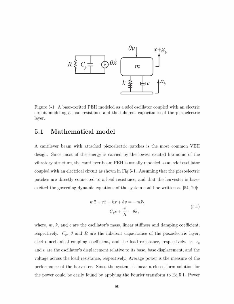
m

ck

Cp

R ˙θx

x+xb

θv

xb

Figure 5-1: A base-excited PEH modeled as a sdof oscillator coupled with an electriccircuit modeling a load resistance and the inherent capacitance of the piezoelectriclayer.

5.1 Mathematical model

A cantilever beam with attached piezoelectric patches is the most common VEH

design. Since most of the energy is carried by the lowest excited harmonic of the

vibratory structure, the cantilever beam PEH is usually modeled as an sdof oscillator

coupled with an electrical circuit as shown in Fig.5-1. Assuming that the piezoelectric

patches are directly connected to a load resistance, and that the harvester is base-

excited the governing dynamic equations of the system could be written as [54, 20]:

𝑚 + 𝑐 + 𝑘𝑥 + 𝜃𝑣 = −𝑚𝑏

𝐶𝑝 +𝑣

𝑅= 𝜃,

(5.1)

where, 𝑚, 𝑘, and 𝑐 are the oscillator’s mass, linear stiffness and damping coefficient,

respectively. 𝐶𝑝, 𝜃 and 𝑅 are the inherent capacitance of the piezoelectric layer,

electromechanical coupling coefficient, and the load resistance, respectively. 𝑥, 𝑥𝑏

and 𝑣 are the oscillator’s displacement relative to its base, base displacement, and the

voltage across the load resistance, respectively. Average power is the measure of the

performance of the harvester. Since the system is linear a closed-form solution for

the power could be easily found by applying the Fourier transform to Eq.5.1. Power

80

is conventionally normalized by the square of input acceleration for the harmonic

excitation. The normalized peak power1 could then be written as

𝑃 (𝜔)

(𝑋𝑏𝜔2)2

=

1

𝑅

𝑉

𝑋𝑏𝜔2

2=

𝑅𝜃2𝜔2((𝑅𝐶𝑝𝜔2

𝑛 + 2𝜁𝜔𝑛 + 𝑅𝜃2

𝑚)𝜔 −𝑅𝐶𝑝𝜔3

)2+ (−𝜔2

𝑛 + (1 + 2𝜁𝑅𝐶𝑝𝜔𝑛𝜔2)𝜔2)2,

where, 𝑋𝑏(𝜔) and 𝑉 (𝜔) are the Fourier transforms of the base displacement and load

voltage, respectively, and 𝜔 is the excitation frequency. Also, by convention natural

frequency 𝜔𝑛 and damping ratio 𝜁 are introduced which are defined as 𝜔𝑛 =√

𝑘/𝑚,

and 𝜁 = 𝑐/2√𝑘𝑚.

We also consider the case where excitation is wideband random excitation. In

this case we use Parseval’s identity which relates the average energy in a signal to its

finite Fourier transform as [57, 46]:

𝑃 (𝑡) = lim𝑇→∞

1

𝑇

∫ 𝑇

0

𝑣2(𝑡)

𝑅d𝑡 =

∫ ∞

0

𝑆𝑣(𝜔)

𝑅d𝜔, (5.2)

where, 𝑆𝑣(𝜔) is the power spectral density of the voltage across the load and is related

to the input acceleration power spectral density 𝑆𝑏(𝜔) by the relation [56, 58, 44]

𝑆𝑣(𝜔) =𝐻𝑣

𝑏(𝜔)

2𝑆𝑏

(𝜔). (5.3)

In Eq.5.3 𝑆𝑏(𝜔) is one-sided power spectral density of input acceleration and 𝐻𝑣

𝑏(𝜔)

is the transfer function from input base acceleration 𝑏 to the load voltage 𝑣 and

could be derived based on governing dynamics equations in Eq.5.1 as

𝐻𝑣𝑏

(𝜔) =𝑅𝜃𝜔(

(𝑅𝐶𝑝𝜔2𝑛 + 2𝜁𝜔𝑛 + 𝑅𝜃2

𝑚)𝜔 −𝑅𝐶𝑝𝜔3

)+ (−𝜔2

𝑛 + (1 + 2𝜁𝑅𝐶𝑝𝜔𝑛𝜔2)𝜔2) 𝑗,

(5.4)

where, 𝑗 =√−1. For a deterministic harvester Eqs.5.2 and 5.2 could be used to study

the effect of different parameters on the harvested power and to optimize them. Here

1For a harmonic excitation the average power is simply half the peak power; hence, we simplyuse the peak power as a performance measure.

81

we assume that some of the parameters are random. This uncertainty in parameters

could be a result of manufacturing tolerances or defects, material degradation, or

environmental effects such as temperature or humidity. Random parameters 𝜉𝑖 are

modelled as Gaussian variables with mean value of 𝜉𝑚𝑖 and standard deviation of 𝜎𝜉𝑖 .

5.2 Uncertainty propagation and optimization for-

mulation

In this study we investigate the effect of uncertainty on the minimum harvested power

i.e. the worst-case performance, and then optimize the mean uncertain parameters to

maximize the minimum power i.e. optimization for the best worst-case performance.

The random parameters are modeled as Gaussian with a mean and a standard de-

viation. Here we assume the mean value of the parameters (𝜉𝑚𝑖) are controllable.

Hence we write the 𝑖thrandom parameter as 𝜉𝑖 = 𝜉𝑚𝑖 + 𝛿𝜉𝑖 where 𝛿𝜉𝑖 is the variation

from the mean value. We know that for random variables with Gaussian distribution

this variation extends from −∞ to +∞; however, the closer it gets to the tails the

smaller gets the probability of the parameter in that range. Therefore, to make the

optimization tractable and non-trivial we have to limit the variation 𝛿𝜉𝑖 for a desired

confidence level. For example for a 99.7% confidence level, −3𝜎𝜉𝑖 < 𝛿𝜉𝑖 < +3𝜎𝜉𝑖 , and

for a 95.5% confidence level we should limit 𝛿𝜉𝑖 as −2𝜎𝜉𝑖 < 𝛿𝜉𝑖 < +2𝜎𝜉𝑖 .

Let’s suppose a manufacturer mass produces a batch of harvesters with parametric

uncertainties. It is important for the customer to know that a certain percentage

of the harvesters i.e. the confidence level, say 95.5% of the harvesters, deliver a

minimum required power. To answer this question, the manufacturer should be able

to quantify the effect of uncertainties on the worst-case performance (minimum power)

for a given confidence level. Moreover, it is clear that the larger the confidence level

fulfilling a minimum power requirement or the larger the minimum power for a given

confidence level, the better the quality of that batch. Assuming that the mean value

of the uncertain parameters are controllable in the manufacturing process, then the

82

manufacturer should optimize the mean values of the parameters to maximize the

worst-case power for a given confidence level or to maximize the confidence level for

a given worst-case power. For the optimization in this study, we do the former i.e.

maximizing the worst-case power for a given confidence level.

As discussed we have two types of problems here:

(P1): uncertainty propagation: Given the confidence level, find the worst-case

(minimum) power as a function of parametric uncertainties (standard deviations

𝜎𝜉𝑖), deterministic parameters, and mean values of uncertain parameters 𝜉𝑚𝑖:

𝑃wc

(𝜉𝑚𝑖, 𝜎𝜉𝑖 , 𝜉det𝑗 ) = min

𝜉𝑖𝑃 (𝑡; 𝜉𝑖, 𝜉

det𝑗 ) : 𝜉𝑖 ∈ (𝜉𝑚𝑖 − max(𝛿𝜉𝑖), 𝜉𝑚𝑖 + max(𝛿𝜉𝑖)).

(5.5)

(P2): optimization for the worst-case scenario under parametric uncer-

tainty: Given the confidence level, find the optimum mean value of the un-

certain parameters 𝜉𝑚𝑖, and the deterministic parameters 𝜉det𝑗 to maximize the

worst-case (minimum) power:

𝑃wc

max(𝜎𝜉𝑖) = max𝜉𝑚𝑖, 𝜉det𝑗

min𝜉𝑖

𝑃 (𝑡; 𝜉𝑖, 𝜉det𝑗 ) : 𝜉𝑖 ∈ (𝜉𝑚𝑖 − max(𝛿𝜉𝑖), 𝜉𝑚𝑖 + max(𝛿𝜉𝑖)),

(5.6)

where 𝜉det𝑗 is the 𝑗th deterministic parameter. P2 is also known as min-max optimiza-

tion problem. To study P1, for given mean values of the uncertain parameters 𝜉𝑖 i.e.

𝜉𝑚𝑖, a search over a grid of 𝜉𝑚𝑖 −max(𝛿𝜉𝑖) < 𝜉𝑖 < 𝜉𝑚𝑖 + max(𝛿𝜉𝑖) is conducted to find

the minimum power. Depending on the confidence level max(𝛿𝜉𝑖) can adopt different

values in terms of the standard deviation 𝜎𝜉𝑖 . For instance, for a confidence level

of 95.5%, max(𝛿𝜉𝑖) = 2𝜎𝜉𝑖 . In addition, depending on the number of simultaneous

uncertain parameters being studied (𝑖 = 1, 2, ..., 𝑛) the search grid will be on a line,

surface, or in an 𝑛-dimensional hypercube in general. Also, optimum parameters for

a deterministic harvester are used as the corresponding mean values for the uncertain

83

parameters (𝜉𝑚𝑖) and deterministic parameters (𝜉det𝑗 ) in P12. This is what we would

refer to as naive optimization i.e. the optimization of the parameters without consid-

ering uncertainties. When 𝜉𝑚𝑖 and 𝜉det𝑗 are chosen this way, P1 shows how uncertainty

in parameters affects the worst-case power of a naively-optimized harvester.

To study P2, the same procedure as described above for P1 is carried out over

feasible deterministic parameters 𝜉det𝑗 and the mean values of the uncertain parameters

𝜉𝑚𝑖 to find the optimum mean values maximizing the worst-case power. In the next

section numerical results are presented and discussed.

5.3 Numerical results and discussion

We explore the effects of uncertainty in three parameters namely, natural frequency

𝜔𝑛, load resistance 𝑅 and electromechanical coupling coefficient 𝜃 on the worst-case

harvested power for different confidence levels (P1). Then considering these uncer-

tainties, we optimize the deterministic parameters and the mean value of the uncertain

parameters to maximize the worst-case power (P2). To be able to visualize the effects

we consider two uncertain parameters at a time and optimize over the mean values

of those two parameters unless otherwise specified.

Figure 5-2 shows the normalized worst-case power as a function of normalized

uncertainty in natural frequency and load resistance when subjected to harmonic

base excitation. Uncertainties are applied to the harvester optimized for deterministic

parameters (naive optimization). Worst-case power is normalized by the maximum

power of a deterministic harvester and the uncertainties in parameters are normalized

by their deterministic optimum values. In all the simulations 𝑚 = 0.001 kg, 𝜁 =

0.02, and 𝐶𝑝 = 100 nF. Also, 𝜔 = 70 rad/s for harmonic excitation. According to

Fig.5-2(a), the worst-case power is very sensitive to the natural frequency but not

much to the load resistance. Sharp resonance peak and wide peak for the optimum

load resistance in linear harvesters explain this sensitivity. Figure 5-2(b) depicts this

dependence on uncertainty in natural frequency for two different uncertainty levels

2If there is no optimum value, a practically reasonable value is selected.

84

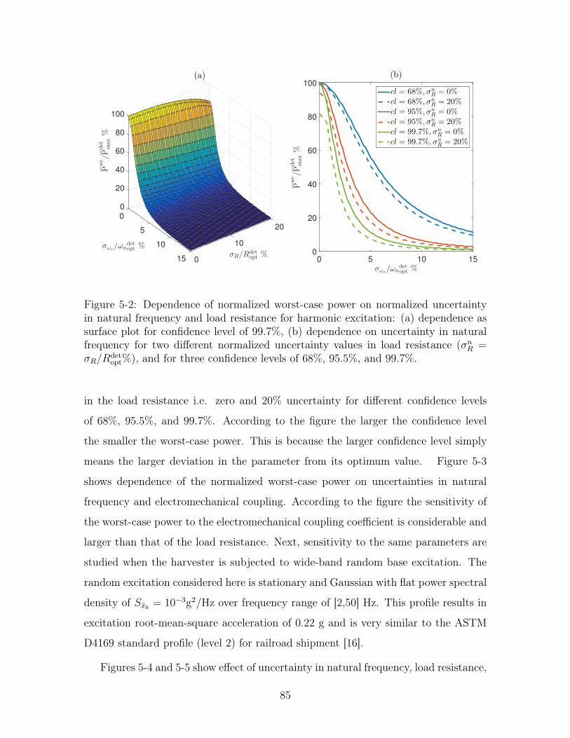
20

σR/Rdetopt %

10

(a)

015

10σωn/ωn

detopt %

5

20

40

0

60

80

100

0

Pwc/Pdet

max

%

σωn/ωn

detopt %

0 5 10 15

Pwc/Pdet

max

%

0

20

40

60

80

100

(b)

cl = 68%, σn

R= 0%

cl = 68%, σn

R= 20%

cl = 95%, σn

R= 0%

cl = 95%, σn

R= 20%

cl = 99.7%, σn

R= 0%

cl = 99.7%, σn

R= 20%

Figure 5-2: Dependence of normalized worst-case power on normalized uncertaintyin natural frequency and load resistance for harmonic excitation: (a) dependence assurface plot for confidence level of 99.7%, (b) dependence on uncertainty in naturalfrequency for two different normalized uncertainty values in load resistance (𝜎𝑛

𝑅 =𝜎𝑅/𝑅

detopt%), and for three confidence levels of 68%, 95.5%, and 99.7%.

in the load resistance i.e. zero and 20% uncertainty for different confidence levels

of 68%, 95.5%, and 99.7%. According to the figure the larger the confidence level

the smaller the worst-case power. This is because the larger confidence level simply

means the larger deviation in the parameter from its optimum value. Figure 5-3

shows dependence of the normalized worst-case power on uncertainties in natural

frequency and electromechanical coupling. According to the figure the sensitivity of

the worst-case power to the electromechanical coupling coefficient is considerable and

larger than that of the load resistance. Next, sensitivity to the same parameters are

studied when the harvester is subjected to wide-band random base excitation. The

random excitation considered here is stationary and Gaussian with flat power spectral

density of 𝑆𝑏= 10−3g2/Hz over frequency range of [2,50] Hz. This profile results in

excitation root-mean-square acceleration of 0.22 g and is very similar to the ASTM

D4169 standard profile (level 2) for railroad shipment [16].

Figures 5-4 and 5-5 show effect of uncertainty in natural frequency, load resistance,

85

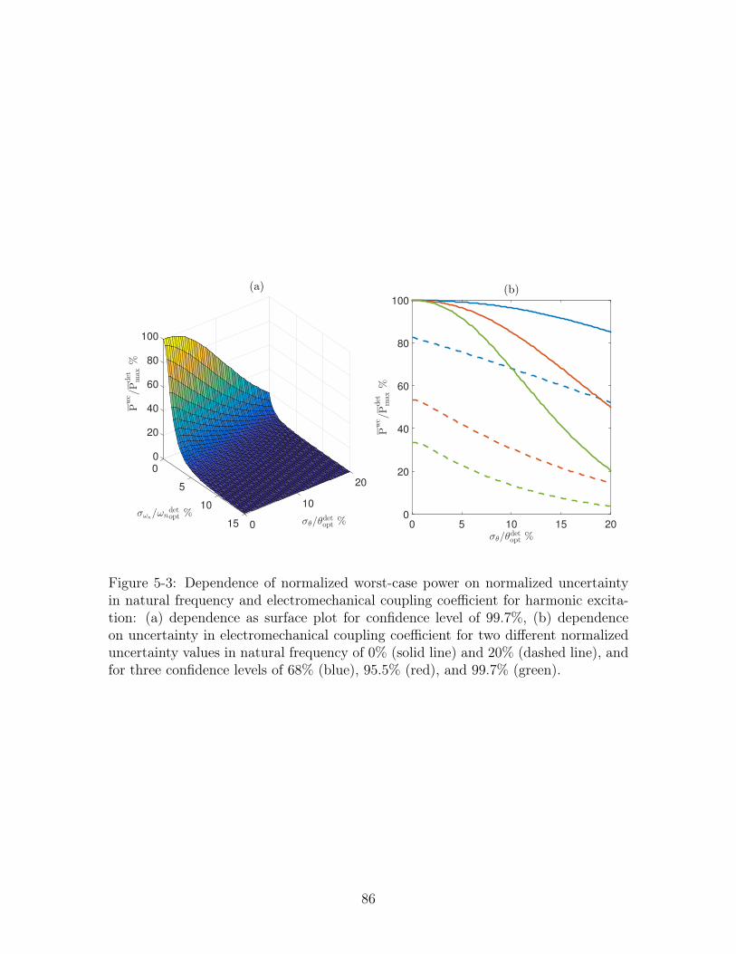
20

σθ/θdetopt %

10

(a)

015

10σωn

/ωndetopt %

5

0

20

40

60

80

100

0

Pwc/Pdet

max

%

σθ/θdetopt %

0 5 10 15 20

Pwc/Pdet

max

%

0

20

40

60

80

100

(b)

Figure 5-3: Dependence of normalized worst-case power on normalized uncertaintyin natural frequency and electromechanical coupling coefficient for harmonic excita-tion: (a) dependence as surface plot for confidence level of 99.7%, (b) dependenceon uncertainty in electromechanical coupling coefficient for two different normalizeduncertainty values in natural frequency of 0% (solid line) and 20% (dashed line), andfor three confidence levels of 68% (blue), 95.5% (red), and 99.7% (green).

86

and electromechanical coupling coefficient on the worst-case power. According to the

figures, worst-case power is not very sensitive to uncertainty in natural frequency. The

reason is two-fold: one is that in general when excitation changes from one harmonic

to wide-band, the narrow peak in the harvester power transforms into a wide peak

and hence becomes less sensitive to changes in natural frequency. This is because the

narrow peak of resonance will be captured over a wider frequency range whereas in the

harmonic excitation this peak is captured only at one frequency. Second, the optimum

natural frequency is 1 Hz3 that is a relatively small number; hence an uncertainty of

say 15% will change the natural frequency in the worst case (in 3𝜎 sense) by only

0.45 Hz which is not a big enough variation to cause a significant change in the

harvested power. Since the worst-case power is not very sensitive to uncertainty in

natural frequency for random excitation, we study the effect of uncertainty in load

resistance and electromagnetic coupling at zero uncertainty in natural frequency in

Figs. 5-4(b) and 5-5 (b). According to the figures, uncertainty in electromechanical

coupling coefficient has larger effect on the worst-case power than that of the load

resistance. It was shown that uncertainty in parameters of a naively-optimized

harvester could drastically decrease its worst-case power. Next we would like to see

if optimization of the deterministic parameters and/or mean value of the uncertain

parameters with the knowledge of uncertainties in the system will help to decrease

the effect of uncertainty on the worst-case power. This could be done by numerically

solving the min-max optimization problem in P2.

Optimization procedure formulated in P2 is applied to the harvester under har-

monic and random excitation. Figures 5-6 and 5-7 illustrate how optimization under

parametric uncertainty improves worst-case power compared to the naively-optimized

system i.e. the system optimized for deterministic parameters. Figure 5-6 shows the

normalized maximum worst-case power as a function of normalized uncertainty in

natural frequency and load resistance. Optimization is done over mean values of the

said uncertain parameters. For comparison, worst-case power of the naively-optimized

3This was the lowest limit for the search for optimum natural frequency; natural frequenciessmaller than this result in large vibration displacements.

87

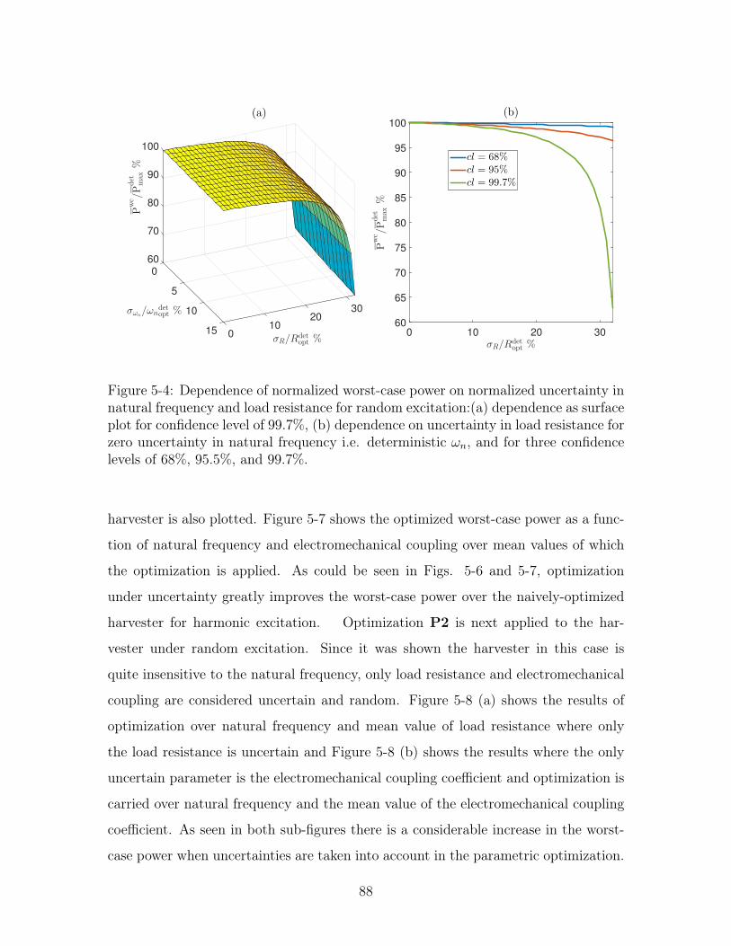
30

σR/Rdetopt %

2010

(a)

015

10σωn/ωn

detopt %

5

60

70

80

90

100

0

Pwc/Pdet

max

%

σR/Rdetopt %

0 10 20 30

Pwc/Pdet

max

%

60

65

70

75

80

85

90

95

100

(b)

cl = 68%cl = 95%cl = 99.7%

Figure 5-4: Dependence of normalized worst-case power on normalized uncertainty innatural frequency and load resistance for random excitation:(a) dependence as surfaceplot for confidence level of 99.7%, (b) dependence on uncertainty in load resistance forzero uncertainty in natural frequency i.e. deterministic 𝜔𝑛, and for three confidencelevels of 68%, 95.5%, and 99.7%.

harvester is also plotted. Figure 5-7 shows the optimized worst-case power as a func-

tion of natural frequency and electromechanical coupling over mean values of which

the optimization is applied. As could be seen in Figs. 5-6 and 5-7, optimization

under uncertainty greatly improves the worst-case power over the naively-optimized

harvester for harmonic excitation. Optimization P2 is next applied to the har-

vester under random excitation. Since it was shown the harvester in this case is

quite insensitive to the natural frequency, only load resistance and electromechanical

coupling are considered uncertain and random. Figure 5-8 (a) shows the results of

optimization over natural frequency and mean value of load resistance where only

the load resistance is uncertain and Figure 5-8 (b) shows the results where the only

uncertain parameter is the electromechanical coupling coefficient and optimization is

carried over natural frequency and the mean value of the electromechanical coupling

coefficient. As seen in both sub-figures there is a considerable increase in the worst-

case power when uncertainties are taken into account in the parametric optimization.

88

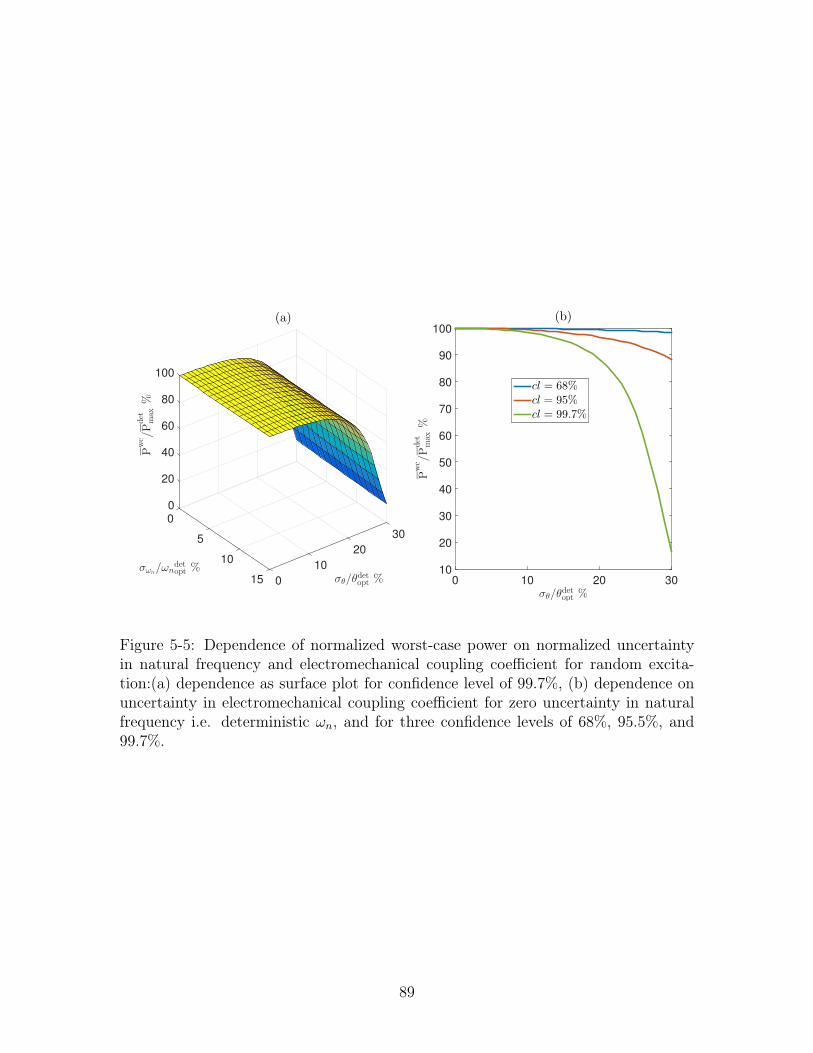
30

σθ/θdetopt %

20

10

(a)

015

10

5

σωn/ωn

detopt %

0

20

40

60

80

100

0

Pwc/Pdet

max

%

σθ/θdetopt %

0 10 20 30

Pwc/Pdet

max

%

10

20

30

40

50

60

70

80

90

100

(b)

cl = 68%cl = 95%cl = 99.7%

Figure 5-5: Dependence of normalized worst-case power on normalized uncertaintyin natural frequency and electromechanical coupling coefficient for random excita-tion:(a) dependence as surface plot for confidence level of 99.7%, (b) dependence onuncertainty in electromechanical coupling coefficient for zero uncertainty in naturalfrequency i.e. deterministic 𝜔𝑛, and for three confidence levels of 68%, 95.5%, and99.7%.

89

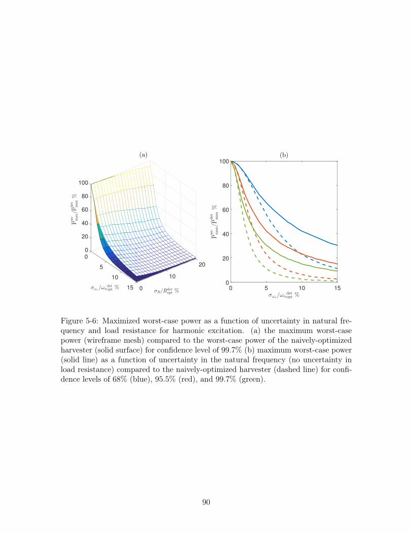
20

σR/Rdetopt %

10

(a)

015σωn/ωn

detopt %

10

5

80

100

40

60

20

0

0

Pwc

max/Pdet

max

%

σωn/ωn

detopt %

0 5 10 15

Pwc

max/Pdet

max

%

0

20

40

60

80

100

(b)

Figure 5-6: Maximized worst-case power as a function of uncertainty in natural fre-quency and load resistance for harmonic excitation. (a) the maximum worst-casepower (wireframe mesh) compared to the worst-case power of the naively-optimizedharvester (solid surface) for confidence level of 99.7% (b) maximum worst-case power(solid line) as a function of uncertainty in the natural frequency (no uncertainty inload resistance) compared to the naively-optimized harvester (dashed line) for confi-dence levels of 68% (blue), 95.5% (red), and 99.7% (green).

90

20

σθ/θdetopt %

10

(a)

015

10

σωn/ωn

detopt %

5

60

80

100

0

20

40

0

Pwc

max/Pdet

max

%

σωn/ωn

detopt %

0 5 10 15

Pwc

max/Pdet

max

%

0

20

40

60

80

100

(b)

Figure 5-7: Maximized worst-case power as a function of uncertainty in natural fre-quency and electromechanical coupling coefficient for harmonic excitation. (a) themaximum worst-case power (wireframe mesh) compared to the worst-case power ofthe naively-optimized harvester (solid surface) for confidence level of 99.7% (b) maxi-mum worst-case power (solid line) as a function of uncertainty in the natural frequency(no uncertainty in electromechanical coupling coefficient) compared to the naively-optimized harvester (dashed line) for confidence levels of 68% (blue), 95.5% (red),and 99.7% (green).

91

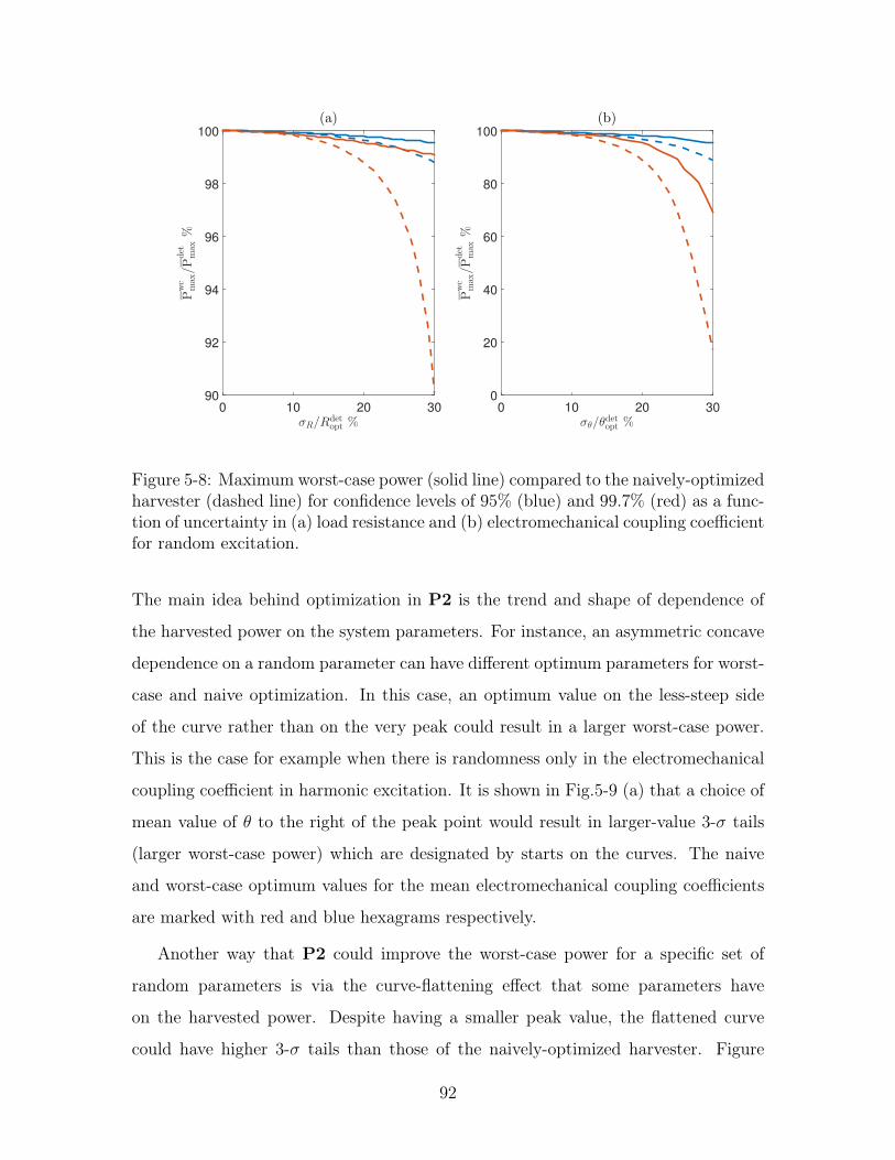
σR/Rdetopt %

0 10 20 30

Pwc

max/Pdet

max

%

90

92

94

96

98

100

(a)

σθ/θdetopt %

0 10 20 30

Pwc

max/Pdet

max

%

0

20

40

60

80

100

(b)

Figure 5-8: Maximum worst-case power (solid line) compared to the naively-optimizedharvester (dashed line) for confidence levels of 95% (blue) and 99.7% (red) as a func-tion of uncertainty in (a) load resistance and (b) electromechanical coupling coefficientfor random excitation.

The main idea behind optimization in P2 is the trend and shape of dependence of

the harvested power on the system parameters. For instance, an asymmetric concave

dependence on a random parameter can have different optimum parameters for worst-

case and naive optimization. In this case, an optimum value on the less-steep side

of the curve rather than on the very peak could result in a larger worst-case power.

This is the case for example when there is randomness only in the electromechanical

coupling coefficient in harmonic excitation. It is shown in Fig.5-9 (a) that a choice of

mean value of 𝜃 to the right of the peak point would result in larger-value 3-𝜎 tails

(larger worst-case power) which are designated by starts on the curves. The naive

and worst-case optimum values for the mean electromechanical coupling coefficients

are marked with red and blue hexagrams respectively.

Another way that P2 could improve the worst-case power for a specific set of

random parameters is via the curve-flattening effect that some parameters have

on the harvested power. Despite having a smaller peak value, the flattened curve

could have higher 3-𝜎 tails than those of the naively-optimized harvester. Figure

92

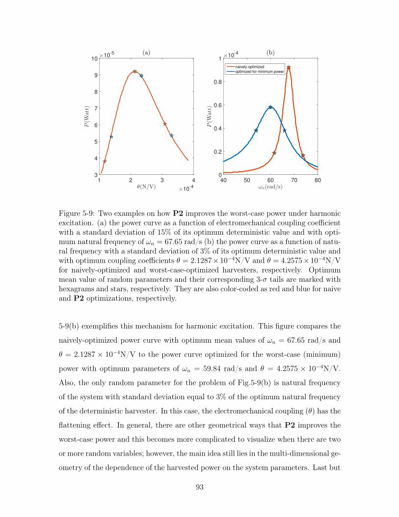
θ(N/V)×10

-4

1 2 3 4

P(W

att)

×10-5

3

4

5

6

7

8

9

10(a)

ωn(rad/s)40 50 60 70 80

P(W

att)

×10-4

0

0.2

0.4

0.6

0.8

1(b)

naively-optimized

optimized for minimum power

Figure 5-9: Two examples on how P2 improves the worst-case power under harmonicexcitation. (a) the power curve as a function of electromechanical coupling coefficientwith a standard deviation of 15% of its optimum deterministic value and with opti-mum natural frequency of 𝜔𝑛 = 67.65 rad/s (b) the power curve as a function of natu-ral frequency with a standard deviation of 3% of its optimum deterministic value andwith optimum coupling coefficients 𝜃 = 2.1287×10−4N/V and 𝜃 = 4.2575×10−4N/Vfor naively-optimized and worst-case-optimized harvesters, respectively. Optimummean value of random parameters and their corresponding 3-𝜎 tails are marked withhexagrams and stars, respectively. They are also color-coded as red and blue for naiveand P2 optimizations, respectively.

5-9(b) exemplifies this mechanism for harmonic excitation. This figure compares the

naively-optimized power curve with optimum mean values of 𝜔𝑛 = 67.65 rad/s and

𝜃 = 2.1287 × 10−4N/V to the power curve optimized for the worst-case (minimum)

power with optimum parameters of 𝜔𝑛 = 59.84 rad/s and 𝜃 = 4.2575 × 10−4N/V.

Also, the only random parameter for the problem of Fig.5-9(b) is natural frequency

of the system with standard deviation equal to 3% of the optimum natural frequency

of the deterministic harvester. In this case, the electromechanical coupling (𝜃) has the

flattening effect. In general, there are other geometrical ways that P2 improves the

worst-case power and this becomes more complicated to visualize when there are two

or more random variables; however, the main idea still lies in the multi-dimensional ge-

ometry of the dependence of the harvested power on the system parameters. Last but

93

not least, it’s worth mentioning that although harvesters designed for the worst-case

have better worst-case power, they do not necessarily have better ensemble expected

power than naively-optimized harvesters or obviously than harvesters optimized for

ensemble expected power.


In this chapter, we proposed a new modeling philosophy for optimization of energy

harvesters under parametric uncertainty. Instead of optimizing for ensemble expec-

tation of average harvested power, we optimize for the worst-case (minimum) power

based on some confidence level over the deterministic parameters and mean values

of the random parameters. The proposed optimization philosophy is practically very

useful when there is a minimum requirement on the harvested power such as those

in medical implants and wireless sensors. We also introduced a different notion of

uncertainty propagation i.e. propagation in the worst-case power instead of the en-

semble expected power. Based on this new modeling philosophy, we presented a very

generic and architecture-independent formulation for uncertainty propagation (P1)

and optimization under uncertainty (P2).

Next, we applied analysis methodologies P1 and P2 to a simple model of a piezo-

electric energy harvester. We have considered parametric uncertainty in natural fre-

quency, load resistance, and electromechanical coupling coefficient of the harvester.

Also, both harmonic and wide-band excitation were considered. Direct application of

P1 showed that for harmonically-excited PEH, the worst-case power of the harvester

is highly sensitive to its natural frequency and then to its electromechanical coupling

but not very sensitive to the load resistance. However, when the PEH is excited by

the wide-band excitation, the worst-case power is not very sensitive to the natural

frequency of the harvester but is sensitive to its load resistance and electromechanical

coupling.

For the harmonic excitation, the optimization P2 was done over mean values of

the natural frequency and load resistance or natural frequency and electromechanical

94

coupling. For the random excitation, since the worst-case power was not sensitive to

uncertainty in natural frequency, the optimization was done over the deterministic

natural frequency and the mean value of the load resistance or electromechanical

coupling coefficient. It was shown that for both harmonic and random excitation,

the optimized system taking into account the parametric uncertainties is much more

robust to uncertainties in terms of its worst-case power compared to the naively-

optimized (deterministically-optimized) harvester.

95

Chapter 6

Robust and adaptive control of

coexisting attractors in nonlinear

vibratory energy harvesters

As detailed in the previous chapters, purposeful inclusion of nonlinearity has been the

basis of a big body of research in the field of vibration energy harvesting, mainly to

increase the frequency bandwidth of the harvester; however, nonlinearity often brings

with itself coexisting chaotic and/or periodic attractors that is in general undesired.

In the context of energy harvesting, mono- and bi-stable quartic potentials are the

most common type of nonlinearites explored by far in the literature.

Nonlinear monostable harvesters driven by periodic excitation often exhibit coex-

isting low and high amplitude orbits usually referred to as low and high energy orbits

(LEO and HEO) in a wide range of excitation frequency. Bistable harvesters give

rise to even richer dynamics where low and high energy periodic, and chaotic attrac-

tors could coexist in a wide range of excitation parameters [20, 48]. The choice of

which attaractor the harvester would finally converge to, is highly dependant on and

sensitive to the initial conditions. For the purpose of energy harvesting, it is always

desired to surf the high energy periodic orbits. If the motion is chaotic, in addition to

its low energy output relative to HEO motion, chaotic response requires a much more

complicated signal conditioning and harvesting circuitry [24]. Therefore, the control

97

of the motion between the coexisting attractors in VEHs is extremely important for

effective harvesting.

In one of the seminal studies in controlling chaos it was shown that one can

convert a chaotic attractor to any one of the possible but probably unstable time-

periodic motions by making only small time-depending perturbations to an available

and accessible system parameter [92]. This approach is known as Ott-Grebogi-Yorke

(OGY) method. Later, researchers in different studies [97, 96, 34] used a slow-periodic

modulation with properly adjusted frequency and amplitude, instead of just a small

perturbation, to move to an adjacent attractor via boundary crises and destruction

of the original attractor.

However, the parameters of the system are not always accessible; hence, the OGY

method is often not practical. Periodic driving is another technique for the control of

coexisting attractors. Pecora and Carrol [95] used what they called pseudoperiodic

signals i.e. periodic signals augmented with a small chaotic component, to control

the coexisting attractors. Yang et al. [130] used a combination of noise and a bias

periodic signal with properly chosen phase to move the attractor to a desired limit

cycle.

feedback-type control is another class of controlling coexisting attractors. Jiang

[61] showed that the main feature of the latter two above-mentioned methods is the pe-

riodic component of their signals and that both approaches have limitations in select-

ing a desired trajectory from arbitrary initial conditions. He/She used feedback-type

periodic drivings containing dynamical features of the desired attractors to control

the attractors and switch to the desired one. Martinez et al. [82] also demonstrated

that multi-stability can be efficiently controlled in autonomous systems by modulat-

ing feedback variable. More recently Liu et al. [77] proposed a feedback controller

with intermittent control force based on Lyapunov analysis to drive the system to a

desired attractor.

Although some of the methods mentioned above could theoretically be applied

to the nonlinear energy harvesters, they do not take into account the control energy

which is crucial in designing the controller for a VEH. Also most of these approaches

98

use some type of crisis that changes the existing structure of the solutions. This is in

general not preferred because not only it could be hard to achieve for some nonlinear

systems but it could also result in the emergence of new complex basins of attraction

[77]. There are very few studies in the context of energy harvesting dealing with the

control of coexisting attractors, a ubiquitous phenomenon in the nonlinear energy

harvesters.

Erturk and Inman [24], in one of the earliest research studies in the field, showed

that a disturbance could push the VEH from LEO to HEO. Masuda et al. [86] pro-

posed an electrical circuitry for an electromagnetic VEH that combined a conventional

load resistance with a negative resistance that could pump energy into the system.

In their proposed approach, when the amplitude drops below a threshold the circuit

switches to the negative resistance for a given period of time to push the system back

to the HEO. This was later validated experimentally in [85]. These approaches will

not be effective when the structure of the coexisting attractors is more complex than

two periodic orbits; this is mainly because this method cannot select between many

chaotic or periodic attractors in a controlled fashion. In another study, Geiyer and

Kauffman [32] applied the intermittent control law proposed in [77] to a piezoelectric

VEH to drive the system from a chaotic attractor to a high energy periodic motion.

However, the control energy was not considered in this study. In a more recent study

Kumar et al. [69] applied an LQR controller on bistable piezoelectric energy harvester

linearized about an operating point corresponding to a chosen HEO. The LQR control

force was applied intermittently on the system based on a proximity threshold with

respect to the desired trajectory. The required control energy was not compared to

the harvested energy in this study too.

In addition to the shortcomings of the proposed methods mentioned above for

driving nonlinear VEHs to their HEOs, these methods are in general not robust or

adaptive. In practical applications of the vibratory energy harvesters there are always

disturbances or unmodelled dynamics on the system such as wind disturbance on a

bridge-motion-excited VEH or unmodelled higher order nonlinearities in the system.

Also, it is usually the case that some of the system parameters such as damping or

99

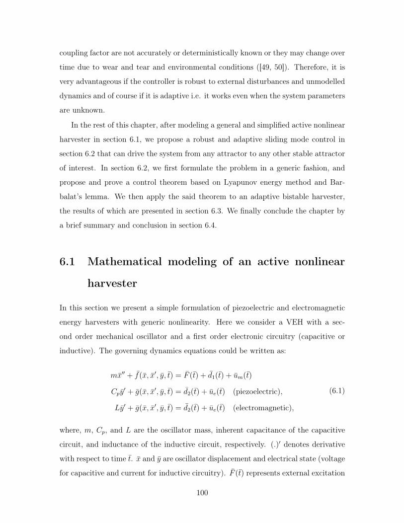
coupling factor are not accurately or deterministically known or they may change over

time due to wear and tear and environmental conditions ([49, 50]). Therefore, it is

very advantageous if the controller is robust to external disturbances and unmodelled

dynamics and of course if it is adaptive i.e. it works even when the system parameters

are unknown.

In the rest of this chapter, after modeling a general and simplified active nonlinear

harvester in section 6.1, we propose a robust and adaptive sliding mode control in

section 6.2 that can drive the system from any attractor to any other stable attractor

of interest. In section 6.2, we first formulate the problem in a generic fashion, and

propose and prove a control theorem based on Lyapunov energy method and Bar-

balat’s lemma. We then apply the said theorem to an adaptive bistable harvester,

the results of which are presented in section 6.3. We finally conclude the chapter by

a brief summary and conclusion in section 6.4.

6.1 Mathematical modeling of an active nonlinear

harvester

In this section we present a simple formulation of piezoelectric and electromagnetic

energy harvesters with generic nonlinearity. Here we consider a VEH with a sec-

ond order mechanical oscillator and a first order electronic circuitry (capacitive or

inductive). The governing dynamics equations could be written as:

𝑚′′ + 𝑓(, ′, 𝑦, 𝑡) = 𝐹 (𝑡) + 𝑑1(𝑡) + 𝑚(𝑡)

𝐶𝑝𝑦′ + 𝑔(, ′, 𝑦, 𝑡) = 𝑑2(𝑡) + 𝑒(𝑡) (piezoelectric),

𝐿𝑦′ + 𝑔(, ′, 𝑦, 𝑡) = 𝑑2(𝑡) + 𝑒(𝑡) (electromagnetic),

(6.1)

where, 𝑚, 𝐶𝑝, and 𝐿 are the oscillator mass, inherent capacitance of the capacitive

circuit, and inductance of the inductive circuit, respectively. (.)′ denotes derivative

with respect to time 𝑡. and 𝑦 are oscillator displacement and electrical state (voltage

for capacitive and current for inductive circuitry). 𝐹 (𝑡) represents external excitation

100

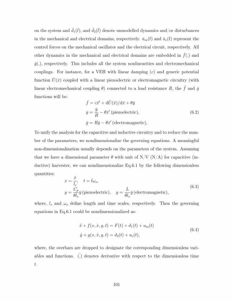
on the system and 𝑑1(𝑡), and 𝑑2(𝑡) denote unmodelled dynamics and/or disturbances

in the mechanical and electrical domains, respectively. 𝑚(𝑡) and 𝑒(𝑡) represent the

control forces on the mechanical oscillator and the electrical circuit, respectively. All

other dynamics in the mechanical and electrical domains are embedded in 𝑓(.) and

𝑔(.), respectively. This includes all the system nonlinearities and electromechanical

couplings. For instance, for a VEH with linear damping (𝑐) and generic potential

function () coupled with a linear piezoelectric or electromagnetic circuitry (with

linear electromechanical coupling 𝜃) connected to a load resistance 𝑅, the 𝑓 and 𝑔

functions will be:𝑓 = 𝑐′ + d()/d + 𝜃𝑦

𝑔 =𝑦

𝑅− 𝜃′ (piezoelectric),

𝑔 = 𝑅𝑦 − 𝜃′ (electromagnetic),

(6.2)

To unify the analysis for the capacitive and inductive circuitry and to reduce the num-

ber of the parameters, we nondimensionalize the governing equations. A meaningful

non-dimensionalization usually depends on the parameters of the system. Assuming

that we have a dimensional parameter 𝜃 with unit of N/V (N/A) for capacitive (in-

ductive) harvester, we can nondimensionalize Eq.6.1 by the following dimensionless

quantities:𝑥 =

𝑙𝑠, 𝑡 = 𝑡𝜔𝑠,

𝑦 =𝐶𝑝

𝜃𝑙𝑠𝑦 (piezoelectric), 𝑦 =

𝐿

𝜃𝑙𝑠𝑦 (electromagnetic),

(6.3)

where, 𝑙𝑠 and 𝜔𝑠 define length and time scales, respectively. Then the governing

equations in Eq.6.1 could be nondimensionalized as:

+ 𝑓(𝑥, , 𝑦, 𝑡) = 𝐹 (𝑡) + 𝑑1(𝑡) + 𝑢𝑚(𝑡)

+ 𝑔(𝑥, , 𝑦, 𝑡) = 𝑑2(𝑡) + 𝑢𝑒(𝑡),(6.4)

where, the overbars are dropped to designate the corresponding dimensionless vari-

ables and functions. ˙(.) denotes derivative with respect to the dimensionless time

𝑡.

101

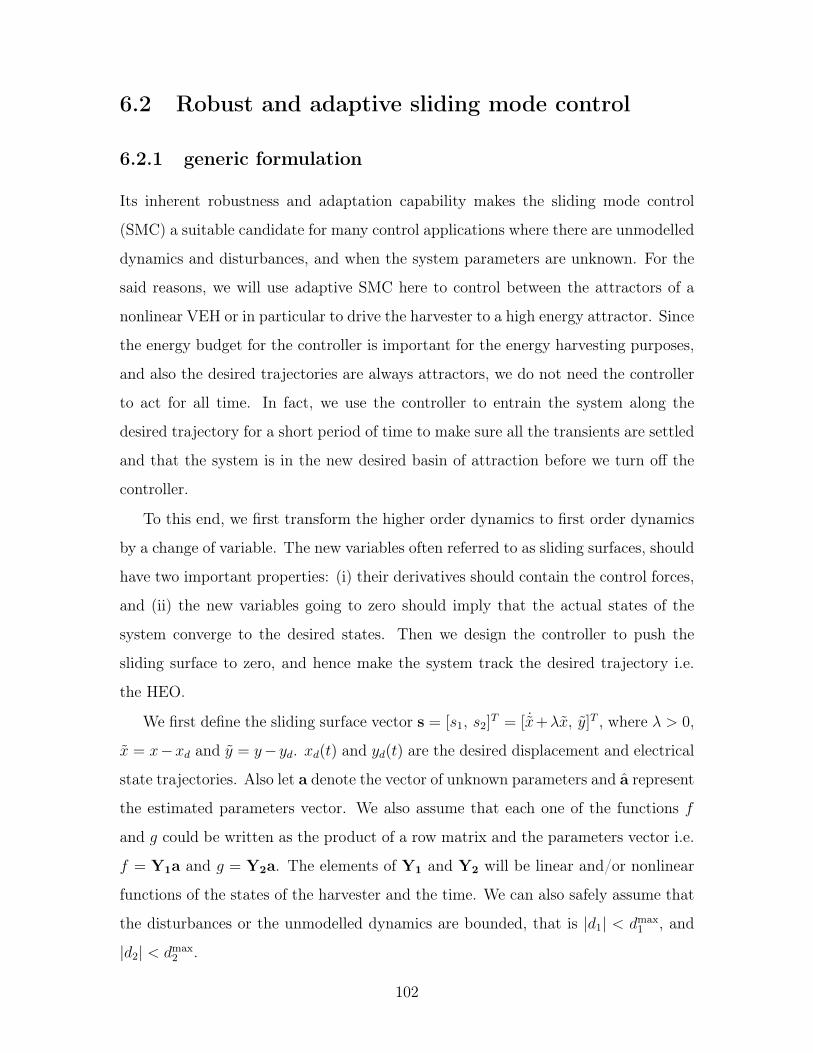
6.2 Robust and adaptive sliding mode control

6.2.1 generic formulation

Its inherent robustness and adaptation capability makes the sliding mode control

(SMC) a suitable candidate for many control applications where there are unmodelled

dynamics and disturbances, and when the system parameters are unknown. For the

said reasons, we will use adaptive SMC here to control between the attractors of a

nonlinear VEH or in particular to drive the harvester to a high energy attractor. Since

the energy budget for the controller is important for the energy harvesting purposes,

and also the desired trajectories are always attractors, we do not need the controller

to act for all time. In fact, we use the controller to entrain the system along the

desired trajectory for a short period of time to make sure all the transients are settled

and that the system is in the new desired basin of attraction before we turn off the

controller.

To this end, we first transform the higher order dynamics to first order dynamics

by a change of variable. The new variables often referred to as sliding surfaces, should

have two important properties: (i) their derivatives should contain the control forces,

and (ii) the new variables going to zero should imply that the actual states of the

system converge to the desired states. Then we design the controller to push the

sliding surface to zero, and hence make the system track the desired trajectory i.e.

the HEO.

We first define the sliding surface vector s = [𝑠1, 𝑠2]𝑇 = [ ˙𝑥+𝜆, 𝑦]𝑇 , where 𝜆 > 0,

= 𝑥−𝑥𝑑 and 𝑦 = 𝑦− 𝑦𝑑. 𝑥𝑑(𝑡) and 𝑦𝑑(𝑡) are the desired displacement and electrical

state trajectories. Also let a denote the vector of unknown parameters and a represent

the estimated parameters vector. We also assume that each one of the functions 𝑓

and 𝑔 could be written as the product of a row matrix and the parameters vector i.e.

𝑓 = Y1a and 𝑔 = Y2a. The elements of Y1 and Y2 will be linear and/or nonlinear

functions of the states of the harvester and the time. We can also safely assume that

the disturbances or the unmodelled dynamics are bounded, that is |𝑑1| < 𝑑max1 , and

|𝑑2| < 𝑑max2 .

102

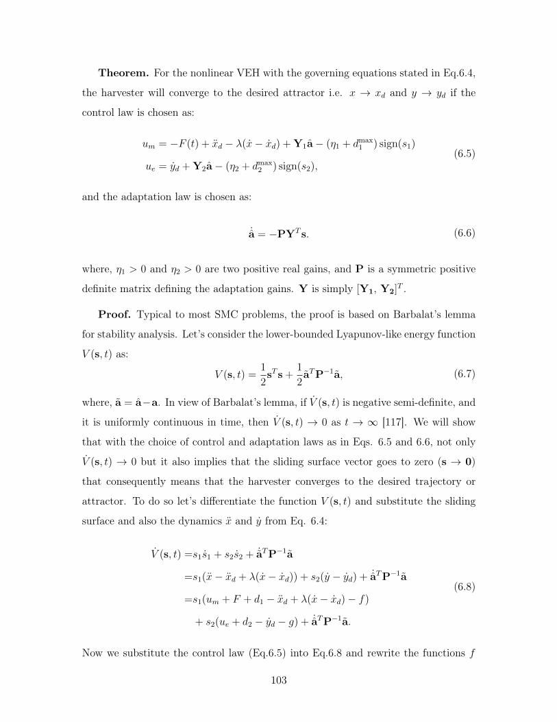
Theorem. For the nonlinear VEH with the governing equations stated in Eq.6.4,

the harvester will converge to the desired attractor i.e. 𝑥 → 𝑥𝑑 and 𝑦 → 𝑦𝑑 if the

control law is chosen as:

𝑢𝑚 = −𝐹 (𝑡) + 𝑑 − 𝜆(− 𝑑) + Y1a− (𝜂1 + 𝑑max1 ) sign(𝑠1)

𝑢𝑒 = 𝑑 + Y2a− (𝜂2 + 𝑑max2 ) sign(𝑠2),

(6.5)

and the adaptation law is chosen as:

˙a = −PY𝑇 s. (6.6)

where, 𝜂1 > 0 and 𝜂2 > 0 are two positive real gains, and P is a symmetric positive

definite matrix defining the adaptation gains. Y is simply [Y1, Y2]𝑇 .

Proof. Typical to most SMC problems, the proof is based on Barbalat’s lemma

for stability analysis. Let’s consider the lower-bounded Lyapunov-like energy function

𝑉 (s, 𝑡) as:

𝑉 (s, 𝑡) =1

2s𝑇 s +

1

2a𝑇P−1a, (6.7)

where, a = a−a. In view of Barbalat’s lemma, if (s, 𝑡) is negative semi-definite, and

it is uniformly continuous in time, then (s, 𝑡) → 0 as 𝑡 → ∞ [117]. We will show

that with the choice of control and adaptation laws as in Eqs. 6.5 and 6.6, not only

(s, 𝑡) → 0 but it also implies that the sliding surface vector goes to zero (s → 0)

that consequently means that the harvester converges to the desired trajectory or

attractor. To do so let’s differentiate the function 𝑉 (s, 𝑡) and substitute the sliding

surface and also the dynamics and from Eq. 6.4:

(s, 𝑡) =𝑠11 + 𝑠22 + ˙a𝑇P−1a

=𝑠1(− 𝑑 + 𝜆(− 𝑑)) + 𝑠2( − 𝑑) + ˙a𝑇P−1a

=𝑠1(𝑢𝑚 + 𝐹 + 𝑑1 − 𝑑 + 𝜆(− 𝑑) − 𝑓)

+ 𝑠2(𝑢𝑒 + 𝑑2 − 𝑑 − 𝑔) + ˙a𝑇P−1a.

(6.8)

Now we substitute the control law (Eq.6.5) into Eq.6.8 and rewrite the functions 𝑓

103

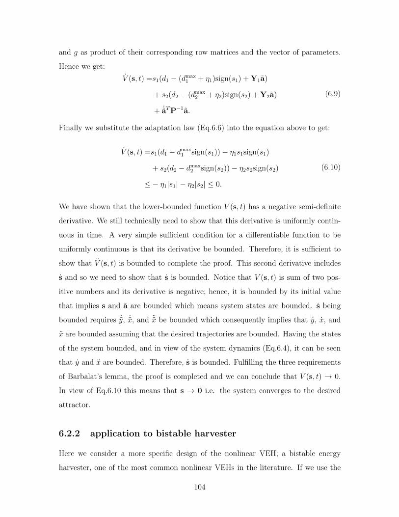
and 𝑔 as product of their corresponding row matrices and the vector of parameters.

Hence we get: (s, 𝑡) =𝑠1(𝑑1 − (𝑑max

1 + 𝜂1)sign(𝑠1) + Y1a)

+ 𝑠2(𝑑2 − (𝑑max2 + 𝜂2)sign(𝑠2) + Y2a)

+ ˙a𝑇P−1a.

(6.9)

Finally we substitute the adaptation law (Eq.6.6) into the equation above to get:

(s, 𝑡) =𝑠1(𝑑1 − 𝑑max1 sign(𝑠1)) − 𝜂1𝑠1sign(𝑠1)

+ 𝑠2(𝑑2 − 𝑑max2 sign(𝑠2)) − 𝜂2𝑠2sign(𝑠2)

≤− 𝜂1|𝑠1| − 𝜂2|𝑠2| ≤ 0.

(6.10)

We have shown that the lower-bounded function 𝑉 (s, 𝑡) has a negative semi-definite

derivative. We still technically need to show that this derivative is uniformly contin-

uous in time. A very simple sufficient condition for a differentiable function to be

uniformly continuous is that its derivative be bounded. Therefore, it is sufficient to

show that 𝑉 (s, 𝑡) is bounded to complete the proof. This second derivative includes

s and so we need to show that s is bounded. Notice that 𝑉 (s, 𝑡) is sum of two pos-

itive numbers and its derivative is negative; hence, it is bounded by its initial value

that implies s and a are bounded which means system states are bounded. s being

bounded requires ˙𝑦, ˙𝑥, and ¨𝑥 be bounded which consequently implies that , , and

are bounded assuming that the desired trajectories are bounded. Having the states

of the system bounded, and in view of the system dynamics (Eq.6.4), it can be seen

that and are bounded. Therefore, s is bounded. Fulfilling the three requirements

of Barbalat’s lemma, the proof is completed and we can conclude that (s, 𝑡) → 0.

In view of Eq.6.10 this means that s → 0 i.e. the system converges to the desired

attractor.

6.2.2 application to bistable harvester

Here we consider a more specific design of the nonlinear VEH; a bistable energy

harvester, one of the most common nonlinear VEHs in the literature. If we use the

104

bistable potential () = 1/2𝑘12 + 1/4𝑘3

4 for the potential function in Eq.6.2,

substitute Eq.6.2 into Eq.6.1 and nondimensionalize using the quantities in Eq.6.3,

we arrive at the dimensionless governing equations as:

+ 2𝜁− 𝑥 + 𝑥3 + 𝜅2𝑦 = 𝐹 (𝑡) + 𝑑1(𝑡) + 𝑢𝑚(𝑡)

+ 𝛼𝑦 = + 𝑑2(𝑡) + 𝑢𝑒(𝑡),(6.11)

where, 𝜁 = 𝑐2𝑚𝜔𝑠

is the dimensionless damping ratio. Electromechanical coupling

coefficient 𝜅2, and the time ratio (mechanical to electrical time constants)𝛼 for piezo-

electric and electromagnetic harvesters are defined as

𝜅2 =𝜃2

𝑚𝜔2𝑠𝐶𝑝

, 𝛼 =1

𝑅𝐶𝑝𝜔𝑠

(piezoelectric)

𝜅2 =𝜃2

𝑚𝜔2𝑠𝐿

, 𝛼 =𝑅

𝐿𝜔𝑠

(electromagnetic).

(6.12)

The dimensional coefficients 𝑘1 and 𝑘3 for the potential function are chosen such that

the derivative of the potential function in the dimensionless form is −𝑥 + 𝑥3.

To design the SMC controller we assume the two parameters 𝜁 and 𝜅2 are unknown

i.e. a = [𝜁, 𝜅2]𝑇 . Also, we choose P a diagonal matrix as P = diag[𝑝1, 𝑝2] with

positive entries 𝑝1 and 𝑝2. Then applying Eq.6.5 yields the control forces as:

𝑢𝑚 = − 𝐹 (𝑡) + 𝑑 − 𝜆(− 𝑑) − 𝑥 + 𝑥3 + 2𝜁 + 2𝑦

− (𝜂1 + 𝑑max1 ) sign(𝑠1)

𝑢𝑒 = − + 𝛼𝑦 + 𝑑 − (𝜂2 + 𝑑max2 ) sign(𝑠2),

(6.13)

and the adaptation law forms into:

˙𝜁 = −2𝑝1𝑠1,

˙𝜅2 = −𝑝2𝑦𝑠1.(6.14)

We would also like to nondimensionalize the harvested and the controller power and

their corresponding energy. The power is made dimensionless by the quantity 𝑚𝑤3𝑠 𝑙

2𝑠

105

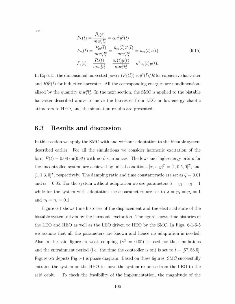
as:

𝑃ℎ(𝑡) =𝑃ℎ(𝑡)

𝑚𝑤3𝑠 𝑙

2𝑠

= 𝛼𝜅2𝑦2(𝑡)

𝑃𝑚(𝑡) =𝑃𝑚(𝑡)

𝑚𝑤3𝑠 𝑙

2𝑠

=𝑚(𝑡)′(𝑡)

𝑚𝑤3𝑠 𝑙

2𝑠

= 𝑢𝑚(𝑡)(𝑡)

𝑃𝑒(𝑡) =𝑃𝑒(𝑡)

𝑚𝑤3𝑠 𝑙

2𝑠

=𝑒(𝑡)𝑦(𝑡)

𝑚𝑤3𝑠 𝑙

2𝑠

= 𝜅2𝑢𝑒(𝑡)𝑦(𝑡).

(6.15)

In Eq.6.15, the dimensional harvested power (𝑃ℎ(𝑡)) is 𝑦2(𝑡)/𝑅 for capacitive harvester

and 𝑅𝑦2(𝑡) for inductive harvester. All the corresponding energies are nondimension-

alized by the quantity 𝑚𝑤2𝑠 𝑙

2𝑠 . In the next section, the SMC is applied to the bistable

harvester described above to move the harvester from LEO or low-energy chaotic

attractors to HEO, and the simulation results are presented.

6.3 Results and discussion

In this section we apply the SMC with and without adaptation to the bistable system

described earlier. For all the simulations we consider harmonic excitation of the

form 𝐹 (𝑡) = 0.08 sin(0.8𝑡) with no disturbances. The low- and high-energy orbits for

the uncontrolled system are achieved by initial conditions [𝑥, , 𝑦]𝑇 = [1, 0.5, 0]𝑇 , and

[1, 1.3, 0]𝑇 , respectively. The damping ratio and time constant ratio are set as 𝜁 = 0.01

and 𝛼 = 0.05. For the system without adaptation we use parameters 𝜆 = 𝜂1 = 𝜂2 = 1

while for the system with adaptation these parameters are set to 𝜆 = 𝑝1 = 𝑝2 = 1

and 𝜂1 = 𝜂2 = 0.1.

Figure 6-1 shows time histories of the displacement and the electrical state of the

bistable system driven by the harmonic excitation. The figure shows time histories of

the LEO and HEO as well as the LEO driven to HEO by the SMC. In Figs. 6-1-6-5

we assume that all the parameters are known and hence no adaptation is needed.

Also in the said figures a weak coupling (𝜅2 = 0.05) is used for the simulations

and the entrainment period (i.e. the time the controller is on) is set to 𝑡 = [57, 58.5].

Figure 6-2 depicts Fig.6-1 is phase diagram. Based on these figures, SMC successfully

entrains the system on the HEO to move the system response from the LEO to the

said orbit. To check the feasibility of the implementation, the magnitude of the

106

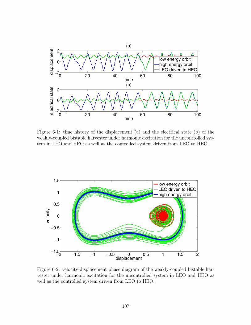
0 20 40 60 80 100−2

0

2

time

dis

pla

cem

ent

(a)

low energy orbithigh energy orbitLEO driven to HEO

0 20 40 60 80 100−2

0

2

time

ele

ctr

ical sta

te

(b)

Figure 6-1: time history of the displacement (a) and the electrical state (b) of theweakly-coupled bistable harvester under harmonic excitation for the uncontrolled sys-tem in LEO and HEO as well as the controlled system driven from LEO to HEO.

−2 −1.5 −1 −0.5 0 0.5 1 1.5 2−1.5

−1

−0.5

0

0.5

1

1.5

displacement

velo

city

low energy orbitLEO driven to HEOhigh energy orbit

Figure 6-2: velocity-displacement phase diagram of the weakly-coupled bistable har-vester under harmonic excitation for the uncontrolled system in LEO and HEO aswell as the controlled system driven from LEO to HEO.

107

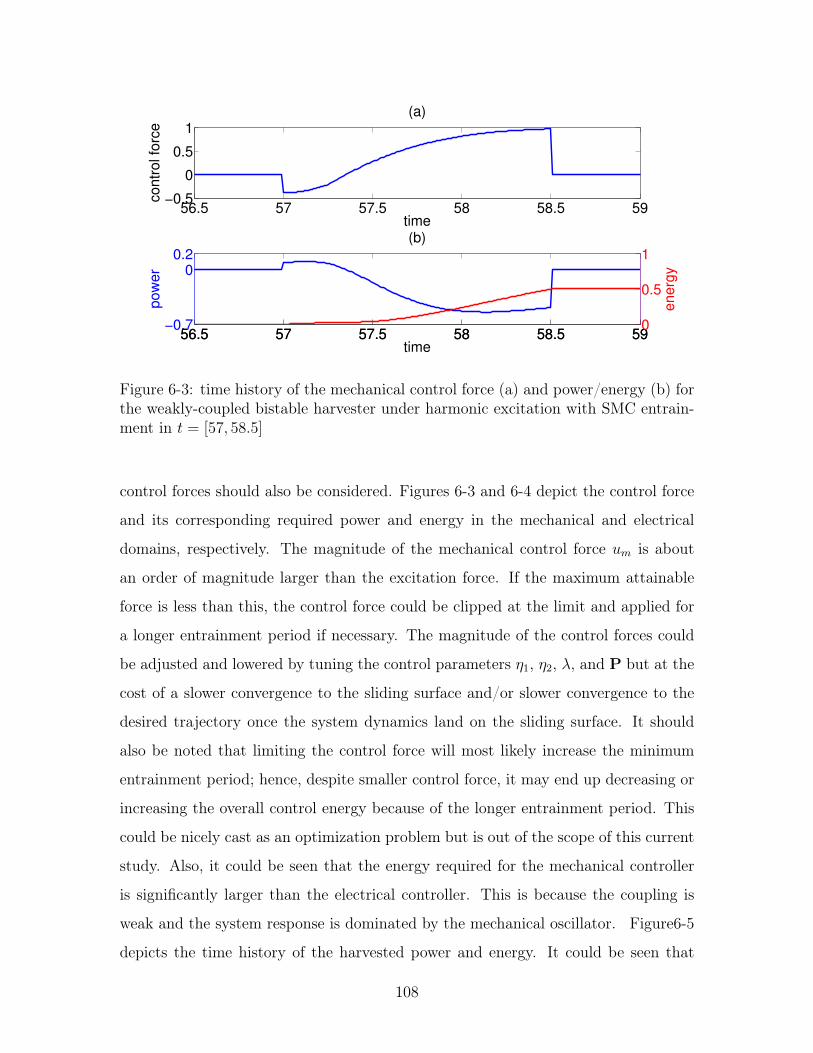
56.5 57 57.5 58 58.5 59−0.5

0

0.5

1

time

contr

ol fo

rce

(a)

56.5 57 57.5 58 58.5 59−0.7

00.2

time

pow

er

(b)

56.5 57 57.5 58 58.5 590

0.5

1

energ

y

Figure 6-3: time history of the mechanical control force (a) and power/energy (b) forthe weakly-coupled bistable harvester under harmonic excitation with SMC entrain-ment in 𝑡 = [57, 58.5]

control forces should also be considered. Figures 6-3 and 6-4 depict the control force

and its corresponding required power and energy in the mechanical and electrical

domains, respectively. The magnitude of the mechanical control force 𝑢𝑚 is about

an order of magnitude larger than the excitation force. If the maximum attainable

force is less than this, the control force could be clipped at the limit and applied for

a longer entrainment period if necessary. The magnitude of the control forces could

be adjusted and lowered by tuning the control parameters 𝜂1, 𝜂2, 𝜆, and P but at the

cost of a slower convergence to the sliding surface and/or slower convergence to the

desired trajectory once the system dynamics land on the sliding surface. It should

also be noted that limiting the control force will most likely increase the minimum

entrainment period; hence, despite smaller control force, it may end up decreasing or

increasing the overall control energy because of the longer entrainment period. This

could be nicely cast as an optimization problem but is out of the scope of this current

study. Also, it could be seen that the energy required for the mechanical controller

is significantly larger than the electrical controller. This is because the coupling is

weak and the system response is dominated by the mechanical oscillator. Figure6-5

depicts the time history of the harvested power and energy. It could be seen that

108

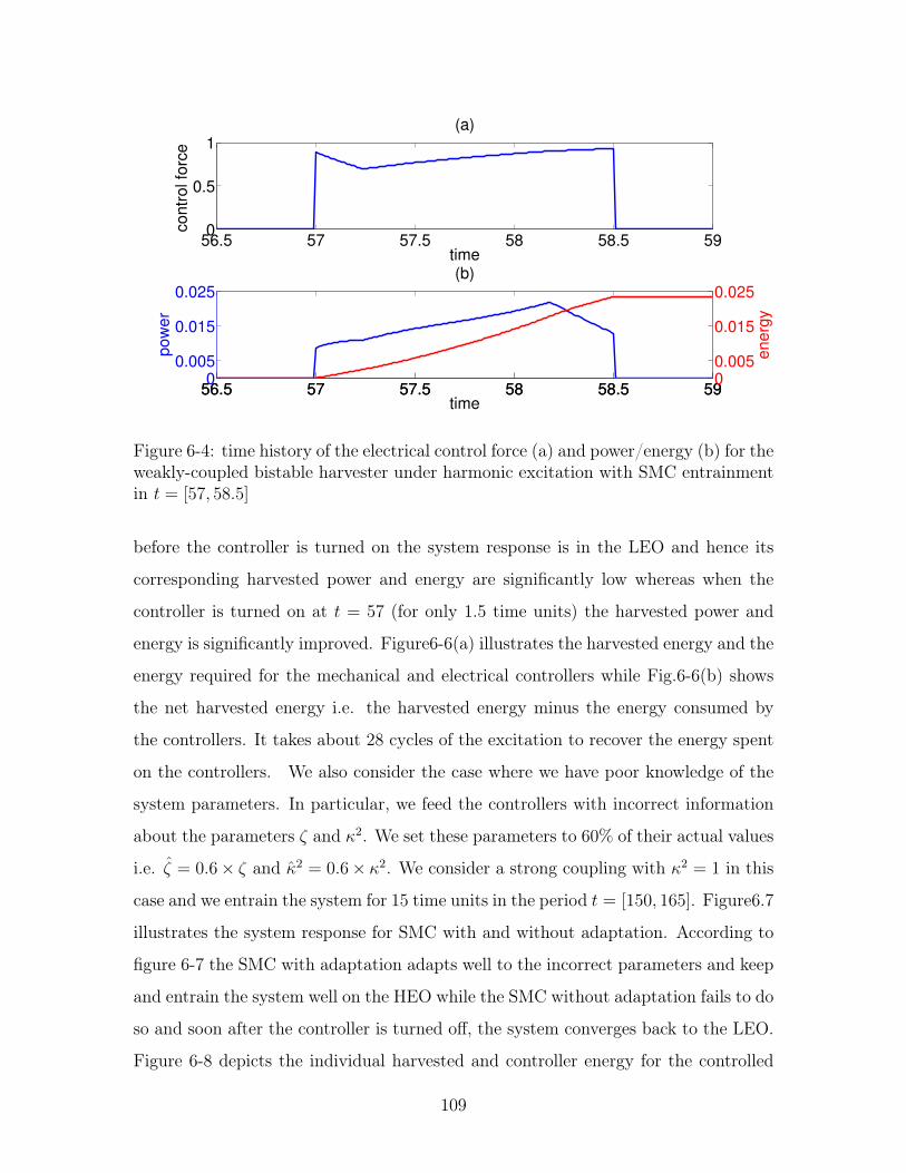
56.5 57 57.5 58 58.5 590

0.5

1

time

contr

ol fo

rce

(a)

56.5 57 57.5 58 58.5 590

0.005

0.015

0.025

time

pow

er

(b)

56.5 57 57.5 58 58.5 5900.005

0.015

0.025

energ

y

Figure 6-4: time history of the electrical control force (a) and power/energy (b) for theweakly-coupled bistable harvester under harmonic excitation with SMC entrainmentin 𝑡 = [57, 58.5]

before the controller is turned on the system response is in the LEO and hence its

corresponding harvested power and energy are significantly low whereas when the

controller is turned on at 𝑡 = 57 (for only 1.5 time units) the harvested power and

energy is significantly improved. Figure6-6(a) illustrates the harvested energy and the

energy required for the mechanical and electrical controllers while Fig.6-6(b) shows

the net harvested energy i.e. the harvested energy minus the energy consumed by

the controllers. It takes about 28 cycles of the excitation to recover the energy spent

on the controllers. We also consider the case where we have poor knowledge of the

system parameters. In particular, we feed the controllers with incorrect information

about the parameters 𝜁 and 𝜅2. We set these parameters to 60% of their actual values

i.e. 𝜁 = 0.6 × 𝜁 and 2 = 0.6 × 𝜅2. We consider a strong coupling with 𝜅2 = 1 in this

case and we entrain the system for 15 time units in the period 𝑡 = [150, 165]. Figure6.7

illustrates the system response for SMC with and without adaptation. According to

figure 6-7 the SMC with adaptation adapts well to the incorrect parameters and keep

and entrain the system well on the HEO while the SMC without adaptation fails to do

so and soon after the controller is turned off, the system converges back to the LEO.

Figure 6-8 depicts the individual harvested and controller energy for the controlled

109

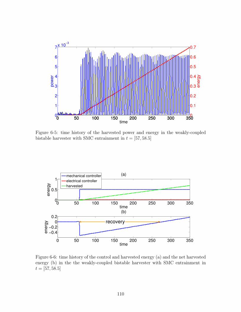
0 50 100 150 200 250 300 3500

1

2

3

4

5

6

7x 10

−3

time

pow

er

0 50 100 150 200 250 300 3500

0.1

0.2

0.3

0.4

0.5

0.6

0.7

energ

y

Figure 6-5: time history of the harvested power and energy in the weakly-coupledbistable harvester with SMC entrainment in 𝑡 = [57, 58.5]

0 50 100 150 200 250 300 3500

0.5

1

time

energ

y

(a)

mechanical controller

electrical controller

harvested

0 50 100 150 200 250 300 350

−0.4

−0.2

0

0.2

time

energ

y

(b)

recovery

Figure 6-6: time history of the control and harvested energy (a) and the net harvestedenergy (b) in the the weakly-coupled bistable harvester with SMC entrainment in𝑡 = [57, 58.5]

110

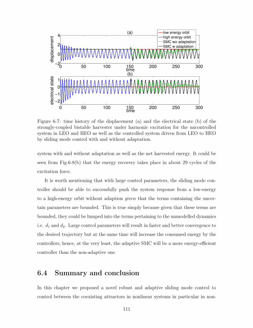
0 50 100 150 200 250 300−2

0

2

4

time

dis

pla

cem

ent

(a)

low energy orbit

high energy orbit

SMC wo adaptation

SMC w adaptation

0 50 100 150 200 250 300

−2

−1

0

1

time

ele

ctr

ical sta

te

(b)

Figure 6-7: time history of the displacement (a) and the electrical state (b) of thestrongly-coupled bistable harvester under harmonic excitation for the uncontrolledsystem in LEO and HEO as well as the controlled system driven from LEO to HEOby sliding mode control with and without adaptation.

system with and without adaptation as well as the net harvested energy. It could be

seen from Fig.6-8(b) that the energy recovery takes place in about 29 cycles of the

excitation force.

It is worth mentioning that with large control parameters, the sliding mode con-

troller should be able to successfully push the system response from a low-energy

to a high-energy orbit without adaption given that the terms containing the uncer-

tain parameters are bounded. This is true simply because given that these terms are

bounded, they could be lumped into the terms pertaining to the unmodelled dynamics

i.e. 𝑑1 and 𝑑2. Large control parameters will result in faster and better convergence to

the desired trajectory but at the same time will increase the consumed energy by the

controllers; hence, at the very least, the adaptive SMC will be a more energy-efficient

controller than the non-adaptive one.


In this chapter we proposed a novel robust and adaptive sliding mode control to

control between the coexisting attractors in nonlinear systems in particular in non-

111

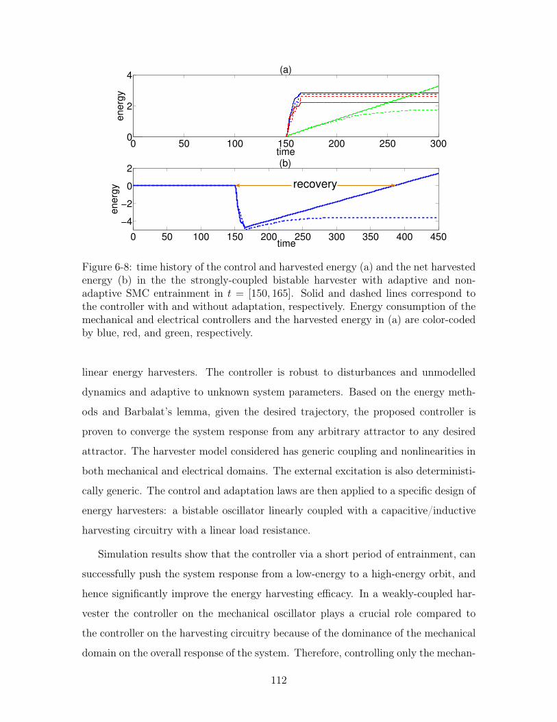
0 50 100 150 200 250 3000

2

4

time

energ

y

(a)

0 50 100 150 200 250 300 350 400 450

−4

−2

0

2

time

energ

y

(b)

recovery

Figure 6-8: time history of the control and harvested energy (a) and the net harvestedenergy (b) in the the strongly-coupled bistable harvester with adaptive and non-adaptive SMC entrainment in 𝑡 = [150, 165]. Solid and dashed lines correspond tothe controller with and without adaptation, respectively. Energy consumption of themechanical and electrical controllers and the harvested energy in (a) are color-codedby blue, red, and green, respectively.

linear energy harvesters. The controller is robust to disturbances and unmodelled

dynamics and adaptive to unknown system parameters. Based on the energy meth-

ods and Barbalat’s lemma, given the desired trajectory, the proposed controller is

proven to converge the system response from any arbitrary attractor to any desired

attractor. The harvester model considered has generic coupling and nonlinearities in

both mechanical and electrical domains. The external excitation is also deterministi-

cally generic. The control and adaptation laws are then applied to a specific design of

energy harvesters: a bistable oscillator linearly coupled with a capacitive/inductive

harvesting circuitry with a linear load resistance.

Simulation results show that the controller via a short period of entrainment, can

successfully push the system response from a low-energy to a high-energy orbit, and

hence significantly improve the energy harvesting efficacy. In a weakly-coupled har-

vester the controller on the mechanical oscillator plays a crucial role compared to

the controller on the harvesting circuitry because of the dominance of the mechanical

domain on the overall response of the system. Therefore, controlling only the mechan-

112

ical oscillator is sufficient for the weakly-coupled VEH. However, a long entrainment

period is needed if the controller is applied only on the mechanical oscillator in a

strongly-coupled harvester. In a weakly-coupled harvester, the mechanical control

force is about 10 times larger than the excitation force in amplitude. If this is not

realizable, the control force could be clipped at the maximum realizable force and

instead applied for a longer entrainment.

Simulation results also show that the sliding mode control with adaptation adapts

well to the system parameters and successfully moves the system to the desired at-

tractor even when our knowledge of the system parameters is poor and incorrect

whereas the same controller without adaptation does not achieve the same with in-

correct knowledge of the parameters. It is also shown that the energy consumed by

the control forces is recovered in a reasonable time (in less than 30 cycles of the exci-

tation). In conclusion, the proposed control method in this chapter could be applied

to a wide range of nonlinear harvesters with nonlinearity in either or both the me-

chanical and electrical domains in a very robust and adaptive fashion to make sure

that the harvester is always operating in the desired high energy orbit.

113

Chapter 7

Conclusion and contributions

This thesis investigates two main directions for effective vibration energy harvesting:

(i) fundamental limits to nonlinear energy harvesting and techniques to approach

them, and (ii) robust energy harvesting under uncertainties. A joint theoretical and

computational approach is adopted in order to find maximal power limits and practi-

cal approaches are proposed to approach them, all detailed in chapters 2 to 4. Chapter

5 and 6 more specifically focus on energy harvesting under uncertainty in passive and

active harvesters, respectively.

In chapter 2 we developed a theoretical framework for calculating maximal power

limit of VEHs in a general setup and under different constraints. Understanding

these limits is not only essential for assessment of the technology potential, but it

also provides a broader perspective on the current harvesting mechanisms and guid-

ance in their improvement. We employed an Euler-Lagrangian variational approach,

which allows for an easy incorporation of almost any constraints and arbitrary forcing

statistics, to cast the problem into an optimization problem over admissible trajecto-

ries. In view of this approach, finding the maximal power boils down to solving a set

of nonlinear DAEs or a standard nonlinear optimization problem. We applied this

approach to two cases of damping-dominated and displacement-constrained motion.

The application of our method to the latter case resulted in the universal but-low-

sell-high strategy for maximizing the harvested energy. We also proposed a practical

design termed latch-assisted harvester to realize the BLSH strategy.

115

Having proposed the BLSH strategy in chapter 2 to maximize the harvested en-

ergy, we proposed a novel, non-resonant, and adaptive bistable harvester to realize

this strategy in chapter 3. Essentially, the passive BLSH strategy keeps the harvester

mass at one of the displacement limits and waits for a condition, based on the BLSH

logic, to release it so that the mass moves to the other end. A bistable potential with

stable points at the displacement limits and an adaptive potential barrier was em-

ployed to implement the strategy. To do this, The potential barrier was designed to

be large enough to confine the harvester mass in one well (displacement limit) before

it vanishes and lets the mass move to the other end according to the BLSH logic. The

idea of an experimental set-up, to realize the adaptive bistability, was put forth using

a conventional piezoelectric cantilever harvester equipped with an electro-magnet and

a magnet as the proof mass. Simulation results showed that the proposed adaptive

bistable harvester outperforms both linear and conventional bistable harvesters.

In Chapter 4, we presented yet another idea for harvesting energy in a non-

resonant and robust fashion: energy harvesting via structural instabilities. We pro-

posed to use the large strain, induced as a result of instability in layered composites,

to create charge and energy via piezoelectricity. Instability in layered composites

e.g. wrinkling, as opposed to classical buckling, takes place throughout the struc-

ture, and hence, can potentially improve the harvesting power to volume ratios in

VEHs. In addition, such instabilities occur at a larger applied stress compared to

the classical buckling which means the system is not experiencing a large displace-

ment/deformation until a larger value of the excitation force is reached. Consequently,

the larger displacement as a result of the instability, at a large input force leads to

larger flow of energy to the system. This is essentially a simplified method for approx-

imately following the BLSH strategy. We specifically focused on wrinkling instability

of stiff layers embedded in a soft matrix. We investigated the harvested energy from

the piezoelectric patches attached at troughs and peaks of the wrinkles on the stiff

layers. It was shown that wrinkling could help improve the harvested power by more

than an order of magnitude. We also suggested future research directions as how to

extend this idea to control instability for tunable structures.

116

Chapter 5 focuses on optimization of VEHs under parametric uncertainties for

more robust harvesting. While all studies have focused on expectation optimization,

here we proposed a new and more practical optimization philosophy; optimization for

the worst-case (minimum) power. The proposed optimization philosophy is practically

very useful when there is a minimum requirement on the harvested power. We for-

mulated the problems of uncertainty propagation and optimization under uncertainty

in a generic and architecture-independent fashion and, as a simple example, applied

it to a linear piezoelectric energy harvester. We studied the effect of parametric un-

certainty in the harvester’s natural frequency, load resistance, and electromechanical

coupling coefficient on its worst-case power and then optimized for it under different

confidence levels. The results showed that there is a significant improvement in the

worst-case power of thus designed harvester compared to that of a naively-optimized

(deterministically-optimized) harvester.

Having detailed optimization of passive harvesters in chapter 5, we focused on

robust energy harvesting for active harvesters in chapter 6. We specifically addressed

the issue of multiple co-existing attractors in nonlinear VEHs. We proposed an adap-

tive nonlinear controller that could drive the harvester from any attractor to the

desired high-energy attractor. This was achieved by entrainment of the harvester,

via the nonlinear controller, on the desired trajectory over a short period of time.

The controller was an sliding mode controller designed based on energy methods and

Barbalat’s lemma that is robust to disturbances and unmodelled dynamics and adap-

tive to unknown system parameters. We then applied the proposed controller to a

bistable harvester with inaccurate knowledge of system parameters; we showed that

the controller could successfully move the harvester to the high-energy orbit in less

than 30 cycles of the excitation.

In brief, we provided, for the very first time, a systematic approach to find maximal

power limits to vibratory energy harvesters under exogenous excitation statistics and

general constraints. Stemming from the fundamental limits study, we proved that

a strategy termed buy-low-sell-high improves efficacy of energy harvesting in a wide

range of harvesting set-ups, and proposed practical approaches to realize this strategy.

117

Also, for the first time, we proposed a new and more practical optimization philosophy,

i.e. optimization for the worst-case scenario, for passive harvesters for more robust

energy harvesting. Furthermore, we designed a novel sliding mode controller for

active harvesters that could control the harvester between co-existing attractors. Last

but not least, we proposed using structural instabilities for more effective energy

harvesting and put forth ideas as how to control such instabilities, and hence use it

for creating tunable structures.

118

Appendix A

List of publications

- Publications resulting directly from my Ph.D. thesis:

[J1] Hosseinloo A. H. & Turitsyn K. 2015 Fundamental limits to nonlinear energy

harvesting. Physical Review Applied 4(6), pp 064009 (selected as editor’s suggestion)

[J2] Hosseinloo A. H. & Turitsyn K. 2015 Non-resonant energy harvesting via an

adaptive bistable potential. Smart Materials and Structures 25 (1), pp 015010

[J3] Hosseinloo A. H. & Turitsyn K. 2016 Design of vibratory energy harvesters

under stochastic parametric uncertainty: a new optimization philosophy. Smart Materials

and Structures 25(5), pp 055023

[J4] Hosseinloo A. H., Slotine J. J., & Turitsyn K. 2017 Robust and adaptive

control of coexisting attractors in nonlinear vibratory energy harvesters. Journal of Vibra-

tion and Control, doi:10.1177/1077546316688992

[J5] Hosseinloo A. H., & Turitsyn K. 2017 Energy harvesting via wrinkling insta-

bilities. Applied Physics Letter 110, pp 013901

[J6] Hosseinloo A. H., & Turitsyn K. Fundamental limits to vibration-based energy

harvesting: a critical review and discussion under preparation

[C1] Hosseinloo A. H. & Turitsyn K. 2017 Effective kinetic energy harvesting via

structural instabilities Proceedings of SPIE: Smart Structures and Materials, Nondestructive

Evaluation and Health Monitoring, Portland, OR, United States.

[C2] Hosseinloo A. H. & Turitsyn K. 2016 Optimization of vibratory energy har-

vesters with stochastic parametric uncertainty: a new perspective Proceedings of SPIE:

119

Smart Structures and Materials, Nondestructive Evaluation and Health Monitoring, Las Ve-

gas, NV, United States.

[C3] Hosseinloo A. H., Vu T. L. & Turitsyn K. 2015 Optimal control strategies

for efficient energy harvesting from ambient vibrations. 54th IEEE Conference on Decision

and Control (CDC), Japan, Osaka.

- Publications resulting from side projects during my Ph.D.:

[J1] Hosseinloo A. H. & Ehteshami S. M. M. 2017 Shock and vibration effects on

performance reliability and mechanical integrity of proton exchange membrane fuel cells: A

critical review and discussion Journal of Power Sources 364, pp 367-373

[J2] Hosseinloo A. H.. 2016 Vibration protection of laptop hard disk drives in harsh

environmental conditions. Microsystem Technologies, doi :10.1007/s00542-016-3172-0

[J3] Taghavifar H., Motlagh A. M., Mardani A., Hassanpour A., Hosseinloo

A. H., Taghavifar L.,& Wei C. 2016 Appraisal of takagisugeno type neuro-fuzzy network

system with a modified differential evolution method to predict nonlinear wheel dynamics

caused by road irregularities. Transport 31(2), pp 211-220

[J4] Taghavifar H., Motlagh A. M., Mardani A., Hassanpour A., Hosseinloo

A. H. & Wei C. 2016 The induced shock and impact force as affected by the obstacle

geometric factors during tire-obstacle collision dynamics. Measurement 84, pp 47-55

[J5] Taghavifar H., Mardani A. & Hosseinloo A. H. 2015 Appraisal of artificial

neural network-genetic algorithm based model for prediction of the power provided by the

agricultural tractors Energy 93, pp 1704-1710

[J6] Taghavifar H., Mardani A. & Hosseinloo A. H. 2015 Experimental analysis

of the dissipated energy through tire-obstacle collision dynamics Energy 91, pp 573-578

120

Bibliography

[1] D Abreu and U Seifert. Extracting work from a single heat bath through feedback.EPL (Europhysics Letters), 94(1):10001, 2011.

[2] SF Ali, MI Friswell, and S Adhikari. Piezoelectric energy harvesting with parametricuncertainty. Smart Materials and Structures, 19(10):105010, 2010.

[3] Howard G. Allen. Analysis and design of structural sandwich panels. Commonwealthand international library. Structures and solid body mechanics division. Oxford ; NewYork : Pergamon Press, 1969., 1969.

[4] R Dean Astumian. Adiabatic operation of a molecular machine. Proceedings of theNational Academy of Sciences, 104(50):19715–19718, 2007.

[5] Kris Baert, Bert Gyselinckx, Tom Torfs, Vladimir Leonov, F Yazicioglu, StevenBrebels, Stephane Donnay, Jan Vanfleteren, Eric Beyne, and Chris Van Hoof. Tech-nologies for highly miniaturized autonomous sensor networks. Microelectronics Jour-nal, 37(12):1563–1568, 2006.

[6] KH Bergey. The lanchester-betz limit (energy conversion efficiency factor for wind-mills). Journal of Energy, 3(6):382–384, 1979.

[7] Stephen Boyd and Lieven Vandenberghe. Convex optimization. Cambridge universitypress, 2004.

[8] Wouter Bracke, P Merken, Robert Puers, and Christiaan Van Hoof. Generic architec-tures and design methods for autonomous sensors. Sensors and Actuators A: Physical,135(2):881–888, 2007.

[9] ID Capel, HM Dorrell, EP Spencer, and MWL Davis. The amelioration of the suf-fering associated with spinal cord injury with subperception transcranial electricalstimulation. Spinal Cord, 41(2):109, 2003.

[10] Enrique Cerda and Lakshminarayanan Mahadevan. Geometry and physics of wrin-kling. Physical review letters, 90(7):074302, 2003.

[11] Vinod R Challa, MG Prasad, and Frank T Fisher. Towards an autonomous self-tuning vibration energy harvesting device for wireless sensor network applications.Smart Materials and Structures, 20(2):025004, 2011.

[12] Vinod R Challa, MG Prasad, Yong Shi, and Frank T Fisher. A vibration energyharvesting device with bidirectional resonance frequency tunability. Smart Materialsand Structures, 17(1):015035, 2008.

121

[13] Raphaël Chetrite, Gregory Falkovich, and Krzysztof Gawedzki. Fluctuation relationsin simple examples of non-equilibrium steady states. Journal of Statistical Mechanics:Theory and Experiment, 2008(08):P08005, 2008.

[14] Raphaël Chetrite and Krzysztof GawÈľdzki. Fluctuation relations for diffusion pro-cesses. Communications in Mathematical Physics, 282(2):469–518, 2008.

[15] F Cottone, H Vocca, and L Gammaitoni. Nonlinear energy harvesting. Physical ReviewLetters, 102(8):080601, 2009.

[16] ASTM D4169âĂŞ14. Standard practice for performance testing of shipping containersand systems, 2014.

[17] Canan Dagdeviren, Byung Duk Yang, Yewang Su, Phat L Tran, Pauline Joe, EricAnderson, Jing Xia, Vijay Doraiswamy, Behrooz Dehdashti, Xue Feng, et al. Confor-mal piezoelectric energy harvesting and storage from motions of the heart, lung, anddiaphragm. Proceedings of the National Academy of Sciences, 111(5):1927–1932, 2014.

[18] Mohammed F Daqaq. Transduction of a bistable inductive generator driven bywhite and exponentially correlated gaussian noise. Journal of Sound and Vibration,330(11):2554–2564, 2011.

[19] Mohammed F Daqaq. On intentional introduction of stiffness nonlinearities for energyharvesting under white gaussian excitations. Nonlinear Dynamics, 69(3):1063–1079,2012.

[20] Mohammed F Daqaq, Ravindra Masana, Alper Erturk, and D Dane Quinn. On therole of nonlinearities in vibratory energy harvesting: a critical review and discussion.Applied Mechanics Reviews, 66(4):040801, 2014.

[21] James Dicken, Paul D Mitcheson, Ivan Stoianov, and Eric M Yeatman. Power-extraction circuits for piezoelectric energy harvesters in miniature and low-power ap-plications. Power Electronics, IEEE Transactions on, 27(11):4514–4529, 2012.

[22] Noël E Dutoit, Brian L Wardle, and Sang-Gook Kim. Design considerations for mems-scale piezoelectric mechanical vibration energy harvesters. Integrated Ferroelectrics,71(1):121–160, 2005.

[23] Niell G Elvin, Nizar Lajnef, and Alex A Elvin. Feasibility of structural monitoringwith vibration powered sensors. Smart materials and structures, 15(4):977, 2006.

[24] A Erturk and DJ Inman. Broadband piezoelectric power generation on high-energyorbits of the bistable duffing oscillator with electromechanical coupling. Journal ofSound and Vibration, 330(10):2339–2353, 2011.

[25] Alper Erturk, J Hoffmann, and DJ Inman. A piezomagnetoelastic structure for broad-band vibration energy harvesting. Applied Physics Letters, 94(25):254102, 2009.

[26] G Falkovich, I Kolokolov, V Lebedev, and A Migdal. Instantons and intermittency.Physical Review E, 54(5):4896, 1996.

122

[27] Xue Feng, Byung Duk Yang, Yuanming Liu, Yong Wang, Canan Dagdeviren,Zhuangjian Liu, Andrew Carlson, Jiangyu Li, Yonggang Huang, and John A Rogers.Stretchable ferroelectric nanoribbons with wavy configurations on elastomeric sub-strates. Acs Nano, 5(4):3326–3332, 2011.

[28] VR Franco and PS Varoto. Parameter uncertainty and stochastic optimization ofcantilever piezoelectric energy harvesters. In Proceedings OF ISMA2012, 2012.

[29] Michael I Friswell, S Faruque Ali, Onur Bilgen, Sondipon Adhikari, Arthur W Lees,and Grzegorz Litak. Non-linear piezoelectric vibration energy harvesting from a ver-tical cantilever beam with tip mass. Journal of Intelligent Material Systems andStructures, 23(13):1505–1521, 2012.

[30] TV Galchev, J McCullagh, RL Peterson, and K Najafi. Harvesting traffic-inducedvibrations for structural health monitoring of bridges. Journal of Micromechanics andMicroengineering, 21(10):104005, 2011.

[31] L Gammaitoni, I Neri, and H Vocca. Nonlinear oscillators for vibration energy har-vesting. Applied Physics Letters, 94(16):164102, 2009.

[32] Daniel Geiyer and Jeffrey L Kauffman. Control between coexistent attractors foroptimal performance of a bistable piezoelectric vibration energy harvester. In SPIESmart Structures and Materials+ Nondestructive Evaluation and Health Monitoring,pages 97990I–97990I. International Society for Optics and Photonics, 2016.

[33] Tatiane C de Godoy and Marcelo A Trindade. Effect of parametric uncertainties onthe performance of a piezoelectric energy harvesting device. Journal of the BrazilianSociety of Mechanical Sciences and Engineering, 34(SPE2):552–560, 2012.

[34] BK Goswami and Alexander N Pisarchik. Controlling multistability by small periodicperturbation. International Journal of Bifurcation and Chaos, 18(06):1645–1673, 2008.

[35] Peter L Green, Evangelos Papatheou, and Neil D Sims. Energy harvesting from humanmotion and bridge vibrations: An evaluation of current nonlinear energy harvestingsolutions. Journal of Intelligent Material Systems and Structures, 24(12):1494–1505,2013.

[36] Daniel Guyomar, Adrien Badel, Elie Lefeuvre, and Claude Richard. Toward energyharvesting using active materials and conversion improvement by nonlinear processing.Ultrasonics, Ferroelectrics, and Frequency Control, IEEE Transactions on, 52(4):584–595, 2005.

[37] Ashkan Haji Hosseinloo, Jean-Jacques Slotine, and Konstantin Turitsyn. Robust andadaptive control of coexisting attractors in nonlinear vibratory energy harvesters.Journal of Vibration and Control, page 1077546316688992, 2017.

[38] Ashkan Haji Hosseinloo and Konstantin Turitsyn. Energy harvesting via wrinklinginstabilities. Applied Physics Letters, 110(1):013901, 2017.

[39] E Halvorsen, C P Le, P D Mitcheson, and E M Yeatman. Architecture-independentpower bound for vibration energy harvesters. Journal of Physics: Conference Series,476:117–121, 2013.

123

[40] Einar Halvorsen. Fundamental issues in nonlinear wideband-vibration energy harvest-ing. Physical Review E, 87(4):042129, 2013.

[41] RL Harne and KW Wang. A review of the recent research on vibration energy har-vesting via bistable systems. Smart materials and structures, 22(2):023001, 2013.

[42] J Heit and S Roundy. A framework for determining the maximum theoretical poweroutput for a given vibration energy. In Journal of Physics: Conference Series, volume557, page 012020. IOP Publishing, 2014.

[43] Ashkan H Hosseinloo, Nader Vahdati, and Fook Fah Yap. Elimination of spades inwheeled military vehicles using mr-fluid dampers. In Active and Passive Smart Struc-tures and Integrated Systems 2011, volume 7977, page 797715. International Societyfor Optics and Photonics, 2011.

[44] Ashkan Haji Hosseinloo. Vibration protection of laptop hard disk drives in harshenvironmental conditions. Microsystem Technologies, 23(10):4427–4433, 2017.

[45] Ashkan Haji Hosseinloo and Mohsen Mousavi Ehteshami. Shock and vibration effectson performance reliability and mechanical integrity of proton exchange membrane fuelcells: A critical review and discussion. Journal of Power Sources, 364:367–373, 2017.

[46] Ashkan Haji Hosseinloo, Siow Pin Tan, Fook Fah Yap, and Kok Chuan Toh. Shockand vibration protection of submerged jet impingement cooling systems: Theory andexperiment. Applied Thermal Engineering, 73(1):1076–1086, 2014.

[47] Ashkan Haji Hosseinloo and Konstantin Turitsyn. Fundamental limits to nonlinearenergy harvesting. Physical Review Applied, 4(6):064009, 2015.

[48] Ashkan Haji Hosseinloo and Konstantin Turitsyn. Non-resonant energy harvesting viaan adaptive bistable potential. Smart Materials and Structures, 25(1):015010, 2015.

[49] Ashkan Haji Hosseinloo and Konstantin Turitsyn. Design of vibratory energy har-vesters under stochastic parametric uncertainty: a new optimization philosophy. SmartMaterials and Structures, 25(5):055023, 2016.

[50] Ashkan Haji Hosseinloo and Konstantin Turitsyn. Optimization of vibratory energyharvesters with stochastic parametric uncertainty: a new perspective. In SPIE SmartStructures and Materials+ Nondestructive Evaluation and Health Monitoring, pages97991L–97991L. International Society for Optics and Photonics, 2016.

[51] Ashkan Haji Hosseinloo and Konstantin Turitsyn. Effective kinetic energy harvestingvia structural instabilities. In SPIE Smart Structures and Materials+ NondestructiveEvaluation and Health Monitoring, pages 101641G–101641G. International Society forOptics and Photonics, 2017.

[52] Ashkan Haji Hosseinloo, Nader Vahdati, and Fook Fah Yap. Performance of spade-less wheeled military vehicles with passive and semi-active suspensions during mortarfiring. Vehicle system dynamics, 50(10):1515–1537, 2012.

[53] Ashkan Haji Hosseinloo, Nader Vahdati, and Fook Fah Yap. A parametric shockanalysis of spade-less, lightweight, wheeled, military vehicles subjected to cannon firing

124

impact: A feasibility study of spade removal. International Journal of Acoustics andVibration, 18(4):183–191, 2013.

[54] Ashkan Haji Hosseinloo, Thanh Long Vu, and Konstantin Turitsyn. Optimal controlstrategies for efficient energy harvesting from ambient vibration. In Decision andControl (CDC), 2015 IEEE 54th Annual Conference on, pages 5391–5396. IEEE, 2015.

[55] Ashkan Haji Hosseinloo and Fook Fah Yap. A new passive vibration isolator design forrandom base excitations in zero and non-zero g-loading situations. In Defense ScienceResearch Conference and Expo (DSR), 2011, pages 1–4. IEEE, 2011.

[56] Ashkan Haji Hosseinloo, Fook Fah Yap, and Eik Tat Chua. Random vibration protec-tion of a double-chamber submerged jet impingement cooling system: A continuousmodel. Aerospace Science and Technology, 35:29–38, 2014.

[57] Ashkan Haji Hosseinloo, Fook Fah Yap, and Liang Ying Lim. Design and analysis ofshock and random vibration isolation system for a discrete model of submerged jetimpingement cooling system. Journal of Vibration and Control, 21(3):468–482, 2015.

[58] Ashkan Haji Hosseinloo, Fook Fah Yap, and Nader Vahdati. Analytical random vi-bration analysis of boundary-excited thin rectangular plates. International Journal ofStructural Stability and Dynamics, 13(03):1250062, 2013.

[59] Demosthenes Iskos, Keith G Lurie, Scott Sakaguchi, and David G Benditt. Termina-tion of implantable pacemaker therapy: experience in five patients. Annals of internalmedicine, 126(10):787–790, 1997.

[60] Christopher Jarzynski. Nonequilibrium equality for free energy differences. PhysicalReview Letters, 78(14):2690, 1997.

[61] Yu Jiang. Trajectory selection in multistable systems using periodic drivings. PhysicsLetters A, 264(1):22–29, 1999.

[62] Han Kyul Joo and Themistoklis P Sapsis. Performance measures for single-degree-of-freedom energy harvesters under stochastic excitation. Journal of Sound and Vibra-tion, 2014.

[63] Seok-Min Jung and Kwang-Seok Yun. Energy-harvesting device with mechanicalfrequency-up conversion mechanism for increased power efficiency and wideband op-eration. Applied Physics Letters, 96(11):111906, 2010.

[64] M Amin Karami and Daniel J Inman. Powering pacemakers from heartbeat vibrationsusing linear and nonlinear energy harvesters. Applied Physics Letters, 100(4):042901,2012.

[65] Narges Kaynia. Instability-induced transformation of interfacial layers in compositesand its multifunctional applications. PhD thesis, Massachusetts Institute of Technol-ogy, 2016.

[66] Jocelyn Maxine Kluger. Nonlinear beam-based vibration energy harvesters and loadcells. Master’s thesis, Massachusetts Institute of Technology, 2014.

125

[67] M Kücken and Alan C Newell. A model for fingerprint formation. EPL (EurophysicsLetters), 68(1):141, 2004.

[68] Haluk Kulah and Khalil Najafi. Energy scavenging from low-frequency vibrations byusing frequency up-conversion for wireless sensor applications. IEEE Sensors Journal,8(3):261–268, 2008.

[69] Aravind Kumar, Shaikh Faruque Ali, and A Arockiarajan. Enhanced energy harvest-ing from nonlinear oscillators via chaos control. IFAC-PapersOnLine, 49(1):35–40,2016.

[70] RS Langley. A general mass law for broadband energy harvesting. Journal of Soundand Vibration, 333(3):927–936, 2014.

[71] D-G Lee, GP Carman, D Murphy, and C Schulenburg. Novel micro vibration energyharvesting device using frequency up conversion. In Solid-State Sensors, Actuators andMicrosystems Conference, 2007. TRANSDUCERS 2007. International, pages 871–874. IEEE, 2007.

[72] Soobum Lee and Byeng D Youn. A new piezoelectric energy harvesting design concept:multimodal energy harvesting skin. IEEE transactions on ultrasonics, ferroelectrics,and frequency control, 58(3):629–645, 2011.

[73] Eli S Leland and Paul K Wright. Resonance tuning of piezoelectric vibration energyscavenging generators using compressive axial preload. Smart Materials and Struc-tures, 15(5):1413, 2006.

[74] Bo Li, Yan-Ping Cao, Xi-Qiao Feng, and Huajian Gao. Mechanics of morphologicalinstabilities and surface wrinkling in soft materials: a review. Soft Matter, 8(21):5728–5745, 2012.

[75] Yaning Li, Narges Kaynia, Stephan Rudykh, and Mary C Boyce. Wrinkling of interfa-cial layers in stratified composites. Advanced Engineering Materials, 15(10):921–926,2013.

[76] G Litak, MI Friswell, and S Adhikari. Magnetopiezoelastic energy harvesting drivenby random excitations. Applied Physics Letters, 96(21):214103, 2010.

[77] Yang Liu, Marian Wiercigroch, James Ing, and Ekaterina Pavlovskaia. Intermittentcontrol of coexisting attractors. Philosophical Transactions of the Royal Society of Lon-don A: Mathematical, Physical and Engineering Sciences, 371(1993):20120428, 2013.

[78] Reza Madankan, M Amin Karami, and Puneet Singla. Uncertainty analysis of en-ergy harvesting systems. In ASME 2014 International Design Engineering Techni-cal Conferences and Computers and Information in Engineering Conference, pagesV006T10A066–V006T10A066. American Society of Mechanical Engineers, 2014.

[79] BP Mann and BA Owens. Investigations of a nonlinear energy harvester with a bistablepotential well. Journal of Sound and Vibration, 329(9):1215–1226, 2010.

[80] BP Mann and ND Sims. Energy harvesting from the nonlinear oscillations of magneticlevitation. Journal of Sound and Vibration, 319(1):515–530, 2009.

126

[81] Brian P Mann, David AW Barton, and Benjamin AM Owens. Uncertainty in per-formance for linear and nonlinear energy harvesting strategies. Journal of IntelligentMaterial Systems and Structures, 23(13):1451–1460, 2012.

[82] BE Martinez-Zerega, AN Pisarchik, and LS Tsimring. Using periodic modulationto control coexisting attractors induced by delayed feedback. Physics Letters A,318(1):102–111, 2003.

[83] Ravindra Masana and Mohammed F Daqaq. Electromechanical modeling and nonlin-ear analysis of axially loaded energy harvesters. Journal of vibration and acoustics,133(1):011007, 2011.

[84] Ravindra Masana and Mohammed F Daqaq. Relative performance of a vibratoryenergy harvester in mono-and bi-stable potentials. Journal of Sound and Vibration,330(24):6036–6052, 2011.

[85] Arata Masuda and Takeru Sato. Global stabilization of high-energy resonance fora nonlinear wideband electromagnetic vibration energy harvester. In SPIE SmartStructures and Materials+ Nondestructive Evaluation and Health Monitoring, pages97990K–97990K. International Society for Optics and Photonics, 2016.

[86] Arata Masuda, Atsuko Senda, Tatsuya Sanada, and Akira Sone. Global stabilization ofhigh-energy response for a duffing-type wideband nonlinear energy harvester via self-excitation and entrainment. Journal of Intelligent Material Systems and Structures,24(13):1598–1612, 2013.

[87] AH Meitzler, HF Tiersten, AW Warner, D Berlincourt, GA Couqin, and FS Welsh III.Ieee standard on piezoelectricity, 1988.

[88] Paul D Mitcheson, Tim C Green, Eric M Yeatman, and Andrew S Holmes. Archi-tectures for vibration-driven micropower generators. Microelectromechanical Systems,Journal of, 13(3):429–440, 2004.

[89] Paul D Mitcheson, Eric M Yeatman, G Kondala Rao, Andrew S Holmes, and Tim CGreen. Energy harvesting from human and machine motion for wireless electronicdevices. Proceedings of the IEEE, 96(9):1457–1486, 2008.

[90] TH Ng and WH Liao. Sensitivity analysis and energy harvesting for a self-powered piezoelectric sensor. Journal of Intelligent Material Systems and Structures,16(10):785–797, 2005.

[91] VA Novikov, Mikhail A Shifman, AI Vainshtein, and Valentin I Zakharov. Instantoneffects in supersymmetric theories. Nuclear Physics B, 229(2):407–420, 1983.

[92] Edward Ott, Celso Grebogi, and James A Yorke. Controlling chaos. Physical reviewletters, 64(11):1196, 1990.

[93] Scott A Ouellette and Michael D Todd. Broadband energy harvesting via adaptivecontrol of bistable potential energy separatrix. In SPIE Smart Structures and Ma-terials+ Nondestructive Evaluation and Health Monitoring, pages 90570Y–90570Y.International Society for Optics and Photonics, 2014.

127

[94] Gyuhae Park, Tajana Rosing, Michael D Todd, Charles R Farrar, and WilliamHodgkiss. Energy harvesting for structural health monitoring sensor networks. Journalof Infrastructure Systems, 14(1):64–79, 2008.

[95] Louis M Pecora and Thomas L Carroll. Pseudoperiodic driving: eliminating multipledomains of attraction using chaos. Physical review letters, 67(8):945, 1991.

[96] AN Pisarchik. Controlling the multistability of nonlinear systems with coexistingattractors. Physical Review E, 64(4):046203, 2001.

[97] AN Pisarchik and BK Goswami. Annihilation of one of the coexisting attractors in abistable system. Physical review letters, 84(7):1423, 2000.

[98] D Dane Quinn, Angela L Triplett, Lawrence A Bergman, and Alexander F Vakakis.Comparing linear and essentially nonlinear vibration-based energy harvesting. Journalof Vibration and Acoustics, 133(1):011001, 2011.

[99] Roszaidi Ramlan, MJ Brennan, BR Mace, and I Kovacic. Potential benefits of a non-linear stiffness in an energy harvesting device. Nonlinear Dynamics, 59(4):545–558,2010.

[100] J Rastegar, C Pereira, and H-L Nguyen. Piezoelectric-based power sources for har-vesting energy from platforms with low-frequency vibration. In Smart Structures andMaterials, pages 617101–617101. International Society for Optics and Photonics, 2006.

[101] Jamil M Renno, Mohammed F Daqaq, and Daniel J Inman. On the optimal energyharvesting from a vibration source. Journal of sound and vibration, 320(1):386–405,2009.

[102] Gerbert J Renzenbrink and Maarten J Ijzerman. Percutaneous neuromuscular electri-cal stimulation (p-nmes) for treating shoulder pain in chronic hemiplegia. effects onshoulder pain and quality of life. Clinical rehabilitation, 18(4):359–365, 2004.

[103] Shad Roundy. On the effectiveness of vibration-based energy harvesting. Journal ofintelligent material systems and structures, 16(10):809–823, 2005.

[104] Nikolaos V Sahinidis. Optimization under uncertainty: state-of-the-art and opportu-nities. Computers & Chemical Engineering, 28(6):971–983, 2004.

[105] Henrik Sandberg, Jean-Charles Delvenne, Nigel J. Newton, and Sanjoy K. Mitter.Maximum work extraction and implementation costs for nonequilibrium maxwell’sdemons. Phys. Rev. E, 90:042119, Oct 2014.

[106] Richard S Sanders and Michel T Lee. Implantable pacemakers. Proceedings of theIEEE, 84(3):480–486, 1996.

[107] Udo Seifert. Entropy production along a stochastic trajectory and an integral fluctu-ation theorem. Physical review letters, 95(4):040602, 2005.

[108] Maria M Seron, Julio H Braslavsky, and Graham C Goodwin. Fundamental Limita-tions in Filtering and Control. London: Springer-Verlag, 1997.

128

[109] SM Shahruz. Design of mechanical band-pass filters for energy scavenging. Journal ofSound and Vibration, 292(3):987–998, 2006.

[110] SM Shahruz. Limits of performance of mechanical band-pass filters used in energyscavenging. Journal of sound and vibration, 293(1):449–461, 2006.

[111] SM Shahruz. Design of mechanical band-pass filters for energy scavenging: multi-degree-of-freedom models. Journal of Vibration and Control, 14(5):753–768, 2008.

[112] Claude E Shannon. Coding theorems for a discrete source with a fidelity criterion.IRE Nat. Conv. Rec, 4(142-163):1, 1959.

[113] William Shockley and Hans J Queisser. Detailed balance limit of efficiency of p-njunction solar cells. Journal of applied physics, 32(3):510–519, 1961.

[114] YC Shu and IC Lien. Analysis of power output for piezoelectric energy harvestingsystems. Smart Materials and Structures, 15(6):1499, 2006.

[115] YC Shu and IC Lien. Efficiency of energy conversion for a piezoelectric power har-vesting system. Journal of micromechanics and microengineering, 16(11):2429, 2006.

[116] YC Shu, IC Lien, and WJ Wu. An improved analysis of the sshi interface in piezo-electric energy harvesting. Smart Materials and Structures, 16(6):2253, 2007.

[117] Jean-Jacques E Slotine and Weiping Li. Applied nonlinear control, volume 199.Prentice-Hall Englewood Cliffs, NJ, 1991.

[118] Henry A Sodano, Daniel J Inman, and Gyuhae Park. A review of power harvestingfrom vibration using piezoelectric materials. Shock and Vibration Digest, 36(3):197–206, 2004.

[119] Samuel C Stanton, Clark C McGehee, and Brian P Mann. Nonlinear dynamics forbroadband energy harvesting: Investigation of a bistable piezoelectric inertial genera-tor. Physica D: Nonlinear Phenomena, 239(10):640–653, 2010.

[120] NG Stephen. On energy harvesting from ambient vibration. Journal of sound andvibration, 293(1):409–425, 2006.

[121] Gyorgy D Szarka, Bernard H Stark, and Stephen G Burrow. Review of power condi-tioning for kinetic energy harvesting systems. Power Electronics, IEEE Transactionson, 27(2):803–815, 2012.

[122] Yonas Tadesse, Shujun Zhang, and Shashank Priya. Multimodal energy harvestingsystem: piezoelectric and electromagnetic. Journal of Intelligent Material Systemsand Structures, 20(5):625–632, 2009.

[123] Lihua Tang, Yaowen Yang, and Chee Kiong Soh. Toward broadband vibration-based energy harvesting. Journal of Intelligent Material Systems and Structures,21(18):1867–1897, 2010.

[124] Lihua Tang, Yaowen Yang, and Chee-Kiong Soh. Improving functionality of vibra-tion energy harvesters using magnets. Journal of Intelligent Material Systems andStructures, page 1045389X12443016, 2012.

129

[125] K Turitsyn, M Chertkov, VY Chernyak, and A Puliafito. Statistics of entropy pro-duction in linearized stochastic systems. Physical review letters, 98(18):180603, 2007.

[126] Lifeng Wang, Carlos E Castro, and Mary C Boyce. Growth strain-induced wrinkledmembrane morphology of white blood cells. Soft Matter, 7(24):11319–11324, 2011.

[127] Qiming Wang and Xuanhe Zhao. A three-dimensional phase diagram of growth-induced surface instabilities. Scientific reports, 5, 2015.

[128] Kumalasari Wardhana and Fabian C Hadipriono. Analysis of recent bridge failuresin the united states. Journal of performance of constructed facilities, 17(3):144–150,2003.

[129] Huan Xue, Yuantai Hu, and Qing-Ming Wang. Broadband piezoelectric energy har-vesting devices using multiple bimorphs with different operating frequencies. IEEEtransactions on ultrasonics, ferroelectrics, and frequency control, 55(9), 2008.

[130] Weiming Yang, Mingzhou Ding, and Hu Gang. Trajectory (phase) selection in mul-tistable systems: Stochastic resonance, signal bias, and the effect of signal phase.Physical review letters, 74(20):3955, 1995.

[131] Jie Yin, Zexian Cao, Chaorong Li, Izhak Sheinman, and Xi Chen. Stress-driven buck-ling patterns in spheroidal core/shell structures. Proceedings of the National Academyof Sciences, 105(49):19132–19135, 2008.

[132] S Zhao and A Erturk. On the stochastic excitation of monostable and bistable elec-troelastic power generators: relative advantages and tradeoffs in a physical system.Applied Physics Letters, 102(10):103902, 2013.

130

Nonlinear Vibration Energy Harvesting - MIT's DSpace

Documents

Transcript of Nonlinear Vibration Energy Harvesting - MIT's DSpace