Machine-Vision Assisted 3D Printing

by

Allen Park

Submitted to theDepartment of Electrical Engineering and Computer Science

in partial fulfillment of the requirements for the degree of

Master of Engineering in Electrical Engineering and Computer Science

at the

MASSACHUSETTS INSTITUTE OF TECHNOLOGY

September 2016

c○ Massachusetts Institute of Technology 2016. All rights reserved.

Author . . . . . . . . . . . . . . . . . . . . . . . . . . . . . . . . . . . . . . . . . . . . . . . . . . . . . . . . . . . . . . . .Department of Electrical Engineering and Computer Science

September 23, 2016

Certified by. . . . . . . . . . . . . . . . . . . . . . . . . . . . . . . . . . . . . . . . . . . . . . . . . . . . . . . . . . . .Wojciech Matusik

Associate ProfessorThesis Supervisor

Accepted by . . . . . . . . . . . . . . . . . . . . . . . . . . . . . . . . . . . . . . . . . . . . . . . . . . . . . . . . . . .Christopher J. Terman

Chairman, Master of Engineering Thesis Committee

2

Machine-Vision Assisted 3D Printing

by

Allen Park

Submitted to theDepartment of Electrical Engineering and Computer Science

on September 23, 2016, in partial fulfillment of therequirements for the degree of

Master of Engineering in Electrical Engineering and Computer Science

Abstract

I augmented a 3D printer with software for a 3D scanning system in order to incorpo-rate feedback into the printing process. After calibration of the scanning system andthe printer, the 3D scanning system is capable of taking depth maps of the printingplatform. The two main extensions of 3D printing enabled by the 3D scanning sys-tem are printing on auxiliary objects and corrective printing. Printing on auxiliaryobjects is accomplished by scanning an auxiliary object, then positioning the printerto print directly onto the object. Corrective printing is using the scanner during theprinting process to correct any errors mid-print.

Thesis Supervisor: Wojciech MatusikTitle: Associate Professor

3

4

Acknowledgments

Thank you to the people working in the CFG for making my work interesting.

Thank you to my friends at Simmons for making my day brighter.

And a special thank you to Kate for always being there.

5

6

Contents

1 Introduction 9

1.1 Thesis Contributions . . . . . . . . . . . . . . . . . . . . . . . . . . . 9

1.2 Document Structure . . . . . . . . . . . . . . . . . . . . . . . . . . . 10

2 Previous Work 11

2.1 Machine Vision and Manufacturing . . . . . . . . . . . . . . . . . . . 11

2.2 Optical Coherence Tomography . . . . . . . . . . . . . . . . . . . . . 12

2.3 GPGPU and CUDA . . . . . . . . . . . . . . . . . . . . . . . . . . . 14

2.4 MultiFab . . . . . . . . . . . . . . . . . . . . . . . . . . . . . . . . . . 14

3 Calibration 17

3.1 Camera Calibration . . . . . . . . . . . . . . . . . . . . . . . . . . . . 18

3.1.1 Qualitative Interference . . . . . . . . . . . . . . . . . . . . . 18

3.1.2 Automatic Interference Detection . . . . . . . . . . . . . . . . 20

3.2 Printhead Calibration . . . . . . . . . . . . . . . . . . . . . . . . . . . 24

3.2.1 Printhead Calibration Background . . . . . . . . . . . . . . . 24

3.2.2 Manual Cross Detection . . . . . . . . . . . . . . . . . . . . . 28

3.2.3 Semi-Automated Cross Detection . . . . . . . . . . . . . . . . 28

4 Depth Map Interpolation 39

4.1 Algebraic Multigrid . . . . . . . . . . . . . . . . . . . . . . . . . . . . 40

4.1.1 Interpolation with Algebraic Multigrid . . . . . . . . . . . . . 40

4.1.2 Results . . . . . . . . . . . . . . . . . . . . . . . . . . . . . . . 41

7

4.2 Using Parallel Computing . . . . . . . . . . . . . . . . . . . . . . . . 43

4.2.1 Results . . . . . . . . . . . . . . . . . . . . . . . . . . . . . . . 43

5 Combining 3D Prints with Auxiliary Objects 47

5.1 User Interface . . . . . . . . . . . . . . . . . . . . . . . . . . . . . . . 48

5.1.1 Procedure . . . . . . . . . . . . . . . . . . . . . . . . . . . . . 48

5.1.2 Interface . . . . . . . . . . . . . . . . . . . . . . . . . . . . . . 48

5.2 Auto-Alignment . . . . . . . . . . . . . . . . . . . . . . . . . . . . . . 51

5.2.1 Algorithm . . . . . . . . . . . . . . . . . . . . . . . . . . . . . 51

5.2.2 Results . . . . . . . . . . . . . . . . . . . . . . . . . . . . . . . 52

5.3 Results . . . . . . . . . . . . . . . . . . . . . . . . . . . . . . . . . . . 55

6 Corrective Printing 57

6.1 Height Correction . . . . . . . . . . . . . . . . . . . . . . . . . . . . . 57

6.1.1 Algorithm . . . . . . . . . . . . . . . . . . . . . . . . . . . . . 58

6.1.2 Analysis . . . . . . . . . . . . . . . . . . . . . . . . . . . . . . 59

6.2 Adaptive Voxelization . . . . . . . . . . . . . . . . . . . . . . . . . . 59

6.2.1 Algorithm . . . . . . . . . . . . . . . . . . . . . . . . . . . . . 60

6.2.2 Results . . . . . . . . . . . . . . . . . . . . . . . . . . . . . . . 62

6.2.3 Analysis . . . . . . . . . . . . . . . . . . . . . . . . . . . . . . 63

6.3 Use for Printing on Auxiliary Objects . . . . . . . . . . . . . . . . . . 63

6.4 Height Correction vs. Adaptive Voxelization . . . . . . . . . . . . . . 65

7 Conclusion 67

7.1 Overview . . . . . . . . . . . . . . . . . . . . . . . . . . . . . . . . . . 67

7.2 Future Work . . . . . . . . . . . . . . . . . . . . . . . . . . . . . . . . 68

Bibliography 71

8

Chapter 1

Introduction

Today, 3D printers are being heavily researched and developed. There is research to

print with metals, print solar cells, and even print successful human organs. However,

in most current 3D printers, there is no feedback when printing. The 3D printer will

usually print fairly accurately, but there is no way for the printer to receive feedback

about whether the actual print successfully resembles the supposed print.

To add a feedback loop to the 3D printer, we augmented the 3D printer with a 3D

scanner. The 3D scanner is able to scan whatever is on the printing platform, thus

allowing for feedback during the printing process.

There are several use cases for this feedback. First, the printer can use the feedback

to correct for any printing errors during printing by simply scanning the print in the

middle of printing and correcting any found errors then and there. Second, the

printer can print accurately on top of auxiliary objects by scanning the auxiliary

object beforehand. Finally, the printer can align multiple printheads together by

seeing where each prints and correcting for that in software.

1.1 Thesis Contributions

This thesis contributes software that interfaces with a 3D scanning system mounted

on a 3D printer. The software builds on an existing 3D scanning system/3D printer

combination. Specifically, the feedback from the 3D scanning system is used for cali-

9

brations for printing with multiple printheads, for combining 3D prints with existing,

auxiliary objects, and for correcting errors in 3D prints during the printing process.

In addition, several improvements to the scanning system were made, specifically by

making automatic procedures for calibrating the scanning system.

1.2 Document Structure

This section is an outline of the rest of the document.

Chapter 2 discusses previous work done with 3D printing, 3D scanning, and the

existing work on MultiFab.

Chapter 3 covers calibration done with the 3D scanning system, which includes

both calibration done for the 3D scanning system and for other parts in the printer.

Chapter 4 describes the interpolation necessary to produce a full depth map from

noisy data.

Chapter 5 describes how the 3D scanning system is used with a new user interface

to allow users to print on top of existing, auxiliary objects.

Chapter 6 describes corrective printing, which scans during printing in order to

immediately correct any potential blemishes that have built up.

Chapter 7 evaluates the system’s current strengths and weaknesses and discusses

future work.

10

Chapter 2

Previous Work

There has not been previous work with machine vision specifically on a 3D printer.

However, there has been much work done on machine vision with manufacturing in

general and on just 3D scanning. We will cover previous work done in both of these

areas in this section. In addition, we will briefly describe previous work done in

parallel computing, since parallel computing will be used in order to speed up some

parts of the processing here.

The Computational Fabrication Group has done previous work on the printer

system, called MultiFab [19], that we will be working with. MultiFab is a multi-

material 3D printer system, and this paper will be discussing machine vision-based

augmentations to that system.

2.1 Machine Vision and Manufacturing

Machine vision has been used in a variety of other manufacturing and robotics con-

texts.

Commonly, machine vision has been used as a form of inspection. Kurada and

Bradley [10] use machine vision to inspect tool conditions. Wu et al. [25] inspect

printed circuit boards to find defects. Golnabi and Asadpour [9] present an overview

of how machine vision can contribute to reliability and product quality in an industrial

process.

11

Calibration problems have also been solved with machine vision. Tsai and Lenz

[21] [22] examine calibrating a robot in 3D using machine vision. For self-calibration,

Wang [23] looks at extrinsically calibrating a camera mounted on a robot and Ma [13]

presents a self-calibration technique for wrist-mounted cameras.

There have also been attempts to assist processes using machine vision. Bulanon

et al. [2] and Subramanian et al. [20] both describe using machine vision to guide

automatic farming. Lu et al. [12] uses machine vision to guide solder paste depositing,

which is similar to a machine vision 3D printing process.

Machine vision has found uses in all varieties of applications, as described above.

As with these previous uses, the addition of machine vision to 3D printing will enable

easier calibration and precise guidance onto existing objects.

2.2 Optical Coherence Tomography

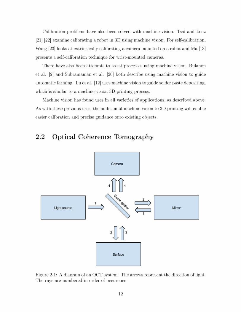
Figure 2-1: A diagram of an OCT system. The arrows represent the direction of light.The rays are numbered in order of occurence

12

We provide here a brief description of an optical coherence tomography (OCT)

system. OCT is a method for taking a 3D scan of an object. The specific OCT

system used is a Time Domain OCT (TDOCT) architecture [8] [24] [7]. For TDOCT,

the reference mirror is mechanically moved over time to provide depths at different

points.

Figure 2-1 shows a diagram of an OCT system that we will refer to for our ex-

planation. Light begins from the light source and moves toward the beam splitter in

the middle (ray 1). The beam splitter splits the light, with one half reflected down

towards the object to be scanned and the other half passing through to the mirror

(rays 2). Both halves are reflected back towards the beam splitter by either the object

or the mirror (rays 3), and some light from both sources make it into the camera lens

(rays 4).

A phenomenon called "interference" occurs when the distance from the beam

splitter to the object is the same as the distance from the beam splitter to the mirror.

In the diagram, these are the distances denoted by the two rays labeled with a "3".

Since the distance from the beam splitter to the mirror is held constant and can be

measured, we can then figure out where on the object is that distance from the beam

splitter by looking for interference.

Visually, interference looks like rapidly changing noise, which can be detected

either manually or automatically, as detailed in section 3.1.2. We can then vary

the height of the object in order to scan the total object and find the heights of all

positions on the object.

However, since interference looks just like rapidly changing noise, real noise in the

printer can look like interference. Reasons for this can include hitting the printer,

hitting the table that the printer is on if the table is frail, vibrations in the building,

etc. These are usually not problems, but if they do occur, then the interference

detection will usually not work well.

We use an OCT system in our machine vision component in order to take 3D

scans. The 3D scans are both of current prints, while they are printing, and of

existing auxiliary components placed on the printer platform.

13

2.3 GPGPU and CUDA

This work will make use of a general-purpose graphics processing unit (GPGPU),

which is simply using a GPU for general computing. As GPUs have gotten more and

more powerful, the computer industry has come to recognize the usefulness of GPUs

as general computing units that can process in many parallel threads. There has been

much work on making the GPU useful and easy to code on, and this system will be

taking advantage of that work to optimize some of the image processing code.

Specifically, we will be using Nvidia CUDA [15]. CUDA is a general programming

model invented and maintained by Nvidia. CUDA works well on Nvidia graphics

cards, making many speed boosts possible via hardware and low-level software opti-

mizations.

In addition to the general use CUDA, Nvidia also offers many other specific li-

braries. For example, cuSPARSE [14] is a specific library for working with sparse

matrices. Libraries such as these offer even more speed boosts than based on plain

CUDA.

2.4 MultiFab

The work in this thesis describes software implemented on top of an previously pub-

lished 3D printer/3D scanner combination known as MultiFab [19]. MultiFab is a

multi-material 3D printing platform that includes both hardware and software. The

software described in this thesis augments and uses the previously existing software.

This section will describe the previously existing software in more detail.

The already published material for MultiFab includes all of the firmware required

to run the 3D printer. In addition, MultiFab includes software to make a complete

3D scan with the 3D scanning system. The 3D scans are used for manual print-

head calibration, as described in section 3.2.2, and for corrective printing via height

correction, as described in section 6.1.

This thesis refines and adds uses of the 3D scanning system. The significant ad-

14

ditions are adaptive voxelization, another method for corrective printing as described

in section 6.2, and auxiliary printing, described in chapter 5.

15

16

Chapter 3

Calibration

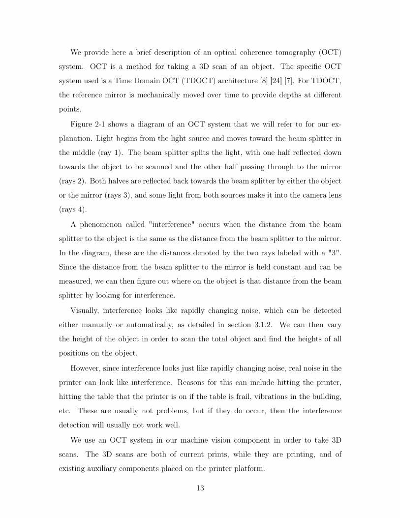
In order to integrate the 3D scanning system into the 3D printer with any sort of

accuracy, we must calibrate the systems together. The three main components that

need to be calibrated are the scanner, the printheads, and the positioning system.

Figure 3-1: A simplified diagram of the 3D printer. The scanner and printheads arerigidly attached together, and move separately from the platform.

Figure 3-1 shows a overview of the 3D scanning system and the 3D printer. As

shown in the figure, the scanner and multiple printheads are attached rigidly together.

That moves separately from the platform, which is where the prints are deposited.

The following specifically enumerates what needs to be calibrated.

1. The intrinsic matrix of the camera in the scanner.

17

2. The homography between the camera image and the real world.

3. The distance at which interference occurs in the scanner.

4. The offset between the camera and the printheads.

5. Any misalignment of the printheads.

These calibrations are split into two main steps: the camera calibration and the

printhead calibration. The first three calibrations are done in the camera calibration,

while the last two calibrations are done in the printhead calibration.

3.1 Camera Calibration

Before doing any work with the scanning system at all, the camera that is in the

scanner must be calibrated. As mentioned in the previous section, there are three

components to this calibration: the camera intrinsic matrix, the homography to world

coordinates, and the interference distance.

The intrinsic matrix describes properties of the camera so that a proper image

can be outputted. The homography between the camera image and the real world

produces an image in world coordinates of the image. With both of these, the cam-

era can construct an image in world coordinates. Finding these are both standard

functions implemented in OpenCV [1], so we will not cover finding these in detail.

The final component of the camera calibration is finding the distance at which

interference occurs, or the "interference distance". Most of this section describes how

to detect interference and the automation of detecting interference.

3.1.1 Qualitative Interference

The phenomenon of interference in the OCT system is described in detail in section

2.2. We will review it briefly here.

18

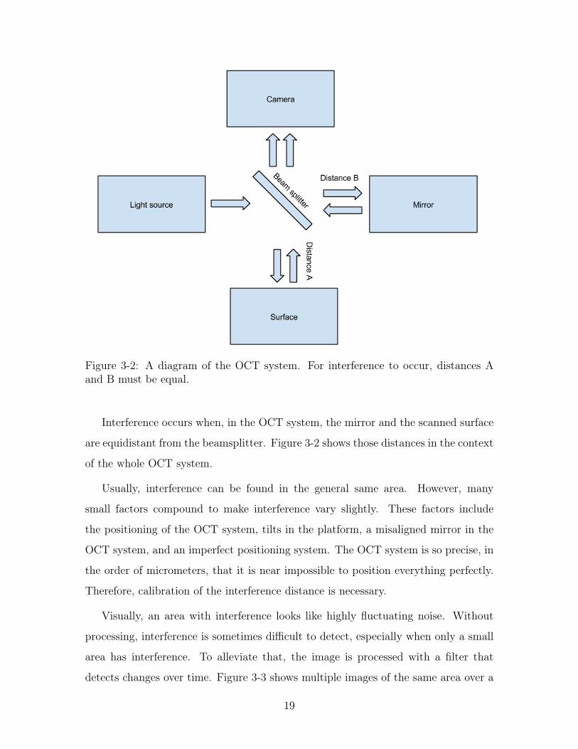
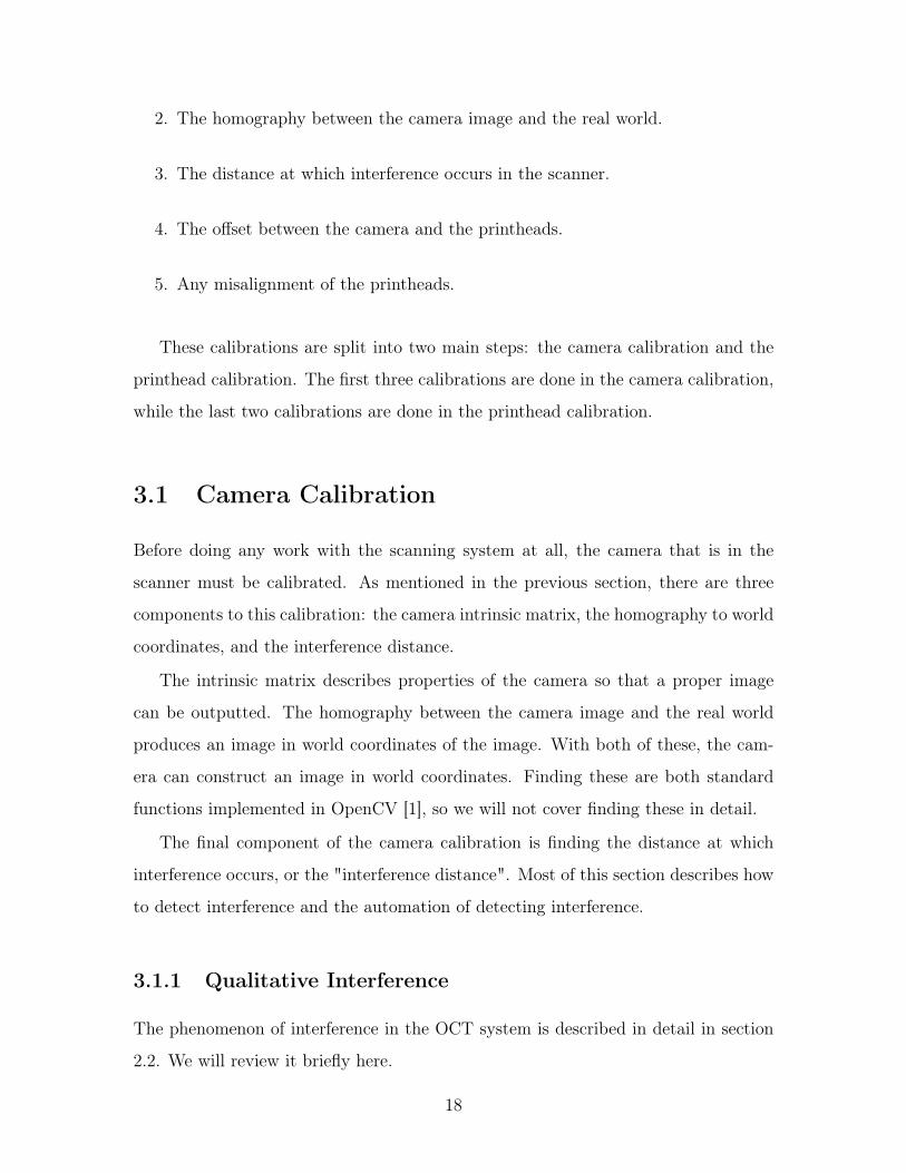
Figure 3-2: A diagram of the OCT system. For interference to occur, distances Aand B must be equal.

Interference occurs when, in the OCT system, the mirror and the scanned surface

are equidistant from the beamsplitter. Figure 3-2 shows those distances in the context

of the whole OCT system.

Usually, interference can be found in the general same area. However, many

small factors compound to make interference vary slightly. These factors include

the positioning of the OCT system, tilts in the platform, a misaligned mirror in the

OCT system, and an imperfect positioning system. The OCT system is so precise, in

the order of micrometers, that it is near impossible to position everything perfectly.

Therefore, calibration of the interference distance is necessary.

Visually, an area with interference looks like highly fluctuating noise. Without

processing, interference is sometimes difficult to detect, especially when only a small

area has interference. To alleviate that, the image is processed with a filter that

detects changes over time. Figure 3-3 shows multiple images of the same area over a

19

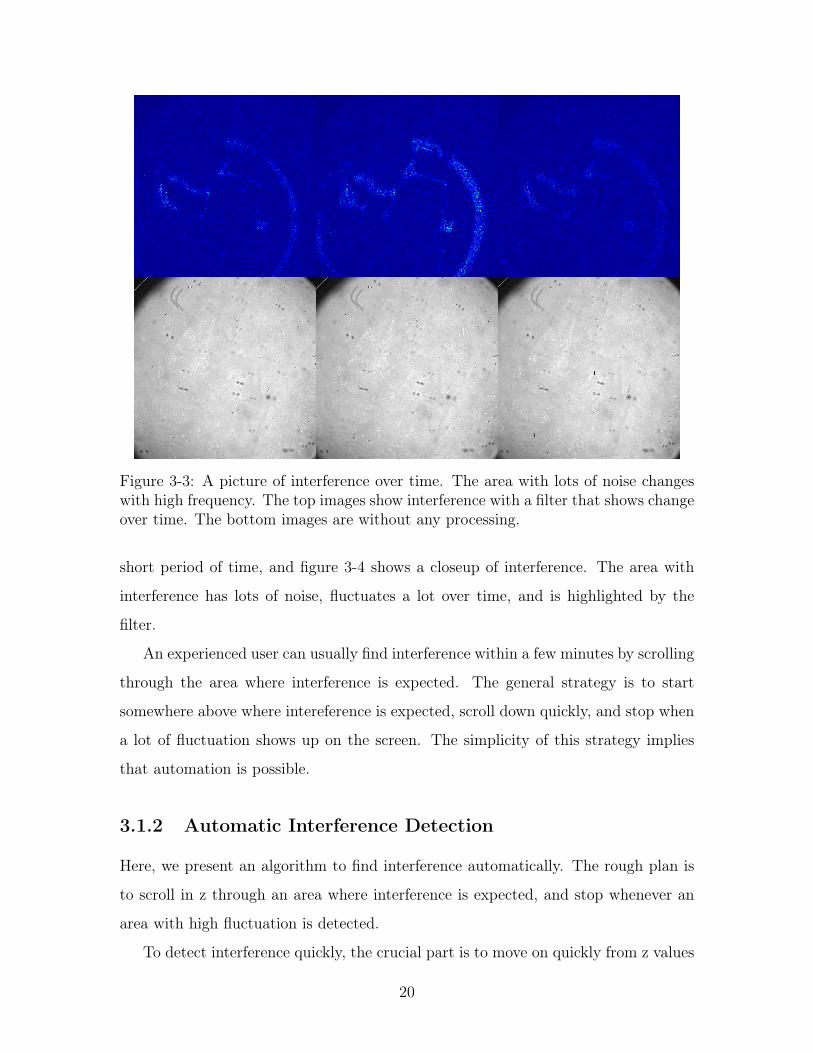
Figure 3-3: A picture of interference over time. The area with lots of noise changeswith high frequency. The top images show interference with a filter that shows changeover time. The bottom images are without any processing.

short period of time, and figure 3-4 shows a closeup of interference. The area with

interference has lots of noise, fluctuates a lot over time, and is highlighted by the

filter.

An experienced user can usually find interference within a few minutes by scrolling

through the area where interference is expected. The general strategy is to start

somewhere above where intereference is expected, scroll down quickly, and stop when

a lot of fluctuation shows up on the screen. The simplicity of this strategy implies

that automation is possible.

3.1.2 Automatic Interference Detection

Here, we present an algorithm to find interference automatically. The rough plan is

to scroll in z through an area where interference is expected, and stop whenever an

area with high fluctuation is detected.

To detect interference quickly, the crucial part is to move on quickly from z values

20

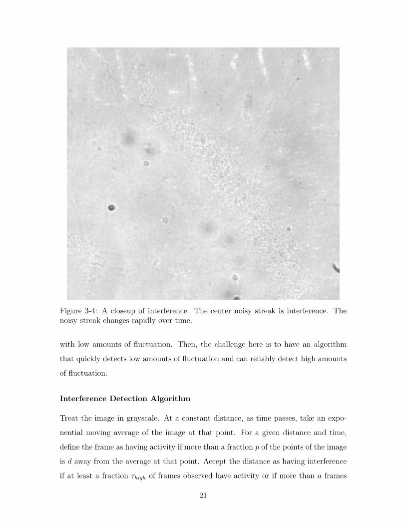
Figure 3-4: A closeup of interference. The center noisy streak is interference. Thenoisy streak changes rapidly over time.

with low amounts of fluctuation. Then, the challenge here is to have an algorithm

that quickly detects low amounts of fluctuation and can reliably detect high amounts

of fluctuation.

Interference Detection Algorithm

Treat the image in grayscale. At a constant distance, as time passes, take an expo-

nential moving average of the image at that point. For a given distance and time,

define the frame as having activity if more than a fraction 𝑝 of the points of the image

is 𝑑 away from the average at that point. Accept the distance as having interference

if at least a fraction 𝜏ℎ𝑖𝑔ℎ of frames observed have activity or if more than 𝑎 frames

21

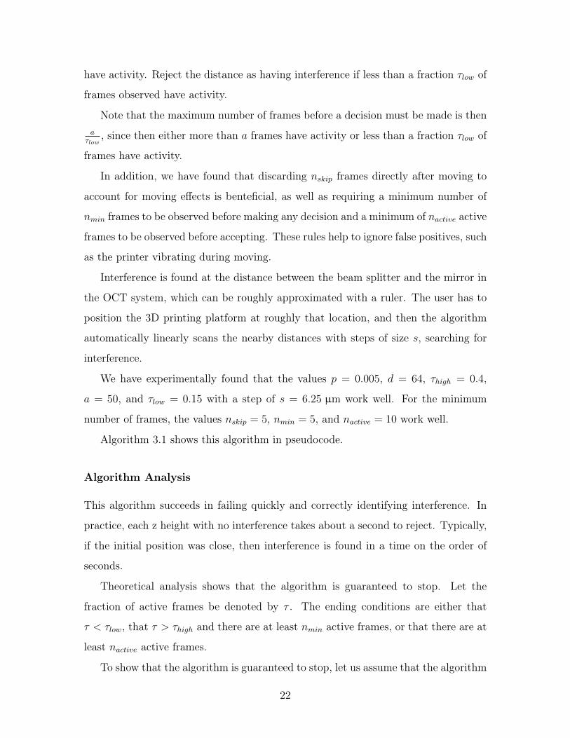
have activity. Reject the distance as having interference if less than a fraction 𝜏𝑙𝑜𝑤 of

frames observed have activity.

Note that the maximum number of frames before a decision must be made is then𝑎

𝜏𝑙𝑜𝑤, since then either more than 𝑎 frames have activity or less than a fraction 𝜏𝑙𝑜𝑤 of

frames have activity.

In addition, we have found that discarding 𝑛𝑠𝑘𝑖𝑝 frames directly after moving to

account for moving effects is benteficial, as well as requiring a minimum number of

𝑛𝑚𝑖𝑛 frames to be observed before making any decision and a minimum of 𝑛𝑎𝑐𝑡𝑖𝑣𝑒 active

frames to be observed before accepting. These rules help to ignore false positives, such

as the printer vibrating during moving.

Interference is found at the distance between the beam splitter and the mirror in

the OCT system, which can be roughly approximated with a ruler. The user has to

position the 3D printing platform at roughly that location, and then the algorithm

automatically linearly scans the nearby distances with steps of size 𝑠, searching for

interference.

We have experimentally found that the values 𝑝 = 0.005, 𝑑 = 64, 𝜏ℎ𝑖𝑔ℎ = 0.4,

𝑎 = 50, and 𝜏𝑙𝑜𝑤 = 0.15 with a step of 𝑠 = 6.25 𝜇m work well. For the minimum

number of frames, the values 𝑛𝑠𝑘𝑖𝑝 = 5, 𝑛𝑚𝑖𝑛 = 5, and 𝑛𝑎𝑐𝑡𝑖𝑣𝑒 = 10 work well.

Algorithm 3.1 shows this algorithm in pseudocode.

Algorithm Analysis

This algorithm succeeds in failing quickly and correctly identifying interference. In

practice, each z height with no interference takes about a second to reject. Typically,

if the initial position was close, then interference is found in a time on the order of

seconds.

Theoretical analysis shows that the algorithm is guaranteed to stop. Let the

fraction of active frames be denoted by 𝜏 . The ending conditions are either that

𝜏 < 𝜏𝑙𝑜𝑤, that 𝜏 > 𝜏ℎ𝑖𝑔ℎ and there are at least 𝑛𝑚𝑖𝑛 active frames, or that there are at

least 𝑛𝑎𝑐𝑡𝑖𝑣𝑒 active frames.

To show that the algorithm is guaranteed to stop, let us assume that the algorithm

22

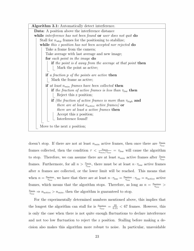
Algorithm 3.1: Automatically detect interference.Data: A position above the interference distancewhile interference has not been found or user does not quit do

Stall for 𝑛𝑠𝑘𝑖𝑝 frames for the positioning to stabilize;while this z position has not been accepted nor rejected do

Take a frame from the camera;Take average with last average and new image;for each point in the image do

if the point is 𝑑 away from the average at that point thenMark the point as active;

if a fraction 𝑝 of the points are active thenMark the frame as active;

if at least 𝑛𝑚𝑖𝑛 frames have been collected thenif the fraction of active frames is less than 𝜏𝑙𝑜𝑤 then

Reject this z position;if (the fraction of active frames is more than 𝜏ℎ𝑖𝑔ℎ and

there are at least 𝑛𝑎𝑐𝑡𝑖𝑣𝑒 active frames) orthere are at least 𝑎 active frames thenAccept this z position;Interference found!

Move to the next z position;

doesn’t stop. If there are not at least 𝑛𝑚𝑖𝑛 active frames, then once there are 𝑛𝑚𝑖𝑛

𝜏𝑙𝑜𝑤

frames collected, then the condition 𝜏 < 𝑛𝑚𝑖𝑛

𝑛𝑚𝑖𝑛/𝜏𝑙𝑜𝑤= 𝜏𝑙𝑜𝑤 will cause the algorithm

to stop. Therefore, we can assume there are at least 𝑛𝑚𝑖𝑛 active frames after 𝑛𝑚𝑖𝑛

𝜏𝑙𝑜𝑤

frames. Furthermore, for all 𝑛 > 𝑛𝑚𝑖𝑛

𝜏𝑙𝑜𝑤, there must be at least 𝑛 · 𝜏𝑙𝑜𝑤 active frames

after 𝑛 frames are collected, or the lower limit will be reached. This means that

when 𝑛 = 𝑛𝑎𝑐𝑡𝑖𝑣𝑒

𝜏𝑙𝑜𝑤, we have that there are at least 𝑛 · 𝜏𝑙𝑜𝑤 = 𝑛𝑎𝑐𝑡𝑖𝑣𝑒

𝜏𝑙𝑜𝑤· 𝜏𝑙𝑜𝑤 = 𝑛𝑎𝑐𝑡𝑖𝑣𝑒 active

frames, which means that the algorithm stops. Therefore, as long as 𝑛 = 𝑛𝑎𝑐𝑡𝑖𝑣𝑒

𝜏𝑙𝑜𝑤>

𝑛𝑚𝑖𝑛

𝜏𝑙𝑜𝑤⇒ 𝑛𝑎𝑐𝑡𝑖𝑣𝑒 > 𝑛𝑚𝑖𝑛, then the algorithm is guaranteed to stop.

For the experimentally determined numbers mentioned above, this implies that

the longest the algorithm can stall for is 𝑛𝑎𝑐𝑡𝑖𝑣𝑒

𝜏𝑙𝑜𝑤= 10

0.15< 67 frames. However, this

is only the case when there is not quite enough fluctuations to declare interference

and not too low fluctuation to reject the z position. Stalling before making a de-

cision also makes this algorithm more robust to noise. In particular, unavoidable

23

vibrations in the printer or the surrounding building can cause fluctuations in the

image. This is only given a false positive if the outside vibrations last longer than 67

frames, which would be very unusual. If there was actually an earthquake during the

interference algorithm, then the user would probably have a larger problem than the

false interference positive.

3.2 Printhead Calibration

The second major part of the calibration is the printhead calibration. Multiple print-

heads need to be calibrated with respect to each other and with respect to the camera.

There are three main reasons for these calibrations.

First, the camera needs to know where the printheads are positioned in order to

take scans of the resulting prints. Second, the printer needs to know the relative

positions of the printheads in order to align them properly. Finally, the printheads

may be slightly tilted, in which case the printer will need to adjust for that offset in

the software.

The printhead calibrations can vary slightly based on where the camera and the

printheads are mounted. Since we would like micrometer accuracy, this is very difficult

to calibrate by hand. Both the printhead positions and the printhead rotations would

be difficult to measure. Therefore, we use the OCT scanning system to obtain a

more accurate measurement of the printhead positions and calibrate through those

measurements.

The general method for calibrating these printheads is to print some patterns

with different nozzles, label where the patterns were printed either manually or semi-

automatically, and then fit the found locations to the expected format of the print-

head. The next few sections cover this method in detail.

3.2.1 Printhead Calibration Background

Before delving into the details about the calibration, we should describe the printhead

structure and our calibration pattern. All printheads used are the same, from the

24

Epson Workforce 30 printer [4]. The specific printhead is the F3-3 Mach Turbo2 type

printhead, which is described in detail in [5].

In addition to describing the printhead used, this section also covers the calibration

pattern used. This is a pattern that is printed at selected locations and is detected

to obtain a measurement of the location of the printheads.

Printhead Structure

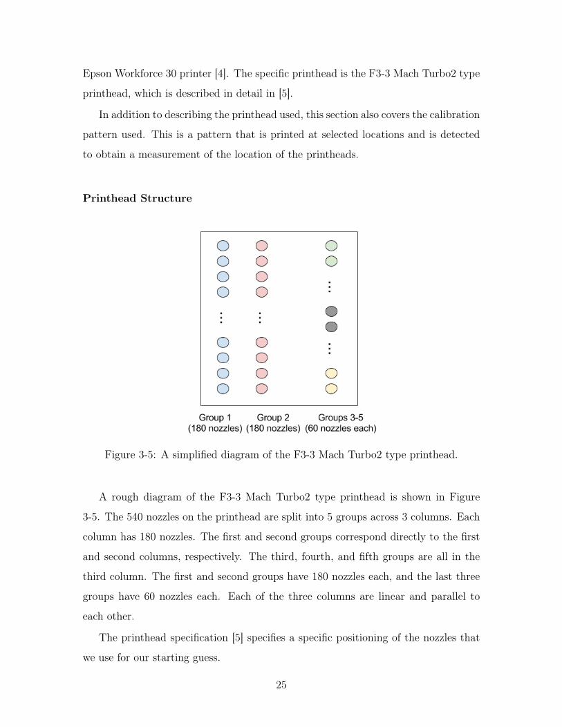
Figure 3-5: A simplified diagram of the F3-3 Mach Turbo2 type printhead.

A rough diagram of the F3-3 Mach Turbo2 type printhead is shown in Figure

3-5. The 540 nozzles on the printhead are split into 5 groups across 3 columns. Each

column has 180 nozzles. The first and second groups correspond directly to the first

and second columns, respectively. The third, fourth, and fifth groups are all in the

third column. The first and second groups have 180 nozzles each, and the last three

groups have 60 nozzles each. Each of the three columns are linear and parallel to

each other.

The printhead specification [5] specifies a specific positioning of the nozzles that

we use for our starting guess.

25

Calibration Pattern

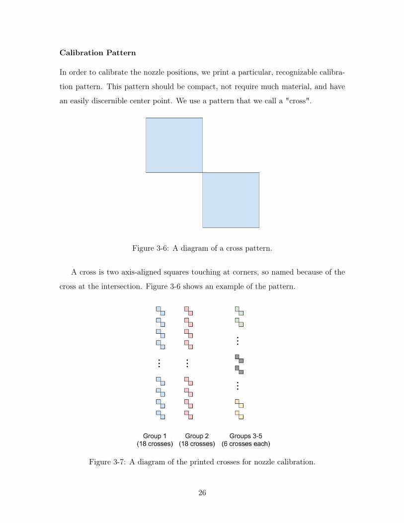
In order to calibrate the nozzle positions, we print a particular, recognizable calibra-

tion pattern. This pattern should be compact, not require much material, and have

an easily discernible center point. We use a pattern that we call a "cross".

Figure 3-6: A diagram of a cross pattern.

A cross is two axis-aligned squares touching at corners, so named because of the

cross at the intersection. Figure 3-6 shows an example of the pattern.

Figure 3-7: A diagram of the printed crosses for nozzle calibration.

26

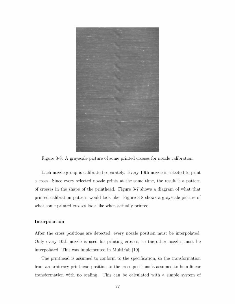
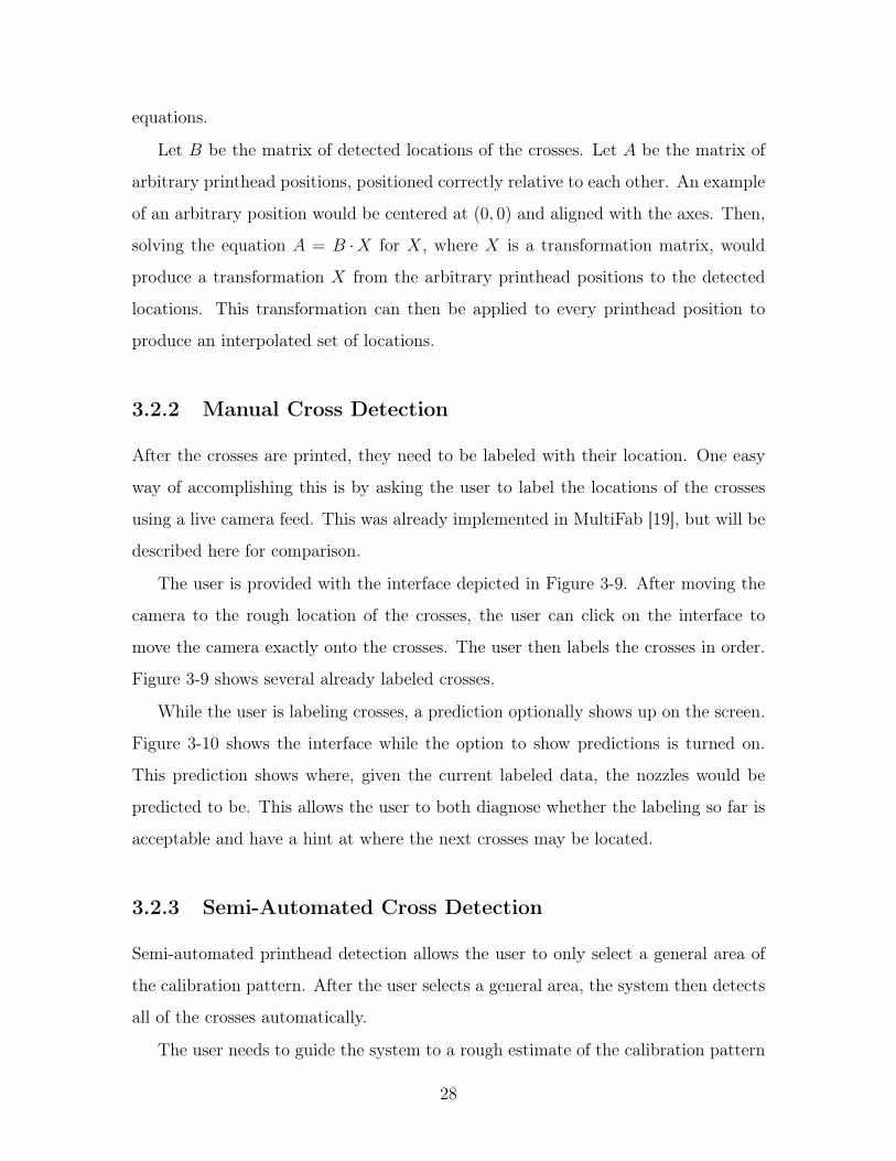
Figure 3-8: A grayscale picture of some printed crosses for nozzle calibration.

Each nozzle group is calibrated separately. Every 10th nozzle is selected to print

a cross. Since every selected nozzle prints at the same time, the result is a pattern

of crosses in the shape of the printhead. Figure 3-7 shows a diagram of what that

printed calibration pattern would look like. Figure 3-8 shows a grayscale picture of

what some printed crosses look like when actually printed.

Interpolation

After the cross positions are detected, every nozzle position must be interpolated.

Only every 10th nozzle is used for printing crosses, so the other nozzles must be

interpolated. This was implemented in MultiFab [19].

The printhead is assumed to conform to the specification, so the transformation

from an arbitrary printhead position to the cross positions is assumed to be a linear

transformation with no scaling. This can be calculated with a simple system of

27

equations.

Let 𝐵 be the matrix of detected locations of the crosses. Let 𝐴 be the matrix of

arbitrary printhead positions, positioned correctly relative to each other. An example

of an arbitrary position would be centered at (0, 0) and aligned with the axes. Then,

solving the equation 𝐴 = 𝐵 ·𝑋 for 𝑋, where 𝑋 is a transformation matrix, would

produce a transformation 𝑋 from the arbitrary printhead positions to the detected

locations. This transformation can then be applied to every printhead position to

produce an interpolated set of locations.

3.2.2 Manual Cross Detection

After the crosses are printed, they need to be labeled with their location. One easy

way of accomplishing this is by asking the user to label the locations of the crosses

using a live camera feed. This was already implemented in MultiFab [19], but will be

described here for comparison.

The user is provided with the interface depicted in Figure 3-9. After moving the

camera to the rough location of the crosses, the user can click on the interface to

move the camera exactly onto the crosses. The user then labels the crosses in order.

Figure 3-9 shows several already labeled crosses.

While the user is labeling crosses, a prediction optionally shows up on the screen.

Figure 3-10 shows the interface while the option to show predictions is turned on.

This prediction shows where, given the current labeled data, the nozzles would be

predicted to be. This allows the user to both diagnose whether the labeling so far is

acceptable and have a hint at where the next crosses may be located.

3.2.3 Semi-Automated Cross Detection

Semi-automated printhead detection allows the user to only select a general area of

the calibration pattern. After the user selects a general area, the system then detects

all of the crosses automatically.

The user needs to guide the system to a rough estimate of the calibration pattern

28

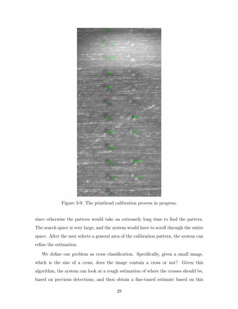
Figure 3-9: The printhead calibration process in progress.

since otherwise the pattern would take an extremely long time to find the pattern.

The search space is very large, and the system would have to scroll through the entire

space. After the user selects a general area of the calibration pattern, the system can

refine the estimation.

We define our problem as cross classification. Specifically, given a small image,

which is the size of a cross, does the image contain a cross or not? Given this

algorithm, the system can look at a rough estimation of where the crosses should be,

based on previous detections, and then obtain a fine-tuned estimate based on this

29

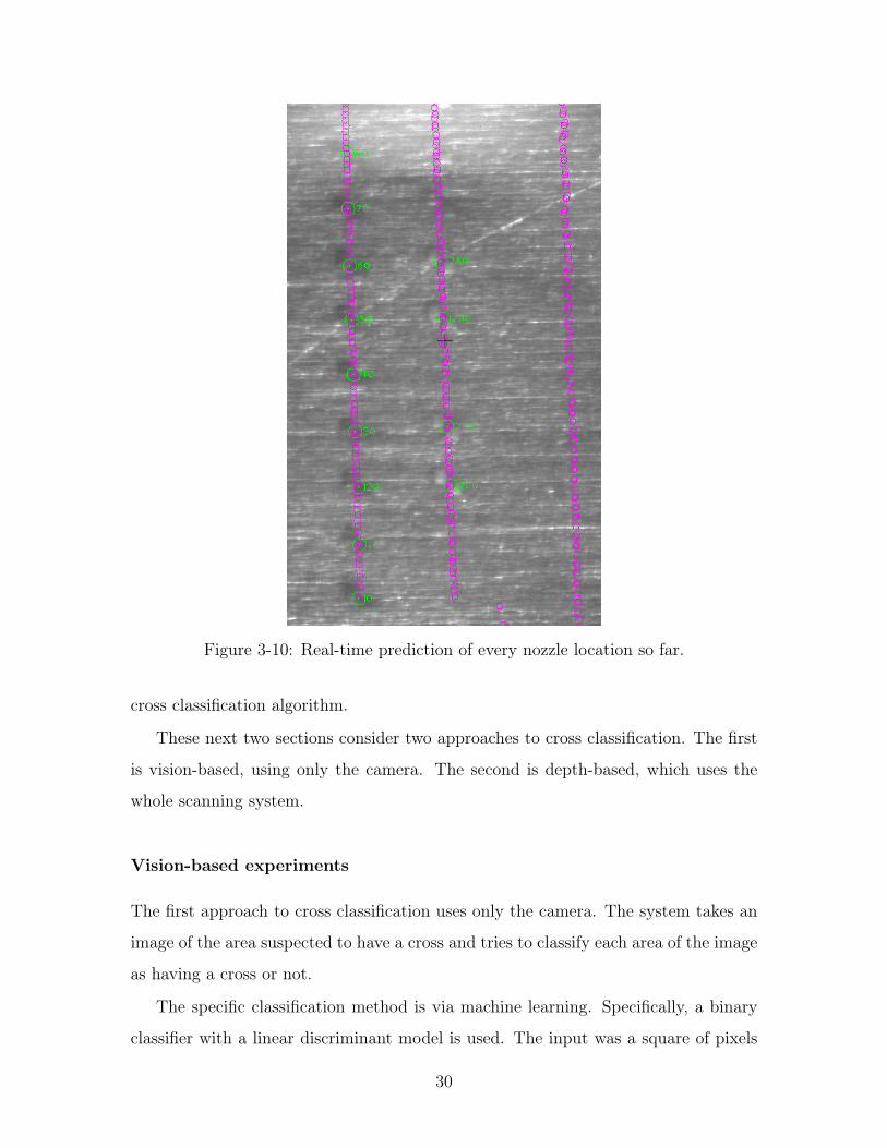
Figure 3-10: Real-time prediction of every nozzle location so far.

cross classification algorithm.

These next two sections consider two approaches to cross classification. The first

is vision-based, using only the camera. The second is depth-based, which uses the

whole scanning system.

Vision-based experiments

The first approach to cross classification uses only the camera. The system takes an

image of the area suspected to have a cross and tries to classify each area of the image

as having a cross or not.

The specific classification method is via machine learning. Specifically, a binary

classifier with a linear discriminant model is used. The input was a square of pixels

30

pre-processed into an array of numbers.

The library used for the classification was Classias [16]. Classias provides a binary

classifier with a linear discriminant model, which is well studied, out of the box.

Therefore, we focus on the other steps of the algorithm here.

Algorithm

This algorithm can be split up into three main parts. First, the image is sharpened

and cleaned up. Second, each 𝑛 by 𝑛 area of the image is classified as either a cross

or not a cross. Lastly, overlapping areas that were classified as crosses are merged

together, since they likely are actually the same cross.

The algorithm is enumerated specifically in Algorithm 3.2.

Algorithm 3.2: Classify an image as a cross or not a cross.Data: A grayscale image of the suspected crossPerform unsharp masking to sharpen the image;Use Otsu thresholding [17] to detect holes;Fill holes using the depth map interpolation from chapter 4;for every n by n pixel area in the image do

Compute average of the area;Normalize by subtracting average from every pixel;if the classifier classifies the area as a cross then

Mark this area as a cross;

Merge overlapping areas to get rid of duplicate positives;

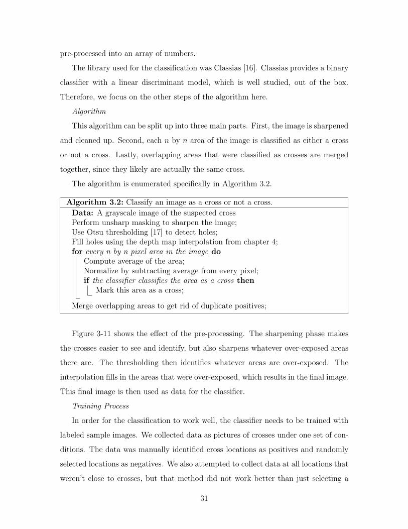
Figure 3-11 shows the effect of the pre-processing. The sharpening phase makes

the crosses easier to see and identify, but also sharpens whatever over-exposed areas

there are. The thresholding then identifies whatever areas are over-exposed. The

interpolation fills in the areas that were over-exposed, which results in the final image.

This final image is then used as data for the classifier.

Training Process

In order for the classification to work well, the classifier needs to be trained with

labeled sample images. We collected data as pictures of crosses under one set of con-

ditions. The data was manually identified cross locations as positives and randomly

selected locations as negatives. We also attempted to collect data at all locations that

weren’t close to crosses, but that method did not work better than just selecting a

31

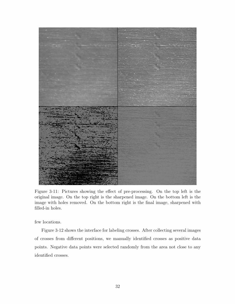
Figure 3-11: Pictures showing the effect of pre-processing. On the top left is theoriginal image. On the top right is the sharpened image. On the bottom left is theimage with holes removed. On the bottom right is the final image, sharpened withfilled-in holes.

few locations.

Figure 3-12 shows the interface for labeling crosses. After collecting several images

of crosses from different positions, we manually identified crosses as positive data

points. Negative data points were selected randomly from the area not close to any

identified crosses.

32

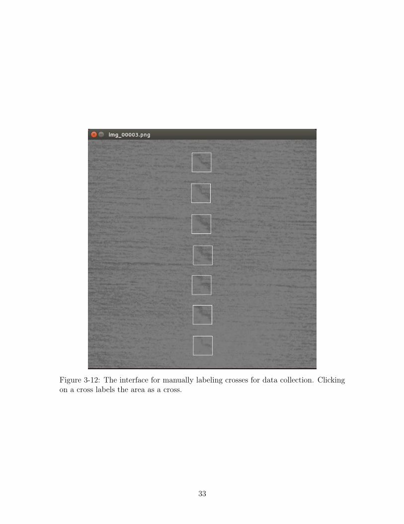
Figure 3-12: The interface for manually labeling crosses for data collection. Clickingon a cross labels the area as a cross.

33

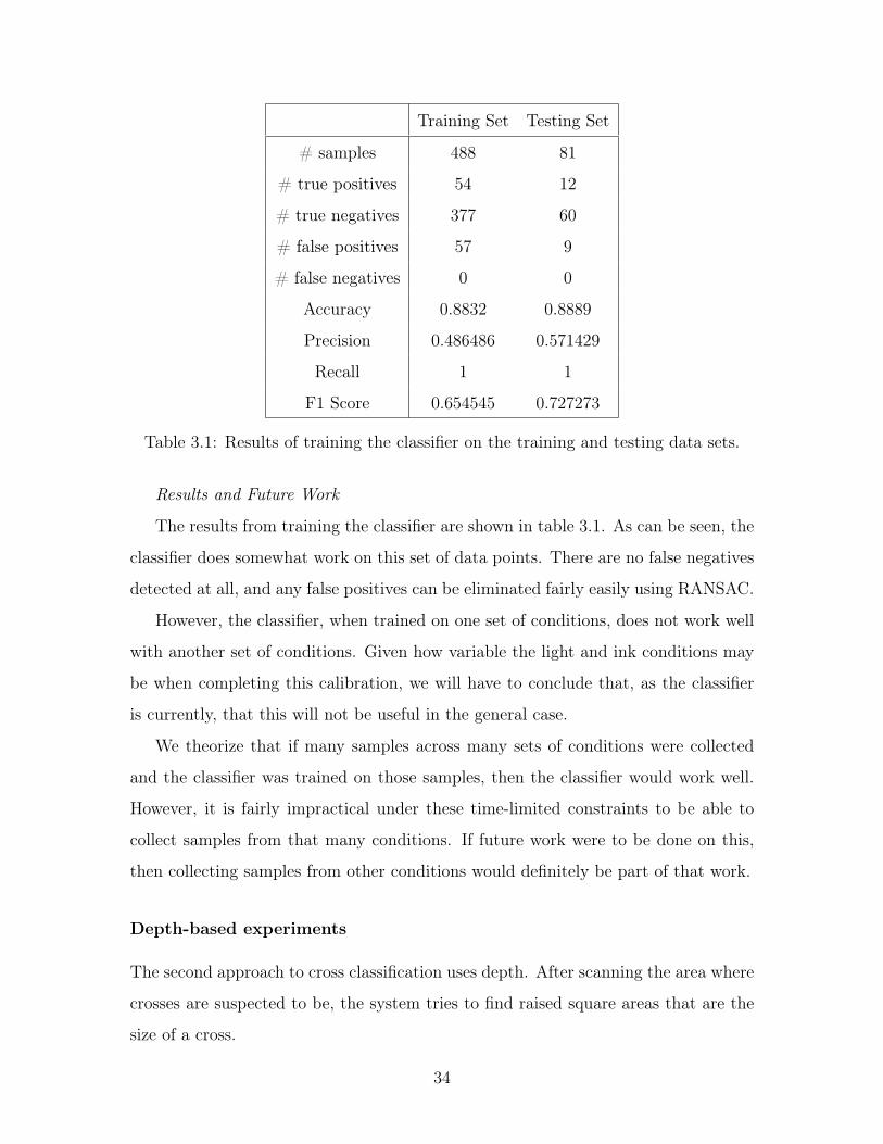
Training Set Testing Set

# samples 488 81

# true positives 54 12

# true negatives 377 60

# false positives 57 9

# false negatives 0 0

Accuracy 0.8832 0.8889

Precision 0.486486 0.571429

Recall 1 1

F1 Score 0.654545 0.727273

Table 3.1: Results of training the classifier on the training and testing data sets.

Results and Future Work

The results from training the classifier are shown in table 3.1. As can be seen, the

classifier does somewhat work on this set of data points. There are no false negatives

detected at all, and any false positives can be eliminated fairly easily using RANSAC.

However, the classifier, when trained on one set of conditions, does not work well

with another set of conditions. Given how variable the light and ink conditions may

be when completing this calibration, we will have to conclude that, as the classifier

is currently, that this will not be useful in the general case.

We theorize that if many samples across many sets of conditions were collected

and the classifier was trained on those samples, then the classifier would work well.

However, it is fairly impractical under these time-limited constraints to be able to

collect samples from that many conditions. If future work were to be done on this,

then collecting samples from other conditions would definitely be part of that work.

Depth-based experiments

The second approach to cross classification uses depth. After scanning the area where

crosses are suspected to be, the system tries to find raised square areas that are the

size of a cross.

34

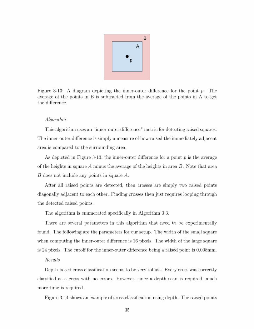
Figure 3-13: A diagram depicting the inner-outer difference for the point 𝑝. Theaverage of the points in B is subtracted from the average of the points in A to getthe difference.

Algorithm

This algorithm uses an "inner-outer difference" metric for detecting raised squares.

The inner-outer difference is simply a measure of how raised the immediately adjacent

area is compared to the surrounding area.

As depicted in Figure 3-13, the inner-outer difference for a point 𝑝 is the average

of the heights in square 𝐴 minus the average of the heights in area 𝐵. Note that area

𝐵 does not include any points in square 𝐴.

After all raised points are detected, then crosses are simply two raised points

diagonally adjacent to each other. Finding crosses then just requires looping through

the detected raised points.

The algorithm is enumerated specifically in Algorithm 3.3.

There are several parameters in this algorithm that need to be experimentally

found. The following are the parameters for our setup. The width of the small square

when computing the inner-outer difference is 16 pixels. The width of the large square

is 24 pixels. The cutoff for the inner-outer difference being a raised point is 0.008mm.

Results

Depth-based cross classification seems to be very robust. Every cross was correctly

classified as a cross with no errors. However, since a depth scan is required, much

more time is required.

Figure 3-14 shows an example of cross classification using depth. The raised points

35

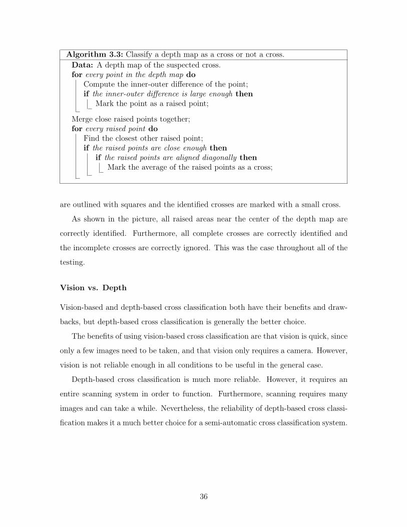
Algorithm 3.3: Classify a depth map as a cross or not a cross.Data: A depth map of the suspected cross.for every point in the depth map do

Compute the inner-outer difference of the point;if the inner-outer difference is large enough then

Mark the point as a raised point;

Merge close raised points together;for every raised point do

Find the closest other raised point;if the raised points are close enough then

if the raised points are aligned diagonally thenMark the average of the raised points as a cross;

are outlined with squares and the identified crosses are marked with a small cross.

As shown in the picture, all raised areas near the center of the depth map are

correctly identified. Furthermore, all complete crosses are correctly identified and

the incomplete crosses are correctly ignored. This was the case throughout all of the

testing.

Vision vs. Depth

Vision-based and depth-based cross classification both have their benefits and draw-

backs, but depth-based cross classification is generally the better choice.

The benefits of using vision-based cross classification are that vision is quick, since

only a few images need to be taken, and that vision only requires a camera. However,

vision is not reliable enough in all conditions to be useful in the general case.

Depth-based cross classification is much more reliable. However, it requires an

entire scanning system in order to function. Furthermore, scanning requires many

images and can take a while. Nevertheless, the reliability of depth-based cross classi-

fication makes it a much better choice for a semi-automatic cross classification system.

36

Figure 3-14: An example of cross detection using the depth map. Raised points areoutlined by squares. Crosses are marked with a small cross.

37

38

Chapter 4

Depth Map Interpolation

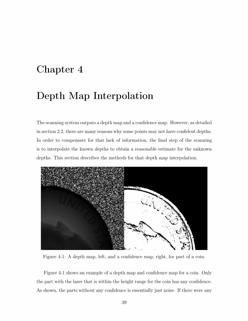
The scanning system outputs a depth map and a confidence map. However, as detailed

in section 2.2, there are many reasons why some points may not have confident depths.

In order to compensate for that lack of information, the final step of the scanning

is to interpolate the known depths to obtain a reasonable estimate for the unknown

depths. This section describes the methods for that depth map interpolation.

Figure 4-1: A depth map, left, and a confidence map, right, for part of a coin.

Figure 4-1 shows an example of a depth map and confidence map for a coin. Only

the part with the laser that is within the height range for the coin has any confidence.

As shown, the parts without any confidence is essentially just noise. If there were any

39

values without confidence within the coin, then interpolation would give reasonable

values for that area of the coin.

4.1 Algebraic Multigrid

The interpolation is done with the algebraic multigrid method [6]. Since speed is an

essential component of the interpolation, the interpolation has an option to be run

using CUDA, the NVIDIA parallel computing platform.

The algebraic multigrid method is a method for solving sets of differential equa-

tions. In this case, algebraic multigrid is used for solving the discrete Poisson equation.

Since both of these use cases are well studied, we will not describe here how multigrid

works. Instead, we focus on the application of the method.

4.1.1 Interpolation with Algebraic Multigrid

The algebraic multigrid method here is used for interpolation. In order to do this,

every point is assumed to have zero for the Laplacian. Simply said, every point is

assumed to have a flat neighborhood. Since there are some points that are treated

as givens, this is usually impossible to achieve. However, algebraic multigrid approx-

imates the solution by interpolating between given points.

Specifically, a point is treated as given if it reaches a confidence threshold. Oth-

erwise, the point is uncertain and is interpolated by algebraic multigrid.

The neighbors of a point are the four cardinal neighbors of the point. Therefore,

for each uncertain point at (𝑖, 𝑗), the depth at that point, 𝑑𝑖,𝑗, is described by the

equation

4 · 𝑑𝑖,𝑗 − 𝑑𝑖−1,𝑗 − 𝑑𝑖,𝑗−1 − 𝑑𝑖+1,𝑗 − 𝑑𝑖,𝑗+1 = 0.

If the point is at the edge of the map, then the corresponding points are treated

as 0 and the coefficient of 𝑑𝑖,𝑗 is decreased correspondingly. In addition, if any of

the neighbors of (𝑖, 𝑗) are given points, then the depth of that point is substituted

40

directly into the equation. The full form of the equation then is

(# neighbors) · 𝑑𝑖,𝑗 −∑︁

𝑛∈{uncertain neighbors}

𝑑𝑛 =∑︁

𝑚∈{confident neighbors}

𝑑𝑚.

Note that 𝑑𝑛 are variables to be solved for, and that 𝑑𝑚 are constants.

In the previous equations, each of the neighbors are weighted equally. We also

experimented with weighting the neighbors by the given confidence. However, this

did not result in substantial differences, so we just discuss the simpler, un-weighted

version of the algorithm.

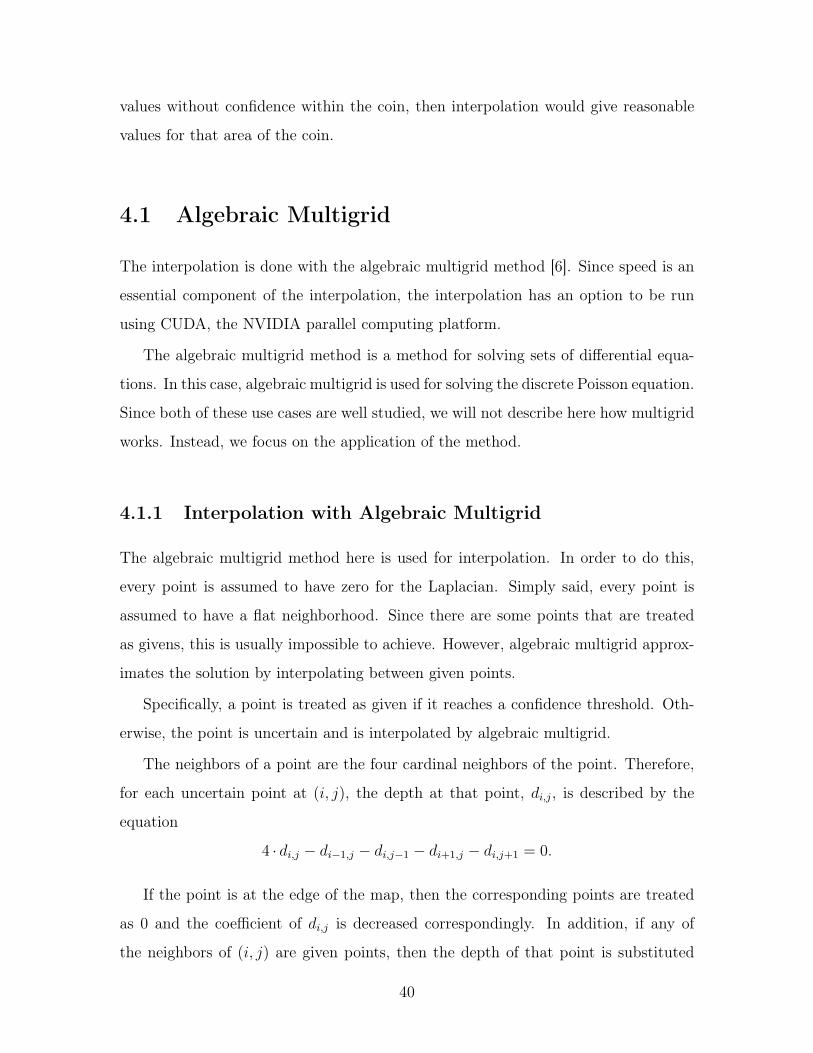
The algorithm for interpolation is enumerated specifically in Algorithm 4.1.

Algorithm 4.1: Interpolate in a depth map given the confidence map.Data: A depth map and a confidence map of the same area.for every point in the map do

if the point is greater than the threshold thenMark the point as given;

elseMark the point as uncertain;

Set up a system of equations to be filled in;for every point in the map do

Set the number of neighbors;Mark which of the neighbors are uncertain;Set the constant on the RHS as the sum of the confident neighbors;

Use algebraic multigrid to solve for the uncertain points;

4.1.2 Results

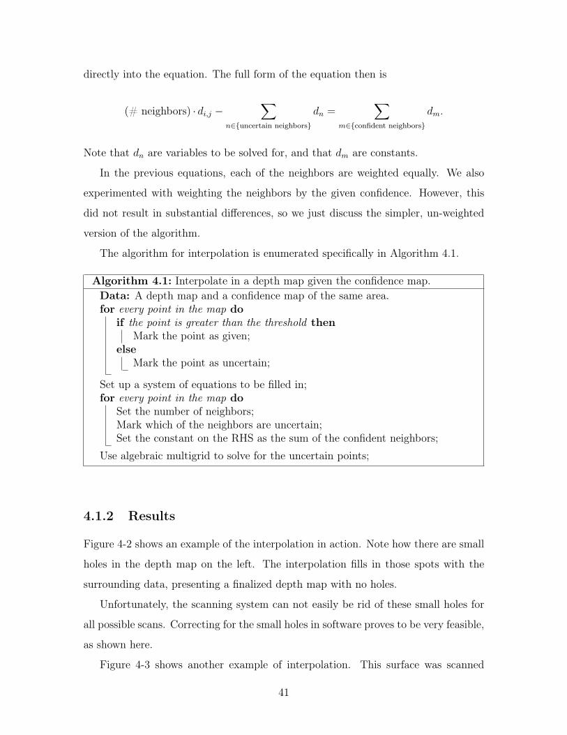
Figure 4-2 shows an example of the interpolation in action. Note how there are small

holes in the depth map on the left. The interpolation fills in those spots with the

surrounding data, presenting a finalized depth map with no holes.

Unfortunately, the scanning system can not easily be rid of these small holes for

all possible scans. Correcting for the small holes in software proves to be very feasible,

as shown here.

Figure 4-3 shows another example of interpolation. This surface was scanned

41

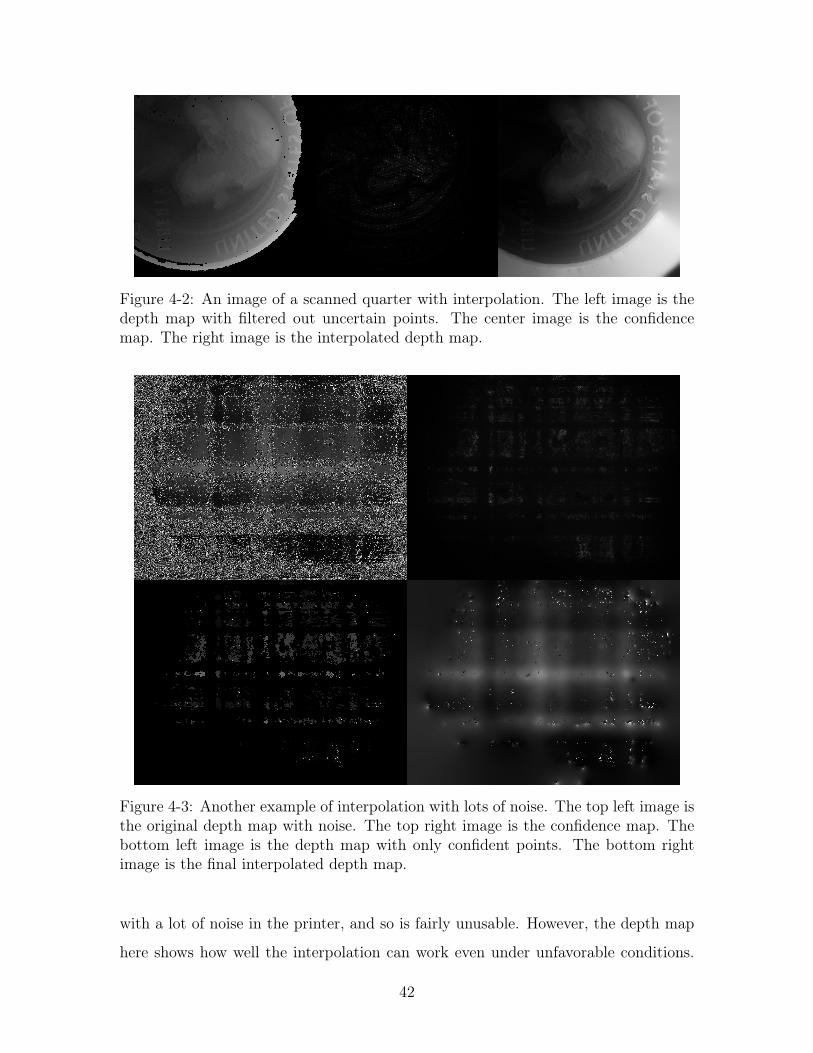
Figure 4-2: An image of a scanned quarter with interpolation. The left image is thedepth map with filtered out uncertain points. The center image is the confidencemap. The right image is the interpolated depth map.

Figure 4-3: Another example of interpolation with lots of noise. The top left image isthe original depth map with noise. The top right image is the confidence map. Thebottom left image is the depth map with only confident points. The bottom rightimage is the final interpolated depth map.

with a lot of noise in the printer, and so is fairly unusable. However, the depth map

here shows how well the interpolation can work even under unfavorable conditions.

42

Even given the massive amounts of noise and small amounts of confident points, the

interpolation was able to recover a fairly clean depth map.

4.2 Using Parallel Computing

Algebraic multigrid is an easily parallelizable method. Therefore, we use parallel

computing when available. Again, this is a well-studied problem, readibly available

in third-party libraries.

The library we used was AMGCL [3], a library for algebraic multigrid with parallel

computing capabilities. When available, AMGCL uses CUDA/cuSPARSE [15] [14].

CUDA is a parallel programming platform provided by NVIDIA. cuSPARSE is a

platform for CUDA provided by NVIDIA that manipulates sparse matrices.

4.2.1 Results

We compared the single-threaded algebraic multigrid implementation by AMGCL,

the parallelized algebraic multigrid implementation by AMGCL, and a baseline filling

filter that naively interpolates from confident neighbors.

43

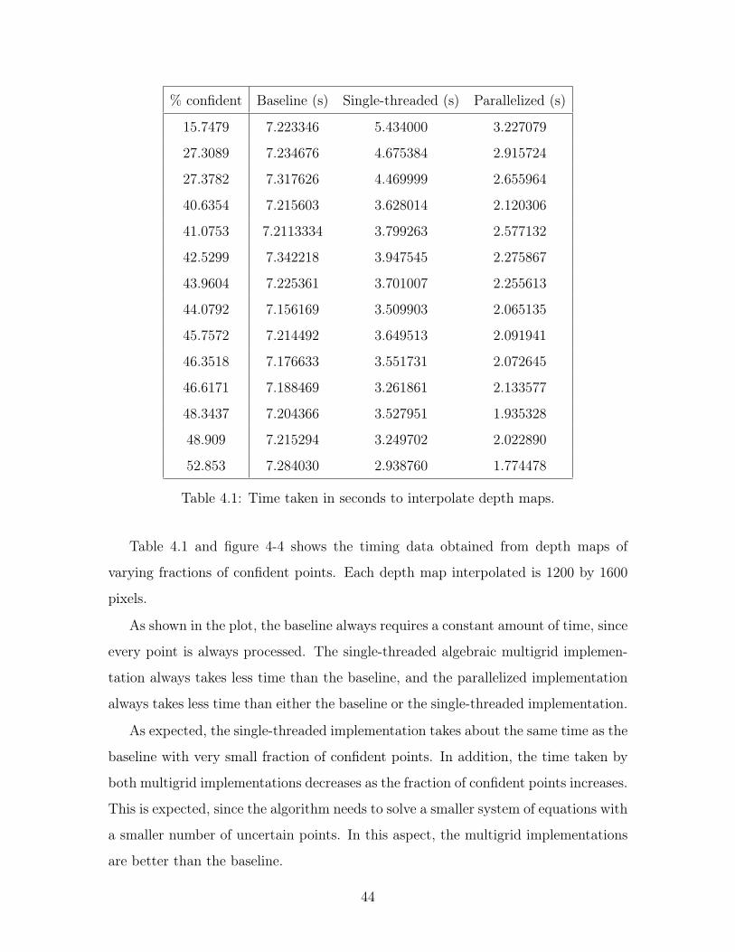
% confident Baseline (s) Single-threaded (s) Parallelized (s)

15.7479 7.223346 5.434000 3.227079

27.3089 7.234676 4.675384 2.915724

27.3782 7.317626 4.469999 2.655964

40.6354 7.215603 3.628014 2.120306

41.0753 7.2113334 3.799263 2.577132

42.5299 7.342218 3.947545 2.275867

43.9604 7.225361 3.701007 2.255613

44.0792 7.156169 3.509903 2.065135

45.7572 7.214492 3.649513 2.091941

46.3518 7.176633 3.551731 2.072645

46.6171 7.188469 3.261861 2.133577

48.3437 7.204366 3.527951 1.935328

48.909 7.215294 3.249702 2.022890

52.853 7.284030 2.938760 1.774478

Table 4.1: Time taken in seconds to interpolate depth maps.

Table 4.1 and figure 4-4 shows the timing data obtained from depth maps of

varying fractions of confident points. Each depth map interpolated is 1200 by 1600

pixels.

As shown in the plot, the baseline always requires a constant amount of time, since

every point is always processed. The single-threaded algebraic multigrid implemen-

tation always takes less time than the baseline, and the parallelized implementation

always takes less time than either the baseline or the single-threaded implementation.

As expected, the single-threaded implementation takes about the same time as the

baseline with very small fraction of confident points. In addition, the time taken by

both multigrid implementations decreases as the fraction of confident points increases.

This is expected, since the algorithm needs to solve a smaller system of equations with

a smaller number of uncertain points. In this aspect, the multigrid implementations

are better than the baseline.

44

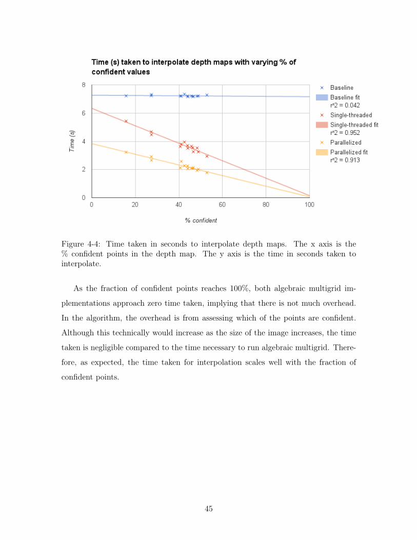
Figure 4-4: Time taken in seconds to interpolate depth maps. The x axis is the% confident points in the depth map. The y axis is the time in seconds taken tointerpolate.

As the fraction of confident points reaches 100%, both algebraic multigrid im-

plementations approach zero time taken, implying that there is not much overhead.

In the algorithm, the overhead is from assessing which of the points are confident.

Although this technically would increase as the size of the image increases, the time

taken is negligible compared to the time necessary to run algebraic multigrid. There-

fore, as expected, the time taken for interpolation scales well with the fraction of

confident points.

45

46

Chapter 5

Combining 3D Prints with Auxiliary

Objects

One use of the scanning system is to enable printing on top of auxiliary objects.

Specifically, a user could take an object from outside of the printer, place it on the

printing platform, and have the printer print exactly on top of the object in the

correct position.

There are many potential use cases for printing on auxiliary objects. Cases for

PCBs could be printed directly on top of the PCB. Broken parts could be fixed with

supplemental 3D printing. Parts that are not easily 3D printable, like glass, metal,

or other such materials, could be augmented with this printing capability.

Without the scanning system, the printer would not be able to align the print

correctly on top of the auxiliary object, since the printer would not be able to detect

where the auxiliary object was placed. However, with the scanning system, the printer

is able to scan with high accuracy where the auxiliary object is placed.

This chapter describes the interface for printing on auxiliary objects, examines

the mechanics of the auto-alignment, and discusses how well the system works.

47

5.1 User Interface

This section describes the procedure and interface for printing on auxiliary objects.

The user interacts with the interface to correctly align the print with the scan of the

auxiliary object. The interface provides a graphical representation of what the final

print aligned with the auxiliary object should look like.

5.1.1 Procedure

First, the user has to position the auxiliary object on the printing platform. The

printer scans the object to produce a depth map. After the user loads the correct

mesh, the interface displays both the depth map and the mesh together. This is

described in section 5.1.2 in more detail. The user can then align the mesh with the

depth map either manually or automatically. The automatic aligmnent is described

in section 5.2 in more detail.

After the mesh is aligned with the depth map, the user triggers pre-processing.

The mesh is first voxelized to produce a voxel grid. Each column of voxels is then

compared to the depth detected at that point. Any voxels below the depth at that

point are removed. Any empty space between the depth and the voxels is filled in with

the latest material to prevent empty space. The printer then moves to the calibrated

print location and prints the finalized voxel grid.

5.1.2 Interface

Figure 5-1 shows the interface seen by the user in order to print on auxiliary objects.

There is a scan of the auxiliary object shown in Figures 5-2 and 5-3, shown in blue.

The mesh of the object to be printed is shown in yellow. Controls are shown on the

right.

As seen in the image, the user has options to scan the auxiliary object, move the

mesh around, rotate the mesh, voxelize the mesh, and move to the print location.

The GUI also offers the user to move the mesh around in 3D space relative to the

scan. Figure 5-4 shows how the user can look at the mesh from different angles, thus

48

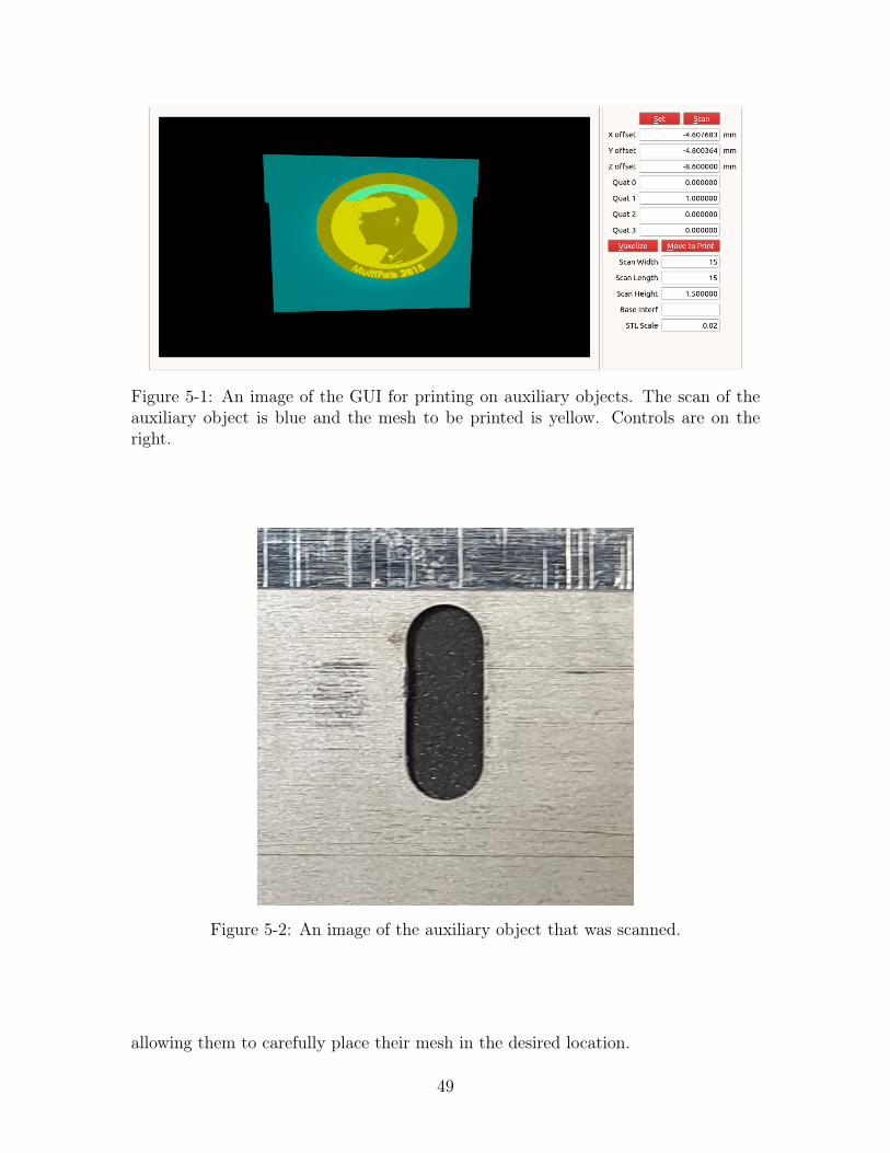
Figure 5-1: An image of the GUI for printing on auxiliary objects. The scan of theauxiliary object is blue and the mesh to be printed is yellow. Controls are on theright.

Figure 5-2: An image of the auxiliary object that was scanned.

allowing them to carefully place their mesh in the desired location.

49

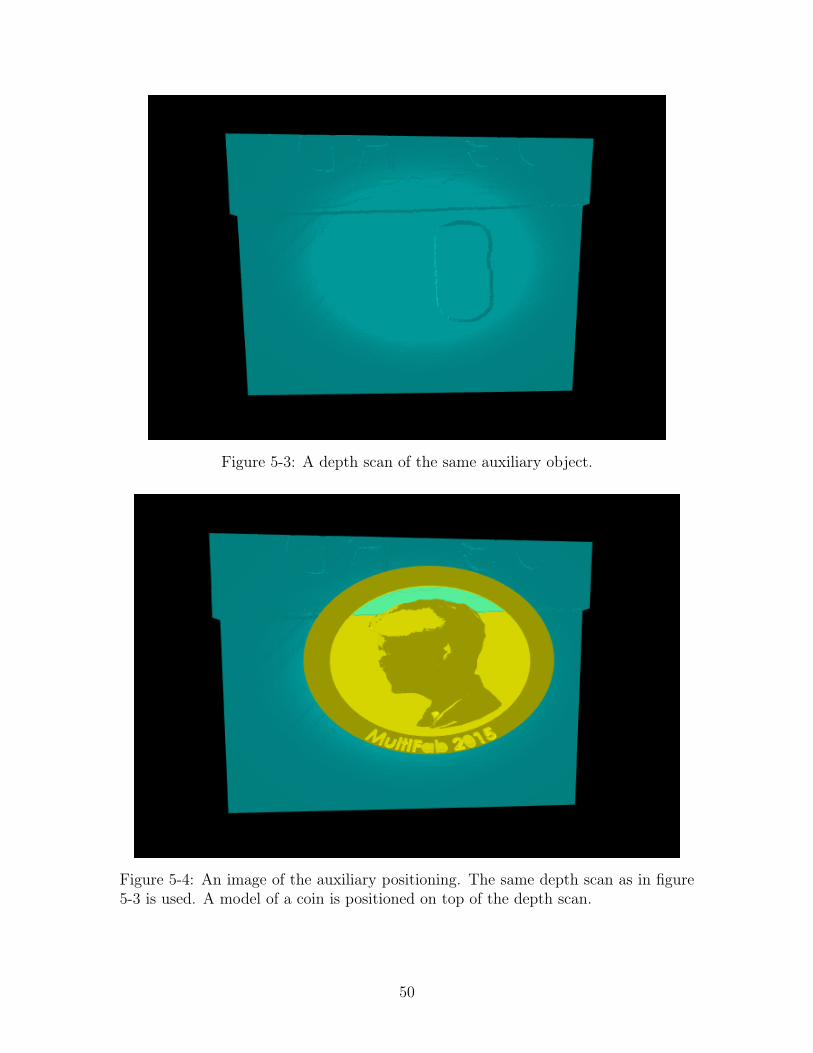
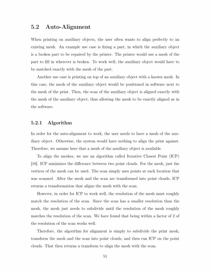
Figure 5-3: A depth scan of the same auxiliary object.

Figure 5-4: An image of the auxiliary positioning. The same depth scan as in figure5-3 is used. A model of a coin is positioned on top of the depth scan.

50

5.2 Auto-Alignment

When printing on auxiliary objects, the user often wants to align perfectly to an

existing mesh. An example use case is fixing a part, in which the auxiliary object

is a broken part to be repaired by the printer. The printer would use a mesh of the

part to fill in wherever is broken. To work well, the auxiliary object would have to

be matched exactly with the mesh of the part.

Another use case is printing on top of an auxiliary object with a known mesh. In

this case, the mesh of the auxiliary object would be positioned in software next to

the mesh of the print. Then, the scan of the auxiliary object is aligned exactly with

the mesh of the auxiliary object, thus allowing the mesh to be exactly aligned as in

the software.

5.2.1 Algorithm

In order for the auto-alignment to work, the user needs to have a mesh of the aux-

iliary object. Otherwise, the system would have nothing to align the print against.

Therefore, we assume here that a mesh of the auxiliary object is available.

To align the meshes, we use an algorithm called Iterative Closest Point (ICP)

[18]. ICP minimizes the difference between two point clouds. For the mesh, just the

vertices of the mesh can be used. The scan simply uses points at each location that

was scanned. After the mesh and the scan are transformed into point clouds, ICP

returns a transformation that aligns the mesh with the scan.

However, in order for ICP to work well, the resolution of the mesh must roughly

match the resolution of the scan. Since the scan has a smaller resolution than the

mesh, the mesh just needs to subdivide until the resolution of the mesh roughly

matches the resolution of the scan. We have found that being within a factor of 2 of

the resolution of the scan works well.

Therefore, the algorithm for alignment is simply to subdivide the print mesh,

transform the mesh and the scan into point clouds, and then run ICP on the point

clouds. That then returns a transform to align the mesh with the scan.

51

5.2.2 Results

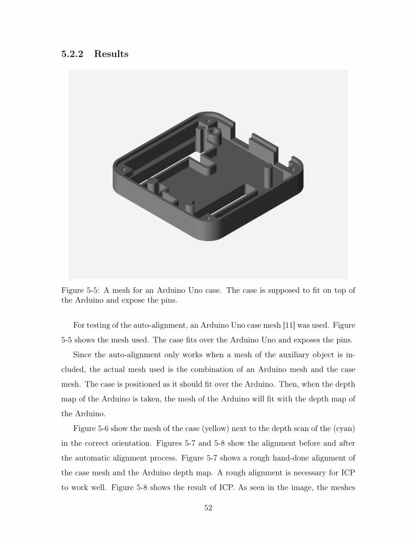
Figure 5-5: A mesh for an Arduino Uno case. The case is supposed to fit on top ofthe Arduino and expose the pins.

For testing of the auto-alignment, an Arduino Uno case mesh [11] was used. Figure

5-5 shows the mesh used. The case fits over the Arduino Uno and exposes the pins.

Since the auto-alignment only works when a mesh of the auxiliary object is in-

cluded, the actual mesh used is the combination of an Arduino mesh and the case

mesh. The case is positioned as it should fit over the Arduino. Then, when the depth

map of the Arduino is taken, the mesh of the Arduino will fit with the depth map of

the Arduino.

Figure 5-6 show the mesh of the case (yellow) next to the depth scan of the (cyan)

in the correct orientation. Figures 5-7 and 5-8 show the alignment before and after

the automatic alignment process. Figure 5-7 shows a rough hand-done alignment of

the case mesh and the Arduino depth map. A rough alignment is necessary for ICP

to work well. Figure 5-8 shows the result of ICP. As seen in the image, the meshes

52

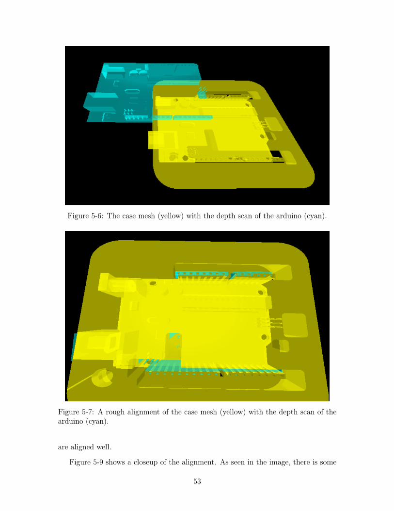
Figure 5-6: The case mesh (yellow) with the depth scan of the arduino (cyan).

Figure 5-7: A rough alignment of the case mesh (yellow) with the depth scan of thearduino (cyan).

are aligned well.

Figure 5-9 shows a closeup of the alignment. As seen in the image, there is some

53

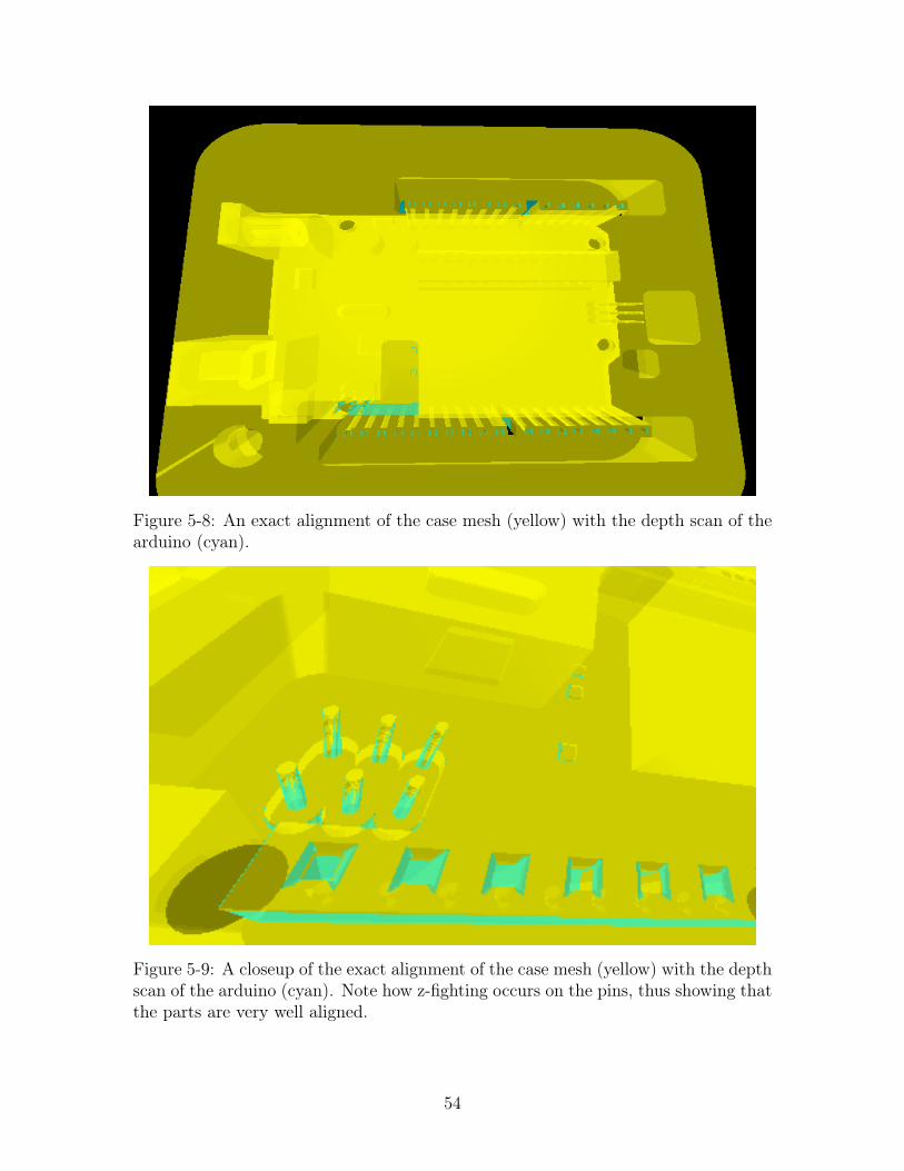
Figure 5-8: An exact alignment of the case mesh (yellow) with the depth scan of thearduino (cyan).

Figure 5-9: A closeup of the exact alignment of the case mesh (yellow) with the depthscan of the arduino (cyan). Note how z-fighting occurs on the pins, thus showing thatthe parts are very well aligned.

54

z-fighting in the pins of the Arduino. Since that is only possible when the meshes

overlap very closely, we can conclude that the alignment works very well.

5.3 Results

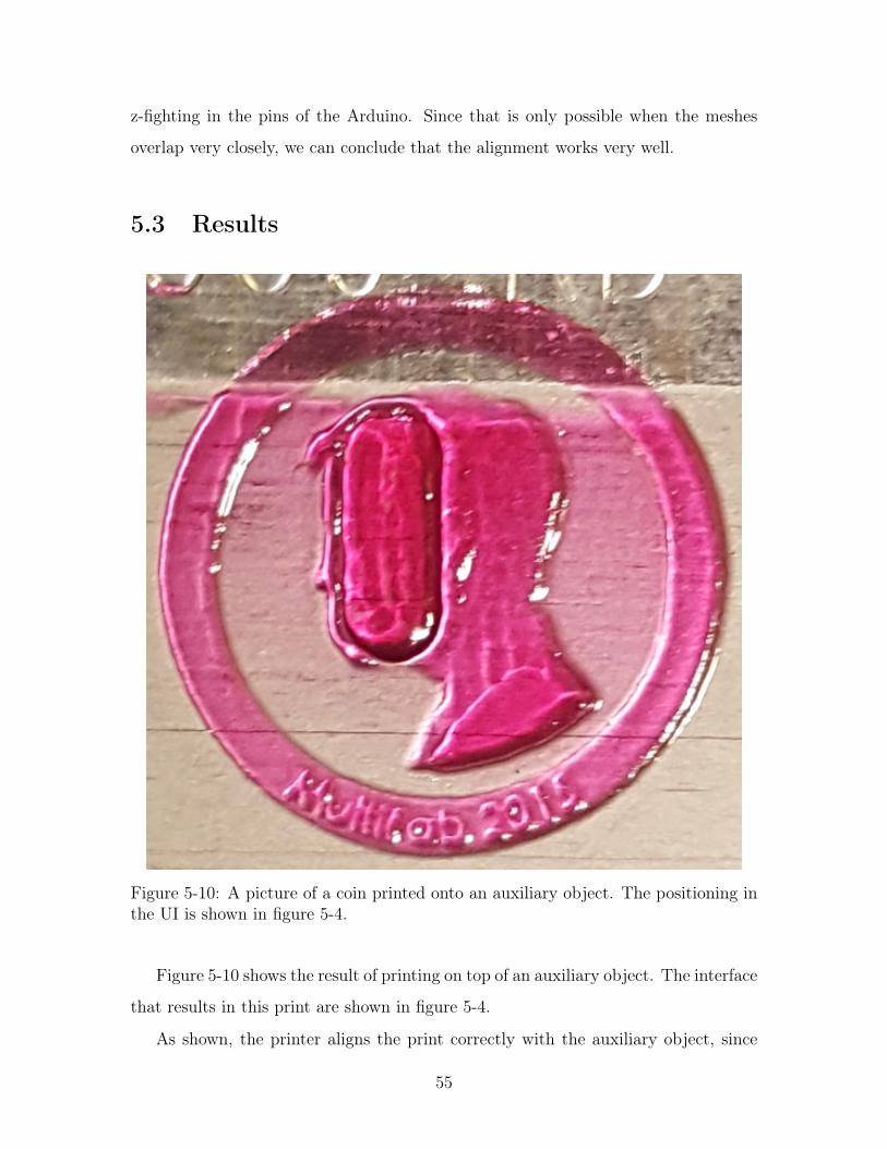
Figure 5-10: A picture of a coin printed onto an auxiliary object. The positioning inthe UI is shown in figure 5-4.

Figure 5-10 shows the result of printing on top of an auxiliary object. The interface

that results in this print are shown in figure 5-4.

As shown, the printer aligns the print correctly with the auxiliary object, since

55

the upper portion of the coin is correctly not printed on top of the edge.

However, the height of each droplet when printing is not correct, as can be seen

by the difference in height in the center hole. Combining auxiliary printing with

corrective printing fixes this problem, as described in section 6.3.

56

Chapter 6

Corrective Printing

When printing with a normal 3D printer, the printer generally operates blindly. The

printer moves to a location, drops material, and repeats. This generally works well.

However, when printhead nozzles fail or do not completely jet in a pattern, there may

be small, visible artifacts. The print will have to be re-printed, which wastes both

time and material.

Usually, there is no way to detect that the print may not be perfect until the print

is visually inspected after finishing. However, with a 3D scanner, a feedback loop

exists between the printer and the print. The printer can use the feedback during the

printing process, and any defects can be fixed during the printing.

We present two methods for corrective printing: height correction, where any

deficiencies in height are printed again, and adaptive voxelization, where the mesh is

revoxelized at the scanned height.

6.1 Height Correction

The first method for corrective printing is height correction. Height correction was

already implemented for MultiFab [19], but will be described here again for the sake

of comparison. The basic idea for height correction is to scan every few layers and fill

in wherever the printer didn’t print up to the supposed height.

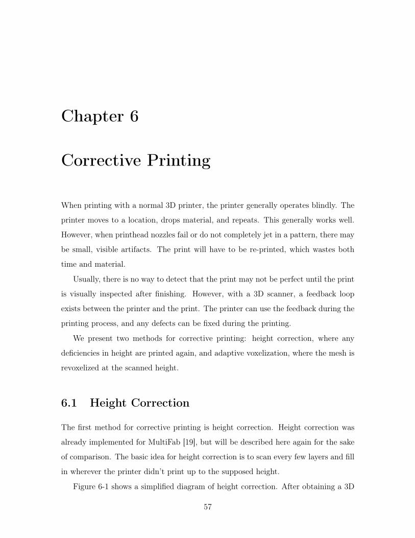
Figure 6-1 shows a simplified diagram of height correction. After obtaining a 3D

57

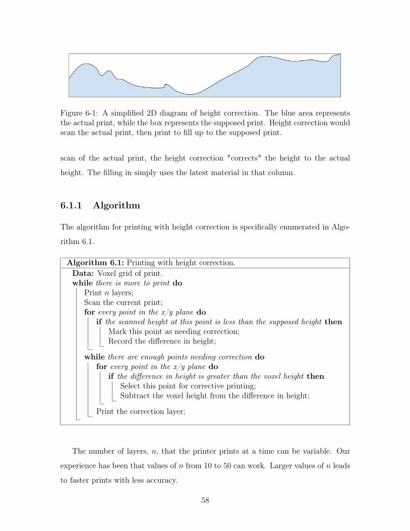
Figure 6-1: A simplified 2D diagram of height correction. The blue area representsthe actual print, while the box represents the supposed print. Height correction wouldscan the actual print, then print to fill up to the supposed print.

scan of the actual print, the height correction "corrects" the height to the actual

height. The filling in simply uses the latest material in that column.

6.1.1 Algorithm

The algorithm for printing with height correction is specifically enumerated in Algo-

rithm 6.1.

Algorithm 6.1: Printing with height correction.Data: Voxel grid of print.while there is more to print do

Print 𝑛 layers;Scan the current print;for every point in the x/y plane do

if the scanned height at this point is less than the supposed height thenMark this point as needing correction;Record the difference in height;

while there are enough points needing correction dofor every point in the x/y plane do

if the difference in height is greater than the voxel height thenSelect this point for corrective printing;Subtract the voxel height from the difference in height;

Print the correction layer;

The number of layers, 𝑛, that the printer prints at a time can be variable. Our

experience has been that values of 𝑛 from 10 to 50 can work. Larger values of 𝑛 leads

to faster prints with less accuracy.

58

6.1.2 Analysis

Height correction works well and quickly for relatively simple prints when the printer

is functioning mostly properly. Any small errors are prevented from building up by

the height correction.

As the complexity of the print increases, then the scanning frequency should also

increase. The reason for that is because the correction layer uses the most recently

used material. If the used material changes frequently in the print, then malfunctions

with some materials may not be detected until too late. This is unavoidable with

any corrective printing where scans are only completed every few layers, since it is

impossible to distinguish where on the z-axis printing malfunctions occured.

When the printer is not functioning well, then height correction has the potential

to double the printing time. For example, if some nozzles are not working at all, then

the positions where those nozzles print must be printed over twice. This may double

the printing time. In this case, the tradeoff for a good print even while the printer is

not functioning well is doubling the time required. This tradeoff may not be worth

the time taken.

6.2 Adaptive Voxelization

Another method for corrective printing is adaptive voxelization. The general idea of

adaptive voxelization is to scan every few layers and revoxelize the mesh to match

wherever the current height is. Instead of enforcing an assumption about voxel height,

as height correction does, adaptive voxelization adapts to the actual height.

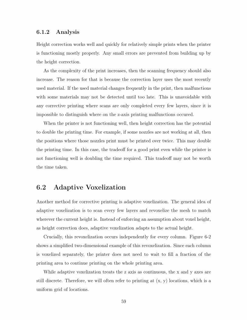
Crucially, this revoxelization occurs independently for every column. Figure 6-2

shows a simplified two-dimensional example of this revoxelization. Since each column

is voxelized separately, the printer does not need to wait to fill a fraction of the

printing area to continue printing on the whole printing area.

While adaptive voxelization treats the z axis as continuous, the x and y axes are

still discrete. Therefore, we will often refer to printing at (x, y) locations, which is a

uniform grid of locations.

59

Figure 6-2: A simplified 2D diagram of adaptive voxelization. The top line representsthe real world print. The second line is the scanned heights. The third line is thenthe result of the adaptive voxelization. Note how the voxels do not have to line up.

6.2.1 Algorithm

The algorithm starts with a set of meshes to print. Each mesh represents a material.

The meshes need to be combined into a set of voxel layers, to be printed.

We will use the term "voxel column" for the ordered set of voxels to be printed at

each (x, y) location. As mentioned, voxel columns do not need to be aligned with each

other. The 𝑛th voxel layer will be the set of 𝑛th voxels from every voxel column. The

voxels in each voxel layer will be printed at the same time by the printer. However,

the voxels in each voxel layer do not need to be physically next to each other.

The algorithm first pre-processes the meshes, then loops through scanning, revox-

elizing, and printing.

Intersection Grid

Before printing starts, the meshes are pre-processed into an "intersection grid" that

contains "intersection columns". For each (x, y) location, the intersection grid con-

60

tains an intersection column, a ordered list of intersections with the meshes from

bottom to top. Each intersection records the material of the mesh that was hit, the

height of the intersection, and an ordered list of the materials present right above the

intersection according to the possibly intersecting meshes. The list is ordered so that

the mesh that intersected most recently is at the end of the list.

To generate this intersection grid, a slightly modified ray tracing is run on the

meshes. The pseudocode for generating the intersection grid from the set of meshes

is in Algorithm 6.2.

Algorithm 6.2: Generate an intersection grid from a set of meshes with mate-rials.Data: Meshes associated with materialsFind the bounding box of the meshes;Overlay a grid over the x-y plane at the desired resolution;for each (x, y) location do

Find intersections with all meshes;for each mesh do

Trace a ray from the bottom of the mesh;for each triangle in the mesh do

if there is an intersection thenRecord the mesh material and the intersection height;

Sort the intersections in order of height;for each intersection (in order) do

Copy the list of materials from the previous intersection;if the material of the intersected mesh is in the previous list then

Remove the material from the list of materials;else

Add the material to the end of the list of materials;

Record the new list of materials in the intersection;

Print Generation

After the intersection grid is generated in pre-processing, the printing loop submits

voxel layers to the print queue to be printed.

To assist in revoxelizing, an array keeps track of the last intersection that the

previous depth was above. Then, when searching for the correct location to revoxelize,

61

the last intersection is used as a starting point for the search.

The pseudocode for the print generation is enumerated specifically in Algorithm

6.3.

Algorithm 6.3: Generate voxel layers from a set of meshes with materials.Data: Meshes associated with materialsGenerate the intersection grid from the meshes;while there are more slices to print do

Scan the print;for each layer to be generated do

Make a new voxel layer;for each (x, y) location do

Set the current depth to be the scanned depth plus the expectedwidth of the layers to be printed;

Find the nearest intersection that is lower than the current depth;Set the voxel to be the last material in the list of materials;

Print the generated slices;

6.2.2 Results

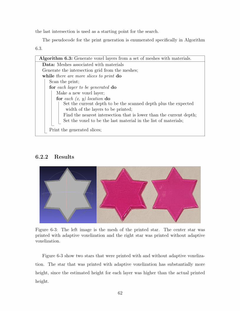
Figure 6-3: The left image is the mesh of the printed star. The center star wasprinted with adaptive voxelization and the right star was printed without adaptivevoxelization.

Figure 6-3 show two stars that were printed with and without adaptive voxeliza-

tion. The star that was printed with adaptive voxelization has substantially more

height, since the estimated height for each layer was higher than the actual printed

height.

62

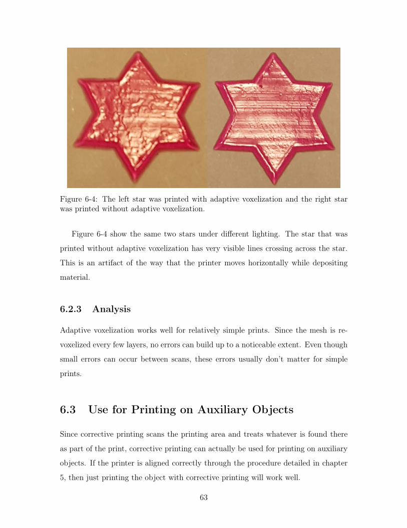
Figure 6-4: The left star was printed with adaptive voxelization and the right starwas printed without adaptive voxelization.

Figure 6-4 show the same two stars under different lighting. The star that was

printed without adaptive voxelization has very visible lines crossing across the star.

This is an artifact of the way that the printer moves horizontally while depositing

material.

6.2.3 Analysis

Adaptive voxelization works well for relatively simple prints. Since the mesh is re-

voxelized every few layers, no errors can build up to a noticeable extent. Even though

small errors can occur between scans, these errors usually don’t matter for simple

prints.

6.3 Use for Printing on Auxiliary Objects

Since corrective printing scans the printing area and treats whatever is found there

as part of the print, corrective printing can actually be used for printing on auxiliary

objects. If the printer is aligned correctly through the procedure detailed in chapter

5, then just printing the object with corrective printing will work well.

63

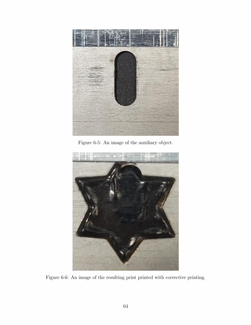
Figure 6-5: An image of the auxiliary object.

Figure 6-6: An image of the resulting print printed with corrective printing.

64

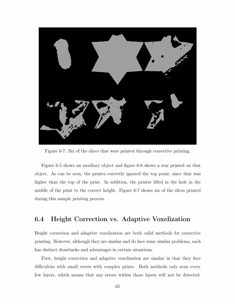
Figure 6-7: Six of the slices that were printed through corrective printing.

Figure 6-5 shows an auxiliary object and figure 6-6 shows a star printed on that

object. As can be seen, the printer correctly ignored the top point, since that was

higher than the top of the print. In addition, the printer filled in the hole in the

middle of the print to the correct height. Figure 6-7 shows six of the slices printed

during this sample printing process.

6.4 Height Correction vs. Adaptive Voxelization

Height correction and adaptive voxelization are both valid methods for corrective

printing. However, although they are similar and do face some similar problems, each

has distinct drawbacks and advantages in certain situations.

First, height correction and adaptive voxelization are similar in that they face

difficulties with small errors with complex prints. Both methods only scan every

few layers, which means that any errors within those layers will not be detected.

65

Furthermore, since we are working with additive printing, these errors cannot be fixed.

The solution to this for both methods is to increase the scanning frequency. Although

only scanning for every single layer will truly fix this problem, prints typically do not

require that degree of accuracy.

Height correction is good for prints where an intermediate step needs to be flat,

or if the material being printed with requires a flatter surface. Since height correction

ensures that the actual height matches the supposed height, the top of the print is

usually fairly flat. However, adaptive voxelization may have a rough surface that it

is adapting to instead of fixing.

However, since height correction requires a flat surface, it may be slower than

adaptive voxelization. The strength of adaptive voxelization is that no fixing is re-

quired for printing to continue. This means that the printer functions at its top

printing speed, which may not be the predicted printing speed.

66

Chapter 7

Conclusion

We have developed several improvements to the 3D printing process by using an

attached 3D scanner. Information from the 3D scanner gives the printer the ability

to adapt to the existing environment while printing, whereas printers without 3D

scanning would not be able to adapt.

The 3D scanner gives information to the 3D printer process both before and

during printing. Before the printing, the printer can handle information from both

the printer itself and any other auxiliary objects. During the printing, the printer

reacts to information about the print being currently printed, thus creating a feedback

loop of printing and scanning.

7.1 Overview

First, we described the various calibrations done with vision. The two main parts

are the camera calibration and the printhead calibration. The camera calibration

consists of standard camera calibrations, like intrinsic matrix calibrations, and finding

interference in the OCT system. We also provided an automatic process for finding

interference. The printhead calibration is for calibrating the printhead positions. The

printhead calibration also has a depth-based automatic detection algorithm.

Second, we reviewed interpolation of depth maps with algebraic multigrid. This

has both a single-threaded and multi-threaded algorithm, both of which completed

67

faster than the baseline algorithm. As expected, the multi-threaded algorithm was

faster than the single-threaded algorithm.

Third, we covered a major use case of the scanning system in printing on auxiliary

objects. We described the procedure taken by the user to initiate this, using the GUI

provided. In addition, an automatic alignment feature for aligning scans and meshes

was discussed.

Finally, we covered the second major use case of the scanning system in corrective

printing, or printing corrections to a print while the printer is still printing. The two

main approaches for corrective printing are height correction and adaptive voxeliza-

tion. Both methods achieved results better than printing without corrective printing.

7.2 Future Work

There are several possible improvements to the scanning system and the accompa-

nying improvements. Many of the possible improvements would require a large-scale

change to the current system, thus preventing their implementation. The features to

improve are the limitations of OCT as a scanning system and the flaws inherent in

the corrective printing.

OCT is used as our 3D scanning system, but has several limitations inherent to

how it works. OCT is a light-based scanning system. This means that specular

objects, like mirrors, are almost impossible to scan if there is any tilt. Any dark or

very diffuse objects are also difficult to scan, since there is not enough reflection into

the camera to detect the interference. In order to fix these issues, either a completely

new 3D scanning system would have to be built or severe limitations of OCT would

have to be overcome.

The frequency of scanning in the corrective printing causes a tradeoff between

speed and accuracy. A higher frequency of scanning leads to more accuracy, since

errors can be fixed quicker, but takes more time with every scan. A lower frequency

of scanning can be very quick, but high-frequency material changes would be ignored

in the subsequent correction. Ideally, the system would have a correction method

68

that is both fast and accurate.

Finally, the scanning itself can take a long time. Depending on the frequency of

scanning, just the scanning can cause the print to take twice as long. The scanning

speed is unfortunately limited by the movement speed of the platform, since the

platform needs to move a certain amount, the shutter speed of the camera, since

many images need to be taken, and the amount of images necessary to scan.

For most of these improvements, the OCT system would have to be redesigned or

replaced in order to deal with these flaws. However, there is no easy alternative, as

the OCT system does appear to be the best option. Significant work can be done in

this area to further improve the 3D scanning system.

69

70

Bibliography

[1] G. Bradski. Opencv library. Dr. Dobb’s Journal of Software Tools, 2000.

[2] D.M. Bulanon, T. Kataoka, H. Okamoto, and S. Hata. Development of a real-time machine vision system for the apple harvesting robot. In SICE 2004 AnnualConference, volume 1, pages 595–598 vol. 1, Aug 2004.

[3] Denis Demidov. Amgcl, 2012.

[4] Epson Workforce 30 Inkjet Printer. http://www.epson.com/cgi-bin/Store/jsp/Product.do?sku=C11CA19201.

[5] F3-3 Mach Turbo2 Type Printhead. Page 23 of https://people.csail.mit.edu/pitchaya/service_manual/C_110_B.pdf.

[6] RD Falgout. An introduction to algebraic multigrid. 2006.

[7] A F Fercher, W Drexler, C K Hitzenberger, and T Lasser. Optical coher-ence tomography - principles and applications. Reports on Progress in Physics,66(2):239, 2003.

[8] A. F. Fercher, C. K. Hitzenberger, G. Kamp, and S. Y. El-Zaiat. Measure-ment of intraocular distances by backscattering spectral interferometry. OpticsCommunications, 117:43–48, February 1995.

[9] H. Golnabi and A. Asadpour. Design and application of industrial machinevision systems. Robotics and Computer-Integrated Manufacturing, 23(6):630 –637, 2007. 16th International Conference on Flexible Automation and IntelligentManufacturing.

[10] S. Kurada and C. Bradley. A review of machine vision sensors for tool conditionmonitoring. Computers in Industry, 34(1):55 – 72, 1997.

[11] Lucas Lira. Arduino uno case, 2015. https://grabcad.com/library/arduino-uno-case-2.

[12] Shenglin Lu, Xianmin Zhang, and Yongcong Kuang. An integrated inspectionmethod based on machine vision for solder paste depositing. In Control andAutomation, 2007. ICCA 2007. IEEE International Conference on, pages 137–141, May 2007.

71

[13] Song De Ma. A self-calibration technique for active vision systems. Robotics andAutomation, IEEE Transactions on, 12(1):114–120, Feb 1996.

[14] Maxim Naumov. Incomplete-lu and cholesky preconditioned iterative methodsusing cusparse and cublas, 2011. Technical Report and White Paper.

[15] John Nickolls, Ian Buck, Michael Garland, and Kevin Skadron. Scalable parallelprogramming with cuda. Queue, 6(2):40–53, March 2008.

[16] Naoaki Okazaki. Classias: a collection of machine-learning algorithms for classi-fication, 2009.

[17] Noboyuki Otsu. A threshold selection method from gray-level histograms. IEEETransactions on Systems, Man, and Cybernetics, 9(1):62–66, Jan 1979.

[18] Szymon Rusinkiewicz and Marc Levoy. Efficient variants of the ICP algorithm.In Third International Conference on 3D Digital Imaging and Modeling (3DIM),June 2001.

[19] Pitchaya Sitthi-Amorn, Javier E. Ramos, Yuwang Wangy, Joyce Kwan, JustinLan, Wenshou Wang, and Wojciech Matusik. Multifab: A machine vision assistedplatform for multi-material 3d printing. ACM Trans. Graph., 34(4):129:1–129:11,July 2015.

[20] Vijay Subramanian, Thomas F. Burks, and A.A. Arroyo. Development of ma-chine vision and laser radar based autonomous vehicle guidance systems for cit-rus grove navigation. Computers and Electronics in Agriculture, 53(2):130 – 143,2006.

[21] R.Y. Tsai and R.K. Lenz. Real time versatile robotics hand/eye calibration using3d machine vision. In Robotics and Automation, 1988. Proceedings., 1988 IEEEInternational Conference on, pages 554–561 vol.1, Apr 1988.

[22] R.Y. Tsai and R.K. Lenz. A new technique for fully autonomous and efficient3d robotics hand/eye calibration. Robotics and Automation, IEEE Transactionson, 5(3):345–358, Jun 1989.

[23] C.-C. Wang. Extrinsic calibration of a vision sensor mounted on a robot. Roboticsand Automation, IEEE Transactions on, 8(2):161–175, Apr 1992.

[24] Maciej Wojtkowski, Rainer Leitgeb, Andrzej Kowalczyk, Tomasz Bajraszewski,and Adolf F. Fercher. In vivo human retinal imaging by fourier domain opticalcoherence tomography. Journal of Biomedical Optics, 7(3):457–463, 2002.

[25] Wen-Yen Wu, Mao-Jiun J. Wang, and Chih-Ming Liu. Automated inspection ofprinted circuit boards through machine vision. Computers in Industry, 28(2):103– 111, 1996.

72