EVALUATION OF GRANULAR ACTIVATED CARBON ADSORPTIONTO REMEDIATE ETHYLENE DIBROMIDE CONTAMINATION AT

FUEL SPILL 28 AT THE MASSACHUSETTS MILITARY RESERVATION

by

Cordula Mitterhofer

B.S., Civil and Environmental EngineeringUniversity of California at Berkeley, 1995

Submitted to the Department of Civil and Environmental Engineeringin Partial Fulfillment of the Requirements for the Degree of

MASTER OF ENGINEERINGin Civil and Environmental Engineering

at the

MASSACHUSETTS INSTITUTE OF TECHNOLOGY

June 1998

0 Cordula Mitterhofer. All rights reserved.The author hereby grants to MIT permission to reproduce and to distribute publicly paper and electronic copies of this

thesis document in whole and in part.

Signature of the AuthorDepartment of Civil and EAvironmental Engineering

May 22, 1998

Certified by_Harold F. Hemond, P.h.D.

William E. Leonhard Professor of Civil and Environmental EngineeringThesis Supervisor

Accepted by_JProfesioroesph M. Sussman

Chairman, Departmental Committee on Graduate Studies

ACHUSETTS N iOF TECH#4OLOGY

JUN 02198LIBRARIES

EVALUATION OF GRANULAR ACTIVATED CARBON ADSORPTION TO

REMEDIATE ETHYLENE DIBROMIDE CONTAMINATION AT FUEL SPILL 28 AT

THE MASSACHUSETTS MILITARY RESERVATION

by

Cordula Mitterhofer

Submitted to the Department of Civil and Environmental EngineeringMay 22, 1998

In Partial Fulfillment of the Requirements for the Degree ofMaster of Engineering in Civil and Environmental Engineering

Abstract

The Massachusetts Military Reservation (MMR) is a Superfund site located on Cape Cod, Massachusetts.Military activities at the MMR have resulted in several groundwater plumes consisting of mostly chlorinatedsolvents and petroleum hydrocarbons. Ethylene Dibromide (EDB) was identified as the main contaminant inone of the groundwater plumes, Fuel Spill (FS) 28. Fuel Spill 28 has recently contaminated the cranberry bogslocated south of the MMR, close to the town of Falmouth. An estimated total of $1 million was spent todestroy the tainted cranberry crop from 1997 and to reimburse the farmers.

As an interim action, a pump-and-treat system using granular activated carbon (GAC) has been installed at thesite to prevent exposure of the residents to EDB, to contain the EDB plume, and to prevent the plume fromfurther contaminating the economically important cranberry bogs. The use of granular activated carbon iscurrently considered the best available treatment (BAT) method for EDB. Unfortunately, breakthrough ofEDB occurred after only 69 days of operation; the bed-life was originally estimated to range from 210 to 540days. This unexpected need for changeout and reactivation of the carbon beds adds significant costs to thesystem.

The objective of this study was to evaluate the use of granular activated carbon adsorption at Fuel Spill 28.Possible explanations for the pre-mature breakthrough were explored using isotherm data developed byCalgon Carbon Corporation and a number of simple analytical models. The possible explanations that wereinvestigated include overestimation of carbon bedlife, desorption, backwashing, bacterial growth, competitiveadsorption, and pre-loading due to total organic carbon. Based on the analysis performed, it can be concludedthat the carbon bedlife was likely overestimated. Using the advection dispersion equation resulted in carbonbedlives ranging from about 60 days to 130 days (accounting for dispersion). Other calculations that ignorethe effects of dispersion, such as the equilibrium column model, resulted in an over-estimate of the carbonbedlife; calculations which were derived directly from the isotherm data significantly overestimated thebedlife. The findings of this study also showed that other factors may have affected the carbon bedlife as well.While pre-loading and competitive adsorption may be feasible explanations at FS-28, no conclusion could bedrawn due to insufficient data collected at the site. Desorption following the backwashing event and bacterialgrowth, however, are likely contributing factors to the pre-mature breakthrough.

Thesis Supervisor: Dr. Harry HemondTitle: Professor of Civil and Environmental Engineering

ACKNOWLEDGEMENTS

I would first like to thank my advisors Prof. Harry Hemond and Prof. Phil Gschwend for their

intelligence, patience and enthusiasm. Special thanks to Prof. Hemond for being encouragingwhen it seemed like this thesis was never-ending. I also want to thank Trish Culligan for hersupport and guidance when I needed it most.

My deepest and warmest gratitude goes to Prof. Dave Marks who always had an open door forus. You are just one of a kind ! I'd also like to thank Jackie and Muriel for being support andCynthia Stewart who has definitely eased the work-load by being flexible when necessary.

I would also like to thank Pete Shanahan and especially Bruce Jacobs for their ideas andcontinuing support. Special thanks also to Ed Pesce, Tom Zsymoniak at Jacobs Engineering,Laura Foster at Jacobs Engineering, Bill Naylor at Norit, and Mark Stenzel at Calgon CarbonCorporation for the information and suggestions.

Many thanks to Ricardo and his wife Marie-Jose (you guys mean a lot to me !), Amparo, Peterand Janani, Sharon, Ana, Jerry, Thu, and Vitto for their positive attitude, continous support andfriendship. I will really miss you guys a lot and hope you will visit whereever I may be! Specialthanks to Derrick who shared those very long nights with us in the MENG room and saved mylife with Gummy Bears. You all made my life here at MIT not only more fun, but also moremeaningful.

Thanks to my long-distance friends, especially Kristi, Cheri, Gabi, Nancy, Amy, Karen, Mika,Ron, and Scott who have been there in the past and have helped me grow into what I am today.Sorry you can't be here for this graduation ! Thanks also to Steve Crane and Jacky Bowen fortheir guidance over the past years.

Charles, thanks so much for everything - I couldn't have made it without your help and support!I will never be able to thank you for all you did for me !

Special thanks also to Marilee and Tim. I am indebted for all you have given to me. You havehelped me overcome rough times and have encouraged my every endeavor. Love you!

Finally to my family, my Dad who has been there for financial and moral support and my brotherand his family who have helped me see that there is more to life than studying. My love alsogoes out to my Mom - I wish you could have lived to see me graduate from MIT and share thismoment with me. You instilled the strength and determination in me which allowed me to comethis far. Thanks !

3

TABLE OF CONTENTS

A BSTRA CT ............................................................................... ....... ----------------------------...................... 2

A CK N O W LED G M EN TS...........................................................................................----------........... 3

LIST O F FIG U R ES..........................................................................................---------------------. ............ 6

LIST O F TA BLES.................................................................................. .......... --------..................---- 7

1. IN TR O DU CTIO N ........................................................................................-- ............--------.. 8

1.1 CONTEXT .................................................................................. ...............---- --........................... 81.2 PROBLEM IDENTIFICATION ................................................................................... ........- 9

1.3 OBJECTIVES ...................................................................................................................-.......---- 101.4 SCOPE ................................................................................................. 10............. ....---- -- -- 10

2. BA CK G R O UN D IN FO R M A TIO N ........................................................................................... 12

2.1 CAPE COD ................................................................................................................... ......... --- 122.1.1 Location................................................................................................................................ 122.1.2 Climate................................................................................................................................. 12

2.1.3 Hydrology .......................................................................................................................... ... 12

2.1.4 Hydrogeology and Topography ...................................................................................... 142.2 MASSACHUSETTS M ILITARY RESERVATION ............................................................................. 14

2.2.1 Setting and D escription.................................................................................................... 14

2.2.2 H istory.................................................................................................................................. 152.2.3 Land Use .............................................................................................................................. 16

2.3 SOIL AND GROUNDWATER CONTAMINATION AT THE MMR ..................................................... 162.4 IMPPORTANCE OF REMEDIATING THE CONTAMINATED AQUIFER............................................. 18

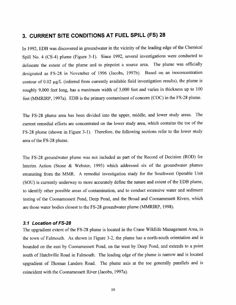
3. CURRENT SITE CONDITIONS AT FUEL SPILL (FS) 28..................................................19

3.1 LOCATION OF FS-28 ..................................................................................................................... 193.2 PREVIOUS FIELD INVESTIGATIONS .......................................................................................... 21

3.3 EXTENT OF ETHYLENE DIBROM IDE CONTAM INATION ............................................................. 21

3.4 GENERAL CHEM ISTRY OF GROUNDW ATER AT FS-28 ................................................................ 26

3.5 SOURCE AREAS ............................................................................................................................ 263.6 GROUNDW ATER AND SURFACE W ATER USES .......................................................................... 28

3.7 GEOLOGIC SETTING ..................................................................................................................... 29

3.8 HYDROGEOLOGIC SETTING.......................................................................................................... 29

3.9 CURRENT M ODELING EFFORTS ................................................................................................ 30

3.10 TIM E-CRITICAL ACTIONS...........................................................................................................313.11 SUM MARY ................................................................................................................................. 32

4. FATE AND TRANSPORT MECHANISMS OF ETHYLENE DIBROMIDE.....................34

4.1 BACKGROUND INFORM ATION.................................................................................................. 34

4.1.1 General D escription............................................................................................................. 34

4.1.2 Regulatory H istory............................................................................................................... 34

4.1.3 Toxicity................................................................................................................................. 35

4.2 USES OF ETHYLENE DIBROM IDE .............................................................................................. 35

4.2.1 Use of Ethylene D ibrom ide as a Fum igant....................................................................... 354.2.2 Use of Ethylene D ibrom ide as a Fuel Additive................................................................ 35

4

4.3 PHYSICAL AND CHEMICAL PROPERTIES OF EDB................................................. ..... ... .... 36

4.4 FATE AND TRANSPORT OF EDB ..................................................................... .......... 37

4.4.1 Vadose Zone Transport.................................................................................................... 37

4.4.2 Saturated Zone Transport................................................................................................ 38

4.4.3 Other Controlling M echanisms......................................................................................... 38

5. USE OF GRANULAR ACTIVATED CARBON ADSORPTION FORHOTSPOT REM OVAL AT FUEL SPILL 28................................................................ .... 405.1 INTERIM REMEDIAL ACTION .............................................................................. 405.2 FINAL REMEDIAL ACTION ............................................................................ ..... 405.3 PUMP-AND-TREAT TECHNOLOGY ..................................................................... 41

5.3.1 Effectiveness of Pump-and-Treat Systems....................................................................... 41

5.3.2 Cleanup with Pump-and-Treat System.............................................................................. 42

5.4 TREATMENT WITH GRANULAR ACTIVATED CARBON .............................................................. 42

5.4.1 Granular Activated Carbon ............................................................................................. 42

5.4.2 Theoretical Adsorption Theory ................................................................................ 44

5.4.3 Design Criteria at FS-28.................................................................................................. 48

5.4.4 Analysis of the Early Breakthrough at Fuel Spill 28........................................................ 61

6. SUGGESTED IMPROVEMENTS AND ALTERNATIVES TO

CARBON ADSORPTION ............................................................................................................. 79

6.1 ALTERNATIVES TO CARBON ADSORPTION................................................................................ 79

6.1.1 A ir S tripp ing ......................................................................................................................... 79

6.1.2 Reductive Dehalogenation ............................................................................................... 80

6.1.3 Advanced Oxidation Processes ......................................................................................... 81

6.1.4 Biological Treatment Processes....................................................................................... 816.1.5 R everse O sm osis................................................................................................................... 8 16.1.6 Adsorptive Resins ................................................................................................................. 82

6.2 IMPROVING OPERATING PROCEDURES ..................................................................................... 82

6.3 DIFFERENT TYPES OF CARBON..................................................................................................... 83

7. CONCLUSIONS.............................................................................................................................84

7.1 EVALUATION OF LABORATORY ISOTHERMS............................................................................ 85

7.2 SENSITIVITY ANALYSIS OF FREUNDLICH CONSTANTS ............................................................. 867.3 EFFECTS OF COMPETITIVE ADSORPTION...................................................................................... 877.4 DETERMINATION OF BREAKTHROUGH TIMES .......................................................................... 87

7.4.1 Results from the Equilibrium M odel.................................................................................... 877.4.2 Results from the Advection Dispersion Equation.............................................................. 88

7.5 DETERMINATION OF THE ACTUAL ADSORPTION CAPACITY.................................................... 887.6 ALTERNATIVE EXPLANATIONS................................................................................................ 89

7.6.1 D esorp tio n ............................................................................................................................ 8 97.6.2 B a ckw ash ing ........................................................................................................................ 8 97.6.3 Pre-Loading due to TOC.................................................................................................. 897.6.4 Bacterial Growth................................................................................................................. 90

8. BIBLIOGRAPHY........................................................................................................................... 91

9. APPENDICES................................................................................................................................. 97

5

LIST OF FIGURES

FIGURE 2-1: LOCATION OF CAPE COD AND THE MMR.................................................................... 13FIGURE 3-1: LOCATION OF THE GROUNDWATER PLUMES AT THE MMR ........................................ 20

FIGURE 3-2: LOCATION OF THE FS-28 GROUNDWATER PLUME......................................................... 22

FIGURE 3-3: LOCATIONS OF CRANBERRY BOGS POTENTIALLY AFFECTED BY THE FS-28

GROUNDWATER PLUME ............................................................................. ...... 24

FIGURE 3-4: VERTICAL EXTENT OF CONTAMINATION AT FS-28 ....................................................... 25

FIGURE 5-1: CONFIGURATION OF A TYPICAL CONTINUOUS, DOWNFLOW COLUMN CONTACTOR ........ 49

FIGURE 5-2: ADSORPTION ISOTHERM DEVELOPED BY CALGON CARBON CORPORATION................. 53

FIGURE 5-3: DETERMINATION OF FREUNDLICH CONSTANTS FROM CALGON CARBON

CORPORATION DATA ..................................................................................... 54

FIGURE 5-4: ADSORPTION ISOTHERM OF EDB AT LOW CONCENTRATIONS....................................... 58

FIGURE 5-5: TYPICAL S-SHAPED BREAKTHROUGH CURVE ............................................................... 60

FIGURE 5-6: ILLLUSTRATION OF THE EC MODEL ............................................................................... 67

FIGURE 5-7: INFLUENT EDB LOADING........................................................................... ............ 71FIGURE 5-8: BREAKTHROUGH CURVE AT FS-28................................................................................. 72

6

LIST OF TABLES

TABLE 3-1: SUMMARY OF EDB DETECTIONS IN THE LOWER STUDY AREA AT FS-28....................23

TABLE 3-2: CHEMISTRY OF DEEP GROUNDWATER AT FS-28 ........................................................ 27

TABLE 3-3: SUMMARY OF AGRICULTURAL W ATER USES.................................................................... 28

TABLE 4-1: PHYSICAL AND CHEMICAL PROPERTIES OF EDB........................................................... 36

TABLE 5-1: COMPARISON OF CARBON USAGE RATES FOR EDB .................................................... 56

TABLE 5-2: COMPARISON OF CARBON EXCHANGE RATES FOR EDB USING AN ADJUSTMENT

FACTOR OF 25% ............................................................................................... ..... ... 56

TABLE 5-3: COMPARISON OF CARBON EXCHANGE RATES FOR EDB USING AN ADJUSTMENT

FA C TO R O F 50% ................................................................................................................ 57

TABLE 5-4: COMPARISON OF CARBON EXCHANGE RATES FOR EDB USING AN EFFECTIVE KD

O F 2 5 A N D 50 ..................................................................................................................... 59

TABLE 5-5: COMPARISON OF LITERATURE FREUNDLICH CONSTANTS AND CALCULATED

C ARBON U SAGE R ATES ................................................................................................. 63

TABLE 5-6: CALCULATION OF CARBON USAGE RATES USING A MULTI-COMPONENT

ISOTHERM MODEL - WORST CASE SCENARIO................................................................. 65

7

EVALUATION OF GRANULAR ACTIVATED CARBON ADSORPTION TO

REMEDIATE ETHYLENE DIBROMIDE CONTAMINATION AT FUEL SPILL 28 AT

THE MASSACHUSETTS MILITARY RESERVATION

1. INTRODUCTION

Historically, the Massachusetts Military Reservation (MMR), located on the upper western part

of Cape Cod, was used as a military reservation by the Army, the Navy, and the Air National

Guard (ANG). Past releases of hazardous materials have resulted in widespread contamination

of both soil and groundwater in the reservation. Documented sources of contamination comprise

former motor pools, landfills, fire-fighting training areas, and drainage structures such as dry

wells. Wastes generated from these activities include oils, solvents, antifreeze, battery

electrolytes, paint, waste fuels, metals, and dielectric fluids from transformers and electrical

equipment (E.C. Jordan, 1989). Several major groundwater plumes have been found to be

migrating from these source areas and have been defined during extensive investigations of the

area.

1.1 ContextOne of the major groundwater plumes, Fuel Spill (FS-28), has recently contaminated the

cranberry crops located south of the MMR, close to the town of Falmouth. The U.S.

Environmental Protection Agency (USEPA), Massachusetts Department of Environmental

Protection (MADEP), and Massachusetts Department of Public Health (MA DPH) have

determined that the use of contaminated surface and groundwater for agricultural purposes

presents an unacceptable risk to public health and the environment. Additionally, the

groundwater contamination from FS-28 has also affected local water supplies, resulting in the

closure of private drinking water wells and the associated need for alternative water supplies.

Tourism is one of the main sources of income at Cape Cod during the summer months.

Therefore, the perception of risk from untreated groundwater plumes might hinder economic

growth on the Cape and result in lost revenues. For these reasons, it is important to treat the

8

contaminated groundwater in order to reduce chemical concentrations in the aquifer to

"acceptable" levels both for regulatory agencies as well as the public.

As an interim action, a pump-and-treat system was installed downgradient of the hotspot

concentration at FS-28 in October 1997. Currently, the groundwater, which is contaminated with

ethylene dibromide (EDB), is being extracted and treated with granular activated carbon (GAC);

the treated water is being discharged to nearby surface water bodies. This interim action has

been implemented as a time-critical action to: 1) prevent the exposure of the residents in the

Town of Falmouth to EDB, 2) to contain the EDB plume, and 3) to prevent the plume from

further contaminating the cranberry bogs.

1.2 Problem IdentificationMost sites that involve contaminated groundwater use pump-and-treat systems to achieve

cleanup goals. Typically, conventional pump-and-treat systems extract relatively large volumes

of water with relatively low contaminant concentrations. Because of the geologic complexity

and slow rates of contaminant desorption and dissolution, these systems typically displace many

pore volumes of aquifer water to flush out the contamination. Conventional pump-and-treat

systems are therefore inherently inefficient for removing contaminants from the subsurface

(Daniel, 1993).

Alternatives for the remediation of EDB-contaminated groundwater have not been as thoroughly

researched as those for the other more common contaminants, such as the chlorinated solvents or

hydrocarbon compounds, typically associated with military sites. A permeable reactive wall,

developed by the University of Waterloo, could provide a remedial alternative to the current

pump-and-treat system at FS-28. Based on laboratory experiments, zero-valent iron, which is the

reactive medium in the permeable wall, readily degrades EDB. However, because the FS-28

plume is very deep at its point of highest concentration, installation of a reactive wall may be

cost-prohibitive.

9

Treatment of the contaminated water being extracted by the pump-and-treat system is currently

achieved with GAC, which is considered the best available treatment (BAT) method for EDB.

Although the system only went into operation in October 1997, a carbon changeout occurred in

February 1998, after breakthrough was detected in the lead carbon canister following 69 days of

operation; the carbon bedlife was originally estimated to range from 210 to 540 days. The need

for changeout (and reactivation) of the carbon beds after an unexpectedly short period of

operation will greatly add to operation and maintenance costs of the system unless the situation

can be improved.

1.3 ObjectivesThe focus of this study was to answer the following questions:

" What are the mechanisms of GAC adsorption ?

" What could be some of the reasonable explanations for the early breakthroughoccurring at the FS-28 treatment system ?

" Can the current pump-and-treat system be improved by using different types ofadsorptive media or by altering operating conditions ?

In order to answer these questions, a thorough understanding of the FS-28 groundwater plume

was necessary. Available background information was summarized from previous reports and

from contacts with Jacobs Engineering. To conduct an in-depth evaluation of the current

treatment system, it was also important to understand the dominant fate and transport

mechanisms of EDB.

1.4 ScopeThe ensuing sections present the following information:

" Section 2, Background Information, provides background information about CapeCod and the MMR and also discusses why aquifer restoration at the Cape isimportant.

" Section 3, Current Site Conditions at Fuel Spill 28, thoroughly describes the currentsite conditions of the FS-28 plume. This includes a description of the extent of

10

contamination, previously conducted investigations, suspected source areas, geologicand hydrogeologic settings, as well as the current remedial actions at the site.

* Section 4, Fate and Transport Mechanisms of Ethylene Dibromide, presents

background information on the fate and transport mechanisms of EDB.

" Section 5, Use of Granular Activated Carbon Adsorption for Hotspot Removal at

Fuel Spill 28, describes the GAC treatment technology and provides some possible

explanations for the pre-mature breakthrough occurring at the system currentlyoperating at FS-28.

" Section 6, Suggested Improvements and/or Alternatives to Carbon Adsorption,evaluates the use of alternatives to carbon adsorption and also provides some

suggestions for improvements of the current system at FS-28.

. Section 7, Conclusions, provides the conclusions of this study.

11

2. BACKGROUND INFORMATION

The following sub-sections provide background information on Cape Cod and the Massachusetts

Military Reservation, its history, population and land use. They also give a brief description of

the contamination present at the military reservation and explain the importance of remediating

the contaminated aquifer.

2.1 Cape Cod

2.1.1 Location

Cape Cod is located in southeastern Massachusetts, as shown in Figure 2-1. It is surrounded by

Cape Cod Bay to the north, Buzzards Bay to the west, Nantucket Sound to the south, and the

Atlantic Ocean to the east. Cape Cod is separated from the rest of Massachusetts by a canal.

2.1.2 ClimateThe climate of western Cape Cod is temperate, with expected annual temperatures ranging from

19 to 81 degrees Fahrenheit (*F). Occasionally, seasonal extremes exceed these limits.

Temperatures are commonly moderate due the proximity to the Atlantic Ocean and associated

Gulf Stream. Wind speeds typically range from 9 to 12 miles per hour (mph), with storm

velocities of 40 to 100 mph. The prevailing winds along Cape Cod are heavily influenced by the

Atlantic Ocean and the Gulf Stream. From November through March, the prevailing winds arise

from the northwest, whereas from April through October, the prevailing winds originate from the

southwest (ANG, 1995).

2.1.3 HydrologyCape Cod receives an average rainfall of 47.8 inches per year (ANG, 1995). The precipitation is

distributed fairly evenly throughout the year, although a slightly higher portion of the

precipitation occurs in the winter months (LeBlanc et al., 1986). The one-year/24-hour rainfall

event for Cape Cod is 2.7 inches.

12

Due to the highly permeable sand and gravel deposits prevalent on Cape Cod, surface water

runoff is less than 1% of the total precipitation. Approximately 55% of the total precipitation is

returned to the atmosphere via evaporation or transpiration by plants. The remaining 45%

infiltrate to recharge the groundwater (LeBlanc et al., 1986).

MS HSETTSrj---

CONN. RJ 4 4 2f

pCape Cod

~5urn M MR,

Sandwic

1, IfI

Nantucket Sound

SII MILES

Figure 2- 1: Location of Cape Cod and the Massachusetts Military Reservation

Although groundwater provides the main source of water for Cape Cod, approximately 4% of thearea is covered by surface-water bodies. These surface-water bodies, mainly intermittent streams

13

or kettle holes, receive a net recharge of approximately 18 inches per year from direct

precipitation (ANG, 1995).

2.1.4 Hydrogeology and Topography

The geology of western Cape Cod was shaped during the Wisconsin period, with the advance

and retreat of two glacial lobes that resulted in glaciofluvial sedimentation. To the north and

west, the Buzzards Bay and Sandwich Moraines are composed mostly of glacial till. To the

south is the Mashpee Pitted Plain, an outwash plain containing poorly sorted, fine- to coarse-

grained outwash sands overlying finer-grained till and marine or lacustrine sediment. This lower

layer of fine sediment has a hydraulic conductivity that is as much as five times lower than that

of the upper outwash layer, so that groundwater flow occurs mostly through the permeable upper

layer. Seepage velocity within the sand and gravel outwash is estimated to range from 1 to 4.6

feet per day, with virtually no vertical flow. The entire plain is dotted with numerous kettle

holes, bodies of water that resulted when large blocks of glacial ice, embedded in the sediment,

melted. These kettle holes are maintained mostly by groundwater recharge (E.C. Jordan, 1989).

The topography of the area can be characterized as a broad, flat, glacial outwash plain, dotted by

kettle holes and other depressions, with marshy lowlands to the south, and flanked along the

north and the west by recessional moraines and hummocky, irregular hills. Remnant river

valleys cross the Mashpee Pitted Plain from north to south, while to the north and west the

Buzzards Bay and Sandwich Moraines lend a higher degree of topographic relief (E.C. Jordan,

1989).

2.2 Massachusetts Military Reservation

2.2.1 Setting and DescriptionThe MMR, previously known as Otis Air Force Base, is located on the upper western part of

Cape Cod, Massachusetts. It encompasses approximately 22,000 acres (30 square miles) within

the towns of Bourne, Sandwich, Mashpee, and Falmouth in Barnstable County (Figure 2-1). The

MMR consists of facilities operated by the U.S. Coast Guard, the Army National Guard, the U.S.

14

Air Force, ANG, Veterans Administration, and the Commonwealth of Massachusetts. Most

facilities are located in the southern portion of the reservation. The northern portion consists of

numerous firing ranges. The MMR is comprised of four principal functional areas (Jacobs,

1997c):

" Cantonment Area: This southern portion of the reservation is the most actively usedsection of the MMR. It occupies 5,000 acres and is the location of administration,operational, maintenance, housing, and support facilities for the base. The Otis AirForce Base facilities are located in the southeast portion of the Cantonment Area.

" Range Maneuver and Impact Area: This northern part of the MMR consists of 14,000acres and is used for training and maneuvers.

* Massachusetts National Cemetery: This area occupies the western edge of the MMRand contains the Veterans Administration Cemetery and support facilities.

* Cape Cod Air Force Station (AFS): This 87-acre section is located in the northernportion of the Range and Maneuver and Impact Area and is known as the PrecisionAcquisition Vehicle Entry - Phased Array Warning System.

2.2.2 HistorySince its origin in 1911, a variety of activities have been conducted on the MMR, including troop

development and deployment, fire-fighting, ordinance development, testing and training, aircraft

and vehicle operation and maintenance, and fuels transport, and storage. Operational units at the

MMR included the U.S. Air Force, U.S. Navy, U.S. Army, U.S. Marine Corps, U.S. National

Guard, U.S. Army National Guard (ANG), and U.S. Coast Guard. From 1955 to 1970, a

substantial number of surveillance and air defense aircraft operated out of the ANG portion of the

reservation. Since that time, the intensity of operations has decreased substantially.

The heaviest military activity occurred from 1940 to 1946 by the U.S. Army, and from 1955 to

1972 by the U.S. Air Force. The use of petroleum fuel products and industrial solvents was at a

height during these periods; it was common practice for many years to dispose of such wastes in

landfills and dry wells, and to use them at firefighting training areas. As a result, contaminants

were released to the unsaturated zone.

15

2.2.3 Land UseLand uses adjacent to the MMR include residential, commercial, recreational, agricultural, and

wildlife management. Land use at the MMR is generally limited to supporting military training

with some residential and recreational usage. Most of the daily activities occur in the southern

portion of the reservation. In the northern portion of the reservation, approximately 80% of the

total area is undeveloped scrub forest and fields. Most of this area is divided into firing ranges,

but also serves as habitats for various indigenous and migratory wildlife. Civilian access to the

entire area is strictly controlled and, for most areas, is completely prohibited because of the threat

of unexploded ordnance.

The population of the towns adjacent to the MMR fluctuates significantly between winter

(29,000) and summer (70,000) due to tourism. The permanent population of the MMR amounts

to approximately 2,000 people, primarily in on-base housing maintained by the U.S. Coast

Guard. Additionally, an estimated 800 non-residents are employed year-round within various

Department of Defense (DOD) and other operations. Periodic activities associated with training

military reserve personnel can increase the base population by several hundred to several

thousand (Cape Cod Commission, 1996).

2.3 Soil and Groundwater Contamination at the MMRThe MMR is located on top of a recharge area that supplies water to all the towns surrounding

the base. In 1978, the town of Falmouth detected detergents in a public water-supply well located

south of the MMR wastewater treatment plant. The United States Geological Survey (USGS)

immediately began conducting groundwater investigations and soon identified a groundwater

plume extending south of the treatment plant and into Ashumet Valley. Subsequently, the ANG

established an Installation Restoration Program (IRP) at Otis ANG Base. In 1989, the MMR was

named a Superfund site by the Environmental Protection Agency (MMRIRP, 1997c).

Between 1982 and 1985, investigations at the MMR revealed 73 contaminated soil and

groundwater sites. Since 1985, five additional sites have been identified, bringing the total

number of contaminated sites to 78. As of September 1996, the ANG and regulators concluded

16

that 31 of the 78 sites at the MMR pose no threat to the public nor the environment and therefore

require no further action (MMRIRP, 1997c). As a result of the investigations conducted at the

base, seven major groundwater plumes have been identified:

" Fuel Spill-12 (FS-12)

" Fuel Spill-28 (FS-28)

" Chemical Spill-4 (CS-4)

" Chemical Spill-10 (CS-10)

" Landfill-i (LF-1)

" Ashumet Valley

" Storm Drain-5 (SD-5)

In 1993, the ANG, in conjunction with the USEPA, MADEP, and various citizen groups, began

addressing the groundwater plumes at the MMR. These groups worked in concert to develop a

containment program that called for 100%, simultaneous remediation of the groundwater plumes.

However, evaluation of the design in 1996 revealed that simultaneous containment was not

possible without adversely impacting the ecosystems of Cape Cod due to excessive watertable

drawdown. As a result, a Technical Review and Evaluation Team (TRET) was established to

evaluate alternatives to the 100%, simultaneous containment design.

In May 1996, TRET concluded that the groundwater plumes would undergo a phased

remediation approach (MMRIRP, 1997c). In July 1996, a Strategic Plan was published that

outlined the Plume Response Project (PRP). This project defined the remedial action and

construction schedule for each of the plumes at the site. However, the remedial action outlined

in the PRP is merely an "interim action" (MMRIRP, 1997c). The PRP is not the final solution

for the groundwater plumes, but rather a short-term solution preventing further contamination.

The long-term solutions, ones that address the bodies of the plumes rather than their advancing

fronts, are still under investigation.

17

2.4 Importance of Remediating the Contaminated AquiferWater resources at the Cape and the MMR are being used in a number of different areas,

including:

* public water supply (drinking water and recreational uses)

* agricultural irrigation/cranberry cultivation,

* industrial and commercial use, and

" habitat for a wide variety of fish and wildlife.

Groundwater is an important source of public water supply, both for recreational uses as well as

drinking water (Massachusetts Department of Environmental Management, 1994). The

Sagamore Lens, the largest lens of the Cape Cod Aquifer, provides drinking water to over 70,000

homes and businesses in the towns of Sandwich, Falmouth, Mashpee, Barnstable, Bourne, and

Yarmouth. In fact, the Cape Cod aquifer has been designated as a sole source aquifer by the

USEPA, meaning that it is the only source of potable water for the residents, businesses, and

visitors to the area. The MMR itself has a yearly population of about 2000 people while the

population of the surrounding towns fluctuates between the winter and summer seasons. During

the off season in 1990, an average of 12.5 million gallons per day were supplied from the lens

(Massachusetts Department of Environmental Management, 1994). Twice as much water is

needed during the summer months due to tourism.

Groundwater is also used for irrigating agricultural crops at Cape Cod. Cranberry bogs are most

affected by the groundwater and surface water contamination due to the flooding practices

described in Section 3. The other agricultural crops which are affected by the contamination

include strawberries and vegetables. Approximately one million gallons of water were used in

1996 during the six-month growing season (Jacobs, February 1997b).

18

3. CURRENT SITE CONDITIONS AT FUEL SPILL (FS) 28

In 1992, EDB was discovered in groundwater in the vicinity of the leading edge of the Chemical

Spill No. 4 (CS-4) plume (Figure 3-1). Since 1992, several investigations were conducted to

delineate the extent of the plume and to pinpoint a source area. The plume was officially

designated as FS-28 in November of 1996 (Jacobs, 1997b). Based on an isoconcentration

contour of 0.02 pg/L (inferred from currently available field investigation results), the plume is

roughly 9,000 feet long, has a maximum width of 3,000 feet and varies in thickness up to 100

feet (MMRIRP, 1997a). EDB is the primary contaminant of concern (COC) in the FS-28 plume.

The FS-28 plume area has been divided into the upper, middle, and lower study areas. The

current remedial efforts are concentrated on the lower study area, which contains the toe of the

FS-28 plume (shown in Figure 3-1). Therefore, the following sections refer to the lower study

area of the FS-28 plume.

The FS-28 groundwater plume was not included as part of the Record of Decision (ROD) for

Interim Action (Stone & Webster, 1995) which addressed six of the groundwater plumes

emanating from the MMR. A remedial investigation study for the Southwest Operable Unit

(SOU) is currently underway to more accurately define the nature and extent of the EDB plume,

to identify other possible areas of contamination, and to conduct extensive water and sediment

testing of the Coonamessett Pond, Deep Pond, and the Broad and Coonamessett Rivers, which

are those water bodies closest to the FS-28 groundwater plume (MMRIRP, 1998).

3.1 Location of FS-28The upgradient extent of the FS-28 plume is located in the Crane Wildlife Management Area, in

the town of Falmouth. As shown in Figure 3-2, the plume has a north-south orientation and is

bounded on the east by Coonamessett Pond, on the west by Deep Pond, and extends to a point

south of Hatchville Road in Falmouth. The leading edge of the plume is narrow and is located

upgradient of Thomas Landers Road. The plume axis at the toe generally parallels and is

coincident with the Coonamessett River (Jacobs, 1997a).

19

Massachusetts Mitary- Reservation .1

SANDWMCH

C Ile

FS-

ASHPEE

4,y4""' iM

PCI MCt mvLd Plume Area Map

cac vu..aa....

Figure 3-1: Location of the Groundwater Plumes at the MMR

(MMRIRP, 1998)

20

3.2 Previous Field InvestigationsDuring a field investigation conducted at the toe of the CS-4 plume by ABB Environmental

Services (Jacobs, 1997a) in April 1993, the presence of a deep EDB plume was confirmed in the

vicinity of the CS-4 extraction well fence. In 1995, ABB-ES conducted another field

investigation to define the downgradient extent of the EDB plume. During this investigation,

EDB was found upgradient of the extraction well fence and also in the underlying silt-clay unit.

At the request of the Installation Restoration Program (IRP), monitoring wells were installed in

the vicinity of Falmouth's Coonamessett Water Supply Well (CWSW). When EDB was

detected in the deep groundwater samples, the search for the downgradient extent of the FS-28

plume extended further south.

An EDB Remedial Investigation/Feasibility Study (RI/FS) Data Gap Sampling Field Program

was conducted by Jacobs in 1996 to determine the downgradient extent of the EDB plume and to

assess whether EDB may be entering the Coonamessett Pond or the CWSW (Jacobs, 1997a).

During the field program, EDB was detected at higher than previously measured concentrations

north of Hatchville Road. Additionally, it was also detected at the top of the water table and in

surface water samples collected from a cranberry bog at the Coonamessett River.

3.3 Extent of Ethylene Dibromide ContaminationStreamflow data indicates that there is significant discharge from the aquifer to the river between

Hatchville Road and Thomas Landers Road (Jacobs, 1997a). The FS-28 plume appears to be

migrating to the surface waters of the Coonamessett River, wetlands, and cranberry bogs shown

in Figure 3-3. The area of discharge to the surface water seems to be confined to within a few

hundred feet of the Coonamessett River Channel and can be inferred from surface water and

shallow groundwater results. Various numerical models indicate that the remainder of the plume

continues to migrate in the subsurface, very close to the river, eventually surfacing at points

along the length of the river north of Great Pond. Based on modeling results, it is also assumed

that the plume is effectively captured in the river valley. The leading edge of the plume is

considered to be at monitoring well 69MW1300, south of monitoring well 69MW1284 shown in

Figure 3-4 (Jacobs, 1997b).

21

Massachusetts MilitaryBD U RReservation

m~ft-- SANDWICH

dl- t.

Hub.d

F IP ASWPEE

Ervironmertal Eellere

Extent of plume JACOBS ENGINEERING

FS-28Plume Area Map

Figure 3-2: Location of the FS-28 Groundwater Plume

(MMRIRP, 1998)

22

The highest concentration of EDB (11 pg/L) was detected in deep groundwater samples

collected from monitoring well 69MW1284A. As shown in Table 3-1, the concentrations of

EDB in the shallow groundwater and surface water are not as high as those in deep ground water

(ranging in concentration from 0.005 pg/L to 4.1 ptg/L in shallow groundwater and from 0.010

[tg/L to 0.096 pg/L in surface water). As expected, concentrations in the shallow groundwater

are higher than the concentrations in the surface water where the EDB is discharging to the

surface. This distribution pattern is consistent with the conceptual model in which EDB

concentrations decrease after reaching the surface due to natural attenuation. EDB was not

detected in the sediment samples collected from the Coonamessett River, which could be

attributed to the concept that EDB might be undergoing natural attenuation, specifically

reductive dehalogenation in the anaerobic sediment of the river. At the CWSW site, EDB has

been detected at concentrations of 0.23 pig/L in samples collected from an adjacent well screened

approximately 195 feet below the bottom of the supply well screen (Jacobs Engineering, 1997b).

Table 3-1: Summary of EDB Detections in the Lower Study Area at FS-28

44(e~rund ter0.016 (69MWI300A) 11.0 (69MWI284A)

0. q spunWAt 0.005 4.1

BfaeWae 0.010 0.096ConaesdtND ND

(Source: Jacobs, 1997a)

J - Is a qualifier that indicates that the value is estimatedND - Not Detected

pg/l - Micrograms per Liter

Notes:1) The maximum values from off-site and field analytical laboratory data are reported here.

2) The current MCL for EDB in Massachusetts is 0.02 tg/L.

23

FaImoi*h Coonamessegr-SupplyWell

CoonamessellPond

Bapt ste691GO00180g

3//

Augusta Bog- as Bog

New BogThompson Bog

S3 Chaston Bog

0 nd -Abandoned

Jenkins "nd'ewsStrawberry Field

Pond S4

Pond14

, Coonamessen SiRiver Legend

4jN~ Cranberry Bog,eservoir Bog .... ... Surface water supply

Flax Cranberry Bog,S6 Fjx Groundwater water supply

PondM Strawberry Field

o Map Number

Plume Contour

Lower Bog JACOBS ENGINEERING

Site Location

Route 28 asshuaetts WaRiry RewvebonCaW Ceo4 MsKevuf

- GreatPond ' 4*7'7'''W Figure2

Figure 3-3: Locations of Cranberry Bogs Potentially Affected by the FS-28Groundwater Plume

(Source: Jacobs, 1997b)

24

ELEVATION - FEET (MSL)

01

0 1 1010

0

I I 3|I, I

W12938

W1284

- "-

S69M

69M% (F 49

o'MW130

IRRIGATION WELL (Id)

69MW1285

4-69MW1296

li I E

CA

r0

Q!

ll -

0

43

2 ~

I t

I - i74:6 4 ~

A 0 FE E (L0 0 0 0 0

ELEVATION - FEET (MSL)

4'1

-u

69MW1295

69MW1300

69MW1302

0 040

Figure 3-4: Vertical Extent of Contamination at FS-28

(Source: Jacobs, 1997b)

25

II

* 69MW0556COONAMESSETTSUPPLY WELL

£ 69MW127842

I04

0I0

I

0

4 4K - - 44

fI

F!

& .< .6

4/~ >

." ; 44

I

3.4 General Chemistry of Groundwater at FS-28As shown in Table 3-2, trichloroethylene (TCE), tetrachloroethene (PCE), toluene, chloroform,

carbon tetrachloride, and methylene chloride were detected in the samples collected from the

monitoring wells in the lower study area of FS-28. The only other compounds detected in

shallow groundwater samples included toluene and 1,1-dichloroethylene (1,1-DCE). These

volatile organics may be associated with the FS-28 plume; however, a strong correlation has not

been established.

Background manganese concentrations appear to be slightly higher in the area and low

concentrations of semivolatile organic compounds (SVOCs) were detected in three wells.

Manganese or SVOCs are not considered to be contaminants of concern for this groundwater

plume (Jacobs, 1997b).

3.5 Source AreasAt this time, a definite source of the FS-28 plume at the MMR has not been established and it is

likely that no definite source area can be linked to the plume. Appendix A of the Draft Fuel Spill

(FS-28) Plume Technical Decision Memorandum (Jacobs, 1997a) identified a number of sites

upgradient of FS-28 that could realistically be responsible for the plume.

During the investigation conducted by Jacobs Engineering, previous releases (including the

dates, volumes, location, and chemical constituents) were investigated. Study areas were broken

up into: non-EDB sources, limited/partial EDB sources, partial EDB sources, significant EDB

sources, and full EDB sources. The various source categories were based on several criteria,

including site history; historical usage of motor fuels, aviation gasoline, and pesticides; aquifer

characteristics; and geomorphology. Additionally, confirmed spillage of fuels and associated

laboratory analyses were also considered.

Jacobs Engineering concluded that FS-28 was not produced by a single source; rather, a

combination of upgradient multiple sources is responsible for the EDB plume (Jacobs, 1997a).

26

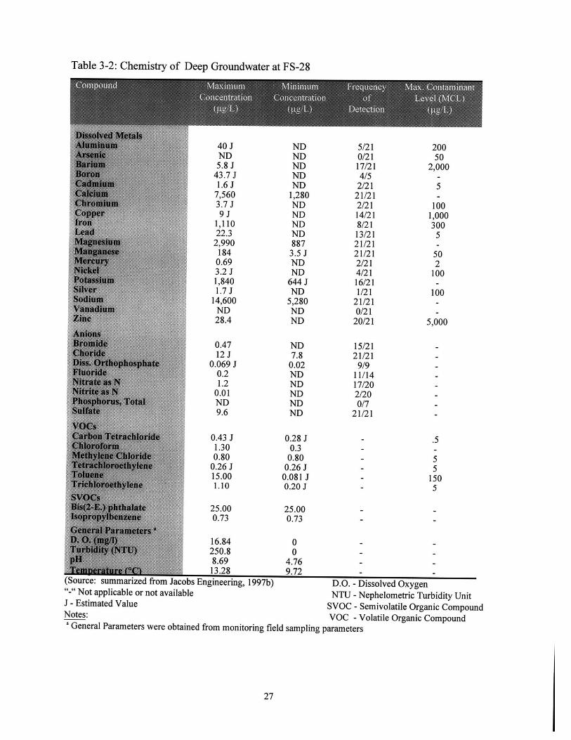
Table 3-2: Chemistry of Deep Groundwater at FS-28

A 40 J ND 5/21 200ND ND 0/21 50

r 5.8 J ND 17/21 2,00043.7 J ND 4/51.6 J ND 2/21 5

7,560 1,280 21/21 -3.7 J ND 2/21 100

per 9 J ND 14/21 1,000..... 1,110 ND 8/21 300

d 22.3 ND 13/21 52,990 887 21/21

g 184 3.5 J 21/21 500.69 ND 2/21 2

N e3.2 J ND 4/21 100Po wsi 1,840 644 J 16/21 -

ver 1.7 J ND 1/21 100I 14,600 5,280 21/21

ND ND 0/2128.4 ND 20/21 5,000

r roid4 0.47 ND 15/2112 J 7.8 21/21

0.069 J 0.02 9/9orlde 0.2 ND 11/14

trate as N 1.2 ND 17/20N 0.01 ND 2/20

s, Total ND ND 0/7S l te9.6 ND 21/21

T 0.43 J 0.28 J - .51.30 0.3 -

pride 0.80 0.80 - 5T.1tyAee 0.26 J 0.26 J - 5

T* Ir 15.00 0.081 J - 150roOne 1.10 0.20 J - 5

VOs(2-E) phthalatt 25.00 25.00 -

0.73 0.73 -Gnera* Para' ters*

D. Omg/l)16.84 0--Turs~dly(TU)250.8 0--pH 8.69 4.76--

TeAOeratlimr M "A!.. 13.28 9.72-(Source: summarized from Jacobs Engineering, 1997b) D.O. - Dissolved Oxygen"-" Not applicable or not available NTU - Nephelometric Turbidity UnitJ - Estimated Value SVOC - Semivolatile Organic CompoundNotes: VOC - Volatile Organic Compounda General Parameters were obtained from monitoring field sampling parameters

27

Due to the presence of EDB in the western and eastern lobes of CS-10 and the presence of

preferential pathways for contaminant migration at CS-10, this plume was identified as the only

significant source area. Jacobs also concluded that cranberry bogs, farms, and golf courses are

not potential sources as pesticides other than EDB were used. Additionally, other study areas

(including CS-4) were identified as partial sources for FS-28. These sites had a history of motor

fuel and aviation gasoline spills containing EDB and displayed moderately favorable aquifer

characteristics (Jacobs, 1997a).

3.6 Groundwater and Surface Water UsesGroundwater and surface water resources in this area provide the drinking water for the

surrounding communities and also provide a habitat for a variety of fish and wildlife in the area.

Additionally, approximately 68 acres of agricultural crops south of Hatchville Road are irrigated

from either groundwater wells or surface water. Table 3-3 presents a summary of the agricultural

water usage for the affected cranberry bogs. The other agricultural crops include strawberries

and vegetables. The farmers of these crops draw surface water from Pond 14 for frost protection

and irrigation. Approximately one million gallons of water were used in 1996 during the six-

month growing season (Jacobs, 1997a).

Table 3-3: Summary of Agricultural Water Usage

CranberryCranberryCranberryCranberryCranberryCranberry

StrawberriesCranberryCranberryCranberry

Ow 81SW 600GW 100SW 150SW 420SW 100SW 800SW 650SW 1,200SW 900

(Source: Jacobs, 1997b)Notes:GW - Groundwater gpm - gallons per minuteSW - Surface Water

28

The cultivated bogs are typically flooded in late November to early December to prevent frost

damage to the cranberry vines. Due to an unusually warm winter, bogs were flooded in

1997/1998 from mid-December to mid-February. During flooding, the Coonamessett River is

dammed up, raising the water level from 0.5 to 2 feet over the area of the cultivated bogs.

Upward vertical gradients are reduced under flooded conditions, keeping the groundwater from

flowing into the bogs (Jacobs, 1997a).

In 1998, the irrigation of the cranberry bogs began in early spring using treated water from the

treatment plant. For frost control, spray irrigation has been conducted and will continue as

needed until mid-June. From mid-June to October, the fields will be irrigated as needed to

provide at least 2 inches of water on the crop per week. During the fall, the bogs are harvested

either dry or wet.

3.7 Geologic SettingPrevious investigations indicate that the FS-28 middle and lower study areas are underlain by

glacial outwash sediments composed of tan, fine to coarse sand with lesser amounts of silts and

gravel (less than 10%). The sands are relatively well-sorted to approximately 120 feet mean sea

level (msl), and become poorly sorted below this depth. Silty and gravelly zones lie within the

sand, ranging from one to ten feet in thickness. Underlying the outwash is a thin glacial till unit,

containing an increased number of gravelly sand and silty sand lenses (to about 170 feet msl).

Below 170 feet msl, fine and coarse sands can be found with little gravel, little silt, and trace

cobbles. An occasional sand lens and silty sand lens is present over the bedrock surface.

Bedrock has typically been encountered at elevations ranging from 220 to 243 feet msl (Jacobs,

1997a).

3.8 Hydrogeologic SettingA single groundwater flow system underlies western Cape Cod, from the Cape Cod Canal to

Barnstable and Hyannis. This sole source aquifer referred to as the Sagamore Lens is the Upper

Cape Cod's only potable water source. The aquifer is unconfined and is recharged by infiltration

29

and precipitation. Recharge is approximately 1.6 feet/year, with seasonal variations producing

fluctuations in the water table of 1 to 3 feet. Groundwater flows out radially from the recharge

mound (Jacobs, 1997a).

A value of 380 ft/day has been accepted as a representative value of average hydraulic

conductivity for the outwash sands (on a regional scale) at the MMR (Tillman, June 1996).

Using an average hydraulic gradient of 0.002 ft/ft and a porosity of 0.39, average linear velocities

ranging from 0.25 to 2.5 ft/day can be calculated for the outwash sands (Jacobs, 1997b).

Vertical gradients at FS-28 range from almost horizontal flow (0.0003 ft/ft) to strongly upward

flow (0.0039 ft/ft). Upward vertical gradients were observed along the western edge of the study

area. Groundwater was observed seeping into the drainage ditches bordering the cranberry bogs.

Artesian conditions were observed in the bogs.

Based on a pumping test conducted at the CWSW, the full thickness of the outwash aquifer at

this site has a transmissivity of approximately 86,000 to 100,000 ft2/day. Furthermore, aquifer

response to pumping indicated that the outwash aquifer is essentially unconfined, with a specific

yield of 0.2. The vertical to horizontal anisotropy ratio in the area of the CWSW well screen is

low, suggesting that silty layers do not have significantly lower vertical hydraulic conductivity

than silt-free layers.

3.9 Current Modeling EffortsThe U.S. Geological Survey (USGS) is conducting studies in the vicinity of the FS-28 plume and

has performed a particle tracking analysis to simulate the contaminant transport, especially as

influenced by the Coonamessett Pond. Additionally, the USGS is conducting studies to date the

age of the groundwater plume in the FS-28 study area, which might be beneficial in better

identifying source areas.

30

Numerical modeling (using MODFLOW) was undertaken by Jacobs to evaluate the migration of

the FS-28 plume, potential discharge locations, and remedial alternatives. MODFLOW was run

under both flooded and non-flooded conditions in the cranberry bogs. To estimate travel times,

hydraulic conductivity was approximated at 250 ft/day and effective porosity was estimated at

0.24. Jacobs predicted that the effective porosity was not likely to vary more than 20% in either

direction and therefore, travel times ought to be within 20% of the estimated value as well.

Plume migration was simulated with particle tracking using MODPATH. This model generates

pathlines for ground-water flow from the MODFLOW output and captures the most significant

transport - advection (Jacobs, 1997a).

Preliminary results for the modeling indicate that the Coonamessett River and the cranberry bogs

present a strong sink for groundwater and plume discharge. Particle tracking indicates that the

upper fringes of the FS-28 plume would discharge in 1998 immediately downstream of

Hatchville Road, but the bulk of the deeper plume would not discharge significantly within the

five-year time period simulated. If flooded conditions were maintained, the plume would

generally travel farther; however, there would still be some discharge of the plume to the bogs

between Hatchville and Thomas B. Landers roads. According to Jacobs, the irrigation wells, if

operated at their maximum flowrates, could potentially have a significant influence on the long-

term migration pathway of the plume. The irrigation wells, if used as capture wells, would only

be able to capture the upper portion of the plume and could allow some of the plume to pass

beneath. Due to the limitations of the model, an evaluation of the most leading part of the plume

could not be conducted thoroughly (Jacobs, 1997a).

3.10 Time-Critical ActionsThe EPA, DEP, and MA DPH have determined that the use of EDB-contaminated surface and

groundwater for agricultural purposes represents an unacceptable risk to public health and the

environment. An Action Memorandum (Jacobs Engineering, 1997b) has been prepared to serve

as the primary decision document for the remedial action at FS-28. The proposed removal action

is being implemented by the Air Force as a time-critical action to: 1) prevent the exposure of the

31

residents of the Hatchville area in the Town of Falmouth to EDB, 2) to contain the EDB plume,

and 3) to prevent the plume from further contaminating the cranberry bogs.

The Air Force Center for Environmental Excellence (AFCEE) has taken immediate actions to

eliminate any exposure or potential exposure to EDB, including:

* Installation of a granular activated carbon wellhead treatment system at the CWSWand at the irrigation well screened in the EDB plume,

" Installation of an extraction well to intercept the deep portion of the EDB plume,

* Supply of bottled water to residents in the Hatchville community,

" Provision of an alternative water supply to the Falmouth community,

" Installation of irrigation wells outside the EDB plume, and

* Definition and monitoring of the plume.

3.11 SummaryThe FS-28 plume was discovered in 1992 south of the CS-4 plume. The plume is roughly 9,000

feet long, has a maximum width of 3,000 ft and varies in thickness up to 100 feet. It has a north-

south orientation and is bounded by Coonamessett Pond on the east, Deep Pond on the west, and

Thomas Landers Road on the south. The leading edge of the plume is narrow and the axis of the

plume generally parallels the Coonamessett River. Due to the significant discharge from the

aquifer to the Coonamessett River, the FS-28 plume migrates to the surface water, wetlands, and

cranberry bogs south of Hatchville Road. The area of discharge can be inferred from surface

water and shallow groundwater results and seems to be confined to a few hundred feet of the

Coonamessett River. Based on modeling, the leading edge of the plume is assumed to continue

to the south to eventually surface again along the river north of Great Pond.

EDB is considered the only significant contaminant of concern at FS-28. The FS-28 plume area

has been divided into the upper, middle, and lower study areas. The current remedial efforts are

32

concentrated on the lower study area, which contains the toe of the FS-28 plume. To address

remediation, the lower study area has been divided up into three major areas to be addressed:

* The hotspot area, which contains the 10 pg/L isoconcentration;

* The portion of the plume which upwells into the cranberry bogs; and

" The leading edge of the plume which continues to travel to the south.

Modeling of the current extraction well has shown that it is not possible to address all of these

areas of contamination in one remediation scheme. In order not to disturb the ecology at the

Coonamessett River, the extraction well is pumping at a maximum flowrate of 750 gpm. This

pumping rate, however, will not capture the portion of the plume which surfaces in the cranberry

bogs nor the leading edge of the FS-28 plume. It has been assumed that the leading edge of the

plume will attenuate naturally (dispersion, hydrolysis, sorption, etc.) so that the concentrations

downstream should not pose a threat to receptors. The following sections will address the

remedial scheme at FS-28.

33

4. FATE AND TRANSPORT MECHANISMS OF ETHYLENE DIBROMIDE

Groundwater contamination results in an increased risk to human health and the environment as

well as an economic threat to public water systems. As a result, it is important to restore the

groundwater resources. In order to remedy groundwater contamination, it is necessary to

understand the basic physical, chemical, and biological properties of the contaminants and to

evaluate their governing fate and transport mechanisms. The purpose of this section is to review

the available environmental chemistry of EDB in order to assess its fate in soil and groundwater.

This section will also discuss the uses of EDB, its regulatory history, mobility, and persistence.

4.1 Background Information

4.1.1 General Description (CAS Number 106-93-4)

Ethylene dibromide, also known by the chemical names EDB, ethylene bromide, and 1,2-

dibromoethane, is a non-flammable, colorless liquid with a mildly sweet odor. At a

concentration of 10 parts per million (ppm) in air, the average person can detect EDB. Ethylene

dibromide has been used as a fumigant and also as a fuel additive as outlined in the following

sub-sections.

4.1.2 Regulatory History

Ethylene dibromide was first detected in groundwater in 1980 in Hawaii (Mink, 1981; Oki and

Giambelluca, 1987). In 1982, it was detected in some Georgia farms wells and in the following

year, EDB was found in groundwater in California and Florida (USEPA, 1983a). With the

increasing incidence of EDB in groundwater and the combined evidence of this chemical's

toxicity as well as its leaching potential, the USEPA issued an emergency order suspending the

registration of EDB as a soil fumigant in September 1983 (USEPA, 1983b). The USEPA

concluded that the use of EDB posed an imminent health hazard. The current maximum

contaminant level (MCL) set in the United States is 0.05 ptg/L; the MCL set by the State of

Massachusetts is 0.02 pg/L.

34

4.1.3 ToxicityEthylene dibromide can be adsorbed via dermal, oral, and inhalation routes; with all of these

exposures, it produces tumors in rats and mice. Ethylene dibromide is also a reproductive toxin,

but is does not appear to be teratogenic. Limited information indicates that EDB can damage the

liver and kidneys following extensive or prolonged exposure; however, few human poisonings

have been reported from either acute or chronic exposure.

Initial risk estimates indicated that citrus fruit workers exposed to EDB had a 100% chance of

contracting cancer. Revised estimates of occupational exposure indicated a lower risk, but the

risk estimates still range from 1 to 40 excess cancer cases per 10,000 persons exposed (Alexeeff

et al.,1990).

4.2 Uses of Ethylene Dibromide

The following sections describe the past uses of EDB as a soil fumigant and additive to gasoline

and aviation fuel.

4.2.1 Use of Ethylene Dibromide as a Fumigant

The use of EDB as a pre-plant soil fumigant constituted over 90% of all agricultural uses in the

U.S. and is undoubtedly the principal source of EDB groundwater contamination nationwide. By

1983, nearly 23 million lbs of EDB (as an active ingredient) were applied to about 400,000 ha of

a variety of crops in the U.S., including citrus fruits, potatoes, tobacco, and tomatoes (Pignatello

and Cohen, 1990). The heaviest application rates probably occurred in the Florida citrus groves.

When used as a soil fumigant, EDB was injected as a liquid directly into the soils. The relatively

high vapor pressure led researchers to believe that EDB would readily volatilize in the soil and

therefore, pesticide applicators were advised to seal the soil surface with water or an impervious

cover which increased the potential for leaching (Weaver et al., 1988).

4.2.2 Use of Ethylene Dibromide as a Fuel AdditiveEthylene dibromide was also used as a lead scavenger in leaded gasoline and aviation fuel. In

1983, an estimated 260 million lbs/year of EDB were used as an additive to gasoline (Weaver et

al., 1988). It is estimated that EDB constitutes approximately 0.03% by weight of gasoline

35

containing 1.1 g of lead/gal (Weaver et al., 1988). Hoag (1984) found an average EDB

concentration of 178 ppm in leaded gasoline while unleaded gasoline has much lower

concentrations of EDB, ranging from 0.1 to 7.2 ppm. Aviation gasoline is thought to contain

twice as much EDB as leaded gasoline (Pignatello and Cohen, 1990). Underground Storage

Tanks (USTs) are known to leak and some groundwater contamination resulted from these leaks

or accidental fuel spills. If EDB is present in combination with other soluble gasoline

constituents, such as benzene, toluene, ethylbenzene, and xylenes (BTEX), the contaminant

source is likely fuel.

4.3 Physical and Chemical Properties of EDB

In order to evaluate the governing fate and transport mechanisms, it is important to understand

the physical and chemical characteristics. Table 4-1 below presents a summary.

Table 4-1: Physical and Chemical Properties of EDB

(Source: Pignatello and Cohen, 1990; Weaver et. al., 1988, Mackay et al., 1993; Montgomery,

1955)

36

As shown above, EDB is a low molecular weight compound. Solubility is one of the most

important characteristics governing a chemical's fate. Because EDB is moderately soluble

compared to other chemicals, it tends to be transported quickly through the aquifer. As shown in

the table above, EDB does not have a high affinity for soils. Its soil/water distribution

coefficient, Kd, has been reported to be less than 3 which is significant since Cohen et al. (1984)

stated that pesticides with a Kd value of less than 5 have the potential to leach into groundwater if

they are persistent.

It should be noted, however, that despite these low reported values of Kd, residual EDB can

become trapped in soil micropores. As a result, Kd values from desorbing EDB from treated soil

were extremely high (Weaver et al.,198 8).

4.4 Fate and Transport of EDB

The following sections describe the pertinent fate and transport mechanisms of EDB. The fate of

this chemical is governed by its physical and chemical properties as well as the chemical,

physical, and microbiological processes in the aquifer.

4.4.1 Vadose Zone Transport

Mostly, transport of EDB in soil is governed by volatilization, advection, and dispersion. Other

factors that will influence vadose zone transport, such as microbial degradation, sorption, and

abiotic transformations are discussed in Section 4.4.2.1.

VolatilizationBecause of its vapor pressure and Henry's Law Constant, a fraction of EDB will volatilize from

the soil. The volatilization half-life of EDB was calculated by Jury et al. (1984) to be 0.4 days

and 3.4 days at a soil depth of 1 cm and 10 cm, respectively.

Advection and Dispersion

Because of its density, EDB will move into the soil when applied or spilled at the surface. In the

subsurface, EDB will degrade, dissolve in soil moisture, or diffuse into soil pore spaces. Vapor

and liquid diffusion in the soil is controlled by Fick's Law and studies of EDB have shown that

37

vapor diffusion (as opposed to liquid diffusion) will dominate until the water content becomes a

high percentage of total porosity.

The advective mobility of a compound in soil will depend on the fraction that has partitioned into

the liquid phase. Therefore, advection in the vadose zone is influenced by the water content and

the organic content of the soil.

4.4.2 Saturated Zone Transport

Volatilization does not occur readily in groundwater. As mentioned above, EDB is moderately

soluble in water. It travels slower than groundwater itself, but faster than most other volatile

organics, including toluene and benzene. Since dissolved EDB does not change the density of

water appreciably, an EDB-contaminated plume in an aquifer will move along the flow paths of

bulk groundwater. The velocity, size, shape, and distribution of the plume will be subject to the

influences of sorption and dispersion of the solute.

4.4.3 Other Controlling MechanismsThe following sections discuss the effects of microbial transformations, sorption, and abiotic

transformations which will also influence the fate of EDB.

Microbial Transformations

A review of available biodegradation data pertaining to EDB concluded that this chemical is

biotransformed quite readily in the environment; lifetimes can be as short as several days in

surface soils and as long as many months in aquifer materials (Pignatello and Cohen, 1990).

Based on laboratory studies, EDB is degraded under all redox conditions, except possibly

denitrifying. Products of microbial transformations include the bromide ion, carbon dioxide, and

ethylene. It must be noted that there is no evidence of microbial degradation of EDB outside of

laboratory experiments where EDB is the only available electron acceptor (Jacobs, 1997g). It

should also be noted that, at high concentrations, EDB is toxic to bacteria. The portion of EDB

entrapped in micropores of the soil is inaccessible to microbial degraders and chemical

processes.

38

Sorption

Sorption can affect the transport of EDB both in the vadose as well as the saturated zone.

Furthermore, degradation rates are also affected by sorption since organic compounds are less

available for microbial attack in the "sorbed state".

As shown in Table 4-1, EDB does not have a high affinity for soils contradicting which

contradicts the evidence that EDB was found in the topsoil of several agricultural sites at

concentrations of up to 300 4g/Kg up to 19 years after the last known fumigation. This

contradiction may be attributable to the concept of non-equilibrium sorption. This concept is not

well understood; however, it is believed to result from slow kinetics, dominated by molecular

diffusion. It has been suggested that sorption of a chemical is rate-limited by diffusion through

the small pores between fine soil grains. The strong occlusion of EDB in the case-study

mentioned above was thought to be a result of physical entrapment in the soil micropores.

Abiotic Transformations

There is increasing evidence that abiotic transformations may play a role in determining the

subsurface fate of EDB. The most important processes involved are hydrolysis and reactions

with sulfur nucleophiles. Photolysis is not discussed due to the limited penetration of sunlight in

the soil column. Several studies have been conducted to investigate hydrolysis of EDB. All

authors agree that under ambient, pure laboratory conditions, the hydrolysis half-life for EDB is

at least two years and probably longer (Weaver et al., 1988).

Ethylene dibromide is readily attacked by sulfur nucleophiles, most importantly hydrogen

sulfide, which is a product of anaerobic microbial activity in the aquifer. Recent work of several

researchers led to the conclusion that the reaction of EDB with sulfur nucleophiles can be highly

competitive with neutral hydrolysis depending on ambient sulfide concentrations and that the

transformation products from this reaction, i.e., alkyl sulfides, will differ from the neutral

hydrolysis reaction products (Weaver et al., 1988).

39

5. USE OF GRANULAR ACTIVATED CARBON ADSORPTION FORHOTSPOT REMOVAL AT FUEL SPILL 28

As described in Section 3.11, from a technical perspective, the contaminated areas at FS-28

ought to be addressed in three "phases." The first phase should address removal and treatment of

the highest concentrations (hotspot) within the plume. Phase 2 should address those parts of the

plume that are not captured by the extraction well and upwell into the cranberry bogs and surface

waters of the Coonamessett River; Phase 3 ought to verify that the leading edge of FS-28 does

not pose a threat to downgradient receptors. This section will focus on the removal and

treatment of the highest concentrations (hotspot) of the lower portion of the FS-28 plume.

5.1 Interim Remedial ActionAs an interim action, one extraction well (69EW0001) has been installed in the northern portion

of FS-28 (south of monitoring well MW1284A, shown in Figure 3-4) and has been extracting

water at a flowrate of approximately 670 gpm. The extracted water is currently being treated

with GAC and then discharged to nearby surface water bodies. Initial influent levels of EDB

were at 4.7 ptg/L; however, they leveled off to 0.8 pg/L during the treatment period. The interim

treatment system went into operation on October 14, 1997. Breakthrough occurred in the lead

canister on December 22, 1997, following only 69 days of operation and the carbon bed was

changed out on February 10, 1998. The carbon bedlife was originally estimated to range from

210 to 540 days (Jacobs, 1998).

5.2 Final Remedial ActionA final remedial alternative has not been chosen for the lower study area at FS-28. A feasibility

study will be conducted to determine which technology will address the overall and long-term

objectives most efficiently.

40

5.3 Pump-and-Treat TechnologyBetween 1982 and 1992, about 73 percent of the cleanup at Superfund sites used pump-and-treat

technology. At that time, however, the limitations of pump-and-treat systems were not fully

recognized as large-scale studies of the effectiveness of pump-and-treat systems were not yet

available. In 1989, the EPA conducted a review of 19 sites where pump-and-treat systems were

operating and concluded that at none of these sites was the aquifer restored to drinking water

standards (USEPA, 1989a,b,c). A review of 77 sites where the efficiency of pump-and-treat

systems was studied by the National Research Council (NRC, 1994) concluded that pump-and-

treat systems appear to be capable of restoring groundwater at sites with simple geology and

dissolved contaminants; however, at most sites, the operation of the pump-and-treat system

should be viewed as a long-term project, in which the system design is modified in response to

improved understanding of the site conditions.

Only two remedial technologies, namely pump-and-treat using GAC and air stripping, have been

found to reduce EDB significantly. Based on a study conducted by Environmental Science and

Engineering (Beaudet, 1983), air stripping is 99% effective in removing EDB from water while

pump-and-treat with GAC is considered 100% effective in removing EDB. Because of the low

concentrations of EDB in the influent and the extremely low MCL set by the State of

Massachusetts (0.02 tg/L), GAC adsorption was chosen as an interim action for the remediation

at FS-28.

5.3.1 Effectiveness of Pump-and-Treat SystemsThe effectiveness of a pump-and-treat system depends heavily on hydrogeologic and

contaminant properties. Two types of contaminant characteristics can complicate groundwater

cleanup significantly: 1) the tendency of the chemical to sorb to solid materials; this is not

expected to pose a problem at FS-28, and 2) the tendency of organic contaminants to remain in

the form of a non-aqueous phase liquid (NAPL). Heterogeneities of the soil further complicate

the cleanup, as geologic complexities can affect the efficiency of the pump-and-treat system by

causing tailing of the contaminant concentrations in the aquifer. Contaminant tailing has been

observed with chlorinated solvents, and it has been found, that while the concentration of the

41

contamination in the extracted groundwater declines, it never reaches zero, even after two or

more plume volumes have been extracted. In the literature, tailing has been attributed to the

presence of NAPLs, the effects of sorption, and heterogeneities in hydraulic conductivity

(Domenico and Schwartz, 1990).

For EDB, however, pump-and-treat systems might be moderately effective as this technology is

focused on where the bulk of the contaminant mass exists - the groundwater.

5.3.2 Cleanup with Pump-and-Treat SystemsTo determine the feasibility of cleanup of the FS-28 hotspot with a pump-and-treat system, the

following parameters need to be determined:

" Total estimated mass of EDB contamination,

" Vertical and horizontal extent of contamination,

" Configuration of the extraction system, and

" Estimated cleanup time.

5.4 Treatment with Granular Activated Carbon (GAC)The use of carbon for its adsorptive qualities was known as early as 1550 B.C., when charcoal

was utilized in the purification of medicines. Current industry is now taking advantage of GAC

to remove a variety of organic compounds from water (Nyer, 1992). Activated carbon

adsorption is regarded as the basis by which other technologies are measured. This section will

review the basic mechanisms of carbon adsorption and provide some possible explanations for

the early breakthrough at the FS-28 GAC treatment system.

5.4.1 Granular Activated CarbonThe adsorbent most frequently used in environmental applications is activated carbon. The

following sub-sections will review the background information on the manufacture, types,

characteristics, and regeneration of activated carbon.

42

5.4.1.1 ManufactureActivated carbon is prepared by producing a char from various materials including almond,

coconut, walnut hulls, woods and coal. The char is produced by heating the material to expel the

hydrocarbons, but under conditions with insufficient air to sustain combustion. The char particle

is then activated by chemical or steam activation. These processes develop a porous structure

and creates a large internal surface area (Tchobanoglous and Burton, 1991). The use of different

raw materials as well as processing allow for many different types of activated carbon, each

differing in adsorption and regeneration characteristics.

5.4.1.2 TypesActivated carbon is available in three general forms: granular, pellets, and powder -- the

application determines which form is most applicable. Carbon used in the gaseous-phase

adsorption typically consists of the granular form. Generally, liquid-phase carbons are either

powdered or granular and tend to have the same surface area as gas-adsorbing carbons, but have

larger total pore volumes (Cheremisinoff and Cheremisinoff, 1993). Powdered activated carbon

(PAC) is more commonly used in biological treatment systems.

5.4.1.3 Adsorbent CharacteristicsSince adsorption is possible only in those pores that can be entered by molecules, the carbon

adsorption process is dependent on the physical characteristics of the activated carbon and the

molecular size of the adsorbate. Therefore, surface area and pore structures are two very

important factors in the adsorption process. Examination of a microscopic cross-section of

activated carbon reveals a porous structure with a large internal surface area. The following

criteria have to be considered in the selection process of an appropriate adsorbent:

* Surface Area - the larger the surface area of the adsorbent, the higher the adsorption.Typically, bituminous carbon (Calgon Filtrasorb 300) has an internal surface area ofapproximately 1,000 m2/g (USEPA, 1971).

43

* Bulk Density - a measure to determine carbon quantity. Typical bulk densities for

Calgon Filtrasorb 300 ranges from 0.45 to 0.48 g/cm3 (28 to 30 lb/ft3)

* Pore volume - a measure to determine how readily a contaminant can be adsorbed;

the pore volume is about 0.85 cm 3/g for Calgon Fitrasorb 300 bituminous carbon

(Cheremisinoff and Cheremisinoff, 1993).

* Particle Size - the effective size of the Calgon Fitrasorb 300 bituminous carbon is

0.8-1 mm (Calgon Carbon Corporation, 1998).

5.4.1.4 RegenerationGranular activated carbon can easily be regenerated by oxidizing the organic matter through

heating. During this process, about 5 to 10 percent of the carbon is typically destroyed and must

be replaced. Regenerated carbon is not as efficient as virgin carbon. One major disadvantage to

PAC is that its regeneration has not been well defined (Tchobanoglous and Burton, 1991).

5.4.2 Theoretical Adsorption Theory

Adsorption is the process in which a soluble contaminant (the adsorbate) is removed from water

by contact with a suitable solid interface (the adsorbent). The amount of adsorption on most

surfaces is exceedingly small, but a number of porous solids with an unusually high surface area

have been developed, including activated carbon, silica gel, and activated alumina. The two most

important types of adsorption are: 1) physical adsorption and 2) chemical adsorption

(Cheremisinoff and Cheremisinoff, 1993). Adsorption on activated carbon is of a physical

nature. The adsorption process is thought to involve the following steps: macrotransport,

microtransport, and sorption.

Macrotransport involves the transport of the adsorbate molecules to the liquid-adsorbent (solid)

interface. Macrotransport may be the rate-limiting step in systems that have poor mixing, dilute

concentrations of adsorbate, small particle sizes of adsorbent, and high affinity of adsorbate for

adsorbents (Helfferich, 1962; Tillman, 1996). Microtransport describes the diffusion of the

molecules through the micropore system of the GAC granule to the adsorption sites. It is this

process that limits the overall transfer for those systems that have good mixing, large particle-

44

size adsorbents, high concentrations of adsorbate, and low affinity of the adsorbent. Sorption

describes the attachment of the organic molecule to the carbon itself. Generally, adsorption is

favored by large, less soluble, less polar compounds. Saturated organics are also adsorbed easily,

as are branched-chain organics (LaGrega et al., 1994).

5.4.2.1 Adsorption IsothermsAdsorption equilibrium is obtained when the rate of adsorption onto the solid phase equals the

rate of desorption from the solid surface back to the water phase. A plot of the amount of the

contaminant sorbed against the concentration of the contaminant in the water is termed the

adsorption isotherm. The amount of contaminant that can be taken up by an adsorbent

(expressed as weight of contaminant per unit weight of carbon) is referred to as the adsorption

capacity, (X), and represents an equilibrium relationship between the contaminant adsorbed andM

the contaminant concentration remaining in solution. The adsorption capacity is a function of

both the characteristics and concentrations of the contaminant as well as temperature.

There are several forms of isotherms, but most experimentally determined isotherms can be fit

with a Freundlich model (Schwarzenbach et al., 1993):

= K -(Cwn) jM

where X = mass of contaminant adsorbed [mg] per dry unitM

weight of carbon [g], also termed adsorptioncapacity for GAC

Cw = concentration of contaminant in solution afteradsorption equilibrium is reached which isassumed to equal the influent concentration, Ci[mg/L]

K, n = are experimentally determined Freundlichconstants at a given temperature, where Khas units of [L/g]

45

Adsorption isotherms are commonly used to determine carbon usage rates, the amount of carbon

needed flbs] to treat 1000 gallons of contaminated water. The mass of contaminant adsorbed in

a carbon column can be determined by:

X = (Ci-Ce) - V (2)

where Ci = influent concentration [mg/L]

Ce = effluent concentration [mg/L]

V = Volume of solution [L]

The constants in the Freundlich isotherm can be determined by plotting I versus Cw as follows:M

Log (I) = log K + n log Cw (3)M

For solutions with dilute concentrations of contaminants, a straight line should be obtained with

K as the intercept and n as the slope of the line. The value obtained for n for adsorption of most

organic compounds by activated carbon is <1. Steeper-line slopes, i.e. when n is close to 1,

indicate a high adsorptive capacity at high equilibrium concentrations that rapidly decreases at

lower equilibrium concentrations covered by the isotherm. Relatively flat slopes, i.e. n is << 1,

indicate that the adsorptive capacity is only slightly reduced at the lower equilibrium

concentrations. As the Freundlich equation indicates, the adsorption capacity X is a function ofM

the equilibrium concentration of the solute; therefore, higher capacities are obtained at higher

equilibrium concentrations (Faust and Aly, 1983).

Given an influent concentration, the theoretical adsorption capacity of the carbon for a particular

contaminant can be determined using an adsorption isotherm. However, since this calculation is

based on equilibrium conditions and since equilibrium conditions are rarely met in the field

(contact times are typically too short), the adsorption capacity as determined from batch tests is

generally overestimated. In the field, the carbon is not typically exhausted (i.e., not all

46

adsorption sites are occupied) and, furthermore, the effects of biological activity present in the

field are not seen with theoretical adsorption isotherms. Additionally, isotherm tests are typically

conducted under steady state conditions, at constant pH, and with virgin carbon, which has a

greater adsorption capacity than reactivated carbon. Column tests that simulate the actual

operation of full-scale units (and influent concentrations) are therefore required to obtain realistic

carbon usage rates for field operating conditions.

5.4.2.2 Multi-Component InfluentsMost influents contain a mixture of contaminants and therefore the adsorption isotherms

determined in the laboratory represent an ideal-case scenario. Because other contaminants may

compete for adsorption sites, the adsorption capacity of any compound may be decreased.

Several mathematical models have been developed that allow for a direct computation of the

solute loading from known concentrations in the mixture. If the concentrations of the solutes in

the mixture are low, no significant decrease is expected in the adsorption capacity (Tillman,

1996).

One of the models developed to describe multi-component adsorption behavior for contaminants

at low concentrations (DiGiano, et al., 1978; Tillman, 1996) can be described as follows:

(W1 n K " (Ki -C," n) ]/n' - C . C,' (4)MN K

where X i = adsorption capacity of solute iM

[mg contaminant/g carbon]

K', n' = average of all ki and ni constants

Ki, ni = Freundlich constants, describing singlesolute adsorption

Ci = concentration of solute i in the mixture

[mg/L]

47

N = number of solutes in the mixture

This model, developed by DiGiano, Baldauf, Frick, and Sontheimer (DiGiano et al., 1978) is a

simplification of the Ideal Adsorbed Solution (IAS) model which was originally developed by

Radke and Prausnitz. The IAS model is based on a thermodynamic framework as it relies on the

assumption that the adsorbed phase forms an ideal solution. It requires single-solute isotherms to

be known which are then used with the initial concentrations of the contaminants to generate

loading rates for multi-component solutions. The IAS model is mathematically more

complicated, especially in systems that contain more than two components. The model described

in equation (4) was derived from the same thermodynamic framework and a comparison between

this model and the IAS model shows that the two models are in good agreement in a

concentration range of less than 0.1 mmol/L (DiGiano et al., 1978). Equation (4) can

mathematically be reduced to the Freundlich equation for a single-component solution.

5.4.3 Design Criteria at FS-28To determine the maximum usage from activated carbon, experimental analysis using actual

influent concentrations is often necessary. Operating factors such as influent water

characteristics, treatment facility configuration, and effluent requirements are controlling criteria

in the selection of the appropriate carbon type and mode of application. The following criteria

were evaluated during selection and design of the adsorption system for the FS-28 hotspot

treatment.

5.4.3.1 Vessel Capacity and ArrangementCarbon beds of 20,000 lbs have become a standard size, as the spent carbon from a single unit

can easily be transported from the site in a single trailer. The two basic liquid-phase equipment

designs for carbon adsorption are the fixed-bed and the pulsed-bed arrangements. Fixed-bed

systems can take the form of either single or multiple columns which can operate in series,

parallel, or both. In most situations, a multiple-column adsorber is used because of the operating

flexibility it provides. Fixed single-column systems are only used when the additional cost of

48

another carbon bed can not be justified (Cheremisinoff and Cheremisinoff, 1993). Fixed-bed

systems can either have downflow columns, upflow-bed or expanded-bed systems. Continuous,

downflow columns are most common. The downflow column is a gravity adsorber that operates

as a filter and not a pressure vessel.

The interim system at FS-28 consists of two 10-ft diameter adsorber vessels filled with Calgon F-

300 GAC. Each vessel contains 20,000 pounds of virgin bituminous carbon. The system has a

two-stage, lead-lag, downflow arrangement, as shown in Figure 5-1. When the effluent from the

first column reaches the breakthrough concentration, the leading bed column is removed and the

second bed becomes the lead column. This arrangement assures high-quality effluent and

complete contaminant removal.

influent

treated effluent

Figure 5-1: Configuration of a typical continuous, downflow column contactor

5.4.3.2 Influent and Effluent Concentrations/Characteristics

Influent concentrations are determined by the concentrations extracted by the pumping wells and

will depend on the distance from the source site, the amount of contaminants reaching the

aquifer, contaminant solubility and density, and the transformations that the contaminant

undergoes. These factors will affect the size of the treatment system and the length of time

49

required for cleanup. The amount of contamination reaching the aquifer will depend on the

amount sorbed to the organic carbon present in the subsurface.

The pH at which the adsorption process occurs has been shown to have a strong influence on the

extent of adsorption. However, this pH dependence is far more important for ionizable organic

chemicals than for EDB (Faust and Aly, 1987). A review of Freundlich constants shows that

some compounds, such as benzoic acid, show a strong dependence on pH, while others, such as

EDB does not show a strong dependence.

The temperature will affect both the rate of adsorption (kinetics) and the extent to which

adsorption occurs (equilibrium). Generally adsorption rates increase with increased temperature;

however, since adsorption is an exothermic process, the degree of adsorption will decrease at

lower temperatures. The temperature of extracted groundwater is generally constant, ranging

from 50 'F to 60 'F and will therefore not influence the adsorption process significantly unless

the water is not directly routed to the treatment system and has time to equilibrate with external

temperatures.

At FS-28, influent levels of EDB were initially 4.7 ptg/L and have subsequently leveled off at

approximately 0.8 [tg/L. The pH in the influent ranged from 6.19 to 8.08; the temperature of the

extracted groundwater was at about 53 'F (Jacobs, 1998).

5.4.3.3 FlowrateUnlike for industrial wastewater treatment plants, flowrates are a design variable in the design of

carbon adsorption systems for the treatment of contaminated groundwater. The flowrate required

will depend on the time needed for the cleanup, weighing the effect of flow on the cost of the

system. The flowrate should be designed so that the contaminant plume is contained,

considering the volumetric flowrate of contaminated groundwater, the number of wells to be

installed, and the final use of the treated water.

50

The system at FS-28 has a maximum design flowrate of 750 gpm, but has been operating at an

average flowrate of about 670 gpm.

5.4.3.4 Contact TimeOne of the most critical design parameters for any adsorption system is contact time (also termed

empty bed contact time [EBCT]). The EBCT is the time required for the flow per vessel to

displace the same amount of volume as taken by the GAC bed and depends on the rate-limiting

steps described in Section 5.4.2. Observation of the carbon usage rate versus EBCT shows that

after an initial rapid decrease in carbon usage rate with increasing EBCT, no significant decrease

in usage rate is obtained by further increasing the EBCT (Tillman, 1996). Therefore, an EBCT

should be chosen in the region where the carbon usage rate has leveled off to its minimum value.

Increasing the depth of carbon for a fixed flowrate or decreasing the flowrate for a fixed depth of

carbon serve as methods to increase contact time.

Generally, most EBCT tests (in the laboratory) are conducted with contact times up to 1 hour as

EBCTs greater than 1 hour are not considered practical in the field. However, some larger

molecules may not reach equilibrium in less than 1 or 2 days and, as a result, isotherms for large

molecules determined with 1 hour or less of contact time can only be used as a rough estimate of

adsorbability (Najm et al., 1991). As a consequence, field adsorption capacities for such

compounds are lower than at equilibrium and need to be adjusted. The effects of short contact

times experienced in actual operations or the accurate prediction of activated carbon usage rates

can be gauged from a scaled column study. In general, a factor ranging from 0.25 to 0.5 is used

in equation (9) (presented in the following section) to account for the adjustment of laboratory

conditions to field conditions (Tchobanoglous and Burton, 1991).

Based on studies conducted by Calgon Carbon Corporation, EBCTs of 7.5 minutes (translating

to 500 gpm per adsorber vessel) are adequate to achieve treatment objectives (Calgon Carbon

Corporation, 1998) for most groundwater systems with low levels of contaminants. The contact

time can thus be determined from the flowrate and the volume of carbon per vessel as follows:

51

EBCT = Bed Volume . 20,000 lbs - 7.48 gallon I ft3 =: 6.5 minutes (5)Flowrate 670 gpm ft 3 29 lbs

At FS-28, an EBCT of 6.5 minutes was designed for each vessel based on an operating flowrate

of 800 gpm. (Jacobs, 1998).

5.4.3.5 Loading RatesIn practice, engineers often like to work with flowrates expressed in terms of hydraulic loading in

gpm/ft2. The surface loading rate is based on the cross-sectional area of the column and will vary

depending on the EBCT and the vessel diameter. Surface loading rates in GAC systems can be

as great as 10 gpm/ft2. Higher surface loading rates typically result in slightly higher carbon

usage rates as the adsorption zone (the area in the column where adsorption is taking place) may

be extended, causing contaminant breakthrough to occur sooner (Stenzel, 1989). The downflow

packed bed columns are designed so that the granular medium retards any channeling or short-

circuiting assuring contact with the carbon (Calgon Carbon Corporation, 1998).

At FS-28, with a flowrate of approximately 670 gpm and a vessel diameter of 10 ft, the surface

hydraulic loading can be calculated as:

Surface hydraulic loading rate = Flowrate 670 gpm

Cross -sec tional Surface Area 257ift 2

= 8.5 gpm/ft2 (6)

In contrast, there is also a volumetric hydraulic loading which is the inverse of the EBCT:

Volumetric hydraulic loading rate = Flowrate - I = 0.13 1 (7)Bed Volume EBCT min

52

5.4.3.6 Calculations of Carbon Usage Rates Using Laboratory Isotherms

Both Calgon Carbon Corporation and the USEPA Drinking Water Research Water Division

evaluated the removal of trace concentrations of EDB from water by activated carbon adsorption

(Calgon Carbon Corporation, 1998). The adsorption isotherm developed by Calgon Carbon

Corporation (shown in Figure 5-2 below) was based on influent concentrations on the order of

557 [ig/L and was conducted using an isotherm mix time of 24 hours. The following

calculations illustrate the estimation of theoretical carbon usage rates based on adsorption

isotherms performed in the laboratory. It is important to note that the following equations are

based on the assumption that the carbon/water mixture was stirred long enough for adsorption

equilibrium to be achieved. This subject will be addressed in more detail later in this section.

Adsorption of Ethylene Dibromide by Calgon FS-300 Activated Carbony = 4.6336Ln(x) + 20.167

16 =R2 =0.9714

14 -

12-

M 10 - * Adsorption Capacity X/M (mg/g)

a>8 - - Log. (Adsorption Capacity X/M

0 6 (mg/g))

4-

0

0 0.05 0.1 0.15 0.2 0.25 0.3 0.35

Equilibrium Concentration Cw (mg/)

Figure 5-2: Adsorption Isotherm developed by Calgon Carbon Corporation(Recreated and modified from Calgon Carbon Corporation)

53

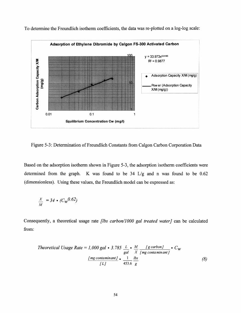
To determine the Freundlich isotherm coefficients, the data was re-plotted on a log-log scale:

FS-300 Activated CarbonAdsorption of Ethylene Dibromide by Calgon

y = 33.973x0-6 185

R2 = 0.9877

Z

CL

0

0CM0 C

.0

a-05

0.1 1

Equilibrium Concentration Cw (mg/I)

+ Adsorption Capacity X/M (mg/g)

Pow er (Adsorption CapacityX/M (rng/g))

Figure 5-3: Determination of Freundlich Constants from Calgon Carbon Corporation Data

Based on the adsorption isotherm shown in Figure 5-3, the adsorption isotherm coefficients were

determined from the graph. K was found to be 34 L/g and n was found to be 0.62

(dimensionless). Using these values, the Freundlich model can be expressed as:

X = 34 - (Cw0 .62)M

Consequently, a theoretical usage rate [bs carbon/1000 gal treated water] can be calculated

from:

Theoretical Usage Rate = 1,000 gal - 3.785

[mg contaminant].[L]

L , M [g carbon] Cwgal X [mgcontaminant]

1 lbs453.6 g

54

0.01

(8)

At an influent concentration of 4.7 ptg/L (the maximum influent concentration), the activated

carbon capacity is 1.23 mg of EDB/g of carbon, translating into a theoretical usage rate of 0.032

lbs carbon/1000 gal of treated water. At an influent concentration of 0.8 pg/L (the concentration

the system has leveled off to), the activated carbon capacity is 0.41 mg of EDB/g of carbon,

translating into a theoretical usage rate of 0.016 lbs carbon/1000 gal of treated water. However,

since field scale carbon adsorption is less efficient than the adsorption capacity determined in

laboratory studies, the full-scale adsorption capacity is a percentage of the theoretical adsorption

capacity. Typically, in practice, the capacity in the field has been shown to be 25 - 50% of the

theoretical capacity (Tchobanoglous and Burton, 1991). Values of both 25% and 50% were used

to determine field scale usage rates (summarized in Table 5-1):

Field-scale Usage Rate = Adjustment Factor * Theoretical Usage Rate (9)

These usage rates are based on the assumption that the effluent concentrations are at 0 mg/L.

Even though effluent concentrations increase in time until breakthrough occurs, this is a

sufficiently close approximation as effluent requirements are very low (< 0.02 pg/L) at FS-28.

For effluent concentrations that exceed the detection threshold, field-scale usage rates can be

calculated using the revised formula (10) below:

Usage Rate = 1,000 gal - 3.785 L . M [g carbon] * (C - Ce) [mg contaminant]gal X [mgcontaminant] [LI

1 lbs * Adjustment Factor (10)453.6 g

Table 5-1 below illustrates the carbon usage rates for three scenarios: 1) an influent

concentrations of 0.8 ptg/L, 2) a maximum influent concentration of 4.7 pg/L using a flowrate of

670 gpm, and 3) an influent concentration of 6 pg/L using a flowrate of 800 gpm, the conditions

Calgon Carbon Corporation based their calculations on prior to the installation of the treatment

system. Adjustment factors of both 25% (the maximum) and 50% (the minimum) were used.

55

Table 5-1: Comparison of Carbon Usage Rates for EDB

Notes:An adjusted carbon capacity of 25% was used to account for field conditions, as illustrated in equation(10).

2 An adjusted carbon capacity of 50% was used to account for field conditions, as illustrated in equation(10).

For an influent concentration of approximately 6 pg/L, Calgon Carbon Corporation estimated a

carbon usage rate ranging from 0.034 lbs carbon/1000 gal of treated water to 0.083 lbs

carbon/1000 gal of treated water for complete removal of EDB in a column adsorber.

Based on the carbon usage rate, the flowrate, and the vessel capacity, a carbon exchange rate can

be determined. The carbon exchange rate dictates how often the vessel containing the carbon has

to be replaced. Again, carbon exchange rates were calculated for three scenarios: 1) at a

maximum influent concentration of 0.8 pg/L, 2) at a maximum influent concentration of 4.7

pg/L using a flowrate of both 670 gpm and 750 gpm. Also, a carbon exchange rate was

calculated using an influent concentration of 6 pg/L at a flowrate of 800 gpm. The carbon

exchange rates are illustrated in Tables 5-2 and 5-3 below.

Table 5-2: Comparison of Carbon Exchange Rates for EDB Using an AdjustmentFactor of 25%

U.UUUZS (-/U U.U640.0047 670 0.1270.0008 750 0.0640.0047 750 0.1270.006 800 0.139

Notes: Calgon Carbon Corporation predicted a carbon service life ranging from 210

56

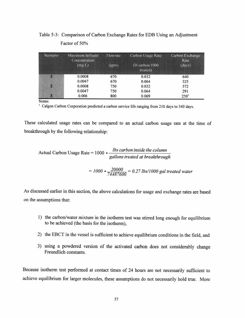
Table 5-3: Comparison of Carbon Exchange Rates for EDB Using an Adjustment

Factor of 50%

Notes:' Calgon Carbon Corporation predicted a carbon service life ranging from 210 days to 540 days.

These calculated usage rates can be compared to an actual carbon usage rate at the time of

breakthrough by the following relationship:

Actual Carbon Usage Rate = 1000 -lbs carbon inside the column

gallons treated at breakthrough

= 1000 20000 = 0.27 lbs/1000 gal treated water74487600

As discussed earlier in this section, the above calculations for usage and exchange rates are based

on the assumptions that:

1) the carbon/water mixture in the isotherm test was stirred long enough for equilibriumto be achieved (the basis for the isotherm),

2) the EBCT in the vessel is sufficient to achieve equilibrium conditions in the field, and

3) using a powdered version of the activated carbon does not considerably changeFreundlich constants.

Because isotherm test performed at contact times of 24 hours are not necessarily sufficient to

achieve equilibrium for larger molecules, these assumptions do not necessarily hold true. More

57

importantly, at contact times of 8 minutes in the carbon vessel, equilibrium may not be achieved.

Therefore, it is important to adjust the carbon capacity by an appropriate factor to account for

these premises.

To obtain a more accurate estimate of the carbon capacity at low influent concentrations, the

isotherm data can be re-plotted. Generally, one can assume that as the concentration of the

contaminant becomes small, the isotherm is linear and thus n = 1. By only plotting the first three

data points, the Calgon isotherm can be expressed as shown below in Figure 5-4. From the linear

interpolation in Figure 5-4, one can assume that the distribution coefficient Kd can be

approximated by 100 L/g. However, because the EBCT in the carbon vessel (8 minutes) was just

a fraction of that one used in the laboratory (24 hours), the "effective" Kd also needs to be

adjusted by a factor ranging from 25% to 50%. The "effective" Kd then ranges from 25 to 50.

Carbon exchange rates for this value are shown in Table 5-4.

It should be noted that for a given Kd the product of in equation (8) reduces to a constant,

irrespective of the influent concentration.

Adsorption of Ethylene Dibromide by Calgon FS-300 ActivatedCarbon

(redrawn at low concentrations)

10 y = 92.909x0R2=.9429

o 8

6

& 4 J

0U 0 0.02 0.04 0.06 0.08 0.1 0.12

Equilibrium Concentration Cw (mg/L) AdsorptionCapacity X/M

58

Figure 5-4: Adsorption Isotherm of EDB at Low Concentrations

Table 5-4: Comparison of Carbon Exchange Rates for EDB Using an Effective Kd

of 25' and 502

I........... 670 0.33 63 0.167 126

2750 0.33 56 0.167 112800 0.33 53 0.167 106

5.4.3.7 SummaryThe carbon usage rates and the carbon exchange rates shown in Tables 5-1 through 5-4 are based

on an extrapolation from the adsorption isotherm developed by Calgon Carbon Corporation. The

carbon bedlife was calculated with two different approaches: 1) using the Freundlich model and

the entire data set from the isotherm, and 2) adjusting the isotherm data to fit a linear relationship

at low concentrations. With the first approach and using the same conditions Calgon Carbon

Corporation used to determine the bed service life, the carbon exchange rate ranges from 125

days to 250 days, as compared to the 210-540 days Calgon Carbon Corporation had predicted.

Using the second approach, the carbon exchange rates ranged from 53 to 126 days for the same

conditions. These calculations are based on the assumption that equilibrium was achieved during

the isotherm test and that an adjustment factor of 25% to 50% is sufficient to account for the

change from laboratory to field conditions. Based on these observations, it appears that the

carbon exchange rates predicted by Calgon Carbon Corporation may have been overestimated.

It is also important to realize that the laboratory isotherm was determined at controlled

conditions. More importantly, the isotherm was determined at much higher influent

concentrations than those present at FS-28; the lowest equilibrium concentration used in the

isotherm was 4 pg/L. The isotherm should be determined within the concentration range

corresponding to the levels likely to be encountered for the compound of interest since the

extrapolation of isothermal data can lead to erroneous results (Faust and Aly, 1983). Calgon

Carbon Corporation used a proprietary analytical technique based on laboratory isotherms to

59

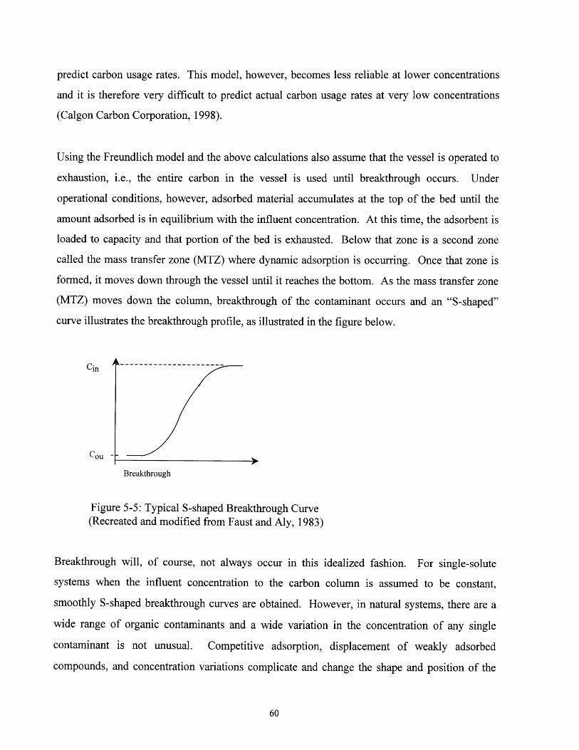
predict carbon usage rates. This model, however, becomes less reliable at lower concentrations

and it is therefore very difficult to predict actual carbon usage rates at very low concentrations

(Calgon Carbon Corporation, 1998).

Using the Freundlich model and the above calculations also assume that the vessel is operated to

exhaustion, i.e., the entire carbon in the vessel is used until breakthrough occurs. Under

operational conditions, however, adsorbed material accumulates at the top of the bed until the

amount adsorbed is in equilibrium with the influent concentration. At this time, the adsorbent is

loaded to capacity and that portion of the bed is exhausted. Below that zone is a second zone

called the mass transfer zone (MTZ) where dynamic adsorption is occurring. Once that zone is

formed, it moves down through the vessel until it reaches the bottom. As the mass transfer zone

(MTZ) moves down the column, breakthrough of the contaminant occurs and an "S-shaped"

curve illustrates the breakthrough profile, as illustrated in the figure below.

Cin

cou -

Breakthrough

Figure 5-5: Typical S-shaped Breakthrough Curve(Recreated and modified from Faust and Aly, 1983)

Breakthrough will, of course, not always occur in this idealized fashion. For single-solute

systems when the influent concentration to the carbon column is assumed to be constant,

smoothly S-shaped breakthrough curves are obtained. However, in natural systems, there are a

wide range of organic contaminants and a wide variation in the concentration of any single

contaminant is not unusual. Competitive adsorption, displacement of weakly adsorbed

compounds, and concentration variations complicate and change the shape and position of the

60

breakthrough curves. Therefore, adsorption studies for the application of activated carbon should

be conducted using either a natural water or a synthetic medium of equivalent composition and

concentration.

Another consideration is the time it takes for an isotherm to achieve equilibrium. A lot of the

isotherms reported in the literature are being conducted with 2 hours at 22 *C. This, however, is

not sufficient time to achieve equilibrium. Crittenden et al. reported adsorption capacities to be

2-3 times higher than those reported by Dobbs & Cohen for similar temperature, carbon, and

adsorbates (1985), illustrating the divergence in data possible under different experimental

conditions. As shown in the previous section, an adjustment might have to be made to correct

for the short contact time in the field. Kinetic data would be needed to estimate the fraction of

equilibrium obtained during an 8-minute EBCT in the field.

In the field, breakthrough occurred after 69 days of operation. It is therefore conceivable that the

service life of the carbon beds was overestimated, assuming that the EBCT of 8 minutes is not

sufficient to achieve adsorption equilibrium. It is not possible to determine this hypothesis

without laboratory experiments and furthermore, other factors could also be responsible for the

pre-mature breakthrough. The following sections undertake a more detailed analysis to explain

the early breakthrough at FS-28.

5.4.4 Analysis of the Early Breakthrough at Fuel Spill 28The following sub-sections investigate the possible causes for early breakthrough at FS-28,

including:

" Overestimation of carbon bedlife,

" Backwashing

" Reversible adsorption/desorption,

" Pre-loading due to naturally occurring organic matter, and

61

. bacterial growth on the carbon column.

5.4.4.1 Overestimation of Carbon BedlifeThe following sections determine and compare carbon exchange rates by:

1) determining usage rates using single-solute isotherms and Freundlich isothermconstants from a literature search,

2) determining the effect of multi-component solutions on the usage rates using a modeldeveloped by DiGiano et al. (1978),

3) determining breakthrough times using

a) equilibrium column model, andb) advection dispersion equation, and

4) determining the true adsorption capacity from the actual loading data at breakthrough.

5.4.4.1.1 Single-Component Adsorption Isotherm Calculations Using the Freundlich Model andFreundlich Constants from a Literature Search

Crittenden et al. (1985) conducted experiments to develop isotherms for both single- and

multiple-component solutions and demonstrated that the Freundlich equation was sufficiently

accurate in representing isotherm data that was collected in the laboratory. The degree of

agreement of the data with the Freundlich equation was expressed in terms of an average percent

error (APE) of 1.1% in q, the single-component solid phase concentration (X).M

Because the carbon usage rates can vary widely with differing Freundlich constants, a literature

search was conducted for Freundlich constants for EDB and the carbon usage and carbon

exchange rates were summarized in the following Table 5-5:

62

Table 5-5: Comparison of Literature Freundlich Constants and Calculated Carbon UsageRates at a Maximum Concentration of 4.7 pg/L and a Maximum Flowrate of750 gpm

69.3 0.5 1 Filtrasorb 400 1.34 0.029 1.4 63655.6 0.4 2 Filtrasorb 400 1.57 0.025 5 740

33.05 0.6 3 PAC 0.42 0.0936 1992

49.71 0.4 4 Filtrasorb 400 1.32 0.029 7 6268

43.4 0.5 5 Hydrodarco 0.67 0.058 3198 GCW 12 x 40

Notes:An intermediate adjustment factor of 35% was used to account for the change from laboratory to fieldconditions.

2 Freundlich constants were determined using an influent concentration of 0.5 pg/L and an equilibriumconcentration of 0.05 pg/L.

3 Freundlich constants were determined using Filtered Ohio water with a total organic carbon (TOC)content of 2 mg/L. A carbon usage rate of 0.053 lbs/1000 gal treated water and a bed life of 804 dayswas predicted in the literature, assuming a single, full-scale contactor with an EBCT of 15 minutes,hydraulic loading of 4 gpm/ft2 , using Filtrasorb 400 GAC. This calculation was performed using apore-surface-diffusion flux ratio of 0.4 for relatively less strongly adsorbed volatiles.

4 Using an adjustment factor of 40% to account for field conditions, a carbon usage rate of 0.059lbs/1000 gal of treated water was calculated.

5 Freundlich constants were determined using de-ionized water with a TOC content of < 0.1 mg/L.6 Freundlich constants were determined using water from Fairfield.7 Crittenden also noted that the adsorption capacities at 10-12 *C were approximately 2-4 times higher

than those observed at 20-22 C.8 Sources:

1 Weber and Pirbazari, 1981.2 Texas Marketplace, 1998.3 Montgomery Watson, 1998.4 Crittenden et al., 1985.5 Norit Americas, Inc., 1998.

The carbon bedlives (exchange rates) calculated from the Freundlich constants found in theliterature range from 199 days to 740 days using an intermediate adjustment factor of 35%. Asdiscussed previously, these values are based on the assumption that equilibrium can be achievedin the field using an 8-minute EBCT. These estimates are notably higher than what wascalculated previously. Some of the Freundlich constants were determined using a considerably

63

higher influent concentration, which will distort the adsorption capacity at lower concentrations.

Furthermore, some of the experiments used a lignite-based carbon which has a higher surface

area than bituminous carbon. Generally, a powdered form of the carbon is used in laboratory

isotherm tests which would also have a larger surface area than the granular form and therefore

overestimate the carbon service lives. Only one estimate, namely the study conducted by Issam

Najm (Montgomery Watson, 1998) was conducted at the concentration range that has been found

at FS-28. The estimated carbon service life using the Freundlich constants that were determined

using PAC and a contact time of 7 days was 199 days.

5.4.4.1.2 Multi-Component Adsorption Isotherm CalculationsAs mentioned in Section 5.4.2.2, the adsorption capacity of any compound may be decreased by

the presence of other contaminants in the influent. Preferential adsorption is important when

considering selective removal of compounds. Generally, compounds with high melting point,

high critical temperature, and low volatility are preferentially adsorbed and may displace other

compounds that have already been adsorbed. If preferential adsorption occurs, the true capacity

of the carbon is lower and therefore single-solute isotherms often are not of practical use.

After examining the analytical results for the influent data to the treatment system, it was noted

that none of the contaminants that were found in the contaminant plume (i.e., carbon

tetrachloride, chloroform, methylene chloride, PCE, toluene, or TCE) were actually detected in

the influent samples. Low concentrations of ethylbenzene (0.56 pg/L) and total xylenes (2.9

ptg/L) were detected in the influent after breakthrough occurred. It is possible that low levels of

organics were present in the influent; however, competitive adsorption by these contaminants is

not expected to significantly increase the usage rate. To confirm this assumption, usage rates

were calculated using the model developed by DiGiano et al. (1978) described in Section 5.4.2.2.

Appendix A presents usage rates for EDB if ethylbenzene had been present in the influent at a

maximum concentration of 0.56 pg/L.

64

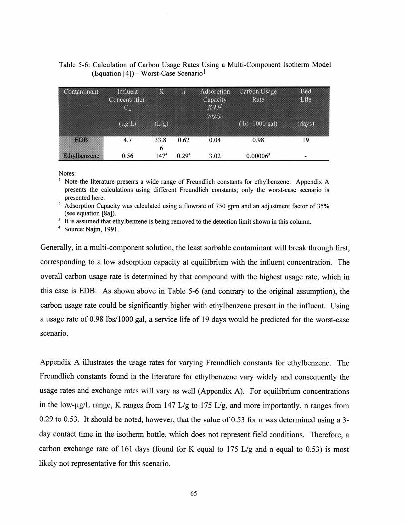
Table 5-6: Calculation of Carbon Usage Rates Using a Multi-Component Isotherm Model(Equation [4]) - Worst-Case Scenario1

4.7 33.8 0.62 0.04 0.98 196

0.56 147 4 0.294 3.02 0.00006 3-

Notes:Note the literature presents a wide range of Freundlich constants for ethylbenzene. Appendix Apresents the calculations using different Freundlich constants; only the worst-case scenario ispresented here.

2 Adsorption Capacity was calculated using a flowrate of 750 gpm and an adjustment factor of 35%(see equation [8a]).

3 It is assumed that ethylbenzene is being removed to the detection limit shown in this column.4 Source:Najm, 1991.

Generally, in a multi-component solution, the least sorbable contaminant will break through first,

corresponding to a low adsorption capacity at equilibrium with the influent concentration. The

overall carbon usage rate is determined by that compound with the highest usage rate, which in

this case is EDB. As shown above in Table 5-6 (and contrary to the original assumption), the

carbon usage rate could be significantly higher with ethylbenzene present in the influent. Using

a usage rate of 0.98 lbs/1000 gal, a service life of 19 days would be predicted for the worst-case

scenario.

Appendix A illustrates the usage rates for varying Freundlich constants for ethylbenzene. The

Freundlich constants found in the literature for ethylbenzene vary widely and consequently the

usage rates and exchange rates will vary as well (Appendix A). For equilibrium concentrations

in the low-pg/L range, K ranges from 147 L/g to 175 L/g, and more importantly, n ranges from

0.29 to 0.53. It should be noted, however, that the value of 0.53 for n was determined using a 3-

day contact time in the isotherm bottle, which does not represent field conditions. Therefore, a

carbon exchange rate of 161 days (found for K equal to 175 L/g and n equal to 0.53) is most

likely not representative for this scenario.

65

So, in summary, it is possible that even though no other contaminants were detected in the

influent prior to breakthrough, usage rates may have been increased by the presence of very low

levels of organic contaminants (other than EDB) in the influent. The 19-day carbon exchange

rate was determined using the most conservative Freundlich constants (i.e., yielding the highest

usage rates); this exchange rate also assumes that EDB is present consistently at a concentration

of 0.56 pg/L. It is more likely, however, that other contaminants may have been present

sporadically, increasing the carbon usage rate.

5.4.4.1.3 Comparison of Breakthrough TimesAs defined previously, the length of time required for the appearance of some percentage of the

initial concentration to reach the effluent is termed the breakthrough time. Several models are

available in the literature to predict the performance of GAC. The following approach was taken

to obtain a theoretical breakthrough time at FS-28:

1) the Equilibrium Column Model, and

2) the advection dispersion equation.

Using the Equilibrium Column Model (ECM)

The EC model is a simple model and is based on two assumptions explained below (Ram et al.,

1990):

1) Adsorption is instantaneous, i.e., there is no mass transfer zone. Based on thisassumption, the breakthrough curve consists of a step rather than the S-shaped curveshown in Figure 5-5. Furthermore, the breakthrough time is independent of thebreakthrough concentration.

2) This model also assumes that at the time of breakthrough, all of the carbon issaturated or in other words, its solid-phase concentration is in equilibrium with thecontaminant liquid-phase concentration. If the actual breakthrough curve issymmetrical in shape, then the ECM breakthrough time should correspond to the timeit takes for the effluent concentration to reach 50% of the influent concentration.

66

Cout/Ci

Breakthrough

--------- EC Model

Figure 5-6: Illustration of EC Model

Mathematically, this model can be expressed as (Ram et al., 1990):

(VB s pB) - Xt = M

B QCw

where tB = breakthrough time [days]

VB = volume of GAC in Column [m3]

PB = density of GA C in carbon bed [g/m3 ]

Q = water flowrate [L/day]

Cw = influent concentration [mg/L]

From Section 5.4.3.6, a distribution coefficient Kd of 100L/g can be assumed. Using a 35%

adjustment factor, a breakthrough time of 125 days can be calculated.

Because kinetics are ignored in this calculation, the breakthrough time obtained from the ECM

model only provides a very rough estimate for the GAC service life. It generally underestimates

the breakthrough time because it neglects the mass transfer zone. Accordingly, it is common

67

practice to divide the ECM breakthrough time by a factor of 2 when laboratory isotherm data is

used (Narbaitz et al., 1994).

Using the One-dimensional Dispersion Advection Equation

The one-dimensional dispersion advection

1994):

Dx- a2RaX2

equation can be expressed as (Hemond and Fechner,

ac acC Rax at

where DX = dispersion coefficient [ft2 /sec]

vx = one-dimensional velocity [fi/sec]

a2

ax2

acaxac

= change in concentration by Fickian transport

= chemical concentration gradient in the fluid

= rate of change of contaminant

R = Retardation factor

In the case of a continuous input, the spreading of the chemical front can be described by:

Rx - vtC(x,t) = (Cw/2) -erfc[ ] (13)

2 RDxt)

where CW, initial concentration of the chemical [pg/L]

erfc complementary error function

In this case, we can assume that:

C0 = 4.7 pg/L

C(x, t) = 0.02 pg/L

v = 0.046 ft/sec (surface hydraulic loading divided byporosity, assuming porosity equals 0.41)

Dx = a - v

where a = median grain size of the carbon particle

68

(12)

Bituminous granular activated carbon has a grain size of about 1mm; a generous value of 1 cm

was chosen for cc. So then

Dx = 0.032ft -0.046ft/sec = 0.0015ft2/sec

x = 9 feet (effective length of the carbon column)

From Section 5.4.3.6, one can assume that the distribution coefficient Kd = 100 L/g. Using an

adjustment factor of 35% for Kd, the retardation factor R can be calculated as:

R = 1 + Kd - b (14)n

Using a bulk density of 0.50 g/ml and a porosity of 0.41,

R = m + 35L/g - - - = 42,684ml L 0.41

Going back to equation (12), [ needs to be determined when erfc[ = 0.0085. From the

listed tables in Hemond and Fechner (1994), this is true mathematically when j = 1.89.

Based on this calculation, a breakthrough time of approximately 97 days was computed for the

effluent to reach 50% of the influent concentration (this would correspond to the estimate from

the EC Model, but taking dispersion into account) and a breakthrough time of 77 days was

computed for the effluent concentration to reach a concentration of 0.02 pg/L. This estimate is

based on a retardation factor which was computed from the isotherm data at low concentrations.

Using this model, it is important to examine the spread (i.e., the deviation about the mean) of the

concentration distribution within the carbon canister. A concentration distribution with a large

standard deviation will be more spread out and breakthrough may occur earlier than in a flow

field with a small standard deviation. Since the concentration distribution of a tracer can be

modeled with a Gaussian distribution, the variance for a one-dimensional column can be

expressed as follows:

69

- DxtJ where a = standard deviation (15)VR

Plugging in the numbers obtained from above results in a value for a of 1.2 ft. This since value

is larger than 10% of the length of the carbon column, dispersion plays a role in determining the

breakthrough time.

5.4.4.1.4 Determination of Actual Adsorption CapacityThe averaged column loading data can be used to determine the actual adsorption capacity of the

carbon vessel at breakthrough. Using this approach, the contaminant solid phase concentration

can be calculated based on the assumption that the mass of contaminant removed by the water

column has adsorbed to the carbon. This model does not provide a breakthrough time, but

allows for comparison of adsorption capacities determined in the laboratory versus those

experienced in the field. The loading will be significantly smaller than that predicted by the

laboratory isotherm since the carbon vessel in the field typically does not get fully exhausted.

Mathematically, this can be expressed as (Narbaitz et al., 1994):

MCONT = >j(C, - Ce,) Qi. t' (16)

where MCONT = mass of contaminant removed by thecarbon column [mg]

Qi = average flowrate during period i [L/d]

Ati = duration ofperiod i [d]

Cwi = average contaminant influent concentrationduring period i [mg/L]

Cei = average contaminant effluent concentrationduring period i [mg/L]

The adsorption capacity can then be determined by:

70

X_ MCONT (17)M VB - PB

where VB -PB= mass of GAC in the column (9,072, 000 g)

This approach yielded a removed contaminant mass of 386 g and an actual averaged adsorption

capacity of 0.042 mg/g (see Appendix B). This adsorption capacity would translate into a carbon

usage rate of 0.24 lbs/1000 gal for an averaged influent concentration of 1.4 jig/L and an

averaged flowrate of 750 gpm. This compares to a theoretical carbon usage rate of 0.064 lb/1000

gal calculated from the laboratory isotherm for an influent concentration of 0.8 ptg/L.

While it is important to compare breakthrough times and carbon usage rates, the actual

breakthrough curve has to also be considered in this analysis. The actual influent loading curve

can be determined from actual influent data and is shown in Figure 5-7 below (Jacobs, 1998):

INFLUENT EDB LOADING

1.000.900.800.70 -

0.600.50..0.40 -.

0.300.200.10

0.000 20 40 60

Time, days

y -2E-063 + 0.0005x2 - 0.0314x + 0.8602R2 0.9737

y = 0.7451e~0

R2 = 0.9156

8 1-Poly. (C/Co)

80 100 120 .. - .. .. Expon. (C/Co)

Figure 5-7: Influent EDB Loading

It is important to examine the actual breakthrough curve. If considerable time elapses before the

breakpoint appears, and the breakthrough curve is sharply defined and steep, the adsorption zone

71

0

is short relative to the over-all bed depth. If on the other hand breakthrough occurs almost

immediately, a relatively deep adsorption zone is indicated (Calgon Carbon Corporation, 1998).

As shown in Figure 5-8, the breakthrough curve is considerably steep, then levels back out to a

constant. This shape would indicate that other factors such as sudden desorption might have

occurred.

Breakthrough Curve at FS-28

0Q

0.05 -

0.04 -

0.03 -

0.02 -

0.01 -

050 100

Backwashing BreakthroughTime (days)

Figure 5-8: Breakthrough Curve at FS-28

5.4.4.2 Reversible Adsorption/DesorptionAdsorption to the carbon surface relies on electrostatic Van der Waals forces, which are

relatively weak bonds, between the contaminant and the carbon. Because adsorption is a

reversible process, desorption of contaminants may occur. Available literature cites the

following causes for desorption of contaminants (Snoeyink et aL, 1987; Thacker et aL, 1983):

* competition from more strongly adsorbing species,

* reduced influent concentration, causing material to be desorbed as a new equilibriumis established,

* destratification of the GAC, causing carbon originally exposed to higher contaminantconcentrations to establish a new equilibrium under low contaminant concentrations,and

* changes in water quality (e.g., pH).

72

Research conducted by Thacker et al. (1983) evaluated reversible adsorption caused either by a

reduction in the influent concentration or by competition from stronger adsorbing species. A

high rate of desorption following a reduction in the influent concentration would indicate higher

effluent concentrations initially after desorption has begun. The findings showed that a change

made in an adsorption system to improve mass transfer (by increasing surface diffusivity or film

transfer coefficients) and adsorption efficiency (such as changing to a smaller size of carbon)

could also result in greater desorption (Thacker et al., 1983). On this basis, increasing the bed

length or decreasing the hydraulic loading would also increase the rate of desorption.

During a study conducted by Narbaitz et al. (1994), pre-mature breakthrough of EDB in point-of-

entry (POE) filters in Florida was attributed to excessive water use and to desorption induced by

sharp variations in the EDB influent concentrations. Several studies have reported desorption of

chloroform due to competitive adsorption at the column, resulting in an effluent concentration

exceeding the influent concentration for the same timeframe (Faust and Aly, 1987).

Cited information in the literature suggests that halogenated aliphatics such as EDB desorb

readily as they are adsorbed more weakly than other contaminants. Zenon Environmental Inc.

(1984) conducted a desorption study in which a column was loaded with low levels of EDB,

dibromochloropropane (DBCP), and 1,2,3-trichloropropane. During the time the columns were

run in desorption mode, EDB was the only chemical to desorb, with the desorbing concentrations

being approximately half of those fed during the loading phase.

A sharp drop in the influent concentration from 4.7 ptg/L to 0.8 tg/L occurred at FS-28 within 40

days of operation. However, its effect on desorbing EDB from the bottom of the carbon column

is debatable. Equilibrium concentrations at the bottom of the carbon column should not be

affected by decreasing influent concentrations entering the top of the carbon column. Therefore,

the breakthrough at FS-28 can not be attributed to desorption as a result of a decrease in the

influent concentration.

73

5.4.4.3 BackwashingIt is plausible that the carbon fines in the column were redistributed during the backwashing

event on December 9, 1997. Generally, backwashing has several effects on a GAC filter: it

loosens and breaks down the suspended solids attached to the GAC granules and removes them

from the filter. Backwashing also produces stratification of carbon particles according to their

size (McGuire and Suffet, 1980). If redistibution occurred during backwashing, it is conceivable

that carbon fines from the top of the carbon vessel traveled down to the bottom of the vessel.

The exhausted carbon at the bottom would prevent further adsorption and possibly desorb

previously adsorbed EDB to establish a new equilibrium.

A similar occurrence was reported by Andrew Hyde (McGuire and Suffet, 1980) who observed a

difference in carbon performance for single- versus multiple-bed systems. He attributed the pre-

mature exhaustion of the single-bed system with respect to chloroform to mixing of the media

during backwashing.

5.4.4.4 Pre-loading from Total Organic CarbonThe performance of GAC can also be affected by the presence of naturally occurring background

organic material (NOM). According to studies conducted by Narbaitz et al. (1986, 1994), Murin

et al. (1979), and Suffet et al. (1989), NOM in the influent is particularly important as it can

reduce the carbon's adsorption capacity by 50% or greater. This reduction in carbon adsorption

capacity can be attributed to the difference in adsorption characteristics of volatile organic

compounds (VOCs) and dissolved NOM (NDOM). While VOCs have relatively fast adsorption

kinetics and many are strongly adsorbed, NOM is very heterogeneic and generally diffuses

slowly (Ram et al., 1990). Predicting the adsorption of NDOM is extremely difficult because of

the heterogeneity of TOC. Apparently, a substantial fraction of carbon particle pores are smaller

than the humic material which would explain the slow adsorption kinetics associated with

NDOM. Furthermore, a number of researchers have found that even though diffusion is slow for

the organic matter, adsorption is usually irreversible, causing a carbon's capacity for a target

compound to be reduced (Ram et al., 1990).

74

Speth has shown a reduced isotherm capacity for TCE on carbon which was pre-loaded with

natural water containing a TOC content of 0.7 mg/L (Ram et al., 1990). Studies conducted by

Speth and other researchers (Zimmer et al., 1987 and 1988) also demonstrated that the adsorption

kinetics (and therefore the carbon adsorption capacity) decreased with time of pre-loading.

A reduced carbon adsorption capacity due to pre-loading from TOC in the influent may be

partially responsible for the pre-mature breakthrough at FS-28. Total organic carbon was not

detected consistently in the influent to the treatment system at FS-28. The samples were only

analyzed for TOC in October, 1997 (which showed no detections of TOC) and then again in

January (which showed a TOC concentration of 0.5 mg/L). In June 1997, a groundwater sample

collected form extraction well 69EW0001 showed a TOC concentration of 0.3 mg/L. Even

though the samples did not show a detection of dissolved organic carbon, it is possible that DOC

was present below the detection limit of 0.52 mg/L. Because the NDOM is weakly adsorbing, it

can travel down the carbon column and slowly adsorb onto the activated carbon ahead of the

adsorbing zone of EDB. Thus EDB is adsorbed in the top portions of the vessel media while the

TOC is adsorbed in the lower portion of the vessel media, what is commonly termed "pre-

loading" the carbon column. As the mass transfer zone passes through the media, the amount of

EDB adsorption is decreased since there are less adsorption sites available. The carbon column

near the bottom would therefore have a lower capacity than near the top of the column,

suggesting a higher rate of carbon exhaustion deeper into the media (Ram et al., 1990).

5.4.4.5 Bacterial Growth on the Activated Carbon ColumnOne of the most intricate issues related to the use of GAC is the presence of bacterial growth and

its interaction with adsorption. As illustrated in Appendix C, groundwater contains a complex

mixture of naturally occurring substances that are often lumped together as biological oxygen

demand (BOD) or TOC. These organic substances may contain a wide range of bacteria which

have been known to attach themselves to the macropores of the carbon, forming a biofilm that

impedes the sorption process. As a result, adsorption takes place only after the contaminant has

diffused across the film. For contaminants that are both adsorbable and biodegradable, these two

75

processes may be complementary and beneficial. This biological phenomenon has been used as

a treatment step to GAC where it is commonly termed biological activated carbon (BAC). For

contaminants that can not be readily biodegraded, adsorption is reduced due to the slowed

diffusion across the biofilm.

A number of hydrodynamic complications related to bacterial growth on the carbon column have

been cited in the literature, including bed expansion as well as liquid and solids mixing (Tien,

1980). Bacterial films are thought to increase the effective size of the carbon granules. This in

turn affects the porosity of the carbon column resulting in continuous expansion of the column

and also in a stratification of the carbon particles. Carbon granules with a larger biofilm

(typically encountered near the inlet of the column) will tend to settle more slowly and will

therefore remain at the top of the column; those particles with the least biofilm will be placed at

the bottom of the column. As a consequence, bed stratification is possible (Tien, 1980).

Other factors associated with bacterial growth on activated carbon columns include clogging,

odors, and gases. Adsorption of the contaminant consists of diffusion into the porous network

where physical adsorption takes place. Because EDB is a large molecule and because it is

retained in the micropores of the carbon, access to the micropores may be hindered if biofilm is

present, thereby restricting adsorption.

It is possible that the pre-mature breakthrough at FS-28 was caused by bacterial growth. Based

on the results of an aerobic plate count, 100 cells were present in the influent and 500 cells were

present in the effluent. The exact type of bacteria could not be identified from the analysis, but a

number of bacteria, including Thiobacillus ferrooxidans and Ferrobacillus ferrooxidans, can

attach themselves to the surface of the carbon column. These chemo-lithotrophs are iron-

oxidizing bacteria that can oxidize ferrous iron to ferric ion under aerobic and acidic conditions.

When ferrous iron is converted to ferric iron, it becomes insoluble and precipitates out of the

water as a rust-colored deposit. The deposit is often in the form of a slimy gelatinous material

which surrounds the bacterial cells (Brock and Madigan, 1991). The following stochoimetric

equation represents this phenomenon:

76

(18)02 + 4 Fe2 + + 10 H20 4 >

The bacteria grow in stringy clumps and are found in most-iron bearing surface waters; they have

been found to proliferate in waters containing iron as low as 0.1 mg/L. In order to function,

these aerobic bacteria need at least 0.3 mg/L of dissolved oxygen in the water. Sulfate reducing

bacteria (SRBs) often live in vicinity of iron bacteria, so both types may be present (Brock and

Madigan, 1991). Iron bacteria and sulfur bacteria are often difficult to distinguish as they portray

similar symptoms. The most obvious sign of sulfur bacteria is the distinctive hydrogen sulfide

gas odor.

Based on the analytical results from extracted groundwater at FS-28, elevated levels of total iron

are present in groundwater and are being removed by the GAC treatment system. Total iron

levels removed during the backwashing event ranged from 32,400 ig/L initially to 3,460 ptg/L at

the end of the backwashing event (Jacobs, 1998). The iron was primarily removed at the top of

the carbon bed. Additionally, during operation of the treatment system and prior to

breakthrough, dissolved oxygen levels dropped by about 0.42 mg/L to 1.92 mg/L between the

influent and effluent port of the first vessel.

A simple mass balance can be performed to evaluate the amount of oxygen that would be used

up by iron-oxidizing bacteria. For this estimate, however, it is necessary to estimate the amount

of dissolved ferrous iron in the groundwater. The influent samples to the treatment system were

sampled for total iron, but not for dissolved iron. Based on analytical results from a monitoring

well in the area, the maximum concentration of dissolved iron present at FS-28 is 1,100 ptg/L.

The form of iron present in groundwater will depend on the pH and the dissolved oxygen. Most

natural waters, including the groundwater at FS-28, have pH values ranging from 2 to 12.

Assuming that the dissolved iron is present as ferrous iron (which would be the pre-dominant

species in the absence of an electron acceptor), the following back-of-the-envelope calculation

can be performed:

77

4 Fe(OH)3 + 8 H+

i mole F ] moleO02 32 g 02_1,100 pg/L Fe x - x x = 0.16 mg/L 02

55.85 g Fe 4 moles Fe 1mole02

From that estimation, there is sufficient oxygen present in the carbon vessel to oxidize the

maximum dissolved iron concentration present at FS-28. In summary, it is possible and very

likely that biological growth in the carbon vessel caused the pre-mature breakthrough at FS-28.

This explanation would also account for the presence of hydrogen sulfide odor at the carbon

vessel.

78

6. Suggested Improvements and/or Alternatives to CarbonAdsorption

As mentioned previously, remedial technologies for EDB-contaminated groundwater

have not been researched as thoroughly as the remedial options for some of the other

contaminants more commonly associated with military sites. Moreover, pump-and-treat

technology with GAC is considered BAT for remediating groundwater contaminated with

EDB. It is therefore likely that pump-and-treat technology along with GAC will be

chosen as the final remedial alternative at FS-28. However, considering the high

operational costs of using granular activated carbon and the problems the GAC system at

FS-28 is currently facing, it is important to consider alternatives to granular activated

carbon adsorption. The following sections address suggested improvements and/or

alternatives to the current system.

6.1 Alternatives to Carbon AdsorptionThis section reviews alternative technologies that were identified as potentially applicable

for the removal of EDB from groundwater.

6.1.1 Air StrippingAir Stripping is commonly used with pump-and-treat systems to remediate contaminated

groundwater and is basically a mass transfer technique. The feasibility of air stripping

for removal of contaminants is determined by the mass transfer rate and Henry's Law

Constant. The mass transfer rate increases with increasing temperature, increasing

Henry's Law Constant, increasing turbulence, and decreasing solubility (USEPA, 1991).

Due to the moderate solubility of EDB in water and its low Henry's Law Constant,

conventional air stripping is not considered as efficient as GAC. Based on a study

conducted by Environmental Science and Engineering, Inc. (Beaudet, 1983), removal

rates of 99% can be achieved with air stripping. Considering the low influent

concentrations at FS-28 (0.8 pg/L), the conventional air stripping process would require

higher air-water ratios or greater packing depth to achieve effluent concentrations of 0.02

79

pg/L. Since air stripping is merely a mass transfer technique, off-gas treatment would

still be required.

6.1.2 Reductive DehalogenationEthylene dibromide has been shown in the laboratory to be readily degraded by reductive

dehalogenation using zero-valent iron. Results from these laboratory studies have been

highly promising, showing rates of degradation that are several orders of magnitude

higher than those observed under natural conditions. The details of the exact processes

and mechanisms are unknown, but it appears the process consists of abiotic reductive

dehalogenation, in which the metal enhances reducing conditions and acts as a reactant

by providing electrons for the reductive dehalogenation of the organic compounds.

Reductive dechlorination is described in more detail in the Project Report (Indelicato,

1998).

To date, all of the plumes treated with reactive walls containing zero-valent iron have

been at depths less than 15 m (50 feet). Many contaminant plumes, however, including

FS-28, are deeper, prohibiting cost-effective installation of reactive walls at this time.

Several methods are currently being researched to emplace granular iron at greater

depths, including slurry walls, deep soil mixing, as well as hydrofracturing and injection.

Above-ground treatment of EDB-contaminated water (see Section 6 of Project Report for

the application of this method to chlorinated solvents) is not appropriate at FS-28 due to

the high flowrate required to contain the hotspot concentrations.

Using zero-valent iron to remediate EDB-contaminated groundwater is promising as it is

a cost-effective, simple, and long-term solution. Compared to pump-and-treat

technology, it does not require energy and more importantly, there are no costs to extract,

treat, and dispose of groundwater as this technology does not simply transfer the

contaminants from one medium to another, but destroys the contaminants.

80

6.1.3 Advanced Oxidation ProcessesOther technologies potentially applicable include advanced oxidation processes (AOPs),

biological treatment processes, and membrane filtration processes. Advanced oxidation

processes have shown to be useful for the transformation of a wide variety of pollutants

found in water. AOPs generate the highly reactive hydroxyl radical, OH., especially

useful for treatment of low concentrations of organic pollutants in contaminated

groundwater because they have the potential to completely oxidize the organic

compounds. Little information is available in the literature on the application of AOPs to

remove EDB from groundwater. Based on a treatability study conducted by Calgon

Carbon Corporation (1998), EDB can be degraded using AOPs; however, the reaction

rates are generally slow and are not considered feasible.

6.1.4 Biological Treatment ProcessesCurrently, reliance on natural attenuation processes is becoming increasingly popular. In

laboratory studies, microbial degradation has been shown to be an important removal

mechanism of EDB in the aquifer; however, despite the prediction of these laboratory

studies, subsurface organisms are not degrading EDB to extinction in reasonable time-

spans. It is therefore doubtful that biodegradation alone can be used to remediate the

groundwater at FS-28. Several researchers have explored the use of biologically active

carbon (BAC) for the removal of contaminants from water. With BAC, a microbial mass

attaches itself to the carbon surface in a GAC bed. The biological community is exposed

to nutrients and the carbon food source, which is dissolved in the aqueous phase (Brown

et al., 1997). No studies have been found to report the use of BAC to degrade EDB in

groundwater.

6.1.5 Reverse OsmosisA variety of membrane separation processes are available for the removal of organic

contaminants from water, including reverse osmosis (RO), nanofiltration, microfiltration,

and ultrafiltration. The latter two processes are generally used for removing relatively

large solutes such as proteins, drugs, or colloids and nanofiltration is a process conceived

81

to soften water by removing divalent cations (Brown et al., 1997). Reverse osmosis has

the greatest potential for removing EDB because it is designed to remove small solutes.

One study tested the effectiveness of RO for the removal of pesticides and chlorinated

hydrocarbons from water (Baier et al., 1986). In this study, the RO membrane was able

to reduce 1,2-dichloropropane concentrations from 85 pg/L to 7 pg/L. Membrane

filtration processes may be cost-prohibitive, especially at the low concentrations present

at FS-28.

6.1.6 Adsorptive ResinsAs described in the previous section 5, adsorption processes are widely used in the

removal of organic contaminants. Polymeric resins might provide an alternative

adsorption medium to GAC. Polymeric resins are water insoluble and consist of cross-

linked beads with a high specific surface area, similar to GAC. While these resins are

similar to ion exchange resins, they have a greater specific surface area and either a

weakly ionizable exchange group, or no ionizable group at all (Kunin, 1977). These

resins have trade names such as Amberlite, Ambersorb, XUS, and Reillex and are made

of polystyrene, sulfonated polystyrene, polyvinylpyridine, and polymethylacrylate.

In a field study funded by the USEPA, Ambersorb XE-340 was compared to GAC and

packed-tower aeration for the removal of cis- 1,2-dichloroethene, 1,1,2-trichloroethene,

and 1,1 ,2,2-tetrachloroethene and was found to have three times the capacity at twice the

flowrate (Parker, G. et al., 1991). While Ambersorb adsorbents have demonstrated

significant performance advantages over GAC for chlorinated hydrocarbons, no results

could be found in the literature regarding their application to EDB

6.2 Improving Operating ProceduresAdditionally, the following improvements can be made to improve the life of the carbon

beds:

* Disinfection,

82

0 Rotating vessels,

* Filtering influent, and

* Using another vessel as a safe-guard.

6.3 Using a Different Type of Carbon as an Adsorption Medium

A number of other types of carbons are available as an adsorptive medium, including

lignite carbon. As shown in Section 4.4, Filtrasorb 400 carbon has a higher surface area

and thus adsorbs more contaminant. An extended service life may significantly outweigh

the additional costs involved with using lignite carbon or Filtrasorb 400.

83

7. Conclusions

Groundwater contamination by organic chemicals has become an increasingly prevalent problem

at many military sites. As a result, many of these sites, including the MMR, have been declared

Superfund sites. The pump-and-treat remediation approach is used at about three quarters of all

Superfund sites where groundwater is contaminated and at most sites where cleanup is required

by the Resource Conservation and Recovery Act (RCRA) and state laws (NRC, 1994). While a

variety of techniques have evolved for the removal of the contaminants from the extracted water,

GAC may be the most common and most approved technology.

Unfortunately, pre-mature exhaustion of the activated carbon poses a considerable problem at

many of the sites where GAC is being used to treat the extracted water. The Honolulu Board of

Water Supply uses GAC to treat EDB-contaminated groundwater on Oahu and has noted a

greater usage of carbon than originally anticipated (USGS, 1998). Pre-mature exhaustion has

also been noted at the FS-28 treatment system at the MMR where breakthrough occurred in the

lead carbon canister following only 69 days of operation; the carbon bedlife was originally

estimated to range from 210 to 540 days. The need for changeout (and reactivation) of the

carbon beds after such a short period of operation will greatly add to operation and maintenance

costs of the system.

The objective of this thesis was to evaluate the use of GAC to treat EDB-contaminated

groundwater at the MMR. While this evaluation is specific to FS-28, the general approach may

be applicable to other sites where pre-mature exhaustion of the carbon beds has been observed.

Some possible explanations for the pre-mature breakthrough at FS-28 included:

" Overestimation of carbon bedlife,

" Backwashing

" Desorption,

" Pre-loading due to TOC, and

84

. Bacterial growth.

A number of approaches were used to determine whether the carbon bedlife was overestimated,

including:

" Laboratory isotherms, and

* Simple analytical models.

7.1 Evaluation of Laboratory IsothermsThe most common means of evaluating adsorption on activated carbon is through the use of

adsorption isotherms. Because isotherms are determined under laboratory conditions, the

accuracy of performance predictions based on them needs to be examined. In the first part of

this evaluation, the laboratory isotherm data determined by Calgon Carbon Corporation was used

to estimate carbon bedlives. The data was fit to the Freundlich equation and a carbon adsorption

capacity [mg EDB/g carbon] was determined. Because field-scale carbon adsorption is less

efficient than the adsorption capacity determined in laboratory studies, adjustment factors of

25% and 50% were used to account for this change. Using the adjusted adsorption capacity, the

carbon usage rate [lbs carbon/1000 gal] and carbon exchange rate [frequency with which the

carbon vessel has to be exchanged] were computed.

Based on a maximum influent concentration of 4.7 ptg/L and a flowrate of 670 gpm, carbon

exchange rates (changeout intervals) were calculated from the Calgon Carbon Corporation

Isotherm to range from 163 days to 325 days. Even though these numbers are well within the

range Calgon Carbon Corporation had predicted, this approach should only be used as a very

rough estimate as it is based on the following assumptions:

1) That the carbon/water mixture was stirred long enough for equilibrium to beestablished between the contaminant concentration in the water and the contaminantadsorbed to the carbon column. This assumption may not be valid as it has beenshown that some larger molecules do not reach equilibrium within the time mostisotherm tests are conducted at (typically 1 hour or 24 hours).

85

2) That an EBCT on the order of minutes is sufficient to achieve equilibrium conditionsin the field. It is likely that equilibrium can not be achieved in the field and it isnecessary to adjust the carbon capacity by an appropriate factor. The adjustmentfactors of 25% - 50% may be sufficient to account for this; however, kinetic data isnecessary to obtain a more accurate estimate.

3) That the isotherms determined at high influent concentrations can be used to predictcarbon usage and exchange rates at much lower influent concentrations; i.e., theisotherm is valid for all concentrations ranges. This assumption is not valid. In fact,ESE (Beaudet, 1986) has shown for some contaminants, such as EDB and methylenechloride, the replacement frequency increases with a decrease in influentconcentrations. This observation may or may not be directly related to the validity ofisotherm data at low concentrations.

To address this last observation and obtain a more accurate estimate of the carbon capacity at

low influent concentrations, the isotherm data was re-plotted, assuming linearity for a small

range of low influent concentrations. Using this approach, carbon exchange rates ranged from

63 days (25% adjustment factor) to 126 days (50% adjustment factor), which are likely more

accurate estimates of the carbon life.

7.2 Sensitivity Analysis of Freundlich ConstantsTo illustrate the divergence in data possible under different laboratory conditions, a literature

search for Freundlich constants was conducted. For a range of influent concentrations and a

number of different carbon adsorbents, carbon exchange rates varied from 199 days to 740 days

(assuming an intermediate adjustment factor of 35%, an influent concentration of 4.7 tg/L and a

flowrate of 670 gpm). Because some of these constants were determined using considerably

higher influent concentrations, the adsorption capacity was most likely overestimated by these

constants. Furthermore, some of these experiments were conducted with a lignite-based carbon

which has a higher surface area than bituminous carbon and should therefore also have a higher

adsorption capacity. This divergence in data illustrates that it is extremely difficult to predict

carbon bedlives based on laboratory isotherm data.

86

7.3 Effects of Competitive AdsorptionTo account for the fact that natural systems typically contain a wide range of contaminants,

competitive adsorption was examined using a simplified version of the IAS theory. Even though

no other contaminants were detected in the influent to the treatment system in October 1997

when the system was started up, both ethylbenzene and total xylenes were detected after

breakthrough had occurred in January 1998.

Carbon usage rates were computed for the scenario if ethylbenzene had been present in the

influent at a maximum concentration of 0.56 pg/L. A wide range of Freundlich constants for

ethylbenzene were found in the literature. Using extreme values from the literature, it was

shown that carbon usage rates could be significantly increased in the presence of other

contaminants such as ethylbenzene. However, due to the wide range of Freundlich constants and

because of the uncertainty of the presence of other contaminants at FS-28, no definitive

conclusions could be made regarding competitive adsorption at FS-28.

7.4 Determination of Breakthrough TimesThe second approach used to determine carbon bedlives involved the use of several simple

analytical models, including:

* The equilibrium column (EC) model, and

* The advection dispersion equation

7.4.1 Results from the Equilibrium Column ModelThe EC model is a simple model which is based on the assumption that adsorption is

instantaneous and that the breakthrough time is independent of the breakthrough concentrations.

This model also assumes that at the time of breakthrough, the solid-phase concentration is in

equilibrium with the influent concentration. This assumption does not hold for field conditions

as the GAC may not achieve equilibrium in the carbon vessel. Approximately 125 days were

calculated for the breakthrough time. The literature generally recommends using a factor of

safety of 1.1-2, which would propose a service life of 63 to 114 days. Because kinetics are

87

accounted for in this calculation by a 35% adjustment factor, the EC model only provides a very

rough estimate for the GAC service life.

Because equilibrium models do not account for dispersion within the column, this can lead to a

significant underestimation of the breakthrough time. To address this issue, the breakthrough

time was also calculated using the advection dispersion equation.

7.4.2 Results from the Advection Dispersion EquationThe advection dispersion equation is a one-dimensional numerical model which computes the

breakthrough time based on retardation of the contaminant to the carbon surface. This model

incorporates dispersion and is therefore more complete than the EC model. A breakthrough time

of approximately 97 days was computed for the effluent to reach 50% of the influent

concentration (this would correspond to the estimate from the EC Model, but taking dispersion

into account) and a time of 77 days was computed for the effluent concentration to reach a

concentration of 0.02 pg/L. This estimate is based on a retardation factor which was computed

from the isotherm data at low concentrations.

7.5 Determination of the Actual Adsorption CapacityThe averaged column loading data was used to determine the actual adsorption capacity of the

carbon vessel at breakthrough. This model does not provide a breakthrough time, but allows for

comparison of adsorption capacities determined in the laboratory versus those experienced in the

field. Based on a removed contaminant mass of 386g, an actual averaged adsorption capacity of

0.042 mg/g was determined. This adsorption capacity would translate into a carbon usage rate of

0.24 lbs/1000 gal for an averaged influent concentration of 1.4 tg/L and an averaged flowrate of

750 gpm. This compares to a theoretical carbon usage rate of 0.064 lb/1000 gal calculated from

the laboratory isotherm for an influent concentration of 0.8 pg/L.

It becomes clear from the models and calculations that the determination of carbon bedlives is

not very accurate. Using laboratory isotherms raises questions about kinetics and it may be more

appropriate to use a numerical model such as the advection dispersion equation that includes the

88

effects of dispersion in order to estimate carbon service lives. It is likely that the carbon bedlife

at FS-28 was overestimated; however, judging from the shape of the breakthrough curve, other

factors, such as desorption, biological growth, and pre-loading due to TOC may be partially

responsible for the pre-mature breakthrough.

7.6 Alternative Explanations

7.6.1 DesorptionDesorption of the contaminant from the carbon column as a result from a rapid decrease in the

influent concentration has been cited in the literature as an explanation for pre-mature

breakthrough. However, because this mechanism is not clear, this theory is not considered a

viable explanation at FS-28.

7.6.2 BackwashingBackwashing occurred prior to the breakthrough at FS-28 and it is possible that the carbon

particles were re-distributed during the backwashing event. It is then conceivable that carbon

particles previously located at the entrance of the column might have traveled to the other end. If

this occurred, the exhausted carbon at the bottom would prevent further adsorption and could

possibly desorb previously adsorbed EDB to establish a new equilibrium at the other end of the

carbon vessel.

7.6.3 Pre-loading due to TOCPre-loading due to TOC is also a possible explanation -- a reduction in carbon adsorption

capacity of 50% or greater due to naturally occurring background material has been observed in

the literature. However, because insufficient data is available to evaluate whether TOC was

continuously present in the influent to the treatment system, no definitive conclusions can be

drawn for this hypothesis.

89

7.6.4 Bacterial GrowthBacterial growth from iron-oxidizing bacteria is a likely phenomenon at FS-28. Monitoring

wells in the area have shown elevated levels of iron in groundwater and the backwashing event

showed that the carbon bed effectively removed total iron. Assuming that some of the iron is

present as ferrous iron, it is feasible that iron-oxidizing bacteria may be present on the carbon

column. These bacteria form an insoluble iron precipitate (biofilm) which would impede further

adsorption. Because sulfide reducing bacteria often live in the vicinity of iron oxidizing bacteria,

this hypothesis might explain the hydrogen sulfide odor observed at the carbon vessel.

90

8. BIBLIOGRAPHY

ANG, 1995. "Ashumet Valley Ground-water Operable Unit Draft Remedial InvestigationReport Vol. 1." Air National Guard: Otis Air Force Base, MA, April 1995.

Alexeef, George V., Wendell W. Kilgore, and Ming-Yu Li, 1990. Ethylene Dibromide:Toxicology and Risk Assessment Reviews of Environmental Contamination andToxicology. Vol. 112. Springer Verlag: New York.

Baier, J.H., B.W. Lykins Jr., C.A. Fronk, and S.J. Kramer, 1986. "Using Reverse Osmosis toRemove Agricultural Chemicals from Groundwater. " Journal of the A WWA, 79, August.

Beaudet, Bevin A, 1983. "Evaluation of the Treatability of Ethylene Dibromide andDibromochloropropane by Activated Carbon and Packed Column Air Stripping."USEPA Contract No. 68-01-6494, Work Assignment No. 8. Environmental Science andEngineering, Inc., Gainesville, Florida.

Brock, Thomas D. and Michael T. Madigan, 1991. Biology of Microorganisms. Sixth Edition.Prentice Hall: New Jersey.

Brown, A., J.S. Devinny, M.K. Davis, T.E. Browne, and R.A. Rodriguez, 1997. "A Review ofPotential Technologies for the Treatment of MTBE in Drinking Water." Proceedings ofthe 1997 Petroleum Hydrocarbons & Organic Chemicals in Groundwater Conference:Prevention, Detection, and Remediation. Sponsored by the National GroundwaterAssociation (NGWA). November 12-14, 1997. Houston, Texas.

Calgon Carbon Corporation, 1998. Personal Communication. January-May, 1998.

Cape Cod Commission, 1996. Cape Trends, Demographic and Economic Characteristics andTrends; Barnstable County - Cape Cod, 3rd Edition, Barnstable MA.

Cheremisinoff, Nicholas P. and Paul N. Cheremisinoff, 1993. Water Treatment and WasteRecovery: Advanced Technology and Applications. Prentice Hall: New Jersey.

Cohen, S.Z., S.M. Creeger, R.F. Carsel, and C.G. Enfield, 1984. "Potential for PesticideContamination of Ground Water Resulting from Agricultural Uses." In: Krueger R.F.,Seiber J.N. (ed) Treatment and Disposal of Pesticide Wastes. ACS Symposium Series#259. Washington, D.C.

Crittenden, John C., Paul Luft, David W. Hand, Jacqueline L. Oravitz, Scott W. Loper, andMetin Ari, 1985. "Prediction of Multicomponent Adsorption Equilibria Using IdealAdsorption Theory." Environmental Science and Technology, Vol. 19, No. 11.

91

Daniel, David E. (Publisher), 1993. Geotechnical Practice for Waste Disposal. Chapman &

Hall, London.

DiGiano, F.A., G. Baldauf, B. Frick, and H. Sontheimer, 1978. "A Simplified Competitive

Equilibrium Adsorption Model." Chemical Engineering Science, Vol. 33.

Dobbs, R.A. and J.M. Cohen, 1980. "Carbon Adsorption Isotherms for Toxic Organics," EPA-600/8-80-023, USEPA, Cincinnati, Ohio.

Domenico, Patrick and A. Franklin W. Schwartz, 1990. Physical and Chemical Hydrogeology.John Wiley & Sons, Inc.: New York.

E.C. Jordan, 1989. "Hydrogeologic Summary, Task 1-8." Installation Restoration Program,Massachusetts Military Reservation, prepared for HAZWRAP, Portland ME.

Faust, Samuel D. and Osman M. Aly, 1983. Chemistry of Water Treatment. ButterworthsPublishers: London.

, 1987. Adsorption Processesfor Water Treatment. Butterworths Publishers: London.

Helfferich, F., 1962. Ion Exchange. McGraw Hill: New York.

Hemond, Harold F. and Elizabeth Fechner, 1994. Chemical Fate and Transport in theEnvironment. Academic Press: San Diego.

Hoag, 1984. "EDB concentrations in Gasoline and Gasoline Vapors." Watersearch 2:5.Connecticut Section AWWA.

Indelicato, Bina M., 1998. "Comparison of Zero-valent Iron and Activated Carbon for TreatingChlorinated Contaminants in Ground Water". Master of Environmental EngineeringThesis. Massachusetts Institute of Technology. June 1998.

Jacobs Engineering Group, Inc. (Jacobs), 1997a. "Draft Fuel Spill (FS-28) Plume TechnicalDecision Memorandum." Otis ANGB, MA. February.

, 1997b. "Draft Final Fuel Spill (FS-28) Plume Action Memorandum." Otis ANGB,MA. June.

, 1997c. "Ecological Studies 1997 Annual Report for FS-12, SD-5, and CS-10 Ground-water Plumes." Jacobs Engineering Group: Otis Air Force Base, MA. December 1997.

, 1998. Personal Communication. January - May, 1998.

92

Jury W.A., W.J. Spencer, and W.J. Farmer, 1984. "Behavioral Assessment Model for TraceOrganics in Soil: II. Chemical Classification and Parameter Sensitivity." Journal Env.Qual., 13.

Kunin, 1977. "Polymeric Adsorbents for Treatment of Waste Effluents." Polymer Engineeringand Science, 17, Nol, 58-62.

LaGrega, Michael, D., Phillip, L. Buckingham, Jeffrey, C. Evans, and the EnvironmentalResources Management, 1994. Hazardous Waste Management. McGraw Hill: NewYork.

LeBlanc, Dennis, John H. Guswa, Michael H. Frimpter, and Clark J. Londquist, 1986."Groundwater Resources of Cape Cod, Massachusetts." USGS, HA-692.

Mackay, Donald, Wan Ying Shiu, and Kuo Ching Ma, 1993. Illustrated Handbook of Physical-Chemical Properties and Environmental Fate for Organic Chemicals. Volume III.Volatile Organic Chemicals. Lewis Publishers: Ann Arbor.

Massachusetts Department of Environmental Management, 1994. "Water Resources of CapeCod, Water Use, Hydrology, and Potential Changes in Groundwater Levels." October.

McGuire, Michael J. and Irwin H. Suffet, 1980. Activated Carbon Adsorption of Organicsfromthe Aqueous Phase. Ann Arbor Science: Michigan.

Mink, J.F.,1981. DBCP and EDB in soil and water at Kunia, Oahu, Hawaii. Report

MMRIRP, 1997a. "Fuel Spill 28 Groundwater Plume," Massachusetts Military ReservationInstallation Restoration Program: Otis ANGB, MA. August.

, 1997b. "FS-28 Plume Map," Cleanup Status.http://www.mmr.org/cleanup/gwp/fs28/map.htm.

,_ 1997c. "Environmental Assessment History." Reports. <http://www.mmr.org/reports/cip/BACKGROUND/assess.htm> (9 Jan., 1998).

, 1998a. "Fieldwork Program Begins." What's New.http://www.mmr.org/news/newsrel/011398.htm. January.

Montgomery, John, H., 1996. Groundwater Chemicals Desk Reference. Second Edition. LewisPublishers: New York.

Montgomery Watson, 1998. Personal Communication with Issam Najm, Applied ResearchDepartment, Montgomery Watson, Pasadena, California. March - May 1998.

93

Murin, C.J., V.L. Snoeyink, 1979. "Competitive Adsorption of 2,4-Dichlorophenol and 2,4,6-Trichlorophenol in the Nanomolar and Micromolar Concentration Range."Environmental Science & Technology, 13:305.

Najm, I.N., V.L. Snoeyink, B.W. Lykins, Jr., and J.Q. Adams, 1991. "Using Powdered

Activated Carbon: A Critical Review." Journal of the American Water Works

Association, January.

Narbaitz, Roberto, M., 1986. "Modeling Competitive Adsorption of 1,1,2-Trichloroethane with

Naturally Occurring Background Organics Onto Activated Carbon." Doctoral

Dissertation, McMaster University, Hamilton, Ontario.

Narbaitz, Roberto, M., Alan Baratta, and Frances Z. Parsons, 1994. "Removing EDB with GACFilters." Innovations in Traditional Treatment. Journal of the American Water Works

Association. August.

National Research Council (NRC), 1994. Alternatives for Groundwater Cleanup. NationalAcademy Press: Washington, D.C.

Norit Americas, 1998. Personal Communication. January-May, 1998.

Nyer, Evan K., 1992. Groundwater Treatment Technology. Von Norstrand Reinhold: NewYork.

Oki, Delwyn S. and T.W. Giambelluca, 1987. "DBCP, EDB, and TCP contamination of groundwater in Hawaii." Groundwater, Vol. 25.

Parker, Garth, R., S. M. Bortko, 1991. "Groundwater Remediation Using AmbersorbAdsorbents." Separation Technologies Research, Rohm and Haas Company, SpringHouse, PA.

Pignatello, J.J. and S.Z. Cohen, 1990. Reviews of Environmental Contamination and Toxicology,Vol. 112. Environmental Chemistry of Ethylene Dibromide in Soil and Ground Water.Springer Verlag: New York.

Ram, Neil M., Russel F. Christman, and Kenneth P. Cantor, 1990. Significance and Treatmentof Volatile Organic Compounds in Water Supplies. Lewis Publishers: Michigan.

Schwarzenbach, R.P., P.M. Gschwend, and D.M. Imboden, 1993. Environmental OrganicChemistry. John Wiley & Sons: New York.

Snoeyink, Vernon L., Sandra L. Graese, and Ramon G. Lee, 1987. "GAC Filter Adsorbers."Submitted to the American Water Works Association Research Foundation. June.

94

Stenzel, Mark H. and J.L. Fisher, 1989. "Granular Activated Carbon Adsorption for VOC

Removal from Drinking Water Supplies." Calgon Carbon Corporation.

Stone & Webster, 1995. Record of Decision for Interim Action. Prepared for National Air

Guard Bueau.

Suffet, I.H., P. MacCarthy, 1989 (editors). "Aquatic Humic Substances: Influence on Fate and

Treatment of Pollutants." Advances in Chem. Ser., 219. ACS, Washington, D.C.

Tchobanoglous, George and Franklin L. Burton, 1991. Wastewater Engineering: Treatment,Disposal, and Reuse. Third Edition. McGraw Hill: New York.

Texas Marketplace, 1998. "Table B. 1. Freundlich Isotherm Data for Filtrasorb 400 GAC in

Clean Water." http://www.texas-one.org/market/biz/listings/bl.htm. April.

Thacker, William E., Vernon L. Snoeyink, and John C. Crittenden, 1983. "Desorption of

Compounds during Operation of GAC Adsorption Systems." Journal of Research and

Technology. March.

Tien, Chi, 1980. Bacterial Growth and Adsorption in a Granular Activated Carbon Column.Activated Carbon Adsorption of Organics from the Aqueous Phase. Volume 2. AnnArbor Science: Ann Arbor, Michigan.

Tillman, Donald, 1996. Combination of Zero-Valent Iron and Granular Activated Carbon for theTreatment of Groundwater Contaminated with Chlorinated Solvents. Master ofEngineering Thesis, MIT, June.

U.S. Environmental Protection Agency (USEPA), 1971. Process Design Manual for CarbonAdsorption. Technology Transfer Program 17020 GNR, USEPA, Washington, D.C.

, 1983a. "Ethylene Dibromide (EDB) Position Document 4." Office of Pesticide

Programs. September 27.

, 1983b. "Ethylene Dibromide - Notices of decision and emergency order suspending

registrations of pesticide products containing EDB for use as a soil fumigant." FederalRegister 48:46228-46248. October 11.

, 1988. "Guidance for Conducting Remedial Investigations and Feasibility Studies Under

CERCLA." OSWER Directive 9355.3-01. Report EPA/540/G-89/004. Office ofEmergency and Response, USEPA, Washington, D.C. October.

, 1989a. "Evaluation of Groundwater Extraction Remedies, Volume 1: Summary

Report." EPA/540/2-89/054a. Washington, D.C.

95

, 1989b. "Evaluation of Groundwater Extraction Remedies, Volume 2: Case Studies."EPA/540/2-89/054b. Washington, D.C.

, 1989c. "Evaluation of Groundwater Extraction Remedies, Volume 3: General Site

Data." EPA/540/2-89/054c. Washington, D.C.

, 1991. "Air Stripping of Aqueous Solutions." Engineering Bulletin. EPA/540/2-91/022. Washington, D.C.

, 1993. "Guidance for Evaluating the Technical Impracticability of GroundwaterRestoration." Directive 9234.2-25. Office of Solid Waste and Emergency Response,USEPA, Washington, D.C.

USGS, 1998. Personal Communication with Delwyn Oki, Hydrogeologist at the USGS inHonolulu, Hawaii. January - May.

Weaver, Martha Fisher, Stuart Z. Cohen, and Joseph J. Pignatello, 1988. "EnvironmentalChemistry of Ethylene Dibromide." Agricultural Impacts on Groundwater Conference.DesMoines, Iowa.

Weber, W.J. and M. Pirbazari, 1981. "Effectiveness of Activated Carbon for Removal of Toxicand/or Carcinogenic Compounds from Water Supplies." EPA-600/2-81-057. Cincinati,Ohio, Drinking Water Research Division, USEPA.

Zenon Environmental Inc., 1984. "Pilot Study of Treatment Systems to Remove EDB, DBCP,TCP, and D-D from Groundwater in the Pearl Harbor Area: Report of TreatabilityStudies." Prepared for Jacobs Engineering Group.

Zimmer, G., B. Haist, and H. Sontheimer, 1987. "The Influence of Organic Matter on theAdsorption Behaviour of Chlorinated Hydrocarbons." In Proceedings, American WaterWorks Association Seminar, Kansas City, MO, June 14-20.

Zimmer, G., J.C. Crittenden, and H. Sontheimer, 1988. "Design Considerations for Fixed-BedAdsorbers that Remove Synthetic Organic Chemicals in the Presence of Natural OrganicChemicals." In Proceedings, American Water Works Association Conference, Orlando,Florida, June 19-28.

96

APPENDIX A

EDB LOADING RATES USING MULTI-COMPONENT ADSORPTIONISOTHERM CALCULATIONS WITH LITERATURE FREUNDLICHCONSTANTS FOR ETHYLBENZENE

97

1. K = 53; n= 0.79; Ranges of remaining aqueous concentrations: 2,100-22,500 ppb

Ci Ce K, ni K' n' (X/M)i Usage Exchange(K(C1-Ce)";)""' (K,/K')*((Ci-Ce),n))l/n Rate Rate,

(mg/L) (mg/L) (L/g) (mg/g) (Ibs/1000 gal) (days)

0 0047 0 00002 33.86 0.62 43.43 0.71 0 206 1.3 00062777 1.216 0.032 576000056 00005 53 079 00 00000237 0.005 0.10533

Sum. 0006

(Sum)"'~I 4.458

Source of ethylbenzene freundlich constant. LaGrega, 1994, Dobbs and Cohen, 1980

2. K =120; n= 0.29; Ranges of remaining aqueous concentration: 3,000-50,000 ppb

C, Ce K, ni K' n' (X/M), Usage Exchange(Ki(C C.)",)' (KiK)*((C'-Ce)"n))/n Rate Rate,

(mg/L) (mg/L) (L/g) (mg/g) (lbs/1000 gal) (days)

0.0047 0.00002 33.86 0 62 76.93 0.46 0.006 1 5 0 0001102 0.146 0.268 690 00056 0 0005 120 029 74.0 00052982 7.010 0.00007

Sum: 0 005

(Sum)",- 17.198

Source of ethylbenzene freundlich constant Najm et al , 1991

3. K =175; n= 0.53; Ranges of remaining aqueous concentration: 5.6-565 ppb

C, Ce K, n, K' n' K X/M), Usage Exchange(K,(C,-C,) i)v"' (K,/K')*((C-Ce),))l/n' Rate Rate,

(mg/L) (mg/L) (L/g) (mg/g) (Ibs/1000 gal) (days)

0.0047 0.00002 33 86 0 62 104.43 0.58 0 032 1 4 0 0004338 0.970 0.040 4600.00056 0 0005 175 0 53 1 0 0.0003054 0.683 0.00071

Sum 0001

(SUM)""- 21.418

Source of ethylbenzene freundlich constant Najm et al , 1991.

4. K =70.2; n= 0.4; Concentration Range: 2,000-21,000 ppb

C, Ce Ki ni K' n' K

(mg/L) (mg/L) (L/g)

0.0047 0 00002 33 86 0.62 52.03 0.51 0.0220 00056 0.0005 70 2 0 4

1.5

2.0

0 00063380 0008556

Sum 0001

(Sum)"'

(X/M), UsageRate

(mg/g) (lbs/1000 gal)

0.801 0.049

1.081 0.00045

24.279

Source of ethylbenzene freundlich constant- Texas Marketplace, 1998.

98

Exchange

Rate,

(days)

380

(Ki(Ci-Cj)";) I"' (K,/K' )*((C,-C.)"i)) " '

5. K =147; n= 0.29; Concentration Range: 4-2820 ppb

C. C' K- ni K' n' K,(nI)Ie n I/n' n (X/M)i Usage Exchange(K,/K')*((C.-Ce)"))"" Rate Rate1

(mg/L) (mg/L) (L/g) (mg/g) (lbs/1000 gal) (days)

0 0047 0.00002 33 86 0.62 90.43 0.46 0 005 1 5 0.0000772 0.115 0.340 54

0.00056 0.0005 147 029 115.6 00058012 8.621 0.00006

Sum. 0.006

(Sum)"' 16.434

Source of ethylbenzene freundlich constant Austin, 1998

6. K =177; n= 0.53; Ranges of remaining aqueous concentration: 700-1,000 ppb

C, Ce K, n, K' n, K1/' (X/M), Usage Exchange(Ki(Ci-Ce),i)"' (Ki/K')*((Ci-Ce)",))" Rate Rate1

(mg/L) (mg/L) (L/g) (mg/g) (lbs/1000 gal) (days)

0.0047 0 00002 33.86 0 62 104.93 0.58 0032 1.4 0 0004302 0.968 0.040 459

0 00056 0 0005 176 0.53 10 00003059 0.689 0.00070

Sum: 0.001

(Sum)"' 21.456

Source of ethylbenzene freundlich constant: Austin, 1998.

7. K =163; n= 0.415; Concentration Range: 26-565 ppb

C, Ce K, ni K' n' K I' (X/M)i Usage Exchange

(Ki(Ci-Ce)",) "/ (K,/K')*((Ci-Ce)i))" Rate Rate1

(mg/L) (mg/L) (L/g) (mg/g) (lbs/1000 gal) (days)

0 0047 0.00002 33 86 0.62 98.43 0.52 0 014 1 5 0 0002057 0.506 0.077 240

0 00056 0.0005 163 0415 75 00010614 2.611 0.00019

Sum 0.001

(Sum)"1 24.998

Source of ethylbenzene freundlich constant Austin, 1998.

Adsorption Capacities and Exchange Rates have not been adjusted for

laboratory conditions (I.e., a factor of 0 35 has not yet been applied)

99

APPENDIX B

ADSORPTION CAPACITY CALCULATION USING FIELD DATA -EQUATIONS (16) AND (17) IN SECTION 5 OF THIS REPORT

100

I14-UCt-?I

15-Oct-9716-Oct-9717-Oct-9731-Oct-9710-Nov-9724-Nov-9708-Dec-97

22-Dec-9702-Jan-98

08-Jan-9814-Jan-9821-Jan-98

10:00 U.UU44 0.00002 0 750 4087800 0 0 010:10 0.0042 0.00002 1 750 4087800 17087.004 0.0042 75010:10 0.0037 0.00002 1 750 4087800 15043.104 0.0037 7508:45 0.0031 0.00002 1 750 4087800 12590.424 0.0031 7508:10 0.0025 0.00002 14 750 4087800 141928.416 0.035 105008:50 0.0013 0.00002 10 750 4087800 52323.84 0.013 7500

15:10 0.00089 0.00002 14 750 4087800 49789.404 0.01246 105009:30 0.00091 0.00002 14 750 4087800 50933.988 0.01274 105009:30 0.00083 0.00003 14 750 4087800 45783.36 0.01162 105009:30 0.00078 0.000038 11 650 3542760 28916.00712 0.00858 71509:30 0.00068 0.000051 6 650 3542760 13370.37624 0.00408 39009:30 0.0007 0.000012 6 650 3542760 14624.51328 0.0042 39009:30 0.00056 0.00002 7 650 3542760 13391.6328 0.00392 4550

385480 0.0014

Mass of EDBRemoved: DataObtained fromJacobsEngineering, 1998

POUNDS REMOVED

1.4

1.2

0.8

Lu 0.6

0.4

0.2

0 20 40 60 80 100 120

Volume, MGDy = 0.0377x0737

R2 = 0.9923

101

750

APPENDIX C

GROUNDWATER CHEMISTRY AT FS-28 AS DETERMINED FROMINFLUENT AND EFFLUENT SAMPLES AT THE TREATMENT SYSTEM

102

Constituent Units Influent Sample Effluent Sample Effluent Monitoring Well1st Canister 2nd Canister 69EW0001

TDS mg/L 46 - - 36 - 64TSS mg/L <2.54 - - <2.54 - <3.6

Bromide mg/L 0.047 0.11 0.1 <0.022 - 0.09Chloride mg/L 7.71 10.2 10.2 7.15 - 8.4Nitrate mg/L 0.121 0.17 0.17 0.042 - 0.17Nitrite mg/L <0.021 <0.02 <0.02 0.054 - <0.02

T. Orthophosphate mg/L <0.017 <0.26 <0.26 0.108 - <0.26Sulfate mg/L 5.04 6.6 6.7 4.15 - 5.1

Alk. As CaCO3 mg/L 16.7 - - 31.3 - 36COD mg/L <4.67 - - <4.67 - <20BOD mg/L - - - - - 0.2DOC mg/L <0.52 - - <0.52 - -TOC mg/L <0.52 0.5 - <0.52 <0.2 0.3

Total Iron pg/L 196 <19.7 - <92.4 <88.1 98.3

- Data not available

103