LIBRA RIES - DSpace@MIT

Analysis of the Operational Impacts of Alternative Propulsion Configurations onSubmarine Maneuverability

Brian D. HeberleyM.E.M., Engineering Management

Old Dominion University, 2008B.S., Naval Architecture and Marine Engineering

Webb Institute, 2001

ASSACHUSETTs INSTITUTEI OF TECHNOLYY

JUL 29 21

LIBRA RIES

Submitted to the Department of Mechanical Engineering for the Degrees of

Naval Engineerand

Master of Science in Mechanical Engineeringat the

Massachusetts Institute of TechnologyJune 2011

ARCHIVES

© 2011 Brian D. Heberley. All rights reserved.

The author hereby grants to MIT permission to reproduce and to distribute publiclypaper and electronic copies of this thesis document in whole or in part.

Signature of Author ................... . .............Brian Heberley

Dwartment of Mechanical Engineering

C ert fie By . ... .... ... ....... . .. ... ... ..........Certified By .Michael S. TriantafyllouWilliam I. Koch Professor of Marine Technology

Director, Center for Ocean EngineeringDepartment of Mechanical Engineering

Accepted By ................... 4 h ..... .......... . ..............David E. Hardt

Ralph E. and Eloise F. Cross Professor of Mechancial EngineeringChairman, Committee on Graduate Students

THIS PAGE INTENTIONALLY LEFT BLANK

Analysis of the Operational Impacts of Alternative Propulsion

Configurations on Submarine Maneuverability

by

Brian D. Heberley

Submitted to the Department of Mechanical Engineering for the Degrees ofNaval Engineer and Master of Science in Mechanical Engineering

at the Massachusetts Institute of TechnologyJune 2011

ABSTRACT

In an effort to develop submarine designs that deliver reduced size submarines withequivalent capabilities of the current USS VIRGINIA (SSN-774 Class) submarine, a jointNavy/Defense Advanced Research Projects Agency (DARPA) called the Tango Bravo (TB)program was initiated in 2004 to overcome technology barriers that have a large impact onsubmarine size and cost. A focus area of the TB program is propulsion concepts notconstrained by a centerline shaft.

This thesis investigates the operational impacts that a conceptual propulsionconfiguration involving the use of azimuthing podded propulsors has on a submarine.Azimuthing pods have been used commercially for years, with applications on cruise shipsbeing quite common although their use on large naval platforms has been nonexistent todate. The use of such systems on a submarine would allow for the removal of systemsrelated to the centerline shaft; freeing up volume, weight, and area that must be allocatedand potentially allowing the submarine designer to get outside the speed-size-resistancecircular path that results in large, expensive platforms. Potential benefits include havingthe pods in a relatively undisturbed wake field -possibly increasing acoustic performanceas well as improving operational maneuvering characteristics.

For this thesis a submarine maneuvering model was created based on analyticaltechniques and empirical data obtained from the DARPA SUBOFF submarine hullform.This model was analyzed for two configurations:

" A centerline shaft configuration utilizing cruciform control surfaces for yaw andpitch control

- A podded configuration utilizing pods for propulsion as well as yaw and pitchcontrolThe maneuvering characteristics for each configuration were investigated and

quantified to include turning, depth changing, acceleration, deceleration, and response tocasualties.

ACKNOWLEDGEMENTS

I would like to thank my Thesis Advisor, Professor Triantafyllou, for providing me

the opportunity to investigate this interesting topic. In addition, I would like to thank the

Navy for allowing me to study here at MIT. Lastly, I would like to thank Christine, Derek,

Scout, and Cassie for all the support they have provided.

TABLE OF CONTENTS

A BST RA CT .......................................................................................................................................... 3

A CK N O W LED G EM EN TS................................................................................................................ 4

TA B LE O F CO N T EN TS.................................................................................................................... 5

LIST O F TA BLES ............................................................................................................................... 9

LIST O F FIGU R ES ........................................................................................................................... 10

Chapter 1 Introduction ......................................................................................................................... 12

1.1 Background and O verview ................................................................................................. 12

1.2 M otivation ...................................................................................................................................... 13

1.3 Project Goals..................................................................................................................................14

Chapter 2 The Concept Subm arine.............................................................................................. 17

2.1 SU B O FF H ullform ........................................................................................................................ 18

2.2 G eneralized H ullform ................................................................................................................ 20

Chapter 3 G overning Equations of M otion ............................................................................. 22

3.1 Coordinate System ...................................................................................................................... 22

3.2 V ehicle D ynam ics ........................................................................................................................ 24

Chapter 4 External Forces and M om ents................................................................................. 28

4.1 H ydrostatic Forces......................................................................................................................28

4.1.1 Em ergency M ain Ballast T ank Blow ..................................................................... 29

4.2 A dded M ass....................................................................................................................................32

4.2.1 A xial A dded M ass................................................................................................................33

4.2.2 Crossflow Added Mass ..................................... 34

4.2.3 R olling A dded M ass ........................................................................................................... 37

4.2.4 A dded M ass Cross Term s........................................................................................... 37

4.3 Hydrodynamic Damping Forces and Moments......................................................... 38

4.3.1 A xial D rag Force..................................................................................................................39

4.3.2 Crossflow D rag and M om ents ....................................................................................... 40

4.3.3 R olling D rag .......................................................................................................................... 42

4.4 Body Lift and M om ents......................................................................................................... 43

4.4.1 B ody Lift Forces .................................................................................................................. 43

4.4.2 B ody Lift M om ents......................................................................................................... 44

4.5 Control Surface Lift and M om ents .................................................................................. 45

4.5.1 Control Surface Lift...................................................................................................... 47

4.5.2 C ontrol Surface M om ents .......................................................................................... 50

4.5.3 Control Surface D rag ................................................................................................... 50

4.6 Sail Lift and M om ents ................................................................................................................ 53

4.7 Propeller Forces and M om ents........................................................................................ 54

4.8 Azimuthing Podded Propulsor Forces and Moments ............................................. 59

4.9 Sum m ation of Forces and M om ents ............................................................................... 64

4.9.1 Cross T erm s..........................................................................................................................64

4.9.2 T otal Forces and M om ents ........................................................................................ 6 4

4.10 Em pirical D ata ........................................................................................................................... 65

C hapter 5 M odel A rchitecture............................................................................................................66

5.1 Sim ulink M odel ............................................................................................................................ 67

5.1.1 C onstant Block ..................................................................................................................... 67

5.1.2 C oordinate Transform ation k .......................................................................... 67

5.1.3 Integrator Block .................................................................................................................. 67

5.1.4 Propeller D ynam ics Block...............................................................................................67

5.1.5 Control Surface Effects Blocks ................................................................................ 67

5.1.6 A zipod D ynam ics B locks ........................................................................................... 68

5.1.7 E M BT Block ........................................................................................................................... 68

5.1.8 M aneuvering Block ....................................................................................................... 68

5.2 N onlinear Equations of M otion ......................................................................................... 69

5.3 Numerical solution to the nonlinear equations of motion................................... 73

5.3.1 R unge-K utta Solver............................................................................................................74

Chapter 6 M aneuvering A nalysis................................................................................................. 75

6.1 Pow ering.........................................................................................................................................75

6.1.1 Standard Configuration ............................................................................................. 75

6.1.2 Podded Configuration................................................................................................. 76

6.2 A cceleration ................................................................................................................................... 78

6.2.1 Standard Configuration .............................................................................................. 78


6.3 D eceleration .................................................................................................................................. 83



6.4 T urning Characteristics...................................................................................................... 89

6.4.1 Standard Configuration .............................................................................................. 90


6.5 D epth Changing M aneuvers .............................................................................................. 95


6.5.2 Podded C onfiguration ....................................................................................................... 99

6.5.3 D epth C hange Scenario ................................................................................................. 101

6.6 Casualty R esponse ................................................................................................................... 102

6.6.1 Standard C onfiguration ................................................................................................ 104

6.6.2 Podded Configuration .................................................................................................... 106

Chapter 7 Conclusions........................................................................................................................109

7.1 Sum m ary ...................................................................................................................................... 109

7.2 Future W ork ............................................................................................................................... 111

7.2.1 Signatures ........................................................................................................................... 111

7.2.2 Structures ........................................................................................................................... 112

7.2.3 Pod M aturity ...................................................................................................................... 112

7.2.4 M aneuvering......................................................................................................................113

A ppendix A : M odel Code ........................................................................................................ 114

B IB LIO G RA PH Y ............................................................................................................................ 137

LIST OF TABLES

TABLE 2.1: SU BO FF H ULL CHARACTERISTICS ........................................................................................................................ 19

TABLE 2.2 SU BO FF A PPENDAGE CHARACTERISTICS ............................................................................................................... 20

TABLE 3.1: COORDINATE SYSTEM N OTATION........................................................................................................................22

TABLE 3.2: G YRADIUS T HUM BRULES....................................................................................................................................26

TABLE 4.1: ADDED MASS PARAMETER A FOR ELLIPSOID OF REVOLUTION ................................................................................. 34

TABLE 4.2: ADDED MASS PARAMETER A FOR A RECTANGULAR PLATE ................................................. 36

TABLE 4.3: PROPELLER N OM ENCLATURE .............................................................................................................................. 54

TABLE 4.4: PROPELLER O PERATING Q UADRANTS ................................................................................................................... 56

TABLE 4.5: FOUR QUADRANT COEFFIENTS FOR WAGENINGEN B5-75, P/D=1.0 PROPELLER . ................................ 58

TABLE 6.1: STANDARD PROPULSION CONFIGURATION POWERING REQUIREMENTS....................................................................76

TABLE 6.2: PODDED CONFIGURATION POWERING REQUIREMENTS ......... ........................ ....... .................... 77

TABLE 6.3: TIM ELINE FOR DEPTH CHANGE SCENARIO ........................................................................................................... 102

TABLE 6.4: ASSUMED TIME SEQUENCE OF CASUALTY IDENTIFICATION AND RESPONSE ................................................................ 104

LIST OF FIGURES

FIGURE 1.1: CONCEPTUAL PODDED PROPULSION SUBMARINE ............................................................................................... 15

FIGURE 1.2: EXAMPLE OF A SUBMERGED OPERATING ENVELOPE ........................................................................................... 16

FIGURE 2.1: SU BO FF H ULLFO RM ...................................................................................................................................... 18

FIGURE 2.2: G EOM ETRY OF G ENERALIZED HULLFORM ............................................................................................................. 21

FIGURE 3.1: BODY-FIXED AND INERTIAL COORDINATE FRAMES ....................................................... 23

FIGURE 4.1: EM BT BLOW CONCEPTUAL DIAGRAM ................................................................................................................ 29

FIGURE 4.2: EM BT BLOW DEBALLASTING RATE AT 800 FEET...................................................................................................30

FIGURE 4.3: ALTERNATIVE CONTROL SURFACE CONFIGURATIONS.....................................................46

FIGURE 4.4: G EO M ETRY FOR RUDDERS ................................................................................................................................ 48

FIGURE 4.5: G EOM ETRY FOR STERN PLANES ......................................................................................................................... 48

FIGURE 4 .6: FO RCES O N RUDDER ........................................................................................................................................ 52

FIGURE 4.7: O PEN W ATER PROPELLER DIAGRAM ................................................................................................................... 56

FIGURE 4.8 PROPELLER O PERATING Q UADRANTS ................................................................................................................... 57

FIGURE 4.9 FOUR Q UADRANT DIAGRAM .............................................................................................................................. 59

FIGURE 4.10: AZiM UTHING POD G EOM ETRY.........................................................................................................................60

FIGURE 4.11: AZIM UTHING POD FORCE COEFFICIENTS........................................................................................................ 62

FIGURE 4.12 POD-O NLY FORCE COEFFICIENTS ...................................................................................................................... 63

FIGURE 5.1: SCHEM ATIC OF SIM U LIN K M ODEL ................................................................................................................... 66

FIGURE 6.1: STANDARD CONFIGURATION ACCELERATION RUN (SPEED VS. TIME) ......................................................... ..... 79

FIGURE 6.2: STANDARD CONFIGURATION ACCELERATION RUN (DISTANCE VS. TIME) ................................................................... 80

FIGURE 6.3: PODDED CONFIGURATION ACCELERATION RUNS (SPEED Vs. TIME) ...................................... ............ 81

FIGURE 6.4: ACCELERATION RUN FOR AHEAD 1/3 TO AHEAD FULL (SPEED VS. TIME)................................................................82

FIGURE 6.5: THRUST VS. TIME FOR AHEAD 1/3 TO AHEAD FUL L.........................................................................82

FIGURE 6.6: STANDARD CONFIGURATION DECELERATION RUN (SPEED VS. TIME) ..................................... ............. 84

FIGURE 6.7: STANDARD CONFIGURATION DECELERATION RUN (DISTANCE VS. TIME) .................................................. .......... 84

FIGURE 6.8: PODDED CONFIGURATION DECELERATION RUNS (SPEED VS. TIME) ........................................ ............ 86

FIGURE 6.9: PODDED CONFIGURATION DECELERATION RUNS (DISTANCE VS. TIME) ................ ............... ............... 87

FIGURE 6.10: DECELERATION DISTANCE COM PARISON ........................................................................................................ 88

FIGURE 6.11: D ECELERATION SPEED COM PARISON ................................................................................................................ 88

FIGURE 6.12: DISTANCE RELATED TURNING CHARACTERISTICS (FROM [26]) .......... ............................. 89

FIGURE 6.13: 5 KNOT DISTANCE RELATED TURNING PARAMETERS .............................. ................................. ........ 90

FIGURE 6.14: 10 DEGREE RUDDER TIME RELATED TURNING CHARACTERISTICS ................. .............. ............ 91

FIGURE 6.15: PATH OF CG FOR DURING A SNAP ROLL TURN ............................................................................................... 92

FIGURE 6.16: 5 KNOT DISTANCE RELATED TURNING PARAMETERS (FOR PODS) ........................................................................ 93

FIGURE 6.17: 10 DEGREE RUDDER TIME RELATED TURNING CHARACTERISTICS (FOR PODS) .......................... ......... ......... 93

FIGURE 6.18: COMPARISON OF 5 KNOT STEADY TURNING RADIUS ........................................................................................ 94

FIGURE 6.19: TIME TO EXECUTE PITCH ANGLES FOR SLOW SPEEDS...........................................................................................96

FIGURE 6.20: TIM E TO EXECUTE PITCH ANGLES FOR HIGH SPEEDS .......................................................................................... 96

FIGURE 6.21: DEPTH CHANGE VS. PITCH ANGLE FOR 10 KNOT SPEED .. ................................... .......................... 97

FIGURE 6.22: DEPTH CHANGE FOR 12.5 DEGREE STERN PLANE ANGLE .............. .............................. ................. 98

FIGURE 6.23: DEPTH CHANGE FOR 12.5 KNOT INITIAL SPEED (STERN PLANES)........................................................................98

FIGURE 6.24: TIME TO EXECUTE PITCH ANGLE FOR 10 KNOT INITIAL SPEED ... ........................... .............. 99

FIGURE 6.25: DEPTH CHANGE FOR 12.5 DEGREE POD ANGLE................................................................................................100

FIGURE 6.26: DEPTH CHANGE FOR A 12.5 KNOT INITIAL SPEED (PODS) ............................................... 100

FIGURE 6.27: COMPARISON OF DEPTH CHANGE TIME FOR 12.5 KNOT INITIAL SPEED ..................... ............... 101

FIGURE 6.28: TIM E TO CHANGE D EPTH SCENARIO ............................................................................................................... 102

FIGURE 6.29: SO E FOR STANDARD CONFIGURATION ........................................................................................................... 105

FIGURE 6.30: SO E FOR PODDED CONFIGURATION .............................................................................................................. 107

CHAPTER 1 INTRODUCTION

1.1 BACKGROUND AND OVERVIEW

In recent years, the U.S. Navy has made great strides towards advancing the

capabilities of its warships while at the same time reducing acquisition and life-cycle costs.

On surface vessels this has involved the increasing use of all-electric ships that employ

electric motors powered by a combined ship service/ship propulsion electric plant. This

provides flexibility in how loads are shared between propulsion, combat, and auxiliary

systems as well as providing significant electrical power margins that allow for future

additions of high energy combat systems such as directed energy weapons and advanced

radars. Although all-electric ships have been fielded in commercial applications such as

cruise ships in recent years, this is a relatively new direction for the Navy. Significant

resources are expended used to build an U.S. engineering base for future electric ships

through the Electric Ship Research and Development Consortium (ESRDC) as well as the

research and development of a land based prototype electric plant for use on naval

combatants. Ship classes such as the LEWIS AND CLARK Dry Cargo/Ammunition ships (T-

AKE class) and the ZUMWALT Class Destroyer (DDG-1000 class) are two examples of

recent all-electric Navy ship designs.

The U.S. Navy has built electric drive submarines in the past. Two such examples

are the TULLIBEE (SSN-597) and the GLENARD P. LIPSCOMB (SSN-685). These early

electric submarines, designed and built in the 1960's and 1970's, experienced significant

operation problems and utilized a centerline shaft propulsion configuration similar to the

majority of U.S. and foreign submarines that have been built to date. Because of these

problems - mostly attributed to the relatively immature electrical propulsion plant

equipment - the Navy continued to design and build primarily mechanical drive

submarines.

The advances made in surface ship all-electric designs and equipment in recent

years should be transferable to submarine design and construction. Should a reliable all-

electric drive submarine be built, this would present the opportunity to explore means of

propulsion other than a centerline shaft configuration that is currently the norm.

1.2 MOTIVATION

In an effort to develop submarine designs that deliver reduced size submarines with

equivalent capabilities of the current USS VIRGINIA (SSN-774 Class) submarine, a joint

Navy/Defense Advanced Research Projects Agency (DARPA) program was initiated in 2004

to overcome technology barriers that have large impact on submarine size and cost[7].

This program, called Tango Bravo, is focused on five main areas:

1. Propulsion concepts not constrained by a centerline shaft.

2. Externally stowed and launched weapons.

3. Conformal alternatives to the existing spherical sonar array.

4. Technologies that eliminate or substantially simplify existing submarine hull,

mechanical and electrical systems.

5. Automation to reduce crew workload for standard tasks.

The first focus area, alternative propulsion configurations to the centerline shaft is the

motivation behind this work.

The typical centerline shaft configuration in submarines today locks the submarine

designer into a constrained set of propulsion train equipment with shaft seals, vibration

reducers, thrust bearings, couplings, and reduction gears. For designs requiring more

speed and more horsepower, these components must be increased in size and weight to

accommodate the power. This results in a larger submarine that has more resistance, and

therefore requires more power. A vicious circle ensues with a resulting submarine design

that is not only large, but also very costly to build. By moving away from the centerline

shaft propulsion configuration - which an all-electric plant would allow - this circle is

broken and the potential exists to design smaller and less expensive submarines for a given

speed.

There are many ways in which a submarine can be propelled without a centerline

shaft driving a propulsor. Flapping foils, azimuthing podded propulsors,

magnetohydrodynamic or water-jet drives are all potential candidates for an alternative

propulsion configuration. All present advantages and disadvantages, as well as technical

difficulties in employing such systems in an actual submarine.

This thesis investigates the operational impacts that a conceptual propulsion

configuration involving the use of azimuthing podded propulsors has on a submarine.

Azimuthing pods have been used commercially for years, with applications on cruise ships

being quite common. Their use on large naval platforms has been nonexistent to date, but

the concept has been considered and investigated [18]. The use of such systems on a

submarine would allow for the removal of systems related to the centerline shaft; freeing

up volume, weight, and area that must allocated and potentially allowing the submarine

designer to get outside the speed-size-resistance circular path that results in large,

expensive platforms. Using pods leverages work already completed and being applied in

the world of electric ships. Other potential benefits include having the pods in a relatively

undisturbed wake field -possibly increasing acoustic performance as well as increased

operational maneuvering characteristics. This project focuses primarily of the operational

maneuvering characteristics.

1.3 PROJECT GOALS

The goal of this research is to investigate the operational impacts that a podded

propulsion system has on a submarine. To do so requires a benchmark - in this case a

conventional submarine configuration using a centerline shaft configuration and a

standard cruciform control surface configuration with rudders and sternplanes. The

concept submarine would replace the control surfaces and propeller with pods. Figure 1.1

provides a conceptual drawing of such a configuration.

Figure 1.1: Conceptual Podded Propulsion Submarine

The operational characteristics of a submarine in terms of maneuvering can be

broken down into a few key areas:

1. Acceleration Performance

2. Deceleration Performance

3. Turning Characteristics

4. Depth Changing Characteristics

5. Response to and Recovery from Casualties

The first four are straightforward and self-explanatory and are quantified in this thesis.

The last area, however, is quite complex. The operations of submarines are normally

limited in certain speed and depth combinations so that they can recover from casualties

that may occur such as flooding or jamming of control surfaces. These limitations are

characterized with a Submerged Operating Envelope (SOE). Figure 1.2 shows an example

of an SOE [5].

Surface

Figure 1.2: Example of a Submerged Operating Envelope

At shallower depths, the limitations on a submarine are such that they can avoid broaching

the surface and potentially colliding with a surface ship should a jam occur in the rise

direction to the control surfaces. At deeper depths the limitations are in place such that the

submarine can recover from seawater flooding, or not exceed the collapse depth of the

submarine hull structure should a jam occur in the dive direction to the control surfaces.

SOE's are sometimes further analyzed for recovery actions such as whether an emergency

main ballast tank blow is initiated or not.

The casualty events that generate the limitations to the SOE for conventional

submarine configurations are well known; they are typically jams to the stern planes. For

the conceptual podded configuration, the limiting casualty events are unknown. In addition

to analyzing the maneuvering performance characteristics, this thesis attempts to identify

the limiting casualties, and quantify the differences between the conventional and podded

configurations.

CHAPTER 2 THE CONCEPT SUBMARINE

The selection of a base submarine hull form was required to allow for the calculation

and use of coefficients needed to analyze the dynamics of a maneuvering submarine. This

could be done in one of two ways.

1. Utilize an existing submarine hull form with known characteristics, geometry, and

possibly empirical data

2. Utilize a notional scalable and configurable submarine hull form

The first way is preferable, especially if the submarine hydrodynamic coefficients are

known through model testing or real world operating characteristics. U.S. submarine

designs are normally classified - as is the data associated with them - so the ability to

utilize an existing hullform is quite limited. The DARPA SUBOFF program was a

Computational Fluid Dynamics (CFD) program that utilized an unclassified submarine

hullform. This hullform has been tested extensively through CFD analysis as well as scale

model testing at the Naval Surface Warfare Center Carderock Division (NSWCCD). The use

of the SUBOFF as a base submarine hull provides the ability to leverage previous work

done in determining hydrodynamic coefficients. A drawback of using the SUBOFF hull is

that it does not provide the flexibility in analyzing submarines with different geometric

configurations.

Using a configurable submarine hull form is useful for conceptual design in that it

allows for unique and variable submarine hulls to be analyzed for maneuvering

characteristics. There exist geometric parameters used in conceptual submarine design

that allow for any shape and size of submarine to be produced. The use of these

parameters provides flexibility in modeling, but has the disadvantage of relying on

analytical predictions of hydrodynamic coefficients. This can present problems when

calculating viscous forces that can be difficult to predict without empirical data.

This thesis utilized both the SUBOFF hullform and a generalized, scalable hullform

that allows for testing submarines of various shapes and sizes. The SUBOFF provides

empirical data that can be used to increase the robustness and accuracy of the model, and

the general hullform provides flexibility that results in a useful evaluation tool.

2.1 SUBOFF HULLFORM

The geometric characteristics of the DARPA SUBOFF hullform are identified through

equations that describe the axisymmetric hull, sail, and control surfaces [12]. Figure 2.1

shows the profile of the SUBOFF hullform with control surfaces removed. NSWCCD built

and tested two geometrically identical models at a linear scale ratio of X=24. A multitude of

experiments were conducted on the hull form by NSWCCD [17]. These experiments

included captive-model testing with a Planar Motion Mechanism (PMM) to predict the

hydrodynamic, stability, and control coefficients of the SUBOFF hullform [23]. The testing

done with the PMM is particularly useful in that it provides empirical hydrodynamic

coefficients for various model configurations including the bare hull with and without the

sail. This provides a good baseline model upon which the propeller, control surfaces, and

azimuthing pods can be added to analyze the effects they have on maneuvering

performance.

Profile of S ubma rine

100

50-

50

-100

50 100 150 200 250 300Axial Location (it)

Figure 2.1: SUBOFF Hulform

The characteristics of the full scale SUBOFF hullform with sail are shown in table 2.1:

Description Parameter Value UnitsLength Overall LOA 343 ftDiameter D 40 ftLength of Forebody LF 80 ftLength of Parallel Midbody Le 175.5 ftLength of Afterbody LA 87.5 ftLength/Diameter Ratio L/D 8.57Length to Center of Buoyancy LCB 158.5 ftSeawater Submerged Displacment A 9753 LTHull Wetted Surface Ws 36701 f

Table 2.1: SUBOFF Hull Characteristics

The SUBOFF hullform is similar in size and L/D ratio to the USS SEA WOLF (SSN-21 Class)

submarines (LOA=353ft, D=40ft, L/D=8.825), but has a much smaller L/D ratio than the

USS LOSANGELAS (SSN-688 Class), VIRGINIA, and USS OHIO (SSBN-726 Class) submarines

that have L/D ratios of 10.9, 11.09, and 13.3 respectively. This means that the hullform

coefficients may be comparable to the SEA WOLF class submarines, but may differ from the

majority of the submarines that make up the current U.S. Naval submarine force. The L/D

ratio does, however, lend itself well to the assumption of length being significantly larger

that the diameter which will make the slender body approximations outlined in chapter 4

reasonable.

The appendages of the SUBOFF hullform include the sail and control surfaces. The

sail is a faired foil section located top dead center. There is no taper from the root to the tip

of the sail section. The control surfaces consist of identical rudder and sternplanes located

in the aft section of the hull. The two rudders are located top and bottom dead center of

the hull centerline and the stern planes are located left and right dead center of the hull -

the typical cruciform configuration. There is a taper from the root of the control surfaces

out to the square tips. The standard control surfaces of the SUBOFF hullform are

undersized, resulting in the submarine being unstable in both horizontal and vertical

planes. Because of this, the size of the control surfaces were increased by using parametric

relationships based on submarine displacements. The geometric characteristics of the

appendages used in this study are listed in table 2.2. The SUBOFF hullform was also tested

with a ring fin appendage to simulate the effects of a pump-jet propulsor. Because the

configurations tested in this thesis were modeled with a propeller, the data from testing

with the ring fin appendages were not used.

Description Parameter Value UnitsSAIL

Sail Planform Area Ssail 492.5 ft2

Sail Mid-chord Location (aft of bow) Xsail 87.3 ftSail Chord Chordsail 29 ftSail Span Spansail 17.5 ftSail Aspect Ratio ARsail 0.603CONTROL SURFACESControl Surface Planform Area Scs 206.4 ft2Control Surface Mid-chord Location (aft of bow) Xcs 323.9 ftControl Surface Root Chord Rootcs 16.9 ftControl Surface Tip Chord Tipcs 12 ftControl Surface Span Spancs 14.4 ftControl Suface Aspect Ratio Arcs 0.74

Table 2.2 SUBOFF Appendage Characteristics

2.2 GENERALIZED HULLFORM

The bodies of submarine hulls are usually made up of ellipsoidal and parabolic

shapes for the fore and afterbody shapes. The equations for true ellipsoids and parabolas

result in shapes that are too fine for submarines. There are modified equations that

provide for fuller shapes that develop more useful geometries for modern submarine

designs [16]. The shape of a submarine can therefore be modeled by:

Yf":D I-x,2 L,

Ya = - 1-2 La

(2.2.1)

where xf and Xa are the distances from the maximum diameter, yr and ya are the hull radius

at xf and Xa, and Lf and La are the lengths of the fore and after bodies. The exponent's 1if and

Ia are used to change how full the shapes are. Their values typically range from 2 to 4

depending on how full of an entrance or exit run is needed for the submarine. Parallel mid

body (PMB) is typically added to increase displacement, which is required to fit the combat

and machinery systems needed to have a functional submarine. The geometries associated

with developing a submarine hull form with this method are shown in figure 2.2

xa

-- P-LLa+L=LOA

_- ---------------

La Lf

With PMB: Y aX

La+LPMB+L =LOA Y

LOA

Figure 2.2: Geometry of Generalized Hullform

A sail and control surfaces can be added to the bare hull form. The size of the sail is

typically driven by the requirements to fit mission related masts and antennas, ventilation

systems, and to ensure a safe height above water for the officer of the deck when

conducting surface transits. Control surfaces are located and sized to allow for adequate

maneuverability for operational requirements.

The use of the generalized hull form and ability to add a sail and control surfaces as

needed provides flexibility in the model created for this project - allowing for new concept

designs to be analyzed for maneuvering characteristics. Any results that are yielded

through this hullform are based entirely on analytical derivations of the hydrodynamic

coefficients and not empirical data - conclusions drawn from those results must therefore

be tempered by that fact.

CHAPTER 3 GOVERNING EQUATIONS OF MOTION

There are several sources of information regarding the methodologies for

simulating the trajectories and responses of submerged bodies. David Taylor Model Basin

has developed standard equations of motion for use in simulations regarding submarines

[10] [8]. Abkowitz and Fossen have both developed general equations for underwater

vehicles [2] [9]. Recent research in Autonomous Undersea Vehicles (AUVs) have employed

these methodologies in various forms [20][21][22]. All of these techniques are related -

based on fundamental principles of kinematics and dynamics. This project follows a

similar approach.

3.1 COORDINATE SYSTEM

Six degrees of freedom (DOF) are required to determine the position and

orientation of a submarine. A summary of the DOFs used in this thesis and their notations

are provided in table 3.1. These are the standardized SNAME notations [25].

Degree of Translation/Rotation Force/Moment Linear and angular Position and

Freedom velocities angles

Surge Motion in x axis X u x

Sway Motion in y axis Y v yHeave Motion in z axis Z w z

Roll Rotation about x axis K p CPitch Rotation about y axis M q 0

Yaw Rotation about z axis N r 1)

Table 3.1: Coordinate System Notation

Two coordinate frames are used. The first, known as the body-fixed frame is fixed to the

submarine, in this case with the origin located at the center of buoyancy:

rB "- [xB YB ZB IT = (.1.1T

The selection of the center of buoyancy as the origin allows for simplifications due to

vehicle symmetry about the x-z plane. The other coordinate frame is the inertial frame. All

motion of the body-fixed frame is relative to the inertial frame. The inertial frame is used

to determine the actual position and orientation of the submarine while the body-fixed

frame is used to determine the linear and angular velocities. Figure 3.1 shows a graphical

depiction of the two coordinate frames and their relation to each other.

Figure 3.1: Body-Fixed and Inertial Coordinate Frames

Using standard SNAME notation the position, orientation, and velocities of the

submarine can be described by vectors:

v [1 T = v T]

v =V [vT9V2 T]IT

where i, =[x,y,z]T and rq2 =[$, 6 ,]T

where v =[u,v,w] 7' and v 2 = [p,q,r]7'

The body-fixed translational velocity vector can be expressed in the inertial frame using a

transformation matrixi (112) such that:

where r1i = [xyz]T

(3.1.3)

(3.1.2)

r7t = J,(r2)v,

The transformation matrixJl(2) is obtained by translating the inertial frame until its origin

is the same as the body-fixed frame, then performing three rotations of the inertial frame

about $, 0, and ip until the body-fixed frame is obtained. The order in which these

rotations occurs will yield different transformation matrices. Abkowitz [2] and Fossen [9]

present two different transformations to link the two coordinate frames - this thesis

utilizes those presented by Fossen whereby the order of rotation is first the yaw angle

about the z-axis, then the pitch angle about the y-axis, then finally the roll angle about the

x-axis. The resulting transformation matrix is shown below, with the notation s(*)

representing sin(*), c(*) representing cos(*) and t(*) representing tan(*).

cIPC6 -sVc#+cVsOs# sVs#+cVcOsB

J12)=pc c=pc# + sq s Os ' -cps# + s0s4c#-so cOs# cOcO ] (3.1.4)

Similarly, the body-fixed angular velocity vector can be expressed in the inertial frame as a

Euler rate vector using a different transformation matrixJ2(12) such that:

112 = 2(n2)2 where 1q2 = [#,PP]T (3.1.5)

The transformation matrixJ2(il2) is obtained once again by rotating the inertial frame with

respect to the body-fixed frame, yielding:

1s~tO cqtOJ2(02)= 0 C# -s#

.0 s#/c6 c#/c6- (3.1.6)

It should be noted that this transformation produces a singularity when pitch angle (0)

reaches a value of +/- 90 degrees as tan(90 0) is undefined. Other transformations will

present singularities in either roll or yaw. A singularity in yaw would be unacceptable,

however a submarine is not expected to reach roll or pitch values that exceed 90 degrees so

this transformation is adequate for the intended purpose.

3.2 VEHICLE DYNAMICS

Dynamic problems are governed by Newton's second law:

dvdt (3.1.7)

With the body-fixed coordinate system of the submarine moving at a velocity v, relative to

the inertial frame and rotating at an angular velocity _> the velocity of the submarine

relative to the inertial frame becomes

i = vO + w x rG (3.1.8)

where rG = [XGIYGZG] T is the vector of the center of gravity of the submarine relative to the

origin which was selected to be at the submarines center of buoyancy. From this follows

dv0 dF=m - +m (wxrG)- dt dt - (3.1.9)

dfl df fhietafrenhUsing the expansion for the total derivative, [ = -+ x f the inertial force on the

dt becmedt

submarine becomes:

F=m d +w x v0( dt

dw+- x rG (qxrG)

dt (3.1.10)

Use of the vector triple product, _> x (o x rG) = (c - ) - (o rG then yields:

F=m +dv0-dt

dw]+---x G +( rG) w(C )rGdt - --- J (3.1.11)

This can be expanded to develop the equations of motion for the three forces X, Y, and Z:

X , = mu+qw- rv - xG 2 2 G(pq -r)+G (pr+ q)]

Ye,= mv-wp+ur+xG(qp+ r) -yG (r 2 + G ( -)

Zextmw-uq+vp+xG(rP q)+YG(rq+P)zG(P +qz a 02 2 . (3 .1 .1 2 )

Using a similar derivation for angular momentum yields the equations of motion for the

three moments K, M and N (equations 3.1.13):

K,,,= I p+ (I, - I,)rq - (r+ pq)I, + (r 2 - 2 )I, + (pr - q)I, + m[yG(w- uq + VP) (V- Wp + ur)]

M,, = I,, q+ (I -,)rp - (p+ qr)I, + (p 2 - r 2 )I, + (qp - r)I, + m[zG + G- uq + vp)

Nxt = r+ (I, - Ix)pq -(q+ rp)Iz + (q2 - I+ (rq- p)I, + m[xG(v- Wp+ ur) - yG(yvr+ wq)]

The moments of inertia for submarines can be estimated using rules of thumb for

the gyradius provided by the Marine Vehicle Weight Engineering handbook[6]. The

gyradius is the virtual point located from the origin where the entire mass of the body

appears to be located. It is defined as

gyradius = 4Ie /A (3.1.14)

Knowing gyradius and the mass displacement (A) for the submarine allows for the

calculation of weight moment of inertias about the principle axes (Ixs). For submarines

the rules of thumb for gyradius are:

Gyradius Axis Rule of ThumbX 40% of BeamY 25% of LOAZ 25% of LOA

Table 3.2: Gyradius Thumbrules

The submarines cross-inertia terms Ixy, Iyz, and Izx are all very small compared to the weight

moment of inertia terms Ix, Iyy, and Izz. The assumption is made that the cross-inertia terms

are zero. This is a valid assumption due to the fact that the submarine has symmetry in the

x-z plane and, with the exception of the sail, symmetry in the x-y plane. Since the sails of

submarines are typically not part of the pressure hull, have relatively little weight

implications for the submarine. The assumption of x-z plane symmetry also allows for a

simplification where yG is zero. This greatly simplifies the equations of motion to:

Xt = m u+ qw - rv -x + 2 zG(pr+)

Y, = m v- wp+ ur+ xG(qp+ r) + zG(qr-

Zex, =m w- uq + vp + xG (r ) G 2 2

K=I p+ (I, - I,)rq -MZG(v- wp+ ur)

Mext = I q+ (Ix - I,)rp + m[zG(u- yr + wq) - XG(W uq + vp)]

Next =IZZ r+ (I, - Ix)pq + mxG (v-wp + ur) (3.1.15)

These inertial force equations equal the summation of the external forces and

moments that are developed on the submarine from various sources. These include:

- Hydrostatic forces due to weight, buoyancy and submarine orientation

e Hydrodynamic forces from added mass effects, viscous drag and lift

- Propulsion forces from propulsion

* Control surface forces from control planes and rudders

- Environmental forces from wind and waves

In the context of the equations of motion, these external forces are usually expressed in

terms of coefficients. The analytic derivation and empirical estimation of these coefficients

are described in Chapter 4.

CHAPTER 4 EXTERNAL FORCES AND MOMENTS

4.1 HYDROSTATIC FORCES

The static forces of weight (W) and buoyancy (B) act through the submarines center

of gravity rG and center of buoyancy rB.. Weight and buoyancy are defined as:

W = mg

B = pVg

Using the outline presented by Fosen [9], these static forces which occur in the inertial

frame can be transformed onto the body of the submarine based on orientation. The

gravitational force, fG 2), from W and the buoyant force, fB (2) from B can be expressed

using the inverse of the coordinate transformation matrix outlined by equation 3.1.4 in

Chapter 3 and the property that J,-1(12)= JLT(2)-

0 0

fG ( 2 ) = 1 (172)0 fB (172 ) = J1(0]

W- B. (4.1.2)

The vector of hydrostatic forces and moments becomes:

g(7)= () + fB(17)

.TG XfA(n))+ B (77)] (4.1.3)

This vector is expanded to provide the individual hydrostatic forces and moments:

X HS = -(W - B)sin(O)

YHs = (W - B)cos(O) sin(#)

ZHS = (W - B)cos(O)cos(p)

KHS -(YGW - YBB)cos(O)cos(p)- (zGW - zBB)cos(O)sin(p)

MHS = -(ZGW - zBB) sin(O) - (xGW - xBB)cos(6)cos(p)

NHS = -(XGW - XBB)sin(O) - (YGW - yBB) sin(O) (4.1.4)

4.1.1 EMERGENCY MAIN BALLAST TANK BLOW

A crucial survivability feature for submarines is the emergency main ballast tank

(EMBT) blow system. Such systems allow for the rapid deballasting of water in the main

ballast tanks by blowing pressurized air into the tanks forcing water out through the

bottom of the tank. This allows for buoyancy to be quickly added to the submarine creating

hydrostatic forces that allow for the submarine to surface. This system can be utilized to

recover from flooding or control surface casualties, and normal surfacing operations for

some submarines. The speed at which deballasting occurs is a function of external

seawater pressure and the pressure and capacity of the pressurized air banks in the

submarine such that the volumetric rate at which water is discharged from the ballast

tanks must equal the volumetric rate at which the pressurized air is expanded. Figure 4.1

shows how this concept works.

- --- Air-

Air Flask

WaterBallast Tank FlowGrates

Figure 4.1: EMBT Blow Conceptual Diagram

It can be shown that this flow rate is proportional to the square of the pressure

differential[5]:

EMBTFlowRate OCAp (4.1.5)

Figure 4.2 shows a graph of the EMBT flow rate as a function of air bank pressure based on

a design depth of 800 feet, and an air bank design pressure of 4500 psi. It is clear that as

air bank pressure approaches the ambient seawater pressure of 352 psi, the flow rate

greatly diminishes. For most of the pressure range of the air bank the flow rate is

significant - only reaching 50% of design flow at around 1500 psi. For shallower depths

where seawater pressure is even lower, the flow rates of the EMBT system are higher.

100% -

90%

c 80%ho

- 70% -InM 60%

50%0- 40%-

C 30%

o 20%

10%

0% -

0 500 1000 1500 2000 2500 3000 3500 4000 4500 5000

Air Bank Pressure (PSI)

Figure 4.2: EMBT Blow Deballasting Rate at 800 feet

For most submarines, EMBT blow systems are designed to recover from a flooding

casualty of an assumed severity that occurs at design depth. Although the capacity and size

of the system are designed for flooding casualties, the system may also be used to combat

control surface casualties, especially jammed stern plane events at deep depths. In this

case the forward main ballast tanks may be blown with air in order to obtain positive

buoyancy as well as impart a positive moment in pitch to assist in arresting further

downward depth excursions due to forward velocity. Typical specifications for an EMBT

air flask system would be a design air pressure of 4500 psi (310 Bar) with a total capacity

of approximately 0.3 ft3 (8.5 liters) per ton of normal surface displacement [15]. The

volume of ballast tanks are typically sized to provide 12.5% reserve buoyancy when on the

surface - called the normal surface condition (NSC); the sum of the NSC and the ballast

tanks is equal to the submerged displacement of the submarine. This allows for an

estimation of the size of the ballast tanks as a function of submerged displacement:

MBTolume = A (4.1.6)9

The volume of the ballast tanks as well as the volume of the air flasks are typically split

with 60% of the total volume in the forward tanks and 40% in the aft tanks.

To estimate the deballasting rate of the EMBT system, a parametric relationship

between submerged displacement and initial blow rate was utilized where the initial blow

rate (IBR) at test depth in m3 air/sec is:

3.

IBR =0.0003 m xA (4.1.7)sec- LT

Combining equations 4.1.5 and 4.1.7 allows for the blow rate of the system to be found for a

given seawater, and air bank pressure. The air bank pressure varies as a function of the

amount of air cumulatively blown into the ballast tanks. For simplicity this can be modeled

as an ideal gas where:

tPbank initial - f Ps,(depth) x BR(t)dt

Pbank(t) _ 0Vbk

(4.1.8)

where Pbank is the air bank pressure as a function of time, Pbankinitial is the initial pressure of

the air banks, Psw is the ambient seawater pressure in the ballast tanks, BR(t) is the blow

rate of the system as a function of time, and Vbank is the volume of the air banks.

When actuated the EMBT blow system will add buoyancy to the submarine at a rate

equal to the EMBT blow rate since this results in water being displaced from the ballast

tanks. This added buoyancy also moves the longitudinal center of buoyancy, XB, depending

on how much buoyancy has been added as well as the location of the ballast tanks. This

added buoyancy and change in XB will affect the hydrostatic forces in equations 4.1.4.

4.2 ADDED MASS

When an object in a fluid accelerates, the body moves some volume of the

surrounding fluid. Added mass is the measure of the additional inertia generated by this

moving water as the body accelerates or decelerates. The added mass can be expressed as

a matrix, Ma:

M=a

X.

Y.U

Z.U

K.U

M.U

N.U

X.V

Y.V

Z.V

K.V

M.

N.V

X.w

Y.w

Z.W

K.

M.w

N.w

X.p

Y.p

Z.K.

p

M.p

N.p

X.q

Y.q

Z.q

K.q

M.q

N.q

X.r

Y.r

Z.r

K.r

M.r

N.'- (4.2.1)

Due to potential flow theory, the added mass matrix is symmetric such that Ma = Ma. This

along with port/starboard and top/bottom symmetry allows for simplification of the added

mass matrix:

Ma =

0

0

M.w

0

M.q

0(4.2.2)

The kinetic energy of a moving object is a function of times mass times velocity squared.

Using the vector of q = (u,v,w,p,q,r)T we get the kinetic energy of the fluid, Ek:

E =- -q Mq(4.2.3)

From Triantafyllou [29] Kirchoff's relations state that for a velocity vector v and angular

velocity vector o the inertia terms expressed on a fixed body coordinate system are:

d dEForce ( )

dt dvS(dEk

dv

d dEMoment = -- ()

at dw

- dEk

dw

- dE

- v (4.2.4)

When Kirchoff's relations are applied to the symmetrically simplified added mass matrix

the following force and moment equations are yielded:

XA =X. u+ Z.wq+ Z.q2 -Y.vr -Y.r 2u w q v r

YA =Y.v+Y. r+X.ur-Z.wp-Z.pqV r U w q

ZA =Z. w+ z. q- X.uq +w q U

Y.vp -Y.rpV r

KA=K.w

MA = M. w+ M. q-(Z. - X.)uw -Yvp + (K. - N.)rp - Z.uqw q w U r p r q

NA = N.v+ N. r-(X. -Y.)uv -Z.wp-(K. - M.)pq-Y.urv r u v q p q r (4.2.5)

4.2.1 AXIAL ADDED MASS

The added mass in the x direction, X., due to an acceleration in the x direction, u,

was determined using empirical formulas presented by Blevins[4] where the submarine is

represented as an ellipsoid of revolution of length L, and hull diameter D. X. is a function of

L, D and the ratio of L/D:

X = 3-a p 2( ()(4)2U 3 2 2 (4.2.6)

Alpha, a, can be found by the following table:

L/B a0.01 -

0.1 6.148000.2 3.008000.4 1.428000.6 0.907800.8 0.651401 0.500001.5 0.303802 0.210002.5 0.156303 0.122005 0.059127 0.0358510 0.0207100 0.00000

Table 4.1: Added Mass Parameter a for Ellipsoid of Revolution

Values from this table can be estimated by fitting an equation through regression analysis.

The equation a=0.4466 ( )-1235 allows for the added mass of any ellipsoid to beD

estimated. For this thesis, it was assumed that the added mass imparted by the control

surfaces and sail would be much less than the added mass from the hull and were

subsequently neglected for simplicity.

4.2.2 CROSSFLOW ADDED MASS

To estimate the added mass resulting from the flow of fluid across the hull, the strip

theory technique presented by Newman was used [19]. Strip theory relies on two basic

assumptions. The first is that the flow over a strip of a body is two dimensional and the

second is that the interaction between strips that are adjacent to each other is small. For

bodies that have a characteristic dimension much larger than another such as a submarine

with a length L much greater than its diameter D, strip theory works quite well. As a body

or submarine becomes less slender (such as when L is no longer much greater than D),

strip theory will not be accurate due to the flow becoming three dimensional around the

ends of the body. For the submarines analyzed in this project, strip theory should provide

an accurate estimation of the crossflow added mass terms.

For a cylindrical two-dimensional slice of a submarine, the added mass per unit

length of the slice is:

ma(X) = xpR(x) 2 (4.2.7)

where R(x) is the hull radius as a function of the submarine's axial position x. For sections

that have control surfaces, the added mass is calculated differently. Blevins [1] provides a

relationship for the added mass of a circle with multiple equally spaced fins.

.4/n ,-2

2 1+(R(x)/afn(x))" 1 R(x)

- - -fai x - (4.2.8)

where n equals the number of fins and afin (x) is the maximum height of the control

surfaces above the centerline of the submarine as a function of axial position x. For a

cruciform control surface configuration with 4 control surfaces, the added mass becomes:

maf (x)= zp afi(x)2 -- R(x)2 + 2afi(x) (4.2.9)

To estimate the cross-flow added mass due to the sail it was modeled as a separate

rectangular plate. Blevins provides an empirical estimate for a plate based on the length

(chord of the sail Csaii) and width (height of the sail, Hsaii) of a plate:

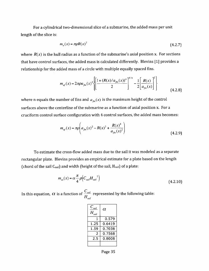
ma,(x) = a-p(CsaaHsau4 (4.2.10)

In this equation, a is a function of Csail represented by the following table:H'sail

Csaii aHsaii

1 0.5791.25 0.64191.59 0.7038

2 0.75682.5 0.8008

4 0.87185 0.8965

6.25 0.91678 0.9344

10 0.9469

Table 4.2: Added Mass Parameter a for a Rectangular Plate

For intermediate values of sail, a can be estimated by fitting an equation throughHsail

regression analysis. In this case:

)4Hsaal Hsaa

2

- .0835 CsaiiHsail

+ .3584 Csail +.3043Hsail

Using the relationships outlined above and integrating over the length of the

submarine by strip theory, the following expressions are derived for the cross-flow added

mass terms.

Xafpn ffn Xbow Xfsail

Y. = -f<ma(x~-f M,( )dx -Sfmaxfx - fmasxdxV

X tail Xapn Iffn Xasail

aan Xffn Xbow

Z. =-f5Mx)dx-fmfx)dx-f ma(x)dxXtail Xapn Xfpn

Xafin Xif, Xbow

M. = -fxm,(x)x -f xmaf<x)dx- fxma<x)dxW

Xafin

N. =-fxma(x)dxV

Xffn X bow Xfsail

-fxmjx )dx - f xma(X)dX - fxMasxdx

Y =N.r I

Z. =M.q W

Xa mdn X mjdn X ma d

M.=- a (.x)dx - f .,X~dX-5X2 M<a X~

(4.2.11)

Xafin Xffi Xbow Xfsadi

N. = -f x 2ma (x)dx -f x 2M<x)dx f x 2m(x)dX - fx2Ms(x)dx

xt Xfin Xffin Xsai (4.2.12)

4.2.3 ROLLING ADDED MASS

To account for the added mass due to the submarine rolling about the x axis, it was

assumed that the cylindrical sections of the hull do not incur any added mass in roll. This

leaves only the sections containing control surfaces and the sail as sources of added mass in

roll. For a section with four equally spaced fins in roll, Blevins [4] provides the following

formula for added mass in roll.

ma' ,.ollx)= -2pai a(X)4- ( (4.2.13)

where afi(x) is the fin height above the vehicle centerline.

The added mass for the sail was determined by using the added mass from

crossflow multiplied by mean height of the sail above the submarine centerline, Zsail, to

apply the appropriate lever arm:

mas roll a p(CsaHsa 2rsa

4 (4.2.14)

When combined and integrated over the appropriate area, the following added mass

equation is obtained for roll about the x axis:

X ffn Xfsail

K. = -2 Pfa, (x)4 dx -af-p(CsaHsa i s)

P JXn 4-a (4.2.15)

4.2.4 ADDED MASS CROSS TERMS

The coefficients from the rest of the added mass cross-terms are evaluated from

terms that are already derived (equations 4.2.16):

Xq = Z. Xq =Z. Xvr= -Y X, = -Y.w q v r

Yr =X. Y =-Z. Y =-Z.u W q

Z uq = -X. z = -Z. Z, =Y.U W r

M =-(Z. - X.) M, =-Y MP =(K. -N.) Muq =-Z.w u r p r q

Nu = -(X. -Y.) N, = Z. Nq =-(K. - M.) Nur =YU V q p q r

4.3 HYDRODYNAMIC DAMPING FORCES AND MOMENTS

Analytically calculating the hydrodynamic damping on a submarine is a difficult

task. The forces involved are highly nonlinear and coupled. To simplify the prediction of

damping forces, some assumptions are usually made. For this project, they are:

- Coupling velocities and accelerations are neglected. This assumption is

based on newton's second law, from which we expect the submarines inertia

forces to be linearly dependent on acceleration.

- The submarine is assumed to have port/stbd (x-z plane) and top/botton (x-y

plane) symmetry with the exception of the sail. This allows for the

elimination of many hydrodynamic coefficients that are negligible. Forces

and moments caused by the asymmetry of the sail will be addressed as

external forces.

- Damping terms greater than second-order are considered very small and

negligible.

There are certain observations that can be made on the damping forces on a submarine.

The damping is comprised of many different components including linear friction due to

laminar and turbulent boundary layers, damping from vortex shedding, radiation-induced

potential damping from body oscillations, and damping from waves. For the case of a

submarine, the damping is dominated by the first two.

The non-dimensional Reynolds number provides a measure of the ratio between

inertial and viscous forces for a body and is defined as:

uLRe = -

V (4.3.1)

where u is the speed of a body, L is the characteristic length of a body, and v is the

kinematic viscosity of the fluid. Seawater at 150 C has a kinematic viscosity of 1.19 X 10-6.

Full scale submarines are of several hundred feet in length and typically operate anywhere

from 2.5 to greater than 13 m/s. This means the Reynolds number is on the order of 108 to

109 - well beyond the transition range from laminar to turbulent flow that occurs at

Reynolds numbers between 10s and 2 X 106 [19]. Subsequently, the assumption that the

submarine will experience turbulent flow is an appropriate one.

4.3.1 AXIAL DRAG FORCE

The axial drag of a body moving through a fluid can be expressed by the following

equation:

AxialDrag = - pACd UjU2 (4.3.2)

where A is the frontal area of the body, p is the fluid density, Cd is the drag coefficient and

u is the fluid velocity. Drag coefficients are estimated from experiments such as tow tank

testing, or from empirical formulas. Several sources are available for empirical formulas of

streamlined body of revolutions [2][13][15][29]. Hoerner's [13] equation for a body of

revolution,

Cd = C, 1+1. 5 (D )32 + 7( )La Lai- (4.3.3)

is modified by Jackson [15] for submarines based on actual submarine resistance data:

C = C 1+1.5( )3'2 + 7 ( D) 3 +0.002(C, -0.6)La La - (4.3.4)

In these equations D is hull diameter, La is the length of the submarine afterbody, Cp is the

prismatic coefficient, and Cf is the frictional drag coefficient. This equation was determined

based on the area in the axial drag equation being the wetted surface area, As. Within the

bracket of the equation, the second term accounts for dynamic pressure, the third term

accounts for flow separation, and the fourth term - Jackson's modification - accounts for

the effects of parallel mid body. The frictional drag coefficient, Cf can be estimated from the

ITTC 1957 Line [26]:

0.075(Logo Re- 2)2 (4.3.5)

The frictional drag coefficient is dependent on Reynolds number - determined by speed

and length of the submarine. For simplicity in modeling, the drag coefficient can be

linearized about an assumed speed. In reality the frictional drag coefficient may vary from

as high as 0.0022 for slower speeds of 1 m/s to around 0.0016 for higher speeds of 13 m/s.

To calculate the axial drag of a submarine, additional terms must be applied.

Jackson adds an additional allowance, Ca to the drag calculation to account for roughness of

the hull, seawater suction and discharge pipes, and additional inaccuracies. He found that

Ca values can range from 0.0002 to 0.0015 for submarines. In addition to the allowance,

the resistance added by appendages such as the sail and control surfaces must be

accounted for. Both the sail and the control surfaces have their own areas and drag

coefficients based on their geometries. When combined, the total axial drag for a

submarine can be expressed as:

11AxialDrag = - pulu|[A,,(Cd+ Ca) + AaiCd sail +Acontrolsurface Cd controlsurface2 ~(4.3.6)

It is from this equation that the axial drag coefficient is found:

X ..= I p[As(Cd+ C )+ AiCd si + AcontrolsurfaeCd controlsurface

4.3.2 CROSSFLOW DRAG AND MOMENTS

To calculate the drag and moments generated by the flow of fluid across the

submarine, a strip theory approach - similar to that used in the calculation of crossflow

added mass in section 4.2.2 is utilized. Although the prediction of axial drag has been well

studied and there are empirical equations that allow for a fairly accurate prediction of the

axial drag analytically, it is very difficult to predict the crossflow drag of a submarine.

There are many non-linearities and complexities such as vortex shedding that are difficult

to predict without doing experimentation on either a scale model or a full size submarine.

Because of this, it is not uncommon to have significant inaccuracies in the prediction of

crossflow drag without model testing. The strip theory approach does, however, allow for

the calculation of the terms found in the equations of motion.

To use the strip theory approach, the cylindrical sections of the submarine are

modeled as 2-D circular discs. The drag coefficient, Cdc for such discs are dependent upon

Reynolds number, but for Reynolds numbers of around 104, Blevins finds the value of Cdc -

1.1 [3]. The crossflow drag from the control surfaces and sail must also be accounted for.

Since the control surfaces and sail are low aspect ratio foil sections, the drag coefficient for

these appendages, Cdc-cs and Cdc-sail, were estimated using empirical equations developed by

Whicker and Fehlner [30]. They found the drag coefficient to be dependent upon the shape

of the tips as well as the taper ratio, A, which is the ratio of the chord at the tip of the foil to

the chord at the base of the foil. For faired tips that are typical for the design of a

submarine sail:

Cdc sail =0.1+ 0.7A (4.3.8)

For square tips which are often seen on control surfaces:

Cdc__, =0.1+1.6A (4.3.9)

Applying strip theory and adding crossflow drag from appendages results in the

following expressions for drag coefficients:

Y = -pC 2R(x)dx -2 - PSCCdC cs PSsailCdc s ailXtail

Z= -- pC f 2R(x)dx - 2 -pSCedC

= Xbo -1 wl 2PCdc f 2xR(x)dx (2 2 PCsdc -c Xaisai~csiXtail

Nd =f p 2xR(x )dx - s 2xI ps c x saii PSsauil dcsail

= pC f2xR(x)dx+2xC IPSCS dCsY,.=- C 2Xtax 2

Y=-1 Xbow 1xl~xd - 1x~

rjr 2 PC&C f 2xRX~d -2x 2 ~PScsCdc cs ) - 2 XsailI Xsaii lPSsai Cdc- sailXtai

Z IpCd 2x x|R(x)dx + 2xcxc IpSCde cs

N - pC f x )dx - 2x pSCS dc - -- pas

Xtail

1 o /11N rjj P d f 2X R(x)dx - 2x c53 2PSCsCdc - 2 X alP ai dc al

1 Xbow 31 1M - -PC, f 2X R(x)dx - 2 x pCs - xj pSaC a

2 Xtal (2 / d(4.3.10)

where p is seawater density, R(x) is the radius of the hull as a function of axial length x, xcs

is the mid-chord axial location of the control surfaces, xsaiI is the mid-chord axial location of

the sail, Scs is the planform area of the control surfaces and Ssani is the planform area of the

sail. The effect that crossflow drag from the sail will have on roll moments can be

accounted for in a similar manner:

1K =- ZsailPSsailCdc sail

12 (4.3.11)

where Zsail is the mid-span vertical location of the sail.

4.3.3 ROLLING DRAG

The submarine will also encounter rolling resistance due to rotation about the x

axis. This resistance will be made up of frictional drag from the hull as well as the

crossflow drag from the sail and control surfaces. It is assumed that the drag in roll due to

the control surfaces and sail will be much greater that that of the hull; because of this the

rolling drag from the hull is neglected. Assuming four control surfaces, the following

rolling drag coefficient is obtained where zcs is the mid-span vertical location of the control

surfaces:

KPII = -4 1pSe C 3 pSsaildc sailZsail 32 (4.3.12)

4.4 BODY LIFT AND MOMENTS

When a slender body moves through a fluid at an angle of attack, helical body

vortices form which create a low pressure suction force. This suction force is usually

located aft of the bodies center of gravity which generates not only a lifting force, but also a

stabilizing moment due to the offset in the location of the force. For small angle of attacks,

these vortices are usually symmetric and stable - allowing for them to be modeled with a

certain degree of accuracy. At higher angles of attack however, the vortices become very

large and may shed asymmetrically which makes them very hard to model and predict.

There are different methods available for estimating the body lift due to angle of attacks,

especially at smaller angles. This project leverages work by Hoerner [14].

4.4.1 BODY LIFT FORCES

Hoerner provides experimental data from streamlined bodies and airplane fuselages

that can be used to predict the lifting forces and moments that are seen by a submarine

moving at an angle of attack. The lift on a body can be characterized by the equation:

Li I pACvU22 (4.4.1)

where A is the area referenced by the diameter of the body squared (A=d 2), Cy is the body

lift coefficient, p is fluid density and u is the forward velocity of the body. The body lift

coefficient can be expressed as:

C,= Cyo = 'Cy 0 /p8/3 (4.4.2)

where P is the angle of attack in degrees. Hoerner found that for streamline bodies with

length to diameter ratios from 5 to 10, the body life coefficient is roughly constant for

modest angles up to 8 to 15 degrees dependent upon body shape, and in terms of degrees is

roughly:

C,d0 =0.003(r in r(4.4.3)

or in radians

,180)CYd = Cyd~

(4.4.4)

The angle of attack is a function of the bodies translational velocities. In reference to the x-

y plane with angle of attack cc and the x-z plane with angle of attack P respectively it is

defined as:

V Wtana = tanp = -

U U (4.4.5)

The assumption that v and w are small compared to u allows for small angle

approximations and the linearization of the angle of attack:

V W

u u (4.4.6)

Using these relationships allows for the calculation of body lift force in the y and z

directions due to angle of attack:

Lift,,d-y = - 1pd 2 vC U2

Liftbd, = -- pd 2 Ca UW2 (4.4.7)

which results in the hydrodynamic body lift coefficients:

1YVI= -- Pd 2 Cd2

ZU, = -- pd 2Cy2 (4.4.8)

4.4.2 BODY LIFT MOMENTS

Hoerner found that for a round shaped streamlined body, the location of lift force is

between 60 to 70% of the length of the body as measured from the leading edge. This is

because the flow of fluid goes smoothly around the forward end of the body and only

develops a force on the leeward side of the after section of the body. For this project, it is

estimated that the center of lift occurs at a location of 65% from the submarine's bow.

Taking into account the origin of the submarine being located at the center of buoyancy, the

moment arm generated by the lift force can be defined as:

xfift = -0.65 -xcb (4.4.9)

where xaift is the location of the lift force, 1 is the submarine length, and Xcb is the location of

the origin (center of buoyancy) measured from bow.

When combined with the lift force, the coefficients for moments caused by body lift

are obtained:

NUV =-pd 2CydXlft2

M, 1= - pd 2C yd lifU!2C ft (4.4.10)

4.5 CONTROL SURFACE LIFT AND MOMENTS

Submarines typically use movable control surfaces to impart forces and moments

that allow for changes in pitch and/or yaw. There are various control surface

configurations that may be used, some of which are graphically depicted in Figure 4.3 [5].

(b)

(d)

Figure 4.3: Alternative Control Surface Configurations

The baseline submarine uses a standard cruciform configuration (configuration (a) in

figure 4.3). In this setup, pitch is controlled with two horizontal stern planes and yaw is

controlled with two vertical rudders. These control surfaces are linked such that both

rudders move together, and both stern planes move together.

4.5.1 CONTROL SURFACE LIFT

The lift generated by a control surface can be expressed as:

1Lift =-pCSV26 (4.5.1)

2

where CL is the lift coefficient of the control surface, Scs is the planform area of the control

surface, V is the total inflow velocity of the fluid, and 6e is the effective effective angle of

attack for the control surface. Hoerner [14] and Triantafyllou [27] provide empirical

equations for estimating the lift coefficient of a control surface:

L = (4.5.2)do

and

C - -CL (4.5.3)1 o 1 1

2ax x(AR,) 2xr(ARe) 2

where a = 0.9, and ARe is the effective aspect ratio of the control surface taking into

account mirroring effects due to proximity to the hull. It can be found by:

ARe = 2(AR) = 2 Span" = 2 .Span2 (4.5.4)Chordc, Areac5

The effective angle of attack of the control surfaces (6re for rudders and 6 se for stern

planes) is comprised of the summation of two components: 1) the angle of the control

surface relative to zero angle (6r for rudders and 6 s for stern planes) and 2) the effective

inflow angle of the fluid (pre for rudders and pse for stern planes).

re = r ire

se = ,- Pse (4.5.5)

The geometry of these components are illustrated in figures 4.4 and 4.5.

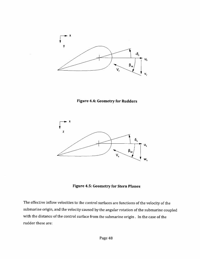
Kx

Figure 4.4: Geometry for Rudders

V

Figure 4.5: Geometry for Stern Planes

The effective inflow velocities to the control surfaces are functions of the velocity of the

submarine origin, and the velocity caused by the angular rotation of the submarine coupled

with the distance of the control surface from the submarine origin. In the case of the

rudder these are:

U, = u+ zq - y~r

V, =V + xrr - zIP

w, = w + yrp - xq (4.5.6)

where Xr, Yr, and Zr are the distances of the rudder from the submarine origin. For this

submarine, the values of yr and Zr are very small relative to the velocities of the submarine

and are therefore neglected. Because the rudders are located far aft in the submarine, the

xr terms can be significant when coupled with rotational velocity. This simplifies these

terms to be:

Ur u

v, v + xrr

w,.- w - x,q (4.5.7)

When combined with the geometric property,

tan(p,.) = vr (4.5.8)Ur

with the assumption of small angles and performing a similar derivation for the stern

planes, the effective inflow angles can be approximated by:

V 1Pre = -(v +xr)

U, U

W = (w -xq) (4.5.9)

With the effective angle of attack for the control surfaces determined, the total lift forces

generated by those surfaces can be approximated by substituting equations 4.5.9, 4.5.5, and

4.5.3 into 4.5.1:

Yudder = pCL6 Sr (U2 - uv - Xrur)2

1Zsternpanes = -- pC6 S(u 2 S + uw - xsuq) (4.5.10)

2

Taking into account two rudders and two stern planes, these can be broken down into the

individual hydrodynamic coefficients:

Ylu6 = -Y uj = PCL6 Sx,

Y,,, = -PCL SX

Zuu = Zuw = -PCL6 SsX

Zu = PCLb Sxs (4.5.11)

4.5.2 CONTROL SURFACE MOMENTS

The axial location of the control surfaces generates a moment on the submarine

when the coupled with the lift force. This yields the following expressions for moments due

to lift:

NATe, =1 - pCL S,.x,(U 2 6, - uv - xrur)''rudder 2 C 6S- r rrr

2

1Mnes = - PCL6 SXs(U 26,+ uw - xuq) (4.5.12)

As in section 4.5.1, counting for two control surfaces each, the coefficients become:

N = -Nvf = PCL6 SrXr

Nur = -PLb r r

MU 6 , = Mu.f = PCLo SsXs

Mu = -pCL6 Ssx2 (4.5.13)

4.5.3 CONTROL SURFACE DRAG

For conditions in which the submarine is not turning, it is appropriate for the drag

from the control surfaces to be included as part of the axial drag - as is done in section

4.2.1. When the control surfaces are at an angle of attack due to either deflection or

submarine motions, the drag coefficient for control surfaces changes as a function of

effective angle of attack. Whicker and Fehlner found that the drag coefficient, CD can be

computed with reasonable accuracy based on the following equation [30]:

CD = C + CL2 (4.5.14)x(ARee)

where Cdois the minimum section drag coefficient (equal to .0065 for NACA 0015 section,

ARe is the effective aspect ratio of the control surface taking into account mirroring due to

hull interaction, and e is the Oswald efficiency factor (e=0.90). As CL is a function of

effective angle of attack, so is CD. This allows for the drag of the control surfaces to be

calculated:

1Drageon=su,1aces = S C VD 2 (4.5.15)

2 C

The total inflow velocity, V, can be determined from the effective inflow velocities

described in section 4.5.1. Using the simplified expressions for effective inflow velocities of

equations 4.5.7 we obtain:

Vrudder = (u2 + v +xrr)2

Vsternpanes = u2 + (w -xqq) 2 (4.5.16)

Although the approximations of equations 4.5.10 and 4.5.12 are relatively accurate

for predicting the lift and moments generated by the control surfaces, they do not account

for the induced drag that is imparted on the submarine due to lift. Lift is always generated

perpendicular to the inflow velocity of the fluid. Because the effective inflow angle of fluid

is not always in line with the direction of the hull, the lift generated will have a component

in the axial direction which contributes to the axial force on the control surface. Figure 4.6

shows these force components for the rudder.

TotalResultantForce

I DDrag, D >

NormalA. Force, Fy

A

Lift, L

\

/Axial Force,

F .

Figure 4.6: Forces on Rudder

The axial and normal forces, as well as the moment (Qzr) from the rudders can be

determined from simple geometry such that:

Xidd, = F, = L sin(re) - Drag,,d, cos(Pre)

Yrudder =Fr = Liftruder COS(,, )+ Drage, sin(pre)

Nrudder = Q,, = Yudder r

Similarly for the stern planes:

Xste,rnplanes =F = Lifts,,,.n,,an,, sin(3,) - D , cos(fP,,)

ZSte,,,plae = F = Liftsternpaes cos(Pse )+ Drag,,,rp, sin(P,,)

Arudder = QZ = -Zsternplanes Xs

Y

Total inflowVelocity (V)

ur

v

(4.5.17)

(4.5.18)

4.6 SAIL LIFT AND MOMENTS

The sail of a submarine is foil section, not unlike a control surface. They are however,

much larger, asymmetrically located, and not movable. The same basic principles outlined

in section 4.5 apply to the sail with the major difference being that the effective angle of

attack of the sail is comprised entirely by the effective inflow velocities at the sail. An

approach similar to section 4.5.3 is applied to the sail with the following exceptions:

1. The vertical location of the sail, Zsail cannot be neglected.

2. The asymmetry of the sail imparts a moment about the x axis in roll.

3. The effective angle of attack, 5 saile, is equal to the effective inflow angle, Psain.

The effective inflow velocities for the sail,

sail = + ail Ysailr

sail xsailr - ZsailP

Wsail = W + YsailP - sailq (4.6.1)

can be simplified knowing that ysaii is zero:

sail sailq

sail = V + xsadr - ZsailP

wsail =wXsailq (4.6.2)

This leads to the angle of attack for the sail being defined as,

p = tan-' ( = tan-i (V + xsair - zsaip (4.6.3)Usail U + Zsailq

and the effective inflow velocity:

Vil ~ j(u+ zsauq)2 + (v + Xsail r - zsailP)2 (4.6.4)

With these parameters defined, the same fundamental equations in section 4.5 for

Lift and Drag - as well as their coefficients can be used to calculate those values for the sail.

Using the same geometry defined in figure 4.4 and applying it to the sail yields:

Xsai = Fs = Liftsal sin(#,ai) - Drag,ai Co(/s#,i)

Ysa = F, = Lifta cos(p01 ) + Dragsaal sin(fisail)

Nsal = Qai = sailxsail

Ksail = QT, = -Ysai

4.7 PROPELLER FORCES AND MOMENTS

(4.6.5)

Propellers are typically used to develop the axial thrust force required to propel a

submarine at forward speed. To achieve a steady-state speed, the thrust force generated

by the propeller must equal the resistance generated by the hull, appendages, and

resistance effects due to the interactions between the hull and the propeller. There is

standard nomenclature to describe the parameters and metrics that are used to define the

operational characteristics of a propeller. Table 4.3 lists the basic parameters.

Parameter Describtion UnitsJ Advance Coefficent Non-DimKT Thrust Coefficient Non-DimKQ Torque Coefficient Non-Dimn Propeller rotational speed rev/sV Vessel Speed m/sVA Advance Velocity m/sT Thrust NQ Torque N-rnD Propeller Diameter mrio Open Water Efficiency Non-DimCT Thrust Coefficient Non-DimCQ Torque Coefficient Non-Dim

Advance Angle at 70% Radius Degw Wake fraction Non-Dimt Thrust deduction factor Non-Dimp Seawater Density Kg/m 3

Table 4.3: Propeller Nomenclature

The advance ratio is defined as,

j VAJ=A

nD

where the advance velocity is:

VA =V (1- w)

(4.7.1)

(4.7.2)

From equation 4.7.2, we see that the wake fraction provides a measure of determining the

incoming velocity into the propeller as a function of submarine speed. The wake fraction is

highly dependent upon the hull shape and is often derived from model testing and working

trial results backward based on data from full scale ships and submarines. Parametric

studies for single screw submarines have been done resulting in the following equation

that provides a means of estimating the wake fraction [15]:

w =1-0.371- 3.04 D (4.7.3)

where Ws is the wetted surface of the submarine. The thrust that must be generated by the

propeller must equal the resistance of the hull to achieve a required speed. When a

propeller is placed behind a submarine it increases the apparent resistance of the hull due

to a reduction in pressure seen at the forward end of the propeller blades. This increased

resistance is accounted for by the thrust deduction coefficient, t, such that:

T =R (4.7.4)(1- t)

where R is the hull resistance at a given speed. Similar to the wake fraction, regression

equations are available that allow for the prediction of the thrust deduction coefficient

[15]:

t =1- .632 - 2.44 D (4.7.5)

The thrust and torque coefficients, KT and KQ, are the coefficients normally used when

describing propellers. They are defined as:

KT- T

pn2D4

K = (4.7.6)Spn 2D 5

These coefficients, along with To, can be plotted as a function of advance coefficient. The

resulting graph, known as an open water diagram to signify the propellers performance

when not in interaction with a hull, is dependent upon the specific propeller geometry and

characteristics. A representative open water diagram is provided in figure 4.7.

"t,

00 0 2 014 06

AtvK~ew: a'o J

0 1) 18

Figure 4.7: Open Water Propeller Diagram

For most propellers, these graphs are developed only for the condition where there

is a positive ship speed and a positive propeller speed - a condition known as the first

quadrant. Other quadrants exist according to ship and propeller speeds, and are

summarized in table 4.4.

Quadrant Description Ship Speed (V) Propeller Speed (n) Beta (13)

1 Ahead + + 0-902 Crashahead -_+ 270-3603 Crashback + - 90-1804 Backing -_- 180-270

Table 4.4: Propeller Operating Quadrants

Here the advance angle at 70% radius, P is defined as:

1V/=tan' A0.7zcnD (4.7.7)

To determine the performance characteristics at quadrants other than the 1st requires the

open water diagrams to be expanded to cover all four quadrants such as those shown in

figure 4.8. This is not typically done for propellers and doing so presents problems since

when propeller speed approaches zero, the advance coefficient, KT, and KQ all approach

infinity and have a discontinuity.

K 10OKQ KT

10K0

negative v, positive vpositive \n, positive n,

positive v,negative n,

negative v,negative n,

Figure 4.8 Propeller Operating Quadrants

To resolve the characterization of four quadrant thrust and torque performance curves are

usually presented using the CT and CQ coefficients a function of P. CT and CQ are defined as:

T 8KTC = = +

' (V +(0.72nD) D2 2 +(0.7.7)22 4

T 8 KQCQ 1(VA2 +(0.7J7nD)2) ' D3 r2+(0.7)2

2 4

(4.7.8)

The Maritime Research Institute Netherland (MARIN) has conducted 4 quadrant propeller

data on several of the Wageningen B-Screw Series of propeller blades. The data from this

testing has been faired by regression to allow for the CT and CQ coefficients to be

determined for 14 of these propellers covering a range of blade numbers, pitch/diameter

ratios, and expanded area ratios [24]. The coefficients can be determined through a

summation of regression coefficients:

CT = f ~AT(k)cos(kP3) + BT(k) sin(k3)}

0

CQ I (FOI{AQ (k) cos(k3) + BQ (k) sin(k3)}k= 0

(4.7.9)

where the regression coefficients are unique to the particular blade series. The regression

coefficients for the 5-bladed B5-75 series with a pitch/diameter ratio of 1.0 as an example

are:

K AT(k) BT(k) AQ(k) BQ(k)0 2.38E+00 0.00E+00 -3.62E+00 0.OOE+001 1.83E+01 -7.79E+01 -2.79E+01 1.16E+022 2.05E+00 -1.08E+00 -6.63E-01 -2.32E+003 3.04E+00 1.14E+01 -5.45E+00 -1.82E+014 -1.89E+00 -1.34E+00 2.93E+00 3.13E+005 -4.58E+00 4.48E+00 6.63E+00 -8.56E+006 7.30E-02 1.33E+00 -1.17E+00 -1.98E+007 3.07E+00 -2.58E-01 -6.17E+00 1.62E+008 3.09E-02 -7.94E-01 8.16E-01 1.98E+009 -1.48E+00 1.69E+00 3.10E+00 -2.55E+0010 3.30E-01 9.53E-01 -9.59E-01 -1.41E+0011 2.14E+00 4.88E-01 -2.82E+00 -9.20E-0112 -1.75E-01 -4.35E-01 1.04E+00 1.03E+0013 2.13E-01 6.79E-01 -1.08E+00 -1.13E+0014 5.65E-01 5.35E-02 -1.12E+00 -1.32E-0115 9.91E-01 -4.86E-01 -1.07E+00 1.27E+0016 -3.94E-01 -1.46E-01 1.28E+00 5.54E-0217 4.53E-01 9.07E-02 -4.27E-01 -6.85E-0118 5.39E-01 7.10E-02 -7.10E-01 -2.33E-0119 4.01E-01 -7.60E-01 -5.47E-01 1.50E+0020 -3.74E-01 -1.56E-01 5.58E-01 -1.36E-0321 3.94E-02 -2.63E-01 -6.83E-02 -6.89E-0222 1.31E-01 -2.92E-02 -4.54E-01 3.13E-0123 -1.27E-01 -5.56E-01 3.86E-01 6.71E-0124 -1.72E-01 7.01E-02 4.36E-01 -2.53E-0125 -1.56E-01 -5.69E-02 -1.06E-01 4.31E-0226 8.81E-02 -9.11E-02 -2.08E-01 2.05E-0127 -3.31E-01 -2.04E-01 5.49E-01 3.82E-0128 -6.73E-02 1.28E-01 3.41E-01 -3.24E-0129 -1.26E-01 6.77E-02 3.56E-02 -3.29E-0130 7.86E-02 -5.43E-02 -8.52E-02 2.54E-01

Table 4.5: Four Quadrant Coeffients for Wageningen B5-75, P/D=1.0 Propeller

This allows for a regression fit of the four quadrant graph for the B5-75 P/D=1.0 series as

shown in figure 4.9:

000

C)-5

Beta

Figure 4.9 Four Quadrant Diagram

This information allows for the thrust and torque to be found for any submarine speed and

shaft rpm, including crashback maneuvers that would occur as part of the response to a

jammed control surface casualty. Any of the 14 Wageningen B-Screw Series that have four

quadrant regression coefficients can be modeled. The thrust and torque can be expressed

in the vehicle force notation as:

Xprop T

(4.7.10)K prop = Q

4.8 AZIMUTHING PODDED PROPULSOR FORCES AND MOMENTS

Azimuthing propulsion pods have been used with increasing frequency on surface

ships, especially on cruise ships. They generally provide improved maneuverability due to

their ability to provide forces at any angle [18]. On submarines their use has been limited

to units that assist in slow speed maneuvers. Their application as the primary propulsion

CT

- -II

has not been done on submarines. To do so would allow the forces and moments created

by the azimuthing pods to replace the forces that are typically generated by the aft control

surfaces and the propeller.

Studies on the force and moment predictions from azimuthing pods have been done.

Stettler characterized the quasi-steady vectored maneuvering forces associated with an

podded propulsor to include the unsteady transient maneuvering forces caused by rapid

changes in azimuth angle and propeller speeds [27]. In his work he developed non-

dimensionalized coefficients to predict the axial (Fx) and normal (Fy) forces for a range of

advance ratios from 0 to 0.58, and azimuth angles over the range of +/- 180 degrees. He

also developed pod-only force coefficients over an azimuth angle of +/- 180 degrees to

account for the forces associated only with the pods' orientation. Figure 4.10 shows the

basic geometry involved with the azimuthing pods in the x-y plane. In this case 6 is the

propulsor azimuth angle and p is the effective inflow angle of the fluid.

X

y

U

FF--t- -----

T

Figure 4.10: Azimuthing Pod Geometry

The effective angle of attack of the pod, a, is found in a similar fashion as the effective angle

of attack of the control surfaces derived in section 4.5.

a pod =pol - fpod (4.8.1)

The non-dimensional force coefficients for surge and sway are:

K =f2',pn 2D4

K = FY (4.8.2)F pn2D4

Knowing the axial distance of the pod from the submarine's origin, Xpod, also allows for the

moment generated by the pod about the z axis to be calculated. These coefficients are

applicable for the x-z plane as well with the exception that sway force is in the z direction

and the moment is about the y axis. In this case the KFx coefficient is the same but the KFy

coefficient would be KFz and the angle of attack for the pod would be based on the x-z

velocites. If the pods operate independently of one another, a moment about the x axis is

also generated dependent upon the pods radial position from the vehicle centerline -

expressed as either ypod or Zpod. These moments, along with the forces in the vehicle force

notation are:

Xpod = F,

Y,, = F,Zod -F

Zpod = F

Npod =Z =pod Xpod

M,pod Q, - -ZodXpod

Kpod QX= -YodZpod ZpodYpod (4.8.3)

Figure 4.11 shows graphs of the force coefficients against azimuth angle. Figure 4.12

shows a graph of the pod-only axial and normal force coefficients against azimuth angle,

which allow for the modeling of the pods when the propeller is not turning. It should be

noted that for this data the azimuth angle is equal to the angle of attack of the pod.

0 t 04

* A

J 0 30J*0 36 J As 0 58

Ja0 48

J - 0 42

K d

K cot) intefp

-50 0 50 100 150

Quasi--steact swi.ay fotc(e tF 1 As aamuth angle vi advime coefcoiuni

,A0r/V

[7f i

J= 0 0 01-0 05

-00 15_01 ~ 3 0

-02

-0 25

K_ - data

K. - cubic intewp

J w 0 30J v 0 36

1 0 J = 0 42'J50 58 . 0-'50 -100 -50 0 50 100 150

Figure 4.11: Azimuthing Pod Force Coefficients

J=*0 1*4J 006

J3 000005

0

005

01

0 15

/

0 &5h

t

-150 _100

0 25

02

0 15

0.1

005

Sa 0 12

Ou~r -Je , sny fr e a armth ape advnco oefilm

it

w

Pod-only force measurements vs. azimuth angle (U = 2.62 ft/s)5

4 -3-

-n

c0

-2

-

Axial force: C =Fa Po2A

-3 Cubic interpNormal force: C=F /0 5pU2A

- Cubic interp-4 Moment C,=M /0 SpU2A LCubic interp

-5-150 -100 -50 0 50 100 150

8 (deg)

Figure 4.12 Pod-Only Force Coefficients

The bare hull hydrodynamic coefficients are assumed to be the same for the

conventionally propelled submarine and one with azimuthing podded propulsion. The

significant differences in modeling are the lack of aft control surfaces and the propeller

being replaced by the pods. Since the radial position of the pods are away from the

centerline of the submarines, the wake fraction used in calculating the advance coefficient

will be a function of the distance from the hull. The wake fraction determined in section 4.7

is the average wake fraction behind the hull. Because of this it is assumed that this will also

be representative of the wake fraction seen by the pods.

A limitation in the data is that it does not allow for crashback conditions of the pods.

In practice, this might be an immediate response by the crew for certain casualties. To

address this, in situations where reverse thrust is required, the pods will be rotated to the

180 degree position. This would likely provide improved thrust characteristics in slowing

forward movement of the submarine since the propellers will be rotating in their designed

forward rotations.

4.9 SUMMATION OF FORCES AND MOMENTS

4.9.1 CROSS TERMS

The different cross-terms from equations 4.2.16, 4.4.8, and 4.5.11 must be combined

to get the total hydrodynamic coefficients on the submarine.

Y" =Y", +Y4

Y =Y", +Y

zuw u ZW+ uwf

Zuq = Z uqf + Zu4

M. = Ma + MWf + Mui

Muq = Muqa + Mu,

N,= Nuva + Nuvi + NU,

Nur Nura + Nur (4.9.1)

Since the control surfaces and sail are accounted for as external forces, they are dropped

from the equations above, leaving only the added mass and body lift force and moment

contributions to the hydrodynamic coefficients.

4.9.2 TOTAL FORCES AND MOMENTS

All the forces and moment coefficients associated with the vehicle are combined

with the external forces from the various components. Equations 4.9.2 below show the

summation of the external forces and moments for the conventional submarine

configuration with propeller and aft control surfaces:

Xex, = XHS + X. U+ Xwq+Xqq + Xvr + Xrr + X + X. + X + Xsenplanes + X }U

Y ,=YHSY.+ r+ Yur + pq+Yvu +Yvv|+Y rr+Yi +{Y },ext =HS u, vpvp WP + , + Ypq u v r r + }rudderV r V

Zext HS + . W+Z. q+ Zuquq + Z~vp + Zrprp + Zuuw + Zw1W WW + Z qlqjqlql +f {Zsternpanes}W q

Ke,= KHS + K. p+ K, rlr|+ K v v|+ Kpp|PpI+ Ksati +{Kprop }p

M, = MHS + M. w+ M. q+ M-uw + Muquq + Mvpvp + Mrprp + M w| + M qq|qq + M }w q

Next = NHS + N. v+ N. r+ Nuur + NUuv + Nwp+ Npqpq + N v v|+ Nrrlr rl + Nsai, + {Nrudder}v r

These equations can be modified to account for the azimuthing pods by replacing the

control surface and prop forces/moments in {.} with the forces/moments associated with

the pods in section 4.8.

4.10 EMPIRICAL DATA

The selection of the DARPA SUBOFF Hullform allowed for the utilization of many

non-dimensional hydrostatic coefficients obtained from captive model measurements

obtained from planar motion mechanism (PMM) testing by NSWCCD [23]. Empirical

coefficients were utilized to the maximum extent possible. For those coefficients that were

not available, the coefficients were obtained using the analytical approach described in this

chapter.

CHAPTER 5 MODEL ARCHITECTURE

To simulate the maneuvering characteristics and response of the submarine, a

MATLAB program was created that utilized the SIMULINK modeling tool. This MATLAB

program consists of two scripts that serve different functions and one SIMULINK model:

1. A MATLAB script is utilized to generate and define the geometric characteristics of

the submarine and the hydrodynamic coefficients, and store them in a matrix.

2. A separate "Driver" MATLAB script is used to load the data from the first script as

well as the four quadrant propeller data. This script runs the SIMULINK model

simulation for a set period of time and is used to retrieve and display data obtained

during the simulation.

3. A SIMULINK model is used as the main tool during the simulation. This model links

together different force inputs and solves the equations of motion in discrete time

steps to predict the motion of the submarine as a function of time. A schematic

representation of the SIMULINK model is shown in figure 5.1.

Figure 5.1: Schematic of SIMULINK Model

5.1 SIMULINK MODEL

Several distinct blocks are used to create the complete SIMULINK model. Each of

these blocks consist of separate input variables that change as a function of time and an

embedded MATLAB script that utilizes the input variables to calculate output variables that

are used in other blocks. The variables are calculated in separate time steps as the

SIMULINK model is sequentially analyzed from start to finish.

5.1.1 CONSTANT BLOCK

The constant block is utilized to define input variables for use in other blocks. This

block is defined in a previously run hydrostatic coefficient MATLAB script and loaded by

the 'Driver' script for use in SIMULINK. It is also used to define four quadrant propeller

data.

5.1.2 COORDINATE TRANSFORMATION BLOCK

The coordinate transfer block utilizes the coordinate transformation matrices

derived in chapter 3.1. The body fixed submarine translational and rotational velocities are

used as input variables and transformed into inertial frame translational and rotational

velocities. These inertial frame translational and rotational velocities are then integrated

to obtain an inertial frame location and orientation, which is then used in other blocks.

5.1.3 INTEGRATOR BLOCK

This block takes the submarine vehicle accelerations that are solved for in the

maneuvering block and integrates them to determine the submarine vehicle velocities.

5.1.4 PROPELLER DYNAMICS BLOCK

This block is based on the theory described in chapter 4.7. It uses submarine

velocity, data from the constant block, and a user configurable propeller RPM scheme as

input variables. The embedded MATLAB script then calculates the resultant thrust and

torque that serve as inputs to the maneuvering block.

5.1.5 CONTROL SURFACE EFFECTS BLOCKS

The control surface effects blocks are used to calculate the external forces and

moments generated by the rudder, sternplanes, bowplanes, and sail described in chapter

4.5. Separate blocks are used for each control surface. These blocks use vehicle

translational and rotational velocities as well as a user configurable scheme that defines the

control surface deflections as inputs. The embedded MATLAB script in these blocks then

calculate effective inflow velocities, angle of attacks, lift and drag. The forces and moments

generated on the submarine by the control surfaces are provided as outputs which are then

used in the maneuvering block.

5.1.6 AZIPOD DYNAMICS BLOCKS

These blocks are used to calculate the forces and moments generated by the podded

propulsion units. These characteristics are outlined in chapter 4.8. For inputs the blocks

utilize the submarine velocities as well as two user defined and configurable variables: 1)

The RPM scheme of the pod and 2) The azimuth angle of the pod. These inputs are initially

used to calculate the effective azimuth angle and the advance ratio. These values are then

used to determine the quasi-steady surge and sway force coefficients that are then used to

calculate the forces and moments generated on the submarine by the pods, which are input

to the maneuvering block.

5.1.7 EMBT BLOCK

The EMBT Block is used to calculate the various dynamics associated with an EMBT

blow. This block utilizes several inputs, including data from the constant block, submarine

depth, as well two inputs that are determined by the output of the EMBT block:

1. The amount of air cumulatively blown by the EMBT system

2. The current air bank pressure

An additional input is the user decision of the time during the simulation at which to

initiate the EMBT blow. The dynamics of this block are described in chapter 4.1.1. The

outputs of buoyancy and longitudinal center of buoyancy are used as inputs to the

maneuvering block. The outputs of blow rate and air bank pressure rate are integrated to

obtain the inputs of blown air and air bank pressure, respectively.

5.1.8 MANEUVERING BLOCK

The maneuvering block receives multiple types of input used to solve the nonlinear

equations of motion to determine the submarine's translational and rotational

accelerations for a given time period during a SIMULINK simulation. The various inputs

into this block include:

1. Submarine translational and rotational velocities (u, v, w, p, q, r): These are

obtained from the output of the integrator block.

2. Submarine orientation (CO,$): The inertial frame orientation of the vehicle

is obtained from the output of the coordinate transfer block.

3. Submarine constants: These inputs, loaded from the constant block, include

the geometric properties, mass properties, moments of inertia, and

hydrodynamic coefficients of the submarine.

4. External forces and moments (Fx, Fy, Fz, Qx, Qy, Qz): These inputs are the

summation of the forces and moments due to the combined outputs of the

propeller dynamics block, the control surface effect's blocks, and azipod

dynamics blocks.

5. Buoyancy characteristics (B, xB): These inputs, obtained from the EMBT

block, take into account the change in buoyancy and the longitudinal center

of buoyancy as a function of an EMBT blow.

The maneuvering block solves for the accelerations of the submarine using the

combined nonlinear equations of motion. These accelerations are the output of this block

which serve as the input to the integration block.

5.2 NONLINEAR EQUATIONS OF MOTION

The governing equations of motion for translation and rotation (3.1.15) can be combined

with the external force and moment equations (4.9.2) to develop the combined nonlinear

equations of motion in all six degrees of motion.

For translation in the x direction:

m u+ qw - rv - xG + r 2 ) + ZG(pr +

XHS + X. u+ Xwwqq + Xqqqq + Xvrvr + Xrrr + (5.2.1)

XuluU+ Xsai +{ Xrudder + Xsternpanes + X prop}

For translation in the y direction:

m v-wp+ ur+xG(qp+r)+ZG(qr-p)

YHS+ Y ur wwp +Yqpq +Yuv + (5.2.2)v r

Yvv|+Y + Ysai + {Yr}dde

For translation in the z direction:

mw-uq+vp+xG(rP -q)-ZG(P +q2

ZHS+Z.w+ Z. q+ Zuquq +ZvpVp +Zrprp + ZU + (5.2.3)W q

wwW + Zqqqq + {Z sternplanes

For rotation about the x-axis:

I, p+ (I - rq - mzG(V WP + ur)(5.2.4)

KHS + K. p+ Krlrir r + Kv v + KM pp + Ksaii + {Kprop (

For rotation about the y-axis:

q+ rp + m ZG(-vr+ wq) - XG(Wuq+ vp)]

MHS + M. w+ M. q+ Mwuw + Muquq+ M,,vp+ Mrp rp+ (5.2.5)w q

M ww|+ MiVqlq|qlq+ {Msternplanes}

For rotation about the z-axis:

Iz r+ (I,, - I.)pq +mxG(v wp + ur)

NHS + N. v+ N. r+ Nurur + Nuvvv + Nwwp + Npqpq + (5.2.6)v r

Nvv|v~vI + N, rlr + Nsaii + {N}dd

As in chapter 4.9, these equations are modified for the azimuthing pods by replacing the

control surface and propeller force and moment terms in {.} with the forces and moments

from the pods. To allow for the acceleration terms of the submarine to be calculated, they

are separated from the rest of the terms such that the combined equations of motion are

rewritten as:

For translation in x direction:

(m - X.) u+ mzGq=X + (Xwq -m)wq+(Xqq + $x)qqU

+(Xv, + m)vr + (Xrr + mxG)rr + Xa U U - MZGpr +Xsail + (5.2.7)

{ X, e,+ sternplanes + Xprop

For translation in y direction:

(m -Y.)v- mZG p+ (mxG -Y)r=YHS + (Yur - m)ur+v r

(Y,+ m)wp + (Ypq - mxG)pq+Y uv +Y 1 vIv +Y r r + (5.2.8)

mzGqr + sai rudder}

For translation in z direction:

(m - Z. )w-(mxG+ Z.)q=ZHS +(Zuq m)uq +W q

(Z - m)vp + (Zrp - mxG)rp + Z uw + Zw + (5.2.9)

Z qqqq + mZG (P+ q2 ) + {Zsternplanes}

For rotation about x-axis:

-mG V+(I - K. ) p =KHS + K rr|+ Kv vv + K 1pp| -P (5.2.10)

(I, - I,,)qr + m(uq - vp) - mZG(wp - ur) + Ksaii + {Kpr}

For rotation about y-axis:

mZG u- (mxG + M. )w+ (I, - M. )q = MHS + MUWuw +W q

(Muq - mxG)uq +(M, + mxG)vp +(M, - (I - I,))rp + (5.2.11)

M wW| + M qlqqq + mZG(vr - wq) + {Msernplanes}

For rotation about z-axis:

(mxG -N.)v+ (I, - N.)r = NHS + (Nur - mxG)ur + Nuuv +V r

(NW, - mxG)wp + (NP, -(I,, - Ix))pq + N, vv| + Nrlr|rlrl +

Nsaii + {Ndde }

Equations 5.2.7 through 5.2.12 can be expressed in matrix form:

0

(m - Y.)V

0

-mZG

0 -(MXG+M.)

-N.) 0

0

0

(m-Z.)

0

-mzG

0 -(mx

0 (I,,0

MZG U

0 (MXG - Y)r

G+Z.) 0q0 0-M.) 0

qo (Iz - N.)

r

This allows for the acceleration terms to be solved for by the following equation:

0

0

(m-Z.)w

0

-(MXG +M.)w

0

0

-mZG

0

(Iu - K.)

0

0

mZG U

0 (MXG -Y)

-(mxG +Z.)q0

(I, ,-M.)q

0

0

(Izz -N.)r

(5.2.12)

(m - X.)U

0

0

0

mZG

0 (In - K.)

0 (mxG

(5.2.13)

(m-X.)U

0

0

0

mzG

0

0

(m - Y.)V

0

-mZG

0

(MXG -N.)V

x

K yj zI K

I M

I N

(5.2.14)

5.3 NUMERICAL SOLUTION TO THE NONLINEAR EQUATIONS OF MOTION

In the case of the nonlinear equations of motion in equation 5.2.14, the accelerations

can be expressed as a vector:

x n = f (x,,I) (5.3.1)

where xn is the state of the submarines kinematics at a time step n:

x = [u'v'w,p,q,r,x,y,z,,8,tp] (5.3.2)

and I is the input forces, moments, and other dynamics at a time step n:

I, = [F,,F,FZ,Q,,QY,Q,,B,xB] (5.3.3)

The accelerations in the nonlinear equations of motion are solved by using

numerical ordinary differential equation (ODE) solvers inherent in MATLAB. There are

several solvers in MATLABs library that are available and are grouped in two main types:

fixed-step and variable-step solvers. In their most basic form, these solvers take the state

of the submarine at a given time, xn, and calculate the rate of change of those states, xn, at

that time. This rate of change x is then multiplied by a time step At and added to original

state to determine the state of the submarine at the next time step. This can be expressed

mathematically by a first order Euler's Method solver:

Xn+i = x, + xn At (5.3.4)

A fixed-step solver uses a defined time step that does not vary while a variable-step

solver adjusts the time-steps such that larger time steps are used during times when the

dynamics of the model are not rapidly changing and smaller time steps are used when the

dynamics of the model are rapidly changing. A variable-step solver is typically used to

reduce computational simulation time, however for this thesis, a fourth order fixed-step

solver using the Runge-Kutta integration technique was used.

5.3.1 RUNGE-KUTTA SOLVER

The Runge-Kutta method improves on the accuracy of the Euler's Method by using a

weighted average of a slope over a time step. For this method, the slope at four points are

calculated:

k, = xn + f (xI ,I)

k2 =f x+ At k1 I2 n+-

)2 (5 .3 .5 )

k3 =f x+ Atk2,I2 n+-

k4 =f(x + Atk,Ij)

where k1 is the slope at the beginning of the time step, k2 is the slope at the midpoint of the

time step using k1, k3 is the slope at the midpoint of the time step using k2 and k4 is the

slope at the end of the time step using k3, and the input vector:

I I = -(I, + I,,,) (5.3.6)n+g 2

These slopes are then weighted to find an average slope and the state at the next time step:

AtXn+i = x, + -(k + 2k2+ 2k3+ k4) (5.3.7)

6

CHAPTER 6 MANEUVERING ANALYSIS

The maneuvering performance of the two submarine configurations is detailed in this

chapter. Key performance aspects looked at include:

1. Powering

2. Acceleration

3. Deceleration

4. Turning

5. Depth changing maneuvers

6. Response and recovery from casualties

For the analyses contained in this chapter, the hydrodynamic coefficients were based on

the DARPA SUBOFF hullform model outlined in chapter 2.1.

6.1 POWERING

The powering requirements of the DARPA SUBOFF hull form were estimated using

the MIT 2N Submarine Mathcad model, based on the theory and equations developed by

Jackson [15]. The SUBOFF hull form was geometrically generated in the Mathcad program,

and the effective horsepower (EHP) requirements at given speeds were determined to

serve as the baseline against which the MATLAB program generated in this thesis would be

validated.

6.1.1 STANDARD CONFIGURATION

Calculating the required power versus speed in the MATLAB program required a

specific propeller to be selected. The 7 meter diameter, Wageningen B4-70 series propeller

with a pitch to diameter (P/D) ratio of 1.4 was selected for use in this analysis. This

propeller was selected because it was the propeller with the highest P/D ratio for

propellers that had four quadrant data available as outlined in 4.7. With this data, the

steady state speed of the submarine is controlled by the propeller RPM. This was done in

an iterative manner until the desired speed was obtained. At this point the thrust (and

power) from the propeller was determined from the output of the propeller dynamic block

described in chapter 5.1.4. The results of this, and the comparison against the Mathcad

predictions are shown in table 6.1 below:

Submarine Propeller MATLAB MATHCAD PercentSpeed RPM EHP EHP (hp) Difference(Knots) (hp)

5 42.5 189 211 11.0%10 85 1491 1577 5.6%15 128 5071 5121 1.0%20 171 12069 11825 2.0%25 214 23626 22645 4.2%

Table 6.1: Standard Propulsion Configuration Powering Requirements

The powering requirement predicted by the MATHLAB SIMULINK model is consistent with

values predicted by the Mathcad program, indicating that the modeling of the resistance is

valid.

6.1.2 PODDED CONFIGURATION

The procedure for determining the power requirement for the podded configuration

was similar to the standard configuration with a few exceptions. The added drag from the

control surfaces is not present since they are not part of the pods. The powering

estimation in the MIT 2N Submarine Mathcad program was adjusted to account for this.

Although the pods themselves do have drag associated with them, the method used to

calculate the thrust and forces associated with the pods takes this resistance into account.

The data source and equations outlined in chapter 4.8 for the pods leave only the

selection of the size of the pods (determined by the diameter of the pod), the selected RPM

of the pod, and the azimuth angle as user configurable parameters. For the case of steady

state speed, the azimuth angle is fixed at zero degrees. This leaves only pod RPM and

diameter as variables that affect the thrust developed by the pods. Although an actual

specific pod in industry was not part of this thesis, a pod design representative of those

currently available was desirable such that a feasible choice of pod in terms of size, power,

and RPM was selected.

Having the extreme ends of the pods within the hull envelope would be

advantageous in that the pods would have some means of protection against debris in the

water or during docking operations. Using azipod product information from ABB Marine

Solutions [1] information revealed that this was impossible if a realistic pod was to be used.

The thrust developed in the pod is proportional to diameter, and also to RPM 2. For the

power requirements for the submarine, the RPM limits for ABB pods are roughly 400-450

RPM. Using this RPM as the design flank speed RPM left only the pod diameter to be

changed to ensure the appropriate thrust was developed at speed. A design pod diameter

of 4.5 meters was ultimately selected. This size, along with a longitudinal location of the

pods at 50 meters aft of the LCB meant that the pods would protrude beyond the extent of

the submarine envelope. A suitable offset from the ends of the propeller to the hull section

was also required to minimize the potential for adverse interactions between the hull and

propeller occuring. In this case a value of 20% of the pod diameter was selected for the

offset. The selection of the longitudinal location was chosen to locate the pods as far aft as

possible, while still having enough space in the hull to house the required bearings,

steering units and structure to support the pods.

Using a procedure similar to the standard configuration propeller, the required RPM

and power at given speeds were determined and compared to the prediction from the MIT

2N Submarine Mathcad model. These results are consistent with each other and are

provided in table 6.2.

Submarine MATLAB MATHCAD PercentSpeed Pod RPM EHP (hp) EHP (hp) Difference(Knots)

5 83 181 203 11.4%10 165 1431 1513 5.5%15 248 4851 4908 1.2%20 330 11452 11319 1.2%25 412 22313 21682 2.9%Table 6.2: Podded Configuration Powering Requirements

Both configurations have very similar propulsion requirements in terms of effective

horsepower. Although from a maneuvering perspective this is fine, it does not tell the

whole story in regards to the amount of power that will have to be produced. Shaft

horsepower (SHP) is a function of propulsive coefficient, the thermal and mechanical

efficiency of the propulsion plant, and the electrical inefficiencies in the electric motors of

the pods. Although not directly calculated as part of this thesis, it is reasonable to assume

that a submarine using pods would be able to have a smaller hull form, and therefore

smaller power requirements due to the removal of reduction gears and the external

location of the motors outside of the pressure hull.

6.2 ACCELERATION

Straight line acceleration simulations were conducted on both configurations. This

required a limit on the rate at which propulsion can change. A nominal value of 10% of

total power per second was applied to the simulation model to account for the rate at

which different bells can be answered. For both configurations, a series of jump bells from

a steady operating condition were analyzed. These transients included:

1. Ahead 1/3 to Ahead Standard (5 knots to 15 knots)

2. Ahead 1/3 to Ahead Full (5 knots to 20 knots)

3. Ahead 1/3 to Ahead Flank (5 knots to 25 knots)

4. Ahead 2/3 to Ahead Flank (10 knots to 25 knots)

The change of speed and distance traveled were both tracked versus time from initiation of

the bell change. Although propeller cavitation is typically a concern during rapid

maneuvering transients, this dynamic was not modeled. Due to the typically deep

operating depth of submarines, the ambient seawater pressure is large enough such that

cavitation is not a major concern even during extreme changes in bells.


The standard submarine configuration shows a similar trend for all bell changes.

There is an initial slow acceleration as the RPM increases to the new bell. This is followed

by a more rapid acceleration once the new RPM is reached. This acceleration rate then

decreases as the new steady state speed is approached. In general roughly 90% of the

desired speed is reached within 2-3 minutes of the initiation of the bell change. The

majority of the remaining speed is reached in the following 2-3 minutes. Another expected

trend is that the acceleration rate of the submarine is very dependent upon the jump bell,

such that the submarine's max acceleration rate is much higher for an Ahead 1/3 to Ahead

Flank bell change than it is for an Ahead 1/3 to Ahead Full bell change. The performance of

the standard configuration submarine is shown in figures 6.1 and 6.2 below:

-U-Ahead 1/3 - Ahead Standard

-+*-Ahead 1/3 - Ahead Full

-dr-Ahead 1/3 - Ahead Flank

-0-Ahead 2/3 - Ahead Flank

/ -4-Ahead 1/3 - Ahead Full

0 50 100 150

Time (sec)

200 250

Figure 6.1: Standard Configuration Acceleration Run (Speed vs. Time)

*0X 0000

Figure 6.2: Standard Configuration Acceleration Run (Distance vs. Time)


The podded configuration displayed a similar trend in acceleration as the standard

configuration, but with a significantly faster response. For the podded configuration, 90%

of new speed was reached in typically 30-50 seconds after the initiation of the bell change,

and the majority of the remaining speed obtained after approximately 90 seconds. These

acceleration runs are shown in figure 6.3.

2500

2000

1500

1000

'0000"

500

0150 200100

Time (sec)

-+-Ahead 1/3 - Ahead Standard

-U-Ahead 1/3 - Ahead Full

-l-Ahead 1/3 - Ahead Flank

-- Ahead 2/3 - Ahead Flank~~_

20 -

150

-U-Ahead 1/3 - Ahead Standard

-- Ahead 1/3 - Ahead Full10

-'--Ahead 1/3 - Ahead Flank

--- Ahead 2/3 - Ahead Flank

5

0

0 20 40 60 80 100

Time (sec)

Figure 6.3: Podded Configuration Acceleration Runs (Speed vs. Time)

This acceleration rate is much quicker than expected and initially was a cause for

concern with the modeling of the azipod dynamics, specifically the axial force coefficient as

a function of advance coefficient obtained from the data in figure 4.11. Figure 6.4 shows a

comparison of the two configurations for an Ahead 1/3 to Ahead Full bell change. In the

case of the podded configuration the advance coefficient drops from 0.41 to 0.15

corresponding in an increase in the axial force coefficient from 0.017 to 0.091; an increase

by a factor of 5. In comparison, for the standard configuration the thrust coefficient jumps

from 0.248 to 0.295; an increase of -1.2. These differences, along with RPM, affect the

delivered thrust for each configuration. A plot of the axial thrust force as a function of time

between the two configurations for the same jump bell is shown in figure 6.5.

I iT ec

Figure 6.4: Acceleration Run for Ahead 1/3 to Ahead Full (Speed vs. Time)

5000000

4500000

4000000

3500000

z' 3000000

2 2500000

2000000

1500000

1000000

500000

0

-- Standard Configuration

-1-0 Podded Configuration

0 5 10 15 20

Time (sec)

Figure 6.5: Thrust vs. Time for Ahead 1/3 to Ahead Full

The standard configuration simulation provides response times that are consistent

with the accelerations for a real submarine. The podded configuration, however, is much

15

0

O -4-Standard Config

5

0

0 20 40 60 80 T.0L.i 120 140 160 180 200

uration

ation

quicker. The type of propeller used to determine the pod dynamics was considered as a

possible reason for the significant difference in performance. The data used in Stettler's

work for the podded configuration was based on a trolling motor propeller [27]. These

propellers are designed for low speed, high thrust situations similar to a bollard condition,

whereas the B-series propellers are designed for steady state conditions at specific

operating speeds[28]. This would explain the results seen in figure 6.4 - when a rapid

jump bell is initiated and the advance coefficient drops significantly, the propellers on the

pods are operating in conditions they were designed for. The B-series propeller in the

standard configuration is not designed for such conditions; subsequently the acceleration

performance is not as good. The fundamental difference between the B-series propeller

and the pod propeller make it impossible to make any definitive conclusion regarding the

acceleration differences between the two configurations, however it is reasonable to expect

that a pod utilizing a propeller geometry similar to the B-series would have a much slower

acceleration performance that what is modeled here.

6.3 DECELERATION

The deceleration performance of the two submarine configurations was conducted

for several initial speeds to measure the ability of the submarine to respond to a back

emergency bell. Four initial conditions from which back emergency was ordered were

examined for each submarine configuration:

1. Ahead Flank (25 knots)

2. Ahead Full (20 knots)

3. Ahead Standard (15 knots)

4. Ahead 2/3 (10 knots)


To decelerate the standard configuration, a crashback on the propeller was used.

This is a condition, outlined in table 4.4, is where the submarine speed is positive but the

propeller RPM is negative. Typically submarines are not capable of generating full

horsepower (or full RPM) in the reverse direction. For the case of a nuclear steam

propulsion plant this is due to the fact that the astern turbines are typically only one or two

stages and not optimized for that direction. To model this condition, the RPM was limited

in the reverse direction to 171 RPM - the same RPM corresponding to Ahead Full. Similar

to chapter 6.2, the propulsion rate of change was also limited to 10% of total power per

second. The performance of the submarine response to a back emergency bell are shown

in figures 6.6 and 6.7.

Figure 6.6: Standard Configuration Deceleration Run (Speed vs. Time)

Standard Configuration700

600

500 -U-Ahead 2/3 - Back Emergency

E 400-*-Ahead Standard - Back

S300 -Emergency

- 200 -4-Ahead Full - Back Emergency

10 1 +Ahead Flank -Back

0 20 40 60 80 100 Emergency

Time (sec)

Figure 6.7: Standard Configuration Deceleration Run (Distance vs. Time)

Standard Configuration

-M-Ahead 2/3 - Back Emergency

-dr-Ahead Standard - BackEmergency

-*--Ahead Full - Back Emergency

-- *-Ahead Flank - BackEmergency

0 20 40 60 80 100

Time (sec)

The response of the submarine is such that the deceleration rate is initially small since it

takes time for the propeller to first slow to zero, then reverse in speed. The deceleration

rate of the submarine increases until the submarine is answering the Back Emergency

condition of negative 171 RPM after 12-19 seconds depending on the initial bell. It is at

this point that the deceleration rate is at a max. This deceleration rate remains roughly

constant until all headway is taken off the submarine, which occurs roughly one to two

minutes after the bell order. As expected, figure 6.7 shows that the distance to stop is

highly dependent on initial speed. In the worst-case scenario (Ahead Flank), it takes

approximately 7 ship's lengths to stop. It should be noted that the stopping characteristics

of the submarine can be improved by cycling the control surfaces to increase drag and/or

put an angle of attack on the hull which will further increase drag.


There are two ways in which the podded configuration can answer a back

emergency. The first way, similar to the standard configuration, involves reversing the

propeller direction to obtain a crashback condition. The second way, is to change the

azimuth angle of the pods 180 degrees and drive the propeller in its ahead direction. The

deceleration runs were conducted by using the later method for two reasons. First, four

quadrant propeller data is not available for the pods - they were only analyzed in the

positive rotation. Secondly, propeller performance is typically better when rotating in the

positive direction which means that the stopping performance should be better by rotating

the pods 180 degrees and answering ahead RPMs on all pods.

The manner in which the azipods were reversed was consistent for all initial speeds

and followed the timeline below:

- Time = 0 to T1: The RPM of the pods is decreased to zero

- Time = T1 to T2: The pods are rotated to 180 degrees

e Time = T2 to T3: The RPM of the pods is increased to Ahead Flank

- Time = T3 to T4: Headway is taken off the submarine until it stops

The times above vary depending upon the initial bell of the submarine as well as the

azimuthing rate of the pods. For submarines, control surface rate limits are typically +/- 4

degrees per second for rudders and +/- 7 degrees for sternplanes. These rates are

adequate for a movement of +/- 25 or 35 degrees typically seen with control surfaces, but

would be unsatisfactory for a pod that is required to rotate +/- 180 degrees particularly

during Back Emergency conditions. Commercially available pods have a maximum

azimuthing rate of 12 degrees per second. To be conservative, a rate of +/- 10 degrees per

second for the pods was utilized.

Although the deceleration performance of the submarine in the podded

configuration can be improved by starting the pod rotation to 180 degrees before the

propeller stops and increasing the pod rotation to Ahead Flank before the pod reaches 180

degrees, this adds significant complexity to the maneuver and can result in extremely large

side forces as the pod passes through azimuth angles ~ 90 degrees. For simplicity of the

analysis, the timeline above was followed. Figures 6.8 and 6.9 depict the performance of

the submarine while decelerating.

Podded Configuration25 A

20

"Ahead 2/3 - Back0 15 Emergency

--"Ahead Standard- Back10 Emergency

C. 10- "Ahead Full - Back

Emergency

5 -0- "Ahead Flank - Back, \Emergency

0

0 10 20 30 40

Time (sec)

Figure 6.8: Podded Configuration Deceleration Runs (Speed vs. Time)

Podded Configuration400

350 -

4 300 -U-Ahead 2/3 - Back Emergency250

i200 -- *Ahead 5tandard -BackCs Emergency

100-4-Ahead Full -Back Emergency

0 I--Ahead Flank - Back

0 10 20 30 40 Emergency

Time (sec)

Figure 6.9: Podded Configuration Deceleration Runs (Distance vs. Time)

The deceleration of the submarine with the pods follows an expected pattern.

Initially, as the advance coefficient of the propellers increase with the pods aligned forward

negative thrust will be generated when the submarine starts to 'outrun' the pod propellers.

The pods are then rotated through 180 degrees to the reverse orientation. During this time

submarine is decelerated due to the resistance of the hull and the added resistance of the

non-spinning pods as they rotate from 0 to 180 degrees. During this time the deceleration

rate is relatively constant. Once at 180 degrees and the pods' RPM start to increase, the

deceleration rate rapidly increases as thrust from the pods are generated in the reverse

direction. The submarine subsequently stops fairly quickly from this point.

It is clear that the deceleration times and distances are much shorter for the podded

configuration than for the standard configuration. These are shown quite clearly in figures

6.10 and 6.11. It should be noted that the same fundamental propeller design issue that

caused significant differences between acceleration runs for the two configurations are still

at work in this case - particularly when the pod propellers are driving in the positive

rotation at the 180 degree orientation. Because of this the deceleration rates of the podded

configuration are most likely higher than they would otherwise be. Regardless, the podded

configuration should result in a shorter stopping distance and stopping time.

Deceleration Distances700

600 -

500 -

E 400 -4-AFull - BE (Pods)

300 -U-AFuII - BE (Standard)

-' 200 -*--AFIank - BE (Pods)

100 7-+-AFlank - BE (Standard)

0

0 20 40 60 80

Time (sec)

Figure 6.10: Deceleration Distance Comparison

Deceleration Speeds25

20

15 -- AFull - BE (Pods)

10 -U-AFull - BE (Standarda.

- -AFlank - BE (Pods)

-44-AFlank - BE (Standard)

0

0 20 40 60 80 100

Time (sec)

Figure 6.11: Deceleration Speed Comparison

6.4 TURNING CHARACTERISTICS

The turning characteristics of the submarine configurations were characterized

based on a circle turning maneuver in which the submarine - answering a bell at a steady

speed - initiates a turn by way of a constant rudder angle (or in the case of the podded

configuration, a steady azimuth angle of the rudder pods). The standard parameters

measured were the advance, transfer and steady turning diameter. These characteristics

are shown in figure 6.12.

Figure 6.12: Distance Related Turning Characteristics (From [261)


A series of runs was conducted to characterize the turning performance of the

submarine. For turns the rudder deflection rate was limited to +/- 4 degrees per second

and the deflection limit was +/-35 degrees; typical rates for submarines. All runs used a

constant RPM input, which result in a speed loss as the turn progresses. This speed loss is

expected and due to the combined effects of the added drag on the hull due to cross flow as

well as the added drag due to the rudder deflection. The speed loss is highly dependent

upon the rudder angle and in the case of a hard-over rudder a speed loss approaching 50%

is seen. This speed loss increases the time it takes to complete a turn. In practice this can

be mitigated by increasing shaft RPMs in an attempt to maintain a constant speed during a

turn.

The submerged turning characteristics of the submarine are displayed in figure 6.13

for a 5 knot initial speed. The distance related parameters for submerged submarines are

mostly dependent upon the rudder angle, with the characteristics of different speeds being

quite similar. Because of this the 10 knot initial speed distance related parameters look

very similar to the 5 knot initial speed. Larger rudder angles obviously result in shorter

turning distances. The figure also shows that at large rudder angles there is a quickly

diminishing effect of turning distances.

5 Knot Turning Parameters2500

2000-

1500C -+--Advancei 1000

"-Transfer

500 - Steady Turning Diameter

0

0 10 20 30 40

Rudder Angle (deg)

Figure 6.13: 5 Knot Distance Related Turning Parameters

Although initial speed has little effect on distance related performance, it does have

a dramatic effect on the time to turn. Figure 6.14 shows the time related turning

characteristics for a 10 degree rudder angle for various speeds.

1600

1400

1200

7 1000

w 800

600 -4-180 Degree Turn

400 - -U-360 Degree Turn

200 -

0

0 5 10 15 20 25

Initial Speed (knots)

Figure 6.14: 10 Degree Rudder Time Related Turning Characteristics

It should be noted that during turning maneuvers, the submarine does experience a

roll about the x-axis. The amount of this roll is very dependent upon the amount of rudder

angle as well as the speed of the submarine. For very small speeds, the roll is quite

minimal. For higher speeds involving larger rudder angles this roll can become extreme

resulting in what is known as a snap roll. A snap roll is caused due to the forward location

of the sail. During a high-speed turn, the asymmetric lift generated by this sail as the

submarine executes a turn at an angle of attack causes the submarine to roll into the turn

while pitching the submarine down. This roll is also compounded by the fact that the

rudder angles begin to act like stern planes causing an even greater downward pitch. The

snap roll can be very difficult to control - often requiring a skilled ship's control party that

can apply a rise on the stern planes and/or sail planes at appropriate times to allow for

large rudders to be used. Other ways to mitigate the effects are through the use of different

control surface configurations such as those in figure 4.3, by projecting more vertical

control surface area below the centerline of the ship than above, or by limiting the amount

of rudder deflection allowed at high speeds.

Figure 6.15 shows the first 200 seconds of the path of a submarine experiencing a

snap roll. The submarine with an initial speed of 20 knots executes a 25 degree rudder

change with no additional operator response (such as stern plane or bow plane operation).

After 100 seconds from the initiation of the turn, the roll angle is 40 degrees into the turn

with the pitch at 42 degrees, causing a rapid increase in depth.

N

-200

-250

-300

-350

-400

-450

-soo-600

-650.

400

-400

Y("M) X m)Figure 6.15: Path of CG for During a Snap Roll Turn


This configuration requires an angle of attack on the pods to generate the forces and

moments required to turn the submarine. To characterize the turning response, both

upper and lower rudder pods were simultaneously operated in a fashion similar to the

rudder control surfaces in the standard configuration. As described in chapter 6.3.2, the

pod deflection rate is +/- 10 degrees per second and the pods are capable of full 360 degree

rotations. As with the standard configuration, the effect of speed has little effect on the

distance related turning characteristics for a given pod angle. Figure 6.16 shows the

distance related turning performance characteristics for a 5 knot initial speed. Figure 6.17

shows the time related turning characteristics for a 10 degree pod deflection for various

speeds.

3000

2500

E 2000

1500 -- Advance

1000 -U-Transfer

500 -,-*Steady Turning Diameter

0

0 20 40 60 80

Pod Angle (deg)

Figure 6.16: 5

Figure 6.17: 10 Degree

Knot Distance Related Turning Parameters (for Pods)

Rudder Time Related Turning Characteristics (for pods)

2000 -

-; 1500 -

E 1000 -- 180 Degree Turn

500 -- 360 Degree Turn

0

0 5 10 15 20 25

Initial Speed (knots)

The trends are the same for the pod configuration as for the standard configuration.

The major difference is the pods are capable of being effectively rotated at angles much

greater than the rudders, which experience stall at large deflection angles. This is shown

explicitly in figure 6.18, which shows the comparison between steady turning radiuses for

the two configurations. For a given deflection, the rudder is more effective than the pods.

This is highly dependent on the size of the control surfaces. Because the pods can deflect at

much greater angles than the rudder, the podded configuration is capable of much tighter

turns. The standard configuration is capable of turns within approximately 3 ship's lengths

using a 35 degree rudder while the podded configuration is capable of turning in just over

one ship's length with a 90 degree pod angle.

1600

1400

1200

I 1000 -

M80080 -4-Standard Configuration

600 -- M-Podded Configuration

400

200

0

0 20 40 60 80

Deflection Angle (deg)

Figure 6.18: Comparison of 5 Knot Steady Turning Radius

It should be noted that at such high pod angles there might be many dynamics that

are not modeled. These may cause many adverse vibration and acoustic effects that would

operationally limit pod deflections to angles much less than 90 degrees. The podded

configuration is also subject to the same snap roll phenomena described in chapter 6.4.1.

This will also contribute to pod angle limitations being operationally imposed.

6.5 DEPTH CHANGING MANEUVERS

At depths greater than periscope depth, submerged submarines are typically

operated at a neutral trim and buoyancy. This means that the submarines must rely on a

combination of a change in ship's angle, 0, and vertical forces created by control surfaces to

change depths. The change in ship's angle allows the submarine to drive itself up or down

in the water column, while the vertical forces from control surfaces such as bow planes or

sail planes assist the depth change. A major factor in determining the speed at which a

depth change can occur is the time it takes to reach different ship's angles. For normal

depth changes, submarine angles are typically limited to +/- 20 degrees so as to not limit

crew mobility or cause equipment and stores to shift or move. The different submarine

configurations were analyzed for the time and distance changes to execute different

submarine angles.

To allow for a direct comparison for the ability to change depth, a nominal scenario

was also analyzed. This scenario involved a series of events outlined below:

1. The submarine is patrolling at 5 knots at a depth of 200 meters.

2. The submarine starts a depth change to achieve an ordered depth of 50

meters.

3. The submarine changes depth and levels out at 50 meters with a level trim

and a speed of 10 knots.

This scenario is used to represent the combined effects that the different configurations

have on the ability to quickly change depths from a deep patrol depth to a shallower depth

from which the submarine will conduct other operations. For this scenario, both

submarines utilize identical bow planes that are otherwise retracted during other analyses.


The standard configuration utilizes stern planes to control the pitch of the

submarine during depth changes. For this analysis, the deflection rate of the stern planes is

+/- 7 degrees per second and the deflection limits are +/- 25 degrees; both are typical

values for submarines. Figures 6.19 and 6.20 provide quantitative results displaying the

time to execute pitch angles for different speed and stern plane angle combinations. As

expected, higher speeds result in quicker pitch angle changes, as does larger stern plane

deflections. Because the pitch response at higher speeds is very quick, it is common for

stern planes to be limited to prevent rapid uncontrolled depth excursions that could either

cause the submarine to broach the surface (possibly causing a collision with surface ships)

or exceed the collapse depth of the submarine.

Figure 6.19: Time to Execute Pitch Angles for Slow Speeds

40

35

30

25-- 15 Knots, 10 Deg

20 -U-15 Knots, 20 DegE

15 -d-20 Knots, 10 Deg

1-*-20 Knots, 20 Deg

10 --- 25 Knots, 20 Deg

5

0

0 2 4 6 8 10 12 14 16 18 20

Pitch Angle (deg)

Figure 6.20: Time to Execute Pitch Angles for High Speeds

100

90

80

70

60

50

40

30

20

10

0

-0-5 Knots, 10 Deg

W5 Knots, 20 Deg

--- 10 Knots, 10 Deg

-4--10 Knots, 20 Deg20~~~~" 471 Kos 2 e

0 2 4 6 8 10 12 14 16 18 2(

Pitch Angle (deg)

When utilizing only stern planes for depth changing, submarines initially experience

a small depth change in the opposite direction of the intended path due to the stern plane

deflection creating a force in the opposite direction. The moment this force creates takes

time to affect the pitch of the submarine. This effect is shown in figure 6.21. At very low

speeds this phenomenon causes what is called a stern planes reversal, where the moment

generated is not large enough overcome the restoring hydrostatic righting forces to achieve

a pitch that will change the depth of the submarine in the desired direction. In this case the

force from the stern planes will cause the submarine to continue to change depth in the

wrong direction.

10 Knot Speed

-40 -Pitch Angle (deg)

-35

-30

-25-- 5 Deg SP Angle

-20 ___- -15 Deg SP Angle

. -15 ,25 Deg SP Angle

-0

-50

Figure 6.21: Depth Change vs. Pitch Angle for 10 Knot Speed

The effect of speed on the time it takes to change depth is quite pronounced. For a

given stern plane angle, a doubling of speed causes a decrease in the time to change depth

by approximately half. Doubling the stern plane angle for a given speed results in a modest

decrease in the time to change depth. These effects are shown in figures 6.22 and 6.23.

Figure 6.22: Depth Change for 12.5 Degree Stern Plane Angle

Figure 6.23: Depth Change for 12.5 Knot Initial Speed (Stern Planes)

-50

0

50

100

150

200

50- 12.5 Degree SP

- 25 Degree SP


The pods for controlling pitch had a deflection rate limit of +/- 10 degrees per

second and the ability to rotate 360 degrees. The time to execute a pitch angle for different

pod angles is shown for the 10 knot initial speed in figure 6.24. Increasing pod angles

significantly decreases the time to execute pitch angles for smaller pod deflections (less

than -40 degrees). This effect gets less pronounced until there is little difference between

an 80 degree pod angle and a 90 degree pod angle.

0 -5 -10 -15 -20 90 Degree

Pitch Angle (deg)

Figure 6.24: Time to Execute Pitch Angle for 10 Knot Initial Speed

As with the standard configuration, the effect of speed on the ability to change pitch

and depth as a function of time is more prominent than the effect of pod angle. This is

shown in figures 6.25 and 6.26 which show the depth change for a given pod angle vs.

varying speed, and a given speed vs. varying pod angle respectively. The relative difference

between the standard configuration and the pod configuration are shown in figure 6.27. It

is clear that the pod configuration is capable of a faster change in depth than the standard

configuration, but only at pod angles that are greater than the angle limits for the stern

planes. As stated in 6.4.2, very large pod angles may introduce adverse vibration and

acoustic effects to the submarine - as well as excite dynamics that were not modeled as

part of this thesis.

50

45

40

35

30

25

20

15

10

5

- 10 Degree

-"-20 Degree

30 Degree

E

- 50 Degree

- 60 Degree

- 70 Degree

-80 Degree

35 in2--Degre

50 -- -

-- 25 Knots

0 12.5KCL

.a 100 -- 12.5Knots

150

200

250

Figure 6.25: Depth Change for 12.5 Degree Pod Angle

Time (sec)-50

10 20! 30 40 50 60 70 80 90 100

0

50 1- 12.5 Deg

E25 Deg

-c 100 -37.5 Deg

- 50 Degca

150

200

250

Figure 6.26: Depth Change for a 12.5 Knot Initial Speed (Pods)

0-

- 12.5 Degree SP

50- -- 25 Degree SP

*40 ------ 12.5 Degree Pod

. 100 - - -- - 25 Degree Pod

37.5 Degree Pod

150 -'----50 Degree Pod

200

250

Figure 6.27: Comparison of Depth Change Time for 12.5 Knot Initial Speed

6.5.3 DEPTH CHANGE SCENARIO

Both configurations were analyzed for the nominal depth changing scenario. During

these simulations, the submarine pitch angle was limited to approximately +/- 20 degrees.

Identical bow planes were also utilized to assist in the depth change maneuver.

Additionally, the ordered bell to accelerate was limited to a full bell instead of a flank bell.

These constraints were used so that the runs would realistically represent the manner in

which operators would change depth. The bow planes used were parametrically sized

based on submarine displacement and have the same operational limitations as the stern

planes.

To achieve the depth change, the scenario was run iteratively changing input

parameters as necessary to minimize the time to change depth as well as the overshoot at

the new depth. The resulting timelines for the configurations are shown in table 6.3 below.

Standard Configuration Pod Configuration

Time Action Time Action

0 * Full Rise on Stern Planes 0 * 60 degree Rise on Stern Pods* Full Rise on Bow Planes * Full Rise on Bow Planes* Ahead Full * Ahead Standard

35 * Zero Stern Planes 9 * Zero Rise on Stern Pods

50 * Ahead 2/3 20 * Zero Bow Planes

60 * Zero Bow Planes 50 * 30 Degree Dive Stern Pods

70 * Full Dive Stern Planes 70 * Ahead 2/3Table 6.3: Timeline for Depth Change Scenario

Figure 6.28 shows the result of the analyses. The pod configuration reaches the ordered

depth in approximately 100 seconds, while the standard configuration reaches the ordered

depth in approximately 120 seconds. The driving difference between the configurations

was the speed at which the submarine could get to the +20 degree pitch angle. The pods

are capable of achieving that pitch angle faster - but again at the possible expense of

acoustic and vibration problems.

Figure 6.28: Time to Change Depth Scenario

6.6 CASUALTY RESPONSE

It is impossible to anticipate every possible casualty scenario that may occur.

Murphy's law dictates that what can go wrong, will go wrong. There is a significant amount

of operational history in naval operations to confirm this. To ensure that submarines can

be operated safely in light of the fact that unknown events can potentially occur requires a

Time (sec)

40 60 80 100 1200 20

25

50

75

100

125

150

175

200

225

100 -Pod 1onfigura11o -- Standard Configuration

-- 'Pod Configuration

rigorous assessment in regards to casualty analysis. This is where the development of the

SOE outlined in chapter 1.3 becomes important. Giddings and Louis studied submarine

control surface jams and flooding casualties in detail, providing general methods of

recovery procedures for such casualties [11]. To analyze the submarine's ability to

respond to, and recover from, the limiting casualties of the SOE certain assumptions must

be made. In the case of the control surface casualties analyzed here they are:

1. The submarine is fully operational, at a steady speed, neutrally buoyant, and

at level trim at the initiation of the casualty.

2. The submarine is manned by an alert crew that is trained to respond to the

casualties that may occur by taking the appropriate immediate and

supplementary actions needed to recover the submarine.

3. The extreme motions of the submarine will not affect the propulsion plant or

the ability of the ship's control party to respond to the casualty.

4. There is only one casualty: the control surface casualty. Compound

casualties will not occur that adversely affect the systems required to recover

the submarine.

5. The affected control surface will jam, and remain in the jammed position

throughout the casualty.

In the case of the podded configuration, the control surface jam scenario is replaced by the

azimuthing of a pod to a deflection angle without the ability to train it back. It is assumed

that the ship's control party can remove power to the pod motor itself.

An assumed time sequence of the events following a casualty leading to the recovery

actions of the ship's control party is presented in table 6.4 below. The actual immediate

actions for casualties are extremely dependent upon the type of casualty. In the case of

control surface casualties, they generally involve taking all way off the submarine to

remove the affects the control surfaces have. This includes a combination of a propulsion

crashback and rudder manipulation to increase drag. In the case of a jam dive casualty

where the stern planes are jammed in the full dive position, an EMBT blow can also be

initiated if needed to add positive buoyancy forward in the submarine. For this project,

only jam dive casualties were examined. These generally have more dire circumstances

that jam rise casualties and due to the general symmetry of the submarine have similar

responses and limitations. Flooding casualties that make up another portion of casualties

that affect the SOE were not analyzed.

Time (seconds) Sequence

T=O - Casualty has finished occurring- Control Surfaces are at the Jammed at the hard over position

T=3.5 0 Ship's Control Party has recognized the Casualty

T=5.5 - Assumed 2 second reaction time to casualty recognition- Code Word to take emergency actions is given, such as 'Jam Dive'

T=7.5 - Assumed 2 second delay to begin immediate recovery actions- Appropriate unaffected control surfaces begin to responde Propulsion train begins to respond

T=9.5 * Assumed 2 second delay to decide on whether to initiate EMBTBlow

- EMBT Blow initiated (if required)

Table 6.4: Assumed Time Sequence of Casualty Identification and Response


For the standard configuration submarine, the casualty of jammed stern planes was

analyzed. For these casualties, the ship is on a level trim and flight. The stern planes then

rotate to the dive position (25 degree dive) where they remain throughout the casualty

response. Once the planes are at their jammed position, the timeline in table 6.4 begins.

The immediate actions used in the model to analyze the submarine response were to

conduct back emergency and a hard rudder at a time 7.5 seconds from the time the stern

planes reach full dive. The back emergency bell takes forward speed off the vessel until

motion is arrested. The hard rudder adds drag and incurs a roll to the submarine, which

serves to put the stern planes at an angle to reduce their affect on generating a downward

pitch. At the point that all speed has been taken off the submarine, the downward depth

rate of the submarine has ceased and supplementary actions such as adjusting internal

ballast to control trim and correcting the cause of the jam dive can be conducted. During

jammed control surface casualties, ship's motions can be quite extreme, with roll and pitch

angles exceeding 45 degrees. In accordance with table 6.4, if an EMBT blow is initiated, it is

done so at a time 9.5 seconds from the time the stern planes reach full dive.

At higher speeds, rudder angle deflections are normally limited to prevent snap rolls

- explained in chapter 6.4. Additionally, the stern plane angle deflections are also normally

limited at high speeds. This is done to limit the severity of the jam dive casualties at higher

speeds. Figure 6.29 shows the SOE developed for the standard configuration submarine.

There are a total of three operationally limiting lines. The first, used at lower speeds has no

restrictions on rudder or stern plane deflections. The other two - used for speeds greater

that 20 knots - utilize a 7.5 degree stern plane, and 10 degree rudder deflection limitations.

The final differentiating feature between the last two is that one utilizes an EMBT blow

while the other does not. For this analysis, the submarine casualties were initiated at an

operating depth of 200 meters.

160

140E

1200.

100 - No Restriction40

80E 60 - 7.5 Deg SP & 10 Deg Rudder0: (NO EMBT)

*407.5 Deg SP & 10 Deg Rudder

20 (EMBT)

0

-20 6 5 10 15 20 25 30

Speed (Knots)

Figure 6.29: SOE for Standard Configuration

The lines in figure 6.29 represent the depths above test depth that the submarine should be

limited to at the given speed and control surface limitations. Doing so will ensure that

should the jam dive casualty occur the submarine will not exceed the test depth of the

submarine if the immediate actions specified in the scenario are taken properly and in

time. It is clear that placing restrictions of stern plane deflections is necessary at higher

speeds - otherwise the SOE would become overly limiting. The degree to which the control

surfaces are limited has a large affect on the SOE line. A more restrictive limitation on stern

plane angle would shift the SOE line down, however this would come at an expense in the

ability of the submarine to maneuver quickly. A balance must therefore be made between

an SOE that allows the crew of the submarine the flexibility to operate in as much of the

water column as possible, while at the same time ensures the submarine has the capability

to maneuver adequately. An additional takeaway from this analysis is that the EMBT blow

only provides an approximate 25 extra meters to the SOE - the driving factor in recovering

from jammed control surfaces is how quickly the submarine can take speed off, not add

buoyancy. An EMBT blow should not be greatly relied upon by the crew to recover the

submarine. Not only is it not very effective if recovering the submarine, but it also adds

significant complexity in the supplementary actions phase of the casualty to prevent the

submarine from rising to the surface in an uncontrolled manner.


The podded configuration was analyzed in a similar fashion to the standard

configuration. The driving casualties analyzed were for both stern pods to azimuth to a

dive rotation then remain stuck there with the pod motor driving the propellers at the

initial RPM. The immediate actions used in these scenarios were to immediately secure

power to the affected pods to remove propulsion from them at a time 7.5 seconds from the

pods becoming 'jammed'. At this same time, the rudder pods' RPM are reduced at the max

rate and they begin to rotate to the 180 degree position. As soon as the rudder pods reach

90 degrees, the RPMs are increased on both to maximum to reduce speed. If needed an

EMBT blow is initiated at a time 9.5 seconds from the pods becoming 'jammed'. For the

podded configuration, the ability of the pods to change pitch more quickly than the stern

planes would lead to the assumption to a jammed pod being more severe than the jammed

stern planes. The ability of the podded configuration to quickly decelerate, however, was

able to mitigate the severity of the pod casualty.

Two pod jam scenarios were investigated. The first involving a 90 degree pod jam

was chosen since it is at that deflection that a pod has the greatest effect on the change of

trim the initial stages of the casualty. Once power is secured to the pod, however, there is

very little vertical force or moment generated by the pod at a 90 degree angle of rotation -

most of the pods interaction with the water results in axial drag which helps to slow down

the submarine. At angles of approximately 60 degrees, there is a maximum vertical force

and moment generated by the 'pod-only' forces due to the interaction of the pod with the

water. This is seen in figure 4.12. For these reason a scenario of a 60 degree pod jam was

also analyzed. The results are shown in figure 6.30 below.

200 -

150.5

0.

100

- 90 Degree Pod JamE

50 - 60 Degree Pod Jam

0

5 10 15 20 25 30

-50Speed (Knots)

Figure 6.30: SOE for Podded Configuration

It is clear from figure 6.30 that the 90 degree jam is more severe than the 60 degree

jam. Even so it is not as severe as a jam dive for the standard configuration, primarily

because of the ability of the podded configuration to quickly decelerate. For example, for

the 25 knot scenarios, it the podded configuration casualty reaches its maximum depth

excursion at 36 seconds from the initiation of the casualty. In the case of the standard

configuration it takes 105 seconds until the maximum depth excursion occurs and forward

speed is removed from the submarine. This difference in time has a great impact on the

effectiveness of an EMBT blow as well. For the podded configuration, initiation of an EMBT

blow only gains an additional 0.5 to 1 meter for the SOE. This is because there is not

enough time for the EMBT blow to add enough positive buoyancy to make an appreciable

difference.

Drawing conclusions between the configurations must be done with some

trepidation. This is because the acceleration and deceleration capabilities of the podded

configuration, as addressed in chapters 6.2 and 6.3 are not very conservative. This

overestimation of the ability of the submarine to decelerate has a direct impact on the

severity of these casualties and the development of the SOE.

CHAPTER 7 CONCLUSIONS

7.1 SUMMARY

This thesis quantifies the operational implications of utilizing podded propulsors as

a primary means powering and control from a maneuvering standpoint. This was

accomplished by generating a six degree of freedom maneuvering simulation model that

allows for testing any number of scenarios. The basic model is also flexible enough to

accommodate additional propulsion concepts and unique configurations - thereby

providing a useful capability for the future.

Chapter 2 provided a description of the concept submarines analyzed during this

thesis. The actual Darpa SUBOFF geometry is a somewhat unique hullform that might not

be ideal for an actual submarine. It has an extremely full stern that might introduce flow

separation problems for a propeller, as well as undersized control surfaces that contribute

to directional stability issues. This last problem was corrected for this thesis by utilizing

larger, parametrically sized control surfaces for the standard non-podded configuration. A

key benefit of using the SUBOFF hullform was in that it allowed for the use of empirically

determined hydrodynamic coefficients. This is very important for calculation of the

damping forces, which not only dominate the dynamics of the submarine maneuvering, but

are also difficult to analytically predict. The generalized geometric hullform in chapter 2.2

provides future flexibility of the model to analyze various submarine geometries in

addition to different propulsion configurations.

Chapter 3 outlined the governing equations of motion for the six degree of freedom

submarine model. The presentation of this material was not unique, but tried to greatly

utilize previous work as well as standard ocean vehicle maneuvering texts.

Chapter 4 provided a thorough presentation of the theory and calculation behind

the external forces and moments that a maneuvering submarine experiences. This was

done methodically with the intention of skipping as few derivational steps as possible in

hopes that future users of this thesis will have no doubts or questions regarding the

manner in which these forces were calculated. The calculation of forces and moments from

the EMBT blow system, the propeller configuration, and pod configuration in particular

represent unique ways in which to model the dynamic effects those systems have on a

submarine.

Chapter 5 provided a brief overview of the architecture and operation of the

SIMULINK/MATLAB model. It assumes that the reader is familiar with computational

programming at a minimum. The actual code of the model is provided in the appendix for

future use.

Chapter 6 addressed the question that this thesis set out to answer: What are the

operational impacts that placing podded propulsors has on submarine maneuverability?

This question was partially answered. Because the Stettler [27] data utilized a propeller

that was not ideally suited for the submarine propulsion application, some of the analysis

presented in chapter 6 must be looked upon with some uncertainty. The acceleration and

deceleration performance of the podded configuration, in particular, is most likely

overestimated. This may have secondary effects on the validity of the SOE development.

The characterization of the turning and depth changing performance should be

representative of actual results, especially for smaller pod deflection angles and speeds.

As expected, the pods provide excellent turning characteristics compared to the

standard configuration. In actual operation, however, the ability to quickly turn (or turn in

a small diameter) is not typically limiting on a submarine's effectiveness at completing its

missions. The ability of the podded configuration to provide superior deceleration

performance was also anticipated based on the ineffectiveness of propellers in crashback

operating conditions. The ability to turn pods 180 degrees and drive them in that direction

provided the superior results that were seen in this thesis.

There are some surprising results that were realized during this thesis, however.

The acceleration performance of the pods, although questionable, was unexpected. The

relatively small difference in depth changing maneuvers (approximately 20 seconds)

between configurations was somewhat surprising as well, but was driven primarily by the

fact that submarine depth changes are dominated by the time it takes to get to a desired

ship's angle. The difference in time to get to the normal ship's angle limitation or +/- 20

degrees is simply not that great between configurations. Another surprising result was the

SOE. Although it was expected that the pods in a jam condition could lead to more severe

depth excursions, the ability of the pods to decelerate the submarine proved to be so

dominant that the SOE for the podded configuration was not overly restrictive. A final

surprising result was the relatively small impact that an EMBT blow had on a control

surface casualty recovery. Although a tremendous amount of buoyancy is added during an

EMBT blow, the driving factor behind recovery still remains how quickly a submarine can

reduce speed.

7.2 FUTURE WORK

The goal of this thesis was to investigate the operational impacts that placing

azipods on a submarine has on maneuvering. The impacts of such a configuration,

however, goes far beyond the aspects of maneuvering. Most of these impacts were not

looked at directly during this thesis, but must be qualitatively and quantitatively answered

to determine if utilizing pods is a practical solution to a non-centerline shaft configuration

submarine. These impacts, each of which must be analyzed in detail, are outlined below.

7.2.1 SIGNATURES

A driving factor behind a submarine's effectiveness is the ability to operate

stealthily. The acoustic performance of external pods is relatively unknown, but could have

a dramatic impact on whether pods are feasible. The fact is that if the acoustic

performance of pods is not equal to or greater than the performance of a standard shaft

configuration, the use of pods on a submarine is unlikely. The acoustics are vital not only

for steady state operations, but also during transient conditions. The vibrations that might

be present at high pod deflections could be quite severe, however it is the ability to utilize

high pod deflections that provides them their superior maneuvering characteristics.

The electrical and magnetic interference (EMI) that may be emitted from external

pods could be detrimental to a submarine if the pods put out exploitable EMI signatures

that can be detected by magnetic anomaly detectors (MAD) on anti-submarine aircraft or

magnetically triggered mines. This may require significant power conditioning equipment

to remove harmonic frequencies sent to the motors, or special shielding or grounding on

the motors to prevent this.

7.2.2 STRUCTURES

A conventional submarine transfers thrust developed by the propeller to the

submarine hull through a thrust bearing that is mounted to the pressure hull. The

structure surrounding the thrust bearing is very robust to allow for extremely high loads to

be transmitted without deforming the submarine hull. The pressure hull is also very

robust in order to withstand high seawater pressures. The locations of the pods - aft of the

submarine aft main ballast tanks - may present structural problems for the submarine.

The ballast tank structure is not designed to the same strength requirements as the

pressure hull, but with the pods located where they are, this structure must now transmit

forces and moments far beyond what it is designed for. The extreme forces generated by

the pods at 90 degree deflections far surpass the forces generated by control surfaces at

their max deflections.

The aft structure of the submarine will have to be designed appropriately to handle

these increased loads. This will likely add weight to the aft structure in addition to the

added weight from the pods themselves. This will change the overall balance of a

submarine, possibly leading to changes in the submarine such as lead distribution, the

relative location of the pressure hull relative to the ballast tanks, the sizing of main ballast

tanks, and the overall geometry of the stern.

7.2.3 POD MATURITY

Pods used in commercial maritime applications today do not experience the deep

external seawater pressures that they would on a submarine. This may present

engineering problems for sealing bearings, and motor housings. These pods are also not

optimized for reducing signatures. Without a commercial demand to do so, the research

and development (R&D) costs associated with producing pods appropriate for submarine

applications will have to be born by the end users. The magnitude of the R&D costs

associated with producing submarine ready pods will need to be quantified.

7.2.4 MANEUVERING

This thesis identified issues related to the available data for azimuthing pods.

Expanding upon Stettler's work on pods to include propellers series more applicable to

submarine or ship applications would be worthwile. The fidelity of the results presented in

this thesis would also be greatly improved by performing remote controlled model (RCM)

testing on scaled submarine models.

APPENDIX A: MODEL CODE

A.1 MATLAB Scripts

Scripts for defining hydrodynamic coefficients and constants and the driver file for

running the SIMULINK model.

A.1.1 Model constants.m

%%%%%%%%%%%%%%%%%%%%%%%%%%%%%%%%%%%%%%%%%%%%%%%%%%%%%%%%%%%%%%%%%%%%%%%%%%%% Calculation of Submarine Hydrodynamic Coefficients

% Utilizing Generic Submarine Hullform ref. Captain Harry Jackson's Notes% on Submarine Design%%%%%%%%%%%%%%%%%%%%%%%%%%%%%%%%%%%%%%%%%%%%%%%%%%%%%%%%%%%%%%%%%%%%%%%%%%%

clear all;close all; clc;

%% Constantsrho = 1025;

g = 9.81;% [kg/m^3] Density of seawater% [m/s^2] Gravitational constant

%%% Generic Submarine Particulars

%L = 110;%D = 10;%Eta f = 2.25;%Eta a = 2.75;%L f = 2*D;%L a = 3*D;%L pmb = L-Lf-La;%U = 10.28;

%% Sail Particulars%X s = 28.39;%R s = 5.7+D/2;%C s = 5.7;%As = (R_s-D/2)*Cs;%T s = 1;

[m] Vessel Length 84.7[m] Vessel Diameter 7.8

[non-dim] Entrance Run[non-dim] Exit Run[m] Foreboady Length[m] Afterboady Length[m] Parallel Midbody Length[m/s] Vessel Nominal Speed

[m] Sail midchord position (from FP)18.39[m] Vessel sail mean height above centerline 4.7[m] Vessel sail chord 9.7[m^2] Vessel sail profile area[non-dim] Sail taper ration

%% Control Surface Particulars%X c = 100;(from FP) 77%R c = 3;baseline at midchord%C c = 3;%T c = .7;%Ac = .5*R c*(C_c-T_c*Cc)+Tc*R-c*C-c;

% [m] Vessel control surface midchord position

% [m] Vessel control surface mean height above

% [m] Vessel control surface chord at Root% [non-dim] Control surface taper ratio% [m^2] Vessel control surface profile area

%% Generic Submarine Shape Functions% Ref. Harry Jackson 'Fundamentals of Submarine Concept Design'

% Submarine Body Definition

% x = 0:.01:L;% yl = zeros(l,length(x));

% % Bow Equation for 0 <= x <= L-f% bow=x<L-f;% yl(bow) = D/2*(l-((L_f-x(bow))/Lf).^Etaf).^(l/Etaf);

% % Parallel Mid Body Equation for Lf <= x <= Lpmb+L_f% pmb=(Lf<=x)&(x<=(Lf+L_pmb));% yl(pmb) = D/2;

% % Afterbody Equation for Lpmb+L f <= x <= L% aft=(Lf+Lpmb)< x;% yl(aft)= D/2*(1-(((x(aft)-(L_f+L_pmb))/L-a).^Eta_a));

% y2 = -yl;

%% Sail Profile Definition

%x2 = X s-C s/2:.01:X s+C s/2;%sail = (X s-C s/2<x2)&(x2<Xs+Cs/2);%y3(sail) = Rs;%y3(X s-Cs/2==x2) = yl(Xs-C_s/2==x);%y3(X-s+Cs/2==x2) = yl(Xs+C_s/2==x);

%% Control Surface Definition

%x3 = X c-C c/2:.01:X c+C c/2;%fin = (Xc-C_c/2<x3)&(x3<X c+C c/2);%y4(fin) = R c+yl(x==Xc);%y4(X c-Cc/2==x3) = yl(X c-Cc/2==x);%y4(X c+Cc/2==x3) = yl(X c+Cc/2==x);%y5 = -y4;

%% Vehicle Profile Shape

%plot(x,yl,x,y2,x2,y3,x3,y4,x3,y5)%xlabel('Axial Location (m)')%ylabel('Radial Location (m)')%title('Profile of Submarine')%axis equal

%% Submerged Characteristics for Generic Hull Shape%vol = pi*trapz(x,yl.^2); % [m^3] Vessel Volumetric Displacement%Lcb = pi*trapz(x,x.*yl.^2)/(pi*trapz(x,yl.^2)); % [m] LCB from FP%Aw = trapz(x,2*pi.*yl);%M = vol*rho;%B = vol*rho*g; % [N] Vessel Bouyancy%W = B; % [N] Vessel Weight - Neutrally BouyantInitially

%%%%%%%%%%%%%%%%%%%%%%%%%%%%%%%%%%%%%%%%%%%%%%%%%%%%%%%%%%%%%%%%%%%%%%%%%%%%%%%%%% DARPA SUBOFF Physical Data (DTRC Model 5470)% Based on DARPA SUBOFF Model (DTRC Model 5470) captive-model experiments% and derived hydrodynamic coefficients

lm = 14.2917;%la= 3.645833;dm = 1.6667;m = 1556.2363;%um = 6.5;%Awm = 63.717;%Afm = 2.1817;%Volm = 24.692;%Asm = .855;T s = 1;%X sm = 3.637;%R sm = 1.19785;%S sm = .729;%AR s = .603;%Acm = .267;T c = .5/.704;

% [ft] Model length% [ft] Model Afterbody Length% [ft] Max. model diameter

% [lbm] Model mass in water% [kts] Model nominal speed% [ft^2] Model wetted surface area% [ft^2] Model frontal area% [ft^3] Model displaced volume% [ft^2] Model sail planform area% Sail Taper Ratio {Whicker and Felner}% [ft] Model sail mid-chord location (from FP)% [ft] Model sail mean height above centerline% [ft] Model sail span with cap% Sail aspect ratio% [ft^2] Model control surface planform area% Control Surface Taper Ratio (each)

%Xcm = 13.498;%R_cm = .3879;%Scm = .438;%Lcbm = 6.6042;

% [ft] Model% [ft] Model% [ft] Model% [ft] Model

control surface mid-chord location (from FP)control surface mean height above centerlinecontrol surface spanlongitudinal center of buoyancy (from FP)

%% Full-scale Submarine Physical Data (based on Full Size Submarine, D=40 feet)% Converted to Metric

Lambda = 24;L = 104.5464;L_a = 26.67;D = 12.192;%%M = 9758318;%%U = 16.38;%Aw = 3409.6;%%Af = 116.74;%vol = 9520.3;A_s = 45.78;Xs = 26.61;R_s = 8.765;%%Ss = 5.334;C_s = 8.832;A_c = 14.296;X_c = 98.77;FP)R_c = 2.839;centerline%%Sc = 3.205;C_c = 5.15;Lcb = 48.32;U = 10.28;

% [non-dim]% [m = 343 ft]% [m = 87.5 ft]% [m = 40 ft]% [kg = 9604.2 LT]% [m/s = 31.84 kts]% [m^2 = 36701 ft^2]% [m^2 = 1256.6 ft^2]% [m^3 = 336147 ft^3]% [m^2 = 492.48 ft^2]% [m = 87.29 ft]% [m = 28.75 ft]% [m = 17.496 ft]% [m = 29 ft]% [m^2 = 153.792 ft^2]% [m = 323.95 ft]

% [m = 9.311 ft]

[m = 10.51 ft][m = 16.89 ft][m = 158.51 ft][m/s]

Geometric ScalingVessel lengthVessel afterbody lengthMax. vessel diameterVesselVesselVesselVesselVesselVesselVesselVesselVesselVesselVesselVessel

mass in water (displacement)nominal speedwetted surface areafrontal areadisplaced volume (SW)sail planform areasail mid-chord location (from FP)sail mean height above centerlinesail span with capsail chordcontrol surface planform area (each)control surface mid-chord location (from

Vessel control surface mean height above

VesselVesselVesselVessel

control surface spancontrol surface chord at Rootlongitudinal center of buoyancy (from FP)Nominal Speed

%% DARPA SUBOFF Shape Functions% From DARPA SUBOFF Model # 5470% Ref. Geometric Characteristics of DARPA

% Submarine Body Definition

xm = 0:.01:lm;

% Bow Equation for 0 <= x <= 3.333333

SUBOFF MODELS - DTRC/SHD-1298-01 March 1989

al = '((1.126395101.*x.*(0.3.*x-1).^4)+0.442874707.*x.^2.*(0.3.*x-1).^3+1-(0.3.*x-1).^4.*(1.2.*x+1)).^(1/2.1)';

% Parallel Mid Body Equation for 3.333333 <= x <= 10.645833a2 = '1';

% Afterbody Equation for 10.645833 <= x <= 13.979167a3 = '(.0138+1.175*((13.979167 - x)/3.333333).^2+(.1491)*((13.979167 -

x)/3.333333).^3+(7.2957)*((13.979167 - x)/3.333333).^4+(-13.8214)*((13.979167 -x)/3.333333).^5+(6.1879)*((13.979167 - x)/3.333333).^6).^.5';

% Afterbody Cap for 13.979167 <= x <= 14.2917a4 = '.1175*(1-(3.2.*x-44.733333).^2).^.5';

ylm = piecewise eval(0:.01:lm,[3.333333 10.64583 13.979167],{al,a2,a3,a4});y2m = -ylm;

x = xm*Lambda/3.28;

yl ylm*dm/2*Lambda/3.28;

% Full Scale in meters

% Full Scale in meters

% Sail Profile Definitionx2m = 3.02:.001:4.24;y3m = piecewise eval(3.02:.001:4.24,[3.03 3.031 4.239 4.24],{1,1.808,1.808,1.808,1});

x2 = x2m*Lambda/3.28;y3 = y3m*dm/2*Lambda/3.28;

% Vehicle Profile Shape

plot(x,yl,x,-yl,x2,y3)

% Full Scale in meters% Full Scale in meters

xlabel('Axial Location (m)')ylabel('Radial Location (m)')title('Profile of Submarine')axis equal

% Sail Planview Definitionx3m = 3.033:.01:4.24;

% Sail Forebody Equation for 3.032986 <= x <= 3.358507bl = '.10 9 3 750*(( 2 .094759*2*3.072*(x3-3.032986).*((3.072*(x3-3.032986))-

1).^ 4+.2 071 7 8 1*.333*(3.072*(x3-3.032986)).^2.*((3.072*(x3-3.032986))-l).^3+1-((3.072*(x3-3 .03 2 9 8 6))-1).^4.*(4*(3.072*(x3-3.032986))+1)).^.5)';

% Sail Mid Body Equation for 3.358507 <= x <= 3.559028b2 = '.1093750';

% Sail Afterbody Equation for 3.559028 <= x <= 4.241319b3 = '.10 9 37 50*( 2 .2 38361*((4.241319-x3)/.6822917).*(((4.241319-x3)/.6822917)-

1).^4+3.106529*((4.241319-x3)/.6822917).^2.*(((4.241319-x3)/.6822917)-1).^3+(l-(((4.241319-x3)/.6822917)-1).^4.*(4*((4.241319-x3)/.6822917)+1)))';

y4m = piecewise eval(3.033:.01:4.24,[3.358507 3.559028],{bl,b2,b3});y5m = -y4m;

x3 = x3m*Lambda/3.28;y4 = y4m*Lambda/3.28;

% Full Scale in meters% Full Scale in meters

% Sail Planview Shape

%plot(x3*Lambda,y4*Lambda,x3*Lambda,y5*Lambda)%xlabel('Axial Location (ft)')%ylabel('Half-Breadth Location (ft)')%title('Planview of Sail')%axis equal

%% Submerged Characteristics for SUBOFF Hull Forvol = pi*trapz(x,yl.^2);Lcb = pi*trapz(x,x.*yl.^2)/(pi*trapz(x,yl.^2))Aw = trapz(x,2*pi.*yl);M = vol*rho;B = vol*rho*g;W = B;

% [m^3] Vessel Volumetric Displacement% [m] LCB from FP

% [N] Vessel Bouyancy% [N] Vessel Weight - Neutrally Bouyant Initially

%% Calculate Inertial Tensor% Taken from SAWE 'Marine Vehicle Weight Engineering' table 8.16 ROT for% submarines gyradius.

Ixx = (0.40*D)^2*B;Iyy = (0.25*L)^2*B;Izz = (0.25*L)^2*B;

% Inertial cross-terms are very small compared primary axis% (Ixy=Ixz=Iyz=0)xcgm = 0;xcg = 0;

%%%%%%%%%%%%%%%%%%%%%%%%%%%%%%%%%%%%%%%%%%%%%%%%%%%%%%%%%%%%%%%%%%%%%%%%%%%%%%%% NOTE: All following hydrodynamic coefficients are non-dimensionalized %%%%%%%%%%%%%%%%%%%%%%%%%%%%%%%%%%%%%%%%%%%%%%%%%%%%%%%%%%%%%%%%%%%%%%%%%%%%%%%%

%% Axial Drag Coefficient% Using ITTC 1957 model-ship correlation for Cf% Non Dimensionalized, but calculated for Full Scale Submarine

nu-sw = 1.83*10^-6;SeawaterRn = L*10/nu sw;m/s nominal speed full scale submarineCf = 0.075/(loglO(Rn)-2)^2;(Varies from -0.0023 at 1m/s to 0.0015 at 16 m/s)Af = pi*(D/2)^2;

% [m^2/s] Kinematic Viscosity of

% [non-dim] Reynolds Number for 10

% [non-dim] Modeled at 10 m/s

% [m^2] Frontal Area of

SubmarineCp = vol/(L*Af);CrCf = 1+1.5*(D/La)^1.5+7*(D/La)^3+.002*(Cp-0.6);modified by Capt. Jackson to account for parallel mid-bodyCdaxial = Cr Cf*Cf;

Cdaxial sail = 0.009;from Capt. Jackson's NotesCdaxial control = 0.006;Coefficient from Capt. Jackson's NotesCa = .00085;from Capt. Jackson's NotesXuu = -0.5*rho*(Aw*(Cdaxial+Ca)) / (0.5*rho*L^2);and control surfaces

% [non-dim]% [non-dim]

% [non-dim]% [non-dim]

Prismatic CoefficientHoerner's Equation

Total Drag CoefficientSail Drag Coefficient

% [non-dim] Control Surface Drag

% [non-dim] Correlation Allowance

% non-dimensionalized without sail

%% Crossflow Drag% Slender-body theory is used to calculate the crossflow drag coefficients,% though this is not always the most accurate means to do so.% Assumes Crossflow relatively small compared to forward velocity -> Low Re% numbers% Assumes Cruciform Control Surfaces

Cdc = 1.1;Cds = 0.l+0.7*T s;

Cd c = 0.l+1.6*T c;

% Drag Coeficient for 2D cylinder {Blevins table 10-18 for Re = 10^4}% Drag Coeficient for faired tip sail section% Drag Coeficient for square tip control surface section

Yvvhull = -0.5*rho*(Cdc*trapz(x,2*yl)) / (0.5*rho*L^2);Yvvsail = -0.5*rho*Cd s*A s / (0.5*rho*L^2);Yvvcontrol = -0.5*rho*2*Cd c*A c / (0.5*rho*L^2);Yvv = Yvvhull+Yvvsail+Yvvcontrol; % Sail + 2 Control SurfacesZww = Yvvhull+Yvvcontrol; % 2 Control Surfaces Nvvhull = -

0.5*rho*(Cdc*trapz(x,2*(Lcb-x).*yl)) / (0.5*rho*L^3);Nvvsail = -0.5*rho*(Lcb-X_s)*Cd s*A s / (0.5*rho*L^3);Nvvcontrol = -0.5*rho*2*(Lcb-X-c)*Cd_c*A_c / (0.5*rho*L^3);Nvv = Nvvhull + Nvvsail +Nvvcontrol;Mww = -Nvvhull - Nvvcontrol;Yrrhull = -0.5*rho*Cdc*trapz(x,2*(Lcb-x).*abs(Lcb-x).*yl) / (0.5*rho*L^4);Yrrsail = -0.5*rho*(Lcb-X_s)*abs(Lcb-X_s)*Cds*As / (0.5*rho*L^4);Yrrcontrol = -0.5*rho*2*(Lcb-X_c)*abs(Lcb-X-c)*Cd-c*Ac / (0.5*rho*L^4);Yrr = Yrrhull+Yrrsail+Yrrcontrol;Zqq = -Yrrhull-Yrrcontrol;Nrrhull = -0.5*rho*Cdc*trapz(x,2*(Lcb-x).^2.*abs(Lcb-x).*yl) / (0.5*rho*L^5);Nrrsail = -0.5*rho*(Lcb-X_s).^2.*abs(Lcb-X_s)*Cds*A5s / (0.5*rho*L^5);Nrrcontrol = -0.5*rho*2*(Lcb-X_c).^2.*abs(Lcb-X_c)*Cd c*A c / (0.5*rho*L^5);Nrr = Nrrhull+Nrrsail+Nrrcontrol; % Sail + 2 Control SurfacesMqq = Nrrhull+Nrrcontrol;

%% Rolling Drag% Drag from sail and control fins

%Generic Hull Form Version%Kpp = -0.5*rho*(4*A-c*Cdc*(y4(Xc)-R_c/2)^3+A-s*Cds*((Rs-D/2)/2+D/2)^3) / (0.5*rho*L^5);

%SUBOFF Hull Form VersionKpp = -0.5*rho*(4*A-c*Cd-c*(R-c)^3+As*Cds*(Rs)^3) / (0.5*rho*L^5);

%% Added Mass - Axial% Based off L/B ratio.% From Blevins "Formulas for Natural Frequency and Mode Shape" Table 14-2% Use Ellipsoid of Revolution to estimate Axial Added Mass

alpha = 0.4466*(L/D)^-1.235;Xudot = -alpha*(4/3)*rho*pi*(L/2)*(D/2)^2 / (0.5*rho*L^3);

%% Added Mass - Crossflow% Can be calculated using strip theory, Use thin rectangular plate for sail

B2Sf = (Xs-Cs/2>x);B2Cf = (Xc-Cc/2>x);Sa2Cf = (x>Xs+Cs/2) & (x<X_c-Cc/2);Cf2Ca = (x>Xc-Cc/2) & (x<Xc+Cc/2);Ca2S = (x>Xc+C_c/2);

SAIL = (X-s-C-s/2<x)&(x<X s+CIs/2);% From Blevin's Rectangular Platealpha-sail = -. 0003*(C_s/(R s-D/2))^4+.0088*(C_s/(R_s-D/2))^3-.0835*(C_s/(R-s-D/2))^2+.3584*(Cs/(R-s-D/2))+.3043;

%Trapezoidal Multiplier for SUBOFF Geometrymult = .01*Lambda/3.28;%Trapezoidal Multiplier for Generic Hull Form Geometry%mult = .01;

ForceB2Cf = -pi*rho*trapz(mult*yl(B2Cf).^2);ForceCa2S = -pi*rho*trapz(mult*yl(Ca2S).'2);ForceCf2Ca = -pi*rho*trapz(mult*((yl(Cf2Ca)+Rc.^2-yl(Cf2Ca)).^2+(yl(Cf2Ca).^4)./(yl(Cf2Ca)+R c).^2));ForceSAIL = -rho*alphasail*(pi/4)*(R s-D/2)^2*C-s;MomentB2Cf = -pi*rho*trapz(mult*(Lcb-x(B2Cf)).*yl(B2Cf).^2);Moment Ca2S = -pi*rho*trapz(mult*(Lcb-x(Ca2S)).*yl(Ca2S).^2);MomentCf2Ca = -pi*rho*trapz(mult*(Lcb-x(Cf2Ca)).*((yl(Cf2Ca)+R-c.^2-yl(Cf2Ca)).^2+(yl(Cf2Ca).^4)./(yl(Cf2Ca)+R c).^2));MomentSAIL = -rho*alphasail*(pi/4)*(R_s-D/2)^2*Cs*(Lcb-X_s);

Moment2_B2Cf = -pi*rho*trapz(mult*(Lcb-x(B2Cf)).^2.*yl(B2Cf).^2);Moment2_Ca2S = -pi*rho*trapz(mult*(Lcb-x(Ca2S)).^2.*yl(Ca2S).^2);Moment2_Cf2Ca = -pi*rho*trapz(mult*(Lcb-x(Cf2Ca)).^2.*((yl(Cf2Ca)+Rc.^2-yl(Cf2Ca)).^2+(yl(Cf2Ca).^4)./(yl(Cf2Ca)+R-c).^2));Moment2_SAIL = -rho*alphasail*(pi/4)*(R_s-D/2)^2*Cs*(Lcb-X_s)^2;

Yvdot = (Force B2Cf+ForceCa2S+ForceCf2Ca+Force SAIL) / (0.5*rho*L^3);Zwdot = (ForceB2Cf+ForceCa2S+ForceCf2Ca) / (0.5*rho*L^3);

Mwdot = -(MomentB2Cf+MomentCa2S+MomentCf2Ca) / (0.5*rho*L^4);Nvdot = (Moment B2Cf+MomentCa2S+MomentCf2Ca+MomentSAIL) / (0.5*rho*L^4);Yrdot = Nvdot;Zqdot = Mwdot;

Mqdot = (Moment2_B2Cf+Moment2_Ca2S+Moment2_Cf2Ca) / (0.5*rho*L^5);Nrdot = (Moment2_B2Cf+Moment2_Ca2S+Moment2_Cf2Ca+MomentSAIL) / (0.5*rho*L^5);

%% Added Mass - Rolling% Assume added mass in roll comes primarily from Sail and Control Surfaces

Kpdot = -rho*(alphasail*(pi/4)*(R s-D/2)^2*C_s*((R_s-D/2)/2+D/2) + Cc*(2/pi)*(R-c^4)) /(0.5*rho*L^5); % Accounts for Sail & 4 Control Surfaces

%% Added Mass Cross-Terms% Derived using Kirchoff's kinetic energy relations% Ref: Triantafyllou, M.S., 2.154 Maneuvering and Control of Underwater% Vehicles, MIT Class Notes, 2009Xwq = Zwdot;Xqq = Zqdot;Xvr = -Yvdot;Xrr = -Yrdot;Yura = Xudot;Ywp = -Zwdot;Ypq = -Zqdot;Zuqa = -Xudot;Zvp = Yvdot;Zrp = Yrdot;Mvp = -Yrdot;Muqa = -Zqdot;Mrp = (Kpdot-Nrdot);Muwa = -(Zwdot-Xudot);Nwp = Zqdot;Nura = Yrdot;Npq = -(Kpdot-Mqdot);Nuv a = -(Xudot-Yvdot);

%% Body Lift Force% From Hoerner (13-3)Clalpha = .003*L/D*180/pi;Yuv_l = -0.5*rho*D^2*Cl_alpha / (.5*rho*L^2);Zuw_1 = -0.5*rho*D^2*Cl_alpha / (.5*rho*L^2);

%% Body Lift Moment% From Hoerner (13-4) Lift force location between .6 and .7 of the lengthNuv_1 = 0.5*rho*0.15*L*D^2*Cl-alpha / (0.5*rho*L^3);Muw_1 = -0.5*rho*0.15*L*D^2*Cl alpha / (0.5*rho*L^3);

%% Sail Lift Force and Moments% Sail will induce a side force and moment at angles of attack in the X,Y% plane

AR s = A s/C s^2;Alphabar = 0.9; % From Hoerner & TriantafyllouClalphaS = 1/(l/(2*pi*Alphabar)+l/(pi*2*AR-s)+1/(2*pi*(2*AR-s^2)));Yuvs = -0.5*rho*Cl alphaS*A s / (0.5*rho*L^2);Yurs = -0.5*rho*Cl-alphaS*A-s*(Lcb-X_s) / (0.5*rho*L^3);Yup-s = 0.5*rho*ClalphaS*As*(-R-s) / (0.5*rho*L^3);Nuvs = -0.5*rho*Cl-alphaS*A-s*(Lcb-X_s) / (0.5*rho*L^3);Nurs = -0.5*rho*Cl-alphaS*A-s*(Lcb-X_s)^2 / (0.5*rho*L^4);Nup-s = 0.5*rho*ClalphaS*A-s*(Lcb-X_s)*(-R_s) / (0.5*rho*L^4);

Kurs = 0.5*rho*ClalphaS*A-s*(Lcb-X_s)*(-RRs) / (0.5*rho*L^4);Kuvs = 0.5*rho*ClalphaS*As*(-R-s) / (0.5*rho*L^3);Kup-s = -0.5*rho*Cl alphaS*As*(-R_s)^2 / (0.5*rho*L^4);

Kur = Kur s;Kuv = Kuv s;Kup = Kup s;%% Control Surface Lift Force and Moments% Control Surfaces will induce a side force and moment at angles of attack% in the X,Y,Z planes

AR c = A c/C c^2;Alphabar = 0.9; % From Hoerner & TriantafyllouClalphaC = 1/(l/(2*pi*Alphabar)+1/(pi*2*AR-c)+1/(2*pi*(2*AR-c)^2));

Yuvc = -0.5*2*rho*ClalphaC*A-c / (0.5*rho*L^2);Yurc = -0.5*2*rho*ClalphaC*A-c*(Lcb-Xc) / (0.5*rho*L^3);

Zuwc = -0.5*2*rho*ClalphaC*A-c / (0.5*rho*L^2);Zuq-c = 0.5*2*rho*Cl-alphaC*Ac*(Lcb-X_c) / (0.5*rho*L^3);

Nuvc = -0.5*2*rho*Cl-alphaC*A-c*(Lcb-X_c) / (0.5*rho*L^3);Nurc = -0.5*2*rho*ClalphaC*A-c*(Lcb-Xc)^2 / (0.5*rho*L^4);

Muwc = 0.5*2*rho*Cl-alphaC*A-c*(Lcb-X_c) / (0.5*rho*L^3);Muqc = -0.5*2*rho*Cl_alphaC*A-c*(Lcb-X_c)^2 / (0.5*rho*L^4);

%% SUBOFF Captive-Model Experiments% Non-Dimensional values below are from Captive-Model Experiments% referenced to the axes which have their origin 6.6042 feet aft of FP% (LCB), along hull centerline.% Ref. DTRC/SHD-1298-08

%Bare Hull Added MassYvdot = -0.013270;Zwdot = -0.013270;Mwdot = -0.000202;Nvdot = 0.000202;Yrdot = 0.000060;Zqdot = -0.000060;Mqdot = -0.000676;

Nrdot = -0.000676;

%Bare Hull DampingYuv = -0.005948;Yur = 0.001811;Zuw = -0.005948;Zuq = -0.001811;Nuv = -0.012795;Nur = -0.001597;Muw = 0.012795;Muq = -0.001597;

%% Save Coefficients to File

savefile = 'coefficient.mat';coefficient = [L D M U Ixx Iyy Izz xcg;

Aw vol m Lcb W B 0 0;Xudot Yvdot Zwdot Kpdot Mwdot Nvdot 0 0;Xuu Yrdot Zqdot Kpp Mqdot Nrdot 0 0;Xvr Yuv Zuw Kuv Muw Nuv 0 0;Xwq Yur Zuq Kur Muq Nur 0 0;Xqq Yvv Zvp Kup Mvp Nvv 0 0;Xrr Ywp Zww 0 Mww Nwp 0 0;0 Ypq Zrp 0 Mrp Npq 0 0;0 Yrr Zqq 0 Mqq Nrr 0 0];

save(savefile,'coefficient')

A.1.2 driver submodel.m

close all; clear all; clc;

%% Load Hydrodynamic Coefficients Calculated from Analytical Data

load coefficient.mathydrovar = coefficient;propdata = xlsread('b4_70_14data.xls');

tend = 130;

%% Run Simulation

sim('Sub Model',[0 tend])% sim('SubModel',[0 tend])

figure(l);plot3(x.signals.values,y.signals.values,-z.signals.values)xlabel('X (m)')ylabel('Y (m)')zlabel('Z (m)')axis equal

figure(2);subplot(2,2,1)

plot(t.signals.values,u.signals.values,'r',t.signals.values,v.signals.values,'b',t.signals.values,w.signals.values,'g')

xlabel('Time (s)')ylabel('Velocities (m/s)')subplot(2,2,2)plot(t.signals.values,phideg.signals.values)xlabel('Time (s)')ylabel('Roll (deg)')subplot(2,2,3)plot(t.signals.values,theta deg.signals.values)xlabel('Time (s)')ylabel('Pitch (deg/s)')subplot(2,2,4)plot(t.signals.values,psideg.signals.values)

xlabel('Time (s)')ylabel('Yaw (deg)')

A.2 Propeller Data

This is the 4 quadrant propeller data used in the submarine model for the standard

configuration.

0 1.89E+00 0.OOE+00 -6.27E+00 0.00E+001 2.80E+01 -6.57E+01 -5.91E+01 1.37E+022 1.89E+00 -2.31E-01 3.48E+00 -6.02E-023 6.OOE-01 7.44E+00 -4.40E+00 -2.06E+014 -1.09E+00 -1.24E+00 -4.05E-01 3.36E+005 -6.44E+00 4.79E+00 1.18E+01 -8.96E+006 -1.56E-01 7.17E-01 3.09E+00 -2.66E+007 5.03E+00 3.43E-02 -1.31E+01 -9.82E-018 -6.39E-02 -2.94E-01 -1.41E+00 2.25E+009 -2.03E+00 2.01E+00 5.68E+00 -8.73E-01

10 6.09E-01 2.71E-01 2.61E-01 -3.17E+0011 1.89E+00 1.65E-01 -4.59E+00 -3.32E+0012 -4.19E-01 -1.80E-01 -5.81E-01 2.13E+0013 6.72E-01 1.10E+00 -1.24E-01 -1.08E+0014 6.42E-01 -1.63E-01 -1.65E+00 -1.36E+0015 7.27E-01 -1.31E+00 -4.35E+00 2.08E+0016 -1.75E-01 -3.06E-03 9.56E-01 2.02E+0017 1.75E-01 4.66E-01 2.01E+00 3.30E-0118 3.55E-01 -4.OOE-01 -6.78E-01 -1.04E+0019 7.97E-02 -7.46E-01 -2.09E+00 1.34E+0020 -9.91E-02 1.86E-02 1.OOE-01 1.26E+0021 2.20E-01 -9.19E-02 1.43E+00 3.93E-0122 -4.75E-02 -4.17E-01 -4.02E-01 -1.53E-0123 -5.25E-01 -3.05E-01 -3.48E-01 1.26E+0024 5.35E-02 1.42E-01 1.12E+00 1.11E+0025 9.95E-02 6.35E-02 1.82E+00 -7.67E-0126 -1.62E-01 -2.74E-01 -3.42E-01 -7.11E-0127 -3.42E-01 9.27E-03 -6.79E-01 7.81E-0228 2.52E-02 1.11E-01 9.00E-01 7.05E-0129 4.63E-03 -1.78E-02 8.46E-01 -6.64E-0130 -2.04E-01 6.47E-03 -8.46E-02 -6.18E-01

A.3 SIMULINK Model

This provides the embedded scripts for the blocks in the SIMULINK Model

A.3.1 Coordinate Transformation Block

function [xdot,ydot,zdot,phidot,thetadot,psidot] = Global(u,v,w,p,q,r,phi,theta,psi)

ql_dot=[u;v;w];q2_dot=[p;q;r];

%Fossen TranformationJ1=[cos(psi)*cos(theta) -sin(psi)*cos(phi)+cos(psi)*sin(theta)*sin(phi)sin(psi)*sin(phi)+cos(psi)*sin(theta)*cos(phi);

sin(psi)*cos(theta) cos(psi)*cos(phi)+sin(psi)*sin(theta)*sin(phi)cos(psi)*sin(phi)+sin(psi)*sin(theta)*cos(phi);

-sin(theta) cos(theta)*sin(phi)J2=[1 sin(phi)*tan(theta)

0 cos(phi)o sin(phi)/cos(theta)

%Alternate Transformation from Cooney thesis

%J1=[cos(phi)*cos(psi)-sin(phi)*sin(theta)*sin(psi)sin(phi)*sin(psi)+cos(phi)*sin(theta)*sin(psi);% cos(phi)*sin(psi)+sin(phi)*sin(theta)*cos(phi)sin(phi)*sin(psi)-cos(phi)*sin(theta)*cos(phi);% -cos(theta)*sin(phi)cos(phi)*cos(theta)%J2=1/cos(theta)*[sin(phi)*sin(theta)cos(phi)*sin(theta)% cos(phi)*cos(theta)cos(theta)*sin(phi)% -sin(phi)];

zero=[0,0,0;0,0,0;0,0,0];

EFCSdot = [Jl zero;zero J2]*[qldot;q2_dot];

xdot=EFCSdot(1,1);ydot=EFCSdot(2,1);zdot=EFCSdot(3,1);phidot=EFCSdot(4,1);thetadot=EFCSdot(5,1);psidot=EFCSdot(6,1);

A.3.2 Propeller Dynamics Block

cos(theta)*cos(phi)];cos(phi)*tan(theta);-sin(phi);cos(phi)/cos(theta)];

-cos(theta)*sin(psi)

cos(theta)*cos(psi)

sin(theta)

cos(theta)

0

cos(phi)

function [Fx,Qx,CT] = Prop(hydrovar,propdata,u,N)

% Propeller Data

D = hydrovar(1,2);Aw = hydrovar(2,1);n = N/60;d = 7;w =1-.371-3.04*d/(Aw)^.5;t = 1-.632-2.44*d/(Aw)^.5;Va =u*(-w);

J = Va/(n*d); %

% 0.7 Radius Advance Angle

if (Va>=0) && (n>=0)beta = atan(Va/(.7*pi*n*d));elseif (Va>=0) &&(n<0)

beta=pi+atan(Va/(.7*pi*n*d));elseif (Va<0) && (n<0)

beta=pi+atan(Va/(.7*pi*n*d));else

[m] Hull Diameter[m^2]Revolutions/second[m] Prop DiameterWake FactorThrust Deduction Factor[m/s] Advance Velocity

Advance Ratio

beta=3*pi/2+atan(Va/(.7*pi*n*d));end

data = propdata;Ct=0;Cq=0;CT=0;CQ=0;for i=1:31

Ct=Ct+data(i,2)*cos(data(i,1)*beta)+data(i,3)*sin(data(i,l)*beta);Cq=data(i,4)*cos(data(i,l)*beta)+data(i,5)*sin(data(i,l)*beta);

endCT=sum(Ct)/100;CQ=sum(Cq)/1000;

Fx = (1-t)*Ct*.5*(Va^2+(.7*pi*n*d)^2)*pi*(d^2)/4;Qx = Cq*.5*(Va^2+(.7*pi*n*d)^2)*pi*(d^3)/4;

Qx=0;

A.3.3 Control Surface Effects Blocks

function [Fx,Fy,Qz] = rudder(u,v,r,delta)

% Submarine Rudder Datarho = 1025; % denc =5.1;h =4.4;Tr= .71; %TapAr = .5*h*(c-T_r*c)+h*c*T-r; % proAR = Ar/c^2; % aspAReff = 2*AR; % effxr = -50; % axi

% Calculate effective inflow velocityUU = sqrt((u)^2+(v+xr*r)^2);beta = atan( (v+xr*r)/(u) );

sity [kg/m^3]hord [m] (sized by parametrics)eight [m]er Ratiojected area [m^2]ect ratioective aspect ratio (due to reflection)al distance from origin/CG (negative aft) [m]

% effective inflow velocity% effective inflow angle

% Calculation of Angle of Attackpsi = delta-beta;

% Calculation of rudder lift coefficient slope (Hoerner)a = 0.9;CLs = 0.5*3.14159*AReff;%1/(l/(2*a*pi)+l/(pi*AReff)+1/(2*pi*AReff^2)); % Hoerner lift theory (lowaspect ratio foil)CL = CLs*psi;Cd = 0.013 + CL^2/(pi*AReff*.9); % Whicker and Fehlner drag

% Calculate lift and drag forces

L = 2*.5*rho*Ar*UU^2*CL;D = 2*.5*rho*Ar*UU^2*Cd;

Fx = -L*sin(beta)-D*cos(beta);Fy = L*cos(beta)+D*sin(beta);Qz = Fy*xr;

function [Fx,Fz,Qy] = sternplanes(u,w,q,deltafin)

% Submarine Sternplane Datarho = 1025;c = 5.1;h = 4.4;Ts = .71;Ar = .5*h*(c-T_s*c)+h*c*T-s;AR = Ar/c^2;AReff = 2*AR;xs = -50;

% Calculate effective inflow velocityUU = sqrt((u)^2+(w-xs*q)^2);beta = atan( (w-xs*q)/(u) );

% density [kg/m^3]% chord [m] (sized by parametrics)% height [m]% Taper Ratio% projected area [m^2]% aspect ratio% effective aspect ratio (due to reflection)% axial distance from origin/CG (negative aft) [m]


% Calculation of Angle of Attackpsi = deltafin-beta;

% Calculation of rudder lift coefficient slope (Hoerner)a = 0.9;CLs = 0.5*3.14159*AReff;%1/(1/(2*a*pi)+l/(pi*AReff)+1/(2*pi*AReff^2)); % Hoerner lift theoryCL = CLs*psi;Cd = 0.013 + CL^2/(pi*AReff*.9); % Whicker and Fehlner drag


L = 2*.5*rho*Ar*UU^2*CL;D = 2*.5*rho*Ar*UU^2*Cd;

Fx = -L*sin(beta)-D*cos(beta);Fz = (L*cos(beta)+D*sin(beta));Qy = -Fz*xs;

function [Fx,Fz,Qy] = bowplanes(retract,u,w,q,deltafin)

% Submarine Sternplane Datarho = 1025;

c = 3.47;h = 3.47;T s = 1;Ar = .5*h*(c-T_s*c)+h*c*T-s;AR = Ar/c^2;AReff = 2*AR;xb = 31;

% density [kg/m^3]% chord [m] (sized by parametrics)% height [m]% Taper Ratio% projected area [m^2]% aspect ratio% effective aspect ratio (due to reflection)% axial distance from origin/CG (negative aft) [m]

% Calculate effective inflow velocityUU = sqrt((u)^2+(w-xb*q)^2);beta = atan( (w-xb*q)/(u) );


% Calculation of Angle of Attackpsi = deltafin-beta;

% Calculation of rudder lift coefficient slope (Hoerner)a = 0.9;CLs = 0.5*3.14159*AReff;%1/(1/(2*a*pi)+l/(pi*AReff)+1/(2*pi*AReff^2)); % Hoerner lift theoryCL = CLs*psi;Cd = 0.013 + CL'2/(pi*AReff*.9); % Whicker and Fehlner drag


L = retract*2*.5*rho*Ar*UU^2*CL;D = retract*2*.5*rho*Ar*UU^2*Cd;

Fx = -L*sin(beta)-D*cos(beta);Fz = (L*cos(beta)+D*sin(beta));Qy = -Fz*xb;

function [Fx,Fy,Qz,Qx] = Sail(u,v,r,p,q)

% Submarine Sail Datarho = 1025; % densityc = 8.832; % chord [i]h = 5.33; % height [mT s = 1; %TaperRatzs = 8.765; % Mean heigAr = .5*h*(c-T_s*c)+h*c*T-s; % projecteAR = Ar/c^2; % aspect raAReff = 2*AR; % effectivexs = 26.61; % axial dis

% Calculate effective inflow velocityUU = sqrt((u+zs*q )A2+(v+xs*r-zs*p)^2);beta = atan( (v+xs*r-zs*p)/(u+zs*q) );

kg/m^3]

]ioht above CL [m]d area [m^2]tioaspect ratio (due to reflection)

tance from origin/CG (negative aft)


% Calculation of rudder lift coefficient slope (Hoerner)a = 0.9;CLs = 1/(l/(2*a*pi)+l/(pi*AReff)+l/(2*pi*AReff^2)); % Hoerner lift theoryCL = CLs*beta;Cd = 0.009 + CL^2/(pi*AReff*.9); % Whicker and Fehlner drag% Calculate lift and drag forces

L = .5*rho*Ar*UU^2*CL;D = .5*rho*Ar*UU^2*Cd;

Fx = -L*sin(beta)-D*cos(beta);Fy = L*cos(beta)+D*sin(beta);Qz = Fy*xs;Qx = Fy*zs;

A.3.4 Azipod Dynamics Block

These Blocks replace the rudder and stern plane blocks in the podded configuration

(only the stern pod blocks are shown)

Switch1 ' Rate Limiter 1

Switch2 Rate Limiter2

Lookup2D

Performs 2-D linear interpolation of input values using the specified table. Extrapolation isperformed outside the table boundaries. The first dimension corresponds to the top (or left)input port.

Main Signal Attributes

Row index input values: -15.0.15.30,45.60.75,90,105.120.135.150.16S.180

Column index input values: 10.0.06,0.12.0.18.0.24.0.3.0.36,0.42,0 48.0.581 Edit

Table data: 055. 0.075.-0.1.-0.065.-0.15.-0.2.-0 245. 0.24.-0.2251.25.10)

Lookup method. 'Interpo ation-Extrapolation

Sample time (-1 for inherited): 1

OK Cancel ( Help .̂ .

K Fy2

Lookup2D

Performs 2-D linear interpolation of input values using the specified table. Extrapolation isperformed outside the table boundaries. The first dimension corresponds to the top (or left)input port.

M iain gnal Attributes

Row index input values. -15.0.15,30.45.60.75.90,105,120.135.150.165.180)

Column index input values: 10.0.06,0.12,0.18.0.24.0.3,0.36.0.42.0.48.0.581 Edit...

Table data: )-02,0.04.0.07.0.125.0.2,0.19.0.225.0.25.0.2,0.14.0.07.0..25.10)

Lookup method: Interpolation-Extrapolation

Sample time (-1 for inherited): -1

OK Cancel Help

function [alpha,n,D,xp,J] = SPPod(RPM,u,w,q,delta)

D = 4.5;

n = RPM/60;J = u/(n*D)xp = -50;

% [M] Nominal Azipod Prop Diameter% (Rev/S] Propeller Speed% Advance Ratio% axial distance from origin/CG (negative aft) [m]

% Calculate effective inflow velocityUU = sqrt((u)^2+(w-xp*q)^2);beta = atan( (w-xp*q)/(u) );

% Calculation of Angle of Attackalpha = 180/pi*(delta-beta);

function [Fx,Fz,Qy] = SPForce(KFx,n,D,xp,KFz)

rho = 1025;

Fx = 2*rho*n^2*D^4*KFx;Fz = 2*rho*n^2*D^4*KFz;Qy = -Fz*xp;


% [kg/m^3] Seawater Density

% [N] Axial Thrust Force% [N] Lateral Force% [N-m] Moment from Azipod

A.3.5 EMBT Block

Constants3

function [B,Xcb,BR,PBankdot] = EMBT(z,Switch,hydrovar,Blown,PBank)

% CapacitiesPsw = 1025*9.81*z+l.01e5; % [Pa] SMBTvol = 1/9*hydrovar(2,2); % [m^3]FMBT vol = 0.6*MBT vol; % [m^3]AirBankvol = .0085*hydrovar(2,2); % [m^3]Fwd ABVol = .6*AirBank vol; % [m^3]

Pbank initial = 31e6; % [Pa] IXcb add = -12.5; % [m] Lo

Lcb = hydrovar(2,4); % [m] LC

% Initial Forward EMBT Blow Rate% From ParametricsIBR = .0003*hydrovar(2,2);BR = Switch*(IBR*(PBank-Psw)^.5)/(29.4465e6)^.5;pressure differential

eawater Pressure in Main Ballast TanksBased on 12.5% reserve buoyancy of NSCBased on 60/40% split Fwd/Aft for MBT TanksBased on Parametric SizingBased on 60/40% split Fwd/Aftnitial Air Bank Pressurecation of Forward MBTsB aft of FP

% [m^3/sec] Initial Blow Rate at test depth% [m^3/sec] Proportional to square of

if Switch > 0

% Air Bank Pressure DropPBankdot = -Psw*BR/FwdABVol;

if Blown < FMBT vol

B = hydrovar(2,5)+Blown*1025*9.81; % [N]Xcb = (hydrovar(2,5)*hydrovar(1,8)-Blown*1025*9.81*(Xcb_add-Lcb))/B;

of FP)

elseB = hydrovar(2,5)+FMBTvol*1025*9.81; % [N] Limit of MBTXcb = (hydrovar(2,5)*hydrovar(1,8)-FMBT-vol*1025*9.81*(Xcb-add-Lcb))/B;

aft of FP)end

elsePBankdot = 0;B= hydrovar(2,5);Xcb=hydrovar(1,8);end

A.3.6 Maneuvering Block

% [m] (negative aft

% [m] (negative

Display

function [u_dot,v_dot,w_dot,p_dot,q_dot,r_dot] =Maneuver(hydrovarFx,Fy,FzQx,QzQyu,v,w,p,q,r,phi,theta,psi,B,xcb)

% [Pa/sec]

%Qx=O;%% Vessel particularsL = hydrovar(l,l); % [i]D = hydrovar(1,2); % [i]Mass = hydrovar(1,3); % [kg]U = hydrovar(1,4); % [mis]Ixx = hydrovar(1,5); % [kg*m^2]Iyy = hydrovar(1,6); % [kgm'2]Izz = hydrovar(1,7); % [kg*m'2]Xcg = hydrovar(1,8); % [m] (negative aft)Xcb = xcb; % [m] (negative aft) From EMBT BlockYcg = 0; % [m] (assume at TCG)Zcg = -0.4; % [i] (Burcher and Rydel 3-4% diameter for BG)WV = hydrovar(2,5); % [N]BV = B; % [N]

rho = 1025; % [kg/m^3]g = 9.81; % [m/s^2]

% Non-dimensionalize vessel particularsMS = Mass /(0.5*rho*L^3); % dimensionless vessel massIX = Ixx /(0.5*rho*L^5); % dimensionless mass moment of inertiaIY = Iyy /(0.5*rho*L"5); % dimensionless mass moment of inertiaIZ = Izz /(0.5*rho*L^5); % dimensionless mass moment of inertiaxcg = Xcg/L; % = Xcg/L dimensionless c.g. (approx. zero)xcb = Xcb/L; % = Xcb/Lycg = Ycg/L; % = Ycg/Lzcg = Zcg/L; % = Zcg/Lwv = WV /(0.5*g*rho*L3); % dimensionless vessel weightby = BV (0.5*g*rho*L3); % dimensionless vessel bouyancy

particulars= hydrovar(2,1);= hydrovar(2,2);= hydrovar(2,3);= hydrovar(2,4);= hydrovar(2,5);= hydrovar(2,6);= hydrovar(2,7);= hydrovar(2,8);= 0;

= 0;

[mn]

[mn][kg][m/s][kg*m^2][kg*m^2][kg*m^2][m] (negative aft)

[m] y-center of mass

[m] z-center of mass

% motion variablesx = [u/U; v/U; w/U; p*L/U; q*L/U; r*L/U];y = [x(l) x(2) x(3) x(4) x(5) x(6) x(l)*abs(x(l)) x(l)*x(2) x(l)*x(3) x(l)*x(4) x(l)*x(5)x(l)*x(6) ...

x(2)*abs(x(2)) x(2)*x(4) x(2)*x(6) x(3)*abs(x(3)) x(3)*x(4) x(3)*x(5) x(4)*abs(x(4))x(4)*x(5) x(4)*x(6) ...

x(5)*abs(x(5)) x(6)*abs(x(6)) x(5)^2 x(6)^2];

% Non-dimensional Coefficients (From Modelconstants.m;X_udot = hydrovar(3,1); Y_vdot = hydrovar(3,2);X_0 = 0; Yrdot = hydrovar(4,2);X_uu = hydrovar(4,1); Yuu = 0;X uv = 0; Y uv = hydrovar(5,2);

= 0;= 0;= 0;= 0;= 0;= 0;

= hydrovar(5,1);= 0;

= 0;


= 0;

= 0;

= hydrovar(7,1);= hydrovar(8,l);= 0;

Y_uwY-upYguqY_urY_vvY vpY_vrY_wwY-wpY-wqY-ppY_pqY_prY_qqY_rrY_u

= 0;= 0;

= 0;= hydrovar(6,2);= hydrovar(7,2);= 0;

= 0;

= 0;


= 0;


= 0;

= hydrovar(10,2);= 0;

LinearZ_wdotZ_qdotZ uuZ uvZ_uwZ upZ-uqZ_urZ vvZ vpZ vrZwwZ-wpZ wqZ-ppZ_pqZ_prZ qqZ rrZ u

Terms Only)= hydrovar(3,3);= hydrovar(4,3);= 0;

= 0;



= 0;



= 0;= 0;= 0;

= hydrovar(9,3);= hydrovar(10,3);= 0;

= 0;

%%%% 0.4m

%% Model%Lm%Dm%Mass m%Um%Ixm%Iym%Izm%xcgm%ycgm%zcgm

X_uwX upX-uqX_urX_vvX vpX_vrX_wwX wpX-wqX-ppX_pqX_prX_qqX_rrXu

= 0;

= 0;

= 0;

= 0;

Y vY-wY pY_qY-r

X-vX-wX-pX_qX-r

K_pdot

K uuK_uvK_uwK_upK_uqK_urK_vvK-vpK_vrK_wwK_wpKwqK_ppK_pqK_prK_qqK_rrK-uKvK-wK_pK_qK-r

M_wdotM-qdotM_uuM_uvM_uwM-upM-uqM_urM_vvMvpM_vrM_wwM-wpM-wqM-ppM_pqM-prM_qqM rrM-uM-vM-wM-pMqM-r

= U;

= 0;

= 0;

= 0;= n.

Z vZ wZ-pZ_qZ-r


= 0;

= hy

0;hy0;0;hy0;hy0;0;0;

drovar(5,5);

drovar(6,5);

drovar(7,5);

drovar(8,5);

= hydrovar(3,4);

= 0;




= 0;

= 0;

= 0;

= 0;= 0;


= 0;

= 0;

= 0;

= 0;

= 0;

= 0;

= 0;

= 0;

= 0;

= 0;

= 0;

= 0;

= 0;

= 0;

= -. 005;

= -. 005;

N_vdotN_rdotN_uuN_uvN_uwN-upN_uqN_urN_vvN vpN vrN_wwN_wpN wqN-ppN_pqN_prN_qqN rrN uN-vN wN-pN_qN-r

= 0;

= 0;

= 0;

= 0;

= 0;



= 0;

= 0;


= 0;

= 0;


= 0;


= 0;

= hydrovar(10,6);= 0;

= 0;

= 0;

= 0;

= 0;

= 0;

% Factor to account for speed loss from hull% Factor to account for speed loss from hull

X = [X_u XV Xw Xp X_qX_pq Xpr 0 0 X_qqY = [Y_u Yv Y_w Yp Y_qY_pq Ypr Y_qq Yrr 0Z = [Z_u ZV Zw Zp Z_qZ_pq Zpr Z_qq Zrr 0K = [K_u K_v K_w Kp K_qK-pq K-pr K_qq Krr 0M = [M-u Mv Mw Mp M_qM_pq Mpr M_qq M_rr 0N = [N-u Nv Nw Np N_qN_pq Npr N_qq Nrr 0

X_r Xuu Xuv XuwX rr];Y_r Y uu Yuv Y uw

0];Z-r

0];K-r

0];M-r0];N-r0];

X_up Xug X-ur X_vv X_vp Xvr X ww X wp X wq Xpp

Y_up Y uq Y-ur Y_vv Yvp Y-vr Y-ww Y-wp Ywq Ypp

Z_uu Zuv Zuw Z_up Z_uq Z-ur Zvv Zvp Zvr Z-ww Zwp Z-wq Zpp

K_uu K_uv K_uw K_up K-uq Kur K_vv K_vp K-vr K-ww K-wp K-wq Kpp

M_uu Muv Muw M_up M-ug M-ur Mvv Mvp M-vr M-ww M-wp M_wq Mpp

N-uu N-uv N-uw Nup Nug N-ur N-vv Nvp N-vr N-ww Nwp N-wq Npp

% hydrodynamic mass matrix coefficientsA = [MS-X udot 0 0

0 MS-Yvdot 00 0 MS-Zwdot0 -MS*zcg 0MS*zcg0

hydrodynamic= [MS-Xudot

0

% 0% MS*zcg 0

0 -MS*xcg-M-wdotMS*xcg-N_vdot 0

mass matrix0

coefficients

MS-Yvdot 00 M-MS*zcg M

-M

S-ZwdotS*ycgS*xcg-M-wdot

0-MS*zcg0IX-Kpdot00

0-MS*zcgMS*ycgIX-Kpdot0

MS*zcg0-MS*xcg-Z_qdot0IY-Mqdot0

MS*zcg0-MS*xcg-Z_qdot0IY-Mqdot

0;MS*xcg-Y_rdot;

0;0;0;IZ-Nrdot];

-MS*ycg;MS*xcg-Y_rdot;

0;0;0;

0;hydrovar(9,5);hydrovar( 10,5);0;0;0;0;0;0;0;

%KpdotK_uvK_upK_ur%KppX_rrX_qq

% -MS*ycg MS*xcg-N_vdot 0

% hydrodynamic coefficients matrixB = [X; Y; Z; K; M; N];

% Hydrostatic Force matrixC = [-(wv-bv)*sin(theta);(wv-bv)*cos(theta)*sin(phi);(wv-bv)*cos(theta)*cos(phi);-(-

zcg*wv)*cos(theta)*sin(phi);(zcg*wv)*sin(theta)-(xcg*wv-xcb*bv)*cos(theta)*cos(phi);-(xcg*wv-xcb*bv)*sin(theta)];

% forcing matrix% non-dimensionalize external forcesF = [XO+Fx/(0.5*rho*U^2*L^2) Fy/(0.5*rho*U^2*L^2) Fz/(0.5*rho*U^2*L^2) Qx/(0.5*rho*U^2*L^3)Qy/(0.5*rho*U^2*L^3) Qz/(0.5*rho*U^2*L^3)]; % External forces

% x = [u,v,w,p,q,r] --- > dx = [udot,vdot,w-dot,pdot,qdot,rdot]dx = inv(A)*(F' + B*y'+C);

% dimensionalize outputsu_dot = dx(l)*U^2/L;v_dot = dx(2)*U^2/L;w_dot = dx(3)*U^2/L;p_dot = dx(4)*U^2/L^2;q_dot = dx(5)*U^2/L^2;r_dot = dx(6)*U^2/L^2;

IZ-N-rdot];

BIBLIOGRAPHY

[1] ABB. Azipod CO Product Information. 18 March 2011

<http://wwwO5.abb.com/global/scot/scot293.nsf/veritydisplay/85d7a5e53e6a8e6ec125

77e7002d2359/$file/azipod-co-product%20introductionrev%20c_lowres.pdf>.

[2] Abkowitz, Martin A. Stability and Motion Control of Ocean Vehicles:

Organization, Development and Initial Notes of a Course of Instruction in the Subject.

Cambridge: MIT, 1969.

[3] Blevins, Robert D. Applied Fluid Dynamics Handbook. Malabar: Krieger,

1984.

[4] -. Formulas for Natural Frequency and Mode Shape. New York: Van

Nostrand Reinhold, 1979.

[5] Burcher, Roy and Louis Rydill. Concepts in Submarine Design. Cambridge:

Cambridge University Press, 1994.

[6] Cimino, Dominick. Marine Vehicle Weight Engineering. Los Angeles: SAWE,

2007.

[7] DARPA TANGO BRAVO. 16 February 2011. 16 February 2011

<http://www.darpa.mil/sto/programs/tango/index.html>.

[8] Feldman, J. DTNSRDC Revised Standard Submarine Equations of Motion. Ship

Performance. Bethesda: David Taylor Naval Ship Research and Development Center, 1979.

[9] Fossen, Thor I. Guidance and Control of Ocean Vehicles. Chichester: Wiley,

1994.

[10] Gertler, Morton and Grant R Hagen. Standard Equations of Motion for

Submarine Simulation. Research and Development. Bethesda: David Taylor Naval Ship

Research and Development Center, 1967.

[11] Giddings, Alfred J and William L. Louis. "Overcoming Submarine Control-

Surface Jams and Flooding Casualties." Naval Engineers Journal (1966): 1055-1067.

[12] Groves, Nancy C, Thomas T Tuang and Ming S Chang. Geometric

Characteristics of DARPA SUBOFF Models (DTRC Model No. 5470 and 5471.

Hydromechanics. Bethesda: David Taylor Research Center, 1989.

[13] Hoerner, Sighard F. Fluid-Dynamic Drag. Bakersfield: Author, 1965.

[14] -. Fluid-Dynamic Lift. Bakersfield: Author, 1985.

[15] Jackson, H A. "Submarine Design Notes." Professional Summer at

Massachusetts Institute of Technology. Cambridge, 2009.

[16] Jackson, Harry A. "Fundamentals of Submarine Concept Design." SNAME

TRANSACTIONS (1992): 419-48.

[17] Liu, Han-Lieh and Thomas T Huang. Summary of DARPA SUBOFF

Experimental Program Data. Hydromechanics. Bethesda: NSWCCD, 1998.

[18] Menard, Loius-Phlippe M. Prediction of Performance and Maneuvering

Dynamics for Marine Vehicles Applied to DDG-1000. SM Thesis. MIT. Cambridge: MIT,

2010.

[19] Newman, J N. Marine Hydrodynamics. Cambridge: MIT, 1977.

[20] Prestero, Timothy. Verification of a Six-Degreee of Freedom Simulation

Model for the REMUS Autonomous Underwater Vehicle. Masters Thesis. Cambridge: MIT,

2001.

[21] Rentschler, Mark. Dynamic Simulation Modeling and Control of the Odyssey

III Autonmous Underwater Vehicle. Masters Thesis. Cambridge: MIT, 2003.

[22] Ridley, Peter, Julien Fontan and Peter Corke. "Submarine Dynamic Modeling."

Australasian Conference on Robotics and Automation. Brisbane, 2003.

[23] Roddy, Robert F. Investigation of the Stability and Conrol Characteristics of

Several Configurations of the DARPA SUBOFF Model (DTRC Model 5470) from Captive-

Model Experiments. Hydromechanics. Bethesda: David Taylor Research Center, 1990.

[24] Roddy, Robert F, David E Hess and Will Faller. Neural Network Predictions of

the 4-Quadrant Wageningen Propeller Series. Hydromechanics Department. Bethesda:

NSWCCD, 2006.

[25] SNAME. Nomenclature for Treating the Motion of a Submerged Body

Through a Fluid. NY: Society of naval Architects and marine Engineers, 1950.

[26] -. Principles of Naval Architecture. Jersey City: SNAME, 1989.

[27] Stettler, Jeffrey W. Steady and Unsteady Dynamics of an Azimuthing Podded

Propulsor Related to Vehicle Maneuvering. Doctoral Thesis. Cambridge: MIT, 2004.

[28] Stettler, Jeffrey W. Interview. 1 April 2011.

[29] Triantafyllou, Michael S. "Maneuvering and Control of Ocean Vehicles."

Lecture Notes for MIT Mechanical Engineering Course 2.154. 2009.

[30] Whicker, L Folger and Leo F Fehlner. Free-Stream Characteristics of a Family

of Low-Aspect Ratio, All-Movalble Control Surfaces for Application to Ship Design.

Hydromechanics. Washington, D.C.: David Taylor Model Basin, 1958.

LIBRA RIES - DSpace@MIT

Documents

Transcript of LIBRA RIES - DSpace@MIT